Scheduling over non-stationary wireless channels with finite rate sets

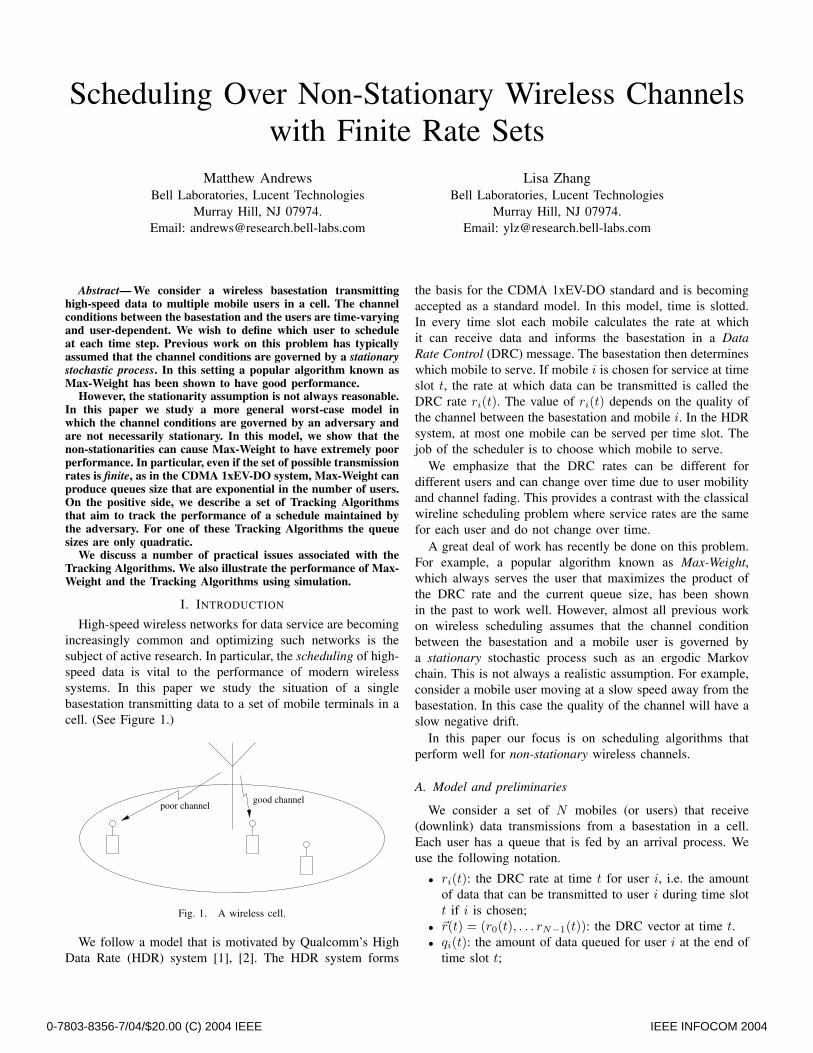
Scheduling Over Non-Stationary Wireless Channelswith Finite Rate Sets

Matthew AndrewsBell Laboratories, Lucent Technologies

Murray Hill, NJ 07974.Email: [email protected]

Lisa ZhangBell Laboratories, Lucent Technologies

Murray Hill, NJ 07974.Email: [email protected]

Abstract— We consider a wireless basestation transmittinghigh-speed data to multiple mobile users in a cell. The channelconditions between the basestation and the users are time-varyingand user-dependent. We wish to define which user to scheduleat each time step. Previous work on this problem has typicallyassumed that the channel conditions are governed by a stationarystochastic process. In this setting a popular algorithm known asMax-Weight has been shown to have good performance.

However, the stationarity assumption is not always reasonable.In this paper we study a more general worst-case model inwhich the channel conditions are governed by an adversary andare not necessarily stationary. In this model, we show that thenon-stationarities can cause Max-Weight to have extremely poorperformance. In particular, even if the set of possible transmissionrates is finite, as in the CDMA 1xEV-DO system, Max-Weight canproduce queues size that are exponential in the number of users.On the positive side, we describe a set of Tracking Algorithmsthat aim to track the performance of a schedule maintained bythe adversary. For one of these Tracking Algorithms the queuesizes are only quadratic.

We discuss a number of practical issues associated with theTracking Algorithms. We also illustrate the performance of Max-Weight and the Tracking Algorithms using simulation.

I. INTRODUCTION

High-speed wireless networks for data service are becomingincreasingly common and optimizing such networks is thesubject of active research. In particular, the scheduling of high-speed data is vital to the performance of modern wirelesssystems. In this paper we study the situation of a singlebasestation transmitting data to a set of mobile terminals in acell. (See Figure 1.)

poor channelgood channel

Fig. 1. A wireless cell.

We follow a model that is motivated by Qualcomm’s HighData Rate (HDR) system [1], [2]. The HDR system forms

the basis for the CDMA 1xEV-DO standard and is becomingaccepted as a standard model. In this model, time is slotted.In every time slot each mobile calculates the rate at whichit can receive data and informs the basestation in a DataRate Control (DRC) message. The basestation then determineswhich mobile to serve. If mobile i is chosen for service at timeslot t, the rate at which data can be transmitted is called theDRC rate ri(t). The value of ri(t) depends on the quality ofthe channel between the basestation and mobile i. In the HDRsystem, at most one mobile can be served per time slot. Thejob of the scheduler is to choose which mobile to serve.

We emphasize that the DRC rates can be different fordifferent users and can change over time due to user mobilityand channel fading. This provides a contrast with the classicalwireline scheduling problem where service rates are the samefor each user and do not change over time.

A great deal of work has recently be done on this problem.For example, a popular algorithm known as Max-Weight,which always serves the user that maximizes the product ofthe DRC rate and the current queue size, has been shownin the past to work well. However, almost all previous workon wireless scheduling assumes that the channel conditionbetween the basestation and a mobile user is governed bya stationary stochastic process such as an ergodic Markovchain. This is not always a realistic assumption. For example,consider a mobile user moving at a slow speed away from thebasestation. In this case the quality of the channel will have aslow negative drift.

In this paper our focus is on scheduling algorithms thatperform well for non-stationary wireless channels.

A. Model and preliminaries

We consider a set of N mobiles (or users) that receive(downlink) data transmissions from a basestation in a cell.Each user has a queue that is fed by an arrival process. Weuse the following notation.

• ri(t): the DRC rate at time t for user i, i.e. the amountof data that can be transmitted to user i during time slott if i is chosen;

• �r(t) = (r0(t), . . . rN−1(t)): the DRC vector at time t.• qi(t): the amount of data queued for user i at the end of

time slot t;

0-7803-8356-7/04/$20.00 (C) 2004 IEEE IEEE INFOCOM 2004

• ai(t): the amount of data that arrives for user i in timeslot t.

The scheduler at the basestation chooses at most one userto service for each time slot. For example, the Max-Weightalgorithm always chooses the user that maximizes ri(t)qi(t)for service in time slot t. If user i is chosen, queue qi(t) isreduced according to ri(t). Data then arrives for all users andtheir queues are increased. More precisely,

qi(t + 1) ← qi(t)−min{qi(t), ri(t)}+ ai(t)qj(t + 1) ← qj(t) + aj(t) ∀j �= i.

In almost all previous work, the DRC process and the arrivalprocess are modeled by stationary stochastic processes. Moreprecisely, the DRC process is defined by an ergodic MarkovChain with state space M such that if the state at time t ism ∈ M then the DRC vector (r0(t), . . . , rN−1(t)) can bewritten as (rm

0 , . . . , rmN−1), i.e. the DRC values are dependent

on the state m. In addition, the arrival process for user iis usually modeled by a Bernoulli process with intensity λi.In this scenario it is known (e.g. [3], [4]) that Max-Weightperforms well.

However, as argued before stationary stochastic processesare not always appropriate for modeling mobility. In this paperwe focus on a worst case model, in which the DRC processand the arrival process are generated by an adversary. By“worst case” we mean that the adversary is attempting to causethe chosen scheduling algorithm as many problems as possi-ble. Scheduling in the context of “adversarial queueing” hasreceived much attention recently, especially for the wirelineenvironment [5], [6].

We assume that the scheduling process against an adversaryis as follows. At the beginning of each time slot t the adversarygenerates a DRC vector, �r(t). The scheduling algorithm thenmakes a decision as to which user it is going to serve. Finallythe adversary injects data into the queues.

In order for the problem to be interesting we require thatthe system is not overloaded. More formally, we say that asequence of DRCs and arrivals is admissible if there is someschedule that can serve all the data. That is, there exist integersxi(t) ∈ {0, 1} (which we call the adversary’s schedule) suchthat for some window w and some loading parameter ε,

τ+w−1∑t=τ

ai(t) ≤τ+w−1∑

t=τ

(1− ε)xi(t)ri(t) ∀i, τ, (1)

∑i

xi(t) = 1 ∀t (2)

In other words, in any window of w time steps the adversaryis able to schedule the users so that each user receives moreservice than the amount of data injected.

However, we stress that the adversary’s schedule cannotbe computed by an online algorithm. Note that at the endof each window [τ, τ + w), a (computationally unbounded)online algorithm could examine the data that arrived during thewindow and could deduce the adversary’s schedule. However,it is too late for the server to implement this schedule. The

bits/slot k-bits/sec0 0

64 38.4128 76.8256 153.6512 307.2

1024 614.41536 921.62048 1228.83072 1843.24096 2457.6

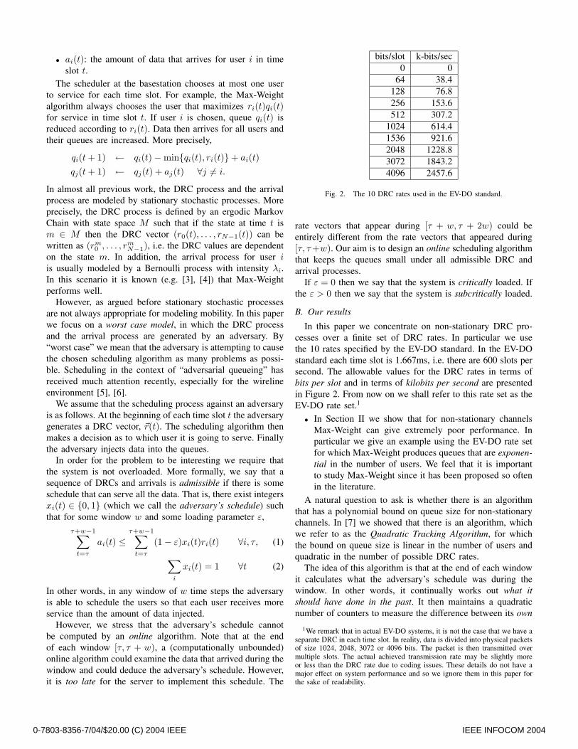
Fig. 2. The 10 DRC rates used in the EV-DO standard.

rate vectors that appear during [τ + w, τ + 2w) could beentirely different from the rate vectors that appeared during[τ, τ +w). Our aim is to design an online scheduling algorithmthat keeps the queues small under all admissible DRC andarrival processes.

If ε = 0 then we say that the system is critically loaded. Ifthe ε > 0 then we say that the system is subcritically loaded.

B. Our results

In this paper we concentrate on non-stationary DRC pro-cesses over a finite set of DRC rates. In particular we usethe 10 rates specified by the EV-DO standard. In the EV-DOstandard each time slot is 1.667ms, i.e. there are 600 slots persecond. The allowable values for the DRC rates in terms ofbits per slot and in terms of kilobits per second are presentedin Figure 2. From now on we shall refer to this rate set as theEV-DO rate set.1

• In Section II we show that for non-stationary channelsMax-Weight can give extremely poor performance. Inparticular we give an example using the EV-DO rate setfor which Max-Weight produces queues that are exponen-tial in the number of users. We feel that it is importantto study Max-Weight since it has been proposed so oftenin the literature.

A natural question to ask is whether there is an algorithmthat has a polynomial bound on queue size for non-stationarychannels. In [7] we showed that there is an algorithm, whichwe refer to as the Quadratic Tracking Algorithm, for whichthe bound on queue size is linear in the number of users andquadratic in the number of possible DRC rates.

The idea of this algorithm is that at the end of each windowit calculates what the adversary’s schedule was during thewindow. In other words, it continually works out what itshould have done in the past. It then maintains a quadraticnumber of counters to measure the difference between its own

1We remark that in actual EV-DO systems, it is not the case that we have aseparate DRC in each time slot. In reality, data is divided into physical packetsof size 1024, 2048, 3072 or 4096 bits. The packet is then transmitted overmultiple slots. The actual achieved transmission rate may be slightly moreor less than the DRC rate due to coding issues. These details do not have amajor effect on system performance and so we ignore them in this paper forthe sake of readability.


schedule in the past and the adversary’s schedule. It uses thesecounters to decide on its schedule in the future. For the sake ofcompleteness we describe the Quadratic Tracking Algorithmin the Appendix.

There are a number of ways in which the Quadratic TrackingAlgorithm could be improved. First, we would like a bound onqueue size that is linear in the number of DRC rates. Second,the definition of the algorithm assumes that we know the valueof w for which the inputs are admissible. This assumptioncould be unrealistic. Lastly, the calculation of the adversary’sschedule at the end of each window requires the solution of aninteger program. Even though it turns out that we only needto solve a linear program, it is unlikely that this could beperformed in hardware. In this paper we address these issues.

• In Section III-C we present a heuristic Linear Trackingalgorithm that only uses a linear number of counters foreach user. As long as these counters remain bounded, thebound on queue size is linear in the number of DRC ratesand does not depend on the number of users. We refer tothe algorithm as a heuristic because we cannot prove thatthe counters remain bounded. However, we do not knowof a situation where they are unbounded.

• In Section III-D we examine the situation where we donot know the correct value of w. If, when calculating theadversary’s schedule, it is impossible to serve all the datain the window, we use linear programming to maximizea weighted sum of the data served.

• In Section III-E we describe a method to calculate theadversary’s schedule when it is impractical to solvea linear program. We present a simple combinatorialalgorithm that can approximate the solution of the linearprogram arbitrarily closely.

• In Section IV we illustrate the behavior of Max-Weightand the Linear Tracking Algorithm through simulations.We first simulate the example from Section II to showthat Max-Weight does indeed produce exponentially largequeues. In contrast, the Linear Tracking Algorithm main-tains extremely small queues. We then present anothersimple non-stationary example where once again the Lin-ear Tracking Algorithm outperforms Max-Weight. Lastlywe simulate a stationary example where Max-Weightwould be expected to do well. We show that here theperformance of the Linear Tracking Algorithm is closeto that of Max-Weight.

Remark 1: In our model, ai(t) represents the amount ofdata injected into the queue for user i at time t. However, itis sometimes unwise to base a scheduling algorithm on actualqueue contents since a misbehaving user could potentially gainmore service by injecting an excessive amount of data into itsqueue. A standard way to solve this problem is for each userto have a token buffer into which tokens are injected at afixed rate. We then use this token buffer for scheduling ratherthe real data queue. If we are able to keep the token bufferbounded then each user will receive a long-term service rateequal to its token rate. For this reason we feel that an important

special case of our problem is when ai(t) is independent oftime since we can then use ai(t) to represent the number oftokens arriving for user i in time slot t. For our negative resultsthe bad examples that we study all have the property that ai(t)is constant. However, we stress that our positive results applyto the case of variable ai(t).

Remark 2: In this paper, we focus on finite rate setsonly. For the case of infinite rate sets, we showed in [7] thatif the DRC rates can be arbitrarily close to 0 then no onlinealgorithm can keep the queues bounded.

C. Previous work

As mentioned earlier, almost all work on scheduling overtime-varying channels has assumed that the channel processis stationary. Under this assumption, Max-Weight was firstshown to perform well by Tassiulas and Ephremides [3], [4].Other papers that study Max-Weight include [8], [9], [10]. Twovariants of Max-Weight are Max-Delay [8], [9] and Exp [11],[12]. The Max-Delay algorithm always serves the user thatmaximizes ∆i(t)ri(t) where ∆i(t) denotes the Head-of-Linedelay for user i at time t. Exp is a more complex algorithm thatprovides more control over the relative delays that the usersexperience. For the case in which each packet has a deadlineand the objective is to meet all the deadlines, [13] shows thatthe Earliest-Deadline-First algorithm is not always optimal (incontrast to the wireline case).

In our model we assume that each queue is fed by anarrival process and we wish to keep the queues small. In adifferent model that is sometimes studied, each queue hasan infinite backlog and we wish to optimize some functionof the service rates that each user receives. For this modela popular and widely implemented algorithm is known asProportional Fair [14]. Proportional Fair always serves the userthat maximizes ri(t)/Ri(t) where Ri(t) is an exponentiallysmoothed average of the service rate received by user i. It isknown [15], [16] that for stationary channels Proportional Fairmaximizes the objective log Ri. However, it is also known [17]that if (as in our model) the queues are fed by an arrivalprocess then Proportional Fair can be unstable (i.e. the queuescan grow without bound).

The problem of providing a target service rate to each userwas studied in [18]. Algorithms for optimizing utility functionssubject to fairness requirements are presented in [19], [20]. In[21], Borst examines the user-level performance of schedulingalgorithms such as Proportional Fair under the assumption thateach user has a finite service demand and leaves the systemonce this demand is satisfied.

II. MAX-WEIGHT

In this section we present examples to show that Max-Weight can give extremely poor performance when the DRCprocess is non-stationary. In particular we present an admissi-ble arrival and DRC process for which Max-Weight producesqueues that are exponential in the number of users. We restrictourselves to the EV-DO rates shown in Figure 2 and constantarrival processes.


Let us consider a system of N users. User 0 has a specialrole. Users 1 through N − 1 all act in a similar manner. Thearrival process for all users is constant. The arrival rate foreach user i ≥ 1 is 1 bit per slot; the arrival rate for user 0 is64 bits per slot. The DRC process is periodic with period 64slots and is defined as follows:

r0(t) =

4096 t = 0 mod 644096 t = −1 mod 640 o.w.

(3)

ri(t) =

64 t = −i mod 64128 t = −(i + 1) mod 64,

and qi(t) > 2qi+1(t)0 o.w.

(4)

640 or 128

640 or 128

644096

user 0

t=w

t=w−1

t=2

t=1

user 3user 2user 1

4096

Fig. 3. DRC process that creates exponential queues for Max-Weight. Therates in the empty slots are zero.

The arrival and DRC processes described above are admissi-ble for w = 64 and ε = 0 (i.e. the system is critically loaded).To see this, let xi(t) = 1 whenever t = −i mod w and letxi(t) = 0 otherwise. (In other words, the adversary servesuser i in time slots t = −i mod w.) Then,

τ+w−1∑t=τ

ai(t) =τ+w−1∑

t=τ

xi(t)ri(t) ∀i, τ,∑

i

xi(t) = 1 ∀t

Theorem 1: Under Max-Weight, the queue size for userN − 1 is exponential in N .

Proof: Let us define a sequence,

f1 = 4096× 62 and fi = 2fi−1 for i ≥ 2.

We prove the following statement by induction on the numberof users. Consider a system of N users and any queueconfiguration at time t. The queue for the last user qN−1(t)is either greater than fN−1 or there exists a future slot t′ > tfor which the queue qN−1(t′) is greater than fN−1.

The base case is 2 users. Note that user 1 can only be servedin time slots t = −1 mod w. At time t = −1 mod w, the queueq0(t) for user 0 is at least 64×62 since the DRC rate for user 0is 0 in the preceding 62 time slots. If the queue q1(t) for user

1 is smaller than f1, then q0(t)× 4096 > q1(t)× 64. Hence,Max-Weight chooses to serve user 0 at time t. This impliesthat the queue for user 1 never receives service as long as itis under f1. Therefore the queue for user 1 eventually growsto f1.

Inductively, we assume the statement holds for a system ofN = n users where n < w and we prove it for N = n + 1users. We use a second induction on the queue size of thelast user n. For k < fn we show that for any slot t eitherqn(t) > k or qn(t′) > k for some t′ > t. This is trivially truefor k = 0 since ai(t) > 0 for all slots but ri(t) = 0 for all but2 slots out of 64. Assume now that the statement holds for allk′ < k.

Consider a time t. By the second inductive hypothesis thereexists at time t′ > t when qn(t′) > k−1. If qn(t′) > k then weare done and so we suppose qn(t′) = k. We claim that theremust be a time t′′ in the future when t′′ = −n mod w andqn−1(t′′) > k/2. If not then rn−1(t′′) never equals 128 andso users 0 through n− 1 act as though they are a system of nusers. That is, users 0 through n−1 act independently of usern. Therefore, by the first inductive hypothesis, at some timet′′ > t′, qn−1(t′′) ≥ fn−1 = fn/2 > k/2. During the timeinterval [t′, t′′), qn(t) essentially remains constant. During thewindow containing t′′, user n−1 is served with a DRC rate of128 and user n is not served. Therefore, after time t′′, qn(t)becomes larger than k. This proves the second induction whichin turn immediately implies the first induction.

Of course the arrival rates, DRC rates and window sizes wehave chosen above have no particular significance. In generallet us choose a window size of w and let N be at most w. Thearrival rate for user 0 is a0 = 4096/w where 4096 representsthe largest DRC rate; the arrival rate for each user i > 0 isstill 1. We define the DRC process as follows.

r0(t) ={

4096 t = 0,−1 mod w0 o.w.

ri(t) =

w t = −i mod w2w t = −(i + 1) mod w,

and qi(t) > 2qi+1(t)0 o.w.

Again the arrival and DRC processes are admissible for acritically loaded system. By an argument similar to that inTheorem 1 the queue for user 1 grows to (w−2) ·a0 ·4096/wand the queue for user i > 1 grows to be twice that for useri− 1. Hence, Theorem 1 holds for,

f1 = (w − 2) · 40962/w2 and fi = 2fi−1 for i ≥ 2.

For the EV-DO rate set, we can set w = 2048. The queue cangrow as high as 8184 · 2N for N as large as 2048.

Our proof for Theorem 1 and the description of the arrivaland DRC processes are for a critically loaded system. How-ever, if the system is subcritically loaded for a small ε > 0we observe in our simulations that the statement of Theorem 1still holds. See Section IV.


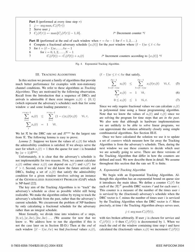
Part I (performed at every time step τ )1 j ← arg maxi Ci(�r(τ))2 Serve user j3 Cj(�r(τ))← max{Cj(�r(τ))− 1, 0}. /* Decrement counter */

Part II (performed at the end of each window when τ = �w − 1 for � = 1, 2, . . .)4 Compute a fractional adversary schedule {xi(t)} for the past window where (�− 1)w ≤ t < �w5 for t = (�− 1)w, . . . , �w − 16 for i = 0, 1, 2, . . . , N − 17 Ci(�r(t))← Ci(�r(t)) + xi(t) /* Increment counters according to {xi(t)} */

Fig. 4. Exponential Tracking Algorithm.

III. TRACKING ALGORITHMS

In this section we present a family of algorithms that providemuch better performance for examples with non-stationarychannel conditions. We refer to these algorithms as TrackingAlgorithms. They are motivated by the following observation.Recall from the Introduction that a sequence of DRCs andarrivals is admissible if there exist integers xi(t) ∈ {0, 1}(which represent the adversary’s schedule) such that for somewindow w and some loading parameter ε,

τ+w−1∑t=τ

ai(t) ≤τ+w−1∑

t=τ

(1− ε)xi(t)ri(t) ∀i, τ,∑

i

xi(t) = 1 ∀t.

We let R be the DRC rate set and Rmax be the largest ratefrom R. The following lemma is easy to prove.

Lemma 2: Suppose we know the values of xi(t) for whichthe admissibility condition is satisfied. If we always serve theuser for which xi(t) = 1 then the queue for user i is boundedby (w + 1)Rmax.

Unfortunately, it is clear that the adversary’s schedule isnot implementable for two reasons. First, we cannot calculatexi(t) online since xi(t) can depend on ai(t′) and ri(t′) fort′ > t. Second, even if we did know the future arrivals andDRCs, finding a set of xi(t) that satisfy the admissibilitycondition for a given window involves solving an instanceof the GENERALIZED ASSIGNMENT PROBLEM (GAP) whichis NP-hard [22].

The key aim of the Tracking Algorithms is to “track” theadversary’s schedule as close as possible whilst still beingrealizable. We make the algorithm online by trying to track theadversary’s schedule from the past, rather than the adversary’scurrent schedule. We circumvent the problem of NP-hardnessby only calculating a fractional schedule for the adversaryrather than an integral schedule.

More formally, we divide time into windows of w steps,[0, w), [w, 2w), [2w, 3w) . . .. (We assume for now that weknow w. We address how to run the algorithm if this isnot the case later on in Section III-D.) Then at the end ofeach window [(� − 1)w, �w) we find fractional values xi(t),

(�− 1)w ≤ t < �w that satisfy,

�w−1∑t=(�−1)w

ai(t) ≤�w−1∑

t=(�−1)w

xi(t)ri(t) ∀i, �, (5)

∑i

xi(t) = 1 ∀t, (6)

0 ≤ xi(t) ≤ 1 ∀i, t. (7)

Since we only require fractional values we can calculate xi(t)in polynomial time using a linear programming algorithm.Note that we know the values of ai(t) and ri(t) since weare solving the program for time steps that are in the past.We also note that although in hardware implementationswe are unlikely to be able to solve linear programs, wecan approximate the solution arbitrarily closely using simplecombinatorial algorithms. See Section III-E.

Once we have calculated the solution we use it to updatea set of counters which measure how far away the TrackingAlgorithm is from the adversary’s schedule. Then, during thenext window we use these counters to decide which userwe are actually going to serve. There are three versions ofthe Tracking Algorithm that differ in how the counters aredefined and used. We now describe them in detail. We assumethroughout this section that the rate set R is finite.

A. Exponential Tracking Algorithm

We begin with an Exponential Tracking Algorithm. Al-though this algorithm has an exponential bound on queue sizeit introduces the main ideas. We define a counter Ci(�r) foreach of the |R|N possible DRC vectors �r and for each user i.This counter is a measure of the number of the times user iis serviced by the (fractional) adversary’s schedule when theDRC vector is �r, minus the number of times user i is servicedby the Tracking Algorithm when the DRC vector is �r. Moreprecisely, at time t the Tracking Algorithm always serves user,

j ∈ arg max Ci(�r(t)),

with ties broken arbitrarily. If user j is chosen for service andCj(�r(t)) > 0 then Cj(�r(t)) is decremented by 1. When wereach the end of the window containing time step t and havecalculated the (fractional) values xi(t) we increment Ci(�r(t))


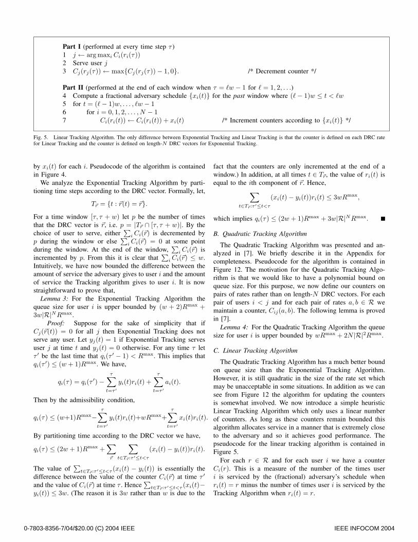
Part I (performed at every time step τ )1 j ← arg maxi Ci(ri(τ))2 Serve user j3 Cj(rj(τ))← max{Cj(rj(τ))− 1, 0}. /* Decrement counter */

Part II (performed at the end of each window when τ = �w − 1 for � = 1, 2, . . .)4 Compute a fractional adversary schedule {xi(t)} for the past window where (�− 1)w ≤ t < �w5 for t = (�− 1)w, . . . , �w − 16 for i = 0, 1, 2, . . . , N − 17 Ci(ri(t))← Ci(ri(t)) + xi(t) /* Increment counters according to {xi(t)} */

Fig. 5. Linear Tracking Algorithm. The only difference between Exponential Tracking and Linear Tracking is that the counter is defined on each DRC ratefor Linear Tracking and the counter is defined on length-N DRC vectors for Exponential Tracking.

by xi(t) for each i. Pseudocode of the algorithm is containedin Figure 4.

We analyze the Exponential Tracking Algorithm by parti-tioning time steps according to the DRC vector. Formally, let,

T�r = {t : �r(t) = �r}.For a time window [τ, τ + w) let p be the number of timesthat the DRC vector is �r, i.e. p = |T�r ∩ [τ, τ + w)|. By thechoice of user to serve, either

∑i Ci(�r) is decremented by

p during the window or else∑

i Ci(�r) = 0 at some pointduring the window. At the end of the window,

∑i Ci(�r) is

incremented by p. From this it is clear that∑

i Ci(�r) ≤ w.Intuitively, we have now bounded the difference between theamount of service the adversary gives to user i and the amountof service the Tracking algorithm gives to user i. It is nowstraightforward to prove that,

Lemma 3: For the Exponential Tracking Algorithm thequeue size for user i is upper bounded by (w + 2)Rmax +3w|R|NRmax.

Proof: Suppose for the sake of simplicity that ifCj(�r(t)) = 0 for all j then Exponential Tracking does notserve any user. Let yj(t) = 1 if Exponential Tracking servesuser j at time t and yj(t) = 0 otherwise. For any time τ letτ ′ be the last time that qi(τ ′ − 1) < Rmax. This implies thatqi(τ ′) ≤ (w + 1)Rmax. We have,

qi(τ) = qi(τ ′)−τ∑

t=τ ′yi(t)ri(t) +

τ∑t=τ ′

ai(t).

Then by the admissibility condition,

qi(τ) ≤ (w+1)Rmax−τ∑

t=τ ′yi(t)ri(t)+wRmax+

τ∑t=τ ′

xi(t)ri(t).

By partitioning time according to the DRC vector we have,

qi(τ) ≤ (2w + 1)Rmax +∑

�r

∑t∈T�r:τ ′≤t<τ

(xi(t)− yi(t))ri(t).

The value of∑

t∈T�r:τ ′≤t<τ (xi(t) − yi(t)) is essentially thedifference between the value of the counter Ci(�r) at time τ ′

and the value of Ci(�r) at time τ . Hence∑

t∈T�r:τ ′≤t<τ (xi(t)−yi(t)) ≤ 3w. (The reason it is 3w rather than w is due to the

fact that the counters are only incremented at the end of awindow.) In addition, at all times t ∈ T�r, the value of ri(t) isequal to the ith component of �r. Hence,∑

t∈T�r:τ ′≤t<τ

(xi(t)− yi(t))ri(t) ≤ 3wRmax,

which implies qi(τ) ≤ (2w + 1)Rmax + 3w|R|NRmax.

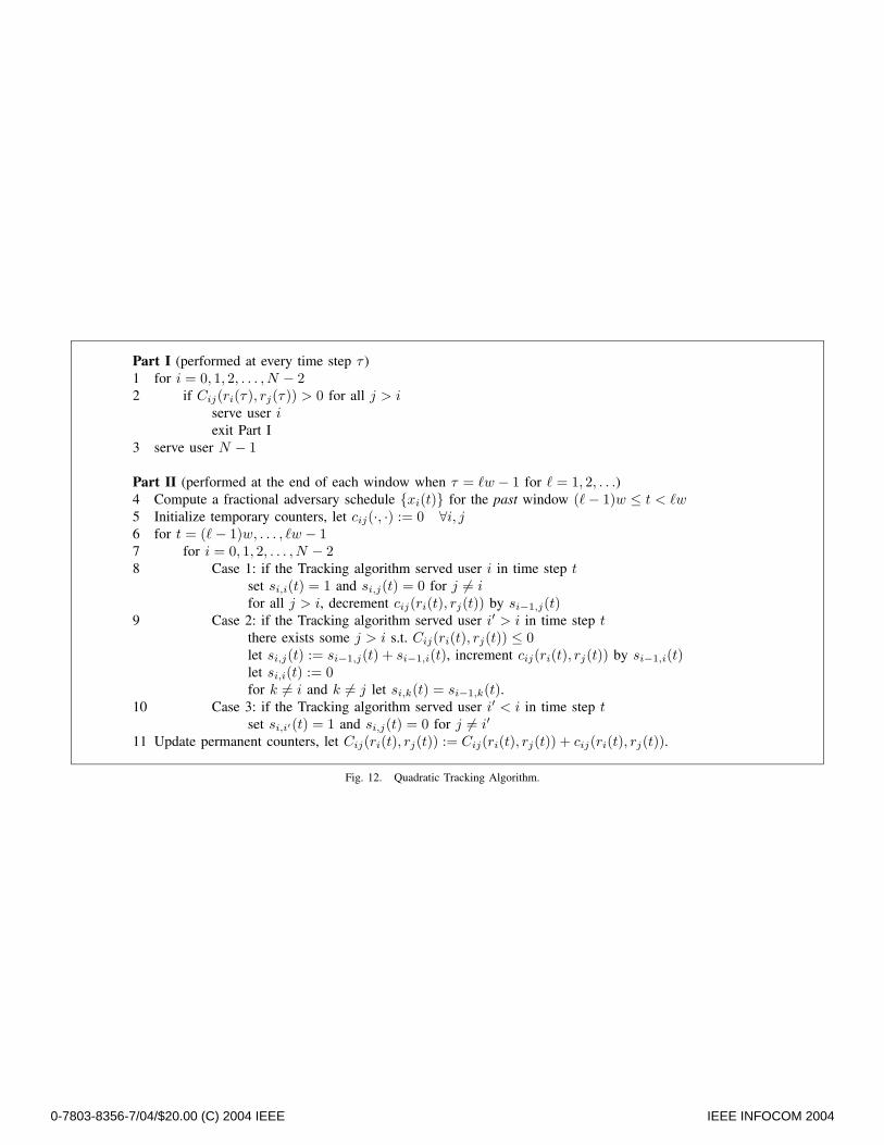
B. Quadratic Tracking Algorithm

The Quadratic Tracking Algorithm was presented and an-alyzed in [7]. We briefly describe it in the Appendix forcompleteness. Pseudocode for the algorithm is contained inFigure 12. The motivation for the Quadratic Tracking Algo-rithm is that we would like to have a polynomial bound onqueue size. For this purpose, we now define our counters onpairs of rates rather than on length-N DRC vectors. For eachpair of users i < j and for each pair of rates a, b ∈ R wemaintain a counter, Cij(a, b). The following lemma is provedin [7].

Lemma 4: For the Quadratic Tracking Algorithm the queuesize for user i is upper bounded by wRmax + 2N |R|2Rmax.

C. Linear Tracking Algorithm

The Quadratic Tracking Algorithm has a much better boundon queue size than the Exponential Tracking Algorithm.However, it is still quadratic in the size of the rate set whichmay be unacceptable in some situations. In addition as we cansee from Figure 12 the algorithm for updating the countersis somewhat involved. We now introduce a simple heuristicLinear Tracking Algorithm which only uses a linear numberof counters. As long as these counters remain bounded thisalgorithm allocates service in a manner that is extremely closeto the adversary and so it achieves good performance. Thepseudocode for the linear tracking algorithm is contained inFigure 5.

For each r ∈ R and for each user i we have a counterCi(r). This is a measure of the number of the times useri is serviced by the (fractional) adversary’s schedule whenri(t) = r minus the number of times user i is serviced by theTracking Algorithm when ri(t) = r.


At time t the Linear Tracking Algorithm always serves user,

j ∈ arg max Ci(ri(t)),

with ties broken arbitrarily. If user j is chosen for servicethen Cj(rj(t)) is decremented by 1. When we reach the endof the window containing time step t and have calculated the(fractional) values xi(t) we increment Ci(ri(t)) by xi(t) foreach i.

If the counters remain bounded then we immediately havea bound on queue size. The proof of the following lemma isalmost identical to the proof of Lemma 3.

Lemma 5: Suppose that during the operation of the LinearTracking Algorithm all counters Ci(r) remain between −αand α. Then the queue size for user i is upper bounded by(2w + 1)Rmax + 2(w + α)|R|Rmax.

D. Incorrect Window Size

The above algorithms rely on our ability to compute afractional schedule for the adversary by finding a solutionto the constraints (5)-(7). However, this relies on knowing avalue of w for which (5)-(7) are satisfiable for all windows.(From now on we shall refer to a window for which (5)-(7) are satisfiable as a satisfiable window.) One solution isto first guess a value of w and then whenever we encounteran unsatisfiable window we simply double w. However, inreality it may be the case that the minimum value of w forwhich 100% of the windows are satisfiable is much larger thanthe minimum value of w for which 99% of the windows aresatisfiable. In this case we would prefer to use the smallerwindow size.

To achieve this, we now have to extend the definition of ouralgorithms to unsatisfiable windows. For this purpose, insteadof trying to satisfy (5)-(7) in window [(�− 1)w, �w) we nowsolve the following the linear program,

max∑

i

(di)2λi (8)

subject to

di = γi,� +�w−1∑

t=(�−1)w

ai(t) ∀i, (9)

λidi =�w−1∑

t=(�−1)w

xi(t)ri(t) ∀i, (10)

λi ≤ 1 ∀i, (11)∑i

xi(t) ≤ 1 ∀t, (12)

xi(t) ≥ 1 ∀i, t. (13)

The parameter di is the amount of user-i data that we wish toserve during the window. We emphasize that di is a parameter,not a variable. It equals

∑�w−1t=(�−1)w ai(t), the data injected for

user i during the window, plus γi,�, the residual user-i datathat was left over from the previous window. The variable λi

is the fraction of di that the adversary is able to serve during

the window. We define the residual data for the next windowby,

γi,�+1 = di(1− λi).

We note that λi is completely determined by the values ofxi(t). If λi = 1 for all i then all the data is served andwe say that the window is satisfied. If the window cannotbe satisfied then the form of the objective function means thatwe give preference to users with more data to serve. We keeptrack of the average fraction of windows that are satisfied. Ifthis fraction exceeds a suitable threshold, say 99%, then wedouble the window size w, otherwise we leave the windowsize unchanged. We remark that if all windows are satisfiedthen the solutions to (8)-(13) will also be solutions to (5)-(7).

E. Efficiently Solving the Linear Program

Although linear programs can be solved in polynomial time,schedulers for wireless data systems are typically implementedin ASICs or DSPs. It is unreasonable to expect that a genericlinear program solver could be implemented in such a device.However, using techniques of Garg and Konemann [23] (whichwere in turn based on earlier techniques of [24] and [25])we can approximate (8)-(13) arbitrarily closely using a simplecombinatorial algorithm. In this section we sketch the ideas.

For any dual variables ui and vt, define,

D(�u,�v) =∑

i

ui +∑

t

vt

α(�u,�v) = mini,t

(ui +

divi

ri(t)

).

Using the theory of complementary slackness, it can be shownthat the dual is equivalent to,

minD(�u,�v)α(�u,�v)

.

(Note that there are no constraints in this formulation.) Ouralgorithm for finding an approximate solution to (8)-(13) is aniterative algorithm that works as follows.

• Initially set xi(t) = 0, ui = 1 and vt = 1 for all i, t.• At each iteration find the (i, t) pair that minimizes

1(di)2

(ui +

divi

ri(t)

).

For this pair let f = max{1, di/ri(t)}. We then updateprimal and dual variables according to,

xi(t) ← xi(t) + f

ui ← ui(1 + θ · f · ri(t)/di)vt ← vt(1 + θ · f),

for some parameter θ.• Terminate after (N +w)�1/θ log2(1+θ) iterations. The

primal variables xi(t) will in general be infeasible. Wecreate a feasible solution by setting,

xi(t)← xi(t)max{∑j xj(t),

∑t′ xi(t′)ri(t′)/di}


The following lemma follows directly from the analysis ofGarg and Konemann for packing linear programs.

Lemma 6: Let β be the optimum solution to (8)-(13). Thevalue of the feasible solution produced by the above iterativealgorithm is at least (1− θ)2β.

0

2e+06

4e+06

6e+06

8e+06

1e+07

0 500 1000 1500 2000

Sol

utio

n

Iterations

Convergence of LP solution

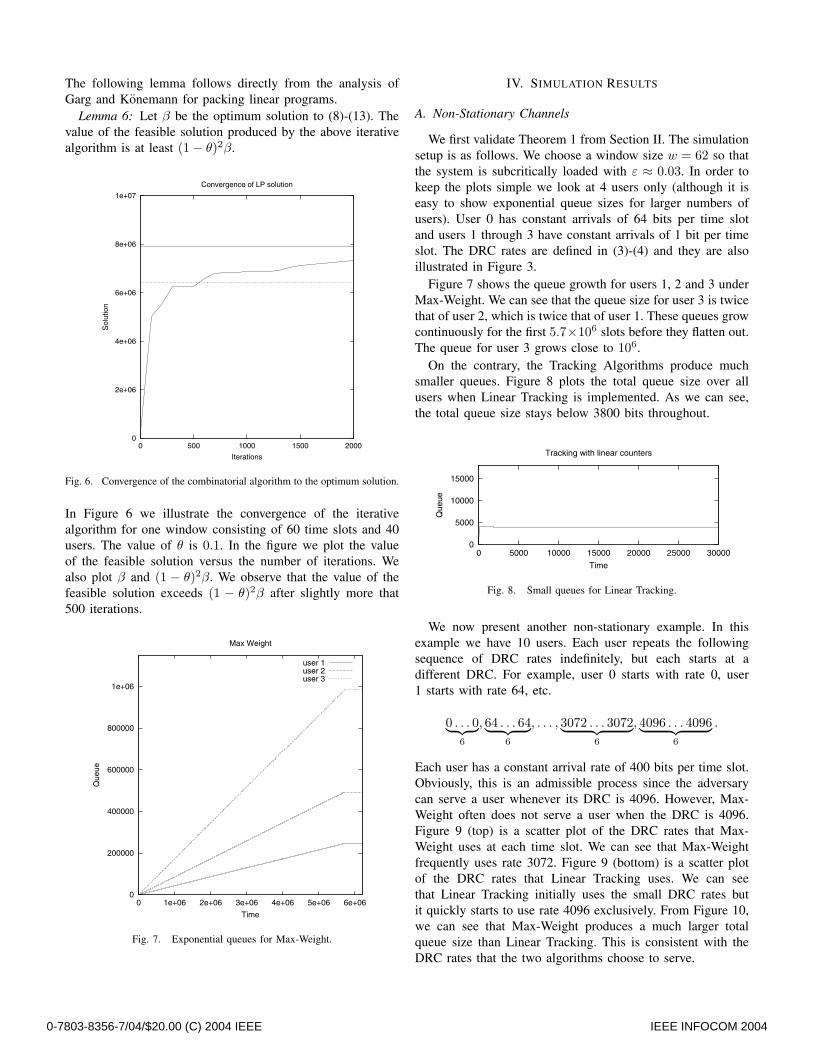
Fig. 6. Convergence of the combinatorial algorithm to the optimum solution.

In Figure 6 we illustrate the convergence of the iterativealgorithm for one window consisting of 60 time slots and 40users. The value of θ is 0.1. In the figure we plot the valueof the feasible solution versus the number of iterations. Wealso plot β and (1 − θ)2β. We observe that the value of thefeasible solution exceeds (1 − θ)2β after slightly more that500 iterations.

0

200000

400000

600000

800000

1e+06

0 1e+06 2e+06 3e+06 4e+06 5e+06 6e+06

Que

ue

Time

Max Weight

user 1user 2user 3

Fig. 7. Exponential queues for Max-Weight.

IV. SIMULATION RESULTS

A. Non-Stationary Channels

We first validate Theorem 1 from Section II. The simulationsetup is as follows. We choose a window size w = 62 so thatthe system is subcritically loaded with ε ≈ 0.03. In order tokeep the plots simple we look at 4 users only (although it iseasy to show exponential queue sizes for larger numbers ofusers). User 0 has constant arrivals of 64 bits per time slotand users 1 through 3 have constant arrivals of 1 bit per timeslot. The DRC rates are defined in (3)-(4) and they are alsoillustrated in Figure 3.

Figure 7 shows the queue growth for users 1, 2 and 3 underMax-Weight. We can see that the queue size for user 3 is twicethat of user 2, which is twice that of user 1. These queues growcontinuously for the first 5.7×106 slots before they flatten out.The queue for user 3 grows close to 106.

On the contrary, the Tracking Algorithms produce muchsmaller queues. Figure 8 plots the total queue size over allusers when Linear Tracking is implemented. As we can see,the total queue size stays below 3800 bits throughout.

0

5000

10000

15000

0 5000 10000 15000 20000 25000 30000

Que

ue

Time

Tracking with linear counters

Fig. 8. Small queues for Linear Tracking.

We now present another non-stationary example. In thisexample we have 10 users. Each user repeats the followingsequence of DRC rates indefinitely, but each starts at adifferent DRC. For example, user 0 starts with rate 0, user1 starts with rate 64, etc.

0 . . . 0︸︷︷︸6

, 64 . . . 64︸︷︷︸6

, . . . , 3072 . . . 3072︸︷︷︸6

, 4096 . . . 4096︸︷︷︸6

.

Each user has a constant arrival rate of 400 bits per time slot.Obviously, this is an admissible process since the adversarycan serve a user whenever its DRC is 4096. However, Max-Weight often does not serve a user when the DRC is 4096.Figure 9 (top) is a scatter plot of the DRC rates that Max-Weight uses at each time slot. We can see that Max-Weightfrequently uses rate 3072. Figure 9 (bottom) is a scatter plotof the DRC rates that Linear Tracking uses. We can seethat Linear Tracking initially uses the small DRC rates butit quickly starts to use rate 4096 exclusively. From Figure 10,we can see that Max-Weight produces a much larger totalqueue size than Linear Tracking. This is consistent with theDRC rates that the two algorithms choose to serve.


1024

1536

2048

4096

512

3072

1536

3072

1024

2048

4096

30000

DRC Rates Used by Max Weight

400020001000Time

10000Time

400030002000

DRC Rates Used by Tracking

Fig. 9. (Top) The DRC rates that Max-Weight chooses. (Bottom) The DRCrates that Linear Tracking chooses. (These are scatter plots. The dots appearlike lines since they are so dense.)

B. Stationary Channels

We conclude by considering a 40-user stationary case inwhich each user has a DRC trace that fluctuates around a meanvalue according to 3km/h Rayleigh fading. Since this exampleis stationary we would expect Max-Weight to perform well.We observe in Figure 11 that Max-Weight does indeed producesmaller queues than Linear Tracking. However, the differenceis much less dramatic than the difference between the twoalgorithms in the non-stationary cases.

V. CONCLUSIONS

In this paper we have studied the problem of scheduling overnon-stationary wireless channels. We presented an example toshow that the popular Max-Weight protocol can produce queuesizes that are exponential in the number of users. In contrast,we presented Tracking algorithms that try to keep close tothe adversary’s schedule and generally produce much smallerqueue sizes.

Some open questions remain. First, we would like to knowif the counters for the Linear Tracking algorithm do indeedremain bounded. Second, are there better Tracking algorithmsthat keep even closer to the adversary’s schedule than thealgorithms that we have presented? Third, we note that theTracking algorithms have to perform different amounts ofcomputation in each time step since we only compute theadversary’s schedule and increase the counters at the end ofeach window. We wonder if there is a smoother schedule that

0

100000

200000

300000

400000

500000

600000

700000

0 1000 2000 3000 4000

Que

ue

Time

Non-stationary Data

Max WeightLinear Tracking

Fig. 10. The total queue size produced by Max-Weight and Linear Trackingfor a non-stationary example.

0

50000

100000

150000

200000

250000

300000

350000

0 10000 20000 30000 40000 50000 60000

Que

ue

Time

Stationary Data

Max WeightLinear Tracking

Fig. 11. The total queue size produced by Max-Weight and Linear Trackingfor a stationary example.

calculates a portion of the adversary’s schedule in each slot.Lastly, our bad example for Max-Weight generated exponentialqueue sizes. It would be interesting to know if the examplecould be extended to an unstable scenario for Max-Weightwhere the queue sizes are unbounded. We note that for this tohappen the DRC process could not be periodic.

REFERENCES

[1] P. Bender, P. Black, M. Grob, R. Padovani, and N. Sindhushayana A.Viterbi, “CDMA/HDR: A bandwidth efficient high speed data servicefor nomadic users,” IEEE Communications Magazine, July 2000.

[2] A. Jalali, R. Padovani, and R. Pankaj, “Data throughput of CDMA-HDR a high efficiency-high data rate personal communication wirelesssystem,” in Proceedings of the IEEE Semiannual Vehicular TechnologyConference, VTC2000-Spring, Tokyo, Japan, May 2000.

[3] L. Tassiulas and A. Ephremides, “Stability properties of constrainedqueueing systems and scheduling policies for maximum throughput in


multihop radio networks,” IEEE Transactions on Automatic Control,vol. 37, no. 12, pp. 1936 – 1948, December 1992.

[4] L. Tassiulas and A. Ephremides, “Dynamic server allocation to parallelqueues with randomly varying connectivity,” IEEE Transactions onInformation Theory, vol. 30, pp. 466 – 478, 1993.

[5] A. Borodin, J. Kleinberg, P. Raghavan, M. Sudan, and D. P. Williamson,“Adversarial queueing theory,” Journal of the ACM, vol. 48, no. 1, pp.13–38, Jan. 2001.

[6] M. Andrews, B. Awerbuch, A. Fernandez, J. Kleinberg, T. Leighton, andZ. Liu, “Universal stability results and performance bounds for greedycontention-resolution protocols,” Journal of the ACM, vol. 48, no. 1,pp. 39–69, Jan. 2001.

[7] M. Andrews and L. Zhang, “Scheduling over a time-varying user-dependent channel with applications to high speed wireless data,” inProceedings of the 43nd Annual Symposium on Foundations of ComputerScience, Vancouver, Canada, November 2002.

[8] M. Andrews, K. Kumaran, K. Ramanan, A. Stolyar, R. Vijayakumar,and P. Whiting, “Providing quality of service over a shared wirelesslink,” IEEE Communications Magazine, February 2001.

[9] M. Andrews, K. Kumaran, K. Ramanan, A. Stolyar, R. Vijayakumar,and P. Whiting, “CDMA data QoS scheduling on the forward link withvariable channel conditions,” Bell Labs Technical Memorandum, April2000.

[10] M. Neely, E. Modiano, and C. Rohrs, “Power and server allocation ina multi-beam satellite with time varying channels,” in Proceedings ofIEEE INFOCOM ’02, New York, NY, June 2002.

[11] S. Shakkottai and A. Stolyar, “Scheduling algorithms for a mixtureof real-time and non-real-time data in HDR,” in Proceedings of 17thInternational Teletraffic Congress (ITC-17), Salvador da Bahia, Brazil,2001, pp. 793 – 804.

[12] S. Shakkottai and A. Stolyar, “Scheduling for multiple flows sharinga time-varying channel: The exponential rule,” Analytic Methods inApplied Probability, 2002, To appear.

[13] S. Shakkottai and R. Srikant, “Scheduling real-time traffic with deadlinesover a wireless channel,” in Proceedings of ACM Workshop on Wirelessand Mobile Multimedia, Seattle, WA, August 1999.

[14] D. Tse, “Forward-link multiuser diversity through rate adaptation andscheduling,” In preparation.

[15] A. Stolyar, “Multiuser throughput dynamics under proportional fair andother gradient based scheduling algorithms,” Submitted.

[16] H. Kushner and P. Whiting, “Asymptotic properties of proportional-fair sharing algorithms,” in 40th Annual Allerton Conference onCommunication, Control, and Computing, 2002.

[17] M. Andrews, “Instability of the proportional fair scheduling algorithmfor HDR,” IEEE Transactions on Wireless Communications, 2003, Toappear.

[18] S. Borst and P. Whiting, “Dynamic rate control algorithms for CDMAthroughput optimization,” in Proceedings of IEEE INFOCOM ’01,Anchorage, AK, April 2001.

[19] X. Liu, E. Chong, and N.B.Shroff, “Opportunistic transmission schedul-ing with resource-sharing constraints in wireless networks,” IEEEJournal on Selected Areas in Communications, vol. 19, no. 10, 2001.

[20] X. Liu, E. Chong, and N.B.Shroff, “A framework for opportunisticscheduling in wireless networks,” Computer Networks. To appear.

[21] S. Borst, “User-level performance of channel-aware scheduling algo-rithms in wireless data networks,” in Proceedings of IEEE INFOCOM’03, San Francisco, CA, April 2003.

[22] D. Shmoys and E. Tardos, “An approximation algorithm for thegeneralized assignment problem,” Mathematical Programming A, vol.62, pp. 461 – 474, 1993, Also in Proceedings of the 4th Annual ACM-SIAM Symposium on Discrete Algorithms, 1993.

[23] N. Garg and J. Konemann, “Faster and simpler algorithms for multicom-modity flow and other fractional packing problems,” in Proceedings ofthe 39th Annual Symposium on Foundations of Computer Science, PaloAlto, CA, November 1998, pp. 300 – 309.

[24] S. Plotkin, D. Shmoys, and E. Tardos, “Fast approximation algorithmsfor fractional packing and covering problems,” Math of OperationsResearch, vol. 20, pp. 257–301, 1995.

[25] N. Young, “Randomized rounding without solving the linear program,”in Proceedings of the 6th Annual ACM-SIAM Symposium on DiscreteAlgorithms, 1995, pp. 170–178.

APPENDIX

We briefly describe the Quadratic Tracking algorithm whichwas presented and analyzed in [7]. Pseudocode for the algo-rithm is contained in Figure 12. For each pair of users i < jand for each pair of rates a, b ∈ R we maintain a counter,Cij(a, b). These counters are kept constant during the window.The algorithm to decide which user to serve is simple. At timet we serve user,

i = min{i : Cij(ri(t), rj(t)) > 0 ∀j > i}.(We provide a motivation for this scheduling rule below.) Thealgorithm to update the counters at the end of a window ismore complicated. We sketch the method here. For detailssee [7]. The counters Cij(a, b) are updated by a set oftemporary counters cij(a, b) which are set to zero at thestart of the update process. These temporary counters areupdated iteratively using a sequence of fractional schedulesS−1, S0, S1, . . . , SN−1. The amount of service that scheduleSi gives to user j at time t is denoted si,j(t). We remark thatwe require

∑j si,j(t) = 1.

The schedule S−1 is equivalent to the adversary’s schedule,i.e. s−1,j(t) = xj(t). The schedule SN−1 is equivalent to theTracking algorithm’s schedule, i.e. if the Tracking algorithmserves user j then sN−1,j(t) = 1. The schedule Si has theproperty that if the Tracking algorithm serves user j for j ≤ ithen si,j(t) = 1.

The fractional schedule Si and the temporary counterscij(a, b) are defined inductively. Suppose that Si−1 and thetemporary counters c(i−1)j(ri−1, rj) are already defined.

• If the Tracking algorithm serves user i at time t then weset si,i(t) = 1 (and hence si,j(t) = 0 for j �= i). For allj > i we decrement counter cij(ri(t), rj(t)) by si−1,j(t).

• If the Tracking algorithm serves user i′ > i at time tthen by the definition of the algorithm, it must be truethat Cij(ri(t), rj(t)) ≤ 0 for some j. For this j we setsi,j(t) = si−1,j(t) + si−1,i(t) and we increment countercij(ri(t), rj(t)) by si−1,i(t). We also set si,i(t) = 0 andsi,k(t) = si−1,k(t) for k �= i, j.

• If the Tracking algorithm serves user i′ < i at time t thenwe set si,i′(t) = 1. No counters are changed.

Once all the temporary counters have been defined,Cij(ri(t), rj(t)) is incremented by cij(ri(t), rj(t)) (whichmay be negative). It is shown in [7] that Ci,j(a, b) measuresthe number of times that schedule Si (fractionally) serves userj minus the number of times that schedule Si−1 (fractionally)serves user j during the time steps that ri(t) = a andrj(t) = b.

The key idea of the stability analysis is that a temporarycounter is only incremented if the corresponding permanentcounter is negative and it is only decremented if the corre-sponding permancent counter is positive. The allows us toprove that the counters remain bounded. The following lemmais proved in [7]. We omit the details here.

Lemma 7: For the Quadratic Tracking Algorithm the queuesize for user i is upper bounded by wRmax + 2N |R|2Rmax.


Part I (performed at every time step τ )1 for i = 0, 1, 2, . . . , N − 22 if Cij(ri(τ), rj(τ)) > 0 for all j > i

serve user iexit Part I

3 serve user N − 1

Part II (performed at the end of each window when τ = �w − 1 for � = 1, 2, . . .)4 Compute a fractional adversary schedule {xi(t)} for the past window (�− 1)w ≤ t < �w5 Initialize temporary counters, let cij(·, ·) := 0 ∀i, j6 for t = (�− 1)w, . . . , �w − 17 for i = 0, 1, 2, . . . , N − 28 Case 1: if the Tracking algorithm served user i in time step t

set si,i(t) = 1 and si,j(t) = 0 for j �= ifor all j > i, decrement cij(ri(t), rj(t)) by si−1,j(t)

9 Case 2: if the Tracking algorithm served user i′ > i in time step tthere exists some j > i s.t. Cij(ri(t), rj(t)) ≤ 0let si,j(t) := si−1,j(t) + si−1,i(t), increment cij(ri(t), rj(t)) by si−1,i(t)let si,i(t) := 0for k �= i and k �= j let si,k(t) = si−1,k(t).

10 Case 3: if the Tracking algorithm served user i′ < i in time step tset si,i′(t) = 1 and si,j(t) = 0 for j �= i′

11 Update permanent counters, let Cij(ri(t), rj(t)) := Cij(ri(t), rj(t)) + cij(ri(t), rj(t)).

Fig. 12. Quadratic Tracking Algorithm.


Scheduling over non-stationary wireless channels with finite rate sets

Documents

Transcript of Scheduling over non-stationary wireless channels with finite rate sets