Schedule execution for two-machine flow-shop with interval processing times

This article appeared in a journal published by Elsevier. The attachedcopy is furnished to the author for internal non-commercial researchand education use, including for instruction at the authors institution

and sharing with colleagues.

Other uses, including reproduction and distribution, or selling orlicensing copies, or posting to personal, institutional or third party

websites are prohibited.

In most cases authors are permitted to post their version of thearticle (e.g. in Word or Tex form) to their personal website orinstitutional repository. Authors requiring further information

regarding Elsevier’s archiving and manuscript policies areencouraged to visit:

http://www.elsevier.com/copyright

http://www.elsevier.com/copyright

Author's personal copy

Mathematical and Computer Modelling 50 (2009) 556–573

Contents lists available at ScienceDirect

Mathematical and Computer Modelling

journal homepage: www.elsevier.com/locate/mcm

Minimizing total weighted flow time of a set of jobs with intervalprocessing timesYu.N. Sotskov a,∗, N.G. Egorova a, T.-C. Lai ba United Institute of Informatics Problems, Surganova Street 6, Minsk 220012, Belarusb National Taiwan University, Sec. 4, Roosevelt Road 85, Taipei 106, Taiwan

a r t i c l e i n f o

Article history:Received 2 December 2008Received in revised form 19 January 2009Accepted 3 March 2009

Keywords:Single-machine schedulingUncertaintyDomination

a b s t r a c t

We consider a single-machine scheduling problem with each job having an uncertainprocessing time which can take any real value within each corresponding closed intervalbefore completing the job. The scheduling objective is to minimize the total weighted flowtime of all n jobs, where there is a weight associated with each job. We establish thenecessary and sufficient condition for the existence of a job permutation which remainsoptimal for any possible realizations of these n uncertain processing times. We alsoestablish the necessary and sufficient condition for another extreme case that for each ofthe n! job permutations there exists a possible realization of the uncertain processing timesthat this permutation is uniquely optimal. Testing each of the conditions takes polynomialtime in terms of the number n of jobs.We develop precedence–dominance relations amongthe n jobs in dealing with the general case of this uncertain scheduling problem. In casethere exist no precedence–dominance relations among a subset of n jobs, a heuristicprocedure to minimize the maximal absolute or relative regret is used for sequencing sucha job subset. Computational experiments for randomly generated instances with n jobs(5 ≤ n ≤ 1000) show that the established precedence–dominance relations are quiteuseful in reducing the total weighted flow time.

© 2009 Elsevier Ltd. All rights reserved.

1. Introduction

Most real-life scheduling problems involve some forms of uncertainty. In dealing with an uncertain parameter (say,an uncertain processing time) of a scheduling problem, a traditional approach is to assume that the uncertain parameteris a random variable with a specific probability distribution (see the second part of monograph [1]). It is worthwhile tomention that in many real-life scheduling situations with an uncertain parameter, we may have no sufficient informationto characterize the probability distribution for the uncertain parameter. Therefore, different approaches and techniques areneeded [2]. A variational inequality approach [3] was proposed with an application to the calculation of dynamic trafficnetwork. A stability radius with a two-stage (off-line planning and on-line scheduling) scheduling approach [4,5] wasproposed. A robust schedule was proposed [6–11] for a decision-maker who prefers a solution that hedges against theworstpossible scenario.Two types of robustness have been distinguished for a scheduling problem with uncertain processing times: Quality

robustness and solution robustness [6]. The former is a property of the schedule whose objective function value doesnot deviate much from optimality while small changes in the job processing times occur. The latter can be described asrobustness in the solution space. A decision-maker might be forced to modify the original schedule when changes in the

∗ Corresponding author.E-mail address: [email protected] (Yu.N. Sotskov).

0895-7177/$ – see front matter© 2009 Elsevier Ltd. All rights reserved.doi:10.1016/j.mcm.2009.03.006


Yu.N. Sotskov et al. / Mathematical and Computer Modelling 50 (2009) 556–573 557

job processing times occur. Thus, quality robustness is a property of a schedule that is more or less stable with respect tochanges of the job processing times before these changes occur (off-line scheduling), while solution robustness refers to theschedule stability after changes of the job processing times have occurred (on-line scheduling).For both types of robustness, it is useful to construct a minimal set of dominant schedules which optimally cover all

possible scenarios (possible realizations of the uncertain job processing times) in the sense that for any possible scenariothere exists at least one schedule in this dominant set which is optimal. If this dominant set consists of one schedule (thesimplest case of off-line scheduling), then this schedulewill remain optimal for any possible scenario. In the general case, theset of dominance schedules enables a decision-maker to quickly make an on-line scheduling decision whenever additionallocal information on a realization of an uncertain job processing time becomes available.In this paper, we consider a single-machine scheduling problem of n jobs in which each uncertain job processing time

is independent and can take any value within each corresponding (closed) interval. There is a weight associated with eachjob. The scheduling objective is to minimize the weighted sum of the job completion times.The paper is organized as follows. In Section 2, the problem settings and a literature review are given. Section 3 contains

some known results for a single-machine scheduling problem with fixed processing times. Section 4 provides a necessaryand sufficient condition in which one job can precede another in an optimal schedule for any possible realization of theuncertain job processing times. Section 5 contains a necessary and sufficient condition for an extreme case in whichthere exists a job permutation remaining optimal for all possible realizations of the uncertain processing times. Section 5also contains a necessary and sufficient condition for the other extreme case in which there exists a possible realizationof the uncertain processing times for each of the n! job permutations to be uniquely optimal. Illustrative examples arediscussed in Section 6. Section 7 provides algorithms for robust scheduling, i.e., worst-case absolute or relative deviationfrom optimality is minimized. Computational results for randomly generated instances of a single-machine schedulingproblem with uncertain (interval) processing times are given in Section 8. We conclude with Section 9.

2. Problem settings and state-of-the-art

There are n ≥ 2 jobs J = {J1, J2, . . . , Jn} to be processed on a single machine. For each job Ji ∈ J, a positive weightwi > 0 is given. The processing time pi of job Ji ∈ J is unknown before scheduling and may take any real value between agiven lower bound pLi > 0 and an upper bound p

Ui ≥ p

Li . In other words, the set T of all possible vectors p = (p1, p2, . . . , pn)

of the uncertain processing times is a rectangular box in the space Rn+of non-negative n-dimensional real vectors:

T = {p | p ∈ Rn+, pLi ≤ pi ≤ p

Ui }. (1)

Let Ci = Ci(πk, p) denote the completion time of job Ji ∈ J in the semi-active schedule defined by permutation πk of njobs from set J, provided that vector p ∈ T of job processing times is fixed. Criterion

∑wiCi denotes a minimization of the

sum of the weighted completion times:∑Ji∈J

wiCi(πt , p) = minπk∈S

{∑Ji∈J

wiCi(πk, p)

},

where S = {π1, π2, . . . , πn!} is a set of all permutations πk = (Jk1 , Jk2 , . . . , Jkn) of n jobs from set J = {J1, J2, . . . , Jn} ={Jk1 , Jk2 , . . . , Jkn}, and permutation πt ∈ S is optimal. By adopting the three-field notation α|β|γ introduced in [12], wedenote the problem of finding a permutation πt that minimizes the value

∑Ji∈J

wiCi(πk, p) among permutations πk ∈ S as1|pLi ≤ pi ≤ p

Ui |∑wiCi. Since vector p ∈ T of the processing times is unknown before scheduling, the completion time

Ci of the job Ji ∈ J cannot be calculated before scheduling. Mathematically, the above problem 1|pLi ≤ pi ≤ pUi |∑wiCi is

not correct. In OR literature, different approaches for correcting optimization problems like 1|pLi ≤ pi ≤ pUi |∑wiCi were

proposed. Next, we survey some settings of the scheduling problems with uncertain processing times.If a vector p ∈ T of the processing times is fixed before scheduling (i.e., equality pLi = p

Ui holds for each job Ji ∈ J), then

problem 1|pLi ≤ pi ≤ pUi |∑wiCi reduces to the conventional problem 1 ‖

∑wiCi with the fixed processing times. The

latter problem 1 ‖∑wiCi is mathematically correct and can be solved in O(n log2 n) time [13].

In what follows, we will call the problem α|pLi ≤ pi ≤ pUi |γ with objective function γ = f (C1, C2, . . . , Cn) an uncertain

problem in contrast to its deterministic counterpart, problem α ‖ γ . We note that for the uncertain problem α|pLi ≤ pi ≤pUi |γ , theremaynot exist a single permutation of n jobs that remains optimal for all possible realizations of the job processingtimes. Therefore, it is necessary to introduce an additional criterion in dealingwith the uncertain problemα|pLi ≤ pi ≤ p

Ui |γ .

In [8,9], a robust schedule minimizing the worst-case absolute (relative) deviation from optimality was proposed to hedgeagainst processing time uncertainty. In [8,10,11], the uncertain problem 1|pLi ≤ pi ≤ p

Ui |∑Ci of minimizing the total flow

time (i.e., wi = 1 for each job Ji ∈ J) has been considered. In [7,8,10,11,14–16], in contrast with the continuous intervals ofthe processing times defined by (1), the processing time uncertainty was described through a finite discrete set T ∗, |T ∗| = m,of possible processing time vectors (scenarios). Each scenario pj = (pj1, p

j2, . . . , p

jn) ∈ T ∗, j ∈ {1, 2, . . . ,m}, represents a set

of fixed processing times for jobs from set J, which can be realized with some positive (but unknown before scheduling)


558 Yu.N. Sotskov et al. / Mathematical and Computer Modelling 50 (2009) 556–573

probability. For a specific scenario pj ∈ T ∗, the deterministic problem 1 ‖∑Ci arises which can be solved using the SPT

rule [13]: Sort the jobs from set J in non-decreasing order of the processing times pji, Ji ∈ J.Let γ tpj (with p

j∈ T ∗) denote the optimal value of the objective function γ = f (C1, C2, . . . , Cn) for the deterministic

problem 1 ‖ γ with vector pj of the job processing times. Let permutation πt ∈ S be optimal:

f (C1(πt , pj), C2(πt , pj), . . . , Cn(πt , pj)) = γ tpj = minπk∈Sγ kpj = minπk∈S

f (C1(πk, pj), C2(πk, pj), . . . , Cn(πk, pj)).

For any permutation πk ∈ S and any scenario pj ∈ T ∗, the difference γ kpj−γtpj = r(πk, p

j) is called the regret for permutationπk with objective function value equal to γ kpj under scenario p

j. For any permutation πk ∈ S, value

Z(πk) = max{r(πk, pj) | pj ∈ T ∗}

is called a worst-case absolute regret. A worst-case relative regret is defined as follows:

Z ′(πk) = max

{r(πk, pj)γ tpj

| pj ∈ T ∗},

where γ tpj 6= 0. While the deterministic problem 1 ‖∑Ci is computationally simple [13], finding a job permutation of

minimizing the worst-case regret to the uncertain counterpart with discrete set T ∗ of possible scenarios is computationallyhard. In [8], finding a permutation πk ∈ S of minimizing the worst-case absolute regret Z(πk) was shown to be binaryNP-hard even for two possible scenarios: |T ∗| = 2. In [11], it was shown that finding a permutation πk ∈ S of minimizingthe worst-case relative regret Z ′(πk) is binary NP-hard even for two possible scenarios (binary NP-complete two-partitionproblemhas beenpolynomially reduced to recognition version ofminimizing Z ′(πk)),while theproblem is unaryNP-hard foran unbounded numberm of possible scenarios (unary NP-complete three-partition problem has been polynomially reducedto recognition version of minimizing Z(πk) or Z ′(πk)).Similarly, worst-case regrets can be defined for a rectangular box T ∈ Rn

+of vectors p ∈ T of the possible processing

times. We save the same notations Z(πk) and Z ′(πk) for worst-case absolute and relative regrets, respectively, if n (closed)intervals of possible processing times are assumed to be given:

Z(πk) = max{r(πk, p) | p ∈ T }; (2)

Z ′(πk) = max

{r(πk, p)γ tpj

| p ∈ T

}, γ tpj 6= 0. (3)

In [10], it was proven that minimizing the worst-case absolute regret Z(πk) for problem 1|pLi ≤ pi ≤ pUi |∑Ci is binary

NP-hard even if the intervals [pLi , pUi ] of the possible processing times have the same center in the real axis for all jobs Ji ∈ J.

It should be noted that in [14], it was shown (by example) that there is no direct relationship between a given finite discreteset T ∗ and infinite continuous set T in the aspect of the complexity of the uncertain problem.In [17], binary NP-hardness was proven for finding a permutation πk ∈ S that minimizes the worst-case absolute regret

Z(πk) for the uncertain two-machine flow-shop problem with the criterion Cmax of minimummakespan:

max{Cmax(πt , p) | Ji ∈ J} = minπk∈S{max{Ci(πk, p) | Ji ∈ J}},

even for two possible scenarios: |T ∗| = 2.There are a few polynomially solvable cases for the uncertain scheduling problems. In [18], an algorithmwith complexity

O(n4) has been developed for minimizing the worst-case regret for the problem 1|pLi ≤ pi ≤ pUi , d

Li ≤ di ≤ d

Ui |Lmax with the

criterion Lmax of minimizing the maximum lateness:

max{Ci(πt , p)− di | Ji ∈ J} = minπk∈S{max{Ci(πk, p)− di | Ji ∈ J}},

when both intervals of the possible processing times pi and the possible due dates di are given as input data. In [10], it wasproven that minimizing Z(πk) for the problem 1|pLi ≤ pi ≤ p

Ui |∑Ci can be realized in O(n log2 n) time, if all the given

intervals [pLi , pUi ], Ji ∈ J, of the possible processing times have the same center in the real axis and the number n of jobs is

even.In summary, it is observed that for the most classical polynomially solvable deterministic scheduling problems, their

uncertain counterparts withminimizing the worst-case regret become binary or unary NP-hard. Indeed, even for the simplecase of only two possible scenarios of the job processing times, minimizing Z(πk) or Z ′(πk) implies a time-consuming searchover the set S of n! permutations of n jobs. In order to overcome this computational complexity in some cases, we combinethe worst-case regret concept with the concept of the minimal set of dominant schedules introduced in [4,5] for solvinguncertain job-shop problem J|pLi ≤ pi ≤ p

Ui |Cmax.



Definition 1. A set of permutations (semi-active schedules) S(T ) ⊆ S is a minimal dominant set for the uncertain problemα|pLi ≤ pi ≤ p

Ui |γ , if for any fixed vector p ∈ T set S(T ) contains at least one permutation (semi-active schedule), which

is optimal for the deterministic problem α ‖ γ associated with this vector p of the job processing times, provided that anyproper subset of set S(T ) loses such a property.

A minimal dominant set S(T ) was investigated in [5,19–21] for the Cmax criterion, and in [20,22] for the total flow timecriterion

∑Ci. In particular, article [22] addresses the total flow time criterion in a two-machine flow-shop problem F2|pLi ≤

pi ≤ pUi |∑Ci. A geometrical algorithmhas been developed for solving the flow-shop problem Fm|pLi ≤ pi ≤ p

Ui , n = 2|

∑Ci

withmmachines and two jobs. For an uncertain flow-shop problem with two or three machines, sufficient conditions havebeen identified when the transposition of two jobs minimizes the total flow time. The work of [20] deals with the case ofseparate setup times with the criterion of minimizing the makespan or the total flow time. Namely, the processing timeswere fixed while each setup time was relaxed to be a distribution-free random variable within a given lower and upperbound. Dominance relations have been identified for an uncertain flow-shop problemwith twomachines. In [19], for a two-machine flow-shop problem F2|pLi ≤ pi ≤ p

Ui |Cmax sufficient conditions have been identified when the transposition of

two jobs minimizes the makespan. In [21], the necessary and sufficient conditions were proven for the case when a singlesemi-active schedule dominates all the others, and the necessary and sufficient conditions were proven for the case whenit is possible to fix the optimal order of two jobs for the makespan criterion with interval processing times.In contrast to references [4,5], where the exponential algorithms based on an exhaustive enumeration of all semi-

active schedules were derived for constructing a minimal dominant set S(T ) for the uncertain shop scheduling problems,in Sections 4 and 5, we show how to obtain a minimal dominant set S(T ) for the uncertain single-machine problem1|pLi ≤ pi ≤ p

Ui |∑wiCi in polynomial time. In the next section, Section 3, we first present the auxiliary results for the

deterministic problem 1 ‖∑wiCi.

3. Fixed processing times

In [13], it was proven that the deterministic problem 1 ‖∑wiCi can be solved in O(n log2 n) time due to the following

sufficient condition for the optimality of permutation πk = (Jk1 , Jk2 , . . . , Jkn) ∈ S:

wk1

pk1≥wk2

pk2≥ · · · ≥

wkn

pkn. (4)

Hereafter, inequality pki > 0 must hold for each job Jki ∈ J. Note that inequalities (4) are also a necessary condition for theoptimality of permutation πk ∈ S as follows from the following theorem which can be found in [23].

Theorem 1. Permutation πk = (Jk1 , Jk2 , . . . , Jkn) ∈ S is optimal for the problem 1 ‖∑wiCi if and only if inequalities (4) hold.

To obtain the corresponding result for the uncertain problem 1|pLi ≤ pi ≤ pUi |∑wiCi we need the following two

corollaries from Theorem 1.

Corollary 1. If inequality wupu >wvpvholds, then in all optimal permutations for the problem 1 ‖

∑wiCi job Ju precedes job Jv .

Proof. By contradiction, we assume that there exists such an optimal permutation πm ∈ S for the problem 1 ‖∑wiCi that

inequality wupu >wvpvholds for jobs Ju ∈ J and Jv ∈ J. However, job Ju follows after job Jv in permutation πm.

Necessity of condition (4) in Theorem 1 implies inequalities wvpv ≥wv+1pv+1≥ · · · ≥

wupu, where it is assumed that v < u.

Thus, we obtain inequality wvpv ≥wupuwhich contradicts the above condition wu

pu> wv

pv. Corollary 1 is proven. �

Corollary 2. If equality wupu =wvpvholds, then the problem 1 ‖

∑wiCi has both optimal permutation πl ∈ S of the form

πl = (. . . , Ju, Jv, . . .) (5)

and optimal permutation πm ∈ S of the form

πm = (. . . , Jv, Ju, . . .). (6)

Proof. Since the set S is finite, there exists at least one permutation πl of the form either

πl = (. . . , Ju, . . . , Jv, . . .) or πl = (. . . , Ju, Jv, . . .),

or permutation πm of the form either

πm = (. . . , Jv, . . . , Ju, . . .) or πm = (. . . , Jv, Ju, . . .)



which is optimal for the problem 1 ‖∑wiCi under consideration. Since equality wu

pu=

wvpvholds, a part of the necessary

and sufficient condition (4) of optimality of permutation πl looks as follows:

· · · ≥wu

pu= · · · =

wv

pv≥ . . . , (7)

and a part of the necessary and sufficient condition (4) of optimality of permutation πm looks as follows:

· · · ≥wv

pv= · · · =

wu

pu≥ · · · . (8)

Obviously, if condition (7) holds, then condition (8) holds without fail, and vice versa. Hence, for the problem 1 ‖∑wiCi

under consideration, there exist both optimal permutation of the form either

πl = (. . . , Ju, . . . , Jv, . . .) or πl = (. . . , Ju, Jv, . . .),

and optimal permutation of the form either

πm = (. . . , Jv, . . . , Ju, . . .) or πm = (. . . , Jv, Ju, . . .).

To complete the proof we have to show that if permutation of the form πl = (. . . , Ju, . . . , Jv, . . .) is optimal, then therealso exists an optimal permutation of the form (. . . , Ju, Jv, . . .). Indeed, if permutation πl = (. . . , Ju, . . . , Jv, . . .) is optimal,then due to Theorem 1 for any job Jk locating between jobs Ju and Jv in permutation πl the following equalities must hold:wupu=

wkpk=

wvpv. Therefore, permutation obtained from permutation πl via rearranging jobs Jk and Jv will be also optimal.

After a finite number of such rearrangements, we obtain an optimal permutation of the form (. . . , Ju, Jv, . . .). This completesthe proof. �

The above results valid for the deterministic problem 1 ‖∑wiCi will be used for finding aminimal dominant set S(T ) for

the uncertain problem 1|pLi ≤ pi ≤ pUi |∑wiCi in general case (Section 4) and in the two special cases, i.e., when |S(T )| = 1

or |S(T )| = n! (Section 5).

4. Uncertain processing times

A minimal dominant set S(T ) for uncertain problem 1|pLi ≤ pi ≤ pUi |∑wiCi will be obtained by constructing a

precedence–dominance relation on the set of jobs J. We define a precedence–dominance relation as follows.

Definition 2. Job Ju dominates job Jv with respect to T (denoted by Ju 7→ Jv) if there exists a minimal dominant set S(T ) forthe problem 1|pLi ≤ pi ≤ p

Ui |∑wiCi such that job Ju precedes job Jv in every permutation of set S(T ).

From Definition 2, it follows that a minimal dominant set S(T ) constructed for the deterministic problem 1 ‖∑wiCi

associated with the vector p ∈ T of the job processing times is a singleton: S(T ) = {πk}, where set T is also a singleton,T = {p}. As a result precedence–dominance relations Jk1 7→ Jk2 7→ Jk3 7→ · · · 7→ Jkn−1 7→ Jkn with respect to set T = {p}hold for the deterministic problem 1 ‖

∑wiCi.

For an uncertain problem 1|pLi ≤ pi ≤ pUi |∑wiCi, we prove the following claim.

Theorem 2. For the problem 1|pLi ≤ pi ≤ pUi |∑wiCi, job Ju dominates job Jv with respect to T if and only if the following

inequality holds:

wu

pUu≥wv

pLv. (9)

Proof. Sufficiency. Let inequality (9) hold. Then we need to prove that job Ju dominates job Jv with respect to T , i.e., thereexists a minimal dominant set S(T ) for the problem 1|pLi ≤ pi ≤ p

Ui |∑wiCi such that job Ju precedes job Jv in every

permutation πk ∈ S(T ).Since the set S is finite, we can construct a minimal dominant set S ′(T ) ⊆ S for the problem 1|pLi ≤ pi ≤ p

Ui |∑wiCi

via consecutively deleting redundant permutations from set S. Let us take any vector p ∈ T of the job processing times.Inequalities pLu ≤ pu ≤ p

Uu imply

wu

pLu≥wu

pu≥wu

pUu. (10)

Inequalities pLv ≤ pv ≤ pUv imply

wv

pLv≥wv

pv≥wv

pUv. (11)



From inequalities (9)–(11) we obtain inequalities

wu

pu≥wu

pUu≥wv

pLv≥wv

pv,

i.e., for any possible processing times pu ∈ [pLu, pUu ] and pv ∈ [p

Lv, p

Uv ], it follows:

wu

pu≥wv

pv. (12)

If at least one of the three strict inequalities pu < pUu , pLv < pv , or wupu > wv

pvholds, then (12) also becomes a strict

inequality: wupu >wvpv. Then due to Corollary 1 job Ju precedes job Jv in any optimal permutation πk ∈ S for the deterministic

problem 1 ‖∑wiCi associatedwith the vector p ∈ T of the job processing times. Hence set S ′(T ) has to include permutation

πk ∈ S of the form either πk = (. . . , Ju, . . . , Jv, . . .) or πk = (. . . , Ju, Jv, . . .).If for a vector p = (p1, p2, . . . , pn) all three equalities pu = pUu , p

Lv = pv , and

wupu=

wvpvhold, then due to Corollary 2

there exist both optimal permutation πl ∈ S of the form πl = (. . . , Ju, Jv, . . .) and optimal permutation πm ∈ S of the formπm = (. . . , Jv, Ju, . . .) for the deterministic problem 1 ‖

∑wiCi associated with the vector p ∈ T of the job processing

times. If for all such vectors p ∈ T set S ′(T ) contains permutation πl ∈ S of the form (5): πl = (. . . , Ju, Jv, . . .), then setS ′(T ) is a desired set: S ′(T ) = S(T ). Otherwise if for some vector p ∈ T set S ′(T ) contains permutation πm ∈ S of theform (6): πm = (. . . , Jv, Ju, . . .), then we replace the permutation of the form (6) by the permutation of the form (5). Due toCorollary 1, the later permutation is also an optimal one for the deterministic problem 1 ‖

∑wiCi associatedwith the vector

p ∈ T of the job processing times. Having done such replacement of the permutation πm ∈ S by the permutation πl ∈ Sfor all specified equalities pu = pUu , p

Lv = pv , and

wupu=

wvpv, we transform the set S ′(T ) to the desired minimal dominant set

S(T ) for the problem 1|pLi ≤ pi ≤ pUi |∑wiCi. Thus, job Ju precedes job Jv in each permutation πk ∈ S(T ). In other words,

job Ju dominates job Jv with respect to T . Sufficiency of condition (9) is proven.

Necessity.Weprove necessity of condition (9) by contradiction. Let job Ju dominate job Jv with respect to T , i.e., let there exista minimal dominant set S(T ) for the problem 1|pLi ≤ pi ≤ p

Ui |∑wiCi such that job Ju precedes job Jv in each permutation

πk ∈ S(T ). However, let condition (9) be violated, i.e., let opposite inequality wupUu< wv

pLvhold. Let us show that there exist

such possible processing times p′u (with pLu ≤ p

′u ≤ p

Uu ) and p

′v (with p

Lv ≤ p

′v ≤ p

Uv ) for which inequality

wup′u< wv

p′vholds.

Indeed, we can set p′u = pUu and p

′v = p

Lv and obtain

wu

p′u=wu

pUu<wv

pLv=wv

p′v.

Thus, for these processing times p′u and p′v , inequality

wup′u< wv

p′vholds. Due to Corollary 1, there is no optimal permutation

πl ∈ S(T ) to the deterministic problem 1 ‖∑wiCi with such processing times p′u and p

′v such that job Ju precedes job Jv

in permutation πl. Hence, the above set S(T ) cannot be a minimal dominant set for the uncertain problem 1|pLi ≤ pi ≤pUi |

∑wiCi under consideration (since this set S(T ) does not contain an optimal permutation for the possible vector of the

job processing times with components p′u = pUu and p

′v = p

Lv). Theorem 2 is proven. �

Theorem 2 allows us to find a minimal dominant set S(T ) for the problem 1|pLi ≤ pi ≤ pUi |∑wiCi in a compact

manner. To this end, we check condition (9) for each pair of jobs Ju and Jv from set J and construct a digraph (J,A) ofprecedence–dominance relation on set J as follows: Arc (Ju, Jv) belongs to setA if and only if dominance relation Ju 7→ Jvholds. Set of arcsA ⊆ J×J of digraph (J,A) defines the transitive binary relation on set J. To construct a digraph (J,A)takes O(n2) time. If for all jobs Ji ∈ J inequality pLi < p

Ui holds, then the digraph (J,A) defines the strict order relation on

set J.On the other hand, if there are two jobs Ju ∈ J and Jv ∈ J (or more than two such jobs) for which their given intervals of

the possible processing times degenerate into a point:

wu

pLu=wu

pUu=wv

pLv=wv

pUv, (13)

then contour (contours) arises in the digraph (J,A). It is clear that the order of such jobs Ju and Jv has no influence on thevalue of the objective function γ =

∑ni=1wiCi. Therefore one can fix an order of these two jobs. For example, to exclude

contours from digraph (J,A) we accept the following agreement: If equalities (13) hold and u < v, then arc (Jv, Ju) isdeleted from the set of arcsA. Having done such deletions of arcs for all specified equalities (13), we obtain the strict orderrelationA∗ ⊂ A ⊆ J × J on the set of jobs J. Let digraph (J,A∗) be denoted as G: G = (J,A∗). If digraph (J,A) has nocontour, we denote it as G, too. Note that instead of using digraph G, it is often useful to adopt a reduction G0 = (J,A0) ofdigraph G. Digraph G0 is obtained from G via deleting transitive arcs.



5. Extreme cases of an uncertain problem

The cardinality of the minimal dominant set S(T ) may be considered as a measure of the uncertainty of the problem1|pLi ≤ pi ≤ p

Ui |∑wiCi: The uncertainty in the problem 1|pLi ≤ pi ≤ p

Ui |∑wiCi is less, if the cardinality of set S(T ) is

smaller.Inclusion S(T ) ⊆ S implies inequalities 1 ≤ |S(T )| ≤ n!. In this section, we present the characterizations of two extreme

cases of a minimal dominant set.

5.1. Dominant singleton: |S(T )| = 1

The simplest case of an uncertain problem 1|pLi ≤ pi ≤ pUi |∑wiCi arises, when equality |S(T )| = 1 holds. In such a

case, a minimal dominant set for the uncertain problem is a singleton: {πk} = S(T ) (as well as an ordinary solution to adeterministic problem 1 ‖

∑wiCi).

Theorem 3. For an existence of a dominant singleton S(T ) = {πk} = {(Jk1 , Jk2 , . . . , Jkn)} for the problem 1|pLi ≤ pi ≤

pUi |∑wiCi, it is necessary and sufficient that the following set of inequalities holds:

wk1

pUk1≥wk2

pLk2,wk2

pUk2≥wk3

pLk3, . . . ,

wkn−1

pUkn−1≥wkn

pLkn. (14)

Proof. Sufficiency. Let condition (14) hold. In this case, sufficiency of condition (9) in Theorem 2 implies the followingprecedence–dominance relation: Jk1 7→ Jk2 7→ Jk3 7→ · · · 7→ Jkn−1 7→ Jkn with respect to T . Hence, according to Definition 2,there exists a minimal dominant set S(T ) for the problem 1|pLi ≤ pi ≤ p

Ui |∑wiCi in which all permutations look as follows:

(Jk1 , Jk2 , Jk3 , . . . , Jkn−1 , Jkn). As a result, we obtain a singleton: S(T ) = {πk}.

Necessity. Let a singleton {πk} be a minimal dominant set S(T ) for the uncertain problem 1|pLi ≤ pi ≤ pUi |∑wiCi, i.e., for

any fixed vector p ∈ T permutation πk is optimal for the deterministic problem 1 ‖∑wiCi associated with the vector p of

the job processing times. Let us show that inequalities (14) should hold.First, we show that the first inequality from (14) should hold. For this purpose, as a vector p ∈ T , we take a vector with

the first and second components defined as follows: p1 := pUk1 and p2 := pLk2. Other components pi, i ∈ {3, 4, . . . , n}, of the

vector p can be arbitrary: pLi ≤ pi ≤ pUi . Since permutationπk is optimal for the deterministic problem1 ‖

∑wiCi associated

with the vector p of the job processing times, the necessity of condition (4) in Theorem 1 implies the first inequality in (14):wk1

pUk1≥wk2

pLk2.

After (n− 1) steps, we can obtain other inequalities from condition (14):wkj

pUkj≥wkj+1

pLkj+1,

via fixing consecutive components pj := pUkj and pj+1 := pLkj+1, j ∈ {2, 3, . . . , n − 1}, in the vector p ∈ T . Theorem 3 is

proven. �

Obviously, if a dominant singleton S(T ) = {πk} for the problem 1|pLi ≤ pi ≤ pUi |∑wiCi exists, then a dominant singleton

can be obtained using Theorem 2 in O(n2) time. Next, we show that as an application for this purpose Theorem 3 allows useither to find a singleton S(T ) (if it exists) faster or to prove that a dominant singleton does not exist.For a fast checking of condition (14) of Theorem 3, we sort jobs of setJ in non-increasing order of the fractions

wkjpkj, where

pkj denotes the midpoint of the segment [pLkj, pUkj ]:

pkj =pUkj − p

Lkj

2.

As a result, we obtain a permutation πk = (Jk1 , Jk2 , . . . , Jkn) ∈ S in O(n log2 n) time. Due to sufficiency in Theorem 3, ifcondition (14) holds, then this permutation πk defines a dominant singleton S(T ) = {πk} for the problem 1|pLi ≤ pi ≤pUi |

∑wiCi.

On the other hand, it is easy to show that if conditions (14) does not hold for all pairs of consecutive jobs in permutationπk = (Jk1 , Jk2 , . . . , Jkn), then a dominant singleton for the problem 1|p

Li ≤ pi ≤ p

Ui |∑wiCi does not exist. It takes O(n)

time to check conditions (14) for a fixed permutation πk of n jobs. Thus, the asymptotic complexity of checking condition ofTheorem 3 is estimated by O(n log2 n).



5.2. Minimal dominant set with the maximal cardinality: |S(T )| = n!

The most uncertain case (in the sense of Definition 1) of the problem 1|pLi ≤ pi ≤ pUi |∑wiCi arises when |S(T )| = n!.

Theorem 4. Let pLi < pUi , Ji ∈ J. For an existence of a minimal dominant set S(T ) for the problem 1|pLi ≤ pi ≤ p

Ui |∑wiCi with

the maximal cardinality |S(T )| = n!, it is necessary and sufficient that the following inequality holds:

max{wi

pUi| Ji ∈ J

}< min

{wi

pLi| Ji ∈ J

}. (15)

Proof. Sufficiency. We denote a = max{ wipUi| Ji ∈ J} and b = min{wi

pLi| Ji ∈ J}. Let inequality (15) hold: a < b. We

choose any permutation πk = (Jk1 , Jk2 , . . . , Jkn) ∈ S of n jobs and show that this permutation has to belong to any minimaldominant set S(T ) constructed for the problem 1|pLi ≤ pi ≤ p

Ui |∑wiCi under consideration.

To this end, we show that there exists a vector p∗ = (p∗1, p∗

2, . . . , p∗n) ∈ T such that the following inequalities hold:

wk1

p∗k1>wk2

p∗k2> · · · >

wkn

p∗kn. (16)

Indeed, due to the strict inequality (15), the length of the segment [a, b], a < b, is strictly positive, and moreover, thesegment [a, b] is equal to the intersection of n segments[

wi

pUi,wi

pLi

], i ∈ {1, 2, . . . , n}, namely: [a, b] =

n⋂i=1

[wi

pUi,wi

pLi

].

Therefore, since segment [a, b], a < b, of non-negative real numbers is dense everywhere, it is possible to find n real numbersp∗ki , Jki ∈ J, which satisfy all inequalities (16). Thus, due to Corollary 1, in any optimal permutation for the deterministicproblem 1 ‖

∑wiCi associatedwith the vector p∗ of the job processing times, job Jk1 precedes job Jk2 , job Jk2 precedes job Jk3 ,

and so on, job Jkn−1 precedes job Jkn . Therefore, permutationπk is the unique optimal permutation for the problem1 ‖∑wiCi

associated with the vector p∗ of the job processing times. Hence, according to Definition 1 any minimal dominant set S(T )constructed for the uncertain problem 1|pLi ≤ pi ≤ p

Ui |∑wiCi necessarily contains permutation πk. Since permutation πk

has been chosen arbitrarily in set S, anyminimal dominant set S(T ) contains all permutations of set S, i.e., set S(T ) coincideswith set S. As a result we obtain |S(T )| = |S| = n!.Necessity. Let |S(T )| = n!. Hence |S(T )| = |S|. We have to show that inequality (15) holds. By contradiction, we assume thatinequality (15) does not hold.Hence, there exist at least two jobs Ju ∈ J and Jv ∈ J such that inequalitywu

pUu≥wv

pLvholds. Then from the sufficiency of condition (9) in Theorem 2, it follows that jobs Ju dominates jobs Jv with respect toT , i.e., there exists a minimal dominant set S ′(T ) for the problem 1|pLi ≤ pi ≤ p

Ui |∑wiCi such that all permutations in

S ′(T ) look like (. . . , Ju, . . . , Jv, . . .) or (. . . , Ju, Jv, . . .). We obtain a contradiction: The above set S(T ) = S is not a minimaldominant set for the uncertain problem 1|pLi ≤ pi ≤ p

Ui |∑wiCi under consideration since S(T ) is not a minimal set with

respect to inclusion (it is possible to remove any permutation πk ∈ S \ S ′(T ) 6= ∅ from set S(T ) = S, and the remaining setS(T ) \ {πk} still satisfies Definition 1). Theorem 4 is proven. �

The above proof of Theorem 4 implies the following claim.

Corollary 3. Let pLi < pUi , Ji ∈ J. For any permutation πk ∈ S there exists a vector p ∈ T such that permutation πk is the unique

optimal permutation for the problem 1 ‖∑wiCi associated with the vector p of the job processing times if and only if inequality

(15) holds.

Proof. The proof of the sufficiency of condition (15) in Corollary 3 is entirely contained in that of Theorem 4. For a proof ofthe necessity of condition (15) in Corollary 3, we note that if for any permutation πk ∈ S there exists a vector p ∈ T such thatpermutation πk is the unique optimal permutation for the deterministic problem 1 ‖

∑wiCi associated with the vector p of

the job processing times, then (due to Definition 1) equality S(T ) = S holds for any minimal dominant set S(T ) constructedfor the uncertain problem 1|pLi ≤ pi ≤ p

Ui |∑wiCi. Hence, |S(T )| = n! and the necessity of condition (15) in Corollary 3

follows from the necessity of condition (15) in Theorem 4. �

It takesO(n) time to check the condition (15) of Theorem4 sinceO(n) is the complexity of finding amaximum (minimum)in the set { wi

pUi| Ji ∈ J} of real numbers (set {wi

pLi| Ji ∈ J}, respectively).



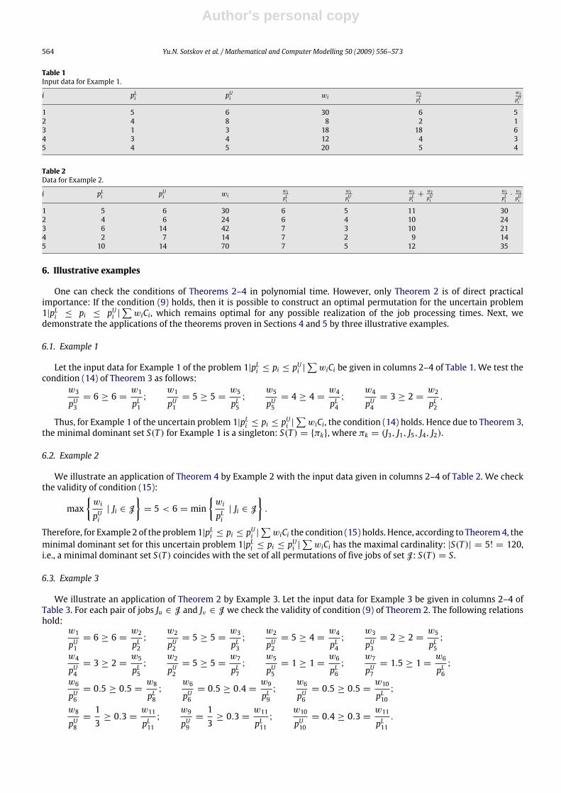
Table 1Input data for Example 1.

i pLi pUi wiwipLi

wipUi

1 5 6 30 6 52 4 8 8 2 13 1 3 18 18 64 3 4 12 4 35 4 5 20 5 4

Table 2Data for Example 2.

i pLi pUi wiwipLi

wipUi

wipLi+

wipUi

wipLi·wipUi

1 5 6 30 6 5 11 302 4 6 24 6 4 10 243 6 14 42 7 3 10 214 2 7 14 7 2 9 145 10 14 70 7 5 12 35

6. Illustrative examples

One can check the conditions of Theorems 2–4 in polynomial time. However, only Theorem 2 is of direct practicalimportance: If the condition (9) holds, then it is possible to construct an optimal permutation for the uncertain problem1|pLi ≤ pi ≤ pUi |

∑wiCi, which remains optimal for any possible realization of the job processing times. Next, we

demonstrate the applications of the theorems proven in Sections 4 and 5 by three illustrative examples.

6.1. Example 1

Let the input data for Example 1 of the problem 1|pLi ≤ pi ≤ pUi |∑wiCi be given in columns 2–4 of Table 1. We test the

condition (14) of Theorem 3 as follows:w3

pU3= 6 ≥ 6 =

w1

pL1;

w1

pU1= 5 ≥ 5 =

w5

pL5;

w5

pU5= 4 ≥ 4 =

w4

pL4;

w4

pU4= 3 ≥ 2 =

w2

pL2.

Thus, for Example 1 of the uncertain problem 1|pLi ≤ pi ≤ pUi |∑wiCi, the condition (14) holds. Hence due to Theorem 3,

the minimal dominant set S(T ) for Example 1 is a singleton: S(T ) = {πk}, where πk = (J3, J1, J5, J4, J2).

6.2. Example 2

We illustrate an application of Theorem 4 by Example 2 with the input data given in columns 2–4 of Table 2. We checkthe validity of condition (15):

max{wi

pUi| Ji ∈ J

}= 5 < 6 = min

{wi

pLi| Ji ∈ J

}.

Therefore, for Example 2 of the problem1|pLi ≤ pi ≤ pUi |∑wiCi the condition (15) holds. Hence, according to Theorem4, the

minimal dominant set for this uncertain problem 1|pLi ≤ pi ≤ pUi |∑wiCi has the maximal cardinality: |S(T )| = 5! = 120,

i.e., a minimal dominant set S(T ) coincides with the set of all permutations of five jobs of set J: S(T ) = S.

6.3. Example 3

We illustrate an application of Theorem 2 by Example 3. Let the input data for Example 3 be given in columns 2–4 ofTable 3. For each pair of jobs Ju ∈ J and Jv ∈ J we check the validity of condition (9) of Theorem 2. The following relationshold:

w1

pU1= 6 ≥ 6 =

w2

pL2;

w2

pU2= 5 ≥ 5 =

w3

pL3;

w2

pU2= 5 ≥ 4 =

w4

pL4;

w3

pU3= 2 ≥ 2 =

w5

pL5;

w4

pU4= 3 ≥ 2 =

w5

pL5;

w2

pU2= 5 ≥ 5 =

w7

pL7;

w5

pU5= 1 ≥ 1 =

w6

pL6;

w7

pU7= 1.5 ≥ 1 =

w6

pL6;

w6

pU6= 0.5 ≥ 0.5 =

w8

pL8;

w6

pU6= 0.5 ≥ 0.4 =

w9

pL9;

w6

pU6= 0.5 ≥ 0.5 =

w10

pL10;

w8

pU8=13≥ 0.3 =

w11

pL11;

w9

pU9=13≥ 0.3 =

w11

pL11;

w10

pU10= 0.4 ≥ 0.3 =

w11

pL11.



Table 3Data for Example 3.

i pLi pUi wiwipLi

wipUi

wipLi+

wipUi

wipLi·wipUi

1 1 3 18 18 6 24 842 5 6 30 6 5 11 303 4 10 20 5 2 7 104 3 4 12 4 3 7 125 4 8 8 2 1 3 26 10 20 10 1 0.5 1.5 0.57 3 10 15 5 1.5 6.5 7.58 10 15 5 0.5 1

356

16

9 5 6 2 0.4 13

1115

215

10 20 26 10 0.5 513 0.5 5

26

11 10 20 3 0.3 0.15 0.45 9200

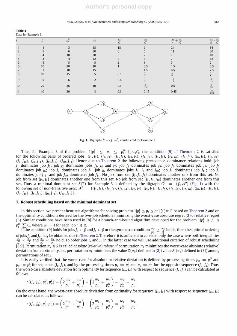
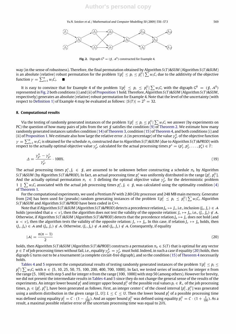
Fig. 1. Digraph G0 = (J,A0) constructed for Example 3.

Thus, for Example 3 of the problem 1|pLi ≤ pi ≤ pUi |∑wiCi, the condition (9) of Theorem 2 is satisfied

for the following pairs of ordered jobs: (J1, J2), (J2, J3), (J2, J4), (J3, J5), (J4, J5), (J2, J7), (J5, J6), (J7, J6), (J6, J8), (J6, J9),(J6, J10), (J8, J11), (J9, J11), (J10, J11). Hence due to Theorem 2 the following precedence–dominance relations hold: JobJ1 dominates job J2; job J2 dominates jobs J3, J4 and J7; job J3 dominates job J5; job J4 dominates job J5; job J5dominates job J6; job J7 dominates job J6; job J6 dominates jobs J8, J9 and J10; job J8 dominates job J11; job J9dominates job J11; and job J10 dominates job J11. No job from set {J3, J4, J7} dominates another one from this set. Nojob from set {J5, J7} dominates another one from this set. No job from set {J8, J9, J10} dominates another one from thisset. Thus, a minimal dominant set S(T ) for Example 3 is defined by the digraph G0 = (J,A0) (Fig. 1) with thefollowing set of non-transitive arcs: A0 = {(J1, J2), (J2, J3), (J2, J4), (J2, J7), (J3, J5), (J4, J5), (J5, J6), (J7, J6), (J6, J8), (J6, J9),(J6, J10), (J8, J11), (J9, J11), (J10, J11)}.

7. Robust scheduling based on the minimal dominant set

In this section, we present heuristic algorithms for solving problem 1|pLi ≤ pi ≤ pUi |∑wiCi based on Theorem 2 and on

the optimality conditions derived for the two-job schedule minimizing the worst-case absolute regret (2) or relative regret(3). Similar conditions have been used in [8] for a branch-and-bound algorithm developed for the problem 1|pLi ≤ pi ≤pUi |

∑Ci, wherewi = 1 for each job Ji ∈ J.

If the condition (9) holds for jobs Ju ∈ J and Jv ∈ J or the symmetric condition wvpUv≥

wupLuholds, then the optimal ordering

of jobs Ju and Jvmay be obtained due to Theorem2. Therefore, it is sufficient to consider only the casewhere both inequalitieswupUu< wv

pLvand wv

pUv< wu

pLuhold. To order jobs Ju and Jv in the latter case we will use additional criterion of robust scheduling

[8,9]. Permutation πk ∈ S is called absolute (relative) robust, if permutation πk minimizes the worst-case absolute (relative)deviation from optimality, i.e., permutation πk minimizes the value Z(πk) defined in (2) (value Z ′(πk) defined in (3)) amongpermutations of set S.It is easily verified that the worst-case for absolute or relative deviation is defined by processing times pu := pUu and

pv := pLv for sequence (Ju, Jv), and by the processing times pu := pLu and pv := p

Uv for the opposite sequence (Jv, Ju). Thus,

the worst-case absolute deviation from optimality for sequence (Ju, Jv)with respect to sequence (Jv, Ju) can be calculated asfollows:

r((Ju, Jv), pUu , pLv) =

(2wu

pUu+wv

pLv

)−

(2wv

pLv+wu

pUu

)=wu

pUu−wv

pLv.

On the other hand, the worst-case absolute deviation from optimality for sequence (Jv, Ju)with respect to sequence (Ju, Jv)can be calculated as follows:

r((Jv, Ju), pLu, pUv ) =

(2wv

pUv+wu

pLu

)−

(2wu

pLu+wv

pUv

)=wv

pUv−wu

pLu.



Therefore, sequence (Ju, Jv) is the absolute robust sequence with respect to sequence (Ju, Jv) if and only if inequalitywu

pUu−wv

pLv≤wv

pUv−wu

pLuholds, or equivalently:

wu

pLu+wu

pUu≤wv

pLv+wv

pUv. (17)

Similarly, the worst-case relative deviation from optimality for sequence (Ju, Jv)with respect to sequence (Jv, Ju) can becalculated as follows:

r((Ju, Jv), pUu , pLv)

γ ∗=

2wupUu+

wv

pLv

2wvpLv+

wupUu

,

where γ ∗ denotes theminimal value of the objective function γ =∑ni=1wiCi for the best sequence of these two jobs, either

(Ju, Jv) or (Jv, Ju), calculated for the actual job processing times. Inequalities n ≥ 2, wi > 0 and pLi > 0 for each job Ji ∈ Jimply γ ∗ > 0. (We remind that the actual processing time of job Ji ∈ J becomes known only after completing job Ji.)On the other hand, theworst-case relative deviation fromoptimality for sequence (Jv, Ju)with respect to sequence (Ju, Jv)

can be calculated as follows:

r((Jv, Ju), pLu, pUv )

γ ∗=

2wvpUv+

wupLu

2wupLu+

wv

pUv

.

Therefore, sequence (Ju, Jv) is the relative robust sequence with respect to sequence (Jv, Ju) if and only if inequality

2wupUu+

wv

pLv

2wvpLv+

wupUu

≤

2wvpUv+

wupLu

2wupLu+

wv

pUv

,

holds or equivalently:wu

pLu·wu

pUu≤wv

pLv·wv

pLv. (18)

As a result, two heuristics for solving problem 1|pLi ≤ pi ≤ pUi |∑wiCi can be derived from the two-job optimality

conditions represented by inequalities (17) and (18). The first heuristic called SUM computes sumwu

pLu+wu

pUufor each job Ju ∈ J, and sorts set of jobs J in non-decreasing order of this sum.The second heuristic called PROD computes productwu

pLu·wu

pUufor each job Ju ∈ J, and sorts set of jobs J in non-decreasing order of this product. Before presenting a formal algorithm forsolving (exactly or heuristically) problem 1|pLi ≤ pi ≤ p

Ui |∑wiCi, we demonstrate its procedure on Examples 1, 2, and 3.

7.1. Exact solution to Example 1

Testing the condition (9) of Theorem 2 for each pair of jobs from set J of Example 1 gives a completely ordered set ofjobs: J3 7→ J1 7→ J5 7→ J4 7→ J2.Thus, permutation πk = (J3, J1, J5, J4, J2) ∈ S provides an exact solution to Example 1 of the uncertain problem

1|pLi ≤ pi ≤ pUi |∑wiCi. In other words, for any vector p of the possible processing times defined in columns 2–4 of Table 1,

permutation πk is optimal for the deterministic problem 1 ‖∑wiCi associated with the vector p ∈ T of the job processing

times.

7.2. Heuristic solutions to Example 2

Testing the condition (9) of Theorem 2 for each pair of jobs from set J = {J1, J2, J3, J4, J5} in Example 2 gives thedigraph G = (J,A) = G0 with an empty set of arcs: A = ∅. Thus, Example 2 is the most uncertain case of the problem1|pLi ≤ pi ≤ p

Ui |∑wiCi with five jobs and so one can only find a heuristic solution to Example 2.

Having applied the heuristic SUM for set J, we obtain permutation πk = (J4, J2, J3, J1, J5) ∈ S(T ) = S, which provides aheuristic solution to Example 2. Having applied the heuristic PROD for set J, we obtain permutation πl = (J4, J3, J2, J1, J5) ∈S(T ) = S, which provides another heuristic solution to Example 2.



7.3. Heuristic solutions to Example 3

Testing the condition (9) of Theorem 2 for each pair of jobs from set J = {J1, J2, J3, J4, J5} in Example 3 gives the digraphG0 = (J,A0) representing a minimal dominant set S(T ) (see Fig. 1). Let Pi denote the list of predecessors of vertex Ji in thedigraph G0. We obtain P1 = ∅, P2 = {J1}, P3 = {J1, J2}, P4 = {J1, J2}, P5 = {J1, J2, J3, J4}, P6 = {J1, J2, J3, J4, J5, J7}, P7 = {J1, J2},P8 = {J1, J2, J3, J4, J5, J6, J7}, P9 = {J1, J2, J3, J4, J5, J6, J7}, P10 = {J1, J2, J3, J4, J5, J6, J7}, P11 = {J1, J2, J3, J4, J5, J6, J7, J8, J9, J10}.Since only job J1 has an empty set P1 of predecessors in the digraphG0, job J1 occupies the first position in the desired optimalpermutation πk = (Jk1 , Jk2 , . . . , Jk10) ∈ S(T ). We fix the first position for job J1 in permutation πk as follows: J1 = Jk1 , anddelete job J1 from all lists of predecessors. As a result, we obtain the following modified lists of predecessors: Pi := Pi \ {J1},i ∈ {2, 3, . . . , 11}.Now, only job J2 has an empty modified list of predecessors. Therefore, job J2 occupies the second position in the desired

optimal permutation πk ∈ S(T ). We fix the second position for job J2 in permutation πk as follows: J2 = Jk2 , and deletejob J2 from all the other lists of predecessors. As a result, we obtain the modified lists of predecessors: Pi := Pi \ {J2},i ∈ {3, 4, . . . , 11}.Now, each of the three jobs J3, J4, and J7 has an empty modified list of predecessors and we cannot find the optimal

positions for jobs J3, J4, and J7 in the desired optimal permutation πk ∈ T . Let us order these three jobs using heuristic PROD.As a result, we obtain the sequence (J7, J3, J4). (Note that the same sequence is obtained due to heuristic SUM.) Thus, job J7occupies the third position, job J3 occupies the forth position, and job J4 occupies the fifth position in permutationπk ∈ S(T ).(Note that the above sequence (J7, J3, J4)was not optimally chosen, and so permutation πkmay be not optimal for the actualprocessing times that are unknown before completing the corresponding jobs).We delete jobs J3, J4, and J7 from all the otherlists of predecessors and obtain the following modified lists of predecessors: Pi := Pi \ {J3, J4, J7}, i ∈ {5, 6, 8, 9, 10, 11}.Now, only job J5 has an empty modified list of predecessors. Therefore, job J5 occupies the sixth position in the desired

optimal permutationπk ∈ S(T ): J5 = Jk6 .We delete job J5 from all the other lists of predecessors, i.e., we obtain the followingmodified lists of predecessors: Pi := Pi \ {J5}, i ∈ {6, 8, 9, 10, 11}.Now, only job J6 has an emptymodified list of predecessors. Therefore, job J6 occupies the seventh position in the desired

optimal permutationπk ∈ S(T ): J6 = Jk7 .We delete job J6 from all the other lists of predecessors, i.e., we obtain the followingmodified lists of predecessors: Pi := Pi \ {J6}, i ∈ {8, 9, 10, 11}.Now, each of three jobs J8, J9, and J10 has an emptymodified list of predecessors andwe cannot find the optimal positions

of jobs J8, J9, and J10 in the desired optimal permutation πk ∈ T . We can order these three jobs using heuristic PROD andobtain sequence (J9, J8, J10). Thus, due to the heuristic PROD, job J9 occupies the eighth position, job J8 occupies the ninthposition, and job J10 occupies the tenth position in the permutation πk ∈ S(T ).Another sequence (J9, J10, J8) can be obtained using heuristic SUM. Due to the heuristic SUM job J9 occupies the eighth

position, job J10 occupies the ninth position, and job J8 occupies the tenth position in permutation πk ∈ S(T ). In both cases,we delete jobs J8, J9, and J10 from the list of predecessors of job J11 and obtain the following modified list of predecessors:P11 := P11 \ {J8, J9, J10} = ∅. As a result, job J11 occupies the last position in the desired optimal permutation.Thus, having applied Theorem 2 and the heuristic PROD for unordered subsets of jobs from set J, we obtain permutation

πk = (J1, J2, J7, J3, J4, J5, J6, J9, J8, J10, J11) ∈ S(T ), which provides a heuristic solution to Example 3. On the other hand,having applied Theorem 2 and the heuristic SUM for unordered subsets of jobs from set J, we obtain permutationπl = (J1, J2, J7, J3, J4, J5, J6, J9, J10, J8, J11) ∈ S(T ), which provides another heuristic solution to Example 3. It should bereminded that before completing all jobs J, one cannot calculate the exact values

∑ni=1wiCi(πk, p) and

∑ni=1wiCi(πl, p) of

the objective function γ =∑ni=1wiCi since the vector p ∈ T remains unknown: The actual vector p

∗∈ T of job processing

times will be known after completing the last job from set J.

7.4. Algorithms for solving problem 1|pLi ≤ pi ≤ pUi |∑wiCi

We will use the following notations in the formal description of the above algorithm used for solving (exactly orheuristically) Examples 1, 2, and 3.Let πmk denote the subsequence of the first m jobs (with 1 ≤ m ≤ n) in the desired permutation πk ∈ S(T ): π

1k = (Jk1),

π2k = (Jk1 , Jk2), . . . , πnk = πk.

π0k denotes an empty subsequence of permutation πk.J denotes the subset of jobs, J ⊆ J, still undetermined in the constructed subsequence πmk of the desired permutation πk.C denotes the subset of jobs of set J, C ⊆ J,without predecessors in the set J .The following Algorithm S(T )&SUM is based on Theorem 2 and the heuristic SUM for the unordered subsets of vertices

from set J in digraph G0.Algorithm S(T )&SUM

Input: Segments [pLi , pUi ] and weightswi for all jobs Ji ∈ J.

Output: Permutation πk ∈ S(T ) ⊆ S providing a heuristic solutionto the problem 1|pLi ≤ pi ≤ p

Ui |∑wiCi.

Step 1: Setm := 0 and J := J;



FOR i = 1 to n DOset Pi := ∅;

END FORstep 2: FOR u = 1 to n DO

FOR v = 1 to n, v 6= u, DOtest condition (9) for the pair of jobs Ju ∈ J and Jv ∈ J;IF condition (9) holds THEN set Pv := Pv ∪ {Ju};

END FOREND FOR

step 3: Set C := ∅;FOR Ji ∈ J DOIF Pi = ∅ THEN set C := C ∪ {Ji};

END FORstep 4: IF |C | = 1 THEN set πm+1k := (Jk1 , Jk2 , . . . , Jkm , Jr),

where πmk = (Jk1 , Jk2 , . . . , Jkm) and C = {Jr};FOR Ji ∈ J DOset Pi := Pi \ {Jr}, J := J \ {Jr};

END FORsetm := m+ 1 GOTO step 3;

ELSEstep 5: FOR Ji ∈ C DO

compute h(Ji) =wipLi+

wipUi;

END FORcreate sequence (Ji1 , Ji2 , . . . , Ji|C |) by sorting all jobs in set Cin non-decreasing order of the values h(Jit ), t ∈ {1, 2, . . . , |C |}.

step 6: Set πm+|C |k := (Jk1 , Jk2 , . . . , Jkm , Ji1 , Ji2 , . . . , Ji|C |),where πmk = (Jk1 , Jk2 , . . . , Jkm);IFm+ |C | = n THEN STOPELSEFOR Ji ∈ J DOset Pi := Pi \ C , J := J \ C;

END FORsetm := m+ |C | GOTO step 3.

To obtain Algorithm S(T )&PROD based on Theorem 2 and the heuristic PROD, it is sufficient to substitute equality

h(Ji) =wi

pLi+wi

pUiby equality h(Ji) =

wi

pLi·wi

pUiat step 5 of Algorithm S(T )&SUM . If either the condition (17) or condition (18) turns out to be an equality, then job Ju precedesjob Jv in permutationπk ∈ S(T )while the other condition (18) (condition (17), respectively) holds as strict inequality. If bothconditions (17) and (18) turn out to be equalities and u < v, then job Ju precedes job Jv in permutationπk ∈ S(T ) constructedby heuristic SUM (by heuristic PROD).Both Algorithm S(T )&SUM and Algorithm S(T )&PROD takeO(n2) time. This complexity is defined by step 2. In the general

case of the problem 1|pLi ≤ pi ≤ pUi |∑wiCi Algorithm S(T )&SUM (Algorithm S(T )&SUM , respectively) generates a heuristic

solution for absolute (relative) robust scheduling. However, there is a special case of the problem 1|pLi ≤ pi ≤ pUi |∑wiCi in

which each of these algorithms provides an exact solution for robust scheduling.Let the set of jobs J in the problem 1|pLi ≤ pi ≤ p

Ui |∑wiCi be decomposed into r ≤ n subsets J = J1 ∪ J2 ∪ · · · ∪ Jr

such that the following conditions hold:

(i) |Jk| ≤ 2 for each k ∈ {1, 2, . . . , r};(ii) precedence–dominance relation Ju 7→ Jv holds for each pair of jobs Ju ∈ Jk and Jv ∈ Js with k < s.

Proposition 1. If for the problem1|pLi ≤ pi ≤ pUi |∑wiCi both conditions (i) and (ii)hold, thenAlgorithmS(T )&SUM (Algorithm

S(T )&PROD, respectively) generates an absolute (relative) robust permutation for this problem.

Proof. Due to conditions (i) and (ii), at each iteration of Algorithm S(T )&SUM (Algorithm S(T )&PROD) the cardinality of setC is not greater than 2. If |C | = 1, then the position of job Jr ∈ J ∈ J in the constructed permutation πk ∈ S(T ) is chosenin an optimal way due to Theorem 2. If |C | = 2, then sequence (Ji1 , Ji2) of jobs Ji1 ∈ C and Ji2 ∈ C is the absolute (relative)robust sequence with respect to the opposite sequence (Ji2 , Ji1) due to the sufficient condition (17) (the sufficient condition(18), respectively). Thus, each local decision for selecting a job from the set J to be processed next is realized in an optimal



Fig. 2. Digraph G0 = (J,A0) constructed for Example 4.

way (in the sense of robustness). Therefore, the final permutation obtained by Algorithm S(T )&SUM (Algorithm S(T )&SUM)is an absolute (relative) robust permutation for the problem 1|pLi ≤ pi ≤ p

Ui |∑wiCi due to the additivity of the objective

function γ =∑ni=1wiCi. �

It is easy to convince that for Example 4 of the problem 1|pLi ≤ pi ≤ pUi |∑wiCi with the digraph G0 = (J,A0)

represented in Fig. 2 both conditions (i) and (ii) of Proposition 1 hold. Therefore, Algorithm S(T )&SUM (Algorithm S(T )&SUM ,respectively) generates an absolute (relative) robust permutation for Example 4. Note that the level of the uncertainty (withrespect to Definition 1) of Example 4 may be evaluated as follows: |S(T )| = 25 = 32.

8. Computational results

Via the testing of randomly generated instances of the problem 1|pLi ≤ pi ≤ pUi |∑wiCi we answer (by experiments on

PC) the question of how many pairs of jobs from the set J satisfies the condition (9) of Theorem 2. We estimate how manyrandomly generated instances satisfies condition (14) of Theorem3, condition (15) of Theorem4, and both conditions (i) and(ii) of Proposition 1.We estimate also how large the relative error∆ (in percentage) of the value γ kp∗ of the objective functionγ =

∑ni=1wiCi is obtained for the scheduleπk constructed due to Algorithm S(T )&SUM (due to Algorithm S(T )&PROD) with

respect to the actually optimal objective value γ tp∗ calculated for the actual processing times p∗= (p∗1, p

∗

2, . . . , p∗n) ∈ T :

∆ =γ kp∗ − γ

tp∗

γ tp∗· 100%. (19)

The actual processing times p∗i , Ji ∈ J, are assumed to be unknown before constructing a schedule πk by AlgorithmS(T )&SUM (by Algorithm S(T )&PROD). In fact, an actual processing time p∗i was uniformly distributed in the range [p

Li , p

Ui ].

And the actually optimal permutation πt ∈ S defining the optimal objective value γ tp∗ for the deterministic problem1 ‖

∑wiCi associated with the actual job processing times p∗i , Ji ∈ J, was calculated using the optimality condition (4)

of Theorem 1.For the computational experiments, we used a Pentium IVwith 2.80 GHz processor and 248MBmainmemory. Generator

from [24] has been used for (pseudo) random generating instances of the problem 1|pLi ≤ pi ≤ pUi |∑wiCi. Algorithm

S(T )&SUM and Algorithm S(T )&PROD have been coded in C++.Note that if Algorithm S(T )&SUM (Algorithm S(T )&PROD) detects a precedence relation Ju 7→ Jv , i.e., inclusion (Ju, Jv) ∈ A

holds (provided that u < v), then the algorithm does not test the validity of the opposite relation: Jv 7→ Ju, i.e., (Jv, Ju) 6∈ A.Otherwise, if Algorithm S(T )&SUM (Algorithm S(T )&PROD) detects that the precedence relation Ju 7→ Jv does not hold (andu < v), then the algorithm tests the validity of the opposite relation: Jv 7→ Ju. In this case, if relation Jv 7→ Ju holds, then(Jv, Ju) ∈ A and (Ju, Jv) 6∈ A. Otherwise, (Jv, Ju) 6∈ A and (Ju, Jv) 6∈ A. Consequently, if equality

|A| =n(n− 1)2

(20)

holds, then Algorithm S(T )&SUM (Algorithm S(T )&PROD) constructs a permutation πk ∈ S(T ) that is optimal for any vectorp ∈ T of job processing timeswithout fail, i.e., equality γ kp∗ = γ

tp∗ must hold. Indeed, in such a case if equality (20) holds, then

digraph G turns out to be a tournament (a complete circuit-free digraph), and so the condition (15) of Theorem 4 necessarilyholds.Tables 4 and 5 represent the computational results of testing randomly generated instances of the problem 1|pLi ≤ pi ≤

pUi |∑wiCi with n ∈ {5, 10, 25, 50, 75, 100, 200, 400, 700, 1000}. In fact, we tested series of instances for integer n from

the range [5, 100]with step 5 and for integer n from the range [100, 1000]with step 50 (among others). However for brevity,we did not present the intermediate results in Tables 4 and 5 since they do not change the general sense of the results of theexperiments. An integer lower bound pLi and integer upper bound p

Ui of the possible real values pi ∈ R+ of the job processing

times, pi ∈ [pLi , pUi ], have been generated as follows. First, an integer center C of the closed interval [p

Li , p

Ui ] was generated

using a uniform distribution in the given range [L,U]: L ≤ C ≤ U . Then the lower bound pLi of a possible processing timewas defined using equality pLi = C · (1−

δ100 ). And an upper bound p

Ui was defined using equality p

Ui = C · (1+

δ100 ). As a

result, a maximal possible relative error of the uncertain processing time was equal to 2δ%.



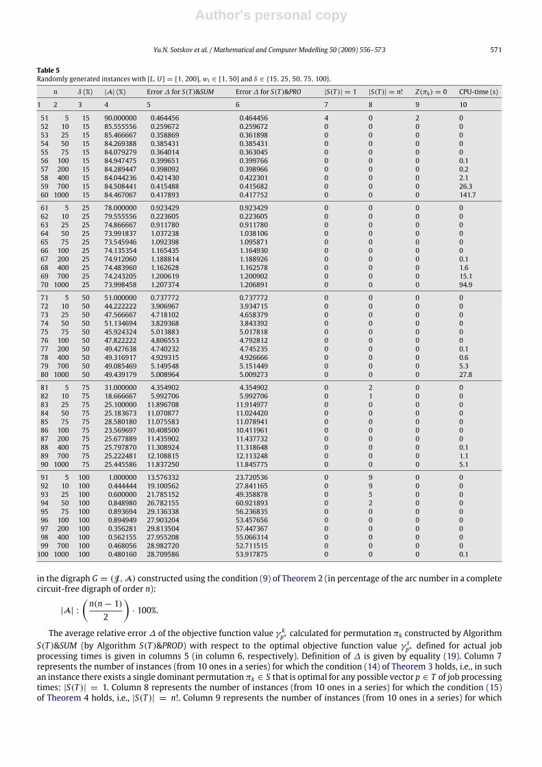
Table 4Randomly generated instances with [L,U] = [1, 200],wi ∈ [1, 50] and δ ∈ {0.1, 0.5, 1, 5, 10}.

n δ (%) |A| (%) Error∆ for S(T )&SUM Error∆ for S(T )&PRO |S(T )| = 1 |S(T )| = n! Z(πk) = 0 CPU-time (s)

1 2 3 4 5 6 7 8 9 10

1 5 0.1 100 0.000000 0.000000 10 0 0 02 10 0.1 100 0.000000 0.000000 10 0 0 03 25 0.1 99.800000 0.000346 0.000346 7 0 0 04 50 0.1 99.910204 0.000054 0.000054 3 0 0 05 75 0.1 99.909910 0.000110 0.000110 1 0 0 06 100 0.1 99.890909 0.000027 0.000027 0 0 0 0.17 200 0.1 99.909045 0.000072 0.000072 0 0 0 0.38 400 0.1 99.890100 0.000172 0.000172 0 0 0 3.39 700 0.1 99.902923 0.000149 0.000150 0 0 0 37.510 1000 0.1 99.895776 0.000156 0.000156 0 0 0 226.4

11 5 0.5 99.000000 0.000000 0.000000 9 0 0 012 10 0.5 99.777778 0.000000 0.000000 9 0 0 013 25 0.5 99.533333 0.000731 0.000731 2 0 0 014 50 0.5 99.420408 0.001109 0.001109 0 0 0 015 75 0.5 99.473874 0.000563 0.000563 0 0 0 016 100 0.5 99.466667 0.000679 0.000679 0 0 0 017 200 0.5 99.481407 0.000604 0.000604 0 0 0 0.218 400 0.5 99.500125 0.000619 0.000622 0 0 0 3.319 700 0.5 99.479542 0.000667 0.000666 0 0 0 44.220 1000 0.5 99.479600 0.000659 0.000658 0 0 0 209.6

21 5 1 98.000000 0.000000 0.000000 8 0 0 022 10 1 99.333333 0.000398 0.000398 7 0 0 023 25 1 98.700000 0.000616 0.000616 1 0 0 024 50 1 99.085714 0.001731 0.001731 0 0 0 025 75 1 99.012613 0.001632 0.001632 0 0 0 026 100 1 99.010101 0.002142 0.002142 0 0 0 027 200 1 98.923618 0.001992 0.001992 0 0 0 0.228 400 1 98.937719 0.002084 0.002073 0 0 0 3.229 700 1 98.967668 0.002089 0.002086 0 0 0 38.630 1000 1 98.953554 0.002085 0.002081 0 0 0 220.8

31 5 5 91.000000 0.129772 0.129772 4 0 2 032 10 5 95.111111 0.084177 0.084177 3 0 0 033 25 5 95.033333 0.041485 0.041485 0 0 0 034 50 5 94.546939 0.054941 0.054941 0 0 0 035 75 5 94.781982 0.044395 0.044254 0 0 0 036 100 5 94.632323 0.044177 0.044327 0 0 0 037 200 5 94.765829 0.048270 0.048372 0 0 0 0.238 400 5 94.854762 0.048875 0.048896 0 0 0 2.939 700 5 94.790170 0.046831 0.046897 0 0 0 38.940 1000 5 94.790170 0.047052 0.047036 0 0 0 199.7

41 5 10 90.000000 0.114561 0.114561 2 0 1 042 10 10 90.444444 0.154431 0.154431 0 0 0 043 25 10 89.533333 0.199577 0.199577 0 0 0 044 50 10 88.873469 0.153312 0.153312 0 0 0 045 75 10 90.061261 0.180604 0.181736 0 0 0 046 100 10 89.664646 0.204054 0.203940 0 0 0 047 200 10 89.246231 0.193124 0.192861 0 0 0 0.148 400 10 89.685088 0.186289 0.186374 0 0 0 2.549 700 10 89.483630 0.190972 0.191143 0 0 0 24.550 1000 10 89.559079 0.190070 0.190204 0 0 0 168.8

In the experiments, we tested instances of the problem1|pLi ≤ pi ≤ pUi |∑wiCiwith the relative errors 2δ% of the random

processing times defined by the following values of δ ∈ {0.1, 0.5, 1.0, 5.0, 10.0, 15.0, 25.0, 50.0, 75.0, 100.0}. Table 4represents the computational results for small relative errors of the job processing times: δ ∈ {0.1, 0.5, 1.0, 5.0, 10.0}, whileTable 5 represents the computational results for large relative errors of the job processing times: δ ∈ {15.0, 25.0, 50.0,75.0, 100.0}. In both Tables 4 and 5, the same range [L,U] for varying center C of the closed interval [pLi , p

Ui ] was used,

namely: L = 1 and U = 200. For each job Ji ∈ J, the real weight wi ∈ R+ was uniformly distributed in the same range[1, 50]. Of course, the weight wi is assumed to be known exactly before scheduling (in contrast to job processing time piwhich is assumed to be unknown before completion time Ci).Tables 4 and 5 represent the computational results for 100 series of the randomly generated instances of the problem

1|pLi ≤ pi ≤ pUi |∑wiCi. Each series includes 10 instances with the same combination of n and δ. The series number is

given in column 1. The number n of jobs in an instance is given in column 2. The half of the maximal possible error δ of therandom processing times (in percentage) is given in column 3. Column 4 represents the average relative number |A| of arcs



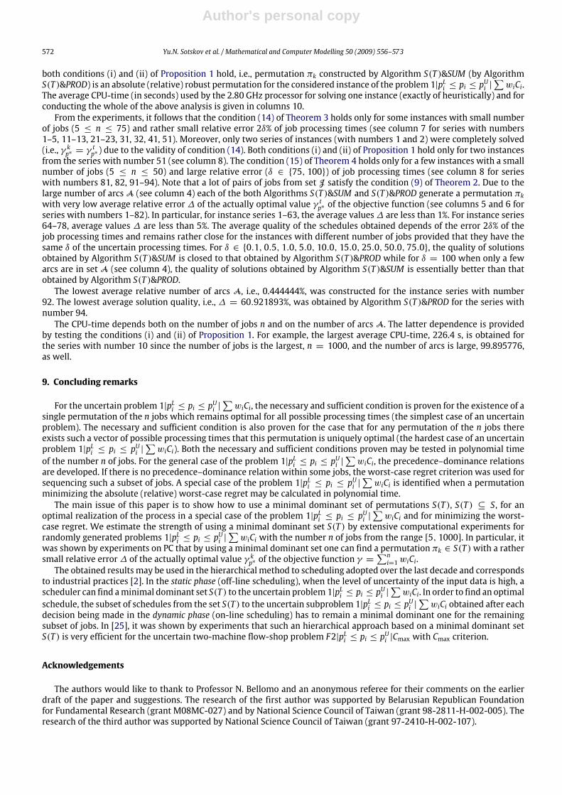
Table 5Randomly generated instances with [L,U] = [1, 200],wi ∈ [1, 50] and δ ∈ {15, 25, 50, 75, 100}.

n δ (%) |A| (%) Error∆ for S(T )&SUM Error∆ for S(T )&PRO |S(T )| = 1 |S(T )| = n! Z(πk) = 0 CPU-time (s)

1 2 3 4 5 6 7 8 9 10

51 5 15 90.000000 0.464456 0.464456 4 0 2 052 10 15 85.555556 0.259672 0.259672 0 0 0 053 25 15 85.466667 0.358869 0.361898 0 0 0 054 50 15 84.269388 0.385431 0.385431 0 0 0 055 75 15 84.079279 0.364014 0.363045 0 0 0 056 100 15 84.947475 0.399651 0.399766 0 0 0 0.157 200 15 84.289447 0.398092 0.398966 0 0 0 0.258 400 15 84.044236 0.421430 0.422301 0 0 0 2.159 700 15 84.508441 0.415488 0.415682 0 0 0 26.360 1000 15 84.467067 0.417893 0.417752 0 0 0 141.7

61 5 25 78.000000 0.923429 0.923429 0 0 0 062 10 25 79.555556 0.223605 0.223605 0 0 0 063 25 25 74.866667 0.911780 0.911780 0 0 0 064 50 25 73.991837 1.037238 1.038106 0 0 0 065 75 25 73.545946 1.092398 1.095871 0 0 0 066 100 25 74.135354 1.165435 1.164930 0 0 0 067 200 25 74.912060 1.188814 1.188926 0 0 0 0.168 400 25 74.483960 1.162628 1.162578 0 0 0 1.669 700 25 74.243205 1.200619 1.200902 0 0 0 15.170 1000 25 73.998458 1.207374 1.206891 0 0 0 94.9

71 5 50 51.000000 0.737772 0.737772 0 0 0 072 10 50 44.222222 3.906967 3.934715 0 0 0 073 25 50 47.566667 4.718102 4.658379 0 0 0 074 50 50 51.134694 3.829368 3.843392 0 0 0 075 75 50 45.924324 5.013883 5.017818 0 0 0 076 100 50 47.822222 4.806553 4.792812 0 0 0 077 200 50 49.427638 4.740232 4.745235 0 0 0 0.178 400 50 49.316917 4.929315 4.926666 0 0 0 0.679 700 50 49.085469 5.149548 5.151449 0 0 0 5.380 1000 50 49.439179 5.008964 5.009273 0 0 0 27.8

81 5 75 31.000000 4.354902 4.354902 0 2 0 082 10 75 18.666667 5.992706 5.992706 0 1 0 083 25 75 25.100000 11.896708 11.914977 0 0 0 084 50 75 25.183673 11.070877 11.024420 0 0 0 085 75 75 28.580180 11.075583 11.078941 0 0 0 086 100 75 23.569697 10.408500 10.411961 0 0 0 087 200 75 25.677889 11.435902 11.437732 0 0 0 088 400 75 25.797870 11.308924 11.318648 0 0 0 0.189 700 75 25.222481 12.108815 12.113248 0 0 0 1.190 1000 75 25.445586 11.837250 11.845775 0 0 0 5.1

91 5 100 1.000000 13.576332 23.720536 0 9 0 092 10 100 0.444444 19.100562 27.841165 0 9 0 093 25 100 0.600000 21.785152 49.358878 0 5 0 094 50 100 0.848980 26.782155 60.921893 0 2 0 095 75 100 0.893694 29.136338 56.236835 0 0 0 096 100 100 0.894949 27.903204 53.457656 0 0 0 097 200 100 0.356281 29.813504 57.447367 0 0 0 098 400 100 0.562155 27.955208 55.066314 0 0 0 099 700 100 0.468056 28.982720 52.711515 0 0 0 0100 1000 100 0.480160 28.709586 53.917875 0 0 0 0.1

in the digraph G = (J,A) constructed using the condition (9) of Theorem 2 (in percentage of the arc number in a completecircuit-free digraph of order n):

|A| :

(n(n− 1)2

)· 100%.

The average relative error∆ of the objective function value γ kp∗ calculated for permutation πk constructed by AlgorithmS(T )&SUM (by Algorithm S(T )&PROD) with respect to the optimal objective function value γ tp∗ defined for actual jobprocessing times is given in columns 5 (in column 6, respectively). Definition of ∆ is given by equality (19). Column 7represents the number of instances (from 10 ones in a series) for which the condition (14) of Theorem 3 holds, i.e., in suchan instance there exists a single dominant permutationπk ∈ S that is optimal for any possible vector p ∈ T of job processingtimes: |S(T )| = 1. Column 8 represents the number of instances (from 10 ones in a series) for which the condition (15)of Theorem 4 holds, i.e., |S(T )| = n!. Column 9 represents the number of instances (from 10 ones in a series) for which



both conditions (i) and (ii) of Proposition 1 hold, i.e., permutation πk constructed by Algorithm S(T )&SUM (by AlgorithmS(T )&PROD) is an absolute (relative) robust permutation for the considered instance of the problem 1|pLi ≤ pi ≤ p

Ui |∑wiCi.

The average CPU-time (in seconds) used by the 2.80 GHz processor for solving one instance (exactly of heuristically) and forconducting the whole of the above analysis is given in columns 10.From the experiments, it follows that the condition (14) of Theorem 3 holds only for some instances with small number

of jobs (5 ≤ n ≤ 75) and rather small relative error 2δ% of job processing times (see column 7 for series with numbers1–5, 11–13, 21–23, 31, 32, 41, 51). Moreover, only two series of instances (with numbers 1 and 2) were completely solved(i.e., γ kp∗ = γ

tp∗ ) due to the validity of condition (14). Both conditions (i) and (ii) of Proposition 1 hold only for two instances

from the series with number 51 (see column 8). The condition (15) of Theorem 4 holds only for a few instances with a smallnumber of jobs (5 ≤ n ≤ 50) and large relative error (δ ∈ {75, 100}) of job processing times (see column 8 for serieswith numbers 81, 82, 91–94). Note that a lot of pairs of jobs from set J satisfy the condition (9) of Theorem 2. Due to thelarge number of arcs A (see column 4) each of the both Algorithms S(T )&SUM and S(T )&PROD generate a permutation πkwith very low average relative error ∆ of the actually optimal value γ tp∗ of the objective function (see columns 5 and 6 forseries with numbers 1–82). In particular, for instance series 1–63, the average values∆ are less than 1%. For instance series64–78, average values ∆ are less than 5%. The average quality of the schedules obtained depends of the error 2δ% of thejob processing times and remains rather close for the instances with different number of jobs provided that they have thesame δ of the uncertain processing times. For δ ∈ {0.1, 0.5, 1.0, 5.0, 10.0, 15.0, 25.0, 50.0, 75.0}, the quality of solutionsobtained by Algorithm S(T )&SUM is closed to that obtained by Algorithm S(T )&PROD while for δ = 100 when only a fewarcs are in set A (see column 4), the quality of solutions obtained by Algorithm S(T )&SUM is essentially better than thatobtained by Algorithm S(T )&PROD.The lowest average relative number of arcs A, i.e., 0.444444%, was constructed for the instance series with number

92. The lowest average solution quality, i.e., ∆ = 60.921893%, was obtained by Algorithm S(T )&PROD for the series withnumber 94.The CPU-time depends both on the number of jobs n and on the number of arcs A. The latter dependence is provided

by testing the conditions (i) and (ii) of Proposition 1. For example, the largest average CPU-time, 226.4 s, is obtained forthe series with number 10 since the number of jobs is the largest, n = 1000, and the number of arcs is large, 99.895776,as well.

9. Concluding remarks

For the uncertain problem 1|pLi ≤ pi ≤ pUi |∑wiCi, the necessary and sufficient condition is proven for the existence of a

single permutation of the n jobs which remains optimal for all possible processing times (the simplest case of an uncertainproblem). The necessary and sufficient condition is also proven for the case that for any permutation of the n jobs thereexists such a vector of possible processing times that this permutation is uniquely optimal (the hardest case of an uncertainproblem 1|pLi ≤ pi ≤ p

Ui |∑wiCi). Both the necessary and sufficient conditions proven may be tested in polynomial time

of the number n of jobs. For the general case of the problem 1|pLi ≤ pi ≤ pUi |∑wiCi, the precedence–dominance relations

are developed. If there is no precedence–dominance relation within some jobs, the worst-case regret criterion was used forsequencing such a subset of jobs. A special case of the problem 1|pLi ≤ pi ≤ p

Ui |∑wiCi is identified when a permutation

minimizing the absolute (relative) worst-case regret may be calculated in polynomial time.The main issue of this paper is to show how to use a minimal dominant set of permutations S(T ), S(T ) ⊆ S, for an

optimal realization of the process in a special case of the problem 1|pLi ≤ pi ≤ pUi |∑wiCi and for minimizing the worst-

case regret. We estimate the strength of using a minimal dominant set S(T ) by extensive computational experiments forrandomly generated problems 1|pLi ≤ pi ≤ p

Ui |∑wiCi with the number n of jobs from the range [5, 1000]. In particular, it

was shown by experiments on PC that by using a minimal dominant set one can find a permutation πk ∈ S(T )with a rathersmall relative error∆ of the actually optimal value γ kp∗ of the objective function γ =

∑ni=1wiCi.

The obtained results may be used in the hierarchical method to scheduling adopted over the last decade and correspondsto industrial practices [2]. In the static phase (off-line scheduling), when the level of uncertainty of the input data is high, ascheduler can find aminimal dominant set S(T ) to the uncertain problem1|pLi ≤ pi ≤ p

Ui |∑wiCi. In order to find an optimal

schedule, the subset of schedules from the set S(T ) to the uncertain subproblem 1|pLi ≤ pi ≤ pUi |∑wiCi obtained after each

decision being made in the dynamic phase (on-line scheduling) has to remain a minimal dominant one for the remainingsubset of jobs. In [25], it was shown by experiments that such an hierarchical approach based on a minimal dominant setS(T ) is very efficient for the uncertain two-machine flow-shop problem F2|pLi ≤ pi ≤ p

Ui |Cmax with Cmax criterion.

Acknowledgements

The authors would like to thank to Professor N. Bellomo and an anonymous referee for their comments on the earlierdraft of the paper and suggestions. The research of the first author was supported by Belarusian Republican Foundationfor Fundamental Research (grant M08MC-027) and by National Science Council of Taiwan (grant 98-2811-H-002-005). Theresearch of the third author was supported by National Science Council of Taiwan (grant 97-2410-H-002-107).



References

[1] M. Pinedo, Scheduling: Theory, Algorithms, and Systems, Prentice-Hall, USA, Englewood Cliffs, 1995.[2] H. Aytug, M.A. Lawley, K. McKay, S. Mohan, R. Uzsoy, Executing production schedules in the face of uncertainties: A review and some future directions,European Journal of Operational Research 161 (2005) 86–110.

[3] A. Barbagallo, Regularity results for time-dependent variational and quasi-variational inequalities and application to the calculation of dynamic trafficnetwork, Mathematical Models and Methods in Applied Sciences 17 (2) (2007) 277–304.

[4] T.-C. Lai, Yu.N. Sotskov, N. Sotskova, F. Werner, Optimal makespan scheduling with given bounds of processing times, Mathematical and ComputerModelling 26 (1997) 67–86.

[5] T.-C. Lai, Yu.N. Sotskov, Sequencing with uncertain numerical data for makespan minimization, Journal of the Operational Research Society 50 (1999)230–243.

[6] M. Sevaux, K. Sorensen, A genetic algorithm for robust schedules in a one-machine environment with ready times and due dates, 4OR A QuarterlyJournal of Operations Research 2 (2) (2004) 129–147.

[7] I. Averbakh, Minmax regret solutions for minmax optimization problems with uncertainty, Operations Research Letters 27 (2000) 57–65.[8] R.L. Daniels, P. Kouvelis, Robust scheduling to hedge against processing time uncertainty in single-stage production, Management Science 41 (2)(1995) 363–376.

[9] P. Kouvelis, G. Yu, Robust Discrete Optimization and Its Applications, Kluwer Academic Publishers, Boston, The USA, 1997.[10] V. Lebedev, I. Averbakh, Complexity of minimizing the total flow time with interval data and minmax regret criterion, Discrete Applied Mathematics

154 (2006) 2167–2177.[11] J. Yang, G. Yu, On the robust single machine scheduling problem, Journal of Combinatorial Optimization 6 (2002) 17–33.[12] R.L. Graham, E.L. Lawler, J.K. Lenstra, A.H.G. Rinnooy Kan, Optimization and approximation in deterministic sequencing and scheduling. A survey,

Annals of Discrete Mathematics 5 (1976) 287–326.[13] W.E. Smith, Various optimizers for single-stage production, Naval Research and Logistics Quarterly 3 (1) (1956) 59–66.[14] I. Averbakh, On the complexity of a class of combinatorial optimization problems with uncertainty, Mathematical Programming, Series A 90 (2001)

263–272.[15] R. Leus, W. Herroelen, The complexity of machine scheduling for stability with a single disrupted job, Operations Research Letters 33 (2005) 151–156.[16] R. Leus, W. Herroelen, Scheduling for stability in single-machine production systems, Journal of Scheduling 10 (2007) 223–235.[17] P. Kouvelis, R.L. Daniels, G. Vairaktarakis, Robust scheduling of a two-machine flow shop with uncertain processing times, IIE Transactions 32 (2000)

421–432.[18] A. Kasperski, Minimizing maximal regret in the single machine sequencing problem with maximum lateness criterion, Operations Research Letters

33 (2005) 431–436.[19] A. Allahverdi, Yu.N. Sotskov, Two-machine flowshopminimum-length scheduling problemwith random and bounded processing times, International

Transactions in Operational Research 10 (2003) 65–76.[20] A. Allahverdi, T. Aldowaisan, Yu.N. Sotskov, Two-machine flowshop scheduling problem tominimizemakespan or total completion timewith random

and bounded setup times, International Journal of Mathematical Sciences 39 (2003) 2475–2486.[21] N.M. Leshchenko, Yu.N. Sotskov, Realization of an optimal schedule for the two-machine flow-shop with interval processing times, International

Journal Information Theories & Applications 14 (2007) 182–189.[22] Yu.N. Sotskov, A. Allahverdi, T.-C. Lai, Flowshop scheduling problem to minimize total completion time with random and bounded processing times,

Journal of the Operational Research Society 55 (2004) 277–286.[23] E.G. Koffman (Ed.), Computer and Job-Shop Scheduling Theory, John Wiley & Sons, 1976.[24] E. Taillard, Benchmarks for basic scheduling problems, European Journal of Operational Research 64 (1993) 278–285.[25] N.M.Matsveichuk, Yu.N. Sotskov, N.G. Egorova, T.-C. Lai, Schedule execution for two-machine flow-shopwith interval processing times,Mathematical

and Computer Modelling 49 (5–6) (2009) 991–1011.

Schedule execution for two-machine flow-shop with interval processing times

Documents

Transcript of Schedule execution for two-machine flow-shop with interval processing times