IJRIM Volume 2, Issue 2 (February 2012) (ISSN 2231-4334) A ...
Upload
khangminh22Category
view
3download
0
Metal Structures Centre – 2011


Published by Laboratory Soete – Ghent University Technologiepark 903 9052 Zwijnaarde – Belgium http://www.tribology-fatigue.ugent.be/ Edited by: Jeroen Van Wittenberghe ISSN: 2032-7471
Sustainable Construction & Design
Volume 2, 2011 Issue 2

Editor
Jeroen Van Wittenberghe
Co-editing organization
MSC - Metal Structures Centre
Editorial Board
Serge Claessens Patrick De Baets Wim De Waele Sergei Glavatskikh Stijn Hertelé Sven Vandeputte Walter Vermeirsch
International Scientific Advisory Committee
Magd Abdel Wahab Rudi Denys Ney Francisco Ferreira Gabor Kalacska Eli Saul Puchi Cabrera Dik Schipper Mariana Staia Laszlo Zsidai
Sustainable Construction & Design, volume 2, issue 2, 2011
ISSN 2032-7471
Published by: Laboratory Soete – Ghent University Technologiepark 903 9052 Zwijnaarde – Belgium http://www.tribology-fatigue.ugent.be/
Cover design by Jeroen Van Wittenberghe
The texts of the papers in this volume were set individually by the authors or under their supervision. Only minor corrections to the text may have been carried out by the publisher.
No responsibility is assumed by the publisher, editor and authors for any injury or damage to persons or property as a matter of products liability, negligence or otherwise, or from any use or operation of any methods, products, instructions or ideas contained in the material herein.
© Laboratory Soete 2011
The rights of this publication are held by the Laboratory Soete according to the Creative Commons, Attribution 2.0. This means users are allowed to share and remix the work, but with attribution to the authors. All with the understanding that other rights on the works are not affected by this license. The full license text can be found on http://creativecommons.org/licenses/by/2.0/be/
Research activities at
Laboratory Soete
http://www.tribology-fatigue.ugent.be/
Labo Soete
Fracture mechanics Tribology
Finite Element Analysis Fatigue
Small to large scale experimental
testing.
Experts in pipeline weld research.
Fatigue testing and analysis. E.g.
research on pipe joints in a full scale
resonant bending fatigue setup.
Modelling of engineering structures
and applications.
LABO SOETE – GHENT UNIVERSITY Dept. of Mechanical Construction & Production
Technologiepark 903
9052 Zwijnaarde – BELGIUM
http://www.tribology-fatigue.ugent.be

Contents
Issue 2: Materials and structures in construction and design
Editorial ........................................................................................................................................................................... 160
Van Wittenberghe J.
Non destructive testing techniques for risk based inspection.................................................................. 161
Van den Abeele F., Goes P.
Product crossing: designing connections using a product example ....................................................... 172
Bleuzé T., Ceupens J., De Baets P., Detand J.
Increasing information feed in the process of structural steel design................................................... 180
Pauwels P., Jonckheere T., De Meyer R., Van Campenhout J.
Metaheuristics in architecture................................................................................................................................ 190
Strobbe T., Pauwels P., Verstraeten R., De Meyer R.
A nice thing about standards................................................................................................................................... 197
Verstraeten R., Jonckheere T., De Meyer R., Van Campenhout J.
Fatigue damage identification in threaded connection of tubular structures through in-situ
modal tests...................................................................................................................................................................... 207
Bui T.T., De Roeck G., Van Wittenberghe J., De Baets P., De Waele W.
Towards better finite element modelling of elastic recovery in sheet metal forming of
advanced high strength steel .................................................................................................................................. 217
Safaei M., De Waele W.
Development and validation of a high constraint modified boundary layer finite element
model................................................................................................................................................................................. 228
Verstraete M., De Waele W., Hertelé S.
Influence of design features on the structural integrity of threaded pipe connections ................. 237
Galle T., De Waele W., De Baets P., Van Wittenberghe J.
Analytical and computational estimation of patellofemoral forces in the knee under squatting
and isometric motion ................................................................................................................................................. 246
Fekete G., Málnási Csizmadia B., Wahab M.A., De Baets P.
Design of a (mini) wide plate specimen for strain-based weld integrity assessment..................... 258
Hertelé S., De Waele W., Denys R., Verstraete M.

Determination of granular assemblies' discrete element material parameters by modelling the
standard shear test...................................................................................................................................................... 269
Keppler I., Csatar A.
Development of a continuum plasticity model for the commercial finite element code
ABAQUS............................................................................................................................................................................ 275
Safaei M., De Waele W.
Fluid mechanical aspects of open- and closed-toe flue organ pipe voicing......................................... 284
Steenbrugge D.
Design of crack arrestors for ultra high grade gas transmission pipelines: material selection,
testing and modelling................................................................................................................................................. 296
Van den Abeele F., Di Biagio M.
Design of crack arrestors for ultra high grade gas transmission pipelines: simulation of crack
initiation, propagation and arrest......................................................................................................................... 307
Van den Abeele F., Di Biagio M., Amlung L.
Stability of offshore structures in shallow water depth .............................................................................. 320
Van den Abeele F., Vande Voorde J.
Design characteristics that improve the fatigue life of threaded pipe connections......................... 334
Van Wittenberghe J., De Baets P., De Waele W., Galle T., Bui T.T., De Roeck G.
On the dynamic stability of high-speed gas bearings: stability study and experimental
validation......................................................................................................................................................................... 342
Waumans T., Peirs J., Reynaerts D., Al-Bender F.

Issue 2 Materials and structures in construction and design
Editorial In the second issue of the 2011 volume, the focus is laid on materials and structures in construction and design. This issue includes work on constructional steel research, assessment techniques for cracks in pipeline welds and threaded pipe connections, design rules in architecture and the use of modern computational techniques for designing and analysing engineering applications. As announced in the previous issue, all MSC partners moved to the central campus in Zwijnaarde. Since the foundation of the MSC in 2009, additional members became involved in the partnership in order to share state-of-the-art research facilities in a modern structure of collaboration, clustering and strategic alliance of research with an important focus on metals. This new cluster has been inaugurated on September 20, 2011 under the name Materials Research Cluster Gent. Additional information can be found on http://www.mrcluster.be/. Jeroen Van Wittenberghe SCAD journal editor
160 Copyright © 2011 by Laboratory Soete

Sustainable Construction and Design 2011
Copyright © 2011 by Laboratory Soete
NON DESTRUCTIVE TESTING TECHNIQUES
FOR RISK BASED INSPECTION
F. Van den Abeele1 and P. Goes1
1
Abstract
OCAS N.V., J.F. Kennedylaan 3, 9060 Zelzate, Belgium
Ensuring the safety of offshore structures is of vital importance for the reliability of oil and gas drilling rigs. Risk based inspection (RBI) is becoming an industry standard for management of equipment integrity. The objective of risk based inspection is to determine the likelihood of equipment failure (probability) and the consequences of such an event. Combining the probability of an event with its possible consequences allows determining the risk of an operation. Risk based inspection enables to optimize the frequency of inspection, by moving from periodic inspection (based on arbitrary calendar dates) to an informed inspection program (based on equipment condition).
One of the most important tools to determine the condition of the equipment, and to calculate its reliability, is the use of non destructive testing (NDT) techniques to detect cracks, flaws and defects. The probability of detection and the probability of sizing depend on the type of NDT method used. Combining NDT information on crack size and depth with fracture mechanics based damage models, allows predicting the remaining life time of a component.
In this paper, the philosophy of risk based inspection is introduced and recent advances in non destructive testing (in particular ultrasonic and electromagnetic techniques) are reviewed. Then, the use of fracture mechanics based damage models is demonstrated to predict fatigue failure for offshore structures.
Keywords inspection, reliability, non destructive testing, ultrasonics, ACFM, structural integrity, risk
1 PHILOSOPHY OF RISK BASED INSPECTION
The objective of Risk Based Inspection (RBI) is to determine what incident could occur (consequence) in the event of an equipment failure, and how likely (probability) it is that the incident could happen. Multiplying the likelihood of an incident with its possible consequences will determine the risk associated to the operation.
Figure 1: Criticality matrix for risks associated with the installation of wind turbines
161

Sustainable Construction and Design 2011
Copyright © 2011 by Laboratory Soete
In a qualitative risk assessment, the combination of probability and consequence can be visualized in a criticality matrix. On Figure 1, such a scheme is presented to evaluate the environmental risks associated
with the installation of large ( 2 MW) wind turbines.
Some failures may occur frequently, but without significant adverse impacts. Similarly, other failures can have potentially serious consequences, but if the probability of the incident is low, than the resulting risk may not warrant immediate action. If the risk is medium, mitigation measures are normally subject to a cost/benefit analysis. Action will be taken if the cost of implementing the measure is lower than the loss, associated with the possible event. When the risk is not acceptable, mitigation measures have to be put in place.
Figure 2: Flowchart for Risk Based Inspection program
As shown on the flowchart, the risk assessment (either qualitative or quantitative) is used as an input to determine the inspection interval for an RBI maintenance program. The aim is to deploy a finite inspection resource according to a ranked list of components and their associated level of risk. In that respect, risk based inspection enables to optimize the frequency of inspection, by moving from period inspection (based on arbitrary calendar dates) to an informed inspection program (based on equipment condition).
Indeed, the hazard rate of most engineering equipment follows a so-called reliability bath tub curve, shown on Figure 3, which is characterised by three distinct regions. The first region corresponds to the start of life, and an increased hazard rate due to variation in material properties and strength, poor design, manufacturing defects and human errors during installation and operation. As a result, most weak items fail during this phase causing a decrease of the initially high hazard rate.
The second region (useful life) is characterised by an approximately constant hazard rate. Failures in this region are not due to age, wear-out or degradation and preventive maintenance does not affect the hazard rate. The third region is characterized by an increased hazard rate due to wear-out and degradation of properties. Figure 3 shows how a profound understanding of these governing failure mechanisms allows optimizing the inspection intervals.
162

Sustainable Construction and Design 2011
Copyright © 2011 by Laboratory Soete
Figure 3: Reliability bathtub curve
It can be demonstrated [#] that the three regions of the bathtub curve can be described by a two parameter Weibull distribution
( ) 1 exp
m
tF t
!
" #$ %& ' '( )* +
( ), -. / (Eq. 01)
which gives the probability that failure will occur before time t for a characteristic life time ! and a shape parameter m. The reliability is, by definition,
( ) 1 ( ) ex p
m
tR t F t
!
" #$ %0 ' '( )* +
( ), -. / (Eq. 02)
Differentiating (Eq. 01) with respect to time yields the probability density function
1
( ) exp
m m
m t tf t
! ! !
' " #$ % $ %& '( )* + * +
( ), - , -. / (Eq. 03)
and the corresponding hazard rate can be calculated as
1
( )( )
( )
m
f t m th t
R t ! !
'$ %
& & * +, -
(Eq. 04)
which is plotted on Figure 3 for different values of the shape factor m. The hazard rate h(t) is decreasing for m < 1 and increasing for m > 1, while the m = 1 corresponds to a constant hazard rate. Hence, a Weibull probability distribution (Eq. 01) with a shape factor m < 1 indicates early-life failures, whereas m > 1 describes wear-out failures. Values in the interval [1 < m < 4] typically indicate early wear-out failures caused by low cycle fatigue, corrosion or erosion. Old age wear-out can be described by higher values of the shape factor (m > 4). For m = 1, the Weibull distribution (Eq. 01) transforms into the negative exponential distribution
1 2( ) 1 expF t t3& ' ' (Eq. 05)
with 3 = 1/!, which describes the useful region of the bath-tub curve, where the probability of failure within a specified time interval does not depend on age. During the useful life, the hazard rate is constant, i.e.
1( )h t 3
!& & (Eq. 06)
163

Sustainable Construction and Design 2011
Copyright © 2011 by Laboratory Soete
Figure 4: Weibull hazard rate for different values of the shape factor m
As evident from the reliability bathtub curve in Figure 3, and the flowchart on Figure 2, the effectiveness of an RBI inspection interval depends on
4 The ability to monitor equipment condition. For processing plants, petrochemical equipment and offshore structures, non destructive testing (NDT) is the preferred technique to evaluate the integrity of pressure vessels, pipelines, tubular joints, underwater welds, piping,... In the next section, some recent advances in non destructive testing (in particular ultrasonic and electromagnetic techniques) are reviewed that enable a more accurate condition monitoring.
4 The inspection reliability. The probability of detection (POD) is a statistical measure of the success of an inspection, whereas the probability of sizing (POS) provides an indication of sizing accuracy. Both POD and POS depend on the type of NDT method used. In section 3, the implications of probability of detection and sizing on an RBI program are briefly discussed.
4 Prediction of the remaining life time. Combining NDT information on crack size and depth with damage models allows predicting the remaining life of a component. At the end of this paper, fracture mechanics is applied to estimate the fatigue life of a cracked component, taking into account the inspection reliability.
2 RECENT ADVANCES IN NON DESTRUCTIVE TESTING
The offshore industry has been aware of the need for an understanding of the performance of the NDT systems used in crack detection and sizing for quite some time [2]. A large number of offshore structures consist of steel welded tubular joints, like shown on Figure 5, the better part of which are underwater. Such nodal joints can be highly stressed and subjected to cyclic loading, which makes them vulnerable to fatigue failure.
Figure 5: Welded tubular joint
164

Sustainable Construction and Design 2011
Copyright © 2011 by Laboratory Soete
An undetected fatigue crack caused the Alexander Keilland to disaster [3] in 1980. The capsize was the worst disaster in Norwegian waters since the second World War, and clearly stresses the importance of underwater inspection. A review of the early developments in diver inspection and the maturation of subsea NDT technologies is given in [4], while [5-6] address the role of non destructive testing in the offshore industry. A comprehensive overview of non destructive testing for the offshore industry is presented in [7]. In this section, some recent advances in ultrasonic testing and electromagnetic NDT techniques are briefly described.
2.1 Ultrasonic non destructive evaluation
Ultrasonic inspection is based on elastic wave propagation and detection. For an intact homogeneous material, the sound path is straight and the wave velocity is constant. Flaws in the material will cause refracted sound waves. The pulse-echo technique, shown on Figure 6, is the most commonly used ultrasonic method for offshore inspection. A transducer/receiver (T/R) probe is acoustically coupled to the specimen and generates an incident sound pulse P. When a flaw is present, the refracted signal F will appear on the oscilloscope before the back wall echo E. The time of flight is an indication of the position of the crack. In addition, time of flight diffraction (TOFD) methods can be used to estimate the crack size.
Figure 6: Pulse-echo technique for a tubular joint
In [8-9], ultrasonic bounded beam interactions are study features of the object under investigation. An incident bounded beam is modelled as a Fourier series of plane ultrasonic waves
1 2 1 2 1 2 1 2exp
, , exp2
x x z x
i tx z t A k i k x k z dk
56
7
89
'9
'" #& 8. /: (Eq. 07)
where the amplitude function can be written as
1 2 1 2( ) expx xA k F i k d; ; ;89
'9
& ': (Eq. 08)
where the components {kx, kz
2
2 2
x zk kc
5$ %8 & * +, -
} of the wave vector are connected to the angular frequency 5 and the acoustic wave velocity c through
(Eq. 09)
and
1 22( ) expf ; ;& ' (Eq. 10)
165
Sustainable Construction and Design 2011
Copyright © 2011 by Laboratory Soete
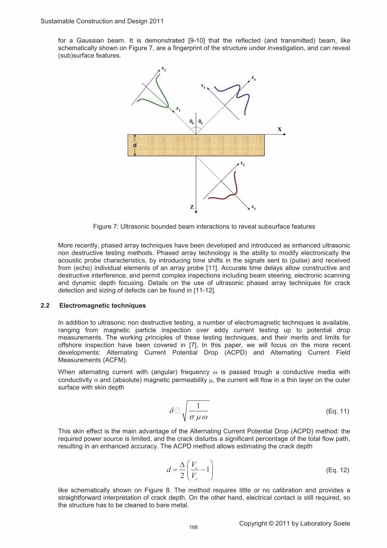
for a Gaussian beam. It is demonstrated [9-10] that the reflected (and transmitted) beam, like schematically shown on Figure 7, are a fingerprint of the structure under investigation, and can reveal (sub)surface features.
Figure 7: Ultrasonic bounded beam interactions to reveal subsurface features
More recently, phased array techniques have been developed and introduced as enhanced ultrasonic non destructive testing methods. Phased array technology is the ability to modify electronically the acoustic probe characteristics, by introducing time shifts in the signals sent to (pulse) and received from (echo) individual elements of an array probe [11]. Accurate time delays allow constructive and destructive interference, and permit complex inspections including beam steering, electronic scanning and dynamic depth focusing. Details on the use of ultrasonic phased array techniques for crack detection and sizing of defects can be found in [11-12].
2.2 Electromagnetic techniques
In addition to ultrasonic non destructive testing, a number of electromagnetic techniques is available, ranging from magnetic particle inspection over eddy current testing up to potential drop measurements. The working principles of these testing techniques, and their merits and limits for offshore inspection have been covered in [7]. In this paper, we will focus on the more recent developments: Alternating Current Potential Drop (ACPD) and Alternating Current Field Measurements (ACFM).
When alternating current with (angular) frequency 5 is passed trough a conductive media with
conductivity < and (absolute) magnetic permeability =, the current will flow in a thin layer on the outer surface with skin depth
1>
< =5 (Eq. 11)
This skin effect is the main advantage of the Alternating Current Potential Drop (ACPD) method: the required power source is limited, and the crack disturbs a significant percentage of the total flow path, resulting in an enhanced accuracy. The ACPD method allows estimating the crack depth
12
c
r
Vd
V
$ %?& '* +
, - (Eq. 12)
like schematically shown on Figure 8. The method requires little or no calibration and provides a straightforward interpretation of crack depth. On the other hand, electrical contact is still required, so the structure has to be cleaned to bare metal.
166

Sustainable Construction and Design 2011
Copyright © 2011 by Laboratory Soete
Figure 8: Alternating Current Potential Drop
The Alternating Current Field Measurement (ACFM) technique was developed for offshore applications [13] to maintain the advantages of ACPD while avoiding its limitations. This is achieved by injecting a uniform incident current, measuring the magnetic field components and relating them to the surface electric field. The ACFM sensor consists of two air wound coils, sensitive to changes in the Bx and Bz fields, which are parallel and normal to the crack respectively. With uniform current flowing in the y-direction and no defects present, Bz = 0 and Bx is uniform.
Figure 9: Alternating Current Field Measurements
167

Sustainable Construction and Design 2011
Copyright © 2011 by Laboratory Soete
The presence of a surface discontinuity diverts the current away from the deepest part and concentrates it near the ends of the defect. This produces a strong peak in the Bz signal near the ends of the crack, while the Bx signal drops in strength. As a result, the Bx signal contains information about the depth of the defect, while Bz
The Alternating Current Field Measurement technique was originally developed for manual inspection of offshore welds, but is now available for use in many applications where reduced cleaning and inspection through coatings is a benefit [14-16]. The technique does not require contact, can cope with marine fouling and coatings, enables crack sizing (depth and length) and allows for considerable cost savings [17].
is a measure for the crack length. The By signal is similar to Bz, but can be measured to distinguish between a crack and a pit. More details on the electromagnetic modelling to relate the field components to the dimensions of the defect can be found in [7].
3 PROBABILITY OF DETECTION AND PROBABILITY OF SIZING
Although Alternating Current Field Measurements and ultrasonic phased array techniques provide innovative means of non destructive evaluation, the accuracy of the RBI program still depends on the inspection reliability. The inspection data should reveal the location of a defect, and the length and depth of the crack. The probability of detection (POD) is a statistical measure of the success of an inspection, whereas the probability of sizing (POS) provides an indication of sizing accuracy. In this section, the implications of POD and POS on an RBI program are briefly discussed.
Probability of Detection (POD) Probability of Sizing (POS)
Figure 10: Probability of Detection (POD) and Probability of Sizing (POS)
3.1 Probability of Detection
The probability of detection (POD) is a statistical measure of the success of inspection, which can be expressed as a function of flaw size (like shown on Figure 10). A measured POD curve is obtained from the result of blind inspection trials, involving a range of defects in representative components and environments. Indeed, it is not possible to consider the performance of an NDT method on all cracks that may exist (i.e. the entire population). Instead, a sample must be chosen which is representative of the population. The confidence that the measured POD is representative of the population is dependent on the sample size. Assuming independent trials, the binomial distribution
1 21 2( )!
( ) 1! !
N SsNP S p p
S N S
'& '
' (Eq. 13)
is valid, and the confidence that the measured POD is representative of the population can be estimated as [18]
168

Sustainable Construction and Design 2011
Copyright © 2011 by Laboratory Soete
1 NC p& ' (Eq. 14)
which provides an elegant means of determining the minimum sample set required to reach a given confidence level [19].
3.2 Probability of Sizing
Probability of sizing (POS) is a measure of a particular inspection method’s ability to accurately quantify the dimensions of a flaw or defect. The reliability of ultrasonic NDT methods to inspect pipelines used in the oil industry is covered in [20], and a similar analysis for the ACFM technique is presented in [21]. An example of a POS distribution is shown on Figure 10, for a non destructive testing method which is bound to under-predict the actual flaw size. Hence, this inspection method is likely to be un-conservative. This information has to be incorporated in the damage predictions, like presented in [19] and explained in the next section.
4 FATIGUE CRACK GROWTH PREDICTIONS FOR OFFSHORE STRUCTURES
In order to evaluate whether or not a (detected) crack is critical, the design engineer has to understand the ability of a structure to resist further damage, and the critical amount of damage that the structure can sustain before remedial action is required. Standards and codes like [22] and [23] were developed for pressure vessels and carbon steel pipes, and can be used for defect assessment of offshore structures as well. These codes use fracture mechanics based damage models to predict crack growth and the remaining life of the structure. However, relatively small errors in initial flaw size could have very large consequences on the predicted remaining life. Therefore, it is important to introduce the inspection reliability in the calculations. The application of POD data in the prediction of corrosion rates for offshore pipelines has been presented in [19]. Here, the influence of probability of detection and probability of sizing on fatigue crack growth calculations is demonstrated.
Figure 11: Prediction of fatigue crack propagation using inspection reliability data
In linear elastic fracture mechanics, the fatigue growth rate can written as
1 2mdaC K
dN& ? (Eq. 15)
with C and m the Paris coefficients, and ?K the range in stress intensity factor, given by
K Y a< 7? & ? (Eq. 16)
169

Sustainable Construction and Design 2011
Copyright © 2011 by Laboratory Soete
where Y is a geometric correction factor and ?< is the applied stress range. As initial flaw, we assume that the largest flaw that could have just escaped inspection is present. Typically, this corresponds to a confidence level of 95% and a lower bound population of 90% POD. Like shown on Figure 11, this initial crack is predicted to grow according to (Eq. 15) until it reaches a critical value, corresponding to fatigue failure.
However, if the POS distribution of Figure 10 is superposed onto the graph, it can be seen that the measured value is likely to be an underestimate of the actual flaw size. Hence, the fatigue life predicted by the damage model would not yield a conservative value! When introducing POS data into the calculations, a more accurate lifetime prediction can be made.
5 REFERENCES
[1] Lewis, E.E., Introduction to Reliability Engineering, 2nd
[2] Dover W.D ;, Brennan F.P., Karé R.F. and Stacey A., Inspection Reliability for Offshore Structures, Proceedings of the 22nd International Conference on Offshore Mechanics and Arctic Engineering, OMEA 2003, Cancun, Mexico, 2003
Edition, ISBN 978-0-471-01833-9
[3] Norwegian Ministry of Justice and Police, The Allexander Keilland Accident, Report of the Public Commission, ISBN B000ED27N, 1981
[4] Clarke M., A Review of the Early Days of Diver Inspection and how Technology has Matured to Greet the Millennium, Offshore Underwater Inspection Insights, vol. 38(6), pp. 395-398, 1996
[5] Raine G.A, The Development and the Role of Non Destructive Testing in the UK Offshore Industry, Offshore Underwater Inspection Insights, vol. 41(12), pp. 772-777 (1999)
[6] Raine G.A, The Changing Face of Inspection of Oil and Gas Offshore Installations, Offshore Underwater Inspection Insights, vol. 40(6), pp. 429-434 (1998)
[7] Van den Abeele F. and Goes P., Electromagnetic Non Destructive Testing Techniques for Defect Sizing of Underwater Welds, Proceedings of the COMSOL Users’ Conference, Paris, France, 2010
[8] Declercq N., Van den Abeele F., Degrieck J. and Leroy O., The Schoch Effect to Distinguish Between Different Liquids in Closed Containers, IEEE Transactions on Ultrasonics, Ferroelectrics and Frequency Control, vol. 51(10), pp. 1354-1357, 2004
[9] Van den Abeele F., Declercq N., Degrieck J. and Leroy O., The Thomson-Haskell Method to Simulate Bounded Beam Interactions on Layered Media, Proceedings of the 3rd International Conference on Advanced Computatonial Methods in Engineering, Ghent, Belgium, 2005
[10] Declercq N. Van den Abeele F., Degrieck J. and Leroy O., On the Use of Bounded Beam Effects to Characterize Fluids in Containers, Proceedings of the 18th International Congress on Acoustics, Kyoto, Japan, 2004
[11] Satyanarayan L., Sridhar C., Krishnamurthy C.V. and Balasubramaniam K., Simulation of Ultrasonic Phased Array Technique for Imaging and Sizing of Defects using Longitudinal Waves, International Journal of Pressure Vessels and Piping, vol. 84, pp. 716-729, 2007
[12] Satyanarayan L., Bharat Kumaran K., Krishnamurthy C.V. and Balasubramanium K., Inverse Method for Detection and Sizing of Cracks in Thin Sections using a Hybrid Genetic Algorithm Based Signal Parametrisation, Theoretical and Applied Fracture Mechanics, vol. 49, pp. 185-198, 2008
[13] Raine G.A., Review of the Development of the Alternating Current Field Measurement Technique for Subsea Inspection, Offshore Underwater Inspection Insights, vol. 44(12),, pp. 748-752, 2002
[14] Raine G.A., ROV Weld Inspection with a Mid Size ROV and ACFM Array, Offshore Underwater Inspection Insights, vol. 39(6), pp. 409-412, 1997
[15] Knight M. J., Brennan F.P. and Dover W.D., Effect of Residual Stress on ACFM Crack Measurements in Drill Collar Threaded Connections, NDT&E International, vol. 37, pp. 337-343, 2004
[16] LeTessier R., Coade R.W. and Geneve B., Sizing of Cracks using the Alternating Current Field Measurement Technique, International Journal of Pressure Vessels and Piping, vol. 79, pp. 549-554, 2002
[17] Raine G.A., Cost Benefit Applications using the Alternating Current Field Measurement Inspection Technique, Offshore Underwater Inspection Insights, vol. 44(1), pp. 25-30, 2002
170

Sustainable Construction and Design 2011
Copyright © 2011 by Laboratory Soete
[18] Packman P.F. et al, Metals Handbook, American Society for Metals, 8th Edition vol. 11, pp. 414-426
[19] Brennan F. and De Leeuw B., The Use of Inspection and Monitoring Reliability Information in Criticality and Defect Assessment of Ship and Offshore Structures, Proceedings of the ASME 27th International Conference on Offshore Mechanics and Arctic Engineering, OMAE2008, Estoril, Portugal, 2008
[20] Carvalho A.A., Rebello J.M.A., Souza M.P.V., Sagrilo L.V.S. and Soares S.D., Reliability of Non Destructive Test Techniques in the Inspection of Pipelines used in the Oil Industry, International Journal of Pressure Vessels and Piping, vol. 85, pp. 745-751, 2008
[21] Dover W.D., Dharmavasan S. Topp D.A. and Lugg M.C., Fitness for Purpose using ACFM for Crack Detection and Sizing and FACTS/FADS for Analysis, Marine Structural Inspection, Maintenance and Monitoring Symposium, Society of Naval Architects and Marine Engineers, Virginia, US, 1991
[22] British Standards Institution, Guide to Methods for Assessing the Acceptability of Flaws in Metallic Structures, BS 7910, 2005
[23] American Petroleum Institute, Fittness For Serivce, API 579-1 / ASME FFS-1, Second Edition, 2007
171

Sustainable Construction and Design 2011
Copyright © 2011 by Laboratory Soete
PRODUCT CROSSING: DESIGNING CONNECTIONS USING A
PRODUCT EXAMPLE.
T. Bleuzé1,2, J. Ceupens1 ,P. De Baets2 and J. Detand1
1 Howest Industrial Design Center, University College of West-Flanders, Associated member of Ghent
University, Belgium 2
Abstract Today, more and more products are made with multi materials, hybrid materials and composite materials to fulfil the more and more requiring product needs. Therefore connections and joints play a key role in (product) design. How to connect different parts remains one of the core questions in the design of products. In practice designers often fall back on a few known joining solutions. Tools like a joining selection software can be useful but can also limit the creativity of the designer. Certainly, in the beginning of the design process. Existing creativity techniques, which are suitable for all types of problems, can be used, but are mostly holistic and superficial. Therefore there is a need for divergent and inspirational techniques that focuses on the design of products and their connections. In this paper the authors discuss an experimental method called “product crossing”, in which a real product is used as inspiration during the idea generation. The method was tested with several students with different backgrounds (industrial (product) design and mechanical design). They translated product properties and aspects of the example product in the specific context of their design which resulted in surprising product idea’s. The different test cases are also discussed in this paper.
Ghent University, Laboratory Soete, Belgium
Keywords Product design, joining methods, creativity technique, product examples, product properties
1 INTRODUCTION
The world of today is a materialized world. People are surrounded with many different products. From a simple toothpick to an aerodynamic airplane, all these things, defined as products, are designed by humans. These products interact with humans, with other products and with the environment. A product can be a consumer good, an industrial machine, a piece of furniture, a vehicle, … They are designed for some reason: they fulfil a need, they have a function. The ideal product or structure would be made out of one part, without the use of joints. Joints are mostly weak points in a product or structure. Actually the most products contains more than one part for several reasons [1]. E.g. to achieve functionality, to facilitate the manufacturability of a product, to minimize the cost or to provide aesthetics.
A connection can be defined as an interface between parts or functions. This interface can be virtual or physical, permanent or removable, flexible or fixed. The connection could be integrated into the parts or could be an external part or process. Hundreds different joining methods and connections are already developed in the past. These are mostly material dependent. Wood joinery, textiles, steel constructions, plastic parts, ... they all have their typical used joining methods. Today, an increasing number of products are made with different materials to
2 BENCHMARKS: EXISTING DESIGN TOOLS AND TECHNIQUES
fulfil the more and more requiring product needs. One of the core questions during the design of products remains how to join the different parts. In practice designers often fall back on a few known joining solutions.
Several tools are already developed to help designers select joining methods. One of the most known tools is Granta Design [2] developed at Cambridge University. It is a software program and methodology that helps designers and engineers choose the best material for their application. A part of the software is dedicated to the selection of production and joining processes. Other tools are available on the internet. Archetype Joint [3] is a consulting firm specialised in joint design, tests and validation. Their website contains a free online tool for selecting fastening and joining methods that meet the joint requirements. Dunneplaat-online [4] is a result of a research in association with FME, TNO and TU Delft. This website gives information about the different ways to join sheet metal parts. A free online selection tool can be used to find the best joining method. Another example is the Adhesive toolkit [5], an online selection tool for
172

Sustainable Construction and Design 2011
Copyright © 2011 by Laboratory Soete
adhesives. This was developed by the major research and technology organisations in the UK. Research at VUB/ULB [6] has the aim to develop a multi criteria decision-aid system for joining process selection at the early product design stage. A software application and decision-aid method called PROMETHEE supports the joining process selection. All these tools are very effective and can be helpful during the design process but still show some disadvantages. They have only a limited quantity of joining methods in their database and the tools don’t stimulate the creativity of the designer. They can even limit the designers creative freedom. Certainly during the concept generation of products.
Actually, industrial designers don’t select joining methods, they should design connections as an integral part of the product. Existing creativity techniques can be used to generate ideas. The existing creativity techniques [7], which are mostly suitable for all types of problems, can be used but are holistic and superficial. Using these techniques for finding new or other joining solutions takes also a lot of time. Therefore there is a need for divergent and inspirational techniques that focuses on the design of products and their connections that can also be used in the early stage of the design process. The Design to Connect (D2C) research project has the aim to develop several of these tools and techniques to support designers without losing their creative freedom. This paper discusses a first experimental technique to inspire designers during the first phases of the design process.
3 PRODUCT CROSSING
3.1 Elementary design properties
As mentioned before, designers don’t select connections, they design connections as an integral part of the design process. The product is designed to fulfil some requirements. In the theory of product properties [8] [9] a product has internal and external properties. The relations of a product with its surroundings (user, other product, systems, ...) are defined as external properties. The relations between different parts in the product are defined as the internal properties. With these properties the product must fulfill the predefined requirements. When a designer designs a physical product he/she considers the different parts of the product. In material selection, a part is defined by four considerations according to Ashby [10]: Function, material, geometry and manufacturing process. The designer also considers the relation and structure between the parts, defined as the product architecture or product structure and the connections between the parts. This results in six considerations:
- The material of a part: the designer must select the material (metal, wood, plastic, ...) and material form (textile, sheet, foam, ...) of the different parts in the product considering the product requirements: strength, ergonomics, ...;
- The production process of the product and its parts: the designer must also select how the product and its parts are manufactured. (extrusion, moulding, ...);
- The geometry of the product and its parts: the designer must define the shape of the product considering the product requirements: usability, manufacturing, aesthetics, personality of the product ...;
- The function of the product and its parts: there are different ways to fulfill a function. The designer must explore different solutions and select the best for the specific context;
- The product structure: when the global shape of a product is defined, there are still different ways to build up the product. The designer must design the product structure as it influences the assembly process of the product;
- The connections: the connections are centred in the framework because this is the starting point of this research. The designer must design the different connections in the product (processes, parts and integral attachments).
These considerations are defined in literature as ‘the elementary design properties’: “With the elementary design properties as the only means, the designers should fulfil all the requirements set on a product by giving it the necessary internal and external properties” [9]. The elementary design properties and the relations between them are shown in the framework [Figure 1.]. During the design process the designer manipulates these ‘elementary design properties’ simultaneously and in no specific order. They are all in relation with each other; when one property changes, it could also influence the others. It is possible to reduce connections in a product or to create other possibilities to change one of the five considerations around the ‘connections’ in the framework. This could be illustrated with an example. When a designer decides to create a product using injection moulding instead of a sheet metal product, he/she creates new possibilities for joining parts. Some parts could also be merged and other shapes (geometry) are possible. In that way the product structure could also change.
173

Sustainable Construction and Design 2011
Copyright © 2011 by Laboratory Soete
Figure 1. The elementary design properties framework
3.2 Forced analogy
The technique discussed in this paper is called ‘product crossing’. It will proceed as follows. During the idea generation phase the designer or design team gets an inspirational product to focus on. They analyze the product and translate aspects of the product in their own context. The name ‘product crossing’ is inspired on the term ‘plant crossing’. Plant crossing is the art and science of combining properties of two plant species to create a new variety. In ‘product crossing’ designers combine aspects from the inspirational product to their own design and create a ‘new’ product. This technique is based on forced analogy [11], a creativity technique. Forced analogy is a problem solving technique based on non-typical associations. The idea behind this technique is to compare the problem with something else that has little or nothing in common with the problem. Using forced analogy results in new and surprising insights.
3.3 Product examples
Designers are visually oriented. Good designers
have the attitude to look to their surrounding and to other products for inspiration. They don’t copy other products but learn from them and use some aspects in a different context and add some new elements to create a new product. A real product communicates much information in a very concentrated way. A product illustrates material and manufacturing properties, it gives a certain feeling or meaning, some parts solve a technical problem, … Therefore it is very interesting to use a real product as inspiration to focus on. The technique, using inspirational products, was tested with a representative sample of design and engineering students. Some of the products used in the test are shown in Figure 2.
Figure 2. Some inspirational products used in the test:
1. Atoma notebook 2. modular toothbrush 3. sweeper system 4. bottle bag
174

Sustainable Construction and Design 2011
Copyright © 2011 by Laboratory Soete
In essence it makes no difference which products are used as inspiration, but the best results were obtain with products that meet these conditions:
- None of the products deal with the context of the case (cfr. 3.2 Forced analogy). If a table is to
be designed no other table or chair should be used as inspiration. A product from a total
different context must be used: e.g. a toothbrush, a measuring tape, …
- The products are composed of different parts but are not too complex. (max. 20 parts) The
functionality of the products could be easily distracted.
- The products could easily be (partially) assembled and contained different connection methods.
4 TEST CASES
4.1 Approach
The ‘product crossing’ technique was tested with a relevant sample of design and engineering students. The test had two aims. Firstly to verify if the students recognised the elementary design properties in the example products and used them in their own design. Secondly to check if the ‘product crossing’ technique generated different and surprising ideas. This resulted in two questions to answer:
- Did students use (unconscious) the ‘elementary design properties’ in their own design?
- Can new and creative ideas been created, using a product from a total different context?
Obviously the framework was not shown to the students. The students worked together in teams of three. Three different cases were defined as starting point:
- a mailbox that could be attached to different pole diameters;
- a coat rack that could be connected to an existing door;
- a planter that could be attached to an existing balustrade.
The selected cases where not to complex, because the students had to realise their ideas in one block of three hours. All the cases contained also a specific joining problem because this is the focus of the research. The test was focussed on the idea generation phase in the design process. Every team had to design different concepts for one of the three cases. Each group also received a different inspirational product. During the design of the concepts they had to focus on this inspirational product and its aspects. This exercise was done three times, each time with other students with a different educational background:
- Master students Civil Engineering (Ghent University, 11 groups)
- Master students Industrial Design (Howest, 8 groups)
- Bachelor students Industrial Product Design (Howest, 19 groups)
In that way it was also possible to evaluate if there’s a difference between the ‘traditionally educated’ civil engineer students and the more ‘creatively educated’ industrial (product) design students. The students sketched their ideas on paper during the exploration phase. These so called ‘design drawings’ [12] do not have the aim to communicate with others but are a part of the thinking process of the designer or design team. An example of design drawings made during the exercise is shown in Figure 3. The students were also asked to indicate on their drawings which aspects of the inspirational product they used in their ideas. Finally the students had to draw an exploded view or a presentation drawing of their total concept.
Figure 3. Design drawings made by students.
175

Sustainable Construction and Design 2011
Copyright © 2011 by Laboratory Soete
4.2 Results
The exercise provided surprising ideas. Six ideas are explained in this paper. It is important to notice that the idea’s are developed in a three hours exercise and are still on a conceptual level. They are not fully technical developed.
4.2.1 The ‘toothbrush’ – mailbox
In this case the students had to design a mailbox with a toothbrush as inspirational product. The students were inspired by a material (material form) of the toothbrush: the brush hairs. The result is a mailbox that is build with brush hairs. The user can ‘post’ the letters between the brushes. They created a mailbox with a total different product architecture, without the use of hinges. By its construction the mailbox can be water proof. This idea was found by students Master Civil Engineering. Students Master Industrial Design had a similar concept. (Figure 4.)
Figure 4. Concept sketches:
1. ‘toothbrush’ – mailbox, 2. ‘Atoma notebook’ – mailbox
4.2.2 The ‘Atoma notebook’ – mailbox
The second case is another idea for a mailbox. Here the students received an Atoma notebook as inspirational product. The result is a mailbox made with polypropylene sheet material. This was the material where the cover of the notebook was made of. They used also the typical connections of the notebook as hinge for the mailbox. The mailbox is aligned to the pole by its shape and attached with two screws, as shown in figure 4. This idea was generated by students Master Industrial Design.
4.2.3 The ‘tape rule’ - coat hanger
The third idea is a concept for a coat hanger (Figure 5.). The students must designed a coat hanger with a tape rule as inspirational product. They used the functionality of a tape rule as inspiration: the retracting mechanism. The idea is a coat hanger with adjustable height. Therefore the hanger can be used by adults and children. The students also used the geometry of the tape rule, because it is typical for the mechanism. The coat hanger is attached to the door using a simple screw. This connection is not visible because the screw is located on the top of the door. This idea was generated by students Master Civil Engineering.
Figure 5. Concept sketches:
1. ‘tape rule’ – coat hanger, 2. ‘bottle bag’ – coat hanger
176

Sustainable Construction and Design 2011
Copyright © 2011 by Laboratory Soete
4.2.4 The ‘bottle bag’ – coat hanger
This is another idea for a coat hanger. In this case the inspirational product was a bag for holding a drink bottle. The flexible fabric (material) which was used in the bag was the inspiration for the students. They created a coat hanger made with fabric that can be attached between a door and the wall (Figure 5.). There must be one requirement. The door must be located in a corner of the room. When a person opens the door, the coat hanger will fold. The hooks are stitched to the fabric and the fabric is attached to the wall and the door using screws. This idea was found by students Master Civil Engineering.
4.2.5 The ‘flashlight’ – planter
This is a concept of a planter that could be attached to an balustrade, designed by students Bachelor Industrial Product Design (Figure 6.). It was found using a flashlight as inspirational product. The flashlight could be attached on the head of the user using straps. The students used this material, the straps, as inspiration. They created loops with a hook and loop fastener (velcro) to attach the planter to the balustrade. Because its flexible interface it is possible to attach the planter to different existing balustrades.
Figure 6. Concept sketches:
1. ‘flashlight’ – planter, 2. ‘sweeper system’ – planter
4.2.6 The ‘sweeper system’ – planter
The second concept of the planter could be attached between the balustrade. (Figure 6.) In this case the inspirational product was a sweeper system. The students used the material of the sweeper system as inspiration: the plastic and the foam material. They used also the connection between the sweeper system and the shaft: a screw nut. The balustrade is clamped between the two parts. The foam material prevents damaging the balustrade. This concept was found by students Bachelor Industrial Product Design.
5 DISCUSSION
The test had two aims: Firstly to verify if the students recognised the elementary design properties in the example products and used them in their own design. Secondly to check if the ‘product crossing’ technique generated different and surprising ideas. Beside this it was also possible to verify if there was a difference between the test groups.
5.1 Did students use (unconscious) the ‘elementary design properties’ in their own design?
One aim of the test was to check if designers (in this case design and engineering students) recognised unconscious the elementary designs properties in the example products. The students were asked to indicate on their drawings the aspects of the inspirational products they used in their new design. They used different aspects of the inspirational products. In general the used aspects can classified in these groups:
- Material aspects: a specific material (ex. polypropylene, aluminum, …) properties of a material
(ex. flexibility, color, …) or a material form (ex. fabric, sheet, …);
- Geometrical aspects: details and forms used in the inspirational product;
- Functional aspects: the functionality of a product or part (ex. flashlight: give light);
- Connections: specific connection methods from the product are translated in the new context;
- Production process: students designed with a specific production process in their mind used in
the example product (ex. injection molding, extrusion, …);
177

Sustainable Construction and Design 2011
Copyright © 2011 by Laboratory Soete
Material, geometry, connections, production process and functions are five of the six elementary design properties shown in the framework. (Figure 1.) The elementary design property ‘structure’ defined in the framework was not mentioned by the students during the test. Probably because this is an abstract understanding. It could be derived from the sketches of the students that in some cases the students unconscious translated the structure of the example product to their own context. This could be explained because the structure of a product is related to the other design properties.
The production process was only mentioned by a few students Industrial (Product) Design. The production process of a product is difficult to distract without specific knowledge of the production process. Other aspects like geometry, material properties of functions are easier to see without specific background knowledge. The students did use (unconscious) the ‘elementary design properties’.
The framework (Figure 1.) could also be used to map a design problem definition. It is possible to see which design properties are already defined and which can still vary. E.g. a table that must be designed in steel. In this case the material (steel) and the main function of the product is already defined. The designer can still explore different geometries, structures, production processes and joining methods to create a table. By seeing the framework the designer can think conscious about the different design properties and possible solutions. This framework can be further developed in future research.
5.2 Can new and creative ideas been created, using a product from a total different context?
In general the results of the product crossing technique generated surprising ideas that could not be created without seeing that specific example product. During the test with students it was noted that the teams found several creative ideas using the technique. This was a first iteration in the design process. The students were also ask to combine several ideas and create one total concept. In this second iteration they worked out their creative idea. Then almost all the teams fall back on known and frequently used joining solutions. They used bolts and screws as a connection method and didn’t questioning this solution.
This can be explained with a psychological phenomena. In the book ‘How designers think’ [12] Bryan Lawson wrote that many studies have demonstrated the mechanising effect of experience. Abraham Luchins was the first to describe this effect experimentally with the water jar test in 1942. The experiment’s participants had to figure out how to measure a certain amount of water using three water jars. Each jar had a different capacity. The test persons used the same method they had used in a previously test to solve a new but similar problem. Even there were better and more efficient solutions for that specific problem. In psychology this effect called the ‘einstellung (set) effect’: “This effect occurs when the first idea that comes to mind, triggered by previous experience with similar situations, prevents alternatives being considered.” [13]
In design contexts this effect is defined as ‘design fixation’: “Fixation occurs when a designers experiences an example of an existing design, and then he/she creates a new product with features similar to the prior example” [14]. When a designer uses a product as inspiration from a total different context, as applied in the ‘product crossing’ technique, he/she is forced to create new insights and analogies. The German word ‘einstellung’ means ‘attitude’. Actually a good designer has the attitude to questioning every solution or step in the design process and considering alternative solutions. In practice designers which have much experience in one company or sector didn’t consider alternative solutions or they have difficulties to find new and ‘out of the box’ solutions. Especially for practical aspects like joining parts in a product or structure.
5.3 Was there a difference between the three test groups?
The test was done three times, each time with a different group of students. Expected was that students Industrial (Product) Design created more creative and “out of the box” ideas, because this is a part of their education. By analysing the results of the test there was no obvious difference between the students Civil Engineering and the students Industrial (Product) Design. When people are triggered or forced to think in alternative ways (in this case by receiving a product from a total different context), surprising and new ideas are created. The only restriction is their own imagination. The quality of the results was mostly depended from the motivation an cooperation from the team of students.
6 CONCLUSIONS
People often fall back on known solutions and don’t consider other and even better solutions. In the first iteration the students created new and creative ideas. In the second iteration they mostly used the known solutions and did not consider others. Therefore it is interesting to do future research how designers could be stimulated to consider many solutions for a specific joining problem. Knowledge and experience can have a mechanising effect and prevent finding new and better solutions. This is one of the reasons why there is a need for divergent and creative tools that could help designers. Good designers have already the ‘attitude’ to consider (unconscious) many solutions for a (connection) problem. ‘Product crossing’, the
178

Sustainable Construction and Design 2011
Copyright © 2011 by Laboratory Soete
technique discussed in this paper, is a useful and inspirational technique for designers who are designing a physic product and its connections. The technique is best used in the early stage of the design process (concept generation) because using this the students generate different and divergent solutions. The tool is not a ‘magic hat’ that generate creative solutions. The success of using this tool is still mainly dependent from the creativity of the designer or the design team. The tool can be further developed to a complete creativity technique. It could be a box that contains different types of inspirational products. Designers or design teams could used them to focus on during a brainstorm. Further research within this project will focus on how designers could be stimulated to generate different solutions for connections during the different iterations of the design process. This with using different tools and physical prototyping techniques. Recent research showed that physical prototyping could help designers to decrease the effect of design fixation. [14] This ‘hands on’ approach is also the basis of the design education in Howest University. [15]
7 REFERENCES
[1] J. R. W. Messler, "Joining of materials and structures", Elsevier, 2004. [2] Granta Design CES selector. Available: www.grantadesign.com [3] Archetype joint. Available: www.archetypejoint.com [4] Dunne plaat online. Available: www.dunneplaat-online.nl [5] Adhesive toolkit. Available: www.adhesivestoolkit.com [6] T. L'Eglise, et al., "A Multicriteria Decision-Aid System for Joining Process Selection," in IEEE
International Symposium on Assembly and Task Planning (ISATP 2001), Fukuoka, Japan, 2001. [7] Innowiz, Industrial Design Center, Howest University. Available: www.innowiz.be [8] N. Roozenburg and J. Eekels, "Productontwerpen, structuur en methoden", Lemma, 1998. [9] G. Johansson, "Product innovation for sustainability: on product properties for
efficientdisassembly," International Journal of Sustainable Engineering, 2008. [10] M. F. Ashby, "Materials selection in mechanical design", Third edition, Elsevier, 2005 [11] M. S. Slocum, "Developing forced analogies creates new solutions"
Available: www.realinnovation.com/content/c080317a.asp , Real innovation
[12] B. Lawson, "How designers think: the design process demystified", Fourth edition, Elsevier, 2005. [13] M. Bilalic, et al., "Why good thoughts block better ones: The mechanism of the pernicious
Einstellung (set) effect," Cognition, 2008. [14] R. J. Youmans, "The effects of physical prototyping and group work on the reduction of design
fixation," Design Studies, 2010 [15] J. Detand, et al., "The role of prototyping in product development.", 2010
179

Sustainable Construction and Design 2011
Copyright © 2011 by Laboratory Soete
INCREASING INFORMATION FEED IN THE PROCESS OF
STRUCTURAL STEEL DESIGN
P. Pauwels1, T. Jonckheere1, R. De Meyer1 and J. Van Campenhout2
1 Department of Architecture and Urban Planning, Ghent University, Belgium
2
Abstract Research initiatives throughout history have shown how a designer typically makes associations and references to a vast amount of knowledge based on experiences to make decisions. With the increasing usage of information systems in our everyday lives, one might imagine an information system that provides designers access to the ‘architectural memories’ of other architectural designers during the design process, in addition to their own physical architectural memory. In this paper, we discuss how the increased adoption of semantic web technologies might advance this idea. We investigate to what extent information can be described with these technologies in the context of structural steel design. This investigation indicates possibilities regarding information reuse in the process of structural steel design and, by extent, in other design contexts as well.
Department of Electronics and Information Systems, Ghent University, Belgium
Keywords architectural design, information, reasoning, semantic web
1 INTRODUCTION
Research initiatives throughout history have shown how a designer typically makes associations and references to a vast amount of knowledge based on experiences to make decisions. In the case of architectural design, this ‘architectural memory’ includes not only real life experiences, but also experiences stemming from literature, images, movies, active discussions, etc. Any experience that is somehow related to architectural design, shapes the designer’s architectural memory, which in turn shapes the designer’s decisions. With the increasing usage of information systems in our everyday lives, one might imagine an information system that provides designers access to the architectural memories of other architectural designers during the design process, in addition to their own physical architectural memory.
The increased adoption of semantic web technologies might advance this idea. These technologies namely promise the means to connect all kinds of different information into one semantic web, so that it is understandable, or at least reusable by computer agents. We investigate to what extent information can be described with these technologies in the context of structural steel design. As the result includes explicit connections to information available in the global semantic web, we aim at giving an idea of what kind of information can be made available easily and to what limits the information feed in the design process can hence be increased. This investigation indicates possibilities regarding global information reuse in a design context.
2 DESIGN THINKING
A significant amount of research has already been spent on the nature of design thinking, in all of its flavours, as this is commonly considered one of the most peculiar activities of the human mind. Through a very complex process of design thinking, designers are able to bring about the most innovative and surprising solutions to the most troublesome situations. Research in this area has boomed with the advent of computers into our world. The remarkable reasoning and computing power of a computer made one imagine how computers could support the design process and, if possible, to what extent. However, before one can build a computer supporting a designer in his or her design thinking, one first needs to understand how a designer thinks, regardless of the context of the design (e.g. automotive, architecture, etc.).
2.1 How designers think
It is hardly possible to give an adequate overview of research on the topic ‘how designers think’. We therefore refer to several already existing historical overviews to get an idea of evolutions in design thinking research [1, 2, 3]. These overviews document the overall movements and most significant approaches and viewpoints in research on design thinking from the 1960s until now. Research in this domain resulted in a long-standing design research tradition that focuses on the importance of context and the specific kind of action and interaction with the situation at hand and with existing knowledge. Major theories in this regard
180

Sustainable Construction and Design 2011
Copyright © 2011 by Laboratory Soete
are those coined by Nigel Cross [3-9], Bryan Lawson [10,11], Donald Schön [12], Herbert Simon [13], and Christopher Alexander [14-18].
As is pointed out in these theories, design thinking relies heavily on a reflective, ‘learning-while-doing’ character. A designer continuously forms theories on his or her design and on design in general while interacting with it. By actively experiencing design, a designer forms a renewed understanding of design in general, which may include his or her own design and which may subsequently effect in important changes on the design at hand. This understanding is found to be the main driver behind design decisions and design alternatives: designers rely on previously experienced design decisions to make new design decisions. Over the years, the design research community has pointed out how this latter kind of reasoning is critical to any creative thought of the human mind. This kind of reasoning is called ‘abductive reasoning’ [5,6] and references are made to the work of Charles Sanders Peirce [19]. This occurs most often in combination with deductive and inductive reasoning, as it is also discussed in [20-25], and as part of a process of ‘scientific enquiry’ [19].
A good description of this process of ‘scientific enquiry’ is given by Flach & Kakas in [24]: “When confronted with a number of observations she seeks to explain, the scientist comes up with an initial hypothesis; then she investigates what other consequences this theory, were it true, would have; and finally she evaluates the extent to which these predicted consequences agree with reality. Peirce calls the first stage, coming up with a hypothesis to explain the initial observations, abduction; predictions are derived from a suggested hypothesis by deduction; and the credibility of that hypothesis is estimated through its predictions by induction.” (Figure 1).
Figure 1. The process of 'scientific enquiry' as outlined by C.S. Peirce [19], indicating how the three reasoning modes, i.e. abduction, induction and deduction, function as a whole, underlying human thought.
The reasoning cycle of abduction-deduction-induction (Figure 1) is most often explained from an observational point of view. The main questions that are supposedly handled in such an observational reasoning cycle are: what do we observe, what would be a good explanation for our observation, and what will we observe next? More scarce are the discussions of how this reasoning cycle is at play in a design context. A good recent overview in this regard can nonetheless be found in the work of Edwin Gardner [26] and in our overview paper [27], which illustrates how a designer relies on all three thinking modes during design thinking, thereby referring to appropriate examples in architectural design contexts.
In [27], we documented this reasoning cycle in the context of design thinking as follows: “When a designer ‘synthesises the facts’, for instance by preliminary sketches or physical models, he or she essentially creates an alternative observation of the same situation, which leads instinctively to abductive reasoning lines and thus to hypotheses about the design situation at hand [(see ‘abduction’ in Figure 1)]. The ‘continuous examples that come to mind from the architect’s repertoire’ indicate the importance of personal experiences of the designer in this abductive process. If a designer underwent 20 years of positive experiences with a grid layout to organise design situations, this has become a very strong and trustworthy rule within this designer’s understanding of ‘good architecture’, and a higher probability value will consequently be attributed when making this hypothesis. By incorporating a hypothesis in a design, a designer consciously or unconsciously adds a whole set of rules to a design, rules that were attributed inductively to the added concepts throughout all kinds of personal experiences with this concept. By ‘plugging in’ these personal understandings or rule sets in a design, implications or predictions can be deduced [(see ‘deduction’ in Figure 1)]. Based on these predictions, experiments are set up and gone through in each reasoning cycle, using a specific representation model. For instance, a designer may choose to just imagine the consequences of his or her hypothesis, he or she might actually make a sketch of the situation, or possibly build a detailed 3D representation. Whatever the designer chooses as a representation model, he or she will always make an observation of this experiment and make some conclusions inductively [(see ‘induction’ in Figure 1)]. Most often, this observation in itself is the starting point of a new reasoning cycle, making it seem as if the design situation in itself steers the design thinking
181

Sustainable Construction and Design 2011
Copyright © 2011 by Laboratory Soete
process one way or another. In other words, the designer learns while doing, he or she is in a reflective conversation with the situation [12].”
What we are interested in in our research, is what parts of this reasoning cycle are already actively supported by information systems, how this support might be improved, and what other parts might be supported additionally. For instance, one can easily see how 3D modelling technologies provide support for the inductive reasoning phase. By enabling a designer to model a building in a 3D model, the software allows him or her to set up a virtual experiment, which can then be observed and serve as a start for a whole range of new reasoning cycles. Similarly, calculation and simulation software clearly provides support for the deductive reasoning phase of the design process, by making calculations and simulations based on a limited set of premises. What appears to be far less obvious, is the support for abductive reasoning lines in the design process. Activities supported by or resulting from this reasoning mode are typically considered first and foremost creative by nature and are hence immediately considered as taboo for anything non-human. Significant attempts can nonetheless be named in support of this reasoning phase, which is the main subject for the remainder of this paper.
2.2 Traditional information system support for abductive reasoning in a design context
In order to understand how one may support abductive thinking in a human mind, one needs a thorough understanding of this kind of reasoning. The most important element for this kind of reasoning, is its starting point: an ever increasing set of ‘experiences’ stored in the human mind. Based on this set of experiences, a designer makes hypotheses which are possibly ‘wrong’, but which lie nonetheless at the basis of further decision-making [19, 26, 27]. This has consequently been the focus of several research initiatives in the context of architectural design: improve / enlarge the set of experiences of a designer through information and communication technology (ICT). By feeding the ‘right’ type of information into a designer’s mind at the right time, a supposedly better or ‘more right’ design will result.
One of the most direct approaches to bring all kinds of architectural information into a digital design environment, is to implement a huge knowledge base containing this information and connect it with one or more of the available digital design environments. Many such knowledge bases can be named in the context of architectural design, in all kinds of flavours and sizes.
Digital object repositories, or digital archives, function similar to regular archives. All kinds of information is labelled and added to the archive, after which this information becomes ‘available’ to all through its labels. The information available in these archives can typically be split up as ‘data’ and ‘metadata’, the former being the information to be stored, and the latter being the labels that can be used to retrieve this information. A good example of such a digital repository can be found in the aDORe framework, which was deployed in the Los Alamos National Library and in the Ghent University Library [28-32]. Examples of such repositories in the context of design, and more specifically of architectural design, are DYNAMO [44], Building Stories[45-50], Europeana [51] and MACE [52].
The Dynamic Architectural Memory On-line (DYNAMO) is a knowledge base designed and implemented at the Department of Architecture at the KULeuven [44]. Similar representative university repositories for architectural information are the Ariadne Knowledge Pool System (KPS) [34-37], the WINDS Web Based Intelligent Design Tutoring System [38-40], and the International Construction Database (ICONDA) of the International Council for Building Research, Studies and Documentation (CIB) [41]. The original aim of the DYNAMO repository was to “provide a platform for interaction and knowledge exchange between designs and (student-)designers in various contexts and at different levels of experience.” (Heylighen in [42]). This includes interaction between designs, between human designer and computer, between (student) designers, and between practice and education [42, 43]. These kinds of interaction are made possible by collecting all kinds of architectural design ‘cases’ and interconnecting them in a labelled web-like structure “that allows retrieving and browsing between design cases in multiple ways. Every project is labelled with several features and linked to projects with common characteristics. If we consider design cases as encapsulations of design knowledge, this web of indices further enhances each case’s value. It allows students to approach a design from different perspectives and to situate it in relation to other designs. The knowledge content of DYNAMO therefore does not only reside in the cases it contains, but also in the web of indices between them.” (Heylighen and Neuckermans in [44]). In the end, DYNAMO was implemented as an SQL database accessible through a graphical user interface in a web browser for online browsing and searching. During the evaluation process, DYNAMO came out as an inspiring addition to the already available information, but important barriers were found regarding privacy and intellectual property [43].
A remarkable alternative approach is the one adopted in the Building Stories project [45-50]. This research project starts from the hypothesis that design typically relies on tacit, experience-based knowledge, which is often communicated effectively through story telling. Instead of constructing a repository of digital objects labelled using a repository-specific or standard metadata schema, as is more or less the case in DYNAMO, WINDS, Ariadne and ICONDA, the Building Stories project aims at building a repository of stories.
182

Sustainable Construction and Design 2011
Copyright © 2011 by Laboratory Soete
Researchers then further focused on how to make the most appropriate stories available depending on the design situation, which is in this case reflected by a search query to the database [47]. This is accomplished by labelling the stories with metadata based on their contents and graphically matching the queried situation and the stories in the database [46].
Over recent years, these initial initiatives are brought on a wider scale through several European projects, including ‘Metadata for Architectural Contents in Europe’ (MACE) and Europeana. MACE represents an European initiative towards an on-line knowledge base for architecture [33]. An online portal merges several of the previously existing architectural repositories into one metadata schema for online browsing and querying of architectural contents [51]. Europeana is a similar European project, focusing alternatively on European culture and scientific heritage [52]. The main contribution of these initiatives is the availability of huge amounts of resources through one portal. Essentially, they provide designers the means to browse through history and learn from resources from the past.
2.3 So, what support is now available for the abductive reasoning of a designer?
When looking a little closer at the initial goals and the now available results of the briefly outlined research projects, at least one important remark should be made. Namely, in many cases the research projects intended to provide architectural designers with information from previous experiences by others. By making a labelled repository of images, texts, 3D models, etc., however, they essentially enable designers to make additional experiences, and not to find information that others acquired through their experiences. There is a subtle but very important difference between those two, and both imply very different expectancies regarding software usage.
In the latter case, one typically expects architectural designers to log in to a huge shared database of information resulting from the experiences of others, search for and find specific information (e.g. details on the curvature of a beam supported at the ends with a span of 2m), and just ‘absorb’ of ‘embrace’ exactly this information as if it were his or her own experience. This does not happen, however. As is more or less clear from the research projects above, one can easily make annotations of how certain objects are experienced or interpreted by others, but when a designer retrieves information, he or she will merely make a new observation in his or her own mind and does not incorporate the information acquired by others through previous experiences.
This appears in agreement with the workings of the abductive – deductive – inductive reasoning cycle briefly documented above. One always starts from a very specific observation, whether this comes from reality (e.g. standing in a building, sketching, 3D modelling) or imagination (e.g. reading a book, making conversation, thinking, etc.). This triggers the abductive reasoning process, eventually resulting in a new observation or experience. By seeing a structural design described on the web, one thus does not incorporate this design information as new information, but instead considers this a completely new observation, a new start point for a new reasoning cycle, possibly resulting in very different information than originally described in the knowledge base.
So, what if this is an equally valid goal? Is the goal ‘support for the abductive reasoning of a designer’ not accomplished by providing a designer the ability to enter keyword(s), find something possibly relevant and making new experiences that help him or her make a certain design decision? Yes, because the knowledge of the designer is enlarged through the extra experience, which might help in his or her decision making. One must nonetheless acknowledge the limits of this kind of support, as it appears almost irrelevant what information is provided to the designer, considering that he or she is building his or her own interpretation from it anyway.
A similar scenario is at play for the way in which architects build up and rely upon their ‘architectural memory’ in a world without computer support. Any architect merely experiences the world by chance. If Le Corbusier would not have received some very specific experiences as a child, he probably would not have decided to go to the School for Decorative Arts in Switzerland. If he would not have received some very specific experiences in the School for Decorative Arts in Switzerland, he would probably not have gone to study with Hoffmann nor Perret. If he would not have received some very specific experiences in his time of study with Hoffman and Perret, he probably would not have become the famous architect he became. Etc. etc. By simply replacing one of his experiences, Le Corbusier would have made different decisions and become somebody else by mere chance. Analogously, providing lots and lots of information in an online knowledge base to a human designer will not necessarily make this person a better designer, nor will it enable him or her to make better decisions. It will just make him or her a different person, shape his or her future decisions similar to how any other experience might shape someone’s future decisions. Support for the abductive reasoning part (the creative thinking part) of a designer can only be useful in this sense.
183

Sustainable Construction and Design 2011
Copyright © 2011 by Laboratory Soete
3 EXTENDING BOUNDARIES USING SEMANTIC WEB TECHNOLOGIES
Considering the objective outlined above, previously documented information systems for abductive reasoning support do show a considerable usefulness. They enable one to make new observations or experiences through a simple query. Simply by browsing through the various resources available in MACE and in Europeana, one enlarges his or her set of experiences and consequently shapes how he or she makes decisions.
A technology that may further improve this approach, can be found in the semantic web domain. This domain has evolved from research in the context of the World Wide Web (WWW), in which information is described so that it “will open up the knowledge and workings of humankind to meaningful analysis by software agents, providing a new class of tools by which we can live, work and learn together.” (Berners-Lee in [53]). By describing all information in one giant semantic web graph, a linked open data (LOD) cloud, a graph structure, or whatever name you might prefer, in principle it would become possible for people to describe each of their experiences in detail and link them together into one global semantic web graph. Digital agents would be able to search through this graph, or any part of the graph you prefer, and find you the most relevant information. The main difference with providing information in separate closed repositories, similar to how it is done in the previously documented examples, is that (1) any information in any (metadata) schema might become available, thus considerably enlarging the knowledge base, and (2) experiences might be described far more densely than is currently the case when following merely one metadata schema, thus allowing considerably more specific search queries. By such a vertical and horizontal enlargement of the available knowledge base, one is able to fine-tune the way in which he or she undergoes experiences and makes observations. This does not imply a better or a more efficient decision-making, because the decisions made will remain as fallible as they ever were. It will only allow people to choose more precisely what they want to experience, similar to how certain architects are more able to choose which buildings, countries, people, etc. they want to visit.
We have already discussed the usage of semantic web technologies for the description of architectural information in [54-56]. This described how we have built a web of semantic Architectural Information Modelling (AIM) information to simulate how information might be available when relying on semantic web technologies. This research has started with expressing building information in a semantic web format, namely the Resource Description Language (RDF) [57], which essentially represents information in a directed, labelled graph. In Figure 2, an example of such a labelled graph is shown, illustrating how one may describe a steel construction as an aggregation of columns and beams.
Figure 2. Part of an RDF graph illustrating how a steel construction may be described as an aggregation of columns and beams [56].
Of significant importance is the possibility to further link this information to any kind of information similarly described using semantic web technologies. Information that is not considered a direct part of a certain subdomain, can thus be connected to a graph describing this subdomain and hence be made available as well. This has resulted in what appears to become the largest data source available online, namely the Linked Open Data (LOD) cloud (Figure 3), which currently contains over 25 billion facts [58,59]. By actively describing architectural information in a semantic web format (Figure 2) and connecting parts of it to this LOD cloud, we target a more specific description of information, both in a vertical (more in-depth detail) and
184

Sustainable Construction and Design 2011
Copyright © 2011 by Laboratory Soete
a horizontal (broader descriptions) sense, thereby further improving the support for abductive reasoning processes in an architectural design context. We will discuss this briefly in the context of structural steel design.
Figure 3. The LOD cloud on 2010-09-22 (original image on [59]).
4 THE CASE OF STRUCTURAL STEEL DESIGN
An example RDF graph was built for a structural steel design in Antwerp, Belgium (Figure 4). A small part of this graph was already given in Figure 2. Largely following an in-house structure of AIM ontologies [56], the complete graph explicitly links design properties to construction type properties, geometric properties, material properties, 3D placement properties, etc. So far, this has resulted in a graph structure of about 100.000 RDF statements.
Figure 4: Building information model visualised in a virtual environment.
What is important here, is that this graph, or parts of this graph, can easily be connected to information that may not be considered a direct part of the AEC domain in which this building model was modelled, but that one may nonetheless want to use to find this building model in an application supporting the abductive reasoning processes of a designer. This may include for instance geographical information, people and organisation information or expert material information. By linking this building model to this kind of information, one can use parameters in these fields as well, consequently actively narrowing his or her
185

Sustainable Construction and Design 2011
Copyright © 2011 by Laboratory Soete
search down to what he or she wants. This allows one, for instance, to search for building models related to very specific photographs, related to very specific types of material, in a specific location, or related to a certain designer, which is not possible when relying solely on the information originally available in the building model. In our experimental case concerning the structural steel design in Antwerp, we tested the connection of the building model to the following resources available in the LOD cloud.
4.1 Linking to geographical information
The GeoNames geographical database [60] provides access to information about all countries and 8 million place names. Information is available in various languages, covering characteristics such as latitude – longitude coordinate pairs, capital names, highest mountains, population statistics, postal codes, country codes, statistics on specific features (parks, military bases, waterfalls, etc.), etc. There is no need to describe all this information in a building model. Instead, one only needs to link the RDF graph of the building model to the element of relevance to make this information available (Figure 4).
Figure 5. Linking a building model to a specific location in the GeoNames database (in red) [60].
4.2 Linking to expert material information
Research by Zhang et al. [61] has targeted the conversion of MATML information into a MatOWL information, in order to make material data more easily accessible to material scientists, namely through semantic queries. Although this research originally focuses on material scientists, added value may be within reach also for AEC specialists when they have the means to connect certain building products to concrete expert material information and hence make this expert information available for calculations and simulations, including for instance a structural calculation of a steel structure.
4.3 Linking to people and organisation information
The Friend of a Friend (FOAF) project has resulted in a machine-readable ontology allowing the description of people and organisations, including their main activities and main relations to other people and organisations [62]. Using this ontology, one can describe this kind of information and subsequently link this information to other relevant information. In this case, the various actors in the AEC project were described in this FOAF ontology and appropriately linked to the structural steel design project.
4.4 Linking to photo material
Currently, flickr is one of the world’s largest online photo archives. Recently, a ‘flickr wrapper’ has been developed as part of the efforts in the semantic web domain to convert existing unstructured information into its structured equivalent [63]. This effort focuses on linking photo collections to articles on DBpedia, which is the largest semantic web archive currently available providing the user with a collection of structured data extracted from the Wikipedia website [64]. Thanks to the flickr wrapper, articles on DBpedia, for instance on the Brandenburg Gate in Berlin, can have a ‘dbpedia:hasPhotoCollection’ property, linking the article in question to a specific photo collection in the flickr repository. Considering the information already available in our RDF graph for the structural steel design in Antwerp, one can easily imagine several links to DBpedia resources, e.g. for the location and for the people and organisations involved, hence also making available several photo collections that might be relevant for applications providing support for abductive reasoning processes in architecture.
5 CONCLUSIONS
A lot of research has already focused on design thinking and the processes underlying this thinking. In this paper we have taken a closer look at one of the most creative of these processes, namely abductive reasoning. Relying on this specific kind of reasoning, a designer is thought to generate the hypotheses that may in further design phases evolve into the core elements of a design idea. We have outlined in this paper how essential the incoming information feed is for this kind of reasoning. Starting from the continuously incoming stream of information, a designer makes the decisions he or she thinks are best.
186

Sustainable Construction and Design 2011
Copyright © 2011 by Laboratory Soete
We have outlined in this paper how ICT support for this reasoning process typically targets an improvement in the information flow towards the designer. Software designers and developers aim at providing the designer with the information he or she needs most. We have discussed why one may want to rely on a slightly different objective, and not focus on providing information he or she needs most, but instead on providing the best search circumstances possible. There exists no ‘information needed most’, there only exists ‘information’, and one can only provide the best means to access and search through this information as efficiently as possible, finding as fast as possible what one really wants to find.
We have discussed why the reliance on semantic web technologies might improve search circumstances or search functionality compared to existing approaches in the AEC domain, because this technology enables one to enlarge information sources both in a vertical and in a horizontal sense. We have briefly indicated how this enlargement can take place in the context of a structural steel design in Antwerp.
6 ACKNOWLEDGEMENTS
This research is a part of research at the UGent SmartLab research groups, supported by both the Department of Electronics and Information Systems and the Department of Architecture and Urban Planning of Ghent University. The authors gratefully acknowledge the funding support from the Research Foundation - Flanders (FWO) and UGent BOF.
7 REFERENCES
[1] Bayazit, N., Investigating design: a review of forty years of design research, Design Issues 20(1), 16-29, 2004.
[2] Cross, N., Design Research Now, In: From a Design Science to a Design Discipline: Understanding Designerly Ways of Knowing and Thinking (pp. 41-54), Basel: Birkhauser, 2007.
[3] Cross, N., Forty years of design research, Design Studies 28(1), 1-4, 2007.
[4] Cross, N., Designerly ways of knowing, Design Studies 3(4), 221-227, 1982.
[5] Cross, N., Styles of learning, designing and computing, Design Studies 6(3), 157-162, 1985.
[6] Cross, N., The nature and nurture of design ability, Design Studies 11(3), 127–140, 1990.
[7] Cross, N., Descriptive models of creative design: application to an example, Design Studies 18(4), 427-455, 1997.
[8] Cross, N., Natural intelligence in design, Design Studies 20(1), 25-39, 1999.
[9] Cross, N., Designerly ways of knowing, London: Springer Verlag, 2006.
[10] Lawson, B., Cognitive strategies in architectural design, Ergonomics 22(1), 59-68, 1979.
[11] Lawson, B., How Designers Think - The Design Process Demystified, Oxford: Architectural Press, 4th edition, 2005.
[12] Schön, D., The Reflective Practitioner: How Professionals Think in Action, London: Temple Smith, 1983.
[13] Simon, H., The Sciences of the Artificial, Cambridge: MIT Press, 3rd edition, 1996.
[14] Alexander, C., Notes on the Synthesis of Form, Cambridge: Harvard University Press, 1964.
[15] Alexander, C., The State of the Art in Design Methods, Design Methods Group Newsletter 5(3), 3-7, 1971.
[16] Alexander, C., Ishikawa, S., Silverstein, M., A Pattern Language: Towns, Buildings, Construction, New York: Oxford University Press, 1977.
[17] Alexander, C., The Timeless Way of Building, New York: Oxford University Press, 1979.
[18] Alexander, C., The Nature of Order: An Essay on the Art of Building and the Nature of the Universe, Berkeley: CES publishing, 2004.
[19] Peirce, C.S., Collected Papers of Charles Sanders Peirce, vols. 1-6 (Eds. C. Hartshorne & P. Weiss) (1931-1935), vols. 7-8 (Ed. A.W. Burks) (1958), Cambridge: Harvard University Press, 1958.
[20] Aliseda-LLera, A., Seeking Explanations: Abduction in Logic Philosophy of Science and Artificial Intelligence, PhD Dissertation, University of Amsterdam, The Netherlands, 1997.
[21] Ray, O., Hybrid Abductive Inductive Learning, PhD Dissertation, University of London, UK, 2005.
187

Sustainable Construction and Design 2011
Copyright © 2011 by Laboratory Soete
[22] Paavola, S., On the Origin of Ideas: An Abductivist Approach to Discovery, PhD Dissertation, University of Helsinki, Finland, 2006.
[23] Fischer, H.R., Abductive Reasoning as a Way of Worldmaking, Foundations of Science 6(4), 361-383, 2001.
[24] Flach, P.A., Kakas, A.C., Abductive and inductive reasoning: background and issues, In: (Eds. P.A. Flach & A.C. Kakas) Abduction and Induction: Essays on their Relation and Integration (pp. 1-27), Dordrecht: Kluwer Academic Press, 2000.
[25] Queiroz, J., Merrell, F., Abduction: Between subjectivity and objectivity, Semiotica 153(1/4), 1-7, 2005.
[26] Gardner, E., Reasoning in Architecture - About the Diagrammatic Nature of Thinking with Real and Imagined Objects, Master thesis, Delft University of Technology, The Netherlands, 2009.
[27] Pauwels, P., De Meyer, R., Van Campenhout, J., The role of reasoning in human design thinking. Design Studies, 2011 (submitted).
[28] Bekaert, J., Standards-based interfaces for harvesting and obtaining assets from digital repositories, PhD Dissertation, Ghent University, Belgium, 2006.
[29] Bekaert, J., Hochstenbach, P., Van de Sompel, H., Using MPEG-21 DIDL to represent complex digital objects in the Los Alamos National Laboratory Digital Library, D-Lib Magazine 9(11), 2003.
[30] Bekaert, J., Balakireva, L., Hochstenbach, P., Van de Sompel, H., Using MPEG-21 DIP and NISO OpenURL for the dynamic dissemination of complex digital objects in the Los Alamos National Laboratory Digital Library, D-Lib Magazine 10(2), 2004.
[31] Van de Sompel, H., Bekaert, J., Liu, X., Balakireva, L., Schwander, T., aDORe: A Modular, Standards-Based Digital Object Repository, The Computer Journal 48(5) 514–535, 2005.
[32] Van de Sompel, H., Chute, R., Hochstenbach, P., The aDORe federation architecture: digital repositories at scale, International Journal on Digital Libraries 9(2) 83–100, 2008.
[33] Neuckermans, H., Wolpers, M., Heylighen, A., Data and metadata in architectural repositories. In: Proceedings of the 12th International Conference on Computer-Aided Architectural Design Research in Asia, 489–497, 2007.
[34] Duval, E., An open infrastructure for learning - the ARIADNE project: share and reuse without boundaries, In: Proceedings of ENABLE99: Enabling Network-Based Learning, 144–151, 1999.
[35] Duval, E., Forte, E., Cardinaels, K., Verhoeven, B., Van Durm, R., Hendrikx, K., Forte, M.W., Ebel, N., Macowicz, M., Warkentyne, K., Haenni, F., The ARIADNE Knowledge Pool System: a Distributed Digital Library for Education, Communications of the ACM 44(5), 73–78, 2001.
[36] Najjar, J., Ternier, S., Duval, E., The actual use of metadata in Ariadne: an empirical analysis, In: Proceedings of the 3rd annual Ariadne conference 1–6, 2003.
[37] Ternier, S., Olmedilla, D., Duval, E., Peer-to-peer versus federated search: towards more interoperable learning object repositories, In: (Eds. P. Kommers & G. Richards) Proceedings of the World Conference on Educational Multimedia, Hypermedia and Telecommunications 1421– 1428, 2005.
[38] Kravcik, M., Specht, M., Flexible navigation support in the WINDS learning environment for architecture and design, In: (Eds. P.D. Bra & W. Nejdl) Proceedings of the 3rd International Conference on Adaptive Hypermedia and Adaptive Web-Based Systems 156–165, 2004.
[39] Kravcik, M., Specht, M., Oppermann, R., Evaluation of WINDS Authoring Environment, In: (Eds. P.D. Bra & W. Nejdl) Proceedings of the 3rd International Conference on Adaptive Hypermedia and Adaptive Web-Based Systems 166–175, 2004.
[40] Kravcik, M., Specht, M., Experience with WINDS virtual university, In: (Eds. P. Kommers & G. Richards) Proceedings of the World Conference on Educational Multimedia, Hypermedia and Telecommunications 642–649, 2005.
[41] Fraunhofer IRB, ICONDA Bibliographic - Find and Access Publications on Planning and Building, http://www.irb.fraunhofer.de/iconda/ (last accessed on 3rd January 2011).
[42] Heylighen, A., In case of architectural design - Critique and praise of Case-Based Design in architecture, PhD Dissertation, KULeuven, 2000.
[43] Heylighen, A., Neuckermans, H., Casaer, M., ICT revisited - From information & communication to integrating curricula?, Journal of Information Technology in Construction 9, 101–120, 2004.
188

Sustainable Construction and Design 2011
Copyright © 2011 by Laboratory Soete
[44] Heylighen, A., Neuckermans, H., DYNAMO: A Dynamic Architectural Memory On-line, Educational Technology and Society 3(2), 86–95, 2000.
[45] Martin, W.M., Heylighen, A., Cavallin, H., Building² stories - a hermeneutic approach to studying design practice, In: Proceedings of the 5th European Academy of Design Conference, 2003.
[46] Heylighen, A., Martin, W.M., Cavallin, H., From repository to resource: Exchanging stories of and for architectural practice, Journal of Design Research 4(1), 2004.
[47] Martin, W.M., Heylighen, A., Cavallin, H., The right story at the right time: towards a tacit knowledge resource for (student) designers, AI & Society 19(1), 34–47, 2005.
[48] Heylighen, A., Martin, W.M., Cavallin, H., Accidental resource: A fable of design research through storytelling, In: International Workshop on Understanding Designers, 343–349, 2005.
[49] Martin, W.M., Heylighen, A., Cavallin, H., Knowledge sharing in the wild: Building Stories’ attempt to unlock the knowledge capital of architectural practice, In: (Eds. S. Emmitt & M. Prins) Proceedings of CIB W096 Architectural Management, ‘Special Meeting’ on Designing Value: New Directions in Architectural Management, 417-424, 2005.
[50] Martin, W.M., Heylighen, A., Cavallin, H., Building Stories revisited: Unlocking the knowledge capital of architectural practice, Architectural Engineering and Design Management 3(1), 65–74, 2007.
[51] Stefaner, M., Vecchia, E.D., Condotta, M., Wolpers, M., Specht, M., Apelt, S., Duval, E., MACE - Enriching architectural learning objects for experience multiplication, In: Proceedings of the 2nd European Conference on Technology Enhanced Learning, 322–336, 2007.
[52] Gradmann, S., Knowledge = Information in Context: on the Importance of Semantic Contextualisation in Europeana, Europeana White Paper, 2010, http://version1.europeana.eu/web/europeana-project/whitepapers/ (last accessed on 3rd January 2011).
[53] Berners-Lee, T., Hendler, J., Lassila, O., The Semantic Web - A new form of Web content that is meaningful to computers will unleash a revolution of new possibilities, Scientific American 284(5), 34–43, 2001.
[54] Pauwels, P., Architectural Information Modelling: a semantic description framework for historical and theoretical knowledge in architecture, In: Proceedings of the 15th Joint Doctoral Seminar in Theory and History of Architecture, 2008.
[55] Pauwels, P., Verstraeten, R., Jonckheere, T., De Meyer, R., Van Campenhout, J., 3D architectural design in the semantic web, In: Proceedings of the 7th Extended Semantic Web Conference, 2010.
[56] Pauwels, P., De Meyer, R., Van Campenhout, J., Interoperability for the design and construction industry through semantic web technology, In: Proceedings of the 5th International Conference on Semantic and Digital Media Technologies, 2010.
[57] Manola, F., Miller, E., RDF Primer - W3C Recommendation 10 February 2004, http://www.w3.org/TR/rdf-primer/ (last accessed on 3rd January 2011).
[58] Bizer, C., Heath, T., Berners-Lee, T., Linked Data – The Story So Far, International Journal on Semantic Web and Information Systems 5(3), 1-22, 2009.
[59] Cyganiak, R., The Linking Open Data cloud diagram, http://richard.cyganiak.de/2007/10/lod/ (last accessed on 3rd January 2011).
[60] GeoNames, http://www.geonames.org/ (last accessed on 3rd January 2011).
[61] Zhang, X., Hu, C., Li, H., Semantic query on materials data based on mapping MATML to an OWL ontology, Data Science Journal 8, 1-17, 2009.
[62] Brickley, D., Miller, L., FOAF Vocabulary Specification 0.98 – Namespace Document 9 August 2010 – Marco Polo Edition, http://xmlns.com/foaf/spec/ (last accessed on 3rd January 2011).
[63] Becker, C., Bizer, C., flickr™ wrappr – Precise photo association, http://www4.wiwiss.fu-berlin.de/flickrwrappr/ (last accessed on 3rd January 2011).
[64] DBpedia - About, http://dbpedia.org/ (last accessed on 3rd January 2011).
189

Sustainable Construction and Design 2011
Copyright © 2011 by Laboratory Soete
METAHEURISTICS IN ARCHITECTURE
T. Strobbe1, P. Pauwels1, R. Verstraeten1 and R. De Meyer1
1
Abstract This paper outlines our findings concerning the use of constraints as design drivers in a design exploration process and investigates a possible application of a heuristic search and optimization method in architecture as a means for constraint solving. Fundamental theoretical research will cover these two aspects, accompanied with an appropriate test-case.
Ghent University, Belgium
Keywords CAD, Generative design, Metaheuristics, Genetic Algorithm
1 INTRODUCTION
Computer-aided design (CAD) has been extended in various ways during the last decades. This evolution resulted in worldwide adoption in the domain of architecture, engineering and construction (AEC), making CAD systems an essential tool for AEC specialists. However, research has shown that recent developments in CAD, such as building information modelling (BIM) and simulation-based design, have mainly affected the later stages of the design process [1]. In these stages, the designer’s concept is already fixed and the influence of recent CAD tools is then limited to very specific fields, most often related to building performance only. However, there is an increasing demand for modelling tools that allow the designer to explore essential variations in an early outlet and scheme design phase [2][3].
The paper is organized as follows. Section 2 presents a summary of existing applications of metaheuristics in architectural design and outlines the research gap. Section 3 provides a study that reviews genetic algorithms. Section 4 presents our proposed design method, accompanied with a simple test case. Section 5 concludes the paper.
2 METAHEURISTICS FOR ARCHITECTURAL DESIGN
2.1 The usage of constraints in generative design systems
A generative design system, operating on top of a parametric CAD system, may provide this kind of functionality, as it enables the designer to produce a solution space instead of one single solution by defining parameters, relations and constraints. This relatively new technique has been introduced in some of the world’s leading architectural practices and academic institutions [4]. The design process starts with an open-ended and multidisciplinary design exploration phase and progresses towards a more specific design solution in the later design phases. Most important in the design exploration process is the notion of ‘constraints’: they form the boundaries between which a design solution is to be found.
This approach lies at the basis of research initiatives that suggest methods to narrow the solution space by implementing constraints related to performance criteria. One of these initiatives is GENE_ARCH [5], a design system in which a generative model is combined with multidisciplinary building simulation software (DOE2.1E), evaluating thermal performance and lighting analysis. “It was developed to help architects in the creation of energy-efficient and sustainable architectural solutions, by using goal-oriented design, a method that allows to set goals for a building’s performance.” [5]. The software was tested by L. Caldas on actual buildings with a considerable complexity and has proven to be reliable [5].
190

Sustainable Construction and Design 2011
Copyright © 2011 by Laboratory Soete
Figure 1. Optimal solutions for Àlvaro Siza’s School of Architecture at Oporto using GENE_ARCH (Caldas, 2007).
Similar precedents can be found in the field of structural optimisation. A generative structural design system, eifForm, is combined with an associative modelling tool, GenerativeComponents, using eXtensible Markup Language (XML) as a modelling language for integrating the two tools [6]. A CAD based example that can be used during all stages of the design development process is the Generative Design Method (GDM) [7].
Firstly, it is possible to further develop such first initiatives by considering that constraints are not limited to purely geometric requirements, but might as well have topological, material or functional characteristics. A designer has to work within the constraints of the client’s budget, brief and government regulations, to accomplish the best compromise from a wide range of design solutions. Secondly, constraints are often considered as restrictive factors in the design, but previous research has shown that constraints can play the role of design drivers as well [8]. This ambiguity can lead to constraints evolving from a limitation in the design process to an effective way for driving the solution space to innovative design solutions.
2.2 Metaheuristics for constraint solving
The design process can be specified as a generation process resulting from the well-defined description of its constraints. To ensure that the best compromise from a wide range of design variations can be found and the designer can find the most eligible outcome, an efficient exploration of the heterogeneous solution space is essential. This solution space can be represented by a performance landscape, in which performance is defined as a predetermined quality, resulting from the combination of several parameters.
Due to the high level of complexity and the vast amount of information, this solution space exploration can be formulated as a combinatorial optimization problem, a topic discussed in computer science and mathematics [9]. Such problems are concerned with the efficient exploration of a discrete set of possible solutions. They can be addressed by the use of a computational optimization method or ‘metaheuristic’, operating on a population of possible solutions and iteratively trying to improve a candidate solution to meet a desired objective.
The field of metaheuristics is a rapidly growing field of research, due to the importance of combinatorial optimization problems in several disciplines. Also, they are believed to play a more effective role in the future of architecture, as stated in [10]. Some of the most used metaheuristics are ‘simulated annealing’ [11], ‘ant colony optimization’ [12], ‘particle swarm optimization’ or ‘neural networks’ [13] and ‘genetic algorithms’ (GA) [14]. If the solutions of the optimization problems can be encoded in linear-strings, they can be solved by genetic algorithms. We will discuss such GA’s in the remainder of this paper.
3 HOW TO OPTIMIZE YOUR DESIGN WITH GENETIC ALGORITHMS
3.1 Genetic Algorithms
GA’s are based on the principles of natural evolution: the inherited characteristics within a population change over generations due to genetic variation, inheritance and natural selection [14]. Some individuals
191

Sustainable Construction and Design 2011
Copyright © 2011 by Laboratory Soete
have an advantageous characteristic and therefore have a greater chance of survival making this advantageous characteristic occur more often in the following generations. Also, new characteristics are created by mutation and recombination (genetic operations). Genetic Algorithms use similar principles applied to a population of feasible design solutions. Traditionally, a GA consists of the four following key components [14].
1. Initialization
Initialization consists of the generation of a random population of x individuals.
2. Selection
Selection consists of selecting a part of the population that will evolve to the next generation. The probability that an individual is selected is proportional to his relative fitness, making it more likely that fitter individuals can reproduce. This selection method is called roulettewheel selection or fitness proportionate selection.
3. Reproduction
Reproduction consists of selecting two individuals that are combined through genetic operations such as crossover and mutation. Crossover consists of the exchange of genomes between two individuals which creates offspring. Through crossover the population evolves towards potentially interesting regions of the solution space. Mutation consists of randomly modifying a small part of the new offspring. In this way genetic diversity is maintained, which avoids convergence to local optima.
4. Termination
The iterative process of initialization, selection and reproduction is stopped once a termination condition is reached. This condition can be defined as a maximum number of generations or an acceptable fitness.
Figure 2. Genetic algorithm process: (a) performance landscape consisting of 2 parameters; (b) random population of x individuals; (c) selection of individuals using fitness proportionate selection.
Previous research has already illustrated the large number of applications of GA’s in several disciplines [10]. In contrast to what happens in these other disciplines, the usage of evolutionary techniques in the AEC domain is not generally known. Nevertheless, pioneering work of Frazer proposes already the concept of evolutionary architecture as a form of artificial life, subject to evolutionary processes in response to the user and the environment [15]. Also, recent theoretical experiments show increasing interest in the topic of
192

Sustainable Construction and Design 2011
Copyright © 2011 by Laboratory Soete
evolutionary algorithms in architectural design [5][7][16]. One theoretical example that explores the use of GA’s in architectural design is ‘EvoArch’ [16]. This tool is concerned with the architectural layout design problem, which is the finding of the best adjacencies between functional spaces under given constraints. An evolutionary algorithm is proposed to solve this combinatorial optimization problem.
Figure 3. Graph representing architectural space topology of the floorplan created using ‘EvoArch’ (Wong, 2009).
3.2 Multidisciplinary Design Optimization
It is possible to extend this concept of metaheuristic optimization methods by combining a number of different solution spaces. This method, applied in other engineering fields such as automobile, aircraft and spacecraft design, is called ‘multidisciplinary design optimization’ (MDO). This technique allows designers to simultaneously incorporate several relevant disciplines (structural and thermal analysis, government regulations, economics, ...). The combination of metaheuristics and MDO can increase the efficiency of the design exploration, by taking into account the interactions between the different disciplines. This technique has the potential to solve complex coupled systems by exploring these interrelated disciplines.
4 PROPOSED APPROACH
This paper proposes a designer-driven generative design method applied to the architectural design process and consisting of the following elements:
1. Definition of constraints that have a decisive influence on the architectural design. Constraints are not limited to geometric requirements, but can cover a whole area of different fields.
2. Exploring the solution space, defined by the constraints, using metaheuristics search and optimization methods or ‘multidisciplinary design optimization’ (MDO) and allowing the designer to interfere with the process by altering parameters.
3. Selection of the most desirable design solution.
It is important to highlight the central role of (1) the constraints that drive the design and (2) the designer, who can modify the generative design process based on the resultant outcomes by altering the parameters. Besides a design generating tool, the focus is also on constraint evaluating.
In order to test this proposed design method, a number of simple experiments are discussed. These experiments relate to problems where geometry is being generated using evolutionary techniques. These techniques are implemented in a common architectural CAD system, Rhinoceros [17], using Grasshopper [18], a graphical algorithm editor tightly integrated with Rhino’s 3d modelling tools. Grasshopper provides an evolutionary solving function, Galapagos, which is used to search and optimize the generated design solutions.
4.1 Experiment 1: one fitness function
The goal is to generate a NURBS surface using evolutionary techniques by defining a specific set of constraints. The constraints in this first experiment are: (1) four fixed points (invariable) that are part of the surface and (2) two attractor points to which the surface must evolve. The single fitness function is calculated by the distance between the surface and the attractor points. The results of the evolutionary solver after 15 generations (n=15) can be found in the following table.
193

Sustainable Construction and Design 2011
Copyright © 2011 by Laboratory Soete
Figure 4. Distance from surface to attractor points (n=0...15).
Figure 5. Surface generated using an evolutionary solver in ‘Grasshopper’ (n=15).
An acceptable design solution was found relatively quick after 15 generations. As demonstrated in table 1, an exponential progression towards this optimal solution can be observed. Figure 5 shows one of the many possible design solutions, but more constraints are necessary to further narrow the solution space.
4.2 Experiment 2: two fitness functions
A designer can decide that the previously generated design solution is not desirable, because the surface is too strongly curved. Therefore, a second fitness function is integrated, the mean curvature. The total fitness function is implemented as follows.
Fitness = daxc
d= total distance between surface and attractor points.
b
c= mean curvature of the surface.
a,b= correction factors to implement the designer’s preference.
Figure 6. Distance from surface to points and mean curvature of surface (n=0...15).
194

Sustainable Construction and Design 2011
Copyright © 2011 by Laboratory Soete
Figure 7. Distance from surface to points and mean curvature of surface (n=0...15).
The final generated surface shows a balanced compromise where both the mean curvature and the distance between the surface and the attractor points are minimized in a relatively quick time. A visualization of this process is demonstrated in figure 8 below.
Figure 8. Surfaces generated using an evolutionary solver in ‘Grasshopper’ (n=0...10)
5 CONCLUSIONS AND FUTURE RESEARCH
This paper describes a design methodology using constraints and a constraint solver to generate design solutions. Theoretical research and a simple test case has proven this a valid method, using existing techniques from other disciplines applied to architectural design. Our goal is to extend these first experiments by considering that constraints are not limited to purely geometric requirements, but might as well have topological, material or functional characteristics.
The final aim is to develop a twofold set of tools that assist the designer in exploring a wide range of design solutions, focusing on both design (1) evaluating and (2) generating methods. Firstly, a method for constraint evaluating is proposed as a way to generate a database of feasible design solutions. This database can be a useful tool for designers to find valuable precedents. Secondly, a designer-driven tool will be developed that can generate possible design variations during the early architectural design phase. This tool does not aim at the automation of the design process, but allows the designer to take into account different design variations, by describing the constraints between which the design solution can be found.
195

Sustainable Construction and Design 2011
Copyright © 2011 by Laboratory Soete
6 REFERENCES
[1] Penttilä H. (2006). Describing the changes in architectural information technology to understand design complexity and free-form architectural expression. ITcon Vol. 11, Special Issue The Effects of CAD on Building Form and Design Quality, pg. 395-408.
[2] Kasik D., Buxton W., Ferguson D. (2005). Ten CAD challenges. In IEEE Computer Graphics and Applications, pg. 81-92.
[3] Salim F. & Burry J. (2009). Software openness: Evaluating parameters of parametric modelling tools to support creativity and multidisciplinary design integration. Spatial Information Architecture Laboratory (SIAL), RMIT University, Melbourne.
[4] Peters B. & De Kestelier X. (2006). The Work of Foster and Partners Specialist Modelling Group. In Proceedings of the Bridges Conference: Mathematical Connections in Art, Music and Science.
[5] Caldas L. (2007). Generation of energy-efficiënt architecture solutions applying GENE_ARCH: An evolution-based generative design system. Advanced Engineering Informatics 22, pg. 59-70.
[6] Shea K., Aish R., Gourtovaia M. (2003). Towards integrated performancedriven generative design tools. Automation in Construction, Volume 14, Issue 2, Education and Research in Computer Aided Architectural Design in Europe (eCAADe 2003), Digital Design, pg. 253-264.
[7] Krish S. (2010). A practical generative design method. Computer-Aided Design, Volume 43, Issue 1, January 2011, pg. 88-100.
[8] Kilian A. (2006). Design exploration through bidirectional modeling of constraints. Department of Architecture, MIT, Massachusetts.
[9] Schrijver A. (2010). A course in Combinatorial Optimization. Department of Mathematics, University of Amsterdam.
[10] Fasoulaki E. (2007). Genetic algorithms in architecture: a necessity or a trend?. In Generative Art Conference 2007.
[11] Kirkpatrick S., Gelatt C., Vecchi M. (1983). Optimization by Simulated Annealing. Science 220 (4598), pg. 671-680.
[12] Dorigo M. (1992). Optimization, Learning and Natural Algorithms. Politecnico di Milano.
[13] Kennedy J., Eberhart R. (1995). Particle Swarm Optimization. In Proceedings of IEEE International Conference on Neural Networks, pg. 1942-1948.
[14] Holland J. (1975). Adaption in natural and artificial systems. University of Michigan Press.
[15] Frazer J. (1995). An evolutionary Architecture. Architectural Association Publications.
[16] Wong S., Chan K. (2009). EvoArch: An evolutionary algorithm for architectural layout design. Computer-Aided Design, Volume 41, pg. 649-667.
[17] Rhinoceros. Modelling tools for designers. Available from: http://www.rhino3d.com (accessed 6th January 2011).
[18] Grasshopper. Generative modelling for Rhino. Available from: http://www.grasshopper3d.com (accessed 6th January 2011).
196

Sustainable Construction and Design 2011
Copyright © 2011 by Laboratory Soete
A NICE THING ABOUT STANDARDS
R. Verstraeten1, T. Jonckheere1, R. De Meyer1 and J. Van Campenhout2
1 Ghent University, Department of Architecture and Urban Planning, Belgium
2
Abstract The paper documents the implementation of automated data exchange process as an alternative to the manual workflow an architect needs to go through if he wants to comply with the EPR and acoustic regulations imposed by recent Flemish standards. This application is able to import specific IFC files and interpret its information. It automatically acquires the information needed and performs the calculations. The results of the calculation are then displayed through a user-friendly interface, to enable a designer evaluate his design and immediately make improvements to his model. This application was tested in a case-study using an exemplary BIM model. The overall functionality of the communication process from BIM to the application is analysed and the resulting concerns are outlined.
Ghent University, Department of Electronics and Information System, Belgium
Keywords Building Information Modelling, Building Simulation, Industry Foundation Classes
1 INTRODUCTION
The research topic elaborated in this paper is summarized as follows: how can we automatically exchange the data required between digital building models and thermal, acoustic evaluation tools, rendering the architectural design process more efficient? The thermal calculation method is based upon the “Calculation method of the primary energy consumption level of residential buildings” as imposed by the Flemish Government[1]. For the acoustic evaluation we rely on the European Standard EN12354-3, “Building Acoustics – Estimation of acoustic performance of buildings from the performance of elements”[4].
But first we need to define the concept of ‘a digital building model’. Recently the application of the Building Information Modelling (BIM) paradigm seems to gain importance in design offices all over the world. This new paradigm stands for a huge shift in the way designers construct digital building models, and the most important difference in comparison to conventional modelling techniques is the semantic richness embedded in BIM models.In contrast to merely describing geometrical objects (lines, arcs, boxes, ...) as in conventional modelling practices, the BIM paradigm introduces the concept of object-oriented modelling, meaning that the building model is composed by objects resembling real world things (door, roof, wall,...). Geometrical descriptions can only exist as a representation of a certain object or building component. Moreover, one has the ability to add all kinds of attributes to the components, e.g. the materials a wall is constituted by. Secondly the idea of parametrically defining component geometry was introduced. As stated before a component is defined by several attributes, which might have a geometrical nature. These kind of parameters describe the component’s shape, possibly in relation to another component, e.g. the position of a door within a wall.
Another feature of present BIM applications is the availability of more abstract objects as rooms, zones or spaces. It should be mentioned that, although the range of applications for those concepts is huge, the present implementations are still young and still have many problems to be resolved. However, the space-object is of outmost importance for our purpose, since thermal and acoustic evaluations both use this concept as the primal starting point for the respective calculations: acoustic performance is measured between rooms or between a room and the environment, as is the case in this research project, since we want to evaluate the acoustical insulation of a building facade. Likewise the energetic or thermal performances also relate to rooms, spaces or zones. In addition, space-objects can be defined in relation with its bounding constructions, meaning that the space-objects have references to components (walls, floors, roofs, windows) delimiting the space or room. These references also provide the geometrical representation for the boundaries.
Considering the facts abovementioned, the BIM paradigm should be able to, theoretically at least, provide digital building models which contain a lot of reusable data for our purpose. Now, what are the possibilities to extract this kind of data from a digital model? For this purpose two strategies exist: one could use a the application programmers interface (API) of the host modeller, which is a proprietary set of objects and methods or one could use the ISO standard for exchanging building information, namely Industry
197

Sustainable Construction and Design 2011
Copyright © 2011 by Laboratory Soete
Foundation Classes (IFC) developed and maintained by the BuildingSmart Alliance [3]. Surely the former is most likely to be more efficient since the internal data structure of the model is exposed. On the other hand, this strategy is exclusively applicable for a particular application and demands for as many exchange modules to be developed as the number of proprietary models one wants to use or serve. This consideration leads us to the conclusion of developing one single module to extract the data required based on a IFC model, the building data is then fed into thermal and acoustic evaluation modules.
2 GEOMETRIC DATA REQUIRED VERSUS PROVIDED
2.1 Geometric data required by calculation methods
Before describing the research objectives more detailed, the data required for energetic and acoustical evaluations is listed. We will focus on the geometrical part of the data transfer, since the geometrical difficulties and respective solutions make up the difference in respect with existing procedures. As summarized in Table1, the required geometrical data consists of the internal and external volume V (m³) per space i.e. as seen from the in- and outside, the internal and external area A (m²) for each bounding construction as well as its surface normal N (providing the orientation and inclination angle i.e. and !).
V,z
on
e (
m³)
A,c
onstr
uction
(m
²)
d,c
on
str
uctio
n (
m)
,c
on
str
uctio
n (
°)
!,c
onstr
uctio
n (
°)
Energy Qt,zone,m (MJ)
Energy Qv,zone,m (MJ)
Energy Qi,zone,m (MJ)
Energy Qs,zone,m (MJ)
Energy "util,zone,m (-)
Acoustic Ratr (dB)
Acoustic La (dB)
Table1, Geometric data required for the energy and acoustic standard [3,4]
2.2 Geometric data provided by the IFC2x3 model scheme
Next, we evaluate the data structure of the IFC2x3 model scheme [5] with respect to the required data previously described. In fact, from a geometric point of view, the IFC model scheme defines the building in two ways. The most straightforward description is the one which individually defines each component accompanied by its own geometrical representation. This representation consists of a two dimensional plan representation as well as a three dimensional solid representation e.g. in most cases a wall is defined by an extrusion of a two-dimensional profile, residing on a certain storey level. Note that spaces also have a three-dimensional representation, albeit not always as accurate as one might expect (in Revit Architecture for example more complex spaces are defined by a bounding box). Thus, the three-dimensional representation for the building as a whole is formed by the collection of the individual building components, with very little, if any, topological relations. In practice, this way of describing a building’s geometry is most likely to be well supported by commercial BIM applications.
In contrast, the second strategy has found until today less attention but is much more interesting from a topological point of view. This strategy starts from the idea of describing a building based on the spaces enclosed by its structure. In addition, each space description holds pointers to the construction components by which it is bounded and, more interesting, to a geometric object representing the shape for that specific
198

Sustainable Construction and Design 2011
Copyright © 2011 by Laboratory Soete
boundary. By generating the geometric representations for each individual boundary and collecting them for all boundaries one is able to reconstitute the inner dimensions of a space instance. The geometric descriptions for the individual boundaries will most likely be a planar curve. Triangulating these curves enables us to calculate the space inner volume and inner area quantities for the bounding constructions. A next step consists of generating the space external volume and external construction areas, based on the information previously processed in combination with data describing the thickness for each bounding construction. A very important step at this point is the processing of a directed, triangulated closed mesh as the geometric representation for the space inner dimensions. Note that in the previous step we already triangulated the curves representing the inner boundaries, however, this step did not necessarily result in a directed, closed mesh representing the spaces. Indeed, some triangles constituting the mesh might not have their neighbourhood defined correctly. Therefore an intersection test for all triangles has to be performed, after which a straightforward offset algorithm for each mesh vertex is executed, resulting in the external dimensions of the space. Summarizing the abovementioned leads to the following objectives:
For each space:
° collect all spaceboundaries and generate the corresponding geometrical representations as described by the model;
° for each spaceboundary: triangulate the original curve provided by the geometrical representation and reference each triangle to the construction component;
° search for intersections between all triangles and retriangulate if necessary, add all triangles to the mesh data structure and check all triangles for neighbourhood, this results in a mesh representing the inner dimensions of the space;
° for each triangle in the mesh data structure: direct the surface normal outwards and generate a solid object based on the construction component thickness, providing the outside dimensions for the boundary, thus for the space mesh as a whole;
° at this point all geometrical data is generated and the required information for the energetic and acoustical evaluation can be delivered in.
3 IMPLEMENTATION METHODS
In collaboration with the Department of Electronics and Information Systems a IFC-Parser application was developed, enabling the mapping of an IFC file on Java and .Net class instances. Combining the IFC2x3 model scheme and the functional requirements needed for the evaluation methods, the set of IfcRelSpaceBoundary instances for each IfcSpace delivers the best entry point. Each of these IfcRelSpaceBoundary instances incorporates the four following properties (fig 01):
° RelatingSpace : references to one space that is delimited by this boundary;
° RelatedBuildingElement : describes the construction element used as a boundary for the space (assuming that such a physical boundary exists);
° ConnectionGeometry : establishes the geometrical relationship between an IfcSpace entity and the related bounding construction;
° InternalOrExternalBoundary : states whether the bounding construction neighbours the exterior or the interior;
° PhysicalOrVirtualBoundary : states whether the space is bounded by a physical boundary or by a virtual (open) boundary.
The argument for using the IfcRelSpaceBoundary instances as a starting point has a geometrical and relational nature. The IFC2x3 model scheme provides for several ways to geometrically represent an IfcSpace, varying from roughly described bounding box definitions to accurately defined B-Rep solid definitions. Evidently, since we want for the evaluations to be as precise as possible, an exactly defined shape for the IfcSpace instances is required. Moreover, each geometrical part of an IfcSpace geometrical representation has to be related to an IfcBuildingElement, since the physical properties of the construction used for this particular IfcBuildingElement are required for the evaluations.
Previous considerations, i.e. the need for an exact geometrical representation of spaces related to the constituting construction components, renders the availability of the shape by the individual IfcSpace geometrical representation useless since there are no relations provided with the IfcBuildingElements which bound it. The only way to process the exact shape with relating components is by using the set of
199

Sustainable Construction and Design 2011
Copyright © 2011 by Laboratory Soete
IfcRelSpaceBoundary instances which each hold a pointer to the IfcElement bounding the space. IfcRelSpaceBoundary instances have an optional property called IfcConnectionGeometry which provides for a geometrical description of the surface connecting a construction component to a space. It is by assembling these connecting surfaces that we are able to develop an interrelated mesh for a given IfcSpace instance.
Figure 1 The EXPRESS definition of the IfcSpace in relation to the IfcRelSpaceBoundary entity
Several possibilities are provided by IFC2x3 model scheme to define the connection geometry and different definitions are encountered when observing IFC models generated in practice. The IfcConnectionGeometry for horizontal slabs, for example, is often defined as an IfcCurveBoundedPlane instance, which provides a closed and planar curve, as a boundary facet. However, in compliance with the model scheme, the wall connection geometry might be defined by means of an IfcSurfaceOfLineairExtrusion instance. In that case, the generation of the curve defining a wall connection geometry is far more complicated. Merely a prismatic surface is provided, determined by a two dimensional profile, an extrusion direction and height (fig 02). Surely, the profile to be extruded matches the line segment where the wall connects to the flooring, but problems arise when trying to define the line segment connecting the wall to the space ceiling. Note that the extrusion height is derived from the IfcSpace individual representation, which is in some cases the space bounding box and therefore does not necessarily coincide with the exact shape. A strategy is presented to generate the exact shape and represent it by a closed, directed mesh.
3.1 Triangulating connection geometry representations.
A first step consists of triangulating the curve or surface which represents the connection geometry between a bounding component and the space. Several algorithms exist to perform a triangulation, but the one preferred is the algorithm by Domiter et al. [6]. This recent algorithm provides a constrained Delaunay triangulation for a planar point set by using a sweep-line paradigm combined with Lawson's legalisation [7]. The algorithm simultaneously triangulates points and constrained edges resulting in a very fast and reliable procedure. The algorithm delivers a constrained Delaunay triangulation and thus the convex hull for the input points. Since the original curve might be concave, we need to perform a last step, namely removing all triangles which violate the original boundary by applying a winding number test for each triangle. Finally, the triangle set is stored in a data structure which holds a list of triangles, each referring to the constituting vertices and connecting edges with a pointer to the neighbouring triangle, resulting in a triangulated, directed mesh for each bounding component.
200

Sustainable Construction and Design 2011
Copyright © 2011 by Laboratory Soete
Figure 2 The intersection of the extruded surface of the wall with the slab curve defines the wall curve.
3.2 Testing for mesh intersections.
The triangulated curves or surfaces are combined representing the IfcSpace shape. However, several triangles do not coincide with the exact shell. By using for instance the IfcSurfaceOfLineairExtrusion entity to represent a wall, the upper boundary is completely incorrect with respect to the ceiling when the latter is not horizontal. To overcome this kind of deviations an intersection test is performed between all triangle sets originating from the different bounding components. The algorithm used for the intersection test is based on the work of S.H. Lo and W.X. Wang [8] which we use to determine the intersection line segments between two sets of triangles.
The previous steps deliver subsets of the original triangle sets which are hit by one or more intersection segments. Those triangles need to be subdivided according to the new segments, which can be seen as newly developed constrained edges for a Delaunay triangulation of the point set originating from the parent triangle vertices combined with the intersection points calculated. At this stage the algorithm explained in 3.1 is called again and the original triangles are replaced with the resulting triangle sets, leading to a subdivided mesh according to the intersection curves.
A last step in defining the exact geometry for the IfcSpace consists in eliminating all redundant triangles for the subdivided mesh. This is done in a very straightforward way, by excluding each triangle which has an empty value for the neighbourhood property for one of its edges. A closed and directed mesh, exactly representing the IfcSpace internal geometry, is delivered (fig 03).
3.3 Generating the external shape.
The resulting mesh does not yet provide the data needed for the evaluations, i.e. the external volume of an IfcSpace or the external area for a component. Gaps appear between neighbouring spaces and the building's outside geometry is completely absent, due to the lack of geometry for all bounding constructions like walls, floors and roofs. Therefore we elaborated an algorithm which inflates the IfcSpace internal geometry, to match its outer boundaries, by generating the boundary volume, based on the thickness of the corresponding construction component. This algorithm results in a new mesh representing the external dimensions for the IfcSpace which enables the calculation of its external volume and external area’s for the construction components (fig 04 & 05).
201

Sustainable Construction and Design 2011
Copyright © 2011 by Laboratory Soete
Figure 3 The closed and directed triangulated mesh, representing the internal geometry.
Figure 4 The inflated mesh, representing the external geometry for a IfcSpace instance.
202

Sustainable Construction and Design 2011
Copyright © 2011 by Laboratory Soete
Figure 5 Collection of closed, directed, interrelated and inflated IfcSpace meshes.
4 THE PROTOTYPE APPLICATION.
Following the investigation of the evaluation methods and the building-specific information found in the IFC model scheme, we implemented a prototype application: the Tiatab BuildingChecker. This application enables the import of a complete BIM model in the IFC file format, starting from which an automated calculation of the evaluation methods can be carried out, resulting in a relatively detailed overview of the energetic and acoustical performance of the different building elements and of the complete building itself. The main concerns thus far in the implementation of the Tiatab BuildingChecker covered the incorporation of the IFC model scheme and its possible successive versions, the extraction of the required data out of specific IFC files, the execution of the evaluation methods, and the development of a user interface with an acceptable level of clarity. The test case used is a building design modelled in Archicad12, consisting of four storey’s containing several spaces with orthogonal as well as curved walls (fig 06).
Figure 6 Test case: building design in Archicad12
203

Sustainable Construction and Design 2011
Copyright © 2011 by Laboratory Soete
Because the evaluation methods procedure itself starts from a Xml-based input files, Xml schemes have been developed comprising all required data. This intermediate step was introduced to enable the import of both model files based on the IFC standard as model files based on other formats (e.g. GbXml). For each import, all IFC objects in memory are thus iterated in order to collect the required data, which is stored into several Xml-files, containing a description of the geometry and the material layers for all construction components, completely in a space-based structure.
The user interface needs to be as intuitive and structured as possible to allow the desired level of understanding for designers and architects, especially those who are not familiar with similar calculation tools. Therefore we decided to split the user interface in a tree view containing the structure of the underlying building model (left in fig 07) and a content view consisting of a 3D view. When an object is selected in the tree view on the left, the corresponding object will also appear visibly selected in the content view on the right and specific properties of the object are shown in a window at the bottom of the left pane. The result of the sample IFC import can be seen in (fig 07).
Although the IFC model scheme enables the description of a material by its physical properties or by an external reference, only visualisation properties can be found in practice. Since this information is needed in the evaluation procedure, a material database is introduced to overcome this problem. This database supplies the required properties, such as thermal conductivity and acoustic profiles per material. Once a material or material layer exists in the database it will automatically be attributed to its corresponding construction component, meaning that the assignment is a non-recurrent user intervention. A screenshot of the material library is shown in (fig 08).
Figure 7 The Tiatab BuildingChecker application, model import.
The material library is a user specific collection of building materials. The BBRI implemented a public database providing building product information: the Tiatab Database. Import functionality is provided by the TiaTab BuildingChecker application to consult the Tiatab Database and import the product information, enabling a quick setup and maintenance of the user specific library. Once each space boundary instance is referenced to the corresponding materials in the library, note that this referencing operation is a nonrecurring step, the geometrical transformation algorithms can be executed, i.e. triangulating the boundary curves, constituting the closed, directed and inflated space meshes.
204
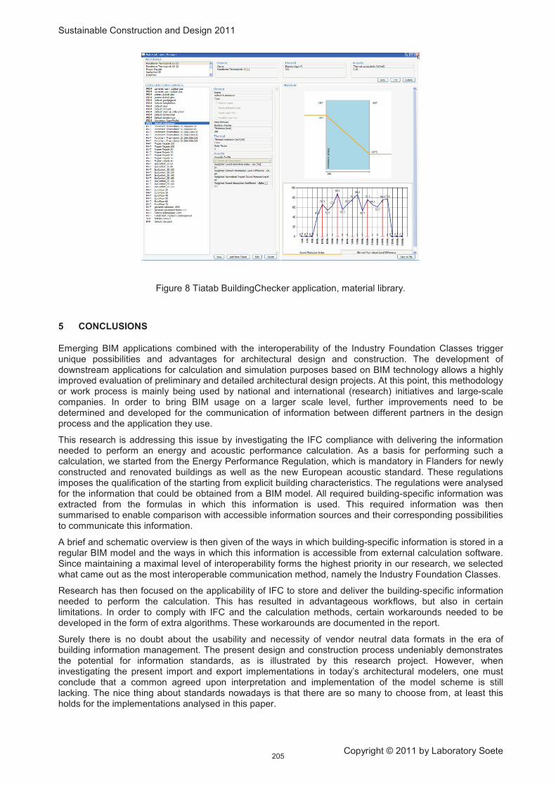
Sustainable Construction and Design 2011
Copyright © 2011 by Laboratory Soete
Figure 8 Tiatab BuildingChecker application, material library.
5 CONCLUSIONS
Emerging BIM applications combined with the interoperability of the Industry Foundation Classes trigger unique possibilities and advantages for architectural design and construction. The development of downstream applications for calculation and simulation purposes based on BIM technology allows a highly improved evaluation of preliminary and detailed architectural design projects. At this point, this methodology or work process is mainly being used by national and international (research) initiatives and large-scale companies. In order to bring BIM usage on a larger scale level, further improvements need to be determined and developed for the communication of information between different partners in the design process and the application they use.
This research is addressing this issue by investigating the IFC compliance with delivering the information needed to perform an energy and acoustic performance calculation. As a basis for performing such a calculation, we started from the Energy Performance Regulation, which is mandatory in Flanders for newly constructed and renovated buildings as well as the new European acoustic standard. These regulations imposes the qualification of the starting from explicit building characteristics. The regulations were analysed for the information that could be obtained from a BIM model. All required building-specific information was extracted from the formulas in which this information is used. This required information was then summarised to enable comparison with accessible information sources and their corresponding possibilities to communicate this information.
A brief and schematic overview is then given of the ways in which building-specific information is stored in a regular BIM model and the ways in which this information is accessible from external calculation software. Since maintaining a maximal level of interoperability forms the highest priority in our research, we selected what came out as the most interoperable communication method, namely the Industry Foundation Classes.
Research has then focused on the applicability of IFC to store and deliver the building-specific information needed to perform the calculation. This has resulted in advantageous workflows, but also in certain limitations. In order to comply with IFC and the calculation methods, certain workarounds needed to be developed in the form of extra algorithms. These workarounds are documented in the report.
Surely there is no doubt about the usability and necessity of vendor neutral data formats in the era of building information management. The present design and construction process undeniably demonstrates the potential for information standards, as is illustrated by this research project. However, when investigating the present import and export implementations in today’s architectural modelers, one must conclude that a common agreed upon interpretation and implementation of the model scheme is still lacking. The nice thing about standards nowadays is that there are so many to choose from, at least this holds for the implementations analysed in this paper.
205

Sustainable Construction and Design 2011
Copyright © 2011 by Laboratory Soete
6 ACKNOWLEDGEMENTS
The authors would like to acknowledge the support of the Belgian Building Research Institute.
7 REFERENCES
[1] Calculation method of the primary energy consumption level of residential buildings (in Dutch), Belgium, Available on: http://www2.vlaanderen.be/economie/energiesparen/epb/doc/bijlage1epb.pdf .
[2] R. Verstraeten, P. Pauwels, R. De Meyer, W. Meeus, J. Van Campenhout, G. Lateur, IFC-based calculation of the Flemish energy performance standard, In (eds. Zarli \& Scherer): 7th European Conference on Product and Process Modelling: eWork and eBusiness in Architecture, Engineering and Construction, Taylor \& Francis Group, London, 2008.
[3] The BuildingSMART Alliance, http://www.buildingsmartalliance.org
[4] European Standard EN12354-3, Building Acoustics – Estimation of acoustic performance of buildings from the performance of elements – Part 3: Airborne sound insulation against outdoor sound.
[5] The BuildingSMART Alliance, http://www.iai-tech.org/products/ifc-overview
[6] V. Domiter, B. Zalik, Sweep-line algorithm for constrained Delaunay triangulation, International Journal of Geographical Information Science 22 (2008) 449-462.
[7] C.L. Lawson, Software for C 1 surface interpolation, Mathematical Software III (1977) 161-194.
[8] S.H. Lo, W.X. Wang, A fast robust algorithm for the intersection of triangulated surfaces, Engineering with Computers 20 (2004) 11-21.
206

Sustainable Construction and Design 2011
Copyright © 2011 by Laboratory Soete
FATIGUE DAMAGE IDENTIFICATION IN THREADED CONNECTION OF
TUBULAR STRUCTURES THROUGH IN-SITU MODAL TESTS
T.T. Bui1, G. De Roeck1, J. Van Wittenberghe2, P. De Baets2 and W. De Waele2
1 K.U. Leuven, Department of Civil Engineering, Belgium.
2
Abstract The use of threaded connection is a valuable alternative to conventional welding in tubular constructions, e.g. pipelines, drill pipes and deep water risers. Those applications are normally exposed to environmental hazards – wave induced vibrations, temperature changes, etc. – as well as subjected to severe service conditions. A classical way to determine fatigue strength in many engineering situations is to calibrate material models by means of ad hoc designed experiments. Unfortunately, it is very difficult in this case even under laboratory conditions due to complicated stress and strain states in the contacting tapered helical thread surfaces of the connection. Therefore, a classical four-point bending fatigue test setup has been built with a real pipe specimen of 3.75 meter long, consisting of two standard API pipes connected by a threaded coupling, under unsymmetric (non-zero average) load control cycles. A complete vibration study has been carried out based on input-output modal tests for the entire period of the fatigue experiment. Input excitation is due to hammer impact and responses are recorded by accelerometers and by reusable dynamic strain gauges. The measured modal strains from the dynamic strain gauges allow for direct calculation of the modal curvatures, rather than deriving approximately from acceleration information. By comparing the measured modal parameters with those of a numerical model of the same structure in undamaged condition, damage detection, localization in the coupling and quantification are possible. This study leads to the following conclusion of practical use: the recent advancement in modal analysis, i.e. the reference based input-output combined deterministic-stochastic subspace identification, makes it possible to identify the structural modal properties from in-situ modal tests, which are performed while the fatigue test is ongoing. In this way the fatigue test is uninterrupted to avoid the problem of stress and strain disturbances happened in un-reversing load cycles test.
Ghent University, Laboratory Soete, Belgium.
Keywords fatigue, four-point bending test, in-situ modal test, modal analysis, threaded connection.
1 INTRODUCTION
In tubular constructions, pieces of linepipes may be of either welded or threaded connection. Threaded construction can offer a range of benefits over welding. The main advantage is in time required to make-up a connection. Welded joint make-up is a slow process, requiring complex procedures to ensure that the weld quality is maintained. This complexity is further increased in situation, such as, a pipe-in-pipe design. Whereas, a threaded connection can be reliably made up in less than five minutes with homogeneous quality, and also has the advantage of allowing the use of high strength steels and composite materials (nonweldable) enabling the overall structure weight to be reduced.
It is believed that the threaded connection provides better fatigue resistance than welding technique, which is evitable to voids and defects. However its performance is still poorly understood. The reason is its complicated geometrical properties and its contact conditions. Therefore it is difficult to detect fatigue damage even in laboratory conditions. And also it might be problematic to develop an ad hoc experimental scheme to calibrate material model due to complicated stress states and strain developments.
Recent development in modal testing with sub-space identification algorithms [1-3] allows for a combination of deterministic and stochastic identification approaches and also both measure artificial and unmeasured ambient excitation sources are utilized. The ambient input in operational condition is considered as a useful source of excitation rather than unwanted noise. These make it possible to carry out modal analysis in a more flexible setting, suitable for large scale civil engineering applications.
Finite element updating, a special treatment of the inverse problem in which the numerical finite element model is continuously updated until differences to the extracted experimental results reach a certain threshold. Then one or several tuned parameters are identified. Although the problem is simple to state mathematically, the solution is dependent on the completeness and the quality of the extracted measured data. Careful treatment is needed in order to overcome the ill-posedness of the formulation and the ill-condition of the problem. Interested readers can be referred to the authoritative book in this area by Friswell
207

Sustainable Construction and Design 2011
Copyright © 2011 by Laboratory Soete
and Mottershead [4] and various particular applications, for examples, Teughels et al. [5] with the introduction of damage function and Reynders et al. [6] with improved experimental data treatment.
The structure of the paper is presented as follows. First, an experimental scheme is described. Then the modal analysis is performed to get meaningful data. Next, a finite element updating with two processes is presented with the final objective of getting the degrading stiffness in the connection region of the structure.
2 THE EXPERIMENTAL PROGRAM
2.1 OMAX testing
In classical Experimental Modal Analysis (EMA), the structure of interest is excited by one or several measured dynamic forces, the response of the structure to these forces is recorded, and the modal parameters in the frequency range of interest are extracted from the analysed data [7,8]. During the test, the structure is essentially isolated from its operating environment and tested in laboratory condition. Due to isolation, the excitation and the boundary conditions may therefore differ significantly from those of structure's real-life operation. Furthermore, EMA methods are in general less suitable for large scale structures, since it is very difficult, if not impossible, to create laboratory condition for testing. As an alternative, output-only or Operational Modal Analysis (OMA) techniques have therefore been developed [3]. They extract the modal parameters from the dynamic response to ambient forces and in operational condition. Consequently, they deliver a linear (modal) model of the structure around the real working point of operation. The unmeasured, ambient forces are usually modelled as stochastic quantities with unknown parameters but with known behaviour, i.e. as white noise time series with zero mean and unknown covariance. However, the existing OMA techniques suffer from several important shortcomings. The first one is that output-only measurements do not allow to determine a complete modal model, since the mode shapes can not be scaled in an absolute sense, e.g., to unit modal mass. Secondly, the ambient excitation is sometimes confined to a narrow frequency band, and as a result only a limited number of modes can be extracted with high quality from the ambient vibration data.
For these reasons, there has been an increasing interest during the last few years towards combined experimental-operational modal testing techniques, also called hybrid vibration testing or Operational Modal Analysis with eXogenous inputs (OMAX) [9,10]. In this technique, artificial forces are used in operational conditions. The main difference between OMAX and the traditional EMA approach is that the operational forces are included in the identified system model: they are not considered as an unwanted noise source, but as useful excitation. As a consequence, the amplitude of the artificial forces can be equal to, or even lower than, the amplitude of the unmeasured, operational forces. This is of crucial importance for the modal testing of large scale structures, since it allows to use excitation devices, e.g. actuators, impact hammers, shakers, etc., which are small and practical when compared to the ones that are needed for EMA testing.
2.2 Experimental fatigue
The task of monitoring the condition of structures working under variable and repeated loading conditions is important, unfortunately, challenging and often tedious when plastic deformations must be taken into account. In threaded connection of tubular constructions in large scale civil engineering application, the stress development is difficult to track due to the complicated tapered helical geometry of the connecting threads that involve frictional contact establishment. Previous studies [11,12] show that the Huber–von Mises equivalent stress in the last engaged thread zone even reaches yield in the assembling process (connection make-up). Moreover, the stress and strain states are rarely symmetric, i.e. reversing, and the structure is often exposed to varyingly repeated loading.
Therefore, it is of paramount importance to distinguish between the two modes of structures collapse under such cyclic loading, i.e. incremental collapse and alternating plasticity. Theoretically, the critical situation will be the one which has the lower plastic limit. In large scale civil engineering practice, alternating (symmetrical) plasticity – in which plastic deformation changes its sign in every cycle leading to a tendency of cancelling each other and the total deformation remains small and the structure only fails in a fatigue phenomenon after a sufficient number of cycles – is rarely the case due to complex combined loading.
At present, the kinds of cyclic tests most frequently adopted are uniaxial tests with fully reversed (i.e. alternating, symmetric) imposed displacements, which usually satisfy the requirement of simple execution. However the stress and strain states generated are nothing close to the real-life application as mentioned earlier.
Cyclic tension–torsion tests under force control are alternatively performed on thin-walled, tubular specimens [13–15], in order to produce in the specimen more sophisticated biaxial stress states which are uniform like in uniaxial tensile tests. This kind of test exhibits a complicated procedure nevertheless it is still not able to replicate the real working condition of the threaded connection.
208

Sustainable Construction and Design 2011
Copyright © 2011 by Laboratory Soete
2.3 Test descriptions
With due consideration to the above mentioned difficulties, a simple full scale four-point bending test setup has been proposed to represent the fatigue test. The test setup has to ensure that the stress/strain distributions at the top and at the bottom fibers of the specimen in the connection region approximately represent those in a uniform axial test of the same magnitude. This requirement is possible when the wall thickness of the specimen is small in comparison to its diameter so that the stress gradient across the wall under bending loads can be adequately approximated by a uniform membrane load.
1 m
3 m
3.75 m
x
z
Hydraulic cylinder Load cell
Ball joint
Pipe
Coupling
LVDT
3D optical
measurement grid
Figure 1: The schematic view of the fatigue test in a four point bending setup.
The assembled specimen consists of two standard API Threaded Linepipes 4.5” with an outside diameter of 114.3 mm and a thickness of 6.0 mm (thickness to diameter ratio is about 1/19) to be connected by a threaded coupling (box). The coupling has an outside diameter of 132.1 mm and a length of 114.3 mm. The specimen (3.750 m in length) is positioned on two supports – 3 m apart – on a rigid stiffened foundation beam (Figure 1).
The tested beam was subjected to a cyclic load at 2 Hz with 7000 N amplitude in a four-point bending test setup until a fatigue crack propagated. A force range from -2000 N to -16000 N was applied by a hydraulic cylinder that is connected to a transverse stiff steel beam by a ball hinge. This beam transmits the load to two points at a distance of 1 m on the tested specimen (that are equally spaced apart from each end, sufficient to exclude the influence of the perturbed stress field around the point loads on the stress distribution of the coupling). This configuration enables the system to create a given uniformly distributed bending moment at the coupling region, resulting from a vertical loading force. It took about 30000 load cycles before fatigue occurred.
A series of modal testing are performed before, during and after the fatigue test. Before and after the fatigue test, vibration measurement is performed in a 2-support configuration (simply supported). During the fatigue test dynamic measurement is carried out after every 1000 cycles in a 4-support configuration with the load is at maximum. At some intervals, the modal test is also performed while the fatigue test is on-going. The measured input for the modal test is the impulse loading from a load cell that is fixed at the hammer head. The measured output is a spectrum of acceleration together with the dynamic strain signals. These signals then produce the modal strains that use to calculate the modal curvature rather than indirectly being estimated from the mode shape information by finite different approximation.
209

Sustainable Construction and Design 2011
Copyright © 2011 by Laboratory Soete
Figure 2: The schematic view of the dynamic measurement grid.
The instrumentation for the modal test is included in Figure 2. Accelerometers (a01 to a19) are attached along and at the top of the specimen, except for a06 and a13, which are at the bottom. Sensors a09 and a10 are on the coupling. Accelerometer a19 is positioned at the end of the specimen, where there is a restraint device with a mass of 2.23 kg. Two extra accelerometers are placed on the loading frame and on the supporting beam. Ten dynamic strain gages (s301 to s310) are grouped in five sections near the two supports at the top and at the bottom fibers of the pipe.
In each modal test the two impact hammer positions are at node 16 (position a) and at node 08 (position b). In this way, both input (force) and output (acceleration) of one identical node can be measured. Therefore the identified mode shapes can be mass normalized and it is possible to combine two tests (a and b) into a single set of modal parameters. The schematic view of the (dynamic) measurement setup is shown in Figure 2, the coordinates of the grid are given in Table 1.
Reference-based combined deterministic-stochastic subspace identification (CSI/ref) method is used with two reference accelerometer channels (node 8 and node 16) plus one reference channel from one of the dynamic strain gages. Half number of block rows is 50 and model order vector is 2:2:140.
Table 1: The coordinates of the (dynamic) measurement grid.
X (m) Y (m) Z (m) Note
-0.376
a01 0.000 0 0 Support 1
a02 0.182 0 0
a03 0.400 0 0
a04 0.600 0 0
a05 0.800 0 0
a06 1.000 0 0 Load point 1
a07 1.200 0 0
a08 1.400 0 0
a09 1.465 0 0
a10 1.535 0 0
a11 1.600 0 0
a12 1.800 0 0
a13 2.000 0 0 Load point 2
a14 2.200 0 0
a15 2.400 0 0
a16 2.595 0 0
a17 2.816 0 0
a18 3.000 0 0 Support 2
a19 3.347 0 0
3.374
01 02 03 04 05
06
14 15 16a 17 18 19
13
07 08b 11 12
09 10
1
2
3
4
5
1 m
3 m
3.750 m
X
Sections with dynamic strain gauges
210

Sustainable Construction and Design 2011
Copyright © 2011 by Laboratory Soete
X (m) Y (m) Z (m) Note
s301 0.130 0 57.15E-3 At the top
s302 0.130 0 -57.15E-3 At the bottom
s303 0.194 0 57.15E-3
s304 0.194 0 -57.15E-3
s305 0.233 0 57.15E-3
s306 0.233 0 -57.15E-3
s307 2.763 0 57.15E-3
s308 2.763 0 -57.15E-3
s309 2.791 0 57.15E-3
s310 2.791 0 -57.15E-3
Besides modal tests, the vertical displacements of the specimen are continuously monitored using a 3D optical measurement system. A measurement was performed after every 1000 cycles of the fatigue test. The optical measurement grid with reflective marker stickers is schematically shown in Figure 1. Since fatigue cracks are expected to initiate from the last engaged thread of either pin, two LVDTs are mounted at either side of the box (Figure 1), to measure the axial distance between the edge of the box and a point on the pipe body of the pin. When a crack starts to grow, the crack tip opening can be observed by subtracting the elastic deformation from the measured values. The treatment of the displacement and crack opening measurement, however, falls outside the scope of this paper and will not be mentioned thereupon.
2.4 Modal analysis results
2.4.1 2-support configuration:
Figure 3: Mode shapes of the first three bending modes in the 2-support configuration (intact specimen).
211
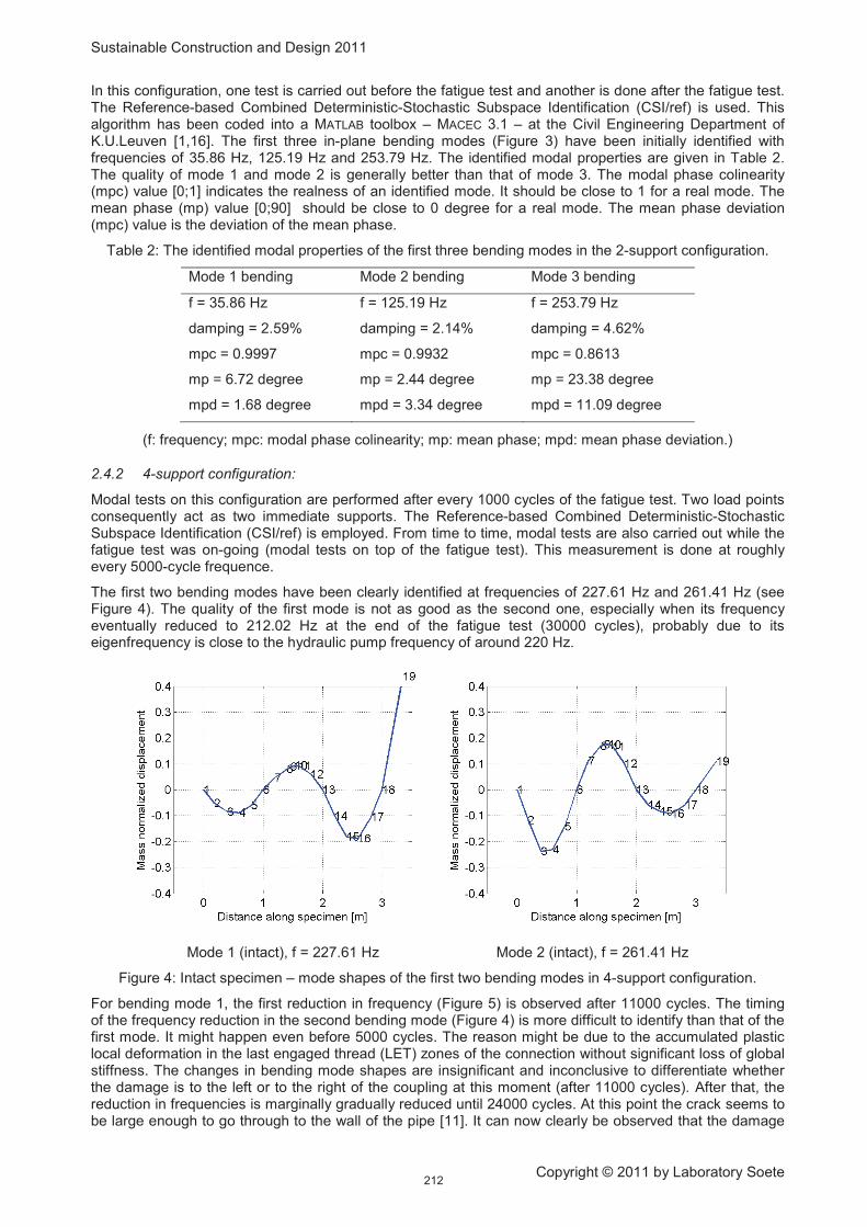
Sustainable Construction and Design 2011
Copyright © 2011 by Laboratory Soete
In this configuration, one test is carried out before the fatigue test and another is done after the fatigue test. The Reference-based Combined Deterministic-Stochastic Subspace Identification (CSI/ref) is used. This algorithm has been coded into a MATLAB toolbox – MACEC 3.1 – at the Civil Engineering Department of K.U.Leuven [1,16]. The first three in-plane bending modes (Figure 3) have been initially identified with frequencies of 35.86 Hz, 125.19 Hz and 253.79 Hz. The identified modal properties are given in Table 2. The quality of mode 1 and mode 2 is generally better than that of mode 3. The modal phase colinearity (mpc) value [0;1] indicates the realness of an identified mode. It should be close to 1 for a real mode. The mean phase (mp) value [0;90] should be close to 0 degree for a real mode. The mean phase deviation (mpc) value is the deviation of the mean phase.
Table 2: The identified modal properties of the first three bending modes in the 2-support configuration.
Mode 1 bending Mode 2 bending Mode 3 bending
f = 35.86 Hz f = 125.19 Hz f = 253.79 Hz
damping = 2.59% damping = 2.14% damping = 4.62%
mpc = 0.9997 mpc = 0.9932 mpc = 0.8613
mp = 6.72 degree mp = 2.44 degree mp = 23.38 degree
mpd = 1.68 degree mpd = 3.34 degree mpd = 11.09 degree
(f: frequency; mpc: modal phase colinearity; mp: mean phase; mpd: mean phase deviation.)
2.4.2 4-support configuration:
Modal tests on this configuration are performed after every 1000 cycles of the fatigue test. Two load points consequently act as two immediate supports. The Reference-based Combined Deterministic-Stochastic Subspace Identification (CSI/ref) is employed. From time to time, modal tests are also carried out while the fatigue test was on-going (modal tests on top of the fatigue test). This measurement is done at roughly every 5000-cycle frequence.
The first two bending modes have been clearly identified at frequencies of 227.61 Hz and 261.41 Hz (see Figure 4). The quality of the first mode is not as good as the second one, especially when its frequency eventually reduced to 212.02 Hz at the end of the fatigue test (30000 cycles), probably due to its eigenfrequency is close to the hydraulic pump frequency of around 220 Hz.
Mode 1 (intact), f = 227.61 Hz Mode 2 (intact), f = 261.41 Hz
Figure 4: Intact specimen – mode shapes of the first two bending modes in 4-support configuration.
For bending mode 1, the first reduction in frequency (Figure 5) is observed after 11000 cycles. The timing of the frequency reduction in the second bending mode (Figure 4) is more difficult to identify than that of the first mode. It might happen even before 5000 cycles. The reason might be due to the accumulated plastic local deformation in the last engaged thread (LET) zones of the connection without significant loss of global stiffness. The changes in bending mode shapes are insignificant and inconclusive to differentiate whether the damage is to the left or to the right of the coupling at this moment (after 11000 cycles). After that, the reduction in frequencies is marginally gradually reduced until 24000 cycles. At this point the crack seems to be large enough to go through to the wall of the pipe [11]. It can now clearly be observed that the damage
212

Sustainable Construction and Design 2011
Copyright © 2011 by Laboratory Soete
has been to the left of the coupling. Since then the frequency reduces quickly until the end of the test (30000 cycles). The modal properties and the mode shapes of the first two bending modes in the 4-support configuration of the intact specimen and after 11000 cycles are given in Table 3. The modal tests while the fatigue test is on-going provide consistent results with other modal tests.
0 2 4 6 8 10 12 14 16 18 20 22 24 26 28 29.5200
210
220
230
240
250
260
270
No. cycles x 103
Fre
qu
en
cy [H
z]
Mode 2
Mode 1
on-going
Figure 5: The reduction in frequencies of the first two bending modes in the 4-support configuration.
Table 3: The identified modal properties of the first two bending modes in the 4-support configuration.
Mode 1 bending
(intact specimen)
Mode 2 bending
(intact specimen)
Mode 1 bending
(after 11000 cycles)
Mode 2 bending
(after 11000 cycles)
model order: 38 model order: 44 model order: 25 model order: 47
f = 227.61 Hz f = 261.41 Hz f = 226.49 Hz f = 259.69 Hz
damping = 2.34% damping = 1.42% damping = 3.00% damping = 1.39%
mpc = 0.9919 mpc = 0.9949 mpc = 0.9930 mpc = 0.9930
mp = 5.31 degree mp = 1.7191 degree mp = 16.90 degree mp = 2.59 degree
mpd = 4.02 degree mpd = 1.69 degree mpd = 3.04 degree mpd = 1.12 degree
2.4.3 Modal curvatures:
-0.5 0 0.5 1 1.5 2 2.5 3 3.5
-1.5
-1
-0.5
0
0.5
1
1.5
Distance along specimen [m]
Modal curv
atu
re [m
m-1
]
Mode 1: beam model
Mode 2: beam model
Mode 3: beam model
Mode 1: measured values
Mode 2: measured values
Mode 3: measured values
Figure 6: The modal curvatures of the original specimen in the 2-support configuration.
As mentioned earlier, dynamic strain sensors (PCB ICP 740B02) are attached to the specimen at five different sections at the top and at the bottom of the speciemen. From the extracted measured modal strains, the modal curvatures can be directly calculated using the following fomula:
12
21
z
!
"# (1)
213

Sustainable Construction and Design 2011
Copyright © 2011 by Laboratory Soete
With 1 is modal strain at the top and 2 is modal strain at the bottom of the section and z12
The modal curvature values of the first three bending mode shapes of the specimen in the 2-support configuration of the original specimen are given in Figure 6. Numerical modal curvature shapes of the intact specimen, which is obtained from beam theory, also be given for reference. It is noted that only the results for section 2, 3 and 4 are included as to avoid the influence of local stress concentration leading to the ovalization of the cross sections near the supports (section 1 and 5). It can be seen that the measured modal curvatures match the beam model theory ones well. The measured modal curvature values stay almost unchanged throughout the fatigue test as the measured sections are far from the localized damaged zones in the coupling except for bending mode 3, which witnesses minor changes.
is the vertical distance between these two strain sensors (114.3 mm). If only accelerations had been measured, the modal curvatures would have to be calculated from the measured modal displacements, using a numerical differentiation procedure, e.g., a central difference approximation [17].
3 FINITE ELEMENT MODEL UPDATING
In FE model updating, the numerical modal data are initially computed using estimated starting values for the unknown model parameters to be updated. These parameters are then adjusted until the discrepancies between the numerical and experimental modal data are minimized. The formulation of the objective function involves some error norms, appropriate bounds and constraints. Data fitting is usually done by means of an error minimization technique, where the distance between prediction vectors of the computational model (eigenfrequencies, mode shapes, modal strains, etc.) and measurements of the corresponding experiment is minimized. In most cases, the least square norm of the residuals is preferred in engineering computations due to its differentiability and ease of implementation.
Two different updating processes are performed, in order to appropriately model the original and the damaged state of the connected specimen. Special boundary condition has to be made to the test setup because of the nature of the specimen is rounded thin walled structure. The specimen is rounded, therefore the roller bearing that is typically applied to the conventional rectangular beam is not suitable. Since the pipe is considered as thin walled structure, the support has to be relatively flexible in order to avoid the local ovalization of the pipe, which might has some effects on the quality of the identified mode shapes.
In the first updating process the vertical stiffness values of the two supports are updated. In the second process, the bending stiffness moduli of the different zones in the coupling region are updated. Since the damage is expected to be in this region. Details of the formulation to a least square problem can be referred to Bui et al. [18].
The finite element model includes 51 BEAM188 elements (in the Ansys Element Library [19]). The support is modelled by two COMBIN14 spring elements with an initial stiffness of 5 x 10
7
In the first updating stage, two identification parameters are sought for, i.e. the spring stiffness of the two supports. The input of the cost function is the differences in the mass normalized mode shapes of the first three bending modes and their associated frequencies. The modal curvature values are not included because the gauges are purposively mounted far from the damage zones in the middle of the specimen. And it is believed that the change in modal curvature is only significant locally near the damaged region [17]. A hybrid algorithm (Genetic Algorithm followed by a Trust Region Newton local search) is again used [18]. The resulting spring stiffness is found to be 479 x 10
N/m. Only the outer boundary surface of the coupling region is considered. Therefore the contact nature among connecting threads is not taken into account. The five different zones in the coupling region are as follow: the thread run-out on the left tube, the thread engaging to the left, the middle coupling, the thread engaging to the right, the thread run-out on the right tube.
7 N/m and 256 x 10
7
In the second updating stage, five identification parameters are sought for: these are the bending stiffness of difference zones in the coupling region. In both updating stages, normalized identification factors are used in order to avoid the convergence problem in optimization procedure. The initial values of the factors are very small numbers (reflecting undamaged situation). If, the updating values were found close to unity, the corresponding stiffness would be totally loss. The obtained updated factor is a
N/m. These values are used in the FE model in the damage identifying stage.
E = {0.8485; 0.1192; 0.0934; 0.1270; 0,4517}
T
. The stiffness is virtually no loss at the middle zone of the coupling. Small stiffness degradation in the thread connecting zone means that the connection is quite secured (tight) in the fatigue life. The loss is concentrated in the last engaged thread zones of the connection. The bigger value is witnessed at the left side of the coupling, which is conformed to visual inspections of the specimen afterward.
214

Sustainable Construction and Design 2011
Copyright © 2011 by Laboratory Soete
4 CONCLUSIONS
In this paper, an experimental modal approach is used to detect and to assess the fatigue damage in the threaded connection of a medium size tabular structure. The fatigue test is based on a four-point bending test setup. Reference-based Combined Deterministic-Stochastic Subspace Identification method is capable of extracting modal parameters of the structure while the fatigue load is still acting on the specimen, which means a four-point bending becomes a 4-support configuration and condition of the connected structure can be monitored continuously during the fatigue test. An updating procedure, which consists of two steps, is proposed to find the stiffness of the supports and to assess the damage in different zone of the coupling due to fatigue. From the resulting degrading stiffness distribution in the box region, large reduction is found in the thread run-out zones, which suggests a proper detailing is this zone might improve the fatigue performance of this particular connection.
The use of low cost sensors for dynamic strain measurement is a step forward in OMAX testing. The extracted modal strains in different mode shapes can be used to directly calculate the modal curvature to complement the reduction in frequencies and the changes in mode shapes to detect timely the initiation of the fatigue crack which is by nature difficult to identify and assess even in laboratory conditions.
Future work is to apply the dynamic strain sensors close the expected damage location and to use the FE updating framework the whole loading history of the test in order to quantify the stiffness degradation of the threaded connection region continuously. Then the same methodology can be applied to a large scale testing in a resonant bending machine for pipes [20] that is currently being developed at the Soete Laboratory, Ghent University.
5 ACKNOWLEDGEMENTS
The authors would like to acknowledge the financial support from the BOF fund B/04939 of the Ghent University and from the Research Foundation – Flanders (FWO), Belgium, project G.0228.06N.
6 REFERENCES
[1] Reynders, E., De Roeck, G., Reference-based combined deterministic-stochastic subspace identification for experimental and operational modal analysis, Mechanical Systems and Signal Processing, 22(3): 617 – 637, 2008.
[2] Reynders, E., Pintelon, R., De Roeck, G., Uncertainty bounds on modal parameters obtained from Stochastic Subspace Identification; Mechanical Systems and Signal Processing, 22(4): 948 – 969, 2008.
[3] Peeters, B., De Roeck, G., Stochastic system identification for operational modal analysis: A review, ASME Journal of Dynamic Systems, Measurement, and Control, 123(4): 659 – 667, 2001.
[4] Friswell, M.I., Mottershead, J.E., Finite element model updating in structural dynamics, Kluwer Academic Publishers Group, 1995.
[5] Teughels, A., Maeck, J., De Roeck, G., Damage assessment by FE model updating using damage functions, Computers and Structures, 80(25): 1869 – 1879, 2002.
[6] Reynders, E., Teughels, A. and De Roeck, G., Finite element model updating and structural damage identification using OMAX data, Mechanical Systems and Signal Processing, 24(5):1306 – 1323, 2010.
[7] Ewins, D.J., Modal Testing: Theory and Practice, second edition, Research Studies Press, Baldock, UK, 2000.
[8] Heylen, W., Lammens, S., Sas, P., Modal Analysis Theory and Testing, Department of Mechanical Engineering, Katholieke Universiteit Leuven, Belgium, 1997.
[9] Guillaume, P., De Troyer, T., Devriendt, C., De Sitter, G., OMAX – a combined experimental-operational modal analysis approach. In: Sas, P., De Munck, M. (Eds.), Proceedings of ISMA2006 International Conference on Noise and Vibration Engineering, Leuven, Belgium, 2006.
[10] Reynders, E., System identification and modal analysis in structural mechanics. PhD thesis, Department of Civil Engineering, K.U.Leuven, 2009.
[11] Van Wittenberghe, J., De Baets, P., and De Waele, W., Nonlinear Contact Analysis of Different API Line Pipe Coupling Modifications, ASME Journal of Pressure Vessel Technology, 132(5), 2010.
215

Sustainable Construction and Design 2011
Copyright © 2011 by Laboratory Soete
[12] Van Wittenberghe, J., De Pauw, J., De Baets, P., De Waele, W., Wahab, M.A., and De Roeck, G., Experimental determination of the fatigue life of modified threaded pipe couplings. Procedia Engineering, 2(1): 1849 – 1858, 2010.
[13] Portier L, Calloch S, Marquis D, and Geyer P., Ratchetting under tension–torsion loadings: experiments and modeling, International Journal of Plasticity,16:303–35, 2000.
[14] Bocher, L. , Delobelle, P. , Robinet, P., and Feaugas, X., Mechanical microstructural investigations of an austenitic stainless steel under non-proportional loadings in tension–torsion internal and external pressure, International Journal of Plasticity,17:1491–530, 2001.
[15] Delobelle, P., Robinet, P., and Bocher, L., Experimental study and phenomenological modelization of ratchet under uniaxial and biaxial loading on an austenitic stainless steel, International Journal of Plasticity, 11(4): 295–330, 1995.
[16] Reynders, E., Schevenels, M., and De Roeck, G., MACEC 3.1: a MATLAB toolbox for experimental and operational modal analysis: user’s manual, Techincal Report BWM-2010-05, Katholieke Universiteit Leuven, Departement of Civil Engineering, 2010.
[17] Abdel Wahab, M., and De Roeck, G., Damage detection in bridges using modal curvatures: Application to a real damage scenario, Journal of Sound and Vibration, 226(2), 217–235, 1999.
[18] Bui, T.T., De Roeck, G., Van Wittenberghe, J., De Baets, P., and De Waele, W. A modal approach to identify fatigue damage in threaded connections of large scale tubular structures. In Sas, P., and Bergen, B. Edition, Proceedings of the International Conference on Noise and Vibration Engineering, ISMA2010, 795–807, 2010.
[19] Ansys, Inc., Elements Reference – Ansys Release 11.0, 2007.
[20] Van Wittenberghe, J., De Pauw, J., De Baets, P., De Waele, W., Ost, W., De Roeck, G., and Bui, T.T., Fatigue investigation of threaded pipe connections. In Van Wittenberghe, J. (Ed.), Sustainable Construction & Design, Volume 1. Day of research, Laboratory Soete – Ghent University, 2010.
216

Sustainable Construction and Design 2011
Copyright © 2011 by Laboratory Soete
TOWARDS BETTER FINITE ELEMENT MODELLING OF ELASTIC RECOVERY IN SHEET METAL FORMING OF ADVANCED HIGH
STRENGTH STEEL
Mohsen Safaei, Wim De Waele
Ghent University, Laboratory Soete, Belgium
Abstract The first part of this study discusses the influence of element type on parameters such as accuracy of the FE simulation, simulation time and convergence. Guidelines on optimal implementation of element types are proposed. It is shown that an inappropriate choice of element type results in difficulties in convergence of the simulation or gives rise to problems such as shear locking in elements. In the second part of this study a series of finite element simulations using the Hill’48 planar anisotropic yield criterion and a standard U-shape forming test based on the NUMISHEET’93 benchmark was performed. The effectiveness of different isotropic hardening laws and different contact models is investigated. The most appropriate hardening and contact definitions are defined from the viewpoint of optimal springback prediction. Finally, the influence of the orientation of sheet strips relative to the rolling direction on springback angles is evaluated.
Keywords Convergence, Element type, Springback, Hardening, Contact model
1 INTRODUCTION
Obtaining accurate results in finite element simulations demands an appropriate use of elements, contact and material definitions. It is important to know how their implementation affects computational expenses and the accuracy of the simulations. Regarding material definition for sheet metal forming processes, a yield function should address the mechanical anisotropy of the material to produce the true amount of yield stress in different directions with respect to the rolling direction. An appropriate hardening law relates the true stress to strain for different loading paths. A variety of hardening models have been employed in research such as simple isotropic hardening laws to the most advanced mixed isotropic-kinematic laws such as Yoshida-Uemori [1] and Teodosiu [2] which can model the elastic-plastic transition, stagnation of hardening and softening caused by reversed load path.
The first part of this paper reports on the influence of element type. Shell and solid elements are discussed, as is the order and integration of the elements. Some guidelines on element selection are listed in annex. The second part of this paper reports on the springback simulation of a U-shape forming test (NUMISHEET’93 benchmark). Different contact models and a variety of hardening laws are investigated.
Finally, the effect of sheet orientation with respect to the rolling direction on springback of an advanced high strength steel is evaluated.
2 ELEMENT TYPE STUDY
2.1 Shell elements Simulations of sheet metal forming processes mostly utilize shell elements rather than solid elements. This is because shell elements can produce comparable accuracy as solid elements for less computational expense. One issue might be the change of shell element thickness during deformation. This thickness change can be calculated based on the simulated in-plane deformations:
217

Sustainable Construction and Design 2011
Copyright © 2011 by Laboratory Soete
(1)
(2)
(3)
A Poisson's ratio equal to zero will keep the shell thickness constant, which is suitable for small strain, large rotation analyses. For analysis of large strain applications such as sheet metal forming, the Poisson's ratio is set to 0.5, which addresses the incompressibility of the material.
Either first-order or second-order elements can be employed. Second-order elements produce higher accuracy than first-order elements for “smooth” problems in which no complex contact conditions nor severe element distortions exist. This kind of elements can model complex geometrical curves with fewer elements and are very effective in bending dominated problems. Moreover, the second-order elements capture stress concentrations more effectively.
Generally, the Gaussian quadrature integration method is used to evaluate the material response at each integration point of an element. Using full versus reduced integration for an element might result in a significant change in simulation results.
Reduced integration uses a lower-order integration to form the element stiffness matrix, thus reducing running time especially in three dimensional simulations. More accurate results are generally expected when this lower integration method is applied for a second-order element. However, for first-order elements the application in which the element is used, defines the accuracy of the result regardless the order of integration used.
Figure 1. Full-integration against reduced-integration for conventional shell elements [3]
2.2 Hourglassing and shear locking Using solid elements for sheet metal forming simulations requires special care. For instance, inherently, first-order triangular and tetrahedral elements are overly stiff and exhibit slow convergence when increasing the number of elements, and therefore they are not suggested for stress analysis.
Shear locking and hourglassing are two major problems when using solid elements. The phenomenon of being overly stiff in bending is called shear locking. Fully integrated first order solid elements may suffer from this problem. Curved edges are expected for a beam element under pure bending moment. However, the linear geometry of a first order element does not allow bending in the element. Therefore it distorts by shear at the corners of the element (Figure 2), resulting in large shear stress in these regions. Erroneous displacement and stress may be observed because of shear locking.
218

Sustainable Construction and Design 2011
Copyright © 2011 by Laboratory Soete
Figure 2. Shear locking for a first order fully integrated element
To avoid the shear locking problem, one may suggest using first order reduced integration elements. In this case, because there is no strain energy at the integration point, zero amounts of normal and shear stresses are obtained at this point. This produces an overly flexible structure, thus resulting in erroneous results such as wrong stress patterns. This problem is called hourglassing that can also be observed when only one layer of the second-order reduced-integration solid element is used. This can easily be solved by using two or more layers of elements. Less than one percent ratio of artificial energy to strain energy denotes no hourglassing problem in the simulation.
2.3 General-purpose conventional shell elements The finite element software ABAQUS benefits from a database of general purpose shell elements (S3/S3R, S3RS, S4, S4R, S4RS, S4RSW, SAX1, SAX2, SAX2T, SC6R, and SC8R). These utilize the thick shell theory as the shell thickness increases and become thin shell elements as the thickness decreases.
Using S4(R) elements
The fully integrated general-purpose finite-membrane-strain shell element, S4, gives accurate solutions to in-plane bending problems, tolerates element distortion and avoids locking. Moreover, no hourglass control is needed for this element, neither for membrane nor bending mode. When compared to S4R reduced integration elements which possess only one integration point per element, the S4 elements with four integration points demand more computational time. In spite of higher computational time, the S4 element outperforms the S4R element type in areas where greater solution accuracy is required or for problems where in-plane bending is expected.
More detailed guidelines for element types are demonstrated in annex.
3 SPRINGBACK SIMULATION OF AN ADVANCED HIGH STRENGTH STEEL
This section discusses the finite element analysis of springback based on the NUMISHEET’93 U-shape forming test [4] for an advanced high strength steel (TRIP780). The geometry is shown in Figure 3; the sheet strips are 380mm long by 35mm wide by 0.81mm thick. Only one quarter of the geometry was analysed due to the symmetrical physics of the model. FE simulations have been performed using ABAQUS v6.10. Special attention is paid to an appropriate representation of the material’s stress-strain relation and contact definition. Figure 4 shows details about the definition of the springback angles and
. Figure 5 depicts positions of the parts before and after loading.
A mesh convergence study was performed and eventually a total of 1350 elements produced most accurate results. The blank was meshed with S4R elements (reduced integration general shell element) and the rigid parts (holder, punch and die) were meshed with S3D4 elements. Details of the employed contact model are presented in the following subsection. The anisotropy was addressed by using the Hill’48 quadratic anisotropic equation [5]:
(4)
Where , , , , and are the components of the Cauchy stress tensor defined in the orthotropic frame and and are the Hill’s coefficients.
The material parameters used in simulations are summarized in Table 1.
Table 1 Material data for TRIP 780 AHSS steel Material (GPa) (mm) TRIP 780 200 0.3 0.81 1.02 0.95 1.14
219

Sustainable Construction and Design 2011
Copyright © 2011 by Laboratory Soete
Figure 3. The NUMISHEET’93 benchmark geometry; (units: mm)
Figure 4. Variables defining springback; (units: mm) [6]
Figure 5. Position of dies and sheet strip in FE model. Because of the symmetrical physics of the model, just
one quarter of the model has been modelled.
3.1 Contact models The effectiveness of three different contact models has been investigated. The first contact model used is the common Coulomb tangential friction with a friction coefficient of 0.165. The second model is a linear penalty type of “hard” pressure-overclosure function combined with the tangential coulomb friction of 0.165. For this model, the contact pressure is linearly proportional to the normal penetration distance. A stiffness Klin of 0.01 was used. Finally, a softened (exponential) constraint enforcement method was used in which the surfaces begin to transmit contact pressure once the clearance between them reduces to . The half of the sheet thickness and 5 MPa were assigned for the parameters and , respectively. In Abaqus/Standard the default is 10 times the element stiffness. The functions of the two last contact models are demonstrated in Figure 6.
Figure 6. Linear and non-linear pressure-overclosure relation (left) and exponential (soft) contact pressure-
overclosure relationship (right) [3]
Based on the performed simulations, it was concluded that the linear penalty contact model provides reasonable accuracy in less computational time. Therefore this model was selected for the study discussed in subsection 3.3.
Blank Holder
The workpiece has a width of 35 mm and is centered with respect to the center line of the die.
Punch
Blank holder f
70m
m
Stro
ke
Die
Punch before loading
Holder
Punch after loading
Undeformed sheet strip
220
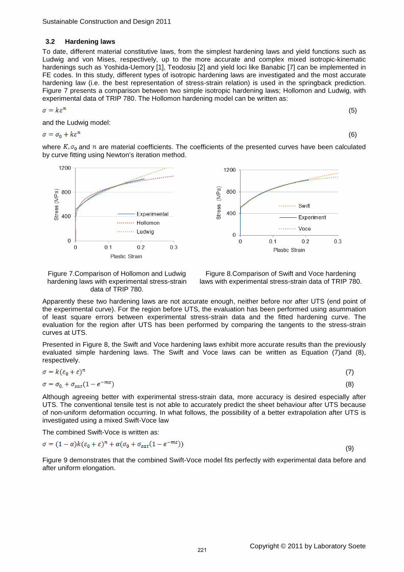
Sustainable Construction and Design 2011
Copyright © 2011 by Laboratory Soete
3.2 Hardening laws To date, different material constitutive laws, from the simplest hardening laws and yield functions such as Ludwig and von Mises, respectively, up to the more accurate and complex mixed isotropic-kinematic hardenings such as Yoshida-Uemory [1], Teodosiu [2] and yield loci like Banabic [7] can be implemented in FE codes. In this study, different types of isotropic hardening laws are investigated and the most accurate hardening law (i.e. the best representation of stress-strain relation) is used in the springback prediction. Figure 7 presents a comparison between two simple isotropic hardening laws; Hollomon and Ludwig, with experimental data of TRIP 780. The Hollomon hardening model can be written as:
(5)
and the Ludwig model:
(6)
where and are material coefficients. The coefficients of the presented curves have been calculated by curve fitting using Newton’s iteration method.
Figure 7.Comparison of Hollomon and Ludwig hardening laws with experimental stress-strain
data of TRIP 780.
Figure 8.Comparison of Swift and Voce hardening laws with experimental stress-strain data of TRIP 780.
Apparently these two hardening laws are not accurate enough, neither before nor after UTS (end point of the experimental curve). For the region before UTS, the evaluation has been performed using asummation of least square errors between experimental stress-strain data and the fitted hardening curve. The evaluation for the region after UTS has been performed by comparing the tangents to the stress-strain curves at UTS.
Presented in Figure 8, the Swift and Voce hardening laws exhibit more accurate results than the previously evaluated simple hardening laws. The Swift and Voce laws can be written as Equation (7)and (8), respectively.
(7)
(8) Although agreeing better with experimental stress-strain data, more accuracy is desired especially after UTS. The conventional tensile test is not able to accurately predict the sheet behaviour after UTS because of non-uniform deformation occurring. In what follows, the possibility of a better extrapolation after UTS is investigated using a mixed Swift-Voce law
The combined Swift-Voce is written as:
(9)
Figure 9 demonstrates that the combined Swift-Voce model fits perfectly with experimental data before and after uniform elongation.
221

Sustainable Construction and Design 2011
Copyright © 2011 by Laboratory Soete
Figure 9. Combined Swift-Voce vs. experimental stress-strain curve.
3.3 AHSS springback An ideal sheet metal product is desired to be without any elastic recovery. In the particular case of an U-bend shape, the walls are expected to be completely flat (i.e. = 90° = ). In reality, the product underperforms the ideal expectations (Figure 10). An increase of and decrease of , increases the springback. Changing the planar orientation of the sheet strip from 0 degrees to 45 degrees orientation with respect to the rolling direction, increases the springback (Figure 11). On the contrary, springback decreases when shifting from 45 degrees to 90 degrees orientation with respect to the rolling direction (Figure 11). The springback observed for the 90 degrees strip is similar to this of the 0 degrees strip.
Figure 10. Illustration of springback after removal of the punch and holder for sheet strips with, from left to right, an orientation of 0, 45 and 90 degrees with respect to the sheet’s rolling direction. Note that only a
half specimen is illustrated.
Figure 12 compares the thickness of the sheet strip at the last step of loading and after unloading for the various strip orientations. Although the 45° orientation shows most elastic recovery, its thickness change in the vertical walls is limited. The 0° and 90° orientations exhibit comparable thinning of their vertical walls.
222

Sustainable Construction and Design 2011
Copyright © 2011 by Laboratory Soete
Figure 11. Springback angles vs. planar orientation
Figure 12. Comparison of sheet thickness before (dotted lines) and after unloading (full
lines) for various sheet orientations. The letters refer to the positions indicated on Figure 10.
4 CONCLUSIONS
In the first part of this paper, appropriate employment of order and integration of elements are presented. Among three contacts model presented in the second part of the paper, it is found that the linear penalty type of “hard” pressure-overclosure function, applied together with a tangential coulomb friction of 0.165 produces enough accuracy and reduces the computational time interestingly. Moreover, the old Hill’48 R-fitted yield criterion was used to address the anisotropy of the material. Although isotropic hardening is only suggested for monotonic loading and not for reversed loading, it is used here as a case study. This is because the main goal was finding an stress-strain function that accurately fits experimental data before and after UTS. At the corners of a U-bend shape, reversed loading happens during forming. Isotropic hardening cannot model the Bauschinger effect by early re-yielding of material upon reversing the load. In case of severe strain path changes, and depending on the material, possibly severe change of hardening, hardening stagnation and softening will occur for which advanced hardening models such as Yoshida-Uemori [1] and Teodosiu [2] are suggested. These models will be used in future studies.
5 NOMENCLATURE
Component of in-plane strain
Reference strain
Component of Cauchy stress tensor
Initial yield stress
Saturated amount of stress
Poisson’s ratio
young’s modulus
Lankford coefficient at ° with respect to the rolling direction
Hardening parameters
Parameter used for exponential pressure-overclosure contact relationship
6 ACKNOWLEDGEMENTS
The authors would like to acknowledge the financial support of the special research fund of Ghent University (BOF grant nr. 01J10608).
7 REFERENCES
1. Yoshida, F. and T. Uemori, A model of large-strain cyclic plasticity describing the Bauschinger effect and workhardening stagnation. International Journal of Plasticity, 2002. 18(5-6): p. 661-686.
A
B C
D
223

Sustainable Construction and Design 2011
Copyright © 2011 by Laboratory Soete
2. Haddadi, H. and S. Belhabib, An Attempt to Identify Hill’s Yield Criterion Parameters Using Strain Field Measured by Dic Technique, in Experimental Analysis of Nano and Engineering Materials and Structures, E.E. Gdoutos, Editor. 2007, Springer Netherlands. p. 677-678.
3. Hibbitt Karlsson and Sorensen Inc, ABAQUS User's Manuals Version 6.10, Pawtucket, Rhode Island, USA.
4. NUMISHEET’93. in Proceedings of the second international conference of numerical simulation of 3-D sheet metal forming processes. 1993. Isehara, Japan.
5. Hill, R., The mathematical theory of plasticity. The Oxford engineering science series. 1950, Oxford,: Clarendon Press. ix, 356 p.
6. Gomes, C., O. Onipede, and M. Lovell, Investigation of springback in high strength anisotropic steels. Journal of Materials Processing Technology, 2005. 159(1): p. 91-98.
7. Banabic, D., et al., Increasing the robustness of the sheet metal forming simulation by the prediction of the forming limit band. NUMIFORM '07: Materials Processing and Design: Modeling, Simulation and Applications, Pts I and II, 2007. 908: p. 171-176.
224

Sustainable Construction and Design 2011
Copyright © 2011 by Laboratory Soete
8 ANNEX
Figure 13. Some remarks on general purpose shell elements
Figure 14. Guidelines for using second order elements
225

Sustainable Construction and Design 2011
Copyright © 2011 by Laboratory Soete
Figure 15. Guidelines for using fully integrated elements
226

Sustainable Construction and Design 2011
Copyright © 2011 by Laboratory Soete
Figure 16. Some remarks on first order shell elements
227

Sustainable Construction and Design 2011
Copyright © 2011 by Laboratory Soete
DEVELOPMENT AND VALIDATION OF A HIGH CONSTRAINT MODIFIED
BOUNDARY LAYER FINITE ELEMENT MODEL
M. Verstraete1, W. De Waele1, S. Hertelé1,2
1 Ghent University, Laboratory Soete, Department of Mechanical Construction and Production, Belgium
2 FWO Flanders (Research Foundation Flanders) aspirant
Abstract When a notched structure is loaded, its behaviour is not only affected by the material properties but also by the geometry (of both the structure and the defect) and loading condition, alternatively termed as constraint condition. Therefore, the relation between the failure behaviour of a small scale fracture mechanics test and a full scale structure needs to be elucidated.
In an attempt to understand and describe such relationships, the crack tip stress fields are analysed by means of finite element simulations and compared for several test specimen geometries. A reference for comparison is the crack tip stress field obtained from a high constraint reference geometry, further called a modified boundary layer model.
First, this article provides some theoretical background on the modified boundary layer model. Second, the development of a 2D model is outlined in detail, focussing on the mesh design in the vicinity of the crack tip and the applied boundary conditions. Afterwards, an analytical and numerical validation is provided, based on the level of the applied load and, on the other hand, on the magnitude of the crack tip stress fields. Finally, this validated model is used for the comparison of several constraint parameters. This comparison indicates a weak influence of the T-stress on the Q-parameter for positive T-stresses. In contrast, negative T-stresses result in more pronounced negative Q-values.
Keywords: Constraint, J-Q theory, crack tip stress fields, validation
1 INTRODUCTION
1.1 General Since the 1920s researchers try to understand the failure behaviour of cracked structures. It has quickly been understood that the shape and magnitude of the stress fields ahead of the crack tip influence this behaviour. Consequently, theoretical concepts have been developed to describe the stress fields ahead of the crack tip. At first, materials have been studied in which hardly any plasticity developed in the vicinity of the crack tip. These studies have resulted in the linear elastic fracture mechanics (LEFM) theory. Within this theoretical concept, the crack tip stress fields are described by an analytical expression developed by Williams in the late 1950s [1].
σij =KI
2πrfij θ +
T 0 00 0 00 0 υT
+ ⋯ (1)
In this so-called Williams expansion, the first term was believed to be dominant over the others. As a result, LEFM theory only considers KI, defining the magnitude of the first term, to describe the crack tip stress fields. Unfortunately, this theory breaks down when the material ahead of the crack tip deforms plastically. To overcome this shortcoming, the elastic plastic fracture mechanics (EPFM) theory has been developed by Hutchinson, Rice and Rosengren (HRR) [2]. They described the crack tip stress fields by means of the following equation, known as the HRR-solution:
σij = σ0 E J
α σ02 In r
1 n+1
σ ij (n, θ) (2)
228

Sustainable Construction and Design 2011
Copyright © 2011 by Laboratory Soete
The above description works well for situations where the plasticity is limited to a small zone in the vicinity of the crack tip, alternatively termed as small scale yielding conditions. Under these conditions, both the shape and magnitude of the crack tip stress field remain geometry independent. In contrast, when fully contained yielding conditions are examined, it is not longer possible to accurately describe the crack tip stress fields by means of a single parameter. Under these conditions the material’s fracture toughness depends on the specimen’s geometry and the loading condition [3, 4]. This dependence is alternatively termed as the constraint condition. Consequently, fracture toughness results, in terms of critical J or KI
values, are no longer directly transferrable between a laboratory scale specimen and a large structure.
1.2 Constraint parameters In an attempt to clarify the influence of different constraint conditions, several new theoretical concepts have been developed. At first, the LEFM theory has been extended, also considering the second term in the Williams expansion. This term’s magnitude is defined by the level of the T-stress. As such, a two parameter theoretical concept was developed, known as the K-T theory [5-7]. However, as already stated in the previous paragraph, this theory is only applicable for situations that lack plasticity in the vicinity of the crack tip.
Nowadays, the most suitable theory for investigating fully contained yielding conditions is an extension of the J-integral concept. This extension has been developed in the early 1990s by O’Dowd & Shih and describes the constraint effects by means of the Q-parameter [8, 9]. This parameter has been defined by the following relationship:
σij = σij HRR+ Q σ0 δij (3)
It is clear that the leading term is still the HRR-solution, setting the size scale of the crack tip stress field. Additionally, the Q-parameter defines the magnitude of a uniform hydrostatic shift in the crack tip stress field. This shift will lead to a lowered stress level for negative Q-values, representing low constraint conditions. In contrast, an increased stress level (positive Q) will be observed for high constraint conditions. O’Dowd & Shih have shown that the expression in Eq.3 is valid for distances r ahead of the crack tip
between J σ0 and 5 J σ0 . As a result, the Q-parameter is most often evaluated at a distance r = 2 J σ0 . In that case, a simple modification of Eq.3 defines the Q-parameter:
Q =σ ii − σ ii HRR
σ0 evaluated at: r = 2 J σ0 (4)
This initial definition, provided by O’Dowd & Shih, is based on the HRR solution as the reference field. However, nowadays applications rather use the small scale yielding (SSY) reference stress field to calculate the Q-parameter.
σij = σij SSY ; T=0+ Q σ0 δij (5)
This field is used because of its good correspondence with the HRR-field in terms of shape and magnitude. Furthermore, the SSY field can be more easily calculated, based on a modified boundary layer (MBL) analysis. This analysis requires a MBL model, of which the development and a validation are presented in this paper.
The remainder of this paper is organized as follows. First, some more detailed theoretical background is provided in the 2
nd paragraph. Afterwards, an analytical and numerical validation is provided in the 3
rd
paragraph. Finally, paragraph 4 describes a comparison between the T-stress and Q-parameter based on the validated model.
229

Sustainable Construction and Design 2011
Copyright © 2011 by Laboratory Soete
2 THE MODIFIED BOUNDARY LAYER MODEL
2.1 General A modified boundary layer model aims to generate a high constraint stress field in the vicinity of the crack tip, representing small scale yielding conditions (see §1.2). These conditions require a situation of plain
strain. In addition, the stress field around the crack tip should be dominated by the 1 𝑟 singularity in accordance to the LEFM theory. This stress field can be obtained from the finite element simulations of a circular body around the crack tip, schematically represented in Figure 1.
Figure 1: Schematic representation of Modified Boundary Layer model
A displacement of the elastic mode I singular field is imposed on the boundaries of this body. This displacement field is defined by the following equations:
𝑢𝑥 = KI1+υ
E
r
2πsin
ϑ
2 3 − 4υ − cos ϑ (6)
𝑢𝑦 = −KI1+υ
E
r
2πcos
ϑ
2 3 − 4υ − cos ϑ (7)
The magnitude of the above displacement fields is controlled by KI. However, since LEFM theory applies, KI can also be expressed in terms of J. For plane strain conditions, the following relationship applies:
𝐽 = 𝐾𝐼
2 1−𝜐2
𝐸 (8)
Apart from the plane strain conditions described so far, the MBL model can also be used to study the effect of other constraint conditions on the magnitude of the crack tip stress field. These constraint conditions are created by applying different T-stress levels on the boundary of the MBL FE model:
𝑢𝑥 ,𝑇 = −T υ ( 1+υ)
Er sin ϑ (9)
𝑢𝑦 ,𝑇 = −T 1−υ²
E r cos ϑ (10)
230
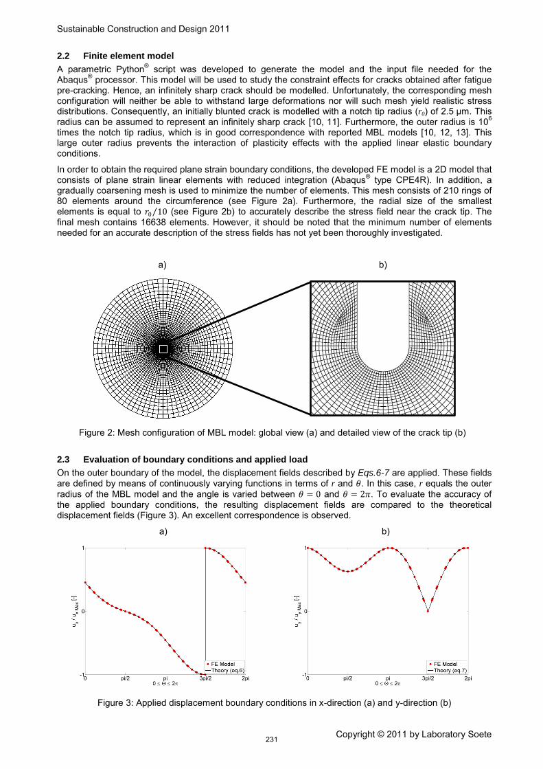
Sustainable Construction and Design 2011
Copyright © 2011 by Laboratory Soete
2.2 Finite element model A parametric Python
® script was developed to generate the model and the input file needed for the
Abaqus® processor. This model will be used to study the constraint effects for cracks obtained after fatigue
pre-cracking. Hence, an infinitely sharp crack should be modelled. Unfortunately, the corresponding mesh configuration will neither be able to withstand large deformations nor will such mesh yield realistic stress distributions. Consequently, an initially blunted crack is modelled with a notch tip radius (r0) of 2.5 µm. This radius can be assumed to represent an infinitely sharp crack [10, 11]. Furthermore, the outer radius is 10
6
times the notch tip radius, which is in good correspondence with reported MBL models [10, 12, 13]. This large outer radius prevents the interaction of plasticity effects with the applied linear elastic boundary conditions.
In order to obtain the required plane strain boundary conditions, the developed FE model is a 2D model that consists of plane strain linear elements with reduced integration (Abaqus
® type CPE4R). In addition, a
gradually coarsening mesh is used to minimize the number of elements. This mesh consists of 210 rings of 80 elements around the circumference (see Figure 2a). Furthermore, the radial size of the smallest elements is equal to 𝑟0 10 (see Figure 2b) to accurately describe the stress field near the crack tip. The final mesh contains 16638 elements. However, it should be noted that the minimum number of elements needed for an accurate description of the stress fields has not yet been thoroughly investigated.
a) b)
Figure 2: Mesh configuration of MBL model: global view (a) and detailed view of the crack tip (b)
2.3 Evaluation of boundary conditions and applied load On the outer boundary of the model, the displacement fields described by Eqs.6-7 are applied. These fields are defined by means of continuously varying functions in terms of r and 𝜃. In this case, r equals the outer
radius of the MBL model and the angle is varied between 𝜃 = 0 and 𝜃 = 2𝜋. To evaluate the accuracy of the applied boundary conditions, the resulting displacement fields are compared to the theoretical displacement fields (Figure 3). An excellent correspondence is observed.
a) b)
Figure 3: Applied displacement boundary conditions in x-direction (a) and y-direction (b)
231

Sustainable Construction and Design 2011
Copyright © 2011 by Laboratory Soete
Considering the above correspondence, the calculated load level should correspond to the applied load level. Therefore, a comparison is made between the applied and calculated J-value. A J-level of 1000 N/mm
is applied. A limited difference of 3% is noted. However, a comparable difference has also been reported in literature [14]. Therefore, this correspondence is considered satisfying.
3 VALIDATION OF CRACK TIP STRESS FIELDS
3.1 Linear elastic validation At first the MBL FE model is validated for a linear elastic material, corresponding to LEFM theory. In such case, the shape of the crack tip stress field should match the theoretical shape described by the Williams expansion (eq.1). For an applied T-stress level equal to zero, this equation reduces to the expression below
for the crack tip opening stress, xx, ahead of the crack tip:
𝜎𝑥𝑥 =𝐾𝐼
2 𝜋 𝑟 (11)
This theoretical distribution is plotted in Figure 4, also presenting the stress distribution obtained from the FE model. An excellent correspondence is observed between both distributions.
Figure 4: Linear elastic validation of MBL crack tip stress fields (at = /2)
3.2 Elastic-plastic validation For a second validation, the plasticity effects around the crack tip are taken into account. Unfortunately, no theoretical solution exists for these SSY crack tip stress fields. Therefore, the results from the MBL FE model are compared to the results obtained from a literature review [8, 15]. For this validation a Ramberg-Osgood stress-strain relationship is assumed:
ε =σ
E+ α
σ
σ0
n−1
σ
E (12)
For the validation, the following values are considered: Young’s modulus E = 200 GPa, yield strength
0 = 400 MPa, = 1 and strain hardening exponent n = 10. Furthermore, small strain conditions are
assumed (NlGeom has been set off in Abaqus®).
The crack tip stress field was studied for an applied load level J = 1000 N/mm and a root radius of 2.5 µm.
The resulting stress field xx is plotted in Figure 5. Comparing this stress field with the results from literature, a fairly good correspondence is achieved. Therefore, the MBL FE model is considered to correctly predict the crack tip stress fields.
232

Sustainable Construction and Design 2011
Copyright © 2011 by Laboratory Soete
Figure 5: Elastic-plastic validation of MBL crack tip stress fields (at = /2)
4 CONSTRAINT
As already briefly described in §2.1, the MBL FE model is a useful tool to investigate the influence of different constraint conditions in terms of T-stress. This paragraph first investigates the exact influence of the T-stress on the magnitude and shape of the crack tip stress fields. Second, the Q-stress is calculated for each of the studied T-stress levels. These calculations lead to a relationship between the T-stress and Q-parameter.
4.1 Influence of T-parameter on crack tip stress field Based on eq.9-10 an extra displacement can be applied on the outer boundary of the MBL model. This will generate different constraint conditions in the vicinity of the crack tip, most likely resulting in a shift of the crack tip stress field. This shift is expected towards higher stress levels for high constraint conditions (positive T-stresses). In contrast, lower stress levels are expected for so-called low constraint conditions
(negative T-stresses). Indeed, as indicated by Figure 6, a positive T-stress results in a higher stress xx,
whereas a negative T-stress results in a lower stress xx.
Figure 6: Influence of T-stress on the stress level ahead of the crack tip (at = /2)
233

Sustainable Construction and Design 2011
Copyright © 2011 by Laboratory Soete
4.2 Relationship between T-stress and Q-parameter From the above crack tip stress fields, the Q-parameter is calculated for different T-stress levels. Consequently, a relationship between these two constraint parameters is obtained. This relationship is displayed in Figure 7. When the results from the MBL FE model are compared to results published in literature [15], an excellent correspondence is achieved. Only for the smallest investigated T-stress level a minor difference is observed.
From the obtained relationship it can be concluded that positive T-stress levels result in limited constraint conditions if expressed by the Q-parameter. In contrast, negative T-stress levels tend to strongly influence the Q-parameter. These results are in correspondence with the results of O’Dowd & Shih [9].
Figure 7: Relationship between T-stress and Q-parameter obtained from MBL analysis
234

Sustainable Construction and Design 2011
Copyright © 2011 by Laboratory Soete
5 CONCLUSIONS
A finite element model was presented to calculate the magnitude of the crack tip stress fields in a MBL model under different constraint conditions. The following conclusions were drawn:
- The relationship between the Q-parameter and T-stress was investigated, showing a weak influence of the T-stress on the Q-parameter for positive T-stresses. In contrast, negative T-stress resulted in pronounced negative Q-values.
- For elastic-plastic conditions the obtained stress field showed an excellent correspondence to the stress fields published by other researchers.
- For linear elastic conditions, the crack tip stress fields corresponded to the analytical crack tip stress field.
- A limited difference was observed between the applied load level in terms of J and the calculated
load level.
6 NOMENCLATURE
𝑓𝑖𝑗 (𝜗) Angular function [-]
𝜗 Angular position centered at the crack-tip [-]
𝑄 Constraint parameter [-]
𝜎 𝑖𝑗 (𝑛,𝜗) Dimensionless functions [-]
𝛼,𝑛 Dimensionless Ramberg-Osgood parameters [-]
𝑢𝑥 Displacement in x-direction [mm]
𝑢𝑦 Displacement in y-direction [mm]
𝑟 Distance ahead of the crack-tip [mm]
𝐽 Energy release rate [N/mm]
𝐼𝑛 Integration constant depending on n [-]
𝛿𝑖𝑗 Kronecker delta [-]
𝐾𝐼 Mode I stress intensity factor [MPa mm]
𝑟0 Notch tip radius [mm]
𝜐 Poisson coefficient [-]
𝜎𝑖𝑗 Stress component in the vicinity of the crack tip [MPa]
True strain [-]
True stress [MPa]
𝑇 T-stress [MPa]
𝜎0 Yield stress of the material [MPa]
E Young’s modulus [MPa]
7 ACKNOWLEDGEMENTS
The authors would like to acknowledge the financial support of the IWT (Agency for innovation by science and technology – grant n° SB-091512) and the FWO (Research Foundation Flanders – grants n° 1.1.880.09.N and 1.5.247.08N.00).
235

Sustainable Construction and Design 2011
Copyright © 2011 by Laboratory Soete
8 REFERENCES
1. Williams, M.L., On the stress distribution at the base of a stationary crack. Journal of Applied Mechanics, 1957. 24: p. 109-114.
2. Anderson, T.L., Fracture Mechanics - Fundamentals and Applications. 1995. 3. Xu, J., et al., Effects of embedded defects in pipelines subjected to plastic strains during operation.
International Journal of Pressure Vessels and Piping, 2009. 86: p. 787-797. 4. Thaulow, C., et al., Constraint correction of high strength steel - selection of test specimens and
applications of direct calculations. Engineering Fracture Mechanics, 2004. 71: p. 2417-2433. 5. Du, Z.Z. and J.W. Hancock, The effect of non-singular stresses on crack-tip constraint. Journal of
Mechanics and Physics of solids, 1991. 39: p. 555-567. 6. Al-Ani, A.M. and J.W. Hancock, J-dominance of short crack in tension and bending. Journal of
Mechanics and Physics of solids, 1991. 39: p. 23-43. 7. Betegon, C. and J.W. Hancock, Two-parameter characterization of elastic-plastic crack tip fields.
ASME Journal of applied mechanics, 1991. 58: p. 104-113. 8. O'Dowd, N.P. and C.F. Shih, Family of crack-tip fields characterized by a triaxiality parameter - Part
I. structure of fields. Journal of Mechanics and Physics of solids, 1991. 99: p. 989-1015. 9. O'Dowd, N.P. and C.F. Shih, Family of crack-tip fields characterized by a triaxiality parameter - Part
II. Fracture Applications. Journal of Mechanics and Physics of solids, 1992. 40: p. 939-963. 10. Cravero, S. and C. Ruggieri, A two-parameter framework to describe the effect of constraint loss on
cleavage fracture and implications for failure assessments of cracked components. Journal of Brazilian Society of Mechanical Sciences and Engineering, 2003. 15: p. 403-412.
11. Ranestad, O., Z.L. Zhang, and C. Thaulow, Quantification of geometry and material mismatch constraint in steel weldments with fusion line cracks. International Journal of Fracture, 1999. 99: p. 211-237.
12. Horn, A.J., Development of an engineering assessment procedure for predicting cleavage fracture from non-sharp defects using the failure assessment diagram, in School of Materials, University of Manchester, 2010, PhD-Thesis.
13. Sherry, A.H., et al., Material constraint parameters for the assessment of shallow defects in structural components - Part I. Parameter solutions. Engineering Fracture Mechanics, 2005. 72: p. 2373-2395.
14. Zhang, Z.L., M. Hauge, and C. Thaulow, The Effect of T stress on the near tip stress field on an elastic-plastic interface crack, in International conference on fracture. 1997: Sydney, Australia.
15. Wang, X., Two-parameter characterization of elastic-plastic crack front fields: surface cracked plates under tensile loading. Engineering Fracture Mechanics, 2009. 76: p. 958-982.
236

Sustainable Construction and Design 2011
Copyright © 2011 by Laboratory Soete
INFLUENCE OF DESIGN FEATURES ON THE STRUCTURAL INTEGRITY OF THREADED PIPE CONNECTIONS
T. Galle1, W. De Waele1, P. De Baets1, J. Van Wittenberghe1
1
Abstract When drilling and completing High Pressure High Temperature (HPHT) wells, the applied casing and tubing have to be able to withstand extreme conditions. Very often, the threaded connections are the most critical components in the entire chain. The overall design of several threaded and coupled (T&C) connections (eg. VAM TOP, JFEBear and the newest PatriotTC) is very similar. However, even by modifying one single feature of the geometry, an improved structural integrity (eg. fatigue resistance, leak tightness or collapse strength) can be obtained. This paper gives an overview of the most important geometrical features and discusses their alleged effects on the structural integrity of the coupling.
Ghent University, Laboratory Soete, Belgium
At first, different thread designs were compared with each other and the effects on maximum allowable torque during make-up and tension during service conditions were evaluated. Secondly, literature shows that the use of an adequate torque shoulder is favourable, especially during the make-up stage. When designing connections for purposes involving gasses, a gastight seal is required. The third part of this paper discusses the influences on the sealability and performance limits when making changes to the sealing area. At last, the effect of overall changes (such as stress relief grooves) in the design and their consequences during running is shortly discussed. Based on this review, design guidelines for ‘optimized’ premium T&C couplings can be formulated.
Keywords Design, Threaded Connection, Pipeline
1 INTRODUCTION
When drilling and operating oil and gas wells, the use of threaded pipe connections is favourable because of the inherent ability to demount and reuse the applied drill strings, tubing and casings. By applying such couplings, the overall cost of drilling and maintaining wells is reduced [1].
In recent years, the traditional OCTG (Oil Country Tubular Goods) products are unable to meet the desired requirements because of the exposure to the harsh conditions of High Pressure High Temperature (HTHP) wells. Due to the increasing development of these wells to reach remote gas and oil reserves, the enhancement of oil and gas tubular threaded joints is a growing economy with an increasing amount of players. Semi-premium and premium threaded connections are designed to fulfil the additional needs of improved reliability, leak resistance and performance. Figure 1 gives a brief overview of the evolution in the field of premium connections. In 1967, the depth of oil and gas wells had increased to over 4500 m and the development [2] and research [3] of threaded couplings has increased significantly.
Figure 1: Timeline - evolution of premium connections and the three leading
manufacturers with some of their most important T&C connections [4]
237

Sustainable Construction and Design 2011
Copyright © 2011 by Laboratory Soete
In the design of new premium connections (PC in Figure 1), three development phases have to be considered. During the first phase, the basic geometrical concept of a connection with chosen nominal size and material grade is engineered to withstand higher loads. Once the final basic geometry is established, the design is extrapolated to a variety of sizes and grades to create a new family of connections. Finally, in the third phase, the newly designed connections are tested in accordance with existing standards and procedures such as described in API 5C5 or ISO 13679. When these tests are successful, the connection should pass additional field-tests and is then considered fit for duty.
Possible adjustments of thread, torque shoulder and sealing area to enhance the design are considered in this paper. A discussion on improvement of fatigue life is reported in a companion paper [5].
2 TYPES OF THREADED PIPE CONNECTIONS
Originally, a sealed threaded pipe joint based on API buttress connectors (API BTC in Figure 1) patented by Samuel Webb [6] provided excellent joint strength. Mismatched leads closed the thread clearance on the stab flanks and provided the required leak resistance as can be seen in Figure 2. Due to improved manufacturing techniques, tighter tolerances are being held and clearances between the stab flanks are achieved, lowering leak resistance [7]. As a result, two new types of connections with an additional seal are developed to ensure the required leak resistance. One group consists of connections with a metal-to-metal seal providing gas tightness, named premium connections. The other group, without a metal-to-metal seal and water type sealability, is called semi-premium connections.
Figure 2: API Buttress thread with a mismatched lead reduces thread clearance resulting in excellent joint
strength [6]
Figure 3: Different types of threaded connections with:
A. threaded and coupled connection B. Integral connections: 1. integral flush, 2. integral semi-flush, 3. Integral upset [8]
238

Sustainable Construction and Design 2011
Copyright © 2011 by Laboratory Soete
Figure 3 shows different types of premium threaded connections which are currently commercially available. Out of these types, two major groups can be defined. At one hand, the Threaded and Coupled (T&C) connections and at the other hand the integral connections, which do not require special coupling stock.
T&C connections are less sensitive to stress concentrations and have proven to have higher tension ratings in comparison with integral connections. Even ratings exceeding the pipe body can be achieved. This implies that the strength of the connection in tension is equal or greater than the pipe body tensile yield strength. However, special attention is required when torsion or external pressure is applied. High leak resistance is guaranteed on static surfaces due to the variety of seal configurations which are possible.
The second group are the integral connections. With a sufficiently thick wall, these connections are efficient if external pressure is applied. When the outer diameter of the connection does not exceed the outer diameter of the pin, the connection is called an integral flush connection. In case the connection’s outer diameters differs slightly from the pipe body, the connection is known as a semi-flush connection. To neutralize the reduced connection’s joint strength due to the reduced wall thickness at the threaded area, a cold working process called swaging of the pin and/or box can be applied. AB Bradley et al [9] indicated that when no thermal relief is applied, a loss of sour service performance is obtained. A last member of the integral connections family is the upset integral connection, a type which is often used in tubing and drill strings. This expensive connection is limited by inner diameter and wall thickness.
It is worth noting that weld-on connectors (upset-type connections) are an additional type of threaded connection. However, because no threads are machined on the pipe body, they are considered to be connectors for pipe and not pipe connections.
3 GEOMETRICAL DETAILS
As stated before, the geometry of a premium connection dictates its success in the field. Figure 4 shows an API buttress threaded connection during make-up (A), with additional tensile loading (B) and with additional tension and internal pressure (C). The goal of the designer is to reduce plastic deformation and stress concentrations throughout the connection to increase its performance limits.
Figure 4: Yielding at working loads with:
A. Make-up, B. Make-up with tension, C. Make up with tension and internal pressure [4]
Most premium connections show comparable design features and have three major geometrical characteristics which are frequently altered to improve performance. The areas of interest are the thread, torque shoulder and metal-to-metal seal which are visible in Figure 5.
239

Sustainable Construction and Design 2011
Copyright © 2011 by Laboratory Soete
Figure 5: Overall view of a premium threaded
connection with indication of the three major design features [8]
Figure 6: A hooked thread profile in comparison
with the regular API buttress [8]
3.1 Thread design Because of the presence of a metal-to-metal seal, the threads of premium connections are not required to interact as a pressure seal and can therefore be designed to maximize structural integrity. For this reason, API buttress type thread or a modified hooked thread with a negative load angle are commonly used (Figure 6). Despite the difficulties of machining a reversed load flank, the hooked thread design often dominates over a common API buttress profile. When tension is applied, the negative oriented load flank in combination with a positive stab flank, also known as a dovetail, reduces outward forces and eliminates radial separation between pin and box, resulting in a connection which is immune to jump-out failures and has higher tensile loading limits. In compression, most of the forces are supported by the stab flank and the hooked thread profile offers no significant advantages in comparison with the conventional buttress thread.
In a conventional thread design, an external tension load is mainly carried by the last engaged thread (LET) of the box. To realise a more uniform and favourable the stress distribution over the threaded surface, K.Yamamoto et al [10] suggested a pitch change concept as illustrated in Figure 7.
Figure 7: The pitch-change concept.
At pitch 2, the gap between the load flanks closes when made up. The standard pitch 1 concentrates the loads in the centre and the gap between the load flanks of the third pitch closes when axial tension is
applied. (FOX connection, JFE) [11]
Figure 8 indicates that this concept improves the contact pressure distribution with reduced peaks at the end, resulting in better anti-galling properties and joint strength.
240

Sustainable Construction and Design 2011
Copyright © 2011 by Laboratory Soete
Figure 8: The pitch-change concept (FOX connection, JFE).
Peak pressures are reduced and pressure-distribution is enhanced [10]
A tapered thread has the inherent ability to establish a certain make-up torque on the thread itself. The steeper the taper, the higher the resistance to cross threading (Figure 9), also known as crest to crest engagement, but the thinner the applicable pin nose (see further). In order to increase resistance to cross threading without reducing the number of threads per inch and maximizing the pin thickness, it is possible to apply a tapered crest and root parallel to the pipe axis [12]. Figure 10 shows that the wider clearance (perpendicular to the connection axis) between thread root and crest allows greater self-alignment, resulting in easier stabbing during make up. This way, the running ability of the threaded connection is increased.
When a chamfer is added to the stabbing flank of the box, the risk of galling due to stabbing damage is further reduced.
Figure 9: Cross threading due to misalignment during assembly [8]
Figure 10: Crest/root taper parallel to the
pipe body axis maximizes the running ability A. basic design, B. VAM21 [12]
3.2 Shoulder design As described above, applying a certain make-up torque is possible by adding a taper to the threaded area. However, this method does not give the ability to apply the high torques required in HTHP wells. To such cases, the use of a shoulder is required. A shoulder can be applied in two different ways, either by using a pin to pin contact (Figure 11) or by adding a torque shoulder to the connection itself (Figure 12).
The pin nose of one pin can be used as the torque shoulder of the other pin. This allows reducing the outer diameter of the coupling, resulting in a reduced minimum required clearance. However, using a shoulder designed in the coupling is useful as a positioning feature for easy make-up and gives the opportunity to control the applied torque. The shoulder can transfer stored torque energy to a nearby seal to maintain contact pressure, resulting in favourable seal properties. It has to be pointed out that an increase in contact pressure increases the risk of galling significantly.
A connection equipped with a reverse torque angle, as illustrated in Figure 13, causes a wedge effect. This phenomenon gives the connection self-alignment [14], radial stability and improved structural strength, which is magnified by the inverse angle of the shoulder itself.
Generally, the larger the contact surface of the shoulder, the higher the torque capabilities.
241

Sustainable Construction and Design 2011
Copyright © 2011 by Laboratory Soete
Figure 11: Pin-to-pin
contact (Seal-Lock HT, Hunting) [13]
Figure 12: Box with torque
shoulder (Seal-lock APEX, Hunting)
[13]
Figure 13: The wedge effect determined by the angle of the torque shoulder and the
load flank of the thread increases the self-aligning abilities of the connection
(VAM TOP) [8]
3.3 Sealing area design In contrast with semi-premium connections, premium connections do not use a thread seal but an extra sealing feature is added to ensure pressure integrity. Usually, a metal-to-metal seal is located near the torque shoulder to energize the sealing surface. Simulations [10] have shown that using the thread-change-concept can increase the contact surface energy of the seal as well.
Unlike polymer seals such as teflon rings, a metal-to-metal seal is one of the most reliable seals and is able to provide a gastight seal under high pressure and extreme temperatures. As a result of this surface contact, special attention has to be given to the surface finish (usually characterized by Ra between 0.8 and 3.2 μm [15]) and the risk of galling has to be taken into account when designing the sealing area. The commonly used configurations are a cone-to-cone sealing (a tapered surface on the pin and box) or a sphere-to-cone sealing (a toroidal surface on the pin and a tapered surface on the box). The steeper the taper, the higher the pressure integrity and the higher the risk of galling.
Figure 14 gives an example of the behaviour of these two variants. The cone-to-cone configuration gives a higher maximum contact pressure (and risk of galling), but has a limited seal length in comparison with the sphere-to-cone design. From these results, it is not possible to determine which design has the best sealing capacity and additional experiments have to be implemented [16].
Figure 14: Comparison of a cone-to-cone and a sphere-to-cone seal design.
The sphere-cone configuration reduces peak pressures and improves pressure-distribution. [16]
242

Sustainable Construction and Design 2011
Copyright © 2011 by Laboratory Soete
K. Yamamoto et al [10] designed a triple radii seal with three blended arcs. The use of different radii triggers a reduction of stress concentrations which leads to an increased galling and overtorque resistance resulting in a high performance seal. Due to the complex shape of this seal, repair is not possible without affecting the seal integrity [17].
Despite their excellent performance, metal-to-metal seals are vulnerable and any kind of distortion will lead to leaking. For this reason, the design has to be optimized to reduce the ability of inflicting damage during handling and make-up. One way of protecting the surface is to design the taper guide as given in Figure 15.
Figure 15: Seal protection mechanism with: A. a conventional premium connection, B. VAM21 [12]
The use of an internal and external seal in a design can be beneficial. When an internal seal protects the thread against internal pressure and the external seal against external pressure, the risk of pressure migration through the thread helix and thus the risk of leaking is reduced considerably.
3.4 Various improvements The design of a threaded coupling is not limited to the three features discussed higher. In order to improve performance with the same or a reduced amount of material, small but significant adjustments can be made.
When connecting pipes with threaded connections, compound greases with graphite are used to reduce the risk of galling and to provide leak tightness in semi-premium connections [18]. Despite the necessity of this lubricant, the grease can initiate a pressure build-up in the threads during make-up and can cause the connection to fail. For this reason, pressure relief grooves can be manufactured in the connection as shown in Figure 16. During make-up, the excess of grease is transferred to this chamber and a pressure build-up is avoided. As from 2003, the disadvantages of lubricants can be avoided by using dopeless technology [19]. This technology consists of a surface treatment instead of greases to avoid galling. The surface treatment of these dry connections often consists of the use of a soft metal plating, a dispersion plating or a solid lubricant coating type [18].
Figure 16: A lubricant relief
groove avoids pressure buildup caused by grease. (Seal lock Apex, Hunting)
Figure 17: prolonging the pin
with a nose increases stiffness (VAM21) [12]
Figure 18: stress relief
grooves at: A. pin and B. box [22]
243

Sustainable Construction and Design 2011
Copyright © 2011 by Laboratory Soete
The pin can be extended with a nose as illustrated in Figure 17. The thickness and length of the nose give extra stiffness to the configuration which is used to amplify the resulting forces of the negative torque shoulder and enhances pressure integrity [20]. At the same time, this nose can be used to protect the seal contact surface against handling and prevents eccentric contact by adding a guiding surface which is used for positioning the box and the pin during stabbing.
When couplings are designed for drill pipes, fatigue lifetime is a significant design requirement. To reduce stress concentrations at the Last Engaged Thread (LET), applying stress reduction grooves might prove beneficial [21]. Figure 18 shows the standard relief grooves for drill collars as described in API 7 [22].
4 CONCLUSIONS
During the design process, special attention is given to several aspects of the threaded connections. By altering the thread, usually a buttress or hooked profile, structural integrity against axial forces, pressure and bending is provided. The design of the shoulder determines the maximal amount of pretension that can be applied and the seal is necessary to prevent the connection from leaking due to internal and/or external gas pressure. It is important to realize that the design is not limited to these three parts of the connection. Other small geometrical enhancements, choice of materials and surface finish can be used to finalize a new connection which is able to withstand harsher conditions and greater loads.
It is important to note that not only the mechanical behaviour of a connection is important. When put in service, all connections should be able to withstand (mis-)handling and vulnerable areas should be protected to ensure reliable performance.
At last, it should be pointed out that this paper describes trends and does not give any numerical results of geometrical changes. Further research is required to determine the effect of isolated changes and to quantify the resulting interactions of combined adaptations.
5 REFERENCES
[1] David Walters, Ricky Thethi, A Step Change Application of Threaded and Coupled Connections, 2H Offshore Inc., USA, 2002
[2] P. D. Weiner, Martin E. True, A Method of Obtaining Leakproof API Threaded Connections In High-pressure Gas Service, Drilling and Production Practice, 1969, American Petroleum Institute
[3] API, WI 2317: Tech Report on LTC/BTC Performance Properties and Leak Resistance: THREAD COMPOUNDS, 2006
[4] API, Presentation: Performance properties: requirements for leak resistance of API connections (LTC/BTC), http://mycommittees.api.org/, December 2010
[5] J. Van Wittenberghe, P. De Baets, W. De Waele, T. Galle, T.T. Bui and G. De Roeck, Design characteristics that improve the fatigue life of threaded pipe connections, Sustainable Construction and Design (SCAD), Ghent, Belgium, 2011
[6] Patent US2772102 – Samuel Webb, Pleasant Hills, Pa. Sealed Threaded Pipe Joint. Patent dated Nov. 27, 1956. Dedication filed Apr. 5, 1962, by the assignee, United Stated Steel Corporation.
[7] API REPORT 86-53 Document Information, Investigation of Leak Resistance of API Buttress Connector, American Petroleum Institute, 1987
[8] Vallourec & Mannesmann, VAM book, http://www.vamservices.com, December 2010.
[9] A. B. Bradley, Premium Connection Design, Testing, and Installation for HPHT Sour Wells, Society of Petroleum Engineers Inc, SPE High Pressure-High Temperature Sour Well Design Applied Technology Workshop, 17-19 May 2005, The Woodlands, Texas, U.S.A., SPE 97585
[10] K. Yamamoto, K. Kobayashi et al, Stress Analysis of Premium Threaded Connection "FOX" by Finite Element Method, Kawasaki Steel Giho, 20 (1989) 3, pp. 202-207
[11] JFE Steel Corporation, FOX Premium Threaded Connection
[12] M. Sugino, K. Nakamura and S. Yamaguchi, Development of an Innovative High-Performance Premium Threaded Connection for OCTG, Offshore Technology Conference, 3-6 May 2010, Houston, Texas, USA, OTC 20734
[13] World Oil, 2008-09 Casing Reference Tables, November 2008
244

Sustainable Construction and Design 2011
Copyright © 2011 by Laboratory Soete
[14] Patent WO/2010/122431 – Tenaris, Threaded Joint for Tubes, Pipes and the Like, Patent dated October 28, 2010. Filed April 22, 2010
[15] Couplings, http://www.exprobase.com/Default.aspx?page=696, December 2008
[16] Eduardo N. Dvorkin, Rita G. Toscano, Finite element models in the steel industry: Part II: Analyses of tubular products performance, Computers & Structures, Volume 81, Issues 8-11, K.J Bathe 60th Anniversary Issue, May 2003, Pages 575-594
[17] Hunting, Recommendations for the repair & re-use of FOX premium threaded connections, 1994
[18] E. Tsuru, Y. Tsukano et al, Dope-free Type Premium Connection for Oil Country Tubular Goods, Nippon Steel Technical Report No. 81, January 2000
[19] Tenaris Hydril, Dopeless Technology, brochure, version 01, October 2010
[20] A. Muradov, J. E. Smith, Development of External Pressure Resistant Tool Joint for Under-balanced Drilling, SPE/IADC Drilling Conference, Amsterdam, The Netherlands, 27 February – 1 March, 2001, SPE/IADC 68771
[21] R. Shilling, M.L. Payne, High-Strength Treaded and Coupled Connectors for Dynamic Riser Applications, International Oil Conference and Exhibition, Veracruz, Mexico, 27 – 30 June, 2007, SPE 108708
[22] API Specification 7, Specification for Rotary Drill Stem Elements, American Petroleum Institute, thirty-ninth edition, December 1998.
245

Sustainable Construction and Design 2011
Copyright © 2011 by Laboratory Soete
ANALYTICAL AND COMPUTATIONAL ESTIMATION OF PATELLOFEMORAL FORCES IN THE KNEE UNDER SQUATTING AND
ISOMETRIC MOTION
G. Fekete1, B. Málnási Csizmadia2, M. A. Wahab1, P. De Baets1
1Laboratory Soete, Ghent University, Belgium. 2
Abstract: This study presents an intermediate step in prosthesis design, by introducing a newly developed two-dimensional mathematical, and a three-dimensional computational knee model. The analytical model is derived from Newton’s law with respect to the equilibrium equations, thus based on theoretical assumptions, and experimentally obtained parameter. The numeric model is built from an existing prosthesis, involving three parts as patella, femur and tibia, and currently it is under development. The models are capable to predict – with their standard deviation – the patellofemoral (numerically tibiofemoral as well) forces in the knee joint during squatting motion. The reason why the squatting is investigated is due to its relative simplicity and the fact, that during the movement the forces reach extremity in the knee joint. The obtained forces – as a function of flexion angle – are used firstly as fundaments to the knee design method, and secondly to extend the results related to the existing isometric kinetics, where one of the newly obtained functions appears as an essential – and so far missing – input function. Most results are compared and validated to the ones found in the relevant literature and put into a dimensionless form in order to have more general meaning.
Institute of Mechanics and Machinery, Szent István University, Hungary.
Keywords: analytical squatting model, patellofemoral forces, isometric motion
1 INTRODUCTION
The widespread occurrence of the various types of arthritis does not only result in significant loss in manpower, but often means immeasurable pain and suffering to many patients. Due to the limited understanding of the phenomena of the knee joint movement, the clinicians only have surgical solution, which mostly involves prosthetic replacement arthroplasty. To develop and design better prosthetic elements, several knee models – patellofemoral and tibiofemoral – have been already developed in order to investigate axial joint contact forces [25], contact points as a function of flexion [28], and the force distribution [16, 9, 17]. By knowing the acting forces in the tendons and ligaments connected to the knee joint, the development of the actual design of the prosthesis can be evaluated sooner, easier and more economically. The substantial difficulty during the building of a theoretical knee joint model, that the complexity of the joint mostly requires computational support, special programs, which does not ease the prosthetic design. But most of all, the greatest problem during the design, is the definition of the loads. This paper is an intermediate step in our research. The major aim is to develop useful methods and models for prosthesis design. The examined motion throughout our research is manly the squatting and additionally the isometric exercises. Although the squatting is considered as an everyday movement, still not that frequently used as the gait or the running. The reason we chose to investigate this specific movement is based on its relative simplicity and the fact, that during the movement the forces in the knee reach extremity. As an engineering rule of thumb, it is always recommended to design on the upper extremity of the forces. However, designing prosthesis is far from easy, thus our program is divided into segments, which are tightly interconnected. The research program involves the following main steps:
A. Creation of a 2D mathematical model to investigate the forces in the connecting ligaments of the knee joint during squatting and isometric motion. The formulas related to the isometric motion are obtained by the use of the references, while the formulas related to the squatting motion are derived from the 2D model. These forces are considered as ‘external forces’, and experimental validation is required.
B. Creation of a 3D computational model in MSC.ADAMS, to investigate the forces between the connecting surfaces of the femur, tibia and patella. These forces are considered as ‘internal forces’, and the point or area of application has to be calculated as well.
246

Sustainable Construction and Design 2011
Copyright © 2011 by Laboratory Soete
In this paper two novel – analytic and computational – models are presented. These models are able to provide estimation – based on analytic and numeric approaches – about the external and internal forces of the knee such as the quadriceps force (Fq), the patellar ligament force (Fpt), the patello-femoral compression force between the patella and femur (Fp) and the tibio-femoral force (Ft
) by deriving them as a function of knee flexion angle, mass of the person, and some ‘human-bond’ quantities [5]. The results are compared to the ones found in the references and to experiments as well. This study is limited to the first and partly the second step of our research program.
2 METHODS
2.1 Mathematical model of squatting
The following simplifications were considered related to the analytical model:
• The model is quasi-static, • Two-dimensional, • The inertial forces during the movement are neglected, • No internal forces between the surfaces are considered, • Only the squatting movement can be investigated with the model, • The load is derived from the mass of the person.
Our model consisted of equilibrium equations which describe the condition of the forces connected to the femur, tibia and patella. Let us introduce the analytical model in two positions – stand and squat – and investigate the motion. It is seen that the patella rotates about a B point and so does the tibia (see Fig. 1).
Fig. 1: Theoretical lengths of the knee joint
The model is represented at an arbitrary angle α, and the G force is derived from the mass. The line of action of G intersects with the theoretical line of femur and tibia. The G force was chosen to be 785 N, which equals to a person with 80 kg of mass but it can be arbitrarily varied. Let us fix the y component of the coordinate system to this line of action, while the origin is at the ground.
247

Sustainable Construction and Design 2011
Copyright © 2011 by Laboratory Soete
Rigid bodies will represent the femur (3), the patella (2), and the foot with the tibia (1) as well. The three rigid bodies are attached to the ground by a hinge of one degree of freedom (point A), and a roller at the intersection of the line of action and the femur (point D). At point A, the ground reaction force is represented as F0 force, which equals to G. The rigid bodies are attached to each other by strings (the elastic elongation is neglected). The calculation is presented as a function of α, and illustrated in three different positions (Fig. 2).
Fig. 2: 2D analytical model in three positions
The denotation of the geometric lengths in standing position:
• l10• l
: the theoretical length of the tibia, 30
• l: the theoretical length of the femur,
p• l
: the theoretical length of the patellar tendon, t
• l: the perpendicular theoretical length between the axis of tibia and the surface of the patella,
f
: the theoretical length between the axis of femur and the line of action of the resultant quadriceps force,
In squatting position:
• l1
• l
(α): the theoretical intersected length of the axis of tibia and the instantaneous line of action of the mass. Measured from the knee joint, 3
• α: the angle between the tibia and the femur,
(α): the theoretical intersected length of the axis of femur and the instantaneous line of action of the mass. Measured from the knee joint,
• β(α): the angle between the axis of tibia and the patellar tendon, • γ(α): the angle between the axis of tibia and the line of action of the mass, • δ(α): the angle between the axis of femur and the line of action of the mass, δ = α- γ, • φ(α): the angle between the axis of tibia and the resultant force of the upper condyles, • ψ(α): the angle between the resultant quadriceps force vector and the axis of femur.
The three elements are plotted as free-body diagrams, where the forces, angles, and the different lengths are shown on Figure 3a-d.
248

Sustainable Construction and Design 2011
Copyright © 2011 by Laboratory Soete
Fig. 3: The construction of the force vectors in an arbitrary position
Where the forces are:
• Fq• F
(α): quadriceps force, p
• F(α): patellofemoral compression force,
pt• F
(α): patellar ligament force, t
The calculation is carried out by the use of the equilibrium equations as a function of angle α. (α): tibial compression force.
The moment equation applied about the z axis through point B on the 1st
element (see Fig. 3a):
)(sin)()(cos)(sin0 11 αγααβαβ ⋅⋅+⋅⋅−⋅⋅−==∑ GlFlFlM pttptpzB (1)
Thus the patellar force can be derived as:
)(cos)(sin
)(sin)()( 1
αβαβαγαα
⋅+⋅⋅
⋅=tp
pt lllGF (2)
In order to simplify and generalize the results let us to introduce dimensionless geometric quantities and forces, thus the acting force will be calculated in a normalized form with respect to the force derived from the body mass (G).
• λ1 ( ) 101 / ll α(α)= : dimensionless, intersected tibia length function,
• λ3 ( ) 303 / ll α(α)= : dimensionless, intersected femur length function,
• λp 10/ ll p= : dimensionless length of patellar tendon,
• λ t 10/ llt= : dimensionless thickness of shin,
• λ f 30/ ll f= : dimensionless thickness of thigh.
249

Sustainable Construction and Design 2011
Copyright © 2011 by Laboratory Soete
By the introduction of these quantities, the acting force in the patellar ligament is:
)(cos)(sin
)(sin)()( 1
αβλαβλαγαλα⋅+⋅
⋅=
tp
pt
GF
(3)
The scalar equilibrium equations related to the 1st
element in the ξ - η coordinate system (see Fig. 3a):
)(cos)(cos)(cos0 αγαβαϕη ⋅+⋅+⋅−==∑ GFFF ptti (4)
)(sin)(sin)(sin0 αγαβαϕξ ⋅+⋅−⋅==∑ GFFF ptti (5)
By some simplification the angle between the axis of tibia and the resultant force of the upper condyles can be derived from Eq. (4) and Eq. (5) as:
( )
⋅
+⋅+⋅
−⋅−= )(
)()()()()(
)(1
1 αγλαβλαγαλ
λαβλαλαϕ tg
tgtgtg
arctgtp
tp (6)
By the use of angle φ the acting normal force in the tibia can be derived from Eq. (4) or Eq. (5) as well:
)(cos)(cos
)(cos)(cos)(
αϕαγ
αϕαβα
+⋅=GF
GF ptt (7)
The moment equation applied about the z axis through point B on the 3rd
element (see Fig. 3c):
)(sin)()(sin)(cos0 3303 αδααψαψ ⋅⋅−⋅⋅+⋅⋅==∑ GlFlFlM qqfib (8)
Taking into account that δ = α- γ, and assuming ψ = 0, the quadriceps force in the tendon:
( )f
q
GF
λαγααλα )(sin)()( 3 −⋅
= (9)
The ψ = 0 assumption means that the direction of the resultant, acting forces in the quadriceps muscle are parallel with the axis of femur, since the muscle is connected to under the hip bone and stretches out until the frontal surface (facies patellaris) [26], thus this approximation is acceptable. The scalar equilibrium equations related to the 2nd
element in the x - y coordinate system (see Fig. 3b):
( ) pxtqix FFFF ++⋅+⋅==∑ )()(sin)()(sin)(0 αβαγααδα (10)
( ) pytqiy FFFF ++⋅−⋅==∑ )()(cos)()(cos)(0 αβαγααδα (11)
Out of Eq. (10) and Eq. (11) equations the magnitude of the patellar compression force can be derived by the use of x,y coordinates with respect to the body mass force:
GFFFF
GFF
GF tqtqpypxp ))()()(cos()()(2)()()( 2222 αγαδαβααααα ++⋅⋅⋅−+
=+
= (12)
Since all the forces are mathematically described, by the use of λ1 (α), λ3 (α), λb, λ t, λ f
, β(α), γ(α), δ(α), φ(α) dimensionless functions and constants [5] with – their standard deviation – the formulas of the forces are complete and usable to estimate the forces in the knee joint during squatting.
2.2 Mathematical model of isometric motions
Several authors investigated the ratio of patellofemoral forces under isometric extension and flexion exercises in the relevant literature [15, 17, 7, 1, 8] with very similar results. In case of isometric motion investigation, it is always emphasized that generally the applied loads are relatively small (e.g. approx. 50 N [27] or 2.2 Nm derived from 0.5 kg of weight [17]) and correlations between the forces are always described as a ratio (Fpt/Fq, Fp/Fq
This approach only shows the ratio, but does not describe the forces individually. In order to gain more information about the forces, the quadriceps force has to be determined as well. The function of the quadriceps force is mostly investigated experimentally [22] or semi-experimentally by using theoretical
) in the function of flexion angle α.
250
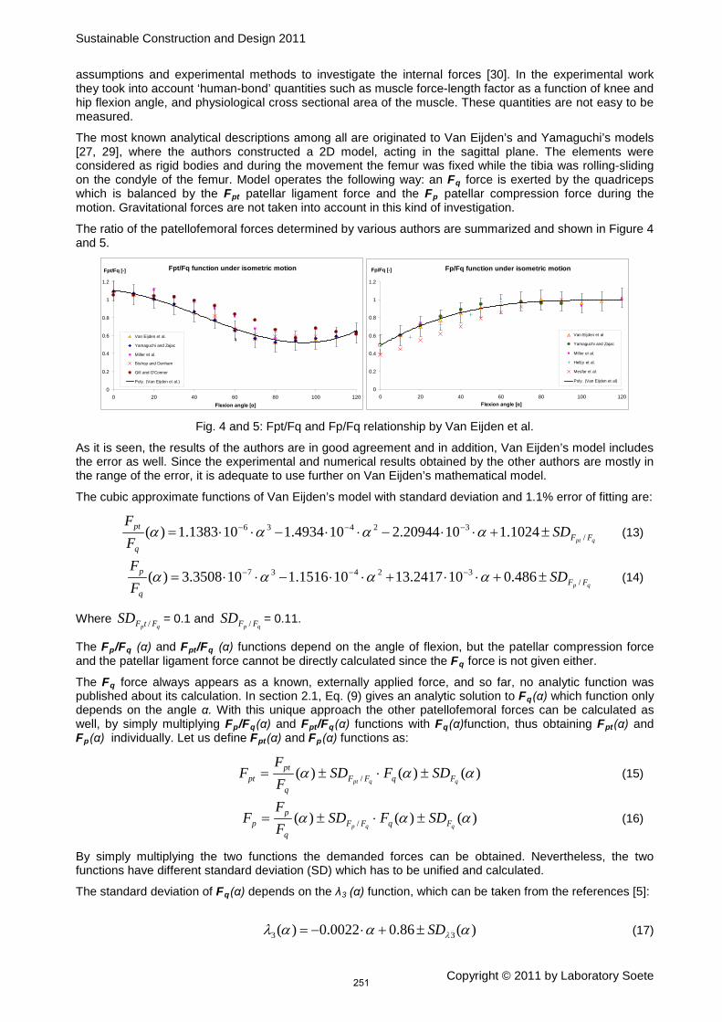
Sustainable Construction and Design 2011
Copyright © 2011 by Laboratory Soete
assumptions and experimental methods to investigate the internal forces [30]. In the experimental work they took into account ‘human-bond’ quantities such as muscle force-length factor as a function of knee and hip flexion angle, and physiological cross sectional area of the muscle. These quantities are not easy to be measured.
The most known analytical descriptions among all are originated to Van Eijden’s and Yamaguchi’s models [27, 29], where the authors constructed a 2D model, acting in the sagittal plane. The elements were considered as rigid bodies and during the movement the femur was fixed while the tibia was rolling-sliding on the condyle of the femur. Model operates the following way: an Fq force is exerted by the quadriceps which is balanced by the Fpt patellar ligament force and the Fp
The ratio of the patellofemoral forces determined by various authors are summarized and shown in Figure 4 and 5.
patellar compression force during the motion. Gravitational forces are not taken into account in this kind of investigation.
Fpt/Fq function under isometric motion
0
0.2
0.4
0.6
0.8
1
1.2
0 20 40 60 80 100 120Flexion angle [α]
Fpt/Fq [-]
Van Eijden et al.
Yamaguchi and Zajac
Miller et al.
Bishop and Denham
Gill and O'Connor
Poly. (Van Eijden et al.)
v
Fp/Fq function under isometric motion
0
0.2
0.4
0.6
0.8
1
1.2
0 20 40 60 80 100 120Flexion angle [α]
Fp/Fq [-]
Van Eijden et al
Yamaguchi and Zajac
Miller et al.
Hefzy et al.
Mesfar et al.
Poly. (Van Eijden et al)
Fig. 4 and 5: Fpt/Fq and Fp/Fq relationship by Van Eijden et al.
As it is seen, the results of the authors are in good agreement and in addition, Van Eijden’s model includes the error as well. Since the experimental and numerical results obtained by the other authors are mostly in the range of the error, it is adequate to use further on Van Eijden’s mathematical model.
The cubic approximate functions of Van Eijden’s model with standard deviation and 1.1% error of fitting are:
qpt FF
q
pt SDFF
/32436 1024.11020944.2104934.1101383.1)( ±+⋅⋅−⋅⋅−⋅⋅= −−− αααα (13)
qp FF
q
p SDFF
/32437 486.0102417.13101516.1103508.3)( ±+⋅⋅+⋅⋅−⋅⋅= −−− αααα (14)
Where qp FtFSD / = 0.1 and
qp FFSD / = 0.11.
The Fp/Fq (α) and Fpt/Fq (α) functions depend on the angle of flexion, but the patellar compression force and the patellar ligament force cannot be directly calculated since the Fq
The F
force is not given either.
q force always appears as a known, externally applied force, and so far, no analytic function was published about its calculation. In section 2.1, Eq. (9) gives an analytic solution to Fq(α) which function only depends on the angle α. With this unique approach the other patellofemoral forces can be calculated as well, by simply multiplying Fp/Fq(α) and Fpt/Fq(α) functions with Fq(α)function, thus obtaining Fpt(α) and Fp(α) individually. Let us define Fpt(α) and Fp
(α) functions as:
)()()( / αααqqpt FqFF
q
ptpt SDFSD
FF
F ±⋅±= (15)
)()()( / αααqqp FqFF
q
pp SDFSD
FF
F ±⋅±= (16)
By simply multiplying the two functions the demanded forces can be obtained. Nevertheless, the two functions have different standard deviation (SD) which has to be unified and calculated.
The standard deviation of Fq(α) depends on the λ3
(α) function, which can be taken from the references [5]:
)(86.00022.0)( 33 αααλ λSD±+⋅−= (17)
251

Sustainable Construction and Design 2011
Copyright © 2011 by Laboratory Soete
Where,
057.0104.51057.1)( 42633 +⋅⋅+⋅⋅=⋅= −− αααλλ stSD (18)
is standard deviation function of λ3
Substituting Eq. (17) and Eq. (18) into Eq. (9), the standard deviation of F
(α), and t = 1.96 according to the 95% confidence.
q
(α) force function is obtained as follows:
1692.71298.40047.0)( 2 −⋅+⋅−= αααqFSD (19)
Since the functions are available, the standard deviation must be also determined for Fpt(α) and Fp(α). To determine the global standard deviation for these functions, let us consider an f(x) function with e.g. three parameters as p1, p2, p3. Each parameter has a measured standard deviation denoted as SDp1, SDp2, and SDp3
. The global deviation of the function can be derived from the principle of error propagation [11, 24] as follows:
321321
pppf SDpfSD
pfSD
pfSD ⋅
∂∂
⋅∂∂
+⋅∂∂
= (20)
Expanding the principle to the case of multiple functions with one variable, let us consider the force functions in Eq. (15) and Eq. (16):
qptqpt FF
qpt
ptF
q
ptF SD
FFF
SDFF
SD //)( ⋅
∂
∂+⋅
∂
∂= α (21)
qpqp FF
qp
pF
q
pF SD
FFF
SDFF
SD //)( ⋅
∂
∂+⋅
∂
∂= α (22)
By undertaking the partial differentiation and the multiplication, then simplifying the equations the following results are obtained related to the standard deviation:
( )⋅+⋅⋅+⋅⋅⋅⋅= −−− 057.0104.51057.1101383.1 4266 ααptFSD
( ) ( ) ( ) 1.0)(sin)(854.2041.131486579.7322
32
222 ⋅−⋅⋅
++⋅−⋅+f
Gλ
αγααλααα (23)
( )⋅+⋅⋅+⋅⋅⋅⋅= −−− 057.0104.51057.1103508.3 4267 ααpFSD
( ) ( ) ( ) 11.0)(sin)(533.3721.502678539.2822
32
222 ⋅−⋅⋅
++⋅−⋅+f
Gλ
αγααλααα (24)
Thus the global standard deviations of the functions are also obtained. The results are general with valid deviation and suitable to calculate directly the forces as a function of flexion angle α.
2.3 Computational squatting model
2.3.1 Knee joint geometry
The model was built in the MSC.ADAMS program system (see Fig. 6 and 7). The bones, such as the tibia, patella and femur were assumed as rigid bodies, since the influence of deformation in this study is irrelevant. The geometry of the femur and tibia is based on a prosthesis prototype, which is under tests and developments.
252

Sustainable Construction and Design 2011
Copyright © 2011 by Laboratory Soete
Fig. 6 and 7: MSC.ADAMS knee model in two positions
2.3.2 Ligaments, muscles
Only the patellar ligament and the quadriceps muscle were considered in the computational model. The quadriceps muscle and the patellar ligament were modelled as simple linear springs. The stiffness coefficient was set to 130 N/mm and the damping coefficient to 0.15 Ns/mm in case of both springs. That corresponds with the measured values in the literature [12, 18].
2.3.3 Loads, constraints and boundary conditions
The same load (G = 785 N) was applied in case of the computational model as it was in the analytical model (see Fig. 6). The point of application was the femur distalis. The femur distalis was constrained by a GENERAL POINT MOTION, where all the coordinates can be prescribed. Only one prescription was set: the endpoint of the femur (distalis) can only perform translational motion along the y axis.
The ankle part of the model was constrained by a SPHERICAL JOINT, which allows rotation about all axes, but all the translational motions equal to zero in that point. By applying this constraint, the tibia can perform a natural rotation, and later on, it can be kinematically analyzed.
Between the femur, tibia and patella, CONTACT constraints were set according to Coulomb’s law with respect to the very low friction (μs = 0.0003 μd
= 0.0001) in case of real joints [19, 21]. The relationship between the internal (contact forces) and external forces was not analyzed in this study.
2.3.4 Solver, simulation, post-procession
The MSC.ADAMS creates and solves simultaneously linear or non-linear Ordinary Differential Equations (ODE) and non-linear Differential-Algebraic Equations (DAE). The DAE is distinct from ODE since it involves an unknown function with its derivatives. Briefly the solution of any DAE is the following: firstly, a consistent initial value must be found, and secondly the trajectory of the DAE must be computed.
The simulation time was set to 0.045 sec in 200 time steps. GSTIFF [6] integrator was used for integrating the ODE and DAE of the motion. The solver routine was set to work maximum 1e-003 tolerance of error, while the maximum order of the polynomial was defined to 12. The solution converged very quickly with these parameters.
The post-procession was carried out in the ADAMS and partly in the Excel [13]. The ADAMS could compute the directly the forces, velocities and accelerations, but not the rotations. The flexion angle was derived by integrating the angular velocities of the femur and tibia about the x axis, taking into account that the model was in an initial 15 degree of squat in the beginning of the motion. In order to deal with the fact that the motion is three-dimensional the angles are decomposed to three separate angles. These angles are Euler angles, thus an order was chosen (313) to define them during the calculation. After integrating the appropriate angular velocities the results were summarized in charts by using the Excel program.
253

Sustainable Construction and Design 2011
Copyright © 2011 by Laboratory Soete
3 RESULTS AND DISCUSSION
In Fig. 8-9-10-11-12-13 the relationship between the angle of flexion and the calculated forces are expressed in case of squatting motion as a function of flexion angle.
Patellofemoral forces under squatting motion
0
2
4
6
8
10
0 20 40 60 80 100 120Flexion angle [α]
F/G [-]
Fq/G - Quadriceps force
Fpt/G - Patellar ligament force
Fp/G - Patello-femoral compression force
Ft/G - Tibio-femoral compression force
Fq/G - Quadriceps force under squatting motion
0
1
2
3
4
5
6
0 20 40 60 80 100 120Flexion angle [α]
F/G [-]
Fq/G - Quadriceps force
Standard deviation
Fq/G - Sharma et al.
Fq/G - Zheng et al.
Fq/G - UGent test rig
Fq/G - Numeric result by MSC.ADAMS
Fig. 8 and 9: Patellofemoral forces and the quadriceps force under squatting motion
Fpt/G - Patellar ligament force under squatting motion
0
2
4
6
8
0 20 40 60 80 100 120Flexion angle [α]
F/G [-]
Fpt/G - Patellar ligament force
Standard deviation
Fpt/G - Numeric result by MSC.ADAMS
Fp/G - Patellofemoral compression force under squatting motion
0
2
4
6
8
0 20 40 60 80 100 120Flexion angle [α]
F/G [-]
Fp/G - Patellofemoral compression force
Standard deviation
Fp/G - Numeric result by MSC.ADAMS
Fp/G - Escamilla et al.
Fig. 10 and 11: Patellar ligament and Patellofemoral force under squatting motion
Ft/G - Tibiofemoral compression force under squatting motion
0
2
4
6
8
0 20 40 60 80 100 120
Flexion angle [α]
F/G [-]
Ft/G - Zheng et al.
Ft/G - Numeric result by MSC.ADAMS
Ft/G - Tibial compression force under squatting motion
0
2
4
6
8
0 20 40 60 80 100 120
Flexion angle [α]
F/G [-]
Ft/G - Tibiofemoral compression force
Standard deviation
Fig. 12 and 13: Tibiofemoral and Tibial compression force under squatting motion
In Figure 8, all the four patellofemoral forces are summarized in one diagram, where the patellar-ligament, patellofemoral compression and the tibiofemoral compression forces have rapidly growing tendency as a function of flexion angle, while the quadriceps force reaches its peak value approximately at 120 degree (see in Fig. 9). The quadriceps force has a good accordance with another author’s result [22], who used reversed dynamics approach based on in vivo measurement of knee kinematics. Beside Sharma’s result, experiments were carried out at the Ghent University with an Oxford type test rig. The test rig is capable to measure the quadriceps force, and the ankle forces. The experimental test provided fairly good result until 80 degree of flexion (see in Fig. 9), above that, at the maximum value of the function; the force is over-predicted approximately with the factor of two, similarly to other authors’ results who used Oxford type test rig. This over-prediction is originated to the Oxford type test rig method [14], and considered average compared other authors [2, 23, 20]. The explanation of the over-prediction is the following: during the dissection of the cadaver knee, the quadriceps muscles are detached from the femur, and the knee capsule is either opened or completely removed. That results that the complete body weight (G) is carried by only the quadriceps and the patellar ligament, thus the estimated – or measured – loads appear higher than the physiological.
Other authors [30] have achieved closely same result with combined (experimental work and theoretical assumptions) methods, although the peak value of the quadriceps force and the tibiofemoral force were both estimated approximately at 90 degree of flexion angle, which corresponds fairly well, if the results were obtained by Oxford type test rig [2, 23, 20]. In case the results are obtained by carrying out
254

Sustainable Construction and Design 2011
Copyright © 2011 by Laboratory Soete
measurements and calculations on human subjects, the peak of the forces (patellofemoral, tibiofemoral forces, including the quadriceps force as well) is shifted positively approximately 30 degree of flexion angle, thus the peak of the forces are approximately between 120-130 degree of flexion angle [22, 10, 3].
In this study a three-dimensional computational model was created and simulated as well, and the results were plotted in Figure 9-10-11-12. In case of the patellofemoral compression force, the analytical and numerical results are compared to the experimental results from the related literature [4] in Figure 11. The analytical model over-predicts the experimental with a factor of one until 60 degree, and a factor of more than two beyond 80 degree of flexion angle. The numeric approach gives better approximation about the patellofemoral force since the ADAMS model has similar characteristic, and 0.4 factor of average difference compared to the results of Escamilla et al., while the analytical model does not break off between 90 and 120 degree of flexion angle, where the estimated peak point is located.
The tibiofemoral force cannot be calculated by the analytical model, thus only the ADAMS model was compared to the related references (see Fig. 10). The numeric result is in good agreement with other author’s result [30], although there was no more comparable date to match above 90 degree of flexion.
Comparable literature for the tibial compression force and patellar ligament force were not found, and only the analytic patellar ligament force could be compared to the numerical results (see Fig. 10). It is clearly seen, that the characteristic of the forces are parabolic and their values are converging to infinite, thus they could be valid only at lower angles.
In Figure 14-15-16 the forces in case of isometric motion are plotted against the flexion angle.
Fpt/G, Fp/G and Fq/G functions under isometric motion
0
1
2
3
4
0 20 40 60 80 100 120Flexion angle [α]
F/G [-]
Fpt/G - Pataller ligament force
Fp/G - Patello-femoral compression force
Fq/G - Quardriceps force
Fpt/G - Patellar ligament force under isometric motion
0
1
2
3
4
0 20 40 60 80 100 120Flexion angle [α]
F/G [-]
Fpt/G - Patellar ligament force
Standard deviation
Fig. 14 and 15: Patellofemoral and Patellar ligament force under isometric motion
Fp/G - Patellofemoral compression force under isometric motion
0
1
2
3
4
5
0 20 40 60 80 100 120Flexion angle [α]
F/G [-]
Fp/G - Patello-femoral compression force
Standard deviation
Fig. 16: Patellofemoral compression force under isometric motion
As it is seen, the forces are substantially smaller under isometric motion than during squatting. By the use of the Fq
(α) force function, the patellofemoral force alongside with the patellar ligament forces can be calculated and plotted with their margin of error as well.
4 CONCLUSION
In summary, two new models were presented in this paper, an analytic and a numeric, which are capable to predict – with their standard deviation – the patellofemoral and tibiofemoral forces in the knee during squatting motion. The analytic model is based on theoretical assumptions and experimentally determined parameters based on multiple human participants, while the numeric, or so called ADAMS model, is built from an existing prosthesis, which is in prototype phase.
The results of the analytical model – especially the quadriceps force – showed good accordance with the compared experimental and analytical results taken from the references.
255

Sustainable Construction and Design 2011
Copyright © 2011 by Laboratory Soete
The obtained Fq
As a further step, the analytic model will be complemented with other flexion angle dependent parameters in order to decrease the deviation between the experiemental result and the analytic, while the in case of the ADAMS model, the internal forces such as the friction and normal force between the connecting surfaces will be investigated as a function of flexion angle.
(α) force function is extended for further use as an input function for isometric motion, since all the descriptive relationships found in the references provide a ratio of the patellofemoral forces divided by the quadriceps force, thus the single components are not possible to derive.
5 ACKNOWLEDGMENT
The study was supported by the FWO (project number: G022506), the Universiteit Gent – Labo Soete, and the Szent István University – Faculty of Mechanical Engineering and Mechanical Engineering PhD School.
References
[1.] Bishop, R.E.D., Denham, R.A. A note on the ratio between tensions in the quadriceps tendon and infrapatellar ligament. Engineering in Medicine, 6, 53-54, 1977.
[2.] Churchill, D.L., Incavo, S.J., Johnson, J.J., Beynnon, B.D. The influence of femoral rollback on patellofemoral contact loads in total knee arthroplasty. Journal of Arthroplasty, 16, 909-918. 2001.
[3.] Dahlkvist, N.J., Mayo, P., Seedhom, B.B. Force during squatting and rising during a deep squat. Engineering in Medicine, 11, 69-76, 1982.
[4.] Escamilla, R.F., Zheng, N., MacLeod, T.D., Edwards, W.B., Hreljak, A., Fleisig, G.S., Wilk, K.E., Moorman III, C.T., Imamura, R. Patellofemoral compressive force and stress during the forward and side lunges with and without stride. Clinical Biomechanics, 23, 1026-1037, 2008.
[5.] Fekete, G. Development of mathematical knee model and its validation. MSc. thesis, Ghent University, Ghent, 2007.
[6.] Gear, C.W. The Simultaneous Solution of Differential Algebraic Systems
[7.] Gill, H.S., O’Connor, J.J. Biarticulating two-dimensional computer model of the human patellofemoral joint. Clinical Biomechanics, 11, 81-89, 1996.
. IEEE Transactions on Circuit Theory, CT-18, No.1, 89-95, 1971.
[8.] Hefzy, M.S., Yang, H. A three-dimensional anatomical model of the human patello-femoral joint for the determination of patello-femoral motions and contact characteristics. Journal of Biomedical Engineering, 15, 289-302, 1993.
[9.] Hsu, R.W., Himeno, S., Coventry, M.B., Chao, E.Y. Normal axial alignment of the lower extremity and load-bearing distribution at the knee. Clinical Orthopaedics and Related Research, 255, 215-227, 1990.
[10.] Komistek, R.D., Kane, T.R., Mahfouz, M., Ochoa, J.A., Dennis, D.A. Knee mechanics: a review of past and present techniques to determine in vivo loads. Journal of Biomechanics, 38, 215-228, 2005.
[11.] Ku, H. Notes on the use of propagation of error formulas. Journal of research of the National Bureau of Standards – C. Engineering and Instrumentation, 70, 263-273, 1966.
[12.] Ling, Z-K., Guo, H-Q., Boersma, S. Analytical study on the kinematic and dynamic behaviors of the knee joint. Medical Engineering & Physics, 19, 29-36, 1997.
[13.] MacDonald, M. Excel for starters: The missing manual. Pogue Press/O’Riley, Sebastopol, 2005. [14.] Mason, J.J., Leszko, F., Johnson, T., Komistek, R.D. Patellofemoral joint forces. Journal of
Biomechanics, 41, 2337-2348, 2008. [15.] Mesfar, W., Shirazi-Adl, A. Biomechanics of the knee joint under various quadriceps forces. The
Knee, 12, 424-434, 2005. [16.] Miller, E.J., Riemer, R.F., Donahue, T.L.H., Kaufman, K.R. Experimental validation of a tibiofemoral
model for analyzing joint force distribution. Journal of Biomechanics, 42, 1355-1359, 2009. [17.] Miller, R.K., Murray, D.W., Gill, H.S., O’Connor, J.J., Goodfellow, J.W. In vitro patellofemoral joint
force determined by a non-invasive technique. Clinical Biomechanics, 12, 1-7, 1997. [18.] Momersteeg, T.J., Blankevoort, L., Huiskes, R., Kooloos, J.G., Kauer, J.M., Hendriks, J.C. The
effect of variable relative insertion orientation of human knee bone-ligament-bone complexes on the tensile stiffness. Journal of Biomechanicsm, 28, 745-752, 1995.
[19.] Mow, V.C., Soslowky, L.J. Friction, lubrication & wear of diarthrodial joints. In. Basic Orthopaedic Biomechanics. Chap. 6 (Edited by Mow, V.C. and Hayes, W.C.). Raven Press, New York, 1991.
[20.] Petersilge, W.J., Oishi, C.S., Kaufman, K.R., Irby, S. E., Colwell, C.W. The effect of trochlear design on patellofemoral shear and compressive forces in total knee arthroplasty. Clinical Orthopaedics and Related Research, 309, 124-130, 1994.
256

Sustainable Construction and Design 2011
Copyright © 2011 by Laboratory Soete
[21.] Quian, S.H., Ge, S.R., Wang, Q.L. The frictional coefficient of bovine knee articular cartilage. Journal of Bionic Engineering, 3, 79-85, 2006.
[22.] Sharma, A., Leszko, F., Komistek, R.D., Scuderi, G.R., Cates, H.E., Liu, F. In vivo patellofemoral forces in high flexion total knee arthroplasty. Journal of Biomechanics, 41, 642-648, 2008.
[23.] Singerman, R., Berilla, J., Archdeacon, Peyser, A. In vitro forces in the normal and cruciate-deficient knee during simulated squatting motion. Journal of Biomechanical Engineering, 121, 234-242, 1999.
[24.] Skoog, D., Holler, J., Crouch, S. Principles of Instrumental Analysis. 6th
[25.] Smith, S. M., Cockburn, R.A., Hemmerich, A., Li, R.M., Wyss, U.P. Tibiofemoral joint contact forces and knee kinematics during squatting. Gait & Posture, 27, 376-386, 2008.
Ed., Thomson Brooks/Cole Press, Belmont, 2007.
[26.] Szentágothai, J. Funkcionális anatómia I. (Functional Anatomy I.). Medicina Könyvkiadó Zrt (Medicina Press), Budapest, 2006.
[27.] Van Eijden, T.M.G.J., Kouwenhoven, E., Verburg, J., Weijs, W.A. A mathematical model of the patellofemoral joint. Journal of Biomechanics, 19, 219-229, 1986.
[28.] Wretenberg, P., Ramsey, D.K., Németh, G. Tibiofemoral contact points relative to flexion angle measured with MRI. Clinical Biomechanics, 17, 477-485, 2002.
[29.] Yamaguchi, G.T., Zajac, F.E. A planar model of the knee joint to characterize the knee extensor mechanism. Journal of Biomechanics, 22, 1-10, 1989.
[30.] Zheng, N., Fleisig, G.S., Escamilla, R.F., Barrentine, S.W. An analytical model of the knee for estimation of internal forces during exercise. Journal of Biomechanics, 31, 963-967, 1998.
257

Sustainable Construction and Design 2011
Copyright © 2011 by Laboratory Soete
DESIGN OF A (MINI) WIDE PLATE SPECIMEN FOR STRAIN-BASED WELD INTEGRITY ASSESSMENT
S. Hertelé1, W. De Waele2, R. Denys2 and M. Verstraete2
1 FWO Aspirant, Ghent University, Laboratory Soete, Belgium 2
Abstract Wide plate tension tests are commonly executed to investigate the integrity of defective welds under a uniaxial load. The specimen can be flat or curved, depending on the geometry from which it has been extracted (plate or pipe). Despite its usefulness, the design of the (curved) wide plate test is still not standardized up-to-date. This paper compares two specimen designs with a different length-to-width ratio through finite element analysis, using a design-of-experiments approach to account for different influential factors. The results reveal significant differences between the interpretation of tests with net section collapse and gross section collapse, promoted by weld strength overmatch. Further, both investigated designs tend to provide similar estimates of failure mode, strain capacity and crack driving force. Hence, the shorter specimen is considered an acceptable alternative to the slightly more representative longer specimen.
Ghent University, Laboratory Soete, Belgium
Keywords – weld, defect, strain-based design, wide plate specimen
1 INTRODUCTION
Weld defects are an unavoidable fact of life. Under installation or operation of welded structures, these defects can give rise to failure, possibly leading to economical or ecological disasters and/or casualties. To avoid catastrophic failure events, weld integrity has to be ensured on the basis of representative tests. The results of these tests allow to develop weld defect tolerance guidelines.
A wide range of small-scale weld integrity tests have been standardized (e.g. ASTM E1820–08a [1]). The extrapolation of small-scale test results to a full-scale structure, however, can be questionable. In the mid-1950’s, Wells published on a medium-scale test, aiming to give a better representation of the actual size of the structure [2,3]. Originally focussing on flat plates, the application field of this so-called wide plate (WP) test was extended to curved plates (originating from pipelines), by Prof. Soete from Ghent University in 1979. Further exploring possibilities, the curved wide plate (CWP) test has since the 1990’s evolved into a valuable tool to evaluate the strain capacity of defected pipeline girth welds [4].
A wide plate test can be described as a uniaxial tensile test on a (cooled) medium-scale sample of a plate or pipe, containing a defected weld or HAZ. The defect can either be natural or machined. To mount the specimen in the test rig and apply the tensile load, it is welded to two end blocks (‘heads’), which requires end ‘shoulders’ to achieve a gradual transfer of load from the head to the actual prismatic part of the specimen (‘body’) (Fig. 1). Conventional (curved) wide plate tests mostly have a prismatic width around 300 mm. A test sample with a significantly lower prismatic width (e.g. 150 mm) is often referred to as a ‘mini’ (curved) wide plate specimen.
Despite being a useful tool to estimate the strain capacity of plastically deformed welded structures, the (curved) wide plate test is not yet standardized. As a consequence, specimen geometry, instrumentation and test procedure have to be carefully designed in order to obtain a meaningful test result. A particular point of attention is the length-to-width ratio (L/W) of the body of the specimen. This ratio has to be large enough to ensure a zone of uniform longitudinal strain [5], enabling a proper measurement of remotely applied strain [6] and leading to representative failure strains [7]. Reported in all three aforementioned studies [5-7] is a minimum L/W-ratio of 3. This ratio is also advised in the recently published UGent guidelines for curved wide plate testing [8].
This paper discusses and compares finite element results of mini wide plate tension tests performed on two possible specimen designs (with a different L/W-ratio), developed for a specific tensile test rig. Section 2 briefly describes the test rig limitations that were taken into account for the specimen designs. Next, Section 3 elaborates the performed finite element simulation programme. Results and their discussion are presented in Section 4. Conclusions are finally drawn in Section 5.
258

Sustainable Construction and Design 2011
Copyright © 2011 by Laboratory Soete
Figure 1. Configuration of a mini wide plate tension test. Figure 2. Geometry of a (mini) wide plate specimen.
2 TEST COUPON DESIGN: LIMITATIONS OF TENSILE TEST RIG
The geometry of a (mini) wide plate specimen can be symbolized as in Fig. 2. In terms of test interpretation, the body width W is the most important parameter. A wider specimen gives a closer approximation of the actual (full-scale) structure, since more material surrounds (restrains) the investigated defect. However, when it comes to establishing an appropriate body width W, two test rig limitations have to be taken into account. First, tensile force is restricted by the capacity of the test rig. For a same level of applied tensile stress, the required tensile force will increase as W increases. Second, specimen length Ltot
The abovementioned restrictions have been applied on a 2500 kN universal test rig owned by Laboratory Soete, resulting in the following rules of thumb for mini wide plate tests with a plate thickness t < 20 mm and linepipe steel grades according to API 5L [9]:
is restricted by the dimensional limitations of the test rig. Aiming to have a sufficient L/W-ratio, this indirectly implies a limitation on W.
− steel grades API 5L X80 and lower: W = 150 mm;
− steel grade API 5L X100: W = 130 mm.
3 FINITE ELEMENT MODELLING
To investigate possible specimen designs for Laboratory Soete’s 2500 kN universal test rig, finite element modelling has been applied. As noted in Section 1, an essential geometric variable to investigate is the body’s length-to-width ratio L/W. This section describes a parametric finite element script which has been used to investigate two mini wide plate designs with W = 150 mm and a different L/W-ratio. A first subsection focuses on the structure of the finite element models. Secondly, the performed simulation programme is elaborated. Results are discussed in Section 4. It is worth mentioning that a companion paper provides an experimental validation of the finite element model [10].
3.1 Finite element script A script, in-house developed using the open-source programming language Python, communicates with the finite element software package ABAQUS®
body
shoulder
shoulder
head
head
notch
body
shoulder
shoulder
head
head
notch
6.9. It creates models that represent (mini) wide plate specimens. The following paragraphs focus on the structure of the created models and the analysis of simulation results.
AA
view A – A
t
Do/2
Ltot L
W
R
Wtot
(prismatic)body section
shouldersection
(defected) weld
tor
AA
view A – A
t
Do/2
Ltot L
W
R
Wtot
(prismatic)body section
shouldersection
(defected) weld
tor
259

Sustainable Construction and Design 2011
Copyright © 2011 by Laboratory Soete
3.1.1 Structure of the created models
The script creates models that represent one half of a wide plate specimen, assuming transversal symmetry. First, a simplified geometry is created (flat plate, weld with vertical fusion lines, simplified defect shape) which is then modified to its final shape using node coordinate transformations. This technique allows to systematically modify important geometrical features, such as plate curvature, weld and defect shape, to the user’s desire.
The specimen is connected to two rigid end blocks, both of which are impeded to rotate. The tensile load is then applied by translating one of the end blocks while keeping the other end block fixed in space.
A large-deformation formulation (‘nlgeom’) has been used. Such formulation is required to obtain realistic deformation patterns in the specimen, and realistic tensile force calculations. All materials have been modelled as rate-independent elastic-plastic, and were assumed to harden isotropically according to the Von Mises yield criterion.
The finite element models consist of three-dimensional solid linear brick elements with reduced integration (ABAQUS®
element type ‘C3D8R’). Analysis duration was optimized by choosing a deliberate mesh density for all regions of the specimen, obtained through a mesh convergence study. In total, the models from the current study contained between 9602 and 17602 elements. An initially blunt defect (tip radius 75 µm) with a sufficiently fine spider-web mesh around the defect tip was modelled. Stable crack initiation and subsequent crack growth has not been included in the model. Fig. 3 shows an example model created by the Python script, including a detail of the near-defect mesh. Note that this example illustrates the possibility to obtain a curved plate, a weld with deliberate fusion line geometry and weld cap reinforcement, and a semi-elliptical defect (of which only one half is modelled due to symmetry). Also note that, for the investigated curved wide plates, the notch was placed at the inner-diameter surface.
Figure 3. An example finite element model of a (curved) wide plate, created by the Python script.
3.1.2 Analysis of results
A first, evident analysis consisted of studying the distributions of stresses, displacements and strains throughout the entire specimen. Second, tensile force F has been extracted. Finally, deformations have been investigated at three levels:
− at the level of the defect, crack mouth opening displacement (CMOD) has been extracted as a measure of crack driving force (the urge of a crack to grow in a stable or unstable way);
− at a plate-specific level, the so-called remote strain er
− at a global level, the so-called overall strain e
has been extracted. Remote strains for both plates (“A” and “B”, Fig. 3) were simulated to be obtained from two “small” LVDTs, placed at the transversal mid-plane of each plate;
o has been extracted. eo
The specific positions and gauge lengths of the LVDTs are discussed in more detail in Section 3.2.
was obtained from a “large” LVDT which traverses the defected weld. According to common practice for curved wide plate tests, the extension of the overall strain LVDT was arbitrarily compensated with CMOD as in [7,8].
From these results, the strain capacity of the investigated wide plate, eo,max
plate “A”
plate “B”
weld
defect
end block
end block
section view
symmetry plane
plate “A”
plate “B”
weld
defect
end block
end block
section view
symmetry plane
, is arbitrarily determined as the overall strain corresponding with maximum tensile force. This event can be related to the onset of necking in the weld section (‘net section collapse’) or in the gross section, away from the weld (‘gross section collapse’). Other similar definitions (e.g. based on remote strain, or overall strain without a compensation with CMOD) may be more appropriate to better represent the failure event in the full-scale structure, but this discussion is outside the scope of the current paper.
260

Sustainable Construction and Design 2011
Copyright © 2011 by Laboratory Soete
Noteworthy is that, despite the choice to define strain capacity on the basis of overall strain, the actual event of failure (i.e. maximum tensile force) was for the simulations that failed due to net section collapse easier to visualize in a plot of CMOD as a function of remote strain. For these simulations, where CMOD increases in an unstable way, the maximum tensile force roughly corresponds with the maximum remote strain (Fig. 4(a)). This was observed not necessarily to be the case for the maximum overall strain (Fig. 4(b)).
(a) (b)
Figure 4. The analysis of a result with net section collapse is more intuitive in terms of remote strain:
(a) Failure approximately corresponds to the maximum remote strain. (b) Failure (strain capacity) does not necessarily correspond to the maximum overall strain.
3.2 Simulation programme Two specimen designs (geometry and instrumentation), both of which are suitable for the 2500 kN test rig mentioned in Section 2, have been compared (Fig. 5). A “shorter” wide plate specimen (Fig. 5(a)) has an L/W-ratio of 3.3, whereas a “longer” wide plate specimen (Fig. 5(b)) has an L/W-ratio of 5.3. The latter approximates the L/W-ratio of standardized small-scale prismatic tension test specimens (e.g. ASTM E8M–04 [11]: L/W = 5.6), and is considered more representative for a uniaxial wide plate test. Nevertheless, it requires more sampling material, and is therefore less practical in use (preparation of specimen, transport, mounting, execution of test).
Figure 5. Two specimen designs are considered in the presented study.
For each design, five dimensionless parameters have been varied between two levels (a lower value “–” and a higher value “+”) as summarized in Table 1. This allows to investigate the influence of material properties, plate geometry and defect size.
As regards the material properties, it can be noted that many modern pipeline steels exhibit a two-stage strain hardening behaviour which cannot be described by most common stress-strain models. To address this shortcoming, the authors developed a new “UGent” stress-strain model [12] which gives a better representation of the stress-strain curves of these pipeline steels [13,14]. Since the influence of the exact stress-strain curve shape is not to be neglected in strain-based design [15], the UGent model is generally advised over other models.
In comparison with most common stress-strain equations, the UGent model has the advantage of increased accuracy, but the disadvantage of an increased number of parameters. Since the aim of this specific study was to obtain general trends rather than exact information on the influence of material properties, it was chosen not to represent material behaviour by the the UGent model but by the more straightforward Ramberg-Osgood [16] equation, which is also readily available in ABAQUS®
Remote strain er00
CMOD
Tensile force F
“failure”(maximum tensile force)
maximumremote strain
Remote strain er00
CMOD
Tensile force F
“failure”(maximum tensile force)
maximumremote strain
. Applied on true stress σ (MPa) and true strain ε (-), this equation is given by:
Overall strain eo00
CMOD
Tensile force F
“failure”(maximum tensile force)
corresponding eo: “strain capacity”
maximumoverall strain
Overall strain eo00
CMOD
Tensile force F
“failure”(maximum tensile force)
corresponding eo: “strain capacity”
maximumoverall strain
“Shorter” specimen (L/W = 3.3)
700500
150
75210
(a)
1000800
150
75210
“Longer” specimen (L/W = 5.3)(b)
75 100 75 250
“small” LVDT
“large” LVDT
“Shorter” specimen (L/W = 3.3)
700500
150
75210
(a)
1000800
150
75210
“Longer” specimen (L/W = 5.3)(b)
75 100 75 250
“small” LVDT
“large” LVDT
261

Sustainable Construction and Design 2011
Copyright © 2011 by Laboratory Soete
n
E
+=
2.0002.0
σσσε (5)
where E is Young’s modulus (MPa), n the strain hardening exponent (-) and σ0.2 the 0.2% proof stress (MPa). n can be uniquely related to the yield-to-tensile ratio Y/T (-) of the material, defined as the ratio between 0.2% proof stress and ultimate tensile stress. It also determines the uniform elongation em (strain corresponding with ultimate tensile stress in a uniaxial small-scale tensile test). Y/T-values corresponding to the chosen n-values are also given in Table 1. The properties of the heat-affected zones were assumed to be equal to those of the base metal. Further, weld and base metal have been given the same strain hardening exponent, but possibly different 0.2% proof stresses related on the basis of yield strength overmatch OMYS
%100,2.0
,2.0,2.0 ⋅
−=
base
baseweldYSOM
σσσ
(%):
(6)
Both designs have been investigated using a design-of-experiments (DOE) approach, reducing the number of simulations for each design to 16. Since two designs have been investigated, the total number of simulations was 32. Note that a full-factorial simulation programme would have required 25
Apart from the five varied parameters, some other parameters have been kept fixed for all simulations:
or 32 simulations per design, or 64 simulations in total. According to DOE theory, the simulation matrix has a resolution five, which means that all effects of single parameters and all possible coupled effects can be identified. Table 2 shows the parameter settings for all simulations, “–” and “+” referring back to the values in Table 1.
− 0.2% proof stress of base metal: σ0.2,base
− weld geometry: root opening 5 mm, bevel angle 10° (defined as the angle between a fusion line and the through-thickness direction), no weld cap reinforcement;
= 500 MPa;
− defect depth: 3 mm (common for weld defects).
Table 1: Values given to the five parameters, included in the parameter study.
Parameter Symbol (dimension) Low value (“–”) High value (“+”)
Yield strength overmatch OMYS 0 (%) 20
Strain hardening exponent n (-)
15
(Y/T ≈ 0.85)
25
(Y/T ≈ 0.93)
Plate outside diameter / plate thickness Do
40 /t (-)
(curved plate)
∞
(flat plate)
Relative defect depth a/t (-) 0.15
(t = 20 mm)
0.30
(t = 10 mm)
Relative defect length 2c/W (-) 0.17
(2c = 25 mm)
0.33
(2c = 50 mm)
Table 2: Parameter matrix.
Parameter set nr.
Parameter 1 2 3 4 5 6 7 8 9 10 11 12 13 14 15 16
OM – YS – – – – – – – + + + + + + + +
n – – – – + + + + – – – – + + + +
Do – /t – + + – – + + – – + + – – + +
a/t + – + – + – + – + – + – + – + –
2c/W + – – + – + + – – + + – + – – +
262

Sustainable Construction and Design 2011
Copyright © 2011 by Laboratory Soete
4 RESULTS AND DISCUSSION
The results and their discussion are divided into two parts. First, Section 4.1 discusses the influence of all varied parameters (Tables 1 and 2) on the outcome of the simulation, specifically for the specimen design with L/W = 3.3 (Fig. 5(a)). Then, Section 4.2 focuses on the influence of specimen design (Fig. 5(a) vs. Fig. 5(b)) on all obtained results.
4.1 Influence of investigated parameters
Table 3 summarizes the observed failure mode and strain capacity (absolute and relative, defined as strain capacity divided by the uniform elongation of the base metal) for all simulations. All simulations with OMYS = 0% (parameter sets 1 to 8) failed due to net section collapse, whereas all simulations with OMYS = 20% (parameter sets 9 to 16) showed gross section collapse. Clearly, the defects in the overmatching welds are to some extent shielded from the remotely applied deformation, whereas this is not the case for the evenly matching welds. This is illustrated in Fig. 6, which compares the simulations with parameter sets 1 and 11 for an equal level of remote strain (er
= 0.03).
Table 3: Observed failure modes and strain capacities for the specimen design with L/W = 3.3.
Parameter set nr.
Failure mode
Strain capacity eo,max
Relative strain capacity
e (-) o,max / em
Parameter (-) set nr.
Failure mode
Strain capacity eo,max
Relative strain capacity
(-) eo,max / em
1 (-)
Net section collapse
0.037 0.51 9
Gross section collapse
0.067 0.91 2 0.064 0.87 10 0.066 0.91 3 0.055 0.76 11 0.066 0.91 4 0.060 0.82 12 0.067 0.92 5 0.029 0.65 13 0.039 0.87 6 0.034 0.76 14 0.038 0.87 7 0.016 0.36 15 0.040 0.91 8 0.036 0.82 16 0.038 0.86
(shown contour values: longitudinal strain)
Figure 6. A weld which is overmatched in strength (b – parameter set 11) shields the weld defect from applied deformations, which is not the case for an evenly matching weld (a – parameter set 1).
Because the mechanism behind net section collapse is fundamentally different from that behind gross section collapse, both are separately discussed below.
4.1.1 Failure due to net section collapse (OMYS
To analyse the left half of Table 3, Fig. 7(a) shows the average strain capacities for all simulations where one of the four parameters Y/T (or n), 2c/W, D
= 0%, parameter sets 1 to 8)
o
- D
/t or a/t has a fixed value (“low” or “high”). Likewise, Fig. 7(b) depicts average relative strain capacities. The following observations can be made:
o
- Y/T has a pronounced effect on strain capacity. This effect is not only due to the dependency of uniform elongation e
/t has no significant effect on (relative) strain capacity. This indicates that the results of a flat wide plate and a (mini) curved wide plate with similar properties (apart from plate curvature) are comparable. The distinction between flat and curved plates is further neglected.
m
- A relatively larger defect (higher a/t and/or higher 2c/W) results in lower (relative) strain capacities. This is logical since defect size influences the net (defective) cross section, where failure eventually occurs. The influence of a/t appears to be more pronounced than the influence of 2c/W.
on Y/T, since the relative strain capacity is also – albeit less pronounced – influenced.
(a) OMYS = 0%
(b) OMYS = 20%concentration of strain
shielding of strain
(a) OMYS = 0%
(b) OMYS = 20%concentration of strain
shielding of strain
263

Sustainable Construction and Design 2011
Copyright © 2011 by Laboratory Soete
Focusing on the evolution of CMOD prior to failure, the influence of Y/T is different from the effects of 2c/W and a/t. Whereas Y/T does not necessarily have a significant influence on the CMOD response before initiation of net section collapse (Fig. 8), 2c/W and a/t have an effect on CMOD at all strain levels (Fig. 9). To this respect, the influence of 2c/W seems to increase as a/t increases (compare Fig. 9(b) with Fig. 9(a)).
Net section collapse, absolute strain capacity
0.00
0.02
0.04
0.06
0.08
low value ("-") high value ("+")
Parameter value
Ave
rage
str
ain
capa
city
(-)
Parameter varied:Y /T (or n )
D o /t 2c /Wa /t
(a)
Net section collapse, relative strain capacity
0.0
0.2
0.4
0.6
0.8
1.0
low value ("-") high value ("+")
Parameter value
Ave
rage
str
ain
capa
city
/un
iform
elo
ngat
ion
(-)
legend: see (a)
(b)
Figure 7. Averagely obtained (a) strain capacities and (b) relative strain capacities, for the simulations with net section collapse (OMYS
= 0%).
a /t = 0.15, 2c /W = 0.17
0
1
2
3
0.00 0.02 0.04 0.06 0.08Remote strain (-)
CM
OD
(mm
)
Parameter set 2Parameter set 8
Y /T = 0.93
Y /T = 0.85
(a)
a /t = 0.30, 2c /W = 0.33
0
1
2
3
4
0.00 0.02 0.04 0.06 0.08Remote strain (-)
CM
OD
(mm
)
Parameter set 1Parameter set 7
Y /T = 0.93
Y /T = 0.85
(b)
Figure 8. Y/T has a pronounced influence on strain capacity. As regards the CMOD response prior to net section collapse, its influence is significant for large defects (b), but marginal for small defects (a).
Y /T = 0.85, a /t = 0.15
0
1
2
3
4
0.00 0.02 0.04 0.06 0.08Remote strain (-)
CM
OD
(mm
)
Parameter set 2Parameter set 4
2c /W = 0.33
2c /W = 0.17uniform
elongation
(a)
Y /T = 0.85, a /t = 0.30
0
1
2
3
4
0.00 0.02 0.04 0.06 0.08Remote strain (-)
CM
OD
(mm
)
Parameter set 1Parameter set 3
2c /W = 0.33
2c /W = 0.17
uniform elongation
(b)
Figure 9. a/t and 2c/W have an influence on both strain capacity and CMOD response prior to net section collapse. The influence of 2c/W is more pronounced for higher a/t-values (b) than for lower a/t-values (a).
264

Sustainable Construction and Design 2011
Copyright © 2011 by Laboratory Soete
The influence of 2c/W and a/t throughout the entire deformation history is reflected in the development of plastic yielding near the defect. Whereas larger defects (high a/t, high 2c/W) encourage the occurrence of ligament (i.e. the material “above” the defect) yielding prior to yielding in the entire net section (Fig. 10(a)), smaller defects tend to synchronise both yielding stages (Fig. 10(b)).
Figure 10. (a) A large defect promotes ligament yielding prior to section yielding (parameter set nr. 1). (b) A small defect stimulates a synchronous ligament and net section yielding (parameter set nr. 2).
Both plots represent the first observation of ligament yielding.
4.1.2 Failure due to gross section collapse (OMYS
Completely similar to Fig. 7, the right half of Table 3 (gross section collapse) is analyzed in Figs. 11(a) and (b). In comparison with net section collapse, D
= 20%, parameter sets 9 to 16)
o
Gross section collapse, absolute strain capacity
0.00
0.02
0.04
0.06
0.08
low value ("-") high value ("+")
Parameter value
Ave
rage
str
ain
capa
city
(-)
2c /W , D o /t , a /tParameter varied:
Y /T (or n )
/t is also of no importance here. On the other hand, significant differences can be observed. In particular, if gross section collapse occurs, strain capacity is only strongly influenced by Y/T and not by 2c/W or a/t. Nevertheless, even the effect of Y/T becomes marginal in terms of relative strain capacity. For all simulations with gross section collapse, the strain capacity approximates the uniform elongation of the base metal. This is to be expected, since gross section collapse involves necking in this base metal, which similarly defines the uniform elongation in a small-scale base metal tension test.
(a)
Gross section collapse, relative strain capacity
0.0
0.2
0.4
0.6
0.8
1.0
low value ("-") high value ("+")
Parameter value
Ave
rage
str
ain
capa
city
/un
iform
elo
ngat
ion
(-)
legend: see (a)
(b)
Figure 11. Averagely obtained (a) strain capacities and (b) relative strain capacities, for the simulations with gross section collapse (OMYS
= 20%).
Despite the strong correspondence between strain capacity and uniform elongation in the case of gross section collapse, the CMOD response is determined by more parameters including relative defect length 2c/W and depth a/t (Fig. 12). Similar to the case of net section collapse (Section 4.1.1), the influence of 2c/W appears to increase as a/t increases. Note that the simulation with a/t = 0.30 and 2c/W = 0.33 was ended prematurely due to convergence problems. Nevertheless, a maximum load had occurred just before the simulation was stopped, and a strain capacity could consequently be derived.
(a)Deep defect, long defect
(= large defect)
(b)Shallow defect, short defect
(= small defect)
ligament
net section
ligament
net section
white = no yieldingblack = yielding
(a)Deep defect, long defect
(= large defect)
(b)Shallow defect, short defect
(= small defect)
ligament
net section
ligament
net section
white = no yieldingblack = yielding
265

Sustainable Construction and Design 2011
Copyright © 2011 by Laboratory Soete
Y /T = 0.85
0
1
2
3
4
0.00 0.02 0.04 0.06 0.08 0.10Overall strain (-)
CM
OD
(mm
)
Parameter set 9Parameter set 10Parameter set 11Parameter set 12
2c /W = 0.332c /W = 0.17
uniform elongation
a /t = 0.30 a /t = 0.15
Figure 12. The CMOD response of wide plate tests that show gross section collapse
is influenced by the shape and dimensions of the defect.
4.2 Influence of specimen design
Comparing the obtained results for both specimen designs (L/W = 3.3 and L/W = 5.3, Fig. 5), the following has been observed:
− both designs result in the same failure mode for all investigated parameter sets (net section collapse if OMYS = 0%, gross section collapse if OMYS
− focussing on specimens that fail due to net section collapse, both designs were found to produce similar relative strain capacities: on average, e
= 20%);
o,max/em
− focussing on specimens that fail due to gross section collapse, the longer specimen (L/W = 5.3) was found to produce strain capacities that closer approximate the base metal’s uniform elongation e
was 0.70 for L/W = 3.3 and 0.69 for L/W = 5.3). For each parameter set, the CMOD responses corresponding to both designs closely approximate each other, an example of which is shown in Fig. 13.
m: on average, eo,max/em
Summarizing the above, both specimen designs give similar CMOD responses for net and gross section collapse. In the case of net section collapse, both specimen designs indicate similar strain capacities. In the case of gross section collapse, the shorter specimen conservatively promotes slightly lower strain capacities, whereas the longer specimen gives a better approximation of the base metal’s uniform elongation. Nevertheless, the relevance of the observed differences between the shorter and the longer specimen in Fig. 14 can be discussed, since:
was 0.89 for L/W = 3.3 and 0.94 for L/W = 5.3. This effect was found more pronounced for base metals with a higher Y/T-ratio (Fig. 14), which is in accordance with literature [7]. The effect of specimen design on the CMOD response before necking was found to be highly limited, the difference between both being comparable to cases of net section collapse (e.g. Fig. 13).
− the uniform elongation of many steels, especially high-strength steels with a high Y/T-ratio, is by nature prone to a high amount of scatter due to challenges in the control of the manufacturing process;
− even without natural scatter, the strain capacity of wide plate specimens that fail due to gross section collapse can be highly sensitive to unavoidable noise peaks of the acquired load signal. This anomaly is due to the flatness of the F-eo
From this consideration, the easier-to-handle shorter specimen design is considered to be a suited alternative to the more representative longer specimen design.
curve near the point of maximum load [6,7].
266

Sustainable Construction and Design 2011
Copyright © 2011 by Laboratory Soete
Y /T = 0.85, a /t = 0.30, 2c /W = 0.33
0
1
2
3
4
5
0.00 0.02 0.04 0.06 0.08Overall strain (-)
CM
OD
(mm
)
uniform elongation
L /W = 3.3
L /W = 5.3
0.8
0.9
1.0
1.1
0 2 4 6Specimen length-to-width ratio
L /W (-)
Ave
rage
str
ain
capa
city
/ un
iform
elo
ngat
ion
(-)
Y /T = 0.85
Y /T = 0.93
Figure 13. Both specimen designs result in a similar
CMOD response. (example result according to parameter set nr. 1)
Figure 14. If failure is due to gross section collapse, strain capacity approximates the base metal’s uniform elongation for longer specimens.
5 CONCLUSIONS
The dimensional and structural limitations of the test rig in which a (mini) wide plate test is performed play an important role in the specimen design. Both impose restrictions to the maximum allowable specimen width W, which have led to concrete guidelines for a particular test rig. Starting from these guidelines, two possible specimen designs with a same body width W but different body length L have been compared through finite element analysis. For the simulations performed in this study (see Section 3.2), the following conclusions can be drawn:
− Weld strength overmatch is a key factor governing the failure mode of a (mini) wide plate test. Whereas an evenly matching weld shows net section collapse, a high weld strength overmatch promotes gross section collapse.
− In the case of failure due to net section collapse, strain capacity is influenced by the base metal’s yield-to-tensile ratio Y/T and defect geometry and size (a/t, 2c/W). a/t and 2c/W also alter the CMOD response prior to net section collapse and the distribution of plasticity originating from the notch. The influence of Y/T on the CMOD response vanishes for smaller defects.
− The strain capacity of specimens that fail due to gross section collapse is strongly related to the base metal’s uniform elongation. Similar to net section collapse, the CMOD response is also influenced by 2c/W and a/t.
− Plate curvature was of no significant influence to the strain capacity of the investigated simulations.
− Both investigated specimen designs give similar CMOD responses and strain capacities under equal conditions (overmatch, Y/T, 2c/W, a/t). Hence, the shorter specimen – which is easier to handle – is advised over the longer specimen.
Note that, while providing useful trends, these conclusions may have to be adjusted to account for stable crack growth, which has not been included in the model.
6 NOMENCLATURE
a defect depth mm L specimen total length tot mm 2c defect length mm n strain hardening exponent - CMOD crack mouth opening displacement mm OM yield strength overmatch of weld YS % D plate outer diameter (if curved) o mm t plate thickness mm e uniform elongation m - R specimen shoulder radius mm e overall strain o - W specimen body width mm e strain capacity o,max - W specimen maximum width tot mm e remote strain r - Y/T yield-to-tensile ratio - E Young’s modulus MPa ε true strain - F tensile force N σ true stress MPa L specimen body length mm
267

Sustainable Construction and Design 2011
Copyright © 2011 by Laboratory Soete
7 ACKNOWLEDGEMENTS
The authors would like to acknowledge the FWO – Vlaanderen (Fund for Scientific Research – Flanders) for its financial support (grant nr. 1.1.880.09N).
8 REFERENCES
[1] ASTM E1820 08a, Standard Test Method for Measurement of Fracture Toughness, ASTM International, 2008.
[2] Wells, A.A., The brittle fracture strengths of welded steel plates, Transactions of the Institution of Naval Architects, 93, 296–326, 1956.
[3] Wells, A.A., A 600-ton test rig for brittle fracture research, British Welding Journal, 3(1), 25. [4] Denys, R., Lefevre, A., De Baets, P., A rational approach to weld an pipe material requirements for a
strain based pipeline design, International Conference on Application and Evaluation of High-Grade Linepipes in Hostile Environments, Yokohama, Japan, 121–158, 2002.
[5] Wang, Y.Y., Liu, M., Chen, Y., Horsley, D., Effects of geometry, temperature, and test procedure on reported failure strains from simulated wide plate tests, Proceedings of the 6th International Pipeline Conference, Calgary, Alberta, Canada, Paper nr. IPC2006-10497, 2006.
[6] Hertelé, S., De Waele, W., Denys, R., Van Wittenberghe, J., Verstraete, M., Investigation of pipe strain measurements in a curved wide plate specimen, Proceedings of the 8th International Pipeline Conference, Calgary, Alberta, Canada, Paper nr. IPC2010-31292, 2010.
[7] Fairchild, D.P., Cheng, W., Ford, S.J., Minnaar, K., Biery, N.E., et al., Recent advances in curved wide plate testing and implications for strain-based design, International Journal of Offshore and Polar Engineering, 18, 161–170, 2008.
[8] Denys, R., Lefevre, A., UGent guidelines for curved wide plate testing, Proceedings of the 4th Pipeline Technology Conference, Ostend, Belgium, 2009.
[9] API 5L, Specification for Line Pipe, 42nd edition, American Petroleum Institute, 2000. [10] De Keyser, K., Van Acker, F., Hertelé, S., Verstraete, M., De Waele, W., Denys, R., Validation of a wide
plate finite element model using digital image correlation, Proceedings of the 3rd Conference on Sustainable Construction and Design, Ghent, Belgium, 2011.
[11] ASTM E8M 04, Standard Test Methods for Tension Testing of Metallic Materials, ASTM International, 2004.
[12] Hertelé, S., De Waele, W., Denys, R., A generic stress-strain model for metallic materials with two-stage strain hardening behaviour, Accepted for publication in International Journal of Non-Linear Mechanics, doi:10.1016/j.ijnonlinmec.2010.12.004.
[13] Hertelé, S., Denys, R., De Waele, W., Full-range stress-strain relation modelling of pipeline steels, Journal of Pipeline Engineering, 8, 213–221, 2009.
[14] Hertelé, S., De Waele W., Denys, R., Determination of full range stress-strain behavior of pipeline steels using tensile characteristics, Proceedings of the 8th
[15] Hertelé, S., De Waele, W., Denys, R., Verstraete, M., Sensitivity of plastic response of defective pipeline girth welds to the stress-strain behavior of base and weld metal, Accepted for the 30th International Conference on Ocean, Offshore and Arctic Engineering, Rotterdam, The Netherlands, Paper nr. OMAE2011-49239, 2011.
International Pipeline Conference, Calgary, Alberta, Canada, Paper nr. IPC2010-31291, 2010.
[16] Ramberg, W., Osgood, W.R., Description of stress-strain curves by three parameters. National Advisory Committee for Aeronautics, Technical note No. 902, 1943.
268

Sustainable Construction and Design 2011
Copyright © 2011 by Laboratory Soete
DETERMINATION OF GRANULAR ASSEMBLIES’ DISCRETE ELEMENT
MATERIAL PARAMETERS BY MODELLING THE STANDARD SHEAR
TEST
I. Keppler1, A. Csatar2
1 Szent István University, Hungary
2 Hungarian Institute of Agricultural Engineering, Hungary
Abstract: Soil and agricultural products interact with the tools and equipment used to manipulate and store them. This interaction causes the load of the tools and of the agricultural product. The practicing engineer has to know how these types of materials behave so as to be able to examine and control their mechanical behaviour. To fulfil this aim we have to find a general model of these materials and apply this to the specific cases. A relatively new model of granular assemblies is the so called discrete element based model. In this model we describe the granular assembly as the collection of large number of small rigid bodies, and the modelling process of the assemblies’ behaviour is based on solving the equations of motion of this large number of particles directly. The question that arises from the practical use is how we can determine the parameters which affect the interaction between the particles: the coefficient of static- and rolling friction, coefficient of restitution, Young modulus and Poisson’s ratio of a given (in some cases very small) particle. The direct measurement of these quantities is of course impossible for really small particles. We developed a new method based on performing the standard shear test of the given materials and by modelling the shear test using discrete element method. If the discrete element parameters of the numerical model are properly set, the output data coming from the measurement will be in good agreement with the data coming from the discrete element model.
Keywords: mechanics of granular materials, discrete element method, shear test
1 INTRODUCTION
Engineers working on the field of agriculture, food- or pharmaceutical industry or in the architecture frequently met problems arising from the special properties of granular assemblies. The most important properties determining their mechanical behaviour are their material- and failure models.
From the mechanical point of view, two different type of material model can be established: the so called discrete element model, where the physical parameters of the interaction between the distinct grain particles (the so called micromechanical parameters) are modelled, and the continuum model, where the whole granular assembly is modelled as a continuum. The difficulty of the mechanical modelling arises from the problem that the continuum model’s (here called as macromechanical) parameters can be determined by measurements developed long ago, but the determination of the micromechanical parameters is difficult and sometimes impossible.
At the department of Mechanics and Engineering Design of Szent István University and at the Hungarian Institute of agricultural Engineering we developed a method for determining the micro mechanical parameters of granular assemblies by carrying out measurements of the macromechanical parameters and by modelling the same measurements using discrete element method.
By presenting a given granular assemblies shear test, we demonstrate the determination of the micromechanical properties of that assembly. The micromechanical parameters of the assembly are determined by modelling the shear test using discrete element method. By changing the micromechanical parameters in the discrete element method it is possible to get different shear diagrams. If the discrete element parameters of the numerical model are properly set, the output data coming from the measurement will be in good agreement with the data coming from the discrete element model. We suppose that the micromechanical parameters describing the shear process with good accuracy are the micromechanical parameters of the granular assembly, and can be used for the discrete element modelling of the given type of granular material.
269

Sustainable Construction and Design 2011
Copyright © 2011 by Laboratory Soete
2 THE DISCRETE ELEMENT METHOD
Granular material is a conglomeration of discrete solid, macroscopic particles. From purely physical point of view, the best way of the modelling of such kind of material is solving the equation of motion for all of the particles assembled, taking into account the collisions and other interactions between them and the other bodies (such as containers, tools). Of course, from the practical point of view, this is impossible for large number of particles. Or it is better to say this has been impossible for all cases until recent years. Nowadays, for suitable number of particles, such kind of modelling is possible.
Figure 1. Granular materials
The method used for this type of modelling is the so called discrete (or distinct) element method. Discrete element method (DEM) is the name of a mathematical method used for describing the kinematical behaviour of particles. As defined by Cundall [1], discrete element methods allow finite displacement, rotation and separation of elements, and new particle contacts are recognized algorithmically as the simulation proceeds.
After Cundall’s pioneering work, the computational backgrounds of DEM based research were established. Even the strong hardware needs of such computing can be satisfied for modest problems. Modest means here sufficient number of particles to model real engineering problems arising from the industry. The difficulties of such kind of modelling are the determination of micromechanical parameters influencing the interaction between the different particles. These parameters to be determined prior to starting the DEM modelling are:
1. The shear modulus of the particles.
2. Poisson’s ratio of the individual particles.
3. Density of the particle.
4. Coefficient of restitution .
5. Coefficient of static friction .
6. Coefficient of rolling friction
7. Cohesive energy density .
The method of finding these parameters is called as the calibration of DEM model. The calibration process is based ono observing and measuring the behaviour of the granular material in given circumstances, and on modeling the same process using DEM. By comparing the results of experiments and their models, the micromechanical parameters can be determined. Our calibration process is based on the so called standard shear test.
270

Sustainable Construction and Design 2011
Copyright © 2011 by Laboratory Soete
3 THE STANDARD SHEAR TEST
The standard shear testing technique for particulate solids is based on the so called Jenike shear cell [2]. The Jenike Shear Cell (fig. 2.) consists [3] of a base (1) shear ring (2) and shear lid (3), the latter having a bracket (4) and pin (5). Before shear the ring is placed in an offset position and a vertical force is applied to the lid and hence to the particulate solid within the cell by means of a weight hanger (6) and weights (7).
Figure 2. Jenike shear cell [4]
A horizontal force is applied to the bracket by a mechanically driven measuring stem (8) which is driven forwards at a steady rate of 1-3 mm/min. This stem is attached to the drive system through a force transducer which measures the shear force . During the shear operation the shear ring moves from the original offset position to the opposite. During shear a shear zoned develops inside the sample, and in this way the shear force vs. time plot can be transformed to a shear force – shear strain plot. Using Jenike shear cell, the friction between the granular material and the container wall (the so called wall friction) also can be determined [3].
Based on the description found in the literature [4] we developed an automatic shear device making the same shear process described above (fig. 3.).
Figure 3. Automatic shear testing device
By using this automatic shear testing device, we determined the yield loci (the envelope of the Mohr circles corresponding the failure at given normal load) of cement powder for demonstrating the usability of our calibration method. First we made critically consolidated samples of the cement powder, critically consolidated means that the shear force – shearing distance diagram has no local maximum point, but
271

Sustainable Construction and Design 2011
Copyright © 2011 by Laboratory Soete
saturates within the shearing distance of the cell. A particulate solid is critically consolidated with respect to the state of stress applied, when it yields without change in bulk density at a constant state of stress [4].
By pre-shearing the material sample using the compressive force corresponding to critically consolidated sample of cement, then lowering the compressive force successively to smaller normal forces (fig. 4.), we made the points of the yield loci for cement powder. Using linear approximation, we determined the yield line of the given powder by fitting a line to points determined by measurements (fig. 6.).
Figure 4. Preshear, lowering and shear [3] Figure 5. Yield loci
4 DEM MODEL OF THE STANDARD SHEAR TEST
By using commercial DEM software, we created a simple shear cell model. The model consisted of two cylinders (having the same size as the standard Jenike cell), an upper plate and a plane dividing these two. We filled the cylinders with spherical particles having radius randomly distributed radiuses varying around
m with a variance m (in DEM models, the particle sizes must not be inevitably the same as the sizes of the real particles [5]). The first phase of modelling was the filling of the cylinders with granular materials, then a pre-compression phase followed the filling. The pre-compression was made by the upper plate, as it was forced to move downwards until pressure on it resulted the vertical force needed to reach critically consolidated sample in the virtual tester.
Figure 6. Shear force – time diagram from the DEM model, critically consolidated sample
After reaching critically consolidated state of the sample, the upper cylinder has started to move in the horizontal direction, modelling the shear process. From the pressure arising from the particles in the cylinder, the vertical force acting on the cylinder wall was determined.
By successive modelling of the shear process with DEM using different micromechanical parameters we managed to get yield loci from the “virtual” shear test being in a good match with the yield line determined by measurements (fig. 7.).
272

Sustainable Construction and Design 2011
Copyright © 2011 by Laboratory Soete
Figure 7. Yield loci in linear case from measurements, and yield points from DEM model
On fig. 7 small black dots are the measured yield points of cement powder, red dots denote the average values and blue dots correspond to the yield loci from the virtual DEM model of the given powder. The micromechanical parameters corresponding to the model were: 15000 Jm
-3 cohesion energy density, 0.25
as Poisson’s ratio, 108 Pa shear modulus, 3000 kgm
-3 density, 0.5 coefficient of restitution, 0.001 coefficient
of rolling friction and 0.5 static friction coefficient.
By using the same method described above, the determination of micromechanical parameters is possible for any kind of granular materials.
5 CONCLUSIONS
We developed a method for determining the micro mechanical parameters of granular assemblies by carrying out measurements of the macromechanical parameters and by modelling the same measurements using discrete element method. Our calibration process is based on measuring the failure properties of the granular material during standard shear test. We demonstrated the usefullness of this method by measuring the failure properties of cement powder, and by doing the same using the virtual discrete element shear tester.
Further question is arising from these preliminary results as we do not know, wheter these values of micromechanical parameters are unique i.e. are there other set of values for the micro parameters resulting the same failure line during DEM shear tests? Are the results good for the practice meaning wheter using these values as micro parameters for modeling other mechanical processes give results beeing in good agreement with the results of measurements?
For finding the ansver for these questions, we plan to execute sensitivity inspections for the data arising from the shear model, and to do triaxial and oedometric tests on the same material samples and compare them against their discrete element model based on the micromechanical paramaters determined by the dicrete element shear test.
273

Sustainable Construction and Design 2011
Copyright © 2011 by Laboratory Soete
6 NOMENCLATURE
shear modulus of the particle Nm-2
Poisson’s ratio of the particle -
density of the particle kgm-3
coefficient of restitution -
coefficient of static friction -
coefficient of rolling friction -
. cohesive energy density Jm-3
vertical force N
shear force N
perticle radius m
7 ACKNOWLEDGEMENTS
The authors would like to acknowledge the support of the Hungarian Academy of Sciences (Bolyai Research Fund).
8 REFERENCES
[1] P.A. Cundall, O.D.L. Strack: A discrete numerical model for granular assemblies, Geotechnique, 29:47–65, 1979.
[2] Jenike, A. W.: Storage and Flow of solids, Bulletin No. 123, Utah Engineering Experiment Station, University of Utah, Salt Lake City, 1964.
[3] Prescott, J. K., Barnum R. A: On powder flowability. Pharmaceutical technology october 2000 pp. 60-84. 2000.
[4] The Institution of chemical engineers: Standard shear testing technique. Published by the institution of chemical engineers, England, 1989. ISBN 0 85295 232 5.
[5] Bagi Katalin: A diszkrét elemek módszere. BME Tartószerkezetek Mechanikája Tanszék, 2007.
274

Sustainable Construction and Design 2011
Copyright © 2011 by Laboratory Soete
DEVELOPMENT OF A CONTINUUM PLASTICITY MODEL FOR THE COMMERCIAL FINITE ELEMENT CODE ABAQUS
Mohsen Safaei, Wim De Waele
Ghent University, Laboratory Soete, Belgium
Abstract The present work relates to the development of computational material models for sheet metal forming simulations. In this specific study, an implicit scheme with consistent Jacobian is used for integration of large deformation formulation and plane stress elements. As a privilege to the explicit scheme, the implicit integration scheme is unconditionally stable. The backward Euler method is used to update trial stress values lying outside the yield surface by correcting them back to the yield surface at every time increment. In this study, the implicit integration of isotropic hardening with the von Mises yield criterion is discussed in detail. In future work it will be implemented into the commercial finite element code ABAQUS by means of a user material subroutine.
Keywords UMAT, Implicit, Backward Euler, Mises, Isotropic
1 INTRODUCTION
Advanced high strength steels (AHSS) are increasingly found in structural applications because of their high specific strength combined with reasonable to good formability. Numerical modeling of AHSS forming processes is confronted with several challenges, primarily because of their specific strain hardening behaviour and the anisotropic nature of its strength properties. In recent years several comprehensive constitutive models have been developed [1-3] and implemented in dedicated software. In the commercial finite element code ABAQUS [4] the user is limited to the Hill 48 model for anisotropic yielding. More advanced models have to be implemented by means of the user material (UMAT) subroutine. Unfortunately, the codes of such subroutines for advanced constitutive models are typically not available as open source.
Implementing material constitutive equations into finite element code can simply be explained as defining stress update algorithms in which an imposed strain increment gives rise to a corresponding stress increment. Describing this incremental relation is not always straightforward. This paper discusses on the fundamentals needed for the implementation in ABAQUS, by means of a user material subroutine UMAT, of von Mises plasticity with isotropic hardening using the implicit backward Euler method. As opposed to explicit integration, implicit integration used with consistent Jacobian overcomes the convergence problems encountered at the transition from elastic to plastic behaviour. As a result, overestimation of stress will not appear. Moreover, contrary to explicit integration which uses small time steps, implicit integration enables the use of larger time steps so CPU time can be highly reduced.
Note that a finite element method is referred to as an implicit finite element method when implicit schemes for the integration of the momentum balance, or equilibrium equations are employed. Therefore an implicit finite element method can use implicit or explicit integration for constitutive equations such as stress update algorithms [5].
2 FUNDAMENTAL CONCEPTS OF PLASTICITY
Throughout the following discussion, the strain tensor is adopted as the primary variable. This is in accordance with the approach used in [6], which considers the elastic-plastic behaviour as a strain-driven problem. In the following subsections, we summarize the governing equations of classical rate-independent plasticity within the context of the three-dimensional infinitesimal theory.
275

Sustainable Construction and Design 2011
Copyright © 2011 by Laboratory Soete
2.1 Strain tensor decomposition and stress-strain relation When a material is deformed, it generally strain hardens. Contrary to perfect plasticity, the stress increases with increasing deformation. The strain tensor can be decomposed into its plastic and elastic components. Classical additive decomposition of the strain tensor can be written as:
(1)
In which and denote elastic and plastic strains. Therefore Hooke’s law for elastic stress can be written as:
(2)
With the tensor of elastic moduli which is assumed constant.
The multi-axial stress tensor can be presented as [7]
(3)
In which and are shear modulus and Lame constant, respectively.
(4)
(5)
For plane stress, in which , the stress and strain tensors are written as
(6)
Note that , although it does not appear explicitly. The above equations take the following form:
(7)
2.2 Incompressibility In metal plasticity, it is generally assumed that deformation occurs without volume change. This assumption can be written as:
or
(8)
In which is the trace function.
2.3 Effective stress and effective plastic strain rate The von Mises effective stress is defined as:
276

Sustainable Construction and Design 2011
Copyright © 2011 by Laboratory Soete
(9)
where denotes a component of the Cauchy stress tensor. This can be written more succinctly using the double dot product:
(10)
Where ||(.)|| is the norm of tensor (.) and is the deviator of the tensorial stress defined by:
(11)
with a third order identity matrix. The hydrostatic stress does not contribute to deformation.
This procedure does not conform for plane stress conditions. For these conditions a mapping matrix is used to relate the stress and its deviator
In vector notation, the deviator is given by
and the mapping matrix is written as
(12)
The effective plastic strain rate is defined as:
Considering the plane stress case, the effective plastic strain rate can be written as:
(14)
Where is called the plastic multiplier (see also section 2.6).
To address the factor 2 of the shear strain component (see Eqn(6)2) when converted to vector notation rather than matrix notation, the mapping matrix is changed to and called the projection matrix.
(15)
Further, is equal to
(16)
in which is the back stress tensor that defines the location of the centre of the yield surface. In many metals subjected to cyclic loading, it has been experimentally observed that the yield surface undergoes a global translation in the direction of plastic flow. This phenomenon is called kinematic hardening. The back stress is omitted in this study, since only isotropic hardening will be considered.
2.4 Yield criterion The yield function defines a locus for which and means elastic and plastic deformation, respectively. The von Mises yield criterion is given by:
(17)
(13)
277

Sustainable Construction and Design 2011
Copyright © 2011 by Laboratory Soete
This can be transformed to
(18)
In these equations is the flow stress corresponding to the equivalent plastic strain .
For the case of plane stress, the yield criterion is written as
(19)
2.5 Loading/un-loading and consistency conditions The Kuhn-Tucker unilateral constraints (also called complementarity conditions) provide the most convenient formulation of the loading/unloading conditions for classical plasticity. Stresses must be admissible and plastic strain can only take place on the yield surface, therefore and sigma are restricted by the following unilateral constraints [8]:
(20)
In addition must satisfy the consistency requirement. This hypothesis describes that when the material hardens, the load point remains on the yield surface, and can be mathematically expressed as:
(21)
These conditions imply that in case of elastic deformation or it follows that . The plastic strain rate is thus equal to zero and the response is instantaneously elastic:
(22)
In the case that the Kuhn-Tucker constraints are automatically satisfied and can be positive or zero. If than it can be concluded that , which corresponds to (elastic) unloading from a plastic state. If than is termed neutral loading and is a state of plastic loading.
In case , the consistency condition Eqn (21) can be written as:
(23)
Note that when working in principal space, the double contracted product is substituted with dot product. Therefore Eqn Error! Reference source not found. results in
(24)
In which is the partial derivative of to .
2.6 Normality hypothesis The normality hypothesis implies that the increment of plastic strain is normal to the yield surface at the load point. This can be written as:
(25)
In which and express the direction of the incremental plastic strain rate and its magnitude, respectively.
Considering the tri-axial von Mises yield function:
(26)
Therefore Eqn (25) can be written as:
(27)
278

Sustainable Construction and Design 2011
Copyright © 2011 by Laboratory Soete
This can be rewritten for the case of plane stress as
(28)
3 IMPLICIT INTEGRATION
One of the advantages of implicit over explicit integration is its unconditional stability in the sense that stress never drifts away from the yield surface, using an elastic (trial) stress and a plastic corrector. For an imposed strain increment, an elastic trial stress (also called predicator stress), which falls outside the yield surface, is calculated. Using a plastic corrector, the stress is corrected to be back on the yield surface. The stress is updated by means of the mentioned plastic corrector in such a way that consistency is satisfied. This concept is schematized in Figure 1. Figure 2 illustrates the corresponding algorithm of the user material subroutine for implementation of isotropic hardening and von Mises plasticity in ABAQUS.
Figure 1 Backward Euler stress update scheme using trial stress and plastic corrector
Figure 2: Schematic illustration of the return mapping algorithm for the ABAQUS UMAT.
Assume that the total and plastic strain fields and the equivalent plastic strain (includes the hardening parameters) at a time are known . The elastic strain and stress tensors are dependent
279

Sustainable Construction and Design 2011
Copyright © 2011 by Laboratory Soete
variables and can be calculated based on these ‘driving’ variables (see section 2.1).
At the start of the algorithm, an increment (determined from a given displacement field) is applied and the total strain at time is updated as
( 29)
First consider a purely elastic step (trial state), which in general will not correspond to an actual state. As depicted in Figure 1 it is concluded that
with .
(30)
In the following step, the yield condition is checked by calculating
in which
(31)
(32)
As stated higher, the variable is omitted in this study since only isotropic hardening is considered. If then the Kuhn-Tucker conditions imply that and the step is elastic. The basic variables are
updated as
(33)
In case the trial (elastic) state cannot be a solution since the constraint condition is violated. The process is thus incrementally plastic, which requires:
(34)
The update process depends parametrically on the multiplier which is determined by enforcing the consistency condition Eqn (23) at time . After some numerical treatment, this results in
(35)
In which is written as:
whith the updated stress at the current step
(36)
Then it follows:
(37)
280

Sustainable Construction and Design 2011
Copyright © 2011 by Laboratory Soete
in which
(38)
Eqn (37) should be solved by Newton iteration, for which:
This iteration results in the converged .
(39)
The function is called modified elastic tangent modulus which in case of isotropic hardening is written as:
(40)
So far most of the parameters required are found and the update procedure is done as follows:
(41)
(42)
(43)
The strain in the thickness direction is updated as follows:
(44)
3.1 Material Jacobian Implementation of plasticity constitutive equations into ABAQUS using implicit integration, demands the definition of the tangent stiffness matrix or material Jacobian ( ) which highly depends on material behavior. It should be noted that the material Jacobian does not affect the accuracy of the solution but the rate of the convergence of the solution. In case of isotropic elasticity the material Jacobian is the same as the elastic tangent stiffness ( ).
(45)
4 CONCLUSIONS
This paper presents elastic-plastic integration of material constitutive law for case of plane stress has been presented. The terminology and method used in this paper owes to the work of Simo and Hoghes [6]. The key parameter in this is the plastic multiplier for which the Newton’s iteration method has been used. Effective plastic strain and plastic strain are stored at the end of the subroutine and are recalled at the next iteration. Stress update for thickness direction is dealt with in a different manner than the one that is used for tri-axial and plane stress cases. Finally, material Jacobian is returned to the program even though that it has no effect on the accuracy of the solution but the rate that it converges.
281

Sustainable Construction and Design 2011
Copyright © 2011 by Laboratory Soete
5 NOMENCLATURE
Component of in-plane strain
Component of Cauchy stress tensor
Initial yield stress
Effective stress
Poisson’s ratio
young’s modulus
Trial stress
Deviator trial stress
Isotropic hardening function
Increment
: Double contracted product
Material Jacobian
G Shear modulus
Plastic multiplier
Modified elastic tangent moduli
Isotropic yield stress
Effective plastic strain
Projection matric for plane stress
Stress
Stress
Elastic tangent stiffness
Iteration number
Time differentiation
Partial derivative of to
6 ACKNOWLEDGEMENTS
The authors would like to acknowledge the financial support of the special research fund of Ghent University (BOF grant nr. 01J10608).
7 REFERENCES
1. Banabic, D., et al., An improved analytical description of orthotropy in metallic sheets. International Journal of Plasticity, 2005. 21(3): p. 493-512.
2. Barlat, F. and K. Lian, Plastic behavior and stretchability of sheet metals. Part I: A yield function for orthotropic sheets under plane stress conditions. International Journal of Plasticity, 1989. 5(1): p. 51-66.
3. Bouvier, S., et al., Characterization of the strain-induced plastic anisotropy of rolled sheets by using sequences of simple shear and uniaxial tensile tests. Journal of Materials Processing Technology, 2006. 174(1-3): p. 115-126.
4. Hibbitt Karlsson and Sorensen Inc, ABAQUS User's Manuals Version 6.10, Pawtucket, Rhode Island, USA.
5. Dunne, F. and N. Petrinic, Introduction to computational plasticity. 2005, Oxford ; New York: Oxford University Press. xiv, 241 p.
282

Sustainable Construction and Design 2011
Copyright © 2011 by Laboratory Soete
6. Simo, J.C. and T.J.R. Hughes, Computational inelasticity. Interdisciplinary applied mathematics. 1998, New York: Springer. xiv, 392 p.
7. Lubliner, J., Plasticity theory. 1990, New York: Macmillan and Collier Macmillan. xiv, 495 p. 8. Belytschko, T., W.K. Liu, and B. Moran, Nonlinear finite elements for continua and structures. 2000,
Chichester: John Wiley. xvi, 650 p.
283

Sustainable Construction and Design 2011
Copyright © 2011 by Laboratory Soete
Fluid mechanical aspects of open- and closed-toe flue organ pipe voicing
D. Steenbrugge
1
1
Hogeschool Gent, Belgium
Abstract Open- and closed-toe voicing of flue organ pipes constitute two opposite extremes of possible ways to determine the air-jet flow rate through the flue. The latter method offers more voicing control parameters and thus more flexibility, at the expense of a necessary pressure loss at the toe hole. Another difference between both cases arises from different air-jet characteristics, such as velocity profile, Re number, flow momentum or aspect ratio, the latter influencing jet instability. Furthermore, for closed-toe voicing, the flow field in the pipe foot is modified by an axisymmetric air jet created through the highly constricted toe hole. Velocity measurements on air jets, pressure measurements in the pipe foot are presented, compared and discussed for both voicing methods. The ratio of flue to toe hole area is shown to be the sole pipe parameter to entirely determine the jet velocity and can be useful to quantitatively characterize flue and toe hole voicing. Open-toe voicing turns out to be the more delicate and low-pressure only method because any modification of the flue has consequences on all aspects of the pipe operation, whereas the closed-toe method, in connection with higher pressures and with active involvement of cut-up adjustment, allows some separation between sound timbre and power regulation. Keywords: musical acoustics, aeroacoustics, aerodynamics, resonators, flue organ pipes, pipe organs, pipe voicing, organ building, conservation, fluid mechanics
1 Introduction:
Flue organ pipes are central components of any pipe organ and their sound signature determines its musical qualities and possibilities. This sound is an aeroacoustic side product of a complex flow phenomenon where an inherently unstable and non-linear air jet drives and is driven by an acoustic resonator, thus constituting a feedback system which, under appropriate phase and amplification conditions, can perform stable self-sustained oscillations. Establishing these conditions is the first major goal of the process called pipe voicing, which essentially involves the pipe mouth geometry. Due to the air jet non-linearity and the multiple modes of the pipe resonator, the feedback cycle can lock various harmonically related frequencies into a rich, periodic regime, this being the mechanism which is ultimately responsible for the distinctive, clear sound of sustained musical instruments. The relative amplitudes of the contributions of these different frequencies depends on the specific nature of the interaction of the various parts of the feedback cycle. Usually sufficient degrees of freedom are available to allow many mode regimes and this constitutes the next phase of the voicing process: the establishment of musically desirable regimes. In flue organ pipes the mouth region again is the region where the most distinctive control can be exerted, but there are other, subtle pipe parts which influence the mode mix, such as tuning devices, external objects near the mouth, pipe wall vibration modes,.... In particular the higher modes are involved, those which generate the higher frequency components of the emitted spectrum, to which the human ear is particularly sensitive. Therefore in this phase of the voicing process the underlying physical mechanisms gradually turn into second and higher order phenomena more and more complex to isolate and describe. Some of the degrees of freedom relate to the air jet formation, specifically to its velocity, aspect ratio and orientation, all of which are basically determined by the flue and the wind pressure in the foot. This paper discusses the various possible jet configurations and the associated flue and toe hole geometries, with the dimensionless parameter D flue/toe
to characterize them:
Dflue/toe=
flue area
toe hole area
284
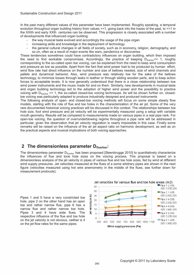
Sustainable Construction and Design 2011
Copyright © 2011 by Laboratory Soete
In the past many different values of this parameter have been implemented. Roughly speaking, a temporal evolution throughout organ building history from values <<1, going back into the hazes of the past, to >>1 in the XIXth and early XXth centuries can be observed. This progression is closely associated with a number of developments that influenced organ building:
the way musical taste evolved and accordingly the usage of the pipe organ
increasing skills and knowledge in the deployment of technology
the general cultural changes in all fields of society, such as in economy, religion, demography, and so on, often as a result of major events like wars, pandemics or discoveries
These tendencies sometimes could have contradictory influences on organ building, which then imposed the need to find workable compromises. Accordingly, the practice of keeping D flue/toe<< 1, roughly corresponding to the so-called open toe voicing, can be explained from the need to keep wind consumption and pressure as low as possible. Apart from the fact that wind power had to be produced by human effort, wind flow rate had direct influence on the number and size of bellows needed, size of wind channels and pallets and dynamical behavior. Also, wind pressure was relatively low for the sake of the bellows technology, to minimize losses through leaks in leather or through sliding wooden parts, and to keep action forces to acceptable levels. It is now generally understood that there is a close relationship between low wind power instruments and the music made for and on them. Similarly, new developments in musical taste and organ building technology led to the adoption of higher wind power and the possibility to practice voicing with D flue/toe
The following analysis of open- and closed-toe voicing methods will focus on some simple steady flow models, starting with the role of flue and toe holes in the characterization of the air jet. Some of the very rare documented historical voicing practices will be discussed in this context. The relationships between toe hole size, foot wind pressure and jet velocity will be experimentally measured using a setup with variable mouth geometry. Results will be compared to measurements made on various pipes in a real pipe rank. For open-toe voicing, the question of over/underblowing regime throughout a pipe rank will be addressed in particular, given the observation that jet velocity regulation is nearly impossible in this case. Finally some remarks will be raised on the influence of the air jet aspect ratio on harmonic development, as well as on the practical aspects and musical implications of both voicing approaches.
>> 1, the so-called closed-toe voicing techniques. As will be shown further on, closed-toe voicing was particularly adapted to produce industrially designed and produced instruments
2 The dimensionless parameter Dflue/toe
The dimensionless parameter D
:
flue/toe
has been proposed [Steenbrugge 2010] to quantitatively characterize the influences of flue and tone hole sizes on the voicing process. This proposal is based on a dimensionless analysis of the jet velocity in pipes of various flue and toe hole sizes, fed by wind at different wind supply pressures. Jet velocities measured at the flues of a some arbitrary pipes are shown in the next figure (velocities measured using hot wire anemometry in the middle of the flues, see further down for measurement protocols):
Pipes 1 and 5 have a very constricted toe hole, pipe 2 on the other hand has an open toe and rather narrow flue, pipe 6 has a narrow flue and rather narrow toe hole. Pipes 3 and 4 have wide flues. The respective influence of the flue and toe hole on the jet velocity is not obvious, neither is it on the jet flow rates for the same pipes:
285

Sustainable Construction and Design 2011
Copyright © 2011 by Laboratory Soete
It can be seen that the narrow flue open toe pipe 2 has about the same flow rate as the very wide flue narrow toe pipe 4.at all pressures. Pipes 1 and 5 have about the same flow rate despite widely differing flue widths. Obviously the possible values of flue and toe hole leave many possible combinations of jet velocity and flow rate, both of which have decisive influence on the operating regime of the pipe. Starting the dimensionless analysis now, the simplest possible dimensionless parameter that incorporates both flue and toe
holes is to consider the ratio of their surface area and try to establish a relationship with a dimensionless jet velocity, which is meaningfully obtained by dividing the measured velocities by a velocity that depends only on wind supply pressure, thus eliminating the influence of the latter. This reference velocity Vsupply
can only be:
where: Psupply
!"#!$%&!'"(!)&*#"$+!"*!,-./ is the wind supply pressure in Pa
3
The following figure shows the dimensionless jet velocity as a function of D flue/toe
for the same velocity measurements on the same pipes blown at the same wind supply pressures as above :
The observation that the dimensionless jet velocities seemingly collapse to one curve indicates that D flue/toe
is the single pipe parameter that completely determines the jet velocity in a flue pipe. In the next section a simple stationary model will be derived to quantitatively describe this behavior.
3 A simple stationary flow model:
For further reference a right-handed coordinate system is chosen with the origin in the middle of the flue edge at the inner side of the lower labium, the x-axis parallel to the pipe axis and positive x-values towards the upper labium.
0 1 2 3 4 5 6
0
0,2
0,4
0,6
0,8
1
1,2
Normalised jet velocities at various wind supply pressures (mmH2O) against Dflue/toe
All pipes
Dflue/hole
No
rma
lis
ed
je
t ve
locity
286

Sustainable Construction and Design 2011
Copyright © 2011 by Laboratory Soete
3.1 Jet velocity – Foot wind pressure relationship:
At the usual wind pressures in flue organ pipes the flow through the flue can be described by considering conservation of energy along a streamline, thereby assuming incompressible, inviscid, and laminar (Re based on flue width ~ 10
2-10
3
) conditions and neglecting possible height differences in the gravitational field. Given that the jet is brought to rest downstream of the flue, the following Bernoulli equation applies:
where: P foot
V is the jet velocity at the flue exit in m/s is the foot wind pressure in Pa
!"#!$%&!'"(!)&*#"$+!"*!,-./
3
When the jet leaves the flue and this flue consists of a 2D constriction with sharp edges, the jet velocity has a top-hat transversal profile which gradually starts to spread and turns into a so-called Bickley profile [Bickley 1937], the central velocity gradually diminishing in order to conserve jet momentum:
where: V0
b is the jet half-width given by: depends on the initial jet velocity V at the flue exit
where in turn: b0
depends on the initial jet velocity and the kinematic viscosity of air.
This theoretical profile for a laminar 2D jet is not valid near the flue as it assumes zero flue width. The direction of the jet is determined by the flue geometry.
3.2 Foot wind pressure – Wind chest pressure relationship:
When the toe hole of the pipe is severely constricted, in the sense that D flue/toe
> 1, the flow through the toe hole experiences a considerable static pressure drop. In a first approximation the toe hole can be modeled as an simple axisymmetric constriction between the wind chest pipe channel and the conical pipe foot. The pressure drop across such an orifice is very sensitive to diameter variations of the constriction but much less to the diameters of the in- and outlet ducts. A usual method to calculate static pressure drop across the constriction again starts from the Bernoulli equation and applies to the result a correction factor, the pressure discharge coefficient C, to take into account the incomplete pressure recovery due to the flow separation:
where: Px
V represents static pressure at point x
x
x=1 is downstream of the orifice and x=2 is at the orifice represents flow velocity at point x
287

Sustainable Construction and Design 2011
Copyright © 2011 by Laboratory Soete
The flow rate Q through the orifice is:
Q= V 1 A1= V 2 A2 where: Ax
represents the surface area of the duct at point x
0%&!#$'$"1!2(&##3(&!)(42!'1(4##!$%&!4("5"1&!67!1'*!$%3#8!"*193)"*-!$%&!14((&1$"4*!)"#1%'(-&!14&55"1"&*$!:8!;&!written as:
where: <!=!A2/A
1
C can be experimentally determined or analytical fitting formulae are available in the literature [Idelchik 1984]. For a circular axisymmetric straight-14(*&(&)! 14*#$("1$"4*! "*! '! 1"(139'(! )31$!>"$%!<??@8! "$#! A'93&! "#!about 0.6 – 0.62.
3.3 Jet velocity dependence on Dflue/toe
:4/;"*"*-!BC#D!@!'*)!E8!'*)!'##3/"*-!<!??!@8!$%&!F&$!A&941"$+!1'*!;&!1'9139'$&)!'#!'!53*1$"4*!45!G
:
flue/toe
:
where: Psupply
is the wind supply pressure in Pa
In the case of extreme toe hole constriction the jet velocity formula will be approximately:
which means that V will monotonously decrease with increasing flue width for any given toe hole size. At the same time however the flow rate, which after all is what provides the necessary driving energy, monotonously rises to a limit value determined by the toe hole size. When the flue width is kept constant, an increase of toe hole diameter obviously leads to a monotonous increase, up to a limit value determined by the wind supply pressure, of both jet velocity and flow rate. This can be summarized in the following design considerations for the flue and toe hole size, assuming that any change in flue size does not influence jet orientation: - for any given toe hole area and wind supply pressure, increasing the flue area decreases the jet velocity but increases the jet flow rate - for closed-toe voicing the flue size has to be large enough that adequate jet velocity regulation is possible with the toe hole and Eq. 5 is valid, say D flue/toe
- Eq. 4 proves that the jet velocity depends only on D
> 3C, which means that the flue area must be at least twice the toe area.
flue/toe
and not on the flue and toe hole areas independently.
In practice a number of voicing families can be distinguished based on D flue/hole
D
:
flue/toe >> 1: what Fisk called 'classical voicing' [Fisk 1976] involves, among other ingredients, a wide open flue and power regulation using the toe hole size. In this method the jet velocity varies along with the regulation, requiring active cut-up adjustments to stabilize operating point.
288

Sustainable Construction and Design 2011
Copyright © 2011 by Laboratory Soete
D flue/toe
D
<< 1: describes the open-toe voicing methods, were jet velocity is kept relatively constant during voicing. So in principle driving power can be regulated by adjusting flue width without influencing the operating point. However, the jet velocity profile is modified in sharpness and possibly in orientation, influencing pipe speech and timbre.
flue/toe ~ 1: in this region both flue and toe hole are adjusted in such a way that D flue/toe
varies less than the previous methods, thus somewhat avoiding their inconveniences. However this method requires fine fitting of both parameters. This method was practiced by classical late Baroque builders such as Gottfried Silbermann, in later periods the method was adopted by Schulze in the XIXth century, who used it with very large areas at relatively low wind supply pressures, leading to his typical impressive flue plena.
4 Experiments:
In this section the model discussed so far to describe open- and closed-toe voicing will be verified through jet velocity and foot pressure measurements on real pipes and an experimental pipe setup which allows continuous and precise adjustment of the voicing parameters involved.
4.1 Method:
Jet velocities were measured using Constant Temperature Anemometry (CTA), allowing to measure air velocity magnitudes with very high spatial resolution in a plane perpendicular to the wire of a hot wire probe. Accordingly, the measurement plane was the y=0 plane. This wire, made of platinum coated tungsten, is 5µm in diameter and 1.5mm long, and is welded to 2 needle-shaped supporting prongs which also supply the heating current. The following picture shows the hot wire next to a human hair at 50x magnification: The probe is mounted on a x-z traverse mechanism which allows the hot wire to reach any position in the measurement plane, movement step size is 30µm. It is not possible to measure velocity directions with this single hot wire probe, but from a measured velocity magnitudes field, assumed 2D, and using mass conservation considerations, velocity vectors could be calculated. The experimental pipe set-up used will not be described in detail here, suffice it to say that the experimental pipes, through their specific geometry, allow continuous and precise step-motor controlled adjustment of toe hole area, flue width, cut-up and upper labium offset (by movement of the resonator along the z-axis). Step sizes are 30µm. The wind is supplied by a wind chest with adjustable pressure and electromagnet controlled pallets. The flue geometry is formed by a straight-cornered lower labium and a sharp edged nickless languid 3mm thick and with a 66° bevel. The languid and the lower labium edge, defining the flue exit, are both located in the x=0 plane and at all times parallel to each other (+/- 50µm). Calibration of each probe is done by a calibrating wind tunnel, which produces a low turbulence air jet. The probe is mounted into the jet at the exit from the tunnel, a range of jet velocities corresponding to the measuring range is successively generated and the static pressure inside the stagnation chamber of the wind tunnel measured. The non-linear correspondence between the air velocity and the hot wire heating power is, in CTA, given by King's law:
where: E is the voltage at the CTA bridge U is the air jet velocity A and B are constants to be determined in the calibration x is a value between 0.45 and 0.5, to be determined in the calibration The figure on the right shows a typical calibration curve. At low but non-zero velocities the simple calibration procedure described above is no longer accurate enough, King's law however remains valid.
289
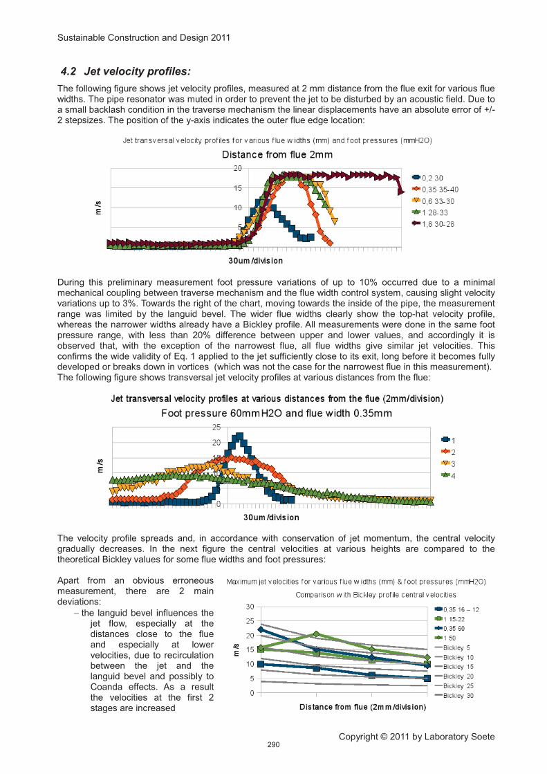
Sustainable Construction and Design 2011
Copyright © 2011 by Laboratory Soete
4.2 Jet velocity profiles:
The following figure shows jet velocity profiles, measured at 2 mm distance from the flue exit for various flue widths. The pipe resonator was muted in order to prevent the jet to be disturbed by an acoustic field. Due to a small backlash condition in the traverse mechanism the linear displacements have an absolute error of +/- 2 stepsizes. The position of the y-axis indicates the outer flue edge location:
During this preliminary measurement foot pressure variations of up to 10% occurred due to a minimal mechanical coupling between traverse mechanism and the flue width control system, causing slight velocity variations up to 3%. Towards the right of the chart, moving towards the inside of the pipe, the measurement range was limited by the languid bevel. The wider flue widths clearly show the top-hat velocity profile, whereas the narrower widths already have a Bickley profile. All measurements were done in the same foot pressure range, with less than 20% difference between upper and lower values, and accordingly it is observed that, with the exception of the narrowest flue, all flue widths give similar jet velocities. This confirms the wide validity of Eq. 1 applied to the jet sufficiently close to its exit, long before it becomes fully developed or breaks down in vortices (which was not the case for the narrowest flue in this measurement). The following figure shows transversal jet velocity profiles at various distances from the flue:
The velocity profile spreads and, in accordance with conservation of jet momentum, the central velocity gradually decreases. In the next figure the central velocities at various heights are compared to the theoretical Bickley values for some flue widths and foot pressures: Apart from an obvious erroneous measurement, there are 2 main deviations:
the languid bevel influences the jet flow, especially at the distances close to the flue and especially at lower velocities, due to recirculation between the jet and the languid bevel and possibly to Coanda effects. As a result the velocities at the first 2 stages are increased
290

Sustainable Construction and Design 2011
Copyright © 2011 by Laboratory Soete
at higher pressures the velocity decreases more rapidly than the Bickley law, possibly due to the jet flow going fully turbulent.
The next figure shows jet transversal velocities for various foot pressures:
By following the locus of maximum measured jet velocity with increasing distance from the flue, it is possible to somehow reconstruct the jet trajectory. These locii are thus taken as the centerline of the jet, as shown in the following figure: The general conclusion to be drawn from this figure is that the jet flow direction, in the geometry used for these measurements, is rather insensitive to either pressure variations or, surprisingly, to flue width variations.
4.3 Pressure drop measurements across the toe hole:
The differential pressure between static wind supply and foot pressures was measured in an experimental pipe for various toe hole diameters and corresponding flow rates. The flow rates were calculated from the simultaneous measurement of the air jet velocity. The following figure shows the pressure drop as a function of toe hole diameter at a constant wind supply pressure of 950 Pa, a flue width of 0.35mm and length of 0,04m. In the same figure the pressure drops calculated from Eq.3 are shown:
The correspondence between measured and 1'9139'$&)! A'93&#! )(42#! )4>*! 54(! 94>! <! A'93&#!where the toe hole no longer behaves like a simple straight-cornered orifice.
291

Sustainable Construction and Design 2011
Copyright © 2011 by Laboratory Soete
4.4 Jet velocity measurements for varying toe hole diameter:
Eq. 4 can be experimentally verified using any flue pipe on condition the toe hole geometry sufficiently approximates an axisymmetric straight-cornered orifice. The figure to the right shows jet velocities corresponding to the measuring points from the previous figure: Next, a large series of velocity measurements was done on an experimental pipe with automatically controlled step-wise change of flue width and toe hole areas, and wind supply pressure as the third parameter. All these parameters were varied over a range encompassing all possible situations in flue pipes. The next figure shows all velocities obtained, normalized using the corresponding pressures, as a function of the corresponding D flue/toe
:
Again the collapse of the normalized velocities shows a dependence of the jet velocity on D flue/toe
only. Deviations are mainly attributed to variations in C for different toe hole areas due to the specific construction of the variable toe hole.
4.5 Jet velocities and cut-up in a closed-toe voiced pipe rank:
It's interesting to calculate the mouth transit time parameter Dmouth
check whether the jet velocity calculation yields realistic values
in real closed-toe voiced pipe ranks using measured jet velocities, in order to:
determine whether the way flue and toe hole are voiced so as to be consistent with the cut-up and the corresponding voicing determinant Dmouth
Dmouth
=fl
V
, defined as:
where: f is the fundamental frequency of the sounding pipe l is the cut-up The following data are measured on a rank of principal pipes [Steenbrugge 2005]:
292

Sustainable Construction and Design 2011
Copyright © 2011 by Laboratory Soete
The figure to the right shows the calculated Dmouth
values for this rank, blown with 850Pa wind pressure:
These are normal values for Dmouth, lying around 1/8, with a normal tendency to rise due to the fact that the cut-up, as can be seen in the table, does not scale like f
-1 but scales with the
diameter and thus becomes relatively high in the treble. D flue/toe thus generates realistic values for Dmouth
, although some irregularities remain in its progression throughout the range. Experimental verification of the actual jet velocities is not yet available for this pipe rank.
5 The open-toe voicing problem:
In open-toe voicing the air jet's aspect ratio is the only variable in the air jet wind supply that can be controlled allowing -by a changing flow rate- to adjust the power supplied to the pipe. However, besides providing this pneumatic power, the air jet, through its aerodynamic properties, also serves to build and maintain the feedback loop necessary for oscillation and these influences are necessarily modified at the same time.
5.1 Cut-up:
In contrast to closed-toe voicing, the previous experiments lead to the hypothesis that in open-toe voicing jet velocities are essentially constant throughout the pipe rank. As the jet transfer time to oscillation period parameter Dmouth is bound to certain limits in order to allow self-sustained oscillation, this would imply that l necessarily scales like f
-1, although in usual practice l is always considered to be a constant fraction, around
1/4 of mouth width (see for example the data of the pipe rank studied above), itself being a constant fraction of the pipe diameter (ibidem), which scales like f
-x
5.2 Jet orientation:
, with x approximately equal to ¾. This raises the question whether in practice open-toe voicing is rigorously applied throughout a complete pipe rank with a frequency range of at least 4 octaves (that is with all foot pressures equal).
In the case of metal pipes and wooden pipes without a flue channel, the jet orientation depends on minor variations in the flue geometry, essentially the relative position and shape of the two edges defining the flue. Changing the relative position of both in the direction parallel to the jet flow direction, or in other words, changing the direction of the flue exit surface (normally a plane if the edges are parallel), may alter the jet orientation. If the flue width is changed in such a way that this flue exit surface is reoriented, the jet direction can change.
5.3 Jet velocity profile:
As observed in the previously mentioned jet velocity profile measurements, changing the flue width at the flue exit changes the velocity profile width all along the jet. This influences the way the jet drives the resonator modes, as illustrated in the next figure [after Fletcher&Rossing 1998], which shows the jet flow
C
G
c 8,50 6,80 1,67 11,00 1,10
g 6,10 5,10 1,24 7,70 1,00
5,35 4,13 1,00 7,00 0,90
4,23 3,25 0,73 6,10 0,80
3,53 2,70 0,67 5,60 0,80
2,72 2,10 0,53 5,20 0,75
2,30 1,70 0,37 4,10 0,70
1,72 1,30 0,31 4,00 0,60
Montre 8’
Diameter (cm)
Flue length (cm)
Cut-up (cm)
Toe hole diameter (mm)
Flue width (mm)
c1
g1
c2
g2
c3
g3
293

Sustainable Construction and Design 2011
Copyright © 2011 by Laboratory Soete
rate U j
into the resonator as a function of jet deflection h -in the z-direction- at the upper lip:
In the figure h0 is the upper lip offset from the jet symmetry plane at the upper lip height, and b the jet half-width. The interrupted broken curve shows
the flow rate in the hypothetical case of a top-hat velocity profile, the jet width 2b is the distance between the abscissa of the breaks in the curve. It can be deduced that the smaller b, the more the flow rate will have a square wave appearance in time, and thus strongly drive the harmonic modes because most of the time it will be saturated to one of the edge sides. The asymmetry resulting from the upper lip offset h0 also determines the proportion in which the various harmonic modes will be driven. The influence of both b and h0 on harmonic drive is summarized in the figure on the left [Fletcher&Douglass 1980], were the calculated relative amplitudes of the first 3 harmonics are plotted as a function of b/h0
.
Experiments are currently under way to find answers to the following issues regarding open-toe voicing:: 1. Jet velocity – cut-up relationship in open-toe voiced pipe rank: In order to characterize an existing open-toe voiced pipe rank, jet velocities and a number of scales -diameter and cut-up- will be measured. As in the previously discussed closed-toe case, specific attention will be given to the progression of Dmouth throughout the rank. It is possible that jet orientation plays an important role in this way of voicing, in that a very precise adjustment of the jet flow angle might allow the pipe to establish the feedback loop at a lower velocity than the central jet velocity, thus avoiding the pipe to overblow right from the start and thus in fact extending the range of Dmouth
2. Jet orientation dependence on flue width: within stable speech is possible.
More experiments with various flue geometries must be done in order to assess their impact on the jet orientation. The preliminary transversal jet velocity measurements presented and discussed higher however seem to indicate that jet orientation is not particularly sensitive to flue width for the most usual geometries. This point needs more specific experimental setups to be exhaustively tested. 3. Jet harmonic drive dependence on flue width: Following the theoretical outline given above experiments will be done to establish links between jet velocity profiles, jet flow rates and acoustic output.
6 Discussion and conclusion:
The relevance of the D flue/toe
Closed-toe voicing can be considered as an easier method than open-toe voicing because it offers more degrees of freedom, allowing to control various aspects of the air jet. A certain amount of pressure loss at the toe hole has to be taken for granted and wide flues can generate unfavorable sizzling sounds which are minimized by nicking the languid. Due to a somewhat wider air jet the sound is usually rounder. The availability of more degrees of freedom allows to specialize one for power regulation (the toe hole) and another for the timbre (the flue). The latter can be set in the factory during the so-called pre-voicing, the former can be adjusted in situ when establishing the tonal balance, with possibly minor cut-up modifications. Open-toe voicing involves adjusting the air jet with control parameters that strongly influence each other. Therefore it can only be performed on site and in a carefully deployed process requiring delicate and patient manipulation. The result can be a genuine lively and more or less irregular sound giving every
voicing determinant was established through dimensionless analysis and through the construction of a simple stationary flow model were it plays a central role in determining the jet velocity. This determinant allows to characterize a number of voicing methods involving flue width and toe hole size. It was shown however that each of these methods has specific implications on other voicing parameters: closed-toe voicing involves active adjustment of the cut-up, whereas open-toe voicing is expected to require very precise languid control in order to allow stable speech.
294

Sustainable Construction and Design 2011
Copyright © 2011 by Laboratory Soete
pipe a strong individuality of its own. As stipulated above, further experimental work will be done to verify the open-toe voicing hypotheses made. Furthermore extensive measurements will be done on existing pipe ranks to test the robustness of D flue/toe
as a tool to quantitatively describe flue width and toe hole voicing.
7 References: [Idelchik 1984] Idelchik, I.E., Handbook of Hydraulic Resistance, Third Edition, 2001. [Fletcher&Douglass 1980] Fletcher, N.H. & Douglass, L.M., Harmonic generation in organ pipes, recorders and flutes, J. Acoust. Soc. Am. 60, 926-936, 1980. [Fletcher&Rossing 1998] Fletcher N.H. & Rossing T., The Physics of Musical Instruments, Springer 1998 [Fisk 1976] Fisk, C., Articulateness and the Organ: A problem for the Organ Builder, Lecture given at the dedication of the Flentrop Organ, Duke University, November 1976 [Bickley 1937] Bickley, W.G., The plane jet, Phil. Mag. 28, 727-731, 1937 [Steenbrugge 2005] Steenbrugge, D., Het Pierre Schyven orgel in de Gentse Sint-Annakerk, Orgelkunst, IV 2005. [Steenbrugge 2010] Steenbrugge, D., Flow acoustical determinants of historic flue organ pipe voicing practices, Proceedings of the International Symposium of Musical Acoustics, Sydney, August 2010.
295

Sustainable Construction and Design 2011
Copyright © 2011 by Laboratory Soete
DESIGN OF CRACK ARRESTORS FOR
ULTRA HIGH GRADE GAS TRANSMISSION PIPELINES
MATERIAL SELECTION, TESTING AND MODELLING
F. Van den Abeele1 and M. Di Biagio2
1 OCAS N.V., J.F. Kennedylaan 3, 9060 Zelzate, Belgium
2
Abstract
Centro Sviluppo Materiali, Rome, Italy
One of the major challenges in the design of ultra high grade (X100) gas pipelines is the identification of a reliable crack propagation strategy. Recent research results have shown that the newly developed high strength and large diameter gas pipelines, when operated at severe conditions, may not be able to arrest a running ductile crack through pipe material properties. Hence, the use of crack arrestors is required in the design of safe and reliable pipeline systems.
A conventional crack arrestor can be a high toughness pipe insert, or a local joint with higher wall thickness. According to experimental results of full-scale burst tests, composite crack arrestors are one of the most promising technologies. Such crack arrestors are made of fibre reinforced plastics which provide the pipe with an additional hoop constraint. In this paper, the material selection, testing and modelling for the design of composite crack arrestors is presented.
First, an overview of the most commonly used (integral and non-integral) crack arrestors is given, indicating that fibre reinforced devices are one the most promising solutions to arrest running fractures. Then, material characterization of unidirectional fibre glass reinforced epoxy is addressed to measure the orthotropic properties of this composite material. Traditional mechanical characterization is compared with a non destructive testing method to measure the elastic constants of the composite material. In the end, micromechanics of fibre reinforced plastics is applied to predict the material properties. The theoretical predictions are compared with experimental values.
In an accompanying paper, numerical tools to simulate crack initiation, propagation and arrest for this type of crack arrestors are introduced. The combination of numerical simulation and experimental research allows deriving design guidelines for composite crack arrestors.
Keywords crack arrestors, toughness modelling, pipeline materials, fibre reinforced plastics, integrity
1 PIPELINE INTEGRITY: A TOUGH CHALLENGE
The occurrence of a longitudinal crack propagating along a gas pipeline is a catastrophic event, which involves both economic losses and environmental damage. Hence, the fracture propagation control is an essential strategy to ensure pipeline integrity. Fracture control is a tough task, since it requires knowledge of the interaction between the dynamic forces driving crack growth, and the resistance forces opposing fracture propagation.
Ductile fracture is typically characterized by wide crack flanks opening, relevant bulging at the crack tip and a large amount of plastic deformation in the vicinity of the flaps. Brittle fracture, on the other hand, is mainly driven by the amount of elastic energy stored in the pipe wall, while only a small amount of plastic deformation occurs near the crack tip. In addition, the elastic surface energy is rate dependent at the typical velocities of brittle fracture, which imposes another level of complexity.
The fashion of crack propagation (brittle or ductile) influences the rupture length. The energy required for brittle fracture propagation is low, which makes it very difficult to control brittle fracture once crack initiation has occurred. On the other hand, ductile fracture propagation requires a large amount of energy, and can be arrested in a controlled manner. However, mixed fracture propagation mechanisms may also occur, depending on the operation conditions and temperature. For instance, typical pipeline steels used in arctic regions exhibit an intermediate behaviour between brittle and ductile fracture.
296

Sustainable Construction and Design 2011
Copyright © 2011 by Laboratory Soete
The distinction between ductile and brittle fracture propagation is particularly relevant for gas pipelines, for which the decompression of the gas during failure is an important driving force. Experimental burst tests [1] reveal that the typical crack speed during ductile fracture propagation in steel pipelines does not exceed 350 m/s. Since the acoustic velocity of gas (such as lean gas or rich methane) under the usual operation conditions is in the range of 350 – 500 m/s, the decompression of the pipe is faster than the crack speed. This implies that the local pressure in the vicinity of the crack tip is lower than the initial (operating) pressure, and decreases with decreasing crack speed. On the contrary, the crack speed during brittle fracture is equal to or higher than the acoustic velocity of the gas, so the crack tip experiences the full initial pressure as it propagates, and the resulting driving force is much more severe.
While brittle fracture control is typically achieved by ensuring that the pipeline is operated well above the Ductile to Brittle Transition Temperature, the ductile fracture propagation can be avoided (or at least limited) by increasing the minimum specified toughness of the pipeline steel. However, for ultra high pipeline grades
( X100), the identification of a reliable crack propagation strategy is not longer straightforward. Indeed, despite excellent toughness values at lab scale (Charpy upper shelf energy and Battelle shear fracture area), one can no longer rely on pipe body arrest [1-3]. As a result, additional mechanical devices such as crack arrestors have to be mounted on the pipeline in order to stop a running ductile crack.
2 REVIEW ON CRACK ARRESTORS FOR HIGH PRESSURE GAS PIPELINES
Although a clear distinction can be difficult, crack arrestors are usually classified as either integral or non-integral, according to their installation procedure. Integral crack arrestors are inserted in the pipeline, and act as an integral part of the system, while non-integral crack arrestors are made of several parts, assembled externally onto the pipe. In this section, the most commonly used crack arrestors for high pressure gas pipelines are reviewed.
2.1 Integral crack arrestors
Integral crack arrestors are generally made of pipes and/or rings with mechanical or geometric properties different from those of the main line. The aim to arrest a running fracture can be achieved by
! increasing fracture resistance (e.g. lengths of higher toughness line pipe)
! decreasing relative driving force (e.g. lengths of heavier wall pipe)
! inducing ring-off (e.g. lengths with weaker spiral seam weld)
Inserting lengths of high toughness pipe with the same wall thickness as the main pipeline, like schematically shown on Figure 1, is one of the most simple and straightforward forms of integral crack arrestors.
Figure 1: Inserting high toughness pipe as integral crack arrestor
In order to assure a good effectiveness of the crack arrestor, the decrease of the crack speed has to be sufficiently high to achieve arrest within the crack arrestor, which requires fracture resistant properties (much) higher than the main pipe. If the toughness of the insert is not adequate, the crack may exit from the arrestor and propagate further down the line. Moreover, since ductile fracture propagation could initiate at any location (e.g. in a remote pipe, but also in a pipe adjacent to the crack arrestor), the device should be capable to cope with the adverse event of a crack initiating nearby, where the crack driving force (governed by the initial pressure) is higher than under steady state conditions.
297

Sustainable Construction and Design 2011
Copyright © 2011 by Laboratory Soete
Heavy wall pipe inserts used as crack arrestors, like shown on Figure 2, are somewhat similar to the high toughness pipe inserts described above. The arrest concept involves a hoop stress reduction in the thicker pipe that has sufficient toughness to cause fracture arrest within the specified crack arrestor length. The required toughness should promote arrest in about half the length of the crack arrestor.
Typically, such a pipe would be manufactured to controlled outer diameter (OD) tolerances, with the excess wall thickness on the inside. However, a pipe with a constant inner diameter (ID) with excess wall thickness at the OD can also be produced, solving possible problems associated with in line inspection and fluid dynamics.
Figure 2: Heavy wall pipe inserts
Other integral devices consist of layered pipe lengths with helical mid-layer slits or notches, which deviate the crack path and dissipate crack propagation energy. Inserts with weaker spiral seam weld or brittle girth welds can be used [4] to induce pipe ring-off. New, but less proven, crack arrestors consist of short inserts of girth welded sections with alternating brittle and high toughness segments, to divide the propagation energy into multiple cracks that run through the brittle sections, but lack the axial orientation and energy to re-initiate in the high toughness segments.
Recently, a Composite Reinforced Linepipe (CRLP) system has been developed from the patented glass fibre reinforced resin technology of NCF industries [5]. The CRLP system consists of E-glass fibres drawn through an iso-polyester resin, and wound round the external surface of the main steel pipe. The wall thickness of the pipe is reduced to approximately half of the thickness required by conventional design codes, and the reinforcement is applied and auto-frettaged during hydrotesting. As a result, the steel pipe is under compression and the composite material is under tensile stress in the hoop direction, prior to pressurizing the whole line. The CRLP system is designed to be operated at pressure values that correspond to less than 40% of the ultimate strength of the composite to ensure long-term durability.
Pipe manufacturers have designed their own composite crack arrestors, based on similar concepts. Europipe, for instance, used the composite crack arrestor shown on Figure 3 (40 mm by 2 meter) on a 36” pipe that was used in the Demopipe full-scale burst test [6].
In general, integral crack arrestors (particularly composite arrestors and those obtained from pipes with greater thickness and/or toughness) have the advantage of easier assembly during the pipeline field construction, although they are more difficult to use on already existing lines. A possible alternative is the use of a composite crack arrestor wrapped around the pipe with an imposed pre-stress. This would permit to increase the crack arrestor bearing capacity under the same wall thickness, hence giving a higher effectiveness in arresting a propagating crack.
298

Sustainable Construction and Design 2011
Copyright © 2011 by Laboratory Soete
Figure 3: Composite crack arrestor used in the Demopipe project
2.2 Non-integral crack arrestors
The competitive advantage of non-integral crack arrestors is the capability of being assembled externally to the pipeline. Hence, they are recognized as particularly adequate for intervention on already existing pipelines, since no considerable operative shutdown or large interventions are required.
As early attempts for developing external crack arrestors, several devices of similar design have been conceived, including multi-strand wire ropes, single strands of small diameter (~ ¼”) wire, or rod that is wrapped around a pipeline to restrain the pipe deformation and flap opening associated with a running ductile fracture. The latter one, shown on Figure 4, can consist of one or more rods and has also been described as a toroidal crack arrestor [7]. Steel rope and steel thread crack arrestors are realized by winding a steel rope or thread around a portion of the pipeline. Steel rope devices, like shown on Figure 4, have been patented since the seventies by CSM [8].
Toroidal crack arrestor [9] Steel rope crack arrestor [8]
Figure 4: Examples of different external crack arrestors
Various types of weights (like lead, concrete, etc) have been proposed [10] as they increase the restraining force of the flap opening associated with a ductile fracture propagation by adding mass to the pipe wall. Although some of them were successfully tested, they do not offer a practical approach and have never gained wide application in service.
Cast iron clamps have been suggested [11] as a ductile fracture control method as well. These clamps are bolted around the main pipe like indicated on Figure 5, and supply the line with a constraint to the deformation associated with a running ductile fracture. As these devices are exposed to soil conditions, they may suffer from accelerated corrosion, which triggers the need for coating and long term protection.
299

Sustainable Construction and Design 2011
Copyright © 2011 by Laboratory Soete
Figure 5: Cast iron clamps as crack arrestor [11]
The most acknowledged and commonly used non-integral arrestors are steel sleeve crack arrestors and Clock Spring. Steel sleeve crack arrestors, shown on Figure 6, are classified as
! Tight sleeves, which are placed around the main linepipe with a close-fitting connection. Since no gap is allowed between the pipe and the arrestor, their installation is not straightforward.
! Loose sleeves and grouted sleeves, which have a radial clearance with respect to the pipe. For grouted sleeves, the gap is filled by cement mortar or epoxy resin.
Tight sleeve Loose sleeve Grouted Sleeve
Figure 6: Classification of steel sleeve crack arrestors
Clock Springs, developed and patented by NCF Industries [12], consist of wound ribbons made of fibre glass dipped in a resin matrix. Such ribbons are wound around the pipe, and their clamping is ensured by an elastic spring-back component, like shown on Figure 7. Thanks to the ease of transportation and assembly on existing pipelines, Clock Springs are especially suitable as repair systems and crack stoppers. Moreover, since their application does not require an interruption in the pipeline service, they offer an adequate solution for those cases where operative pressure reduction is not feasible or allowable [13].
Figure 7: ClockSpring crack arrestor (1: composite coil, 2: adhesive and 3: filler)
300

Sustainable Construction and Design 2011
Copyright © 2011 by Laboratory Soete
2.3 Design criteria for crack arrestors
Given the wide variety of crack arrestor typologies, geometries and properties, no single set of design guidelines can be developed to account for every crack arrestor. Moreover, no design criteria exist and only very limited experimental data is available for crack arrestors designed to deviate running cracks into a helical path. As a result, this type of crack arrestors is not frequently used in the industry.
The design of integral crack arrestors mainly consists in defining the adequate wall thickness, length and/or toughness values to assure fracture arrest. Since integral devices act within the line, their design can be achieved by using similar predictive tools normally used to outline the ductile fracture propagation control of the main pipe, e.g. the Charpy based Battelle Two Curve method [14-15].
For non-integral crack arrestors, design guidelines have been proposed by the Pipeline Research Council International PRCI [7]. In addition, an alternative approach has been proposed by Leis [16].
Today, numerical methods like finite element analysis are commonly used in the design of crack arrestors [2]. In [17-18], a combined numerical/experimental approach is presented to design composite crack arrestors.
First, micromechanics of fibre reinforced plastics is applied to predict the properties of the composite material. The micromechanical predictions are compared with experimental values. Then, orthotropic failure measures are introduced to describe the onset of material failure under complex loading patterns. In addition, the in-use behaviour of composite crack arrestors is evaluated by means of large scale tensile tests and four point bending experiments. In the end, computational fracture mechanics is applied to simulate crack propagation and arrest. The combination of numerical simulation and experimental research allows deriving design guidelines for composite crack arrestors.
3 COMPOSITE MATERIAL MODELLING AND EXPERIMENTAL VALIDATION
For this investigation, a composite crack arrestor made out of unidirectional glass fibre reinforced epoxy was selected as the best compromise between mechanical performance and cost considerations. For such fibre reinforced plastics, the material properties depend on the fibre orientation. The most commonly used composites are orthotropic materials, requiring 9 independent elastic constants to define the compliance matrix. When unidirectional (UD) glass fibre reinforced epoxy is used, the constitutive law reduces to transverse isotropy, where only 5 constants are to be determined to build the stiffness matrix [19]. In this section, the properties of the composite material under study are determined by means of traditional mechanical characterization, non destructive testing and micromechanical modelling.
3.1 Mechanical characterization
Due to the orthotropic nature of unidirectional glass fibre reinforced epoxy, the elastic properties of this composite material are not straightforward to measure. An extensive testing program has been completed to characterize the composite material by means of tensile tests, compression tests and rail shear tests. This experimental program is documented in detail in [20], and the results are summarized in Table 1.
Table 1: Orthotropic properties of unidirectional glass fibre reinforced epoxy
1
TE
36.4 GPa
2
TE
8.5 GPa
1
CE
35 GPa
2
CE
6.5 GPa
TX
700 MPa
TY
7.2 MPa
CX
588 MPa
CY
42 MPa
12G
3 335 MPa
S
30.1 MPa
R 30.1 MPa
301

Sustainable Construction and Design 2011
Copyright © 2011 by Laboratory Soete
3.2 Non destructive testing
The in-plane elastic properties {E1, E2, "12, G12
Figure 8 shows a typical Frequency Response Function (FRF). Such a signal is a frequency domain function expressing the ratio between the response signal (output) and the reference signal (input). The peaks in the FRF indicate that low input levels correspond to high response levels, which reveals resonance frequencies. The corresponding mode shapes (torsion, saddle and breathing) are shown as well.
} can be determined by a dynamic modulus identification using resonant frequencies [21]. Both the determination of the real part (elastic constants) and the imaginary part (damping behaviour) are based on the measurement of the vibrational response of a rectangular test plate, submitted to a controlled excitation. A test plate is suspended on a frame with elastic threads, simulating completely free boundary conditions. The plate is then excited by an impulse with a hammer. The vibration amplitude of the plate as a function of time is monitored by the data acquisition system. The resonance frequencies of the plate in the band of interest are detected by taking the Fast Fourier Transform (FFT) of the signal. Then, a sinusoidal signal with a frequency coinciding with each resonance frequency is sent to a loudspeaker, acoustically exciting the test plate. The decay of the signal allows extracting the modal damping ratios and the mode shapes associated with the resonance frequencies.
Figure 8: Measured frequency response function and mode shapes
The measured frequencies are compared with the computed resonance frequencies of a numerical parameter model of the test plate. The parameters in the model are the unknown elastic properties. Starting from an initial guess, the parameters of the numerical model are tuned until the computed resonant frequencies match the measured ones. This tuning technique is a Bayesian parameter estimation method, based on the sensitivities of the resonant frequencies for parameter changes. The obtained elastic material properties are homogenised over the plate surface, and hence suitable as averaged input values in finite element models for composite structures like crack arrestors.
Table 2: Comparison between mechanical and non destructive testing
TRADITIONAL NON DESTRUCTIVE
E [MPa] 1 36 400 44 200
E [MPa] 2 8 500 11 400
G [MPa] 12 3 335 4 420
" [-] 12 0.32 0.356
302

Sustainable Construction and Design 2011
Copyright © 2011 by Laboratory Soete
The non destructive testing (NDT) methodology is described in [22], and the results of the NDT experiments are compared with the values measured in the traditional mechanical tests in Table 2. The tensile test results yield stiffness values which are considerably lower than the non destructive test results. The rail shear test gives a rather low value for the shear modulus as well. The NDT method tends to over-estimate the values measured in the traditional experiments. Indeed, non destructive testing will typically give higher stiffness values because
! It allows measuring the virgin material properties. When performing traditional mechanical testing, sample preparation can already induce microscopic damage, leading to a lower stiffness and strength. Moreover, the effects of slip are avoided when performing NDT, again resulting in higher (and more accurate) estimates for the elastic constants.
! It measures the global (homogenized) properties of a composite structure, rather than the local stiffness of a small specimen, which can exhibit quite some scatter. Hence, the NDT results are recommended as input values for finite element simulations of crack arrestors.
3.3 Micromechanical modelling
Micromechanical models are used to calculate the elastic constants of composite materials, based on the properties of the (glass) fibre and the (epoxy) matrix. The properties of the constituents, and their volume fraction, are listed in Table 3.
Table 3: Properties of the glass fibre and the epoxy resin
E-GLASS FIBRE EPOXY RESIN
Stiffness E f E = 74 GPa m
Poisson
= 3.5 GPa
" f " = 0.3 m
Density
= 0.35
#f # = 2 555 kg/m³ m
Tensile strength
= 1 175 kg/m³
X f X = 3.45 GPa m
Volume fraction
= 60 MPa
V f V = 0.6 m
= 0.4
A detailed review of micromechanical mixture rules for fibre reinforced plastics was presented in [23]. The results of those calculations are summarized in Table 4. While the Voigt rules of mixtures are generally accepted [24] as a good approximation of the longitudinal stiffness E1 and the Poisson
coefficient "12, the Reuss series model provides merely a lower bound for the transverse modulus E2 and the shear modulus G12. Tsai [25] predicts a very high value for the shear modulus G12
Table 4: Micromechanics of unidirectional reinforced laminates
.
E1 E [GPa]
2 " [GPa]
12 " [-]
23 G [-]
12 G [GPa]
23
Voigt-Reuss
[GPa]
45.8 8.17 0.32 3.033
Puck-Foye 45.8 14.86 0.32 0.389 5.497 5.349
Greszczuck 45.8 13.2 0.32 0.389 5.960 4.750
Hashin 45.8 13.5 0.317 0.343 4.436 5.027
Tsai 45.8 14.66 0.313 0.389 7.956 5.274
Halpin-Tsai 45.8 14.98 0.32 0.319 4.436 5.677
303
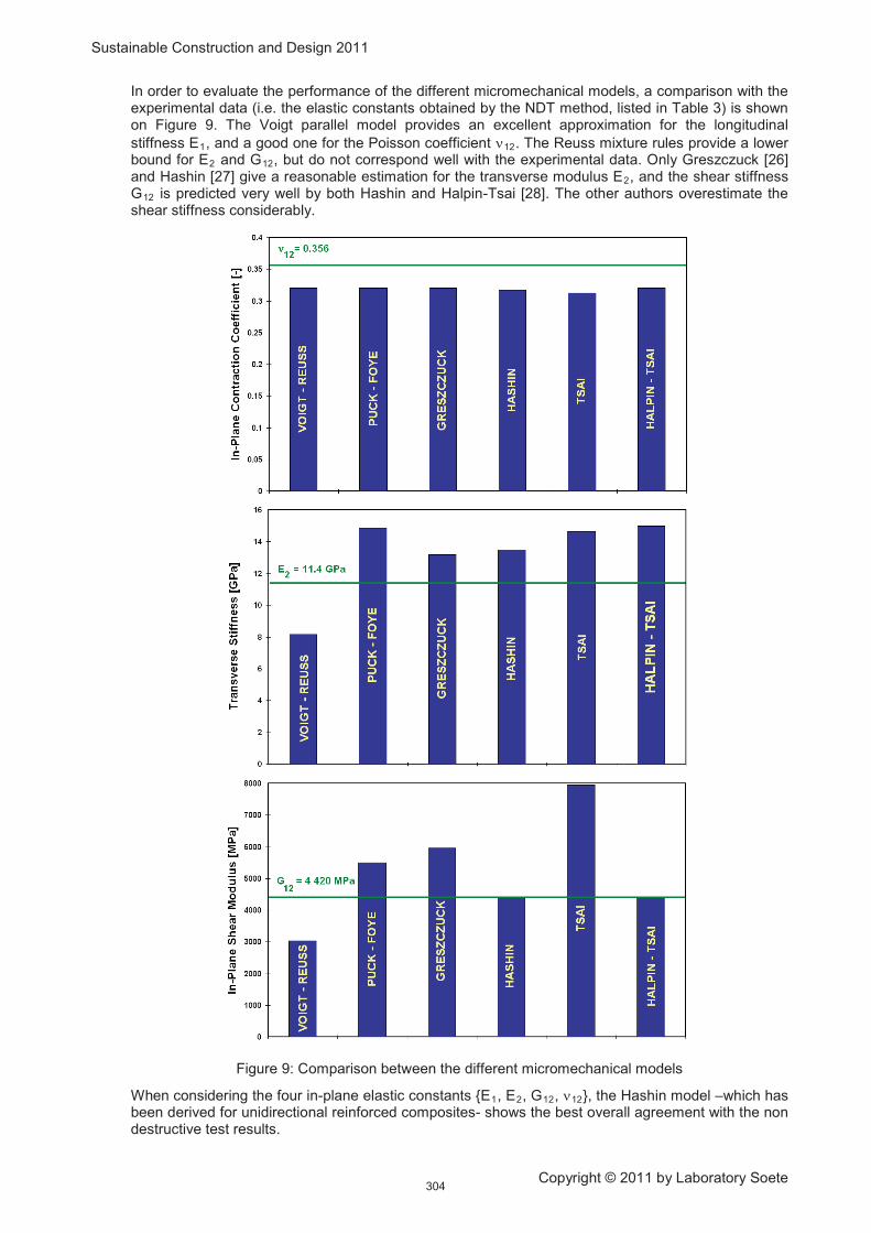
Sustainable Construction and Design 2011
Copyright © 2011 by Laboratory Soete
In order to evaluate the performance of the different micromechanical models, a comparison with the experimental data (i.e. the elastic constants obtained by the NDT method, listed in Table 3) is shown on Figure 9. The Voigt parallel model provides an excellent approximation for the longitudinal
stiffness E1, and a good one for the Poisson coefficient "12. The Reuss mixture rules provide a lower bound for E2 and G12, but do not correspond well with the experimental data. Only Greszczuck [26] and Hashin [27] give a reasonable estimation for the transverse modulus E2, and the shear stiffness G12 is predicted very well by both Hashin and Halpin-Tsai [28]. The other authors overestimate the shear stiffness considerably.
Figure 9: Comparison between the different micromechanical models
When considering the four in-plane elastic constants {E1, E2, G12, "12}, the Hashin model –which has been derived for unidirectional reinforced composites- shows the best overall agreement with the non destructive test results.
304

Sustainable Construction and Design 2011
Copyright © 2011 by Laboratory Soete
4 CONCLUSIONS AND OUTLOOK
In this paper, the requirements for material selection, testing and modelling were reviewed for the design of crack arrestors for ultra high gas transmission pipelines. First, a review on different types of crack arrestors and their application was presented. Crack arrestors are usually classified as integral or non-integral, the first one consisting of (parts of) pipes acting as an integral part of the line, whereas the latter type is being made of mechanical devices mounted externally onto the pipeline. According to experimental results of full-scale burst tests, steel sleeve arrestors and composite crack arrestors are the most promising technologies.
For composite arrestors, unidirectional glass fibre reinforced epoxy was identified as the best balance between mechanical properties and cost considerations. Traditional mechanical characterization was performed to determine the orthotropic properties: both tensile tests, compression tests and three rail shear tests were conducted in fibre direction and in transverse direction. The in-plane elastic properties were determined by a dynamic identification technique using resonant frequencies. This non destructive method compares the measured vibrational response of a rectangular test plate with the computed frequencies of a numerical parameter model of the plate. The unknown material properties of the numerical method are optimised until convergence is reached. The obtained elastic properties are homogenised over the plate surface, and hence suitable as averaged input values in finite element models for composite structures like crack arrestors.
In the end, several micromechanical mixture rules were evaluated to calculate the elastic constants of the unidirectional laminate, based on the properties of the (glass) fibre and the (epoxy) matrix. The Hashin model –which has been derived for unidirectional reinforced composites, shows the best agreement with the experimental data.
In an accompanying paper [18], numerical techniques to simulate subsequent crack initiation, propagation and arrest are introduced. The combination of numerical simulation and experimental research allows deriving design guidelines for composite crack arrestors.
5 ACKNOWLEDGEMENTS
The research results, presented in this paper, were obtained in the scope of the LINESPEC project on Special Components and Strain Based Requirements for High Strength High Pressure Pipeline Applications. This project is funded by the Research Fund for Coal and Steel (RFCS).
The authors gratefully acknowledge the support of the project partners BP, SZMF, Corus, ISQ, RWTH and the Soete Lab (UGent).
6 REFERENCES
[1] Demofonti G. et. al., Fracture Propagation Resistance Evaluation of X100 TMCP Steel Pipes for High Pressure Gas Transportation Pipelines Using Full Scale Burst Tests, Proceedings of the Fourth International Conference on Pipeline Technology, 9-13 May 2004, Ostend, Belgium
[2] Mannucci G., Di Biagio M., Demofonti G., Fonzo A., Salvini P. and Edwards A., Crack Arrestor Design by Finite Element Analysis for X100 Gas Transportation Pipelines, Proceedings of the Fourth International Conference on Pipeline Technology, 9-13 May 2004, Ostend, Belgium
[3] Mannucci G. and Demofonti G., Control of Ductile Fracture Propagation in X80 Gas Linepipe, Proceedings of the Fifth International Conference on Pipeline Technology, 12-14 October 2009, Ostend, Belgium
[4] Proceedings of the International Seminar on Application of Rolled Quasi Laminated Crack Arrestors in Gas Transmission Pipelines, Kiev, USSR, October 1985
[5] Fawley, N.C., Development of Fibreglass Composite Systems for Natural Gas Pipeline Service, NCF Industries Report to the Gas Research Institute, GRI-94/0072, March 1994
[6] Demofonti G. et. al., Fracture Behaviour of X100 Gas Pipelines by Full Scale Tests, Proceedings of the Conference on Application and Evaluation of High Grade Linepipe in Hostile Environments, Yokohama, Japan, November 2002
[7] Wilkowski G.M., Scott P.M. and Maxey W., Design and Optimization of Mechanical Crack Arrestors for Pipelines, NG-18 Report no. 134 to the Gas Research Institute, NR1983-08E, July 1983
305

Sustainable Construction and Design 2011
Copyright © 2011 by Laboratory Soete
[8] Bonomo F., Bramante M. and Spedaletti M., Ductile Fracture Propagation in Pipelines – Results of Instrumented Full Scale Burst Tests on 48” and 56” Diameter Pipes for Gas Transmission, Proceedings of the International Conference on Analytical and Experimental Fracture Mechanics, Sijthoff & Noordhoff, Roma, 1980
[9] Maxey W.A., Fracture Propagation Behaviour of Offshore Pipelines based on Underwater Burst Tests, 6
th
[10] Shoemaker A.K., McCartney R.F. and Ives K.D., Mechanical Crack Arrestor Concepts for Linepipe Applications, Proceedings of Materials Engineering in the Arctic, St. Jovite, Quebec, Canada, 1976
Biennial Joint Technical Meeting, NG-18/EPRG, Camogli, Italy, September 1985
[11] Anon, Preliminary Cost Analysis of Crack Arrestor Designs, Canadian Arctic Gas Study, Northern Engineering Services Company Ltd., 1974
[12] Fawley N.C., Development of Composite Reinforced Materials for the Natural Gas Industry, NCF Industries Report to the Gas Research Institute, GRI-88/0264, November 1988
[13] Marsili D.L. and Stevick G.R., Reducing the Risk of Ductile Fracture on the Canyon Reef Carriers CO2 Pipeline, Society of Petroluem Engineers Annual Conference 1990, pp. 311-319, Texas, US, 1990
[14] Maxey W.A., Fracture Initiation, Propagation and Arrest, Proceeding of the Fifth Symposium on Line Pipe Research, Pipeline Research Council International, PRCI-L301/74, November 1974
[15] Eiber R., Buebenik T.A. and Maxey W.A., Fracture Control Technology for Natural Gas Pipelines, Battelle Memorial Institute Report to the Pipeline Research Council International, PRCI-39113, December 1993
[16] Leis B.N., Zhu X.K., Forte T.P. and Glenn B.C., Design Basis for Fracture Arrestors in Gas Transmission Pipelines, Proceedings of the Fourth International Conference on Pipeline Technology, Ostend, Belgium, 9-12 May 2004
[17] Van den Abeele F. and Di Biagio M., Design of Crack Arrestors for Ultra High Grade Gas Transmission Pipelines – Material Selection, Testing and Modelling, Conference on Sustainable Construction and Design, Gent, Belgium, 16-17 February 2011
[18] Van den Abeele F., Di Biagio M. and Amlung L., Design of Crack Arrestors for Ultra High Grade Gas Transmission Pipelines – Simulation of Crack Initiation, Propagation and Arrest, Conference on Sustainable Construction and Design, Gent, Belgium, 16-17 February 2011
[19] Jones R.M., Mechanics of Composite Materials, Scripta Book Company, 352 pp., 1975
[20] Van den Abeele F., Amlung L., Di Biagio M. and Zimmermann S., Numerical Design of Composite Crack Arrestors for High Pressure Gas Pipelines, Proceedings of the 8
th
[21] Sol H., Hua H., De Visscher J., Vantomme J., De Wilde W.P., A Mixed Numerical-Experimental Technique for the Non Destructive Identification of the Stiffness Properties of Fibre Reinforced Composite Materials, Journal of NDT&E International, vol. 30(2), pp. 85-91, 1997
International Pipeline Conference, IPC2010-31191, Calgary, Canada, September 2010
[22] Van den Abeele F., Rogerio De Oliveira J. and Huertos F.J., Identification of the Complex Moduli of Orthotropic Materials using Modal Analysis, Proceedings of the 5
th
[23] Van den Abeele F. and Skocovsky T., Enhanced Failure Criteria for Composite Crack Arrestors, Proceedings of the Fifth International Conference on Pipeline Technology, Ostend, Belgium, 12-14 October 2009
COMSOL Users’ Conference, Paris, France, 17-19 November 2010
[24] Ashton J.E., Halpin J.C. and Petit P.H., Primer on Composite Materials: Analysis, Progress in Materials Science vol. III, 1969
[25] Tsai S.W., Structural Behaviour of Composite Materials, NASA CR-71, 1964
[26] Greszczuck L.B., Damage in Composite Materials due to Low Velocity Impact, in Impact Dynamics, Zukas J.A., J. Wiley & Sons, 1982
[27] Hashin Z., Failure Criteria for Unidirectional Fibre Composites, Journal of Applied Mechanics vol. 47, pp. 329-334, 1980
[28] Halpin J.C. and Tsai S.W., The Effects of Environmental Factors on Composite Materials, AFML-TR 67-423, 1969
306

Sustainable Construction and Design 2011
Copyright © 2011 by Laboratory Soete
DESIGN OF CRACK ARRESTORS FOR
ULTRA HIGH GRADE GAS TRANSMISSION PIPELINES
SIMULATION OF CRACK INITIATION, PROPAGATION AND ARREST
F. Van den Abeele1, M. Di Biagio2 and L. Amlung3
1 OCAS N.V., J.F. Kennedylaan 3, 9060 Zelzate, Belgium
2 Centro Sviluppo Materiali, Rome, Italy
3
RWTH Aachen University, Aachen, Germany
Abstract
One of the major challenges in the design of ultra high grade (X100) gas pipelines is the identification of a reliable crack propagation strategy. Recent research results have shown that the newly developed high strength and large diameter gas pipelines, when operated at severe conditions, may not be able to arrest a running ductile crack through pipe material properties. Hence, the use of crack arrestors is required in the design of safe and reliable pipeline systems.
A conventional crack arrestor can be a high toughness pipe insert, or a local joint with higher wall thickness. According to experimental results of full-scale burst tests, composite crack arrestors are one of the most promising technologies. Such crack arrestors are made of fibre reinforced plastics which provide the pipe with an additional hoop constraint. In this paper, numerical tools to simulate crack initiation, propagation and arrest in composite crack arrestors are introduced.
First, the in-use behaviour of composite crack arrestors is evaluated by means of large scale tensile tests and four point bending experiments. The ability of different stress based orthotropic failure measures to predict the onset of material degradation is compared. Then, computational fracture mechanics is applied to simulate ductile crack propagation in high pressure gas pipelines, and the corresponding crack growth in the composite arrestor. The combination of numerical simulation and experimental research allows deriving design guidelines for composite crack arrestors.
Keywords crack arrestors, toughness modelling, pipeline materials, fibre reinforced plastics, integrity
1 INTRODUCTION: COMPOSITE CRACK ARRESTORS
The occurrence of a longitudinal crack propagating along a gas pipeline is a catastrophic event, which involves both economic losses and environmental damage. Hence, the fracture propagation control is an essential strategy to ensure pipeline integrity. Fracture control is a tough task, since it requires knowledge of the interaction between the dynamic forces driving crack growth, and the resistance forces opposing fracture propagation.
While brittle fracture control is typically achieved by ensuring that the pipeline is operated well above the Ductile to Brittle Transition Temperature, the ductile fracture propagation can be avoided (or at least limited) by increasing the minimum specified toughness of the pipeline steel. However, for ultra high pipeline grades
( X100), the identification of a reliable crack propagation strategy is not longer straightforward. Indeed, despite excellent toughness values at lab scale (Charpy upper shelf energy and Battelle shear fracture area), one can no longer rely on pipe body arrest [1-3]. As a result, additional mechanical devices such as crack arrestors have to be mounted on the pipeline in order to stop a running ductile crack.
According to experimental results of full-scale burst tests, it is argued [4] that the most promising materials are
! Steel sleeve arrestors, in particular tight sleeves, which are placed around the main linepipe with a close fitting connection
! Composite arrestors, made of fibre reinforced plastics which provide the pipe with an additional hoop constraint.
307

Sustainable Construction and Design 2011
Copyright © 2011 by Laboratory Soete
In an accompanying paper [5], the requirements for material selection, testing and modelling were reviewed for the design of crack arrestors for ultra high grade gas transmission pipelines. For composite arrestors, uni-directional glass fibre reinforced epoxy was identified as the best balance between mechanical properties and cost considerations. Traditional mechanical characterization was performed to determine the orthotropic properties: both tensile tests, compression tests and three rail shear tests were conducted in fibre direction and in transverse direction. The in-plane elastic properties were determined by a dynamic identification technique using resonant frequencies as well. The elastic properties, obtained with this non destructive testing method, are homogenised over the plate surface, and hence suitable as averaged input values in finite element models for composite structures. Several micromechanical mixture rules to calculate the elastic constants of the unidirectional laminate were proposed in [6]. The Hashin model, which has been derived for unidirectional reinforced composites, shows the best agreement with the experimental data.
In this paper, numerical techniques to simulate subsequent crack initiation, propagation and arrest are introduced. First, the in-use behaviour of composite crack arrestors is evaluated by means of large scale tensile tests and four point bending experiments. The ability of different stress based orthotropic failure measures to predict the onset of material degradation is compared. Then, computational fracture mechanics is applied to simulate ductile crack propagation in high pressure gas pipelines, and the corresponding crack growth in the composite arrestor. For the finite element simulations of the composite crack arrestor, the initial material properties obtained in [5] and listed in Table 1 are used.
Table 1: Stiffness and strength values used in the finite element simulations
E
44 200 MPa
1 E2 = E
11 400 MPa
3 "12 = "
0.356
13 "
0.343
23 G12 = G
4 420 MPa
13 G
5 027 MPa
23
X
700 MPa
T Y
7.2 MPa
T X
588 MPa
C Y
42 MPa
C R
30.1 MPa
S
30.1 MPa
2 IN-SERVICE BEHAVIOUR OF COMPOSITE CRACK ARRESTORS
When a pipeline is being installed, the crack arrestor can be subjected to tensile loads and bending stresses. In addition, during the operational life of the pipeline system, the composite crack arrestor is exposed to environmental loads, low temperatures, external damage, fatigue, ...
In order to evaluate the in-service behaviour of composite arrestors, an extensive testing program was undertaken, including three and four point bending experiments and tensile tests at different temperatures. In addition, low cycle fatigue and ageing were studied as well. For these experiments, the behaviour of a unidirectional reinforced crack arrestor was compared with an arrestor with a winding pattern including inclined fibres, contributing to the axial reinforcement. The winding patterns are compared on Figure 1.
Figure 1: Different winding patterns for the composite crack arrestors
308
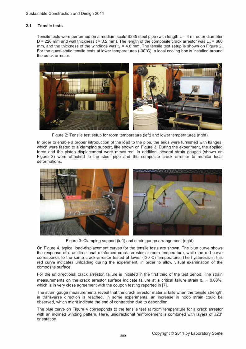
Sustainable Construction and Design 2011
Copyright © 2011 by Laboratory Soete
2.1 Tensile tests
Tensile tests were performed on a medium scale S235 steel pipe (with length L = 4 m, outer diameter D = 220 mm and wall thickness t = 3.2 mm). The length of the composite crack arrestor was La = 660 mm, and the thickness of the windings was ta = 4.8 mm. The tensile test setup is shown on Figure 2. For the quasi-static tensile tests at lower temperatures (-30°C), a local cooling box is installed around the crack arrestor.
Figure 2: Tensile test setup for room temperature (left) and lower temperatures (right)
In order to enable a proper introduction of the load to the pipe, the ends were furnished with flanges, which were fasted to a clamping support, like shown on Figure 3. During the experiment, the applied force and the piston displacement were measured. In addition, several strain gauges (shown on Figure 3) were attached to the steel pipe and the composite crack arrestor to monitor local deformations.
Figure 3: Clamping support (left) and strain gauge arrangement (right)
On Figure 4, typical load-displacement curves for the tensile tests are shown. The blue curve shows the response of a unidirectional reinforced crack arrestor at room temperature, while the red curve corresponds to the same crack arrestor tested at lower (-30°C) temperature. The hysteresis in this red curve indicates unloading during the experiment, in order to allow visual examination of the composite surface.
For the unidirectional crack arrestor, failure is initiated in the first third of the test period. The strain
measurements on the crack arrestor surface indicate failure at a critical failure strain #c
The strain gauge measurements reveal that the crack arrestor material fails when the tensile strength in transverse direction is reached. In some experiments, an increase in hoop strain could be observed, which might indicate the end of contraction due to debonding.
$ 0.08%,
which is in very close agreement with the coupon testing reported in [7].
The blue curve on Figure 4 corresponds to the tensile test at room temperature for a crack arrestor
with an inclined winding pattern. Here, unidirectional reinforcement is combined with layers of %20° orientation.
309

Sustainable Construction and Design 2011
Copyright © 2011 by Laboratory Soete
Figure 4: Load-deflection curves for static tensile tests on crack arrestors
Thanks to this axial reinforcement, the inclined winding pattern has a higher resistance to pure tensile loading. The higher strain capacity of the inclined rovings is demonstrated in Figure 5 as well, where the signals of the axial strain gauges are compared with the unidirectional crack arrestor. For the unidirectional reinforcement, failure of the epoxy resin initiated at stress levels close to the yielding point of the parent pipe.
Figure 5: Comparison of axial strains on unidirectional crack arrestor and inclined winding pattern
Although the strain gauges clearly indicated composite material failure, no macroscopic damage could be observed after the experiments. Dye penetrant testing revealed the exact location of the cracks due to tensile loading. On Figure 6, the results of such a dye penetrant inspection are shown. The tested specimen is shown before (left) and after (right) a developer has been applied to reveal the penetrant, and hence the location of the surface-breaking cracks.
310
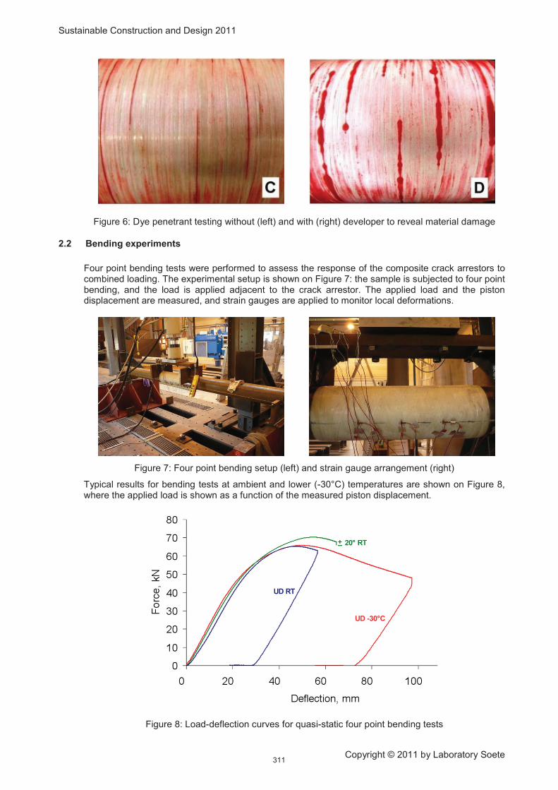
Sustainable Construction and Design 2011
Copyright © 2011 by Laboratory Soete
Figure 6: Dye penetrant testing without (left) and with (right) developer to reveal material damage
2.2 Bending experiments
Four point bending tests were performed to assess the response of the composite crack arrestors to combined loading. The experimental setup is shown on Figure 7: the sample is subjected to four point bending, and the load is applied adjacent to the crack arrestor. The applied load and the piston displacement are measured, and strain gauges are applied to monitor local deformations.
Figure 7: Four point bending setup (left) and strain gauge arrangement (right)
Typical results for bending tests at ambient and lower (-30°C) temperatures are shown on Figure 8, where the applied load is shown as a function of the measured piston displacement.
Figure 8: Load-deflection curves for quasi-static four point bending tests
311
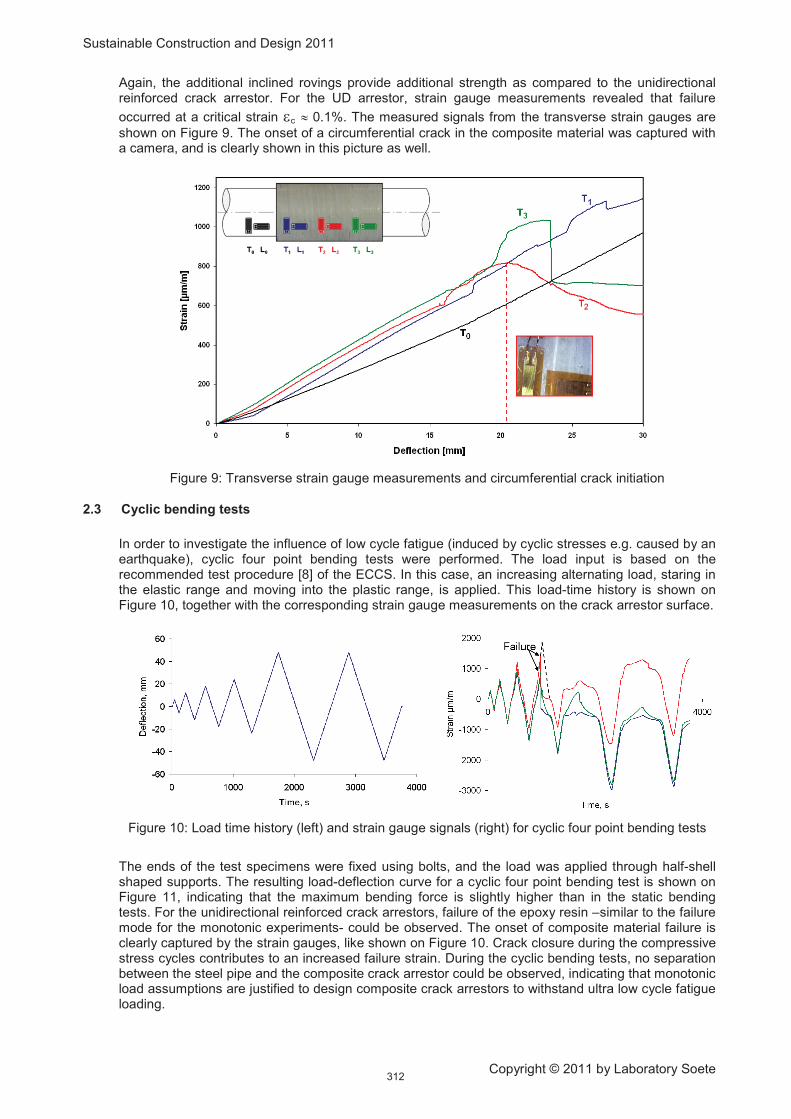
Sustainable Construction and Design 2011
Copyright © 2011 by Laboratory Soete
Again, the additional inclined rovings provide additional strength as compared to the unidirectional reinforced crack arrestor. For the UD arrestor, strain gauge measurements revealed that failure
occurred at a critical strain #c $ 0.1%. The measured signals from the transverse strain gauges are
shown on Figure 9. The onset of a circumferential crack in the composite material was captured with a camera, and is clearly shown in this picture as well.
Figure 9: Transverse strain gauge measurements and circumferential crack initiation
2.3 Cyclic bending tests
In order to investigate the influence of low cycle fatigue (induced by cyclic stresses e.g. caused by an earthquake), cyclic four point bending tests were performed. The load input is based on the recommended test procedure [8] of the ECCS. In this case, an increasing alternating load, staring in the elastic range and moving into the plastic range, is applied. This load-time history is shown on Figure 10, together with the corresponding strain gauge measurements on the crack arrestor surface.
Figure 10: Load time history (left) and strain gauge signals (right) for cyclic four point bending tests
The ends of the test specimens were fixed using bolts, and the load was applied through half-shell shaped supports. The resulting load-deflection curve for a cyclic four point bending test is shown on Figure 11, indicating that the maximum bending force is slightly higher than in the static bending tests. For the unidirectional reinforced crack arrestors, failure of the epoxy resin –similar to the failure mode for the monotonic experiments- could be observed. The onset of composite material failure is clearly captured by the strain gauges, like shown on Figure 10. Crack closure during the compressive stress cycles contributes to an increased failure strain. During the cyclic bending tests, no separation between the steel pipe and the composite crack arrestor could be observed, indicating that monotonic load assumptions are justified to design composite crack arrestors to withstand ultra low cycle fatigue loading.
312

Sustainable Construction and Design 2011
Copyright © 2011 by Laboratory Soete
Figure 11: Load-deflection curve for a cyclic four point bending test
3 ORTHOTROPIC FAILURE MEASURES TO PREDICT THE ONSET OF FAILURE
Orthotropic (plane stress) failure measures are indications of composite material degradation, where a sound material has an index IF = 0.0 and a failed material has an index IF
To predict damage initiation, Hashin and Rotem propose four different criteria to distinguish between matrix
and fibre failure in tension and compression. For fibre rupture in tension (&
= 1.0. The orthotropic linear elastic behaviour can be extended with a failure envelope, according to different criteria. In [6], the ability of different orthotropic failure measures was presented, and their ability to describe failure for composite crack arrestors was evaluated. The criterion of Hashin [9] and Rotem [10] was identified as the best failure measure for unidirectional reinforced composites.
11
22 2
12 1311
21
T
T
FX S
' '&( ) *+ * ,- ./ 0
> 0), they suggest
(Eq. 01)
while
22 2
12 1311
21
C
C
FX S
' '&( ) *+ * ,- ./ 0
(Eq. 02)
is proposed for fibre buckling/kinking in compression (&11 < 0). The initiation criterion for matrix cracking
under transverse tension and shearing (&22 + &33
22
11 33 23 22 33
21
T
T
M
Y T
& & ' & &( )* 1+ * ,- ./ 0
> 0) reads
(Eq. 03)
and compressive matrix damage (&22 + &33
2 32 22 2 2
22 3322 33 23 22 33 12 13
2 2 21 1
2 4
C C
C
YM
Y T T T S
& && & & & & ' '4 5 *( )* 1 *6 7+ 1 * * * ,- .6 7/ 08 9
< 0) is described by
(Eq. 04)
These failure measures are used to define the internal variables that characterize fibre damage
11
11
ˆ; 0
ˆ; 0
T
fC
Fd
F
&
&
: ;+ <
,;= (Eq. 05)
313

Sustainable Construction and Design 2011
Copyright © 2011 by Laboratory Soete
matrix damage
11
11
ˆ; 0
ˆ; 0
T
fC
Fd
F
&
&
: ;+ <
,;= (Eq. 06)
and shear damage
2 32 32 32 31 1 1 1 1T C T C
sd F F M M+ 1 1 1 1 1 (Eq. 07)
respectively, where the effective stress tensor ˆ D& &+ is computed from the damage operator
10 0
1
10 0
1
10 0
1
f
m
s
d
Dd
d
4 56 716 76 7
+ 6 716 7
6 76 7
18 9
(Eq. 08)
The damage initiation criteria (Eq. 01) - (Eq. 04) according to Hashin are implemented in a finite element model of the four point bending tests reported in the previous section. The pipe is modelled as a deformable solid, with three elements through the thickness to accurately capture the bending stresses. The unidirectional reinforced epoxy is modelled as an orthotropic composite material, with the elastic properties of Table 1. The total problem size was 48 678 elements and 212 052 degrees of freedom. In Figure 12, the four point bending simulation is compared with the experimental curve, indicating that the tensile matrix cracking criterion M
T = 1 is capable of predicting the onset of damage in the composite crack
arrestor.
Figure 12: Four point bending simulation with the Hashin tensile matrix cracking criterion
4 SIMULATION OF DUCTILE CRACK PROPAGATION
For the simulation of ductile crack propagation in high pressure gas pipelines, the PICPRO (Pipe Crack Propagation) code, developed by CSM and the University of Rome [11-12] was used. The model uses an explicit integration algorithm based on a central difference scheme. As a result, it is able to take both steady-state and transient fracture propagation conditions into account during the analysis, including abrupt changes of constraint characteristics such as those which occur in the vicinity of crack arrestors.
The code also accounts for local strain rate effects [12], soil constraint effects [13] and decompression of the gas flowing through the fracture breach according to the actual gas composition, pressure and temperature. Material ductility is described by a Fracture Process Zone, which is explained in [14-15].
314
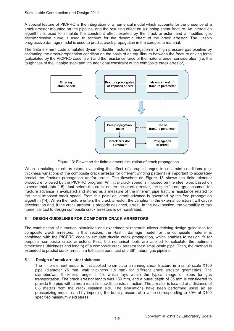
Sustainable Construction and Design 2011
Copyright © 2011 by Laboratory Soete
A special feature of PICPRO is the integration of a numerical model which accounts for the presence of a crack arrestor mounted on the pipeline, and the resulting effect on a running shear fracture. An interaction algorithm is used to simulate the constraint effect exerted by the crack arrestor, and a modified gas decompression curve is used to account for the dynamic effect of the crack arrestor. The Hashin progressive damage model is used to predict crack propagation in the composite material.
The finite element code simulates dynamic ductile fracture propagation in a high pressure gas pipeline by estimating the arrest/propagation condition on the basis of an equilibrium between the fracture driving force (calculated by the PICPRO code itself) and the resistance force of the material under consideration (i.e. the toughness of the linepipe steel and the additional constraint of the composite crack arrestor).
Figure 13: Flowchart for finite element simulation of crack propagation
When simulating crack arrestors, evaluating the effect of abrupt changes in constraint conditions (e.g. thickness variations of the composite crack arrestor for different winding patterns) is important to accurately predict the fracture propagation and/or arrest. The flowchart on Figure 13 shows the finite element procedure followed by the PICPRO program. An initial crack speed is imposed on the steel pipe, based on experimental data [15]. Just before the crack enters the crack arrestor, the specific energy consumed for fracture advance is evaluated and stored as a measure of the inherent pipe fracture resistance related to the initial imposed crack speed. From this point on, crack advance is governed by the free propagation algorithm [14]. When the fracture enters the crack arrestor, the variation in the external constraint will cause deceleration and, if the crack arrestor is properly designed, arrest. In the next section, the versatility of this numerical tool to design composite crack arrestors is demonstrated.
5 DESIGN GUIDELINES FOR COMPOSITE CRACK ARRESTORS
The combination of numerical simulation and experimental research allows deriving design guidelines for composite crack arrestors. In this section, the Hashin damage model for the composite material is combined with the PICPRO code to simulate ductile crack propagation, which enables to design ‘fit for purpose’ composite crack arrestors. First, the numerical tools are applied to calculate the optimum dimensions (thickness and length) of a composite crack arrestor for a small-scale pipe. Then, the method is extended to predict crack arrest in a full-scale burst test of a 36” natural gas pipeline.
5.1 Design of crack arrestor thickness
The finite element model is first applied to simulate a running shear fracture in a small-scale X100 pipe (diameter 75 mm, wall thickness 1.5 mm) for different crack arrestor geometries. The diameter/wall thickness range is 50, which lays within the typical range of pipes for gas transportation. The crack arrestor length was 150 mm, and a burial depth of 35 mm is considered to provide the pipe with a more realistic backfill constraint action. The arrestor is located at a distance of 0.8 meters from the crack initiation site. The simulations have been performed using air as pressurizing medium and by imposing the burst pressure at a value corresponding to 80% of X100 specified minimum yield stress.
315

Sustainable Construction and Design 2011
Copyright © 2011 by Laboratory Soete
Figure 14: Predicted crack speed diagrams for ta = 1.5 mm (left) and ta
For a composite reinforcement with a thickness of 1.5 mm (i.e. equal to the pipe wall thickness), no crack arrest is predicted. As shown in the crack speed diagram of Figure 14, the crack is initially imposed to propagate at a speed of 250 m/s, for an internal pressure of 220 bar. When entering the composite crack arrestor, the fracture speed is predicted to slow down to ca. 70 m/s, but propagates further with an increasing speed. The composite reinforcement is predicted to be totally destroyed and proves ineffective in arresting the fracture. When increasing the thickness of the crack arrestor to 3.0 mm, the simulated fracture is effectively slowed down and crack arrest is predicted.
= 3.0 mm (right)
5.2 Design of crack arrestor length
Similar simulations can be performed to calculate the optimum crack arrestor length. For an internal pressure of 200 bar and a composite thickness of 2.0 mm, the performance of a long crack arrestor (L = 150 mm) is compared to the behaviour of a short crack arrestor (L = 37.5 mm) on Figure 15.
Figure 15: Predicted crack speed diagrams for La = 37.5 mm (left) and La
Although the crack speed is considerably decreased in the short arrestor, by virtue of the constraint action exerted by the composite windings, the crack arrestor length is not sufficient to stop the running fracture. When the length is increased to 150 mm, crack arrest is achieved within 35 mm. The composite material damage predicted by the finite element analysis is compared in Figure 16.
= 150 mm (right)
Figure 16: Predicted composite material damage for La = 37.5 mm (left) and La = 150 mm (right)
316

Sustainable Construction and Design 2011
Copyright © 2011 by Laboratory Soete
5.3 Crack arrestor design for full-scale burst test
As a final validation, one of the full-scale burst tests performed during the Demopipe [16] project is simulated. The parameters for the experiment are summarized in Table 2. The composite crack arrestor, made out of unidirectional glass fibre reinforced epoxy, is shown on Figure 17 before and after the experiment.
Table 2: Data for the Demopipe full-scale burst test
PIPE
Outer diameter [“] 36
Wall thickness [mm] 20.0
Burial depth [mm] 1.5
MATERIAL
Grade API 5L X100
Elongation [%] 16.5
Yield Stress [MPa] 760
Tensile strength [MPa] 813
GAS
Pressurizing medium natural gas
Burst pressure [bar] 226
Temperature [°C] 14
CRACK ARRESTOR
Length [mm] 1 600
Thickness [mm] 40.0
Ultimate strength [MPa] 826.8
Ultimate strain [-] 0.018
Crack speed [m/s] 135
EXPERIMENTAL RESULT
arrest within 0.5 m
Figure 17: Demopipe composite crack arrestor before and after full-scale burst test [16]
317

Sustainable Construction and Design 2011
Copyright © 2011 by Laboratory Soete
With the settings listed in Table 2, the full-scale burst test was simulated using the PICPRO code and the Hashin damage model. The results are shown in Figure 18: the Critical Crack Tip Opening Angle (CTOAC) is predicted as 5.4°. The imposed crack speed of 135 m/s is slowed down rapidly, and the crack is arrested within 250 mm in the composite crack arrestor. The results of the simulation show a fairly good agreement with the experimental observations, endorsing the use of finite element analysis in the design of crack arrestors for high pressure gas pipelines.
Figure 18: Simulated crack speed diagram for the Demopipe full-scale burst test
6 CONCLUSIONS
Design considerations for crack arrestors used in ultra high grade gas transmission pipelines were reviewed. In [5], unidirectional glass fibre reinforced epoxy was identified as the most promising material for the manufacture of composite crack arrestors. An extensive experimental program was presented to measure the elastic properties of the composite materials. The results from traditional mechanical characterization and non destructive testing were compared. Micromechanical modelling of unidirectional reinforced plastics revealed that the Hashin model is best fit to calculate the stiffness matrix, based on the properties of the fibre reinforcement and the reson.
In this paper, the in-use behaviour of composite crack arrestors was evaluated by means of quasi-static tensile tests and (both monotonic and cyclic) four point bending experiments. The Hashin damage model was applied to predict the onset of composite material degradation. Finite element simulations confirmed that the tensile matrix cracking criterion can accurately predict damage initiation.
In order to assess the ability of composite crack arrestors to stop a running fracture in a high pressure gas pipeline, numerical simulations were performed. The combination of experimental data and finite element analysis allows deriving design guidelines for composite crack arrestors. The design methodology was validated by comparing numerical predictions with the results of a full-scale burst test.
7 ACKNOWLEDGEMENTS
The research results, presented in this paper, were obtained in the scope of the LINESPEC project on Special Components and Strain Based Requirements for High Strength High Pressure Pipeline Applications. This project is funded by the Research Fund for Coal and Steel (RFCS).
The authors gratefully acknowledge the support of the project partners BP, SZMF, Corus, ISQ, RWTH and the Soete Lab (UGent).
318

Sustainable Construction and Design 2011
Copyright © 2011 by Laboratory Soete
8 REFERENCES
[1] Demofonti G. et. Al., Fracture Propagation Resistance Evaluation of X100 TMCP Steel Pipes for High Pressure Gas Transportation Pipelines Using Full Scale Burst Tests, Proceedings of the Fourth International Conference on Pipeline Technology, 9-13 May 2004, Ostend, Belgium
[2] Mannucci G., Di Biagio M., Demofonti G., Fonzo A., Salvini P. and Edwards A., Crack Arrestor Design by Finite Element Analysis for X100 Gas Transportation Pipelines, Proceedings of the Fourth International Conference on Pipeline Technology, 9-13 May 2004, Ostend, Belgium
[3] Mannucci G. and Demofonti G., Control of Ductile Fracture Propagation in X80 Gas Linepipe, Proceedings of the Fifth International Conference on Pipeline Technology, 12-14 October 2009, Ostend, Belgium
[4] Leis B.N., Clark E.B. and Eiber R.J., Crack Arrestor Review – Concepts, Design, Testing and In-Service use, Battelle Institute, Report to BP Exploration and Production (2005)
[5] Van den Abeele F. and Di Biagio M., Design of Crack Arrestors for Ultra High Grade Gas Transmission Pipelines – Material Selection, Testing and Modelling, Conference on Sustainable Construction and Design, Gent, Belgium, 16-17 February 2011
[6] Van den Abeele F. and Skocovsky T., Enhanced Failure Criteria for Composite Crack Arrestors, Proceedings of the Fifth International Conference on Pipeline Technology, Ostend, Belgium, 12-14 October 2009
[7] Van den Abeele F., Amlung L., Di Biagio M. and Zimmermann S., Numerical Design of Composite Crack Arrestors for High Pressure Gas Pipelines, Proceedings of the 8
th
[8] ECCS Technical Committee 1, Technical Working Group 1.3, Recommended Testing Procedure for Assessing the Behaviour of Structural Steel Elements under Cyclic Loads, Brussels, Belgium, 1986
International Pipeline Conference, IPC2010-31191, Calgary, Canada, September 2010
[9] Hashin Z., Failure Criteria for Unidirectional Fibre Composites, Journal of Applied Mechanics, vol. 47, pp. 329-334, 1980
[10] Hashin Z. and Rotem A., A Fatigue Criterion for Fibre Reinforced Materials, Journal of Composite Materials, vol. 7, pp. 448-464, 1973
[11] Berardo G., Salvini P., Mannucci G. and Demofonti G., On Longitudinal Propagation of a Ductile Fracture in a Gas Line Pipe: Numerical and Experimental Analysis, Proceedings of the Third International Pipeline Conference IPC2000, Calgary, Canada
[12] Fonzo A., Salvini P., Di Biagio M. and Mannucci G., Full History Burst Test Through Finite Element Analysis, Proceedings of the Fourth International Pipeline Conference, IPC2002-27120, Calgary, Canada
[13] Salvini P., Berardo G., Demofonti G. and Mannucci G., Numerical Model of the Backfill Constraint Effect During Fracture Propagation on Buried Large Diameter Gas Pipelines, Proceedings of the Third International Pipeline Conference IPC2000, Calgary, Canada
[14] Fonzo A., Meleddu A., Di Biagio M., Mannucci G., Demofonti G., Peterson C.W. and Biery N.E., Crack Propagation Modelling and Crack Arrestor Design for X120, Proceedings of the Sixth International Pipeline Conference, IPC2006-10319, Calgary, Canada
[15] Van den Abeele F., Di Biagio M. and Amlung L., Numerical Design of Composite Crack Arrestors for High Pressure Gas Pipelines, Proceedings of the 8
th
[16] Demofonti G., Mannucci G., Di Vito L.F., Aristotile R., Di Biagio M., Malatesta G., Harris D; and Harrison P., Ultra High Strength Pipeline Prototyping for Natural Gas Transmission, Demopipe, EUR 21440 EN, 2003
International Pipeline Conference IPC2010-31191, Calgary, Canada
319

Sustainable Construction and Design 2011
Copyright © 2011 by Laboratory Soete
STABILITY OF OFFSHORE STRUCTURES IN SHALLOW WATER DEPTH
F. Van den Abeele1 and J. Vande Voorde1
1OCAS N.V., J.F. Kennedylaan 3, 9060 Zelzate, Belgium
Abstract
The worldwide demand for energy, and in particular fossil fuels, keeps pushing the boundaries of offshore engineering. Oil and gas majors are conducting their exploration and production activities in remote locations and water depths exceeding 3000 meters. Such challenging conditions call for enhanced engineering techniques to cope with the risks of collapse, fatigue and pressure containment.
On the other hand, offshore structures in shallow water depth (up to 100 meter) require a different and dedicated approach. Such structures are less prone to unstable collapse, but are often subjected to higher flow velocities, induced by both tides and waves. In this paper, numerical tools and utilities to study the stability of offshore structures in shallow water depth are reviewed, and three case studies are provided.
First, the Coupled Eulerian Lagrangian (CEL) approach is demonstrated to combine the effects of fluid flow on the structural response of offshore structures. This approach is used to predict fluid flow around submersible platforms and jack-up rigs.
Then, a Computational Fluid Dynamics (CFD) analysis is performed to calculate the turbulent Von Karman street in the wake of subsea structures. At higher Reynolds numbers, this turbulent flow can give rise to vortex shedding and hence cyclic loading. Fluid structure interaction is applied to investigate the dynamics of submarine risers, and evaluate the susceptibility of vortex induced vibrations.
As a third case study, a hydrodynamic analysis is conducted to assess the combined effects of steady current and oscillatory wave-induced flow on submerged structures. At the end of this paper, such an analysis is performed to calculate drag, lift and inertia forces on partially buried subsea pipelines.
Keywords fluid structure interaction, multiphysics, offshore structures, wave loads, stability, design
1 INTRODUCTION: DESIGN CONSIDERATIONS FOR OFFSHORE STRUCTURES
Offshore structures like oil and gas platforms, drilling rigs, semi-submersibles and jack-up barges have to withstand complex, combined loading patterns during their entire design life. The anticipated loads include the dead weight of the structure, hydrostatic pressure and any imposed forces. In addition, the structure has to cope with environmental loading, including wind and wave action combined with sometimes strong tidal flows. The main design considerations for such offshore structures are structural redundancy, corrosion resistance and fatigue life, especially for welded nodal joints.
The implications on material selection are shown on Figure 1. For topsides, deck structures and module walls, which are only subjected to wind loading and dead weight, secondary structural steels (like S275) can be used. Cranes and modules supports, which require a higher level of structural integrity, are typically made out of quenched and tempered steel grades like S420. Jack-up legs are tubular sections made out of primary structural steels, whereas steel piles will typically be quenched and tempered grades. Welded nodal joints require special attention, as they are prone to fatigue damage. For such critical components, special structural steels are often required.
During normal operations, the offshore structure will be subjected to waves loading and tidal flows. In addition, the part of the structure above the sea water level is exposed to wind loading. Moreover, the wind contributes to the current velocity at the still water level as well. This contribution can be estimated as
( )00 0
0
0d z
W W d zd
+= − ≤ ≤ (Eq. 01)
with W0 the wind-generated current velocity at the still water level and d0 the reference depth.
320

Sustainable Construction and Design 2011
Copyright © 2011 by Laboratory Soete
Figure 1: Material selection for offshore structures
Currents induce time-constant water particle velocities, although they normally vary along the spatial coordinates. Current velocity as a function of depth is commonly estimated by a one-seventh power law
( )1 7
0( ) 0d z
V z V zd
+� �= ≤� �� �
(Eq. 02)
where d is the water depth and V0 is the tidal current at the still water level. In shallow waters, the current
induced velocity can generate a significant load on the structure. Differences in (measured) tidal height δH can be converted to expected current velocity V by the Voith relation
( )n
V m Hδ= (Eq. 03)
where m is a scaling factor and n the shape exponent. A prediction of current velocity is shown on Figure 2, indicating that the fluid flow velocity in shallow water can range between V = 1 m/s to V = 5 m/s.
Figure 2: Fluid flow velocity induced by tidal flow
A sea state consists not only of currents, but also of waves. In reality, there is always a steady current underlying waves. Based on the water depth d and the (measured) wave period T, the corresponding wave length can be calculated with Airy wave theory [1] by iteratively solving the transcendent equation
2 2tanh
2
gT dL
L
π
π
� �=
� �(Eq. 04)
321

Sustainable Construction and Design 2011
Copyright © 2011 by Laboratory Soete
A wave with wave length L, height H and period T in a water depth d induces a horizontal water particle velocity
( ){ }{ }
cosh 2cos 2
sinh 2x
z d LH x tu
T d L L T
πππ
π
+ �� �= −� �
� �� �(Eq. 05)
which gives rise to a drag and a lift force, and the corresponding acceleration
( ){ }{ }
2
2
cosh 22sin 2
sinh 2x
z d LH x ta
T d L L T
πππ
π
+ �� �= −� �
� �� �(Eq. 06)
will induce an inertia force. When designing offshore structures in shallow water, the water depth is generally (much) smaller than the wave length:
20
Ld < (Eq. 07)
and the wave length (Eq. 04) can be approximated by
L T g d≈ (Eq. 08)
and the simplified equations for velocity (Eq. 06) and acceleration (Eq. 07) read
2
2
cos
2sin
x
x
Hu
k d T
Ha
k d T
πθ
πθ
≈�
��� ≈��
(Eq. 09)
with 2k Lπ= the wave number and 2x t
L Tθ π
� �= −
� � the phase angle.
In this paper, three case studies are presented for which the shallow water approximation (Eq. 07) holds. First, the Coupled Eulerian Lagrangian approach is demonstrated to predict the response of a jack-up barge subjected to wave loading and strong tidal flows. Then, a Computational Fluid Dynamics (CFD) analysis is performed to calculate the turbulent Von Karman street in the wake of subsea structures. As a third case study, a hydrodynamic analysis is conducted to assess the combined effects of steady current and oscillatory wave-induced flow and the drag, lift and inertia forces exerted on partially buried subsea pipelines.
2 COUPLED EULERIAN LAGRANGIAN APPROACH TO SIMULATE JACK-UP RIGS
Jack-up barges are floating vessels with long legs that can be raised or lowered. The jack-up barge is towed onto location with its legs in the upright position, and the barge floating on the water surface. Once arrived at location, the legs are jacked down onto the seabed. Jack-up barges can be used as drilling rigs or service vessels (e.g. to install offshore windmills or to decommission obsolete production platforms), and typically operate in shallow water depth.
In Figure 3, a typical jack-up barge is shown, where the accommodation and deck structure is supported by four tubular legs. With a leg length of up to 100 meters, a diameter of 3 meters and a wall thickness of 50 mm, jack-up barges are slender structures which are susceptible to the effects of hydrodynamic loading.
To predict the response of a jack-up barge subjected to wave loading and strong tidal flows, fluid structure interaction (FSI) is required. To enable full coupling between the fluid flow and the structural response, a general purpose finite element code has to be coupled with a CFD solver, which is a tedious and expensive operation when contact conditions are complex. The Coupled Eulerian Lagrangian (CEL) approach, demonstrated here, allows the fluid and structural solution to proceed in a single framework, without constraints on the mesh motion or the topology of the fluid-structure interface.
322

Sustainable Construction and Design 2011
Copyright © 2011 by Laboratory Soete
Figure 3: Jack-up barge supported by four tubular legs
For structural mechanics simulations, the Lagrangian formulation is commonly used, in which the nodes move with the underlying material. This formulation makes it easy to track the free surfaces of a material, but may result in extensive mesh distortion when strain gradients are high. To minimize mesh distortion, the arbitrary Lagrangian Eulerian (ALE) adaptive meshing technique can be used, where the mesh motion is constrained to the material motion at the free boundaries only. For analyses with more extreme deformations, such as fluid flow, the Eulerian technique may be the only method that can provide a solution. In an Eulerian formulation, the nodes stay fixed, while the material flows through the mesh. Although this approach makes it more difficult to track the material boundaries, it has the distinct advantage of completely eliminating mesh distortion due to material deformation.
To simulate the response of a jack-up barge to tidal flows and wave loading, a Coupled Eulerian Lagrangian (CEL) approach is followed. In a CEL analysis, an Eulerian mesh (the fluid flow domain) and a Lagrangian mesh (the jack-up barge, modelled as compliant structure) are assembled in the same model, and interactions between the two meshes are enforced using general contact.
The structural response of the Lagrangian parts is calculated by applying the principle of virtual work [2]
i i ij ij i i ij j i
V V V S
u u dV dV f u dV n u dSρ δ σ δ ε δ σ δ+ − =� � � � (Eq. 09)
where S is the boundary of the Lagrangian body V, σij are the stress components, εij the strain components, fi the external forces and ui the unknown displacements. To model the jack-up barge, a rigid deck structure with a mass M = 3000 tonnes is assumed. The 50 meter long legs are modelled as perfectly plastic steel
tubulars (with a yield stress σy = 355 MPa) with a diameter D = 2.5 m and a wall thickness t = 50 mm.
323

Sustainable Construction and Design 2011
Copyright © 2011 by Laboratory Soete
Figure 4: Assessment of structural redundancy for jack-up barges subjected to wave loading and tidal flows
324

Sustainable Construction and Design 2011
Copyright © 2011 by Laboratory Soete
The fluid flow is modelled in the Eulerian domain, where the combined actions of a design wave with height H = 10 m and an underlying fluid flow with velocity v = 1 m/s are imposed in an initial water depth d = 25 m. The constitutive behaviour of the water is specified with an equation of state, reducing the equations of motion to the Navier-Stokes equations for incompressible Newtonian fluids without bulk viscosity:
2vv v p v f
tρ µ� �∂
+ ⋅ ∇ = −∇ + ∇ + ∂� �
��� �� �
(Eq. 10)
where ρ is the density, v�
the velocity field, p the pressure and µ the dynamic viscosity. Under the
assumption of incompressible fluids, the density ρ is constant and the continuity of mass can be expressed as
0v∇ ⋅ =� �
(Eq. 10)
Figure 4, the results of the CEL approach are presented for a jack-up barge subjected to tidal flow (v = 1 m/s) and wave loading (H = 10 m). Fluid-structure interaction is compared for a jack-up barge with six legs, and one with three legs. Although both designs can withstand the combined loading of waves and currents, the platform with six legs has a much higher stability. This is evident from Figure 5, where the transverse displacements of the top of the derrick are compared for both barges. The use of the CEL approach to evaluate structural redundancy for offshore platforms is presented in more detail in [3].
Figure 5: Cross-flow displacements of the derrick for both jack-up barges
Jack-up barges with four legs are commonly used, although the design with three legs has a wide application range as well. The latter one, however, has no structural redundancy, and is more vulnerable when operating in a disturbed sea state. While a mobile offshore structure like a jack-up barge is designed to operate within a certain tidal window, it may not be able to cope with a 100 year design wave, like shown on Figure 6. As a result, it is important to monitor the flow conditions, and interrupt operations if the environmental conditions dictate the need for evacuation.
325

Sustainable Construction and Design 2011
Copyright © 2011 by Laboratory Soete
Figure 6: Collapse of the tubular legs when the jack-up barge is subjected to a 100 year design wave
3 FLUID STRUCTURE INTERACTION TO PREDICT VORTEX INDUCED VIBRATIONS
Vortex induced vibration (VIV) is a major cause of fatigue failure in submarine oil and gas pipelines [4] and steel catenary risers [5]. Even moderate currents can induce vortex shedding, alternately at the top and bottom of the tubular structure, at a rate determined by the flow velocity. Each time a vortex sheds, a force is generated in both the in-line and cross-flow direction, causing an oscillatory multi-mode vibration. This vortex induced vibration can give rise to fatigue damage of submarine pipeline spans and risers, especially in the vicinity of the girth welds. The huge financial loss associated with riser failure is an important incentive to develop more enhanced numerical tools to predict the VIV response of offshore structures [6].
Vortex shedding is governed by the Strouhal number
sf DStU
= (Eq. 11)
where fs is the vortex shedding frequency, D is the diameter of the riser (or pipeline) and U is the flow velocity. The Strouhal number is a function of the reynolds number
ReU D
υ= (Eq. 12)
which expresses the ratio of inertia forces to viscous forces, with the kinematic viscosity
µυ
ρ= (Eq. 13)
as the ratio of the dynamic viscosity µ with the density ρ. A slender structure like a marine riser will start to oscillate in-line with the flow when the vortex shedding frequency
01
3 2sf
ω
π≈ (Eq. 14)
with ω0 the lowest natural frequency of the riser, given by
326

Sustainable Construction and Design 2011
Copyright © 2011 by Laboratory Soete
0 2
e
C EI
L mω = (Eq. 15)
with C the end boundary coefficient, L the unsupported length, E the Young’s modulus of the material, and
( )4 4
64o iI D D
π= − (Eq. 16)
the moment of inertia, where
0 2iD D t= − (Eq. 17)
is the inner diameter of the riser. The effective mass me includes the mass of the steel structure
( ) ( )2 2
4st o i st om D D D t t
πρ ρ π= − = − (Eq. 18)
the internal fluid mass
2
4
ii i
Dm
πρ= (Eq. 19)
and the added mass
2
4
oa a
Dm C
πρ= (Eq. 20)
where the added mass coefficient Ca = 1 for vertical pipes and risers. On Figure 7, a Von Karman street in the wake of a marine riser is shown at the onset of turbulence. Each time a vortex sheds, a force is generated in both the in-line and cross-flow directions, causing an oscillatory multi-mode vibration. These oscillations can give rise to an ‘8-shaped’ motion of the marine riser, which is detrimental to its fatigue resistance. A comprehensive review on vortex induced vibration is given in [7]. The implications of VIV on the design of marine risers are addressed in [8-10]. Details on fluid-structure interaction to predict flow induced oscillations in marine risers are given in [11]. In this paper, these modelling techniques are applied to study proximity effects of adjacent marine risers exhibiting wake interference.
Figure 7: Von Karman vortex street in the wake of a marine riser
A careful review of flow interference between two circular cylinders in various arrangements has been presented by Zdravkovich [12], including an extensive list of references on this subject. Different studies for the tandem arrangement of two adjacent risers [13-16] have shown that the changes in drag, lift and vortex shedding are not continuous. Instead, an abrupt change for all flow characteristics is observed at a critical spacing between the risers.
It has been shown experimentally [13-16] that there is strong interference between two cylinders in tandem
arrangement for spacing ratios with L/D < 3.5. At a spacing L/D ≈ 3.5, a sudden change of the flow pattern
327

Sustainable Construction and Design 2011
Copyright © 2011 by Laboratory Soete
in the gap between the adjacent risers is observed. A parametric CFD model [5] enables an easy and straightforward means to evaluate the influence of riser spacing. On Figure 8, flow patterns for different spacings L/D are shown, indeed endorsing the experimental observations of King [14], Zdravkovich [15] and Allen [17].
Figure 8: Flow patterns for different riser spacing L/D
Drag coefficient data [16-17] shows that the upstream cylinder takes the brunt of the burden, and that the downstream riser has little or no effect on the upstream one. For different values of spacing L/D, the drag coefficient
2
( )
12
DD
F tC
U Dρ= (Eq. 21)
predicted by the CFD model is shown in Figure 9. Clearly, the drag coefficient on the upstream cylinder is not influenced by the downstream one, but a significant change in drag is observed on the downstream cylinder for L/D > 3.5.
328

Sustainable Construction and Design 2011
Copyright © 2011 by Laboratory Soete
Figure 9: Predicted drag coefficients for twin risers in tandem arrangement
More details on proximity effects for risers in tandem arrangements at different flow directions can be found in [18]. Numerical simulations on multiple risers in tandem arrangements, risers in staggered arrangements and the application to platform legs are presented in [5] and [6].
4 STABILITY CONDITIONS FOR PARTIALLY BURIED SUBSEA PIPELINES
Subsea pipelines are installed on the seabed, and they are expected to stay in their installed position throughout their operational lifetime. As already indicated in the introduction, a subsea pipeline is subjected to environmental forces due to waves and currents, which may move the pipe and hence cause damage to its coatings or even overstressing the structure in case of excessive displacements. To ensure long term safe operation, pipelines are designed to be able under worst case conditions, and a concrete coating is applied to satisfy the stability conditions.
When assuming shallow water conditions, expressed by (Eq. 07), the horizontal water particle velocity and corresponding acceleration, induced by wave loading, is given by (Eq. 09). Moreover, a steady current can give rise to an additional fluid flow velocity (Eq. 02). Assuming that the waves are approaching the pipeline
at an angle α and the current flow direction is at an angle β, the flow velocity will impose a lift force [19]
( )21
cos cos2
L L o xF C D u Vρ α β= + (Eq. 22)
and a drag force
( )1
cos cos cos cos2
D D o x xF C D u V u Vρ α β α β= + + (Eq. 23)
where CL and CD are the lift and drag coefficients respectively, and Do is the outer diameter of the pipe, including corrosion allowance, coating thickness and marine fouling. On top of that, the wave induced acceleration ax gives rise to an inertia force
2
cos4
oI I x
DF C a
πρ α= (Eq. 24)
with CI the inertia coefficient. The empirical relations (Eq. 22) - (Eq. 24) are known as the Morison equations, relating the hydrodynamic forces (lift, drag and inertia) to the pipe diameter. On Figure 10, these
forces are shown as a function of the phase angle θ, for a unit length of a pipeline with diameter D = 1 meter, subjected to a wave of height H = 10 meter and period T = 10 s and a steady current with velocity V = 0.5 m/s.
329

Sustainable Construction and Design 2011
Copyright © 2011 by Laboratory Soete
Figure 10: Hydrodynamic forces acting on a pipeline sitting on the seabed
The Morison’s equations show that the drag and lift forces are proportional to the square of the fluid particle velocity, and that the inertia force is directly proportional to the fluid particle acceleration. The drag force acts in a direction parallel to the fluid flow, while the lift force is vertically upwards (i.e. normal to the seabed). The inertia force acts in the direction of the flow or against it, depending on whether the flow is accelerating or decelerating.
The Morison’s equations are used to determine the appropriate thickness of a concrete weight coating to ensure offshore pipeline stability. The pipeline stability condition is considered to be satisfied when the forces that resist the pipeline displacement are greater than the forces that tend to displace it. The pipeline is stable when the submerged weight of the pipe wp is greater than the lift force in vertical direction:
p B Lw W F Fλ= − ≥ (Eq. 25)
with W the weight of the pipe, coatings and contents, and FB the buoyancy forces acting on the pipe. At the same time, the horizontal frictional force has to remain greater than the combined drag and inertia forces:
( ) ( )B L D IW F F F Fµ λ− − ≥ + (Eq. 26)
where µ is the coefficient of friction between the pipe and the seabed. In the stability conditions (Eq. 25)
and (Eq. 26), λ = 1.1 is a safety factor. Self-weight of the pipe (and its contents) is generally not sufficient to satisfy these criteria. In order to achieve stability, subsea pipelines are coated on the outside with high density concrete. The required thickness of the concrete coating is determined by an iterative procedure [#] such that the above criteria are satisfied for the most severe load combination, and for every value of the
phase angle θ.
When the pipeline is sitting on the seabed, the hydrodynamic coefficients are frequently fixed to CD = 0.7, CL = 0.9 and CI = 3.29. However, the hydrodynamic coefficients depend on both the Reynolds number (Eq. 12) and the Keulegan-Carpenter number [20]
U TKC
D= (Eq. 27)
In addition, the value for CD, CL and CI is dependent on the position of the pipe. If the pipeline is sitting on the seabed –which is always intended by design- the hydrodynamic coefficients will be significantly different from those for pipeline spans with a gap between the pipe and the seabed, or for partially buried pipes. When the pipeline is trenched, the pipe weight must be higher than the lift forces induced by waves and currents in order to remain buried. As shown on Figure 11, the side slope will contribute to the horizontal stability.
330

Sustainable Construction and Design 2011
Copyright © 2011 by Laboratory Soete
Figure 11: Stability conditions for a trenched offshore pipeline
The effect of the slope angle on the apparent pipe weight can be written as
1
sincos
t
o
W
W ϕϕ
µ
=+
(Eq. 28)
Where Wt is the weight in the trench, and Wo the weight outside the trench. According to [#], the fluid flow velocity in the trench can be estimated as
1 0.305tt
o
Vd
V= − (Eq. 29)
with dt the depth below the undisturbed seabed.
Unsupported pipeline span
Pipeline sitting on the seabed
Partially buried pipeline
Figure 12: Fluid patterns for different pipe positions
331

Sustainable Construction and Design 2011
Copyright © 2011 by Laboratory Soete
A distinct difference between the flow patterns of a pipe sitting on the seabed, an unsupported pipeline span and a partially buried subsea pipe is observed from Figure 12. More details on boundary proximity effects and the evolution of the hydrodynamic forces can be found in [21].
5 CONCLUSIONS
In this paper, numerical tools and utilities to study the stability of offshore structures in shallow water depth were reviewed, and three case studies were presented:
1. The Coupled Eulerian Lagrangian (CEL) approach was demonstrated to combine the effects of fluid flow on the structural response of offshore structures. This approach was used to predict fluid flow around jack-up rigs, and to study to assess structural redundancy for different designs.
2. A computational fluid dynamics (CFD) analysis was performed to calculate the turbulent von Karman street in the wake of subsea structures. At higher Reynolds numbers, this turbulent flow can give rise to vortex shedding and hence cyclic loading. Simulations of fluid structure interaction were performed to reveal the effects of vortex induced vibrations for adjacent marine risers in tandem arrangements.
3. A hydrodynamic analysis was performed to evaluate the combined effects of steady current and oscillatory wave induced flow on partially buried subsea pipelines. The lift, drag and inertia forces are given by the Morison’s equations, and a concrete weight coating is required to satisfy the stability conditions. It was shown that the values of the hydrodynamic coefficients depend on the Reynolds number, the Keulegan-Carpenter number and the position of the pipe relative to the seabed.
6 REFERENCES
[1] Sarpkaya T ; and Isaacson M., Mechanics of Wave Forces on Offshore Structures, 651 pp, 1981
[2] Wahab M.A., Finite Element Modelling of Several Physical Engineering Problems, Sustainable Construction and Design, Ghent, 2010
[3] Van den Abeele F. and Vande Voorde J., Coupled Eulerian Lagrangian Approach to Model Offshore Platform Movements in Strong Tidal Flows, Proceedings of the ASME 2011 30th International Conference on Ocean, Offshore and Arctic Engineering, OMAE2011-49639
[4] Van den Abeele F., Vande Voorde J. and Goes P., Numerical Modelling of Vortex Induced Vibrations in Submarine Pipelines, COMSOL Users’ Conference Stuttgart, Germany, 2008
[5] Van den Abeele F. and Vande Voorde J., Flow Induced Oscillations of Marine Risers with Wake Interference, COMSOL Users’ Conference Paris, France, 2010
[6] Van den Abeele F. and Vande Voorde J., Numerical Simulation of Multiple Marine Risers Exhibiting Wake Interference, Proceedings of the ASME 2011 30
th International Conference on Ocean, Offshore
and Arctic Engineering, OMAE2011-49639
[7] Gabbai R.D. and Benaroya H., An Overview of Modelling and Experiments of Vortex Induced Vibrations for Circular Cylinders, Journal of Sound and Vibration, vol. 282, pp. 575-616, 2005
[8] Ofougbu E.I., Review of Vortex Induced Vibration in Marine Risers, M.Sc. Thesis, Cranfield University, School of Applied Sciences, Offshore and Ocean Technology, 2008
[9] Ashiru A., Assessment of Vortex Induced Vibration Response in Higher Harmonics Mode, M.Sc. Thesis, Cranfield University, School of Applied Sciences, Offshore and Ocean Technology, 2007
[10] Shanks J.M., Static and Dynamic Analysis of Marine Pipelines and Risers, PhD Thesis, Cranfield Institute of Technology, College of Aeronautics, 1985
[11] Van den Abeele F., Vande Voorde J. and Goes P., Fluid Structure Interaction to Predict Fatigue Properties of Subsea Pipelines Subjected to Vortex Induced Vibrations, Proceedings of the 5
th Pipeline
Technology Conference, Ostend, Belgium, 2009
[12] Zdravkovich M.M., Review of Flow Interference between Two Circular Cylinders in Various Arrangements, Journal of Fluids Engineering, vol. 99(4), pp. 618-633, 1977
332

Sustainable Construction and Design 2011
Copyright © 2011 by Laboratory Soete
[13] Allen D.W. and Henning D.L., Vortex Induced Vibration Current Tank Tests of Two Equal Diameter Cylinders in Tandem, Journal of Fluids and Structures, vol. 17, pp. 767-781, 2003
[14] King R., Wake Interaction Experiments with Two Flexible Circular Cylinders in Flowing Water, Journal of Sound and Vibration, vol. 45(2), pp. 559-583, 1976
[15] Zdravkovich M.M., Flow Induced Oscillations of Two Interfering Circular Cylinders, Journal of Sound and Vibration, vol. 101(4), pp. 511-521, 1985
[16] Zhang H. and Melbourne W.H., Interference between Two Cylinders in Tandem in Turbulent Flow, Journal of Wind Engineering and Industrial Aerodynamics, vol. 41-44, pp. 589-600, 1992
[17] Allen D.W., Henning D.L. and Lee L., Riser Interference Tests on Flexible Tubulars at Prototype Reynolds Numbers, Proceedings of the Offshore Technology Conference, OTC-17290, 2005
[18] Mittal S. and Kumar V., Flow Induced Oscillations of Two Cylinders in Tandem and Staggered Arrangements, Journal of Fluids and Structures, vol. 15, pp. 717-736, 2001
[19] Mohitpour M., Golshan H. and Murray A., Pipeline Design and Construction, a Practical Approach, Third Edition, ASME, 2007
[20] Teh T.C., Palmer A.C., Bolton M.D. and Damgaard J.S., Stability of Submarine Pipelines on Liquefied Seabeds, Journal of Waterway, Port, Coastal and Ocean Engineering, ASCE, pp. 244-251, 2006
[21] Van den Abeele F. and Vande Voorde J., Stability of Offshore Pipelines in Close Proximity to the Seabed, Proceedings of the International Pipeline Technology Conference, Hannover, Germany, 2011
333

Sustainable Construction and Design 2011
Copyright © 2011 by Laboratory Soete
DESIGN CHARACTERISTICS THAT IMPROVE THE FATIGUE LIFE OF
THREADED PIPE CONNECTIONS
J. Van Wittenberghe1, P. De Baets1, W. De Waele1, T. Galle1, T.T. Bui2 and G. De Roeck2
1 Ghent University, Laboratory Soete, Belgium 2 K.U.Leuven, Department of Civil Engineering, Belgium
Abstract Threaded pipe connections are commonly used to connect risers, tendons, drill pipes and well casing strings. In these applications fatigue resistance plays an important role. A large variety of patented design features exist, all claiming to improve the connection’s fatigue life. However, patent documents only contain claims and numerical or experimental data about these connection’s performance is generally not published. This makes it hard to make a quantitative comparison between different designs. In this study an overview is given of fatigue resistant threaded connections. Two major methods to improve the fatigue life of a connection were identified. First of all, local stress concentrations can be reduced by optimizing the geometry of the threads. Second the global shape of the connection can be optimized to obtain a more uniform load distribution.
Using a parametric finite element model, different designs were compared. The connections were modelled by a 2D axisymmetric geometry with non-linear material properties and elaborate contact conditions. Selected designs have been subjected to experimental tests in a four-point bending fatigue setup. The experimental tests serve as a validation for the results of the numerical simulations. It was found that the multiaxial stress distribution at the thread roots is the defining factor for the fatigue life of the connection. Nevertheless, these stresses can be changed by the global geometry of the connection. It can be concluded that the fatigue life of threaded connections is determined by a combination of global and local aspects which should both be analysed for fatigue life calculations.
Keywords threaded pipe connection, fatigue, patent, experiment, finite element model
1 FATIGUE RESISTANT THREADED PIPE CONNECTIONS
1.1 General trends
Specialized threaded connections are developed and optimized for the use in dynamic applications. Those fatigue resistant designs are all aimed at reducing the maximum appearing stress peaks in the connection. Throughout the existing patented designs two general trends can be identified to achieve this goal. Firstly, the global box geometry is changed to obtain a more uniform load distribution over the threads and hence reducing the high stresses appearing at the last engaged threads (LET) which are typical for general threaded connections. The second trend to obtain a fatigue resistant connection is to provide a local modified thread shape. By changing the thread profile, the local stress intensity can be reduced and by altering the thread shape or interference over the engaged thread length the load distribution can be additionally optimized.
1.2 Global box geometry modifications
In 1961 a new connection was invented by Bodine [1] (illustrated in Figure 1.a). This connection was developed to be used in a sonic well pump tubing string. In this application, important fluctuating axial stresses are introduced by the pumping action. Due to the high load carried by the last engaged thread of the pin, fatigue cracks would develop at this location in conventional connection designs. Bodine’s connection however, was constructed in such a way that the loads are distributed more uniformly over the different threads, hereby lowering the concentrated load at the LET of the pin and hence increasing the fatigue life of the entire connection. This improved distribution was obtained by changing the box geometry. In general, the box of the connection has a bigger wall thickness than the pin and is the most rigid part of the connection. However, when reducing the stiffness of the box locally, by applying a groove in its outer surface located over the last engaged threads of the pin, the box is able to elastically deform and to transfer the load more easily to the following threads.
The same idea of local stiffness reductions to redistribute loads has been used ever since in a variety of other patents. In 1963 a string connection with a changed box was patented by Schreier [2]. This connection is shown in Figure 1.b.
334

Sustainable Construction and Design 2011
Copyright © 2011 by Laboratory Soete
Figure 1: Patented box modifications: a) Bodine, 1961 [1], b) Schreier, 1963 [2], c) DeLange and Evans, 2003 [3], d) Verdillon, 2004 [4].
The coupling by DeLange and Evans [3] (Figure 1.c) claims to provide better fatigue performance by changing the so-called stiffness gradient of the recess region of the box. Here the stiffness of the pin or box is equal to the area moment of inertia Iz at a certain section. The stiffness gradient zI∇ is defined by Delange and Evans as the difference in stiffness ratio between pin and box divided by the length L of the chamfer as noted in Eq. (1):
L
I
I
I
I
I 4,z
3,z
2,z
1,z
z∇ = (1)
In this equation Iz,1 and Iz,2 are respectively the stiffness of the box and pin section at the end of the box recess. It is specified that the chamfer should start at the location of the last fully engaged thread of the pin. Hence, Iz,3 and Iz,4 are the stiffness of respectively the box and pin section at LET of the pin, calculated at the pitch line of the threads. Additionally, this design proposes a long engaged thread length, including a thread run-out region where the threads are only partly engaged. This long engaged thread region can also be found in the connection of Verdillon [4] as shown in Figure 1.d. Next to this it uses a waisted groove over the highest loaded threads similar to the original design of Bodine [1]. This connection is commercially available and is named the VAM TOP FE connection. Verdillon added the possibility of filling up the machined groove with an elastic filler material, as long as the stiffness of the used filler is sufficiently lower than the stiffness of the material of the connection.
1.3 Local thread modifications
To optimize the connection threads for fatigue purposes, their profile can be changed to reduce the stress intensity at the thread roots. Additional to this, the thread taper, pitch, interference or tolerances can be changed over the engaged threads to modify the load distribution. Since these modifications generally result in complex and hard to produce thread shapes that require very fine tolerances, local thread modifications can be considered as less robust ways to influence the connection’s fatigue behaviour. This is because wear or local damage during service can change those tight tolerances and hence eliminate the desired fatigue properties.
335

Sustainable Construction and Design 2011
Copyright © 2011 by Laboratory Soete
Figure 2: Patented thread types: a) Saunders et. al., 1985 [5], b) Gunderson et. al., 1990 [6], c) DeLange et. al., 1999 [7], d) Olivier, 2002 [8], e) Pallini et. al., 2007 [9], f) Noel and Roussie, 2009 [10].
Nevertheless, numerous patented thread modifications exist. The so-called Reed-thread developed by Saunders et. al. [5] as shown in Figure 2.a, is a modified rounded triangular thread. It contains a stress relief groove at the thread root with an increased root radius as compared to standard thread shapes to reduce the stress intensity factor. Additionally the connection contains a pin with a slightly lower taper angle than the box. This results in an artificial change in pitch and radial interference which improves the load distribution.
Both Gunderson et. al. [6] and DeLange et. al. [7] proposed a modified buttress thread with enhanced fatigue properties to be used in connections for risers, tendons or drill applications (see Figure 2.b and c). They both use a zero degree load flank and increased root radii. The zero degree load flank ensures that the axial load on the connection does not produce any significant radial component which would tend to separate the pin from the box.
Worth mentioning is that modified buttress threads also exist with a negative load flank. An example of this can be found in the drill string thread proposed by Olivier [8] as shown in Figure 2.d. The negative load flank locks the connection together and prevents separation of the threads. Next to reducing fretting fatigue failure, this kind of threads are generally more resistant to yielding and overtorque. The thread type of Olivier has improved fatigue properties due to the rounded corners of the load flank.
The irregular thread type for riser connections of Pallini et. al. [9] (Figure 2.e) has an S-shaped load flank that provides a variable load angle depending on the radial position along the contact interface. The thread
336

Sustainable Construction and Design 2011
Copyright © 2011 by Laboratory Soete
profile uses a combination of thread cuts that vary in shape and pitch to provide load and stab flanks that vary along the axial length of the engaged threads. Due to the changing interference between the threads, the load distribution becomes more uniform over the engaged length. It is obvious that this kind of threads with varying pitch and profile demands extremely tight tolerances and advanced production tools. This results in high production and maintenance costs since connection repairs can only be carried out by specialized workshops. Additionally, the irregular thread shape hinders thread inspection.
Noel and Roussie [10] developed an additional modification of the buttress thread type. But instead of optimizing the root radii, they provided a portion of the threads with an additional groove in the thread crests as can be seen in Figure 2.f. This groove is machined only at the first and last engaged threads. The groove reduces the thread stiffness, which makes that a part of the load is transferred to the subsequent threads. The improved load distribution should result in an increased fatigue life of the connection. Nevertheless, the extra groove in the threads makes inspection and repair of the threads more difficult.
1.4 Additional fatigue life improving features
Next to the two general trends of improving the fatigue strength of a connection either by changing the global box shape or the local thread shape, some other techniques are used. The fatigue strength of rounded triangular threads can be improved by cold working the thread roots. For example by rolling the threads after they have been machined into the connection as was shown by Knight et. al. in their study of drill pipe connections [12]. This way compressive residual stresses are introduced at the location where the fatigue cracks tend to initiate, which is beneficial for the fatigue life of the connection. A connection where this introduction of residual stresses is proposed was developed by Benedict et. al. [13].
Stress relief grooves can be used to locally reduce the stiffness of the connection around the first and last engaged thread. This way the load on these locations is partly transferred to the next threads. Since stress relief grooves result in a locally decreased wall, they are only used in upset connections which have a bigger wall thickness than the pipe material. An example of a connection with stress relief grooves is shown in Figure 3.a.
Metal-to-metal surfaces are used as seals to prevent leakage, but when the connection is subjected to dynamic bending loads, those seals can have a beneficial effect on the connection’s fatigue life. This is because the metal-to-metal seals also provide structural support for the contacting parts and transmits a part of the bending load. This partly decreases the stresses in the threaded region of the connection. In Figure 3.b an example of such a connection is given [15]. However, as was shown by Santus [16], the metal-to-metal surface is a region susceptible to fretting fatigue damage.
Figure 3: a) Patented stress relief grooves by Pallini et. al. [14], the grooves are indicated by the arrows, b) Metal-to-metal sealing surfaces (indicated by the arrow) [15], c) Patented thread run-out by Nisida et. al [17].
a
b
c
337

Sustainable Construction and Design 2011
Copyright © 2011 by Laboratory Soete
A final feature that is claimed to provide better fatigue resistance can be found in the patent of Nisida et. al. [17]. Although this patent is aimed at bolts, it might be applicable to threaded pipe connections as well. As illustrated in Figure 3.c, the last engaged threads of the connection’s pin have crests that are cut off. This way the last engaged threads of the box will only be partly engaged. When subjected to axial loads, the last engaged threads of the box will bend and the load will be redistributed to the subsequent threads of the connection. This approach can be considered as a combination of the grooved threads of Noel and Roussie [10] (Figure 2.f) and the long thread run-out of DeLange and Evans [3] (Figure 1.c).
2 UGENT RESEARCH ON FATIGUE RESISTANCE OF THREADED PIPE CONNECTIONS
2.1 Parametric finite element model
Since patent documents only provide general claims on the fatigue life improvement of a specific design without providing quantifiable data, it is hard to compare the different patented connections. To overcome
this problem a parametric finite element program called ThreadGen© was developed at the Laboratory Soete of Ghent University [18]. This program enables a uniform approach to quantify the fatigue resistance of threaded pipe connections. To simulate the threaded connections a 2D axisymmetric model is used. This is common practice when modelling threaded connections [19], [20] because of the reduced calculation time compared to full 3D models. Next to this it was shown that the results of 3D models are in good agreement with 2D axisymmetric models [21].
The axisymmetric model of an API Line Pipe threaded connection is shown in Figure 4. The model’s geometry is built in such a way that all dimensions can be changed parametrically. Only a half box is modelled since a plane of symmetry is assumed at the centreline of the box (see the boundary conditions at the right in Figure 1). The unthreaded pipe body of the pin has a sufficient length to eliminate boundary effects when an external tensile stress is applied at its free end. Besides axial tension loading, the model is also capable of simulating make-up (i.e. the assembly process of pin and box), internal and external pressure.
Figure 4: 2D axisymmetric model of an API Line Pipe connection
2.2 Experimental testing
Based on results from finite element simulations of different coupling designs, specific connection designs were selected for experimental fatigue testing [22]. Two different four-point bending test setups were used as described in [23] to test threaded pipe connections of different sizes. The obtained fatigue data was used to construct S-N curves where the applied dynamic stress amplitude Sa is plotted against the number of cycles to failure N. In Figure 5 the test data of one of the designs with a predicted enhanced fatigue life by reducing the box wall thickness of an API Line Pipe coupling is compared to the mean curve obtained for a standard API Line Pipe coupling. These tests were carried out on 1” couplings made of API Grade B material at a frequency of 15 Hz and with a load ratio of R = 0.1. It can be seen that the optimized design indeed results in an increased fatigue life of the connection since its mean S-N curve lays above the mean curve of the standard connection. For example, the fatigue life increases from 6.6 · 104 to 10.7 · 104 cycles at a stress amplitude of 20 % of the yield stress and the fatigue limit (defined at 2 · 106 cycles) slightly increases from 9.3 % σy to 10.3 % σy.
Axis of symmetry
Pin outside radius
Axial tension Pin
Box
LET
box recess
338
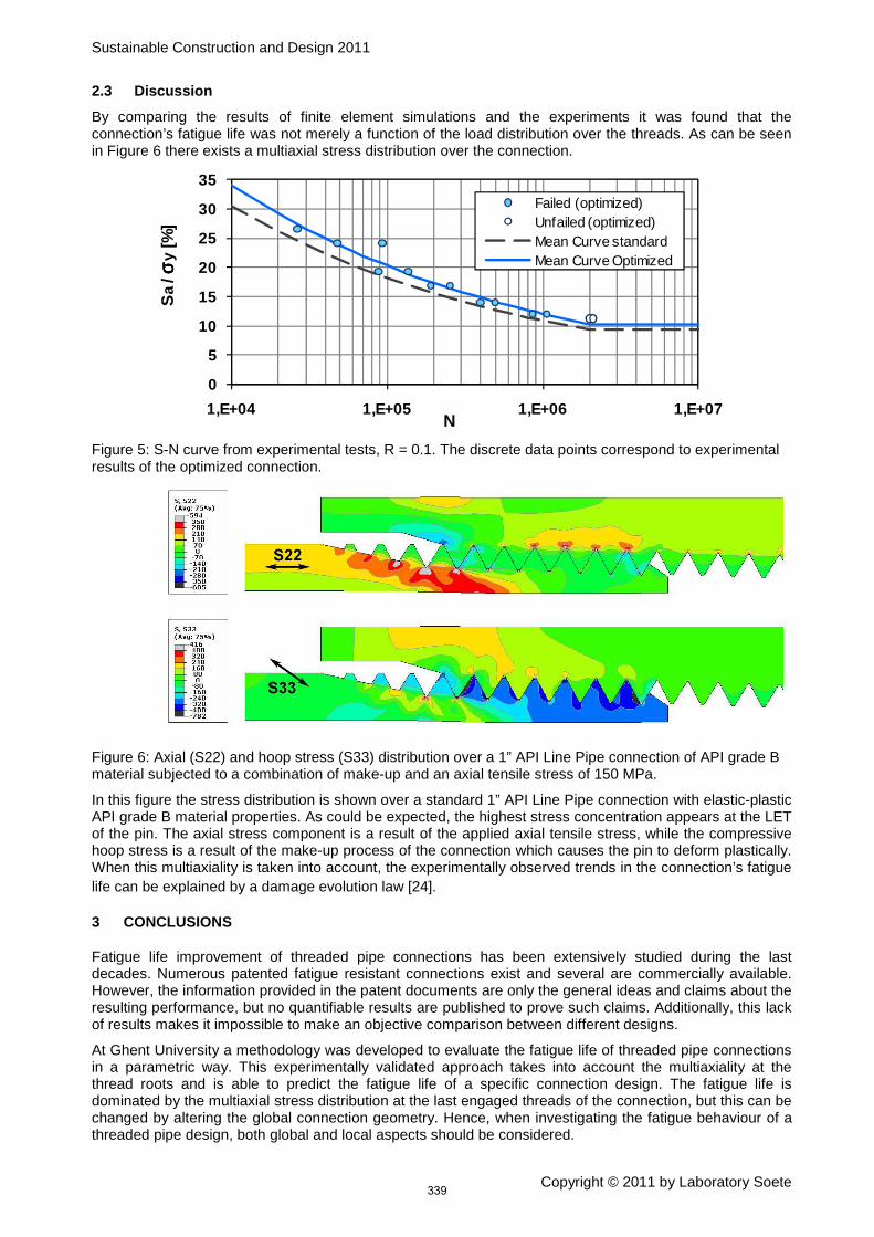
Sustainable Construction and Design 2011
Copyright © 2011 by Laboratory Soete
2.3 Discussion
By comparing the results of finite element simulations and the experiments it was found that the connection’s fatigue life was not merely a function of the load distribution over the threads. As can be seen in Figure 6 there exists a multiaxial stress distribution over the connection.
0
5
10
15
20
25
30
35
1,E+04 1,E+05 1,E+06 1,E+07
Sa
/ σσ σσy
[%]
N
Failed (optimized)Unfailed (optimized)Mean Curve standardMean Curve Optimized
Figure 5: S-N curve from experimental tests, R = 0.1. The discrete data points correspond to experimental results of the optimized connection.
Figure 6: Axial (S22) and hoop stress (S33) distribution over a 1” API Line Pipe connection of API grade B material subjected to a combination of make-up and an axial tensile stress of 150 MPa.
In this figure the stress distribution is shown over a standard 1” API Line Pipe connection with elastic-plastic API grade B material properties. As could be expected, the highest stress concentration appears at the LET of the pin. The axial stress component is a result of the applied axial tensile stress, while the compressive hoop stress is a result of the make-up process of the connection which causes the pin to deform plastically. When this multiaxiality is taken into account, the experimentally observed trends in the connection’s fatigue life can be explained by a damage evolution law [24].
3 CONCLUSIONS
Fatigue life improvement of threaded pipe connections has been extensively studied during the last decades. Numerous patented fatigue resistant connections exist and several are commercially available. However, the information provided in the patent documents are only the general ideas and claims about the resulting performance, but no quantifiable results are published to prove such claims. Additionally, this lack of results makes it impossible to make an objective comparison between different designs.
At Ghent University a methodology was developed to evaluate the fatigue life of threaded pipe connections in a parametric way. This experimentally validated approach takes into account the multiaxiality at the thread roots and is able to predict the fatigue life of a specific connection design. The fatigue life is dominated by the multiaxial stress distribution at the last engaged threads of the connection, but this can be changed by altering the global connection geometry. Hence, when investigating the fatigue behaviour of a threaded pipe design, both global and local aspects should be considered.
339

Sustainable Construction and Design 2011
Copyright © 2011 by Laboratory Soete
4 ACKNOWLEDGEMENTS
The authors would like to acknowledge the financial support of the BOF fund (B/04939) of the Ghent University and of the FWO Vlaanderen (3G022806). Next to this the help of the Laboratory Soete staff and the friendship and collegiality of all researchers is most gratefully acknowledged.
5 REFERENCES
[1] Bodine, A.G., Sonic well pump tubing string, United States Patent, US 2992613, 1961.
[2] Schreier, K., Jonction filetée, notamment pour tige de forage, French Patent, FR 1317815, 1963.
[3] De Lange, R.W., Evans, M.E., Threaded and coupled connection for improved fatigue resistance, United States Patent, US 6609735 B1, 2003.
[4] Verdillon, L., Fatigue-resistant threaded bevelled tubular element, United States Patent, US 6752436 B1, 2004.
[5] Saunders, D.D., Kalsi, M.S., Chen, G.S., Tool joint, United States Patent, US 4549754, 1985.
[6] Gunderson, R.H., Burns, J.Q., Fox, S.A., Fatigue-resistant threaded connector, United States Patent, US 4892337, 1990.
[7] De Lange, R.W., Evans, E., Buster, J.L., Threaded Connection for Enhanced Fatigue Resistance, United States Patent, US 5931511, 1999.
[8] Olivier, H.P., Connection, United States Patent, US 6485063 B1, 2002.
[9] Pallini, J.W., Munk, B.N., Riha, J.B., Lyle, R.D., Threaded Pipe Connector, United States Patent, US 2007/0063517 A1, 2007.
[10] Noel, T., Roussie, G., Fatigue-resistant threaded component for tubular threaded joint, United States Patent, US 751534, 2009.
[11] Toscano, R.G., Di Toro N.H.M., Sucker Rod Connection with Improved Fatigue Resistance Formed by Applying Diametrical Interference to reduce Axial Interference, United States Patent, US 7735879 B2, 2010.
[12] Knight, M.J., Brennan, F.P., Dover, W.D., Controlled fatigue design of drillstring threaded connections, Fatigue and Fracture of Engineering Materials and Structures, 26, 1081-1090, 2003.
[13] Benedict, D., Düber, H., Flörke, H., Modular Thread Connection With High Fatigue Resistance, United States Patent, US 7150479 B2, 2006.
[14] Pallini, J.P., Lyle, R.D., Munk, B.N., Threaded Connector, United States Patent, US 6478344 B2, 2002.
[15] Church, K.L., Thread form with multifaced flanks, United States Patent, US 6254146 B1, 2001.
[16] Santus, C., Fretting fatigue of aluminum alloy in contact with steel in oil drill pipe connections, modeling to interpret test results, Int. J. of Fatigue, 30, 677-688, 2008.
[17] Nisida, S., Urashima, C., Masumoto, H., Screwed connection having improved fatigue strength, United States Patent, US 4189975, 1980.
[18] Van Wittenberghe, J., De Baets, P., De Waele, W., Modelling of preloaded threaded pipe connections, Proc. of the 8th Nat. Congress on Theor. and App. Mechanics, 149–156, 2009.
[19] Guangjie, Y., Zhenqiang, Y., Qinghua, W., Zhentong, T., Numerical and experimental distribution of temperature and stress fields in API round threaded connection, Engineering Failure Analysis, 13(8), 1275-1284, 2006.
[20] Sugino, M., Nakamura, K., Yamaguchi, S., Daly, D., Briquet, G., Verger, E., Development of an innovative high-performance premium threaded connection for OCTG, Offshore Technology Conference, OTC20734, 2010.
[21] Van Wittenberghe, J., De Baets, P., De Waele, W., Fatigue life improvement of threaded pipe couplings, ASME Pressure Vessels and Piping Conference, PVP2010-25687, 2010.
[22] Meertens, B., De Baets, P., De Waele, W., Van Wittenberghe, J., Fatigue behaviour of threaded couplings - Experimental Research, Sustainable Construction & Design, 1, 50-57, 2010.
340

Sustainable Construction and Design 2011
Copyright © 2011 by Laboratory Soete
[23] Van Wittenberghe, J., De Pauw, J., De Baets, P., De Waele, W., Abdel Wahab, M., Ost, W., De Roeck, G., Bui, T.T., Fatigue Investigation of Threaded Pipe Connections, Sustainable Construction & Design, 1, 182-189, 2010.
[24] Van Wittenberghe, J., De Pauw, J., De Baets, P., De Waele, W., Wahab, M.A., De Roeck, G., Experimental determination of the fatigue life of modified threaded pipe couplings, Procedia Engineering, 2(1), 1849-1858, 2010.
341
Sustainable Construction and Design 2011
Copyright © 2011 by Laboratory Soete
ON THE DYNAMIC STABILITY OF HIGH-SPEED GAS BEARINGS:
STABILITY STUDY AND EXPERIMENTAL VALIDATION
T. Waumans, J. Peirs, D. Reynaerts and F. Al-Bender
Dept. of Mechanical Engineering, Katholieke Universiteit Leuven, Belgium
Abstract For high-speed applications, gas lubricated bearings offer very specific advantages over other, more conventional bearing technologies: a clean and oil-free solution, virtually wear-free operation, low frictional losses, wide operating temperature range, etc. However, the principal drawback involved in the application of high-speed gas bearings concerns the dynamic stability problem. Successful application therefore requires control of the rotor-bearing dynamics so as to avoid instabilities.
After a detailed study of the dynamic stability problem and the formulation of a convenient stability criterium, a brief overview is given of the currently existing bearing types and configurations for improving the stability. In addition, three strategies are introduced: (i) optimal design of plain aerostatic bearings; (ii) modification of the bearing geometry to counteract the destabilising effects in the gas film; and (iii) introduction of damping external to the gas film as to compensate for the destabilising effects.
These strategies are worked out into detail leading to the formulation of a series of design rules. Their effectiveness is validated experimentally at a miniature scale. In recent experiments a rotational speed of 1.2 million rpm has been achieved with a 6 mm rotor on aerodynamic journal bearings, leading to a record DN-number of 7.2 million.
Keywords air bearing, high speed, stability
1 INTRODUCTION
High-speed bearings constitute a key component of an increasing number of applications. In rotating equipment such as machine tool spindles, various kinds of turbomachines and dental drills, a clear trend has become evident towards an increase in rotational speed and towards a continual downscaling. Gas lubricated bearings offer, for these purposes, very specific advantages over other, more conventional bearing technologies. They provide a clean, oil-free bearing solution characterised by virtually wear-free operation, low frictional losses and a wide operating temperature range.
These advantages come forth from the fact that both bearing members are completely separated by a thin gas film, typically ranging from a few micrometers up to 50 µm in height. Through the generation of a positive pressure distribution in between both surfaces, the bearing is able to carry a load. This pressure generation can be the result of an external supply of pressurised air (aerostatic bearing), or of a combination of relative shearing motion and a converging gap height profile (self-acting or aerodynamic bearing).
Disadvantages, of course, also exist. The low specific load-carrying capacity and limited damping are the result of low viscosity of gasses and of their compressible nature. For high-speed applications, however, the principal drawback concerns the dynamic stability problem. Successful application therefore requires control of the rotor-bearing dynamics so as to avoid instabilities in the envisaged operational speed range.
This paper treats the dynamic stability problem of high-speed gas bearings. First, a study is performed to determine the underlying mechanism and to formulate a convenient stability criterium. After a brief overview of currently existing measures to improve the stability, the paper describes three additional strategies. Each of these strategies is experimentally validated at a miniature scale. Figure 1 illustrates how the stability performance of a conventional aerostatic bearing is improved by a modification of the film geometry (a-b). The introduction of external damping, finally, makes it possible to operate a self-acting bearing at a rotational speed of 1.2 million rpm (c). This translates to a DN-number
1
1 The DN-number is defined as the product of the diameter in mm and the rotational speed in rpm, and is a measure for
the circumferential speed at the bearing surface. Although not dimensionless, it can be regarded as a size-independent performance indicator.
of 7.2 million DN, which represents, to our knowledge, a record for an air bearing of the self-acting type.
342

Sustainable Construction and Design 2011
Copyright © 2011 by Laboratory Soete
Figure 1: Illustration of the outcome of the three stabilising strategies: (a) conventional aerostatic bearings at high supply pressures; (b) aerostatic bearing with a modified film geometry; and (c) stabilisation by the
introduction of ‘external’ damping.
author affiliation year dia. [mm]
rotational speed [rpm]
DN-number
type
H. Signer NASA Lewis Research Center
1973 120 25 000 3 000 000 ball bearings
C. Zwyssig ETH Zürich 2008 3.17 1 000 000 3 175 000 ball bearings
S. Tanaka Tohoku University 2003 4 1 250 000 5 000 000 hydroinertia
S. Tanaka Tohoku University 2009 8 642 000 5 136 000 foil bearing
A. Epstein MIT 2006 4.2 1 700 000 7 140 000 aerostatic
T. Waumans K.U.Leuven 2010 6 1 203 000 7 218 000 aerodynamic
J. W. Beams University of Virginia 1937 9 1 300 000 11 700 000 aerostatic
J. W. Beams University of Virginia 1946 0.521 37 980 000 20 130 000 magnetic
Table 1: Overview of high-speed bearing achievements (in order of increasing DN-number).
2 THE DYNAMIC STABILITY PROBLEM
In general, two types of dynamic instability can be encountered when dealing with gas lubricated rotor-bearing systems: pneumatic hammering and subsynchronous rotor whirl. Both are self-excited instabilities, but with a different underlying mechanism.
For an externally pressurised gas bearing system, the possible occurrence of pneumatic hammering exists due to a loss of film damping. This loss of damping is caused by a time-lag effect due to the compressible nature of gasses. In literature, this first type of instability has already been studied extensively ([2],[3],[4],[5]) and it is therefore not treated in this paper.
A second type of instability, which is of greater importance here, is generally referred to as half-speed (or more generally sub- or non-synchronous) whirling. The underlying source of this type of instability involves rotation which causes a cross-coupling effect in the gas film. This can lead to sudden sub-synchronous shaft whirling being very destructive in nature.
Before discussing the nature and underlying mechanism of self-excited whirl in high-speed gas bearings, a clear distinction has to be made between the various types of whirling encountered in rotating machinery.
2.1 Synchronous versus self-excited whirl
When dealing with rotating machinery on gas lubricated bearings, the gas film supporting the rotating shaft is rarely in a steady-state condition. Shaft whirling can always be observed. This whirling, however, does not automatically preclude the stability of the non steady-state working condition. Therefore, it is important to distinguish between different types of whirling and their implications on stability.
Whirling that occurs synchronous with the rotational speeds is, in fact, the passive response of the rotor-bearing system to excitation induced by residual imbalance. Depending on the presence of respectively static or dynamic rotor imbalance, cylindrical or conical whirling will be observed (although a combination of both is more likely in practice). As shown in Figure 2, the synchronous response features a maximum at the resonance frequency of the rotor-bearing system. This operating point is referred to as a critical speed in
343

Sustainable Construction and Design 2011
Copyright © 2011 by Laboratory Soete
rotordynamic terms. Once above a critical speed, the synchronous response amplitude reduces gradually before reaching a constant value which reflects the mismatch between geometrical axis of rotation and the mass line of the rotor. This shift in axis of rotation is referred to as inversion [9]. Depending on the balancing conditions and the amount of damping present in the system, safe passage can be assured through the encountered critical speeds. When compared to rolling element bearings or hydrodynamic/static bearings of similar size, gas bearings usually possess lower stiffness values. This often makes that for a high-speed application, the design speed lies in the supercritical operating range.
Figure 2: Typical (and qualitative) behaviour of the synchronous bearing response for a system with a supercritical operational speed range.
Once the system is operating at a supercritical speed, a further increase of the rotational speed will inevitably lead to the occurrence of sudden and destructive whirling. In contract to synchronous whirl, this dynamic instability is of a self-excited nature and manifests itself at a nonsynchronous (and mostly subsynchronous) frequency. The operating point at which self-excited whirl sets in, is referred to as the threshold or onset speed of the rotor-bearing system (see Figure 2). Due to the sudden increase in amplitude with respect to speed, this most often corresponds to the maximal attainable rotational speed of the system (see Figure 3). Postponing the onset speed of this whirling therefore poses the greatest challenge in a high-speed gas bearing design. In literature, this instability is also referred to as half-speed or half-frequency whirl [6],[3].
Figure 3: Waterfall diagram of a runup experiment showing sudden self-excited whirling at a subsynchronous frequency. The synchronous response is marked with ‘1x’.
2.2 Formulation of a stability criterium
Before considering solutions to this stability problem, it might be interesting to determine its underlying mechanism and to investigate how and to what extent the different rotor-bearing parameters affect the situation. To this end, a relatively simple Jeffcott configuration is adopted [9] consisting of a rotordynamic system with only two degrees of freedom (x and y) as shown in Figure 4. The linearisation of the dynamic gas film behaviour around the steady-state operating point leads to the formulation of a set of stiffness and damping coefficients. Two coefficients respectively represent the direct stiffness and damping behaviour (kxx, kyy and cxx, cyy) of the supporting film, while the two other coefficients describe the cross-coupled behaviour (kxy, kyx and cxy, cyx). This cross-coupling is best understood as a reaction of the gas film in a direction perpendicular to the applied perturbation.
344

Sustainable Construction and Design 2011
Copyright © 2011 by Laboratory Soete
Figure 4: Dynamic model of a Jeffcott rotor-bearing system.
The formulation of the equations of motion of this system and the subsequent analysis of its eigenvalues, reveal that the cross-coupled stiffness acts as negative damping to the rotor-bearing system [1]. Furthermore, it is possible to derive a simple stability criterium which allows us to reason on the effect of the various parameters of the problem. To this end, a few simplifications have to be made first: the assumption of a symmetric rotor-bearing system, i.e. k ii = kxx = kyy en k ij = kxy = -kyx ; and neglecting the effect of the cross-coupled damping, i.e. cxy = cxy
iiij ii
kk c
m
= 0. This stability criterium expresses the maximal allowable amount of cross-coupling as function of the other parameters:
or, in terms of the ratio between the cross-coupled stiffness k = k ij/k ii and the damping ratio at zero speed
!n = c ii/(2m"n
2 n# !
)
.
When observing the typical behaviour of the dynamic gas film coefficients as a function of the speed (see top graph of Figure 5), the occurrence of self-excited whirl seems inevitable when no measures are taken. The left side of the above equations will only increase with speed since the destabilising cross-coupling effect (k ij) originates from aerodynamic film action. The film damping (c ii
Figure 5
), on the other hand, decreases due to compressibility effects (at infinitely high perturbation frequencies a gaseous film offers no damping). At a certain operating point, the damping is unable to oppose the destabilising forces in the film which will result in the onset of self-excited whirl. This loss of damping is represented graphically in the bottom part of
. The onset speed is marked by the intersection point with zero line. At this point, the rotor-bearing system is marginally stable.
Figure 5: Typical behaviour of the dynamic coefficients k ii, k ij and c ii
with respect to rotor speed (top); and resulting damping ratio ! (bottom).
345
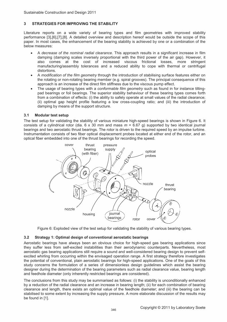
Sustainable Construction and Design 2011
Copyright © 2011 by Laboratory Soete
3 STRATEGIES FOR IMPROVING THE STABILITY
Literature reports on a wide variety of bearing types and film geometries with improved stability performance [3],[6],[7],[8]. A detailed overview and description hereof would be outside the scope of this paper. In most cases, the enhancement of the bearing stability is achieved by one or a combination of the below measures:
$ A decrease of the nominal radial clearance. This approach results in a significant increase in film damping (damping scales inversely proportional with the third power of the air gap). However, it also comes at the cost of increased viscous frictional losses, more stringent manufacturing/assembly tolerances and a reduced ability to cope with thermal or centrifugal distortions.
$ A modification of the film geometry through the introduction of stabilising surface features either on the rotating or non-rotating bearing member (e.g. spiral grooves). The principal consequence of this approach is an increase of the direct film stiffness due to the viscous pump effect.
$ The usage of bearing types with a conformable film geometry such as found in for instance tilting-pad bearings or foil bearings. The superior stability behaviour of these bearing types comes forth from a combination of effects: (i) the ability to safely operate at small values of the radial clearance; (ii) optimal gap height profile featuring a low cross-coupling ratio; and (iii) the introduction of damping by means of the support structure.
3.1 Modular test setup
The test setup for validating the stability of various miniature high-speed bearings is shown in Figure 6. It consists of a cylindrical rotor (dia. 6 x 30 mm and mass m = 6.67 g) supported by two identical journal bearings and two aerostatic thrust bearings. The rotor is driven to the required speed by an impulse turbine. Instrumentation consists of two fiber optical displacement probes located at either end of the rotor, and an optical fiber embedded into one of the thrust bearings for recording the speed.
Figure 6: Exploded view of the test setup for validating the stability of various bearing types.
3.2 Strategy 1: Optimal design of conventional aerostatic bearings
Aerostatic bearings have always been an obvious choice for high-speed gas bearing applications since they suffer less from self-excited instabilities than their aerodynamic counterparts. Nevertheless, most aerostatic gas bearing applications still require a sound and well-considered bearing design to prevent self-excited whirling from occurring within the envisaged operation range. A first strategy therefore investigates the potential of conventional, plain aerostatic bearings for high-speed applications. One of the goals of this study concerns the formulation of a series of dimensionless design guidelines which assist the bearing designer during the determination of the bearing parameters such as radial clearance value, bearing length and feedhole diameter (only inherently restricted bearings are considered).
The conclusions from this study may be summarised as follows: (i) the stability is unconditionally enhanced by a reduction of the radial clearance and an increase in bearing length; (ii) for each combination of bearing clearance and length, there exists an optimal value of the feedhole diameter; and (iii) the bearing can be stabilised to some extent by increasing the supply pressure. A more elaborate discussion of the results may be found in [1].
346

Sustainable Construction and Design 2011
Copyright © 2011 by Laboratory Soete
These conclusions have some important implications for practical bearing design. Acceptable performance in terms of high-speed stability can only be attained by reverting to small values of the radial clearance. This, in turn, demands closer control of the manufacturing tolerances, leads to increased viscous frictional losses and creates problems due to thermal and centrifugal distortions. Stabilisation by means of a supply pressure increase, on the other hand, is also not interesting from a practical point of view.
The limitations of conventional aerostatic bearings are illustrated by a first series of experiments performed by the author. By means of a modular setup, shown in Figure 6, plain aerostatic journal bearings with various design parameters have been evaluated at high speed. Rotational speeds up to 506 880 rpm and 3.1 million DN could only be attained through the combination of a relatively small clearance value (ca. 7.5 µm) and elevated supply pressures up to 16 bar.
3.3 Strategy 2: Attempts to reduce the cross-coupling
In a second strategy, the root cause of self-excited whirling is tackled by a modification of the film and entrance geometry. For this purpose, an aerostatic bearing with an innovative geometry has been designed, as shown in Figure 7. The sectioned and strongly asymmetric geometry enables the counteraction of the aerodynamically induced cross-coupling in the film. In contrast to previous implementations of this strategy by means of angled injection [10], the current implementation allows for a complete elimination of the driving force of self-excited whirling up to high values of the rotational speed. It proves even to be possible to over-compensate for the cross-coupling present in a film, which results in backward self-excited whirl rather than the normally observed forward whirl.
Figure 7: Schematic drawing of proposed geometry to counteract cross-coupling in the film (left); and detail view of the realised test bearing (right) [1].
Due to the pronounced pressure-dependency of the counteraction effect, the supply pressure must be kept between a lower and upper threshold value to prevent respectively forward or backward whirling from setting in. These threshold values shift upwards with speed, resulting in a lower and upper stability boundary. This is illustrated by the stability map of Figure 8. In practice this pressure-dependency implies that the supply pressure has to be increased in a controlled way when speeding up the rotor in order to remain within the stable operating range.
Figure 8 also provides an experimental proof-of-principle of this counteraction strategy at a moderate speed of 120 000 rpm. The frequency spectra at the lower and upper stability boundary indicate respectively forward and backward subsynchronous whirling, while stable operation is seen at a supply pressure value between both boundaries. By gradually increasing both the rotational speed and supply pressure, a maximal speed of 438 600 rpm has been achieved (= 2.6 million DN).
347

Sustainable Construction and Design 2011
Copyright © 2011 by Laboratory Soete
Figure 8: Experimental proof-of-principle at 120 000 rpm showing the frequency spectra respectively at the lower stability boundary, in between both stability boundaries, and at the upper stability boundary.
When compared to conventional aerostatic bearings, this bearing geometry offers the capability of stable high-speed operation at lower values of the supply pressure, making it more attractive for practical use. The main drawback, however, proves to be the lack of film damping caused by the measures taken to counteract the cross-coupling.
3.4 Strategy 3: Introducing external damping
In a last strategy, the destabilising forces are compensated for outside of the gas film, rather than eliminated within the film itself. This introduction of so-called external damping proves to be the only fundamental solution to the stability problem of high-speed gas bearings, since any gaseous film provides only little or negligible damping at high frequencies. This concept of adding damping is however not confined to the field of gas bearings. In aircraft gas turbine engines, rolling element bearings are supported by oil-based squeeze-film dampers to prevent excessive rotor vibrations when passing resonance frequencies [11].
3.4.1 Proposed implementation of the concept of external damping
In our case, damping is introduced to the rotor-bearing system by a flexibly supported bearing bush (see Figure 9 and [12]). The bearing bush does not rotate, but is able to give way when the shaft starts whirling. This flexible support is realised by means of elastomeric O-rings. The oil film surrounding the bush acts in this way as a squeeze-film damper to the system. This configuration combines the low friction properties of a gas film with the controllable, high damping capability of a liquid film. On the inside, the bearing bush has a wave-shaped aerodynamic film geometry which combines a relatively high direct stiffness with favourable stability characteristics [12].
348
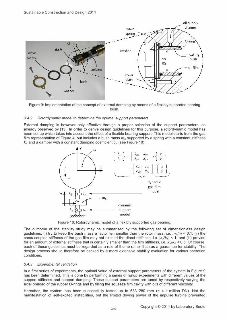
Sustainable Construction and Design 2011
Copyright © 2011 by Laboratory Soete
Figure 9: Implementation of the concept of external damping by means of a flexibly supported bearing bush.
3.4.2 Rotordynamic model to determine the optimal support parameters
External damping is however only effective through a proper selection of the support parameters, as already observed by [13]. In order to derive design guidelines for this purpose, a rotordynamic model has been set up which takes into account the effect of a flexible bearing support. This model starts from the gas film representation of Figure 4, but includes a bush mass mb supported by a spring with a constant stiffness ke and a damper with a constant damping coefficient ce Figure 10 (see ).
Figure 10: Rotordynamic model of a flexibly supported gas bearing.
The outcome of the stability study may be summarised by the following set of dimensionless design guidelines: (i) try to keep the bush mass a factor ten smaller than the rotor mass, i.e. mb/m < 0.1; (ii) the cross-coupled stiffness of the gas film may not exceed the direct stiffness, i.e. |k ij/k ii| < 1; and (iii) provide for an amount of external stiffness that is certainly smaller than the film stiffness, i.e. ke/k ii
3.4.3 Experimental validation
< 0.5. Of course, each of these guidelines must be regarded as a rule-of-thumb rather than as a guarantee for stability. The design process should therefore be backed by a more extensive stability evaluation for various operation conditions.
In a first series of experiments, the optimal value of external support parameters of the system in Figure 9 has been determined. This is done by performing a series of runup experiments with different values of the support stiffness and support damping. These support parameters are tuned by respectively varying the axial preload of the rubber O-rings and by filling the squeeze film cavity with oils of different viscosity.
Hereafter, the system has been successfully tested up to 683 280 rpm (= 4.1 million DN). Not the manifestation of self-excited instabilities, but the limited driving power of the impulse turbine prevented
349

Sustainable Construction and Design 2011
Copyright © 2011 by Laboratory Soete
reaching even higher speeds. More recently, a runup experiment (Figure 11) has been performed by driving the turbine with helium instead of air. Thanks to the higher sonic exit speed at the driving nozzles (ca. 1000 m/s), the speed could be further increased to 1 203 000 rpm (= 7.2 million DN). This achievement represents to our knowledge the highest DN-number ever reported for a gas bearings of the self-acting type (see Table 1).
The above achievement shows the effectiveness of this last stabilising strategy. In contrast to other measures, the introducing external damping proves itself as a fundamental solution to the stability problem of high-speed gas bearings. The onset of self-excited whirl is not postponed, as is done in other methods, but its driving force is compensated for outside of the gas film.
Current research focuses on the study of alternative support structures which introduce damping in a controllable and reliable way but with an improved compatibility to high-temperature working conditions.
Figure 11: Waterfall diagram of a runup experiment with a helium-driven turbine up to 1 203 000 rpm.
3.4.4 Instrumentation artefects
The waterfall diagram of Figure 11 shows nonsynchronous whirling above rotational speeds of ca. 300 000 rpm. Initially, this particular whirling phenomenon was attributed to the nonlinear behaviour of the rotor-bearing configuration as observed in for instance limit-cycle orbits. A somewhat similar behaviour was also reported in measurements performed by [14]. To conclude on whether this so-called ‘random whirl’ is not a measurement artefact, a runup experiment is performed during which the whirling behaviour is recorded simultaneously by the in-house developed fiber optical measurement system, and by a commercial laser vibrometer (Polytec OFV 2200).
The outcome of this experiment is shown in Figure 12. In contrast to the waterfall diagram as recorded by the fiber optical system, the one obtained by the laser vibrometer is free from any ‘random’ whirling. This confirms the particular nonsynchronous whirling as being a measurement artefact. Apart from this conclusion, the synchronous amplitude recorded by the laser vibrometer seems to be somewhat larger (0.5 to 1 µm difference) at high values of the rotational speed.
The exact explanation of this artefact is not entirely clear. But, it has been found that the problem becomes more prominent when the optical measurement surface is of poor quality. Since the fiber optical measurement system is based on the amount of light that is reflected back into the fiber, any surface irregularity in the form of fingerprints, scratches or indentations will induce problems.
350

Sustainable Construction and Design 2011
Copyright © 2011 by Laboratory Soete
Figure 12: Comparison of waterfall diagram as recorded by a laser vibrometer (left); and an in-house developed fiber optical measurement system (right). The synchronous whirl response is indicated by ‘1x’.
4 CONCLUSIONS
This paper has treated the dynamic stability problem of high-speed gas bearings. The underlying mechanism of self-excited whirling has been identified and a convenient stability criterium has been formulated. The currently existing stabilising techniques are briefly discussed, as well as three additional strategies for further improving the stability. The last strategy poses a fundamental solution to the stability problem by the introduction of damping external to the gas film. The effectiveness of this approach is demonstrated by the successful operation of a 6 mm aerodynamic bearing at 1.2 million rpm, which translates to a record DN-number of 7.2 million.
5 REFERENCES
[1] T. Waumans, On the design of high-speed miniature air bearings: dynamic stability, optimisation and experimental validation, PhD thesis, Katholieke Universiteit Leuven - Dept. Mechanical Engineering, 2009.
[2] V. N. Constantinescu, Gas Lubrication, ASME, New York, 1969.
[3] W. A. Gross, L. A. Matsch, V. Castelli, A. Eshel, J. Vohr, and M. Wildmann, Fluid Film Lubrication, John Wiley & Sons, New York, 1980.
[4] E. Blondeel, R. Snoeys, and L. Devrieze, Dynamic stability of externally pressurised gas bearings, Trans. ASME - Journal of Lubrication Technology, 102:511–519, October 1980.
[5] P. Plessers, Dynamische instabiliteit van aërostatische gaslagers in mechanische systemen, PhD thesis, Katholieke Universiteit Leuven - Dept. Mechanical Engineering, 1985.
[6] N. S. Grassam and J. W. Powell, Gas Lubricated Bearings, Butterworths, London, 1964.
[7] D. D. Fuller, A review of the state-of-the-art for the design of self-acting gas lubricated bearings, Journal of Lubrication Technology, 91(1):1–16, 1969.
[8] C. H. T. Pan, Rotor-bearing dynamics technology design guide. Part VI. Status of gas bearing technology applicable to aero propulsion machinery, Report ADA094167, SHAKER RESEARCH CORP, Ballston Lake NY, October 1980.
[9] J. M. Vance, Rotordynamics of Turbomachinery, John Wiley & Sons, New York, 1987.
[10] L. San Andrés and D. Childs, Angled injection - hydrostatic bearings analysis and comparison to test results, Trans. ASME - Journal of Tribology, 119(1):179–187, 1997.
[11] L. Della Pietra, G. Adiletta, The squeeze film damper over four decades of investigations, Part I: Characteristics and operating features, Shock and Vibration Digest, 34(1), 2002, pp. 3-26.
[12] T. Waumans, J. Peirs, F. Al-Bender, and D. Reynaerts, Design, optimisation and testing of a high-speed aerodynamic journal bearing with a flexible, damped support, in Proc. of the 9th International Workshop on Micro and Nanotechnology for Power Generation and Energy Conversion Applications, pp. 83-86, Washington DC, USA, December 2009.
[13] J. W. Lund, The stability of an elastic rotor in journal bearings with flexible, damped supports, Trans. ASME - Journal of Applied Mechanics, 87(4):911–920, 1965.
[14] Ce C, JianWei L, JinFu Y, and ChaoQun N 2008, Experimental study on nonlinear dynamics characteristics of high-speed rotor-gas lubrication bearing system, Proc. of the ASME Turbo Expo 2008: Power for Land, Sea and Air (Berlin, Germany, June 2008) GT2008-50250.
351

ISSN : 2032-7471
Copyright © 2022 FDOKUMEN