
Sborník příspěvků studentské konference - Blansko 2016
108
Blansko 2016 29. - 31. 8. Sborník příspěvků studentské konference
-
Upload
khangminh22 -
Category
Documents
-
view
0 -
download
0
Transcript of Sborník příspěvků studentské konference - Blansko 2016

Blansko
2016
29. - 31. 8.
Sborník příspěvků studentské konference

Název: Sborník příspěvků studentské konference Blansko 2016
Editor: Ondřej Zach
Vydavatel: Vysoké učení technické v Brně
Fakulta elektrotechniky a komunikačních technologií
Rok vydání: 2016
Vydání: první
Organizační výbor konference:
Miroslav Cupal
Martin Hrabina
Roman Mego
Ondřej Zach
Tato publikace neprošla jazykovou úpravou.
Za obsah, původnost a literární citace odpovídají autoři jednotlivých příspěvků.
ISBN 978-80-214-5389-0

Konferenci podpořili
Zlatý sponzor
Bronzový sponzor
Další partneři

Úvodní slovo
Drazí přátelé,
dovolte mi, abych Vás krátkým slovem přivítal na stránkách sborníku již tradiční konference
Blansko 2016, pořádané studentskou sekcí IEEE při VUT v Brně. Jsme rádi, že se můžeme i
tento rok setkat v přátelské atmosféře a navázat nová přátelství, ať již osobní nebo profesní.
Tento ročník konference se koná v rekreačním zařízení Vyhlídka v obci Češkovice u Blanska
na hranici chráněné krajinné oblasti Moravský kras. Letošního ročníku konference se účastní
velké množství studentů z několika českých i slovenských technických univerzit. Pevně
věříme, že účast studentů z různých vědních oborů pomůže rozšířit obzory všech účastníků a
navázat dobré profesionální a přátelské vztahy.
Rád bych poděkoval našim partnerům a sponzorům za podporu, bez které by naše
konference nemohla proběhnout. Velké díky patří československé sekci IEEE a také
partnerům z řad firem, kterými jsou Rohde and Schwarz jako zlatý sponzor, a firmy ESI group
a H test jako bronzový sponzor.
Na závěr bychom Vám chtěli poděkovat za účast na konferenci a tím podporu myšlenky
IEEE. Přejeme Vám příjemně strávený čas s kolegy a přáteli na konferenci Blansko 2016.
Za studentskou sekci IEEE v Brně
Miroslav Cupal

Obsah
Arm Jakub, Zdeněk Bradáč
Real-time Virtual Machine Simulator with Collision Detection 4
Báňa Josef
Parallel computing on graphics cards and possible contemporary solutions 8
Miroslav Cupal
3D Textile Integrated TIW Horn Antenna for UWB Wirelles Link 13
Dvořák Jan, Gajdoš Adam, Jeřábek Jan
Electronically Reconfigurable Universal Frequency Filter with Controllability of its Pole Frequency 17
Dvořák Vojtěch
High Precision Motor Control in FPGA for Space Applications 21
Havlíček Jaroslav
Arrangements of capacitively loaded dipoles for 20 bit chipless RFID tag 25
Hubka Patrik
Textile Linearly Polarized HMSIW U-Slot antenna for Off-Body Communication 28
Kotol Martin, Raida Zbyněk
The Neural models for differrent training algorithms 31
Krejčí Lukáš, Novák Jiří
Model-Based Testing Framework with Automatic Testing Priority Assignment for Automotive Distributed Systems 35
Krutílek David
Design and Limitations of the Metal – Composite Hybrid Joint Structures 39
Kufa Jan, Stavěk Marek, Kratochvíl Tomáš
High Frame Rate Video: Is It Always Better? 43
Kupková Kristýna, Sedlář Karel, Provazník Ivo
Correlated Mutation Analysis Improvement by Proteomic Signal Processing 47
Liberdová Ivana, Kolář Radim
Video Quality Assessment in experimental retinal imaging 51
Maršánová Lucie
Detection of P, QRS and T Components of ECG Using Phasor Transform 55
Mego Roman
Implementation of retargetable configurable CORDIC algorithm for FPGA devices 59
Mrnka Michal
Low Temperature Co-Fired Ceramics for High Radiation Efficiency Antenna Design 63
Němcová Andrea, Vítek Martin
Compression of ECG signals using SPIHT – alternatives to wavelet transform 67
Novák Marek, Cingel Marian
Lockless Shared Memory Based Multicore Communication Protocol 71
Polak Josef, Jeřábek Jan, Langhammer Lukáš
Automated measuring system used to measure input and output impedances of current amplifiers 74

Schneider Ján, Novák Daniel, Gamec Ján
Using UWB impulse radar system for measuring of wideband antenna parameters and its comparison 78
Smíšek Radovan, Vítek Martin
Detection of QRS Notching Using Continuous Wavelet Transform 83
Starý Vadim, Křivánek Václav
UAS Model Using WEBOTS Robot Simulator 87
Vašina Petr, Jakubíček Marek
Study of wearable antenna for 2.4 GHz ISM frequency band 91
Vélim Jan
Analysis of Microstrip Line Relative Permittivity Measurement 95
Vychodil Josef
System Impulse Response Measurement Using M-sequences in the Presence of Non-linearities 98
Ondřej Zach, Eva Klejmová
When the Numbers Speak - Hidden Statistics of a Crowdsourced QoE Study 102
Real-time Virtual Machine Simulator with CollisionDetection
Jakub ArmDepartment of Control and Instrumentation
Brno University of TechnologyBrno, Czech Republic
Email: [email protected]
Zdenek BradacDepartment of Control and Instrumentation
Brno University of TechnologyBrno, Czech Republic
Email: [email protected]
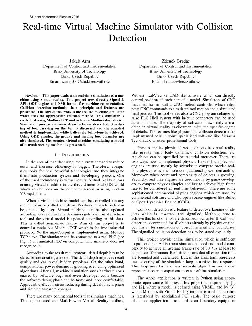
Abstract—This paper deals with real-time simulation of a ma-chine using virtual reality. This project uses directly OpenGLAPI, ODE engine and X3D format for machine representation.Collision detection methods, their principle and features arepresented. The core of this work is the created machine simulatorwhich uses the appropriate collision method. This simulator iscontrolled using Modbus TCP and acts as a Modbus slave device.Simulation process and some drawbacks are described. Simulat-ing of box carrying on the belt is discussed and the simplestmethod is implemented while believable behaviour is achieved.Using ODE physics, the gravity and moving box dynamics arealso simulated. The created virtual machine simulating a modelof a trunk sorting machine is presented.
I. INTRODUCTION
In the area of manufacturing, the current demand to reducecosts and increase efficiency is bigger. Therefore, compa-nies looks for new powerful technologies and they integratethem into production system and developing process. Oneof the used technology is virtual reality. Virtual reality allowscreating virtual machine in the three-dimensional (3D) worldwhich can be seen on the computer screen or using modernVR equipment.
When a virtual machine model can be controlled via anyinput, it can be called simulator. Positions of each parts canbe defined by user. Virtual machine can be also updatedaccording to a real machine. A camera gets position of machinetool and the virtual model is updated according to this data.This is called augmented reality. Aim of this project is tocontrol a model via Modbus TCP which is the free industrialprotocol. So the input/output is implemented using ModbusTCP slave. The simulator can be connected to a real PLC (seeFig. 1) or simulated PLC on computer. The simulator does notrecognize it.
According to the result requirements, detail depth has to bestated before creating a model. The detail depth improves resultquality and can reveal hidden problems. On the other hand,computational power demand is growing even using optimizedalgorithms. After all, machine simulation saves hardware costscaused by software bugs and even developer costs becausethe software debug phase can be faster and more comfortable.Appreciable effect is stress reducing during development phaseand simpler hardware changes.
There are many commercial tools that simulates machines.The sophisticated are Matlab with Virtual Reality toolbox,
Witness, LabView or CAD-like software which can directlycontrol position of each part of a model. Simulators of CNCmachines has in-built a CNC motion controller which inter-prets CNC commands to simulated tool motion and a simulatedfinal product. This tool serves also to CNC program debugging.Also PLC HMI system with in-built connectors can be usedas a simulator. The majority of software draws only a ma-chine in virtual reality environment with the specific degreeof details. The features like physics and collision detection areimplemented only in some specialized software like SiemensTecnomatix or other professional tools.
Physics applies physical laws to objects in virtual realitylike gravity, rigid body dynamics, collision detection, etc.An object can be specified by material moreover. There aretwo ways how to implement physics. Firstly, high precisionengines are used mostly by scientist to compute precise real-istic physics which is more computational power demanding.Moreover, when count and complexity of objects is growing.Secondly, real-time engines are used mostly by game develop-ers to compute physics simpler and fast to achieve high framerate to be considered as real-time behaviour. There are somesophisticated commercial physics engines which are used bycommercial software and also open-source engines like Bulletor Open Dynamics Engine (ODE).
Collision detection is a feature to detect overlapping of ob-jects which is unwanted and signalled. Methods, how toachieve this functionality, are described in Chapter II. Collisiondetection is computed for all objects already by physics engine,but this is for simulation of object material and boundaries.The signalled collision detection has to be stated explicitly.
This project provide online simulation which is sufficientto project aims. All is about simulation speed and model com-plexity to achieve an average frame rate of 30 fps at least tobe pleasant for human. Real-time means that all execution timeare bounded and guaranteed. But, in this area, term representsfast executing of the simulation loop to achieve fast response.This loop uses fast and less accurate algorithms and modelrepresentation in comparison to exact offline simulation.
The whole application is written in Python using appro-priate open-source libraries. This project is inspired by [1]and [2], where a model is defined using VRML, and by [3],where Matlab with Virtual Reality toolbox is used and controlis interfaced by specialized PCI cards. The basic purposeof created application is to simulate an laboratory equipment
Student conference Blansko 2016
4

Fig. 1. Overall diagram of the system
as a simulator controlled by PLC system for educationalpurpose.
II. COLLISION DETECTION
The collision detection is implemented basicallyby a physics engine. Developer has to declare whichcollision will be signalled. Also, a reaction to this unwantedcollision has to be declared. So objects can be groupedby their collision domain.
This article aims to collision detection algorithms usedfor real-time purposes. So the complexity of objects is usuallysimplified to basic shapes like box, cylinder or sphere, or someapproximations are done mostly when computational costlytriangular mesh to mesh collision is being detected. Meshto mesh collision detection is powerful because any object canbe decomposed [4]. Some real-time algorithms how to detectcollisions are :
• bounding box - any object or mesh is representedby bounding box which is faster to calculate. The sim-pler option is AABB (Axis-Aligned Bounding Box)where bounding boxes are orthogonal to axis. Thismethod can be combined also with hierarchicalmethod to achieve less computational demands (seehierarchical method). The more accurate option isOBB (Oriented Bounding Box) tree that is basedon decomposing an object to oriented boxes whereeach box is placed such that it is almost minimal [5].
• separating planes - this algorithm is usable for convexobjects. When a separating line or plane betweenvertices of each object is founded out using algorithmsimilar to perceptron, objects do not collide [5].
• hierarchical - this method reduces computational de-mands using grouping objects into hierarchical BV(Bounding Volume) tree. First, bounding boxes at thetop level are checked. In case of collision, objectvolumes at lower levels are checked down to basic ob-jects. The computation time reducing arises from non-checking of all objects together but checking togetheronly if their volume box collide [5].
• points and voxels - one object is represented by voxelsand another is represented by equidistant contourpoints. In case of intersection, voxel bits are set whichis detected. Voxel representation is on the other handmemory-inefficient [5].
• space indexing data structures - many data structuresto checking collision using space decomposing hasbeen developed. Cell subdivision method is basedon definition that if a space cell is occupied by moreobjects, they collide [5].
• image space method - this method represents an objectas a image with minimal and maximal depth. If pixelexists where depths are intersected, objects collide.This method is usable for convex objects [6].
The physics engine has a problem when the refreshcycle frequency is smaller than frame rate. This can becaused by high frame rate, high count of objects, complexityof objects, precision of physics or non-optimized algorithm.As a consequence, some high speed object can move throughanother object without collision detection. This effect canbe caught using direction vector method that considers alsothe previous position of an object.
III. CREATED SIMULATOR
In this chapter, the created simulator is described. Firstly,used tools are presented, then control of the simulation isdescribed, then the core of the simulator is drawn as a diagram,then real-time capabilities are discussed and in the end, simu-lator response is measured and some workaround approachesare proposed.
A. Graphics and physics engine
In this project, the scene is drawn directly using OpenGLAPI. A model is created in X3D (Extensible 3D) format that isthe successor of VRML (Virtual Reality Modelling Language)format that is used in industrial virtual reality [2]. X3D is basedon XML (Extensible Markup Language) and it is a standardof virtual reality languages. X3D language supports creatingof textured objects like sphere, box, or cone, and indexed face-set. It is even implemented in HTML5 technology. A modelfile is then parsed using specialized parser and processedby OpenGL driver. Using raw OpenGL functions is thereforenecessary. There are two ways how to pass objects to OpenGL.Array based model is faster and more difficult to work with.On the other hand, display list can be optimized to achievenearly the same speed as array based model.
As a physics engine, ODE is used. It provides rigid bodydynamics, joints, friction simulation and basic collision detec-tion which is sufficient to the project needs. It is open-sourceBSD licensed and belongs to real-time physics. The gravityand dynamics are simulated and applied only on the movingbox representing material because everything else should bestatic. This reduces computational demands and the simulationloop can be more frequent.
For collision detection, it uses fast spaces method describedin Chapter II. Signalled collision detection is provided by dec-laration of object collision domain. When the signalization isperformed, the simulation is stopped. Then it has to be reset.Non-signalled collision are used to simulate physics and sensorreaction like object in front of photoelectric sensor.
There are a lot of methods how to implement physics likeLagrange multipliers, reduced coordinate, Jakobsens or im-pulse dynamics. It is good to implement something between
Student conference Blansko 2016
5
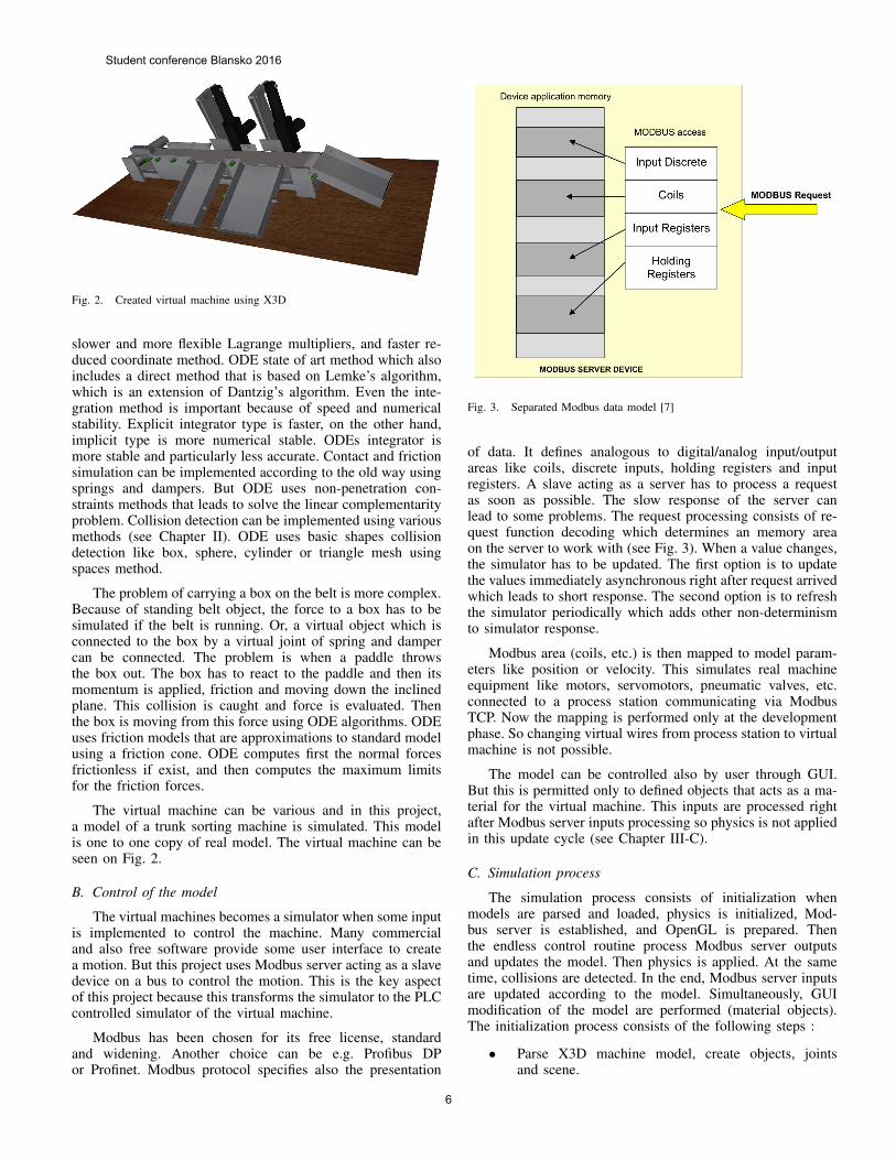
Fig. 2. Created virtual machine using X3D
slower and more flexible Lagrange multipliers, and faster re-duced coordinate method. ODE state of art method which alsoincludes a direct method that is based on Lemke’s algorithm,which is an extension of Dantzig’s algorithm. Even the inte-gration method is important because of speed and numericalstability. Explicit integrator type is faster, on the other hand,implicit type is more numerical stable. ODEs integrator ismore stable and particularly less accurate. Contact and frictionsimulation can be implemented according to the old way usingsprings and dampers. But ODE uses non-penetration con-straints methods that leads to solve the linear complementarityproblem. Collision detection can be implemented using variousmethods (see Chapter II). ODE uses basic shapes collisiondetection like box, sphere, cylinder or triangle mesh usingspaces method.
The problem of carrying a box on the belt is more complex.Because of standing belt object, the force to a box has to besimulated if the belt is running. Or, a virtual object which isconnected to the box by a virtual joint of spring and dampercan be connected. The problem is when a paddle throwsthe box out. The box has to react to the paddle and then itsmomentum is applied, friction and moving down the inclinedplane. This collision is caught and force is evaluated. Thenthe box is moving from this force using ODE algorithms. ODEuses friction models that are approximations to standard modelusing a friction cone. ODE computes first the normal forcesfrictionless if exist, and then computes the maximum limitsfor the friction forces.
The virtual machine can be various and in this project,a model of a trunk sorting machine is simulated. This modelis one to one copy of real model. The virtual machine can beseen on Fig. 2.
B. Control of the model
The virtual machines becomes a simulator when some inputis implemented to control the machine. Many commercialand also free software provide some user interface to createa motion. But this project uses Modbus server acting as a slavedevice on a bus to control the motion. This is the key aspectof this project because this transforms the simulator to the PLCcontrolled simulator of the virtual machine.
Modbus has been chosen for its free license, standardand widening. Another choice can be e.g. Profibus DPor Profinet. Modbus protocol specifies also the presentation
Fig. 3. Separated Modbus data model [7]
of data. It defines analogous to digital/analog input/outputareas like coils, discrete inputs, holding registers and inputregisters. A slave acting as a server has to process a requestas soon as possible. The slow response of the server canlead to some problems. The request processing consists of re-quest function decoding which determines an memory areaon the server to work with (see Fig. 3). When a value changes,the simulator has to be updated. The first option is to updatethe values immediately asynchronous right after request arrivedwhich leads to short response. The second option is to refreshthe simulator periodically which adds other non-determinismto simulator response.
Modbus area (coils, etc.) is then mapped to model param-eters like position or velocity. This simulates real machineequipment like motors, servomotors, pneumatic valves, etc.connected to a process station communicating via ModbusTCP. Now the mapping is performed only at the developmentphase. So changing virtual wires from process station to virtualmachine is not possible.
The model can be controlled also by user through GUI.But this is permitted only to defined objects that acts as a ma-terial for the virtual machine. This inputs are processed rightafter Modbus server inputs processing so physics is not appliedin this update cycle (see Chapter III-C).
C. Simulation process
The simulation process consists of initialization whenmodels are parsed and loaded, physics is initialized, Mod-bus server is established, and OpenGL is prepared. Thenthe endless control routine process Modbus server outputsand updates the model. Then physics is applied. At the sametime, collisions are detected. In the end, Modbus server inputsare updated according to the model. Simultaneously, GUImodification of the model are performed (material objects).The initialization process consists of the following steps :
• Parse X3D machine model, create objects, jointsand scene.
Student conference Blansko 2016
6

• Set the initial state (position etc.) of all objects.
• Create joints in the dynamics world.
• Attach the joints to the objects.
• Set the parameters of all joints.
• Create a collision world and collision geometry ob-jects, as necessary.
• Create collision domains to get collisions signalled.
• Initialize Modbus server.
• Create mapping from Modbus area to parametersof objects.
The simulation loop consists of the following steps :
• Get Modbus server outputs as model inputs.
• Apply outputs to objects as parameters or forcesas necessary.
• Apply user requests like new material insertion, etc.
• Adjust the joint parameters as necessary.
• Call collision detection and signal collisions acrosscollision domains.
• Create a contact joint for every collision point and putit in the contact joint group.
• Calculate forces coming from collisions and joints.
• Take a simulation step calling ODE physics.
• Remove all joints in the contact joint group.
• Determines Modbus inputs according to model param-eters using non-signalled sensor-object collisions.
In the end, destroying of dynamics, collision world, jointsand Modbus server is called.
D. Further work
In our further work, we plan to test the created simulatoramong students as an educational equipment. Some physicsproblem solutions and simplifications are going to be made.Then new connector will be created to simulate a Profibus DPslave process station. Some parameters and mappings are goingto be changeable using settings. The biggest challenge will beconnecting the simulator virtually on PLC inputs/outputs usingSiemens S7 protocol to avoid Modbus client in PLC and usingIO addresses directly.
IV. CONCLUSION
This project aims to online simulating of a machine usingvirtual reality. This is done using standard and nearly industrialtechnology X3D. Graphics is painted using fast OpenGL whichis able to use GPU and on the other hand, it provides onlyraw API. To this model, physics engine ODE is implementedproviding collision detection and simulation of physics laws.Some other collision detection methods are presented. A Mod-bus TCP server is implemented to control the model usingstandard industrial communication protocol to be controllableusing PLC. The simulation loop is described. The whole
simulator is written from scratch in Python language usingOpenGL wrapper, ODE physics wrapper and Modbus TCPserver library. The simulator is inteded to use for educationalpurposes and will be tested among students as a real modelsimulator for their PLC control application.
ACKNOWLEDGMENT
The research was financially supported by Brno Universityof Technology. This work was supported also by the project“TA04021653 - Automatic Lift Inspection” granted by Tech-nology Agency of the Czech Republic (TA CR). Partof the work was carried out with the support of core facilitiesof CEITEC – Central European Institute of Technology. Partof this paper was made possible by grant No. FEKT-S-14-2429 - “The research of new control methods, measurementprocedures and intelligent instruments in automation”, whichwas funded by the Internal Grant Agency of Brno Universityof Technology. The above-mentioned grants and institutionsfacilitated efficient performance of the presented researchand associated tasks.
REFERENCES
[1] S. Qin, R. Harrison, A. West, and D. Wright, “Development of a novel 3dsimulation modelling system for distributed manufacturing,” Computersin Industry, vol. 54, no. 1, pp. 69 – 81, 2004. [Online]. Available:http://www.sciencedirect.com/science/article/pii/S0166361503001878
[2] S. Ressler, A. Godil, Q. Wang, and G. Seidman, “A vrml integrationmethodology for manufacturing applications,” in Proceedings of theFourth Symposium on Virtual Reality Modeling Language, ser. VRML’99. New York, NY, USA: ACM, 1999, pp. 167–172. [Online].Available: http://doi.acm.org/10.1145/299246.299291
[3] J. Bathelt and A. Jonsson, “How to implement the virtual machineconcept using xpc target,” Nordic MATLAB Conference 2003, 2003.
[4] R. Tesic and P. Banerjee, “Exact collision detectionusing virtual objects in virtual reality modeling of amanufacturing process,” Journal of Manufacturing Systems,vol. 18, no. 5, pp. 367 – 376, 1999. [Online]. Available:http://www.sciencedirect.com/science/article/pii/S0278612500876396
[5] T. Mujber, T. Szecsi, and M. Hashmi, “Virtual reality applicationsin manufacturing process simulation,” Journal of MaterialsProcessing Technology, vol. 155–156, pp. 1834 – 1838, 2004,proceedings of the International Conference on Advances inMaterials and Processing Technologies: Part 2. [Online]. Available:http://www.sciencedirect.com/science/article/pii/S0924013604005618
[6] H. Aiqing, The Research on Collision Detection in Virtual Reality.Berlin, Heidelberg: Springer Berlin Heidelberg, 2012, pp. 71–76.
[7] Modbus, “Modbus application protocol specification v1.1b3,” ModbusOrganization, Tech. Rep., 2012.
Student conference Blansko 2016
7
Parallel computing on graphics cards and possible
contemporary solutions
Josef Báňa
Department of Radio Electronics
Brno University of Technology
Brno, Czech Republic
Abstract — This paper deals with parallel computing on
graphics cards compared with conventional solutions to
contemporary architecture x86. The main objective is to
emphasize the benefits and pitfalls of possible solutions. It also
deals with the possibilities of potential programming approaches,
especially for languages such as C / C ++.
Keywords—Parallel computing, FLOPS, performance, NVIDIA
CUDA, Intel Xeon Phi, AMD stream, OpenCL, C / C++ parallel
programing.
I. INTRODUCTION
An increasing amount of information entails the need to
process huge amounts of data. Joining the performance of
multiple computers across the network means a large
slowdown. Acceleration of problem solving through
parallelization and distribution to multiple threads (or kernels)
and processing with multi-core processors is already quite
common today.
In the long used computer architecture, serial data
processing has been used or with various data has been
processed as multiplexed, which entails a certain way of
thinking of programmers accustomed to the established
concept. However, with parallel processing of multiple
programmes at once, programming in low-level languages, led
to significantly increased demands on the programmer and his
thinking.
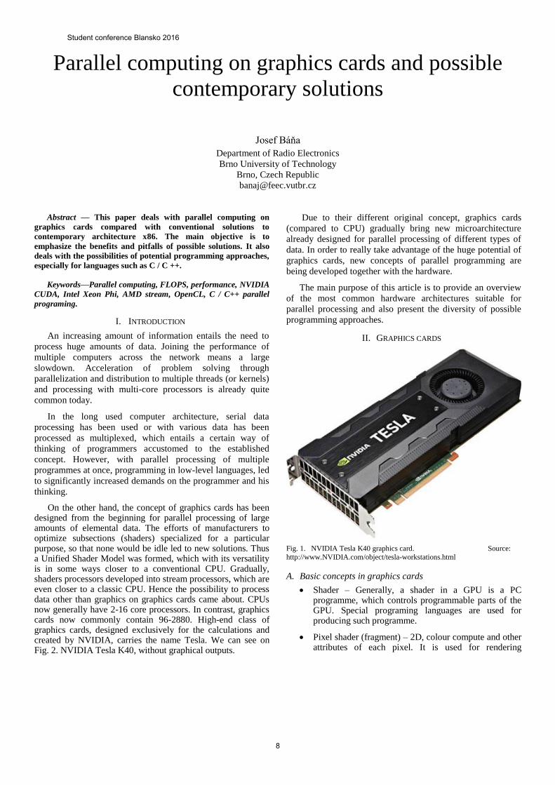
On the other hand, the concept of graphics cards has been designed from the beginning for parallel processing of large amounts of elemental data. The efforts of manufacturers to optimize subsections (shaders) specialized for a particular purpose, so that none would be idle led to new solutions. Thus a Unified Shader Model was formed, which with its versatility is in some ways closer to a conventional CPU. Gradually, shaders processors developed into stream processors, which are even closer to a classic CPU. Hence the possibility to process data other than graphics on graphics cards came about. CPUs now generally have 2-16 core processors. In contrast, graphics cards now commonly contain 96-2880. High-end class of graphics cards, designed exclusively for the calculations and created by NVIDIA, carries the name Tesla. We can see on Fig. 2. NVIDIA Tesla K40, without graphical outputs.
Due to their different original concept, graphics cards
(compared to CPU) gradually bring new microarchitecture
already designed for parallel processing of different types of
data. In order to really take advantage of the huge potential of
graphics cards, new concepts of parallel programming are
being developed together with the hardware.
The main purpose of this article is to provide an overview
of the most common hardware architectures suitable for
parallel processing and also present the diversity of possible
programming approaches.
II. GRAPHICS CARDS
Fig. 1. NVIDIA Tesla K40 graphics card. Source:
http://www.NVIDIA.com/object/tesla-workstations.html
A. Basic concepts in graphics cards
Shader – Generally, a shader in a GPU is a PC programme, which controls programmable parts of the GPU. Special programing languages are used for producing such programme.
Pixel shader (fragment) – 2D, colour compute and other attributes of each pixel. It is used for rendering
Student conference Blansko 2016
8
advanced graphical features such as bump mapping and shadows.
Vertex shader – 3D, it is oriented on scene geometry, it transforms each vertex's 3D position in virtual space to the 2D coordinates in which it appears on the screen. [1]
Geometry shader – it can generate new graphics primitives (points, lines, triangles, etc.) and can perform calculations on it. [2]
Compute shader – possible use for non-graphics applications. [3]
Unified Shader Model (USM known as Shader Model 4.0 in Direct3D 10) – where all of the shader stages in the rendering pipeline (geometry, vertex, pixel, etc.) have the same capabilities. They can all read textures and buffers, and they use instruction sets that are almost identical. Before USM the system was less flexible, sometimes leaving one set of shaders idle if the workload used one more than the other. [4]
GPGPU (General-Purpose computing on graphics processing unit). GPGPU is a technique using parallelization of the graphics card for computing common algorithms, which are usually performed by CPU. These are a few adjustments for increased GPU calculation accuracy and simplify programming, with support for accessible programming interfaces and industry-standard languages. [5]
Single Precision floating-point – computer format of real number that can use 32 bits of memory.
Double Precision floating-point - computer format of real number that can use 64 bits of memory.
SIMD (Single Instruction Multiple Data) - all parallel units share the same instruction, but they carry it out on different data elements. They perform the same operation on multiple data points simultaneously. SIMD threads are used in GPU to minimize thread management.
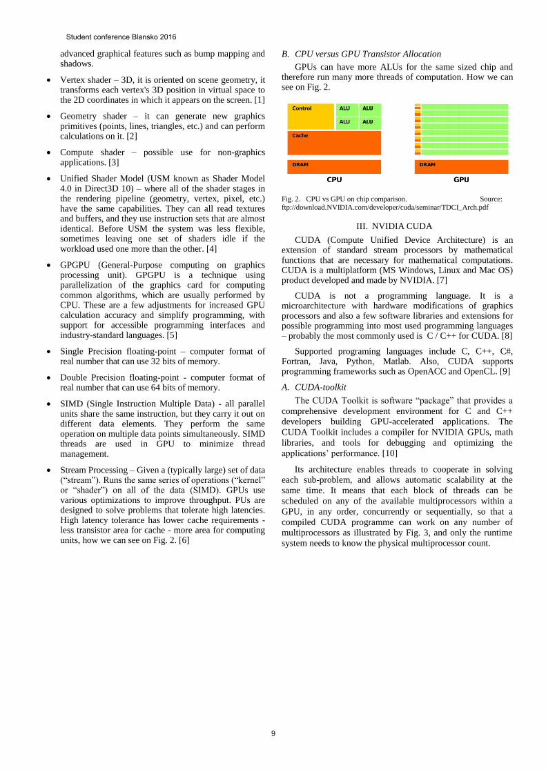
Stream Processing – Given a (typically large) set of data (“stream”). Runs the same series of operations (“kernel” or “shader”) on all of the data (SIMD). GPUs use various optimizations to improve throughput. PUs are designed to solve problems that tolerate high latencies. High latency tolerance has lower cache requirements - less transistor area for cache - more area for computing units, how we can see on Fig. 2. [6]
B. CPU versus GPU Transistor Allocation
GPUs can have more ALUs for the same sized chip and therefore run many more threads of computation. How we can see on Fig. 2.
Fig. 2. CPU vs GPU on chip comparison. Source: ftp://download.NVIDIA.com/developer/cuda/seminar/TDCI_Arch.pdf
III. NVIDIA CUDA
CUDA (Compute Unified Device Architecture) is an extension of standard stream processors by mathematical functions that are necessary for mathematical computations. CUDA is a multiplatform (MS Windows, Linux and Mac OS) product developed and made by NVIDIA. [7]
CUDA is not a programming language. It is a microarchitecture with hardware modifications of graphics processors and also a few software libraries and extensions for possible programming into most used programming languages – probably the most commonly used is C / C++ for CUDA. [8]
Supported programing languages include C, C++, C#, Fortran, Java, Python, Matlab. Also, CUDA supports programming frameworks such as OpenACC and OpenCL. [9]
A. CUDA-toolkit
The CUDA Toolkit is software “package” that provides a
comprehensive development environment for C and C++
developers building GPU-accelerated applications. The
CUDA Toolkit includes a compiler for NVIDIA GPUs, math
libraries, and tools for debugging and optimizing the
applications’ performance. [10]
Its architecture enables threads to cooperate in solving
each sub-problem, and allows automatic scalability at the
same time. It means that each block of threads can be
scheduled on any of the available multiprocessors within a
GPU, in any order, concurrently or sequentially, so that a
compiled CUDA programme can work on any number of
multiprocessors as illustrated by Fig. 3, and only the runtime
system needs to know the physical multiprocessor count.
Student conference Blansko 2016
9
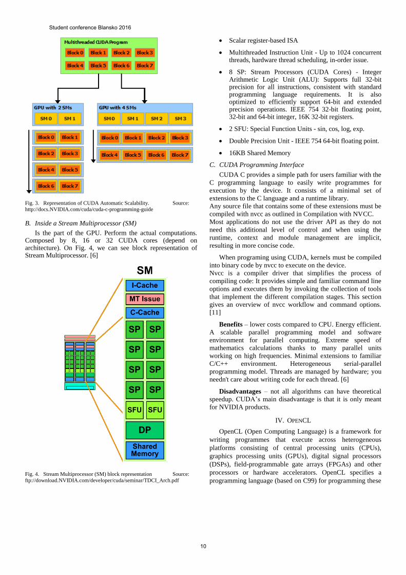
Fig. 3. Representation of CUDA Automatic Scalability. Source: http://docs.NVIDIA.com/cuda/cuda-c-programming-guide
B. Inside a Stream Multiprocessor (SM)
Is the part of the GPU. Perform the actual computations. Composed by 8, 16 or 32 CUDA cores (depend on architecture). On Fig. 4, we can see block representation of Stream Multiprocessor. [6]
Fig. 4. Stream Multiprocessor (SM) block representation Source:
ftp://download.NVIDIA.com/developer/cuda/seminar/TDCI_Arch.pdf
Scalar register-based ISA
Multithreaded Instruction Unit - Up to 1024 concurrent threads, hardware thread scheduling, in-order issue.
8 SP: Stream Processors (CUDA Cores) - Integer Arithmetic Logic Unit (ALU): Supports full 32-bit precision for all instructions, consistent with standard programming language requirements. It is also optimized to efficiently support 64-bit and extended precision operations. IEEE 754 32-bit floating point, 32-bit and 64-bit integer, 16K 32-bit registers.
2 SFU: Special Function Units - sin, cos, log, exp.
Double Precision Unit - IEEE 754 64-bit floating point.
16KB Shared Memory
C. CUDA Programming Interface
CUDA C provides a simple path for users familiar with the
C programming language to easily write programmes for
execution by the device. It consists of a minimal set of
extensions to the C language and a runtime library.
Any source file that contains some of these extensions must be
compiled with nvcc as outlined in Compilation with NVCC.
Most applications do not use the driver API as they do not
need this additional level of control and when using the
runtime, context and module management are implicit,
resulting in more concise code.
When programing using CUDA, kernels must be compiled
into binary code by nvcc to execute on the device.
Nvcc is a compiler driver that simplifies the process of
compiling code: It provides simple and familiar command line
options and executes them by invoking the collection of tools
that implement the different compilation stages. This section
gives an overview of nvcc workflow and command options.
[11]
Benefits – lower costs compared to CPU. Energy efficient.
A scalable parallel programming model and software
environment for parallel computing. Extreme speed of
mathematics calculations thanks to many parallel units
working on high frequencies. Minimal extensions to familiar
C/C++ environment. Heterogeneous serial-parallel
programming model. Threads are managed by hardware; you
needn't care about writing code for each thread. [6]
Disadvantages – not all algorithms can have theoretical
speedup. CUDA’s main disadvantage is that it is only meant
for NVIDIA products.
IV. OPENCL
OpenCL (Open Computing Language) is a framework for
writing programmes that execute across heterogeneous
platforms consisting of central processing units (CPUs),
graphics processing units (GPUs), digital signal processors
(DSPs), field-programmable gate arrays (FPGAs) and other
processors or hardware accelerators. OpenCL specifies a
programming language (based on C99) for programming these
Student conference Blansko 2016
10

devices and application programming interfaces (APIs) to
control the platform and execute programmes on the
computing devices. OpenCL provides a standard interface for
parallel computing using task-based and data-based
parallelism. The first initiator of OpenCL is Apple Inc. [12]
OpenCL is an extension to existing languages. OpenCL is
a low-level API for heterogeneous computing that runs on
CUDA-powered GPUs. Using the OpenCL API, developers
can launch written compute kernels using a limited subset of
the C programming language on a GPU. [13]
The OpenCL standard defines host APIs for C and C++;
third-party APIs exist for other programming languages and
platforms such as Python, Java and .NET.
OpenCL version 2.2 library functions can take advantage
of the C++ language to provide increased safety and reduced
undefined behaviour while accessing features such as atomics,
iterators, images, samplers, pipes, and device queue built-in
types and address spaces. [14]
Benefits – universal programming usable for different
hardware. Highly portable to another hardware architectures.
It is planned to add support for other hardware architectures
e.g. DSPs (digital signal processors). In version OpenCL 2.2
was more implemented support for FPGAs (field-
programmable gate arrays)
Disadvantages – more knowledge is necessary, a more
difficult programme compared to the standard approach.
It is necessary to rewrite lot of code.
V. DEVICE PERFORMANCE COMPARISON
A. NVIDIA graphics cards with CUDA
Fir high level programming, you need add only a few
CUDA headers to your C / C++ code. But parallel programing
on graphics cards needs current code rewriting.
Graphics cards have lower performance than the competition
at double precision computing. It is due to the fact that every
third stream processor also has a support double. In newer
cards intended primarily for the gaming segment (GeForce
and Quadro series), double precision performance is even
worse. [6]
NVIDIA Maxwell architecture (3th)
• 512 – 3584 CUDA cores, • 2 – 16 GB DDR5.
Benefits – (there is no need to learn a new programming
language. Only the techniques of parallel processing. Using
ready-optimized libraries. Already programmed codes can be
used, which do not require parallel processing. Detailed
documentation. Own CUDA repository for many Linux
distributions).
Disadvantages – Elements of calculations must not be
dependent per se, thus it can not be used for addressing all
issues – for example it is totally inefficient for the finite
element method. Parallel programing on graphics cards needs
code rewriting. In many models of graphics cards there is
lower performance when working with double numbers -
double precision.
B. AMD stream graphics cards with OpenCL
AMD lags in benchmark tests behind competing NVIDIA
products. Lower throughput and fewer operations per second
This is probably primarily due to the fact that in recent years,
AMD focused on inventing new architecture GCN (Graphics
Core Next) suitable for parallel computing and easier
programming, whereas NVIDIA expanded the existing
graphics cards concept.
AMD Volcanic Architecture (3rd)
• 1792 – 4096 stream processors, • 2 – 8 GB DDR5.
Benefits – lower price (about 2/3) with a similar absolute
output (absolute performance) of the competing NVIDIA.
Disadvantages – AMD lags in benchmark tests behind
competing NVIDIA latest products. Lower throughput and
fewer operations per second. Only OpenCL support.
C. Intel Xeon Phi
This is not a graphics card, its philosophy is based largely on
the x86 multi-core CPU concept. Design is derived from
Atom, but they hat Hyper-Treading support. Knights Landing
has 4 thread per core.
Programmes designed for today's Xeon processors in
supercomputers will thus operate almost without any
problems, yet optimization will be necessary for making use
of ultimate performance. It is not necessary however to
completely overwrite programmes and thus programmers can
focus only on optimizing. A more universal application for
computations of a wider range of problems. [15] [16]
Intel Knights Landing Architecture (2rd)
• 50 – 72 cores, • 8 – 16 GB DDR4.
Benefits - Programs designed for contemporary Xeon
server processors will operate almost without any problems,
but it will be necessary code optimization for ultimate
performance. There is no need to rewrite existing programs
and programmers can focus only on optimizing. Universal
application for computations, wider spectrum of problems.
Newer “nanometres technology”. [17]
Disadvantages – At the moment they do not achieve so
much FLOPS, compared to competitive solutions. Intel is the
youngest in the field of parallel computing cards. Neither the
hiring many top engineers it fails to catch up with the years of
experience of competing brands.
Student conference Blansko 2016
11
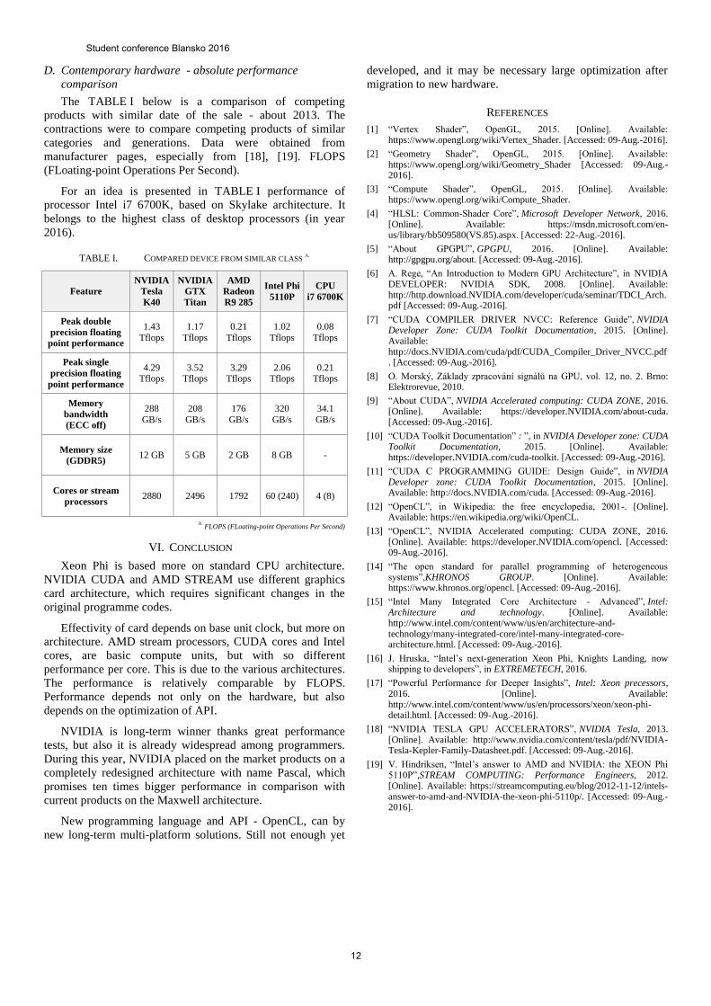
D. Contemporary hardware - absolute performance
comparison
The TABLE I below is a comparison of competing
products with similar date of the sale - about 2013. The
contractions were to compare competing products of similar
categories and generations. Data were obtained from
manufacturer pages, especially from [18], [19]. FLOPS
(FLoating-point Operations Per Second).
For an idea is presented in TABLE I performance of
processor Intel i7 6700K, based on Skylake architecture. It
belongs to the highest class of desktop processors (in year
2016).
TABLE I. COMPARED DEVICE FROM SIMILAR CLASS A.
Feature
NVIDIA
Tesla
K40
NVIDIA
GTX
Titan
AMD
Radeon
R9 285
Intel Phi
5110P
CPU
i7 6700K
Peak double
precision floating
point performance
1.43
Tflops
1.17
Tflops
0.21
Tflops
1.02
Tflops
0.08
Tflops
Peak single
precision floating
point performance
4.29 Tflops
3.52 Tflops
3.29 Tflops
2.06 Tflops
0.21 Tflops
Memory
bandwidth
(ECC off)
288
GB/s
208
GB/s
176
GB/s
320
GB/s
34.1
GB/s
Memory size
(GDDR5) 12 GB 5 GB 2 GB 8 GB -
Cores or stream
processors 2880 2496 1792 60 (240) 4 (8)
a. FLOPS (FLoating-point Operations Per Second)
VI. CONCLUSION
Xeon Phi is based more on standard CPU architecture.
NVIDIA CUDA and AMD STREAM use different graphics
card architecture, which requires significant changes in the
original programme codes.
Effectivity of card depends on base unit clock, but more on
architecture. AMD stream processors, CUDA cores and Intel
cores, are basic compute units, but with so different
performance per core. This is due to the various architectures.
The performance is relatively comparable by FLOPS.
Performance depends not only on the hardware, but also
depends on the optimization of API.
NVIDIA is long-term winner thanks great performance
tests, but also it is already widespread among programmers.
During this year, NVIDIA placed on the market products on a
completely redesigned architecture with name Pascal, which
promises ten times bigger performance in comparison with
current products on the Maxwell architecture.
New programming language and API - OpenCL, can by
new long-term multi-platform solutions. Still not enough yet
developed, and it may be necessary large optimization after
migration to new hardware.
REFERENCES
[1] “Vertex Shader”, OpenGL, 2015. [Online]. Available: https://www.opengl.org/wiki/Vertex_Shader. [Accessed: 09-Aug.-2016].
[2] “Geometry Shader”, OpenGL, 2015. [Online]. Available: https://www.opengl.org/wiki/Geometry_Shader [Accessed: 09-Aug.-2016].
[3] “Compute Shader”, OpenGL, 2015. [Online]. Available: https://www.opengl.org/wiki/Compute_Shader.
[4] “HLSL: Common-Shader Core”, Microsoft Developer Network, 2016. [Online]. Available: https://msdn.microsoft.com/en-us/library/bb509580(VS.85).aspx. [Accessed: 22-Aug.-2016].
[5] “About GPGPU”, GPGPU, 2016. [Online]. Available: http://gpgpu.org/about. [Accessed: 09-Aug.-2016].
[6] A. Rege, “An Introduction to Modern GPU Architecture”, in NVIDIA DEVELOPER: NVIDIA SDK, 2008. [Online]. Available: http://http.download.NVIDIA.com/developer/cuda/seminar/TDCI_Arch.pdf [Accessed: 09-Aug.-2016].
[7] “CUDA COMPILER DRIVER NVCC: Reference Guide”, NVIDIA Developer Zone: CUDA Toolkit Documentation, 2015. [Online]. Available: http://docs.NVIDIA.com/cuda/pdf/CUDA_Compiler_Driver_NVCC.pdf. [Accessed: 09-Aug.-2016].
[8] O. Morský, Základy zpracování signálů na GPU, vol. 12, no. 2. Brno: Elektrorevue, 2010.
[9] “About CUDA”, NVIDIA Accelerated computing: CUDA ZONE, 2016. [Online]. Available: https://developer.NVIDIA.com/about-cuda. [Accessed: 09-Aug.-2016].
[10] “CUDA Toolkit Documentation” : ”, in NVIDIA Developer zone: CUDA Toolkit Documentation, 2015. [Online]. Available: https://developer.NVIDIA.com/cuda-toolkit. [Accessed: 09-Aug.-2016].
[11] “CUDA C PROGRAMMING GUIDE: Design Guide”, in NVIDIA Developer zone: CUDA Toolkit Documentation, 2015. [Online]. Available: http://docs.NVIDIA.com/cuda. [Accessed: 09-Aug.-2016].
[12] “OpenCL”, in Wikipedia: the free encyclopedia, 2001-. [Online]. Available: https://en.wikipedia.org/wiki/OpenCL.
[13] “OpenCL”, NVIDIA Accelerated computing: CUDA ZONE, 2016. [Online]. Available: https://developer.NVIDIA.com/opencl. [Accessed: 09-Aug.-2016].
[14] “The open standard for parallel programming of heterogeneous systems”,KHRONOS GROUP. [Online]. Available: https://www.khronos.org/opencl. [Accessed: 09-Aug.-2016].
[15] “Intel Many Integrated Core Architecture - Advanced”, Intel: Architecture and technology. [Online]. Available: http://www.intel.com/content/www/us/en/architecture-and-technology/many-integrated-core/intel-many-integrated-core-architecture.html. [Accessed: 09-Aug.-2016].
[16] J. Hruska, “Intel’s next-generation Xeon Phi, Knights Landing, now shipping to developers”, in EXTREMETECH, 2016.
[17] “Powerful Performance for Deeper Insights”, Intel: Xeon precessors, 2016. [Online]. Available: http://www.intel.com/content/www/us/en/processors/xeon/xeon-phi-detail.html. [Accessed: 09-Aug.-2016].
[18] “NVIDIA TESLA GPU ACCELERATORS”, NVIDIA Tesla, 2013. [Online]. Available: http://www.nvidia.com/content/tesla/pdf/NVIDIA-Tesla-Kepler-Family-Datasheet.pdf. [Accessed: 09-Aug.-2016].
[19] V. Hindriksen, “Intel’s answer to AMD and NVIDIA: the XEON Phi 5110P”,STREAM COMPUTING: Performance Engineers, 2012. [Online]. Available: https://streamcomputing.eu/blog/2012-11-12/intels-answer-to-amd-and-NVIDIA-the-xeon-phi-5110p/. [Accessed: 09-Aug.-2016].
Student conference Blansko 2016
12
3D Textile Integrated TIW Horn Antenna for UWB
Wirelles Link
Miroslav Cupal
Department of Radio Electronics
Brno University of Technology
Technická 12, 61600, Brno, Czech Republic
Abstract—This paper deals with textile integrated H–plane
horn antenna for in-car communication. The antenna is designed
on 3D textile material produced by SINTEX Company. The
antenna is placed close to conductive plate which simulates roof
of a car or small planes and buses. Results for different distances
between the antenna and the metal plate are presented as well.
Keywords— horn antenna; 3D textile; TIW; car; UWB;
I. INTRODUCTION
Most of automobile manufacturers produce automobiles with large number of sensors. These sensors improve quality of traveling, safety and they help with driving. There are first examples of full autonomy cars that can drive without driver’s assistance. Small wire networks are used for connection small modules like parking cameras, radars, air-condition sensors etc. The weight of the wires is approximately 35 kg for one car. The part of the wires would be replaced with wireless system.
UWB system could be very good solution for in-car communication between central unit and sensors, safety systems or between central unit and audio-video equipment. The theoretical bandwidth of UWB system is more than 500 MHz or 20% of fractional bandwidth [1].
The spectrum for UWB has been defined up 3.1-10.6 GHz. The WiMedia alliance has defined fourteen 528 MHz bands in 2002. The band group 6 is very interesting because it is the only band where all countries agree. The division of the UWB is shown in Fig. 1 [1].
Fig. 1. Ultra-wide band frequency map
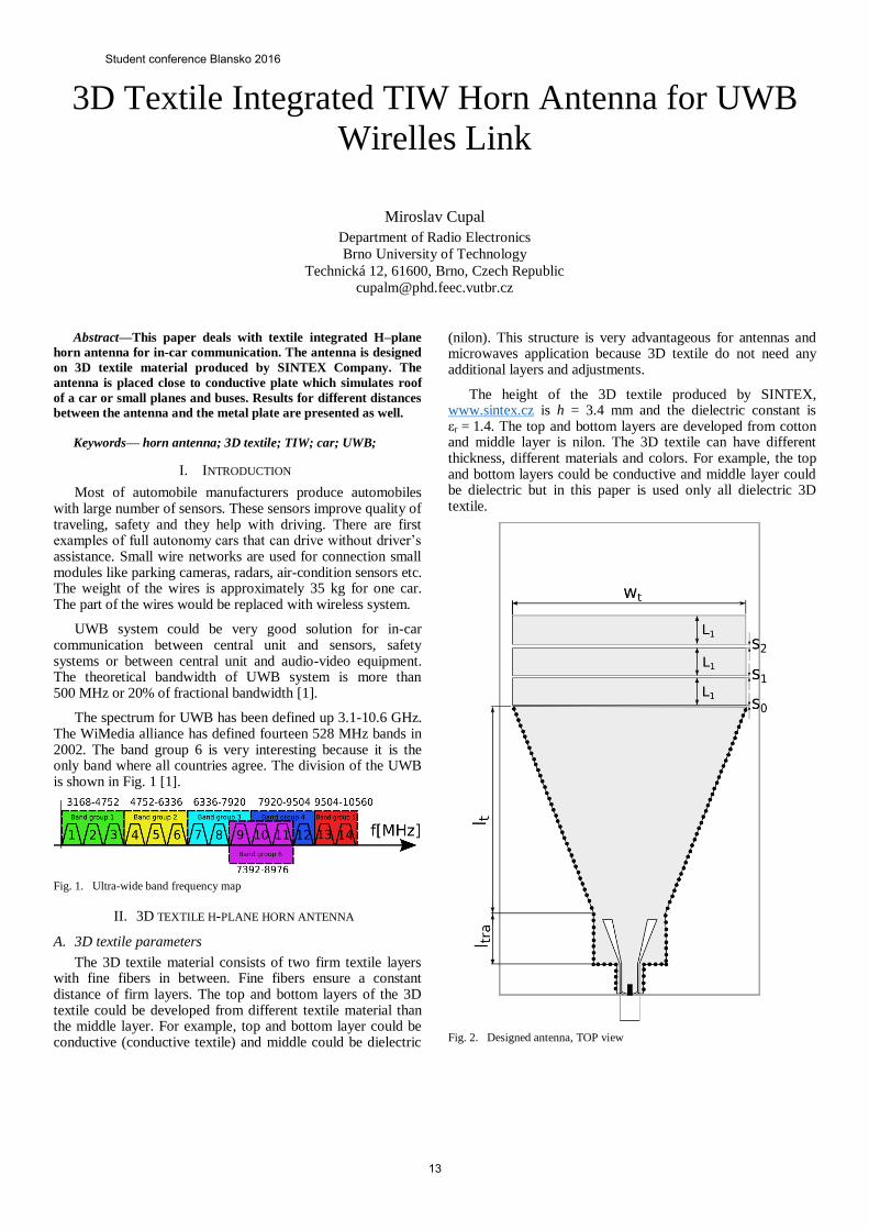
II. 3D TEXTILE H-PLANE HORN ANTENNA
A. 3D textile parameters
The 3D textile material consists of two firm textile layers with fine fibers in between. Fine fibers ensure a constant distance of firm layers. The top and bottom layers of the 3D textile could be developed from different textile material than the middle layer. For example, top and bottom layer could be conductive (conductive textile) and middle could be dielectric
(nilon). This structure is very advantageous for antennas and microwaves application because 3D textile do not need any additional layers and adjustments.
The height of the 3D textile produced by SINTEX, www.sintex.cz is h = 3.4 mm and the dielectric constant is εr = 1.4. The top and bottom layers are developed from cotton and middle layer is nilon. The 3D textile can have different thickness, different materials and colors. For example, the top and bottom layers could be conductive and middle layer could be dielectric but in this paper is used only all dielectric 3D textile.
Fig. 2. Designed antenna, TOP view
Student conference Blansko 2016
13

B. H-plne horn antenna design
The design of an H-plane TIW horn antenna is very similar of a conventional pyramidal horn antenna. The antenna is fed with textile integrated waveguide. I have to respect basic design rules for a single mode excitation resulting in the condition 1[2].
𝜆0√2𝜀𝑟 < 𝑎 <𝜆0
𝜀𝑟,
,where λ0 is wavelength in free space, εr dielectric constant, a is width of waveguide.
The excitation of the TIW is realized with GCPW (grounded coplanar waveguide). There is a small problem because the width of the GCPW is large than the diameter of the SMA connector. Therefore, I need to use the edited GCPW close to SMA connector [2] and [3,7-9].
Fig. 3. Antenna feeding structure
I use planar resonators front of the horn to improve bandwidth and radiation patterns of the antenna. There are three planar resonators front of the horn with the same dimensions. Gaps between resonators are different to improve frequency bandwidth and radiation patterns. The resonance frequency of one resonator is
𝑓𝑟1 =𝑐
2𝑙𝑒𝑞√𝜀𝑟
where fr1 is resonant frequency, c is speed of light, leq is equivalent length of the resonator and εr is the dielectric constant of the substrate. There are capacitive couples between resonators. The resonant frequency of the coupled resonator can be calculated with:
𝑓𝑟2± =𝑓𝑟1
√1±𝑘2
where k2 is the coupling factor [4-6].
C. Designed antenna
Feeding of the textile integrated waveguide is realized with SMA connector connected to grounded coplanar waveguide. You can see the detail of the feeding structure at the Fig. 3. The feeding structure is designed for minimal radiation into surrounding space. The designed antenna is depicted in Fig. 1 and the numerical values are shown in Table 1.
TABLE I. PARAMETERS OF DESIGNED ANTENNA
Dimension wt ltra lt L1 S0
Value [mm] 90 18.85 80 10.05 0.25
Dimension S1 S2
Value [mm] 0.88 1.77
III. SIMULATION RESULTS
The antenna was simulated in the CST Microwave Studio. The antenna was simulated in free space and close to conductive plate. The conductive plate was covered with 3D textile material and the gap between metal plate and the 3D textile material was 0 mm.
A. Antnna 0 milimetrs of metal plate
Frequency response of the reflection coefficient of the designed antenna operating close to metal plate is depicted in Fig. 4. The impedance bandwidth for S11 < -10 dB is BW = 4.86 GHz (55 %). The antenna covers 100 % of UWB band-group 6 (7.392 to 8.976 GHz).
Fig. 4. Frequency response of reflection coefficient antenna close to metal
plate
In Chyba! Nenalezen zdroj odkazů. and Chyba!
Nenalezen zdroj odkazů. are radiations patterns of the
antenna in planes E and H for nine frequencies. The simulated
maximal gain of the antenna close to metal plate is 13.23 dBi
in the main lobe direction at 8 GHz. The elevation angle in E-
plane is 20°. In H-plane, the simulated gain is 11.87 dBi. At a
frequency 8 GHz, the antenna radiates perpendicularly to the
plane of the substrate. A high level of side lobes is the
disadvantage of the antenna. The average side lobe level is
12 dBi in E-plane.
B. Antenna in different distances of metal plate
H-plane horn antenna was simulated in different distances between antenna and metal plate. The attention was paid to
Simulations and experiments in laboratories of the SIX
Center were financed by the project LO1401 INWITE of the
National Sustainability Program. Research is a part of the
COST Action IC 1301 WiPE supported by the grant LD14057
of the Czech Ministry of Education.
Student conference Blansko 2016
14
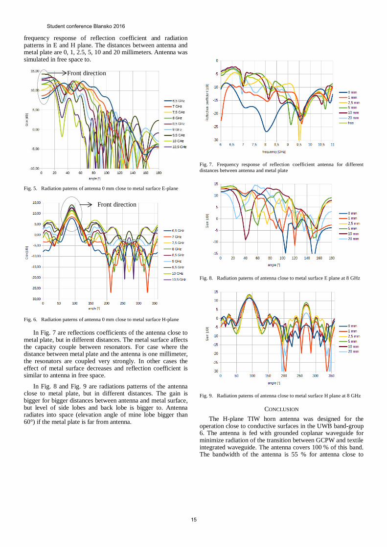
frequency response of reflection coefficient and radiation patterns in E and H plane. The distances between antenna and metal plate are 0, 1, 2.5, 5, 10 and 20 millimeters. Antenna was simulated in free space to.
Fig. 5. Radiation paterns of antenna 0 mm close to metal surface E-plane
Fig. 6. Radiation paterns of antenna 0 mm close to metal surface H-plane
In Fig. 7 are reflections coefficients of the antenna close to metal plate, but in different distances. The metal surface affects the capacity couple between resonators. For case where the distance between metal plate and the antenna is one millimeter, the resonators are coupled very strongly. In other cases the effect of metal surface decreases and reflection coefficient is similar to antenna in free space.
In Fig. 8 and Fig. 9 are radiations patterns of the antenna close to metal plate, but in different distances. The gain is bigger for bigger distances between antenna and metal surface, but level of side lobes and back lobe is bigger to. Antenna radiates into space (elevation angle of mine lobe bigger than 60°) if the metal plate is far from antenna.
Fig. 7. Frequency response of reflection coefficient antenna for different
distances between antenna and metal plate
Fig. 8. Radiation paterns of antenna close to metal surface E plane at 8 GHz
Fig. 9. Radiation paterns of antenna close to metal surface H plane at 8 GHz
CONCLUSION
The H-plane TIW horn antenna was designed for the operation close to conductive surfaces in the UWB band-group 6. The antenna is fed with grounded coplanar waveguide for minimize radiation of the transition between GCPW and textile integrated waveguide. The antenna covers 100 % of this band. The bandwidth of the antenna is 55 % for antenna close to
Front direction
Front direction
Student conference Blansko 2016
15

metal surface as is possible. The antenna shows an elevation 20° in proximity of a conductive plate.
Antenna was simulated in different distances of metal plate. Metal plate affects planar resonators front of the horn and properties of the antenna. To use the antenna in different distances have to be edited length of the resonators and the gaps between them.
REFERENCES
[1] I. Oppermann, M. Hämäläinen and J. Iinatti. UWB theory and applications. Chichester: Wiley, 2004.
[2] X. Chen, W. Hong, T. Cui, J. Chen, and K. Wu. "Substrate integrated waveguide (SIW) linear phase filter," IEEE Microwave and Wireless Components Letters, vol. 15, issue 11, pp.
[3] F. Giuppi, A. Georgiadis, A. Collado, M. Bozzi, and L. Perregrini. "Tunable SIW cavity backed active antenna oscillator," Electronics Letters, vol. 46, issue 15, pp. 1053-, 2010.
[4] C. I. Yeh, D. H. Yang, T. H. Liu, Jeffrey S. Fu, K. S. Chin, J. C. Cheng, Chiu, and C. P. Kao. "MMIC compatibility study of SIW H-plane horn antenna," 2010 International Conference on Microwave and Millimeter Wave Technology, pp. 933-936, 2010.
[5] M. Esquius-Morote, B. Fuchs, Jean-Francois Zurcher, and J. R. Mosig. "A Printed Transition for Matching Improvement of SIW Horn Antennas," IEEE Transactions on Antennas and Propagation, vol. 61, issue 4, pp. 1923-1930, 2013.
[6] M. Esquius-Morote, B. Fuchs, Jean-Francois Zurcher, and J. R. Mosig. "Novel Thin and Compact H-Plane SIW Horn Antenna," IEEE Transactions on Antennas and Propagation, vol. 61, issue 6, pp. 2911-2920, 2013.
[7] C. A. Balanis. Antenna theory: analysis and design, 3rd ed. Hoboken: Wiley-Interscience, 2005. ISBN 978-0-471-66782-7.
[8] T. Mikulasek, A. Georgiadis, A. Collado, and J. Lacik. Microstrip Patch Antenna Array Fed by Substrate Integrated Waveguide for Radar Applications,"IEEE Antennas and Wireless Propagation Letters, vol. 12, pp. 1287-1290, 2013.
[9] J. Lacik and T. Mikulasek, “Circular ring-slot antenna fed by SIW for WBAN applications,” in Proc. 7th Eur. Conf. on Antennas and Propagation (EuCAP), Gothenburg, Sweden, Apr. 2013, pp. 213–216
Student conference Blansko 2016
16
Electronically Reconfigurable Universal FrequencyFilter with Controllability of its Pole Frequency
Jan DvorakFaculty of Electrical Engineering and
CommunicationBrno University of Technology
Brno 616 00, Technicka 12Email: [email protected]
Adam GajdosFaculty of Electrical Engineering and
CommunicationBrno University of Technology
Brno 616 00, Technicka 12Email: [email protected]
Jan JerabekFaculty of Electrical Engineering and
CommunicationBrno University of Technology
Brno 616 00, Technicka 12Email: [email protected]
Abstract—This paper deals with electronically reconfigurablecurrent-mode filter with controllable pole frequency. The pro-posed filter contains these active elements: Current ConveyorTransconductance Amplifier (CCTA), Operational Transconduc-tance Amplifier (OTA) and Adjustable Current Amplifier (ACA).The filter contains only single input and output (SISO). Thefiltering functions of the circuit can be electronically switched bycurrent gain of the ACA elements without any reconnection intopology. The reconfigurable filter provides the ability to controlpole frequency without disturbing quality factor. The PSpicesimulator was used for verifying function of the proposed filterusing available models of the active elements.
I. INTRODUCTION
The digital signal processing is the highly interested topicnowadays. However, there are still many scientific teams, whoare interest about analogue frequency filters [1] – [15]. Thegreat area of interest are filtering structures, which can realizevarious filtering functions or it is possible to control some ofits parameters (pole frequency, quality factor, pass–band gain,bandwidth or the order of the filter).
Most of the papers describe the filtering structures, whichallow to obtain all types of the transfer functions (low-pass,band-pass, high-pass, band-reject or all-pass) with adjustableparameters [1] – [11]. The transfer functions are usuallyobtained by manual reconnection of an output or input of thefilter. The frequency filters can be divided according to numberof inputs and outputs: single input-multiple output (SIMO) [1],[2], [4], [6] – [8], multiple input-single output (MISO) [3] orsingle input-single output (SISO) [9] – [14] filtering structures.
Reconfigurable filtering circuits represent one of the newertopic, which is attractive to many scientific teams [9] –[15]. These circuits contain only one input and output (SISOtype of filtering structure). Nevertheless, the various typesof transfer functions can be obtained from single output ofthe structure using electronically controlling of parametersof active elements. It is thus a filter which provides moretypes of transfer functions without manual reconnection of itsinput or output. Except reconfiguration of the type of transferfunction, controllability of the pole frequency or quality factoris possible depending to selected types of the active elementsof a proposed filter. The wide variety of active elements canbe used for the design of a reconfigurable filter. For example,Operational Transconductance Amplifier (OTA) [6], [16], Cur-rent Conveyor Transconductance Amplifier (CCTA) [8], [16],
[17], Voltage Differencing Current Conveyor (VDCC) [16],Modified Current Differencing Unit (MCDU) [9] or AdjustableCurrent Amplifier (ACA) [18].
This paper deals with proposal of the universal recon-figurable frequency filter that operates in current mode. Thecircuit consists of CCTA, OTA and ACA active elements asdescribed in section II. The proposed filter provides electronicswitching of the various types of transfer functions and tuningof the pole frequency using adjustable parameters of the usedactive elements. The filter features were verified by PSpicesimulations.
II. USED ACTIVE ELEMENTS
This section present the description of active elements,which are used for proposal of the filter. The filter structurecontains three types of the used active elements.
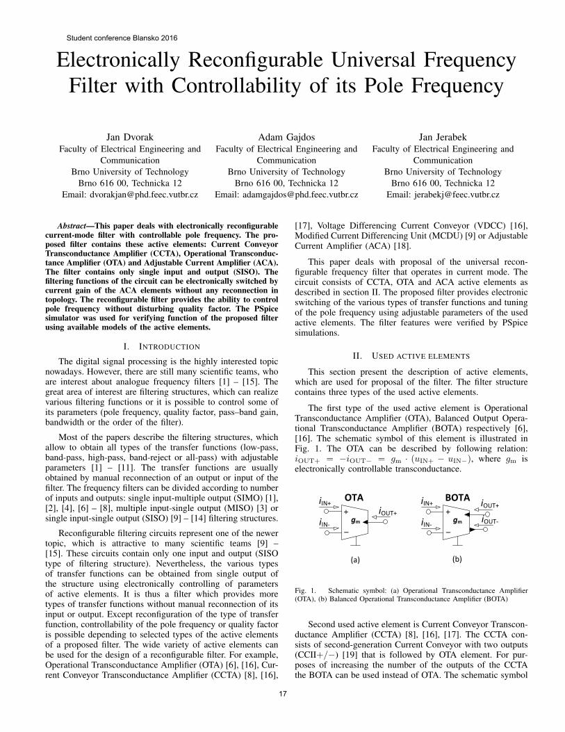
The first type of the used active element is OperationalTransconductance Amplifier (OTA), Balanced Output Opera-tional Transconductance Amplifier (BOTA) respectively [6],[16]. The schematic symbol of this element is illustrated inFig. 1. The OTA can be described by following relation:iOUT+ = −iOUT− = gm · (uIN+ − uIN−), where gm iselectronically controllable transconductance.
OTA
+
_gm
iIN+
iIN-iOUT+
BOTA
+
_gm
iIN+
iIN-
iOUT+
iOUT-
(a) (b)
Fig. 1. Schematic symbol: (a) Operational Transconductance Amplifier(OTA), (b) Balanced Operational Transconductance Amplifier (BOTA)
Second used active element is Current Conveyor Transcon-ductance Amplifier (CCTA) [8], [16], [17]. The CCTA con-sists of second-generation Current Conveyor with two outputs(CCII+/−) [19] that is followed by OTA element. For pur-poses of increasing the number of the outputs of the CCTAthe BOTA can be used instead of OTA. The schematic symbol
Student conference Blansko 2016
17
is shown in Fig. 2, together with internal block structure. Thebasic adjustable parameter of this element is transconductancegm. This element can be described by the following matrix: iY
uXiZiOUT
=
0 0 01 0 00 1 00 0 gm
· [uYiXuZ
]. (1)
OTA
+
_gm
iOUT
(a)
YS
XS
ZS+
ZS-
CCII+/-
CCTA
iZ
iX
iYCCTA
iX
iY
iZ
iOUTY
XZ
(b)
gm OUT
Fig. 2. Current Conveyor Transconductance Amplifier (CCTA): (a) Schematicsymbol, (b) internal block structure
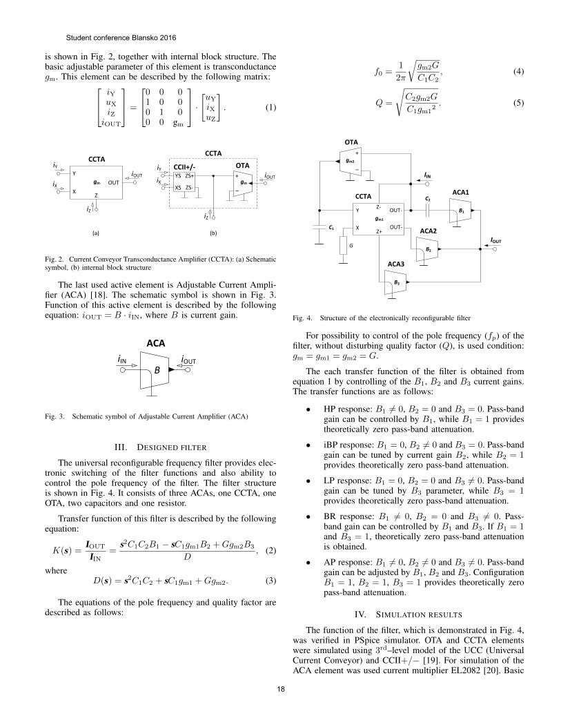
The last used active element is Adjustable Current Ampli-fier (ACA) [18]. The schematic symbol is shown in Fig. 3.Function of this active element is described by the followingequation: iOUT = B · iIN, where B is current gain.
B
ACA
iIN iOUT
Fig. 3. Schematic symbol of Adjustable Current Amplifier (ACA)
III. DESIGNED FILTER
The universal reconfigurable frequency filter provides elec-tronic switching of the filter functions and also ability tocontrol the pole frequency of the filter. The filter structureis shown in Fig. 4. It consists of three ACAs, one CCTA, oneOTA, two capacitors and one resistor.
Transfer function of this filter is described by the followingequation:
K(s) =IOUT
IIN=
s2C1C2B1 − sC1gm1B2 +Ggm2B3
D, (2)
whereD(s) = s2C1C2 + sC1gm1 +Ggm2. (3)
The equations of the pole frequency and quality factor aredescribed as follows:
f0 =1
2π
√gm2G
C1C2, (4)
Q =
√C2gm2G
C1gm12. (5)
CCTA
Y
X
Z-
gm1
OUT-
Z+OUT-C1
ACA1
B1
+
_
gm2
OTA
G
C2
ACA2
B2
ACA3
B3
IIN
IOUT
Fig. 4. Structure of the electronically reconfigurable filter
For possibility to control of the pole frequency (fp) of thefilter, without disturbing quality factor (Q), is used condition:gm = gm1 = gm2 = G.
The each transfer function of the filter is obtained fromequation 1 by controlling of the B1, B2 and B3 current gains.The transfer functions are as follows:
• HP response: B1 6= 0, B2 = 0 and B3 = 0. Pass-bandgain can be controlled by B1, while B1 = 1 providestheoretically zero pass-band attenuation.
• iBP response: B1 = 0, B2 6= 0 and B3 = 0. Pass-bandgain can be tuned by current gain B2, while B2 = 1provides theoretically zero pass-band attenuation.
• LP response: B1 = 0, B2 = 0 and B3 6= 0. Pass-bandgain can be tuned by B3 parameter, while B3 = 1provides theoretically zero pass-band attenuation.
• BR response: B1 6= 0, B2 = 0 and B3 6= 0. Pass-band gain can be controlled by B1 and B3. If B1 = 1and B3 = 1, theoretically zero pass-band attenuationis obtained.
• AP response: B1 6= 0, B2 6= 0 and B3 6= 0. Pass-bandgain can be adjusted by B1, B2 and B3. ConfigurationB1 = 1, B2 = 1, B3 = 1 provides theoretically zeropass-band attenuation.
IV. SIMULATION RESULTS
The function of the filter, which is demonstrated in Fig. 4,was verified in PSpice simulator. OTA and CCTA elementswere simulated using 3rd–level model of the UCC (UniversalCurrent Conveyor) and CCII+/− [19]. For simulation of theACA element was used current multiplier EL2082 [20]. Basic
Student conference Blansko 2016
18
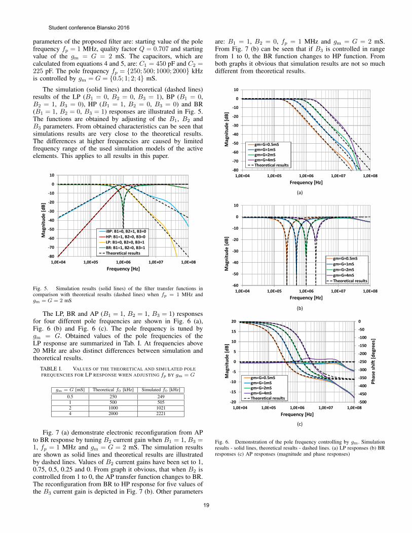
parameters of the proposed filter are: starting value of the polefrequency fp = 1 MHz, quality factor Q = 0.707 and startingvalue of the gm = G = 2 mS. The capacitors, which arecalculated from equations 4 and 5, are: C1 = 450 pF and C2 =225 pF. The pole frequency fp = 250; 500; 1000; 2000 kHzis controlled by gm = G = 0.5; 1; 2; 4 mS.
The simulation (solid lines) and theoretical (dashed lines)results of the LP (B1 = 0, B2 = 0, B3 = 1), BP (B1 = 0,B2 = 1, B3 = 0), HP (B1 = 1, B2 = 0, B3 = 0) and BR(B1 = 1, B2 = 0, B3 = 1) responses are illustrated in Fig. 5.The functions are obtained by adjusting of the B1, B2 andB3 parameters. From obtained characteristics can be seen thatsimulations results are very close to the theoretical results.The differences at higher frequencies are caused by limitedfrequency range of the used simulation models of the activeelements. This applies to all results in this paper.
-80
-70
-60
-50
-40
-30
-20
-10
0
10
1,0E+04 1,0E+05 1,0E+06 1,0E+07 1,0E+08
Ma
gnit
ud
e[d
B]
Frequency [Hz]
iBP: B1=0, B2=1, B3=0HP: B1=1, B2=0, B3=0LP: B1=0, B2=0, B3=1BR: B1=1, B2=0, B3=1Theoretical results
Fig. 5. Simulation results (solid lines) of the filter transfer functions incomparison with theoretical results (dashed lines) when fp = 1 MHz andgm = G = 2 mS
The LP, BR and AP (B1 = 1, B2 = 1, B3 = 1) responsesfor four different pole frequencies are shown in Fig. 6 (a),Fig. 6 (b) and Fig. 6 (c). The pole frequency is tuned bygm = G. Obtained values of the pole frequencies of theLP response are summarized in Tab. I. At frequencies above20 MHz are also distinct differences between simulation andtheoretical results.
TABLE I. VALUES OF THE THEORETICAL AND SIMULATED POLEFREQUENCIES FOR LP RESPONSE WHEN ADJUSTING fp BY gm = G
gm = G [mS] Theoretical f0 [kHz] Simulated f0 [kHz]0.5 250 2491 500 5052 1000 10214 2000 2221
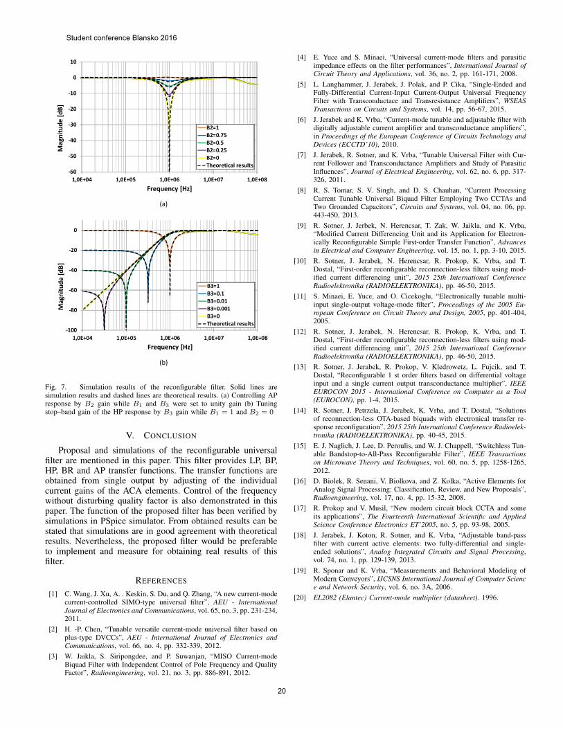
Fig. 7 (a) demonstrate electronic reconfiguration from APto BR response by tuning B2 current gain when B1 = 1, B3 =1, fp = 1 MHz and gm = G = 2 mS. The simulation resultsare shown as solid lines and theoretical results are illustratedby dashed lines. Values of B2 current gains have been set to 1,0.75, 0.5, 0.25 and 0. From graph it obvious, that when B2 iscontrolled from 1 to 0, the AP transfer function changes to BR.The reconfiguration from BR to HP response for five values ofthe B3 current gain is depicted in Fig. 7 (b). Other parameters
are: B1 = 1, B2 = 0, fp = 1 MHz and gm = G = 2 mS.From Fig. 7 (b) can be seen that if B3 is controlled in rangefrom 1 to 0, the BR function changes to HP function. Fromboth graphs it obvious that simulation results are not so muchdifferent from theoretical results.
(a)
(b)
(c)
-60
-50
-40
-30
-20
-10
0
10
1,0E+04 1,0E+05 1,0E+06 1,0E+07 1,0E+08
Mag
nit
ud
e[d
B]
Frequency [Hz]
gm=G=0.5mS
gm=G=1mS
gm=G=2mS
gm=G=4mS
Theoretical results
-80
-70
-60
-50
-40
-30
-20
-10
0
10
1,0E+04 1,0E+05 1,0E+06 1,0E+07 1,0E+08
Ma
gnit
ud
e[d
B]
Frequency [Hz]
gm=G=0.5mSgm=G=1mSgm=G=2mSgm=G=4mSTheoretical results
-500
-450
-400
-350
-300
-250
-200
-150
-100
-50
0
-20
-15
-10
-5
0
5
10
15
20
1,0E+04 1,0E+05 1,0E+06 1,0E+07 1,0E+08
Ph
ase
shif
t [d
egre
es]
Mag
nit
ud
e[d
B]
Frequency [Hz]
gm=G=0.5mSgm=G=1mSgm=G=2mSgm=G=4mSTheoretical results
Fig. 6. Demonstration of the pole frequency controlling by gm. Simulationresults - solid lines, theoretical results - dashed lines. (a) LP responses (b) BRresponses (c) AP responses (magnitude and phase responses)
Student conference Blansko 2016
19
(a)
-60
-50
-40
-30
-20
-10
0
10
1,0E+04 1,0E+05 1,0E+06 1,0E+07 1,0E+08
Mag
nit
ud
e[d
B]
Frequency [Hz]
B2=1B2=0.75B2=0.5B2=0.25B2=0Theoretical results
(b)
-100
-80
-60
-40
-20
0
1,0E+04 1,0E+05 1,0E+06 1,0E+07 1,0E+08
Mag
nit
ud
e[d
B]
Frequency [Hz]
B3=1B3=0.1B3=0.01B3=0.001B3=0Theoretical results
Fig. 7. Simulation results of the reconfigurable filter. Solid lines aresimulation results and dashed lines are theoretical results. (a) Controlling APresponse by B2 gain while B1 and B3 were set to unity gain (b) Tuningstop–band gain of the HP response by B3 gain while B1 = 1 and B2 = 0
V. CONCLUSION
Proposal and simulations of the reconfigurable universalfilter are mentioned in this paper. This filter provides LP, BP,HP, BR and AP transfer functions. The transfer functions areobtained from single output by adjusting of the individualcurrent gains of the ACA elements. Control of the frequencywithout disturbing quality factor is also demonstrated in thispaper. The function of the proposed filter has been verified bysimulations in PSpice simulator. From obtained results can bestated that simulations are in good agreement with theoreticalresults. Nevertheless, the proposed filter would be preferableto implement and measure for obtaining real results of thisfilter.
REFERENCES
[1] C. Wang, J. Xu, A. . Keskin, S. Du, and Q. Zhang, “A new current-modecurrent-controlled SIMO-type universal filter”, AEU - InternationalJournal of Electronics and Communications, vol. 65, no. 3, pp. 231-234,2011.
[2] H. -P. Chen, “Tunable versatile current-mode universal filter based onplus-type DVCCs”, AEU - International Journal of Electronics andCommunications, vol. 66, no. 4, pp. 332-339, 2012.
[3] W. Jaikla, S. Siripongdee, and P. Suwanjan, “MISO Current-modeBiquad Filter with Independent Control of Pole Frequency and QualityFactor”, Radioengineering, vol. 21, no. 3, pp. 886-891, 2012.
[4] E. Yuce and S. Minaei, “Universal current-mode filters and parasiticimpedance effects on the filter performances”, International Journal ofCircuit Theory and Applications, vol. 36, no. 2, pp. 161-171, 2008.
[5] L. Langhammer, J. Jerabek, J. Polak, and P. Cika, “Single-Ended andFully-Differential Current-Input Current-Output Universal FrequencyFilter with Transconductace and Transresistance Amplifiers”, WSEASTransactions on Circuits and Systems, vol. 14, pp. 56-67, 2015.
[6] J. Jerabek and K. Vrba, “Current-mode tunable and adjustable filter withdigitally adjustable current amplifier and transconductance amplifiers”,in Proceedings of the European Conference of Circuits Technology andDevices (ECCTD’10), 2010.
[7] J. Jerabek, R. Sotner, and K. Vrba, “Tunable Universal Filter with Cur-rent Follower and Transconductance Amplifiers and Study of ParasiticInfluences”, Journal of Electrical Engineering, vol. 62, no. 6, pp. 317-326, 2011.
[8] R. S. Tomar, S. V. Singh, and D. S. Chauhan, “Current ProcessingCurrent Tunable Universal Biquad Filter Employing Two CCTAs andTwo Grounded Capacitors”, Circuits and Systems, vol. 04, no. 06, pp.443-450, 2013.
[9] R. Sotner, J. Jerbek, N. Herencsar, T. Zak, W. Jaikla, and K. Vrba,“Modified Current Differencing Unit and its Application for Electron-ically Reconfigurable Simple First-order Transfer Function”, Advancesin Electrical and Computer Engineering, vol. 15, no. 1, pp. 3-10, 2015.
[10] R. Sotner, J. Jerabek, N. Herencsar, R. Prokop, K. Vrba, and T.Dostal, “First-order reconfigurable reconnection-less filters using mod-ified current differencing unit”, 2015 25th International ConferenceRadioelektronika (RADIOELEKTRONIKA), pp. 46-50, 2015.
[11] S. Minaei, E. Yuce, and O. Cicekoglu, “Electronically tunable multi-input single-output voltage-mode filter”, Proceedings of the 2005 Eu-ropean Conference on Circuit Theory and Design, 2005, pp. 401-404,2005.
[12] R. Sotner, J. Jerabek, N. Herencsar, R. Prokop, K. Vrba, and T.Dostal, “First-order reconfigurable reconnection-less filters using mod-ified current differencing unit”, 2015 25th International ConferenceRadioelektronika (RADIOELEKTRONIKA), pp. 46-50, 2015.
[13] R. Sotner, J. Jerabek, R. Prokop, V. Kledrowetz, L. Fujcik, and T.Dostal, “Reconfigurable 1 st order filters based on differential voltageinput and a single current output transconductance multiplier”, IEEEEUROCON 2015 - International Conference on Computer as a Tool(EUROCON), pp. 1-4, 2015.
[14] R. Sotner, J. Petrzela, J. Jerabek, K. Vrba, and T. Dostal, “Solutionsof reconnection-less OTA-based biquads with electronical transfer re-sponse reconfiguration”, 2015 25th International Conference Radioelek-tronika (RADIOELEKTRONIKA), pp. 40-45, 2015.
[15] E. J. Naglich, J. Lee, D. Peroulis, and W. J. Chappell, “Switchless Tun-able Bandstop-to-All-Pass Reconfigurable Filter”, IEEE Transactionson Microwave Theory and Techniques, vol. 60, no. 5, pp. 1258-1265,2012.
[16] D. Biolek, R. Senani, V. Biolkova, and Z. Kolka, “Active Elements forAnalog Signal Processing: Classification, Review, and New Proposals”,Radioengineering, vol. 17, no. 4, pp. 15-32, 2008.
[17] R. Prokop and V. Musil, “New modern circuit block CCTA and someits applications”, The Fourteenth International Scientific and AppliedScience Conference Electronics ET’2005, no. 5, pp. 93-98, 2005.
[18] J. Jerabek, J. Koton, R. Sotner, and K. Vrba, “Adjustable band-passfilter with current active elements: two fully-differential and single-ended solutions”, Analog Integrated Circuits and Signal Processing,vol. 74, no. 1, pp. 129-139, 2013.
[19] R. Sponar and K. Vrba, “Measurements and Behavioral Modeling ofModern Conveyors”, IJCSNS International Journal of Computer Science and Network Security, vol. 6, no. 3A, 2006.
[20] EL2082 (Elantec) Current-mode multiplier (datasheet). 1996.
Student conference Blansko 2016
20
High Precision Motor Control in FPGA for Space
Applications
Vojtech Dvorak
Department of Microelectronics
Brno University of Technology
Technicka 10, 616 00, Brno, Czech Republic
Abstract—This paper describes an architecture of a motor
controller implemented in FPGA. The proposed controller is
designed to drive a permanent magnet synchronous motor.
The intended application of the proposed motor controller is
in space applications to rotate the motor with high accuracy and
slow speed according incoming synchronization signals.
The presented architecture is optimized in order to achieve
acceptable resource utilization of a target space qualified FPGA.
Keywords—Clarke Transform, FPGA, Motor Control, Park
Transform, Permanent Magnet Synchronous Motor, Vector
Control
I. INTRODUCTION
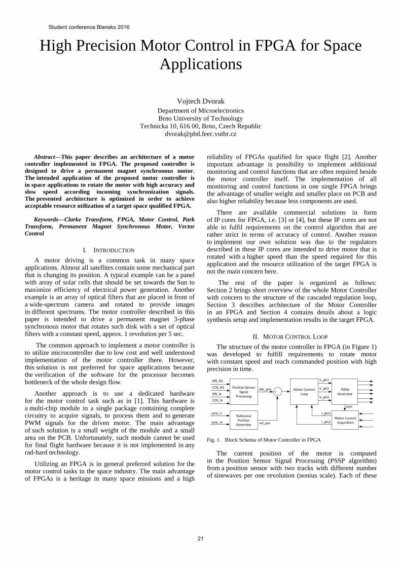
A motor driving is a common task in many space applications. Almost all satellites contain some mechanical part that is changing its position. A typical example can be a panel with array of solar cells that should be set towards the Sun to maximize efficiency of electrical power generation. Another example is an array of optical filters that are placed in front of a wide-spectrum camera and rotated to provide images in different spectrums. The motor controller described in this paper is intended to drive a permanent magnet 3-phase synchronous motor that rotates such disk with a set of optical filters with a constant speed, approx. 1 revolution per 5 sec.
The common approach to implement a motor controller is to utilize microcontroller due to low cost and well understood implementation of the motor controller there. However, this solution is not preferred for space applications because the verification of the software for the processor becomes bottleneck of the whole design flow.
Another approach is to use a dedicated hardware for the motor control task such as in [1]. This hardware is a multi-chip module in a single package containing complete circuitry to acquire signals, to process them and to generate PWM signals for the driven motor. The main advantage of such solution is a small weight of the module and a small area on the PCB. Unfortunately, such module cannot be used for final flight hardware because it is not implemented in any rad-hard technology.
Utilizing an FPGA is in general preferred solution for the motor control tasks in the space industry. The main advantage of FPGAs is a heritage in many space missions and a high
reliability of FPGAs qualified for space flight [2]. Another important advantage is possibility to implement additional monitoring and control functions that are often required beside the motor controller itself. The implementation of all monitoring and control functions in one single FPGA brings the advantage of smaller weight and smaller place on PCB and also higher reliability because less components are used.
There are available commercial solutions in form of IP cores for FPGA, i.e. [3] or [4], but these IP cores are not able to fulfil requirements on the control algorithm that are rather strict in terms of accuracy of control. Another reason to implement our own solution was due to the regulators described in these IP cores are intended to drive motor that is rotated with a higher speed than the speed required for this application and the resource utilization of the target FPGA is not the main concern here.
The rest of the paper is organized as follows: Section 2 brings short overview of the whole Motor Controller with concern to the structure of the cascaded regulation loop, Section 3 describes architecture of the Motor Controller in an FPGA and Section 4 contains details about a logic synthesis setup and implementation results in the target FPGA.
II. MOTOR CONTROL LOOP
The structure of the motor controller in FPGA (in Figure 1) was developed to fulfill requirements to rotate motor with constant speed and reach commanded position with high precision in time.
SIN_N1
COS_N1
SIN_N
COS_N
PWM Generator
V_ph1
V_ph2
V_ph3
Motor Control Loop
Position Sensor Signal
Processing
I_phi1
abs_pos
I_phi2
+-
Reference Position
Generator ref_pos
sync_n
sync_mMotor Current
Acquisition
sync
Fig. 1. Block Schema of Motor Controller in FPGA
The current position of the motor is computed in the Position Sensor Signal Processing (PSSP algorithm) from a position sensor with two tracks with different number of sinewaves per one revolution (nonius scale). Each of these
Student conference Blansko 2016
21
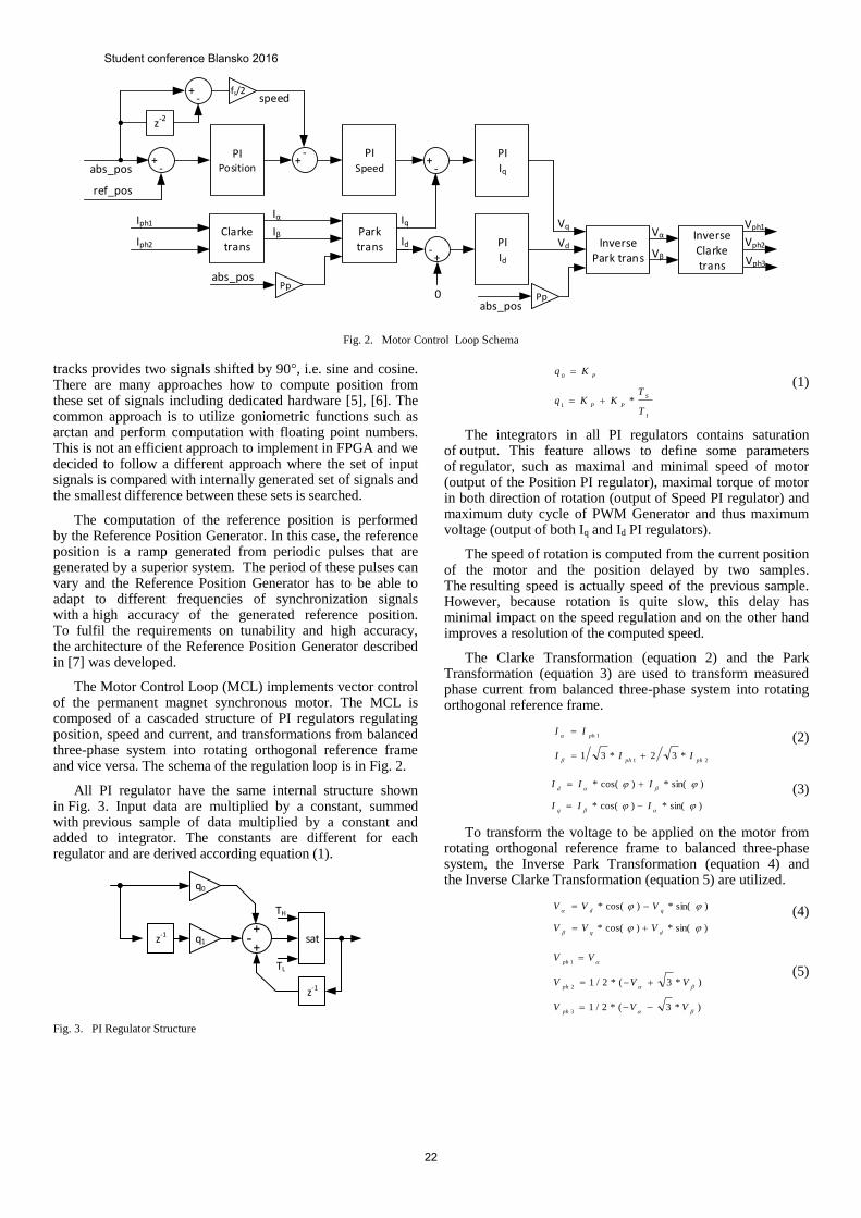
PIPosition
PISpeed
PIId
PIIq
Clarke trans
abs_pos+
-
ref_pos
+-
speed+
-
z-2
fs/2
+-
-+
0
Park trans
Ppabs_pos
Iph1
Iph2
Ppabs_pos
Iq
Id Inverse Clarke trans
Inverse Park trans
Iα
Iβ Vα
Vβ
Vq
Vd
Vph1
Vph2
Vph3
Fig. 2. Motor Control Loop Schema
tracks provides two signals shifted by 90°, i.e. sine and cosine. There are many approaches how to compute position from these set of signals including dedicated hardware [5], [6]. The common approach is to utilize goniometric functions such as arctan and perform computation with floating point numbers. This is not an efficient approach to implement in FPGA and we decided to follow a different approach where the set of input signals is compared with internally generated set of signals and the smallest difference between these sets is searched.
The computation of the reference position is performed by the Reference Position Generator. In this case, the reference position is a ramp generated from periodic pulses that are generated by a superior system. The period of these pulses can vary and the Reference Position Generator has to be able to adapt to different frequencies of synchronization signals with a high accuracy of the generated reference position. To fulfil the requirements on tunability and high accuracy, the architecture of the Reference Position Generator described in [7] was developed.
The Motor Control Loop (MCL) implements vector control of the permanent magnet synchronous motor. The MCL is composed of a cascaded structure of PI regulators regulating position, speed and current, and transformations from balanced three-phase system into rotating orthogonal reference frame and vice versa. The schema of the regulation loop is in Fig. 2.
All PI regulator have the same internal structure shown in Fig. 3. Input data are multiplied by a constant, summed with previous sample of data multiplied by a constant and added to integrator. The constants are different for each regulator and are derived according equation (1).
q0
q1 sat-+
+
z-1
z-1
TH
TL
Fig. 3. PI Regulator Structure
I
S
PP
P
T
TKKq
Kq
*1
0
(1)
The integrators in all PI regulators contains saturation of output. This feature allows to define some parameters of regulator, such as maximal and minimal speed of motor (output of the Position PI regulator), maximal torque of motor in both direction of rotation (output of Speed PI regulator) and maximum duty cycle of PWM Generator and thus maximum voltage (output of both Iq and Id PI regulators).
The speed of rotation is computed from the current position of the motor and the position delayed by two samples. The resulting speed is actually speed of the previous sample. However, because rotation is quite slow, this delay has minimal impact on the speed regulation and on the other hand improves a resolution of the computed speed.
The Clarke Transformation (equation 2) and the Park Transformation (equation 3) are used to transform measured phase current from balanced three-phase system into rotating orthogonal reference frame.
21
1
*32*31phph
ph
III
II
(2)
)sin(*)cos(*
)sin(*)cos(*
III
III
q
d
(3)
To transform the voltage to be applied on the motor from rotating orthogonal reference frame to balanced three-phase system, the Inverse Park Transformation (equation 4) and the Inverse Clarke Transformation (equation 5) are utilized.
)sin(*)cos(*
)sin(*)cos(*
dq
qd
VVV
VVV
(4)
)*3(*2/1
)*3(*2/1
3
2
1
VVV
VVV
VV
ph
ph
ph
(5)
Student conference Blansko 2016
22

Where angle φ is an electrical angle of the motor and is computed as the current position multiplied by the number of the motor pole pairs.
III. MOTOR CONTROLLER IMPLEMENTATION
The Motor Controller described in the previous section was implemented with concern to the efficient resource utilization rather than a latency of algorithm computation or a power consumption of the controller. A simplified schema of the Motor Controller is in Fig. 4. It is composed of a shared arithmetic unit, two controllers implementing computation algorithm (PSSP algorithm to compute position and Motor Control Loop algorithm to drive the motor), a control logic (Motor Control Block Controller) that drives access to the shared arithmetic unit and dedicated RAM blocks, one for each controller (RAM blocks are not part of the Fig. 4).
Motor Control
LoopMotor Control
Block Controller
Position Sensor
Signal
Processing
I_phi_*_DC
abs_pos
speed
motor_curr
out_reg
Arithmetic Unit
+
CMD
PS_we
PS_waddr
PS_re
PS_raddr
MCL_we
MCL_waddr
MCL_re
MCL_raddr
*SIN_N1 COS_N1
start
done
PS_rdata
I_phi 3
SIN_N2 COS_N2
MCL_rdata
SINE_data
3
start
done
Fig. 4. Motor Controller Structure
The Motor Control Block Controller (MCBC) is implemented as a finite state machine that drives overall process of the motor driving. After appropriate command is received, MCBC periodically generates start signals to acquire sensor data, compute position with the PSSP algorithm and run motor driving with the MCL algorithm. The MCBC also control access to the control ports of the arithmetic unit and provides access to the PSSP controller or the MCL controller according the state of the computation.
A. Arithemtic Unit
The proposed arithmetic unit is designed to be able to perform arithmetic operations for both, the PSSP algorithm and the MCL algorithm. It supports arithmetic operation addition and multiplication in 16-bit fixed point numbers. The schema of the shared arithmetic unit is in Fig. 5. It is composed of three main parts – fixed-point adder with saturation logic, fixed-point multiplier and a switching logic.
The fixed-point adder and the fixed-point multiplier have flip-flops with write enable ports on their inputs and outputs. The write enable ports of the inputs registers allow to save data into the registers in advance before they are used in the algorithm. The purpose of the registers on the output ports of the arithmetic unit is to hold results of the last valid operation.
The adder in the arithmetic unit contains a saturation logic that is required by the computation algorithm of the PI regulators. The threshold for saturation are saved in dedicated registers in the arithmetic unit and the saturation itself is activated by the enable signal. Values of the thresholds are loaded from the memory before the saturation is performed.
*EN
D Q
EN
D Q
ROUND mul_res
switch_ctrl
neg
EN
D Q+SAT
EN
D Q
EN
D Q
EN
D Q
add_res
add_sat_en
EN
D Q
Swit
chin
g Lo
gic
I_ph1
CONST
I_ph2
PS_rdata
MCL_rdata
SINE_rdata
ref_pos
abs_res
SIN_N1
COS_N1
SIN_N2
COS_N2
mul_res
add_res
Fig. 5. Structure of the Shared Arithmetic Unit
The Switching Logic is arrays of multiplexers that are able to route all signals needed to perform arithmetic operations for PSSP algorithm and MCL algorithm. These arrays were carefully optimize to minimize the number of multiplexed signals and thus to minimize the number of utilized resources and the transport delay of the switching logic.
B. Motor Control Loop Logic
The Motor Control Loop of the Motor Controller implements the regulation algorithm described in the Section 2. The regulation algorithm was analyzed and optimized for implementation in a hardware. As a result, the computation of each PI regulator takes approximately 10 clock cycles and computation of the transformations (either forward or inverse) lasts 11 clock cycles. The computation of the MCL algorithm then lasts 62 clock periods and is performed in the following order: Position regulation → Speed regulation → Clarke & Park transformations → Iq regulation → Id regulation → Inverse Park & Inverse Clarke transformations.
The Motor Control Loop drives the control signals of the arithmetic unit, a write port and a read port of the dedicated MCL memory. The MCL memory is implemented in one block RAM protected with EDAC (Error Detection And Correction) logic and its structure corresponds to the computation steps of the algorithm. That means that an address of data in the MCL memory is the same as a value of the computation step when these data shall be loaded into the registers in the arithmetic unit. This approach leads to a very efficient implementation. Only one counter to control the progress of the algorithm computation without any additional logic is needed to generate addresses for the write port of the MCL memory. The same progress counter is used to generate all control signals and only one small LUT for each control signal is needed.
Student conference Blansko 2016
23

A value of a sine/cosine of the motor electrical angle is needed in the Park transformation and in the Inverse Park transformation. The values of sine/cosine are read from a LUT table with saved sinewave samples. The address in the LUT is computed from the current position of the motor according to the equation (6).
360
*2048*
Ppposaddr (6)
The address computed in equation (6) can be greater than the size of the sine samples by factor Pp and a modular reduction is necessary to be used. However, the size of the LUT was chosen to be a power of 2 and the modular reduction is simple here, MSB bits are discarded.
To save additional resources, only the first quadrant of a sine period is saved in the LUT. The rest of the sine period and the cosine values are computed according the TABLE I.
TABLE I. SINE LUT ADDRESSING SCHEMA
Address Value
Sine Cosine
addr < 512:
addr[10:9] = 00
LUT(addr) LUT(512-addr)
addr >= 512 ˄ addr < 1024:
addr[10:9] = 01 LUT(512-addr) -LUT(addr-512)
addr >=1024 ˄ addr < 1536: addr[10:9] = 10
-LUT(addr-1024) -LUT(1536-addr)
addr >= 1536 ˄ addr < 2048:
addr[11:10] = 11 -LUT(2048-addr) LUT(addr-2048)
IV. IMPLEMENTATION RESULTS
The Motor Controller implementing the proposed MCL algorithm was synthesized into the target FPGA Microsemi RTAX 2000S qualified for space flights. The logic synthesis was performed with the tool Synopsis Synplify Pro G-2012-09A. The synthesis results can be found in TABLE II.
TABLE II. FPGA RESOURCE UTILIZATION
Component Resource Utilization
fclk,max [MHz] LUT [-] FF [-]
Arithmetic Unit 942 185 67.5
16-bit mutliplier 632 108 67.5
16-bit adder 132 80 82.3
switching logic 151 - -
MCL 79 27 204.4
total 1021 212 67.5
The frequency of the system clock in the target FPGA is 50 MHz. To have required 20% margin on the worst case path, the target frequency for the synthesis was set to 60 MHz. As can be seen in the synthesis results, the target frequency was reached after a retiming had been allowed. The FPGA RTAX 2000S does not contain any DSP blocks. The 16-bit multiplier is thus implemented into 632 4-input LUTs. This is the largest single combinational network in the whole FPGA design and it also creates the critical path that limits the frequency of the system clock.
V. CONCLUSION
The paper introduced an architecture of the motor controller suitable for implementation in an FPGA. The controller involves the PSSP algorithm to compute position from two pairs of harmonic signals (nonius scale), the Reference Position Generator and the Motor Control Loop.
The developed regulation loop is intended to be used with permanent magnet synchronous motor in space application. The most important property of the regulation loop is high accuracy of the regulation with slow speed of the motor rotation.
The paper is mostly focused on architecture of the Motor Control Loop. The proposed architecture contains an arithmetic unit shared with the PSSP algorithm and efficient implementation of regulation algorithm utilizing just one 6-bit counter and a few LUTs to generate control signals for the shared arithmetic unit and memory access.
The implementation into flight FPGA was performed and results of the synthesis were presented in the paper. The FPGA RTAX 2000S by Microsemi was chosen as the flight FPGA due to heritage in many space missions. These FPGAs are manufactured in 150 nm rad-hard technology and are rather large and slow compared with modern FPGAs. Moreover, this specific type of FPGA does not contain DSP blocks and the 16-bit multiplier in the arithmetic unit had to be implemented in the combinational network. However, the proposed architecture is designed to share the multiplier wherever it is needed and thus a lot of resources can be saved.
ACKNOWLEDGMENT
Research described in this paper was financed by the National Sustainability Program under Grant LO1401, by the Czech Science Foundation under Grant No. P102-14-07724S and by the project no. FEKT-S-14-2300 "A new types of electronic circuits and sensors for specific applications". For the research, infrastructure of the SIX Center was used. Cadence software was used with support through the Cadence Academic Network.
REFERENCES
[1] G. C. Caprini, F. Innocenti, L. Fanucci, S. Ricci, G. Taraschi, P. Terreni, M. Tonarelli, L. Tosi, “Embedded system for brushless motor control in space application”, 7th annual MAPLD International Conference, 2004
[2] K. O’Neill “FPGAs for Space Applications”, SEFUW: SpacE FPGA Users Workshop 1st edition, 2012
[3] Microsemi: Dual-Axis Motor Control on a Single SoC FPGA, Microsemi, 2015
[4] Altera: Motor Control IP Suite Components for Drive-on-Chip Reference Designs, Altera, 2014
[5] iC Haus: High-Precision Sine/Cosine Interpolation, iC-House GmbH, 2014
[6] GEMAC: 2-Channel Interpolation Circuit with Nonius Calculation, GEMAC, 2013
[7] V. Dvorak, “High Precision Reference Position Generator for Motor Control in FPGA”, Proceedings of the 22nd Conference STUDENT EEICT 2016, pp. 625-629, Vysoke Uceni Technicke, 2016
Student conference Blansko 2016
24
Arrangements of Capacitively Loaded Dipoles for
20-bit Chipless RFID Tag
Jaroslav Havlíček
Department of Electromagnetic field
Czech Technical University in Prague
Prague, Czech Republic
Abstract—This paper presents three arrangements of
uniplanar capacitively loaded dipole scatterers used as a basic
building element for a 20-bit chipless RFID tag with frequency
domain information coding. Proposed simulation results of the
arrangements demonstrate that strong mutual coupling between
scatterers can negatively affect uniformity of tag radar cross-
section response which is crucial for readability of the tag.
Keywords—chipless RFID, tag, scatterer, mutual coupling,
radar cross-section, spectral response coding
I. INTRODUCTION
The radiofrequency identification (RFID) is a widespread technology, which is applied mainly in industry (production process monitoring), logistics (acceleration of storing procedures), commerce (antitheft feature), health care (elimination of patient confusions) and inventorying (e.g. books in libraries). RFID is expected to have an important role in the internet of things concept [1].
There is a perfect opportunity for further spreading in commerce, provided that the RFID transponders (tags) are suitable for optical barcode replacement [2]. The advantage of the tag consists in the possibility to be read without necessity of clear line of sight. Low price of the tag is essential for reaching this goal. Unfortunately conventional tags which consists a chip are about hundred times more expensive than barcode [3]. Perspective approach to reduce the tag cost is chipless RFID which provides different methods of storing information without chip.
Promising examples of the chipless RFID technology are tags based on spectral signature [4], [5], which in most cases consist of resonating scatterers. Presence or non-presence of each scatterer's peak in tag's spectral signature represents logic one or zero, respectively. This method of the chipless tag design is employed in this paper. Second part discusses required properties of the scatterer and describes capacitively loaded dipole. Third part presents three arrangements of the scatterers for 20-bit chipless RFID tag. First of them demonstrates negative effect of mutual coupling between scatterers on uniformity of tag radar cross-section response which is crucial for readability of the tag. Two other arrangements were design for mutual coupling reduction.
II. CAPACITIVELY LOADED DIPOLE
There are many different types of planar resonators which can be used as a scatterer for the chipless RFID tag. [6] Each of these resonators can be described via three important quantities. First of them is radar cross-section (RCS) which determines the reading range of the tag. The higher RCS results in the longer reading range.
Second quantity is bandwidth (BW) of resonance peak which depends on quality factor of resonance. It can be evaluated from frequency characteristic of the resonator as frequency range of three decibel resonance peak drop. This value is important from spectral bit capacity point of view. For example when bandwidth is 200 MHz there cannot be stored more than only five bits for each GHz in the spectrum.
Last quantity is product ka where k is wave number and a is radius of circle circumscribed the resonator. This quantity represents rate of electric reduction of the resonator. Resonators with ka below one are suitable candidates because small scale is essential for purposes of chipless RFID.
Theory of electrically small antennas says that resonance structures with small ka have high quality factor Q which implicates low bandwidth which is beneficial for high spectral bit capacity and low RCS which is inappropriate for reading range. Therefore there is always a trade-off between spectral bit capacity and reading range of the tag.
Fig. 1. Capacitively loaded dipole
Capacitively loaded dipole represents quite advantageous choice from the point of view of this trade-off [6]. Its width n is 2.5 mm, length m depends on resonant frequency (m = 16.7 mm is maximum). Dipole is loaded via four spiral (one turn and half) endings. Width of all lines as well as spacing between arms equals 0.1 mm. Its RCS is -33.5 dBsm, BW is 17.2 MHz and ka is 0.35.
E
m
n
Student conference Blansko 2016
25
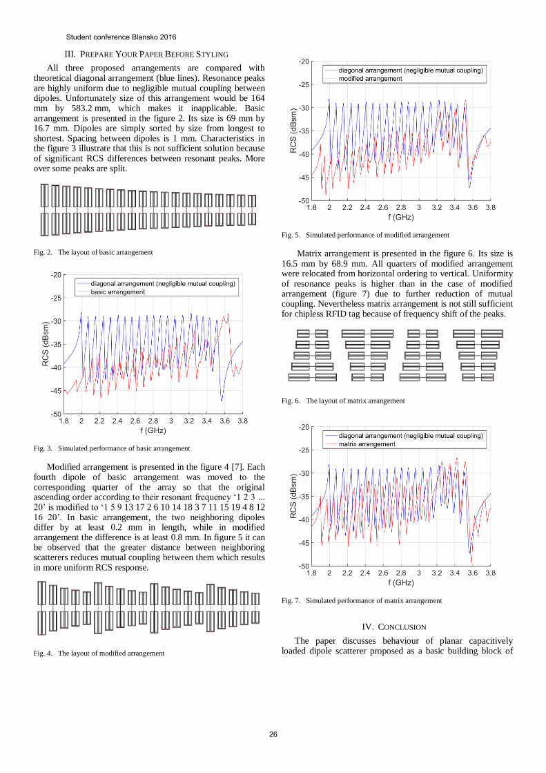
III. PREPARE YOUR PAPER BEFORE STYLING
All three proposed arrangements are compared with theoretical diagonal arrangement (blue lines). Resonance peaks are highly uniform due to negligible mutual coupling between dipoles. Unfortunately size of this arrangement would be 164 mm by 583.2 mm, which makes it inapplicable. Basic arrangement is presented in the figure 2. Its size is 69 mm by 16.7 mm. Dipoles are simply sorted by size from longest to shortest. Spacing between dipoles is 1 mm. Characteristics in the figure 3 illustrate that this is not sufficient solution because of significant RCS differences between resonant peaks. More over some peaks are split.
Fig. 2. The layout of basic arrangement
Fig. 3. Simulated performance of basic arrangement
Modified arrangement is presented in the figure 4 [7]. Each fourth dipole of basic arrangement was moved to the corresponding quarter of the array so that the original ascending order according to their resonant frequency ‘1 2 3 ... 20’ is modified to ‘1 5 9 13 17 2 6 10 14 18 3 7 11 15 19 4 8 12 16 20’. In basic arrangement, the two neighboring dipoles differ by at least 0.2 mm in length, while in modified arrangement the difference is at least 0.8 mm. In figure 5 it can be observed that the greater distance between neighboring scatterers reduces mutual coupling between them which results in more uniform RCS response.
Fig. 4. The layout of modified arrangement
Fig. 5. Simulated performance of modified arrangement
Matrix arrangement is presented in the figure 6. Its size is 16.5 mm by 68.9 mm. All quarters of modified arrangement were relocated from horizontal ordering to vertical. Uniformity of resonance peaks is higher than in the case of modified arrangement (figure 7) due to further reduction of mutual coupling. Nevertheless matrix arrangement is not still sufficient for chipless RFID tag because of frequency shift of the peaks.
Fig. 6. The layout of matrix arrangement
Fig. 7. Simulated performance of matrix arrangement
IV. CONCLUSION
The paper discusses behaviour of planar capacitively loaded dipole scatterer proposed as a basic building block of
Student conference Blansko 2016
26

the RFID chipless tag working in the frequency domain mode. Three presented arrangements illustrate how important is reduction of mutual coupling between scatterers for readability of the tag. It is essential to propose a new arrangement minimizing this mutual coupling for the design of high bit capacity tag. Further work on this project will be focused on describing mutual coupling in more exact way using equivalent circuit.
ACKNOWLEDGMENT
This work was supported by the Czech Technical University in Prague under the project SGS10/271/OHK3/3T/13.
REFERENCES
[1] S. Dey, J. K. Saha and N. C. Karmakar, N. Smart Sensing: Chipless
RFID Solutions for the Internet of Everything. IEEE Microwave
Magazine, 2015, vol.16, no.10, pp.26-39. DOI: 10.1109/MMM.2015.2465711
[2] P. Harrop, R.Das, Printed and Chipless RFID Forecasts, Technologies & Players 2011-2021. [Online] Cited 2016-04-25. Available at: http://www.idtechex.com/research/reports/printed-and-chipless-rfid-forecasts-technologies-and-players-2011-2021-000254.asp.
[3] S. Preradovic, and N.C. Karmakar, “Chipless RFID: Bar Code of the Future,” IEEE Microw. Mag., vol. 11, no. 7, pp. 87-97, Dec. 2010.
[4] R. Rezaiesarlak, and M. Manteghi, “Complex-Natural-Resonance-Based Design of Chipless RFID Tag for High-Density Data”, IEEE Transactions on Antennas and Propagation, vol. 62, no. 2, pp. 898-904, 2014.
[5] A. Vena, E. Perret, and S. Tedjini, “A Fully Printable Chipless RFID Tag With Detuning Correction Technique”, IEEE Microwave and Wireless Component Letters., vol. 22, no. 4, pp. 219-229, 2016.
[6] J. Havlicek, M. Svanda, J. Machac, M. Polivka, “Improvement of Reading Performance of Frequency-Domain Chipless RFID Transponders”, Radioengineering, vol. 25, no. 2, pp. 209-211, 2012.
[7] M. Polivka, M. Svanda, J. Machac, Chipless RFID Tag with an Improved RCS Response, Proc. of 44th European Microw. Conf. (EuMC), 2014, pp.770-773, ISBN: 9781479955985, DOI: 10.1109/EuMC.2014.6986548
Student conference Blansko 2016
27
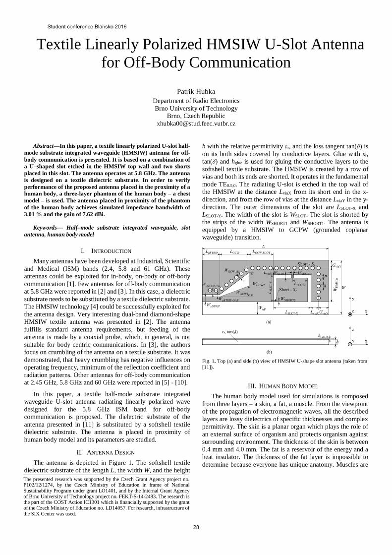
Textile Linearly Polarized HMSIW U-Slot Antenna
for Off-Body Communication
Patrik Hubka
Department of Radio Electronics
Brno University of Technology
Brno, Czech Republic
Abstract—In this paper, a textile linearly polarized U-slot half-
mode substrate integrated waveguide (HMSIW) antenna for off-
body communication is presented. It is based on a combination of
a U–shaped slot etched in the HMSIW top wall and two shorts
placed in this slot. The antenna operates at 5.8 GHz. The antenna
is designed on a textile dielectric substrate. In order to verify
performance of the proposed antenna placed in the proximity of a
human body, a three-layer phantom of the human body – a chest
model – is used. The antenna placed in proximity of the phantom
of the human body achieves simulated impedance bandwidth of
3.01 % and the gain of 7.62 dBi.
Keywords— Half–mode substrate integrated waveguide, slot
antenna, human body model
I. INTRODUCTION
Many antennas have been developed at Industrial, Scientific
and Medical (ISM) bands (2.4, 5.8 and 61 GHz). These
antennas could be exploited for in-body, on-body or off-body
communication [1]. Few antennas for off-body communication
at 5.8 GHz were reported in [2] and [3]. In this case, a dielectric
substrate needs to be substituted by a textile dielectric substrate.
The HMSIW technology [4] could be successfully exploited for
the antenna design. Very interesting dual-band diamond-shape
HMSIW textile antenna was presented in [2]. The antenna
fulfills standard antenna requirements, but feeding of the
antenna is made by a coaxial probe, which, in general, is not
suitable for body centric communications. In [3], the authors
focus on crumbling of the antenna on a textile substrate. It was
demonstrated, that heavy crumbling has negative influences on
operating frequency, minimum of the reflection coefficient and
radiation patterns. Other antennas for off-body communication
at 2.45 GHz, 5.8 GHz and 60 GHz were reported in [5] - [10].
In this paper, a textile half-mode substrate integrated
waveguide U-slot antenna radiating linearly polarized wave
designed for the 5.8 GHz ISM band for off-body
communication is proposed. The dielectric substrate of the
antenna presented in [11] is substituted by a softshell textile
dielectric substrate. The antenna is placed in proximity of
human body model and its parameters are studied.
II. ANTENNA DESIGN
The antenna is depicted in Figure 1. The softshell textile
dielectric substrate of the length L, the width W, and the height
h with the relative permittivity εr, and the loss tangent tan(δ) is
on its both sides covered by conductive layers. Glue with εr,
tan(δ) and hglue is used for gluing the conductive layers to the
softshell textile substrate. The HMSIW is created by a row of
vias and both its ends are shorted. It operates in the fundamental
mode TE0.5,0. The radiating U-slot is etched in the top wall of
the HMSIW at the distance LviaX from its short end in the x-
direction, and from the row of vias at the distance LviaY in the y-
direction. The outer dimensions of the slot are LSLOT-X and
LSLOT-Y. The width of the slot is WSLOT. The slot is shorted by
the strips of the width WSHORT1 and WSHORT1. The antenna is
equipped by a HMSIW to GCPW (grounded coplanar
waveguide) transition.
Fig. 1. Top (a) and side (b) view of HMSIW U-shape slot antenna (taken from
[11]).
III. HUMAN BODY MODEL
The human body model used for simulations is composed
from three layers – a skin, a fat, a muscle. From the viewpoint
of the propagation of electromagnetic waves, all the described
layers are lossy dielectrics of specific thicknesses and complex
permittivity. The skin is a planar organ which plays the role of
an external surface of organism and protects organism against
surrounding environment. The thickness of the skin is between
0.4 mm and 4.0 mm. The fat is a reservoir of the energy and a
heat insulator. The thickness of the fat layer is impossible to
determine because everyone has unique anatomy. Muscles are
The presented research was supported by the Czech Grant Agency project no. P102/12/1274, by the Czech Ministry of Education in frame of National Sustainability Program under grant LO1401, and by the Internal Grant Agency of Brno University of Technology project no. FEKT-S-14-2483. The research is the part of the COST Action IC1301 which is financially supported by the grant of the Czech Ministry of Education no. LD14057. For research, infrastructure of the SIX Center was used.
Student conference Blansko 2016
28

tissues with elastic properties. Muscles are able to contract and
relax. The layer of muscle has various thicknesses which
depend on the type of muscle and the location on the body.
The configuration of the multilayer model (the phantom) of
a chest is shown in Figure 2. The parameters of the phantom are
summarized in Table 1 [12]. The phantom is a block of base
200 mm × 200 mm. The height of the phantom is given by the
thicknesses of the layers representing the skin, the fat and the
muscle. The distance d between the human body model and the
antenna is 1 mm.
TABLE I. PARAMETERS OF THE CHEST PHANTOM
εr tan(δ) σ (S/m) thickness [mm]
Dry skin 35.114 0.32807 3.7170 2
Fat 4.955 0.18335 0.29313 10
Muscle 48.485 0.31715 4.9615 28
Fig. 2. The chest phantom (taken from [11]).
IV. ANTENNA DESIGN AND SIMULATED RESULTS
The softshell antenna was designed with the help of the time
domain solver of CST Microwave Studio (CST MWS), where
local optimization procedures Trust Region Framework were
used, for the operating frequency of 5.8 GHz on the softshell
textile dielectric substrate with relative permittivity εr = 1.32,
tangent loss tan(δ) = 0.025, and height h = 1.32 mm. The glue
is applied on the bottom and the top side of the softshell textile
substrate with εr = 2.8, tan(δ) = 0.025 and hglue = 0.0075 mm.
The resultant dimensions of the antenna are summarized in
Table 2.
TABLE II. DIMENSIONS OF DESIGNED ANTENNA (FIGURE 1)
[mm] [mm] [mm]
L 64.66 W 21.28 WAP 2.92
LμSTRIP 8.87 WμSTRIP 2.34 WHMSIW 15.15
LGCW 9.12 WμSTRIP-GAP 1.00 GviaX 3.29
LGCW-SLOT 15.99 WμSTRIP-via 1.15 GviaY 3.21
LSLOT-X 25.13 WGCW1 2.98 h 1.32
LSLOT-Y 12.64 WGCW2 11.66 hGLUE 0.0075
LSLOT2 12.60 WSLOT 1.10 p 0.75
LviaX 2.26 WSHORT1 0.47 d 0.45
LviaY 2.51 WSHORT2 0.47
The distribution of the electric field in the substrate at the
frequency 5.8 GHz is depicted in Figure 3. Thanks to the short
S1, the electric field at the slot is cutted into two halves and the
linearly horizontally polarized wave in the far field is obtained.
Fig. 3. Distribution of electric filed intensity at 5.8 GHz in softshell textile
substrate (magnitude).
The simulated reflection coefficient of the antenna in the
free-space and in the proximity of the chest phantom is depicted
in Figure 4. The simulated reflection coefficient of the antenna
achieves impedance bandwidth about 3.23% and 3.01% for the
antenna placed in the free-space and in the proximity of human
body, respectively. The minimum of the reflection coefficient
of the antenna placed in proximity on human body is slightly
shifted about 30 MHz to lower frequencies due to the influence
of the phantom.
The normalized simulated radiation patterns in two
orthogonal cutting planes in the free-space and in the proximity
of the phantom at the frequency 5.8 GHz are depicted in Figure
5. It can be observed that the co-polarizations are in good
agreement at the boresight direction in E-plane. In H-plane, the
co-polarization of the antenna near of the phantom of human
body model has narrower radiation beam. The level of the
cross-polarization at the boresight direction reaches higher level
due to the influence of phantom in comparison to the cross-
polarization of the antenna placed in the free-space. The
simulated antenna peak gain is 6.28 dBi and 7.62 dBi for the
antenna placed in the free-space and in the proximity of the
phantom, respectively.
Simulated total efficiency at operating frequency f = 5.8
GHz of the antenna is 43% and 36% in the free-space and in
proximity of the phantom of human body model, respectively.
Total efficiency is lower thanks to the higher losses in the
softshell textile dielectric substrate.
Student conference Blansko 2016
29
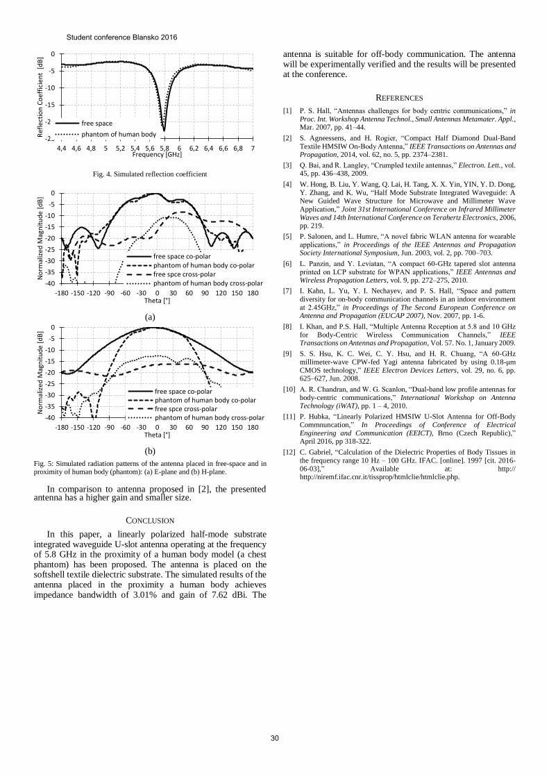
Fig. 4. Simulated reflection coefficient
(a)
(b)
Fig. 5: Simulated radiation patterns of the antenna placed in free-space and in proximity of human body (phantom): (a) E-plane and (b) H-plane.
In comparison to antenna proposed in [2], the presented antenna has a higher gain and smaller size.
CONCLUSION
In this paper, a linearly polarized half-mode substrate integrated waveguide U-slot antenna operating at the frequency of 5.8 GHz in the proximity of a human body model (a chest phantom) has been proposed. The antenna is placed on the softshell textile dielectric substrate. The simulated results of the antenna placed in the proximity a human body achieves impedance bandwidth of 3.01% and gain of 7.62 dBi. The
antenna is suitable for off-body communication. The antenna will be experimentally verified and the results will be presented at the conference.
REFERENCES
[1] P. S. Hall, “Antennas challenges for body centric communications,” in Proc. Int. Workshop Antenna Technol., Small Antennas Metamater. Appl., Mar. 2007, pp. 41–44.
[2] S. Agneessens, and H. Rogier, “Compact Half Diamond Dual-Band Textile HMSIW On-Body Antenna,” IEEE Transactions on Antennas and Propagation, 2014, vol. 62, no. 5, pp. 2374–2381.
[3] Q. Bai, and R. Langley, “Crumpled textile antennas,” Electron. Lett., vol. 45, pp. 436–438, 2009.
[4] W. Hong, B. Liu, Y. Wang, Q. Lai, H. Tang, X. X. Yin, YIN, Y. D. Dong, Y. Zhang, and K. Wu, “Half Mode Substrate Integrated Waveguide: A New Guided Wave Structure for Microwave and Millimeter Wave Application,” Joint 31st International Conference on Infrared Millimeter Waves and 14th International Conference on Terahertz Electronics, 2006, pp. 219.
[5] P. Salonen, and L. Humre, “A novel fabric WLAN antenna for wearable applications,” in Proceedings of the IEEE Antennas and Propagation Society International Symposium, Jun. 2003, vol. 2, pp. 700–703.
[6] L. Panzin, and Y. Leviatan, “A compact 60-GHz tapered slot antenna printed on LCP substrate for WPAN applications,” IEEE Antennas and Wireless Propagation Letters, vol. 9, pp. 272–275, 2010.
[7] I. Kahn, L. Yu, Y. I. Nechayev, and P. S. Hall, “Space and pattern diversity for on-body communication channels in an indoor environment at 2.45GHz,” in Proceedings of The Second European Conference on Antenna and Propagation (EUCAP 2007), Nov. 2007, pp. 1-6.
[8] I. Khan, and P.S. Hall, “Multiple Antenna Reception at 5.8 and 10 GHz for Body-Centric Wireless Communication Channels,” IEEE Transactions on Antennas and Propagation, Vol. 57. No. 1, January 2009.
[9] S. S. Hsu, K. C. Wei, C. Y. Hsu, and H. R. Chuang, “A 60-GHz millimeter-wave CPW-fed Yagi antenna fabricated by using 0.18-μm CMOS technology,” IEEE Electron Devices Letters, vol. 29, no. 6, pp. 625–627, Jun. 2008.
[10] A. R. Chandran, and W. G. Scanlon, “Dual-band low profile antennas for body-centric communications,” International Workshop on Antenna Technology (iWAT), pp. 1 – 4, 2010.
[11] P. Hubka, “Linearly Polarized HMSIW U-Slot Antenna for Off-Body Commnuncation,” In Proceedings of Conference of Electrical Engineering and Communication (EEICT), Brno (Czech Republic),” April 2016, pp 318-322.
[12] C. Gabriel, “Calculation of the Dielectric Properties of Body Tissues in the frequency range 10 Hz – 100 GHz. IFAC. [online]. 1997 [cit. 2016-06-03],” Available at: http:// http://niremf.ifac.cnr.it/tissprop/htmlclie/htmlclie.php.
-25
-20
-15
-10
-5
0
4,4 4,6 4,8 5 5,2 5,4 5,6 5,8 6 6,2 6,4 6,6 6,8 7
Ref
lect
ion
Co
effi
cien
t [d
B]
Frequency [GHz]
free space
phantom of human body
-40
-35
-30
-25
-20
-15
-10
-5
0
-180 -150 -120 -90 -60 -30 0 30 60 90 120 150 180
No
rmal
ized
Mag
nit
ud
e[d
B]
Theta [°]
free space co-polarphantom of human body co-polarfree spce cross-polarphantom of human body cross-polar
-40
-35
-30
-25
-20
-15
-10
-5
0
-180 -150 -120 -90 -60 -30 0 30 60 90 120 150 180
No
rmal
ized
Mag
nit
ud
e[d
B]
Theta [°]
free space co-polarphantom of human body co-polarfree spce cross-polarphantom of human body cross-polar
Student conference Blansko 2016
30

The Neural models for differrent training algorithms
Martin Kotol
Brno University of Technology, Technická 12, 616 00
Brno, Czech republic
Abstract—This paper is aimed on artificial neural networks
that are used for modeling of a transmission channel. The neural
networks were trained with different training algorithms and
results of estimation were compared. The paper describes the
procedure of measurement and the further processing of results.
Keywords—Artificial neural networks, Feed-forward neural
networks, training algorithms, measurement, transmission function
I. INTRODUCTION
This paper is aimed on the Feed-forward (FF) artificial neural networks (ANN). The NNs accuracy approximation will be compared for particular training algorithm. At first a general NN is introduced; later the principle of the FF ANN will be introduced. Training algorithms of the FF neural networks will be described in the following part of text. Modeling the properties a of transmission channel can be computationally and time demanding. Parallel structure of the ANN can used for modeling of the transmission channel.
For the accuracy verification of experimental measurement results the channel transfer function (CTF) is used. This experimental measurement is described in detail (a specification of used antennas type, localization antennas, setting measuring instrument, etc. ).
The following text describes the measured values processing and pattern trainging and verification for ANN. The results will be compared for several training algorithms.
II. GENERAL ARTIFICIAL NEURAL NETWORK
This chapter is aimed on general description of neurons and their implementation into the ANN.
ANN is a universal computational tool which is composed of simple units called neurons. Neurons are organized into layers which are interconnected and form a network. Input of each neuron in the layer M is connected to the outputs of all
neurons in the previous layer M1. Output of the neuron in the layer M is connected to inputs of all the neurons in the next layer M+1. Interconnections in between neurons are associated with different weights. Weights are set randomly during the initialization. During the training of the network, weights are adjusted in order to minimize the error at the output of the ANN (the difference between the expected response and the actual one) [1].
Figure 1 shows a general ANN containing the input layer, the hidden layer and the output layer. Here, x1 to xn are signals at the input of input neurons, w11 to wmn denote weights between neurons and f1 to fn are signals at the output of output neurons. The input layer distributes input signals among hidden neurons [2]. Neurons in the hidden layer transform signals using a specific activation function. The output layer forms output signals of ANN.
For the comparison of the accuracy approximation the FF ANN was used and it depends on the training algorithm used. In the FF ANN the information flows from inputs directly to outputs without any feedback. During the training weights between neurons are set to minimize the difference between expected and actual outputs. After training the network is ready to estimate an appropriate output target from an arbitrary input pattern.
The FF ANN contains three layers of neurons; the input layer, the hidden layer and the output layer [2]. Each of these layers has a specific task:
The input layer consists of input neurons which are
described by the linear activation function. Input neurons
distribute input signal to hidden neurons.
The hidden layer consists of neurons with a specific
activation function (sigma function, sigmoid function, …).
The sigma function is shown in equation 1. All neurons in
the hidden layer have a parameter vector.
𝑎𝑗𝑚 =1
(1+𝑒−𝑆𝑗𝑚)
𝑤ℎ𝑒𝑟𝑒 𝑆𝑗𝑚 = ∑ 𝑤𝑖𝑗𝑥𝑎𝑖𝑥
𝑛
𝑥=0
Where ajm is activation function for mth neuron in j
th layer,Sj
is the sum of the products the activations nodes by their respective weights; the member wij is the set of all weights between layers i and j which are associated with neurons that feed into neuron m of layer j.
The output layer forms output targets as a linear
combination of signals from outputs of hidden neurons.
The Figure 2 shows the general structure of a FF network. Here, x1 to xn are inputs, w11 to wnm are weights between neurons, and f1 to fn are outputs. During the training weights are
Student conference Blansko 2016
31
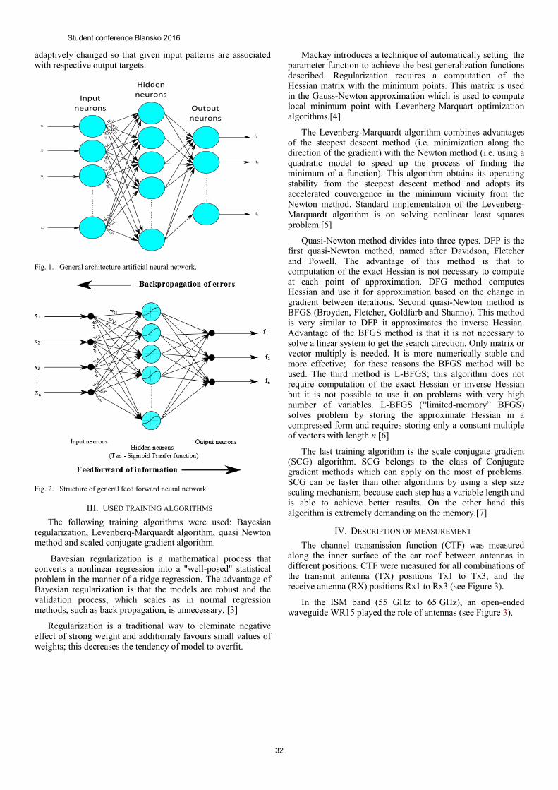
adaptively changed so that given input patterns are associated with respective output targets.
Fig. 1. General architecture artificial neural network.
Fig. 2. Structure of general feed forward neural network
III. USED TRAINING ALGORITHMS
The following training algorithms were used: Bayesian regularization, Levenberq-Marquardt algorithm, quasi Newton method and scaled conjugate gradient algorithm.
Bayesian regularization is a mathematical process that converts a nonlinear regression into a "well-posed" statistical problem in the manner of a ridge regression. The advantage of Bayesian regularization is that the models are robust and the validation process, which scales as in normal regression methods, such as back propagation, is unnecessary. [3]
Regularization is a traditional way to eleminate negative effect of strong weight and additionaly favours small values of weights; this decreases the tendency of model to overfit.
Mackay introduces a technique of automatically setting the parameter function to achieve the best generalization functions described. Regularization requires a computation of the Hessian matrix with the minimum points. This matrix is used in the Gauss-Newton approximation which is used to compute local minimum point with Levenberg-Marquart optimization algorithms.[4]
The Levenberg-Marquardt algorithm combines advantages of the steepest descent method (i.e. minimization along the direction of the gradient) with the Newton method (i.e. using a quadratic model to speed up the process of finding the minimum of a function). This algorithm obtains its operating stability from the steepest descent method and adopts its accelerated convergence in the minimum vicinity from the Newton method. Standard implementation of the Levenberg-Marquardt algorithm is on solving nonlinear least squares problem.[5]
Quasi-Newton method divides into three types. DFP is the first quasi-Newton method, named after Davidson, Fletcher and Powell. The advantage of this method is that to computation of the exact Hessian is not necessary to compute at each point of approximation. DFG method computes Hessian and use it for approximation based on the change in gradient between iterations. Second quasi-Newton method is BFGS (Broyden, Fletcher, Goldfarb and Shanno). This method is very similar to DFP it approximates the inverse Hessian. Advantage of the BFGS method is that it is not necessary to solve a linear system to get the search direction. Only matrix or vector multiply is needed. It is more numerically stable and more effective; for these reasons the BFGS method will be used. The third method is L-BFGS; this algorithm does not require computation of the exact Hessian or inverse Hessian but it is not possible to use it on problems with very high number of variables. L-BFGS (“limited-memory” BFGS) solves problem by storing the approximate Hessian in a compressed form and requires storing only a constant multiple of vectors with length n.[6]
The last training algorithm is the scale conjugate gradient (SCG) algorithm. SCG belongs to the class of Conjugate gradient methods which can apply on the most of problems. SCG can be faster than other algorithms by using a step size scaling mechanism; because each step has a variable length and is able to achieve better results. On the other hand this algorithm is extremely demanding on the memory.[7]
IV. DESCRIPTION OF MEASUREMENT
The channel transmission function (CTF) was measured along the inner surface of the car roof between antennas in different positions. CTF were measured for all combinations of the transmit antenna (TX) positions Tx1 to Tx3, and the receive antenna (RX) positions Rx1 to Rx3 (see Figure 3).
In the ISM band (55 GHz to 65 GHz), an open-ended waveguide WR15 played the role of antennas (see Figure 3).
Student conference Blansko 2016
32
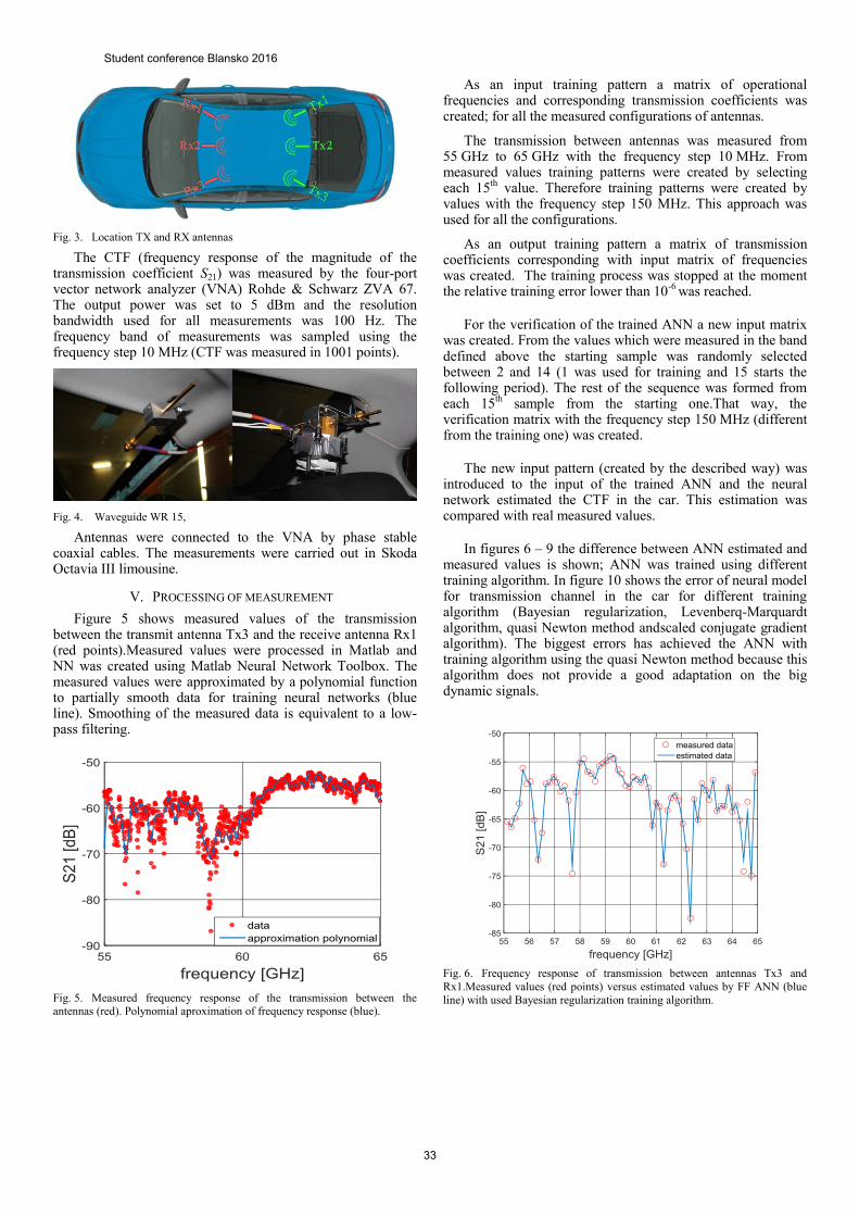
Fig. 3. Location TX and RX antennas
The CTF (frequency response of the magnitude of the transmission coefficient S21) was measured by the four-port vector network analyzer (VNA) Rohde & Schwarz ZVA 67. The output power was set to 5 dBm and the resolution bandwidth used for all measurements was 100 Hz. The frequency band of measurements was sampled using the frequency step 10 MHz (CTF was measured in 1001 points).
Fig. 4. Waveguide WR 15,
Antennas were connected to the VNA by phase stable coaxial cables. The measurements were carried out in Skoda Octavia III limousine.
V. PROCESSING OF MEASUREMENT
Figure 5 shows measured values of the transmission between the transmit antenna Tx3 and the receive antenna Rx1 (red points).Measured values were processed in Matlab and NN was created using Matlab Neural Network Toolbox. The measured values were approximated by a polynomial function to partially smooth data for training neural networks (blue line). Smoothing of the measured data is equivalent to a low-pass filtering.
Fig. 5. Measured frequency response of the transmission between the antennas (red). Polynomial aproximation of frequency response (blue).
As an input training pattern a matrix of operational frequencies and corresponding transmission coefficients was created; for all the measured configurations of antennas.
The transmission between antennas was measured from 55 GHz to 65 GHz with the frequency step 10 MHz. From measured values training patterns were created by selecting each 15
th value. Therefore training patterns were created by
values with the frequency step 150 MHz. This approach was used for all the configurations.
As an output training pattern a matrix of transmission coefficients corresponding with input matrix of frequencies was created. The training process was stopped at the moment the relative training error lower than 10
-6 was reached.
For the verification of the trained ANN a new input matrix was created. From the values which were measured in the band defined above the starting sample was randomly selected between 2 and 14 (1 was used for training and 15 starts the following period). The rest of the sequence was formed from each 15
th sample from the starting one.That way, the
verification matrix with the frequency step 150 MHz (different from the training one) was created.
The new input pattern (created by the described way) was introduced to the input of the trained ANN and the neural network estimated the CTF in the car. This estimation was compared with real measured values.
In figures 6 – 9 the difference between ANN estimated and measured values is shown; ANN was trained using different training algorithm. In figure 10 shows the error of neural model for transmission channel in the car for different training algorithm (Bayesian regularization, Levenberq-Marquardt algorithm, quasi Newton method andscaled conjugate gradient algorithm). The biggest errors has achieved the ANN with training algorithm using the quasi Newton method because this algorithm does not provide a good adaptation on the big dynamic signals.
Fig. 6. Frequency response of transmission between antennas Tx3 and
Rx1.Measured values (red points) versus estimated values by FF ANN (blue
line) with used Bayesian regularization training algorithm.
Student conference Blansko 2016
33
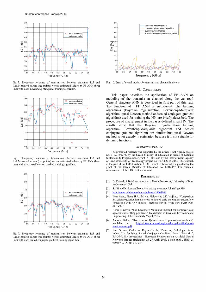
Fig. 7. Frequency response of transmission between antennas Tx3 and
Rx1.Measured values (red points) versus estimated values by FF ANN (blue
line) with used Levenberq-Marquardt training algorithm.
Fig. 8. Frequency response of transmission between antennas Tx3 and
Rx1.Measured values (red points) versus estimated values by FF ANN (blue line) with used quasi Newton method training algorithm.
Fig. 9. Frequency response of transmission between antennas Tx3 and
Rx1.Measured values (red points) versus estimated values by FF ANN (blue line) with used scaled conjugate gradient training algorithm.
Fig. 10. Error of neural models for transmission channel in the car.
VI. CONCLUSION
This paper describes the application of FF ANN on modeling of the transmission channel along the car roof. General structure ANN is described in first part of this text. The function of FF ANN is introduced. The training algorithms (Bayesian regularization, Levenberq-Marquardt algorithm, quasi Newton method andscaled conjugate gradient algorithm) used for training the NN are briefly described. The procedure of measurement in the car is defined in part IV. The results show that the Bayesian regularization training algorithm, Levenberq-Marquardt algorithm and scaled conjugate gradient algorithm are similar but quasi Newton method is not exactly in estimation because it is not suitable for dynamic functions.
ACKNOWLEDGMENT
The presented research was supported by the Czech Grant Agency project no. P102/12/1274, by the Czech Ministry of Education in frame of National Sustainability Program under grant LO1401, and by the Internal Grant Agency of Brno University of Technology project no. FEKT-S-14-2483. The research is the part of the COST Action IC1301 which is financially supported by the grant of the Czech Ministry of Education no. LD14057. For research, infrastructure of the SIX Center was used.
REFERENCES
[1] D. Kriesel, A Brief Instroduction o Neural Networks, University of Born in Germany,2005.
[2] Š. Jiří and N. Roman,Teoretické otázky neuronových sítí, pp.389.
[3] http://www.ncbi.nlm.nih.gov/pubmed/19065804
[4] Wen Wang, Pieter H.A.J.M. van Gelder and J.K. Vrijling, “Comparison Bayesian regularization and cross-validated early-stoping for streamflow forecasting with ANN models” Methodology in Hydrology. IAHS Publ 311, 2007
[5] Henri P. Gavin, “The Levenberg-Marquardt method for nonlinear least squares curve-fitting problems”, Department of Civil and Environmental Engineering Duke University May 4, 2016
[6] Andrew Galen, “Overview of Quasi-Newton optimization methods”, available on : https://homes.cs.washington.edu/~galen/files/quasi-newton-notes.pdf
[7] José Orozco, Carlos A. Reyes García, “Detecting Pathologies from Infant Cry Applying Scaled Conjugate Gradient Neural Networks”, ESANN'2003 proceedings - European Symposium on Artificial Neural Networks Bruges (Belgium), 23-25 April 2003, d-side publi., ISBN 2-930307-03-X, pp. 349-354
Student conference Blansko 2016
34

Model-Based Testing Framework with Automatic
Testing Priority Assignment for Automotive
Distributed Systems
Lukáš Krejčí, Jiří Novák
Czech Technical University in Prague, Faculty of Electrical Engineering, Technická 2, 166 27 Prague 6, Czech Republic
Abstract—The paper presents an optimized framework for
model-based testing of automotive distributed system and a
method of automatic assignment of testing priorities used within the framework. The proposed method, envisioned for integration
into existing, currently developed model-based testing tool, utilizes
classifiers in order to assign testing priorities automatically to specific parts of the tested system. The paper also introduces a
set of supplemental data enriching the modeling language that are
exploited by the proposed method during the classification
process. It is shown, that the presented approach’s advantages, such as low requirements for the testing operators’ insight, are
valuable for the automotive distributed systems testing process.
Keywords—Model-Based; Testing; Automotive; Classification; Classifiers; Artificial Neural Networks
I. INTRODUCTION
The Aim of this paper is to propose a new, optimized framework for Model-Based Testing (MBT) of automotive distributed systems and particularly present its automated testing priority assignment procedure.
The MBT is a popular approach of automated testing, which utilizes an abstract model of a System-Under-Test (SUT) in order to generate a testing sequence or drive the testing procedure in real time. The MBT can be applied even on complex software or hardware SUTs, such as automotive distributed systems.
Typically, the automotive industry uses a testing process composed of three distinct parts: the mandatory standard assessments, the specific test cases, and integration testing. The mandatory standard assessments are given by various international, national or organization safety standards and are thus unavoidable. The prearranged specific test cases are often based on the organization know-how and are therefore desirable, as they can uncover specific corner-case faults. The purpose of integration testing is to evaluate the automotive system as a whole since such testing can discover possible failures caused by distributed systems interconnection. Such failures characteristically originate from the inconsistent interpretation of the system specification among the subsystems suppliers, which may result in incorrect implementation and consequently in malfunction of multiple subsystems. Presently, the integration testing is usually performed manually by testing operators and thus can be automated using the MBT principles. However, as
the automotive distributed systems are reactive, real-time and parallel, it was necessary to develop the appropriate testing tool.
II. BACKGROUND
The developed testing tool, called Taster, is based on diploma thesis [1] and described in paper [2]. Since automotive systems are real-time and reactive, a modeling language used by this tool is based on the theory of timed automata, developed by UPPAAL team [3]. This modeling language allows describing modeled system as a network of Timed Safely Automata (each is referred as a template) bound by a set of variables.
Due to significant complexity of a typical SUT, it is impossible to execute its complete evaluation, and only some parts of its state space can be tested. Therefore, the test sequence generation can be driven by various strategies. The Taster tool currently utilizes a generation of pseudorandom test sequences according to priorities manually inscribed in the model. Since the correct assignment of priorities is affected by multiple parameters, this approach requires significant insight from testing operators. Furthermore, pseudorandom sequences can be suboptimal in several cases. Consequently, a new optimized testing framework for this tool was designed to reduce the mean time required for the failure detection and to lower the amount of insight required from testing operators. Fig. 1 shows its structure.
Fig. 1. Framework structure
The framework is defined as a pipeline chain consisting of following parts:
The Model Parser, which loads a model from its XML-formatted file.
The Automated Pinpointing Analyzer, which encases the procedure of labeling the model with testing priorities.
The Line-Up Generator responsible for generating the testing sequences. This block takes an enriched
Student conference Blansko 2016
35
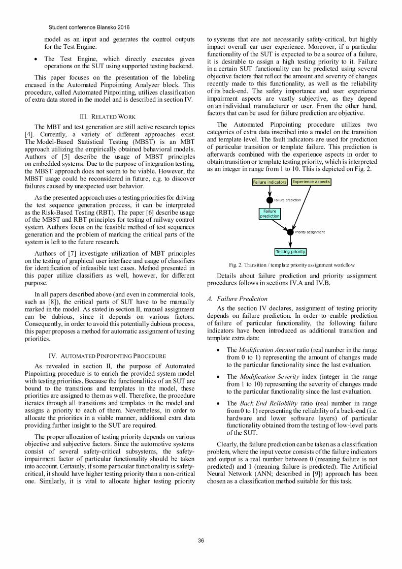
model as an input and generates the control outputs for the Test Engine.
The Test Engine, which directly executes given operations on the SUT using supported testing backend.
This paper focuses on the presentation of the labeling encased in the Automated Pinpointing Analyzer block. This procedure, called Automated Pinpointing, utilizes classification of extra data stored in the model and is described in section IV.
III. RELATED WORK
The MBT and test generation are still active research topics [4]. Currently, a variety of different approaches exist. The Model-Based Statistical Testing (MBST) is an MBT approach utilizing the empirically obtained behavioral models. Authors of [5] describe the usage of MBST principles on embedded systems. Due to the purpose of integration testing, the MBST approach does not seem to be viable. However, the MBST usage could be reconsidered in future, e.g. to discover failures caused by unexpected user behavior.
As the presented approach uses a testing priorities for driving the test sequence generation process, it can be interpreted as the Risk-Based Testing (RBT). The paper [6] describe usage of the MBST and RBT principles for testing of railway control system. Authors focus on the feasible method of test sequences generation and the problem of marking the critical parts of the system is left to the future research.
Authors of [7] investigate utilization of MBT principles on the testing of graphical user interface and usage of classifiers for identification of infeasible test cases. Method presented in this paper utilize classifiers as well, however, for different purpose.
In all papers described above (and even in commercial tools, such as [8]), the critical parts of SUT have to be manually marked in the model. As stated in section II, manual assignment can be dubious, since it depends on various factors. Consequently, in order to avoid this potentially dubious process, this paper proposes a method for automatic assignment of testing priorities.
IV. AUTOMATED PINPOINTING PROCEDURE
As revealed in section II, the purpose of Automated Pinpointing procedure is to enrich the provided system model with testing priorities. Because the functionalities of an SUT are bound to the transitions and templates in the model, these priorities are assigned to them as well. Therefore, the procedure iterates through all transitions and templates in the model and assigns a priority to each of them. Nevertheless, in order to allocate the priorities in a viable manner, additional extra data providing further insight to the SUT are required.
The proper allocation of testing priority depends on various objective and subjective factors. Since the automotive systems consist of several safety-critical subsystems, the safety-impairment factor of particular functionality should be taken into account. Certainly, if some particular functionality is safety-critical, it should have higher testing priority than a non-critical one. Similarly, it is vital to allocate higher testing priority
to systems that are not necessarily safety-critical, but highly impact overall car user experience. Moreover, if a particular functionality of the SUT is expected to be a source of a failure, it is desirable to assign a high testing priority to it. Failure in a certain SUT functionality can be predicted using several objective factors that reflect the amount and severity of changes recently made to this functionality, as well as the reliability of its back-end. The safety importance and user experience impairment aspects are vastly subjective, as they depend on an individual manufacturer or user. From the other hand, factors that can be used for failure prediction are objective.
The Automated Pinpointing procedure utilizes two categories of extra data inscribed into a model on the transition and template level. The fault indicators are used for prediction of particular transition or template failure. This prediction is afterwards combined with the experience aspects in order to obtain transition or template testing priority, which is interpreted as an integer in range from 1 to 10. This is depicted on Fig. 2.
Fig. 2. Transition / template priority assignment workflow
Details about failure prediction and priority assignment procedures follows in sections IV.A and IV.B.
A. Failure Prediction
As the section IV declares, assignment of testing priority depends on failure prediction. In order to enable prediction of failure of particular functionality, the following failure indicators have been introduced as additional transition and template extra data:
The Modification Amount ratio (real number in the range from 0 to 1) representing the amount of changes made to the particular functionality since the last evaluation.
The Modification Severity index (integer in the range from 1 to 10) representing the severity of changes made to the particular functionality since the last evaluation.
The Back-End Reliability ratio (real number in range from 0 to 1) representing the reliability of a back-end (i.e. hardware and lower software layers) of particular functionality obtained from the testing of low-level parts of the SUT.
Clearly, the failure prediction can be taken as a classification problem, where the input vector consists of the failure indicators and output is a real number between 0 (meaning failure is not predicted) and 1 (meaning failure is predicted). The Artificial Neural Network (ANN; described in [9]) approach has been chosen as a classification method suitable for this task.
Student conference Blansko 2016
36
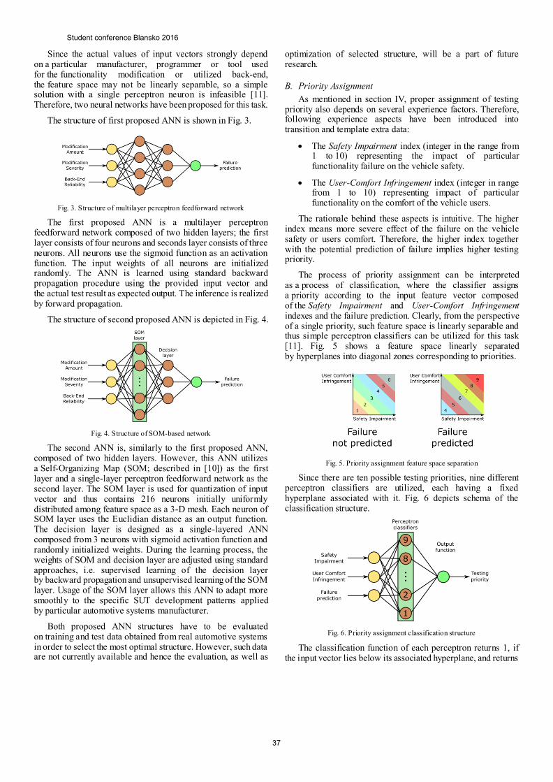
Since the actual values of input vectors strongly depend on a particular manufacturer, programmer or tool used for the functionality modification or utilized back-end, the feature space may not be linearly separable, so a simple solution with a single perceptron neuron is infeasible [11]. Therefore, two neural networks have been proposed for this task.
The structure of first proposed ANN is shown in Fig. 3.
Fig. 3. Structure of multilayer perceptron feedforward network
The first proposed ANN is a multilayer perceptron feedforward network composed of two hidden layers; the first layer consists of four neurons and seconds layer consists of three neurons. All neurons use the sigmoid function as an activation function. The input weights of all neurons are initialized randomly. The ANN is learned using standard backward propagation procedure using the provided input vector and the actual test result as expected output. The inference is realized by forward propagation.
The structure of second proposed ANN is depicted in Fig. 4.
Fig. 4. Structure of SOM-based network
The second ANN is, similarly to the first proposed ANN, composed of two hidden layers. However, this ANN utilizes a Self-Organizing Map (SOM; described in [10]) as the first layer and a single-layer perceptron feedforward network as the second layer. The SOM layer is used for quantization of input vector and thus contains 216 neurons initially uniformly distributed among feature space as a 3-D mesh. Each neuron of SOM layer uses the Euclidian distance as an output function. The decision layer is designed as a single-layered ANN composed from 3 neurons with sigmoid activation function and randomly initialized weights. During the learning process, the weights of SOM and decision layer are adjusted using standard approaches, i.e. supervised learning of the decision layer by backward propagation and unsupervised learning of the SOM layer. Usage of the SOM layer allows this ANN to adapt more smoothly to the specific SUT development patterns applied by particular automotive systems manufacturer.
Both proposed ANN structures have to be evaluated on training and test data obtained from real automotive systems in order to select the most optimal structure. However, such data are not currently available and hence the evaluation, as well as
optimization of selected structure, will be a part of future research.
B. Priority Assignment
As mentioned in section IV, proper assignment of testing priority also depends on several experience factors. Therefore, following experience aspects have been introduced into transition and template extra data:
The Safety Impairment index (integer in the range from 1 to 10) representing the impact of particular functionality failure on the vehicle safety.
The User-Comfort Infringement index (integer in range from 1 to 10) representing impact of particular functionality on the comfort of the vehicle users.
The rationale behind these aspects is intuitive. The higher index means more severe effect of the failure on the vehicle safety or users comfort. Therefore, the higher index together with the potential prediction of failure implies higher testing priority.
The process of priority assignment can be interpreted as a process of classification, where the classifier assigns a priority according to the input feature vector composed of the Safety Impairment and User-Comfort Infringement indexes and the failure prediction. Clearly, from the perspective of a single priority, such feature space is linearly separable and thus simple perceptron classifiers can be utilized for this task [11]. Fig. 5 shows a feature space linearly separated by hyperplanes into diagonal zones corresponding to priorities.
Fig. 5. Priority assignment feature space separation
Since there are ten possible testing priorities, nine different perceptron classifiers are utilized, each having a fixed hyperplane associated with it. Fig. 6 depicts schema of the classification structure.
Fig. 6. Priority assignment classification structure
The classification function of each perceptron returns 1, if the input vector lies below its associated hyperplane, and returns
Student conference Blansko 2016
37

0 otherwise. The output function of classification structure,
defined as 𝑓𝑜𝑢𝑡(𝑥1, … , 𝑥9) = 10 −∑ 𝑥𝑖9𝑖=1 , counts the outputs
of separate perceptron classifiers and subtracts this sum from 10, which is then used as testing priority for given transition or template.
Since the testing priority is not objectively measurable, the priority assignment procedure does not use learning and utilizes a fixed configuration instead.
V. CONCLUSIONS AND FUTURE WORK
In this paper, a part of new framework for the model-based testing of an automotive distributed systems is presented. The presented framework part, called Automated Pinpointing procedure, exploits the SUT model supplemented with the extra data in order to automatically assign testing priorities to model’s transitions and templates. This is useful for automatic pinpointing of the SUT parts that are most worthwhile to be tested.
Additionally, an appropriate set of extra data was introduced. The proposed system of transition and template extra data includes both subjective factors (i.e. experience aspects), as well as objective factors (i.e. fault indicators). As supplemental data take into account various factors influencing the testing priority, the proposed method significantly lowers overall testing operators’ insight requirements, as most of the required model parameters can be obtained repetitively by automatic procedures (the objective factors) or once by empirical research (the subjective factors).
Presently, the framework is being implemented into developed tool Taster that currently utilizes pseudorandom test sequence generation. Since this tool uses a modeling language based on timed automata, the presented framework, Automated Pinpointing procedure and proposed extra data utilize it as well.
Future research will be focused on the optimization of the classification structures used within the procedure. Since the priority assignment procedure makes use of strongly subjective User-Comfort Infringement index extra data, proper values of this parameter will be acquired by empirical research. Also, it is necessary to gather training data to optimize the ANN structure for failure prediction. Furthermore, other classifiers than ANN will be evaluated, so the most optimal approach could be found. For example, the rule-based methods seem to be promising for this purpose.
Additional research will be focused on the methods for prediction of possible regression in particular functionality caused by influences originating in other, possibly similar, SUT functionality. Such information can be obtained using the static analysis principles from the SUT source code or can be provided by the system modeler. Afterward, such information can be exploited by the context-sensitive classifiers for more precise prediction of functionalities failures.
Finally, since the developed tool currently generates testing sequences pseudo-randomly, more optimal approaches will be explored.
The proposed procedure and complete Taster tool will be evaluated, thanks to the co-operation with Škoda Auto a. s., on the real automotive systems developed and manufactured by this company. Moreover, Škoda Auto a. s. will supply data from real automotive systems that are necessary for the procedure optimization.
ACKNOWLEDGMENT
Research described in the paper was supported by the Grant Agency of the Czech Technical University in Prague, project Model-Based Testing methods for automotive electronics systems (grant No. SGS16/171/OHK3/2T/13) and by the support of EU Regional Development Fund in OP R&D for Innovations (OP VaVpI) and The Ministry of Education, Youth and Sports, Czech Republic, project # CZ.1.05/2.1.00/03.0125 Acquisition of Technology for Vehicle Center of Sustainable Mobility.
REFERENCES
[1] Tomáš Grus, “Implementation of Integration Testing Test Cases
Generation Tool,” Master’s Thesis, CTU in Prague, 2014.
[2] Sobotka, J. and Novák, J., “Testing Automotive Reactive Systems using Timed Automata,” In BEC 2016 - 2016 15th Biennial Baltic Electronics Conference. Tallin: Tallin University of Technology, 2016, [under review].
[3] Behrmann, G., David and A., Larsen, K. G., “A tutorial on UPPAAL,” In proceedings of the 4th International School on Formal Methods for the Design of Computer, Communication, and Software Systems (SFM-RT'04).
[4] S. Rösch, S. Ulewicz, J. Provost, and B. Vogel-Heuser, “Review of Model-Based Testing Approaches in Production Automation and Adjacent Domains—Current Challenges and Research Gaps,“ J. Softw. Eng. Appl., vol. 08, no. 09, pp. 499–519, 2015.
[5] F. Böhr, “Model Based Statistical Testing of Embedded Systems,” 2011 IEEE Fourth Int. Conf. Softw. Testing, Verif. Valid. Work., pp. 18–25, 2011.
[6] Zimmermann, F., Eschbach, R., Kloos, J. and Bauer, T., “Risk-based Statistical Testing: A Refinement-based Approach to the Reliability Analysis of Safety-Critical Systems,” 12th European Workshop on Dependable Computing, EWDC 2009, Toulouse, France, 2009.
[7] Gove, R., Faytong, J., “Chapter 4 – Machine Learning and Event-Based Software Testing: Classifiers for Identifying Infeasible GUI Event Sequences,” Advances in Computers, vol. 86, pp. 109–135, 2012.
[8] MaTeLo, http://www.all4tec.net/MaTeLo/homematelo.html.
[9] Aleksander, I. and Morton, H., “An introduction to neural computing,” International Thomson Computer Press, 2nd edition, 1995.
[10] Kohonen, T., “Self-Organizing Maps,” New York : Springer-Verlag, 1997.
[11] Minky, M. and Papert, S., “Perceptrons: An Introduction to Computational Geometry,” M.I.T. Press, 1969.
Student conference Blansko 2016
38

Design and Limitations of the
Metal – Composite Hybrid Joint Structures
David Krutílek
Department of Radio Electronic
Brno University of Technology
Brno, Czech Republic
Abstract—This paper provides an overview of design aspects
and limitations of joints in metal-composite hybrid structures
and identifies limitations and recommendations regarding
electromagnetic properties of the joints. Besides the design
recommendations, the most frequently used ways of modelling
the joints during the design stage is provided.
Keywords—joint; transfer impedance Zt; Discrete circuit
elements; Shielding efficiency; lightning damage rating
I. INTRODUCTION
The materials used in aircraft industry are being permanently improved and developed to reduce weight, increase flexibility and strength, and decrease the price. Conventional metal materials are therefore replaced by different composite materials. Composite materials are also advantageous due to their easy shaping ability.
From the EMC point of view, one of the most important aspects of metal-composite joints is to safely conduct possible currents flowing through the joint and, if necessary, protect electromagnetically sensitive equipment against external electromagnetic fields leaking into the internal parts of the aircraft. Ideally, to achieve such a goal, the whole joint area would need to be completely sealed by a highly conductive material with good conductive contact to both adjacent surfaces (contact area between composite and metallic parts). Unfortunately, similar goals are usually not achievable or they represent significant increase of the joint’s cost from both time and financial point of view.
In case of riveted metal-composite joints, the main design problems consist of preventing the joint from excessive heating and sparking that can result in damaging of the joint. This is followed by decrease of the shielding effectiveness (SE), degradation of mechanical/strength properties of the composite material near the joint and shortening of its service lifespan.
II. DESCRIPTION OF THE JOINTS USING TRANSMISSIONS
CHARACTERISTICS
Transmission characteristic of a joint describes a joint behavior depending on the frequency. Transmission characteristic of a joint are as follows:
• Transfer impedance Zt • Discrete circuit elements
• Shielding efficiency (SE evaluation)
Fig. 1 Illustrative characterization of impedance behavior of a riveted joint
(sketch)
For low frequency (maximum sample dimension is λ/10) it is appropriate to use description based on discrete element circuit. Shielding efficiency (SE evaluation) is used for high frequency description.
A. Discrete circuit elements
Fig. 1 shows behavior impedance (Zj) of the joint. The path should be subsequently designed with the view of the following aspects:
1) Resistive behavior The total contact area of all rivets in the considered area,
which should be large enough to carry the expected amount of electric current and the conductivity of the path through the joint and should be sufficiently high (e.g. below 2.5 mΩ [1]). If the conductivity is poor, overheat of the joint is possible. Resistivity of the joint is a very important aspect especially when designing lightning strike protection or evaluating paths for current return (e.g. [2]).
2) Capacitive behavior Between the adjacent parts of the joint there should not be
any significant accumulation of electric charges, because the formation of spark is possible. When dealing with electro-static discharge (ESD) measures or sparking issues, the property of
Student conference Blansko 2016
39

the joint is important, especially capacitance. Moreover, in combination with inductance it defines a resonant behavior of the joint.
3) Inductive behavior Inductance of the joint is increasing with increasing the
length of the conductive path through the joint. For this reason, the path should be as short and straight as possible. There should not be a significant problem in case of riveted joint. High inductance of the joint successfully prevents quickly changing currents (high di/dt) to easily pass through the joint despite its low DC resistivity. It is very important to design the conductive path with significantly lower inductance.
B. Shielding efficiency (SE evaluation)
A device made of conductive and / or magnetic material which isolates two regions or space, one with some electromagnetic sources and the other without any source. A way to measure the efficiency of an electromagnetic shied. It is given by formula:
shieldwith
shieldwithout
dbField
FieldSE
_
_
10log20 (1)
A positive SE corresponds to attenuation. A negative value is also possible, it corresponds to resonances. Shielding effectiveness can be affected by different factors:
• The type of material used for the screen • Presence of slots, seams, gaskets • Holes, wires
Shielding effectiveness is evaluated in the context of the considered system (like as panel with cover). It is therefore the global assessment of the whole connection, which consists of more joints on the sample. Poor construction and design of joints may affect on the shielding effectiveness of the materials on high frequency band (especially cover, panels, inspect doors etc.)
A distance between the neighboring rivets (which are creating the conductive paths through the joint) should be small enough (ca. λ/10 for a maximal considered frequency) to prevent the penetration / re-radiation of electromagnetic fields / currents through the joint (remark: Despite very low DC resistance of riveted joints, an approximate SE of riveted aluminum panels with nonconductive sealants can be expected on the order of 20 dB. In case of a metal-composite riveted joint, it is reasonable to count with the SE below this threshold.[3], [4])
III. SUMMARY OF PROPOSED TESTS
The main purpose of this project is to describe the electrical properties of joints using RLC parameters, and the verification of their hardness against lightning. Since the tests and measurements are principally different, for each test method, it is necessary to produce various samples. Moreover, once the tests for resistance to lightning strikes are finished, it is likely that the sample is permanently damaged.
To determine the RLC parameters, maximum size of the sample is recommended. The maximum dimensions (Lmax) can be determined with the aid of simple formula:
Lmax = λ/10 (2)
The test sample, which length is approximately 50 mm, can be measured on maximum frequency fmax = 300 MHz. Testing the lightning strike is performed on samples of dimensions 500 x 500 mm (550 x 550 mm). These tests can permanently damage and devalue the samples.
A. Impedance measurement method
Electromagnetic properties of a riveted joint can be described via its impedance behavior. The simplest way to describe impedance in both the frequency and the time domain is in a form of an equivalent electric circuit (R, L, C, and G).
However, prior to making any equivalent circuit model of a junction, it is necessary to find out the junction’s transfer impedance. Depending on circumstances, it can be done by one of the following measurement setups [5]:
1) Bridge method The value of the unknown impedance (Zx) can be obtained
by the relationship of the other bridge elements. When no current flows through the detector (D), the bridge is balanced. Various types of bridge circuits, employing combinations of R, L and C components as the bridge elements, are used for various applications. Applicable frequency range is from DC to 300 MHz.
Advantages
• High accuracy (0.1% typ.) • Wide frequency coverage by using by different types
of bridges • Low cost
Disadvantages
• Needs to be manually balanced • Narrow frequency coverage with a single instrument
Fig. 2 Principe of bridge method.[5]
2) Auto-balancing bridge method The current Ix balances with the current Ir which flows
through the range resistor (Rr), by operation of the I-V converter. A “virtual ground” is maintained at zero volts the potential at the Low point. Using the voltage measured at the High terminal (Vx) and across Rr (Vr) is calculated the impedance of the DUT.
Student conference Blansko 2016
40
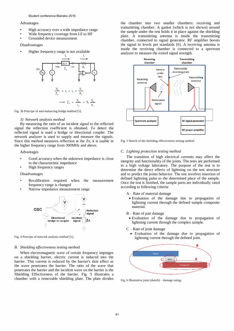
Advantages
• High accuracy over a wide impedance range • Wide frequency coverage from LF to HF • Grounded device measurement
Disadvantages
• Higher frequency range is not available
Fig. 3b Principe of auto-balancing bridge method [5].
3) Network analysis method By measuring the ratio of an incident signal to the reflected
signal the reflection coefficient is obtained. To detect the reflected signal is used a bridge or directional coupler. The network analyzer is used to supply and measure the signals. Since this method measures reflection at the Zx, it is usable in the higher frequency range from 300MHz and above.
Advantages
• Good accuracy when the unknown impedance is close to the characteristic impedance
• High frequency ranges
Disadvantages
• Recalibration required when the measurement frequency range is changed
• Narrow impedance measurement range
Fig. 4 Principe of network analysis method [5].
B. Shielding effectiveness testing method
When electromagnetic wave of certain frequency impinges on a shielding barrier, electric current is induced into the barrier. This current is reduced by the barrier's skin effect as the wave penetrates the barrier. The ratio of the wave that penetrates the barrier and the incident wave on the barrier is the Shielding Effectiveness of the barrier. Fig. 5 illustrates a chamber with a removable shielding plate. The plate divides
the chamber into two smaller chambers: receiving and transmitting chamber. A gasket (which is not shown) around the sample under the test holds it in place against the shielding plate. A transmitting antenna is inside the transmitting chamber, connected to signal generator. RF amplifier boosts the signal to levels per standards [6]. A receiving antenna is inside the receiving chamber is connected to a spectrum analyzer to measure the exited signal strength.
Fig. 5 Sketch of the shielding effectiveness testing method
C. Lightnig protection testing method
The transition of high electrical currents may affect the integrity and functionality of the joints. The tests are performed in a high voltage laboratory. The purpose of the test is to determine the direct effects of lightning on the test structure and to predict the joints behavior. The test involves insertion of defined lightning pulse to the determined place of the sample. Once the test is finished, the sample parts are individually rated according to following criteria:
A – Rate of material damage
Evaluation of the damage due to propagation of lightning current through the defined sample composite material.
B – Rate of part damage
Evaluation of the damage due to propagation of lightning current through the complex sample.
C – Rate of joint damage
Evaluation of the damage due to propagation of lightning current through the defined joint.
Fig. 6 Illustrative joint (sketch) – damage rating.
Student conference Blansko 2016
41

These experiments are realized in special laboratories. A variety of test rigs are available to accommodate different sizes of test panel and aircraft structural components. Many structural assessments can be performed on square panels (typically 500mm, or 550mm). For larger structural items or parts of flight control surfaces bespoke test rigs and return conductor paths are set up as required.
Figure 15 illustrates the principle of lightning protection testing. The sample is fixed in the grounded fixture. A thin copper wire is inserted between the electrode (sphere) and the top side of the sample (attachment point). The copper wire helps only to create lightning arc and is not involved in the current distribution. Lightning pulse generator boosts the current to levels per standard [6].
Fig. 7 Principle of lightning protection testing method
IV. ELECTROMAGNETIC MODELING
As mentioned in Chapter II, electromagnetic properties of a riveted joint can be described via its impedance behavior. The simplest way to describe impedance in both the frequency and the time domains, is in a form of an equivalent electric circuit (R, L, C, G; see Fig. 8).
Fig. 8 General equivalent schematic representation of a transmission line
element.
As can be seen in Fig. 1, geometrical character of a junction can be „easily“ described by those basic elements and formed into more complex nets, that could be solved by computational means (for example via transmission line matrix method (TLM), partial element equivalent circuit method (PEEC), etc.).
However, prior to making any equivalent circuit model of a junction, it is necessary to find out the junction’s transfer impedance. Depending on circumstances, it can be done by one of the following ways:
- By measurement: this is the most common, straightforward, and usually the most exhaustive approach how to obtain real impedance behavior of a joint. Data is usually
obtained only in frequency domain at specific frequencies and has to be subsequently processed into an appropriate form used for time domain analyses.
- By analytical means: description of a junction is made via simple analytical formulas which are able take into account basic shapes and dimensions of its real composition / structure. It is one of the quickest, but not always accurate, ways how to describe the impedance behavior. It should be noted that impedance information obtained by this way is naturally defined by inherent limits of used analytical formulas.
- By computational means: impedance behavior of a junction is computed from its realistic CAD model representation (in 2D or 3D) with the help of computational electromagnetics (computationally efficient approximations to Maxwell’s equations). Contrary to both previous ways, using of computational electromagnetics allows us to analyze junctions’ impedance relatively quickly, precisely and in the whole necessary frequency spectrum that is of our interest from the EMC and design points of view (DC – 40GHz).
V. CONCLUSION
The measured RCL values of joint characteristics can be easily included in the EM-analyzes. This can lead to more precise calculation and helps to define the requirements for the joint. The tests of resistance against lightning strike aim to obtain the information whether such a joint or set of joint is suitable for the area and concrete place on the airplane. In case that the original design is poor, the information obtained from EM-analyzes can help to eliminate deficiencies before application on the real sample.
ACKNOWLEDGMENT
Research described in this paper was financed by Czech Ministry of Education in frame of National Sustainability Program under grant LO1401.This work also receives funding through specific research grant project FEKT-S-14-2281. Special thanks belong to EVEKTOR Company for providing the aircraft model data
REFERENCES
[1] SAE ARP 1870A, Aerospace Systems Electrical Bonding and Grounding for Electromagnetic Compatibility and Safety, Stabilized: August 2012
[2] MULAZIMOGLU, H., HAYLOCK, L. Recent Developments in Techniques to Minimize Lightning Current Arcing Between Fasteners and Composite Structure, Alcoa New Product Development, Aerospace Fasteners, 2011 < https://www.alcoa.com/fastening_systems_and_rings/ aerospace/en/pdf/hasim_icosle_2011.pdf >
[3] GOOCH, J. W., DAHER, J. K. Electromagnetic Shielding and Corrosion Protection for Aerospace Vehicles, Springer, March 2007, ISBN-10: 0471126993
[4] [14] NASA-STD-P023 DRAFT, Electrical bonding for NASA launch vehicles, spacecraft, payloads, and flight equipment, 17th August 2001
[5] AGILENT IMPEDANCE MEASUREMENT HANDBOOK: A GUIDE TO MEASUREMENT TECHNOLOGY AND TECHNIQUES 4TH EDITION, 2013, < http://cp.literature.agilent.com/litweb/ pdf/5950-3000.pdf >
[6] SAE ARP 5412B, Aircraft Lightning Environment and Related Test Waveform
Student conference Blansko 2016
42
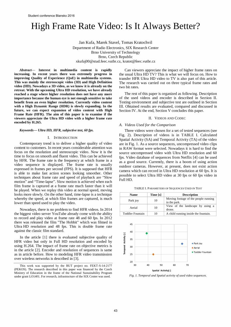
High Frame Rate Video: Is It Always Better?
Jan Kufa, Marek Stavel, Tomas Kratochvil
Department of Radio Electronics, SIX Research Center
Brno University of Technology
Brno, Czech Republic
[email protected], [email protected]
Abstract— Interest in multimedia content is rapidly
increasing. In recent years there was extremely progress in
improving Quality of Experience (QoE) in multimedia systems.
This was mainly the stereoscopic video (3D) and High Definition
video (HD). Nowadays a 3D video, as we know it is already on the
retreat. With the upcoming Ultra HD resolution, we have already
reached a stage where higher resolution does not have any more
importance because the human eye is not enough sensitive to take
benefit from an even higher resolution. Currently video content
with a High Dynamic Range (HDR) is slowly expanding. In the
future, we can expect expansion of video content with High
Frame Rate (HFR). The aim of this paper is to examine if the
viewers appreciate the Ultra HD video with a higher frame rate
encoded by H.265.
Keywords— Ultra HD, HFR, subjective test, 60 fps.
I. INTRODUCTION
Contemporary trend is to deliver a higher quality of video content to customers. In recent years considerable attention was focus on the resolution and stereoscopic video. Now it is the time to focus on smooth and fluent video. This can be achieved by HFR. The frame rate is the frequency at which frame in a video sequence is displayed. The frame rate is usually expressed in frames per second (FPS). It is supposed that HFR is able to make fast action scenes looking smoother. Other techniques about frame rate and speed of playback are “Slow motion” and “Time-lapse”. Slow motion is achieved when each film frame is captured at a frame rate much faster than it will be played. When we replay this video at normal speed, moving looks more slowly. On the other hand, time-lapse is a technique whereby the speed, at which film frames are captured, is much lower than speed used to play the video.
Nowadays, there is no problem to find HFR videos. In 2014 the biggest video server YouTube already come with the ability to record and play video at frame rate 48 and 60 fps. In 2012 there was released the film "The Hobbit" which was filmed in Ultra HD resolution and 48 fps. This is double frame rate against the classic film standard.
In the article [1] there is evaluated subjective quality of HFR video but only in Full HD resolution and encoded by using H.264. The impact of frame rate on objective metrics is in the article [2]. Encoder and resolution of sequences is same as in article before. How to modeling HFR video transmission over wireless networks is described in [3].
This work was supported by the BUT project no. FEKT-S-14-2177
(PEKOS). The research described in this paper was financed by the Czech
Ministry of Education in the frame of the National Sustainability Program
under grant LO1401. For research, infrastructure of the SIX Center was used.
Can viewers appreciate the impact of higher frame rates on the usual Ultra HD TV? This is what we will focus on. How to transfer HFR Ultra HD video to TV is also part of this article. The research was carried out on three typical frame rates and two bit rates.
The rest of this paper is organized as following. Description of the used videos and encoder is described in Section II. Testing environment and subjective test are outlined in Section III. Obtained results are evaluated, compared and discussed in Section IV. At the end, Section V concludes this paper.
II. VIDEOS AND CODEC
A. Videos Used for the Comparison
Three videos were chosen for a set of tested sequences (see
Fig. 2). Description of videos is in TABLE I. Calculated
Spatial Activity (SA) and Temporal Activity (TA) of the video
are in Fig. 1. As a source sequences, uncompressed video clips
in RAW format were selected. Nowadays it is hard to find the
source uncompressed video with Ultra HD resolution and 60
fps. Video database of sequences from Netflix [4] can be used
as a good source. Currently, there is a boom of using action
outdoor cameras. However, at present, does not exist action
camera which can record in Ultra HD resolution at 60 fps. It is
possible to select Ultra HD video at 30 fps or 60 fps video in
Full HD.
TABLE I. PARAMETERS OF SEQUENCES USED IN TEST
Name Time [s] Description
Park joy 10 Moving footage of the people running
in the park.
Aerial 10 View of the landscape by using a
drone.
Toddler Fountain 10 A child running inside the fountain.
Fig. 1. Temporal and Spatial activity of used video sequences.
Student conference Blansko 2016
43

a) Park Joy b) Aerial
c) Toddler Fountain
Fig. 2. Thumbnails of used videos.
B. Codec H.265/ HEVC
Source sequences were encoded by codec H.265 known as
HEVC. This codec is able to encode video up to 8k resolution
and frame rate 120 fps. The most widespread implementation
of this codec, x265, was selected. Parameters for encoder are
in the TABLE II. Level 5.1 was set in the encoder because
Level 5.0 does not support frame rate 60 fps with Ultra HD
video. The group of pictures (GOP) was set to 8. Other
parameters of encoder were selected according to the
recommendations in document [5].
TABLE II. PARAMETERS OF USED ENCODER HEVC
Implementation x265
Built date 24.4.2016
Encoder version 1.9
Preset Medium
Profile Main
Two quality levels were chosen and each level is defined
by its bit rate, see TABLE III. Low bit rate 5 Mb/s represents
streaming with very limited bandwidth. On the other hand, bit
rate 50 Mb/s represents almost limitless bandwidth, for
example Ultra Blu-ray disk. We also focus on the fact if
viewers appreciate the HFR video provided that are not
limited by bandwidth. What is the difference if they are very
limited by the bandwidth? In the case where we have the same
bit rate, then at a HFR, the size of one frame is smaller than
the size of the frame at low frame rates. That means whether
people appreciate more fluency than image quality.
TABLE III. USED FRAME RATES AND BIT RATES
Parameter Value
Frame rate [FPS] 24 30 60
Bit rate [Mb/s] 5 50
Used frame rates are also in the table TABLE III. Frame
rate 24 fps represents film standard, almost all films that can
be downloaded from the internet have this frame rate.
Generally mobile phones and other consumer electronics
record in frame rate 30 fps. Video with 60 fps represents HFR
playback.
III. TESTING ENVIRONMENT AND SUBJECTIVE TEST SETUP
To ensure reproducibility of results, the subjective experiment was realized in a laboratory of video and multimedia technology. Laboratory conditions were set up according to ITU BT.500-13[6]. A workplace in a room with controlled lighting was created. Ultra HD television 49-inches LG 49UF8527 was used to display video sequences. The distance of the participants from the Ultra HD display was 1.5 meters.
The bit rate for decompressed Ultra HD video with 60 fps, color depth 8 bit and color model 4:2:0 is approximately 6 Gb/s. The TV was fed by a personal computer (PC), it was equipped with a fast SSD connected via PCI-Express with a read speed up 11 Gb/s. The reading speed of the disk must exceed the data stream of movies. The PC is equipped with NVIDIA GTX 960 that supports HDMI 2.0. Older version HDMI 1.4 is also capable of transmitting an image in Ultra HD resolution, however only in 30 fps. For the considered subjective test, it is necessary to use a newer version HDMI 2.0 which can handle image in Ultra HD resolution in 60 fps [7]. DisplayPort (DP) in version 1.2 is an additional interface, which is able to transfer the video in Ultra HD resolution in frame rate 60 fps to display. This interface, however it is not often used in television, is mainly used in monitors [8].
As a subjective method, Pair Comparison (PC) was
chosen. This method was chosen because of its suitability to
comparing two similar videos. The time to vote was 8 second.
Sequences were played randomly and observers did not know
what frame rate is currently presented. Total groups of 22
people were joined into the subjective test, half recruited from
university students and second half from the public. An
average age was 25 years.
IV. RESULTS AND EVALUATION
The impact of frame rate is more subjective aspect than
evaluation of image quality. From this point of view, it is
difficult to evaluate the exact perceptual improvement by
switching from normal to the high frame rate. Participants
compared a pair of two videos on a scale from -2 to +2. The
limit value -2 means that the viewer conclusively prefers a
smaller frame rate, while the value +2 indicates that viewer
prefers video with higher frame rate. A detail description of
the scale for comparison between 24 and 30 fps is in TABLE
IV. The same meaning of scale is in the comparison between
30 and 60 fps.
TABLE IV. DESCRIPTION OF SCALE USED IN GRAPHS
Scale Description
-2 Frame rate 24 fps definitely better than 30 fps
-1 Frame rate 24 fps slightly better than 30 fps
0 The same quality for both frame rate
+1 Frame rate 30 fps slightly better than 24 fps
+2 Frame rate 30 fps definitely better than 24 fps
Student conference Blansko 2016
44
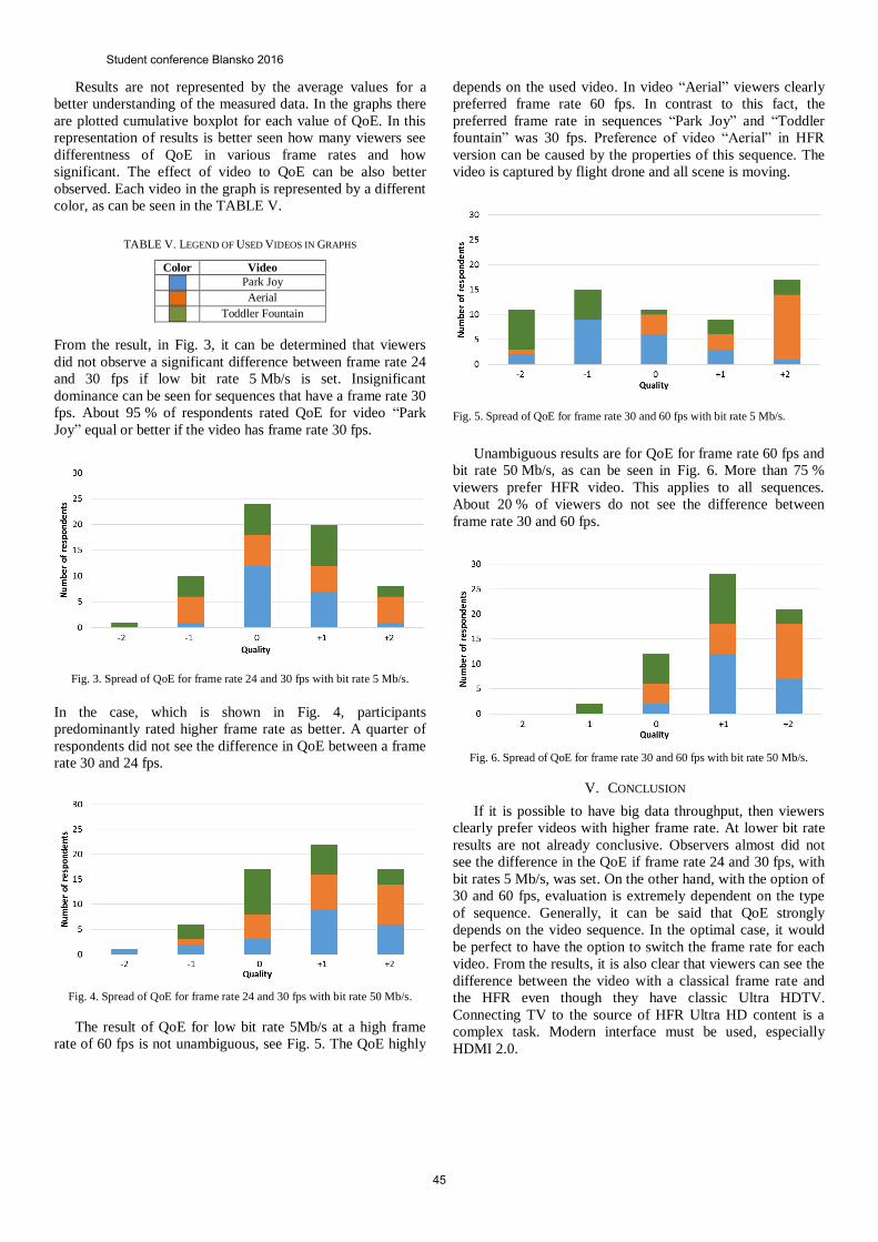
Results are not represented by the average values for a
better understanding of the measured data. In the graphs there
are plotted cumulative boxplot for each value of QoE. In this
representation of results is better seen how many viewers see
differentness of QoE in various frame rates and how
significant. The effect of video to QoE can be also better
observed. Each video in the graph is represented by a different
color, as can be seen in the TABLE V.
TABLE V. LEGEND OF USED VIDEOS IN GRAPHS
Color Video
Park Joy
Aerial
Toddler Fountain
From the result, in Fig. 3, it can be determined that viewers
did not observe a significant difference between frame rate 24
and 30 fps if low bit rate 5 Mb/s is set. Insignificant
dominance can be seen for sequences that have a frame rate 30
fps. About 95 % of respondents rated QoE for video “Park
Joy” equal or better if the video has frame rate 30 fps.
Fig. 3. Spread of QoE for frame rate 24 and 30 fps with bit rate 5 Mb/s.
In the case, which is shown in Fig. 4, participants
predominantly rated higher frame rate as better. A quarter of
respondents did not see the difference in QoE between a frame
rate 30 and 24 fps.
Fig. 4. Spread of QoE for frame rate 24 and 30 fps with bit rate 50 Mb/s.
The result of QoE for low bit rate 5Mb/s at a high frame
rate of 60 fps is not unambiguous, see Fig. 5. The QoE highly
depends on the used video. In video “Aerial” viewers clearly
preferred frame rate 60 fps. In contrast to this fact, the
preferred frame rate in sequences “Park Joy” and “Toddler
fountain” was 30 fps. Preference of video “Aerial” in HFR
version can be caused by the properties of this sequence. The
video is captured by flight drone and all scene is moving.
Fig. 5. Spread of QoE for frame rate 30 and 60 fps with bit rate 5 Mb/s.
Unambiguous results are for QoE for frame rate 60 fps and
bit rate 50 Mb/s, as can be seen in Fig. 6. More than 75 %
viewers prefer HFR video. This applies to all sequences.
About 20 % of viewers do not see the difference between
frame rate 30 and 60 fps.
Fig. 6. Spread of QoE for frame rate 30 and 60 fps with bit rate 50 Mb/s.
V. CONCLUSION
If it is possible to have big data throughput, then viewers
clearly prefer videos with higher frame rate. At lower bit rate
results are not already conclusive. Observers almost did not
see the difference in the QoE if frame rate 24 and 30 fps, with
bit rates 5 Mb/s, was set. On the other hand, with the option of
30 and 60 fps, evaluation is extremely dependent on the type
of sequence. Generally, it can be said that QoE strongly
depends on the video sequence. In the optimal case, it would
be perfect to have the option to switch the frame rate for each
video. From the results, it is also clear that viewers can see the
difference between the video with a classical frame rate and
the HFR even though they have classic Ultra HDTV.
Connecting TV to the source of HFR Ultra HD content is a
complex task. Modern interface must be used, especially
HDMI 2.0.
Student conference Blansko 2016
45

ACKNOWLEDGMENT
The authors acknowledge all the observers who took part in the subjective experiments.
REFERENCES
[1] R. M. Nasiri, J. Wang, A. Rehman, S. Wang and Z. Wang, "Perceptual quality assessment of high frame rate video," in Proceedings of IEEE 17th International Workshop on Multimedia Signal Processing (MMSP), 2015, Xiame (PRC), pp. 1-6. doi: 10.1109/MMSP.2015.7340831
[2] T. Zinner, O. Hohlfeld, O. Abboud and T. Hossfeld, "Impact of frame rate and resolution on objective QoE metrics," ," in Proceedings of Quality of Multimedia Experience (QoMEX) 2010, Trondheim, (Norway), pp. 29-34. doi: 10.1109/QOMEX.2010.5518277
[3] J. Wu, C. Yuen, N. M. Cheung, J. Chen and C. W. Chen, "Modeling and Optimization of High Frame Rate Video Transmission Over Wireless
Networks," in IEEE Transactions on Wireless Communications, vol. 15, no. 4, pp. 2713-2726, April 2016. doi: 10.1109/TWC.2015.2509063
[4] Xiph.org::Derf\’s Test Media Collection. Xiph.org Video Test Media. [online]. [cit. 2016-07-06]. Available from: https://media.xiph.org/ video/derf
[5] x265 HEVC High Efficiency Video Coding H.265 Encoder. x265. [online]. [cit. 2016-07-06]. Available from: http://x265.org/index.html
[6] ITU-R BT.500-13. “Methodology for the subjective assessment of the quality of television pictures.” ITU, January 2012.
[7] HDMI Forum’s Technical Working Group. [cit. 2016-07-06]. Available from: http://www.hdmi.org/manufacturer/hdmi_2_0/
[8] C. Wiley, “DisplayPort Technical Overview” in Proceedings of IEEE International Conference on Consumer Electronics (ICCE), 2011, Las Vegas (USA). Available from: http://www.vesa.org/wp-content/uploads/2011/01/ICCE-Presentation-on-VESA-DisplayPort.pdf
Student conference Blansko 2016
46
Correlated Mutation Analysis Improvement by
Proteomic Signal Processing
Kristyna Kupkova, Karel Sedlar, Ivo Provaznik
Department of Biomedical Engineering
Brno University of Technology
Brno, Czech Republic
Abstract— Correlated mutation analysis has become a
powerful tool in protein contact prediction based on multiple
sequence alignments of homologous proteins. Here, we introduce
a novel method for the computation of correlated mutations
based on prior transformation of protein sequences into their
numerical form, which provides important biological properties
about the amino acids. The method is then incorporated into a
compact technique replacing the previously proposed Jaccard
index. This results in the significant improvement of all of the
statistical parameters used in this study.
Keywords— correlated mutations; protein contact map;
numerical representation
I. INTRODUCTION
The function of a protein is fully determined by its spatial structure, which makes it a fundamental carrier of information in molecular biology. However, the current methodologies for protein structure assessment (such as X-ray crystallography or electron microscopy) are financially demanding and time consuming. Therefore, there is an incomplete protein structure database and it is not possible to follow the impact of fast mutational changes on molecular dynamics [1]. In order to overcome this barrier, there have been attempts since 1960s to devise a method for the determination of a 3D protein structure directly from its primary amino acid sequence [2]. One of the subproblems of this issue is the requirement for the construction of a protein contact map, which would indicate amino acid residues in close proximity to each other in the 3D model but distant from each other in the primary amino acid sequence. Correlated mutation analysis (CMA) which uses the multiple sequence alignment (MSA) of homologous proteins has become a popular approach to the construction of such a map. It is essential for a protein to maintain its structure intact in order to maintain its function. Therefore, negative point mutations at contact sites need to be compensated by other mutations. This mechanism, whereby pairs of residues in contact with each other need to co-evolve in synchrony, then results in a high correlation score for the pairs of positions in the MSA which are in contact with each other in the tertiary structure of homologous proteins [3].
Many CMA approaches have been tested over the past 30 years [3]-[8] with an achieved precision which is typically between 20% to 40%. These low precision values reflect a
large number of false positives in the predictions and are caused by additional phylogenetic residue correlation [9]. In order to reduce this background correlation, several CMA improvements have been introduced e.g. the application of specific filters [4], the combination of CMA results obtained from amino acid sequences with CMA results at codon level [5], or the combination of CMA results with neural networks [6]. Although these improvements reduce false positive detection, recall reflecting the number of correctly predicted contacts out of all existing contacts remains low. Recall enhancement has been introduced in [7], wherein several CMA methods were combined into a compact method, which leads to minimal precision impairment with significant recall improvement.
In this study, a novel approach to CMA, which uses a proteomic signal processing technique named proteomic signal correlation (PSC), is introduced. Numerical representation of the protein carrying information about important biological properties of amino acids has already proven useful in the prediction of the functional sites of proteins [10]. In this paper, we use a transformation method based on the hydrophobicity and hydropathy of amino acids in combination with Pearson’s correlation coefficient. The technique is then incorporated into the method introduced in [7], which results in further recall improvement with only low precision impairment.
II. MATERIALS AND METHODS
A. Data Preparation
The input for the CMA consists of the MSA of homologous proteins. These protein sequences can either be retrieved from suitable databases (such as Pfam of HSSP) or by performing a BLAST run against the protein database. Since the latter approach has provided better results [11], we used PSI-BLAST (Position-Specific Iterated BLAST) [12] on the non-redundant protein sequences database at NCBI (National Center for Biotechnology Information) [13]. Both orthologous and paralogous sequences were included in the dataset, for the exclusion of either seemed to be counter-productive [11]. Only sequences with a similarity between 70-90% with the reference sequence were selected and then aligned by using the Clustal Omega program [14]. Sequences with a similarity to each other which was higher than 90% were removed from the formed
Student conference Blansko 2016
47

TABLE I. DATASET DETAILS
PDB ID/
chain Seq lengtha MSA widthb MSA depthc
1A6K/A 151 142 61
1AFC/A 140 93 24
1HM6/A 346 313 51
3BCQ/A 143 137 88
4DT6/A 210 162 69
a. Original length of a reference sequence. b. Length of sequences after preprocessing.
c. Number of sequences in MSA after preprocessing
MSA in order to reduce the phylogenetic background of closely related sequences. Completely conserved positions were excluded from the MSA, since these positions do not provide any relevant information for the CMA [11]. In addition, positions containing more than 20% of gaps and positions with a gap occurrence in a reference sequence were removed. The details of the final MSA dataset consisting of five protein sets are listed in TABLE I.
B. Proteomic Signal Correlation
The novel method introduced in this paper, proteomic signal correlation (PSC), involves two steps. First, each column of the constructed MSA is transformed into a suitable proteomic signal form. The second step involves the computation of the Pearson’s correlation coefficient between all pairs of columns.
Many transformation techniques have been introduced over the past decade which convert the primary amino acid sequence into signal representation based on the biological properties of amino acids [10], [15], [16]. Finding the suitable transformation technique is crucial for the PSC outcome. In order to compute the Pearson’s correlation coefficient, the final signal representation should ideally be 1D while carrying a sufficient amount of information about a given amino acid. For this reason, we chose the transformation technique introduced in [16]. The conversion of column x in the MSA is undertaken according to following equation:
𝑥𝑖 = 𝐻𝑝𝑡
1
𝐸𝐻𝑡1
where i is the index of the sequence in the MSA and Hp1 and EH1 are values derived from the hydropathy and hydrophobicity of amino acid t accordingly. The values for each amino acid t can be obtained from [16].
The final correlation coefficient r between the two positions x and y is computed as follows:
𝑟(𝑥, 𝑦) = 1
𝑁−1∑ (
𝑥𝑖−𝜇𝑥
𝜎𝑥) (
𝑦𝑖−𝜇𝑦
𝜎𝑦)𝑁
𝑖=1 .
Here, i means the index of a sequence running from 1 to N and N is the number of sequences in the final MSA. Values µx and σx are the mean value and standard deviation of column x respectively.
C. Character-based Correlated Mutation Analysis
Compared to PSC, the CMA methods introduced in this section are purely character-based and work directly with the formed MSA.
1) Mutual Information Mutual information (MI) as a measure of mutual
dependence between two columns has been computed according to [3]. In order to reduce background MI caused by the finite sample effect and phylogenetic influence, the final values of MI were normalized by using MI/Hxy, where Hxy is the joint entropy of positions x and y.
2) Residue Correlation Analysis The residue correlation analysis (RCA) has been computed
according to [8]. We used the BLOSUM62 substitution matrix for obtaining the values of s(x,k,l) at position x between the two sequences k and l since the dominance of the McLachlan substitution matrix has not been proven [17]. The final correlation score was normalized by using RCAxy = (RCAxy – min(RCA)/(max(RCA) - min(RCA)) in order for the values to fall into the 0 to 1 interval.
3) Jaccard Index The Jaccard index (JI), representing the last measure of
CMA used in this paper, has been computed by using the equation in [18].
D. Compact Correlated Mutation Analysis
The CMA approaches described above can be combined into a compact method by using the following equation:
𝑀𝐼𝑥𝑦
2
𝑀𝐼𝑐𝑢𝑡2 +
𝑅𝐶𝐴𝑥𝑦2
𝑅𝐶𝐴𝑐𝑢𝑡2 +
𝐽𝐼𝑥𝑦2
𝐽𝐼𝑐𝑢𝑡2 +
𝑃𝑆𝐶𝑥𝑦2
𝑃𝑆𝐶𝑐𝑢𝑡2 > 1.
In this equation, a numerator represents the squared value of the correlation coefficient between positions x and y computed by the given single CMA technique and the denominator refers to the squared cutoff value of the corresponding technique. A pair of protein amino acid residues is considered to be in contact if the condition of equation (3) is satisfied.
A compact method combining only two or three CMA techniques has been carried out by including only these desired techniques into equation (3) and omitting the rest.
E. Protein Contact Map Construction
In order to statistically evaluate the results of the different CMA methods, we have constructed a protein contact map for each protein set by using information about the reference protein structure from its Protein Databank (PDB) file. A protein contact map is a binary matrix, where 1 represents a pair of residues which are considered to be in contact. In this study, we have adopted the definition of contact of [19], where two residues are regarded as being in contact and, therefore, represent true positive values in the final statistical evaluation, if the distance between their Cα atoms is lower than 8Å.
Student conference Blansko 2016
48
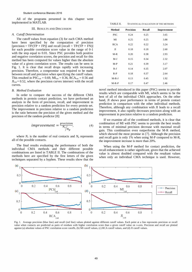
Fig. 1. Average precision (blue line) and recall (red line) values plotted against different cutoff values. Each point at a line represents precision or recall
value when contacts are predicted as pairs of residues with higher correlation score than a given cutoff value on x-axis. Precision and recall are plotted
against (a) absolute values of PSC correlation score cutoffs, (b) MI cutoff values, (c) RCA cutoff values, and (d) JI cutoff values.
TABLE II. STATISTICAL EVALUATION OF THE METHODS
Method Precision Recall Improvement
PSC 0.24 0.25 3.65
MI 0.25 0.25 3.88
RCA 0.22 0.22 3.24
JI 0.18 0.18 2.60
M-R 0.20 0.38 2.93
M-J 0.15 0.34 2.32
M-P 0.21 0.39 3.17
R-J 0.14 0.35 2.07
R-P 0.18 0.37 2.64
M-R-J 0.13 0.45 1.92
M-R-P 0.17 0.47 2.46
All of the programs presented in this chapter were implemented in MATLAB.
III. RESULTS AND DISCUSSION
A. Cutoff Determination
The cutoff values from equation (3) for each CMA method have been specified by the computation of precision [precision = TP/(TP + FP)] and recall [recall = TP/(TP + FN)] for each possible correlation score value in the range of 0-1 with the step equal to 0.01. Since PSC provides both positive and negative correlation scores, the precision and recall for this method has been computed for values higher than the absolute value of a given correlation score. The results can be seen in Fig. 1. It is clear that recall drops rapidly with increasing precision. Therefore, a compromise was required to be made between recall and precision when specifying the cutoff values. This resulted in PSCcut = 0.69, MIcut = 0.36, RCAcut = 0.56 and JIcut = 0.52, where the precision curves intersect with the recall curves.
B. Method Evaluation
In order to compare the success of the different CMA methods in protein contact prediction, we have performed an analysis in the form of precision, recall, and improvement in precision relative to a random prediction for every protein set. The improvement in precision relative to a random prediction is the ratio between the precision of the given method and the precision of the random predictor [8]:
𝑖𝑚𝑝𝑟𝑜𝑣𝑒𝑚𝑒𝑛𝑡 =𝑝𝑟𝑒𝑐𝑖𝑠𝑖𝑜𝑛
𝑁𝑐𝑁𝑝
⁄
where Nc is the number of real contacts and Np represents all of the possible contacts.
The final results evaluating the performance of both the individual CMA methods and their different possible combinations are listed in TABLE II. The combinations of the methods here are specified by the first letters of the given techniques separated by a hyphen. These results show that the
novel method introduced in this paper (PSC) seems to provide results which are comparable with MI, which seems to be the best of all of the individual CMA approaches. On the other hand, JI shows poor performance in terms of protein contact prediction in comparison with the other individual methods. Therefore, although any combination with JI leads to a recall improvement, it also rapidly decreases precision along with an improvement in precision relative to a random prediction.
If we examine all of the combined methods, it is clear that combination of MI with PSC seems to provide the best results in terms of minimal precision decrease with maximal recall gain. This combination even outperforms the M-R method, which showed the most promise in [7]. Although the precision and recall gain is only 1% when using M-P compared to M-R, the improvement increase is more than 20%.
When using the M-P method for contact prediction, the recall enhancement is rather significant, given that the achieved value is almost doubled compared with the resultant values when only an individual CMA technique is used. However,
Student conference Blansko 2016
49

when we are aiming for further recall gain, the best option would be a combination of M-R-P, by which the average recall achieved a value of 0.47 with only a 0.08 drop from the highest reached precision with the use of MI. This triple combination (M-R-P) also outperformed the triple combination with JI introduced earlier (M-R-J) [7] in all three statistical evaluations. Therefore, we can conclude that the use of PSC instead of JI can improve the performance of the compact method.
IV. CONCLUSION
Until this point, all CMA methods have been working with MSAs in their original character-based forms. Such form does not provide any additional information about an amino acid apart from its identity. Here, we presented an entirely new approach for the computation of CMA by using MSAs in the form in which each amino acid is represented by a number derived from its hydrophobicity and hydropathy. The correlation score is then obtained by a simple computation of Pearson’s correlation coefficient. It is the simplicity and low computational requirement of the method which make it so unique compared to character-based techniques. At the same time PSC achieves statistical results which are comparable with the best approaches. Furthermore, the technique provides information about new contacts in comparison with other CMA techniques, which is proven by the rapid recall increase when the PSC is incorporated into the multidimensional CMA method formed by multiple techniques. It is clear that the results obtained by the PSC outmatch the statistical results obtained by the RCA, which has been, for so long, the “holy grail” of CMA. Since PSC is the first method of its kind to use protein sequences in a numerical form, we believe that, with further refinements and by the combination of the outcome with advanced machine learning techniques (such as neural networks or support vector machines), this approach provides great potential for advancement in the field of protein structure prediction.
REFERENCES
[1] K. Hamacher, “Relating sequence evolution of HIV1-protease to its
underlying molecular mechanics”, Gene, vol. 422, no. 1-2, pp. 30-36, 2008.
[2] Y. Xu, D. Xu and J. Liang, Computational methods for protein structure prediction and modeling. New York: Springer, 2007.
[3] L. Martin, G. Gloor, S. Dunn and L. Wahl, “Using information theory to search for co-evolving residues in proteins”, Bioinformatics, vol. 21, no. 22, pp. 4116-4124, 2005.
[4] P. Kundrotas and E. Alexov, “Predicting residue contacts using pragmatic correlated mutations method: reducing the false positives”, BMC Bioinformatics, vol. 7, no. 1, p. 503, 2006.
[5] E. Jacob, R. Unger and A. Horovitz, “Codon-level information improves predictions of inter-residue contacts in proteins by correlated mutation analysis”, eLife, vol. 4, 2015.
[6] P. Fariselli, O. Olmea, A. Valencia and R. Casadio, “Prediction of contact maps with neural networks and correlated mutations”, Protein Engineering Design and Selection, vol. 14, no. 11, pp. 835-843, 2001.
[7] K. Kupkova, K. Sedlar and I. Provaznik, “Multidimensional Correlated Mutation Analysis for Protein Contact Map Prediction”, Advances in Intelligent Systems and Computing, pp. 133-145, 2016.
[8] U. Göbel, C. Sander, R. Schneider and A. Valencia, “Correlated mutations and residue contacts in proteins”, Proteins: Structure, Function, and Genetics, vol. 18, no. 4, pp. 309-317, 1994.
[9] D. Jones, D. Buchan, D. Cozzetto and M. Pontil, “PSICOV: precise structural contact prediction using sparse inverse covariance estimation on large multiple sequence alignments”, Bioinformatics, vol. 28, no. 2, pp. 184-190, 2011.
[10] A. Tamulewicz and E. Tkacz, “Human Fibroblast Growth Factor 2 Hot Spot Analysis by Means of Time-Frequency Transforms”, Advances in Intelligent Systems and Computing, pp. 147-159, 2016.
[11] H. Ashkenazy, R. Unger and Y. Kliger, “Optimal data collection for correlated mutation analysis”, Proteins, vol. 74, no. 3, pp. 545-555, 2009.
[12] S. Altschul, “Gapped BLAST and PSI-BLAST: a new generation of protein database search programs”, Nucleic Acids Research, vol. 25, no. 17, pp. 3389-3402, 1997.
[13] K. Pruitt, “NCBI Reference Sequence (RefSeq): a curated non-redundant sequence database of genomes, transcripts and proteins”, Nucleic Acids Research, vol. 33, no., pp. D501-D504, 2004.
[14] F. Sievers, A. Wilm, D. Dineen, T. Gibson, K. Karplus, W. Li, R. Lopez, H. McWilliam, M. Remmert, J. Soding, J. Thompson and D. Higgins, “Fast, scalable generation of high-quality protein multiple sequence alignments using Clustal Omega”, Molecular Systems Biology, vol. 7, no. 1, pp. 539-539, 2014.
[15] Z. Wu, X. Xiao and K. Chou, “2D-MH: A web-server for generating graphic representation of protein sequences based on the physicochemical properties of their constituent amino acids”, Journal of Theoretical Biology, vol. 267, no. 1, pp. 29-34, 2010.
[16] Y. Zhang, Y. Sheng, W. Zheng, P. He and J. Ruan, “Novel Numerical Characterization of Protein Sequences Based on Individual Amino Acid and Its Application”, BioMed Research International, vol. 2015, pp. 1-8, 2015.
[17] S. Salzberg and T. Warnow, Algorithms in Bioinformatics. Berlin, Heidelberg: Springer Berlin Heidelberg, 2009.
[18] Z. Li, Y. Huang, Y. Ouyang, Y. Jiao, H. Xing, L. Liao, S. Jiang, Y. Shao and L. Ma, “CorMut: an R/Bioconductor package for computing correlated mutations based on selection pressure”, Bioinformatics, vol. 30, no. 14, pp. 2073-2075, 2014.
[19] A. Tegge, Z. Wang, J. Eickholt and J. Cheng, “NNcon: improved protein contact map prediction using 2D-recursive neural networks”, Nucleic Acids Research, vol. 37, no., pp. W515-W518, 2009.
Student conference Blansko 2016
50
Video Quality Assessment in Experimental Retinal
Imaging
Ivana Liberdová
Department of Biomedical engineering
Brno University of Technology
Brno, Czech Republic
Radim Kolář
Department of Biomedical engineering
Brno University of Technology
Brno, Czech Republic
Abstract—This paper is focused on video quality assessment
of experimental retinal video image sequences with two different
approaches (automatic and expert analysis). Methods utilizing
both video quality evaluations are presented and described
within the paper. Evaluations consider the most frequent retinal
imaging artefacts (contrast distortion, noise and blurriness).
Automatic evaluating algorithm estimates the image quality
based on three different parameters characterizing the image
over time (signal to noise ratio - SNR, blurriness quality
evaluation - BQE and contrast quality evaluation - CQE). Four
different experts performed the evaluation with their subjective
image perceiving and assess the degree of noise, blurriness and
contrast in the images over time. The reliability of proposed
algorithm for automatic retinal image video quality assessment
seems to be correct for all three parameters. Medians of SNR as
well as the medians of CQE are decreasing with decreasing image
quality evaluated with 4 experts, and medians of BQE are
increasing.
Keywords—retinal imaging, video quality assessment, cross
correlation, noise
I. INTRODUCTION
This paper is focused on image quality assessment in experimental retinal imaging. The experimental retinal imaging lies in new approach of ophthalmoscopy measurements presented in [1], which provide long-term ophthalmoscopic video records. These records can give the information about the temporal changes of blood vessels and the hemodynamic analysis can be applied on recorded data. This new approach can clarify the process of glaucoma degenerative mechanism [1] or diseases connected with cardiovascular disease.
Shortly described, generally there exists only the one equipment providing the long-term video records of retina – mydriatic fundus camera (company Imedos Systems - Germany). In paper [1] were presented new approach – non-mydriatic videoophthalmoscope (VO) which uses single LED light source of low illumination level to measure the long-term records of retina as well without any eye damage. Advantage of this approach is that there is no need to use any mydriasis which can cause the negative effects. On the other hand the records are noisier in comparison with the fundus camera. There are also other artefacts in video records caused by the eye movements (saccadic movements, blinking). These distortions in video sequences must be considered while the
evaluation or analysis is performed, because bad quality video records can skew the results.
II. VIDEO QUALITY ASSESSMENT
Before each analysis/study using the video, the video quality evaluation is needed to consider its appropriateness and usability. In extensive studies is very difficult and expensive to subjectively evaluate the large number of video records. That is why the objective video quality assessment (VQA) is needed.
VQA is common problem in the field of image quality processing. Generally there are many different approaches for video quality evaluation. Statistic error metrics (mathematical methods) as e.g. mean squared difference, average difference [2] [3], are computationally convenient but they ignore the human visual system (HVS).
Modern VQA approaches are classified into three groups – full-reference, reduced-reference, no-reference [2]. No reference methods are also called the “blind model” and have no access to original signal [2]. The example of the no-reference approach is e.g. BRISQUE metrics [4]. Reduced-reference methods use only certain features of the original image [3]. The most widespread are full-reference methods, which include methods based on HVS. Example of these methods can be SSIM method [2] and also method based on phase correlation presented below.
The mathematical methods are still very attractive mainly because of low computational complexity and because of independence on viewing conditions [5]. The image quality can be evaluated on base of many different viewing conditions which are not fixed in most cases. Considering N different viewing condition there will be N various results of quality measurements [5]. In [5] were presented and applied the new mathematical approach of universal image quality index which consider three viewing conditions – loss of correlation, luminance distortion and contrast distortion.
In this paper, the objective evaluation focused on retinal data is presented and compared with subjective evaluation. Due to retinal imaging and its artefacts, both objective and subjective image quality evaluation is based on three viewing conditions – contrast distortion, noise and blurriness.
Student conference Blansko 2016
51
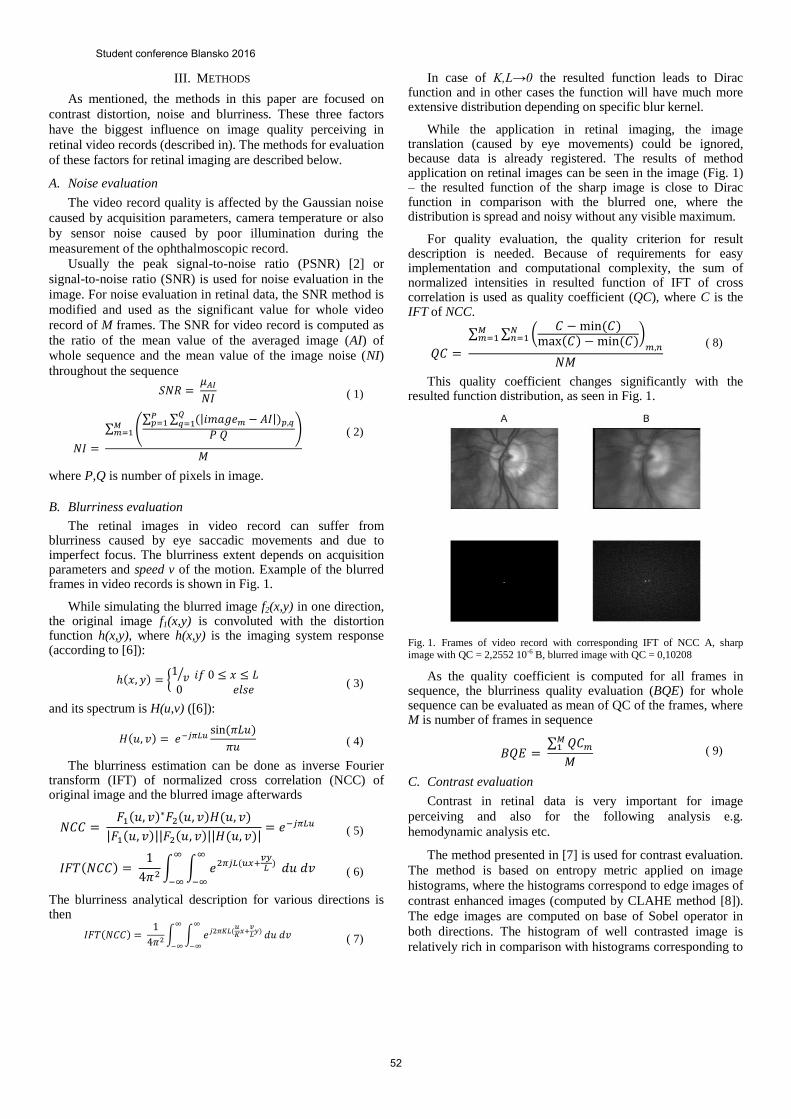
III. METHODS
As mentioned, the methods in this paper are focused on
contrast distortion, noise and blurriness. These three factors
have the biggest influence on image quality perceiving in
retinal video records (described in). The methods for evaluation
of these factors for retinal imaging are described below.
A. Noise evaluation
The video record quality is affected by the Gaussian noise
caused by acquisition parameters, camera temperature or also
by sensor noise caused by poor illumination during the
measurement of the ophthalmoscopic record.
Usually the peak signal-to-noise ratio (PSNR) [2] or
signal-to-noise ratio (SNR) is used for noise evaluation in the
image. For noise evaluation in retinal data, the SNR method is
modified and used as the significant value for whole video
record of M frames. The SNR for video record is computed as
the ratio of the mean value of the averaged image (AI) of
whole sequence and the mean value of the image noise (NI)
throughout the sequence
𝑆𝑁𝑅 = 𝜇𝐴𝐼
𝑁𝐼 ( 1)
𝑁𝐼 =
∑ (∑ ∑ (|𝑖𝑚𝑎𝑔𝑒𝑚 − 𝐴𝐼|)𝑝,𝑞
𝑄𝑞=1
𝑃𝑝=1
𝑃 𝑄)𝑀
𝑚=1
𝑀
( 2)
where P,Q is number of pixels in image.
B. Blurriness evaluation
The retinal images in video record can suffer from blurriness caused by eye saccadic movements and due to imperfect focus. The blurriness extent depends on acquisition parameters and speed v of the motion. Example of the blurred frames in video records is shown in Fig. 1.
While simulating the blurred image f2(x,y) in one direction, the original image f1(x,y) is convoluted with the distortion function h(x,y), where h(x,y) is the imaging system response (according to [6]):
ℎ(𝑥, 𝑦) = 1
𝑣⁄ 𝑖𝑓 0 ≤ 𝑥 ≤ 𝐿0 𝑒𝑙𝑠𝑒
( 3)
and its spectrum is H(u,v) ([6]):
𝐻(𝑢, 𝑣) = 𝑒−𝑗𝜋𝐿𝑢sin (𝜋𝐿𝑢)
𝜋𝑢 ( 4)
The blurriness estimation can be done as inverse Fourier transform (IFT) of normalized cross correlation (NCC) of original image and the blurred image afterwards
𝑁𝐶𝐶 = 𝐹1(𝑢, 𝑣)∗𝐹2(𝑢, 𝑣)𝐻(𝑢, 𝑣)
|𝐹1(𝑢, 𝑣)||𝐹2(𝑢, 𝑣)||𝐻(𝑢, 𝑣)|= 𝑒−𝑗𝜋𝐿𝑢 ( 5)
𝐼𝐹𝑇(𝑁𝐶𝐶) = 1
4𝜋2∫ ∫ 𝑒2𝜋𝑗𝐿(𝑢𝑥+
𝑣𝑦𝐿
)∞
−∞
∞
−∞
𝑑𝑢 𝑑𝑣 ( 6)
The blurriness analytical description for various directions is then
𝐼𝐹𝑇(𝑁𝐶𝐶) = 1
4𝜋2∫ ∫ 𝑒𝑗2𝜋𝐾𝐿(
𝑢𝐾𝑥+
𝑣𝐿𝑦)
∞
−∞
𝑑𝑢 𝑑𝑣∞
−∞
( 7)
In case of K,L→0 the resulted function leads to Dirac function and in other cases the function will have much more extensive distribution depending on specific blur kernel.
While the application in retinal imaging, the image translation (caused by eye movements) could be ignored, because data is already registered. The results of method application on retinal images can be seen in the image (Fig. 1) – the resulted function of the sharp image is close to Dirac function in comparison with the blurred one, where the distribution is spread and noisy without any visible maximum.
For quality evaluation, the quality criterion for result description is needed. Because of requirements for easy implementation and computational complexity, the sum of normalized intensities in resulted function of IFT of cross correlation is used as quality coefficient (QC), where C is the IFT of NCC.
𝑄𝐶 =
∑ ∑ (𝐶 − min (𝐶)
max(𝐶) − min (𝐶))
𝑚,𝑛
𝑁𝑛=1
𝑀𝑚=1
𝑁𝑀
( 8)
This quality coefficient changes significantly with the resulted function distribution, as seen in Fig. 1.
Fig. 1. Frames of video record with corresponding IFT of NCC A, sharp image with QC = 2,2552 10-6 B, blurred image with QC = 0,10208
As the quality coefficient is computed for all frames in sequence, the blurriness quality evaluation (BQE) for whole sequence can be evaluated as mean of QC of the frames, where M is number of frames in sequence
𝐵𝑄𝐸 = ∑ 𝑄𝐶𝑚
𝑀1
𝑀 ( 9)
C. Contrast evaluation
Contrast in retinal data is very important for image
perceiving and also for the following analysis e.g.
hemodynamic analysis etc.
The method presented in [7] is used for contrast evaluation.
The method is based on entropy metric applied on image
histograms, where the histograms correspond to edge images of
contrast enhanced images (computed by CLAHE method [8]).
The edge images are computed on base of Sobel operator in
both directions. The histogram of well contrasted image is
relatively rich in comparison with histograms corresponding to
Student conference Blansko 2016
52

the images of bad contrast, which contains sharp peaks. The
histogram changes can be evaluated then
𝐸 = − ∑ 𝑝𝑖log (𝑝𝑖)
𝑁
𝑖=1
( 10)
where pi is probability of a density function [7].
The mean of E of whole sequence is taken for contrast quality
evaluation (CQE).
D. Expert Analysis (Subjective assessment)
All video records were also evaluated subjectively by 4
people who evaluated the quality by the described viewing
conditions – noise, contrast and blurriness. The observers
assess the records by numbers 1-3 according to next rules: 1 –
nice record, 2 – moderate record, 3 – bad record. For each
parameter, the vectors of parameter quality were averaged
over experts.
E. Comparison between the algorithm and expert analysis
Because of the expert analysis procedure, the quality
output vector of each expert and the averaged vector can be
considered as a discrete random variable. For that reason, the
standard statistical tests for continuous random variables (e.g.
t-test or Wilcox, etc.) cannot be used. Because of that we have
arranged a simple way for the data comparison. The domain of
subjective assessment was divided into 3 intervals of same
length 1≤F≤1,5, 1,5<F<2,5, 2,5≤F≤3. Then objective values
of each sequence can be selected on corresponding positions
of each interval and classified into 3 groups. The objective
parameter’s probability density function (p.d.f.) on
corresponding interval is characterized then as a boxplot from
selected parameter values.
IV. DATA
All three methods are applied on retinal data which were measured by experimental non-mydriatic ophthalmoscope in Eye clinic, University Hospital in Erlangen in the framework of the Erlangen Glaucoma Registry (a clinical registry Clinical-Trials.gov identifier: NCT00494923).
There are 62 video records available for the VQA. The video records were measured on 21 both healthy and ill patients. Each video record includes 261 frames of 640 x 480 pixels. For recording was used CCD camera (iDS, UI-2210 SE-M-GL) and 1 pixel corresponds to 9,3 µm on retina. The records are with centered optic nerve.
Each video record was registered before applying the VQA methods.
V. RESULTS AND DISCUSSION
While applying described automatic methods on the retinal
data, the three numbers – SNR, BQE, CQE were computed for
each video sequence. The objective values for each video
sequence are visualized in Fig. 2.
The averaged value of subjective evaluations for each
viewing condition is visualized in Fig. 3.
Fig. 2. Results of objective VQA methods for video sequences
Fig. 3. Averaged subjective evaluation result for video sequences
The first boxplot graph (Fig. 4) describes the relation
between subjective and the objective evaluation of noise. For
the objective method apply that the quality increases with the
SNR value. This verify the correctness of the objective
method that rightly classify the bad video sequences.
The second boxplot graph (Fig. 5) describes the relation
between the subjective and objective quality evaluation of
blurriness. The quality increases with decreases BQE.
According to the boxplot, the minimal values are rightly
classified into the first group and the medians in the groups
increase.
The third boxplot graph (Fig. 6) describes the last view
condition, contrast. The contrast as the noise in the first
boxplot is increasing with its quality coefficient CQE. That is
why medians of CQE rightly decrease through the groups.
For better view on the values of coefficient the median
values for three groups for each view condition are noted in
the table below (TABLE I).
The median changes of objective quality coefficients agree
with the subjective assessments. Mostly, the same trend is
observable also for quartiles of p.d.f.-s. Although it seems that
the median changes are not so significant, it must be
considered the small ranges of coefficient values in
measurements.
Student conference Blansko 2016
53
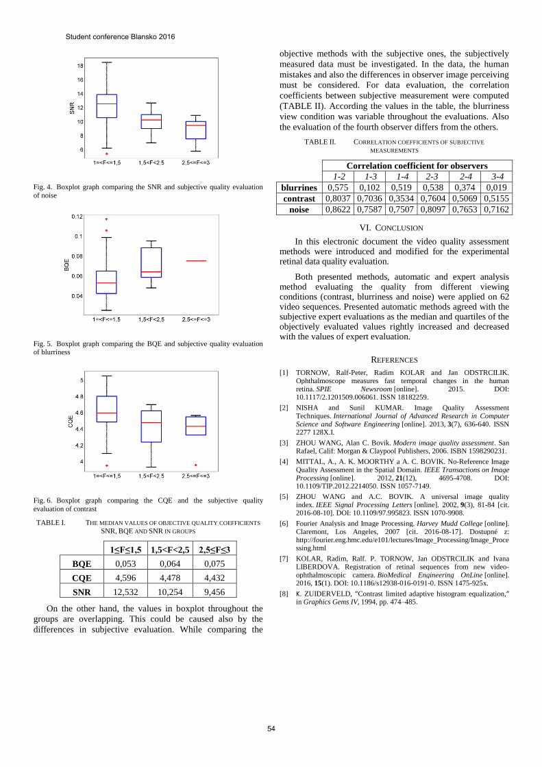
Fig. 4. Boxplot graph comparing the SNR and subjective quality evaluation
of noise
Fig. 5. Boxplot graph comparing the BQE and subjective quality evaluation of blurriness
Fig. 6. Boxplot graph comparing the CQE and the subjective quality
evaluation of contrast
TABLE I. THE MEDIAN VALUES OF OBJECTIVE QUALITY COEFFICIENTS
SNR, BQE AND SNR IN GROUPS
1≤F≤1,5 1,5<F<2,5 2,5≤F≤3
BQE 0,053 0,064 0,075
CQE 4,596 4,478 4,432
SNR 12,532 10,254 9,456
On the other hand, the values in boxplot throughout the
groups are overlapping. This could be caused also by the
differences in subjective evaluation. While comparing the
objective methods with the subjective ones, the subjectively
measured data must be investigated. In the data, the human
mistakes and also the differences in observer image perceiving
must be considered. For data evaluation, the correlation
coefficients between subjective measurement were computed
(TABLE II). According the values in the table, the blurriness
view condition was variable throughout the evaluations. Also
the evaluation of the fourth observer differs from the others.
TABLE II. CORRELATION COEFFICIENTS OF SUBJECTIVE
MEASUREMENTS
Correlation coefficient for observers
1-2 1-3 1-4 2-3 2-4 3-4
blurrines 0,575 0,102 0,519 0,538 0,374 0,019
contrast 0,8037 0,7036 0,3534 0,7604 0,5069 0,5155
noise 0,8622 0,7587 0,7507 0,8097 0,7653 0,7162
VI. CONCLUSION
In this electronic document the video quality assessment methods were introduced and modified for the experimental retinal data quality evaluation.
Both presented methods, automatic and expert analysis method evaluating the quality from different viewing conditions (contrast, blurriness and noise) were applied on 62 video sequences. Presented automatic methods agreed with the subjective expert evaluations as the median and quartiles of the objectively evaluated values rightly increased and decreased with the values of expert evaluation.
REFERENCES
[1] TORNOW, Ralf-Peter, Radim KOLAR and Jan ODSTRCILIK. Ophthalmoscope measures fast temporal changes in the human retina. SPIE Newsroom [online]. 2015. DOI: 10.1117/2.1201509.006061. ISSN 18182259.
[2] NISHA and Sunil KUMAR. Image Quality Assessment Techniques. International Journal of Advanced Research in Computer Science and Software Engineering [online]. 2013, 3(7), 636-640. ISSN 2277 128X.I.
[3] ZHOU WANG, Alan C. Bovik. Modern image quality assessment. San Rafael, Calif: Morgan & Claypool Publishers, 2006. ISBN 1598290231.
[4] MITTAL, A., A. K. MOORTHY a A. C. BOVIK. No-Reference Image Quality Assessment in the Spatial Domain. IEEE Transactions on Image Processing [online]. 2012, 21(12), 4695-4708. DOI: 10.1109/TIP.2012.2214050. ISSN 1057-7149.
[5] ZHOU WANG and A.C. BOVIK. A universal image quality index. IEEE Signal Processing Letters [online]. 2002, 9(3), 81-84 [cit. 2016-08-10]. DOI: 10.1109/97.995823. ISSN 1070-9908.
[6] Fourier Analysis and Image Processing. Harvey Mudd College [online]. Claremont, Los Angeles, 2007 [cit. 2016-08-17]. Dostupné z: http://fourier.eng.hmc.edu/e101/lectures/Image_Processing/Image_Processing.html
[7] KOLAR, Radim, Ralf. P. TORNOW, Jan ODSTRCILIK and Ivana LIBERDOVA. Registration of retinal sequences from new video-ophthalmoscopic camera. BioMedical Engineering OnLine [online]. 2016, 15(1). DOI: 10.1186/s12938-016-0191-0. ISSN 1475-925x.
[8] K. ZUIDERVELD, “Contrast limited adaptive histogram equalization,” in Graphics Gems IV, 1994, pp. 474–485.
Student conference Blansko 2016
54
Detection of P, QRS and T Components of ECG
Using Phasor Transform
Lucie Maršánová
Department of biomedical engineering
Brno University of Technology
Brno, Czech republic
Abstract— This work introduces a new method of detection of P,
QRS and T components of ECG based on phasor transform (PT).
PT converts each ECG sample into a phasor and therefore
enhances changes in the ECG signal. Waves with small voltage are
then easily detectable. The method has been tested on standard
ECG databases (MIT-BIH arrhythmia database, QT database and
CSE database). The results of detection of P wave and QRS
complex are better than results presented in previous works. The
result of T wave detection is slightly worse than results of the most
of previous works.
Keywords—ecg, detection of P wave, detection of T wave,
detection of QRS complex, phasor transform, ECG databases
I. INTRODUCTION
Cardiovascular disorders are still the most common cause of
death in Western countries. Due to the ease of use, non-
invasiveness and cheapness, electrocardiogram (ECG) is
nowadays still the most available and widely used method for
the cardiovascular system examination [1]. The ECG reflects
two heart activities: the atrial activity (represented by P wave)
and ventricular activity (represented by QRS complex and T
wave). Automatic analysis of ECG (especially detection of
QRS, P and T wave) is fundamental task in cardiac monitoring
and mainly in long-term ECG monitoring [2]. Due to the large
volume of such data, it is not possible to do only manual
evaluation, but it is also necessary to use automatic uter
methods.
The automatic detection of QRS complex has been studied in
many previous works. Most of them are mentioned in [3]. The
results of these studies are sufficient and trusted, because they
are evaluated on several ECG databases (usually around
100 000 beats). The automatic and reliable detection of P waves
and T waves is more difficult task. The reasons are mentioned
below. Moreover, the algorithms for P waves and T waves
detection are tested at a much lower number of cycles (usually
QTDB [4] from [5]).
P waves are difficult to detect primarily for these reasons: 1) P
waves have a low voltage resulting in low signal-to-noise ratio
(SNR), 2) P waves have no exclusive time and frequency
characteristics, 3) P waves have high inter-patient variability, in
case of AV dissociations, 4) P waves do not respect normal time
sequence ordering and 5) P waves can be hidden within T wave.
Reliable T waves detection is difficult (as well as in the case of
P waves) for their low voltage and mainly for their high
morphology and amplitude variability.
Algorithms for P, QRS a T waves detection from previous
works are based on very different approaches such as wavelet
transform [6] and [7], moving average [8], phasor transform [9],
quality-supported analysis of characteristic templates or by
using marginalized particle filter [10]. However, none of them
can achieve completely satisfactory results. This means, that
there is still desirable further research.
In this paper, we introduce robust and mathematically simple
methods for P, QRS and T wave detection based on phasor
transform (PT). Phasor transform converts each ECG sample
into a phasor, which can highlight P waves and T waves. These
have lower amplitude than the QRS complex and are difficult
detect. Method based on phasor transform was presented also
in [9], but approach presented in this paper is simplified and its
realization and reproducibility is clearer and easier. The authors
of work [9] do not fully explained the necessary preprocessing
and postprocessing operations before and after applying the PT.
In this paper is also pointed out to the insufficiency of standard
databases, which contain mostly physiological records without
pathology.
II. PROCESSING OF ECG
A. Preprocessing
For successful signal analysis is necessary to remove noise and
artifacts from the ECG signal.
For QRS detection, signal is filtered by bandpass filter with
cutoff frequencies 12 and 19 Hz. In this frequency range lies the
most of QRS complex energy. Using this filter suppresses P and
T waves and also high frequency artifacts. On the other hand,
QRS complexes are highlighted.
For P wave detection is signal firstly filtered by lowpass filter
with cutoff frequency 0.67 Hz. Then, smoothing signal by
nonlinear median filter with 40 msec window size is perform.
Smooth signal is necessary for accurate performing of PT.
B. Phasor transform
PT transforms each sample of the signal into a complex value
preserving the signal information. It enhances ECG waves and
makes the detection easier. Phasor transform for detection of
ECG waves was firstly presented in [9].
Converting each ECG sample into a phasor enhances changes
in the ECG signal (the waves). Thus, considering instantaneous
Student conference Blansko 2016
55
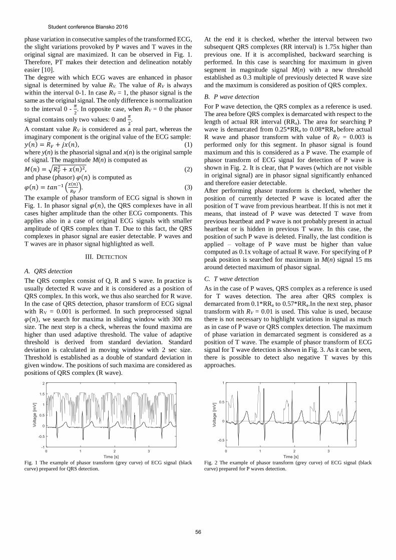
phase variation in consecutive samples of the transformed ECG,
the slight variations provoked by P waves and T waves in the
original signal are maximized. It can be observed in Fig. 1.
Therefore, PT makes their detection and delineation notably
easier [10].
The degree with which ECG waves are enhanced in phasor
signal is determined by value RV. The value of RV is always
within the interval 0-1. In case RV = 1, the phasor signal is the
same as the original signal. The only difference is normalization
to the interval 0 - 𝜋
2. In opposite case, when RV = 0 the phasor
signal contains only two values: 0 and 𝜋
2.
A constant value RV is considered as a real part, whereas the
imaginary component is the original value of the ECG sample:
𝑦(𝑛) = 𝑅𝑉 + 𝑗𝑥(𝑛), (1)
where y(n) is the phasorial signal and x(n) is the original sample
of signal. The magnitude M(n) is computed as
𝑀(𝑛) = √𝑅𝑉2 + 𝑥(𝑛)2, (2)
and phase (phasor) 𝜑(𝑛) is computed as
𝜑(𝑛) = 𝑡𝑎𝑛−1 (𝑥(𝑛)
𝑅𝑉). (3)
The example of phasor transform of ECG signal is shown in
Fig. 1. In phasor signal 𝜑(𝑛), the QRS complexes have in all
cases higher amplitude than the other ECG components. This
applies also in a case of original ECG signals with smaller
amplitude of QRS complex than T. Due to this fact, the QRS
complexes in phasor signal are easier detectable. P waves and
T waves are in phasor signal highlighted as well.
III. DETECTION
A. QRS detection
The QRS complex consist of Q, R and S wave. In practice is
usually detected R wave and it is considered as a position of
QRS complex. In this work, we thus also searched for R wave.
In the case of QRS detection, phasor transform of ECG signal
with RV = 0.001 is performed. In such preprocessed signal
𝜑(𝑛), we search for maxima in sliding window with 300 ms
size. The next step is a check, whereas the found maxima are
higher than used adaptive threshold. The value of adaptive
threshold is derived from standard deviation. Standard
deviation is calculated in moving window with 2 sec size.
Threshold is established as a double of standard deviation in
given window. The positions of such maxima are considered as
positions of QRS complex (R wave).
Fig. 1 The example of phasor transform (grey curve) of ECG signal (black
curve) prepared for QRS detection.
At the end it is checked, whether the interval between two
subsequent QRS complexes (RR interval) is 1.75x higher than
previous one. If it is accomplished, backward searching is
performed. In this case is searching for maximum in given
segment in magnitude signal M(n) with a new threshold
established as 0.3 multiple of previously detected R wave size
and the maximum is considered as position of QRS complex.
B. P wave detection
For P wave detection, the QRS complex as a reference is used.
The area before QRS complex is demarcated with respect to the
length of actual RR interval (RRa). The area for searching P
wave is demarcated from 0.25*RRa to 0.08*RRa before actual
R wave and phasor transform with value of RV = 0.003 is
performed only for this segment. In phasor signal is found
maximum and this is considered as a P wave. The example of
phasor transform of ECG signal for detection of P wave is
shown in Fig. 2. It is clear, that P waves (which are not visible
in original signal) are in phasor signal significantly enhanced
and therefore easier detectable.
After performing phasor transform is checked, whether the
position of currently detected P wave is located after the
position of T wave from previous heartbeat. If this is not met it
means, that instead of P wave was detected T wave from
previous heartbeat and P wave is not probably present in actual
heartbeat or is hidden in previous T wave. In this case, the
position of such P wave is deleted. Finally, the last condition is
applied – voltage of P wave must be higher than value
computed as 0.1x voltage of actual R wave. For specifying of P
peak position is searched for maximum in M(n) signal 15 ms
around detected maximum of phasor signal.
C. T wave detection
As in the case of P waves, QRS complex as a reference is used
for T waves detection. The area after QRS complex is
demarcated from 0.1*RRa to 0.57*RRa.In the next step, phasor
transform with RV = 0.01 is used. This value is used, because
there is not necessary to highlight variations in signal as much
as in case of P wave or QRS complex detection. The maximum
of phase variation in demarcated segment is considered as a
position of T wave. The example of phasor transform of ECG
signal for T wave detection is shown in Fig. 3. As it can be seen,
there is possible to detect also negative T waves by this
approaches.
Fig. 2 The example of phasor transform (grey curve) of ECG signal (black
curve) prepared for P waves detection.
Student conference Blansko 2016
56

Fig. 3 The example of phasor transform (grey curve) of ECG signal (black
curve) prepared for T waves detection.
IV. TESTING DATABASES
A. MIT-BIH Arrhythmia Database
The MIT-BIH Arrhythmia Database [12] is the most commonly
used database for QRS detectors evaluation. The MIT-BIH
Arrhythmia Database includes reference positions of QRS
complexes. Database contains 48 half-hour two-channel ECG
records. The sampling frequency is 360 Hz.
B. QT Database
The QT database (QTDB) [13] is the most commonly used
database for heartbeat delineation and detection of P waves and
T waves. Database contains 105 15 minutes two-channel ECG
records. For all records are available reference positions of QRS
complexes. Database includes manual annotations of P waves
onset and offset positions, QRS complexes positions and
positions of T waves offset. All these annotations are available
for 79 out of 105 recording at least for 30 beats per record. The
sampling frequency is 250 Hz.
C. CSE database
The CSE database [14] is the second most commonly used
database for heartbeats delineation and detection of P waves
and T waves. Database includes reference positions of onsets
and offsets of P waves, QRS complexes and offsets of T waves.
Reference positions of these ECG significant points are
available only for one selected beat of each record. Database
contains 125 10 second three-channel ECG records. The
sampling frequency is 250 Hz.
D. Evaluation
Two standard benchmark parameters are calculated to evaluate
designed detection algorithm (P, QRS and T) and compare it
with previous works. The sensitivity (SE) and the positive
predictivity (PP) of the algorithm are computed as:
SE=TP/(TP+FN) and P+=TP/(TP+FP). The sensitivity reports
percentage of correct detection of given ECG component. The
positive predictivity reports the percentage of detections, which
were in reality true ECG components.
TABLE 1 THE RESULTS OF QRS DETECTION AND COMPARISON WITH PREVIOUS
WORKS.
Methods Database Se [%] P+ [%]
This work QTDB 99.85 99.83
This work MIT-BIH 99.62 99.65
This work CSE 100 100
Correlation
[15] MIT-BIH 99.81 99.70
PT [12] MIT-BIH 98.41 86.75
Power [16] MIT-BIH 99.21 99.34
Power [16] CSE 99.51 99.69
V. RESULTS
A. QRS detection
Performance of QRS detection algorithm was tested on the
whole MIT-BIH arrhythmia database, QT database and CSE
database. The achieved results are summarized in Table 1. In
comparison with previous works, (see Table 1), the results of
our method are comparable or even slightly better.
B. P wave and T wave detection
The performance of P wave and T wave detection algorithms
was tested on manually annotated part of QT database (it
contains around 3600 beats). The QRS detection was also tested
on this part of QT database. The achieved results are
summarised in Table 2. The results of P wave and QRS complex
detection are better, than results presented in previous works.
The result of T wave detection is slightly worse, than results of
the most of previous works.
In Fig. 4 is shown example of detection algorithm results. P
waves are marked by grey line with “*”, QRS complexes with
“o” and T waves with “x”.
TABLE 2 THE RESULTS OF P WAVE AND T WAVE DETECTION IN QTDB AND
COMPARISON WITH PERVIOUS WORKS.
P wave QRS complex T wave
Method Se [%] P+
[%]
Se
[%]
P+
[%]
Se
[%]
P+
[%]
This work 99.84 99.84 100 100 98.33 98.04
PT [9] 99.28 99.75 99.91 99.94 99.66 99.66
WT [7] 98.87 91.03 99.97 N/R 99.77 97.79
Correlatio
n [10] 99.63 99.83 99.83 99.98 99.74 99.89
Student conference Blansko 2016
57
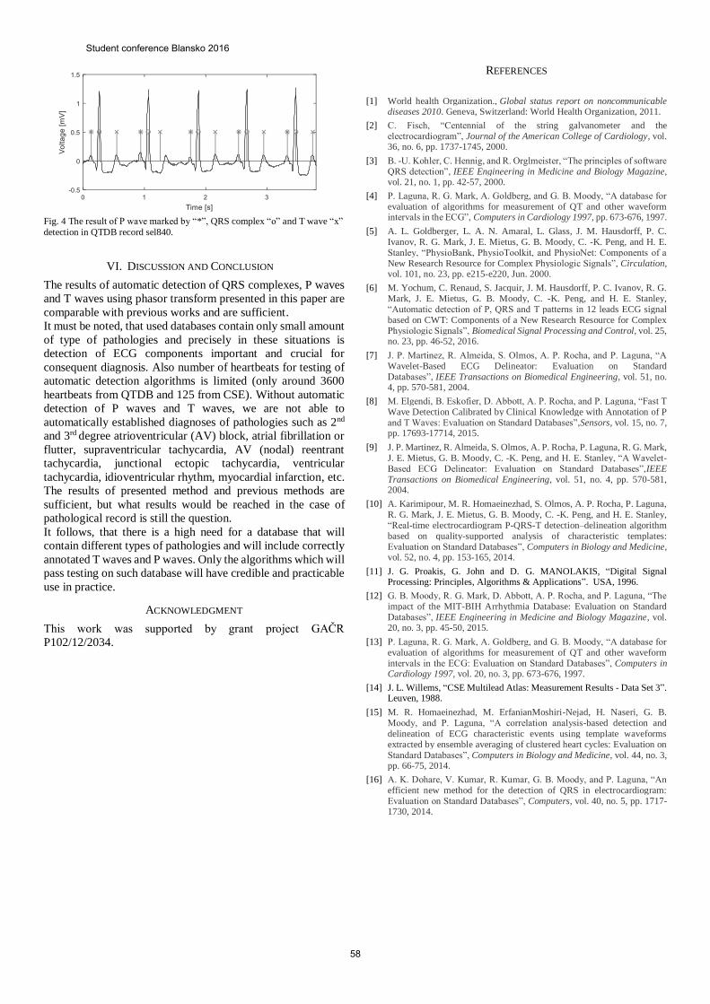
Fig. 4 The result of P wave marked by “*”, QRS complex “o” and T wave “x”
detection in QTDB record sel840.
VI. DISCUSSION AND CONCLUSION
The results of automatic detection of QRS complexes, P waves
and T waves using phasor transform presented in this paper are
comparable with previous works and are sufficient.
It must be noted, that used databases contain only small amount
of type of pathologies and precisely in these situations is
detection of ECG components important and crucial for
consequent diagnosis. Also number of heartbeats for testing of
automatic detection algorithms is limited (only around 3600
heartbeats from QTDB and 125 from CSE). Without automatic
detection of P waves and T waves, we are not able to
automatically established diagnoses of pathologies such as 2nd
and 3rd degree atrioventricular (AV) block, atrial fibrillation or
flutter, supraventricular tachycardia, AV (nodal) reentrant
tachycardia, junctional ectopic tachycardia, ventricular
tachycardia, idioventricular rhythm, myocardial infarction, etc.
The results of presented method and previous methods are
sufficient, but what results would be reached in the case of
pathological record is still the question.
It follows, that there is a high need for a database that will
contain different types of pathologies and will include correctly
annotated T waves and P waves. Only the algorithms which will
pass testing on such database will have credible and practicable
use in practice.
ACKNOWLEDGMENT
This work was supported by grant project GAČR
P102/12/2034.
REFERENCES
[1] World health Organization., Global status report on noncommunicable
diseases 2010. Geneva, Switzerland: World Health Organization, 2011.
[2] C. Fisch, “Centennial of the string galvanometer and the electrocardiogram”, Journal of the American College of Cardiology, vol. 36, no. 6, pp. 1737-1745, 2000.
[3] B. -U. Kohler, C. Hennig, and R. Orglmeister, “The principles of software QRS detection”, IEEE Engineering in Medicine and Biology Magazine, vol. 21, no. 1, pp. 42-57, 2000.
[4] P. Laguna, R. G. Mark, A. Goldberg, and G. B. Moody, “A database for evaluation of algorithms for measurement of QT and other waveform intervals in the ECG”, Computers in Cardiology 1997, pp. 673-676, 1997.
[5] A. L. Goldberger, L. A. N. Amaral, L. Glass, J. M. Hausdorff, P. C. Ivanov, R. G. Mark, J. E. Mietus, G. B. Moody, C. -K. Peng, and H. E. Stanley, “PhysioBank, PhysioToolkit, and PhysioNet: Components of a New Research Resource for Complex Physiologic Signals”, Circulation, vol. 101, no. 23, pp. e215-e220, Jun. 2000.
[6] M. Yochum, C. Renaud, S. Jacquir, J. M. Hausdorff, P. C. Ivanov, R. G. Mark, J. E. Mietus, G. B. Moody, C. -K. Peng, and H. E. Stanley, “Automatic detection of P, QRS and T patterns in 12 leads ECG signal based on CWT: Components of a New Research Resource for Complex Physiologic Signals”, Biomedical Signal Processing and Control, vol. 25, no. 23, pp. 46-52, 2016.
[7] J. P. Martinez, R. Almeida, S. Olmos, A. P. Rocha, and P. Laguna, “A Wavelet-Based ECG Delineator: Evaluation on Standard Databases”, IEEE Transactions on Biomedical Engineering, vol. 51, no. 4, pp. 570-581, 2004.
[8] M. Elgendi, B. Eskofier, D. Abbott, A. P. Rocha, and P. Laguna, “Fast T Wave Detection Calibrated by Clinical Knowledge with Annotation of P and T Waves: Evaluation on Standard Databases”,Sensors, vol. 15, no. 7, pp. 17693-17714, 2015.
[9] J. P. Martinez, R. Almeida, S. Olmos, A. P. Rocha, P. Laguna, R. G. Mark, J. E. Mietus, G. B. Moody, C. -K. Peng, and H. E. Stanley, “A Wavelet-Based ECG Delineator: Evaluation on Standard Databases”,IEEE Transactions on Biomedical Engineering, vol. 51, no. 4, pp. 570-581, 2004.
[10] A. Karimipour, M. R. Homaeinezhad, S. Olmos, A. P. Rocha, P. Laguna, R. G. Mark, J. E. Mietus, G. B. Moody, C. -K. Peng, and H. E. Stanley, “Real-time electrocardiogram P-QRS-T detection–delineation algorithm based on quality-supported analysis of characteristic templates: Evaluation on Standard Databases”, Computers in Biology and Medicine, vol. 52, no. 4, pp. 153-165, 2014.
[11] J. G. Proakis, G. John and D. G. MANOLAKIS, “Digital Signal Processing: Principles, Algorithms & Applications”. USA, 1996.
[12] G. B. Moody, R. G. Mark, D. Abbott, A. P. Rocha, and P. Laguna, “The impact of the MIT-BIH Arrhythmia Database: Evaluation on Standard Databases”, IEEE Engineering in Medicine and Biology Magazine, vol. 20, no. 3, pp. 45-50, 2015.
[13] P. Laguna, R. G. Mark, A. Goldberg, and G. B. Moody, “A database for evaluation of algorithms for measurement of QT and other waveform intervals in the ECG: Evaluation on Standard Databases”, Computers in Cardiology 1997, vol. 20, no. 3, pp. 673-676, 1997.
[14] J. L. Willems, “CSE Multilead Atlas: Measurement Results - Data Set 3”. Leuven, 1988.
[15] M. R. Homaeinezhad, M. ErfanianMoshiri-Nejad, H. Naseri, G. B. Moody, and P. Laguna, “A correlation analysis-based detection and delineation of ECG characteristic events using template waveforms extracted by ensemble averaging of clustered heart cycles: Evaluation on Standard Databases”, Computers in Biology and Medicine, vol. 44, no. 3, pp. 66-75, 2014.
[16] A. K. Dohare, V. Kumar, R. Kumar, G. B. Moody, and P. Laguna, “An efficient new method for the detection of QRS in electrocardiogram: Evaluation on Standard Databases”, Computers, vol. 40, no. 5, pp. 1717-1730, 2014.
Student conference Blansko 2016
58
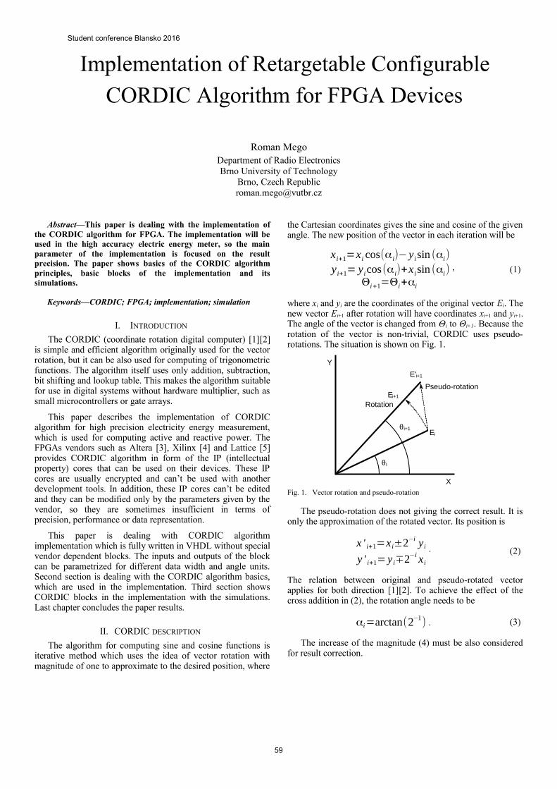
Implementation of Retargetable Configurable
CORDIC Algorithm for FPGA Devices
Roman MegoDepartment of Radio ElectronicsBrno University of Technology
Brno, Czech [email protected]
Abstract—This paper is dealing with the implementation ofthe CORDIC algorithm for FPGA. The implementation will beused in the high accuracy electric energy meter, so the mainparameter of the implementation is focused on the resultprecision. The paper shows basics of the CORDIC algorithmprinciples, basic blocks of the implementation and itssimulations.
Keywords—CORDIC; FPGA; implementation; simulation
I. INTRODUCTION
The CORDIC (coordinate rotation digital computer) [1][2]is simple and efficient algorithm originally used for the vectorrotation, but it can be also used for computing of trigonometricfunctions. The algorithm itself uses only addition, subtraction,bit shifting and lookup table. This makes the algorithm suitablefor use in digital systems without hardware multiplier, such assmall microcontrollers or gate arrays.
This paper describes the implementation of CORDICalgorithm for high precision electricity energy measurement,which is used for computing active and reactive power. TheFPGAs vendors such as Altera [3], Xilinx [4] and Lattice [5]provides CORDIC algorithm in form of the IP (intellectualproperty) cores that can be used on their devices. These IPcores are usually encrypted and can’t be used with anotherdevelopment tools. In addition, these IP cores can’t be editedand they can be modified only by the parameters given by thevendor, so they are sometimes insufficient in terms ofprecision, performance or data representation.
This paper is dealing with CORDIC algorithmimplementation which is fully written in VHDL without specialvendor dependent blocks. The inputs and outputs of the blockcan be parametrized for different data width and angle units.Second section is dealing with the CORDIC algorithm basics,which are used in the implementation. Third section showsCORDIC blocks in the implementation with the simulations.Last chapter concludes the paper results.
II. CORDIC DESCRIPTION
The algorithm for computing sine and cosine functions isiterative method which uses the idea of vector rotation withmagnitude of one to approximate to the desired position, where
the Cartesian coordinates gives the sine and cosine of the givenangle. The new position of the vector in each iteration will be
x i+1=x i cos(α i)− y isin (αi)y i+1= y icos (α i)+x isin (αi)
Θi+1=Θi+αi
, (1)
where xi and yi are the coordinates of the original vector Ei. Thenew vector Ei+1 after rotation will have coordinates xi+1 and yi+1.The angle of the vector is changed from Θi to Θi+1. Because therotation of the vector is non-trivial, CORDIC uses pseudo-rotations. The situation is shown on Fig. 1.
Rotation
Pseudo-rotation
Ei
Ei+1
E'i+1
θi
θi+1
X
Y
Fig. 1. Vector rotation and pseudo-rotation
The pseudo-rotation does not giving the correct result. It isonly the approximation of the rotated vector. Its position is
x ' i+1=x i±2−i y i
y ' i+1= y i∓2−i x i
. (2)
The relation between original and pseudo-rotated vectorapplies for both direction [1][2]. To achieve the effect of thecross addition in (2), the rotation angle needs to be
αi=arctan(2−1
) . (3)
The increase of the magnitude (4) must be also consideredfor result correction.
Student conference Blansko 2016
59
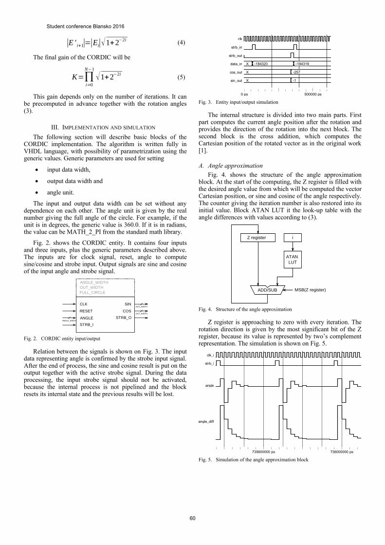
|E ' i+1|=|Ei|√1+2−2i (4)
The final gain of the CORDIC will be
K=∏i=0
N−1
√1+2−2i (5)
This gain depends only on the number of iterations. It canbe precomputed in advance together with the rotation angles(3).
III. IMPLEMENTATION AND SIMULATION
The following section will describe basic blocks of theCORDIC implementation. The algorithm is written fully inVHDL language, with possibility of parametrization using thegeneric values. Generic parameters are used for setting
input data width,
output data width and
angle unit.
The input and output data width can be set without anydependence on each other. The angle unit is given by the realnumber giving the full angle of the circle. For example, if theunit is in degrees, the generic value is 360.0. If it is in radians,the value can be MATH_2_PI from the standard math library.
Fig. 2. shows the CORDIC entity. It contains four inputsand three inputs, plus the generic parameters described above.The inputs are for clock signal, reset, angle to computesine/cosine and strobe input. Output signals are sine and cosineof the input angle and strobe signal.
CLK
RESET
ANGLE
STRB_I
SIN
COS
STRB_O
ANGLE_WIDTHOUT_WIDTHFULL_CIRCLE
ANGLE_WIDTH
OUT_WIDTH
OUT_WIDTH
Fig. 2. CORDIC entity input/output
Relation between the signals is shown on Fig. 3. The inputdata representing angle is confirmed by the strobe input signal.After the end of process, the sine and cosine result is put on theoutput together with the active strobe signal. During the dataprocessing, the input strobe signal should not be activated,because the internal process is not pipelined and the blockresets its internal state and the previous results will be lost.
X -184320 -184319
X -257
X -1
0 ps 500000 ps
clk
strb_in
strb_out
data_in X -184320 -184319
cos_out X -257
sin_out X -1
Fig. 3. Entity input/output simulation
The internal structure is divided into two main parts. Firstpart computes the current angle position after the rotation andprovides the direction of the rotation into the next block. Thesecond block is the cross addition, which computes theCartesian position of the rotated vector as in the original work[1].
A. Angle approximation
Fig. 4. shows the structure of the angle approximationblock. At the start of the computing, the Z register is filled withthe desired angle value from which will be computed the vectorCartesian position, or sine and cosine of the angle respectively.The counter giving the iteration number is also restored into itsinitial value. Block ATAN LUT it the look-up table with theangle differences with values according to (3).
Z register
ADD/SUB
ATAN LUT
i
MSB(Z register)
Fig. 4. Structure of the angle approximation
Z register is approaching to zero with every iteration. Therotation direction is given by the most significant bit of the Zregister, because its value is represented by two’s complementrepresentation. The simulation is shown on Fig. 5.
735600000 ps 736000000 ps
clk_i
strb_i
angle
angle_diff
Fig. 5. Simulation of the angle approximation block
Student conference Blansko 2016
60
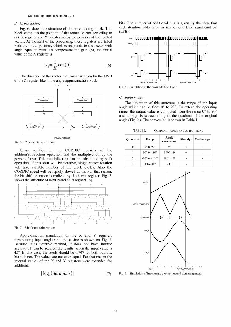
B. Cross adding
Fig. 6. shows the structure of the cross adding block. Thisblock computes the position of the rotated vector according to(2). X register and Y register keeps the position of the rotatedvector. At the start of the processing, these registers are filledwith the initial position, which corresponds to the vector withangle equal to zero. To compensate the gain (5), the initialvalue of the X register is
x0=1Kcos (0) (6)
The direction of the vector movement is given by the MSBof the Z register like in the angle approximation block.
>> i
X register Y register
>> i
ADD/SUB ADD/SUB
COS SIN
MSB(Z register)
Fig. 6. Cross addition structure
Cross addition in the CORDIC consists of theaddition/subtraction operation and the multiplication by thepower of two. This multiplication can be substituted by shiftoperation. If this shift will be iterative, single vector rotationwill take variable number of the clock cycles. Also theCORDIC speed will be rapidly slowed down. For that reason,the bit shift operation is realized by the barrel register. Fig. 7.shows the structure of 8-bit barrel shift register [6].
0 1 0 1 0 1 0 1 0 1 0 1 0 1 0 1
0 10 1 0 1 0 1 0 1 0 1 0 1 0 1
0 1 0 1 0 1 0 1 0 1 0 1 0 1 0 1
0 a7 a6 a5 a4 a3 a2 a1 a0
a2
a1
a0
y7 y6 y5 y4 y3 y2 y1 y0
Fig. 7. 8-bit barrel shift register
Approximation simulation of the X and Y registersrepresenting input angle sine and cosine is shown on Fig. 8.Because it is iterative method, it does not have infiniteaccuracy. It can be seen on the results, when the input value is45°. In this case, the result should be 0.707 for both outputs,but it is not. The values are not even equal. For that reason theinternal values of the X and Y registers were extended foradditional
⌈ log2(iterations)⌉ (7)
bits. The number of additional bits is given by the idea, thateach iteration adds error in size of one least significant bit(LSB).
42647600000 ps 42648000000 ps
clk_i
strb_i
sin
cos
Fig. 8. Simulation of the cross addition block
C. Input range
The limitation of this structure is the range of the inputangle which can be from 0° to 90°. To extend the operatingrange, the output value is computed from the range 0° to 90°and its sign is set according to the quadrant of the originalangle (Fig. 9.). The conversion is shown in Table I.
TABLE I. QUADRANT RANGE AND OUTPUT SIGNS
Quadrant RangeAngle
conversionSine sign Cosine sign
0 0° to 90° Θ + +
1 90° to 180° 180° - Θ + -
2 -90° to -180° 180° + Θ - -
3 0°to -90° - Θ - +
2 3 0 1
0 ps 100000000000 ps
angle_i
angle_normalized
quadrant 2 3 0 1
sin_o
cos_o
Fig. 9. Simulation of input angle conversion and sign assignment
Student conference Blansko 2016
61

Fig. 9. shows the simulation of the input data translationfrom full range ±180° to 0°-90° with quadrant detection. Thesine and cosine results are also shown to demonstrate correctassignment of the signs.
IV. CONCLUSION
This paper showed the implementation of the CORDICalgorithm for the FPGA devices. The algorithm is implementedin the VHDL without using any special vendor dependentblocks. This implementation was verified in ModelSim for thefull range of the input angle with several widths of thefractional part of the fixed point number representation. Theaccuracy of the results is ideal for the high precision electricenergy meter, for which was the algorithm originallyimplemented.
REFERENCES
[1] Jack E. Volder, “The CORDIC Trigonometric Computing Technique,”in IRE Transactions on Electronic Computers, 1959. doi:10.1109/TEC.1959.5222693
[2] Jack E. Volder, “The CORDIC Computing Technique,” in Proceedingsof the Western Joint Computer Conference, 1959. doi:10.1145/1457838.1457886
[3] Altera Corporation. (2016). ALTERA_CORDIC IP user guide[Online]. Available: https://www.altera.com/en_US/pdfs/literature/ug/ug_cordic.pdf
[4] Xilinx. (2015). CORDIC v6.0 LogiCORE IP Product Guide[Online]. Available: http://www.xilinx.com/support/documentation/ip_documentation/cordic/v6_0/pg105-cordic.pdf
[5] Lattice Semiconductor. (2012). CORDIC IP Core User’s Guide[Online]. Available: http://www.latticesemi.com/view_document?document_id=33597
[6] Matthew R. Pillmeier, Michael J. Schulte and E. George Walters III,“Design alternatives for barrel shifters,” in Proceedings of the SPIE,2002. doi: 10.1117/12.452034
Student conference Blansko 2016
62
Low Temperature Co-Fired Ceramics for High
Radiation Efficiency Antenna Design
Michal Mrnka
Department of Radio Electronics
Brno University of Technology
Brno, Czech Republic
Abstract— In the paper, we utilize Low Temperature Co-fired
Ceramics (LTCC) as a dielectric material for design of a directive
Dielectric Resonator Antenna (DRA). The antenna accomplishes
its enhanced directivity by higher order modes excitation in
relatively narrow frequency band. By using a slot in Substrate
Integrated Waveguide (SIW) for feeding the resonator, the back
radiation is significantly reduced as compared to microstrip feed
line. The antenna produces broadside radiation pattern with
linear polarization and radiation efficiency of about 87 %. The
desired center frequency of the antenna is 25.5 GHz; however
due to manufacturing tolerances, the resonant frequency of the
fabricated antenna is shifted to 25.8 GHz.
Index Terms—Directive antennas, LTCC, millimetre-wave
antennas, substrate integrated waveguide.
I. INTRODUCTION
Dielectric resonator antennas are very promising
candidates for the deployment in millimeter-wave bands due
to their inherently low conduction losses [2]. In majority of
applications, the DRAs operate in one of their low-order
modes producing radiation patterns comparable with a short
magnetic dipole with gain about 5 dBi (very similar to the
microstrip antennas). If more directive radiation pattern is
needed, the antennas are mostly grouped into antenna array. In
the last decade, different techniques were developed to
increase the gain of a single element DRA. These include
shaping of the ground plane [3], deployment of the
electromagnetic band-gap structures [4] and superstrates [5],
and finally, excitation of the higher order modes inside the
simple shaped DRAs [6]. The last approach requires the least
amount of additional features and does not significantly
increase the complexity of the manufacturing process. A novel
DRA element operating with higher order modes and
achieving maximum gain of about 11.7 dBi has been proposed
very recently [7].
The paper briefly describes development of a millimeter-
wave LTCC based DRA utilizing the antenna concept
described in [7], i.e. excitation of higher order modes, mainly
HEM133 (hybrid electro-magnetic) mode in a cylindrical
resonator at a center frequency of interest 25.5 GHz. This
work should verify the suitability of the LTCC technology for
building this type of antenna with high radiation efficiency at
lower millimeter wave bands. More elaborate description of
the topic can be found in [10]. This technology is
advantageous when it comes to the fabrication of more
complex resonator shapes for very high frequency bands
(millimeter waves), where it can be very difficult to meet the
required tolerances with classical manufacturing methods.
Resonator shapes with increased geometrical complexity and
operating in higher modes might provide improved impedance
bandwidth, similarly to the DRAs operating in lower modes.
However, as in our case, the complex manufacturing process
might cause slight errors in the dimensions of the final
resonator (i.e. after firing) if the desired structure needs to be
built from several layers of LTCC tape.
Green Tape 9K7 shows very low loss tangent at millimeter
wave bands and according to the manufacturer it is suitable for
applications up to approximately 100 GHz. Moreover, to mitigate the losses and spurious radiation as
much as possible the antenna is fed by a slot inside a substrate integrated waveguide (SIW). This solution decreases the losses when compared to the microstrip feed line on one hand and on the other hand decreases the back lobe radiation levels.
The paper is organized as follows. Section II briefly outlines the concept of the antenna and the properties of the materials used for design and fabrication. Design methodology utilized for obtaining the antenna dimensions is given in section III. Prototype of the antenna as well as the measurement setup are described in section IV. In addition, this section includes the final results, comparing simulation and measurement outcomes. Finally, we briefly conclude the paper in section V.
II. ANTENNA CONCEPT
The antenna is configured as a simple cylindrical dielectric
resonator from LTCC material (Green Tape 9K7) with
electrical properties εr = 7.1 and tan δ = 0.0009 as defined at
10 GHz, placed above a conducting ground plane of square
footprint. The properties of LTCC during field simulations at
25.5 GHz are extrapolated utilizing the 3rd order electric
dispersion model by “Constant fit tangent delta” option in
CST MWS.
The radiating element of the antenna is based on the higher
order mode excitation inside a cylindrical dielectric resonator
according to [7], providing relatively directive radiation
Student conference Blansko 2016
63
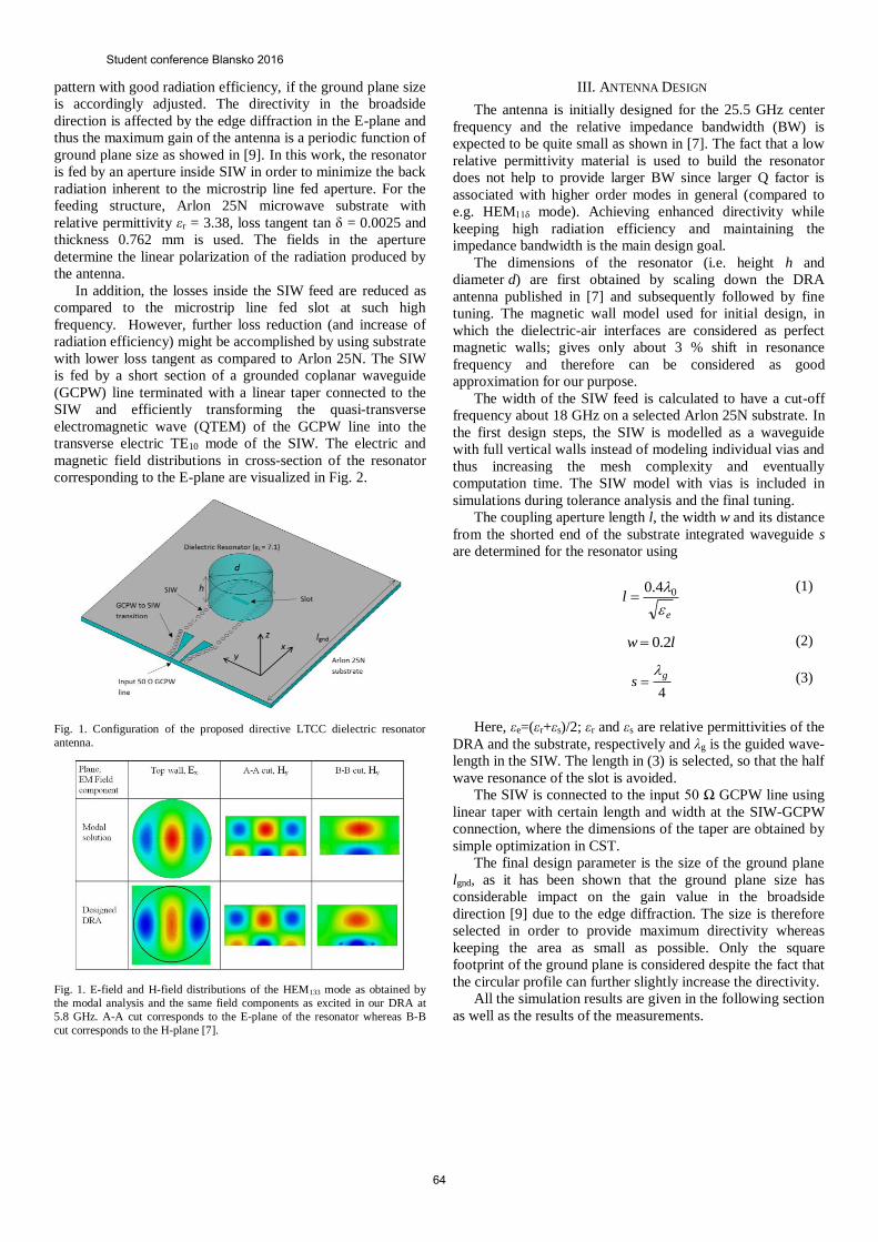
pattern with good radiation efficiency, if the ground plane size
is accordingly adjusted. The directivity in the broadside
direction is affected by the edge diffraction in the E-plane and
thus the maximum gain of the antenna is a periodic function of
ground plane size as showed in [9]. In this work, the resonator
is fed by an aperture inside SIW in order to minimize the back
radiation inherent to the microstrip line fed aperture. For the
feeding structure, Arlon 25N microwave substrate with
relative permittivity εr = 3.38, loss tangent tan δ = 0.0025 and
thickness 0.762 mm is used. The fields in the aperture
determine the linear polarization of the radiation produced by
the antenna.
In addition, the losses inside the SIW feed are reduced as
compared to the microstrip line fed slot at such high
frequency. However, further loss reduction (and increase of
radiation efficiency) might be accomplished by using substrate
with lower loss tangent as compared to Arlon 25N. The SIW
is fed by a short section of a grounded coplanar waveguide
(GCPW) line terminated with a linear taper connected to the
SIW and efficiently transforming the quasi-transverse
electromagnetic wave (QTEM) of the GCPW line into the
transverse electric TE10 mode of the SIW. The electric and
magnetic field distributions in cross-section of the resonator
corresponding to the E-plane are visualized in Fig. 2.
Fig. 1. Configuration of the proposed directive LTCC dielectric resonator
antenna.
Fig. 1. E-field and H-field distributions of the HEM133 mode as obtained by
the modal analysis and the same field components as excited in our DRA at
5.8 GHz. A-A cut corresponds to the E-plane of the resonator whereas B-B
cut corresponds to the H-plane [7].
III. ANTENNA DESIGN
The antenna is initially designed for the 25.5 GHz center
frequency and the relative impedance bandwidth (BW) is
expected to be quite small as shown in [7]. The fact that a low
relative permittivity material is used to build the resonator
does not help to provide larger BW since larger Q factor is
associated with higher order modes in general (compared to
e.g. HEM11δ mode). Achieving enhanced directivity while
keeping high radiation efficiency and maintaining the
impedance bandwidth is the main design goal.
The dimensions of the resonator (i.e. height h and
diameter d) are first obtained by scaling down the DRA
antenna published in [7] and subsequently followed by fine
tuning. The magnetic wall model used for initial design, in
which the dielectric-air interfaces are considered as perfect
magnetic walls; gives only about 3 % shift in resonance
frequency and therefore can be considered as good
approximation for our purpose.
The width of the SIW feed is calculated to have a cut-off
frequency about 18 GHz on a selected Arlon 25N substrate. In
the first design steps, the SIW is modelled as a waveguide
with full vertical walls instead of modeling individual vias and
thus increasing the mesh complexity and eventually
computation time. The SIW model with vias is included in
simulations during tolerance analysis and the final tuning.
The coupling aperture length l, the width w and its distance
from the shorted end of the substrate integrated waveguide s
are determined for the resonator using
e
l
04.0
(1)
lw 2.0 (2)
4
gs
(3)
Here, εe=(εr+εs)/2; εr and εs are relative permittivities of the
DRA and the substrate, respectively and λg is the guided wave-
length in the SIW. The length in (3) is selected, so that the half
wave resonance of the slot is avoided.
The SIW is connected to the input 50 Ω GCPW line using
linear taper with certain length and width at the SIW-GCPW
connection, where the dimensions of the taper are obtained by
simple optimization in CST.
The final design parameter is the size of the ground plane
lgnd, as it has been shown that the ground plane size has
considerable impact on the gain value in the broadside
direction [9] due to the edge diffraction. The size is therefore
selected in order to provide maximum directivity whereas
keeping the area as small as possible. Only the square
footprint of the ground plane is considered despite the fact that
the circular profile can further slightly increase the directivity.
All the simulation results are given in the following section
as well as the results of the measurements.
Student conference Blansko 2016
64
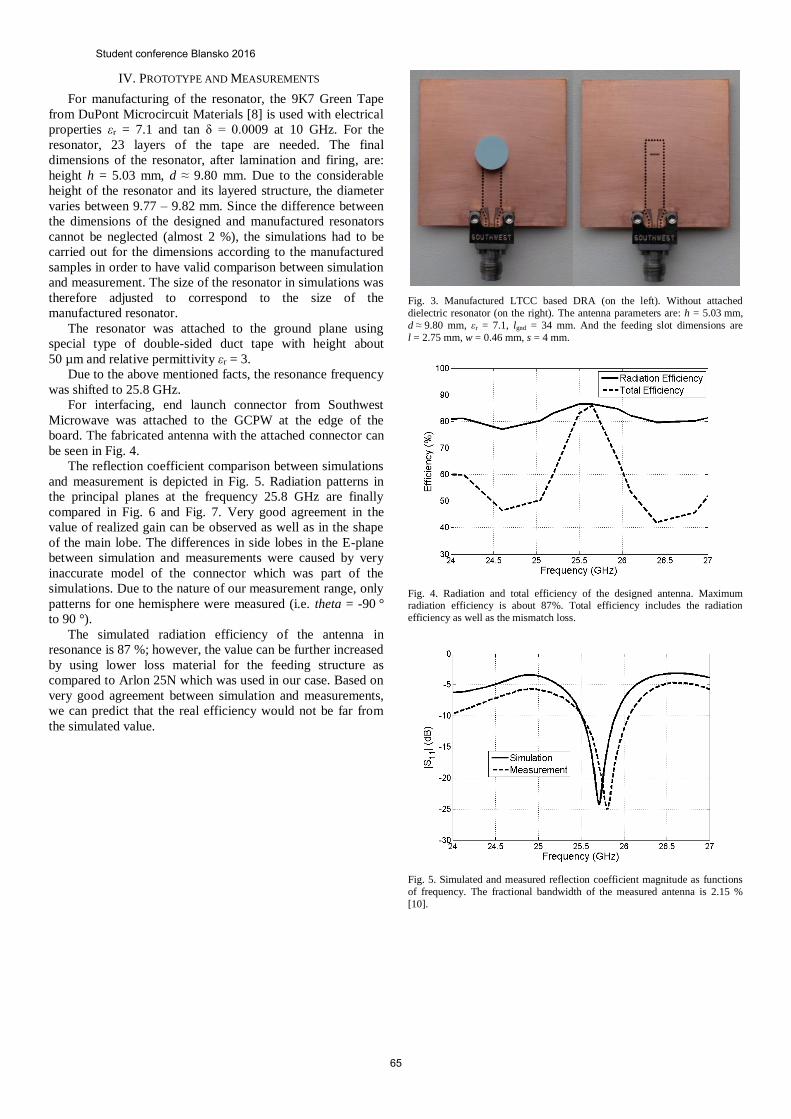
IV. PROTOTYPE AND MEASUREMENTS
For manufacturing of the resonator, the 9K7 Green Tape
from DuPont Microcircuit Materials [8] is used with electrical
properties εr = 7.1 and tan δ = 0.0009 at 10 GHz. For the
resonator, 23 layers of the tape are needed. The final
dimensions of the resonator, after lamination and firing, are:
height h = 5.03 mm, d ≈ 9.80 mm. Due to the considerable
height of the resonator and its layered structure, the diameter
varies between 9.77 – 9.82 mm. Since the difference between
the dimensions of the designed and manufactured resonators
cannot be neglected (almost 2 %), the simulations had to be
carried out for the dimensions according to the manufactured
samples in order to have valid comparison between simulation
and measurement. The size of the resonator in simulations was
therefore adjusted to correspond to the size of the
manufactured resonator.
The resonator was attached to the ground plane using
special type of double-sided duct tape with height about
50 µm and relative permittivity εr = 3.
Due to the above mentioned facts, the resonance frequency
was shifted to 25.8 GHz.
For interfacing, end launch connector from Southwest
Microwave was attached to the GCPW at the edge of the
board. The fabricated antenna with the attached connector can
be seen in Fig. 4.
The reflection coefficient comparison between simulations
and measurement is depicted in Fig. 5. Radiation patterns in
the principal planes at the frequency 25.8 GHz are finally
compared in Fig. 6 and Fig. 7. Very good agreement in the
value of realized gain can be observed as well as in the shape
of the main lobe. The differences in side lobes in the E-plane
between simulation and measurements were caused by very
inaccurate model of the connector which was part of the
simulations. Due to the nature of our measurement range, only
patterns for one hemisphere were measured (i.e. theta = -90 °
to 90 °).
The simulated radiation efficiency of the antenna in
resonance is 87 %; however, the value can be further increased
by using lower loss material for the feeding structure as
compared to Arlon 25N which was used in our case. Based on
very good agreement between simulation and measurements,
we can predict that the real efficiency would not be far from
the simulated value.
Fig. 3. Manufactured LTCC based DRA (on the left). Without attached
dielectric resonator (on the right). The antenna parameters are: h = 5.03 mm,
d ≈ 9.80 mm, εr = 7.1, lgnd = 34 mm. And the feeding slot dimensions are
l = 2.75 mm, w = 0.46 mm, s = 4 mm.
Fig. 4. Radiation and total efficiency of the designed antenna. Maximum radiation efficiency is about 87%. Total efficiency includes the radiation
efficiency as well as the mismatch loss.
Fig. 5. Simulated and measured reflection coefficient magnitude as functions
of frequency. The fractional bandwidth of the measured antenna is 2.15 %
[10].
Student conference Blansko 2016
65
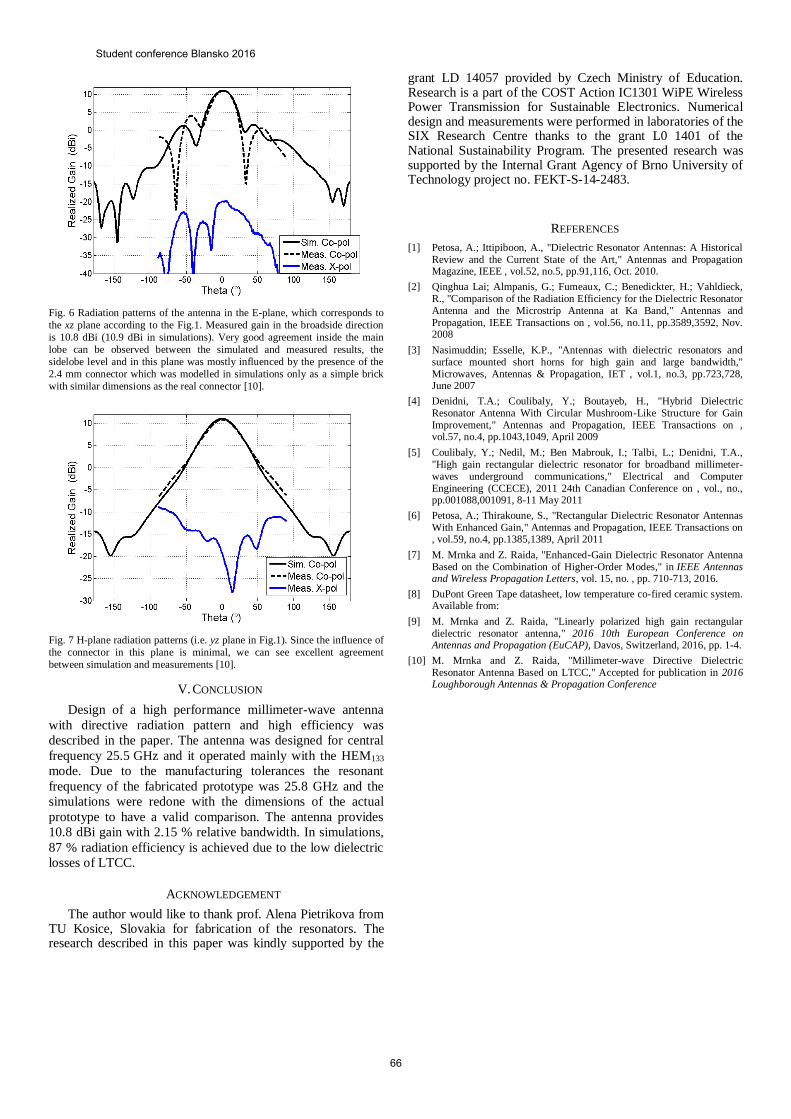
Fig. 6 Radiation patterns of the antenna in the E-plane, which corresponds to
the xz plane according to the Fig.1. Measured gain in the broadside direction
is 10.8 dBi (10.9 dBi in simulations). Very good agreement inside the main
lobe can be observed between the simulated and measured results, the
sidelobe level and in this plane was mostly influenced by the presence of the
2.4 mm connector which was modelled in simulations only as a simple brick
with similar dimensions as the real connector [10].
Fig. 7 H-plane radiation patterns (i.e. yz plane in Fig.1). Since the influence of
the connector in this plane is minimal, we can see excellent agreement
between simulation and measurements [10].
V. CONCLUSION
Design of a high performance millimeter-wave antenna
with directive radiation pattern and high efficiency was
described in the paper. The antenna was designed for central
frequency 25.5 GHz and it operated mainly with the HEM133
mode. Due to the manufacturing tolerances the resonant
frequency of the fabricated prototype was 25.8 GHz and the
simulations were redone with the dimensions of the actual
prototype to have a valid comparison. The antenna provides
10.8 dBi gain with 2.15 % relative bandwidth. In simulations,
87 % radiation efficiency is achieved due to the low dielectric
losses of LTCC.
ACKNOWLEDGEMENT
The author would like to thank prof. Alena Pietrikova from TU Kosice, Slovakia for fabrication of the resonators. The research described in this paper was kindly supported by the
grant LD 14057 provided by Czech Ministry of Education. Research is a part of the COST Action IC1301 WiPE Wireless Power Transmission for Sustainable Electronics. Numerical design and measurements were performed in laboratories of the SIX Research Centre thanks to the grant L0 1401 of the National Sustainability Program. The presented research was supported by the Internal Grant Agency of Brno University of Technology project no. FEKT-S-14-2483.
REFERENCES
[1] Petosa, A.; Ittipiboon, A., "Dielectric Resonator Antennas: A Historical Review and the Current State of the Art," Antennas and Propagation Magazine, IEEE , vol.52, no.5, pp.91,116, Oct. 2010.
[2] Qinghua Lai; Almpanis, G.; Fumeaux, C.; Benedickter, H.; Vahldieck, R., "Comparison of the Radiation Efficiency for the Dielectric Resonator Antenna and the Microstrip Antenna at Ka Band," Antennas and Propagation, IEEE Transactions on , vol.56, no.11, pp.3589,3592, Nov. 2008
[3] Nasimuddin; Esselle, K.P., "Antennas with dielectric resonators and surface mounted short horns for high gain and large bandwidth," Microwaves, Antennas & Propagation, IET , vol.1, no.3, pp.723,728, June 2007
[4] Denidni, T.A.; Coulibaly, Y.; Boutayeb, H., "Hybrid Dielectric Resonator Antenna With Circular Mushroom-Like Structure for Gain Improvement," Antennas and Propagation, IEEE Transactions on , vol.57, no.4, pp.1043,1049, April 2009
[5] Coulibaly, Y.; Nedil, M.; Ben Mabrouk, I.; Talbi, L.; Denidni, T.A., "High gain rectangular dielectric resonator for broadband millimeter-waves underground communications," Electrical and Computer Engineering (CCECE), 2011 24th Canadian Conference on , vol., no., pp.001088,001091, 8-11 May 2011
[6] Petosa, A.; Thirakoune, S., "Rectangular Dielectric Resonator Antennas With Enhanced Gain," Antennas and Propagation, IEEE Transactions on , vol.59, no.4, pp.1385,1389, April 2011
[7] M. Mrnka and Z. Raida, "Enhanced-Gain Dielectric Resonator Antenna Based on the Combination of Higher-Order Modes," in IEEE Antennas and Wireless Propagation Letters, vol. 15, no. , pp. 710-713, 2016.
[8] DuPont Green Tape datasheet, low temperature co-fired ceramic system. Available from:
[9] M. Mrnka and Z. Raida, "Linearly polarized high gain rectangular dielectric resonator antenna," 2016 10th European Conference on Antennas and Propagation (EuCAP), Davos, Switzerland, 2016, pp. 1-4.
[10] M. Mrnka and Z. Raida, "Millimeter-wave Directive Dielectric Resonator Antenna Based on LTCC," Accepted for publication in 2016 Loughborough Antennas & Propagation Conference
Student conference Blansko 2016
66
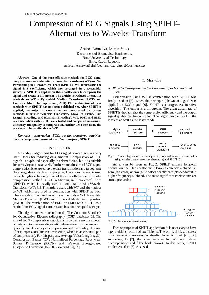
Compression of ECG Signals Using SPIHT –
Alternatives to Wavelet Transform
Andrea Němcová, Martin Vítek
Department of Biomedical Engineering
Brno University of Technology
Brno, Czech Republic
[email protected], [email protected]
Abstract—One of the most effective methods for ECG signal
compression is a combination of Wavelet Transform (WT) and Set
Partitioning in Hierarchical Trees (SPIHT). WT transforms the
signal into coefficients, which are arranged in a pyramidal
structure. SPIHT is applied on these coefficients to compress the
signal and create a bit stream. The article introduces alternative
methods to WT – Pyramidal Median Transform (PMT) and
Empirical Mode Decomposition (EMD). The combination of these
methods with SPIHT has not been published yet. After SPIHT is
applied, the output stream is further compressed by lossless
methods (Burrows-Wheeler Transform, Move to Front, Run
Length Encoding, and Huffman Encoding). WT, PMT and EMD
in combination with SPIHT were tested and compared in terms of
efficiency and quality of compression. Neither PMT nor EMD did
not show to be as effective as WT.
Keywords—compression, ECG, wavelet transform, empirical
mode decomposition, pyramidal median transform, SPIHT
I. INTRODUCTION
Nowadays, algorithms for ECG signal compression are very useful tools for reducing data amount. Compression of ECG signals is exploited especially in telemedicine, but it is suitable for archiving of data as well. Furthermore, the aim of ECG signal compression is to speed up the data transmission and to decrease the energy demands. For this purpose, lossy compression is used to reach higher efficiency. One of the most effective and popular compression method is Set Partitioning in Hierarchical Trees (SPIHT), which is usually used in combination with Wavelet Transform (WT) [1]. This article deals with WT and alternatives to WT, which are used in combination with SPIHT as well. There are described and tested three methods – WT, Pyramidal Median Transform (PMT) and Empirical Mode Decomposition (EMD). The combination of PMT or EMD with SPIHT as a method for ECG signal compression has not been published yet.
The algorithms were tested on the The Common Standards for Quantitative Electrocardiography (CSE) database [2]. The aim of ECG compression algorithms is to decrease the amount of data and to preserve diagnostic information. It is necessary to quantify the efficiency of compression and the quality of signal after compression (and reconstruction, which is an essential part of compression). For this purpose, Average Value Length (avL), Compression Factor (CF), Normalized Percentage Root Mean Square Difference (PRDN) and Wavelet Energy-based Diagnostic Distortion (WEDD) are used [3], [4].
II. METHODS
A. Wavelet Transform and Set Partitioning in Hierarchical
Trees
Compression using WT in combination with SPIHT was firstly used in [5]. Later, the principle (shown in Fig. 1) was applied on ECG signal [6]. SPIHT is a progressive iterative algorithm. The output is a bit stream. The great advantage of SPIHT is the fact, that the compression efficiency and the output signal quality can be controlled. This algorithm can work in the lossless as well as the lossy mode.
As it can be seen in Fig. 2, SPIHT utilizes temporal orientation tree. One coefficient in lower frequency subband has zero (red color) or two (blue color) coefficients (descendants) in higher frequency subband. The most significant coefficients are stored preferably.
For the purpose of SPIHT application, it is necessary to have a pyramidal structure of coefficients. Therefore, the fast discrete time wavelet transform in dyadic form is used [6], [7]. According to [7], the ideal settings for WT are 6-level decomposition and filter bank bior4.4. In this work, SPIHT implemented in [8] was used.
Fig. 2. Temporal orientation tree.
Fig. 1. Block diagram of the principle of compression and reconstruction
using wavelet transform (or any alternative) and SPIHT [6].
Student conference Blansko 2016
67

B. Pyramidal Median Transform
The PMT is a nonlinear transform. It has been used especially for denoising [9], not much for compression [10]. It decomposes the signal into scales. Fig. 3 shows the block diagram of 2-level PMT. PMT consists of two parts – decomposition and reconstruction. At first, the original signal x(n) is filtered by a median filter. The length of filter window is an adjustable parameter. Then, the filtered signal is downsampled with factor M (an adjustable parameter as well, for our purpose M = 2). The output is the input of branches 1 and 2. In the branch 1, the signal is upsampled and interpolation filter is applied (in our case, cubic interpolation was used). Interpolated signal is subtracted from the original signal and the residual signal y1(n) is obtained (the first and the finest scale). In the branch 2, the filtered and downsampled signal is filtered and downsampled again. In the branch 3, the output is upsampled, the interpolation filter is applied and it is subtracted. The residual signal y2(n) is the second, coarser scale. In the branch 4, the signal y3(n) is stored. The reconstruction is performed in the reverse order. PMT is a lossless transform; the signal can be reconstructed without an error.
C. Empirical Mode Decomposition
EMD is a nonlinear method used for a nonstationary signal decomposition. It decomposes the signal into Intrinsic Mode Functions (IMF), which should met two criteria [11]:
The number of extrema is equal or differ at most by one from the number of zero crossings.
The mean value calculated from the local minima envelope and the local maxima envelope should be zero for every sample.
The algorithm works as follows. At first, a local minima and maxima are found. Then, they are interpolated and two envelopes are created. Later, the mean is calculated from these two envelopes and subtracted from the original signal. This process (called sifting) is iteratively repeated until the stop criterion is reached. The output of this process is the first IMF. Then, the first IMF is subtracted from the original signal and the second IMF is searched (using the sifting process). The EMD algorithm can be stopped after the trend of the signal is found or after the preset number of iterations (IMFs) is reached [11].
In this work, the fast EMD algorithm [12] was used. Different settings of this algorithm were tested – the number of
IMFs and the number of sifting iterations. Results are described in chapter III.
After EMD, the IMFs are gradually downsampled by the factor of 2 and its powers (similarly as in the dyadic WT).
D. Lossless Compression
After the compression of ECG signal using SPIHT, the output bit stream is further compressed using lossless compression methods and transforms. After SPIHT, Burrows-Wheeler Transform (BWT), Move to Front (MTF), Run Length Encoding (RLE) and Huffman Encoding (HE) are applied.
E. CSE Database
The compression algorithms were tested on the CSE database [2]. It contains original as well as artificial ECG signals. Data set 3 was used for this purpose. It includes 125 ECG records, each with 15 leads. In this work, only the first Frank´s orthogonal lead (lead X) was used. Signals no. 60, 68, 76, 84, 92, 100, 108, and 124 were excluded from further analysis, because they are not considered as ECG signals. The original length of each record is 10 seconds, the sampling frequency is 500 Hz, the bit resolution is 16 bits/sample (bps).
F. Evaluation Algorithms
For evaluation of compression efficiency, avL (1) and CF (2) were used [3], [4].
𝑎𝑣𝑙 (𝑏𝑝𝑠) = 𝑠𝑖𝑧𝑒 𝑜𝑓 𝑡ℎ𝑒 𝑜𝑢𝑡𝑝𝑢𝑡 𝑠𝑡𝑟𝑒𝑎𝑚
𝑜𝑟𝑖𝑔𝑖𝑛𝑎𝑙 𝑠𝑖𝑔𝑛𝑎𝑙 𝑙𝑒𝑛𝑔𝑡ℎ (1)
𝐶𝐹 (−) = 𝑠𝑖𝑧𝑒 𝑜𝑓 𝑡ℎ𝑒 𝑖𝑛𝑝𝑢𝑡 𝑠𝑡𝑟𝑒𝑎𝑚
𝑠𝑖𝑧𝑒 𝑜𝑓 𝑡ℎ𝑒 𝑜𝑢𝑡𝑝𝑢𝑡 𝑠𝑡𝑟𝑒𝑎𝑚 (2)
The quality of the signal after compression was evaluated using objective method without diagnostic information – PRDN (3):
𝑃𝑅𝐷𝑁 (%) = 100 × √∑ (𝑋𝑠(𝑛)−𝑋𝑟(𝑛))
2𝑁−1𝑛=0
∑ (𝑋𝑠(𝑛)−)2𝑁−1𝑛=0
, (3)
where Xs is the original signal, Xr the signal after compression and reconstruction, and X is the mean of the original signal [3]. PRDN is the most commonly used method. Signals with PRDN ≤ 5 % are acceptable for further analysis [13]. The second method for signal quality evaluation, which is used in this work is WEDD [14]. WEDD is an advanced objective method, which reflects diagnostic information. It is based on a wavelet transform. According to [15] the signal with very good quality has WEDD ≤ 2 %. Calculation of WEDD is not trivial and more details can be found in [14].
III. RESULTS AND DISCUSSION
Combination of WT and SPIHT is considered as a reference. Only one ideal setting (according to [7]) was tested. For EMD and PMT, different settings were tested on the whole CSE database. The SPIHT algorithm is equally set for WT, PMT and EMD. For the testing of parameters of PMT and EMD, the SPIHT was set to have the maximum length of output bit stream equal to 10,000 samples. Criterion for selecting optimal parameters of the tested algorithms is the quality of ECG signal after reconstruction (values of PRDN and WEDD).
Fig. 3. Block diagram of 2-level Pyramidal Median Transform [9].
Student conference Blansko 2016
68

A. Pyramidal Median Transform
For PMT, the different level of decomposition and the length of the median filter window were tested. The results are shown in Table I. It is obvious from Table I, that the lowest (it means the best) PRDN and WEDD were reached with 4-level decomposition and window length of 3 (highlighted in red). According to the results, 2-level PMT is not appropriate for compression; it reaches very good avL and CF, but the signals are too much distorted (high PRDN and WEDD). With increasing window length of the median filter, the quality of the reconstructed signal is decreasing (increasing PRDN and WEDD).
TABLE I. RESULTS FOR PYRAMIDAL MEDIAN TRANSFORM
levels of
decomposition
window
length
avL
[bps]
CF
[-]
PRDN
[%]
WEDD
[%]
2
3 0.7862 22.4924 16.1133 14.9297
5 0.7808 22.6807 17.3834 16.3283
7 0.8167 21.5042 17.7888 16.8155
9 0.8313 21.2318 19.1260 18.1573
3
3 1.5441 10.4540 7.0468 6.0187
5 1.5852 10.1903 7.7924 6.6606
7 1.5827 10.2050 8.8094 7.4756
9 1.5539 10.3956 10.2821 8.6424
4
3 1.8539 8.6452 6.8170 5.8839
5 1.8513 8.6599 7.6754 6.6491
7 1.8451 8.6888 8.8823 7.6768
9 1.8231 8.7951 10.4552 8.9767
5
3 1.9361 8.2701 7.5705 6.7592
5 1.9389 8.2599 8.7292 7.8909
7 1.9218 8.3333 9.7497 8.7762
9 1.8951 8.4513 11.3935 10.2226
B. Empirical Mode Decomposition
EMD was tested in two steps. In the first step, the number of sifting iterations was set to 4 (based on the previous testing on 5 signals from the CSE database). The performance of the EMD and SPIHT algorithm with various levels of decomposition was tested. The results are shown in Table II. It is evident, that the best quality is reached with 5-level EMD (highlighted in red).
TABLE II. RESULTS FOR EMPIRICAL MODE DECOMPOSITION –
CHANGING LEVEL OF DECOMPOSITION
level of
decomposition
avL
[bps]
CF
[-]
PRDN
[%]
WEDD
[%]
2 0.6238 27.0537 45.7640 43.0589
3 1.4863 11.5463 16.1926 15.0036
4 2.2226 7.2977 8.4215 7.3493
5 2.4483 6.5542 7.7330 6.7411
6 2.5130 6.3726 7.9736 7.0522
7 2.5318 6.3233 8.4238 7.5284
8 2.5485 6.2817 8.8453 8.0748
9 2.5415 6.2988 8.9240 7.9950
In the second step, the 5-level EMD was used and the number of sifting iterations was changed. Table III shows the results. The lowest distortion of reconstructed signal is reached with the number of sifting iterations of 7 (according to PRDN) and 9 (according to WEDD). Because WEDD reflects the diagnostic information, number of sifting iterations of 9 was selected for further testing and comparison.
TABLE III. RESULTS FOR EMPIRICAL MODE DECOMPOSITION – CHANGING
NUMBER OF SIFTING ITERATIONS
no. of sifting
iterations
avL
[bps]
CF
[-]
PRDN
[%]
WEDD
[%]
1 2.2949 6.9942 13.6683 12.7562
2 2.4028 6.6785 9.2950 8.4083
3 2.4255 6.6140 8.2391 7.2942
4 2.4483 6.5542 7.7330 6.7411
5 2.4356 6.5845 7.5260 6.4903
6 2.4352 6.5826 7.4859 6.4337
7 2.4423 6.5638 7.4289 6.3538
8 2.4402 6.5728 7.4462 6.3289
9 2.4546 6.5350 7.4524 6.3094
10 2.4458 6.5575 7.5818 6.4274
C. Comparison of WT, PMT and EMD
All algorithms were tested for three levels of compression
(maximum length of output bit stream was set to 10,000
samples, 15,000 samples, and 20,000 samples in the SPIHT
algorithm). The final length was further influenced by lossless
compression. PMT and EMD were tested with the best settings
(described above). Results are shown in Table IV.
It is obvious from the table, that the combination of WT and
SPIHT is the most effective one. The reconstructed signal is
minimally distorted; average PRDN is 2.2550 % and WEDD is
even smaller than PRDN, only 1.1714 % for the highest tested
level of compression. The criteria mentioned in chapter II.F are
met. This combination has the highest potential, because the
efficiency of compression (avL and CF) can be further
increased and it is highly probable, that the distortion will be
still acceptable. EMD and PMT in the combination with SPIHT
are not as effective as WT and SPIHT. The distortion is
significantly higher and does not meet the criteria from II.F
(except for PMT and maximum length of bit stream of 20,000
samples). On the other hand, PMT reaches lower avL and
higher CF (higher efficiency) than WT. Table IV shows, that
PMT is better than EMD in terms of both efficiency and quality.
EMD works on different (empirical) principles than PMT and
WT and its performance is highly dependent on the signal.
Fig. 4 and 5 show the examples of compressed signals. In
Fig. 4, there is signal no. 117 compressed with the lowest
distortion. In Fig. 4, there is shown signal no. 20, which was
compressed with the highest distortion.
IV. CONCLUSION
The ECG signal was decomposed by three different algorithms – WT, PMT and EMD. Then the tree (pyramidal) structure was created for all algorithms using gradual downsampling. SPIHT algorithm was applied on the tree structures in order to compress the ECG signal. The output of this process was a bit stream, which was further compressed using lossless compression algorithms (BWT, MTF, RLE, and HE). PMT and EMD were optimized in terms of parameters settings. PMT performed the lowest distortion with 4-level decomposition and the median transform window length of 3. Using EMD, the lowest distortion was reached with 5-level decomposition and the number of sifting iterations of 9.
The comparison between WT, PMT, and EMD in the combination with SPIHT shows, that WT and SPIHT reaches the highest efficiency and the processed signal has the lowest
Student conference Blansko 2016
69
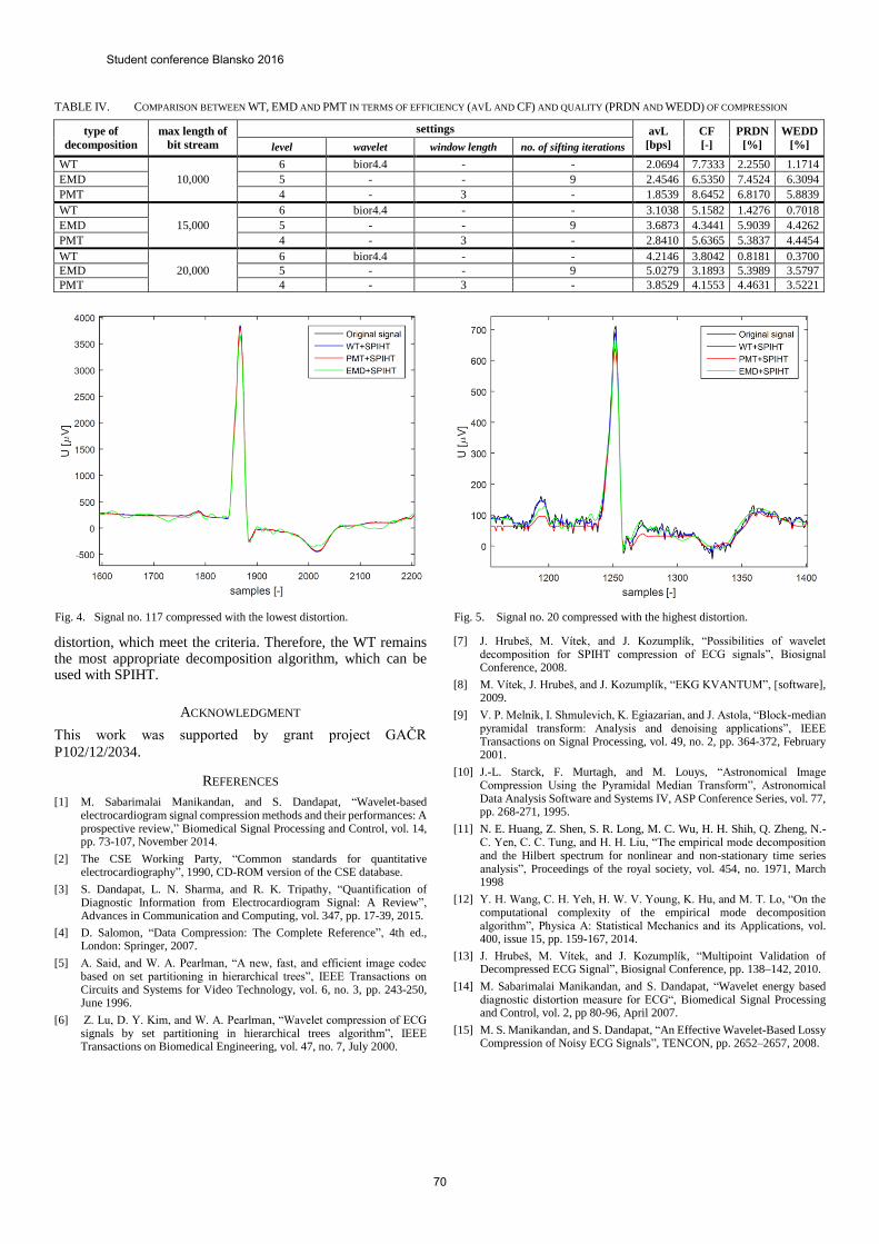
distortion, which meet the criteria. Therefore, the WT remains the most appropriate decomposition algorithm, which can be used with SPIHT.
ACKNOWLEDGMENT
This work was supported by grant project GAČR
P102/12/2034.
REFERENCES
[1] M. Sabarimalai Manikandan, and S. Dandapat, “Wavelet-based electrocardiogram signal compression methods and their performances: A prospective review,” Biomedical Signal Processing and Control, vol. 14, pp. 73-107, November 2014.
[2] The CSE Working Party, “Common standards for quantitative electrocardiography”, 1990, CD-ROM version of the CSE database.
[3] S. Dandapat, L. N. Sharma, and R. K. Tripathy, “Quantification of Diagnostic Information from Electrocardiogram Signal: A Review”, Advances in Communication and Computing, vol. 347, pp. 17-39, 2015.
[4] D. Salomon, “Data Compression: The Complete Reference”, 4th ed., London: Springer, 2007.
[5] A. Said, and W. A. Pearlman, “A new, fast, and efficient image codec based on set partitioning in hierarchical trees”, IEEE Transactions on Circuits and Systems for Video Technology, vol. 6, no. 3, pp. 243-250, June 1996.
[6] Z. Lu, D. Y. Kim, and W. A. Pearlman, “Wavelet compression of ECG signals by set partitioning in hierarchical trees algorithm”, IEEE Transactions on Biomedical Engineering, vol. 47, no. 7, July 2000.
[7] J. Hrubeš, M. Vítek, and J. Kozumplík, “Possibilities of wavelet decomposition for SPIHT compression of ECG signals”, Biosignal Conference, 2008.
[8] M. Vítek, J. Hrubeš, and J. Kozumplík, “EKG KVANTUM”, [software], 2009.
[9] V. P. Melnik, I. Shmulevich, K. Egiazarian, and J. Astola, “Block-median pyramidal transform: Analysis and denoising applications”, IEEE Transactions on Signal Processing, vol. 49, no. 2, pp. 364-372, February 2001.
[10] J.-L. Starck, F. Murtagh, and M. Louys, “Astronomical Image Compression Using the Pyramidal Median Transform”, Astronomical Data Analysis Software and Systems IV, ASP Conference Series, vol. 77, pp. 268-271, 1995.
[11] N. E. Huang, Z. Shen, S. R. Long, M. C. Wu, H. H. Shih, Q. Zheng, N.-C. Yen, C. C. Tung, and H. H. Liu, “The empirical mode decomposition and the Hilbert spectrum for nonlinear and non-stationary time series analysis”, Proceedings of the royal society, vol. 454, no. 1971, March 1998
[12] Y. H. Wang, C. H. Yeh, H. W. V. Young, K. Hu, and M. T. Lo, “On the computational complexity of the empirical mode decomposition algorithm”, Physica A: Statistical Mechanics and its Applications, vol. 400, issue 15, pp. 159-167, 2014.
[13] J. Hrubeš, M. Vítek, and J. Kozumplík, “Multipoint Validation of Decompressed ECG Signal”, Biosignal Conference, pp. 138–142, 2010.
[14] M. Sabarimalai Manikandan, and S. Dandapat, “Wavelet energy based diagnostic distortion measure for ECG“, Biomedical Signal Processing and Control, vol. 2, pp 80-96, April 2007.
[15] M. S. Manikandan, and S. Dandapat, “An Effective Wavelet-Based Lossy Compression of Noisy ECG Signals”, TENCON, pp. 2652–2657, 2008.
type of
decomposition
max length of
bit stream
settings avL
[bps]
CF
[-]
PRDN
[%]
WEDD
[%] level wavelet window length no. of sifting iterations
WT
10,000
6 bior4.4 - - 2.0694 7.7333 2.2550 1.1714
EMD 5 - - 9 2.4546 6.5350 7.4524 6.3094
PMT 4 - 3 - 1.8539 8.6452 6.8170 5.8839
WT
15,000
6 bior4.4 - - 3.1038 5.1582 1.4276 0.7018
EMD 5 - - 9 3.6873 4.3441 5.9039 4.4262
PMT 4 - 3 - 2.8410 5.6365 5.3837 4.4454
WT
20,000
6 bior4.4 - - 4.2146 3.8042 0.8181 0.3700
EMD 5 - - 9 5.0279 3.1893 5.3989 3.5797
PMT 4 - 3 - 3.8529 4.1553 4.4631 3.5221
TABLE IV. COMPARISON BETWEEN WT, EMD AND PMT IN TERMS OF EFFICIENCY (AVL AND CF) AND QUALITY (PRDN AND WEDD) OF COMPRESSION
Fig. 4. Signal no. 117 compressed with the lowest distortion.
Fig. 5. Signal no. 20 compressed with the highest distortion.
Student conference Blansko 2016
70
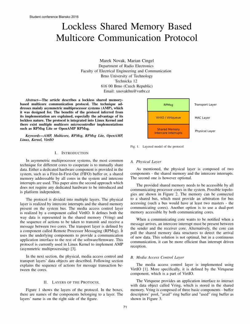
Lockless Shared Memory BasedMulticore Communication Protocol
Marek Novak, Marian CingelDepartment of Radio Electronics
Faculty of Electrical Engineering and CommunicationBrno University of Technology
Technicka 12616 00 Brno (Czech Republic)
Email: [email protected]
Abstract—The article describes a lockless shared memory-based multicore communication protocol. The technique ad-dresses mainly asymmetric multiprocessor systems (AMP), whichit was designed for. The benefits of the protocol inferred fromits implementation are explained, especially the advantage of itslockless nature. The protocol is integrated into Linux Kernel andthere exist multiple multicore microcontroller implementationssuch as RPMsg Lite or OpenAMP RPMsg.
Keywords—AMP, Multicore, RPMsg, RPMsg Lite, OpenAMP,Linux, Kernel, VirtIO
I. INTRODUCTION
In asymmetric multiprocessor systems, the most commontechnique for different cores to cooperate is to mutually sharedata. Either a dedicated hardware component is provided in thesystem, such as a First-In-First-Out (FIFO) buffer or, a sharedmemory addressable by all cores in the system and intercoreinterrupts are used. This paper aims the second approach whichdoes not require any dedicated hardware to be introduced andis platform independent.
The protocol is divided into multiple layers. The physicallayer is realized by intercore interrupts and the shared memorypresent on the system bus. The media access control layeris realized by a component called VirtIO. It defines both theway data is represented in the shared memory (Vring) andthe sequence of actions to be taken to transmit and receive amessage between two cores. The transport layer is defined bya component called Remote Processor Messaging (RPMsg). Ituses the underlying components to provide a communicationapplication interface to the rest of the software/firmware. Thisprotocol is currently used in Linux Kernel to implement AMP(asymmetric multiprocessing) [3].
In the next section, the physical, media access control andtransport layers’ data objects are described. Following sectionexplains the sequence of actions for message transaction be-tween the cores.
II. LAYERS OF THE PROTOCOL
Figure 1 shows the layers of the protocol. In the boxes,there are names of the components belonging to a layer. Thelayers’ name is on the right side of the figure.
Shared MemoryIntercore Interrupts
VirtIO / Virtqueue
Transport LayerRPMsg
MAC Layer
Physical Layer
Fig. 1. Layered model of the protocol
A. Physical Layer
As mentioned, the physical layer is composed of twocomponents - the shared memory and the intercore interrupts.The second one is however optional.
The provided shared memory needs to be accessible by allcommunicating processor cores in the system. Possible topolo-gies are shown in Figure 2. The memory can be connectedto a shared bus, which must provide an arbitration for busaccessing (such a bus would have at least two masters - thecommunicating cores). Another option is to use a dual-portmemory accessible by both communicating cores.
When a communicating core wants to be notified when amessage arrives, an intercore interrupt must be present betweenthe sender and the receiver core. Alternatively, the core canpoll the shared memory data structures to detect the arrivalof new data. This solution is not optimal, but in a continuouscommunication, it can be more efficient than interrupt drivenreception.
B. Media Access Control Layer
The media access control layer is implemented usingVirtIO [1]. More specifically, it is defined by the Virtqueuecomponent, which is a part of VirtIO.
The Virtqueue provides an application interface to interactwith data object called Vring, which is stored in the sharedmemory. Vring is composed of three basic components - bufferdescriptors’ pool, ”avail” ring buffer and ”used” ring buffer asshown in Figure 3.
Student conference Blansko 2016
71
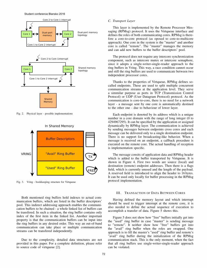
Core 1 Core 2Dual-portmemory
Core 2 to Core 1 interrupt
Core 1 to Core 2 interrupt
Core 1 Core 2
Core 2 to Core 1interrupt
Core 1 to Core 2 interrupt
SharedMemory
Dual-port memorytopology
Shared memorytopology
Fig. 2. Physical layer - possible implementations
Buffer Descriptors
"Avail" Ring Buffer
"Used" Ring Buffer
VRING
In Shared Memory
TX
FREE
Fig. 3. Vring - bookkeeping structure for Virtqueue
Both mentioned ring buffers hold indexes to actual com-munication buffers, which are listed in the buffer descriptors’pool. This indirect addressing approach enables the communi-cation buffers to be chained - a whole linked list of buffers canbe transfered. In such a situation, the ring buffer contains onlyindex of the first item in the linked list. Another importantproperty is that the communication buffers can be input intothe ring buffers in any desired order. This way an out-of-bandcommunication can take place or multiple communicationstreams can be transfered independently.
Due to the complexity, detailed data structures are notprovided in this paper. For a complete definition, please referto source code of virtqueue [2].
C. Transport Layer
This layer is implemented by the Remote Processor Mes-saging (RPMsg) protocol. It uses the Virtqueue interface anddefines the roles of both communicating cores. RPMsg is there-fore a core-to-core protocol (as oposed to core-to-multicoreapproach). One core in the system is the ”master” and anothercore is called ”remote”. The ”master” manages the memoryand can add new buffers to the buffer descriptors’ pool.
The protocol does not require any intercore synchronizationcomponent, such as intercore mutex or intercore semaphore,since it adopts a single-writer-single-reader approach to thering buffers in Vring. This way, a race condition cannot occurand still the ring buffers are used to communicate between twoindependent processor cores.
Thanks to the properties of Virtqueue, RPMsg defines so-called endpoints. These are used to split multiple concurrentcommunication streams at the application level. They servea simmilar purpose as ports in TCP (Transmission ControlProtocol) or UDP (User Datagram Protocol) protocol. As thecommunication is core-to-core, there is no need for a networklayer - a message sent by one core is automatically destinedto the other one - due to behaviour of lower layer.
Each endpoint is denoted by its address which is a uniquenumber in a core domain with the range of long integer (0 to4294967295). It can be specified by the application or assigneddynamically by RPMsg layer. The communication is achievedby sending messages between endpoints cross cores and eachmessage can be delivered only to a single destination endpoint.There is no support for broadcasting-like behavior. When amessage is received on an endpoint, a callback procedure isexecuted on the remote core. The actual handling of receptionis implementation specific.
The message consits of application data and RPMsg headerwhich is added to the buffer transported by Virtqueue. It isshown in Figure 4. First two words are source (local) anddestination (remote) endpoint addresses. Then there is a flagsfield, which is currently unused and the length of the payload.A reserved field is introduced to align the header to 16 bytes.It can be used only locally for buffer processing in the RPMsgprotocol implementation.
III. TRANSACTION OF DATA BETWEEN CORES
Having defined the memory layout and which interruptshould be used to trigger interrupt at the remote core, it isalso needed to define the actual sequence of execution toaccomplish a transfer of data. Figure 5 shows this.
Figure 5 does not show how ”free” buffers initially get intothe ”used” ring buffer in case ”master” is sending messageto ”remote”. It neither show how ”free” buffers get intothe ”avail” ring buffer when the roles are swapped. Oneapproach is to fill the master’s ”used” ring buffer and remote’s”avail” ring buffer during the initialization of the RPMsgcommunication stack. This is the only moment, when the factthat all ring buffers use single-writer-single-reader approachcan be violated.
Student conference Blansko 2016
72
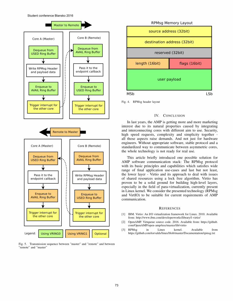
Write RPMsg Headerand payload data
Trigger interrupt forthe other core
Pass it to theendpoint callback
Trigger interrupt forthe other core
Dequeue fromUSED Ring Buffer
Enqueue toAVAIL Ring Buffer
Dequeue fromAVAIL Ring Buffer
Enqueue toUSED Ring Buffer
Core A (Master) Core B (Remote)
Optional
Pass it to theendpoint callback
Trigger interrupt forthe other core
Write RPMsg Headerand payload data
Trigger interrupt forthe other core
Dequeue fromUSED Ring Buffer
Enqueue toAVAIL Ring Buffer
Dequeue fromAVAIL Ring Buffer
Enqueue toUSED Ring Buffer
Core A (Master) Core B (Remote)
Master to Remote
Remote to Master
Using VRING1Using VRING0Legend:
Fig. 5. Transmission sequence between ”master” and ”remote” and between”remote” and ”master”
user payload
reserved (32bit)
flags (16bit)length (16bit)
RPMsg Memory Layout
MSb LSb
destination address (32bit)
source address (32bit)
Fig. 4. RPMsg header layout
IV. CONCLUSION
In last years, the AMP is getting more and more marketinginterest due to its natural properties caused by integratingand interconnecting cores with different aim to use. Security,high speed requests, complexity and simplicity together -all those aspects raise demands. And not just for hardwareengineers. Without appropriate software, stable protocol and astandardized way to communicate between asymmetric cores,the whole technology is not ready for real use.
This article briefly introduced one possible solution forAMP software communication stack: The RPMsg protocolwith its basic principles and capabilities which satisfies widerange of final application use-cases and last but not least,the lower layer - Virtio and its approach to deal with issuesof shared resources using a lock free algorithm. Virtio hasproven to be a solid ground for building high-level layers,especially in the field of para-virtualization, currently presentin Linux kernel. We consider the presented technology (RPMsgand VirtIO) to be suitable for current requirements of AMPcommunication.
REFERENCES
[1] IBM. Virtio: An I/O virtualization framework for Linux. 2010. Availablefrom: http://www.ibm.com/developerworks/library/l-virtio/
[2] OpenAMP. Virtqueue source code. 2016. Available from: https://github.com/OpenAMP/open-amp/tree/master/lib/virtio
[3] RPMsg in Linux kernel. Available fromhttps://github.com/torvalds/linux/blob/master/Documentation/rpmsg.txt
Student conference Blansko 2016
73
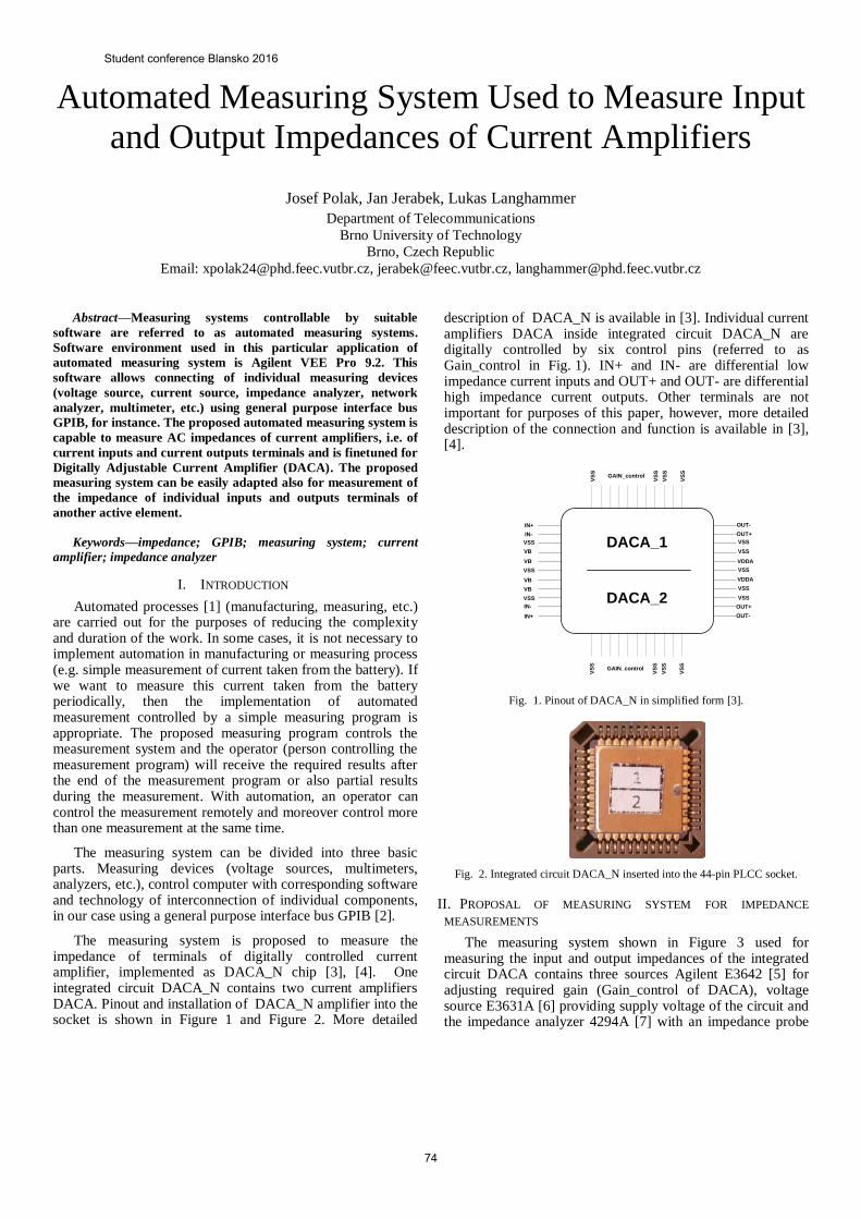
Automated Measuring System Used to Measure Input
and Output Impedances of Current Amplifiers
Josef Polak, Jan Jerabek, Lukas Langhammer
Department of Telecommunications
Brno University of Technology
Brno, Czech Republic
Email: [email protected], [email protected], [email protected]
Abstract—Measuring systems controllable by suitable
software are referred to as automated measuring systems.
Software environment used in this particular application of
automated measuring system is Agilent VEE Pro 9.2. This
software allows connecting of individual measuring devices
(voltage source, current source, impedance analyzer, network
analyzer, multimeter, etc.) using general purpose interface bus
GPIB, for instance. The proposed automated measuring system is
capable to measure AC impedances of current amplifiers, i.e. of
current inputs and current outputs terminals and is finetuned for
Digitally Adjustable Current Amplifier (DACA). The proposed
measuring system can be easily adapted also for measurement of
the impedance of individual inputs and outputs terminals of
another active element.
Keywords—impedance; GPIB; measuring system; current
amplifier; impedance analyzer
I. INTRODUCTION
Automated processes [1] (manufacturing, measuring, etc.) are carried out for the purposes of reducing the complexity and duration of the work. In some cases, it is not necessary to implement automation in manufacturing or measuring process (e.g. simple measurement of current taken from the battery). If we want to measure this current taken from the battery periodically, then the implementation of automated measurement controlled by a simple measuring program is appropriate. The proposed measuring program controls the measurement system and the operator (person controlling the measurement program) will receive the required results after the end of the measurement program or also partial results during the measurement. With automation, an operator can control the measurement remotely and moreover control more than one measurement at the same time.
The measuring system can be divided into three basic parts. Measuring devices (voltage sources, multimeters, analyzers, etc.), control computer with corresponding software and technology of interconnection of individual components, in our case using a general purpose interface bus GPIB [2].
The measuring system is proposed to measure the impedance of terminals of digitally controlled current amplifier, implemented as DACA_N chip [3], [4]. One integrated circuit DACA_N contains two current amplifiers DACA. Pinout and installation of DACA_N amplifier into the socket is shown in Figure 1 and Figure 2. More detailed
description of DACA_N is available in [3]. Individual current amplifiers DACA inside integrated circuit DACA_N are digitally controlled by six control pins (referred to as Gain_control in Fig. 1). IN+ and IN- are differential low impedance current inputs and OUT+ and OUT- are differential high impedance current outputs. Other terminals are not important for purposes of this paper, however, more detailed description of the connection and function is available in [3], [4].
VS
S
GAIN_control
VS
S
VS
S
VS
S
VS
S
GAIN_control
VS
S
VS
S
VS
S
VSS
VB
VB
VSS
VSS
VB
VB
IN+
IN-
IN+
IN-
VSS
VSS
VDDA
VSS
VSS
VSS
VDDA
OUT-
OUT+
OUT-
OUT+
DACA_1
DACA_2
Fig. 1. Pinout of DACA_N in simplified form [3].
Fig. 2. Integrated circuit DACA_N inserted into the 44-pin PLCC socket.
II. PROPOSAL OF MEASURING SYSTEM FOR IMPEDANCE
MEASUREMENTS
The measuring system shown in Figure 3 used for measuring the input and output impedances of the integrated circuit DACA contains three sources Agilent E3642 [5] for adjusting required gain (Gain_control of DACA), voltage source E3631A [6] providing supply voltage of the circuit and the impedance analyzer 4294A [7] with an impedance probe
Student conference Blansko 2016
74
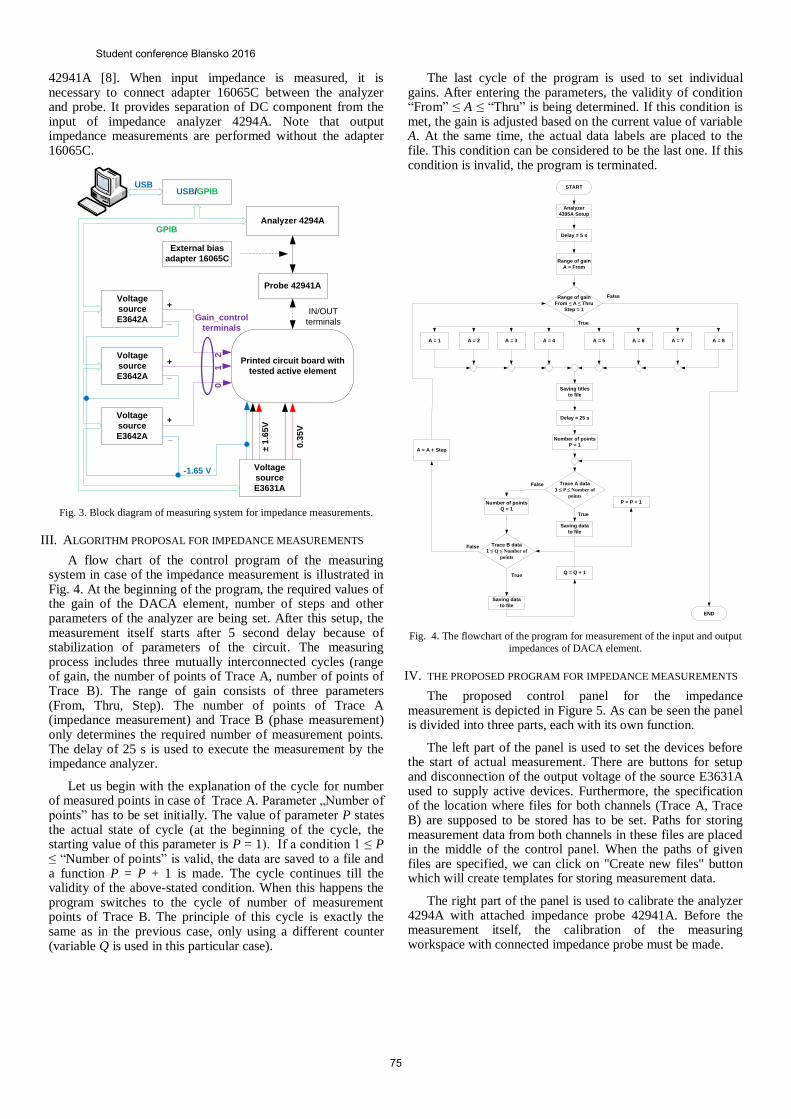
42941A [8]. When input impedance is measured, it is necessary to connect adapter 16065C between the analyzer and probe. It provides separation of DC component from the input of impedance analyzer 4294A. Note that output impedance measurements are performed without the adapter 16065C.
Voltage
source
E3642A
Voltage
source
E3642A
Voltage
source
E3642A
Voltage
source
E3631A
Printed circuit board with
tested active element
Analyzer 4294A
Probe 42941A
External bias
adapter 16065C
+
+
+
_
_
_
-1.65 V
0.3
5V
± 1
.65
V
01
2
USB/GPIB
GPIB
USB
Gain_control
terminals
IN/OUT
terminals
Fig. 3. Block diagram of measuring system for impedance measurements.
III. ALGORITHM PROPOSAL FOR IMPEDANCE MEASUREMENTS
A flow chart of the control program of the measuring system in case of the impedance measurement is illustrated in Fig. 4. At the beginning of the program, the required values of the gain of the DACA element, number of steps and other parameters of the analyzer are being set. After this setup, the measurement itself starts after 5 second delay because of stabilization of parameters of the circuit. The measuring process includes three mutually interconnected cycles (range of gain, the number of points of Trace A, number of points of Trace B). The range of gain consists of three parameters (From, Thru, Step). The number of points of Trace A (impedance measurement) and Trace B (phase measurement) only determines the required number of measurement points. The delay of 25 s is used to execute the measurement by the impedance analyzer.
Let us begin with the explanation of the cycle for number of measured points in case of Trace A. Parameter „Number of points” has to be set initially. The value of parameter P states the actual state of cycle (at the beginning of the cycle, the starting value of this parameter is P = 1). If a condition 1 ≤ P ≤ “Number of points” is valid, the data are saved to a file and a function P = P + 1 is made. The cycle continues till the validity of the above-stated condition. When this happens the program switches to the cycle of number of measurement points of Trace B. The principle of this cycle is exactly the same as in the previous case, only using a different counter (variable Q is used in this particular case).
The last cycle of the program is used to set individual gains. After entering the parameters, the validity of condition “From” ≤ A ≤ “Thru” is being determined. If this condition is met, the gain is adjusted based on the current value of variable A. At the same time, the actual data labels are placed to the file. This condition can be considered to be the last one. If this condition is invalid, the program is terminated.
START
Analyzer
4395A Setup
Delay = 5 s
Range of gain
A = From
Range of gain
From ≤ A ≤ Thru
Step = 1
A = 4
Saving titles
to file
Delay = 25 s
Number of points
P = 1
Trace A data
1 ≤ P ≤ Number of
points
Saving data
to file
P = P + 1Number of points
Q = 1
Trace B data
1 ≤ Q ≤ Number of
points
Q = Q + 1
A = A + Step
END
A = 3A = 2A = 1 A = 5 A = 6 A = 7 A = 8
False
True
True
False
True
False
Saving data
to file
Fig. 4. The flowchart of the program for measurement of the input and output
impedances of DACA element.
IV. THE PROPOSED PROGRAM FOR IMPEDANCE MEASUREMENTS
The proposed control panel for the impedance measurement is depicted in Figure 5. As can be seen the panel is divided into three parts, each with its own function.
The left part of the panel is used to set the devices before the start of actual measurement. There are buttons for setup and disconnection of the output voltage of the source E3631A used to supply active devices. Furthermore, the specification of the location where files for both channels (Trace A, Trace B) are supposed to be stored has to be set. Paths for storing measurement data from both channels in these files are placed in the middle of the control panel. When the paths of given files are specified, we can click on "Create new files" button which will create templates for storing measurement data.
The right part of the panel is used to calibrate the analyzer 4294A with attached impedance probe 42941A. Before the measurement itself, the calibration of the measuring workspace with connected impedance probe must be made.
Student conference Blansko 2016
75
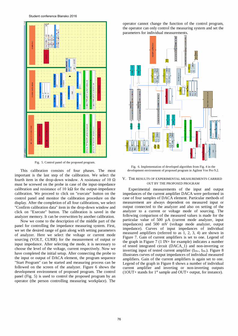
Fig. 5. Control panel of the proposed program.
This calibration consists of four phases. The most
important is the last step of the calibration. We select the
fourth item in the drop-down window. A resistance of 10 Ω
must be screwed on the probe in case of the input-impedance
calibration and resistance of 10 kΩ for the output-impedance
calibration. We proceed to click on "execute" button on the
control panel and monitor the calibration procedure on the
display. After the completion of all four calibrations, we select
"Confirm calibration data" item in the drop-down window and
click on "Execute" button. The calibration is saved in the
analyzer memory. It can be overwritten by another calibration.
Now we come to the description of the middle part of the
panel for controlling the impedance measuring system. First,
we set the desired range of gain along with setting parameters
of analyzer. Here we select the voltage or current mode
sourcing (VOLT, CURR) for the measurement of output or
input impedance. After selecting the mode, it is necessary to
choose the level of the voltage, current respectively. Now we
have completed the initial setup. After connecting the probe to
the input or output of DACA element, the program sequence
"Start Program" can be started and measuring process can be
followed on the screen of the analyzer. Figure 6 shows the
development environment of proposed program. The control
panel (Fig. 5) is used to control the proposed program by an
operator (the person controlling measuring workplace). The
operator cannot change the function of the control program,
the operator can only control the measuring system and set the
parameters for individual measurements.
Fig. 6. Implementation of developed algorithm from Fig. 4 in the
development environment of proposed program in Agilent Vee Pro 9.2.
V. THE RESULTS OF EXPERIMENTAL MEASUREMENTS CARRIED
OUT BY THE PROPOSED PROGRAM
Experimental measurements of the input and output impedances of the current amplifier DACA were performed in case of four samples of DACA element. Particular methods of measurement are always dependent on measured input or output connected to the analyzer and also on setting of the analyzer to a current or voltage mode of sourcing. The following comparison of the measured values is made for the particular value of 500 µA (current mode analyzer, input impedances) and 500 mV (voltage mode analyzer, output impedance). Curves of input impedances of individual measured amplifiers (referred to as 1, 2, 3, 4) are shown in Figure 7. Gain of current amplifiers is set to one. Legend of the graph in Figure 7 (1 IN+ for example) indicates a number of tested integrated circuit (DACA_1) and non-inverting or inverting input of tested current amplifier (IIN+, IIN-). Figure 8 illustrates curves of output impedances of individual measured amplifiers. Gain of the current amplifiers is again set to one. Legend of the graph in Figure 8 shows a number of individual current amplifier and inverting or non-inverting outputs (1OUT+ stands for 1st sample and OUT+ output, for instance).
Student conference Blansko 2016
76
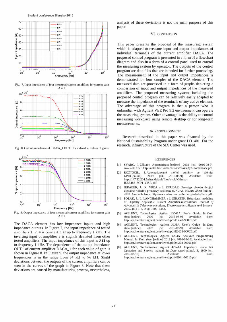
Fig. 7. Input impedance of four measured current amplifiers for current gain
A = 1.
Fig. 8. Output impedance of DACA_1 OUT+ for individual values of gains.
Fig. 9. Output impedance of four measured current amplifiers for current gain
A = 1.
The DACA element has low impedance inputs and high impedance outputs. In Figure 7, the input impedance of tested amplifiers 1, 2, 4 is constant 3 Ω up to frequency 1 kHz. The inverting input of amplifier 3 is slightly deviated from other tested amplifiers. The input impedance of this input is 5 Ω up to frequency 1 kHz. The dependence of the output impedance OUT+ of current amplifier DACA_1 for each value of gain is shown in Figure 8. In Figure 9, the output impedance at lower frequencies is in the range from 74 kΩ to 96 kΩ. Slight deviations between the outputs of the current amplifiers can be seen in the curves of the graph in Figure 8. Note that these deviations are caused by manufacturing process, nevertheless,
analysis of these deviations is not the main purpose of this paper.
VI. CONCLUSION
This paper presents the proposal of the measuring system
which is adapted to measure input and output impedances of
individual terminals of the current amplifier DACA. The
proposed control program is presented in a form of a flowchart
diagram and also in a form of a control panel used to control
the measuring system by operator. The outputs of the control
program are data files that are intended for further processing.
The measurement of the input and output impedances is
demonstrated for four samples of the DACA element. The
measured data are processed in a form of graphs depicting a
comparison of input and output impedances of the measured
amplifiers. The proposed measuring system, including the
proposed control program can be relatively easily adapted to
measure the impedance of the terminals of any active element.
The advantage of this program is that a person who is
unfamiliar with Agilent VEE Pro 9.2 environment can operate
the measuring system. Other advantage is the ability to control
measuring workplace using remote desktop or for long-term
measurements.
ACKNOWLEDGMENT
Research described in this paper was financed by the National Sustainability Program under grant LO1401. For the research, infrastructure of the SIX Center was used.
REFERENCES
[1] SVARC, I. Základy Automatizace [online]. 2002 [cit. 2016-08-9]. Available from: http://autnt.fme.vutbr.cz/svarc/ZakladyAutomatizace.pdf
[2] ROZTOCIL, J. Automatizované měřící systémy se sběrnicí GPIB [online]. 2009 [cit. 2016-08-9]. Available from: http://147.32.204.5/sites/default/files/vyuk/x38msp-IEEE488_SCPI_VISA.pdf
[3] JERABEK, J., K. VRBA a I. KOUDAR. Prototyp obvodu dvojitý digitálně řiditelný proudový zesilovač (DACA). In:Data Sheet [online]. 2010. Available from: http://www.utko.feec.vutbr.cz/~jerabekj/daca.pdf
[4] POLAK, J., L. LANGHAMMER a J. JERABEK. Behavioral modeling of Digitally Adjustable Current Amplifier.International Journal of Advances in Telecommunications, Electrotechnics, Signals and Systems. 2015, 4(1), 1-7. ISSN 1805- 5443.
[5] AGILENT, Technologies. Agilent E3642A User’s Guide. In: Data sheet [online]. 2000 [cit. 2016-08-9]. Available from: http://cp.literature.agilent.com/litweb/pdf/E3640-90001.pdf
[6] AGILENT, Technologies. Agilent 3631A User’s Guide. In: Data sheet [online]. 2007 [cit. 2016-08-9]. Available from: http://cp.literature.agilent.com/litweb/pdf/E3631-90002.pdf
[7] AGILENT, Technologies. Agilent 4294A Analyzer Programming Manual. In: Data sheet [online]. 2012 [cit. 2016-08-10]. Available from: http://cp.literature.agilent.com/litweb/pdf/04294-90061.pdf
[8] AGILENT, Technologies. Agilent 42941A Impedance Probe Kit Operation and Service manual. In: Data sheet[online]. 3. 1999 [cit. 2016-08-10]. Available from: http://cp.literature.agilent.com/litweb/pdf/42941-90010.pdf
103
104
105
106
107
108
0
10
20
30
40
50
60
70
Frequency [Hz]
Inp
ut
imp
ed
an
ce
[
]
1 IN+
1 IN-
2 IN+
2 IN-
3 IN+
3 IN-
4 IN+
4 IN-
103
104
105
106
107
108
0
2
4
6
8
10x 10
4
Frequency [Hz]
Ou
tpu
t im
pe
da
nc
e
[ ]
A=1
A=2
A=3
A=4
A=5
A=6
A=7
A=8
103
104
105
106
107
108
0
2
4
6
8
10x 10
4
Frequency [Hz]
Ou
tpu
t im
pe
da
nc
e [
]
1 OUT+
1 OUT-
2 OUT+
2 OUT-
3 OUT+
3 OUT-
4 OUT+
4 OUT-
Student conference Blansko 2016
77
Using UWB Impulse Radar System for Measuring of
Wideband Antenna Parameters and Its Comparison
Ján Schneider, Daniel Novák, Ján Gamec
Dept. of Electronics and Multimedia Communications
Technical University of Košice
Košice, Slovakia
jan.schneider; danie.novak; [email protected]
Abstract—The article presents non-standard method of the
antenna measuring and compares it with conventional method of
measurement. In this case, the use of ultra-wideband (UWB)
impulse radar is considered to non-standard method. Relatively
low cost measuring system, its calibration, verification and
calculation methods of the required parameters (impulse
response, return loss and radiation pattern) are presented in this
paper. For the measurements was used self-designed Vivaldi
antenna and commercially available wideband antennas. The
paper compares reflection impulse response of Vivaldi antenna
with other reflection impulse responses of commercial antennas
and also paper compares experimental results obtained by UWB
radar with the results obtained by measurements with vector
network analyzer.
Keywords—UWB; radar; antenna measurement; Vivaldi
antenna
I. INTRODUCTION
Ultra-wideband (UWB) technology or UWB radars, where UWB device is defined as any device operating in absolute bandwidth greater than 500 MHz or fractional bandwidth greater than 0.2 of central frequency [1] has recently become one of the most promising solutions for a variety of applications [2].
Strong potential of progressive ultra-wideband radar systems for motion sensing and imaging can be use in impedance spectroscopy to detection the presence of impurities in the liquid (for example: lactose in milk, wet granular materials, etc.) [3], in medicine to detect, non-invasively, the movements of the heart wall [4], in ground penetrating radar (GPR) systems to detecting and estimating buried pipes and cables [5], in through-wall measurements to human being detection, localization and tracking [6] and more. The UWB radar system can also be used in another way than mentioned above – UWB antenna measurement system.
The most important thing in any UWB radar system is one or more antennas, depending on the application. All UWB systems have specific demands on the electric properties of the antennas. Elementary electric properties of the antennas verified by the measurements are return loss and radiation pattern (polarization of electromagnetic field, gain). The above mentioned properties of the antenna are normally measured using a vector network analyzer in an anechoic chamber. The anechoic chamber is a very expensive measuring device which
needs a lot of space for measuring radiation pattern of the antenna in the near field or the far field.
Electric properties of the antenna could be measured using impulse UWB radar in addition to using anechoic chamber devices. The radar works by sending and receiving simple impulses. The received impulse responses are further processed and evaluated. From the impulse responses, the electric properties of the antenna, such as ringing, return loss and radiation pattern can be obtained. In the measurement of the UWB radar, it is also important to reach a plane wave i.e. the antenna is to be placed and measured in the far field. This implies that the antenna can be measured in the open air. UWB impulse radar provides a more compact and cheaper option for verification of the properties of the antenna.
The following sections present the UWB antennas used for measurements, UWB impulse radar measuring system, experimental results of measurements and the final conclusion.
II. MEASURING BY UWB IMPULSE RADAR
A. Measuring system
System for measuring return loss of the antenna uses reflection impulse responses. The system consists of a pulse generator, scope, measured antenna, microwave coupling elements and cables. Position of the scope window is selected according to the cable length (line a, line b, line c) to avoid any reflections from inhomogeneities and from the measurement configuration in the observed time interval. The time which electromagnetic wave needs to overcome distance between antenna and walls (floors etc.) and back to antenna is longer as the end of scope observation window. The pulse generator transmits a narrow pulse with peak amplitude U≈30V/50Ω and width of the pulse t<50ps to the antenna. The reflected signal is received from the antenna after adjusting the observation window of the scope according to the lengths of lines a, b and c. The whole principle of measuring using impulse UWB radar is shown in Fig. 1.
Student conference Blansko 2016
78
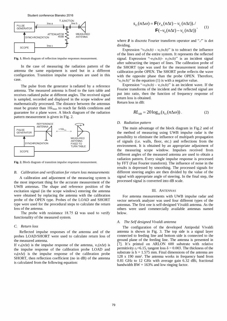
Fig. 1. Block diagram of reflection impulse responses measurement.
In the case of measuring the radiation pattern of the
antenna the same equipment is used but in a different
configuration. Transition impulse responses are used in this
case.
The pulse from the generator is radiated by a reference
antenna. The measured antenna is fixed to the turn table and
receives radiated pulse at different angles. The received signal
is sampled, recorded and displayed in the scope window and
mathematically processed. The distance between the antennas
must be greater than 10λmax to reach far fields conditions and
guarantee for a plane wave. A block diagram of the radiation
pattern measurement is given in Fig. 2.
Fig. 2. Block diagram of transition impulse responses measurement.
B. Calibration and verification for return loss measurements
A calibration and adjustment of the measuring system is
the most important thing for the accurate measurement of the
UWB antennas. The shape and reference position of the
excitation signal (in the scope window) entering the antenna
were obtained by replacing the antenna with the calibration
probe of the OPEN type. Probes of the LOAD and SHORT
type were used for the procedural steps to calculate the return
loss of the antenna.
The probe with resistance 18.75 Ω was used to verify
functionality of the measured system.
C. Return loss
Reflected impulse responses of the antenna and of the
probes LOAD/SHORT were used to calculate return loss of
the measured antenna.
If vA(nΔt) is the impulse response of the antenna, vL(nΔt) is
the impulse response of the calibration probe LOAD and
vS(nΔt) is the impulse response of the calibration probe
SHORT, then reflection coefficient (no in dB) of the antenna
is calculated from the following equation:
))Δ()Δ((
/)).Δ()Δ(()(
LS
LA11
tnvtnv
tnvtnvns
F
F, (1)
where F is discrete Fourier transform operator and “./” is dot
dividing.
Expression “vA(nΔt) - vL(nΔt)” is to subtract the influence
of the lines and of the entire system. It represents the reflected
signal. Expression “-vS(nΔt)- vL(nΔt)” is an incident signal
after subtracting the impact of lines. The calibration probe of
the SHORT type was used for the measurement instead of
calibration probe OPEN. The SHORT probe reflects the wave
with the opposite phase than the probe OPEN. Therefore,
"vL(nΔt)" in the equation (1) is with a negative value.
Expression “-vS(nΔt) - vL(nΔt)” is an incident wave. If the
Fourier transforms of the incident and the reflected signal are
put into ratio, then the function of frequency response of
return loss is obtained.
Return loss in dB:
))((log20 1110 nsRLdB . (2)
D. Radiation pattern
The main advantage of the block diagram in Fig.2 and of
the method of measuring using UWB impulse radar is the
possibility to eliminate the influence of multipath propagation
of signals (i.e. walls, floor, etc.) and reflections from the
environment. It is obtained by an appropriate adjustment of
the measuring scope window. Impulses received from
different angles of the measured antenna are used to obtain a
radiation pattern. Every single impulse response is processed
by FFT (Fast Fourier transform). The influence of noise in the
results is depressed by smoothing. The processed signals for
different steering angles are then divided by the value of the
signal with appropriate angle of steering. In the final step, the
processed signal is converted into dB scale.
III. ANTENNAS
For antenna measurements with UWB impulse radar and vector network analyzer was used four different types of the antennas. The first one is self-designed Vivaldi antenna. As the others were used commercially available antennas named below.
A. The Self designed Vivaldi antenna
The configuration of the developed Antipodal Vivaldi antenna is shown in Fig. 3. The top side is a signal layer connected to feeding line and bottom side is connected to the ground plane of the feeding line. The antenna is presented in [7]. It’s printed on ARLON 600 substrate with relative permitivity εr=6.15, tangent loss δ = 0.003. The thickness of the substrate is h = 1.575 mm. Final dimensions of the antenna are 128 x 190 mm². The antenna works in frequency band from 0.81 GHz to 12 GHz with average gain 6.32 dBi, fractional bandwidth BW = 163% and low ringing factor.
Student conference Blansko 2016
79
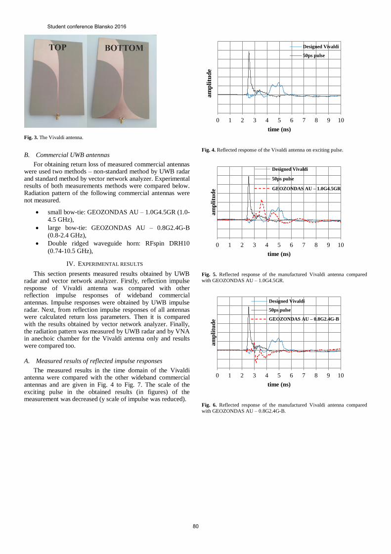
Fig. 3. The Vivaldi antenna.
B. Commercial UWB antennas
For obtaining return loss of measured commercial antennas were used two methods – non-standard method by UWB radar and standard method by vector network analyzer. Experimental results of both measurements methods were compared below. Radiation pattern of the following commercial antennas were not measured.
small bow-tie: GEOZONDAS AU – 1.0G4.5GR (1.0-
4.5 GHz),
large bow-tie: GEOZONDAS AU – 0.8G2.4G-B
(0.8-2.4 GHz),
Double ridged waveguide horn: RFspin DRH10
(0.74-10.5 GHz),
IV. EXPERIMENTAL RESULTS
This section presents measured results obtained by UWB radar and vector network analyzer. Firstly, reflection impulse response of Vivaldi antenna was compared with other reflection impulse responses of wideband commercial antennas. Impulse responses were obtained by UWB impulse radar. Next, from reflection impulse responses of all antennas were calculated return loss parameters. Then it is compared with the results obtained by vector network analyzer. Finally, the radiation pattern was measured by UWB radar and by VNA in anechoic chamber for the Vivaldi antenna only and results were compared too.
A. Measured results of reflected impulse responses
The measured results in the time domain of the Vivaldi antenna were compared with the other wideband commercial antennas and are given in Fig. 4 to Fig. 7. The scale of the exciting pulse in the obtained results (in figures) of the measurement was decreased (y scale of impulse was reduced).
0 1 2 3 4 5 6 7 8 9 10
am
pli
tud
e
time (ns)
Designed Vivaldi
50ps pulse
Fig. 4. Reflected response of the Vivaldi antenna on exciting pulse.
0 1 2 3 4 5 6 7 8 9 10
am
pli
tud
e
time (ns)
Designed Vivaldi
50ps pulse
GEOZONDAS AU – 1.0G4.5GR
Fig. 5. Reflected response of the manufactured Vivaldi antenna compared
with GEOZONDAS AU – 1.0G4.5GR.
0 1 2 3 4 5 6 7 8 9 10
am
pli
tud
e
time (ns)
Designed Vivaldi
50ps pulse
GEOZONDAS AU – 0.8G2.4G-B
Fig. 6. Reflected response of the manufactured Vivaldi antenna compared
with GEOZONDAS AU – 0.8G2.4G-B.
Student conference Blansko 2016
80

0 1 2 3 4 5 6 7 8 9 10
am
pli
tud
e
time (ns)
Designed Vivaldi
50ps pulse
Double ridged waveguide horn
Fig. 7. Reflected response of the manufactured Vivaldi antenna compared
with Double ridged waveguide horn.
The reflected impulse responses (Fig. 4 - Fig. 7) of the
proposed Vivaldi antenna have satisfactory frequency
character in the wide bandwidth applications. Positive
feedback from measurements in the time domain is that
antenna has a very low ringing in comparison with
commercially available antennas. The result presented above
predestinates the manufactured antenna for applications
sensitive to changes in group delay receiving and transmitting
signal – UWB radar systems.
B. Measured results of return loss
The return loss parameter was obtained by impulse response of the antenna according to chapter 2 part C and also obtained by VNA. Both measured results for every one antenna alone are depicted from Fig. 8 to Fig. 11. For The Vivaldi antenna are depicted simulated results of return loss (Fig.8).
Fig. 8. Return loss of the Vivaldi antenna
-40
-35
-30
-25
-20
-15
-10
-5
0
0 2 4 6 8 10
Ret
urn
loss
[dB
]
Frequency [GHz]
Small bow-tie by UWB radar
Small bow-tie by VNA
Fig. 9. Return loss of the small BOW-TIE antenna.
-40
-35
-30
-25
-20
-15
-10
-5
0
0 2 4 6 8 10
Re
turn
loss
[dB
]
Frequency [GHz]
Large bow-tie by UWB Radar
Large bow-tie by VNA
Fig. 10. Return loss of the large BOW-TIE antenna.
-40
-35
-30
-25
-20
-15
-10
-5
0
0 2 4 6 8 10
Re
turn
loss
[dB
]
Frequency [GHz]
Double ridged waveguide horn by UWB Radar
Double ridged waveguide horn by VNA
Fig. 11. Return loss of the Double ridged waveguide horn antenna.
From the results obtained (Fig. 8-Fig. 11), it is obvious that
the results of measurements with the VNA and those from
impulse responses (by UWB radar) show satisfactory match of
results up to 5-6 GHz. The diversity of return loss over the
mentioned frequency 5-6 GHz is observed. This gradual
increase of diversity may be caused by noise and hardware
bandwidth limitations of the pulse UWB radar.
Student conference Blansko 2016
81
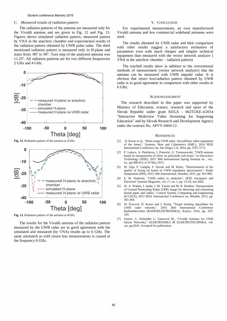
C. Measured results of radiation pattern
The radiation patterns of the antenna are measured only for
the Vivaldi antenna and are given in Fig. 12 and Fig. 13.
Figures shows simulated radiation pattern, measured pattern
by VNA in the anechoic chamber and experimental results of
the radiation pattern obtained by UWB pulse radar. The third
mentioned radiation pattern is measured only in H-plane and
starts from -90° to 90°. Turn step of the analyzed antenna was
11.25°. All radiation patterns are for two different frequencies
2 GHz and 4 GHz.
Fig. 12. Radiation pattern of the antenna at 2GHz.
Fig. 13. Radiation pattern of the antenna at 4GHz.
The results for the Vivaldi antenna of the radiation pattern
measured by the UWB radar are in good agreement with the
simulated and measured (by VNA) results up to 6 GHz. The
same mismatch as with return loss measurements is caused at
the frequency 6 GHz.
V. CONCLUSION
For experimental measurements, an own manufactured Vivaldi antenna and few commercial wideband antennas were used.
The results obtained by UWB radar and their comparison with other results suggest a satisfactory estimation of parameters even with much cheaper and simpler technical equipment than measured with the vector network analyzer ( VNA in the anechoic chamber – radiation pattern)
The reached results show in addition to the conventional methods of measurement (vector network analyzer) that the antenna can be measured with UWB impulse radar. It is obvious that return loss/radiation pattern obtained by UWB radar is in good agreement in comparison with other results to 6 GHz.
ACKNOWLEDGMENT
The research described in this paper was supported by
Ministry of Education, science, research and sport of the
Slovak Republic under grant KEGA - 062TUKE-4/2014
”Interactive Multiview Video Streaming for Supporting
Education” and by Slovak Research and Development Agency
under the contract No. APVV-0404-12.
REFERENCES
[1] D. Kocur et al., "Short-range UWB radar: Surveillance robot equipment of the future", Systems, Man and Cybernetics (SMC), 2014 IEEE International Conference on, San Diego, CA, 2014, pp. 3767-3772.
[2] P. Lukacs, A. Pietrikova, J. Potencki, G. Tomaszewski, "UWB antenna based on nanoparticles of silver on polyimide sub-strate," in Electronics Technology (ISSE), 2015 38th International Spring Seminar on , vol., no., pp.408-413, 6-10 May 2015.
[3] M. Ziga, P. Galajda, S. Slovak and M. Kmec, "Determination of the quality of frying oil based on UWB impedance spectrometer", Radar Symposium (IRS), 2015 16th International, Dresden, 2015, pp. 955-960.
[4] E. M. Staderini, "UWB radars in medicine", IEEE Aerospace and Electronic Systems Magazine, vol. 17, no. 1, pp. 13-18, Jan 2002.
[5] W. A. Wahab, J. Jaafar, I. M. Yassin and M. R. Ibrahim, "Interpretation of Ground Penetrating Radar (GPR) image for detecting and estimating buried pipes and cables," Control System, Computing and Engineering (ICCSCE), 2013 IEEE International Conference on, Mindeb, 2013, pp. 361-364.
[6] M. Švecová, D. Kocur and J. Kožej, "Target tracking algorithms for UWB radar network," 2016 26th International Conference Radioelektronika (RADIOELEKTRONIKA), Kosice, 2016, pp. 319-324.
[7] Gamec, J.; Schneider J.; Gamcová M., “Vivaldi Antenna for UWB Sensor Networks,” ELEKTRONIKA IR ELEKTROTECHNIKA, vol. ,no, pp,2016. Accepted for publication.
Student conference Blansko 2016
82
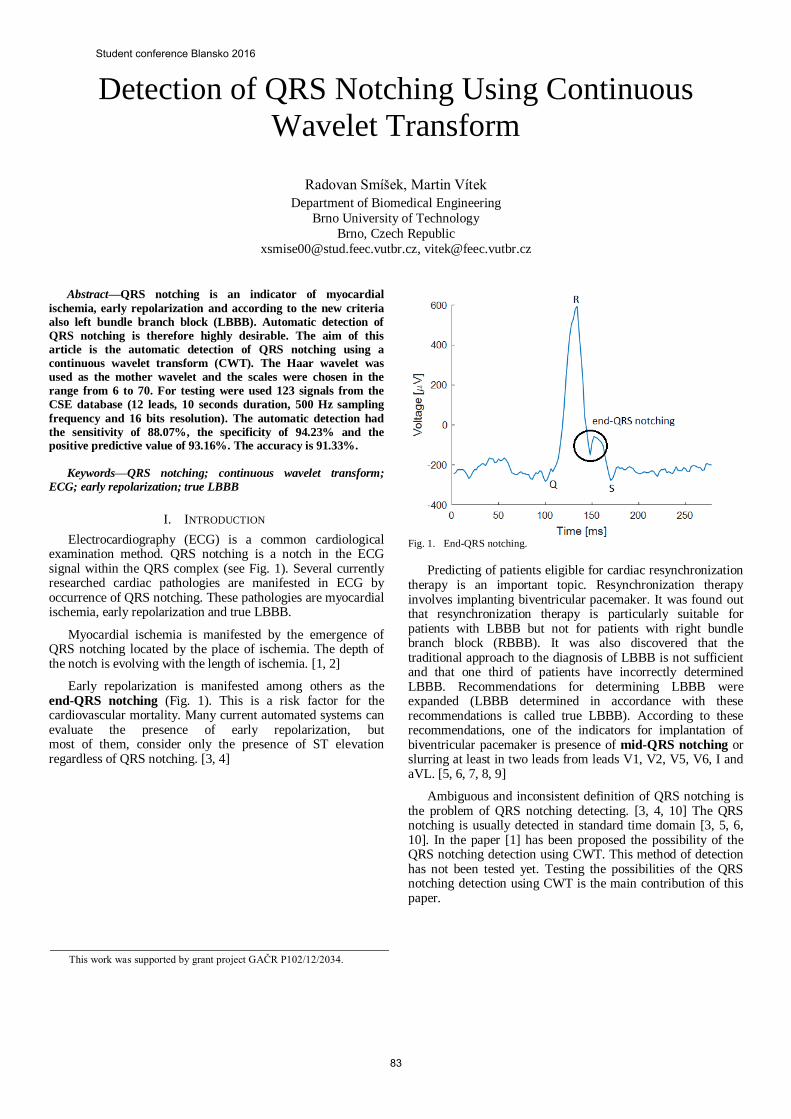
Detection of QRS Notching Using Continuous
Wavelet Transform
Radovan Smíšek, Martin Vítek
Department of Biomedical Engineering
Brno University of Technology
Brno, Czech Republic
[email protected], [email protected]
Abstract—QRS notching is an indicator of myocardial
ischemia, early repolarization and according to the new criteria
also left bundle branch block (LBBB). Automatic detection of
QRS notching is therefore highly desirable. The aim of this
article is the automatic detection of QRS notching using a
continuous wavelet transform (CWT). The Haar wavelet was
used as the mother wavelet and the scales were chosen in the
range from 6 to 70. For testing were used 123 signals from the
CSE database (12 leads, 10 seconds duration, 500 Hz sampling
frequency and 16 bits resolution). The automatic detection had
the sensitivity of 88.07%, the specificity of 94.23% and the positive predictive value of 93.16%. The accuracy is 91.33%.
Keywords—QRS notching; continuous wavelet transform;
ECG; early repolarization; true LBBB
I. INTRODUCTION
Electrocardiography (ECG) is a common cardiological examination method. QRS notching is a notch in the ECG signal within the QRS complex (see Fig. 1). Several currently researched cardiac pathologies are manifested in ECG by occurrence of QRS notching. These pathologies are myocardial ischemia, early repolarization and true LBBB.
Myocardial ischemia is manifested by the emergence of QRS notching located by the place of ischemia. The depth of the notch is evolving with the length of ischemia. [1, 2]
Early repolarization is manifested among others as the end-QRS notching (Fig. 1). This is a risk factor for the cardiovascular mortality. Many current automated systems can evaluate the presence of early repolarization, but most of them, consider only the presence of ST elevation regardless of QRS notching. [3, 4]
Fig. 1. End-QRS notching.
Predicting of patients eligible for cardiac resynchronization therapy is an important topic. Resynchronization therapy involves implanting biventricular pacemaker. It was found out that resynchronization therapy is particularly suitable for patients with LBBB but not for patients with right bundle branch block (RBBB). It was also discovered that the traditional approach to the diagnosis of LBBB is not sufficient and that one third of patients have incorrectly determined LBBB. Recommendations for determining LBBB were expanded (LBBB determined in accordance with these recommendations is called true LBBB). According to these recommendations, one of the indicators for implantation of biventricular pacemaker is presence of mid-QRS notching or slurring at least in two leads from leads V1, V2, V5, V6, I and aVL. [5, 6, 7, 8, 9]
Ambiguous and inconsistent definition of QRS notching is the problem of QRS notching detecting. [3, 4, 10] The QRS notching is usually detected in standard time domain [3, 5, 6, 10]. In the paper [1] has been proposed the possibility of the QRS notching detection using CWT. This method of detection has not been tested yet. Testing the possibilities of the QRS notching detection using CWT is the main contribution of this paper.
This work was supported by grant project GAČR P102/12/2034.
Student conference Blansko 2016
83
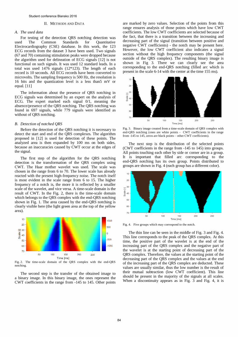
II. METHODS AND DATA
A. The used data
For testing of the detection QRS notching detection was used The Common Standards for Quantitative Electrocardiography (CSE) database. In this work, the 123 ECG records from the dataset 3 have been used. Two signals (67 and 70) containing stimulation peaks were dropped because the algorithm used for delineation of ECG signals [12] is not functional on such signals. It was used 12 standard leads. In a total was used 1476 signals (12*123). The length of each record is 10 seconds. All ECG records have been converted to microvolts. The sampling frequency is 500 Hz, the resolution is 16 bits and the quantization level is a less than5 mV or equal. [11]
The information about the presence of QRS notching in ECG signals was determined by an expert on the analysis of ECG. The expert marked each signal 0/1, meaning the absence/presence of the QRS notching. The QRS notching was found in 697 signals, while 779 signals were identified as without of QRS notching.
B. Detection of notched QRS
Before the detection of the QRS notching it is necessary to detect the start and end of the QRS complexes. The algorithm proposed in [12] is used for detection of these points. The analyzed area is then expanded by 100 ms on both sides, because an inaccuracies caused by CWT occur at the edges of the signal.
The first step of the algorithm for the QRS notching detection is the transformation of the QRS complex using CWT. The Haar mother wavelet was used. The scale was chosen in the range from 6 to 70. The lower scale has already reacted with the present high-frequency noise. The notch itself is most evident in the scale range from 6 to 15. The higher frequency of a notch is, the more it is reflected by a smaller scale of the wavelet, and vice versa. A time-scale domain is the result of CWT. In the Fig. 2, there is the time-scale domain which belongs to the QRS complex with the end-QRS notching shown in Fig. 1. The area caused by the end-QRS notching is clearly visible here (the light green area at the top of the yellow area).
Fig. 2. The time-scale domain of the QRS complex with the end-QRS notching.
The second step is the transfer of the obtained image to a binary image. In this binary image, the ones represent the CWT coefficients in the range from -145 to 145. Other points
are marked by zero values. Selection of the points from this range ensures analysis of those points which have low CWT coefficients. The low CWT coefficients are selected because of the fact, that there is a transition between the increasing and decreasing part of the signal (transition between positive and negative CWT coefficients) - the notch may be present here. However, the low CWT coefficient also indicates a signal section without the high frequency components (the signal outside of the QRS complex). The resulting binary image is shown in Fig 3. There we can clearly see the area corresponding to the end-QRS notching (filled arc which is present in the scale 6-14 with the center at the time 155 ms).
Fig. 3. Binary image created from a time-scale domain of QRS complex with
end-QRS notching (ones are white points - CWT coefficients in the range from -145 to 145, zeros are black points – other CWT coefficients).
The next step is the distribution of the selected points (CWT coefficients in the range from -145 to 145) into groups. All points touching each other by side or corner are in a group. It is important that filled arc corresponding to the end-QRS notching has its own group. Points distributed to groups are shown in Fig. 4 (each group has a different color).
Fig. 4. Five groups which may correspond to the notch.
The thin line can be seen in the middle of Fig. 3 and Fig. 4. This line corresponds to the peak of the QRS complex. At this time, the positive part of the wavelet is at the end of the increasing part of the QRS complex and the negative part of the wavelet is at the starting point of decreasing part of the QRS complex. Therefore, the values at the starting point of the decreasing part of the QRS complex and the values at the end of the increasing part of the QRS complex are deducted. These values are usually similar, thus the low number is the result of their mutual subtraction (low CWT coefficient). This line should be present in the majority of the signals at all scales. When a discontinuity appears as in Fig. 3 and Fig. 4, it is
Student conference Blansko 2016
84
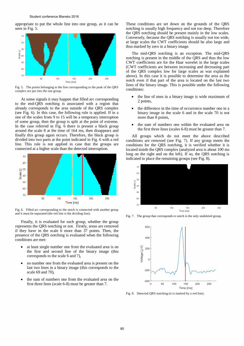
appropriate to put the whole line into one group, as it can be seen in Fig. 5.
Fig. 5. The points belonging to the line corresponding to the peak of the QRS
complex are put into the one group.
At some signals it may happen that filled arc corresponding to the end-QRS notching is associated with a region that already corresponds to the area outside of the QRS complex (see Fig. 6). In this case, the following rule is applied. If in a one of the scales from 9 to 15 will be a temporary interruption of some group, then the group is split at the point of extreme. In the case referred in Fig. 6 there is present a black group around the scale 8 at the time of 164 ms, then disappears and finally this group again occurs. Therefore, the black group is divided into two parts at the point indicated in Fig. 6 with a red line. This rule is not applied in case that the groups are connected at a higher scale than the detected interruption.
Fig. 6. Filled arc corresponding to the notch is connected with another group
and it must be separated (the red line is the dividing line).
Finally, it is evaluated for each group, whether the group represents the QRS notching or not. Firstly, areas are removed if they have in the scale 6 more than 37 points. Then, the presence of the QRS notching is evaluated when the following conditions are met:
at least single number one from the evaluated area is on the first and second line of the binary image (this corresponds to the scale 6 and 7),
no number one from the evaluated area is present on the last two lines in a binary image (this corresponds to the scale 69 and 70),
the sum of numbers one from the evaluated area on the first three lines (scale 6-8) must be greater than 7.
These conditions are set down on the grounds of the QRS notching is usually high frequency and not too deep. Therefore the QRS notching should be present mainly in the low scales. Conversely, because the QRS notching is usually not too wide, at large scales the CWT coefficients should be also large and thus marked by zero in a binary image.
The mid-QRS notching is an exception. The mid-QRS notching is present in the middle of the QRS and thus the low CWT coefficients are for the Haar wavelet in the large scales (CWT coefficients are between increasing and decreasing part of the QRS complex low for large scales as was explained above). In this case it is possible to determine the area as the notch even if that part of the area is located on the last two lines of the binary image. This is possible under the following conditions:
the line of ones in a binary image is wide maximum of 2 points,
the difference in the time of occurrence number one in a binary image in the scale 6 and in the scale 70 is not more than 8 points,
the sum of numbers one within the evaluated area on the first three lines (scales 6-8) must be greater than 7.
All groups which do not meet the above described conditions are removed (see Fig. 7). If any group meets the conditions for the QRS notching, it is verified whether it is located inside the QRS complex (analyzed area is about 100 ms long on the right and on the left). If so, the QRS notching is indicated in place the remaining groups (see Fig. 8).
Fig. 7. The group that corresponds to notch is the only undeleted group.
Fig. 8. Detected QRS notching (it is marked by a red line).
Student conference Blansko 2016
85

III. RESULTS AND DISCUSSION
This chapter describes the achieved accuracy of the QRS notching detection.
Accuracy of the QRS notching detection is described by: accuracy (Acc), sensitivity (Se), specificity (Sp) and positive predictive value (PV+). These variables are calculated as follows:
Acc = (TP+TN) / Y, (1) Se = TP / (TP + FN), (2) Sp = TN / (TN + FP), (3) PV+ = TP / (TP + FP), (4)
where TP (true positive) is the number of correctly detected QRS notching, TN (true negative) is the number of correctly marked signals without the QRS notching, FP (false positive) is the number of signals without the QRS notching with incorrectly detected QRS notching, FN (false negative) is the number of signals with a notch where a notch is not detected, Y is the number of all signals.
Achieved accuracy of the QRS notching detection is shown at the first line of Table I. The achieved sensitivity is 88.07%, specificity is 94.23% and positive predictive value is 93.16%. The achieved accuracy is 91.33%. From the results it is evident, that more times the situation arose, where a signal with the QRS notching is identified as a signal without the QRS notching than the opposite situation.
The results of this study can be compared with the previous studies. This comparison is shown in Table I. The column "Detected phenomenon" shows what was detected in the corresponding study (QRS notching, mid-QRS notching or end-QRS notching). In paper [3], there was detected simultaneously the QRS notching and slurring without differentiation. The sensitivity, specificity and positive predictive value achieved in this work are similar with other studies. In other studies, one of the parameters is usually higher and one lower than in this study. This means, that the results of the proposed algorithm are the middle way between the emphasis on high sensitivity or high specificity.
TABLE I. THE ACCURACY OF THE QRS NOTCHING DETECTION IN THIS
AND OTHER STUDIES
Authors Detected
phenomenon Se [%] Sp [%] PV+ [%]
This study QRS notching 88.07 94.23 93.16
Xia [6] QRS notching 87 96 -
Xia [6] mid-QRS
notching 95 85 -
Xia [10] mid-QRS
notching 74 100 94
Clarka [3]
end-QRS
notching and
slurring
90.5 96.5 87.9
a. The QRS notching and slurring without differentiation were detected simultaneously.
IV. CONCLUSION
Algorithm for the QRS notching detection was proposed in this article. This is a significant indicator of several currently researched cardiac pathologies. The method used in this work was based on CWT. The Haar wavelet was used as the mother wavelet and the scales were chosen in the range from 6 to 70. QRS notching is most pronounced at the scales from 6 to 15. Detection of a notch in this manner has not been tested until now. For testing of the proposed algorithm were used 123 signals from the CSE database. The achieved results (Se 88.07%, Sp 94.23% and PV+ 93.16%) were compared with the results from scientific articles published in the last two years. The accuracy of the detection achieved in this study is comparable with those studies. It has been tested, that detection of the QRS notching using a CWT is possible. An ambiguous and inconsistent definition of QRS notching is obstacle for greater accuracy of automatic detection achievement in this and also in other studies.
ACKNOWLEDGMENT
This work was supported by grant project GAČR P102/12/2034.
REFERENCES
[1] J. Sekora, I. Provazník, J. Kolářová, and M. Nováková, “A Wavelet
Based Detection of Abnormal Intra-QRS Potentials,” in Proceedings of the World Congress 2009 for Medical Physics and Biomedical
Engineering, 2009.
[2] J. Sekora, M. Nováková, and I. Provazník, “Behavior of Intra-QRS Potentials during Induced Ischemia in Isolated Guinea Pig Hearts,” in
BIOSIGNAL, 2010, pp. 447–450.
[3] E. N. Clark, I. Katibi, and P. W. Macfarlane, “Automatic detection of end QRS notching or slurring,” J. Electrocardiol., vol. 47, no. 2, pp.
151–154, 2014.
[4] P. W. Macfarlane and E. N. Clark, “ECG measurements in end QRS
notching and slurring,” J. Electrocardiol., vol. 46, no. 5, pp. 385–389, 2013.
[5] D. G. Strauss, R. H. Selvester, and G. S. Wagner, “Defining left bundle
branch block in the era of cardiac resynchronization therapy.,” Am. J. Cardiol., vol. 107, no. 6, pp. 927–934, 2011.
[6] X. Xia, A.-C. Ruwald, M. H. Ruwald, N. Ugoeke, B. Szepietowska, et
al., “Automatic Diagnosis of Strict Left Bundle Branch Block from Standard 12-lead Electrocardiogram,” in Computing in Cardiology,
2016, vol. 42, pp. 665–668.
[7] M. H. Nikoo, A. Aslani, and M. V. Jorat, “LBBB: State-of-the-art criteria,” Int. Cardiovasc. Res. J., vol. 7, no. 2, pp. 39–40, 2013.
[8] Y. Tian, P. Zhang, X. Li, Y. Gao, T. Zhu, et al., “True complete left
bundle branch block morphology strongly predicts good response to cardiac resynchronization therapy,” Europace, vol. 15, no. 10, pp. 1499–
1506, 2013.
[9] D. G. Strauss, “Differentiation between left bundle branch block and left ventricular hypertrophy: Implications for cardiac resynchronization
therapy,” J. Electrocardiol., vol. 45, no. 6, pp. 635–639, 2012.
[10] X. Xia, B. Wieslander, D. G. Strauss, G. S. Wagner, W. Zareba, et al.,
“Automatic QRS Selvester scoring system in patients with left bundle branch block.,” Europace, vol. 18, no. 2, pp. 308–314, 2015.
[11] The CSE working party, Common standards for quantitative
electrocardiography. 1990.
[12] M. Vítek, “Automatic delineation of ECG signals,” Brno University of Technology, 2010.
Student conference Blansko 2016
86
UAS Model Using WEBOTS Robot Simulator
Vadim Stary and Vaclav KrivanekFaculty of Military Technology, University of Defence
Kounicova 65, Brno, Czech [email protected], [email protected]
Abstract—The paper deals with the Unmanned Aerial Systemmodelling in WEBOTS1 robot simulator environment. Mainpurpose is to create initial conditions for further usage forproject of UAS autonomous landing application. The model iscomposed of several elements: unmanned aerial vehicle, groundbased control station and environment with physical behaviour.Virtual reality modelling language (VRML) was used for modelparts description.
Keywords—UAV; UAS; WEBOTS; VRML; modelling; simula-tion
I. INTRODUCTION AND MOTIVATION
UAS is a term for the Uncrewed Aerial System whichconsists of the aerial part, the Unmanned Aerial Vehicle (UAV)and the ground based part. Many categories of UAS exist.This paper is focused on the most widespread category, themini UAV (up to 20 kg) based on copter design [1], [2].As a reference UAV was chosen a quadcopter PHANTOMIII from DJI Company. Parameters of this copter are in [3].Visualization of UAV is based on PHANTOM III [4], but themodel represents general quad-copter with different kinds ofsensors.
The article describes a part of a long term research atthe Department of Air Defence Systems at University ofDefence [5], [6]. This research is mainly focused on detection,protection and defence against UAS and among others dealswith their guidance systems for autonomous behaviour, i.e.autonomous landing application [7]. Basic idea for landingapplication is to modify current missile guiding systems anduse them for UAS [8], [9]. As the appropriate one seemsthe usage of a laser beam guidance because of suppressionof unwanted emission and confidentiality [10], [11]. The aimof this article is to describe the environment, conditions andbasics of creation UAS model in WEBOTS robot simulator.
Graphic model of UAV was edited in 3D creation suiteBlender and imported as a .wrl file, which is a standard fileformat of VRML 2.0 for representing 3D interactive vectorgraphics in WEBOTS simulator.
Because of the wide range of the project and for purposeof this article, several simplifications were made:
• UAV and ground post model visual simplification.
• Ideal and known external conditions.
• No UAV dynamics, limited communication.
1Registered trademark, version WEBOTS PRO 8.4.0
II. WEBOTS AND MODEL PARTS
This part describes elementary philosophy and informationabout simulator and tools which were used.
A. WEBOTS Robot Simulator and VRML 2.0
WEBOTS is a commercial robot simulator developed byCyberbotics company with cooperation with Swiss FederalInstitute of Technology, Lausanne. It is used to model andsimulate robots in 3D. A Webots simulation is composed ofthe items bellow, more details are described in [12].
• World file (.wbt) – includes environment and descrip-tion of all entities based on VRML nodes structure.
• Controller file – it is a program to control and specifythe behaviour of world entities. Control can be doneby C, C++, Python, Java or Matlab controller code.
• Optional plugin for physics.
The general simulation schema on Fig. 1 illustrates thestandards and supported file formats of entities, environmentand controllers.
The structure of entities is based on nodes using VRMLsyntax. A lot of sensors, actuators and even robot platformsare available in WEBOTS from developer in default. Allnodes, which were used, are described at each entity. Asa controller was used C++ programming language code in.cpp file. WEBOTS has a built-in Application ProgrammingInterface (API) with editor and compiler.
The structure of VRML nodes is hierarchical with inheri-tance relationship. Derived nodes are called “children”. Somenodes are abstract (not visible) and for 3D representation itis necessary to bound them with a 3D geometry object. Forexample:
Main node ROBOT→ Children TRANSFORM
→ Children LIGHT SENSOR→ Children SHAPE
All these sensors, nodes and parameters can be foundin [13].
B. World & Environment
World is made of essential entities for the creation of thesimulation. It consists of these nodes (set parameter values arein brackets):
• WorldInfo – contains meta information about theworld, define gravitational acceleration (9.81 ms−2),
Student conference Blansko 2016
87
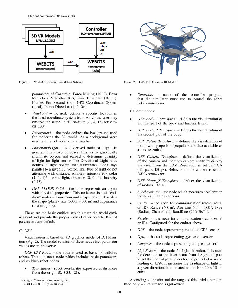
Figure 1. WEBOTS General Simulation Schema
parameters of Constraint Force Mixing (10−5), ErrorReduction Parameter (0.2), Basic Time Step (16 ms),Frames Per Second (60), GPS Coordinate System(local), North Direction (1, 0, 0)2.
• ViewPoint – the node defines a specific location inthe local coordinate system from which the user mayobserve the scene. Initial position (-1, 4, 18) for viewon UAV.
• Background – the node defines the background usedfor rendering the 3D world. As a background wereused textures of noon sunny weather.
• DirectionalLight – is a derived node of Light. Ingeneral it has two purposes. First is to graphicallyilluminate objects and second to determine quantityof light for light sensor. The Directional Light nodedefines a light source that illuminates along raysparallel to a given 3D vector. This type of light do notattenuate with distance. Ambient intensity (0), color(1, 1, 1)3 – white light, direction (0, 0, -1). Intensity(0.75).
• DEF FLOOR Solid – the node represents an objectwith physical properties. This node consists of “chil-dren” nodes – Transform and Shape, which describesthe shape (plane), size (500 m×300 m) and appearance(texture grass).
These are the basic entities, which create the world envi-ronment and provide the proper view of other objects. Rest ofparameters are default.
C. UAV
Visualization is based on 3D graphics model of DJI Phan-tom (Fig. 2). The model consists of these nodes (set parametervalues are in brackets):
DEF UAV Robot – the node is used as basis for buildingrobots. This is a main node which includes basic parametersand children robot nodes.
• Translation – robot coordinates expressed as distancesfrom the origin (0, 3.33, -21).
2x, y, z Cartesian coordinate system3RGB form 0 to 1 (0÷ 100%)
Figure 2. UAV DJI Phantom III Model
• Controller – name of the controller programthat the simulator must use to control the robotUAV control.cpp.
Children nodes:
• DEF Body 1 Transform – defines the visualization ofthe first part of the body and landing frame.
• DEF Body 2 Transform – defines the visualization ofthe second part of the body.
• DEF Rotors Transform – defines the visualization ofrotors with propellers (propellers are also available asa unique entity).
• DEF Camera Transform – defines the visualizationof the camera and includes camera entity to displaythe view from the UAV. Resolution is set as VGA(640 px × 480 px). Behavior of the camera is set inUAV control.cpp.
• DEF Motor X Transform – defines the visualizationof motors 1 to 4.
• Accelerometer – the node which measures accelerationforces in three dimensions.
• Emitter – the node for communication (radio, serialor IR). Range (500 m). Aperture (-1) = 360. Type(Radio). Channel (1). BaudRate (20 MBs−1).
• Receiver – the node for communication (radio, serialor IR). Configured for the emitter above.
• GPS – the node representing model of GPS sensor.
• Gyro – the node representing gyroscope sensor.
• Compass – the node representing compass sensor.
• LightSensor – the node for light detection. It is usedfor detection of the laser beam from the ground postto get the control parameters for the project of assistedlanding of UAV. It measures the irradiance of light ina given direction. It is created as the 10× 10× 10 cmcube.
According to the aim and the range of this article there areused only – Camera and LightSensor.
Student conference Blansko 2016
88
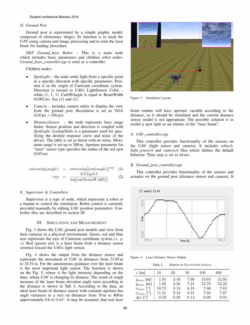
D. Ground Post
Ground post is represented by a simple graphic model,composed of elementary shapes. Its function is to track theUAV using camera and image processing and to emit the laserbeam for landing procedure.
DEF Ground base Robot – This is a main nodewhich includes basic parameters and children robot nodes.Ground base controller.cpp is used as a controller.
Children nodes:
• SpotLight – the node emits light from a specific pointin a specific direction with specific parameters. Posi-tion is in the origin of Cartesian coordinate system.Direction is toward to UAVs LightSensor. Color –white (1, 1, 1). CutOffAngle is equal to BeamWidth(0.002 m). See (1) and (2).
• Camera – includes camera entity to display the viewfrom the ground post. Resolution is set as VGA(640 px× 480 px).
• DistanceSensor – the node represents laser rangefinder. Sensor position and direction is coupled withSpotLight. LookupTable is a parameter used for spec-ifying the desired response curve and noise of thedevice. The table is set as linear with no noise. Maxi-mum range is set up to 500 m. Aperture parameter for“laser” sensor type specifies the radius of the red spot(0.03 m).
intensity(angle) = intensity[(cos(angle)]exp (1)
exp =0.5 log 0.5
log[cos(beamWidth)](2)
E. Supervisor & Controllers
Supervisor is a type of node, which represents a robot ora human to control the simulation. Robot control is currentlyprovided manually by editing UAV position parameters. Con-troller files are described in section III.
III. SIMULATION AND MEASUREMENT
Fig. 3 shows the UAV, ground post models and view fromtheir cameras in a physical environment. Green, red and blueaxis represents the axis of Cartesian coordinate system (x, y,z). Red (green) axis is a laser beam from a distance sensororiented toward the UAVs light sensor.
Fig. 4 shows the output from the distance sensor andrepresents the movement of UAV in distances from 23.05 mto 24.51 m. For the autonomous guidance over the laser beamis the most important light sensor. The function is shownon the Fig. 5, where is the light intensity depending on thetime, where UAV is changing its distance. The result of roughmeasure of the laser beam elevation angle error according tothe distance is shown in Tab. I. According to the data, anideal laser beam of distance sensor with constant aperture hasangle variances in y axis on distances from 10 m to 400 mapproximately 0.6 to 0.04. It may be assumed, that real laser
Figure 3. Simulation Layout
beam emitter will have aperture variable according to thedistance, so it should be simulated and the current distancesensor model is not appropriate. The possible solution is tomodel a spot light as an emitter of the “laser beam”.
A. UAV controller.cpp
This controller provides functionality of the sensors onthe UAV (light sensor and camera). It includes robot.h,light sensor.h and camera.h files which defines the defaultbehavior. Time step is set to 64 ms.
B. Ground post controller.cpp
This controller provides functionality of the sensors andactuator on the ground post (distance sensor and camera). It
Figure 4. Laser Distance Sensor Output
Table I. ERROR OF ELEVATION ANGLE
z [m] 10 20 50 100 400
ymin [m] 1.85 3.16 7.09 13.64 52.94ymax [m] 1.95 3.26 7.21 13.78 53.23αmin [°] 10.72 9.13 8.18 7.86 7.63αmax [°] 11.31 9.42 8.31 7.94 7.67∆α [°] 0.59 0.29 0.14 0.08 0.04
Student conference Blansko 2016
89
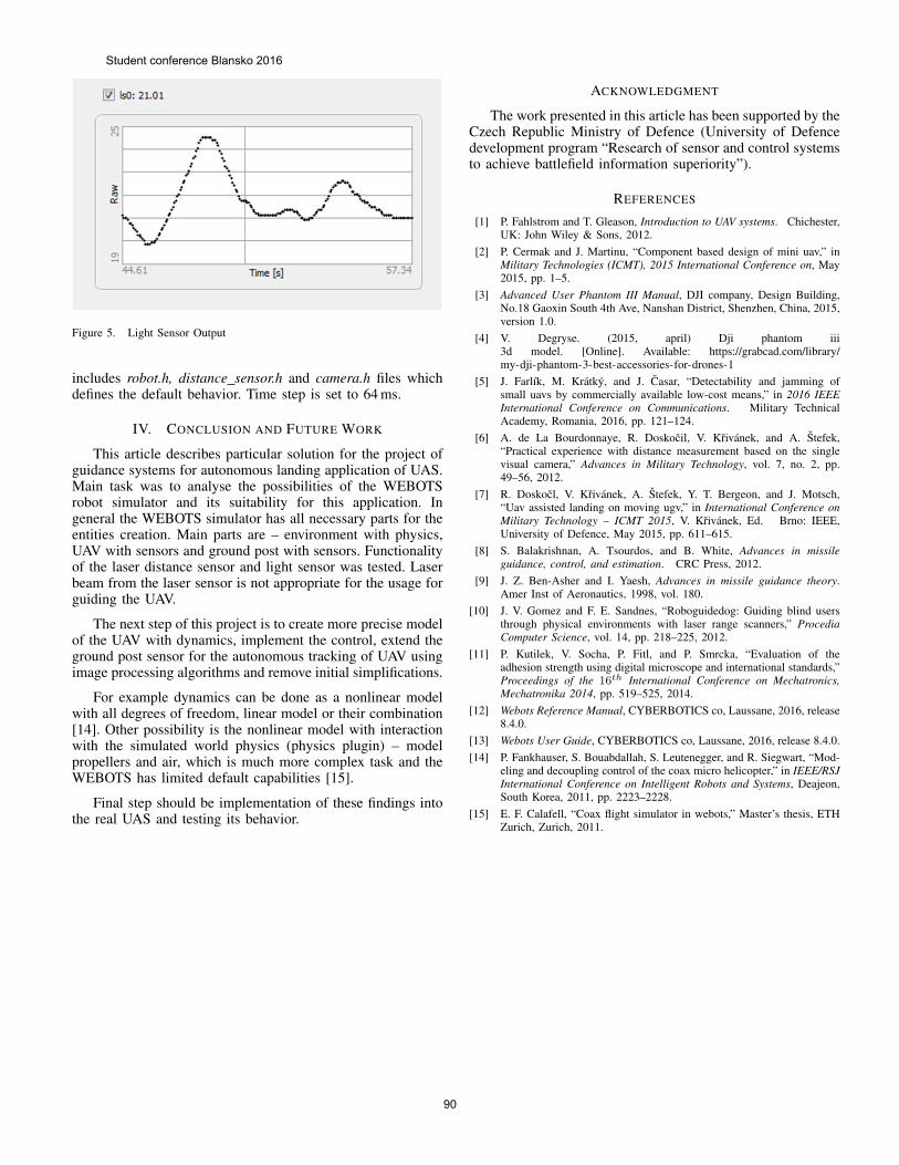
Figure 5. Light Sensor Output
includes robot.h, distance sensor.h and camera.h files whichdefines the default behavior. Time step is set to 64 ms.
IV. CONCLUSION AND FUTURE WORK
This article describes particular solution for the project ofguidance systems for autonomous landing application of UAS.Main task was to analyse the possibilities of the WEBOTSrobot simulator and its suitability for this application. Ingeneral the WEBOTS simulator has all necessary parts for theentities creation. Main parts are – environment with physics,UAV with sensors and ground post with sensors. Functionalityof the laser distance sensor and light sensor was tested. Laserbeam from the laser sensor is not appropriate for the usage forguiding the UAV.
The next step of this project is to create more precise modelof the UAV with dynamics, implement the control, extend theground post sensor for the autonomous tracking of UAV usingimage processing algorithms and remove initial simplifications.
For example dynamics can be done as a nonlinear modelwith all degrees of freedom, linear model or their combination[14]. Other possibility is the nonlinear model with interactionwith the simulated world physics (physics plugin) – modelpropellers and air, which is much more complex task and theWEBOTS has limited default capabilities [15].
Final step should be implementation of these findings intothe real UAS and testing its behavior.
ACKNOWLEDGMENT
The work presented in this article has been supported by theCzech Republic Ministry of Defence (University of Defencedevelopment program “Research of sensor and control systemsto achieve battlefield information superiority”).
REFERENCES
[1] P. Fahlstrom and T. Gleason, Introduction to UAV systems. Chichester,UK: John Wiley & Sons, 2012.
[2] P. Cermak and J. Martinu, “Component based design of mini uav,” inMilitary Technologies (ICMT), 2015 International Conference on, May2015, pp. 1–5.
[3] Advanced User Phantom III Manual, DJI company, Design Building,No.18 Gaoxin South 4th Ave, Nanshan District, Shenzhen, China, 2015,version 1.0.
[4] V. Degryse. (2015, april) Dji phantom iii3d model. [Online]. Available: https://grabcad.com/library/my-dji-phantom-3-best-accessories-for-drones-1
[5] J. Farlık, M. Kratky, and J. Casar, “Detectability and jamming ofsmall uavs by commercially available low-cost means,” in 2016 IEEEInternational Conference on Communications. Military TechnicalAcademy, Romania, 2016, pp. 121–124.
[6] A. de La Bourdonnaye, R. Doskocil, V. Krivanek, and A. Stefek,“Practical experience with distance measurement based on the singlevisual camera,” Advances in Military Technology, vol. 7, no. 2, pp.49–56, 2012.
[7] R. Doskocl, V. Krivanek, A. Stefek, Y. T. Bergeon, and J. Motsch,“Uav assisted landing on moving ugv,” in International Conference onMilitary Technology – ICMT 2015, V. Krivanek, Ed. Brno: IEEE,University of Defence, May 2015, pp. 611–615.
[8] S. Balakrishnan, A. Tsourdos, and B. White, Advances in missileguidance, control, and estimation. CRC Press, 2012.
[9] J. Z. Ben-Asher and I. Yaesh, Advances in missile guidance theory.Amer Inst of Aeronautics, 1998, vol. 180.
[10] J. V. Gomez and F. E. Sandnes, “Roboguidedog: Guiding blind usersthrough physical environments with laser range scanners,” ProcediaComputer Science, vol. 14, pp. 218–225, 2012.
[11] P. Kutilek, V. Socha, P. Fitl, and P. Smrcka, “Evaluation of theadhesion strength using digital microscope and international standards,”Proceedings of the 16th International Conference on Mechatronics,Mechatronika 2014, pp. 519–525, 2014.
[12] Webots Reference Manual, CYBERBOTICS co, Laussane, 2016, release8.4.0.
[13] Webots User Guide, CYBERBOTICS co, Laussane, 2016, release 8.4.0.[14] P. Fankhauser, S. Bouabdallah, S. Leutenegger, and R. Siegwart, “Mod-
eling and decoupling control of the coax micro helicopter,” in IEEE/RSJInternational Conference on Intelligent Robots and Systems, Deajeon,South Korea, 2011, pp. 2223–2228.
[15] E. F. Calafell, “Coax flight simulator in webots,” Master’s thesis, ETHZurich, Zurich, 2011.
Student conference Blansko 2016
90
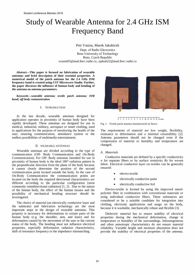
Study of Wearable Antenna for 2.4 GHz ISM
Frequency Band
Petr Vasina, Marek Jakubicek
Dept. of Radio Electronics
Brno University of Technology
Brno, Czech Republic
[email protected], [email protected]
Abstract—This paper is focused on fabrication of wearable
antennas and brief description of their essential properties. A
numerical model of the patch antenna for the 2.4 GHz ISM
frequency band is created using CST Microwave Studio. Further,
the paper discusses the influence of human body and bending of
the antenna on antenna parameters.
Keywords—wearable antenna; textile patch antenna; ISM
band; off-body communication
I. INTRODUCTION
In the last decade, wearable antennas designed for
application operates in proximity of human body have been rapidly developed. These antennas are designed for use in medical, industrial, military, aerospace or smart clothing, used in applications for the purpose of monitoring the health of the user, ensuring communication, attendance system or the endless possibilities of multimedia entertainment.
II. WEARABLE ANTENNAS
Wearable antennas are divided according to the type of communication (Off- Body Communication and On-Body Communication). For Off- Body antennas intended for use in proximity of human body is the ideal 180° radiation pattern in the perpendicular direction from the plane of the body because it cannot clearly determine the position of the second communication point located outside the body. In the case of On-Body Communication the communication points are located on the body the required directional characteristics are different according to the particular configuration (most commonly omnidirectional radiation) [1, 2]. Due to the nature of the human body, the effect of the human tissues and the possibility of mechanical bending structure should be investigated.
The choice of material (an electrically conductive layer and the substrate) and fabrication technology are the most important steps in the design of wearable antennas. This property is necessary for deformations in certain parts of the human body (e.g. the shoulder, arm, and knee) and for deformation caused by the movement of the user or the current status of the body. The bending must not influence electrical properties, especially deformation radiation characteristics, shift of resonance frequency or the impedance mismatching.
Fig. 1. Textile patch antenna manufactured on fleece.
The requirements of material are low weight, flexibility, resistance to deformation and a minimal extensibility [2]. Antenna parameters should not be changed even if the compression of material or humidity and temperature are changed.
A. Materials
Conductive materials are defined by a specific conductivity σ for separate fibers or by surface resistivity Rs for woven fabric. Electrical conductive layer on textiles can be generally ensured:
electro-textile
electrically conductive paint
electrically conductive foil
Electro-textile is formed by using the improved metal-
polymer fiber in combination with conventional materials or
using individual conductive fibers. These substances are
considered to be a suitable candidate for integration into
clothing, electronic applications and usage on the body,
because it is washable, mechanically robust and flexible [3].
Dielectric material has to ensure stability of electrical properties during the mechanical deformation, change in temperature or humidity of the surroundings. Inhomogeneous and often anisotropic characteristics do not ensure material reliability. Variable height and moisture absorption does not provide the stability of electrical properties of the antenna.
Student conference Blansko 2016
91
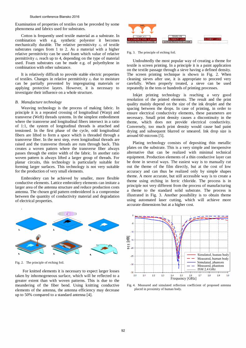
Examination of properties of textiles can be preceded by some phenomena and fabrics used for substrates.
Cotton is frequently used textile material as a substrate. In combination with e.g. synthetic polyester it becomes mechanically durable. The relative permittivity εr of textile substrates ranges from 1 to 2. As a material with a higher relative permittivity can be used foam which value of relative permittivity εr reach up to 4, depending on the type of material used. Foam substrates can be made e.g. of polyethylene in combination with other substance.
It is relatively difficult to provide stable electric properties of textiles. Changes in relative permittivity εr due to moisture can be partially prevented by impregnating materials or applying protective layers. However, it is necessary to investigate their influence on a whole structure.
B. Manufacture technology
Weaving technology is the process of making fabric. In principle it is a repeated crossing of longitudinal (Warp) and transverse (Weft) threads systems. In the simplest embodiment where the transverse and longitudinal fibers intersect in a ratio of 1:1, the system of longitudinal threads is attached and tensioned. In the first phase of the cycle, odd longitudinal fibers are lifted to form a space which is threaded through a transverse fiber. In the next step, even longitudinal threads are raised and the transverse threads are runs through back. This creates a woven pattern where the transverse fiber always passes through the entire width of the fabric. In another ratio woven pattern is always lifted a larger group of threads. For planar circuits, this technology is particularly suitable for forming larger surfaces. This technology is not very suitable for the production of very small elements.
Embroidery can be achieved by smaller, more flexible conductive elements. Lattice embroidery elements can imitate a larger area of the antenna structure and reduce production costs antenna. The chosen grid pattern embroidered is a compromise between the quantity of conductivity material and degradation of electrical properties.
.
Fig. 2. The principle of etching foil.
For knitted elements it is necessary to expect larger losses
taken by inhomogeneous surface, which will be reflected to a
greater extent than with woven patterns. This is due to the
meandering of the fiber bend. Using knitting conductive
elements of the antenna, the antenna efficiency may decrease
up to 50% compared to a standard antenna [4].
Fig. 3. The principle of etching foil.
Undoubtedly the most popular way of creating a theme for textile is screen printing. In a principle it is a paint application on the textile passage through a sieve having a defined density. The screen printing technique is shown in Fig. 2. When cleaning sieves after use, it is appropriate to proceed very carefully. When properly treated, a sieve can be used repeatedly in the tens or hundreds of printing processes.
Inkjet printing technology is reaching a very good resolution of the printed elements. The result and the print quality mainly depend on the size of the ink droplet and the spacing between the drops. In case of printing, in order to ensure electrical conductivity elements, these parameters are necessary. Small print density causes a discontinuity in the theme, which does not provide electrical conductivity. Conversely, too much print density would cause bad paint drying and subsequent blurred or smeared. Ink drop size is around 60 microns [5].
Plating technology consists of depositing thin metallic
plates on the substrate. This is a very simple and inexpensive
alternative that can be realized with minimal technical
equipment. Production elements of a thin conductive layer can
be done in several ways. The easiest way is to manually cut
out the theme of the film directly, but at the cost of low
accuracy and can thus be realized only by simple shapes
theme. A more accurate, but still accessible way is to create a
theme using etching in ferric chloride. The process is in
principle not very different from the process of manufacturing
a theme to the standard solid substrate. The process is
illustrated in Fig. 3. Another possibility is to obtain theme
using automated laser cutting, which will achieve more
accurate dimensions but at a higher cost.
Fig. 4. Measured and simulated reflection coefficient of proposed antenna
placed in proximity of human body.
Student conference Blansko 2016
92
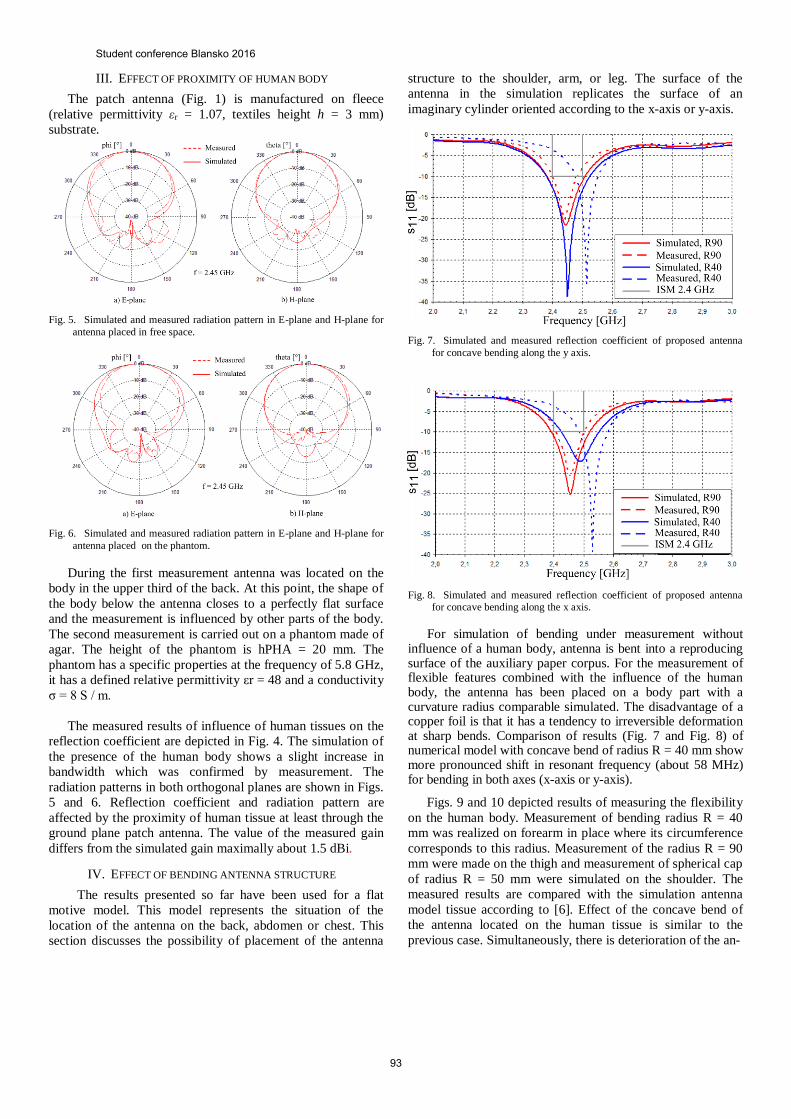
III. EFFECT OF PROXIMITY OF HUMAN BODY
The patch antenna (Fig. 1) is manufactured on fleece
(relative permittivity εr = 1.07, textiles height h = 3 mm)
substrate.
Fig. 5. Simulated and measured radiation pattern in E-plane and H-plane for
antenna placed in free space.
Fig. 6. Simulated and measured radiation pattern in E-plane and H-plane for
antenna placed on the phantom.
During the first measurement antenna was located on the
body in the upper third of the back. At this point, the shape of
the body below the antenna closes to a perfectly flat surface
and the measurement is influenced by other parts of the body.
The second measurement is carried out on a phantom made of
agar. The height of the phantom is hPHA = 20 mm. The
phantom has a specific properties at the frequency of 5.8 GHz,
it has a defined relative permittivity εr = 48 and a conductivity
σ = 8 S / m.
The measured results of influence of human tissues on the
reflection coefficient are depicted in Fig. 4. The simulation of
the presence of the human body shows a slight increase in
bandwidth which was confirmed by measurement. The
radiation patterns in both orthogonal planes are shown in Figs.
5 and 6. Reflection coefficient and radiation pattern are
affected by the proximity of human tissue at least through the
ground plane patch antenna. The value of the measured gain
differs from the simulated gain maximally about 1.5 dBi.
IV. EFFECT OF BENDING ANTENNA STRUCTURE
The results presented so far have been used for a flat
motive model. This model represents the situation of the
location of the antenna on the back, abdomen or chest. This
section discusses the possibility of placement of the antenna
structure to the shoulder, arm, or leg. The surface of the
antenna in the simulation replicates the surface of an
imaginary cylinder oriented according to the x-axis or y-axis.
Fig. 7. Simulated and measured reflection coefficient of proposed antenna
for concave bending along the y axis.
Fig. 8. Simulated and measured reflection coefficient of proposed antenna for concave bending along the x axis.
For simulation of bending under measurement without influence of a human body, antenna is bent into a reproducing surface of the auxiliary paper corpus. For the measurement of flexible features combined with the influence of the human body, the antenna has been placed on a body part with a curvature radius comparable simulated. The disadvantage of a copper foil is that it has a tendency to irreversible deformation at sharp bends. Comparison of results (Fig. 7 and Fig. 8) of numerical model with concave bend of radius R = 40 mm show more pronounced shift in resonant frequency (about 58 MHz) for bending in both axes (x-axis or y-axis).
Figs. 9 and 10 depicted results of measuring the flexibility
on the human body. Measurement of bending radius R = 40
mm was realized on forearm in place where its circumference
corresponds to this radius. Measurement of the radius R = 90
mm were made on the thigh and measurement of spherical cap
of radius R = 50 mm were simulated on the shoulder. The
measured results are compared with the simulation antenna
model tissue according to [6]. Effect of the concave bend of
the antenna located on the human tissue is similar to the
previous case. Simultaneously, there is deterioration of the an-
Student conference Blansko 2016
93
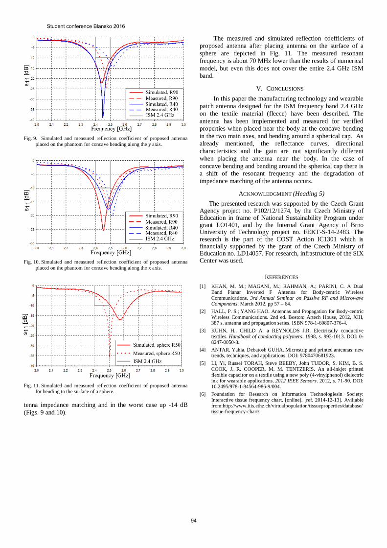
Fig. 9. Simulated and measured reflection coefficient of proposed antenna
placed on the phantom for concave bending along the y axis.
Fig. 10. Simulated and measured reflection coefficient of proposed antenna
placed on the phantom for concave bending along the x axis.
Fig. 11. Simulated and measured reflection coefficient of proposed antenna for bending to the surface of a sphere.
tenna impedance matching and in the worst case up -14 dB
(Figs. 9 and 10).
The measured and simulated reflection coefficients of
proposed antenna after placing antenna on the surface of a
sphere are depicted in Fig. 11. The measured resonant
frequency is about 70 MHz lower than the results of numerical
model, but even this does not cover the entire 2.4 GHz ISM
band.
V. CONCLUSIONS
In this paper the manufacturing technology and wearable
patch antenna designed for the ISM frequency band 2.4 GHz
on the textile material (fleece) have been described. The
antenna has been implemented and measured for verified
properties when placed near the body at the concave bending
in the two main axes, and bending around a spherical cap. As
already mentioned, the reflectance curves, directional
characteristics and the gain are not significantly different
when placing the antenna near the body. In the case of
concave bending and bending around the spherical cap there is
a shift of the resonant frequency and the degradation of
impedance matching of the antenna occurs.
ACKNOWLEDGMENT (Heading 5)
The presented research was supported by the Czech Grant Agency project no. P102/12/1274, by the Czech Ministry of Education in frame of National Sustainability Program under grant LO1401, and by the Internal Grant Agency of Brno University of Technology project no. FEKT-S-14-2483. The research is the part of the COST Action IC1301 which is financially supported by the grant of the Czech Ministry of Education no. LD14057. For research, infrastructure of the SIX Center was used.
REFERENCES
[1] KHAN, M. M.; MAGANI, M.; RAHMAN, A.; PARINI, C. A Dual Band Planar Inverted F Antenna for Body-centric Wireless Communications. 3rd Annual Seminar on Passive RF and Microwave Components. March 2012, pp 57 – 64.
[2] HALL, P. S.; YANG HAO. Antennas and Propagation for Body-centric Wireless Communications. 2nd ed. Boston: Artech House, 2012, XIII, 387 s. antenna and propagation series. ISBN 978-1-60807-376-4.
[3] KUHN, H., CHILD A. a REYNOLDS J.R. Electrically conductive textiles. Handbook of conducting polymers. 1998, s. 993-1013. DOI: 0-8247-0050-3.
[4] ANTAR, Yahia, Debatosh GUHA. Microstrip and printed antennas: new trends, techniques, and applications. DOI: 9780470681923.
[5] LI, Yi, Russel TORAH, Steve BEEBY, John TUDOR, S. KIM, B. S. COOK, J. R. COOPER, M. M. TENTZERIS. An all-inkjet printed flexible capacitor on a textile using a new poly (4-vinylphenol) dielectric ink for wearable applications. 2012 IEEE Sensors. 2012, s. 71-90. DOI: 10.2495/978-1-84564-986-9/004.
[6] Foundation for Research on Information Technologiesin Society: Interactive tissue frequency chart. [online]. [ref. 2014-12-13]. Aviliable from:http://www.itis.ethz.ch/virtualpopulation/tissueproperties/database/tissue-frequency-chart/.
Student conference Blansko 2016
94

Analysis of Microstrip Line Relative PermittivityMeasurement
Jan Velim, Michal MrnkaDepartment of Radio Electronics, Brno University of Technology
Email: [email protected]
Abstract—The paper describes a methodology how to mea-sure the relative permittivity by a microstrip line. The relativepermittivity is calculated from measured scattering parameters.The results are corrected to achieve the more precisely values.
I. INTRODUCTION
The transmission line method is used for measurement ofthe permittivity in many articles e.g [1], [2]. This method hasthe advantage of broadband measurements compared with aresonant techniques. In spite of that the resonant techniquehas narrow band it is more popular for its accuracy, moreovernumerical models are used for evaluation of the relative per-mittivity that means that no analytical equations are necessaryto include. The results are achieved by optimization techniquesand comparison between measured data and simulated data. Inthis article is shown that analytical processing does not bringadditional errors only, but can contribute to the reduction oferrors and smoothing of the results.
The next section explain the methodology how to get thevalue of the relative permittivity of a material which serves asdielectric layer in a microstrip line structure. The third sectionpresents the source of inaccuracies and their removal.
II. MEASUREMENT METHODOLOGY
There is necessary to have two samples of microstrip lineswith different length (Fig. 1) for measurement of a relativepermittivity by the transmission line method. We get valuesof scattering parameters for the shorter microstrip line STand for the longer microstrip line SL through the vectornetwork analyzer (VNA). There is no need of any calibrationof the VNA because the precise value of the transmissioncoefficient T of the segment (15 mm long) is calculated fromthe measured values SL and ST . Because of mathematicaloperations in next steps it is more useful to transform matricesof the scattering parameters in to transmission matrices TL andTT by equations [3]:
T11 =1
S21, (1)
T12 = −S22
S21, (2)
T21 =S11
S21, (3)
135 mm
120 mm
Fig. 1. Measured samples of the microstrip lines.
T22 = S12 −S11S22
S21, (4)
where T11, T12, T21, T22 are coefficients of the transmis-sion matrices and S11, S12, S21, S22 are coefficients of thescattering matrices.
The transmission coefficient of the 15 mm long segmentT is calculated by function ”eig()” how is presented in [4].The input arguments are the transmissions matrices and theoutputs are eigen values which correspond with transmissioncoefficient (5):
[T ] = eig(TLT−1T ) =
(e−γls
eγls
), (5)
where ls represents the length of the segment of themicrostrip line and γ is the propagation constant. This complexnumber γ = α + jβ is evaluated by equation (6). The αrepresents attenuation and β represents phase constant of theelectromagnetic waves in the structure.
γ = − ln(T )ls
. (6)
As proved by equation 7, only imaginary part of thepropagation constant has influence to the value of the relative
Student conference Blansko 2016
95
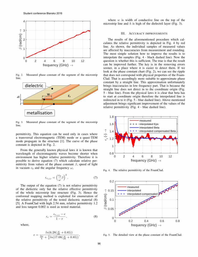
frequency (GHz) !0 2 4 6 8 10 12
- (
rad/
cm) !
0
1
2
3
4
Fig. 2. Measured phase constant of the segment of the microstripline.
εr
metallisation
dielectric
w
h
Fig. 3. Measured phase constant of the segment of the microstripline.
permittivity. This equation can be used only in cases wherea transversal electromagnetic (TEM) mode or a quasi-TEMmode propagate in the structure [1]. The curve of the phaseconstant is depicted in Fig. 2.
From the generally known physical laws it is known thatwavelength of electromagnetic waves become shorter whenenvironment has higher relative permittivity. Therefore it ispossible to derive equation (7) which calculate relative per-mittivity from values of the phase constant β, speed of lightin vacuum c0 and the angular frequency ω,
εreff=
(c0ωβ)2
. (7)
The output of the equation (7) is not relative permittivityof the dielectric only but the relative effective permittivityof the whole microstrip line structure (Fig. 3). Hence theconformal mapping method is exploited for enumeration ofthe relative permittivity of the tested dielectric material (8)[5]. A FoamClad with high 2.54 mm, relative permittivity 1.2and loss tangent 0.002 is used as tested material.
εr =εreff
− e
1− e, (8)
where,
e =ln(6.28( w2h + 0.85))
2wh + 2
π ln(17.08(w2h + 0.85))
,
where w is width of conductive line on the top of themicrostrip line and h is high of the dielectril layer (Fig. 3).
III. ACCURACY IMPROVEMENTS
The results of the aforementioned procedure which cal-culates the relative permittivity is depicted in Fig. 4 by redline. As shown, the individual samples of measured valuesare affected by inaccuracies from measurement and rounding.The most simple solution how to improve the results is tointerpolate the samples (Fig. 4 - black dashed line). Now thequestion is whether this is sufficient. The true is that the resultcan be improved further. The key is in the removing errorssooner, in a place where it is easier to detect them. If welook at the phase constant chart (Fig. 2), we can see the ripplethat does not correspond with physical properties of the Foam-Clad. That is accordingly more suitable to approximate phaseconstant by a straight line. This approximation unfortunatelybrings inaccuracies in low frequency part. That is because thestraight line does not direct in to the coordinate origin (Fig.5 - blue line). From the physical laws it is clear that beta hasto start at coordinate origin therefore the interpolated line isredirected in to it (Fig. 5 - blue dashed line). Above mentionedadjustment brings significant improvement of the values of therelative permittivity (Fig. 4 - blue dashed line).
frequency (GHz) !0 2 4 6 8 10 12
0 r (-)
!
0.8
1
1.2
1.4
1.6
1.8measuredinterpolated Epsinterpolated Betainterpolated compensated Beta
Fig. 4. The relative permittivity of the FoamClad.
frequency (GHz) !0 0.2 0.4 0.6 0.8
- (
rad/
cm) !
0
0.05
0.1
0.15
0.2
measuredinterpolatedinterpolated-compensated
Fig. 5. The detailed view at the phase constant of the FoamClad.
Student conference Blansko 2016
96

IV. CONCLUSION
The article proves that transmission line method is suitabletechnique for the broadband measurement of a relative permit-tivity. The microstrip line can be used up to 13.6 GHz. Usinga corrections, which are based on physical knowledge, causesthe more accurate results. The significant improvement wasachieved especially in the lower parts of the frequency bandas shown in Fig. 4.
ACKNOWLEDGMENT
Research described in this paper was financially sup-ported by the Czech Science Foundation under grant no.P102/12/1274. Research is a part of the COST Action IC1301supported by the grant LD14057 of the Czech Ministry ofEducation. The presented research was supported by the Inter-nal Grant Agency of Brno University of Technology project
no. FEKT-s-14-2483. For research, infrastructure of the SIXCenter was used.
REFERENCES
[1] P. Seiler, B. Klein and D. Plettemeier, ”Broadband characterization ofplanar transmission line substrate permittivity up to 67 GHz,” Antennasand Propagation (ISAP), 2014 International Symposium on, Kaohsiung,2014, pp. 373-374.
[2] S. F. Barot and J. T. Bernhard, ”Permittivity measurement of layeredmedia using a microstrip test bed,” 2008 IEEE Antennas and PropagationSociety International Symposium, San Diego, CA, 2008, pp. 1-4.
[3] Radmanesh, M. M., RF & Microwave Design Essentials: EngineeringDesign and Analysis from DC to Microwaves, AuthorHouse, 2007.
[4] Y. Rolain, A. Barel, F. Gubbels and W. van Moer, ”Microwave permittiv-ity measurement of polymers by deposition on a coplanar wave guide,”Instrumentation and Measurement Technology Conference, 2004. IMTC04. Proceedings of the 21st IEEE, 2004, pp. 333-338 Vol.1.
[5] SVACINA, J.: Resenı mikrovlnnych planarnıch struktur metodou kon-formnıho zobrazenı. Akademicke nakladatelstvı CERN, 2006
Student conference Blansko 2016
97

System Impulse Response Measurement UsingM-sequences in the Presence of Non-linearities
Josef VychodilDepartment of Radio ElectronicsBrno University of Technology
Technicka 3082/12, 616 00 Brno, Czech RepublicEmail: [email protected]
Abstract—The m-sequence cross-correlation method is a pow-erful approach for obtaining a linear system impulse responseestimate. However, when the system under test exhibits non-linearbehaviour, the obtained estimate contains some artefacts, whichare not part of the linear system impulse response. This paperdescribes the origin of these artefacts and how they arise.
I. INTRODUCTION
The m-sequence cross-correlation method is a widely usedapproach for measuring impulse responses of linear systems.For example, it is used in many time domain channel sounders,like it was shown in [1] or [2].
The method is usually performed as follows. A seamlessrepeating m-sequence is fed to the input of the system. Theoutput of the system is then sampled and a correlation oper-ation (usually performed using Fast Fourier Transform (FFT)for faster computation) between the output and the original m-sequence is computed. Because the auto-correlation function ofa m-sequence can be approximated as ideal impulse function,the result is an estimate of the channel impulse response.
However, real (not only) electronic devices like amplifiers,mixers, etc. exhibit at least weak non-linear behavior. Whenthe measured system is non-linear, the resulting estimate ofthe channel impulse response contains artefacts, which are notpart of the linear impulse response.
II. LINEAR CASE
The input-output relationship of a linear time invariantsystem can be expressed as
y(t) =
∞∫0
g1(τ1)u(t− τ1)dτ1, (1)
where u(t) is the input of the system, y(t) is the output andg1(τ1) is the system’s impulse response.
From now, consider the input signal u(t) as a seamlessrepeating m-sequence with number of chips N , period of Tand duration of one chip ∆t. The cross-correlation betweenthe input u(t) and output y(t) can be expressed as [3]
Ruy(τ) = u(t− τ)y(t) (2)
where means time (t) average over one period (T ) ofthe signal. When considering the system described by Eq. 1,
the cross-correlation becomes
Ruy(τ) =u(t− τ)y(t)
=u(t− τ)
∞∫0
g1(τ1)u(t− τ1)dτ1
=
∞∫0
g1(τ1)u(t− τ)u(t− τ1)dτ1
=
∞∫0
g1(τ1)Ruu(τ, τ1)dτ1,
(3)
where Ruu(τ, τ1) is the second moment of the input m-sequence u(t) [3], which can be expressed as
Ruu(τ, τ1) = u(t− τ)u(t− τ1) =
1 if τ = τ1− 1
N if τ 6= τ1,(4)
Equation 3 then becomes
Ruy(τ) ' ∆tg1(τ), (5)
which corresponds to the conventional system impulse re-sponse measurements utilizing m-sequences.
III. NON-LINEAR CASE
When the system is weakly non-linear, its input-outputrelation can be expressed using the Volterra series expansion,which is generalization of the system impulse response andthe Taylor series, as
y(t) =
∞∫0
g1(τ1)u(t− τ1)dτ1
+
∞∫0
∞∫0
g2(τ1, τ2)u(t− τ1)u(t− τ2)dτ1dτ2
+
∞∫0
∞∫0
∞∫0
g3(τ1, τ2, τ3)u(t− τ1)u(t− τ2)u(t− τ3)dτ1dτ2dτ3
+ . . .
+
∞∫0
. . .
∞∫0
gi(τ1, . . . , τi)u(t− τ1) . . . u(t− τi)dτ1 . . . dτi
(6)
Student conference Blansko 2016
98

or in shorter form as
y(t) =∞∑i=1
∞∫0
. . .
∞∫0
gi(τ1, . . . , τi)u(t−τ1) . . . u(t−τi)dτ1 . . . dτi,
(7)where u(t) is the input to the system, y(t) is the output ofthe system and gi(τ1, . . . , τi) is the i-th order Volterra kernel,which can be viewed as higher order impulse response ofthe system. Please note that if the system is linear, onlythe first order Volterra kernel g1(τ1) (first term of Eq. 6) isnon zero. The equation then reduces to ordinary convolution,where g1(τ1) is the linear impulse response, e.g. the equationbecomes Eq. 1.
Now, let’s introduce one of the properties of m-sequences,the so-called shift and add property [4]. When we take anym-sequence and multiply it by the same but shifted sequence,we obtain the same sequence, but with different time shift. Forexample, with a sequence u[n] with length of 15 chips
u[n] =[ ]
·u[n− 1] =[ ]= u[n− 4] =[ ],
(8)
where the -1 and 1 numbers are for better illustration repre-sented by and symbols, respectively, it can be clearly seenthat the original sequence multiplied by the same sequencebut shifted by one chip to the right equals the same sequencebut shifted by 4 chips to the right. The shifts are unique forevery m-sequence and can be determined from the generatingpolynomial of the m-sequence.
Equation 4 can be generalized to the i-th moment of u(t)as
Ruu...u(τ, τ1, . . . , τi) = u(t− τ)u(t− τ1) . . . u(t− τi)
=
1 under certain values of τ, τ1, . . . , τi− 1
N otherwise.
(9)
The crosscorrelation between the input u(t) and the outputy(t) using 3, 7 and 9 can be rewritten as [5]
Ruy(τ) =u(t− τ)y(t)
=u(t− τ)
∞∑i=1
∞∫0
. . .
∞∫0
gi(τ1, . . . , τi)
·u(t− τ1) . . . u(t− τi)dτ1 . . . dτi
=∞∑i=1
∞∫0
. . .
∞∫0
gi(τ1, . . . , τi)
· u(t− τ)u(t− τ1) . . . u(t− τi)dτ1 . . . dτi
=∞∑i=1
∞∫0
. . .
∞∫0
gi(τ1, . . . , τi)
·Ruu...u(τ, τ1, . . . , τi)dτ1 . . . dτi,
(10)
which can be aproximated, when neglecting 4th and higher
order kernels as
Ruy(τ) '∆tg1(τ) + F3(τ)
+2!
m2∑j=1
(∆t)2g2(τ − k(j)21 ∆t, τ − k(j)22 ∆t)
+3!
m3∑j=1
(∆t)3g3(τ − k(j)31 ∆t, τ − k(j)32 ∆t, τ − k(j)33 ∆t),
(11)
where the integers k(j)ir (1 ≤ r ≤ i) are the unique shift
coefficients of the m-sequence, mi is the count of the sets ofnumbers k(j)ir . We can observe that the cross-correlation nowcontains the first order kernel (linear impulse response) andalso shifted cross sections of higher order kernels. The termF3(τ) is the sum of the third order Volterra kernels, whichhave one or more parameters the same and equals to
F3(τ) = (∆t)3g3(τ, τ, τ) + 3(∆t)3m1∑q=1
g3(τ, q, q). (12)
A. Unobservable and overlapped kernels
As can be seen from Eq. 11 and Eq. 12 there are severalparts of Volterra kernels, which are not directly observable orare overlapped with other kernels.
In the concrete, we cannot observe any second orderVolterra kernel, which have equal parameter, e.g. g2(q, q). Thisis because when the binary m-sequence is multiplied by thesame m-sequence, the result is a constant 1, e.g. u(t)·u(t) = 1[6]. This can be generalized for all even order kernels, butin the scope of this work only kernels up to third order areconsidered.
From Eq. 12 we can see that any third order Volterra kernel,which have one or more parameters the same, overlap with thefirst order kernel. The explanation is as follows: u(t) · u(t) ·u(t) = u(t) or more generally u(t) ·u(t− τ) ·u(t− τ) = u(t).This property can also be generalized for all odd order kernels.
IV. EXAMPLES
This section gives some examples of the described prin-ciples. Those examples were carried out using computer sim-ulation. Consider one of the simplest non-linear system, theso-called Wiener model.
h(τ) f [z(t)]u(t) z(t) y(t)
Fig. 1. Wiener type non-linear model.
This model consists of cascade of a linear memory block,which can be characterized by its impulse response h(τ), anda static (memory-less) non-linearity, which can be modeled bya (possibly truncated) polynomial, e.g.
y(t) = c1z(t) + c2z2(t) + c3z
3(t), (13)
when considering non-linearities only up to third order.
Student conference Blansko 2016
99
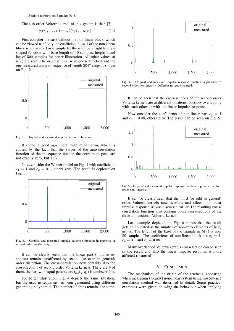
The i-th order Volterra kernel of this system is then [7]
gi(τ1, . . . , τi) = cih(τ1) . . . h(τi). (14)
First consider the case without the non-linear block, whichcan be viewed as if only the coefficient c1 = 1 of the non-linearblock is non-zero. For example let the h(τ) be a right triangleshaped function with base length of 10 samples, height 1 andlag of 500 samples for better illustration. All other values ofh(τ) are zero. The original impulse response function and theone measured using m-sequence of length 2047 chips is shownon Fig. 2.
0 500 1,000 1,500 2,000
0
0.5
1originalmeasured
Fig. 2. Original and measured impulse response function.
It shows a good agreement, with minor error, which iscaused by the fact, that the values of the auto-correlationfunction of the m-sequence outside the correlation peak arenot exactly zero, but 1/N .
Now, consider the Wiener model on Fig. 1 with coefficientsc1 = 1 and c2 = 0.1, others zero. The result is depicted onFig. 3.
0 500 1,000 1,500 2,000
0
0.5
1originalmeasured
Fig. 3. Original and measured impulse response function in presence ofsecond order non-linearity.
It can be clearly seen, that the linear part (impulse re-sponse) remains unaffected by second (or even in general)order distortion. The cross-correlation now contains also thecross-sections of second order Volterra kernels. There are 9 ofthem, the part with equal parameters (g2(q, q)) is unobservable.
For better illustration, Fig. 4 depicts the same situation,but the used m-sequence has been generated using differentgenerating polynomial. The number of chips remains the same.
0 500 1,000 1,500 2,000
0
0.5
1originalmeasured
Fig. 4. Original and measured impulse response function in presence ofsecond order non-linearity. Different m-sequence used.
It can be seen that the cross-sections of the second orderVolterra kernels are at different positions, possibly overlappingwith each other or with the linear impulse response.
Now consider the coefficients of non-linear part c1 = 1and c3 = 0.08, others zero. The result can be seen on Fig. 5.
0 500 1,000 1,500 2,000
0
0.5
1
1.5originalmeasured
Fig. 5. Original and measured impulse response function in presence of thirdorder non-linearity.
It can be clearly seen that the third (or odd in general)order Volterra kernels now overlaps and affects the linearimpulse response, as was discussed earlier. The resulting cross-correlation function also contains more cross-sections of thethree dimensional Volterra kernel.
Last example depicted on Fig. 6 shows that the resultgets complicated as the number of non-zero elements of h(τ)grows. The length of the base of the triangle in h(τ) is now50 samples. The coefficients of non-linear block are c1 = 1,c2 = 0.1 and c3 = 0.08.
Many overlapped Volterra kernels cross-section can be seenin the result and also the linear impulse response is moreaffected (distorted).
V. CONCLUSION
The mechanism of the origin of the artefacts, appearingwhen measuring (weakly) non-linear system using m-sequencecorrelation method was described in detail. Some practicalexamples were given, showing the behaviour when applying
Student conference Blansko 2016
100

0 500 1,000 1,500 2,000
0
2
4originalmeasured
Fig. 6. Original and measured impulse response function for h(τ) with 50non-zero elements in presence of second and third order non-linearity.
the method to one of the simplest non-linear system, theWiener type non-linear model.
Future work will cover examining the possibility of recov-ering the linear impulse response of the system from one ormultiple m-sequence cross-correlation measurements, or evenutilizing the m-sequence cross-correlation method for non-linear system identification.
ACKNOWLEDGMENT
This work was supported by the Czech Science Foundationproject No. 13-38735S Research into wireless channels forintra-vehicle communication and positioning, and was per-formed in laboratories supported by the SIX project, No.CZ.1.05/2.1.00/03.0072, the operational program Research andDevelopment for Innovation. Research described in this paperwas financed by Czech Ministry of Education in frame ofNational Sustainability Program under grant LO1401. Forresearch, infrastructure of the SIX Center was used.
REFERENCES
[1] R. Zetik, M. Kmec, J. Sachs, and R. S. Thoma, “Real-time mimochannel sounder for emulation of distributed ultrawideband systems,”International Journal of Antennas and Propagation, vol. 2014, p. 16,2014. [Online]. Available: http://dx.doi.org/10.1155/2014/317683
[2] A. Durantini, W. Ciccognani, and D. Cassioli, “UWB propagationmeasurements by PN-sequence channel sounding,” in Communications,2004 IEEE International Conference on, vol. 6, June 2004, pp. 3414–3418 Vol.6.
[3] H. Harada, Y. Toyozawa, M. Shigaki, H. Kashiwagi, and T. Yamaguchi,“Identification of nonlinear parameters by using m-sequence and har-monic probing method,” Journal of System Design and Dynamics, vol. 2,no. 1, pp. 209–217, 2008.
[4] Y. Lin, “Shift and add property of m-sequences and its application tochannel characterisation of digital magnetic recording,” IEE Proceedings- Communications, vol. 142, no. 3, pp. 135–140, Jun 1995.
[5] H. Tsukino, H. Harada, Y. Toyozawa, H. Kashiwagi, and R. Ohtsubo,“Identification of nonlinear parameters by using low-pass filtered M-sequence,” in ICCAS-SICE, 2009, Aug 2009, pp. 4512–4515.
[6] E. Nishiyama, “Identification of first order volterra kernels of m-sequencecorrelation method for nonlinear system,” in Control, Automation andSystems, 2007. ICCAS ’07. International Conference on, Oct 2007, pp.939–942.
[7] V. Kekatos, D. Angelosante, and G. B. Giannakis, “Sparsity-awareestimation of nonlinear volterra kernels,” in Computational Advances inMulti-Sensor Adaptive Processing (CAMSAP), 2009 3rd IEEE Interna-tional Workshop on, Dec 2009, pp. 129–132.
Student conference Blansko 2016
101
When the Numbers Speak - Hidden Statistics of aCrowdsourced QoE Study
Ondrej Zach, Eva KlejmovaDept. of Radio Electronics
Brno University of TechnologyTechnicka 12, 616 00 Brno, Czech Republic
Email: [email protected], [email protected]
Abstract—Presented paper deals with a crowdsourcing-basedQuality of Experience study. Using crowdsourcing for QoEevaluation has become very popular, however, the gathered dataneed to be processed carefully. In this work, we try to take adifferent look on the data gathered and possibly present someinteresting aspects regarding the users and their behavior.
I. INTRODUCTION
Crowdsourcing has become a very convenient tool inthe field of Quality of Experience (QoE). Conventional QoEstudies need to be run according to variety of conditions in acontrolled environment (ambient light, viewing distance, etc.).Such a study brings good insight in the quality of testedmultimedia content as perceived by the viewers. However,running a conventional study has high demands on resources,both material and financial. On the other hand, running acrowd-sourced study may bring results faster and with afraction of the costs compared to a laboratory-based testing.Nevertheless, a crowdsourced QoE study has to be designedcarefully based on the expected participants, their equipmentetc.
The challenges the researcher has to deal with are mainlyfocused on the final processing of the gathered data. As theparticipants are working on the given task in an uncontrolledenvironment (usually at their homes and using their owncomputer), the task has to be designed with emphasis onmonitoring of the users action. In home environment, it is veryeasy for the participant to cheat and not to answer properly.These issues are well addressed in [1], [2]. As the unreliableusers usually choose their answers randomly, such a behaviorhas to be detected and corresponding results then omitted fromthe final processing of the gathered data.
The focus of the paper is to analyze the ”hidden in-formation” from a crowdsourcing QoE study to address thepossible issues e.g. regarding crowd selection, which might bebeneficial for future research.
The rest of the paper is divided as follows. Section 2describes the studies during which we gathered the data weuse. In Section 3 we take a closer look at different issues,that can be found in the processed results and the last Sectionconcludes.
II. THE STUDY
For purposes of this paper, we ran several crowdsourcing-based QoE studies previously published in [3], [4]. However, in
this work we offer a different approach to gathered data and tryto look at the results from a different perspective. The researchpublished in [4] is focused on a comparison of Advanced VideoCoding (AVC) and High Efficiency Video Coding (HEVC)coded video content. An innovative feature of the study was anadaptive approach to allocation of the sequences to the users.The sequences to be played to the next participant were chosenaccording to the length of the confidence interval (CI) of thepreviously gathered quality scores of that respective sequence.Such an approach may lead to faster convergence of the scoresto values with lower CIs. In [3] we evaluate the performanceof the adaptive approach compared to conventional randomor pseudo-random approach. For this study, we used AVCcoded content only. We also try to suggest the best approachto content and quality level selection based on criteria of betterstatistical properties of the results (e.g. CI length, distributionetc.).
The video database created for the studies consisted of 5different contents, each encoded to 5 different bitrate levels.This results in 25 different AVC encoded processed videosequences (PVS) and 25 HEVC encoded PVSs. These PVSswere then used for the crowdsourced studies. The length ofeach sequence was adjusted to 10 s. The study was run using aweb-based application similar to [5]. The framework includedwide variety of features to monitor user’s activity and to detectpossible cheating. For example, a set of simple user question ispresented to the participant twice, at the beginning and at theend of the test, with different order of the answers. If the useranswered some of these question differently, his ratings weremarked as inconsistent. Also, the framework could monitor ifthe user switched to another tab of the web browser etc. Theparticipants watched five PVSs with different content each.The study was available as a micro job on the Microworkers1
crowdsourcing platform. Every user could participate and wasrewarded with 0.30$ upon completion of the test.
III. PROCESSING OF THE RESULTS
During the run of the study, we gathered wide varietyof information from the participants. The framework itselfmonitored the behavior of the users (e.g. cheating, not focusingon the test properly) and information about equipment they use(used web browser, screen resolution, download speed etc.).Other information needed users’ input, e.g. participants’ sex,age, education, occupation, nationality and using of web-based
1https://microworkers.com
Student conference Blansko 2016
102

video services. In following Section, we analyze some of thesehidden aspects of the study.
A. Users’ demography
Alltogether, the test was finished 1392 times. The studywas divided in several runs, hence, this number does notneed to represent the number of the participants as the user(identified by his unique mwID) could participate in all ofthe runs without any limitation. After omitting the repeatingmwIDs, we had 672 unique users. These users came from 78different countries, mainly from Bangladesh. More detailedinformation about the origin of the participants can be seenin Fig. 1. Quite surprisingly, among the countries with highshare of participants is Belgium, which is, unlike the others, awell developed country.
BD
RS
RO IN BE BG
other
Representation of countries in test
Fig. 1: Representation of participants’ countries.
Another interesting finding might be the share of internetbrowser in the crowdsourcing society. Also in this case, theanswer was quite surprising. More than 65% of the users usedGoogle Chrome. The Windows’ built-in Microsoft InternetExplorer was identified only in 4 cases. The situation can beseen in Fig. 2. The figure depicts only the type of the browserand not its specific version. As an The knowledge of the mostoften used browser can help the researcher in designing thestudy in the terms of features of the browser the research canuse.
B. Cheating behavior
As already mentioned, the test’s framework could monitorcheating-like behavior. The users were asked simple questionsregarding the content of just presented sequence. If the userdid not answer properly, his all ratings were neglected. Thiswas detected in 52 cases. Other participants tried to switchto another browser tab during the playback. This was alsomonitored. If such an event occurred, the user was firstly askedto focus properly on the task and was offer to re-play thesequence. If he tried again to switch to another tab, his ratingswere removed from further processing of the results. To sum
Google Chrome
Mozilla Firefox
other unknown
Browser share
Fig. 2: Browser share.
30
40
50
60
70
80
RS BE BG average RO IN BD
Inco
nsi
ste
nt
answ
ers
[%
]
Country
Fig. 3: Percentage of unreliable users among countries.
up, only about 44 % of the completed tests were finishedwithout any disruption or attempts to cheat.
As each user has to be payed for completion of the task,identifying the groups of unreliable users may bring benefitsfor further studies. Hence, we asked the question, if there isa relation between nationality of the users and the percentageof inconsistent answer. In Fig. 3 the percentage of unreliableusers among the users’ countries is presented. We can seea surprisingly high value of unreliability of the users whoclaimed to come from Bangladesh. The value is about 75 %,which far beyond the average. If we try to express this in theway of costs, this means, that from 90$ spent on bangladeshiusers, only 22$ were converted to usable results.
Other countries with unreliabilty rate above the avaragewere India (70%) and Romania (62%). All this are countrieswith low quality of living, which may be interpreted in such away, that the users earn their monthly income as crowdworkersand try to complete as many tasks as possible in short time,without regards to correctness of the results. Therefore, whendesigning a crowdsourcing study, the choosing of the right”crowd” should be one of the essential questions.
Student conference Blansko 2016
103
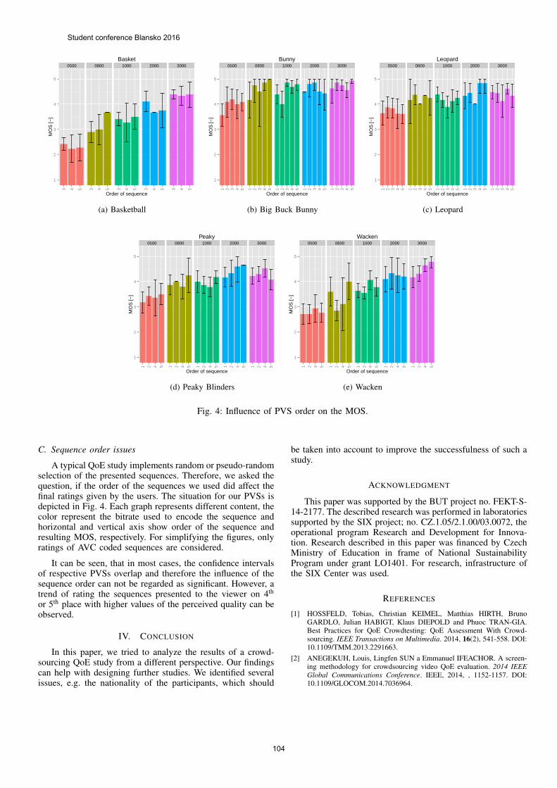
0500 0800 1000 2000 3000
57 13 18 19 6 3 44 11 18 19 3 4 41 15 13
1
2
3
4
5
3 4 5 3 4 5 3 4 5 3 4 5 3 4 5Order of sequence
MO
S [−
]
Basket
(a) Basketball
0500 0800 1000 2000 3000
2311212234 6 4 4 7 3 139211614 2 5 7 6 7 8 7201816
1
2
3
4
5
1 2 3 4 5 1 2 3 4 5 1 2 3 4 5 1 2 3 4 5 1 2 3 4 5
Order of sequence
MO
S [−
]
Bunny
(b) Big Buck Bunny
0500 0800 1000 2000 3000
141661626 6 8 1 3 4 131891612 9 9 3 6 6 211682312
1
2
3
4
5
1 2 3 4 5 1 2 3 4 5 1 2 3 4 5 1 2 3 4 5 1 2 3 4 5
Order of sequence
MO
S [−
]
Leopard
(c) Leopard
0500 0800 1000 2000 3000
22211114 15 1 5 4 19221411 6 9 5 3 9 201512
1
2
3
4
5
1 2 4 5 1 2 4 5 1 2 4 5 1 2 4 5 1 2 4 5
Order of sequence
MO
S [−
]
Peaky
(d) Peaky Blinders
0500 0800 1000 2000 3000
24211630 1013 9 9 25291523 10 9 4 5 23321714
1
2
3
4
5
1 2 4 5 1 2 4 5 1 2 4 5 1 2 4 5 1 2 4 5
Order of sequence
MO
S [−
]
Wacken
(e) Wacken
Fig. 4: Influence of PVS order on the MOS.
C. Sequence order issues
A typical QoE study implements random or pseudo-randomselection of the presented sequences. Therefore, we asked thequestion, if the order of the sequences we used did affect thefinal ratings given by the users. The situation for our PVSs isdepicted in Fig. 4. Each graph represents different content, thecolor represent the bitrate used to encode the sequence andhorizontal and vertical axis show order of the sequence andresulting MOS, respectively. For simplifying the figures, onlyratings of AVC coded sequences are considered.
It can be seen, that in most cases, the confidence intervalsof respective PVSs overlap and therefore the influence of thesequence order can not be regarded as significant. However, atrend of rating the sequences presented to the viewer on 4th
or 5th place with higher values of the perceived quality can beobserved.
IV. CONCLUSION
In this paper, we tried to analyze the results of a crowd-sourcing QoE study from a different perspective. Our findingscan help with designing further studies. We identified severalissues, e.g. the nationality of the participants, which should
be taken into account to improve the successfulness of such astudy.
ACKNOWLEDGMENT
This paper was supported by the BUT project no. FEKT-S-14-2177. The described research was performed in laboratoriessupported by the SIX project; no. CZ.1.05/2.1.00/03.0072, theoperational program Research and Development for Innova-tion. Research described in this paper was financed by CzechMinistry of Education in frame of National SustainabilityProgram under grant LO1401. For research, infrastructure ofthe SIX Center was used.
REFERENCES
[1] HOSSFELD, Tobias, Christian KEIMEL, Matthias HIRTH, BrunoGARDLO, Julian HABIGT, Klaus DIEPOLD and Phuoc TRAN-GIA.Best Practices for QoE Crowdtesting: QoE Assessment With Crowd-sourcing. IEEE Transactions on Multimedia. 2014, 16(2), 541-558. DOI:10.1109/TMM.2013.2291663.
[2] ANEGEKUH, Louis, Lingfen SUN a Emmanuel IFEACHOR. A screen-ing methodology for crowdsourcing video QoE evaluation. 2014 IEEEGlobal Communications Conference. IEEE, 2014, , 1152-1157. DOI:10.1109/GLOCOM.2014.7036964.
Student conference Blansko 2016
104

[3] SEUFERT, Michael, Ondrej ZACH, Tobias HOSSFELD, Martin SLAN-INA and Phuoc TRAN-GIA. Impact of test condition selection inadaptive crowdsourcing studies on subjective quality. 2016 Eighth In-ternational Conference on Quality of Multimedia Experience (QoMEX).IEEE, 2016, , 1-6. DOI: 10.1109/QoMEX.2016.7498939.
[4] ZACH, O. Let the Crowd Be Heard - A Crowdsourcing- based Study onVideo Coding. Proceedings of the 22nd Conference STUDENT EEICT2016. Brno: Vysok uen technick v Brn, Fakulta elektrotechniky akomunikanch technologi, 2016. p. 390-394.
[5] HOSSFELD, Tobias, Michael SEUFERT, Matthias HIRTH, ThomasZINNER, Phuoc TRAN-GIA and Raimund SCHATZ. Quantification ofYouTube QoE via Crowdsourcing. 2011 IEEE International Symposiumon Multimedia. IEEE, 2011, , 494-499. DOI: 10.1109/ISM.2011.87.
Student conference Blansko 2016
105