Department of Civil and Environmental Engineering - BIT Mesra
Upload
khangminh22Category
view
2download
0
Dr. Awatif Soaded & Dr. Basim H. Sanitary and Environmental Engineering 2019-2020
Page 1 of 10
These lectures are intended to be a guide documentation of the course held. Please, revise and check out the references if any errors or
discrepancies have occurred.
Sanitary and Environmental Engineering
PART 1: WATER SUPPLY ENGINEERING
Dr. Awatif Soaded & Dr. Basim H. Sanitary and Environmental Engineering 2019-2020
Page 2 of 10
These lectures are intended to be a guide documentation of the course held. Please, revise and check out the references if any errors or
discrepancies have occurred.
Sanitary and Environmental Engineering (Syllabus)
Assistant Professor Dr. Basim Hussein Khudair Al-Obaidi
E-Mail: [email protected]
Text Books:
1) Water Supply and Sewerage by: E. W. Steel and T. J. McGhee
2) Water Supply and Wastewater Engineering (Part 1 and 2) by: D.Lal and A. K. Upadhyay
FIRST SEMESTER
Part One: Water Supply Engineering
3-9 Introduction Lecture 1 Chapter One (1) (2)
10-22 Quantity of water: Consumption for various purposes, the per capita demand, variation in rate of consumption, factors affecting consumption, fire demand, forecasting population
Lecture 2 Chapter Two (1) (2)
23-36 Quality of water supplies: Impurities of water: Potable water, polluted water, water borne diseases, lead poisoning, fluoride, water bacteria, pathogen and coliform, soluble mineral, standards for drinking water
Lecture 3 Chapter Eight (1) Chapter Four (2)
37-55 Water distribution systems: The pipe system, design, of water distribution systems, flow in pipes, equivalent pipe method, hardy cross method
Lecture 4 Chapter Six (1) (2)
56-64 Collection and distribution of water: Intakes, intakes of impounding reservoirs, river intakes
Lecture 5 Chapter Six(1) Chapter Three(2)
65-73 Pumps and Pumping Stations: Classification of Pumps, Work and efficiency of pumps, Pump capacity, head, efficiency, and power, Effect of varying speed, Characteristics curves of centrifugal pumps, Suction lift, Cavitation, pump station.
Lecture 6 Chapter Seven(1)
74-83 Treatment of water–Clarification- Plain Sedimentation: Screens, principles of sedimentation, discrete particles, sedimentation tank details, scour.
Lecture 7 Chapter Nine(1) Chapter Five(2)
84-98 Treatment of water–Clarification- Sedimentation with chemicals (Coagulation and Flocculation): purposes and action of coagulation, simplified coagulation reactions, mixing, flocculation, suspended solids contact clarifiers, design criteria
Lecture 8 Chapter Nine(1) Chapter Five(2)
99-112 Treatment of water-Filtration: Filter types, rapid filters, theory of filtration through coarse media, filter media, gravel, filtration rates, under drain system, washing process, operating problems, pressure filters
Lecture 9 Chapter Ten(1) Chapter Five(2)
113-119 Miscellaneous water treatment methods-Disinfection: Chlorine in water, chlorination, chloramines, use of chlorine gas, hypochlorination, other disinfection techniques, water softening, cation exchange method
Lecture 10 Chapter Eleven(1) Chapter Five(2)
120-128 Special Treatments: Hardness Removal or Water Softening: water hardness, Softening Processes, Ion Exchange method, Membrane filtration.
Lecture 11 Chapter Eleven(1)
Dr. Awatif Soaded & Dr. Basim H. Sanitary and Environmental Engineering 2019-2020
Page 3 of 10
These lectures are intended to be a guide documentation of the course held. Please, revise and check out the references if any errors or
discrepancies have occurred.
PART 1: WATER SUPPLY ENGINEERING
Lecture 1: Introduction
Sanitary Engineering: The branch of civil engineering associated with the supply of water, disposal of
sewage, other public health services and the management of water and sewage in civil engineering.
Sanitary Engineer:
1. An expert or specialist in the branch of civil engineering associated with the supply of water, collect and disposal of sewage, and other public health services.
2. An engineer whose training or occupation is in sanitary engineering.
3. An engineer specializing in the maintenance of urban environmental conditions conductive to the preservation of public health.
Work of sanitary engineering:
The development of sanitary engineering has paralleled and contributed to the growth of cities. Without
an adequate supply of safe water, the great city could not exist, and life in it would be both unpleasant and
dangerous unless and other wastes were promptly removed. The concentration of population in relatively
small areas has made the task of the sanitary engineer more complex.
Groundwater supplies are frequently inadequate to the huge demand and surface waters, polluted by
cities, towns, and villages on watersheds, must be treated more and more elaborated as the population
density increases. Industry also demands more and better water from all available sources. The river
receives ever-increasing amounts of sewage and industrial wastes, thus requiring more attention to sewage
treatment, stream pollution, and the complicated phenomena of self-purification.
The public looks to the sanitary engineer for assistance in such matters as design, construction, and
operation of water and sewage works are treated, the control of malaria by mosquito control, the
eradication of other dangerous insects, rodent control collection and disposal of municipal refuse,
industrial hygiene, and sanitation of housing and swimming pools. The activities just given, which are likely
to be controlled by local or state health departments, are sometimes known as public health or
environmental engineering, terms which while descriptive are not accepted by all engineering. The terms,
however, are indicative of the important place the engineer holds in the field of public health and in the
prevention of diseases.
EPA: Environmental Protection Agency
NPSES: National Pollutional Discharge Elimination System
FWPCA: Federal Water Pollution Control Administration
USPHS: U.S. Public Health Service
Dr. Awatif Soaded & Dr. Basim H. Sanitary and Environmental Engineering 2019-2020
Page 4 of 10
These lectures are intended to be a guide documentation of the course held. Please, revise and check out the references if any errors or discrepancies have occurred.
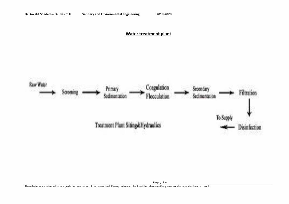
Water treatment plant

Dr. Awatif Soaded & Dr. Basim H. Sanitary and Environmental Engineering 2019-2020
Page 5 of 10
These lectures are intended to be a guide documentation of the course held. Please, revise and check out the references if any errors or discrepancies have occurred.
Dr. Awatif Soaded & Dr. Basim H. Sanitary and Environmental Engineering 2019-2020
Page 6 of 10
These lectures are intended to be a guide documentation of the course held. Please, revise and check out the references if any errors or discrepancies have occurred.
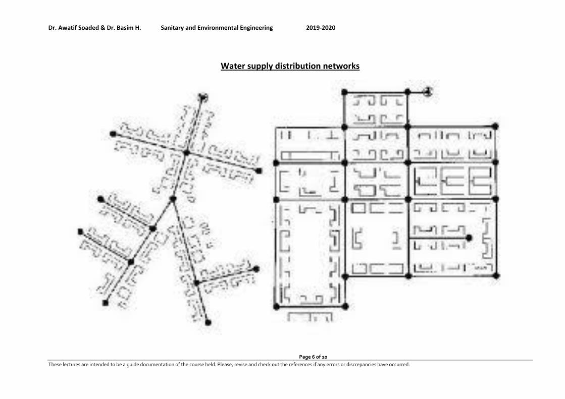
Water supply distribution networks
Dr. Awatif Soaded & Dr. Basim H. Sanitary and Environmental Engineering 2019-2020
Page 7 of 10
These lectures are intended to be a guide documentation of the course held. Please, revise and check out the references if any errors or discrepancies have occurred.
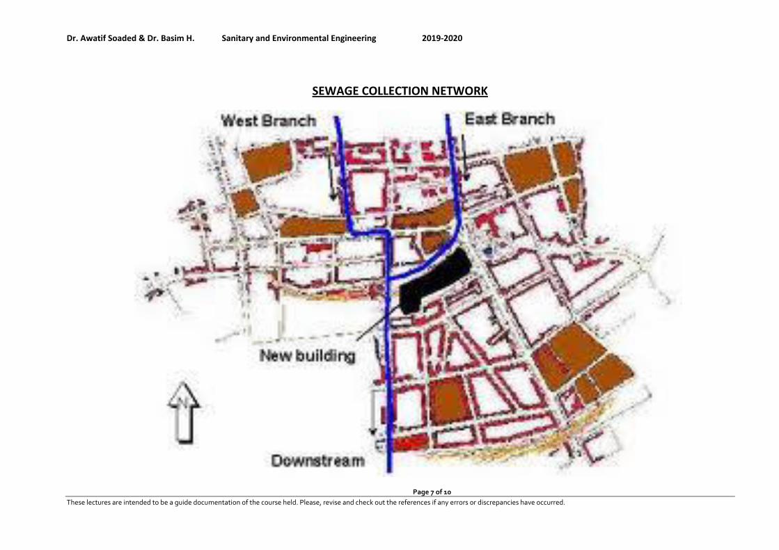
SEWAGE COLLECTION NETWORK
Dr. Awatif Soaded & Dr. Basim H. Sanitary and Environmental Engineering 2019-2020
Page 8 of 10
These lectures are intended to be a guide documentation of the course held. Please, revise and check out the references if any errors or discrepancies have occurred.
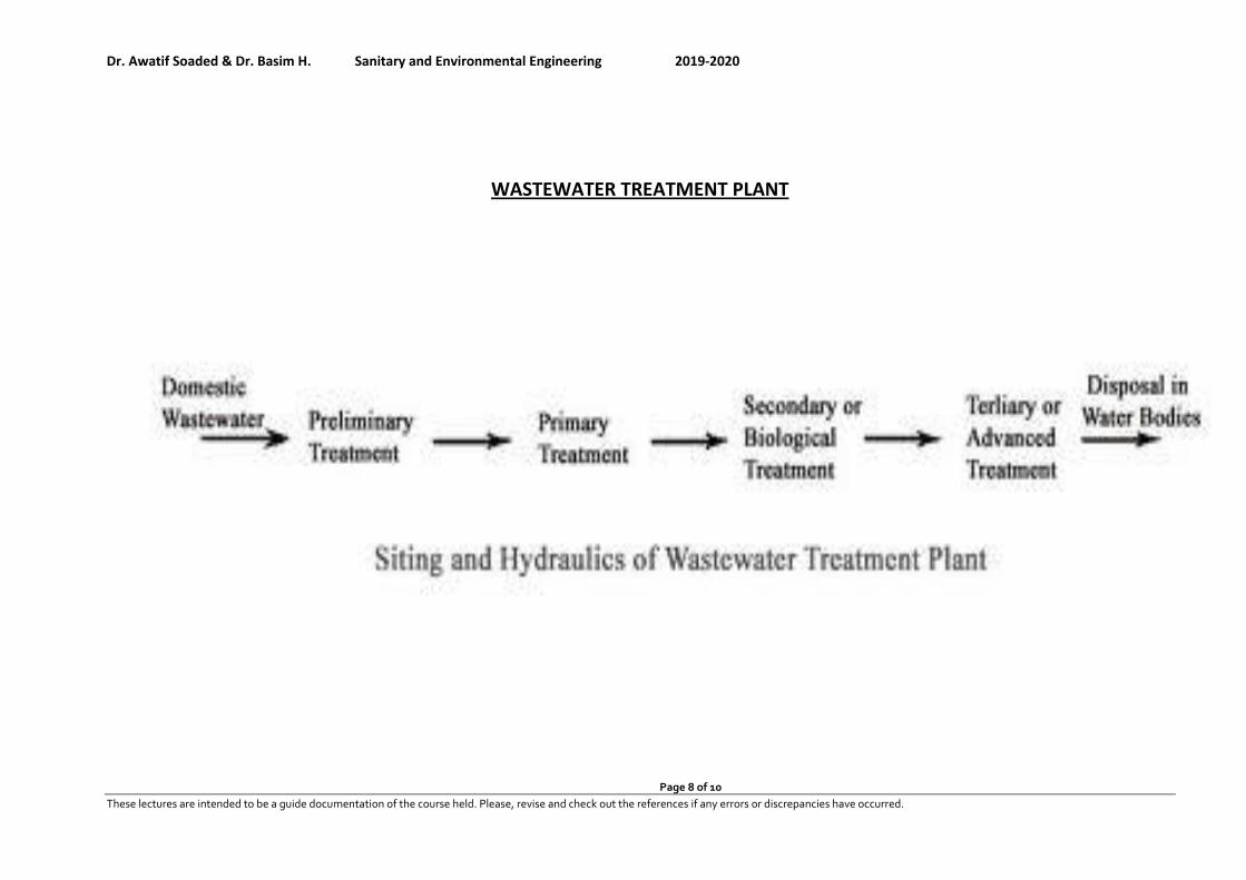
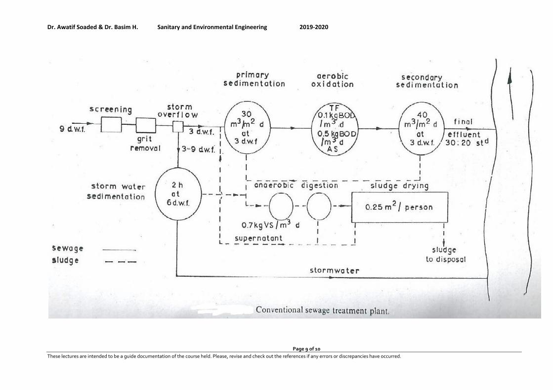
WASTEWATER TREATMENT PLANT
Dr. Awatif Soaded & Dr. Basim H. Sanitary and Environmental Engineering 2019-2020
Page 9 of 10
These lectures are intended to be a guide documentation of the course held. Please, revise and check out the references if any errors or discrepancies have occurred.

Dr. Awatif Soaded & Dr. Basim H. Sanitary and Environmental Engineering 2018-2019
Page 10 of 10
These lectures are intended to be a guide documentation of the course held. Please, revise and check out the references if any errors or
discrepancies have occurred.
How to Choose a DRM Software to protect your document?
Dr. Awatif Soaded & Dr. Basim H. Sanitary and Environmental Engineering 2019-2020
Page 1 of 14
These lectures are intended to be a guide documentation of the course held. Please, revise and check out the references if any errors or
discrepancies have occurred.
Sanitary and Environmental Engineering
PART 1: WATER SUPPLY ENGINEERING
Dr. Awatif Soaded & Dr. Basim H. Sanitary and Environmental Engineering 2019-2020
Page 2 of 14
These lectures are intended to be a guide documentation of the course held. Please, revise and check out the references if any errors or
discrepancies have occurred.
PART 1: WATER SUPPLY ENGINEERING
Lecture 2: Quantity of Water
Water Consumption
In the design of any waterworks project it is necessary to estimate the amount of water that is required.
This involves determining the number of people who will be served and their per capita water consumption,
together with an analysis of factors that may operate to affect consumption.
It is usual to express water consumption in liters or gallons per capita per day, obtaining this figure by
dividing the total number of people in the city into the total daily water consumption. For many purposes
the average daily consumption is convenient. It is obtained by dividing the population into the total daily
consumption averaged over one year.
Water consumption (L
(Cap. day)) =
Total daily water consumption (L
day)
Total number of people in the city (Capita)
Average daily consumption (L
(Cap. day)) =
Total daily consumption averaged over one year (L
day)
Total population in the city (Capita)
Average daily per capita demand (L
(Cap. day)) =
Quantity Required in 12 Months (L
day)
(360 x Population (Capita)).
If this average demand is supplied at all the times, it will not be sufficient to meet the fluctuations.
Consumption for various purposes (Water Demand):
1. Domestic or Residential use 40 – 60% of the total water demand.
2. Industrial use 25- 30% a)domestic, b)industrial process
3. Commercial use 10 - 15%.
4. Public use 5 -10%.
5. Fire demand
For calculating the total water demand 10 -15% is added for losses and wastage.
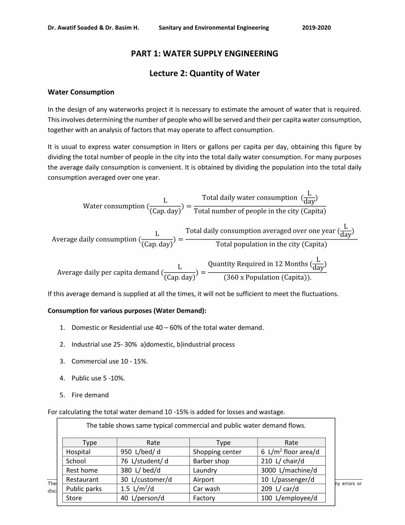
The table shows same typical commercial and public water demand flows.
Rate Type Rate Type
6 L/m2 floor area/d Shopping center 950 L/bed/ d Hospital
210 L/ chair/d Barber shop 76 L/student/ d School
3000 L/machine/d Laundry 380 L/ bed/d Rest home
10 L/passenger/d Airport 30 L/customer/d Restaurant
209 L/ car/d Car wash 1.5 L/m2/d Public parks
100 L/employee/d Factory 40 L/person/d Store

Dr. Awatif Soaded & Dr. Basim H. Sanitary and Environmental Engineering 2019-2020
Page 3 of 14
These lectures are intended to be a guide documentation of the course held. Please, revise and check out the references if any errors or
discrepancies have occurred.
Domestic or Residential demand:
Domestic demand (volume/time) = rate of consumption (volume/time/capita) X population (capita)
Industrial demand:
For water used in industrial processing, Symons formula maybe used water demand =12.2 m3/ 103 m2 floor area
per day. The table shows typical industrial water demands:
Consumption for various purposes (Summary):
Type of Consumption
Use Purposes Depend upon
Average Water
Demand (L/c.d)
Percentage of Total
Domestic Houses, hotels, etc
Sanitary, culinary, drinking, washing, bathing, air conditions of residences and irrigation or sprinkling of privately owned gardens or lawns
Living conditions of consumers
190-340 50
Commercial and industrial
Industrial and Commercial plants
Water process according to floor area per day (12.2m3/1000m2)
Local conditions
200 15-30
Public Public building and public service
- City halls, jails, and school. - flushing streets and fire protection)
Local conditions
50-75 10
Loss and waste
Uncounted Network, equipment Execution degree
50-75 10
Quantity m3/metric ton Type of industry
2 -3 Dairy
8 - 10 Chemicals
15 – 25 Meat packing
30 -60 Canning
200 – 800 Paper
260 - 300 Steel
250 - 350 Textile
80 gallon/barrel Petroleum
Dr. Awatif Soaded & Dr. Basim H. Sanitary and Environmental Engineering 2019-2020
Page 4 of 14
These lectures are intended to be a guide documentation of the course held. Please, revise and check out the references if any errors or
discrepancies have occurred.
Factors affecting water consumption (per capita demand):
1. Size of the city: Per capita demand for big cities is generally large as compared to that for smaller towns as
big cities have sewered houses.
2. Presence of industries and commerce.
3. Quality of water: If water is aesthetically and medically safe, the consumption will increase as people will
not depend to private wells, etc.
4. Cost of water.
5. Pressure in the water distribution system.
6. Climatic conditions.
7. Characteristics of population: Habits of people and their economic status.
8. Policy of metering and charging method: Water tax is charged in two different ways: on the basis of meter
reading and on the basis of certain fixed monthly rate.
9. Efficiency of waterworks administration: Leaks in water mains and services; and unauthorized use of water
can be kept to a minimum by surveys.
Fluctuations in Rate of Demand
1. Annual or yearly variation:
2. Seasonal variation: The demand peaks during summer. Fire break outs are generally more in summer,
increasing demand. So, there is seasonal variation.
3. Monthly variation:
4. Weekly variation:
5. Daily variation: Depends on the activity. People draw out more water on holidays and Festival days, thus
increasing demand on these days.
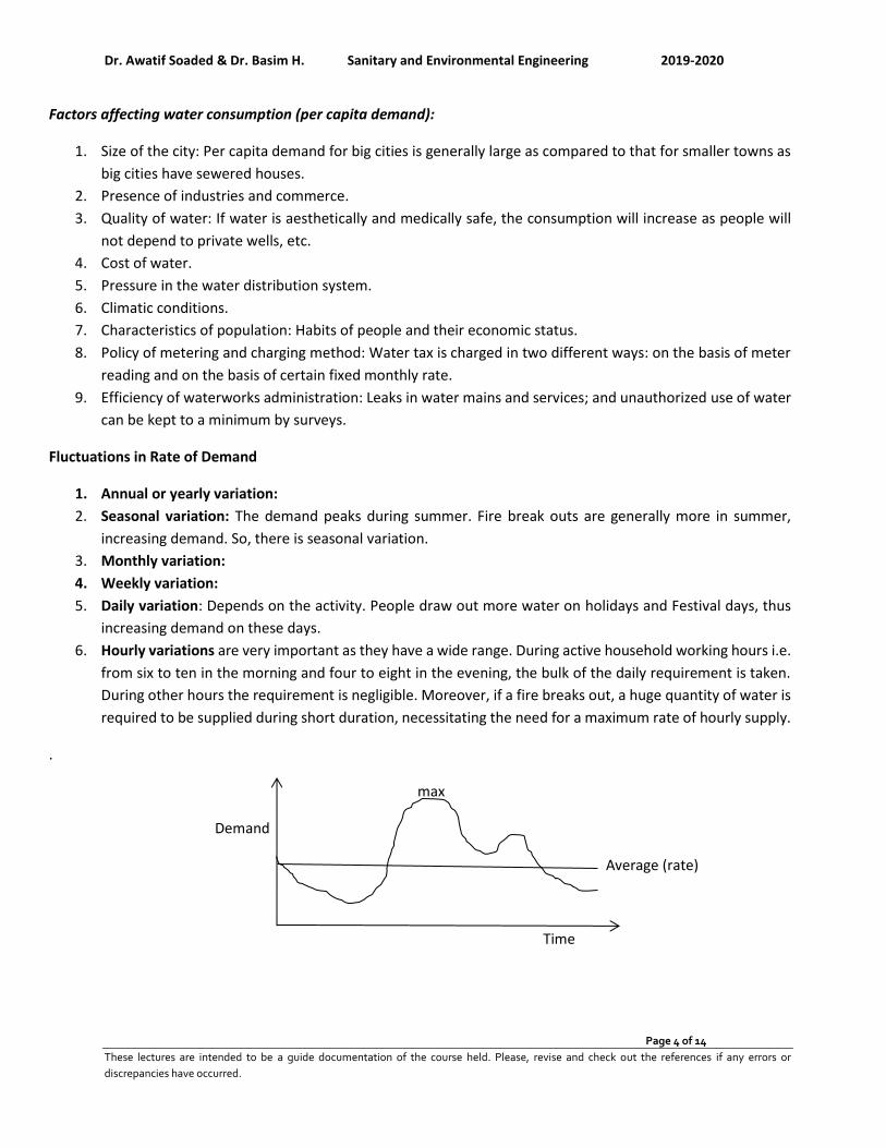
6. Hourly variations are very important as they have a wide range. During active household working hours i.e.
from six to ten in the morning and four to eight in the evening, the bulk of the daily requirement is taken.
During other hours the requirement is negligible. Moreover, if a fire breaks out, a huge quantity of water is
required to be supplied during short duration, necessitating the need for a maximum rate of hourly supply.
.
max
Demand
Average (rate)
Time
Dr. Awatif Soaded & Dr. Basim H. Sanitary and Environmental Engineering 2019-2020
Page 5 of 14
These lectures are intended to be a guide documentation of the course held. Please, revise and check out the references if any errors or
discrepancies have occurred.
So, an adequate quantity of water must be available to meet the peak demand. To meet all the fluctuations, the
supply pipes, service reservoirs and distribution pipes must be properly proportioned. The water is supplied by
pumping directly and the pumps and distribution system must be designed to meet the peak demand. The effect of
monthly variation influences the design of storage reservoirs and the hourly variations influences the design of
pumps and service reservoirs. As the population decreases, the fluctuation rate increases. Figure above shows
variation of water consumption with time.
Goodrich formula to estimate the percentage of annual average consumption ( p = 180 t -0.1 )
Where: p = percentage of the annual average consumption for time t
t = time in day (2hr/24 – 360). Hence; day (t=1), weekly (t=7), monthly (30) and yearly (360).
The formula gives the percentage of the maximum daily as 180 percent, the weekly consumption as 148 percent,
and the monthly as 128 percent of the average daily demand. The maximum hourly consumption is likely to be
about 150 percent of the maximum for that day.
Maximum hourly demand of maximum day i.e. Peak demand in certain area of a city will affect design of the distribution system while minimum rate of consumption is of less important than maximum flow but is required in connection with design of pump plants, usually it will vary from (25-50) percent of the daily demand.
Average daily demand = Average water consumption (L/Cap.day) x NO. of population
Maximum daily demand = p x average daily demand=1.8 x average daily demand
Maximum weekly demand = p x average daily demand=1.48 x average daily demand
Maximum monthly demand = p x average daily demand=1.28 x average daily demand
Maximum hourly demand = p x maximum daily demand =1.5 x maximum daily demand=1.5 x 1.8 x average daily demand=2.7 x average daily demand
Minimum hourly demand = p x maximum daily demand = 0.5 x maximum daily demand=0.5 x 1.8 x average daily demand=0.9 x average daily demand
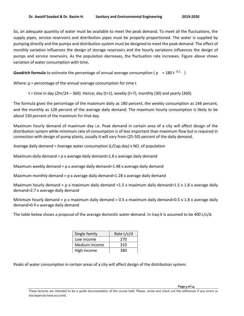
The table below shows a proposal of the average domestic water demand. In Iraq it is assumed to be 400 L/c/d.
Peaks of water consumption in certain areas of a city will affect design of the distribution system.
Rate L/c/d Single family
270 Low income
310 Medium income
380 High income
Dr. Awatif Soaded & Dr. Basim H. Sanitary and Environmental Engineering 2019-2020
Page 6 of 14
These lectures are intended to be a guide documentation of the course held. Please, revise and check out the references if any errors or
discrepancies have occurred.
Fire demand
Firefighting systems: a) with water, b) without water
a) Firefighting systems using water
1-Hydrants: an outdoor system 2-Hose reel: an indoor system 3- Sprinkler: an indoor system b) Firefighting systems without water
Fire extinguishers are used with engineering criteria for location and number of cylinders. It should not be used for:
1) electrical risk, 2) flammable liquids.
Fire demand formulas: The per capita fire demand is very less on an average basis but the rate at which the water
is required is very large. The rate of fire demand is sometimes treated as a function of population and is worked out
from following empirical formulas:
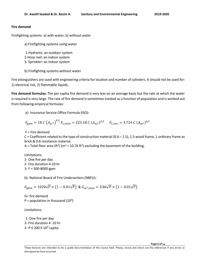
a)- Insurance Service Office Formula (ISO):
𝐹𝑔𝑝𝑚 = 18 𝐶 (𝐴𝑓𝑡2)0.5
𝐹𝐿/𝑚𝑖𝑛 = 223.18 𝐶 (𝐴𝑚2)0.5 𝐹𝐿/𝑠𝑒𝑐 = 3.724 𝐶 (𝐴𝑚2)0.5
F = Fire demand C = Coefficient related to the type of construction material (0.6 – 1.5), 1.5 wood frame, 1 ordinary frame as brick & 0.6 resistance material. A = Total floor area (ft2) (m2 = 10.76 ft2) excluding the basement of the building. Limitations: 1- One fire per day 2- Fire duration 4-10 hr 3- F = 500-8000 gpm b)- National Board of Fire Underwriters (NBFU):
𝐺𝑔𝑝𝑚 = 1020√𝑃 × (1 − 0.01√𝑃) & 𝐺𝑚3/𝑚𝑖𝑛 = 3.86√𝑃 × (1 − 0.01√𝑃)
G= fire demand P = population in thousand (103) Limitations:
1- One fire per day
2- Fire duration 4 -10 hr
3- P ≤ 200 X 103 capita
Dr. Awatif Soaded & Dr. Basim H. Sanitary and Environmental Engineering 2019-2020
Page 7 of 14
These lectures are intended to be a guide documentation of the course held. Please, revise and check out the references if any errors or
discrepancies have occurred.
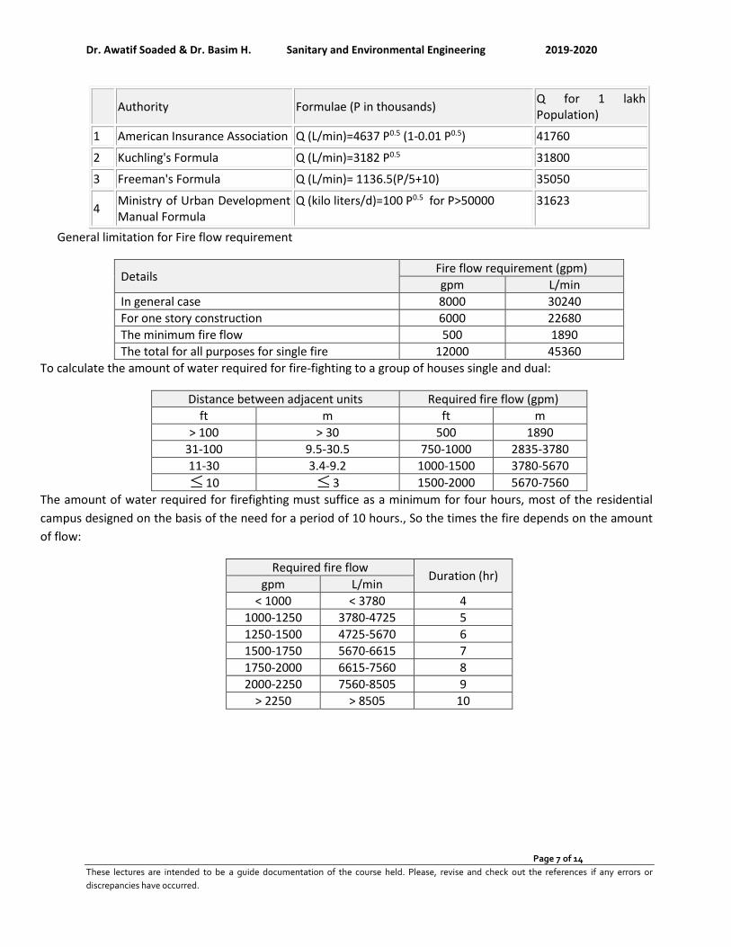
Authority Formulae (P in thousands) Q for 1 lakh Population)
1 American Insurance Association Q (L/min)=4637 P0.5 (1-0.01 P0.5) 41760
2 Kuchling's Formula Q (L/min)=3182 P0.5 31800
3 Freeman's Formula Q (L/min)= 1136.5(P/5+10) 35050
4 Ministry of Urban Development Manual Formula
Q (kilo liters/d)=100 P0.5 for P>50000 31623
General limitation for Fire flow requirement
Fire flow requirement (gpm) Details
L/min gpm
30240 8000 In general case
22680 6000 For one story construction
1890 500 The minimum fire flow
45360 12000 The total for all purposes for single fire
To calculate the amount of water required for fire-fighting to a group of houses single and dual:
Distance between adjacent units Required fire flow (gpm)
ft m ft m
> 100 > 30 500 1890
31-100 9.5-30.5 750-1000 2835-3780
11-30 3.4-9.2 1000-1500 3780-5670
10 3 1500-2000 5670-7560
The amount of water required for firefighting must suffice as a minimum for four hours, most of the residential
campus designed on the basis of the need for a period of 10 hours., So the times the fire depends on the amount
of flow:
Required fire flow Duration (hr)
gpm L/min
< 1000 < 3780 4
1000-1250 3780-4725 5
1250-1500 4725-5670 6
1500-1750 5670-6615 7
1750-2000 6615-7560 8
2000-2250 7560-8505 9
> 2250 > 8505 10
Dr. Awatif Soaded & Dr. Basim H. Sanitary and Environmental Engineering 2019-2020
Page 8 of 14
These lectures are intended to be a guide documentation of the course held. Please, revise and check out the references if any errors or
discrepancies have occurred.
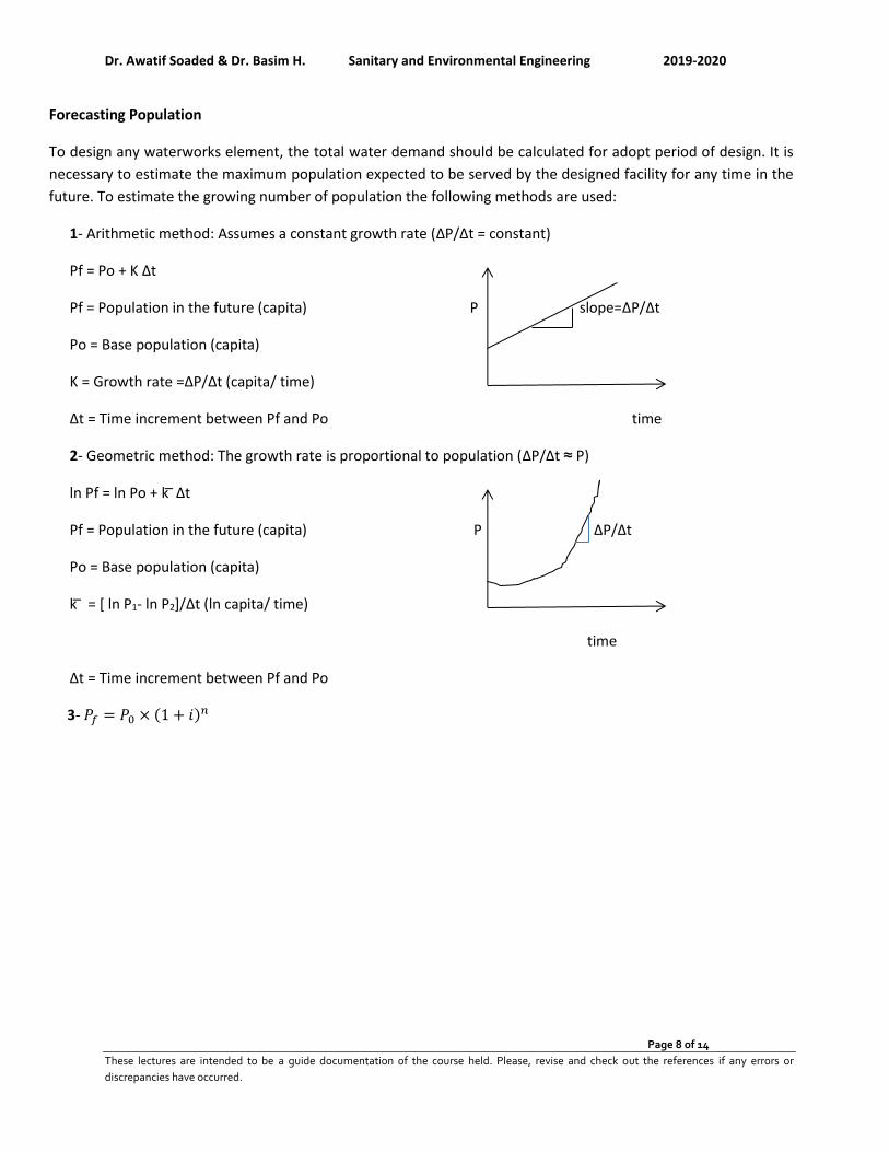
Forecasting Population
To design any waterworks element, the total water demand should be calculated for adopt period of design. It is
necessary to estimate the maximum population expected to be served by the designed facility for any time in the
future. To estimate the growing number of population the following methods are used:
1- Arithmetic method: Assumes a constant growth rate (∆P/∆t = constant)
Pf = Po + K ∆t
Pf = Population in the future (capita) P slope=∆P/∆t
Po = Base population (capita)
K = Growth rate =∆P/∆t (capita/ time)
∆t = Time increment between Pf and Po time
2- Geometric method: The growth rate is proportional to population (∆P/∆t ≈ P)
ln Pf = ln Po + k ̅∆t
Pf = Population in the future (capita) P ∆P/∆t
Po = Base population (capita)
k ̅ = [ ln P1- ln P2]/∆t (ln capita/ time)
time
∆t = Time increment between Pf and Po
3- 𝑃𝑓 = 𝑃0 × (1 + 𝑖)𝑛
Dr. Awatif Soaded & Dr. Basim H. Sanitary and Environmental Engineering 2019-2020
Page 9 of 14
These lectures are intended to be a guide documentation of the course held. Please, revise and check out the references if any errors or
discrepancies have occurred.
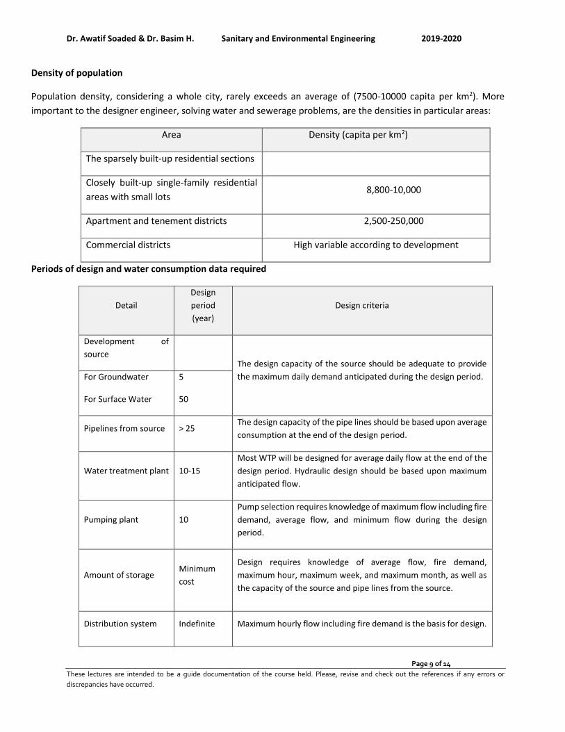
Density of population
Population density, considering a whole city, rarely exceeds an average of (7500-10000 capita per km2). More
important to the designer engineer, solving water and sewerage problems, are the densities in particular areas:
Area Density (capita per km2)
The sparsely built-up residential sections 3,800
Closely built-up single-family residential
areas with small lots 8,800-10,000
Apartment and tenement districts 2,500-250,000
Commercial districts High variable according to development
Periods of design and water consumption data required
Detail
Design
period
(year)
Design criteria
Development of
source
The design capacity of the source should be adequate to provide
the maximum daily demand anticipated during the design period. For Groundwater
For Surface Water
5
50
Pipelines from source > 25 The design capacity of the pipe lines should be based upon average
consumption at the end of the design period.
Water treatment plant 10-15
Most WTP will be designed for average daily flow at the end of the
design period. Hydraulic design should be based upon maximum
anticipated flow.
Pumping plant 10
Pump selection requires knowledge of maximum flow including fire
demand, average flow, and minimum flow during the design
period.
Amount of storage Minimum
cost
Design requires knowledge of average flow, fire demand,
maximum hour, maximum week, and maximum month, as well as
the capacity of the source and pipe lines from the source.
Distribution system Indefinite Maximum hourly flow including fire demand is the basis for design.
Dr. Awatif Soaded & Dr. Basim H. Sanitary and Environmental Engineering 2019-2020
Page 10 of 14
These lectures are intended to be a guide documentation of the course held. Please, revise and check out the references if any errors or
discrepancies have occurred.
Solved problems
Problem 2.1: Find the maximum daily domestic demand for a population of 1000 capita with a rate of 300 L/c/d?
Solution:
Average domestic daily demand=1000 x300=300 x103 L/day=300 m3/day
Maximum daily demand =1.8 x average daily demand=1.8 x300=540 m3/day
Problem 2.2: For the above Problem find the maximum demand if p = 250%?
Average domestic daily demand=1000 x300=300 x103 L/day=300 m3/day
Maximum daily demand =2.5 x average daily demand=2.5 x300=750 m3/day
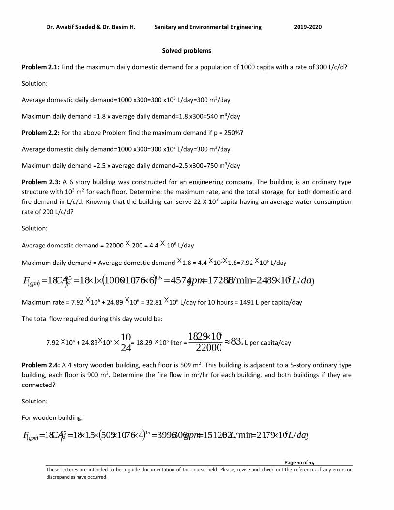
Problem 2.3: A 6 story building was constructed for an engineering company. The building is an ordinary type
structure with 103 m2 for each floor. Determine: the maximum rate, and the total storage, for both domestic and
fire demand in L/c/d. Knowing that the building can serve 22 X 103 capita having an average water consumption
rate of 200 L/c/d?
Solution:
Average domestic demand = 22000 200 = 4.4 106 L/day
Maximum daily demand = Average domestic demand 1.8 = 4.4 1061.8=7.92 106 L/day
( ) ( ) dayLLgpmCAFftgpm /1089.24min/172884574676.10100011818 65.05.0
2 =====
Maximum rate = 7.92 106 + 24.89 106 = 32.81 106 L/day for 10 hours = 1491 L per capita/day
The total flow required during this day would be:
7.92 106 + 24.89106 2410
= 18.29 106 liter = 83222000
1029.18 6
L per capita/day
Problem 2.4: A 4 story wooden building, each floor is 509 m2. This building is adjacent to a 5-story ordinary type
building, each floor is 900 m2. Determine the fire flow in m3/hr for each building, and both buildings if they are
connected?
Solution:
For wooden building:
( ) ( ) dayLLgpmCAFftgpm /1079.21min/02.15126306.3996476.105095.11818 65.05.0
2 =====
Dr. Awatif Soaded & Dr. Basim H. Sanitary and Environmental Engineering 2019-2020
Page 11 of 14
These lectures are intended to be a guide documentation of the course held. Please, revise and check out the references if any errors or
discrepancies have occurred.
For ordinary building:
( ) ( ) dayLLgpmCAFftgpm /1059.21min/696.1499181.3960576.109000.11818 65.05.0
2 =====
By using the fractional area:
𝑇𝑜𝑡𝑎𝑙 𝑎𝑟𝑒𝑎 = 4 × 509 + 5 × 900 = 6536 𝑚2
𝐹𝑟𝑎𝑐𝑡𝑖𝑜𝑛 𝑓𝑜𝑟 𝑤𝑜𝑜𝑑𝑒𝑛 𝑏𝑢𝑖𝑙𝑑𝑖𝑛𝑔 =4 × 509
6536= 0.311
𝐹𝑟𝑎𝑐𝑡𝑖𝑜𝑛 𝑓𝑜𝑟 𝑜𝑟𝑑𝑖𝑛𝑎𝑟𝑦 𝑏𝑢𝑖𝑙𝑑𝑖𝑛𝑔 =5 × 900
6536= 0.689
𝑇𝑜𝑡𝑎𝑙 𝑓𝑖𝑟𝑒 𝑓𝑙𝑜𝑤
= 18
× [1.5 × 0.311 × √4 × 509 × 10.76 + 1 × 0.689 × √5 × 900 × 10.76 = 3971.844 𝑔𝑝𝑚
= 902𝑚3
ℎ𝑟= 21648.138
𝑚3
𝑑𝑎𝑦]
Which equivalent to 16500 population
Problem 2.5: For the data given find the population in year 2035.
2005 1995 1985 1975 1965 Year
32000 38100 33500 29000 24700 Population
Solution:
Info
rmatio
n
year
po
pu
lation
∆P ∆t
Arithmetic method Geometric method
K KAverage Pt k kAverage LN (Pt) Pt
1965 24700
1975 29000 4300 10 430 0.016049
1985 33500 4500 10 450 0.014425
1995 38100 4600 10 460 0.012867
Base year 2005 32000 6100 10 610 487.5 -0.01745 0.006473
Period design (t)
30
First stage 2020 39312.5 10.47059 35263.05
Second stage 2035 46625 10.56769 38858.83
Dr. Awatif Soaded & Dr. Basim H. Sanitary and Environmental Engineering 2019-2020
Page 12 of 14
These lectures are intended to be a guide documentation of the course held. Please, revise and check out the references if any errors or
discrepancies have occurred.
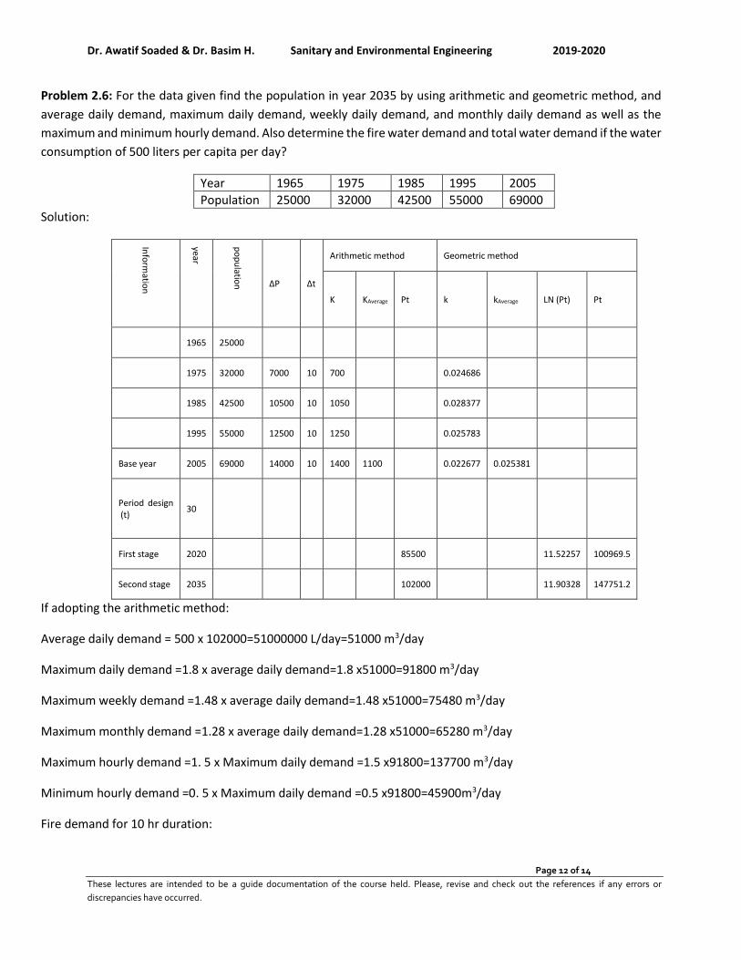
Problem 2.6: For the data given find the population in year 2035 by using arithmetic and geometric method, and
average daily demand, maximum daily demand, weekly daily demand, and monthly daily demand as well as the
maximum and minimum hourly demand. Also determine the fire water demand and total water demand if the water
consumption of 500 liters per capita per day?
2005 1995 1985 1975 1965 Year
69000 55000 42500 32000 25000 Population
Solution:
Info
rmatio
n
year
po
pu
lation
∆P ∆t
Arithmetic method Geometric method
K KAverage Pt k kAverage LN (Pt) Pt
1965 25000
1975 32000 7000 10 700 0.024686
1985 42500 10500 10 1050 0.028377
1995 55000 12500 10 1250 0.025783
Base year 2005 69000 14000 10 1400 1100 0.022677 0.025381
Period design (t)
30
First stage 2020 85500 11.52257 100969.5
Second stage 2035 102000 11.90328 147751.2
If adopting the arithmetic method:
Average daily demand = 500 x 102000=51000000 L/day=51000 m3/day
Maximum daily demand =1.8 x average daily demand=1.8 x51000=91800 m3/day
Maximum weekly demand =1.48 x average daily demand=1.48 x51000=75480 m3/day
Maximum monthly demand =1.28 x average daily demand=1.28 x51000=65280 m3/day
Maximum hourly demand =1. 5 x Maximum daily demand =1.5 x91800=137700 m3/day
Minimum hourly demand =0. 5 x Maximum daily demand =0.5 x91800=45900m3/day
Fire demand for 10 hr duration:
Dr. Awatif Soaded & Dr. Basim H. Sanitary and Environmental Engineering 2019-2020
Page 13 of 14
These lectures are intended to be a guide documentation of the course held. Please, revise and check out the references if any errors or
discrepancies have occurred.
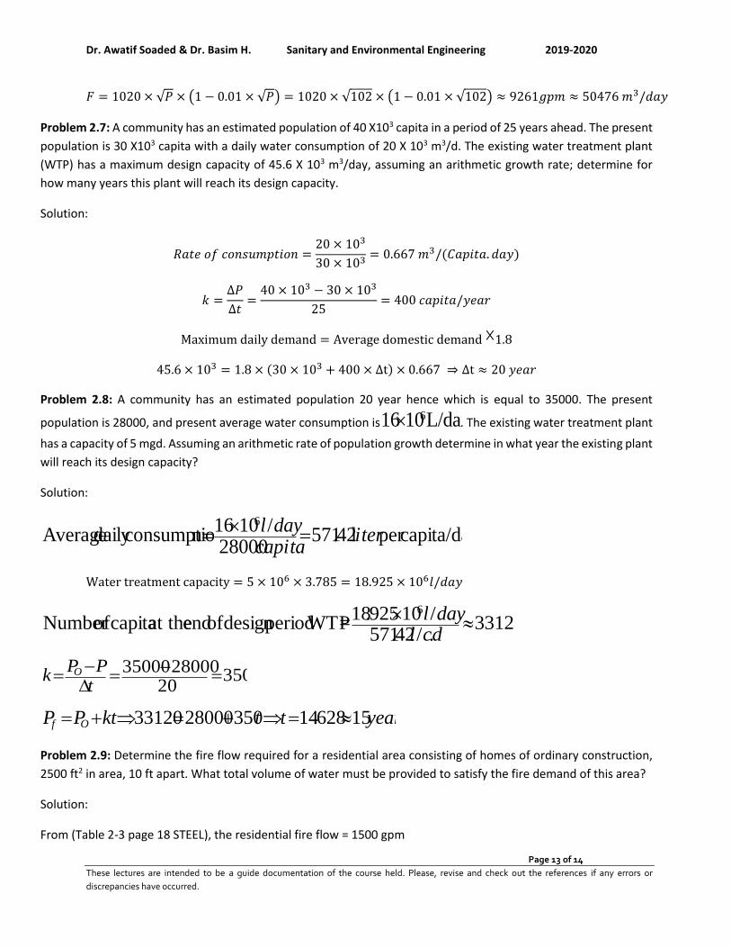
𝐹 = 1020 × √𝑃 × (1 − 0.01 × √𝑃) = 1020 × √102 × (1 − 0.01 × √102) ≈ 9261𝑔𝑝𝑚 ≈ 50476 𝑚3/𝑑𝑎𝑦
Problem 2.7: A community has an estimated population of 40 X103 capita in a period of 25 years ahead. The present
population is 30 X103 capita with a daily water consumption of 20 X 103 m3/d. The existing water treatment plant
(WTP) has a maximum design capacity of 45.6 X 10³ m3/day, assuming an arithmetic growth rate; determine for
how many years this plant will reach its design capacity.
Solution:
𝑅𝑎𝑡𝑒 𝑜𝑓 𝑐𝑜𝑛𝑠𝑢𝑚𝑝𝑡𝑖𝑜𝑛 =20 × 103
30 × 103= 0.667 𝑚3/(𝐶𝑎𝑝𝑖𝑡𝑎. 𝑑𝑎𝑦)
𝑘 =∆𝑃
∆𝑡=
40 × 103 − 30 × 103
25= 400 𝑐𝑎𝑝𝑖𝑡𝑎/𝑦𝑒𝑎𝑟
Maximum daily demand = Average domestic demand 1.8
45.6 × 103 = 1.8 × (30 × 103 + 400 × ∆t) × 0.667 ⇒ ∆t ≈ 20 𝑦𝑒𝑎𝑟
Problem 2.8: A community has an estimated population 20 year hence which is equal to 35000. The present
population is 28000, and present average water consumption is L/day1016 6 . The existing water treatment plant
has a capacity of 5 mgd. Assuming an arithmetic rate of population growth determine in what year the existing plant
will reach its design capacity?
Solution:
capita/dayper l42.57128000
/1016n consumptiodaily Average
6
itercapita
dayl=
=
Water treatment capacity = 5 × 106 × 3.785 = 18.925 × 10⁶𝑙/𝑑𝑎𝑦
33120./42.571/10925.18
= WTPperioddesign of end at the capita ofNumber 6
dcldayl
35020
2800035000=
−=
−
=tPP
k O
yearttktPP Of 15628.143502800033120 =+=+=
Problem 2.9: Determine the fire flow required for a residential area consisting of homes of ordinary construction,
2500 ft2 in area, 10 ft apart. What total volume of water must be provided to satisfy the fire demand of this area?
Solution:
From (Table 2-3 page 18 STEEL), the residential fire flow = 1500 gpm
Dr. Awatif Soaded & Dr. Basim H. Sanitary and Environmental Engineering 2019-2020
Page 14 of 14
These lectures are intended to be a guide documentation of the course held. Please, revise and check out the references if any errors or
discrepancies have occurred.
( ) ( ) gpmCAFftgpm 900250011818 5.05.0
2 ===
Water demand = 900 + 1500 = 2400 gpm = 9084 L/min = 545040 l/hr
33
22710001
2410
l/hr 545040 = V ml
m=
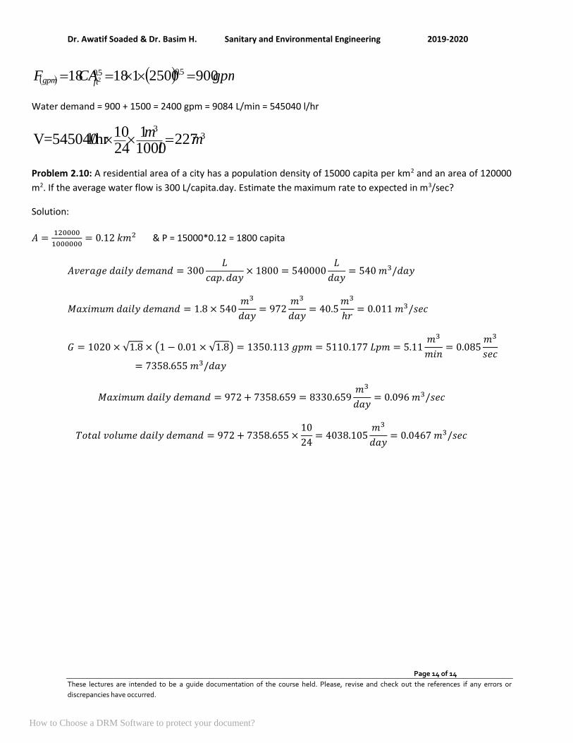
Problem 2.10: A residential area of a city has a population density of 15000 capita per km2 and an area of 120000
m2. If the average water flow is 300 L/capita.day. Estimate the maximum rate to expected in m3/sec?
Solution:
𝐴 =120000
1000000= 0.12 𝑘𝑚2 & P = 15000*0.12 = 1800 capita
𝐴𝑣𝑒𝑟𝑎𝑔𝑒 𝑑𝑎𝑖𝑙𝑦 𝑑𝑒𝑚𝑎𝑛𝑑 = 300𝐿
𝑐𝑎𝑝. 𝑑𝑎𝑦× 1800 = 540000
𝐿
𝑑𝑎𝑦= 540 𝑚3/𝑑𝑎𝑦
𝑀𝑎𝑥𝑖𝑚𝑢𝑚 𝑑𝑎𝑖𝑙𝑦 𝑑𝑒𝑚𝑎𝑛𝑑 = 1.8 × 540𝑚3
𝑑𝑎𝑦= 972
𝑚3
𝑑𝑎𝑦= 40.5
𝑚3
ℎ𝑟= 0.011 𝑚3/𝑠𝑒𝑐
𝐺 = 1020 × √1.8 × (1 − 0.01 × √1.8) = 1350.113 𝑔𝑝𝑚 = 5110.177 𝐿𝑝𝑚 = 5.11𝑚3
𝑚𝑖𝑛= 0.085
𝑚3
𝑠𝑒𝑐= 7358.655 𝑚3/𝑑𝑎𝑦
𝑀𝑎𝑥𝑖𝑚𝑢𝑚 𝑑𝑎𝑖𝑙𝑦 𝑑𝑒𝑚𝑎𝑛𝑑 = 972 + 7358.659 = 8330.659𝑚3
𝑑𝑎𝑦= 0.096 𝑚3/𝑠𝑒𝑐
𝑇𝑜𝑡𝑎𝑙 𝑣𝑜𝑙𝑢𝑚𝑒 𝑑𝑎𝑖𝑙𝑦 𝑑𝑒𝑚𝑎𝑛𝑑 = 972 + 7358.655 ×10
24= 4038.105
𝑚3
𝑑𝑎𝑦= 0.0467 𝑚3/𝑠𝑒𝑐
How to Choose a DRM Software to protect your document?

Dr. Awatif Soaded & Dr. Basim H. Sanitary and Environmental Engineering 2018-2019
Page 1 of 15
These lectures are intended to be a guide documentation of the course held. Please, revise and check out the references if any errors or
discrepancies have occurred.
Sanitary and Environmental Engineering
PART 1: WATER SUPPLY ENGINEERING

Dr. Awatif Soaded & Dr. Basim H. Sanitary and Environmental Engineering 2018-2019
Page 2 of 15
These lectures are intended to be a guide documentation of the course held. Please, revise and check out the references if any errors or
discrepancies have occurred.
PART 1: WATER SUPPLY ENGINEERING
Lecture 3: Common Impurities in Water
Raw Water Source
The various sources of water can be classified into two categories:
1. Surface sources, such as (Ponds and lakes; Streams and rivers; Storage reservoirs; and Oceans,
generally not used for water supplies, at present).
2. Sub-surface sources or underground sources, such as (springs; Infiltration wells; and Wells and
Tube-wells).
Water is in continuous recirculation between the earth’s surface and the atmosphere through various
processes which are collectively bound under the heading ‘The Hydrological Cycle’ as shown in the diagram
below explains the hydrological cycle which maintains the balance of the world’s water.
Water absolutely pure is not found in nature. Water picks up different types of materials as it passes
through the hydrological cycle. These particles make the water not pure and are called impurities which
are suspended and dissolved in water.
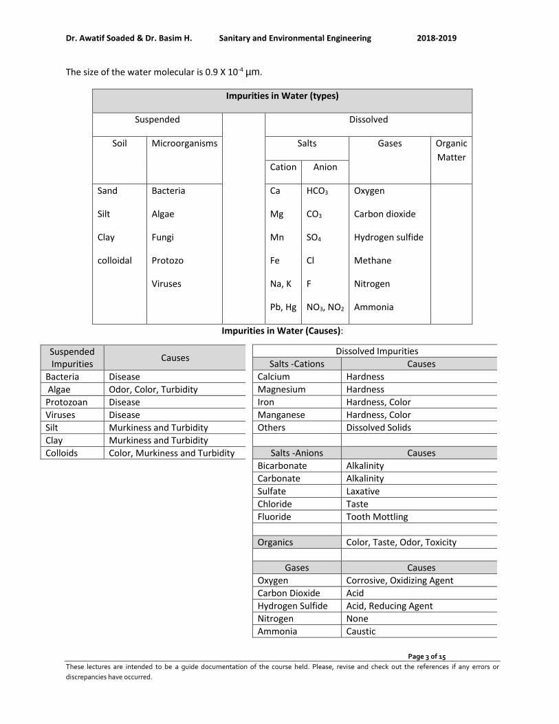
Impurities in Water (sizes)
10-7 10-6 10-5 10-4 10-3 10-2 10-1 1 mm
10-4 10-3 10-2 10-1 1 10 102 103 µm
Dissolved Suspended
Clay Silt Sand Colloidal
Viruses Bacteria
Protozoa, Algae, Fungi
Dr. Awatif Soaded & Dr. Basim H. Sanitary and Environmental Engineering 2018-2019
Page 3 of 15
These lectures are intended to be a guide documentation of the course held. Please, revise and check out the references if any errors or
discrepancies have occurred.
The size of the water molecular is 0.9 X 10⁻⁴ µm.
Impurities in Water (types)
Suspended Dissolved
Soil Microorganisms Salts Gases Organic
Matter Cation Anion
Sand
Silt
Clay
colloidal
Bacteria
Algae
Fungi
Protozo
Viruses
Ca
Mg
Mn
Fe
Na, K
Pb, Hg
HCO3
CO3
SO4
Cl
F
NO3, NO2
Oxygen
Carbon dioxide
Hydrogen sulfide
Methane
Nitrogen
Ammonia
Impurities in Water (Causes):
Suspended Impurities
Causes
Bacteria Disease
Algae Odor, Color, Turbidity
Protozoan Disease
Viruses Disease
Silt Murkiness and Turbidity
Clay Murkiness and Turbidity
Colloids Color, Murkiness and Turbidity
Dissolved Impurities
Salts -Cations Causes
Calcium Hardness
Magnesium Hardness
Iron Hardness, Color
Manganese Hardness, Color
Others Dissolved Solids
Salts -Anions Causes
Bicarbonate Alkalinity
Carbonate Alkalinity
Sulfate Laxative
Chloride Taste
Fluoride Tooth Mottling
Organics Color, Taste, Odor, Toxicity
Gases Causes
Oxygen Corrosive, Oxidizing Agent
Carbon Dioxide Acid
Hydrogen Sulfide Acid, Reducing Agent
Nitrogen None
Ammonia Caustic
Dr. Awatif Soaded & Dr. Basim H. Sanitary and Environmental Engineering 2018-2019
Page 4 of 15
These lectures are intended to be a guide documentation of the course held. Please, revise and check out the references if any errors or
discrepancies have occurred.
Impurities of water may be divided into two classes: 1. Suspended Impurities:
a) Microorganisms: They may get into water from the air with dust, etc., as rain falls, or commonly when soil polluted with human and animal wastes is washed into the water source. The latter type of impurity in water is the most dangerous one because a good number of microorganisms are pathogenic and cause disease.
b) Suspended solids: Minute particles of soil, clay, silt, soot particles, dead leaves and other insoluble material get into water because of erosion from higher ground, drainage from swamps, ponds, top soil, etc. Toxic chemicals such as insecticides and pesticides are also included in this category. They are introduced to streams either as industrial wastes or drained in after rain from land treated with these chemicals. Generally, suspended solids cause taste, color or turbidity.
c) Algae: Algae are minute plants that grow in still or stagnant water. Some algae are green, brown or red, and their presence in water causes taste, color and turbidity.
Some species of algae could be poisonous both for aquatic animals and humans. There are different types of algae found in water:
i. Asterionell – Gives water an unpleasant odor. ii. Spirogyra – Is a green scum found in small ponds and polluted water. It grows in thread like groups. It is
slippery and non-toxic. iii. Anabaena – Is blue- green and occurs in fishponds, pools, reservoir, and clogs filters.
2. Dissolved Impurities: a) Gases: Oxygen (O2), carbon dioxide (CO2), hydrogen sulphide (H2S), etc, find their way into water
as it falls as rain or, in the case of the latter two, from the soil as water percolates through the ground. All-natural water contains dissolved oxygen, and in certain circumstances carbon dioxide. The presence of CO2 and H2S (but not O2) causes acidity in water. In addition, H2S imparts a bad odor to the water.
b) Minerals: Minerals get into water as it percolates downward though the earth layers. The type of minerals dissolved will depend on the nature of the specific rock formation of an area. Most common dissolved minerals in water are salts of calcium, magnesium, sodium, potassium, etc. Salts of the first two elements cause hardness in water, while salts of the latter two elements cause alkalinity. Salts of toxic elements, such as lead, arsenic, chromium, etc, get into water mainly as industrial wastes dumped into streams.
c) Plant dyes: These originate from plants, which grow in or around water and cause acidity and color.
Dr. Awatif Soaded & Dr. Basim H. Sanitary and Environmental Engineering 2018-2019
Page 5 of 15
These lectures are intended to be a guide documentation of the course held. Please, revise and check out the references if any errors or
discrepancies have occurred.
Dr. Awatif Soaded & Dr. Basim H. Sanitary and Environmental Engineering 2018-2019
Page 6 of 15
These lectures are intended to be a guide documentation of the course held. Please, revise and check out the references if any errors or
discrepancies have occurred.
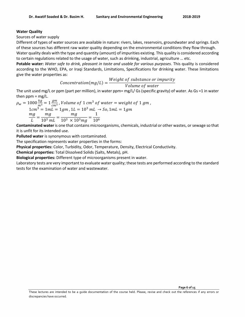
Water Quality Sources of water supply Different of types of water sources are available in nature: rivers, lakes, reservoirs, groundwater and springs. Each of these sources has different raw water quality depending on the environmental conditions they flow through. Water quality deals with the type and quantity (amount) of impurities existing. This quality is considered according to certain regulations related to the usage of water, such as drinking, industrial, agriculture … etc. Potable water: Water safe to drink, pleasant in taste and usable for various purposes. This quality is considered according to the WHO, EPA, or Iraqi Standards, Limitations, Specifications for drinking water. These limitations give the water properties as:
𝐶𝑜𝑛𝑐𝑒𝑛𝑡𝑟𝑎𝑡𝑖𝑜𝑛(𝑚𝑔/𝐿) =𝑊𝑒𝑖𝑔ℎ𝑡 𝑜𝑓 𝑠𝑢𝑏𝑠𝑡𝑎𝑛𝑐𝑒 𝑜𝑟 𝑖𝑚𝑝𝑢𝑟𝑖𝑡𝑦
𝑉𝑜𝑙𝑢𝑚𝑒 𝑜𝑓 𝑤𝑎𝑡𝑒𝑟
The unit used mg/L or ppm (part per million), in water ppm= mg/L/ Gs (specific gravity) of water. As Gs =1 in water then ppm = mg/L.
𝜌𝑤 = 1000𝑘𝑔
𝑚3 = 1𝑔𝑚
𝑐𝑚3 , 𝑉𝑜𝑙𝑢𝑚𝑒 𝑜𝑓 1 𝑐𝑚3 𝑜𝑓 𝑤𝑎𝑡𝑒𝑟 = 𝑤𝑒𝑖𝑔ℎ𝑡 𝑜𝑓 1 𝑔𝑚 ,
1𝑐𝑚3 = 1𝑚𝐿 = 1𝑔𝑚 , 1𝐿 = 103 𝑚𝐿 → 𝑆𝑜, 1𝑚𝐿 = 1𝑔𝑚 𝑚𝑔
𝐿=
𝑚𝑔
103 𝑚𝐿=
𝑚𝑔
103 × 103𝑚𝑔=
1
106
Contaminated water is one that contains microorganisms, chemicals, industrial or other wastes, or sewage so that it is unfit for its intended use. Polluted water is synonymous with contaminated. The specification represents water properties in the forms: Physical properties: Color, Turbidity, Odor, Temperature, Density, Electrical Conductivity. Chemical properties: Total Dissolved Solids (Salts, Metals), pH. Biological properties: Different type of microorganisms present in water. Laboratory tests are very important to evaluate water quality; these tests are performed according to the standard tests for the examination of water and wastewater.
Dr. Awatif Soaded & Dr. Basim H. Sanitary and Environmental Engineering 2018-2019
Page 7 of 15
These lectures are intended to be a guide documentation of the course held. Please, revise and check out the references if any errors or
discrepancies have occurred.
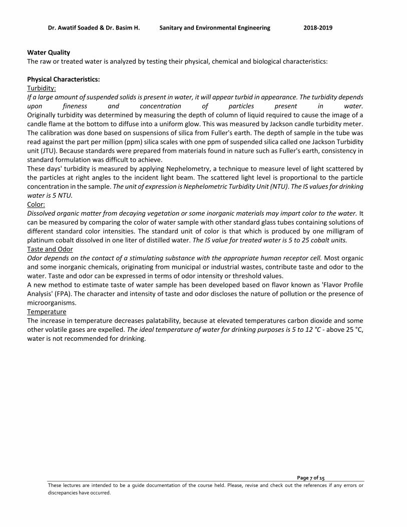
Water Quality The raw or treated water is analyzed by testing their physical, chemical and biological characteristics: Physical Characteristics: Turbidity: If a large amount of suspended solids is present in water, it will appear turbid in appearance. The turbidity depends upon fineness and concentration of particles present in water. Originally turbidity was determined by measuring the depth of column of liquid required to cause the image of a candle flame at the bottom to diffuse into a uniform glow. This was measured by Jackson candle turbidity meter. The calibration was done based on suspensions of silica from Fuller's earth. The depth of sample in the tube was read against the part per million (ppm) silica scales with one ppm of suspended silica called one Jackson Turbidity unit (JTU). Because standards were prepared from materials found in nature such as Fuller's earth, consistency in standard formulation was difficult to achieve. These days' turbidity is measured by applying Nephelometry, a technique to measure level of light scattered by the particles at right angles to the incident light beam. The scattered light level is proportional to the particle concentration in the sample. The unit of expression is Nephelometric Turbidity Unit (NTU). The IS values for drinking water is 5 NTU. Color: Dissolved organic matter from decaying vegetation or some inorganic materials may impart color to the water. It can be measured by comparing the color of water sample with other standard glass tubes containing solutions of different standard color intensities. The standard unit of color is that which is produced by one milligram of platinum cobalt dissolved in one liter of distilled water. The IS value for treated water is 5 to 25 cobalt units. Taste and Odor Odor depends on the contact of a stimulating substance with the appropriate human receptor cell. Most organic and some inorganic chemicals, originating from municipal or industrial wastes, contribute taste and odor to the water. Taste and odor can be expressed in terms of odor intensity or threshold values. A new method to estimate taste of water sample has been developed based on flavor known as 'Flavor Profile Analysis' (FPA). The character and intensity of taste and odor discloses the nature of pollution or the presence of microorganisms. Temperature The increase in temperature decreases palatability, because at elevated temperatures carbon dioxide and some other volatile gases are expelled. The ideal temperature of water for drinking purposes is 5 to 12 °C - above 25 °C, water is not recommended for drinking.
Dr. Awatif Soaded & Dr. Basim H. Sanitary and Environmental Engineering 2018-2019
Page 8 of 15
These lectures are intended to be a guide documentation of the course held. Please, revise and check out the references if any errors or
discrepancies have occurred.
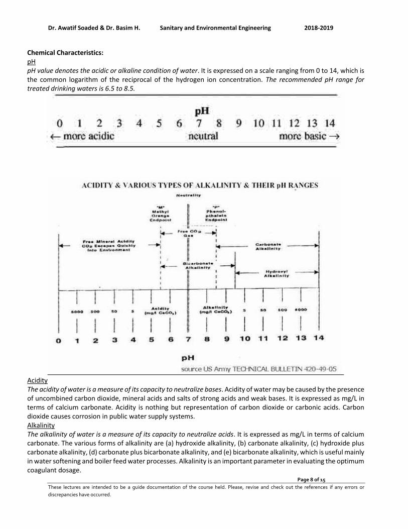
Chemical Characteristics: pH pH value denotes the acidic or alkaline condition of water. It is expressed on a scale ranging from 0 to 14, which is the common logarithm of the reciprocal of the hydrogen ion concentration. The recommended pH range for treated drinking waters is 6.5 to 8.5.
Acidity The acidity of water is a measure of its capacity to neutralize bases. Acidity of water may be caused by the presence of uncombined carbon dioxide, mineral acids and salts of strong acids and weak bases. It is expressed as mg/L in terms of calcium carbonate. Acidity is nothing but representation of carbon dioxide or carbonic acids. Carbon dioxide causes corrosion in public water supply systems. Alkalinity The alkalinity of water is a measure of its capacity to neutralize acids. It is expressed as mg/L in terms of calcium carbonate. The various forms of alkalinity are (a) hydroxide alkalinity, (b) carbonate alkalinity, (c) hydroxide plus carbonate alkalinity, (d) carbonate plus bicarbonate alkalinity, and (e) bicarbonate alkalinity, which is useful mainly in water softening and boiler feed water processes. Alkalinity is an important parameter in evaluating the optimum coagulant dosage.

Dr. Awatif Soaded & Dr. Basim H. Sanitary and Environmental Engineering 2018-2019
Page 9 of 15
These lectures are intended to be a guide documentation of the course held. Please, revise and check out the references if any errors or
discrepancies have occurred.
Hardness If water consumes excessive soap to produce lather, it is said to be hard. Hardness is caused by divalent metallic cations. The principal hardness causing cations are calcium, magnesium, strontium, ferrous and manganese ions. The major anions associated with these cations are sulphates, carbonates, bicarbonates, chlorides and nitrates. The total hardness of water is defined as the sum of calcium and magnesium concentrations, both expressed as calcium carbonate, in mg/L. Hardness are of two types, temporary or carbonate hardness and permanent or non-carbonate hardness. Temporary hardness is one in which bicarbonate and carbonate ion can be precipitated by prolonged boiling. Non-carbonate ions cannot be precipitated or removed by boiling, hence the term permanent hardness. IS value for drinking water is 300 mg/Las CaCO3. Chlorides Chloride ion may be present in combination with one or more of the cations of calcium, magnesium, iron and sodium. Chlorides of these minerals are present in water because of their high solubility in water. Each human being consumes about six to eight grams of sodium chloride per day, a part of which is discharged through urine and night soil. Thus, excessive presence of chloride in water indicates sewage pollution. IS value for drinking water is 250 to 1000 mg/L. Sulphates Sulphates occur in water due to leaching from sulphate mineral and oxidation of sulphide. Sulphates are associated generally with calcium, magnesium and sodium ions. Sulphate in drinking water causes a laxative effect and leads to scale formation in boilers. It also causes odor and corrosion problems under aerobic conditions. Sulphate should be less than 50 mg/L, for some industries. Desirable limit for drinking water is 150 mg/L. May be extended up to 400 mg/L. Iron Iron is found on earth mainly as insoluble ferric oxide. When it comes in contact with water, it dissolves to form ferrous bicarbonate under favorable conditions. This ferrous bicarbonate is oxidized into ferric hydroxide, which is a precipitate. Under anaerobic conditions, ferric ion is reduced to soluble ferrous ion. Iron can impart bad taste to the water, causes discoloration in clothes and incrustations in water mains. IS value for drinking water is 0.3 to 1.0 mg/L. Solids The sum total of foreign matter present in water is termed as 'total solids'. Total solids are the matter that remains as residue after evaporation of the sample and its subsequent drying at a defined temperature (103 to 105 °C). Total solids consist of volatile (organic) and non-volatile (inorganic or fixed) solids. Further, solids are divided into suspended and dissolved solids. Solids that can settle by gravity are settleable solids. The others are non-settleable solids. IS acceptable limit for total solids is 500 mg/L and tolerable limit is 3000 mg/Lof dissolved limits. Nitrates Nitrates in surface waters occur by the leaching of fertilizers from soil during surface run-off and also nitrification of organic matter. Presence of high concentration of nitrates is an indication of pollution. Concentration of nitrates above 45 mg/L causes a disease methemoglobin. IS value is 45 mg/L. Bacteriological Characteristics: Bacterial examination of water is very important, since it indicates the degree of pollution. Water polluted by sewage contains one or more species of disease producing pathogenic bacteria. Pathogenic organisms cause water borne diseases, and many non-pathogenic bacteria such as E.Coli, a member of coliform group, also live in the intestinal tract of human beings. Coliform itself is not a harmful group but it has more resistance to adverse condition than any other group. So, if it is ensured to minimize the number of coliforms, the harmful species will be very less. So, coliform group serves as indicator of contamination of water with sewage and presence of pathogens. The methods to estimate the bacterial quality of water are:

Dr. Awatif Soaded & Dr. Basim H. Sanitary and Environmental Engineering 2018-2019
Page 10 of 15
These lectures are intended to be a guide documentation of the course held. Please, revise and check out the references if any errors or
discrepancies have occurred.
Standard Plate Count Test In this test, the bacteria are made to grow as colonies, by inoculating a known volume of sample into a solidifiable nutrient medium (Nutrient Agar), which is poured in a petridish. After incubating (35°C) for a specified period (24 hours), the colonies of bacteria (as spots) are counted. The bacterial density is expressed as number of colonies per 100 mL of sample. Most Probable Number Most probable number is a number which represents the bacterial density which is most likely to be present. E. coli is used as indicator of pollution. E.Coli ferment lactose with gas formation with 48 hours incubation at 35°C. Based on this E.Coli density in a sample is estimated by multiple tube fermentation procedure, which consists of identification of E.Coli in different dilution combination. MPN value is calculated as follows: Five 10 mL (five dilution combination) tubes of a sample is tested for E.Coli. If out of five only one gives positive test for E.Coli and all others negative. From the tables, MPN value for one positive and four negative results is read which is 2.2 in present case. The MPN value is expressed as 2.2 per 100 mL. These numbers are given by Maccardy based on the laws of statistics. Membrane Filter Technique In this test a known volume of water sample is filtered through a membrane with opening less than 0.5 microns. The bacteria present in the sample will be retained upon the filter paper. The filter paper is put in contact of a suitable nutrient medium and kept in an incubator for 24 hours at 35°C. The bacteria will grow upon the nutrient medium and visible colonies are counted. Each colony represents one bacterium of the original sample. The bacterial count is expressed as number of colonies per 100 mL of sample.
Dr. Awatif Soaded & Dr. Basim H. Sanitary and Environmental Engineering 2018-2019
Page 11 of 15
These lectures are intended to be a guide documentation of the course held. Please, revise and check out the references if any errors or
discrepancies have occurred.
Water Treatment To use water for drinking from the available raw water in nature, it should be within drinking specifications; if not then water treatment is required. Water treatment, a number of processes that are required for the removal of:
1. Pathogenic organisms; 2. Unpleasant taste and odor 3. Color and turbidity 4. Dissolved minerals 5. Harmful chemicals
The degree of treatment depends on: 1. Degree of contamination 2. Type of impurity 3. Size of impurity
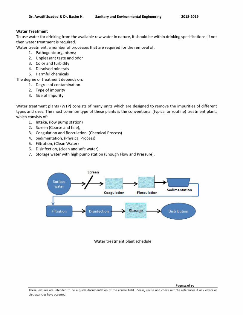
Water treatment plants (WTP) consists of many units which are designed to remove the impurities of different types and sizes. The most common type of these plants is the conventional (typical or routine) treatment plant, which consists of:
1. Intake, (low pump station) 2. Screen (Coarse and fine), 3. Coagulation and flocculation, (Chemical Process) 4. Sedimentation, (Physical Process) 5. Filtration, (Clean Water) 6. Disinfection, (clean and safe water) 7. Storage water with high pump station (Enough Flow and Pressure).
Water treatment plant schedule
Dr. Awatif Soaded & Dr. Basim H. Sanitary and Environmental Engineering 2018-2019
Page 12 of 15
These lectures are intended to be a guide documentation of the course held. Please, revise and check out the references if any errors or
discrepancies have occurred.
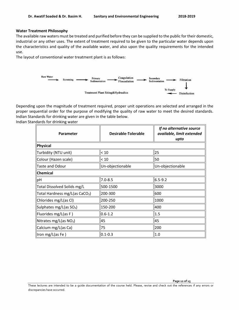
Water Treatment Philosophy The available raw waters must be treated and purified before they can be supplied to the public for their domestic, industrial or any other uses. The extent of treatment required to be given to the particular water depends upon the characteristics and quality of the available water, and also upon the quality requirements for the intended use. The layout of conventional water treatment plant is as follows:
Depending upon the magnitude of treatment required, proper unit operations are selected and arranged in the proper sequential order for the purpose of modifying the quality of raw water to meet the desired standards. Indian Standards for drinking water are given in the table below. Indian Standards for drinking water
Parameter Desirable-Tolerable If no alternative source
available, limit extended upto
Physical
Turbidity (NTU unit) < 10 25
Colour (Hazen scale) < 10 50
Taste and Odour Un-objectionable Un-objectionable
Chemical
pH 7.0-8.5 6.5-9.2
Total Dissolved Solids mg/L 500-1500 3000
Total Hardness mg/L(as CaCO3) 200-300 600
Chlorides mg/L(as Cl) 200-250 1000
Sulphates mg/L(as SO4) 150-200 400
Fluorides mg/L(as F ) 0.6-1.2 1.5
Nitrates mg/L(as NO3) 45 45
Calcium mg/L(as Ca) 75 200
Iron mg/L(as Fe ) 0.1-0.3 1.0
Dr. Awatif Soaded & Dr. Basim H. Sanitary and Environmental Engineering 2018-2019
Page 13 of 15
These lectures are intended to be a guide documentation of the course held. Please, revise and check out the references if any errors or
discrepancies have occurred.
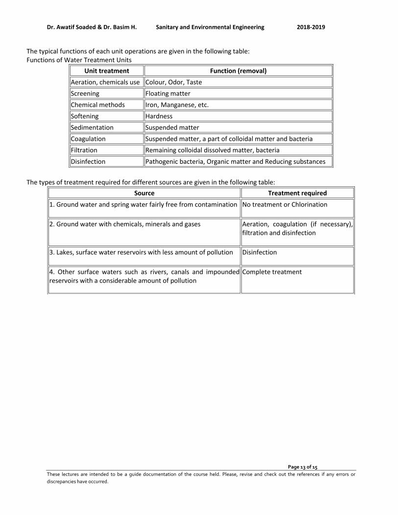
The typical functions of each unit operations are given in the following table: Functions of Water Treatment Units The types of treatment required for different sources are given in the following table:
Unit treatment Function (removal)
Aeration, chemicals use Colour, Odor, Taste
Screening Floating matter
Chemical methods Iron, Manganese, etc.
Softening Hardness
Sedimentation Suspended matter
Coagulation Suspended matter, a part of colloidal matter and bacteria
Filtration Remaining colloidal dissolved matter, bacteria
Disinfection Pathogenic bacteria, Organic matter and Reducing substances
Source Treatment required
1. Ground water and spring water fairly free from contamination No treatment or Chlorination
2. Ground water with chemicals, minerals and gases Aeration, coagulation (if necessary), filtration and disinfection
3. Lakes, surface water reservoirs with less amount of pollution Disinfection
4. Other surface waters such as rivers, canals and impounded reservoirs with a considerable amount of pollution
Complete treatment
Dr. Awatif Soaded & Dr. Basim H. Sanitary and Environmental Engineering 2018-2019
Page 14 of 15
These lectures are intended to be a guide documentation of the course held. Please, revise and check out the references if any errors or
discrepancies have occurred.
Dr. Awatif Soaded & Dr. Basim H. Sanitary and Environmental Engineering 2018-2019
Page 15 of 15
These lectures are intended to be a guide documentation of the course held. Please, revise and check out the references if any errors or
discrepancies have occurred.
How to Choose a DRM Software to protect your document?

Dr. Awatif Soaded & Dr. Basim H. Sanitary and Environmental Engineering 2018-2019
Page 1 of 20
These lectures are intended to be a guide documentation of the course held. Please, revise and check out the references if any errors or
discrepancies have occurred.
Sanitary and Environmental Engineering
PART 1: WATER SUPPLY ENGINEERING

Dr. Awatif Soaded & Dr. Basim H. Sanitary and Environmental Engineering 2018-2019
Page 2 of 20
These lectures are intended to be a guide documentation of the course held. Please, revise and check out the references if any errors or
discrepancies have occurred.
PART 1: WATER SUPPLY ENGINEERING
Lecture 4: Water Distribution Systems
The primary purpose of this system is to transport treated water from the treatment facilities
(plants) to the consumers. This system should have sufficient capacity to meet the water supply
needs (demand) of the consumer, under all demand conditions in quantity, quality and pressure.
In some communities this system may provide water for fire demand also. Distribution system is
used to describe collectively the facilities used to supply water from its source to the point of
usage.
Design stages of water distribution systems: 1. Preparation of a master plan. 2. Topography survey of the study area 3. Hydraulic study of the existing system. 4. The improvement programs.
Requirements of Good Distribution System:
5. Water quality should not get deteriorated in the distribution pipes. 6. It should be capable of supplying water at all the intended places with sufficient pressure
head. 7. It should be capable of supplying the requisite amount of water during firefighting. 8. The layout should be such that no consumer would be without water supply, during the
repair of any section of the system. 9. All the distribution pipes should be preferably laid one meter away or above the sewer
lines. 10. It should be fairly water-tight as to keep losses due to leakage to the minimum.
Methods of distribution
1. By gravity 2. By means of pumps and storage 3. By pumps only
A typical distribution system consists of: pipes, nodes and loops, by which a network will be
formed. The main components in this system are the pipes, which are in the following form
according to their size:
1. Primary feeders. 2. Secondary feeders. 3. Small distribution mains. 4. Service pipes.
Dr. Awatif Soaded & Dr. Basim H. Sanitary and Environmental Engineering 2018-2019
Page 3 of 20
These lectures are intended to be a guide documentation of the course held. Please, revise and check out the references if any errors or
discrepancies have occurred.
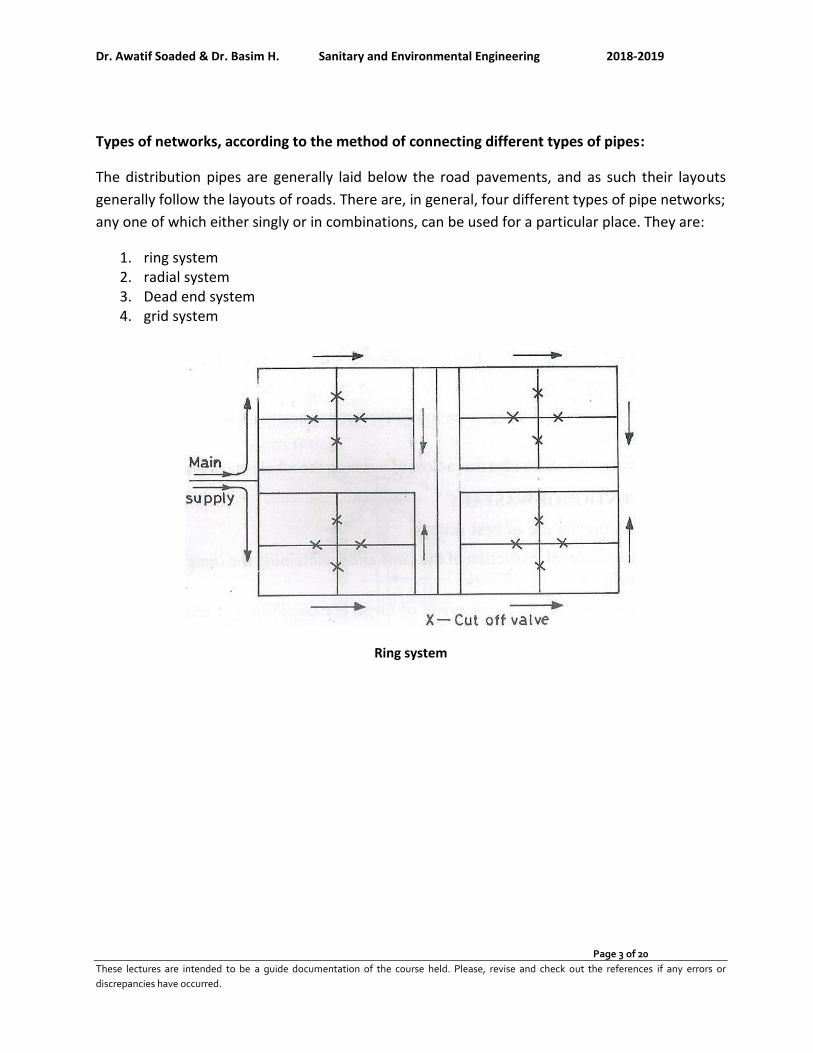
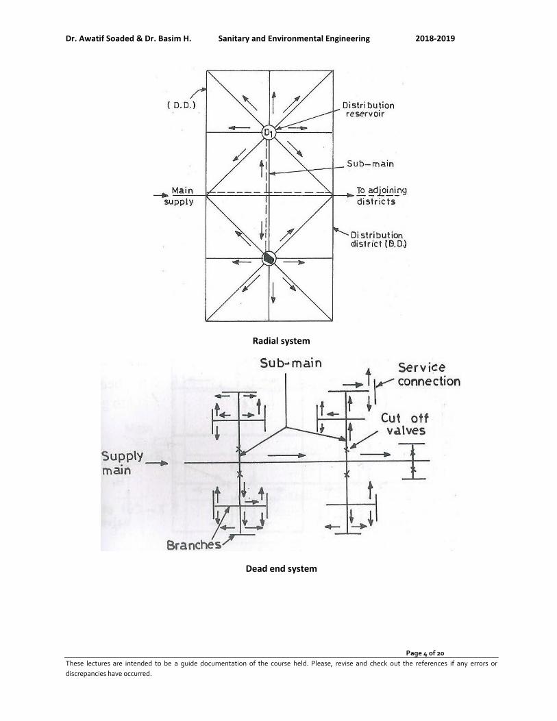
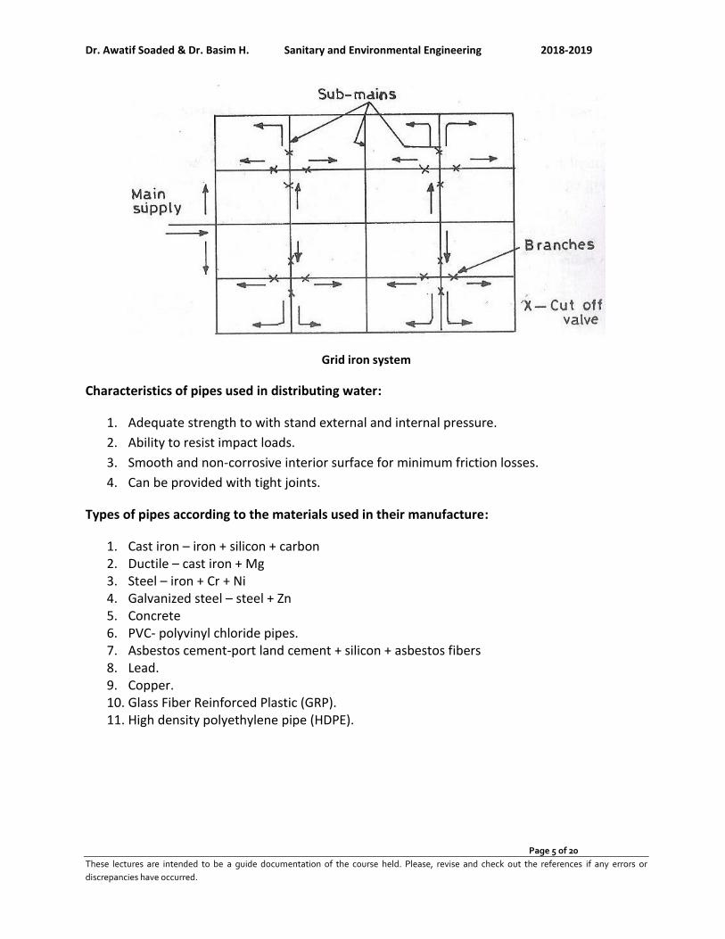
Types of networks, according to the method of connecting different types of pipes:
The distribution pipes are generally laid below the road pavements, and as such their layouts
generally follow the layouts of roads. There are, in general, four different types of pipe networks;
any one of which either singly or in combinations, can be used for a particular place. They are:
1. ring system 2. radial system 3. Dead end system 4. grid system
Ring system
Dr. Awatif Soaded & Dr. Basim H. Sanitary and Environmental Engineering 2018-2019
Page 4 of 20
These lectures are intended to be a guide documentation of the course held. Please, revise and check out the references if any errors or
discrepancies have occurred.
Radial system
Dead end system
Dr. Awatif Soaded & Dr. Basim H. Sanitary and Environmental Engineering 2018-2019
Page 5 of 20
These lectures are intended to be a guide documentation of the course held. Please, revise and check out the references if any errors or
discrepancies have occurred.
Grid iron system
Characteristics of pipes used in distributing water:
1. Adequate strength to with stand external and internal pressure.
2. Ability to resist impact loads.
3. Smooth and non-corrosive interior surface for minimum friction losses.
4. Can be provided with tight joints.
Types of pipes according to the materials used in their manufacture:
1. Cast iron – iron + silicon + carbon 2. Ductile – cast iron + Mg 3. Steel – iron + Cr + Ni 4. Galvanized steel – steel + Zn 5. Concrete 6. PVC- polyvinyl chloride pipes. 7. Asbestos cement-port land cement + silicon + asbestos fibers 8. Lead. 9. Copper. 10. Glass Fiber Reinforced Plastic (GRP). 11. High density polyethylene pipe (HDPE).
Dr. Awatif Soaded & Dr. Basim H. Sanitary and Environmental Engineering 2018-2019
Page 6 of 20
These lectures are intended to be a guide documentation of the course held. Please, revise and check out the references if any errors or
discrepancies have occurred.
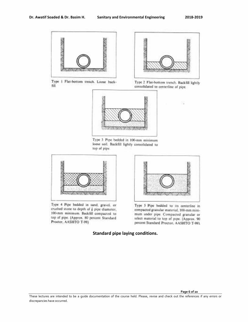
Standard pipe laying conditions.
Dr. Awatif Soaded & Dr. Basim H. Sanitary and Environmental Engineering 2018-2019
Page 7 of 20
These lectures are intended to be a guide documentation of the course held. Please, revise and check out the references if any errors or
discrepancies have occurred.
Distribution Reservoirs
Distribution reservoirs, also called service reservoirs, are the storage reservoirs, which store the
treated water for supplying water during emergencies (such as during fires, repairs, etc.) and also
to help in absorbing the hourly fluctuations in the normal water demand.
Functions of Distribution Reservoirs:
• To absorb the hourly variations in demand. • To maintain constant pressure in the distribution mains. • Water stored can be supplied during emergencies.
Location and Height of Distribution Reservoirs:
• Should be located as close as possible to the center of demand. • Water level in the reservoir must be at a sufficient elevation to permit gravity flow at an
adequate pressure.
Types of Reservoirs
• Underground reservoirs. • Small ground level reservoirs. • Large ground level reservoirs. • Overhead tanks.
Storage Capacity of Distribution Reservoirs
The total storage capacity of a distribution reservoir is the summation of:
1. Balancing Storage: The quantity of water required being stored in the reservoir for equalizing or balancing fluctuating demand against constant supply is known as the balancing storage (or equalizing or operating storage). The balance storage can be worked out by mass curve method.
2. Breakdown Storage: The breakdown storage or often called emergency storage is the storage preserved in order to tide over the emergencies posed by the failure of pumps, electricity, or any other mechanism driving the pumps. A value of about 25% of the total storage capacity of reservoirs, or 1.5 to 2 times of the average hourly supply, may be considered as enough provision for accounting this storage.
3. Fire Storage: The third component of the total reservoir storage is the fire storage. This provision takes care of the requirements of water for extinguishing fires. A provision of 1 to 4 liter per person per day is sufficient to meet the requirement.
The total reservoir storage can finally be worked out by adding all the three storages.
Dr. Awatif Soaded & Dr. Basim H. Sanitary and Environmental Engineering 2018-2019
Page 8 of 20
These lectures are intended to be a guide documentation of the course held. Please, revise and check out the references if any errors or
discrepancies have occurred.
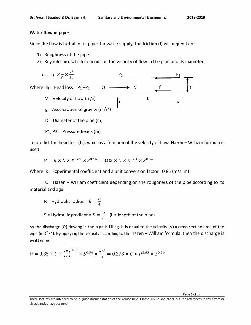
Water flow in pipes
Since the flow is turbulent in pipes for water supply, the friction (f) will depend on:
1) Roughness of the pipe.
2) Reynolds no. which depends on the velocity of flow in the pipe and its diameter.
ℎ𝑙 = 𝑓 ×𝐿
𝐷×
𝑉2
2𝑔 P1 P2
Where: hl = Head loss = P1 –P2 Q V f D
V = Velocity of flow (m/s) L
g = Acceleration of gravity (m/s2)
D = Diameter of the pipe (m)
P1, P2 = Pressure heads (m)
To predict the head loss (hl), which is a function of the velocity of flow, Hazen – William formula is
used:
𝑉 = 𝑘 × 𝐶 × 𝑅0.63 × 𝑆0.54 = 0.85 × 𝐶 × 𝑅0.63 × 𝑆0.54
Where: k = Experimental coefficient and a unit conversion factor= 0.85 (m/s, m)
C = Hazen – William coefficient depending on the roughness of the pipe according to its
material and age.
R = Hydraulic radius = 𝑅 =𝐷
4
S = Hydraulic gradient = 𝑆 =ℎ𝑙
𝐿 (L = length of the pipe)
As the discharge (Q) flowing in the pipe is filling, it is equal to the velocity (V) x cross section area of the
pipe (π D2 /4). By applying the velocity according to the Hazen – William formula, then the discharge is
written as
𝑄 = 0.85 × 𝐶 × (𝐷
4)
0.63
× 𝑆0.54 ×𝜋𝐷2
4= 0.278 × 𝐶 × 𝐷2.63 × 𝑆0.54
Dr. Awatif Soaded & Dr. Basim H. Sanitary and Environmental Engineering 2018-2019
Page 9 of 20
These lectures are intended to be a guide documentation of the course held. Please, revise and check out the references if any errors or
discrepancies have occurred.
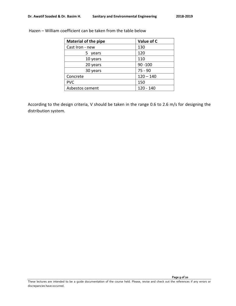
Hazen – William coefficient can be taken from the table below
Material of the pipe Value of C
Cast Iron - new 130
5 years 120
10 years 110
20 years 90 -100
30 years 75 - 90
Concrete 120 – 140
PVC 150
Asbestos cement 120 - 140
According to the design criteria, V should be taken in the range 0.6 to 2.6 m/s for designing the
distribution system.
Dr. Awatif Soaded & Dr. Basim H. Sanitary and Environmental Engineering 2018-2019
Page 10 of 20
These lectures are intended to be a guide documentation of the course held. Please, revise and check out the references if any errors or
discrepancies have occurred.
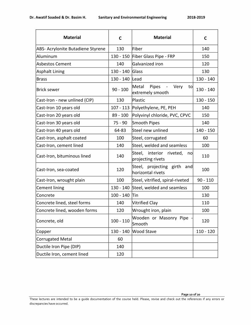
Material C Material C
ABS- Acrylonite Butadiene Styrene 130 Fiber 140
Aluminum 130 - 150 Fiber Glass Pipe - FRP 150
Asbestos Cement 140 Galvanized iron 120
Asphalt Lining 130 - 140 Glass 130
Brass 130 - 140 Lead 130 - 140
Brick sewer 90 - 100 Metal Pipes - Very to extremely smooth
130 - 140
Cast-Iron - new unlined (CIP) 130 Plastic 130 - 150
Cast-Iron 10 years old 107 - 113 Polyethylene, PE, PEH 140
Cast-Iron 20 years old 89 - 100 Polyvinyl chloride, PVC, CPVC 150
Cast-Iron 30 years old 75 - 90 Smooth Pipes 140
Cast-Iron 40 years old 64-83 Steel new unlined 140 - 150
Cast-Iron, asphalt coated 100 Steel, corrugated 60
Cast-Iron, cement lined 140 Steel, welded and seamless 100
Cast-Iron, bituminous lined 140 Steel, interior riveted, no projecting rivets
110
Cast-Iron, sea-coated 120 Steel, projecting girth and horizontal rivets
100
Cast-Iron, wrought plain 100 Steel, vitrified, spiral-riveted 90 - 110
Cement lining 130 - 140 Steel, welded and seamless 100
Concrete 100 - 140 Tin 130
Concrete lined, steel forms 140 Vitrified Clay 110
Concrete lined, wooden forms 120 Wrought iron, plain 100
Concrete, old 100 - 110 Wooden or Masonry Pipe - Smooth
120
Copper 130 - 140 Wood Stave 110 - 120
Corrugated Metal 60
Ductile Iron Pipe (DIP) 140
Ductile Iron, cement lined 120
Dr. Awatif Soaded & Dr. Basim H. Sanitary and Environmental Engineering 2018-2019
Page 11 of 20
These lectures are intended to be a guide documentation of the course held. Please, revise and check out the references if any errors or
discrepancies have occurred.
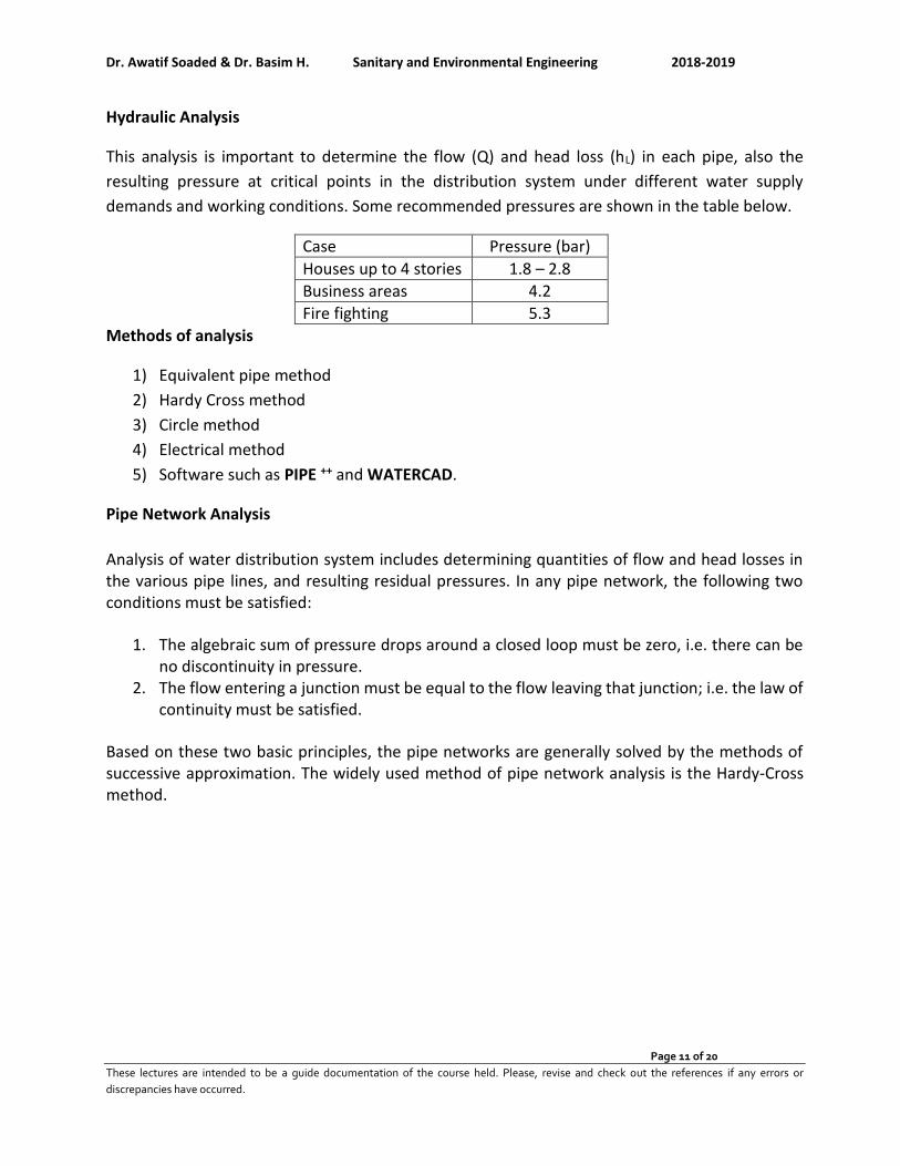
Hydraulic Analysis
This analysis is important to determine the flow (Q) and head loss (hL) in each pipe, also the
resulting pressure at critical points in the distribution system under different water supply
demands and working conditions. Some recommended pressures are shown in the table below.
Case Pressure (bar)
Houses up to 4 stories 1.8 – 2.8
Business areas 4.2
Fire fighting 5.3
Methods of analysis
1) Equivalent pipe method
2) Hardy Cross method
3) Circle method
4) Electrical method
5) Software such as PIPE ++ and WATERCAD.
Pipe Network Analysis
Analysis of water distribution system includes determining quantities of flow and head losses in the various pipe lines, and resulting residual pressures. In any pipe network, the following two conditions must be satisfied:
1. The algebraic sum of pressure drops around a closed loop must be zero, i.e. there can be no discontinuity in pressure.
2. The flow entering a junction must be equal to the flow leaving that junction; i.e. the law of continuity must be satisfied.
Based on these two basic principles, the pipe networks are generally solved by the methods of successive approximation. The widely used method of pipe network analysis is the Hardy-Cross method.
Dr. Awatif Soaded & Dr. Basim H. Sanitary and Environmental Engineering 2018-2019
Page 12 of 20
These lectures are intended to be a guide documentation of the course held. Please, revise and check out the references if any errors or
discrepancies have occurred.
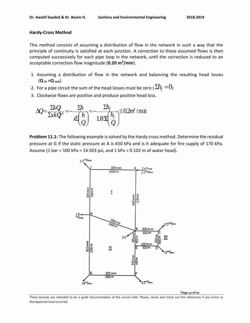
Hardy-Cross Method
This method consists of assuming a distribution of flow in the network in such a way that the principle of continuity is satisfied at each junction. A correction to these assumed flows is then computed successively for each pipe loop in the network, until the correction is reduced to an acceptable correction flow magnitude (0.20 m3/min).
1. Assuming a distribution of flow in the network and balancing the resulting head losses (Q in =Q out).
2. For a pipe circuit the sum of the head losses must be zero ( 0= fh )
3. Clockwise flows are positive and produce positive head loss.
min/2.085.1
31
1
1 m
Q
hh
Qh
x
hxkQkQ
Qf
fx
x
−=
−=
= −
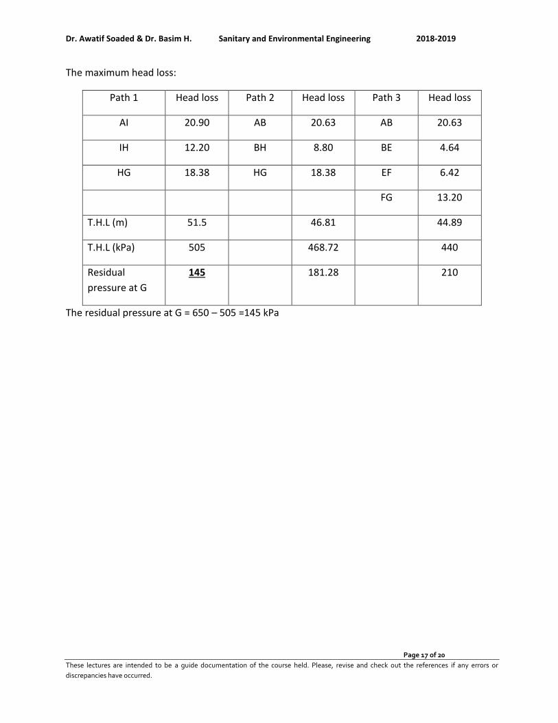
Problem 11.1: The following example is solved by the Hardy cross method. Determine the residual
pressure at G if the static pressure at A is 650 kPa and is it adequate for fire supply of 170 kPa.
Assume (1 bar = 100 kPa = 14.503 psi, and 1 kPa = 0.102 m of water head).
Dr. Awatif Soaded & Dr. Basim H. Sanitary and Environmental Engineering 2018-2019
Page 13 of 20
These lectures are intended to be a guide documentation of the course held. Please, revise and check out the references if any errors or
discrepancies have occurred.
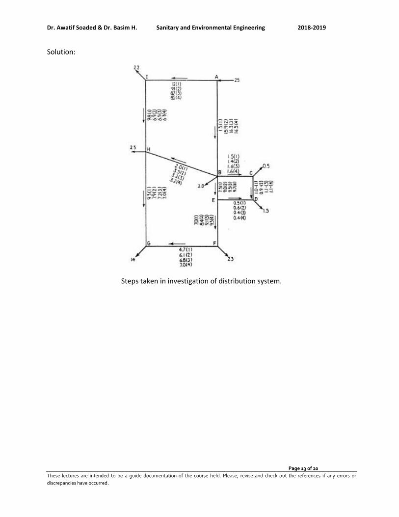
Solution:
Steps taken in investigation of distribution system.
Dr. Awatif Soaded & Dr. Basim H. Sanitary and Environmental Engineering 2018-2019
Page 14 of 20
These lectures are intended to be a guide documentation of the course held. Please, revise and check out the references if any errors or
discrepancies have occurred.
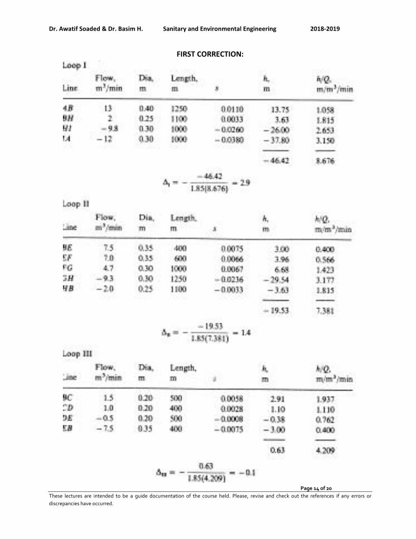
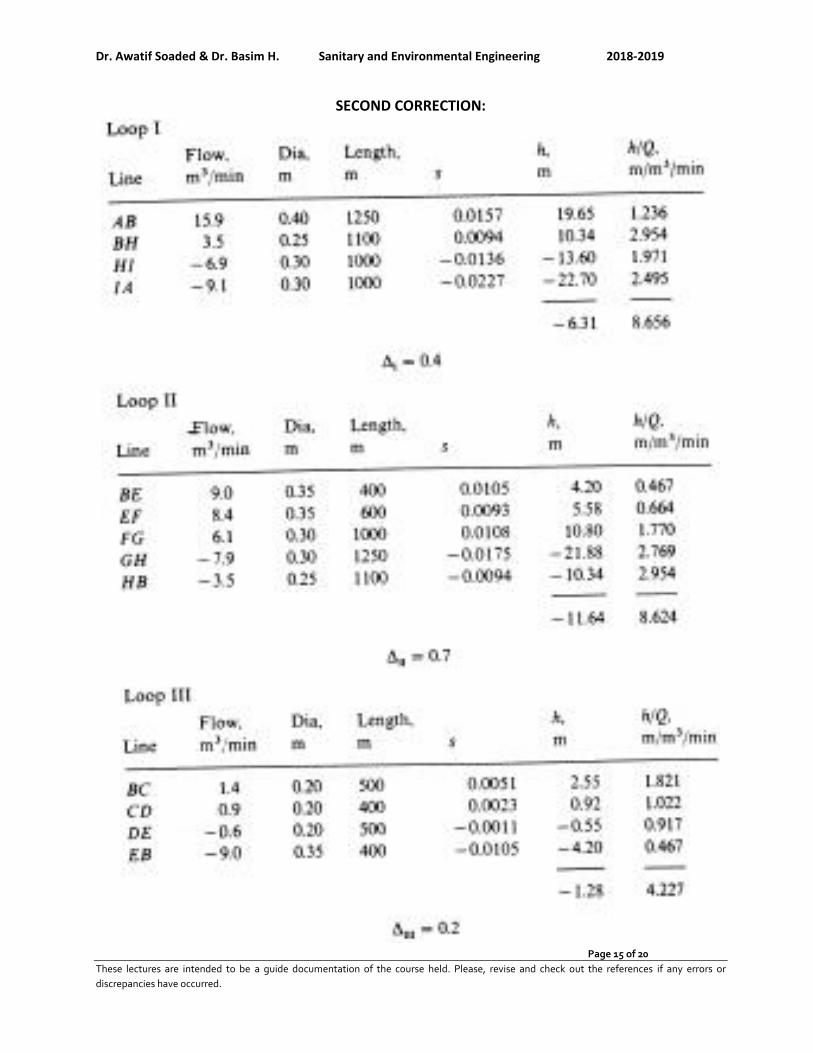
FIRST CORRECTION:
Dr. Awatif Soaded & Dr. Basim H. Sanitary and Environmental Engineering 2018-2019
Page 15 of 20
These lectures are intended to be a guide documentation of the course held. Please, revise and check out the references if any errors or
discrepancies have occurred.
SECOND CORRECTION:
Dr. Awatif Soaded & Dr. Basim H. Sanitary and Environmental Engineering 2018-2019
Page 16 of 20
These lectures are intended to be a guide documentation of the course held. Please, revise and check out the references if any errors or
discrepancies have occurred.
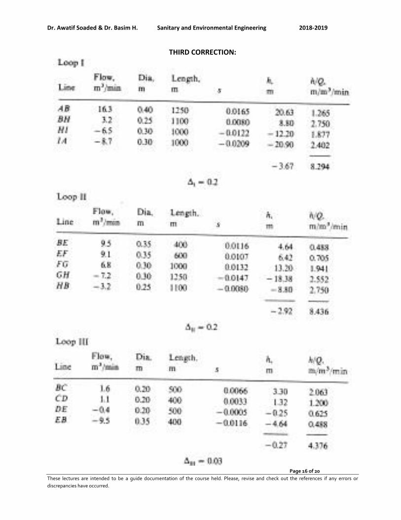
THIRD CORRECTION:
Dr. Awatif Soaded & Dr. Basim H. Sanitary and Environmental Engineering 2018-2019
Page 17 of 20
These lectures are intended to be a guide documentation of the course held. Please, revise and check out the references if any errors or
discrepancies have occurred.
The maximum head loss:
Path 1 Head loss Path 2 Head loss Path 3 Head loss
AI 20.90 AB 20.63 AB 20.63
IH 12.20 BH 8.80 BE 4.64
HG 18.38 HG 18.38 EF 6.42
FG 13.20
T.H.L (m) 51.5 46.81 44.89
T.H.L (kPa) 505 468.72 440
Residual
pressure at G
145 181.28 210
The residual pressure at G = 650 – 505 =145 kPa
Dr. Awatif Soaded & Dr. Basim H. Sanitary and Environmental Engineering 2018-2019
Page 18 of 20
These lectures are intended to be a guide documentation of the course held. Please, revise and check out the references if any errors or
discrepancies have occurred.
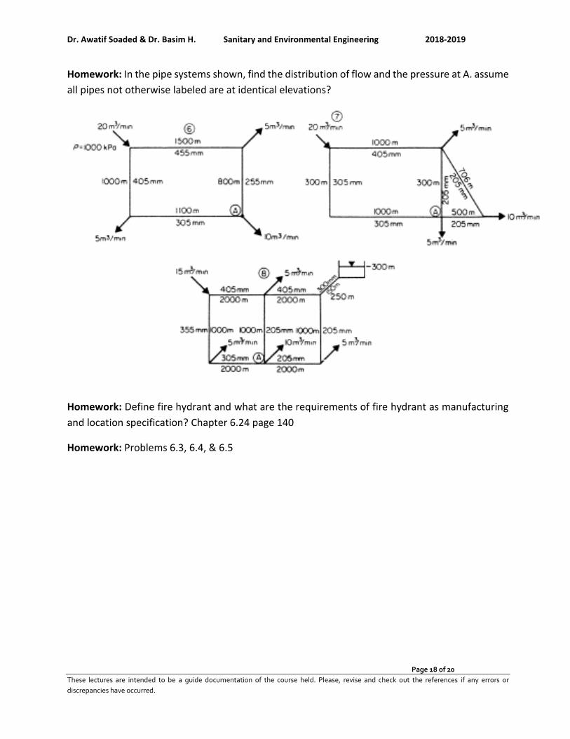
Homework: In the pipe systems shown, find the distribution of flow and the pressure at A. assume
all pipes not otherwise labeled are at identical elevations?
Homework: Define fire hydrant and what are the requirements of fire hydrant as manufacturing
and location specification? Chapter 6.24 page 140
Homework: Problems 6.3, 6.4, & 6.5
Dr. Awatif Soaded & Dr. Basim H. Sanitary and Environmental Engineering 2018-2019
Page 19 of 20
These lectures are intended to be a guide documentation of the course held. Please, revise and check out the references if any errors or
discrepancies have occurred.
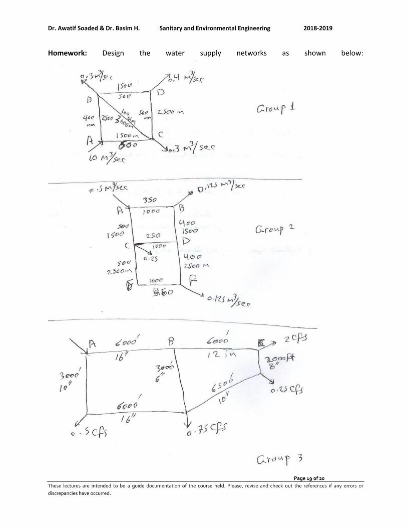
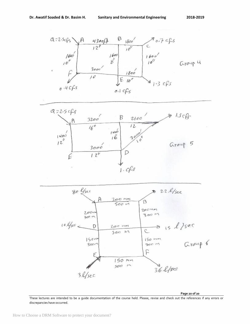
Homework: Design the water supply networks as shown below:
Dr. Awatif Soaded & Dr. Basim H. Sanitary and Environmental Engineering 2018-2019
Page 20 of 20
These lectures are intended to be a guide documentation of the course held. Please, revise and check out the references if any errors or
discrepancies have occurred.
How to Choose a DRM Software to protect your document?

Dr. Awatif Soaded & Dr. Basim H. Sanitary and Environmental Engineering 2018-2019
Page 1 of 10
These lectures are intended to be a guide documentation of the course held. Please, revise and check out the references if any errors or
discrepancies have occurred.
Sanitary and Environmental Engineering
PART 1: WATER SUPPLY ENGINEERING
Dr. Awatif Soaded & Dr. Basim H. Sanitary and Environmental Engineering 2018-2019
Page 2 of 10
These lectures are intended to be a guide documentation of the course held. Please, revise and check out the references if any errors or
discrepancies have occurred.
PART 1: WATER SUPPLY ENGINEERING
Lecture 5: Intakes and Screens
Intakes:
Definition: The intake is a structure made of several parts, mainly constructed to collect raw water from
the source to water treatment plant. Intakes consist of the opening, strainer, or grating through which the
water enters and conduit conveying the water, usually by gravity, to a well or sump. From the well the
water is pumped to the mains or treatment plant.
Intakes should be so located and designed that possibility of interference with the supply is minimized and
where uncertainty of continuous serviceability exists, intakes should be duplicated.
The following must be considered in designing and locating intakes:
a) The sources of water supply, whether impounding reservoir, lakes, or river (including the possibility of wide fluctuation in water level).
b) The character of the intake surroundings, depth of water, character of bottom, navigation requirements, the effects of currents, floods, and storms upon the structure and in scouring the bottom.
c) The location with respect to sources of pollution; and d) The prevalence of the floating material such as ice, legs, and vegetation.
General requirements for the location of an intake:
1) Near to the water treatment plant (WTP). 2) Upstream waste disposal sites. 3) In pure water to avoid additional loading and/or complicated treatment. 4) Far away from navigation area. 5) It should be in deep water to provide sufficient quantity of water in dry weather conditions and if
expansion is required in the water treatment plant. 6) Far away from the effects of currents, erosion and deposition. 7) In meandering rivers, the best location is on the concave side.
Intake criteria design:
1) Water velocity through foot valve = (0.15-0.3) m/sec 2) Detention time in suction well = 20 min 3) Water velocity through suction pipe = (1-1.5) m/sec 4) Water velocity through back wash pipe = (3) m/sec
5) Water discharge through backwash pipe = suction31
pipe
6) TV
Q= & vAQ=
Dr. Awatif Soaded & Dr. Basim H. Sanitary and Environmental Engineering 2018-2019
Page 3 of 10
These lectures are intended to be a guide documentation of the course held. Please, revise and check out the references if any errors or
discrepancies have occurred.
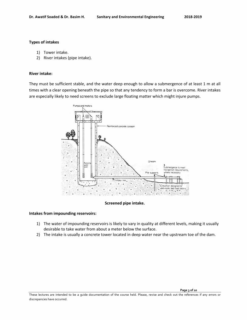
Types of intakes
1) Tower intake. 2) River intakes (pipe intake).
River intake:
They must be sufficient stable, and the water deep enough to allow a submergence of at least 1 m at all
times with a clear opening beneath the pipe so that any tendency to form a bar is overcome. River intakes
are especially likely to need screens to exclude large floating matter which might injure pumps.
Screened pipe intake.
Intakes from impounding reservoirs:
1) The water of impounding reservoirs is likely to vary in quality at different levels, making it usually desirable to take water from about a meter below the surface.
2) The intake is usually a concrete tower located in deep water near the upstream toe of the dam.
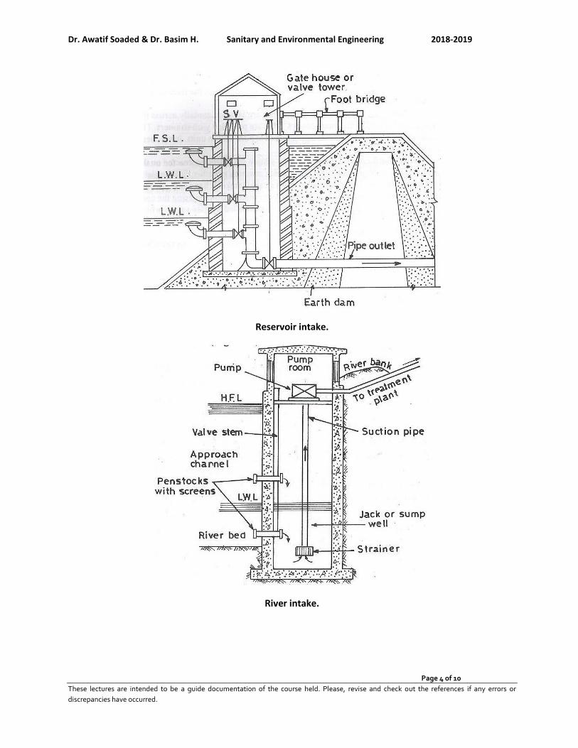
Dr. Awatif Soaded & Dr. Basim H. Sanitary and Environmental Engineering 2018-2019
Page 4 of 10
These lectures are intended to be a guide documentation of the course held. Please, revise and check out the references if any errors or
discrepancies have occurred.
Reservoir intake.
River intake.
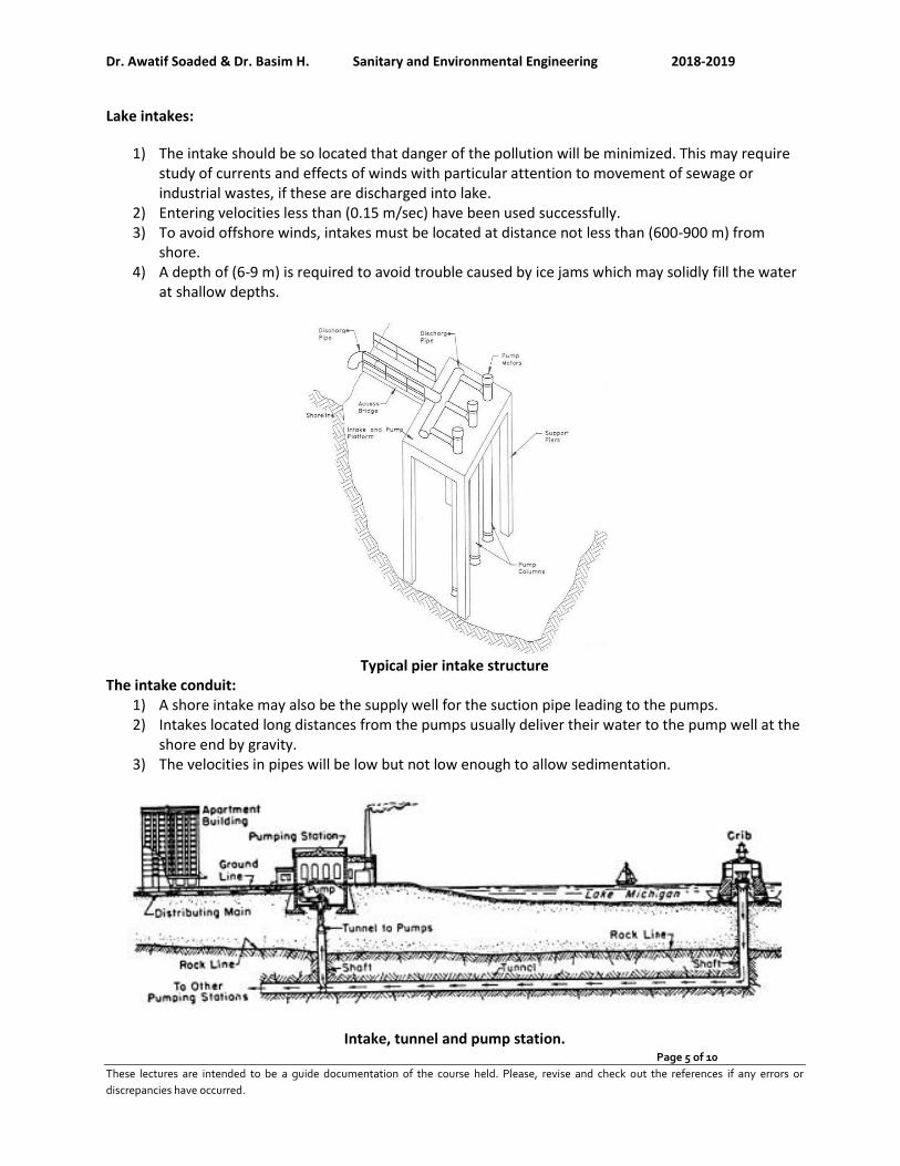
Dr. Awatif Soaded & Dr. Basim H. Sanitary and Environmental Engineering 2018-2019
Page 5 of 10
These lectures are intended to be a guide documentation of the course held. Please, revise and check out the references if any errors or
discrepancies have occurred.
Lake intakes:
1) The intake should be so located that danger of the pollution will be minimized. This may require study of currents and effects of winds with particular attention to movement of sewage or industrial wastes, if these are discharged into lake.
2) Entering velocities less than (0.15 m/sec) have been used successfully. 3) To avoid offshore winds, intakes must be located at distance not less than (600-900 m) from
shore. 4) A depth of (6-9 m) is required to avoid trouble caused by ice jams which may solidly fill the water
at shallow depths.
Typical pier intake structure
The intake conduit: 1) A shore intake may also be the supply well for the suction pipe leading to the pumps. 2) Intakes located long distances from the pumps usually deliver their water to the pump well at the
shore end by gravity. 3) The velocities in pipes will be low but not low enough to allow sedimentation.
Intake, tunnel and pump station.
Dr. Awatif Soaded & Dr. Basim H. Sanitary and Environmental Engineering 2018-2019
Page 6 of 10
These lectures are intended to be a guide documentation of the course held. Please, revise and check out the references if any errors or
discrepancies have occurred.
Screens
Definition: Screening is a unit operation that removes floating and large suspended matter from water.
Screens may be classified as coarse, fine, microstrainer, depending on the size of material removed. Screens
may be located at the intake structure, raw water pump station, or water treatment plant.
The screen is a device with openings uniform in size. It is placed across the flow to retain floating particles.
It serves as a protective unit.
Types of screens:
1) According to its shape 1- rack 2- mesh
2) According to its size:
a) Course, openings ˃ 25 mm:
Intake ports should be equipped with a coarse screen or bar rack to prevent large objects from
entering the conveyance system. These screens consist of vertical flat bars or, in some cases a
round pipes spaced with (5-8) cm of clear opening. The velocity through the coarse screen is
generally less than 8 cm/s. Screens should be installed outside (on the water side) of any sluice gate
or stop log slot, to prevent debris from interfering with their operation.
b) Medium 6 mm ˂ openings ˂ 25 mm
c) Fine, openings ˂ 6 mm:
Fine screens are used to remove smaller objects that may damage pumps or other equipment. They
may be located either at the intake structure or at the raw water pump station. These screens
consist of heavy wire mesh with 0.5 cm square openings or circular passive screens with similar
opening widths. The screen area efficiency factor (0.5-0.6) and the typical velocity through the
effective area is in the range of (0.4-0.8) m/s.
d) Microstrainer are used for the removal of plankton and algae from impounded waters. Therefore,
microstrainer installed before chemical coagulation will often improve the performance of
clarifiers.
3) According to its workability, manual and mechanical.
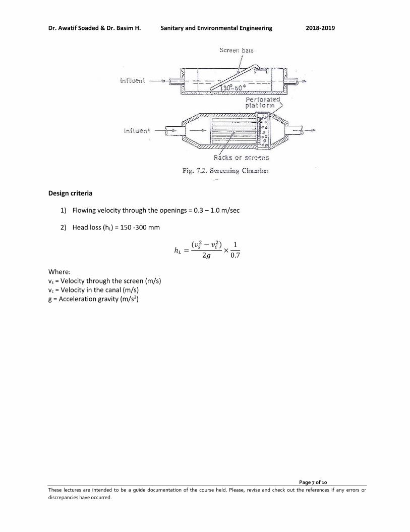
Dr. Awatif Soaded & Dr. Basim H. Sanitary and Environmental Engineering 2018-2019
Page 7 of 10
These lectures are intended to be a guide documentation of the course held. Please, revise and check out the references if any errors or
discrepancies have occurred.
Design criteria
1) Flowing velocity through the openings = 0.3 – 1.0 m/sec
2) Head loss (hL) = 150 -300 mm
ℎ𝐿 =(𝑣𝑠
2 − 𝑣𝑐2)
2𝑔×
1
0.7
Where: vs = Velocity through the screen (m/s) vc = Velocity in the canal (m/s) g = Acceleration gravity (m/s2)
Dr. Awatif Soaded & Dr. Basim H. Sanitary and Environmental Engineering 2018-2019
Page 8 of 10
These lectures are intended to be a guide documentation of the course held. Please, revise and check out the references if any errors or
discrepancies have occurred.
SOLVED PROBLEMS
Problem 5.1: Design a coarse screen (rack) for a flow of 0.15 m3/sec. The screen is placed in a canal 0.6 m in
width and 0.4 m in height. Use rectangular bars 10 X 30 mm in cross section, assume size of the openings = 25
mm?
Solution:
Assume n = number of bars
Width of the canel = n × Size of the bar + (n + 1) × Size of the openning
600 mm = n × 10 mm + (n + 1) × 25 ⇛ 575 = 35n ⇛ n = 16.4 ≈ 16
Number of spacing = n+1= 16 +1 = 17
Check the velocity:
ASpacing = 𝐴𝑟𝑒𝑎 𝑜𝑓 𝑜𝑝𝑒𝑛𝑖𝑛𝑔𝑠 = 𝐻𝑒𝑖𝑔ℎ𝑡 × 𝑊𝑖𝑑𝑡ℎ 𝑜𝑓 𝑜𝑝𝑒𝑛𝑖𝑛𝑔𝑠
Width = 600 − 16 × 10 = 440 mm = 0.44m
Velocity through the rack =0.15
m3
𝑠𝑒𝑐0.4 × 0.44
= 0.852m
sec with acceptable velocity O. K
Assume the velocity through the canal vc =Q
ACanal=
0.15
0.6 × 0.4= 0.625 m/sec
Head loss through the openings hL =(vs
2 − vc2)
2g×
1
0.7=
(0.8522 − 0.6252)
2 × 9.81×
1
0.7= 0.0244m
Or using 10 mm bars 35 mm c/c
Number of spaces =Width
Spacescc
=0.6 m
0.035≈ 17
Number of bars = Number of spaces − 1 = 17 − 1 = 16
𝑆𝑖𝑧𝑒 𝑜𝑓 𝑜𝑝𝑒𝑛𝑖𝑛𝑔𝑠 = 35 − (5 + 5) = 25 𝑚𝑚 , also, check vs
Or using velocity through openings 0.85 m/sec
Check the velocity: vs =Q
ASpacing⇛ 𝐴𝑠 =
0.15
0.85= 0.176 𝑚2
𝐴𝑠 = 0.6 × 0.4 − 10 × 10−3 × 𝑛 × 0.4 ⇛ 𝑛 = 16 & 𝑛 + 1 = 17
Also, check: 𝑆𝑖𝑧𝑒 𝑜𝑓 𝑠𝑝𝑎𝑐𝑖𝑛𝑔 = 0.176 = 0.4 × 17 × 𝑠 ⇛ 𝑠 = 0.026 𝑚 = 26 𝑚𝑚
Dr. Awatif Soaded & Dr. Basim H. Sanitary and Environmental Engineering 2018-2019
Page 9 of 10
These lectures are intended to be a guide documentation of the course held. Please, revise and check out the references if any errors or
discrepancies have occurred.
Problem 5.2: Design a coarse screen (rack) for a flow of 0.8 m3/sec. The screen is placed in a channel 1.5 m in
depth and 2 m width. Use square bars 13 X 13 mm in cross section, assume size of the openings c/c = 80 mm?
Solution:
Width of the openning = 8 −13
10= 6.7 cm
Assume n= number of bars
Width of the channel = n × Size of the bar + (n + 1) × Size of the openning
2 m = n × 0.013 m + (n + 1) × 0.067 m ⇛ 1.933 = 0.08n ⇛ n = 24.16 ≈ 24
Number of openings = 24+1 = 25
Or, Number of spaces =Width
Spaces c/c=
2 m
0.08= 25
Number of bars = Number of spaces − 1 = 25 − 1 = 24
Assume freeboard depth for maintenance = 20 cm
Depth of flow = channel depth − freeboard depth = 1.5 − 0.2 = 1.3 m
Area of openings A = No. of opening × Clear distance between bars × Depth of flow
Area of openings A = 25 × 0.067 × 1.3 = 2.178 m2
Velocity through the rack =0.8
m3
sec2.178
= 0.367m
sec with acceptable velocity
assume the velocity through the canal = 0
Head loss through the openings hL =(vs
2 − vc2)
2g×
1
0.7=
(0.3672 − 0)
2 × 9.81×
1
0.7= 0.0098 m
Head loss through the openings, hL =(vs
2 − vc2)
2g×
1
0.7=
(0.3642 − 0)
2 × 9.81×
1
0.7= 0.00964 m
Dr. Awatif Soaded & Dr. Basim H. Sanitary and Environmental Engineering 2018-2019
Page 10 of 10
These lectures are intended to be a guide documentation of the course held. Please, revise and check out the references if any errors or
discrepancies have occurred.
Problem 5.3: Design a raw water intake system as a headwork to water treatment plant at design capacity
10000 m3/hr including (10 suction pipes, 10 discharge pipes, 2 header or distributor, backwash pipe and wet
well)? Assume water velocity in suction, discharge, header and backwash pipes 1, 2.25, 2, and 3 m/sec
respectively and detention time in wet well 20 min.
Solution:
Suction Pipe:
𝑄𝑆𝑃 = 𝑣 × 𝐴 =10000
10= 1000
𝑚3
ℎ𝑟= 0.278
𝑚3
𝑠𝑒𝑐= 1
𝑚
𝑠𝑒𝑐×
𝜋
4× 𝐷𝑆𝑃
2 → 𝐷𝑆𝑃 = 0.595 ≈ 0.6 𝑚
Discharge Pipe:
𝑄𝐷𝑃 = 𝑣 × 𝐴 =10000
10= 1000
𝑚3
ℎ𝑟= 0.278
𝑚3
𝑠𝑒𝑐= 2.25
𝑚
𝑠𝑒𝑐×
𝜋
4× 𝐷𝐷𝑃
2 → 𝐷𝐷𝑃 = 0.396 ≈ 0.4 𝑚
Header Pipe:
𝑄𝐻𝑃 = 𝑣 × 𝐴 =10000
2= 5000
𝑚3
ℎ𝑟= 1.388
𝑚3
𝑠𝑒𝑐= 2
𝑚
𝑠𝑒𝑐×
𝜋
4× 𝐷𝐻𝑃
2 → 𝐷𝐻𝑃 = 0.94 ≈ 1 𝑚
Backwash Pipe:
𝑄𝐵𝑃 = 𝑣 × 𝐴 =1000
3= 333.34
𝑚3
ℎ𝑟= 0.0926
𝑚3
𝑠𝑒𝑐= 3
𝑚
𝑠𝑒𝑐×
𝜋
4× 𝐷𝐵𝑃
2 → 𝐷𝐵𝑃 = 0.198 ≈ 0.2 𝑚
Wet well:
Assume one wet well with two department
𝑄𝑊𝑊 =𝑉
𝑡= 5 × 1000 = 5000
𝑚3
ℎ𝑟=
𝑉
2060
→ 𝑉 = 1666.67 𝑚3
Assume effective water depth = 3 m
Assume rectangular cross-section and L = 4W
𝑉 = 𝐷𝑒𝑝𝑡ℎ × 𝐴 → 1666.67 = 3 × 𝐴 → 𝐴 = 555.556 𝑚2 = 4𝑊2 → 𝑊 = 11.785 ≈ 12 𝑚 𝑎𝑛𝑑 𝐿 = 48 𝑚
𝑇𝑜𝑡𝑎𝑙 𝑑𝑒𝑝𝑡ℎ = 3 + 𝐹𝑟𝑒𝑒𝑏𝑜𝑎𝑟𝑑(0.5) = 3.5 𝑚
So, use two wet well each at dimension (48 x 12 x 3.5) m
How to Choose a DRM Software to protect your document?

Dr. Awatif Soaded & Dr. Basim H. Sanitary and Environmental Engineering 2018-2019
Page 1 of 10
These lectures are intended to be a guide documentation of the course held. Please, revise and check out the references if any errors or
discrepancies have occurred.
Sanitary and Environmental Engineering
PART 1: WATER SUPPLY ENGINEERING

Dr. Awatif Soaded & Dr. Basim H. Sanitary and Environmental Engineering 2018-2019
Page 2 of 10
These lectures are intended to be a guide documentation of the course held. Please, revise and check out the references if any errors or
discrepancies have occurred.
PART 1: WATER SUPPLY ENGINEERING
Lecture 6: Pumps and Pumping Stations
A pump is a device which converts mechanical energy into hydraulic energy. It lifts water from a lower to a higher level and delivers it at high pressure. Pumps are employed in water supply projects at various stages for following purposes:
1. To lift raw water from wells. 2. To deliver treated water to the consumer at desired pressure. 3. To supply pressured water for fire hydrants. 4. To boost up pressure in water mains. 5. To fill elevated overhead water tanks. 6. To back-wash filters. 7. To pump chemical solutions, needed for water treatment.
Classification of Pumps
Based on principle of operation, pumps may be classified as follows:
1. Displacement pumps (reciprocating, rotary) 2. Velocity pumps (centrifugal, turbine and jet pumps) 3. Buoyancy pumps (air lift pumps) 4. Impulse pumps (hydraulic rams)
Work and efficiency of pumps
The work done by a pump is equal to the product of the mass flow and the total head against which the flow is moved.
Head, hydraulic energy, kinetic or potential energy is defining as equivalent to the potential energy of a column of water of specified height.
Pressure may be expressed in terms of either absolute or gauge reading
𝑂𝑛𝑒 𝑓𝑜𝑜𝑡 𝑜𝑓 𝑤𝑎𝑡𝑒𝑟 = 0.433 𝑝𝑠𝑖 or 𝑂𝑛𝑒 𝑚𝑒𝑡𝑒𝑟 𝑜𝑓 𝑤𝑎𝑡𝑒𝑟 = 9.81 𝑘𝑃𝑎
Total dynamic head (TDH) of a pump is the sum of the static suction head (SSH), the static discharge head (SDH), the total friction head ( T.H.L), and velocity head (DH)
𝑇𝑆𝐻 = 𝑆𝑆𝐻 + 𝑆𝐷𝐻
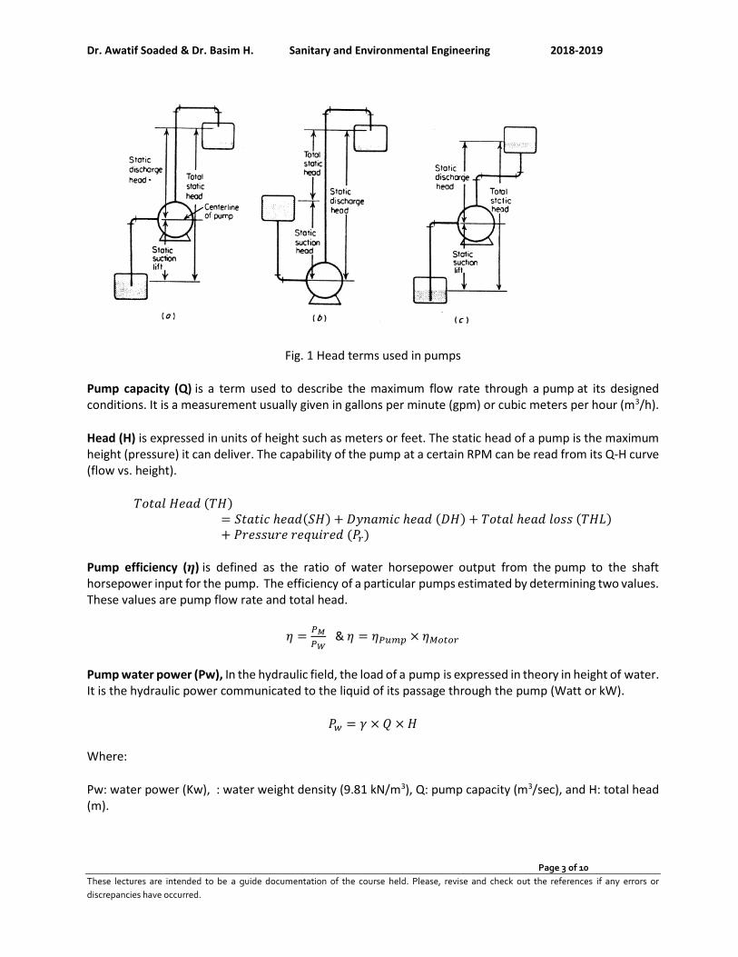
Dr. Awatif Soaded & Dr. Basim H. Sanitary and Environmental Engineering 2018-2019
Page 3 of 10
These lectures are intended to be a guide documentation of the course held. Please, revise and check out the references if any errors or
discrepancies have occurred.
Fig. 1 Head terms used in pumps
Pump capacity (Q) is a term used to describe the maximum flow rate through a pump at its designed conditions. It is a measurement usually given in gallons per minute (gpm) or cubic meters per hour (m3/h).
Head (H) is expressed in units of height such as meters or feet. The static head of a pump is the maximum height (pressure) it can deliver. The capability of the pump at a certain RPM can be read from its Q-H curve (flow vs. height).
𝑇𝑜𝑡𝑎𝑙 𝐻𝑒𝑎𝑑 (𝑇𝐻)= 𝑆𝑡𝑎𝑡𝑖𝑐 ℎ𝑒𝑎𝑑(𝑆𝐻) + 𝐷𝑦𝑛𝑎𝑚𝑖𝑐 ℎ𝑒𝑎𝑑 (𝐷𝐻) + 𝑇𝑜𝑡𝑎𝑙 ℎ𝑒𝑎𝑑 𝑙𝑜𝑠𝑠 (𝑇𝐻𝐿)+ 𝑃𝑟𝑒𝑠𝑠𝑢𝑟𝑒 𝑟𝑒𝑞𝑢𝑖𝑟𝑒𝑑 (𝑃𝑟)
Pump efficiency (𝜼) is defined as the ratio of water horsepower output from the pump to the shaft horsepower input for the pump. The efficiency of a particular pumps estimated by determining two values. These values are pump flow rate and total head.
𝜂 =𝑃𝑀
𝑃𝑊 & 𝜂 = 𝜂𝑃𝑢𝑚𝑝 × 𝜂𝑀𝑜𝑡𝑜𝑟
Pump water power (Pw), In the hydraulic field, the load of a pump is expressed in theory in height of water. It is the hydraulic power communicated to the liquid of its passage through the pump (Watt or kW).
𝑃𝑤 = 𝛾 × 𝑄 × 𝐻
Where:
Pw: water power (Kw), : water weight density (9.81 kN/m3), Q: pump capacity (m3/sec), and H: total head (m).
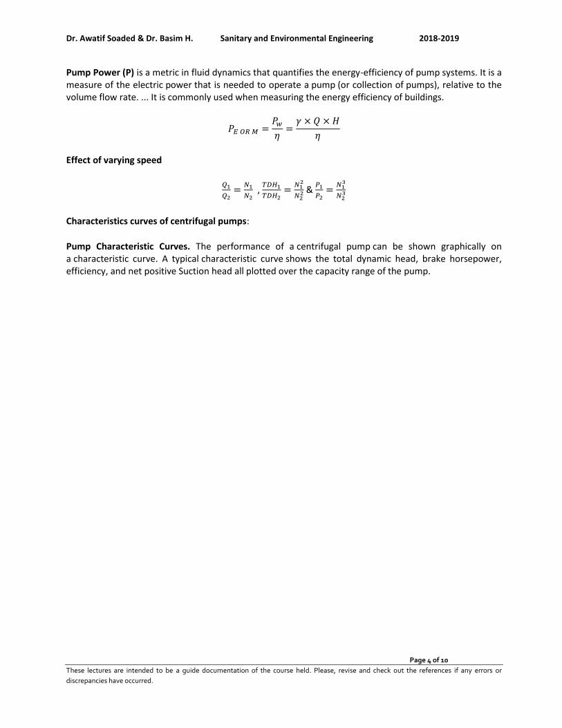
Dr. Awatif Soaded & Dr. Basim H. Sanitary and Environmental Engineering 2018-2019
Page 4 of 10
These lectures are intended to be a guide documentation of the course held. Please, revise and check out the references if any errors or
discrepancies have occurred.
Pump Power (P) is a metric in fluid dynamics that quantifies the energy-efficiency of pump systems. It is a measure of the electric power that is needed to operate a pump (or collection of pumps), relative to the volume flow rate. ... It is commonly used when measuring the energy efficiency of buildings.
𝑃𝐸 𝑂𝑅 𝑀 =𝑃𝑤
𝜂=
𝛾 × 𝑄 × 𝐻
𝜂
Effect of varying speed
𝑄1
𝑄2=
𝑁1
𝑁2 ,
𝑇𝐷𝐻1
𝑇𝐷𝐻2=
𝑁12
𝑁22 &
𝑃1
𝑃2=
𝑁13
𝑁23
Characteristics curves of centrifugal pumps:
Pump Characteristic Curves. The performance of a centrifugal pump can be shown graphically on a characteristic curve. A typical characteristic curve shows the total dynamic head, brake horsepower, efficiency, and net positive Suction head all plotted over the capacity range of the pump.

Dr. Awatif Soaded & Dr. Basim H. Sanitary and Environmental Engineering 2018-2019
Page 5 of 10
These lectures are intended to be a guide documentation of the course held. Please, revise and check out the references if any errors or
discrepancies have occurred.
Fig. 2 Characteristic curves of a centrifugal pump at constant speed

Dr. Awatif Soaded & Dr. Basim H. Sanitary and Environmental Engineering 2018-2019
Page 6 of 10
These lectures are intended to be a guide documentation of the course held. Please, revise and check out the references if any errors or
discrepancies have occurred.
Suction lift:
Net positive suction head (NPSH) is total head at pump suction branch over and above the vapor pressure of the liquid being pumped. Also, it’s a function of the system design, and represent the force available to drive the flow into the pump.
NPSH required (NPSHr) is a function of the pump design and is the lowest value of NPSH at which the pump can be guaranteed to operate without significant cavitation.
Available NPSH is the sum of the barometric pressure and the static head on the pump inlet, less the losses and fittings and vapor pressure of the water.
𝑁𝑃𝑆𝐻𝐴𝑣𝑎𝑖𝑙𝑎𝑏𝑙𝑒 = 𝑃𝐵 − ℎ𝐿 − 𝑃𝑣 − 𝑃𝑠
Where; PB: Barometric Pressure, hL: Head losses, Pv: Vapor Pressure, Ps: Allowable suction lift of the pump.
Cavitation is the formation of vapor cavities in a liquid, small liquid-free zones ("bubbles" or "voids"), that are the consequence of forces acting upon the liquid.
NPSH available < NPSH required
Barometric pressure vs. altitude
Vapor pressure of water vs. temperature

Dr. Awatif Soaded & Dr. Basim H. Sanitary and Environmental Engineering 2018-2019
Page 7 of 10
These lectures are intended to be a guide documentation of the course held. Please, revise and check out the references if any errors or
discrepancies have occurred.
Pump stations:
Pumping stations are facilities including pumps and equipment for pumping fluids from one place to another. They are used for a variety of infrastructure systems, such as the supply of water to canals, the drainage of low-lying land, and the removal of sewage to processing sites.
Design consideration for pump stations:
1) Location: the location of pump stations has an important bearing on the pressure maintained in the distribution system.
2) Architecture: the building should be adequate in size and have space for placing additional units as needed. It should be fireproof, pleasing in appearance, and have well-kept grounds. Its architecture can and should be in harmony with surroundings.
3) Capacity and operation: the pumps must have sufficient capacity to care for peak load, and the designer and operator must furnish and the pumping plant may operate 8-12 hours.
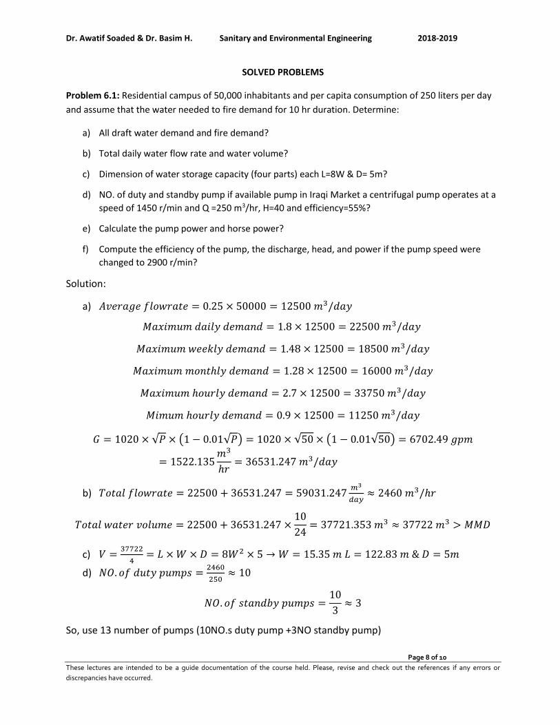
Dr. Awatif Soaded & Dr. Basim H. Sanitary and Environmental Engineering 2018-2019
Page 8 of 10
These lectures are intended to be a guide documentation of the course held. Please, revise and check out the references if any errors or
discrepancies have occurred.
SOLVED PROBLEMS
Problem 6.1: Residential campus of 50,000 inhabitants and per capita consumption of 250 liters per day
and assume that the water needed to fire demand for 10 hr duration. Determine:
a) All draft water demand and fire demand?
b) Total daily water flow rate and water volume?
c) Dimension of water storage capacity (four parts) each L=8W & D= 5m?
d) NO. of duty and standby pump if available pump in Iraqi Market a centrifugal pump operates at a
speed of 1450 r/min and Q =250 m3/hr, H=40 and efficiency=55%?
e) Calculate the pump power and horse power?
f) Compute the efficiency of the pump, the discharge, head, and power if the pump speed were
changed to 2900 r/min?
Solution:
a) 𝐴𝑣𝑒𝑟𝑎𝑔𝑒 𝑓𝑙𝑜𝑤𝑟𝑎𝑡𝑒 = 0.25 × 50000 = 12500 𝑚3/𝑑𝑎𝑦
𝑀𝑎𝑥𝑖𝑚𝑢𝑚 𝑑𝑎𝑖𝑙𝑦 𝑑𝑒𝑚𝑎𝑛𝑑 = 1.8 × 12500 = 22500 𝑚3/𝑑𝑎𝑦
𝑀𝑎𝑥𝑖𝑚𝑢𝑚 𝑤𝑒𝑒𝑘𝑙𝑦 𝑑𝑒𝑚𝑎𝑛𝑑 = 1.48 × 12500 = 18500 𝑚3/𝑑𝑎𝑦
𝑀𝑎𝑥𝑖𝑚𝑢𝑚 𝑚𝑜𝑛𝑡ℎ𝑙𝑦 𝑑𝑒𝑚𝑎𝑛𝑑 = 1.28 × 12500 = 16000 𝑚3/𝑑𝑎𝑦
𝑀𝑎𝑥𝑖𝑚𝑢𝑚 ℎ𝑜𝑢𝑟𝑙𝑦 𝑑𝑒𝑚𝑎𝑛𝑑 = 2.7 × 12500 = 33750 𝑚3/𝑑𝑎𝑦
𝑀𝑖𝑚𝑢𝑚 ℎ𝑜𝑢𝑟𝑙𝑦 𝑑𝑒𝑚𝑎𝑛𝑑 = 0.9 × 12500 = 11250 𝑚3/𝑑𝑎𝑦
𝐺 = 1020 × √𝑃 × (1 − 0.01√𝑃) = 1020 × √50 × (1 − 0.01√50) = 6702.49 𝑔𝑝𝑚
= 1522.135𝑚3
ℎ𝑟= 36531.247 𝑚3/𝑑𝑎𝑦
b) 𝑇𝑜𝑡𝑎𝑙 𝑓𝑙𝑜𝑤𝑟𝑎𝑡𝑒 = 22500 + 36531.247 = 59031.247𝑚3
𝑑𝑎𝑦≈ 2460 𝑚3/ℎ𝑟
𝑇𝑜𝑡𝑎𝑙 𝑤𝑎𝑡𝑒𝑟 𝑣𝑜𝑙𝑢𝑚𝑒 = 22500 + 36531.247 ×10
24= 37721.353 𝑚3 ≈ 37722 𝑚3 > 𝑀𝑀𝐷
c) 𝑉 =37722
4= 𝐿 × 𝑊 × 𝐷 = 8𝑊2 × 5 → 𝑊 = 15.35 𝑚 𝐿 = 122.83 𝑚 & 𝐷 = 5𝑚
d) 𝑁𝑂. 𝑜𝑓 𝑑𝑢𝑡𝑦 𝑝𝑢𝑚𝑝𝑠 =2460
250≈ 10
𝑁𝑂. 𝑜𝑓 𝑠𝑡𝑎𝑛𝑑𝑏𝑦 𝑝𝑢𝑚𝑝𝑠 =10
3≈ 3
So, use 13 number of pumps (10NO.s duty pump +3NO standby pump)
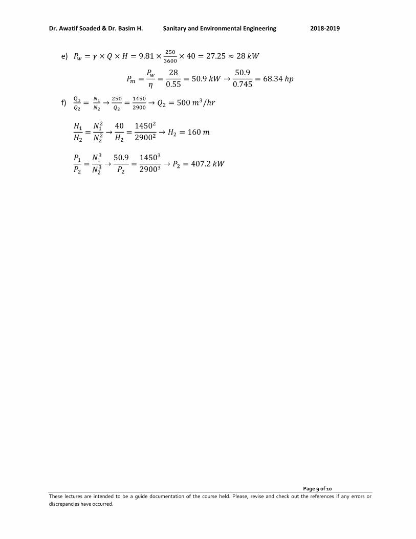
Dr. Awatif Soaded & Dr. Basim H. Sanitary and Environmental Engineering 2018-2019
Page 9 of 10
These lectures are intended to be a guide documentation of the course held. Please, revise and check out the references if any errors or
discrepancies have occurred.
e) 𝑃𝑤 = 𝛾 × 𝑄 × 𝐻 = 9.81 ×250
3600× 40 = 27.25 ≈ 28 𝑘𝑊
𝑃𝑚 =𝑃𝑤
𝜂=
28
0.55= 50.9 𝑘𝑊 →
50.9
0.745= 68.34 ℎ𝑝
f) Q1
𝑄2=
𝑁1
𝑁2→
250
𝑄2=
1450
2900→ 𝑄2 = 500 𝑚3/ℎ𝑟
𝐻1
𝐻2=
𝑁12
𝑁22 →
40
𝐻2=
14502
29002→ 𝐻2 = 160 𝑚
𝑃1
𝑃2=
𝑁13
𝑁23 →
50.9
𝑃2=
14503
29003→ 𝑃2 = 407.2 𝑘𝑊

Dr. Awatif Soaded & Dr. Basim H. Sanitary and Environmental Engineering 2018-2019
Page 10 of 10
These lectures are intended to be a guide documentation of the course held. Please, revise and check out the references if any errors or
discrepancies have occurred.
How to Choose a DRM Software to protect your document?

Dr. Awatif Soaded & Dr. Basim H. Sanitary and Environmental Engineering 2018-2019
Page 1 of 11
These lectures are intended to be a guide documentation of the course held. Please, revise and check out the references if any errors or
discrepancies have occurred.
Sanitary and Environmental Engineering
PART 1: WATER SUPPLY ENGINEERING
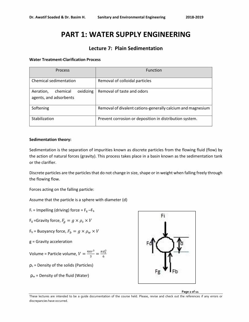
Dr. Awatif Soaded & Dr. Basim H. Sanitary and Environmental Engineering 2018-2019
Page 2 of 11
These lectures are intended to be a guide documentation of the course held. Please, revise and check out the references if any errors or
discrepancies have occurred.
PART 1: WATER SUPPLY ENGINEERING
Lecture 7: Plain Sedimentation
Water Treatment-Clarification Process
Process Function
Chemical sedimentation Removal of colloidal particles
Aeration, chemical oxidizing
agents, and adsorbents
Removal of taste and odors
Softening Removal of divalent cations-generally calcium and magnesium
Stabilization Prevent corrosion or deposition in distribution system.
Sedimentation theory:
Sedimentation is the separation of impurities known as discrete particles from the flowing fluid (flow) by
the action of natural forces (gravity). This process takes place in a basin known as the sedimentation tank
or the clarifier.
Discrete particles are the particles that do not change in size, shape or in weight when falling freely through
the flowing flow.
Forces acting on the falling particle:
Assume that the particle is a sphere with diameter (d)
Fi = Impelling (driving) force = Fg –Fb
Fg =Gravity force, 𝐹𝑔 = 𝑔 × 𝜌𝑠 × 𝑉
Fb = Buoyancy force, 𝐹𝑏 = 𝑔 × 𝜌𝑤 × 𝑉
g = Gravity acceleration
Volume = Particle volume, 𝑉 =4𝜋𝑟3
3=
𝜋𝑑𝑠3
6
ρs = Density of the solids (Particles)
ρw = Density of the fluid (Water)
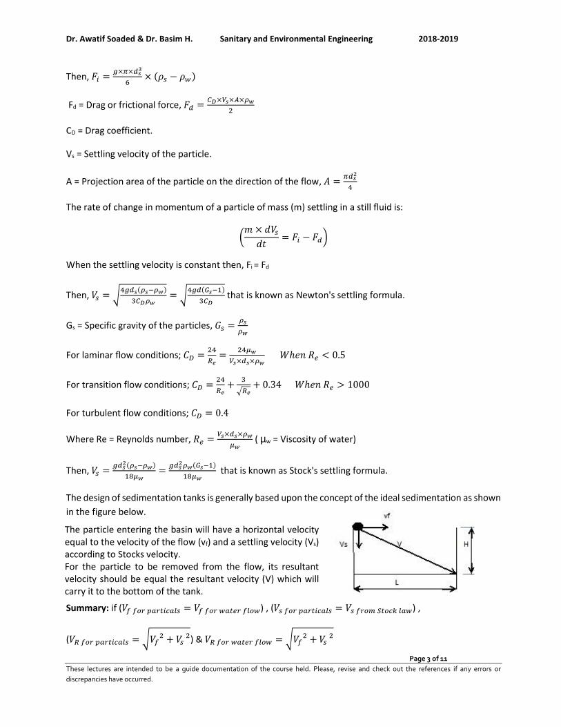
Dr. Awatif Soaded & Dr. Basim H. Sanitary and Environmental Engineering 2018-2019
Page 3 of 11
These lectures are intended to be a guide documentation of the course held. Please, revise and check out the references if any errors or
discrepancies have occurred.
Then, 𝐹𝑖 =𝑔×𝜋×𝑑𝑠
3
6× (𝜌𝑠 − 𝜌𝑤)
Fd = Drag or frictional force, 𝐹𝑑 =𝐶𝐷×𝑉𝑠×𝐴×𝜌𝑤
2
CD = Drag coefficient.
Vs = Settling velocity of the particle.
A = Projection area of the particle on the direction of the flow, 𝐴 =𝜋𝑑𝑠
2
4
The rate of change in momentum of a particle of mass (m) settling in a still fluid is:
(𝑚 × 𝑑𝑉𝑠
𝑑𝑡= 𝐹𝑖 − 𝐹𝑑)
When the settling velocity is constant then, Fi = Fd
Then, 𝑉𝑠 = √4𝑔𝑑𝑠(𝜌𝑠−𝜌𝑤)
3𝐶𝐷𝜌𝑤= √
4𝑔𝑑(𝐺𝑠−1)
3𝐶𝐷 that is known as Newton's settling formula.
Gs = Specific gravity of the particles, 𝐺𝑠 =𝜌𝑠
𝜌𝑤
For laminar flow conditions; 𝐶𝐷 =24
𝑅𝑒=
24𝜇𝑤
𝑉𝑠×𝑑𝑠×𝜌𝑤 𝑊ℎ𝑒𝑛 𝑅𝑒 < 0.5
For transition flow conditions; 𝐶𝐷 =24
𝑅𝑒+
3
√𝑅𝑒+ 0.34 𝑊ℎ𝑒𝑛 𝑅𝑒 > 1000
For turbulent flow conditions; 𝐶𝐷 = 0.4
Where Re = Reynolds number, 𝑅𝑒 =𝑉𝑠×𝑑𝑠×𝜌𝑤
𝜇𝑤 ( µw = Viscosity of water)
Then, 𝑉𝑠 =𝑔𝑑𝑠
2(𝜌𝑠−𝜌𝑤)
18𝜇𝑤=
𝑔𝑑𝑠2𝜌𝑤(𝐺𝑠−1)
18𝜇𝑤 that is known as Stock's settling formula.
The design of sedimentation tanks is generally based upon the concept of the ideal sedimentation as shown
in the figure below.
Summary: if (𝑉𝑓 𝑓𝑜𝑟 𝑝𝑎𝑟𝑡𝑖𝑐𝑎𝑙𝑠 = 𝑉𝑓 𝑓𝑜𝑟 𝑤𝑎𝑡𝑒𝑟 𝑓𝑙𝑜𝑤) , (𝑉𝑠 𝑓𝑜𝑟 𝑝𝑎𝑟𝑡𝑖𝑐𝑎𝑙𝑠 = 𝑉𝑠 𝑓𝑟𝑜𝑚 𝑆𝑡𝑜𝑐𝑘 𝑙𝑎𝑤) ,
(𝑉𝑅 𝑓𝑜𝑟 𝑝𝑎𝑟𝑡𝑖𝑐𝑎𝑙𝑠 = √𝑉𝑓2 + 𝑉𝑠
2) & 𝑉𝑅 𝑓𝑜𝑟 𝑤𝑎𝑡𝑒𝑟 𝑓𝑙𝑜𝑤 = √𝑉𝑓2 + 𝑉𝑠
2
The particle entering the basin will have a horizontal velocity equal to the velocity of the flow (vf) and a settling velocity (Vs) according to Stocks velocity. For the particle to be removed from the flow, its resultant velocity should be equal the resultant velocity (V) which will carry it to the bottom of the tank.
Dr. Awatif Soaded & Dr. Basim H. Sanitary and Environmental Engineering 2018-2019
Page 4 of 11
These lectures are intended to be a guide documentation of the course held. Please, revise and check out the references if any errors or
discrepancies have occurred.
So, the particles will be removed 100% if (𝑉𝑅 𝑓𝑜𝑟 𝑝𝑎𝑟𝑡𝑖𝑐𝑎𝑙𝑠 = 𝑉𝑅 𝑓𝑜𝑟 𝑤𝑎𝑡𝑒𝑟 𝑓𝑙𝑜𝑤)
Considering the velocity vector triangle and the dimensions of the tank (L= length, H = height and W = width).
𝐻𝑜𝑟𝑖𝑧𝑜𝑛𝑡𝑎𝑙 𝑣𝑒𝑙𝑜𝑐𝑖𝑡𝑦 𝑣𝑓 =𝑄
𝐴𝑐=
𝑄
𝑊 × 𝐻
If particle is to be removed, it's settling velocity and horizontal velocity (𝑣𝑓) must be such that their
resultant, (V), will carry it to the bottom of the tank before the outlet zone is reached, all particles with the same settling velocity will be removed.
𝑣𝑓
𝑉𝑠=
𝐿
𝐻 𝑡ℎ𝑒𝑛 𝑠𝑒𝑡𝑡𝑙𝑖𝑛𝑔 𝑣𝑒𝑙𝑜𝑐𝑖𝑡𝑦 𝑉𝑠 =
𝑣𝑓 × 𝐻
𝐿=
𝑄
𝑊 × 𝐻×
𝐻
𝐿=
𝑄
𝑊 × 𝐿=
𝑄
𝐴𝑠
Where: Q: The discharge entering the tank; Ac: The cross-sectional area of the tank perpendicular to the flow = 𝑊 × 𝐻 As: The surface area= 𝑊 × 𝐿 Surface overflow rate (SOR or Vs) is numerically equal to the flow divide by the plan or surface area of the
basin, but which physically represents the settling velocity of the smallest particle to be 100% removed
from the flow or to be settled. Any particle of (Vs) larger or equal to SOR will settle (𝑉𝑠 𝑓𝑜𝑟 𝑝𝑎𝑟𝑡𝑖𝑐𝑙𝑒 ≥ 𝑆𝑂𝑅),
and while those which settle at lower velocities will be removed in direct proportion to the ratio of their
settling velocity to (Vs), so, if Vs is smaller than SOR, it will not settle (𝑉𝑠 𝑓𝑜𝑟 𝑝𝑎𝑟𝑡𝑖𝑐𝑙𝑒 < 𝑆𝑂𝑅).
Weir Overflow Rates is the flow rate of the clarifier effluent per the length of the overflow weir. It is argued
that if the weir loading rates exceed the recommended values, the velocity of currents approaching the
weirs may be such that excessive solids are carried over the weir.
Ideal sedimentation
Solid liquid separation process in which a suspension is separated into two phases:
1) Clarified supernatant leaving the top of the sedimentation tank (overflow).
2) Concentrated sludge leaving the bottom of the sedimentation tank (underflow).
The following characteristics exhibit in an ideal sedimentation process:
1) The flow is evenly distributed across the tank;
2) The particles are evenly distributed in the flow.
Purpose of Settling:
1) To remove coarse dispersed phase.
2) To remove coagulated and flocculated impurities.
3) To remove precipitated impurities after chemical treatment.
4) To settle the sludge (biomass) after activated sludge process / tricking filters.
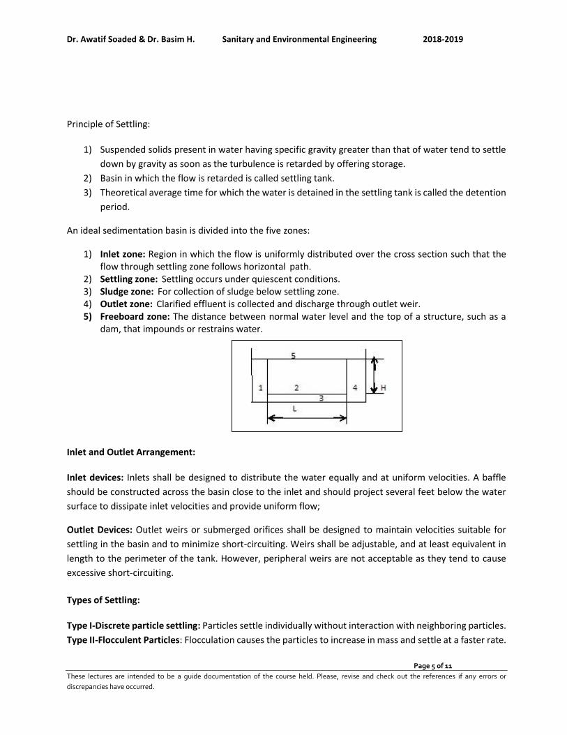
Dr. Awatif Soaded & Dr. Basim H. Sanitary and Environmental Engineering 2018-2019
Page 5 of 11
These lectures are intended to be a guide documentation of the course held. Please, revise and check out the references if any errors or
discrepancies have occurred.
Principle of Settling:
1) Suspended solids present in water having specific gravity greater than that of water tend to settle
down by gravity as soon as the turbulence is retarded by offering storage.
2) Basin in which the flow is retarded is called settling tank.
3) Theoretical average time for which the water is detained in the settling tank is called the detention
period.
An ideal sedimentation basin is divided into the five zones:
1) Inlet zone: Region in which the flow is uniformly distributed over the cross section such that the flow through settling zone follows horizontal path.
2) Settling zone: Settling occurs under quiescent conditions. 3) Sludge zone: For collection of sludge below settling zone. 4) Outlet zone: Clarified effluent is collected and discharge through outlet weir. 5) Freeboard zone: The distance between normal water level and the top of a structure, such as a
dam, that impounds or restrains water.
Inlet and Outlet Arrangement:
Inlet devices: Inlets shall be designed to distribute the water equally and at uniform velocities. A baffle
should be constructed across the basin close to the inlet and should project several feet below the water
surface to dissipate inlet velocities and provide uniform flow;
Outlet Devices: Outlet weirs or submerged orifices shall be designed to maintain velocities suitable for
settling in the basin and to minimize short-circuiting. Weirs shall be adjustable, and at least equivalent in
length to the perimeter of the tank. However, peripheral weirs are not acceptable as they tend to cause
excessive short-circuiting.
Types of Settling:
Type I-Discrete particle settling: Particles settle individually without interaction with neighboring particles.
Type II-Flocculent Particles: Flocculation causes the particles to increase in mass and settle at a faster rate.
Dr. Awatif Soaded & Dr. Basim H. Sanitary and Environmental Engineering 2018-2019
Page 6 of 11
These lectures are intended to be a guide documentation of the course held. Please, revise and check out the references if any errors or
discrepancies have occurred.
Type III-Hindered or Zone settling: The mass of particles tends to settle as a unit with individual particles
remaining in fixed positions with respect to each other.
Type IV-Compression: The concentration of particles is so high that sedimentation can only occur through
compaction of the structure.
Types of sedimentation tanks: 1) Shape: rectangular, square, circular (cylindrical);
a) Sedimentation tanks may function either intermittently or continuously. The intermittent tanks also called quiescent type tanks are those which store water for a certain period and keep it in complete rest. In a continuous flow type tank, the flow velocity is only reduced and the water is not brought to complete rest as is done in an intermittent type.
b) Settling basins may be either long rectangular or circular in plan. Long narrow rectangular tanks with horizontal flow are generally preferred to the circular tanks with radial or spiral flow.
2) Direction of flow: horizontal, radial, vertical; 3) Detention time: full and with draw, continuous flow; 4) Plain sedimentation, sedimentation with chemicals
Design criteria
1) SOR: 20 – 80 m/d. 2) Detention time: 2- 6 hr (Average 3 –4 hr). 3) Depth or height (H): 2-6 m (Average 3–4 m). 4) Inlet velocity (vf) 0.15 – 0.5 m/min. 5) In rectangular tanks L/W = (2/1 – 5/1), L max less than 100 m. 6) In circular tanks Diameter (D) max less than 50m, inlet diameter less than 10%D.
7) Weir loading rate (Q
Weir Effluent Length): 120 – 250 m3/m/d.
8) scouring velocity (vh)
The horizontal velocity that will re-suspend the settled particles, vh = √8βgd𝑠(Gs−1)
f
β = 0.04 – 0.06, f = 0.02 – 0.03
Why is it hard to reach ideal settling in sedimentation tanks?
1) Variable inlet flowing velocity.
2) Variable temperature inside the tank that will give different ρw and µw.
3) Un-similar particle distribution.
4) Short circuiting due to the shape of the tank.
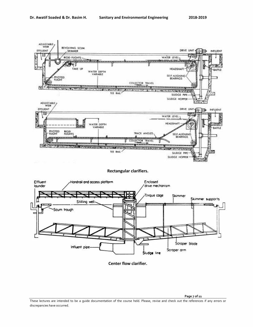
Dr. Awatif Soaded & Dr. Basim H. Sanitary and Environmental Engineering 2018-2019
Page 7 of 11
These lectures are intended to be a guide documentation of the course held. Please, revise and check out the references if any errors or
discrepancies have occurred.
Rectangular clarifiers.
Center flow clarifier.
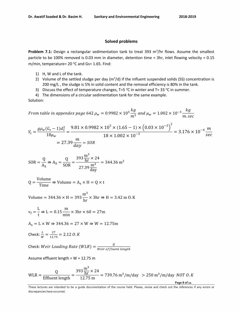
Dr. Awatif Soaded & Dr. Basim H. Sanitary and Environmental Engineering 2018-2019
Page 8 of 11
These lectures are intended to be a guide documentation of the course held. Please, revise and check out the references if any errors or
discrepancies have occurred.
Solved problems
Problem 7.1: Design a rectangular sedimentation tank to treat 393 m3/hr flows. Assume the smallest
particle to be 100% removed is 0.03 mm in diameter, detention time = 3hr, inlet flowing velocity = 0.15
m/min, temperature= 20 oC and Gs= 1.65. Find:
1) H, W and L of the tank. 2) Volume of the settled sludge per day (m3/d) if the influent suspended solids (SS) concentration is
200 mg/L , the sludge is 5% in solid content and the removal efficiency is 80% in the tank. 3) Discuss the effect of temperature changes, T=5 oC in winter and T= 33 oC in summer. 4) The dimensions of a circular sedimentation tank for the same example.
Solution:
𝐹𝑟𝑜𝑚 𝑡𝑎𝑏𝑙𝑒 𝑖𝑛 𝑎𝑝𝑝𝑒𝑛𝑑𝑒𝑥 𝑝𝑎𝑔𝑒 642 𝜌𝑤 = 0.9982 × 10³𝑘𝑔
𝑚3 𝑎𝑛𝑑 𝜇𝑤 = 1.002 × 10⁻³
𝑘𝑔
𝑚. 𝑠𝑒𝑐
𝑉𝑠 =𝑔𝜌𝑤(𝐺𝑠 − 1)𝑑𝑠
2
18𝜇𝑤=
9.81 × 0.9982 × 103 × (1.65 − 1) × (0.03 × 10−3)
2
18 × 1.002 × 10−3= 3.176 × 10⁻⁴ 𝑚
𝑠𝑒𝑐
= 27.39𝑚
𝑑𝑎𝑦= 𝑆𝑂𝑅
SOR =Q
AS⇛ AS =
Q
SOR=
393m3
hr× 24
27.39m3
day
= 344.36 m2
Q =Volume
Time⇛ Volume = As × H = Q × t
Volume = 344.36 × H = 393m3
hr× 3hr ⇛ H = 3.42 m O. K
vf =L
t⇛ L = 0.15
m
min× 3hr × 60 = 27m
As = L × W ⇛ 344.36 = 27 × W ⇛ W = 12.75m
Check: 𝐿
𝑊=
27
12.75= 2.12 𝑂. 𝐾
Check: 𝑊𝑒𝑖𝑟 𝐿𝑜𝑎𝑑𝑖𝑛𝑔 𝑅𝑎𝑡𝑒 (𝑊𝐿𝑅) =𝑄
𝑊𝑒𝑖𝑟 𝑒𝑓𝑓𝑙𝑢𝑒𝑛𝑡 𝑙𝑒𝑛𝑔𝑡ℎ
Assume effluent length = W = 12.75 m
WLR =Q
Effluent length=
393m3
hr× 24
12.75 m= 739.76 m3/m/day > 250 m3/m/day 𝑁𝑂𝑇 𝑂. 𝐾
Dr. Awatif Soaded & Dr. Basim H. Sanitary and Environmental Engineering 2018-2019
Page 9 of 11
These lectures are intended to be a guide documentation of the course held. Please, revise and check out the references if any errors or
discrepancies have occurred.
𝐴𝑠𝑠𝑢𝑚𝑒 𝑤𝑒𝑖𝑟 𝑙𝑜𝑎𝑑𝑖𝑛𝑔 𝑟𝑎𝑡𝑒 = 250 m3/m/day =393 × 24
Length⇛ Length = 37.7 ≈ 38 m
Check the scouring velocity:
Assume β
f= 2
vh = √8βg(Gs−1)d
f= √8 × 2 × 9.81 × (1.65 − 1)(0.03 × 10⁻³) = 0.055
m
sec= 3.319 m/min
∴ 𝑣𝑓 = 0.15𝑚/ min 𝑎𝑛𝑑 𝑉𝑠 > 𝑣𝑓 𝑂. 𝐾
2) Total amount of suspended solids in the effluent:
200mg
L× 393
m3
hr×
103
106× 24 = 1886.4 kg/day
80% removal (sedimentation in the tank)
∴ 𝑆𝑒𝑡𝑡𝑙𝑒𝑑 𝑠𝑜𝑙𝑖𝑑𝑠 = 0.8 × 1886.4 = 1509𝑘𝑔
𝑑𝑎𝑦= 𝑚𝑠
𝑆𝑙𝑢𝑑𝑔𝑒 𝑎𝑚𝑜𝑢𝑛𝑡 = 𝑆𝑜𝑙𝑖𝑑𝑠 𝑎𝑚𝑜𝑢𝑛𝑡 + 𝑊𝑎𝑡𝑒𝑟 𝑎𝑚𝑜𝑢𝑛𝑡
5
100=
𝑤𝑠
𝑤𝑠 + 𝑤𝑤=
1509
1509 + 𝑤𝑤⇛ 𝑤𝑤 = 28671 kg/day
Volume of solids =ms
ρs & Volume of water =
mw
ρw
Assume ρw = 998.2kg
m3 at T = 200C ≈ 1000 kg/m3
Volume of sludge = Volume of solids + Volume of water =1509
1.65 × 10³+
28671
103= 29.58
m3
day
≈ 30m3
day
⇛ 𝑇𝑜 𝑏𝑒 𝑢𝑠𝑒𝑑 𝑖𝑛 𝑠𝑖𝑧𝑒 𝑐𝑎𝑙𝑐𝑢𝑙𝑎𝑡𝑖𝑜𝑛 𝑎𝑛𝑑 𝑡ℎ𝑒 𝑛𝑢𝑚𝑏𝑒𝑟 𝑜𝑓 𝑡𝑖𝑚𝑒𝑠 𝑐𝑙𝑒𝑎𝑛𝑖𝑛𝑔 𝑜𝑓 𝑡ℎ𝑒 ℎ𝑜𝑝𝑝𝑒𝑟
3) Settling velocity changeability with temperature or water mass density and viscosity and compare it with
the design criteria:
Season Temperature
( 0C)
Water mass density
ρw (𝑘𝑔
𝑚3)
Water viscosity
μw (𝑘𝑔
𝑚.𝑠𝑒𝑐)
Winter 5 0.9999 × 10³ 1.519 × 10⁻³
Dr. Awatif Soaded & Dr. Basim H. Sanitary and Environmental Engineering 2018-2019
Page 10 of 11
These lectures are intended to be a guide documentation of the course held. Please, revise and check out the references if any errors or
discrepancies have occurred.
Summer 33 0.9957 × 10³ 0.7983 × 10⁻³
So, for sedimentation tank design the best water temperature degree at winter temperature (50C), and
then increase the settling velocity with increase temperature due to (𝑉𝑠 > 𝑆𝑂𝑅).
Fig. 1 Settling velocity variation with different temperature.
Problem 7.2: A settling tank if designed for an overflow rate of 4000-liter pr m2 per hour. What percentage
of particles of diameter (a) 0.05 mm (b) 0.02 mm, will be removed in the tank at 100C? Assume specific
gravity of particles S.G = 2.65.
Solution:
𝑆𝑒𝑡𝑡𝑙𝑖𝑛𝑔 𝑣𝑒𝑙𝑜𝑐𝑖𝑡𝑦 𝑉𝑠 = 𝑆𝑂𝑅 =𝑄
𝐴𝑠=
4000×10−3
3600
1= 1.111 × 10⁻³ 𝑚
𝑠𝑒𝑐= 0.111 𝑐𝑚/𝑠𝑒𝑐
(a) For 0.05 mm particles:
S.G = 2.65,
𝐹𝑟𝑜𝑚 𝑡𝑎𝑏𝑙𝑒 at T = 100C 𝜌𝑤 = 0.9997 × 10³𝑘𝑔
𝑚3 𝑎𝑛𝑑 𝜇𝑤 = 1.307 × 10⁻³
𝑘𝑔
𝑚. 𝑠𝑒𝑐
𝑉𝑠 =𝑔𝜌𝑤(𝐺𝑠 − 1)𝑑𝑠
2
18𝜇𝑤=
9.81 × 0.9997 × 103 × (2.65 − 1) × (0.05 × 10−3)
2
18 × 1.307 × 10−3
= 1.719 × 10⁻³ 𝑚
𝑠𝑒𝑐= 0.1719
𝑐𝑚
𝑠𝑒𝑐= 148.56
𝑚
𝑑𝑎𝑦> 𝑆𝑂𝑅
0.00
0.50
1.00
1.50
2.00
2.50
3.00
3.50
4.00
4.50
0 20 40 60 80 100
SETTLING VELOCITY(Vs)
SETTLING VELOCITY(Vs)
Dr. Awatif Soaded & Dr. Basim H. Sanitary and Environmental Engineering 2018-2019
Page 11 of 11
These lectures are intended to be a guide documentation of the course held. Please, revise and check out the references if any errors or
discrepancies have occurred.
% 𝑆𝑒𝑡𝑡𝑙𝑒𝑑 =0.1719
0.111× 100 = 154.86% > 100%, Hence all the particles of 0.05 mm diameter will
settle.
(b) For 0.02 mm particles:
𝑉𝑠 =𝑔𝜌𝑤(𝐺𝑠 − 1)𝑑𝑠
2
18𝜇𝑤=
9.81 × 0.9997 × 103 × (2.65 − 1) × (0.02 × 10−3)
2
18 × 1.307 × 10−3
= 2.751 × 10⁻⁴ 𝑚
𝑠𝑒𝑐= 0.0275
𝑐𝑚
𝑠𝑒𝑐= 23.771
𝑚
𝑑𝑎𝑦< 𝑆𝑂𝑅
% 𝑆𝑒𝑡𝑡𝑙𝑒𝑑 =0.0275
0.111× 100 = 24.774% < 100%, Hence the particles of 0.02 mm diameter will
settle at 24.774%.
Problem 7.3: Find the diameter of the particles with specific gravity of 1.2 removed in a tank having a
surface area of 250 m2 and treating 8 million liters per day (MLD)? Assume temperature 260C and specific
gravity of particles S.G = 2.65.
Solution:
𝑂𝑣𝑒𝑟𝑓𝑙𝑜𝑤 𝑟𝑎𝑡𝑒 =(8 × 106) × 10−3
250 × 24= 1.333 𝑚3/𝑚2/ℎ𝑜𝑢𝑟
∴ 𝑆𝑒𝑡𝑡𝑙𝑖𝑛𝑔 𝑣𝑒𝑙𝑜𝑐𝑖𝑡𝑦 𝑉𝑠 =1.333 × 100
1 × 3600= 0.037 𝑐𝑚/𝑠𝑒𝑐
Applying stoke,s law:
S.G = 2.65,
𝐹𝑟𝑜𝑚 𝑡𝑎𝑏𝑙𝑒 at T = 260C 𝜌𝑤 = 0.99681 × 10³𝑘𝑔
𝑚3 𝑎𝑛𝑑 𝜇𝑤 = 0.8746 × 10⁻³
𝑘𝑔
𝑚. 𝑠𝑒𝑐
𝑉𝑠 =𝑔𝜌𝑤(𝐺𝑠 − 1)𝑑2
18𝜇𝑤= 3.702 × 10−4 =
9.81 × 0.99681 × 103 × (2.65 − 1) × 𝑑2
18 × 0.8746 × 10−3⇛ 𝑑
= 0.019 𝑚𝑚
𝑉𝑠 =𝑔𝜌𝑤(𝐺𝑠 − 1)𝑑2
18𝜇𝑤= 3.702 × 10−4 =
9.81 × 0.99681 × 103 × (1.2 − 1) × 𝑑2
18 × 0.8746 × 10−3⇛ 𝑑 = 5.4 × 10−5
= 5.4 × 10⁻²𝑚𝑚
How to Choose a DRM Software to protect your document?

Dr. Awatif Soaded & Dr. Basim H. Sanitary and Environmental Engineering 2018-2019
Page 1 of 16
These lectures are intended to be a guide documentation of the course held. Please, revise and check out the references if any errors or
discrepancies have occurred.
Sanitary and Environmental Engineering
PART 1: WATER SUPPLY ENGINEERING

Dr. Awatif Soaded & Dr. Basim H. Sanitary and Environmental Engineering 2018-2019
Page 2 of 16
These lectures are intended to be a guide documentation of the course held. Please, revise and check out the references if any errors or
discrepancies have occurred.
PART 1: WATER SUPPLY ENGINEERING
Lecture 9: Filtration
Filtration is the separation of non-settleable solids from water by passing it through a porous
media. Filtration also removes from water: color, taste, odor, iron, manganese and
microorganisms such as bacteria. In water treatment plants this is done in a unit known as the
filter.
Types of filter according to process workability:
1) Gravity filter:
a) Slow sand filter: They consist of fine sand, supported by gravel. They capture particles
near the surface of the bed and are usually cleaned by scraping away the top layer of
sand that contains the particles.
b) Rapid-sand filter: They consist of larger sand grains supported by gravel and capture
particles throughout the bed. They are cleaned by backwashing water through the bed
to 'lift out' the particles.
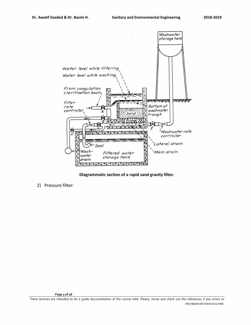
Dr. Awatif Soaded & Dr. Basim H. Sanitary and Environmental Engineering 2018-2019
Page 3 of 16
These lectures are intended to be a guide documentation of the course held. Please, revise and check out the references if any errors or
discrepancies have occurred.
Diagrammatic section of a rapid sand gravity filter.
2) Pressure filter:
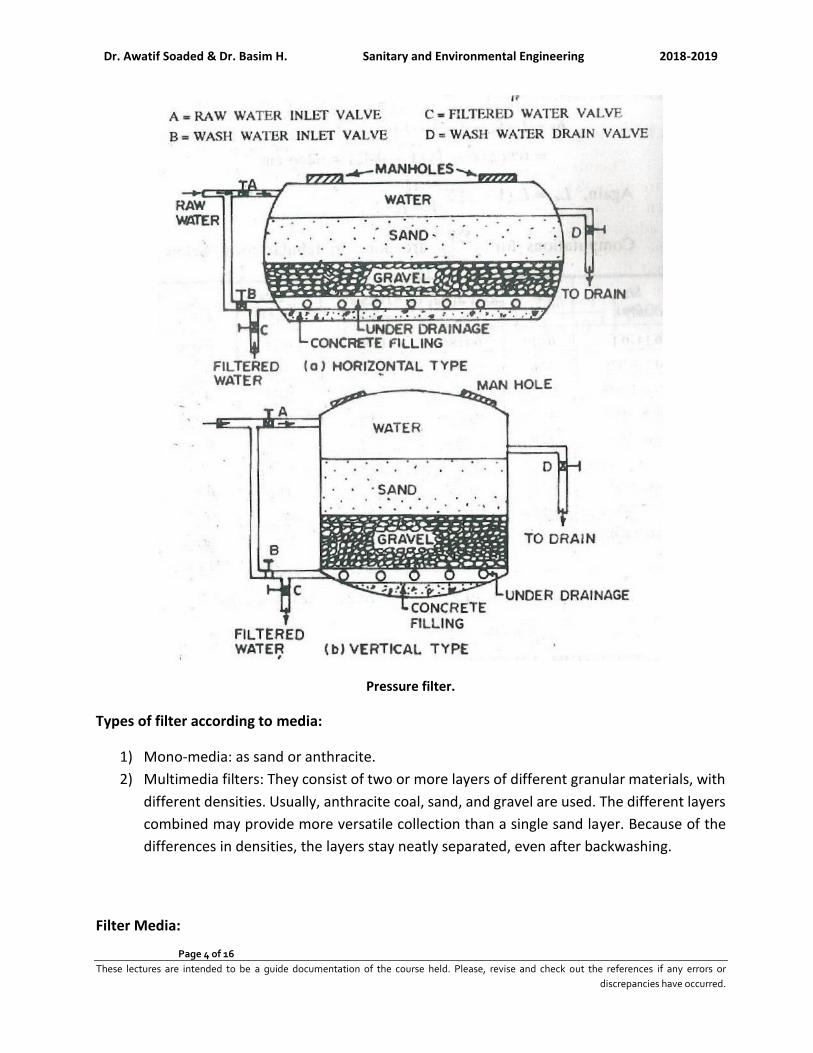
Dr. Awatif Soaded & Dr. Basim H. Sanitary and Environmental Engineering 2018-2019
Page 4 of 16
These lectures are intended to be a guide documentation of the course held. Please, revise and check out the references if any errors or
discrepancies have occurred.
Pressure filter.
Types of filter according to media:
1) Mono-media: as sand or anthracite.
2) Multimedia filters: They consist of two or more layers of different granular materials, with
different densities. Usually, anthracite coal, sand, and gravel are used. The different layers
combined may provide more versatile collection than a single sand layer. Because of the
differences in densities, the layers stay neatly separated, even after backwashing.
Filter Media:
Dr. Awatif Soaded & Dr. Basim H. Sanitary and Environmental Engineering 2018-2019
Page 5 of 16
These lectures are intended to be a guide documentation of the course held. Please, revise and check out the references if any errors or
discrepancies have occurred.
The choice of a filter medium is dictated by the durability required, the desired degree of purification, and the length of filter run and ease of backwash sought. The ideal medium should have such a size and be of such material that it will provide a satisfactory effluent, return a maximum quantity of solids, and be readily cleaned with a minimum of wash water.
1) Sand: Sand, either fine or coarse, is generally used as filter media. The size of the sand is
measured and expressed by the term called effective size. The effective size, i.e. D10 may
be defined as the size of the sieve in mm through which ten percent of the sample of sand
by weight will pass. The uniformity in size or degree of variations in sizes of particles is
measured and expressed by the term called uniformity coefficient. The uniformity
coefficient, i.e. (𝐷𝑈 =𝐷60
𝐷10) may be defined as the ratio of the sieve size in mm through
which 60 percent of the sample of sand will pass, to the effective size of the sand.
2) Gravel: The layers of sand may be supported on gravel, which permits the filtered water
to move freely to the underdrains, and allows the wash water to move uniformly upwards.
3) Other materials: Instead of using sand, sometimes, anthracite is used as filter media.
Anthracite is made from anthracite, which is a type of coal-stone that burns without smoke
or flames. It is cheaper and has been able to give a high rate of filtration.
Fine material Coarse material
1) Better effluent 2) High head loss in upper layers of the bed. 3) Short filter runs. 4) Most difficult in cleaning upon backwash
1) Better utilization of the storage capacity of the filter.
2) Permit deeper penetration of the floc. 3) Longer filter runs. 4) Easier cleaning upon backwash
Sand Anthracite Gravel
1) Clean, hard, and resistance. 2) Not lose more than 5% by
weight after being placed in 40% hydrochloric acid for 24 hr.
3) Sand depth 600-700 mm. 4) Effective size of 0.45-0.55 mm. 5) Uniformity coefficient not less
than 1.2 and not exceed 1.7.
1) Anthracite depth 600-700 mm.
2) Effective size of 0.7 mm.
3) Uniformity coefficient of 1.75 or less.
1) Hard, rounded, durable, free from flat, thin, and contain no foreign material.
2) Effective size between 0.8 to 2 mm.
3) Uniformity coefficient of not over 1.7.
Filtration Mechanisms: There are four basic filtration mechanisms:
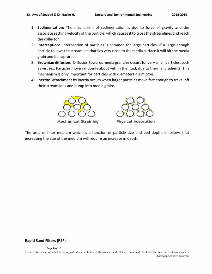
Dr. Awatif Soaded & Dr. Basim H. Sanitary and Environmental Engineering 2018-2019
Page 6 of 16
These lectures are intended to be a guide documentation of the course held. Please, revise and check out the references if any errors or
discrepancies have occurred.
1) Sedimentation: The mechanism of sedimentation is due to force of gravity and the
associate settling velocity of the particle, which causes it to cross the streamlines and reach
the collector.
2) Interception: Interception of particles is common for large particles. If a large enough
particle follows the streamline that lies very close to the media surface it will hit the media
grain and be captured.
3) Brownian diffusion: Diffusion towards media granules occurs for very small particles, such
as viruses. Particles move randomly about within the fluid, due to thermal gradients. This
mechanism is only important for particles with diameters < 1 micron.
4) Inertia: Attachment by inertia occurs when larger particles move fast enough to travel off
their streamlines and bump into media grains.
The area of filter medium which is a function of particle size and bed depth, it follows that
increasing the size of the medium will require an increase in depth.
Rapid Sand Filters (RSF)
Dr. Awatif Soaded & Dr. Basim H. Sanitary and Environmental Engineering 2018-2019
Page 7 of 16
These lectures are intended to be a guide documentation of the course held. Please, revise and check out the references if any errors or
discrepancies have occurred.
Rapid filtration generally implies a process which includes coagulation, flocculation, clarification,
filtration, and disinfection.
Essential characteristics of a rapid filter:
1) The turbidity of water applied to the filters should not exceed 10 units and preferably 5
units,
2) High rate of filtration, 120 to 240 m/day,
3) Washing the filter units by revising flow of filtered water upward through the filter to
remove mud and other impurities which have lodged.
Filter component: As shown in the figures above:
A) Water head: Clearance, 600-900 mm in depth.
B) Filer bed (Sand layer), 600- 1200 mm in depth. The objectives of this layer:
i. Coarse to retain large quantity of solid particles. ii. Fine to prevent the passage of small solid particles.
iii. Deep layer to allow long filtration run. iv. Graded to permit good backwash cleaning.
Properties: Effective size (D10)= 0.45 -0.55 mm, Uniformity coefficient (Cu)= D60/D10
=1.2-1.7.
C) Gravel layer (bed), 400-600 mm in depth. The objectives of this layer:
i. Support the filter bed (sand layer). ii. Permit the filtered water to move freely towards the underdrain system.
iii. Allows the washing water to move uniformly upwards to the filter bed. Properties: clean, free from flat and thin shapes, hard, round, durable and ρs = 1600 kg/m3
D) Underdrain system: The objectives of this layer:
i. To collect the filtered water. ii. To distribute the washing water evenly.
Mathematical equation of filtration process:
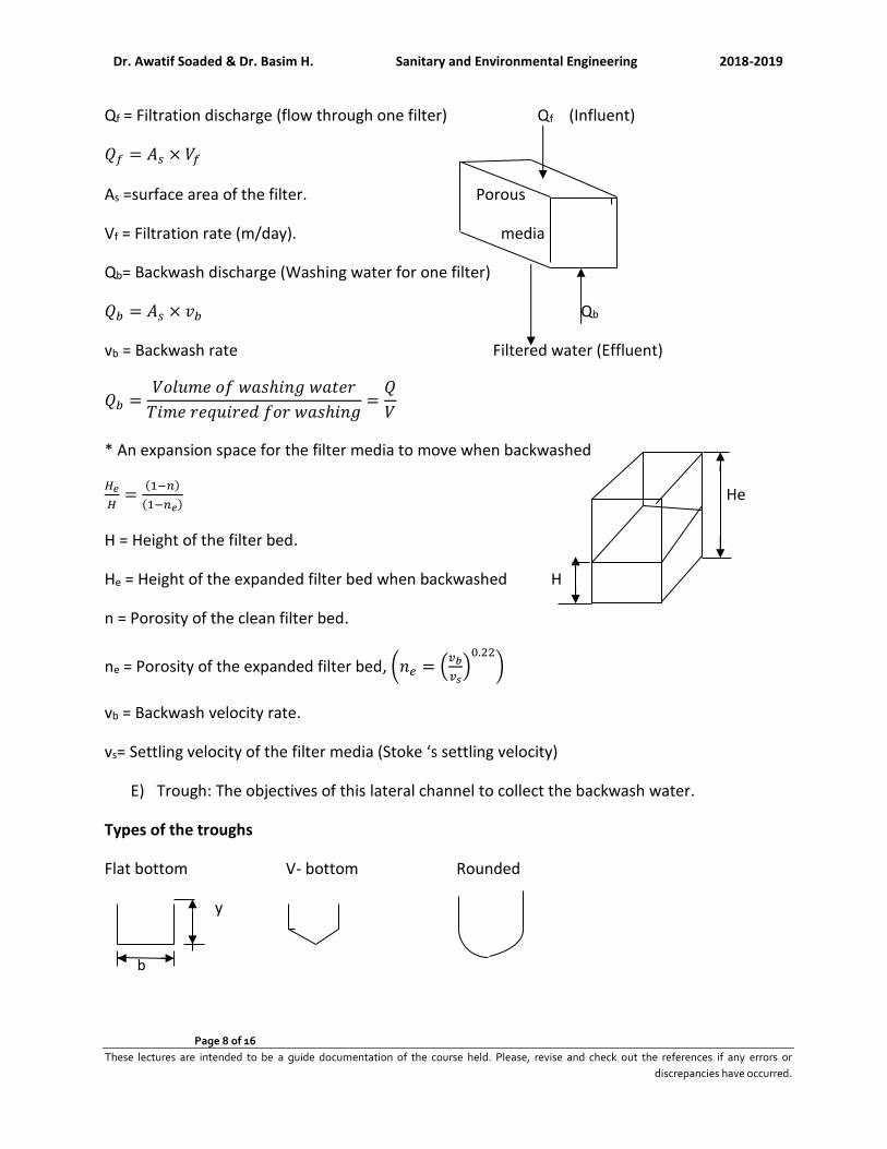
Dr. Awatif Soaded & Dr. Basim H. Sanitary and Environmental Engineering 2018-2019
Page 8 of 16
These lectures are intended to be a guide documentation of the course held. Please, revise and check out the references if any errors or
discrepancies have occurred.
Qf = Filtration discharge (flow through one filter) Qf (Influent)
𝑄𝑓 = 𝐴𝑠 × 𝑉𝑓
As =surface area of the filter. Porous
Vf = Filtration rate (m/day). media
Qb= Backwash discharge (Washing water for one filter)
𝑄𝑏 = 𝐴𝑠 × 𝑣𝑏 Qb
vb = Backwash rate Filtered water (Effluent)
𝑄𝑏 =𝑉𝑜𝑙𝑢𝑚𝑒 𝑜𝑓 𝑤𝑎𝑠ℎ𝑖𝑛𝑔 𝑤𝑎𝑡𝑒𝑟
𝑇𝑖𝑚𝑒 𝑟𝑒𝑞𝑢𝑖𝑟𝑒𝑑 𝑓𝑜𝑟 𝑤𝑎𝑠ℎ𝑖𝑛𝑔=
𝑄
𝑉
* An expansion space for the filter media to move when backwashed
𝐻𝑒
𝐻=
(1−𝑛)
(1−𝑛𝑒) He
H = Height of the filter bed.
He = Height of the expanded filter bed when backwashed H
n = Porosity of the clean filter bed.
ne = Porosity of the expanded filter bed, (𝑛𝑒 = (𝑣𝑏
𝑣𝑠)
0.22
)
vb = Backwash velocity rate.
vs= Settling velocity of the filter media (Stoke ‘s settling velocity)
E) Trough: The objectives of this lateral channel to collect the backwash water.
Types of the troughs
Flat bottom V- bottom Rounded
y
b
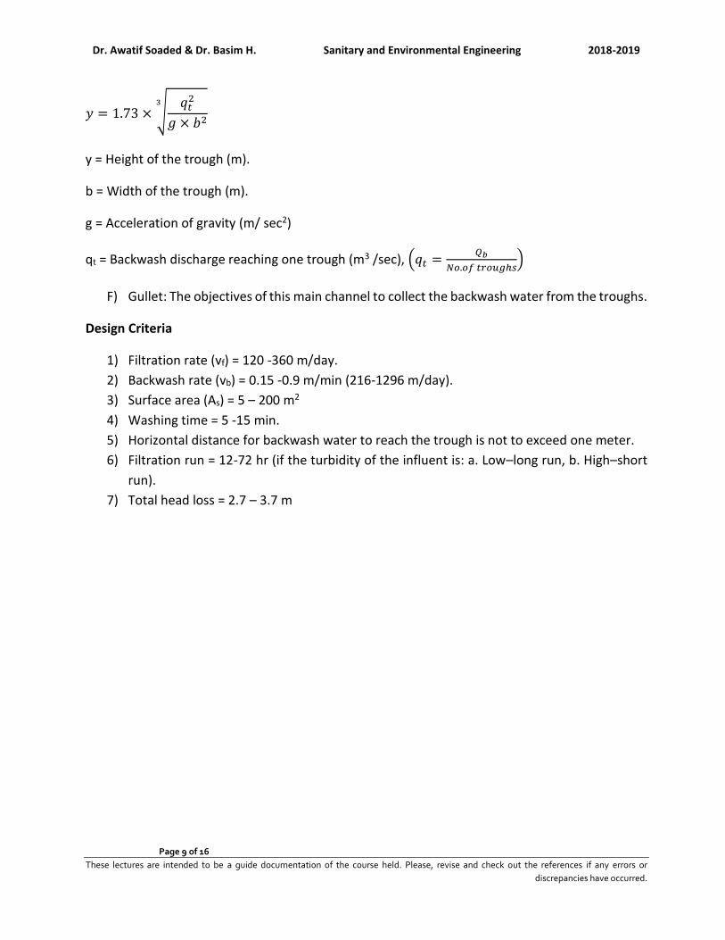
Dr. Awatif Soaded & Dr. Basim H. Sanitary and Environmental Engineering 2018-2019
Page 9 of 16
These lectures are intended to be a guide documentation of the course held. Please, revise and check out the references if any errors or
discrepancies have occurred.
𝑦 = 1.73 × √𝑞𝑡
2
𝑔 × 𝑏2
3
y = Height of the trough (m).
b = Width of the trough (m).
g = Acceleration of gravity (m/ sec2)
qt = Backwash discharge reaching one trough (m3 /sec), (𝑞𝑡 =𝑄𝑏
𝑁𝑜.𝑜𝑓 𝑡𝑟𝑜𝑢𝑔ℎ𝑠)
F) Gullet: The objectives of this main channel to collect the backwash water from the troughs.
Design Criteria
1) Filtration rate (vf) = 120 -360 m/day.
2) Backwash rate (vb) = 0.15 -0.9 m/min (216-1296 m/day).
3) Surface area (As) = 5 – 200 m2
4) Washing time = 5 -15 min.
5) Horizontal distance for backwash water to reach the trough is not to exceed one meter.
6) Filtration run = 12-72 hr (if the turbidity of the influent is: a. Low–long run, b. High–short
run).
7) Total head loss = 2.7 – 3.7 m

Dr. Awatif Soaded & Dr. Basim H. Sanitary and Environmental Engineering 2018-2019
Page 10 of 16
These lectures are intended to be a guide documentation of the course held. Please, revise and check out the references if any errors or
discrepancies have occurred.
Operation Problems In RSFs
1) Air Binding: a) When the filter is newly commissioned, the loss of head of water percolating
through the filter is generally very small. However, the loss of head goes on increasing as more and more impurities get trapped into it.
b) A stage is finally reached when the frictional resistance offered by the filter media exceeds the static head of water above the bed. Most of this resistance is offered by the top 10 to 15 cm sand layer. The bottom sand acts like a vacuum, and water is sucked through the filter media rather than getting filtered through it.
c) The negative pressure so developed, tends to release the dissolved air and other gases present in water. The formation of bubbles takes place which stick to the sand grains. This phenomenon is known as Air Binding as the air binds the filter and stops its functioning.
d) To avoid such troubles, the filters are cleaned as soon as the head loss exceeds the optimum allowable value.
2) Mud accumulation: The mud from the atmosphere usually accumulates on the sand
surface to form a dense mat. During inadequate washing this mud may sink down into the sand bed and stick to the sand grains and other arrested impurities, thereby forming mud balls.
3) Sand Incrustation (cracking of filter): to solve this problem a-Skimming b-Use anthracite
as a top layer on the filter Media-Carbonation. The fine sand contained in the top layers of the filter bed shrinks and causes the development of shrinkage cracks in the sand bed. With the use of filter, the loss of head and, therefore, pressure on the sand bed goes on increasing, which further goes on widening these cracks.
Remedial measures to prevent cracking of filters and formation of mud balls by:
a) Breaking the top fine mud layer with rakes and washing off the particles.
b) Washing the filter with a solution of caustic soda.
c) Removing, cleaning and replacing the damaged filter sand.
Backwashing of Rapid Sand Filter
1) For a filter to operate efficiently, it must be cleaned before the next filter run. If the water applied to a filter is of very good quality, the filter runs can be very long. Some filters can operate longer than one week before needing to be backwashed. However, this is not recommended as long filter runs can cause the filter media to pack down so that it is difficult to expand the bed during the backwash.
2) Treated water from storage is used for the backwash cycle. This treated water is generally taken from elevated storage tanks or pumped in from the clear well.
Dr. Awatif Soaded & Dr. Basim H. Sanitary and Environmental Engineering 2018-2019
Page 11 of 16
These lectures are intended to be a guide documentation of the course held. Please, revise and check out the references if any errors or
discrepancies have occurred.
3) The filter backwash rate has to be great enough to expand and agitate the filter media and suspend the floc in the water for removal. However, if the filter backwash rate is too high, media will be washed from the filter into the troughs and out of the filter.
When is Backwashing Needed?
The filter should be backwashed when the following conditions have been met:
1) The head loss is so high that the filter no longer produces water at the desired rate; and/or 2) Floc starts to break through the filter and the turbidity in the filter effluent increases;
and/or 3) A filter run reaches a given hour of operation.
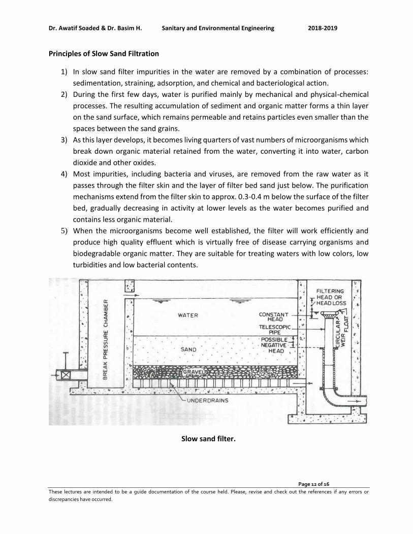
Dr. Awatif Soaded & Dr. Basim H. Sanitary and Environmental Engineering 2018-2019
Page 12 of 16
These lectures are intended to be a guide documentation of the course held. Please, revise and check out the references if any errors or
discrepancies have occurred.
Principles of Slow Sand Filtration
1) In slow sand filter impurities in the water are removed by a combination of processes:
sedimentation, straining, adsorption, and chemical and bacteriological action.
2) During the first few days, water is purified mainly by mechanical and physical-chemical
processes. The resulting accumulation of sediment and organic matter forms a thin layer
on the sand surface, which remains permeable and retains particles even smaller than the
spaces between the sand grains.
3) As this layer develops, it becomes living quarters of vast numbers of microorganisms which
break down organic material retained from the water, converting it into water, carbon
dioxide and other oxides.
4) Most impurities, including bacteria and viruses, are removed from the raw water as it
passes through the filter skin and the layer of filter bed sand just below. The purification
mechanisms extend from the filter skin to approx. 0.3-0.4 m below the surface of the filter
bed, gradually decreasing in activity at lower levels as the water becomes purified and
contains less organic material.
5) When the microorganisms become well established, the filter will work efficiently and
produce high quality effluent which is virtually free of disease carrying organisms and
biodegradable organic matter. They are suitable for treating waters with low colors, low
turbidities and low bacterial contents.
Slow sand filter.
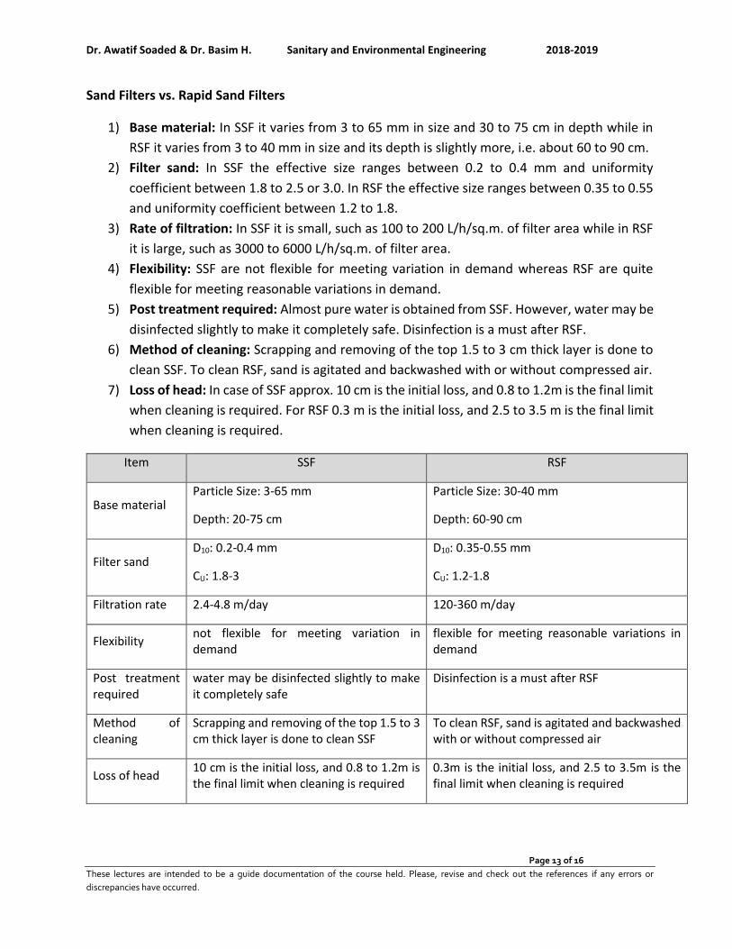
Dr. Awatif Soaded & Dr. Basim H. Sanitary and Environmental Engineering 2018-2019
Page 13 of 16
These lectures are intended to be a guide documentation of the course held. Please, revise and check out the references if any errors or
discrepancies have occurred.
Sand Filters vs. Rapid Sand Filters
1) Base material: In SSF it varies from 3 to 65 mm in size and 30 to 75 cm in depth while in
RSF it varies from 3 to 40 mm in size and its depth is slightly more, i.e. about 60 to 90 cm.
2) Filter sand: In SSF the effective size ranges between 0.2 to 0.4 mm and uniformity
coefficient between 1.8 to 2.5 or 3.0. In RSF the effective size ranges between 0.35 to 0.55
and uniformity coefficient between 1.2 to 1.8.
3) Rate of filtration: In SSF it is small, such as 100 to 200 L/h/sq.m. of filter area while in RSF
it is large, such as 3000 to 6000 L/h/sq.m. of filter area.
4) Flexibility: SSF are not flexible for meeting variation in demand whereas RSF are quite
flexible for meeting reasonable variations in demand.
5) Post treatment required: Almost pure water is obtained from SSF. However, water may be
disinfected slightly to make it completely safe. Disinfection is a must after RSF.
6) Method of cleaning: Scrapping and removing of the top 1.5 to 3 cm thick layer is done to
clean SSF. To clean RSF, sand is agitated and backwashed with or without compressed air.
7) Loss of head: In case of SSF approx. 10 cm is the initial loss, and 0.8 to 1.2m is the final limit
when cleaning is required. For RSF 0.3 m is the initial loss, and 2.5 to 3.5 m is the final limit
when cleaning is required.
Item SSF RSF
Base material Particle Size: 3-65 mm
Depth: 20-75 cm
Particle Size: 30-40 mm
Depth: 60-90 cm
Filter sand D10: 0.2-0.4 mm
CU: 1.8-3
D10: 0.35-0.55 mm
CU: 1.2-1.8
Filtration rate 2.4-4.8 m/day 120-360 m/day
Flexibility not flexible for meeting variation in demand
flexible for meeting reasonable variations in demand
Post treatment required
water may be disinfected slightly to make it completely safe
Disinfection is a must after RSF
Method of cleaning
Scrapping and removing of the top 1.5 to 3 cm thick layer is done to clean SSF
To clean RSF, sand is agitated and backwashed with or without compressed air
Loss of head 10 cm is the initial loss, and 0.8 to 1.2m is the final limit when cleaning is required
0.3m is the initial loss, and 2.5 to 3.5m is the final limit when cleaning is required
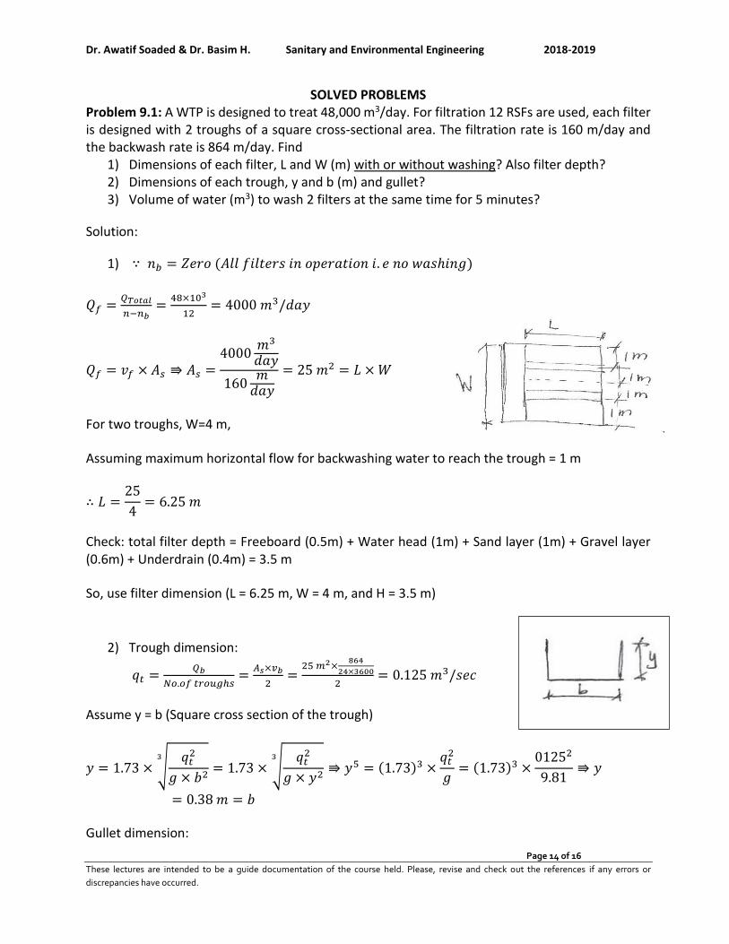
Dr. Awatif Soaded & Dr. Basim H. Sanitary and Environmental Engineering 2018-2019
Page 14 of 16
These lectures are intended to be a guide documentation of the course held. Please, revise and check out the references if any errors or
discrepancies have occurred.
SOLVED PROBLEMS Problem 9.1: A WTP is designed to treat 48,000 m3/day. For filtration 12 RSFs are used, each filter is designed with 2 troughs of a square cross-sectional area. The filtration rate is 160 m/day and the backwash rate is 864 m/day. Find
1) Dimensions of each filter, L and W (m) with or without washing? Also filter depth? 2) Dimensions of each trough, y and b (m) and gullet? 3) Volume of water (m3) to wash 2 filters at the same time for 5 minutes?
Solution:
1) ∵ 𝑛𝑏 = 𝑍𝑒𝑟𝑜 (𝐴𝑙𝑙 𝑓𝑖𝑙𝑡𝑒𝑟𝑠 𝑖𝑛 𝑜𝑝𝑒𝑟𝑎𝑡𝑖𝑜𝑛 𝑖. 𝑒 𝑛𝑜 𝑤𝑎𝑠ℎ𝑖𝑛𝑔)
𝑄𝑓 =𝑄𝑇𝑜𝑡𝑎𝑙
𝑛−𝑛𝑏=
48×103
12= 4000 𝑚3/𝑑𝑎𝑦
𝑄𝑓 = 𝑣𝑓 × 𝐴𝑠 ⇛ 𝐴𝑠 =4000
𝑚3
𝑑𝑎𝑦
160𝑚
𝑑𝑎𝑦
= 25 𝑚2 = 𝐿 × 𝑊
For two troughs, W=4 m,
Assuming maximum horizontal flow for backwashing water to reach the trough = 1 m
∴ 𝐿 =25
4= 6.25 𝑚
Check: total filter depth = Freeboard (0.5m) + Water head (1m) + Sand layer (1m) + Gravel layer (0.6m) + Underdrain (0.4m) = 3.5 m
So, use filter dimension (L = 6.25 m, W = 4 m, and H = 3.5 m)
2) Trough dimension:
𝑞𝑡 =𝑄𝑏
𝑁𝑜.𝑜𝑓 𝑡𝑟𝑜𝑢𝑔ℎ𝑠=
𝐴𝑠×𝑣𝑏
2=
25 𝑚2×864
24×3600
2= 0.125 𝑚3/𝑠𝑒𝑐
Assume y = b (Square cross section of the trough)
𝑦 = 1.73 × √𝑞𝑡
2
𝑔 × 𝑏2
3
= 1.73 × √𝑞𝑡
2
𝑔 × 𝑦2
3
⇛ 𝑦5 = (1.73)3 ×𝑞𝑡
2
𝑔= (1.73)3 ×
01252
9.81⇛ 𝑦
= 0.38 𝑚 = 𝑏
Gullet dimension:

Dr. Awatif Soaded & Dr. Basim H. Sanitary and Environmental Engineering 2018-2019
Page 15 of 16
These lectures are intended to be a guide documentation of the course held. Please, revise and check out the references if any errors or
discrepancies have occurred.
𝑞𝐺 =𝑄𝑏
𝑁𝑜. 𝑜𝑓 𝐺𝑢𝑙𝑙𝑒𝑡=
𝐴𝑠 × 𝑣𝑏
1=
25 𝑚2 ×864
24 × 36001
= 0.25 𝑚3/𝑠𝑒𝑐
Assume y = b (Square cross section of the gullet)
𝑦 = 1.73 × √𝑞𝐺
2
𝑔 × 𝑏2
3
= 1.73 × √𝑞𝐺
2
𝑔 × 𝑦2
3
⇛ 𝑦5 = (1.73)3 ×𝑞𝐷
2
𝑔= (1.73)3 ×
0252
9.81⇛ 𝑦
= 0.505 𝑚 = 𝑏
3) 𝑊𝑎𝑡𝑒𝑟 𝑣𝑜𝑙𝑢𝑚𝑒 𝑓𝑜𝑟 𝑤𝑎𝑠ℎ𝑖𝑛𝑔 = 𝑄𝑏 × 𝑡 × 𝑛𝑏 = 864𝑚
𝑑𝑎𝑦× 25 𝑚2 ×
5 𝑚𝑖𝑛
60×24× 2 =
150 𝑚3 (𝑊𝑎𝑠ℎ𝑖𝑛𝑔 𝑤𝑎𝑡𝑒𝑟 𝑓𝑜𝑟 𝑡𝑤𝑜 𝑓𝑖𝑙𝑡𝑒𝑟𝑠)
𝑉𝑜𝑙𝑢𝑚𝑒 𝑓𝑜𝑟 𝑜𝑛𝑒 𝑓𝑖𝑙𝑡𝑒𝑟 =150
2= 75 𝑚3
Note: The ratio of water washing amount for one filter does not exceed 7% of the water filtration amount.
𝑉𝑜𝑙𝑢𝑚𝑒 𝑜𝑓 𝑓𝑖𝑙𝑡𝑟𝑎𝑡𝑒𝑑 𝑤𝑎𝑡𝑒𝑟 = 4000𝑚3
𝑑𝑎𝑦× 1 = 4000 𝑚3
𝑅𝑎𝑡𝑖𝑜 𝑓𝑜𝑟 𝑜𝑛𝑒 𝑏𝑎𝑐𝑘 𝑤𝑎𝑠ℎ𝑖𝑛𝑔 =75
4000× 100 = 1.875% < 7% 𝑂. 𝐾
Problem 9.2: A city has a population of 100,000 capita with an average rate of demand of 160
L/cap.day. Find the area of rapid sand filter? Assume an average filtration rate of 120 m3/m2.day
of filter area, the filter length equal 1.5 width and filter area not exceed 40 m2.
Solution:
𝑀𝑎𝑥𝑖𝑚𝑢𝑚 𝑑𝑎𝑖𝑙𝑦 𝑑𝑒𝑚𝑎𝑛𝑑 = 1.8 × 160 × 10−3 × 100000 = 28800 𝑚3/𝑑𝑎𝑦
𝐴𝑟𝑒𝑎 𝑜𝑓 𝑓𝑖𝑙𝑡𝑒𝑟𝑠 = 28800
120= 240 𝑚2 𝑁𝑜. 𝑜𝑓 𝑓𝑖𝑙𝑡𝑒𝑟𝑠 =
240
40= 6 𝑓𝑖𝑙𝑡𝑒𝑟𝑠
𝐴𝑠 = 40 = 𝐿 × 𝑊 = 1.5𝑊2 ⟹ 𝑊 ≈ 5.20 𝑚 & 𝐿 = 7.8 𝑚
Problem 9.3: A flat bottom trough is to receive the wash water from a section of the filter which
is 2 m wide and 3 m long. The wash water rate is 700 liters per min per m2. If the water is to have
a depth of 25 cm at the upper end of the trough, what should be the dimensions of the trough?
Solution:
Dr. Awatif Soaded & Dr. Basim H. Sanitary and Environmental Engineering 2018-2019
Page 16 of 16
These lectures are intended to be a guide documentation of the course held. Please, revise and check out the references if any errors or
discrepancies have occurred.
𝑄𝑏 = 𝑣𝑏 × 𝐴𝑠 = 700 × 2 × 3 = 4200𝐿
𝑚𝑖𝑛= 4.2
𝑚3
𝑚𝑖𝑛= 0.07 𝑚3/𝑠𝑒𝑐
𝑦 = 1.73 × √𝑞𝑡
2
𝑔 × 𝑏2
3
⟹ 0.25 = 1.73 × √0.072
9.81 × 𝑏2
3
⟹ 𝑏 = 0.406 𝑚
Assume freeboard = 5 cm, the depth of trough will be = 25 + 5 = 30 cm
How to Choose a DRM Software to protect your document?

Dr. Awatif Soaded & Dr. Basim H. Sanitary and Environmental Engineering 2018-2019
Page 1 of 8
These lectures are intended to be a guide documentation of the course held. Please, revise and check out the references if any errors or
discrepancies have occurred.
Sanitary and Environmental Engineering
PART 1: WATER SUPPLY ENGINEERING
Dr. Awatif Soaded & Dr. Basim H. Sanitary and Environmental Engineering 2018-2019
Page 2 of 8
These lectures are intended to be a guide documentation of the course held. Please, revise and check out the references if any errors or
discrepancies have occurred.
PART 1: WATER SUPPLY ENGINEERING
Lecture 10: Disinfection
The filtered water may normally contain some harmful disease producing bacteria in it. These bacteria must be killed in order to make the water safe for drinking. The process of killing these bacteria is known as Disinfection or Sterilization, or, is the killing of microorganisms causing diseases. Methods of disinfection
1. Treatment with chlorine (Chlorination). 2. Treatment with Ozone (Ozonation). 3. Treatment with Iodine and Bromine. 4. Treatment with Ultraviolet irradiation. 5. Extreme values of pH. 6. Treatment with ultrasonic waves. 7. Treatment with oxidizing agents (Potassium permanganate). 8. Boiling of water. 9. Chlorine dioxide.
Chlorination:
Chlorination is a cheap and reliable process, not difficult in handling. Chlorine is a disinfect that destroys
the enzymes of the bacterial cells and enters to attack the intracellular system. Chlorine may remove colour
and iron also the destruction of taste and odour. The efficiency of chlorine is reduced by increasing pH and
at low water temperature (less than 24 0C).
1) Chlorine in water: Chlorine and water react:
Cl2 + H2O HOCl + H+ + Cl- (HOCl hypochlorous acid)
HOCl H+ + OCl- (OCl- hypochlorite ion)
HOCl and OCl accomplish the disinfection process. Since the concentration of these components is a
function of the hydrogen ion concentration, so the efficiency of disinfection is affected by pH. Chlorine and
its products are most effective at low pH. Under pH = 3, molecular chlorine maybe present. Chlorine existing
in water as HOCl, OCl and molecular chlorine is defined as free available chlorine.
Free available chlorine will react with nitrogenous compounds like ammonia to form chloramines. The
reaction of ammonia with HOCl is shown below:
NH3 + HOCl H2O + NH2Cl (monochloramine) at pH over 7.5
NH2Cl + HOCl H2O + NHCl2 (dichloramine) at pH 5 – 6.5
NHCl2 + HOCl H2O + NCl3 (nitrogen trichloride) at pH 4.4

Dr. Awatif Soaded & Dr. Basim H. Sanitary and Environmental Engineering 2018-2019
Page 3 of 8
These lectures are intended to be a guide documentation of the course held. Please, revise and check out the references if any errors or
discrepancies have occurred.
Chlorine in water reacting with ammonia, nitrogenous compounds and organic matter is defined as
combined available chlorine. The above compounds are less active than free available chlorine as
disinfecting agents, but may maintain residuals for longer time than free chlorine.
2) Chlorine Demand = Chlorine added – Residual chlorine
It is the difference between the mount of chlorine added and the mount present as residual either Free or
Combined after a contact time.
Chlorine demand to kill microorganism = C X t
Where: C = Concentration of the disinfect (chlorine) and t = Contact time between the microorganism and
the disinfect (chlorine).
Residual chlorine is the remaining chlorine after disinfection in water. This may be necessary in the
distribution system and storage tanks to protect water in the pipes from any pollution.
3) What is used in chlorination?
a) Chlorine gas, chlorine is obtained in pressurized cylinders ranging in weight from 45 to 1000 kg.
b) Hypochlorination, chemical compounds such as Sodium hypochlorite NaOCl (laundry bleach) and
Calcium Hypochlorite Ca (OCl)2. 4H2O.
Hypochlorites are useful in disinfecting waters of reservoirs and swimming pools also in controlling algae
growth. Hypochlorites in water will give free available chlorine:
Ca(OCl) Ca+2 + 2OCl-
NaOCl Na+ + OCl-
OCl- + H+ HOCl
4) Chlorination is classified according to its point application as:
a) Plain Chlorination is used with no other treatment. Chlorine is added to the water from the
source. The dose added depends on the degree of contamination. About 0.5 mg/L or more is
used for disinfection and obtain residual chlorine free or combined.
b) Pre-chlorination, applying chlorine before any other treatment. It may be added to the suction
pipe of the raw water pumps or in the flash mixer. Its advantages:
i. Improve the coagulation process.
ii. Reduce taste and odor caused by organic sludge in sedimentation tanks.
iii. Killing algae and other microorganisms, so filters may remain clean to obtain long
filtration runs.
A dose of 5 – 10 mg/L is used to obtain 0.1 – 0.5 mg/L residual chlorine free or combined.
c) Post-chlorination, applying chlorine at the end of the treatment process. A contact time for
about 30 minutes is required for disinfection when adding 0.25 – 0.5 mg/L chlorine dose to
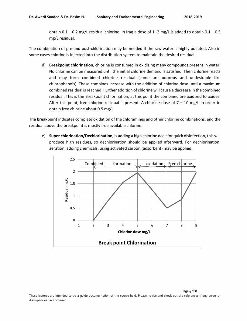
Dr. Awatif Soaded & Dr. Basim H. Sanitary and Environmental Engineering 2018-2019
Page 4 of 8
These lectures are intended to be a guide documentation of the course held. Please, revise and check out the references if any errors or
discrepancies have occurred.
obtain 0.1 – 0.2 mg/L residual chlorine. In Iraq a dose of 1 -2 mg/L is added to obtain 0.1 – 0.5
mg/L residual.
The combination of pre-and post-chlorination may be needed if the raw water is highly polluted. Also in
some cases chlorine is injected into the distribution system to maintain the desired residual.
d) Breakpoint chlorination, chlorine is consumed in oxidizing many compounds present in water.
No chlorine can be measured until the initial chlorine demand is satisfied. Then chlorine reacts
and may form combined chlorine residual (some are odorous and undesirable like
chlorophenols). These combines increase with the addition of chlorine dose until a maximum
combined residual is reached. Further addition of chlorine will cause a decrease in the combined
residual. This is the Breakpoint chlorination, at this point the combined are oxidized to oxides.
After this point, free chlorine residual is present. A chlorine dose of 7 – 10 mg/L in order to
obtain free chlorine about 0.5 mg/L.
The breakpoint indicates complete oxidation of the chloramines and other chlorine combinations, and the
residual above the breakpoint is mostly free available chlorine.
e) Super chlorination/Dechlorination, is adding a high chlorine dose for quick disinfection, this will
produce high residues, so dechlorination should be applied afterward. For dechlorination:
aeration, adding chemicals, using activated carbon (adsorbent) may be applied.
0
0.5
1
1.5
2
2.5
1 2 3 4 5 6 7 8 9
Re
sid
ual
mg/
L
Chlorine dose mg/L
Break point Chlorination
Combined formation oxidation Free chlorine
Dr. Awatif Soaded & Dr. Basim H. Sanitary and Environmental Engineering 2018-2019
Page 5 of 8
These lectures are intended to be a guide documentation of the course held. Please, revise and check out the references if any errors or
discrepancies have occurred.
Ozone: It's manufactured by electrical discharge into cooled dried air. Approximately 1% of the atmospheric
oxygen is converted to O3 at an energy consumption of 0.025 kWh per gram O3. The mixture of air and ozone
is transferred into water either by bubbling it through the bulk solution or by permitting droplets of water to
fall through a rising column of gas.
Advantage Disadvantage
1) It is effective as oxidizing agent and
germicide, in destruction of organic
matter which might produce tastes and
odors, and in oxidation or iron and
manganese.
2) More rapid in action than other oxidizing
agents with small dose (0.25-1.5) mg/L at
low contact time (45 sec-2 min).
3) It is not particularly sensitive to pH within
range of pH (5-8), but is significantly
affected by temperature.
1) It's restricted of use.
2) On-site generation
3) Its cost relative to chlorine.
4) It is not providing residual disinfection in
water distribution system.
Chlorine dioxide: It is produced by the chlorination of sodium chlorite in a ratio of 1 mole chlorine to 2
moles chlorite, and the result compound (ClO2).
Advantage Disadvantage
1) It is effective as oxidizing agent and germicide, in
destruction of organic matter which might produce tastes
and odors, and in oxidation or iron and manganese.
2) It does not react with ammonia.
3) More rapid in action and appears to be able to oxidize
organics without formation of halogenated hydrocarbons.
4) It is unaffected by pH within the normal range encountered
in water.
5) It is relatively persistent at ordinary temperatures and can
provide residual protection.
1) It's restricted of use.
2) On-site generation
3) Its cost relative to chlorine.
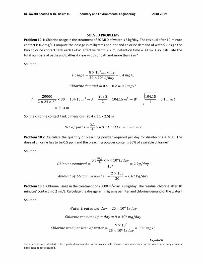
Dr. Awatif Soaded & Dr. Basim H. Sanitary and Environmental Engineering 2018-2019
Page 6 of 8
These lectures are intended to be a guide documentation of the course held. Please, revise and check out the references if any errors or
discrepancies have occurred.
SOLVED PROBLEMS Problem 10.1: Chlorine usage in the treatment of 20 MLD of water is 8 kg/day. The residual after 10-minute
contact is 0.2 mg/L. Compute the dosage in milligrams per liter and chlorine demand of water? Design the
two chlorine contact tank each L=4W, effective depth = 2 m, detention time = 30 m? Also, calculate the
total numbers of paths and baffles if clear width of path not more than 2 m?
Solution:
𝐷𝑜𝑠𝑎𝑔𝑒 =8 × 10⁶𝑚𝑔/𝑑𝑎𝑦
20 × 106 𝐿/𝑑𝑎𝑦= 0.4 𝑚𝑔/𝐿
𝐶ℎ𝑙𝑜𝑟𝑖𝑛𝑒 𝑑𝑒𝑚𝑎𝑛𝑑 = 0.4 − 0.2 = 0.2 𝑚𝑔/𝐿
𝑉 =20000
2 × 24 × 60× 30 = 104.15 𝑚3 → 𝐴 =
208.3
2= 104.15 𝑚2 → 𝑊 = √
104.15
4= 5.1 𝑚 & 𝐿
= 20.4 𝑚
So, the chlorine contact tank dimensions (20.4 x 5.1 x 2.5) m
𝑁𝑂. 𝑜𝑓 𝑝𝑎𝑡ℎ𝑠 =5.1
3& 𝑁𝑂. 𝑜𝑓 𝑏𝑎𝑓𝑓𝑒𝑙 = 3 − 1 = 2
Problem 10.2: Calculate the quantity of bleaching powder required per day for disinfecting 4 MLD. The
dose of chlorine has to be 0.5 ppm and the bleaching powder contains 30% of available chlorine?
Solution:
𝐶ℎ𝑙𝑜𝑟𝑖𝑛𝑒 𝑟𝑒𝑞𝑢𝑖𝑟𝑒𝑑 =0.5
𝑚𝑔𝐿
× 4 × 106𝐿/𝑑𝑎𝑦
106= 2 𝑘𝑔/𝑑𝑎𝑦
𝐴𝑚𝑜𝑢𝑛𝑡 𝑜𝑓 𝑏𝑙𝑒𝑎𝑐ℎ𝑖𝑛𝑔 𝑝𝑜𝑤𝑑𝑒𝑟 =2 × 100
30= 6.67 𝑘𝑔/𝑑𝑎𝑦
Problem 10.3: Chlorine usage in the treatment of 25000 m3/day is 9 kg/day. The residual chlorine after 10
minutes' contact is 0.2 mg/L. Calculate the dosage in milligrams per liter and chlorine demand of the water?
Solution:
𝑊𝑎𝑡𝑒𝑟 𝑡𝑟𝑒𝑎𝑡𝑒𝑑 𝑝𝑒𝑟 𝑑𝑎𝑦 = 25 × 106 𝐿/𝑑𝑎𝑦
𝐶ℎ𝑙𝑜𝑟𝑖𝑛𝑒 𝑐𝑜𝑛𝑠𝑢𝑚𝑒𝑑 𝑝𝑒𝑟 𝑑𝑎𝑦 = 9 × 10⁶ 𝑚𝑔/𝑑𝑎𝑦
𝐶ℎ𝑙𝑜𝑟𝑖𝑛𝑒 𝑢𝑠𝑒𝑑 𝑝𝑒𝑟 𝑙𝑖𝑡𝑒𝑟 𝑜𝑓 𝑤𝑎𝑡𝑒𝑟 =9 × 10⁶
25 × 106 𝐿/𝑑𝑎𝑦= 0.36 𝑚𝑔/𝐿
Dr. Awatif Soaded & Dr. Basim H. Sanitary and Environmental Engineering 2018-2019
Page 7 of 8
These lectures are intended to be a guide documentation of the course held. Please, revise and check out the references if any errors or
discrepancies have occurred.
𝐶ℎ𝑙𝑜𝑟𝑖𝑛𝑒 𝑑𝑒𝑚𝑎𝑛𝑑 = 0.36 − 0.2 = 0.16 𝑚𝑔/𝐿
Problem 10.4: A new water main is disinfected using a 50 mg/L chlorine dosage by applying a 2 percent
hypochlorite solution. (a) How many kilograms of dry hypochlorite powder, containing 70 percent available
chlorine, must be dissolved in 100 liters of water to make a 2 percent (20000 mg/L) solution? (b) At what
rate should this solution be applied to the water entering the main (400 L of water volume) to provide a
concentration of 50 mg/L? (c) If 34000 liters of water are used to fill the main at a dosage of 50 mg/L, how
many liters of hypochlorite solution are used?
Solution:
a) 𝐾𝑖𝑙𝑜𝑔𝑟𝑎𝑚 𝑜𝑓 ℎ𝑦𝑝𝑜𝑐ℎ𝑙𝑜𝑟𝑖𝑡𝑒 𝑝𝑜𝑤𝑑𝑒𝑟 𝑓𝑜𝑟 2% 𝑠𝑜𝑙𝑢𝑡𝑖𝑜𝑛 =100 𝐿×1
𝑘𝑔
𝐿×0.02
0.7= 2.86
𝑘𝑔
100 𝐿
b) 𝐹𝑒𝑒𝑑 𝑟𝑎𝑡𝑒 𝑓𝑜𝑟 50𝑚𝑔
𝐿=
50𝑚𝑔
𝐿
20000𝑚𝑔
𝐿
=1 𝑉𝑜𝑙𝑢𝑚𝑒 𝑜𝑓 2% 𝑠𝑜𝑙𝑢𝑡𝑖𝑜𝑛
400 𝑉𝑜𝑙𝑢𝑚𝑒 𝑜𝑓 𝑤𝑎𝑡𝑒𝑟= 2.5 × 10⁻³
c) 𝑆𝑜𝑙𝑢𝑡𝑖𝑜𝑛 𝑢𝑠𝑎𝑔𝑒 = 34000 𝐿 × 2.5 × 10−3 = 85 𝐿
Problem 10.8: Results of chlorine demand test on a raw water are given below. Determine the break-point
dosage and the chlorine demand?
Sample No.
Chlorine dosage mg/L
Residual chlorine after 10 min. mg/L
1 0.2 0.18
2 0.4 0.34
3 0.6 0.48
4 0.8 0.46
5 0.9 0.27
6 1 0.18
7 1.2 0.38
8 1.4 0.58
9 1.6 0.78 Solution:
Sample No.
Chlorine dosage mg/L
Residual chlorine after 10 min.
mg/L
Chlorine demand
mg/L
1 0.2 0.18 0.02
2 0.4 0.34 0.06
3 0.6 0.48 0.12
4 0.8 0.46 0.34
5 0.9 0.27 0.63
6 1 0.18 0.82
Dr. Awatif Soaded & Dr. Basim H. Sanitary and Environmental Engineering 2018-2019
Page 8 of 8
These lectures are intended to be a guide documentation of the course held. Please, revise and check out the references if any errors or
discrepancies have occurred.
7 1.2 0.38 0.82
8 1.4 0.58 0.82
9 1.6 0.78 0.82
Figure bellows the curve plotted the basis of the above data.
From the curve, we find that break point occurs at point D, at which the applied chlorine = 1 mg/L.
So, the break point dosage = 1.0 mg/L
Chlorine demand at break point = 1.0 -0.18 = 0.82 mg/L
It is observed that since the slope of curve C is 450, the chlorine demand (=0.82 mg/L) remains constant after
break point, since all additional chlorine added after point D appears as free chlorine.
Even from the data, at a dose of 1.2 mg/L, the residual chlorine = 0.38 mg/L.
Hence, residual chlorine = 1.2 – 0.38 = 0.82 mg/L.
How to Choose a DRM Software to protect your document?

Dr. Awatif Soaded & Dr. Basim H. Sanitary and Environmental Engineering 2018-2019
Page 1 of 10
These lectures are intended to be a guide documentation of the course held. Please, revise and check out the references if any errors or
discrepancies have occurred.
Sanitary and Environmental Engineering
PART 1: WATER SUPPLY ENGINEERING
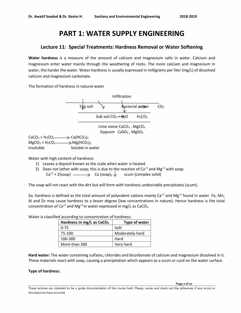
Dr. Awatif Soaded & Dr. Basim H. Sanitary and Environmental Engineering 2018-2019
Page 2 of 10
These lectures are intended to be a guide documentation of the course held. Please, revise and check out the references if any errors or
discrepancies have occurred.
PART 1: WATER SUPPLY ENGINEERING
Lecture 11: Special Treatments: Hardness Removal or Water Softening
Water hardness is a measure of the amount of calcium and magnesium salts in water. Calcium and
magnesium enter water mainly through the weathering of rocks. The more calcium and magnesium in
water, the harder the water. Water hardness is usually expressed in milligrams per liter (mg/L) of dissolved
calcium and magnesium carbonate.
The formation of hardness in natural water
Infiltration
Top soil Bacterial action CO2
Sub soil CO2 + H2O H2CO3
Lime stone CaCO3 , MgCO3 Gypsum CaSO4 , MgSO4
CaCO3 + H2CO3 Ca(HCO3)2 MgCO3 + H2CO3 Mg(HCO3)2 Insoluble Soluble in water Water with high content of hardness:
1) Leaves a deposit known as the scale when water is heated. 2) Does not lather with soap; this is due to the reaction of Ca+2 and Mg+2 with soap:
Ca+2 + 2(soap) - Ca (soap)2 scum (complex solid) The soap will not react with the dirt but will form with hardness undesirable precipitates (scum). So, hardness is defined as the total amount of polyvalent cations mainly Ca+2 and Mg+2 found in water. Fe, Mn, Al and Zn may cause hardness to a lesser degree (low concentrations in nature). Hence hardness is the total concentration of Ca+2 and Mg+2 in water expressed in mg/L as CaCO3. Water is classified according to concentration of hardness:
Hardness in mg/L as CaCO3 Type of water
0-75 Soft
75-100 Moderately hard
100-300 Hard
More than 300 Very hard
Hard water: The water containing sulfates, chlorides and bicarbonate of calcium and magnesium dissolved in it. These materials react with soap, causing a precipitation which appears as a scum or curd on the water surface. Type of hardness:
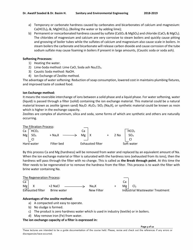
Dr. Awatif Soaded & Dr. Basim H. Sanitary and Environmental Engineering 2018-2019
Page 3 of 10
These lectures are intended to be a guide documentation of the course held. Please, revise and check out the references if any errors or
discrepancies have occurred.
a) Temporary or carbonate hardness caused by carbonates and bicarbonates of calcium and magnesium: Ca(HCO3)2 &; Mg(HCO3)2 (Boiling the water or by adding lime);
b) Permanent or noncarbonated hardness caused by sulfate (CaSO4 & MgSO4) and chloride (CaCl2 & MgCl2). The chlorides of magnesium and calcium are very corrosive to steam boilers and quickly cause pitting and grooving of boiler tubes while the sulfates of calcium and magnesium also cause scale in boilers. In steam boilers the carbonate and bicarbonate will release carbon dioxide and cause corrosion of the tube sodium sulfate may cause foaming in boilers if present in large amounts, (Caustic soda or soda ash).
Softening Processes:
1) Heating the water. 2) Lime-Soda method: Lime CaO, Soda ash Na2CO3. 3) Caustic Soda method: NaOH. 4) Ion Exchange of Zeolite method.
The advantage of water softening: Reduction of soap consumption, lowered cost in maintains plumbing fixtures, and improved taste of cooked food. Ion Exchange method: It means the reversible interchange of ions between a solid phase and a liquid phase. For water softening, water (liquid) is passed through a filter (solid) containing the ion exchange material. This material could be a natural material known as zeolite (green sand) Na2O: Al2O3: SiO2 (Na2X), or synthetic material could be known as resin which is higher in the exchange capacity. Zeolites are complex of aluminum, silica and soda, some forms of which are synthetic and others are naturally occurring. The Filtration Process: Ca HCO3 Ca HCO3 Mg SO4 + Na2X Mg X + 2 Na SO4 Cl Cl Hard water Filter bed Exhausted filter Soft water By this process Ca and Mg (hardness) will be removed from water and replaced by an equivalent amount of Na. When the ion exchange material or filter is saturated with the hardness ions (exhausted from its ions), then the hardness will pass through the filter with no change. This is called as the Break through point. At this time the filter needs to be regenerated or to remove the hardness from the filter. This process is to wash the filter with brine water containing Na. The Regeneration Process: Ca Ca Mg X +2 NaCl Na2X + Mg Cl2 Exhausted filter Brine water New Filter Industrial Wastewater Treatment Advantages of the zeolite method:
a) A compacted unit easy to operate. b) No sludge is formed. c) The product is zero hardness water which is used in industry (textile) or in boilers. d) May remove iron (Fe) from water.
The ion exchange capacity of a filter is expressed in:
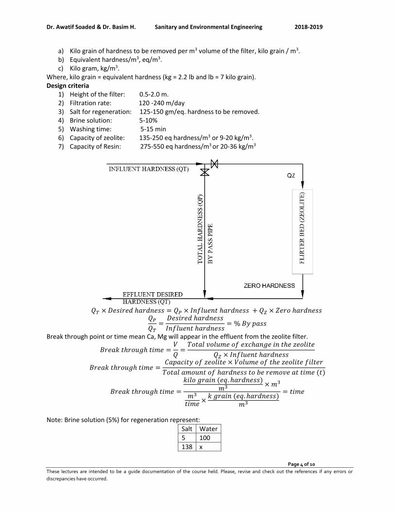
Dr. Awatif Soaded & Dr. Basim H. Sanitary and Environmental Engineering 2018-2019
Page 4 of 10
These lectures are intended to be a guide documentation of the course held. Please, revise and check out the references if any errors or
discrepancies have occurred.
a) Kilo grain of hardness to be removed per m3 volume of the filter, kilo grain / m3. b) Equivalent hardness/m3, eq/m3. c) Kilo gram, kg/m3.
Where, kilo grain = equivalent hardness (kg = 2.2 lb and lb = 7 kilo grain). Design criteria
1) Height of the filter: 0.5-2.0 m. 2) Filtration rate: 120 -240 m/day 3) Salt for regeneration: 125-150 gm/eq. hardness to be removed. 4) Brine solution: 5-10% 5) Washing time: 5-15 min 6) Capacity of zeolite: 135-250 eq hardness/m3 or 9-20 kg/m3. 7) Capacity of Resin: 275-550 eq hardness/m3 or 20-36 kg/m3
𝑄𝑇 × 𝐷𝑒𝑠𝑖𝑟𝑒𝑑 ℎ𝑎𝑟𝑑𝑛𝑒𝑠𝑠 = 𝑄𝑃 × 𝐼𝑛𝑓𝑙𝑢𝑒𝑛𝑡 ℎ𝑎𝑟𝑑𝑛𝑒𝑠𝑠 + 𝑄𝑍 × 𝑍𝑒𝑟𝑜 ℎ𝑎𝑟𝑑𝑛𝑒𝑠𝑠
𝑄𝑃
𝑄𝑇=
𝐷𝑒𝑠𝑖𝑟𝑒𝑑 ℎ𝑎𝑟𝑑𝑛𝑒𝑠𝑠
𝐼𝑛𝑓𝑙𝑢𝑒𝑛𝑡 ℎ𝑎𝑟𝑑𝑛𝑒𝑠𝑠= % 𝐵𝑦 𝑝𝑎𝑠𝑠
Break through point or time mean Ca, Mg will appear in the effluent from the zeolite filter.
𝐵𝑟𝑒𝑎𝑘 𝑡ℎ𝑟𝑜𝑢𝑔ℎ 𝑡𝑖𝑚𝑒 =𝑉
𝑄=
𝑇𝑜𝑡𝑎𝑙 𝑣𝑜𝑙𝑢𝑚𝑒 𝑜𝑓 𝑒𝑥𝑐ℎ𝑎𝑛𝑔𝑒 𝑖𝑛 𝑡ℎ𝑒 𝑧𝑒𝑜𝑙𝑖𝑡𝑒
𝑄𝑍 × 𝐼𝑛𝑓𝑙𝑢𝑒𝑛𝑡 ℎ𝑎𝑟𝑑𝑛𝑒𝑠𝑠
𝐵𝑟𝑒𝑎𝑘 𝑡ℎ𝑟𝑜𝑢𝑔ℎ 𝑡𝑖𝑚𝑒 =𝐶𝑎𝑝𝑎𝑐𝑖𝑡𝑦 𝑜𝑓 𝑧𝑒𝑜𝑙𝑖𝑡𝑒 × 𝑉𝑜𝑙𝑢𝑚𝑒 𝑜𝑓 𝑡ℎ𝑒 𝑧𝑒𝑜𝑙𝑖𝑡𝑒 𝑓𝑖𝑙𝑡𝑒𝑟
𝑇𝑜𝑡𝑎𝑙 𝑎𝑚𝑜𝑢𝑛𝑡 𝑜𝑓 ℎ𝑎𝑟𝑑𝑛𝑒𝑠𝑠 𝑡𝑜 𝑏𝑒 𝑟𝑒𝑚𝑜𝑣𝑒 𝑎𝑡 𝑡𝑖𝑚𝑒 (𝑡)
𝐵𝑟𝑒𝑎𝑘 𝑡ℎ𝑟𝑜𝑢𝑔ℎ 𝑡𝑖𝑚𝑒 =
𝑘𝑖𝑙𝑜 𝑔𝑟𝑎𝑖𝑛 (𝑒𝑞. ℎ𝑎𝑟𝑑𝑛𝑒𝑠𝑠)𝑚3 × 𝑚3
𝑚3
𝑡𝑖𝑚𝑒 ×𝑘 𝑔𝑟𝑎𝑖𝑛 (𝑒𝑞. ℎ𝑎𝑟𝑑𝑛𝑒𝑠𝑠)
𝑚3
= 𝑡𝑖𝑚𝑒
Note: Brine solution (5%) for regeneration represent:
Salt Water
5 100
138 x
Dr. Awatif Soaded & Dr. Basim H. Sanitary and Environmental Engineering 2018-2019
Page 5 of 10
These lectures are intended to be a guide documentation of the course held. Please, revise and check out the references if any errors or
discrepancies have occurred.
x= Weight of water (kg) for 5% solution.
𝑉𝑜𝑙𝑢𝑚𝑒 =𝑥
𝜌𝑤
Membrane filtration: It’s a physicochemical separation technique that used difference permeability as a separation mechanism. Water is pumped against the membrane surface resulting in the production of product and waste streams. Membrane is a synthetic material less than 1 mm thick, semi-permeable (highly permeable to some components in the feed stream and less permeable to others). Microfiltration (M.F): A membrane separation process in which particles greater than about 20 nanometers in diameter are screened out of a liquid in which they are suspended. Ultra-filtration (U.F): Filtration through a filter capable of removing very minute (ultramicroscopic) particles. The filtration of a colloidal substance through a semi-permeable medium that allows only the passage of small molecules. Nanofiltration (N.F): Nanofiltration is a relatively recent membrane filtration process used most often with low total dissolved solids water such as surface water and fresh groundwater, with the purpose of softening and removal of disinfection by-product precursors such as natural organic matter and synthetic. Pressure-driven filtration through a membrane that removes particles of about two nanometers or larger. Reverse osmosis: It is perhaps the best demonstrated technology for saline water conservation. If a semi-permeable membrane separates two bodies of water with differing salt concentrations the water will flow from less to more concentrated. The flow can be halted by applying pressure equal to the osmotic pressure of the concentrated solution, and reversed by exceeding that pressure. In practice the pressure ranges from 5-50 times the osmotic pressure of the water. Reverse osmosis systems include the membrane, a support structure, a pressure vessel and a pump. Reverse osmosis is not easily applied to seawater although development of new membrane materials and configurations and use multistage processes. The cost of treating brackish water by this technique ranged (0.06-0.25) $/m3. Advantage:
1. Remove suspended with no coagulation up to a turbidly 200 NTU. 2. Very high removal in microorganisms. 3. Less space required than conventional filtration (1 m2 floor area=100 m2 membrane area). 4. High quality of filtered water.
Item Membrane filter Conventional filter
Filtration rate (vf) 0.03-0.17 m/hr 5-15 m/hr
Pressure 0.2-2 bar 0.18-0.3 bar
Filtration run 30-90 min 1-4 day
Backwash 1-5 min 5-15 min
1 bar = 14.5 psi = 100 kPa
Dr. Awatif Soaded & Dr. Basim H. Sanitary and Environmental Engineering 2018-2019
Page 6 of 10
These lectures are intended to be a guide documentation of the course held. Please, revise and check out the references if any errors or
discrepancies have occurred.
Solved Problem Problem 11.1: Design a cylindrical softener to be used in a textile factory. The influent flow is 500 m3/day with hardness of 246 mg/L as CaCO3. The softener is supplied with zeolite of an exchange capacity of 250 kilograin/m3. Find height (H) and diameter (D) of the softener (assume H=D)? Solution: Assume break through time = 1 day The amount of hardness to be removed = Flow (Q) X Concentration = Loading rate
𝐿𝑜𝑎𝑑𝑖𝑛𝑔 𝑟𝑎𝑡𝑒 =500
𝑚3
𝑑𝑎𝑦× 246
𝑚𝑔𝐿
× 103
106= 123
𝑘𝑔
𝑑𝑎𝑦𝑓𝑜𝑟 𝑜𝑛𝑒 𝑑𝑎𝑦 𝑝𝑟𝑜𝑐𝑒𝑠𝑠
123 × 2.2 × 7 = 1894 𝑘𝑖𝑙𝑜 𝑔𝑟𝑎𝑖𝑛/𝑑𝑎𝑦
𝑉𝑜𝑙𝑢𝑚𝑒 𝑜𝑓 𝑧𝑒𝑜𝑙𝑖𝑡𝑒 𝑟𝑒𝑞𝑢𝑖𝑟𝑒𝑑 =𝐿𝑜𝑎𝑑𝑖𝑛𝑔 𝑟𝑎𝑡𝑒
𝑍𝑒𝑜𝑙𝑖𝑡𝑒 𝑒𝑥𝑐ℎ𝑎𝑛𝑔𝑒 𝑐𝑎𝑝𝑎𝑐𝑖𝑡𝑦=
1894 𝑘𝑖𝑙𝑜 𝑔𝑟𝑎𝑖𝑛/𝑑𝑎𝑦
250 𝑘𝑖𝑙𝑜 𝑔𝑟𝑎𝑖𝑛/𝑚3
= 7.6 𝑚3 𝑓𝑜𝑟 𝑜𝑛𝑒 𝑑𝑎𝑦 𝑝𝑟𝑜𝑐𝑒𝑠𝑠
𝐷𝑖𝑎𝑚𝑒𝑡𝑒𝑟 (𝐷) = √7.6 𝑚3
𝜋4
3= 2.13 𝑚 = 𝐻𝑒𝑖𝑔ℎ𝑡(𝐻)
𝑇𝑜𝑡𝑎𝑙 𝑐𝑎𝑝𝑎𝑐𝑖𝑡𝑦 𝑜𝑓 𝑒𝑥𝑐ℎ𝑎𝑛𝑔𝑒 = 𝐶𝑎𝑝𝑎𝑐𝑖𝑡𝑦 × 𝑉𝑜𝑙𝑢𝑚𝑒
𝑇𝑜𝑡𝑎𝑙 𝑐𝑎𝑝𝑎𝑐𝑖𝑡𝑦 𝑜𝑓 𝑒𝑥𝑐ℎ𝑎𝑛𝑔𝑒 = 250 𝑘𝑖𝑙𝑜𝑔𝑟𝑎𝑖𝑛
𝑚3× 7.6
𝑚3
𝑑𝑎𝑦= 1900 𝑘𝑖𝑙𝑜𝑔𝑟𝑎𝑖𝑛/𝑑𝑎𝑦
In this problem the break through time is one day (24 hours). Different conditions may appear that will change the break through time:
1) Increasing or decreasing in influent hardness. 2) Increasing or decreasing in influent flow. 3) Increasing or decreasing the exchange capacity (Changing the zeolite material).
For the same problem above, the hardness increased from 246 to 400 mg/L as CaCO3
𝐿𝑜𝑎𝑑𝑖𝑛𝑔 𝑟𝑎𝑡𝑒 =400 × 500 × 2.2 × 7 × 103
106= 3080
𝑘 𝑔𝑟𝑎𝑖𝑛
𝑑𝑎𝑦𝑓𝑜𝑟 𝑜𝑛𝑒 𝑑𝑎𝑦 𝑝𝑟𝑜𝑐𝑒𝑠𝑠
Available volume for exchange = 7.6 X 250 =1900 k grain/day
𝐵𝑟𝑒𝑎𝑘 𝑡ℎ𝑟𝑜𝑢𝑔ℎ 𝑡𝑖𝑚𝑒 (𝐵𝑇) =𝐴𝑣𝑎𝑖𝑙𝑎𝑏𝑙𝑒 𝑣𝑜𝑙𝑢𝑚𝑒 𝑜𝑟 𝑐𝑎𝑝𝑎𝑐𝑖𝑡𝑦 𝑓𝑜𝑟 𝑒𝑥𝑐ℎ𝑎𝑛𝑔𝑒
𝐿𝑜𝑎𝑑𝑖𝑛𝑔 𝑟𝑎𝑡𝑒=
1900 𝑘 𝑔𝑟𝑎𝑖𝑛
3080𝑘 𝑔𝑟𝑎𝑖𝑛
𝑑𝑎𝑦
= 0.616 𝑑𝑎𝑦
= 14.90 ℎ𝑜𝑢𝑟 (𝐸𝑣𝑒𝑟𝑦 15 ℎ𝑟 𝑡ℎ𝑒 𝑓𝑖𝑙𝑡𝑒𝑟 𝑚𝑢𝑠𝑡 𝑏𝑒 𝑟𝑒𝑔𝑒𝑛𝑒𝑟𝑎𝑡𝑒𝑑 If a new zeolite is used of a capacity from 250 to 480 kgrain/m3. Find break through time:
𝐿𝑜𝑎𝑑𝑖𝑛𝑔 𝑟𝑎𝑡𝑒 =500
𝑚3
𝑑𝑎𝑦× 246
𝑚𝑔𝐿 × 103
106= 123
𝑘𝑔
𝑑𝑎𝑦𝑓𝑜𝑟 𝑜𝑛𝑒 𝑑𝑎𝑦 𝑝𝑟𝑜𝑐𝑒𝑠𝑠
123 × 2.2 × 7 = 1894 𝑘𝑖𝑙𝑜 𝑔𝑟𝑎𝑖𝑛/𝑑𝑎𝑦

Dr. Awatif Soaded & Dr. Basim H. Sanitary and Environmental Engineering 2018-2019
Page 7 of 10
These lectures are intended to be a guide documentation of the course held. Please, revise and check out the references if any errors or
discrepancies have occurred.
𝑉𝑜𝑙𝑢𝑚𝑒 𝑜𝑓 𝑧𝑒𝑜𝑙𝑖𝑡𝑒 𝑟𝑒𝑞𝑢𝑖𝑟𝑒𝑑 =𝐿𝑜𝑎𝑑𝑖𝑛𝑔 𝑟𝑎𝑡𝑒
𝑍𝑒𝑜𝑙𝑖𝑡𝑒 𝑒𝑥𝑐ℎ𝑎𝑛𝑔𝑒 𝑐𝑎𝑝𝑎𝑐𝑖𝑡𝑦=
1894 𝑘𝑖𝑙𝑜 𝑔𝑟𝑎𝑖𝑛/𝑑𝑎𝑦
480 𝑘𝑖𝑙𝑜 𝑔𝑟𝑎𝑖𝑛/𝑚3
= 3.945 𝑚3 𝑓𝑜𝑟 𝑜𝑛𝑒 𝑑𝑎𝑦 𝑝𝑟𝑜𝑐𝑒𝑠𝑠
𝐷𝑖𝑎𝑚𝑒𝑡𝑒𝑟 (𝐷) = √3.945 𝑚3
𝜋4
3= 1.713 𝑚 = 𝐻𝑒𝑖𝑔ℎ𝑡(𝐻)
𝑇𝑜𝑡𝑎𝑙 𝑐𝑎𝑝𝑎𝑐𝑖𝑡𝑦 𝑜𝑓 𝑒𝑥𝑐ℎ𝑎𝑛𝑔𝑒 = 𝐶𝑎𝑝𝑎𝑐𝑖𝑡𝑦 × 𝑉𝑜𝑙𝑢𝑚𝑒
𝑇𝑜𝑡𝑎𝑙 𝑐𝑎𝑝𝑎𝑐𝑖𝑡𝑦 𝑜𝑓 𝑒𝑥𝑐ℎ𝑎𝑛𝑔𝑒 = 480 𝑘𝑖𝑙𝑜𝑔𝑟𝑎𝑖𝑛
𝑚3× 3.945
𝑚3
𝑑𝑎𝑦= 1893.6 𝑘𝑖𝑙𝑜𝑔𝑟𝑎𝑖𝑛/𝑑𝑎𝑦
𝐵𝑟𝑒𝑎𝑘 𝑡ℎ𝑟𝑜𝑢𝑔ℎ 𝑡𝑖𝑚𝑒 (𝐵𝑇) =𝑇𝑜𝑡𝑎𝑙 𝑐𝑎𝑝𝑎𝑐𝑖𝑡𝑦 𝑓𝑜𝑟 𝑒𝑥𝑐ℎ𝑎𝑛𝑔𝑒
𝐿𝑜𝑎𝑑𝑖𝑛𝑔 𝑟𝑎𝑡𝑒=
480 𝑘𝑔𝑟𝑎𝑖𝑛
𝑚3 × 3.945 𝑚3
1894𝑘 𝑔𝑟𝑎𝑖𝑛
𝑑𝑎𝑦
= 0.999 𝑑𝑎𝑦
= 23.995 ℎ𝑜𝑢𝑟 (𝐸𝑣𝑒𝑟𝑦 𝑑𝑎𝑦 𝑡ℎ𝑒 𝑓𝑖𝑙𝑡𝑒𝑟 𝑚𝑢𝑠𝑡 𝑏𝑒 𝑟𝑒𝑔𝑒𝑛𝑒𝑟𝑎𝑡𝑒𝑑 Problem 11.2: Design soft water softener as shown in the figure. The zeolite capacity is 235 eq. hardness/m3. Find:
1) Surface area of the filter? 2) Amount of salt used for regeneration, assume 150 gm/eq. hardness is required? 3) Volume of water for regeneration (10% solution)?
Qin=240 m3/day, Qp Qz zeolite filter H= 2.5 m 300 mg/L asCaCO3 300 mg/L hardness zero hardness Desired hardness 60 mg/L as CaCO3 Solution:
1) Mass Balance (Output)
60𝑚𝑔
𝐿𝑎𝑠 𝐶𝑎𝐶𝑂3 × 240
𝑚3
𝑑𝑎𝑦= 𝑄𝑝 × 300
𝑚𝑔
𝐿+ 𝑄𝑧 × 𝑧𝑒𝑟𝑜
𝑄𝑝 = 𝐼𝑛𝑓𝑙𝑢𝑒𝑛𝑡 𝑓𝑙𝑜𝑤 ×𝐷𝑒𝑠𝑖𝑟𝑒𝑑 ℎ𝑎𝑟𝑑𝑛𝑒𝑠𝑠
𝐼𝑛𝑓𝑙𝑢𝑒𝑛𝑡 ℎ𝑎𝑟𝑑𝑛𝑒𝑠𝑠= 240
𝑚3
𝑑𝑎𝑦×
60 𝑚𝑔/𝐿
300 𝑚𝑔/𝐿= 48 𝑚3/𝑑𝑎𝑦
𝑄𝑧 = 𝑄𝐼𝑛𝑓𝑙𝑢𝑒𝑛𝑡 − 𝑄𝑝 = 240 − 48 = 192 𝑚3/𝑑𝑎𝑦
𝐴𝑚𝑜𝑢𝑛𝑡 𝑜𝑓 ℎ𝑎𝑟𝑑𝑛𝑒𝑠𝑠 𝑡𝑜 𝑏𝑒 𝑟𝑒𝑚𝑜𝑣𝑒𝑑 (𝐿𝑜𝑎𝑑𝑖𝑛𝑔 𝑟𝑎𝑡𝑒) =192
𝑚3
𝑑𝑎𝑦× 300
𝑚𝑔𝐿 × 103
106= 57.7
𝑘𝑔
𝑑𝑎𝑦
= 57.6 × 2.2 × 7 = 887.04𝑘𝑔𝑟𝑎𝑖𝑛
𝑚3= 887.04 𝑒𝑞. ℎ𝑎𝑟𝑑𝑛𝑒𝑠𝑠 𝑓𝑜𝑟 𝑜𝑛𝑒 𝑑𝑎𝑦 𝑝𝑟𝑜𝑐𝑒𝑠𝑠
Dr. Awatif Soaded & Dr. Basim H. Sanitary and Environmental Engineering 2018-2019
Page 8 of 10
These lectures are intended to be a guide documentation of the course held. Please, revise and check out the references if any errors or
discrepancies have occurred.
𝑉𝑜𝑙𝑢𝑚𝑒 𝑜𝑓 𝑧𝑒𝑜𝑙𝑖𝑡𝑒 =887.04 𝑒𝑞. ℎ𝑎𝑟𝑑𝑛𝑒𝑠𝑠/𝑑𝑎𝑦
235 𝑒𝑞. ℎ𝑎𝑟𝑑𝑛𝑒𝑠𝑠/𝑚3= 3.77 𝑚3
𝑆𝑢𝑟𝑓𝑎𝑐𝑒 𝑎𝑟𝑒𝑎 𝐴𝑠 =3.77
2.5= 1.52 𝑚2
2) Amount of salt required for regeneration:
𝐴𝑚𝑜𝑢𝑛𝑡 𝑜𝑓 𝑠𝑎𝑙𝑡 𝑟𝑒𝑞𝑢𝑖𝑟𝑒𝑑 𝑓𝑜𝑟 𝑟𝑒𝑔𝑒𝑛𝑒𝑟𝑎𝑡𝑖𝑜𝑛 = 150𝑔𝑚
𝑒𝑞. ℎ𝑎𝑟𝑑𝑛𝑒𝑠𝑠×
887.04 𝑒𝑞. ℎ𝑎𝑟𝑑𝑛𝑒𝑠𝑠
𝑑𝑎𝑦
1000= 133.056 𝑘𝑔/𝑑𝑎𝑦
3) Weight of water for 10% brine solution: Water salt 100 10 x= 1330 kg For ρw = 103 kg/m3 x 133 Volume of water = 1330/103 = 1.33 m3
Problem 10.3: For water softening, a cylindrical zeolite filter is used with capacity 48 kg/m3, in a water system designed for treating 500 m3/day. In this system 30% by-pass is used and the influent has hardness 500 mg/L as CaCO3. Find the:
a) Number of filters need if each filter has 0.5 m diameter and 2 m height if the one-day break through time?
b) Determine the desired effluent hardness? c) Break through time (hr) if the hardness of the influent reach 750 mg/L as CaCO3?
Solution: 𝑄𝑇 = 500 𝑚3/𝑑𝑎𝑦 , 𝑄𝑝 = 0.3 × 500 = 150 𝑚3/𝑑𝑎𝑦 , 𝑄𝑧 = 0.7 × 500 = 350 𝑚3/𝑑𝑎𝑦
𝑍𝑒𝑜𝑙𝑖𝑡𝑒 𝑐𝑎𝑝𝑎𝑐𝑖𝑡𝑦 = 48𝑘𝑔
𝑚3= 48
𝑘𝑔
𝑚3× 2.2 × 7 = 739.2 𝑘𝑖𝑙𝑜𝑔𝑟𝑎𝑖𝑛/𝑚3
Assume break through time = 1 day The amount of hardness (kg/day) = flow rate (m3/day) * concentration (kg/m3)
𝐿𝑜𝑎𝑑𝑖𝑛𝑔 𝑟𝑎𝑡𝑒 = 350𝑚3
𝑑𝑎𝑦× 500 × 10−3
𝑘𝑔
𝑚3= 175
𝑘𝑔
𝑑𝑎𝑦× 2.2 × 7 = 2695 𝑘𝑖𝑙𝑜𝑔𝑟𝑎𝑖𝑛/𝑑𝑎𝑦
𝑉𝑜𝑙𝑢𝑚𝑒 𝑜𝑓 𝑧𝑒𝑜𝑙𝑖𝑡𝑒 𝑟𝑒𝑞𝑢𝑖𝑟𝑒𝑑 =𝐿𝑜𝑎𝑑𝑖𝑛𝑔 𝑟𝑎𝑡𝑒
𝑍𝑒𝑜𝑙𝑖𝑡𝑒 𝑒𝑥𝑐ℎ𝑎𝑛𝑔𝑒 𝑐𝑎𝑝𝑎𝑐𝑖𝑡𝑦=
2695 𝑘𝑖𝑙𝑜𝑔𝑟𝑎𝑖𝑛/𝑑𝑎𝑦
739.2 𝑘𝑖𝑙𝑜𝑔𝑟𝑎𝑖𝑛/𝑚3
= 3.645 𝑚3 𝑓𝑜𝑟 𝑜𝑛𝑒 𝑑𝑎𝑦 𝑝𝑟𝑜𝑐𝑒𝑠𝑠
𝑉𝑜𝑙𝑢𝑚𝑒 𝑜𝑓 𝑒𝑎𝑐ℎ 𝑓𝑖𝑙𝑡𝑒𝑟 =𝜋
4× 0.52 × 2 = 0.3925 𝑚3
𝑁𝑜 𝑜𝑓 𝑓𝑖𝑙𝑡𝑒𝑟𝑠 =3.645
0.3925= 9.286 ≈ 10 𝑓𝑖𝑙𝑡𝑒𝑟
𝐸𝑓𝑓𝑙𝑢𝑒𝑛𝑡 ℎ𝑎𝑟𝑑𝑛𝑒𝑠𝑠 =350 × 0 + 150 × 500
500= 150 𝑚𝑔/𝐿
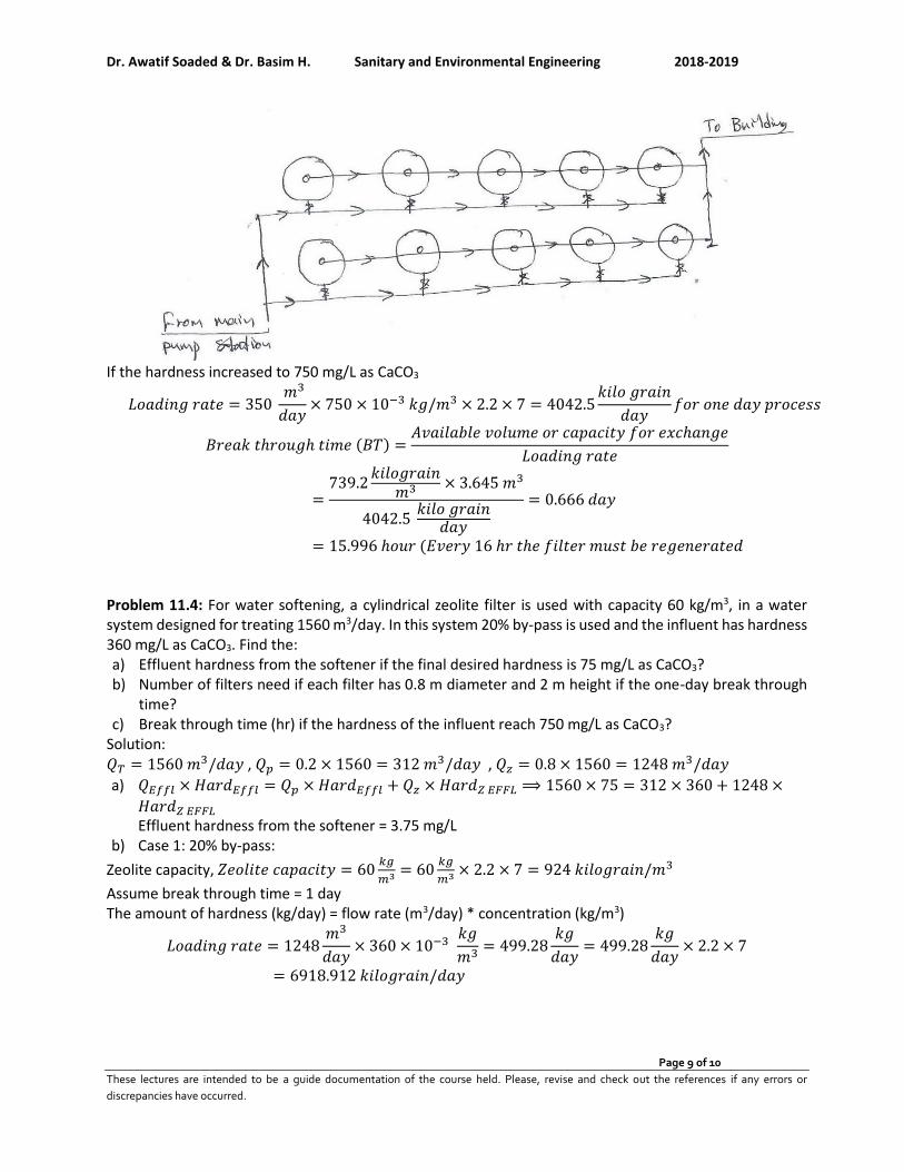
Dr. Awatif Soaded & Dr. Basim H. Sanitary and Environmental Engineering 2018-2019
Page 9 of 10
These lectures are intended to be a guide documentation of the course held. Please, revise and check out the references if any errors or
discrepancies have occurred.
If the hardness increased to 750 mg/L as CaCO3
𝐿𝑜𝑎𝑑𝑖𝑛𝑔 𝑟𝑎𝑡𝑒 = 350 𝑚3
𝑑𝑎𝑦× 750 × 10−3 𝑘𝑔/𝑚3 × 2.2 × 7 = 4042.5
𝑘𝑖𝑙𝑜 𝑔𝑟𝑎𝑖𝑛
𝑑𝑎𝑦𝑓𝑜𝑟 𝑜𝑛𝑒 𝑑𝑎𝑦 𝑝𝑟𝑜𝑐𝑒𝑠𝑠
𝐵𝑟𝑒𝑎𝑘 𝑡ℎ𝑟𝑜𝑢𝑔ℎ 𝑡𝑖𝑚𝑒 (𝐵𝑇) =𝐴𝑣𝑎𝑖𝑙𝑎𝑏𝑙𝑒 𝑣𝑜𝑙𝑢𝑚𝑒 𝑜𝑟 𝑐𝑎𝑝𝑎𝑐𝑖𝑡𝑦 𝑓𝑜𝑟 𝑒𝑥𝑐ℎ𝑎𝑛𝑔𝑒
𝐿𝑜𝑎𝑑𝑖𝑛𝑔 𝑟𝑎𝑡𝑒
=739.2
𝑘𝑖𝑙𝑜𝑔𝑟𝑎𝑖𝑛𝑚3 × 3.645 𝑚3
4042.5 𝑘𝑖𝑙𝑜 𝑔𝑟𝑎𝑖𝑛
𝑑𝑎𝑦
= 0.666 𝑑𝑎𝑦
= 15.996 ℎ𝑜𝑢𝑟 (𝐸𝑣𝑒𝑟𝑦 16 ℎ𝑟 𝑡ℎ𝑒 𝑓𝑖𝑙𝑡𝑒𝑟 𝑚𝑢𝑠𝑡 𝑏𝑒 𝑟𝑒𝑔𝑒𝑛𝑒𝑟𝑎𝑡𝑒𝑑
Problem 11.4: For water softening, a cylindrical zeolite filter is used with capacity 60 kg/m3, in a water system designed for treating 1560 m3/day. In this system 20% by-pass is used and the influent has hardness 360 mg/L as CaCO3. Find the: a) Effluent hardness from the softener if the final desired hardness is 75 mg/L as CaCO3? b) Number of filters need if each filter has 0.8 m diameter and 2 m height if the one-day break through
time? c) Break through time (hr) if the hardness of the influent reach 750 mg/L as CaCO3?
Solution: 𝑄𝑇 = 1560 𝑚3/𝑑𝑎𝑦 , 𝑄𝑝 = 0.2 × 1560 = 312 𝑚3/𝑑𝑎𝑦 , 𝑄𝑧 = 0.8 × 1560 = 1248 𝑚3/𝑑𝑎𝑦
a) 𝑄𝐸𝑓𝑓𝑙 × 𝐻𝑎𝑟𝑑𝐸𝑓𝑓𝑙 = 𝑄𝑝 × 𝐻𝑎𝑟𝑑𝐸𝑓𝑓𝑙 + 𝑄𝑧 × 𝐻𝑎𝑟𝑑𝑍 𝐸𝐹𝐹𝐿 ⟹ 1560 × 75 = 312 × 360 + 1248 ×
𝐻𝑎𝑟𝑑𝑍 𝐸𝐹𝐹𝐿 Effluent hardness from the softener = 3.75 mg/L
b) Case 1: 20% by-pass:
Zeolite capacity, 𝑍𝑒𝑜𝑙𝑖𝑡𝑒 𝑐𝑎𝑝𝑎𝑐𝑖𝑡𝑦 = 60𝑘𝑔
𝑚3 = 60𝑘𝑔
𝑚3 × 2.2 × 7 = 924 𝑘𝑖𝑙𝑜𝑔𝑟𝑎𝑖𝑛/𝑚3
Assume break through time = 1 day The amount of hardness (kg/day) = flow rate (m3/day) * concentration (kg/m3)
𝐿𝑜𝑎𝑑𝑖𝑛𝑔 𝑟𝑎𝑡𝑒 = 1248𝑚3
𝑑𝑎𝑦× 360 × 10−3
𝑘𝑔
𝑚3= 499.28
𝑘𝑔
𝑑𝑎𝑦= 499.28
𝑘𝑔
𝑑𝑎𝑦× 2.2 × 7
= 6918.912 𝑘𝑖𝑙𝑜𝑔𝑟𝑎𝑖𝑛/𝑑𝑎𝑦
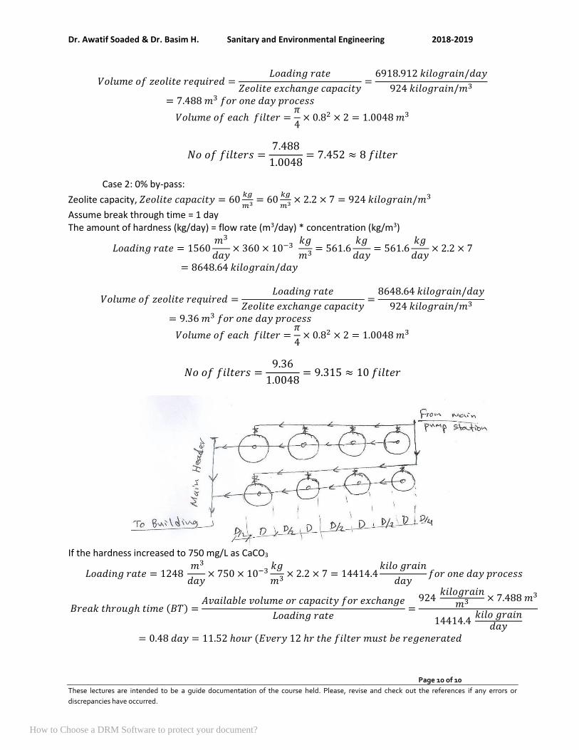
Dr. Awatif Soaded & Dr. Basim H. Sanitary and Environmental Engineering 2018-2019
Page 10 of 10
These lectures are intended to be a guide documentation of the course held. Please, revise and check out the references if any errors or
discrepancies have occurred.
𝑉𝑜𝑙𝑢𝑚𝑒 𝑜𝑓 𝑧𝑒𝑜𝑙𝑖𝑡𝑒 𝑟𝑒𝑞𝑢𝑖𝑟𝑒𝑑 =𝐿𝑜𝑎𝑑𝑖𝑛𝑔 𝑟𝑎𝑡𝑒
𝑍𝑒𝑜𝑙𝑖𝑡𝑒 𝑒𝑥𝑐ℎ𝑎𝑛𝑔𝑒 𝑐𝑎𝑝𝑎𝑐𝑖𝑡𝑦=
6918.912 𝑘𝑖𝑙𝑜𝑔𝑟𝑎𝑖𝑛/𝑑𝑎𝑦
924 𝑘𝑖𝑙𝑜𝑔𝑟𝑎𝑖𝑛/𝑚3
= 7.488 𝑚3 𝑓𝑜𝑟 𝑜𝑛𝑒 𝑑𝑎𝑦 𝑝𝑟𝑜𝑐𝑒𝑠𝑠
𝑉𝑜𝑙𝑢𝑚𝑒 𝑜𝑓 𝑒𝑎𝑐ℎ 𝑓𝑖𝑙𝑡𝑒𝑟 =𝜋
4× 0.82 × 2 = 1.0048 𝑚3
𝑁𝑜 𝑜𝑓 𝑓𝑖𝑙𝑡𝑒𝑟𝑠 =7.488
1.0048= 7.452 ≈ 8 𝑓𝑖𝑙𝑡𝑒𝑟
Case 2: 0% by-pass:
Zeolite capacity, 𝑍𝑒𝑜𝑙𝑖𝑡𝑒 𝑐𝑎𝑝𝑎𝑐𝑖𝑡𝑦 = 60𝑘𝑔
𝑚3 = 60𝑘𝑔
𝑚3 × 2.2 × 7 = 924 𝑘𝑖𝑙𝑜𝑔𝑟𝑎𝑖𝑛/𝑚3
Assume break through time = 1 day The amount of hardness (kg/day) = flow rate (m3/day) * concentration (kg/m3)
𝐿𝑜𝑎𝑑𝑖𝑛𝑔 𝑟𝑎𝑡𝑒 = 1560𝑚3
𝑑𝑎𝑦× 360 × 10−3
𝑘𝑔
𝑚3= 561.6
𝑘𝑔
𝑑𝑎𝑦= 561.6
𝑘𝑔
𝑑𝑎𝑦× 2.2 × 7
= 8648.64 𝑘𝑖𝑙𝑜𝑔𝑟𝑎𝑖𝑛/𝑑𝑎𝑦
𝑉𝑜𝑙𝑢𝑚𝑒 𝑜𝑓 𝑧𝑒𝑜𝑙𝑖𝑡𝑒 𝑟𝑒𝑞𝑢𝑖𝑟𝑒𝑑 =𝐿𝑜𝑎𝑑𝑖𝑛𝑔 𝑟𝑎𝑡𝑒
𝑍𝑒𝑜𝑙𝑖𝑡𝑒 𝑒𝑥𝑐ℎ𝑎𝑛𝑔𝑒 𝑐𝑎𝑝𝑎𝑐𝑖𝑡𝑦=
8648.64 𝑘𝑖𝑙𝑜𝑔𝑟𝑎𝑖𝑛/𝑑𝑎𝑦
924 𝑘𝑖𝑙𝑜𝑔𝑟𝑎𝑖𝑛/𝑚3
= 9.36 𝑚3 𝑓𝑜𝑟 𝑜𝑛𝑒 𝑑𝑎𝑦 𝑝𝑟𝑜𝑐𝑒𝑠𝑠
𝑉𝑜𝑙𝑢𝑚𝑒 𝑜𝑓 𝑒𝑎𝑐ℎ 𝑓𝑖𝑙𝑡𝑒𝑟 =𝜋
4× 0.82 × 2 = 1.0048 𝑚3
𝑁𝑜 𝑜𝑓 𝑓𝑖𝑙𝑡𝑒𝑟𝑠 =9.36
1.0048= 9.315 ≈ 10 𝑓𝑖𝑙𝑡𝑒𝑟
If the hardness increased to 750 mg/L as CaCO3
𝐿𝑜𝑎𝑑𝑖𝑛𝑔 𝑟𝑎𝑡𝑒 = 1248 𝑚3
𝑑𝑎𝑦× 750 × 10−3
𝑘𝑔
𝑚3× 2.2 × 7 = 14414.4
𝑘𝑖𝑙𝑜 𝑔𝑟𝑎𝑖𝑛
𝑑𝑎𝑦𝑓𝑜𝑟 𝑜𝑛𝑒 𝑑𝑎𝑦 𝑝𝑟𝑜𝑐𝑒𝑠𝑠
𝐵𝑟𝑒𝑎𝑘 𝑡ℎ𝑟𝑜𝑢𝑔ℎ 𝑡𝑖𝑚𝑒 (𝐵𝑇) =𝐴𝑣𝑎𝑖𝑙𝑎𝑏𝑙𝑒 𝑣𝑜𝑙𝑢𝑚𝑒 𝑜𝑟 𝑐𝑎𝑝𝑎𝑐𝑖𝑡𝑦 𝑓𝑜𝑟 𝑒𝑥𝑐ℎ𝑎𝑛𝑔𝑒
𝐿𝑜𝑎𝑑𝑖𝑛𝑔 𝑟𝑎𝑡𝑒=
924 𝑘𝑖𝑙𝑜𝑔𝑟𝑎𝑖𝑛
𝑚3 × 7.488 𝑚3
14414.4 𝑘𝑖𝑙𝑜 𝑔𝑟𝑎𝑖𝑛
𝑑𝑎𝑦= 0.48 𝑑𝑎𝑦 = 11.52 ℎ𝑜𝑢𝑟 (𝐸𝑣𝑒𝑟𝑦 12 ℎ𝑟 𝑡ℎ𝑒 𝑓𝑖𝑙𝑡𝑒𝑟 𝑚𝑢𝑠𝑡 𝑏𝑒 𝑟𝑒𝑔𝑒𝑛𝑒𝑟𝑎𝑡𝑒𝑑
How to Choose a DRM Software to protect your document?

Dr. Awatif Soaded & Dr. Basim H. Sanitary and Environmental Engineering 2018-2019
Page 1 of 6
These lectures are intended to be a guide documentation of the course held. Please, revise and check out the references if any errors or
discrepancies have occurred.
Sanitary and Environmental Engineering
PART 2: WASTEWATER ENGINEERING
Dr. Awatif Soaded & Dr. Basim H. Sanitary and Environmental Engineering 2018-2019
Page 2 of 6
These lectures are intended to be a guide documentation of the course held. Please, revise and check out the references if any errors or
discrepancies have occurred.
PART 2: WASTEWATER ENGINEERING
Lecture 1: Introduction to Wastewater or Sewage
The liquid waste generated from various activities: residential, industrial, commercial and public areas,
due to the consumption of potable water. It is collected and transmitted in a pipe system known as the
sewer system. This wastewater contains impurities and/ or pollutants in the form of solids, liquids and
gases in concentrations harmful to the environment. The management of this wastewater require
knowing its quantity and quality.
Sewerage is applied to the art of collecting, treating, and disposing of sewage. It implies the collecting of
wastewaters from occupied areas and conveying them to some point of disposal. The liquid wastes will
require treatment before they can be discharged into a body of water or otherwise disposed of without
endangering the public health or causing offensive condition.
Sewerage works are comprehensive terms covering all structures and procedures required for collecting,
treating, and disposing of sewage.
Types of wastewater flowing in the sewer system:
1) Municipal-Sanitary-Domestic sewage: The liquid wastes conducted away from residences, business buildings, and institutions.
2) Industrial wastewater: The liquid waste from industrial establishments. 3) Rainwater-Runoff-Storm sewage. 4) Infiltration: Groundwater entering sanitary sewers through defective pipe joints and broken
pipes. Infiltration will occur where local groundwater elevation is higher than the sewer pipe. Gravel bedding materials in sewer pipe trenches act as a French drain. Groundwater flows parallel to the sewer until it reaches the area of damaged pipe. In areas of low groundwater, sewage may exfiltration into groundwater from a leaking sewer.
Sewage treatment covers any process to which sewage is subjected in order to remove or alter its objectionable constituents so as to render it less dangerous or offensive. Treatment which produces an effluent containing not more than 20 mg/L BOD5 and 30 mg/L suspended solids (SS). Sewage disposal applies to act of disposing of sewage by any method. It may be done with or without previous treatment. Note: The degree of treatment required depends upon the water quality standards applicable to the receiving stream and the flow and quality of both the stream and waste.
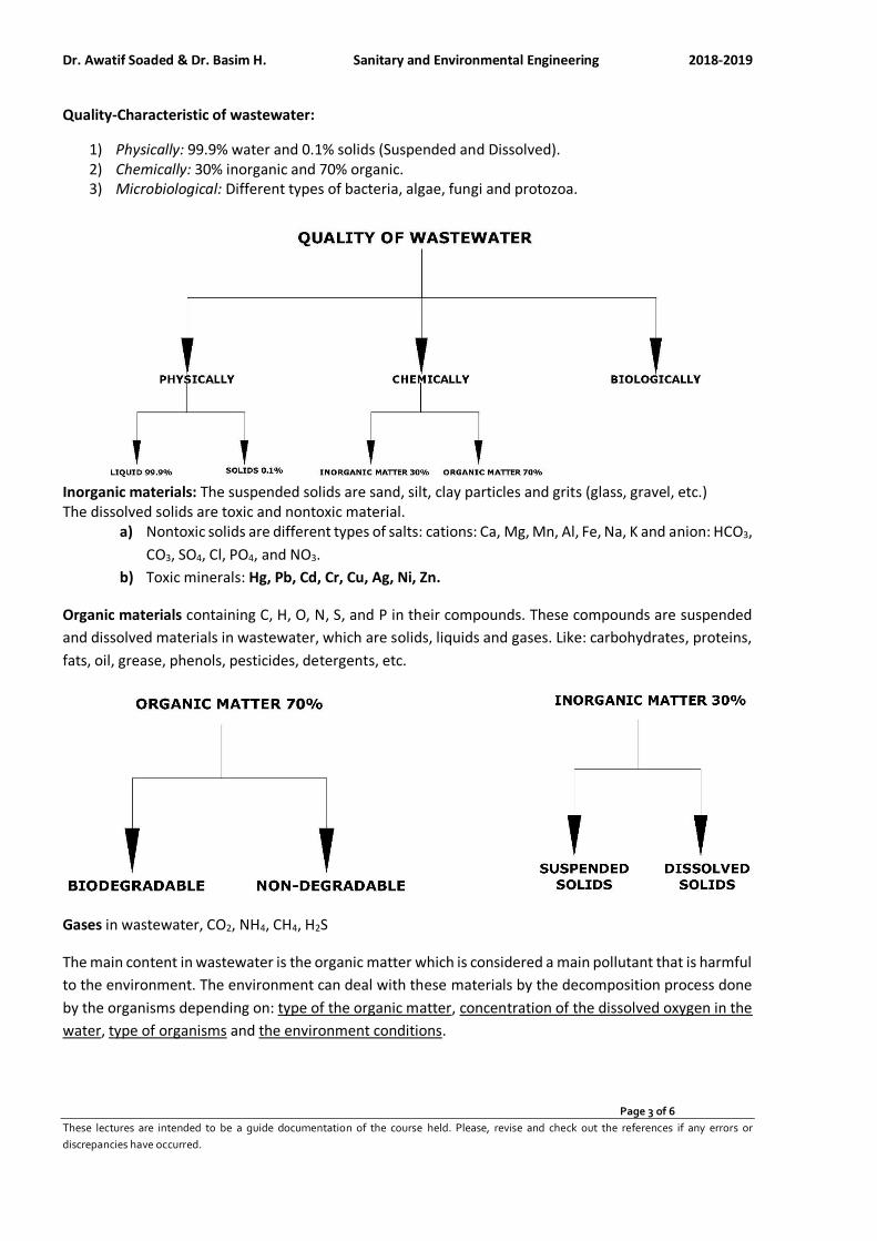
Dr. Awatif Soaded & Dr. Basim H. Sanitary and Environmental Engineering 2018-2019
Page 3 of 6
These lectures are intended to be a guide documentation of the course held. Please, revise and check out the references if any errors or
discrepancies have occurred.
Quality-Characteristic of wastewater:
1) Physically: 99.9% water and 0.1% solids (Suspended and Dissolved). 2) Chemically: 30% inorganic and 70% organic. 3) Microbiological: Different types of bacteria, algae, fungi and protozoa.
Inorganic materials: The suspended solids are sand, silt, clay particles and grits (glass, gravel, etc.) The dissolved solids are toxic and nontoxic material.
a) Nontoxic solids are different types of salts: cations: Ca, Mg, Mn, Al, Fe, Na, K and anion: HCO3,
CO3, SO4, Cl, PO4, and NO3.
b) Toxic minerals: Hg, Pb, Cd, Cr, Cu, Ag, Ni, Zn.
Organic materials containing C, H, O, N, S, and P in their compounds. These compounds are suspended
and dissolved materials in wastewater, which are solids, liquids and gases. Like: carbohydrates, proteins,
fats, oil, grease, phenols, pesticides, detergents, etc.
Gases in wastewater, CO2, NH4, CH4, H2S
The main content in wastewater is the organic matter which is considered a main pollutant that is harmful
to the environment. The environment can deal with these materials by the decomposition process done
by the organisms depending on: type of the organic matter, concentration of the dissolved oxygen in the
water, type of organisms and the environment conditions.
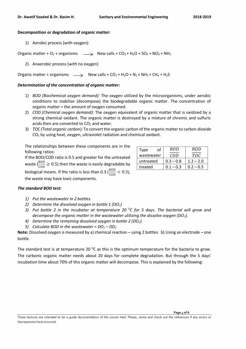
Dr. Awatif Soaded & Dr. Basim H. Sanitary and Environmental Engineering 2018-2019
Page 4 of 6
These lectures are intended to be a guide documentation of the course held. Please, revise and check out the references if any errors or
discrepancies have occurred.
Decomposition or degradation of organic matter:
1) Aerobic process (with oxygen):
Organic matter + O2 + organisms New calls + CO2 + H2O + SO4 + NO3 + NH3
2) Anaerobic process (with no oxygen)
Organic matter + organisms New calls + CO2 + H2O + N2 + NH3 + CH4 + H2S
Determination of the concentration of organic matter:
1) BOD (Biochemical oxygen demand): The oxygen utilized by the microorganisms, under aerobic conditions to stabilize (decompose) the biodegradable organic matter. The concentration of organic matter = the amount of oxygen consumed.
2) COD (Chemical oxygen demand): The oxygen equivalent of organic matter that is oxidized by a strong chemical oxidant. The organic matter is destroyed by a mixture of chromic and sulfuric acids then are converted to CO2 and water.
3) TOC (Total organic carbon): To convert the organic carbon of the organic matter to carbon dioxide CO2 by using heat, oxygen, ultraviolet radiation and chemical oxidant.
The standard BOD test:
1) Put the wastewater in 2 bottles. 2) Determine the dissolved oxygen in bottle 1 (DO1) 3) Put bottle 2 in the incubator at temperature 20 0C for 5 days. The bacterial will grow and
decompose the organic matter in the wastewater utilizing the dissolve oxygen (DO1). 4) Determine the remaining dissolved oxygen in bottle 2 (DO2). 5) Calculate BOD in the wastewater = DO1 – DO2
Note: Dissolved oxygen is measured by a) chemical reaction – using 2 bottles b) Using an electrode – one
bottle.
The standard test is at temperature 20 0C as this is the optimum temperature for the bacteria to grow.
The carbonic organic matter needs about 20 days for complete degradation. But through the 5 days'
incubation time about 70% of this organic matter will decompose. This is explained by the following:
The relationships between these components are in the following ratios: If the BOD/COD ratio is 0.5 and greater for the untreated
waste (𝐵𝑂𝐷
𝐶𝑂𝐷≥ 0.5) then the waste is easily degradable by
biological means. If the ratio is less than 0.3 (𝐵𝑂𝐷
𝐶𝑂𝐷< 0.3),
the waste may have toxic components.
𝐵𝑂𝐷
𝑇𝑂𝐶
𝐵𝑂𝐷
𝐶𝑂𝐷
Type of wastewater
1.2 – 2.0 0.3 – 0.8 untreated
0.2 – 0.5 0.1 – 0.3 treated

Dr. Awatif Soaded & Dr. Basim H. Sanitary and Environmental Engineering 2018-2019
Page 5 of 6
These lectures are intended to be a guide documentation of the course held. Please, revise and check out the references if any errors or
discrepancies have occurred.
The decomposition of organic matter is a 1st order reaction: y
𝑑𝑦
𝑑𝑡= −𝐾1𝑦 ⇛
𝑑𝑦
𝑦= −𝐾1𝑑𝑡 mg/L
By integration: L
ln 𝑦 = −𝐾1𝑡 + 𝑐 (1) dy/dt L-y = BOD
At t = 0, y = L
So, c = ln L and eq. 1 will be: y
ln 𝑦 = −𝐾1𝑡 + ln 𝐿 𝑜𝑟 ln𝑦
𝐿= −𝐾1𝑡
𝑦
𝐿= 𝑒−𝐾1𝑡 𝑜𝑟 𝑦 = 𝐿𝑒−𝐾1𝑡 5 time t (day)
y: The non-degradable (remaining) organic matter at time t (mg/L). L: The ultimate organic matter at time 0 = BODu (mg/L).
K1: Degradation (deoxygenation) rate (day -1). t: Time for decomposition (day). The oxygen utilized or organic matter decomposed through time t (day) at temperature T (0C) will be:
𝐵𝑂𝐷𝑡−𝑇 = 𝐿 − 𝑦 = 𝐿 − 𝐿𝑒−𝐾1𝑡 = 𝐿(1 − 𝑒−𝐾1𝑡), So, the standard test gives BOD 5-20:
For domestic sewage K1 = 0.23 /day at T = 20 0C
To change the rate from any temperature to 20 0C by using (𝐾1(𝑇) = 𝐾1(20) × 1.047(𝑇−20)).
𝐵𝑂𝐷5−20 = 𝐿(1 − 𝑒−0.23×5) ⇛𝐵𝑂𝐷5−20
𝐿≈ 0.68 ≈ 70%
Typical domestic sewage characteristic
Strong Medium Weak Parameter mg/L
860 500 270 Total dissolved solids
400 210 120 Total suspended solids
350 190 110 BOD5
800 430 250 COD
260 140 80 TOC
70 40 20 Total N
12 7 4 Total P
90 50 30 Chloride
50 30 20 Sulfate

Dr. Awatif Soaded & Dr. Basim H. Sanitary and Environmental Engineering 2018-2019
Page 6 of 6
These lectures are intended to be a guide documentation of the course held. Please, revise and check out the references if any errors or
discrepancies have occurred.
Solved problems
Problem 1: The results from the laboratory show that the BOD 1-30 = 110 mg/L for a wastewater sample. Find: 1-ultimate BOD (BODu), 2- BOD 5-20? Solution:
𝐾1(𝑇) = 𝐾1(20) × 1.047(𝑇−20) ⟹ 𝐾1(30) = 0.23 × 1.047(30−20) = 0.364 𝑑𝑎𝑦−1
𝐵𝑂𝐷𝑡−𝑇 = 𝐿(1 − 𝑒−𝐾1𝑡) ⟹ 𝐵𝑂𝐷1−30 = 𝐿(1 − 𝑒−𝐾1−30𝑡) ⟹ 110𝑚𝑔
𝐿= 𝐿(1 − 𝑒−0.364×1) ⟹
𝐿 = 360.527 𝑚𝑔/𝐿
𝐵𝑂𝐷𝑡−𝑇 = 𝐿(1 − 𝑒−𝐾1𝑡) ⟹ 𝐵𝑂𝐷5−20 = 𝐿(1 − 𝑒−𝐾1−20𝑡) ⟹ 𝐵𝑂𝐷5−20 = 360.527 × (1 − 𝑒−0.23×5)= 246.371 𝑚𝑔/𝐿
Problem 2: If the waste with ultimate BODu equal 190 mg/L and k1-20 = 0.23/day is discharge to a stream at an average temperature 250C,
a) compute the BOD would be exerted in 3 and 5 days at temperature 20 and 25 0C, (𝐵𝑂𝐷3−20 ,
𝐵𝑂𝐷5−20 , (𝐵𝑂𝐷3−25 ), 𝐵𝑂𝐷5−25 ?
b) Compute the organic loading in (kg/day) for 𝐵𝑂𝐷5−20 if the flowrate 50 m3/hr?
Solution:
a) 𝐵𝑂𝐷5−20 = 190 × (1 − 𝑒−0.23×5) = 129.939 𝑚𝑔/𝐿
𝐵𝑂𝐷3−20 = 190 × (1 − 𝑒−0.23×3) = 94.7 𝑚𝑔/𝐿
𝐾1(25) = 𝐾1(20) × 1.047(𝑇−20) = 0.23 × 1.047(25−20) = 0.289 /𝑑𝑎𝑦
𝐵𝑂𝐷3−25 = 190 × (1 − 𝑒−0.289×3) = 110.16 𝑚𝑔/𝐿
𝐵𝑂𝐷5−25 = 190 × (1 − 𝑒−0.289×5) = 145.208 𝑚𝑔/𝐿
b) 𝑂𝑟𝑎𝑛𝑖𝑐 𝑙𝑜𝑎𝑑𝑘𝑔
𝑑𝑎𝑦= 129.939 × 10⁻³ 𝑘𝑔
𝑚3 × 50 × 24𝑚3
𝑑𝑎𝑦= 155.926 𝑘𝑔/𝑑𝑎𝑦
How to Choose a DRM Software to protect your document?
Dr. Awatif Soaded & Dr. Basim H. Sanitary and Environmental Engineering 2019-2020
Page 1 of 10
These lectures are intended to be a guide documentation of the course held. Please, revise and check out the references if any errors or
discrepancies have occurred.
Sanitary and Environmental Engineering
PART 2: WASTEWATER ENGINEERING
Dr. Awatif Soaded & Dr. Basim H. Sanitary and Environmental Engineering 2019-2020
Page 2 of 10
These lectures are intended to be a guide documentation of the course held. Please, revise and check out the references if any errors or
discrepancies have occurred.
PART 2: WASTEWATER ENGINEERING
Lecture 2: Quantity of wastewater: The proportion of the water consumed which reach the sewer will must be decided upon after careful consideration of local conditions. Although the sewage may vary in individual cities from 70-130 percent of the water consumed, designers frequently assume that the average rate of sewage flow, including a moderate allowance for infiltration, equal the average rate of water consumption.
1) Domestic: 80-90% water consumption. 2) Industrial: a) domestic as in 1; b) Water process. 3) Public: as in 1. 4) Runoff or storm sewage: Using the rational formula:
𝐴𝑣𝑒𝑟𝑎𝑔𝑒 𝑑𝑎𝑖𝑙𝑦 𝑑𝑒𝑚𝑎𝑛𝑑 = (70 − 130) × 𝑜𝑓 𝑤𝑎𝑡𝑒𝑟 𝑐𝑜𝑛𝑠𝑢𝑚𝑝𝑡𝑖𝑜𝑛
Fluctuations in Dry Weather Flow
Since dry weather flow depends on the quantity of water used, and as there are fluctuations in rate of water consumption, there will be fluctuations in dry weather flow also. In general, it can be assumed that:
𝑀𝑎𝑥𝑖𝑚𝑢𝑚 𝑠𝑒𝑤𝑎𝑔𝑒 𝑑𝑎𝑖𝑙𝑦 𝑑𝑒𝑚𝑎𝑛𝑑 𝑄𝑀𝑎𝑥 = (1.5 − 2) × 𝐴𝑣𝑒𝑟𝑎𝑔𝑒 𝑠𝑒𝑤𝑎𝑔𝑒 𝑑𝑎𝑖𝑙𝑦 𝑑𝑒𝑚𝑎𝑛𝑑
𝑀𝑖𝑛𝑖𝑚𝑢𝑚 𝑠𝑒𝑤𝑎𝑔𝑒 𝑑𝑎𝑖𝑙𝑦 𝑑𝑒𝑚𝑎𝑛𝑑 𝑄𝑀𝑖𝑛 = (0.5 − 0.67) × 𝐴𝑣𝑒𝑟𝑎𝑔𝑒 𝑠𝑒𝑤𝑎𝑔𝑒 𝑑𝑎𝑖𝑙𝑦 𝑑𝑒𝑚𝑎𝑛𝑑
Observation of fluctuations in various cities indicates that the peak for a small residential area is likely to be 225 percent of the average for that day. For commercial area the peak may reach 150 percent of the average and for industrial areas somewhat less. The flow in the outfall line of a sewer system serving a city having a normal population and commercial and industrial activities will have a peak flow of about 150 percent of the daily average. Some designers use the following formula to estimate the maximum rate of domestic sewage flow from small areas:
𝑀 = 1 +14
4 + √𝑃
Where:
M: Ratio of the maximum sewage flow to the average (𝑀 =𝑀𝑎𝑥𝑖𝑚𝑢𝑚 𝑠𝑒𝑤𝑎𝑔𝑒 𝑓𝑙𝑜𝑤
𝐴𝑣𝑒𝑟𝑎𝑔𝑒 𝑠𝑒𝑤𝑎𝑔𝑒 𝑓𝑙𝑜𝑤).
P: Population served in thousands.
The maximum sewage flow will be the hourly maximum, or the peak rate of the maximum day plus the maximum infiltration.
IMPORTANT NOTE: The minimum rates of sewage flow are useful in the design of sewage pumping plants and occasionally to investigate the velocities in sewers during low flow periods. Generally, the minimum flow may be taken as 50 percent of the average.
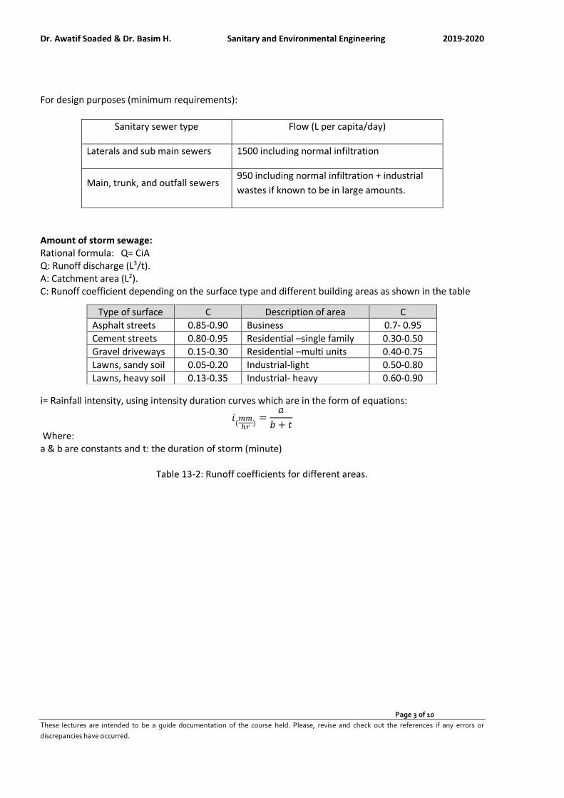
Dr. Awatif Soaded & Dr. Basim H. Sanitary and Environmental Engineering 2019-2020
Page 3 of 10
These lectures are intended to be a guide documentation of the course held. Please, revise and check out the references if any errors or
discrepancies have occurred.
For design purposes (minimum requirements):
Sanitary sewer type Flow (L per capita/day)
Laterals and sub main sewers 1500 including normal infiltration
Main, trunk, and outfall sewers 950 including normal infiltration + industrial
wastes if known to be in large amounts.
Amount of storm sewage: Rational formula: Q= CiA Q: Runoff discharge (L3/t). A: Catchment area (L2). C: Runoff coefficient depending on the surface type and different building areas as shown in the table
i= Rainfall intensity, using intensity duration curves which are in the form of equations:
𝑖(𝑚𝑚ℎ𝑟
)=
𝑎
𝑏 + 𝑡
Where: a & b are constants and t: the duration of storm (minute)
Table 13-2: Runoff coefficients for different areas.
C Description of area C Type of surface
0.7- 0.95 Business 0.85-0.90 Asphalt streets
0.30-0.50 Residential –single family 0.80-0.95 Cement streets
0.40-0.75 Residential –multi units 0.15-0.30 Gravel driveways
0.50-0.80 Industrial-light 0.05-0.20 Lawns, sandy soil
0.60-0.90 Industrial- heavy 0.13-0.35 Lawns, heavy soil
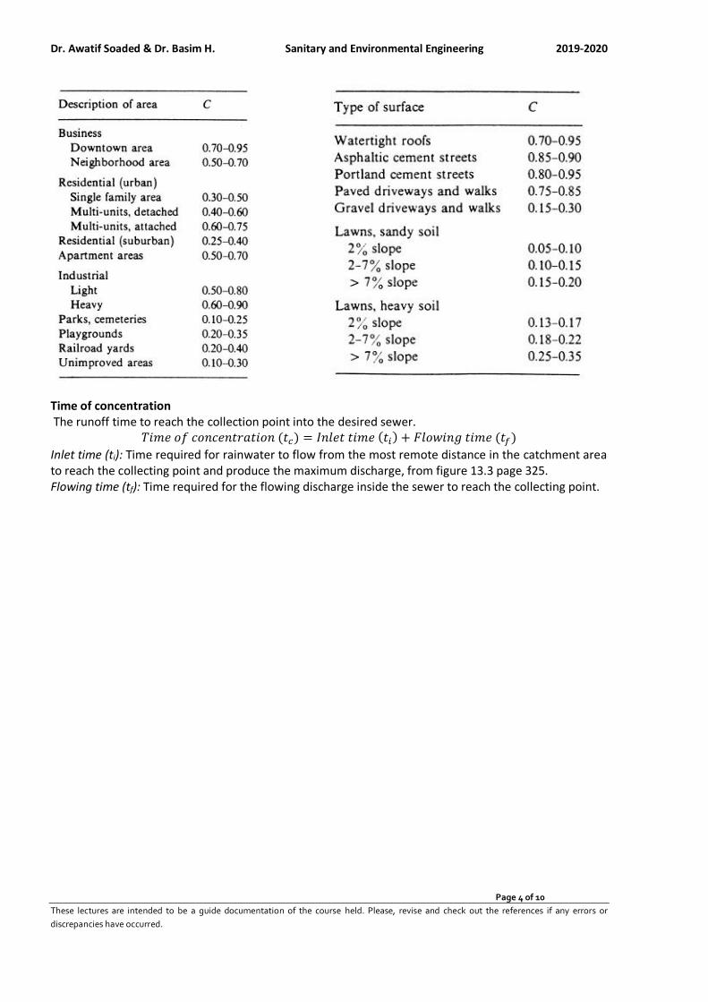
Dr. Awatif Soaded & Dr. Basim H. Sanitary and Environmental Engineering 2019-2020
Page 4 of 10
These lectures are intended to be a guide documentation of the course held. Please, revise and check out the references if any errors or
discrepancies have occurred.
Time of concentration The runoff time to reach the collection point into the desired sewer.
𝑇𝑖𝑚𝑒 𝑜𝑓 𝑐𝑜𝑛𝑐𝑒𝑛𝑡𝑟𝑎𝑡𝑖𝑜𝑛 (𝑡𝑐) = 𝐼𝑛𝑙𝑒𝑡 𝑡𝑖𝑚𝑒 (𝑡𝑖) + 𝐹𝑙𝑜𝑤𝑖𝑛𝑔 𝑡𝑖𝑚𝑒 (𝑡𝑓)
Inlet time (ti): Time required for rainwater to flow from the most remote distance in the catchment area to reach the collecting point and produce the maximum discharge, from figure 13.3 page 325. Flowing time (tf): Time required for the flowing discharge inside the sewer to reach the collecting point.

Dr. Awatif Soaded & Dr. Basim H. Sanitary and Environmental Engineering 2019-2020
Page 5 of 10
These lectures are intended to be a guide documentation of the course held. Please, revise and check out the references if any errors or
discrepancies have occurred.
Fig.13-1: Inlet time. Fig. 13-2: Inlet time and flow time.
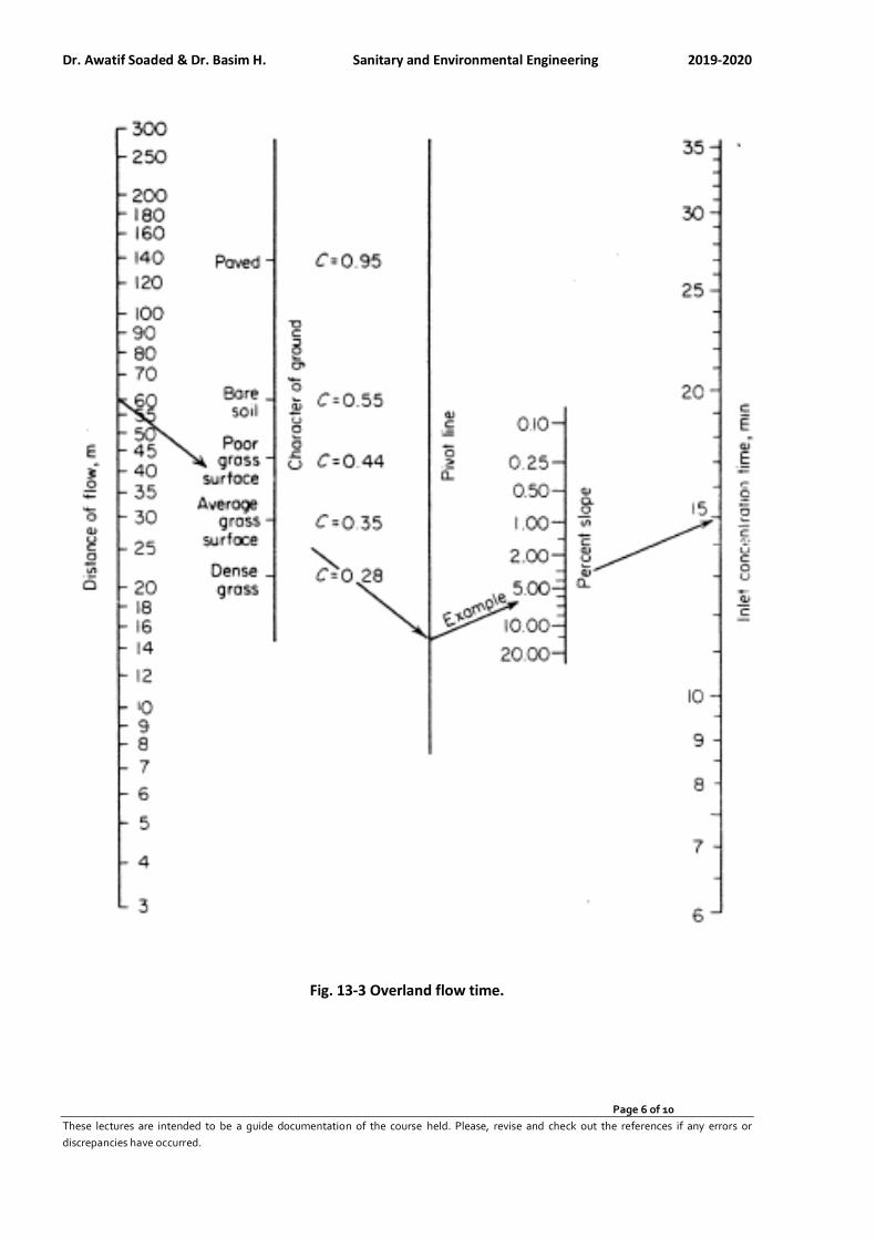
Dr. Awatif Soaded & Dr. Basim H. Sanitary and Environmental Engineering 2019-2020
Page 6 of 10
These lectures are intended to be a guide documentation of the course held. Please, revise and check out the references if any errors or
discrepancies have occurred.
Fig. 13-3 Overland flow time.
Dr. Awatif Soaded & Dr. Basim H. Sanitary and Environmental Engineering 2019-2020
Page 7 of 10
These lectures are intended to be a guide documentation of the course held. Please, revise and check out the references if any errors or
discrepancies have occurred.
Design periods and use of sewage flow data:
Detail Design period
(year) Design criteria
Design of a
sewer system indefinite
It is necessary to estimate maximum population densities expected in
various districts and locations of commercial and industrial districts
together with maximum rates of sewage flow per second and maximum
infiltration per day.
Sewage
pumping plant 10
Rate of flow required are average daily, peak, and minimum flow rates,
including infiltration.
Sewage
treatment plant 15-20 Flow rate required are average and peak rates, both include infiltration.
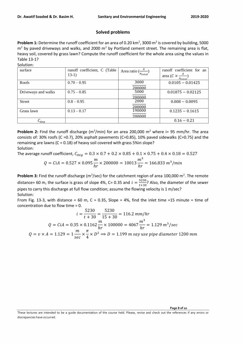
Dr. Awatif Soaded & Dr. Basim H. Sanitary and Environmental Engineering 2019-2020
Page 8 of 10
These lectures are intended to be a guide documentation of the course held. Please, revise and check out the references if any errors or
discrepancies have occurred.
Solved problems
Problem 1: Determine the runoff coefficient for an area of 0.20 km2, 3000 m2 is covered by building, 5000 m2 by paved driveways and walks, and 2000 m2 by Portland cement street. The remaining area is flat, heavy soil, covered by grass lawn? Compute the runoff coefficient for the whole area using the values in Table 13-1? Solution:
surface runoff coefficient, C (Table
13-1) Area ratio (
𝐴
𝐴𝑡𝑜𝑡𝑎𝑙) runoff coefficient for an
area (𝐶 ×𝐴
𝐴𝑡𝑜𝑡𝑎𝑙)
Roofs 0.70 – 0.95 3000
200000
0.0105 − 0.01425
Driveways and walks 0.75 – 0.85 5000
200000
0.01875 − 0.02125
Street 0.8 – 0.95 2000
200000
0.008 − 0.0095
Grass lawn 0.13 – 0.17 190000
200000
0.1235 − 0.1615
𝐶𝐴𝑣𝑔 0.16 − 0.21
Problem 2: Find the runoff discharge (m3/min) for an area 200,000 m2 where i= 95 mm/hr. The area consists of: 30% roofs (C =0.7), 20% asphalt pavements (C=0.85), 10% paved sidewalks (C=0.75) and the remaining are lawns (C = 0.18) of heavy soil covered with grass 5%in slope? Solution: The average runoff coefficient, 𝐶𝐴𝑣𝑔 = 0.3 × 0.7 + 0.2 × 0.85 + 0.1 × 0.75 + 0.4 × 0.18 = 0.527
𝑄 = 𝐶𝑖𝐴 = 0.527 × 0.095𝑚
ℎ𝑟× 200000 = 10013
𝑚3
ℎ𝑟= 166.833 𝑚3/𝑚𝑖𝑛
Problem 3: Find the runoff discharge (m3/sec) for the catchment region of area 100,000 m2. The remote
distance= 60 m, the surface is grass of slope 4%, C= 0.35 and 𝑖 =5230
𝑡+30? Also, the diameter of the sewer
pipes to carry this discharge at full flow condition; assume the flowing velocity is 1 m/sec? Solution: From Fig. 13-3, with distance = 60 m, C = 0.35, Slope = 4%, find the inlet time =15 minute = time of concentration due to flow time = 0.
𝑖 =5230
𝑡 + 30=
5230
15 + 30= 116.2 𝑚𝑚/ℎ𝑟
𝑄 = 𝐶𝑖𝐴 = 0.35 × 0.1162𝑚
ℎ𝑟× 100000 = 4067
𝑚3
ℎ𝑟= 1.129 𝑚3/𝑠𝑒𝑐
𝑄 = 𝑣 × 𝐴 = 1.129 = 1𝑚
𝑠𝑒𝑐×
𝜋
4× 𝐷2 ⟹ 𝐷 = 1.199 𝑚 𝑠𝑎𝑦 𝑢𝑠𝑒 𝑝𝑖𝑝𝑒 𝑑𝑖𝑎𝑚𝑒𝑡𝑒𝑟 1200 𝑚𝑚
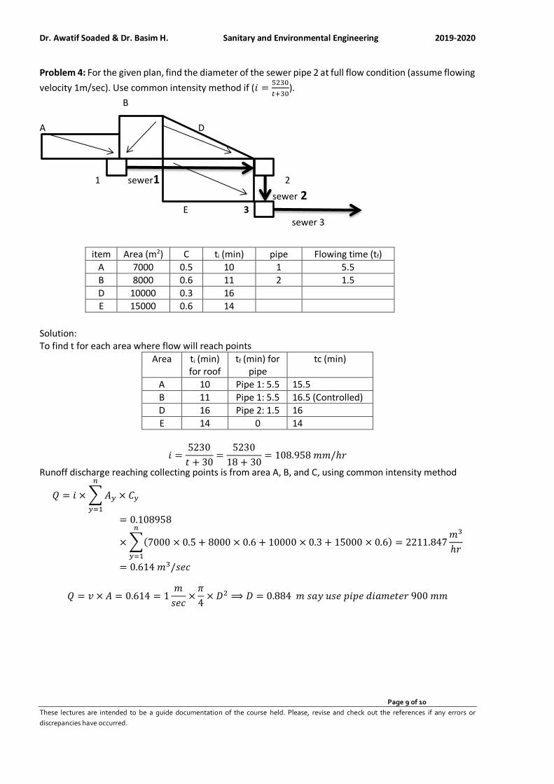
Dr. Awatif Soaded & Dr. Basim H. Sanitary and Environmental Engineering 2019-2020
Page 9 of 10
These lectures are intended to be a guide documentation of the course held. Please, revise and check out the references if any errors or
discrepancies have occurred.
Problem 4: For the given plan, find the diameter of the sewer pipe 2 at full flow condition (assume flowing
velocity 1m/sec). Use common intensity method if (𝑖 =5230
𝑡+30).
B A D
1 sewer1 2
sewer 2 E 3 sewer 3
Solution: To find t for each area where flow will reach points
Area ti (min) for roof
tf (min) for pipe
tc (min)
A 10 Pipe 1: 5.5 15.5
B 11 Pipe 1: 5.5 16.5 (Controlled)
D 16 Pipe 2: 1.5 16
E 14 0 14
𝑖 =5230
𝑡 + 30=
5230
18 + 30= 108.958 𝑚𝑚/ℎ𝑟
Runoff discharge reaching collecting points is from area A, B, and C, using common intensity method
𝑄 = 𝑖 × ∑ 𝐴𝑦 × 𝐶𝑦
𝑛
𝑦=1
= 0.108958
× ∑(7000 × 0.5 + 8000 × 0.6 + 10000 × 0.3 + 15000 × 0.6) = 2211.847𝑚3
ℎ𝑟
𝑛
𝑦=1
= 0.614 𝑚3/𝑠𝑒𝑐
𝑄 = 𝑣 × 𝐴 = 0.614 = 1𝑚
𝑠𝑒𝑐×
𝜋
4× 𝐷2 ⟹ 𝐷 = 0.884 𝑚 𝑠𝑎𝑦 𝑢𝑠𝑒 𝑝𝑖𝑝𝑒 𝑑𝑖𝑎𝑚𝑒𝑡𝑒𝑟 900 𝑚𝑚
Flowing time (tf) pipe ti (min) C Area (m2) item
5.5 1 10 0.5 7000 A
1.5 2 11 0.6 8000 B
16 0.3 10000 D
14 0.6 15000 E
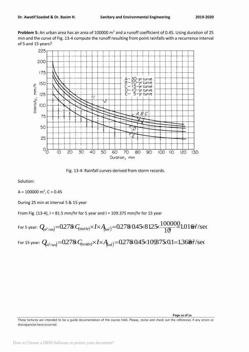
Dr. Awatif Soaded & Dr. Basim H. Sanitary and Environmental Engineering 2019-2020
Page 10 of 10
These lectures are intended to be a guide documentation of the course held. Please, revise and check out the references if any errors or
discrepancies have occurred.
Problem 5: An urban area has an area of 100000 m2 and a runoff coefficient of 0.45. Using duration of 25 min and the curve of Fig. 13-4 compute the runoff resulting from point rainfalls with a recurrence interval of 5 and 15 years?
Fig. 13-4: Rainfall curves derived from storm records.
Solution:
A = 100000 m2, C = 0.45
During 25 min at interval 5 & 15 year
From Fig. (13-4), I = 81.5 mm/hr for 5 year and I = 109.375 mm/hr for 15 year
For 5 year: ( ) ( ) ( ) sec/016.110
10000025.8145.0278.0278.0 3
6/sec/ 23 mAICQkmhrmmm
===
For 15 year: ( ) ( ) ( ) sec/368.11.0375.10945.0278.0278.0 3/sec/ 23 mAICQ
kmhrmmm===
How to Choose a DRM Software to protect your document?

Dr. Awatif Soaded & Dr. Basim H. Sanitary and Environmental Engineering 2019-2020
Page 1 of 21
These lectures are intended to be a guide documentation of the course held. Please, revise and check out the references if any errors or
discrepancies have occurred.
Sanitary and Environmental Engineering
PART 2: WASTEWATER ENGINEERING

Dr. Awatif Soaded & Dr. Basim H. Sanitary and Environmental Engineering 2019-2020
Page 2 of 21
These lectures are intended to be a guide documentation of the course held. Please, revise and check out the references if any errors or
discrepancies have occurred.
PART 2: WASTEWATER ENGINEERING
Lecture 3: Sewer systems
1) Separate system: Two pipes are used, one to carry DWF and another pipe to carry WWF. 2) Combined system: One pipe to carry both DWF and WWF.
DWF is the dry weather flow and WWF is the wet weather flow.
Comparison of characteristics of combined wastewater with other sources:
Domestic wastewater
Combined wastewater
Runoff Rainwater unit Parameter
120 - 370 270 -550 67 - 101 <1 mg/L Total suspended solids TSS
120 -380 60 -220 8 -10 1 -13 mg/L BOD
260 -900 260 - 480 40 - 73 9 -16 mg/L COD
105 -107 105 -106 103 -104 MPN/100mL Coliform Bacteria
0.43 – 0.91 0.05 -1.0 mg/L Nitrate 4-12 1.2 -2.8 0.67 -1.66 0.02 -0.15 mg/L Phosphorous
27 - 33 µg/L Copper Cu
140 - 600 30 -144 0 - 70 µg/L Lead Pb
135 - 226 µg/L Zinc Zn
Sewer types according to its sewage type:
1) Sanitary sewers carry sanitary sewage and industrial wastes after treatment produced by the community and only such ground, surface, and storm water as may enter through poor joints, around manhole covers, and through deficiencies.
2) Storm sewers are designed to carry the surface and storm water which runs in the same conduits. Sewer types according to its flow type:
3) Combined sewers carry all types of sewage in the same conduits. 4) Separate sewer: it is said to be separate sewer if storm sewage is carried separately from the
domestic and industrial wastes. Sewer types according to its location:
1) House sewer is a pipe conveying sewage from the plumbing system of a single building to a common sewer or point of immediate disposal.
2) Lateral sewer has no other common sewer discharging into it. 3) Submain sewer is one that receives the discharge of a number of lateral sewers.
4) Main sewer or trunk sewer receives the discharge of one or more Submain sewers. 5) Outfall sewer receives the discharge from the collecting system and conducts it to treatment
plant or point of final disposal. 6) Intercepting sewer is one that cuts transversely a number of other sewers to intercept dry-
weather flow, with or without a determined quantity of storm water, if used in combined system. 7) Relief sewer is one that has been built to relieve an existing sewer of inadequate system.
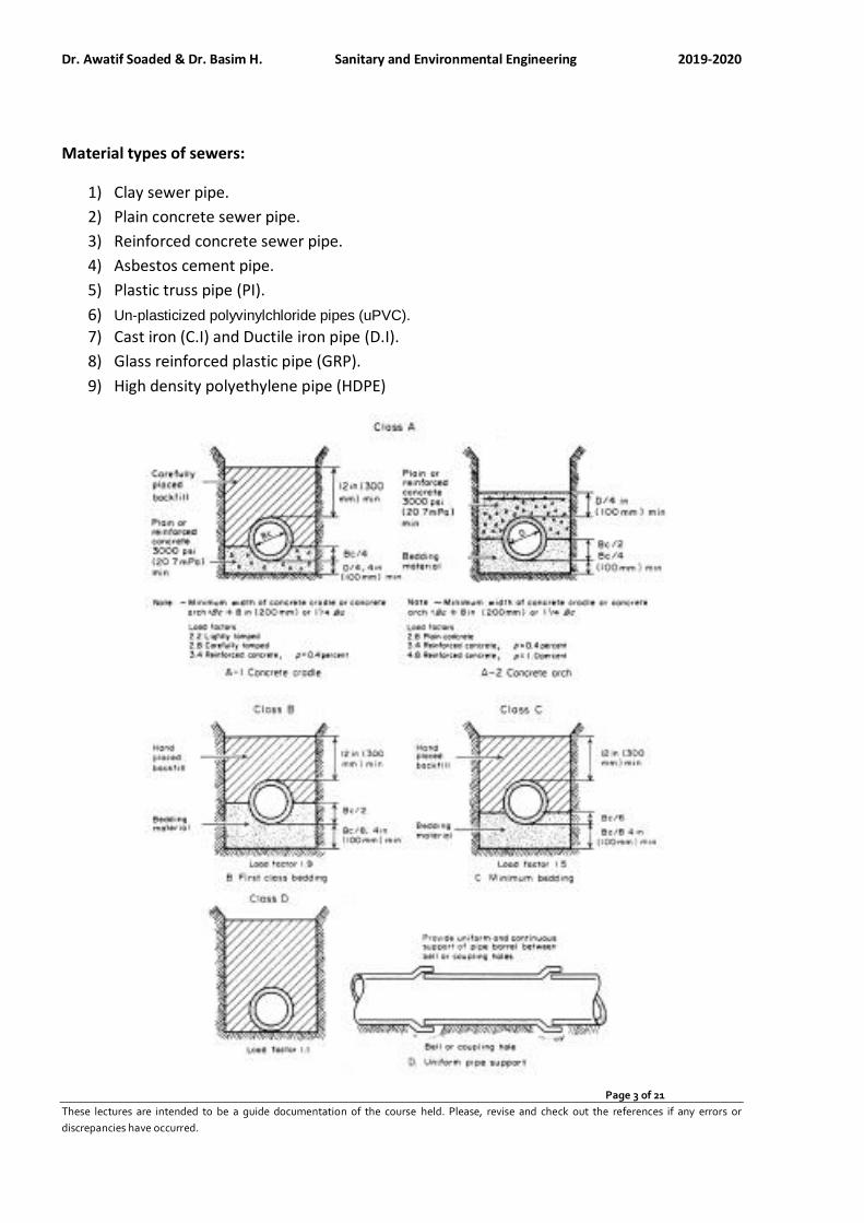
Dr. Awatif Soaded & Dr. Basim H. Sanitary and Environmental Engineering 2019-2020
Page 3 of 21
These lectures are intended to be a guide documentation of the course held. Please, revise and check out the references if any errors or
discrepancies have occurred.
Material types of sewers:
1) Clay sewer pipe.
2) Plain concrete sewer pipe.
3) Reinforced concrete sewer pipe.
4) Asbestos cement pipe.
5) Plastic truss pipe (PI).
6) Un-plasticized polyvinylchloride pipes (uPVC).
7) Cast iron (C.I) and Ductile iron pipe (D.I).
8) Glass reinforced plastic pipe (GRP).
9) High density polyethylene pipe (HDPE)

Dr. Awatif Soaded & Dr. Basim H. Sanitary and Environmental Engineering 2019-2020
Page 4 of 21
These lectures are intended to be a guide documentation of the course held. Please, revise and check out the references if any errors or
discrepancies have occurred.
Method of pipe bedding and load factors applicable to strength.

Dr. Awatif Soaded & Dr. Basim H. Sanitary and Environmental Engineering 2019-2020
Page 5 of 21
These lectures are intended to be a guide documentation of the course held. Please, revise and check out the references if any errors or discrepancies have occurred.
Bedding methods for concrete pipe.

Dr. Awatif Soaded & Dr. Basim H. Sanitary and Environmental Engineering 2019-2020
Page 6 of 21
These lectures are intended to be a guide documentation of the course held. Please, revise and check out the references if any errors or
discrepancies have occurred.
Corrosion in sewers:
Organic matter may accumulate in the sewer pipe as the result of low flowing velocity (d/D less than 0.3) or/and
the accumulation of grease and oil on the surface of the wastewater. The organic matter will undergo anaerobic
decomposition. This will form fatty acids (low pH) and the reduction of sulfates that will produce H2S. The
thiobacillus can oxidize H2S into sulfuric acid H2SO4 that will lead to the destruction of the crown.
How to control corrosion:
1) Control the flowing velocity where d/D should be more than 0.3. 2) Ventilation. 3) Flushing the sewer system from any depositions. 4) Chlorination. 5) Lining the crown with protective material.
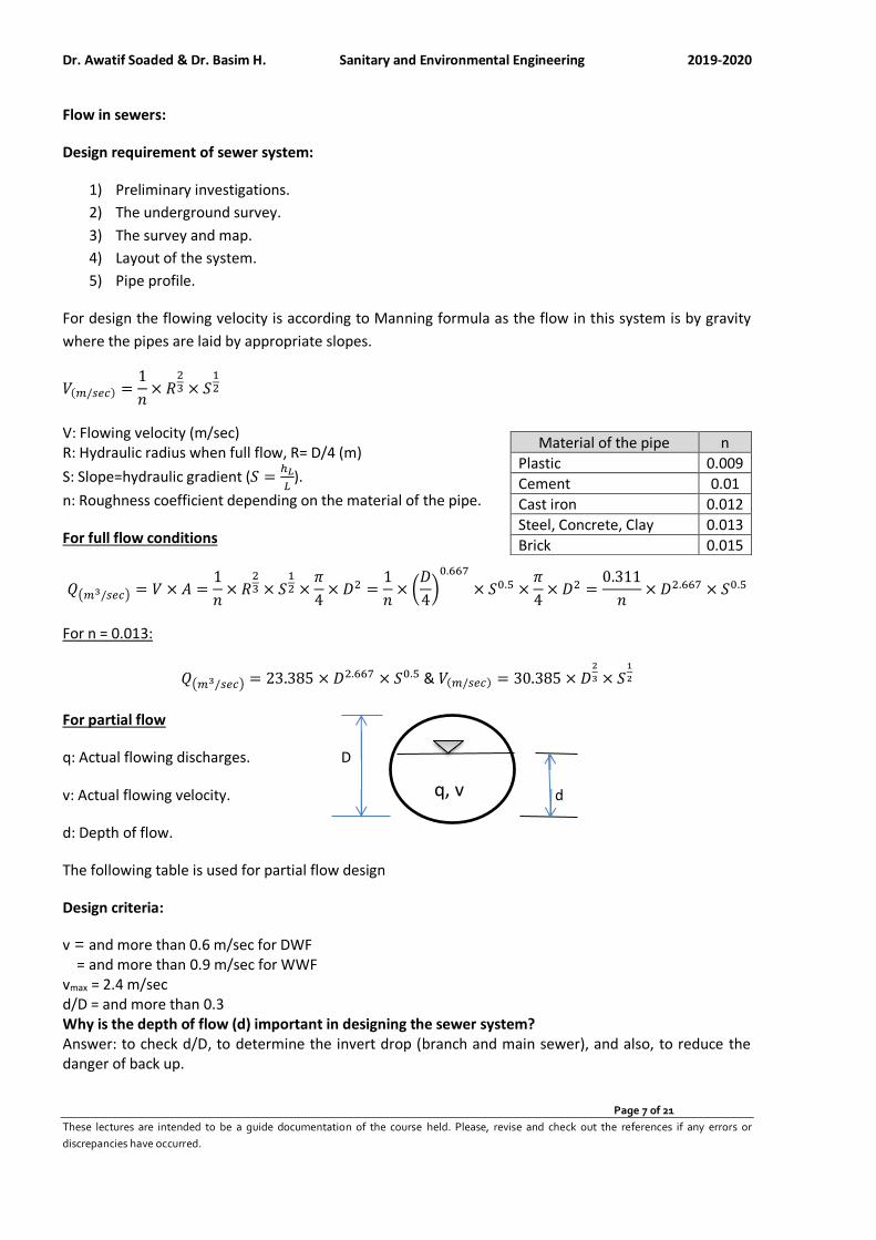
Dr. Awatif Soaded & Dr. Basim H. Sanitary and Environmental Engineering 2019-2020
Page 7 of 21
These lectures are intended to be a guide documentation of the course held. Please, revise and check out the references if any errors or
discrepancies have occurred.
Flow in sewers:
Design requirement of sewer system:
1) Preliminary investigations.
2) The underground survey.
3) The survey and map.
4) Layout of the system.
5) Pipe profile.
For design the flowing velocity is according to Manning formula as the flow in this system is by gravity
where the pipes are laid by appropriate slopes.
𝑉(𝑚/𝑠𝑒𝑐) =1
𝑛× 𝑅
23 × 𝑆
12
V: Flowing velocity (m/sec) R: Hydraulic radius when full flow, R= D/4 (m)
S: Slope=hydraulic gradient (𝑆 =ℎ𝐿
𝐿).
n: Roughness coefficient depending on the material of the pipe.
For full flow conditions
𝑄(𝑚3/𝑠𝑒𝑐) = 𝑉 × 𝐴 =1
𝑛× 𝑅
23 × 𝑆
12 ×
𝜋
4× 𝐷2 =
1
𝑛× (
𝐷
4)
0.667
× 𝑆0.5 ×𝜋
4× 𝐷2 =
0.311
𝑛× 𝐷2.667 × 𝑆0.5
For n = 0.013:
𝑄(𝑚3/𝑠𝑒𝑐) = 23.385 × 𝐷2.667 × 𝑆0.5 & 𝑉(𝑚/𝑠𝑒𝑐) = 30.385 × 𝐷2
3 × 𝑆1
2
For partial flow
q: Actual flowing discharges. D
v: Actual flowing velocity. d
d: Depth of flow.
The following table is used for partial flow design
Design criteria:
v = and more than 0.6 m/sec for DWF = and more than 0.9 m/sec for WWF vmax = 2.4 m/sec d/D = and more than 0.3 Why is the depth of flow (d) important in designing the sewer system? Answer: to check d/D, to determine the invert drop (branch and main sewer), and also, to reduce the danger of back up.
Material of the pipe n
Plastic 0.009
Cement 0.01
Cast iron 0.012
Steel, Concrete, Clay 0.013
Brick 0.015
q, v
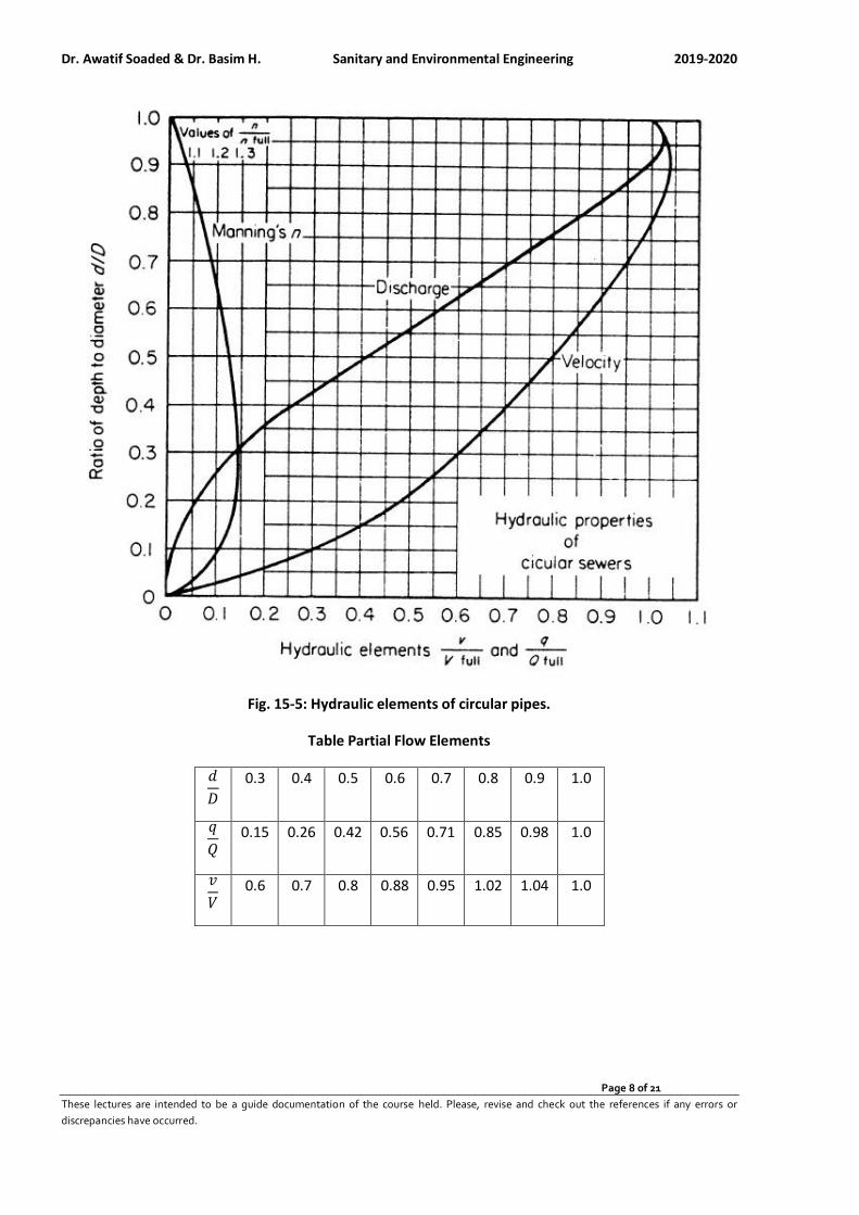
Dr. Awatif Soaded & Dr. Basim H. Sanitary and Environmental Engineering 2019-2020
Page 8 of 21
These lectures are intended to be a guide documentation of the course held. Please, revise and check out the references if any errors or
discrepancies have occurred.
Fig. 15-5: Hydraulic elements of circular pipes.
Table Partial Flow Elements
𝑑
𝐷
0.3 0.4 0.5 0.6 0.7 0.8 0.9 1.0
𝑞
𝑄 0.15 0.26 0.42 0.56 0.71 0.85 0.98 1.0
𝑣
𝑉 0.6 0.7 0.8 0.88 0.95 1.02 1.04 1.0

Dr. Awatif Soaded & Dr. Basim H. Sanitary and Environmental Engineering 2019-2020
Page 9 of 21
These lectures are intended to be a guide documentation of the course held. Please, revise and check out the references if any errors or
discrepancies have occurred.
Solved problems
Problem 1: Find the diameter of the sewer to carry 3.4 m3/min at a slope of 0.003 (assume full flow, n=0.013). Solution:
𝑄 = 𝑣 × 𝐴 =1
𝑛× 𝐴 × 𝑅
23 × 𝑆
12 =
1
0.013× (
𝜋
4× 𝐷2) × (
𝐷
4)
23
× (0.003)12
𝑄 =3.4
60
𝑚3
𝑠𝑒𝑐= 0.0567
𝑚3
𝑠𝑒𝑐= 1.3125 × 𝐷
83 ⟹ 𝐷 = 0.307𝑚 𝑠𝑜 𝑢𝑠𝑒 𝐷 = 300 𝑚𝑚
Problem 2: A sewer is to carry 25 m3/min wastewater at a slope of 0.003 (assume n=0.013) Find 1- Standard size (mm) 2- actual flowing velocity (m/sec) 3-depth of flow
Design diameter
100 150 200 250 300 400 450 500 600
Nominal diameter
110 160 210 255 305 400 450 500 630
Design diameter
700 800 900 1000 1100 1200 1400 1600 1800
Nominal diameter
710 800 900 1000 1100 1200 1400 1600 1800
Solution:
𝑄 = 25𝑚3
𝑚𝑖𝑛= 0.4167 𝑚3/𝑠𝑒𝑐
𝑄 = 𝑣 × 𝐴 =1
𝑛× 𝐴 × 𝑅
23 × 𝑆
12 =
1
0.013× (
𝜋
4× 𝐷2) × (
𝐷
4)
23
× (0.003)12
𝑄 = 0.4167𝑚3
𝑠𝑒𝑐= 1.3125 × 𝐷
83 ⟹ 𝐷 = 0.650 𝑚
Check the standard size = 700 mm: Full Flow:
𝑉 =1
𝑛× 𝑅
23 × 𝑆
12 =
1
0.013× (
0.7
4)
23
× (0.003)12 = 1.318 𝑚/𝑠𝑒𝑐
𝑄 = 𝑉 × 𝐴 = 1.318 ×𝜋
4× 0.72 = 0.507 𝑚3/𝑠𝑒𝑐
Partial Flow: for 25 m3/min in pipe diameter 700 mm.
𝑞
𝑂=
0.4167
0.507= 0.821
From hydraulic elements figure or table, find: 𝑑
𝐷= 0.77 > 0.3 ⟹ 𝑑 = 0.539 𝑚𝑚 &
𝑣
𝑉= 1.0 ⟹ 𝑣 = 1.318
𝑚
𝑠𝑒𝑐> 0.6 𝑚/ sec 𝑂. 𝐾
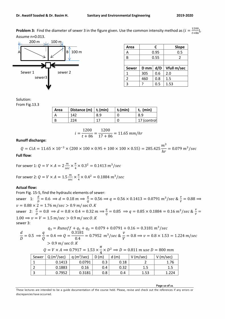
Dr. Awatif Soaded & Dr. Basim H. Sanitary and Environmental Engineering 2019-2020
Page 10 of 21
These lectures are intended to be a guide documentation of the course held. Please, revise and check out the references if any errors or
discrepancies have occurred.
Problem 3: Find the diameter of sewer 3 in the figure given. Use the common intensity method as (𝑖 =1200
𝑡+86),
Assume n=0.013. 200 m 100 m A B 100 m Sewer 1 sewer 2 sewer3
Solution: From Fig.13.3
Area Distance (m) ti (min) tf (min) tc (min)
A 142 8.9 0 8.9
B 224 17 0 17 (control)
𝑖 =1200
𝑡 + 86=
1200
17 + 86= 11.65 𝑚𝑚/ℎ𝑟
Runoff discharge:
𝑄 = 𝐶𝑖𝐴 = 11.65 × 10−3 × (200 × 100 × 0.95 + 100 × 100 × 0.55) = 285.425𝑚3
ℎ𝑟= 0.079 𝑚3/𝑠𝑒𝑐
Full flow:
For sewer 1: 𝑄 = 𝑉 × 𝐴 = 2𝑚
𝑠𝑒𝑐×
𝜋
4× 0.32 = 0.1413 𝑚3/𝑠𝑒𝑐
For sewer 2: 𝑄 = 𝑉 × 𝐴 = 1.5𝑚
𝑠𝑒𝑐×
𝜋
4× 0.42 = 0.1884 𝑚3/𝑠𝑒𝑐
Actual flow: From Fig. 15-5, find the hydraulic elements of sewer:
sewer 1: 𝑑
𝐷= 0.6 ⟹ 𝑑 = 0.18 𝑚 ⟹
𝑞
𝑄= 0.56 ⟹ 𝑞 = 0.56 × 0.1413 = 0.0791 𝑚3/𝑠𝑒𝑐 &
𝑣
𝑉= 0.88 ⟹
𝑣 = 0.88 × 2 = 1.76 𝑚/𝑠𝑒𝑐 > 0.9 𝑚/ sec 𝑂. 𝐾
sewer 2: 𝑑
𝐷= 0.8 ⟹ 𝑑 = 0.8 × 0.4 = 0.32 𝑚 ⟹
𝑞
𝑄= 0.85 ⟹ 𝑞 = 0.85 × 0.1884 = 0.16 𝑚3/𝑠𝑒𝑐 &
𝑣
𝑉=
1.00 ⟹ 𝑣 = 𝑉 = 1.5 𝑚/𝑠𝑒𝑐 > 0.9 𝑚/ sec 𝑂. 𝐾 sewer 3:
𝑞3 = 𝑅𝑢𝑛𝑜𝑓𝑓 + 𝑞1 + 𝑞2 = 0.079 + 0.0791 + 0.16 = 0.3181 𝑚3/𝑠𝑒𝑐 𝑑
𝐷= 0.5 ⟹
𝑞
𝑄= 0.4 ⟹ 𝑄 =
0.3181
0.4= 0.7952 𝑚3/𝑠𝑒𝑐 &
𝑣
𝑉= 0.8 ⟹ 𝑣 = 0.8 × 1.53 = 1.224 𝑚/𝑠𝑒𝑐
> 0.9 𝑚/ sec 𝑂. 𝐾
𝑄 = 𝑉 × 𝐴 ⟹ 0.7917 = 1.53 ×𝜋
4× 𝐷2 ⟹ 𝐷 = 0.811 𝑚 𝑢𝑠𝑒 𝐷 = 800 𝑚𝑚
Sewer Q (m3/sec) q (m3/sec) D (m) d (m) V (m/sec) V (m/sec)
1 0.1413 0.0791 0.3 0.18 2 1.76
2 0.1883 0.16 0.4 0.32 1.5 1.5
3 0.7952 0.3181 0.8 0.4 1.53 1.224
Area C Slope
A 0.95 0.5
B 0.55 2
Sewer D mm d/D Vfull m/sec
1 305 0.6 2.0
2 460 0.8 1.5
3 ? 0.5 1.53
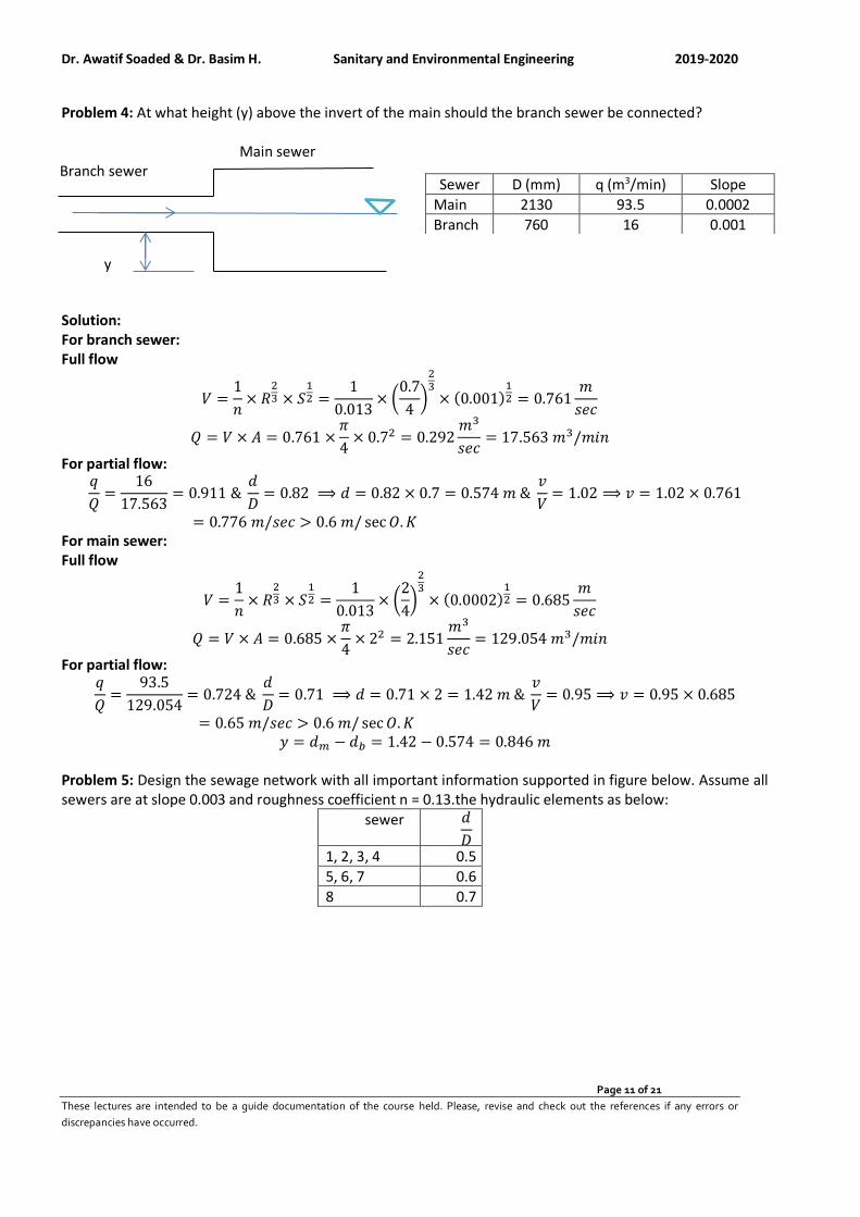
Dr. Awatif Soaded & Dr. Basim H. Sanitary and Environmental Engineering 2019-2020
Page 11 of 21
These lectures are intended to be a guide documentation of the course held. Please, revise and check out the references if any errors or
discrepancies have occurred.
Problem 4: At what height (y) above the invert of the main should the branch sewer be connected? Main sewer Branch sewer
y
Solution: For branch sewer: Full flow
𝑉 =1
𝑛× 𝑅
23 × 𝑆
12 =
1
0.013× (
0.7
4)
23
× (0.001)12 = 0.761
𝑚
𝑠𝑒𝑐
𝑄 = 𝑉 × 𝐴 = 0.761 ×𝜋
4× 0.72 = 0.292
𝑚3
𝑠𝑒𝑐= 17.563 𝑚3/𝑚𝑖𝑛
For partial flow: 𝑞
𝑄=
16
17.563= 0.911 &
𝑑
𝐷= 0.82 ⟹ 𝑑 = 0.82 × 0.7 = 0.574 𝑚 &
𝑣
𝑉= 1.02 ⟹ 𝑣 = 1.02 × 0.761
= 0.776 𝑚/𝑠𝑒𝑐 > 0.6 𝑚/ sec 𝑂. 𝐾 For main sewer: Full flow
𝑉 =1
𝑛× 𝑅
23 × 𝑆
12 =
1
0.013× (
2
4)
23
× (0.0002)12 = 0.685
𝑚
𝑠𝑒𝑐
𝑄 = 𝑉 × 𝐴 = 0.685 ×𝜋
4× 22 = 2.151
𝑚3
𝑠𝑒𝑐= 129.054 𝑚3/𝑚𝑖𝑛
For partial flow: 𝑞
𝑄=
93.5
129.054= 0.724 &
𝑑
𝐷= 0.71 ⟹ 𝑑 = 0.71 × 2 = 1.42 𝑚 &
𝑣
𝑉= 0.95 ⟹ 𝑣 = 0.95 × 0.685
= 0.65 𝑚/𝑠𝑒𝑐 > 0.6 𝑚/ sec 𝑂. 𝐾 𝑦 = 𝑑𝑚 − 𝑑𝑏 = 1.42 − 0.574 = 0.846 𝑚
Problem 5: Design the sewage network with all important information supported in figure below. Assume all sewers are at slope 0.003 and roughness coefficient n = 0.13.the hydraulic elements as below:
sewer 𝑑
𝐷
1, 2, 3, 4 0.5
5, 6, 7 0.6
8 0.7
Slope q (m3/min) D (mm) Sewer
0.0002 93.5 2130 Main
0.001 16 760 Branch
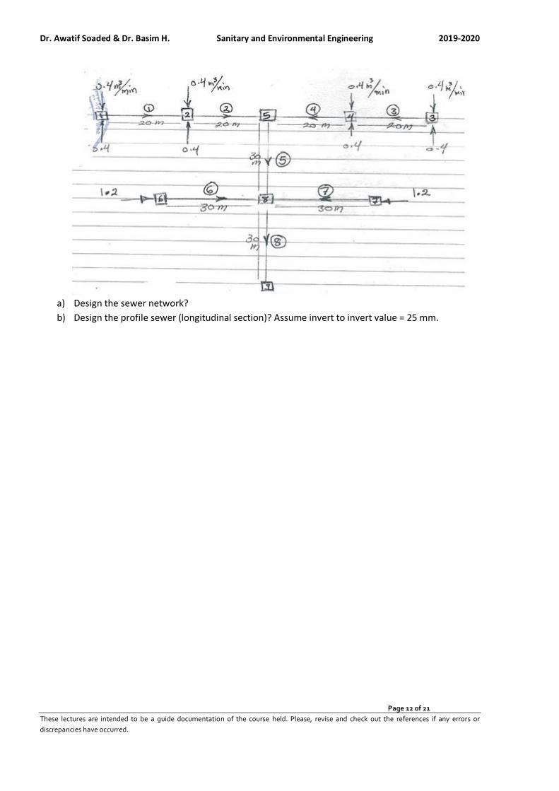
Dr. Awatif Soaded & Dr. Basim H. Sanitary and Environmental Engineering 2019-2020
Page 12 of 21
These lectures are intended to be a guide documentation of the course held. Please, revise and check out the references if any errors or
discrepancies have occurred.
a) Design the sewer network?
b) Design the profile sewer (longitudinal section)? Assume invert to invert value = 25 mm.
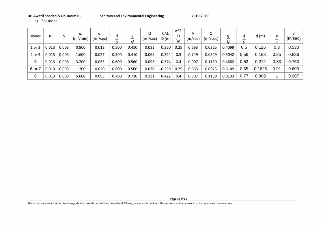
Dr. Awatif Soaded & Dr. Basim H. Sanitary and Environmental Engineering 2019-2020
Page 13 of 21
These lectures are intended to be a guide documentation of the course held. Please, revise and check out the references if any errors or discrepancies have occurred.
a) Solution:
sewer n S q,
(m3/min) q,
(m3/sec) 𝑑
𝐷
𝑞
𝑄
Q (m3/sec)
CAL. D (m)
ASS. D
(m)
V (m/sec)
Q (m3/sec)
𝑞
𝑄
𝑑
𝐷
d (m) 𝑣
𝑉
v (m/sec)
1 or 3 0.013 0.003 0.800 0.013 0.500 0.410 0.033 0.250 0.25 0.663 0.0325 0.4099 0.5 0.125 0.8 0.530
2 or 4 0.013 0.003 1.600 0.027 0.500 0.410 0.065 0.324 0.3 0.749 0.0529 0.5042 0.56 0.168 0.85 0.636
5 0.013 0.003 3.200 0.053 0.600 0.560 0.095 0.374 0.4 0.907 0.1139 0.4682 0.53 0.212 0.83 0.753
6 or 7 0.013 0.003 1.200 0.020 0.600 0.560 0.036 0.259 0.25 0.663 0.0325 0.6149 0.65 0.1625 0.91 0.603
8 0.013 0.003 5.600 0.093 0.700 0.710 0.131 0.422 0.4 0.907 0.1139 0.8193 0.77 0.308 1 0.907
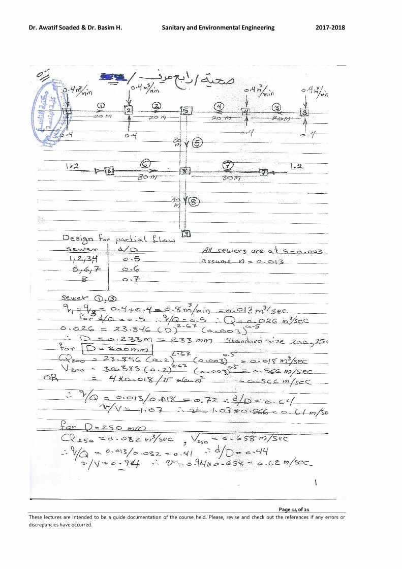
Dr. Awatif Soaded & Dr. Basim H. Sanitary and Environmental Engineering 2017-2018
Page 14 of 21
These lectures are intended to be a guide documentation of the course held. Please, revise and check out the references if any errors or
discrepancies have occurred.
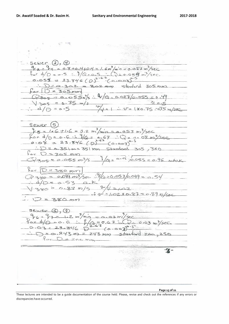
Dr. Awatif Soaded & Dr. Basim H. Sanitary and Environmental Engineering 2017-2018
Page 15 of 21
These lectures are intended to be a guide documentation of the course held. Please, revise and check out the references if any errors or
discrepancies have occurred.
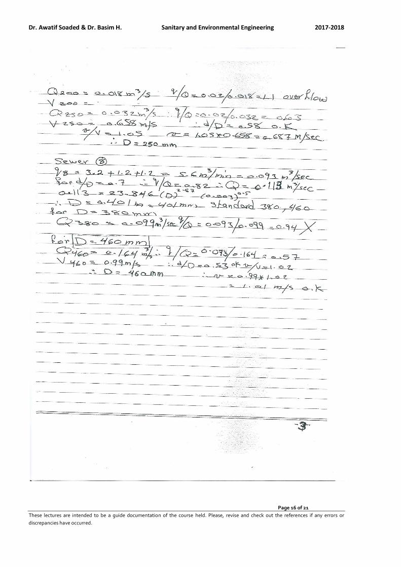
Dr. Awatif Soaded & Dr. Basim H. Sanitary and Environmental Engineering 2017-2018
Page 16 of 21
These lectures are intended to be a guide documentation of the course held. Please, revise and check out the references if any errors or
discrepancies have occurred.
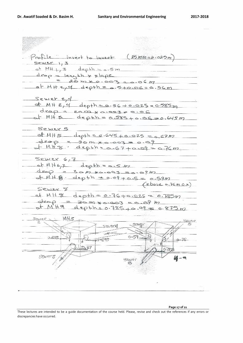
Dr. Awatif Soaded & Dr. Basim H. Sanitary and Environmental Engineering 2017-2018
Page 17 of 21
These lectures are intended to be a guide documentation of the course held. Please, revise and check out the references if any errors or
discrepancies have occurred.
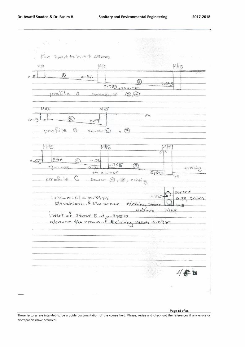
Dr. Awatif Soaded & Dr. Basim H. Sanitary and Environmental Engineering 2017-2018
Page 18 of 21
These lectures are intended to be a guide documentation of the course held. Please, revise and check out the references if any errors or
discrepancies have occurred.
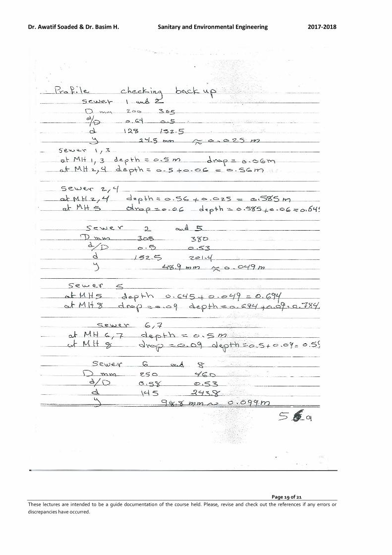
Dr. Awatif Soaded & Dr. Basim H. Sanitary and Environmental Engineering 2017-2018
Page 19 of 21
These lectures are intended to be a guide documentation of the course held. Please, revise and check out the references if any errors or
discrepancies have occurred.
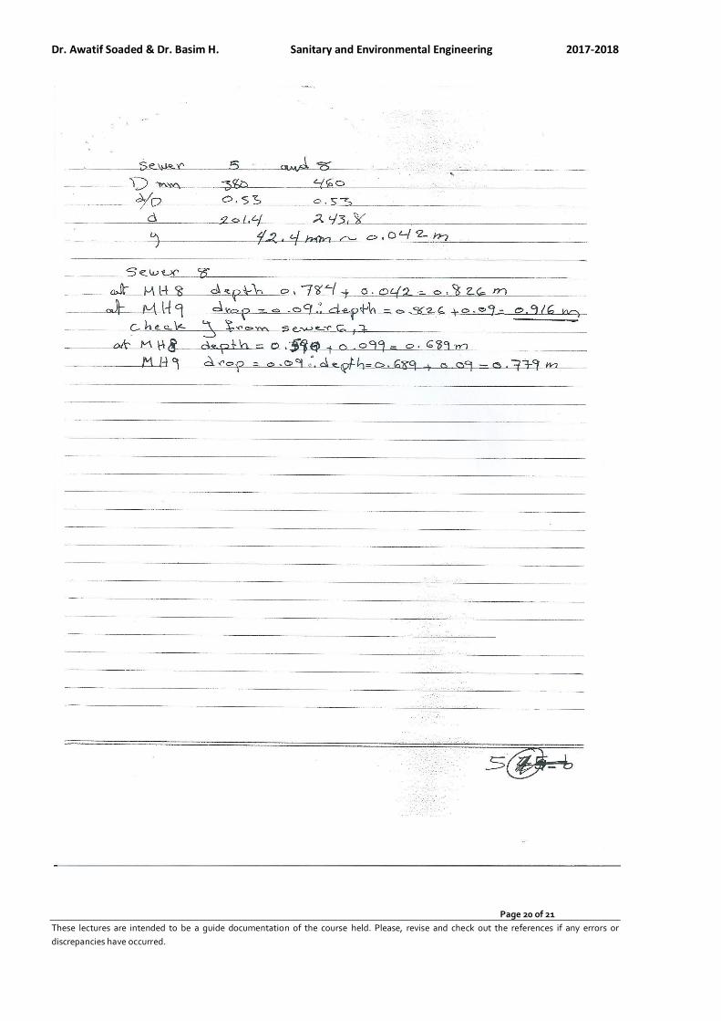
Dr. Awatif Soaded & Dr. Basim H. Sanitary and Environmental Engineering 2017-2018
Page 20 of 21
These lectures are intended to be a guide documentation of the course held. Please, revise and check out the references if any errors or
discrepancies have occurred.
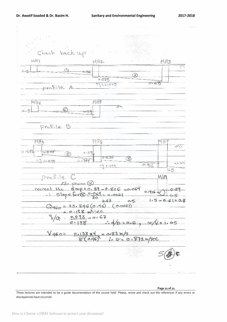
Dr. Awatif Soaded & Dr. Basim H. Sanitary and Environmental Engineering 2017-2018
Page 21 of 21
These lectures are intended to be a guide documentation of the course held. Please, revise and check out the references if any errors or
discrepancies have occurred.
How to Choose a DRM Software to protect your document?
Dr. Awatif Soaded & Dr. Basim H. Sanitary and Environmental Engineering 2019-2020
Page 1 of 9
These lectures are intended to be a guide documentation of the course held. Please, revise and check out the references if any errors or
discrepancies have occurred.
Sanitary and Environmental Engineering
PART 2: WASTEWATER ENGINEERING
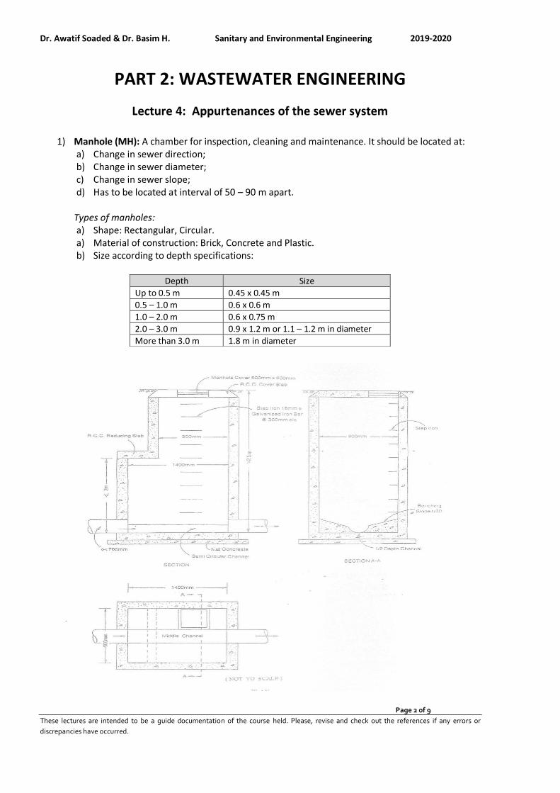
Dr. Awatif Soaded & Dr. Basim H. Sanitary and Environmental Engineering 2019-2020
Page 2 of 9
These lectures are intended to be a guide documentation of the course held. Please, revise and check out the references if any errors or
discrepancies have occurred.
PART 2: WASTEWATER ENGINEERING
Lecture 4: Appurtenances of the sewer system
1) Manhole (MH): A chamber for inspection, cleaning and maintenance. It should be located at: a) Change in sewer direction; b) Change in sewer diameter; c) Change in sewer slope; d) Has to be located at interval of 50 – 90 m apart.
Types of manholes: a) Shape: Rectangular, Circular. a) Material of construction: Brick, Concrete and Plastic. b) Size according to depth specifications:
Size Depth
0.45 x 0.45 m Up to 0.5 m
0.6 x 0.6 m 0.5 – 1.0 m
0.6 x 0.75 m 1.0 – 2.0 m
0.9 x 1.2 m or 1.1 – 1.2 m in diameter 2.0 – 3.0 m
1.8 m in diameter More than 3.0 m

Dr. Awatif Soaded & Dr. Basim H. Sanitary and Environmental Engineering 2019-2020
Page 3 of 9
These lectures are intended to be a guide documentation of the course held. Please, revise and check out the references if any errors or
discrepancies have occurred.
2) Street inlets: Openings on the street surface, through which runoff water (WWF) is admitted and
conveyed to a storm or combined sewer system. Common types: a-Curb, Vertical openings b-Gutter,
Horizontal openings.
3) Catch basin: Small settling chamber constructed below the street inlet, to allow grit, sand and large solids to settle from the flowing wastewater.
4) Oil, grease and sand trap: Tank or basin used to remove oil, grease, sand, mud…etc., from the sewage of industries, hotels, restaurants, kitchens and car garages. These materials are harmful and may cause clogging in the sewer system.
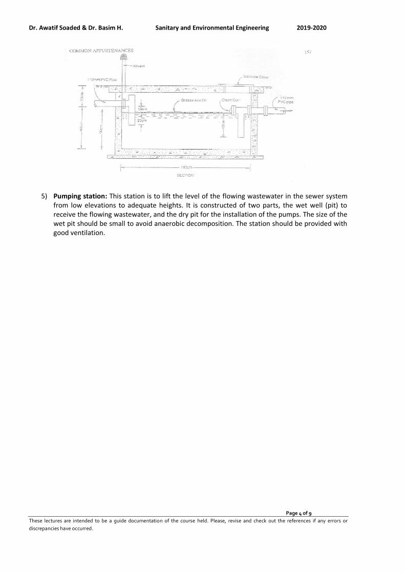
Dr. Awatif Soaded & Dr. Basim H. Sanitary and Environmental Engineering 2019-2020
Page 4 of 9
These lectures are intended to be a guide documentation of the course held. Please, revise and check out the references if any errors or
discrepancies have occurred.
5) Pumping station: This station is to lift the level of the flowing wastewater in the sewer system
from low elevations to adequate heights. It is constructed of two parts, the wet well (pit) to receive the flowing wastewater, and the dry pit for the installation of the pumps. The size of the wet pit should be small to avoid anaerobic decomposition. The station should be provided with good ventilation.
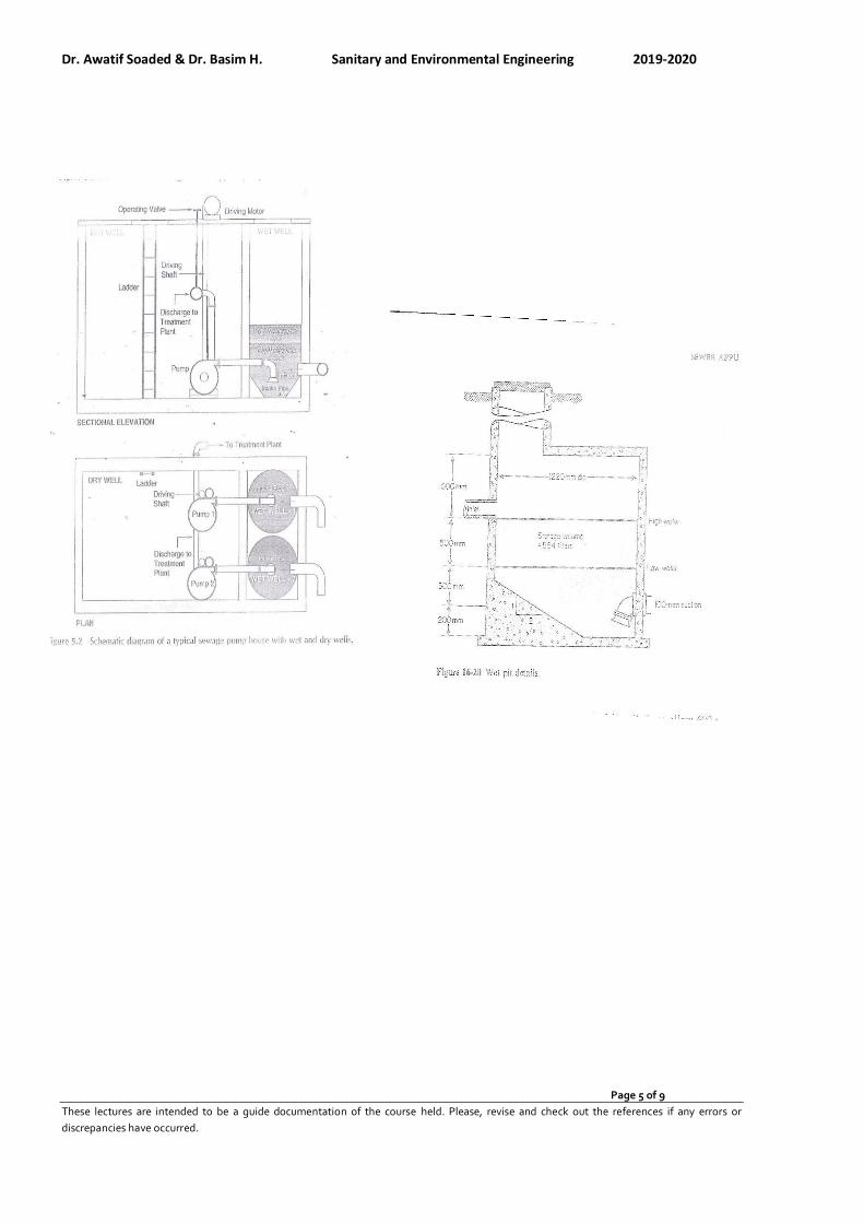
Dr. Awatif Soaded & Dr. Basim H. Sanitary and Environmental Engineering 2019-2020
Page 5 of 9
These lectures are intended to be a guide documentation of the course held. Please, revise and check out the references if any errors or
discrepancies have occurred.

Dr. Awatif Soaded & Dr. Basim H. Sanitary and Environmental Engineering 2019-2020
Page 6 of 9
These lectures are intended to be a guide documentation of the course held. Please, revise and check out the references if any errors or
discrepancies have occurred.
Sewage pumps station requirements: a) Self-cleansing velocities = 0.6 m/sec. b) In small pump stations the pump is sized to meet peak flow and lower flows accumulate in the
wet well until sufficient liquid is present to permit the pump to run for at least (running time, tr = 2min) for sewage flow and (tr = 4min) for storm flow.
c) In standard practice, the pump will not start than ones in (filling time, tf = 5min). Peak Flow
( )2460
/ FlowPeak
=
dayLwtewaterFloMaximumWasD
d) The pump running time: QD
Vtr −= , Where:
V: Storage Volume;
D: Pump Discharge;
Q: Influent Flow (Average Wastewater Flow).
e) The filling time, with the pump off: QV
t f =
f) The total cycle time: QV
QDV
ttt frc +−
=+=
g) Minimum sewage volume when (tr = 2min), DDtV r 2== and Minimum storm volume when
(tr = 4min), DDtV r 4==
h) The Volume When (tf = 5min) min5=+− Q
VQD
V, so take the volume covers the starting and
stopping elevation which is large = VActual.
i) The actual cycle time at average flow: Q
VQD
Vt actualactual+
−=
j) Assume D = (1.5-2) Q Total Depth = Pump Suction (200mm) + Submergence (300mm) + Free Board Level (600mm)
Wet pit details.
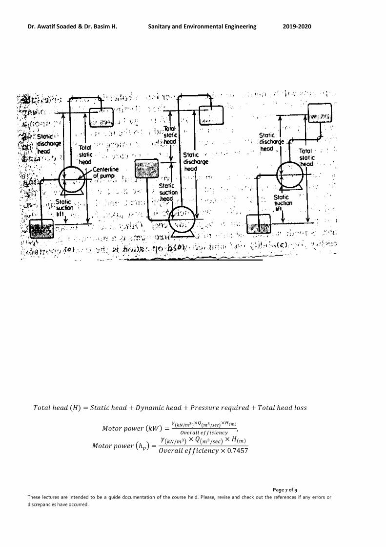
Dr. Awatif Soaded & Dr. Basim H. Sanitary and Environmental Engineering 2019-2020
Page 7 of 9
These lectures are intended to be a guide documentation of the course held. Please, revise and check out the references if any errors or
discrepancies have occurred.
𝑇𝑜𝑡𝑎𝑙 ℎ𝑒𝑎𝑑 (𝐻) = 𝑆𝑡𝑎𝑡𝑖𝑐 ℎ𝑒𝑎𝑑 + 𝐷𝑦𝑛𝑎𝑚𝑖𝑐 ℎ𝑒𝑎𝑑 + 𝑃𝑟𝑒𝑠𝑠𝑢𝑟𝑒 𝑟𝑒𝑞𝑢𝑖𝑟𝑒𝑑 + 𝑇𝑜𝑡𝑎𝑙 ℎ𝑒𝑎𝑑 𝑙𝑜𝑠𝑠
𝑀𝑜𝑡𝑜𝑟 𝑝𝑜𝑤𝑒𝑟 (𝑘𝑊) =𝛾
(𝑘𝑁/𝑚3)×𝑄
(𝑚3/𝑠𝑒𝑐)×𝐻(𝑚)
𝑂𝑣𝑒𝑟𝑎𝑙𝑙 𝑒𝑓𝑓𝑖𝑐𝑖𝑒𝑛𝑐𝑦,
𝑀𝑜𝑡𝑜𝑟 𝑝𝑜𝑤𝑒𝑟 (ℎ𝑝) =𝛾(𝑘𝑁/𝑚3) × 𝑄(𝑚3/𝑠𝑒𝑐) × 𝐻(𝑚)
𝑂𝑣𝑒𝑟𝑎𝑙𝑙 𝑒𝑓𝑓𝑖𝑐𝑖𝑒𝑛𝑐𝑦 × 0.7457

Dr. Awatif Soaded & Dr. Basim H. Sanitary and Environmental Engineering 2017-2018
Page 8 of 9
These lectures are intended to be a guide documentation of the course held. Please, revise and check out the references if any errors or
discrepancies have occurred.
Solved problems Problem 1: Find the volume of the wet well in a pumping station. Assume the pump stops 10 times/hr. Solution:
𝑇𝑜𝑡𝑎𝑙 𝑐𝑦𝑐𝑙𝑒 𝑡𝑖𝑚𝑒 = 𝑅𝑢𝑛𝑛𝑖𝑛𝑔 𝑡𝑖𝑚𝑒 + 𝐹𝑖𝑙𝑙𝑖𝑛𝑔 𝑡𝑖𝑚𝑒 =𝑉
𝐷 − 𝑄+
𝑉
𝑄
Assume D = 2Q, so, 𝑇𝑜𝑡𝑎𝑙 𝑐𝑦𝑐𝑙𝑒 𝑡𝑖𝑚𝑒 =60 𝑚𝑖𝑛
10 𝑡𝑖𝑚𝑒𝑠/ℎ𝑟= 6 𝑚𝑖𝑛
𝑇𝑜𝑡𝑎𝑙 𝑐𝑦𝑐𝑙𝑒 𝑡𝑖𝑚𝑒 = 6 =𝑉
2𝑄 − 𝑄+
𝑉
𝑄=
2𝑉
𝑄⟹ 𝑉 =
6𝑄
2= 3𝑄
Problem 2: A small subdivision produces an average wastewater flow of 120,000 L/day, the minimum
hourly flow is estimated to be 15,000 L/day, and the maximum, 420,000 L/day. Determine the design
pumping rate and wet well capacity? Also calculate the pump pipe diameter? Assume the average sewage
velocity limitation (1-3) m/sec, use average sewage velocity 1.5 m/sec.
Solution:
The minimum pump delivers: 𝐷𝑚𝑖𝑛 =15000
1440= 10.416 𝐿/𝑚𝑖𝑛
The maximum pump delivers: 𝐷𝑚𝑎𝑥 =420000
1440= 292 𝐿/𝑚𝑖𝑛
The average flow: 𝑄 =120000
1440= 83.333 𝐿/𝑚𝑖𝑛
The pump running time, 𝑡𝑟 =𝑉
𝐷−𝑄, the filling time, 𝑡𝑓 =
𝑉
𝑄, and 𝑡𝑐 =
𝑉
𝐷−𝑄+
𝑉
𝑄
To assure 2 min running time, the minimum volume: 𝑉 = 𝑡𝑟 × 𝐷 = 2𝑚𝑖𝑛 × 292𝐿
𝑚𝑖𝑛= 548 𝐿
To assure a 5 min cycle, at average flow:
𝑡𝑐 =𝑉
𝐷−𝑄+
𝑉
𝑄⟹ 5 =
𝑉
292−83.33+
𝑉
83.333=
𝑉
208.667+
𝑉
83.333=
292𝑉
17388.847⟹ 𝑉 = 297.754 𝐿 ≈ 298 𝐿
Therefore, the running time governs, the volume between starting and stopping elevations will be about
600 L (approximate volume).
The actual cycle time at average flow:
𝑡𝑐 = 𝑡𝑟 + 𝑡𝑓 =600
292 − 83.333+
600
83.333= 2.875 + 7.2 = 10.075 𝑚𝑖𝑛
The minimum depth of water below the suction pipe of about 200 mm.
At an intake velocity 0.6 m/sec a submergence of about 300 mm.
Freeboard about anticipated maximum water level = 600 mm
Total minimum depth of the pump station: mmmmmmmmmm 1600600500300200 =+++=
𝑄 = 𝑣 × 𝐴 ⟹420
24 × 3600= 1.5 ×
𝜋
4× 𝐷𝑃𝑈𝑀𝑃
2 ⟹ 𝐷 = 0.064 𝑚
Dr. Awatif Soaded & Dr. Basim H. Sanitary and Environmental Engineering 2017-2018
Page 9 of 9
These lectures are intended to be a guide documentation of the course held. Please, revise and check out the references if any errors or
discrepancies have occurred.
If use, 𝐷 = 50 𝑚𝑚 𝑤𝑖𝑡ℎ 𝑎𝑣𝑒𝑟𝑎𝑔𝑒 𝑣𝑒𝑙𝑜𝑐𝑖𝑡𝑦 = 2.47 𝑚/ sec 𝑂. 𝐾
So, use, 𝐷 = 65 𝑚𝑚 𝑤𝑖𝑡ℎ 𝑎𝑣𝑒𝑟𝑎𝑔𝑒 𝑣𝑒𝑙𝑜𝑐𝑖𝑡𝑦 = 1.46 𝑚/ sec 𝑂. 𝐾
Problem 3: Determine the total head and the power of the sewage pump according to the information
(Sewage flow =100 m3/hr, static head =15.4 m, total head losses = 7 m, pressure required at the end of
the pipe =15 m, dynamic head = 10 m, and overall efficiency of the pump = 64%)? Also calculate the pump
pipe diameter? Assume the average sewage velocity limitation (1-3) m/sec, use average sewage velocity
2 m/sec.
Solution:
𝑄 =100 𝑚3/ℎ𝑟
3600= 0.0278 𝑚3/𝑠𝑒𝑐
𝑇𝑜𝑡𝑎𝑙 ℎ𝑒𝑎𝑑 (𝐻) = 15.4 + 10 + 15 + 7 = 47.4 𝑚
𝑀𝑜𝑡𝑜𝑟 𝑝𝑜𝑤𝑒𝑟 =9.81
𝑘𝑁
𝑚3×0.0278𝑚3
𝑠𝑒𝑐×47.4𝑚
0.64= 20.198 𝑘𝑊 ≈ 27 ℎ𝑝,
𝑄 = 𝑣 × 𝐴 ⟹100
3600= 2 ×
𝜋
4× 𝐷𝑃𝑈𝑀𝑃
2 ⟹ 𝐷 = 0.133 𝑚
So, 𝐷 = 150 𝑚𝑚 𝑤𝑖𝑡ℎ 𝑎𝑣𝑒𝑟𝑎𝑔𝑒 𝑣𝑒𝑙𝑜𝑐𝑖𝑡𝑦 = 1.57 𝑚/ sec 𝑂. 𝐾
How to Choose a DRM Software to protect your document?

Dr. Awatif Soaded & Dr. Basim H. Sanitary and Environmental Engineering 2019-2020
Page 1 of 10
These lectures are intended to be a guide documentation of the course held. Please, revise and check out the references if any errors or
discrepancies have occurred.
Sanitary and Environmental Engineering
PART 2: WASTEWATER ENGINEERING
Dr. Awatif Soaded & Dr. Basim H. Sanitary and Environmental Engineering 2019-2020
Page 2 of 10
These lectures are intended to be a guide documentation of the course held. Please, revise and check out the references if any errors or
discrepancies have occurred.
PART 2: WASTEWATER ENGINEERING
Lecture 5: Sewage Disposal
Sewage disposal to water bodies such as rivers will be described by Streeter-Phelps equation.
This equation calculates the amount of the oxygen deficit in the river due to the degradation of
the organic matter that is dumped into it. This equation describes a process known as the self-
purification process, where the river can deal with certain amounts (concentrations) of organic
matter that are aerobically decomposed and not cause pollution. This equation can give the
following information:
1) The critical oxygen deficit (minimum concentration of the dissolved oxygen) in the river.
2) The allowable amount (concentration) of organic matter to be dumped into the river.
3) The location downstream for other waste disposal sites.
4) Drawing the variation of the dissolved oxygen with time or distance after the disposal of
the sewage into the river. This curve is known as the oxygen sag curve.
Application of formulas:
The Streeter-Phelps equation may be used to predict:
1) The effect of a particular waste load upon a receiving stream;
2) Determine the waste load which can be discharged without reducing the dissolved oxygen
below some prescribed level.
Effect of stream discharge:
1) Organic matter which enters the stream is broken down by bacteria to ammonia, nitrates,
sulfates, carbon dioxide, etc., which are utilized by plants and algae to produce
carbohydrates and oxygen.
2) Excessive quantities of waste materials can upset the cycle by causing rapid bacterial
growth and resulting depletion of dissolved oxygen in the stream.
3) Self-purification process defines as the stabilization of the excess organic matter through
the normal cycle will be re-established.
4) Water quality standards are often based upon maintenance of some minimum dissolved
oxygen concentration which will protect the natural cycle in the stream while taking
advantage of its natural assimilative capacity.
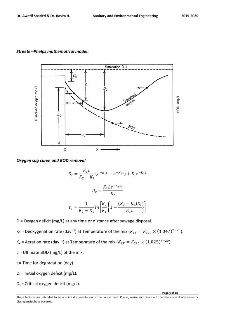
Dr. Awatif Soaded & Dr. Basim H. Sanitary and Environmental Engineering 2019-2020
Page 3 of 10
These lectures are intended to be a guide documentation of the course held. Please, revise and check out the references if any errors or
discrepancies have occurred.
Streeter-Phelps mathematical model:
Oxygen sag curve and BOD removal
𝐷𝑡 =𝐾1𝐿
𝐾2 − 𝐾1
(𝑒−𝐾1𝑡 − 𝑒−𝐾2𝑡) + 𝐷𝑖𝑒−𝐾2𝑡
𝐷𝑐 =𝐾1𝐿𝑒−𝐾1𝑡𝑐
𝐾2
𝑡𝑐 =1
𝐾2 − 𝐾1𝑙𝑛 [
𝐾2
𝐾1{1 −
(𝐾2 − 𝐾1)𝐷𝑖
𝐾1𝐿}]
D = Oxygen deficit (mg/L) at any time or distance after sewage disposal.
K1 = Deoxygenation rate (day -1) at Temperature of the mix (𝐾1𝑇 = 𝐾120 × (1.047)𝑇−20).
K2 = Aeration rate (day -1) at Temperature of the mix (𝐾2𝑇 = 𝐾220 × (1.025)𝑇−20).
L = Ultimate BOD (mg/L) of the mix.
t = Time for degradation (day).
Di = Initial oxygen deficit (mg/L).
Dc = Critical oxygen deficit (mg/L).
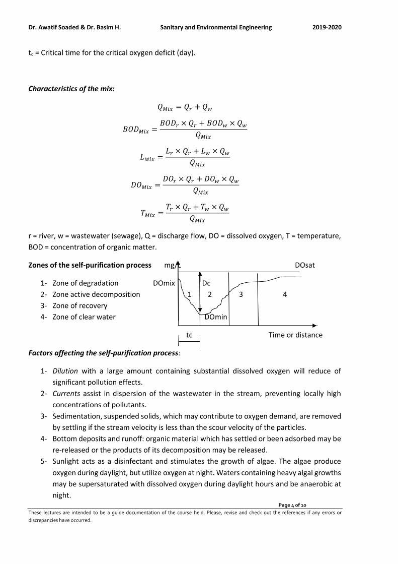
Dr. Awatif Soaded & Dr. Basim H. Sanitary and Environmental Engineering 2019-2020
Page 4 of 10
These lectures are intended to be a guide documentation of the course held. Please, revise and check out the references if any errors or
discrepancies have occurred.
tc = Critical time for the critical oxygen deficit (day).
Characteristics of the mix:
𝑄𝑀𝑖𝑥 = 𝑄𝑟 + 𝑄𝑤
𝐵𝑂𝐷𝑀𝑖𝑥 =𝐵𝑂𝐷𝑟 × 𝑄𝑟 + 𝐵𝑂𝐷𝑤 × 𝑄𝑤
𝑄𝑀𝑖𝑥
𝐿𝑀𝑖𝑥 =𝐿𝑟 × 𝑄𝑟 + 𝐿𝑤 × 𝑄𝑤
𝑄𝑀𝑖𝑥
𝐷𝑂𝑀𝑖𝑥 =𝐷𝑂𝑟 × 𝑄𝑟 + 𝐷𝑂𝑤 × 𝑄𝑤
𝑄𝑀𝑖𝑥
𝑇𝑀𝑖𝑥 =𝑇𝑟 × 𝑄𝑟 + 𝑇𝑤 × 𝑄𝑤
𝑄𝑀𝑖𝑥
r = river, w = wastewater (sewage), Q = discharge flow, DO = dissolved oxygen, T = temperature,
BOD = concentration of organic matter.
Zones of the self-purification process mg/L DOsat
1- Zone of degradation DOmix Dc
2- Zone active decomposition 1 2 3 4
3- Zone of recovery
4- Zone of clear water DOmin
tc Time or distance
Factors affecting the self-purification process:
1- Dilution with a large amount containing substantial dissolved oxygen will reduce of
significant pollution effects.
2- Currents assist in dispersion of the wastewater in the stream, preventing locally high
concentrations of pollutants.
3- Sedimentation, suspended solids, which may contribute to oxygen demand, are removed
by settling if the stream velocity is less than the scour velocity of the particles.
4- Bottom deposits and runoff: organic material which has settled or been adsorbed may be
re-released or the products of its decomposition may be released.
5- Sunlight acts as a disinfectant and stimulates the growth of algae. The algae produce
oxygen during daylight, but utilize oxygen at night. Waters containing heavy algal growths
may be supersaturated with dissolved oxygen during daylight hours and be anaerobic at
night.

Dr. Awatif Soaded & Dr. Basim H. Sanitary and Environmental Engineering 2019-2020
Page 5 of 10
These lectures are intended to be a guide documentation of the course held. Please, revise and check out the references if any errors or
discrepancies have occurred.
6- Temperature affects the solubility of oxygen in water, the rate of bacterial action, and the
rate of re-aeration. The critical condition is generally in warm weather when utilization
rates are high and availability.
The effect of K1 and K2 on the self- purification process
1) Increasing K1 will increase Dc and displace Dc upstream. Decreasing K1 will decrease Dc
and displace Dc downstream.
2) Increasing K2 will decrease Dc and displace Dc upstream. Decreasing K2 will increase Dc
and displace Dc downstream.

Dr. Awatif Soaded & Dr. Basim H. Sanitary and Environmental Engineering 2019-2020
Page 6 of 10
These lectures are intended to be a guide documentation of the course held. Please, revise and check out the references if any errors or
discrepancies have occurred.
General requirements:
1. The BOD at distance x: )1()(
31
)(
0)(
3131 ux
KKau
xKK
X eKK
LeLL
+−+−−
++= ,
Where: LO = the BOD in the stream at x = 0
2.
( ) ( )( )
( )
.12
2312
312
1
2310
312
1
−
+
++
−
+
−+−
+=
−
−+−−
ux
K
aRux
Kux
KKux
K
OX
e
KKKLK
KS
eeKK
LaL
KKKK
eDD
Where: DO = the deficit in the stream at x = 0
3. The critical deficit:
( )( )
( )
−−
+−++−
+++−
=1
2
3131
312
31
2
312
lnK
SDKKK
LLLKK
KKKKK
KKKK
uX Roa
aoc
K1: Deoxygenation Constant
K2: Reaeration constant =2
1
3
HUDM sec/10037.2 cmD s
M−= at 200C
( ) 20)20(2)(2 025.1 −= T
cT KK
4. If BOD decreases along a reach and BODX is less than predicted by:
ux
K
ox eLL1−
= , So La = 0, ( )
ux
KK
Ox eLL31+−
=
5. If BOD increases with (x) or decreases less than predicted by:
ux
K
ox eLL1−
= So K3 =0
−+=
−−ux
kau
xK
Ox eKL
eLL11
11
6. In absence of values (K3, La, SR) may be reduced to Classic Streeter- Phelps Formulation:
( )
−
−+=
−−−ux
Kux
K
oux
K
ox eeLKK
KeDD
212
12
1
( )
−−
−= o
oc D
LKKK
KK
kKu
x1
12
1
2
12
1ln , ux
t =
( ) ( )tKtKo
tKot eeLeDD 212)(
−−− −+=
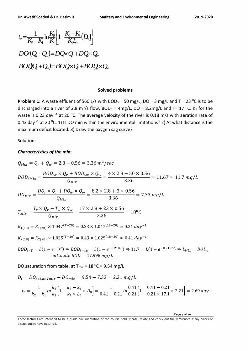
Dr. Awatif Soaded & Dr. Basim H. Sanitary and Environmental Engineering 2019-2020
Page 7 of 10
These lectures are intended to be a guide documentation of the course held. Please, revise and check out the references if any errors or
discrepancies have occurred.
( )
−−
−= o
oc D
LKKK
KK
KKt
1
12
1
2
12
1ln1
( ) wwssws QDOQDOQQDO +=+
( ) wwssws QBODQBODQQBOD +=+ 555
Solved problems
Problem 1: A waste effluent of 560 L/s with BOD5 = 50 mg/L, DO = 3 mg/L and T = 23 0C is to be
discharged into a river of 2.8 m3/s flow, BOD5 = 4mg/L, DO = 8.2mg/L and T= 17 0C. K1 for the
waste is 0.23 day -1 at 20 0C. The average velocity of the river is 0.18 m/s with aeration rate of
0.43 day -1 at 20 0C. 1) Is DO min within the environmental limitations? 2) At what distance is the
maximum deficit located. 3) Draw the oxygen sag curve?
Solution:
Characteristics of the mix:
𝑄𝑀𝑖𝑥 = 𝑄𝑟 + 𝑄𝑤 = 2.8 + 0.56 = 3.36 𝑚3/𝑠𝑒𝑐
𝐵𝑂𝐷5𝑀𝑖𝑥 =𝐵𝑂𝐷5𝑟 × 𝑄𝑟 + 𝐵𝑂𝐷5𝑤 × 𝑄𝑤
𝑄𝑀𝑖𝑥=
4 × 2.8 + 50 × 0.56
3.36= 11.67 ≈ 11.7 𝑚𝑔/𝐿
𝐷𝑂𝑀𝑖𝑥 =𝐷𝑂𝑟 × 𝑄𝑟 + 𝐷𝑂𝑤 × 𝑄𝑤
𝑄𝑀𝑖𝑥=
8.2 × 2.8 + 3 × 0.56
3.36= 7.33 𝑚𝑔/𝐿
𝑇𝑀𝑖𝑥 =𝑇𝑟 × 𝑄𝑟 + 𝑇𝑤 × 𝑄𝑤
𝑄𝑀𝑖𝑥=
17 × 2.8 + 23 × 0.56
3.36= 180𝐶
𝐾1(18) = 𝐾1(20) × 1.047(𝑇−20) = 0.23 × 1.047(18−20) ≈ 0.21 𝑑𝑎𝑦−1
𝐾2(18) = 𝐾2(20) × 1.025(𝑇−20) = 0.43 × 1.025(18−20) ≈ 0.41 𝑑𝑎𝑦−1
𝐵𝑂𝐷𝑡−𝑇 = 𝐿(1 − 𝑒−𝐾1𝑡) ⇛ 𝐵𝑂𝐷5−18 = 𝐿(1 − 𝑒−0.21×5) ⇛ 11.7 = 𝐿(1 − 𝑒−0.21×5) ⇛ 𝐿𝑀𝑖𝑥 = 𝐵𝑂𝐷𝑢
= 𝑢𝑙𝑡𝑖𝑚𝑎𝑡𝑒 𝐵𝑂𝐷 = 17.998 𝑚𝑔/𝐿
DO saturation from table, at Tmix = 18 0C = 9.54 mg/L
𝐷𝑖 = 𝐷𝑂𝑆𝑎𝑡.𝑎𝑡 𝑇𝑚𝑖𝑥 − 𝐷𝑂𝑚𝑖𝑥 = 9.54 − 7.33 = 2.21 𝑚𝑔/𝐿
𝑡𝑐 =1
𝑘2 − 𝑘1𝑙𝑛
𝑘2
𝑘1[1 −
𝑘2 − 𝑘1
𝑘1 × 𝐿0× 𝐷0] =
1
0.41 − 0.21𝑙𝑛
0.41
0.21[1 −
0.41 − 0.21
0.21 × 17.1× 2.21] = 2.69 𝑑𝑎𝑦

Dr. Awatif Soaded & Dr. Basim H. Sanitary and Environmental Engineering 2019-2020
Page 8 of 10
These lectures are intended to be a guide documentation of the course held. Please, revise and check out the references if any errors or
discrepancies have occurred.
𝐷𝑐 =𝐾1𝐿𝑒−𝐾1𝑡𝑐
𝐾2=
0.21 × 17.1 × 𝑒−0.21×2.69
0.41= 4.96 𝑚𝑔/𝐿
𝐷𝑚𝑖𝑛 = 𝐷𝑂𝑆𝑎𝑡.𝑎𝑡 𝑇𝑚𝑖𝑥 − 𝐷𝑐 = 9.54 − 4.98 = 4.58𝑚𝑔
𝐿> 4
𝑚𝑔
𝐿 𝑂. 𝐾
𝐷𝑖𝑠𝑡𝑎𝑛𝑐𝑒 = 𝑉𝑒𝑙𝑜𝑐𝑖𝑡𝑦 × 𝑡𝑖𝑚𝑒 = 0.18 𝑚/ sec×2.95 × 24 × 3600
1000= 45.878 𝑘𝑚
Problem 2: A city discharges 1.25 m3/sec of wastewater onto a stream whose minimum rate of flow is 8
m3/sec. The velocity of stream is 0.8 m/sec. The temperature of the wastewater is 20 0C and that of the
stream is 15 0C. The BOD5 of the wastewater is 183 mg/L, and that of the stream is 2 mg/L. The wastewater
contains no dissolved oxygen but the stream is 90 percent saturated upstream of the discharge. At 20 0C,
deoxygenation coefficient (K1 ) is estimated to be 0.3 per day and reaeration coefficient (K2 ) is 0.9 per
day. Determine the critical-oxygen deficit and its location. Also, estimate the 20 0C BOD5 of the sample
taken at the critical point. Use temperature coefficient of 1.135 for deoxygenation coefficient (K1 ) and
1.024 for reaeration coefficient (K2 ). Also, plot the dissolved-oxygen sag curve? Given the saturation
concentration at 15 0C and at mixed temperature = 10.15 mg/L
Solution:
1. Characteristics of the mix:
𝑄𝑀𝑖𝑥 = 𝑄𝑟 + 𝑄𝑤 = 8 + 1.25 = 9.25 𝑚3/𝑠𝑒𝑐
DO of the stream, 𝐷𝑂𝑟 = 0.9 × 10.15 = 9.14 𝑚𝑔/𝐿
𝐷𝑂𝑀𝑖𝑥 =𝐷𝑂𝑟 × 𝑄𝑟 + 𝐷𝑂𝑤 × 𝑄𝑤
𝑄𝑀𝑖𝑥=
9.14 × 8 + 0 × 1.25
9.25= 7.9 𝑚𝑔/𝐿
𝑇𝑀𝑖𝑥 =𝑇𝑟 × 𝑄𝑟 + 𝑇𝑤 × 𝑄𝑤
𝑄𝑀𝑖𝑥=
15 × 8 + 20 × 1.25
9.25= 15.6750𝐶
𝐾1(15.675) = 0.3 × 1.135(15.675−20) ≈ 0.173 𝑑𝑎𝑦−1
𝐾2(15.675) = 0.9 × 1.024(15.675−20) ≈ 0.812 𝑑𝑎𝑦−1
𝐵𝑂𝐷5𝑀𝑖𝑥 =𝐵𝑂𝐷5𝑟 × 𝑄𝑟 + 𝐵𝑂𝐷5𝑤 × 𝑄𝑤
𝑄𝑀𝑖𝑥=
2 × 8 + 183 × 1.25
9.25= 26.46 𝑚𝑔/𝐿
𝐵𝑂𝐷𝑡−𝑇 = 𝐿(1 − 𝑒−𝐾1𝑡) ⇛ 𝐵𝑂𝐷5−15.675 = 𝐿(1 − 𝑒−0.173×5) ⇛ 26.46 = 𝐿(1 − 𝑒−0.173×5) ⇛ 𝐿𝑀𝑖𝑥
= 𝐵𝑂𝐷𝑢 = 𝑢𝑙𝑡𝑖𝑚𝑎𝑡𝑒 𝐵𝑂𝐷 = 45.702 𝑚𝑔
𝐿= 𝐿𝑀𝑖𝑥
2. Initial dissolved oxygen deficit at mixed temperature (TMix = 15.675 0C)
From table, DO saturation concentration at 15.675 0C = 10.15 mg/L
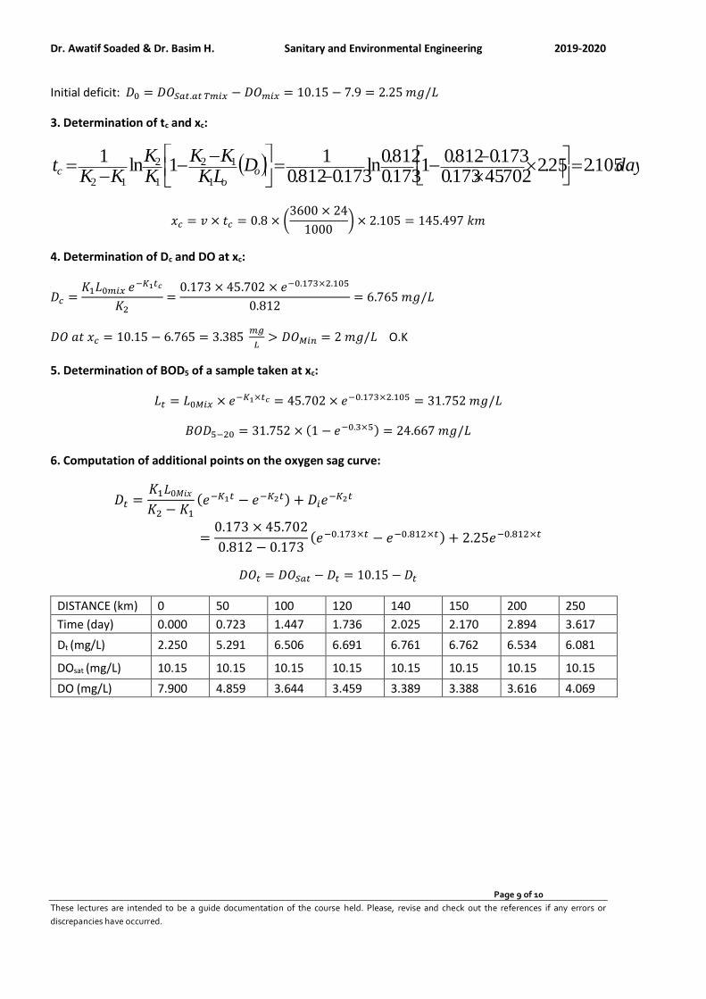
Dr. Awatif Soaded & Dr. Basim H. Sanitary and Environmental Engineering 2019-2020
Page 9 of 10
These lectures are intended to be a guide documentation of the course held. Please, revise and check out the references if any errors or
discrepancies have occurred.
Initial deficit: 𝐷0 = 𝐷𝑂𝑆𝑎𝑡.𝑎𝑡 𝑇𝑚𝑖𝑥 − 𝐷𝑂𝑚𝑖𝑥 = 10.15 − 7.9 = 2.25 𝑚𝑔/𝐿
3. Determination of tc and xc:
( ) dayDLKKK
KK
KKt o
oc 105.225.2
702.45173.0173.0812.0
1173.0812.0
ln173.0812.0
11ln
1
1
12
1
2
12
=
−
−−
=
−−
−=
𝑥𝑐 = 𝑣 × 𝑡𝑐 = 0.8 × (3600 × 24
1000) × 2.105 = 145.497 𝑘𝑚
4. Determination of Dc and DO at xc:
𝐷𝑐 =𝐾1𝐿0𝑚𝑖𝑥 𝑒
−𝐾1𝑡𝑐
𝐾2=
0.173 × 45.702 × 𝑒−0.173×2.105
0.812= 6.765 𝑚𝑔/𝐿
𝐷𝑂 𝑎𝑡 𝑥𝑐 = 10.15 − 6.765 = 3.385 𝑚𝑔
𝐿> 𝐷𝑂𝑀𝑖𝑛 = 2 𝑚𝑔/𝐿 O.K
5. Determination of BOD5 of a sample taken at xc:
𝐿𝑡 = 𝐿0𝑀𝑖𝑥 × 𝑒−𝐾1×𝑡𝑐 = 45.702 × 𝑒−0.173×2.105 = 31.752 𝑚𝑔/𝐿
𝐵𝑂𝐷5−20 = 31.752 × (1 − 𝑒−0.3×5) = 24.667 𝑚𝑔/𝐿
6. Computation of additional points on the oxygen sag curve:
𝐷𝑡 =𝐾1𝐿0𝑀𝑖𝑥
𝐾2 − 𝐾1
(𝑒−𝐾1𝑡 − 𝑒−𝐾2𝑡) + 𝐷𝑖𝑒−𝐾2𝑡
=0.173 × 45.702
0.812 − 0.173(𝑒−0.173×𝑡 − 𝑒−0.812×𝑡) + 2.25𝑒−0.812×𝑡
𝐷𝑂𝑡 = 𝐷𝑂𝑆𝑎𝑡 − 𝐷𝑡 = 10.15 − 𝐷𝑡
DISTANCE (km) 0 50 100 120 140 150 200 250
Time (day) 0.000 0.723 1.447 1.736 2.025 2.170 2.894 3.617
Dt (mg/L) 2.250 5.291 6.506 6.691 6.761 6.762 6.534 6.081
DOsat (mg/L) 10.15 10.15 10.15 10.15 10.15 10.15 10.15 10.15
DO (mg/L) 7.900 4.859 3.644 3.459 3.389 3.388 3.616 4.069
Dr. Awatif Soaded & Dr. Basim H. Sanitary and Environmental Engineering 2019-2020
Page 10 of 10
These lectures are intended to be a guide documentation of the course held. Please, revise and check out the references if any errors or
discrepancies have occurred.
Oxygen sag curve
Problem 3: The domestic sewage of a town is to be discharged into a stream after treatment.
Determine the maximum permissible effluent BOD and the percentage purification required in
the treatment given the following particulars:
Population of town: 50000 capita, DWF of sewage: 150 liters per capita, BOD contribution per
capita: 0.075 kg/day, Minimum flow of stream: 0.20 m3/sec, BOD of stream: 3 mg/L, Maximum
BOD of stream on downstream: 5 mg/L.
Problem 4: A stream, saturated with DO, has a flow of 1.2 m3/sec, BOD of 4 mg/L and oxygenation
rate constant of 0.3 per day (based 10). It receives an effluent discharge of 0.25 m3/sec having
BOD 20 mg/L, DO 5 mg/L and deoxygenation rate constant 0.13 per day (based 10). The average
velocity of flow of the stream is 0.18 m/sec. Calculate the DO deficit at point 20 km and 40 km
downstream? Assume that the temperature is 200C throughout and BOD is measured at 5 days.
Take saturated DO at 200C as 9.17 mg/L.
Problem 5: A city discharge at the rate of 1200 liters per second, into a stream whose minimum
flow is 5000 liters per second, the temperature of both being 200C. The 5-day BOD at 200C for
sewage is 160 mg/L and that of river water is 2 mg/L. The DO content of sewage is zero while
that of stream is 90% of the saturation DO. Find out the degree of treatment required if the
minimum DO to be maintained in the stream is 4 mg/L? Assume deoxygenation coefficient as 0.1
(based 10) and reoxygenation coefficient as 0.3 (based 10). Given saturation DO at 200C as 9.17
mg/L.
0
2
4
6
8
10
12
0 50 100 150 200 250 300
Dis
solv
ed
Oxy
gen
(m
g/L)
Distance (km)
DO…
How to Choose a DRM Software to protect your document?
Dr. Awatif Soaded & Dr. Basim H. Sanitary and Environmental Engineering 2016-2017
Sanitary and Environmental Engineering
PART 2: WASTEWATER ENGINEERING
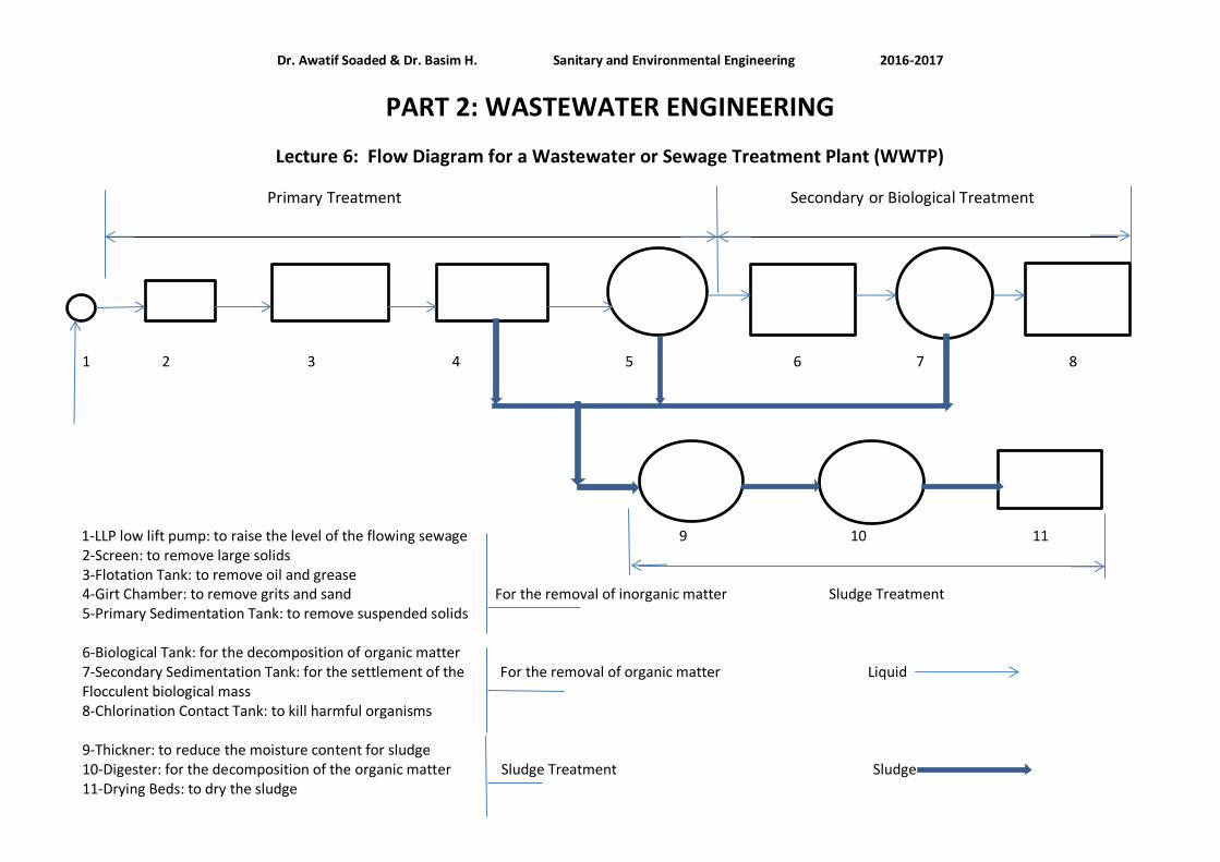
Dr. Awatif Soaded & Dr. Basim H. Sanitary and Environmental Engineering 2016-2017
PART 2: WASTEWATER ENGINEERING
Lecture 6: Flow Diagram for a Wastewater or Sewage Treatment Plant (WWTP)
Primary Treatment Secondary or Biological Treatment
1 2 3 4 5 6 7 8
1-LLP low lift pump: to raise the level of the flowing sewage 9 10 11
2-Screen: to remove large solids 3-Flotation Tank: to remove oil and grease 4-Girt Chamber: to remove grits and sand For the removal of inorganic matter Sludge Treatment 5-Primary Sedimentation Tank: to remove suspended solids 6-Biological Tank: for the decomposition of organic matter 7-Secondary Sedimentation Tank: for the settlement of the For the removal of organic matter Liquid Flocculent biological mass 8-Chlorination Contact Tank: to kill harmful organisms 9-Thickner: to reduce the moisture content for sludge 10-Digester: for the decomposition of the organic matter Sludge Treatment Sludge 11-Drying Beds: to dry the sludge
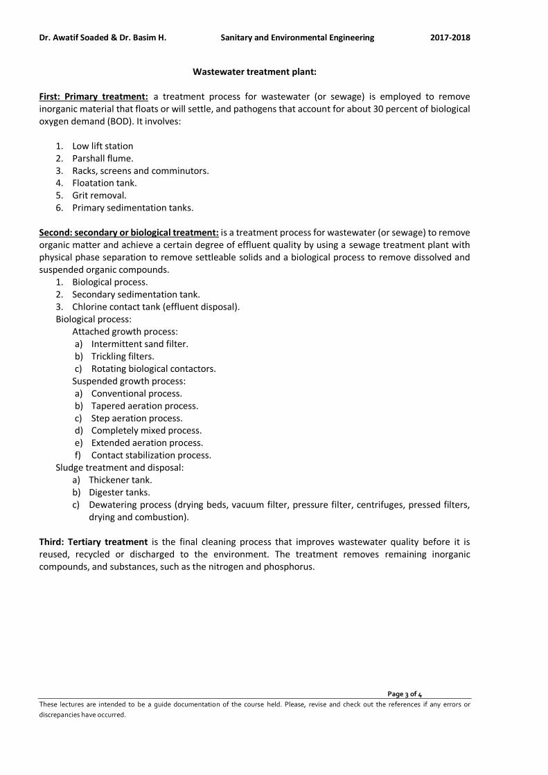
Dr. Awatif Soaded & Dr. Basim H. Sanitary and Environmental Engineering 2017-2018
Page 3 of 4
These lectures are intended to be a guide documentation of the course held. Please, revise and check out the references if any errors or
discrepancies have occurred.
Wastewater treatment plant: First: Primary treatment: a treatment process for wastewater (or sewage) is employed to remove inorganic material that floats or will settle, and pathogens that account for about 30 percent of biological oxygen demand (BOD). It involves:
1. Low lift station 2. Parshall flume. 3. Racks, screens and comminutors. 4. Floatation tank. 5. Grit removal. 6. Primary sedimentation tanks.
Second: secondary or biological treatment: is a treatment process for wastewater (or sewage) to remove organic matter and achieve a certain degree of effluent quality by using a sewage treatment plant with physical phase separation to remove settleable solids and a biological process to remove dissolved and suspended organic compounds.
1. Biological process. 2. Secondary sedimentation tank. 3. Chlorine contact tank (effluent disposal). Biological process:
Attached growth process: a) Intermittent sand filter. b) Trickling filters. c) Rotating biological contactors.
Suspended growth process: a) Conventional process. b) Tapered aeration process. c) Step aeration process. d) Completely mixed process. e) Extended aeration process. f) Contact stabilization process.
Sludge treatment and disposal: a) Thickener tank. b) Digester tanks. c) Dewatering process (drying beds, vacuum filter, pressure filter, centrifuges, pressed filters,
drying and combustion).
Third: Tertiary treatment is the final cleaning process that improves wastewater quality before it is reused, recycled or discharged to the environment. The treatment removes remaining inorganic compounds, and substances, such as the nitrogen and phosphorus.
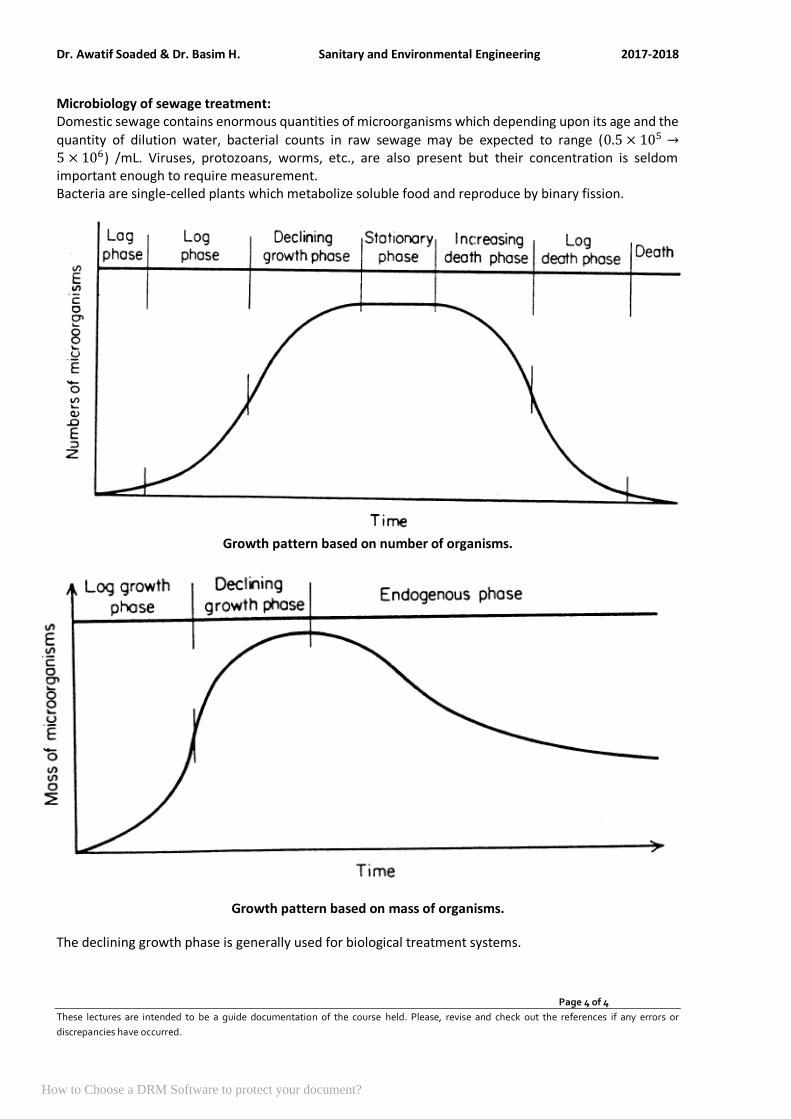
Dr. Awatif Soaded & Dr. Basim H. Sanitary and Environmental Engineering 2017-2018
Page 4 of 4
These lectures are intended to be a guide documentation of the course held. Please, revise and check out the references if any errors or
discrepancies have occurred.
Microbiology of sewage treatment: Domestic sewage contains enormous quantities of microorganisms which depending upon its age and the
quantity of dilution water, bacterial counts in raw sewage may be expected to range (0.5 × 10⁵ →5 × 10⁶) /mL. Viruses, protozoans, worms, etc., are also present but their concentration is seldom important enough to require measurement. Bacteria are single-celled plants which metabolize soluble food and reproduce by binary fission.
Growth pattern based on number of organisms.
Growth pattern based on mass of organisms.
The declining growth phase is generally used for biological treatment systems.
How to Choose a DRM Software to protect your document?
Dr. Awatif Soaded & Dr. Basim H. Sanitary and Environmental Engineering 2019-2020
Page 1 of 10
These lectures are intended to be a guide documentation of the course held. Please, revise and check out the references if any errors or
discrepancies have occurred.
Sanitary and Environmental Engineering
PART 2: WASTEWATER ENGINEERING
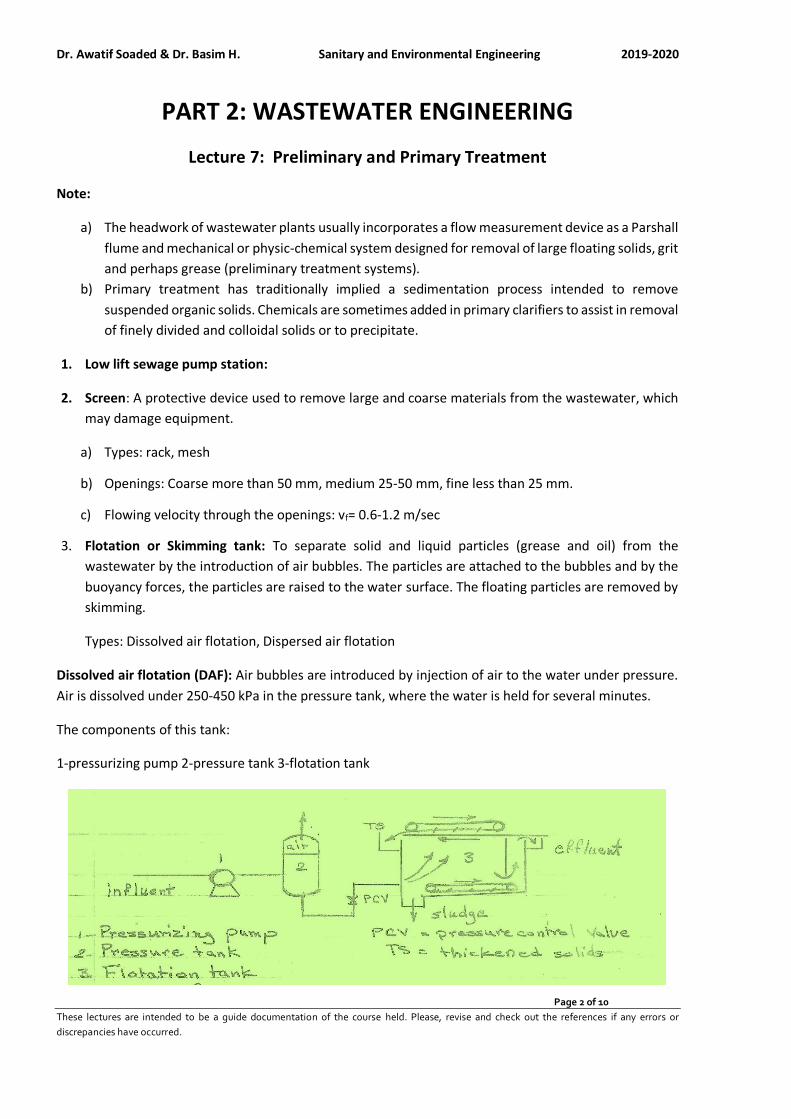
Dr. Awatif Soaded & Dr. Basim H. Sanitary and Environmental Engineering 2019-2020
Page 2 of 10
These lectures are intended to be a guide documentation of the course held. Please, revise and check out the references if any errors or
discrepancies have occurred.
PART 2: WASTEWATER ENGINEERING
Lecture 7: Preliminary and Primary Treatment
Note:
a) The headwork of wastewater plants usually incorporates a flow measurement device as a Parshall
flume and mechanical or physic-chemical system designed for removal of large floating solids, grit
and perhaps grease (preliminary treatment systems).
b) Primary treatment has traditionally implied a sedimentation process intended to remove
suspended organic solids. Chemicals are sometimes added in primary clarifiers to assist in removal
of finely divided and colloidal solids or to precipitate.
1. Low lift sewage pump station:
2. Screen: A protective device used to remove large and coarse materials from the wastewater, which
may damage equipment.
a) Types: rack, mesh
b) Openings: Coarse more than 50 mm, medium 25-50 mm, fine less than 25 mm.
c) Flowing velocity through the openings: vf= 0.6-1.2 m/sec
3. Flotation or Skimming tank: To separate solid and liquid particles (grease and oil) from the
wastewater by the introduction of air bubbles. The particles are attached to the bubbles and by the
buoyancy forces, the particles are raised to the water surface. The floating particles are removed by
skimming.
Types: Dissolved air flotation, Dispersed air flotation
Dissolved air flotation (DAF): Air bubbles are introduced by injection of air to the water under pressure.
Air is dissolved under 250-450 kPa in the pressure tank, where the water is held for several minutes.
The components of this tank:
1-pressurizing pump 2-pressure tank 3-flotation tank
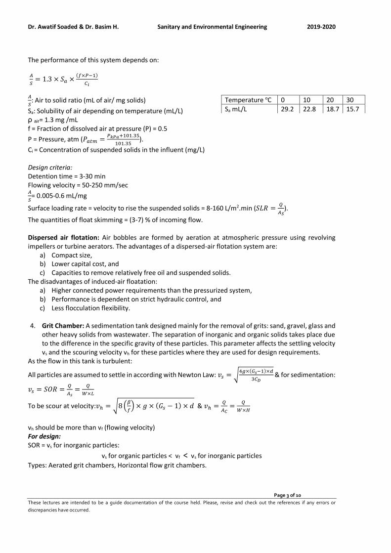
Dr. Awatif Soaded & Dr. Basim H. Sanitary and Environmental Engineering 2019-2020
Page 3 of 10
These lectures are intended to be a guide documentation of the course held. Please, revise and check out the references if any errors or
discrepancies have occurred.
The performance of this system depends on:
𝐴
𝑆= 1.3 × 𝑆𝑎 ×
(𝑓×𝑃−1)
𝐶𝑖
𝐴
𝑆: Air to solid ratio (mL of air/ mg solids)
Sa: Solubility of air depending on temperature (mL/L) ρ air= 1.3 mg /mL f = Fraction of dissolved air at pressure (P) = 0.5
P = Pressure, atm (𝑃𝑎𝑡𝑚 =𝑃𝑘𝑃𝑎+101.35
101.35).
Ci = Concentration of suspended solids in the influent (mg/L) Design criteria: Detention time = 3-30 min Flowing velocity = 50-250 mm/sec 𝐴
𝑆= 0.005-0.6 mL/mg
Surface loading rate = velocity to rise the suspended solids = 8-160 L/m2.min (𝑆𝐿𝑅 =𝑄
𝐴𝑆).
The quantities of float skimming = (3-7) % of incoming flow. Dispersed air flotation: Air bobbles are formed by aeration at atmospheric pressure using revolving impellers or turbine aerators. The advantages of a dispersed-air flotation system are:
a) Compact size, b) Lower capital cost, and c) Capacities to remove relatively free oil and suspended solids.
The disadvantages of induced-air floatation: a) Higher connected power requirements than the pressurized system, b) Performance is dependent on strict hydraulic control, and c) Less flocculation flexibility.
4. Grit Chamber: A sedimentation tank designed mainly for the removal of grits: sand, gravel, glass and
other heavy solids from wastewater. The separation of inorganic and organic solids takes place due to the difference in the specific gravity of these particles. This parameter affects the settling velocity vs and the scouring velocity vh for these particles where they are used for design requirements.
As the flow in this tank is turbulent:
All particles are assumed to settle in according with Newton Law: 𝑣𝑠 = √4𝑔×(𝐺𝑠−1)×𝑑
3𝐶𝐷 & for sedimentation:
𝑣𝑠 = 𝑆𝑂𝑅 =𝑄
𝐴𝑠=
𝑄
𝑊×𝐿
To be scour at velocity:𝑣ℎ = √8 (𝛽
𝑓) × 𝑔 × (𝐺𝑠 − 1) × 𝑑 & 𝑣ℎ =
𝑄
𝐴𝐶=
𝑄
𝑊×𝐻
vh should be more than vf (flowing velocity) For design: SOR = vs for inorganic particles:
vs for organic particles ˂ vf ˂ vs for inorganic particles
Types: Aerated grit chambers, Horizontal flow grit chambers.
Temperature oC 0 10 20 30
Sa mL/L 29.2 22.8 18.7 15.7
Dr. Awatif Soaded & Dr. Basim H. Sanitary and Environmental Engineering 2019-2020
Page 4 of 10
These lectures are intended to be a guide documentation of the course held. Please, revise and check out the references if any errors or
discrepancies have occurred.
Aerated grit chamber: The separation of different types of solids is done by producing a rolling flow similar to the spiral flow by using air. The velocity of the flow vf is to be below vs for inorganic particles and above vs organic particles.
vs for organic particles ˂ vf ˂ vs for inorganic particles
Design criteria: 1- Detention time= 2-4 min 2- Dimensions for a rectangular tank: L = 8-20 m, W = 2-5 m, H = 2-7 m W/H = 1:1 – 5:1 L/H = 3:1 – 5:1 3- Air flow rate = 0.015-0.5 m3/min/ m length Horizontal flow grit chamber: It is designed to provide sufficient time for inorganic particles to settle and the flowing velocity will carry out the organic particles. The velocities for design (vs and vh) are being controlled for the variation of the wastewater flow. To control the velocities; 1- Using the proportional weir; 2- Using the parabolic cross section. Design criteria: 1- Detention time= 30 -90 min 2- vf = 0.2-0.4 m/sec 3- Dimensions: L = 3 -25 m, H = 1-2 m L/H less than 12
4- Quantity of grit = 2.5 × 10⁻⁶ − 1.8 × 10⁻⁴ 𝑚3
𝑚3 𝑜𝑓 𝑤𝑎𝑠𝑡𝑒𝑤𝑎𝑡𝑒𝑟
NOTE: To assure removal of grit (inorganic matter), while permitting such organic matter as might settle to be re-suspended by scour, the necessary condition may be calculated as follow: For particles of grit (inorganic matter), with diameter of 0.2 mm and specific gravity = 2.65,
𝑣𝑠 = √4𝑔 × (𝐺𝑠 − 1) × 𝑑
3𝐶𝐷= √
4 × 980 × (2.65 − 1) × 0.02
3 × 10= 2.1 𝑐𝑚/𝑠𝑒𝑐
The scour velocity of inorganic particles is given by:
𝑣ℎ = √8 (𝛽
𝑓) × 𝑔 × (𝐺𝑠 − 1) × 𝑑 = √8 (
0.06
0.03) × 980 × (2.65 − 1) × 0.02 = 23 𝑐𝑚/𝑠𝑒𝑐
For particles of organic matter, with diameter of 0.2 mm and specific gravity = 1.1,
𝑣𝑠 = √4𝑔 × (𝐺𝑠 − 1) × 𝑑
3𝐶𝐷= √
4 × 980 × (1.1 − 1) × 0.02
3 × 10= 0.511 𝑐𝑚/𝑠𝑒𝑐
The scour velocity of organic particles is given by:
𝑣ℎ = √8 (𝛽
𝑓) × 𝑔 × (𝐺𝑠 − 1) × 𝑑 = √8 (
0.06
0.03) × 980 × (1.1 − 1) × 0.02 = 5.6 𝑐𝑚/𝑠𝑒𝑐
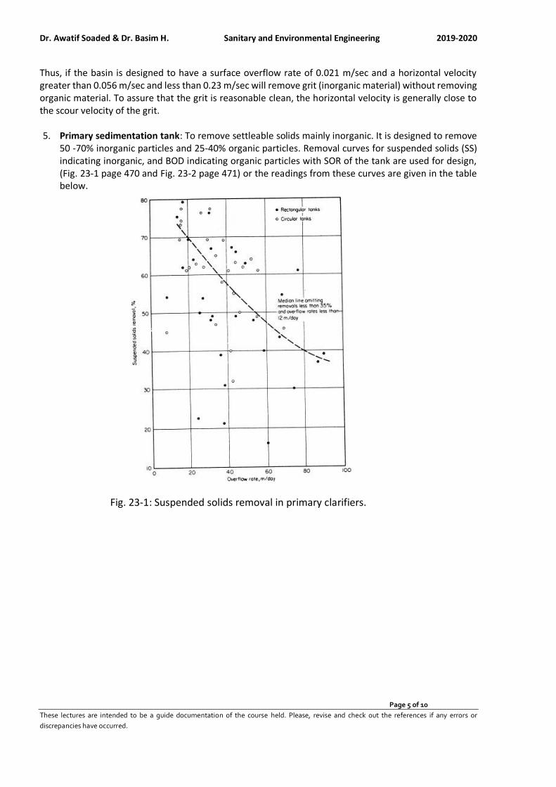
Dr. Awatif Soaded & Dr. Basim H. Sanitary and Environmental Engineering 2019-2020
Page 5 of 10
These lectures are intended to be a guide documentation of the course held. Please, revise and check out the references if any errors or
discrepancies have occurred.
Thus, if the basin is designed to have a surface overflow rate of 0.021 m/sec and a horizontal velocity greater than 0.056 m/sec and less than 0.23 m/sec will remove grit (inorganic material) without removing organic material. To assure that the grit is reasonable clean, the horizontal velocity is generally close to the scour velocity of the grit.
5. Primary sedimentation tank: To remove settleable solids mainly inorganic. It is designed to remove
50 -70% inorganic particles and 25-40% organic particles. Removal curves for suspended solids (SS) indicating inorganic, and BOD indicating organic particles with SOR of the tank are used for design, (Fig. 23-1 page 470 and Fig. 23-2 page 471) or the readings from these curves are given in the table below.
Fig. 23-1: Suspended solids removal in primary clarifiers.

Dr. Awatif Soaded & Dr. Basim H. Sanitary and Environmental Engineering 2019-2020
Page 6 of 10
These lectures are intended to be a guide documentation of the course held. Please, revise and check out the references if any errors or
discrepancies have occurred.
Fig. 23-2: BOD removal in primary clarifiers.
SOR m/d 20 30 40 50 60 70 80
% SS removal 70 65 58 53 48 45 40
% BOD removal 36 34 32.8 30 27.5 25 22.5
Design criteria: 1- Detention time = 1 -4 hr 2- SOR = Average flow 30-50 m/d & maximum flow 80 – 120 m/d 3- vf = 0.6-3.6 m/min 4- Weir loading rate = 125-600 m3/m/d 5- Dimensions: Rectangular L = 15-100 m, H = 3 -5 m, W = 3 -30m Circular D less than 60m
6- Scum removed average about = 7.5 × 10⁻⁶ 𝑚3
𝑚3 𝑜𝑓 𝑤𝑎𝑠𝑡𝑒𝑤𝑎𝑡𝑒𝑟 𝑓𝑙𝑜𝑤

Dr. Awatif Soaded & Dr. Basim H. Sanitary and Environmental Engineering 2019-2020
Page 7 of 10
These lectures are intended to be a guide documentation of the course held. Please, revise and check out the references if any errors or
discrepancies have occurred.
Solved problems
Problem 1: A flotation tank is used for thickening suspended solids (oil) of 3000 mg/L, knowing that: 𝐴
𝑆=
0.008 mL/mg, temperature =20oC, surface loading rate = 8 L/m2.min, Q= 400 m3/d. Find: 1-required pressure P (kPa) inside pressure tank, 2- Surface area of the flotation tank (m2) & 3) The quantities of float skimming if (7)% of incoming flow? ? Solution: 1) From table at T = 20oC, air solubility Sa = 18.7 mL/L
𝐴
𝑆= 1.3 × 𝑆𝑎 ×
(𝑓×𝑃−1)
𝐶𝑖⇛ 0.008 = 1.3 × 18.7 ×
(0.5×𝑃−1)
3000⇛ 𝑃 = 3.98 𝑎𝑡𝑚
∴ 𝑃 = 3.98 𝑎𝑡𝑚 =𝑃𝑘𝑃𝑎 + 101.35
101.35⇛ 𝑃 = 302 𝑘𝑃𝑎
2) 𝐴𝑠 =𝑄
𝑆𝑢𝑟𝑓𝑎𝑐𝑒 𝐿𝑜𝑎𝑑𝑖𝑛𝑔=
400×103 𝐿/𝑑𝑎𝑦
8 ×24×60 𝐿/𝑑𝑎𝑦= 34.7 𝑚2
3) 𝑘𝑔
𝑑𝑎𝑦= 3000
𝑚𝑔
𝐿× 10−3 × 400
𝑚3
𝑑𝑎𝑦× 0.07 = 84 𝑘𝑔/𝑑𝑎𝑦
Problem 2: Design a horizontal flow girt chamber (rectangular) of a parabolic section. Knowing that Qmax = 18,000 m3/d, Qavg = 15,000 m3/d ,Qmin = 10,000 m3/d, Gs inorganic particles = 2.65, Gs organic particles = 1.1, CD =10, β/f = 2, detention time = 1 min, particles to be removed = 0.2 mm in diameter? Solution: For inorganic particles, Gs = 2.65:
𝑣𝑠 = √4𝑔 × (𝐺𝑠 − 1) × 𝑑𝑠
3𝐶𝐷= √
4 × 980 × (2.65 − 1) × 0.02
3 × 10= 2.076 ≈ 2.1 𝑐𝑚/𝑠𝑒𝑐
𝑣𝑠 𝑓𝑜𝑟 𝑖𝑛𝑜𝑟𝑔𝑎𝑛𝑖𝑐 𝑝𝑎𝑟𝑡𝑖𝑐𝑙𝑒𝑠 = 𝑆𝑂𝑅 =𝑄
𝐴𝑆
Surface area of grit chamber:
𝐴𝑠 =18000
0.021×24×60×60= 9.921 𝑚2 = 𝐿 × 𝑊 (1)
𝑣ℎ = √8 (𝛽
𝑓) × 𝑔 × (𝐺𝑠 − 1) × 𝑑𝑠 = √8 (
0.06
0.03) × 980 × (2.65 − 1) × 0.02 = 23 𝑐𝑚/𝑠𝑒𝑐
For organic particles, Gs = 1.1:
𝑣ℎ = √8 (𝛽
𝑓) × 𝑔 × (𝐺𝑠 − 1) × 𝑑𝑠 = √8 (
0.06
0.03) × 980 × (1.1 − 1) × 0.02 = 5.6 𝑐𝑚/𝑠𝑒𝑐
For design Ac: 𝑣ℎ 𝑜𝑟𝑔𝑎𝑛𝑖𝑐 < 𝑣ℎ 𝑑𝑒𝑠𝑖𝑔𝑛 < 𝑣ℎ 𝑖𝑛𝑜𝑟𝑔𝑎𝑛𝑖𝑐
Assume 𝑣ℎ 𝑑𝑒𝑠𝑖𝑔𝑛 = 0.2 𝑚/𝑠𝑒𝑐
∴ 𝐴𝑐 =𝑄
𝑣ℎ=
18000
0.2×24×60×60= 1.042 𝑚2 = 𝐻 × 𝑊 (2)
𝑉 = 𝑄 × 𝑡 =18000×1 𝑚𝑖𝑛
24×60= 12.5 𝑚3 = 𝐿 × 𝑊 × 𝐻 (3)
Solving eq. 1, 2, & 3 and find: 𝐿 = 12 𝑚 , 𝑊 = 0.827 𝑚, & 𝐻 = 1.26 𝑚
Assume use area of parabolic section = 2
3𝑊𝑍, Where:
W: Width at the design level. Z: Height at the design level.
𝑍 = 𝐶 × 𝑊2
So, for AC , 𝐴𝐶 =2
3𝑊𝑍 → 1.042 =
2
3× 0.827 × 𝑍 → 𝑍 = 1.889 𝑚

Dr. Awatif Soaded & Dr. Basim H. Sanitary and Environmental Engineering 2019-2020
Page 8 of 10
These lectures are intended to be a guide documentation of the course held. Please, revise and check out the references if any errors or
discrepancies have occurred.
𝑍 = 𝐶 × 𝑊2 → 1.889 = 𝐶 × 0.8272 → 𝐶 = 2.763 Q (m3/day) AC (m2) W (m) Z (m)
18000 1.042 0.827 1.889
15000 0.868 0.78 1.68
10000 0.579 0.68 1.289
Problem 3: Design a primary sedimentation tank for 60% SS removal. The influent flow is 10,000 m3/d, and assume the detention time = 2hr? Also find the SS settling and effluent sludge if the influent SS concentration 2000 mg/L? Solution: From Fig. 23-1 or Table for 60% SS removal, SOR = 37 m/day and from Fig. 23-2 or Table 33% BOD removal.
𝑆𝑂𝑅 =𝑄
𝐴𝑠→ 𝐴𝑠 =
𝑄
𝑆𝑂𝑅=
10000
37= 270 𝑚2
If circular tank: 𝐴 =𝜋
4𝐷2 → 270 =
𝜋
4𝐷2 → 𝐷 = 18.5 𝑚
𝑉 = 𝑄 × 𝑡 = 𝐴𝑠 × 𝐻 →10000
24× 2 ℎ𝑟 = 270 × 𝐻 → 𝐻 = 3.1 𝑚
Weir loading rate, 𝑊𝐿𝑅 =𝑄
𝑊𝑒𝑖𝑟 𝑙𝑒𝑛𝑔𝑡ℎ=
10000
𝜋×18.5= 172 𝑚3/(𝑚. 𝑑𝑎𝑦) O.K
If rectangular tank: Assume W = 10 m, so, 𝐴 = 𝐿 × 𝑊 → 270 = 𝐿 × 10 → 𝐿 = 27 𝑚
Weir loading rate, 𝑊𝐿𝑅 =𝑄
𝑊𝑒𝑖𝑟 𝑙𝑒𝑛𝑔𝑡ℎ=
10000
10= 1000 𝑚3/(𝑚. 𝑑𝑎𝑦) not O.K
Assume weir loading rate = 600 m3/(m.day) & weir length = 17 m
The influent sewage SS, 𝑘𝑔
𝑑𝑎𝑦= 2000 × 10−3 × 10000 = 20000 𝑘𝑔/𝑑𝑎𝑦
The influent SS settling sludge, 𝑘𝑔
𝑑𝑎𝑦= 2000 × 10−3 × 10000 × 0.6 = 12000 𝑘𝑔/𝑑𝑎𝑦
The effluent SS, 𝑘𝑔
𝑑𝑎𝑦= 2000 × 10−3 × 10000 × 0.4 = 8000 𝑘𝑔/𝑑𝑎𝑦
Problem 4: A raw wastewater containing 250 mg/L SS and 200 mg/L BOD passes through a clarifier with a surface area of 500 m2. The flow ranges from 10000 m3/day to 30000 m3/day. Estimate the effluent BOD and SS at maximum and minimum flow, and the maximum and minimum rate of sludge production? Assume the sludge is 95 percent water. Problem 5: Design a primary clarifier system for a community with population of 50000 persons. Size the clarifiers so that the SOR will be not more than 40 m/day at peak flow with one unit out of service and not more than 25 m/day at average flow? The minimum retention time is to be 1 hour and maximum weir loading rate 370 m3/m.day. Also estimate the quantity of sludge which must be removed? If the sludge pumping cycle is 15 min/hour at maximum, what flow must the pump be sized to handle?
Dr. Awatif Soaded & Dr. Basim H. Sanitary and Environmental Engineering 2019-2020
Page 9 of 10
These lectures are intended to be a guide documentation of the course held. Please, revise and check out the references if any errors or
discrepancies have occurred.
Problem 6: Design a primary clarifier system for a community with population of 50000 persons with a water supply demand 180 L/capita.day, and assuming that 80% of water supplied to the community is converted into sewage. Size the clarifiers so that the SOR will be not more than 40 m/day at peak flow (case 1) and not more than 25 m/day at average flow (case 2) with one unit out of service? The minimum retention time is to be 1 hour and maximum weir loading rate 370 m3/m.day. Also, find the percent removal SS and BOD for each SOR?
SOR m/d 20 30 40 50 60 70 80
% SS removal 70 65 58 53 48 45 40
% BOD removal 36 34 32.8 30 27.5 25 22.5
Solution:
Average sewage flow: 𝑄𝐴𝑣𝑔 = 0.8 × 180 × 50000 = 7200000𝐿
𝑑𝑎𝑦= 7200 𝑚3/𝑑𝑎𝑦
Peak sewage flow: 𝑄𝑃𝑒𝑎𝑘 = 0.8 × 1.8 × 180 × 50000 = 12960000 𝐿
𝑑𝑎𝑦= 12960 𝑚3/𝑑𝑎𝑦
Case 1: SOR = 40 m/day at peak flow:
𝑆𝑂𝑅 =𝑄
𝐴𝑠→ 𝐴𝑠 =
12960
40= 324 𝑚2 → 𝐷 = 20.32 𝑚 use D = 20 m & 𝑄 =
𝑉
𝑡→ 𝑉 = 12960 ×
1
24= 540 𝑚3, 𝐻 =
𝑉
𝐴𝑠=
540
324= 1.667 𝑚
𝑊𝐿𝑅 =𝑄
𝐿=
12960
𝜋×20= 206.369
𝑚3
𝑚.𝑑𝑎𝑦< 370
𝑚3
𝑚.𝑑𝑎𝑦 O.K
From table at SOR = 40 m/day: SS% removal = 58% and BOD% removal = 32.8%
Case 2: SOR = 25 m/day at average flow:
𝑆𝑂𝑅 =𝑄
𝐴𝑠→ 𝐴𝑠 =
7200
25= 288 𝑚2 → 𝐷 = 19.15 𝑚 use D= 19 m & 𝑄 =
𝑉
𝑡→ 𝑉 = 7200 ×
1
24= 300 𝑚3, 𝐻 =
𝑉
𝐴𝑠=
300
288= 1.041 𝑚
𝑊𝐿𝑅 =𝑄
𝐿=
7200
𝜋×19= 120.683
𝑚3
𝑚.𝑑𝑎𝑦< 370
𝑚3
𝑚.𝑑𝑎𝑦 O.K
From table at SOR = 25 m/day: SS% removal = 67.5% and BOD% removal = 35%
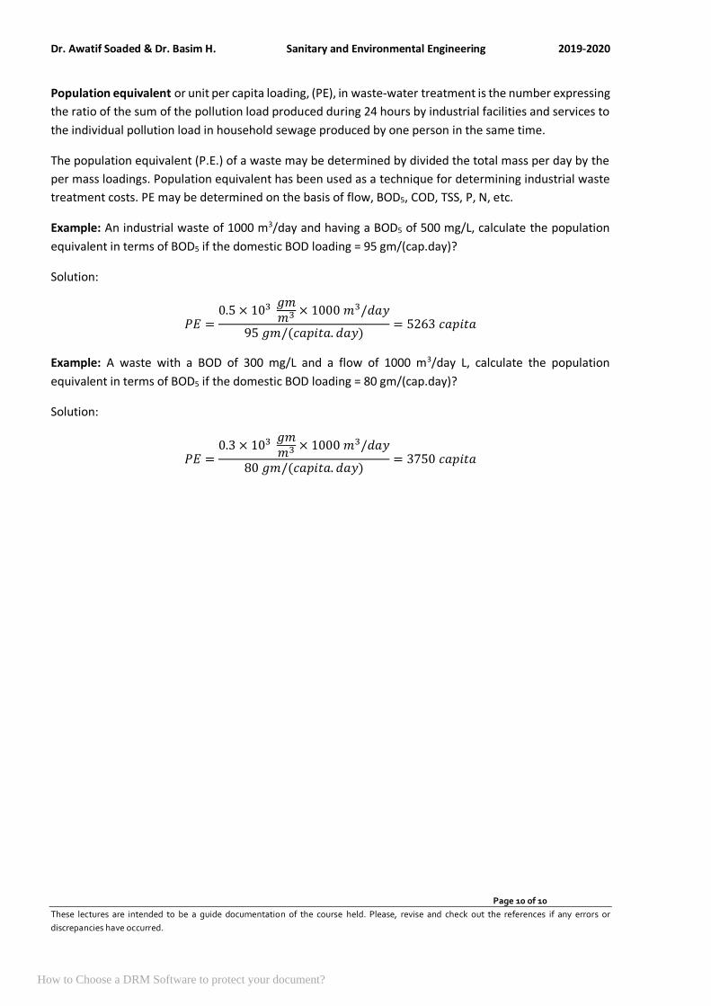
Dr. Awatif Soaded & Dr. Basim H. Sanitary and Environmental Engineering 2019-2020
Page 10 of 10
These lectures are intended to be a guide documentation of the course held. Please, revise and check out the references if any errors or
discrepancies have occurred.
Population equivalent or unit per capita loading, (PE), in waste-water treatment is the number expressing
the ratio of the sum of the pollution load produced during 24 hours by industrial facilities and services to
the individual pollution load in household sewage produced by one person in the same time.
The population equivalent (P.E.) of a waste may be determined by divided the total mass per day by the
per mass loadings. Population equivalent has been used as a technique for determining industrial waste
treatment costs. PE may be determined on the basis of flow, BOD5, COD, TSS, P, N, etc.
Example: An industrial waste of 1000 m3/day and having a BOD5 of 500 mg/L, calculate the population
equivalent in terms of BOD5 if the domestic BOD loading = 95 gm/(cap.day)?
Solution:
𝑃𝐸 =0.5 × 10³
𝑔𝑚𝑚3 × 1000 𝑚3/𝑑𝑎𝑦
95 𝑔𝑚/(𝑐𝑎𝑝𝑖𝑡𝑎. 𝑑𝑎𝑦)= 5263 𝑐𝑎𝑝𝑖𝑡𝑎
Example: A waste with a BOD of 300 mg/L and a flow of 1000 m3/day L, calculate the population
equivalent in terms of BOD5 if the domestic BOD loading = 80 gm/(cap.day)?
Solution:
𝑃𝐸 =0.3 × 10³
𝑔𝑚𝑚3 × 1000 𝑚3/𝑑𝑎𝑦
80 𝑔𝑚/(𝑐𝑎𝑝𝑖𝑡𝑎. 𝑑𝑎𝑦)= 3750 𝑐𝑎𝑝𝑖𝑡𝑎
How to Choose a DRM Software to protect your document?
Dr. Awatif Soaded & Dr. Basim H. Sanitary and Environmental Engineering 2019-2020
Page 1 of 18
These lectures are intended to be a guide documentation of the course held. Please, revise and check out the references if any errors or
discrepancies have occurred.
Sanitary and Environmental Engineering
PART 2: WASTEWATER ENGINEERING
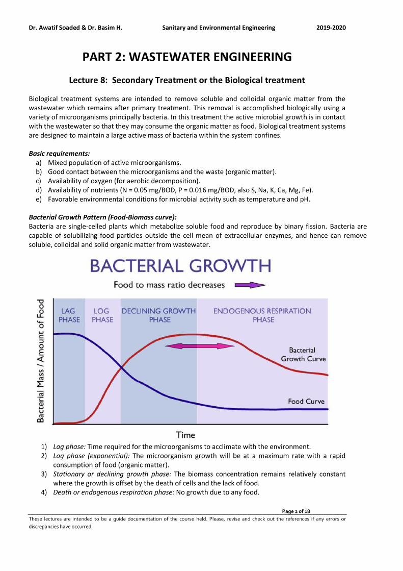
Dr. Awatif Soaded & Dr. Basim H. Sanitary and Environmental Engineering 2019-2020
Page 2 of 18
These lectures are intended to be a guide documentation of the course held. Please, revise and check out the references if any errors or
discrepancies have occurred.
PART 2: WASTEWATER ENGINEERING
Lecture 8: Secondary Treatment or the Biological treatment
Biological treatment systems are intended to remove soluble and colloidal organic matter from the wastewater which remains after primary treatment. This removal is accomplished biologically using a variety of microorganisms principally bacteria. In this treatment the active microbial growth is in contact with the wastewater so that they may consume the organic matter as food. Biological treatment systems are designed to maintain a large active mass of bacteria within the system confines. Basic requirements:
a) Mixed population of active microorganisms. b) Good contact between the microorganisms and the waste (organic matter). c) Availability of oxygen (for aerobic decomposition). d) Availability of nutrients (N = 0.05 mg/BOD, P = 0.016 mg/BOD, also S, Na, K, Ca, Mg, Fe). e) Favorable environmental conditions for microbial activity such as temperature and pH.
Bacterial Growth Pattern (Food-Biomass curve): Bacteria are single-celled plants which metabolize soluble food and reproduce by binary fission. Bacteria are capable of solubilizing food particles outside the cell mean of extracellular enzymes, and hence can remove soluble, colloidal and solid organic matter from wastewater.
1) Lag phase: Time required for the microorganisms to acclimate with the environment. 2) Log phase (exponential): The microorganism growth will be at a maximum rate with a rapid
consumption of food (organic matter). 3) Stationary or declining growth phase: The biomass concentration remains relatively constant
where the growth is offset by the death of cells and the lack of food. 4) Death or endogenous respiration phase: No growth due to any food.
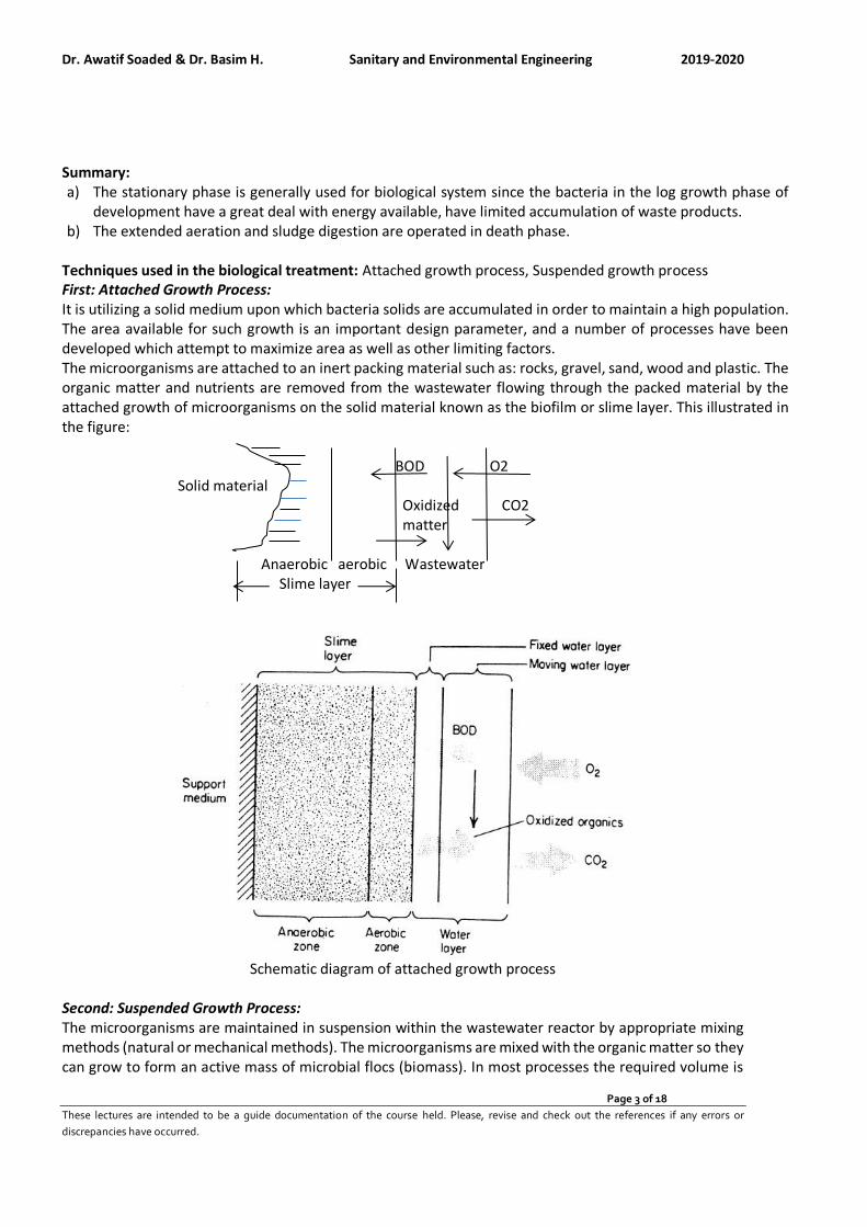
Dr. Awatif Soaded & Dr. Basim H. Sanitary and Environmental Engineering 2019-2020
Page 3 of 18
These lectures are intended to be a guide documentation of the course held. Please, revise and check out the references if any errors or
discrepancies have occurred.
Summary: a) The stationary phase is generally used for biological system since the bacteria in the log growth phase of
development have a great deal with energy available, have limited accumulation of waste products. b) The extended aeration and sludge digestion are operated in death phase.
Techniques used in the biological treatment: Attached growth process, Suspended growth process First: Attached Growth Process: It is utilizing a solid medium upon which bacteria solids are accumulated in order to maintain a high population. The area available for such growth is an important design parameter, and a number of processes have been developed which attempt to maximize area as well as other limiting factors. The microorganisms are attached to an inert packing material such as: rocks, gravel, sand, wood and plastic. The organic matter and nutrients are removed from the wastewater flowing through the packed material by the attached growth of microorganisms on the solid material known as the biofilm or slime layer. This illustrated in the figure: BOD O2 Solid material Oxidized CO2 matter Anaerobic aerobic Wastewater Slime layer
Schematic diagram of attached growth process
Second: Suspended Growth Process: The microorganisms are maintained in suspension within the wastewater reactor by appropriate mixing methods (natural or mechanical methods). The microorganisms are mixed with the organic matter so they can grow to form an active mass of microbial flocs (biomass). In most processes the required volume is

Dr. Awatif Soaded & Dr. Basim H. Sanitary and Environmental Engineering 2019-2020
Page 4 of 18
These lectures are intended to be a guide documentation of the course held. Please, revise and check out the references if any errors or
discrepancies have occurred.
reduced by returning bacteria from the secondary clarifier in order to maintain a high solids concentration. It includes activated sludge and its various modifications, oxidation ponds and sludge digestion systems. Attached Growth Process Surface growth process include intermittent sand filter, trickling filters, rotating biological contactors, and a variety of similar proprietary devices. One of the treatment units designed by this technique is the Trickling Filter. Trickling filters utilize a relative porous bacteria growth medium such as rock or formed plastic shapes.
Types of Trickling Filters: Low rate, High rate
Item Low Rate High Rate
Depth (m) 1.5-3.0 1.0-2.0
Hydraulic loading (m3/m2/d) 1.0 – 4.0 10-40
Organic loading (kg BODu/m3/d) 0.08 – 1.5 1.5-18.7
Recirculation ratio 0 1.0-3.0
BOD removal (%) 74 -80 80-85
Filter files many few
Advantages of recirculation:
a) Increase the biomass in the system; b) Maintain uniform hydraulic and organic loadings; c) Dilution of the influent with water of a better quality; d) Thinning of the slime layer (biofilm).

Dr. Awatif Soaded & Dr. Basim H. Sanitary and Environmental Engineering 2019-2020
Page 5 of 18
These lectures are intended to be a guide documentation of the course held. Please, revise and check out the references if any errors or
discrepancies have occurred.
Techniques of recirculation used in the operation process may vary widely. The different configurations being used are listed in Fig. 24-6 page 483. The basic forms depending on the flow pattern are:
1- Single stage, one Trickling filter is used. 2- Two stages, two filers are used in series.
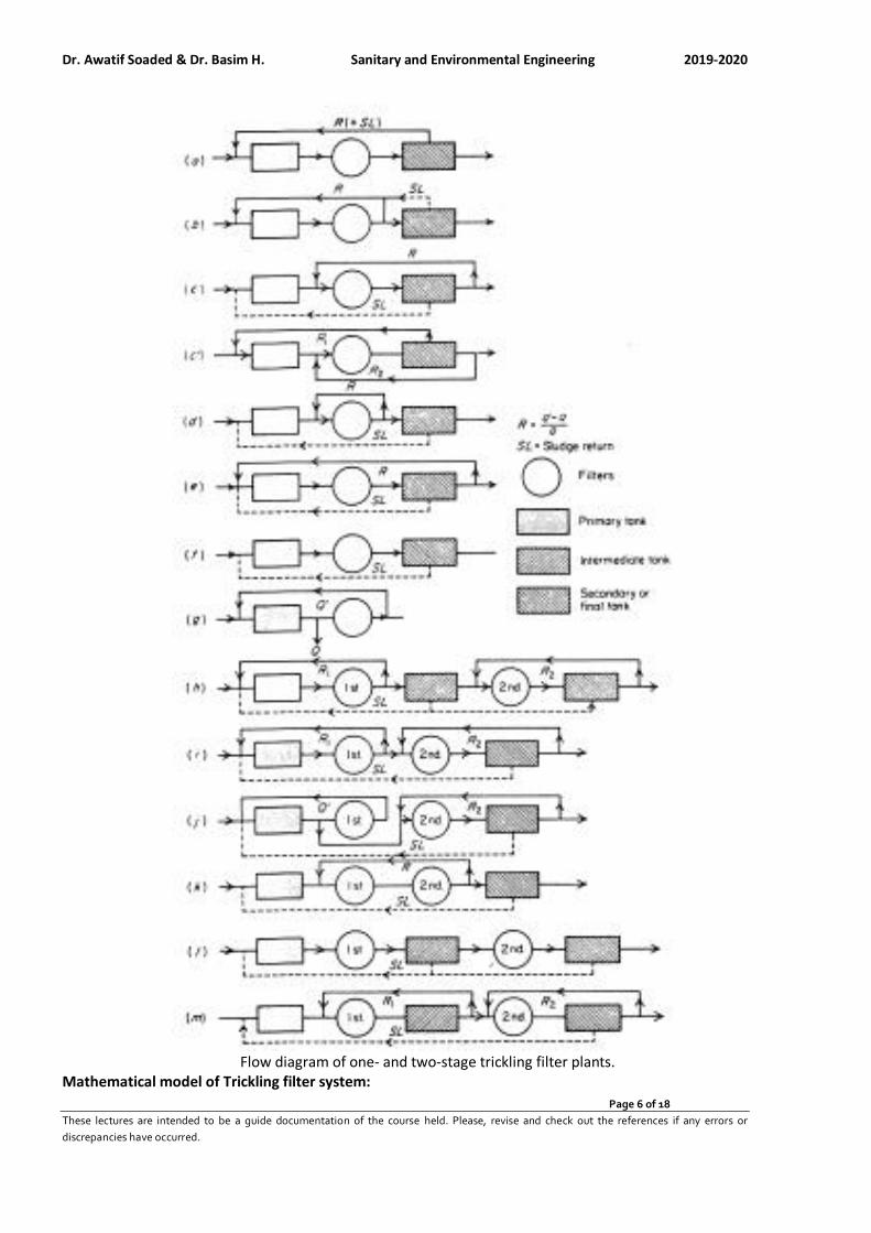
Dr. Awatif Soaded & Dr. Basim H. Sanitary and Environmental Engineering 2019-2020
Page 6 of 18
These lectures are intended to be a guide documentation of the course held. Please, revise and check out the references if any errors or
discrepancies have occurred.
Flow diagram of one- and two-stage trickling filter plants.
Mathematical model of Trickling filter system:
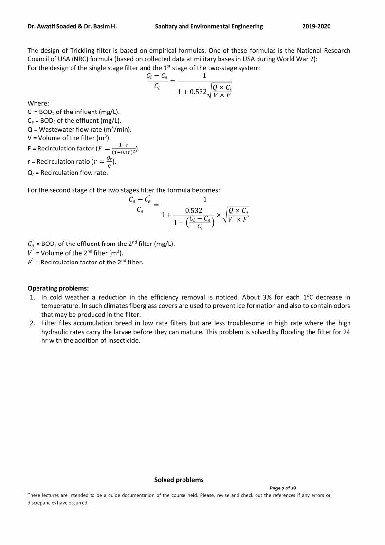
Dr. Awatif Soaded & Dr. Basim H. Sanitary and Environmental Engineering 2019-2020
Page 7 of 18
These lectures are intended to be a guide documentation of the course held. Please, revise and check out the references if any errors or
discrepancies have occurred.
The design of Trickling filter is based on empirical formulas. One of these formulas is the National Research Council of USA (NRC) formula (based on collected data at military bases in USA during World War 2): For the design of the single stage filter and the 1st stage of the two-stage system:
𝐶𝑖 − 𝐶𝑒
𝐶𝑖=
1
1 + 0.532√𝑄 × 𝐶𝑖𝑉 × 𝐹
Where: Ci = BOD5 of the influent (mg/L). Ce = BOD5 of the effluent (mg/L). Q = Wastewater flow rate (m3/min). V = Volume of the filter (m3).
F = Recirculation factor (𝐹 =1+𝑟
(1+0.1𝑟)2).
r = Recirculation ratio (𝑟 =𝑄𝑟
𝑄).
Qr = Recirculation flow rate. For the second stage of the two stages filter the formula becomes:
𝐶𝑒 − 𝐶𝑒`
𝐶𝑒=
1
1 +0.532
1 − (𝐶𝑖 − 𝐶𝑒
𝐶𝑖)
× √𝑄 × 𝐶𝑒
𝑉` × 𝐹`
𝐶𝑒` = BOD5 of the effluent from the 2nd filter (mg/L).
𝑉` = Volume of the 2nd filter (m3).
𝐹` = Recirculation factor of the 2nd filter. Operating problems: 1. In cold weather a reduction in the efficiency removal is noticed. About 3% for each 1oC decrease in
temperature. In such climates fiberglass covers are used to prevent ice formation and also to contain odors that may be produced in the filter.
2. Filter files accumulation breed in low rate filters but are less troublesome in high rate where the high hydraulic rates carry the larvae before they can mature. This problem is solved by flooding the filter for 24 hr with the addition of insecticide.
Solved problems

Dr. Awatif Soaded & Dr. Basim H. Sanitary and Environmental Engineering 2019-2020
Page 8 of 18
These lectures are intended to be a guide documentation of the course held. Please, revise and check out the references if any errors or
discrepancies have occurred.
Problem 1: Calculate the effluent BOD5 of a two-stage trickling filter with the following flows, BOD5 and dimensions: Q =3.15 m3/min, BOD5 = 290 mg/L Volume of filter NO.1 = 830 m3 Volume of filter NO.2 = 830 m3 Filter depth = 2 m Recirculation (filter NO.1) = 125 percent Q & r1 = 125% Recirculation (filter NO.2) = 100 percent Q & r2 = 100% Solution: By using NRC formula:
For the first stage: VFQCC
CC
ii
ei
532.01
1
+=
−
( ) ( )78.1
125.125.11
1.011
221
11 =
+=
++
=r
rF
( )( )78.183029015.3
532.01
1290
290
+=
− eC, So, Ce= 85.5 mg/L
For the second stage:
( )65.1
21.12
1.011
22
22 ==
++
=r
rF
( ) //
/
1
532.01
1
FVQC
CCC
CCC
e
ii
ei
e
ee
−−
+=
−
( ) ( )
65.18305.8515.3
290/5.852901532.0
1
15.85
5.85 /
−−+
=− eC
LmgCe /38=
If the effluent BOD5, from the first stage is assumed to about 100 mg/L, the organic loading rate, including recirculation is:
𝑂𝑟𝑎𝑔𝑎𝑛𝑖𝑐 𝑙𝑜𝑎𝑑𝑖𝑛𝑔 𝑟𝑎𝑡𝑒 = 𝑄𝐼𝑛𝑓𝑙𝑢𝑒𝑛𝑡 × 𝐵𝑂𝐷5𝐼𝑛𝑓𝑙𝑢𝑒𝑛𝑡 + (𝑄𝐼𝑛𝑓𝑙𝑢𝑒𝑛𝑡 + 𝑄𝑟) × 𝐵𝑂𝐷5𝐸𝑓𝑓𝑙𝑢𝑒𝑛𝑡
𝑂𝑟𝑎𝑔𝑎𝑛𝑖𝑐 𝑙𝑜𝑎𝑑𝑖𝑛𝑔 𝑟𝑎𝑡𝑒 = 3.15𝑚3
𝑚𝑖𝑛× 290
𝑚𝑔
𝐿× 10−3 + 3.15 × 1.25
𝑚3
𝑚𝑖𝑛× 100
𝑚𝑔
𝐿× 10−3
= 1.307 𝑘𝑔/ min = 1882.44 𝑘𝑔/𝑑𝑎𝑦
The organic loading rate for each filter: 𝑂𝐿𝑅 =1882 𝑘𝑔/𝑑𝑎𝑦
830 𝑚3 = 2.27𝑘𝑔
𝑚3 𝑝𝑒𝑟 𝑑𝑎𝑦
First stage efficiency:=𝐶𝑖−𝐶𝑒
𝐶𝑖=
290−85.5
290× 100 = 70.517%
Second stage efficiency:=𝐶𝑒−𝐶𝑒
′
𝐶𝑒=
85.5−38
85.5× 100 = 55.55%
Overall stage efficiency:=𝐶𝑖−𝐶𝑒
′
𝐶𝑖=
290−38
290× 100 = 86.89%
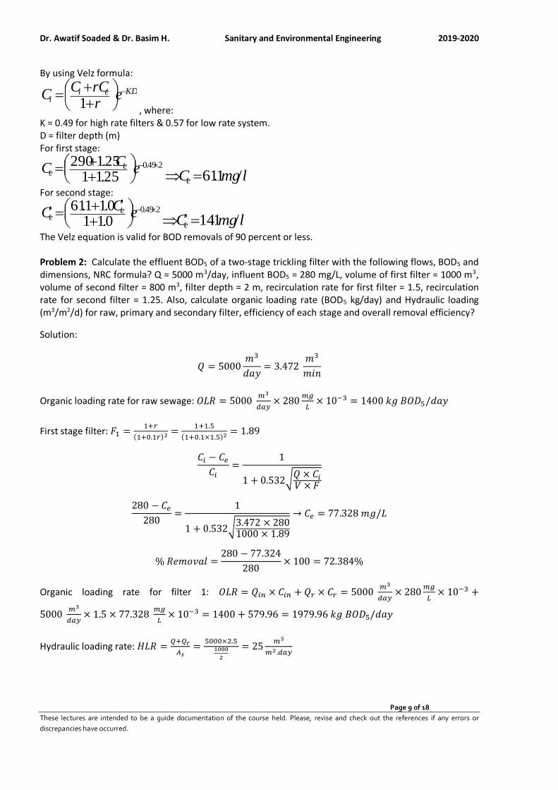
Dr. Awatif Soaded & Dr. Basim H. Sanitary and Environmental Engineering 2019-2020
Page 9 of 18
These lectures are intended to be a guide documentation of the course held. Please, revise and check out the references if any errors or
discrepancies have occurred.
By using Velz formula:
KDeii e
rrCC
C −
++
=1
, where: K = 0.49 for high rate filters & 0.57 for low rate system. D = filter depth (m) For first stage:
249.0
25.1125.1290 −
++
= eC
C ee lmgCe /1.61=
For second stage:
249.0
0.110.11.61 −
++
= eC
C ee lmgCe /1.14=
The Velz equation is valid for BOD removals of 90 percent or less. Problem 2: Calculate the effluent BOD5 of a two-stage trickling filter with the following flows, BOD5 and dimensions, NRC formula? Q = 5000 m3/day, influent BOD5 = 280 mg/L, volume of first filter = 1000 m3, volume of second filter = 800 m3, filter depth = 2 m, recirculation rate for first filter = 1.5, recirculation rate for second filter = 1.25. Also, calculate organic loading rate (BOD5 kg/day) and Hydraulic loading (m3/m2/d) for raw, primary and secondary filter, efficiency of each stage and overall removal efficiency?
Solution:
𝑄 = 5000𝑚3
𝑑𝑎𝑦= 3.472
𝑚3
𝑚𝑖𝑛
Organic loading rate for raw sewage: 𝑂𝐿𝑅 = 5000 𝑚3
𝑑𝑎𝑦× 280
𝑚𝑔
𝐿× 10−3 = 1400 𝑘𝑔 𝐵𝑂𝐷5/𝑑𝑎𝑦
First stage filter: 𝐹1 =1+𝑟
(1+0.1𝑟)2 =1+1.5
(1+0.1×1.5)2 = 1.89
𝐶𝑖 − 𝐶𝑒
𝐶𝑖=
1
1 + 0.532√𝑄 × 𝐶𝑖𝑉 × 𝐹
280 − 𝐶𝑒
280=
1
1 + 0.532√3.472 × 2801000 × 1.89
→ 𝐶𝑒 = 77.328 𝑚𝑔/𝐿
% 𝑅𝑒𝑚𝑜𝑣𝑎𝑙 =280 − 77.324
280× 100 = 72.384%
Organic loading rate for filter 1: 𝑂𝐿𝑅 = 𝑄𝑖𝑛 × 𝐶𝑖𝑛 + 𝑄𝑟 × 𝐶𝑟 = 5000 𝑚3
𝑑𝑎𝑦× 280
𝑚𝑔
𝐿× 10−3 +
5000 𝑚3
𝑑𝑎𝑦× 1.5 × 77.328
𝑚𝑔
𝐿× 10−3 = 1400 + 579.96 = 1979.96 𝑘𝑔 𝐵𝑂𝐷5/𝑑𝑎𝑦
Hydraulic loading rate: 𝐻𝐿𝑅 =𝑄+𝑄𝑟
𝐴𝑠=
5000×2.51000
2
= 25𝑚3
𝑚2.𝑑𝑎𝑦
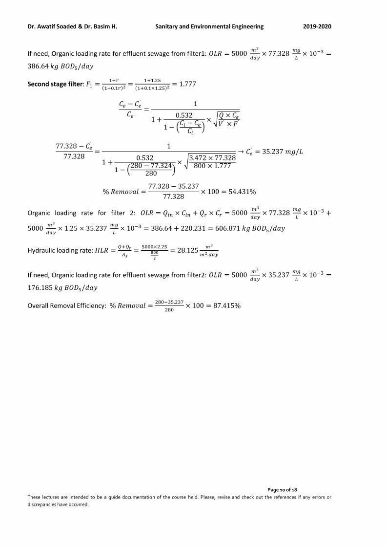
Dr. Awatif Soaded & Dr. Basim H. Sanitary and Environmental Engineering 2019-2020
Page 10 of 18
These lectures are intended to be a guide documentation of the course held. Please, revise and check out the references if any errors or
discrepancies have occurred.
If need, Organic loading rate for effluent sewage from filter1: 𝑂𝐿𝑅 = 5000 𝑚3
𝑑𝑎𝑦× 77.328
𝑚𝑔
𝐿× 10−3 =
386.64 𝑘𝑔 𝐵𝑂𝐷5/𝑑𝑎𝑦
Second stage filter: 𝐹1 =1+𝑟
(1+0.1𝑟)2 =1+1.25
(1+0.1×1.25)2 = 1.777
𝐶𝑒 − 𝐶𝑒`
𝐶𝑒=
1
1 +0.532
1 − (𝐶𝑖 − 𝐶𝑒
𝐶𝑖)
× √𝑄 × 𝐶𝑒
𝑉` × 𝐹`
77.328 − 𝐶𝑒`
77.328=
1
1 +0.532
1 − (280 − 77.324
280)
× √3.472 × 77.328800 × 1.777
→ 𝐶𝑒` = 35.237 𝑚𝑔/𝐿
% 𝑅𝑒𝑚𝑜𝑣𝑎𝑙 =77.328 − 35.237
77.328× 100 = 54.431%
Organic loading rate for filter 2: 𝑂𝐿𝑅 = 𝑄𝑖𝑛 × 𝐶𝑖𝑛 + 𝑄𝑟 × 𝐶𝑟 = 5000 𝑚3
𝑑𝑎𝑦× 77.328
𝑚𝑔
𝐿× 10−3 +
5000 𝑚3
𝑑𝑎𝑦× 1.25 × 35.237
𝑚𝑔
𝐿× 10−3 = 386.64 + 220.231 = 606.871 𝑘𝑔 𝐵𝑂𝐷5/𝑑𝑎𝑦
Hydraulic loading rate: 𝐻𝐿𝑅 =𝑄+𝑄𝑟
𝐴𝑠=
5000×2.25800
2
= 28.125𝑚3
𝑚2.𝑑𝑎𝑦
If need, Organic loading rate for effluent sewage from filter2: 𝑂𝐿𝑅 = 5000 𝑚3
𝑑𝑎𝑦× 35.237
𝑚𝑔
𝐿× 10−3 =
176.185 𝑘𝑔 𝐵𝑂𝐷5/𝑑𝑎𝑦
Overall Removal Efficiency: % 𝑅𝑒𝑚𝑜𝑣𝑎𝑙 =280−35.237
280× 100 = 87.415%
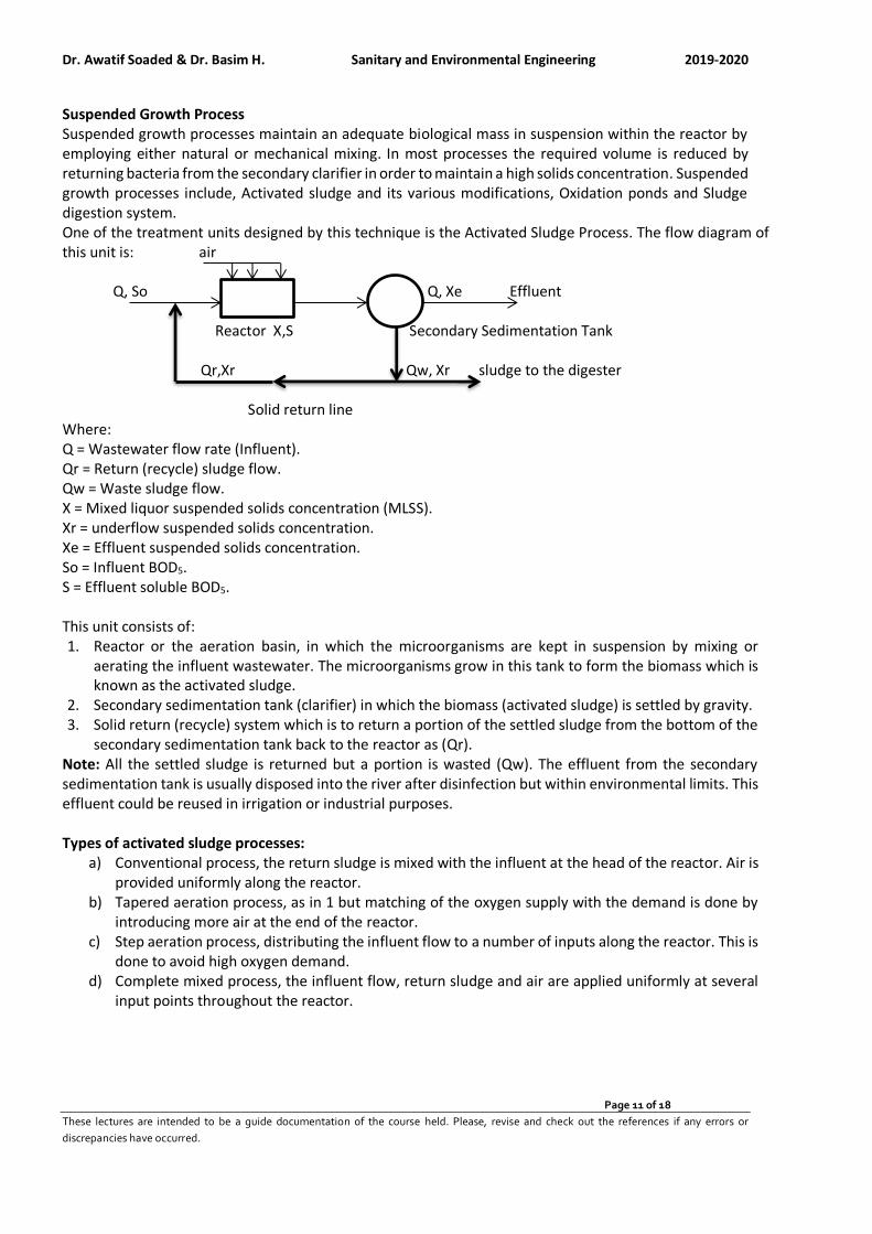
Dr. Awatif Soaded & Dr. Basim H. Sanitary and Environmental Engineering 2019-2020
Page 11 of 18
These lectures are intended to be a guide documentation of the course held. Please, revise and check out the references if any errors or
discrepancies have occurred.
Suspended Growth Process Suspended growth processes maintain an adequate biological mass in suspension within the reactor by employing either natural or mechanical mixing. In most processes the required volume is reduced by returning bacteria from the secondary clarifier in order to maintain a high solids concentration. Suspended growth processes include, Activated sludge and its various modifications, Oxidation ponds and Sludge digestion system. One of the treatment units designed by this technique is the Activated Sludge Process. The flow diagram of this unit is: air Q, So Q, Xe Effluent Reactor X,S Secondary Sedimentation Tank Qr,Xr Qw, Xr sludge to the digester Solid return line Where: Q = Wastewater flow rate (Influent). Qr = Return (recycle) sludge flow. Qw = Waste sludge flow. X = Mixed liquor suspended solids concentration (MLSS). Xr = underflow suspended solids concentration. Xe = Effluent suspended solids concentration. So = Influent BOD5. S = Effluent soluble BOD5. This unit consists of: 1. Reactor or the aeration basin, in which the microorganisms are kept in suspension by mixing or
aerating the influent wastewater. The microorganisms grow in this tank to form the biomass which is known as the activated sludge.
2. Secondary sedimentation tank (clarifier) in which the biomass (activated sludge) is settled by gravity. 3. Solid return (recycle) system which is to return a portion of the settled sludge from the bottom of the
secondary sedimentation tank back to the reactor as (Qr). Note: All the settled sludge is returned but a portion is wasted (Qw). The effluent from the secondary sedimentation tank is usually disposed into the river after disinfection but within environmental limits. This effluent could be reused in irrigation or industrial purposes. Types of activated sludge processes:
a) Conventional process, the return sludge is mixed with the influent at the head of the reactor. Air is provided uniformly along the reactor.
b) Tapered aeration process, as in 1 but matching of the oxygen supply with the demand is done by introducing more air at the end of the reactor.
c) Step aeration process, distributing the influent flow to a number of inputs along the reactor. This is done to avoid high oxygen demand.
d) Complete mixed process, the influent flow, return sludge and air are applied uniformly at several input points throughout the reactor.
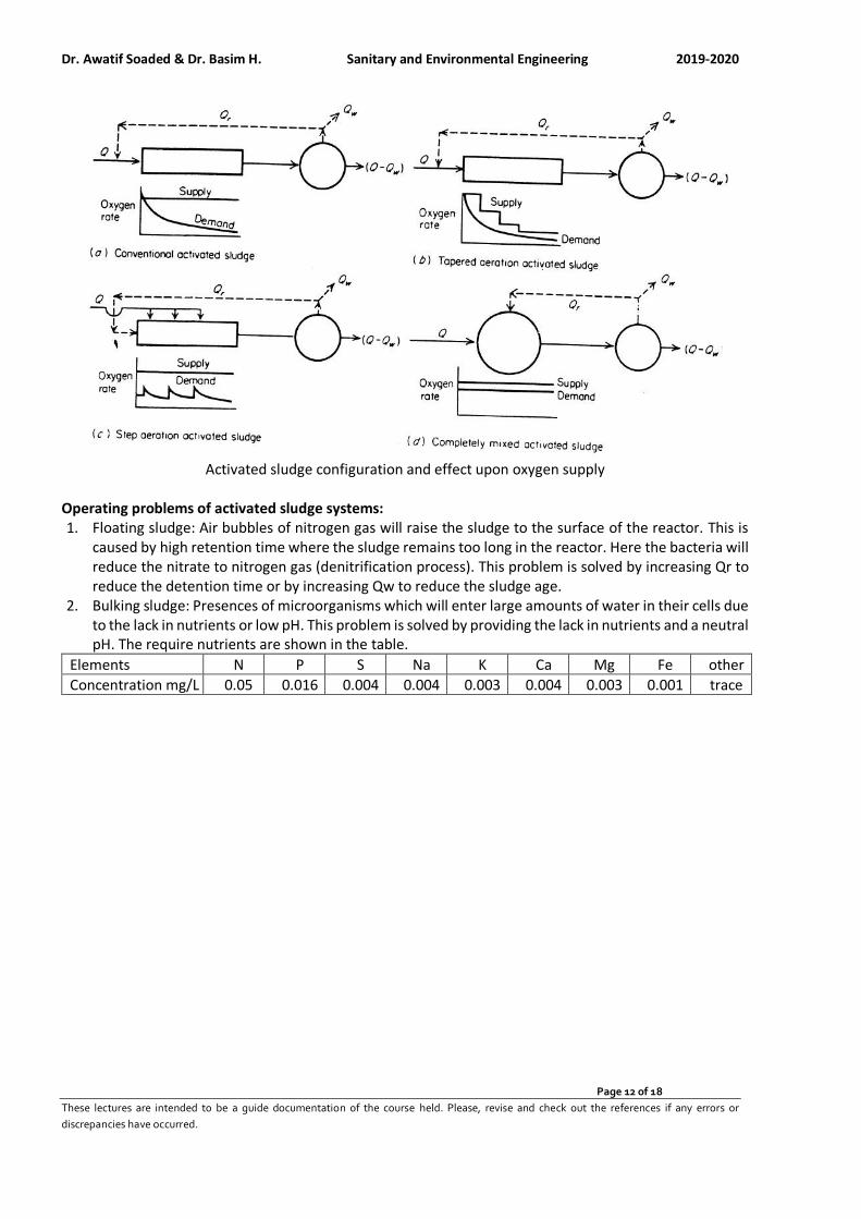
Dr. Awatif Soaded & Dr. Basim H. Sanitary and Environmental Engineering 2019-2020
Page 12 of 18
These lectures are intended to be a guide documentation of the course held. Please, revise and check out the references if any errors or
discrepancies have occurred.
Activated sludge configuration and effect upon oxygen supply
Operating problems of activated sludge systems: 1. Floating sludge: Air bubbles of nitrogen gas will raise the sludge to the surface of the reactor. This is
caused by high retention time where the sludge remains too long in the reactor. Here the bacteria will reduce the nitrate to nitrogen gas (denitrification process). This problem is solved by increasing Qr to reduce the detention time or by increasing Qw to reduce the sludge age.
2. Bulking sludge: Presences of microorganisms which will enter large amounts of water in their cells due to the lack in nutrients or low pH. This problem is solved by providing the lack in nutrients and a neutral pH. The require nutrients are shown in the table.
Elements N P S Na K Ca Mg Fe other
Concentration mg/L 0.05 0.016 0.004 0.004 0.003 0.004 0.003 0.001 trace
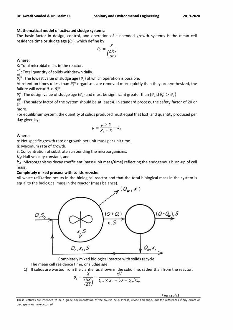
Dr. Awatif Soaded & Dr. Basim H. Sanitary and Environmental Engineering 2019-2020
Page 13 of 18
These lectures are intended to be a guide documentation of the course held. Please, revise and check out the references if any errors or
discrepancies have occurred.
Mathematical model of activated sludge systems: The basic factor in design, control, and operation of suspended growth systems is the mean cell residence time or sludge age (𝜃𝑐), which define by:
𝜃𝑐 =𝑋
(∆𝑋∆𝑡
)
Where: X: Total microbial mass in the reactor. ∆𝑋
∆𝑡: Total quantity of solids withdrawn daily.
𝜃𝑐𝑚: The lowest value of sludge age (𝜃𝑐) at which operation is possible.
At retention times 𝜃 less than 𝜃𝑐𝑚 organisms are removed more quickly than they are synthesized, the
failure will occur 𝜃 < 𝜃𝑐𝑚.
𝜃𝑐𝑑: The design value of sludge age (𝜃𝑐) and must be significant greater than (𝜃𝑐),(𝜃𝑐
𝑑 > 𝜃𝑐) 𝜃𝑐
𝑑
𝜃𝑐𝑚: The safety factor of the system should be at least 4. In standard process, the safety factor of 20 or
more. For equilibrium system, the quantity of solids produced must equal that lost, and quantity produced per day given by:
𝜇 =�̂� × 𝑆
𝐾𝑠 + 𝑆− 𝑘𝑑
Where: 𝜇: Net specific growth rate or growth per unit mass per unit time. �̂�: Maximum rate of growth. S: Concentration of substrate surrounding the microorganisms. 𝐾𝑠: Half velocity constant, and 𝑘𝑑 : Microorganisms decay coefficient (mass/unit mass/time) reflecting the endogenous burn-up of cell mass. Completely mixed process with solids recycle: All waste utilization occurs in the biological reactor and that the total biological mass in the system is equal to the biological mass in the reactor (mass balance).
Completely mixed biological reactor with solids recycle.
The mean cell residence time, or sludge age: 1) If solids are wasted from the clarifier as shown in the solid line, rather than from the reactor:
𝜃𝑐 =𝑋
(∆𝑋∆𝑡
)=
𝑥𝑉
𝑄𝑤 × 𝑥𝑟 + (𝑄 − 𝑄𝑤)𝑥𝑒
Dr. Awatif Soaded & Dr. Basim H. Sanitary and Environmental Engineering 2019-2020
Page 14 of 18
These lectures are intended to be a guide documentation of the course held. Please, revise and check out the references if any errors or
discrepancies have occurred.
Where: Q: Waste flow rate, x: Mixed liquor suspended solid concentration (MLSS). xr: Clarifier underflow suspended solids concentration. xe: Effluent suspended solids concentration. Qw: Waste sludge flow rate, and Qr: Return sludge flow rate.
2) If solids are wasted from the reactor as shown in the dashed line, rather than from the clarifier:
𝜃𝑐 =𝑥𝑉
𝑄𝑤 × 𝑥 + (𝑄 − 𝑄𝑤)𝑥𝑒
Lawrence and McCarty have shown the total microbial mass in the reactor is given by:
𝑥𝑉 =𝑌×𝑄×(𝑆0−𝑆)×𝜃𝑐
1+𝑘𝑑×𝜃𝑐 & 𝑥 =
𝜃𝑐
𝜃×
𝑌×(𝑆0−𝑆)
1+𝑘𝑑×𝜃𝑐
Where: Y: Growth yield coefficient relating cell yield to the material metabolized. S0: Influent BOD5. S: Effluent soluble BOD5
𝜃: Liquid retention time in the reactor, 𝜃 =𝑉
𝑄
Secondary Sedimentation Tank
a) In trickling filters: is used to remove large particles of sloughed slime layer. Its design is similar to Primary Sedimentation tanks. For design requirements: SOR 25 – 33 m/d and not to exceed 50 m/d at peak flow.
b) In activated sludge process: is used to contribute BOD of the effluent and for thickening the sludge to maintain the required sludge age. For design requirements: Solid loading rate = 2.5 -6.2 kg/m2/hr at average flow and not to exceed 10.2 kg/m2/hr at peak flow SOR = 16 – 32 m/d at average flow and 40 – 64 m/d at peak flow Weir loading 125 – 375 m3/m /d Depth = 2.5 – 6 m
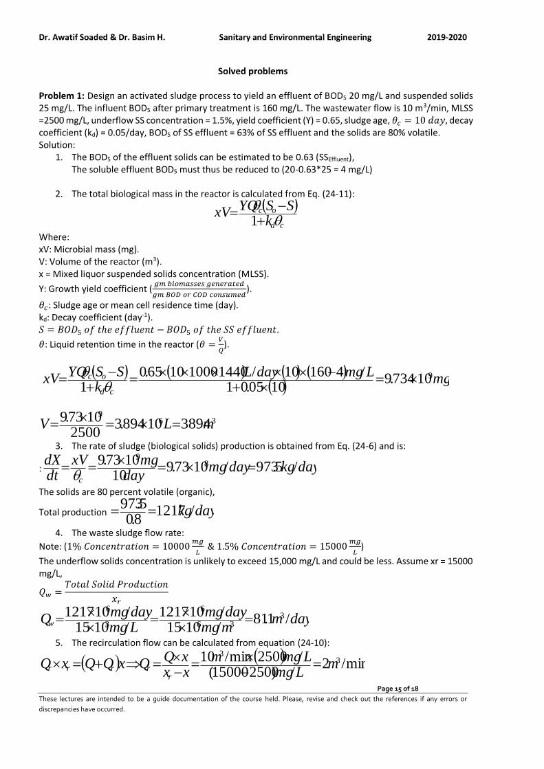
Dr. Awatif Soaded & Dr. Basim H. Sanitary and Environmental Engineering 2019-2020
Page 15 of 18
These lectures are intended to be a guide documentation of the course held. Please, revise and check out the references if any errors or
discrepancies have occurred.
Solved problems Problem 1: Design an activated sludge process to yield an effluent of BOD5 20 mg/L and suspended solids 25 mg/L. The influent BOD5 after primary treatment is 160 mg/L. The wastewater flow is 10 m3/min, MLSS =2500 mg/L, underflow SS concentration = 1.5%, yield coefficient (Y) = 0.65, sludge age, 𝜃𝑐 = 10 𝑑𝑎𝑦, decay coefficient (kd) = 0.05/day, BOD5 of SS effluent = 63% of SS effluent and the solids are 80% volatile. Solution:
1. The BOD5 of the effluent solids can be estimated to be 0.63 (SSEffluent), The soluble effluent BOD5 must thus be reduced to (20-0.63*25 = 4 mg/L)
2. The total biological mass in the reactor is calculated from Eq. (24-11):
( )cd
oc
kSSYQ
xV
+
−=
1
Where: xV: Microbial mass (mg). V: Volume of the reactor (m3). x = Mixed liquor suspended solids concentration (MLSS).
Y: Growth yield coefficient (𝑔𝑚 𝑏𝑖𝑜𝑚𝑎𝑠𝑠𝑒𝑠 𝑔𝑒𝑛𝑒𝑟𝑎𝑡𝑒𝑑
𝑔𝑚 𝐵𝑂𝐷 𝑜𝑟 𝐶𝑂𝐷 𝑐𝑜𝑛𝑠𝑢𝑚𝑒𝑑).
𝜃𝑐: Sludge age or mean cell residence time (day). kd: Decay coefficient (day-1). 𝑆 = 𝐵𝑂𝐷5 𝑜𝑓 𝑡ℎ𝑒 𝑒𝑓𝑓𝑙𝑢𝑒𝑛𝑡 − 𝐵𝑂𝐷5 𝑜𝑓 𝑡ℎ𝑒 𝑆𝑆 𝑒𝑓𝑓𝑙𝑢𝑒𝑛𝑡.
𝜃: Liquid retention time in the reactor (𝜃 =𝑉
𝑄).
( ) ( ) ( ) ( )
( ) mgLmgdayL
kSSYQ
xVcd
oc 910734.91005.01
/416010/144010001065.01
=+
−=
+−
=
369
389410894.32500
1073.9mLV ==
=
3. The rate of sludge (biological solids) production is obtained from Eq. (24-6) and is:
: daykgdaymgday
mgxVdtdX
c
/5.973/1073.910
1073.9 89
==
==
The solids are 80 percent volatile (organic),
Total production daykg/12178.05.973==
4. The waste sludge flow rate:
Note: (1% 𝐶𝑜𝑛𝑐𝑒𝑛𝑡𝑟𝑎𝑡𝑖𝑜𝑛 = 10000𝑚𝑔
𝐿 & 1.5% 𝐶𝑜𝑛𝑐𝑒𝑛𝑡𝑟𝑎𝑡𝑖𝑜𝑛 = 15000
𝑚𝑔
𝐿)
The underflow solids concentration is unlikely to exceed 15,000 mg/L and could be less. Assume xr = 15000 mg/L,
𝑄𝑤 =𝑇𝑜𝑡𝑎𝑙 𝑆𝑜𝑙𝑖𝑑 𝑃𝑟𝑜𝑑𝑢𝑐𝑡𝑖𝑜𝑛
𝑥𝑟
daymmmgdaymg
Lmgdaymg
Qw /1.81/1015/101217
/1015/101217 3
36
6
3
6
=
=
=
5. The recirculation flow can be calculated from equation (24-10):
( ) ( )min/2
/)250015000(/2500min/10 3
3
mLmgLmgm
xxxQ
QxQQxQr
rrrr =−
=−
=+=
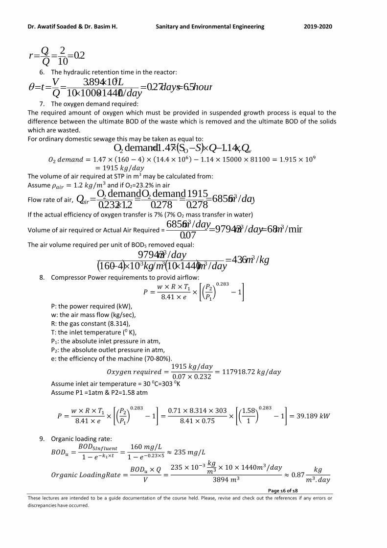
Dr. Awatif Soaded & Dr. Basim H. Sanitary and Environmental Engineering 2019-2020
Page 16 of 18
These lectures are intended to be a guide documentation of the course held. Please, revise and check out the references if any errors or
discrepancies have occurred.
2.0102===
r r
6. The hydraulic retention time in the reactor:
hoursdaysdayL
LQV
t 5.627.0/1440100010
10894.3 3
==
===
7. The oxygen demand required: The required amount of oxygen which must be provided in suspended growth process is equal to the difference between the ultimate BOD of the waste which is removed and the ultimate BOD of the solids which are wasted. For ordinary domestic sewage this may be taken as equal to:
( ) wrQxQS 14.1S1.47demand O O2 −−=
𝑂2 𝑑𝑒𝑚𝑎𝑛𝑑 = 1.47 × (160 − 4) × (14.4 × 106) − 1.14 × 15000 × 81100 = 1.915 × 109
= 1915 𝑘𝑔/𝑑𝑎𝑦 The volume of air required at STP in m3 may be calculated from: Assume 𝜌𝑎𝑖𝑟 = 1.2 𝑘𝑔/𝑚3 and if O2=23.2% in air
Flow rate of air, daymQair /6856278.0
1915278.0
demand O2.1232.0
demand O 322 ===
=
If the actual efficiency of oxygen transfer is 7% (7% O2 mass transfer in water)
Volume of air required or Actual Air Required = min/68/9794307.0
/6856 333
mdaymdaym
==
The air volume required per unit of BOD5 removed equal:
( ) ( ) kgmdaymmkg
daym/6.43
/144010/104160/97943 3
333
3
=− −
8. Compressor Power requirements to provid airflow:
𝑃 =𝑤 × 𝑅 × 𝑇1
8.41 × 𝑒× [(
𝑃2
𝑃1)
0.283
− 1]
P: the power required (kW), w: the air mass flow (kg/sec), R: the gas constant (8.314), T: the inlet temperature (0 K), P1: the absolute inlet pressure in atm, P2: the absolute outlet pressure in atm, e: the efficiency of the machine (70-80%).
𝑂𝑥𝑦𝑔𝑒𝑛 𝑟𝑒𝑞𝑢𝑖𝑟𝑒𝑑 =1915 𝑘𝑔/𝑑𝑎𝑦
0.07 × 0.232= 117918.72 𝑘𝑔/𝑑𝑎𝑦
Assume inlet air temperature = 30 0C=303 0K Assume P1 =1atm & P2=1.58 atm
𝑃 =𝑤 × 𝑅 × 𝑇1
8.41 × 𝑒× [(
𝑃2
𝑃1)
0.283
− 1] =0.71 × 8.314 × 303
8.41 × 0.75× [(
1.58
1)
0.283
− 1] = 39.189 𝑘𝑊
9. Organic loading rate:
𝐵𝑂𝐷𝑢 =𝐵𝑂𝐷5𝐼𝑛𝑓𝑙𝑢𝑒𝑛𝑡
1 − 𝑒−𝑘1×𝑡=
160 𝑚𝑔/𝐿
1 − 𝑒−0.23×5≈ 235 𝑚𝑔/𝐿
𝑂𝑟𝑔𝑎𝑛𝑖𝑐 𝐿𝑜𝑎𝑑𝑖𝑛𝑔𝑅𝑎𝑡𝑒 =𝐵𝑂𝐷𝑢 × 𝑄
𝑉=
235 × 10−3 𝑘𝑔𝑚3 × 10 × 1440𝑚3/𝑑𝑎𝑦
3894 𝑚3≈ 0.87
𝑘𝑔
𝑚3. 𝑑𝑎𝑦
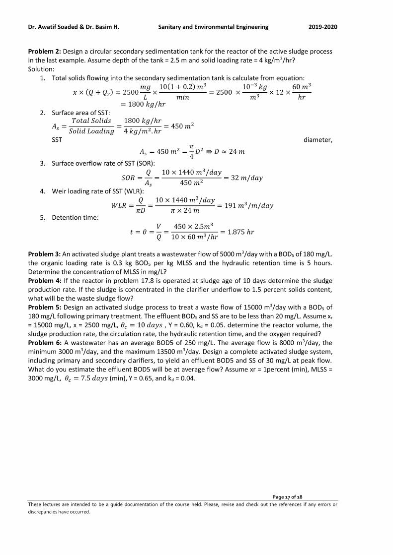
Dr. Awatif Soaded & Dr. Basim H. Sanitary and Environmental Engineering 2019-2020
Page 17 of 18
These lectures are intended to be a guide documentation of the course held. Please, revise and check out the references if any errors or
discrepancies have occurred.
Problem 2: Design a circular secondary sedimentation tank for the reactor of the active sludge process in the last example. Assume depth of the tank = 2.5 m and solid loading rate = 4 kg/m2/hr? Solution:
1. Total solids flowing into the secondary sedimentation tank is calculate from equation:
𝑥 × (𝑄 + 𝑄𝑟) = 2500𝑚𝑔
𝐿×
10(1 + 0.2) 𝑚3
𝑚𝑖𝑛= 2500 ×
10−3 𝑘𝑔
𝑚3× 12 ×
60 𝑚3
ℎ𝑟= 1800 𝑘𝑔/ℎ𝑟
2. Surface area of SST:
𝐴𝑠 =𝑇𝑜𝑡𝑎𝑙 𝑆𝑜𝑙𝑖𝑑𝑠
𝑆𝑜𝑙𝑖𝑑 𝐿𝑜𝑎𝑑𝑖𝑛𝑔=
1800 𝑘𝑔/ℎ𝑟
4 𝑘𝑔/𝑚2. ℎ𝑟= 450 𝑚2
SST diameter,
𝐴𝑠 = 450 𝑚2 =𝜋
4𝐷2 ⇛ 𝐷 ≈ 24 𝑚
3. Surface overflow rate of SST (SOR):
𝑆𝑂𝑅 =𝑄
𝐴𝑠=
10 × 1440 𝑚3/𝑑𝑎𝑦
450 𝑚2= 32 𝑚/𝑑𝑎𝑦
4. Weir loading rate of SST (WLR):
𝑊𝐿𝑅 =𝑄
𝜋𝐷=
10 × 1440 𝑚3/𝑑𝑎𝑦
𝜋 × 24 𝑚= 191 𝑚3/𝑚/𝑑𝑎𝑦
5. Detention time:
𝑡 = 𝜃 =𝑉
𝑄=
450 × 2.5𝑚3
10 × 60 𝑚3/ℎ𝑟= 1.875 ℎ𝑟
Problem 3: An activated sludge plant treats a wastewater flow of 5000 m3/day with a BOD5 of 180 mg/L. the organic loading rate is 0.3 kg BOD5 per kg MLSS and the hydraulic retention time is 5 hours. Determine the concentration of MLSS in mg/L? Problem 4: If the reactor in problem 17.8 is operated at sludge age of 10 days determine the sludge production rate. If the sludge is concentrated in the clarifier underflow to 1.5 percent solids content, what will be the waste sludge flow? Problem 5: Design an activated sludge process to treat a waste flow of 15000 m3/day with a BOD5 of 180 mg/L following primary treatment. The effluent BOD5 and SS are to be less than 20 mg/L. Assume xr = 15000 mg/L, x = 2500 mg/L, 𝜃𝑐 = 10 𝑑𝑎𝑦𝑠 , Y = 0.60, kd = 0.05. determine the reactor volume, the sludge production rate, the circulation rate, the hydraulic retention time, and the oxygen required? Problem 6: A wastewater has an average BOD5 of 250 mg/L. The average flow is 8000 m3/day, the minimum 3000 m3/day, and the maximum 13500 m3/day. Design a complete activated sludge system, including primary and secondary clarifiers, to yield an effluent BOD5 and SS of 30 mg/L at peak flow. What do you estimate the effluent BOD5 will be at average flow? Assume xr = 1percent (min), MLSS = 3000 mg/L, 𝜃𝑐 = 7.5 𝑑𝑎𝑦𝑠 (min), Y = 0.65, and kd = 0.04.

Dr. Awatif Soaded & Dr. Basim H. Sanitary and Environmental Engineering 2019-2020
Page 18 of 18
These lectures are intended to be a guide documentation of the course held. Please, revise and check out the references if any errors or
discrepancies have occurred.
How to Choose a DRM Software to protect your document?

Dr. Awatif Soaded & Dr. Basim H. Sanitary and Environmental Engineering 2019-2020
Page 1 of 17
These lectures are intended to be a guide documentation of the course held. Please, revise and check out the references if any
errors or discrepancies have occurred.
Sanitary and Environmental
Engineering
SANITARY LABORATORY EXPERIMENTS
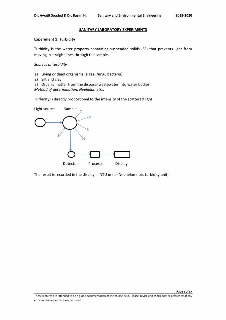
Dr. Awatif Soaded & Dr. Basim H. Sanitary and Environmental Engineering 2019-2020
Page 2 of 17
These lectures are intended to be a guide documentation of the course held. Please, revise and check out the references if any
errors or discrepancies have occurred.
SANITARY LABORATORY EXPERIMENTS
Experiment 1: Turbidity
Turbidity is the water property containing suspended solids (SS) that prevents light from
moving in straight lines through the sample.
Sources of turbidity
1) Living or dead organisms (algae, fungi, bacteria). 2) Silt and clay. 3) Organic matter from the disposal wastewater into water bodies. Method of determination: Nephelometric
Turbidity is directly proportional to the intensity of the scattered light
Light source Sample
The result is recorded in the display in NTU units (Nephelometric turbidity unit).
Detector Processer Display
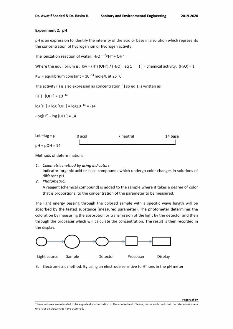
Dr. Awatif Soaded & Dr. Basim H. Sanitary and Environmental Engineering 2019-2020
Page 3 of 17
These lectures are intended to be a guide documentation of the course held. Please, revise and check out the references if any
errors or discrepancies have occurred.
Experiment 2: pH
pH is an expression to identify the intensity of the acid or base in a solution which represents
the concentration of hydrogen ion or hydrogen activity.
The ionization reaction of water: H2O H + + OH -
Where the equilibrium is: Kw = (H+) (OH -) / (H2O) eq 1 ( ) = chemical activity, (H2O) = 1
Kw = equilibrium constant = 10 -14 mole/L at 25 oC
The activity ( ) is also expressed as concentration [ ] so eq 1 is written as
[H+] [OH -] = 10 -14
log[H+] + log [OH -] = log10 -14 = -14
-log[H+] - log [OH -] = 14
Let –log = p
pH + pOH = 14
Methods of determination:
1. Colemetric method by using indicators: Indicator: organic acid or base compounds which undergo color changes in solutions of different pH.
2. Photometric:
A reagent (chemical compound) is added to the sample where it takes a degree of color
that is proportional to the concentration of the parameter to be measured.
The light energy passing through the colored sample with a specific wave length will be
absorbed by the tested substance (measured parameter). The photometer determines the
coloration by measuring the absorption or transmission of the light by the detector and then
through the processer which will calculate the concentration. The result is then recorded in
the display.
Light source Sample Detector Processer Display
3. Electrometric method: By using an electrode sensitive to H+ ions in the pH meter
0 acid 7 neutral 14 base
Dr. Awatif Soaded & Dr. Basim H. Sanitary and Environmental Engineering 2019-2020
Page 4 of 17
These lectures are intended to be a guide documentation of the course held. Please, revise and check out the references if any
errors or discrepancies have occurred.
Experiment 3: Color
Sources of color: present of some ions (Fe, Mg, Mn), organic material, soil particles and
industrial and domestic sewage.
Types: 1-True color caused by dissolved matter which can be removed by chemical processes.
2- Apparent color caused by suspended colloidal matter and could be removed by
sedimentation and/ or filtration.
Methods of determination
1- Color comparison with standard colors of potassium chloro platinum K2PtCl6 , using the lavibond
device.
Put 50 mL of the sample in the nessler tube.
Put the tube on the right side in the device.
Put an empty tube on the left side in the device.
Compare the color of the sample with the color on the hazen disc (K2PtCl6 colors) and read the
result which is expressed as unit color.
Note: if the reading is more than 70 then the sample should be diluted with distilled water.
Color = reading x dilution factor
2- Photometric method, using the wave length for color determination.
Dr. Awatif Soaded & Dr. Basim H. Sanitary and Environmental Engineering 2019-2020
Page 5 of 17
These lectures are intended to be a guide documentation of the course held. Please, revise and check out the references if any
errors or discrepancies have occurred.
Experiment 4: Total Solids, Total Suspended Solids, and Total Dissolved Solids
Is the matter (suspended and dissolved solids) that remain as residue upon evaporating and
drying of a known volume of a water sample, at 103 -105 oC for 24 hrs. It is expressed as TS
and reported in mg/L.
Methods of determination:
1. Weight a clean pan (A1) gm.
2. Put a measured volume of sample (Vs) mL.
3. Put the pan in the drying oven at 103-105 oC for 24 hrs .
4. Weight the pan and residues after drying (A2) gm.
5. Calculate concentration of total solids mg/L, 𝑇𝑆 =(𝐴2−𝐴1)
𝑉𝑠× 106
Total solids (TS) = Total dissolved solids (TDS) + Total suspended solids (TSS)
Total dissolved solids (Filterable): Consist mainly of inorganic salts present in water and any
amounts of dissolved organic matter. It is expressed as TDS and reported as mg/L. It refers to the
material that passes through filter paper (no.1) and the filtrated water is dried at 103 -105 oC for
24 hrs .
Total suspended solids (nonfilterable): The non-dissolved matter such as silt, clay and
microorganisms resent in water. It is expressed as TSS and reported as mg/L. It refers to the
material that remains on the filter paper and after drying at 103 -105 oC for 24 hrs .
Methods of determination
1. Weight a clean pan (B1) gm and a clean dry filter paper (no.1) (C1) gm.
2. Filter a measured volume of sample (Vs) mL through the filter paper.
3. Put the pan and filter paper in the drying oven at 103-105 oC for 24 hrs .
4. Weight the pan and residues after drying (B2) gm.
5. Weight the filter paper and residues after drying (C2) gm.
6. Calculate concentration of total dissolved solids mg/L, 𝑇𝐷𝑆 =(𝐵2−𝐵1)
𝑉𝑠× 106
7. Calculate concentration of total suspended solids mg/L, 𝑇𝑆𝑆 =(𝐶2−𝐶1)
𝑉𝑠× 106
Note: The hot pans and filter papers should be kept in a desiccator to cool out before
weighing.

Dr. Awatif Soaded & Dr. Basim H. Sanitary and Environmental Engineering 2019-2020
Page 6 of 17
These lectures are intended to be a guide documentation of the course held. Please, revise and check out the references if any
errors or discrepancies have occurred.
Example: Total solids (TS)
A1 = 60.05 gm, A2 = 60.0773 gm, Vs = 50 ml
𝑇𝑆 =(𝐴2 − 𝐴1)
𝑉𝑠× 106 =
(60.0773 − 60.05)
50× 106 = 546 𝑚𝑔/𝐿
Example: Total dissolved and suspended solids (TDS, TSS)
B1 = 60.065 gm, B2 = 60.0894 gm
C1 = 1.005 gm, C2 = 1.0081 gm
Vs = 50 mL
𝑇𝐷𝑆 =(𝐵2 − 𝐵1)
𝑉𝑠× 106 =
(60.0894 − 60.065)
50× 106 = 488 𝑚𝑔/𝐿
𝑇𝑆𝑆 =(𝐶2 − 𝐶1)
𝑉𝑠× 106 =
(1.0081 − 1.005)
50× 106 = 62 𝑚𝑔/𝐿
𝑇𝑆 = 𝑇𝐷𝑆 + 𝑇𝑆𝑆 = 488 + 62 = 550 𝑚𝑔/𝐿
Experiment 5: Electrical Conductivity
It is a numerical expression to represent the ability of a water sample to carry an electrical
current. It depends on the concentration and type of the ions existing in the water (TDS).
Temperature of water affects the movement and direction flow of the ions, as 1oC increase
causes 2% increase in conductivity.
The standard unit of electrical resistance is ohms (Ω), and the conductivity is the reciprocal of
the resistivity. It is expressed as 1/ ohms. cm or mhos/cm. in practical the unit used is
µmhos/cm (mhos/cm = 106 µmhos/cm). Fresh distilled water has 0.5 – 2 µmhos/cm
conductivity.
This measurement is used as a rapid estimation of TDS in a water sample:
TDS mg/L= f x conductivity µmhos/cm
Where f is a factor that depends on the ionic component in the solution and on temperature,
f = 0.55 – 0.9.
Methods of determination
Conductivity is measured by an electrical meter, using an electrode sensitive to the ionic
concentration of the water.
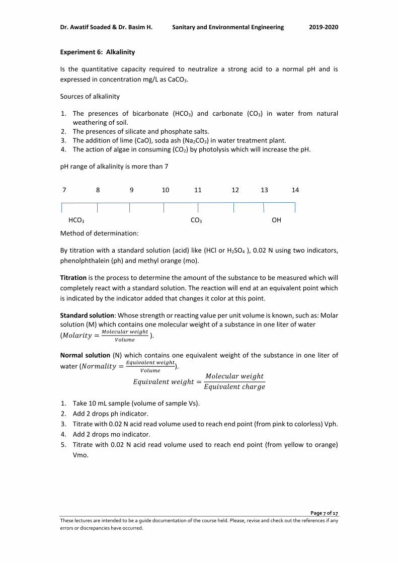
Dr. Awatif Soaded & Dr. Basim H. Sanitary and Environmental Engineering 2019-2020
Page 7 of 17
These lectures are intended to be a guide documentation of the course held. Please, revise and check out the references if any
errors or discrepancies have occurred.
Experiment 6: Alkalinity
Is the quantitative capacity required to neutralize a strong acid to a normal pH and is
expressed in concentration mg/L as CaCO3.
Sources of alkalinity
1. The presences of bicarbonate (HCO3) and carbonate (CO3) in water from natural weathering of soil.
2. The presences of silicate and phosphate salts. 3. The addition of lime (CaO), soda ash (Na2CO3) in water treatment plant. 4. The action of algae in consuming (CO2) by photolysis which will increase the pH.
pH range of alkalinity is more than 7
Method of determination:
By titration with a standard solution (acid) like (HCl or H2SO4 ), 0.02 N using two indicators,
phenolphthalein (ph) and methyl orange (mo).
Titration is the process to determine the amount of the substance to be measured which will
completely react with a standard solution. The reaction will end at an equivalent point which
is indicated by the indicator added that changes it color at this point.
Standard solution: Whose strength or reacting value per unit volume is known, such as: Molar solution (M) which contains one molecular weight of a substance in one liter of water
(𝑀𝑜𝑙𝑎𝑟𝑖𝑡𝑦 =𝑀𝑜𝑙𝑒𝑐𝑢𝑙𝑎𝑟 𝑤𝑒𝑖𝑔ℎ𝑡
𝑉𝑜𝑙𝑢𝑚𝑒 ).
Normal solution (N) which contains one equivalent weight of the substance in one liter of
water (𝑁𝑜𝑟𝑚𝑎𝑙𝑖𝑡𝑦 =𝐸𝑞𝑢𝑖𝑣𝑎𝑙𝑒𝑛𝑡 𝑤𝑒𝑖𝑔ℎ𝑡
𝑉𝑜𝑙𝑢𝑚𝑒).
𝐸𝑞𝑢𝑖𝑣𝑎𝑙𝑒𝑛𝑡 𝑤𝑒𝑖𝑔ℎ𝑡 =𝑀𝑜𝑙𝑒𝑐𝑢𝑙𝑎𝑟 𝑤𝑒𝑖𝑔ℎ𝑡
𝐸𝑞𝑢𝑖𝑣𝑎𝑙𝑒𝑛𝑡 𝑐ℎ𝑎𝑟𝑔𝑒
1. Take 10 mL sample (volume of sample Vs).
2. Add 2 drops ph indicator.
3. Titrate with 0.02 N acid read volume used to reach end point (from pink to colorless) Vph.
4. Add 2 drops mo indicator.
5. Titrate with 0.02 N acid read volume used to reach end point (from yellow to orange)
Vmo.
7 8 9 10 11 12 13 14
HCO3 CO3 OH
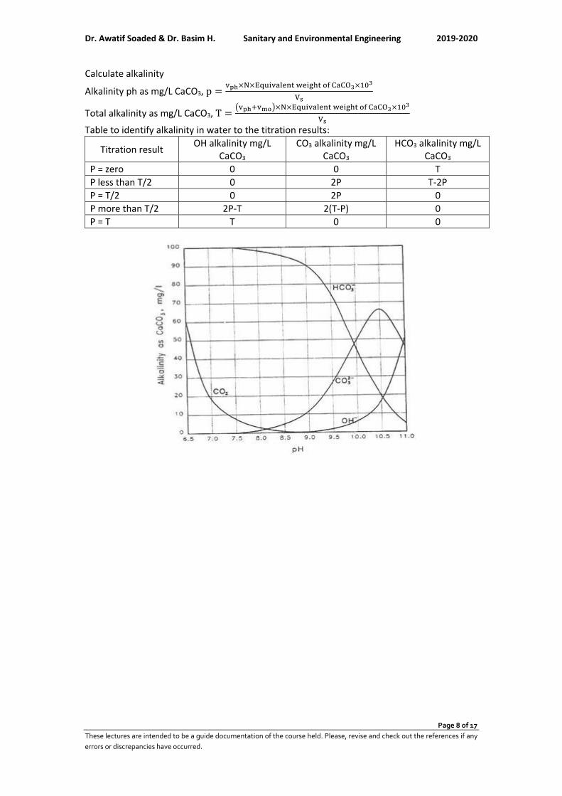
Dr. Awatif Soaded & Dr. Basim H. Sanitary and Environmental Engineering 2019-2020
Page 8 of 17
These lectures are intended to be a guide documentation of the course held. Please, revise and check out the references if any
errors or discrepancies have occurred.
Calculate alkalinity
Alkalinity ph as mg/L CaCO3, p =vph×N×Equivalent weight of CaCO3×103
Vs
Total alkalinity as mg/L CaCO3, T =(vph+vmo)×N×Equivalent weight of CaCO3×103
Vs
Table to identify alkalinity in water to the titration results:
HCO3 alkalinity mg/L CaCO3
CO3 alkalinity mg/L CaCO3
OH alkalinity mg/L CaCO3
Titration result
T 0 0 P = zero
T-2P 2P 0 P less than T/2
0 2P 0 P = T/2
0 2(T-P) 2P-T P more than T/2
0 0 T P = T
Dr. Awatif Soaded & Dr. Basim H. Sanitary and Environmental Engineering 2019-2020
Page 9 of 17
These lectures are intended to be a guide documentation of the course held. Please, revise and check out the references if any
errors or discrepancies have occurred.
Experiment 7: Jar Test
The jar test is a common laboratory procedure used to determine the optimum operating
conditions for water or wastewater treatment. This method allows adjustments in pH, variations
in coagulant or polymer dose, alternating mixing speeds, or testing of different coagulant or
polymer types, on a small scale in order to predict the functioning of a large-scale treatment
operation.
Jar Testing Apparatus
The jar testing apparatus consists of six paddles which stir the contents of six 1 liter containers.
One container acts as a control while the operating conditions can be varied among the remaining
five containers. A rpm gage at the top-center of the device allows for the uniform control of the
mixing speed in all of the containers.
Jar Test Procedure
The jar test procedure involves the following steps:
1. Fill the jar testing apparatus containers with sample water. One container will be used as a
control while the other 5 containers can be adjusted depending on what conditions are being
tested. For example, the pH of the jars can be adjusted or variations of coagulant dosages can
be added to determine optimum operating conditions.
2. Add the coagulant to each container and stir at approximately 100 rpm for 1 minute. The rapid
mix stage helps to disperse the coagulant throughout each container.
3. Reduce the stirring speed to 25 to 35 rpm and continue mixing for 15 to 20 minutes. This
slower mixing speed helps promote floc formation by enhancing particle collisions which lead
to larger flocs.
4. Turn off the mixers and allow the containers to settle for 30 to 45 minutes. Then measure the
final turbidity in each container.
Residual turbidity vs. coagulant dose is then plotted and optimal conditions are determined. The
values that are obtained through the experiment are correlated and adjusted in order to account
for the actual treatment system.
Dr. Awatif Soaded & Dr. Basim H. Sanitary and Environmental Engineering 2019-2020
Page 10 of 17
These lectures are intended to be a guide documentation of the course held. Please, revise and check out the references if any
errors or discrepancies have occurred.
Experiment 8: Hardness
Methods of determination:
1-The calculation method
Based on water analysis for cations concentrations causing
hardness (which could be determined by the photometric method).
The hardness is calculated by summing the concentrations of these
cations after multiplying each cation by a factor. The result is
recorded as:
Total hardness mg/Las CaCO3 = ∑M+ X Factor
𝐹𝑎𝑐𝑡𝑜𝑟 =𝐸𝑞𝑢𝑖𝑣𝑎𝑙𝑒𝑛𝑡 𝑤𝑒𝑖𝑔ℎ𝑡 𝑜𝑓 𝐶𝑎𝐶𝑂3
𝐸𝑞𝑢𝑖𝑣𝑎𝑙𝑒𝑛𝑡 𝑤𝑒𝑖𝑔ℎ𝑡 𝑜𝑓 𝑀+
2-Titration with EDTA
Take 10 mL sample (volume of sample Vs).
Add 10 drops of buffer solution (to make the pH about 10 for the reaction).
Add 2 drops indicator (Eriochrom black T).
Titrate with 0.01 M EDTA read volume (V) used to reach end point (from red to blue).
𝑇𝑜𝑡𝑎𝑙 ℎ𝑎𝑟𝑑𝑛𝑒𝑠𝑠𝑚𝑔
𝐿𝑎𝑠 𝐶𝑎𝐶𝑂3 =
𝑉 × 𝐵 × 103
𝑉𝑠
which is equivalent to 1 ml EDTA =1 3B = mg CaCO
Relationship between hardness and alkalinity
1-If total hardness ˃ total alkalinity
Then carbonate hardness = total alkalinity (alkalinity is HCO3 and CO3)
Non-carbonate hardness = total hardness – total alkalinity
2-If total hardness ˂ total alkalinity
Then total hardness = carbonate hardness (due to HCO3)
Alkalinity due to HCO3 and CO3 = total hardness
Alkalinity due to OH = total alkalinity - total hardness
Element equivalent wt.
CaCO3 50
M+
Ca 20
Mg 12
Fe 26
Mn 27
Al 9
Zn 32
Dr. Awatif Soaded & Dr. Basim H. Sanitary and Environmental Engineering 2019-2020
Page 11 of 17
These lectures are intended to be a guide documentation of the course held. Please, revise and check out the references if any
errors or discrepancies have occurred.
Water Quality analysis
The analytical measurements for inorganic elements in a water sample, should qualify the
following equation:
The sum of the positive ions (cations) must equal the sum of the negative ions (anions) in the
solution:
∑ cations = ∑ anions
Check the accuracy of the chemical analysis of the sample is done by calculating the
percentage difference which is determined by:
𝑃𝑒𝑟𝑐𝑒𝑛𝑡𝑎𝑔𝑒 𝑑𝑖𝑓𝑓𝑒𝑟𝑒𝑛𝑐𝑒 =(∑ 𝐶𝑎𝑡𝑖𝑜𝑛𝑠 − ∑ 𝐴𝑛𝑖𝑜𝑛𝑠)
(∑ 𝐶𝑎𝑡𝑖𝑜𝑛𝑠 + ∑ 𝐴𝑛𝑖𝑜𝑛𝑠)× 100
Where the cations and anions in the sample should be in meq / L
The acceptance criteria is given as
Problem: The following analysis has been completed for a water sample. Check the accuracy
of the analysis.
Cation Concentration mg/L
Anion Concentration mg/L
Ca 42 HCO3 115
Mg 8.6 SO4 29
Na 10 Cl 26
K 1.3 NO3 1.0
Solution:
Cation Concentration mg/L
Eq.wt. mg/meq
meq/L Anion Concentration mg/L
Eq.wt. mg/meq
meq/L
Ca 42 20 2.1 HCO3 115 61 1.89
Mg 8.6 12 0.72 SO4 29 48 0.6
Na 10 23 0.43 Cl 26 35.5 0.73
K 1.3 39 0.03 NO3 1.0 62 0.02
∑ cations 3.28 ∑ anions 3.24
𝑃𝑒𝑟𝑐𝑒𝑛𝑡𝑎𝑔𝑒 𝑑𝑖𝑓𝑓𝑒𝑟𝑒𝑛𝑐𝑒 =(∑ 𝐶𝑎𝑡𝑖𝑜𝑛𝑠 − ∑ 𝐴𝑛𝑖𝑜𝑛𝑠)
(∑ 𝐶𝑎𝑡𝑖𝑜𝑛𝑠 + ∑ 𝐴𝑛𝑖𝑜𝑛𝑠)=
(3.28 − 3.24)
(3.28 + 3.24)= 0.46%
The analysis is acceptable as ∑ anions is in the range 3 -10 and % difference is less than 2.
∑ anions meq/L Percentage difference %
0 -3.0 +- 0.2
3.0 -10.0 +- 2
10 -800 +- 5
Dr. Awatif Soaded & Dr. Basim H. Sanitary and Environmental Engineering 2019-2020
Page 12 of 17
These lectures are intended to be a guide documentation of the course held. Please, revise and check out the references if any
errors or discrepancies have occurred.
Experiment 9: Chlorine (Residual)
The determination of chlorine is to ensure the activity of the chlorination process and to
determine the residual chlorine concentration in the treated water which is supplied to the
consumer.
Methods of determination:
Photometric:
A reagent (DPD) is added to the sample where it takes a degree of color which is proportional
to the concentration of the chlorine to be measured. Put the colored sample in the device.
Set the device on chlorine and wait for the sign. The result is recorded in the display as mg/L
chlorine.
Add DPD1 + DPD2 to the sample to determine the residual as free chlorine. Then add DPD3 to
the same sample to determine total residual chlorine. So,
Combined chlorine = Total chlorine – Free chlorine.
Experiment 10: Chloride
Chloride in the form of Cl-1 ion is the major anion in water and wastewater. This ion is
considered one of the pollution indicators, as one person may produce 15 mg/L chloride in
domestic sewage.
Methods of determination
Argentometric method: titration with silver nitrate (AgNO3)
Take 10 ml water sample(Vs)
Add 2 drops potassium chromate indicator K2CrO4 indicator
Titrate with standard solution, (0.0141 N) AgNO3to reach end point yellow to reddish brown
read the volume required (V)
Calculate chloride concentration as Cl mg/L= V x N x eq. wt of Cl x103/ Vs
= V x 0.0141 x 35.5 x103/ Vs

Dr. Awatif Soaded & Dr. Basim H. Sanitary and Environmental Engineering 2019-2020
Page 13 of 17
These lectures are intended to be a guide documentation of the course held. Please, revise and check out the references if any
errors or discrepancies have occurred.
Experiment 11: Microbiology of water
Water is a good environment for different types of microorganisms to live, as it supplies the
nutrients they require. But potable water should be safe to drink which does not contain
microorganisms that cause diseases. By disinfection these microorganisms are killed. To
determine the efficiency of the disinfection process and the degree of water pollution,
microbiology tests are required.
Laboratory equipment:
1) Glass wares, pipettes, test tubes, bottles, Petri-dishes… etc.
2) Auto clave, for the sterilization of all the glass wares, liquid… etc, this is performed at
121 0C and 1 bar pressure for 15 minute.
3) Incubator, for providing the proper environment of temperature (desirable and
constant) for the growth of the microorganisms.
Samples:
1) Water samples are collected in clean and sterilized bottles.
2) The samples are to be tested immediately. If not they should be stored at 4oC (to stop
the microbial activity).
3) Samples should be diluted: river, lake, wastewater and any polluted water.
Dilution procedure:
1) Prepare a number of clean test tubes. 2) Put 9 mL of distilled water in each tube. 3) Cover each tube with cotton. 4) Sterilize the tubes in the auto clave. 5) Dilution proportions.
a) Put 1ml sample to one test tube of 9mL distilled water = 0.1 dilution(1:10). b) Put 1ml from (a) to another test tube of 9ml distilled water = 0.01 dilution (1:100). c) Put 1ml from (b) to another test tube of 9ml distilled water = 0,001 dilution and so on
(1:1000). Methods used to determine the microorganisms living in water (bacteria):
1) Total Plate count
This procedure is to determine the density of microorganisms (bacteria) in water. It is an
empirical measurement because bacteria grow in pairs, chains and colonies. Also no single
media (nutrient) will satisfy all types of bacteria. In this procedure, counting the number of
bacteria that will grow on a solid media (ager) is performed.
a) Put 1 mL of the collected sample (or diluted) in a sterilized Petri-dish.
b) Pure a suitable amount of warm and sterilized media (nutrient agar) in the Petri-
dish.
c) Put the Petri-dish in the incubator at 35 oC.
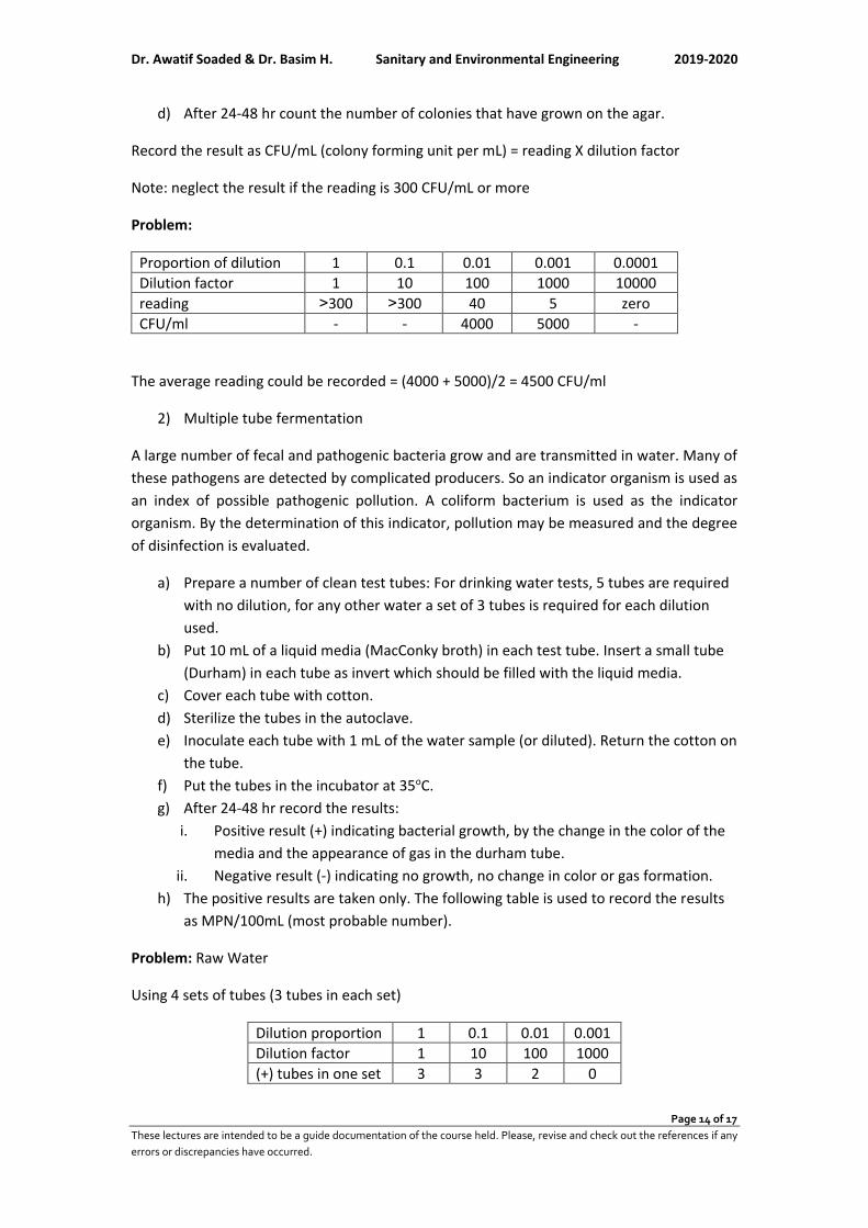
Dr. Awatif Soaded & Dr. Basim H. Sanitary and Environmental Engineering 2019-2020
Page 14 of 17
These lectures are intended to be a guide documentation of the course held. Please, revise and check out the references if any
errors or discrepancies have occurred.
d) After 24-48 hr count the number of colonies that have grown on the agar.
Record the result as CFU/mL (colony forming unit per mL) = reading X dilution factor
Note: neglect the result if the reading is 300 CFU/mL or more
Problem:
Proportion of dilution 1 0.1 0.01 0.001 0.0001
Dilution factor 1 10 100 1000 10000
reading ˃300 ˃300 40 5 zero
CFU/ml - - 4000 5000 -
The average reading could be recorded = (4000 + 5000)/2 = 4500 CFU/ml
2) Multiple tube fermentation
A large number of fecal and pathogenic bacteria grow and are transmitted in water. Many of
these pathogens are detected by complicated producers. So an indicator organism is used as
an index of possible pathogenic pollution. A coliform bacterium is used as the indicator
organism. By the determination of this indicator, pollution may be measured and the degree
of disinfection is evaluated.
a) Prepare a number of clean test tubes: For drinking water tests, 5 tubes are required
with no dilution, for any other water a set of 3 tubes is required for each dilution
used.
b) Put 10 mL of a liquid media (MacConky broth) in each test tube. Insert a small tube
(Durham) in each tube as invert which should be filled with the liquid media.
c) Cover each tube with cotton.
d) Sterilize the tubes in the autoclave.
e) Inoculate each tube with 1 mL of the water sample (or diluted). Return the cotton on
the tube.
f) Put the tubes in the incubator at 35oC.
g) After 24-48 hr record the results:
i. Positive result (+) indicating bacterial growth, by the change in the color of the
media and the appearance of gas in the durham tube.
ii. Negative result (-) indicating no growth, no change in color or gas formation.
h) The positive results are taken only. The following table is used to record the results
as MPN/100mL (most probable number).
Problem: Raw Water
Using 4 sets of tubes (3 tubes in each set)
Dilution proportion 1 0.1 0.01 0.001
Dilution factor 1 10 100 1000
(+) tubes in one set 3 3 2 0

Dr. Awatif Soaded & Dr. Basim H. Sanitary and Environmental Engineering 2019-2020
Page 15 of 17
These lectures are intended to be a guide documentation of the course held. Please, revise and check out the references if any
errors or discrepancies have occurred.
Select the last 3 dilutions for recording the results: 320 and from the table read: 93
MPN/100mL.
The raw water contains: the reading X dilution factor (the middle of the 3 dilutions used)
=93 X 100= 9300 MPN/100mL
Problem: Drinking Water Test
Using 5 tubes inoculated with 1mL of the treated water in each tube. No (+) result: less than 2.2 MPN/100mL One (+) results: 2.2 MPN/100mL Two and more (+) results: 5.1 and more MPN/100mL
Dr. Awatif Soaded & Dr. Basim H. Sanitary and Environmental Engineering 2019-2020
Page 16 of 17
These lectures are intended to be a guide documentation of the course held. Please, revise and check out the references if any
errors or discrepancies have occurred.
Experiment 12: Dissolved oxygen (DO)
The amount of oxygen gas dissolved in water, rivers, potable water, sewage …etc depends mainly on
temperature and salt content of the water. In water bodies this amount will vary with: flowing
velocity, surface area and depth. The main source of oxygen in water is from the atmosphere.
Methods of determination:
1) DO meter: By using an electrode sensitive to oxygen molecules in water.
2) Azide modification method.
a) Put the sample in a BOD bottle (250 or 300 mL)
b) Add 2mL MnSO4 solution
c) Add 2 mL alkaline –azide solution (NaOH. NaI. NaN3)
d) Shake the bottle for complete mixing:
i. IF a- a white color appears- there is no DO in the sample, then stop the
test.
ii. b-a yellow or brown color appears – there is DO in the sample , continue
the test.
e) Leave the sample to settle for 10 to 15 minutes.
f) Add 2mL H2SO4 and shake the bottle to dissolve the settle matter.
g) Take 203 mL from the bottle in a flask.
h) Add 1 mL starch as an indicator, a black color will appear.
i) Titrate with 0.025 N sodium thiosulfate Na2S2O3.
The reaction will give a blue color and the end point will be a colorless solution. Read the
volume used for titration A mL.
The concentration of DO in the sample is calculated from:
DO (mg/L)= A x N x eq.wt of O2 x 103 / volume of sample(with no additions)
= A x 0.025 x 8 x 103 / 200 = A
So DO (mg/L)= A(mL)= volume of sodium thiosulfate used for titration.
Why is a volume of 203 mL of the sample used in the titration process:
300x200/(300-4) = 202.7mL OR 250x200/(250-4) = 203.3mL
Where 250 or 300 mL =Volume of the BOD bottle used in the test
4mL = the amount of chemicals added for reaction (2mL MnSO4 = 2mL azide solution)
203mL represents the volume required for titration which is equivalent to the original
sample 200mL that satisfies the equation above.

Dr. Awatif Soaded & Dr. Basim H. Sanitary and Environmental Engineering 2019-2020
Page 17 of 17
These lectures are intended to be a guide documentation of the course held. Please, revise and check out the references if any
errors or discrepancies have occurred.
Experiment 13: Biochemical oxygen demand (BOD)
For the determination of organic matter concentrations in different types of water samples.
If high amounts of organic matter exist in the sample, the sample should be diluted to provide
enough dissolved oxygen for biodegradation.
Dilution water:
1) Take one liter of distilled water.
2) Add 2ml FeCl3 + 2ml CaCl2 + 2mL MgSO4 as nutrients.
3) Aerate the water by shaking or using an air compressor to saturate the water with
dissolve oxygen.
Dilute the water sample according to:
a) Put the diluted sample into 2 BOD bottles.
b) Determine the existing dissolved oxygen in bottle 1(by the azide method) DO2.
c) Put the 2nd bottle in the incubator for 5 days at 20oC temperature, for the
biodegradation of the organic matter in the sample.
d) Determine the remaining dissolved oxygen in the 2nd bottle DO2.
e) Calculate BOD5-20 = (DO1 –DO2) x dilution factor (Dilution factor = 1/ proportion of
dilution).
Sample Proportion of
Dilution
River water 1:3
Low strength sewage 1:5 – 1:10
High strength sewage 1:50 – 1:100
How to Choose a DRM Software to protect your document?
Copyright © 2022 FDOKUMEN