Salinity Budget and WRAP Salinity Simulation Studies of the ...

COLLEGE OF AGRICULTURE AND LIFE SCIENCES

TR-352

2009

Salinity Budget and WRAP Salinity Simulation Studies of the Brazos River/Reservoir System

By: Ralph Wurbs and Chihun Lee

Texas Water Resources Institute Technical Report No. 352 Texas A&M University System

College Station, Texas 77843-2118

July 2009

Salinity Budget and WRAP Salinity Simulation Studies of the Brazos River/Reservoir System

Prepared by

Ralph Wurbs and Chihun Lee Zachry Department of Civil Engineering and

Texas Water Resources Institute Texas A&M University

for

WRAP Modifications Project

Sponsored by the Texas Commission on Environmental Quality and Texas Water Resources Institute

Lake Whitney Comprehensive Assessment

Conducted by Baylor University Sponsored through the U.S. Department of Energy

Operations Management Model Project

Sponsored by the Brazos River Authority

Technical Report No. 352 Texas Water Resources Institute Texas A&M University System

College Station, Texas 77843-2118

July 2009

iii

ABSTRACT Natural salt pollution in the upper watersheds of the Brazos River Basin and other neighboring river basins contribute large total dissolved solids (TDS) loads to the rivers. The objectives of the studies of the Brazos River Basin reported here are (1) to enhance understanding of the occurrence, transport, and impacts of salinity in the Brazos River and Lakes Possum Kingdom, Granbury, and Whitney and (2) to improve salinity simulation capabilities of the Water Rights Analysis Package (WRAP) modeling system. Water volume and TDS load budgets are presented for five river reaches covering about 500 miles of the upper Brazos River. WRAP is applied to model the river basin for alternative modeling premises and water management scenarios. The impacts of salinity and salinity control measures on water supply capabilities are assessed.

v

TABLE OF CONTENTS Chapter 1 Introduction .................................................................................................................. 1 Scope and Objectives .................................................................................................................. 1 Organization of this Report ......................................................................................................... 2 TCEQ Water Availability Modeling (WAM) System ............................................................... 3 Dataset from USACE/USGS Natural Salt Pollution Studies ..................................................... 3 Salinity Concentrations in the Brazos River Basin .................................................................... 7 TDS Load and Concentration Versus Flow Volume Relationships ........................................ 10 Reservoirs in the Brazos River Basin ......................................................................................... 14 Lakes Possum Kingdom, Granbury, and Whitney ..................................................................... 15 Salinity Concentrations in Lakes Granbury and Whitney .......................................................... 17 River/Reservoir System Reaches for the Salinity Budget Study ................................................ 21 Chapter 2 Volume and Load Budget Procedures ...................................................................... 23 River Reaches and Gaging Stations ........................................................................................... 23 Water and Salinity Balance Relationships .................................................................................. 25 Reach Inflows and Outflows ....................................................................................................... 26 Computed Mean Storage Concentration .................................................................................... 27 Reach from the Seymour Gage to the South Bend Gage ........................................................... 28 Reach from the South Bend Gage to the Graford Gage ............................................................. 31 Reach from the Graford Gage to the Dennis Gage .................................................................... 34 Reach from the Dennis Gage to the Glen Rose Gage ................................................................ 35 Reach from the Glen Rose Gage to the Whitney Gage .............................................................. 37 Chapter 3 Volume and Load Budget Results ............................................................................. 41 Alternative Variations of TDS Load Budgets ............................................................................ 41 Volume and Load Budget Summary Tables .............................................................................. 42 Time Series Plots of Volumes, Loads, and Concentrations ....................................................... 45 Comparisons of Reservoir Storage and Outflow Quantities ...................................................... 46 Chapter 4 Alternative Variations of Load Budgets ................................................................... 67 Comparison of Alternative Methods for Synthesizing South Bend Loads .............................. 67 Alternative Methods for Distributing Excess Load for South Bend to Graford Reach ............ 71 Alternative Methods for Distributing Excess Load for Glen Rose to Whitney Reach ............. 80 Chapter 5 Relationships between Concentrations of Reservoir Outflow and Storage ......... 83 Mean Storage and Outflow Concentrations ............................................................................... 83 Relationship of Outflow Concentration to Storage Concentration ........................................... 84 Chapter 6 Salinity Routing through Reservoirs ...........................................................................95 Water Rights Analysis Package (WRAP) Modeling System .................................................... 95 Salinity Routing Methodology .................................................................................................... 96 WRAP Simulation Input Dataset for Validating and Calibrating Salinity Routing Methods ... 97

vi

Initial Simulation Results ......................................................……………………………….. 113 Simulation Studies to Explore Reservoir Routing Methods and Calibrate Parameters ........ 117 Possum Kingdom Reservoir with Lag Option 1 ...................................................................... 119 Possum Kingdom Reservoir with Lag Option 2 ...................................................................... 131 Whitney Reservoir with Lag Option 1 ...................................................................................... 142 Whitney Reservoir with Lag Option 2 ...................................................................................... 155 Reservoir Salinity Routing Parameter Calibration Summary .................................................. 166 Conclusions ................................................................................................................................ 170 Chapter 7 WRAP-SALT Salinity Input Dataset for the Brazos River Basin ...................... 171 WRAP-SIM Input Dataset ................................................................................................…… 171 WRAP-SALT Salinity Input Dataset ........................................................................................ 172 Volume and Load Balance Summaries ..................................................................................... 176 Methodology for Developing Inflow Loads and Concentrations …..……….....…………… 179 Load Losses in Reservoirs ………………………………………………………………… 183 Statistics and Plots of Stream Flow Volumes, Loads, and Concentrations ............................. 184 Salinity Inflow Data Summary …………………..............................………………………. 221 Chapter 8 WRAP Simulation of the Brazos River Basin ........................................................ 223 Brazos River Basin .................................................................................................................... 223 WRAP-SIM Input Datasets ………...................…....…….................………………………. 226 WRAP- SALT Input Dataset …………....................…….................………………………. 227 Alternative WRAP-SIM/SALT Simulations …………………........………………………. 232 Salinity Simulations with the Bwam8 Dataset ......................................................................... 233 Salinity Simulation with the BRAC8 Dataset ........................................................................... 246 Salinity Simulations with the BRAC2008 Dataset ................................................................... 256 Multiple-Reservoir System Operations .................................................................................... 281 Natural Salt Pollution Control Impoundments ......................................................................... 292 Chapter 9 Summary and Conclusions ....................................................................................... 303 Natural Salt Pollution in the Brazos River Basin ..................................................................... 303 Volume and Load Budget Studies ............................................................................................. 304 Simulation Studies with the WRAP Modeling System ......................................................... 308 Salinity Routing through Reservoirs ........................................................................................ 308 Salinity Inflows to the River System ......................................................................................... 310 Simulation of the Brazos River/Reservoir System ................................................................... 312 References ........................................................................................................................................ 315

vii

LIST OF TABLES 1.1 USGS Stream Flow and Water Quality Stations ...................................................................... 7 1.2 Period-of-Record Mean Discharge and Salt Loads and Concentrations .................................. 8 1.3 Major Reservoirs and Tributaries Upstream of Lakes Possum Kingdom,

Granbury, and Whitney ......................................................................................................... 14 1.4 Possum Kingdom, Granbury, and Whitney Reservoirs on the Brazos River .......................... 16 1.5 Reservoir Storage Capacity ....................................................................................................... 16 1.6 Watershed Drainage Area and Lake Surface Precipitation and Evaporation .......................... 17 1.7 Gaging Stations Defining Volume and Load Balance Reaches .............................................. 22 2.1 Availability of Observed Monthly Stream Flow, Storage, and Salinity Data ......................... 24 3.1 1964-1986 Mean Monthly Flow Volumes .............................................................................. 43 3.2 1964-1986 Mean Monthly Loads ............................................................................................ 43 3.3 1964-1986 Mean TDS Concentrations ................................................................................... 43 3.4 Reservoir Volumes, TDS Loads, and TDS Concentrations .................................................... 44 3.5 1964-1986 Mean Flows, Loads, and Concentrations at Gages on the Brazos River ............. 44 3.6 Other Inflow Volumes as a Watershed Runoff Depth Equivalent ......................................... 44 3.7 Portion of 1964-1986 Period-of-Anlaysis Covered by USGS Observed Data ...................... 45 3.8 Observed Storage and Outflow Concentrations for Lake Whitney ........................................ 66 4.1 Comparison of Means for Upstream Reach ............................................................................ 68 4.2 Comparison of Storage TDS loads and TDS concentration ................................................... 72 4.3 Period, Storage TDS load and TDS concentration of each method ........................................ 80 5.1 Correlation Coefficients and Regression Equations for Possum Kingdom and Whitney Storage Concentration versus Outflow Concentration ......................................................... 84 6.1 WRAP-SIM Simulation Summary Mean Monthly Flow Volumes (acre-feet/month) .......... 100 6.2 WRAP-SALT Salinity Input File Summary Monthly Loads (tons/month) ........................... 100 6.3 Concentrations for Quantities in Tables 22 and 23 (milligrams/liter) .................................... 101 6.4 Comparison of Simulated and Observed 1964-1986 Mean Concentrations .......................... 104 6.5 Linear Correlation and Regression Coefficients for Alternative Lags .................................... 120 6.6 Statistics for Possum Kingdom Reservoir Storage and Outflow Concentrations from the Salinity Budget Dataset .................................................. 127 6.7 Statistics for Concentrations at Graford Gage (TM Option 1, Lag Option 1) ........................ 127 6.8 Statistics for Concentrations at Graford Gage (TM Option 2, Lag Option 1) ........................ 128 6.9 Statistics for Possum Kingdom Storage Concentrations (TM Option 1, Lag Option 1) ....... 128 6.10 Statistics for Possum Kingdom Storage Concentrations (TM Option 2, Lag Option 1) ....... 128 6.11 Linear Correlation and Regression Coefficients for Alternative Multiplier Factors ............. 132 6.12 Statistics for Possum Kingdom Storage Concentrations (TM Option 1, Lag Option 2) ....... 138 6.13 Statistics for Concentrations at Graford Gage (TM Option 1, Lag Option 2) ........................ 139 6.14 Statistics for Possum Kingdom Storage Concentrations (TM Option 2, Lag Option 2) ....... 139 6.15 Statistics for Concentrations at Graford Gage (TM Option 2, Lag Option 2) ........................ 140 6.16 Linear Correlation and Regression Coefficients for Alternative Lags .................................... 143 6.17 Statistics for Whitney Reservoir Storage and Outflow Concentrations from the Salinity Budget Dataset .................................................. 150 6.18 Statistics for Concentrations at Whitney Gage (TM Option 1, Lag Option 1) ...................... 151 6.19 Statistics for Concentrations at Whitney Gage (TM Option 2, Lag Option 1) ...................... 151 6.20 Statistics for Whitney Storage Concentrations (TM Option 1, Lag Option 1) ....................... 152 6.21 Statistics for Whitney Storage Concentrations (TM Option 2, Lag Option 1) ....................... 152

viii

LIST OF TABLES (Continued) 6.22 Linear Correlation and Regression Coefficients for Alternative Multiplier Factors ............. 155 6.23 Statistics for Whitney Storage Concentrations (TM Option 1, Lag Option 2) ....................... 162 6.24 Statistics for Concentrations at Whitney Gage (TM Option 1, Lag Option 2) ....................... 162 6.25 Statistics for Whitney Storage Concentrations (TM Option 2, Lag Option 2) ...................... 163 6.26 Statistics for Concentrations at Whitney Gage (TM Option 2, Lag Option 2) ....................... 163 6.27 Parameter Calibration Statistics for Concentrations of Flows at Graford Gage .................... 168 6.28 Parameter Calibration Statistics for Storage Concentrations at Possum Kingdom ............... 168 6.29 Parameter Calibration Statistics for Concentrations of Flows at Whitney Gage .................... 169 6.30 Parameter Calibration Statistics for Storage Concentrations at Whitney Reservoir ............... 168 7.1 Number of Control Points and Reservoirs in Brazos Basin WRAP-SIM Input Datasets ...... 171 7.2 1964-1986 Mean Flows, Loads, and Concentrations at Selected Control Points ................... 173 7.3 Total Dissolved Solids (TDS) Data Entered in Salinity Input SIN File ................................ 174 7.4 Means of Incremental Volumes, Loads, and Concentrations of Inflows and Losses

in WRAP-SALT Salinity Input Dataset ............................................................................... 178 7.5 1964-1986 Mean TDS Load Losses Not Associated with Volumes ...................................... 184 7.6 Statistics of the Results from Linear Interpolation Method for the Seymour Gage ............... 186 7.7 Statistics of the Results from Linear Regression Method for the Seymour Gage .................. 186 7.8 Statistics of the Results from Linear Interpolation Method for the Graford Gage ................. 193 7.9 Statistics of the Results from Linear Regression Method for the Graford Gage ................... 194 7.10 Statistics of the Results from Linear Interpolation Method for the Whitney Gage ................ 200 7.11 Statistics of the Results from Linear Regression Method for the Whitney Gage .................. 201 7.12 Statistics of the Results from Linear Interpolation Method for the Cameron Gage ............... 208 7.13 Statistics of the Results from Linear Regression Method for the Cameron Gage ................. 208 7.14 Statistics of the Results from Linear Interpolation Method for the Richmond Gage ............ 215 7.15 Statistics of the Results from Linear Regression Method for the Richmond Gage ............... 215 8.1 Control Points Included in Salinity Simulation Results Tables .............................................. 224 8.2 Total Dissolved Solids Data Entered in Salinity Input SIN File ............................................. 229 8.3 WRAP-SALT Salinity Input SIN File for Use with Bwam8, BRAC8, and BRAC2008 Datasets ...................................................................................................... 230 8.4 Beginning-of-Simulation Reservoir Storage Concentrations ................................................. 231 8.5 Alternative Simulations .......................................................................................................... 233 8.6 Total Volume and Load Summary in SMS File for Simulation 1 (Bwam8, 1940-2007) 8.7 TABLES Input TIN File ........................................................................................................... 234 8.8 TABLES Output TOU File for Simulation 1 (Bwam8, 1940-2007) ................................... 237 8.9 Total Volume and Load Summary in SMS File for Simulation 2 (Bwam8, 1900-2007) ... 244 8.10 TABLES Output TOU File for Simulation 2 (Bwam8, 1900-2007) .................................. 245 8.11 BRAC8 Control Points for Stream Confluences and the Basin Outlet ............................. 248 8.12 BRAC8 Control Points at USGS Gaging Stations .............................................................. 249 8.13 BRAC Control Points for Reservoirs .................................................................................. 250 8.14 Total Volume and Load Summary in SMS File for Simulation 3 (BRAC8, 1940-2007) ...251 8.15 Control Point Summary for Simulation 3 (BRAC8, 1940-2007) ..................................... 252 8.16 Comparison of Control Point Summaries of Simulations 2 and 3 Simulation 3 (Table 8.13) as a Percentage of Simulation 2 (Table 8.8) ............................ 252 8.17 Comparison of Mean Stream Flow Concentrations ........................................................... 253 8.18 Frequency Tables for Simulation 3 (BRAC8, 1940-2007) ............................................... 254

ix

LIST OF TABLES (Continued) 8.19 Diversion Reliabilities With and Without Salinity Constraint of 1,000 mg/l for Simulation 3 (BRAC8, 1940-2007) .......................................................................... 255 8.20 Water Supply Diversions by BRA Customers During 2008 ................................................. 257 8.21 WRAP-SIM Input DAT File for the BRAC2008 Dataset ................................................. 258 8.22 Total Volume and Load Summary from SMS File for Simulation 4 (BRAC2008, 1940-2007) ....................................................................... 263 8.23 TABLES Input TIN File .................................................................................................... 264 8.24 Control Point Summary from TOU File for Simulation 4 (BRAC2008, 1940-2007) ......... 265 8.25 Concentration Frequency for Downstream Stream Flows from TOU File for Simulation 4 (BRAC2008, 1940-2007) ............................................. 266 8.26 Concentration Frequency for Reservoir Storage for Simulation 4 (BRAC2008, 1940-2007) ..................................................................... 266 8.27 Reliabilities With and Without Salinity Constraints for Simulation 4 (BRAC2008, 1940-2007) ...................................................................... 267 8.29 Reservoirs Operated by the Corps of Engineers and Brazos River Authority ..................... 281 8.30 Multiple-Reservoir System Diversions .............................................................................. 282 8.31 Concentration Statistics for Alternative Simulations .......................................................... 285 8.32 Diversion Reliabilities for Limit of 1,000 mg/l .................................................................. 286 8.33 Concentration Frequency for Downstream Stream Flows for Simulation 5 ......................... 287 8.34 Concentration Frequency for Reservoir Storage for Simulation 5 ..................................... 287 8.35 Concentration Frequency for Downstream Stream Flows for Simulation 6 ......................... 288 8.36 Concentration Frequency for Reservoir Storage for Simulation 6 ...................................... 288 8.37 Concentration Frequency for Downstream Stream Flows for Simulation 7 ......................... 289 8.38 Concentration Frequency for Reservoir Storage for Simulation 7 ....................................... 289 8.39 Concentration Frequency for Downstream Stream Flows for Simulation 8 ......................... 290 8.40 Concentration Frequency for Reservoir Storage for Simulation 8 ....................................... 290 8.41 Concentration Frequency for Downstream Stream Flows for Simulation 9 ......................... 291 8.42 Concentration Frequency for Reservoir Storage for Simulation 9 ..................................... 291 8.43 Flows and Loads in the Upper Basin .................................................................................. 294 8.44 Flows and Loads at Impoundment Sites as Percentage of Flows and Loads at the Seymour Gage ...................................................... 295 8.45 Mean Flow Volume and Load Without and With Salt Dams (Simulations 4 and 10) ......... 296 8.46 Comparison of Stream Flow Concentrations ...................................................................... 298 8.47 Comparison of Reservoir Storage Concentrations ............................................................. 297 8.48 Total Volume and Load Summary for Simulation 10 with Salt Control Impoundments ..... 299 8.49 Control Point Summary for Simulation 10 with Salt Control Impoundments .................... 300 8.50 Concentration Frequency for Stream Flows for Simulation 10 with Salt Control Impoundments ......................................................... 301 8.51 Concentration Frequency for Reservoir Storage for Simulation 10 with Salt Control Impoundments ......................................................... 301 8.52 Reliabilities With and Without Salinity Constraint of 1,000 mg/l for Simulation 10 with Salt Control Impoundments ........................................................ 302

1

CHAPTER 1 INTRODUCTION

Scope and Objectives The studies of the Brazos River Basin documented by this report build upon and combine the Texas Commission on Environmental Quality (TCEQ) Water Availability Modeling (WAM) System and salinity data collected by the U.S. Geological Survey (USGS). • The WAM System developed and maintained by the TCEQ consists of the generalized Water

Rights Analysis Package (WRAP) river/reservoir system simulation model and input datasets for the 23 river basins of Texas, including the Brazos. The WAM System deals with water quantity, not water quality. However, WRAP does have a salinity modeling component called WRAP-SALT, which is still in a developmental stage. The investigation documented in this report included testing, improving, and applying WRAP-SALT. The effects of salinity on water supply capabilities were assessed based on WRAP simulation studies with input data for the Brazos River Basin from the WAM System combined with a WRAP-SALT salinity input file developed from the following USGS dataset.

• The USGS conducted an extension salinity data collection program from October 1963 through

September 1986 in support of natural salt pollution control studies performed by the U.S. Army Corps of Engineers. This dataset of water year 1964-1986 monthly salt loads and concentrations was adopted for the studies presented in this report. Volume and load budget studies were performed for five sub-reaches of a 405-mile reach of the upper Brazos River extending from the Seymour gage located 160 miles upstream of Morris Sheppard Dam to the Whitney gage located just downstream of Whitney Dam. The volume and load budget studies provide insight into salinity characteristics of the Brazos River independently of the WRAP simulation study. The volume and load budget studies for the upper Brazos River supplemented with salinity data at other locations throughout the river basin also supported development of a WRAP-SALT salinity input file for the WRAP simulation studies.

Thus, the studies described here support improvement and application of salinity simulation features that are being developed for the WRAP modeling system to incorporate consideration of water quality, particularly natural salt pollution, in assessments of water supply capabilities. The studies also provide insight into the salinity characteristics of the Brazos River Basin and impacts of salinity on water supply capabilities. The objectives of the investigation are to:

• enhance understanding of the occurrence, transport, and characteristics of salinity in the Brazos River and Lakes Possum Kingdom, Granbury, and Whitney

• test and improve the salinity simulation capabilities of the WRAP modeling system • formulate, test, and apply methods for routing salinity through reservoirs in the WRAP-

SALT model and determining parameters for the salinity routing methods • formulate, test, and apply methods for developing a salinity input dataset for WRAP-

SALT for use in water availability and water supply reliability assessments for the Brazos River Authority reservoir system

• perform a WRAP simulation study to evaluate the impacts of salinity and salinity mitigation measures on water supply capabilities of the Brazos River Authority system

2

Organization of this Report This report is organized as follows.

Background information (Chapter 1) Volume and salinity budget studies (Chapters 2, 3, 4, 5) WRAP-SALT simulation studies (Chapters 6, 7, 8) Summary and conclusions (Chapter 9)

Chapter 1 describes the Brazos River and its tributaries and reservoirs located thereon and natural salt pollution in the river system. The WRAP/WAM modeling system and USGS salinity data used in the investigation are introduced. Chapter 9 presents the summary and conclusions of the overall investigation. The remainder of report is divided between two different types of analyses: (1) volume and salinity budgets and (2) WRAP-SALT simulations. The volume and salinity budget studies are presented in Chapters 2−5 independently of the WRAP modeling system and provide insight regarding the occurrence, transport, and characteristics of salinity even without the WRAP-SALT simulation studies of Chapters 6−8. However, the volume and load budgets also support development of input for WRAP-SALT. Water volume and total dissolved solids (TDS) load budgets are developed for each of five subreaches of a 405 reach of the Brazos River that includes Possum Kingdom, Granbury, and Whitney Reservoirs and extends from below the primary salt source subwatersheds to below Whitney dam. An accounting of the components of inflow and outflow and storage loads and volumes is performed for each month of the analysis period October 1963 through September 1986. Observed flow, load, and concentration data are adopted where available and additional data are synthesized as necessary. The procedures for compiling the necessary data and performing the accounting computations are outlined in Chapter 2. Results are presented in Chapter 3. Additional analyses and discussions of aspects of the volume and load budgets are presented in Chapters 4 and 5. Chapter 4 discusses alternative methods for synthesizing missing data. Chapter 5 presents relationships between TDS concentrations of reservoir outflow and storage to support investigation of methods for routing salinity through reservoirs. Chapters 6, 7, and 8 focus on the WRAP simulation modeling system and its application to the Brazos River Basin. Chapter 6 deals with methodologies for routing salinity through reservoirs and approaches for estimating values for the parameters used in the routing methods. Chapter 7 outlines the development of a WRAP-SALT salinity input file for the Brazos River Basin. TDS loads and concentrations of inflows to the river system are specified at all pertinent locations in the river basin for each month of a 1900-2007 hydrologic period-of-analysis based on observed monthly salinity data for 1964-1986. WRAP-SALT simulation studies for the Brazos River Basin are presented in Chapter 8. Various WRAP studies without consideration of salinity have been performed in the past using the WAM System datasets noted in Chapter 1 and variations thereof. The WRAP-SALT salinity input dataset described in Chapter 7 allows incorporation of salinity considerations. Chapter 8 provides analyses of the impacts of salinity and salinity mitigation measures on the water supply capabilities of the Brazos River Authority reservoir system.

3

TCEQ Water Availability Modeling (WAM) System The Texas Commission on Environmental Quality (TCEQ) Water Availability Modeling (WAM) System described at the following website

http://www.tceq.state.tx.us/permitting/water_supply/water_rights/wam.html

consists of the generalized WRAP river/reservoir system simulation model (Wurbs 2006 and 2009),

http://ceprofs.civil.tamu.edu/rwurbs/wrap.htm

and input datasets for the 23 river basins of Texas. The WAM System is routinely applied in regional and statewide planning studies and administration of the water rights permit system, but without consideration of salinity. A major objective of the research documented by this report is to improve capabilities for incorporating salinity and measures for dealing with salinity in assessments of water availability for municipal, industrial, agricultural, and other water uses. WRAP input datasets for the Brazos River Basin for alternative water management/use scenarios are available from the TCEQ WAM System. Consulting firms developed the original Brazos WAM System datasets under contract with the TCEQ in two phases. The first phase focused on converting observed stream flows to 1940-1997 sequences of monthly naturalized stream flows representing natural hydrology without human water resources development and use (Freese and Nichols, Inc. 2001). The second phase consisted of developing complete WRAP input data for the river basin and simulating specified water management scenarios (HDR, Inc. 2001). Wurbs and Kim (2008) recently developed modified versions of the Brazos WAM datasets by extending the hydrologic period-of-analysis to 1900-2007 and condensing the dataset to focus on the Brazos River Authority reservoir system while preserving the effects of the numerous other water rights.

The Brazos River Basin WAM datasets were used in the WRAP water supply reliability studies performed in the research project reported here. Water quantities from the TCEQ WAM System WRAP input dataset and backup files were also used in the water and salinity balance studies presented in this report.

Dataset from USACE/USGS Natural Salt Pollution Studies Natural salt pollution severely constrains the water supply capabilities of the Brazos River and other neighboring rivers shown in Figure 1.1 (Wurbs 2002). Geologic formations in the Permian Basin geologic region are the primary source of the salinity. Salt springs and seeps and salt flats in the upper watersheds of the Brazos, Colorado, Pecos, Red, Canadian, and Arkansas Rivers contribute large salt loads to these rivers. The salinity drastically limits the municipal, industrial, and agricultural use of water that could otherwise be supplied by a number of existing large reservoirs located on these rivers. Water quality in Possum Kingdom, Granbury, and Whitney Reservoirs on the Brazos River shown in Figure 1.2 is seriously degraded by natural contamination by salts consisting largely of sodium chloride with moderate amounts of calcium sulfate and other dissolved solids. The primary source of the salinity is groundwater emissions in an area of about 1,500 square miles in the upper basin consisting of the Salt Fork Brazos River watershed and portions of the adjacent Double Mountain Fork Brazos River and North Croton Creek watersheds. The salinity concentrations in the Brazos River decrease significantly in the lower basin with dilution from low-salinity tributaries.

4

Figure 1.1 Major Rivers Affected by Permian Basin Salt The Fort Worth District (FWD) of the U.S. Army Corps of Engineers (USACE) in collaboration with the U.S. Geological Survey (USGS), U.S. Environmental Protection Agency (USEPA), and other agencies conducted extensive Brazos River Basin natural salt pollution studies during the 1960's-1980's (Wurbs 2002). The USGS conducted an extensive water quality data collection program from October 1963 through September 1986 in support of USACE salt pollution control studies. The USACE-sponsored USGS salinity measurement program was discontinued in 1986. The USACE later contracted with Texas A&M University to compile the USGS salinity data into a more conveniently usable format and to perform various analyses (Wurbs et al. 1993). Water year (October-September) 1964-1986 USGS/USACE observed data described by Wurbs et al. (1993) were used to develop basin-wide salinity input for the WRAP modeling studies. The salinity component of WRAP requires specification of time sequences of monthly loads entering the river system covering the 1940-1997 TCEQ WAM System simulation period throughout the river basin or the extended 1940-2007 or 1900-2007 hydrologic periods-of-analysis developed by Wurbs and Kim (2008), which are developed based on the 1964-1986 USGS data. The 1964-1986 USGS data are also used to develop the volume and load budgets presented in this report. The volume and load budgets contribute to development of WRAP salinity input data and modeling methods as well as independently providing insight regarding salinity characteristics.

5

Figure 1.2 Brazos River Basin with BRA Reservoirs and Hubbard Creek Reservoir Shown USGS water quality sampling activities in the Brazos River Basin date back to 1906 and continue to the present. However, the salinity data collection program during October 1963 through September 1986 was much more extensive than salinity measurement activities before or since. A total of 39 stations in the basin have monthly salinity data for at least three years during 1964-1986. The 26 stations listed in Tables 1.1 and 1.2 with locations shown in Figure 1.3 were selected for the compilation and analyses of Wurbs et al. (1993) because of their record length and pertinent locations. The water quality measurements occurred at or near stream flow gaging stations included in the regular USGS stream flow data collection program. The USGS continues to measure flow rates at most of the gaging stations even though the water quality measurements ended in 1986. The USGS aggregated daily flow and concentration observations into mean monthly flows and monthly concentrations and loads of total dissolved solids (TDS), chloride, and sulfate. Chloride and sulfate are major constituents of total dissolved solids (salinity) in the Brazos River. Discharges and salt loads are cited by the USGS in units of cubic feet per second (cfs) and tons/day, respectively. Monthly discharges and loads cited in this report in acre-feet/month and tons/month are based on summations of daily amounts. Salt concentrations are cited in units of milligrams of salt solute per liter of water (mg/l). Assuming a liter of water has a mass of one kilogram, the units mg/l and parts of salt solute per million parts of water (ppm) are equivalent.

6

Figure 1.3 USGS Stream Flow and Water Quality Stations (Wurbs et al. 1993)

The USGS has also periodically conducted water quality surveys of selected reservoirs in Texas. Andrews and Strause (1981, 1983) document collection of water quality data for Lake Granbury. Strauss and Andrews (1983 and 1984) document collection of water quality data for Lake Whitney. These data from water quality surveys of Lakes Whitney and Granbury are discussed later in this chapter and are used in the salinity budget studies. The main stream of the Brazos River begins at the confluence of the Salt Fork and Double Mountain Fork, which is 923 river miles above the Brazos River mouth at the Gulf of Mexico. The Aspermont and Peacock gages (Figure 1.3 map numbers 1 and 2) are located on the Salt Fork and Double Mountain Fork of the Brazos River, respectively, 35 and 54 river miles above their confluence. The Seymour, Possum Kingdom, Whitney, College Station, and Richmond gages (map numbers 7, 13, 15, 21, and 25) are located at river miles 847, 687, 442, 281, and 92, respectively, above the Gulf of Mexico. The Seymour gage is downstream of the primary salt source areas and upstream of Possum Kingdom, Granbury, and Whitney Reservoirs, which are the only reservoirs on the main-stem of the Brazos River. The Graford gage is just downstream of Morris Sheppard Dam and Possum Kingdom Reservoir. The gaging station near the town of Whitney is just below Whitney Dam and Reservoir.

7

Salinity Concentrations in the Brazos River Basin Periods-of-record for the monthly salinity data at the sampling stations shown in Figure 1.3 are listed in Table 1.1. Since the period-of-record varies between stations, the mean flows, loads, and concentrations in Table 1.2 are not strictly comparable but still provide a good representation of the great spatial variability of salinity in the Brazos River Basin. Salinity levels at stations 2, 3, 4, 5, and 6 are very high, representing runoff from the primary salt source areas. Tributaries entering the Brazos River downstream of Possum Kingdom Reservoir have relatively low salinity concentrations. Salt concentrations in the Brazos River decrease in a downstream direction with tributary inflows. The 1964-1986 mean TDS concentrations shown in Table 1.2 at the Seymour, Graford, Whitney, and Richmond gages (Figure 1.3 map numbers 7, 13, 15, and 25) are 3,590 mg/l, 1,510 mg/l, 928 mg/l, and 339 mg/l, respectively. The 1964-1986 mean salinity (TDS) concentration of 263 mg/l at the Cameron gage (20) on the Little River is representative of the water quality of tributaries entering the Brazos River below Possum Kingdom Reservoir.

Table 1.1

USGS Stream Flow Gaging and Water Quality Sampling Stations (Wurbs et al. 1993)

Map Station Station Name Drainage Period-of No. Number (nearest town) Stream Area Record

(sq miles) 1 08080500 Aspermont Double Mountain Fork 8,796 1964-86 2 08081000 Peacock Salt Fork of Brazos 4,619 1965-86 3 08081200 Jayton Croton Creek 290 1966-86 4 08081500 Aspermont Salt Croton Creek 64 1969-77 5 08082000 Aspermont Salt Fork of Brazos 5,130 1964-82 6 08082180 Knox City North Croton Creek 251 1966-86 7 08082500 Seymour Brazos River 15,538 1964-86 8 08083240 Hawley Clear Fork of Brazos 1,416 1968-79,82-84 9 08085500 Fort Griffin Clear Fork of Brazos 3,988 1968-76,79,82-8410 08086500 Breckenridge Hubbard Creek 1,089 1968-75 11 08087300 Eliasville Clear Fork of Brazos 5,697 1964-82 12 08088000 South Bend Brazos River 22,673 1978-81 13 08088600 Graford Brazos River 23,596 1964-86 14 08090800 Dennis Brazos River 25,237 1971-86 15 08092600 Whitney Brazos River 27,189 1964-86 16 08093360 Aquilla Aquilla Creek 255 1980-82 17 08093500 Aquilla Aquilla Creek 308 1968-81 18 08098290 Highbank Brazos River 30,436 1968-79,81-86 19 08104500 Little River Little River 5,228 1965-73,80-86 20 08106500 Cameron Little River 7,065 1964-86 21 08109500 College Station Brazos River 39,599 1967-83 22 08110000 Somerville Yegua Creek 1,009 1964-66 23 08110325 Groesbeck Navasota River 239 1968-86 24 08111000 Bryan Navasota River 1,454 1964-81 25 08114000 Richmond Brazos River 45,007 1964-86 26 08116650 Rosharon Brazos River 45,339 1969-80

8

Table 1.2 Period-of-Record Mean Discharge and Salt Loads and Concentrations

USGS Gaging Station Flow Load (tons/day) Concentration (mg/l) (nearest town, stream) (cfs) TDS Chloride Sulfate TDS Chloride Sulfate 1 Aspermont, Double Mountain 126 580 153 209 1,540 416 548 2 Peacock, Salt Fork Brazos 40 684 339 81 5,782 2,830 698 3 Jayton, Croton Creek 13 225 93 53 6,391 2,541 1,591 4 Aspermont, Salt Croton Cr 4 676 425 33 56,923 32,856 2,273 5 Aspermont, Salt Fork 60 1,660 1,094 219 12,407 6,066 1,235 6 Knox City, North Croton Cr 17 211 80 58 4,723 1,786 1,323 7 Seymour, Brazos River 269 2,601 1,074 504 3,591 1,482 696 8 Hawley, Clear Fork Brazos 46 235 51 94 1,893 411 759 9 Fort Griffin, Clear Fork 151 391 105 116 961 258 286 10 Breckenridge, Hubbard Cr 93 73 25 4 268 91 20 11 Eliasville, Clear Fork Brazos 319 614 201 148 715 234 172 12 South Bend, Brazos River 760 2,601 996 561 1,261 486 274 13 Graford, Brazos River 712 2,947 1,127 571 1,534 601 309 14 Dennis, Brazos River 892 3,103 1,205 622 1,291 501 259 15 Whitney, Brazos River 1,230 3,075 1,134 591 928 342 178 16 Aquilla, Aquilla Creek 55 35 2 10 236 14 69 17 Aquilla, Aquilla Creek 147 102 6 29 257 14 73 18 Highbank, Brazos River 2,530 4,154 1,287 772 609 189 113 19 Little River, Little River 912 768 79 61 313 32 25 20 Cameron, Little River 1,544 1,094 129 126 256 31 30 21 College Station, Brazos 4,529 5,348 1,368 938 438 112 77 22 Somerville, Yequa Creek 252 114 20 33 167 30 48 23 Groesbeck, Navasota River 161 56 9 6 131 22 13 24 Bryan, Navasota River 600 232 61 38 144 38 23 25 Richmond, Brazos River 6,868 6,267 1,466 1,030 339 79 56 26 Rosharon, Brazos River 7,305 6,462 1,491 1,004 328 76 51

The 1964-1986 observed monthly flow volumes and concentrations at the Seymour, Graford, and Whitney gages are plotted in Figures 1.4, 1.5, and 1.6. These plots illustrate the variability in the flows and concentrations. Characteristics of variability are also displayed by the presentation of the volume and load budgets and associated concentrations in Chapter 3. Wurbs et al. (1993) document various analyses of spatial and temporal distributions of flows and salt loads and concentrations. The 1964-1986 USGS data are characterized by tremendous apparently random variations over time. The variability in TDS concentrations is affected by the spatial distribution of rainfall during flood events over primary salt source subwatersheds versus other subwatersheds with less salt. Reservoirs have the effect of smoothing out the variations in concentrations somewhat. A seasonal pattern of concentration variations is more pronounced for the Seymour gage and other upper basin gages than for the gages located downstream of reservoirs which exhibit essentially no seasonal patterns. Trends or long-term changes in salt loads and concentrations that may have occurred during 1964-1986 are very small relative to the tremendous random variability. No clearly defined trends were detected by various trend analyses performed by Wurbs et al. (1993).

9

Time (months)

1965 1970 1975 1980 1985

Flow

(1,0

00 a

c-ft/

mon

th)

0

100

200

300

400

500

600

Con

cent

ratio

n (m

g/l)

0

2000

4000

6000

8000

10000

12000Flow VolumeConcentration

Figure 1.4 Monthly Stream Flow Volume and TDS Concentration at the Seymour Gage

Time (months)

1965 1970 1975 1980 1985

Flow

(1,0

00 a

c-ft/

mon

th)

0

200

400

600

800

Con

cent

ratio

n (m

g/l)

0

500

1000

1500

2000

2500

3000

Flow VolumeConcentration

Figure 1.5 Monthly Stream Flow Volume and TDS Concentration at the Graford Gage

10

Time (months)

1965 1970 1975 1980 1985

Flow

(1,0

00 a

c-ft/

mon

th)

0

200

400

600

800

Con

cent

ratio

n (m

g/l)

0

500

1000

1500

2000

2500

Flow VolumeConcentration

Figure 1.6 Monthly Stream Flow Volume and TDS Concentration at the Whitney Gage Mean concentrations of total dissolved solids (TDS), chloride, and sulfate are presented in Table 1.2. For comparison, the U.S. Environmental Protection Agency secondary drinking water standards for maximum concentrations of TDS, chloride, and sulfate are 500 mg/l, 250 mg, and 250 mg/l, respectively. The mean concentrations in milligrams/liter (mg/l) at three of the gaging stations in Table 1.2 are copied below along with the mean chloride and sulfate concentrations expressed as a percentage of the total dissolved solids concentration. The Seymour and Whitney gages (map numbers 7 and 15 in Figure 1.3) define the upper and lower end of the 405 mile segment of the Brazos River adopted for the water and salinity budget analyses as described later in this chapter.

Gage TDS Chloride Sulfate 7 Seymour 3,590 mg/l 1,480 mg/l (41.3 %) 696 mg/l (19.4%) 15 Whitney 928 mg/l 342 mg/l (36.9%) 178 mg/l (19.2%) 25 Richmond 339 mg/l 79 mg/l (23.3%) 56 mg/l (16.5%)

TDS Load and Concentration Versus Flow Volume Relationships

Relationships between monthly river flow volumes versus TDS loads or concentrations are pertinent. Time periods covered by TDS load records are extended by relating loads to flow volumes. Monthly TDS load generally increases with monthly flow volume. TDS concentrations tend to decrease a little with high flood flows. However, monthly volume−concentration relationships at the gaging stations on the Brazos River are characterized by a low degree of correlation. Observed October 1963 through September 1986 monthly TDS loads and concentrations at the Seymour (map number 7), Graford (13), and Whitney (15) gaging stations are plotted versus the corresponding monthly stream flow volumes in Figures 1.7 through 1.12.

11

Flow (1,000 ac-ft/month)

0 100 200 300 400 500 600

Load

(1,0

00 to

ns)

0

200

400

600

800

1000

Figure 1.7 Monthly Flow Volume Versus Load at the Seymour Gage


0 100 200 300 400 500 600

Con

cent

ratio

n (m

g/l)

0

2000

4000

6000

8000

10000

12000

14000

Figure 1.8 Monthly Flow Volume Versus Concentration at Seymour Gage

12


0 200 400 600 800

Load

(1,0

00 to

ns)

0

200

400

600

800

1000

1200

1400

1600

Figure 1.9 Monthly Flow Volume Versus Load at Graford Gage


0 200 400 600 800

Con

cent

ratio

n (m

g/l)

0

500

1000

1500

2000

2500

3000

Figure 1.10 Monthly Flow Volume Versus Concentration at Graford Gage

13


0 200 400 600 800

Load

(1,0

00 to

ns)

0

200

400

600

800

1000

1200

Figure 1.11 Monthly Flow Volume Versus Load at Whitney Gage


0 200 400 600 800

Con

cent

ratio

n (m

g/l)

0

500

1000

1500

2000

2500

Figure 1.12 Monthly Flow Volume Versus Concentration at Whitney Gage

14

Reservoirs in the Brazos River Basin Texas has 196 major reservoirs with storage capacities of at least 5,000 acre-feet and about 3,500 other smaller reservoirs with storage capacities ranging between 200 and 5,000 acre-feet. The Brazos River Basin has 43 major reservoirs with storage capacities of at least 5,000 acre-feet and several hundred other smaller reservoirs with storage capacities ranging between 200 and 5,000 acre-feet. Possum Kingdom Lake has the largest conservation storage capacity in the Brazos River Basin, and Lake Whitney has the second largest conservation storage capacity. Considering the combined total of both flood control and conservation storage capacity, Lake Whitney is the largest reservoir in the Brazos River Basin and the seventh largest reservoir in Texas. Lakes Whitney, Granbury, and Possum Kingdom are the only major reservoirs on the main stream of the Brazos River. The 40 other major reservoirs in the Brazos River Basin are on tributaries. Pertinent data for five reservoirs located upstream of Lakes Possum Kingdom, Granbury, and Whitney on tributaries are provided in Table 1.3. The five tributary lakes affect flows into Lakes Possum Kingdom, Granbury, and Whitney. Most of the other major reservoirs are located on tributaries that eventually flow into the Brazos River at various distances below Whitney Dam, though several of the other relative small major reservoirs are on tributaries that enter the Brazos river at various distances upstream of Whitney Dam.

Table 1.3 Major Reservoirs on Tributaries Upstream of Lakes Possum Kingdom, Granbury, and Whitney

Drainage Initial Storage

Name of Reservoir Name of Dam Stream Area Impoundment Capacity (mile2) Date (acre-feet)

Hubbard Creek Hubbard Creek Hubbard Creek 1,085 Dec 1962 314,280 Graham Eddleman & Graham Salt Creek 221 1929/1958 53,680 Palo Pinto Palo Pinto Palo Pinto 471 Apr 1964 44,100 Squaw Creek Squaw Creek Squaw Creek 64 1977 151,500 Pat Cleburne Pat Cleburne Nolan River 100 Aug 1964 25,560

The Fort Worth District of the U.S. Army Corps of Engineers (USACE) operates a system of nine reservoirs in the Brazos River Basin that contain about half of the conservation storage capacity and all of the flood control storage capacity in the basin. The locations of the nine Corps of Engineers reservoirs are shown in Figures 1.2 and 1.3. The nine federal reservoirs are Whitney, Aquilla, Waco, Proctor, Belton, Stillhouse Hollow, Georgetown, Granger, and Somerville. The USACE constructed, owns, and operates the federal multiple-purpose reservoirs and is responsible for operating the nine-reservoir system for flood control. The Brazos River Authority (BRA) has contracted for most of the conservation storage capacity in the nine federal reservoirs, and owns three other non-federal reservoir projects: Lakes Possum Kingdom, Granbury, and Limestone. The conservation storage in Lakes Waco and Proctor are dedicated to meeting local water supply needs in the vicinity of each individual reservoir. The BRA operates the ten other reservoirs as a system to meet water supply needs in the lower Brazos River Basin and adjoining coastal basins as well as in the vicinity of the reservoirs. Hydroelectric power is generated at Whitney and Possum Kingdom Reservoirs. All of the reservoirs are used for recreation.

15

Lakes Possum Kingdom, Granbury, and Whitney These three reservoirs are located on the main-stream Brazos River below the primary salt source sub-watersheds. The multiple-purpose Whitney Reservoir is a component of the federal nine-reservoir system operated by the USACE FWD for flood control. Whitney Reservoir is also a component of the multiple-reservoir system operated by the BRA for water supply that includes the nine USACE reservoirs and three other non-federal reservoirs. Possum Kingdom and Granbury Reservoirs are non-federal conservation storage projects owned and operated by the BRA. Pertinent data for Lakes Possum Kingdom (PK), Granbury, and Whitney are tabulated in Tables 1.4 and 1.5 and their locations are shown on the Figures 1.3 and 1.13 maps. The BRA holds water right permits to store and divert the amounts of water noted in Table 1.4 for municipal, industrial, and agricultural uses. The BRA water right permits provide flexibility for multiple-reservoir and multiple-purpose reservoir/river system operations. The majority of the water released from these three reservoirs for water supply purposes is diverted from the lower reaches of the Brazos River many miles below Whitney Dam for use in the lower Brazos Basin and adjoining San Jacinto-Brazos Coastal Basin. Actual water use is typically significantly less than permitted diversion amounts. The last column of Table 1.4 shows the diversion amounts associated with the water rights attached to each reservoir included in the TCEQ WAM System current use scenario dataset, which reflects the maximum actual use in any year during the ten-year period 1988-1997.

Figure 1.13 Brazos River Basin

16

Table 1.4 Possum Kingdom, Granbury, and Whitney Reservoirs on the Brazos River

Initial Permitted Permitted WAM 1988-1997

Name of Reservoir Name of Dam Impoundment Storage Diversions Diversions Date (acre-feet) (ac-ft/yr) (acre-feet/year)

Possum Kingdom Morris Sheppard March 1941 724,739 230,750 57,483 Granbury De Cordova Bend September 1970 155,000 64,712 36,025 Whitney Whitney December 1951 50,000 18,336 18,336

Table 1.5 Reservoir Storage Capacity

Initial Sediment Inactive Top of Conservation Pool Flood

Reservoir Storage Survey Pool Original Surveyed WAM 2000 Control Date Update (acre-feet) (acre-feet) (acre-feet) (acre-feet) (acre-feet)

PK 1941 1974 221,000 724,740 570,240 552,010 −0− Granbury 1970 − 52,500 153,490 − 132,820 −0− Whitney 1951 1959 379,100 642,180 627,100 549,790 1,372,400

Hydroelectric power is generated at Whitney and Possum Kingdom Reservoirs. The Southwest Power Administration is responsible for marketing hydroelectric power generated at Lake Whitney, which it sells to the Brazos Electric Power Cooperative. The BRA sells the power generated at Possum Kingdom also to the Brazos Electric Power Cooperative. No water rights exist specifically for hydropower at the two Brazos River reservoir/hydropower projects. Hydropower is generated by excess flows (spills) and releases for downstream water supply diversions. In addition to releases for water supply diversions from the lower Brazos River, Possum Kingdom and Granbury Reservoirs supply water as needed to maintain constant operating levels in Lakes Squaw Creek, Tradinghouse Creek and Lake Creek which are owned and operated by utility companies for steam-electric power plant cooling. The BRA operates a desalting water treatment plant that allows use of water from Lake Granbury to supplement the water supply for the City of Granbury. The BRA holds a water right permit to impound 50,000 acre-feet of storage in Lake Whitney between elevations 520 feet (387,024 acre-feet) and 533 feet (642,179 acre-feet) to supply a diversion of 18,336 acre-feet/year for municipal use. The BRA has a water supply contract with the USACE for the 50,000 acre-feet of storage capacity in Lake Whitney. The Corps of Engineers operates the 1,372,400 acre-feet flood control pool of Lake Whitney as a component of the system of nine federal flood control reservoirs to reduce downstream flooding. The flood control pool is emptied as quickly as feasible after flood events while not contributing to flows exceeding specified non-damaging levels at downstream gaging stations. The bottom of the flood control pool is the top of the conservation pool. Flood control operations are in effect whenever the lake water surface rises above the top of conservation pool elevation.

17

Storage capacity data for Lakes Possum Kingdom, Granbury, and Whitney are shown in Table 1.5. Inactive pools at Lakes Whitney and Possum Kingdom provide dead storage for hydropower. The inactive pool at Lake Granbury is set to accommodate lakeside withdrawals of cooling water for a steam-electric power plant. Reservoir storage capacity is lost over time due to sedimentation. The total storage capacity below the top of conservation pool elevation at the completion of construction (date of initial impoundment) is shown in the fifth column of Table 1.5. Sediment surveys of Lakes Possum Kingdom and Whitney in 1974 and 1959 resulted in the revised storage capacity estimates in the sixth column. The TCEQ WAM System current use dataset includes approximate estimates of storage capacities of all major reservoirs as of the year 2000. These estimates for the Brazos River reservoirs are also included in Table 1.5. The 1971-2000 mean annual precipitation falling on the reservoir water surface and 1950-1979 mean annual reservoir surface evaporation rates in Table 1.6 are estimated from information provided by the Texas Water Development Board (2007). The 1940-1997 annual net evaporation less precipitation rates tabulated as the last column of Table 1.6 were obtained from monthly data in the TCEQ WAM System dataset. The net evaporation-precipitation depths in the last column of Table 6 do not necessarily equal the differences between the two preceding columns.

Texas Water Development Board (2007) data indicate that average annual stream flow runoff for the incremental watershed above Whitney Dam but below the dam at Possum Kingdom Lake is about 2.0 inches/year or a little more. The mean annual runoff for the watershed above Possum Kingdom Lake ranges from zero to 2 inches with most of the watershed contributing less than 1.0 inch of annual runoff.

Table 1.6

Watershed Drainage Area and Lake Surface Precipitation and Evaporation

Drainage Mean Lake Mean Lake WAM Name of Reservoir Name of Dam Area Precipitation Evaporation Net E-P

(mile2) (inches/year) (inches/year) (inches/year) Possum Kingdom Morris Sheppard 14,030 31 70 33.5 Granbury De Cordova Bend 16,110 33 69 26.0 Whitney Whitney 17,620 34 66 24.6

Salinity Concentrations in Lakes Granbury and Whitney The U.S. Geological Survey (USGS) in cooperation with the Texas Department of Water Resources, Corps of Engineers, and Brazos River Authority performed water quality surveys of Lake Granbury during water years 1970-1979 (Andrews and Strause 1981, 1983) and Lake Whitney during water years 1970-1980 (Strause and Andrews 1983 and 1984). The data collection program included measurements of dissolved oxygen, specific conductance, pH, temperature, selected dissolved chemical constituents, and nutrients at a number of selected locations in the

18

reservoirs. Dissolved solids data from the USGS investigations are summarized below and incorporated in the analyses presented in subsequent chapters. Measurements were made at 16 sites in Lake Granbury 28 times during water years 1970-1979 and at 27 sites in Lake Whitney 30 times during water years 1970-1980. During each reservoir survey, the specific conductance of the water at each data collection site was determined at depth intervals of 5 to 10 feet. These data and results of analyses for dissolved solids, dissolved chloride, dissolved sulfate, and hardness for samples collected near the surface and near the bottom at selected sites were used to estimate concentrations of dissolved constituents during each of the reservoir surveys and to compute volume-weighted average concentrations of selected dissolved constituents within the reservoir. The volume-weighted mean concentrations are plotted in Figures 1.14 and 1.15 for Lakes Whitney and Granbury, respectively.

Figure 1.14 Volume-Weighted Mean Concentrations of Dissolved Solids,

Chloride, Sulfate, and Hardness for Lake Whitney (Strause and Andrews 1983 and 1984)

19

Figure 1.15 Volume-Weighted Mean Concentrations of Dissolved Solids, Chloride, Sulfate, and Hardness for Lake Granbury

(Strause and Andrews 1981 and 1983)

20

Figure 1.16 Variations in Average Concentrations in Dissolved Solids in Lake Whitney During Summer and Winter Surveys, September 1970 - May 1980

(Strause and Andrews 1983 and 1984) Seasonal and spatial variations in average concentrations of dissolved solids in Lake Whitney are shown in Figure 1.16. Average dissolved solids concentrations at both Lakes Granbury and Whitney were slightly higher during the winter than the summer. Average dissolved solids concentrations generally were higher near the bottom of the reservoir than near the surface. The USGS conclusions regarding their investigation of Lake Granbury are summarized as follows. The concentrations of dissolved solids, chloride, sulfate, and hardness varied spatially and seasonally, but in an erratic pattern dependent upon releases from Possum Kingdom Lake and runoff from the intervening drainage area. The concentrations of these constituents usually averaged less than 1,800 mg/l of dissolved solids, 700 mg/l of chloride, and 350 mg/l of sulfate. The water was generally very hard with greater than 180 mg/l of calcium carbonate. Stratification of dissolved solids occurred in some areas in the middle part of the lake in conjunction with localized inflow. The USGS conclusions regarding their investigation of Lake Whitney are summarized as follows. The concentrations of dissolved solids, chloride, sulfate, and hardness varied spatially and seasonally in an erratic pattern dependent upon releases from Lake Granbury and runoff from the intervening drainage area. The concentrations of these constituents in Lake Whitney usually

21

averaged less than 1,300 mg/l of dissolved solids, 500 mg/l of chloride, and 300 mg/l of sulfate. The water was generally very hard with greater than 180 mg/l of calcium carbonate. Average concentrations of dissolved solids are slightly higher during the winter than during the summer and commonly are higher near the bottom of the lake than near the surface. Average concentrations of dissolved solids also are slightly higher near the headwaters of the lake than near the dam.

River/Reservoir System Reaches for the Salinity Budget Study The five reaches of the Brazos river adopted for the water and salinity budget study reported here are defined by the USGS stream flow gaging and/or water quality stations listed in Table 1.7 with locations shown in Figure 1.17. The most upstream reach defined by the Seymour and South Bend gages lies between the primary salt source watersheds and the most upstream reservoir. Three of the other four reaches contain Lakes Possum Kingdom, Granbury, and Whitney, respectively. The six USGS gaging stations defining the five river reaches are listed in Table 1.7. The USGS salinity dataset includes monthly flows as well as monthly loads and concentrations. The monthly flows from the salinity dataset are used in the analyses. Although the salinity data collection program was terminated in 1986, stream flow data continues to be collected at five of the gages. The flow gaging stations near the towns of Seymour, South Bend, Graford, and Dennis also served as water quality stations during the USACE-sponsored USGS salinity data collection program. The flow gage near Glen Rose was not included in the salinity data collection program. Although another stream flow gage is located nearby, gage 08092600 near the City of Whitney below Whitney Dam was used to collect flow and salinity data during the 1964-1986 salinity program but was not continued as a regular flow gage. As indicated in Table 1.7, the Seymour, Whitney, and Graford gages have complete monthly stream flow volume and salinity data covering the entire water year 1964-1986 period (October 1963 through September 1986). The Glen Rose gage has complete flow data for the 276 months of water years 1964-1986 but no salinity data. The South Bend gage has complete flow data and salinity data for 1978-1981. The Dennis gage has flows for 1968-1986 and salinity data for 1970-1986. As discussed in the preceding section of this chapter, volume-weighted dissolved solids concentrations of water stored in Lakes Granbury and Whitney are available from reservoir water quality survey reports prepared by the USGS. The USGS computed these volume-weighted dissolved solids concentrations from measurements performed during 28 reservoir surveys conducted during water years 1970-1979 for Lake Granbury and 30 surveys performed during water years 1970-1980 for Lake Whitney. These data represent storage concentrations at the 28 or 30 specific points in time. The portion of the Brazos River Basin shown in Figure 1.17 includes the reach of the Brazos River extending from the Seymour gage at river mile 847 downstream to the Whitney gage at river mile 442 above the Gulf of Mexico. The Seymour gage is about 76 miles below the origin of the main-stem Brazos River at the confluence of the Salt Fork and Double Mountain Fork. The river miles in Table 1.3 are measured from the river’s mouth at the Gulf of Mexico. The river miles of the Whitney and Graford gages are from USGS studies. The river miles for the other four gages were estimated in the present study from GIS maps available from the WAM System dataset.

22

Drainage areas are from published USGS data. A 9,566 square mile flat arid portion of the river basin in and near New Mexico is considered by the USGS to not contribute to flows in the Brazos River.

Table 1.7 Gaging Stations Defining Volume and Load Balance Reaches

Fig. USGS WAM Flow-Only Salinity River Drainage Area (mile2)

Station 1.3 Number CP ID Gage Record and Flow Mile Total Contrib Increm Seymour 7 08082500 BRSE11 1923-present 1964-86 847 15,538 5,972 5,972 South Bend 12 08088000 BRSB23 1938-present 1978-81 687 22,673 13,107 13,107Graford at PK 13 08088600 SHGR26 1976-present 1964-86 614 23,596 14,030 923 Dennis 14 08090800 BRDE29 1968-present 1971-86 571 25,237 15,671 1,641 Glen Rose − 08091000 BRGR30 1923-present none 524 25,818 16,252 581 Whitney 15 08092600 − − 1964-86 442 27,189 17,623 1,371

Figure 1.17 Map of Volume and Load Balance Reaches and Vicinity

23

CHAPTER 2 VOLUME AND LOAD BUDGET PROCEDURES

The objectives for developing and analyzing river flow and reservoir storage volume budgets, total dissolved solids (TDS) load budgets, and associated TDS concentrations are to:

1. Develop an understanding of the magnitude, timing, variability, and other characteristics of salinity moving through the river/reservoir system.

2. Support the development and testing of methods for routing salinity through reservoirs for use in the Water Rights Analysis Package (WRAP) modeling system and methods for determining values for the parameters in the salinity routing methods.

3. Develop a salinity input dataset for use in applying WRAP in assessing water supply capabilities for the Brazos River Authority reservoir system.

The studies support improvement and application of the WRAP modeling system. The volume and load balance analyses also directly provide insight regarding the physical processes of salinity being transported through the river/reservoir system. For each of the five river reaches, the volume and load budgets consist of Microsoft Excel spreadsheet tabulations for each month of the October 1963 through September 1986 period-of-analysis of:

• flow volumes and TDS loads entering the reach during the month • flow volumes and TDS loads leaving the reach during the month • volume and TDS load in reservoir storage at the end of each month

Concentrations are computed for given loads and volumes. Some components of the volume and load budget inflows and outflows consist of observed data. Estimates for other components are computed from available data based on formulating reasonable assumptions and premises. Computation of TDS loads and volume-weighted mean TDS concentrations of the water stored in the three reservoirs is a key aspect of the analyses.

River Reaches and Gaging Stations A flow and storage volume budget and total dissolved solids load budget are developed for each of the five reaches of the Brazos River defined by the U.S. Geological Survey (USGS) stream flow gaging and/or water quality stations shown in Figures 1.17 and 2.1 and Table 1.7. The volume and load budgets cover the period from October 1963 through September 1986 using a time step of one month. The water year (October-September) 1964-1986 period-of-analysis and monthly time step were adopted based on availability of data collected by the U.S. Geological Survey salinity sampling program. This 23 year (276 month) period covers a wide range of variability in flows and salinity concentrations. The portions of the October 1963 through September 1986 period-of-analysis for which observed data have been published by the USGS are listed in Table 2.1. Mean monthly flows are available for most of this period at the Dennis gage and for the complete period at the five other gages. End-of-month storage volumes are available for the complete period-of-analysis for the

24

three reservoirs. The salinity observations cover the complete period-of-analysis at the Seymour, Graford, and Whitney gages and portions of the period-of-analysis at the South Bend gage. Observed data were used where available. Additional data were synthesized as required to develop complete sequences of flows and loads at all of the gages and end-of-month storage loads for the three reservoirs. Volume-weighted mean reservoir storage concentrations were computed by combining observed storage volumes and the storage loads computed in the load budgets.

Figure 2.1 Volume and Load Balance Reaches

Table 2.1 Availability of Observed Monthly Stream Flow, Storage, and Salinity Data

Gage or Lake Volume Observations Salinity Observations

Seymour Gage Oct 1963 − Sep 1986 Oct 1963 − Sep 1986 South Bend Gage above Lake Possum Kingdom Oct 1963 − Sep 1986 Nov 1977 − Sep 1981 Graford Gage below Lake Possum Kingdom Oct 1963 − Sep 1986 Oct 1963 − Sep 1986 Dennis Gage above Lake Granbury Jun 1968 − Sep 1986 Oct 1970 − Sep 1986 Glen Rose Gage between Granbury & Whitney Oct 1963 − Sep 1986 − Whitney Gage below Lake Whitney Oct 1963 − Sep 1986 Oct 1963 − Sep 1986 Lake Possum Kingdom Oct 1963 − Sep 1986 − Lake Granbury Oct 1963 − Sep 1986 − Lake Whitney Oct 1963 − Sep 1986 −

25

Water and Salinity Balance Relationships The water and salt budgets are based on the following relationships which are valid for each of the 276 individual months or the overall 23 year period-of-analysis.

∑ components of inflow volume − ∑ components of outflow volume = ∆ volume in storage

∑ components of inflow load − ∑ components of outflow load = ∆ load in storage

∆ volume in storage = end-of-period storage volume − beginning-of-period storage volume

∆ load in storage = end-of-period storage load − beginning-of-period storage load

loadconcentration = (conversion factor)volume

Acre-feet, tons, and mg/l are the units adopted in this report. With concentration in milligrams per liter (mg/l), load in tons, and volume in acre-feet, the conversion factor is 735.48 in the equation above. With concentration in mg/l, load in tons/day, and volumetric flow rate in ft3/s, the conversion factor is 370.81. The following notation is used to define the components of the volume and load budgets. F − flow volume in acre-feet/month L − TDS load in tons/month C − TDS concentration in milligrams/liter (mg/l)

LC = (conversion factor)V

Subscripts: US − upstream gage representing river inflow to reach DS − downstream gage representing river outflow from reach WS − water supply diversions OI − other inflow volume and associated load entering reach OO − other outflow volume and associated load leaving reach X − other load required to balance load budget SCA− storage concentration adjustment load for Lake Whitney

EP − net evaporation less precipitation volume in acre-feet/month

S − storage volume in acre-feet SL − TDS load in storage in tons C − TDS concentration in milligrams/liter (mg/l)

SLC = (conversion factor)S

Subscripts B and E for storage at beginning and end of month or period-of-analysis

∆S − change in storage volume during the month in acre-feet ∆SL − change in TDS load in storage during the month in tons

26

Reach Inflows and Outflows The following inflow and outflow components are included in the volume budgets for each of the 276 months of the water year 1964-1986 period-of-analysis. FUS − Observed or synthesized flows at the upstream gage are the river flows into the reach. FDS − Observed or synthesized flows at the downstream gage are the river flows leaving the reach. EP − Net evaporation from the water surface less precipitation falling on the water surface at

Lakes Possum Kingdom, Granbury, and Whitney are taken from TCEQ WAM data. FWS − Water supply diversions at Lake Granbury are the only recorded data adopted for lakeside

withdrawals of water. FOI − Both FOO and FOI are computed together as the amounts required to balance volumes each

month, with positive results for other flows in a particular month being adopted as FOI and negative results as FOO. Other inflows represent rainfall runoff from the local incremental watershed entering the reach between the upstream and downstream gages and subsurface base flow as well as possible effects of hydrograph timing and measurement inaccuracies.

FOO − Other outflows are the negative values from a volume balance. These outflows represent

water supply diversions, seepage, and other losses. As noted above, a volume difference is computed by summing all other components of the volume budget each month, with a positive difference in a particular month being adopted as FOI and negative results as FOO.

The following inflow and outflow components are included in the TDS load budgets for each of the 276 months of the water year 1964-1986 period-of-analysis. LUS − Observed or synthesized loads at the upstream gage are the river flows into the reach. LDS − Observed or synthesized flows at the downstream gage are the river flows leaving the reach. LWS − Loads of water supply diversions at Lake Granbury. The Lake Granbury diversion loads are

estimated based on estimated storage concentrations. LOI − Loads associated with other inflow volumes FOI represent rainfall runoff loads from the

local incremental watershed entering the reach between the upstream and downstream gages. For some of the reaches, these inflows are estimated based on the assumption that incremental flows FOI have a concentration of 270 mg/l which is representative of observed concentrations for other watersheds in the vicinity.

LOO − For some of the reaches, loads associated with other outflow volumes FOO are estimated

based on the assumption that the other outflow volumes FOO have the same concentration as the downstream river flows FDS.

LX − LX is the load required to balance the long-term 1964-1986 load budget. These other loads

(LX) represent inaccuracies in the other load budget terms and additional inflows and outflows not otherwise reflected in the other load budget terms. The total 1964-1986 LX is computed as the load needed to zero-out the summation when all known loads are summed.

27

Computed Mean Storage Concentration The TDS load and mean concentration of the water in storage in Possum Kingdom, Granbury, and Whitney Reservoirs at the beginning of October 1963 and at the end of each of the 276 months of the 1964-1986 period-of-analysis are key computed amounts to result from the water and salinity balances. The computations for Lake Granbury are very different than for Lakes Possum Kingdom and Whitney due primarily to data availability and the later initial impoundment of Lake Granbury. The storage loads for Lakes Possum Kingdom and Whitney are computed given known load inflows and outflows. Loads are further adjusted to make Lake Whitney storage concentrations match observed values. For Lake Granbury, storage and outflow loads are computed concurrently. Construction of the Possum Kingdom and Whitney projects was completed long before the 1964-1986 period-of-analysis, with impoundment beginning in 1941 and 1951. Construction of De Cordova Bend Dam impounding Lake Granbury occurred during the 1964-1986 period-of-analysis with impoundment of Lake Granbury beginning in September 1970. Lake Granbury is also much smaller than Possum Kingdom and Whitney. Lake Granbury is the only reservoir with a desalination plant and water supply diversion data.

The reservoir storage concentrations computed in this study are volume-weighted mean monthly concentrations computed as the total load in tons divided by total volume in acre-feet multiplied by a factor to convert to mg/l. In reality, concentrations vary spatially throughout the reservoir at any instant in time. Likewise, long-term mean concentrations also vary spatially at different locations in a reservoir. Volume-weighted mean concentrations represent an average of the concentrations occurring throughout the reservoir.

The reservoir outflow concentration refers to the concentration in the river just below the

dam. The outflow concentration should be representative of the concentration of water stored in the reservoir near the outlet structure, which is different than the volume-weighted storage concentration reflected in the load budget computations. A lag time of perhaps many months may be required for the salt entering the reservoir to be mixed and transported to the reservoir outlet.

The long-term 1964-1986 mean reservoir outflow concentration can also be expected to be

different than the long-term 1964-1986 mean volume-weighed storage concentration because inflows and outflows with different concentrations occur along the length of the reservoir. Concentrations in Possum Kingdom, Granbury, and Whitney Reservoirs are generally decreased by precipitation runoff from the local incremental watersheds entering the reach between the gages defining the upstream and downstream ends of the reach. Precipitation falling directly on the reservoir water surface also decreases the concentration of the water in storage. Evaporation from the reservoir water surface increases storage concentrations. For each of the Brazos River reservoirs, river flows entering the reservoir have higher concentrations than the river flows below the dam. Thus, the 1964-1986 mean volume-weighed storage concentration should be greater than the 1964-1986 mean concentration of the releases through the dam to the river. TDS concentrations of the river flows entering Possum Kingdom Reservoir vary tremendously over time. Concentrations below Possum Kingdom are also highly variable though fluctuations are dampened somewhat by reservoir storage. Fluctuations in concentrations are great at all of the river gaging stations. Variability in concentrations over time at a particular location in the reservoirs on the Brazos River can also be expected to be large.

28

Reach from the Seymour Gage to the South Bend Gage The most upstream of the five reaches of the Brazos River considered in the water and salinity balance analyses extends from the USGS gaging station near Seymour downstream to the USGS gaging station near South Bend which is located just upstream of Possum Kingdom Reservoir. A key objective of the water and salinity budget computations for this first reach is estimating missing loads at the South Bend gage which serve as the load inflows to the second reach containing Possum Kingdom Reservoir. The final methodology adopted for determining missing loads is outlined here. Chapter 3 includes a comparative discussion of other alternative methods for estimating loads at the South Bend gage. The volume and load balances were developed as follows. Seymour − South Bend Volume Budget The volume budget is represented by the following equation which is applicable to each of the individual 276 months as well as to the overall 1964-1986 period-of-analysis.

South Bend flow = Seymour flow + other inflows − other outflows

FDS = FUS + FOI – FOO Complete monthly flow volume data for water years 1964-1986 are available from the USGS database for the Seymour and South Bend gages (FUS and FDS). Other inflows (FOI) and outflows (FOO) are assigned based on balancing the above equation. The other flow required to balance the volume budget in individual months may be either positive (FOI) or negative (FOO).

The other inflows or outflows (FOI and FOO) are the differences FDS minus FUS occurring each month. Incremental inflows may reflect subsurface base flow entering the river between the gages and precipitation runoff from the incremental local watershed. Outflows may include water supply diversions, evapotranspiration, and seepage losses. In any month, the flow differences may be actually caused by a combination of both inflows and outflows along with storage effects and measurement inaccuracies. However, due to data limitations, other flows in each individual month are assigned as either other inflow (FOI) if positive or other outflow (FOO) if negative, with either FOI or FOO being zero and the other being either a positive quantity or possibly also zero. The volume budget for the reach of the Brazos River between the Seymour and South Bend gages described above is very simple. The volume budget is reformulated slightly as outlined below to support the load budget computations in regard to extending the TDS load record at the South Bend gage. The Eliasville gage is incorporated in the determination of other flows and TDS loads entering or leaving the Brazos River between the Seymour and South Bend gages. The Eliasville gage on Hubbard Creek is labeled map number 11 in Figure 1.2 and Table 1.1. The refinement in determining other inflow and outflow volumes and loads is reflected in the following expanded volume budget representation.

South Bend flow = Seymour flow + Eliasville flow +or− (incremental inflow or outflow)

FSouth Bend = FSeymour + FEliasville +or− (incremental inflow or outflow) The above load budget equation can also be written as

29

FDS = FUS + FOI – FOO where:

FDS = FSouth Bend = flow volume at the South Bend gage

FUS = FSeymour = flow volume at the Seymour gage

incremental inflow or outflow = FSouth Bend − FSeymour − FEliasville

If (FEliasville + incremental inflow or outflow) is positive: FOI = FEliasville + (incremental inflow or outflow) FOO = 0.0

If (FEliasville + incremental inflow or outflow) is negative: FOI = 0.0 FOO = FEliasville + (incremental inflow or outflow)

Seymour − South Bend Load Budget The TDS load budget for the reach of the Brazos River from the Seymour gage to the South Bend gage was developed based on the following equation.

South Bend load = Seymour load + other inflow load – other outflow load

LDS = LUS + LOI – LOO Flow and load data at the Eliasville gage are also used to estimate the other load (LOI and LOO) terms. The Eliasville gage on Hubbard Creek is labeled map number 11 in Figure 1.2 and Table 1.1. Periods of the water years 1964-1986 period-of-analysis covered by the USGS observed monthly flow volume and TDS load data are as follows.

Gage Flow Volume Record TDS Load Record

Seymour Oct 1963 – Sep 1986 Oct 1963 – Sep 1986 Eliasville Oct 1963 – Sep 1986 Oct 1963 – Sep 1982

South Bend Oct 1963 – Sep 1986 Nov 1977 – Sep 1981

The key aspect of the Seymour−to−South Bend volume and load budget computations is

estimation of loads at South Bend for the missing portions of the 1964-1986 period-of-analysis. After experimentation with several alternative approaches discussed in Chapter 3, the following procedure was adopted.

Observed TDS loads at the Eliasville gage cover the period October 1963 through September 1982. Loads at Eliasville for the missing period October 1982 through September 2006 were synthesized by a regression analysis with flow volumes at Eliasville. TDS Loads at the South Bend gage for the period November 1977 through September 1981 are available in the USGS dataset. Loads for October 1963 through October 1977 and October 1981 through September 1986 are estimated as follows.

30

South Bend load = Seymour load + other inflow load – other outflow load

LDS = LUS + LOI – LOO where LOI and LOO are determined by combining loads at the Eliasville gage with incremental loads between the Eliasville, Seymour, and South Bend gages as follows. Incremental flows and loads between the Eliasville, Seymour, and South Bend gages were computed as follows.

Fincremental = FSouth Bend − FEliasville − FSeymour

Lincremental = LSouth Bend − LEliasville − LSeymour Incremental flows were determined for each month of the entire 1964-1986 period-of-analysis. Incremental loads were determined for each month of the period November 1977 through September 1981 for which loads are available for the South Bend gage as well as for the Seymour and Eliasville gages.

The incremental flows and loads between the Eliasville, Seymour, and South Bend gages for the 47 months during the period November 1977 through September 1981 were used to determine an inflow concentration and outflow concentration as follows. The 47 months were divided between months in which the computed incremental flow is positive (representing net inflows) versus negative (representing net outflows). Volume-weighted concentrations for each of these two groups of months were computed by dividing the total load by the total volume. The incremental flows were positive in 34 months. The flow volume-weighted mean TDS concentration during these 34 months was computed as 1,312 mg/l. The incremental flows were negative during 13 months. The volume-weighted mean concentration during these 13 months is 2,099 mg/l.

The incremental load between the Eliasville, Seymour, and South Bend gages for each month of the periods October 1963 through October 1977 and October 1981 through September 1986 was computed as follows based on the mean concentrations of the inflow and outflow of 1,312 mg/l and 2,099 mg/l, respectively, determined as described above.

load = (concentration) (volume) / (conversion factor) load = (concentration) (volume) / (735.48)

If (Fincremental) > 0 Lincremental = (1,312 mg/l) (Fincremental) / (735.48) If (Fincremental) < 0 Lincremental = (2,099 mg/l) (Fincremental) / (735.48) If (Fincremental) = 0 Lincremental = 0.0 The other inflow load LOI and other outflow load LOO terms for each month of the 1964-1986 period-of-analysis were computed as follows.

Lother = Lincremental + LEliasville

If Lother > 0 LOI = Lother and LOO = 0.0

If Lother < 0 LOO = Lother and LOI = 0.0

31

Reach from the South Bend Gage to the Graford Gage The water and salinity balance reach that contains Possum Kingdom Reservoir extends from the USGS gaging station near South Bend to the USGS gaging station near Graford. A key aspect of the load budget for this reach is a significant excess load represented by the term LX and its distribution over the 1964-1986 period-of-analysis. Alternative methods for dealing with LX are compared in Chapter 3. The volume and load balances were developed as follows. South Bend−Graford Volume Budget The volume budget is represented by the following equation which is applicable to each of the individual 276 months as well as to the overall 1964-1986 period-of-analysis.

Δ Possum Kingdom storage = South Bend flow − Graford flow + other inflow − other outflow − net reservoir evaporation-precipitation

ΔS = FUS − FDS + FOI − FOO − EP

Monthly volumes are available from existing datasets for ΔS, FUS, FDS, and EP. Other inflows (FOI) and outflows (FOO) are assigned based on balancing the above equation. The other flow required to balance the volume budget in individual months may be either positive (FOI) or negative (FOO). The volume budget is based on the following considerations. • A complete 1964-1986 record of monthly flows at both the South Bend and Graford gages

available from the USGS was adopted. The regular USGS flow data for the Graford gage begins in 1976, but the flows included in the special salinity dataset cover 1964-1986.

• A complete 1964-1986 record of end-of-month storage volume of Possum Kingdom Reservoir

is available from the USGS. However, the storage volume data are significantly affected by the 1974 sediment survey. Published observed storage volumes are derived by combining water surface measurements with an elevation versus storage volume relationship, which as indicated in Table 1.5 changed significantly for Possum Kingdom Lake in 1974. For purposes of the volume budget, the capacity of Possum Kingdom Lake was assumed to decrease linearly from 724,700 acre-feet in March 1941 to 570,240 acre-feet in October 1973 to obtain a 14.8 percent decrease by September 1963. The Possum Kingdom storage volumes for October 1963 through September 1973 were adjusted by multiplying by a factor of 0.852.

• Net evaporation-precipitation volumes consist of evaporation losses from the Possum Kingdom

Reservoir water surface less precipitation falling on the reservoir water surface. Net evaporation-precipitation volumes were obtained from the HDR work files associated with the WAM dataset. HDR computed the volumes as an average water surface area during the month multiplied by a monthly net evaporation-precipitation depth from a dataset maintained by the Texas Water Development Board. These monthly net evaporation-precipitation depths are also found in the TCEQ WAM System WRAP input dataset.

• The other inflows (FOI) and outflows (FOO) represent volumes of all other inflows and outflows

entering or leaving the reach between the South Bend and Graford gages along with any

32

inaccuracies in the other terms. These additional incremental flows were computed based on balancing the volume budget equation.

other inflow or outflow = ΔS − FUS + FDS + EP

FOI = other inflow if positive

FOO = other outflow if negative

Thus, the water balance equation is automatically balanced in each month. These computations completed the volume budget, with inflows, outflows, and storage changes summing to zero in each month. The other inflows (FOI) may include rainfall runoff from the 923 square mile incremental watershed, stream underflow not measured by the upstream gage, water supply diversions, and water supply return flows. The other outflows (FOO) may be stream underflow not measured by the downstream gage, seepage from the river and reservoir into the ground, evapotranspiration not accounted for by the reservoir surface evaporation term, and water supply diversions. Other flows may also reflect timing effects of flows passing through the reach and inaccuracies in the other components of the water budget.

South Bend−Graford Load Budget The TDS load budget for the South Bend to Graford reach was developed after completion of the volume budget. Upon completion of the load budget, computed Possum Kingdom Reservoir storage loads are combined with storage volumes from the volume budget to compute storage concentrations. The load budget is represented by the following equation which is applicable to each of the individual 276 months and to the overall 1964-1986 period-of-analysis.

South Bend load + other inflow load − other outflow load + other load − Graford load − Δ storage load = zero

LUS + LOI − LOO + LX − LDS − ∆SL = 0

Incremental flow volumes from the volume budget are used in estimating the incremental loads for the load budget. The other load term LX in the load balance is the loads required to make the load budget balance. The other load LX represents the net total of all other inflow and outflow loads not otherwise accounted for in the load budget and any inaccuracies in the other terms. The components of the load budget were developed as follows. • The USGS salinity data includes loads for November 1978 through September 1981 at the

South Bend gage. Loads at the South Bend gage for the missing portions of the 1964-1986 period-of-analysis were developed in the previously outlined load budget computations for the reach between the Seymour and South Bend gages. The USGS salinity data includes loads for the complete 1964-1986 period-of-analysis at the Graford gage which were adopted.

• The other inflow loads LOI were determined by combining the FOI from the volume budget with

a constant concentration of 270 mg/l, adopted based on concentrations at gages with similar neighboring watersheds. Mean TDS concentrations at the Breckenridge (Fig. 1.2 map number 10), Little River (map number 19), and Aquilla (map number 17) gages are 268 mg/l, 313 mg/l, and 257 mg/l.

33

• The other outflow loads LOO associated with the other outflows FOO from the volume budget were determined by combining the FOO with the concentration of the downstream flows at the Graford gage each month.

• The unknown concentrations of the water in storage in Possum Kingdom Reservoir at the

beginning and the end of the 1964-1986 period-of-analysis were set based on the corresponding observed outflow concentrations. This is the storage concentration at the beginning of October 1963 and the end of September 1986. The October 1963 beginning concentration was set equal to the mean outflow concentration during the first 21 months beginning in October 1963. The first 21 months represent the retention period during which the outflows sum to approximately the storage volume at the beginning of October 1963. The September 1986 storage concentration was set equal to the September 1986 outflow concentration.

• The storage load at the beginning and the end of the 1964-1986 period-of-analysis were set by

combining the known storage volumes with the concentrations set as described above. • The other load term LX makes the load balance sum to zero. LX represents all loads not

reflected in the other load budget terms and inaccuracies in the other terms. The 1964-1986 mean load difference (∑LX) was computed based on the following equation.

1964-1986 mean load difference = 1964-1986 mean LDS − 1964-1986 mean LUS

− 1964-1986 mean LLIF + 1964-1986 mean LLOF + 1964-1986 mean ∆SL

1964-1986 mean load difference = 1964-1986 mean of Graford loads − 1964-1986 mean of South Bend loads − 1964-1986 mean of other inflow loads

+ 1964-1986 mean of other outflow loads + 1964-1986 mean difference in storage load The 1964-1986 mean load difference was found to be a negative value indicating an

unexplained loss in load. The monthly other outflow loads (LX) were computed by allocating the 1964-1986 mean load difference (∑LX) between months using alternative methods compared in Chapter 3. As discussed in Chapter 3, the load budget results for this reach between the South Bend and Graford gages are sensitive to the methodology adopted for distributing the total 1964-1986 ∑LX to individual months.

• As noted earlier, the reservoir storage loads at the beginning and end of the 1964-1986 period-

of-analysis were set based on combining known storage volumes with storage concentrations set based on outflow concentrations. Storage loads at the end of each of the 276 months from October 1963 through August 1986 were computed based on the following equation.

SLE = SLB + LUS + LOI − LOO + LX − LDS

end-of-month storage load = beginning-of-month storage load

+ South Bend load + other inflow load − other outflow load + other load − Graford load • Upon completion of the load budget, the end-of-month concentration of the water in storage in

Possum Kingdom Reservoir was computed by combining the storage loads computed in the load budget with the observed storage volumes.

34

Reach from the Graford Gage to the Dennis Gage The Graford to Dennis reach has no reservoir on the Brazos River. The volume and load balances were developed as follows. Graford−Dennis Volume Budget The volume budget is represented by the following equation which is applied to each of the 276 months of the 1964-1986 period-of-analysis.

FUS + FOI − FOO − FDS = 0

Graford flow + other inflow − other outflow − Dennis flow = zero Additional positive and negative flows (FOI and FOO) were computed based on the equation above. Thus, the water balance equation is automatically balanced in each month. These local incremental flows representing all inflows (FOI) entering and outflows (FOO) leaving the reach between the South Bend and Graford gages. The local incremental flows include rainfall runoff from the 1,641 square mile incremental watershed, stream underflow not measured by the gages, channel seepage, evapotranspiration, water supply diversions, return flows, and inaccuracies in the flow values adopted at the Graford and Dennis gages. The volume budget was developed as follows. • The complete 1964-1986 record of monthly flows at the Graford gage are outflows from the

South Bend-to-Graford reach and inflows to the Graford-to-Dennis reach. • Observed monthly flows at the Dennis gage are available for the period June 1968 through

October 1986. Incremental flows during this period were computed as the observed flows at the Dennis gage minus the observed flows at the Graford gage.

• Incremental flows for September 1963 through April 1968 were computed as the naturalized

flows from the WAM dataset at the Dennis gage minus naturalized flows at the Graford gage adjusted for Lake Palo Pinto. In any month during September 1963 through April 1968 in which the storage in Lake Palo Pinto increased, the storage increase was subtracted from the incremental naturalized flows. If Lake Palo Pinto was full to capacity at the end of the month, the net evaporation-precipitation volume was subtracted from the incremental naturalized flows.

• The observed monthly flows at the Dennis gage available for the period June 1968 through

October 1986 were adopted as outflows. The flows at Dennis during the period from September 1963 through April 1968 were computed as the flows at Graford plus the incremental flows.

Graford−Dennis Load Budget The TDS load budget for the Graford to Dennis reach was developed after completion of the volume budget. Incremental flow volumes from the volume budget are used in estimating the incremental loads for the load budget. The load budget is represented by the following equation.

LUS + LOI − LOO − LDS = 0

Graford load + other inflow load − other outflow load − Dennis load = zero

35

The components of the load budget were developed as follows. • The USGS salinity data includes loads for the complete 1964-1986 period-of-analysis at the

Graford gage which were adopted for the load budget. • The USGS salinity data includes loads for October 1970 through October 1986 at the Dennis

gage. These loads were adopted as the Dennis outflows for this period. • The incremental loads for the period from October 1970 through October 1986 were computed

by subtracting Graford loads from Dennis loads. • The incremental loads for the period from September 1963 through September 1970 were

computed by multiplying incremental volumes by the mean concentration computed for the October 1970 through October 1986 incremental flows and loads.

• The loads at the Dennis gage during September 1963 through September 1970 were computed

as the summation of the Graford loads plus incremental loads.

Reach from the Dennis Gage to the Glen Rose Gage The Dennis to Glen Rose reach contains Lake Granbury, which was constructed during the first several years of the 1964-1986 period-of-analysis. The load budget computations are different than for the other three reaches largely because there are no salinity data at the Glen Rose gage defining the downstream limit of the reach. This is also the only reach with data for water supply diversions. The volume and load balances were developed as follows. Dennis−Glen Rose Volume Budget The volume budget is represented by the following equation.

FUS − FDS + FOI − FOO − FWS − EP − ∆S = 0

Dennis flow − Glen Rose flow+ Dennis-to-Granbury incremental flow + Granbury-to-Glen Rose other inflow − Granbury-to-Glen Rose other outflow

− water supply diversions − Granbury evaporation-precipitation − Δ Granbury storage = zero

The volume budget was developed as follows. • The complete record of observed storage volumes in Lake Granbury are available, but the dam

and reservoir project was constructed during the early years of the 1964-1986 period-of-analysis. An initial small non-zero volume of 270 acre-feet was stored during October 1968 but the total storage volume did not exceed inflows each month until November 1969. September 1970 has been cited as the official initial impoundment date for the completed project.

• Net reservoir evaporation-precipitation volumes were taken from the data files prepared by

HDR, Inc. for the TCEQ during development of the WAM System dataset for the Brazos.

36

• Water supply diversions from Lake Granbury were also obtained from the HDR WAM files. • The flows at the Dennis gage were previously developed in conjunction with the Graford-to-

Dennis volume budget. • USGS flows at Glen Rose are available for the complete 1964-1986 period-of-analysis. • Local incremental flows were computed as follows.

FOI = FDS − FUS + FOO + FWS + ΔS + EP + ΔS

Other inflow = Glen Rose flow − Dennis flow + other outflow + water supply diversion + Granbury evaporation-precipitation + Δ Granbury storage

The incremental flows were divided between the two sub-reaches upstream and downstream of

the dam in proportion to drainage area. Of the total incremental drainage area between the Dennis and Glen Rose gages of 581 square miles, 442 square miles (76.1 percent) is above De Cordova Bend Dam (Lake Granbury) and the remaining 139 square miles (23.9 percent) is below. The incremental flows were divided 76.1 and 23.9 percent.

Dennis−Glen Rose Load Budget • The loads at Dennis were previously developed with the Graford-to-Dennis load budget. • Incremental loads were determined by combining the incremental flows (FOI) from the volume

budget with a constant concentration of 270 mg/l. The estimated 270 mg/l was adopted based on concentrations of gages with similar neighboring watersheds. As previously noted, mean TDS concentrations at the Breckenridge, Little River, and Aquilla gages are 268 mg/l, 313 mg/l, and 257 mg/l, respectively.

Incremental loads entering Lake Granbury were assumed to be 76.1 percent of the total, with the remaining 23.9 percent entering the Brazos River between the dam and Glen Rose gage.

• During the period from October 1963 through September 1968, construction of Lake Granbury

had not been completed and reservoir storage was zero. The loads at Glen Rose were computed as the summation of Dennis loads plus total incremental loads.

• Non-zero ponding occurred during the period from October 1968 through early 1969. Prior to

November 1969, the storage volume was much smaller than monthly inflows. The storage volume was greater than the monthly inflow for the first time in November 1969. From October 1968 through September 1986, the load budget computations were performed following an algorithm that combines the following premises.

Flow volumes at the Glen Rose gage are the Lake Granbury outflow volume plus 23.9 percent

of incremental flows. Lake Granbury outflow volumes are computed as observed flow at the Glen Rose gage less 23.9 percent of incremental flows.

Water supply diversion loads are estimated based on assuming the diversion concentration

during a month is equal to the storage concentration at the beginning of the month.

37

A net inflow load to Lake Granbury is defined as consisting of the load at the Dennis gage plus 76.1 percent of incremental load less the diversion load. In each month, this net inflow load is divided between Granbury change-in-storage load and Granbury outflow load in direct proportion to the change-in-storage volume and outflow volume.

Lake Granbury storage loads are computed based on the following relationships.

SLE = [SLB + LUS + LOI − LOO − LWS] DS

DS DS

FF S⎡ ⎤⎢ ⎥+⎣ ⎦

end-of-month storage load = [beginning-of-month storage load + Dennis load + 76.1 percent of other inflow load − 76.1 percent of other outflow load − diversion load] [assigned proportion]

• For the period October 1968 through October 1986, loads at the Glen Rose gage were computed

as the summation of Lake Granbury outflow loads and 23.9 percent of incremental loads.

Reach from the Glen Rose Gage to the Whitney Gage The most downstream of the five reaches contains Lake Whitney. The volume and load balances were developed as follows, which is similar to the procedure applied to the South Bend to Graford reach which contains Possum Kingdom Lake except an additional adjustment is added to the load budget to match the observed Whitney storage concentrations from USGS reservoir water quality surveys (Strause and Andrews 1984) plotted in Figure 1.12 of Chapter 1. This is the only reach for which the salinity budget includes adjustments for volume-weighted storage concentrations determined by the USGS from actual reservoir water quality survey measurements. Glen Rose Gage−Whitney Gage Volume Budget The volume budget is represented by the following equation which is applicable to each of the individual 276 months and to the overall 1964-1986 period-of-analysis.

Δ Lake Whitney storage = Glen Rose gage flow − Whitney gage flow + other inflow − other outflow − net reservoir evaporation-precipitation

ΔS = FUS − FDS + FOI − FOO − EP

Monthly volumes are available from existing datasets for ΔS, FUS, FDS, and EP. Other inflows (FOI) and outflows (FOO) are assigned based on balancing the above equation. The other flow required to balance the volume budget in individual months may be either a positive FOI with zero FOO or a negative FOO with FOI. The water balance equation is automatically balanced in each month. The other flows (FOI and FOO) represent all other inflows and outflows entering or leaving the reach between the Glen Rose and Whitney gages. The other flows include rainfall runoff from the 1,370 square mile incremental watershed, stream underflow not measured by the gages, seepage from the river and reservoir into the ground, evapotranspiration not accounted for by the reservoir surface evaporation term, water supply diversions, return flows, timing of rainfall runoff entering and leaving reach in different months, and inaccuracies in the other components of the water budget.

38

The Glen Rose to Whitney volume budget is based on the following considerations. • A complete 1964-1986 record of monthly flows at both the Glen Rose and Whitney gages

available from the USGS was adopted. • A complete record of end-of-month storage volume of Whitney Reservoir available from the

USGS was adopted. These data were taken from files compiled by HDR Engineering, Inc. in developing the TCEQ WAM System dataset.

• Net evaporation-precipitation volumes consist of evaporation losses from the Lake Whitney

water surface less precipitation falling on the water surface. Net evaporation-precipitation volumes were also obtained from the HDR work files associated with the WAM dataset. HDR computed the volumes as an average water surface area during the month multiplied by a monthly net evaporation-precipitation depth from a dataset maintained by the Texas Water Development Board.

• Other inflows FOI and outflows FOO represent all other flows entering or leaving the reach

between the Glen Rose and Whitney gages that are not already reflected in the other terms of the volume budget. The other flows FOI and FOO were computed based on balancing the volume budget in the same way for both the Glen Rose to Whitney and South Bend to Graford reaches.

Glen Rose−Whitney Load Budget The TDS load budget for the Glen Rose gage to Whitney gage reach was developed after completion of the volume budget. Upon completion of the load budget, computed Lake Whitney storage loads are combined with storage volumes from the volume budget to compute storage concentrations. After completion of an initial load budget, further adjustments are performed to force Lake Whitney storage concentrations to equal observed values at selected points in time based actual measurements.

The initial load budget is represented by the following equation which is applicable to each of the individual 276 months and to the overall 1964-1986 period-of-analysis.

LUS + LOI − LOO + LX − LDS − ∆SL = 0

Glen Rose load + other inflow load − other outflow load + other load − Whitney gage load − Δ storage load = zero

Other flow volumes (FOI and FOO) from the volume budget are used in estimating the other loads (LOI and LOO) for the load budget. The other load term LX in the load balance are the additional loads required to maintain the 1964-1986 load budget. The other load LX represents the net total of all other inflow and outflow loads not otherwise accounted for in the load budget and any inaccuracies in the other terms. The components of the load budget were developed as follows. • The loads at Glen Rose were computed in the Dennis-to-Glen Rose load budget computations. • The USGS salinity data includes loads for the complete 1964-1986 period-of-analysis at the

Whitney gage which were adopted for the load budget.

39

• Other inflow loads LOI were determined by combining the incremental flows from the volume budget with a constant concentration of 270 mg/l. As previously discussed, the estimated 270 mg/l was adopted based on concentrations of gages with similar neighboring watersheds.

• The other outflow loads LOO associated with the other outflows FOO from the volume budget

were determined by combining the FOO with the concentration of the downstream flows at the Whitney gage each month.

• The unknown concentrations of the water in storage in Whitney Reservoir at the beginning and

the end of the 1964-1986 period-of-analysis were set based on the corresponding observed outflow concentrations. The October 1963 beginning concentration was set equal to the mean outflow concentration during the October 1963 through August 1964. These first 11 months represent the retention period during which the outflows sum to approximately the storage volume at the beginning of October 1963. The September 1986 storage concentration was set equal to the September 1986 outflow concentration.

• The storage load at the beginning and the end of the 1964-1986 period-of-analysis were set by

combining the known storage volumes with the concentrations set as described above. • The other load term LX makes the load balance to sum to zero. LX represents all loads not

reflected in the other load budget terms and inaccuracies in the other terms. The monthly LX amounts were determined as follows in the same manner as applied to the other reaches.

The 1964-1986 mean load difference is computed based on the following equation.

1964-1986 mean load difference = 1964-1986 mean LDS − 1964-1986 mean LUS − 1964-1986 mean LLIF + 1964-1986 mean LLOF + 1964-1986 mean ∆SL

1964-1986 mean load difference = 1964-1986 mean of Whitney gage loads

− 1964-1986 mean of Glen Rose loads − 1964-1986 mean of other inflow loads + 1964-1986 mean of other outflow loads + 1964-1986 mean difference in storage load

The 1964-1986 mean difference in storage load was estimated based on the difference between

the October 1963 beginning and September 1986 ending storage volumes with corresponding beginning and ending storage concentrations assumed to be the 1964-1986 mean outflow concentration at the Graford gage.

The 1964-1986 mean load difference was computed to be 1,298 tons/month, with the positive

sign indicating a gain in load. The monthly other outflow loads LX were computed by distributing the 1964-1986 mean load gain of 1,298 tons/month over the 276 months in proportion to the summation of Glen Rose loads (LUS) and other inflow loads (LOI). Thus, the other losses required to balance the load budget are distributed over time in proportion to load inflows to the reach.

• Storage loads are computed based on the following equation.

SLE = SLB + LUS + LOIF − LOOF + LX − LDS

40

end-of-month storage load = beginning-of-month storage load + Glen Rose load + other inflow load − other outflow load + other load − Whitney load

The computational algorithm is the same for both the Possum Kingdom Lake and Whitney Lake

reaches. • Upon completion of the load budget, the end-of-month concentration of the water in storage in

Lake Whitney was computed by combining the storage loads computed in the load budget with the observed storage volumes.

Additional Adjustments to Match Observed Lake Whitney Storage Concentrations As discussed in Chapter 1, the U.S. Geological Survey conducted water quality surveys of Lake Granbury (Andrews and Strause 1983) and Lake Whitney (Strause and Andrews 1984). Surveys were performed at 16 sites in Lake Granbury 28 times during water years 1970-1979 and at 27 sites in Lake Whitney 30 times during water years 1970-1980. From these measurements, the USGS computed volume-weighted mean storage concentrations. Plots from the USGS reports are reproduced as Figures 1.12 and 1.13 of Chapter 1. The volume-weighted mean storage concentrations for Lake Granbury determined by the USGS are compared with the values developed in the present salinity budget computations in the next chapter but are not used to actually adjust the salinity budget. However, the volume-weighted mean concentrations of storage in Lake Whitney based on the USGS investigations were used as follows to adjust the Glen Rose to Whitney load budget.

A TDS load budget for the reach from the Glen Rose gage to the Whitney gage which contains Lake Whitney was developed following the procedure outlined above which is essentially the same procedure applied in developing the load budget for the South Bend gage to Graford gage reach which contains Possum Kingdom Lake. However, upon completion of this procedure, the Glen Rose to Whitney loads were further adjusted to force the storage concentrations to match the available USGS data compiled by Strause and Andrews (1984) which are plotted in Figure 1.12. The monthly time step salinity budget covers each of the 276 months of the 1964-1986 period-of-analysis. The volume-weighted mean concentrations of storage in Lake Whitney reported by Strause and Andrews (1984) represent 30 points in time spaced at somewhat irregular intervals between September 23, 1970 and May 6, 1980. The following procedure was adopted for adjusting the salinity budget to match the results of the 30 water quality surveys of Lake Whitney. • The storage volumes, loads, and concentrations in the salinity budget are end-of-month

amounts. Each of the 30 reservoir survey dates were assigned to the nearest end-of-month date. • The TDS load in storage for each of the 30 months was determined by combining the storage

concentration reported by Strause and Andrews (1984) with the known storage volume. • The storage concentration adjustment load (LSCA) is the difference between the previously

computed storage load and the storage load based on the storage concentration reported by Strause and Andrews (1984). The computed LSCA for each of the 30 months is the additional inflow or outflow load required to make the storage concentration match the value reported by Strause and Andrews (1984) while continuing to maintain a load balance.

41

CHAPTER 3 VOLUME AND LOAD BUDGET RESULTS

The river flow volume budgets and total dissolved solids (TDS) load budgets for the five river reaches consist of Microsoft Excel spreadsheet tabulations of pertinent amounts for each of the 276 months of the October 1963 through September 1986 period-of-analysis. Concentrations are determined by applying a conversion factor to load divided by volume. The results of the volume and load budget analyses are displayed in this chapter in the form of summary tables and plots. The results are further analyzed and discussed in subsequent chapters.

Alternative Variations of TDS Load Budgets As discussed in the preceding Chapters 1 and 2, Strause and Andrews (1984) compiled volume-weighted mean dissolved solids concentrations of storage in Lake Whitney for 30 different days between September 23, 1970 and May 6, 1980 based on 30 reservoir water quality surveys performed by the USGS. The TDS load budget data were adjusted to match these volume-weighted mean storage concentrations that have been determined by the USGS based on sampling measurements. Two versions of the salinity budget for the reach between the Glen Rose and Whitney gages are presented in this chapter. An initial version of the salinity budget is developed without consideration of the Lake Whitney storage concentration data provided by Strause and Andrews (1984). The second version incorporates inflow and outflow load adjustments (LSCA) referred to as storage concentration adjustments (SCA) that result in Lake Whitney storage loads being modified to match the 30 storage concentrations reported by Strause and Andrews (1984). The SCA adjustments consist of outflow loads in 13 months averaging 5,402 tons/month (total load adjustment divided by 13 months) and inflow loads in 17 months averaging 5,446 tons/month. The USGS also conducted 28 water quality surveys of Lake Granbury during water years 1970-1979 (Andrews and Strause 1983). The volume-weighted mean dissolved solids concentrations of storage in Lake Granbury developed by the USGS based on field data measurements are compared with the results of the salinity budget for the Dennis gage to Glen Rose gage reach later in this chapter. However, the USGS reservoir water quality survey data for Lake Granbury were not incorporated into the load budget computations. Various computational strategies and methods and variations thereof were investigated during the development of the volume and load budgets for the five river reaches. The results presented in this chapter (Chapter 3) are based upon those premises and methods that were adopted as being most realistic. Results derived with alternative premises addressing key issues are presented in Chapter 4 for comparison. The comparative evaluation of alternative methods presented in the next chapter (Chapter 4) highlight the following two particularly significant issues dealing with estimating TDS loads.

1. TDS Loads at the South Bend gage for the period November 1977 through September 1981 are available in the USGS dataset. Loads for October 1963 through October 1977 and October 1981 through September 1986 are estimated.

2. The other load LX term required to balance the load budget is relatively large. Load

budget results vary significantly depending upon the method adopted to allocate LX between individual months.

42

Volume and Load Budget Summary Tables The 1964-1986 means of the components of the volume budgets and load budgets are tabulated in Tables 3.1 and 3.2. The components of the volume and load budgets listed in Tables 3.1 and 3.2 are defined in the preceding Chapter 2 and discussed in later chapters. Each of the volume and load budgets sums to zero. Mean concentrations corresponding to the Tables 3.1 and 3.2 load and flow means are shown in Table 3.3. The concentrations in Table 3.3 are derived directly from Tables 3.1 and 3.2 by dividing loads by volumes and multiplying by the unit conversion factor of 735.48. The naturalized flows from the TCEQ Water Availability Modeling (WAM) System dataset shown as the last two lines of Table 3.1 are not a part of the actual volume budget. Naturalized flows were developed for the WAM System by adjusting gaged flows to remove the effects of water resources development and use. A comparison of the actual river flows in the first two lines of Table 3.1 with the naturalized flows in the last two lines provides a measure of the reduction in flows due to reservoir storage and water supply diversions in the river system upstream of the gages. The 1964-1986 means of end-of-month storage volumes and loads and 1964-1986 mean concentrations for Possum Kingdom, Granbury, and Whitney Reservoirs are summarized in Table 3.4. The storage volume, load, and concentration at the beginning of October 1963 and end of September 1986 are also included in Table 3.4. Reservoir storage concentrations are volume-weighted mean (spatially averaged) concentrations for the entire reservoir. The last two columns of Tables 3.2, 3.3, and 3.4 summarize salinity budget results for the two alternative versions of the load budget for the reach between the Glen Rose and Whitney gages. The first version of the salinity budget was developed without incorporating the data from USGS water quality surveys of Lake Whitney (Strause and Andrews 1984). The second refined salinity budget reflects storage concentration adjustments (SCA) in which Lake Whitney storage loads were modified to match the storage concentrations provided by Strause and Andrews (1984). The means of flows, loads, and concentrations at the six gaging stations and two other downstream gages (College Station and Richmond gages) are tabulated in Table 3.5 along with the means expressed as a percentage of the means at the Whitney gage. The last three columns of Table 3.5 show the dramatic decrease in salinity concentrations in a downstream direction caused by dilution from low-salinity tributary inflows. The means of the other inflow volumes (FOI) from Table 3.1 are expressed as an equivalent depth of runoff from the local incremental watershed with drainage areas shown in Table 3.6 as a check on the reasonableness of the computed amounts. The 1964-1986 mean inflow volume as an equivalent depth over the watershed is computed by dividing FOI in acre-feet/month by the watershed area and applying conversion factors. The FOI volume equivalents of 3.9, 2.5, 2.1, 3.2, and 3.2 inches/year listed in the last column of Table 3.6 appear to be reasonable amounts when viewed as rainfall runoff from the local incremental watersheds above the gages. For comparison, the Aquilla Creek at Aquilla and Little River at Little River gages (gages 17 and 19 in Figure 1.2 and Tables 1.2 and 1.3) have mean flows of 147 and 912 cfs and drainage areas of 308 and 5,228 mile2, which translate to 6.5 and 2.4 inches/year, respectively. Texas Water Development Board (2007) data indicate that average annual stream flow runoff for the incremental watershed above Whitney Dam but below the dam at Possum Kingdom Lake is about 2.0 inches/year or a little more.

43

Table 3.1 1964-1986 Mean Monthly Flow Volumes (acre-feet/month)

Components of Seymour to South Bend Graford to Dennis to Glen Rose

Volume Balance South Bend to Graford Dennis Glen Rose to Whitney (acre-feet/month) Upstream river flow (FUS, +) 16,215 38,712 42,999 57,077 61,670 Downstream river flow (FDS, −) 38,712 42,999 57,077 61,670 74,193 Other inflow (FOI, +) 22,913 10,240 15,280 8,350 19,447 Other outflow (FOO, −) 416 1,967 1,202 1,020 2,233 Water supply diversions (FWS, −) −0− −0− −0− 924 −0− Net evaporation-precipitation (EP, −) −0− 3,731 −0− 1,272 3,603 Change in storage volume (∆S, −) −0− 255 −0− 541 1,088 --------------------------------------------- Upstream naturalized flows 16,215 44,178 53,868 68,376 75,682 Downstream naturalized flows 44,178 53,868 68,376 75,682 93,761

Table 3.2

1964-1986 Mean Monthly Loads (tons/month)

Components of Seymour South Bend Graford Dennis Glen Rose to WhitneyLoad Balance South Bend Graford Dennis Glen Rose Initial After SCA

(tons/month) Upstream river flow (LUS, +) 79,127 105,068 89,712 91,475 90,017 90,017 Downstream river flow (LDS, −) 105,068 89,712 91,475 90,017 93,538 93,538 Other inflow load (LOI, +) 28,069 3,759 6,939 3,065 7,139 7,139 Other outflow load (LOO, −) 2,128 4,416 5,177 1,517 3,103 3,103 Water supply diversions (LWS,−) −0− −0− −0− 1,855 −0− −0− Load to balance budget (LX, +) −0− − 12,787 −0− −0− 1,298 1,298 Change in storage load (∆SL, −) −0− 1,911 −0− 1,149 1,813 1,857 Lake Whitney storage concentration adjustment (SCA) loads SCA inflow load (LSCA, +) −0− −0− −0− −0− −0− 5,446 SCA outflow load (LSCA, −) −0− −0− −0− −0− −0− 5,402

Table 3.3

1964-1986 Mean TDS Concentrations (milligrams/liter)

Components of Seymour South Bend Graford Dennis Glen Rose to WhitneyLoad Balance South Bend Graford Dennis Glen Rose Initial After SCA

(mg/l) Upstream river flow 3,589 1,996 1,534 1,204 1,073 1,073 Downstream river flow 1,996 1,534 1,204 1,073 927 927 Other inflows 901 270 444 270 270 270 Other outflows 3,762 1,651 3,389 1,102 1,022 1,022 Water supply diversions −0− −0− −0− 1,477 −0− −0− Reservoir storage change −0− 5,512 −0− 1,562 1,226 1,255

44

Table 3.4 Reservoir Volumes, TDS Loads, and TDS Concentrations

Possum Granbury Whitney Reservoir

Kingdom Reservoir Initial After SCA 276-month mean storage volume (acre-feet) 517,008 107,420 475,928 475,928 276-month mean storage load (tons) 1,142,683 190,115 717,672 686,969 276-month mean storage concentration (mg/l) 1,626 1,302 1,109 1,062 276-month mean outflow concentration (mg/l) 1,534 1,073 927 927 Storage volume beginning of Oct 1963 (ac-ft) 477,802 −0− 332,300 332,300 Storage volume at end of Sept 1986 (ac-ft) 548,300 149,200 632,500 632,500 Load at the beginning of October 1963 (tons) 938,630 −0− 491,069 491,069 Load at the end of September 1986 (tons) 1,466,130 317,040 1,039,626 1,054,472Concentration beginning October 1963 (mg/l) 1,445 −0− 1,199 1,199 Concentration end of September 1986 (mg/l) 1,967 1,563 1,209 1,226

Table 3.5

1964-1986 Mean Flows, Loads, and Concentrations at Gages on the Brazos River

USGS Gaging Fig. 2 River Mean Mean Mean Mean Mean Mean Station No. Mile Flow Load Concen Flow Load Concen

(ac-ft/yr) (tons/yr) (mg/l) Percentage of Whitney Gage Seymour 7 847.4 194,600 949,500 3,589 21.9% 84.6% 387% South Bend 12 686.5 464,500 1,260,800 1,996 52.2% 112% 215% Graford 13 614.2 516,000 1,076,500 1,534 58.0% 95.9% 165% Dennis 14 571.0 684,900 1,097,700 1,179 76.9% 97.8% 127% Glen Rose − 523.6 740,000 1,080,096 1,073 83.1% 96.2% 116% Whitney 15 442.4 890,300 1,122,500 927 100% 100% 100% College Station 21 281.1 3,279,000 1,952,000 438 368% 174% 47% Richmond 25 92.0 4,972,000 2,287,000 339 558% 204% 37%

Table 3.6

Other Inflow Volumes as a Watershed Runoff Depth Equivalent

Watershed Area Other Inflow (FOI) Other Inflow Depth Reach (square miles) (acre-feet/month) (inches/year)

Seymour to South Bend 13,107 22,913 3.9 South Bend to Graford 923 10,240 2.5 Graford to Dennis 1,641 15,280 2.1 Dennis to Glen Rose 581 8,350 3.2 Glen Rose to Whitney 1,371 19,447 3.2

45

Time Series Plots of Volumes, Loads, and Concentrations

The October 1963 through September 1986 monthly river flow volumes (Figures 3.1−3.6), TDS loads (Figures 3.7−3.12), and TDS concentrations (Figures 3.13−3.18) at the six gaging stations are plotted in Figures 3.1 through 3.18. The volumes, loads, and concentrations of water stored in Possum Kingdom, Granbury, and Whitney Reservoirs are plotted in Figures 3.19−3.27. Various comparisons of storage and outflow volumes, loads, and concentrations for Possum Kingdom, Granbury, and Whitney Reservoirs are presented in Figures 3.28−3.38. All of the plots cover the 276 months of the October 1963 through September 1986 period-of-analysis. The first sets of figures are the flows, loads, and concentrations at the six gaging stations listed in Table 3.7.

Figures 3.1-3.6 monthly flow volumes in acre-feet/month Figures 3.7-3.12 monthly TDS loads in tons/month

Figures 3.13-3.18 mean monthly TDS concentrations in mg/l

The portion of the October 1963 through September 1986 period for which monthly flow volumes and salinity data are available from the original USGS dataset is tabulated in Table 3.7. Complete sets of flow volume observations are available at five of the gaging stations. Complete sets of loads and concentrations determined by the USGS based on field measurements are available at three of the gaging stations. Data were synthesized as part of the volume and load balance study reported here for the time periods not covered by the USGS dataset.

Table 3.7

Portion of 1964-1986 Period-of-Analysis Covered by USGS Observed Data

USGS Gaging Station Volume Record Salinity Record Seymour Gage complete complete South Bend Gage above Lake Possum Kingdom complete Nov 1977 − Sep 1981Graford Gage below Lake Possum Kingdom complete complete Dennis Gage above Lake Granbury Jun 1968 − Sep 1986 Oct 1970 − Sep 1986Glen Rose Gage between Granbury & Whitney complete none Whitney Gage below Lake Whitney complete complete

End-of-month storage volumes in acre-feet for Lakes Possum Kingdom, Granbury, and Whitney are plotted in Figures 3.19, 3.20, and 3.21. These are data collected and published by the USGS. End-of-month storage loads for Lakes Possum Kingdom, Granbury, and Whitney are plotted in Figures 3.22, 3.23, and 3.24. The corresponding storage concentrations are plotted in Figures 3.24, 3.26, and 3.27. These data were computed by the load budget analyses. The Lake Whitney storage loads and concentrations without the storage concentration adjustments (SCA) are plotted in Figures 3.24 and 3.27. Comparison of Whitney storage concentrations before and after SCA is plotted in Figure 3.36. As previously discussed, the storage concentration adjustments

46

(SCA) modify the load budget as necessary to match the storage concentrations determined in the 30 reservoir water quality surveys of Lake Whitney reported by Strause and Andrews (1984).

Comparisons of Reservoir Storage and Outflow Quantities Figures 3.28 through 3.38 provide various comparisons of the 1984-1986 time series of monthly storage and outflow volumes, loads, and concentrations for Possum Kingdom, Granbury, and Whitney Reservoirs.

Figure 3.28 Lake Whitney storage concentration computed without SCA and measured Figure 3.29 Lake Granbury computed and measured storage concentration Figures 3.30-32 storage volume and storage load for the three reservoirs

Figures 3.33-35 storage concentration and outflow concentration for the three reservoirs Figures 3.36 Whitney storage concentration before and after SCA Figures 3.37 Whitney storage concentration after SCA and outflow concentration Figure 3.38 Whitney measured storage concentration versus outflow concentration Reservoir water quality surveys for Lakes Whitney and Granbury are documented by Strause and Andrews (1984) and Andrews and Strause (1983). The USGS computed volume-weighted mean dissolved solids concentrations of storage in Lake Whitney based on surveys performed on the 30 dates listed in Table 3.8. Likewise, volume-weighted mean dissolved solids concentrations of storage in Lake Granbury were developed by the USGS based on 28 water quality surveys during water years 1970-1979. The salinity budget for the reach between the Glen Rose and Whitney gages was adjusted to match the 30 measurement-based mean storage concentrations available for Lake Whitney. These TDS load budget adjustments are referenced here as storage concentration adjustments (SCA).

Lake Whitney storage loads and concentrations computed in the salinity budget analyses without the storage concentration adjustments (SCA) are plotted in Figures 3.24 and comparison of Whitney storage concentrations before and after SCA is plotted in Figure 3.36. The 30 measurement-based Whitney storage concentrations are plotted in Figure 44 along with the initial storage concentrations computed in the salinity budget analysis without the SCA. The 28 Lake Granbury measurement-based storage concentrations are plotted in Figure 3.29 along with the storage concentrations computed in the salinity budget analysis. The 1964-86 time series of end-of-month storage volumes and loads for the three reservoirs are plotted for comparison in Figures 3.30, 3.31, and 3.32. The TDS loads in storage in the reservoirs fluctuate more than storage volumes.

Figures 3.33, 3.34, and 3.35 compare storage concentrations developed by the salinity budget computations versus outflow concentrations for the three reservoirs. The outflow concentrations for Lakes Possum Kingdom and Whitney are the USGS observed concentrations at the Graford and Whitney gages. The outflow concentrations for Granbury plotted in Figure 3.34 are the concentrations at the Glen Rose gage computed in conjunction with developing the salinity budget. Table 3.8 is a tabulation of the volume-weighted mean dissolved solids concentrations of storage in Lake Whitney computed by the USGS based on field measurements (Strause and

47

Andrews 1984) and measured mean monthly flow concentrations at the Whitney gaging station. Thirty reservoir water quality surveys of Lake Whitney were made on the dates listed in Table 3.8. The flow concentrations at the Whitney gage are monthly mean concentrations for the month during which the reservoir survey was made. Figure 3.38 is a plot of the quantities in Table 3.8 which shows the relationship between Lake Whitney storage concentration versus outflow concentration.

T im e (m onths)

1965 1970 1975 1980 1985

Flow

(1,0

00 a

c-ft/

mon

th)

0

50

100

150

200

250

300

Figure 3.1 Monthly Flows at the Seymour Gage

Time (months)

1965 1970 1975 1980 1985

Flow

(1,0

00 a

c-ft/

mon

th)

0

100

200

300

400

500

600

700

Figure 3.2 Monthly Flows at the South Bend Gage

48

Time (months)

1965 1970 1975 1980 1985

Flow

(1,0

00 a

c-ft/

mon

th)

0

200

400

600

800

Figure 3.3 Monthly Flows at the Graford Gage

Time (months)

1965 1970 1975 1980 1985

Flow

(1,0

00 a

c-ft/

mon

th)

0

200

400

600

800

1000

1200

Figure 3.4 Monthly Flows at the Dennis Gage

49

Time (months)

1965 1970 1975 1980 1985

Flow

(1,0

00 a

c-ft/

mon

th)

0

200

400

600

800

1000

1200

Figure 3.5 Monthly Flows at the Glen Rose Gage

Time (months)

1965 1970 1975 1980 1985

Flow

(1,0

00 a

c-ft/

mon

th)

0

200

400

600

800

Figure 3.6 Monthly Flows at the Whitney Gage

50

Time (months)

1965 1970 1975 1980 1985

Load

(1,0

00 to

ns/m

onth

)

0

200

400

600

800

Figure 3.7 Monthly TDS Loads at the Seymour Gage

Time (months)

1965 1970 1975 1980 1985

Load

(1,0

00 to

ns/m

onth

)

0

200

400

600

800

1000

1200

Figure 3.8 Monthly TDS Loads at the South Bend Gage

51

Time (months)

1965 1970 1975 1980 1985

Load

(1,0

00 to

ns/m

onth

)

0

200

400

600

800

1000

1200

1400

1600

Figure 3.9 Monthly TDS Loads at the Graford Gage

Time (months)

1965 1970 1975 1980 1985

Load

(1,0

00 to

ns/m

onth

)

0

200

400

600

800

1000

1200

1400

Figure 3.10 Monthly TDS Loads at the Dennis Gage

52

Time (months)

1965 1970 1975 1980 1985

Load

(1,0

00 to

ns/m

onth

)

0

200

400

600

800

1000

1200

1400

Figure 3.11 Monthly TDS Loads at the Glen Rose Gage

Time (months)

1965 1970 1975 1980 1985

Load

(1,0

00 to

ns/m

onth

)

0

200

400

600

800

1000

1200

Figure 3.12 Monthly TDS Loads at the Whitney Gage

53

Time (months)

1965 1970 1975 1980 1985

Con

cent

ratio

n (m

g/l)

0

2000

4000

6000

8000

10000

12000

14000

16000

18000

Figure 3.13 TDS Concentrations at the Seymour Gage

Time (months)

1965 1970 1975 1980 1985

Con

cent

ratio

n (m

g/l)

0

5000

10000

15000

20000

25000

30000

35000

Figure 3.14 TDS Concentrations at the South Bend Gage

54

Time (months)

1965 1970 1975 1980 1985

Con

cent

ratio

n (m

g/l)

0

500

1000

1500

2000

2500

3000

Figure 3.15 TDS Concentrations at the Graford Gage

Time (months)

1965 1970 1975 1980 1985

Con

cent

ratio

n (m

g/l)

0

1000

2000

3000

4000

5000

Figure 3.16 TDS Concentrations at the Dennis Gage

55

Time (months)

1965 1970 1975 1980 1985

Con

cent

ratio

n (m

g/l)

0

500

1000

1500

2000

2500

Figure 3.17 TDS Concentrations at the Glen Rose Gage

Time (months)

1965 1970 1975 1980 1985

Con

cent

ratio

n (m

g/l)

0

500

1000

1500

2000

2500

Figure 3.18 TDS Concentrations at the Whitney Gage

56

Time (months)

1965 1970 1975 1980 1985

Stor

age

(1,0

00 a

c-ft)

0

100

200

300

400

500

600

700

Figure 3.19 Storage Volumes in Possum Kingdom Reservoir

Time (months)

1965 1970 1975 1980 1985

Stor

age

(1,0

00 a

c-ft)

0

20

40

60

80

100

120

140

160

180

Figure 3.20 Storage Volumes in Granbury Reservoir

57

Time (months)

1965 1970 1975 1980 1985

Stor

age

(1,0

00 a

c-ft)

0

200

400

600

800

1000

Figure 3.21 Storage Volumes in Whitney Reservoir

Time (months)

1965 1970 1975 1980 1985

Load

(1,0

00 to

ns)

0

500

1000

1500

2000

2500

Figure 3.22 Storage Load in Possum Kingdom Reservoir

58

Time (m onths)

1965 1970 1975 1980 1985

Load

(1,0

00 to

ns)

0

100

200

300

400

500

Figure 3.23 Storage Load in Granbury Reservoir

Time (minths)

1965 1970 1975 1980 1985

Load

(1,0

00 to

ns)

0

200

400

600

800

1000

1200

1400

1600

Figure 3.24 Storage Load in Whitney Reservoir (Without SCA adjustments)

59

Time (months)

1965 1970 1975 1980 1985

Con

cent

ratio

n (m

g/l)

0

1000

2000

3000

4000

5000

6000

Figure 3.25 Storage Concentration in Possum Kingdom Reservoir

Time (months)

1965 1970 1975 1980 1985

Con

cent

ratio

n (m

g/l)

0

500

1000

1500

2000

2500

Figure 3.26 Storage Concentration in Granbury Reservoir

60

Time (months)

1965 1970 1975 1980 1985

Con

cent

ratio

n (m

g/l)

0

500

1000

1500

2000

Figure 3.27 Storage Concentration in Whitney Reservoir (without SCA adjustments)

Time (months)

1965 1970 1975 1980 1985

Con

cent

ratio

n (m

g/l)

400

600

800

1000

1200

1400

1600

1800

Com puted storage concentrationM easured storage concentration

Figure 3.28 Comparison of Whitney Computed and Measured Storage Concentration

61

Time (months)

1965 1970 1975 1980 1985

Con

cent

ratio

n (m

g/l)

0

500

1000

1500

2000

2500

Computed storage concentrationM easured storage concentration

Figure 3.29 Comparison of Granbury Computed and Measured Storage Concentration

Time (months)

1965 1970 1975 1980 1985

Stor

age

(1,0

00 a

c-ft)

0

100

200

300

400

500

600

700

Load

(1,0

00 to

ns)

0

200

400

600

800

1000

1200

1400

1600

1800

2000

2200

Storage VolumeStorage Load

Figure 3.30 Comparison of Possum Kingdom Storage Volume and Load

62

Time (months)

1965 1970 1975 1980 1985

Stor

age

(1,0

00 a

c-ft)

0

20

40

60

80

100

120

140

160

180

Load

(1,0

00 to

ns)

0

100

200

300

400

500


Figure 3.31 Comparison of Granbury Storage Volume and Load

Time (months)

1965 1970 1975 1980 1985

Stor

age

(1,0

00 a

c-ft)

0

200

400

600

800

1000

Load

(1,0

00 to

ns)

0

200

400

600

800

1000

1200

1400

1600


Figure 3.32 Comparison of Whitney Storage Volume and Load

63

Time (months)

1965 1970 1975 1980 1985

Con

cent

ratio

n (m

g/l)

0

1000

2000

3000

4000

5000

6000

Outflow_concentrationStorage_concentration

Figure 3.33 Comparison of Possum Kingdom Storage and Outflow Concentrations

Time (months)

1965 1970 1975 1980 1985

Con

cent

ratio

n (m

g/l)

0

500

1000

1500

2000

2500

3000


Figure 3.34 Comparison of Granbury Storage and Outflow Concentrations

64

Time (months)

1965 1970 1975 1980 1985

Con

cent

ratio

n (m

g/l)

0

500

1000

1500

2000

2500


Figure 3.35 Comparison of Whitney Storage and Outflow Concentrations before SCA

Time (months)

1965 1970 1975 1980 1985

Con

cent

ratio

n (m

g/l)

0

200

400

600

800

1000

1200

1400

1600

1800

W hitney_Storage_Concentration Afther SCA W hitney_Storage_Concentration Before SCA

Figure 3.36 Comparison of Whitney Storage Concentrations Before and After SCA

65

Time (months)

1965 1970 1975 1980 1985

Con

cent

ratio

n (m

g/l)

0

500

1000

1500

2000

2500

W hitney_Storage_Concentration Afther SCA W hitney Outflow Concentration

Figure 3.37 Comparison of Whitney Storage Concentration after SCA and Outflow Concentration

Storage concentration (mg/l)

400 600 800 1000 1200 1400 1600 1800

Out

flow

con

cent

ratio

n (m

g/l)

400

600

800

1000

1200

1400

1600

1800

2000

2200

Figure 3.38 Whitney Measured Storage Concentration versus Outflow Concentration

66

Table 3.8 Observed Storage and Outflow Concentrations for Lake Whitney

Reservoir Survey Date Storage Concentration Flow Concentration

(Strause and Andrews 1984) (Strause and Andrews 1984) at Whitney Gage (mg/l) (mg/l)

September 23, 1970 637 551 February 10 and 17, 1971 862 674

May 25, 1971 769 722 September 16, 1971 956 768

February 29, 1972 770 727 May 22, 1972 770 700

September 28-29, 1972 1,257 996 January 19, 1973 1,538 1,341

May 24, 1973 1,389 1,324 September 13, 1973 1,240 1,141

January 20, 1974 1,278 1,202 May 12, 1974 1,260 1,201

September 10, 1974 1,204 1,202 January 27, 1975 1,242 1,104

June 2, 1975 1,037 950 September 6, 1975 1,075 951

January 27, 1976 1,132 1,022 May 9, 1976 1,151 1,052

August 28, 1976 1,095 991 February 2, 1977 1,190 1,043

May 6, 1977 779 852 September 2, 1977 761 685

March 15, 1978 724 761 June 23, 1978 930 762

September 5-6, 1978 706 2,052 February 22, 1979 1,660 1,538 June 11-12, 1979 895 942 August 10, 1979 764 814 January 23, 1980 634 708

May 6, 1980 803 723 ___________ ___________

Arithmetic Mean 1,017 988 Volume-Weighted Mean 1,034 992

Note: Table 3.8 is a tabulation of the volume-weighted mean dissolved solids concentrations of storage in Lake Whitney computed by the USGS based on reservoir water quality surveys conducted on the dates shown, which are documented by Strause and Andrews (1984), and mean monthly flow concentration at the Whitney gaging station for the month during which the reservoir survey was conducted. These data are plotted in Figure 3.38.

67

CHAPTER 4 ALTERNATIVE VARIATIONS OF LOAD BUDGETS

Various computational approaches and variations thereof were investigated during the development of the volume and load budgets for the five river reaches. The results presented in the preceding Chapter 3 are based upon those premises and methods that were adopted as being most realistic. Results derived with alternative premises addressing key issues are presented in Chapter 4 for comparison. This chapter focuses on the following two particularly significant issues dealing with estimating TDS loads.

1. TDS Loads at the South Bend gage for the period November 1977 through September 1981 are available in the USGS dataset. Loads for October 1963 through October 1977 and October 1981 through September 1986 are synthesized.

2. The other load LX term required to balance the load budget is relatively large. Load

budget results vary significantly depending upon the method adopted to allocate LX between individual months.

Comparison of Alternative Methods for Synthesizing South Bend Loads

The USGS salinity data includes loads for November 1978 through September 1981 at the

South Bend gage. The method adopted to synthesize South Bend Loads for the remainder of the October 1963 through September 1986 period-of-analysis is presented in Chapter 2. Two other alternative methods are presented as follows for comparison. Alternative Method 1

The loads for the missing portions of the 1964-1986 period-of-analysis were computed for the load budget by regression analyses as a function of South Bend flows and loads at the Seymour (Figure 1.2 map number 7) and Eliasville (11) gages. The 1964-1986 flow record at South Bend is complete. The 1964-1986 load record at Seymour is complete. Loads are available at Eliasville for September 1963 through September 1982.

Missing loads in the Eliasville load (L11) record were synthesized by regression with flows at Eliasville. The South Bend loads (L12) for September 1963 through November 1978 are computed as a function of South Bend flows (F12) and the summation of Seymour loads (L7) and Eliasville loads (L11), as follows. The correlation coefficient (R) is 0.968. The subscripts refer to the map numbers in Figure 2.

( )0.30940.502212 12 11 7L = 15.10 F L L+

Alternative Method 2

The second alternative method uses regression analyses as a function of incremental flow (Fincremental) and incremental loads (Lincremental). Incremental flows were determined for each month of the entire 1964-1986 period-of-analysis. Incremental loads were determined for each month of the period November 1977 through September 1981 for which loads are available for the South Bend as

68

well as for the Seymour and Eliasville gages. Incremental flows and incremental loads were computed as follows. The correlation coefficients (R) are 0.86 and 0.83.

Fincremental = FSouth Bend − FEliasville − FSeymour

Lincremental = LSouth Bend − LEliasville − LSeymour

If Fincremental > 0 Lincremental = LOI = 2.889 FOI + 151.79 If Fincremental < 0 Lincremental = LOO = 8.761 FO0

0.8478 + 151.79

The results of TDS load and TDS concentration from the adopted method described in Chapter 2 and each of the two other alternative methods are presented below in Table 4.1. The October 1963 through September 1986 monthly TDS loads (Figures 4.1-4.2), and TDS concentrations (Figures 4.3-4.4) of each alternative method are plotted Figures 4.1 through 4.4.

Table 4.1

Comparison of Means for Upstream Reach

Gaging Station Flow (ac-ft/month)

Load (tons/month)

Concentration (mg/l)

October 1963 − September 1986 (276 months)

Seymour 16,215 79,127 3,589 Eliasville 17,720 18,918 785

South Bend (Adopted Method) 105,068 1,996 South Bend (Alternative Method 1) 89,395 1,698 South Bend (Alternative Method 2)

38,712 104,937 1,994

October 1963 − October 1977 (168 months)


South Bend (Adopted Method) 112,646 2,363 South Bend (Alternative Method 1) 89,182 1,871 South Bend (Alternative Method 2)

35,055 112,507 2,361

November 1977 − September 1981 (47 months)


South Bend 37,654 72,023 1,407

October 1981 − September 1986 (61 months)


South Bend (Adopted Method) 109.608 1,617 South Bend (Alternative Method 1) 103,690 1,530 South Bend (Alternative Method 2)

49,843 109,400 1,614

69

Time (months)

1965 1970 1975 1980 1985

Load

(1,0

00 to

ns)

0

200

400

600

800

1000

1200

Figure 4.1 Monthly TDS Load at South Bend (Alternative Method 1)

Time (months)

1965 1970 1975 1980 1985

Load

(1,0

00 to

ns)

0

200

400

600

800

1000

1200

Figure 4.2 Monthly TDS Load at South Bend (Alternative Method 2)

70

Time (months)

1965 1970 1975 1980 1985

Con

cent

ratio

n (m

g/l)

0

10000

20000

30000

Figure 4.3 TDS Load Concentration at South Bend (Alternative Method 1)

Time (months)

1965 1970 1975 1980 1985

Con

cent

ratio

n (m

g/l)

0

5000

10000

15000

20000

25000

30000

35000

Figure 4.4 TDS Load Concentration at South Bend (Alternative Method 2)

71

Alternative Methods for Distributing Excess Load for South Bend to Graford Reach

The other load LX defined and computed in Chapter 2 is the load required to balance the

long-term 1964-1986 load budget. Other loads (LX) represent inaccuracies in the other load budget terms and additional inflows and outflows not otherwise reflected in the other load budget terms. The other load LX term between South Bend Gage and Graford Gage is relatively large. Possum Kingdom reservoir storage loads results vary significantly depending on how the total 1964-1986 LX is distributed to each individual month. Seven alternative methods for allocating LX between individual months are presented and compared as follows. Alternative method 5 was adopted.

Alternative method 1 is based on net inflow loads defined by the following equation.

Net inflow load = Inflow load – Outflow load

A positive net inflow load means storage load increase and a negative net inflow load represents storage load decreases. The other load LX were distributed by the proportions to net inflow load during months with positive net inflow load and the proportions for each month were developed based on the following procedure.

Net Inflow Load at each monthProportions = Positive Net Inflow Loads∑

xL Proportions Positive Net Inflow Load at each month= ×

If (Net inflow load) = 0 LX = 0.0

Unlike alternative method 1 which allocates LX to each of 276 months of the October 1963 through September 1986 period-of-analysis, alternative methods 2 through 7 distribute LX during specific periods selected by turning points and peak points. These turning points and peak points were selected from the results of alternative method 1. Turning points represent the occurrence of significant changes during these period-of-analysis. Peak points were selected as the month with a maximum load value or maximum concentration. After determining the periods, LX were allocated uniformly during selected periods. Method 5 considered the retention time. Retention time is a representation of the time required for a monthly volume of water and its salt load to flow through a reservoir. Possum Kingdom Reservoir retention time for the beginning storage volume of October 1963 was computed as 21 months. Table 4.2 shows the volume-weighted storage load and concentration resulting from the alternative methods. Alternative method 5 was adopted as the method for developing load budget between South Bend Gage and Graford Gage after comparing and analyzing with the results of other alternative methods. Figure 4.5 shows the different periods of alternative methods. The October 1963 through September 1986 monthly storage TDS loads (Figure 4.6-4.12) at the Possum Kingdom reservoir, the comparison of Possum Kingdom storage and outflow TDS concentration (Figure 4.13-4.19) were plotted in Figure 4.6 through 4.19.

72

Time (months)

1965 1970 1975 1980 1985

Con

cent

ratio

n (m

g/l)

0

1000

2000

3000

4000

5000

6000

Method 2

Center

Method 3

Method 4

Method 5

Method 6

Method 7

Method 1

Storage_concentrationOutflow_concentration

Figure 4.5 The periods for distributing LX depended upon the alternative methods

Table 4.2 Comparison of Storage TDS load and TDS concentration

276-month mean storage TDS load (tons)

276-month mean storage TDS concentration (mg/l)

Alternative Method 1 1,973,839 2,808 Alternative Method 2 1,264,164 1,798 Alternative Method 3 1,302,527 1,853 Alternative Method 4 1,008,415 1,435 Alternative Method 5 1,142,683 1,626 Alternative Method 6 1,078,746 1,535 Alternative Method 7 1,097,927 1,562

73

Time (months)

1965 1970 1975 1980 1985

Load

(1,0

00 to

ns)

0

1000

2000

3000

4000

Figure 4.6 Storage Load in Possum Kingdom Reservoir (Method 1)

Time (months)

1965 1970 1975 1980 1985

Load

(1,0

00 to

ns)

0

1000

2000

3000

4000


74

Time (months)

1965 1970 1975 1980 1985

Load

(1,0

00 to

ns)

0

1000

2000

3000

4000


Time (months)

1965 1970 1975 1980 1985

Load

(1,0

00 to

ns)

0

1000

2000

3000

4000


75

Time (months)

1965 1970 1975 1980 1985

Load

(1,0

00 to

ns)

0

1000

2000

3000

4000


Time (months)

1965 1970 1975 1980 1985

Load

(1,0

00 to

ns)

0

1000

2000

3000

4000


76

Time (months)

1965 1970 1975 1980 1985

Load

(1,0

00 to

ns)

0

1000

2000

3000

4000


Time (months)

1965 1970 1975 1980 1985

Con

cent

ratio

n (m

g/l)

0

1000

2000

3000

4000

5000

6000

Outflow_concentrationStorage_concentration(Method 1)

Figure 4.13 Comparison of Possum Kingdom Storage and Outflow Concentrations (Method 1)

77

Time (months)

1965 1970 1975 1980 1985

Con

cent

ratio

n (m

g/l)

0

1000

2000

3000

4000

5000

6000



Time (months)

1965 1970 1975 1980 1985

Con

cent

ratio

n (m

g/l)

0

1000

2000

3000

4000

5000

6000



78

Time (months)

1965 1970 1975 1980 1985

Con

cent

ratio

n (m

g/l)

0

1000

2000

3000

4000

5000

6000



Time (months)

1965 1970 1975 1980 1985

Con

cent

ratio

n (m

g/l)

0

1000

2000

3000

4000

5000

6000



79

Time (months)

1965 1970 1975 1980 1985

Con

cent

ratio

n (m

g/l)

0

1000

2000

3000

4000

5000

6000



Time (months)

1965 1970 1975 1980 1985

Con

cent

ratio

n (m

g/l)

0

1000

2000

3000

4000

5000

6000



80

Alternative Methods for Distributing Excess Load for Glen Rose to Whitney Reach

The other loads LX between Glen Rose and Whitney reach are 358,254 tons for the period

from October 1963 through September 1986. Like the computation of Possum Kingdom Reservoir storage concentrations, the results of Whitney Reservoir storage concentrations also vary significantly depending on how LX is distributed to each month.

Two alternative methods were examined and compared to compute Whitney Reservoir storage concentrations. Alternative method 1 for distributing LX to each month is the same as the alternative method 1 for computing Possum Kingdom Reservoir storage concentrations. Alternative method 2 distributes LX during selected periods. Figure 4.20 represents the periods for allocating LX to each month. Alternative method 2 was adopted as the method for developing load budget between Glen Rose and Whitney reach. The 1964-1986 storage load, volume-weighed storage concentrations, and the period for each method are presented in Table 4.3. Figures 4.21 through 4.24 represent storage loads of each method and the comparisons of Whitney storage and outflow concentrations from each method.

Table 4.3 Period, Storage TDS load and TDS concentration of each method

276-month mean storage TDS load (tons)

276-month mean storage TDS concentration (mg/l) Period

Alternative Method 1 836,316 1,292 Oct 1963 – Sep1986 Alternative Method 2 717,722 1,109 May 1979 – Sep1986

Figure 4.20 The periods for distributing LX depended upon the alternative methods

81

Time (months)

1965 1970 1975 1980 1985

Load

(1,0

00 to

ns)

0

200

400

600

800

1000

1200

1400

1600

1800

Figure 4.21 Storage Load in Whitney Reservoir (Method 1)

Time (months)

1965 1970 1975 1980 1985

Load

(1,0

00 to

ns)

0

200

400

600

800

1000

1200

1400

1600

1800

Figure 4.22 Storage Load in Whitney Reservoir (Method 2)

82

Time (months)

1965 1970 1975 1980 1985

Con

cent

ratio

n (m

g/l)

0

500

1000

1500

2000

2500

Outflow_concentrationStorage_concnetration(M ethod 1)

Figure 4.23 Comparison of Whitney Storage and Outflow Concentrations (Method 1)

Time (months)

1965 1970 1975 1980 1985

Con

cent

ratio

n (m

g/l)

0

500

1000

1500

2000

2500

Outflow_concentrationStorage_concentration(M ethod 2)

Figure 4.24 Comparison of Whitney Storage and Outflow Concentrations (Method 2)

83

CHAPTER 5 RELATIONSHIPS BETWEEN CONCENTRATIONS

OF RESERVOIR OUTFLOW AND STORAGE The Water Rights Analysis Package (WRAP) modeling system is addressed in Chapters 6, 7, and 8. WRAP includes a salinity simulation program called WRAP-SALT that is designed for tracking salinity through a river/reservoir system. A key feature embedded within WRAP-SALT is the computation of the concentration of the water released or withdrawn from a reservoir as a function of the volume-weighted mean concentration of the water stored in the reservoir in the current month and/or previous months. Plots and regression analyses are presented in this chapter to investigate relationships between reservoir storage concentration and outflow concentration for Possum Kingdom and Whitney Reservoirs. Granbury Reservoir is not included in this chapter because of differences in the load budget analyses associated with differences in data availability and the later initial impoundment and size of Lake Granbury.

Mean Storage and Outflow Concentrations The reservoir outflow concentration refers to the TDS concentration in the Brazos River just below Morris Sheppard Dam (Possum Kingdom Lake) and Whitney Dam. The concentration of water flowing at these two locations on the river fluctuates over time and may vary significantly during the course of a month. The outflow concentration is a discharge (volume) weighted mean concentration for a month representing the total load in tons during the month divided by total volume in acre-feet during the month multiplied by the factor 735.48 to convert to mg/l.

The end-of-month reservoir storage concentrations computed in the volume and load budget analyses are volume-weighted mean monthly concentrations computed as the total load in tons at an instant in time divided by the total volume in acre-feet at the same instant in time multiplied by a conversion factor to convert to units of mg/l. Possum Kingdom and Whitney are very large reservoirs. Spatial variations in concentrations throughout the reservoirs at any instant in time may be significant. Likewise, long-term mean concentrations also vary spatially at different locations in the reservoirs. Volume-weighted mean concentrations represent an average of the concentrations occurring throughout the reservoir.

The outflow concentration should be representative of the concentration of water stored in

the reservoir near the outlet structure, which is different than the volume-weighted storage concentration reflected in the load budget computations. A significant lag time of may be required for the salt entering the reservoir to be mixed and transported to the reservoir outlet.

The long-term 1964-1986 mean reservoir outflow concentration can also be expected to be

different than the long-term 1964-1986 mean volume-weighed storage concentration because inflows and outflows with different concentrations occur along the length of each reservoir. Concentrations in the Brazos River reservoirs are generally decreased by precipitation runoff from the local incremental watersheds entering the reach between the gages defining the upstream and downstream ends of the reach. Precipitation falling directly on the reservoir water surface also decreases the concentration of the water in storage. Evaporation from the reservoir water surface

84

increases storage concentrations. For each of the Brazos River reservoirs, river flows entering the reservoir have higher concentrations than the river flows below the dam. Thus, the 1964-1986 mean volume-weighed storage concentration should be greater than the 1964-1986 mean concentration of the releases through the dam to the river.

Relationship of Outflow Concentration to Storage Concentration Referring to Table 3.14 in Chapter 3, the long-term 1964-1986 volume-weighed mean concentration of water stored in Possum Kingdom Reservoir is 1,626 mg/l and the corresponding 1964-1986 volume-weighed mean stream flow concentration at the Graford gage is 1,534 mg/l. Thus, the mean outflow concentration is 94.3 percent of the storage concentration. The 1964-1986 volume-weighed mean concentration of water stored in Whitney Reservoir is 1,062 mg/l and the corresponding stream flow concentration at the Whitney gage is 927 mg/l. Thus, the mean flow concentration in the river below the dam is 87.3 percent of the Lake Whitney mean storage concentration.

Regression and correlation analyses were performed to assess the relationship between outflow concentrations and storage concentrations for Possum Kingdom and Whitney reservoirs. The end-of-month storage concentration is compared with the flow concentration at the downstream gaging station (Graford or Whitney gages) for the same month or a later month. The lag is the number of months for which the outflow concentration follows the storage concentration in the regression analyses and plots. Lagging the outflow concentration was found to have little effect on the storage concentration versus outflow concentration relationship.

The linear regression equation and corresponding correlation coefficient (R) for the

regression analyses are tabulated in Table 5.1 with X denoting the reservoir storage concentration and F(X) denoting the outflow concentration. Figures 5.1 through 5.20 are plots with the fitted linear regression line.

Table 5.1 Correlation Coefficients and Regression Equations for Possum Kingdom and Whitney

Outflow Concentration versus Storage Concentration

Possum Kingdom Whitney

Lag Time Correlation Coefficient

Linear Regression

Correlation Coefficient

Linear Regression

(months) R Equation R Equation 0 0.966 F(X) = 0.9813 X 0.979 F(X) = 0.8881 X 1 0.968 F(X) = 0.9845 X 0.977 F(X) = 0.8858 X 2 0.969 F(X) = 0.9865 X 0.973 F(X) = 0.8826 X 3 0.968 F(X) = 0.9874 X 0.969 F(X) = 0.8785 X 4 0.966 F(X) = 0.9877 X 0.966 F(X) = 0.8759 X 5 0.964 F(X) = 0.9873 X 0.962 F(X) = 0.8730 X 6 0.961 F(X) = 0.9862 X 0.958 F(X) = 0.8705 X 7 0.959 F(X) = 0.9855 X 0.954 F(X) = 0.8684 X 8 0.956 F(X) = 0.9847 X 0.951 F(X) = 0.8664 X 9 0.953 F(X) = 0.9832 X 0.947 F(X) = 0.8646 X

85

Figure 5.1 Possum Kingdom Storage Versus Outflow Concentration (Lag Time = 0)

Figure 5.2 Possum Kingdom Storage Versus Outflow Concentration (Lag Time = 1 month)

86

Figure 5.3 Possum Kingdom Storage Versus Outflow Concentration (Lag Time = 2 months)


87



88



89



90

Figure 5.11 Whitney Storage Versus Outflow Concentration (Lag Time = 0 months)


91



92



93



94



95

CHAPTER 6 SALINITY ROUTING THROUGH RESERVOIRS

The salinity budget analyses presented in the preceding chapters provide an enhanced understanding of the characteristics of dissolved solids moving through a river/reservoir system that is relevant regardless of interest in applying the Water Rights Analysis Package (WRAP) modeling system. However, a primary motivation of the salinity budget study is to:

• Support the development and testing of methods for routing salinity through reservoirs for use in the WRAP-SALT model (Chapters 5 and 6).

• Determine values of the parameters for the Brazos River reservoirs required to apply

the methodologies adopted for salinity routing (Chapter 6).

• Develop a dataset of salinity inflow data (Chapter 7) for all pertinent locations in the Brazos River Basin for use in applying WRAP in assessing water supply capabilities of the Brazos River Authority reservoir system (Chapter 8).

Relationships between reservoir storage concentration and outflow concentration are explored in the preceding Chapter 5 from the perspective of incorporating lag time in salinity routing. The present Chapter 6 investigates computational methods for routing salinity through reservoirs for incorporation into WRAP-SALT simulation routines and methods for determining values for the parameters of the routing methods. Chapter 7 deals with developing loads and concentrations of salinity entering the river/reservoir system at pertinent locations throughout the river basin, which represents most of the data contained in a WRAP-SALT salinity input file. The WRAP-SALT salinity input dataset used in the final simulation studies presented in Chapter 8 is comprised of the salinity inflows developed in Chapter 7 combined with reservoir routing information from Chapter 6.

Water Rights Analysis Package (WRAP) Modeling System The WRAP modeling system introduced in Chapter 1 is documented by basic Reference and Users Manuals (Wurbs 2009) and several auxiliary manuals. WRAP includes a salinity simulation program called WRAP-SALT that tracks constituents through a river/reservoir system. WRAP-SALT is covered by a separate manual (Wurbs 2009) dealing specifically with modeling salinity. The WRAP-SALT salinity simulation features discussed in this chapter are described in detail in the Salinity Manual. A WRAP simulation is performed for a multiple year hydrologic period-of-analysis using a monthly time step. A river/reservoir water management/allocation/use system is simulated using the simulation program WRAP-SIM. The simulation results are time series of an array of water quantities. The salinity simulation program WRAP-SALT reads the program SIM simulation results output file and a salinity input file and tracks salt loads and concentrations through the system of river reaches and reservoirs. SIM steps sequentially through time accounting for the components of water volume budgets each month while operating reservoir systems and meeting water management and use requirements. The program SALT steps through time accounting for the components of salinity budgets each month given the water quantities computed by SIM and input loads or concentrations provided in a salinity input file.

96

Salinity Routing Methodology The salinity budget study provides a dataset used to investigate salinity routing methods. The WRAP-SALT simulation includes computation of end-of-month reservoir storage concentrations and mean monthly reservoir outflow concentrations for each month of the simulation. The model computes reservoir storage loads and concentrations based on load balance accounting algorithms and computes concentrations of water released and withdrawn from a reservoir as a function of the volume-weighted mean concentration of the water stored in the reservoir in the current month or previous months. A load budget accounting of the various component load inflows and outflows entering and leaving a reservoir is performed. A time history of storage concentrations computed for previous months is maintained for use in the lag procedure. Reservoir outflow concentration refers to the monthly concentration of the regulated stream flow in the river downstream of the dam and the monthly concentration of the water withdrawn from the reservoir as lakeside diversions. The computed downstream river flows and lakeside diversions may have either the same or different concentrations. Reservoir storage concentration is the volume-weighted concentration of the water stored in the reservoir either at the end of a month or the average of the beginning-of-month and end-of-month concentrations. The research reported here included refinements to a previously developed WRAP-SIM salinity routing procedure. The resulting reservoir routing procedure combines two components.

1. The first component is a lag routine incorporating Equations 6-1 and 6-3. The outflow concentration for a particular month is computed as a function of the storage concentration in that month or 1, 2, 3, or more months earlier. The lag procedure relates the outflow concentration to the storage concentration that occurred some integer number of months earlier. The lag time in months may be entered as an input parameter or computed automatically within WRAP-SALT based on flow retention time and a multiplier factor input parameter.

2. The second component of the routing methodology is based on Equation Eq. 6-2 which

is used to compute outflow concentration as a function of storage concentration in the current month or a previous month. The outflow concentration may exceed, be less than, or equal the storage concentration.

The outflow concentration is computed as a function of storage concentration. OCM = SCM-L (6-1) OCM denotes outflow concentration in month M, and SC is the storage concentration in month M-L (L months before month M). Lag L is an integer number of months. Equation 6-2 is an expanded version of Equation 6-1 with SCM-L multiplied by a factor computed as a function of the two input parameters F1 and F2. With F1 and F2 defaults of 1.0, Equation 6-2 reduces to Equation 6-1.

( )M M-L 1 2C

VOC = SC F 1.0 + F - 1.0V

⎡ ⎤⎛ ⎞× ⎢ ⎥⎜ ⎟

⎝ ⎠⎣ ⎦

(6-2)

97

VC in Eq. 6-2 is a storage volume entered as an input parameter which is typically the storage capacity of the reservoir. V is the average storage contents of the reservoir during the current month computed within WRAP-SALT. The ratio V/VC represents storage contents as a fraction of capacity or other specified volume. The lag (L) in months may be entered directly as an input parameter. Alternatively, the lag L may be computed internally within WRAP-SALT based on the concept of retention time.

R reservoir storage volume

retention time T in months = outflow volume per month

WRAP-SALT includes an algorithm for summing reservoir storage volume and outflow volume over multiple months for use in computing a retention time TR. The lag time L is computed by WRAP-SALT as the following function of retention time TR. L is truncated to an integer number of months. The multiplier factor FL is an input parameter with a default of 1.0. L = TR (FL) (6-3) Salinity routing in WRAP-SALT is based on Eq. 6-1 which can optionally be expanded to Eq. 6-2. Two approaches are available for setting the lag parameter L. The first option is for L to be a constant integer provided by the model-user as an input parameter. The second option is for L to be computed within WRAP-SALT based on Equation 6-3 with the parameter FL provided by the user as an input parameter. With the second option, the lag is allowed to vary from month to month. With a zero for the lag L, and 1.0 for F1 and F2, the reservoir outflow concentration equals the storage concentration. The parameters F1 and F2 allow the outflow concentration to differ from the storage concentration. The optionally either constant or variable lag L accounts for the time required for salinity entering a reservoir to be mixed and transported through the reservoir.

WRAP Simulation Input Dataset for Validating and Calibrating Salinity Routing Methods

The volume and load budget analyses provide a dataset that is used to investigate WRAP salinity simulation capabilities in general. However, this chapter focuses on validating salinity routing methods and calibrating routing parameters. Storage and outflow concentrations for Possum Kingdom, Granbury, and Whitney Reservoirs can be computed with WRAP-SALT, and the results compared with the storage and outflow concentrations from the salinity budget study.

A WRAP-SALT input dataset was developed for purposes of calibrating salinity routing parameters based on the volume and load budgets. The objective is for WRAP-SALT to compute reservoir storage concentrations and release concentrations with all input set by the volume and load budgets. The reservoir storage and release concentrations computed by WRAP-SALT with alternative values for salinity routing parameters are then compared with the corresponding concentrations from the salinity budget. The volume budget results are adopted as a fixed given. A WRAP-SIM output file was developed that exactly reproduces a particular form of the volume budget. This SIM simulation results file is read by SALT as an input file. A WRAP-SALT salinity input file was developed based on the results of the load budget study.

98

The system modeled with WRAP is represented spatially by the following control points.

1. Seymour − Seymour gaging station 2. South Bend − South Bend gaging station 3. PK − Graford gaging station which represents Lake Possum Kingdom 4. Dennis − Dennis gaging station 5. Granbury − De Cordova Bend Dam at Lake Granbury 6. Glen Rose − Glen Rose gaging station 7. Whitney − Whitney gaging station which represents Lake Whitney

The SIM output file (treated by SALT as an input file) and the SALT salinity input file model the salinity budget study system of six river reaches and three reservoirs. The reach between the Dennis and Glen Rose gages is divided into two sub-reaches above and below De Cordova Bend Dam (Lake Granbury). A variation of the SALT salinity input file isolates Lake Whitney from Granbury and Possum Kingdom reservoir operations by treating the Glen Rose gage control point as an upstream boundary for input salt loads. All quantities in the WRAP-SIM output file are monthly values for each of the 276 months of the October 1963 through September 1986 (water year 1964-1986) simulation period-of-analysis. The WRAP-SIM output file was simplified to include only the following variables.

• naturalized stream flows at all control points • regulated stream flows at all control points • diversion targets for the Granbury control point • reservoir storage volumes for the PK, Granbury, and Whitney control points • reservoir evaporation volumes for the PK, Granbury, and Whitney control points

For purposes of this simulation exercise, naturalized flows are defined as the flows that would occur without the storage/release/evaporation effects of the three reservoirs. Regulated flows are the actual observed flows. The difference between regulated and naturalized flows is the volume changes associated with the storage/release/evaporation effects of the three reservoirs. The diversion targets at the Granbury control point are the actual recorded diversions at Lake Granbury. Zero is entered in the WRAP-SIM output file for diversion shortages, making the diversion targets equal actual diversions. The end-of-month storage volumes for each of the three reservoirs and monthly reservoir surface net evaporation-precipitation volumes are also included in the WRAP-SIM output file. Loads corresponding to the volumes are defined similarly. The differences between regulated and naturalized flow volumes and corresponding loads represent the effects of the three reservoirs. Possum Kingdom Lake affects flow volumes and loads at the Possum Kingdom (PK) control point and all downstream control points. Lake Granbury affects flow volumes and loads at the Granbury control point and downstream control points. Lake Whitney affects flow volumes and loads at the Whitney control point. In developing the WRAP input dataset, all volume inflows and outflows between control points were aggregated in a single 1964-1986 series of incremental flows. Likewise, all load inflows and outflows were aggregated into 1964-1986 sequences of incremental loads. Naturalized flow volumes and loads at the seven control points are defined as follows.

99

• Naturalized flow volumes and corresponding loads at the Seymour control point are the USGS observed flow volumes and loads at the Seymour gaging station.

• Naturalized flow volumes and corresponding loads at the South Bend control point are the

naturalized flow volumes and loads at the Seymour control point plus incremental flow volumes and loads between the Seymour and South Bend gaging stations. Thus, the naturalized flow volumes and corresponding loads at the South Bend control point are the observed flow volumes and loads at the South Bend gage.

• Naturalized flow volumes and corresponding loads at the Graford control point are the

naturalized flow volumes and loads at the South Bend control point plus incremental flow volumes and loads between the South Bend and Graford gaging stations plus adjustments for storage changes and evaporation in Possum Kingdom Reservoir.

• Naturalized flow volumes and corresponding loads at the Dennis control point are the

naturalized flow volumes and loads at the Graford control plus incremental flow volumes and loads between the Graford and Dennis gaging stations.

• Naturalized flow volumes and corresponding loads at the Granbury control point are the

naturalized flow volumes and loads at the Dennis control point plus incremental flow volumes and loads between the Dennis and Granbury control points plus adjustments for storage changes and evaporation in Granbury Reservoir.

• Naturalized flow volumes and corresponding loads at the Glen Rose control point are the

naturalized flow volumes and loads at the Granbury control point plus incremental flow volumes and loads between the Granbury and Glen Rose control points.

• Naturalized flow volumes and corresponding loads at the Whitney control point are the

naturalized flow volumes and loads at the Glen Rose control point plus incremental flow volumes and loads between the Glen Rose and Whitney gaging stations plus adjustments for storage changes and evaporation in Whitney Reservoir.

Naturalized flow volumes are included in the SIM output file read by SALT as an input file. Since the Seymour control point is the most upstream control point, salt loads entering the river system at the Seymour control point are the observed salt loads at the Seymour gaging station. The salt loads entering at the other control points are the net aggregated incremental loads between that control point and the next upstream control point. These salt loads entering the river/reservoir system are provided in the WRAP-SALT salinity input file. Reservoir storage concentrations for the three reservoirs at the beginning of the 1964-1986 simulation period-of-analysis are also provided in the SALT salinity input file. These are the same beginning storage concentrations adopted in the salinity budget study. The diversion volumes at Lake Granbury are entered directly in the SIM output file rather than included in the aggregated net incremental naturalized flows. Thus, the diversion concentrations and loads at the Granbury control point are computed within WRAP-SALT during the salinity simulation.

100

WRAP-SALT computes the reservoir storage loads and corresponding concentrations and the downstream release (outflow) concentrations and loads. The WRAP-SALT computed reservoir storage and outflow concentrations are compared to the concentrations developed in the salinity budget study in the analyses reported in this chapter. WRAP-SALT Input Dataset for Salinity Routing Validation and Calibration Study The WRAP-SIM output file read by WRAP-SALT as an input file consists of quantities for each of the 276 months of the 1964-1986 hydrologic simulation period. Likewise, the TDS loads in the WRAP-SALT salinity input file are time series of monthly loads for the 276 months of the 1964-1986 period-of-analysis. The means of these data are included in the volume and load budget summaries of Tables 6.1 and 6.2. The volume and load budget summaries presented in Tables 3.1, 3.2, and 3.3 of Chapter 3 are rearranged as Tables 6.1, 6.2, and 6.3 to support the explanation of the procedure adopted for creating a WRAP-SALT dataset to validate and calibrate salinity routing methods. Tables 6.1 and 6.2 are tabulations of mean flow volumes in acre-feet/month and the corresponding mean TDS loads in tons/month. Table 6.3 shows the concentrations obtained by dividing the Table 6.2 loads by the Table 6.1 flow volumes.

Table 6.1

WRAP-SIM Simulation Summary Mean Monthly Flow Volumes (acre-feet/month)

Control Natural Regulated Incremental Flow Volume Storage Net Diver- Point Flow Flow Inflow Outflow Net Change Evap sion

Seymour 16,215 16,215 -0- -0- -0- 22,913 416 22,497 South Bend 38,712 38,712 -0- -0- -0- 10,240 1,967 8,273 PK Graford 46,985 42,999 255 3,731 -0- 15,280 1,202 14,078 Dennis 61,063 57,077 -0- -0- -0- 6,354 776 5,578 Granbury 66,641 59,919 541 1,272 924 1,996 244 1,752 Glen Rose 68,393 61,670 -0- -0- -0- 19,447 2,233 17,214 Whitney 85,607 74,193 1,088 3,603 -0-

Naturalized and regulated flows are key terms used in the WRAP modeling system. These monthly flow volumes are defined in the context of the present model formulation created based on the Chapter 3 volume and load budget dataset as follows. naturalized flows − Brazos river flow volumes and TDS loads at the seven control points

representing natural conditions without the effects of storage, downstream releases, and net water surface evaporation-precipitation associated with Lakes Possum Kingdom, Granbury, and Whitney.

101

regulated flows − Brazos river flow volumes and TDS loads at the seven control points that do reflect the effects of storage, downstream releases, and net water surface evaporation-precipitation associated with Lakes Possum Kingdom, Granbury, and Whitney. These are the actual observed flow volumes and loads.

Table 6.2 WRAP-SALT Salinity Input File Summary

Monthly Loads (tons/month)

Control Natural Regulated Incremental Flow Load Storage Diver- Point Flow Flow Inflow Outflow Net Change sion

Seymour 79,127 79,127 -0- -0- 28,069 2,128 25,941 South Bend 105,068 105,068 -0- -0- 3,759 17,203 −13,444 PK Graford 91,624 89,712 1,911 -0- 6,939 5,177 1,762 Dennis 93,386 91,475 -0- -0- 2,332 1,154 1,178 Granbury 94,564 89,649 1,149 1,855 733 365 368 Glen Rose 94,932 90,017 -0- -0- 13,883 8,506 5,377 Whitney 100,309 93,538 1,856 -0-

Table 6.3 Concentrations for Quantities in Tables 6.1 and 6.2 (milligrams/liter)

Control Natural Regulated Incremental Flow Storage Diver- Point Flow Flow Inflow Outflow Net Change sion

(mg/l) (mg/l) (mg/l) (mg/l) (mg/l) (mg/l) (mg/l) Seymour 3,589 3,589 -0- -0- 901 3,762 848 South Bend 1,996 1,996 -0- -0- 270 6,432 -1,195 PK Graford 1,434 1,534 5,512 -0- 334 3,168 92 Dennis 1,125 1,179 -0- -0- 270 1,094 155 Granbury 1,044 1,100 1,562 1,476 270 1,100 154 Glen Rose 1,021 1,074 -0- -0- 525 2,801 230 Whitney 862 927 1,254 -0-

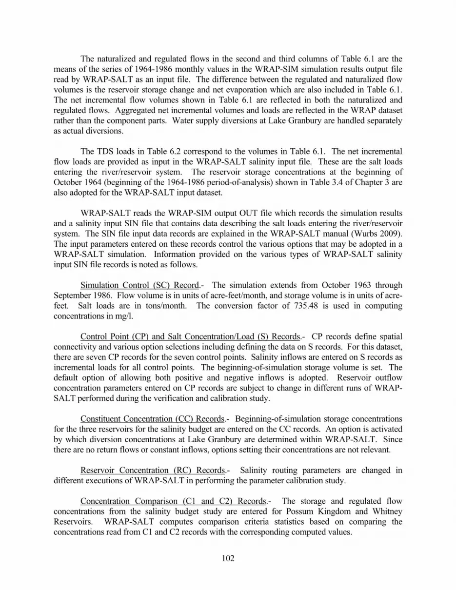
102

The naturalized and regulated flows in the second and third columns of Table 6.1 are the means of the series of 1964-1986 monthly values in the WRAP-SIM simulation results output file read by WRAP-SALT as an input file. The difference between the regulated and naturalized flow volumes is the reservoir storage change and net evaporation which are also included in Table 6.1. The net incremental flow volumes shown in Table 6.1 are reflected in both the naturalized and regulated flows. Aggregated net incremental volumes and loads are reflected in the WRAP dataset rather than the component parts. Water supply diversions at Lake Granbury are handled separately as actual diversions. The TDS loads in Table 6.2 correspond to the volumes in Table 6.1. The net incremental flow loads are provided as input in the WRAP-SALT salinity input file. These are the salt loads entering the river/reservoir system. The reservoir storage concentrations at the beginning of October 1964 (beginning of the 1964-1986 period-of-analysis) shown in Table 3.4 of Chapter 3 are also adopted for the WRAP-SALT input dataset. WRAP-SALT reads the WRAP-SIM output OUT file which records the simulation results and a salinity input SIN file that contains data describing the salt loads entering the river/reservoir system. The SIN file input data records are explained in the WRAP-SALT manual (Wurbs 2009). The input parameters entered on these records control the various options that may be adopted in a WRAP-SALT simulation. Information provided on the various types of WRAP-SALT salinity input SIN file records is noted as follows.

Simulation Control (SC) Record.- The simulation extends from October 1963 through September 1986. Flow volume is in units of acre-feet/month, and storage volume is in units of acre-feet. Salt loads are in tons/month. The conversion factor of 735.48 is used in computing concentrations in mg/l.

Control Point (CP) and Salt Concentration/Load (S) Records.- CP records define spatial connectivity and various option selections including defining the data on S records. For this dataset, there are seven CP records for the seven control points. Salinity inflows are entered on S records as incremental loads for all control points. The beginning-of-simulation storage volume is set. The default option of allowing both positive and negative inflows is adopted. Reservoir outflow concentration parameters entered on CP records are subject to change in different runs of WRAP-SALT performed during the verification and calibration study.

Constituent Concentration (CC) Records.- Beginning-of-simulation storage concentrations for the three reservoirs for the salinity budget are entered on the CC records. An option is activated by which diversion concentrations at Lake Granbury are determined within WRAP-SALT. Since there are no return flows or constant inflows, options setting their concentrations are not relevant.

Reservoir Concentration (RC) Records.- Salinity routing parameters are changed in different executions of WRAP-SALT in performing the parameter calibration study.

Concentration Comparison (C1 and C2) Records.- The storage and regulated flow concentrations from the salinity budget study are entered for Possum Kingdom and Whitney Reservoirs. WRAP-SALT computes comparison criteria statistics based on comparing the concentrations read from C1 and C2 records with the corresponding computed values.

103

Initial Simulation Results The WRAP-SALT input dataset described in the preceding section was developed to explore, validate, and calibrate salinity routing methods. The results of two initial WRAP-SALT simulations with only the TM option varied are summarized as follows. In these initial simulations, the lag L defined in Equation 6-1 is set at zero and the parameters F1 and F2 in Equation 6-3 are set at the defaults of 1.0. The retention-based lag option represented by Equation 6-2 is not applied in these initial simulations. Simulation studies presented later in this chapter investigate the effects of varying these options. WRAP-SALT computes reservoir outflow concentrations as a function of storage concentration. With a lag L of zero and default F1 and F2 of 1.0, the outflow concentration is set equal to the storage concentration. However, WRAP-SALT has an option controlled by the input parameter TM allowing adoption of either the beginning-of-month or mean monthly storage concentration in determining the outflow concentration.

• With TM option 1, the outflow concentration is determined as a function of the mean storage concentration computed as the average of the beginning-of-month and end-of-month storage concentrations.

• With TM option 2, the outflow concentration is determined as a function of the beginning-of-month storage concentration.

Simulation results are presented here alternatively with TM options 1 and 2. TM options are applicable only to control points with reservoir storage. Mean concentrations resulting from the WRAP-SALT simulation are compared with the mean observed concentration from the salinity budget study in Table 6.4. For the 276 months in the 1964-1986 simulation, the Seymour gage control point has a mean regulated TDS concentration of 3,589 mg/l. The mean regulated TDS concentration at the South Bend gage is 1,996 mg/l. Due to the manner in which the WRAP-SALT input dataset was created, with none of the three reservoirs located upstream, the concentrations at the Seymour and South Bend gages must be exactly the same in the WRAP-SALT results and salinity budget study. The reservoir storage and outflow concentrations vary between the WRAP-SALT simulation results and salinity budget study affecting simulation results at the control point of each reservoir and downstream control points. TM option 1 in WRAP-SALT sets simulated reservoir outflow concentrations equal to the average of the beginning-of-month and end-of-month storage concentration. TM option 2 sets reservoir outflow concentrations equal to beginning-of-month storage concentrations. Flow and storage concentrations from the water and salinity budget study and WRAP-SALT simulations with TM option 1 activated are compared in the plots of Figures 6.1 through 6.12. The plots are repeated in Figures 6.13 through 6.24 for TM option 2. The reservoir storage and outflow concentration results are almost the same with either of the two alternative TM options. However, the plots show that relatively small differences do occur with TM options 1 versus 2 at some locations in some months particularly during 1978 and later. Figures 6.1−6.6 and 6.13−6.18 are plots of concentrations for regulated flows from the WRAP-SALT simulation and observed flows from the volume/load budget dataset. The simulated

104

regulated flow concentrations would be the same as observed concentrations for a perfect simulation. Differences between the simulated and observed flow concentrations are evident in the plots. End-of-month reservoir storage concentrations from the WRAP-SALT simulation are compared in Figures 6.7−6.9 and 6.19−6.21 with the end-of-month storage concentrations computed with the volume and load budget. The "observed or measured" concentrations of the stored water are actually computed in the volume and load budget analyses of Chapters 2 and 3 from other observed data. Figures 6.10−6.12 and 6.22−6.24 compare WRAP-SALT simulated end-of-month reservoir storage concentrations with the observed concentrations of flow during the month at the nearest gage located downstream of the dam. These plots provide a means to visualize the time lag between storage concentration and outflow concentration. However, the plots do not appear to display a pronounced lag effect. As a minor note, the timing is off by about half of a month in the plots since the end-of-month storage concentration is plotted with the mean flow concentration during the month. The lag effect is also explored in the preceding Chapter 5 and in the remainder of Chapter 6. In the WRAP-SALT simulations reflected in Figures 6.1 through 6.24, the lag L is set at zero and the parameters F1 and F2 are set at the defaults of 1.0. The resulting stream flow and reservoir storage concentrations vary between the values computed in the WRAP-SALT simulations and the observed or synthesized values from the volume and load budgets. The plots visually display these differences. The remainder of this chapter explores the effects of varying the lag and multiplier factors in an attempt to better calibrate these parameters.

Table 6.4 Comparison of Simulated and Observed 1964-1986 Mean Concentrations

Control Points Simulated Concentrations Observed and Reservoirs TM Option 1 TM Option 2 Concentration

(mg/l) (mg/l) (mg/l)

Stream Flow Concentrations

Seymour gage 3,589 3,589 3,589 South Bend gage 1,996 1,996 1,996 Graford gage 1,539 1,540 1,534 Dennis gage 1,195 1,196 1,204 Lake Granbury 1,109 1,110 - Glen Rose gage 1,076 1,077 1,073 Whitney gage 928 929 927

Reservoir Storage Concentrations

Lake Possum Kingdom 1,689 1,611 1,626 Lake Granbury 1,271 - 1,302 Lake Whitney 923 962 1,062

105

Time (month)

1965 1970 1975 1980 1985

Con

cent

ratio

n (m

g/l)

0

2000

4000

6000

8000

10000

12000

14000

16000

18000M easured_Seymour_Outflow_Concentration W RAP_Seymour_Outflow_Concentration

Figure 6.1 Observed and Simulated Concentration at Seymour Gage (TM Option 1)

Time (month)

1965 1970 1975 1980 1985

Con

cent

ratio

n (m

g/l)

0

5000

10000

15000

20000

25000

30000

35000

M easured_South Bend_Outflow_Concentration W RAP_South Bend_Outflow_Concentration

Figure 6.2 Observed and Simulated Concentration at South Bend Gage (TM Option 1)

106

Time (month)

1965 1970 1975 1980 1985

Con

cent

ratio

n (m

g/l)

0

500

1000

1500

2000

2500

3000

M easured_Graford_Outflow_Concentration W RAP_Graford_Outflow_Concentration

Figure 6.3 Observed and Simulated Concentration at Graford Gage (TM Option 1)

Time (month)

1965 1970 1975 1980 1985

Con

cent

ratio

n (m

g/l)

0

1000

2000

3000

4000

5000

M easured_Dennis_Outflow_Concentration W RAP_Dennis_Outflow_Concentration

Figure 6.4 Observed and Simulated Concentration at Dennis Gage (TM Option 1)

107

Time (month)

1965 1970 1975 1980 1985

Con

cent

ratio

n (m

g/l)

0

500

1000

1500

2000

2500

M easured_GlenRose_Outflow_Concentration W RAP_GlenRose_Outflow_Concentration

Figure 6.5 Observed and Simulated Concentration at Glen Rose Gage (TM Option 1)

Time (month)

1965 1970 1975 1980 1985

Con

cent

ratio

n (m

g/l)

0

500

1000

1500

2000

2500M easured_W hitney_Outflwo_Concentration W RAP_W hitney_Outflow_Concentration

Figure 6.6 Observed and Simulated Concentration at Whitney Gage (TM Option 1)

108

Time (months)

1965 1970 1975 1980 1985

Stor

age

Con

cent

ratio

n (m

g/l)

0

500

1000

1500

2000

2500

3000

Measured_PK_Storage_ConcentrationWRAP_PK_Storage_Concentration

Figure 6.7 Possum Kingdom Reservoir Storage Concentration (TM Option 1)

Time (months)

1965 1970 1975 1980 1985

Stor

age

Con

cent

ratio

n (m

g/l)

0

500

1000

1500

2000

2500Measured_Granbury_Storage_ConcentrationWRAP_Granbury_Storage_Concentration

Figure 6.8 Granbury Reservoir Storage Concentration (TM Option 1)

109

Time (months)

1965 1970 1975 1980 1985

Stor

age

Con

cent

ratio

n (m

g/l)

0

200

400

600

800

1000

1200

1400

1600

1800

2000

Measured_Whitney_Storage_ConcentrationWRAP_Whitney_Storage_Concentration

Figure 6.9 Whitney Reservoir Storage Concentration (TM Option 1)

Time (months)

1965 1970 1975 1980 1985

Con

cent

ratio

n (m

g/l)

0

500

1000

1500

2000

2500

3000

Measured_Graford_Outflow_ConcentrationWRAP_PK_Storage_Concentration

Figure 6.10 Possum Kingdom Simulated Storage Concentration and Graford Gage Observed Flow Concentration (TM Option 1)

110

Time (months)

1965 1970 1975 1980 1985

Con

cent

ratio

n (m

g/l)

0

500

1000

1500

2000

2500

Measured_Glen Rose_Outflow_ConcentrationWRAP_Granbury_Storage_Concentration

Figure 6.11 Granbury Simulated Storage Concentration and Glen Rose Gage Observed Flow Concentration (TM Option 1)

Time (months)

1965 1970 1975 1980 1985

Con

cent

ratio

n (m

g/l)

0

500

1000

1500

2000

2500

Measured_Whitney_Outflow_ConcentrationWRAP_Whitney_Storage_Concentration

Figure 6.12 Whitney Simulated Storage Concentration and Glen Rose Gage Observed Flow Concentration (TM Option 1)

111

Time (month)

1965 1970 1975 1980 1985

Con

cent

ratio

n (m

g/l)

0

2000

4000

6000

8000

10000

12000

14000

16000

18000M easured_Seymour_Outflow_Concentration W RAP_Seymour_Outflow_Concentration

Figure 6.13 Observed and Simulated Concentration at Seymour Gage (TM Option 2)

Time (month)

1965 1970 1975 1980 1985

Con

cent

ratio

n (m

g/l)

0

5000

10000

15000

20000

25000

30000

35000

M easured_South Bend_Outflow_Concentration W RAP_South Bend_Outflow_Concentration

Figure 6.14 Observed and Simulated Concentration at South Bend Gage (TM Option 2)

112

Time (month)

1965 1970 1975 1980 1985

Con

cent

ratio

n (m

g/l)

0

500

1000

1500

2000

2500

3000

M easured_Graford_Outflow_Concentration W RAP_Graford_Outflow_Concentration

Figure 6.15 Observed and Simulated Concentration at Graford Gage (TM Option 2)

Time (month)

1965 1970 1975 1980 1985

Con

cent

ratio

n (m

g/l)

0

1000

2000

3000

4000

5000

M easured_Dennis_Outflow_Concentration W RAP_Dennis_Outflow_Concentration

Figure 6.16 Observed and Simulated Concentration at Dennis Gage (TM Option 2)

113

Time (month)

1965 1970 1975 1980 1985

Con

cent

ratio

n (m

g/l)

0

500

1000

1500

2000

2500

M easured_Glen Rose_Outflwo_Concentration W RAP_Glen Rose_Outflow_Concentration

Figure 6.17 Observed and Simulated Concentration at Glen Rose Gage (TM Option 2)

Time (month)

1965 1970 1975 1980 1985

Con

cent

ratio

n (m

g/l)

0

500

1000

1500

2000

2500

M easured_W hitney_Outflow_Concentration W RAP_W hitney_Outflow_Concentration

Figure 6.18 Observed and Simulated Concentration at Whitney Gage (TM Option 2)

114

Time (months)

1965 1970 1975 1980 1985

Stor

age

Con

cent

ratio

n (m

g/l)

0

500

1000

1500

2000

2500

3000

M easured_PK_Storage_ConcentrationW RAP_PK_Storage_Concentration

Figure 6.19 Possum Kingdom Reservoir Storage Concentration (TM Option 2)

Time (months)

1965 1970 1975 1980 1985

Stor

age

Con

cent

ratio

n (m

g/l)

0

500

1000

1500

2000

M easured_Granbury_Storage_ConcentrationW RAP_Granbury_Storage_Concentration

Figure 6.20 Granbury Reservoir Storage Concentration (TM Option 2)

115

Time (months)

1965 1970 1975 1980 1985

Stor

age

Con

cent

ratio

n (m

g/l)

0

500

1000

1500

2000

M easured_W hitney_Storage_concentrationW RAP_W hitney_Storage_concentration

Figure 6.21 Whitney Reservoir Storage Concentration (TM Option 2)

Time (months)

1965 1970 1975 1980 1985

Con

cent

ratio

n (m

g/l)

0

500

1000

1500

2000

2500

3000

M easured_Graford_Outflow_ConcentrationW RAP_PK_Storage_Concentration

Figure 6.22 Possum Kingdom Simulated Storage Concentration and Graford Gage Observed Flow Concentration (TM Option 2)

116

Time (months)

1965 1970 1975 1980 1985

Con

cent

ratio

n (m

g/l)

0

1000

2000

3000M easured_G len Rose_Outflow_concentrationW RAP_Granbury_Storage_concentration

Figure 6.23 Granbury Simulated Storage Concentration and Glen Rose Gage Observed Flow Concentration (TM Option 2)

Time (months)

1965 1970 1975 1980 1985

Con

cent

ratio

n (m

g/l)

0

500

1000

1500

2000

2500

M easured_W hitney_Outflow_ConcentrationW RAP_W hitney_Storage_Concentration

Figure 6.24 Whitney Reservoir Simulated Storage Concentration and Whitney Gage Observed Flow Concentration at (TM Option 2)

117

Simulation Studies to Explore Reservoir Routing Methods and Calibrate Parameters

In the real-world, salt loads are carried by stream flows into the upper reaches of a

reservoir, and mixing occurs over time. Salt loads may require long periods of time to move through a reservoir and reach the outlet. As illustrated by Figure 1.16 in Chapter 1, salt concentrations may vary spatially both horizontally and vertically in a reservoir. The lag options in WRAP-SALT represent physically the time required for the salt loads to reach the reservoir outlet after entering the reservoir in a particular month. The remainder of this chapter documents WRAP-SALT simulation studies focused on storage and outflow concentration at Possum Kingdom and Whitney Reservoirs designed to investigate the alternative routing methods and develop values for the lag parameters. Salinity Routing Options Applied for Possum Kingdom and Whitney Reservoirs The general methodology adopted in WRAP-SALT for routing salt though reservoirs and the options incorporated in this methodology are outlined earlier in this chapter. Routing is based on Equations 6-1, 6-2, and 6-3 which are introduced earlier in this chapter and repeated as follows. OCM = SCM-L (6-1)

( )M M-L 1 2C

VOC = SC F 1.0 + F - 1.0V

⎡ ⎤⎛ ⎞× ⎢ ⎥⎜ ⎟

⎝ ⎠⎣ ⎦

(6-2)

L = TR (FL) (6-3) The outflow concentration (OCM) in month M is computed as a function of storage concentration (SC) in month M-L (L months before month M). Lag L is an integer number of months. SALT has an option controlled by the input parameter TM that allows adoption of either the beginning-of-month or mean monthly storage concentrations in determining reservoir outflow concentrations. Two options are included in WRAP-SALT for setting the lag L.

Lag Option 1 − The lag L in Eqs 6-1 and 6-2 is provided by the model-user as an input data parameter. Equation 6-3 is not relevant and is not applied.

Lag Option 2 − The lag L in Eqs 6-1 and 6-2 is computed within WRAP-SALT based

on Eq. 6-2 with retention time TR computed based on methodology described earlier in this chapter. L is truncated to an integer number of months. The factor FL is an input parameter with a default of 1.0.

Thus, Option 1 is for the lag L to be a constant integer provided by the model-user as an input parameter. With Option 2, the lag L is computed within WRAP-SALT based on Equation 6-2 with the multiplier factor FL provided by the user as an input parameter. With the second option, the lag is allowed to vary from month to month.

The following salinity routing parameters are entered in the SALT input SIN file on CP and RC records which are described in the Salinity Manual.

118

TM − TM is entered in CP record field 6. With option 1, the outflow concentration is determined as a function of mean storage concentration computed as the average of the beginning-of-month and end-of-month storage concentrations. With option 2, the outflow concentration is set as a function of the beginning-of-month storage concentration.

LAG1 − LAG1 is entered in CP record field 7. If LAG2(cp) is zero, LAG1(cp) is a constant lag

in months corresponding to L in Equations 6-1 and 6-2. If LAG2(cp) is not zero, LAG1(cp) is a maximum limit on the lag in months computed with Equation 6-3.

LAG2 − LAG2 is entered in CP record field 8. If LAG2(cp) is zero, the retention based lag option

is not activated. If not zero, LAG2(cp) is the multiplier factor FL in Equation 6-3. RCF1 − RCF1 entered in RC record field 3 is the factor F1 in Equation 6-2. RCF2 − RCF2 entered in RC record field 4 is the factor F2 in Equation 6-2. Organization of the Presentation of Simulation Results WRAP-SALT was executed with the input dataset described earlier in this chapter with alternative combinations of values for the parameters described above. The remainder of this chapter consists of a presentation and assessment of the simulation results organized as the six sections listed below. The next four sections present results of applying the two lag options at each of the two reservoirs as outlined in Figure 6.25. The last two sections of the chapter provide calibration statistics and an overall summary and conclusions for the salinity routing study. Possum Kingdom Reservoir with Lag Option 1 Possum Kingdom Reservoir with Lag Option 2 Whitney Reservoir with Lag Option 1 Whitney Reservoir with Lag Option 2 Reservoir Salinity Routing Parameter Calibration Summary Conclusions

Figure 6.25 Lag Options Applied for Possum Kingdom and Whitney Reservoirs

Simulation results are presented in various tables and plots for comparison. Stream flow

and reservoir storage concentrations from the WRAP-SALT simulation results are compared with the observed stream flow concentrations and reservoir storage concentrations from the salinity budgets of Chapters 2 and 3.

119

Possum Kingdom Reservoir with Lag Option 1

Stream flows at the Graford gage located downstream of the dam are comprised of outflows from Possum Kingdom Reservoir. Storage and outflow concentrations from WRAP-SALT simulations are compared with storage concentrations computed in the salt budget analysis and USGS observed stream flow concentrations at the Graford gaging station.

The results of alternative simulations with lag option 1 with constant lags (L in Equation 6-

1) of 0, 1, 2, 3, 4, 5, 6, 7, 8, 9, 10, 15, and 20 months are presented in this section. Alternative simulations with lag option 2 performed with lag multiplier factors (FL in Equation 6-2) of 0.1, 0.2, 0.3, 0.4, 0.5, 0.6, 0.7, 0.8, 0.9, and 1.0 are presented in the next section. The simulations with lag options 1 and 2 were repeated with TM options 1 and 2 dictating whether monthly mean versus beginning-of-month storage concentrations are used to compute outflow concentrations. Linear correlation and regression coefficients are tabulated in Table 6.5 as indices for comparing pairs of 276-month (1964-1986) sequences of monthly TDS concentrations. Table 6.5 reflects the results of 26 WRAP-SIM simulations with all simulations being identical except for the choice of TM option and the constant lag (L in Equation 6.1) for Possum Kingdom Lake which is tabulated in column 1. The label observed refers to the salinity budget dataset of Chapters 2 and 3. Simulated means computed in the WRAP-SALT simulation. The following pairs of sequences of Possum Kingdom Reservoir outflow and/or storage concentrations are compared in Table 6.5.

Column 2 − Observed outflow (flows at Graford gage) versus simulated outflow concentrations. TM option 1 (mean concentration) is activated.

Column 3 − Observed (computed in salinity budget) versus simulated storage concentrations. TM option 1 (mean concentration) is activated.

Column 4 − Observed outflow (flows at Graford gage) versus simulated outflow concentrations. TM option 2 (beginning-of-month)) is activated.

Column 5 − Observed (computed in salinity budget) versus simulated storage concentrations. TM option 2 (beginning-of-month)) is activated.

Column 6 − Observed outflow (flows at Graford gage) versus simulated outflow concentrations. TM option 1 (mean concentration) is activated.


Column 8 − Observed outflow (flows at Graford gage) versus simulated outflow concentrations. TM option 2 (beginning-of-month)) is activated.


The linear correlation coefficient (R) is defined in most statistics books. The regression

coefficient is the factor 'a' in the regression equation Y = aX. The relative closeness of the correlation and regression coefficients to 1.0 provides an index for comparing the results of the simulations to the storage and outflow concentrations from the salinity budget analysis of Chapters 2 and 3. A value of precisely 1.0 for the correlation coefficient and regression coefficient would be an indication that the 1964-1986 sequences of simulated and observed concentrations are identical.

120

Table 6.5 Linear Correlation and Regression Coefficients for Alternative Lags

(1) (2) (3) (4) (5) (6) (7) (8) (9)

Observed Outflow Storage Outflow Storage Outflow Storage Outflow Storage Simulated Outflow Storage Outflow Storage Outflow Storage Outflow Storage

TM 1 1 2 2 1 1 2 2 Lag Correlation Coefficient (R) Regression Coefficient (a) for Y = aX

(months) 0 0.990 0.972 0.984 0.982 0.9944 0.9917 0.9612 0.9739 1 0.985 0.974 0.971 0.982 1.0740 1.1278 1.0202 1.0868 2 0.977 0.972 0.961 0.973 1.1061 1.1858 1.0323 1.1214 3 0.973 0.970 0.955 0.972 1.1160 1.2458 1.0405 1.1792 4 0.969 0.970 0.951 0.974 1.1274 1.3105 1.0570 1.2516 5 0.965 0.971 0.946 0.976 1.1409 1.3414 1.0688 1.2834 6 0.961 0.970 0.936 0.974 1.1413 1.3987 1.0592 1.3302 7 0.954 0.967 0.927 0.973 1.1335 1.4519 1.0386 1.3702 8 0.946 0.963 0.912 0.962 1.1307 1.5061 1.0505 1.4398 9 0.938 0.959 0.903 0.959 1.1290 1.5291 1.0429 1.4568 10 0.932 0.958 0.898 0.959 1.1209 1.5749 1.0349 1.5033 15 0.926 0.954 0.890 0.954 1.0862 1.7581 1.0022 1.6908 20 0.932 0.952 0.902 0.948 1.1048 1.6335 1.0289 1.5753

Table 6.5 includes WRAP-SALT simulations with the alternative lag times tabulated in column 1 and the two alternative TM options. The statistical analysis summarized in Table 6.5 implies that zero lag (no lag) is the optimal choice if lag option 1 is adopted for Possum Kingdom Reservoir. The correlation coefficient decreases with increases in the lag. Likewise, the regression coefficient departs from 1.0 as the value for the lag entered in the WRAP-SALT input is increased. TM option 1 appears to provide a little closer fit than TM option 2 though the differences between the TM options 1 and 2 statistics in Table 6.5 are minimal.

Plots of the observed and simulated reservoir storage and outflow concentrations are provided in Figures 6.26 through 6.28 for simulations with no lag and lags of 1 month and 2 months. The plots show significant differences between the magnitudes of the observed and simulated concentrations. However, the differences in magnitude are not greatly influenced by timing or lag. The differences between the two 1964-1986 sequences of monthly concentrations plotted in each of the graphs are dominated by vertical differences (concentration magnitudes) rather than horizontal (timing pattern) differences. Statistics for the 1964-1986 sequences of end-of-month storage concentrations for Possum Kingdom Reservoir and the monthly mean concentrations at the Graford gage are tabulated in Tables 6.6 through 6.10. Statistics are provided in Table 6.6 for the dataset developed in the salinity budget study of Chapters 2 and 3. The same statistics for the WRAP-SALT simulation results for alternative lags and TM options are tabulated in Tables 6.7, 6.8, 6.9, and 6.10 for comparison. The tables reflect lag option 1 applied with alternative simulations representing a range of different lags. The statistics include mean and standard deviation of the concentrations and a frequency relationship with concentrations tabulated for specified exceedance frequencies.

121

Time (months)

1965 1970 1975 1980 1985

Out

flow

Con

cenr

atio

n (m

g/l)

0

500

1000

1500

2000

2500

3000

Observed outflow concentrationNo_lag outflow concentration (TM 1)

Figure 6.26 Comparison of Observed and Simulated Flow Concentrations at Graford Gage (No Lag, TM Option 1)

Time (months)

1965 1970 1975 1980 1985

Out

flow

Con

cenr

atio

n (m

g/l)

0

500

1000

1500

2000

2500

3000

Observed outflow concentrationLag_1 outflow concentration (TM 1)

Figure 6.27 Comparison of Observed and Simulated Flow Concentrations at Graford Gage

(Lag 1 month, TM Option 1)

122

Time (months)

1965 1970 1975 1980 1985

Out

flow

Con

cenr

atio

n (m

g/l)

0

500

1000

1500

2000

2500

3000

3500


Figure 6.28 Comparison of Observed and Simulated Outflow Concentrations at Graford Gage

(Lag 2 months, TM Option 1)

T im e (m onths)

1965 1970 1975 1980 1985

Stor

age

Con

cenr

atio

n (m

g/l)

0

500

1000

1500

2000

2500

3000

O bserved storage concentrationN o_lag s torage concentration

Figure 6.29 Comparison of Observed and Simulated Storage Concentrations at Possum Kingdom

Reservoir (No Lag, TM Option 1)

123

Time (months)

1965 1970 1975 1980 1985

Stor

age

Con

cenr

atio

n (m

g/l)

0

500

1000

1500

2000

2500

3000

Observed storage concentrationLag_1 storage concentration


Reservoir (Lag 1 month, TM Option 1)

Time (months)

1965 1970 1975 1980 1985

Stor

age

Con

cenr

atio

n (m

g/l)

0

500

1000

1500

2000

2500

3000

3500



Reservoir (Lag 2 months, TM Option 1)

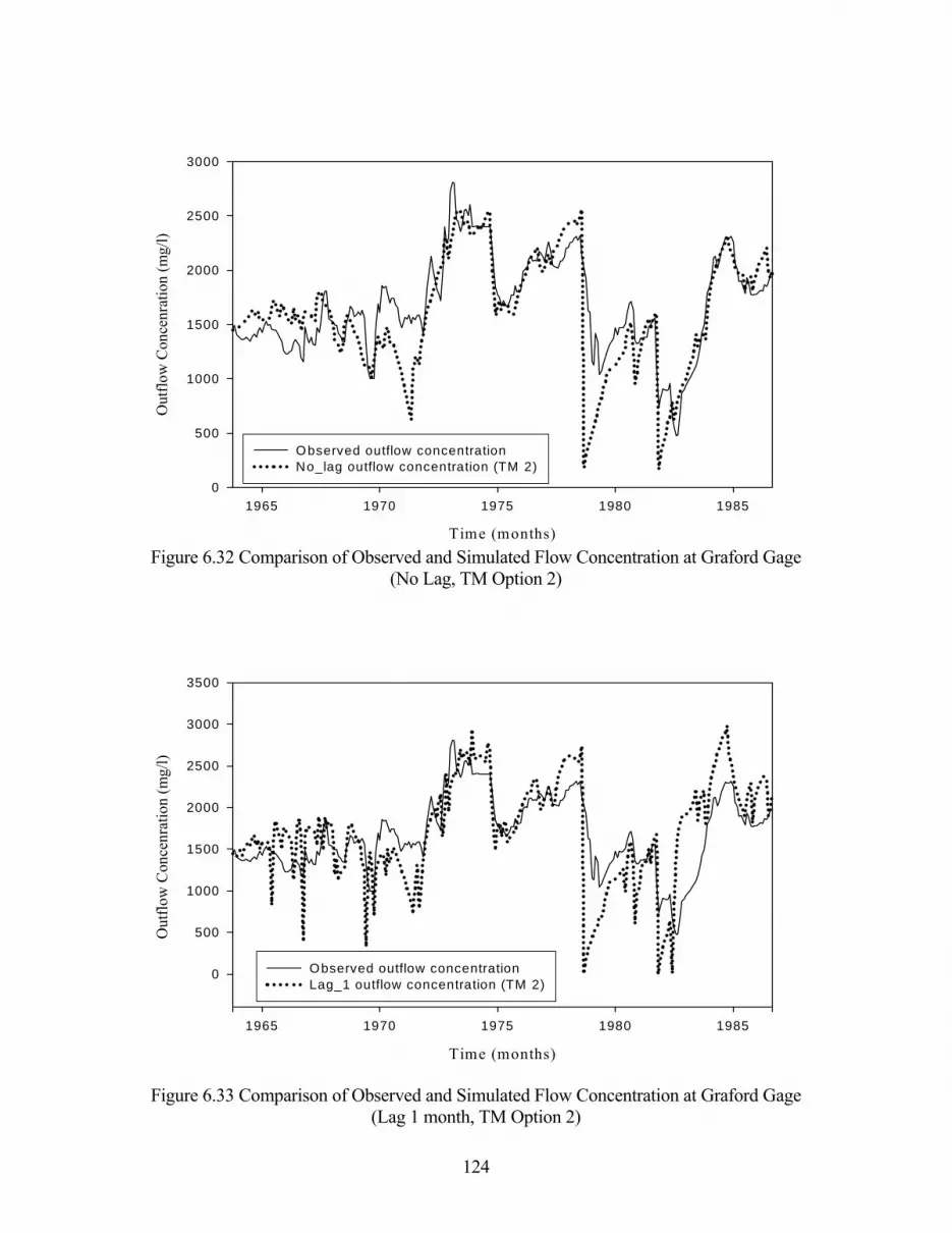
124

Time (months)

1965 1970 1975 1980 1985

Out

flow

Con

cenr

atio

n (m

g/l)

0

500

1000

1500

2000

2500

3000


Figure 6.32 Comparison of Observed and Simulated Flow Concentration at Graford Gage

(No Lag, TM Option 2)

Time (months)

1965 1970 1975 1980 1985

Out

flow

Con

cenr

atio

n (m

g/l)

0

500

1000

1500

2000

2500

3000

3500


Figure 6.33 Comparison of Observed and Simulated Flow Concentration at Graford Gage (Lag 1 month, TM Option 2)

125

Time (months)

1965 1970 1975 1980 1985

Out

flow

Con

cenr

atio

n (m

g/l)

0

500

1000

1500

2000

2500

3000

3500


Figure 6.34 Comparison of Observed and Simulated Flow Concentration at Graford gage

(Lag 2 months, TM Option 2)

Time (months)

1965 1970 1975 1980 1985

Stor

age

Con

cenr

atio

n (m

g/l)

0

500

1000

1500

2000

2500

3000

Observed storage concentrationNo_lag storage concentration (TM 2)


Reservoir (No Lag, TM Option 2)

126

Time (months)

1965 1970 1975 1980 1985

Stor

age

Con

cenr

atio

n (m

g/l)

0

500

1000

1500

2000

2500

3000

3500

Observed storage concentrationLag_1 storage concentration (TM 2)


Reservoir (Lag 1 month, TM Option 2)

Time (months)

1965 1970 1975 1980 1985

Stor

age

Con

cenr

atio

n (m

g/l)

0

500

1000

1500

2000

2500

3000

3500



Reservoir (Lag 2 months, TM Option 2)

127

Table 6.6 Statistics for Possum Kingdom Reservoir Storage and

Outflow Concentrations from the Salinity Budget Dataset

Exceedance PK Storage Graford Flow Frequency or Concentration Concentration Other Statistic (mg/l) (mg/l)

10 % 2,230 2,294 25 % 2,078 2,008 40 % 1,837 1,773 50 % 1,717 1,615 60 % 1,562 1,509 75 % 1,278 1,379 90 % 798 1,130 95 % 572 940 98 % 402 739 99 % 331 562 100% 319 475

Mean 1,626 1,534 Standard Deviation 544 466

Maximum 2,464 2,809

Table 6.7 Statistics for Concentrations at Graford Gage (TM Option 1, Lag Option 1)

Lag

(months) 0 1 2 3 4 5 6 7 8 9 10 15 20

Exceed Fr Concentration (mg/l)

10 % 2,350 2,585 2,735 2,828 2,904 3,005 2,951 2,885 2,927 3,017 3,086 3,250 2,971 25 % 2,014 2,140 2,212 2,280 2,327 2,317 2,337 2,375 2,422 2,446 2,417 2,262 2,233 40 % 1,686 1,917 2,005 2,013 2,042 2,098 2,094 2,012 1,971 1,883 1,856 1,772 1,854 50 % 1,585 1,792 1,871 1,849 1,825 1,841 1,776 1,730 1,693 1,660 1,602 1,571 1,617 60 % 1,520 1,677 1,704 1,652 1,642 1,654 1,645 1,590 1,531 1,486 1,445 1,445 1,475 75 % 1,289 1,512 1,503 1,481 1,471 1,445 1,435 1,352 1,294 1,239 1,208 1,105 1,348 90 % 946 1,304 1,235 1,133 1,033 1,022 938 923 900 924 929 823 960 95 % 624 1,126 1,011 860 839 799 814 720 716 729 670 706 638 98 % 401 952 794 711 635 673 539 517 493 453 459 528 415 99 % 290 904 618 428 460 363 389 424 463 430 437 293 299 100 % 169 551 331 174 198 192 200 275 435 266 134 250 223

Mean 1,609 1,833 1,882 1,887 1,895 1,913 1,906 1,886 1,879 1,874 1,857 1,795 1,846 SD 528 458 549 628 686 731 778 826 875 919 946 956 903

Max 2,560 2,795 3,212 3,522 3,810 4,064 4,251 4,403 4,594 4,769 4,911 5,535 4,897

128


Lag

(months) 0 1 2 3 4 5 6 7 8 9 10 15 20

Ex Freq Concentration (mg/l)

10 % 2,350 2,580 2,707 2,800 2,907 2,917 2,956 2,899 3,037 3,029 3,115 3,201 2,922 25 % 2,014 2,165 2,209 2,220 2,274 2,316 2,252 2,258 2,380 2,344 2,339 2,177 2,204 40 % 1,686 1,866 1,912 1,919 1,966 2,008 2,018 1,856 1,837 1,741 1,688 1,654 1,673 50 % 1,585 1,713 1,731 1,727 1,684 1,720 1,654 1,596 1,532 1,521 1,445 1,445 1,469 60 % 1,520 1,582 1,588 1,549 1,542 1,500 1,482 1,445 1,394 1,335 1,282 1,205 1,407 75 % 1,289 1,364 1,276 1,269 1,214 1,231 1,158 1,084 1,004 938 901 878 1,017 90 % 946 897 690 661 723 674 477 370 438 445 368 448 610 95 % 624 529 404 386 342 265 120 162 136 27 40 127 311 98 % 401 292 138 33 0 0 0 0 0 0 0 47 0 99 % 290 132 0 0 0 0 0 0 0 0 0 0 0 100 % 169 0 0 0 0 0 0 0 0 0 0 0 0

Mean 1,609 1,712 1,721 1,721 1,742 1,757 1,731 1,687 1,710 1,694 1,677 1,621 1,692 SD 528 623 710 776 822 867 920 962 1,029 1,066 1,085 1,089 1,023

Max 2,560 2,980 3,259 3,578 3,846 4,089 4,267 4,408 4,623 4,808 4,941 5,601 5,063

Table 6.9 Statistics for Possum Kingdom Storage Concentrations (TM Option 1, Lag Option 1)

Lag

(months) 0 1 2 3 4 5 6 7 8 9 10 15 20


10 % 2,350 2,607 2,771 2,920 3,050 3,072 3,182 3,318 3,459 3,633 3,752 4,460 4,457 25 % 2,014 2,256 2,411 2,548 2,654 2,700 2,798 2,918 3,083 3,209 3,309 3,648 3,297 40 % 1,687 2,008 2,131 2,249 2,377 2,464 2,599 2,686 2,793 2,868 2,943 3,222 2,898 50 % 1,590 1,860 1,993 2,082 2,207 2,300 2,410 2,510 2,563 2,564 2,616 2,842 2,686 60 % 1,526 1,776 1,839 1,899 1,980 2,020 2,110 2,185 2,234 2,227 2,315 2,553 2,299 75 % 1,289 1,603 1,632 1,680 1,769 1,802 1,849 1,913 1,973 1,956 2,015 2,277 1,867 90 % 946 1,429 1,456 1,490 1,540 1,535 1,560 1,613 1,622 1,616 1,637 1,789 1,601 95 % 624 1,302 1,317 1,367 1,452 1,461 1,508 1,528 1,530 1,523 1,555 1,595 1,527 98 % 401 1,158 1,156 1,212 1,309 1,354 1,443 1,461 1,468 1,441 1,482 1,507 1,415 99 % 290 1,035 1,032 1,079 1,222 1,257 1,363 1,430 1,438 1,404 1,458 1,474 1,322 100 % 169 798 793 839 984 1,087 1,253 1,331 1,353 1,309 1,307 1,446 1,196

Mean 1,610 1,930 2,028 2,128 2,237 2,286 2,383 2,476 2,572 2,611 2,688 2,994 2,749 SD 528 436 491 542 576 596 629 670 727 780 816 978 1,022

Max 2,560 2,810 3,070 3,241 3,462 3,581 3,760 3,974 4,189 4,332 4,547 5,358 5,221

Tables 6.7, 6.8, 6.9, and 6.10 include tabulations of TDS concentrations in mg/l associated with the exceedance frequencies listed in the first column. Means, standard deviations, and maximum values of the concentrations are also tabulated at the bottom of the tables. These statistics are for the results of WRAP-SALT simulations with the lag times in months cited in the first row of the tables.

129


Lag

(months) 0 1 2 3 4 5 6 7 8 9 10 15 20


10 % 2,350 2,599 2,754 2,898 3,011 3,032 3,146 3,210 3,523 3,626 3,719 4,485 4,494 25 % 2,014 2,270 2,390 2,505 2,606 2,649 2,754 2,856 3,106 3,176 3,261 3,567 3,225 40 % 1,687 1,954 2,077 2,189 2,314 2,400 2,480 2,508 2,712 2,746 2,834 3,143 2,805 50 % 1,590 1,777 1,803 1,905 2,079 2,225 2,285 2,300 2,392 2,356 2,474 2,635 2,557 60 % 1,526 1,648 1,654 1,697 1,800 1,836 1,905 1,952 1,990 2,009 2,100 2,375 2,106 75 % 1,289 1,465 1,461 1,488 1,573 1,577 1,640 1,665 1,692 1,663 1,747 1,950 1,686 90 % 946 1,080 1,087 1,132 1,190 1,151 1,209 1,285 1,314 1,303 1,405 1,547 1,356 95 % 624 681 648 703 870 840 983 1,008 984 980 1,137 1,359 944 98 % 401 383 361 394 516 477 545 522 492 438 438 609 424 99 % 290 270 244 285 384 360 357 335 306 252 252 426 252 100 % 169 142 97 106 172 104 101 80 52 0 0 170 0

Mean 1,610 1,804 1,859 1,952 2,074 2,119 2,199 2,266 2,390 2,417 2,496 2,812 2,589 SD 528 597 657 702 722 749 783 817 910 952 974 1,128 1,174

Max 2,560 2,950 3,105 3,239 3,438 3,543 3,755 3,971 4,190 4,330 4,565 5,391 5,224

Percentage of months with concentration equaling or exceeding values (%)

20 40 60 80 100

Res

ervo

ir St

orag

e C

once

ntra

tion

(mg/

l)

0

1000

2000

3000

4000

5000

Lag_0 Lag_1 Lag_2 Lag_3 Lag_4 Lag_5 Lag_6 Lag_7 Lag_8 Lag_9 Lag_10 Lag_15 Lag_20

Figure 6.38 Storage Concentration-Duration Curves for Possum Kingdom Reservoir for Alternative

Lags (Lag Option 1, TM Option 1)

130


20 40 60 80 100

Out

flow

Con

cent

ratio

n (m

g/l)

0

500

1000

1500

2000

2500

3000

3500


Figure 6.39 Concentration-Duration Curves at the Graford Gage for Alternative Lags (Lag Option 1, TM Option 1)


20 40 60 80 100

Res

ervo

ir St

orag

e C

once

ntra

tion

(mg/

l)

0

1000

2000

3000

4000

5000


Figure 6.40 TDS Concentration-Duration Curves at the Possum Kingdom Reservoir for Alternative

Lags (Lag Option 1, TM Option 2)

131


20 40 60 80 100

Out

flow

Con

cent

ratio

n (m

g/l)

0

500

1000

1500

2000

2500

3000

3500


Figure 6.41 Concentration-Duration Curves at the Graford Gage for Alternative Lags (Lag Option 1, TM Option 2)

Additional analyses based on parameter calibration statistics are presented in the last section of this chapter for both Possum Kingdom and Whitney Reservoirs for both lag options 1 and 2.

Possum Kingdom Reservoir with Lag Option 2 Lag option 2 is based on Equations 6-1, 6-2, and 6-3 with the lag time in months being computed within WRAP-SALT as a function of detention time. The lag is computed for each month of the simulation. The input parameters are the multiplier factor FL defined by Equation 6-3 and an upper limit on the lag. The user-specified upper limit on the lag is adopted in any particular month if the computed lag exceeds the limit. These two parameters are entered as LAG1(cp) and LAG2(cp) on the control point CP record. This section presents the results of applying WRAP-SALT alternatively with values for the multiplier factor (FL) of 0.1, 0.2, 0.3, 0.4, 0.5, 0.6, 0.7, 0.8, 0.9, and 1.0 adopted for Possum Kingdom Reservoir. Since the results of applying lag option 1 presented in the preceding section indicates that the lag should be zero or relatively small, an upper limit of 3 months was placed on the lag using the parameter LAG1(cp) on the CP record. Table 6.11 is comparable to the previously discussed Table 6.5. The second column of Table 6.11 representing no lag was copied from Table 6.5. Otherwise, each line represents simulations alternatively with TM options 1 and 2, with the specified value of the multiplier factor listed in the first row. The correlation and regression coefficients for the simulation with no lag are closer to 1.0 than the correlation and regression coefficients with lag option 2 activated with any of the multiplier factor values tabulated in Table 6.11.

132

Table 6.11 Linear Correlation and Regression Coefficients for Alternative Values for Multiplier Factor

(1) (2) (3) (4) (5) (6) (7) (8) (9)


TM 1 1 2 2 1 1 2 2 FL Correlation Coefficient (R) Regression Coefficient (a) for Y = aX

No Lag 0.990 0.972 0.984 0.982 0.9944 0.9917 0.9612 0.9739

0.1 0.970 0.858 0.954 0.862 0.8824 2.8372 0.8150 2.7801 0.2 0.983 0.939 0.967 0.941 1.0527 1.2969 0.9880 1.2405 0.3 0.977 0.965 0.961 0.968 1.0986 1.1724 1.0289 1.1110 0.4 0.974 0.959 0.959 0.963 1.0937 1.2487 1.0228 1.1860 0.5 0.974 0.962 0.958 0.964 1.106 1.2441 1.0317 1.1778 0.6 0.980 0.954 0.963 0.953 1.0733 1.3167 0.9919 1.2458 0.7 0.979 0.955 0.963 0.953 1.0767 1.3230 0.9997 1.2560 0.8 0.974 0.965 0.957 0.967 1.1135 1.2643 1.0378 1.1991 0.9 0.974 0.965 0.957 0.967 1.1141 1.2644 1.0385 1.2014 1.0 0.974 0.965 0.957 0.967 1.1139 1.2668 1.0385 1.2019

Plots of observed (salinity budget) versus WRAP-SALT simulated concentrations of reservoir storage and stream flows below the dam are provided as Figures 6.42 through 6.53 for alternative multiplier factors (FL).

Time (months)

1965 1970 1975 1980 1985

Out

flow

Con

cenr

atio

n (m

g/l)

0

500

1000

1500

2000

2500

3000

Observed outflow concentrationMultiplier 0.1

Figure 6.42 Comparison of Observed and Simulated Concentration at Graford Gage

(Multiplier 0.1, TM Option 1)

133

Time (months)

1965 1970 1975 1980 1985

Out

flow

Con

cenr

atio

n (m

g/l)

0

500

1000

1500

2000

2500

3000

3500


Figure 6.43 Comparison of Observed and Simulated Concentration at Graford Gage

(Multiplier 0.2, TM Option 1)

Time (months)

1965 1970 1975 1980 1985

Out

flow

Con

cenr

atio

n (m

g/l)

0

500

1000

1500

2000

2500

3000

3500


Figure 6.44 Comparison of Observed and Simulated Concentration at Graford Gage (Multiplier 0.3, TM Option 1)

134

Time (months)

1965 1970 1975 1980 1985

Stor

age

Con

cenr

atio

n (m

g/l)

0

500

1000

1500

2000

2500

3000

3500

4000

Observed storage concentrationM ultiplier 0.3

Figure 6.45 Comparison of Observed and Simulated Storage Concentration at Possum Kingdom Reservoir (Multiplier 0.3, TM Option 1)

Time (months)

1965 1970 1975 1980 1985

Stor

age

Con

cenr

atio

n (m

g/l)

0

500

1000

1500

2000

2500

3000

3500

4000Observed storage concentrationMultiplier 0.8


135

Time (months)

1965 1970 1975 1980 1985

Stor

age

Con

cent

ratio

n (m

g/l)

0

500

1000

1500

2000

2500

3000

3500

4000

Observed storage concentrationMultiplier 0.9


Time (months)

1965 1970 1975 1980 1985

Out

flow

Con

cenr

atio

n (m

g/l)

0

500

1000

1500

2000

2500

3000



136

Time (months)

1965 1970 1975 1980 1985

Out

flow

Con

cenr

atio

n (m

g/l)

0

500

1000

1500

2000

2500

3000

3500

Observed outflow concentrationM ultiplier 0.2


Time (months)

1965 1970 1975 1980 1985

Out

flow

Con

cenr

atio

n (m

g/l)

0

500

1000

1500

2000

2500

3000

3500



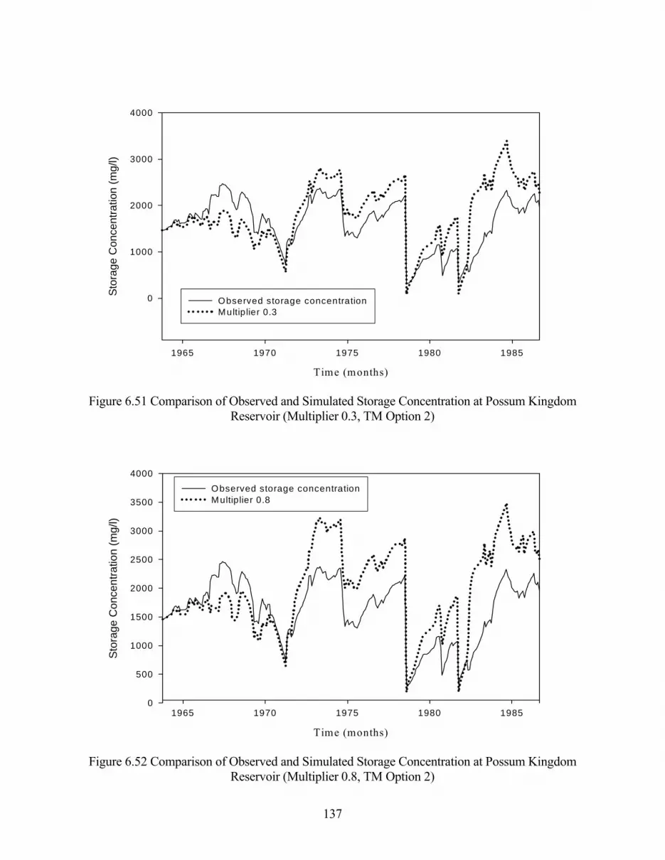
137

Time (months)

1965 1970 1975 1980 1985

Stor

age

Con

cent

ratio

n (m

g/l)

0

1000

2000

3000

4000



Time (months)

1965 1970 1975 1980 1985

Stor

age

Con

cent

ratio

n (m

g/l)

0

500

1000

1500

2000

2500

3000

3500



138

Tim e (m onths)

1965 1970 1975 1980 1985

Stor

age

Con

cent

ratio

n (m

g/l)

0

500

1000

1500

2000

2500

3000

3500

4000

O bserved storage concentrationM ultip lier 0 .9


Tables 6.12−6.15 contain the same statistics as Tables 6.7−6.10. These statistics from the SALT simulations results can be compared with the statistics from the salinity budget study tabulated in Table 6.6.


Factor (FL) No Lag 0.1 0.2 0.3 0.4 0.5 0.6 0.7 0.8 0.9 1.0

Exceed Freq Concentration (mg/l)

10 % 2,350 8,469 3,510 2,716 2,937 2,962 3,404 3,404 3,030 3,033 3,033 25 % 2,014 6,557 2,713 2,482 2,682 2,683 2,788 2,800 2,679 2,679 2,682 40 % 1,687 6,123 2,261 2,128 2,251 2,233 2,263 2,272 2,281 2,286 2,286 50 % 1,590 5,663 2,049 1,901 2,049 2,019 2,046 2,052 2,056 2,057 2,063 60 % 1,526 4,870 1,900 1,787 1,915 1,888 1,900 1,904 1,909 1,909 1,909 75 % 1,289 2,812 1,640 1,585 1,643 1,628 1,630 1,630 1,657 1,659 1,659 90 % 946 1,866 1,436 1,413 1,481 1,461 1,472 1,476 1,479 1,481 1,481 95 % 624 1,568 1,278 1,240 1,355 1,304 1,319 1,321 1,344 1,361 1,361 98 % 401 1,528 960 1,103 1,237 1,156 1,178 1,181 1,205 1,220 1,220 99 % 290 1,484 750 903 1,028 947 969 971 1,007 1,040 1,040 100 % 169 1,461 501 659 788 704 727 730 766 800 800

Mean 1,610 5,125 2,229 2,007 2,146 2,129 2,237 2,247 2,160 2,164 2,164 Stand Dev 528 2,380 781 532 586 595 745 749 592 588 588 Maximum 2,560 10,642 4,519 3,426 3,650 3,576 4,221 4,221 3,518 3,518 3,518

139


Factor (FL) No Lag 0.1 0.2 0.3 0.4 0.5 0.6 0.7 0.8 0.9 1.0


10 % 2,350 2,096 2,606 2,719 2,757 2,774 2,676 2,689 2,815 2,815 2,818 25 % 2,014 1,800 2,075 2,185 2,207 2,214 2,168 2,187 2,204 2,204 2,208 40 % 1,686 1,628 1,877 1,978 1,979 1,982 1,892 1,896 2,008 2,013 2,015 50 % 1,585 1,565 1,740 1,887 1,872 1,853 1,747 1,714 1,861 1,862 1,864 60 % 1,520 1,446 1,638 1,714 1,673 1,681 1,598 1,598 1,662 1,666 1,666 75 % 1,289 1,218 1,460 1,480 1,460 1,462 1,430 1,430 1,461 1,467 1,467 90 % 946 853 1,154 1,239 1,193 1,225 1,208 1,192 1,186 1,197 1,197 95 % 624 562 908 902 910 955 859 861 999 940 940 98 % 401 368 646 673 679 744 582 587 800 811 811 99 % 290 191 324 363 366 368 347 347 636 646 646 100 % 169 77 84 99 99 99 85 85 99 99 99

Mean 1,609 1,497 1,777 1,866 1,857 1,877 1,804 1,808 1,888 1,889 1,888 Stand Dev 528 497 536 565 579 593 589 598 602 602 603 Maximum 2,560 2,663 3,184 3,246 3,270 3,417 3,468 3,513 3,516 3,519 3,519


Factor (FL) No Lag 0.1 0.2 0.3 0.4 0.5 0.6 0.7 0.8 0.9 1.0


10 % 2,350 8,432 3,474 2,688 2,914 2,948 3,376 3,376 3,019 3,020 3,020 25 % 2,014 6,480 2,731 2,433 2,650 2,624 2,734 2,762 2,632 2,636 2,636 40 % 1,687 5,806 2,097 2,035 2,196 2,181 2,200 2,233 2,217 2,217 2,220 50 % 1,590 5,301 1,860 1,765 1,865 1,845 1,847 1,859 1,884 1,888 1,888 60 % 1,526 4,377 1,666 1,630 1,674 1,661 1,663 1,668 1,698 1,698 1,698 75 % 1,289 2,711 1,492 1,431 1,473 1,461 1,462 1,465 1,478 1,478 1,478 90 % 946 1,770 1,019 1,022 1,145 1,059 1,061 1,061 1,096 1,124 1,124 95 % 624 1,571 747 623 778 695 696 697 712 713 713 98 % 401 1,529 541 337 498 441 433 432 434 434 434 99 % 290 1,484 449 218 378 322 316 316 318 318 318 100 % 169 1,461 331 86 240 185 185 183 185 185 185

Mean 1,610 4,970 2,070 1,842 1,978 1,955 2,054 2,069 1,986 1,990 1,991 Stand Dev 528 2,390 891 677 723 739 879 889 742 739 740 Maximum 2,560 10,619 4,480 3,390 3,615 3,541 4,180 4,180 3,482 3,482 3,482

140


Factor (FL) No Lag 0.1 0.2 0.3 0.4 0.5 0.6 0.7 0.8 0.9 1.0


10 % 2,350 2,093 2,619 2,680 2,721 2,762 2,675 2,701 2,785 2,785 2,788 25 % 2,014 1,740 2,035 2,143 2,139 2,145 2,055 2,055 2,147 2,147 2,155 40 % 1,686 1,556 1,792 1,921 1,930 1,925 1,780 1,782 1,904 1,904 1,906 50 % 1,585 1,431 1,648 1,772 1,745 1,745 1,618 1,618 1,727 1,718 1,726 60 % 1,520 1,296 1,517 1,586 1,576 1,563 1,486 1,489 1,552 1,555 1,549 75 % 1,289 933 1,288 1,334 1,271 1,266 1,234 1,229 1,259 1,259 1,259 90 % 946 470 654 670 670 676 679 680 708 711 711 95 % 624 285 279 299 301 355 360 358 399 399 399 98 % 401 0 0 0 0 0 0 0 35 35 35 99 % 290 0 0 0 0 0 0 0 0 0 0 100 % 169 0 0 0 0 0 0 0 0 0 0

Mean 1,609 1,350 1,630 1,712 1,700 1,714 1,632 1,641 1,722 1,723 1,723 Stan Dev 528 609 690 715 728 741 721 737 752 752 753 Maximum 2,560 2,672 3,285 3,247 3,304 3,437 3,482 3,571 3,573 3,576 3,576


20 40 60 80 100

Stor

age

Con

cent

ratio

n (m

g/l)

0

2000

4000

6000

8000

10000

Factor_0.1 Factor_0.2 Factor_0.3 Factor_0.4 Factor_0.5 Factor_0.6 Factor_0.7 Factor_0.8 Factor_0.9 Factor_1.0

Figure 6.54 Concentration-Duration Curves at Possum Kingdom Reservoir for Different Multiplier Factors (Lag option 2, TM Option 1)

141


20 40 60 80 100

Out

flow

Con

cent

ratio

n (m

g/l)

0

500

1000

1500

2000

2500

3000


Figure 6.55 Concentration-Duration Curves at the Graford Gage for Different Multiplier Factors (Lag option 2, TM Option 1)


20 40 60 80 100

Stor

age

Con

cent

ratio

n (m

g/l)

0

2000

4000

6000

8000

10000


Figure 6.56 Concentration-Duration Curves at the Possum Kingdom Reservoir for Different Multiplier Factors (Lag Option 2, TM Option 2)

142


20 40 60 80 100

Out

flow

Con

cent

ratio

n (m

g/l)

0

500

1000

1500

2000

2500

3000


Figure 6.57 Concentration-Duration Curves at the Graford Gage for Different Multiplier Factors (Lag Option 2, TM Option 2)

Whitney Reservoir with Lag Option 1 The same lag options were applied to both Whitney and Possum Kingdom Reservoirs. The following presentation of the study results for Whitney Reservoir is organized in the same format as the preceding discussion of Possum Kingdom Reservoir. Stream flows at the Whitney gage located on the Brazos River below Whitney Dam near Aquilla are comprised of outflows from the reservoir. Storage and outflow concentrations from WRAP-SALT simulations are compared with storage concentrations computed in the salt budget analysis and USGS observed stream flow concentrations at the Whitney (Aquilla) gaging station. Linear correlation and regression coefficients are tabulated in Table 6.16 as indices for comparing pairs of 276-month 1964-1986 sequences of monthly TDS concentrations. Table 6.16 reflects the results of 26 WRAP-SIM simulations with all simulations being identical except for the choice of TM option and the constant lag (L in Equation 6.1) for Whitney Reservoir which is tabulated in column 1. The label observed refers to the salinity budget dataset of Chapters 2 and 3. Simulated means computed in the WRAP-SALT simulation. The following pairs of sequences of Whitney Reservoir outflow and/or storage concentrations are compared in Table 6.16.

Column 2 − Observed outflow (flows at Whitney gage) versus simulated outflow concentrations. TM option 1 (mean concentration) is activated.


143

Column 4 − Observed outflow (flows at Whitney gage) versus simulated outflow concentrations. TM option 2 (beginning-of-month)) is activated.


Column 6 − Observed outflow (flows at Whitney gage) versus simulated outflow concentrations. TM option 1 (mean concentration) is activated.


Column 8 − Observed outflow (flows at Whitney gage) versus simulated outflow concentrations. TM option 2 (beginning-of-month)) is activated.


Table 6.16 Linear Correlation and Regression Coefficients for Alternative Lags

(1) (2) (3) (4) (5) (6) (7) (8) (9)


TM 1 1 2 2 1 1 2 2 Lag Correlation Coefficient (R) Regression Coefficient (a) for Y = aX

(months) 0 0.979 0.985 0.976 0.982 0.9887 0.9040 0.9858 0.9006 1 0.954 0.975 0.940 0.917 1.1133 1.1209 1.0799 1.0842 2 0.921 0.963 0.902 0.960 1.1801 1.2947 1.1277 1.2367 3 0.899 0.962 0.883 0.963 1,2107 1.4405 1.1474 1.3662 4 0.885 0.961 0.865 0.959 1.2352 1.5614 1.1907 1.5092 5 0.873 0.957 0.850 0.952 1.2533 1.6485 1.1976 1.5816 6 0.864 0.954 0.835 0.948 1.2514 1.6874 1.1909 1.6130 7 0.854 0.949 0.826 0.942 1.2558 1.7034 1.1977 1.6271 8 0.838 0.942 0.802 0.928 1.2711 1.8113 1.2150 1.7329 9 0.817 0.929 0.775 0.909 1.3006 1.9179 1.2698 1.8666 10 0.803 0.921 0.773 0.913 1.3288 1.9964 1.2862 1.9447 15 0.767 0.903 0.728 0.894 1.3161 2.1595 1.2489 2.0839 20 0.773 0.794 0.741 0.773 1.2649 1.2642 1.2057 1.2117

Table 6.16 lists linear correlation and regression coefficients computed from WRAP-SALT simulation results for alternative lag times. Simulation results without activation of lag features (zero lag) exhibit the best fit to the observed outflow and storage concentrations. The correlation coefficients decrease with increases in lag time for Whitney Reservoir as well as Possum Kingdom Reservoir. Figures 6.58 through 6.69 are plots of the observed and simulated reservoir storage and outflow concentration with different lag times.

144

Time (months)

1965 1970 1975 1980 1985

Out

flow

Con

cenr

atio

n (m

g/l)

0

500

1000

1500

2000

2500


Figure 6.58 Comparison of Observed and Simulated Flow Concentrations at Whitney gage (No lag, TM option 1)

Time (months)

1965 1970 1975 1980 1985

Out

flow

Con

cenr

atio

n (m

g/l)

0

500

1000

1500

2000

2500Observed outflow concentrationLag_1 outflow concentration (TM 1)

Figure 6.59 Comparison of Observed and Simulated Flow Concentrations at Whitney gage (Lag 1 month, TM option 1)

145

Time (months)

1965 1970 1975 1980 1985

Out

flow

Con

cenr

atio

n (m

g/l)

0

500

1000

1500

2000

2500


Figure 6.60 Comparison of Observed and Simulated Flow Concentrations at Whitney gage

(Lag 2 months, TM option 1)

Time (months)

1965 1970 1975 1980 1985

Stor

age

Con

cenr

atio

n (m

g/l)

0

500

1000

1500

2000

2500

Observed storage concentrationNo_lag storage concentration (TM 1)

Figure 6.61 Comparison of Observed and Simulated Storage Concentrations at Whitney Reservoir (No lag, TM option 1)

146

Time (months)

1965 1970 1975 1980 1985

Stor

age

Con

cenr

atio

n (m

g/l)

0

500

1000

1500

2000

2500


Figure 6.62 Comparison of Observed and Simulated Storage Concentrations at Whitney Reservoir (Lag 1 month, TM option 1)

Time (months)

1965 1970 1975 1980 1985

Stor

age

Con

cenr

atio

n (m

g/l)

0

500

1000

1500

2000

2500Observed storage concentrationLag_2 storage concentration (TM 1)

Figure 6.63 Comparison of Observed and Simulated Storage Concentrations at Whitney Reservoir (Lag 2 months, TM option 1)

147

Time (months)

1965 1970 1975 1980 1985

Out

flow

Con

cenr

atio

n (m

g/l)

0

500

1000

1500

2000

2500


Figure 6.64 Comparison of Observed and Simulated Flow Concentrations at Whitney gage (No lag, TM option 2)

Time (months)

1965 1970 1975 1980 1985

Out

flow

Con

cenr

atio

n (m

g/l)

0

500

1000

1500

2000

2500Observed outflow concentrationLag_1 outflow concentration (TM 2)

Figure 6.65 Comparison of Observed and Simulated Flow Concentrations at Whitney gage (Lag 1 month, TM option 2)

148

Time (months)

1965 1970 1975 1980 1985

Out

flow

Con

cenr

atio

n (m

g/l)

0

500

1000

1500

2000

2500

3000


Figure 6.66 Comparison of Observed and Simulated Flow Concentrations at Whitney gage (Lag 2 months, TM option 2)

Time (months)

1965 1970 1975 1980 1985

Stor

age

Con

cenr

atio

n (m

g/l)

0

500

1000

1500

2000

2500

Observed storage concentrationNo_lag storage concentration

Figure 6.67 Comparison of Observed and Simulated Storage Concentrations at Whitney Reservoir (No Lag, TM option 2)

149

Time (months)

1965 1970 1975 1980 1985

Stor

age

Con

cenr

atio

n (m

g/l)

0

500

1000

1500

2000

2500


Figure 6.68 Comparison of Observed and Simulated Storage Concentrations at Whitney Reservoir (Lag 1 month, TM option 2)

Time (months)

1965 1970 1975 1980 1985

Stor

age

Con

cenr

atio

n (m

g/l)

0

500

1000

1500

2000

2500Observed storage concentrationLag_2 storage concentration

Figure 6.69 Comparison of Observed and Simulated Storage Concentrations at Whitney Reservoir (Lag 2 months, TM option 2)

150

Storage and outflow concentration statistics for Whitney Reservoir from the salinity budget dataset are reproduced in Table 6.17. The mean, standard deviation, and exceedance frequency relationships are for the 1964-1986 sequences of end-of-month storage concentrations for Whitney Reservoir and the monthly mean flow concentrations at the Whitney gage. These statistics are presented in Tables 6.17 through 6.21 for the results of WRAP-SALT simulations with alternative lags and TM options. The simulation results statistics in Tables 6.17 through 6.21 can be compared with the Table 6.17 statistics of the observed data from the load budget studies of Chapters 2 and 3.

Figures 6.70 through 6.73 are concentration-duration curves for Whitney Reservoir storage

and Whitney gage flows for alternative lags and TM options. These figures are plots of the frequency data tabulated in Tables 6.18 through 6.21.

Table 6.17 Statistics for Whitney Reservoir Storage and

Outflow Concentrations from the Salinity Budget Dataset

Exceedance Whitney Storage Whitney Flow Frequency or Concentration Concentration Other Statistic (mg/l) (mg/l)

10 % 1,389 1,256 25 % 1,242 1,104 40 % 1,157 997 50 % 1,075 942 60 % 983 858 75 % 820 730 90 % 705 664 95 % 646 638 98 % 626 561 99 % 598 544 100% 472 456

Mean 1,062 927 Standard Deviation 253 250

Maximum 1,661 2,052

151

Table 6.18 Statistics for Concentrations at Whitney Gage (TM Option 1, Lag Option 1)

Lag

(months) 0 1 2 3 4 5 6 7 8 9 10 15 20


10 % 1,299 1,530 1,834 1,938 2,029 2,065 2,131 2,240 2,492 2,605 2,547 2,546 2,266 25 % 1,154 1,325 1,401 1,512 1,671 1,711 1,712 1,795 1,833 1,811 1,863 1,733 1,459 40 % 1,059 1,188 1,223 1,248 1,311 1,330 1,344 1,316 1,285 1,305 1,308 1,239 1,199 50 % 965 1,098 1,126 1,179 1,191 1,199 1,153 1,150 1,116 1,132 1,138 1,165 1,127 60 % 892 1,009 1,072 1,044 1,050 1,033 1,020 994 981 976 958 849 852 75 % 760 901 920 894 819 816 812 754 722 694 626 579 711 90 % 609 663 657 618 562 490 363 367 343 324 400 377 435 95 % 527 545 497 434 345 278 267 267 261 281 329 269 276 98 % 430 444 367 268 241 214 206 204 213 244 295 207 197 99 % 313 399 292 222 182 191 195 185 208 220 212 162 147 100 % 263 331 190 156 165 182 157 128 124 147 105 147 101

Mean 956 1,098 1,181 1,219 1,245 1,263 1,260 1,264 1,281 1,317 1,352 1,334 1,273 SD 263 326 439 517 576 630 664 701 761 846 905 1,031 984

Max 1,681 1,891 2,217 2,575 2,897 3,408 3,643 3,709 3,481 4,003 4,152 4,999 5,265


Lag

(months) 0 1 2 3 4 5 6 7 8 9 10 15 20


10 % 1,310 1,584 1,820 1,881 1,990 2,029 2,099 2,239 2,549 2,671 2,669 2,741 2,249 25 % 1,173 1,317 1,403 1,508 1,662 1,718 1,728 1,774 1,796 1,859 1,913 1,775 1,460 40 % 1,038 1,129 1,182 1,228 1,289 1,267 1,284 1,272 1,267 1,356 1,336 1,199 1,199 50 % 959 1,066 1,088 1,139 1,139 1,159 1,128 1,149 1,104 1,093 1,114 1,044 984 60 % 849 987 1,018 1,015 1,009 1,001 964 928 917 927 973 779 780 75 % 732 865 842 826 782 752 724 684 637 530 516 406 615 90 % 580 606 542 491 400 207 169 135 44 119 197 221 277 95 % 498 402 382 0 0 0 0 0 0 0 13 10 78 98 % 375 307 0 0 0 0 0 0 0 0 0 0 0 99 % 283 0 0 0 0 0 0 0 0 0 0 0 0 100 % 222 0 0 0 0 0 0 0 0 0 0 0 0

Mean 948 1,065 1,125 1,150 1,193 1,197 1,190 1,194 1,216 1,282 1,304 1,258 1,215 SD 292 376 493 556 637 698 739 779 860 976 986 1,122 1,041

Max 1,896 1,846 2,382 2,543 3,014 3,694 3,800 3,894 4,033 4,514 4,325 5,096 5,376

152

Table 6.20 Statistics for Whitney Storage Concentrations (TM Option 1, Lag Option 1)

Lag

(months) 0 1 2 3 4 5 6 7 8 9 10 15 20


10 % 1,308 1,598 1,958 2,125 2,277 2,393 2,467 2,495 2,742 3,205 3,448 4,059 2,995 25 % 1,155 1,438 1,687 1,841 2,019 2,144 2,189 2,257 2,451 2,625 2,728 2,925 1,956 40 % 1,051 1,316 1,482 1,667 1,793 1,913 1,941 1,952 2,065 2,124 2,182 2,403 1,459 50 % 964 1,204 1,373 1,560 1,713 1,799 1,822 1,817 1,866 1,952 1,995 2,136 1,251 60 % 884 1,145 1,298 1,473 1,620 1,666 1,673 1,682 1,776 1,850 1,902 1,971 962 75 % 756 997 1,120 1,219 1,375 1,466 1,532 1,542 1,565 1,634 1,689 1,783 508 90 % 598 737 896 988 1,023 1,009 986 967 1,003 1,030 1,058 1,033 78 95 % 526 659 728 788 831 867 888 836 868 893 946 842 0 98 % 448 507 587 674 733 769 774 725 788 836 827 693 0 99 % 309 387 485 591 680 752 766 717 751 772 769 565 0 100 % 253 356 463 580 665 716 739 701 728 715 674 450 0

Mean 956 1,201 1,397 1,559 1,691 1,784 1,825 1,843 1,965 2,090 2,182 2,363 1,363 SD 271 330 407 448 487 545 583 616 688 795 866 1,060 1,056

Max 1,811 1,986 2,285 2,552 2,967 3,477 3,730 3,787 3,934 4,208 4,643 5,284 4,359

Table 6.21

Statistics for Whitney Storage Concentrations (TM Option 2, Lag Option 1)

Lag (months) 0 1 2 3 4 5 6 7 8 9 10 15 20


10 % 1,310 1,623 1,921 2,030 2,209 2,345 2,390 2,422 2,820 3,371 3,491 4,082 3,049 25 % 1,173 1,447 1,599 1,768 1,971 2,068 2,137 2,228 2,465 2,632 2,679 2,844 1,814 40 % 1,038 1,249 1,434 1,580 1,757 1,842 1,898 1,923 1,971 2,036 2,106 2,315 1,380 50 % 959 1,130 1,291 1,464 1,644 1,716 1,727 1,735 1,778 1,859 1,933 2,047 1,169 60 % 849 1,078 1,206 1,368 1,489 1,530 1,586 1,617 1,682 1,768 1,845 1,849 942 75 % 732 926 1,044 1,202 1,308 1,346 1,347 1,290 1,327 1,396 1,557 1,686 376 90 % 580 708 780 904 952 944 918 873 898 921 1,034 945 11 95 % 498 601 686 728 763 770 755 700 746 818 903 721 0 98 % 375 476 550 626 675 695 708 657 704 720 802 461 0 99 % 283 348 437 530 614 675 690 629 676 685 674 417 0 100 % 222 315 416 515 591 617 523 402 356 439 587 332 0

Mean 949 1,161 1,332 1,476 1,628 1,704 1,739 1,753 1,875 2,036 2,124 2,278 1,304 SD 292 341 415 428 505 577 609 653 756 894 898 1,091 1,089

Max 1,896 1,934 2,342 2,518 3,060 3,673 3,795 3,835 3,985 4,589 4,662 5,376 4,401

153


20 40 60 80 100

Stor

age

Con

cent

ratio

n (m

g/l)

0

1000

2000

3000

4000

5000


Figure 6.70 Storage Concentration-Duration Curves for Whitney Reservoir for Alternative Lags (Lag Option 1, TM Option 1)


20 40 60 80 100

Out

flow

Con

cent

ratio

n (m

g/l)

0

500

1000

1500

2000

2500

3000


Figure 6.71 Concentration-Duration Curves at the Whitney gage for Alternative Lags (Lag Option 1, TM Option 1)

154


20 40 60 80 100

Stor

age

Con

cent

ratio

n (m

g/l)

0

1000

2000

3000

4000

5000


Figure 6.72 Storage Concentration-Duration Curves for Whitney Reservoir for Alternative Lags Months (Lag option 1, TM option 2)


20 40 60 80 100

Out

flow

Con

cent

ratio

n (m

g/l)

0

500

1000

1500

2000

2500

3000


Figure 6.73 Concentration-Duration Curves at the Whitney gage for Alternative Lags (Lag option 1, TM option 2)

155

Whitney Reservoir with Lag Option 2 As previously discussed, lag option 2 is based on Equations 6-1, 6-2, and 6-3 with the lag time in months being computed within WRAP-SALT as a function of detention time. The lag is computed for each month of the simulation. The input parameters are the multiplier factor FL defined by Equation 6-3 and an upper limit on the lag. The user-specified upper limit on the lag is adopted in any particular month if the computed lag exceeds the limit. These two parameters are entered as LAG1(cp) and LAG2(cp) on the control point CP record. Since the results of applying lag option 1 indicates that the lag should be zero or relatively small, an upper limit of 3 months was placed on the lag using the parameter LAG1(cp) for both Lakes Possum Kingdom and Whitney. This section presents the results of applying WRAP-SALT alternatively with values for the multiplier factor (FL) of 0.1, 0.2, 0.3, 0.4, 0.5, 0.6, 0.7, 0.8, 0.9, and 1.0 adopted for Whitney Reservoir. The format of the presentation is the same as the previous comparable section on Possum Kingdom Reservoir. Table 6.22 is comparable to Table 6.11 and similar to the previously discussed Tables 6.5 and 6.16. The correlation and regression coefficients for the simulation with no lag are closer to 1.0 than the correlation and regression coefficients with lag option 2 activated with any of the multiplier factor values in Table 6.22.

Comparisons of observed and simulated flow concentrations for multiplier factors of 0.3, 0.4, and 0.5 and the two TM options are plotted as Figures 6.74 through 6.76 and Figures 6.80 through 6.82. Observed and simulated storage concentrations for multiplier factors of 0.8, 0.9 and 1.0 are compared at Figures 6.77 through 6.79 and Figures 6.83 through 6.85. Statistics are tabulated in Tables 6.23 through 6.26.

Table 6.22

Linear Correlation and Regression Coefficients for Alternative Values for Multiplier Factor

(1) (2) (3) (4) (5) (6) (7) (8) (9) Observed Outflow Storage Outflow Storage Outflow Storage Outflow Storage Simulated Outflow Storage Outflow Storage Outflow Storage Outflow Storage

TM 1 1 2 2 1 1 2 2 FL Correlation Coefficient (R) Regression Coefficient (a) for Y = aX

No Lag 0.979 0.970 0.976 0.982 0.9887 0.9040 0.9858 0.9006 0.1 0.853 0.883 0.832 0.883 0.7719 8.3071 0.7222 8.2529 0.2 0.928 0.856 0.904 0.852 0.9063 4.7564 0.8355 4.6727 0.3 0.934 0.903 0.917 0.901 0.9959 3.7229 0.9477 3.6662 0.4 0.938 0.921 0.922 0.918 1.0210 2.5160 0.9695 2.4548 0.5 0.930 0.940 0.917 0.939 1.0855 2.1723 1.0385 2.1191 0.6 0.930 0.946 0.916 0.944 1.0948 2.1379 1.0463 2.0831 0.7 0.903 0.960 0.886 0.959 1.1577 2.1610 1.1104 2.1067 0.8 0.906 0.961 0.890 0.959 1.1688 1.7321 1.1146 1.6716 0.9 0.907 0.960 0.893 0.959 1.1803 1.5814 1.1233 1.5146 1.0 0.935 0.979 0.918 0.977 1.1250 1.5128 1.0856 1.4626

156

Time (months)

1965 1970 1975 1980 1985

Out

flow

Con

cenr

atio

n (m

g/l)

0

500

1000

1500

2000

2500

Observed outflow concentrationMultiplier 0.3 (TM 1)

Figure 6.74 Comparison of Observed and Simulated Flow Concentration at Whitney Gage (Multiplier 0.3, TM option 1)

Time (months)

1965 1970 1975 1980 1985

Out

flow

Con

cenr

atio

n (m

g/l)

0

500

1000

1500

2000

2500

Observed outflow concentrationM ultiplier 0.4 (TM 1)

Figure 6.75 Comparison of Observed and Simulated Flow Concentration at Whitney Gage (Multiplier 0.4, TM Option 1)

157

Time (months)

1965 1970 1975 1980 1985

Out

flow

Con

cenr

atio

n (m

g/l)

0

500

1000

1500

2000

2500



Time (months)

1965 1970 1975 1980 1985

Sto

rage

Con

cent

ratio

n (m

g/l)

0

500

1000

1500

2000

2500

3000

3500Observed storage concentrationMultiplier 0.8 (TM 1)

Figure 6.77 Comparison of Observed and Simulated Storage Concentration at Whitney Reservoir (Multiplier 0.8, TM Option 1)

158

Time (months)

1965 1970 1975 1980 1985

Stor

age

Con

cent

ratio

n (m

g/l)

0

500

1000

1500

2000

2500

3000

Observed storage concentrationMultiplier 0.9 (TM 1)


Time (months)

1965 1970 1975 1980 1985

Stor

age

Con

cent

ratio

n (m

g/l)

0

500

1000

1500

2000

2500



159

Time (months)

1965 1970 1975 1980 1985

Out

flow

Con

cenr

atio

n (m

g/l)

0

500

1000

1500

2000

2500Observed outflow concentrationMultiplier 0.3 (TM 2)


Time (months)

1965 1970 1975 1980 1985

Out

flow

Con

cenr

atio

n (m

g/l)

0

500

1000

1500

2000

2500



160

Time (months)

1965 1970 1975 1980 1985

Out

flow

Con

cenr

atio

n (m

g/l)

0

500

1000

1500

2000

2500



Time (months)

1965 1970 1975 1980 1985

Stor

age

Con

cent

ratio

n (m

g/l)

0

500

1000

1500

2000

2500

3000



161

Time (months)

1965 1970 1975 1980 1985

Stor

age

Con

cent

ratio

n (m

g/l)

0

500

1000

1500

2000

2500

3000



Time (months)

1965 1970 1975 1980 1985

Stor

age

Con

cent

ratio

n (m

g/l)

0

500

1000

1500

2000

2500

Observed storage concentrationM ultiplier 1.0


162


Factor (FL) No Lag 0.1 0.2 0.3 0.4 0.5 0.6 0.7 0.8 0.9 1.0


10 % 1,308 14,188 9,970 6,818 4,814 3,742 3,601 3,168 2,595 2,400 2,148 25 % 1,155 12,461 6,269 4,946 2,855 2,782 2,659 2,740 2,201 2,041 1,890 40 % 1,051 10,818 5,456 4,326 2,598 2,298 2,258 2,465 1,955 1,806 1,763 50 % 964 9,787 5,001 3,971 2,497 2,168 2,143 2,340 1,845 1,672 1,659 60 % 884 8,830 4,685 3,720 2,424 2,072 2,077 2,242 1,752 1,556 1,556 75 % 756 7,217 3,640 3,078 2,026 1,861 1,833 2,057 1,584 1,366 1,394 90 % 598 1,548 1,377 1,489 1,535 1,505 1,504 1,562 1,215 1,044 1,044 95 % 526 1,180 1,163 1,161 1,166 1,175 1,175 1,175 1,143 962 962 98 % 448 1,006 960 951 968 978 978 978 978 831 831 99 % 309 941 889 881 909 921 925 925 925 817 817 100 % 253 840 751 746 769 780 788 788 788 788 788

Mean 956 9,302 5,289 4,103 2,732 2,362 2,322 2,360 1,888 1,716 1,627 Stand Dev 271 4,152 2,870 1,760 1,139 824 780 607 495 487 384 Maximum 1,811 17,543 13,138 8,822 6,088 4,594 4,404 3,638 3,041 2,780 2,148


Factor (FL) No Lag 0.1 0.2 0.3 0.4 0.5 0.6 0.7 0.8 0.9 1.0


10 % 1,299 1,404 1,364 1,454 1,454 1,590 1,590 1,904 1,908 1,909 1,632 25 % 1,154 1,115 1,184 1,213 1,243 1,341 1,341 1,394 1,384 1,469 1,375 40 % 1,059 847 993 1,086 1,097 1,185 1,193 1,205 1,206 1,203 1,199 50 % 965 739 892 988 1,007 1,072 1,102 1,133 1,129 1,128 1,121 60 % 892 647 757 864 924 996 1,024 1,046 1,040 996 1,003 75 % 760 324 474 675 759 813 813 856 878 872 869 90 % 609 134 253 414 519 580 596 596 643 653 660 95 % 527 81 155 191 290 453 442 427 491 495 536 98 % 430 35 48 116 155 182 183 190 280 283 303 99 % 313 28 31 82 122 146 149 171 186 186 241 100 % 263 26 22 32 93 88 89 119 117 110 110

Mean 956 756 857 958 997 1,075 1,086 1,161 1,175 1,185 1,119 Stand Dev 263 468 443 424 390 400 398 489 476 481 381 Maximum 1,681 1,902 2,343 2,258 2,184 2,220 2,192 2,442 2,442 2,424 2,231

163


Factor (FL) No Lag 0.1 0.2 0.3 0.4 0.5 0.6 0.7 0.8 0.9 1.0


10 % 1,310 14,120 9,899 6,812 4,762 3,698 3,544 3,061 2,576 2,344 2,036 25 % 1,173 12,345 6,151 4,915 2,739 2,593 2,480 2,698 2,075 1,935 1,885 40 % 1,038 10,720 5,398 4,292 2,561 2,284 2,235 2,414 1,881 1,737 1,719 50 % 959 9,706 4,962 3,979 2,472 2,153 2,112 2,300 1,790 1,597 1,597 60 % 849 8,786 4,673 3,663 2,369 2,046 2,035 2,220 1,703 1,498 1,498 75 % 732 7,174 3,631 3,033 1,974 1,779 1,767 2,002 1,518 1,298 1,298 90 % 580 1,364 1,190 1,260 1,327 1,325 1,405 1,411 1,177 992 992 95 % 498 1,167 1,091 1,114 1,133 1,141 1,149 1,149 1,075 912 912 98 % 375 971 932 928 948 954 956 956 956 796 796 99 % 283 876 759 751 768 776 841 841 841 779 779 100 % 222 801 726 683 731 728 761 761 761 761 761

Mean 949 9,235 5,190 4,034 2,658 2,299 2,258 2,299 1,821 1,642 1,576 Stand Dev 292 4,163 2,890 1,780 1,155 826 777 612 496 476 379 Maximum 1,896 17,524 13,047 8,741 6,039 4,559 4,368 3,626 3,011 2,751 2,310


Factor (FL) No Lag 0.1 0.2 0.3 0.4 0.5 0.6 0.7 0.8 0.9 1.0


10 % 1,310 1,394 1,387 1,480 1,485 1,544 1,551 1,831 1,829 1,830 1,652 25 % 1,173 1,081 1,161 1,227 1,249 1,335 1,334 1,429 1,422 1,454 1,432 40 % 1,038 805 897 1,103 1,077 1,173 1,195 1,199 1,202 1,199 1,197 50 % 959 682 798 932 980 1,056 1,094 1,094 1,107 1,101 1,093 60 % 849 601 678 828 877 968 971 988 996 978 973 75 % 732 256 406 630 674 780 805 826 864 831 831 90 % 580 30 104 172 387 476 486 500 523 531 537 95 % 498 0 0 0 0 0 0 0 161 211 254 98 % 375 0 0 0 0 0 0 0 0 0 0 99 % 283 0 0 0 0 0 0 0 0 0 0 100 % 222 0 0 0 0 0 0 0 0 0 0

Mean 948 702 781 904 939 1,026 1,036 1,113 1,121 1,124 1,080 Stan Dev 292 486 464 463 433 434 433 527 507 515 432 Maximum 1,896 1,803 1,791 1,967 1,786 1,900 1,885 2,421 2,423 2,395 1,917

164


20 40 60 80 100

Stor

age

Con

cent

ratio

n (m

g/l)

0

2000

4000

6000

8000

10000

12000

14000

16000


Figure 6.86 Concentration-Duration Curves at Whitney Reservoir for Different Multiplier Factors (Lag option 2, TM Option 1)


20 40 60 80 100

Out

flow

Con

cent

ratio

n (m

g/l)

0

500

1000

1500

2000

2500


Figure 6.87 Concentration-Duration Curves at Whitney Gage for Different Multiplier Factors (Lag option 1, TM Option 1)

165


20 40 60 80 100

Stor

age

Con

cent

ratio

n (m

g/l)

0

2000

4000

6000

8000

10000

12000

14000

16000


Figure 6.88 Concentration-Duration Curves at Whitney Reservoir for Different Multiplier Factors (Lag option 2, TM Option 2)


20 40 60 80 100

Out

flow

Con

cent

ratio

n (m

g/l)

0

500

1000

1500

2000


Figure 6.89 Concentration-Duration Curves at Whitney Gage for Different Multiplier Factors (Lag option 2, TM Option 2)

166

Reservoir Salinity Routing Parameter Calibration Summary

This final summary section of Chapter 6 is a comparative evaluation of calibration statistics developed from simulation results for Possum Kingdom and Whitney Reservoirs. WRAP-SALT reads a salinity input SIN file and a WRAP-SIM simulation results OUT file. The analyses presented in this chapter are based on WRAP-SALT simulations with SIN and OUT files developed from the volume and load budget study results of Chapters 2 and 3 for the specific purpose of testing and calibrating reservoir salinity routing methods. Calibration statistics are tabulated in Tables 6.27, 6.28, 6.29, and 6.30 for TDS concentrations in mg/l of the end-of-month storage in Possum Kingdom and Whitney Reservoirs and mean monthly stream flows at the Graford and Whitney gaging stations for the 276-month period-of-analysis extending from October 1963 through September 1986. The term "observed" is applied to the storage concentrations computed in the salinity budget analyses of Chapters 2 and 3 and to the observed concentrations at the two USGS gaging stations. The term "simulated" refers to the concentrations computed with WRAP-SALT. The plan identifier listed in column 1 of the tables refers to the combination of parameters tabulated in columns 2, 3, 4, and 5. The calibration statistics for each plan are tabulated in Columns 6 through 13 of each of the four tables. Salinity Routing Parameters

The calibration statistics presented in the following Tables 6.27−6.30 were developed from simulation results for Possum Kingdom and Whitney Reservoirs for selected combinations of the following routing parameters. The previously discussed TM option 1 was adopted for all of these simulations, meaning outflow concentrations are based on average monthly storage concentrations rather than beginning-of-month storage concentrations.

LAG1 − LAG1 from CP record field 7 is tabulated in Column 2 of Tables 6.27−6.30. If LAG2(cp) is zero, LAG1(cp) is a constant lag in months. If LAG2(cp) is not zero, LAG1(cp) is a maximum limit on the lag in months for the retention option. A maximum limit of 3 months was adopted for the retention option.

LAG2 − LAG2 from CP record field 8 is tabulated in Column 3 of Tables 6.27−6.30. If

LAG2(cp) is zero, the retention based lag option is not activated. If not zero, LAG2(cp) is the multiplier factor FL in Equation 6-3.

RCF1 − RCF1 is tabulated in Column 4 of Tables 6.27−6.30. RCF1 entered in RC

record field 3 is the factor F1 in Equation 6-2. RCF2 − RCF2 is tabulated in Column 5 of Tables 6.27−6.30. RCF1 entered in RC

record field 4 is the factor F2 in Equation 6-2.

The plans listed in column 1 of Tables 6.27−6.30 refer to combinations of the four parameters listed above. Plans 1, 2, 3, 4, 5, 6, and 7 are also included in the presentations of the preceding sections of this chapter. Plans 8, 9, 10, and 11 are discussed for the first time in the present section. Plan 1 is included in Tables 6.4, 6.5, and 6.16 (TM option 1) and Figures 6.1−6.12. Plans 1 through 5 are included in Tables 6.5 and 6.16, Figures 6.26−6.31, and Tables 6.7−6.10. Plans 6 and 7 likewise are addressed in earlier sections of this chapter.

167

Calibration Summary Tables Each of the 11 rows of Tables 6.27−6.30 represents a WRAP-SALT simulation. The computer program WRAP-SALT contains a calibration feature that computed the statistics tabulated in columns 6 through 13 of Tables 6.27−6.30. The 13 columns of each of the four tables contain the following information. Columns 1-5 − The plan identifier in column 1 refers to the combination of the four calibration

parameters LAG1, LAG2, RCF1, and RCF2 listed in columns 2-5.

Column 6 − MO (Mean Observed) is the mean of the 276 observed monthly flow concentrations or end-of-month storage concentrations in mg/l.

Column 7 − MS (Mean Simulated) is the mean of the 276 simulated monthly flow concentrations or end-of-month storage concentrations in mg/l.

Column 8 − MD (Mean Difference) is the mean of the 276 differences between observed less simulated flow concentrations or storage concentrations in mg/l.

Column 9 − MD+ is the mean of the 276 differences between observed less simulated monthly flow concentrations or end-of-month storage concentrations that are positive numbers.

Column 10 − MD− is the mean of the 276 differences between observed less simulated monthly flow concentrations or end-of-month storage concentrations that are negative numbers.

Column 11 − MDS (Mean of Differences Squared) is the mean of the square of the 276 differences between observed less simulated monthly flow concentrations or end-of-month storage concentrations.

Column 12 − Max+ is the maximum of the 276 differences between observed less simulated monthly flow concentrations or end-of-month storage concentrations in mg/l.

Column 13 − Max− is the minimum of the 276 differences between observed less simulated monthly flow concentrations or end-of-month storage concentrations in mg/l.

Calibration Results There are two different aspects of salinity routing with one aspect represented by LAG1 and LAG2 and the other represented by RCF1 and RCF2. The parameters LAG1 and LAG2 control the timing (lag time) features of the WRAP-SALT algorithms for routing salinity through reservoirs. The parameters RCF1 and RCF2 address differences between the long-term levels of volume-weighted outflow concentrations versus volume-weighted storage concentrations reflecting losses or gains of salinity load in the reservoir. The two different dimensions of reservoir salinity routing are addressed separately in the following discussion. Chapter 5 and the preceding sections of Chapter 6 focus on the lag time dimension of salinity routing controlled by LAG1 and LAG2. The calibration statistics of Tables 6.27−6.30 as well as the analyses presented in Chapter 5 and the preceding sections of Chapter 6 indicate that reservoir outflow concentrations are not governed by lag considerations as originally anticipated. WRAP-SALT simulation results are not significantly improved by activation of the lag options. The statistics of Tables 6.27−6.30 are not improved by the lag features of WRAP-SALT.

168

Plans 1, 2, 3, 4, and 5 consist of activating the lag option in which a constant lag is entered as the LAG1 parameter. Plans 6 and 7 activate the retention based option with a maximum lag limit of 3 months. Of these seven salinity routing plans, the optimal for both Whitney and Possum Kingdom Reservoirs is plans 1 or 2 which represent an lag of either zero or one month. The calibration statistics in Tables 6.27−6.30 worsen with increases in lag.

Table 6.27

Parameter Calibration Statistics for Concentrations of Flows at Graford Gage

1 2 3 4 5 6 7 8 9 10 11 12 13 Plan LAG1 LAG2 RCF1 RCF2 MO MS MD MD+ MD− MDS Max+ Max−

1 0 0 1.0 1.0 1,534 1,539 -4 234 -166 20 978 -425 2 1 0 1.0 1.0 1,534 1,530 4 235 -296 20 1,055 -1,044 3 2 0 1.0 1.0 1,534 1,525 10 258 -391 93 1,214 -1,351 4 3 0 1.0 1.0 1,534 1,519 16 320 -429 253 1,161 -1,381 5 6 0 1.0 1.0 1,534 1,507 27 327 -549 751 1,285 -1,847

6 3 1.0 1.0 1.0 1,534 1,507 27 306 -418 749 1,195 -1,585 7 3 0.5 1.0 1.0 1,534 1,506 28 286 -409 793 1,203 -1,585

8 0 0 0.943 1.0 1,534 1,534 1 229 -161 1 911 -448 9 0 0 0.9 1.0 1,534 1,529 5 220 -164 29 861 -466 10 0 0 1.0 0.943 1,534 1,534 1 239 -160 0 919 -449 11 0 0 1.0 0.90 1,534 1,530 5 226 -166 24 876 -469

Table 6.28

Parameter Calibration Statistics for Storage Concentrations in Possum Kingdom Reservoir

1 2 3 4 5 6 7 8 9 10 11 12 13 Plan LAG1 LAG2 RCF1 RCF2 MO MS MD MD+ MD− MDS Max+ Max−

1 0 0 1.0 1.0 1,626 1,689 -63 307 -314 3,964 783 -820 2 1 0 1.0 1.0 1,626 1,931 -305 204 -484 93,288 506 -1,002 3 2 0 1.0 1.0 1,626 2,028 -402 179 -591 161,583 429 -1,165 4 3 0 1.0 1.0 1,626 2,127 -501 149 -689 251,388 389 -1,331 5 6 0 1.0 1.0 1,626 2,380 -755 48 -884 569,361 152 -1,539

6 3 1.0 1.0 1.0 1,626 2,162 -537 168 -750 288,295 416 -1,495 7 3 0.5 1.0 1.0 1,626 2,127 -501 168 -810 251,287 477 -1,540

8 0 0 0.943 1.0 1,626 1,792 -166 295 -384 27,606 670 -954 9 0 0 0.9 1.0 1,626 1,878 -252 274 -451 63,572 577 -1,066 10 0 0 1.0 0.943 1,626 1,789 -164 289 -385 26,822 664 -945 11 0 0 1.0 0.90 1,626 1,873 -248 269 -446 61,297 566 -1,050

169

Table 6.29 Parameter Calibration Statistics for Concentrations of Flows at Whitney Gage

1 2 3 4 5 6 7 8 9 10 11 12 13

Plan LAG1 LAG2 RCF1 RCF2 MO MS MD MD+ MD− MDS Max+ Max− 1 0 0 1.0 1.0 927 928 -1 147 -117 1 1,146 -360 2 1 0 1.0 1.0 927 924 4 190 -286 14 1,049 -941 3 2 0 1.0 1.0 927 920 8 225 -450 59 1,389 -1,563 4 3 0 1.0 1.0 927 915 12 269 -545 142 1,377 -1,924 5 6 0 1.0 1.0 927 911 16 343 -710 268 1,145 -2,645

6 3 1.0 1.0 1.0 927 909 18 249 -387 340 1,422 -1,281 7 3 0.5 1.0 1.0 927 865 62 273 -354 3,854 1,481 -1,261

8 0 0 0.873 1.0 927 923 5 153 -126 21 1,148 -336 9 0 0 0.9 1.0 927 924 3 155 -121 11 1,148 -341 10 0 0 1.0 0.9 927 924 4 158 -129 13 1,154 -378 11 0 0 1.0 0.8 927 918 10 166 -164 91 1,160 -480

Table 6.30 Parameter Calibration Statistics for Storage Concentrations in Whitney Reservoir

1 2 3 4 5 6 7 8 9 10 11 12 13

Plan LAG1 LAG2 RCF1 RCF2 MO MS MD MD+ MD− MDS Max+ Max− 1 0 0 1.0 1.0 1,062 956 105 167 -71 11,058 701 -150 2 1 0 1.0 1.0 1,062 1,217 -155 173 -235 24,121 451 -854 3 2 0 1.0 1.0 1,062 1,414 -353 149 -394 124,344 322 -1,547 4 3 0 1.0 1.0 1,062 1,576 -515 83 -550 265,045 259 -1,914 5 6 0 1.0 1.0 1,062 1,838 -776 62 -797 602,016 212 -2,575

6 3 1.0 1.0 1.0 1,062 1,651 -589 13 -587 347,151 53 -1,402 7 3 0.5 1.0 1.0 1,062 2,407 -1,345 2 -1,323 1,809,568 3 -3,410

8 0 0 0.873 1.0 1,062 1,136 -74 271 -143 5,523 537 -367 9 0 0 0.9 1.0 1,062 1,097 -36 213 -116 1,286 577 -315 10 0 0 1.0 0.9 1,062 1,097 -36 213 -116 1,286 577 -315 11 0 0 1.0 0.8 1,062 1,255 -193 265 -260 37,351 512 -641

Plans 8, 9, 10, and 11 consist of making outflow concentrations less than the corresponding storage concentrations by entering values of less than the default of 1.0 for RCF1 or RCF2. The lag options are not activated, thus the lag is zero. Observed reservoir storage and outflow volume-weighted TDS concentrations are shown in Table 6.4 and Tables 6.27−6.30 and repeated in Table 6.31. The 1964-1986 mean outflow concentrations are 94.3 percent and 87.3 percent of the 1964-1986 mean storage concentrations of Possum Kingdom and Whitney Reservoirs. These percentages (as decimal fractions) are adopted for the parameters RCF1 and RCF2 in plans 8, 9, 10, and 11.

170

Table 6.31 Outflow Concentration as a Percentage of Storage Concentration

Possum Kingdom Whitney Storage Concentration (mg/l) 1,626 1,062 Outflow Concentration (mg/l) 1,534 927 Outflow Concentration (percent) 94.3% 87.3%

Differences between the volume-weighted mean outflow concentration and storage concentration for the total 1964-1986 period-of-analysis are due to:

• differences between the storage contents at the beginning and end of the period-of-analysis • otherwise unaccounted for losses or gains in salinity loads during individual months.

Arithmetic means of storage and outflow concentrations differ from volume-weighted mean concentrations due to timing effects of magnitudes of concurrent volumes and concentrations. The mean concentrations presented in Table 6.31 and throughout this report are volume-weighted means. Specifying values other than 1.0 for the parameters RCF1 and RCF2 (F1 and F2 in Equation 6-2) provides a mechanism for allowing outflow concentrations to deviate from the storage concentration in the corresponding same or lagged month. Another WRAP-SALT option, which is not explored in this chapter, consists of specifying load losses or gains as a percentage of reservoir inflows or storage. This option provides a more direct method for dealing with load losses or gains.

Conclusions WRAP-SALT contains flexible optional features for routing salinity through reservoirs based on Equations 6-1, 6-2, and 6-3 and the input parameters LAG1, LAG2, RCF1, and RCF2. The parameter TM provides additional flexibility for using mean monthly versus beginning-of-month storage concentrations in the computation of outflow concentrations. The parameters LAG1 and LAG2 deal with the timing aspect of salts transported through the reservoir. The parameters RCF1 and RCF2 deal with deviations between outflow concentrations and storage concentrations. The concept of lag time addresses the issue of the time required for entering salt loads to be transported through a large reservoir. Lag options have been extensively investigated in this study based on the initial premise that lag time is an important key consideration in salinity routing. However, this was found to not be the case for the two reservoirs analyzed. Lag times of zero or one month were found to be optimal for Possum Kingdom and Whitney Reservoirs. These reservoirs can probably be best simulated without activation of the lag options (zero lag). If the lag option is activated, the optimal lag is one month. A reasonable approach is to adopt the beginning-of-month TM option combined with zero lag. Loss of salinity load in the two reservoirs is another consideration. Load losses can be modeled in WRAP-SALT either by using the parameters RCF1 and RCF2 in the routing equation or alternatively by expressing losses as a specified fraction of inflow or storage loads. The approach of modeling load losses as a fraction of inflow loads is adopted in the simulation studies of Chapter 8.

171

CHAPTER 7 WRAP-SALT SALINITY INPUT DATASET FOR THE BRAZOS RIVER BASIN

This chapter documents development of a salinity inflow dataset for the Brazos River Basin which accounts for most of the salinity input file read by WRAP-SALT along with the WRAP-SIM simulation results file. The preceding Chapter 6 focuses on salinity routing through reservoirs which also represents a portion of the salinity input data. The WRAP-SALT salinity input file contains data defining the salt loads entering the river system. A WRAP-SALT simulation consists of tracking these salinity loads and corresponding concentrations through the river/reservoir system. This chapter outlines the approach adopted in developing the salinity load input data for the Brazos River Basin using data from the volume and salinity budget study of Chapters 2 and 3. The salinity input file developed in Chapter 7 is applied in the simulation study described in Chapter 8.

WRAP-SIM Input Datasets The WRAP program SALT reads a salinity input (SIN) file along with simulation results from an output (OUT) file created by the WRAP program SIM. A single WRAP-SALT salinity input SIN file is discussed in this chapter that is designed for use with either of the several available versions of the Brazos WRAP-SIM input datasets (DAT, FLO, EVA, DIS, and RUF files). The TCEQ Water Availability Modeling (WAM) System WRAP-SIM input dataset for the Brazos River Basin, last updated in August 2007, contains over 3,800 control points. Dataset refinements currently underway at the TCEQ include reducing the number of control points. Wurbs and Kim (2008) document development of a condensed WRAP-SIM Brazos River Basin input dataset at Texas A&M University based on reducing the full TCEQ WAM System DAT file to essentially those river/reservoir system water management/allocation/use features that are directly connected to the Brazos River Authority (BRA) reservoir system. The TCEQ Brazos WAM (Bwam) and Brazos River Authority Condensed (BRAC) datasets both include authorized use scenario (Bwam3 and BRAC3) and current use scenario (Bwam8 and BRAC8) versions as described by Wurbs and Kim (2008). The number of control points, primary control points, and reservoirs contained in each of these four datasets are shown in Table 7.1. Sequences of monthly stream flows are provided in a FLO file for each of the primary control points. Flows at secondary control points are computed within the SIM simulation based on the primary control point flows in the FLO file and watershed parameters and flow distribution specifications provided in a DIS file.

Table 7.1

Number of Control Points and Reservoirs in Brazos River Basin WRAP-SIM Input Datasets

Number of Brazos River Basin Primary

WRAP-SIM Input Dataset Control Points Control points Reservoirs Bwam3 Authorized Use (August 2007) 3,830 77 670 Bwam8 Current Use (August 2007) 3,834 77 711 BRAC3 Authorized Use (December 2008) 48 48 15 BRAC8 Current Use (December 2008) 48 48 14

172

The Brazos River Authority Condensed (BRAC) datasets are designed for simulating the operation of the Brazos River Authority (BRA) reservoir system. The effects of the numerous other water users and water control structures in the Brazos River Basin are captured through the stream inflows stored in FLO and RUF files. The 12 BRA reservoirs, which include Possum Kingdom, Granbury, Whitney, and nine others, are included in the dataset along with the non-BRA Hubbard Creek and Squaw Creek Reservoirs. The proposed but not yet constructed Allens Creek Reservoir is included in the BRAC3 dataset but not in the BRAC8 dataset. The number of control points is reduced from over 3,800 to 48. The stream flow inflows in the BRAC3 and BRAC8 input datasets are flows available to the BRA after consideration of all the other water users and management/use features in the river basin that have been removed from the Bwam3 and Bwam8 datasets.

The sequences of monthly streamflow inflow volumes in the TCEQ WAM System FLO files are naturalized flows representing natural hydrology without human water resources development, management, and use. The inflows in the WRAP-SIM FLO input file for the Brazos River Authority Condensed (BRAC) dataset are not naturalized flows but rather are flows that are available to the Brazos River Authority reservoir system and to the non-BRA Hubbard Creek and Squaw Creek Reservoirs which are also included in the BRAC3 and BRAC8 DAT files. The flows reflect the effects of all other water management and use in the river basin. The term inflows is adopted in the following discussion to refer to the WRAP-SIM input sequences of monthly stream flow volumes which are naturalized flows for the TCEQ WAM System input datasets and adjusted flows representing flows to the primary system modeled by the BRAC datasets. A WRAP-SIM simulation with the BRAC DAT, FLO, and EVA input files provide all of the normal SIM simulation results except regulated flows. Regulated−unappropriated flow RUF files are added to the BRAC3 and BRAC8 input datasets for use by SIM in determining inflows and regulated stream flows based on adjustments to unappropriated flows retrieved from a RUF file. The hydrologic period-of-analysis for the TCEQ WAM System Brazos River Basin dataset is January 1940 through December 1997. Wurbs and Kim (2008) extended the hydrologic period-of analysis to 1900-2007. The 1964-1986 salinity data were used as outlined in this chapter to develop a WRAP-SALT salinity input SIN file that covers 1900-2007. This SIN file can be applied to cover any sub-period of interest including 1900-2007, 1940-2007, or 1940-1997. The single SIN file with salinity inflow data at six key control points is applied with either the BRAC3, BRAC8, Bwam3, or Bwam8 datasets or other variations of the BRAC or Bwam datasets.

WRAP-SALT Salinity Input Dataset WRAP-SALT provides flexibility for defining monthly salt inflows as loads in tons/month (or other units) or concentrations in milligrams/liter (or other units). If salt inflows are defined as concentrations, the model combines the concentrations with monthly flow volumes to convert to loads. Inflow loads or concentrations are provided in a salinity input file with filename extension SIN. The SIN file may contain time series sequences of loads or concentrations for each of the months of the simulation entered on S records. Alternatively, constant mean concentrations entered as input on CC records may be repeated within the WRAP-SALT simulation for all months.

The WRAP-SALT load or concentration input data is entered for specific control points representing locations in the river system (sites on the main stream or tributaries). The load or

173

concentration data entered for a particular control point may be repeated automatically within WRAP-SALT for any number of other control points. Options allow the salinity input data entered at a particular control point to be repeated for either upstream control points or downstream control points. Salinity data may be entered for any number of control points with data for all other control points generated within WRAP-SALT by the repetition options.

USGS Gaging Stations Used in Developing the Brazos Salinity Input Dataset Data in the salinity input (SIN) file describing total dissolved solids (TDS) concentrations or loads of inflows to the river system are assigned to six key control points representing the five USGS gaging stations listed in Table 7.2 and the basin outlet where the Brazos River flows into the Gulf of Mexico. Salt loads entering the river system at other control points are computed within WRAP-SALT based on repetition of concentration data from the salinity input file entered for these selected control points. The control point identifier used in the Bwam and BRAC datasets for the gaging station sites are listed in the third column of Table 7.2. The 1964-1986 mean monthly flow volumes, loads, and concentrations from the observed USGS dataset are tabulated.

Table 7.2 1964-1986 Mean Flows, Loads, and Concentrations at Selected Control Points

USGS Gaging Station Fig. 1.3 WAM Mean Mean Mean

(Control Point Location) Map No. CP ID Flow Load Concentration (ac-ft/mon) (tons/month) (mg/l)

Brazos River at Seymour gage 7 BRSE11 16,215 79,127 3,589 Gage at Graford below Possum Kingdom 13 SHGR26 42,999 89,712 1,534 Gage near Aquilla below Whitney Dam 15 BRAQ33 74,193 93,538 927 Little River at Cameron gage 20 LRCA58 89,374 33,276 256 Brazos River at Richmond gage 25 BRRI70 414,328 190,628 338

The locations of the USGS gaging stations listed in Table 7.2 are shown in Figure 1.3 of Chapter 1. The Seymour, Graford, and Whitney (Aquilla) gages are included in the salinity budget analysis outlined in this report. The Cameron gage on the Little River represents the largest low-salinity tributary sub-basin of the Brazos River Basin. Lakes Proctor, Belton, Stillhouse Hollow, Georgetown, and Granger are Brazos River Authority reservoirs located above the Cameron gage. The Richmond gage is on the lower Brazos River. A major portion of the water supply needs supplied by releases from the BRA reservoir system involve diversions from the lower Brazos River in the general vicinity of the Richmond gage. Salinity concentrations at the Richmond gage represent a mixture of high-salinity flows passing through the Whitney gage, low-salinity flows from the Little River sub-basin which pass through the Cameron gage, and low-salinity inflows entering the river system above the Richmond gage and below the Cameron and Whitney gages.

As indicated in Table 1.1 of Chapter 1, all five of the gages have a complete record of salinity data covering the October 1963 through September 1986 period-of-record. The means in Table 7.2 for the Seymour, Graford, and Whitney gages are reproduced from Tables 2.9, 2.10, and 2.11. The means for the Cameron and Richmond gages are found in both Table 1.2 and Table 7.2.

174

The gaging stations on the Brazos River near the cities of Seymour, Graford, Aquilla, and Richmond and on the Little River near the city of Cameron are assigned control point identifiers of BRSE11, SHGR26, BRAQ33, BRRI70, and LRCA58 in the Brazos WAM dataset. The Graford gage is located just downstream of the dam at Possum Kingdom Lake. The gage near Aquilla is located just downstream of Whitney Dam and is referred to as the Whitney gage in this report. Salinity inflow data in the SIN file dataset is assigned to the six control points representing the five gaging stations listed in Table 7.3 and the Brazos River outlet at the Gulf of Mexico. Additional otherwise unaccounted for salinity outflows (losses) were developed for Lakes Possum Kingdom, Granbury, and Whitney. The SIN file input data for additional losses not reflected in the net inflows and computed channel losses involve only the three reservoirs. The reservoirs are assigned control point identifiers 515531, 515631, 515731 in the Brazos WAM dataset. Concentrations of Inflows to the River System As shown in Table 7.1, the Brazos Water Availability Model (WAM) authorized use Bwam3 and current use Bwam8 datasets contain 3,830 and 3,834 control points and the Brazos River Authority Condensed BRAC3 and BRAC8 datasets have 48 control points. The same SIN file is used with each of the WRAP-SIM input datasets listed in Table 7.1 and variations thereof.

The WRAP-SALT input SIN file includes total dissolved solids (TDS) loads at control point BRSE11, a mean regulated flow TDS concentration at LRCA58, and concentrations of river inflows assigned to the five other control points listed in Table 7.3. Concentrations are repeated within the WRAP-SALT simulation computations for all other control points, except those sites located upstream of the Seymour gage and Cameron gage control points (BRSE11 and LRCA58). The dataset is designed for SIM/SALT salinity simulation studies focused on determining concentrations at the control points on the main-stem Brazos River extending from the Seymour gage to the outlet at the Gulf of Mexico, for alternative river/reservoir system water management plans.

Table 7.3

Total Dissolved Solids (TDS) Data Entered in Salinity Input SIN File

Control 1900-2007 Monthly Sequences on S Records Point ID Control Point Location or Constant Concentration on CC Record

BRSE11 Brazos River at Seymour gage load series for total regulated flows SHGR26 Brazos River at Graford gage concentration series for incremental inflows BRAQ33 Brazos River at Aquilla gage concentration series for incremental inflows LRCA58 Little River at Cameron gage constant 256 mg/l for total regulated flows BRRI70 Brazos River at Richmond gage concentration series for incremental inflows BRGM73 Brazos River at Gulf of Mexico constant 339 mg/l for incremental inflows

The Seymour gage (BRSE11) and Cameron gage (LRCA58) control points are treated as upstream boundaries in WRAP-SALT upstream of which the salinity simulation is not extended. The SIM simulation includes computation of water quantities for all control points including those

175

located upstream of the Seymour and Cameron gages. However, the SALT simulation begins at the Seymour and Cameron gages and extends downstream to the outlet of the Brazos River at the Gulf of Mexico. Salinity loads and concentrations are computed within a WRAP-SALT simulation for all control points except those located upstream of the Seymour and Cameron gages. The TDS loads or concentrations of the inflows to the river system are entered in the salinity input SIN file as summarized in Table 7.3. A 1900-2007 time sequence of monthly loads is entered on S records assigned to control point BRSE11. 1900-2007 time sequences of monthly concentrations are entered on sets of S records assigned to control points SHGR26, BRAQ33, and BRRI70. Constant concentrations are assigned on the two CC records for LRCA58 and BRGM73. The term inflows as used in Table 7.3 and this chapter is defined differently for WRAP-SIM simulations with the Brazos Water Availability Model (Bwam) versus Brazos River Authority Condensed (BRAC) datasets. The inflows on IN records in the FLO file of the WRAP-SIM input datasets for the Bwam datasets are naturalized flows. The same FLO file with naturalized flows recorded on inflow IN records is applicable to both the Bwam3 and Bwam8 datasets. The inflows to the river system for the BRAC model consist of flows on IN records in a FLO file combined within WRAP-SIM with flow adjustments from RU records from a RUF file. The FLO and RUF files vary between the BRAC3 and BRAC8 datasets. These inflows represent flows available to the primary system that reflect the effects of the numerous secondary water rights in the Bwam3 and Bwam8 DAT files that are removed in the BRAC3 and BRAC8 DAT files. Regardless of SIM inflow dataset version, the inflows are recorded in the WRAP-SIM output file and read by WRAP-SALT. The 1964-1986 (October 1963 through September 1986) monthly observed salinity loads and flow volumes from Chapters 2 and 3 are used in combination with 1900-2007 naturalized flow volumes from the Bwam and BRAC datasets to develop salinity inflow concentrations for the 1900-2007 period-of-analysis. The resulting SIN file includes a mean concentration for control points LRCA58 and BRGM73 and January 1900 through December 2007 sequences of monthly loads for BRSE11 and concentrations for the three other control points. Concentrations are in units of mg/l. The SIN file contains salinity inflow data assigned to the six control points of Table 7.3 as follows. 1. TDS loads recorded in the SIN file for the Seymour gage control point for each month of the

1900-2007 period-of-analysis represent loads entering the river upstream of that location. These are salinity loads of regulated stream flows at the Seymour control point. Concentrations at the Seymour control point are computed within WRAP-SALT by combining the SIN file loads with WRAP-SIM output file regulated flows. For purposes of developing the TDS concentrations at the Seymour gage included in the SIN file, regulated and naturalized flows during 1964-1986 are assumed to be essentially identical and equal to observed flows.

2. TDS concentrations recorded in the SIN file for the Graford gage control point for each month

of the 1900-2007 period-of-analysis represent the concentrations of incremental stream flow inflows entering the river system upstream of the Graford gage but downstream of the Seymour gage. These concentrations are repeated within the WRAP-SALT simulation computations for all control points located upstream of the Graford gage control point but downstream of the Seymour gage control point. Incremental loads of inflows are computed within WRAP-SALT by combining the SIN file concentrations with incremental inflow volumes computed from the total inflows read from the WRAP-SIM output file.

176

3. TDS concentrations for the Whitney (Aquilla) gage control point for each month of the 1900-2007 period-of-analysis represent the concentrations of incremental river inflows entering the river system at locations that are upstream of the Whitney gage but are not upstream of the Graford gage. The concentrations are repeated within the WRAP-SALT simulation computations for all control points located upstream of the Whitney gage control point but not upstream of the Graford gage control point. The concentrations are combined with incremental inflow volumes within WRAP-SALT to compute entering loads.

4. A single TDS concentration of 256 mg/l is provided in the SIN file for the Cameron gage

control point, which is applicable for each month of 1900-2007. This concentration represents the concentration of regulated stream flows at the Cameron gage. The 256 mg/l concentration is combined with regulated flow volumes within WRAP-SALT to compute total salinity loads at the Cameron gage control point. Thus, the concentration of WRAP-SALT simulated regulated flows at the Cameron gage control point is assumed equal to the mean concentration of 1964-1986 observed gaged flows.

5. TDS concentrations for the Richmond gage control point for each month of the 1900-2007

simulation period represent the concentrations of incremental inflows entering the river system upstream of the Richmond gage but downstream of the Whitney and Cameron gages. The concentrations are repeated in the WRAP-SALT simulation for all control points located upstream of the Richmond gage control point but downstream of the Whitney gage and Cameron gage control points. The concentrations are combined with incremental inflow volumes within WRAP-SALT to compute entering TDS loads.

6. A concentration of 339 mg/l is provided in the SIN file for the control point at the Gulf of

Mexico. The 339 mg/l is the 1964-1986 mean of total naturalized flows at the Richmond gage and is applied to incremental naturalized flows entering the river below the Richmond gage for each month of 1900-2007. The mean concentration of naturalized flows in the Brazos River is assumed to be the same from the Richmond gage downstream to the outlet at the Gulf.

TDS Load Losses at Lakes Possum Kingdom, Granbury, and Whitney TDS load losses are included in the WRAP-SALT salinity input SIN file for Lakes Possum Kingdom, Granbury, and Whitney which are located in the model at control points 515531, 515631, and 515731. The losses reduce inflow loads to the three reservoirs in the WRAP-SALT simulation. The losses are not repeated at any other control points. The load losses are computed within WRAP-SALT as 17.42%, 6.59%, and 3.00%, respectively, of the inflows into Lakes Possum Kingdom, Granbury, and Whitney. These percentages are specified in the SIN file. The procedure for establishing the load loss percentages is described later in this chapter.

Volume and Load Balance Summaries The schematic of Figure 7.1 shows the six USGS gaging stations that define the salinity budget reaches of Chapters 2 and 3 (Seymour, South Bend, Graford, Dennis, Glen Rose, Whitney) and the five USGS gaging stations adopted for developing the WRAP-SALT salinity input SIN file dataset described in the present Chapter 7 (Seymour, Graford, Whitney, Cameron, Richmond). Inflow volumes and loads between the gaging stations are shown in Figure 7.1.

177

Figure 7.1 1964-1986 Means of Incremental Inflow Volumes and Loads

The 1964-1986 volume and salinity budget is summarized in Tables 3.1, 3.2, and 3.3 of

Chapter 3. Table 7.4 is a reorganized summary of the volume and salinity budget structured to represent the WRAP-SALT salinity input SIN file dataset. Mean inflows, losses, and net inflow less losses are included in Table 7.4. The 1964-1986 means of incremental flow volumes and loads from the salinity budget study dataset used to develop the WRAP-SALT salinity input for each of the five control points are tabulated. The load outflow (losses) from Tables 3.9 and 3.10 are assigned to the three reservoirs and also tabulated in Table 7.4. The concentrations in the last column of Table 7.4 are computed as the mean load (column 4) divided by the mean volume (column 3) multiplied by the conversion factor of 735.48 to convert to mg/l.

178

Table 7.4 Means of Incremental Volumes, Loads, and Concentrations of Inflows and Losses

Control Figure 1.3 Mean Mean Mean Mean Point Map Volume Load Load Concentration

Number (ac-ft/month) (tons/month) (percentage) (mg/l)

Inflows Entering the River System

Seymour gage 7 16,215 79,127 34.9 3,589 Graford gage 13 33,153 31,828 14.1 706 Whitney gage 15 43,077 18,485 8.2 316 Cameron gage 20 89,374 31,134 13.7 256 Richmond 25 251,443 65,956 29.1 193

Subtotal 432,262 226,530 100.0 385

Losses Leaving the River System

Lake Possum Kingdom 2,383 19,331 66.4 5,966 Lake Granbury 2,222 6,694 23.0 2,216 Lake Whitney 2,233 3,103 10.6 1,022

Subtotal 6,838 29,128 100.0 3,140

Total Net Inflows Less Losses

Brazos River Basin Total 440,100 197,402 330

Outflow volumes and loads summarized in Tables 3.1 and 3.2 of Chapter 3 are included in the lower portion of Table 7.4. Outflow loads (losses) are assigned to the control points representing Lakes Possum Kingdom, Granbury, and Whitney in the WRAP-SALT input dataset. Basin totals are provided at the bottom of Table 7.4. The WRAP-SALT input dataset has a 1964-1986 mean total TDS load of 197,395 tons/month entering the Brazos River and its tributaries above the Richmond gage control point. Of course, the 276 monthly inflow loads at each control point are highly variable, fluctuating greatly from the mean loads. The 1964-1986 mean total load of 190,628 tons/month at the Richmond gage shown in Table 7.2 is the mean of the observed flows from the original USGS dataset. The 190,628 tons/month is the mean TDS load of the river flows at the Richmond gage that actually occurred during 1964-1986. The 197,402 tons/month is the mean TDS load of the river flows at the Richmond gage that are entered in the WRAP-SALT input SIN file dataset. The difference is 6,774 tons/month as shown below.

Total basin load in Table 7.4 = 197,402 tons/month Actual load at Richmond gage in Table 7.2 = 190,628 tons/month Difference = 6,774 tons/month

Change in storage in the three reservoirs = 4,917 tons/month Granbury water supply diversions = 1,855 tons/month Total 6,772 tons/month

179

The main difference is the increase in the amount of water in storage in Possum Kingdom, Granbury, and Whitney Reservoirs between the beginning of September 1963 and end of October 1986 which averaged over 276 months is 4,917 tons/month from Table 3.2. The Granbury water supply diversion accounts for the remaining 1,855 tons/month of the difference.

Salt concentrations throughout the Brazos River and its tributaries exhibit extreme variability both spatially and temporally. The concentrations tabulated in the last column of Table 7.4 illustrate the spatial variability of salinity concentrations. A governing objective of the methodology outlined here is to reasonably accurately capture the variability of TDS concentrations with time as well as location.

Methodology for Developing Inflow Loads and Concentrations

The strategy for developing the salt inflows for the WRAP-SALT salinity input (SIN) file consists of applying the following methods at each of the six control points listed in Table 7.3. The methods differ at the different control points. The dataset is designed based on salinity computations not being performed in WRAP-SALT for any control points located upstream of the Seymour gage (BRSE11) and Cameron gage (LRCA58) control points. The WRAP-SALT simulation begins at the upstream limits with the total salinity loads of the regulated river flows at control points BRSE11 and LRCA58 and progresses downstream with incremental additional loads entering the river system at each control point. The TDS load inflows for all other control points are computed automatically within WRAP-SALT by repeating concentrations entered for control points SHGR26, BRAQ33, BRRI70, and BRGM73.

Seymour gage.- The Seymour gage serves as an upstream boundary in WRAP-SALT. Although the WRAP-SIM simulation computes water quantities at control points located upstream of the Seymour gage control point, the WRAP-SALT salinity tracking begins at this control point. The observed loads for October 1963 through September 1986 are included in the SIN file without modification. The loads for the remainder of the 1900-2007 simulation period-of-analysis were synthesized as a function of monthly naturalized flow volumes combined with October 1963 through September 1986 observed flow volumes and loads using the methodology described later in this chapter. The January 1900 through December 2007 monthly loads represent salinity loads of regulated flows entering the river upstream of the Seymour gage and reaching the Seymour gage. These TDS loads flow through the site of the Seymour gage. The corresponding regulated flow volumes are computed by WRAP-SIM. Water year 1964-1986 means of the observed flow volumes and loads at the Seymour gage are 16,215 acre-feet/month and 79,127 tons/month with a concentration of 3,589 mg/l as shown in Table 7.4. These means are also tabulated in Tables 3.1, 3.2, and 3.3. The observed loads are the loads included in the SIN file for 1964-1986 and are treated as the total loads of the regulated flows. Graford gage.- The concentrations provided in the SIN file for the Graford gage represent the concentrations of incremental flows entering the river between the Seymour and Graford gages. The loads are the difference in inflow loads between the Seymour and Graford gages each month adjusted to remove the timing effects of storage in Possum Kingdom Lake. The volumes are the differences in flow volumes between the Seymour and Graford gages adjusted to remove net evaporation and storage effects of Possum Kingdom Lake.

180

The means tabulated in Table 7.4 for the Graford gage salinity input data are related to the means in Tables 3.1 and 3.2 as follows. The corresponding mean concentration shown in Table 7.4 is 706 mg/l.

incremental inflow volume = other inflow Seymour-to-SB + other inflow SB-to-Graford = 22,913 + 10,240 = 33,153 acre-feet/month

incremental inflow load = inflow load Seymour-to-SB + inflow load SB-to-Graford = 28,069 + 3,759 = 31,828 tons/month Concentrations for each of the 276 months during 1964-1986 are determined by combining the incremental loads and volumes from the salinity and volume budget data. These concentrations are provided in the WRAP-SALT salinity input file for the months during 1964-1986.

The loads and corresponding concentrations for the remainder of the 1900-2007 simulation are synthesized as a function of monthly WRAP-SIM inflow volumes using the methodology described later in this chapter. The concentrations for the months in water years 1900-1963 and 1987-2007 are combined with the 1964-1986 concentrations to complete the salinity input file concentrations for the Graford gage control point. These concentrations are repeated automatically within WRAP-SALT for all control points between the Seymour and Graford control points. Whitney gage.- The concentrations provided in the SIN file for the Whitney gage represent the concentrations of incremental flows entering the river/reservoir system between the Graford and Whitney gages. The means tabulated in Table 7.4 for the Whitney gage salinity input data are related to the means in Tables 3.1 and 3.2 as follows The corresponding mean concentration shown in Table 7.4 is 315 mg/l.

incremental inflow volume (Graford-to-Dennis, Dennis-to-Glen Rose, Glen Rose-Whitney) = 15,280 + 8,350 + 19,447 = 43,077 acre-feet/month

incremental inflow load (Graford-to-Dennis, Dennis-to-Glen Rose, Glen Rose-to-Whitney) = 6,939 + 3,065 + 7,139 + 1,298 + (5,446 − 5,402) = 18,485 tons/month Concentrations for 1900-1963 and 1987-2007 were synthesized as a function of monthly naturalized flow volumes combined with the 1964-1986 flow volumes and loads. Concentrations of incremental inflows at the Whitney gage control point are repeated within WRAP-SALT for incremental inflows at all control points between the Graford and Whitney gages. Cameron gage.- The Cameron gage control point is treated as an upper boundary in the WRAP-SALT simulation above which salinity concentrations are not computed. A single constant concentration provided in the SIN file for the Cameron gage control point represents the concentration of regulated flows flowing through the Cameron gage control point. The volume-weighted mean concentration of 256 mg/l (Table 7.4) from the observed 1964-1986 USGS data was adopted for the entire simulation period-of-analysis. The concentration of 256 mg/l is entered in the SIN file for the Cameron gage and applied within WRAP-SALT as the concentration of the regulated flow computed within WRAP-SIM. Another alternative option for modeling salinity in the river system above the Cameron gage was also investigated. The alternative is based on developing a 1900-2007 sequence of monthly

181

TDS concentrations for the Cameron gage applying the same methodology used for the other gaging stations. The results for the Cameron gage are presented later in this chapter along with the results for the other gaging stations. The concentration series is designed to be applied to the inflows at all control points located upstream of the Cameron gage. This modeling approach was found to work fine. However, applying a constant concentration to regulated flows was concluded to be more realistic and better serves the purposes of anticipated modeling applications. Salinity concentrations in the Little River subbasin are small relative to the Brazos River. Richmond gage.- The concentrations provided in the SIN file for the Richmond gage represent the concentrations of incremental flows entering the river above the Richmond gage at locations that are not above the Cameron and Whitney gages. The incremental loads are the loads at the Richmond gage less the loads at the Cameron and Whitney gages. Incremental loads and volumes and corresponding concentrations for 1964-1986 were computed using available USGS data. The concentrations for the remainder of the 1900-2007 simulation were synthesized as a function of monthly naturalized flow volumes using the methodology described next. These concentrations are repeated within WRAP-SALT for all control points located above the Richmond gage but not above the Cameron and Whitney gages. Basin outlet.- The mean concentration of naturalized flows in the Brazos River is assumed to be the same from the Richmond gage downstream to the outlet at the Gulf of Mexico and is set at the 1964-1986 volume-weighted mean of the observed concentrations at the Richmond gage. The 1964-1986 mean of total regulated flows at the Richmond gage of 339 mg/l is provided in the SIN file for control point BEGM73 representing the point where the Brazos River flows into the Gulf of Mexico. The constant concentration is applied within the WRAP-SALT simulation to all incremental inflows between the Richmond gage (BRRI70) and outlet (BEGM73) control points. Extending Salinity Data to 1900-2007 based on Relationships Between Flow Volumes and Loads The salinity budget study documented in Chapters 2 and 3 was based on data from a major salinity data collection program conducted by the USGS from October 1963 through September 1986. The salinity budget data described in Chapters 2 and 3 were used to develop a dataset that includes the following data.

• Total TDS loads and flow volumes at the Seymour and Cameron gages for each of the 276 months of USGS water years 1964-1986.

• Incremental loads and volumes at the Graford, Whitney, and Richmond gages for the 276 months of USGS water years 1964-1986.

These data were then combined with naturalized flow volumes for 1900-1963 and 1987-2007 to develop the salinity input SIN file data extending from January 1900 through December 2007. The WAM System datasets for the Brazos River Basin have a hydrologic period-of-analysis extending from January 1940 through December 1997. Recent work extending the period-of-analysis to January 1900 through December 2007 is documented by Wurbs and Kim (2008). The WRAP-SALT salinity input SIN file provides TDS concentrations for the period from January 1900 through December 2007. A methodology for extending the salinity data from 1964-1986 to 1900-2007 based on relating loads to naturalized flow volumes is outlined as follows.

182

WRAP includes a program called SALIN which is designed for use in developing WRAP-SALT salinity input SIN files. The computational methods outlined below are incorporated in SALIN. The program was applied to develop the salinity data for the SIN file for the Brazos River Basin. SALIN also computes the data statistics presented later in this chapter.

Observed loads, volumes, and/or concentrations are adopted for 1964-1986. The monthly loads were extended to cover the complete 1900-2007 period-of-analysis as follows. The October 1963 through September 1986 loads and flows from the salinity budget dataset provide a flow volume versus load table which can be read numerically by a linear interpolation routine. The monthly naturalized flows from the Brazos WAM (Bwam) WRAP-SIM input dataset for January 1900 through September 1963 and from October 1986 through December 2007 were combined within program SALIN with the volume-load table to synthesize loads. The procedure results in a sequence of loads in tons/month for each month. The monthly loads are divided by corresponding monthly naturalized flow volumes to obtain concentrations. The observed loads at the Seymour gage for 1964-1986 are included in the SIN file without modification. The loads at the Seymour gage for the remainder of the 1900-2007 period-of-analysis were synthesized as a function of naturalized flow volumes. Unlike the Cameron gage, 1964-1986 observed flows at the Seymour gage closely approximate naturalized flows. The SIN file loads at the Seymour gage are treated in WRAP-SALT as the total loads of the regulated flows at this site. The 1964-1986 observed concentrations in mg/l were adopted for the WRAP-SALT input dataset for the control points at the Graford, Whitney, and Richmond gages. The following procedure was applied to develop concentrations for 1900-1963 and 1987-2007. The 1964-1986 loads and flow volumes from the salinity budget dataset were stored as a monthly flow volume-load table designed to be read numerically by a linear interpolation routine. The naturalized flows from the Bwam SIM input dataset were converted to incremental flows as necessary and then combined with the flow-load relationship to synthesize loads. The synthesized loads and naturalized flows from the Bwam SIM input dataset were combined to compute concentrations. This resulted in sequences of concentrations in mg/l for each month from January 1900 through December 2007 at the Graford, Whitney, and Richmond gages. The concentrations are repeated within the WRAP-SALT simulation computations for numerous other control points. WRAP-SALT computes load inflows by combining concentrations read from the input file with incremental inflow volumes. As previous discussed, two alternative approaches were applied for the Cameron gage control point. The approach adopted as best consists simply of applying the observed 1964-1986 mean concentration within WRAP-SIM to computed regulated flows in all months of the 1900-2007 simulation. However, the methodology described in the preceding paragraph was also applied for comparison. Regulated flows differ significantly from naturalized flows at the Cameron gage. Concentrations are relatively small compared to the Brazos River. Figures 1.7, 1.8, 1.9, 1.10, 1.11, and 1.12 in Chapter 1 are plots of flow volume versus TDS load and flow volume versus TDS concentration at the Seymour, Graford, and Whitney gages. Total rather than incremental volumes and loads are plotted. For the analysis described in the present Chapter 7, totals are used for the Seymour and Cameron gages and incremental loads and volumes for the Graford, Whitney, and Richmond gages. The flow-load and flow-concentration relationships exhibit considerable scatter.

183

The conventional approach for defining a flow volume versus load relationship is to apply least squares linear or non-linear regression. The expected value of load is expressed as function of flow volume. This approach works fine in preserving mean values of loads and concentrations but variability is lost. The resulting computed concentrations exhibit little or no variability. Plots found in Chapters 1 and 3 of observed monthly TDS concentrations over 1964-1986 at the various gaging stations demonstrate the great variability in concentrations that are characteristic of flows in the Brazos River and its tributaries. The volume-load table interpolation approach was applied to better model the high degree of variability exhibited by salinity loads and concentrations. However, an alternative dataset was developed based on least-squares linear regression for comparison. Linear Interpolation Methodology Figure 1.7 is a plot of flow volume versus load at the Seymour gage that can be viewed for illustrative purposes. The primary load synthesis methodology adopted is equivalent to simply connecting the points in Figure 1.7 and reading the loads corresponding to given flow volumes. The procedure is implemented numerically within the WRAP program SALIN as follows.

1. The sequences of 1964-1986 observed monthly flow volumes and loads from the salinity budget study are stored as a two-dimensional array and sorted in increasing order of volume magnitude.

2. Linear interpolation is applied to the volume-load table to compute the loads

corresponding to given volumes. The volumes are the 1900-1963 and 1987-2007 monthly incremental naturalized flows for the Graford, Whitney, and Richmond gages and total naturalized flows for the Seymour and Cameron gages. Incremental flow volumes are computed as differences between total flow volumes at upstream and downstream control points.

3. The final concentrations included in the WRAP-SALT salinity input file are computed

by dividing loads by the corresponding volumes and applying a conversion factor.

Load Losses in Reservoirs WRAP-SIM computes channel losses and channel loss credits associated with water supply diversions, return flows, reservoir storage, and other water management operations that affect river flows. Channel losses and loss credits in WRAP are the increases (losses) and decreases (loss credits) in channel losses that result from water control and use. Naturally occurring channel losses are assumed to already be reflected in the naturalized stream flows provided to WRAP-SIM as input data. Likewise, the salinity loads defined in the WRAP-SALT input file are assumed to already reflect naturally occurring losses. WRAP-SALT computes loads associated with water quantities derived from WRAP-SIM reservoir system operations and other water management practices, including loads associated with channel losses and channel loss credits. The losses of loads addressed below represent additional other losses not associated with the WRAP-SIM channel losses and channel loss credits. These are loads that are not associated with any component of the volume budget. These other losses at the three reservoirs were developed as follows and are expressed in the WRAP-SALT input as percentages of inflow loads. Outflow volumes and loads summarized in Tables 3.1 and 3.2 of Chapter 3 are included in the lower portion

184

of Table 7.4. Outflow loads (losses) were assigned to control points 515531, 515631, and 515731 representing Lakes Possum Kingdom, Granbury, and Whitney in the WRAP-SALT input dataset. The 1964-1986 mean TDS load quantities in Table 7.5 are computed from quantities in Table 7.4. The inflow load to Possum Kingdom Lake shown in Table 7.5 is computed from the quantities in Table 7.4 as the cumulative total inflows to the Graford gage.

inflow load to PK = 79,127 + 31,828 = 110,955 tons/month Losses (outflow loads) of 19,331 tons/day (Tables 3.2 and 7.5) are assigned to control point 51531 representing Possum Kingdom Lake. The mean losses of 19,331 tons/day are 17.4 percent of the mean inflow loads to the reservoir of 110,955 tons/day before removing the losses. The net inflow load to Possum Kingdom Lake after removing these losses is 91,624 tons/day.

Table 7.5 1964-1986 Mean TDS Load Losses Not Associated with Volumes

WAM CP Inflow Load Net Before Load

Reservoir Identifier Load Losses Inflow Losses Losses (tons/month) (tons/month) (tons/month) (tons/month) (percentage)

Possum Kingdom 515531 110,955 19,331 91,624 110,955 17.422 Granbury 515631 10,004 6,694 94,934 101,628 6.587 Whitney 515731 8,481 3,103 100,312 103,415 3.0005 ________________ ______________ _______________

Total 129,440 29,128 100,312

The mean TDS load entering Lake Granbury is 101,628 tons/day before accounting for the losses of 6,694 tons/day. The losses of 6,694 tons/day assigned to the Lake Granbury control point are 6.6 percent of the load inflows.

inflow to Lake Granbury = 91,624 + 10,004 = 101,628 tons/day The mean TDS load entering Lake Whitney is 103,415 tons/day before accounting for the losses of 3,103 tons/day assigned to Lake Whitney. The losses of 3,103 tons/day are 3.0 percent of the load inflows to the Lake Whitney control point of 103,415 tons/day.

inflow to Lake Whitney = 94,934 + 8,481 = 103,415 tons/day WRAP-SALT has a feature for modeling otherwise unaccounted losses of load that are associated with components of the volume budget. These losses each month are computed within SALT by applying a multiplier factor to loads entering the reservoir. For the Brazos dataset, losses are assigned to the control points of Lakes Possum Kingdom, Granbury, and Whitney. The input parameters in the WRAP-SALT input file are the percentages 17.422%, 6.587%, and 3.0005% from Table 7.5 for Lakes Possum Kingdom, Granbury, and Whitney, respectively. SALT computes losses by multiplying these percentages by the regulated inflow loads to the reservoir each month.

185

Statistics and Plots of Stream Flow Volumes, Loads, and Concentrations The salinity data for the WRAP-SALT salinity input SIN file was developed by applying the methodology outlined in the preceding section of this chapter using Microsoft Excel and the WRAP program SALIN. A table of salt loads and flow volumes is read as input by program SALIN along with monthly stream flow volumes to develop a set of WRAP-SALT salinity input SIN file S records for a longer simulation period. Observed October 1963 through September 1986 TDS loads and concentrations are extended based on TCEQ WAM System naturalized flows to cover the period from January 1900 through December 2007. The salinity data in the SIN file are assigned to six control points which represent five USGS gaging stations and the outlet of the Brazos River at the Gulf of Mexico. With completion of a WRAP-SALT salinity input SIN file, the salt concentrations can then be repeated at other control points within the WRAP-SALT simulation. The October 1963 through September 1986 (1964-1986) monthly TDS loads and flow volumes were used to synthesize loads and concentrations for January 1900 through September 1963 (1900-1963) and October 1986 through December 2007 (1987-2007) by linear interpolation and alternatively by linear regression. The interpolation method is considered preferable over the regression method since application of linear regression results in no variability in the synthesized concentrations for 1900-1963 and 1987-2007. The loads synthesized with the interpolation method are adopted for the simulation studies presented in Chapter 8. However, loads and concentrations computed using linear regression were also developed for comparison. This section consists of plots and tables of statistics of the flow and salinity data for the five gaged control points. The program SALIN develops salinity data recorded as S records based on linear interpolation of volume-load tables, performs linear regression, and develops tables containing the following statistics.

Number of months Means of volumes, loads, and concentrations Standard deviations of volumes, loads, and concentrations Autocorrelation coefficients for volumes, loads, and concentrations Correlation coefficient for volumes and loads for regression analysis Smallest and greatest concentrations

Seymour Gage

The Seymour gage serves as an upstream boundary in the WRAP-SALT simulation. The flows and loads represent total inflows entering the river upstream of the Seymour gage. The WRAP-SALT salinity input SIN file includes 1900-2007 TDS loads at the Seymour gage.

The JC record in the program SALIN input SAI file is reproduced below.

JC 1900 108 1 2 2 2 276 101963 091986 The job control (JC) record contains specifications controlling the SALIN computations. The method for synthesizing loads or concentrations is selected by the sixth field of the JC record. The integer 1 is entered in JC record field 6 to select the linear interpolation method. Option 2 is the linear regression method. Loads for zero flow or negative flow volume were set to zero.

186

Statistics for the results from the interpolation and regression methods are presented in Tables 7.6 and 7.7. The 1964-1986 mean load and concentration at the Seymour gage is 79,127 tons/months and 3,589 mg/l. Means of 1900-1963 and 1987-2007 loads synthesized by the linear interpolation method are 94,196 and 82,164 tons/month, and the corresponding concentrations are 2,862 and 3,441 mg/l. Means of 1900-1963 and 1987-2007 loads generated by linear regression are 79,579 and 57,724 tons/months, and the mean concentration is 2,418 mg/l for both periods. The 1900-2007 data includes 1900-1963 and 1987-2007 naturalized flow volumes and synthesized loads and concentrations and 1964-1986 observed flow volumes, loads and concentrations.

Table 7.6

Statistics for the Results from the Linear Interpolation Method for the Seymour Gage

Period 1964-1986 Observed 1900-2007 1900-1963 1987-2007

Number of months 276 1,296 765 255 Mean of volume (ac-ft/month) 16,215 21,199 24,210 17,561 Mean of load (tons/month) 79,127 88,620 94,196 82,164 Mean of concentrations (mg/l) 3,589 3,075 2,862 3,441 Standard deviation of volume 28,937 42,261 48,773 31,251 Standard deviation of load 96,548 116,006 129,311 89,385 Standard deviation of concentration 4,725 4,639 4,681 4,172 Autocorrelation coefficient for volume 0.921 0.284 0.287 0.196 Autocorrelation coefficient for load 0.714 0.319 0.316 0.326 Autocorrelation coeff. for concentration 0.697 0.603 0.525 0.614 Smallest concentration (mg/l) 0 0 0 0 Greatest concentration (mg/l) 15,375 15,375 15,290 15,008

Table 7.7

Statistics for the Results from Linear Regression Method for the Seymour Gage

Period 1964-1986 Observed 1900-2007 1900-1963 1987-2007

Number of months 276 1,296 765 255 Mean of volume (ac-ft/month) 16,215 21,199 24,210 17,561 Mean of load (tons/month) 79,127 75,183 79,579 57,725 Mean of concentrations (mg/l) 3,589 2,608 2,418 2,418 Standard deviation of volume 28,937 42,261 48,773 31,251 Standard deviation of load 96,548 138,876 160,317 102,722 Standard deviation of concentration 4,725 2,547 546 0 Autocorrelation coefficient for volume 0.921 0.284 0.287 0.196 Autocorrelation coefficient for load 0.714 0.284 0.287 0.196 Autocorrelation coeff. for concentration 0.697 0.813 0.231 0.934 Correlation coeff. for linear regression 0.776 - - - Smallest concentration (mg/l) 0 0 0 0 Greatest concentration (mg/l) 15,375 15,375 2,418 2,418

187

Monthly flow volumes, loads, and concentrations at the Seymour gage are plotted in Figures 7.2−7.6. A dashed line is used in the plots for the period from October 1963 through September 1986 for which the USGS observed volumes, loads, and concentrations are adopted. The solid lines are the monthly naturalized flow volumes from the Brazos WAM dataset and the synthesized TDS loads and concentrations for January 2000 through September 1963 and October 1986 through December 2007. Figure 7.2 is a plot of the 1900-1963 and 1987-2007 naturalized stream flows and 1964-1986 observed flows. The solid lines in Figures 7.3 and 7.4 are the 1900-1963 and 1987-2007 monthly TDS loads and concentrations that were synthesized based on linear interpolation. The solid lines in Figures 7.5 and 7.6 are the January 1900 through September 1963 and October 1986 through December 2007 loads and concentrations synthesized by linear regression. The October 1963 through September 1986 observed loads in Figures 7.3 and 7.5 are the same, and the observed concentrations in Figures 7.4 and 7.6 are the same. The regressed loads in Figure 7.5 exhibit great variability. However, Figure 7.6 illustrates the lost of variability that occurs in monthly concentrations synthesized based on linear regression. The synthesized concentrations are a constant value for all non-zero loads and volumes and undefined for zero volume. Relationships between 1964-1986 monthly flow volumes versus TDS loads and concentrations are shown in Figures 7.7 and 7.8. Relationships between 1900-1963 and 1986-2007 monthly naturalized flow volumes versus loads and concentrations synthesized by interpolation are presented in Figures 7.9 and 7.10. The corresponding relations for the results of the regression-based synthesis are shown in Figures 7.11 and 7.12.

Time (months)

1900 1920 1940 1960 1980 2000

Flow

(ac-

ft/m

onth

)

0

1e+5

2e+5

3e+5

4e+5

5e+5

Figure 7.2 Stream Flows at the Seymour Gage

188

Time (months)

1900 1920 1940 1960 1980 2000

Load

(ton

s)

0.0

2.0e+5

4.0e+5

6.0e+5

8.0e+5

1.0e+6

1.2e+6

1.4e+6

Synthesized loads1963-86 loads

Figure 7.3 Loads at Seymour Gage Synthesized by Linear Interpolation

Time (months)

1900 1920 1940 1960 1980 2000

Con

cent

ratio

n (m

g/l)

0

5000

10000

15000

Synthesized concentrations1963-86 concentrations

Figure 7.4 Concentrations at Seymour Gage based on by Linear Interpolation of Loads

189

Time (months)

1900 1920 1940 1960 1980 2000

Load

(ton

s)

0.0

2.0e+5

4.0e+5

6.0e+5

8.0e+5

1.0e+6

1.2e+6

1.4e+6

1.6e+6


Figure 7.5 Loads at Seymour Gage Synthesized by Linear Regression

Time (months)

1900 1920 1940 1960 1980 2000

Con

cent

ratio

n (m

g/l)

0

2000

4000

6000

8000

10000

12000

14000

16000

18000


Figure 7.6 Concentrations at Seymour Gage Synthesized by Linear Regression

190

Flow (ac-ft/month)

0.0 5.0e+4 1.0e+5 1.5e+5 2.0e+5 2.5e+5

Load

(ton

s)

0

2e+5

4e+5

6e+5

8e+5

1e+6

Figure 7.7 Monthly Flow versus Load from 1964 to 1986 at Seymour gage

Flow (ac-ft/month)

0.0 5.0e+4 1.0e+5 1.5e+5 2.0e+5 2.5e+5

Con

cent

ratio

n (m

g/l)

0

2000

4000

6000

8000

10000

12000

14000

16000

18000

Figure 7.8 Monthly Flow versus Concentration from 1964 to 1986 at Seymour Gage

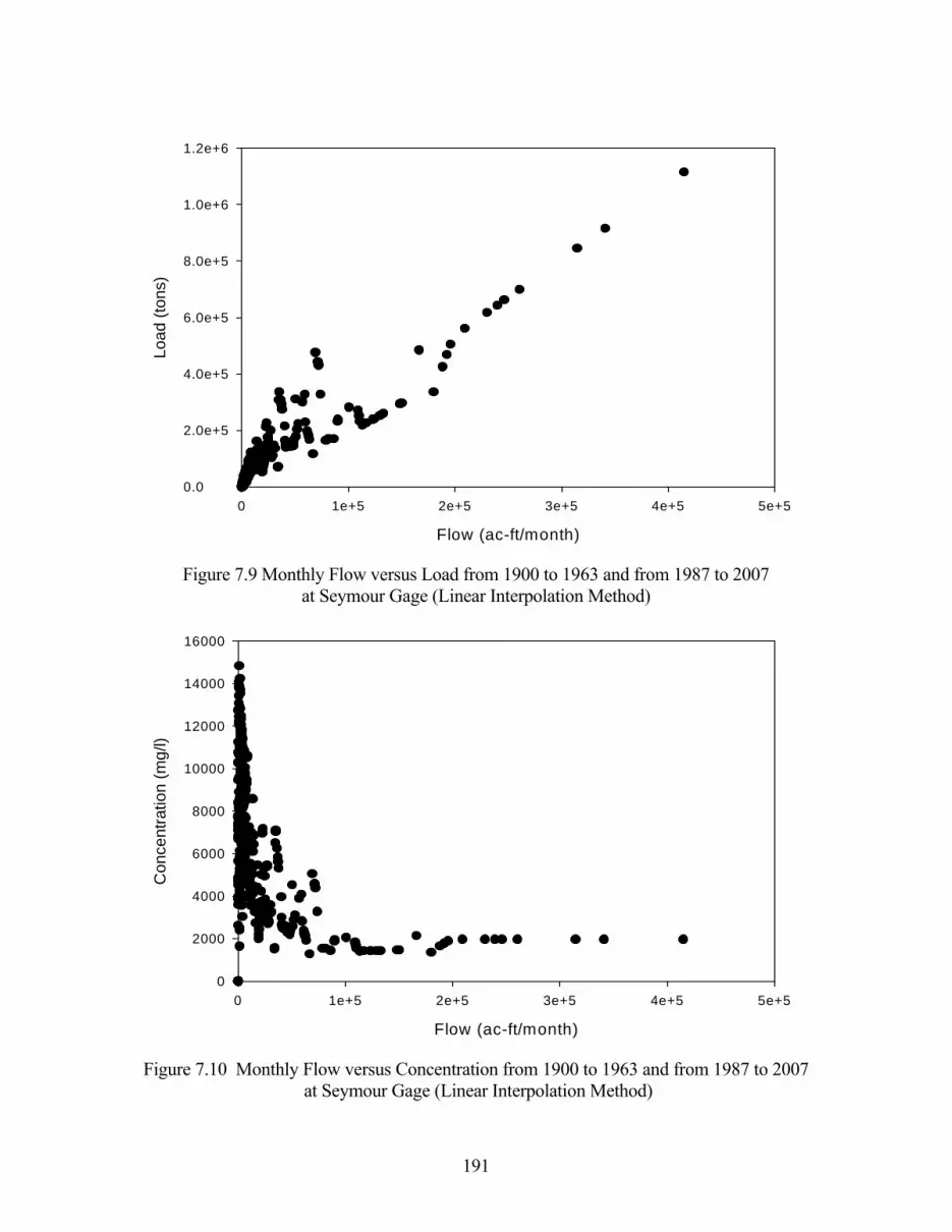
191

Flow (ac-ft/month)

0 1e+5 2e+5 3e+5 4e+5 5e+5

Load

(ton

s)

0.0

2.0e+5

4.0e+5

6.0e+5

8.0e+5

1.0e+6

1.2e+6

Figure 7.9 Monthly Flow versus Load from 1900 to 1963 and from 1987 to 2007 at Seymour Gage (Linear Interpolation Method)

Flow (ac-ft/month)

0 1e+5 2e+5 3e+5 4e+5 5e+5

Con

cent

ratio

n (m

g/l)

0

2000

4000

6000

8000

10000

12000

14000

16000

Figure 7.10 Monthly Flow versus Concentration from 1900 to 1963 and from 1987 to 2007 at Seymour Gage (Linear Interpolation Method)

192

Flow (ac-ft/month)

0 1e+5 2e+5 3e+5 4e+5 5e+5

Load

(ton

s)

0.0

2.0e+5

4.0e+5

6.0e+5

8.0e+5

1.0e+6

1.2e+6

1.4e+6

1.6e+6

Figure 7.11 Monthly Flow versus Load from 1900 to 1963 and from 1987 to 2007 at Seymour Gage (Linear Regression Method)

Flow (ac-ft/month)

0 1e+5 2e+5 3e+5 4e+5 5e+5

Con

cent

ratio

n (m

g/l)

0

500

1000

1500

2000

2500

3000

Figure 7.12 Monthly Flow versus Concentration from 1900 to 1963 and from 1987 to 2007 at Seymour Gage (Linear Regression Method)

193

Graford Gage

The WRAP-SALT salinity input file contains 1900-2007 monthly TDS concentrations at the Graford gage that represent the concentrations of incremental flows entering the river between the Seymour gage and Graford gage. The naturalized flows from the Brazos WAM dataset at the Seymour gage and Graford gage were entered in the program SALIN input SAI file to compute the incremental natural inflows between the Seymour gage and Graford gage. These incremental monthly inflow volumes are plotted in Figure 7.13.

The concentrations for negative incremental flows were assigned as the USGS water year 1964-1986 (October 1963 through September 1986) mean concentration. The 1964-1986 mean concentration value of 706.09 mg/l was entered in JC record field 14 in the SAI file.

JC 1900 108 2 1 1 2 276 101963 091986 706.09

Statistics for the results from the linear interpolation and linear regression methods are tabulated in Tables 7.8 and 7.9. The 1900-1963 mean of loads synthesized by linear interpolation is 46,184 tons/months with a concentration of 683 mg/l. The 1987-2007 mean of the interpolated loads is 43,041 tons/month with a concentration of 711 mg/l. The 1964-1986 mean is 706 mg/l. TDS loads and concentrations at the Graford gage are plotted in Figures 7.14 through 7.17. A dashed line is used in the plots for the period from October 1963 through September 1986 during which USGS observed volumes, loads, and concentrations are available. The solid lines are the monthly TDS loads and concentrations for January 1900 through September 1963 and October 1986 through December 2007 that were synthesized based on either linear interpolation or linear regression. Relationships between monthly flow volumes versus TDS loads and concentrations are shown in Figures 7.18 through 7.23.

Table 7.8

Statistics for the Results from the Linear Interpolation Method for the Graford gage

Period 1964-1986 1900-2007 1900-1963 1987-2007

Number of months 276 1,296 765 255 Mean of volume (acre-feet/month) 33,153 45,195 49,761 44,532 Mean of load (tons/month) 31,828 42,508 46,184 43,041 Mean of concentrations (mg/l) 706 692 683 711 Standard deviation of volume 78,260 96,948 106,421 83,681 Standard deviation of load 57,452 71,539 77,594 65,152 Standard deviation of concentration 719 602 580 511 Autocorrelation coefficient for volume 0.161 0.300 0.298 0.425 Autocorrelation coefficient for load 0.188 0.284 0.278 0.363 Autocorrelation coeff. for concentration 0.455 0.310 0.259 0.249 Smallest concentration (mg/l) 0 0 2 0 Greatest concentration (mg/l) 4,166 4,166 4,109 3,926

194

Table 7.9 Statistics for the Results from the Linear Regression Method for the Graford Gage

Period 1964-1986 1900-2007 1900-1963 1987-2007

Number of months 276 1,296 765 255 Mean of volume (acre-feet/month) 33,153 45,195 49,761 44,532 Mean of load (tons/month_ 31,828 34,171 35,743 31,987 Mean of concentrations (mg/l) 706 556 528 528 Standard deviation of volume 78,260 96,948 106,421 83,681 Standard deviation of load 57,452 69,718 76,442 60,108 Standard deviation of concentration 719 362 53 33 Autocorrelation coefficient for volume 0.161 0.300 0.298 0.425 Autocorrelation coefficient for load 0.188 0.301 0.298 0.425 Autocorrelation coeff. for concentration 0.455 0.579 0.232 0.000 Correlation coeff. for linear regression 0.907 - - - Smallest concentration (mg/l) 0 0 528 0 Greatest concentration (mg/l) 4,166 4,166 706 706

Time (months)

1900 1920 1940 1960 1980 2000

Flow

(ac-

ft/m

onth

)

0.0

2.0e+5

4.0e+5

6.0e+5

8.0e+5

1.0e+6

1.2e+6

1.4e+6

1.6e+6

1.8e+6

Figure 7.13 Incremental Stream Flows at the Graford Gage

195

Time (months)

1900 1920 1940 1960 1980 2000

Load

(ton

s)

0

2e+5

4e+5

6e+5

8e+5

1e+6


Figure 7.14 Loads at Graford Gage Synthesized by Linear Interpolation

Time (months)

1900 1920 1940 1960 1980 2000

Con

cent

ratio

n (m

g/l)

0

1000

2000

3000

4000

5000Synthesized concentrations1963-86 concentrations

Figure 7.15 Concentrations at Graford Gage based on by Linear Interpolation of Loads

196

Time (months)

1900 1920 1940 1960 1980 2000

Load

(ton

s)

0.0

2.0e+5

4.0e+5

6.0e+5

8.0e+5

1.0e+6

1.2e+6


Figure 7.16 Loads at Graford Gage Synthesized by Linear Regression

Time (months)

1900 1920 1940 1960 1980 2000

Con

cent

ratio

n (m

g/l)

0

1000

2000

3000

4000Synthesized concentrations1963-86 concentrations

Figure 7.17 Concentrations at Graford Gage Synthesized by Linear Regression

197

Flow (ac-ft/month)

0 2e+5 4e+5 6e+5 8e+5

Load

(ton

s)

0

1e+5

2e+5

3e+5

4e+5

5e+5

Figure 7.18 Monthly Incremental Inflow versus Load from 1964 to 1986 at Graford Gage

Flow (ac-ft/month)

0 2e+5 4e+5 6e+5 8e+5

Con

cent

ratio

n (m

g/l)

0

1000

2000

3000

4000

5000

Figure 7.19 Monthly Incremental Inflow versus Concentration from 1964 to 1986 at Graford Gage

198

Flow (ac-ft/month)

0 1e+5 2e+5 3e+5 4e+5 5e+5 6e+5

Load

(ton

s)

0.0

5.0e+4

1.0e+5

1.5e+5

2.0e+5

2.5e+5

3.0e+5

3.5e+5

Figure 7.20 Monthly Incremental Inflow versus Load from 1900 to 1963 and from 1987 to 2007 at Graford Gage (Linear Interpolation Method)

Flow (ac-ft/month)

0.0 2.0e+5 4.0e+5 6.0e+5 8.0e+5 1.0e+6 1.2e+6 1.4e+6 1.6e+6 1.8e+6

Con

cent

ratio

n (m

g/l)

0

1000

2000

3000

4000

5000

Figure 7.21 Monthly Incremental Inflow versus Concentration from 1900 to 1963 and from 1987 to 2007 at Graford Gage (Linear Interpolation Method)

199

Flow (ac-ft/month)

0 1e+5 2e+5 3e+5 4e+5 5e+5 6e+5

Load

(ton

s)

0

1e+5

2e+5

3e+5

4e+5

5e+5

Figure 7.22 Monthly Incremental Inflow versus Load from 1900 to 1963 and from 1987 to 2007 at Graford Gage (Linear Regression Method)

Flow (ac-ft/month)

0.0 2.0e+5 4.0e+5 6.0e+5 8.0e+5 1.0e+6 1.2e+6 1.4e+6 1.6e+6 1.8e+6

Con

cent

ratio

n (m

g/l)

0

200

400

600

800

Figure 7.23 Monthly Incremental Inflow versus Concentration from 1900 to 1963 and from 1987 to 2007 at Graford Gage (Linear Regression Method)

200

Whitney Gage

The WRAP-SALT salinity input file contains 1900-2007 monthly TDS concentrations at the Whitney gage located below Whitney Dam that represents the concentrations of incremental flows entering the river between the Graford gage and Whitney Dam. The naturalized flow volumes from the Brazos WAM dataset at the Graford gage and Whitney gage were entered in the program SALIN input SAI file to compute the incremental natural inflows. These incremental monthly inflow volumes are plotted in Figure 7.24. The USGS water year 1964-1986 incremental inflow TDS loads entering the river/reservoir system were computed by considering the Graford-to-Dennis, Dennis-to-Glen Rose, and Glen Rose-to-Whitney load inflows.

The concentrations for negative incremental flows were assigned as a mean concentration value for the 1964-1986 period. The 1964-1986 mean concentration of 315.63 mg/l for was entered in JC record field 14 in the program SALIN input file.

JC 1900 108 2 1 1 2 276 101963 091986 315.63

The statistics of the results from the linear interpolation and linear regression methods are represented in Tables 7.10 and 7.11. The 1900-1963 mean of loads synthesized by linear interpolation is 23,149 tons/month with a concentration of 308 mg/l. The mean load value for 1987-2007 is 29,980 tons/month and mean concentration is 306 mg/l. Figures 7.25 and 7.26 show the loads and concentrations developed using the linear interpolation method. The loads and concentrations synthesized by linear regression are plotted in Figures 7.27 and 7.28.

Table 7.10 Statistics for the Results from Linear Interpolation Method for the Whitney Gage

Period 1964-1986 1900-2007 1900-1963 1987-2007

Number of months 276 1,296 765 255 Mean of volume (acre-feet/month) 43,078 55,968 55,232 72,127 Mean of load (tons/month) 18,487 23,500 23,149 29,980 Mean of concentrations (mg/l) 316 309 308 306 Standard deviation of volume 68,403 108,030 112,366 126,542 Standard deviation of load 71,934 54,679 47,647 52,371 Standard deviation of concentration 2,682 3,727 4,542 974 Autocorrelation coefficient for volume 0.947 0.32 0.244 0.489 Autocorrelation coefficient for load 0.058 0.153 0.15 0.34 Autocorrelation coeff. for concentration 0.085 0.024 0.019 0.082 Smallest concentration (mg/l) 0 0 55 0 Greatest concentration (mg/l) 35,295 86,109 86,109 10,524

201

Table 7.11 Statistics for the Results from Linear Regression Method for the Whitney Gage

Period 1964-1986 1900-2007 1900-1963 1987-2007

Number of months 276 1,296 765 255 Mean of volume (acre-feet/month) 43,078 55,968 55,232 72,127 Mean of load (tons/month) 18,488 21,290 20,482 26,747 Mean of concentrations (mg/l) 316 280 273 273 Standard deviation of volume 68,403 108,030 112,366 126,542 Standard deviation of load 71,930 50,626 41,670 46,926 Standard deviation of concentration 2,682 1,239 14 8 Autocorrelation coefficient for volume 0.292 0.320 0.244 0.489 Autocorrelation coefficient for load 0.055 0.207 0.244 0.489 Autocorrelation coeff. for concentration 0.052 0.060 0.171 0.125 Correlation coeff. for linear regression 0.328 - - - Smallest concentration (mg/l) 0 22 273 0 Greatest concentration (mg/l) 35,295 35,295 316 316

Time (months)

1900 1920 1940 1960 1980 2000

Flow

(ac-

ft/m

onth

)

0.0

2.0e+5

4.0e+5

6.0e+5

1.2e+6

1.3e+6

1.4e+6

Figure 7.24 Incremental Stream Flows at the Whitney gage

202

Time (months)

1900 1920 1940 1960 1980 2000

Load

(ton

s)

0

1e+5

2e+5

6e+5

8e+5 Synthesized loads1963-86 loads

Figure 7.25 Incremental Loads at Whitney Gage Synthesized by Linear Interpolation

Time (months)

1900 1920 1940 1960 1980 2000

Con

cent

ratio

n (m

g/l)

0

1e+3

2e+3

3e+3

4e+3

5e+3

1e+5

2e+5

3e+5Synthesized conc1963-86 conc

Figure 7.26 Incremental Inflow Concentrations at Whitney Gage based on by Linear Interpolation of Loads

203

Time (months)

1900 1920 1940 1960 1980 2000

Load

(ton

s)

0.0

2.0e+5

4.0e+5

6.0e+5

8.0e+5

1.0e+6

1.2e+6

1.4e+6


Figure 7.27 Incremental Loads at Whitney Gage Synthesized by Linear Regression

Time (months)

1900 1920 1940 1960 1980 2000

Con

cent

ratio

n (m

g/l)

0

300

600

900

1200

1500

1800 Synthesized concentrations1963-86 concentrations

Figure 7.28 Incremental Inflow Concentrations at Whitney Gage by Linear Interpolation

204

Flow (ac-ft/month)

0 1e+5 2e+5 3e+5 4e+5 5e+5

Load

(ton

s)

0

1e+5

2e+5

8e+5

9e+5

Figure 7.29 Monthly Inflow Volumes versus Loads from 1967 to 1986 at Whitney Gage

Flow (ac-ft/month)

0 1e+5 2e+5 3e+5 4e+5 5e+5

Con

cent

ratio

n (m

g/l)

0

5000

1000030000

35000

40000

Figure 7.30 Monthly Flows versus Concentrations from 1967 to 1986 at Whitney Gage

205

Flow (ac-ft/month)

0 1e+6 2e+6 3e+6 4e+6 5e+6 6e+6

Load

(ton

s)

0

5e+5

1e+6

2e+6

2e+6

Figure 7.31 Monthly Flows versus Loads from 1900 to 1963 and from 1986 to 2007 at Whitney Gage (Linear Interpolation Method)

Flow (ac-ft/month)

0 1e+6 2e+6 3e+6 4e+6 5e+6 6e+6

Con

cent

ratio

n (m

g/l)

0

200

400

600

800

1000

1200

1400

1600

1800

2000

Figure 7.32 Monthly Flows versus Concentration from 1900 to 1963 and from 1986 to 2007 at

Whitney Gage (Linear Interpolation Method)

206

Flow (ac-ft/month)

0 1e+6 2e+6 3e+6 4e+6 5e+6 6e+6

Load

(ton

s)

0.0

4.0e+5

8.0e+5

1.2e+6

1.6e+6

Figure 7.33 Monthly Flows versus Loads from 1900 to 1963 and from 1986 to 2007 at Whitney Gage (Linear Regression Method)

Flow (ac-ft/month)

0 1e+6 2e+6 3e+6 4e+6 5e+6 6e+6

Con

cent

ratio

n (m

g/l)

0

50

100

150

200

250

Figure 7.34 Monthly Flows versus Concentration from 1940 to 1963 and from 1986 to 1997 at Whitney Gage (Linear Interpolation Method)

207

Cameron Gage Two alternative methods for modeling loads and concentrations in the Little River subbasin above the Cameron gage were investigated. The alternative adopted was to treat the Cameron gage as an upstream boundary with the observed 1964-1986 mean concentration of 256 mg/l applied to the entire 1900-2007 simulation period. The TDS loads entering at this upstream boundary location are computed within WRAP-SALT by combining the constant 256 mg/l concentration with the regulated flow at the Cameron gage during each month of the 1900-2007 simulation period. The second alternative simulation approach investigated was to treat the Cameron gage similarly to the other gage locations, with a 1900-2007 time series of inputted monthly concentrations applied to flows at all locations in the Little River subbasin at and above the Cameron gage. The concentrations of flows entering the river above the Cameron gage were synthesized as follows alternatively applying the linear interpolation and linear regression methods. The 1900-2007 naturalized flows at the Cameron gage are plotted in Figure 7.35. Since these are total flows, there are no negative incremental inflows to deal with. The statistics from the datasets resulting from applying the linear interpolation and linear regression methods are presented in Tables 7.12 and 7.13, respectively. The 1900-1963 means of loads and concentrations synthesized by the linear interpolation method shown in Table 7.12 are 37,136 tons/months and 250 mg/l. The 1987-2007 mean loads and concentrations from Table 7.12 based on the linear interpolation method are 52,107 tons/month and 244 mg/l.

Time (months)

1900 1920 1940 1960 1980 2000

Flow

(ac-

ft/m

onth

)

0.0

2.0e+5

4.0e+5

6.0e+5

8.0e+5

1.0e+6

1.2e+6

1.4e+6

1.6e+6

1.8e+6

Figure 7.35. Stream Flows at the Cameron gage

208

Application of linear regression results in the 1900-1963 mean load and concentration of 36,155 tons/month and 243 mg/l shown in Table 7.13. The 1987-2007 means of the loads and concentrations determined linear regression method are 51,897 tons/month and 243 mg/l. The correlation coefficient for the linear relationship between 1964-1986 monthly flow volumes and loads is 0.982. Time series plots of monthly loads and concentrations are presented as Figures 7.37 through 7.39. Flow volume versus loads and concentrations are plotted in Figures 7.40 − 7.45.

Table 7.12 Statistics for the Results from Linear Interpolation Method for the Cameron Gage

Period 1964-1986 1900-2007 1900-1963 1987-2007

Number of months 276 1,296 765 255 Mean of volume (acre-feet/month) 89,374 114,370 109,243 156,807 Mean of load (tons/month) 31,134 38,804 37,136 52,107 Mean of concentrations (mg/l) 256 250 250 244 Standard deviation of volume 111,421 180,924 183,597 222,470 Standard deviation of load 36,202 59,008 60,081 72,291 Standard deviation of concentration 77.6 79 82 68 Autocorrelation coefficient for volume 0.916 0.489 0.392 0.633 Autocorrelation coefficient for load 0.863 0.474 0.379 0.605 Autocorrelation coeff. for concentration 0.737 0.638 0.587 0.629 Smallest concentration (mg/l) 0 0 0 0 Greatest concentration (mg/l) 474 474 474 436

Table 7.13 Statistics for the Results from Linear Regression Method for the Cameron Gage

Period 1964-1986 1900-2007 1900-1963 1987-2007

Number of months 276 1,296 765 255 Mean of volume (acre-feet/month) 89,374 114,370 109,243 156,807 Mean of load (tons/month) 31,134 38,183 36,155 51,897 Mean of concentrations (mg/l) 256 246 243 243 Standard deviation of volume 111,421 180,924 183,597 222,470 Standard deviation of load 36,202 59,749 60,764 73,629 Standard deviation of concentration 77.6 42 20 0 Autocorrelation coefficient for volume 0.592 0.489 0.392 0.633 Autocorrelation coefficient for load 0.626 0.491 0.392 0.633 Autocorrelation coeff. for concentration 0.753 0.713 0.200 0.993 Correlation coeff. for linear regression 0.982 - - - Smallest concentration (mg/l) 0 0 0 0 Greatest concentration (mg/l) 474 474 243 243

209

Time (months)

1900 1920 1940 1960 1980 2000

Load

(ton

s)

0

1e+5

2e+5

3e+5

4e+5

5e+5

6e+5


Figure 7.36 Loads at Cameron Gage Synthesized by Linear Interpolation

Time (months)

1900 1920 1940 1960 1980 2000

Con

cent

ratio

n (m

g/l)

0

100

200

300

400

500

600


Figure 7.37 Concentrations at Cameron Gage Synthesized by Linear Interpolation

210

Time (months)

1900 1920 1940 1960 1980 2000

Load

(ton

s)

0

1e+5

2e+5

3e+5

4e+5

5e+5

6e+5


Figure 7.38 Loads at Cameron Gage Synthesized by Linear Regression

Time (months)

1900 1920 1940 1960 1980 2000

Con

cent

ratio

n (m

g/l)

0

100

200

300

400

500

600


Figure 7.39 Concentrations at Cameron Gage Synthesized by Linear Regression

211

Flow (ac-ft/month)

0 2e+5 4e+5 6e+5 8e+5 1e+6

Load

(ton

s)

0

5e+4

1e+5

2e+5

2e+5

3e+5

3e+5

Figure 7.40 Monthly Flows versus Loads from 1967 to 1986 at Cameron Gage

Flow (ac-ft/month)

0 2e+5 4e+5 6e+5 8e+5 1e+6

Con

cent

ratio

n (m

g/l)

0

100

200

300

400

500

Figure 7.41 Monthly Flows versus Concentrations from 1967 to 1986 at Cameron Gage

212

Flow (ac-ft/month)

0.0 2.0e+5 4.0e+5 6.0e+5 8.0e+5 1.0e+6 1.2e+6 1.4e+6 1.6e+6 1.8e+6

Load

(ton

s)

0

1e+5

2e+5

3e+5

4e+5

5e+5

6e+5

7e+5

Figure 7.42 Monthly Flows versus Loads from 1900 to 1963 and from 1986 to 2007 at Cameron Gage (Linear Interpolation Method)

Flow (ac-ft/month)

0.0 2.0e+5 4.0e+5 6.0e+5 8.0e+5 1.0e+6 1.2e+6 1.4e+6 1.6e+6 1.8e+6

Con

cent

ratio

n (m

g/l)

0

100

200

300

400

500

Figure 7.43 Monthly Flows versus Concentrations from 1900 to 1963 and from 1986 to 2007 at Cameron Gage (Linear Interpolation Method)

213

Flow (ac-ft/month)

0.0 2.0e+5 4.0e+5 6.0e+5 8.0e+5 1.0e+6 1.2e+6 1.4e+6 1.6e+6 1.8e+6

Load

(ton

s)

0

1e+5

2e+5

3e+5

4e+5

5e+5

6e+5

Figure 7.44 Monthly Flows versus Loads from 1900 to 1963 and from 1986 to 2007 at Cameron Gage (Linear Regression Method)

Flow (ac-ft/month)

0.0 2.0e+5 4.0e+5 6.0e+5 8.0e+5 1.0e+6 1.2e+6 1.4e+6 1.6e+6 1.8e+6

Con

cent

ratio

n (m

g/l)

0

50

100

150

200

250

300

Figure 7.45 Monthly Flows versus Concentrations from 1900 to 1963 and from 1986 to 2007 at Cameron Gage (Linear Regression Method)

214

Richmond gage

The WRAP-SALT salinity input file contains January 1900 through December 2007 monthly TDS concentrations at the Richmond gage that represent the concentrations of incremental flows entering the river upstream of the Richmond gage but downstream of the Whitney and Cameron gages. The naturalized flows from the Brazos WAM dataset at the Richmond, Whitney, and Cameron gages were entered in the program SALIN input SAI file to compute the incremental natural inflows as the flows at Richmond less the flows at the Whitney and Cameron gages. These incremental monthly inflow volumes for 1900-1963 and 1987-2007 naturalized flows and 1964-1986 observed flows are plotted in Figure 7.46.

Time (months)

1900 1920 1940 1960 1980 2000

Flow

(ac-

ft/m

onth

)

0

1e+6

2e+6

3e+6

4e+6

5e+6

6e+6

Figure 7.46 Incremental Inflows at the Richmond Gage The observed 1964-1986 monthly incremental TDS loads and flow volumes were used in combination with 1900-1963 and 1987-2007 naturalized flows to synthesize concentrations for 1900-1963 and 1987-2007 alternatively by linear interpolation and linear regression. The 1900-1963 and 1987-2007 loads are synthesized by using the relationship between incremental inflow volumes and incremental inflow loads for 1964-1986. Concentrations for negative incremental flows were set at the 1964-1986 mean concentration of 192.92 mg/l. As repeated in `Tables 7.4, 7.14, and 7.15, the 1964-1986 means of the incremental inflow volumes and loads are 251,443 ac-ft/month and 65,956 tons/month. Statistics for the results from linear interpolation and linear regression methods are tabulated in Tables 7.14 and 7.15. The 1900-1963 mean of incremental loads synthesized by linear interpolation is 65,121 tons/months with a concentration of 205 mg/l. The 1987-2007 mean of the interpolated loads is 88,044 tons/month

215

with a mean concentration of 198 mg/l. Means of the 1900-1963 loads and concentrations synthesized by the linear interpolation method are 60,110 tons/month and 189 mg/l. The mean of the 1987-2007 loads is 84,297 tons/month with a concentration of 189 mg/l. The linear correlation coefficient for the 1964-1986 incremental inflow volumes versus loads at the Richmond gage is 0.838.

Table 7.14 Statistics for the Results from Linear Interpolation Method for the Richmond Gage

Period 1964-1986 1900-2007 1900-1963 1987-2007

Number of months 276 1,296 765 255 Mean of volume (acre-feet/month) 251,443 255,956 233,671 327,695 Mean of load (tons/month) 65,955 69,801 65,121 88,004 Mean of concentrations (mg/l) 193 201 205 198 Standard deviation of volume 321,302 379,503 395,169 382,268 Standard deviation of load 97,383 116,211 124,208 108,479 Standard deviation of concentration 190 152 150 123 Autocorrelation coefficient for volume 0.914 0.409 0.364 0.557 Autocorrelation coefficient for load 0.593 0.309 0.278 0.497 Autocorrelation coeff. for concentration 0.046 0.166 0.141 0.170 Smallest concentration (mg/l) 0 4 8 0 Greatest concentration (mg/l) 1,742 1,742 1,533 705

Table 7.15 Statistics from the Results from Linear Regression Method for the Richmond Gage

Period 1964-1986 1900-2007 1900-1963 1987-2007

Number of months 276 1,296 765 255 Mean of volume (acre-feet/month) 251,443 255,956 233,671 327,695 Mean of load (tons/month) 65,955 66,114 60,110 84,297 Mean of concentrations (mg/l) 193 190 189 189 Standard deviation of volume 321,302 379,503 395,169 382,268 Standard deviation of load 97,383 100,466 101,654 98,336 Standard deviation of concentration 190 83 1 0 Autocorrelation coefficient for volume 0.368 0.409 0.364 0.557 Autocorrelation coefficient for load 0.202 0.374 0.364 0.557 Autocorrelation coeff. for concentration 0.082 0.224 0.042 0.991 Correlation coeff. for linear regression 0.838 - - - Smallest concentration (mg/l) 0 4 189 0 Greatest concentration (mg/l) 1,742 1,742 193 189

216

Time (months)

1900 1920 1940 1960 1980 2000

Load

(ton

s)

0.0

3.0e+5

6.0e+5

9.0e+5

1.2e+6

1.5e+6

1.8e+6

2.1e+6


Figure 7.47 Incremental Loads at Richmond Gage Synthesized by Linear Interpolation

Time (months)

1900 1920 1940 1960 1980 2000

Con

cent

ratio

n (m

g/l)

0

500

1000

1500

2000


Figure 7.48 Incremental Inflow Concentrations at Richmond Gage by Linear Interpolation

217

Time (months)

1900 1920 1940 1960 1980 2000

Load

(ton

s)

0.0

2.0e+5

4.0e+5

6.0e+5

8.0e+5

1.0e+6

1.2e+6

1.4e+6


Figure 7.49 Incremental Inflow Concentrations at Richmond Gage by Linear Regression

Time (months)

1900 1920 1940 1960 1980 2000

Con

cent

ratio

n (m

g/l)

0

300

600

900

1200

1500

1800 Synthesized concentrations1963-86 concentrations

Figure 7.50 Incremental Inflow Concentrations at Richmond Gage by Linear Regression

218

Flow (ac-ft/month)

0.0 5.0e+5 1.0e+6 1.5e+6 2.0e+6 2.5e+6

Load

(ton

s)

0

2e+5

4e+5

6e+5

8e+5

1e+6

Figure 7.51 Monthly Flows versus Loads from 1967 to 1986 at Richmond Gage

Flow (ac-ft/month)

0.0 5.0e+5 1.0e+6 1.5e+6 2.0e+6 2.5e+6

Con

cent

ratio

n (m

g/l)

0

200

400

600

800

1000

1200

1400

1600

1800

2000

Figure 7.52 Monthly Flows versus Concentrations from 1967 to 1986 at Richmond Gage

219

Flow (ac-ft/month)

0 1e+6 2e+6 3e+6 4e+6 5e+6 6e+6

Load

(ton

s)

0

5e+5

1e+6

2e+6

2e+6

Figure 7.53 Monthly Flows versus Loads from 1900 to 1963 and from 1986 to 2007 at Richmond Gage (Linear Interpolation Method)

Flow (ac-ft/month)

0 1e+6 2e+6 3e+6 4e+6 5e+6 6e+6

Con

cent

ratio

n (m

g/l)

0

200

400

600

800

1000

1200

1400

1600

1800

2000

Figure 7.54 Monthly Flows versus Concentrations from 1900 to 1963 and from 1986 to 2007 at Richmond Gage (Linear Interpolation Method)

220

Flow (ac-ft/month)

0 1e+6 2e+6 3e+6 4e+6 5e+6 6e+6

Load

(ton

s)

0.0

4.0e+5

8.0e+5

1.2e+6

1.6e+6

Figure 7.55 Monthly Flows versus Loads from 1900 to 1963 and from 1986 to 2007 at Richmond Gage (Linear Regression Method)

Flow (ac-ft/month)

0 1e+6 2e+6 3e+6 4e+6 5e+6 6e+6

Con

cent

ratio

n (m

g/l)

0

50

100

150

200

250

Figure 7.56 Monthly Flows versus Concentrations from 1900 to 1963 and from 1986 to 2007 at Richmond Gage (Linear Regression Method)

221

Salinity Inflow Data Summary The Water Rights Analysis Package (WRAP) computer program SALT reads a salinity input file with the filename extension SIN. The majority of the data contained in the SIN file consists of concentrations and/or loads that define the salinity inflows to the river/reservoir system. Time series sequences of loads or concentrations for each of the months of the simulation are entered on S records. Alternatively, constant mean concentrations may be input on CC records and repeated within the WRAP-SALT simulation for all months. The WRAP-SALT load or concentration input data are entered in the SIN file for specific control points representing locations in the river system. The load or concentration data entered for a particular control point may be repeated automatically within WRAP-SALT for any number of other control points. Salinity inflow data for the WRAP-SALT input SIN file were developed by applying the methodology outlined in this chapter using Microsoft Excel and the WRAP utility program SALIN. A single SIN file was developed which is designed for use with the various versions of the Brazos River Basin datasets from the Texas Commission on Environmental Quality (TCEQ) Water Availability Modeling (WAM) System or the Brazos River Authority Condensed (BRAC) datasets. The SIN file is applicable for the entire 1900-2007 period-of-analysis or simulations for any sub-period of 1900-2007 such as 1940-1997 or 1940-2007.

Table 7.16

Total Dissolved Solids (TDS) Data Entered in Salinity Input SIN File

Control 1900-2007 Monthly Sequences on S Records Point ID Control Point Location or Constant Concentration on CC Record

BRSE11 Brazos River at Seymour gage

below primary salt source areas Load series for total regulated flows. These inflow loads are plotted in Figure 7.3.

SHGR26 Brazos River at Graford gage below Possum Kingdom Lake.

Concentration series for incremental inflows which is plotted in Figure 7.15.

BRAQ33 Brazos River at Whitney (Aquilla) gage below Whitney Dam


LRCA58 Little River at Cameron gage Constant concentration of 256 mg/l for total regulated flows.

BRRI70 Brazos River at Richmond gage Concentration series for incremental inflows which is plotted in Figure 7.48.

BRGM73 Brazos River at Gulf of Mexico Constant concentration of 339 mg/l for incremental inflows.

The salinity data in the SIN file are assigned to six control points which represent the five USGS gaging stations listed in Table 7.16 and the outlet of the Brazos River at the Gulf of Mexico. The salt concentrations provided in the SIN file are repeated at other control points within the WRAP-SALT simulation. Observed October 1963 through September 1986 total dissolved solids (TDS) loads and concentrations described in Chapters 1, 2, and 3 are extended based on TCEQ

222

WAM System naturalized flows using the methodology outlined in the present Chapter 7 to cover the period from January 1900 through December 2007. Control points BRSE11 and LRCA58 at the Seymour and Cameron gages are upstream boundaries for the WRAP-SALT salinity simulation. WRAP-SIM simulation results providing the water quantities that are read by WRAP-SALT as input to the salinity simulation include all control points including those located above the Seymour and Cameron gage control points. However, the salinity simulation does not extend upstream of these boundaries. A 1900-2007 sequence of monthly TDS loads are incorporated in the SIN file for control point BRSE11 (Seymour gage). Observed loads for USGS water years 1964-1986 (October 1963 through September 1986) are combined with flows synthesized by linear interpolated as a function of Brazos WAM naturalized flow volumes for the periods 1900-1963 and 1987-2007. These loads are treated within WRAP-SALT as the loads of the regulated flows at control point BRSE11. A constant TDS concentration of 256 mg/l is assigned in the SIN file to control point LRCA58 (Little River at Cameron gage). The 256 mg/l is the 1964-1986 mean observed concentration. This concentration is applied within WRAP-SALT to the regulated flows at control point LRCA58 in all months of the 1900-2007 simulation. The resulting computed loads represent the total TDS load flowing pass control point LRCA58 during each month of the simulation. Sequences of TDS concentrations covering each month of the 1,296-month 1900-2007 simulation period-of-analysis are incorporated in the SIN file for control points SHGR26, BRAQ33, and BRRI70 located at the Graford, Whitney (Aquilla), and Richmond gages. These are the concentrations of the incremental inflows that enter the river/reservoir system at any control point located on the Brazos River or tributaries that flow into the reaches of the Brazos River between control points SHGR26, BRAQ33, and BRRI70. These inflow concentrations are combined with incremental inflow volumes within the WRAP-SALT simulation to determine the salt loads entering the river/reservoir system. The incremental inflow volumes are determined by WRAP-SALT from the total naturalized or otherwise adjusted flow volumes read by WRAP-SIM from the IN records in its FLO input file. Incremental flows are computed as differences between total flows. A constant TDS concentration of 339 mg/l is assigned in the SIN file to control point BRGM73 which is the Brazos River outlet at the Gulf of Mexico. This concentration is applied within WRAP-SALT to the incremental inflows at all control points below control point BRRI70 (Richmond gage) in all months of the 1900-2007 simulation. The WRAP-SALT simulation model performs salt load accounting computations that track the entering loads through the river/reservoir over time. Loads leave the river/reservoir system with the WRAP-SIM simulated diversions, channel losses, and regulated flows at the outlet. WRAP-SALT also has a feature for modeling additional otherwise unaccounted losses of load. For the Brazos River Basin, such additional losses are assigned to the control points of Possum Kingdom, Granbury, and Whitney Reservoirs. The losses each month are computed within WRAP-SALT as a specified fraction of the loads entering the reservoir. The input parameters in the WRAP-SALT salinity SIN input file are the percentages 17.42%, 6.59%, and 3.00% from Table 7.5 for Lakes Possum Kingdom, Granbury, and Whitney, respectively. WRAP-SALT computes losses by multiplying these percentages by the regulated inflow loads to the reservoir each month.

223

CHAPTER 8 WRAP SIMULATION OF THE BRAZOS RIVER BASIN

This chapter presents a simulation study in which the WRAP computer program SALT is applied in combination with the WRAP programs SIM and TABLES to model the Brazos River Basin. Impacts of natural salt pollution on water supply capabilities are investigated with the simulation model. The impacts of multiple-reservoir system operations and salinity control measures on salinity concentrations throughout the river system are also explored. WRAP-SIM and TABLES are described in the basic WRAP Reference Manual and Users Manual (Wurbs 2009). WRAP-SALT and salinity related features of TABLES are covered in the Salinity Manual (Wurbs 2009).

Brazos River System The Brazos River Basin, its major reservoirs, and characteristics of its natural salt pollution are described in Chapter 1. Figure 1.2 of Chapter 1 is a map of the Brazos River Basin showing its location within Texas and New Mexico. Figure 8.1 is a more detailed basin map showing the 12 Brazos River Authority (BRA) reservoirs, Hubbard Creek Reservoir owned by the West Central Texas Municipal Water District, and five stream gaging stations. The dry flat upper basin in and near New Mexico, which contributes little or no flow to the river system, is omitted from Figure 8.1. WRAP-SALT input and output data are referenced by control point. Several key control points referenced throughout this chapter are shown in Figure 8.1 and Table 8.1. The Bwam8 dataset has 3,834 control points. The BRAC8 and BRAC2008 datasets have 48 control points described later in this chapter. The 15 selected control points listed in Table 8.1 are included in all of the datasets. The first six control points listed in Table 8.1 are locations of U.S. Geological Survey (USGS) stream gaging stations. BRGM73 is the outlet of the Brazos River at the Gulf of Mexico. The last eight control points listed are the locations of major reservoirs. The locations of the control points listed in Table 8.1 are shown in Figure 8.1. Mean flows, loads, and concentrations from the U.S. Geological Survey (USGS) 1984-1986 water quality sampling program are tabulated in Table 1.2 for 26 stations shown in Figure 1.3. Figures 8.2, 8.3, and 8.4 illustrate the dramatic spatial and temporal variability of salt concentrations. Figure 8.2 shows 1964-1986 mean concentrations, loads, and flows at four gaging stations on the Brazos River and the Cameron gage on the Little River from the USGS data discussed in Chapter 1. The 1964-1986 monthly concentrations at the Seymour and Richmond gages are plotted in Figures 8.3 and 8.4. Figure 8.2 shows the 1964-86 mean TDS concentrations of Brazos River flows of 3,590 mg/l, 1,510 mg/l, 928 mg/l, and 339 mg/l at the Seymour, Possum Kingdom, Whitney, and Richmond gages. The mean concentration at the Cameron gage on the Little River is 256 mg/l. The flow volume and TDS load at each site is expressed in Figure 8.2 as a percentage of the mean flow volume and load at the Richmond gage. The flow volume and load at the Seymour gage are 3.92 and 41.5 percent of the amounts at the Richmond gage. Flow volume and load at the Graford gage below Possum Kingdom Lake are 10.0 and 44.6 percent of the values at the Richmond gage and at the Cameron gage are 21.6 and 16.3 percent of the values at the Richmond gage.

224


Table 8.1

Control Points Included in Salinity Simulation Results Tables

Control Point ID Reservoir or Gage Stream Watershed Area (square miles)

USGS Stream Gaging Stations

BRSE11 Seymour Gage Brazos River 6,000 BRSB23 Southbend Gage Brazos River 13,170 BRBR59 Bryan Gage Brazos River 30,020 BRHE68 Hempstead Gage Brazos River 34,370 BRRI70 Richmond Gage Brazos River 35,450 LRCA58 Cameron Gage Little River 7,100 BRGM73 Gulf of Mexico Brazos River 36,030

Reservoirs

421331 Hubbard Creek Lake Hubbard Creek 1,085 515531 Possum Kingdom Lake Brazos River 14,030 515631 Granbury Lake Brazos River 16,110 515731 Whitney Lake Brazos River 17,620 515831 Aquilla Lake Aquilla Creek 252 509431 Waco Lake Bosque River 1,650 516531 Limestone Lake Navasota River 675 516431 Somerville Lake Yequa Creek 1,010

225

Figure 8.2 Mean Flow Volumes, Loads, and Concentrations

Figures 8.3 and 8.4 illustrate the tremendous temporal variability as well as tremendous spatial variability of TDS concentrations. The October 1964 through September 1986 monthly concentrations at the Seymour gage in Figure 8.3 are dramatically higher than the concentrations at the Richmond gage plotted in Figure 8.4. Concentrations at both locations varied greatly from month to month during the 22 year water quality sampling program.

Figure 8.3 Monthly TDS Concentration at the Seymour Gage

226

Figure 8.4 Monthly TDS Concentration at the Richmond Gage

WRAP-SIM Input Datasets Simulations are performed using a single WRAP-SALT salinity input dataset combined with the following alternative WRAP-SIM input datasets.

1. The Texas Commission on Environmental Quality (TCEQ) Water Availability Modeling (WAM) System dataset for the Brazos River Basin and San Jacinto-Brazos Coastal Basin with the authorized use scenario (run 8) consists of SIM input files with the following filenames: Bwam8.DAT, Bwam8.FLO, Bwam8.EVA, and Bwam8.DIS. These files are called the Bwam8 dataset. This dataset obtained from the TCEQ WAM website cited in Chapter 1 was last updated by the TCEQ in August 2007.

2. The Brazos River Authority Condensed (BRAC) dataset with the authorized use

scenario (run 8) consists of SIM input files with the filenames BRAC8.DAT, BRAC8.FLO, BRAC8.EVA, and BRAC8.RUF. Development of the BRAC dataset is described by Wurbs and Kim (2008).

3. The Brazos River Authority Condensed 2008 Actual Use (BRAC2008) dataset is a

variation of the BRAC8 dataset in which the water use data in the DAT file represents actual water use by Brazos River Authority customers during the year 2008. The BRAC2008 dataset was adopted in the study presented in this chapter to model the impacts of natural salt pollution on water supply capabilities and the potential effects of salinity control measures and alternative reservoir system operating strategies.

Wurbs and Kim (2008) describe the TCEQ Brazos WAM (Bwam) dataset and development of the Brazos River Authority Condensed (BRAC) datasets. Condensed datasets were developed for both the authorized use (Bwam3 and BRAC3) and current use (Bwam8 and BRAC8) scenarios. The current use scenario (Bwam8 and BRAC8) was adopted for the salinity simulation study. The BRAC input files for WRAP-SIM are designed for simulating the operation of the Brazos River Authority reservoir system. The effects of the numerous other water users and water control

227

structures in the Brazos River Basin are modeled through the inflows stored in the FLO and RUF files. Thus, the inflows in the BRAC FLO file are defined differently than the naturalized flows in the Bwam FLO file. The sizes of the Bwam and BRAC datasets are compared in Table 7.1 of the preceding Chapter 7. The present Chapter 8 presents salinity simulations with the Bwam8 and BRAC8 datasets as well as the further modified BRAC2008 dataset. The BRAC2008 dataset incorporates actual recorded water supply diversions for BRA customers during the year 2008, which was a dry year with below normal stream flows and high water supply demands. The Bwam and original BRAC datasets treat all diversions supplied by reservoirs as lakeside diversions at the reservoirs. In reality, a major portion of the water supplied by the Brazos River Authority reservoirs for municipal, industrial, and agricultural water supply is diverted from the river at locations significant distances downstream of the dams. Diversions for Brazos River Authority customers from the lower Brazos River are supplied by releases from multiple reservoirs as well as unregulated flows at the diversion sites. The BRAC2008 input DAT file was created by modifying the BRAC8 DAT file to reflect actual 2008 diversion amounts and locations from BRA records. The BRAC8 FLO, EVA, and RUF files were not changed. The computational time step is monthly. The hydrologic period-of-analysis in the TCEQ WAM System dataset for the Brazos Basin extends from January 1940 through December 1997. Wurbs and Kim (2008) extended the hydrologic period-of-analysis to cover the 108 year period from January 1900 through December 2007. The salinity dataset described in Chapter 7 covers the entire January 1900 through December 2007 simulation period. Simulations for both the 1940-2007 and 1900-2007 periods-of-analysis are presented in the present Chapter 8. The Bwam8 WRAP-SIM input dataset from the TCEQ WAM System contains 3,834 control points and 711 reservoirs. The condensed BRAC8 and BRAC2008 SIM datasets contain 48 control points and 14 reservoirs. However, the same WRAP-SALT salinity input SIN file is applied with either the Bwam8, BRAC8, or BRAC2008 SIM simulation results. Applicability with all the alternative WRAP-SIM datasets was a key consideration in designing the salinity input SIN file.

WRAP-SALT Input Dataset A WRAP-SALT input dataset consists of the following input files:

• simulation results OUT and beginning reservoir storage BRS files created with SIM • salinity input SIN file that includes the data developed in the preceding Chapters 6 and 7

along with additional salinity information described in Chapter 8 WRAP-SIM OUT and BRS Files The WRAP-SIM simulation results output file, with filename extension OUT, is required by WRAP-SALT and must contain output records for all control points included in the input DAT file. WRAP-SALT reads only control point output records. Water right and reservoir output records in an OUT file are skipped over without being read by WRAP-SALT. The various quantities from the OUT file serve as the basis for the WRAP-SIM monthly volume accounting computations. WRAP-SALT has alternative options for inputting beginning-of-simulation reservoir storage contents. The most convenient option for large datasets is to include a BRS file created with

228

SIM in the SALT input dataset. Beginning reservoir storage files, with the filename extension BRS, were developed in the study based on the cycling approach of matching beginning and ending storage. Three BRS files were created for use with Bwam8, BRAC8, and BRAC2008 simulations. The SIM parameters BES and BRS on the DAT file JO record controls the creation of a BRS file.

Preliminary SIM simulations were performed to determine beginning-of-simulation (beginning of January 1900 or January 1940) storage volumes for each reservoir that are approximately equal to end-of-simulation (end of December 2007) storage volumes. SIM simulations for 1940-2007 were performed with the beginning of January 1940 storage contents set at capacity in all reservoirs. The end of December 2007 storage contents for each reservoir were recorded in a BES file. These ending storage volumes were adopted as beginning-of-simulation storage contents recorded in a BRS file. The Bwam8, BRAC8, and BRAC2008 beginning reservoir storage (BRS) files from the 1940-2007 simulation are also applied with the 1900-2007 simulation since the December 2007 storage volumes are essentially the same with either period-of-analysis. WRAP-SALT Salinity Input SIN File WRAP-SALT reads a salinity input file with the filename extension SIN which contains information controlling the salinity simulation and describing the salt loads entering the river system. The SIN file contains salinity inflows to the river system, parameters controlling routing of salinity through reservoirs, and data controlling concentrations of diversions, return flows, and other components of the volume and load budgets. The same SIN file is applied with the SIM simulation results from either the Bwam8, BRAC8, or BRAC2008 datasets. Development of the total dissolved solids (TDS) inflows incorporated into the Brazos SIN file is described in the preceding Chapter 7. TDS loads or concentrations were developed for the six control points listed in Table 7.3. These data are assigned to the seven control points listed in Table 8.2. The locations of the control points are shown in Figure 8.5. Concentrations provided for these locations are repeated within the SALT simulation at upstream control points as necessary to provide salinity inflows at all control points below the two specified upstream boundaries. Salinity inflow data developed in Chapter 7 for control points SHGR26 and BRAQ33 at the Graford (below PK) and Aquilla (Whitney) gages on the Brazos River are assigned to control points 515531, 515631, and 515731, representing Lakes Possum Kingdom, Granbury, and Whitney. The same sequences of concentrations of incremental flows between control points SHGR26 and BRAQ33 are entered for control points 515631 (Lake Granbury) and 515731 (Lake Whitney). Salt loads or concentrations of the inflows to the river system are entered in the salinity input SIN file as summarized in Table 8.2. A 1940-2007 or 1900-2007 sequence of monthly loads is entered on S1 records assigned to control point BRSE11. 1940-2007 or 1900-2007 sequences of monthly concentrations of incremental inflows are input on sets of S1 records assigned to control points 515531, 515631, and BRRI70. The concentration sequences are entered for 515631 are repeated for control point 515731. Constant concentrations are entered on CC records for LRCA58 and BRGM73. The SIN file, excluding most of the S1 records, is presented as Table 8.3. Control points BRSE11 (Seymour gage) on the Brazos River and LRCA58 (Cameron gage) on the Little River are treated as upper boundaries in WRAP-SALT, upstream of which the salinity

229

simulation is not extended. The SIM simulation includes computation of water quantities for all control points including those located upstream of the Seymour and Cameron gages. However, the SALT salinity tracking simulation begins at the Seymour and Cameron gages and extends downstream to the Brazos River outlet at the Gulf of Mexico. Salinity loads and concentrations are computed within the SALT simulation for all control points except those located at and upstream of the Seymour and Cameron gages. The repeat option in SALT is used to assign salinity inflows at the control points located upstream of control points 515531, 515631, 515731, BRRI70, and BRGM73 but not upstream of BRSE11 and LRCA58.

Table 8.2 Total Dissolved Solids (TDS) Data Entered in Salinity Input SIN File

Control Monthly Sequences on S1 Records or Point ID Control Point Location Constant Concentration on CC Record BRSE11 Brazos River at Seymour gage load series for total regulated flows 515531 Possum Kingdom Dam (Graford gage) concentration series for incremental inflows 515631 Granbury Dam concentration series for incremental inflows 515731 Whitney Dam (Aquilla gage on Brazos) concentration series for incremental inflows LRCA58 Little River at Cameron gage constant 256 mg/l for total regulated flows BRRI70 Brazos River at Richmond gage concentration series for incremental inflows BRGM73 Brazos River Outlet at Gulf of Mexico constant 339 mg/l for incremental inflows

Figure 8.5 Locations at which Salinity Inflow Data is Entered in SIN File

230

Table 8.3 WRAP-SALT Salinity Input SIN File for

Use with Bwam8, BRAC8, and BRAC2008 Datasets ** WRAP-SALT Input File Brazos.SIN ** Accompanying WRAP-SIM Datasets Bwam8, BRAC8, and BRAC2008 ** 1 2 3 4 5 6 7 8 **34567890123456789012345678901234567890123456789012345678901234567890123456789012345678 ** ! ! ! ! ! ! ! ! ! ! ! SC 1940 68 1 0 0 0 1 0 2 1 2 2 0 0.1 ** CO 3 BRSB23 BRBR59 BRHE68 CO 5 421331 515831 509431 516531 516431 ** ! ! ! ! ! ! ! ! ! ! ! ** Seymour gage on Brazos River CPBRSE11 0 3 ** Possum Kingdom Reservoir on Brazos River CP515531 0 0 0 2 0 0 0 1626. 0.1742 CC 800. -1. -1. -1. 0. 10000. 0. 5000. 1626. ** Granbury Reservoir on Brazos River CP515631 0 0 0 2 0 0 0 1302. 0.06587 CC 400. -1. -1. -1. 0. 8000. 0. 5000. 1302. ** Whitney Reservoir on Brazos River CP515731 5 0 0 2 0 0 0 1062. 0.0300 CC 300. -1. -1. -1. 0. 6000. 0. 4000. 1062. ** Cameron gage on Little River CPLRCA58 2 4 0 2 0 0 0 CC 256. -1. -1. -1. 0. 2000. ** Richmond gage on Brazos River CPBRRI70 0 0 0 2 0 0 0 CC 250. -1. -1. -1. 0. 2000. 0. 2000. 339. ** Outlet at Gulf of Mexico CPBRGM73 2 0 0 2 0 0 0 CC 339. 250. -1. -1. -1. 0. 2000. 0. 2000. 339. ED ** 1 2 3 4 5 6 7 8 9 1 **34567890123456789012345678901234567890123456789012345678901234567890123456789012345678901234567890123456789012 S1BRSE11 1940 0. 16683. 17. 56128. 121810. 116720. 54327. 169760. 121700. 69. 52160. 35593. S1515531 1940 530. 542. 340. 901. 395. 567. 614. 1104. 517. 2365. 1109. 1005. S1515631 1940 761. 316. 2787. 102. 20932. 359. 118. 1895. 256. 207. 403. 351. S1BRRI70 1940 372. 166. 620. 233. 33. 41. 144. 193. 605. 233. 232. 259. S1BRSE11 1941 1725. 39100. 147470. 258900.1115700. 505460. 224790. 198110. 230130. 916940. 177100. 74173. S1515531 1941 1378. 966. 1205. 993. 432. 504. 798. 613. 949. 513. 676. 833. S1515631 1941 127. 323. 206. 196. 344. 408. 283. 207. 972. 316. 127. 376. S1BRRI70 1941 205. 159. 172. 330. 184. 176. 194. 241. 166. 193. 77. 208. S1BRSE11 1942 52100. 33947. 4418. 165930. 49791. 104640. 82521. 110800. 302290. 165760. 62689. 64450. S1515531 1942 324. 426. 1926. 506. 518. 537. 1425. 706. 585. 632. 680. 550. S1515631 1942 332. 389. 2193. 232. 185. 279. 474. 316. 99. 299. 426. 703. S1BRRI70 1942 134. 289. 205. 232. 193. 149. 220. 108. 222. 386. 225. 259. S1BRSE11 1943 54450. 9574. 47555. 114220. 62031. 140670. 77553. 0. 0. 493. 632. 12736. S1515531 1943 1262. 484. 770. 942. 965. 659. 929. 1687. 784. 932. 649. 706. S1515631 1943 191. 316. 288. 240. 509. 2991. 16317. 618. 259. 1193. 2130. 674. S1BRRI70 1943 208. 69. 417. 250. 252. 217. 264. 136. 436. 105. 83. 317. S1BRSE11 1944 8140. 62108. 20108. 2262. 82062. 117870. 124160. 5695. 89303. 50677. 15841. 65208. S1515531 1944 816. 1386. 1018. 1105. 582. 570. 376. 1530. 927. 657. 518. 797. S1515631 1944 385. 94. 305. 358. 100. 257. 320. 2322. 292. 771. 316. 391. S1BRRI70 1944 188. 208. 194. 315. 171. 226. 39. 516. 203. 604. 220. 191. S1BRSE11 1945 26550. 8284. 67950. 37682. 5201. 65486. 198950. 16150. 65029. 308400. 20029. 5695. S1515531 1945 414. 648. 559. 850. 536. 700. 639. 480. 706. 818. 642. 568. S1515631 1945 474. 401. 312. 214. 92. 122. 442. 316. 5743. 69. 5248. 316. S1BRRI70 1945 186. 294. 195. 148. 191. 326. 370. 134. 314. 232. 233. 210.

S1 records for 1946 through 2007 are omitted from Table 8.3 for brevity.

231

Alternative options provided in WRAP-SALT for specifying beginning-of-simulation reservoir storage concentrations were investigated including application of the beginning reservoir concentration (BRC) file with recycling. Unlike the beginning-ending-storage (BES) file feature discussed earlier, the end-of-simulation concentrations are sensitive to beginning concentrations. Due to this issue, the approach of developing a BRC file based on recycling was not adopted.

The beginning-of-simulation storage concentrations tabulated in Table 8.4 were adopted. The beginning-of-simulation concentrations of 1,626 mg/l, 1,302 mg/l, and 1,062 mg/l adopted for Lakes Possum Kingdom, Granbury, and Whitney are the mean 1964-1986 storage concentrations at these three reservoirs from the salinity budget study of Chapter 3. These concentrations are entered in columns 52-56 of the CP records shown in Table 8.3.

Table 8.4 Beginning-of-Simulation Reservoir Storage Concentration


Control Point Reservoir Reservoir at Upstream Control Point Reservoirs

515531 Possum Kingdom 1,626 800 515631 Granbury 1,302 400 515731 Whitney 1,062 300 BRRI70 − − 250 BRGM73 − − 250

The Bwam8 DAT file has 711 reservoirs, and the BRAC8 and BRAC2008 DAT files have

14 reservoirs. Beginning-of-simulation storage concentrations are required for all reservoirs except those located upstream of control points BRSE11 and LRCA58 at the Seymour and Cameron gages. These reservoirs are assigned the beginning concentrations shown in the last column of Table 8.4 and entered in CC record field 4 (columns 17-24). Salinity routing methods and parameters are described in the Salinity Manual. Application of the WRAP-SALT salinity routing capabilities to Possum Kingdom and Whitney Reservoirs is investigated in Chapter 6 of this report. Based on the studies described in Chapter 6, the lag feature controlled by LAG1 and LAG2 in CP record fields 7 and 8 was not adopted for this simulation study. The beginning-of-month TM option (CP record field 6) is combined with zero lag. WRAP-SALT provides alternative options for assigning concentrations to water supply diversions, return flows, CI record constant inflows, channel losses, and channel loss credits which are activated on CC records as explained in the WRAP Salinity Manual. These concentrations are specified in the Brazos SIN file as follows. Concentrations of lakeside diversions are set at the concentration of reservoir storage. Concentrations of run-of-river diversions are the same as the regulated flow leaving the control point. Concentrations of return flows, CI record constant inflows, channel losses, and channel loss credits are based on outflow concentrations at upstream control points. Outflow volumes and concentrations at the upstream control points may be zero in some months, in which case the concentrations of return flows, CI record constant inflows, channel

232

losses, and channel loss credits are set at the values entered in CC record columns 81-88. Maximum concentration limits are also specified on the CC records shown in Table 8.3. Components of salinity loads are normally connected to specific components of the flow and storage volume budget in WRAP-SALT. For example, TDS loads are associated with stream flows, water supply diversions, and return flows. However, options activated by the parameters LLI(cp) and LLS(cp) in control point CP record fields 10 and 11 allow specification of additional salinity load losses or gains that are not associated with flow or storage volumes. These otherwise unaccounted for loads, not connected to any particular component of the volume budget, are computed in SALT by multiplying either reservoir inflow loads or storage loads by the factors LLI(cp) and LLS(cp). The load and volume budgets of Chapter 3 include such losses of TDS loads at Lakes Possum Kingdom, Granbury, and Whitney. The parameter LLI(cp) is computed in Table 7.5 for Possum Kingdom, Granbury, and Whitney Reservoirs as 0.1742, 0.06587, and 0.03000.

Alternative WRAP-SIM/SALT Simulations The WRAP simulations documented in this chapter are performed in three steps.

1. WRAP-SIM is executed with either the Bwam8, BRAC8, or BRAC2008 input files. The OUT and BRS files created by SIM are adopted as input files for WRAP-SALT.

2. WRAP-SALT is executed with an input dataset comprised of OUT, BRS, and SIN

files. The same SIN file is combined with either version of the OUT and BRS files.

3. TABLES is executed to read the WRAP-SALT output SAL file and organize the salinity simulation results as a TABLES output TOU file. TABLES can also create a DSS file to be read by HEC-DSSVue. Additional information regarding the results of the WRAP-SALT simulation is provided in the SALT message SMS file.

The results of the ten simulations listed in Table 8.5 are presented in the remainder of this chapter. The first two simulations use the TCEQ Water Availability Modeling (WAM) System dataset (Bwam8) alternatively with the 1940-2007 and 1900-2007 hydrologic periods-of-analysis. The 1940-2007 period-of-analysis is adopted for the other simulations. The third simulation is based on the Brazos River Authority Condensed (BRAC8) dataset. The Bwam3 simulations demonstrate that WRAP-SALT works fine with a large complex dataset. The BRAC8 simulation confirms that WRAP-SALT is compatible with the methodology developed by Wurbs and Kim (2008) for working with condensed datasets.

The Bwam8 and BRAC8 datasets reflect the current use scenario originally labeled simulation run 8 in the TCEQ WAM System. The current use scenario includes the maximum annual water supply diversion amount of any year during the period 1898-1997 for each water right permit and best estimates of return flows. Reservoir storage capacities are adjusted to reflect year 2000 conditions of reservoir sedimentation.

The Brazos River Authority Condensed 2008 Actual Use (BRAC2008) dataset, described

later in this chapter, was adopted for more detailed salinity simulation studies. BRAC2008 is a revised version of the BRAC8 model that incorporates BRA water supply diversions recorded during the year 2008. Simulations 5, 6, 7, 8, and 9 apply the BRAC2008 dataset to explore impacts

233

on salt concentrations of alternative multiple-reservoir system operating strategies. Flows and loads are adjusted in simulation 10 to model a natural salt pollution control impoundment plan previously proposed by the Corps of Engineers.

Table 8.5

Alternative Simulations

WRAP-SIM Simulation Simulation Input Data Period Description

1 Bwam8 1940-2007 Original basic WAM dataset. 2 Bwam8 1900-2007 Original basic WAM dataset.

3 BRAC8 1940-2007 Original basic BRAC8 dataset.

4 BRAC2008 1940-2007 Original basic BRAC2008 dataset. 5, 6, 7, 8, 9 BRAC2008 1900-2007 Multiple-reservoir system operations.

10 BRAC2008 1940-2007 Natural salt pollution control impoundments.

Salinity Simulations with the Bwam8 Dataset The Bwam8 dataset from the TCEQ Water Availability Modeling (WAM) System is described in Chapter 3 of Wurbs and Kim (2008). The DAT file contains 3,834 control point CP records, 1,725 water right WR records, and 144 instream flow IF records, along with other input records. The DAT file includes 711 reservoirs. Naturalized flows are provided in the FLO file for 77 primary control points. Flows are distributed to the 3,757 other secondary control points based on information provided in the flow distribution DIS file. The EVA file contains net reservoir surface evaporation less precipitation rates for 67 different areas of the river basin. The Bwam8 dataset from the TCEQ Water Availability Modeling (WAM) System was adopted for the salinity simulation study reported here with only the following modifications.

• The original Bwam8 dataset has a 1940-1997 hydrologic period-of-analysis. Alternative periods-of-analysis of 1940-2007 and 1900-2007 were adopted for the salinity simulation study.

• The original Bwam8 dataset sets the beginning-of-simulation storage contents at capacity. The present study includes a BRS file developed based on setting the beginning-of-simulation storage contents at the initially simulated end-of-simulation storage contents.

The Bwam8 dataset combines a representation of current water resources development, management, and use as of the 1990’s with an assumed repetition of historical hydrology. Hydrology is represented by 1940-1997 naturalized stream flows and net reservoir evaporation-precipitation rates which have been extended to cover 1900-2007 (Wurbs and Kim 2008). The hydrologic data prior to the 1940’s involve greater uncertainties due to the fewer number of stream gaging stations. The salinity inflows are based on 1964-1986 measured salinity data extended by synthesis computations as described in the preceding Chapter 7 to cover 1900-2007.

234

The simulation results OUT file and beginning reservoir storage BRS file are created with WRAP-SIM with Bwam8 DAT, FLO, EVA, and DIS input files. WRAP-SALT reads the OUT and BRS files along with the salinity SIN file reproduced in Table 8.3. The simulation is repeated with alternative simulation periods of 1940-2007 and 1900-2007. The SIN file of Table 8.3 is for the 1940-2007 simulation period. The SIN file for 1900-2007 is the same except for the parameters defining the simulation period on the SC record and the addition of S1 records for 1900-1939.

The total volume and load summary reproduced as Table 8.6 is from the message SMS file created by SALT. The TABLES input TIN file reproduced as Table 8.7 results in the TOU file reproduced as Table 8.8. Tables 8.6 and 8.8 reflect an 816-month simulation extending from January 1940 through December 2007. The results of the simulation based on the 108-year January 1900 through December 2007 hydrologic period-of-analysis is presented as Tables 8.9 and 8.10.

Table 8.6

Total Volume and Load Summary in SMS File for Simulation 1 (Bwam8, 1940-2007) Volume Load Concentration

Naturalized flows 321151552. 127202104. 291.3 Regulated flows at boundary 97300496. 97986664. 740.7 Return flows 5898104. 5360824. 668.5 CI record constant inflows 2941136. 1461161. 365.4 Channel loss credits 12373307. 15560305. 924.9 Channel losses 1698884. 2737613. 1185.2 Regulated flows at outlet 351355488. 164130256. 343.6 Diversions 71257824. 57220640. 590.6 Other flows and loads -7571298. -3530724. 343.0 Net evaporation 23265614. 0. 0.0 Load losses from CP record CLI(cp) 26945616. ---------- ---------- ---------- Inflows - Outflows -341917. 67657. -145.5 ---------- ---------- ---------- Beginning reservoir storage 2803318. 3210527. 842.3 Ending reservoir storage 2789651. 3084914. 813.3 ---------- ---------- ---------- Change in storage -13667. -125614. 6759.8 ---------- ---------- ---------- Volume and load differences -328250. 193271. -433.0

Negative inflows to cpts 4066677. 25240842. 4564.9

Negative incremental nat flows 432835520.

Naturalized flows at outlet 434901216. Number of control points in SIM DAT and OUT files: 3834 Number of control points included in SALT simulation: 1941

The volume and load budget components included in the summaries shown in Tables 8.6 and 8.9 are defined in the WRAP Salinity Manual. The flow volumes in acre-feet and loads in tons are 1940-2007 or 1900-2007 totals. The reservoir storage volumes in acre-feet and loads in tons are totals at the beginning of January 1940 or 1900 and end of December 2007. The concentrations are computed in SALT by combining the total volumes and total loads.

235

The WRAP-SIM DAT and OUT files contain 3,834 control points. However, the WRAP-SALT salinity tracking computations are performed for 1,941 control points. The 1,941 control points included in the salinity simulation are BRGM73 (outlet of Brazos River at the Gulf of Mexico), LRCA58 (Cameron gage), BRSE11 (Seymour gage), and the 1,938 control points that are located upstream of control point BRGM73 but are not upstream of LRCA58 and BRSE11. Those control points in the Brazos River Basin located upstream of control points LRCA58 and BRSE11 and those control points located in the adjacent Brazos-San Jacinto Coastal Basin are not included in the salinity computations. Control points LRCA58 and BRSE11 are upstream boundaries for which only the loads and concentrations of the regulated stream flows enter the salinity simulation.

The regulated flows at boundary of 97,300,496 acre-feet and 97,986,664 tons in Table 8.6 are the sum of the 1940-2007 total volumes and loads at control points BRSE11 and LRCA58 at the Seymour and Cameron gages. All of the other volumes and loads in Table 8.6 are 1940-2007 totals in acre-feet and tons for all locations in the Brazos River Basin downstream of the Cameron and Seymour gages. Locations upstream of the upper boundaries at the Cameron and Seymour gages or in the adjacent coastal basin are not included in the WRAP-SALT salinity tracking and summary table though included in the SIM simulation. The last column of Table 8.6 consists of volume-weighted concentrations in mg/l computed by multiplying loads/volumes by the factor 735.48. Incremental naturalized flows are computed by subtracting flow at an upstream control point(s) from the flow at the next downstream control point. The 1,941 control points represent a large number of relatively closely spaced sites. The incremental naturalized flows between these control points may be either positive or negative. The first line of Table 8.6 indicates that the incremental naturalized flows for the 816 months of the 1940-2007 hydrologic period-of-analysis sum to 321,151,552 acre-feet, which includes negative incremental monthly flow volumes totaling 432,835,520 acre-feet and positive incremental flow volumes totaling 753,987,072 acre-feet. All of the volume and load budget components in Table 8.6 are defined in the WRAP Salinity Manual (Wurbs 2009). The volume and load balance differences in Table 8.6 of −328,250 acre-feet and 193,271 tons are the additional amounts required for perfectly precise volume and load balances. These are the amounts by which the budgets do not balance and ideally should be zero. The volume difference of −328,250 acre-feet is 0.078 percent of the sum of the net naturalized flow inflows of 321,151,552 acre-feet plus regulated flow inflows of 97,300,496 acre-feet. The load difference of 193,326 tons is 0.086 percent of the sum of the net naturalized flow inflow load of 127,202,104 tons plus regulated flow inflow load of 97,986,664 tons. These differences are minimal considering the complexities of performing volume and load accounting for a complex river basin modeled with 1,941 control points. The volume and load balance summary of Table 8.9 is reproduced from the WRAP-SALT message SMS file for the simulation with a 1900-2007 hydrologic period-of-analysis. The volumes and loads in Table 8.9 are larger than the corresponding volumes and loads of Table 8.6 since they are summations of 1,296 months (108 years) rather than 816 months (68 years). The concentrations are similar in the 1940-2007 and 1900-2007 summaries of Tables 8.6 and 8.9. The volume-weighted concentration of the regulated flows at the basin outlet is 343.6 mg/l and 362.8 mg/l in Tables 8.6 and 8.9 and 352.8 mg/l at the Richmond gage in Table 8.8. The 1964-1986 mean concentration of the flows measured by the USGS at the Richmond gage is 339 mg/l.

236

The simulated concentrations are expected to be somewhat higher than the 1964-1986 measurements due to increased water supply diversions from the low-salinity tributaries and increased reservoir surface evaporation with the construction of more reservoirs during or after the 1964-1986 period of the USGS data collection program. WRAP-SALT creates a salinity simulation results output file with filename extension SAL which can be read by the program TABLES, which organizes the simulation results as tables written to a TOU file. Specifications for creating these tables are provided in a TABLES input file with filename extension TIN created following instructions from the Salinity Manual. Tables created by the TIN file reproduced below as Table 8.7 are reproduced in Table 8.8.

Table 8.7 TABLES Input TIN File

8SUM 8FRE 10 8FRE 6 8 IDEN 421331 515531 515631 515731 515831 509431 516531 516431 8SAL 1 0 0 7 0 2 IDEN BRSE11 BRHE68 8SAL 1 0 0 8 0 -2 8SAL 1 0 0 9 0 -2 ENDF

The first table in Table 8.8 is a control point summary table. The 1940-2007 means of

volumes (acre-feet), TDS loads (tons), and TDS concentrations are tabulated for inflows, outflows, and reservoir storage at each of the control points. These control points are described in Figure 8.1 and Table 8.1. The volume-weighted concentrations in mg/l are computed by multiplying loads/volumes by the factor 735.48. Since control points LRCA58 and BRSE11 are upstream boundaries, only outflows are included in the simulation and the summary table. The mean concentrations of flows leaving the Cameron gage (LRCA58), Seymour gage (BRSE11), Richmond gage (BRRI70), and basin outlet (BRGM73) are 256 mg/l, 3,267 mg/l, 353 mg/l, and 344 mg/l. The second and third tables in Table 8.8 are frequency tables for concentrations of stream flows below each of the selected control points and concentrations of reservoir storage at selected control points. The means are arithmetic averages for the 816 months rather than volume-weighted means. Again, these control points are described in Figure 8.1 and Table 8.1. At the Richmond gage (BRRI70), the 50% exceedance frequency (median) TDS concentration is 349 mg/l for the conditions and premises represented by the model. The TDS concentration at the Richmond gage equals or exceeds 861mg/l ten percent of the time. The concentration at the Cameron gage (control point LRCA58) is 256 mg/l for all frequencies in the flow frequency table because a constant 256 mg/l was specified in the input SIN file. The last six tables in Table 8.8 are outflow volumes, loads, and concentrations at the Seymour gage (BRSE11) and Hempstead gage (BRHE68). Monthly amounts in each month of the simulation and annual totals are shown. These simulation results are the 816 monthly quantities from which the summary and frequency tables are constructed. The concentrations (mg/l) for each month consist of loads (tons) divided by volumes (acre-feet) and multiplied by the factor 735.48. Essentially all of the variables in a simulation can be tabulated in various formats with TABLES.

237

Table 8.8 TABLES Output TOU File for Simulation 1 (Bwam8, 1940-2007)

CONTROL POINT SUMMARY

------------------------------------------------------------------------------------------------- CONTROL MEAN MONTHLY VOLUME (AC-FT) MEAN MONTHLY LOAD (TONS) MEAN CONCENTRATION (MG/L) POINT Inflow Outflow Storage Inflow Outflow Storage Inflow Outflow Storage ------------------------------------------------------------------------------------------------- LRCA58 0. 100048. 0. 0. 34824. 0. 0.0 256.0 0.0 BRSE11 0. 19193. 0. 0. 85258. 0. 0.0 3266.8 0.0 421331 7271. 3869. 251401. 6641. 6366. 438680. 671.7 1210.0 1283.2 BRSB23 45617. 45617. 0. 119898. 119899. 0. 1932.9 1932.9 0.0 515531 56368. 51985. 544292. 130472. 131046. 1275992. 1702.2 1853.8 1724.0 515631 70650. 69015. 127349. 106851. 108361. 226961. 1112.2 1154.6 1310.6 515731 94957. 90530. 545895. 108501. 109235. 699968. 840.3 887.4 943.0 515831 6999. 6403. 39081. 2016. 2004. 13309. 211.8 230.1 250.4 509431 32532. 30573. 197111. 9624. 9473. 70991. 217.6 227.9 264.9 BRBR59 304019. 304019. 0. 173757. 173757. 0. 420.3 420.3 0.0 516431 20026. 18895. 130109. 5681. 5685. 41148. 208.6 221.3 232.6 516531 19940. 18115. 187562. 5637. 5638. 61168. 207.9 228.9 239.8 BRHE68 413723. 413723. 0. 205875. 205875. 0. 365.9 365.9 0.0 BRRI70 452223. 452223. 0. 216953. 216954. 0. 352.8 352.8 0.0 BRGM73 430583. 430583. 0. 201140. 201140. 0. 343.5 343.5 0.0 ------------------------------------------------------------------------------------------------- CONCENTRATION FREQUENCY FOR DOWNSTREAM STREAMFLOWS

------------------------------------------------------------------------------------------------------------------------------- CONTROL STANDARD PERCENTAGE OF MONTHS WITH CONCENTRATION EQUALING OR EXCEEDING VALUES SHOWN IN THE TABLE POINT N MEAN DEVIATION 100% 99% 98% 95% 90% 75% 60% 50% 40% 25% 10% MAXIMUM ------------------------------------------------------------------------------------------------------------------------------- LRCA58 816 256. 0. 256.0 256.0 256.0 256.0 256. 256. 256. 256. 256. 256. 256. 256. BRSE11 816 6331. 3456. 0.0 0.0 1128.2 1553.5 2093. 3566. 5052. 5932. 7152. 8778. 11059. 26422. 421331 816 1369. 508. 600.0 626.4 661.2 710.2 799. 1014. 1129. 1228. 1346. 1768. 2113. 3290. BRSB23 816 4117. 3425. 0.0 477.2 751.9 1039.6 1372. 2112. 3019. 3574. 4109. 5211. 7384. 56526. 515531 816 1729. 447. 0.0 457.2 721.5 946.8 1126. 1497. 1678. 1783. 1866. 1998. 2276. 2867. 515631 816 1307. 738. 0.0 0.0 0.0 152.6 538. 885. 1137. 1236. 1351. 1592. 2103. 5000. 515731 816 935. 380. 0.0 0.0 0.0 453.8 577. 709. 808. 897. 948. 1129. 1463. 2192. 515831 816 254. 106. 0.0 9.1 14.1 114.4 147. 192. 215. 233. 257. 322. 408. 580. 509431 816 260. 96. 0.0 0.0 0.0 126.1 177. 220. 245. 259. 271. 296. 356. 1280. BRBR59 816 517. 400. 0.0 26.8 59.4 92.8 128. 204. 316. 421. 515. 724. 1117. 2541. 516431 816 245. 71. 0.0 91.7 144.6 163.1 181. 206. 221. 231. 244. 271. 327. 860. 516531 816 246. 57. 74.2 105.4 143.2 172.2 184. 209. 227. 237. 249. 277. 327. 446. BRHE68 816 457. 350. 0.0 48.5 73.7 110.1 140. 206. 296. 364. 443. 594. 924. 3236. BRRI70 816 436. 344. 0.0 38.4 69.3 113.9 144. 209. 286. 349. 416. 544. 861. 3733. BRGM73 816 825. 6923. 0.0 30.1 77.2 124.3 154. 222. 294. 341. 398. 526. 838. 148400. ------------------------------------------------------------------------------------------------------------------------------- CONCENTRATION FREQUENCY FOR RESERVOIR STORAGE

------------------------------------------------------------------------------------------------------------------------------- CONTROL STANDARD PERCENTAGE OF MONTHS WITH CONCENTRATION EQUALING OR EXCEEDING VALUES SHOWN IN THE TABLE POINT N MEAN DEVIATION 100% 99% 98% 95% 90% 75% 60% 50% 40% 25% 10% MAXIMUM ------------------------------------------------------------------------------------------------------------------------------- 421331 816 1370. 508. 600.0 626.4 661.2 710.2 803. 1018. 1131. 1231. 1348. 1768. 2113. 3290. 515531 816 1728. 448. 0.0 457.2 721.5 946.8 1126. 1494. 1678. 1783. 1866. 1998. 2276. 2867. 515631 816 1317. 749. 0.0 0.0 0.0 152.6 551. 885. 1141. 1237. 1359. 1615. 2123. 5365. 515731 816 948. 372. 0.0 0.0 105.2 516.2 587. 713. 817. 904. 955. 1135. 1473. 2287. 515831 816 254. 106. 0.0 9.1 14.1 114.4 147. 192. 215. 233. 257. 324. 409. 580. 509431 816 267. 90. 0.0 62.0 101.7 151.6 189. 224. 248. 261. 272. 299. 358. 1280. 516531 816 246. 57. 74.2 105.4 143.2 172.2 184. 209. 227. 237. 249. 277. 327. 446. 516431 816 244. 72. 0.0 83.5 124.5 161.0 180. 206. 221. 231. 244. 271. 326. 878. -------------------------------------------------------------------------------------------------------------------------------

238

OUTFLOW VOLUME (AC-F) AT CONTROL POINT BRSE11 ------------------------------------------------------------------------------------------------------------------------------- YEAR JAN FEB MAR APR MAY JUN JUL AUG SEP OCT NOV DEC TOTAL ------------------------------------------------------------------------------------------------------------------------------- 1940 10. 765. 11. 5294. 7496. 25435. 6784. 79772. 24028. 15. 17483. 2833. 169927. 1941 310. 2159. 28894. 131023. 414452. 194833. 51683. 25679. 58830. 341030. 23712. 12204. 1284810. 1942 4762. 2311. 1285. 38958. 2903. 16020. 6982. 28654. 52792. 78365. 8508. 8568. 250108. 1943 4518. 930. 3390. 13054. 15533. 38869. 11515. 5. 12. 66. 71. 987. 88949. 1944 1415. 3878. 2872. 376. 12084. 11584. 20957. 563. 5998. 4232. 2826. 5558. 72344. 1945 2311. 1312. 9229. 2593. 369. 17201. 55418. 956. 10739. 32812. 1068. 570. 134579. 1946 638. 752. 199. 631. 6134. 33982. 10319. 49164. 59392. 55009. 4258. 20000. 240478. 1947 2688. 911. 961. 1257. 308686. 12508. 2746. 310. 1439. 2138. 3612. 13496. 350753. 1948 853. 8669. 6238. 286. 2745. 63418. 53110. 4938. 810. 7955. 11806. 210. 161038. 1949 2232. 3751. 1185. 2765. 75479. 97358. 4658. 4817. 48258. 10233. 2619. 1267. 254624. 1950 1393. 1378. 334. 8573. 105692. 21561. 43559. 15783. 109729. 7083. 1727. 1975. 318787. 1951 1528. 2854. 1738. 789. 31190. 30923. 7145. 22514. 5622. 12. 140. 146. 104600. 1952 261. 633. 455. 1420. 17538. 2662. 10466. 115. 41. 12. 624. 831. 35058. 1953 10. 1424. 3721. 702. 6690. 405. 37386. 38920. 868. 111602. 10184. 2445. 214357. 1954 1407. 700. 269. 61310. 181136. 16534. 483. 5. 14. 12. 1363. 1244. 264476. 1955 689. 3870. 24631. 1006. 138284. 60563. 44756. 7425. 227365. 245401. 8015. 5198. 767202. 1956 3743. 3067. 1336. 551. 18749. 4539. 32. 1234. 12. 2904. 188. 627. 36982. 1957 114. 11036. 1563. 60254. 235164. 165286. 10535. 4210. 5691. 41988. 40704. 2621. 579165. 1958 2181. 1529. 3224. 9111. 73161. 8185. 12947. 3916. 8054. 2515. 2217. 511. 127551. 1959 383. 331. 145. 3204. 5703. 107817. 88937. 13341. 230. 48440. 2537. 13787. 284857. 1960 5081. 2991. 1436. 578. 2091. 12075. 106285. 2177. 489. 259742. 13073. 9442. 415459. 1961 6310. 7212. 6814. 3049. 15061. 121926. 128910. 5842. 3860. 2830. 9980. 3119. 314913. 1962 1837. 964. 839. 3517. 2842. 46949. 6097. 8009. 130610. 9891. 19018. 9130. 239705. 1963 3253. 2164. 2567. 8566. 26854. 115886. 4106. 643. 11795. 2805. 6869. 2515. 188024. 1964 1057. 2919. 1033. 437. 946. 11141. 231. 231. 33571. 2253. 2088. 619. 56524. 1965 720. 485. 269. 6243. 59875. 19271. 1176. 35395. 9688. 56621. 3038. 1719. 194501. 1966 1998. 1362. 3498. 18670. 23486. 7176. 660. 93821. 139950. 6412. 2695. 2259. 301988. 1967 1870. 1174. 2918. 49173. 5744. 98905. 60841. 4026. 15138. 2655. 1189. 1420. 245053. 1968 14775. 5718. 27291. 15792. 12173. 59346. 16591. 9965. 1720. 1004. 3159. 4256. 171790. 1969 674. 921. 2621. 1526. 82381. 9989. 543. 1954. 75673. 31749. 20294. 5113. 233437. 1970 4785. 2414. 24411. 5073. 5862. 7666. 383. 273. 1587. 2617. 520. 476. 56067. 1971 543. 427. 485. 516. 37187. 18458. 1201. 102922. 57904. 50337. 10324. 7095. 287400. 1972 2740. 2298. 2333. 2088. 10383. 9565. 10416. 203762. 70696. 31265. 40580. 8667. 394792. 1973 14669. 14097. 39637. 14675. 4142. 32867. 1971. 2996. 16756. 2470. 1889. 1333. 147502. 1974 1002. 947. 1882. 1747. 6747. 20119. 429. 2493. 43070. 28881. 13081. 3990. 124387. 1975 4005. 6239. 3047. 2844. 41184. 11028. 45496. 19549. 32506. 4769. 9048. 2929. 182645. 1976 2560. 1682. 1691. 10935. 7602. 1313. 11836. 7086. 17660. 27483. 11213. 3585. 104646. 1977 3603. 2785. 2198. 21170. 46355. 12464. 2968. 7159. 4500. 245. 331. 466. 104244. 1978 803. 949. 1258. 202. 11713. 12107. 866. 64994. 28157. 6841. 3345. 2801. 134037. 1979 2552. 2244. 8417. 3990. 13013. 28014. 26601. 18787. 1931. 105. 3325. 1686. 110664. 1980 1407. 1858. 908. 1266. 104981. 16064. 1878. 3038. 75676. 25312. 4950. 7100. 244438. 1981 3859. 4832. 9327. 11873. 11048. 27617. 2449. 6850. 2153. 58042. 5564. 3573. 147186. 1982 2837. 3324. 4182. 1459. 149764. 178811. 20727. 5702. 6096. 1767. 843. 1545. 377056. 1983 3070. 6170. 2872. 2653. 48620. 10756. 3135. 114. 465. 147825. 22441. 7683. 255803. 1984 5771. 3211. 3311. 1624. 1266. 708. 205. 3867. 2949. 15120. 14675. 13633. 66341. 1985 11538. 10570. 14795. 29333. 49469. 59799. 15993. 3647. 3243. 82259. 9239. 4410. 294296. 1986 2473. 2360. 1846. 6967. 8120. 46580. 30108. 28430. 89134. 148909. 27885. 15777. 408590. 1987 11509. 21446. 22468. 7564. 147597. 80343. 33770. 8786. 11068. 2550. 1398. 2586. 351084. 1988 3829. 3092. 3002. 2345. 1362. 1438. 19224. 1207. 34802. 2713. 1951. 1502. 76467. 1989 1400. 6187. 2268. 1573. 43862. 42542. 2007. 2579. 40207. 1838. 1231. 1400. 147095. 1990 5374. 2056. 17604. 77129. 33405. 205321. 10567. 19834. 7178. 4009. 5065. 3739. 391282. 1991 7766. 4184. 2398. 1736. 33598. 187928. 5371. 26662. 45946. 14856. 12822. 37222. 380490. 1992 26640. 71542. 30313. 20762. 70117. 179189. 24250. 11579. 8135. 1601. 6115. 6686. 456927. 1993 5590. 17681. 17746. 5532. 9130. 18151. 1677. 1295. 4382. 1681. 1028. 2229. 86122. 1994 1427. 2403. 2459. 1277. 44887. 5055. 704. 1671. 11295. 5342. 5972. 2287. 84778. 1995 2162. 1156. 2506. 1092. 39081. 46143. 5373. 61250. 12857. 5040. 6138. 2059. 184858. 1996 2440. 1325. 1984. 1345. 498. 6543. 2279. 14649. 86875. 4556. 4109. 4208. 130812. 1997 1283. 16081. 6255. 32206. 46120. 41332. 20321. 11548. 4971. 2530. 1168. 5194. 189010. 1998 3033. 7461. 13608. 2921. 3005. 2622. 3928. 557. 499. 263. 469. 214. 38579. 1999 2472. 2067. 8608. 3960. 34678. 129452. 15197. 3946. 4362. 1204. 304. 477. 206728. 2000 618. 409. 58785. 10215. 10364. 20502. 9913. 181. 141. 20161. 20509. 3687. 155486. 2001 3316. 13912. 41755. 8659. 8360. 8528. 431. 2267. 3040. 344. 10981. 2886. 104479. 2002 672. 658. 1163. 18189. 5060. 14185. 38306. 6709. 1020. 8597. 8428. 6298. 109286. 2003 3675. 2100. 2114. 1057. 1319. 43681. 5488. 1426. 4440. 322. 455. 258. 66336. 2004 517. 1470. 17865. 14873. 2122. 31120. 89015. 32432. 5695. 27868. 102120. 27767. 352863. 2005 15976. 15068. 11398. 5469. 3892. 9840. 5843. 146525. 8946. 8311. 3239. 2604. 237110. 2006 2250. 2083. 3151. 4355. 37923. 3325. 1281. 1000. 10319. 81816. 13649. 6816. 167968. 2007 6867. 5150. 12569. 16326. 37521. 45068. 16464. 41012. 9805. 3980. 2533. 4197. 201493. MEAN 3618. 5031. 7994. 11878. 45029. 44832. 19028. 19752. 26660. 32377. 9029. 5084. 230314. -------------------------------------------------------------------------------------------------------------------------------

239

OUTFLOW VOLUME (AC-F) AT CONTROL POINT BRHE68 ------------------------------------------------------------------------------------------------------------------------------- YEAR JAN FEB MAR APR MAY JUN JUL AUG SEP OCT NOV DEC TOTAL ------------------------------------------------------------------------------------------------------------------------------- 1940 18282. 140340. 24719. 125058. 281723. 548296. 1032702. 238282. 83569. 36765. 1393661. 2525605. 6449002. 1941 940777. 1232646. 1365163. 936043. 2478220. 1804034. 957100. 292467. 150814. 675690. 410842. 124711. 11368506. 1942 85604. 61736. 51028. 2067007. 1777472. 1112325. 148122. 63381. 747254. 679411. 340009. 226671. 7360020. 1943 241720. 82622. 159869. 236887. 199317. 176464. 70823. 50744. 61754. 59407. 31956. 48813. 1420376. 1944 427286. 742929. 881304. 217134. 2792848. 888225. 90531. 59515. 175248. 45136. 291523. 614471. 7226150. 1945 1219862. 847909. 1356906. 2539024. 670244. 517594. 417801. 174202. 245987. 404781. 80322. 382321. 8856952. 1946 619312. 807426. 1131319. 413661. 1545917. 688857. 118587. 59462. 143762. 195647. 843179. 512661. 7079789. 1947 919546. 236269. 761085. 392287. 917758. 239667. 77384. 248450. 73625. 45136. 52214. 67455. 4030876. 1948 69834. 152392. 239457. 112797. 209649. 167577. 140173. 16284. 53713. 25108. 19383. 20148. 1226516. 1949 41488. 162724. 292489. 602667. 909496. 477181. 113728. 30039. 107623. 209168. 136795. 200950. 3284348. 1950 191342. 725866. 109380. 459477. 456913. 433264. 223723. 148604. 237103. 68733. 27110. 15954. 3097468. 1951 20355. 31476. 40419. 42454. 72086. 216584. 18888. 21433. 45299. 23641. 22660. 22784. 578078. 1952 19715. 27410. 54243. 173630. 302635. 151581. 48786. 19757. 33382. 15419. 46629. 81081. 974267. 1953 196696. 110690. 154637. 84281. 1241096. 86741. 124303. 52731. 56679. 407424. 136314. 452006. 3103598. 1954 91587. 34358. 28227. 76409. 445060. 86794. 26793. 38042. 18597. 31257. 24351. 17960. 919435. 1955 23315. 163391. 37657. 247540. 295773. 196320. 80786. 55730. 160700. 566928. 43578. 22741. 1894460. 1956 24736. 73005. 32675. 40960. 197450. 35940. 10624. 20998. 18891. 24054. 32532. 44966. 556830. 1957 11860. 108081. 67696. 1534961. 5583368. 1442791. 308420. 92342. 38472. 1389570. 897518. 357424. 11832502. 1958 404604. 897002. 639896. 435941. 1516707. 182770. 322524. 56127. 240037. 141223. 74301. 64425. 4975556. 1959 44632. 243415. 46466. 675558. 367136. 329639. 201760. 78238. 53391. 1503948. 326479. 586451. 4457113. 1960 964852. 580244. 288280. 178915. 288702. 248787. 296100. 64172. 30420. 438957. 770974. 1442156. 5592559. 1961 2053278. 1722401. 606679. 198506. 113042. 864791. 727367. 106104. 514387. 240628. 243615. 327348. 7718145. 1962 179851. 127752. 77062. 90996. 109374. 459907. 233711. 101797. 478286. 160410. 143886. 296809. 2459840. 1963 94583. 200626. 44171. 248922. 129505. 203021. 59283. 20801. 17409. 35587. 47726. 41612. 1143246. 1964 43202. 66309. 124310. 86796. 89085. 110138. 42513. 40634. 104355. 84753. 258562. 89184. 1139842. 1965 452214. 971330. 273152. 355598. 3212101. 648819. 92190. 47472. 62519. 106049. 280293. 425654. 6927391. 1966 175189. 368464. 289941. 1121037. 1665654. 220980. 69900. 119199. 707773. 187776. 39098. 36614. 5001624. 1967 35851. 26086. 27392. 103027. 149594. 196320. 124443. 36508. 85550. 36858. 216798. 126482. 1164910. 1968 1275408. 557190. 1102555. 979927. 2082516. 1431508. 852216. 96833. 192851. 74227. 171899. 401206. 9218335. 1969 96322. 448632. 793356. 1258763. 1392218. 196320. 77212. 79174. 77880. 79852. 147990. 305870. 4953589. 1970 269688. 374108. 1481288. 620648. 651663. 211905. 73273. 54919. 101979. 186015. 65085. 36010. 4126582. 1971 35053. 28805. 35953. 61715. 108195. 44304. 76709. 231698. 141323. 391080. 196037. 680114. 2030987. 1972 333771. 140281. 53811. 54129. 266704. 79859. 54264. 93977. 140798. 106941. 311139. 144778. 1780452. 1973 460249. 419127. 799502. 1079958. 693268. 1209281. 211836. 81812. 81950. 1279140. 360938. 285180. 6962239. 1974 599884. 259026. 118647. 84452. 227009. 51381. 45344. 93470. 1157797. 725285. 1705180. 611789. 5679264. 1975 432229. 1226550. 347654. 523345. 1613933. 901276. 315366. 159879. 106601. 68555. 60740. 46061. 5802190. 1976 43731. 61598. 92336. 680148. 1096620. 499604. 613412. 82364. 125926. 374341. 281160. 985056. 4936300. 1977 272734. 1027979. 624759. 2145349. 867618. 212763. 61265. 42327. 51965. 33409. 35550. 47314. 5423029. 1978 93305. 122634. 124053. 55644. 48522. 63431. 27082. 481171. 90972. 23418. 84710. 45293. 1260235. 1979 419033. 408924. 861923. 923227. 1541658. 1613881. 433061. 243621. 105541. 62037. 59653. 103238. 6775796. 1980 276294. 275243. 196928. 244042. 961355. 99148. 49794. 31261. 52914. 207848. 36424. 74171. 2505421. 1981 47907. 62947. 149969. 124647. 206827. 1790392. 265198. 46806. 143658. 1244680. 546991. 90227. 4720248. 1982 62337. 76079. 124310. 258519. 1281049. 909430. 420222. 63225. 38566. 31535. 38345. 111082. 3414698. 1983 145482. 530642. 543423. 151816. 849176. 255593. 68695. 134013. 94818. 87218. 54196. 70869. 2985943. 1984 64415. 44261. 142970. 33365. 52841. 71225. 41124. 23960. 32970. 684856. 375880. 675648. 2243516. 1985 550829. 528105. 719885. 294260. 310457. 196320. 60471. 23141. 31032. 228526. 497808. 830163. 4270998. 1986 97373. 776644. 120175. 78014. 614182. 1322145. 110408. 79878. 318944. 559186. 448173. 1291070. 5816193. 1987 540141. 607463. 929356. 237592. 507220. 2468565. 318053. 77761. 60698. 45121. 81322. 162139. 6035428. 1988 102947. 84168. 170701. 72024. 59095. 127672. 58383. 43068. 52910. 29400. 20093. 29971. 850431. 1989 95645. 136491. 235788. 203660. 1263944. 1160195. 178161. 166952. 104146. 30179. 36415. 27497. 3639072. 1990 61036. 120580. 650090. 1437554. 2147362. 664846. 111306. 68916. 117771. 53973. 104228. 54955. 5592616. 1991 1320888. 537307. 194731. 681285. 747730. 686630. 89260. 147045. 200446. 371289. 411083. 4168818. 9556514. 1992 2430914. 4301786. 2352820. 752102. 1409334. 1718381. 354533. 192334. 129443. 70292. 120058. 439304. 14271301. 1993 579581. 700424. 1195430. 747016. 1003524. 875971. 211463. 70319. 52897. 162959. 69671. 65047. 5734302. 1994 85570. 231815. 244121. 96110. 868455. 255077. 62870. 61928. 55013. 1189807. 248669. 893868. 4293303. 1995 728545. 206590. 748912. 827518. 936226. 672845. 129555. 659250. 161546. 95275. 44836. 123149. 5334246. 1996 36988. 31444. 28106. 50163. 42767. 67286. 37187. 52731. 459867. 145041. 206659. 458046. 1616283. 1997 373315. 1973709. 1902907. 1663730. 1105651. 1093465. 348245. 111933. 54483. 82031. 93006. 585020. 9387496. 1998 1384866. 937184. 1402630. 504523. 146625. 88155. 66083. 52731. 201571. 1233191. 1434892. 1042139. 8494590. 1999 423822. 607428. 297448. 233351. 236527. 208329. 92602. 59398. 49821. 20072. 21789. 21594. 2272183. 2000 41569. 22566. 108903. 100095. 195484. 418032. 60247. 48843. 48034. 43188. 771780. 489029. 2347770. 2001 950693. 915360. 1987865. 629451. 467276. 330548. 130601. 93212. 522489. 185938. 401687. 1140446. 7755566. 2002 331323. 393536. 331641. 437720. 139585. 121923. 370225. 195336. 72778. 332416. 992608. 1146596. 4865686. 2003 571718. 1319389. 923713. 255447. 107619. 217362. 79778. 60230. 109732. 419142. 143468. 67868. 4275465. 2004 244134. 741161. 490456. 580424. 1358671. 1893752. 1312217. 390435. 223633. 294079. 2528681. 1607047. 11664689. 2005 781038. 1234254. 1302387. 336575. 164840. 122348. 83764. 610369. 131499. 74669. 61050. 71336. 4974129. 2006 64972. 93918. 143155. 136771. 313786. 69167. 64531. 45970. 47815. 307600. 57688. 93760. 1439134. 2007 1203038. 146775. 1388601. 1226502. 2643394. 3128569. 3794267. 1224842. 942057. 476025. 133297. 144959. 16452326. MEAN 405005. 494956. 509837. 509694. 863954. 592416. 264549. 131333. 171084. 293372. 304312. 424164. 4964676. -------------------------------------------------------------------------------------------------------------------------------

240

OUTFLOW LOAD (TONS) AT CONTROL POINT BRSE11 ------------------------------------------------------------------------------------------------------------------------------- YEAR JAN FEB MAR APR MAY JUN JUL AUG SEP OCT NOV DEC TOTAL ------------------------------------------------------------------------------------------------------------------------------- 1940 0. 16683. 17. 56128. 121810. 116720. 54327. 169760. 121700. 69. 52160. 35593. 744967. 1941 1725. 39100. 147470. 258900. 1115700. 505460. 224790. 198110. 230130. 916940. 177100. 74173. 3889598. 1942 52100. 33947. 4418. 165930. 49791. 104640. 82521. 110800. 302290. 165760. 62689. 64450. 1199336. 1943 54450. 9574. 47555. 114220. 62031. 140670. 77553. 0. 0. 493. 632. 12736. 519914. 1944 8140. 62108. 20108. 2262. 82062. 117870. 124160. 5695. 89303. 50677. 15841. 65208. 643434. 1945 26550. 8284. 67950. 37682. 5201. 65486. 198950. 16150. 65029. 308400. 20029. 5695. 825406. 1946 7632. 7331. 2676. 6271. 73399. 285230. 69537. 177600. 181140. 328750. 45322. 94298. 1279186. 1947 36719. 18256. 14847. 9011. 845900. 113900. 37324. 2011. 13656. 39236. 37067. 128930. 1296857. 1948 15443. 73260. 89738. 2665. 49463. 475930. 301160. 55506. 13298. 100910. 63826. 2567. 1243766. 1949 33556. 36922. 4044. 44247. 170490. 282070. 59723. 51078. 203870. 96825. 29424. 11984. 1024233. 1950 8531. 15363. 1709. 66276. 272920. 214510. 156610. 62415. 232610. 93040. 33330. 15946. 1173260. 1951 14159. 33658. 28303. 7745. 71278. 72592. 46089. 213810. 72152. 0. 1361. 1415. 562562. 1952 2341. 6293. 4496. 10172. 105320. 25185. 103410. 1090. 187. 0. 6070. 14299. 278863. 1953 0. 10753. 42410. 7811. 56814. 3035. 216520. 146940. 16110. 239360. 95593. 40241. 875587. 1954 21975. 7788. 2739. 167250. 425560. 104890. 6609. 0. 35. 0. 3033. 9627. 749506. 1955 7543. 57369. 166580. 9074. 298210. 190760. 143990. 71545. 618500. 662170. 123590. 52126. 2401457. 1956 53115. 51286. 15550. 5551. 82243. 47933. 72. 9333. 0. 38035. 2729. 6115. 311962. 1957 1009. 85957. 12365. 117160. 644320. 484930. 64969. 33601. 31459. 154920. 149600. 18850. 1799140. 1958 39266. 11351. 16865. 66726. 329430. 58657. 93818. 60827. 86657. 37235. 35174. 3113. 839119. 1959 2476. 1742. 1429. 51566. 41305. 218750. 231790. 97332. 2295. 178880. 18369. 134790. 980724. 1960 65178. 49118. 16050. 6360. 38748. 108520. 252040. 37965. 7000. 700400. 162320. 69462. 1513161. 1961 59448. 93250. 44376. 15051. 69351. 242310. 253330. 67482. 17211. 16631. 59072. 45873. 983385. 1962 26644. 15775. 14776. 42276. 41894. 312150. 42737. 103470. 260670. 75914. 54823. 63468. 1054597. 1963 26836. 31939. 24710. 66154. 109090. 226790. 36430. 6628. 60883. 16510. 39630. 30410. 676010. 1964 16830. 48320. 13250. 2840. 6710. 59280. 170. 30. 60350. 19330. 16380. 5500. 248990. 1965 6070. 4340. 1590. 54230. 494990. 90230. 5450. 78450. 52750. 312560. 31100. 15680. 1147440. 1966 25110. 22700. 49370. 226110. 261930. 98510. 1920. 163120. 766980. 112390. 41410. 39480. 1809030. 1967 33690. 19930. 40340. 337820. 77660. 268740. 205770. 28690. 89830. 27180. 9590. 11880. 1151120. 1968 133570. 82910. 182740. 168590. 130200. 331330. 198890. 62370. 7650. 6860. 16010. 43710. 1364830. 1969 6550. 8470. 46260. 26580. 395070. 78750. 2630. 2110. 287810. 155830. 135760. 58750. 1204570. 1970 67550. 31290. 236220. 69610. 60350. 58120. 72. 0. 3260. 19770. 2910. 2000. 551152. 1971 2260. 2090. 1510. 1290. 341610. 105770. 5380. 214990. 250800. 170350. 112850. 94130. 1303030. 1972 39100. 37420. 38050. 20640. 106890. 73480. 51280. 533220. 434630. 159000. 211000. 127000. 1831710. 1973 150000. 163000. 239000. 133000. 60200. 94300. 12300. 13800. 61600. 26300. 14100. 13400. 981000. 1974 11700. 10600. 15800. 8810. 46800. 96600. 343. 23800. 157000. 137000. 109000. 63400. 680853. 1975 63700. 90600. 46200. 37200. 140000. 74800. 134000. 64000. 110000. 45900. 67000. 36400. 909800. 1976 39400. 22800. 22300. 83700. 65700. 11400. 53000. 41800. 73200. 108000. 91000. 50400. 662700. 1977 55800. 43400. 28600. 154000. 222000. 73200. 18900. 43300. 16200. 751. 1170. 2280. 659601. 1978 5600. 12300. 14400. 1000. 50700. 45900. 3770. 115000. 105000. 44400. 31300. 30400. 459770. 1979 34500. 31400. 59200. 45100. 61300. 126000. 51100. 90100. 12600. 132. 18400. 18000. 547832. 1980 14900. 28400. 10800. 7410. 294000. 102000. 18300. 31500. 160000. 95300. 52100. 72500. 887210. 1981 52200. 47200. 97900. 74700. 82100. 117000. 7850. 25400. 10900. 190000. 66200. 51500. 822950. 1982 36500. 51800. 53100. 19500. 321000. 295000. 103000. 44000. 37800. 18600. 8190. 24100. 1012590. 1983 46600. 59600. 37700. 41300. 177000. 80800. 24700. 208. 1490. 299000. 219000. 114000. 1101398. 1984 84800. 48300. 50300. 24900. 19400. 7000. 747. 24800. 14300. 53300. 77900. 91800. 497547. 1985 96200. 96200. 120000. 139000. 188000. 142000. 63100. 13100. 11100. 174000. 88500. 60200. 1191400. 1986 34700. 38300. 23700. 44100. 76400. 131000. 101000. 90800. 186000. 296020. 108000. 75151. 1205171. 1987 57405. 105020. 225720. 103700. 293880. 169870. 335670. 56964. 65875. 40028. 8376. 24060. 1486568. 1988 57802. 50585. 37174. 37656. 9440. 15688. 72730. 6786. 337110. 27050. 19697. 15341. 687059. 1989 8315. 65769. 33133. 16700. 146120. 170930. 13255. 31525. 147230. 26709. 8452. 8345. 676483. 1990 51388. 41300. 90481. 164540. 70282. 562580. 59877. 82005. 70591. 48765. 51203. 59012. 1352024. 1991 100760. 45729. 34098. 15508. 307600. 469260. 67242. 102680. 144400. 73110. 76284. 273980. 1710651. 1992 200400. 431070. 137550. 109420. 444880. 337280. 133190. 114520. 63598. 17211. 87104. 69253. 2145476. 1993 59969. 91522. 135440. 81518. 72018. 57459. 18688. 22750. 53582. 18201. 12368. 34500. 658015. 1994 16818. 18701. 30802. 13130. 158060. 45231. 7833. 17685. 80146. 62514. 50009. 24040. 524969. 1995 31580. 8354. 27959. 21050. 142620. 146420. 49294. 178070. 69072. 42125. 73734. 38341. 828619. 1996 40893. 19780. 14991. 10613. 2417. 95269. 27548. 105000. 239510. 54994. 47526. 50216. 708757. 1997 8129. 102460. 76041. 293330. 147170. 144870. 149090. 63417. 51451. 18103. 7054. 62653. 1123768. 1998 49020. 82206. 95224. 40393. 32120. 38035. 19740. 5695. 1920. 2284. 6382. 2823. 375842. 1999 30963. 37965. 78548. 52348. 265920. 257140. 86331. 19929. 56610. 6003. 2230. 6061. 900048. 2000 10743. 3168. 181630. 70774. 82693. 233460. 73296. 2508. 1415. 88876. 143420. 45100. 937083. 2001 33806. 132860. 152480. 76429. 77909. 122780. 3701. 26924. 40860. 5122. 57899. 32433. 763203. 2002 12453. 14490. 33631. 64031. 46832. 54210. 148370. 82244. 11906. 76032. 56734. 44188. 645121. 2003 43804. 37061. 34814. 7830. 15295. 154350. 69092. 13946. 47323. 1910. 6218. 2057. 433700. 2004 18590. 21443. 66569. 69284. 29419. 69588. 271000. 335940. 40557. 105820. 284300. 107420. 1419930. 2005 70515. 67332. 117720. 75631. 61921. 73296. 79592. 296900. 85736. 62940. 33632. 25100. 1050315. 2006 33094. 37723. 22512. 52596. 184490. 28629. 14067. 8741. 68088. 167680. 155120. 57306. 830046. 2007 44418. 50957. 65590. 102270. 261440. 140910. 219270. 145100. 55208. 51300. 32169. 46402. 1215034. MEAN 38280. 47705. 57524. 66716. 171983. 153933. 86191. 75339. 106906. 113087. 59376. 46054. 1023095. -------------------------------------------------------------------------------------------------------------------------------

241

OUTFLOW LOAD (TONS) AT CONTROL POINT BRHE68 ------------------------------------------------------------------------------------------------------------------------------- YEAR JAN FEB MAR APR MAY JUN JUL AUG SEP OCT NOV DEC TOTAL ------------------------------------------------------------------------------------------------------------------------------- 1940 8083. 38453. 16293. 60101. 49575. 731962. 233155. 620515. 25500. 16388. 909289. 769843. 3479155. 1941 554693. 618886. 293036. 613619. 299242. 2590830. 846788. 395430. 25332. 3390. 34908. 156642. 6432797. 1942 113080. 17300. 31877. 203139. 2077255. 930907. 52970. 26600. 149798. 358815. 86236. 156604. 4204582. 1943 72729. 40976. 50033. 177997. 47213. 137069. 29332. 14724. 44045. 13372. 7179. 17577. 652247. 1944 124108. 170128. 330097. 57807. 1119879. 237870. 73110. 48537. 46395. 42047. 92173. 157287. 2499438. 1945 425151. 176123. 798829. 398138. 551462. 325360. 58642. 69181. 123851. 308823. 41741. 126604. 3403902. 1946 164751. 405684. 233542. 322595. 267174. 434070. 32717. 59217. 5138. 287928. 204038. 669451. 3086306. 1947 478214. 54430. 313935. 105828. 900788. 49911. 48930. 95056. 49295. 77492. 11998. 22556. 2208434. 1948 11219. 191497. 70858. 62435. 237731. 13824. 234303. 27903. 75587. 21178. 12414. 14936. 973885. 1949 11723. 63886. 131568. 178245. 1281750. 77121. 83837. 18544. 193396. 21786. 54063. 81787. 2197708. 1950 60413. 391108. 33515. 250289. 86670. 190296. 671671. 141285. 8069. 69740. 24820. 12752. 1940627. 1951 10402. 18959. 20168. 29544. 143428. 472945. 17019. 35376. 56818. 20045. 22754. 20439. 867899. 1952 11532. 11338. 29070. 114215. 50388. 31157. 37966. 28149. 22955. 8039. 102560. 42679. 490048. 1953 67120. 77912. 115502. 120580. 237493. 47142. 49820. 120273. 45907. 483185. 50450. 114430. 1529813. 1954 47758. 10677. 15041. 51788. 740875. 7807. 28591. 41884. 15057. 49386. 12925. 5233. 1027022. 1955 15202. 35906. 26537. 65648. 123059. 354603. 150015. 48427. 706986. 584739. 5895. 23320. 2140336. 1956 12516. 47824. 16906. 54934. 349193. 16389. 10205. 19667. 28829. 52580. 31696. 65163. 705901. 1957 12487. 294283. 16451. 1336081. 665711. 2346328. 246148. 63676. 30546. 754946. 829642. 103483. 6699782. 1958 172493. 231390. 277202. 67362. 716402. 52562. 291509. 8712. 179316. 50625. 33979. 32480. 2114032. 1959 26872. 63270. 31459. 230887. 58545. 311795. 29616. 53750. 44075. 1137364. 83507. 318429. 2389569. 1960 178659. 551093. 100317. 43391. 142783. 79384. 196332. 30120. 14624. 190812. 256151. 295655. 2079322. 1961 888865. 339231. 468742. 57203. 73096. 119082. 690658. 27029. 217167. 35726. 285641. 53038. 3255478. 1962 152004. 25220. 42304. 20891. 68262. 28855. 581606. 182601. 7. 366039. 190658. 245724. 1904172. 1963 57094. 71344. 25655. 361109. 226055. 8058. 57476. 7220. 5958. 30321. 63458. 24101. 937849. 1964 48926. 65574. 82468. 131488. 17866. 55361. 11972. 32734. 37408. 21473. 163829. 22546. 691646. 1965 135193. 201683. 255470. 147038. 562584. 436252. 43569. 20211. 67595. 132719. 209950. 170021. 2382286. 1966 69652. 209972. 142568. 632323. 247408. 321613. 93680. 128875. 1139053. 54722. 47485. 14879. 3102230. 1967 24358. 16337. 14696. 48393. 45467. 159904. 1880. 60671. 152358. 53850. 47442. 69710. 695066. 1968 281089. 610094. 1241762. 209427. 1417226. 301310. 509861. 20754. 86247. 19788. 73041. 100377. 4870975. 1969 42788. 123724. 364047. 192340. 1110937. 37263. 66870. 29381. 100830. 12895. 182652. 68585. 2332311. 1970 296964. 93121. 892194. 164976. 488262. 71777. 30446. 31413. 28886. 69725. 17793. 24166. 2209723. 1971 16834. 20660. 14508. 43086. 36894. 38070. 7503. 231617. 7894. 329932. 45401. 819011. 1611409. 1972 51717. 154790. 48450. 77878. 153095. 28550. 42168. 14103. 281687. 30132. 347902. 40773. 1271245. 1973 286512. 54993. 551859. 135385. 737978. 870290. 91767. 108000. 51277. 412217. 174543. 88629. 3563452. 1974 221303. 43452. 82081. 28651. 112194. 14181. 32070. 49234. 284700. 654142. 326399. 370738. 2219146. 1975 388136. 817094. 162975. 417308. 376418. 629299. 101033. 142666. 35427. 36662. 31747. 21749. 3160514. 1976 22112. 45478. 70486. 259353. 266323. 288494. 128116. 34552. 192747. 41155. 278301. 246678. 1873795. 1977 130823. 396395. 114955. 1264567. 250895. 175614. 51883. 26578. 22259. 31141. 22342. 17225. 2504676. 1978 28918. 32372. 43256. 26228. 33655. 7161. 33953. 553741. 39967. 15555. 24809. 16276. 855890. 1979 149784. 106326. 601065. 163705. 1734003. 324771. 277763. 80338. 48512. 37350. 25479. 41646. 3590743. 1980 156774. 105648. 91377. 77276. 216081. 57574. 16013. 9550. 81093. 469322. 9938. 101347. 1391994. 1981 9254. 49772. 158110. 24898. 152167. 796542. 81831. 32276. 57791. 1101248. 227821. 85667. 2777378. 1982 23260. 109711. 118791. 50529. 1532294. 21862. 704689. 25021. 34585. 17649. 30352. 22403. 2691148. 1983 59172. 81575. 221134. 37077. 373912. 57785. 63053. 37176. 43946. 74917. 16997. 22884. 1089629. 1984 77799. 12495. 70052. 5688. 28073. 21608. 17850. 17303. 19439. 141399. 111828. 283241. 806776. 1985 122675. 281116. 146370. 368382. 43525. 321113. 17416. 33247. 5744. 211254. 135508. 184626. 1870977. 1986 52896. 300460. 38363. 51858. 110945. 790845. 14582. 83508. 263031. 90557. 459424. 803629. 3060096. 1987 261925. 169546. 785072. 114436. 462497. 587530. 181367. 42549. 37182. 21690. 33119. 105904. 2802817. 1988 73360. 67272. 82907. 33386. 32291. 270320. 46511. 23635. 69379. 8338. 13130. 17647. 738175. 1989 20545. 48659. 129680. 43527. 892084. 210670. 135587. 163522. 224994. 20897. 20854. 17904. 1928922. 1990 47775. 139659. 577076. 130029. 2596875. 167927. 69820. 24914. 141367. 12004. 58191. 7974. 3973612. 1991 309454. 79011. 92015. 131364. 419556. 57744. 92034. 331877. 330446. 625658. 58998. 2586540. 5114697. 1992 629416. 1792587. 539951. 464703. 367711. 1141346. 142263. 136560. 77430. 15114. 65943. 85207. 5458230. 1993 229852. 147043. 629468. 216668. 359589. 230128. 93737. 39712. 25308. 181128. 18134. 52122. 2222889. 1994 14332. 103065. 45465. 93492. 97161. 215160. 62790. 13330. 89758. 324972. 326696. 154562. 1540783. 1995 395504. 66080. 358940. 149863. 679108. 96366. 249093. 337236. 115881. 16016. 33499. 40723. 2538309. 1996 9461. 23018. 12271. 39464. 13270. 53505. 19204. 33164. 55458. 264628. 231817. 78706. 833966. 1997 246316. 269050. 1726529. 301666. 762395. 294778. 383969. 98143. 22359. 39070. 41410. 227951. 4413636. 1998 264337. 547375. 202101. 414159. 221702. 136709. 5652. 76487. 72612. 352575. 291495. 343895. 2929098. 1999 70360. 365287. 67700. 188500. 57709. 189405. 33086. 50333. 17687. 8664. 9542. 8695. 1066968. 2000 11882. 9887. 39829. 54541. 49656. 359431. 9966. 91907. 5336. 25489. 274374. 228597. 1160894. 2001 349886. 169828. 1709262. 190834. 238591. 110841. 73549. 14653. 177076. 61632. 161645. 258895. 3516693. 2002 166884. 85768. 223676. 103823. 253909. 27541. 191076. 64613. 61689. 208775. 228895. 449474. 2066123. 2003 131326. 479812. 203516. 193288. 70340. 53094. 83289. 67245. 39513. 138251. 38365. 47162. 1545202. 2004 85772. 294184. 269582. 136498. 598273. 501847. 899102. 103040. 264550. 137346. 527024. 1245569. 5062788. 2005 173120. 621806. 263640. 329707. 92562. 34152. 77520. 138448. 176843. 108176. 80131. 109753. 2205858. 2006 78540. 89758. 207788. 91721. 388910. 66419. 83007. 7617. 49958. 114753. 46834. 66113. 1291418. 2007 357996. 81578. 666474. 193933. 2053282. 486102. 2640895. 361713. 631832. 135878. 95927. 33977. 7739588. MEAN 151502. 198971. 262484. 193489. 459848. 304612. 187734. 91287. 115938. 174494. 134047. 196094. 2470501. -------------------------------------------------------------------------------------------------------------------------------

242

OUTFLOW CONCENTRATION (MG/L) AT CONTROL POINT BRSE11 ------------------------------------------------------------------------------------------------------------------------------- YEAR JAN FEB MAR APR MAY JUN JUL AUG SEP OCT NOV DEC MEAN ------------------------------------------------------------------------------------------------------------------------------- 1940 0. 16031. 1088. 7798. 11951. 3375. 5890. 1565. 3725. 3308. 2194. 9240. 5514. 1941 4090. 13318. 3754. 1453. 1980. 1908. 3199. 5674. 2877. 1978. 5493. 4470. 4183. 1942 8047. 10804. 2530. 3133. 12613. 4804. 8692. 2844. 4211. 1556. 5419. 5533. 5849. 1943 8864. 7573. 10317. 6435. 2937. 2662. 4953. 0. 0. 5523. 6590. 9489. 5445. 1944 4231. 11778. 5148. 4426. 4995. 7483. 4357. 7445. 10950. 8808. 4122. 8629. 6864. 1945 8449. 4646. 5415. 10686. 10379. 2800. 2640. 12425. 4453. 6913. 13794. 7343. 7495. 1946 8799. 7170. 9906. 7310. 8801. 6173. 4956. 2657. 2243. 4395. 7829. 3468. 6142. 1947 10047. 14734. 11365. 5272. 2015. 6697. 9996. 4768. 6982. 13495. 7548. 7026. 8329. 1948 13319. 6215. 10580. 6859. 13253. 5520. 4171. 8268. 12078. 9329. 3976. 8975. 8545. 1949 11056. 7239. 2510. 11771. 1661. 2131. 9429. 7798. 3107. 6959. 8262. 6956. 6573. 1950 4505. 8199. 3767. 5686. 1899. 7317. 2644. 2909. 1559. 9661. 14191. 5938. 5690. 1951 6816. 8675. 11977. 7220. 1681. 1727. 4744. 6985. 9439. 0. 7133. 7148. 6129. 1952 6587. 7309. 7263. 5267. 4417. 6958. 7267. 6983. 3393. 0. 7155. 12660. 6272. 1953 0. 5553. 8383. 8184. 6246. 5510. 4260. 2777. 13644. 1577. 6904. 12106. 6262. 1954 11490. 8186. 7496. 2006. 1728. 4666. 10054. 0. 1873. 0. 1636. 5694. 4569. 1955 8050. 10904. 4974. 6631. 1586. 2317. 2366. 7087. 2001. 1985. 11342. 7376. 5551. 1956 10437. 12300. 8562. 7408. 3226. 7766. 1670. 5561. 0. 9632. 10661. 7171. 7033. 1957 6521. 5729. 5820. 1430. 2015. 2158. 4536. 5870. 4066. 2714. 2703. 5289. 4071. 1958 13244. 5460. 3847. 5386. 3312. 5270. 5330. 11424. 7914. 10887. 11670. 4482. 7352. 1959 4752. 3869. 7234. 11836. 5327. 1492. 1917. 5366. 7332. 2716. 5325. 7191. 5363. 1960 9435. 12077. 8220. 8095. 13629. 6610. 1744. 12827. 10537. 1983. 9132. 5411. 8308. 1961 6929. 9510. 4790. 3630. 3387. 1462. 1445. 8495. 3279. 4322. 4353. 10816. 5202. 1962 10666. 12033. 12950. 8840. 10843. 4890. 5155. 9502. 1468. 5645. 2120. 5113. 7435. 1963 6067. 10858. 7079. 5680. 2988. 1439. 6525. 7579. 3796. 4329. 4243. 8892. 5790. 1964 11712. 12177. 9438. 4779. 5218. 3913. 540. 96. 1322. 6310. 5771. 6538. 5651. 1965 6197. 6585. 4347. 6389. 6080. 3444. 3409. 1630. 4004. 4060. 7530. 6707. 5032. 1966 9242. 12262. 10381. 8907. 8203. 10096. 2138. 1279. 4031. 12891. 11299. 12855. 8632. 1967 13248. 12488. 10167. 5053. 9943. 1998. 2487. 5241. 4364. 7528. 5932. 6155. 7050. 1968 6649. 10664. 4925. 7852. 7866. 4106. 8817. 4603. 3272. 5027. 3728. 7554. 6255. 1969 7143. 6767. 12981. 12815. 3527. 5798. 3562. 794. 2797. 3610. 4920. 8451. 6097. 1970 10384. 9532. 7117. 10092. 7572. 5576. 138. 0. 1510. 5557. 4117. 3089. 5390. 1971 3060. 3598. 2290. 1838. 6756. 4214. 3295. 1536. 3186. 2489. 8039. 9758. 4172. 1972 10497. 11975. 11996. 7269. 7571. 5650. 3621. 1925. 4522. 3740. 3824. 10777. 6947. 1973 7521. 8504. 4435. 6666. 10690. 2110. 4590. 3387. 2704. 7831. 5491. 7395. 5944. 1974 8591. 8236. 6174. 3709. 5102. 3531. 587. 7022. 2681. 3489. 6128. 11688. 5578. 1975 11698. 10680. 11153. 9619. 2500. 4989. 2166. 2408. 2489. 7078. 5446. 9139. 6614. 1976 11320. 9968. 9700. 5630. 6357. 6386. 3293. 4339. 3049. 2890. 5969. 10339. 6603. 1977 11390. 11460. 9569. 5350. 3522. 4320. 4683. 4449. 2648. 2251. 2598. 3600. 5487. 1978 5127. 9532. 8420. 3636. 3184. 2788. 3201. 1301. 2743. 4774. 6882. 7982. 4964. 1979 9943. 10293. 5173. 8314. 3465. 3308. 1413. 3527. 4798. 928. 4070. 7854. 5257. 1980 7787. 11242. 8745. 4306. 2060. 4670. 7166. 7626. 1555. 2769. 7741. 7510. 6098. 1981 9950. 7184. 7720. 4627. 5465. 3116. 2357. 2727. 3724. 2408. 8751. 10600. 5719. 1982 9464. 11462. 9339. 9829. 1576. 1213. 3655. 5675. 4560. 7743. 7146. 11470. 6928. 1983 11166. 7105. 9655. 11448. 2678. 5525. 5795. 1345. 2356. 1488. 7177. 10913. 6388. 1984 10807. 11062. 11174. 11278. 11271. 7267. 2686. 4717. 3566. 2593. 3904. 4952. 7106. 1985 6132. 6694. 5965. 3485. 2795. 1746. 2902. 2642. 2517. 1556. 7045. 10040. 4460. 1986 10321. 11935. 9441. 4655. 6920. 2068. 2467. 2349. 1535. 1462. 2849. 3503. 4959. 1987 3668. 3602. 7389. 10084. 1464. 1555. 7311. 4769. 4378. 11547. 4405. 6843. 5585. 1988 11103. 12034. 9108. 11809. 5097. 8021. 2783. 4136. 7124. 7333. 7426. 7512. 7790. 1989 4368. 7818. 10746. 7809. 2450. 2955. 4857. 8990. 2693. 10686. 5051. 4383. 6067. 1990 7032. 14773. 3780. 1569. 1547. 2015. 4168. 3041. 7233. 8946. 7435. 11609. 6096. 1991 9543. 8038. 10458. 6571. 6733. 1837. 9207. 2832. 2311. 3620. 4376. 5414. 5912. 1992 5533. 4432. 3337. 3876. 4666. 1384. 4040. 7274. 5750. 7904. 10477. 7619. 5524. 1993 7891. 3807. 5613. 10839. 5801. 2328. 8196. 12916. 8993. 7963. 8851. 11383. 7882. 1994 8670. 5724. 9213. 7562. 2590. 6581. 8184. 7785. 5219. 8606. 6159. 7731. 7002. 1995 10744. 5315. 8205. 14183. 2684. 2334. 6748. 2138. 3951. 6147. 8835. 13694. 7081. 1996 12327. 10978. 5557. 5802. 3570. 10708. 8892. 5272. 2028. 8877. 8507. 8778. 7608. 1997 4659. 4686. 8941. 6699. 2347. 2578. 5396. 4039. 7613. 5263. 4440. 8871. 5461. 1998 11888. 8104. 5147. 10172. 7860. 10669. 3696. 7515. 2832. 6387. 10012. 9712. 7833. 1999 9212. 13509. 6712. 9721. 5640. 1461. 4178. 3714. 9546. 3667. 5400. 9338. 6841. 2000 12785. 5694. 2272. 5096. 5868. 8375. 5438. 10207. 7367. 3242. 5143. 8996. 6707. 2001 7499. 7024. 2686. 6492. 6854. 10588. 6309. 8733. 9887. 10954. 3878. 8266. 7431. 2002 13630. 16205. 21269. 2589. 6807. 2811. 2849. 9016. 8585. 6504. 4951. 5160. 8365. 2003 8767. 12979. 12111. 5447. 8526. 2599. 9260. 7190. 7838. 4364. 10051. 5862. 7916. 2004 26422. 10730. 2741. 3426. 10195. 1645. 2239. 7618. 5238. 2793. 2048. 2845. 6495. 2005 3246. 3287. 7596. 10171. 11701. 5479. 10018. 1490. 7049. 5570. 7638. 7089. 6694. 2006 10819. 13320. 5255. 8883. 3578. 6332. 8079. 6426. 4853. 1507. 8359. 6184. 6966. 2007 4757. 7277. 3838. 4607. 5125. 2300. 9795. 2602. 4141. 9481. 9339. 8132. 5949. MEAN 8622. 9131. 7460. 6815. 5504. 4346. 4773. 5075. 4640. 5287. 6514. 7804. 6331. -------------------------------------------------------------------------------------------------------------------------------

243

OUTFLOW CONCENTRATION (MG/L) AT CONTROL POINT BRHE68 ------------------------------------------------------------------------------------------------------------------------------- YEAR JAN FEB MAR APR MAY JUN JUL AUG SEP OCT NOV DEC MEAN ------------------------------------------------------------------------------------------------------------------------------- 1940 325. 202. 485. 353. 129. 982. 166. 1915. 224. 328. 480. 224. 484. 1941 434. 369. 158. 482. 89. 1056. 651. 994. 124. 4. 62. 924. 446. 1942 972. 206. 459. 72. 860. 616. 263. 309. 147. 388. 187. 508. 416. 1943 221. 365. 230. 553. 174. 571. 305. 213. 525. 166. 165. 265. 313. 1944 214. 168. 275. 196. 295. 197. 594. 600. 195. 685. 233. 188. 320. 1945 256. 153. 433. 115. 605. 462. 103. 292. 370. 561. 382. 244. 331. 1946 196. 370. 152. 574. 127. 463. 203. 732. 26. 1082. 178. 960. 422. 1947 382. 169. 303. 198. 722. 153. 465. 281. 492. 1263. 169. 246. 404. 1948 118. 924. 218. 407. 834. 61. 1229. 1260. 1035. 620. 471. 545. 644. 1949 208. 289. 331. 218. 1037. 119. 542. 454. 1322. 77. 291. 299. 432. 1950 232. 396. 225. 401. 140. 323. 2208. 699. 25. 746. 673. 588. 555. 1951 376. 443. 367. 512. 1463. 1606. 663. 1214. 923. 624. 739. 660. 799. 1952 430. 304. 394. 484. 122. 151. 572. 1048. 506. 383. 1618. 387. 533. 1953 251. 518. 549. 1052. 141. 400. 295. 1678. 596. 872. 272. 186. 567. 1954 384. 229. 392. 498. 1224. 66. 785. 810. 596. 1162. 390. 214. 562. 1955 480. 162. 518. 195. 306. 1328. 1366. 639. 3236. 759. 100. 754. 820. 1956 372. 482. 381. 986. 1301. 335. 707. 689. 1122. 1608. 717. 1066. 814. 1957 774. 2003. 179. 640. 88. 1196. 587. 507. 584. 400. 680. 213. 654. 1958 314. 190. 319. 114. 347. 212. 665. 114. 549. 264. 336. 371. 316. 1959 443. 191. 498. 251. 117. 696. 108. 505. 607. 556. 188. 399. 380. 1960 136. 699. 256. 178. 364. 235. 488. 345. 354. 320. 244. 151. 314. 1961 318. 145. 568. 212. 476. 101. 698. 187. 311. 109. 862. 119. 342. 1962 622. 145. 404. 169. 459. 46. 1830. 1319. 0. 1678. 975. 609. 688. 1963 444. 262. 427. 1067. 1284. 29. 713. 255. 252. 627. 978. 426. 564. 1964 833. 727. 488. 1114. 148. 370. 207. 592. 264. 186. 466. 186. 465. 1965 220. 153. 688. 304. 129. 495. 348. 313. 795. 920. 551. 294. 434. 1966 292. 419. 362. 415. 109. 1070. 986. 795. 1184. 214. 893. 299. 587. 1967 500. 461. 395. 345. 224. 599. 11. 1222. 1310. 1075. 161. 405. 559. 1968 162. 805. 828. 157. 501. 155. 440. 158. 329. 196. 313. 184. 352. 1969 327. 203. 337. 112. 587. 140. 637. 273. 952. 119. 908. 165. 397. 1970 810. 183. 443. 196. 551. 249. 306. 421. 208. 276. 201. 494. 361. 1971 353. 528. 297. 513. 251. 632. 72. 735. 41. 620. 170. 886. 425. 1972 114. 812. 662. 1058. 422. 263. 572. 110. 1471. 207. 822. 207. 560. 1973 458. 96. 508. 92. 783. 529. 319. 971. 460. 237. 356. 229. 420. 1974 271. 123. 509. 250. 363. 203. 520. 387. 181. 663. 141. 446. 338. 1975 660. 490. 345. 586. 172. 514. 236. 656. 244. 393. 384. 347. 419. 1976 372. 543. 561. 280. 179. 425. 154. 309. 1126. 81. 728. 184. 412. 1977 353. 284. 135. 434. 213. 607. 623. 462. 315. 686. 462. 268. 403. 1978 228. 194. 256. 347. 510. 83. 922. 846. 323. 489. 215. 264. 390. 1979 263. 191. 513. 130. 827. 148. 472. 243. 338. 443. 314. 297. 348. 1980 417. 282. 341. 233. 165. 427. 237. 225. 1127. 1661. 201. 1005. 527. 1981 142. 582. 775. 147. 541. 327. 227. 507. 296. 651. 306. 698. 433. 1982 274. 1061. 703. 144. 880. 18. 1233. 291. 660. 412. 582. 148. 534. 1983 299. 113. 299. 180. 324. 166. 675. 204. 341. 632. 231. 237. 308. 1984 888. 208. 360. 125. 391. 223. 319. 531. 434. 152. 219. 308. 347. 1985 164. 392. 150. 921. 103. 1203. 212. 1057. 136. 680. 200. 164. 448. 1986 400. 285. 235. 489. 133. 440. 97. 769. 607. 119. 754. 458. 399. 1987 357. 205. 621. 354. 671. 175. 419. 402. 451. 354. 300. 480. 399. 1988 524. 588. 357. 341. 402. 1557. 586. 404. 964. 209. 481. 433. 570. 1989 158. 262. 404. 157. 519. 134. 560. 720. 1589. 509. 421. 479. 493. 1990 576. 852. 653. 67. 889. 186. 461. 266. 883. 164. 411. 107. 459. 1991 172. 108. 348. 142. 413. 62. 758. 1660. 1212. 1239. 106. 456. 556. 1992 190. 306. 169. 454. 192. 488. 295. 522. 440. 158. 404. 143. 314. 1993 292. 154. 387. 213. 264. 193. 326. 415. 352. 817. 191. 589. 350. 1994 123. 327. 137. 715. 82. 620. 735. 158. 1200. 201. 966. 127. 449. 1995 399. 235. 352. 133. 533. 105. 1414. 376. 528. 124. 550. 243. 416. 1996 188. 538. 321. 579. 228. 585. 380. 463. 89. 1342. 825. 126. 472. 1997 485. 100. 667. 133. 507. 198. 811. 645. 302. 350. 327. 287. 401. 1998 140. 430. 106. 604. 1112. 1141. 63. 1067. 265. 210. 149. 243. 461. 1999 122. 442. 167. 594. 179. 669. 263. 623. 261. 317. 322. 296. 355. 2000 210. 322. 269. 401. 187. 632. 122. 1384. 82. 434. 261. 344. 387. 2001 271. 136. 632. 223. 376. 247. 414. 116. 249. 244. 296. 167. 281. 2002 370. 160. 496. 174. 1338. 166. 380. 243. 623. 462. 170. 288. 406. 2003 169. 267. 162. 557. 481. 180. 768. 821. 265. 243. 197. 511. 385. 2004 258. 292. 404. 173. 324. 195. 504. 194. 870. 344. 153. 570. 357. 2005 163. 371. 149. 720. 413. 205. 681. 167. 989. 1066. 965. 1132. 585. 2006 889. 703. 1068. 493. 912. 706. 946. 122. 768. 274. 597. 519. 666. 2007 219. 409. 353. 116. 571. 114. 512. 217. 493. 210. 529. 172. 326. MEAN 353. 378. 396. 380. 468. 430. 550. 590. 590. 524. 435. 389. 457. -------------------------------------------------------------------------------------------------------------------------------

244

Bwam8 Simulation for 1900-2007 Hydrologic Period-of-Analysis The Bwam8 simulation was repeated for a hydrologic period-of-analysis of 1900-2007 with all other input data remaining the same. Sequences of 1900-1939 monthly naturalized flows and net evaporation less precipitation rates were activated in the FLO and EVA files of the SIM input dataset. S1 records for 1900-1939 were added to the SIN file. The volume and load budget from the SMS file is reproduced below as Table 8.9. The TOU file with a control point summary and frequency tables is reproduced as Table 8.10. These tables were created with TABLES with the 8SUM and 8FRE records of Table 8.7. The results with the two alternative simulation periods are similar. A WRAP simulation develops frequency and reliability statistics based on simulating a specified scenario of water resources development, management, and use during historical hydrologic sequences representing natural river basin hydrology. A 1,296 month (1900-2007) simulation would normally provide a better estimate of these statistics than a 816 month (1940-2007) simulation. However, greater uncertainties are inherent in the naturalized flows prior to 1940 due to fewer stream gaging stations. The salinity data are based on October 1964 through September 1986 measurements extended computationally to cover the entire 1900-2007 simulation period as outlined in Chapter 7. The 1940-1997 alternative may be best for the salinity simulation studies.

Table 8.9 Total Volume and Load Summary in SMS File for Simulation 2 (Bwam8, 1900-2007)

Volume Load Concentration

Naturalized flows 285978112. 118702120. 305.3 Regulated flows at boundary 92405288. 102139544. 813.0 Return flows 5807254. 5381234. 681.5 CI record constant inflows 2941136. 1462790. 365.8 Channel loss credits 12774677. 16028811. 922.8 Channel losses 1699773. 2859973. 1237.5 Regulated flows at outlet 310745280. 153290912. 362.8 Diversions 70703080. 59816424. 622.2 Other flows and loads -7909404. -3033864. 282.1 Net evaporation 25339908. 0. 0.0 Load losses from CP record CLI(cp) 29383456. ---------- ---------- ---------- Inflows - Outflows -672170. 1397596. -1529.2 ---------- ---------- ---------- Beginning reservoir storage 2803318. 3210527. 842.3 Ending reservoir storage 2455284. 4340482. 1300.2 ---------- ---------- ---------- Change in storage -348033. 1129955. -2387.9 ---------- ---------- ---------- Volume and load differences -324136. 267641. -607.3



Naturalized flows at outlet 394708928. Number of control points in SIM DAT and OUT files: 3834 Number of control points included in SALT simulation: 1941

245

Table 8.10 TABLES Output TOU File for Simulation 2 (Bwam8, 1900-2007)


------------------------------------------------------------------------------------------------- CONTROL MEAN MONTHLY VOLUME (AC-FT) MEAN MONTHLY LOAD (TONS) MEAN CONCENTRATION (MG/L) POINT Inflow Outflow Storage Inflow Outflow Storage Inflow Outflow Storage ------------------------------------------------------------------------------------------------- LRCA58 0. 90260. 0. 0. 31417. 0. 0.0 256.0 0.0 BRSE11 0. 22982. 0. 0. 93754. 0. 0.0 3000.0 0.0 421331 7494. 3756. 267457. 7372. 7092. 511710. 723.4 1388.4 1407.0 BRSB23 54012. 54012. 0. 132587. 132596. 0. 1805.2 1805.4 0.0 515531 64566. 59927. 544854. 142330. 142295. 1177749. 1621.1 1746.2 1589.6 515631 76580. 74814. 127425. 116702. 117706. 221019. 1120.7 1157.0 1275.6 515731 104882. 99905. 545269. 117603. 117635. 671892. 824.6 865.9 906.2 515831 6169. 5531. 39128. 1847. 1839. 15073. 220.1 244.5 283.3 509431 27690. 25610. 196267. 8522. 8515. 75305. 226.3 244.5 282.2 BRBR59 275710. 275710. 0. 169688. 169689. 0. 452.6 452.6 0.0 516431 19106. 17987. 129072. 5601. 5624. 41817. 215.6 229.9 238.3 516531 18373. 16526. 186393. 5405. 5385. 63291. 216.3 239.6 249.7 BRHE68 374288. 374288. 0. 200226. 200226. 0. 393.4 393.4 0.0 BRRI70 406593. 406593. 0. 209478. 209479. 0. 378.9 378.9 0.0 BRGM73 380815. 380815. 0. 187857. 187857. 0. 362.8 362.8 0.0 ------------------------------------------------------------------------------------------------- CONCENTRATION FREQUENCY FOR DOWNSTREAM STREAMFLOWS

------------------------------------------------------------------------------------------------------------------------------- CONTROL STANDARD PERCENTAGE OF MONTHS WITH CONCENTRATION EQUALING OR EXCEEDING VALUES SHOWN IN THE TABLE POINT N MEAN DEVIATION 100% 99% 98% 95% 90% 75% 60% 50% 40% 25% 10% MAXIMUM ------------------------------------------------------------------------------------------------------------------------------- LRCA58 816 256. 0. 256.0 256.0 256.0 256.0 256. 256. 256. 256. 256. 256. 256. 256. BRSE11 816 6109. 3592. 0.0 0.0 0.0 978.6 1583. 3152. 4891. 5729. 6957. 8629. 11224. 15380. 421331 816 1469. 453. 607.3 770.7 804.7 861.1 943. 1153. 1298. 1436. 1536. 1670. 2100. 3432. BRSB23 816 4666. 16796. 0.0 0.0 0.0 738.1 1143. 1964. 2770. 3399. 3895. 4905. 6647. 458354. 515531 816 1593. 416. 0.0 595.3 805.7 955.9 1106. 1338. 1467. 1571. 1695. 1879. 2063. 2870. 515631 816 1269. 753. 0.0 0.0 0.0 148.8 429. 857. 1075. 1161. 1257. 1585. 2112. 5000. 515731 816 903. 374. 0.0 0.0 0.0 334.4 535. 660. 774. 861. 941. 1093. 1373. 2278. 515831 816 287. 95. 0.0 16.6 113.3 152.8 182. 227. 257. 272. 299. 345. 418. 580. 509431 816 280. 108. 0.0 0.0 4.4 134.8 193. 235. 257. 268. 280. 305. 393. 759. BRBR59 816 568. 501. 0.0 16.5 36.1 81.0 127. 216. 335. 445. 560. 764. 1200. 5658. 516431 816 248. 65. 0.0 119.6 152.5 166.3 182. 212. 230. 240. 251. 281. 321. 868. 516531 816 254. 55. 74.2 108.0 146.3 174.8 193. 222. 236. 249. 262. 286. 330. 446. BRHE68 816 508. 460. 0.0 25.2 64.3 109.3 141. 219. 305. 389. 474. 624. 1037. 4904. BRRI70 816 497. 508. 0.0 36.6 64.4 114.1 142. 220. 297. 370. 443. 583. 988. 7774. BRGM73 816 697. 4610. 0.0 28.3 69.4 122.1 151. 232. 300. 352. 420. 556. 970. 120257. ------------------------------------------------------------------------------------------------------------------------------- CONCENTRATION FREQUENCY FOR RESERVOIR STORAGE


246

Salinity Simulation with the BRAC8 Dataset Wurbs and Kim (2008) explain the concept of a condensed WRAP input dataset and document the development of the Brazos River Authority Condensed (BRAC3 and BRAC8) datasets by condensing the TCEQ WAM System Brazos datasets for the authorized use (Bwam3) and current use (Bwam8) scenarios. The objective of the condensed dataset methodology is to develop and apply a much simpler dataset for purposes of decision support studies for a particular reservoir/river water management system. The condensed model allows alternative operating plans for the primary water management system to be simulated based on the premise of assuring protection of all other water rights. Selected water rights, control points, and reservoirs are removed with their effects retained in the adjusted stream inflow input data for the condensed dataset. The BRAC8 current use scenario dataset developed by condensing the Bwam8 dataset is focused on operation of the Brazos River Authority system. The Bwam8 dataset has 3,834 control points, 711 reservoirs, 1,725 water right WR records, 144 instream flow IF records, and 3,138 flow distribution FD records. The BRAC8 dataset contains 48 control points, 14 reservoirs, 135 WR and IF records, and no FD records. The impacts on stream flow available to the BRA system of the numerous water rights and reservoirs removed from the Bwam8 dataset are reflected in the river system inflows in the FLO file of the condensed BRAC8 dataset. Figure 8.6 is a schematic of the spatial configuration of the system as defined by the 48 control points. Figure 8.7 is a BRAC8 control point map. The 48 control points included in the BRAC8 dataset are listed in Tables 8.11, 8.12, and 8.13. The 11 control points in Table 8.11 represent stream confluences and the basin outlet. The 22 control points in Table 8.12 are locations of stream gaging stations. The 15 control points in Table 8.13 are locations of reservoirs including the proposed Allens Creek Reservoir project which is not included in the BRAC8 dataset though included in the authorized use BRAC3 dataset. The control points are referenced by the six-character identifiers originally assigned in the Brazos WAM data files and continued in the BRAC datasets. The six-character WAM reservoir identifiers are shown in parenthesis under the control point identifiers in the Figure 8.7 schematic. The BRAC8 dataset consists of the following WRAP-SIM input files:

BRAC8.DAT − information describing water resources development, allocation, management, and use

BRAC8.FLO − 1940-2007 monthly stream flow inflows at the 48 control points which reflect the effects of all reservoirs and water users in the Bwam8 DAT file that are not included in the BRAC8 DAT file

BRAC8.EVA − 1940-2007 monthly net reservoir surface evaporation less precipitation rates for the 14 reservoirs

BRAC8.RUF − adjustments to convert unappropriated stream flows to regulated flows and the following WRAP-SALT input files:

BRAC8.OUT − SIM simulation results output file BRAC8.BRS − beginning-of-simulation reservoir storage file created with SIM BRAC9.SIN − salinity input file shown in Table 8.3

247

DMAS09 BRSE11

BRSB23

421331(HUBBRD)

515531(POSDOM)

BRPP27

515631(GRNBRY)

BRGR30

409732(SQWCRK)

515731(WHITNY)

BRAQ33

515831(AQUILA)CON070

433901

509431

BRWA41

BRHB42

CON111

BRBR59

CON130

516531(LMSTNE)

NAEA66

NABR67CON147

BRHE68

CON234292531(ALLENS)

BRRI70

BRGM73

CON108LRLR53CON096LABE52516131(STLHSE)

LEBE49

516031(BELTON)

LEGT47

LEHM46

515931(PRCTOR)

516431(SMRVLE)

BRDE29

LRCA58

GALA57

516331(GRNGER)

516231(GRGTWN)

BRRO72

CON036

CON063

Figure 8.6 BRAC8 Control Point Schematic (Not to Scale)

248

Figure 8.7 BRAC8 Control Points

Table 8.11

BRAC8 Control Points for Stream Confluences and the Basin Outlet

Control Point Location

CON036 Confluence of Hubbard Creek and Brazos River CON063 Confluence of Squaw Creek and Brazos River CON070 Confluence of Aquilla Creek and Brazos River 433901 Confluence of Bosque and Brazos River CON096 Confluence of Lampasas and Little River CON108 Confluence of Little River and San Gabriel CON111 Confluence of Little River and Brazos River CON130 Confluence of Yegua Creek and Brazos River CON147 Confluence of Navasota River and Brazos River CON234 Confluence of Allens Creek and Brazos River BRGM73 Brazos River Outlet at the Gulf of Mexico

249

Table 8.12 BRAC8 Control Points at USGS Gaging Stations

WAM Nearest USGS Watershed CP ID River City Gage No. Area

(square miles)DMAS09 Double Mountain Fork Aspermont 08080500 265 BRSE11 Brazos River Seymour 08082500 5,996 BRSB23 Brazos River South Bend 08088000 13,171 BRPP27 Brazos River Palo Pinto 08089000 14,309 BRDE29 Brazos River Dennis 08090800 15,733 BRGR30 Brazos River Glen Rose 08091000 16,320 BRAQ33 Brazos River Aquilla 08093100 17,746 BRWA41 Brazos River Waco 08096500 20,065 BRHB42 Brazos River Highbank 08098290 20,900 LEHM46 Leon River Hamilton 08100000 1,928 LEGT47 Leon River Gatesville 08100500 2,379 LEBE49 Leon River Belton 08102500 3,579 LABE52 Lampasas River Belton 08104100 1,321 LRLR53 Little River Little River 08104500 5,266 GALA57 San Gabriel River Laneport 08105700 737 LRCA58 Little River Cameron 08106500 7,100 BRBR59 Brazos River Bryan 08109000 30,016 NAEA66 Navasota River Easterly 08110500 936 NABR67 Navasota River Bryan 08111000 1,427 BRHE68 Brazos River Hempstead 08111500 34,374 BRRI70 Brazos River Richmond 08114000 35,454 BRRO72 Brazos River Rosharon 08116650 35,775

The 14 reservoirs included in the BRAC8 input DAT file and the water supply diversions from the reservoirs are tabulated in Table 8.13. These lakeside diversions from the 14 reservoirs are the only diversions included in the BRAC8 DAT file. The total storage capacity of 3,124,685 acre-feet in these 14 reservoirs account for 77.7 percent of the 4,023,350 acre-feet of storage capacity in the 711 reservoirs in the Bwam8 DAT file. The 2,655,920 acre-feet of storage capacity in the 12 Brazos River Authority reservoirs represent 66.0 percent of the total Bwam8 storage capacity. The total annual diversion demand of 446,008 acre-feet/year is 29.8 percent of the total diversion demand in the Bwam8 dataset. The effects of all reservoirs and water use demands included in the Bwam8 dataset but omitted from the BRAC8 DAT file are reflected in the river system inflows in the BRAC8 FLO file. The Brazos River Authority system has access in the BRAC8 model to only the stream flow to which it has access in the Bwam8 model. The stream flows at the 48 BRAC8 control points are provided as input in the FLO file. The BRA system has access to its stream flow depletions plus unappropriated flows. The RUF file flow adjustments represent the differences between regulated and unappropriated flows and facilitate computation of regulated flows in the condensed model.

250

Table 8.13 BRAC Control Points for Reservoirs

Control Reservoir Storage Diversion Point Reservoir Identifier (acre-feet) (ac-ft/yr)

Brazos River Authority and Corps of Engineers

515531 Possum Kingdom POSDOM 552,013 59,482 515631 Granbury GRNBRY 132,821 36,025 515731 Whitney WHIT 561,074 18,336 515831 Aquilla AQUILA 41,700 2,394 509431 Waco WACO 206,562 38,348 515931 Proctor PRCTOR 54,702 14,068 516031 Belton BELTON 432,978 107,738 516131 Stillhouse Hollow STLHSE 224,279 67,768 516231 Georgetown GRGTWN 36,980 11,943 516331 Granger GRNGER 50,540 2,569 516531 Limestone LMSTNE 208,017 39,337 516431 Somerville SMRVLE 154,254 48,000

Total 2,655,920 446,008

292531 Allens Creek Site of proposed reservoir.

West Central Texas Municipal Water District

421331 Hubbard Creek HUBBRD 317,750 9,924

Comanche Peak Nuclear Power Plant

409732 Squaw Creek SQWCRK 151,015 17,536

Results of BRAC8 Simulation Conceptually, most of the BRAC8 and Bwam8 results should be the same. However, naturalized stream flows are conceptually different. The Bwam8 "naturalized flows" represent natural flows without the effects of human water resources development. The BRAC8 "naturalized flows" are the stream flows adjusted for the effects of all of the Bwam8 water management and use activities except those included in the BRAC8 DAT file. The simulation results from the two simulations match very closely as they conceptually should, though not absolutely perfectly. A perfect match would be essentially impossible. The BRAC8 simulation results appear to be a reasonably good match to the Bwam8 results. The total load and volume summary table of Table 8.14 reproduced from the SMS file from the BRAC8 simulation is comparable to the Bwam8 summary table of Table 8.6. The control point summary of Table 8.15 is reproduced from the TOU file created by TABLES from the results of the BRAC8 simulation. Likewise, the TOU file frequency tables for flow concentration and storage concentration reproduced in Table 8.17 are the BRAC8 version of similar frequency tables for the Bwam8 simulation found in Table 8.8.

251

Table 8.14 Total Volume and Load Summary in SMS File for Simulation 3 (BRAC8, 1940-2007)

Volume Load Concentration Naturalized flows 278926528. 108170504. 285.2 Regulated flows at boundary 97568304. 98088264. 739.4 Return flows 2855916. 3912242. 1007.5 CI record constant inflows 0. 0. 0.0 Channel loss credits 6689860. 6563654. 721.6 Channel losses 550760. 379075. 506.2 Regulated flows at outlet 351597984. 174007296. 364.0 Diversions 18046118. 19631056. 800.1 Other flows and loads -97744. -2966901. 22324.7 Net evaporation 15942490. 0. 0.0 Load losses from CP record CLI(cp) 25875628. ---------- ---------- ---------- Inflows - Outflows 999. -191489. -140989.5 ---------- ---------- ---------- Beginning reservoir storage 2262063. 2842918. 924.3 Ending reservoir storage 2262063. 2274362. 739.5 ---------- ---------- ---------- Change in storage 0. -568556. 0.0 ---------- ---------- ---------- Volume and load differences 999. 377067. 277626.6 Negative inflows to cpts 3397. 980390. 212246.6 Negative incremental nat flows 50916092. Naturalized flows at outlet 390631424. Number of control points in SIM DAT and OUT files: 48 Number of control points included in SALT simulation: 34

The tables presented in this report represent a sampling of the options provided by TABLES and WRAP-SALT for organizing simulation results. The variables included in the simulation results as well as the data entered in the input files are explained in the Salinity Manual. From Table 8.15, the mean TDS inflow loads at the upper boundaries in the model are 34,948 tons/month at control point LRCA59 (Cameron gage on the Little River) and 85,258 tons/month at control point BRSE11 (Seymour gage on the Brazos River), which expressed as a total load over 68 years is the 98,088,264 tons shown in Table 8.14. The mean TDS outflow load at control point BRGM73 (outlet at Gulf) is 213,305 tons/month (Table 8.15) which is equivalent to a total load over 816 months of 174,007,296 tons (Table 8.14). The mean TDS concentration of outflows at control point BRGM73 (basin outlet) is 364 mg/l as shown in both Tables 8.14 and 8.15. Table 8.16 provides a comparison of the BRAC8 summary in Table 8.15 with the Bwam8 summary from Table 8.8. In Table 8.16, each of the BRAC8 quantities in Table 8.15 is expressed as a percentage of the corresponding Bwam8 quantity in the summary table of Table 8.8. For example, the outflow concentration at BRHE68 of 375.1 mg/l shown in Table 8.15 is 102.51 percent of the corresponding concentration of 365.9 mg/l from Table 8.8.

252

Table 8.15 Control Point Summary for Simulation 3 (BRAC8, 1940-2007)


------------------------------------------------------------------------------------------------- CONTROL MEAN MONTHLY VOLUME (AC-FT) MEAN MONTHLY LOAD (TONS) MEAN CONCENTRATION (MG/L) POINT Inflow Outflow Storage Inflow Outflow Storage Inflow Outflow Storage ------------------------------------------------------------------------------------------------- LRCA58 0. 100405. 0. 0. 34948. 0. 0.0 256.0 0.0 BRSE11 0. 19164. 0. 0. 85258. 0. 0.0 3271.7 0.0 421331 7279. 3877. 251374. 6554. 6289. 432635. 662.2 1192.9 1265.7 BRSB23 45029. 45029. 0. 112095. 112095. 0. 1830.7 1830.7 0.0 515531 55721. 51338. 544291. 122277. 122761. 1201669. 1613.8 1758.5 1623.6 515631 70532. 68894. 127657. 106634. 107764. 250905. 1111.8 1150.3 1445.4 515731 96074. 91646. 545949. 112859. 113475. 714129. 863.9 910.6 961.9 515831 7003. 6406. 39117. 2016. 2005. 13288. 211.7 230.2 249.8 509431 34059. 32100. 197163. 10013. 9927. 67602. 216.2 227.4 252.1 BRBR59 304376. 304376. 0. 179291. 179291. 0. 433.2 433.2 0.0 516431 20028. 18896. 130110. 5492. 5496. 39749. 201.7 213.9 224.7 516531 19940. 18115. 187558. 5586. 5585. 59330. 206.0 226.7 232.6 BRHE68 414067. 414067. 0. 211178. 211178. 0. 375.1 375.1 0.0 BRRI70 452558. 452558. 0. 223052. 223052. 0. 362.5 362.5 0.0 BRGM73 430889. 430889. 0. 213204. 213305. 0. 363.9 364.0 0.0 -------------------------------------------------------------------------------------------------

Table 8.16

Comparison of Control Point Summaries of Simulations 2 and 3 Simulation 3 (Table 8.13) as a Percentage of Simulation 2 (Table 8.8)

Volume (%) Load (%) Concentration (%)

CP Inflow Outflow Storage Inflow Outflow Storage Inflow Outflow Storage LRCA58 − 100.36 − − 100.36 − − 100.00 − BRSE11 − 99.85 − − 100.00 − − 100.15 − 421331 100.11 100.21 99.99 98.69 98.79 98.62 98.59 98.59 98.64 BRSB23 98.71 98.71 − 93.49 93.49 − 94.71 94.71 − 515531 98.85 98.76 100.00 93.72 93.68 94.18 94.81 94.86 94.18 515631 99.83 99.82 100.24 99.80 99.45 110.55 99.96 99.63 110.29 515731 101.18 101.23 100.01 104.02 103.88 102.02 102.81 102.61 102.00 515831 100.06 100.05 100.09 100.00 100.05 99.84 99.95 100.04 99.76 509431 104.69 104.99 100.03 104.04 104.79 95.23 99.36 99.78 95.17 BRBR59 100.12 100.12 − 103.18 103.18 − 103.07 103.07 − 516431 100.01 100.01 100.00 96.67 96.68 96.60 96.69 96.66 96.60 516531 100.00 100.00 100.00 99.10 99.06 97.00 99.09 99.04 97.00 BRHE68 100.08 100.08 − 102.58 102.58 − 102.51 102.51 − BRRI70 100.07 100.07 − 102.81 102.81 − 102.75 102.75 − BRGM73 100.07 100.07 − 106.00 106.05 − 105.94 105.97 − In Table 8.16, the BRAC8 flow volumes and TDS loads and concentrations in Table 8.15 are expressed as a percent of the corresponding quantities Bwam8 quantities from Table 8.8 for purposes of comparison. Table 8.16 shows that the BRAC8 model reproduces the Bwam8

253

simulation results closely though not perfectly. A perfect match would be indicated by all values in Table 8.16 being 100.00 percent. The means of the simulated total inflow volumes, outflow volumes, and reservoir storage volumes for each of the 15 control points included in Table 8.16 are close to 100 percent. This indicates that the methodology for developing a condensed dataset developed by Wurbs and Kim (2008) works reasonably well. The means of the corresponding inflow loads, outflow loads, and reservoir storage loads are not as closely matched as the volumes, but the BRAC8 model does appear to reproduce the Bwam8 salinity simulation results reasonably closely. Control point BRGM73 represents the outlet of the Brazos River at the Gulf of Mexico. In reality, the flow of the Brazos River mixes with sea water near the outlet. The concentration in the lower reach of the river is affected by salt water intrusion from the Gulf of Mexico which is not modeled by WRAP. There is also another unrelated modeling issue at control point BRGM73 in the BRAC8 model. The computed concentrations at control point BRGM73 are unrealistically high in some months and the 1940-2007 mean concentration is a little too high. Due to significant diversions from the lower Brazos River in the original Bwam8 model at control points just upstream of BRGM8, the flows in the BRAC8 FLO file at control point BRGM8 are less than flows upstream but salt loads are higher. This effect is captured imperfectly in the BRAC8 model. BRGM73 is included in the BRAC8 dataset for completeness but does not affect the simulation results at the other control points or the usefulness of the model. The mean flow concentrations at five gaging stations from the 1964-1986 U.S. Geological Survey (USGS) water quality sampling program, shown in Table 1.2, and the Bwam8 and BRAC8 simulations are compared below in Table 8.17. The concentrations from the Bwam8 and BRAC8 simulations ideally should be the same. Both the Bwam8 and BRAC8 models combine a representation of current (1990’s) water management/use with 1940-2007 hydrology. The measured concentrations represent actual water management/use during 1964-1986 and actual 1964-1986 hydrology.

Table 8.17 Comparison of Mean Stream Flow Concentrations

Stream Gaging Station CP USGS Bwam8 BRAC8

Table 1.2 Table 8.8 Table 8.15 (mg/l) (mg/l) (mg/l) Cameron gage on Little River LRCA58 256 256 256 Seymour gage on Brazos River BRSE11 3,590 3,267 3,272 Graford gage below PK Dam 515531 1,531 1,854 1,759 Whitney gage below Whitney Dam 515731 928 1,155 1,150 Richmond gage on Brazos River BRRI70 339 352.8 362.5

Whereas the concentrations in Tables 8.14 and 8.15 are volume-weighted concentrations computed based on combining total volumes and total loads, the means in the frequency tables are of Table 8.18 are arithmetic averages of 816 volume-weighted monthly concentrations. The

254

volume-weighted mean storage concentration of Possum Kingdom Reservoir located at control point 515531 is 1,624 mg/l (Table 8.15) and the arithmetic average for the 816 months of the simulation is 1,628 mg/l (Table 8.18). The median (50% exceedance frequency) concentration of Possum Kingdom Reservoir is 1,676 mg/l (Table 8.18). The TDS concentration equals or exceeds 1,901 mg/l during 25 percent of the time and 2,132 mg/l for 10 percent of the time. There is an estimated 90% probability that the volume-weighted TDS concentration of the water stored in Possum Kingdom Reservoir will equal or exceed 1,067 mg/l at any randomly selected point in time. The outflow at control point BRHE68 at the Hempstead gage consists of the regulated flow in the Brazos River just downstream of this site. The flow frequency table of Table 8.18 indicates that the estimated probability that the TDS concentration will equal or exceed 518 mg/l at any randomly selected time at this location is 25 percent. The mean monthly flow equaled or exceeded 271 mg/l during 75 percent of the 816 months of the simulation. Thus, concentrations are expected to equal or exceed 271 mg/l about 75 percent of the time.

Table 8.18

Frequency Tables for Simulation 3 (BRAC8, 1940-2007) CONCENTRATION FREQUENCY FOR DOWNSTREAM STREAMFLOWS

------------------------------------------------------------------------------------------------------------------------------- CONTROL STANDARD PERCENTAGE OF MONTHS WITH CONCENTRATION EQUALING OR EXCEEDING VALUES SHOWN IN THE TABLE POINT N MEAN DEVIATION 100% 99% 98% 95% 90% 75% 60% 50% 40% 25% 10% MAXIMUM ------------------------------------------------------------------------------------------------------------------------------- BRSE11 816 6362. 3531. 0.0 0.0 1127.6 1545.2 2111. 3566. 5052. 5932. 7152. 8787. 11123. 26420. 421331 816 1350. 496. 584.6 622.1 653.9 696.7 793. 1002. 1114. 1208. 1331. 1753. 2072. 3205. BRSB23 816 3530. 2553. 435.7 728.1 893.8 1122.8 1382. 1888. 2475. 3016. 3467. 4446. 6144. 31251. 515531 816 1628. 415. 311.5 581.8 692.5 912.7 1067. 1354. 1568. 1676. 1758. 1901. 2132. 2688. 515631 816 1335. 824. 0.0 0.0 0.0 220.7 580. 878. 1108. 1222. 1358. 1583. 2113. 5000. 515731 816 960. 411. 0.0 0.0 250.2 536.0 603. 686. 820. 878. 937. 1150. 1431. 2706. 515831 816 253. 105. 0.0 8.4 14.5 113.9 146. 192. 214. 232. 257. 321. 406. 578. 509431 816 254. 80. 0.0 100.6 125.2 161.9 183. 212. 231. 246. 261. 285. 338. 1189. LRCA58 816 256. 0. 256.0 256.0 256.0 256.0 256. 256. 256. 256. 256. 256. 256. 256. BRBR59 816 503. 309. 25.8 171.9 196.4 228.1 252. 307. 364. 403. 454. 588. 902. 2408. 516431 816 236. 69. 0.0 87.7 135.8 159.4 174. 198. 214. 224. 235. 260. 314. 821. 516531 816 238. 53. 60.8 89.0 160.5 171.5 182. 204. 217. 227. 244. 265. 312. 415. BRHE68 816 444. 275. 23.6 157.7 176.7 203.7 226. 271. 321. 363. 410. 518. 783. 2632. BRRI70 816 432. 283. 28.8 141.2 162.2 194.9 220. 262. 310. 350. 398. 497. 754. 3100. BRGM73 816 31301. 427943. 0.0 0.0 0.0 145.7 193. 249. 305. 350. 420. 642. 1788. 10122996. ------------------------------------------------------------------------------------------------------------------------------- CONCENTRATION FREQUENCY FOR RESERVOIR STORAGE

------------------------------------------------------------------------------------------------------------------------------- CONTROL STANDARD PERCENTAGE OF MONTHS WITH CONCENTRATION EQUALING OR EXCEEDING VALUES SHOWN IN THE TABLE POINT N MEAN DEVIATION 100% 99% 98% 95% 90% 75% 60% 50% 40% 25% 10% MAXIMUM ----------------------------------------------------------------------------------------------------------------------------- 421331 816 1350. 495. 584.6 622.1 653.9 696.7 793. 1008. 1114. 1208. 1332. 1753. 2072. 3205. 515531 816 1628. 415. 311.5 581.8 692.5 912.7 1067. 1354. 1566. 1676. 1758. 1901. 2132. 2688. 515631 816 1459. 1559. 0.0 0.0 0.0 220.7 583. 878. 1112. 1230. 1363. 1591. 2154. 15147. 515731 816 968. 407. 0.0 129.1 329.6 554.0 609. 691. 825. 879. 938. 1154. 1436. 2706. 515831 816 254. 105. 0.0 8.4 14.5 113.9 146. 192. 214. 232. 257. 322. 406. 578. 509431 816 255. 80. 0.0 100.6 125.2 161.9 183. 212. 231. 246. 261. 285. 340. 1189. 516531 816 238. 53. 60.8 89.0 160.5 171.5 182. 204. 217. 227. 244. 265. 312. 415. 516431 816 235. 70. 0.0 83.7 116.4 158.2 173. 198. 214. 224. 235. 259. 314. 838. -------------------------------------------------------------------------------------------------------------------------------

255

All of the water supply diversion targets included in the DAT file of the BRAC8 input dataset are included in Table 8.13. The reliability table reproduced from the TABLES TOU file as Table 8.19 includes only the diversions at those control points included in the salinity simulation, which are those control points that are not upstream of the specified upper boundaries at LRCA58 and BRSE11. Thus, diversion at Lakes Proctor, Belton, Stillhouse Hollow, Georgetown, and Granger included in Table 8.13 and Figure 8.1 are not included in Table 8.19.

Table 8.19 Diversion Reliabilities With and Without Salinity Constraint of 1,000 mg/l

for Simulation 3 (BRAC8, 1940-2007) --------------------------------------------------------------------------------------------------------------- | Both Quantity & Quality |----- Quantity Only -----|+++++ Quality Only ++++++|Number Months CONTROL TARGET | *RELIABILITY* | *RELIABILITY* | *RELIABILITY* |Concentration POINT DIVERSION | SHORTAGE |VOLUME|PERIOD | SHORTAGE |VOLUME|PERIOD | SHORTAGE |VOLUME|PERIOD | is |exceeds (AC-FT/YR) |(AC-FT/YR)| (%) | (%) |(AC-FT/YR)| (%) | (%) |(AC-FT/YR)| (%) | (%) | Zero| Limit --------------------------------------------------------------------------------------------------------------- BRSE11 0.0 0.00 There are no diversions at this control point. 421331 9923.5 7450.87 24.92 24.75 0.00 100.00 100.00 7450.87 24.92 24.75 0 614 BRSB23 0.0 0.00 There are no diversions at this control point. 515531 59482.1 55145.52 7.29 7.23 0.00 100.00 100.00 55145.52 7.29 7.23 0 757 515631 36025.4 24940.79 30.77 31.37 0.00 100.00 100.00 24940.79 30.77 31.37 25 560 515731 18336.0 6371.19 65.25 64.22 0.00 100.00 100.00 6371.19 65.25 64.22 8 292 515831 2394.3 0.00 100.00 100.00 0.00 100.00 100.00 0.00 100.00 100.00 2 0 509431 38348.0 119.75 99.69 99.75 0.00 100.00 100.00 119.75 99.69 99.75 2 2 LRCA58 0.0 0.00 There are no diversions at this control point. BRBR59 0.0 0.00 There are no diversions at this control point. 516431 48000.1 81.57 99.83 99.51 81.57 99.83 99.51 0.00 100.00 100.00 1 0 516531 39337.1 0.00 100.00 100.00 0.00 100.00 100.00 0.00 100.00 100.00 0 0 BRHE68 0.0 0.00 There are no diversions at this control point. BRRI70 0.0 0.00 There are no diversions at this control point. BRGM73 0.0 0.00 There are no diversions at this control point. --------------------------------------------------------------------------------------------------------------- Total 251846.3 94109.70 62.63 81.57 99.97 94028.12 62.66 ---------------------------------------------------------------------------------------------------------------

A constrain limit of 1,000 mg/l was entered in the TABLES input TIN file. Volume and period reliabilities are computed based on supplying diversion targets only if the TDS concentration at the diversion location in a given month is at or below the limit of 1,000 mg/l. The reliability table can be constructed for any specified maximum concentration limit. The reliability table provides three sets of period and volume reliabilities. The first set is based on declaring a diversion shortage in a particular month is either the supply is insufficient in either quantity or quality. The second set considers only quantity and result in identically the same reliabilities computed for a WRAP-SIM simulation with WRAP-SALT. The third set of reliabilities considers only water quality, declaring shortages only if the concentration exceeds the specified limit. The annual diversion target of 36,025 acre-feet/year at Granbury Reservoir is located at control point 515631 is distributed over the 12 months of the year in WRAP-SIM based on a set or 12 factors. Without the salinity constraint, the period and volume reliability are 100%. However, the TDS concentration in Granbury Reservoir is 1,000 mg/l or less during only 31.37 percent of the 816 months. The volume reliability is 30.77 percent.

256

Salinity Simulation with the BRAC2008 Dataset The remainder of this chapter presents the results of WRAP-SIM and WRAP-SALT simulations with the BRAC2008 dataset. Impacts on salinity concentrations of alternative multiple-reservoir system operating strategies and a natural salt pollution impoundment plan are investigated. The BRAC2008 dataset is a modified version of the BRAC8 dataset with the DAT file revised to reflect actual water use by Brazos River Authority customers during 2008. The year 2008 was relatively dry with below normal stream flows and high water supply demands. The 2008 water use data are adopted as a reasonable representation of current water use conditions. These data are used to partially update the current use scenario reflected in the Bwam8 and BRAC8 datasets. The BRAC8 dataset and the Bwam8 dataset from which the BRAC8 is derived reflect the TCEQ WAM System current use scenario, which includes the maximum annual water supply diversion amount for each water right permit during any year of the period 1998-1997, best estimates of return flows, and year 2000 conditions of reservoir sedimentation. The inflows in the FLO file of the BRAC8 and BRAC2008 datasets reflect the effects of the numerous water users and reservoirs in the river basin that are not included in the DAT file. The BRAC2008 dataset replaces BRA diversions in the BRAC8 DAT file with actual measured water supply diversions for BRA customers during the year 2008. The BRAC8 FLO, EVA, and RUF files are not changed.

The Bwam8 and BRAC8 datasets treat all diversions supplied by reservoirs as lakeside diversions at the reservoirs. In reality, a major portion of the water supplied by the Brazos River Authority reservoirs for municipal, industrial, and agricultural water supply is diverted from the river at locations significant distances downstream of the dams. Diversions for Brazos River Authority customers from the lower Brazos River and Little River are supplied by releases from multiple reservoirs as well as unregulated flows at the diversion sites. The diversions are placed at control points approximating actual diversion locations in the BRAC2008 DAT file. BRAC2008 Input Dataset The BRAC8 input file with filename extension DAT was the only WRAP-SIM input file modified to create the BRAC2008 model. The BRAC8 files with filename extensions FLO, EVA, and RUF were adopted for the BRAC2008 dataset without change. The WRAP-SALT input SIN file was adopted with the only change being a tightening on the limits placed on reservoir storage and outflow concentrations. The proposed salinity impoundment plan described later in this chapter was modeled as small adjustments to both the DAT and SIN files. The adjustments to model salt control measures are applicable with either the BRAC2008, BRAC8, or Bwam8 models. Water use in the BRAC8 input DAT file was modified as follows. The annual diversion amounts for the Brazos River Authority water rights (WR records) were replaced with the quantities tabulated in Table 8.20. The diversion targets were placed at the control points shown in the table. Diversions located at a particular reservoir are treated as a lakeside diversion supplied by that reservoir. Diversions at non-reservoir control points are supplied by available stream flow supplemented as necessary by releases from reservoirs located upstream.

Lake Waco is managed differently than the other BRA reservoirs. The Brazos River Authority holds a water supply storage contract with the U.S. Army Corps of Engineers for the

257

conservation pool in the federal Lake Waco, but the City of Waco holds the water right permit. The Lake Waco water supply storage is committed totally to supplying the City of Waco. Water use from Lake Waco is not included in the diversions listed in Table 8.20. The Bwam8 and BRAC8 diversions at Lake Waco as well as water use from the non-BRA Hubbard Creek and Squaw Creek Reservoirs remain in the BRAC2008 DAT file without modification.

Table 8.20

Water Supply Diversions by BRA Customers During 2008

2008 Annual Diversion (acre-feet/year) Water Supply Control Indus- Irri- Muni-

Diversion Location Point trial gation Mining cipal Total

Lake Possum Kingdom 515531 1,016 321 1,229 1,401 3,968Brazos River at Palo Pinto gage BRPP27 0 0 277 0 277Brazos River at Dennis gage BRDE29 0 112 2,045 0 2,157Lake Granbury 515631 51,196 3,091 1,077 6,912 62,276Brazos River at Glen Rose gage BRGR30 0 103 1,001 0 1,103Lake Whitney 515731 1,046 786 30 13 1,875Lake Aquilla 515831 0 0 0 5,716 5,716Brazos River at Waco gage BRWA41 0 333 0 325 658Brazos River at Highbank gage BRHB42 0 1,977 0 0 1,977Lake Proctor 515931 0 4,438 0 2,695 7,134Leon River at Belton LEBE49 0 204 0 6,268 6,472Lake Belton 516031 0 0 0 43,212 43,212Lake Stillhouse Hollow 516131 0 56 0 26,774 26,830Lake Georgetown 516231 0 0 0 13,440 13,440Lake Granger 516331 0 1 0 2,803 2,804Little River at Little River gage LRLR53 0 93 0 0 93Confluence of San Gabriel & Little R. CON108 2,606 0 8 0 2,614Confluence of Little and Brazos Rivers CON111 0 120 13 0 133Lake Somerville 516431 0 0 0 3,499 3,499Lake Limestone 516531 32,391 0 5 181 32,577Navasota River at Easterly gage NAEA66 3,665 0 0 0 3,665Brazos River at Hempstead gage BRHE68 35,938 30 0 0 35,968Brazos River at Rosharon gage BRRO72 0 232 0 0 232

Totals 127,858 11,897 5,685 113,239 258,680

Proctor Reservoir is committed to lakeside diversions and downstream diversions above Lake Belton which can not be supplied by any other reservoir. The other ten BRA reservoirs are operated as a multiple-reservoir system to supply diversion demands at downstream control points. Alternative multiple-reservoir system operating strategies are addressed later in the chapter. Waco and Whitney Reservoirs are modeled as multiple owner reservoirs in the BWAM8 and BRAC8 DAT files but are simplified in the BRAC2008 DAT files by removing the multiple-component differentiation. The dual simulation feature connected to Waco and Whitney Reservoirs in the Bwam8 and BRAC8 DAT files is also deactivated.

258

The BRAC2008 DAT file is reproduced as Table 8.21. The input records are explained in the WRAP Users Manual. The BRAC8 FLO, EVA, and RUF files are adopted for the BRAC2008 dataset without any changes. New BES and BRS files were generated.

Table 8.21 WRAP-SIM Input DAT File for the BRAC2008 Dataset

T1 BRAC2008.DAT File - BRAC8 DAT File Modified to Incorporate 2008 Water Use for BRA Customers ** JD 68 1940 1 -1 0 0 5 JO 2 1 2 1 ** UC MUN1 0.066 0.064 0.071 0.077 0.092 0.100 0.115 0.104 0.092 0.079 0.070 0.068 UC MUN2 0.065 0.063 0.068 0.072 0.085 0.093 0.118 0.114 0.095 0.087 0.071 0.069 UC MUN3 0.065 0.063 0.066 0.069 0.082 0.105 0.111 0.106 0.100 0.089 0.074 0.069 ** UC IND1 0.054 0.060 0.070 0.083 0.094 0.105 0.113 0.106 0.096 0.083 0.072 0.062 UC IND2 0.054 0.060 0.070 0.083 0.094 0.105 0.113 0.106 0.096 0.083 0.072 0.062 UC IND3 0.058 0.077 0.087 0.097 0.107 0.124 0.128 0.124 0.078 0.041 0.038 0.041 ** UC IRR1 0.024 0.033 0.050 0.058 0.082 0.182 0.201 0.178 0.087 0.046 0.036 0.023 UC IRR2 0.005 0.007 0.017 0.033 0.092 0.163 0.267 0.235 0.117 0.044 0.014 0.007 UC IRR3 0.005 0.008 0.018 0.032 0.075 0.189 0.304 0.253 0.079 0.022 0.008 0.007 ** UC D&L1 0.066 0.064 0.071 0.077 0.092 0.100 0.115 0.104 0.092 0.079 0.070 0.068 UC WHIT1 0.0579 0.061 0.0704 0.0789 0.0766 0.073 0.134 0.1287 0.095 0.0844 0.0715 0.0644 ** UC MIN1 31. 28. 31. 30. 31. 30. 31. 31. 30. 31. 30. 31. UC MIN2 31. 28. 31. 30. 31. 30. 31. 31. 30. 31. 30. 31. UC MIN3 31. 28. 31. 30. 31. 30. 31. 31. 30. 31. 30. 31. ** RFRABIL1 0.7226 0.7138 0.5753 0.4824 0.4602 0.4082 0.3228 0.3411 0.4636 0.5381 0.6894 0.6892 RFR42131 0.5556 0.5910 0.6053 0.4697 0.4703 0.4235 0.3051 0.3240 0.3544 0.4142 0.4784 0.5055 RFR50941 0.8119 0.8291 0.8120 0.7529 0.6557 0.6047 0.4785 0.5086 0.6143 0.6568 0.7570 0.7817 ** CPDMAS09 BRSE11 1 NONE 0.4918 CPBRSE11 CON036 1 NONE 0.4146 CP421331 CON036 1 0.2275 CPCON036 BRSB23 1 NONE 0.0100 CPBRSB23 515531 1 NONE 0.0179 CP515531 BRPP27 1 0.0050 CPBRPP27 BRDE29 1 NONE 0.0198 CPBRDE29 515631 1 NONE 0.0119 CP515631 BRGR30 1 0.0060 CPBRGR30 CON063 1 NONE 0.0010 CP409732 CON063 1 0.0000 CPCON063 515731 1 NONE 0.0198 CP515731 BRAQ33 1 0.0000 CPBRAQ33 CON070 1 NONE 0.0050 CP515831 CON070 1 0.0050 CPCON070 433901 1 NONE 0.0020 CP509431 433901 1 0.0199 CP515931 LEHM46 1 0.3795 CPLEHM46 LEGT47 1 NONE 0.0119 CPLEGT47 516031 1 NONE 0.0252 CP516031 LEBE49 1 0.0010 CPLEBE49 CON096 1 NONE 0.0040 CP516131 LABE52 1 0.0010 CPLABE52 CON096 1 NONE 0.0020 CPCON096 LRLR53 1 NONE 0.0020 CPLRLR53 CON108 1 NONE 0.0208 CP516231 516331 1 0.0080 CP516331 GALA57 1 0.0060 CPGALA57 CON108 1 NONE 0.0139 CPCON108 LRCA58 1 NONE 0.0020 CPLRCA58 CON111 1 NONE 0.0267 CP433901 BRWA41 1 NONE 0.0020 CPBRWA41 BRHB42 1 NONE 0.0100

259

CPBRHB42 CON111 1 NONE 0.0040 CPCON111 BRBR59 1 NONE 0.0100 CPBRBR59 CON130 1 NONE 0.0119 CP516431 CON130 1 0.0110 CP516531 NAEA66 1 0.0050 CPNAEA66 NABR67 1 NONE 0.0100 CPNABR67 CON147 1 NONE 0.0296 CPCON130 CON147 1 NONE 0.0040 CPCON147 BRHE68 1 NONE 0.0090 CPBRHE68 CON234 1 NONE 0.0177 CP292531 CON234 1 NONE 0.0040 CPCON234 BRRI70 1 NONE 0.0060 CPBRRI70 BRRO72 1 NONE 0.0100 CPBRRO72 BRGM73 1 NONE 0.0169 CPBRGM73 OUT 1 NONE 0.0000 ** ** Lake Hubbard Creek ** WR421331 3349. MUN119570528 1 2 0.0000 C4213_1 C421364213001 WSHUBBRD 317750. WR421331 2768. MUN119570528 1 4 RABIL1 CON036 C4213_2 C421364213001 WSHUBBRD 317750. WR421331 300. MUN119570528 1 2 0.0000 C4213_3 C421364213001 WSHUBBRD 317750. WR421331 329. MUN119570528 1 2 0.0000 C4213_4 C421364213001 WSHUBBRD 317750. WR421331 396. MUN119570528 1 4 R42131 CON036 C4213_5 C421364213001 WSHUBBRD 317750. WR421331 1026.3 D&L119720814 1 2 0.0000 C4213_6 C421364213001 WSHUBBRD 317750. WR421331 1013.2 MIN119570528 1 2 0.0000 C4213_8 C421364213001 WSHUBBRD 317750. WR421331 742. IRR119720814 1 2 0.0000 C4213_9 C421364213001 WSHUBBRD 317750. ** ** Lake Possum Kingdom ** WR515531 1401. MUN219380406 1 2 0.5000 BRPP27 PKmun C515565155001 WSPOSDOM 552013. WR515531 1016. IND219380406 1 2 0.0000 PKind C515565155001 WSPOSDOM 552013. WR515531 321. IRR219380406 1 2 0.0000 PKirr C515565155001 WSPOSDOM 552013. WR515531 1229. MIN219380406 1 2 0.0000 PKmin C515565155001 WSPOSDOM 552013. ** WRBRPP27 277. MIN219380406 2 2 0.0000 PaloPinto C515565155001 WSPOSDOM 552013. ** WRBRDE29 112. IRR219380406 2 2 0.0000 DennisIrr C515565155001 WSPOSDOM 552013. WRBRDE29 2045. MIN219380406 2 2 0.0000 DennisMin C515565155001 WSPOSDOM 552013. ** ** Lake Proctor ** WR515931 2695. MUN219631216 1 2 0.0000 ProctorMun C515965159001 WSPRCTOR 54702. WR515931 4438. IRR219631216 1 2 0 ProctorIrr C515965159001 WSPRCTOR 54702. ** ** Lake Granbury ** WR515631 6912. MUN219640213 1 2 0.0000 GranburyMun C515665156001 WSGRNBRY 132821. WR515631 51196. IND219640213 1 2 0.0000 GranburyInd C515665156001 WSGRNBRY 132821. WR515631 3091. IRR219640213 1 2 0.0000 GranburyIrr C515665156001 WSGRNBRY 132821. WR515631 1077. MIN219640213 1 2 0.0000 GranburyMin C515665156001 WSGRNBRY 132821. **

260

WRBRGR30 103. IRR219640213 2 2 0.0000 GlenRoseIrr C515665156001 WSGRNBRY 132821. WRBRGR30 1001. MIN219640213 2 2 0.0000 GlenRoseMin C515665156001 WSGRNBRY 132821. ** ** Squaw Creek Reservoir ** WR409732 17536. IND219730425 1 2 0.0000 C4097_1 C409764097002 WSSQWCRK 151015. ** ** Lake Whitney ** WR515731 13. MUN219820830 1 2 0.0000 WhitneyMun C515765157001 WSWHITNY 311998. WR515731 1046. IND219820830 1 2 0.0000 WhitneyInd C515765157001 WSWHITNY 311998. WR515731 786. IRR219820830 1 2 0.0000 WhitneyInd C515765157001 WSWHITNY 311998. WR515731 30. MIN219820830 1 2 0.0000 WhitneyMin C515765157001 WSWHITNY 311998. ** ** Lake Aquilla ** WR515831 5716. MUN219761025 1 2 0.0000 AquillaMun C515865158001 WSAQUILA 41700. ** ** Lake Waco ** WR509431 37448. MUN219290110 1 4 R50941 BRHB42 C2315_1 C231562315001 WSLKWACO 39100. WR509431 900. IRR219790221 1 2 0.0000 C2315_5 C231562315001 WSLKWACO 65000. ** ** Lake Belton ** WR516031 43212. MUN219530824 1 2 0.0000 BeltonMun C293662936001 WSBELTON 432978. ** WRLEBE49 6268. MUN219530824 2 2 0.0000 LeonRiverMun C293662936001 WSBELTON 432978. WRLEBE49 204. IRR219530824 2 2 0.0000 LeonRiverIrr C293662936001 WSBELTON 432978. ** ** Lake Stillhouse Hollow ** WR516131 26774. MUN319631216 1 2 0.0000 StillhouseMun C516165161001 WSSTLHSE 224279. WR516131 56. IRR319631216 1 2 0.0000 StillhouseIrr C516165161001 WSSTLHSE 224279. ** ** Lake Georgetown ** WR516231 13440. MUN319680212 1 2 0.0000 GeorgetownMun C516265162001 WSGRGTWN 36980. ** ** Lake Granger ** WR516331 2830. MUN319680212 1 2 0.0000 GrangerMun C516365163001 WSGRNGER 50540. WR516331 1. IRR319680212 1 2 0.0000 GrangerIrr C516365163001 WSGRNGER 50540. ** ** Lake Somerville ** WR516431 3499. MUN319631216 1 2 0.0000 SomervilleMun C516465164001 WSSMRVLE 154254. ** ** Lake Limestone ** WR516531 181. MUN319740506 1 2 0.0000 LimestoneMun C516565165001 WSLMSTNE 208017. WR516531 32391. IND319740506 1 2 0.0000 LimestoneInd C516565165001

261

WSLMSTNE 208017. ** WRNAEA66 3665. IND319740506 2 2 0.0000 EasterlyInd C516565165001 WSLMSTNE 208017. ** ** Multiple-Reservoir System Diversions from the Little River ** WRLRLR53 93. IRR388888888 2 2 0.0000 LittleRiver WSBELTON 432978. WSSTLHSE 224279. ** WRCON108 2614. IND388888888 2 2 0.0000 SanGabriel&LR WSGRGTWN 36980. WSGRNGER 50540. WSBELTON 432978. WSSTLHSE 224279. ** ** Multiple-Reservoir System Diversions from the Brazos River ** WRBRWA41 325. MUN288888888 2 2 0.0000 WacoGageMun WSAQUILA 41700. WSWHITNY 311998. WSGRNBRY 132821. WSPOSDOM 552013. WR515831 333. IRR288888888 2 2 0.0000 WacoGageIrr WSAQUILA 41700. WSWHITNY 311998. WSGRNBRY 132821. WSPOSDOM 552013. ** WRBRHB42 1977. IRR288888888 2 2 0.0000 HighbankIrr WSAQUILA 41700. WSWHITNY 311998. WSGRNBRY 132821. WSPOSDOM 552013. ** WRCON111 133. IRR288888888 2 2 0.0000 Confluence WSAQUILA 41700. WSWHITNY 311998. WSGRNBRY 132821. WSPOSDOM 552013. WSGRGTWN 36980. WSGRNGER 50540. WSBELTON 432978. WSSTLHSE 224279. ** WRBRHE68 35938. IND388888888 2 2 0.0000 HempsteadInd WSSMRVLE 154254. WSLMSTNE 208017. WSGRGTWN 36980. WSGRNGER 50540. WSBELTON 432978. WSSTLHSE 224279. WSAQUILA 41700. WSWHITNY 311998. WSGRNBRY 132821. WSPOSDOM 552013. ** WRBRHE68 30. IRR388888888 2 2 0.0000 HempsteadIrr WSSMRVLE 154254. WSLMSTNE 208017. WSGRGTWN 36980. WSGRNGER 50540. WSBELTON 432978. WSSTLHSE 224279. WSAQUILA 41700. WSWHITNY 311998. WSGRNBRY 132821. WSPOSDOM 552013. ** WRBRRO72 232. IRR388888888 2 2 0.0000 RosharonIrr WSSMRVLE 154254.

262

WSLMSTNE 208017. WSGRGTWN 36980. WSGRNGER 50540. WSBELTON 432978. WSSTLHSE 224279. WSAQUILA 41700. WSWHITNY 311998. WSGRNBRY 132821. WSPOSDOM 552013. ** ** Refilling Storage in System Reservoirs ** WR516431 99999999 WSSMRVLE 154254. WR516531 99999999 WSLMSTNE 208017. WR516231 99999999 WSGRGTWN 36980. WR516331 99999999 WSGRNGER 50540. WR516031 99999999 WSBELTON 432978. WR516131 99999999 WSSTLHSE 224279. WR515831 99999999 WSAQUILA 41700. WR515731 99999999 WSWHITNY 311998. WR515631 99999999 WSGRNBRY 132821. WR515531 99999999 WSPOSDOM 552013. ** ** SV/SA record tables of reservoir storage volume (acre-feet) versus surface area (acres). ** SVHUBBRD 2. 7957. 14547. 38268. 91346. 163480. 254538. 267783. 281398. 295383. 309738. 324464. SA 4. 1337. 1964. 3476. 6439. 9743. 13060. 13430. 13800. 14170. 14540. 14911. SVPOSDOM 11. 10239. 28266. 51042. 91793. 285330. 398262. 453997. 469291. 517806. 534693. 552013. SA 22. 1070. 2076. 3043. 4392. 9734. 12933. 15043. 15546. 16718. 17058. 17582. SVGRNBRY 10. 5035. 35590. 57327. 74491. 90667. 96832. 103341. 110183. 117358. 124866. 132821. SA 19. 654. 2480. 3835. 4822. 5993. 6337. 6681. 7003. 7347. 7668. 8242. SVWHITNY 0. 331. 5092. 20903. 53464. 107476. 189087. 311998. 357512. 484640. 549788. SA 0. 66. 886. 2276. 4236. 6566. 9756. 14826. 15516. 20806. 22626. SVAQUILA 13. 147. 273. 911. 2012. 3050. 3682. 5142. 5980. 6900. 35877. 41700. SA 25. 107. 145. 285. 449. 597. 667. 797. 878. 963. 2766. 3087. SVLKWACO 0. 1835. 9147. 13563. 25062. 129865. 137800. 143833. 158523. 198117. 207751. SA 0. 200. 2054. 2373. 3349. 6811. 6968. 7221. 7457. 8421. 8611. SVPRCTOR 12. 736. 2613. 5375. 28567. 31371. 34596. 38135. 41940. 45966. 50184. 54702. SA 24. 463. 783. 1037. 2554. 3055. 3395. 3684. 3926. 4127. 4309. 4727. SVBELTON 1. 1761. 14310. 45904. 177939. 221135. 254271. 263115. 363078. 374193. 408820. 432978. SA 2. 311. 1360. 2720. 6522. 7876. 8727. 8962. 11005. 11225. 11864. 12371. SVSTLHSE 4. 418. 1816. 4111. 7413. 12327. 19189. 28324. 40117. 54580. 130087. 224279. SA 8. 133. 267. 380. 593. 825. 1136. 1497. 1869. 2287. 4174. 6412. SVGRGTWN 0. 3436. 13457. 30849. 32024. 34450. 35700. 36980. SA 1. 303. 681. 1164. 1188. 1238. 1263. 1297. SVGRNGER 5. 1273. 2924. 6353. 14665. 16468. 18406. 20493. 22737. 30477. 33380. 50540. SA 10. 384. 697. 1045. 1739. 1867. 2010. 2163. 2324. 2822. 2983. 3905. SVSMRVLE 101. 2241. 7518. 16667. 28863. 44569. 104040. 113192. 122765. 132779. 143215. 154254. SA 202. 1138. 2453. 3606. 4526. 5982. 8966. 9336. 9810. 10218. 10653. 11424. SVSQWCRK 1. 2541. 6186. 9599. 13861. 19162. 32061. 40662. 50734. 97814. 118170. 151015. SA 2. 293. 432. 548. 674. 841. 1140. 1325. 1562. 2382. 2714. 3295. SVLMSTNE 0. 3445. 7688. 11604. 19404. 36889. 45924. 68450. 113097. 140812. 172421. 208017. SA 0. 1128. 1699. 2218. 2975. 4123. 4935. 6381. 8644. 9824. 11289. 12553. ED

The WRAP-SALT salinity input SIN file reproduced as Table 8.3 was adopted for the BRAC2008 model with the only modification being the minimum reservoir storage and maximum outflow concentrations entered on the CC limits were revised. The minimum storage concentration limit (MINSC) in CC record field 10 was set at 300 mg/l for Lakes Possum Kingdom, Granbury,

263

and Whitney. The SALT simulation algorithm adheres to this minimum storage concentration limit if possible, but the limit is not necessarily guaranteed. The outflow concentration limit (MACROC) in CC record field 11 was set at 4,000 mg/l, 3,000 mg/l, and 2,000 mg/l for Lakes Possum Kingdom, Granbury, and Whitney, respectively. Tightening these limits was found to improve the simulation results a little by reducing a few months of unrealistically low or high concentrations. Results of BRAC2008 Simulation The volume and volume balance summary from the WRAP-SALT SMS file is shown in Table 8.22. The tables in Tables 8.24, 8.25, 8.26, and 8.27 were created with TABLES from the WRAP-SALT simulation results using the TIN file reproduced as Table 8.23. The 8SAL records in the TIN file also create a Data Storage System (DSS) file. HEC-DSSVue (Hydrologic Engineering Center 2005) was used to read the DSS file and create the plots of Figures 8.8 through 8.31.

Table 8.22

Total Volume and Load Summary from SMS File for Simulation 4 (BRAC2008, 1940-2007)

Naturalized flows 278926528. 108170504. 285.2 Regulated flows at boundary 101629552. 99505560. 720.1 Return flows 1843957. 2691733. 1073.6 CI record constant inflows 0. 0. 0.0 Channel loss credits 5256028. 5420298. 758.5 Channel losses 245065. 255773. 767.6 Regulated flows at outlet 359092288. 175248864. 358.9 Diversions 14821904. 14983512. 743.5 Other flows and loads -536204. -789991. 1083.6 Net evaporation 14032627. 0. 0.0 Load losses from CP record CLI(cp) 26077196. ---------- ---------- ---------- Inflows - Outflows 387. 12741. 24241.8 ---------- ---------- ---------- Beginning reservoir storage 1872393. 2435549. 956.7 Ending reservoir storage 1872393. 2049735. 805.1 ---------- ---------- ---------- Change in storage 0. -385814. 0.0 ---------- ---------- ---------- Volume and load differences 387. 398555. 758327.2



Naturalized flows at outlet 390631424.

Number of control points in SIM DAT and OUT files: 48 Number of control points included in SALT simulation: 34

As previously noted, all WRAP-SALT input, output, and computational variables including those in Table 8.22 are defined in the Salinity Manual (Wurbs 2009). The flow volumes and loads in Table 8.22 are 1940-2007 totals in acre-feet and tons. The reservoir storage volumes in acre-feet and loads in tons are totals at the beginning of January 1940 and end of December 2007. The salinity simulation results include quantities for 34 control points which excludes the 14 control points above the upper boundaries defined by control points LRCA58 and BRSE11.

264

The volume and load balance differences in Table 8.22 of 387 acre-feet and 398,555 tons are the additional amounts required for perfectly precise volume and load balances. These are the amounts by which the budgets do not balance and ideally should be zero. The volume difference of 387 acre-feet is small enough to be viewed as essentially zero. The load difference of 398,555 tons is 0.19 percent of the sum of the net naturalized flow inflow load of 108,170,504 tons plus regulated flow inflow load of 99,505,560 tons. Thus, the load difference is also reasonably minimal.

Table 8.23

TABLES Input TIN File

**** 1 2 3 4 5 6 ****5678901234567890123456789012345678901234567890123456789012345678 8SUM 8FRE 10 8FRE 6 8 IDEN 421331 515531 515631 515731 515831 509431 516531 516431 8REL 0 0 0 1000. 8SAL 0 4 0 7 0 5 IDEN BRSB23 BRSE11 BRBR59 BRHE68 BRRI70 8SAL 0 4 0 8 0 -5 8SAL 0 4 0 9 0 -5 8SAL 0 4 0 4 0 3 IDEN 515531 515631 515731 8SAL 0 4 0 5 0 -3 8SAL 0 4 0 6 0 -3 ENDF

The following tables were created with TABLES from SALT simulation results as specified by the TIN file reproduced above as Table 8.23. Mean volumes (acre-feet/month), loads (tons/month), and concentrations (mg/l) are tabulated in Table 8.24 for each of the 34 control points included in the salinity simulation. Inflows and outflows refer to the means of all flows entering and leaving the control point. Storage is non-zero only if a reservoir is located at the control point. The mean concentrations are volume weighted concentrations computed as:

mean concentration in mg/l = ((mean load in tons)/(mean volume in acre-feet)) 735.48

No inflows are indicated for control points BRSE11 at the Seymour gage on the Brazos River and LRCA58 at the Cameron gage on the Little River since these are upstream computational boundaries in the salinity tracking simulation model. The mean outflow concentrations at BRSE11, LRCA58, and BRRI70 (Richmond gage) are 3,274 mg/l, 256 mg/l, and 358 mg/l, respectively. The 1964-2007 volume weighted storage concentration for Lakes Possum Kingdom, Granbury, and Whitney located at control points 515531, 515631, and 515731 are 1,624 mg/l, 1,294 mg/l, and 979 mg/l. The mean outflow concentrations at these reservoirs are 1,760 mg/l, 1,135 mg/l, 883 mg/l. Flow frequency and storage frequency tables from the TABLES output TOU file are reproduced as Tables 8.25 and 8.26. The mean concentrations in these tables are arithmetic averages for the 816 months of the 1940-2007 simulation and thus differ from the volume-weighted means of Table 8.24. The reliability table of Table 8.27 is also reproduced from the TABLES TOU file. The reliability table was created for a specified concentration limit of 1,000 mg/l entered on the 8REL record of the TIN file of Table 8.23.

265

Table 8.24 Control Point Summary from TOU File for Simulation 4 (BRAC2008, 1940-2007)

------------------------------------------------------------------------------------------------- CONTROL MEAN MONTHLY VOLUME (AC-FT) MEAN MONTHLY LOAD (TONS) MEAN CONCENTRATION (MG/L) POINT Inflow Outflow Storage Inflow Outflow Storage Inflow Outflow Storage ------------------------------------------------------------------------------------------------- BRSE11 0. 19151. 0. 0. 85258. 0. 0.0 3274.0 0.0 421331 7279. 3877. 251384. 6554. 6289. 432665. 662.2 1192.9 1265.7 CON036 46067. 46067. 0. 114249. 114249. 0. 1823.8 1823.8 0.0 BRSB23 45127. 45127. 0. 112358. 112358. 0. 1831.0 1831.0 0.0 515531 55818. 51415. 546844. 122539. 123022. 1207620. 1614.4 1759.6 1624.0 BRPP27 51680. 51680. 0. 100130. 100124. 0. 1424.8 1424.7 0.0 BRDE29 65543. 65543. 0. 104598. 104833. 0. 1173.6 1176.2 0.0 515631 72871. 71268. 125168. 109594. 109981. 220302. 1106.0 1134.9 1294.3 BRGR30 69520. 69520. 0. 97391. 97371. 0. 1030.2 1030.0 0.0 409732 1360. 1187. 23463. 793. 722. 14701. 428.7 447.5 460.8 CON063 74840. 74840. 0. 99978. 99978. 0. 982.4 982.4 0.0 515731 97165. 94282. 305855. 113072. 113220. 407180. 855.8 883.1 979.0 BRAQ33 95027. 95027. 0. 109610. 109610. 0. 848.3 848.3 0.0 515831 6988. 6407. 37894. 2009. 1999. 12736. 211.4 229.4 247.2 CON070 108934. 108934. 0. 113944. 113942. 0. 769.2 769.2 0.0 509431 33829. 32785. 59093. 9907. 9914. 20368. 215.4 222.4 253.5 433901 139399. 139399. 0. 123077. 123077. 0. 649.3 649.3 0.0 BRWA41 139550. 139550. 0. 123111. 123077. 0. 648.8 648.6 0.0 BRHB42 173988. 173988. 0. 134922. 134922. 0. 570.3 570.3 0.0 LRCA58 0. 105396. 0. 0. 36685. 0. 0.0 256.0 0.0 CON111 301932. 301932. 0. 178092. 178092. 0. 433.8 433.8 0.0 BRBR59 312446. 312446. 0. 181375. 181375. 0. 426.9 426.9 0.0 516431 20028. 18756. 149477. 5492. 5496. 47569. 201.7 215.5 234.0 CON130 348002. 348002. 0. 191716. 191716. 0. 405.1 405.1 0.0 516531 19940. 18104. 189172. 5586. 5585. 59910. 206.0 226.9 232.9 NAEA66 23229. 23229. 0. 6933. 6933. 0. 219.5 219.5 0.0 NABR67 30131. 30131. 0. 8797. 8801. 0. 214.7 214.8 0.0 CON147 409875. 409875. 0. 209343. 209343. 0. 375.6 375.6 0.0 BRHE68 423567. 423567. 0. 213243. 213243. 0. 370.2 370.2 0.0 292531 3834. 3834. 0. 1180. 1180. 0. 226.3 226.3 0.0 CON234 464201. 464201. 0. 225793. 225793. 0. 357.7 357.7 0.0 BRRI70 462008. 462008. 0. 225097. 225097. 0. 358.3 358.3 0.0 BRRO72 458728. 458728. 0. 223637. 223644. 0. 358.5 358.5 0.0 BRGM73 440070. 440070. 0. 215082. 215163. 0. 359.4 359.6 0.0 -------------------------------------------------------------------------------------------------

The following statistics for monthly concentrations of flows at control point BRHE68 representing the site of the USGS gaging station on the Brazos River near the City of Hempstead are listed below to illustrate the information presented in Tables 8.24, 8.25, and 8.26. Exceedance frequencies are computed as the percentage of the 816 months during which a quantity is equaled or exceeded and can be interpreted either as a percentage of time or as the probability at a randomly selected point in time that the quantity is equaled or exceeded. 1940-2007 mean of flow volume both entering and leaving BRHE68 = 423,567 ac-ft/month (Table 8.24) 1940-2007 mean of TDS load both entering and leaving BRHE68 = 213,243 tons/month (Table 8.24)

volume-weighted mean concentration of the flows = 370.3 mg/l (Table 8.24) arithmetic average of the concentrations for the 816 months = 448 mg/l (Table 8.25) standard deviation of the concentrations for the 816 months = 266 mg/l (Table 8.25) median or 50% exceedance frequency flow concentration = 369 mg/l (Table 8.25) concentration that is equaled or exceeded 75% of time = 276 mg/l (Table 8.25) concentration that is equaled or exceeded 25% of time = 528 mg/l (Table 8.25) smallest flow concentration during the 816 months = 83.6 mg/l (Table 8.25)

266

Table 8.25 Concentration Frequency for Downstream Stream Flows

from TOU File for Simulation 4 (BRAC2008, 1940-2007) ------------------------------------------------------------------------------------------------------------------------------- CONTROL STANDARD PERCENTAGE OF MONTHS WITH CONCENTRATION EQUALING OR EXCEEDING VALUES SHOWN IN THE TABLE POINT N MEAN DEVIATION 100% 99% 98% 95% 90% 75% 60% 50% 40% 25% 10% MAXIMUM ------------------------------------------------------------------------------------------------------------------------------- BRSE11 816 6363. 3529. 0.0 0.0 1127.6 1545.2 2117. 3566. 5052. 5932. 7152. 8778. 11123. 26420. 421331 816 1350. 496. 584.6 622.1 653.9 696.7 793. 1002. 1114. 1208. 1331. 1753. 2073. 3205. CON036 816 3503. 2516. 431.7 723.8 890.0 1123.2 1375. 1880. 2464. 2997. 3453. 4418. 6097. 30531. BRSB23 816 3530. 2553. 435.7 728.1 893.6 1128.8 1382. 1888. 2475. 3016. 3467. 4445. 6144. 31252. 515531 816 1628. 415. 311.6 582.1 692.7 912.7 1067. 1353. 1564. 1675. 1756. 1897. 2133. 2685. BRPP27 816 1749. 1181. 0.0 534.8 628.2 815.2 1001. 1298. 1551. 1662. 1778. 1953. 2390. 28661. BRDE29 816 1405. 869. 0.0 0.0 258.3 418.5 593. 862. 1116. 1268. 1450. 1735. 2247. 8731. 515631 816 1275. 579. 0.0 0.0 70.3 357.1 627. 912. 1128. 1230. 1358. 1528. 1992. 3000. BRGR30 816 10283. 259173. 0.0 0.0 0.0 144.8 412. 771. 988. 1135. 1289. 1502. 2037. 7404650. 409732 816 473. 639. 0.0 0.0 0.0 0.0 0. 300. 372. 396. 431. 503. 675. 8894. CON063 816 1095. 849. 0.0 34.5 122.3 260.4 359. 621. 836. 994. 1123. 1378. 1833. 12596. 515731 816 959. 369. 0.0 279.0 301.9 453.7 574. 715. 806. 885. 987. 1171. 1457. 2000. BRAQ33 816 938. 400. 0.0 234.2 278.7 384.5 530. 687. 784. 854. 956. 1138. 1447. 3666. 515831 816 253. 105. 0.0 8.4 13.8 113.9 146. 192. 214. 232. 256. 322. 406. 587. CON070 816 841. 426. 0.0 176.7 226.6 294.8 412. 561. 671. 750. 853. 1029. 1390. 3361. 509431 816 256. 109. 0.0 0.0 0.5 100.9 138. 193. 224. 244. 267. 313. 384. 681. 433901 816 788. 518. 36.2 204.2 222.8 271.5 345. 469. 575. 659. 761. 963. 1377. 5519. BRWA41 816 823. 682. 0.0 179.0 214.2 268.1 341. 462. 581. 663. 770. 984. 1422. 10493. BRHB42 816 680. 422. 25.3 177.5 201.7 243.0 301. 394. 488. 553. 660. 859. 1232. 3947. LRCA58 816 256. 0. 256.0 256.0 256.0 256.0 256. 256. 256. 256. 256. 256. 256. 256. CON111 816 520. 304. 106.3 202.0 217.2 242.1 268. 317. 379. 420. 478. 618. 919. 2736. BRBR59 816 514. 309. 107.7 197.7 213.2 237.6 263. 312. 374. 414. 473. 607. 905. 2790. 516431 816 236. 62. 43.2 87.6 138.6 159.6 173. 198. 214. 225. 239. 260. 319. 450. CON130 816 487. 290. 114.5 189.4 207.4 228.3 248. 297. 351. 395. 446. 572. 864. 2508. 516531 816 238. 53. 60.4 88.6 160.7 171.8 182. 204. 217. 227. 244. 265. 312. 410. NAEA66 816 250. 91. 41.5 83.3 106.2 141.8 171. 199. 218. 230. 246. 288. 357. 1076. NABR67 816 244. 127. 0.0 0.0 0.0 69.8 132. 191. 207. 223. 240. 291. 390. 1354. CON147 816 454. 268. 89.3 167.1 191.3 212.2 235. 280. 327. 372. 428. 540. 802. 2204. BRHE68 816 448. 266. 83.6 161.7 186.8 209.8 231. 276. 324. 369. 420. 528. 790. 2346. 292531 816 219. 154. 0.0 0.0 0.0 0.0 0. 144. 193. 203. 227. 284. 416. 1742. CON234 816 429. 262. 79.2 149.9 172.0 201.0 223. 268. 314. 352. 395. 502. 743. 2606. BRRI70 816 435. 272. 81.8 149.7 173.1 201.8 224. 269. 314. 354. 401. 507. 763. 2693. BRRO72 816 576. 1301. 0.0 77.8 145.3 193.4 217. 262. 313. 357. 416. 572. 920. 23153. BRGM73 816 654250.4948911. 0.0 0.0 0.0 153.4 200. 254. 306. 360. 431. 666. 1815. 72352808. -------------------------------------------------------------------------------------------------------------------------------

Table 8.26 Concentration Frequency for Reservoir Storage for Simulation 4 (BRAC2008, 1940-2007)


267

Table 8.27 Reliabilities With and Without Salinity Constraints

for Simulation 4 (BRAC2008, 1940-2007) --------------------------------------------------------------------------------------------------------------- | Both Quantity & Quality |----- Quantity Only -----|+++++ Quality Only ++++++|Number Months CONTROL TARGET | *RELIABILITY* | *RELIABILITY* | *RELIABILITY* |Concentration POINT DIVERSION | SHORTAGE |VOLUME|PERIOD | SHORTAGE |VOLUME|PERIOD | SHORTAGE |VOLUME|PERIOD | is |exceeds (AC-FT/YR) |(AC-FT/YR)| (%) | (%) |(AC-FT/YR)| (%) | (%) |(AC-FT/YR)| (%) | (%) | Zero| Limit --------------------------------------------------------------------------------------------------------------- BRSE11 0.0 0.00 There are no diversions at this control point. 421331 9923.5 7450.87 24.92 24.75 0.00 100.00 100.00 7450.87 24.92 24.75 0 614 CON036 0.0 0.00 There are no diversions at this control point. BRSB23 0.0 0.00 There are no diversions at this control point. 515531 3967.0 3678.94 7.26 7.23 0.00 100.00 100.00 3678.94 7.26 7.23 0 757 BRPP27 277.0 249.15 10.07 10.05 0.00 100.00 100.00 249.15 10.07 10.05 2 734 BRDE29 2157.0 1444.63 33.03 33.21 0.00 100.00 100.00 1444.63 33.03 33.21 10 545 515631 62275.9 43694.09 29.84 30.39 0.00 100.00 100.00 43694.09 29.84 30.39 14 568 BRGR30 1104.0 662.46 39.99 40.44 0.00 100.00 100.00 662.46 39.99 40.44 26 486 409732 17536.1 4302.58 75.46 69.85 3918.74 77.65 71.32 927.39 94.71 94.73 103 43 CON063 0.0 0.00 There are no diversions at this control point. 515731 1875.0 662.74 64.65 61.76 0.00 100.00 100.00 662.74 64.65 61.76 1 312 BRAQ33 0.0 0.00 There are no diversions at this control point. 515831 5716.0 0.00 100.00 100.00 0.00 100.00 100.00 0.00 100.00 100.00 2 0 CON070 0.0 0.00 There are no diversions at this control point. 509431 38348.0 0.00 100.00 100.00 0.00 100.00 100.00 0.00 100.00 100.00 17 0 433901 0.0 0.00 There are no diversions at this control point. BRWA41 658.0 168.55 74.38 76.10 0.00 100.00 100.00 168.55 74.38 76.10 3 195 BRHB42 1977.0 436.71 77.91 82.35 0.00 100.00 100.00 436.71 77.91 82.35 0 144 LRCA58 0.0 0.00 There are no diversions at this control point. CON111 133.0 14.63 89.00 92.16 0.00 100.00 100.00 14.63 89.00 92.16 0 64 BRBR59 0.0 0.00 There are no diversions at this control point. 516431 3499.0 0.00 100.00 100.00 0.00 100.00 100.00 0.00 100.00 100.00 0 0 CON130 0.0 0.00 There are no diversions at this control point. 516531 32572.0 0.00 100.00 100.00 0.00 100.00 100.00 0.00 100.00 100.00 0 0 NAEA66 3665.0 2.21 99.94 99.88 0.00 100.00 100.00 2.21 99.94 99.88 0 1 NABR67 0.0 0.00 There are no diversions at this control point. CON147 0.0 0.00 There are no diversions at this control point. BRHE68 35968.0 1742.40 95.16 95.34 0.00 100.00 100.00 1742.40 95.16 95.34 0 38 292531 0.0 0.00 There are no diversions at this control point. CON234 0.0 0.00 There are no diversions at this control point. BRRI70 0.0 0.00 There are no diversions at this control point. BRRO72 232.0 29.50 87.29 92.03 0.00 100.00 100.00 29.50 87.29 92.03 1 65 BRGM73 0.0 0.00 There are no diversions at this control point. --------------------------------------------------------------------------------------------------------------- Total 221883.5 64539.45 70.91 3918.74 98.23 61164.27 72.43 ---------------------------------------------------------------------------------------------------------------

Diversion targets totaling 221,883.5 acre-feet/year are assigned to 17 control points as indicated in Table 8.27. The 14 control points located upstream of BRSE11 and LRCA58 are not included in the WRAP-SALT salinity tracking computations and thus are not included in Table 8.27. Several of the BRA diversions listed in Table 8.20 are located in the Little River Basin above control point LRCA58 and thus not included in the WRAP-SALT simulation.

If salinity is not considered, the monthly diversion targets at 17 control points totaling 221,883.5 acre-feet/year incur shortages averaging 3,918.74 acre-feet/year resulting in a volume reliability of 98.23 percent computed as:

volume reliability = [(221,883.5 ac-ft/yr − 3,918.74 ac-ft/yr)/ 221,883.5 ac-ft/yr](100%) = 98.23%

268

The reliability table of Table 8.27 reflects a specified maximum concentration limit of 1,000 mg/l. Thus, the period reliabilities of Table 8.27 are a count of the percentage of the 816 months of the simulation for which the TDS concentrations at the locations of the diversion targets did not exceed 1,000 mg/l. Thus, the period reliabilities represent the percentage-of-time or probability (likelihood) of reservoir storage or stream flow concentrations exceeding 1,000 mg/l. Any other concentration limit of interest can be easily set on the 8REL record in the TABLES input TIN file. Volume and period reliabilities are computed based on supplying diversion targets only if the TDS concentration at the diversion location in a given month is at or below the limit of 1,000 mg/l. The reliability table provides three sets of period and volume reliabilities. The first set is based on declaring a diversion shortage in a particular month if the supply is insufficient in either quantity or quality. The second set of reliability indices considers only quantity and results in identically the same reliabilities computed for a WRAP-SIM simulation without WRAP-SALT. The third set of reliabilities considers only water quality, declaring shortages only if the concentration exceeds the specified maximum limit. The annual diversion target of 35,968 acre-feet/year at control point BRHE68 is distributed over the 12 months of the year in WRAP-SIM based on a set or 12 factors. The monthly diversions are supplied by stream flow at control point BRHE68 which is partially controlled by releases from ten BRA reservoirs located upstream. Without the salinity constraint, the period and volume reliability for the 35,968 acre-feet/year demand are 100.0%. However, the TDS concentration at control point BRHE68 is 1,000 mg/l or less during only 95.34 percent of the 816 months, resulting in a period reliability of 95.34 percent shown in Table 8.27. The volume reliability is 95.16 percent. The plots of Figures 8.8 through 8.31 were created with HEC-DSSVue from a DSS file created by TABLES. The locations of the control point for which the simulated 1940-2007 monthly volumes, loads, and concentrations are plotted are shown in Figure 8.1. Figures 8.8 through 8.31 are presented in upstream-to-downstream order. The following variables are plotted.

Figures 8.8 − 8.11 Stream flow volumes and loads at the Seymour and Southbend gages which are located upstream of Possum Kingdom Reservoir

Figures 8.12 − 8.17 Storage volumes and loads in Lakes Possum Kingdom, Granbury, and Whitney

Figures 8.18 − 8.23 Stream flow volumes and loads at the Bryan, Hempstead, and Richmond gages

Figures 8.24 − 8.25 Flows concentrations at the Seymour and Southbend gages

Figures 8.26 − 8.28 Storage concentrations at the three reservoirs

Figures 8.29 − 8.31 Flows concentrations at Bryan, Hempstead, and Richmond gages The great spatial and temporal variability of flow volumes, loads, and concentrations are evident from the plots. Reservoir storage loads and concentrations are also highly variable though draw-down volumes are not as dramatic. Impacts of the 1950-1957 drought and April-May 1957 flood are noticeable at several sites. Salt concentrations tend to increase during drought conditions and decrease, sometimes dramatically, during floods.

269

1940 1950 1960 1970 1980 1990 2000

FLO

W A

T S

EY

MO

UR

(AC

RE

-FE

ET/

MO

NTH

)

0

50000

100000

150000

200000

250000

300000

350000

400000

450000

BRSE11 ID7 8SAL Figure 8.8 Stream Flow (acre-feet/month) below the Seymour Gage (BRSE11)

1940 1950 1960 1970 1980 1990 2000

LOA

D A

T S

EY

MO

UR

(TO

NS

/MO

NTH

)

0

200000

400000

600000

800000

1000000

1200000

BRSE11 ID8 8SAL Figure 8.9 TDS LOAD (tons/month) below the Seymour Gage (BRSE11)

270

1940 1950 1960 1970 1980 1990 2000

FLO

W A

T S

OU

THB

EN

D (A

CR

E-F

EE

T/M

ON

TH)

0

200000

400000

600000

800000

1000000

1200000

1400000

BRSB23 ID7 8SAL Figure 8.10 Stream Flow (acre-feet/month) below the Southbend Gage (BRSB23)

1940 1950 1960 1970 1980 1990 2000

LOA

D A

T S

OU

THB

EN

D (T

ON

S/M

ON

TH)

0

200000

400000

600000

800000

1000000

1200000

1400000

1600000

1800000

BRSB23 ID8 8SAL Figure 8.11 TDS Load (tons/month) below the Southbend Gage (BRSB23)

271

1940 1950 1960 1970 1980 1990 2000

STO

RA

GE

VO

LUM

E (A

CR

E-F

EE

T)

0

50000

100000

150000

200000

250000

300000

350000

400000

450000

500000

550000

600000

515531 ID4 8SAL Figure 8.12 Possum Kingdom Reservoir Storage Volume in acre-feet

1940 1950 1960 1970 1980 1990 2000

STO

RA

GE

LO

AD

(TO

NS

)

0

500000

1000000

1500000

2000000

2500000

515531 ID5 8SAL Figure 8.13 Possum Kingdom Reservoir Storage Load in Tons

272

1940 1950 1960 1970 1980 1990 2000

STO

RA

GE

VO

LUM

E (A

CR

E-F

EE

T)

0

20000

40000

60000

80000

100000

120000

140000

515631 ID4 8SAL Figure 8.14 Granbury Reservoir Storage Volume in acre-feet

1940 1950 1960 1970 1980 1990 2000

STO

RA

GE

LO

AD

(TO

NS

)

0

100000

200000

300000

400000

500000

600000

700000

800000

900000

1000000

515631 ID5 8SAL Figure 8.15 Granbury Reservoir Storage Load in tons

273

1940 1950 1960 1970 1980 1990 2000

STO

RA

GE

VO

LUM

E (A

CR

E-F

EE

T)

0

50000

100000

150000

200000

250000

300000

350000

515731 ID4 8SAL Figure 8.16 Whitney Reservoir Storage Volume in Acre-Feet

1940 1950 1960 1970 1980 1990 2000

STO

RA

GE

LO

AD

(TO

NS

)

0

200000

400000

600000

800000

1000000

1200000

1400000

1600000

515731 ID5 8SAL Figure 8.17 Whitney Reservoir Storage Load in Tons

274

1940 1950 1960 1970 1980 1990 2000

FLO

W A

T B

RY

AN

(AC

RE

-FE

ET/

MO

NTH

)

0

500000

1000000

1500000

2000000

2500000

3000000

3500000

4000000

4500000

5000000

BRBR59 ID7 8SAL Figure 8.18 Stream Flow (acre-feet/month) below the Bryan Gage (BRBR59)

1940 1950 1960 1970 1980 1990 2000

LOA

D A

T B

RY

AN

(TO

NS

/MO

NTH

)

0

500000

1000000

1500000

2000000

2500000

3000000

BRBR59 ID8 8SAL Figure 8.19 TDS Load (tons/month) below the Bryan Gage (BRBR59)

275

1940 1950 1960 1970 1980 1990 2000

FLO

W A

T H

EM

PS

TEA

D (A

CR

E-F

EE

T/M

ON

TH)

0

1000000

2000000

3000000

4000000

5000000

6000000

BRHE68 ID7 8SAL Figure 8.20 Stream Flow (acre-feet/month) below the Hempstead Gage (BRHE68)

1940 1950 1960 1970 1980 1990 2000

LOA

D A

T H

EM

PS

TEA

D (T

ON

S/M

ON

TH)

0

500000

1000000

1500000

2000000

2500000

3000000

3500000

BRHE68 ID8 8SAL Figure 8.21 TDS Load (tons/month) below the Hempstead Gage (BRHE68)

276

1940 1950 1960 1970 1980 1990 2000

FLO

W A

T R

ICH

MO

ND

(AC

RE

-FE

ET/

MO

NTH

)

0

1000000

2000000

3000000

4000000

5000000

6000000

7000000

BRRI70 ID7 8SAL Figure 8.22 Stream Flow (acre-feet/month) below the Richmond Gage (BRRI68)

1940 1950 1960 1970 1980 1990 2000

LOA

D A

T R

ICH

MO

ND

(TO

NS

/MO

NTH

)

0

500000

1000000

1500000

2000000

2500000

3000000

3500000

BRRI70 ID8 8SAL Figure 8.23 TDS Load (tons/month) below the Richmond Gage (BRRI68)

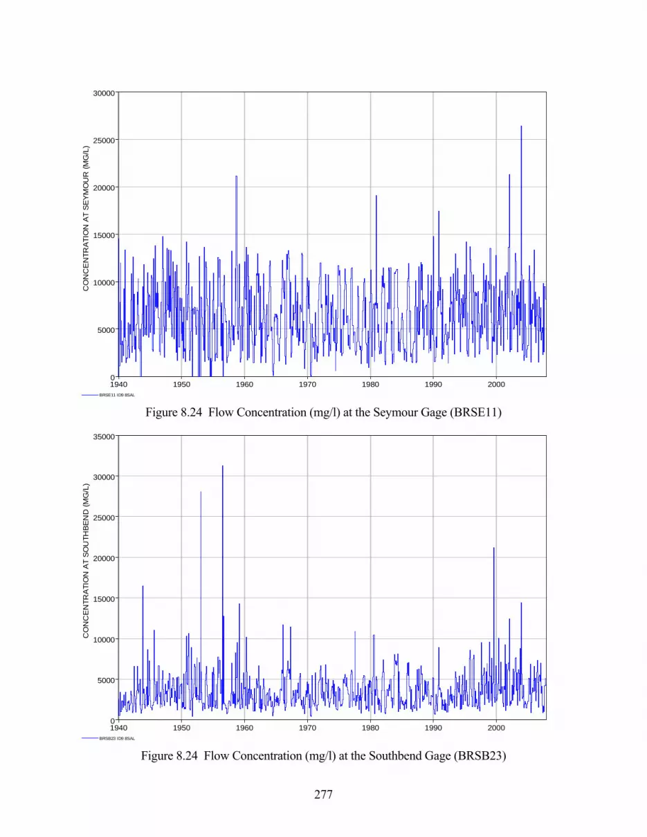
277

1940 1950 1960 1970 1980 1990 2000

CO

NC

EN

TRA

TIO

N A

T S

EY

MO

UR

(MG

/L)

0

5000

10000

15000

20000

25000

30000

BRSE11 ID9 8SAL Figure 8.24 Flow Concentration (mg/l) at the Seymour Gage (BRSE11)

1940 1950 1960 1970 1980 1990 2000

CO

NC

EN

TRA

TIO

N A

T S

OU

THB

EN

D (M

G/L

)

0

5000

10000

15000

20000

25000

30000

35000

BRSB23 ID9 8SAL Figure 8.24 Flow Concentration (mg/l) at the Southbend Gage (BRSB23)

278

1940 1950 1960 1970 1980 1990 2000

STO

RA

GE

CO

NC

EN

TRA

TIO

N (M

G/L

)

500

1000

1500

2000

2500

515531 ID6 8SAL Figure 8.26 Possum Kingdom Reservoir Storage Concentration (mg/l)

1940 1950 1960 1970 1980 1990 2000

STO

RA

GE

CO

NC

EN

TRA

TIO

N (M

G/L

)

0

1000

2000

3000

4000

5000

6000

515631 ID6 8SAL Figure 8.27 Granbury Reservoir Storage Concentration (mg/l)

279

1940 1950 1960 1970 1980 1990 2000

RE

SE

RV

OIR

STO

RA

GE

CO

NC

EN

TRA

TIO

N (M

G/L

)

0

500

1000

1500

2000

2500

3000

3500

515731 ID6 8SAL Figure 8.28 Whitney Reservoir Storage Concentration (mg/l)

1940 1950 1960 1970 1980 1990 2000

CO

NC

EN

TRA

TIO

N A

T B

RY

AN

(MG

/L)

0

500

1000

1500

2000

2500

3000

BRBR59 ID9 8SAL Figure 8.29 Flow Concentration (mg/l) at the Bryan Gage (BRBR59)

280

1940 1950 1960 1970 1980 1990 2000

CO

NC

EN

TRA

TIO

N A

T H

EM

PS

TEA

D (M

G/L

)

0

500

1000

1500

2000

BRHE68 ID9 8SAL Figure 8.30 Flow Concentration (mg/l) at the Hempstead Gage (BRHE68)

1940 1950 1960 1970 1980 1990 2000

CO

NC

EN

TRA

TIO

N A

T R

ICH

MO

ND

(MG

/L)

0

500

1000

1500

2000

2500

3000

BRRI70 ID9 8SAL Figure 8.31 Flow Concentration (mg/l) at the Seymour Gage (BRRI70)

281

Multiple-Reservoir System Operations Much of the salt in the Brazos River is from relatively small sub-watershed salt source areas located above the Seymour gage. As illustrated by Figure 8.2, the salt concentration of the Brazos River decreases in a downstream direction with low-salinity tributary inflows from Aquilla Creek, Bosque River, Little River, Navasota River, Yequa Creek, and other tributaries. The Little River Sub-Basin is the largest of the low-salinity tributary water sources. The dramatic differences in salt concentrations in the three main-stem upper Brazos River reservoirs versus the reservoirs located on tributary streams suggest the possibility of multiple-reservoir operating plans designed to lower salt concentrations in the lower Brazos River. Multiple-reservoir system operating plans may alter the blending of water from the high salinity upper Brazos River and low-salinity tributaries. The WRAP modeling system is applied to explore the potential impacts of multiple-reservoir system operations on salinity concentrations. Multiple-Reservoir System Operations The 12 reservoirs owned and operated by U.S. Army Corps of Engineers and Brazos River Authority are listed in Table 8.29. The locations of the reservoirs are shown in Figure 8.1. Possum Kingdom, Granbury, and Limestone Reservoirs are owned and operated by the BRA. The other nine reservoirs are owned and operated by the Fort Worth District of the Corps of Engineers. The BRA has contracted for most of the water supply storage capacity of the nine federal reservoirs. The Corps of Engineers is responsible for flood control operations.

Table 8.29 Reservoirs Operated by the Corps of Engineers and Brazos River Authority

Reservoir Control Storage

Reservoir Identifier River Point Capacity in Model Identifier (acre-feet)

Possum Kingdom POSDOM Brazos River 515531 552,013 Granbury GRNBRY Brazos River 515631 132,821 Whitney WHIT Brazos River 515731 561,074

Aquilla AQUILA Aquilla Creek 515831 41,700 Belton BELTON Leon River 516031 432,978 Stillhouse Hollow STLHSE Lampases River 516131 224,279 Georgetown GRGTWN San Gabriel River 516231 36,980 Granger GRNGER San Gabriel River 516331 50,540 Limestone LMSTNE Navasota River 516531 208,017 Somerville SMRVLE Yequa Creek 516431 154,254

Proctor PRCTOR Leon River 515931 54,702

Waco LKWACO Bosque River 509431 206,562

The conservation storage capacity of each of the reservoirs is shown in the last column of Table 8.29. The nine federal reservoirs also contain large flood control storage pools which are not

282

included in the storage capacity shown in the table. Flood control operations are not included in the monthly computational time step WRAP-SIM/SALT model. The model is based on the premise that flood waters are stored and released within the same month. Hydroelectric power plants are located at Possum Kingdom and Whitney Reservoirs. However, there are no priority water rights for generating hydroelectric energy. Energy is generated by passing spills and water released for downstream water supply diversions through the turbines. Hydropower operations are not included in the model. The City of Waco holds the water right permit for use of water from Lake Waco. The BRA holds a storage contract with the Corps of Engineers. Lake Waco is operated in the model to meet only lakeside diversions for the City of Waco. The BRA holds water right permits for the 11 other reservoirs listed in Table 8.29. Lake Proctor is committed both in reality and in the model to supplying lakeside diversions and diversions from the Leon River above Lake Belton. The other ten reservoirs are operated as a multiple-reservoir system supplying diversions at downstream sites as well as lakeside diversions. The BRA water supply diversions incorporated in the BRAC2008 model are listed in Table 8.19. The diversions are placed in the model at the control points listed in Table 8.19 and supplied by stream flows at the diversion site supplemented by releases from reservoirs located upstream as required. Those diversions from the Brazos River that can be supplied by releases from two or more upstream reservoirs are listed in Table 8.30. Other diversions from the Little River are also supplied from multiple upstream reservoirs. Several of the diversions listed in Table 8.19 are supplied from a single upstream reservoir. However, the modifications to reservoirs operations in the alternative BRAC2008 simulations discussed here deal with the water supply diversions from the Brazos River listed in Table 8.30.

Table 8.30 Multiple-Reservoir System Diversions

Diversion Location Control Annual Point Diversion (ac-ft/yr) Brazos River at Waco gage BRWA41 658 Brazos River at Highbank gage BRHB42 1,977 Confluence of Little and Brazos Rivers CON111 133 Brazos River at Hempstead gage BRHE68 35,968 Brazos River at Rosharon gage BRRO72 232

WRAP-SIM contains flexible options for defining multiple-reservoir operating rules which are described in the Reference and Users Manuals. However, reservoir operations in the simulations presented here are very simple. The details of more complex alternative operating plans are not explored. Rather, operating extremes are modeled to assess the general magnitude of the impact of alternative operating strategies on salt concentrations.

283

In simulation 4 presented in the preceding section, multiple-reservoir system release decisions are based on balancing storage. In a given month, for a particular diversion requirement associated with releases from multiple upstream reservoirs, available unregulated stream flow at the diversion site is appropriated first. Reservoir releases are then made as needed. The storage contents expressed as a percentage of storage capacity of each of the multiple reservoirs are compared within WRAP-SIM. The diversion is supplied that month from the reservoir with the lowest storage contents expressed as a percentage of storage capacity. Multiple-reservoir system operations in simulation 7 as well as simulation 4 are based on balancing storage. Multiple-reservoir operations in simulations 5, 6, 8, and 9 continue to be based on balancing storage depletions, with the following key exceptions. In simulations 5 and 6, the diversions listed in Table 8.30 are supplied from Possum Kingdom, Granbury, and Whitney Reservoirs. In simulations 8 and 9, the diversions requirements listed in Table 8.30 are met from the tributary reservoirs. These simulations represent the extremes of supplying diversions totally from the high-salinity upper Brazos River reservoirs versus the low-salinity tributary reservoirs. During low-flow conditions, the choice of which reservoirs from which to make releases for diversion demands from the lower Brazos River will obviously impact salt concentrations of river flows as well as the diverted water. However, modifications in multiple-reservoir system operations were found to have little impact on the concentration statistics derived from the simulation model due the relatively small magnitude of the lower Brazos River diversions listed in 8.30. These diversions are supplied largely by unregulated stream flows supplemented by reservoir releases when needed. The reservoir releases were found to not greatly impact the simulated concentrations. Therefore, a large hypothetical diversion at control point BRRI70 (Richmond gage) was added to explore the effects on salinity of reservoir operations for an increased water supply demand. Simulations 7, 8, and 9 include an additional municipal water supply diversion demand of 260,000 acre-feet/year at control point BRRI70 (Richmond gage). This hypothetic diversion was added simply to investigate the impacts on salinity of increasing the diversion. Without consideration of salinity constraints, the 260,000 acre-feet/year has volume and period reliabilities of 100 percent in all of the alternative simulations. For purposes of comparing relative magnitudes of water supply diversions, the total annual diversions associated with BRA water rights in each of the datasets are listed below.

Bwam3 and BRAC3 authorized use: 853,428 acre-feet/year Bwam3 and BRAC8 current use: 446,008 acre-feet/year (Table 8.13) BRAC2008 actual use during 2008: 258,680 acre-feet/year (Table 8.19)

The potential impacts of multiple-reservoir system operations are assessed by comparing the results of the six simulations listed on the next page. All six simulations are based on the same WRAP-SALT input SIN file without any revisions. The only input file that changes is the WRAP-SIM DAT file. The only changes are:

• the specification of which reservoirs are operated to supply the diversion demands listed in Table 8.30

• the addition of a 260,000 acre-feet/year diversion at control point BRRI70 in the DAT file for simulations 7, 8, and 9

284

All of the simulations of this chapter are listed in Table 8.5. The following BRAC2008-based simulations explore multiple-reservoir system operations. Simulation 4: The BRAC2008 simulation presented in the preceding section of this chapter is

viewed as the base scenario in the comparisons. Simulation 5: The BRAC2008 DAT file is modified to model multiple-reservoir system operations

based on maximizing releases from Lakes Possum Kingdom, Granbury, and Whitney and minimizing releases from the tributary reservoirs. The Table 8.30 diversions are supplied by stream flows at the diversion sites supplemented by releases from Lakes Possum Kingdom, Granbury, and Whitney.

Simulation 6: Multiple-reservoir system operations are based on maximizing releases from the

tributary reservoirs and minimizing releases from Lakes Possum Kingdom, Granbury, and Whitney. The Table 8.30 diversions are supplied by stream flows at the diversion sites supplemented by releases from Aquilla, Belton, Stillhouse Hollow, Georgetown, Granger, Somerville, and Limestone Reservoirs.

Simulation 8: The diversion of 260,000 acre-feet/year at BRRI70 is added to the BRAC2008 DAT

file of simulation 4. Simulation 8: The diversion of 260,000 acre-feet/year at BRRI70 is added to the BRAC2008 DAT

file of simulation 5.

Simulation 9: The diversion of 260,000 acre-feet/year at BRRI70 is added to the BRAC2008 DAT file of simulation 6.

Simulation Results Results for the six simulations are compared in Tables 8.31 and 8.32. Volume-weighted mean concentrations, arithmetic averages of the 816 concentrations, and concentrations that are equaled or exceeded during 90%, 75%, 50%, 25%, and 10% of the 816 months of the 1940-2007 hydrologic period-of-analysis are compared in Table 8.31 for storage concentrations in Lake Whitney and concentration of stream flows at the Bryan, Hempstead, and Richmond gages. The locations of these sites are shown in Figure 8.1. These statistics are from the frequency tables created with TABLES which are reproduced as Tables 8.33−8.41.

The median (50% frequency) and 10% frequency flow concentrations at the Hempstead gage copied below provide a concise summary comparison of the six simulations. These concentrations were equaled or exceeded during 50% or 10% of the 816 months.

50% 10% simulation 4 369 mg/l 790 mg/l simulation 5 370 mg/l 787 mg/l simulation 6 369 mg/l 786 mg/l simulation 7 372 mg/l 810 mg/l simulation 8 351 mg/l 671 mg/l simulation 9 384 mg/l 847 mg/l

285

Table 8.31 Concentration Statistics for Alternative Simulations

Simulation 4 5 6 7 8 9 Reservoirs balanced Brazos tributary balanced Brazos tributary

Added Diversion no no no yes yes yes Storage Concentration (mg/l) of Whitney Reservoir (515731)

Weighted Mean 979.0 979.7 980.9 1,021.4 961.3 991.3 Arithmetic Mean 983 984 985 1,042 973 996

90% 580 580 574 569 559 573 75% 717 720 722 717 727 719 50% 890 889 892 909 932 888 25% 1,177 1,178 1,175 1,170 1,172 1,183 10% 1,468 1,467 1,454 1,494 1,468 1,456

Concentration (mg/l) at Bryan Gage (BRBR59)

Weighted Mean 426.9 426.7 429.4 425.5 415.0 426.0 Arithmetic Mean 514 515 544 521 535 486

90% 263 262 262 258 258 262 75% 312 312 313 309 309 309 50% 414 415 410 413 436 397 25% 607 608 609 626 678 566 10% 905 903 897 929 1,003 833

Concentration (mg/l) at Hempstead Gage (BRHE68)


90% 231 231 230 228 229 230 75% 276 276 277 273 272 273 50% 369 370 369 372 384 351 25% 528 527 522 539 569 480 10% 790 787 786 810 847 671

Concentration (mg/l) at Richmond Gage (BRRI70)


90% 224 223 223 222 223 222 75% 269 269 268 265 264 264 50% 354 355 355 355 368 344 25% 507 507 506 518 547 467 10% 763 762 761 777 796 652

286

Table 8.32 Diversion Reliabilities for Limit of 1,000 mg/l

Simulation 4 5 6 7 8 9 Reservoirs balanced Brazos tributary balanced Brazos tributary

Added Diversion no no no yes yes yes

CP Diversion (ac-ft/year) Period Reliability (%)

BRHE58 35,968 95.34 95.34 95.47 94.73 95.10 97.43 BRRI70 260,000 − − − 95.47 95.71 97.43

Volume Reliability (%) BRHE58 35,968 95.16 95.16 95.34 94.61 95.01 97.25 BRRI70 260,000 − − − 94.86 94.94 97.13

Total 221,884 72.43 72.43 72.32 − − − Total 481,883 − − − 84.25 84.49 85.86

The reliabilities for BRA diversions shown in Table 8.32 are for a maximum TDS concentration limit of 1,000 mg/l. The reliabilities for the diversions at control points BRHE58 and BRRI70 and most of the other diversions are 100% if salinity is not considered. Period and volume reliabilities for the 35,968 acre-feet/year diversion at control point BRHE58 (Hempstead gage) and the 260,000 acre-feet/year hypothetical added diversion at control point BRRI70 (Richmond gage) are presented in Table 8.32 for the six alternative simulations. Volume reliabilities for the aggregated totals of all the BRA diversions plus the 260,000 acre-feet/year hypothetical are also included in Table 8.32.

Period reliabilities are computed as the percentage of the months during a simulation for

which the demand is fully supplied. The period reliabilities in Table 8.32 are the percentage of the 816 months of the 1940-2007 simulation during the TDS concentration at the diversion site was 1,000 mg/l or less. Volume reliability is the percentage of the total demand that was supplied. Simulations 4, 5, and 6 show little variation in concentrations with variations in multiple-reservoir system operating strategies. Simulations 5 and 6 represent opposite extremes of releasing only from the 7 tributary reservoirs versus releasing only from the 3 main-stem Brazos River reservoirs to supply the diversions listed in Table 8.30. The differences in the simulation results are minimal. The flows in the lower Brazos River are relatively large compared to the diversions of Table 8.30 most of the time. Reservoir releases for water supply diversions represent a relatively small portion of the river flow and load most of the time. However, the choice of reservoir from which to release may significantly affect downstream concentrations during low flow conditions The hypothetical 260,000 acre-feet/year diversion at the Richmond gage was added to test the impact of increasing water supply demands. With the increased diversion, concentrations in the lower Brazos River are significantly more sensitive to reservoir release choices. The differences in lower Brazos River concentrations between simulations 7, 8, and 9 are greatest for high concentrations which tend to be associated with low flows.

287

Table 8.33 Concentration Frequency for Downstream Stream Flows for Simulation 5

------------------------------------------------------------------------------------------------------------------------------- CONTROL STANDARD PERCENTAGE OF MONTHS WITH CONCENTRATION EQUALING OR EXCEEDING VALUES SHOWN IN THE TABLE POINT N MEAN DEVIATION 100% 99% 98% 95% 90% 75% 60% 50% 40% 25% 10% MAXIMUM ------------------------------------------------------------------------------------------------------------------------------- BRSE11 816 6363. 3529. 0.0 0.0 1127.6 1545.2 2117. 3566. 5052. 5932. 7152. 8778. 11123. 26420. 421331 816 1350. 496. 584.6 622.1 653.9 696.7 793. 1002. 1114. 1208. 1331. 1753. 2072. 3205. CON036 816 3503. 2515. 431.7 723.8 890.0 1123.2 1375. 1880. 2464. 2997. 3453. 4418. 6097. 30531. BRSB23 816 3530. 2553. 435.7 728.1 893.6 1128.8 1382. 1888. 2475. 3016. 3467. 4445. 6144. 31252. 515531 816 1628. 415. 311.6 581.1 692.2 912.7 1067. 1353. 1564. 1676. 1757. 1898. 2132. 2685. BRPP27 816 1739. 1176. 0.0 533.3 632.4 828.7 1004. 1296. 1551. 1661. 1769. 1941. 2316. 28662. BRDE29 816 1396. 857. 0.0 0.0 291.6 419.1 595. 865. 1117. 1266. 1450. 1728. 2213. 8720. 515631 816 1277. 576. 0.0 0.0 140.6 365.3 627. 912. 1130. 1233. 1360. 1531. 1990. 3000. BRGR30 816 10284. 259160. 0.0 0.0 0.0 223.8 425. 771. 1013. 1138. 1292. 1499. 2035. 7404271. 409732 816 473. 639. 0.0 0.0 0.0 0.0 0. 300. 372. 396. 431. 503. 675. 8894. CON063 816 1103. 847. 0.0 36.9 128.0 260.4 367. 646. 842. 1006. 1134. 1390. 1851. 12663. 515731 816 960. 369. 0.0 279.0 301.8 455.6 573. 716. 805. 886. 987. 1171. 1457. 2000. BRAQ33 816 952. 668. 0.0 208.4 269.7 386.1 531. 688. 781. 854. 957. 1136. 1443. 16373. 515831 816 253. 105. 0.0 8.4 13.8 113.9 146. 192. 214. 232. 256. 322. 406. 587. CON070 816 842. 427. 0.0 198.5 226.6 294.8 412. 561. 674. 748. 856. 1029. 1394. 3361. 509431 816 256. 109. 0.0 0.0 0.5 100.9 138. 193. 224. 244. 267. 313. 384. 681. 433901 816 789. 521. 36.2 202.2 222.6 271.6 344. 470. 577. 659. 759. 966. 1376. 5662. BRWA41 816 823. 683. 0.0 185.9 212.9 268.2 336. 465. 582. 664. 772. 989. 1418. 10504. BRHB42 816 681. 424. 49.7 177.2 201.5 243.0 299. 394. 490. 554. 661. 861. 1232. 4052. LRCA58 816 256. 0. 256.0 256.0 256.0 256.0 256. 256. 256. 256. 256. 256. 256. 256. CON111 816 520. 305. 117.8 201.1 217.3 242.1 267. 316. 379. 421. 479. 624. 914. 2826. BRBR59 816 515. 310. 118.1 198.2 213.2 237.7 262. 312. 373. 415. 475. 608. 903. 2881. 516431 816 236. 62. 43.2 87.6 138.6 159.6 173. 198. 214. 225. 239. 260. 319. 450. CON130 816 487. 290. 114.5 189.7 207.4 228.6 248. 297. 350. 397. 445. 572. 864. 2589. 516531 816 238. 53. 60.4 88.6 160.7 171.8 182. 204. 217. 227. 244. 265. 312. 410. NAEA66 816 250. 91. 41.5 83.3 106.2 141.7 171. 199. 218. 230. 246. 289. 357. 1076. NABR67 816 245. 127. 0.0 0.0 0.0 69.8 132. 191. 207. 223. 240. 291. 390. 1354. CON147 816 455. 268. 89.3 167.3 191.5 212.9 234. 279. 327. 373. 428. 542. 801. 2205. BRHE68 816 448. 266. 83.6 161.7 188.1 209.8 231. 276. 324. 370. 420. 527. 787. 2348. 292531 816 219. 154. 0.0 0.0 0.0 0.0 0. 144. 193. 203. 227. 284. 416. 1742. CON234 816 430. 262. 79.2 150.0 172.7 201.9 223. 268. 313. 352. 399. 503. 743. 2608. BRRI70 816 435. 272. 81.8 149.9 173.2 202.1 223. 269. 314. 355. 401. 507. 762. 2694. BRRO72 816 576. 1303. 0.0 84.1 148.9 193.1 217. 262. 313. 355. 417. 573. 920. 23152. BRGM73 816 661470.5049026. 0.0 0.0 0.0 153.2 200. 254. 306. 358. 431. 665. 1760. 77748520. -------------------------------------------------------------------------------------------------------------------------------

Table 8.34 Concentration Frequency for Reservoir Storage for Simulation 5


288





289





290





291





292

Natural Salt Pollution Control Impoundments

Natural salt pollution in the Brazos River Basin is described in Chapter 1. The Permian Basin Region encompasses the upper watersheds of the Brazos and neighboring river basins as delineated in Figure 1.1. Much of the salinity of the rivers shown in Figure 1.1 originates from geologic formations in this region. Wurbs (2002) discusses various natural salt pollution control measures that have been proposed and in some cases implemented in the river basins of Figure 1.1. Salt Control Impoundments During the 1960’s−1970’s, the Fort Worth District of the U.S. Army Corps of Engineers, in collaboration with other federal and non-federal agencies, investigated a variety of measures for dealing with natural salt pollution in the Brazos River Basin (USACE 1973 and 1983). These studies resulted in a proposal to construct a system of three brine impoundments which would be located at the sites shown in Figures 8.32 and 8.33. Wurbs et al (1993) further investigated the effects of the impoundments on downstream salinity concentrations. The proposed salt control plan has not been implemented due to economic, financial, institutional, and environmental constraints. WRAP-SIM/SALT simulation 10 consists of altering the BRAC2008 dataset to approximate the effects of a hypothetical implementation of this previously proposed salt impoundment plan. The water quality sampling program in the Brazos River Basin conducted by the U.S. Geological Survey from October 1963 through September 1986 in support of the Corps of Engineers natural salt pollution control studies is described in Chapter 1. The locations of the 26 stream flow and water quality sampling stations listed in Table 1.1 are shown in Figure 1.3. The first six stations listed in Table 1.1 are shown in Figure 8.32 which is an enlargement of the upper basin portion of Figure 1.3. The USACE (1973 and 1983) investigations included formulation and evaluation of an array of strategies for dealing with the salt problem. The final recommended plan consists of three impoundments.

• Croton Lake on Croton Creek • Dove Lake on Salt Croton Creek • Kiowa Peak Lake on North Croton Creek

The proposed salt control dams would impound the runoff from their respective watersheds which have been identified as encompassing primary salt source areas. A connecting pipeline would be provided for conveying excess water from Croton and Dove Lakes to Kiowa Peak Lake. The impounded water will be partially lost over time due to evaporation, with the remaining brine being permanently stored in Kiowa Peak Lake. The dams would consist of earth-fill embankments with outlet structures for emergencies only. No outflows are planned during the project life.

WRAP-SIM/SALT simulation 10 consists of modifying the BRAC2008 model to approximate the effects of implementing the proposed salt impoundments. The impoundments are modeled based on the premise that all flows and loads at gaging stations 3, 4, and 6 in Figures 1.3 and 8.32 are prevented from flowing into the Brazos River. The flows and loads at control point BRSE11 at the Seymour gage (station 7 in Figure 1.3) are reduced to represent removal of all flows and loads at stations 3, 4, and 6.

293

Figure 8.32 Gaging Stations and Proposed Impoundments in Upper Brazos Basin


294

The compilation and analysis of the USGS/USACE salinity data reported by Wurbs et al. (1993) includes an investigation of the potential impacts of the salt control dams on salinity at downstream locations on the Brazos River. The data in Table 8.43 is reproduced from that study. The gage on Salt Croton Creek near Aspermont (Figures 1.3 and 8.32 map number 4) has a period-of-record of 1969-1977. Other periods-of-record are as follows.

3 Croton Creek at Jayton 1964-1986 4 Salt Croton Creek at Aspermont 1966-1977 6 North Croton Creek at Knox City 1966-1986 7 Brazos River at Seymour 1964-1986

Regression analyses were applied to the flows and loads to develop complete water year 1964-1986 sequences at all stations. Table 8.9 includes means for water years 1966-1977 which contain only observed data and water years 1964-1986 which contains both observed and regressed data. The mean flows and loads are expressed in the last two columns of Table 8.43 as a percentage of the means at the Seymour gage on the Brazos River. The percentages shown in Table 8.44 were adopted for the simulation study. The 1940-2007 monthly naturalized flow volumes in the WRAP-SIM BRAC2008 model at control point BRSE11 (Seymour gage) are reduced 12.7 percent. A water right is inserted in the DAT file with a diversion at control point BRSE11 computed as 12.7 percent of the flow at BRSE11. The 1940-2007 monthly salt loads in the WRAP-SALT BRAC2008 model at control point BRSE11 are reduced 41.8 percent using a multiplier factor of 0.582 entered on the CP record for BRSE11 in the SIN file.

Table 8.43 Flows and Loads in the Upper Basin

Map Mean Mean Mean Mean Mean

USGS Gaging Station Number Flow Load Conc Flow Load (cfs) (tons/day) (mg/l) (%) (%)

October 1968 through September 1977

Salt Fork of Brazos at Peacock 2 41 594 5,380 16.3 22.1 Croton Creek at Jayton 3 12 200 6,030 4.8 7.4 Salt Croton Creek at Aspermont 4 4 673 56,920 1.6 25.0 Salt Fork of Brazos at Aspermont 5 63 1,548 9,090 25.1 57.5 North Croton Creek at Knox City 6 11 163 5,400 4.4 6.2

Brazos River at Seymour 7 251 2,693 3,980 100.0 100.0

October 1963 through September 1986

Salt Fork of Brazos at Peacock 2 40 684 5,780 14.9 26.3 Croton Creek at Jayton 3 13 225 6,540 4.8 8.7 Salt Croton Creek at Aspermont 4 5 676 54,560 1.9 26.0 Salt Fork of Brazos at Aspermont 5 62 1,660 10,000 23.0 63.8 North Croton Creek at Knox City 6 17 211 4,720 6.3 8.1

Brazos River at Seymour 7 269 2,601 3,590 100.0 100.0

295

Table 8.44 Flows and Loads at Impoundment Sites as

Percentage of Flows and Loads at the Seymour Gage

Flow (%) Load (%) 3 Croton Creek at Jayton 4.8% 8.7% 4 Salt Croton Creek at Aspermont 1.6% 25.0% 6 North Croton Creek at Knox City 6.3% 8.1%

Total 12.7% 41.8%

Much of the salt impounded by the salt control dams may be naturally loss anyway in its flow through the river system due to bank seepage and other losses. Channel losses are a key complexity addressed only approximately in modeling the salt control impoundments. In general, channel loss factors in the SIM input file and computations related to channel losses in both WRAP-SIM and WRAP-SALT are approximate involving significant uncertainties. These modeling uncertainties are magnified when adding the salt control impoundments to the model.

Losses of flow and load between the salt control dams and the Seymour gage (BRSE11) are

not considered in the modeling strategy adopted. Also, as explained below, the salt load and concentration reductions due to the salt impoundments in the model at all locations on the Brazos River from the Seymour gage downstream to the Gulf of Mexico may be high due to only partially adjusting for the impacts of channel losses all along the river. Natural losses of load in the river may be greater than reflected in the model. This would mean that the salt control impoundments are less effective in reducing downstream concentrations then indicated by the model. The control point configuration of the model is shown in Figure 8.6. Control points CON036 and BRSE23 (South Bend gage) are located between control point BRSE11 (Seymour gage) and control point 515531 (Possum Kingdom Reservoir). Channel loss factors are provided on the control point CP records of the BRAC2008 input DAT file that is reproduced as Table 8.20. Channel loss factors of 0.4146, 0.0100, and 0.179 are entered for control points BRSE11, CON036, and BRSB23. Channel loss factors for the other reaches of the Brazos River further downstream are relatively small. Channel loss computations are included in the WRAP-SIM simulation. Channel losses are considered by SIM in the downstream propagation of the diversion at BRSE11 representing the 12.7% reduction of the flows at BRSE11. Channel loss effects on river flows associated with diverted flows are reflected in the SIM computations as channel loss credits as explained in the WRAP Reference Manual.

Salinity load losses are addressed by two different features of WRAP-SALT as explained below. Both are activated in the simulations reported in this report. The first modeling feature connects load losses to WRAP-SIM channel losses and channel loss credits. The second feature for dealing with losses of salt load is an option that involves additional load losses that are not associated with volume losses.

296

WRAP-SALT assigns a concentration to channel losses and channel loss credits during each month of the salinity tracking simulation based on combining the channel loss/credit volumes from the SIM simulation results with concentrations approximated as the concentration of the regulated flows at upstream control points. Since the flow reduction is much less than the 41.8% load reduction at control point BRSE11, the effects of channel losses on the downstream propagation of the salt load reduction will probably be significantly underestimated by this modeling feature. On the other hand, flow volume losses conceivably could actually be greater than salt losses due to evaporation. In reality, salt losses may not necessarily be linearly proportional to volume losses as assumed in the model.

Another pertinent optional feature is activated in the Brazos SIN file shown in Table 8.3.

Loads entering Possum Kingdom, Granbury, and Whitney Reservoirs are reduced by 17.42%, 6.587%, and 3.00%, respectively, as described in Chapter 7. This feature also reduces the effects of the salt control impoundments in the downstream propagation of the load reductions.

Simulation Results The results of simulations 4 and 10 are compared in Tables 8.45, 8.46, and 8.47. Simulation 4 is based on the original BRAC2008 dataset. Simulation 10 uses the same BRAC2008 dataset with the only change being addition of the salt control impoundments. Mean flow volumes and TDS loads without and with the salt dams are compared in Tables 8.45 and 8.46, and TDS concentrations are compared in Table 8.47. The total volume and load budget summary from the SMS file for simulation 10 is reproduced as Table 8.48. The comparable table for simulation 4 was previously presented as Table 8.22. The control point summary and frequency and reliability tables for simulation 10 created with TABLES are reproduced as Tables 8.49−8.52. The reduction in the 1940-2007 means of simulated flow volumes and loads at five locations on the Brazos River due to the salt control impoundments are shown in Table 8.45 by comparing results from simulations 4 and 10. The reduction in TDS load at the Seymour gage due to the salt control impoundments is 35,638 tons/month, which is 41.80 percent of the load of 85,258 tons/month without the salt control impoundments. The reduction in TDS load at the Richmond gage due to the salt control impoundments is 23,346 tons/month. The load reduction at the Richmond gage is significantly less than the load reduction at the Seymour gage due to channel losses and additional losses of load in the three reservoirs.

Table 8.45 Mean Flow Volume and Load Without and With Salt Dams (Simulations 4 and 10)

Gaging Control Mean Flow (acre-feet/month) Mean Load (tons/month) Station Point Sim 4 Sim 10 Loss Loss Sim 4 Sim 10 Loss Loss

Seymour BRSE11 19,151 17,386 1,765 9.22% 85,258 49,620 35,638 41.80%Southbend BRSB23 45,127 44,171 956 2.12% 112,358 78,978 33,380 29.71%Bryan BRBR59 312,446 311,539 907 0.29% 181,375 158,077 23,298 12.85%Hempstead BRHE68 423,567 422,682 885 0.21% 213,243 189,973 23,270 10.91%Richmond BRRI70 462,008 461,144 864 0.19% 225,097 201,751 23,346 10.37%

297

Table 8.46 Comparison of Stream Flow Concentrations

Simulation 4 10

Mean Concentrations (mg/l)

Seymour Gage (BRSE11)

Weighted Mean 3,274 2,099 Arithmetic Mean 6,363 3,913

90% 2,117 1,350 75% 3,566 2,191 50% 5,932 3,689 25% 8,778 5,359 10% 11,123 6,849

Southbend Gage (BRSE23)

Weighted Mean 1,831 1,315 Arithmetic Mean 3,530 2,345

90% 1,382 1,036 75% 1,888 1,424 50% 3,016 2,043 25% 4,445 2,926 10% 6,144 3,921

Bryan Gage (BRBR59)

Weighted Mean 426.9 373.1 Arithmetic Mean 514 447

90% 263 251 75% 312 289 50% 414 372 25% 607 521 10% 905 741

Hempstead Gage (BRHE68)


90% 231 224 75% 276 262 50% 369 336 25% 528 464 10% 790 639

Richmond Gage (BRRI70)


90% 224 217 75% 269 255 50% 354 325 25% 507 453 10% 763 627

298

Table 8.47 Comparison of Reservoir Storage Concentrations

Simulation 4 10

Mean Storage Concentrations (mg/l)

Possum Kingdom Reservoir (515531)

Weighted Mean 1,624.0 1,193 Arithmetic Mean 1,627 1,195

90% 1,067 813 75% 1,353 1,022 50% 1,675 1,210 25% 1,897 1,380 10% 2,133 1,540

Granbury Reservoir

Weighted Mean 1,294.3 970.9 Arithmetic Mean 1,305 981

90% 631 516 75% 915 722 50% 1,239 938 25% 1,541 1,183 10% 1,994 1,468

Whitney Reservoir (515731)


90% 580 458 75% 717 583 50% 890 715 25% 1,177 929 10% 1,468 1,106

Statistics for the concentration of the stream flows of the Brazos River at the USGS gaging stations near the cities of Bryan, Hempstead, and Richmond are presented in Table 8.46. Statistics for the concentration of the water stored in Lakes Possum Kingdom, Granbury, and Whitney are tabulated in Table 8.47. The volume-weighted mean concentration, arithmetic average the 816 concentrations, and concentrations that are equaled or exceeded during 90%, 75%, 50%, 25%, and 10% of the 816 months of the 1940-2007 hydrologic period-of-analysis are compared for simulation 10 versus 4. Again, simulations 4 and 10 are identical except for the addition of the three salt control impoundments to simulation 10. The differences between the simulation results statistics in Tables 8.46 and 8.47 are fairly large. The TABLES output TOU file for simulation 10 is reproduced as Tables 8.48, 8.49, 8.50, 8.51, and 8.52. The reliability indices of Tables 8.27 and 8.52 for simulations 4 and 10 include

299

reliabilities constrained by a maximum TDS limit of 1,000 mg/l as discussed earlier in this chapter in conjunction with simulation 4. The corresponding SIM simulation results for simulations 4 and 10 can be found in the following tables created by TABLES.

Simulation 4 Simulation 10

total volume and load summary Table 8.22 Table 8.48 control point summary Table 8.24 Table 8.49 stream flow concentration frequency statistics Table 8.25 Table 8.50 reservoir storage concentration statistics Table 8.26 Table 8.51 water supply diversion reliabilities Table 8.27 Table 8.52

A comparison of the results of simulations 4 and 10 indicate that the previously proposed

salt control impoundments potentially could significantly reduce the salinity loads and concentrations in the three reservoirs and at all locations on the Brazos River from the impoundments downstream to the Gulf of Mexico. Of course, the results necessarily reflect all of the approximations and uncertainties inherent in the model including the previously discussed issue of inaccuracies in modeling natural losses of volume and load in river channels and reservoirs.

Table 8.48 Total Volume and Load Summary for Simulation 10 with Salt Control Impoundments

Volume Load Concentration

Naturalized flows 278926528. 108170504. 285.2 Regulated flows at boundary 100189360. 70425016. 517.0 Return flows 1843957. 2095855. 836.0 CI record constant inflows 0. 0. 0.0 Channel loss credits 6014266. 6608504. 808.1 Channel losses 245215. 208892. 626.5 Regulated flows at outlet 358406304. 156218288. 320.6 Diversions 14821904. 12405419. 615.6 Other flows and loads -531327. -652687. 903.5 Net evaporation 14031595. 0. 0.0 Load losses from CP record CLI(cp) 19304390. ---------- ---------- ---------- Inflows - Outflows 419. -184423. -323709.0 ---------- ---------- ---------- Beginning reservoir storage 1872393. 2435549. 956.7 Ending reservoir storage 1872393. 1852446. 727.6 ---------- ---------- ---------- Change in storage 0. -583103. 0.0 ---------- ---------- ---------- Volume and load differences 419. 398680. 699786.2



Naturalized flows at outlet 390631424.

Number of control points in SIM DAT and OUT files: 48 Number of control points included in SALT simulation: 34

300

Table 8.49 Control Point Summary for Simulation 10 with Salt Control Impoundments

------------------------------------------------------------------------------------------------- CONTROL MEAN MONTHLY VOLUME (AC-FT) MEAN MONTHLY LOAD (TONS) MEAN CONCENTRATION (MG/L) POINT Inflow Outflow Storage Inflow Outflow Storage Inflow Outflow Storage ------------------------------------------------------------------------------------------------- BRSE11 0. 17386. 0. 0. 49620. 0. 0.0 2098.8 0.0 421331 7279. 3877. 251384. 6554. 6289. 432665. 662.2 1192.9 1265.7 CON036 45035. 45035. 0. 80314. 80314. 0. 1311.5 1311.5 0.0 BRSB23 44171. 44171. 0. 78978. 78978. 0. 1314.9 1314.9 0.0 515531 54873. 50470. 546846. 89145. 89833. 887134. 1194.7 1309.0 1193.0 BRPP27 50722. 50722. 0. 73415. 73413. 0. 1064.4 1064.4 0.0 BRDE29 64609. 64609. 0. 77679. 78115. 0. 884.2 889.1 0.0 515631 71904. 70301. 125153. 82677. 82984. 165238. 845.6 868.1 970.9 BRGR30 68558. 68558. 0. 73729. 73723. 0. 790.9 790.8 0.0 409732 1360. 1187. 23463. 793. 722. 14701. 428.7 447.5 460.8 CON063 73879. 73879. 0. 76340. 76340. 0. 759.9 759.9 0.0 515731 96222. 93341. 305774. 89409. 89573. 322569. 683.3 705.7 775.8 BRAQ33 94092. 94092. 0. 86779. 86778. 0. 678.2 678.2 0.0 515831 6988. 6407. 37894. 2009. 1999. 12736. 211.4 229.4 247.2 CON070 108004. 108004. 0. 91095. 91093. 0. 620.3 620.3 0.0 509431 33829. 32785. 59093. 9907. 9914. 20368. 215.4 222.4 253.5 433901 138471. 138471. 0. 100214. 100214. 0. 532.2 532.2 0.0 BRWA41 138623. 138623. 0. 100245. 100222. 0. 531.8 531.7 0.0 BRHB42 173071. 173071. 0. 111639. 111639. 0. 474.4 474.4 0.0 LRCA58 0. 105395. 0. 0. 36685. 0. 0.0 256.0 0.0 CON111 301018. 301018. 0. 154837. 154837. 0. 378.3 378.3 0.0 BRBR59 311539. 311539. 0. 158077. 158077. 0. 373.1 373.1 0.0 516431 20028. 18756. 149477. 5492. 5496. 47569. 201.7 215.5 234.0 CON130 347106. 347106. 0. 168386. 168386. 0. 356.8 356.8 0.0 516531 19940. 18104. 189172. 5586. 5585. 59910. 206.0 226.9 232.9 NAEA66 23229. 23229. 0. 6933. 6933. 0. 219.5 219.5 0.0 NABR67 30131. 30131. 0. 8797. 8801. 0. 214.7 214.8 0.0 CON147 408983. 408983. 0. 186072. 186072. 0. 334.6 334.6 0.0 BRHE68 422682. 422682. 0. 189973. 189973. 0. 330.5 330.5 0.0 292531 3834. 3834. 0. 1180. 1180. 0. 226.3 226.3 0.0 CON234 463332. 463332. 0. 202462. 202462. 0. 321.3 321.3 0.0 BRRI70 461144. 461144. 0. 201751. 201751. 0. 321.7 321.7 0.0 BRRO72 457873. 457873. 0. 200268. 200275. 0. 321.7 321.7 0.0 BRGM73 439230. 439230. 0. 191630. 191750. 0. 320.8 321.0 0.0 -------------------------------------------------------------------------------------------------

301

Table 8.50 Concentration Frequency for Stream Flows for Simulation 10 with Salt Control Impoundments


Table 8.51 Concentration Frequency for Reservoir Storage for Simulation 10 with Salt Control Impoundments


302

Table 8.52 Reliabilities With and Without Salinity Constraint of 1,000 mg/l

for Simulation 10 with Salt Control Impoundments --------------------------------------------------------------------------------------------------------------- | Both Quantity & Quality |----- Quantity Only -----|+++++ Quality Only ++++++|Number Months CONTROL TARGET | *RELIABILITY* | *RELIABILITY* | *RELIABILITY* |Concentration POINT DIVERSION | SHORTAGE |VOLUME|PERIOD | SHORTAGE |VOLUME|PERIOD | SHORTAGE |VOLUME|PERIOD | is |exceeds (AC-FT/YR) |(AC-FT/YR)| (%) | (%) |(AC-FT/YR)| (%) | (%) |(AC-FT/YR)| (%) | (%) | Zero| Limit --------------------------------------------------------------------------------------------------------------- BRSE11 21196.4 0.00 100.00 100.00 0.00 100.00 100.00 0.00 100.00 100.00 361 0 421331 9923.5 7450.87 24.92 24.75 0.00 100.00 100.00 7450.87 24.92 24.75 0 614 CON036 0.0 0.00 There are no diversions at this control point. BRSB23 0.0 0.00 There are no diversions at this control point. 515531 3967.0 3043.11 23.29 23.41 0.00 100.00 100.00 3043.11 23.29 23.41 0 625 BRPP27 277.0 205.73 25.74 25.74 0.00 100.00 100.00 205.73 25.74 25.74 2 606 BRDE29 2157.0 1025.29 52.47 52.82 0.00 100.00 100.00 1025.29 52.47 52.82 15 385 515631 62275.9 26158.89 58.00 57.72 0.00 100.00 100.00 26158.89 58.00 57.72 14 345 BRGR30 1104.0 407.06 63.13 63.36 0.00 100.00 100.00 407.06 63.13 63.36 27 299 409732 17536.1 4302.58 75.46 69.85 3918.74 77.65 71.32 927.39 94.71 94.73 103 43 CON063 0.0 0.00 There are no diversions at this control point. 515731 1875.0 319.67 82.95 80.51 0.00 100.00 100.00 319.67 82.95 80.51 1 159 BRAQ33 0.0 0.00 There are no diversions at this control point. 515831 5716.0 0.00 100.00 100.00 0.00 100.00 100.00 0.00 100.00 100.00 2 0 CON070 0.0 0.00 There are no diversions at this control point. 509431 38348.0 0.00 100.00 100.00 0.00 100.00 100.00 0.00 100.00 100.00 17 0 433901 0.0 0.00 There are no diversions at this control point. BRWA41 658.0 90.60 86.23 87.13 0.00 100.00 100.00 90.60 86.23 87.13 3 105 BRHB42 1977.0 203.43 89.71 91.30 0.00 100.00 100.00 203.43 89.71 91.30 0 71 LRCA58 0.0 0.00 There are no diversions at this control point. CON111 133.0 5.88 95.58 96.08 0.00 100.00 100.00 5.88 95.58 96.08 0 32 BRBR59 0.0 0.00 There are no diversions at this control point. 516431 3499.0 0.00 100.00 100.00 0.00 100.00 100.00 0.00 100.00 100.00 0 0 CON130 0.0 0.00 There are no diversions at this control point. 516531 32572.0 0.00 100.00 100.00 0.00 100.00 100.00 0.00 100.00 100.00 0 0 NAEA66 3665.0 2.21 99.94 99.88 0.00 100.00 100.00 2.21 99.94 99.88 0 1 NABR67 0.0 0.00 There are no diversions at this control point. CON147 0.0 0.00 There are no diversions at this control point. BRHE68 35968.0 785.17 97.82 98.04 0.00 100.00 100.00 785.17 97.82 98.04 0 16 292531 0.0 0.00 There are no diversions at this control point. CON234 0.0 0.00 There are no diversions at this control point. BRRI70 0.0 0.00 There are no diversions at this control point. BRRO72 232.0 19.51 91.59 95.10 0.00 100.00 100.00 19.51 91.59 95.10 1 40 BRGM73 0.0 0.00 There are no diversions at this control point. --------------------------------------------------------------------------------------------------------------- Total 243079.8 44020.00 81.89 3918.74 98.39 40644.82 83.28 ---------------------------------------------------------------------------------------------------------------

The diversion target at control point BRSE11 located at the Seymour gage averaging 21,196.4 acre-feet/year is the WR record water right added to the DAT file to represent to depletion of stream flow by the salt control impoundments. Since control point BRSE11 is the upstream boundary of the salinity simulation, the 21,196.4 acre-feet/year diversion is not assigned a concentration in the SALT simulation and is not constrained by the 1,000 mg/l limit in TABLES.

303

CHAPTER 9 SUMMARY AND CONCLUSIONS

This report documents the merging of the following two research endeavors:

• salinity budget analyses of the Brazos River system based primarily on observed stream flow, reservoir storage, and total dissolved solids (TDS) data compiled by the U.S. Geological Survey (USGS) from October 1963 through September 1986

• testing, improving, and applying the salinity simulation capabilities of the Water Rights Analysis Package (WRAP) modeling system using the Brazos River Basin dataset from the Texas Commission on Water Quality (TCEQ) Water Availability Modeling (WAM) System and variations thereof combined with the USGS salinity data

The flow and storage volume budget and TDS load budget studies and related analyses presented in Chapters 2, 3, 4, and 5 represent a complete research investigation even without the WRAP-based studies presented Chapters 6, 7, and 8. The primary motivation for the volume and load budget studies was the development of a database to support the WRAP simulation studies. However, the analyses of observed and synthesized data reported in Chapters 2, 3, 4, and 5 also provide insight into the characteristics of flow and storage volumes and salinity loads and concentrations in the river/reservoir system independently of the WRAP modeling studies of Chapters 6, 7, and 8. The WRAP modeling system provides capabilities for evaluating the impacts of salinity on water supplies and the impacts of alternative water management measures on salinity.

Natural Salt Pollution in the Brazos River Basin Natural salt pollution originating from geologic formations in the Permian Basin geologic region in the High Plains of Texas, Oklahoma, New Mexico, and Kansas severely constrains the water supply capabilities of the Brazos River and other neighboring rivers. Salt springs and seeps and salt flats in the upper watersheds of the Brazos, Colorado, Pecos, Red, Canadian, and Arkansas Rivers contribute large salt loads to these rivers. The salinity limits the municipal, industrial, and agricultural use of water supplied by a number of large reservoirs located on these rivers. Much of the salinity of the Brazos River originates from salt seeps and springs in sub-watersheds of the Salt Fork and Double Mountain Fork of the Brazos River some distance upstream of the USGS gage on the Brazos River near Seymour. Salt concentrations are extremely high on several of the small streams originating in these primary salt source sub-watersheds such as Croton Creek, Salt Croton Creek, North Croton Creek, and others. Salinity concentrations of the Brazos River decrease in a downstream direction with inflows from low-salinity tributaries such as Aquilla Creek, Bosque River, Little River, Navasota River, Yequa Creek, and other streams. The Fort Worth District of the U.S. Army Corps of Engineers in collaboration with other agencies conducted extensive Brazos River Basin natural salt pollution control studies during the 1960's-1980's. The USGS conducted an extensive water quality data collection program from October 1963 through September 1986 in support of the USACE salt control studies. The work presented in this report is based on these 1964-1986 data along with other additional data from the USGS and elsewhere. The USGS collected salinity data before 1964-1986 and has continued since then but not nearly as extensively as during the USACE-sponsored sampling program.

304

Mean flows and TDS loads and concentrations during water years 1964-1986 at eight gaging stations are shown in Table 3.5 expressed as a percentage of the amounts at the Whitney gage located downstream of Whitney Dam. Locations of the gages are shown in Figure 1.3. The Seymour gage on the Brazos River is located 405 miles upstream of the Whitney. The mean flow at the Seymour gage is 21.9 percent of the mean flow at the Whitney gage. However, the mean TDS load at the Seymour gage is 84.6 percent of the mean TDS load at the Whitney gage. The mean TDS concentration of the flow at the Seymour gage is 387 percent of the mean TDS concentration at the Whitney gage. Likewise, the mean flow at the Richmond gage 350 river miles below the Whitney gage is 558% of the mean flow at the Whitney gage. The mean TDS load and concentration at the Richmond gage are 204% and 37%, respectively, of the load and concentration at the Whitney gage. Monthly volumes of river flows during the period October 1963 through September 1986 at six gaging stations are plotted in Figures 3.1 through 3.6. The corresponding TDS loads are plotted in Figures 3.7 through 3.12. The mean monthly TDS concentrations are shown in Figures 3.13−3.18. The monthly flows, loads, and concentrations fluctuate greatly during the 23-year period-of-analysis. The monthly flow volumes show tremendous variability including the extremes of floods and droughts. TDS loads fluctuate along with the flow volumes. The TDS concentrations also exhibit dramatic variability. The fluctuations in concentrations are dampened somewhat by reservoir storage at the gages located below the dams. Though less variable than stream flow concentrations, storage concentrations also fluctuate over time and can vary greatly over short time periods of a few days or weeks. Salt concentrations can vary greatly with the timing and location of rainfall events causing floods as well as responding to longer periods of low-flows and prolonged droughts. The WRAP simulation results show the impact of the 1950's drought in decreasing stream flows and increasing salinity concentrations. The example of major flooding causing a rapid decrease in salinity concentrations that is probably most noticeable in the plots in this report occurred during the first week of August 1978 as a result of Tropical Storm Amelia. Much of the lower-salinity Hubbard Creek watershed located above Lake Possum Kingdom received 15 to 30 inches of rainfall during July 31 to August 5, 1978 while the primary salt source areas in the Salt Fork and Double Maintain Fork watersheds received relatively little rain. The mean monthly TDS concentration of the August 1978 flows at the South Bend gage just above Possum Kingdom Lake was 420 mg/l, compared to the 1964-1986 mean of 1,700 mg/l. The flood greatly lowered TDS concentrations through the river/reservoir system downstream of the South Bend gage as is evident from the plots in this report. The USGS reported a significant impact of the flood on water quality in streams throughout central Texas.

Volume and Load Budget Studies Chapters 2, 3, and 4 cover water and salinity budget studies for five sub-reaches of a 405 mile long reach of the Brazos River between the USGS stream gaging stations near Seymour and Whitney, which includes Lakes Possum Kingdom, Granbury, and Whitney. The studies were based primarily upon water year 1964-1986 monthly flow volumes and TDS loads from the USACE-sponsored USGS water quality sampling program supplemented as needed by other observed or synthesized (computed) water quantity and quality data.

305

The budgets consist of Microsoft Excel spreadsheets of October 1963 through September 1986 sequences of 276 monthly inflow, outflow, and storage volumes and the corresponding inflow, outflow, and storage TDS loads for each of the 5 reaches. The inflows and outflows are subdivided into components. Component inflow and outflow quantities and storage changes sum to zero as appropriate to balance the budgets. Some components such as monthly stream flow volumes and loads and end-of-month reservoir storage volumes are observed data, with only gaps in the records synthesized (computed) as part of the study. Other components such as end-of-month reservoir storage loads were computed in conjunction with the study since observed data are not available. Concentrations were computed by combining volumes and loads. Summaries of means of the quantities for the 276 months are also included in this report along with plots of the 276-month (1964-1986) sequences. Components of the Volume and Load Budgets The 1964-1986 mean flow and storage volumes and total dissolved solids (TDS) loads for the components of the volume and load budgets for the five river reaches are tabulated in Tables 3.1 and 3.2. The budgets include flow and load components defined as the quantities required to balance the budgets. Thus, the component amounts sum to zero, balancing each budget. The concentrations determined by dividing the mean loads by the corresponding mean flow volumes are shown in Table 3.3. Reservoir storage volumes, loads, and volume-weighted mean concentrations are summarized in Table 3.4. Most of the inflow and outflow for each reach is reflected in the river flows at the upstream and downstream gages defining the upper and lower ends of the reach. The 1964-1986 mean flow at the Glen Rose gage upstream of Lake Whitney and the Whitney gage downstream of Lake Whitney are 61,670 acre-feet/month and 74,193 acre-feet/month (Table 3.1). The mean TDS loads at the upstream and downstream ends of the Glen Rose to Whitney reach are 90,017 and 93,538 tons/month (Table 3.2). The corresponding concentrations are 1,073 mg/l and 927 mg/l (Table 3.3). The naturalized flows from the TCEQ WAM System dataset are shown as the last two lines of Table 3.1 though not a part of the actual volume budget. Naturalized flows were developed for the WAM System by adjusting gaged flows to remove the effects of water resources development and use. Naturalized flows represent natural river basin conditions without reservoirs and human water use. A comparison of the actual river flows in the first two lines of Table 3.1 with the naturalized flows in the last two lines provides a measure of the reduction in flows due to reservoir storage and water supply diversions in the river system upstream of the gages. The net reservoir water surface evaporation less precipitation for Lake Whitney is 3,603 acre-feet/month (Table 3.1). The volume in storage in Lake Whitney at the beginning of October 1963 was 332,300 ac-ft and at the end of September 1986 was 632,500 ac-ft (Table 3.4) resulting in a net increase in storage of 1,088 ac-ft/month (Table 3.1) when averaged over 276 months. The 1964-1986 mean storage volume of Lake Whitney of 475,928 acre-feet (Table 3.4) is equivalent to 6.4 months of outflow at the downstream mean flow rate of 74,193 acre-feet/month (Table 3.1). The Lake Whitney conservation pool storage capacity of 627,100 ac-ft (Table 1.5) is equivalent to 8.5 months of outflow at the rate of 74,193 acre-feet/month. The 570,240 acre-feet capacity of Possum Kingdom Lake is equivalent to 13.3 months of outflow at the mean rate of 42,998 acre-feet/month. The storage capacity of Granbury Lake is 2.5 months of its mean outflow.

306

Recorded water supply diversion data available for Lake Granbury indicate that diversions averaged 923 acre-feet/month over the 1964-1986 period-of-analysis. Concentrations of the water diverted each month were assumed equal to the storage concentration at the beginning of the month in the load budget calculations. The other inflow volume (FOI) and other outflow volume (FOO) are monthly amounts required to balance the volume budget each month. The other flow volume differences are the summation of all other components of the volume budget and are positive in some months and negative in other months. This volume difference was assigned to the variable FOI if positive in a particular month and FOO if negative. Of course, the volume difference required to balance the volume budget in a particular month is probably the net of both other inflows and outflows. Thus, the procedure adopted here of assigning the monthly volume differences as being either totally inflow (FOI) or totally outflow (FOO) is an approximation. The other inflows (FOI) may include rainfall runoff from the incremental watersheds, stream underflow not measured by the upstream gage, water supply diversions, and water supply return flows. The other outflows (FOO) may be stream underflow not measured by the downstream gage, seepage from the river and reservoir into the ground, evapotranspiration not accounted for by the reservoir surface evaporation term, and water supply diversions. The other flows (FOI and FOO) terms may also reflect timing effects of flows passing through the reach and inaccuracies in the other components of the water budget. The 1964-1986 means of the other inflow volume (FOI) and other outflow volume (FOO) for the Glen Rose to Whitney reach are 19,447 and 2,233 acre-feet/month, respectively (Table 3.1). The other inflow volume (FOI) should consist largely of rainfall runoff from the local incremental watersheds draining to the reaches between their upstream and downstream gages. The mean other inflow volume (FOI) of 19,447 acre-feet/month is equivalent to a depth of 3.2 inches (Table 3.6) for the 1,371 square mile incremental watershed, which is a reasonable rainfall runoff depth for this region. The other outflow volumes (FOO) reflecting diversions and losses are a relatively small component of the volume budget. For the three reaches containing Possum Kingdom, Granbury, and Whitney Reservoirs, the other inflow load (LOI) was estimated by applying a concentration of 270 mg/l to the other inflow volume (FOI). This concentration is representative of other similar watersheds in the vicinity for which salinity measurements are available. The other outflow load (LOO) was estimated by applying the monthly concentration at the downstream gage each month. The 1964-1986 means of the other inflow load (LOI) and other outflow load (LOO) for the Glen Rose to Whitney reach are 7,139 and 3,103 tons/month (Table 3.2). The other load (LX) term is the additional load difference required to balance the load budget for the South Bend to Graford (Lake Possum Kingdom) and Glen Rose to Whitney (Lake Whitney) reaches. The 1964-1986 mean load difference was calculated by summing the 1964-1986 means of the other components and then distributing to the 276 individual months. Several alternative methods for allocating LX to each month were investigated as discussed in Chapter 4. The load balances are achieved automatically in the computational algorithms for the other two reaches. The other loads (LX) required to balance the load budgets for the South Bend to Graford and Glen Rose to Whitney reaches are additional outflows of 12,787 and inflows of 1,298 tons/month, respectively (Table 3.2). Ideally LX should be zero. The LX term represents inaccuracies in the other terms or

307

additional loads not reflected in the other terms. There are no outflow volumes in the volume budget corresponding to the LX load losses. The salinity budget for Lake Whitney was further adjusted to match the volume-weighted storage concentration determined by the USGS based on lake water quality surveys performed at 30 points in time between September 1970 and May 1980. The adjustments involved changing the timing of load inflows and outflows as necessary to match the observed storage concentrations. Reservoir Storage Volumes, Loads, and Concentrations Observed storage volumes for Lakes Possum Kingdom, Granbury, and Whitney are plotted in Figures 3.19−3.21. The corresponding computed TDS loads in storage are plotted in Figures 3.22−3.24. Storage concentrations are plotted in Figures 3.25−3.27. Means are tabulated in Tables 3.4 and 3.5. The computed reservoir storage concentrations are volume-weighted mean end-of-month concentrations. Impoundment of water Lakes Possum Kingdom, Granbury, and Whitney began in 1941, 1970, and 1951, respectively. A sediment survey in 1974 indicated that the storage capacity of Possum Kingdom Lake had decreased significantly since initial impoundment in 1941. The storage volumes for October 1963 through September 1973 at Possum Kingdom Lake plotted in Figure 3.19 were adjusted in the volume budget calculations to partially correct the USGS data for sediment accumulation not otherwise reflected in the published data. End-of-month storage loads and volume-weighted storage concentrations were computed for the three reservoirs. The computations for Lake Granbury are very different than for Lake Possum Kingdom and Lake Whitney due primarily to differences in data availability but also due to the smaller size and later construction of Lake Granbury.

Storage loads in Lakes Possum Kingdom and Whitney were computed for the end of each of the 276 months based on summing inflow and outflow loads for each month starting with the specified load shown in Table 3.4 in storage at the beginning of October 1963. The unknown concentrations of water stored in Lakes Possum Kingdom and Whitney at the beginning and the end of the October 1963 to September 1986 period-of-analysis were set based on the corresponding observed outflow concentrations. This is the storage concentration at the beginning of October 1963 and the end of September 1986. The October 1963 beginning concentration in Possum Kingdom Reservoir was set equal to the mean outflow concentration during the first 21 months beginning in October 1963. The first 21 months represent the retention period during which the outflows sum to approximately the storage volume at the beginning of October 1963. Likewise, the October 1963 beginning concentration in Whitney Reservoir was set equal to the mean outflow concentration during the first 11 months beginning in October 1963. The September 1986 storage concentrations of both reservoirs were set equal to the September 1986 outflow concentrations.

Volume-weighted mean dissolved solids concentrations of storage in Lake Whitney and Lake Granbury are available from USGS reports as follows. Water quality surveys of Lake Whitney were performed on 30 dates between 1970 and 1980. Measurements were made in Lake Granbury on 28 dates between 1970 and 1979. The salinity budget for the reach between the Glen Rose and Whitney gages was adjusted to match the 30 measurement-based volume-weighted mean storage concentrations for Lake Whitney tabulated in Table 3.8. The 28 Lake Granbury measurement-based storage concentrations are plotted in Figure 3.29 along with the storage

308

concentrations computed in the salinity budget analysis. The 30 measurement-based Whitney storage concentrations are plotted in Figure 3.28 along with the initial storage concentrations computed in the salinity budget analysis without the calibration adjustments. Lake Whitney storage concentrations computed in the salinity budget analyses with and without the storage concentration adjustments are plotted in Figure 3.36.

Simulation Studies with the WRAP Modeling System Chapters 6, 7, and 8 deal with the salinity simulation features of the Water Rights Analysis Package (WRAP) modeling system. Chapter 6 presents an investigation of methods for routing salinity through reservoirs using a dataset derived from the volume and load analyses of Chapters 2, 3, and 4. Chapter 7 documents the development of a salinity inflow dataset for the WRAP-SALT input file for the entire Brazos River Basin. Chapter 8 presents a WRAP-SIM and SALT simulation study assessing the interactions between water management and salinity.

Salinity Routing Through Reservoirs WRAP-SALT contains flexible optional features for routing salinity through reservoirs which are documented in detail in the WRAP Salinity Manual (Wurbs 2009). The studies reported in Chapter 6 consisted of testing and refining the salinity routing methodology and associated parameter calibration methods. The salinity budget study of Chapters 2, 3, and 4 provided a dataset used to investigate salinity routing methods. The final conclusion was that the simplest routing, without the additional options provided by WRAP-SALT, works best for the Brazos reservoirs. WRAP-SALT Reservoir Salinity Routing Methodology Salinity routing consists basically of computing the concentrations of the outflows from a reservoir. Reservoir outflow concentration refers to the monthly concentration of the regulated stream flow in the river downstream of the dam and the monthly concentration of the water withdrawn from the reservoir as lakeside diversions. The computed downstream river flows and lakeside diversions may have either the same or different concentrations. Reservoir storage concentration is the volume-weighted concentration of the water stored in the reservoir either at the end of a month or the average of the beginning-of-month and end-of-month concentrations. The WRAP-SALT salinity simulation methodology is summarized as follows. The outflow concentration (OCM) in month M is computed as a function of storage concentration (SCM-L) in month M-L (L months before month M). Lag L is an integer number of months. OCM = SCM-L (9-1)

( )M M-L 1 2C

VOC = SC F 1.0 + F - 1.0V

⎡ ⎤⎛ ⎞× ⎢ ⎥⎜ ⎟

⎝ ⎠⎣ ⎦

(9-2)

Equation 9-2 is an expanded version of Equation 9-1 with SCM-L multiplied by a factor computed as a function of the two input parameters F1 and F2. With F1 and F2 defaults of 1.0, Equation 9-2 reduces to Equation 9-1. VC in Eq. 9-2 is a storage volume entered as an input parameter which is typically the storage capacity of the reservoir. V is the average storage contents of the reservoir

309

during the current month computed within WRAP-SALT. The ratio V/VC represents storage contents as a fraction of capacity or other specified volume. The lag (L) in months may be entered directly as an input parameter. Alternatively, the lag L may be computed internally within WRAP-SALT based on the concept of retention time.

R reservoir storage volume

retention time T in months = outflow volume per month

WRAP-SALT includes an algorithm for summing reservoir storage volume and outflow volume over multiple months for use in computing a retention time TR. The lag time L is computed by WRAP-SALT as the following function of retention time TR. L is truncated to an integer number of months. The multiplier factor FL is an input parameter with a default of 1.0.

L = TR (FL) (9-3) Salinity routing in WRAP-SALT is based on Eq. 9-1 which can optionally be expanded to Eq. 9-2. Two approaches are available for setting the lag parameter L. The first option is for L to be a constant integer provided by the model-user as an input parameter. The second option is for L to be computed within WRAP-SALT based on Equation 9-3 with the parameter FL provided by the user as an input parameter. With the second option, the lag is allowed to vary from month to month. Another option provides additional flexibility for using mean monthly versus beginning-of-month storage concentrations in the computation of outflow concentrations. With a zero for the lag L, and 1.0 for F1 and F2, the reservoir outflow concentration equals the storage concentration. The parameters F1 and F2 allow the outflow concentration to differ from the storage concentration. The optionally either constant or variable lag L accounts for the time required for salinity entering a reservoir to be mixed and transported through the reservoir. Summary and Conclusions of the Salinity Routing Parameter Calibration Studies A WRAP-SIM and SALT input dataset was created based on the water and salinity budget data of Chapter 3. The dataset is designed for the sole purpose of testing the salinity routing methods and calibrating the salinity routing parameters. The salinity input dataset of Chapter 7 serves a completely different purpose and is totally different from the salinity dataset of Chapter 6. The dataset of Chapter 6 for investigating computational methods and input parameters for routing salinity through reservoirs incorporates the volume and salinity budget results for six reaches of the Brazos River between the Seymour and Whitney gaging stations. These reaches contain Lakes Possum Kingdom, Granbury, and Whitney. The volume budget data are converted into a WRAP-SIM simulation results output file and WRAP-SALT salinity input file. The program SIM output file read by program SALT precisely reproduces the volume budget. All TDS load and flow volume inflows and outflows other than the flows in the river below the dams are aggregated together in the SIM output and salinity input files read by SALT. Thus, SALT computes volume-weighted storage loads and concentrations and the loads and concentrations of the river flows below the dams with all other variables fixed to perfectly match the results of the volume and load budget study. Computed storage and outflow concentrations from the WRAP-SALT simulation results can be compared with the measurement-based data from the salinity budget study.

310

The results of extensive calibration studies are presented in Chapter 6. The regression analyses and plots of Chapter 5 serve to explore the relationships between reservoir outflow and storage concentration for alternative lags. The analysis of the Chapter 3 data in Chapter 5 is designed to complement the analyses of Chapter 6. Chapter 5 focuses on the lag time dimension of salinity routing. The WRAP-SALT reservoir salinity routing procedure is based on Equations 9-1, 9-2, and 9-3 and associated input parameters. There are two different aspects of salinity routing with one aspect represented by the lag options and the other represented by the factors F1 and F2 in Equation 9.2. The lag parameter and lag options control the timing (lag time) features of the WRAP-SALT algorithms for routing salinity through reservoirs. The parameters F1 and F2 address differences between the long-term levels of volume-weighted outflow concentrations versus volume-weighted storage concentrations reflecting losses or gains of salinity load in the reservoir. The concept of lag time addresses the issue of the time required for entering salt loads to be transported through a large reservoir. Lag options have been extensively investigated in this study based on the initial premise that lag time is an important key consideration in salinity routing. However, this was found to not be the case for the two reservoirs analyzed. Lag times of zero or one month were found to be optimal for Possum Kingdom and Whitney Reservoirs. These reservoirs can probably be best simulated without activation of the lag options (zero lag). If the lag option is activated, the optimal lag is one month. A reasonable approach is to adopt the beginning-of-month option combined with zero lag. Loss of salinity load in the reservoirs is another consideration. Load losses can be modeled in WRAP-SALT either by using the parameters F1 and F2 in the routing equation or alternatively by expressing losses as a specified fraction of inflow or storage loads. The approach of modeling load losses as a fraction of inflow loads was adopted in the simulation studies presented in Chapter 8. The load loss input data are discussed further in the next section.

Salinity Inflows to the River System Chapter 7 documents the development of a salinity inflow dataset for the Brazos River Basin for incorporation into the WRAP-SALT input SIN file used in the simulation studies presented in Chapter 8. The reservoir salinity routing specifications from Chapter 6 discussed above are also included in SALT input file. However, most of the data in the SIN file is composed of loads or concentrations defining salt loads entering the river system. Formulation and application of methodologies for developing these salt inflow sequences are covered in Chapter 7. The Water Rights Analysis Package (WRAP) computer program SALT reads a salinity input file with the filename extension SIN. The majority of the data contained in the SIN file consists of concentrations and/or loads that define the salinity inflows to the river/reservoir system. Time series sequences of loads or concentrations may be entered in the SIN file for each of the months of the simulation. Alternatively, constant mean concentrations may be input and repeated within the WRAP-SALT simulation for all months. The WRAP-SALT load or concentration input data are entered in the SIN file for specific control points representing locations in the river system. The load or concentration data entered for a particular control point may be repeated automatically within WRAP-SALT for any number of other control points.

311

Salinity inflow data for the WRAP-SALT input SIN file were developed by applying the methodology outlined in Chapter 7 using Microsoft Excel and the WRAP utility program SALIN. A single SIN file was developed which is designed for use with the Brazos River Basin datasets from the Texas Commission on Environmental Quality (TCEQ) Water Availability Modeling (WAM) System or the Brazos River Authority Condensed (BRAC) datasets. Observed October 1963 through September 1986 total dissolved solids (TDS) loads and concentrations described in Chapters 1, 2, and 3 are extended based on TCEQ WAM System naturalized flows using the methodology outlined in the Chapter 7 to cover the period from January 1900 through December 2007. The salinity data were developed for six control points as outlined below.

Brazos River at Seymour gage below primary salt source areas.

Load series for total regulated flows. These inflow loads are plotted in Figure 7.3.

Brazos River at Graford gage below Possum Kingdom Lake.


Brazos River at Whitney (Aquilla) gage below Whitney Dam.


Little River at Cameron gage. Constant concentration of 256 mg/l for total regulated flows.

Brazos River at Richmond gage. Concentration series for incremental inflows which is plotted in Figure 7.48.

Brazos River at Gulf of Mexico. Constant concentration of 339 mg/l for incremental inflows.

The WRAP-SALT input data representing TDS loads entering the Brazos River and its

tributaries represents actual 1964-1986 conditions with adjustments removing the effects of Lakes Possum Kingdom, Granbury, and Whitney. The volume and TDS load data used in developing the salinity dataset have been adjusted to remove the timing effects of storage in Lakes Possum Kingdom, Granbury, and Whitney. The volume budget also allows consideration of net reservoir evaporation less precipitation by which the three reservoirs affect volumes and concentrations but not loads. Loads and volumes of water supply diversions from Lake Granbury are also separated out. TCEQ WAM System naturalized flows reflect natural hydrology. The Brazos River Authority Condensed (BRAC8) dataset described in Chapter 8 includes stream flow inflows reflecting all water management and use in the Brazos River Basin except that associated with the BRA System.

The WRAP-SALT salinity input dataset maintains the load budget established in the load budget study for water years 1964-1986. The means for the 276-month 1964-1986 period will match between the WRAP-SALT input dataset and the load budget dataset. The loads entering the river system during the months of the 1900-1963 and 1987-2007 portions of the WRAP hydrologic simulation period-of-analysis are synthesized as a function of stream flow volumes and thus should not and do not exactly match the 1964-1986 mean loads. A linear interpolation methodology for extending salinity data sequences was formulated and implemented in the new computer program SALIN. The 1964-1986 salinity data was extended to cover the entire 1900-2007 hydrologic period-of-analyses based on 1900-2007 sequences of

312

monthly naturalized stream flow volumes from the TCEQ WAM System. Regression analysis was also explored. However, maintaining variability in the concentrations is important. The variability of the concentrations is lost with regression analysis. The linear interpolation method was found to work well in maintaining variability and the other characteristics of the loads and concentrations. The WRAP-SALT simulation model performs salt load accounting computations that track the entering loads through the river/reservoir over time. Loads leave the river/reservoir system with the WRAP-SIM simulated diversions, channel losses, and regulated flows at the outlet. WRAP-SALT also has a feature for modeling additional otherwise unaccounted losses of load. For the Brazos River Basin, such additional losses are assigned to the control points of Possum Kingdom, Granbury, and Whitney Reservoirs. The losses each month are computed within WRAP-SALT as a specified fraction of the loads entering the reservoir. The input parameters in the WRAP-SALT salinity SIN input file are the percentages 17.42%, 6.59%, and 3.00% for Lakes Possum Kingdom, Granbury, and Whitney, respectively. WRAP-SALT computes losses by multiplying these percentages by the regulated inflow loads to the reservoir each month.

Simulation of the Brazos River/Reservoir System The Texas Commission on Environmental Quality (TCEQ) Water Availability Modeling (WAM) System consists of the generalized Water Rights Analysis Package (WRAP) river/reservoir system simulation model and input datasets for the 23 river basins of Texas. The WAM System is routinely applied by agencies and consulting firms in regional and statewide planning studies and administration of the water rights permit system, but without consideration of salinity. Chapter 8 documents a salinity simulation study of the Brazos River Basin using the WRAP modeling system, variations of the TCEQ WAM System dataset for the Brazos River Basin, and the salinity dataset developed in this study. The simulation model provides capabilities for computing frequency statistics of salinity concentrations and water supply reliability indices for alternative scenarios of water management and use. The computer program WRAP-SALT is the salinity simulation component of the WRAP modeling system. SIM is the basic simulation model that simulates river basin hydrology, water control infrastructure, river/reservoir system operations, water allocation systems, water use scenarios, and water management strategies. SALT reads a SIM simulation results output file and salinity input file and tracks salt loads and concentrations through a river/reservoir system. The WRAP program TABLES is used to develop frequency tables and reliability indices and otherwise organize the simulation results from SIM and SALT. The software is documented in detail by a set of reference and users manuals. The TCEQ WAM System includes variations of WRAP input datasets for the Brazos River Basin for authorized use and current use scenarios. The TCEQ WAM System current use dataset contains 3,834 control points and 711 reservoirs. A condensed WRAP input dataset focusing on the Brazos River Authority System was recently developed at Texas A&M University that contains 48 control points and 14 reservoirs. The impacts of all other water users and water management activities on the Brazos River Authority System are reflected in the stream flow input data in the condensed dataset. Another version of the condensed dataset was developed for this study which incorporated actual recorded water use of Brazos River Authority customers during 2008.

313

WRAP-SALT combines a SIM simulation results output file and salinity input SIN file. A single salinity input file was developed which is applicable with any of the SIM input datasets. Developing WRAP-SALT simulation algorithms and a Brazos River Basin salinity input dataset that can be combined with variations of any of the available WRAP-SIM datasets was a key objective of the study which was successfully accomplished. The same SIN file is applied with a complete Brazos WAM (Bwam8) dataset with 3,834 control points and 711 reservoirs and the Brazos River Authority Condensed (BRAC8) dataset with 48 control points and 14 reservoirs. The results of the following ten alternative simulations are presented in Chapter 8.

WRAP-SIM Simulation Simulation Input Data Period Description

1 Bwam8 1940-2007 TCEQ WAM current use dataset. 2 Bwam8 1900-2007 TCEQ WAM current use dataset.

3 BRAC8 1940-2007 BRA Condensed BRAC8 current use dataset.

4 BRAC2008 1940-2007 BRAC2008 dataset with 2008 water use. 5, 6, 7, 8, 9 BRAC2008 1940-2007 Multiple-reservoir system operations.

10 BRAC2008 1940-2007 Natural salt pollution control impoundments.

Simulations 1 and 2 demonstrate that WRAP-SALT can be effectively applied with a complex TCEQ WAM System dataset for a large river basin. Simulations with 1900-2007 and 1940-2007 hydrologic periods-of-analysis yield similar results. Results for both simulations appear to be reasonable. The 1940-2007 simulation was adopted for the remaining simulations since the naturalized flows for 1900-1939 are based on fewer stream gaging stations than the later flows. Simulation 3 confirms that the model works fine with a condensed dataset. The results for simulations 2 and 3 with the Bwam8 and BRAC8 dataset match closely. Simulation 4 with the BRAC2008 dataset is designed to combine actual current water resources development, management, and use with historical 1940-2007 natural river basin hydrology. The discharge-weighted 1940-2007 mean regulated flow concentration at the Richmond gage on the lower Brazos River is 358 mg/l in the BRAC2008 simulation 4 as compared to a 1964-1986 mean of 339 mg/l for observed concentrations. The current conditions simulated concentrations are expected to be somewhat greater than the 1964-1986 observed concentrations due to increased water supply diversions from the low-salinity tributaries and increased reservoir surface evaporation with the construction of additional reservoirs during and after the 1964-1986 period of the USGS water quality sampling program. The 1940-2007 hydrologic period-of-analysis also includes the 1950-1957 drought. Simulation results show a significant increase in concentrations during the 1950-1957 drought and other extended periods of low flows. Simulations 5, 6, 7, 8, and 9 were performed to explore the effects on salinity concentrations of multiple-reservoir system operations. The concentrations of water supply diversions and stream flows along the lower Brazos River should be dependent on whether reservoir releases for the downstream diversions are from the reservoirs on the low-salinity tributaries or Lakes Possum

314

Kingdom, Granbury, and Whitney on the upper Brazos River. The BRAC2008 simulations indicated little difference in lower Brazos River salinity concentration statistics with different multiple-reservoir system operating strategies. Reservoir releases for lower basin water supply diversions are a relatively small portion of the flow of the lower Brazos River most of the time. The sensitivity of lower Brazos River concentrations to different multiple-reservoir system operating strategies was demonstrated in increase with a large increase in diversions from the lower Brazos. The Corps of Engineers during the 1970’s−1980’s performed investigations of alternative measures for controlling natural salt pollution in the Brazos River Basin. Primary salt source areas were identified. The studies resulted in a recommendation to construct a system of three dams on small tributaries of the Salt Fork and Double Mountain Forks of the Brazos River to impound runoff from key salt source watersheds. The salt control plan was never implemented due to economic, financial, and other constraints. Simulation 10 consists of adding the three salt control impoundments to the BRAC2008 model. The simulation is based on the premise that all flows and loads at gaging stations near the sites of the salt dams are permanently prevented from entering the Brazos River. Simulation results indicate that reductions in salt concentration could potentially be significant. Of course, simulation results always reflect the premises and approximations incorporated in the model. The question of natural loss of portions of the salt load even without the salt dams is pertinent. Model estimates of losses of salt load along the length of the river and in the reservoirs are uncertain. TDS concentrations with and without the proposed salt control impoundments are compared as follows.

Simulation 4 4 10 10 Without or With Salt Dams without without with with Exceedance Frequency 50% 10% 50% 10%


Seymour Gage on Brazos River 5,932 11,123 3,689 6,849

Possum Kingdom Reservoir 1,675 2,133 1,210 1,540 Granbury Reservoir 1,239 1,994 938 1,468 Whitney Reservoir 890 1,468 715 1,106

Bryan Gage on Brazos River 414 905 372 741 Hempstead Gage on Brazos River 369 790 336 639 Richmond Gage on Brazos River 354 763 325 627

The table compares the concentrations of reservoir storage and stream flows that are equaled or exceeded during 50 percent (median) and 10 percent of the 816 months of the 1940-2007 hydrologic period-of-analysis for the two alternative simulations without and with the proposed salt control dams. The table also illustrates the decrease of TDS concentrations in a downstream direction. Without the system of three salt control impoundments, the estimated median storage concentration of Possum Kingdom Lake is 1,675 mg/l compared with an estimated 1,210 mg/l with the proposed salt control project. The median concentration of the flow at the Richmond gage is estimated to be 354 mg/l and 325 mg/l without and with construction of the proposed project.

315

REFERENCES Andrews, F. L. and J. L. Strause., Water Quality of Lake Granbury, North-Central Texas, U.S.

Geological Survey Open-File Report 82-676, 1981.

Andrews, F. L. and J. L. Strause., Water Quality of Lake Granbury, North-Central Texas, Report 284, Texas Department of Water Resources, December 1983.

Freese and Nichols, Inc., HDR Engineering, Inc., Crespo Consulting Services, Inc., and Densmore and DuFrain Consulting, Naturalized Flow Estimates for the Brazos River Basin and the San Jacinto-Brazos Coastal Basin, prepared for the Texas Natural Resource Conservation Commission, October 2001.

HDR Engineering, Inc., Water Availability in the Brazos River Basin and the San Jacinto-Brazos Coastal Basin, prepared for the Texas Natural Resource Conservation Commission, December 2001.

Strause, J.L. and F.L. Andrews, Water Quality of Lake Whitney, North-Central Texas, U.S. Geological Survey Open-File Report 82-677, 1983.

Strause, J.L. and F.L. Andrews, Water Quality of Lake Whitney, North-Central Texas, Report 290, Texas Department of Water Resources, December 1984.

Texas Water Development Board, Water for Texas 2007, Document GP-8-1, January 2007.

U.S. Army Corps of Engineers, Fort Worth District, Natural Pollution Control Study, Brazos River Basin, Texas, December 1973.

U.S. Army Corps of Engineers, Fort Worth District, Final Environmental Impact Statement, Natural Pollution Control Study, Brazos River Basin, Texas, January 1976.

U.S. Army Corps of Engineers, Fort Worth District, Brazos Natural Pollution Control, Brazos River Basin, Texas, Design Memorandum No.1, General, Phase I - Plan Formulation, April 1983.

Wurbs, R.A., A.S. Karama, I. Saleh, and C.K. Ganze, Natural Salt Pollution and Water Supply Reliability in the Brazos River Basin, Technical Report 160, Texas Water Resources Institute, August 1993.

Wurbs, R.A., G. Sanchez-Torres, and D.D. Dunn, Reservoir/River System Reliability Considering Water Rights and Water Quality, TR-165, Texas Water Resources Institute, March 1994.

Wurbs, R.A., "Natural Salt Pollution Control in the Southwest," Journal of the American Water Works Association, Vol. 94, No. 12, December 2002.

Wurbs, R.A., and Tae Jin Kim, Extending and Condensing the Brazos River Basin Water Availability Model, TR-340, Texas Water Resources Institute, December 2008.

Wurbs, R.A., Water Rights Analysis Package Modeling System Reference Manual, Technical Report 255, Texas Water Resources Institute, Sixth Edition, January 2009.

Wurbs, R.A., Water Rights Analysis Package Modeling System Users Manual, Technical Report 256, Texas Water Resources Institute, Sixth Edition, January 2009.

Wurbs, R.A., Salinity Simulation with WRAP, Technical Report 317, Texas Water Resources Institute, July 2009.

Salinity Budget and WRAP Salinity Simulation Studies of the ...

Documents

Transcript of Salinity Budget and WRAP Salinity Simulation Studies of the ...