SAFETY CENTRIC SERVICES IN SMART CITIES

By

YAWEI PANG

A DISSERTATION PRESENTED TO THE GRADUATE SCHOOLOF THE UNIVERSITY OF FLORIDA IN PARTIAL FULFILLMENT

OF THE REQUIREMENTS FOR THE DEGREE OFDOCTOR OF PHILOSOPHY

UNIVERSITY OF FLORIDA

2019

c© 2019 Yawei Pang

To my parents and my girlfriend

ACKNOWLEDGMENTS

First and foremost, I would like to express my sincere appreciation to my advisor, Prof.

Yuguang Fang, for his invaluable guidance and strong support during my PhD study at

University of Florida. I have learned so much from him about being a serious thinker and

researcher.

I also would like to thank Dr. Dapeng Wu, Dr. Shigang Chen, and Dr. Xiaolin Li

for serving on my supervisory committee. I appreciate this opportunity to learn invaluable

suggestions from them.

I would like to extend my thanks to all my colleagues and friends in Wireless Information

and Networked Things Laboratory (WINET) for providing me a family-like environment and

for their collaboration and insightful advice. In particular, I would like to acknowledge my

appreciation to Dr. Haichuan Ding, Yaodan Hu, Lan Zhang, Kaichen Yang, Xianhao Chen, and

Di Han for many valuable discussions.

I owe a special gratitude to my parents and girlfriend. Thank you for supporting me all

the way to today, even in my most difficult time. I love you!

Last but not least, I would like to give special thanks to the funding source, US National

Science Foundation grants under CNS-1409797, CNS-1343356, and CNS-1718708.

4

TABLE OF CONTENTS

page

ACKNOWLEDGMENTS . . . . . . . . . . . . . . . . . . . . . . . . . . . . . . . . . . . 4

LIST OF TABLES . . . . . . . . . . . . . . . . . . . . . . . . . . . . . . . . . . . . . . 7

LIST OF FIGURES . . . . . . . . . . . . . . . . . . . . . . . . . . . . . . . . . . . . . 8

ABSTRACT . . . . . . . . . . . . . . . . . . . . . . . . . . . . . . . . . . . . . . . . . 9

CHAPTER

1 INTRODUCTION . . . . . . . . . . . . . . . . . . . . . . . . . . . . . . . . . . . 11

1.1 Safety and Challenge of Modern Cities . . . . . . . . . . . . . . . . . . . . . 111.2 Safety Service Platform . . . . . . . . . . . . . . . . . . . . . . . . . . . . . 121.3 Dissertation Contribution and Organization . . . . . . . . . . . . . . . . . . . 16

2 RELATED WORK . . . . . . . . . . . . . . . . . . . . . . . . . . . . . . . . . . . 19

2.1 Safety Services . . . . . . . . . . . . . . . . . . . . . . . . . . . . . . . . . . 192.2 Vehicle as Resource . . . . . . . . . . . . . . . . . . . . . . . . . . . . . . . 21

3 PRELIMINARIES . . . . . . . . . . . . . . . . . . . . . . . . . . . . . . . . . . . 23

3.1 Radio Frequency Identification . . . . . . . . . . . . . . . . . . . . . . . . . . 233.2 Video Summarization . . . . . . . . . . . . . . . . . . . . . . . . . . . . . . 243.3 Matching Theory . . . . . . . . . . . . . . . . . . . . . . . . . . . . . . . . . 253.4 Genetic Algorithm . . . . . . . . . . . . . . . . . . . . . . . . . . . . . . . . 27

4 L-TRACK:CHILDREN TRACKING IN THEME PARKS . . . . . . . . . . . . . . . 29

4.1 Background . . . . . . . . . . . . . . . . . . . . . . . . . . . . . . . . . . . 294.2 Architecture . . . . . . . . . . . . . . . . . . . . . . . . . . . . . . . . . . . 32

4.2.1 Overview . . . . . . . . . . . . . . . . . . . . . . . . . . . . . . . . . 324.2.2 System Model . . . . . . . . . . . . . . . . . . . . . . . . . . . . . . 34

4.3 Problem Formulation . . . . . . . . . . . . . . . . . . . . . . . . . . . . . . . 364.3.1 Reader Association . . . . . . . . . . . . . . . . . . . . . . . . . . . . 374.3.2 Maximum Power Limitation . . . . . . . . . . . . . . . . . . . . . . . 374.3.3 QoS Requirement . . . . . . . . . . . . . . . . . . . . . . . . . . . . . 374.3.4 EE Optimization . . . . . . . . . . . . . . . . . . . . . . . . . . . . . 38

4.4 Matching Approach . . . . . . . . . . . . . . . . . . . . . . . . . . . . . . . 384.4.1 Preference Establishment . . . . . . . . . . . . . . . . . . . . . . . . . 384.4.2 Dynamic Updating Matching Algorithm . . . . . . . . . . . . . . . . . 41

4.5 Performance Evaluation . . . . . . . . . . . . . . . . . . . . . . . . . . . . . 434.5.1 Simulation Setup . . . . . . . . . . . . . . . . . . . . . . . . . . . . . 434.5.2 Results and Analysis . . . . . . . . . . . . . . . . . . . . . . . . . . . 44

5

5 SPATH: A SAFE WALKING NAVIGATION SERVICE . . . . . . . . . . . . . . . . 50

5.1 Backgroud . . . . . . . . . . . . . . . . . . . . . . . . . . . . . . . . . . . . 505.2 System Architecture . . . . . . . . . . . . . . . . . . . . . . . . . . . . . . . 53

5.2.1 Overview . . . . . . . . . . . . . . . . . . . . . . . . . . . . . . . . . 535.2.2 System Model . . . . . . . . . . . . . . . . . . . . . . . . . . . . . . 55

5.3 Problem Formulation . . . . . . . . . . . . . . . . . . . . . . . . . . . . . . . 595.4 Algorithm . . . . . . . . . . . . . . . . . . . . . . . . . . . . . . . . . . . . 60

5.4.1 Computing Resource Optimization . . . . . . . . . . . . . . . . . . . . 615.4.2 Task Assignment . . . . . . . . . . . . . . . . . . . . . . . . . . . . . 625.4.3 Fast Iterative Matching (FIM) algorithm . . . . . . . . . . . . . . . . . 63

5.5 Performance Evaluation . . . . . . . . . . . . . . . . . . . . . . . . . . . . . 655.5.1 Simulation Setup . . . . . . . . . . . . . . . . . . . . . . . . . . . . . 655.5.2 Results and Analysis . . . . . . . . . . . . . . . . . . . . . . . . . . . 66

6 VISS: VEHICLE BASED INTELLIGENT SURVEILLANCE SYSTEM . . . . . . . . . 70

6.1 Background . . . . . . . . . . . . . . . . . . . . . . . . . . . . . . . . . . . 706.2 System Architecture . . . . . . . . . . . . . . . . . . . . . . . . . . . . . . . 72

6.2.1 Architecture Overview . . . . . . . . . . . . . . . . . . . . . . . . . . 736.2.2 System Model . . . . . . . . . . . . . . . . . . . . . . . . . . . . . . 74

6.3 Problem Formulation . . . . . . . . . . . . . . . . . . . . . . . . . . . . . . . 786.4 Algorithm . . . . . . . . . . . . . . . . . . . . . . . . . . . . . . . . . . . . 796.5 Performance Evaluation . . . . . . . . . . . . . . . . . . . . . . . . . . . . . 81

7 SUMMARY AND CONCLUSIONS . . . . . . . . . . . . . . . . . . . . . . . . . . 86

REFERENCES . . . . . . . . . . . . . . . . . . . . . . . . . . . . . . . . . . . . . . . . 87

BIOGRAPHICAL SKETCH . . . . . . . . . . . . . . . . . . . . . . . . . . . . . . . . . 95

6

LIST OF TABLES

Table page

4-1 Table of parameters . . . . . . . . . . . . . . . . . . . . . . . . . . . . . . . . . . 36

5-1 Symbols and definitions . . . . . . . . . . . . . . . . . . . . . . . . . . . . . . . . 58

6-1 Symbols and description . . . . . . . . . . . . . . . . . . . . . . . . . . . . . . . . 78

7

LIST OF FIGURES

Figure page

1-1 Overview of safety centric platform. . . . . . . . . . . . . . . . . . . . . . . . . . . 14

1-2 Architecture of safety centric platform. . . . . . . . . . . . . . . . . . . . . . . . . 15

3-1 Illustration of RFID communication. . . . . . . . . . . . . . . . . . . . . . . . . . . 24

3-2 Illustration of matching. . . . . . . . . . . . . . . . . . . . . . . . . . . . . . . . . 26

3-3 Illustration of crossover and mutation. . . . . . . . . . . . . . . . . . . . . . . . . 28

4-1 System architecture. . . . . . . . . . . . . . . . . . . . . . . . . . . . . . . . . . . 31

4-2 Whole process of data processing and transmissions. . . . . . . . . . . . . . . . . . 34

4-3 A snapshot of mobile device location with N=70. . . . . . . . . . . . . . . . . . . . 43

4-4 Comparison to the optimal solution. . . . . . . . . . . . . . . . . . . . . . . . . . . 47

4-5 Comparison of different matching algorithms. . . . . . . . . . . . . . . . . . . . . . 47

4-6 Comparison of different power allocation approaches. . . . . . . . . . . . . . . . . . 48

4-7 EE under different density of mobile devices. . . . . . . . . . . . . . . . . . . . . . 48

4-8 EE under different computation capability of mobile device. . . . . . . . . . . . . . 49

5-1 System architecture. . . . . . . . . . . . . . . . . . . . . . . . . . . . . . . . . . . 51

5-2 Illustration of SPATH. . . . . . . . . . . . . . . . . . . . . . . . . . . . . . . . . . 54

5-3 Illustration of video summarizations and transmissions. . . . . . . . . . . . . . . . . 55

5-4 The comparison of different schemes. . . . . . . . . . . . . . . . . . . . . . . . . . 68

5-5 Impact of available computing power. . . . . . . . . . . . . . . . . . . . . . . . . . 68

5-6 Impact of data size . . . . . . . . . . . . . . . . . . . . . . . . . . . . . . . . . . 69

5-7 Impact of bandwidth. . . . . . . . . . . . . . . . . . . . . . . . . . . . . . . . . . 69

6-1 System architecture. . . . . . . . . . . . . . . . . . . . . . . . . . . . . . . . . . . 71

6-2 Illustration of working process . . . . . . . . . . . . . . . . . . . . . . . . . . . . . 75

6-3 Evaluation results for network size. . . . . . . . . . . . . . . . . . . . . . . . . . . 83

6-4 Impact of target regions. . . . . . . . . . . . . . . . . . . . . . . . . . . . . . . . 84

6-5 Impact of participants. . . . . . . . . . . . . . . . . . . . . . . . . . . . . . . . . . 85

8

Abstract of Dissertation Presented to the Graduate Schoolof the University of Florida in Partial Fulfillment of theRequirements for the Degree of Doctor of Philosophy

SAFETY CENTRIC SERVICES IN SMART CITIES

By

Yawei Pang

August 2019

Chair: Yuguang FangMajor: Electrical and Computer Engineering

Smart cities are the future to handle population shifts and the increased demand of

services. However, safety becomes one of the most important concerns with respect to the fact

that more than 1 million crimes happened in U.S. every year. In this dissertation, we propose

a safety centric platform leveraging redundant computing and communication capabilities of

mobile devices or autonomous vehicles to enable local processing, which reduces the service

latency, eliminates potential network congestion, and improves resource utilization. Our

current contributions are mainly threefold. In the first work, we design a children tracking

service for theme parks based on radio-frequency identification (RFID) technology. In order to

guarantee efficient children tracking, we further optimize the utilization of available computing

resource for service provisioning. In the second work, we design another service, SPATH (the

Safest PATH), to provide a safe walking navigation in smart cities. To support this service,

wireless cameras, existing cellular infrastructure, and vehicles are utilized to process and

transmit surveillance videos, which can be viewed by users to check the current safety status.

Furthermore, video summarizing technology is applied to extract valuable information from

a video file to avoid network congestion. Since the quality of service for this application is

strongly correlated with the latency for video delivery, we address a latency minimization

problem by jointly considering the computing resource allocation and task assignment. In

the third work, we design a Vehicle based Intelligent Surveillance System (VISS) to improve

public safety in smart cities. VISS recruits vehicles as the mobile monitoring nodes to expand

9

geographical monitoring regions. Cooperating with slowly moving or parked vehicles with

sufficient computing capability, VISS can extract potential victims from the monitoring video

files and recruit mobile monitoring nodes to monitor potential victims as long as possible. To

measure the performance of VISS, coverage problems with limited budget are investigated by

considering recruitment of mobile monitoring nodes.

10

CHAPTER 1INTRODUCTION

1.1 Safety and Challenge of Modern Cities

The world we currently live in is highly urbanized with an estimated more than 54% of

the global population lives in urban centers today. This growing trend is likely to maintain for

the next ten years with roughly 95% of urban sprawl taking place in the developing countries.

By 2050, the population dwelling in the urban areas will be expected to rise to 66% of the

global population [1]. The speed of urban expansion as well as migration to city areas seems

faster than the growth of city infrastructure, spaces and services, which may lead to insufficient

provision of infrastructure and services thus may affect the safety quality of citizens living in

urban areas, especially for children and women.

The crime reports revealed by the Federal Bureau of Investigation (FBI) from its Uniform

Crime Reporting (UCR) program shows increasing rates of nationwide violent crimes and

homicide. Specifically, the rate of violent crime reached 386.3 per 100,000 in 2016 [2]. Other

data from the UCR and the National Crime Victimization Survey (NCVS) suggest higher crime

rates in city areas that are densely populated than in suburban or rural areas in general [3].

According to the report, around 50% of robberies happened in urban areas. Given that

residents in city areas were exposed to the highest crime rates, how to utilize technology to

improve the safety quality of residents of urban areas is a challenging problem.

In light of this, scholars and technology companies propose new and advanced services

to improve the safety quality and well-beings of citizens in urban areas. For instance, crime

hotspots is a popular tools used by researchers and police to improve the safety of cities.

The term hotspots, which refers to areas where crimes frequently take place, are used by

scholars and police in various ways [4, 5]. In [4], Paulsen has observed the increasing usage of

crime hotspots that prompts police officers to locate areas with safety concerns within their

beats using crime maps and then make adjustment to their patrol strategies correspondingly.

The author investigates the effects of crime maps on officers? perceptions of crime patterns

11

and their subsequent patrol activities. Bogomolov et al. have made an attempt to predict

crime hotspots to improve the public safety by using human behavioral data that stem

from various sources including mobile network activity, demography, along with open data

pertaining to crime events in [5]. Safe navigation services are proposed to help citizens find

the safe and shot path to their destinations [6, 7, 8, 9]. Pedestrian safety services have been

introduced to solve the distracted walking problem, since pedestrian often perform multiple

task simultaneously such as talking over the mobile phone, listening to music, or browsing the

news while walking [10, 11, 12, 13, 14]. Driving safety service are offered to reduce motor

vehicle crashes [15, 16, 17, 18].

1.2 Safety Service Platform

There are serval drawbacks for new and advanced public safety related services. First,

different safety services focus on the different areas, thus each new service is based on facilities

that are newly deployed. Thus, the high maintenance cost of these facilities compel the service

providers provide the services to users with high fees. For example, in order to avoid children

missing in the public areas such as theme parks or shopping malls, parents buy locators, the

GPS (Global Positioning System) based tracking services, to monitor their children. The cost

for a locator itself starts from 50 dollars up to serval hundreds dollars, and the tracking plans

start from $30 up [19]. The cost is very high for most families. Second, actually, some services

utilize the same data, since these services are belonging to different systems, the data may

need to be processed many times, which means the data are transmitted and computed more

than once. Thus, a large amount of computing and communication resources are wasted.

For example, most cities have video surveillance system for traffic control or target vehicle

searching service. Since two services are used for different purposes, they do not cooperate

with each other. When there is a target vehicle to be located, all related videos need to be

processed again to find the target vehicle. Third, some data from one public safety subsystem

can be utilized by another system. All these useful data is wasted since the difference between

subsystems makes them not to cooperate to work together. For example. The amber alert

12

system is a message distributed system to ask the public for help in finding abducted children.

Amber alerts distribute related vehicle information via commercial and public radio stations,

television stations or text messages. Video surveillance for the traffic control is also a powerful

system to find the target vehicle. Actually, video surveillance can help to improve the efficiency

of the Amber alert system

On the other hand, as the era of Internet of Things with various kinds of applications

starts to emerge, the Internet is evolving and becoming an integral part of our lives. The time

has now come when everything is connected to everything else. All the smart devices like

autonomous vehicles, smart phones, and other electronics exist in everyone’s life. According

to the report, there were around 1.56 billion smartphones sales worldwide only in 2018 [20].

Actually, all these smart devices have plentiful computing and communication capabilities.

However, the average time spend by users on their smartphones is nearly 3 hours, which means

there is a mass of redundant computation and communication capabilities of smart devices can

be reused [21].

Therefore, in spite of all the facts mentioned above, we propose a system by leveraging

redundant computation and communication capabilities of mobile devices or autonomous

vehicles to support public safety related services (as shown in Figure 1-1). To the best of

our knowledge, the definition of a platform, integrating all safety centric services, leveraging

redundant computation and communication capabilities of mobile devices or autonomous

vehicles to enable local processing is novel. The proposed system can reduce the service delay,

eliminate potential network congestion, and improve resource utilization. Figure 1-2 shows key

components of this platform and the corresponding function of key components are as follows.

IoT node: For safety centric services, there are generally three IoT nodes: RFID, sensor,

and camera. RFID technology offers automatic identification of objects to which the tags are

attached. Passive RFID tags are not battery powered, which leverages the power from reader’s

interrogation signal to communicate with the reader. Sensors play an important roles in safety

services with their availability, which are smaller, cheaper, and intelligent. Cameras can be

13

Figure 1-1. Overview of safety centric platform.

static street cameras or dash cameras on vehicles with communication capacity. All IoT nodes

communicate with edge nodes with short-range communication technology, such as Bluetooth,

WiFi, or mmWave.

Edge node: This can be an autonomous vehicle or mobile device such as smartphone,

which have sufficient computing, communication, and storage capability. Edge nodes can help

reduce energy consumption on IoT devices, save network bandwidth, filter massive redundant

data, and reduce latency for specific safety services or achieve application-specific requirements.

The communication among the edge nodes via harvested bands. Computing results would be

uploaded to the cloud for further proceed or serve remote users. For local users, the system

can offer the same service through localized protocols.

Controller: The controller periodically monitors the status of edge nodes and collects

status information for decision making. Controller decides whether an edge node is qualified for

14

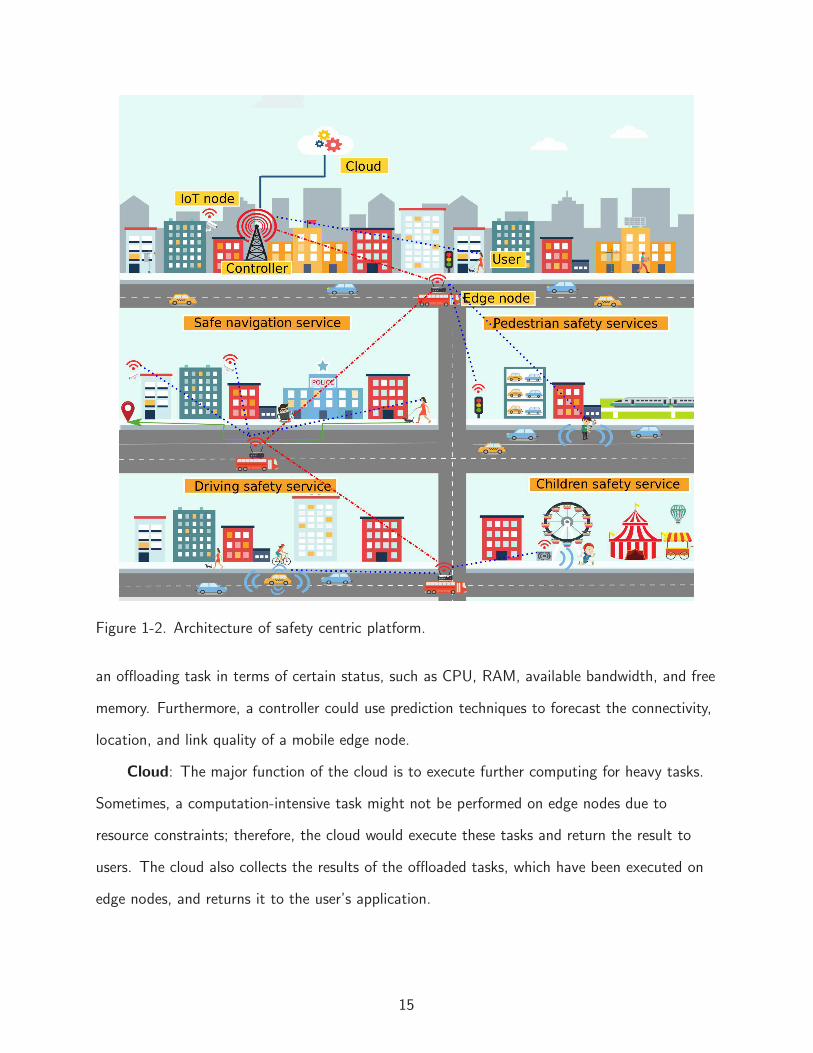
Figure 1-2. Architecture of safety centric platform.

an offloading task in terms of certain status, such as CPU, RAM, available bandwidth, and free

memory. Furthermore, a controller could use prediction techniques to forecast the connectivity,

location, and link quality of a mobile edge node.

Cloud: The major function of the cloud is to execute further computing for heavy tasks.

Sometimes, a computation-intensive task might not be performed on edge nodes due to

resource constraints; therefore, the cloud would execute these tasks and return the result to

users. The cloud also collects the results of the offloaded tasks, which have been executed on

edge nodes, and returns it to the user’s application.

15

User end: This is an application installed on the user’s mobile device, which has multiple

interface that can be used for safe navigation, children tracking, or other safety services.

The proposed framework is characterized by a flexible and scalable structure that permits

its use in potential safety centric services. Each special service may utilize different components

of the system. The general process to provide the safety service to users includes following

steps.

Step1) Users submit their requests to the system.

Step2) The controller collect information of IoT nodes and edge computing nodes, such as

the available computing resource on edge computing nodes.

Step3) Based on the collected information and objective of services, the controller

distributes the control messages to IoT nodes or edge nodes. For example, if the IoT nodes

need to offload the computing task to edge nodes, the controller makes decision how to offload

data collected from IoT nodes to edge nodes for computing (such as object identification or

image feature detection and extraction).

Step4) Related data is transmitted from IoT nodes to edge computing nodes and the data

is processed.

Step5) Edge computing units send analysis result back to the controller or upload result to

the Cloud for further processing.

Step6) The system sends the corresponding result to the users. Furthermore, the system

can offer the same service to local users through localized protocols.

1.3 Dissertation Contribution and Organization

Utilizing the safety centric platform to support safety related services brings in significant

challenges. In this dissertation, I mainly contribute three unique challenges of safety centric

services in a smart city.

Children tracking service: We propose a children tracking application under the

architecture of safety centric platform. With the designed application, the locations of children

can be tracked with simple carry-on devices, namely, RFID tags. We utilize the mobile devices

16

carried by park employees and/or visitors as local processing units to avoid the potential

congestion problem. With the help of remote control center, each reader is matched with a

mobile device for data processing. EE of mobile devices is critical in our scenario because of

the energy limitation of associated mobile devices. We formulate an Energy efficiency (EE)

optimization problem by jointly considering the resource allocation and user association.

We adopt dynamic update matching algorithm to provide an suboptimal solution. Through

extensive simulations, we show that our proposed schemes are effective in improving the EE

performance of associated mobile devices.

Safe walking navigation service: We propose a safe walking navigation application,

SPATH (the Safest PATH). In this design, wireless cameras, existing cellular infrastructure,

and vehicles with underutilized computing resources are utilized to process and transmit

surveillance videos, which can be viewed by users to check the current safety status of

different walking paths. Noting the long-distance transmission of a large volume of videos

may cause network congestion, video summarizing technology, which is realized by utilizing

the underutilized computing capability in vehicles, is applied to extract valuable information

from a video file while effectively compressing its data size. Since the quality of service for

this application is strongly correlated with the latency of delivering videos, we formulate a

latency minimization problem by jointly considering the computing resource allocation and

computing task assignment. A Fast Iterative Matching (FIM) is proposed with low complexity

to effectively solve the optimization problem. Simulation results demonstrates the effectiveness

and efficiency of proposed solution.

Intelligent surveillance service: We propose a Vehicle based Intelligent Surveillance

System (VISS) to improve public safety in smart cities. Video surveillance systems as the

popular tools to improve public safety have been widely used in many cities. However, blind

areas and high cost for maintenance and deployment make the city contain public safety

uncovered holes. Vehicle based monitoring systems, utilizing vehicles installed dash cameras

to monitor target regions, is the potential solution improving the public safety. With the

17

consideration of video data size, limited budget ,and safety status difference, a Vehicle based

Intelligent Surveillance System (VISS) is designed to improve public safety in smart cities.

First, VISS recruit vehicles as the mobile monitoring nodes to expand geographical monitoring

regions. Cooperating with slowly moving or parked vehicles with sufficient computing

capability, VISS can extract potential victims from the monitoring video files and recruit mobile

monitoring node to monitor potential victims as long as possible. Thanks to the high mobility

of vehicles, VISS has an opportunity to achieve potential victims searching and monitoring with

lower budget. To measure the performance of VISS, two optimization problems, i.e., spatial

coverage maximization problem and temporal coverage problem, are formulated by considering

mobile monitoring nodes recruitment and computing resource allocation. A heuristic algorithm

is proposed with low complexity to effectively solve the optimization problems. Simulation

results demonstrated the effectiveness and efficiency of VISS.

The rest of this dissertation is organized as follows. Chapter 2 overviews the related

works. Chapter 3 describes the corresponding concepts in this dissertation. Chapter 4 discusses

the L-TRACK service for public areas in smart cities. Chapter 5 presents the SPATH service

in smart cities. Chapter 6 gives the VISS service in smart cities. Chapter 7 summarizes this

dissertation.

18

CHAPTER 2RELATED WORK

2.1 Safety Services

The role of Smart Cities in ensuring public safety and improving citizens’ quality of life has

gained increasing attention. Using cutting-edge technology (e.g., the Internet of Things) to

effectively combat crime and increase the interconnectivity among citizens can transform Smart

Cities into Safe Cities. Accordingly, this section summarizes related work on safety services.

Children Tracking Services

We classify the existing applications for tracking children into three types. The Type-I

applications [22, 23, 24, 25, 26] rely on GPS technology. In [22], Gupta et al. design a system

utilizing GPS, SMS (Short Messaging Service) and smartphones. Smartphones as the locators

are carried by the children, so they can send location information to the parents through the

Internet. SMS plays as a backup option in the system. Once children enter the area where

there is no Internet connection, the location information can be sent as a short message

through the cellular networks. Even though the proposed system in [22] can easily track the

children, it has several drawbacks. First, the large size of a smartphone makes it inconvenient

to carry around for children. Second, the smartphone has energy limitation. Third, there is a

high risk of losing the smartphone, which results in the failure of the system.

The Type-II applications [27, 28, 29, 30] employ the Bluetooth technology. A tracking

system using Bluetooth MANET (Mobile Ad hoc NETwork) has been proposed in [28]. In the

scenario of Morii et al., every target child has an android terminal, which can autonomously

configure a wireless network based on autonomous clustering technique. Android terminals in

the cluster communicate with each other to collect group information. As a result, each parent

can check whether his/her child becomes alone or not. In addition, parents also receive the

current locations of their children. In [28], they design two-tier networks to support the system.

The first tier is a Bluetooth MANET, which can easily form a group. The second tier is the

mesh networks that deliver the data from the group to the Internet. However, this system still

19

has its own limitations, such as large device size, limited device energy, and heavy reliance

on the Internet. In [27], Liu et al. propose a BLE tag based system that utilizes the limited

communication range between the locator and the receiver. The devices (e.g., smartphones)

carried by users keep receiving signals from BLE tags as long as the children stay in the safety

range (e.g., communication range) of the users (e.g., parents of the children). Once losing the

communications from the locators, the users’ devices get an alert. To overcome the weakness

that the system may fail to work when children disappear from the range, Liu and Li [27]

design a collaborative approach to finding the lost children. However, the limited energy

problem of BLE tags remains unsolved.

The Type-III applications construct RFID networks to track children. According to the

scheme of Lin et al. [31], RFID readers are deployed in key areas to monitor tags (which

are attached to children) passing by. Depending on the location, readers can choose to

either directly transmit data to nearby storage node or rely on packet passing nodes (e.g.,

visitors or employees) to deliver the data. The major problem of this RFID system is that the

packet nodes may lead to a long delay in sending the data to the nearby storage node. To

overcome this weakness, Chen in [32] creates a scenario in which RFID readers are placed in

the landmarks of a theme park, making it easier to keep monitoring the children when they

play around the landmarks. The wireless sensor networks would subsequently transmit the data

to the gateway. However, the coverage is a serious problem in this scenario.

Pre-crime Warning Applications

Early works on the pre-crime warning applications, such as [6, 7, 8, 9], are focused on

utilizing historical crime data and crowdsourced feedbacks to assess the safety status. In [6],

Galbrun et al. develop a crime probability model based on the historical crime data in Chicago

and Philadelphia. They estimate the possible crime hot spots with Gaussian kernel density

estimation. In order to measure the safety status of the navigation path, crime activity density

is proposed, which is quantified by aggregating crime probability of each point on the walking

20

path. Moreover, they design an algorithm to offer candidate paths for users with a different

tradeoff between distance and safety.

By observing the drawbacks of the approach in [6], Goel et al. improve the safety model

with two types of data, namely static and dynamic [7]. The static data is open data including

historical crime data, road quality information, locations of police stations, and schedule of

public transport, etc. Information in static data can be used to measure whether a navigation

path is safe to walk or not. However, the static data may not accurately capture the actual

situation as the information may be outdated. Therefore, the authors build a dynamic dataset

to adapt to the information change. Dynamic data includes feedback from users in near real

time, which is gathered in a crowdsourced manner. Users can report the safety status of any

point on their walking path. Following the design of Goel et al., Mata et al. identify the crime

level of the walking path with the official crime data and the useful information from online

social media as in [8]. Criminal data repository is first built from tweets related to crime

events. Then, the crime records are classified based on crime type, time, and location. Finally,

a safe route is obtained from the estimation of crime rates.

Different from previous works, Garvey et al. [9] integrate pre-crime warning and post-crime

service. In order to overcome the inaccuracy of the estimation of safety status, they develop

the PASSAGE, a safety application. In [9], Garvey et al. also offer possible walking path of

a user by applying estimation model of crime points and allows the user to add friends or

relatives as the guardians, who receive the current location of the user.

2.2 Vehicle as Resource

Today, the global automotive industry is being transformed with the advancement of

computation and communication technologies. Now drivers have more and more options of

smart cars for everyday use. Generally speaking, the function of a smart car can be improved

with the following devices in place: computing devices, GPS devices, communication devices,

sensing devices, radar devices, cameras, and storage devices. which can be used to improve

21

driving safety by sensing and processing the driving environment. As such, it is reasonable to

view a vehicle such as a smart car as a resource.

In [33], Zhang et al. propose a system architecture, where vehicles are service providers for

smartphones. When infrastructure-based cloud does not have enough resource to support the

service for users, residual computing in vehicles is allocated to accomplish mobile application

offloading. In [34, 35], Ding et al. design a V-CCHN (Vehicular Cognitive Capability Harvesting

Network) architecture, which utilizes CR routers enabled vehicles to handle the explosively

growing wireless data traffic. The V-CCHN involves several new features, such as the capacity

of reconfiguring agile communication interfaces to interoperate with other devices and mobility

to realize data exchange within proximity, to fully exploit available vehicles. For more details of

this architecture, readers are referred to [34].

22

CHAPTER 3PRELIMINARIES

3.1 Radio Frequency Identification

The technology of Radio Frequency Identification (RFID) can automatically detect a

person or an object via radio waves within a wide range of distance (e.g., from a few inches to

hundreds of feet) [36]. As an automatic data capture system, RFID can largely improve system

efficiency. Without direct contact, RFID is able to communicate via RF signals. With silicon

chips (where data is kept) being tagged to people, animals or non-living objects, RFID provides

an electronic product code (EPC) which is a unique identification number for each identified

target [37]. Overall, there are three main categories of the RFID tags.

Active tag: It has a power support system for the circuitry and antenna of the tag.

The strength an active RFID tag is manifested in the long-distance (e.g., over a hundred

feet) readability and the incorporation of other sensors powered by alternative current (AC).

Nonetheless, the main weakness lies in the limited lifespan of an active RFID tag. Specifically,

the tag is very costly and large in size. It may also increase the maintenance expense in the

case of battery replacement. Further, battery outages in this type of tag may entail high

chances of misreads [38].

Semi-passive tag: In order to deliver identification information, semi-passive tags reflect

RF singnal back to the tag reader. With a battery to power ICs, this type of tags give birth

to various innovative products. For instance, with a built-in sensor, the tag can transmit

information such as lighting, temperature and humidity in real time. By using the battery only

to power a simple IC and sensor, the semi-passive tags are able to keep a balance between

cost, size, and range [38].

Passive tag: Instead of having a power source, the passive tag is powered by the reader.

It relies on the power drawn from the inductive coupling with reader antenna. However,

a noticeable problem is that a passive tag is only readable within a few feet of distance.

Nevertheless, the advantages of a passive tag are evident: First, its life cycle can be extended

23

to more than 20 years as the tag can function properly in the absence of a battery. Moreover,

the passive tag is much cheaper (costs only 10 cents) and physically smaller compared to an

active tag, hence it is commonly applied to consumer products and a wide range of areas [38].

Figure 3-1. Illustration of RFID communication.

Passive tags send radio waves that contain EPC/information to the reader, which

then sends continuous waves (CW) to provide power for the tag and allow the chip in the

tag to function [39]. Passive tag can transmit information to the reader via radio waves

without having direct contact with the reader. This is made possible by the technology called

backscattering (as shown in Figure 3-1). When tuned to a certain frequency, passive tag

is capable to take in most energy at the same frequency level. However, when there is an

impedance mismatch at this frequency, the antenna will reflect back some of the energy (as

tiny waves) toward the reader [40]. The RFID technology has demonstrated considerable

value across fields. For example, it enables the automation of supply chain management, asset

tracking, animal monitoring medical applications, warehouse and access control in contactless

manner [41].

3.2 Video Summarization

The creation of video content has experienced a tremendous increase within the past

few years, causing a series of problems in relation to information congestion and content

management. With the growing number of videos released on the web, there is a need to

24

efficiently extract useful information from the videos. As such, technologies focusing on video

content processing deserve greater attention from the scholars [42, 43].

The various stages of video summary algorithms based on key frames are as described

below [44, 45].

Step 1) Data Input. The format of the videos can be diverse. A typical format is AVI

(Audio Video Interleave).

Step 2) Frame Division. This step involves processing the video which can be achieved

through frame division. In this step, the recorded video is split into multiple frames, which may

take up a lot of memory space. The number of frames is determined by the size of the video.

Moreover, the frame rate is about 20 to 30 frames per second.

Step 3) Feature Extraction. This step is to extract visual features of the key frames

through feature extraction. These features include color, edge and motion features. Features

are extracted based on different frames’ characteristics, which are determined by the frame

difference values.

Step 4) Frame Selection. It starts with naming the first frame as a key frame. If the

difference between the current frame and the previous key frame is sufficiently large, the

current frame will be named as the key frame hence be selected. Such selection process is

applied for all video frames.

3.3 Matching Theory

There are two major approaches to solve the optimization problems. One is the

centralized algorithms which use highly complex computation to obtain optimal outcomes.

The other is distributed approaches which use less complex computation to achieve suboptimal

solutions. Matching game is one of the distributed approaches that are commonly used

to address issues regarding optimization. Studies on Matching Theory examine the ways

through which agents from different groups can be linked with one another according to

their preferences. The theory was brought up by David Gale and Lloyd Shapley in 1962 in an

attempt to solve the two-sided matching problem [46]. Afterwards researchers have applied this

25

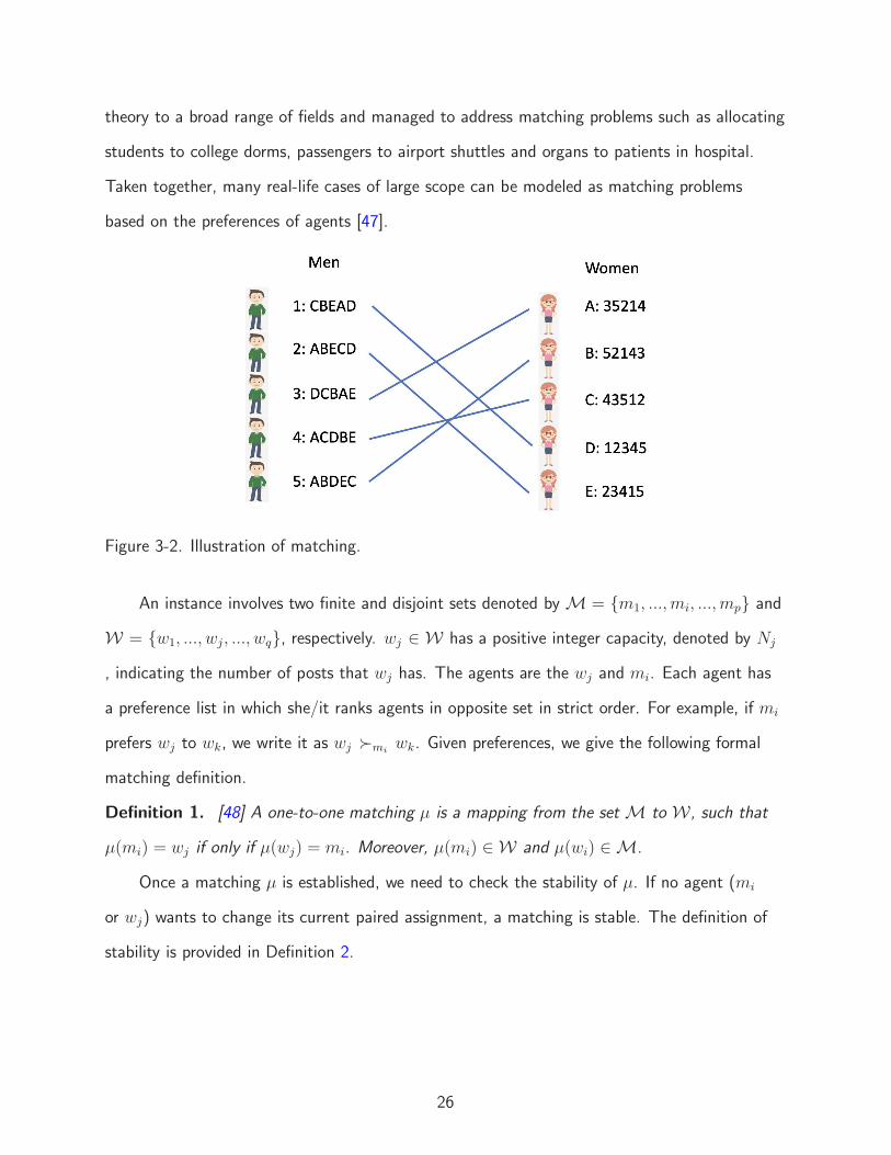
theory to a broad range of fields and managed to address matching problems such as allocating

students to college dorms, passengers to airport shuttles and organs to patients in hospital.

Taken together, many real-life cases of large scope can be modeled as matching problems

based on the preferences of agents [47].

Figure 3-2. Illustration of matching.

An instance involves two finite and disjoint sets denoted byM = m1, ..., mi, ..., mp and

W = w1, ..., wj, ..., wq, respectively. wj ∈ W has a positive integer capacity, denoted by Nj

, indicating the number of posts that wj has. The agents are the wj and mi. Each agent has

a preference list in which she/it ranks agents in opposite set in strict order. For example, if mi

prefers wj to wk, we write it as wj ≻miwk. Given preferences, we give the following formal

matching definition.

Definition 1. [48] A one-to-one matching µ is a mapping from the setM to W, such that

µ(mi) = wj if only if µ(wj) = mi. Moreover, µ(mi) ∈ W and µ(wi) ∈M.

Once a matching µ is established, we need to check the stability of µ. If no agent (mi

or wj) wants to change its current paired assignment, a matching is stable. The definition of

stability is provided in Definition 2.

26

Definition 2. [47] A matching µ is said to be stable if it admits no blocking pairs. A pair

(mi, wj) is a blocking pair if the following the conditions hold: (1) mi is either unassigned or

prefers wj to µ(mi); (2) wj is either unassigned or prefers mi to µ(wj)

Matching theory also provides tractable solution to the problem of multiple agents in two

distinct groups. Each agent wants to match with one or multiple agents in the opposite group.

Mathematically, the many to one matching can be defined as follows.

Definition 3. [49] Given two distinct setM and W, a matching µ is a mapping function from

M∪W into 2M∪W , such that: µ(mi) ⊆ W and |µ(mi)| ≤ 1 for all mi ∈M; µ(wj) ⊆M and

|µ(wj)| ≤ Nj for all wj ∈ W, where Nj is the capacity of agent wj ∈ W; µ(mi) = wj if and

only if wj ⊆ µ(mi) for all (mi, wj) ∈ M×W

3.4 Genetic Algorithm

During 1960s to1970s, Holland along with other researchers first proposed the concept of

Genetic Algorithm (GA) which are inspired by the evolutionist theory [50]. According to the

evolutionist theory, all species on the earth face natural selection. While the strong species

gain greater chance to survive and preserve their genes through reproduction, the weak ones

are eliminated in the natural selection process. As a result, species with the preferable genetic

combination make up the majority of the population over the long term. Meanwhile, random

genetic changes may take place during the chronic process of evolution. If the changes are

beneficial for survival, such changes will be retained as new species evolve from their ancestors.

On the other hand, changes that do not increase the chance of survival are discarded in the

natural selection process.

Chromosomes, a key term in the Genetic Algorithm (GA), are made of genes that control

core features of the chromosome. Originally genes are used to indicate binary digits, whereas

their current implementations are commonly used to denote variables [51]. Generally speaking,

with the mapping technique called encoding, a chromosome is mapped to a particular solution

in the feasible solution set. A population composed of multiple chromosomes is randomly

27

Figure 3-3. Illustration of crossover and mutation.

initialized. Within a population, two operations of GA namely crossover and mutation are used

to generate new solutions.

As the most critical operator of GA, the crossover combines two chromosomes (known as

parents) to produce new chromosomes (known as offspring) [52]. Those chromosomes with

superior genes are more likely to be selected as parents to pass on their good genes to the

next generation. With the repetition of crossover operator, chromosome containing good genes

would become dominant in the population hence result in convergence to a local optima.

Another operation of GA is called mutation. Operating at the gene units, mutation is

specialized in preserving genes diversity. Mutation allows changes of characteristics to take

place randomly in chromosomes. Since the probability of mutation is quite small, the newly

produced chromosome will be similar to its parent. To sum up, both operations play an

important part in GA. Whilst crossover is capable to retain good genes in the population,

mutation can introduce slight changes to the population.

28

CHAPTER 4L-TRACK:CHILDREN TRACKING IN THEME PARKS

4.1 Background

Losing a beloved child is no doubt the worst thing for every parent. In some cases, parents

find that their children are lost while they are talking with others for a few seconds. Based

on the statistical data for Missing and Exploited Children released by the National Center, we

learn that roughly 800,000 children are missing every year in the United States, which means

roughly 2,000 children are reported missing every day [53]. Some incidents occur when parents

take their children to public places, especially the markets, shopping malls, and theme parks.

For example, in large theme parks like Walt Disney World, there are tens of thousands of

visitors every day. It may be just a turn-around and the next thing you realize is that your child

is missing. To make matters worse, finding a missing child in a huge park is almost impossible.

To prevent parents from losing their beloved children, researchers have developed many

systems and approaches. The most popular one is to place the GPS (Global Positioning

System) locators on their children. The Paw tracker, Trax GPS Tracker, and HEREO GPS

watch [54] are the popular products based on GPS. The main issues of using GPS systems

are high cost and energy limitation of a locator. When a GPS locator works in a continuous

mode, it consumes energy rapidly. Thus, Bluetooth Low Energy (BLE) is emerging as the

alternative approach to solve the children missing problem. In the BLE tracking systems,

the locator can directly communicate with a user’s device (e.g., smartphone). As mentioned

in [55, 56], a Bluetooth tracker company named Chipolo can help parents locate their children

by attaching BLE tags to children’s shoes or clothes. Even though the energy consumption has

been reduced using BLE tags, the energy problem still limits the popularity of BLE tracking

systems. Another drawback of the systems relying on BLE is that if the children go out of

the communication range, their parents may not locate their children any more. Given the

weakness mentioned above, it is imperative to design a new children tracking system, which is

energy efficient and robust to dynamically changing environments.

29

Nowadays, RFID technology [57, 58], especially the passive RFID, which relies on the

backscatter technology, has emerged as a promising approach due to its low cost and less

restriction on energy. In [31], Lin et al. construct an RFID based opportunistic network to

locate children. They use distributed nodes to store the location data of tags. In their design,

the system relies on moving people, who acts as carry-and-forward nodes to transmit data.

When users query the information of tags, the control center can find the corresponding

information in the distributed storage nodes. Chen et. al in [32] have proposed another system

that combines RFID networks with wireless sensor networks for tracking children in theme

parks. In their design, the readers rely on the wireless sensor networks for data transmissions.

However, there are several challenges facing RFID based children tracking system.

Firstly, potential congestion would reduce quality of service. Most of RFID based children

tracking systems adopt the centralized design. In this design, a reader would transmit collected

data to the remote control center (such as a base station) for processing and storage. For

example, the proposed system in [32] is designed in the centralized fashion. In their design,

reading data would be relayed back to the remote control center through multi-hop wireless

sensor networks. Actually, the remote control center would be congested due to all of devices

waiting for transmitting and computing data in its coverage. Secondly, unnecessary waste of

communication resource is another problem. Most of the situations, the readers would operate

in the continuous model. The continuously reading may incur significant traffic. Notice that it

is not necessary to transmit reading data all the time to remote control center since children

might stay in the same place, such as waiting in line for a spot of interest in a theme park.

Thirdly, full coverage of children activity area is critical. In the design of Lin et al. [31] and

Chen et. al [32], they both propose to simply place the fixed readers in key points. Without

full coverage of children activity area, the system may have the blind area. As a result, it is

critical to design an efficient and effective RFID based children tracking system.

Inspired by previous works, we propose a new children tracking system based on UHF

RFIDs (as shown in Fig 4-1). Similar to previous works, we propose to fasten the passive

30

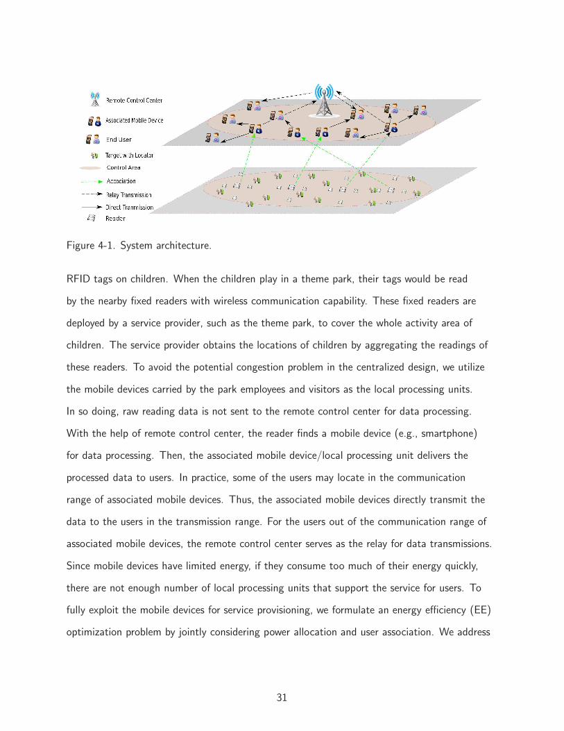
Figure 4-1. System architecture.

RFID tags on children. When the children play in a theme park, their tags would be read

by the nearby fixed readers with wireless communication capability. These fixed readers are

deployed by a service provider, such as the theme park, to cover the whole activity area of

children. The service provider obtains the locations of children by aggregating the readings of

these readers. To avoid the potential congestion problem in the centralized design, we utilize

the mobile devices carried by the park employees and visitors as the local processing units.

In so doing, raw reading data is not sent to the remote control center for data processing.

With the help of remote control center, the reader finds a mobile device (e.g., smartphone)

for data processing. Then, the associated mobile device/local processing unit delivers the

processed data to users. In practice, some of the users may locate in the communication

range of associated mobile devices. Thus, the associated mobile devices directly transmit the

data to the users in the transmission range. For the users out of the communication range of

associated mobile devices, the remote control center serves as the relay for data transmissions.

Since mobile devices have limited energy, if they consume too much of their energy quickly,

there are not enough number of local processing units that support the service for users. To

fully exploit the mobile devices for service provisioning, we formulate an energy efficiency (EE)

optimization problem by jointly considering power allocation and user association. We address

31

the EE optimization problem by adopting the dynamic updating matching algorithm. As such,

the main contributions of this chapter are summarized as follows:

First, we propose a novel RFID system to track children in public areas. With the

designed system, the locations of children can be tracked with simple carry-on devices, namely,

RFID tags. We utilize the mobile devices carried by park employees and/or visitors as local

processing units to avoid the potential congestion problem. With the help of remote control

center, each reader is matched with a mobile device for data processing.

Second, EE of mobile devices is critical in our scenario because of the energy limitation of

associated mobile devices. We formulate an EE optimization problem by jointly considering the

resource allocation and user association. Since the formulated EE problem is NP-complete, we

adopt dynamic update matching algorithm to provide an suboptimal solution.

Finally, through extensive simulations, we show that our proposed schemes are effective in

improving the EE performance of associated mobile devices.

4.2 Architecture

4.2.1 Overview

Fig. 4-1 gives a high-level overview of our proposed system. RFID tags are attached to

the visitors of theme parks. We call the tag attached on child is the target tag and the tag

placed on a normal visitor is the interference tag. In addition, we also deploy RFID reference

tags which can help readers locate target tags more easily. RFID readers are deployed in theme

parks to make sure that every point of the children’s activity area is covered at least by one

reader. We also assume that readers are equipped with communication radio interface with

other mobile devices, which can be done with certain customization. When children travel

in the theme parks, the attached tags will be scanned by the nearby fixed RFID readers. As

we mentioned in the previous section, we employ the wireless communication readers. Then,

readers send the scanned data to local processing units for data processing. Local processing

units are the mobile devices carried by park employees and visitors. Actually, visitors can access

this system via an application which is downloaded and installed on their mobile devices.

32

Parents can track their children through this application. If the smartphone of a visitor has

enough power, the visitor can apply as the local processing unit to perform processing and get

monetary compensation. Finally, local processing units send the processed data to devices of

users.

We divide the time into discrete fixed time period, called slot. At the beginning of the

slot, readers first scan its coverage area to read data from tags in the area. The reader utilizes

power control to tune the transmission power level in order to read the tags since power

control not only helps improve the location accuracy of target tags, but also avoids the reading

collision problem among readers. We group readers into clusters. In each cluster, one central

reader acts as the cluster head to gather reading data of all other readers. The cluster head

also has ability to buffer the reading data. Then, the cluster heads gather all the raw reading

data from their cluster members.

The raw reading data will go through two stages before being delivered to the users.

The first stage is the processing stage, which includes reference tag elimination, target tag

location estimation, and so on. In the beginning of processing stage, all cluster heads request

the remote control center help them find the local processing units. At the same time, the

remote control center requires information of all mobile devices registered as the candidates

of local processing units. The reader-mobile device association process will be finished at the

remote control center. Then readers send the raw reading data to the associated mobile device

(e.g., d1 in the Fig. 4-2 ). The raw reading data will be locally processed by the associated

mobile devices. Then, the processed data is passed to the second stage, the delivery stage.

In this system, we assume both readers and mobile devices have limited device to device

communication range. In the delivery stage, the associated mobile devices directly transmit the

processed data to the nearby end users (e.g., d2 and d3 in the Fig. 4-2) in its communication

range. For the end users out of the communication range of the associated mobile device

(such as d4 in the Fig. 4-2), the remote control center serves as the rely nodes for data

transmissions. In addition, in the subsequent development of this chapter, when we say the

33

reader, we mean the head of a reader cluster. The whole process are summarized in the

Fig. 4-2.

Figure 4-2. Whole process of data processing and transmissions..

4.2.2 System Model

We denote the set of the readers as R = 1, 2, · · · , j, · · · , R, the j-th reader by rj. We

also denote the mobile devices by D = 1, 2, · · · , i, · · · , D, the i-th mobile device by di. To

evaluate the performance of our system, we first elaborate a few important concepts we will

use in the subsequent development.

Link Data Rate

In our scenario, orthogonal channels are adopted in the transmissions among mobile

devices and transmissions from mobile devices to remote control center. Thus, transmissions

among different channels are interference free. According to the Shannon-Hartly theorem, the

data rate of the link between mobile device di and mobile device dk or remote control center B

is

ci,× = Wi× log2

(

1 +pi,×hi,×

N0Wi,×

)

. (4-1)

where × indicates a target node (either dk or base station B), and pi,× denotes the transmission

power of mobile device di, hi,× is the channel gain from mobile device di to dk or base station

34

B, and N0 is the power spectral density of Additive White Gaussian Noise (AWGN). Then, we

can get the total achieved data rate via the mobile device di is

Ci =∑

k∈Ti∪B

Wi,k log2

(

1 +pi,khi,k

N0Wi,k

)

. (4-2)

where Ti is the set of neighboring nodes, which means the end users within i’s transmission

range. For example, in the Fig. 4-2, the set of neighboring nodes of mobile device d1 is

d2,d3 since only these destinations/end users in its communication range. |Ti| is the

cardinality of the set Ti. Actually, Ti is determined by the reader association selection xj,i.

That is, when mobile device di associates with different reader ri, the set Ti is different.

Power Consumption

The total power consumption of each mobile device di includes two parts, which are the

aggregated power consumption for data processing EPi and the power consumption for data

transmissions, respectively. We define fi as the computation ability of mobile device di. The

power consumption of mobile device di for data processing can be calculated as[59]

EPi = κ(fi)

3 (4-3)

where κ is the coefficient depending on the chip architecture. Power consumption for data

transmissions can be characterized by[60]

ETRi =

∑

k∈Ti∪B

ηpi,k + P ciri (4-4)

Here, P ciri is denoted as the circuit power consumption and η is the power amplifier efficiency.

The power consumptions of the infrastructure nodes and fixed readers are assumed not to be

considered as all of them are powered by more powerful external power source.

Matching Matrix

We introduce an R × D reader association matrix. Element xj,i in the matrix indicates

whether or not the reader rj is associated with mobile device di. That is, fixed reader rj

transmits the raw data to mobile device di for processing when xj,i = 1; otherwise, xj,i = 0.

35

Table 4-1. Table of parameters

Parameter DescriptionR Set of readersD Set of mobile devicesrj j-th fiexd readerdi i-the mobile devicePi,× Transmission power of the mobile device dihi,× Channel gainN0 Power spectral density of additive white Gaussian noise

T ji Set of connected devices within di’s transmission range

EPi Power consumption for data processing of di

P ciri Circuit power consumption

η Power amplifier efficiency

To improve the clarity, notations of key parameters are summarized in Table 4-1

4.3 Problem Formulation

Given the model described before, we target at the problem on maximizing the energy

efficiency of associated mobile devices. In our design, sufficient number of available local

processing units can provide long and stable service for users. However, if all mobile devices

consume their energy quickly, there are few mobile devices would act as local processing units

to support users. Thus, improving energy efficiency of mobile devices can maintain quality of

experience and make the whole system stable [61]. Hence, we consider a joint EE optimization

problem for reader association decision and resource allocation. We first formulate the EE

function for each mobile device di, which is given by

EEi =Ci

EPi + ETR

i

(4-5)

where Ci is the total achieved data rate via mobile device di to users (mobile devices carried

by parents). That is to say, data from readers is processed on mobile device di, and then the

processed data is sent to users. To process data Cj,i for users, mobile device di consumes a

certain amount of power, which includes the power consumption for data processing EPi and

the power consumption for data transmissions ETRi .

Furthermore, we need to consider several constraints for the EE optimization problem.

36

4.3.1 Reader Association

The fixed reader rj can only associate with one mobile device for data processing. This

constraint can be captured as follows

∑

i∈N

xj,i = 1 (4-6)

4.3.2 Maximum Power Limitation

In our scenario, we assume each mobile device can just utilize transmission power below

the maximum Pmax, that is,

pi,k ≤ Pmax (k ∈ Ti ∪ B) (4-7)

4.3.3 QoS Requirement

In order to guarantee the QoS requirement for the users, we introduce the constraint as

Wi,k log2

(

1 +pi,khi,k

N0Wi,k

)

≥ cmin (k ∈ Ti ∪ B) (4-8)

where cmin is denoted as the QoS threshold.

37

4.3.4 EE Optimization

Based on the constraints we mentioned above, we have the following optimization problem

maxxj,i,pi,k

∑

i∈N

∑

j∈M xj,iωiCj,i

|∑j∈M xj,i|EPi +

∑

i∈M xj,iETRj,i

(4-9)

s.t.

Cj,i =∑

k∈Tj,i∪B

Wi,k log2

(

1 +pi,khi,k

N0Wi,k

)

ETRi =

∑

k∈Tj,i

ηpi,k + P ciri

EPi = κ(fi)

3

0 ≤ pi,k ≤ Pmax (k ∈ Tj,i ∪B)

Wi,k log2

(

1 +pi,khi,k

N0Wi,k

)

≥ cmin (k ∈ Tj,i ∪ B)

∑

i∈N

xj,i = 1

xj,i ∈ 0, 1

where ωi is a balancing weighting factor related to the residual energy of mobile device di

and the stable time. Actually, if a mobile device has more residual energy and does not move

frequently, it would be a better choice to be a local processing unit. Here, Tj,i is device di’s

neighboring nodes that request the data from reader rj . Clearly, our formulated optimization

problem (4-9) is a mixed-integer nonlinear programming problem, which is NP-complete as

proved in [62]. In the next section, we adopt matching theory to find the feasible solution to

the EE maximization problem.

4.4 Matching Approach

4.4.1 Preference Establishment

We first establish each player’s preference list. Notice that mobile devices’ preference lists

cannot be set up since the neighboring nodes set Tj,i for each device di is unknown before the

reader mapping decisions between readers and devices have been made. We consider the case

of two adjacent time slots. Assume the network condition changes slightly because the time

38

slot is short. That is to say, only a small number of readers’ or mobile devices’ preferences are

changed. Under this assumption, we can set up mobile devices’ preference lists of the current

time slot according to the knowledge from previous slot.

Preference Establishment

The basic idea to establish the preference of a mobile device is to use knowledge from

previous time period to obtain the set of neighboring nodes. We first set up the preference

list of rj . All readers establish their preference lists according to their benefit functions .

The benefit of reader rj depends on the achievable data transmission rate, which can be

characterized as µCj,i, where µ is the benefit factor. Without loss of generality, we set µ = 1.

Thus, the preference list of rj over device di at time slot t is VRj (t) = (V R

j,i(t)), where V Rj,i(t) is

abtained according to

V Rj,i(t) = ωi

∑

k∈Tj,i(t−1)∪B

Wi,klog2

(

1 +pi,k(t)hi,k(t)

N0Wi,k

)

(4-10)

We now introduce the preference establishment of a mobile device. Mobile device di

sets up its preference based on its transmission cost function. The cost function is the power

consumption for transmissions and processing, which is ν(EPi + ETR

j,i ). Similarly, we also

assume ν = 1 for ease of presentation. Then the preferences of di over device rj at time slot t

is VDi (t) = (V D

i,j (t)) and V Di,j (t) can be captured according to

V Di,j (t) = κ(fi)

3 +∑

k∈Tj,i∪B

ηpi,k(t) + P ciri (4-11)

We model di’s preference and rj ’s preference according to local maximum achievable EE

with the set of neighboring nodes Tj,i(t−1) at time slot t. Thus, we develop the following Fast

Iterative Power Allocation algorithm (FIPA) to obtain the transmission power between device

di and neighboring nodes set Tj,i, which is obtained from the formulated local power allocation

39

problem

maxpi,k

UEEi (t) =

Ci[pi,k(t)]

Ei[pi,k(t)](4-12)

s.t.

Ci[pi,k(t)] = ωi

∑

k∈Tj,i(t−1)∪B

Wi,k log2

(

1 +pi,k(t)hi,k(t)

N0Wi,k

)

Ei[pi,k(t)] = κ(fi)3 +

∑

k∈Tj,i(t−1)∪B

ηpi,k(t) + P ciri

0 ≤ pi,k ≤ Pmax (k ∈ Ti ∪ B)

Wi,k log2

(

1 +pi,khi,k

N0Wi,k

)

≥ cmin (k ∈ Ti ∪ B)

Since the problem formulated in (4-12) is a nonlinear fractional programming, we first

employ fractional programming theory to transform it to an equivalent convex programming.

Thus, based on what Dinkelback has elaborated in [63] and more recent studies [64] [65], we

have the following proposition:

Proposition 4.1. [63] Define the function Q as

Q(λ) = maxpi,k

Ci(pi,k)− λEi(pi,k). (4-13)

Then, the optimal power allocation p∗i,k is achieved if and only if there is λ∗ such that Q(λ∗) =

Ci(p∗i,k)− λ∗Ei(p

∗i,k) = 0.

From this result, we develop the FIPA algorithm.

FIPA Algorithm

The equivalent optimization problem is given by

maxpi,k

Ci(pi,k)− λ∗Ei(pi,k) (4-14)

s.t.

0 ≤ pi,k ≤ Pmax (k ∈ Ti ∪ B)

ci,k ≥ cmin (k ∈ Ti ∪ B)

40

Then we utilize FIPA algorithm based on the well-known Dinkelbach algorithm [63] to get the

specific values of λ∗. At the nth iteration, with the value of λ(n − 1) from the (n − 1)th

iteration, pi,k(n) are obtained by

pi,k(n) = [1

ηλ(n− 1)ln2− N0Wi,k

hi,k

]+. (4-15)

where [x]+ = maxx, 0. Then, if pi,k(n) > Pmax, we set value of pi,k(n) to Pmax. If

pi,k(n) < Pmini,k (which is obtained from (4-8)), we set value of pi,k(n) to Pmin

i,k . Finally, if

Ci[pi,k(n)]− λ(n− 1)Ei[pi,k(n)] < ∆ holds, the algorithm stops. Otherwise, update n = n+1,

λ = Ci[pi,k(n)]/Ei[pi,k(n)], and go to the next iteration. We can also use more efficient

algorithms developed in [64] [65], but we choose Dinkelbach’s algorithm for the ease of

presentation.Algorithm 4.1. FIPA Algorithm

1: procedure PIFA(∆,λ(0),N ,n)2: Calculate each Pmin

i,k according to (4-8)3: while n ≤ N do4: Obtain pi,k(n) by (4-15)5: if pi,k(n) < Pmin

i,k then6: Set pi,k(n) = Pmin

i,k

7: end if8: if pi,k(n) > Pmax then9: Set pi,k(n) = Pmax

10: end if11: if Ci[pi,k(n)]− λ(n− 1)Ei[pi,k(n)] ≥ ∆ then12: Set λ(n) = Ci[pi,k(n)]/Ei[pi,k(n)];13: else14: pi,k(t) = pi,k(n)15: end if16: Update n = n+ 117: end while18: end procedure

4.4.2 Dynamic Updating Matching Algorithm

When the preference establishment is completed, we can start with the matching. We

propose the Dynamic Updating Matching (DUM) algorithm, which proceeds iteratively.The

DUM algorithm has two stages. At the first stage, readers conduct the matching based on

41

the preference list VRj . In each iteration, reader ri proposes to its most preferred device di.

After this, di is removed from preference list VRj . Then device di decides whether to accept or

reject the proposal based on its preference list over the reader rj . If there are more than one

proposal, device di chooses to keep the reader rj that it favors the most, and rejects the rest.

The proposing and accepting/rejecting iterations run for as many rounds as needed until all

readers are matched or all readers’ preferences that are fully examined. We also consider the

case all readers’ preferences are fully examined but some readers are still unmatched. We let

device di increase its accepting capacity and reader rj updates its preference list based on the

current matching. Then readers conduct the new matching based on the new preference lists.Algorithm 4.2. DUM Algorithm

1: procedure DUM(pi,k(t)) ⊲ Matching Construction;2: Each rj sets up its preference VR

j according to (4-10)

3: Each di sets up its preference VDi according to (4-11)

4: Construct unmatched set Run, set Run=R ⊲ Matching;5: while Run 6= ∅ do6: for each rj ∈ Run do7: Proposes to the first di in its preference list and remove di from VR

j ;8: end for9: for di ∈ D do10: if di receives one proposal then11: di keeps the proposal;12: Remove rj from Run;13: else14: di keeps the most preferred proposal from rj∗, and rejects the rest;15: di removes rj∗ from the Run, and add the rejected readers into the Run;16: end if17: end for18: end while ⊲ State Update;19: if Run 6= ∅ then20: Update preference list VD

i ;21: Update preference list VR

i ;22: Go to step 6;23: end if24: end procedure

42

Figure 4-3. A snapshot of mobile device location with N=70.

4.5 Performance Evaluation

4.5.1 Simulation Setup

This section presents EE of the proposed solution. There are R readers placed in the

grid topology and D mobile devices randomly distributed in the area. A snapshot of mobile

device locations with D = 70 and reader locations with R = 49 is shown in Fig. 4-3. The

big diamond is the remote control center, the stars are the RFID readers, and the dots are the

mobile devices. We assume the communication range between mobile devices is up to 100 m.

The mobile devices are assumed to have an circuitry power consumption Pcir = 50mW . We

also set the effective switched capacitance κ = 10−28[59]. The channel fading is modeled by

complex normal distribution, CN (0, 1)[66].

To evaluate the performance, the proposed matching algorithm is compared with classical

stable marriage matching (SMM) algorithm and one heuristic algorithm. The heuristic

algorithm is called reader-greedy algorithm, which readers are always matched with the mobile

devices most preferred according to readers’ preferences. In addition, for the purpose of

43

comparing the impact of our proposed power allocation approach, we also introduce random

power allocation approach and greedy power allocation approach. In particular, greedy power

allocation approach allocates the maximum transmission power Pmax for every transmission

link of associated mobile devices. Random power allocation approach employs transmission

power distributed in the range [0, Pmax]

4.5.2 Results and Analysis

Performance comparison with the optimal solution

Figure 4-4 shows EE performance of our proposed algorithm and the optimal solution,

which serves as a benchmark for comparison. The optimal solution is obtained by the

exhaustive enumeration method. Considering the high computational complexity of the

exhaustive enumeration method, a small-scale network size is set to evaluate the performance

of the proposed algorithm. We set the number of readers R is to be varied in [26] and the

number of mobile devices is 5. As it is shown, the performance of proposed algorithm achieves

more than 80% of the optimum one. Hence, we can conclude that DUM can attain an

approximated optimal energy efficiency by comparing with the exhaustive enumeration scheme.

Furthermore, although there is gap between DUM and the optimal matching scheme, DUM

can obtain a suboptimal performance with lower computational complexity.

Performance comparison of different matching algorithms

In Fig. 4-5, we evaluate the energy efficiency versus different network size. Since the

readers are deployed in grid topology and have the fixed reading range, the number of readers

varies with the network size. We assume that the number of readers R is varied in [949].

We set the density of mobile devices to be fixed, Ω = 0.005 devices/m2. Simulation results

demonstrate that the EE of the proposed matching approach first increases fast and then

grows slowly. The reason is that with the network size increasing, both readers and mobile

devices have a wider variety of expanded matching candidates. In the three approaches, the

proposed matching algorithm achieves the best energy efficiency, which indicates that it can

exploit more benefits from the diverse choices than the other two algorithms. The performance

44

of stable marriage matching algorithm is not as good as the proposed algorithm since it

cannot update preference timely and ignores the benefits from the previous matching. The

performance of the reader-greedy approach is not as good as the other two algorithms since

it cannot fully exploit the diverse matching candidates and ignores the benefits from power

allocation process of data transmissions.

Comparison of power allocation approaches

Figure 4-6 shows the EE of diffident power allocation strategies. We employ the same

values of R and Ω as in the previous simulation. We set the maximum allocated power to

Pmax = 30dBm. The result demonstrates that proposed power allocation approach achieves

the best EE and outperforms the random power allocation approach and the greedy power

allocation approach by 375% and 452% for R = 25, respectively. The random power allocation

gets the second best performance since it has higher probability to take full advantage

of the available power. We also find that benefits from the increasing power is not able

to compensate for the EE loss. The greedy power allocation approach achieves the worst

performance due to two reasons. The first is that the power allocation is fully ignored since

it employs the fixed power. The second is that increasing transmission power has higher

probability for passing the point for the optimum EE. Thus, increasing transmission power does

not really improve the EE, rather causes significant EE loss.

EE with respect to the density of mobile devices

In Fig. 4-7, EE of different algorithms with respect to the varied density of mobile devices

are evaluated. In this evaluation study, the density of mobile devices varying within [5 35] and

the step size is 5. We set the number of readers to R = 36. The result demonstrates that the

impact of the density of mobile devices is evident only at lower values. When the density of

mobile devices is not large, the EE grows almost linearly with the increasing density of mobile

devices. Then, the EE stays nearly constant even when the density of mobile devices continues

to increase. The reason is that when the density of mobile devices is small, the system gains

more benefits from the density of mobile devices. Once density of mobile devices exceeds the

45

point for the optimum EE, the reader can always be matched with perfect mobile devices to

obtain the best EE.

EE with respect to the computation capability of mobile device

We evaluate the energy efficiency versus different computation ability of mobile devices.

In this evaluation study, the computation capability of mobile devices varies within [0.5 0.9]

GHz and the step size is 0.05. We set the number of readers to R = 16. The results are shown

in Fig. 4-8. It can be seen that three matching algorithms demonstrate the same relationship

between energy efficiency and the computation capability of mobile devices. The result shows

that the EE decreases nearly constant when the computation capability of mobile devices

stays at low values. Then, the EE decreases evidently with the computation capability of

mobile devices continues to increase. The reason is that when the computation capability of

mobile devices is low, the system loses less benefits from the computation capability of mobile

devices. That is to say the energy consumption of computing process is not dominant when

the computation capability is low. Once the computation capability of mobile devices is high,

computing process becomes the major source of energy consumption. Thus, the EE decreases

evidently.

46

Figure 4-4. Comparison to the optimal solution.

Figure 4-5. Comparison of different matching algorithms.

47

Figure 4-6. Comparison of different power allocation approaches.

Figure 4-7. EE under different density of mobile devices.

48

Figure 4-8. EE under different computation capability of mobile device.

49

CHAPTER 5SPATH: A SAFE WALKING NAVIGATION SERVICE

5.1 Backgroud

Public safety is one of the most important concerns in the United States. According

to the annual compilation of crimes reported by the law enforcement agencies, there were

estimated 1,247,321 violent crimes committed in 2017. Moreover, there were estimated

319,356 robberies all the year round [67]. That is to say, nearly 38 robberies were reported

every hour. In fact, most robberies occur in urban areas, especially at night. To improve

public safety in cities, technology companies have already taken steps to design safety related

applications. Recently, Mobile Software AS designs a new application, bsafe [68], which

allows a user to add contacts as the guardians. When an imminent danger is perceived, a

user can activate this application, which automatically sends alert to the recorded guardian.

Similarly, Safe Apps Ltd. launches a StaySafe [69], which involves a new safety feature, called

timed sessions. A user can set check-in intervals as their estimated session time. Once the

user misses the session time deadline, this application will notify the corresponding contacts.

However, all those applications are the post-crime services. Thus, how to offer a pre-crime

warning is still an open problem.

Open crime dataset is considered by many researchers recently to identify the safest and

shortest path for users [6, 7, 8, 9]. In [6], Galbrun et al. utilize a crime probability model based

on the existing crime data to measure the safety status of a walking path. Given historical

crime locations, the estimated density of crime at a point can be quantified with Gaussian

Kernel Density Estimation (KDE). Then, the estimated crime density of a walking path can

be measured by aggregating crime occurring points on walking path. Goel et al. improve

Galbrun’s model in [7]. They design a safety model based on both the static and dynamic

information. The static information is composed of crime related dataset belongs to different

administrations. Dynamic information involves feedback received from users (crowdsourced).

Users update the safety status of any point on their walking paths. Different from previous

50

works, Garvey et al. [9] integrate pre-crime warning and post-crime support to design a novel

safety application called PASSAGE. PASSAGE not only recommends safe paths to a user but

also allows the user to share her current walking location with a friend.

Figure 5-1. System architecture.

However, the previous models suffer from the following limitations: (a) The historical

crime data may be outdated; (b) The crime estimation model is not adapted well to small time

scale; (c) Crowdsourced data cannot guarantee sufficient feedback; (d) User feedback based

on personal experience is not accurate. In order to overcome these limitations, we propose

to utilize street cameras with high resolution and wireless communication capability as the

“remote eye” since street cameras has been widely deployed for many applications in smart

cities. For example, Moscow has installed 160,000 outdoor cameras to support several public

services such as trash removal, traffic management and crime monitoring [70]. Chicago has

developed two public safety related programs, which has deployed over 32,000 cameras in the

city in order to respond to traffic-related issues, monitor large crowds such as parades, and

validate calls for fires or EMS [71].

Even though utilizing street cameras can overcome the limitations of previous design,

long latency caused by the transmissions of large volumes of videos will impose restrictions

on the use of these cameras. Edge computing provides a popular solution to this issue, which

pairs data source with powerful edge servers [72, 73, 74]. Such servers are deployed at the

proximity of data source to perform task computing or processing, data storage, and caching.

51

For example, Rodrigues et al. [74] present a method by utilizing virtual machine migration

and transmission power control to minimize service delay. As a result, their approach based

on simultaneously lowering the time for transmission and the time for processing does reduce

service delay significantly, particularly when the application involves with transmitting a

large amount of data. Furthermore, in order to deal with communication and computing

demands at edge more efficiently and conveniently, recent works propose a novel idea, which

leverages vehicles as a service [75, 33, 34, 76, 77, 78]. Apart from the edge computing

characteristics, such as proximity to end users, computing, and storage, employing vehicles

as a service distinguishes itself from dense geographical distribution of communication and

computing devices and support for mobility [75]. In [34], Ding et al. propose a V-CCHN

(Vehicular Cognitive Capability Harvesting Network) architecture. In this work, Cognitive

Radio (CR) router enabled vehicles are employed to utilize harvested spectrum resources to

opportunistically transmit large volume of data. Furthermore, with the built-in computing

capability of CR routers, vehicles serve as edge cloud servers for local data processing and

aggregation to solve network congestion problems and reduce long latency caused by the

long-distance transmissions for large volumes of data.

Inspired by all previous works, we propose SPATH to effectively find the safest walking

path in smart cities (as shown in Figure 5-1). The potential walking path of a user is divided

into several road segments. To indicate the estimated safety status, each road segment is

labeled by a numerical value, namely crime index. We utilize the historical crime data and

kernel density estimation to estimate the crime index of each road segment. Wireless street

cameras are employed to capture the street view of each road segment to provide fresh

on-time street safety status. Based on the crime index, the captured videos are transmitted

through the cellular infrastructure to users for identifying the safety status. It is reasonable

to consider the slowly moving and parked vehicles (such as connected and autonomous

vehicles) have plentiful and underutilized computing resources, which can be used to provide

public services [75, 79, 34]. In order to handle the huge volume data of captured videos

52

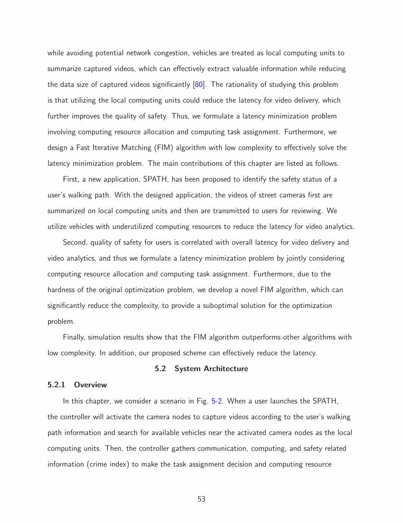
while avoiding potential network congestion, vehicles are treated as local computing units to

summarize captured videos, which can effectively extract valuable information while reducing

the data size of captured videos significantly [80]. The rationality of studying this problem

is that utilizing the local computing units could reduce the latency for video delivery, which

further improves the quality of safety. Thus, we formulate a latency minimization problem

involving computing resource allocation and computing task assignment. Furthermore, we

design a Fast Iterative Matching (FIM) algorithm with low complexity to effectively solve the

latency minimization problem. The main contributions of this chapter are listed as follows.

First, a new application, SPATH, has been proposed to identify the safety status of a

user’s walking path. With the designed application, the videos of street cameras first are

summarized on local computing units and then are transmitted to users for reviewing. We

utilize vehicles with underutilized computing resources to reduce the latency for video analytics.

Second, quality of safety for users is correlated with overall latency for video delivery and

video analytics, and thus we formulate a latency minimization problem by jointly considering

computing resource allocation and computing task assignment. Furthermore, due to the

hardness of the original optimization problem, we develop a novel FIM algorithm, which can

significantly reduce the complexity, to provide a suboptimal solution for the optimization

problem.

Finally, simulation results show that the FIM algorithm outperforms other algorithms with

low complexity. In addition, our proposed scheme can effectively reduce the latency.

5.2 System Architecture

5.2.1 Overview

In this chapter, we consider a scenario in Fig. 5-2. When a user launches the SPATH,

the controller will activate the camera nodes to capture videos according to the user’s walking

path information and search for available vehicles near the activated camera nodes as the local

computing units. Then, the controller gathers communication, computing, and safety related

information (crime index) to make the task assignment decision and computing resource

53

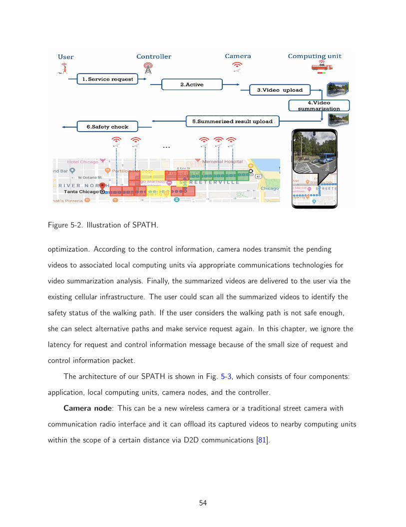
Figure 5-2. Illustration of SPATH.

optimization. According to the control information, camera nodes transmit the pending

videos to associated local computing units via appropriate communications technologies for

video summarization analysis. Finally, the summarized videos are delivered to the user via the

existing cellular infrastructure. The user could scan all the summarized videos to identify the

safety status of the walking path. If the user considers the walking path is not safe enough,

she can select alternative paths and make service request again. In this chapter, we ignore the

latency for request and control information message because of the small size of request and

control information packet.

The architecture of our SPATH is shown in Fig. 5-3, which consists of four components:

application, local computing units, camera nodes, and the controller.

Camera node: This can be a new wireless camera or a traditional street camera with

communication radio interface and it can offload its captured videos to nearby computing units

within the scope of a certain distance via D2D communications [81].

54

Local computing unit: This can be a moving or parking vehicle with sufficient

computing and storage capability and it can perform video summarization task. Each vehicle

can be matched with several camera nodes to summarize videos.

Controller: This is a static facility, which can be a base station or a roadside unit (RSU)

or an access point (AP). It collects communication and computing information from camera

nodes and vehicles. Based on the collected information and the crime index for each video

task, it makes the task assignment decision and optimizes the computing resource.

Application: Application is installed on the user’s mobile device. A user can use it

to navigate, scan the summarized videos of the walking path, and make service request for

alternative paths.

Controller

Camera

Computing capacity

Figure 5-3. Illustration of video summarizations and transmissions..

5.2.2 System Model

Denote the set of the camera nodes as C = c1, c2, · · · , ci, · · · , cn, the i-th camera

node by ci. Local computing units are indexed as V = v1, v2, · · · , vj, · · · , vm, the j-th

local computing unit by vj . In this chapter, we consider a widely used task model to describe

video summarization task Di, i.e., Di=(αi,βi,I(ci)), where αi stands for required CPU cycle

of the task Di, and βi denotes the data size of computing task Di to be delivered toward the

comping unit and I(ci) is the crime index of each task. Crime index indicates the significance

55

of each task since the larger crime index, the higher probability of observing a crime incident.

Then, we discuss communication, computing, and crime index model, which will be used in the

subsequent development.

Communication Model

In this chapter, we consider adopt orthogonal channels to support the data transmissions

between camera nodes and local computing units. We assume camera nodes communicate

with local computing units via D2D links and computing units transmit summarized videos

to the user via cellular links. The data rate for the camera nodes offloading tasks to the

associated computing units can be obtained as follows:

ri,j = Wi,j log2

(

1 +pihi,j

N0

)

, (5-1)

where Wi,j indicates the allocated bandwidth and hi,j denotes the channel gain between the

camera ci and the computing unit vj. Furthermore, pi is the transmission power of camera

node ci, and N0 is the noise power. We assume the mobility of local computing units is low

and the offloading time is relative short, thus hi,j is a constant.

The transmission latency for transmitting the task Di from camera node ci to computing

unit vj is therefore given by

tTi =βi

Wi,j log2

(

1 +pihi,j

N0

) . (5-2)

Similar to previous works such as [82], this chapter ignores the transmission latency of

delivering summarized video from computing units to the user end, since the data size of

summarized videos is much smaller than the original videos.

Computing Model

In this chapter, we consider the difference of computing resource among local computing

units and denote the computing resource of local computing units as F = f0, f1, · · · , fj, · · · , fm.

We assume several camera nodes can share the computing resource of a local computing unit

56

during the video summarization process. Thus, the computing time of task Di can be written

as

tCi =αi

κi,jfj, (5-3)

where κi,j is the proportion of computing resource that computing unit vj allocated to

complete task Di.

Crime Index Model

Crime index is a numerical value, which is used to label each road segment to indicate

the estimated safety status. In this chapter, crime index is measured based on the historical

criminal activity probability and the estimated criminal activity probability. Thus, crime index

is proportional to the probability that a crime incident on each road segment is observed. In

general, the road segment with higher crime index are more dangerous because of the higher

probability of observing a crime incident. For example, road segments in the urban area of

Chicago [6] has a higher crime index since these road segments not only have been observed

with a large number of criminal activities according to the historical data, but also have a

high probability of observing a crime incident in the future based on the criminal activity

probability estimation. In this chapter, we apply Gaussian kernel density estimation to model

the estimated criminal activity probability density. Given n points of crime locations are marked

as (qx,1, qy,1), (qx,2, qy,2), · · · , (qx,n, qy,n), the density of crime at a location (lx, ly) can be

quantified as follows [6]:

f(lx, ly) =1

nσ2

n∑

i=1

1

2πexp

(

−‖lx − qx,i‖2 + ‖ly − qy,i‖22σ2

)

, (5-4)

where σ is a parameter that controls the smoothness of the density estimation, which can

be determined by the Scott’s rule [83]. We denote the set of the road segments as S =

s1, s2, · · · , sk, · · · , sK, the k-th road segments by sk. Therefore, we can obtain the crime

57

index of road segment sk by

I(sk) = − log(

ǫ(1 − P hsk) + (1− ǫ) (1− Psk)

)

, (5-5)

where Psk =∫ eU

x,k

eLx,k

∫ eUy,k

eLy,k

f(lx, ly)dlxdly is the estimated criminal activity probability and

eLx,k,eUx,k,e

Ly,k, e

Uy,k are edge positions for road segments sk. P

hsk

denotes the historical criminal

activity probability. ǫ is the weighting factor. Therefore, for each camera node ci located in the

road segment sk, the crime index can be written as

I(ci) = I(sk), (5-6)

which means all camera nodes located in the same road segment sk has the same crime index.

The main notations adopted in this chapter are presented in Table 6-1

Table 5-1. Symbols and definitions

Symbol DefinitionC Set of camera nodesB Set of local computing unitsS Set of road segmentsDi Video summarization task for camera node cici i-th camera nodevj j-th computing unitsk k-th road segmentpi Transmission power for camera cihi,j Channel gainfj Computing resource of local computing unit vjN0 Noise powerαi Amount of the taskβi Data size of computing taskWi,j BandwithtTi Transmission latency for video summarization task Di

tCi Computing latency for video summarization task Di

f(lx, ly) Probability density of crimes at location (lx, ly)I(sk) Crime index of road segment skǫ Weighting factor

58

5.3 Problem Formulation

By leveraging communication, computing, and storage (CCS) capability, together with the

crime index model proposed in the previous section, we design our SPATH by formulating a

latency minimization problem considering computing task assignment and computing resource

optimization. We first discuss several constraints for the latency minimization problem.

Task Assignment

To be specific, we define the integral decision matrix x = (xi,j) with xi,j ∈ 0, 1, where

xi,j = 1 indicates camera node ci is associated with computing unit vj for video summarization

while xi,j = 0 otherwise. Since we assume the captured video cannot be split, the camera node

ci can only be matched with one computing unit. This matching constraint can be written as

follows:

∑

j∈V

xi,j ≤ 1. (5-7)

Maximum Computing Power Limitation

In this chapter, we consider the total amount of computing resource assigned to each task

placed on computing unit vj cannot exceed its limitation, that is,

∑

i∈C

xi,jκi,j ≤ 1. (5-8)

Maximum Communication Channel Limitation

We consider each computing unit has limited available frequency sub-channels to

communicate with camera nodes, we introduce the constraint as

∑

i∈C

xi,j ≤ Q. (5-9)

Safety Guarantee

We consider that if a camera node is associated with a computing unit for video

summarization, the status of this road segment is safest for a user since the user can obtain

59

the fresh safety information. Thus, we redefine the crime index of selected camera node is

I(ci) = 0. In order to guarantee the safety of a user, we introduce the crime index requirement

for a user’s walking path as

∑

i∈C

(1− xi,j)I(ci) ≤ Ith. (5-10)

Latency Minimization

Under the above setup, we pursue a latency minimization problem by jointly considering

computing resource allocation and computing task assignment, which is formulated as

OPT :minx,κ

∑

i∈C

xi,j(tTi + tCi ) (5-11)

s.t.

∑

i∈C

xi,jκi,j ≤ 1

∑

i∈C

xi,j ≤ Q

∑

i∈C

(1− xi,j)I(ci) ≤ Ith

∑

j∈V

xi,j ≤ 1

xi,j ∈ 0, 1

It is clear that the proposed latency minimization problem is a mixed integer non-linear

programming (MINLP) problem since it contains both binary variables x and continuous

variables κ. In the next section, we adopt matching theory with low complexity to find an

approximate solution to the proposed optimization problem because of the hardness of the

original optimization problem.

5.4 Algorithm

In this section, a FIM algorithm is proposed to solve the optimization problem, since the

MINLP optimization problem has a high complexity with the increasing number of camera

nodes and computing units. The objective function can be rewritten as follows:

60

g(κ,x) =∑

i∈C

xi,j(βi

ri,j+

αi

κi,jfj). (5-12)

We consider the original problem can be decoupled into two sub-problems, computing

resource optimization problem and task assignment problem. Given xi,j = xi, which means

xi,j is fixed, the original latency minimization problem in (6-8) is converted as a computing

resource optimization problem, which is a convex problem. Therefore, optimal solution, κ∗i,j , of

computing resource optimization can be obtained by adopting the Karush-Kuhn-Tucker (KKT)

conditions. With the optimal solution, κ∗i,j , obtained from the computing resource optimization

problem, the latency minimization problem is converted as task assignment problem, which is

an integer programming problem. Then, we adopt the matching theory to obtain the solution.

5.4.1 Computing Resource Optimization

We consider the OPT with the following OPT-RA when xi = xi, a fixed value.

OPT-RA :minκ

g(κ, x) =∑

i∈C

xi,j(βi

ri,j+

αi

κi,jfj) (5-13)

s.t.

∑

i∈C

xi,jκi,j ≤ 1

Therefore, the Hessian matrix of the OPT-RA can be derived as follows:

H =

∂2g

∂2κ1,j

∂2g

∂κ1,j∂κ2,j. . . ∂2g

∂κ1,j∂κn,j

∂2g

∂κ2,j∂κ1,j

∂2g

∂2κ2,j. . . ∂2g

∂κ2,j∂κn,j

......

. . ....

∂2g

∂κn,j∂κ1,j

∂2g

∂κn,j∂κ2,j. . . ∂2g

∂2κn,j

(5-14)

61

Further, we can obtain each specific element of the Hessian matrix is:

∂2g

∂κp,j∂κq,j

=

2αi

κ3

i,jfjif p = q

0 otherwise

(5-15)

It is observed that all parameters in (5-15) are positive since 2αi

κ3

i,jfj≥ 0. We conclude that

OPT-RA is convex because the Hessian matrix H is a positive definite matrix [84]. Since the

constraints are linear, optimal solution of OPT-RA can be obtained with the KKT conditions.

We introduce the Lagrange function of OPT-RA according to the previous analysis,

which can be written as follows:

L(κ,γ) =∑

i∈C

xi,j(βi

ri,j+

αi

κi,jfj) +

∑

j∈V

γj(∑

i∈Cj

κi,j − 1), (5-16)

where γ = (γ1, · · · , γm) are the Lagrange multipliers corresponding to the inequality

constraints. Since Slater’s condition holds for OPT-RA, then the KKT conditions provide

necessary and sufficient conditions for optimality [85]. If κ∗ and γ∗ is the optimal point with

zero duality gap, then the gradient for L(κ,γ) must vanish at point κ∗. Therefore, we can

obtain:

∇(∑

i∈C

xi,j(βi

ri,j+

αi

κ∗i,jfj

)) +∑

j∈V

γ∗j∇(

∑

i∈Cj

κ∗i,j − 1) = 0, (5-17)

γ∗j (∑

i∈C

xi,jκi,j − 1) = 0.

Moreover, we can derive the optimal value of κ∗i,j form (5-17), which can be written as follows:

κ∗i,j =

√αi

∑

i∈C

√

xi,jαi

. (5-18)

5.4.2 Task Assignment

After obtaining the optimal computing resource allocation, we develop an algorithm based

on the matching theory [86] to solve the task assignment problem.

62

To better describe a matching, the preference lists of agents should be defined. Each

agent holds a preference list to opposite group. All the actions, such as proposal, acceptance,

and rejection are according to the preference list. In this chapter, we establish each agent’s

preference list as follows.

Preferences of camera nodes

From the camera node’s perspective, each camera node seeks the minimum of its

transmission time to a local computing unit. Therefore, we propose a utility function for a

camera node to form its preference list among computing units as follows:

φCi,j =

βi

Wi,j log2

(

1 +pihi,j

N0

) . (5-19)

Thus, the preference list ≻Ci,j of camera node ci can be constructed by using (5-19).

Preferences of computing units

The preference list of local computing units can be established according to the time

cost of the video summarization for a matched camera node. The utility function for a local

computing unit can be calculated as follows:

φVi,j =

αi

κi,jfj. (5-20)

According to the above utility function, the preference list for computing unit vj among camera

nodes in the opposite group can be constructed as ≻Vj,i.

5.4.3 Fast Iterative Matching (FIM) algorithm

We now introduce our proposed FIM algorithm, which is illustrated Algorithm 0. The

FIM algorithm operates in an iterative way until achieving the stability. Initially, each camera

node forms its preference list ≻Ci,j . The whole FIM algorithm consists of two major phases: one

is for matching and the other is for optimizing. At the beginning of matching in each round,

each camera node ci proposes to its most preferred computing unit vj and removes vj from its

preference list ≻Ci,j. When receiving ci’s proposal, vj may face two conditions: either enough

available communication channels for the transmission of ci’s video have been found or there

63

are not enough available channels to support the ci’s video transmission. Computing nodes

vj first forms its preference list ≻Vi,j with the optimized computing resource, which can be

calculated by (5-18). If vj finds enough available communication channels to support the video

transmission, it accepts the most preferred proposal and the matched camera node is removed

from unmatched set Cun. If vj does not find enough communication channels to support its

video transmission, it discards the worst camera node and the discarded camera node is added

to the unmatched set Cun. At the end of each round, if the constraint (5-10) is not satisfied,

then camera nodes conduct next iteration. When there are no available communication

channels for all computing units in the new iteration, all computing units discard the camera

nodes with the smallest crime index. The matching and optimizing process iterates until safety

related constraint (5-10) is satisfied, or all cameras are matched.Algorithm 5.1. FIM Algorithm

1: procedure FIM(≻Ci,j)

2: Set Qj = Q for all vj ⊲ Matching Construction;3: Construct set Cun,set Cun=C;4: for each ci ∈ Cun do ⊲ Matching;5: Proposes to the first vj in its preference list and remove vj from ≻C

i,j ;6: end for7: for vj ∈ V do8: Forms its preference list ≻V

j,i with the κ∗i,j by (5-18).

9: if Qj > 0 then10: vj keeps the most preferred cpi among proposals;11: Removes c∗i from Cun12: Qj = Qj − 113: else14: vj rejects the worst cdi and keeps the rest;15: Add cdi to Cun16: end if17: end for18: if constraint (5-10) is not satisfied then ⊲ Constraint Check;19: if Qj > 0 for any vj then20: Go back to step 4;21: else22: for vj ∈ V do23: Discards cdi with the smallest safety index24: Go back to step 4;25: end for

64

26: end if27: end if28: end procedure

5.5 Performance Evaluation

In this section, we evaluate the performance of the proposed scheme in three aspects:

(i) The comparison among different task assignment schemes; (ii) The impact of available

computing power; (iii) The impact of key parameters, such as the data size of videos and

the bandwidth of communication channels. We introduce the simulation setup at first. Then

extensive simulations are provided and analyzed.

5.5.1 Simulation Setup

We consider that the camera nodes are placed in the grid topology and a group of

local computing units are randomly deployed. We assume the communication range of local

computing units is up to 100 m. The data size and computing amount of tasks follow uniform

distribution with a mean value of 5 MB and 1 Gigacycles, respectively [87]. The computing

resources of computing units are distributed within the range [10, 20] GHz. The channel fading

of the communication links is modeled by the complex normal distribution, CN (0, 1) [88].

The FIM, proposed in this chapter, is compared with two task assignment schemes:

Greedy assignment scheme: each camera node sends the proposal to match with the

most powerful computing unit in its communication range. If a computing unit has enough

communication channels to support all camera nodes, it will hold all video summarization

task. If the received proposals have reached the limitation, the computing unit will accept the

proposal according to the safety index. The computing resource allocation for each computing

unit is according to (5-18).

Random assignment scheme: camera nodes match with computing units randomly. If the

communication limitation is reached, computing units are matched with camera nodes with

respect to the safety index. The computing resource optimization is carried out according to

(5-18).

65

5.5.2 Results and Analysis

Comparison among different task assignment schemes

The performance comparison among our FIM, greedy scheme, and random scheme is

illustrated in Fig. 5-4. We let the number of camera nodes vary in [5, 25]. The density of

the computing nodes is set to be a constant value with respect to the number of camera

nodes. Results in Fig. 5-4 demonstrate that the proposed FIM achieves significantly better

performance over the other two schemes. This is because the available number of computing

units for each camera node is increasing with the network size increases. Therefore, FIM

algorithm could exploit more benefits from the diverse choices. However, greedy and random

schemes ignore the possible gain from the increasing number of computing units. Moreover,

resource optimization for FIM can enhance the gain from diverse choices, since the matching

choice is based on the result of resource optimization. Noticing that resource optimization

can also achieve performance gain for greedy and random schemes. However, the benefit of

resource optimization does not compensate for the loss of matching scheme.

Impact of available computing power

We further compare the performance of the FIM algorithm with two heuristic schemes

under different available computing power. We set the number of camera nodes to 15 and

the computing power in each local unit to be varying in [2, 10] Gigacycles. Figure 5-5 shows

that FIM scheme achieves significantly higher performance gain over the other two schemes,

particularly when the number of computing units is small. Noticing that FIM is introduced

to adjust the matching choice according to available computing power when computing

resource is insufficient, it is not surprising that a more significant performance gain can be

observed when the computing power is smaller. Moreover, the latency of all schemes is reduced

slowly when the number of computing units is large. The reason is that sufficient computing

resource makes all task assignment schemes achieve less benefit with respect to the variation of

computing resource.

66

Impact of data size

In Fig. 5-6, we investigate the latency of different task assignment schemes with respect

to the varying data size of captured videos. The parameter settings are the same as those in

Fig. 5-5 and the data size of the video varies within [1, 9] MB. The results shown in Fig. 5-6

demonstrate that three algorithms have the same relationship between latency and the data

size of videos. The result shows that the larger of the data size, the longer of the latency.

The result also demonstrates that the impact of the data size is evident, especially at large

data size. The reason is that when the data size is large, FIM algorithm not only reduces the

latency in terms of the choice of computing units but also achieves significant benefits from

the transmissions of videos.

Impact of bandwidth

We also consider the impact of the bandwidth of communication channels. In this

evaluation, The parameter settings are the same as those in Fig. 5-5 and the bandwidth of

communication channels is set to the range [0.5, 2.5] MHz. The results shown in Fig. 5-7

demonstrate that the performance gaps of three task assignment schemes are narrowing along

with the increasing of bandwidth. When the communication resource is sufficient, FIM can

only achieve benefits from computing resource and the loss of greedy and random schemes

is less for transmissions of videos. Fig. 5-7 also shows that the impact of bandwidth is more

significant when bandwidth is small. The proposed FIM can achieve 85.6% better performance

compared with random assignment scheme and 87.3% compared with greedy assignment

scheme when bandwidth is 1 MHz. The reason is that when bandwidth is small, FIM can

obtain more benefit from better communication channels.

67

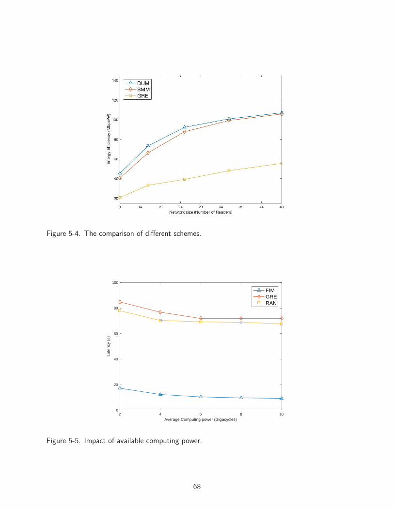
Figure 5-4. The comparison of different schemes.

2 4 6 8 10

Average Computing power (Gigacycles)

0

20

40

60

80

100

Late

ncy

(s)

FIMGRERAN

Figure 5-5. Impact of available computing power.

68

1 3 5 7 9

Average Data Size (MB)

0

20

40

60

80

100

120

140

Late

ncy

(s)

FIMGRERAN

Figure 5-6. Impact of data size

0.5 1 1.5 2 2.5

Bandwidth (MHz)

0

20

40

60

80

100

120

140

Late

ncy

(s)

FIMGRERAN

Figure 5-7. Impact of bandwidth.

69

CHAPTER 6VISS: VEHICLE BASED INTELLIGENT SURVEILLANCE SYSTEM

6.1 Background

As cities and towns expand, safety in public areas such as parks, shopping streets,

and downtowns becomes more and more important. How to monitor there public area and

guarantee the safety of citizens and visitors are vital for cities. Video surveillance system is a

great security tool to keep city safe and local business thriving. Thus, more and more local

governments in the world are beginning to install surveillance cameras in public areas to help

improve the safety of cities. According to the security industry, Beijing installed more than

400k surveillance cameras in the public area to keep this supercity safe. Chicago establishes a

Homeland Security Grid, which utilizes more than 17,000 cameras and 600 miles of fiber optics

to capture street view of the city and processes the video in real time to detect dangerous

activities [89] .

Even though video surveillance system can help make public area hospitable for citizen

and visitors, drawbacks limit the use of video surveillance system. Due to the high cost of

deployment of video surveillance system, blind areas exist in most video surveillance systems.

Second, outdoor cameras can be damaged by weather or car accidents, which means the

local governments cost enormous maintenance fee to keep systems work well. Can we use the

low-cost method help to improve the safety of blind areas of video surveillance system?

With the development of sensing and communication, more and more vehicles have

installed dash cameras with communication interface. Therefore, vehicle based video

monitoring system is a potential solution to cover blind areas of fixed video surveillance

system with low maintenance cost. Actually, Substantial numbers of applications using

vehicle based monitoring system are emerging. Chen et.al. [90] design a system to utilize the

three-axis accelerometer and the GPS sensor embedded on vehicles to monitor road condition

when vehicles are traveling around the city. Li et.al. [91] apply vehicle based sensing system to

solve the large scale traffic sensing problem. They aggregate instant speed and position data,

70

which is sensed by each vehicle periodically, to monitor traffic condition. ParkNet is a system

design by Mathur et al. to solve the urban street-parking problem [92]. They utilize vehicles,

equipped with GPS receivers and a passenger-side-facing ultrasonic rangefinders, to determine

parking spot occupancy. However, utilizing vehicles to do the safety monitoring is challenging

with respect to the following consideration. First, the data size of the monitoring video is very

large, if all the vehicles upload monitoring video may cause the network congestions. Another

problem caused by the long distance transmission of video files is the long delay, which may

make the monitoring system not improve the safety. Second, recruiting a large number of

vehicles may result in large amount of payment for participants. Third, given equal attention to

each monitored area is an ineffective way to improve the public safety.

Figure 6-1. System architecture.

In order to deal with the problems mentioned above, we design a Vehicle based Intelligent

Surveillance System (VISS) to improve public safety in smart cities. In our design, vehicles

equipped dash cameras with wireless communication interface are recruited as the mobile

monitoring nodes to help monitor the blind areas of the exiting surveillance system. In order

to improve quality of safety, VISS has two major tasks. The first one is expanding the spatial

monitoring area to find potential victims. Thanks to the development of techniques for vision

based human activity recognition, VISS can extract potential victims from the monitoring

video files. The second task is that VISS recruits mobile monitoring nodes to monitor potential

71

victims as long as possible. Due to the high mobility of vehicles, VISS has an opportunity to

achieve potential victims searching and monitoring with less budget. Actually, each recruited

moving vehicle can cover multiple geographical regions, some can be used for potential victims

searching and others can be used for potential victims monitoring. On the other hand, slowly

moving or parked vehicles with sufficient computing capability are utilized as local computing

units to handle the long delay problem of video transmission. Therefore, we formulate two

optimization problems, i.e., spatial coverage maximization problem and temporal coverage

problem, involving mobile monitoring nodes recruitment and computing resource allocation. To

solve these optimization problems, a heuristic algorithm with low complexity is proposed. The

main contributions of this chapter are listed as follows.

First, a new system, VISS, has been proposed to improve public safety in smart cities.

With the designed system, two types of vehicles are utilized. Vehicles equipped dash cameras

are recruited as the mobile monitoring nodes to expand geographical monitoring regions

and extend monitoring time of potential victims. Another typed vehicles are utilized as local

computing units to detect potential victims and reduce transmission delay of videos.

Second, we formulate two optimization problems by jointly considering recruitment

decision and resource allocation. The spatial coverage maximization problem is related to

geographical regions expanding for potential victims searching. Another temporal coverage

problem is used to extend monitoring time of potential victims. In order to handle the hardness

of two optimization problems, a heuristic algorithm with low complexity is proposed to provide

a suboptimal solution.

Third, in the performance evaluation part, results demonstrate that the proposed

algorithm performs better compared to other algorithms.Furthermore, the proposed scenario

can significantly improve the spatial and temporal coverage with low budget.

6.2 System Architecture

The proposed VISS mainly include four components. We first present an overview of

VISS. Thereafter, corresponding models are explained in detail.

72

6.2.1 Architecture Overview

The overall architecture of the proposed VISS includes four parts: local computing units,

mobile monitoring nodes, controller, and data center.

Local Computing Unit

In this scenario, two types of vehicles are utilized. Slowly moving or parked vehicles with

sufficient computing capability are recruited as local computing units, which can perform video

analysis tasks to find the potential victims. Each local computing unit can be connected with

several mobile monitoring nodes to analyze videos.

Mobile Monitoring Nodes

Vehicles installed dash cameras with communication radio interface are the second typeof

vehicles, which can be the mobile monitoring nodes. If the regions of interest on their driving

path or drivers are interested to get credits to help monitor several regions of interest, vehicles

can apply to be the candidates of mobile monitoring nodes. Mobile monitoring nodes connect

with local computing units within a certain distance to offload captured videos via D2D

communications [81].

Controller

A base station or a roadside unit (RSU) belongs to the service provider can be the

controller. It collects applications of vehicles to be the mobile monitoring nodes, and monitors

the status of communication and computing resource. Based on the collected information,

controller makes recruitment decision and optimizes communication the computing resource

allocation.

Data Center

Data center is used to collect the analysis result from the local computing units and store

the result. It also can cooperate with local computing units to do the video analysis when the

workload of local computing units is too heavy.

Then, we present the working process of VISS. When public safety authority sends the

service request to the VISS, it works in the following steps.

73

Step1) public safety authority submits its request to the VISS.

Step2) Controller collects and information, such as blind areas of the fixed surveillance

system, crime data, and people distribution, to find the regions of interest. Then, the controller

spreads out the information of regions.

Step3) Vehicles interested to participate to help monitor will be registered as the

candidates of mobile monitoring nodes that submit corresponding information such as location

and credits for tasks.

Step4) Controller bases on the information of candidates, status of communication, and

computing resource to make recruitment decision and optimizes computing resource allocation

for each mobile monitoring node. Then, controller updates its database and sends the control

information to mobile monitoring nodes and local computing units.

Step5) Mobile monitoring nodes according to the control information to capture videos

and send videos to the assigned local computing units.

Step6) Local computing units first bases on the optimization information from controller

to allocate the computing resource for video tasks and do the video analysis. Second, local

computing units send analysis result back to the controller.

Step7) Controller according to the quality of analysis result pays credits for mobile

monitoring nodes, updates their trustworthiness score, and uploads the result to the data

center

Step8) The VISS sends the corresponding result to the public safety authority.

6.2.2 System Model

In the following section, the precise definition and models of VISS, which are used in the

subsequent development, are presented.

In this chapter, we assume that the VISS does the monitoring for a period of time T =

t1, · · · , to, and the set of candidates to be recruited as mobile monitoring nodes are denoted

asM = m1, m2, · · · , mi, · · · , mp, the i-th candidates of mobile monitoring node by mi.

Denotes the set of geographical regions of interests as R = r1, r2, · · · , rj, · · · , rq, the j-th

74

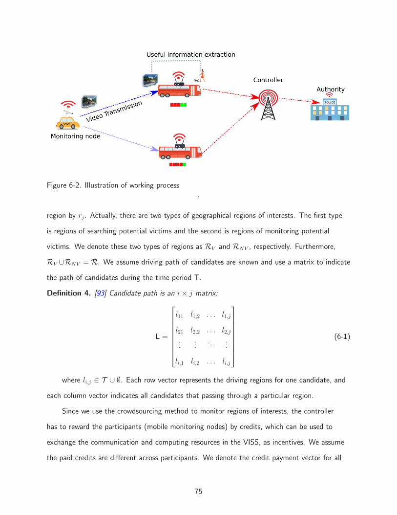
Controller

Monitoring node

Figure 6-2. Illustration of working process.

region by rj . Actually, there are two types of geographical regions of interests. The first type

is regions of searching potential victims and the second is regions of monitoring potential

victims. We denote these two types of regions as RV and RNV , respectively. Furthermore,

RV ∪RNV = R. We assume driving path of candidates are known and use a matrix to indicate

the path of candidates during the time period T.

Definition 4. [93] Candidate path is an i× j matrix:

L =

l11 l1,2 . . . l1,j

l21 l2,2 . . . l2,j...

.... . .

...

li,1 li,2 . . . li,j

(6-1)

where li,j ∈ T ∪ ∅. Each row vector represents the driving regions for one candidate, and

each column vector indicates all candidates that passing through a particular region.

Since we use the crowdsourcing method to monitor regions of interests, the controller

has to reward the participants (mobile monitoring nodes) by credits, which can be used to

exchange the communication and computing resources in the VISS, as incentives. We assume

the paid credits are different across participants. We denote the credit payment vector for all

75

participants as B= b1,1, b1,2, · · · , bi,j. Due to the limited budget, the overall credits paid to

participants must be limited.

Furthermore, the captured video by mobile monitoring nodes are sent to the local

computing units to analyze. Local computing units are labeled as C = c1, c2, · · · , ck, · · · , cs,

the k-th local computing unit by ck. This chapter adopts a commonly used computing task to

model captured video Vi,j, i.e., Vi,j=(αi,j,βi,j), where αi,j represents for required CPU cycle of

the video task Vi,j, and βi,j denotes the data size of Vi,j.

Definition of Spatial and Temporal Coverage

In this chapter, spatial and temporal coverage are two metrics related to quality of safety.

As we mentioned above, we are more interested in investigating how to find potential victims

fast and how to guarantee the safety of potential victims as much as possible. Spatial coverage

metric is related to the problem of finding the potential victims and temporal coverage metric

is related to the problem of monitoring potential victims. We also consider it adequate to cover

a geographic region with a single vehicle at a particular point of time.

Definition 5. [93] Spatial Coverage (SC) is the total percentage of geographical regions of

interests covered during the time period T. Formally, it can be defined as:

SC(xi,j) =

∑

j∈R∨i∈Mxi,j

|R| . (6-2)

where x = (xi,j) is an integral decision matrix with xi,j ∈ 0, 1. We assume xi,j = 1

indicates candidate node mi is recruited to monitor region rj during the time li,j while xi,j = 0

otherwise.

Definition 6. [93] Temporal coverage (TC) is the percentage of minimum covered time length

during the time period T for all geographical regions of interests covered. It can be formally

defined as:

TC(xi,j) =minj∈RV

|∪i∈Mxi,jli,j||T | . (6-3)

76

Communication and Computing Model

We assume the communication and computing process since time cost for transmission

and analysis is large. Captured video must be processed completely within limited time to

guarantee the safety of potential victims. In the transmission process, orthogonal channels

are adopted to transmit the captured video from mobile monitoring nodes to local computing

units. We consider mobile monitoring nodes communicate with local computing units though

D2D links. Local computing units send analysis result back to the controller via cellular links.

Thus, data rate between mobile monitoring node mi and connected local computing units ci

can be modeled as follows:

ri,j,k = Wi,j,k log2

(

1 +pihi,j,k

N0

)

, (6-4)

where Wi,j,k indicates the bandwidth and hi,j,k is the channel gain. Furthermore, pi is the

transmission power and N0 is the noise power. In this chapter, we utilize slowly moving or

parked vehicles as local computing units and the data transmission time is relatively short, thus

hi,j,k is a constant.

The time cost for the transmission of video task Vi,j from mobile monitoring node mi to

computing unit cj is therefore given by

DTi,j =

βi,j

Wi,j,k log2

(

1 +pihi,j,k

N0

) . (6-5)

In line with previous works as [82], the data size of analysis result significantly decreases

compared to the original data, we therefore ignore the transmission time cost of delivering

analysis result from local computing units via the controller to the data center.

This chapter takes into account the difference of computing capability among local

computing units. Accordingly, the computing capability of local computing units is denoted

as F = f1, f2, · · · , fk, · · · , fp. The computing capability on a local computing unit can be

shared by several mobile monitoring nodes. Consequently, the computing time cost of task Vi,j

can be written as

77

DCi,j =

αi,j

κi,j,kfk, (6-6)

where κi,j,k is the proportion of computing resource that computing unit ck is allocated to

complete task Vi,j.

Table 6-1. Symbols and description

Symbol DefinitionC Set of local computing unitsM Set of mobile monitoring nodesR Set of interested regionsVi,j Video captured by camera node ci at region rjmi i-th mobile monitoring noderj j-th interested regionck k-th rlocal computing unitpi Transmission power for camera cihi,j,k Channel gainfk Computing resource of local computing unit ckN0 Noise powerαi,j Amount of the taskβi,j Data size of computing taskWi,j,k Bandwith

6.3 Problem Formulation

As we mention above, the regions of interest consists of two types. The first one is the

regions with potential victims. The temporal coverage of regions with potential victims should

be maximized in order to guarantee the safety of the potential victims. The second type

is regions without potential victims. Maximizing the spatial coverage is the goal of regions

without potential victims since more potential victims can be found with the increased spatial

coverage of the whole area. Thus, with the system model, it is reasonable to formulate the

Spatial and Temporal Coverage problems as two optimization problems by jointly considering

computing resource allocation and mobile monitoring nodes selection, which is formulated as

78

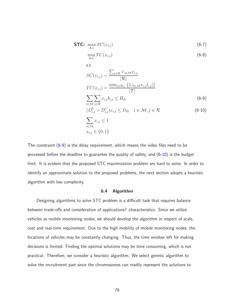
STC: maxx,κ

SC(xi,j) (6-7)

minx,κ

TC(xi,j) (6-8)

s.t.

SC(xi,j) =

∑

j∈R ∨i∈Mxi,j

|R|

TC(xi,j) =minj∈RV

|∪i∈Mxi,jli,j||T |

∑

i∈M

∑

j∈R

xi,jbi,j ≤ Bth (6-9)

(DTi,j +DC

i,j)xi,j ≤ Dth i ∈M, j ∈ R (6-10)

∑

i∈M

xi,j ≤ 1

xi,j ∈ 0, 1

The constraint (6-9) is the delay requirement, which means the video files need to be

processed before the deadline to guarantee the quality of safety, and (6-10) is the budget

limit. It is evident that the proposed STC maximization problem are hard to solve. In order to

identify an approximate solution to the proposed problems, the next section adopts a heuristic

algorithm with low complexity.

6.4 Algorithm

Designing algorithms to solve STC problem is a difficult task that requires balance

between trade-offs and consideration of applications? characteristics. Since we utilize

vehicles as mobile monitoring nodes, we should develop the algorithm in respect of scale,

cost and real-time requirement. Due to the high mobility of mobile monitoring nodes, the

locations of vehicles may be constantly changing. Thus, the time window left for making

decisions is limited. Finding the optimal solutions may be time consuming, which is not

practical. Therefore, we consider a heuristic algorithm. We select genetic algorithm to

solve the recruitment part since the chromosomes can readily represent the solutions to

79

mobile monitoring selection. We apply greedy algorithm to deal with the computing resource

optimization part, which has a low complexity.

VISS Algorithm

The following procedure are performed to generate and hold a population to solve our

proposed STC problem.

Step 0 (Initialization): We randomly generate a number of chromosomes as the solutions

in the beginning.

Step 1 (Fitness assignment): At each generation, we assign a fitness value to each

solution by taking the following steps: We first generate random numbers usc and utc in [0,1].

Then, we calculate the random weight of two objectives as wsc = uscusc+utc

and wtc = utcusc+utc

respectively. Then, we calculate the fitness value of each chromosome with the weights defined

above.

Step 2 (Selection): We sort all the chromosomes according to the fitness values.By

defining the sp% as the survival probability for each generation, we allow top sp% of the

population to survive. The chromosomes service in top position of sorted population are kept

as the candidates for the best solution.

Step 3 (Crossover ): A crossover operation is applied to to generate an offspring with the

crossover probability Pc for each chromosome.

Step 4 (Mutation): We also apply a mutation operation with a mutation probability Pm.

Step 5 (Repair): We remove the infeasible solutions since they may be generated by

crossover and mutation once the constraints are violated. In VISS algorithm, we remove the

mobile monitoring nodes with the highest cost until the constraint (6-9) is reached and then

we also remove the mobile monitoring nodes without satisfying constraint (6-10).

Step 6 (Termination test): The algorithm terminates once one of the following conditions

is fulfilled: 1) Maximum number of iterations is reached. 2) The gap between solution of

previous round and current round is small enough.

The complete algorithm is shown as Algorithm 6.1.

80

Algorithm 6.1. VISS Algorithm

1: procedure VISS(MaxIte,sp,cp,size)2: POP ← INITIALIZATION3: n ← 04: solution ← ∅5: while solution[n]-solution[n-1]≥ GAP do6: while n≤ MaxIte do7: for s∈ POP do8: Calculate fitness value of s9: end for10: ORDERPOP← SORT(s) according to fitness value11: POP← Top sp% of ORDERPOP12: solution ← ORDERPOP[0]13: while |POP | ≤ size do14: for s∈ POP do15: if RANDOM(0, 1) ≤ Pc then16: s ← CROSSOVER17: end if18: if RANDOM(0, 1) ≤ Pm then19: s ← MUTATION20: end if21: end for22: end while23: Repair s according to constraint (6-9) and constraint (6-10)24: end while25: end whilereturn solution26: end procedure

6.5 Performance Evaluation

In this section, we evaluate the performance of the proposed schemes. For comparison, we

adopt two baseline algorithms, namely random solution and greedy algorithm. Specifically, the

random solution is obtained by recruiting the mobile monitoring nodes randomly. The greedy

algorithm always recruits vehicles with the shortest transmission delays. For both random

solution and greedy algorithm, they apply the same repair scheme with VISS algorithm to

satisfy constraint (6-9). In the simulation, the location of local computing units, the regions

of interest, and trajectories of mobile monitoring nodes are randomly generated. We divide the

target area into square blocks with edge length of 20 m. Without specific demonstration, the

81

recruitment cost is randomly selected. We also assume the maximum communication distance

is 100 m.

Performance comparison with respect to the network size

Fig. 6-3 depicts the evaluation results. We can observe from both figures that our

algorithm outperforms random solution and greedy algorithm. Furthermore, we find that,

with the increasing of network size, the TC and SC is small. That is because the increasing

ratio of interested regions is slower than the increasing ratio of participants. Lower candidates

density essentially reduces the cover opportunity for all regions of interests, thus more and

more regions are losing opportunities to be monitored. Furthermore, we can find that, when

the network size is small, the performance of three schemes are very similar. This is because,

with high density of participants and low number of interested regions, all three schemes have

a high probability to cover the interested regions in spatial dimension with the limited budget.

The impact of number of interested regions

Fig. 6-4 compares TC and SC with respect to the number of interested regions. As

expected, the performance of VISS algorithm is the best among three schemes. We can

find that, in SC, the performance of all three schemes reduces slowly at first. However, the

performance of all three schemes reduces fast in TC. The reason is the increasing ratio of

interested time slots is much faster than the increasing ratio of interested geography regions.

That is to say, for the same number of interested regions, the density of participants is enough

to cover most spatial regions, but the density of participants is not enough to cover most

temporal time slots.

The impact of number of participants

We observe in Fig. 6-5 VISS algorithm performs significantly better than random solution

and greedy algorithm. As a result, the TC and SC first falsely rises under three algorithms.

However, once achieving some points, the SC nearly remains stable as network number of

participants grows. This is because there are sufficient number of the candidates of mobile

82

monitoring nodes to monitor most regions with the limited budget. Basically, when the

performance of all the schemes remains stable, the limited budget becomes the major factor.

1000 2000 3000 4000 5000

Network Size (square meters )

0.7

0.75

0.8

0.85

0.9

0.95

1

1.05

1.1

Spa

tial C

over

age

VISSGRERAN

A Spatial Coverage

1000 2000 3000 4000 5000

Network Size (square meters )

0

0.05

0.1

0.15

0.2

0.25

0.3

0.35

0.4

0.45

0.5

Tem

pora

l Cov

erag

e

VISSGRERAN

B Temporal Coverage

Figure 6-3. Evaluation results for network size.

83

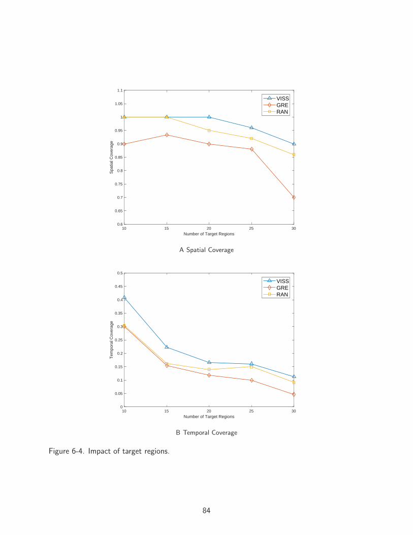
10 15 20 25 30

Number of Target Regions

0.6

0.65

0.7

0.75

0.8

0.85

0.9

0.95

1

1.05

1.1

Spa

tial C

over

age

VISSGRERAN

A Spatial Coverage

10 15 20 25 30

Number of Target Regions

0

0.05

0.1

0.15

0.2

0.25

0.3

0.35

0.4

0.45

0.5

Tem

pora

l Cov

erag

e

VISSGRERAN

B Temporal Coverage

Figure 6-4. Impact of target regions.

84

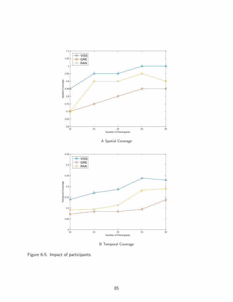
10 15 20 25 30

Number of Participants

0.6

0.65

0.7

0.75

0.8

0.85

0.9

0.95

1

1.05

1.1

Spa

tial C

over

age

VISSGRERAN

A Spatial Coverage

10 15 20 25 30

Number of Participants

0

0.05

0.1

0.15

0.2

0.25

0.3

0.35

Tem

pora

l Cov

erag

e

VISSGRERAN

B Temporal Coverage

Figure 6-5. Impact of participants.

85

CHAPTER 7SUMMARY AND CONCLUSIONS

In this dissertation, we focus on designing and implementing architectures for safety

centric IoT platform to support public safety related services in the smart cities. We start

from the overall design of the IoT platform. We first utilize the proposed architecture to solve

the children safety problem in public areas. We have proposed a novel UHF RFID system for

tracking children in the public area. In our RFID networks, readers are associated with mobile

devices for target localization. With the help of remote central center, the reader is matched

with an mobile device to transmit raw data for processing. Then, the associated mobile devices

deliver the processed data to the users. Then, safe walking navigation problem is solved under

the safety centric IoT platform. We have proposed a safety application, SPATH, to handle

safety issues in smart cities. We have utilized existing cellular infrastructures to transmit

surveillance videos from street cameras to the users to identify the safety status. To handle the

large volume of videos, we have leveraged the vehicles with underutilized computing resources

as the local computing units to summarize videos. In addition, vehicle based intelligent

surveillance system (VISS) is proposed to improve public safety in smart cities. Vehicle based

monitoring system utilizes vehicles installed dash cameras to monitor target regions. VISS

recruits vehicles as the mobile monitoring nodes to expand geographical monitoring regions.

Cooperating with slowly moving or parked vehicles with sufficient computing capability, VISS

can extract potential victims from the monitoring video files and recruit mobile monitoring

nodes to monitor potential victims as long as possible.

86

REFERENCES

[1] M. Press. Leading the Smart City Revolution with Safety First. [May 8, 2018]. [Online].Available: https://www.ul.com/newsroom/featured/leading-the-smart-city-revolution-with-safety-first/

[2] N. James, “Recent violent crime trends in the united states,” 2018.

[3] Office for Victims of Crime . 2018 National Crime Victims? Rights Week Resource Guide:Crime and Victimization Fact Sheets. [April 8, 2018]. [Online]. Available: https://ovc.ncjrs.gov/ncvrw2018/info flyers/fact sheets/2018NCVRW UrbanRural 508 QC.pdf

[4] D. J. Paulsen, “To map or not to map: Assessing the impact of crime maps on policeofficer perceptions of crime,” International Journal of Police Science & Management,vol. 6, no. 4, pp. 234–246, 2004.

[5] A. Bogomolov, B. Lepri, J. Staiano, N. Oliver, F. Pianesi, and A. Pentland, “Once upona crime: towards crime prediction from demographics and mobile data,” in Proceedings ofthe 16th international conference on multimodal interaction, 2014, pp. 427–434.

[6] E. Galbrun, K. Pelechrinis, and E. Terzi, “Urban navigation beyond shortest route: Thecase of safe paths,” Information Systems, vol. 57, pp. 160–171, 2016.

[7] N. Goel, R. Sharma, N. Nikhil, S. Mahanoor, and M. Saini, “A crowd-sourced adaptive safenavigation for smart cities,” in Multimedia (ISM), 2017 IEEE International Symposium on,2017, pp. 382–387.

[8] F. Mata, M. Torres-Ruiz, G. Guzman, R. Quintero, R. Zagal-Flores, M. Moreno-Ibarra, andE. Loza, “A mobile information system based on crowd-sensed and official crime data forfinding safe routes: A case study of mexico city,” Mobile Information Systems, vol. 2016,2016.

[9] M. Garvey, N. Das, J. Su, M. Natraj, and B. Verma, “Passage: A travel safety assistantwith safe path recommendations for pedestrians,” in Companion Publication of the 21stInternational Conference on Intelligent User Interfaces, 2016, pp. 84–87.

[10] K. Holbø, S. Bøthun, and Y. Dahl, “Safe walking technology for people with dementia: whatdo they want?” in Proceedings of the 15th International ACM SIGACCESS Conference onComputers and Accessibility, 2013, p. 21.

[11] D. C. Schwebel, D. Stavrinos, K. W. Byington, T. Davis, E. E. O Neal, and D. De Jong,“Distraction and pedestrian safety: how talking on the phone, texting, and listening tomusic impact crossing the street,” Accident Analysis & Prevention, vol. 45, pp. 266–271,2012.

[12] T. Wang, G. Cardone, A. Corradi, L. Torresani, and A. T. Campbell, “Walksafe: apedestrian safety app for mobile phone users who walk and talk while crossing roads,” inProceedings of the twelfth workshop on mobile computing systems & applications, 2012,p. 5.

87

[13] S. Jain, C. Borgiattino, Y. Ren, M. Gruteser, Y. Chen, and C. F. Chiasserini, “Lookup:Enabling pedestrian safety services via shoe sensing,” in Proceedings of the 13thAnnual International Conference on Mobile Systems, Applications, and Services, 2015, pp.257–271.

[14] J. Mwakalonge, S. Siuhi, and J. White, “Distracted walking: Examining the extent topedestrian safety problems,” Journal of traffic and transportation engineering (Englishedition), vol. 2, no. 5, pp. 327–337, 2015.

[15] H. Qin, Z. Li, Y. Wang, X. Lu, W. Zhang, and G. Wang, “An integrated network ofroadside sensors and vehicles for driving safety: Concept, design and experiments,” inPervasive Computing and Communications (PerCom), 2010 IEEE International Conferenceon, 2010, pp. 79–87.

[16] H. S. Park, M. W. Park, K. H. Won, K.-H. Kim, and S. K. Jung, “In-vehicle ar-hud systemto provide driving-safety information,” ETRI journal, vol. 35, no. 6, pp. 1038–1047, 2013.

[17] B. Aytekin and E. Altug, “Increasing driving safety with a multiple vehicle detectionand tracking system using ongoing vehicle shadow information,” in Systems Man andCybernetics (SMC), 2010 IEEE International Conference on, 2010, pp. 3650–3656.

[18] J. Wang, S. Zhu, and Y. Gong, “Driving safety monitoring using semisupervised learning ontime series data,” IEEE Transactions on Intelligent Transportation Systems, vol. 11, no. 3,pp. 728–737, 2010.

[19] Rebecca Edwards . The Best Kids GPS Trackers and Wearables. [June 7, 2019]. [Online].Available: https://www.safewise.com/resources/wearable-gps-tracking-devices-for-kids-guide/

[20] Deyan G. 60+ Smartphone Statistics in 2019. [March 28, 2019]. [Online]. Available:https://techjury.net/stats-about/smartphone-usage/

[21] Bankmycell.com. Six smartphone addiction facts and phone usage statistics. [March 28,2019]. [Online]. Available: https://www.bankmycell.com/blog/smartphone-addiction/#chapter2

[22] A. Gupta and V. Harit, “Child safety tracking management system by using gps,geo-fencing android application: An analysis,” in 2016 Second International Conference onComputational Intelligence Communication Technology (CICT), Feb 2016, pp. 683–686.

[23] R. Velayutham, M. Sabari, and M. S. Rajeswari, “An innovative approach for women andchildren’s security based location tracking system,” in 2016 International Conference onCircuit, Power and Computing Technologies (ICCPCT), March 2016, pp. 1–5.

[24] A. R. Al-Ali, F. A. Aloul, N. R. Aji, A. A. Al-Zarouni, and N. H. Fakhro, “Mobile rfidtracking system,” pp. 1–4, April 2008.

88

[25] Y. Mori, H. Kojima, E. Kohno, S. Inoue, T. Ohta, Y. Kakuda, and A. Ito, “Aself-configurable new generation children tracking system based on mobile ad hoc networksconsisting of android mobile terminals,” pp. 339–342, March 2011.

[26] J. Saranya and J. Selvakumar, “Implementation of children tracking system on androidmobile terminals,” pp. 961–965, April 2013.

[27] K. Liu and X. Li, “Finding nemo: Finding your lost child in crowds via mobile crowd sensing,”2014 IEEE 11th International Conference on Mobile Ad Hoc and Sensor Systems, pp. 1–9,October 2014.

[28] K. Morii, K. Taketa, Y. Mori, H. Kojima, E. Kohno, S. Inoue, T. Ohta, and Y. Kakuda,“A new generation children tracking system using bluetooth manet composed of androidmobile terminals,” in 2012 9th International Conference on Ubiquitous Intelligence andComputing and 9th International Conference on Autonomic and Trusted Computing, Sept2012, pp. 405–407.

[29] A. Yudhahutama and A. I. Wuryandari, “Network and application design for childrentracking and identification system with html5 and asynchronous communication (futurekindergarten project),” pp. 1–6, Nov 2013.

[30] A. Gupta and V. Harit, “Child safety tracking management system by using gps, geo-fencingandroid application: An analysis,” pp. 683–686, Feb 2016.

[31] X. Lin, R. Lu, D. Kwan, and X. S. Shen, “React: An rfid-based privacy-preserving childrentracking scheme for large amusement parks,” Computer Networks, vol. 54, no. 15, pp.2744 – 2755, 2010.

[32] C. Chen, “Design of a child localization system on rfid and wireless sensor networks,”Journal of Sensors, vol. 2010, 2010.

[33] H. Zhang, Q. Zhang, and X. Du, “Toward vehicle-assisted cloud computing forsmartphones,” IEEE Transactions on Vehicular Technology, vol. 64, no. 12, pp. 5610–5618,2015.

[34] H. Ding, C. Zhang, Y. Cai, and Y. Fang, “Smart cities on wheels: a newly emergingvehicular cognitive capability harvesting network for data transportation,” IEEE WirelessCommunications, vol. 25, no. 2, pp. 160–169, 2018.

[35] H. Ding, C. Zhang, B. Lorenzo, and Y. Fang, “Access point recruitment in a vehicularcognitive capability harvesting network: How much data can be uploaded?” IEEETransactions on Vehicular Technology, vol. 67, no. 7, pp. 6438–6445, 2018.

[36] A. Juels et al., “Rfid security and privacy: A research survey,” IEEE journal on selectedareas in communications, vol. 24, no. 2, pp. 381–394, 2006.

[37] M. Langheinrich, “A survey of rfid privacy approaches,” Personal and UbiquitousComputing, vol. 13, no. 6, pp. 413–421, 2009.

89

[38] M. A. Khan, M. Sharma, and B. R. Prabhu, “A survey of rfid tags,” International Journalof Recent Trends in Engineering, vol. 1, no. 4, p. 68, 2009.

[39] M. S. Trotter and G. D. Durgin, “Survey of range improvement of commercial rfid tagswith power optimized waveforms,” in 2010 IEEE International Conference on RFID (IEEERFID 2010), 2010, pp. 195–202.

[40] V. Chawla and D. S. Ha, “An overview of passive rfid,” IEEE Communications Magazine,vol. 45, no. 9, pp. 11–17, 2007.

[41] S. Li, L. Da Xu, and S. Zhao, “The internet of things: a survey,” Information SystemsFrontiers, vol. 17, no. 2, pp. 243–259, 2015.

[42] D. Potapov, M. Douze, Z. Harchaoui, and C. Schmid, “Category-specific videosummarization,” in European conference on computer vision, 2014, pp. 540–555.

[43] Z. Lu and K. Grauman, “Story-driven summarization for egocentric video,” in Proceedings ofthe IEEE Conference on Computer Vision and Pattern Recognition, 2013, pp. 2714–2721.

[44] S. P. Rajendra and N. Keshaveni, “A survey of automatic video summarization techniques,”International Journal of Electronics, Electrical and Computational System, vol. 2, no. 1,2014.

[45] A. G. Money and H. Agius, “Video summarisation: A conceptual framework and survey ofthe state of the art,” Journal of Visual Communication and Image Representation, vol. 19,no. 2, pp. 121–143, 2008.

[46] D. Gale and L. S. Shapley, “College admissions and the stability of marriage,” TheAmerican Mathematical Monthly, vol. 69, no. 1, pp. 9–15, 1962.

[47] K. Li, Q. Zhang, S. Kwong, M. Li, and R. Wang, “Stable matching-based selectionin evolutionary multiobjective optimization,” IEEE Transactions on EvolutionaryComputation, vol. 18, no. 6, pp. 909–923, 2013.

[48] A. E. Roth and M. Sotomayor, “Two-sided matching,” Handbook of game theory witheconomic applications, vol. 1, pp. 485–541, 1992.

[49] T. Sonmez, “Strategy-proofness in many-to-one matching problems,” Economic Design,vol. 1, no. 1, pp. 365–380, 1994.

[50] D. Whitley, “A genetic algorithm tutorial,” Statistics and computing, vol. 4, no. 2, pp.65–85, 1994.

[51] M. Srinivas and L. M. Patnaik, “Genetic algorithms: A survey,” computer, vol. 27, no. 6,pp. 17–26, 1994.

[52] J. Genlin, “Survey on genetic algorithm [j],” Computer Applications and Software, vol. 2,pp. 69–73, 2004.

90

[53] A. N. Staff. Missing Children in America: Unsolved Cases. [May 8, 2013]. [Online].Available: https://abcnews.go.com/US/missing-children-america-unsolved-cases/story?id=19126967

[54] Top 11 GPS tracker for modern family of 2016-kids smart watches. [June 03, 2016].[Online]. Available: https://www.thepawtracker.com/blogs/the-pet-tracker-blog-by-the-paw-tracker/128819843-11-kids-gps-tracker-for-the-modern-families-of-2016

[55] C. Gartenberg. Chipolo claims its new Bluetooth trackers are the smallest and thinnestin the world. [January 5, 2017]. [Online]. Available: https://www.theverge.com/circuitbreaker/2017/1/5/14180294/chipolo-bluetooth-trackers-sticker-clip-ces-2017

[56] L. Chan. Chipolo-Bluetooth Item Finder for iPhone and Android. [February 5, 2014].[Online]. Available: https://lesterchan.net/blog/2014/02/05/chipolo-bluetooth-item-finder-for-iphone-and-android/

[57] J. Chen, M. Chen, C. Chen, and Y. Chang, “Architecture design and performanceevaluation of rfid object tracking systems,” Computer Communications, vol. 30, no. 9, p.20702086, 2007.

[58] M. Bonuccelli, F. Lonetti, and F. Martelli, “Instant collision resolution for tag identificationin rfid networks,” Ad Hoc Networks, vol. 5, no. 8, p. 12201232, 2007.

[59] X. Hu, K. K. Wong, and K. Yang, “Wireless powered cooperation-assisted mobile edgecomputing,” IEEE Transactions on Wireless Communications, vol. PP, no. 99, pp. 1–1,2018.

[60] H. Gao, M. Wang, and T. Lv, “Energy efficiency and spectrum efficiency tradeoff in thed2d-enabled hetnet,” IEEE Transactions on Vehicular Technology, vol. 66, no. 11, pp.10 583–10 587, 2017.

[61] J. Liu, H. Ding, Y. Cai, H. Yue, Y. Fang, and S. Chen, “An energy-efficient strategy forsecondary users in cooperative cognitive radio networks for green communications,” IEEEJournal on Selected Areas in Communications, vol. 34, no. 12, pp. 3195–3207, 2016.

[62] R. W. Freund and F. Jarre, “Solving the sum-of-ratios problem by an interior-pointmethod,” Journal of Global Optimization, vol. 19, no. 1, pp. 83–102, 2001.

[63] W. Dinkelbach, “On nonlinear fractional programming,” Management Science, vol. 13,no. 7, pp. 492–498, 1967.

[64] J. Gao, L. Zhao, and X. Shen, “Network utility maximization based on incentive mechanismfor truthful reporting of local information,” IEEE Transactions on Vehicular Technology,pp. 1–1, 2018.

[65] P. He, L. Zhao, S. Zhou, and Z. Niu, “Water-filling: A geometric approach and itsapplication to solve generalized radio resource allocation problems,” IEEE Transactions onWireless Communications, vol. 12, no. 7, pp. 3637–3647, 2013.

91

[66] Y. Luo, P. Hong, R. Su, and K. Xue, “Resource allocation for energy harvesting-poweredd2d communication underlaying cellular networks,” IEEE Transactions on VehicularTechnology, vol. 66, no. 11, pp. 10 486–10 498, 2017.

[67] F. N. P. Office. 2017 crimes in the United States. [September 24, 2018]. [Online].Available: https://ucr.fbi.gov/crime-in-the-u.s/2017/crime-in-the-u.s.-2017/topic-pages/violent-crime

[68] Smartertravel.com. Best Apps to Prevent Travel Disasters. [December 06, 2017]. [Online].Available: https://www.huffingtonpost.com/smartertravel/best-apps-to-prevent-trav b5606425.html

[69] A. Bouman. Five personal safety apps that watch your back. [ October 28, 2013]. [Online].Available: https://www.pcworld.com/article/2057930/5-personal-safety-apps-that-watch-your-back.html

[70] Matt Hamblen. Moscow’s smart tech includes 160,000 outdoor cameras. [February 28,2017 ]. [Online]. Available: https://www.computerworld.com/article/3175063/moscows-smart-tech-includes-160000-cameras-to-detect-traffic-violators.html

[71] Scott Goldfine. 32K Surveillance Cameras Aim to Keep Chicago Safe. [October 31, 2018].[Online]. Available: https://www.campussafetymagazine.com/technology/surveillance-cameras-keeping-chicago-safe/

[72] T. G. Rodrigues, K. Suto, H. Nishiyama, N. Kato, and K. Temma, “Cloudlets activationscheme for scalable mobile edge computing with transmission power control and virtualmachine migration,” IEEE Transactions on Computers, vol. 67, no. 9, pp. 1287–1300,2018.

[73] W. Shi, J. Cao, Q. Zhang, Y. Li, and L. Xu, “Edge computing: Vision and challenges,”IEEE Internet of Things Journal, vol. 3, no. 5, pp. 637–646, 2016.

[74] T. G. Rodrigues, K. Suto, H. Nishiyama, and N. Kato, “Hybrid method for minimizingservice delay in edge cloud computing through vm migration and transmission powercontrol,” IEEE Transactions on Computers, vol. 66, no. 5, pp. 810–819, 2017.

[75] X. Hou, Y. Li, M. Chen, D. Wu, D. Jin, and S. Chen, “Vehicular fog computing: Aviewpoint of vehicles as the infrastructures,” IEEE Transactions on Vehicular Technology,vol. 65, no. 6, pp. 3860–3873, 2016.

[76] J. A. Guerrero-Ibanez, S. Zeadally, and J. Contreras-Castillo, “Integration challenges ofintelligent transportation systems with connected vehicle, cloud computing, and internet ofthings technologies,” IEEE Wireless Communications, vol. 22, no. 6, pp. 122–128, 2015.

[77] S. Abdelhamid, H. Hassanein, and G. Takahara, “Vehicle as a resource (vaar),” IEEENetwork, vol. 29, no. 1, pp. 12–17, 2015.

92

[78] L. Zhang, Z. Zhao, Q. Wu, H. Zhao, H. Xu, and X. Wu, “Energy-aware dynamic resourceallocation in uav assisted mobile edge computing over social internet of vehicles,” IEEEAccess, vol. 6, pp. 56 700–56 715, 2018.

[79] M. Whaiduzzaman, M. Sookhak, A. Gani, and R. Buyya, “A survey on vehicular cloudcomputing,” Journal of Network and Computer applications, vol. 40, pp. 325–344, 2014.

[80] Y. J. Lee, J. Ghosh, and K. Grauman, “Discovering important people and objects foregocentric video summarization,” pp. 1346–1353, 2012.

[81] Y. Pang, H. Ding, J. Liu, Y. Fang, and S. Chen, “A uhf rfid-based system for childrentracking,” IEEE Internet of Things Journal, vol. 5, no. 6, pp. 5055–5064, 2018.

[82] C. Long, Y. Cao, T. Jiang, and Q. Zhang, “Edge computing framework for cooperativevideo processing in multimedia iot systems,” IEEE Transactions on Multimedia, vol. 20,no. 5, pp. 1126–1139, 2018.

[83] D. W. Scott, Multivariate density estimation: theory, practice, and visualization. JohnWiley & Sons, 2015.

[84] D. P. Bertsekas and A. Scientific, Convex optimization algorithms. Athena ScientificBelmont, 2015.

[85] S. Boyd and L. Vandenberghe, Convex optimization. Cambridge university press, 2004.

[86] L. Lovasz and M. D. Plummer, Matching theory. American Mathematical Soc., 2009, vol.367.

[87] X. Lyu, H. Tian, W. Ni, Y. Zhang, P. Zhang, and R. P. Liu, “Energy-efficient admission ofdelay-sensitive tasks for mobile edge computing,” IEEE Transactions on Communications,vol. 66, no. 6, pp. 2603–2616, 2018.

[88] F. Wang, J. Xu, X. Wang, and S. Cui, “Joint offloading and computing optimizationin wireless powered mobile-edge computing systems,” IEEE Transactions on WirelessCommunications, vol. 17, no. 3, pp. 1784–1797, 2018.

[89] VinTech Systems. Top 5 Cities with the Largest Surveillance Camera Networks. [May 4,2011]. [Online]. Available: https://vintechnology.com/2011/05/04/top-5-cities-with-the-largest-surveillance-camera-networks/

[90] K. Chen, M. Lu, X. Fan, M. Wei, and J. Wu, “Road condition monitoring using on-boardthree-axis accelerometer and gps sensor,” in 2011 6th International ICST Conference onCommunications and Networking in China (CHINACOM), 2011, pp. 1032–1037.

[91] Z. Li, Y. Zhu, H. Zhu, and M. Li, “Compressive sensing approach to urban trafficsensing,” in 2011 31st International Conference on Distributed Computing Systems, 2011,pp. 889–898.

93

[92] S. Mathur, T. Jin, N. Kasturirangan, J. Chandrasekaran, W. Xue, M. Gruteser, andW. Trappe, “Parknet: drive-by sensing of road-side parking statistics,” in Proceedings ofthe 8th international conference on Mobile systems, applications, and services, 2010, pp.123–136.

[93] Z. He, J. Cao, and X. Liu, “High quality participant recruitment in vehicle-basedcrowdsourcing using predictable mobility,” in 2015 IEEE Conference on ComputerCommunications (INFOCOM), 2015, pp. 2542–2550.

94

BIOGRAPHICAL SKETCH

Yawei Pang received his B.Eng. degree in electric information engineering from Hefei

University of Technology, Hefei, China, in 2010. He received his M.S. degree in computer

science from Texas Southern University in 2015. He received his Ph.D. degree in electrical

and computer engineering from University of Florida in 2019. His research focuses on wireless

networking, edge computing, and Internet of Things. He has published papers in prestigious

journals including IEEE Internet of Things Journal and IEEE Transactions on Vehicular

Technology. He is a student member of IEEE.

95