Multi-type Display Calculus for DynamicEpistemic Logic

Sabine Frittella∗ Giuseppe Greco† Alexander Kurz‡

Alessandra Palmigiano§ Vlasta Sikimic¶

October 24, 2014

Abstract

In the present paper, we introduce a multi-type display calculus for dy-namic epistemic logic, which we refer to as Dynamic Calculus. The display-approach is suitable to modularly chart the space of dynamic epistemic logicson weaker-than-classical propositional base. The presence of types endowsthe language of the Dynamic Calculus with additional expressivity, allowsfor a smooth proof-theoretic treatment, and paves the way towards a gen-eral methodology for the design of proof systems for the generality of dy-namic logics, and certainly beyond dynamic epistemic logic. We prove thatthe Dynamic Calculus adequately captures Baltag-Moss-Solecki’s dynamicepistemic logic, and enjoys Belnap-style cut elimination.Keywords: display calculus, dynamic epistemic logic, modularity, multi-typesystem.Math. Subject Class. 2010: 03B42, 03B20, 03B60, 03B45, 03F03, 03G10,03A99.

Contents

1 Introduction 2

2 Preliminaries 42.1 The logic of epistemic actions and knowledge . . . . . . . . . . . 42.2 Intuitionistic EAK . . . . . . . . . . . . . . . . . . . . . . . . . . 72.3 Display calculi . . . . . . . . . . . . . . . . . . . . . . . . . . . 82.4 A single-type display calculus for EAK . . . . . . . . . . . . . . 10

∗Laboratoire d’Informatique Fondamentale de Marseille (LIF) - Aix-Marseille Universite.†Department of Values, Technology and Innovation - TU Delft.‡Department of Computer Science - University of Leicester.§Department of Values, Technology and Innovation - TU Delft. The research of the second and

fourth author has been made possible by the NWO Vidi grant 016.138.314, by the NWO Aspasiagrant 015.008.054, and by a Delft Technology Fellowship awarded in 2013 to the fourth author.

¶The Institute of Philosophy of the Faculty of Philosophy - University of Belgrade.

1

3 Multi-type calculi, and cut elimination metatheorem 133.1 Multi-type calculi . . . . . . . . . . . . . . . . . . . . . . . . . . 133.2 Quasi-properly displayable multi-type calculi . . . . . . . . . . . 143.3 Belnap-style metatheorem for multi-types . . . . . . . . . . . . . 16

4 The Dynamic Calculus for EAK 19

5 Soundness 30

6 Completeness and cut elimination 336.1 Derivable rules and completeness . . . . . . . . . . . . . . . . . . 336.2 Belnap-style cut-elimination, and subformula property . . . . . . 36

7 Conservativity 37

8 Conclusions and further directions 41

9 Appendix 439.1 Cut elimination . . . . . . . . . . . . . . . . . . . . . . . . . . . 439.2 Completeness . . . . . . . . . . . . . . . . . . . . . . . . . . . . 45

10 Cut Elimination for the Dynamic Calculus for EAK 52

1 Introduction

Motivation. The range of nonclassical logics has been rapidly expanding, drivenby influences from other fields which have opened up new opportunities for ap-plications. The logical formalisms which have been developed as a result of thisinteraction have attracted the interest of a research community wider than the lo-gicians, and their theory has been intensively investigated, especially w.r.t. theirsemantics and computational complexity.

However, most of these logics lack a comparable proof-theoretic development.More often than not, the hurdles preventing a standard proof-theoretic developmentfor these logics are due precisely to the very features which make them suitablefor applications, such as e.g. their not being closed under uniform substitution, orthe existence of certain interactions between logical connectives, which cannot beexpressed within the language itself.

A case in point is Baltag-Moss-Solecki’s logic of epistemic actions and knowl-edge (EAK), which is the main focus of the present paper. The Hilbert-style pre-sentation of EAK prominently features non schematic axioms such as

[α]p↔ (Pre(α)→ p),

2

where the variable p ranges over atomic propositions, and Pre(α) is a meta-linguisticabbreviation for an arbitrary formula, and axioms such as

[α][a]A↔ (Pre(α)→∧{[a][β]A | αaβ}),

in which the extra-linguistic label αaβ expresses the fact that actions α and β areindistinguishable for agent a.

Difficulties posed by features such as these caused the existing proposals ofcalculi in the literature to be often ad hoc, not easily generalizable e.g. to other log-ics, and more in general lacking a smooth proof-theoretic behaviour. In particular,the difficulty in smoothly transferring results from one logic to another is a prob-lem in itself, since logics such as EAK typically come in large families. Hence,proof-theoretic approaches which uniformly apply to each logic in a given familyare in high demand (for an expanded discussion of the existing proof systems fordynamic epistemic logics, see [15, Section 3]).

The problem of the transfer of results, tools and methodologies has been ad-dressed in the proof-theoretic literature for the families of substructural and modallogics, and has given rise to the development of several generalizations of Gentzensequent calculi (such as hyper-, higher level-, display- or labelled-sequent calculi).

Contribution. The present paper focuses on the core technical aspects of a proof-theoretic methodology and set-up closely linked to Belnap’s display calculi [3].Specifically, our main contribution is the introduction of a methodology for the de-sign of display calculi based on multi-type languages. In the case study provided byEAK, we start by observing that having to resort to the label αaβ is symptomatic ofthe fact that the language of EAK lacks the necessary expressivity to autonomouslycapture the piece of information encoded in the label.

In order to provide the desired additional expressivity, we introduce a languagein which not only formulas are generated from formulas and actions (as it happensin the symbol 〈α〉A) and formulas are generated from formulas and agents (as ithappens in the symbol 〈a〉A), but also actions are generated from the interactionbetween agents and actions, which is precisely what the label αaβ is about.

In the multi-type language for EAK introduced in the present paper, each gen-eration step mentioned above is explicitly accounted for via special connectivestaking arguments of different types. In principle, more than one alternative is pos-sible in this respect; our choice for the present setting consists of the followingtypes: Ag for agents, Fnc for functional actions, Act for actions, and Fm for for-mulas. Hence, the present setting introduces a separation between functional, i.e.deterministic actions, of type Fnc, and possibly nondeterministic actions, of typeAct (see discussion at the end of section 4).

The proposed calculus provides an interesting and in our opinion very promis-ing methodological platform towards the uniform development of a general proof-theoretic account of all dynamic logics, and also, from a purely structurally proof-theoretic viewpoint, for clarifying and sharpening the formulation of criteria lead-

3

ing to the statement and proof of meta-theoretic results such as Belnap-style cut-elimination (see Section 8).

Structure of the paper. In Section 2, we collect the relevant preliminaries onEAK, display calculi, and the (single-type) display calculus D’.EAK. In Section3.1, we sketch the general features of the environment of multi-type display calculi,extend Wansing’s definition of properly displayable calculi to the multi-type set-ting, and prove the corresponding extension of Belnap’s cut elimination metatheo-rem. In Section 4, we propose a novel display calculus for EAK, which we refer toas Dynamic Calculus, and which concretely exemplifies the notion of multi-typedisplay calculus. In Sections 5-7, we prove that the Dynamic Calculus adequatelycaptures EAK, and enjoys Belnap-style cut elimination. In Section 8, we collectsome conclusions and indicate further directions. The routine proofs and deriva-tions are collected in Section 9, the appendix.

2 Preliminaries

In the present section, we collect the needed preliminaries: in 2.1, we review thelogic of epistemic actions and knowledge. Our presentation slightly departs from[2], and closely follows [20, 18].1 In 2.2, we briefly review the intuitionistic versionof EAK, the axiomatization of which is directly captured in the rules of the calculusintroduced in Section 4. In 2.3, we sketch the main relevant features of displaycalculi. In 2.4, we briefly report on the (single-type) display calculus for EAKintroduced in [15].

2.1 The logic of epistemic actions and knowledge

The logic of epistemic actions and knowledge (further on EAK) is a logical frame-work which combines a multi-modal classical logic with a dynamic-type propo-sitional logic. Static modalities in EAK are parametrized with agents, and theirintended interpretation is epistemic, that is, 〈a〉A intuitively stands for ‘agent athinks that A might be the case’. Dynamic modalities in EAK are parametrizedwith epistemic action-structures (defined below) and their intended interpretationis analogous to that of dynamic modalities in e.g. Propositional Dynamic Logic.That is, 〈α〉A intuitively stands for ‘the action α is executable, and after its execu-tion A is the case’. Informally, action structures loosely resemble Kripke models,and encode information about epistemic actions such as e.g. public announcements,private announcements to a group of agents, with or without (actual or suspected)wiretapping, etc. Action structures consist of a finite nonempty domain of action-states, a designated state, binary relations on the domain for each agent, and a

1The account of EAK developed in [20, 18] is specifically tailored to facilitate the dual charac-terization at the base of the definition of the intuitionistic counterparts of EAK, which the calculusintroduced in Section 4 takes as basic. So for the sake of a tighter presentation we include it here.

4

precondition map. Each state in the domain of an action structure α representsthe possible appearance of the epistemic action encoded by α. The designatedstate represents the action actually taking place. Each binary relation of an actionstructure represents the type, or degree, of uncertainty entertained by the agent as-sociated with the given binary relation about the action taking place; for instance,the agents’ knowledge, ignorance, suspicions. Finally, the precondition functionmaps each state in the domain to a formula, which is intended to describe the stateof affairs under which it is possible to execute the (appearing) action encoded bythe given state. This formula encodes the preconditions of the action-state. Thereader is referred to [2] for further intuition and concrete examples.

Let AtProp be a countable set of atomic propositions, and Ag be a nonemptyset (of agents). The set L of formulas A of the logic of epistemic actions andknowledge (EAK), and the set Act(L) of the action structures α over L are definedsimultaneously as follows:

A := p ∈ AtProp | ¬A | A ∨ A | 〈a〉A | 〈α〉A (α ∈ Act(L), a ∈ Ag),

where an action structure over L is a tuple α = (K, k, (αa)a∈Ag, Preα), such that Kis a finite nonempty set, k ∈ K, αa ⊆ K × K and Preα : K → L.

The symbol Pre(α) stands for Preα(k). For each action structure α and every i ∈K, let αi := (K, i, (αa)a∈Ag, Preα). Intuitively, the family of action structures {αi |

kαai} encodes the uncertainty of agent a about the action α = αk that is actuallytaking place. Perhaps the best known epistemic actions are public announcements,formalized as action structures α such that K = {k}, and αa = {(k, k)} for all a ∈Ag. The logic of public announcements (PAL) [22] can then be subsumed as thefragment of EAK restricted to action structures of the form described above. Theconnectives >, ⊥, ∧,→ and↔ are defined as usual.

Standard models for EAK are relational structures M = (W, (Ra)a∈Ag,V) suchthat W is a nonempty set, Ra ⊆ W ×W for each a ∈ Ag, and V : AtProp → P(W).The interpretation of the static fragment of the language is standard. For everyKripke frame F = (W, (Ra)a∈Ag) and each action structure α, let the Kripke frame∐

α F := (∐

K W, ((R × α)a)a∈Ag) be defined as follows:∐

K W is the |K|-foldcoproduct of W (which is set-isomorphic to W × K), and (R × α)a is a binaryrelation on

∐K W defined as

(w, i)(R × α)a(u, j) iff wRau and iαa j.

For every model M and each action structure α, let∐α

M := (∐α

F ,∐

K

V)

be such that∐

α F is defined as above, and (∐

K V)(p) :=∐

K V(p) for every p ∈AtProp. Finally, let the update of M with the action structure α be the submodelMα := (Wα, (Rαa)a∈Ag,Vα) of

∐α M the domain of which is the subset

Wα := {(w, j) ∈∐

K

W | M,w Preα( j)}.

5

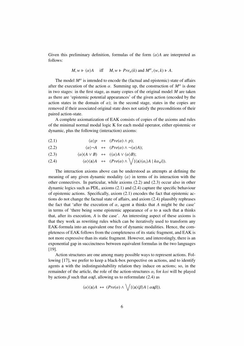
Given this preliminary definition, formulas of the form 〈α〉A are interpreted asfollows:

M,w 〈α〉A iff M,w Preα(k) and Mα, (w, k) A.

The model Mα is intended to encode the (factual and epistemic) state of affairsafter the execution of the action α. Summing up, the construction of Mα is donein two stages: in the first stage, as many copies of the original model M are takenas there are ‘epistemic potential appearances’ of the given action (encoded by theaction states in the domain of α); in the second stage, states in the copies areremoved if their associated original state does not satisfy the preconditions of theirpaired action-state.

A complete axiomatization of EAK consists of copies of the axioms and rulesof the minimal normal modal logic K for each modal operator, either epistemic ordynamic, plus the following (interaction) axioms:

〈α〉p ↔ (Pre(α) ∧ p);(2.1)

〈α〉¬A ↔ (Pre(α) ∧ ¬〈α〉A);(2.2)

〈α〉(A ∨ B) ↔ (〈α〉A ∨ 〈α〉B);(2.3)

〈α〉〈a〉A ↔ (Pre(α) ∧∨{〈a〉〈αi〉A | kαai}).(2.4)

The interaction axioms above can be understood as attempts at defining themeaning of any given dynamic modality 〈α〉 in terms of its interaction with theother connectives. In particular, while axioms (2.2) and (2.3) occur also in otherdynamic logics such as PDL, axioms (2.1) and (2.4) capture the specific behaviourof epistemic actions. Specifically, axiom (2.1) encodes the fact that epistemic ac-tions do not change the factual state of affairs, and axiom (2.4) plausibly rephrasesthe fact that ‘after the execution of α, agent a thinks that A might be the case’in terms of ‘there being some epistemic appearance of α to a such that a thinksthat, after its execution, A is the case’. An interesting aspect of these axioms isthat they work as rewriting rules which can be iteratively used to transform anyEAK-formula into an equivalent one free of dynamic modalities. Hence, the com-pleteness of EAK follows from the completeness of its static fragment, and EAK isnot more expressive than its static fragment. However, and interestingly, there is anexponential gap in succinctness between equivalent formulas in the two languages[19].

Action structures are one among many possible ways to represent actions. Fol-lowing [17], we prefer to keep a black-box perspective on actions, and to identifyagents a with the indistinguishability relation they induce on actions; so, in theremainder of the article, the role of the action-structures αi for kαi will be playedby actions β such that αaβ, allowing us to reformulate (2.4) as

〈α〉〈a〉A ↔ (Pre(α) ∧∨{〈a〉〈β〉A | αaβ}).

6

AxiomsA→ (B→ A)(A→ (B→ C))→ ((A→ B)→ (A→ C))A→ (B→ A ∧ B)A ∧ B→ AA ∧ B→ BA→ A ∨ BB→ A ∨ B(A→ C)→ ((B→ C)→ (A ∨ B→ C))⊥ → A

[a](A→ B)→ ([a]A→ [a]B)〈a〉(A ∨ B)→ 〈a〉A ∨ 〈a〉B¬〈a〉⊥

FS1 〈a〉(A→ B)→ ([a]A→ 〈a〉B)FS2 (〈a〉A→ [a]B)→ [a](A→ B)

Inference RulesMP if ` A→ B and ` A, then ` BNec if ` A, then ` [a]A

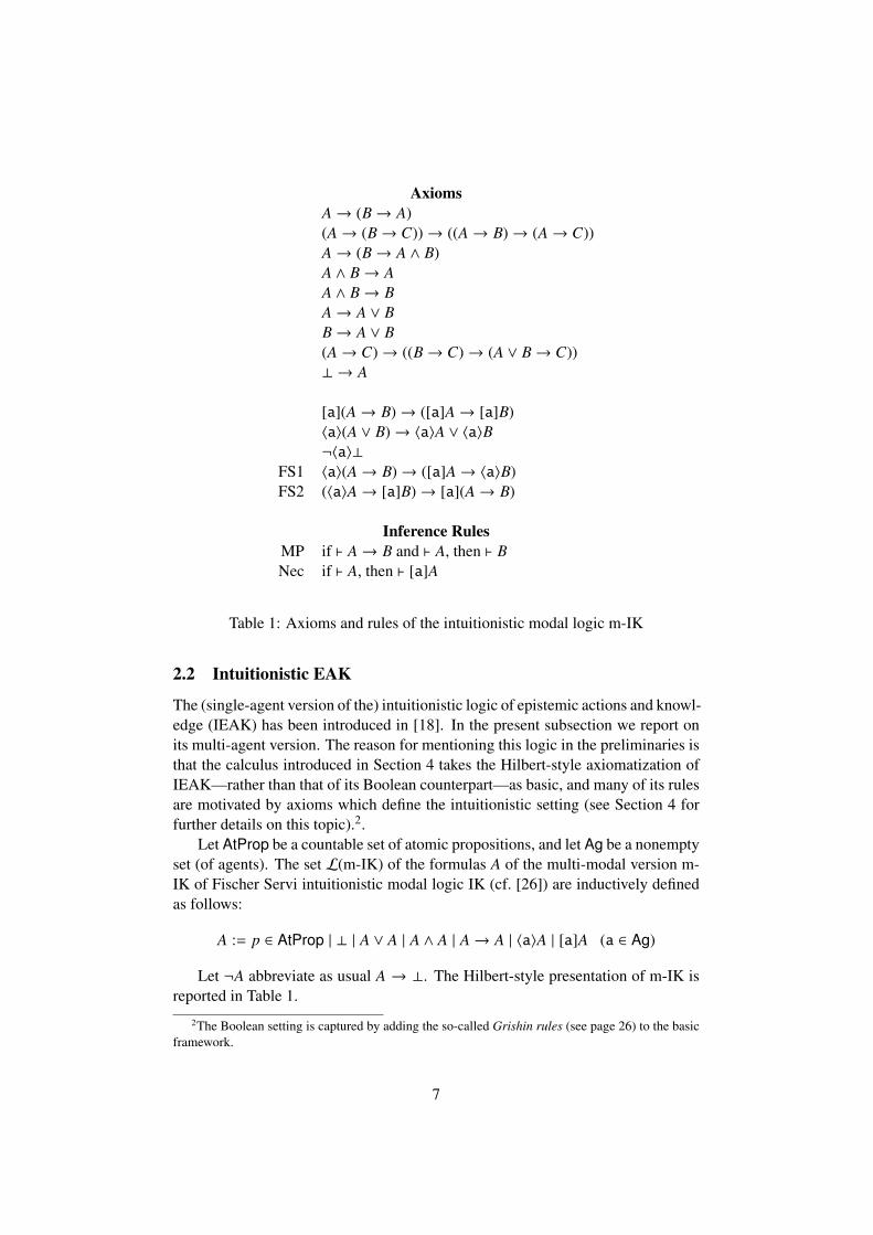
Table 1: Axioms and rules of the intuitionistic modal logic m-IK

2.2 Intuitionistic EAK

The (single-agent version of the) intuitionistic logic of epistemic actions and knowl-edge (IEAK) has been introduced in [18]. In the present subsection we report onits multi-agent version. The reason for mentioning this logic in the preliminaries isthat the calculus introduced in Section 4 takes the Hilbert-style axiomatization ofIEAK—rather than that of its Boolean counterpart—as basic, and many of its rulesare motivated by axioms which define the intuitionistic setting (see Section 4 forfurther details on this topic).2.

Let AtProp be a countable set of atomic propositions, and let Ag be a nonemptyset (of agents). The set L(m-IK) of the formulas A of the multi-modal version m-IK of Fischer Servi intuitionistic modal logic IK (cf. [26]) are inductively definedas follows:

A := p ∈ AtProp | ⊥ | A ∨ A | A ∧ A | A→ A | 〈a〉A | [a]A (a ∈ Ag)

Let ¬A abbreviate as usual A → ⊥. The Hilbert-style presentation of m-IK isreported in Table 1.

2The Boolean setting is captured by adding the so-called Grishin rules (see page 26) to the basicframework.

7

Interaction Axioms〈α〉p↔ Pre(α) ∧ p[α]p↔ Pre(α)→ p〈α〉⊥ ↔ ⊥

〈α〉> ↔ Pre(α)[α]> ↔ >[α]⊥ ↔ ¬Pre(α)[α](A ∧ B)↔ [α]A ∧ [α]B〈α〉(A ∧ B)↔ 〈α〉A ∧ 〈α〉B〈α〉(A ∨ B)↔ 〈α〉A ∨ 〈α〉B[α](A ∨ B)↔ Pre(α)→ (〈α〉A ∨ 〈α〉B)〈α〉(A→ B)↔ Pre(α) ∧ (〈α〉A→ 〈α〉B)[α](A→ B)↔ 〈α〉A→ 〈α〉B〈α〉〈a〉A↔ Pre(α) ∧

∨{〈a〉〈β〉A | αaβ}

[α]〈a〉A↔ Pre(α)→∨{〈a〉〈β〉A | αaβ}

[α][a]A↔ Pre(α)→∧{[a][β]A | αaβ}

〈α〉[a]A↔ Pre(α) ∧∧{[a][β]A | αaβ}

Inference RulesvNec if ` A, then ` [α]A

Table 2: Axioms and rules of the intuitionistic epistemic logic IEAK

To define the language of IEAK, let AtProp be a countable set of atomic propo-sitions, and let Ag be a nonempty set. The set L(IEAK) of formulas A of the intu-itionistic logic of epistemic actions and knowledge (IEAK), and the set Act(L) ofthe action structures α over L are defined simultaneously as follows:

A := p ∈ AtProp | ⊥ | A→ A | A ∨ A | A ∧ A | 〈a〉A | [a]A | 〈α〉A | [α]A,

where a ∈ Ag, and an action structure α over L(IEAK) is defined in a completelyanalogous way as action structures in the classical case, the only difference lyingin the codomain of Preα. Then, the logic IEAK is defined in a Hilbert-style pre-sentation which includes the axioms and rules of m-IK plus the axioms and rulesin Table 2.

2.3 Display calculi

The first display calculus appears in Belnap’s paper [3], as a sequent system aug-menting and refining Gentzen’s basic design of sequent calculi, which admit twotypes of rules: the structural, and the operational. Belnap’s refinement is basedon the introduction of a special syntax for the constituents of each sequent, whichincludes structural connectives along with logical, or operational connectives. Foran expanded discussion of these ideas, the reader is referred to [15, 28, 25].

8

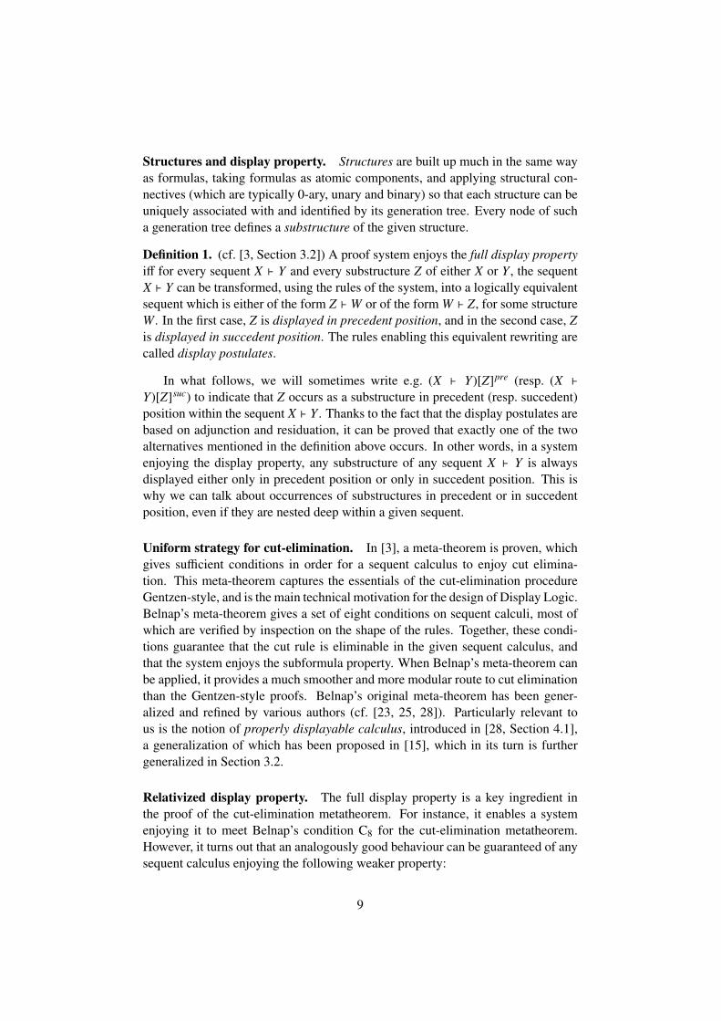
Structures and display property. Structures are built up much in the same wayas formulas, taking formulas as atomic components, and applying structural con-nectives (which are typically 0-ary, unary and binary) so that each structure can beuniquely associated with and identified by its generation tree. Every node of sucha generation tree defines a substructure of the given structure.

Definition 1. (cf. [3, Section 3.2]) A proof system enjoys the full display propertyiff for every sequent X ` Y and every substructure Z of either X or Y , the sequentX ` Y can be transformed, using the rules of the system, into a logically equivalentsequent which is either of the form Z ` W or of the form W ` Z, for some structureW. In the first case, Z is displayed in precedent position, and in the second case, Zis displayed in succedent position. The rules enabling this equivalent rewriting arecalled display postulates.

In what follows, we will sometimes write e.g. (X ` Y)[Z]pre (resp. (X `

Y)[Z]suc) to indicate that Z occurs as a substructure in precedent (resp. succedent)position within the sequent X ` Y . Thanks to the fact that the display postulates arebased on adjunction and residuation, it can be proved that exactly one of the twoalternatives mentioned in the definition above occurs. In other words, in a systemenjoying the display property, any substructure of any sequent X ` Y is alwaysdisplayed either only in precedent position or only in succedent position. This iswhy we can talk about occurrences of substructures in precedent or in succedentposition, even if they are nested deep within a given sequent.

Uniform strategy for cut-elimination. In [3], a meta-theorem is proven, whichgives sufficient conditions in order for a sequent calculus to enjoy cut elimina-tion. This meta-theorem captures the essentials of the cut-elimination procedureGentzen-style, and is the main technical motivation for the design of Display Logic.Belnap’s meta-theorem gives a set of eight conditions on sequent calculi, most ofwhich are verified by inspection on the shape of the rules. Together, these condi-tions guarantee that the cut rule is eliminable in the given sequent calculus, andthat the system enjoys the subformula property. When Belnap’s meta-theorem canbe applied, it provides a much smoother and more modular route to cut eliminationthan the Gentzen-style proofs. Belnap’s original meta-theorem has been gener-alized and refined by various authors (cf. [23, 25, 28]). Particularly relevant tous is the notion of properly displayable calculus, introduced in [28, Section 4.1],a generalization of which has been proposed in [15], which in its turn is furthergeneralized in Section 3.2.

Relativized display property. The full display property is a key ingredient inthe proof of the cut-elimination metatheorem. For instance, it enables a systemenjoying it to meet Belnap’s condition C8 for the cut-elimination metatheorem.However, it turns out that an analogously good behaviour can be guaranteed of anysequent calculus enjoying the following weaker property:

9

Definition 2. A proof system enjoys the relativized display property iff for everyderivable sequent X ` Y and every substructure Z of either X or Y , the sequentX ` Y can be transformed, using the rules of the system, into a logically equivalentsequent which is either of the form Z ` W or of the form W ` Z, for some structureW.

The calculus defined in Section 4 does not enjoy the full display property, butdoes enjoy the relativized display property above (more about this in Sections 4 and7), which enables it to verify the condition C’8 (see Section 3.2). More details aboutit are collected in Section 9.1. Finally, notice that the definition of substructures inprecedent or succedent position within each sequent can be given in a way whichdoes not rely on the full display property. It is enough to rely on the polarity ofthe coordinates of each structural connective: if these polarities are assigned, thenfor any sequent X ` Y , if Z is a substructure of X, then Z is in precedent (resp.succedent) position if, in the generation tree of X, the path from Z to the root goesthrough an even (resp. odd) number of coordinates with negative polarity. If Zis a substructure of Y , then Z is in succedent (resp. precedent) position if, in thegeneration tree of Y , the path from Z to the root goes through an even (resp. odd)number of coordinates with negative polarity.

2.4 A single-type display calculus for EAK

In [15], a display calculus is introduced for EAK, which is shown to be soundw.r.t. the final coalgebra semantics, syntactically complete w.r.t. EAK and to enjoycut-elimination Belnap-style. In the present subsection we briefly report on it, notonly for the sake of providing a relevant example of display calculus, but aboveall because a translation can be established between the operational language ofD’.EAK and of the Dynamic Calculus (cf. Section 4). This translation is importantfor the further treatment of Sections 5 and 7.

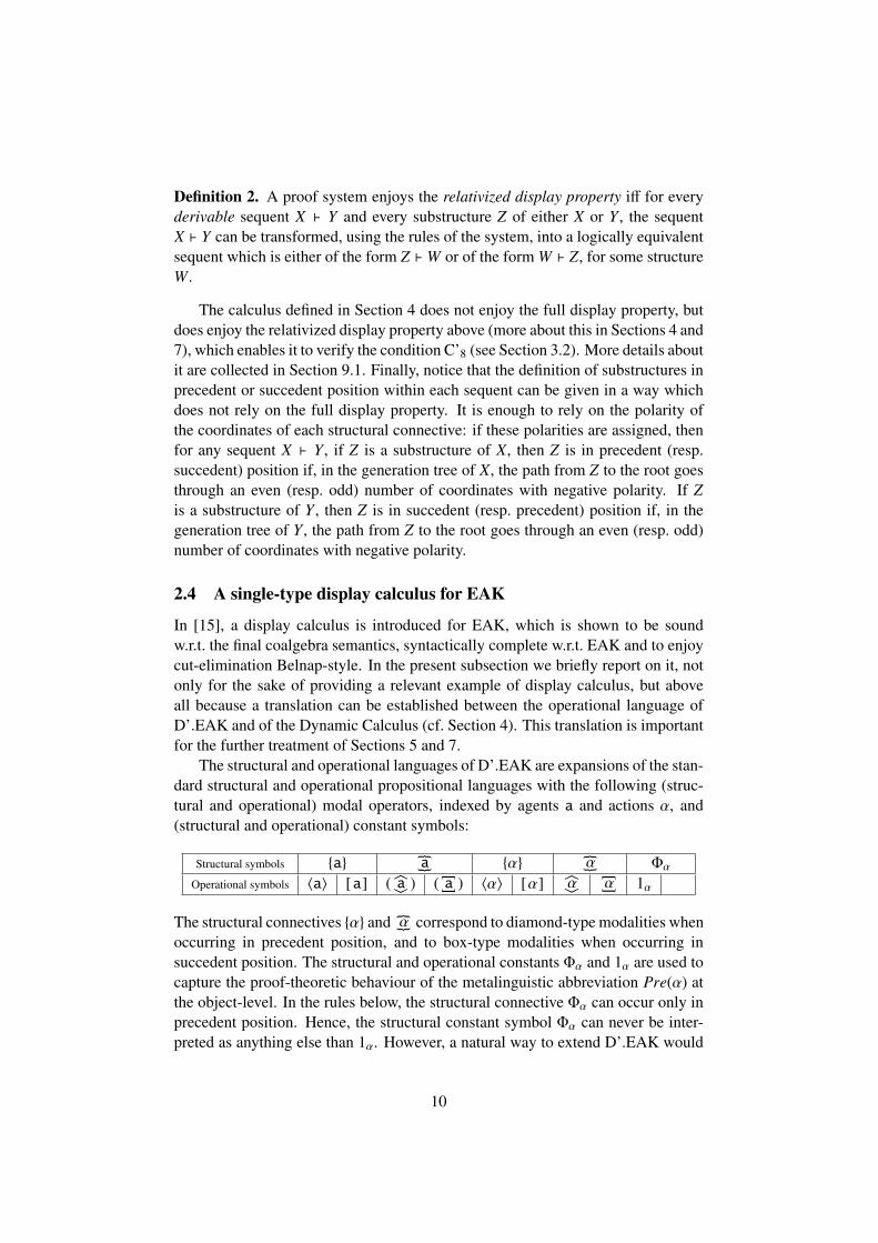
The structural and operational languages of D’.EAK are expansions of the stan-dard structural and operational propositional languages with the following (struc-tural and operational) modal operators, indexed by agents a and actions α, and(structural and operational) constant symbols:

Structural symbols {a} {a

}

{α} {α

}

Φα

Operational symbols 〈a〉 [a] ( 〈a

〉 ) ( [a

] ) 〈α〉 [α] 〈α

〉

[α

] 1α

The structural connectives {α} and {α

} correspond to diamond-type modalities whenoccurring in precedent position, and to box-type modalities when occurring insuccedent position. The structural and operational constants Φα and 1α are used tocapture the proof-theoretic behaviour of the metalinguistic abbreviation Pre(α) atthe object-level. In the rules below, the structural connective Φα can occur only inprecedent position. Hence, the structural constant symbol Φα can never be inter-preted as anything else than 1α. However, a natural way to extend D’.EAK would

10

be to introduce an operational constant symbol 0α, intuitively standing for the post-conditions of α for each action α, and dualize the relevant rules so as to capture thebehaviour of postconditions.

The connectives 〈α

〉 and [α

] occur within brackets since they are not actuallypart of the logical language of D’.EAK, but point at the fact that the structuralconnective {α

} is interpreted in the final coalgebra as the diamond (resp. box) asso-ciated with the converse of the relation associated with the epistemic action α (foran expanded discussion on this, the reader is referred to [15, Section 5.2]). The keyaspect of the final coalgebra as a semantic environment for EAK is that it makesit possible to see the dynamic connectives [α] and 〈α〉 as parts of adjoint pairs,precisely involving the additional modalities 〈α

〉 and [α

] . Specifically, we have thefollowing (syntactic) adjunction relations 〈α〉 a [α

] and 〈α

〉

a [α]: for all formulasA, B,

〈α〉A ` B iff A ` [α

] B 〈α〉 A ` B iff A ` [α]B(2.5)

The reader is referred to [15, Section 5] for a detailed discussion. The two tablesbelow introduce the structural rules for the dynamic modalities which have thesame shape as those for the agent-indexed modalities, here omitted.

Structural RulesI ` X

necdynL {α} I ` X

X ` Inecdyn

RX ` {α} I

I ` XdynnecL

{α

} I ` XX ` I dynnecRX ` {α

} I

{α}Y > {α}Z ` XFS dyn

L {α}(Y > Z) ` XY ` {α}X > {α}Z

FS dynRY ` {α}(X > Z)

{α}X ; {α}Y ` Zmondyn

L {α}(X ; Y) ` ZZ ` {α}Y ; {α}X

mondynRZ ` {α}(Y ; X)

{α

} Y > {α

} X ` ZdynFS L

{α

} (Y > X) ` Z

Y ` {α

} X > {α

} ZdynFS RY ` {α

} (X > Z)

{α

} X ; {α

} Y ` ZdynmonL

{α

} (X ; Y) ` Z

Z ` {α

} Y ; {α

} XdynmonRZ ` {α

} (Y ; X)

{a}(X ; {a

} Y) ` Zcon j

{a}X ; Y ` Z

X ` {a}(Y ; {a

} Z)con j

X ` {a}Y ; Z

{a

} (X ; {a}Y) ` Zcon j

{a

} X ; Y ` Z

X ` {a

} (Y ; {a}Z)con j

X ` {a

} Y ; Z

The con j-rules and the FS -rules can be shown to be interderivable thanks to thefollowing display postulates.

Display Postulates

{α}X ` Y({α}, {α

} )X ` {α

} Y

Y ` {α}X( {α

} , {α})

{α

} Y ` X

11

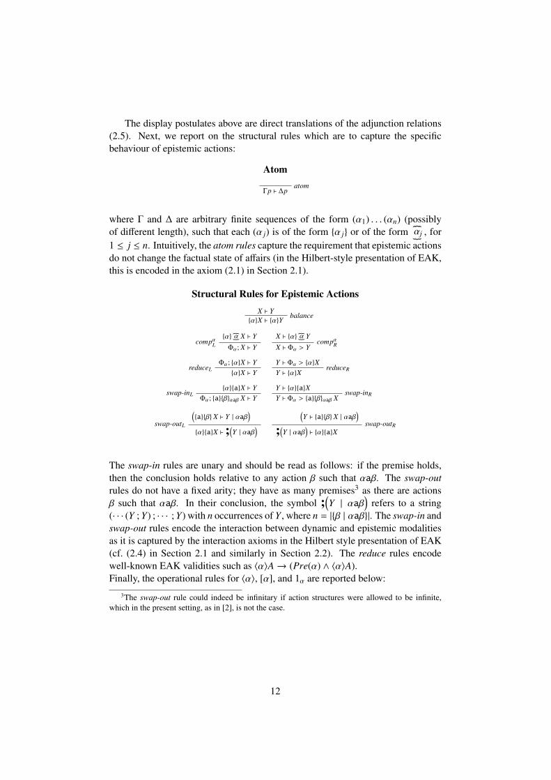
The display postulates above are direct translations of the adjunction relations(2.5). Next, we report on the structural rules which are to capture the specificbehaviour of epistemic actions:

Atomatom

Γp ` ∆p

where Γ and ∆ are arbitrary finite sequences of the form (α1) . . . (αn) (possiblyof different length), such that each (α j) is of the form {α j} or of the form

{

αj

}

, for1 ≤ j ≤ n. Intuitively, the atom rules capture the requirement that epistemic actionsdo not change the factual state of affairs (in the Hilbert-style presentation of EAK,this is encoded in the axiom (2.1) in Section 2.1).

Structural Rules for Epistemic ActionsX ` Y

balance{α}X ` {α}Y

{α} {α

} X ` YcompαL Φα; X ` Y

X ` {α} {α

} YcompαRX ` Φα > Y

Φα; {α}X ` YreduceL

{α}X ` YY ` Φα > {α}X reduceRY ` {α}X

{α}{a}X ` Yswap-inL

Φα; {a}{β}αaβ X ` YY ` {α}{a}X

swap-inRY ` Φα > {a}{β}αaβ X({a}{β} X ` Y | αaβ

)swap-outL

{α}{a}X ` ;(Y | αaβ

)(Y ` {a}{β} X | αaβ

)swap-outR;(

Y | αaβ)` {α}{a}X

The swap-in rules are unary and should be read as follows: if the premise holds,then the conclusion holds relative to any action β such that αaβ. The swap-outrules do not have a fixed arity; they have as many premises3 as there are actionsβ such that αaβ. In their conclusion, the symbol ;

(Y | αaβ

)refers to a string

(· · · (Y ; Y) ; · · · ; Y) with n occurrences of Y , where n = |{β | αaβ}|. The swap-in andswap-out rules encode the interaction between dynamic and epistemic modalitiesas it is captured by the interaction axioms in the Hilbert style presentation of EAK(cf. (2.4) in Section 2.1 and similarly in Section 2.2). The reduce rules encodewell-known EAK validities such as 〈α〉A→ (Pre(α) ∧ 〈α〉A).Finally, the operational rules for 〈α〉, [α], and 1α are reported below:

3The swap-out rule could indeed be infinitary if action structures were allowed to be infinite,which in the present setting, as in [2], is not the case.

12

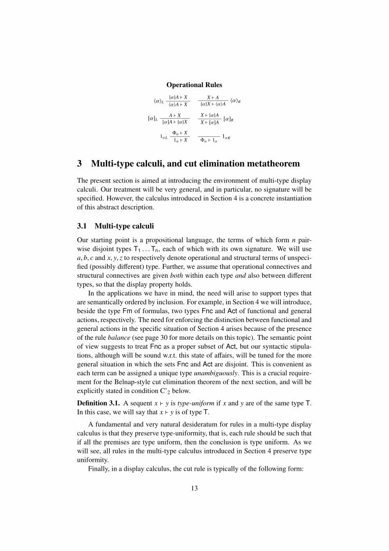
Operational Rules

{α}A ` X〈α〉L

〈α〉A ` XX ` A

〈α〉R{α}X ` 〈α〉A

A ` X[α]L [α]A ` {α}XX ` {α}A

[α]RX ` [α]A

Φα ` X1αL 1α ` X

1αRΦα ` 1α

3 Multi-type calculi, and cut elimination metatheorem

The present section is aimed at introducing the environment of multi-type displaycalculi. Our treatment will be very general, and in particular, no signature will bespecified. However, the calculus introduced in Section 4 is a concrete instantiationof this abstract description.

3.1 Multi-type calculi

Our starting point is a propositional language, the terms of which form n pair-wise disjoint types T1 . . .Tn, each of which with its own signature. We will usea, b, c and x, y, z to respectively denote operational and structural terms of unspeci-fied (possibly different) type. Further, we assume that operational connectives andstructural connectives are given both within each type and also between differenttypes, so that the display property holds.

In the applications we have in mind, the need will arise to support types thatare semantically ordered by inclusion. For example, in Section 4 we will introduce,beside the type Fm of formulas, two types Fnc and Act of functional and generalactions, respectively. The need for enforcing the distinction between functional andgeneral actions in the specific situation of Section 4 arises because of the presenceof the rule balance (see page 30 for more details on this topic). The semantic pointof view suggests to treat Fnc as a proper subset of Act, but our syntactic stipula-tions, although will be sound w.r.t. this state of affairs, will be tuned for the moregeneral situation in which the sets Fnc and Act are disjoint. This is convenient aseach term can be assigned a unique type unambiguously. This is a crucial require-ment for the Belnap-style cut elimination theorem of the next section, and will beexplicitly stated in condition C’2 below.

Definition 3.1. A sequent x ` y is type-uniform if x and y are of the same type T.In this case, we will say that x ` y is of type T.

A fundamental and very natural desideratum for rules in a multi-type displaycalculus is that they preserve type-uniformity, that is, each rule should be such thatif all the premises are type uniform, then the conclusion is type uniform. As wewill see, all rules in the multi-type calculus introduced in Section 4 preserve typeuniformity.

Finally, in a display calculus, the cut rule is typically of the following form:

13

X ` A A ` Y CutX ` Y

where X,Y are structures and A is a formula. This translates straightforwardly tothe multi-type environment, by the stipulation that cut rules of the form

x ` a a ` yCutx ` y

are allowed in the given multi-type system for each type. These cut rules will beasked to satisfy the following additional requirement:

Definition 3.2. A rule is strongly type-uniform if its premises and conclusion areof the same type.

3.2 Quasi-properly displayable multi-type calculi

In [15], to show that Belnap-style cut elimination holds for the display calculusD’.EAK, the definition of quasi-properly displayable calculi is given (generaliz-ing Wansing’s definition of properly displayable calculi [28, Section 4.2]), and itscorresponding Belnap style meta-theorem is discussed. We are working towardsthe proof that the multi-type display calculus introduced in Section 4 enjoys cutelimination Belnap-style. The aim of the present subsection is then to extend thenotion of quasi-properly displayable calculi to the multi-type environment. Let aquasi-properly displayable multi-type calculus be any displaycalculus in a multi-type language satisfying the following list of conditions4:

C1: Preservation of operational terms. Each operational term occurring in apremise of an inference rule inf is a subterm of some operational term in the con-clusion of inf.

C2: Shape-alikeness of parameters. Congruent parameters5 are occurrences ofthe same structure.

C’2: Type-alikeness of parameters. Congruent parameters have exactly thesame type. This condition bans the possibility that a parameter changes type alongits history.

4See [15] for a discussion on C’5 and C”5.5The congruence relation is an equivalence relation which is meant to identify the different oc-

currences of the same formula or substructure along the branches of a derivation [3, section 4], [25,Definition 6.5]. Condition C2 can be understood as a condition on the design of the rules of thesystem if the congruence relation is understood as part of the specification of each given rule; that is,each rule of the system should come with an explicit specification of which elements are congruentto which (and then the congruence relation is defined as the reflexive and transitive closure of theresulting relation). In this respect, C2 is nothing but a sanity check, requiring that the congruence isdefined in such a way that indeed identifies the occurrences which are intuitively “the same”.

14

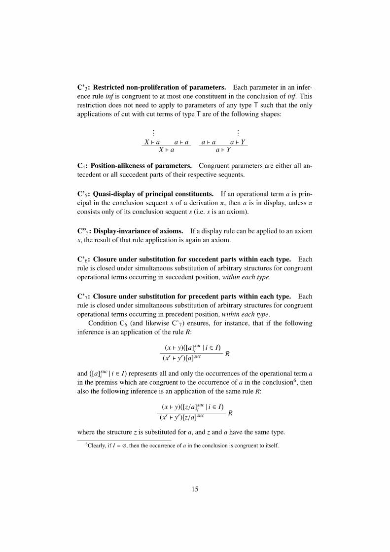
C’3: Restricted non-proliferation of parameters. Each parameter in an infer-ence rule inf is congruent to at most one constituent in the conclusion of inf. Thisrestriction does not need to apply to parameters of any type T such that the onlyapplications of cut with cut terms of type T are of the following shapes:

...X ` a a ` a

X ` aa ` a

...a ` Y

a ` Y

C4: Position-alikeness of parameters. Congruent parameters are either all an-tecedent or all succedent parts of their respective sequents.

C’5: Quasi-display of principal constituents. If an operational term a is prin-cipal in the conclusion sequent s of a derivation π, then a is in display, unless πconsists only of its conclusion sequent s (i.e. s is an axiom).

C”5: Display-invariance of axioms. If a display rule can be applied to an axioms, the result of that rule application is again an axiom.

C’6: Closure under substitution for succedent parts within each type. Eachrule is closed under simultaneous substitution of arbitrary structures for congruentoperational terms occurring in succedent position, within each type.

C’7: Closure under substitution for precedent parts within each type. Eachrule is closed under simultaneous substitution of arbitrary structures for congruentoperational terms occurring in precedent position, within each type.

Condition C6 (and likewise C’7) ensures, for instance, that if the followinginference is an application of the rule R:

(x ` y)([a]suc

i | i ∈ I)

R(x′ ` y′)[a]suc

and([a]suc

i | i ∈ I)

represents all and only the occurrences of the operational term ain the premiss which are congruent to the occurrence of a in the conclusion6, thenalso the following inference is an application of the same rule R:

(x ` y)([z/a]suc

i | i ∈ I)

R(x′ ` y′)[z/a]suc

where the structure z is substituted for a, and z and a have the same type.

6Clearly, if I = ∅, then the occurrence of a in the conclusion is congruent to itself.

15

C’8: Eliminability of matching principal constituents. This condition requestsa standard Gentzen-style checking, which is now limited to the case in which bothcut formulas are principal, and hence each of them has been introduced with thelast rule application of each corresponding subdeduction. In this case, analogouslyto the proof Gentzen-style, condition C’8 requires being able to transform the givendeduction into a deduction with the same conclusion in which either the cut iseliminated altogether, or is transformed in one or more applications of the cut rule,involving proper subterms of the original operational cut-term. In addition to this,specific to the multi-type setting is the requirement that the new application(s) ofthe cut rule be also strongly type-uniform (cf. condition C10 below).

C”8: Closure of axioms under cut. If x ` a and a ` y are axioms, then x ` y isagain an axiom.

C9: Type-uniformity of derivable sequents. Each derivable sequent is type-uniform.

C10: Strong type-uniformity of cut rules. All cut rules are strongly type-uniform(cf. Definition 3.2).

3.3 Belnap-style metatheorem for multi-types

In the present subsection, we state and prove the Belnap-style metatheorem whichwe will appeal to when establishing the cut elimination Belnap-style for the calcu-lus we will introduce in the next section.

Theorem 3.3. Any multi-type display calculus satisfying C2, C’2, C’3, C4, C’5,C”5, C’6, C’7, C’8, C”8, C9 and C10 is cut-admissible. If also C1 is satisfied, thenthe calculus enjoys the subformula property.

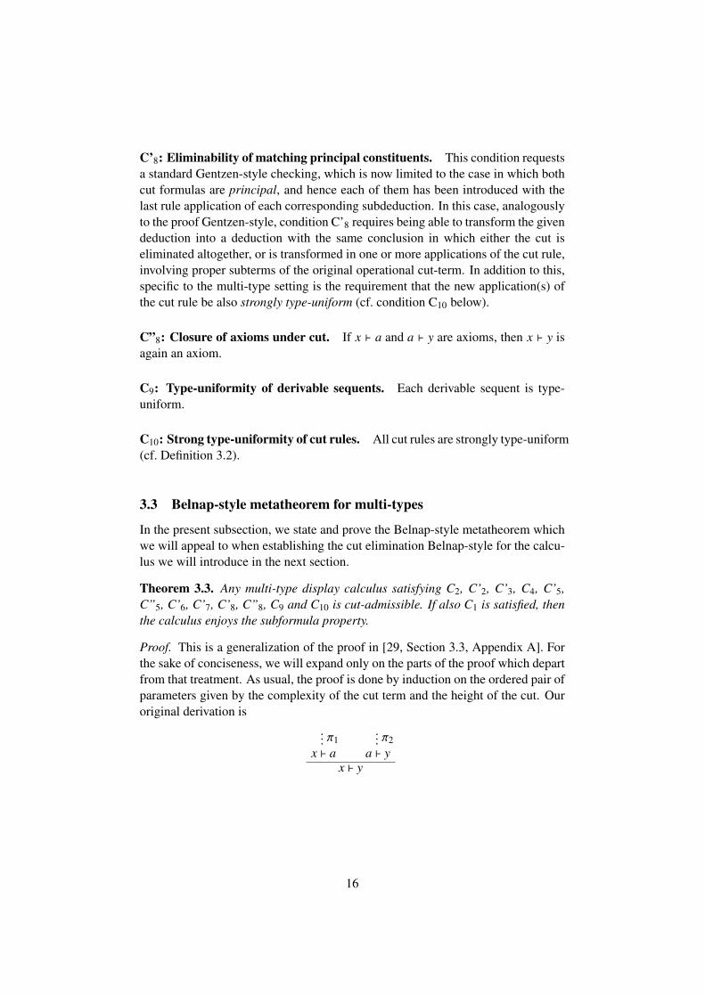
Proof. This is a generalization of the proof in [29, Section 3.3, Appendix A]. Forthe sake of conciseness, we will expand only on the parts of the proof which departfrom that treatment. As usual, the proof is done by induction on the ordered pair ofparameters given by the complexity of the cut term and the height of the cut. Ouroriginal derivation is

... π1x ` a

... π2a ` y

x ` y

16

Principal stage: both cut formulas are principal. There are three subcases.If the end sequent x ` y is identical to the conclusion of π1 (resp. π2), then we

can eliminate the cut simply replacing the derivation above with π1 (resp. π2).If the premises x ` a and a ` y are axioms, then, by C”8, the conclusion x ` y

is an axiom, therefore the cut can be eliminated by simply replacing the originalderivation with x ` y.

If one of the two premises of the cut in the original derivation is not an axiom,then, by C’8, there is a proof of x ` y which uses the same premise(s) of the originalderivation and which involves only strongly uniform cuts on proper subterms of a.

Parametric stage: at least one cut term is parametric. There are two subcases:either one cut term is principal or they are both parametric.

Consider the subcase in which one cut term is principal. W.l.o.g. we assumethat the cut-term a is principal in the left-premise x ` a of the cut in the originalproof (the other case is symmetric). We can assume w.l.o.g. that the conclusion ofthe cut is different from either of its premises. Then, conditions C2 and C’3 makeit possible to trace the history-tree of the occurrences of the cut-term a in π2 (cf.[15, Remark 1]), and by conditions C’2 and C4, any ancestor of a is of the sametype and in the same position (that is, is in precedent position). The situation canbe pictured as follows:

... π1x ` a

... π2.iai ` yi

. . .

... π2. j

(x j ` y j)[a j]pre

...

... π2.k

(xk ` yk)[ak]pre

. ..

. . .... . .. π2

a ` yx ` y

where, for i, j, k ∈ {1, . . . , n}, the nodes

ai ` yi, (x j ` y j)[a j]pre, and (xk ` yk)[ak]pre

represent the three ways in which the leaves ai, a j and ak in the history-tree of ain π2 can be introduced, and which will be discussed below. The notation a (resp.a) indicates that the given occurrence is principal (resp. parametric). Notice thatcondition C4 guarantees that all occurrences in the history of a are in precedentposition in the underlying derivation tree, and condition C’2 guarantees that thetype of a never changes along its history. Let al be introduced as a parameter (asrepresented in the picture above in the conclusion of π2.k for al = ak). Assumethat (xk ` yk)[ak]pre is the conclusion of an application inf of the rule Ru (forinstance, in the calculus of Section 4, this situation arises if ak is of type Fm andhas been introduced with an application of Weakening, or if ak is of type Fnc and

17

has been introduced with an application of Atom, or Balance). Since ak is a leafin the history-tree of a, we have that ak is congruent only to itself in xk ` yk.Notice that the assumption that every derivable sequent is type-uniform (C9), andthe type-alikeness of parameters (C’2) imply that the sequent a1, ak and x have thesame type. Hence, C’7 implies that it is possible to substitute x for ak by meansof an application of the same rule Ru. That is, (xk ` yk)[ak] can be replaced by(xk ` yk)[x/ak].

Let al be introduced as a principal formula. The corresponding subcase in [29]splits into two subsubcases: either al is introduced in display or it is not.

If al is in display (as represented in the picture above in the conclusion of π2.ifor al = ai), then we form a subderivation using π1 and π2.i and applying cut as thelast rule. The assumptions that the original cut is strongly type-uniform (C10), thatevery derivable sequent is type-uniform (C9), and the type-alikeness of parameters(C’2) imply that the sequent ai ` yi is of the same type as the sequents x ` a anda ` y. Hence, the new cut is strongly type-uniform.

If al is not in display (as represented in the picture above in the conclusionof π2. j for al = a j), then condition C’5 implies that (x j ` y j)[a j]

pre is an axiom,and C”5 implies that some axiom a j ` y′j exists, which is display-equivalent tothe first axiom, and in which a j occurs in display. Let π′ be the derivation whichtransforms a j ` y′i into (x j ` y j)[a j]

pre. We form a subderivation using π1 anda j ` y′j and joining them with a cut application, then attaching π′[x/a j]pre belowthe new cut.

The transformations just discussed explain how to transform the leaves of thehistory tree of a. Finally, since, as discussed above, x has the same type of a,condition C’7 implies that substituting x for each occurrence of a in the historytree of the cut term a in π2 (and in each occurring π′ as above) gives rise to anadmissible derivation π2[x/a]pre (use C’6 for the symmetric case).

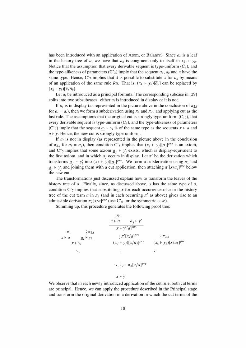
Summing up, this procedure generates the following proof tree:

... π1x ` a

... π2.iai ` yi

x ` yi

. . .

... π1x ` a a j ` y′

x ` y′[a]suc

... π′[x/a]pre

(x j ` y j)[x/a j]pre

...

... π2.k

(xk ` yk)[x/ak]pre

. ..

. . .... . .. π2[x/a]pre

x ` y

We observe that in each newly introduced application of the cut rule, both cut termsare principal. Hence, we can apply the procedure described in the Principal stageand transform the original derivation in a derivation in which the cut terms of the

18

newly introduced cuts have strictly lower complexity than the original cut terms.When the newly introduced applications of cut are of lower height than the originalone, we do not need to resort to the Principal stage.7

Finally, as to the subcase in which both cut terms are parametric, considera proof with at least one cut. The procedure is analogous to the previous case.Namely, following the history of one of the cut terms up to the leaves, and ap-plying the transformation steps described above, we arrive at a situation in which,whenever new applications of cuts are generated, in each such application at leastone of the cut formulas is principal. To each such cut, we can apply (the symmetricversion of) the Parametric stage described so far.

�

4 The Dynamic Calculus for EAK

As mentioned in the introduction, the key idea is to introduce a language in whichnot only formulas are generated from formulas and actions (as it happens in thesymbol 〈α〉A) and formulas are generated from formulas and agents (as it happensin the symbol 〈a〉A), but also actions are generated from the interactions betweenagents and actions.

An algebraically motivated introduction. In the present section, we define amulti-type language into which the language of (I)EAK translates, and in whicheach generation step mentioned above is explicitly accounted for via special binaryconnectives taking arguments of different types. More than one alternative is possi-ble in this respect; our choice for the present setting consists of the following types:Ag for agents, Fnc for functional actions, Act for actions, and Fm for formulas. Wealso stipulate that Ag, Act, Fm and Fnc are pairwise disjoint. The new connectives,and their types, are:

M0, N0 : Fnc × Fm→ Fm(4.1)

M1, N1 : Act × Fm→ Fm(4.2)

M2, N2 : Ag × Fm→ Fm(4.3)

M3, N3 : Ag × Fnc→ Act(4.4)

We stipulate that the interpretations of the connectives are maps preserving exist-ing joins in each coordinate (see below) with algebras as domains and codomainssuitable to interpret (functional) actions, formulas, and agents respectively. For in-stance, suitable choices for domains of interpretation for formulas can be complete

7 This is for instance the case if, in the original derivation, the history-tree of the cut term a (in theright-hand-side premise of the given cut application) contains at most one leaf al which is principal.However, the procedure described above in the Parametric stage does not always produce cuts oflower height. For instance, in the calculus introduced in Section 4, this situation may arise when twoancestors of a cut term of type Fm are introduced as principal along the same branch, and then areidentified via an application of the rule Contraction.

19

atomic Boolean algebras or perfect Heyting algebras (cf. [18]); in the setting ofe.g. epistemic action logic (cf. [27]), following [1], the domain of interpretationfor actions can be a quantale or a relation algebra (of which the functional actionscan be a sub-monoid). In the setting of EAK, in which no algebraic structure is re-quired of actions and agents, a suitable domain of interpretation can be a completejoin-semilattice, which is completely join-generated by a given subset (interpretingthe functional actions), and the domain of interpretation of agents can be a set.8

In Section 5, the final coalgebra Z (cf. [15, Section 5]) is taken as semanticenvironment for the Dynamic Calculus. In this setting, the boolean algebra PZ istaken as the domain of interpretation for Fm-type terms, Fnc-type terms are inter-preted as graphs of partial functions on Z, subject to certain restrictions, and thedomain of interpretation of Act-type terms is the complete

⋃-semilattice generated

by the domain of interpretation of Fnc.In all the domains of interpretation which are complete lattices (i.e. the algebras

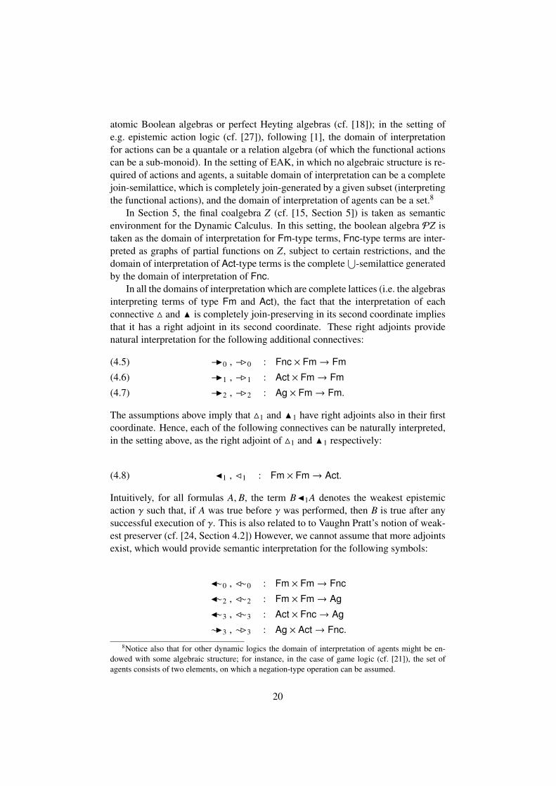
interpreting terms of type Fm and Act), the fact that the interpretation of eachconnective M and N is completely join-preserving in its second coordinate impliesthat it has a right adjoint in its second coordinate. These right adjoints providenatural interpretation for the following additional connectives:

−I0 , −B0 : Fnc × Fm→ Fm(4.5)

−I1 , −B1 : Act × Fm→ Fm(4.6)

−I2 , −B2 : Ag × Fm→ Fm.(4.7)

The assumptions above imply that M1 and N 1 have right adjoints also in their firstcoordinate. Hence, each of the following connectives can be naturally interpreted,in the setting above, as the right adjoint of M1 and N 1 respectively:

J1 , C1 : Fm × Fm→ Act.(4.8)

Intuitively, for all formulas A, B, the term BJ1A denotes the weakest epistemicaction γ such that, if A was true before γ was performed, then B is true after anysuccessful execution of γ. This is also related to to Vaughn Pratt’s notion of weak-est preserver (cf. [24, Section 4.2]) However, we cannot assume that more adjointsexist, which would provide semantic interpretation for the following symbols:

J∼0 , C∼0 : Fm × Fm→ Fnc

J∼2 , C∼2 : Fm × Fm→ Ag

J∼3 , C∼3 : Act × Fnc→ Ag

∼I3 , ∼B3 : Ag × Act→ Fnc.

8Notice also that for other dynamic logics the domain of interpretation of agents might be en-dowed with some algebraic structure; for instance, in the case of game logic (cf. [21]), the set ofagents consists of two elements, on which a negation-type operation can be assumed.

20

Virtual adjoints. We adopt the following notational convention about the threedifferent shapes of arrows introduced so far. Arrows with straight tails (−B and−I ) stand for connectives which have a semantic counterpart and which are in-cluded in the language of the Dynamic Calculus (see the grammar of operationalterms on page 23); arrows with no tail (e.g. J and C ) do have a semantic interpre-tation but are not included in the language at the operational level, and arrows withsquiggly tails (∼B , C∼ , ∼I and J∼ ) stand for syntactic objects, called virtual ad-joints, which do not have a semantic interpretation, but will play an important role,namely guaranteeing the Dynamic Calculus to enjoy the relativized display prop-erty (cf. Definition 2). In what follows, virtual adjoints will be introduced only asstructural connectives. That is, they will not correspond to any operational con-nective, and they will not appear actively in any rule schema other than the displaypostulates (cf. Definition 1). As will be shown in Section 7, these limitations keepthe calculus sound even if virtual adjoints do not have an independent semanticinterpretation.The M a −I and N a −B adjunction relations stipulated above translate into thefollowing clauses for every agent a, every functional action α, every action γ, andevery formula A:

α M0 A ≤ B iff A ≤ α−I0 B αN0 A ≤ B iff A ≤ α−B0 B(4.9)

γ M1 A ≤ B iff A ≤ γ−I1 B γN1 A ≤ B iff A ≤ γ−B1 B(4.10)

a M2 A ≤ B iff A ≤ a−I2 B aN2 A ≤ B iff A ≤ a−B2 B.(4.11)

The adjunction relations M1 a J 1 and N1 a C 1 translate into the following clausesfor every action γ and every formula A:

γ M1 A ≤ B iff γ ≤ BJ1A γN1 A ≤ B iff γ ≤ BC1A.(4.12)

As we will see, the display postulates corresponding to triangle- and arrow-shaped connectives are modelled over the conditions (4.9)-(4.12) above. Also thedisplay postulates involving virtual adjoints are shaped in the same way, whichexplains their name.

Translating D’.EAK into the multi-type setting. The intended link between thelanguage of D’.EAK (cf. Section 2.4) and the language of the Dynamic Calculusis illustrated in the following table:

〈α〉A becomes α M0 A 〈α

〉 A becomes αN0 A〈a〉A becomes a M2 A 〈a

〉 A becomes aN2 A[α]A becomes α−B0 A [α

] A becomes α−I0 A[a]A becomes a−B2 A [a

] A becomes a−I2 A1α becomes α M0 >.

The table above can be extended to the definition of a formal translation betweenthe operational language of D’.EAK and that of the Dynamic Calculus, simply

21

by preserving the non modal propositional fragment. We omit the details of thisstraightforward inductive definition. In Section 5, this translation will be elabo-rated on, and the interpretation of the language of the Dynamic Calculus in thefinal coalgebra will be defined so that the translation above preserves the validityof sequents. In the light of this translation, the adjunction conditions in clauses(4.9) correspond to the adjunction conditions (2.5) in D’.EAK, which, in their turn,motivate the display postulates reported on in Section 2.4:

〈α〉 a [α

]

〈α

〉

a [α].

The connectives M3 and N 3 have no counterpart in the language of D’.EAK, but theintroduction of N 3 is exactly what brings the additional expressiveness we need inorder to eliminate the label. Indeed, we stipulate that for every a and α as above,

aN3 α =∨{β | αaβ}. (4.13)

A way to understand this stipulation is in the light of the discussion in [15, Section4.3] after clause (8). There, in the context of a discussion about the proof systemin [1], the link between the semantic condition f M

A (m?q) ≤ f MA (m)? f Q

A (q) (cf. [1,Definitions 2.2(2) and 2.3]) and the axiom (2.4)—which in [1] was left implicit—ismade more explicit, by understanding the action f Q

A (q) as the join, taken in Q, ofall the actions q′ which are indistinguishable from q for the agent A. In the presentsetting, the stipulation (4.13) says that aN3 α encodes exactly the same informationencoded in f Q

A (q), namely, the nondeterministic choice between all the actions thatare indistinguishable from α for the agent a.

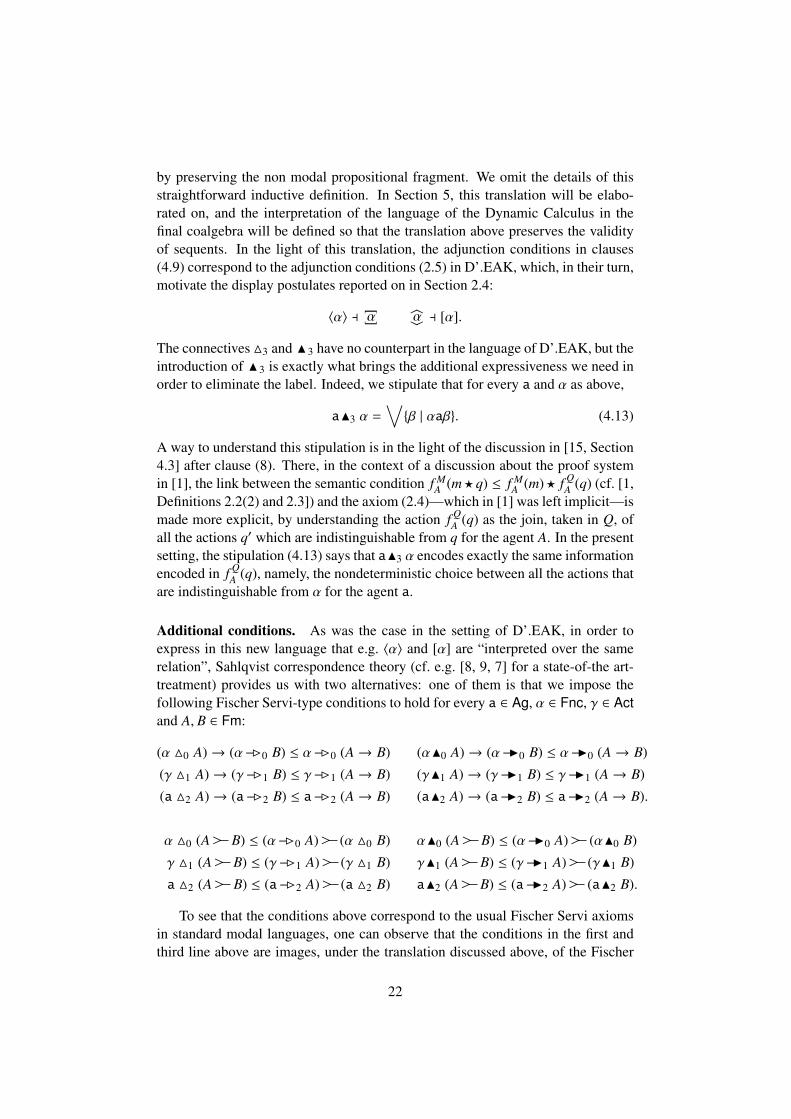
Additional conditions. As was the case in the setting of D’.EAK, in order toexpress in this new language that e.g. 〈α〉 and [α] are “interpreted over the samerelation”, Sahlqvist correspondence theory (cf. e.g. [8, 9, 7] for a state-of-the art-treatment) provides us with two alternatives: one of them is that we impose thefollowing Fischer Servi-type conditions to hold for every a ∈ Ag, α ∈ Fnc, γ ∈ Actand A, B ∈ Fm:

(α M0 A)→ (α−B0 B) ≤ α−B0 (A→ B) (αN0 A)→ (α−I0 B) ≤ α−I0 (A→ B)

(γ M1 A)→ (γ−B1 B) ≤ γ−B1 (A→ B) (γN1 A)→ (γ−I1 B) ≤ γ−I1 (A→ B)

(a M2 A)→ (a−B2 B) ≤ a−B2 (A→ B) (aN2 A)→ (a−I2 B) ≤ a−I2 (A→ B).

α M0 (A

∧

B) ≤ (α−B0 A)

∧

(α M0 B) αN0 (A

∧

B) ≤ (α−I0 A)

∧

(αN0 B)

γ M1 (A

∧

B) ≤ (γ−B1 A)

∧

(γ M1 B) γN1 (A

∧

B) ≤ (γ−I1 A)

∧

(γN1 B)

a M2 (A

∧

B) ≤ (a−B2 A)

∧

(a M2 B) aN2 (A

∧

B) ≤ (a−I2 A)

∧

(aN2 B).

To see that the conditions above correspond to the usual Fischer Servi axiomsin standard modal languages, one can observe that the conditions in the first andthird line above are images, under the translation discussed above, of the Fischer

22

Servi axioms reported on in Section 2.2). The second alternative is to imposethat, for every 0 ≤ i ≤ 2, the connectives Mi and N i yield conjugated diamonds(cf. discussion in [15, Section 6.2]); that is, the following inequalities hold for alla ∈ Ag, α, β ∈ Fnc, and A, B ∈ Fm:

(α M0 A) ∧ B ≤ α M0 (A ∧ αN0 B) (αN0 A) ∧ B ≤ αN0 (A ∧ α M0 B)

(γ M1 A) ∧ B ≤ γ M1 (A ∧ γN1 B) (γN1 A) ∧ B ≤ γN1 (A ∧ γ M1 B)

(a M2 A) ∧ B ≤ a M2 (A ∧ aN2 B) (aN2 A) ∧ B ≤ aN2 (A ∧ a M2 B).

α−B 0(A ∨ α−I0 B) ≤ (α−B 0A) ∨ B α−I0 (A ∨ α−B 0B) ≤ (α−I0 A) ∨ B

γ−B 1(A ∨ γ−I1 B) ≤ (γ−B 1A) ∨ B γ−I1 (A ∨ γ−B 1B) ≤ (γ−I1 A) ∨ B

a−B 2(A ∨ a−I2 B) ≤ (a−B 2A) ∨ B a−I2 (A ∨ a−B 2B) ≤ (a−I2 A) ∨ B.

The conditions in the first and third line above are images, under the translationdiscussed above, of the conjugation conditions reported on in [15, Section 6.2].

The operational language, formally. Let us introduce the operational terms ofthe multi-type language by the following simultaneous induction, based on setsAtProp of atomic propositions, Fnc of functional actions, and Ag of agents:

Fm 3 A ::= p | ⊥ | > | A ∧ A | A ∨ A | A→ A | A

∧

A |

α M0 A | α−B0 A | γ M1 A | γ−B1 A | a M2 A | a−B2 A |

αN0 A | α−I0 A | γN1 A | γ−I1 A | aN2 A | a−I2 A

Fnc 3 α ::= α

Act 3 γ ::= aN3 α | a M3 α

Ag 3 a ::= a

The fundamental difference between the language above and the language of D’.EAKis that, in D’.EAK, agents and actions are parametric indexes in the constructionof formulas, which are the only first-class citizens. In the present setting, however,each type lives on a par with any other. Because of the relative simplicity of theEAK setting, two of the four types are attributed no algebraic structure at the op-erational level. However, it is not difficult to enrich the algebraic structure of thosetypes with sensible and intuitive operations: for instance, the skip and crash actionsare functional, and parallel and sequential composition and iteration on functionalactions preserve functionality, hence can be added to the array of constructors forFnc. As a consequence of the fact that each type is a first-class citizen, as we willsee shortly, four types of structures will be defined, and the turnstile symbol in thesequents of this calculus will be interpreted in the appropriate domain.

On the meta-linguistic labels αaβ. Let us illustrate how the label αaβ can besubsumed when translating D’.EAK-formulas in the multi-type language. Con-

23

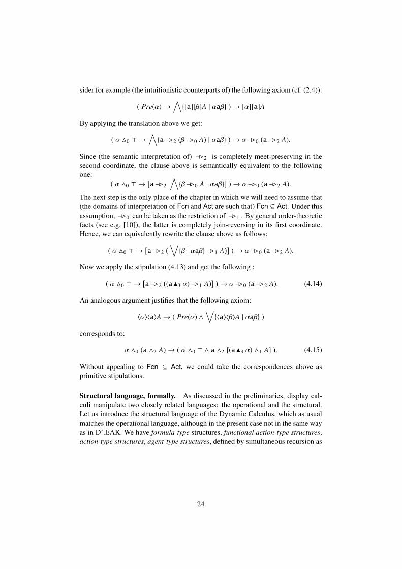
sider for example (the intuitionistic counterparts of) the following axiom (cf. (2.4)):

( Pre(α)→∧{[a][β]A | αaβ} )→ [α][a]A

By applying the translation above we get:

( α M0 > →∧{a−B2 (β−B0 A) | αaβ} )→ α−B0 (a−B2 A).

Since (the semantic interpretation of) −B2 is completely meet-preserving in thesecond coordinate, the clause above is semantically equivalent to the followingone:

( α M0 > →[a−B2

∧{β−B0 A | αaβ}

])→ α−B0 (a−B2 A).

The next step is the only place of the chapter in which we will need to assume that(the domains of interpretation of Fcn and Act are such that) Fcn ⊆ Act. Under thisassumption, −B0 can be taken as the restriction of −B1 . By general order-theoreticfacts (see e.g. [10]), the latter is completely join-reversing in its first coordinate.Hence, we can equivalently rewrite the clause above as follows:

( α M0 > →[a−B2

(∨{β | αaβ} −B1 A

)])→ α−B0 (a−B2 A).

Now we apply the stipulation (4.13) and get the following :

( α M0 > →[a−B2

((aN3 α)−B1 A

)])→ α−B0 (a−B2 A). (4.14)

An analogous argument justifies that the following axiom:

〈α〉〈a〉A→ ( Pre(α) ∧∨{〈a〉〈β〉A | αaβ} )

corresponds to:

α M0 (a M2 A)→ ( α M0 > ∧ a M2 [(aN3 α) M1 A] ). (4.15)

Without appealing to Fcn ⊆ Act, we could take the correspondences above asprimitive stipulations.

Structural language, formally. As discussed in the preliminaries, display cal-culi manipulate two closely related languages: the operational and the structural.Let us introduce the structural language of the Dynamic Calculus, which as usualmatches the operational language, although in the present case not in the same wayas in D’.EAK. We have formula-type structures, functional action-type structures,action-type structures, agent-type structures, defined by simultaneous recursion as

24

follows:

FM 3 X ::= A | I | X ; X | X > X |

F10 X | F

1

0 X | Γ11 X | Γ

1

1 X | a12 X | a1

2 X |

Fa0 X | F

a

0 X | Γa1 X | Γ

a

1 X | aa2 X | a

a

2 X

FNC 3 F ::= α | X2∼0 X | Xb∼0 X | a∼43 Γ | a∼d3 Γ

ACT 3 Γ ::= aa3 F | a13 F | X 11 X | X a1 X

AG 3 a ::= a | X2∼2 X | Xb∼2 X | Γ2∼3 F | Γb∼3 F.

The propositional base. As is typical of display calculi, each operational con-nective corresponds to one structural connective. In particular, the propositionalbase connectives behave exactly as in D’.EAK, but for the sake of self-containment,we are going to report on these rules below:

Structural symbols < > ; IOperational symbols ∧ ←

∧

→ ∧ ∨ > ⊥

Structural Rules

Id p ` pX ` A A ` Y CutX ` Y

X ` YI1

L I ` Y < XX ` Y

I1RX < Y ` I

X ` YI2

L I ` X > YX ` Y

I2RY > X ` I

I ` XIWL Y ` XX ` I IWRX ` Y

X ` ZW1L Y ` Z < X

X ` Z W1RX < Z ` Y

X ` ZW2L Y ` X > Z

X ` Z W2RZ > X ` Y

X ; X ` YCL X ` Y

Y ` X ; XCRY ` X

Y ; X ` ZEL X ; Y ` Z

Z ` X ; YERZ ` Y ; X

X ; (Y ; Z) ` WAL (X ; Y) ; Z ` W

W ` (Z ; Y) ; XARW ` Z ; (Y ; X)

25

Display Postulates

X ; Y ` Z( , <)

X ` Z < Y

Z ` X ; Y(<, ; )

Z < Y ` X

X ; Y ` Z( , >)

Y ` X > Z

Z ` X ; Y(>, ; )

X > Z ` Y

The classical base is obtained by adding the so-called Grishin rules (followinge.g. [16]), which encode classical, but not intuitionistic validities:

X > (Y ; Z) ` WGriL

(X > Y) ; Z ` W

W ` X > (Y ; Z)GriR

W ` (X > Y) ; Z

Operational Rules

⊥L⊥ ` I

X ` I⊥RX ` ⊥

I ` X>L

> ` X>RI ` >

A ; B ` Z∧L A ∧ B ` Z

X ` A Y ` B∧RX ; Y ` A ∧ B

A ` X B ` Y∨L A ∨ B ` X ; Y

Z ` A ; B∨RZ ` A ∨ B

B ` Y X ` A←L B← A ` Y < XZ ` B < A ←RZ ` B← A

B < A ` Z

∧ L B ∧ A ` ZY ` B A ` X

∧ RY < X ` B ∧ A

X ` A B ` Y→L A→ B ` X > YZ ` A > B →RZ ` A→ B

A > B ` Z∧

L A

∧

B ` ZA ` X Y ` B ∧

RX > Y ` A

∧

B

Rules for heterogeneous connectives. Unlike what was the case in the setting ofD’.EAK, in the present setting, each heterogeneous structural connective is associ-ated with at most one operational connective, as illustrated in the following table:for 0 ≤ i ≤ 3 and j ∈ {0, 2},

Structural symbols 1i ai

1

j

a

jOperational symbols Mi Ni −Bj −Ij

That is, structural connectives are to be interpreted as usual in a context-sensitiveway, but the present language lacks the operational connectives which would cor-respond to them on one of the two sides. This is of course because in the presentsetting we do not need them. However, in a setting in which they would turn outto be needed, it would not be difficult to introduce the missing operational connec-tives. We can now introduce the operational rules for heterogeneous connectives.Let x, y stand for structures of an undefined type, and let a, b denote operationalterms of the appropriate type. Then, for 0 ≤ i ≤ 3,

26

a1i b ` zMiL a Mi b ` z

x ` a y ` bMiR

x1i y ` a Mi b

aai b ` zNiL aNi b ` z

x ` a y ` bNiR

xai y ` aNi b

and for 0 ≤ i ≤ 2,

x ` a B ` Y−BiLa−BiB ` x

1

iYZ ` a

1iB −BiRZ ` a−BiB

x ` a B ` Y−IiLa−IiB ` x

aiY

Z ` a

a

iB −IiRZ ` a−IiB

where B,Y,Z are formula-type operational and structural terms. Clearly, the rulesin the two tables above for i = 0, 2 yield the operational rules for the dynamicand epistemic modal operators under the translation given early on. Notice thateach sequent is always interpreted in one domain. However, since heterogeneousconnectives take arguments of different types (which justifies their name), premisesof binary rules are of course interpreted in different domains.Axioms will be given in three types9, as follows:

a ` a α ` α p ` p ⊥ ` I I ` >

where the first and second axioms from the left are of type Ag and Fnc respectively,and the remaining ones are of type Fm. A generalization of p ` p will be addedbelow to the system (see atom axiom on page 29).Further, we allow the following strongly type-uniform (cf. Definition 3.2) cut ruleson operational terms:

a ` a a ` ba ` b

F ` α α ` GF ` G

Γ ` γ γ ` ∆

Γ ` ∆

X ` A A ` YX ` Y

Next, we give the display postulates for heterogeneous connectives. In what fol-lows, let x, y, z stand for structures of an undefined type. Then, for 0 ≤ i ≤ 2,

x1i y ` z(Mi, −Ii)

y ` x

a

i z

xai y ` z(N i, −Bi)

y ` x

1

i z

For i = 1, we also have

x11 y ` z(M1, J−1)

x ` z a1 y

xa1 y ` z(N1 , C−1)

x ` z 11 y9Indeed, there is no axiom schema for atomic terms of type Act, because the language does not

admit them.

27

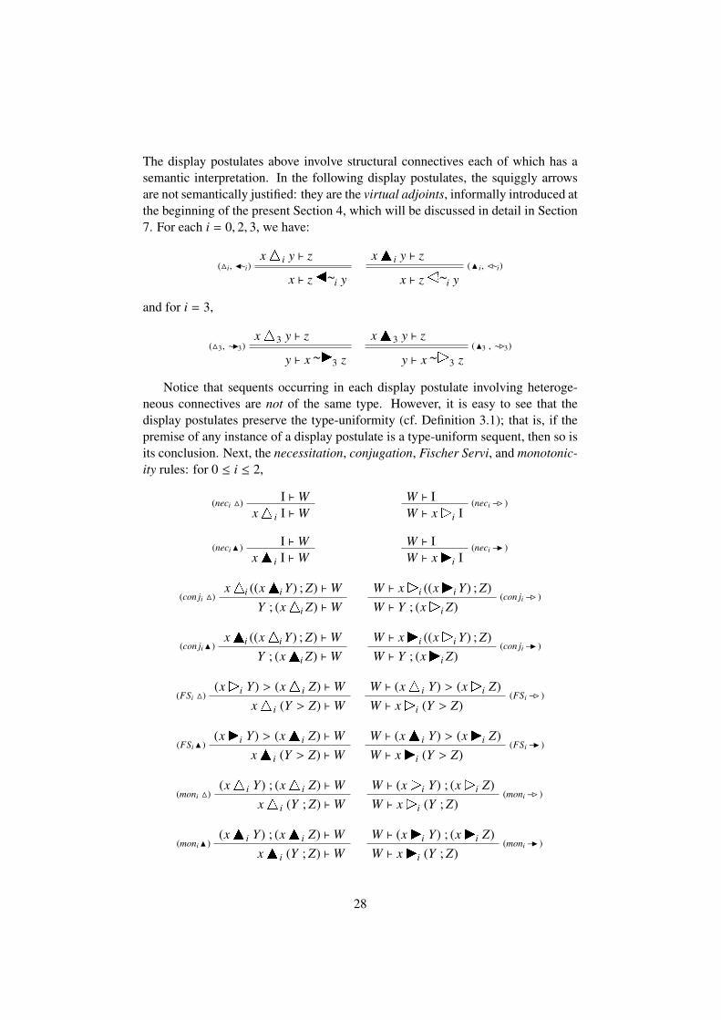
The display postulates above involve structural connectives each of which has asemantic interpretation. In the following display postulates, the squiggly arrowsare not semantically justified: they are the virtual adjoints, informally introduced atthe beginning of the present Section 4, which will be discussed in detail in Section7. For each i = 0, 2, 3, we have:

x1i y ` z(Mi, J∼i)

x ` zb∼i y

xai y ` z(N i, C∼i)

x ` z2∼i y

and for i = 3,

x13 y ` z(M3, ∼I3)

y ` x∼d3 z

xa3 y ` z(N3 , ∼B3)

y ` x∼43 z

Notice that sequents occurring in each display postulate involving heteroge-neous connectives are not of the same type. However, it is easy to see that thedisplay postulates preserve the type-uniformity (cf. Definition 3.1); that is, if thepremise of any instance of a display postulate is a type-uniform sequent, then so isits conclusion. Next, the necessitation, conjugation, Fischer Servi, and monotonic-ity rules: for 0 ≤ i ≤ 2,

I ` W(neci M)x1i I ` W

W ` I (neci −B )W ` x

1

i I

I ` W(neciN )xai I ` W

W ` I (neci −I )W ` x

a

i I

x1i ((xai Y) ; Z) ` W(con ji M)

Y ; (x1i Z) ` WW ` x

1

i ((x

a

i Y) ; Z)(con ji −B )

W ` Y ; (x

1

i Z)

xai ((x1i Y) ; Z) ` W(con jiN )

Y ; (xai Z) ` WW ` x

a

i ((x

1

i Y) ; Z)(con ji −I )

W ` Y ; (x

a

i Z)

(x

1

i Y) > (x1i Z) ` W(FSi M)

x1i (Y > Z) ` WW ` (x1i Y) > (x

1

i Z)(FSi −B )

W ` x

1

i (Y > Z)

(x

a

i Y) > (xai Z) ` W(FSiN )

xai (Y > Z) ` WW ` (xai Y) > (x

a

i Z)(FSi −I )

W ` x

a

i (Y > Z)

(x1i Y) ; (x1i Z) ` W(moni M)

x1i (Y ; Z) ` WW ` (x

1

i Y) ; (x

1

i Z)(moni −B )

W ` x

1

i (Y ; Z)

(xai Y) ; (xai Z) ` W(moniN )

xai (Y ; Z) ` WW ` (x

a

i Y) ; (x

a

i Z)(moni −I )

W ` x

a

i (Y ; Z)

28

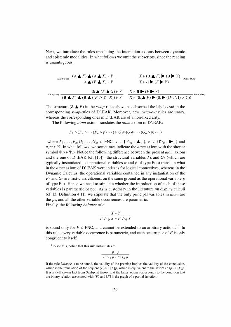
Next, we introduce the rules translating the interaction axioms between dynamicand epistemic modalities. In what follows we omit the subscripts, since the readingis unambiguous.

(aa F)a (aa X) ` Yswap-outL

aa (Fa X) ` YX ` (aa F)

a

(a

a

Y)swap-outR

X ` aa

(F

a

Y)

aa (Fa X) ` Yswap-inL

(aa F)a (aa ((F1 I) ; X)) ` YX ` a

a(F

a

Y)swap-inR

X ` (aa F)

a

(a

a

((F1 I) > Y))

The structure (aa F) in the swap-rules above has absorbed the labels αaβ in thecorresponding swap-rules of D’.EAK. Moreover, new swap-out rules are unary,whereas the corresponding ones in D’.EAK are of a non-fixed arity.

The following atom axiom translates the atom axiom of D’.EAK:

F1 ◦ (F2 ◦ · · · (Fn ◦ p) · · · ) ` G1B(G2B · · · (GmBp) · · · )

where F1, . . . , Fn,G1, . . . ,Gm ∈ FNC, ◦ ∈ {10 , a0 }, B ∈ {

1

0 ,

a

0 } andn,m ∈ N. In what follows, we sometimes indicate the atom axiom with the shortersymbol Φp ` Ψp. Notice the following difference between the present atom axiomand the one of D’.EAK (cf. [15]): the structural variables Fs and Gs (which aretypically instantiated as operational variables α and β of type Fnc) translate whatin the atom axiom of D’.EAK were indexes for logical connectives, whereas in theDynamic Calculus, the operational variables contained in any instantiation of theFs and Gs are first-class citizens, on the same ground as the operational variable pof type Fm. Hence we need to stipulate whether the introduction of each of thesevariables is parametric or not. As is customary in the literature on display calculi(cf. [3, Definition 4.1]), we stipulate that the only principal variables in atom arethe ps, and all the other variable occurrences are parametric.Finally, the following balance rule:

X ` YF10 X ` F

1

0 Y

is sound only for F ∈ FNC, and cannot be extended to an arbitrary actions.10 Inthis rule, every variable occurrence is parametric, and each occurrence of F is onlycongruent to itself.

10To see this, notice that this rule instantiates to

p ` p

F10 p ` F

1

0 p

If the rule balance is to be sound, the validity of the premise implies the validity of the conclusion,which is the translation of the sequent 〈F〉p ` [F]p, which is equivalent to the axiom 〈F〉p → [F]p.It is a well known fact from Sahlqvist theory that the latter axiom corresponds to the condition thatthe binary relation associated with 〈F〉 and [F] is the graph of a partial function.

29

Justifying the two types of actions. As discussed in the introduction, one ofthe initial aims of the present paper was introducing a formal framework expres-sive enough so as to capture at the object-level the information encoded in themeta-linguistic label αaβ. From the order-theoretic analysis at the beginning of thepresent section, it emerged that the additional expressivity encoded in the connec-tive N3 and its interpretation (4.13) requires a semantic environment which cannotbe restricted to functional actions. The introduction of the general type Act servesthis purpose. However, the fact that the rule balance is only sound for functional ac-tions is the reason why both types Fnc and Act are needed in order for the DynamicCalculus to satisfy conditions C’6 and C’7 of Section 3.2. Indeed, the distinct typeFnc allows for the rule balance to be formulated so that all parametric variablesoccur unrestricted within each type.

5 Soundness

In the present section, we discuss the soundness of the rules of the Dynamic Cal-culus and prove that those which do not involve virtual adjoints (cf. Section 4) aresound with respect to the final coalgebra semantics. In [15, Section 5], basic factsabout the final coalgebra have been collected and it is explained in detail how therules of display calculi are to be interpreted in the final coalgebra. Here we willbriefly recall some basics, and refer the reader to [15, Section 5] for a completediscussion.

Structures will be translated into operational terms of the appropriate type, andoperational terms will be interpreted according to their type. Specifically, eachatomic proposition p is assigned to a subset [[p]] of the final coalgebra Z, eachagent a a binary relation aZ = [[a]] on Z representing as usual a’s uncertainty aboutthe world, and each functional actions α is assigned a functional (i.e. deterministic)relation αZ = [[α]] ⊆ Z × Z subject to the restriction defining the specific feature ofepistemic actions, namely, that for all z, z′ ∈ Z, if zαZz′, then z ∈ [[p]] iff z′ ∈ [[p]]for every atomic proposition p.

Further, each agent a is associated with an auxiliary binary relation aFnc onthe domain of interpretation of Fnc, which is the collection of graphs of partialfunctions having subsets of Z as domain and range. For each agent a, the relationaFnc represents a’s uncertainty about which action takes place).

In order to translate structures as operational terms, structural connectives needto be translated as logical connectives. To this effect, non-modal structural connec-tives are associated with pairs of logical connectives, and any given occurrence ofa structural connective is translated as one or the other, according to its (antecedentor succedent) position. The following table illustrates how to translate each propo-sitional structural connective of type FM, in the upper row, into one or the other ofthe logical connectives corresponding to it on the lower row: the one on the left-hand (resp. right-hand) side, if the structural connective occurs in precedent (resp.succedent) position.

30

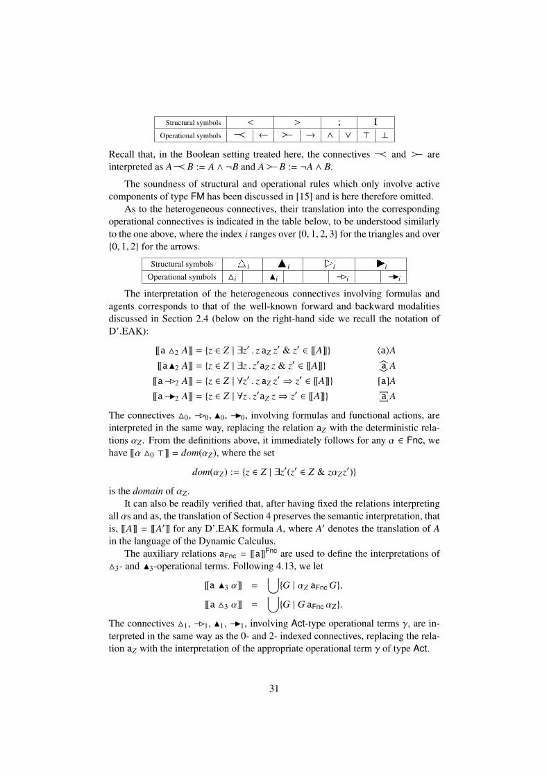
Structural symbols < > ; IOperational symbols ∧ ←

∧

→ ∧ ∨ > ⊥

Recall that, in the Boolean setting treated here, the connectives ∧ and

∧

areinterpreted as A ∧ B := A ∧ ¬B and A

∧

B := ¬A ∧ B.

The soundness of structural and operational rules which only involve activecomponents of type FM has been discussed in [15] and is here therefore omitted.

As to the heterogeneous connectives, their translation into the correspondingoperational connectives is indicated in the table below, to be understood similarlyto the one above, where the index i ranges over {0, 1, 2, 3} for the triangles and over{0, 1, 2} for the arrows.

Structural symbols 1i ai

1

i

a

iOperational symbols Mi Ni −Bi −Ii

The interpretation of the heterogeneous connectives involving formulas andagents corresponds to that of the well-known forward and backward modalitiesdiscussed in Section 2.4 (below on the right-hand side we recall the notation ofD’.EAK):

[[a M2 A]] = {z ∈ Z | ∃z′ . z aZ z′ & z′ ∈ [[A]]} 〈a〉A

[[aN2 A]] = {z ∈ Z | ∃z . z′aZ z & z′ ∈ [[A]]} 〈a

〉 A

[[a−B2 A]] = {z ∈ Z | ∀z′ . z aZ z′ ⇒ z′ ∈ [[A]]} [a]A

[[a−I2 A]] = {z ∈ Z | ∀z . z′aZ z⇒ z′ ∈ [[A]]} [a] A

The connectives M0, −B0, N0, −I0, involving formulas and functional actions, areinterpreted in the same way, replacing the relation aZ with the deterministic rela-tions αZ . From the definitions above, it immediately follows for any α ∈ Fnc, wehave [[α M0 >]] = dom(αZ), where the set

dom(αZ) := {z ∈ Z | ∃z′(z′ ∈ Z & zαZz′)}

is the domain of αZ .It can also be readily verified that, after having fixed the relations interpreting

all αs and as, the translation of Section 4 preserves the semantic interpretation, thatis, [[A]] = [[A′]] for any D’.EAK formula A, where A′ denotes the translation of Ain the language of the Dynamic Calculus.

The auxiliary relations aFnc = [[a]]Fnc are used to define the interpretations ofM3- and N3-operational terms. Following 4.13, we let

[[a N3 α]] =⋃{G | αZ aFnc G},

[[a M3 α]] =⋃{G | G aFnc αZ}.

The connectives M1, −B1, N1, −I1, involving Act-type operational terms γ, are in-terpreted in the same way as the 0- and 2- indexed connectives, replacing the rela-tion aZ with the interpretation of the appropriate operational term γ of type Act.

31

The soundness of all operational rules for heterogeneous connectives immedi-ately follows from the fact that their semantic counterparts as defined above aremonotone or antitone in each coordinate.

The soundness of the rule balance immediately follows from the fact that thefunctional actions are interpreted as deterministic relations (for more details cf.[15, Section 6.2]).

The soundness of the cut-rules follows from the transitivity of the inclusionrelation in the domain of interpretation of each type.

The soundness of the Atom axioms is argued similarly to that of the Atom ax-ioms of the system D’.EAK, crucially using the fact that epistemic actions do notchange the factual states of affairs (cf. [15, Section 6.2]).

The display rules (Mi, −Ii) and (N i, −Bi) for 0 ≤ i ≤ 2, and (M1, J−1) and(N1, C−1) are sound as the semantics of the triangle and arrow connectives formadjoint pairs.

On the other hand, in the display rules (M3, ∼I3), (N3, ∼B3), (Mi, J∼i) and(N i, C∼i) for i = 0, 2, 3, the arrow-connectives are what we call virtual adjoints(cf. Section 4), that is, they do not have a semantic interpretation. In the nextsection, we will account for the fact that their presence in the calculus is safe.

Soundness of necessitation, conjugation, Fischer Servi, and monotonicity rulesis straightforward and proved as in [15]. In the remainder of the section, we discussthe soundness of the new rules swap-in and swap-out recalled below.

Fact 5.1. The following defining clause for the interpretation of N1-operationalterms

[[γ N1 A]] = {z ∈ Z | ∃z . z′γZ z & z′ ∈ [[A]]}

immediately implies that the semantic interpretation of N1 is completely⋃

-preservingin its first coordinate.

Proof. If γZ =⋃

i∈I βi, then clearly z′γZz iff z′βiz′ for some i ∈ I. �

As to the soundness of swap-outL, assume that the structures a, F, X and Yhave been given the following interpretations, according to their type, as discussedabove: aZ ⊆ Z × Z, aFnc is a binary relation on graphs of partial functions on Z, FZ

is a functional relation on Z, and XZ ,YZ ⊆ Z. Let

aZ N3 FZ :=⋃{β | FZaFncβ}.

Assume that the premise of swap-outL is satisfied. That is:

aZN3FZ

〈

aZ

〉

XZ ⊆ YZ ,

where the symbols aZN3FZ and

〈

aZ

〉

denote the semantic diamond operations as-sociated with the converses of the relations aZ N 3FZ and aZ respectively. Then, thefollowing chain of equivalences holds:

32

aZN3FZ

〈

aZ

〉

XZ ⊆ YZ iff⋃{

〈

G

〉

〈

aZ

〉

XZ | FZaFnc G} ⊆ YZ (fact 5.1)

iff

〈

G

〉

〈

aZ

〉

XZ ⊆ YZ for every G s.t. FZaFnc G

iff XZ ⊆ [aZ][G]YZ for every G s.t. FZaFnc Giff XZ ⊆

⋂{[aZ][G]YZ | FZaFnc G}

hence XZ ⊆ (dom(FZ))c ∪⋂{[aZ][G]YZ | FZaFnc G}.

Consider the new variables p, q, a, α, and βi for each Gi such that FZaFncGi. Letus stipulate that [[p]] := XZ , [[q]] := YZ , [[a]] := aZ , [[α]] := FZ , and [[βi]] := Gi.Hence [[Pre(α)]] = [[α M0 >]] = dom(FZ). Therefore, the computation above cancontinue as follows:

XZ ⊆ (dom(FZ))c ∪⋂{[aZ][G]YZ | FZaFnc G}.

iff [[p]] ⊆ [[Pre(α)→∧{[a][β]q | αa β}]]

iff [[p]] ⊆ [[[α][a]q]]iff XZ ⊆ [FZ][aZ]YZ

iff

〈

aZ

〉

〈

FZ

〉

XZ ⊆ YZ

which completes the proof of the soundness of swap-outL. The proof of the sound-ness of the remaining swap-rules is similar.

6 Completeness and cut elimination

In 6.1, we discuss the completeness of the Dynamic Calculus w.r.t. the final coalge-bra semantics. We show that the translation (cf. Section 4) of each of the EAK ax-ioms is derivable in the Dynamic Calculus. Our proof is indirect, and relies on thefact that EAK is complete w.r.t. the final coalgebra semantics, and that the trans-lation preserves the semantic interpretation on the final coalgebra (as discussedin Section 5). In 6.2, we show that the Dynamic Calculus is quasi-properly dis-playable (cf. Section 3.2). By Theorem 3.3, this is enough to establish that thecalculus enjoys cut elimination and the subformula property.

6.1 Derivable rules and completeness

In what follows, a and α are atomic variables (and also the generic operationalterms) of type Ag and Fnc respectively, and A, B are generic operational terms oftype Fm. Since the reading is unambiguous, in the remainder of the present paperthe indexes of the heterogeneous connectives are dropped.Under the stipulations above, the translations of the rules reduce from D’.EAK

(cf. Section 2.4) can be derived in the Dynamic Calculus as follows.

33

α1 I ;α1 A ` XDis0M

α1 (I ; A) ` X

I ; A ` α

a

X

I ` α

a

X < A

A ` α

a

X

α1 A ` X

Also the translations of the comp rules are derivable in the Dynamic Calculus asfollows.

α1 (αa X) ` Y

αa X ` αa

Y

I ` αa X > α

a

Y

αa X ; I ` α

a

Y

α1 (αa X ; I) ` Yconj0M

X ;α1 I ` Y

α1 I ; X ` Y

Let us derive the axiom (4.14):

a ` a

a ` a α ` α

aaα ` aNα A ` A

(aNα)−B A ` (aaα)

1

A

a−B ((aNα)−B A) ` a

1

((aaα)

1

A)

aa (a−B ((aNα)−B A)) ` ((aaα)

1

A)

((aaα)a (aa (a−B ((aNα)−B A))) ` Aswap-outL

aa (αa (a−B ((aNα)−B A))) ` A

αa (a−B ((aNα)−B A)) ` a

1

A

αa (a−B ((aNα)−B A)) ` a−B A

a−B ((aNα)−B A) ` α

1

(a−B A)a−B ((aNα)−B A) ` α−B (a−B A)

Let us derive the axiom (4.15):

a ` a

A ` Aa ` a α ` α

aaα ` aNα

(aaα)1 A ` (aNα) M A

a1 ((aaα)1 A) ` a M ((aNα) M A)

(aaα)1 A ` (a

a

(a M ((aNα) M A)))

A ` (aaα)

a

(a

a

(a M ((aNα) M A)))swap-outR

A ` a

a

(α

a

(a M ((aNα) M A))

a1 A ` α

a

(a M ((aNα) M A)

a M A ` α

a

(a M ((aNα) M A)

α1 (a M A) ` a M ((aNα) M A)α M (a M A) ` a M ((aNα) M A)

A slight difference between the setting of [12] and the present setting is that inthat paper only the dynamic boxes are allowed in the object language, even if theirpropositional base is taken as non classical. In the present setting however, both the

34

dynamic boxes and diamonds are taken as primitive connectives. When moving toa propositional base which is weaker than the Boolean one, also the diamond/boxinteraction axioms such as the following one become primitive:

[α]〈a〉A↔ 1α →∨{〈a〉〈β〉A | αaβ}.

The axiom above translates as:

α−B (a M A)↔ α M > → a M ((aNα) M A).

α ` α

a ` a

a ` a α ` α

aaα ` aNα A ` A(aaα)1 A ` (aNα) M A

a1 ((aaα)1 A) ` a M ((aNα) M A)(aaα)1 A ` a

a

(a M ((aNα) M A))A ` (aaα)

a

(a

a

(a M ((aNα) M A)))swap-outR

A ` a

a

(α

a

(a M ((aNα) M A)))a1 A ` α

a

(a M ((aNα) M A))a M A ` α

a

(a M ((aNα) M A))α−B (a M A) ` α

1

(α

a

(a M ((aNα) M A)))αa (α−B (a M A)) ` α

a

(a M ((aNα) M A))I ` (αa (α−B (a M A))) > (α

a

(a M ((aNα) M A)))αa (α−B (a M A)) ; I ` α

a

(a M ((aNα) M A))α1 (αa (α−B (a M A)) ; I) ` a M ((aNα) M A)

conj0M(α−B (a M A)) ; (α1 I) ` a M ((aNα) M A)

α1 I ` (α−B (a M A)) > (a M ((aNα) M A))I ` α

a

(α−B (a M A)) > (a M ((aNα) M A))> ` α

a

(α−B (a M A)) > (a M ((aNα) M A))α1> ` (α−B (a M A)) > (a M ((aNα) M A))α M > ` (α−B (a M A)) > (a M ((aNα) M A))

(α−B (a M A)) ;α M > ` a M ((aNα) M A)α M > ; (α−B (a M A)) ` a M ((aNα) M A)

α−B (a M A) ` α M > > a M ((aNα) M A)α−B (a M A) ` α M > → a M ((aNα) M A)

For the other direction, recall that the counterpart of the rule reduce is derivablein the Dynamic Calculus 33:

35

α ` α I ` >α1 I ` α M >

a ` a A ` Aa1 A ` a M A

balanceα1 (a1 A) ` α

1

(a M A)a1 A ` α

a

(α

1

(a M A))A ` a

a

(α

a

(α

1

(a M A)))swap-inR

A ` (aaα)

a

(a

a

((α1 I) > (α1

(a M A))))(aaα)1 A ` a

a

((α1 I) > (α

1

(a M A)))aaα ` (a

a

((α1 I) > (α1

(a M A)))) a AaNα ` (a

a

((α1 I) > (α1

(a M A)))) a A(aNα)1 A ` a

a

((α1 I) > (α

1

(a M A)))(aNα) M A ` a

a

((α1 I) > (α

1

(a M A)))a1 ((aNα) M A) ` (α1 I) > (α

1

(a M A))reduceR

a1 ((aNα) M A) ` α1

(a M A)a M ((aNα) M A) ` α

1

(a M A)α M > → a M ((aNα) M A) ` α1 I > α

1

(a M A)reduceR

α M > → a M ((aNα) M A) ` α1

(a M A)α M > → a M ((aNα) M A) ` α−B (a M A)

The derivations (of the translations) of the remaining axioms have been relegatedto the appendix.

6.2 Belnap-style cut-elimination, and subformula property

In the present subsection, we prove that the Dynamic Calculus for EAK is a quasi-properly displayable calculus (cf. Section 3.2). By Theorem 3.3, this is enough toestablish that the calculus enjoys the cut elimination and the subformula property.Conditions C1, C2, C4, C’5, C’6, C’7 and C10 are straightforwardly verified byinspecting the rules and are left to the reader.

Condition C”5 can be straightforwardly argued by observing that the only ax-ioms to which a display postulate can be applied are of the atom form: Φp ` Ψp.In this case, the only applicable display postulates are those rewriting 1 - or a -structures into

a

- and

1

-structures and vice versa, which indeed preserve theatom shape. Condition C”8 is straightforwardly verified by inspection on the ax-ioms. Condition C’2 can be straightforwardly verified by inspection on the rules,for instance by observing that the domains and codomains of adjoints are rigidlydetermined.

The following proposition shows that condition C9 is met:

Proposition 6.1. Any derivable sequent in the Dynamic Calculus for EAK is type-uniform.

Proof. We prove the proposition by induction on the height of the derivation. Thebase case is verified by inspection; indeed, the following axioms are type-uniformby definition of their constituents:

a ` a α ` α Φp ` Ψp ⊥ ` I I ` >

36

As to the inductive step, one can verify by inspection that all the rules of the Dy-namic Calculus preserve type-uniformity, and that the Cut rules are strongly type-uniform. �

As to condition C’3, all parameters in all but the swap-in rules satisfy the con-dition of non-proliferation. In each swap-in rule, the parameters of type Ag andFnc in the premise are congruent to two parameters in the conclusion. However, itis not difficult to see that in each derivation, each application of any cut rule

...x ` a

...a ` y

x ` y

of type Ag or Fnc must be such that the structure x reduces to the atomic term a.Indeed, because the sequent x ` a is derivable, by Proposition 6.1 it must be typeuniform, that is, the structure x needs to be of type AG if a is, or of type FNC ifa is. If x was not atomic, then its main structural connective would be a squig-gly arrow 2∼ or b∼ . Because these connectives do not have any operationalcounterpart, such a structure cannot have been introduced by an application of anoperational rule. Hence, the only remaining possibility is that it has been intro-duced via a display postulate. But also this case is impossible, since in displaypostulates introduce these connectives only in the succedent, and x is in precedentposition. This finishes the verification of condition C’3.Finally, the verification steps for C’8 are collected in Section 9.1.

7 Conservativity

In the definition of the language of the Dynamic Calculus, we have adopted a ratherinclusive policy. That is, the operational language includes almost all the logicalsymbols which could be assigned a natural interpretation purely on the basis ofreasonable assumptions on the order-theoretic properties of the domains of inter-pretation of the various types of terms, the only exception being the connectivesJ1 and C1, which are excluded from the language although they are semanticallyjustified. A very useful and powerful consequence of the fact that the DynamicCalculus enjoys cut elimination Belnap-style is that this cut elimination is theninherited by the subcalculi corresponding to each fragment of the operational lan-guage of the Dynamic Calculus which verify as they stand the assumptions ofTheorem 3.3. However, the question is still open about whether these subcalculiinteract with each other in unwanted ways when their proof power is concerned:for any two such fragments L1 ⊆ L2, does the subcalculus corresponding to L2conservatively extend the one corresponding to L1? Typically, the absence of un-wanted interactions among subcalculi is deduced from having cut elimination, andsoundness and completeness w.r.t. a given semantics. This way, in [15] it is alsoshown that the system D’.EAK conservatively extends EAK.

37

However, this strategy is not immediately applicable to the setting of the Dy-namic Calculus, due to the structural symbols referred to as virtual adjoints, whichare easily recognizable, since they are shaped like arrows with a squiggly tail:b∼ , ∼4 etc. Virtual adjoints have no semantic justification, and hence, the rulesin which they specifically occur (that is, the display postulates relative to them)cannot be justified on semantic grounds. The reason for including virtual adjointsin the language of the Dynamic Calculus is for it to enjoy the relativized displayproperty, discussed in Section 2.3, which is key to guarantee the crucial condi-tion C’8, requiring the existence of a way to solve the principal stage of the cutelimination theorem (cf. Section 3.3, see also Section 9.1).

When discussing virtual adjoints in Section 4, we claimed that, since they areonly introduced in a derivation by way of display postulates and do not specificallyintervene in any other structural rule, their presence in the calculus does not addunwanted proof power compared to D’.EAK (and hence to EAK). This is the sensein which the introduction of the virtual adjoints can be regarded as syntacticallysound. The aim of the present section is to prove this claim.

A general and very powerful method for proving the conservativity of displaycalculi has been introduced in [5, 6] for the full intuitionistic linear logic. Thismethod involves no less than two translations, one from the given display calculusinto an intermediate shallow inference nested sequent calculus, and another onefrom the intermediate calculus into a deep inference nested sequent calculus. Thismethod is very intricate, requiring the verification of hundreds of cases which ac-count for every possible interaction between the shallow and the deep calculus. Theintricacy of this proof was such that the correctness of the results in [5, 6] has beenestablished by formalizing them in the proof assistant Isabelle/HOL, as reported in[11].

However, in the present section, a much smoother proof of conservativity isgiven for the Dynamic Calculus for EAK, which does not rely on any nested se-quent calculus. Rather, the proof below relies on very specific and uncommonfeatures of the design of the Dynamic Calculus for EAK. In a sense, the very factthat such a smooth proof is possible witnesses how uncommonly well behavedEAK is.

Definition 7.1. A sequent x ` y is severe if in the generation trees of either x or ythere are occurrences of structural connectives to which no display postulates canbe applied. Such occurrences will be referred to as severe.

Clearly, the definition above makes sense only in the context of calculi which,as is the case of the Dynamic Calculus, do not enjoy the full display property(cf. Definition 1). It can be easily verified that, in the specific case of the Dy-namic Calculus, there are only two types of severe occurrences: triangle-typeconnectives rooting a structure in succedent position, and arrow-type connectivesrooting a structure in precedent position. Examples of severe sequents then are(a

1

α)1 A ` B and A ` a1 B.

38

Lemma 7.2. Any rule in the Dynamic Calculus preserves the severity of sequents.That is, if a rule is applied to a severe sequent, the conclusion of that rule applica-tion is also severe.

Proof. By inspection on the rules. �

Fact 7.3. Let x ` y be a sequent of type AG or FNC, in the full language of DynamicCalculus, which is derivable by means of a derivation π in which no applicationof Weakening, Necessitation, Balance or Atom introduce occurrences of virtualadjoints. Then x = a for some operational term a of the appropriate type.

Proof. If x is not an atomic structure, then the grammar of AG and FNC prescribesthat x has a virtual adjoint as a main connective. However, the assumptions im-ply that such structures can be introduced only by way of applications of displaypostulates, which introduce them in succedent position. Hence, given the assump-tions, there is no way in which such a connective can be introduced in precedentposition. �

Lemma 7.4. Let X ` Y be a sequent of type FM which is derivable in the Dy-namic Calculus by means of a derivation π in which no application of Weakening,Necessitation, Balance or Atom introduce occurrences of virtual adjoints. Then aderivation π′ of X ` Y exists every node of which (hence the conclusion in particu-lar) is free of virtual adjoints.

Proof. Let s be some node/sequent in π where the given virtual adjoint has beenintroduced. Since virtual adjoints in the Dynamic Calculus are all virtual “right ad-joints”, and since, by assumption, they are introduced only by way of applicationsof display postulates, the given virtual adjoint is the main connective in the succe-dent of the sequent s. Moreover, virtual adjoints are main connectives of structuresof type AG and FNC. By type uniformity, this implies that the sequent s is eitherof type AG or FNC, and therefore s cannot be the conclusion of π. Some rule Rmust exist which takes s as a premise. It can be easily verified by inspection thatR cannot coincide with any structural rule in the Dynamic Calculus which is nei-ther a cut of the appropriate type nor a display postulate, since all structural rulesdifferent from Cut and display postulates have premises of type FM. We can alsoassume w.l.o.g. that R is not an application of Cut. Indeed, by Fact 7.3, s is of theform a ` x, with a being an operational term, and x being a non-atomic structureby assumption. Hence, if R was a Cut-application, the inference must be of theform

...y ` a

...a ` x

y ` x

Because Cut rules in the Dynamic Calculus are strongly type-regular, also y ` awould be a (derivable) sequent of type AG or FNC, hence Fact 7.3 applies to y `a. That is, y must be atomic, and because y ` a is derivable, y must coincide

39

with a. Hence, the conclusion of that Cut application is again s. This shows thatif R was Cut, w.l.o.g. we would be able remove that application from the prooftree. The remaining options are that R coincides with an introduction rule of someheterogeneous logical connective. Recall that, by Fact 7.3, s is of the form a ` x,where a is an operational term. Then, it can be verified by inspection that noheterogeneous rule is applicable if x is not an atomic structure, which is not thecase of the sequent s, as discussed above. Finally, since the left-hand side of s isatomic, no other display postulates are applicable to s but the converse directionof the same display postulate which had introduced the virtual adjoint and whichmakes it disappear. Therefore, the refinement π′ of π consists in removing thesedouble and redundant applications of display postulates. �

Lemma 7.5. If inf is an application of Balance, Atom, Necessitation or Weakeningin which some occurrence of a virtual adjoint is introduced, then the conclusion ofinf is a severe sequent.

Proof. As to Balance, Atom and Necessitationi with i = 0, 2, notice that each ofthese rules introduces a structure x of type FNC or AG in precedent position. Ifa virtual adjoint is introduced as a substructure of x, then x is non-atomic, and itcan be immediately verified by inspecting the syntax of FNC and AG that the mainconnective of x is an arrow-type connective, which would then be in precedentposition. Hence, the resulting sequent is severe.

As to Weakening and Necessitation1, notice that these rules introduce struc-tures x of type FM and ACT respectively. Recall that virtual adjoints root structuresof type FNC or AG. Hence, if some virtual adjoint occurs in the generation tree ofx, it cannot occur at the root of x. Hence, the virtual adjoint must occur in the scopeof some other structural connective. Notice that the heterogeneous connectives arethe only ones which can take as argument a structure rooted in a virtual adjoint.We claim that either the virtual adjoint occurs in precedent position (which wouldbe enough to conclude that the conclusion of inf is severe), or under the scope ofsome structural connective to which no display postulate can be applied. Assumethat the virtual adjoint occurs in succedent position. If its immediate ancestor inthe generation tree of X is a triangle-type connective, then these connectives arein succedent position too, and hence no display postulate can be applied to them,which makes the conclusion of inf severe, as required. Similarly, if the immedi-ate ancestor of the virtual adjoint is an arrow-type connective, then it can be easilychecked by inspection that these connectives take structures of type FNC or AG ex-clusively in their antitone coordinate (that is, on the flat side of the arrow). Hence,the arrow-type connective is in precedent position, and hence no display postulatecan be applied to it, as required. �

Corollary 7.6. Let A′ ` B′ be a sequent of type Fm in the language of the DynamicCalculus, such that A′ and B′ are, respectively, images of some D’.EAK-formulasA and B under the translation of Section 4. If A′ ` B′ is derivable in the DynamicCalculus, then A ` B is derivable in D’.EAK.

40

Proof. Let π be a derivation of A′ ` B′ in the Dynamic Calculus. By assump-tion, A′ ` B′ is not severe. Hence, no rule application in π can introduce severesequents, since these, by Lemma 7.2, would then propagate till the conclusion.Hence in particular, by Lemma 7.5, in π there cannot be any applications of Bal-ance, Atom, Necessitation or Weakening in which some occurrence of a virtualadjoint is introduced. Therefore, by Lemma 7.4, a derivation π′ of A′ ` B′ existsin which no virtual adjoints occur. By the results collected in Section 5, the deriva-tion π′ is sound w.r.t. the final coalgebra semantics. Hence A′ ` B′ is satisfied onthe final coalgebra semantics. Since, as discussed in Section 5, [[A]] = [[A′]] and[[B]] = [[B′]], this implies that A ` B is satisfied. Since D’.EAK is complete w.r.t.the final coalgebra semantics, a D’.EAK-derivation of A ` B exists. �

8 Conclusions and further directions

The present paper is part of a line of research aimed at developing adequate proof-calculi for dynamic logics. These logics have proven to be very difficult to treatwith standard proof-theoretic tools, due to the very features which characterizethem and make them applicable to diverse fields of science, spanning from arti-ficial intelligence to social science and economics. A central desideratum in thisline of research is the development of methods which apply uniformly to differ-ent logics, and which allow a smooth transfer of results from one logic to another.The framework of display calculi has successfully met this desideratum for wideclasses of logics in the family of modal and substructural logics. In particular, inthe framework of display calculi it is possible to state and prove metatheoremswhich guarantee any given proof system to enjoy the all-important cut eliminationproperty, provided it meets certain conditions on its design.

The main contribution of the present paper is the definition of a display cal-culus which smoothly encompasses the most proof-theoretically impervious fea-tures of Baltag Moss and Solecki’s logic of epistemic actions and knowledge.Besides being well performing (it adequately captures EAK and enjoys Belnap-style cut elimination), this calculus provides an interesting and in our opinion verypromising methodological platform towards the uniform development of a generalproof-theoretic account of all dynamic logics, and also, from a purely structurallyproof-theoretic viewpoint, for clarifying and sharpening the formulation of criterialeading to the statement and proof of meta-theoretic results such as Belnap-stylecut-elimination, or conservativity issues.

Seminal approaches. The starting point of this methodology is to introduceenough syntactic devices, both at the operational and at the structural level, so thatthe parameters indexing logical connectives can be accounted for in the system asterms in the language of choice. This gives rise to the definition of multi-type lan-guages, endowed with connectives which manage the interaction of the differenttypes. This approach appears seminally in both [1] and [12]; however, in neither

41

paper it is fully explored: in [1] there is no theory of contexts governing the in-teraction of different types, and in [12], this interaction is clarified, but only at themetalinguistic level.

Multi-type calculus for PDL. The multi-type approach has been applied to PDLin [14]. In that setting, introducing two separate types for transitive actions and forgeneral actions makes it possible to overcome the big hurdle given by the fact thatthe induction axiom features occurrences of the same formula in precedent and insuccedent position, which makes it is severely non amenable to the treatment instandard display calculi. Another interesting case study is given by Parikh’s gamelogic, which is ongoing work [13].

Refinements of Belnap’s conditions, and type-uniformity. The multi-type set-ting will hopefully prove to be conceptually advantageous to achieve a better graspand a simpler statement of Wansing’s and Belnap’s regularity requirements (cf.conditions C6/C7 in [28], [4, Section 2]) for the Belnap-style cut elimination, viathe notion of type-uniformity (Definition 3.1). In [3], Belnap motivates his condi-tion C7

11 saying that “rules need not be wholly closed under substitution of struc-tures for congruent formulas which are antecedent parts, but they must be closedenough.” Then he explains that closed enough refers to the closure under sub-stitution of formulas A for structures X such that a derivation is available in thesystem for the sequent X ` A, in which the occurrence of A in the conclusion isprincipal. The crucial observation is that, even if a system is not defined a priorias multi-type, it can be regarded as a multi-type setting: indeed, the type of A canbe defined as consisting of all the structures X such that the shape of derivation al-luded to above exists. Then, condition C6/C7 can be equivalently reformulated asthe requirement that rules should be closed under uniform substitution within eachtype. Notice that, under the stipulations above, different types must be separatedby at least one structural rule. For instance, in the Dynamic Calculus for EAK, therule balance separates Fnc from Act. In conclusion, our conjecture is that Wans-ing’s and Belnap’s conditions C6/C7 boil down to a type-uniformity requirement ina context in which types are not given explicitly. The observations above indicatethat type-uniformity is a desirable design requirement for general dynamic calculi,and in particular for the development of an adequate proof theory for dynamiclogics, particularly in view of a uniform path to Belnap-style cut-elimination.

Non-proliferation. Our analysis towards Belnap-style cut elimination led us torefine and weaken various aspects of the cut elimination metatheorem. For in-stance, the requirement of non-proliferation of parameters for quasi-properly dis-playable multi-type calculi applies only to types the grammar of which is rich

11Recall that Belnap’s condition C7 corresponds to Wansing’s cons-regularity for formulas occur-ring in precedent position. An analogous explanation holds of course for the ant-regularity conditionof formulas in succedent position.

42

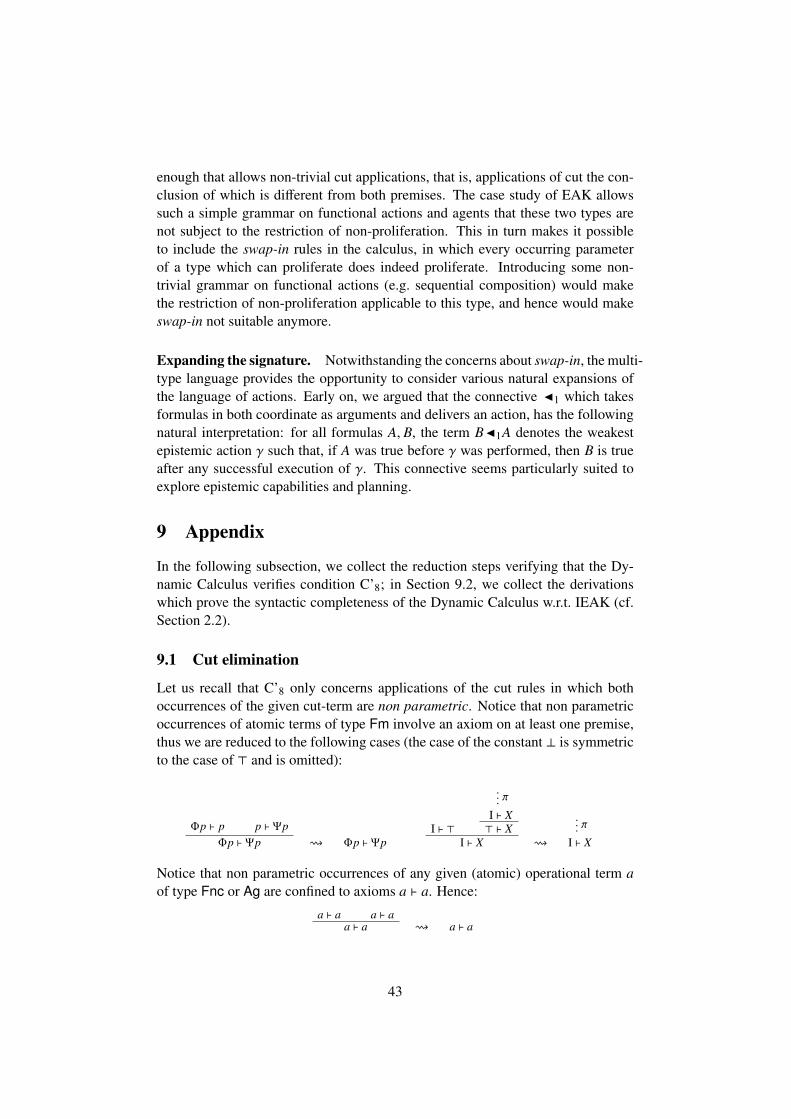
enough that allows non-trivial cut applications, that is, applications of cut the con-clusion of which is different from both premises. The case study of EAK allowssuch a simple grammar on functional actions and agents that these two types arenot subject to the restriction of non-proliferation. This in turn makes it possibleto include the swap-in rules in the calculus, in which every occurring parameterof a type which can proliferate does indeed proliferate. Introducing some non-trivial grammar on functional actions (e.g. sequential composition) would makethe restriction of non-proliferation applicable to this type, and hence would makeswap-in not suitable anymore.

Expanding the signature. Notwithstanding the concerns about swap-in, the multi-type language provides the opportunity to consider various natural expansions ofthe language of actions. Early on, we argued that the connective J1 which takesformulas in both coordinate as arguments and delivers an action, has the followingnatural interpretation: for all formulas A, B, the term BJ1A denotes the weakestepistemic action γ such that, if A was true before γ was performed, then B is trueafter any successful execution of γ. This connective seems particularly suited toexplore epistemic capabilities and planning.

9 Appendix

In the following subsection, we collect the reduction steps verifying that the Dy-namic Calculus verifies condition C’8; in Section 9.2, we collect the derivationswhich prove the syntactic completeness of the Dynamic Calculus w.r.t. IEAK (cf.Section 2.2).

9.1 Cut elimination

Let us recall that C’8 only concerns applications of the cut rules in which bothoccurrences of the given cut-term are non parametric. Notice that non parametricoccurrences of atomic terms of type Fm involve an axiom on at least one premise,thus we are reduced to the following cases (the case of the constant ⊥ is symmetricto the case of > and is omitted):

Φp ` p p ` ΨpΦp ` Ψp Φp ` Ψp

I ` >

... π

I ` X> ` X

I ` X

... π

I ` X

Notice that non parametric occurrences of any given (atomic) operational term aof type Fnc or Ag are confined to axioms a ` a. Hence:

a ` a a ` aa ` a a ` a

43

In each case above, the cut in the original derivation is strongly uniform by as-sumption, and is eliminated by the transformation. As to cuts on non atomic terms,let us restrict our attention to those cut-terms the main connective of which isMi, Ni , −B i, −I i for 0 ≤ i ≤ 3 (the remaining operational connectives are straight-forward and left to the reader).

... π0

x ` a

... π1

y ` b

x1i y ` a Mi b

... π2

a1i b ` za Mi b ` z

x1i y ` z

... π1

y ` b

... π0

x ` a

... π2

a1i b ` z

a ` zb∼i b

x ` zb∼i bx1i b ` z

b ` x

a

i z

y ` x

a

i z

x1i y ` z

... π1

y ` a1

i by ` a−Bi b

... π0

x ` a

... π2

b ` za−Bi b ` x

1

i z

y ` x

1

i z

... π0

x ` a

... π1

y ` a

1

i b

aai y ` b

a ` b2∼i y

x ` b2∼i y

xai y ` b

... π2

b ` z

xai y ` z

y ` x

1

i z

... π0

x ` a

... π1

y ` b

xai y ` aNi b

... π2

aai b ` zaNi b ` z

xai y ` z

... π1

y ` b

... π0

x ` a

... π2

aai b ` z

a ` z2∼i b

x ` z2∼i bxai b ` z

b ` x

1

i z

y ` x

1

i z

xai y ` z

... π1

y ` a

a

i by ` a−Ii b

... π0

x ` a

... π2

b ` za−Ii b ` x

a

i z

y ` x

a

i z

... π0

x ` a

... π1

y ` a

a

i b

a1i y ` b

a ` bb∼i y

x ` bb∼i y

x1i y ` b

... π2

b ` z

x1i y ` z

y ` x

a

i z

44

In each case above, the cut in the original derivation is strongly uniform by as-sumption, and after the transformation, cuts of lower complexity are introducedwhich can be easily verified to be strongly uniform for each 0 ≤ i ≤ 3.

9.2 Completeness

To prove the completeness of the Dynamic Calculus it is enough to show that all theaxioms and rules of H.IEAK are theorems and, respectively, derived or admissiblerules of Dynamic Calculus. Below we show the derivations of the dynamic axioms.

• α M p a` (α M >) ∧ p

α ` α I ` >α1 I ` α M > α1 p ` p

(α1 I) ; (α1 p) ` (α M >) ∧ p

α1 (I ; p) ` (α M >) ∧ p

I ; p ` αa

(α M >) ∧ p

p ` αa

(α M >) ∧ p

α1 p ` (α M >) ∧ pα M p ` (α M >) ∧ p

α ` α

αa p ` p

I ` (αa p) > p

> ` (αa p) > p

(αa p) ;> ` p

α1 ((αa p) ;>) ` α M p

(α1>) ; p ` α M p

α1> ` α M p < pα M > ` p > α M p

α M > ; p ` α M p(α M >) ∧ p ` α M p

• α−B p a` (α M >)→ p

α ` α p ` α

a

p

α−B p ` α

1

(α

a

p)

αaα−B p ` α

a

p

I ` (αaα−B p) > α

a

p

> ` (αaα−B p) > α

a

p

(αaα−B p) ;> ` α

a

p

α1 ((αaα−B p) ;>) ` p

α−B p ;α1> ` pα M > ` α−B p > p

α−B p ;α M > ` pα M > ;α−B p ` p

α−B p ` α M > > pα−B p ` (α M >)→ p

α ` α I ` >α1 I ` α M > p ` α

1

p

(α M >)→ p ` (α1 I) > α

1

p

(α M >)→ p ` α

1

(I > p)

αa (α M >)→ p ` I > p

αa (α M >)→ p ` p

(α M >)→ p ` α

1

p(α M >)→ p ` α−B p

• 〈α〉> a` 1α α M > a` α M >

α ` α > ` >

α1> ` α M >

α M > ` α M >

45

• α−B⊥ a` α M > → ⊥

α ` α

⊥ ` I⊥ ` α

a

I

α−B⊥ ` α

1

(α

a

I)

αa (α−B⊥) ` α

a

I

I ` αa (α−B⊥) > α

a

I

> ` αa (α−B⊥) > α

a

I

αa (α−B⊥) ;> ` α

a

I

α1 (αa (α−B⊥) ;>) ` I

α−B⊥ ; (α1>) ` I

α−B⊥ ; (α1>) ` ⊥

α1> ` α−B⊥ > ⊥

α M > ` α−B⊥ > ⊥α−B⊥ ;α M > ` ⊥α M > ;α−B⊥ ` ⊥

α−B⊥ ` α M > > ⊥α−B⊥ ` α M > → ⊥

α ` α I ` >α1 I ` α M >

⊥ ` I⊥ ` α

1

I

αa⊥ ` I

αa⊥ ` ⊥

⊥ ` α

1

⊥

α M > → ⊥ ` α1 I > α

1

⊥

α M > → ⊥ ` α

1

(I > ⊥)

αa (α M > → ⊥) ` I > ⊥

I;αa (α M > → ⊥) ` ⊥

I ` ⊥ < αa (α M > → ⊥)

αa (α M > → ⊥) ` ⊥

α M > → ⊥ ` α

1

⊥

α M > → ⊥ ` α−B⊥

• α M ⊥ a` ⊥

⊥ ` I⊥ ` α

a

I

α1⊥ ` Iα M ⊥ ` Iα M ⊥ ` ⊥

⊥ ` I⊥ ` α M ⊥

• α−B> a` >

I ` >α−B> ` >

I ` >αa I ` >

I ` α

1

>

> ` α

1

>

αa> ` >

> ` α

1

>

> ` α−B>

• α−B (A ∧ B) a` α−B A ∧ α−B B

α ` α

A ` AA ; B ` A

A ∧ B ` Aα−B (A ∧ B) ` α

1

Aα−B (A ∧ B) ` α−B A

α ` α

B ` BA ; B ` B

A ∧ B ` Bα−B (A ∧ B) ` α

1

Bα−B (A ∧ B) ` α−B B

α−B (A ∧ B) ;α−B (A ∧ B) ` α−B A ∧ α−B Bα−B (A ∧ B) ` α−B A ∧ α−B B

α ` α A ` Aα−B A ` α

1

Aαa (α−B A) ` A

α ` α B ` Bα−B B ` α

1

Bαa (α−B B) ` B

αa (α−B A) ;αa (α−B B) ` A ∧ Bαa (α−B A ;α−B B) ` A ∧ B

α−B A ;α−B B ` α

1

(A ∧ B)α−B A ∧ α−B B ` α−B (A ∧ B)

46

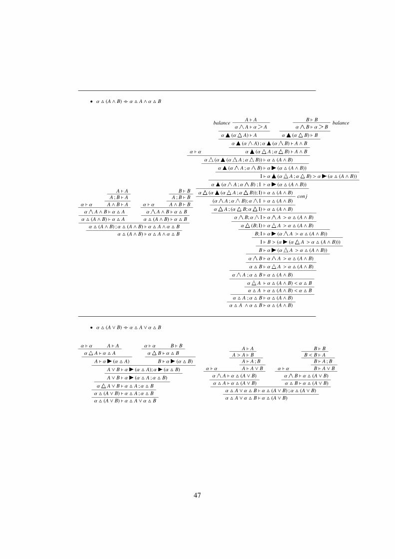
• α M (A ∧ B) a` α M A ∧ α M B

α ` α

A ` AA ; B ` A

A ∧ B ` Aα1 A ∧ B ` α M Aα M (A ∧ B) ` α M A

α ` α

B ` BA ; B ` B

A ∧ B ` Bα1 A ∧ B ` α M Bα M (A ∧ B) ` α M B

α M (A ∧ B) ;α M (A ∧ B) ` α M A ∧ α M Bα M (A ∧ B) ` α M A ∧ α M B

α ` α

A ` Abalance

α1 A ` α

1

A

αa (α1 A) ` A

B ` Bbalance

α1 B ` α

1

B

αa (α1 B) ` B

αa (α1 A) ;αa (α1 B) ` A ∧ B

αa (α1 A ;α1 B) ` A ∧ B

α1 (αa (α1 A ;α1 B)) ` α M (A ∧ B)

αa (α1 A ;α1 B) ` α

a

(α M (A ∧ B))

I ` αa (α1 A ;α1 B) > α

a

(α M (A ∧ B))

αa (α1 A ;α1 B) ; I ` α

a

(α M (A ∧ B))

α1 (αa (α1 A ;α1 B)); I) ` α M (A ∧ B)con j

(α1 A ;α1 B);α1 I ` α M (A ∧ B)

α1 A ; (α1 B;α1 I) ` α M (A ∧ B)

α1 B;α1 I ` α1 A > α M (A ∧ B)

α1 (B; I) ` α1 A > α M (A ∧ B)

B; I ` α

a

(α1 A > α M (A ∧ B))

I ` B > (α

a

(α1 A > α M (A ∧ B)))

B ` α

a

(α1 A > α M (A ∧ B))

α1 B ` α1 A > α M (A ∧ B)

α M B ` α1 A > α M (A ∧ B)

α1 A ;α M B ` α M (A ∧ B)

α1 A ` α M (A ∧ B) < α M Bα M A ` α M (A ∧ B) < α M B

α M A ;α M B ` α M (A ∧ B)α M A ∧ α M B ` α M (A ∧ B)

• α M (A ∨ B) a` α M A ∨ α M B

α ` α A ` Aα1 A ` α M A

A ` α

a

(α M A)

α ` α B ` Bα1 B ` α M B

B ` α

a

(α M B)

A ∨ B ` α

a

(α M A);α

a

(α M B)

A ∨ B ` α

a

(α M A ;α M B)

α1 A ∨ B ` α M A ;α M Bα M (A ∨ B) ` α M A ;α M Bα M (A ∨ B) ` α M A ∨ α M B

α ` α

A ` AA > A ` B

A ` A ; BA ` A ∨ B

α1 A ` α M (A ∨ B)α M A ` α M (A ∨ B)

α ` α

B ` BB < B ` A

B ` A ; BB ` A ∨ B

α1 B ` α M (A ∨ B)α M B ` α M (A ∨ B)

α M A ∨ α M B ` α M (A ∨ B) ;α M (A ∨ B)α M A ∨ α M B ` α M (A ∨ B)

47

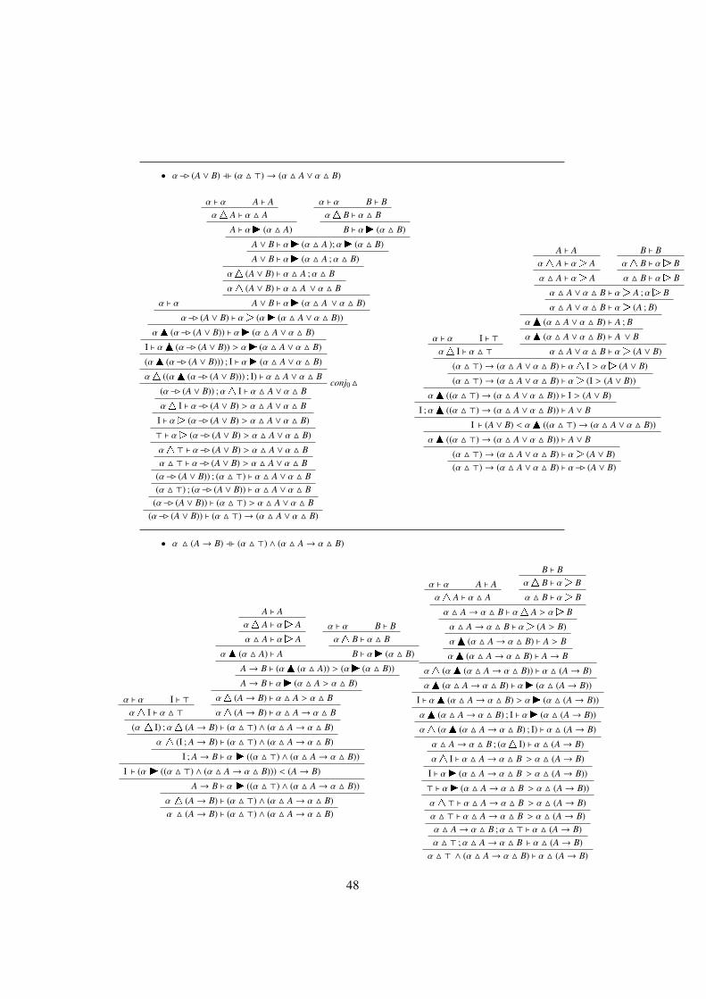
• α−B (A ∨ B) a` (α M >)→ (α M A ∨ α M B)

α ` α

α ` α A ` Aα1 A ` α M A

A ` α

a

(α M A)

α ` α B ` Bα1 B ` α M B

B ` α

a

(α M B)

A ∨ B ` α

a

(α M A );α

a

(α M B)

A ∨ B ` α

a

(α M A ;α M B)

α1 (A ∨ B) ` α M A ;α M B

α1 (A ∨ B) ` α M A ∨ α M B

A ∨ B ` α

a

(α M A ∨ α M B)

α−B (A ∨ B) ` α

1

(α

a

(α M A ∨ α M B))

αa (α−B (A ∨ B)) ` α

a

(α M A ∨ α M B)

I ` αa (α−B (A ∨ B)) > α

a

(α M A ∨ α M B)

(αa (α−B (A ∨ B))) ; I ` α

a

(α M A ∨ α M B)

α1 ((αa (α−B (A ∨ B))) ; I) ` α M A ∨ α M Bconj0M

(α−B (A ∨ B)) ;α1 I ` α M A ∨ α M B

α1 I ` α−B (A ∨ B) > α M A ∨ α M B

I ` α

1

(α−B (A ∨ B) > α M A ∨ α M B)

> ` α

1

(α−B (A ∨ B) > α M A ∨ α M B)

α1> ` α−B (A ∨ B) > α M A ∨ α M Bα M > ` α−B (A ∨ B) > α M A ∨ α M B

(α−B (A ∨ B)) ; (α M >) ` α M A ∨ α M B(α M >) ; (α−B (A ∨ B)) ` α M A ∨ α M B

(α−B (A ∨ B)) ` (α M >) > α M A ∨ α M B(α−B (A ∨ B)) ` (α M >)→ (α M A ∨ α M B)

α ` α I ` >α1 I ` α M >

A ` Aα1 A ` α

1

A

α M A ` α

1

A

B ` Bα1 B ` α

1

B

α M B ` α

1

B

α M A ∨ α M B ` α

1

A ;α

1

B

α M A ∨ α M B ` α

1

(A ; B)

αa (α M A ∨ α M B) ` A ; B

αa (α M A ∨ α M B) ` A ∨ B

α M A ∨ α M B ` α

1

(A ∨ B)

(α M >)→ (α M A ∨ α M B) ` α1 I > α

1

(A ∨ B)

(α M >)→ (α M A ∨ α M B) ` α

1

(I > (A ∨ B))

αa ((α M >)→ (α M A ∨ α M B)) ` I > (A ∨ B)

I ;αa ((α M >)→ (α M A ∨ α M B)) ` A ∨ B

I ` (A ∨ B) < αa ((α M >)→ (α M A ∨ α M B))

αa ((α M >)→ (α M A ∨ α M B)) ` A ∨ B

(α M >)→ (α M A ∨ α M B) ` α

1

(A ∨ B)(α M >)→ (α M A ∨ α M B) ` α−B (A ∨ B)

• α M (A→ B) a` (α M >) ∧ (α M A→ α M B)

α ` α I ` >α1 I ` α M >

A ` Aα1 A ` α

1

A

α M A ` α

1

A

αa (α M A) ` A

α ` α B ` Bα1 B ` α M B

B ` α

a

(α M B)

A→ B ` (αa (α M A)) > (α

a

(α M B))

A→ B ` α

a

(α M A > α M B)

α1 (A→ B) ` α M A > α M B

α1 (A→ B) ` α M A→ α M B

(α 1 I) ;α1 (A→ B) ` (α M >) ∧ (α M A→ α M B)

α 1 (I ; A→ B) ` (α M >) ∧ (α M A→ α M B)

I ; A→ B ` α

a

((α M >) ∧ (α M A→ α M B))

I ` (α

a

((α M >) ∧ (α M A→ α M B))) < (A→ B)

A→ B ` α

a

((α M >) ∧ (α M A→ α M B))

α 1 (A→ B) ` (α M >) ∧ (α M A→ α M B)α M (A→ B) ` (α M >) ∧ (α M A→ α M B)

α ` α A ` Aα1 A ` α M A

B ` Bα1 B ` α

1

B

α M B ` α

1

B

α M A→ α M B ` α1 A > α

1

B

α M A→ α M B ` α

1

(A > B)

αa (α M A→ α M B) ` A > B

αa (α M A→ α M B) ` A→ B

α1 (αa (α M A→ α M B)) ` α M (A→ B)

αa (α M A→ α M B) ` α

a

(α M (A→ B))

I ` αa (α M A→ α M B) > α

a

(α M (A→ B))

αa (α M A→ α M B) ; I ` α

a

(α M (A→ B))

α1 (αa (α M A→ α M B) ; I) ` α M (A→ B)

α M A→ α M B ; (α1 I) ` α M (A→ B)

α1 I ` α M A→ α M B > α M (A→ B)

I ` α

a

(α M A→ α M B > α M (A→ B))

> ` α

a

(α M A→ α M B > α M (A→ B))

α1> ` α M A→ α M B > α M (A→ B)α M > ` α M A→ α M B > α M (A→ B)α M A→ α M B ;α M > ` α M (A→ B)α M > ;α M A→ α M B ` α M (A→ B)α M > ∧ (α M A→ α M B) ` α M (A→ B)

48

• α−B (A→ B) a` α M A → α M B

α ` α

A ` Aα1 A ` α

1

A

αa (α1 A) ` A

α ` α B ` Bα1 B ` α M B

B ` α

a

(α M B)

A→ B ` αa (α1 A) > α

a

(α M B)

A→ B ` α

a

(α1 A > α M B)

α−B (A→ B) ` α

1

(α

a

(α1 A > α M B))

αa (α−B (A→ B) ` α

a

(α1 A > α M B)

I ` αa (α−B (A→ B) > α

a

(α1 A > α M B)

αa (α−B (A→ B) ; I ` α

a

(α1 A > α M B)

α1 (αa (α−B (A→ B) ; I) ` α1 A > α M Bcon j

α−B (A→ B) ; (α1 I) ` α1 A > α M B

(α1 I) ;α−B (A→ B) ` α1 A > α M B

α1 A ; ((α1 I) ;α−B (A→ B)) ` α M B

(α1 A ; (α1 I)) ;α−B (A→ B) ` α M B

α1 A ; (α1 I) ` α M B < α−B (A→ B)

α1 (A ; I) ` α M B < α−B (A→ B)

A ; I ` α

a

(α M B < α−B (A→ B))

I ` A > (α

a

(α M B < α−B (A→ B)))

A ` α

a

(α M B < α−B (A→ B))

α1 A ` α M B < α−B (A→ B)α M A ` α M B < α−B (A→ B)α M A ` α M B < α−B (A→ B)

α M A ;α−B (A→ B) ` α M Bα−B (A→ B) ` α M A > α M Bα−B (A→ B) ` α M A → α M B

α ` α A ` Aα1 A ` α M A

α ` α B ` Bα1 B ` α

1

B

α M B ` α

1

B

α M A→ α M B ` α1 A > α

1

B

α M A→ α M B ` α

1

(A > B)

αa (α M A→ α M B) ` A > B

αa (α M A→ α M B) ` A→ B

α M A→ α M B ` α

1

A→ Bα M A→ α M B ` α−B (A→ B)

49

• 1α ∧∨{〈a〉〈β〉A |αaβ} ` 〈α〉〈a〉A (α M > ) ∧ (a M ((aNα) M A)) ` α M (a M A)

α ` α

a ` a A ` Aa1 A ` a M A

α1 (a1 A) ` α M (a M A)a1 A ` α

a

(α M (a M A))A ` a

a

(α

a

(α M (a M A)))swap-inR

A ` (aaα)

a

(a

a

((α1 I) > (α M (a M A))))(aaα)1 A ` a

a

((α1 I) > (α M (a M A)))aaα ` (a

a

((α1 I) > (α M (a M A)))) a AaNα ` (a

a

((α1 I) > (α M (a M A)))) a A(aNα) M A ` a

a

((α1 I) > (α M (a M A)))a1 ((aNα) M A) ` (α1 I) > (α M (a M A))a M ((aNα) M A) ` (α1 I) > (α M (a M A))

(α1 I); (a M ((aNα) M A)) ` α M (a M A)α1 I ` (α M (a M A)) < (a M ((aNα) M A))

I ` α

a

((α M (a M A)) < (a M ((aNα) M A)))> ` α

a

((α M (a M A)) < (a M ((aNα) M A)))α1> ` (α M (a M A)) < (a M ((aNα) M A))α M > ` (α M (a M A)) < (a M ((aNα) M A))

(α M >); (a M ((aNα) M A)) ` α M (a M A)(α M >) ∧ (a M ((aNα) M A)) ` α M (a M A)

• [α][a]A ` Pre(α)→∧{[a][β]A |αaβ} α−B (a−B A) ` (α M >)→ (a−B ((aNα)−B A))

α ` α

a ` a A ` Aa−B A ` a

1

Aα−B (a−B A) ` α

1

(a

1

A)αa (α−B (a−B A)) ` a

1

Aaa (αa (α−B (a−B A))) ` A

swap-inL(aaα)a (aa ((α1 I); (α−B (a−B A)))) ` A

aaα ` A 1 (aa ((α1 I); (α−B (a−B A))))aNα ` A 1 (aa ((α1 I); (α−B (a−B A))))

(aNα)a (aa ((α1 I); (α−B (a−B A)))) ` Aaa ((α1 I); (α−B (a−B A))) ` (aNα)

1

Aaa ((α1 I); (α−B (a−B A))) ` (aNα)−B A

(α1 I); (α−B (a−B A)) ` a

1

((aNα)−B A)(α1 I); (α−B (a−B A)) ` a−B ((aNα)−B A)

α1 I ` (a−B ((aNα)−B A)) < (α−B (a−B A))I ` α

a

((a−B ((aNα)−B A)) < (α−B (a−B A)))> ` α

a

((a−B ((aNα)−B A)) < (α−B (a−B A)))α1> ` (a−B ((aNα)−B A)) < (α−B (a−B A))α M > ` (a−B ((aNα)−B A)) < (α−B (a−B A))

(α M >); (α−B (a−B A)) ` a−B ((aNα)−B A)(α−B (a−B A)) ` (α M >) > (a−B ((aNα)−B A))(α−B (a−B A)) ` (α M >)→ (a−B ((aNα)−B A))

50

• 〈α〉[a]A ` Pre(α) ∧∧{[a][β]A |αaβ} α M (a−B A) ` (α M >) ∧ (a−B ((aNα)−B A))

α ` α I ` >α1 I ` α M >

a ` a A ` Aa−B A ` a

1

Abalance

α1 (a−B A) ` α1

(a

1

A)

αa (α1 (a−B A)) ` a1

A

aa (αa (α1 (a−B A))) ` Aswap-inL

(aaα)a (aa ((α1 I); (α1 (a−B A)))) ` A

aaα ` A a (aa ((α1 I); (α1 (a−B A))))

aNα ` A a (aa ((α1 I); (α1 (a−B A))))

(aNα)a (aa ((α1 I); (α1 (a−B A)))) ` A

aa ((α1 I); (α1 (a−B A))) ` (aNα)

1

A

aa ((α1 I); (α1 (a−B A))) ` (aNα)−B A

(α1 I); (α1 (a−B A)) ` a

1

((aNα)−B A)

(α1 I); (α1 (a−B A)) ` a−B ((aNα)−B A)reduce′L

α1 (a−B A) ` a−B ((aNα)−B A)

(α1 I); (α1 (a−B A)) ` (α M >) ∧ (a−B ((aNα)−B A))reduce′L

α1 (a−B A) ` (α M >) ∧ (a−B ((aNα)−B A))α M (a−B A) ` (α M >) ∧ (a−B ((aNα)−B A))

• Pre(α) ∧∧{[a][β]A |αaβ} ` 〈α〉[a]A (α M >) ∧ a−B ((aNα)−B A) ` α M (a−B A)

α ` α

a ` a

a ` a α ` α

aaα ` aNα A ` A

(aNα)−B A ` (aaα)

1

A

a−B ((αNα)−B A) ` a

1

((aaα)

1

A)

aa (a−B ((αNα)−B A)) ` (aaα)

1

A

(aaα)a (aa (a−B ((αNα)−B A))) ` Aswap-outLaa (αa (a−B ((αNα)−B A))) ` A

αa (a−B ((αNα)−B A)) ` a

1

A

αa (a−B ((αNα)−B A)) ` a−B A

I ` αa (a−B ((αNα)−B A)) > a−B A

αa (a−B ((αNα)−B A)) ; I ` a−B A

α1 (αa (a−B ((αNα)−B A)) ; I) ` α M (a−B A)con j0M

a−B ((αNα)−B A) ; (α1 I) ` α M (a−B A)

α1 I ` a−B ((αNα)−B A) > α M (a−B A)

I ` α

a

(a−B ((αNα)−B A) > α M (a−B A))

> ` α

a

(a−B ((αNα)−B A) > α M (a−B A))

α1> ` a−B ((αNα)−B A) > α M (a−B A)α M > ` a−B ((αNα)−B A) > α M (a−B A)

a−B ((αNα)−B A) ;α M > ` α M (a−B A)(α M >) ; a−B ((aNα)−B A) ` α M (a−B A)

(α M >) ∧ a−B ((aNα)−B A) ` α M (a−B A)

51

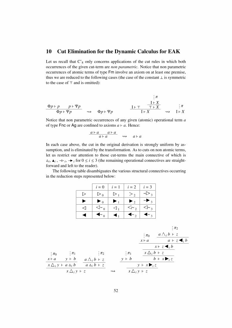
10 Cut Elimination for the Dynamic Calculus for EAK

Let us recall that C’8 only concerns applications of the cut rules in which bothoccurrences of the given cut-term are non parametric. Notice that non parametricoccurrences of atomic terms of type Fm involve an axiom on at least one premise,thus we are reduced to the following cases (the case of the constant ⊥ is symmetricto the case of > and is omitted):

Φp ` p p ` ΨpΦp ` Ψp Φp ` Ψp

I ` >

... π

I ` X> ` X

I ` X

... π

I ` X

Notice that non parametric occurrences of any given (atomic) operational term aof type Fnc or Ag are confined to axioms a ` a. Hence:

a ` a a ` aa ` a a ` a

In each case above, the cut in the original derivation is strongly uniform by as-sumption, and is eliminated by the transformation. As to cuts on non atomic terms,let us restrict our attention to those cut-terms the main connective of which isMi, Ni , −B i, −I i for 0 ≤ i ≤ 3 (the remaining operational connectives are straight-forward and left to the reader).

The following table disambiguates the various structural connectives occurringin the reduction steps represented below:

i = 0 i = 1 i = 2 i = 3

1 1

0

1

1

1

2 ∼4 3

a a

0

a

1

a

2 ∼d 3

1 2∼ 0 1 1 2∼ 2 2∼ 3

a b∼ 0 a 1 b∼ 2 b∼ 3

... π0x ` a

... π1

y ` bx1i y ` a Mi b

... π2

a1i b ` za Mi b ` z

x1i y ` z

... π1

y ` b

... π0x ` a

... π2

a1i b ` za ` z ai b

x ` z ai bx1i b ` z

b ` x

a

i zy ` x

a

i zx1i y ` z

52

... π1

y ` a

1

i by ` a−Bi b

... π0x ` a

... π2

b ` za−Bi b ` x

1

i zy ` x

1

i z

... π0x ` a

... π1

y ` a

1

i baai y ` b

a ` b 1i yx ` b 1i y

xai y ` b

... π2

b ` zxai y ` z

y ` x

1

i z

... π0x ` a

... π1

y ` bxai y ` aNi b

... π2

aai b ` zaNi b ` z

xai y ` z

... π1

y ` b

... π0x ` a

... π2

aai b ` za ` z 1i b

x ` z 1i bxai b ` z

b ` x

1

i zy ` x

1

i zxai y ` z

... π1

y ` a

a

i by ` a−Ii b

... π0x ` a

... π2

b ` za−Ii b ` x

a

i zy ` x

a

i z

... π0x ` a

... π1

y ` a

a

i ba1i y ` b

a ` b ai yx ` b ai y

x1i y ` b

... π2

b ` zx1i y ` z

y ` x

a

i z

In each case above, the cut in the original derivation is strongly uniform by as-sumption, and after the transformation, cuts of lower complexity are introducedwhich can be easily verified to be strongly uniform for each 0 ≤ i ≤ 3.

References

[1] Alexandru Baltag, Bob Coecke, and Mehrnoosh Sadrzadeh. Epistemic ac-tions as resources. J. Log. Comput., 17(3):555–585, 2007.

[2] Alexandru Baltag, Lawrence S. Moss, and Slawomir Solecki. The logic ofpublic announcements, common knowledge and private suspicious. TechnicalReport SEN-R9922, CWI, Amsterdam, 1999.

53

[3] Nuel Belnap. Display logic. J. Philos. Logic, 11:375–417, 1982.

[4] Nuel Belnap. Linear logic displayed. Notre Dame Journal of Formal Logic,31(1):14–25, 1990.

[5] Ranald Clouston, Jeremy E. Dawson, Rajeev Gore, and Alwen Tiu.Annotation-free sequent calculi for full intuitionistic linear logic. CSL, pages197–214, 2013.

[6] Ranald Clouston, Jeremy E. Dawson, Rajeev Gore, and Alwen Tiu.Annotation-free sequent calculi for full intuitionistic linear logic - extendedversion. CoRR, 2013.

[7] Willem Conradie, Silvio Ghilardi, and Alesssandra Palmigiano. Unified cor-respondence. In A. Baltag and S. Smets, editors, Johan F.A.K. van Benthemon Logical and Informational Dynamics, Outstanding Contributions to Logic.Springer, in print 2014.

[8] Willem Conradie and Alessandra Palmigiano. Algorithmic correspondenceand canonicity for distributive modal logic. Annals of Pure and AppliedLogic, 163(3):338 – 376, 2012.

[9] Willem Conradie, Alessandra Palmigiano, and Sumit Sourabh. Algebraicmodal correspondence: Sahlqvist and beyond. Submitted.

[10] Brian A. Davey and Hilary A. Priestley. Lattices and Order. CambridgeUniverity Press, 2002.

[11] Jeremy Dawson, Ranald Clouston, Rajeev Gore, and Alwen Tiu. From dis-play calculi to deep nested sequent calculi: Formalised for full intuitionisticlinear logic. In Proceedings of IFIP Theoretical Computer Science, LectureNotes in Computer Science, International Federation for Information Pro-cessing, 2014.

[12] Roy Dyckhoff, Mehrnoosh Sadrzadeh, and Julien Truffaut. Algebra, prooftheory and applications for an intuitionistic logic of propositions, actions andadjoint modal operators. ACM Transactions on Computational Logic, 14(4),2013.

[13] Sabine Frittella, Giuseppe Greco, Alexander Kurz, and Alessandra Palmi-giano. A multi-type display calculus for game logic. In preparation.

[14] Sabine Frittella, Giuseppe Greco, Alexander Kurz, and Alessandra Palmi-giano. Multi-type display calculus for propositional dynamic logic. Journalof Logic and Computation, Special Issue on Substructural Logic and Infor-mation Dynamics, Forthcoming, 2014.

54

[15] Sabine Frittella, Giuseppe Greco, Alexander Kurz, Alessandra Palmigiano,and Vlasta Sikimic. A proof-theoretic semantic analysis of dynamic epis-temic logic. Journal of Logic and Computation, Special Issue on Substruc-tural Logic and Information Dynamics, Forthcoming, 2014.

[16] Rajeev Gore. Dual intuitionistic logic revisited. In Roy Dyckhoff, editor,Automated Reasoning with Analytic Tableaux and Related Methods, volume1847 of Lecture Notes in Computer Science, pages 252–267. Springer, 2000.

[17] Giuseppe Greco, Alexander Kurz, and Alessandra Palmigiano. Dynamicepistemic logic displayed. In Huaxin Huang, Davide Grossi, and Olivier Roy,editors, Proceedings of the 4th International Workshop on Logic, Rationalityand Interaction (LORI-4), volume 8196 of LNCS, 2013.

[18] Alexander Kurz and Alessandra Palmigiano. Epistemic updates on algebras.Logical Methods in Computer Science, 2013. arXiv:1307.0417.

[19] Carsten Lutz. Complexity and succinctness of public announcement logic.AAMAS ’06 Proceedings or the fifth international joint conference on Au-tonomous agents and multiagent system, pages 137–143, 2006.

[20] Minghui Ma, Alessandra Palmigiano, and Mehrnoosh Sadrzadeh. Al-gebraic semantics and model completeness for intuitionistic publicannouncement logic. Annals of Pure and Applied Logic, 2013.http://dx.doi.org/10.1016/j.apal.2013.11.004.

[21] Marc Pauly and Rohit Parikh. Game logic - an overview. Studia Logica,75(2):165–182, 2003.

[22] Jan Plaza. Logics of public communications. Synthese, 158(2):165–179,2007.

[23] Francesca Poggiolesi. Gentzen Calculi for Modal Propositional Logic.Trends in logic. Springer, 2010.

[24] Vaughan Pratt. Action logic and pure induction. In Proceedings JELIA 1990,volume LNCS 478, pages 97–120. Springer, 1991.

[25] Greg Restall. An Introduction to Substructural Logics. Routledge, London,2000.

[26] Gisele Fischer Servi. Axiomatizations for some intuitionistic modal logics.Rend. Sem. Mat Polit. di Torino, 42:179–194, 1984.

[27] Hans P. van Ditmarsch, Wiebe van der Hoek, and Barteld Kooi. DynamicEpistemi Logic. Springer, 2007.

[28] Heinrich Wansing. Displaying Modal Logic. Kluwer, 1998.

55

[29] Heinrich Wansing. Sequent systems for modal logics. Handbook of Philo-sophical Logic, 8:61–45, 2002.

56