University of Tennessee, Knoxville University of Tennessee, Knoxville

TRACE: Tennessee Research and Creative TRACE: Tennessee Research and Creative

Exchange Exchange

Chancellor’s Honors Program Projects Supervised Undergraduate Student Research and Creative Work

12-2016

Rural School Wastewater Treatment System Rural School Wastewater Treatment System

Parker J. Dulin University of Tennessee, Knoxville, pdulin@vols.utk.edu

Payton M. Smith University of Tennessee, Knoxville, dys265@vols.utk.edu

James W. Swart University of Tennessee, Knoxville, jswart@vols.utk.edu

Follow this and additional works at: https://trace.tennessee.edu/utk_chanhonoproj

Part of the Bioresource and Agricultural Engineering Commons

Recommended Citation Recommended Citation Dulin, Parker J.; Smith, Payton M.; and Swart, James W., "Rural School Wastewater Treatment System" (2016). Chancellor’s Honors Program Projects. https://trace.tennessee.edu/utk_chanhonoproj/2012

This Dissertation/Thesis is brought to you for free and open access by the Supervised Undergraduate Student Research and Creative Work at TRACE: Tennessee Research and Creative Exchange. It has been accepted for inclusion in Chancellor’s Honors Program Projects by an authorized administrator of TRACE: Tennessee Research and Creative Exchange. For more information, please contact trace@utk.edu.

The University of Tennessee

Rural School Wastewater

Treatment System

authors

Parker Dulin Payton Smith James Swart

mentor

Dr. John Buchanan

2

Acknowledgements

The Rural School Wastewater Treatment Senior Design team would like to thank the

following people for their assistance and guidance. Without the continual support and

help from the department and the following individuals, we would not have been able to

develop this project to the degree in which we did.

We would like to thank our Biosystems Engineering Apprentice students, Cabot

Anderson, Topher Keller, Luke Martin, Patrick Rimer, and Taylor Spivey, for their hard

work and interest in our project. They cooperated to design and build a sturdy and

visually appealing stand for our lab scale sequencing batch reactor and impressed us

with their enthusiasm and knowledge of AutoCAD.

We would also like to thank Dr. John Buchanan, our senior design mentor. He kept us

on track, encouraged us to be innovative thinkers, and lent us the use of his laboratory

and equipment.

Special thanks to:

Dr. Paul Ayers Brittani Perez David Smith Scott Tucker Dr. Daniel Yoder

Wesley Wright

3

Abstract

Homes and businesses located in rural areas depend upon on-site or near-site

treatment for wastewater management. Most rural, residential locations implement

septic systems that utilize the soil to provide wastewater treatment and healthy

dispersal of water back into the environment. Larger facilities, such as rural schools,

often generate more wastewater than can be treated by the soils, thus requiring an on-

site wastewater treatment plant and permit establishing parameters for the

discharge. Generally speaking, these plants are poorly supervised and are often in

violation of their discharge permit – especially with regard to the ammonia

concentration. The goal of the Rural School Wastewater Treatment System is to

provide a means of wastewater treatment that can measure nitrogen concentrations and

effectively provide the conditions necessary for nitrogen removal. The proposed

treatment system would be composed of a septic tank, sequencing, moving bed, batch

reactor (SBBR), and UV disinfection. A laboratory scale model with a treatable volume

of 13 gallons has been constructed and preliminary testing has occurred. A

programmable controller and various sensors have been installed to monitor the

reduction and oxidation processes required to remove nitrogen from wastewater. After

inoculating the reactor with biomass from the Knoxville Utilities Board (KUB), the system

experienced approximately 30% removal or ammonia and nearly 100% removal of E.

coli. With continuous operation of the system, removal rates are expected to improve

as the colonies of necessary heterotrophic and autotrophic bacteria continue to grow.

Keywords: wastewater, nitrogen, ammonia, nitrate, ammonification, nitrification,

denitrification, bacteria, sequencing batch reactor, flow equalization tank, septic tank

4

Table of Contents Abstract ......................................................................................................................................................................... 3

1.0 Introduction ........................................................................................................................................................... 5

2.0 Background ............................................................................................................................................................ 6

2.1 Wastewater Treatment ....................................................................................................................................... 6

2.2 NPDES Permits ..................................................................................................................................................... 7

3.0 Project Needs ......................................................................................................................................................... 8

4.0 Project Goals .......................................................................................................................................................... 8

5.0 Project Objectives .................................................................................................................................................. 9

6.0 Justification of Selected Design Approach ............................................................................................................. 9

6.1 Primary Treatment .............................................................................................................................................. 9

6.2 Secondary Treatment ........................................................................................................................................ 10

6.3 Tertiary Treatment ............................................................................................................................................ 14

7.0 Nitrogen Removal ................................................................................................................................................ 15

8.0 Theoretical Full Scale System Design ................................................................................................................... 18

9.0 Lab Scale System .................................................................................................................................................. 22

9.1 Lab Scale Components ...................................................................................................................................... 22

9.2 Lab Scale System Sizing and Justification .......................................................................................................... 23

10.0 Integrated Control Design................................................................................................................................... 33

10.1 Hardware ......................................................................................................................................................... 33

10.2 Software .......................................................................................................................................................... 39

11.0 Results .................................................................................................................... Error! Bookmark not defined.

12.0 Conclusion.............................................................................................................. Error! Bookmark not defined.

12.2 Budget ............................................................................................................................................................. 46

13.0 Recommendations ................................................................................................. Error! Bookmark not defined.

References ................................................................................................................................................................... 48

Appendix ...................................................................................................................................................................... 50

A.1 Drawings ........................................................................................................................................................... 50

A.2 Morph Charts for Justification of Choices ......................................................................................................... 54

A.3 Pump Curves ..................................................................................................................................................... 55

A.4 Disinfection Curve ............................................................................................................................................. 56

A.5 Calibration Curves ............................................................................................................................................. 56

A.6 Instrumentation and Controls ........................................................................................................................... 58

A.7 Biosystems 104 Student Apprentice Contribution ............................................................................................ 79

5

1.0 Introduction

Controlling the treatment and management of wastewater has been of great concern to

civilizations for thousands of years. Wastewater treatment is critical in preventing

waterborne diseases from causing damage to both ecological and human health

(Center for Sustainable Systems, 2014). The beginning of wastewater treatment

practices date as far back as 1,500 B.C. with the construction of the city Mohenjo-Daro,

located in present day Pakistan (Wiesmann, Choi, and Dombrowski, 2007). Although

this treatment practice can be traced back early civilization, wastewater treatment has

only been a major industry in the United States since the 1800s (Macalester College,

n.d.). In the 1850’s, the U.S. built its first municipal sewer system in Chicago, Illinois.

During this time period, it was still a commonly accepted practice to discharge

wastewater directly into streams without treatment. In fact, the importance of

wastewater treatment was not fully recognized until the late 1800s. Since then, there

has been a steady progression of wastewater treatment technologies (Macalester

College, n.d.).

The progression of wastewater engineering led to the creation and implementation of

important laws. Around the turn of the 20th century, the United States’ government

started recognizing the significance of wastewater treatment. The Federal Water

Pollution Control Act of 1948, enacted by congress, laid the groundwork for more

stringent discharge regulations. The act was later amended in 1972 and became

known as the Clean Water Act. This act in particular provided the funding necessary to

construct sewage treatment plants across the country (EPA, 2015).

Pressure from urbanization and stricter regulations led to an immense amount of

development and implementation of wastewater control during the mid-1900s. Over the

past 65 years, innovative treatment methods and technologies have been developed,

extending the realm of wastewater treatment further than metropolitan areas (Burian, et

al., 2000). Although wastewater treatment can be implemented in numerous different

ways, the process operates under a basic pattern of steps, including: primary,

secondary, and tertiary treatment. These steps all include critical timing and flow rates

6

that are essential to being able to adequately treat wastewater. Heavy operational

maintenance and full time staff are a requirement in larger facilities.

2.0 Background

2.1 Wastewater Treatment

Wastewater treatment is a multiple step process that typically includes primary

treatment, secondary treatment, and tertiary treatment. Primary treatment initiates

wastewater treatment. This primary treatment induces the settling of suspended solids.

Suspended solids refer mostly to fecal matter, but also include sediment and other solid,

sinkable particles. Depending on the system, this includes environmental debris, as

well as fats, oils, and grease (FOG). As the wastewater flows through primary

treatment, heavy particles will settle to the bottom as “sludge” (The World Bank Group,

2015). Depending on the method, primary treatment has the potential to lessen the

biochemical oxygen demand (BOD), an indirect measurement of organic material

present in the water, from 25 to 50% and the total suspended solids concentration from

50 to 70% (Natural Resources Management and Environment Department, n.d.).

Secondary treatment is a stage of chemical and biological significance. This stage is

critical for the removal of nutrient concentrations. Removal of biodegradable dissolved

and colloidal organic matter are fundamental to this process, as well as the

transformation of nitrogen from an environmentally harmful form to an environmentally

inert form (Natural Resources Management and Environment Department, n.d.). Both

processes are facilitated by aerobic and anaerobic microbes that degrade organic

material and nitrogenous compounds. Together, secondary and primary treatments

typically remove 85% of the BOD from the original effluent (The World Bank Group,

2015).

Tertiary treatment is typically the last step before the wastewater is discharged. Prior to

this step, most of the nutrients and organic matter have been removed, but it allows for

the effluent to approach drinking water quality and is typically characterized by a

disinfection technique (The World Bank Group, 2015). This process is commonly done

7

with chlorine, which is required to be removed before discharge. Other sources of

treatment can come from ozone or ultraviolet radiation treatment (Natural Resources

Management and Environment Department, n.d.). Once this process is complete, the

wastewater is allowed to be discharged.

2.2 NPDES Permits

National Pollutant Discharge Elimination System or NPDES permits are a requirement

established by the aforementioned Clean Water Act. NPDES permits were set in place

to regulate point discharge into surface water from industrial, municipal, and other

facilities (EPA, 2015). There are two overall types of permits: general permits and

individual permits. General permits regulate a geographical region to categorize their

discharge standards, most construction sites and industrial sites are under the

standards of general permits. Individual permits set the standard for individual facilities

that have a unique design. Figure 1 shows an NPDES permit with the contaminants

being monitored, as well as the allowable levels in the effluent.

Figure 1. A sample NPDES Permit for A.V. Systems, Inc. in Ann Arbor, MI (A V Systems, Inc., 2008).

8

3.0 Project Needs

When constructing a new building with restroom facilities, wastewater management

must be addressed to ensure compliance with governmental regulations. Unfortunately,

sites not located within the domain of public sewers must exploit other means to handle

wastewater. Such locations commonly implement septic systems to treat the

wastewater. Traditional septic systems employ the usage of a septic tank for primary

treatment and an absorption field for biochemical treatment. However, a rural school is

currently being constructed in a location where the depth of soil is shallow. With the

distance from the soil surface to the bedrock layer being short, a septic field is not an

applicable method for higher-level treatment. For septic fields to be successful, suitable

soil must be present to act as a natural sponge, absorbing contaminants and nutrients.

Therefore, the design proposed must employ other mechanistic means of contaminant

removal. Furthermore, the system must be capable of handling inconsistent influent, as

well as operating with minimal amounts of supervision. Since the flow is coming from a

school, the levels of ammonia present in the influent will be higher than those in a

typical municipal wastewater treatment system. Consequently, the system will require

programmable controls and sensors that determine necessary conditions during the

treatment process. Most importantly, the treatment system needs to be competent at

contaminant and nutrient removal to the degree established by the site’s National

Pollutant Discharge Elimination System Permit.

4.0 Project Goals

Develop treatment system that can be implemented at any location discharging

into an open water source

Construct integrated control system that monitors the treatment process while

logging data concerning contaminant concentration levels

Design for longevity

Design system with a minimal footprint

Design for minimal environmental impact

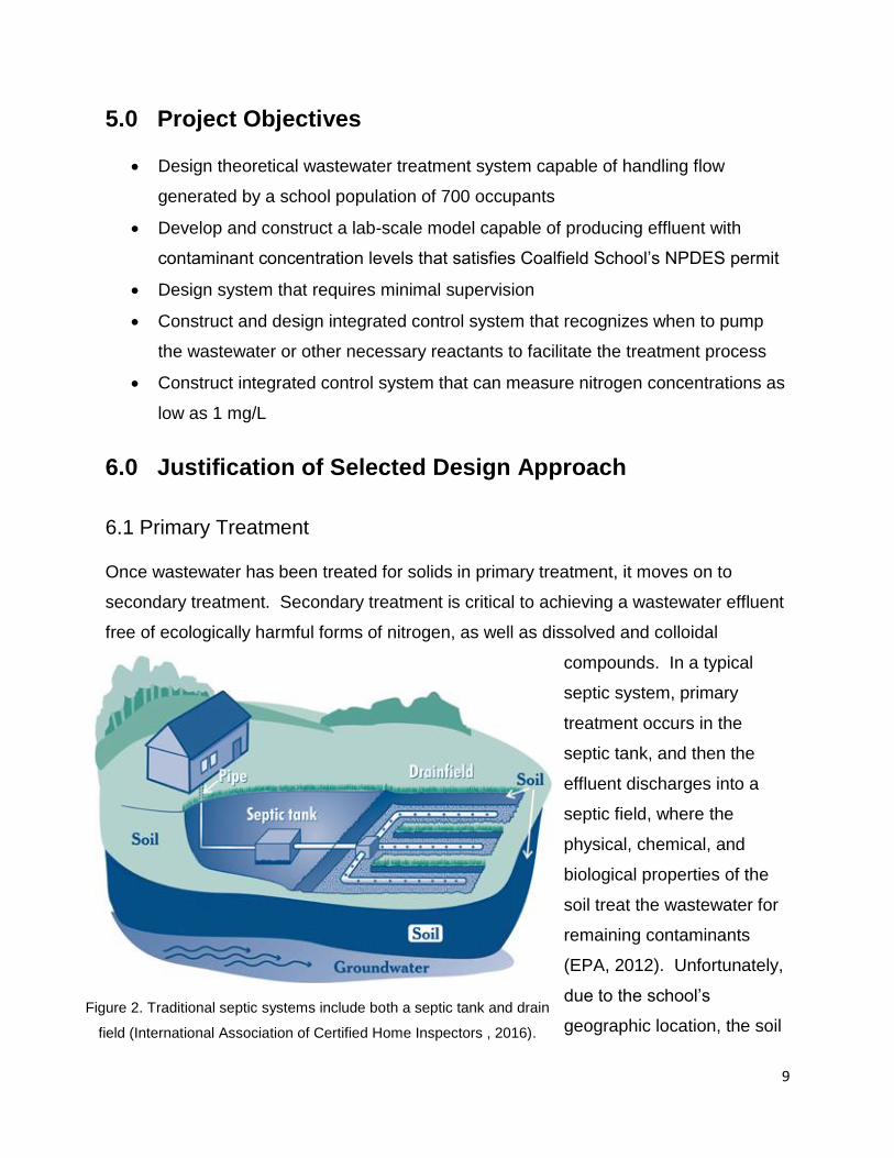
9

Figure 2. Traditional septic systems include both a septic tank and drain

field (International Association of Certified Home Inspectors , 2016).

5.0 Project Objectives

Design theoretical wastewater treatment system capable of handling flow

generated by a school population of 700 occupants

Develop and construct a lab-scale model capable of producing effluent with

contaminant concentration levels that satisfies Coalfield School’s NPDES permit

Design system that requires minimal supervision

Construct and design integrated control system that recognizes when to pump

the wastewater or other necessary reactants to facilitate the treatment process

Construct integrated control system that can measure nitrogen concentrations as

low as 1 mg/L

6.0 Justification of Selected Design Approach

6.1 Primary Treatment

Once wastewater has been treated for solids in primary treatment, it moves on to

secondary treatment. Secondary treatment is critical to achieving a wastewater effluent

free of ecologically harmful forms of nitrogen, as well as dissolved and colloidal

compounds. In a typical

septic system, primary

treatment occurs in the

septic tank, and then the

effluent discharges into a

septic field, where the

physical, chemical, and

biological properties of the

soil treat the wastewater for

remaining contaminants

(EPA, 2012). Unfortunately,

due to the school’s

geographic location, the soil

10

Figure 3. Example of a membrane bioreactor (ATAC Solutions Ltd, 2014).

depth does not extend deep enough for an absorption field to be an effective means of

higher-level treatment. Therefore, a tradition septic system, as depicted in Figure 2,

cannot be implemented in its entirety.

However, septic tanks, by themselves, still provide an effective means of primary

treatment. Therefore, our design will incorporate a septic tank for primary treatment,

followed by an alternative form of secondary treatment that does not rely on soil

filtration.

6.2 Secondary Treatment

In the realm of wastewater management, a plethora of methodologies and mechanisms

exist to conduct secondary treatment. These mechanical treatment methods can be

separated into two broad categories: suspended growth and attached growth.

Suspended growth involves the free flow of wastewater in a large tank. The treatment

comes from suspended

microorganisms in the

wastewater agitated by an

air pump. Settlement in the

system causes bacteria to

be retained for future

treatments. In contrast, the

attached growth method

models natural movement

of water in a soil profile

(NESC 2004). The

wastewater passes through a fixed media bed, composed of a non-toxic material on

which bio-films form. As the wastewater interacts with the bio-films, the bacteria treat

the wastewater (Westerling 2014). Under the umbrella of these two main categories,

the membrane bioreactor, trickling filter, and sequencing batch reactor were considered

as viable options. The mechanism of initial interest was the membrane bioreactor

(MBR). Membrane bioreactors use the practice of suspended growth. MBRs have a

11

minimal footprint compared to other typical suspended growth systems. Lately, there

has been an increase in use of membrane filtration in larger systems; however, the

membrane was originally designed for use in small flow systems (EPA 2007). An

advantage to this system is its capability of receiving influent with high contaminant

concentrations. The membrane, which gives this system its name, acts as a filter for

contaminants. Having the added filter system ensures that the high load of pollutants is

removed. Unfortunately, the initial and operational cost is high when compared to other

treatment methods. Although the fabrication price is lowering, there is still a high cost

associated with pumping for aeration, maintenance, and the inevitable replacement of

the membrane (Champman, Leslie and Law). Since the membrane bioreactor would

not be economically feasible, trickling filtration was the next treatment method

considered. The trickling filter method is the most common type of attached growth

system. Attached growth media can be gravel, peat moss, ceramic, plastic, or textile

media, as long as the media is conducive for growth and non-toxic to microbes. As

water trickles down through the system, contaminants are degraded by the attached

communities of microorganisms growing on the media. Various advantages and

disadvantages exist relating to this type of system. A strong advantage for this system

is the low operating cost. Trickling filters do not employ the use of a large energy-

intensive blower; the system is aerated by the gravitational movement of the water

through the filters. The overall footprint of the system is not large, making trickling filters

ideal for sites dealing with size constraints (EPA 2000). Yet, costs associated with

construction, maintenance, and recirculation of the water would prove to be excessive.

Furthermore, trickling filters cannot handle large, instantaneous fluxes, making them

inapplicable to systems that experience flow inconsistencies (NESC

2004). Furthermore, one common issue associated with continuous flow systems

relates to recirculation; if a certain volume of water continues to have a high level of

pollutants at the conclusion of the treatment process, it must be recirculated through the

system. As more water requires recirculation, an accumulation of water can occur,

eventually leading to the overflow of the system. Pairing a continuous system with

variable influent flow rates and concentrations is simply an illogical application. A

trickling filter can be seen on the next page in Figure 4.

12

Figure 4. Example of a trickling filter system (The Asian Development Bank, 2011).

Finally, the last treatment method considered was the sequencing batch reactor

(SBR). Sequencing batch reactors are a specific type of suspended growth that uses a

batch method and only one chamber to treat the wastewater. A requirement for this

system is a large amount of electronic instrumentation and control. Sequencing batch

reactors perform well at filtering out nutrients and have a small footprint, which is ideal

for a rural school. The biggest advantage when using a SBR is the immense amount of

control over the final product. Since this system will be paired with a high level of

controls and automation, the system can start and end when necessary without the

involvement of an operator. The need for intricate electronic controls makes the

construction of this system more complicated and expensive, yet it increases flexibility

and reduces the need for operator attention (EPA 1999d).

13

Figure 5. Treatment process of a Sequencing Batch Reactor (WAPP).

The treatment process followed by a Sequencing Batch Reactor can be seen in Figure

5. Based on the applicability to the given situation, the sequencing batch reactor method

will be employed as the means of secondary treatment.

Using the SBR method alone is useful, but it is also important to consider methods of

making this technology even better for the specific application. Wastewater treatment is

highly dependent on available surface area. One method of increasing the system’s

internal surface area is use of Integrated Moving Bed Biofilm Reactor Technology

(MBBR). These porous suspended media help to increase surface area for the

denitrifying bacteria to grow on, reducing the footprint of the system. Also, by

increasing microbial activity, the wastewater will not need to experience as long of a

treatment time, decreasing the time of use of the money intensive aerator

(HeadworksBIO 2015). This technology will be a useful addition to the SBR system in

order to increase production while keeping the footprint small. An image of the MBBR’s

used in the system can be seen in Figure 6.

Figure 6. Moving Bed Biofilm Reactor that will be used in the SBR (Amazon, 2016).

14

6.3 Tertiary Treatment

Based on the surrounding county’s NPDES permit, the water must also be disinfected

prior to discharge. Thus, the next area of analysis for the system was the method of

tertiary treatment. The EPA recommends several disinfection techniques for effluent

being directly discharged to surface water. The most common methods include:

chlorination, ozone, and ultraviolet light. Each of these methods has different

advantages and disadvantages.

Chlorination is the most common method of disinfection for wastewater treatment

plants, both on a large and small scale. It has been proven to be extremely effective at

removing bacteria and pathogens. Chlorination has also proven to be the most cost

effective method of disinfection used on wastewater; however, this cost does not

include the cost of dechlorinating the water, which is necessary prior to discharge since

chlorine is harmful to aquatic life (EPA 1999a).

The second method of disinfection that was considered was disinfection by

ozone. Ozone has proven to be more effective than chlorine at removing pathogens,

viruses, and bacteria. In addition, this method requires a short 10 to 30 minutes of

contact time for disinfection. Since ozone decomposes quickly after treatment, it does

not need to be removed from the wastewater prior to discharge (EPA 1999b). Ozone

generation for disinfection can be done on site, but the process proves to be expensive

and is only economically feasible for large treatment facilities.

The final method of disinfection considered was treatment by ultraviolet (UV)

light. UV light is currently being used at many small wastewater treatment plants on

school grounds in East Tennessee, such as Coalfield School in Morgan County. Unlike

the use of chlorine or ozone, this method does not employ the use of hazardous

chemicals. UV requires the shortest contact time of any current disinfection method,

ranging from 20 to 30 seconds of contact with the lamp. UV has proven to be user

friendly for operators and does not require any additional processes after disinfection

prior to discharge. Unlike the other disinfection methods, if the water’s turbidity is high,

the method will not be effective (EPA 1999c).

15

After analyzing cost, ease of operation, and effectiveness, it was clear that UV

disinfection would best serve the system. Since the schools will not have an operator on

site, this system also requires the least amount of maintenance and would not require

removal of any compound prior to discharge.

7.0 Nitrogen Removal

The SBR is vital to the system’s operation since it is the site of nitrogen removal. In

addition, this step in the treatment process will lead to a further reduction in BOD and

other contaminants; however, the SBR will be operated with respect to nitrogen

concentration and removal, considering nitrogen will require the most time and attention

to remove. As wastewater flows through the sequencing batch reactor, nitrogenous

compounds experience multiple reactions that ultimately lead to the production of

nitrogen gas. Therefore, to fully comprehend the processes involved with the

sequencing batch reactor, a strong understanding of nitrogen degradation must be

established. In essence, the nitrogen cycle is composed of five steps: nitrogen fixation,

nitrification, assimilation, ammonification, and denitrification (Environmental). However,

wastewater entering the sequencing batch reactor will only be experiencing

ammonification, nitrification, and denitrification. Throughout these steps, nitrogen is

converted to numerous different forms, and knowing when these reactions take place,

as well as the conditions best suited for them, is crucial to managing the nitrogen

removal process. By means of the integrated control system, sensors determine the

various concentrations of nitrogenous compounds present, and then incorporate the

necessary reactants to facilitate the chemical reactions. By implementing an automated

system capable of sensing required conditions will greatly reduce operator supervision

and increase water quality. Currently, we believe the system will need 4 probes to aid

in automation, including: ammonium, nitrate, dissolved oxygen, and pH.

During ammonification, waste compounds, such as proteins and uric acids, are

converted into ammonia.

H2O + CH4N2O → NH4+ + NH3 + OH- + CO2 (1)

16

For example, urea, CH4N2O, reacts with water to generate ammonium ions, ammonia,

hydroxide, and carbon dioxide. Since ammonification occurs in the absence of oxygen,

wastewater is initially exposed to anaerobic conditions. During this conversion process,

the ammonium concentration will be monitored through the ammonium sensor. To

enforce quality control, the sensors will be coded to establish a standard deviation that

will reduce the likelihood incorrect instrumentation.

Once complete conversion from urea to ammonia occurs, which typically occurs shortly

after entering the SBR, nitrification takes place, converting ammonia into nitrite, which

inevitability breaks down into nitrate. As seen in the successive chemical equations

below, diatomic oxygen is required as a reagent. The dissolved oxygen probe will aid in

gauging the transfer of air into the solution.

2NH3 + 3O2 → 2NO2 + 2H+ + 2H2O (2)

2NO2- + O2 → 2NO3

- (3)

To induce this aerobic environment, an aerator will transfer air into the system that will

be programmed to recognize the commencement of nitrification. Chemically speaking,

the integrated controls must be closely monitoring not only the nitrate concentration, but

also the pH of the solution. As seen in equation 2, the decomposition of ammonia leads

to the production of hydronium ions, acidifying the solution. Unfortunately, various

species of bacteria present in wastewater require a neutral environment to thrive. Thus,

the pH probe is necessary to monitor the acidity of the environment and determine the

correct amount of sodium bicarbonate (NaHCO3) needed to neutralize the water. If the

pH starts to drop below 6, a calculated amount of NaHCO3 will be pumped into the

SBR.

Finally, nitrate will undergo denitrification.

6NO3- + 5CH3OH → 5CO2 + 3N2 + 7H2O + 6OH- (4)

This final step in the conversion process requires anaerobic conditions. During this

stage, a few hours are provided to allow the settling of suspended solids, as well as to

17

ensure the system enters an anaerobic state. This final step in the degradation of

nitrogen is determined by the availability of a carbon source. Since this reaction is

occurring at the end of the treatment process, main sources of organic material have

either been settled or filtered out. Therefore, the system will be automated to recognize

entry into the second stage of anaerobic conditions and determine the necessary

amount of methanol to add based on the concentration of nitrate. Once the nitrogen is

in a gaseous state, it escapes the solution and reenters the atmosphere (Water, 2012).

The theoretical conversion trends between ammonium and nitrate are expected to

follow the pattern seen below in figure 7.

Figure 7. Displaying the relationship between ammonium and nitrate conversion.

The intersection between ammonium and nitrate is the definitive separation between

ammonification and nitrification. Finally, as the concentration of nitrate levels off,

denitrification takes place, converting nitrate into nitrogen gas.

Although this process merely appears to be a list of simple, successive chemical

reactions, the treatment system gains complexity when considering the success of

Co

nce

ntr

atio

n (

mg

/L)

Time

Ammonium

Nitrate

18

Figure 8. This visual depicts how a septic tank interacts with wastewater (Honey Bee Septic Service).

these reactions is dependent on populations of microorganisms that thrive in different

environmental conditions. As described previously, different nitrogen compounds are

produced depending on whether the sequencing batch reactor is inducing aerobic or

anaerobic conditions. Although the presence or absence of oxygen is a function of

nitrogen degradation through the duration of the entire treatment process,

understanding when to initiate anaerobic conditions is pivotal in the transition from

nitrification to denitrification. Since the final stage of the treatment process utilizes

facultative, heterotrophic bacteria, the organisms can thrive in either aerobic or

anaerobic environments. By producing an anaerobic environment, the sequencing

batch reactor is ensuring the heterotrophs are utilizing nitrate as their source of oxygen,

stimulating the final step of nitrogen degradation and generating N2 gas (Weaver, 2003).

Developing populations of these microorganisms is crucial to the system’s ability to

remove nitrogen.

8.0 Theoretical Full Scale System Design

Now that the reasoning behind our choice in secondary and tertiary systems has been

expressed, a more holistic view of the system will be explained, as well as each step in

the treatment process. Upon leaving the confines of the school building, the wastewater

enters a septic tank. This well-established, effective form of primary treatment simply

utilizes baffles and strategically placed pipes to physically separate the floatable fats,

oils, grease, (FOG) and sinkable sludge from the water (Sun Plumbing 2015).

19

During this first stage in the treatment process, a dramatic decrease in BOD and TSS

concentrations is expected. Research conducted through the Washington State

Department of Health reveals that traditional, residential septic systems receive

wastewater with BOD and TSS concentrations as high as 220 mg/L and 145 mg/L,

respectfully, and produce effluent with low concentrations ranges, from 100 to 140 mg/L

for BOD and 20 to 55 mg/L for TSS (Washington). Although septic tanks induce high

reduction of certain contaminants, they do not enable nitrogen removal or disinfection,

revealing the necessity for secondary and tertiary treatment. However, it is worth noting

that septic tanks stimulate anaerobic conditions, leading to an increased concentration

of ammonia in the effluent. In raw wastewater, typically 70% of the nitrogen exists in

the organic form and the remaining percentage exists as ammonium, yet, after

experiencing anaerobic conditions in the tank, approximately 70 to 90% is expressed as

ammonium and 10 to 30% appears as organic nitrogen in the septic effluent. Being

aware of this chemical conversion is crucial to nitrogen removal in the subsequent

steps.

Upon further review of the treatment system’s organization and progression, one

obvious disconnect becomes clear. A septic tank operates via a continuous process,

generating effluent by displacement through the entrance of new wastewater in the

tank, whereas a sequencing batch reactor conducts wastewater treatment via a batch

process, meaning the systems cannot be readily positioned consecutively. Flow

inconsistency is a common issue in wastewater treatment that is correctable through a

flow equalization tank. By introducing another tank to the system, the treatment

process will incidentally become more complicated and expensive; however, the

introduction of this tank provides numerous benefits. For example, the tank will be

equipped with a pump, providing more control concerning the volumetric size of the

batch entering the reactor. Furthermore, without the presence of an equalization tank,

either a pump or metering valve would need to be installed on the septic tank outlet,

which could lead to obvious complications. If water was constantly being pumped out of

the septic tank, its ability to separate FOG and sludge would be compromised by the

agitation induced by the pump; in addition, metering the flow out of the septic tank could

20

cause clogging or overflow. The addition of this equalization tank will create a more

seamless, controllable process. As mentioned previously, septic tanks encourage the

conversion of organic nitrogen to ammonium –this process is defined as

ammonification. Since ammonification is the first step in nitrogen degradation, this

process will be encouraged between the septic and flow equalization tanks by inducing

an anaerobic environment. Thus, upon entering the sequencing batch reactor, nearly

all nitrogen should exist as ammonium. Finally, upon the completion of secondary

treatment, the water will be pumped through the UV disinfection system. Each step in

the treatment process is graphically outlined in Figure 9.

Figure 9. Overview of treatment process.

Sizing a wastewater treatment system is dependent on the amount of occupants a

building is estimated to contain daily. The number of occupants this system will be

sized for is 700 people. It is estimated that for a school with gyms, cafeterias, and

showers each occupant will result in 25 gallons of waste flow per day. Combining the

number of occupants and estimated waste per person will result in the value of 17,500

gal/day of waste effluent from the school (MDE, 2013).

21

Septic tank sizing is based on time requirements of the wastewater in the tank.

According to the Alabama State Board of Health and Bureau of Environmental Services

any given volume of wastewater in the tank needs to have a minimum hydraulic

retention time of two days (48 hours) (ADPH, 2010). Therefore, the septic tank volume

was calculated by multiplying the daily 17,500 gal/day inflow by 2. In addition, this

number was sized up by 25% as a factor of safety.

Flow equalization tank sizing is based on current average daily flow and the peaking

factor. The peaking factor is dependent on the design capacity range, which is 0 to 0.25

MGD for this system. For this range the peaking factor is 3. The average daily flow and

the peaking factor are multiplied resulting in a value of approximately 56,104 gallons.

Having a larger capacity than the average estimated flow will create extra space in the

system in case an unexpectedly large amount of wastewater inflows into the system at

any given time (MDE, 2013).

Sequencing batch reactor sizing is based on the number of batches required in one day

and the amount of time it takes to treat each batch. The estimated time for a

sequencing batch reactor to fully treat the wastewater is 4 to 6 hours (Toprak, 2006).

The true residence time in the batch will vary and is dependent on the composition of

the wastewater as it leaves the septic tank. It was decided that there would be four

batches in a day (Dr. John Buchanan, University of Tennessee, personal

communication, 7 December 2015). Taking the value of 17,500 gal/day of wastewater

flow and dividing it by 4 for the number of batches per day and including a 25% factor of

safety results in a 5,745 gallon volume for the SBR.

Table 1. Displaying representative sizes for actual treatment system.

TANK SIZES

System Volume (gallons)

Volume (ft³)

Length (ft)

Width (ft)

Height (ft)

Septic Tank 45,242 6,048 42 12 12

Flow Equalization Tank 56,104 7,500 25 25 12

Sequencing Batch Reactor 5,745 768 8 8 12

22

9.0 Lab Scale System

9.1 Lab Scale Components

Lab Scale Flow Equalization Tank

Flow Equalization Tank Decanter

Flow Equalization Tank Float Sensor

SBR Inflow Pump

SBR Aeration Pump

SBR Aeration Piping

SBR High Float Sensor

SBR Low Float Sensor

Ammonium and Nitrate Sample Chamber Pump

Dissolved Oxygen and pH Sample Chamber Pump

Ammonium and Nitrate Sample Chamber

Dissolved Oxygen and pH Sample Chamber

SBR Decanter

SBR Outflow Pump

UV Disinfection

Figure 10. Hydraulic diagram of flow through the lab scale system.

23

9.2 Lab Scale System Sizing and Justification

The beginning of the lab scale system is the flow equalization tank. This piece of the

lab scale system was modeled using a 55 gallon blue industrial plastic drum with a

black removable lid. The lid has a 2.5 inch diameter threaded hole for a cap, which acts

as the orifice from which the 3/8 inch decanter tubing emerges. A 1-5/8 inch hole was

drilled 3 inches from the bottom of the tank in order to fasten a polypropylene bulkhead

tank fitting with an EDPM gasket to the side. This fitting was used to thread the wires

for the float sensor, as well as keep the hole watertight. The float sensor was attached

using schedule 40 PVC piping configured to place the float sensor 11 inches from the

bottom of the flow equalization tank. This ensures that the volume in the flow

equalization tank is large enough to fill the sequencing batch reactor to approximately

Figure 11. Image of laboratory scale flow equalization tank, sequencing batch reactor, and disinfection.

24

13 gallons of treating water space. The bulkhead fitting opening is attached to a ½ inch

Schedule 40 PVC Male Adaptor which is connected to a 90 degree elbow using a 1-1/2

inch piece of cut schedule 40 PVC, which is extended upward using a piece of 6 inch

PVC connected to a schedule 40 end cap. The end cap has a 3/8 inch hole drilled out of

it which was then threaded with the float sensor’s male connector end.

A decanter was used to remove water from the flow equalization tank and deposit it into

the sequencing batch reactor. This decanter was made with Styrofoam, shaped into a

rectangle with dimensions of 14 x 11 x 2-1/2 inches. A hole was cut into the center and

3/8 inch tubing was glued in place using JB Water Weld. The 3/8 inch tubing connects

to a 3/8 inch hose barb to ½ inch MPT adapter which screws into a Flojet pump, model

2100-12 Type IV. The pump is a self-priming diaphragm pump up to 7 feet vertical lift

with a DC electric motor. It delivers from 1.0 to 2.0 GPM and operating pressures up to

50 PSI, works off 12 volts, and draws a current of 8 amps. Calculated when attached to

the system the pump has a flow rate of approximately 1.3 GPM filling the tank in

approximately 10 minutes. The pump was sized to deliver the treatable volume in a

reasonable amount of time, as well as be sized at a velocity over 2 ft/s. The Ten State

Standards note that a velocity of over 2 ft/s is required to prevent settling in the piping of

a wastewater system (Wastewater Commitee of the Great Lakes - Upper Mississippi

River, 2014). The velocity is calculated to be approximately 8.5 ft/s, which is on the

higher end of the allowable speed in the standards, but works well for the lab scale

system filling speed.

The sequencing batch reactor is a tank with a lid, both made completely out of ¼ inch

Plexiglas. The tank when glued together is approximately 36 x 12 x 12 inches. The lid is

37 x 13 x 2 inches. The tank is approximately 23 gallons, however the treatable volume

is 13 gallons. The fill time for the tank is 10 minutes and the decanting time is

approximately the same. Approximately 25% of the treatable volume is composed of

moving bed biofilm reactors. This amount of MBBRs in the system increases the

surface area by approximately 54 ft2. The maximum fill for MBBRs is approximately

70% of the treatable volume however the exact volume to add is dependent on the

25

Figure 13. Sequencing Batch Reactor tray for aeration.

application and convenience of the system (Odegaard, Rusten, & Westrum, 1994). In a

large scale system the addition of more would be likely.

The lid has multiple holes for various purposes, including inflow to SBR, outflow from

SBR, two for inflow to both sample chambers, two for sample chamber solenoids, pH

and dissolved oxygen sample chamber outflow tubing, cords for sample pumps,

aeration tubing, extra for gas and potential sodium bicarbonate, high float sensor, and

low float sensor. Drilling into the lid made the system more likely to stay watertight, as

well as easy to organize and more appealing visually.

In the bottom of the tank is a Plexiglas removable tray, designed to hold up grating, hold

down aeration, and be removed for lab scale

design cleaning purposes. The base is

composed of ¼ inch Plexiglas while the

sides are ½ inch Plexiglas. The height of the

end pieces are 2 ½, just ¼ inch taller than

Figure 12. Sequencing Batch Reactor tank and lid with labeled entrance holes.

26

Figure 14. Aeration piping attached to the SBR tray.

the rest of the system so that the aeration system was able to be tied down onto the tray

with small cable ties through ¼ inch holes drilled into the tray. The length of the tray is

35 ¾ inches and the width is 11 ¾ inches.

The aeration piping was crafted using ½ inch schedule 40 PVC. The aeration was sized

to fit snuggly in the

bottom of the tank

tray, while configured

in a pattern that would

evenly aerate the

wastewater. The

three horizontal

lengths of piping were

sized to be 32 inches

long with 90 degree elbows connecting them to the two 4 inch pieces. The end is

capped off and the entrance to the aeration is attached to a 90 degree elbow and 12

inch length of pipe which exits the lid and is attached to a ½ inch male adapter. The

male adapter is then connected to a ½ inch threaded coupling which connects to a ½

inch male thread to 3/8 inch hose barb adapter. The aeration hosing connects to the

aeration pump with another ½ inch male thread to 3/8 inch hose barb adapter. The

holes drilled into the piping for aerating were spaced five inches apart, allowing for a

significant number of holes. The holes drilled for the escapement of air are of size 9/64

inch.

The pump for aeration was sized up significantly from the original recommendations

from the Ten State Standards. Originally the aeration pump was sized to be a small fish

tank aerator, the Top Fin Aquarium Air-3000. The pump is recommended for a fish tank

of size 40 US Gallons and has a flow rate of 0.78 GPM. The ten state standards

recommend a minimum of 1.25 cfm/1000 gal (Wastewater Commitee of the Great

Lakes - Upper Mississippi River, 2014). This measurement would be approximately

0.01625 CFM or 0.12155 GPM for the 13 gallon treatment system. However, upon

aerating the system it was clear that this minimum value would not enable a uniformly

27

Figure 15. Layers of #5 mesh and stainless steel grate.

mixed wastewater in the SBR in lieu of a mechanical mixing mechanism. Therefore,

another aeration pump of nearly 75 times the CFM was chosen. The aeration pump

used in the final system is the Rietchle Thomas model 927CA 18 diaphragm vacuum

pump. The pump operates at a flow rate of 1.2 CFM, runs off of 115 Volts AC, and

draws 3.6 Amps.

Above the aeration piping, resting on the SBR tray, are two layers of grating. The first

layer is plastic knitting mesh with openings of 1/8 inch, also known as #5 mesh,

referring to the

number of holes per

linear inch. The

second layer of grating

is a layer of stainless

steel grating cut to

size. The second layer

adds weight to aid in

keeping the plastic

mesh from floating up

during aeration. Both mesh layers together help to disperse the aeration bubbles as

well as keep the Moving Bed Biofilm Reactors and other significant solids from falling

below and amongst the aeration system.

An important part of the sequencing batch reactor is the float sensors. The float

sensors are attached through the lid of the sequencing batch reactor, using a similar

method as in the flow equalization tank. The float sensors are attached to the end of a

threaded ½ inch end cap as mentioned before, followed by a length of cut ½ inch

schedule 40 PVC. The low sensor reaches down to hover just above the grating (9

inches below the lid) and is kept in place using a cable tie on the outside of the lid. The

high sensor is attached in the same way but it located 2 inches below the lid, leaving a 7

inch height of treating water.

28

Figure 16. Ammonium and Nitrate Sample Chamber.

Apart from the sequencing batch reactor, two more liquid holding chamber designs were

implemented. One is the sample chamber for the ammonium and nitrate probes, the

second is the sample chamber for the dissolved oxygen and pH probes. The two

chambers are nearly identical in design except for one minor difference. The dissolved

oxygen sensor requires water to be moving past it, so the entrance to the chamber was

placed low and the exit high, to allow for new

water to fill up the chamber and spill out the top

constantly. The ammonium and nitrate sensors

prefer water to be stagnant, therefore there is no

higher opening for an exit, there is a high exit for

an entrance in order to let the water fill it up and

sit without moving for readings.

29

Figure 17. Dissolved Oxygen and pH Chamber.

The sample chambers are built out of all 4 inch schedule 40 PVC and have an

approximate volume of 0.7 gallons that fill in approximately 40 seconds. The top is

composed of a DWM PVC Cleanout adapter SP x FPT and a DWV PVC cleanout plug.

The plug has two 1 inch diameter holes drilled

into them which contain the top 1-1/2 inch

portion of two storage solution sensor bottles.

The sensor bottles are glued into the plus using

JB Weld. Using this method allowed for the

sensors to be easily removed and cleaned, as

well as kept the sensors in place with tightening

grommets. The middle of the chamber is

composed of a coupling which attaches to a 4-

1/2 cut piece of 4 inch schedule 40 piping,

which connects to a DMV cap, which composes

the bottom.

Each chamber has a 5/8 inch hole drilled into

the bottom to allow for the connection of a

solenoid. On both chambers an ASCO ½ inch

solenoid was attached using a threaded

connecting piece of PVC. The solenoid on the

ammonium and nitrate chamber dropped water

out every time a sample was taken, however because water needs to be moving

through the dissolved oxygen and pH chamber, the solenoid will only be employed if

there are no samples being taken and the sequencing batch reactor is not being used.

The ammonium and nitrate chamber has an entrance 2 inches from the top, with a ¾

inch threaded to 1/4 inch hose barb which allows for 3/8 inch outer diameter tubing to

carry water from the sample pump into the chamber. The dissolved oxygen and pH

chamber has an entrance 1-1/2 inches from the bottom which allows for water to be

carried in through a ¾ inch threaded to 1/4 inch hose barb through outer diameter inch

tubing. This chamber has an exit in order to allow for the water to continuously flow

30

Figure 18. First generation sample chamber pumps.

Figure 19. Second generation sample chamber pumps.

through. The exit hole is 2 inches from the top of the chamber and has a ¾ inch

threaded to 3/4 inch hose barb, which allows for water to flow out through 1 inch outer

diameter tubing.

In order to pump the water from the sequencing batch reactor into sample chambers,

pumps were chosen to allow for water to pump in and be able to take a reading every

six minutes. The original pumps chosen

were two aquarium pumps made by

Sicce called the Mi Mouse. These

pumps are submersible recirculation

pumps that are equipped with a variable

flow rate regulator and operate at 82

GPH. The max head is 1.8 ft, the

voltage is 120 volts, and draws current of

0.084 amps. These first generation

pumps did not have a way of easily

attaching them to the wall of the SBR,

so a device was constructed using Plexiglas and flexible metal in order to hang the

pumps down into the tank. The true downfall of using these pumps was the position of

the inlet. The pumps were above part of the aeration system, so when the aeration

would turn on air bubbles would enter into the inlet and the pumps would not be capable

of sending water up from the SBR into the sample chambers. Therefore, another

generation of pumps was needed.

The second generation of pumps used

was the Top Fin Power Head 30. The

choice of this pump was preferable for

multiple reasons. First, the position of

the inlet faces to the side and includes a

water inlet strainer. The position and

strainer both greatly decrease the

likelihood that air bubbles will enter the

31

Figure 20. First generation sequencing batch reactor decanter.

pump while aeration is running. Second, the pumps are equipped with four small

suction cups, therefore mounting was simplified. The second generation pumps have a

flow rate of 118.89 GPH and a voltage of 120 V. It is also a position outcome that the

sample chambers fill up faster than they did with the first generation pumps.

Settling in a sequencing batch reactor is inevitable; therefore a method for removing

water that will disturb settled solids the least is preferable. A decanting mechanism was

built for this purpose.

The first

generation of

decanting was

built using

Styrofoam. This

recycled material

was adequate at

floating, however

it flaked off bits of

Styrofoam into the system which would make the water inadequate to discharge. The

structure also had issues interfering with, float sensors and inlet tubing. The first

generation decanter was designed in an elongated H shape in order to prevent it from

hitting the sample chambers, however as the design of the sequencing batch reactor

evolved, so did the decanter. In addition to the Styrofoam, a 90 degree hose barb was

fixed to a 2 inch piece of 3/8 inch tubing, which was glued into a 3/8 inch hole in the

decanter to serve as an outlet and attachment for the 3/8 inch tubing leading out of the

sequencing batch reactor.

The second generation decanter was built using ½ inch schedule 40 PVC. The need for

a second generation arose from the very specific final location of pumps, float sensors,

and tubing in the sequencing batch reactor. The decanter needs to be able to move

freely vertically, but have more restricted movement horizontally. The entire decanter

is composed of a 1-1/2 inch length of tubing, a 90 degree 3/8 inch hose barb, a 10 inch

32

Figure 22. Sterilight Silver SSM-17 UV Disinfection.

Figure 21.Second generation sequencing batch reactor decanter.

of flexible silicone tubing, two cross fittings, four tee fittings, two 90 degree elbows, six

end caps, and various lengths of standard ½ inch schedule 40 PVC.

Being completely waterproof, the PVC decanter floats evenly atop the water’s surface.

The inlet was drilled using a 3/8 inch drill bit and fits the small piece of ridged tubing with

the hose barb snuggly as well as has a layer of JB Water Weld to ensure that it is water

proof. At the longest points on the decanter the final dimensions are approximately 35-

3/4 inches and 11-3/4 inches.

The pump attached to the decanter is identical to the one used for inflow into the

Sequencing Batch Reactor. The flow rate for the disinfection system used is

approximately 3.0 GPM, therefore the 1.3 GPM Flo Jet pump allows for enough time for

disinfection to occur properly.

The ultra violet light

disinfection chosen for use

in the lab scale system is

the Sterilight Silver SSM-

17. Rated at a flow rate of

3.0 GPM, voltage of 100 to

240 V, and a 0.6 Amp

maximum. After

disinfection the lab scale

water was tested for consistency in the laboratory.

33

10.0 Integrated Control Design

10.1 Hardware

The control panel located directly above the SBR is equipped with the following

electronic components:

power strip

120 volt AC to 12 volt DC transformer

two breadboards

Arduino Uno microprocessor

three solid-state relays

eight electromechanical relays

three 10k ohm resistors

three float sensors

four analog protoboard adapters

two ion-selective electrodes

pH probe

dissolved oxygen probe

The three solid-state relays deliver power accordingly to the components that require

120 volts AC to operate, including the two sample pumps and the aeration pump. Their

coil voltage is only five volts, making them ideal for application with an Arduino Uno,

which is only capable of generating an output of five volts. The two solenoids, inflow

pump, and outflow pump, only require 12 volts DC to operate and are relayed power

from the transformer via the electromechanical relays, which can be applied to circuits

experiencing direct current. Furthermore, the resistors are each utilized as pull-down

resistors in conjunction with the float sensors, reducing the leakage of any stray voltage.

Most importantly, the analog protoboard adapters allows the sensors to interface with

the Arduino Uno through transmission of an analog signal.

34

10.2 Sensors

As mentioned in the previous list, the sensors used in this lab-scale system include an

ammonium selective electrode, nitrate selective electrode, pH probe, and dissolved

oxygen probe. The justification for implementing these sensors is directly related to the

reactions involved with the process of nitrogen removal. It is worth noting that the

NPDES permit being used to model this system has a discharge limitation written in

terms of ammonia concentration, opposed to ammonium; however, in terms of design,

application of an ammonium sensor is far more feasible and simplistic. Typically,

wastewater exists between a pH of 6 and 8. As seen in figure 23 below, for that pH

range, over 90% of the species in solution is expected to be ammonium.

Figure 23. Revealing the relationship between ammonium and pH.

Therefore, to use an ammonia sensor, it would be necessary to increase the pH of the

sample through addition of a reagent to achieve an accurate measurement. This

additional step would complicate the sampling process, and the reagent could skew the

results of other sensors. With implementation of the ammonium, nitrate, pH, and

dissolved oxygen sensors, it is possible to follow and quantify the process of nitrogen

35

Figure 24.Graph of ammonium exponential relationship.

removal. As for operation and calibration, both ion-selective electrodes are governed by

the Nernst equation -- an equation that models electromotive forces.

𝐸 = 𝐸0 + 𝑚(ln 𝐶) (5)

where

E = measured voltage

E0 = standard potential for combination of two half cells

m = slope

C = concentration of measured ion species

By creating stock solutions of varying concentrations and plotting them against voltage

readings measured from the electrode, an exponential relationship becomes clear.

Taking the natural logarithm of the concentrations and once again plotting that

information against the voltage outputs, develops a linear relationship. (The ammonium

calibration process is identical to the nitrate calibration process, but the nitrate

calibration plots can be found in the appendix.)

0

0.5

1

1.5

2

2.5

0 20 40 60 80 100 120

Vo

ltag

e (

mV

)

Concentration (mg/L)

Ammonium: Exponential Relationship

36

Figure 25. Graph of ammonium calibration.

The slope and intercept are then applied to the software so that the voltages can be

immediately converted to concentrations during data acquisition. The equation below

was derived by isolation of concentration in the Nernst equation; therefore, all variables

are the same as previously defined.

𝐶 = 𝑒(𝐸−𝐸𝑜

𝑚) (6)

The pH and dissolved oxygen sensors both have a direct linear relationship with

measured voltage, as seen in fig below.

y = 0.1418x + 1.4142R² = 0.9978

0

0.5

1

1.5

2

2.5

0.0 1.0 2.0 3.0 4.0 5.0

Vo

ltag

e (

mV

)

ln(C)

Ammonium Calibration

y = -3.8216x + 13.56R² = 1

0

2

4

6

8

10

12

0.0 0.5 1.0 1.5 2.0 2.5 3.0

pH

Voltage (mV)

pH Calibration

Figure 26. Graph of pH calibration

37

Upon calibration, the slope and intercept is applied to a linear equation that interprets

voltage into either pH or dissolved oxygen concentration. (The dissolved oxygen

calibration process is identical to the pH calibration process, but the dissolved oxygen

calibration plots can be found in the appendix.)

𝑦 = 𝑚(𝐸) + 𝑏 (7)

where

y = pH or DO concentration

m = slope

E = measured voltage

b = intercept

The operational constraints of the sensors were a limiting factor that required particular

attention with regards to design. Upon programming, calibrating, and submerging all 4

sensors in the same sample, it was discovered that major electronic interference exists

amongst the sensors, leading to erroneous measured concentrations and values;

however, if powered individually and allowed time to cycle through each sensor, a

complete data set containing all 4 values can be generated in a timely manner. By

pairing each sensor with a relay, power could be delivered to each sensor for an allotted

amount of time, completely expelling any electrical interference.

Figure 27. Circuit Diagram

38

Yet, allotting enough time for each sensor to stabilize is also crucial when acquiring

accurate data. The initial software was written so that each sensor had 20 seconds to

stabilize and report a measurement. With a total of 4 sensors, this seemed ideal,

considering it would be possible to cycle through all the sensors and compose a

complete data set in only a minute. After running this original software, it was quite clear

the concentrations reported were incorrect. Upon this realization, the time required for

each sensor to stabilize was thoroughly researched. To measure the capability and

sensitivity of the sensors, each was exposed to a known concentration or pH change

and the time required to reach a stabilized measurement was recorded.

Figure 28. pH and dissolved oxygen stabilization time curves.

As seen in the pH stabilization plot, upon removing the sensor from a pH 4 stock

solution and placing it in a solution of pH 10, the sensor was capable of completely

stabilizing in a matter of 10 seconds. The DO probe’s ability to stabilize was tested

within its prospective sample chamber. For this test, tap water was merely pumped in

via the sample pump and the time required for the DO reading to stabilize was

recorded. Similar to pH sensor, the DO sensor experienced stabilization in

approximately 10 seconds. Even though the pH and DO probes are capable of

measuring and reporting accurate values in a rapid manner, the ion-selective electrodes

require more time to stabilize and are definitely a limiting factor with regards to the time

needed for data acquisition.

39

Figure 29. ammonium and nitrate stabilization time curves.

In both of the plotted scenarios above, the sensors were removed from a stock solution

of 1 mg/L, then immediately submerged in a stock solution of 100 mg/L. The ammonium

ISE experienced stabilization around the minute mark, but the nitrate sensor did not

start experiencing stabilization until approximately 75 seconds. Equipped with this

knowledge concerning the limitations of the sensors, it was possible to update and alter

the Arduino software to produce more accurate values. As a precaution, in the second

generation of the software, it was programmed to power each sensor individually for a

period of 2 minutes, ensuring accurately measured values. However, the increased time

interval was not ideal for the procurement of real-time data, explaining yet another

reason for the necessity of the multiple sample chambers. By having two sample

chambers, it is possible to have two sensors powered simultaneously, each in its own

isolated chamber. If the sensors were all in one chamber and had to be powered

individually, between the 2 minutes required for each sensor and time to pump in and

out, it would take nearly 10 minutes to obtain a full data set composed of pH,

ammonium, DO, and nitrate values. As a result of the two sample chamber design, the

time required to obtain a data set it only 6 minutes.

10.2 Software

The system’s software has been programmed through Arduino and Python. The bulk of

the logic exists in Arduino, while the code composed in Python provides a means of

plotting live data and transferring the values to excel. As the Arduino code conducts and

collects the various measurements, the Python code interprets and plots the data so

40

that an operator can visually comprehend the state of the system. Essentially, the logic

composed in the Arduino interface mirrors the nitrogen cycle. By constantly measuring

the change in certain nitrogenous compounds, it is possible to identify different stages in

the process of nitrogen removal.

Figure 30. Sensor logic diagram.

As seen in the flowchart above, the program was composed to change the

environmental conditions based on the prevalence of ammonium or nitrate. Every 6

minutes, a full data set containing all 4 values (pH, ammonium, DO, and nitrate) is

generated; however, the manner in which the software interprets those data points is

contingent on the state of nitrogen removal. When water first enters the SBR, the water

will be monitored for ammonification. After taking the first ammonium measurement, the

value is saved in E2PROM. During the second round of measurements, the new

ammonium measurement is subtracted from the old ammonium measurement, and then

the new measured concentration replaces the previous in E2PROM. This process

continues until the absolute value of the new measurement minus the old measurement

41

becomes less than 1. If the absolute value is greater than 1, clearly the system is still

experiencing conversion of organic nitrogen to ammonium, yet if the absolute value is

less than 1, the ammonium concentration is stabilizing, and ready for conversion to

nitrate. To act as a fail-safe mechanism, if this requirement is satisfied, and the system

is required to take another ammonium measurement and once again produce an

absolute value below 1. Once in the nitrification state, the same logic is repeated,

except with nitrate measurements. Upon exiting the nitrification state, nitrate

measurements are still saved to E2PROM and compared to the new measurements

during the denitrification state. This time, the comparative process is used to determine

when the concentration of nitrate has reached a minimum, meaning the available nitrate

has converted into nitrogen gas.

11.0 Results

Values for ammonia, pH, and dissolved oxygen were found using laboratory calibrated

sensors. Values for total coliform count and E.coli were found through the use of

standard laboratory testing. This testing included making 1 ml, 2ml, 3ml, 4ml, and 5ml

dilutions of wastewater sample with the remainder of the sample being deionized water.

The sample is mixed with Coliert and incubated in quanti-trays for 24 hours. The total

coliform count is found by counting the number of yellow wells and the E.coli count is

found by counting the number of wells that are both yellow and fluorescing. These

values are compared to a chart and multiplied with their respective dilution values.

42

0

1

2

3

4

5

6

7

8

9

10

0 1 2 3 4 5 6 7 8 9

DO

(m

g/L)

Time (hours)

Trial 1: DO vs. Time

Table 2. Comparison of residential and school wastewater values.

Name Unit Residential Septic

Effluent School Septic

Effluent

Ammonia mg/L 61 158

Total Coliform

#/100mL 148,000 150,000

E.coli #/100mL 61,600 75,000

Obtaining enough school effluent to treat in the lab scale SBR proved to be an issue

due to the school’s distance from the lab. In hopes of achieving a more continuous

system and seamless process, the septic effluent pumped into the SBR was sampled

from a residential location on property owned by the University of Tennessee. It is

crucial to note the source of the septic effluent because of the drastically different

ammonia concentrations among sources, seen in Table 2. For the means of

prototyping the system and the sake of availability, residential wastewater was utilized

to gauge the system’s effectiveness at removing nitrogen and other contaminants.

Figure 31. Results for dissolved oxygen during trial 1.

43

0

5

10

15

20

25

30

35

40

0 1 2 3 4 5 6 7 8 9

NH

4+

(mg/

L)

Time (hours)

Trial 1: Ammonium vs. Time

0

1

2

3

4

5

6

7

8

0 0.5 1 1.5 2 2.5 3 3.5 4

DO

(m

g/L)

Time (hours)

Trial 2: DO vs. Time

Figure 32. Results for ammonium during trial 1.

Figure 33. Results for dissolved oxygen during trial 2.

44

0

5

10

15

20

25

0 0.5 1 1.5 2 2.5 3 3.5 4

NH

4+

(mg/

L)

Time (hours)

Trial 2: Ammonium vs. Time

Figures 31 through 34 are plots of the concentrations measured by the dissolved

oxygen and ammonium probes collected via the software described in the previous

section. Figures 31 and 32 represent the first trial, and Figures 33 and 34 represent the

second trial. Both trials followed the expected ammonification and nitrification trends.

Upon enter the SBR, ammonium concentrations were at their maximum, allowing for

nitrification to commence soon after entering the tank. As seen in both trials, small

amounts of ammonium conversion were occurring prior to aeration; this conversion can

be explained by the small concentration of dissolved oxygen already present in the

water. Once aeration occurred, nearly all ammonium experienced conversion,

eventually stabilizing at a concentration of approximately 5 mg/L. As expected, the

septic effluent was anoxic when initially entering the system and experienced a dramatic

spike in dissolved oxygen during aeration to approximately 8.5 mg/L. To become fully

aerobic, the system only required approximately 30 minutes, but to reenter an anoxic

state, the SBR required an extensive amount of time. During the first trial, the SBR took

four hours to become anoxic; however, during the second trial, the SBR only required

approximately two hours. This drop between trials in the time necessary to become

anoxic is indicative of the growing populations of bacteria in the system. Since the SBR

probably had larger populations of bacteria for the second trial, the oxygen demand was

Figure 34. Results for ammonium during trial 2.

45

greater, decreasing the time to become anoxic. Unfortunately, due to biological

constraints, successful denitrification was not witnessed. Without an adequate

population of denitrifiers, conversion of nitrate to nitrogen gas cannot be expected to

take place. The denitrifiers are delicate bacteria that have slower reproductive cycles

compared to the other microorganisms in the system.

Table 3. Values for NPDES requirements, septic effluent, and system effluent from trials 1 and 2

Name Units NPDES Values

(Daily Maximum)

Septic Effluent

Trial #1

Trial #2

Ammonia mg/L 10 61 42 46

pH ͞ 6 - 9 7.37 7.69 7.74

Dissolved Oxygen mg/L 6 0.63 0.29 0.47

Total Coliform #/100mL ͞ 148,000 100 185

E.coli #/100mL 941 61,600 < 1 < 1

The first trial was conducted without MBBRs, whereas the second trial was conducted in

the presence of MBBRs. Although the values between trials do not differ significantly, it

is suspected that the longer the MBBRs are in the tank, the more they will contribute to

nitrogen removal. As seen in Table 3, averaged between trials 1 and 2, the system

removed 27.9% of the ammonia and nearly 100% of the E. coli.

46

12.0 Conclusion

The process of ammonification and nitrification followed the expected theoretical trends.

Unfortunately, due to biological constraints, there was not an excessive amount of

denitrification. Without an adequate population of denitrifiers, conversion of nitrate to

nitrogen cannot be expected to take place. As the system continues to treat batches,

the necessary colonies of microorganisms will continue to grow. Already it is noticeable

based on the second trial that the time to induce anoxic conditions is decreased,

meaning there is a growing population of microorganisms cultivating within the SBR.

12.1 Budget

An element of success for this project was depended on whether or not the lab scale

system could be built at a reasonable price and within the constraints of the allotted

money for the project. Having a budget restraint had an effect on the choice of sensors

especially. Typically the Vernier sensors chosen are used for less industrial settings

and not necessarily used to detect various concentrations in wastewater. In a true

sensing unit the sensors would be of a higher price, yet more durable and resilient.

The amount of money allotted for the project was $3,000, however not all of it was used.

For supplies implementing into the lab scale system, approximately $1,730 was spent.

As mentioned before, if being implemented long term in a large scale treatment system

the price for sensors would increase from $700 and the price for the sample chambers

would stay approximately the same, however, the price for the lab scale sequencing

batch reactor would not need to be included.

47

Supplier Item Cost

Vernier Sensors $699.00 Hach Calibration Chemicals $132.48 Delcity Solenoid Valves $264.82 Home Depot Lumber for System Stand $80.47 Arduino Arduino Uno Board $24.95 Ace Hardware PVC joints, piping, and tubing $75.86 Aquariums of Knoxville Sample Chamber Pumps $20.79 Fisher Science Sensor storage solution $96.10 Laser Precise Reactor Acrylic and cutting $150.48 Radioshack Electronic Components $104.92 Home Depot Sample Chamber Supplies $65.46 Digi Key Corp. Electronic Components $13.62 Total $1,728.95

13.0 Recommendations

Continue testing to obtain multiple trials of data

o Test using wastewater collected from the school

Apply wireless capabilities and develop a downloadable app for

notification

Implement use of industrial-grade sensors

Test sample chambers in a large scale system

Develop a more rigorous statistical analysis to determine the presence of

outliers

Implement fail safe mechanisms, including multiple float switches

48

References

A V Systems, Inc. (2008). NPDES Sample Documents. Retrieved from Material Inventory Report System:

http://www.mirsinfo.com

Burian , S., Nix, S., & Durrans, S. (2000). Urban Wastewater Management in the United States: Past,

Present, and Future. Journal of Urban Technology, 33-62.

Chapman, S., Leslie, G., & Law, I. (2000). Membrane Bioreactors (MBR) for Municipal Wastewater

Treatment - An Australian Perspective. Australia: CH2M HILL.

Detroit Water and Sewerage Department. (2003). Diurnal Flow Analysis of Wastewater Treatment Plant

Influent. Detroit: Detroit Water and Sewerage Department.

Fondriest Staff. (2010, August 2). The Nitrogen Cycle. Retrieved from Environmental Monitor:

http://www.fondriest.com

Gurpal, S., Lusk, M., & Obreza, T. (2011, November). Onsite Sewage Treatment and Disposal Systems:

Trace Organic Chemicals. Retrieved from IFAS Extension: University of Florida:

http://edis.ifas.ufl.edu

HeadworksBIO. (2015). Active Cell: MBBR/IFAS Wastewater Treatment. Retrieved from HeadworksBio:

http://www.headworksinternational.com

Lenntech. (2003). Part II of Matter Cycles: The Nitrogen Cycle. Rotterdam,The Netherlands: Lenntech.

Macalester College. (n.d.). History of Wastewater Treatment in the United States. Retrieved from Urban

Wastewater Management in the Great Lakes Watershed: http://www.macalester.edu

National Small Flows Clearinghouse. (2004). The Attached Growth Process - An old technology takes on

new forms. Pipeline , 1-7.

Odegaard, H., Rusten, B., & Westrum, T. (1994). A New Moving Bed Biofilm Reactor - Applications and

Results. Wat. Sci. Tech., 157-165.

SOPAC. (1999). Report on Project Criteria, Guidelines, and Technologies. Suva, Fiji: South Pacific Applied

Geoscience Commission.

Sun Plumbing. (2015). How do Septic Systems Work. Retrieved from Sun Plumbing:

http://www.sunplumbing.com

The United States Environmental Protection Agency. (1999a). Wastewater Technology Fact Sheet:

Chlorine Disinfection. Washington, D.C.: EPA.

The United States Environmental Protection Agency. (1999b). Wastewater Technology Fact Sheet: Ozone

Disinfection. Washington, D.C.: EPA.

49

The United States Environmental Protection Agency. (1999c). Wastewater Technology Factsheet:

Ultraviolet Disinfection. Washington, D.C: EPA.

The United States Environmental Protection Agency. (1999d). Wastewater Technology Factsheet:

Sequencing Batch Reactor. Washington, D.C.: EPA.

The United States Environmental Protection Agency. (2000). Wastewater Technology Factsheet:

Trickling Filters. Washington, D.C.: EPA.

The United States Environmental Protection Agency. (2007). Wastewater Management Factsheet:

Membrane Bioreactors. Washington, D.C.: EPA.

The United States Environmental Protection Agency. (2012). Leanr about Small Wastewater Systems.

2012: EPA.

The United States Environmental Protection Agency. (2014). Water: Permitting (NPDES). Wasington,

D.C.: EPA.

The United States Environmental Protection Agency. (2015). Summary of the Clean Water Act.

Washington, D.C.: EPA.

University of Michigan Center for Sustainable Systems . (2015, November 20). Factsheets Water.

Retrieved from U.S. Wastewater Treatment: http://css.snre.umich.edu

VANIS Industrial Automation. (2015). Wastewater Solutions. Retrieved from VANIS Industrial

Automation: http://www.vanis.hr

Washington State Department of Health. (2003). Septic Tank Effluent Values. Seattle: Washington State

Department of Health.

Water Environment Research Foundation. (n.d.). Fact Sheet T2 Treatment Series: Suspended Growth

Aerobic Treatment. Alexandria, VA: WERF.

Weaver, G. (n.d.). Nitrogen Removal from Wastewater: A Primer. New London, CT: The Water Plant

Company. Retrieved from The .

Westerling, K. (2014). Biological Treatment 101: Suspended Growth vs. Attached Growth. Retrieved from

Water Online: http://www.wateronline.com

Wiesmann, U., Choi, I., & Dombrowski, E. (2007). Fundamentals of Biological Wastewater: Historical

Development of Wastewater Collection and Treatment.

Winzler & Kelly Consulting Engineers. (2003). City of Antioch Wastewater Collection System Master Plan.

San Francisco, CA: City of Antioch.

World Bank Group. (n.d.). Introduction to Wastewater Treatment Processes.

http://www.worldbankgroup.org: WBG.

50

Appendix

A.1 Drawings

List of Drawings:

Sequencing Batch Reactor Tank

Sequencing Batch Reactor Lid

Sequencing Batch Reactor Cutting Diagram

Sequencing Batch Reactor Isometric

Dissolved Oxygen and pH Sensor Sample Chamber

Ammonium and Nitrate Sensor Sample Chamber

51

52

53

54

A.2 Morph Charts for Justification of Choices

The following morph charts were developed to weigh the pros and cons of both

secondary and tertiary treatment for the needs of the system.

Constraint

Sequencing

Batch

Reactor

Trickling

Filter

Membrane

Bioreactor

Cost 1 3 2

Maintenance 1 3 2

Flexibility 1 3 2

Size 2 1 3

Suitability for Nitrogen 1 3 1

Total 6 13 10

Constraint Chlorination UV Light Ozone

Cost 1 2 3

Bacteria Removal 2 1 2

Treatment Time 2 1 2

Size 2 1 3

Energy Consumption 1 2 3

Post Disinfection Treatment 3 1 2

Total 11 8 15

Using morph charts to compare similar options helps to narrow down which one will work

the best. This method of comparison is not a one hundred percent guarantee that the method

chosen will be the best in the end, but is a good indicator. Using the morph chart the secondary

treatment was a Sequencing Batch Reactor, later to include Moving Bed Bioflm Reactors. In

addition, for tertiary treatment, UV Light Disinfection was chosen.

Table 1. Morph chart for choosing optimal secondary treatment.

Table 2. Morph chart for choosing optimal tertiary treatment.

55

A.3 Pump Curves

0

0.2

0.4

0.6

0.8

1

1.2

1.4

1.6

0 5 10 15 20 25 30 35 40

CFM

PSI

CFM vs. PSI for Rietschle Thomas Aeration Pump

0

0.2

0.4

0.6

0.8

1

1.2

1.4

1.6

1.8

2

0 5 10 15 20 25 30 35 40 45 50

GP

M

PSI

Gal/Min of Flojet 2100-12 Pump

Figure 35. Pump curve for Flojet 2100-12 Inflow and Outflow Pump.

Figure 36. Pump curve for Rietschle Thomas Aeration Pump.

56

A.4 Disinfection Curve

A.5 Calibration Curves

Figure 37. Disinfection curve for Sterilight Silver SSM-17.

Figure 38. Nitrate exponential relationship.

57

Figure 39. Nitrate calibration curve.

Figure 40. Dissolved Oxygen calibration curve.

58

A.6 Instrumentation and Controls

Arduino Code -

#include <EEPROM.h>

const int FlowEQ = 2;

const int SBRlow = 3;

const int SBRhigh = 4;

const int Pump1 = 5;

const int SamplePump1 = 6;

const int SamplePump2 = 7;

const int Solenoid1 = A4;

const int Solenoid2 = A5;

const int AirPump = 8;

const int Pump2 = 9;

const int pHpower = 13;

const int DOpower = 12;

const int AmmoniumPower = 11;

const int NitratePower = 10;

const int pHsensor = A0;

const int DOsensor = A1;

const int AmmoniumSensor = A2;

const int NitrateSensor = A3;

float pHslope = -3.8459;

float pHintercept = 13.551;

float pH = 0;

float DOslope = 3.6827;

float DOintercept = -1.0312;

float DO = 0;

float AmmoniumSlope = 0.1194;

float AmmoniumIntercept = 1.48;

float AmmoniumCount = 0;

float AmmoniumVoltage = 0;

float Ammonium = 0;

float AmmoniumCountNew = 0;

float AmmoniumVoltageNew = 0;

float AmmoniumNew = 0;

float AmmoniumOldI = 0;

float AmmoniumOldII = 0;

float AmmoniumCalcI = 0;

59

float AmmoniumCalcII = 0;

float NitrateSlope = -0.1325;

float NitrateIntercept = 2.1;

float NitrateCount = 0;

float NitrateVoltage = 0;

float Nitrate = 0;

float NitrateCountNew = 0;

float NitrateVoltageNew = 0;

float NitrateNew = 0;

float NitrateOld = 0;

float NitrateCalc = 0;

float TotalNitrate = 0;

float TIN = 0;

float e = 2.718281828459045235360287471352;

//////////////////////////////////////////////////

void setup()

{

Serial.begin(250000);

analogReference(DEFAULT);

pinMode(FlowEQ, INPUT);

pinMode(SBRlow, INPUT);

pinMode(SBRhigh, INPUT);

pinMode(Pump1, OUTPUT);

pinMode(Pump2, OUTPUT);

pinMode(SamplePump1, OUTPUT);

pinMode(SamplePump2, OUTPUT);

pinMode(Solenoid1, OUTPUT);

pinMode(Solenoid2, OUTPUT);

pinMode(AirPump, OUTPUT);

pinMode(pHpower, OUTPUT);

pinMode(DOpower, OUTPUT);

pinMode(AmmoniumPower, OUTPUT);

pinMode(NitratePower, OUTPUT);

pinMode(pHsensor, INPUT);

pinMode(DOsensor, INPUT);

pinMode(AmmoniumSensor, INPUT);

EEPROM.put(4, AmmoniumOldI);

pinMode(NitrateSensor, INPUT);

EEPROM.put(5, AmmoniumOldII);

EEPROM.put(6, NitrateOld);

}

void loop()

{

START();

}

60

/////////////////////////START/////////////////////////

void START()

{

FlowEqualization();

}

/////////////////////////Flow Equalization/////////////////////////

void FlowEqualization()

{

Serial.println("FLOW EQ filling");

delay(1000);

while (digitalRead(FlowEQ) == LOW) {}

if (digitalRead(FlowEQ) == HIGH)

{

delay(1000);

CheckSBR();

}

}

/////////////////////////CHECK SBR/////////////////////////

void CheckSBR()

{

while (digitalRead(SBRhigh) == LOW || digitalRead(SBRlow) == LOW)

{

Serial.println("SBR in current use");

delay(1000);

}

if (digitalRead(SBRhigh) == HIGH && digitalRead(SBRlow) == HIGH)

{

Serial.println("SBR Empty");

delay(1000);

SBRfilling();

}

}

/////////////////////////SBR FILLING/////////////////////////

void SBRfilling()

{

while (digitalRead(SBRhigh) == HIGH)

{

Serial.println("SBR Filling");

61

digitalWrite(Pump1, HIGH);

delay(1000);

Serial.println("Pump1 ON");

}

if (digitalRead(SBRhigh) == LOW)

{

digitalWrite(Pump1, LOW);

Serial.println("Pump1 OFF");

delay(1000);

SBRfull();

}

}

/////////////////////////SBR FULL/////////////////////////

void SBRfull()

{

Serial.println("SBR Full");

delay(1000);

SamplePumpsAmmonium();

}

/////////////////////////AMMONIUM SAMPLE PUMPS/////////////////////////

void SamplePumpsAmmonium()

{

delay(1000);

digitalWrite(SamplePump1, HIGH);

digitalWrite(SamplePump2, HIGH);

delay(40000);

digitalWrite(SamplePump1, LOW);

delay(1000);

AmmoniumState();

}

/////////////////////////AMMONIUM GATE/////////////////////////

void AmmoniumState()

{

/////////////////////////pH & Ammonium/////////////////////////

digitalWrite(pHpower, HIGH);

digitalWrite(AmmoniumPower, HIGH);

digitalWrite(NitratePower, LOW);

digitalWrite(DOpower, LOW);

delay(120000);

62

float pHcount = analogRead(pHsensor);

float pHvoltage = pHcount / 1023.0 * 5.0;

float pH = pHintercept + pHvoltage * pHslope;

Serial.print(pH);

Serial.print(" , ");

delay(5000);

float AmmoniumCountNew = analogRead(AmmoniumSensor);

float AmmoniumVoltageNew = AmmoniumCountNew / 1023.0 * 5.0;

float AmmoniumNew = pow(e, ((AmmoniumVoltageNew - AmmoniumIntercept) / AmmoniumSlope));

Serial.print(AmmoniumNew);

Serial.print(" , ");

delay(5000);

/////////////////////////PAUSE/////////////////////////

digitalWrite(pHpower, LOW);

digitalWrite(AmmoniumPower, LOW);

digitalWrite(NitratePower, LOW);

digitalWrite(DOpower, LOW);

delay(5000);

/////////////////////////DO & Nitrate/////////////////////////

digitalWrite(pHpower, LOW);

digitalWrite(AmmoniumPower, LOW);

digitalWrite(NitratePower, HIGH);

digitalWrite(DOpower, HIGH);

delay(120000);

float DOcount = analogRead(DOsensor);

float DOvoltage = DOcount / 1023.0 * 5.0;

float DO = DOvoltage * DOslope + DOintercept;

Serial.print(DO);

Serial.print(" , ");

delay(5000);

float NitrateCount = analogRead(NitrateSensor);

float NitrateVoltage = NitrateCount / 1023.0 * 5.0;

float Nitrate = pow(e, ((NitrateVoltage - NitrateIntercept) / NitrateSlope));

Serial.println(Nitrate);

delay(5000);

/////////////////////////PAUSE/////////////////////////

digitalWrite(pHpower, LOW);

digitalWrite(AmmoniumPower, LOW);

digitalWrite(NitratePower, LOW);

63

digitalWrite(DOpower, LOW);

delay(5000);

/////////////////////////Ammonium Calculation/////////////////////////

Serial.print("AmmoniumNew: ");

Serial.println(AmmoniumNew);

float AmmoniumOldI = EEPROM.get(4, AmmoniumOldI);

Serial.print("AmmoniumOld: ");

Serial.println(AmmoniumOldI);

delay(3000);

AmmoniumCalcI = abs(AmmoniumNew - AmmoniumOldI);

Serial.println(AmmoniumCalcI);

delay(3000);

digitalWrite(Solenoid1, HIGH);

delay(30000);

digitalWrite(Solenoid1, LOW);

delay(2000);

AmmoniumOldI = AmmoniumNew;

delay(2000);

EEPROM.put(4, AmmoniumNew);

delay(2000);

if (AmmoniumCalcI > 1)

{

delay(6000);

SamplePumpsAmmonium();

}

if (AmmoniumCalcI < 1)

{

delay(6000);

SamplePumpsAmmoniumDoubleCheck();

}

}

/////////////////////////AMMONIUM DOUBLE CHECK/////////////////////////

/////////////////////////AMMONIUM SAMPLE PUMPS DOUBLE CHECK/////////////////////////

void SamplePumpsAmmoniumDoubleCheck()

{

delay(1000);

digitalWrite(SamplePump1, HIGH);

digitalWrite(SamplePump2, HIGH);

64

delay(40000);

digitalWrite(SamplePump1, LOW);

delay(1000);

AmmoniumStateDoubleCheck();

}

/////////////////////////AMMONIUM GATE DOUBLE CHECK/////////////////////////

void AmmoniumStateDoubleCheck()

{

/////////////////////////pH & Ammonium/////////////////////////

Serial.println("Ammonium Double Check");

digitalWrite(pHpower, HIGH);

digitalWrite(AmmoniumPower, HIGH);

digitalWrite(NitratePower, LOW);

digitalWrite(DOpower, LOW);

delay(120000);

float pHcount = analogRead(pHsensor);

float pHvoltage = pHcount / 1023.0 * 5.0;

float pH = pHintercept + pHvoltage * pHslope;

Serial.print(pH);

Serial.print(" , ");

delay(5000);

float AmmoniumCountNew = analogRead(AmmoniumSensor);

float AmmoniumVoltageNew = AmmoniumCountNew / 1023.0 * 5.0;

float AmmoniumNew = pow(e, ((AmmoniumVoltageNew - AmmoniumIntercept) / AmmoniumSlope));

Serial.print(AmmoniumNew);

Serial.print(" , ");

delay(5000);

/////////////////////////PAUSE/////////////////////////

digitalWrite(pHpower, LOW);

digitalWrite(AmmoniumPower, LOW);

digitalWrite(NitratePower, LOW);

digitalWrite(DOpower, LOW);

delay(5000);

/////////////////////////DO & Nitrate/////////////////////////

digitalWrite(pHpower, LOW);

digitalWrite(AmmoniumPower, LOW);

digitalWrite(NitratePower, HIGH);

digitalWrite(DOpower, HIGH);

65

delay(120000);

float DOcount = analogRead(DOsensor);

float DOvoltage = DOcount / 1023.0 * 5.0;

float DO = DOvoltage * DOslope + DOintercept;

Serial.print(DO);

Serial.print(" , ");

delay(5000);

float NitrateCount = analogRead(NitrateSensor);

float NitrateVoltage = NitrateCount / 1023.0 * 5.0;

float Nitrate = pow(e, ((NitrateVoltage - NitrateIntercept) / NitrateSlope));

Serial.println(Nitrate);

delay(5000);

/////////////////////////PAUSE/////////////////////////

digitalWrite(pHpower, LOW);

digitalWrite(AmmoniumPower, LOW);

digitalWrite(NitratePower, LOW);

digitalWrite(DOpower, LOW);

delay(5000);

/////////////////////////Ammonium Calculation/////////////////////////

Serial.print("AmmoniumNew: ");

Serial.println(AmmoniumNew);

float AmmoniumOldI = EEPROM.get(4, AmmoniumOldI);

Serial.print("AmmoniumOld: ");

Serial.println(AmmoniumOldI);

AmmoniumCalcI = abs(AmmoniumNew - AmmoniumOldI);

delay(3000);

Serial.println(AmmoniumCalcI);

delay(3000);

digitalWrite(Solenoid1, HIGH);

delay(30000);

digitalWrite(Solenoid1, LOW);

delay(2000);

AmmoniumOldI = AmmoniumNew;

delay(2000);

EEPROM.put(4, AmmoniumNew);

delay(2000);

if (AmmoniumCalcI > 1)

66

{

delay(6000);

SamplePumpsAmmonium();

}

if (AmmoniumCalcI < 1)

{

delay(6000);

SamplePumpsNitrate();

}

}

/////////////////////////NITRATE SAMPLE PUMPS/////////////////////////

void SamplePumpsNitrate()

{

Serial.println("Nitrate Gate");

digitalWrite(AirPump, HIGH);

delay(1000);

digitalWrite(SamplePump1, HIGH);

digitalWrite(SamplePump2, HIGH);

delay(40000);

digitalWrite(SamplePump1, LOW);

delay(1000);

NitrateState();

}

/////////////////////////NITRATE GATE/////////////////////////

void NitrateState()

{

/////////////////////////pH & Ammonium/////////////////////////

Serial.println("Nitrate State");

digitalWrite(pHpower, HIGH);

digitalWrite(AmmoniumPower, HIGH);

digitalWrite(NitratePower, LOW);

digitalWrite(DOpower, LOW);

delay(120000);

float pHcount = analogRead(pHsensor);

float pHvoltage = pHcount / 1023.0 * 5.0;

float pH = pHintercept + pHvoltage * pHslope;

Serial.print(pH);

Serial.print(" , ");

delay(5000);

67

float AmmoniumCountNew = analogRead(AmmoniumSensor);

float AmmoniumVoltageNew = AmmoniumCountNew / 1023.0 * 5.0;

float AmmoniumNew = pow(e, ((AmmoniumVoltageNew - AmmoniumIntercept) / AmmoniumSlope));

Serial.print(AmmoniumNew);

Serial.print(" , ");

delay(5000);

/////////////////////////PAUSE/////////////////////////

digitalWrite(pHpower, LOW);

digitalWrite(AmmoniumPower, LOW);

digitalWrite(NitratePower, LOW);

digitalWrite(DOpower, LOW);

delay(5000);

/////////////////////////DO & Nitrate/////////////////////////

digitalWrite(pHpower, LOW);

digitalWrite(AmmoniumPower, LOW);

digitalWrite(NitratePower, HIGH);

digitalWrite(DOpower, HIGH);

delay(120000);

float DOcount = analogRead(DOsensor);

float DOvoltage = DOcount / 1023.0 * 5.0;

float DO = DOvoltage * DOslope + DOintercept;

Serial.print(DO);

Serial.print(" , ");

delay(5000);

float NitrateCount = analogRead(NitrateSensor);

float NitrateVoltage = NitrateCount / 1023.0 * 5.0;

float Nitrate = pow(e, ((NitrateVoltage - NitrateIntercept) / NitrateSlope));

Serial.println(Nitrate);

delay(5000);

/////////////////////////PAUSE/////////////////////////

digitalWrite(pHpower, LOW);

digitalWrite(AmmoniumPower, LOW);

digitalWrite(NitratePower, LOW);

digitalWrite(DOpower, LOW);

delay(5000);

/////////////////////////Nitrate Calculation/////////////////////////

Serial.print("AmmoniumNew: ");

Serial.println(AmmoniumNew);

68

float AmmoniumOldII = EEPROM.get(5, AmmoniumOldII);

Serial.print("AmmoniumOld: ");

Serial.println(AmmoniumOldII);

delay(3000);

AmmoniumCalcII = abs(AmmoniumNew - AmmoniumOldII);

Serial.println(AmmoniumCalcII);

delay(3000);

digitalWrite(Solenoid1, HIGH);

delay(30000);

digitalWrite(Solenoid1, LOW);

delay(2000);

AmmoniumOldII = AmmoniumNew;

delay(2000);

EEPROM.put(5, AmmoniumNew);

delay(2000);

if (AmmoniumCalcII > 1)

{

delay(6000);

SamplePumpsNitrate();

}

if (AmmoniumCalcII < 1)

{

delay(6000);

SamplePumpsNitrateDoubleCheck();

}

}

/////////////////////////NITRATE DOUBLE CHECK/////////////////////////

/////////////////////////NITRATE SAMPLE PUMPS DOUBLE CHECK/////////////////////////

void SamplePumpsNitrateDoubleCheck()

{

Serial.println("Nitrate Gate Double Check");

digitalWrite(AirPump, HIGH);

delay(1000);

digitalWrite(SamplePump1, HIGH);

digitalWrite(SamplePump2, HIGH);

delay(40000);

digitalWrite(SamplePump1, LOW);

delay(1000);

69

NitrateStateDoubleCheck();

}

/////////////////////////NITRATE GATE DOUBLE CHECK/////////////////////////

void NitrateStateDoubleCheck()

{

/////////////////////////pH & Ammonium/////////////////////////

digitalWrite(pHpower, HIGH);

digitalWrite(AmmoniumPower, HIGH);

digitalWrite(NitratePower, LOW);

digitalWrite(DOpower, LOW);

delay(120000);

float pHcount = analogRead(pHsensor);

float pHvoltage = pHcount / 1023.0 * 5.0;

float pH = pHintercept + pHvoltage * pHslope;

Serial.print(pH);

Serial.print(" , ");

delay(5000);

float AmmoniumCountNew = analogRead(AmmoniumSensor);

float AmmoniumVoltageNew = AmmoniumCountNew / 1023.0 * 5.0;

float AmmoniumNew = pow(e, ((AmmoniumVoltageNew - AmmoniumIntercept) / AmmoniumSlope));

Serial.print(AmmoniumNew);

Serial.print(" , ");

delay(5000);

/////////////////////////PAUSE/////////////////////////

digitalWrite(pHpower, LOW);

digitalWrite(AmmoniumPower, LOW);

digitalWrite(NitratePower, LOW);

digitalWrite(DOpower, LOW);

delay(5000);

/////////////////////////DO & Nitrate/////////////////////////

digitalWrite(pHpower, LOW);

digitalWrite(AmmoniumPower, LOW);

digitalWrite(NitratePower, HIGH);

digitalWrite(DOpower, HIGH);

delay(120000);

float DOcount = analogRead(DOsensor);

float DOvoltage = DOcount / 1023.0 * 5.0;

70

float DO = DOvoltage * DOslope + DOintercept;

Serial.print(DO);

Serial.print(" , ");

delay(5000);

float NitrateCount = analogRead(NitrateSensor);

float NitrateVoltage = NitrateCount / 1023.0 * 5.0;

float Nitrate = pow(e, ((NitrateVoltage - NitrateIntercept) / NitrateSlope));

Serial.println(Nitrate);

delay(5000);

/////////////////////////PAUSE/////////////////////////

digitalWrite(pHpower, LOW);

digitalWrite(AmmoniumPower, LOW);

digitalWrite(NitratePower, LOW);

digitalWrite(DOpower, LOW);

delay(5000);

/////////////////////////Nitrate Calculation/////////////////////////

Serial.print("AmmoniumNew: ");

Serial.println(AmmoniumNew);

float AmmoniumOldII = EEPROM.get(5, AmmoniumOldII);

Serial.print("AmmoniumOld: ");

Serial.println(AmmoniumOldII);

delay(3000);

AmmoniumCalcII = abs(AmmoniumNew - AmmoniumOldII);

Serial.println(AmmoniumCalcII);

delay(3000);

digitalWrite(Solenoid1, HIGH);

delay(30000);

digitalWrite(Solenoid1, LOW);

delay(2000);

AmmoniumOldII = AmmoniumNew;

delay(2000);

EEPROM.put(5, AmmoniumNew);

delay(2000);

if (AmmoniumCalcII > 1)

{

delay(6000);

SamplePumpsNitrate();

}

71

if (AmmoniumCalcII < 1)

{

delay(6000);

SamplePumpsNitrateDrop();

}

}

/////////////////////////NITRATE DROP SAMPLE PUMPS/////////////////////////

void SamplePumpsNitrateDrop()

{

Serial.println("Total Nitrogen");

digitalWrite(AirPump, LOW);

delay(1000);

digitalWrite(SamplePump1, HIGH);

digitalWrite(SamplePump2, HIGH);

delay(40000);

digitalWrite(SamplePump1, LOW);

delay(1000);

NitrateDrop();

}

/////////////////////////NITRATE DROP GATE/////////////////////////

void NitrateDrop()

{

/////////////////////////pH & Ammonium/////////////////////////

digitalWrite(pHpower, HIGH);

digitalWrite(AmmoniumPower, HIGH);

digitalWrite(NitratePower, LOW);

digitalWrite(DOpower, LOW);

delay(120000);

float pHcount = analogRead(pHsensor);

float pHvoltage = pHcount / 1023.0 * 5.0;

float pH = pHintercept + pHvoltage * pHslope;

Serial.print(pH);

Serial.print(" , ");

delay(5000);

float AmmoniumCountNew = analogRead(AmmoniumSensor);

float AmmoniumVoltageNew = AmmoniumCountNew / 1023.0 * 5.0;

float AmmoniumNew = pow(e, ((AmmoniumVoltageNew - AmmoniumIntercept) / AmmoniumSlope));

Serial.print(AmmoniumNew);

72

Serial.print(" , ");

delay(5000);

/////////////////////////PAUSE/////////////////////////

digitalWrite(pHpower, LOW);

digitalWrite(AmmoniumPower, LOW);

digitalWrite(NitratePower, LOW);

digitalWrite(DOpower, LOW);

delay(5000);

/////////////////////////DO & Nitrate/////////////////////////

digitalWrite(pHpower, LOW);

digitalWrite(AmmoniumPower, LOW);

digitalWrite(NitratePower, HIGH);

digitalWrite(DOpower, HIGH);

delay(120000);

float DOcount = analogRead(DOsensor);

float DOvoltage = DOcount / 1023.0 * 5.0;

float DO = DOvoltage * DOslope + DOintercept;

Serial.print(DO);

Serial.print(" , ");

delay(5000);

float NitrateCountNew = analogRead(NitrateSensor);

float NitrateVoltageNew = NitrateCountNew / 1023.0 * 5.0;

float NitrateNew = pow(e, ((NitrateVoltageNew - NitrateIntercept) / NitrateSlope));

Serial.println(NitrateNew);

delay(5000);

/////////////////////////PAUSE/////////////////////////

digitalWrite(pHpower, LOW);

digitalWrite(AmmoniumPower, LOW);

digitalWrite(NitratePower, LOW);

digitalWrite(DOpower, LOW);

delay(5000);

/////////////////////////Nitrate DROP Calculation/////////////////////////

Serial.print("NitrateNew: ");

Serial.println(NitrateNew);

delay(2000);

float NitrateOld = EEPROM.get(6, NitrateOld);

Serial.print("NitrateOld: ");

Serial.println(NitrateOld);

delay(2000);

73

NitrateCalc = abs(NitrateNew - NitrateOld);

Serial.println(NitrateCalc);

delay(2000);

digitalWrite(Solenoid1, HIGH);

delay(30000);

digitalWrite(Solenoid1, LOW);

delay(2000);

NitrateOld = NitrateNew;

delay(2000);

EEPROM.put(6, NitrateNew);

delay(2000);

if (NitrateCalc > 1)

{

delay(6000);

SamplePumpsNitrateDrop();

}

if (NitrateCalc < 1)

{

delay(6000);

SamplePumpsTN();

}

}

/////////////////////////FINAL CHECK before DISCHARGE sample pumps/////////////////////////

void SamplePumpsTN()

{

Serial.println("Total Nitrogen");

delay(1000);

digitalWrite(SamplePump1, HIGH);

digitalWrite(SamplePump2, HIGH);

delay(40000);

digitalWrite(SamplePump1, LOW);

delay(1000);

FINALCHECK();

}

/////////////////////////FINAL CHECK before DISCHARGE/////////////////////////

void FINALCHECK()

{

74

/////////////////////////pH & Ammonium/////////////////////////

digitalWrite(pHpower, HIGH);

digitalWrite(AmmoniumPower, HIGH);

digitalWrite(NitratePower, LOW);

digitalWrite(DOpower, LOW);

delay(120000);

float pHcount = analogRead(pHsensor);

float pHvoltage = pHcount / 1023.0 * 5.0;

float pH = pHintercept + pHvoltage * pHslope;

Serial.print(pH);

Serial.print(" , ");

delay(5000);

float AmmoniumCount = analogRead(AmmoniumSensor);

float AmmoniumVoltage = AmmoniumCount / 1023.0 * 5.0;

float Ammonium = pow(e, ((AmmoniumVoltage - AmmoniumIntercept) / AmmoniumSlope));

Serial.print(Ammonium);

Serial.print(" , ");

delay(5000);

/////////////////////////PAUSE/////////////////////////

digitalWrite(pHpower, LOW);

digitalWrite(AmmoniumPower, LOW);

digitalWrite(NitratePower, LOW);

digitalWrite(DOpower, LOW);

delay(5000);

/////////////////////////DO & Nitrate/////////////////////////

digitalWrite(pHpower, LOW);

digitalWrite(AmmoniumPower, LOW);

digitalWrite(NitratePower, HIGH);

digitalWrite(DOpower, HIGH);

delay(120000);

float DOcount = analogRead(DOsensor);

float DOvoltage = DOcount / 1023.0 * 5.0;

float DO = DOvoltage * DOslope + DOintercept;

Serial.print(DO);

Serial.print(" , ");

delay(5000);

float NitrateCount = analogRead(NitrateSensor);

float NitrateVoltage = NitrateCount / 1023.0 * 5.0;

float Nitrate = pow(e, ((NitrateVoltage - NitrateIntercept) / NitrateSlope));

Serial.println(Nitrate);

75

delay(5000);

/////////////////////////PAUSE/////////////////////////

digitalWrite(pHpower, LOW);

digitalWrite(AmmoniumPower, LOW);

digitalWrite(NitratePower, LOW);

digitalWrite(DOpower, LOW);

delay(5000);

/////////////////////////Final Gate/////////////////////////

TIN = Ammonium + Nitrate;

//Serial.println(TN);

delay(10000);

if (pH >= 6 && pH <= 9 && DO <= 6 && TIN <= 4)

{

digitalWrite(Solenoid1, HIGH);

delay(30000);

digitalWrite(Solenoid1, LOW);

delay(10000);

EmptySBRI();

}

else

{

digitalWrite(Solenoid1, HIGH);

delay(30000);

digitalWrite(Solenoid1, LOW);

delay(10000);

SamplePumpsNitrateDrop();

}

}

/////////////////////////Empty SBR I/////////////////////////

void EmptySBRI()

{

Serial.println("Empty");

digitalWrite(SamplePump2, LOW);

delay(1000);

digitalWrite(Solenoid2, HIGH);

delay(1000);

while (digitalRead(SBRlow) == LOW && digitalRead(SBRhigh) == LOW)

{

76

delay(1000);

digitalWrite(Pump2, HIGH);

}

if (digitalRead(SBRlow) == LOW && digitalRead(SBRhigh) == HIGH)

{

digitalWrite(Solenoid2, LOW);

delay(1000);

EmptySBRII();

}

}

/////////////////////////Empty SBR II/////////////////////////

void EmptySBRII()

{

while (digitalRead(SBRlow) == LOW)

{

delay(1000);

digitalWrite(Pump2, HIGH);

}

if (digitalRead(SBRlow) == HIGH)

{

delay(1000);

digitalWrite(Pump2, LOW);

delay(1000);

FlowEqualization();

}

}

Python Code -

import serial # import Serial Library

import numpy # Import numpy

import matplotlib.pyplot as plt #import matplotlib library

from drawnow import *

from openpyxl import Workbook

from openpyxl.compat import range

from openpyxl.cell import get_column_letter

import xlsxwriter

NH4ArrayLiveGraph = []

NH4ArrayExcel = []

NO3ArrayLiveGraph = []

NO3ArrayExcel = []

77

ArduinoSensorData = serial.Serial('com5', 115200) # Creating our serial object named arduinoData

plt.ion() #Tell matplotlib you want interactive mode to plot live data

def plotNH4andNO3():

plt.title('Ammonium and Nitrate vs. Time')

plt.ylim(0, 40)

plt.grid(True)

plt.ylabel('Ammonium Concentration (mg/L)')

plt.xlabel('Time')

plt.plot(NH4ArrayLiveGraph, 'go', label = 'NH4 Conc.')

plt.legend(loc = 'upper left')

plt2 = plt.twinx()

plt.ylim(0, 40)

plt2.set_ylabel('Nitrate Concentration (mg/L)')

plt2.plot(NO3ArrayLiveGraph, 'co', label = 'NO3 Conc.')

plt2.legend(loc = 'upper right')

while True: # While loop that loops forever

while (ArduinoSensorData.inWaiting()==0): # Wait here until there is data

pass #do nothing

ArduinoString = ArduinoSensorData.readline() #Read the line of text from the serial port

print ArduinoString

SensorDataArray = ArduinoString.split(',')

NH4float = float(SensorDataArray[2])

NO3float = float(SensorDataArray[3])

NH4ArrayLiveGraph.append(NH4float)

NO3ArrayLiveGraph.append(NO3float)

drawnow(plotNH4andNO3)

plt.pause(0.00001)

NH4list = list(SensorDataArray[2])

NO3list = list(SensorDataArray[3])

NH4listjoin = ''.join(NH4list)

NO3listjoin = ''.join(NO3list)

NH4ArrayExcel.append(NH4listjoin)

CorrectedNH4ArrayExcel = [[i.replace('\r\n','') for i in NH4ArrayExcel]]

NO3ArrayExcel.append(NO3listjoin)

CorrectedNO3ArrayExcel = [[i.replace('\r\n','') for i in NO3ArrayExcel]]

workbook = xlsxwriter.Workbook('AmmoniumNitrateData.xlsx')

worksheet1 = workbook.add_worksheet()

worksheet2 = workbook.add_worksheet()

row = 1

78

for col, data in enumerate(CorrectedNH4ArrayExcel):

worksheet1.write_column(row, col, data)

for col, data in enumerate(CorrectedNO3ArrayExcel):

worksheet2.write_column(row, col, data)

workbook.close()

79

A.7 Biosystems 104 Student Apprentice Contribution

1. Each individually designed a stand for

the Sequencing Batch Reactor

2. Collaborated to decide what the final

design for the stand would be

3. Drafted the design in AutoCAD

4. Build the final stand design

Figure 41. (right) The isometric view of the sequencing

batch reactor.

Figure 42. (bottom) Biosystems 104 Student Apprentices:

Cabot Anderson, Taylor Spivey, Topher Keller, Luke

Martin, and Patrick Rimer.