Rollover Procedures for Crashworthiness Assessment of ...
233
Florida State University Libraries Electronic Theses, Treatises and Dissertations The Graduate School 2014 Rollover Procedures for Crashworthiness Assessment of Paratransit Bus Structures Bronislaw Dominik Gepner Follow this and additional works at the FSU Digital Library. For more information, please contact [email protected]
-
Upload
khangminh22 -
Category
Documents
-
view
1 -
download
0
Transcript of Rollover Procedures for Crashworthiness Assessment of ...
Florida State University Libraries
Electronic Theses, Treatises and Dissertations The Graduate School
2014
Rollover Procedures for CrashworthinessAssessment of Paratransit Bus StructuresBronislaw Dominik Gepner
Follow this and additional works at the FSU Digital Library. For more information, please contact [email protected]
FLORIDA STATE UNIVERSITY
FAMU-FSU COLLEGE OF ENGINEERING
ROLLOVER PROCEDURES FOR CRASHWORTHINESS ASSESSMENT OF
PARATRANSIT BUS STRUCTURES
By
BRONISLAW DOMINIK GEPNER
A Dissertation submitted to the Department of Civil and Environmental Engineering
in partial fulfillment of the requirements for the degree of
Doctor of Philosophy
Degree Awarded: Fall, 2014

ii
Bronislaw D. Gepner defended this dissertation on October 17, 2014. The members of the supervisory committee were:
Jerry Wekezer Professor Co-Directing Dissertation Sungmoon Jung Professor Co-Directing Dissertation Zhiyong Liang University Representative Primus V. Mtenga Committee Member Tomasz Plewa Committee Member
The Graduate School has verified and approved the above-named committee members, and certifies that the dissertation has been approved in accordance with university requirements.
iii
ACKNOWLEDGMENTS
I would like to express my gratitude to Dr. Jerry Wekezer, and Dr. Sungmoon Jung, my major
professors, for their generous support, guidance, and continuous encouragement through the
course of this research. I would also like to direct my gratefulness to my colleagues
at the Crashworthiness and Impact Analysis Laboratory (CIAL), Dr. Leslaw Kwasniewski who
offered help with his expertise and guidance, and provided much needed motivation. I am grateful
to Jeff Siervogel from CIAL who worked on all the experiments conducted under this research and
who offered critical IT support for the CIAL cluster used for the LS-DYNA simulations.
This research was sponsored by the Florida Department of Transportation. I wish to
acknowledge the assistance and support from the Project Managers; Mr. Robert Westbrook and
Ms. Erin K. Schepers, from the FDOT Transit Office. All experimental tests were professionally
conducted in cooperation with Mr. Cecil Carter, Mr. Allen Carlton, and Mr. Kevin Daniels. The
guidance, comments, advice, and technical support provided by this group of professionals are
highly appreciated.
The Transportation Research and Analysis Computing Center (TRACC) at Argonne National
Laboratory (ANL) was an essential computational resource for this research. Dr. Cezary
Bojanowski and Wally Nowakowski, provided exceptional support throughout the course of this
dissertation. Training classes organized by TRACC, and expertise of Dr. Cezary Bojanowski have
proved to be very beneficial for this research.
I wish to express my gratitude to my PhD committee members Dr. Primus V. Mtenga and Dr.
Zhiyong Liang and Dr. Tomasz Plewa for their guidance.

iv
TABLE OF CONTENTS
LIST OF TABLES ........................................................................................................................ vii
LIST OF FIGURES ........................................................................................................................ x
ABSTRACT ............................................................................................................................... xviii
INTRODUCTION .......................................................................................................................... 1
1.1. Background and Motivation ..................................................................................... 1
1.2. Objectives of the Dissertation ................................................................................... 4
1.3. Organization of the Dissertation ............................................................................... 5
LITERATURE REVIEW ............................................................................................................... 7
2.1. Bus Accident Statistics ............................................................................................. 7
2.2. Bus Accident Statistics for Paratransit Buses ......................................................... 16
2.3. Standards Review.................................................................................................... 18
2.4. FE Simulations for Bus Rollover Protection .......................................................... 24
2.5. FE Model Verification and Validation ................................................................... 29
FE MODELS USED FOR LS-DYNA ANALYSES .................................................................... 35
3.1. Paratransit Bus Models Used for Analysis ............................................................. 35
3.2. Methodology for FE Analyses – Used Software and Hardware ............................. 41
3.3. Selection of Constitutive Material Models ............................................................. 42
3.4. Element Formulation .............................................................................................. 49
3.5. Contact Definition ................................................................................................... 50
3.6. Initial Conditions for the Simulations ..................................................................... 51
3.7. FE Model Verification ............................................................................................ 54
3.8. FE Model Validation............................................................................................... 57
FULL SCALE ROLLOVER TESTING ....................................................................................... 70

v
4.1. Limitations of FMVSS220 ...................................................................................... 70
4.2. Experimantal and Numerical Rollover Testing Following the ECE-R66 .............. 76
4.3. Deformantion Pattern of a Paratransit Bus During Rollover .................................. 83
4.4. Deformation Energy Distribution During Rollover ................................................ 85
EQUIVALENT ROLLOVER TESTING PROCEDURE ............................................................ 88
5.1. Introduction ............................................................................................................. 88
5.2. Goals and Expected Benefits .................................................................................. 90
5.3. General Assumptions .............................................................................................. 90
5.4. ERT Procedure Development Summary ................................................................. 91
5.5. Energy Concept ....................................................................................................... 92
5.6. Compensation for Inertial Effects in Static Testing Setup .................................... 104
5.7. Plastic Chain Concept ........................................................................................... 113
5.8. Experimental Testing in ERT ............................................................................... 118
5.9. Summary of the ERT Procedure ........................................................................... 129
EVALUATION OF THE EQUIVALENT ROLLOVER TESTING PROCEDURE ................ 131
6.1. FE Models Used .................................................................................................... 131
6.2. Tests on Components ............................................................................................ 132
6.3. Analysis of Results ............................................................................................... 134
SUMMARY AND CONCLUSIONS ......................................................................................... 150
7.1. Summary ............................................................................................................... 150
7.2. Objectives ............................................................................................................. 153
7.3. Practical Recommendations .................................................................................. 154
7.4. Suggestions for Further Research ......................................................................... 154
APPENDICES ............................................................................................................................ 155
A: VERIFICATION AND VALIDATION DATA FOR BUS 2 THROUGH BUS 4 ............... 155
vi
B: THE DATA FOR 132 ROLLOVER USED FOR EVALUATION OF THE EQUIVALENT
ROLLOVER TESTING PROCEDURE ..................................................................................... 161
C: MATLAB CODE OF THE ERT PROCEDURE FOR BUS 3 .............................................. 168
D: PRINCIPAL COMPONENT ANALYSIS AND RECEIVER OPERATING
CHARACTERISTIC CURVE MATLAB CODES .................................................................... 185
LIST OF REFERENCES ............................................................................................................ 204
BIOGRAPHICAL SKETCH ...................................................................................................... 213

vii
LIST OF TABLES
Table 1: Casualties in buses and coaches in accident where buses where involved, France (UN ECE, 2008). ............................................................................................................................... 8
Table 2: Fatality Analysis Reporting System (FARS) data for passenger vehicles and buses involved in fatal crashes. Data for the year 2012...................................................................... 9
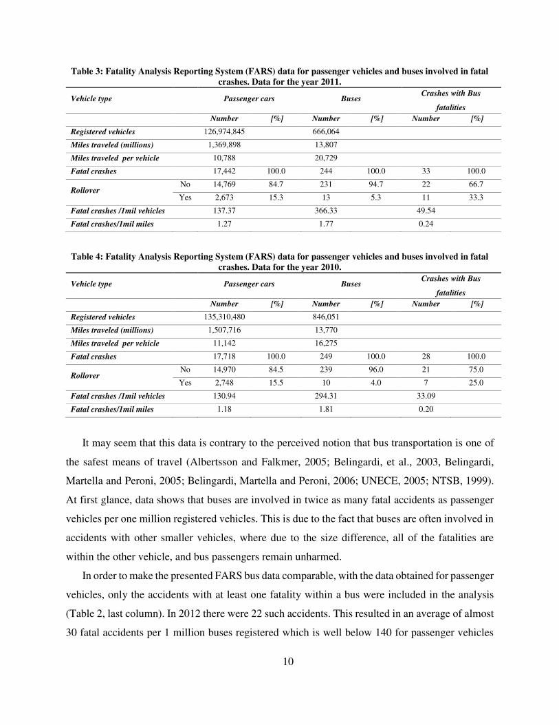
Table 3: Fatality Analysis Reporting System (FARS) data for passenger vehicles and buses involved in fatal crashes. Data for the year 2011.................................................................... 10
Table 4: Fatality Analysis Reporting System (FARS) data for passenger vehicles and buses involved in fatal crashes. Data for the year 2010.................................................................... 10
Table 5: Fatality Analysis Reporting System (FARS) data for bus accidents resulting with at least one fatality in the crash. Combined data for years 2010-2012. .............................................. 13
Table 6: Fatality Analysis Reporting System (FARS) data for bus accidents resulting with at least one bus occupant fatality. Combined data for years 2010-2012. ............................................ 14
Table 7: Injury distribution in bus accidents, FARS data (USA) (NHTSA, 2014), compared with Spanish data from 1995-1999 (Martinez, et al., 2003). .......................................................... 14
Table 8: The injury mechanisms of the occupants (UN ECE, 2008). ........................................... 15
Table 9: Fatality Analysis Reporting System (FARS) data for van-based bus accidents resulting with at least one fatality in the crash. Combined data for years 2011-2012. .......................... 17
Table 10: Fatality Analysis Reporting System (FARS) data for van-based bus accidents resulting with at least one bus occupant fatality. Combined data for years 2011-2012. ....................... 17
Table 11: Statistics of the Bus 1 FE model. .................................................................................. 37
Table 12: Statistics of the Bus 2 FE model. .................................................................................. 38
Table 13: Statistics of the Bus 3 FE model. .................................................................................. 39
Table 14: Statistics of the Bus 4 FE model. .................................................................................. 39
Table 15: Statistics of the Bus 5 FE model. .................................................................................. 40
Table 16: Constitutive material models used in FE models of paratransit buses. ........................ 42
viii
Table 17: Three point bending test results. Experiment versus FE simulation. ........................... 57
Table 18: Parameters optimized for MAT_098_SIMPLIFIED_JOHNSON_COOK. ................. 61
Table 19: Optimization cases for the fixed p parameter. .............................................................. 65
Table 20: Comparison of experimental tests and numerical simulation results for Bus 1 validation experiments. ............................................................................................................................ 68
Table 21: Comparison of experimental tests and numerical simulation results for panel impact validation experiments (Rawl, 2010), (Bojanowski, 2009). ................................................... 69
Table 22: Variables used in the optimization process with assumed thickness range from 11 to 18 ga. ............................................................................................................................................ 74
Table 23: Internal energy distribution within the developed bus FE models during ECE-R66 rollover. ................................................................................................................................... 87
Table 24: The percentage of total energy absorbed by the bus structure during rollover. ........... 94
Table 25: Values of the coefficient κRW for the shortest and the longest buses........................ 101
Table 26: Selected energies and corresponding rotations for three deformation patterns .......... 117
Table 27: Benchmark test cases used for evaluation of the ERT procedure. ............................. 131
Table 28: Eigenvalues obtained for the ERT data set. ................................................................ 137
Table 29: Correlation coefficients obtained for the Deformation Index (DIRoll) and DIERT data set. FR - frontal ring, RW – rear wall, WF – wall to floor connection ,WR – wall to roof connection, P – panel impact test, ST – 3 point static tube bending, DT – tube impact test. .................. 138
Table 30: Eigenvalues obtained for the reduced ERT data set. .................................................. 140
Table 31: Loadings calculated for supplementary variables....................................................... 141
Table 32: Comparison of experimental tests and numerical simulation results for Bus 2 validation experiments. .......................................................................................................................... 159
Table 33: Comparison of experimental tests and numerical simulation results for Bus 3 validation experiments. .......................................................................................................................... 159
Table 34: Comparison of experimental tests and numerical simulation results for Bus 4 and Bus 5 validation experiments. ......................................................................................................... 161

ix
Table 35: The data for 132 rollover used for evaluation of the equivalent rollover testing procedure............................................................................................................................................... 162
x
LIST OF FIGURES
Figure 1: An example of a paratransit bus. ..................................................................................... 1
Figure 2: An example of a paratransit bus assembly process, preparation of the chassis (a), attachment of the floor assembly (b), attachment of the bus cage (c), complete vehicle (d). .. 2
Figure 3: Two paratransit buses subjected to the ECE-R66 rollover test. Venerable bus design (a), versus strong bus design (b). ..................................................................................................... 3
Figure 4: Comparison of casualty rates among vehicle occupants. USA data (NHTSA, 2014) vs European data (European Commission, 2003). ...................................................................... 12
Figure 5: Example of buses built on heavy duty truck chassis. Ford F-550 (a) and Intercontinental 3200 series (b) (Champion Bus, 2014). .................................................................................. 18
Figure 6: Test setup for the ECE-R66 rollover test, with marked Center of Gravity (COG) of the bus. a) bus placed onto the tilting table, b) position in unstable equilibrium, c) impact into the 800 mm deep concrete ditch ................................................................................................... 19
Figure 7: Residual space and a Deformation Index concept (UN ECE, 2006). ........................... 21
Figure 8: Test setup for FMVSS 220 School Bus Rollover Protection (US DOT, 1998). ........... 22
Figure 9: A test schematic of the FDOT Standard (Bojanowski, 2009). ...................................... 22
Figure 10: Verification, validation and conformation in relation to reality of interest, mathematical model, and computer model (Schlesinger, et al., 1979). ......................................................... 30
Figure 11: Hierarchical validation process (Thacker, et al., 2004; Oberkampf, Trucano and Hirsch, 2003). ...................................................................................................................................... 33
Figure 12: FE models developed by CIAL as of July 2014, a) Bus 1, b) Bus 2, c) Bus 3, d) Bus 4, and e) Bus 5 ............................................................................................................................ 36
Figure 13: Bus 1, a) Picture obtained from the manufacturer (Turtle Top, 2014), b) FE model developed. ............................................................................................................................... 37
Figure 14: Bus 2, a) Test vehicle prepared for the rollover test, b) FE model developed. ........... 38
Figure 15: Bus 3 a) Paratransit bus selected for a rollover test, b) FE model developed. ............ 39
xi
Figure 16: Bus 4, a) Picture obtained from the manufacturer (Turtle Top, 2014), b) FE model developed. ............................................................................................................................... 40
Figure 17: Bus 5, a) Picture obtained from the manufacturer (model in the picture is not equipped with the rear passenger lift) (Turtle Top, 2014), b) FE model developed. ............................. 40
Figure 18: Energy balance plot for the rollover simulation with the deformable-to-rigid switch 52
Figure 19: Timestep plot for the rollover simulation with the deformable-to-rigid switch .......... 52
Figure 20: Deformable-to-rigid switch, a) initial position of the bus (switch from deformable to rigid), b) moment instance right before the impact (switch from rigid to deformable), c) impact.................................................................................................................................................. 53
Figure 21: Energy balance for Bus 1 rollover simulation. ............................................................ 55
Figure 22: Energy ratio for Bus 1 rollover simulation. ................................................................. 55
Figure 23: A numerical three point bending test used for spatial discretization error estimation with two elements across the tube. .................................................................................................. 56
Figure 24: Three point bending test, experiment versus FE simulation with various spatial discretization. .......................................................................................................................... 57
Figure 25: Deformation of the bus structure during rollover. ....................................................... 58
Figure 26: Components selected for the validation procedure: wall to floor connection (1), wall to roof connection (2), and sidewall panel (3). ........................................................................... 59
Figure 27: Fiberglass tensile test samples prepared for testing (left), failed fiberglass test sample (right). ..................................................................................................................................... 60
Figure 28: Comparison of FE results with experiment for MAT_98 material model definition. True Stress [MPa] vs True Strain; for a strain rate of 0.0005 in/s (a), strain rate of 0.5in/s (b), strain rate of 1.5in/s (c). .................................................................................................................... 61
Figure 29: Three point bending test results obtained for a 14ga square tube. Experiment and FE simulation. ............................................................................................................................... 62
Figure 30: Fiberglas test samples after 3 point bending test. Test sample 2 with polyurethane foam facing down (left), test sample 3 with no polyurethane foam (right). .................................... 62
Figure 31: FE model used for the foam facing down 3 point bending test. .................................. 63
xii
Figure 32: Comparison of FE results with experiment for 3 point bending test. Force [N] vs displacement [mm]; foam up sample orientation (a), foam down sample orientation (b), sample with no foam (c). ..................................................................................................................... 63
Figure 33: Impact apparatus (a), FE model (b) ............................................................................. 64
Figure 34: Displacement (a) and acceleration (b) of the impact hammer vs. time from the impact for the 1500 mm drop height. Comparison of the experimental and FEM results. No strain rate definition included. ................................................................................................................. 65
Figure 35: Displacement (a) and acceleration (b) of the impact hammer vs. time from the impact for the 1500 mm drop height. Comparison of the experimental and FEM results. Strain rate definition included. ................................................................................................................. 65
Figure 36: A plan of a connection testing apparatus, with a specimen fixed for testing (Rawl, 2010).................................................................................................................................................. 66
Figure 37: Connection testing apparatus, experiment (a), and FE simulation (b). ....................... 67
Figure 38: Wall to floor connection test for Bus 1. Experimental results compared with FE analysis.................................................................................................................................................. 67
Figure 39: Roof to wall connection test for Bus 1. Experimental results compared with FE analysis.................................................................................................................................................. 68
Figure 40: Experimental setup for panel impact tests (Bojanowski 2009). .................................. 69
Figure 41: Residual space compromised by the bus structure. View of complete bus (a), view without skin (b). ...................................................................................................................... 71
Figure 42: Force recorded on load application plate during the FMVSS 220 testing procedure. Results for 1s and 2 s simulations. .......................................................................................... 72
Figure 43: Location of the structural elements used in definition of design variables. ................ 74
Figure 44: Sensitivity study for the Deformation Index response based on (a) ANOVA (b) Sobol’s Indices. .................................................................................................................................... 75
Figure 45: Sensitivity study for the Resultant Force response based on (a) ANOVA (b) Sobol’s Indices. .................................................................................................................................... 75
Figure 46: Cumulative global sensitivity in (a) ECE-R66 test (b) FMVSS 220 test. ................... 75
xiii
Figure 47: Bus 3 rollover test, with 909 mm ditch depth. Front of the bus (a), and inside view during largest deformation (b). ............................................................................................... 77
Figure 48: Bus 3 rollover test, with 800 mm ditch depth. Front of the bus (a), and back of the bus (b). ........................................................................................................................................... 77
Figure 49: Bus 2 rollover test, with 800 mm ditch depth. Front of the bus (a), and back of the bus (b). ........................................................................................................................................... 78
Figure 50: Bus 3 rollover with the 909 mm ditch depth. Experiment (a) and FE analysis (b). .... 79
Figure 51: Comparison of Deformation Index (DI) between the experiment and FE analysis. Data from the Bus 3 rollover tests with 909 mm ditch depth. ......................................................... 79
Figure 52: Experimental and FE results for the Bus 3, 909 mm rollover. Cage deformation at t=0.28 s. .............................................................................................................................................. 80
Figure 53: Bus 3 rollover with the 800 mm ditch depth. Experiment (a) and FE analysis (b). .... 80
Figure 54: Comparison of Deformation Index (DI) between the experiment and FE analysis. Data from the Bus 3 rollover tests with 800 mm ditch depth. ......................................................... 81
Figure 55: Experimental and FE results for the Bus 3, 800 mm rollover. Cage deformation at t=0.25 s. .............................................................................................................................................. 81
Figure 56: Bus 2 rollover with the 800 mm ditch depth. Front view - experiment (a) and FE analysis (b), back view - experiment (c) and FE analysis (d). .............................................................. 82
Figure 57: Comparison of Deformation Index (DI) between the experiment and FE analysis. Data from the Bus 2 rollover tests with 800 mm ditch depth. ......................................................... 82
Figure 58: Experimental and FE results for the Bus 2, 800 mm rollover. Cage deformation at t=0.31 s. .............................................................................................................................................. 83
Figure 59: Deformation in the frontal area during Bus 2 rollover, experiment (a), FE simulation (b). ........................................................................................................................................... 84
Figure 60: Deformation in the frontal area during Bus 3 rollover. Bus with skin (a), exposed deformation of the cage (b). .................................................................................................... 84
Figure 61: Center of Gravity (COG) location overlaid onto the picture of the bus. Loaded bus prepared for rollover testing (a), corresponding FE model (b). .............................................. 85
xiv
Figure 62: Bus structure divided into subcomponents for internal energy analysis. Entire bus before subdivision (b), frontal cap (a), bus skin with windows (c), chassis (d), rear wall (e), cage without rear wall (f). ............................................................................................................... 86
Figure 63: Energy transfer during the bus rollover. Bus at the moment of unstable equilibrium (a), bus during concrete ditch impact, with COG at its lowest position (b). ................................. 94
Figure 64: Assumed deformation throughout the length of the bus. ............................................ 95
Figure 65: Positions of the COG during roll-over test. ................................................................. 97
Figure 66: Energy distribution according to the energy concept of the ERT procedure. ........... 102
Figure 67: Spacing of rings, with identification of the frontal ring and rear wall. ..................... 103
Figure 68: Total Reference Energy with reduction coefficients. ................................................ 104
Figure 69: Simplified model of a bus structure during a rigid wall impact, a) Spring-damper model without internal energy dissipation, b) Spring-damper model with internal energy dissipation................................................................................................................................................ 105
Figure 70: Deformation Index (DI) vs. time during rollover test. .............................................. 106
Figure 71: Water ballast dummies representing passenger weight. ............................................ 106
Figure 72: Large displacement of water ballast dummies relative to the seats during rollover test................................................................................................................................................ 107
Figure 73: Inertial forces and bending moment diagrams in a) rollover test, b) ring based static experiment............................................................................................................................. 108
Figure 74: Generic model of a paratransit bus passenger compartment prepared for rollover testing, a) Cage #1, b) Cage #2, c) Cage #3. ..................................................................................... 108
Figure 75: Considered test cases: a) Cage #1, b) Cage #2 and c) Cage #3. ................................ 109
Figure 76: Kinetic and internal energy vs. time for all three test cases. ..................................... 110
Figure 77: Deformation index vs. Time for all three test cases. ................................................. 111
Figure 78: Static pushover analysis test setup. Cage #1, a) test setup, b) deformed state. Cage#2, c) test setup, d) deformed state. ............................................................................................ 111
Figure 79: Energy dissipation vs. Deformation Index for static and dynamic test cases. .......... 112

xv
Figure 80: Plastic hinge developed in the bus during rollover. .................................................. 113
Figure 81: Case A. Deformation pattern of the ring corresponding to sidewall intrusion into residual space due to vulnerability of the wall to floor connection. ..................................... 115
Figure 82: Case B. Deformation pattern of the ring corresponding to maximum deformation in the plastic hinge developed at the waistrail. ............................................................................... 115
Figure 83: Case C. Typical deformation pattern of the ring. ...................................................... 116
Figure 84: Moment – rotation relationships for different bus connections tested experimentally, and approximated bilinear elastic – perfectly plastic moment – rotation characteristics. .... 117
Figure 85: Determination of the loading direction for the ring test. ........................................... 119
Figure 86: Frontal ring test setup. ............................................................................................... 120
Figure 87: Example calculation of absorbed energy for a quasi-static pushing test controlled by forced displacement in prescribed direction, and derived from the measured load-deformation curve (UN ECE, 2006). ......................................................................................................... 121
Figure 88: Rear wall test setup.................................................................................................... 122
Figure 89: Test setup for three point bending with a=300 mm................................................... 127
Figure 90: Permanent angle ∆ as a measure of plastic deformation generated by the impact in the plastic hinge, assumed a=300 mm. ....................................................................................... 128
Figure 91: Summary of the ERT procedure. ............................................................................... 130
Figure 92: Test setup for the frontal ring test. Residual space profile (orange), load application plate (red). Original configuration (a), deformed stage (b). ................................................. 133
Figure 93: Test setup for the rear wall test. Residual space profile (orange), load application plate (red). Original configuration (a), deformed stage (b). .......................................................... 133
Figure 94: ERT data projected onto its first two principal components (a), Eigenvalues of the covariance matrix of data X (b). ........................................................................................... 136
Figure 95: ERT data trimmed to a maximum valued of 3 projected onto its first two principal components (a), Eigenvalues of the covariance matrix of data X (b). .................................. 137
Figure 96: ERT data projected onto its first two principal components (a), Eigenvalues of the covariance matrix of data X (b). ........................................................................................... 140
xvi
Figure 97: ERT data plotted in the component space (a,c,e), circles of correlation with plot of loadings of supplementary variables; Deformation Index (DIRoll), Average DIERT value (Avg DIERT), maximum of all DIERT (Max DIERT), wheelbase of the bus (WB), and weight of the bus (Weight) (b,d,f). .................................................................................................................... 142
Figure 98: First and second component space, with the heat map of the average DIERT component test result. .............................................................................................................................. 143
Figure 99: First and second component space, with the heat map of the rollover Deformation Index (DI) values. ........................................................................................................................... 143
Figure 100: First and second component space, with the heat map of the mass of a tested bus. 143
Figure 101: Deformation Index versus the average ERT component test result (Avg DIERT). Results for all 132 buses. ................................................................................................................... 145
Figure 102: Deformation Index versus the maximum DIERT. Results for all 132 buses............. 146
Figure 103: Sensitivity and Specificity versus the DIERT threshold value. ................................. 148
Figure 104: Receiver Operating Characteristic (ROC) curve. .................................................... 148
Figure 105: Energy balance for Bus 2 rollover simulation. ........................................................ 155
Figure 106: Energy ratio for Bus 2 rollover simulation. ............................................................. 155
Figure 107: Energy balance for Bus 3 rollover simulation. ........................................................ 156
Figure 108: Energy ratio for Bus 3 rollover simulation. ............................................................. 156
Figure 109: Energy balance for Bus 4 rollover simulation. ........................................................ 156
Figure 110: Energy ratio for Bus 4 rollover simulation. ............................................................. 157
Figure 111: Energy balance for Bus 5 rollover simulation. ........................................................ 157
Figure 112: Energy ratio for Bus 5 rollover simulation. ............................................................. 157
Figure 113: Wall to floor connection test for Bus 2. Experimental results compared with FE analysis. ................................................................................................................................. 158
Figure 114: Roof to wall connection test for Bus 2. Experimental results compared with FE analysis. ................................................................................................................................. 158

xvii
Figure 115: Wall to floor connection test for Bus 3. Experimental results compared with FE analysis. ................................................................................................................................. 159
Figure 116: Roof to wall connection test for Bus 3. Experimental results compared with FE analysis. ................................................................................................................................. 160
Figure 117: Wall to floor connection test for Bus 4 and Bus 5. Experimental results compared with FE analysis. ........................................................................................................................... 160
Figure 118: Roof to wall connection test for Bus 4 and Bus 5. Experimental results compared with FE analysis. ........................................................................................................................... 161

xviii
ABSTRACT
The following dissertation presents the initial stages of the development of the new rollover safety
assessment protocol developed for paratransit buses. Each year, the State of Florida purchases over
300 paratransit buses. In 2011, the purchased buses came with over 40 different
floor/wheelbase/chassis configurations. Such variety of purchased vehicles gives the ordering
agencies a flexibility of ordering vehicles optimized for desired purpose, but also creates a
challenge for the rollover safety assessment procedures.
Currently, there are two standards available to be used for rollover crashworthiness assessment
of buses, the FMVSS 220 standard and the UN-ECE Regulation 66. The FMVSS 220 is commonly
used in the United States to evaluate rollover crashworthiness of wide variety of buses. Its quasi-
static nature offers an attractive, easy to perform test that provides good repeatability of results.
Nevertheless, due to the nature of applied load, this procedure may not be the best choice for
evaluating the dynamic behavior of a bus during a rollover accident. In contrast, the UN-ECE
Regulation 66 employs a full scale, dynamic rollover test to examine response of buses in rollover
accidents. The dynamic rollover, which forms the basis of the ECE-R66 approval procedure
closely resembles the real world rollover accident and this regulation has been adopted by over 40
countries in the world. However, the dynamic nature of this test makes it expensive, time
consuming and difficult to perform.
This situation calls for an update of an approval procedure, in order to test the purchased buses
within the available time and budget. The initial development of the new assessment protocol, the
Equivalent Rollover Testing (ERT) procedure, was carried out in this dissertation. The ERT
procedure is conceived as an alternative approval method for the experimental or virtual full scale
rollover testing. The new protocol was developed based on collected experimental experience,
extensive numerical studies and theoretical considerations. The ERT procedure establishes a set
of experimental tests, on the components of bus structure, that if satisfied give a high level of
confidence that the tested bus will pass the requirements of the ECE-R66 rollover procedure.
The proposed ERT procedure is further tested through the parametric studies on five detailed
finite element models of paratransit buses. The models, developed in the Crashworthiness and
Impact Analysis Laboratory (CIAL), cover a wide range of buses, from small 138 in to a large 255
in wheelbase configurations. Through the modifications of structural components of each of the
xix
buses, a set of 132 bus designs and corresponding 132 rollover tests was established. Each of the
developed buses was also subjected to the provisions of the ERT procedure. The comparison of
results showed that ERT procedure presents a conservative approach to paratransit bus safety
evaluation. Out of all 132 test cases there was not a single bus that passed the provisions of the
ERT procedure, but has failed the full scale ECE-R66 rollover test. The proposed ERT procedure,
complemented by future validation experimental study presents a promising alternative for the
paratransit bus rollover safety evaluation.
1
CHAPTER 1
INTRODUCTION
1.1. Background and Motivation
The Americans with Disabilities Act (ADA) recognizes an equal right of people with disabilities
to access public services and facilities, including transportation. Paratransit transport has a task of
providing all Americans with an access to basic transit services. It is defined by the Americans
with Disabilities Act (ADA) (US DOL, 1990), as a specialized, per request transport service,
provided for people who cannot use a fixed route public transportation (Amputee Coalition, 2012).
According to American Public Transportation Association (APTA) Fact Book, after the
introduction of ADA number of passenger trips on demand response services increased from 68
million in 1990 to 190 million in 2010 (Dickens, Neff and Grisby, 2012). Introduction of ADA
has highlighted a need for a new vehicle type, providing the passengers on wheelchairs with greater
accessibility, as well as capable to operate off the regular route schedule. Often used for such
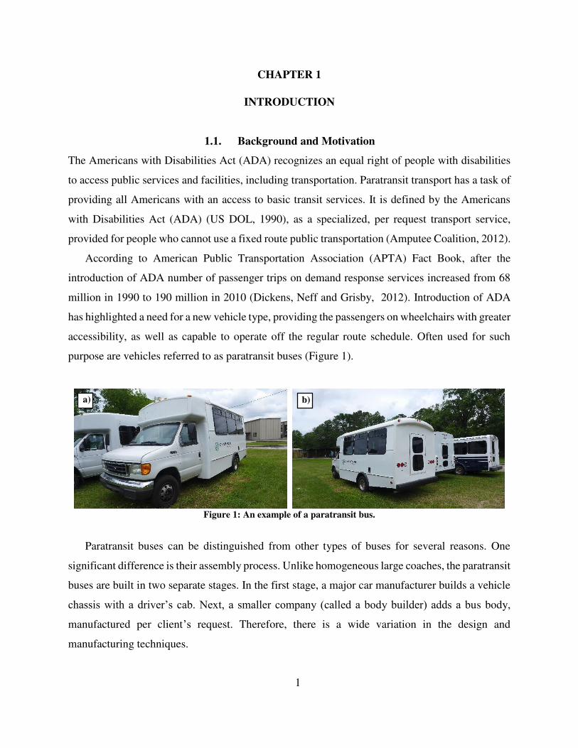
purpose are vehicles referred to as paratransit buses (Figure 1).
Figure 1: An example of a paratransit bus.
Paratransit buses can be distinguished from other types of buses for several reasons. One
significant difference is their assembly process. Unlike homogeneous large coaches, the paratransit
buses are built in two separate stages. In the first stage, a major car manufacturer builds a vehicle
chassis with a driver’s cab. Next, a smaller company (called a body builder) adds a bus body,
manufactured per client’s request. Therefore, there is a wide variation in the design and
manufacturing techniques.
a) b)

2
Figure 2 shows a sample paratransit bus assembly process. First, a body builder obtains the
pre-manufactured bus chassis and prepares it for the assembly process (Figure 2a), cuts out body
panels, and stretches the chassis if necessary. Next, the floor assembly, previously welded together,
is secured onto the bus frame (Figure 2b), and fitted with a prebuilt cage and fiberglass front cap
(Figure 2c, d).
Figure 2: An example of a paratransit bus assembly process, preparation of the chassis (a), attachment of the
floor assembly (b), attachment of the bus cage (c), complete vehicle (d).
Process shown in Figure 2 varies from manufacturer to the manufacturer. Some assemble the
passenger compartment cage and fit it with the outside skin layer before attaching it onto the bus
(Figure 2), in other cases, the cage is built directly on the bus frame and the skin is attached in a
separate construction step. This variability of designs and assembly techniques results in a large
differences in crashworthy behavior of these vehicles (Figure 3).
Another factor, that makes these vehicles unique is, lack of specific and applicable safety
standards. Out of all bus accident scenarios, rollover is considered to be the most dangerous one
(Matolcsy, 2003). Unfortunately, paratransit buses of Gross Vehicle Weight Rating (GVWR)
which exceeds 10,000 lb. are not subjected to any design restrictions, unless required by a specific
bidding process. Clients often try to close this loophole by requesting compliance with an existing
a) b)
c) d)
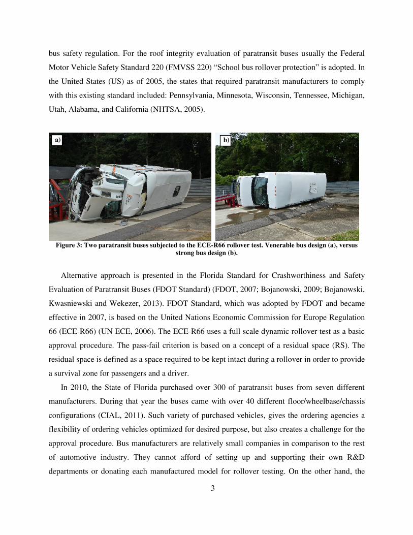
3
bus safety regulation. For the roof integrity evaluation of paratransit buses usually the Federal
Motor Vehicle Safety Standard 220 (FMVSS 220) “School bus rollover protection” is adopted. In
the United States (US) as of 2005, the states that required paratransit manufacturers to comply
with this existing standard included: Pennsylvania, Minnesota, Wisconsin, Tennessee, Michigan,
Utah, Alabama, and California (NHTSA, 2005).
Figure 3: Two paratransit buses subjected to the ECE-R66 rollover test. Venerable bus design (a), versus
strong bus design (b).
Alternative approach is presented in the Florida Standard for Crashworthiness and Safety
Evaluation of Paratransit Buses (FDOT Standard) (FDOT, 2007; Bojanowski, 2009; Bojanowski,
Kwasniewski and Wekezer, 2013). FDOT Standard, which was adopted by FDOT and became
effective in 2007, is based on the United Nations Economic Commission for Europe Regulation
66 (ECE-R66) (UN ECE, 2006). The ECE-R66 uses a full scale dynamic rollover test as a basic
approval procedure. The pass-fail criterion is based on a concept of a residual space (RS). The
residual space is defined as a space required to be kept intact during a rollover in order to provide
a survival zone for passengers and a driver.
In 2010, the State of Florida purchased over 300 of paratransit buses from seven different
manufacturers. During that year the buses came with over 40 different floor/wheelbase/chassis
configurations (CIAL, 2011). Such variety of purchased vehicles, gives the ordering agencies a
flexibility of ordering vehicles optimized for desired purpose, but also creates a challenge for the
approval procedure. Bus manufacturers are relatively small companies in comparison to the rest
of automotive industry. They cannot afford of setting up and supporting their own R&D
departments or donating each manufactured model for rollover testing. On the other hand, the
a) b)
4
process of development, validation and verification of FE models for all purchased vehicles is an
overwhelming task for a research institution such as Crashworthiness and Impact Analysis
Laboratory (CIAL). It became apparent that the full scale experimental rollover tests and the
process of developing FE model for computer simulations are too expensive and time consuming
to be effectively used in the current setting.
This situation calls for an update of an approval procedure. There is a need of a simplified
assessment tool that will allow for a reasonably accurate safety evaluation of a given paratransit
bus within reasonable time and budget.
1.2. Objectives of the Dissertation
The objective of this dissertation is to develop, based on parametric studies on existing FE models
with accompanying full scale rollover tests, a series of simple experiments, which combined
together will result in a set of mathematical formulae for evaluation of the structure of each
individual paratransit bus. The goals of this dissertation can be listed as:
Development of a new Equivalent Rollover Testing (ERT) procedure for the
assessment of safety of paratransit buses during rollover accidents.
The new testing procedure is thought out as a balance between simplicity and efficiency
of the testing procedure and complexity of the mechanics describing deformation and
energy distribution during a rollover test.
The ERT procedure must consist of a series of relatively simple and inexpensive
experimental tests on bus structure components.
Each test is defined by giving a detailed description of the testing procedure,
measurements and calculations of Threshold Values which post requirements for
passing each test.
Development of new reliable testing procedures, which allow for assessment of the bus
safety without the need of full rollover experiment, will result in the overall
improvement of safety of paratransit buses.
Low cost and simplicity of selected experiments will allow more buses to be effectively
tested in a shorter period of time. It will serve as a very useful tool for assessing vehicle
safety for decision makers within purchasing organizations.

5
1.3. Organization of the Dissertation
Chapter 1
The first chapter contains an introduction to this dissertation. It highlights special characteristics
of paratransit buses, and shows the current state of regulations bounding their construction process.
This chapter also presents the up to date regulatory work performed in the state of Florida. It
highlights problems with existing standards which serve as a motivation for this research. The first
chapter defines research objectives and it is concluded with a dissertation summary.
Chapter 2
Second chapter presents the literature overview performed while working on the development of
the new testing standard. It reviews bus accident statistics from across the world, and highlights
the injury mechanism for bus passengers. This chapter discusses the current existing testing
standards, their advantages and limitations, and presents a need to develop a new simplified testing
procedure. It summarizes up to date research work on bus rollover crashworthiness performed by
other researchers. Chapter two concludes with the review of the current validation and verification
requirements for obtaining trustworthy finite element (FE) simulations.
Chapter 3
Chapter three contains a description of the developed FE models of paratransit buses. This chapter
summarizes model statistics, methodology for FE analyses, definition of used constitutive models,
description of contact definition and element formulation. Chapter three concludes with the
description of validation and verification procedures performed for the developed FE models.
Chapter 4
Chapter four presents the unique characteristics of paratransit buses identified throughout the
research performed at the CIAL. It compares the test outcomes while a paratransit bus is subjected
to the FMVSS 220 and ECE-R66 rollover and highlights the differences between the two tests.
Chapter four summarizes the experimental and numerical experience on bus rollover gathered by
CIAL, and highlights the unique deformation pattern and energy distribution observed in
paratransit buses. These two observations are used in the Chapter 5 as a theoretical basis for a
development of the Equivalent Rollover Testing (ERT) procedure.
Chapter 5
6
Chapter five presents the concept of the ERT Procedure, starting from the energy dissipation
concept, through description of required experiments, and the definition of acceptable threshold
values.
Chapter 6
Chapter six shows the evaluation of the ERT procedure. 132 FE models of paratransit buses are
subjected to both, ECE-R66 rollover test, and the provisions of the developed ERT procedure. The
tests outcome are compared in order to evaluate the newly developed standard. Obtained data is
analyzed using the Principal Component Analysis (PCA) and Receiver Operating Characteristic
curve (ROC) analysis. Based on the obtained results the number of necessary tests in the ERT
procedure is reduced.
Chapter 7
Chapter seven presents the summary of this dissertation and lists the recommendations for further
research.
Chapter 8
Chapter eight shows the list of references used in this dissertation.
Chapter 9
Chapter nine presents the biographical sketch of the author.
7
CHAPTER 2
LITERATURE REVIEW
2.1. Bus Accident Statistics
Paratransit bus accident statistics are not easily accessible. In the past, these types of buses were
often lumped into general bus statistics, or “other buses” category. Until 2010, Fatality Analysis
Reporting System (FARS), established by National Highway Traffic Safety Administration
(NHTSA), did not contain a specific category for paratransit buses (NHTSA, 2012). Starting from
the Traffic Safety Facts 2011 report (NHTSA, 2013), a new special category named “Van-Based
Bus (GVWR > 10,000 lb.)” was created to accommodate paratransit buses. So far, there is only
two year data (2011, 2012) available, and accounting a small number of this vehicles on the road,
this is not sufficient to draw a full picture of fatal accidents for paratransit buses.
Another possible source of data on paratransit bus statistics is Crash Injury Research (CIREN)
and National Automotive Sampling System (NASS) databases established by NHTSA. The
CIREN database consists of multiple recorded severe vehicle crashes, including accident
reconstruction and injury profile data. CIREN contains data extending back to 1996 and is
available for public viewing (NHTSA, 2014). NASS on the other hand, collects a nationally
representative sample of police reported vehicle crashes of all types. Data is randomly sampled
from available accident data and coded in detail according to NASS requirements (NHTSA, 2014).
Unfortunately, no cases for any bus accidents have been located in the CIREN database, and no
data for bus rollover was found in NASS database.
Due to the lack of the long term accident statistics for paratransit buses, general bus accident
statistics are more useful in drawing conclusions on injury mechanism of bus occupants. United
Nations Economic Commission for Europe (UNECE) has been collecting data on bus accidents
since 1973, when Hungary raised a problem of lack of requirements for the bus superstructure
(Matolcsy, 2003). Up until 2008 over 570 cases of bus rollover has been reported (UNECE, 2008).
Unfortunately no unified reporting system for bus rollover accidents exists in Europe, and provided
data is scattered and country specific. Often authors of the presented statistical data were forced to
refer to media coverage of these events which in regard to injury type, injury severity is
questionable (UNECE, 2008).

8
Looking at the available data on country by country basis one can obtain a more detailed picture
of bus rollover statistics (UNECE, 2008). In 2005, Norway reported 28,783 of registered buses.
With 42 rollover accidents reported over 4 years (2002-2005) there were 5 fatalities, 13 seriously
injured and 166 slightly injured passengers. German experts reported 19,948 buses registered in
Germany in 2004. There was no rollover specific information available, but bus accidents
accounted for 16 fatalities of bus occupants, and 460 seriously injured. Belgian data reported a
total of 34,075 buses and minibuses registered in 2004, and provided casualty figures with no
rollover dissemination. There was 6 reported fatalities in the buses and the total number of Killed
or Seriously Injured (KSI) was reported at 157 (UNECE, 2008).
In Netherlands there were 10,396 bused registered in 2004, and 10 year data showed (1997-
2006) 26 fatalities and 353 seriously injured among bus occupants. No rollover specific data was
provided. For 2005 Spain reported a national fleet of buses and coaches at 58,248. There were 177
bus rollovers reported during that year, with 26 fatalities and 153 seriously injured among bus
occupants. For rollovers the KSI value was at 62 (UNECE, 2008).
A comprehensive overview of French bus rollover data was presented during the expert group
IG/R.66 meeting in Madrid in January 2008 (UNECE, 2008). In 2005, French bus fleet consisted
of 88,417 registered vehicles, and it was estimated that these vehicles traveled 1,023 million miles
during that year. A four year casualty data for accidents in which buses were involved was
provided and it is presented below in Table 1.
Table 1: Casualties in buses and coaches in accident where buses where involved, France (UN ECE, 2008).
Year 2002 2003 2004 2005 Sum
No. of bus accidents 1643 1405 1295 1320 5663
No. of fatalities 10 44 21 14 89
No. of serious
injuries
47 85 31 170 333
No. of all injuries 905 872 732 926 3435
The French data also consists of a study of 94 bus accidents where at least one bus occupant
was killed or seriously injured. The study spans over 25 years (1980-2005). There were two major
groups of crashes identified within this data, frontal impact and rollover. Frontal Impact accidents
accounted for 45% of all crashes, and rollover accounted for 42%. The remaining 13% was
classified as other type of accidents.

9
Other countries represented at the expert group IG/R.66 meeting in Madrid in January 2008,
such as Czech Republic, United Kingdom, Italy, and Poland presented only fleet data, and did not
provide bus accident statistics for their regions.
Another study performed on Spanish bus data from 1995 to 1999 shows that the rollover
accounted for 4% of all bus accidents, but the risk of fatalities was five times higher than for any
other bus accident type (Martinez, et al., 2003).
Fatality Analysis Reporting System (FARS) is a useful tool for obtaining bus accident data for
the United States. FARS is a nationwide database providing the public and decision makers with
a yearly data regarding fatal injuries suffered in motor vehicle traffic crashes (NHTAS, 2014).
FARS data comparing fatal crashes involving passenger vehicles and buses is presented below.
Data covers FARS records for the years 2012 (Table 2), 2011 (Table 3), and 2010 (Table 4).
Registration numbers were obtained from the Federal Highway Administration (FHWA) (FHWA
2014).
In 2012 there were over 127 million passenger cars registered in the US, and they were
involved in over 18,000 fatal accidents (Table 2). Comparison of these numbers to the data of
buses registered and involved in fatal crashes leads to interesting findings. Out of over 750,000
buses registered in the US in the 2012 there were only 249 fatal crashes that involved buses. This
results in 140 fatal accidents per 1 million passenger vehicles registered, and over 300 fatal
accidents per 1 million buses registered.
Table 2: Fatality Analysis Reporting System (FARS) data for passenger vehicles and buses involved in fatal
crashes. Data for the year 2012.
Vehicle type Passenger cars Buses Crashes with Bus
fatalities
Number [%] Number [%] Number [%]
Registered vehicles 127,091,286 764,509
Miles traveled (millions) 1,377,833 14,755
Miles traveled per vehicle 10,841 19,299
Fatal crashes 18,092 100.0 251 100.0 22 100.0
Rollover No 15,284 84.5 240 95.6 15 68.2
Yes 2,808 15.5 11 4.4 7 31.8
Fatal crashes /1mil vehicles 142.35 328.32 28.78
Fatal crashes/1mil miles 1.31 1.70 0.15
10
Table 3: Fatality Analysis Reporting System (FARS) data for passenger vehicles and buses involved in fatal
crashes. Data for the year 2011.
Vehicle type Passenger cars Buses Crashes with Bus
fatalities
Number [%] Number [%] Number [%]
Registered vehicles 126,974,845 666,064
Miles traveled (millions) 1,369,898 13,807
Miles traveled per vehicle 10,788 20,729
Fatal crashes 17,442 100.0 244 100.0 33 100.0
Rollover No 14,769 84.7 231 94.7 22 66.7
Yes 2,673 15.3 13 5.3 11 33.3
Fatal crashes /1mil vehicles 137.37 366.33 49.54
Fatal crashes/1mil miles 1.27 1.77 0.24
Table 4: Fatality Analysis Reporting System (FARS) data for passenger vehicles and buses involved in fatal
crashes. Data for the year 2010.
Vehicle type Passenger cars Buses Crashes with Bus
fatalities
Number [%] Number [%] Number [%]
Registered vehicles 135,310,480 846,051
Miles traveled (millions) 1,507,716 13,770
Miles traveled per vehicle 11,142 16,275
Fatal crashes 17,718 100.0 249 100.0 28 100.0
Rollover No 14,970 84.5 239 96.0 21 75.0
Yes 2,748 15.5 10 4.0 7 25.0
Fatal crashes /1mil vehicles 130.94 294.31 33.09
Fatal crashes/1mil miles 1.18 1.81 0.20
It may seem that this data is contrary to the perceived notion that bus transportation is one of
the safest means of travel (Albertsson and Falkmer, 2005; Belingardi, et al., 2003, Belingardi,
Martella and Peroni, 2005; Belingardi, Martella and Peroni, 2006; UNECE, 2005; NTSB, 1999).
At first glance, data shows that buses are involved in twice as many fatal accidents as passenger
vehicles per one million registered vehicles. This is due to the fact that buses are often involved in
accidents with other smaller vehicles, where due to the size difference, all of the fatalities are
within the other vehicle, and bus passengers remain unharmed.
In order to make the presented FARS bus data comparable, with the data obtained for passenger
vehicles, only the accidents with at least one fatality within a bus were included in the analysis
(Table 2, last column). In 2012 there were 22 such accidents. This resulted in an average of almost
30 fatal accidents per 1 million buses registered which is well below 140 for passenger vehicles
11
and is consistent with previous findings (Albertsson and Falkmer, 2005; Belingardi, et al., 2003,
Belingardi, Martella and Peroni, 2005; Belingardi, Martella and Peroni, 2006; UNECE, 2005).
This data is consistent for all three reported years (2012, 2011, and 2010).
Throughout all three considered years, 2012, 2011, and 2010 bus rollovers accounted for 4-5%
of all bus accidents which is consistent with the data presented by Spanish researchers (Martinez,
et al., 2003). Data collected from Spain from 1995 to 1999 shows a rollover frequency of 4%.
Unfortunately, there is no information on the type of data collected in Spain, and the types of
accidents included.
Considering only the accidents where at least one bus occupant suffered fatal injuries (Table
2, last column), one can see that the percentage of rollovers in all bus accidents increases
significantly, from 4% of all bus crashes to 30% in bus fatal crashes. Also, out of all bus rollovers
each year at least 70% results in at least one fatality. For the 2012 data this is true for 7 out of 11
rollovers. This data is consistent for all three reported years (2012, 2011, and 2010).
Casualties among bus occupants are among the lowest of all vehicles on the road. This is due
to the fact that the number of buses on the roads is significantly smaller as compared to the
passenger vehicles (Table 2 -Table 4). These vehicles are usually also operated by specially trained
drivers, required to have a professional driving licenses, which improves the overall safety and
accident avoidance. Comparison of data obtained from FARS database (NHTSA, 2014) with data
gathered during Enhanced Coach and Bus Occupant Safety (ECBOS) project funded by the
European Commission (European Commission, 2003; Technical University Graz; 2003), shows
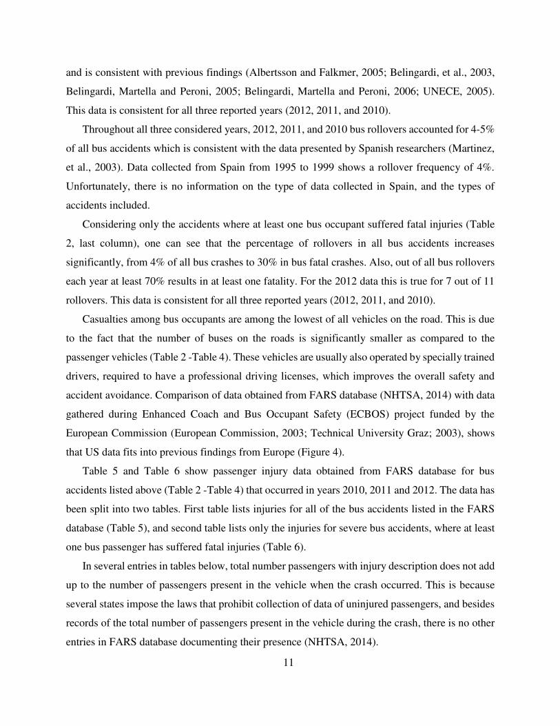
that US data fits into previous findings from Europe (Figure 4).
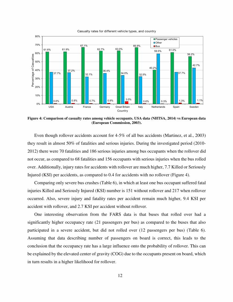
Table 5 and Table 6 show passenger injury data obtained from FARS database for bus
accidents listed above (Table 2 -Table 4) that occurred in years 2010, 2011 and 2012. The data has
been split into two tables. First table lists injuries for all of the bus accidents listed in the FARS
database (Table 5), and second table lists only the injuries for severe bus accidents, where at least
one bus passenger has suffered fatal injuries (Table 6).
In several entries in tables below, total number passengers with injury description does not add
up to the number of passengers present in the vehicle when the crash occurred. This is because
several states impose the laws that prohibit collection of data of uninjured passengers, and besides
records of the total number of passengers present in the vehicle during the crash, there is no other
entries in FARS database documenting their presence (NHTSA, 2014).
12
Figure 4: Comparison of casualty rates among vehicle occupants. USA data (NHTSA, 2014) vs European data
(European Commission, 2003).
Even though rollover accidents account for 4-5% of all bus accidents (Martinez, et al., 2003)
they result in almost 50% of fatalities and serious injuries. During the investigated period (2010-
2012) there were 70 fatalities and 186 serious injuries among bus occupants when the rollover did
not occur, as compared to 68 fatalities and 156 occupants with serious injuries when the bus rolled
over. Additionally, injury rates for accidents with rollover are much higher, 7.7 Killed or Seriously
Injured (KSI) per accidents, as compared to 0.4 for accidents with no rollover (Figure 4).
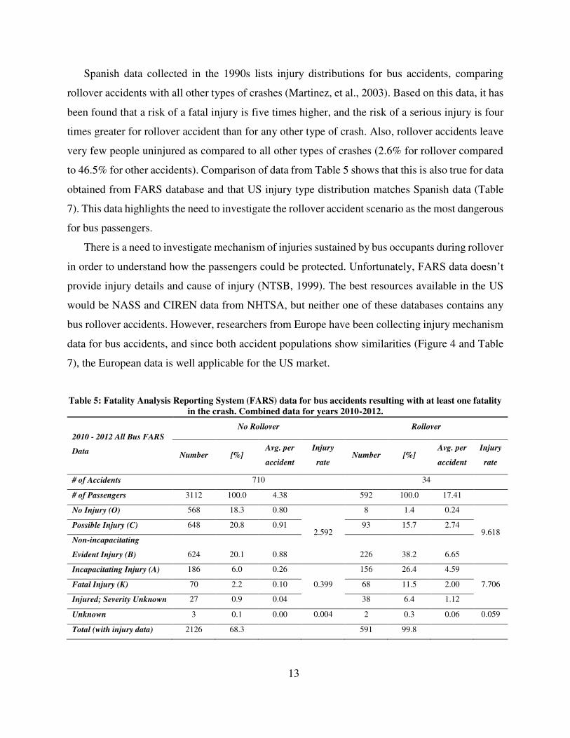
Comparing only severe bus crushes (Table 6), in which at least one bus occupant suffered fatal
injuries Killed and Seriously Injured (KSI) number is 151 without rollover and 217 when rollover
occurred. Also, severe injury and fatality rates per accident remain much higher, 9.4 KSI per
accident with rollover, and 2.7 KSI per accident without rollover.
One interesting observation from the FARS data is that buses that rolled over had a
significantly higher occupancy rate (21 passengers per bus) as compared to the buses that also
participated in a severe accident, but did not rolled over (12 passengers per bus) (Table 6).
Assuming that data describing number of passengers on board is correct, this leads to the
conclusion that the occupancy rate has a large influence onto the probability of rollover. This can
be explained by the elevated center of gravity (COG) due to the occupants present on board, which
in turn results in a higher likelihood for rollover.
13
Spanish data collected in the 1990s lists injury distributions for bus accidents, comparing
rollover accidents with all other types of crashes (Martinez, et al., 2003). Based on this data, it has
been found that a risk of a fatal injury is five times higher, and the risk of a serious injury is four
times greater for rollover accident than for any other type of crash. Also, rollover accidents leave
very few people uninjured as compared to all other types of crashes (2.6% for rollover compared
to 46.5% for other accidents). Comparison of data from Table 5 shows that this is also true for data
obtained from FARS database and that US injury type distribution matches Spanish data (Table
7). This data highlights the need to investigate the rollover accident scenario as the most dangerous
for bus passengers.
There is a need to investigate mechanism of injuries sustained by bus occupants during rollover
in order to understand how the passengers could be protected. Unfortunately, FARS data doesn’t
provide injury details and cause of injury (NTSB, 1999). The best resources available in the US
would be NASS and CIREN data from NHTSA, but neither one of these databases contains any
bus rollover accidents. However, researchers from Europe have been collecting injury mechanism
data for bus accidents, and since both accident populations show similarities (Figure 4 and Table
7), the European data is well applicable for the US market.
Table 5: Fatality Analysis Reporting System (FARS) data for bus accidents resulting with at least one fatality
in the crash. Combined data for years 2010-2012.
2010 - 2012 All Bus FARS
Data
No Rollover Rollover
Number [%] Avg. per
accident
Injury
rate Number [%]
Avg. per
accident
Injury
rate
# of Accidents 710 34
# of Passengers 3112 100.0 4.38 592 100.0 17.41
No Injury (O) 568 18.3 0.80
2.592
8 1.4 0.24
9.618 Possible Injury (C) 648 20.8 0.91 93 15.7 2.74
Non-incapacitating
Evident Injury (B) 624 20.1 0.88 226 38.2 6.65
Incapacitating Injury (A) 186 6.0 0.26
0.399
156 26.4 4.59
7.706 Fatal Injury (K) 70 2.2 0.10 68 11.5 2.00
Injured; Severity Unknown 27 0.9 0.04 38 6.4 1.12
Unknown 3 0.1 0.00 0.004 2 0.3 0.06 0.059
Total (with injury data) 2126 68.3 591 99.8
14
Table 6: Fatality Analysis Reporting System (FARS) data for bus accidents resulting with at least one bus
occupant fatality. Combined data for years 2010-2012.
2010 - 2012 Severe Bus
Crash Data
No Rollover Rollover
Number [%] Avg. per
accident
Injury
rate Number [%]
Avg. per
accident
Injury
rate
# of Accidents 56 25
# of Passengers 659 100.0 11.77 517 100.0 20.68
No Injury (O) 25 3.8 0.45
7.357
6 1.2 0.24
11.160 Possible Injury (C) 155 23.5 2.77 67 13.0 2.68
Non-incapacitating
Evident Injury (B) 232 35.2 4.14 206 39.8 8.24
Incapacitating Injury (A) 81 12.3 1.45
2.696
149 28.8 5.96
9.400 Fatal Injury (K) 70 10.6 1.25 68 13.2 2.72
Injured; Severity Unknown 0 0.0 0.00 18 3.5 0.72
Unknown 0 0.0 0.00 0.000 2 0.4 0.08 0.080
Total (with injury data) 563 85.4 516 99.8
Table 7: Injury distribution in bus accidents, FARS data (USA) (NHTSA, 2014), compared with Spanish
data from 1995-1999 (Martinez, et al., 2003).
USA Spain
Injury severity Others [%] Rollover [%] Others [%] Rollover [%]
Fatalities 2.2 11.5 2.5 9.6
Serious injured 6.0 26.4 7.7 32.1
Minor injured 49.9 53.9 43.3 55.6
Not injured 40.9 1.6 46.5 2.6
Injured, Unknown 0.9 6.4 - -
Unknown 0.1 0.3 - -
Total number of occupants 3112 592 14151 1037
Hungarian researcher (Matolcsy, 2007) identified injury mechanisms for bus accidents and
divided them into four different groups defined as follows:
Intrusion. Due to large scale structural deformations and the loss of the residual space,
structural elements impact or crush the bodies of the occupants.
Projection. Due to the uncontrolled movement of the occupants inside the bus, their bodies
impact the structural parts of the passenger compartment.
15
Partial Ejection. During the rollover process the parts of occupant’s body could be
partially ejected through the broken or fallen windows and crushed by the rolling bus.
Complete Ejection. During the rollover process the occupants could be ejected through
the broken or fallen windows and crushed by the rolling bus.
Unfortunately, this data did not provide detailed distribution of passengers injuries sustained
during rollover accidents.
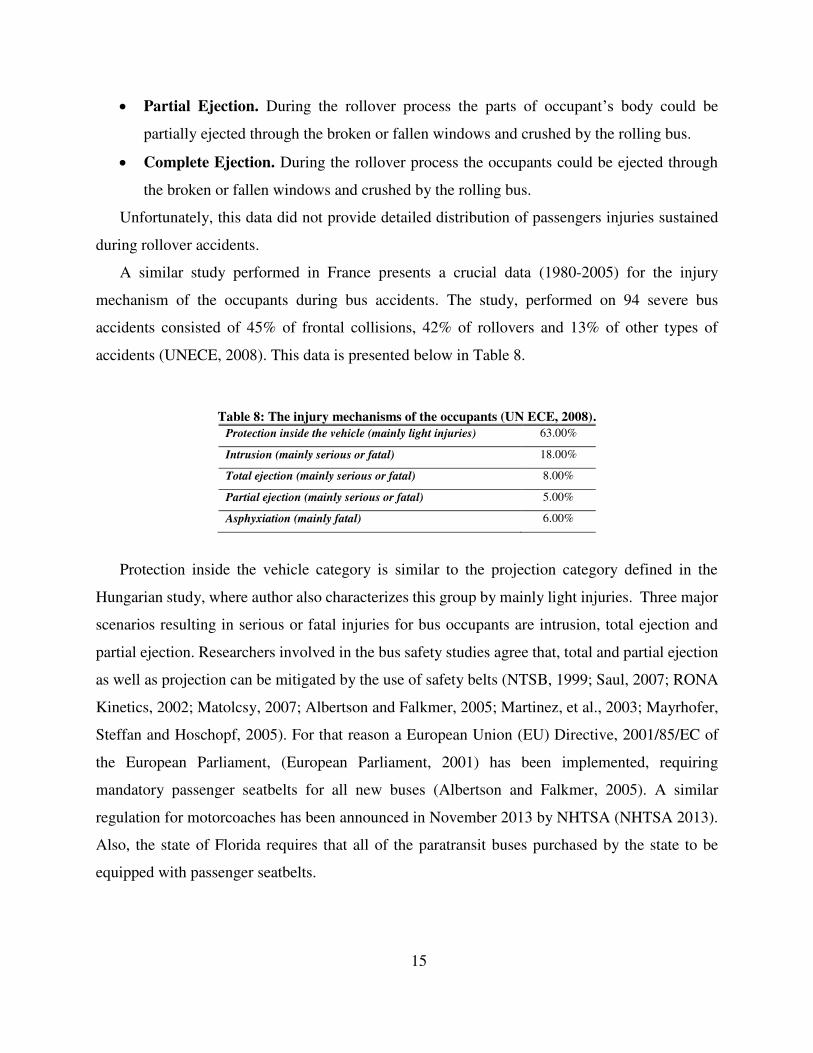
A similar study performed in France presents a crucial data (1980-2005) for the injury
mechanism of the occupants during bus accidents. The study, performed on 94 severe bus
accidents consisted of 45% of frontal collisions, 42% of rollovers and 13% of other types of
accidents (UNECE, 2008). This data is presented below in Table 8.
Table 8: The injury mechanisms of the occupants (UN ECE, 2008).
Protection inside the vehicle (mainly light injuries) 63.00%
Intrusion (mainly serious or fatal) 18.00%
Total ejection (mainly serious or fatal) 8.00%
Partial ejection (mainly serious or fatal) 5.00%
Asphyxiation (mainly fatal) 6.00%
Protection inside the vehicle category is similar to the projection category defined in the
Hungarian study, where author also characterizes this group by mainly light injuries. Three major
scenarios resulting in serious or fatal injuries for bus occupants are intrusion, total ejection and
partial ejection. Researchers involved in the bus safety studies agree that, total and partial ejection
as well as projection can be mitigated by the use of safety belts (NTSB, 1999; Saul, 2007; RONA
Kinetics, 2002; Matolcsy, 2007; Albertson and Falkmer, 2005; Martinez, et al., 2003; Mayrhofer,
Steffan and Hoschopf, 2005). For that reason a European Union (EU) Directive, 2001/85/EC of
the European Parliament, (European Parliament, 2001) has been implemented, requiring
mandatory passenger seatbelts for all new buses (Albertson and Falkmer, 2005). A similar
regulation for motorcoaches has been announced in November 2013 by NHTSA (NHTSA 2013).
Also, the state of Florida requires that all of the paratransit buses purchased by the state to be
equipped with passenger seatbelts.

16
The intrusion, which is the largest component of all serious and fatal injuries, can only be
mitigated by strengthening of the superstructure. In the US this goal is achieved by the use of
FMVSS 220, which requires the bus roof structure to withstand a symmetric static load with a
limited deformation. The most popular international standard fit for that purpose, which has been
accepted by over 40 countries in the world, is UNECE Regulation 66 (ECE-R66) (UNECE, 2006).
ECE-R66 defines a residual space that needs to remain intact during standard rollover in order to
provide passengers with a survival space.
In one of the studies (Matolcsy, 2007) the author analyzed over 300 bus rollovers. Not
accounting for very severe accidents, the author has established a definition of a Protectable
Rollover Accident (PRA), in which the passengers should be protected. Out of all the data, 191
rollovers fit into that category. The 191 PRAs have been than analyzed for injury and fatality rates
with relation to the intrusion of bus structure into the survival space. The conclusion was that if
the survival space was breached the fatality rate was 15 times higher and the serious injury rate
was 3.5 times higher as compared to the situation where the survival space was preserved. This
highlights the importance of survival space concept as defined by existing regulations.
2.2. Bus Accident Statistics for Paratransit Buses
Starting from 2011, a separate category specified as “Van-Based Bus (GVWR > 10,000 lb.)” was
created in the FARS database. This was done in order to accommodate paratransit buses and extract
them from “Other Bus” category. Unfortunately, according to NHTSA’s 2012 FARS coding and
validation manual (NTHSA, 2013) this category describes a bus body type built on a van-based
chassis with Gross Vehicle Weight Rating (GVWR) over 10,000 lb. Some of the paratransit buses
are built with the GVWR below 10,000 lb., and according to FARS Coding manual such buses
would be classified as “Van-Based Light Trucks (GVWR < = 10,000 lbs.)”. On the other hand,
paratransit bus manufacturers do not use van chassis for larger buses. Instead, they utilize heavy
duty truck chassis, such as Ford F-550, International 3200, or Freightliner M2 (Figure 5), and these
buses are still classified as “Other Bus” category.
These limitations indicate that not all paratransit buses are included into the “Van-Based Bus
(GVWR > 10,000 lb.)” body type category. Nevertheless, data collected throughout 2011 and 2012
is still useful to obtain general picture of paratransit bus accidents. The data collected to date is
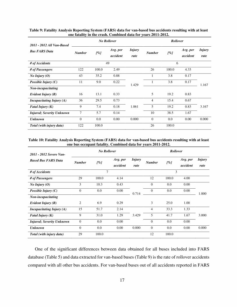
presented below in Table 9 and Table 10.
17
Table 9: Fatality Analysis Reporting System (FARS) data for van-based bus accidents resulting with at least
one fatality in the crash. Combined data for years 2011-2012.
2011 - 2012 All Van-Based
Bus FARS Data
No Rollover Rollover
Number [%] Avg. per
accident
Injury
rate Number [%]
Avg. per
accident
Injury
rate
# of Accidents 49 6
# of Passengers 122 100.0 2.49 26 100.0 4.33
No Injury (O) 43 35.2 0.88
1.429
1 3.8 0.17
1.167 Possible Injury (C) 11 9.0 0.22 1 3.8 0.17
Non-incapacitating
Evident Injury (B) 16 13.1 0.33 5 19.2 0.83
Incapacitating Injury (A) 36 29.5 0.73
1.061
4 15.4 0.67
3.167 Fatal Injury (K) 9 7.4 0.18 5 19.2 0.83
Injured; Severity Unknown 7 5.7 0.14 10 38.5 1.67
Unknown 0 0.0 0.00 0.000 0 0.0 0.00 0.000
Total (with injury data) 122 100.0 26 100.0
Table 10: Fatality Analysis Reporting System (FARS) data for van-based bus accidents resulting with at least
one bus occupant fatality. Combined data for years 2011-2012.
2011 - 2012 Severe Van-
Based Bus FARS Data
No Rollover Rollover
Number [%] Avg. per
accident
Injury
rate Number [%]
Avg. per
accident
Injury
rate
# of Accidents 7 3
# of Passengers 29 100.0 4.14 12 100.0 4.00
No Injury (O) 3 10.3 0.43
0.714
0 0.0 0.00
1.000 Possible Injury (C) 0 0.0 0.00 0 0.0 0.00
Non-incapacitating
Evident Injury (B) 2 6.9 0.29 3 25.0 1.00
Incapacitating Injury (A) 15 51.7 2.14
3.429
4 33.3 1.33
3.000 Fatal Injury (K) 9 31.0 1.29 5 41.7 1.67
Injured; Severity Unknown 0 0.0 0.00 0 0.0 0.00
Unknown 0 0.0 0.00 0.000 0 0.0 0.00 0.000
Total (with injury data) 29 100.0 12 100.0
One of the significant differences between data obtained for all buses included into FARS
database (Table 5) and data extracted for van-based buses (Table 9) is the rate of rollover accidents
compared with all other bus accidents. For van-based buses out of all accidents reported in FARS

18
database 11% were rollovers, compared with 4% for all other buses. It is possible that van-based
buses are more prone to rollover, as accident data indicates. This could be explained by a raised
center of gravity, due to added mass of the passenger compartment in these vehicles, but
unfortunately, accident data sample is still too small to draw such conclusion. The data should be
analyzed with caution due to the small size of the sample. Similar conclusions were reached by
Mayrhofer, Steffan and Hoschopf (2005) due to the small size of data available for bus accidents
during Enhanced Coach and Bus Occupant Safety (ECBOS) study.
Figure 5: Example of buses built on heavy duty truck chassis. Ford F-550 (a) and Intercontinental 3200 series
(b) (Champion Bus, 2014).
2.3. Standards Review
Rollover is recognized as the most dangerous accident scenario for buses (Matolcsy, 2007;
Martinez, et al., 2003; Albertson and Falkmer, 2005; Liang and Le, 2010; Bojanowski, 2009).
Even though it is a rare event, only 4-5% of bus accidents are rollovers, it causes almost 50% of
serious and fatal injuries (Table 5). This fact is widely accepted in the research community and the
crash and safety regulations for buses focus on rollover.
Two major safety standards for roof integrity are currently used around the world. In United
States and Canada buses are subjected to the Federal Motor Vehicle Safety Standard 220 (FMVSS
220) titled School Bus Rollover Protection (US DOT, 1998). FMVSS 220 establishes performance
requirements for rollover performance of school buses, but it is also commonly used for all other
types of buses sold in the US.
Another safety standard, used for crashworthy evaluation of buses, is the United Nations
Economic Commission for Europe Regulation 66 titled “Uniform technical prescriptions
concerning the approval of large passenger vehicles with regard to the strength of their
a) b)
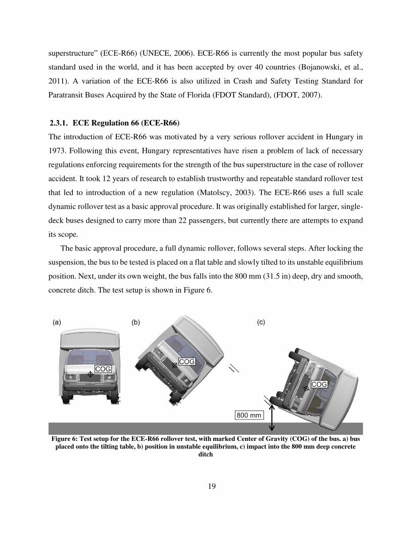
19
superstructure” (ECE-R66) (UNECE, 2006). ECE-R66 is currently the most popular bus safety
standard used in the world, and it has been accepted by over 40 countries (Bojanowski, et al.,
2011). A variation of the ECE-R66 is also utilized in Crash and Safety Testing Standard for
Paratransit Buses Acquired by the State of Florida (FDOT Standard), (FDOT, 2007).
ECE Regulation 66 (ECE-R66)
The introduction of ECE-R66 was motivated by a very serious rollover accident in Hungary in
1973. Following this event, Hungary representatives have risen a problem of lack of necessary
regulations enforcing requirements for the strength of the bus superstructure in the case of rollover
accident. It took 12 years of research to establish trustworthy and repeatable standard rollover test
that led to introduction of a new regulation (Matolscy, 2003). The ECE-R66 uses a full scale
dynamic rollover test as a basic approval procedure. It was originally established for larger, single-
deck buses designed to carry more than 22 passengers, but currently there are attempts to expand
its scope.
The basic approval procedure, a full dynamic rollover, follows several steps. After locking the
suspension, the bus to be tested is placed on a flat table and slowly tilted to its unstable equilibrium
position. Next, under its own weight, the bus falls into the 800 mm (31.5 in) deep, dry and smooth,
concrete ditch. The test setup is shown in Figure 6.
Figure 6: Test setup for the ECE-R66 rollover test, with marked Center of Gravity (COG) of the bus. a) bus
placed onto the tilting table, b) position in unstable equilibrium, c) impact into the 800 mm deep concrete
ditch

20
In the rollover test, the amount of energy applied to the bus is proportional to the overall vehicle
weight and location of the center of gravity (COG). For the buses equipped with passenger
restraints, such as seatbelts, the mass of the occupants should be added to the tested bus. If the bus
does not have seatbelts, it should be tested for unladen vehicle mass (UNECE, 2006).
The pass-fail criterion established in ECE-R66 is based on the concept of the residual space
(RS). The residual space is defined as a space required to be kept intact in order to provide a
survival zone for passengers and a driver. No part or element of the vehicle can intrude into the
RS during or after the impact. The envelope of the residual space is shown in Figure 7.
ECE-R66 also allows for the application of equivalent simplified approval procedures such as
(UNECE, 2006):
Rollover of a body section. A body section must contain at least two bays, adjusted for
correct mass distribution to match the COG measurements for the unloaded vehicle, in case
the vehicle is not equipped with the seatbelts, or a COG measurements for a vehicle with
passengers in case the vehicle is equipped with seatbelts. Testing procedure and approval
method is the same as for the full rollover test.
Quasi static test of bus body section. A body section constructed as described above is
subjected to a static loading test. Force versus displacement of the loading plate is measured
and recorded, and absorbed energy is calculated as the area below the curve. The body
section is required to absorb the fraction of the total energy proportional to the sections
mass. Total energy absorbed by the superstructure is calculated as 75% of energy delivered
to the structure during the rollover test.
Quasi static calculations. Quasi static calculations are carried by pre locating plastic
hinges (PH) and plastic zones (PZ) throughout the bus cross section. The assumption is
made that all of the kinetic energy delivered to the bus during rollover is dissipated within
these plastic regions. The calculations are run until the residual space is compromised, and
absorbed energy is compared with required total energy. Also a dynamic factor of 1.2 is
introduced in this method.
Computational mechanics simulations. General code and procedure requirements are
listed within ECE-R66. There is no specific validation and verifications measures defined.

21
Figure 7: Residual space and a Deformation Index concept (UN ECE, 2006).
FMVSS220
Federal Motor Vehicle Safety Standard 220 (FMVSS 220) establishes performance requirements
for school bus rollover protection, but is also frequently used as a required safety standard for the
other types of buses in the US. The concept of FMVSS 220 is to statically apply a force equal to
1.5 times of the weight of an unloaded vehicle (UVW) (US DOT, 1998). The force is applied
symmetrically to the roof through a flat, rigid rectangular plate, with the loading rate not exceeding
12.7 mm/s (0.5 in/s). For vehicles with a GVWR of more than 10,000 lb., the loading plate is
required to be 12 inches shorter than the roof of the tested vehicle and 36 inches wide. For vehicles
with GVWR of 10,000 or less, the load application plate should be 5 inches longer and 5 inches
wider than the vehicle roof dimensions. If the resulting maximum vertical displacement does not
exceed 130.2 mm (5.125 in) and all of the emergency exits are operable during loading and after
releasing the force, then the vehicle is considered to have passed the test (see Figure 8).
Florida Standard
The Transit Office of the Florida Department of Transportation (FDOT) has been putting a lot of
attention in selecting the best quality buses which exhibit the highest crashworthy characteristics
and the safest environment for their passengers. These efforts resulted in a development of the
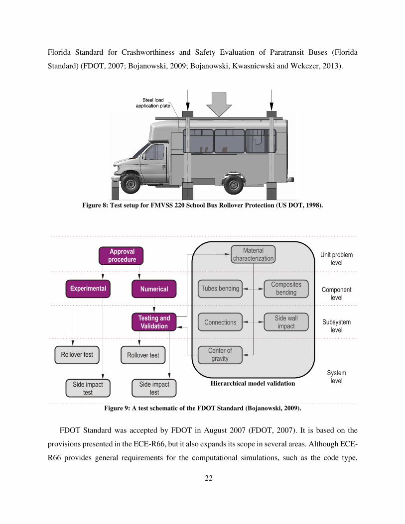
22
Florida Standard for Crashworthiness and Safety Evaluation of Paratransit Buses (Florida
Standard) (FDOT, 2007; Bojanowski, 2009; Bojanowski, Kwasniewski and Wekezer, 2013).
Figure 8: Test setup for FMVSS 220 School Bus Rollover Protection (US DOT, 1998).
Figure 9: A test schematic of the FDOT Standard (Bojanowski, 2009).
FDOT Standard was accepted by FDOT in August 2007 (FDOT, 2007). It is based on the
provisions presented in the ECE-R66, but it also expands its scope in several areas. Although ECE-
R66 provides general requirements for the computational simulations, such as the code type,
Approvalprocedure
Numerical
Material characterization
Testing and Validation
Tubes bendingExperimental
Rollover test
Side impact test
Rollover test
Connections
Side impact test
Side wall impact
Center of gravity
Unit problemlevel
Componentlevel
Subsystemlevel
Systemlevel
Composites bending
Hierarchical model validation
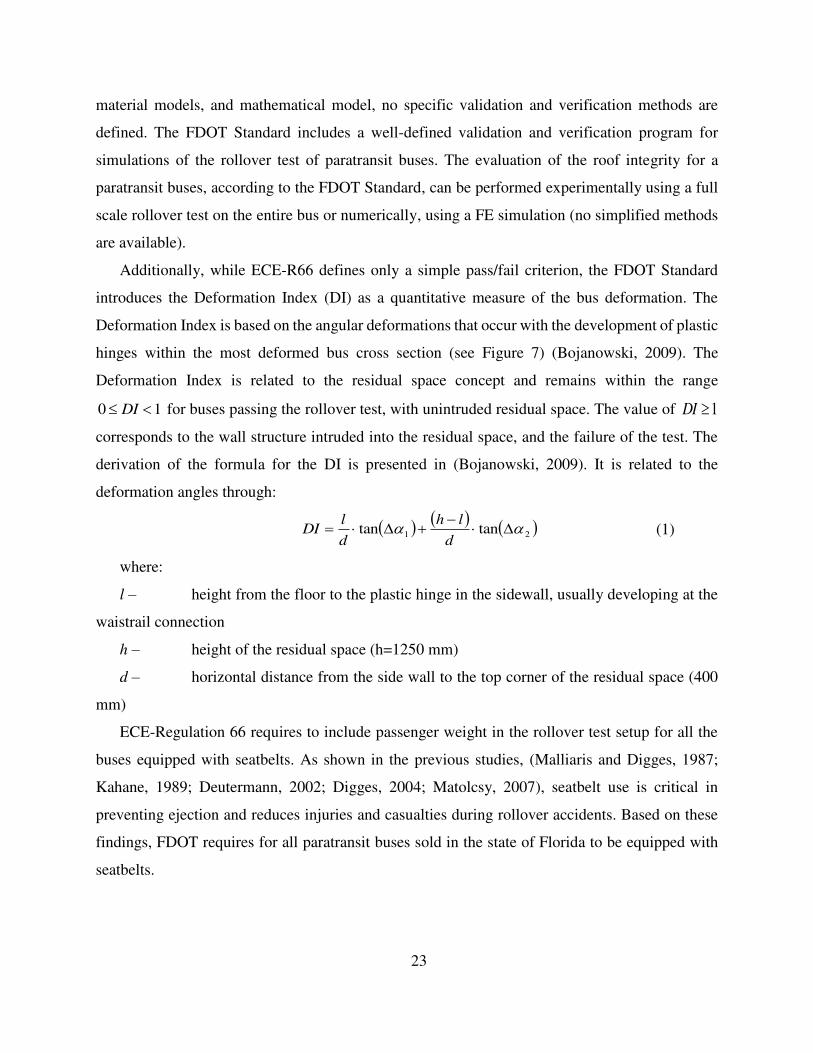
23
material models, and mathematical model, no specific validation and verification methods are
defined. The FDOT Standard includes a well-defined validation and verification program for
simulations of the rollover test of paratransit buses. The evaluation of the roof integrity for a
paratransit buses, according to the FDOT Standard, can be performed experimentally using a full
scale rollover test on the entire bus or numerically, using a FE simulation (no simplified methods
are available).
Additionally, while ECE-R66 defines only a simple pass/fail criterion, the FDOT Standard
introduces the Deformation Index (DI) as a quantitative measure of the bus deformation. The
Deformation Index is based on the angular deformations that occur with the development of plastic
hinges within the most deformed bus cross section (see Figure 7) (Bojanowski, 2009). The
Deformation Index is related to the residual space concept and remains within the range
10 DI for buses passing the rollover test, with unintruded residual space. The value of 1DI
corresponds to the wall structure intruded into the residual space, and the failure of the test. The
derivation of the formula for the DI is presented in (Bojanowski, 2009). It is related to the
deformation angles through:
21 tantan
d
lh
d
lDI
(1)
where:
l – height from the floor to the plastic hinge in the sidewall, usually developing at the
waistrail connection
h – height of the residual space (h=1250 mm)
d – horizontal distance from the side wall to the top corner of the residual space (400
mm)
ECE-Regulation 66 requires to include passenger weight in the rollover test setup for all the
buses equipped with seatbelts. As shown in the previous studies, (Malliaris and Digges, 1987;
Kahane, 1989; Deutermann, 2002; Digges, 2004; Matolcsy, 2007), seatbelt use is critical in
preventing ejection and reduces injuries and casualties during rollover accidents. Based on these
findings, FDOT requires for all paratransit buses sold in the state of Florida to be equipped with
seatbelts.

24
2.4. FE Simulations for Bus Rollover Protection
In the past, multiple researchers focused on Finite Element (FE) analysis use for improving
passenger rollover protection. First publications utilizing computational analysis concentrated on
representing bus cage structures using beam elements. These simple models were a necessary
compromise between complexity and availability of computational resources at the time.
Subic and He (1997) constructed a beam element bus cage model using pro/MECHANICA
computer program in an attempt to reduce the experimental load associated with the rollover
testing. Modal analysis was used in this paper to identify cage’s dynamic characteristics and
improve its design. This effort was complemented by a full scale experimental testing on a standard
roll cage structure. The sensitivity study performed in this paper resulted in the mass decrease and
a reduction of the COG position.
Another study (Boada, et al., 2007) utilized a beam element model of the bus superstructure.
Authors used genetic algorithms to optimize structures torsional stiffness and weight. FE analysis
was carried out using Ansys, coupled with Matlab package for optimization.
Gadekar, Kshirsagar and Anilkumar (2005) also used beam elements and LS-DYNA Finite
Element software to predict rollover strength of the bus structure. They have calibrated their model
through a series of joint bending experiments. Instead of performing a full numerical rollover test,
which is computationally expensive, the authors performed a series of pendulum impacts,
following the requirements of ECE-R66. Although the fine tuning plastic hinge location and joint
stiffness was necessary, the authors found a significant computational time reduction with their
approach.
Valladares, Miralbes and Castejon (2010) carried out a study on development of a numerical
technique for bus rollover test simulations. Authors investigated different modeling techniques
ranging from beam elements with rigidity curves, to a complete detailed shell element model. No
validation effort has been presented by the authors, and all of the presented models produced
diverging results.
Increasing computing power and parallelization capabilities introduced into the FE codes made
it possible to develop and utilize more advanced FE models, improving the accuracy of the results,
without sacrificing computing speed. Up to date, multiple researchers have utilized very complex
FE models (with size over 1 million finite elements) in research on bus crashworthiness.
25
Gursel and Gruseli (2010) performed a numerical rollover test of the bus superstructure using
ANSYS software. The test was carried out according to the ECE-R66. The authors presented a
successful design process of a structure that has passed the rollover test. For validation purposes
the rollover test on a bus section was performed and compared with FE results. No passenger
weights were included in the test.
Elitok et al. (2006) investigated the effect of seat structure and passenger weight on the rollover
performance on the intercity coach. The numerical test followed the guidelines of the ECE-R66
and validation on the FE model was performed through experimental tests on breast and roof knots.
The authors found that the passenger and luggage weight had a significant influence onto the final
test results. Bus fitted with passenger mass experienced larger deformation and failed the rollover
test. The authors noted that additional mass accounted for almost 40% of additional energy in the
rollover.
Guler et al. (2007) looked into the effectiveness of a seatbelt usage on the rollover
crashworthiness of the intercity coach. Authors attempted to evaluate passenger injury risk and
compare the effectiveness of seatbelt usage during rollover accident. The authors used a Hybrid
III 50th projectile dummy model obtained from LSTC to evaluate passenger injury in all
investigated cases. Passenger restraints considered included passengers without seatbelts, 2 point
lap belt and a 3 point shoulder belt. Use of the seatbelts during rollover test resulted in mitigation
of projection and ejection of bus passengers and injury reduction.
Ko et al. (2009) performed a study on the crashworthiness and rollover characteristics of the
low-floor bus made of sandwich composites. The composite incorporated into the vehicle structure
was composed of the aluminum honeycomb and fiberglass-epoxy facesheets. The paper
investigated two crash scenarios, a 60km/h frontal impact and the ECE-R66 rollover. Although
material property tests were carried out on composite samples, no detailed validation effort was
presented.
Liang and Le (2009) analyzed the rollover protection under different legislated standards using
LS-DYNA simulation technique. A comparison of two testing standards, FMVSS 220 and ECE-
R66 was performed using a numerical bus model. The authors have discovered that both standards
evaluate buses under significantly different conditions, and different components became critical
for bus behavior under these standards. In FMVSS 220 significant deformation and energy
26
absorption was localized in the roof structure. In case of ECE-R66 rollover test most plastic
internal energy was localized within the sidewall of the vehicle.
Qiang et al. (2012) investigated the effect of bus skin on rollover crash simulation outcome.
The authors concluded that the skin has a large influence onto the outcomes of the FE ECE-R66
rollover simulation. No validation efforts were presented in this paper.
Ozcanli and Yilmaz (2014) investigated the effects of foam application to the bus structure in
order to improve its crashworthiness during rollover accidents. Although the foam application to
the structural beams reduced the deformation of the bus, the results were insignificant (0.25%).
Also no validation effort of FE model was presented in the discussed paper.
Deshmukh (2006), in a thesis submitted to the Wichita State University, presents an analysis
of a rollover and roof crush resistance for the low-floor transit buses. LS-DYNA FE model in this
study is subjected to the ECE-R66 rollover test and the FMVSS 220 roof crush resistance test.
Author investigates the influence of the passenger mass onto the rollover scenario, and its influence
onto bus deformation during rollover. The study is complemented by MADYMO software
occupant kinematics investigation and injury analysis depending on seating orientation and
passenger position.
Li, Lan and Chen (2012) performed a numerical study on the influence of the superstructure
configuration on coach performance when subjected to the ECE-R66 rollover. Using the baseline
FE coach model the authors derived seven different FE models considering structural
configurations, such as closed rings, wall to floor connections, column structure and waistrail
location. Conclusions highlight that all of the investigated configurations, with the exception of
the location of the waistrail, had a large influence onto the rollover performance.
Zhang et al. (2012) presents an experimental and numerical study on bus rollover. The
numerical study is performed using LS-DYNA, and the authors present an energy absorption
distribution during the numerical rollover. Experimental rollover is presented in this paper,
although no reference to the numerical model is made.
Mayrhofer, Steffan and Hoschopf (2005) presented a detailed and comprehensive study on bus
collision data, reconstruction of real world accidents, component and section testing, development
of numerical models for vehicle structure and occupant behavior and detection of injury
mechanism for bus occupants. Presented paper was a summary of an extensive research project
titled Enhanced Coach and Bus Occupant Safety (European Commission, 2003) sponsored by
27
European Commission. The authors investigated multiple bus accident scenario such as frontal
impact, rear impact and rollover of both small and large buses.
A large part of the ECBOS project focused on rollover, and recommendations for rollover
procedure and bus regulations were made based on the presented findings. Authors argued that
seatbelt use is strongly recommended, since large part of the injuries in the rollover accident comes
from the occupant impact within the bus. They stated that the number casualties and severity of
injury is reduced if the bus is equipped with proper restraint system, and if the seatbelts were used.
Participants of the ECBOS project also attempted to quantify the effect of belted passengers
onto the calculation and testing. The conclusion was that belted passengers increased the energy
needed to be absorbed by the structure during rollover. They quantified the amount of mass needed
to be added to the bus structure depending on different restrains systems used. For 2-point safety
belts they concluded that 70% of passenger mass should be added to the vehicle mass and rigidly
attached to the seat structure. For 3-point belts the recommended number was 90%.
Mayrhofer has also concluded that some of the equivalent approval procedures available in the
ECE-R66 regulation are not comparable to a rollover which is a basic approval procedure in this
regulation. It was discovered that the pendulum test, allowed under the ECE-R66 regulation,
generates different deformation and energy absorption within the structure than the rollover test.
The recommendation was to delete pendulum test from the approval procedure.
Borkowski and Hyrciow (2006) presented a numerical comparison of a full vehicle rollover
test with a test carried out on the bay section. Both of these test have been performed following
the guidelines of the ECE-R66. Although results from the bus section rollover showed larger
deformations as compared to the full vehicle rollover, the conclusion of the presented study was
that since the discrepancies between two tests were small, the rollover test of the bus section is a
useful tool for the approval process.
Schwartz et al. (2006) used LS-DYNA FE solver to simulate ECE-R66 approval procedures
for the coach structure. The paper investigated rollover tests performed on the section of the bus
and compared it with results from pendulum impact equivalent approval procedure. Cases with
rigid and deformable undercarriage were investigated, and coefficient of friction was varied
through the simulations. Authors showed that the pendulum impact generates a different
deformation pattern than the rollover test of the bus section. These results are consistent with
results presented in (Mayrhofer, Steffan and Hoschopf, 2005). Higher coefficient of friction
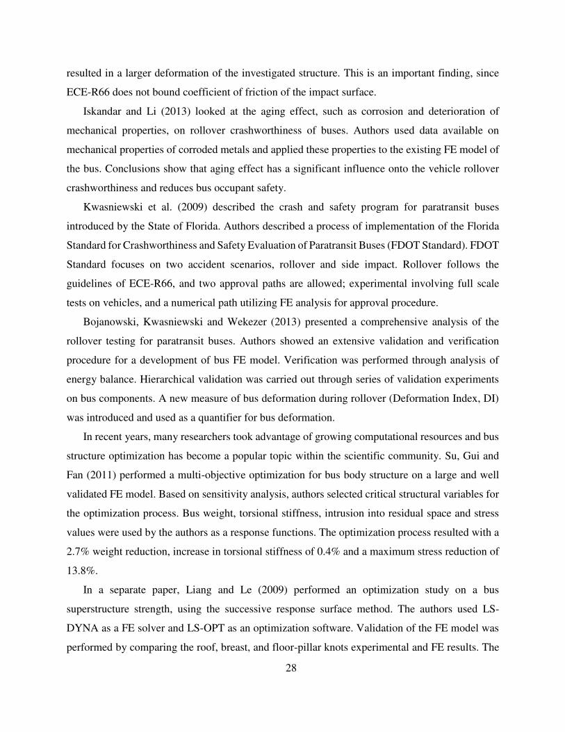
28
resulted in a larger deformation of the investigated structure. This is an important finding, since
ECE-R66 does not bound coefficient of friction of the impact surface.
Iskandar and Li (2013) looked at the aging effect, such as corrosion and deterioration of
mechanical properties, on rollover crashworthiness of buses. Authors used data available on
mechanical properties of corroded metals and applied these properties to the existing FE model of
the bus. Conclusions show that aging effect has a significant influence onto the vehicle rollover
crashworthiness and reduces bus occupant safety.
Kwasniewski et al. (2009) described the crash and safety program for paratransit buses
introduced by the State of Florida. Authors described a process of implementation of the Florida
Standard for Crashworthiness and Safety Evaluation of Paratransit Buses (FDOT Standard). FDOT
Standard focuses on two accident scenarios, rollover and side impact. Rollover follows the
guidelines of ECE-R66, and two approval paths are allowed; experimental involving full scale
tests on vehicles, and a numerical path utilizing FE analysis for approval procedure.
Bojanowski, Kwasniewski and Wekezer (2013) presented a comprehensive analysis of the
rollover testing for paratransit buses. Authors showed an extensive validation and verification
procedure for a development of bus FE model. Verification was performed through analysis of
energy balance. Hierarchical validation was carried out through series of validation experiments
on bus components. A new measure of bus deformation during rollover (Deformation Index, DI)
was introduced and used as a quantifier for bus deformation.
In recent years, many researchers took advantage of growing computational resources and bus
structure optimization has become a popular topic within the scientific community. Su, Gui and
Fan (2011) performed a multi-objective optimization for bus body structure on a large and well
validated FE model. Based on sensitivity analysis, authors selected critical structural variables for
the optimization process. Bus weight, torsional stiffness, intrusion into residual space and stress
values were used by the authors as a response functions. The optimization process resulted with a
2.7% weight reduction, increase in torsional stiffness of 0.4% and a maximum stress reduction of
13.8%.
In a separate paper, Liang and Le (2009) performed an optimization study on a bus
superstructure strength, using the successive response surface method. The authors used LS-
DYNA as a FE solver and LS-OPT as an optimization software. Validation of the FE model was
performed by comparing the roof, breast, and floor-pillar knots experimental and FE results. The

29
optimization process resulted in the 40% and 50% of deformation reduction while increasing a bus
weight by only 1.6%.
Tech and Iturrioz (2009) used a genetic algorithm to perform a structural optimization of a bus
in rollover conditions. The authors constructed a simplified rigid beam FE model of a bus structure,
and implemented addition plastic hinges in places where deformation was expected. Plastic hinges
have been characterized by a series of experimental tests on bus components. Vehicle mass and
mechanical response for the rollover experiment were chosen as the objective functions in this
research.
In a separate study, Bojanowski and Kulak (2011) performed a multi objective optimization of
the paratransit bus structure subjected to side impact and rollover tests. The objectives for the
optimization included: mass of the cage structure, deformation in the rollover, intrusion distance
in the side impact test. The authors concluded that the most important components of the bus
structure responsible for 63% of variation in the objective functions were side wall and front cap
structures.
2.5. FE Model Verification and Validation
In July 2006 American Society of Mechanical Engineers (ASME) Standards Committee on
Verification and Validation in Computational Solid Mechanics approved a Guide for Verification
and Validation in Computational Solid Mechanics (Schwer, 2007). This publication followed a
similar guide published by the Computational Fluid Dynamics Committee of the American
Institute of Aeronautics and Astronautics (AIAA) (AIAA, 1998) titled Guide for the Verification
and Validation of Computational Fluid Dynamics Committee on Standards. The field of
Computational Fluid Dynamics (CFD) was often an area of pioneering and development of new
methodologies (Oberkampf, Trucano and Hirsch, 2003). This was also the case with regards to the
Verification and Validation (V&V) procedures.
Verification and Validation is defined as a methodology of building and quantifying
confidence in computational simulations (Oberkampf, Trucano and Hirsch, 2003; Thacker, et al.,
2004). It defines the relation between Reality of Interest, Mathematical Model and Computer
Model (Figure 10), (Schlesinger, et al., 1979). Reality of Interest is defined as a particular physical
system being studied (Thacker, et al., 2004), such as analysis aircraft wing tip deflection under
distributed load (Schwer, 2007), or a paratransit bus subjected to the ECE-R66 rollover test
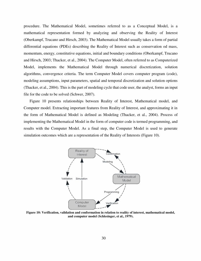
30
procedure. The Mathematical Model, sometimes referred to as a Conceptual Model, is a
mathematical representation formed by analyzing and observing the Reality of Interest
(Oberkampf, Trucano and Hirsch, 2003). The Mathematical Model usually takes a form of partial
differential equations (PDEs) describing the Reality of Interest such as conservation od mass,
momentum, energy, constitutive equations, initial and boundary conditions (Oberkampf, Trucano
and Hirsch, 2003; Thacker, et al., 2004). The Computer Model, often referred to as Computerized
Model, implements the Mathematical Model through numerical discretization, solution
algorithms, convergence criteria. The term Computer Model covers computer program (code),
modeling assumptions, input parameters, spatial and temporal discretization and solution options
(Thacker, et al., 2004). This is the part of modeling cycle that code user, the analyst, forms an input
file for the code to be solved (Schwer, 2007).
Figure 10 presents relationships between Reality of Interest, Mathematical model, and
Computer model. Extracting important features from Reality of Interest, and approximating it in
the form of Mathematical Model is defined as Modeling (Thacker, et al., 2004). Process of
implementing the Mathematical Model in the form of computer code is termed programming, and
results with the Computer Model. As a final step, the Computer Model is used to generate
simulation outcomes which are a representation of the Reality of Interests (Figure 10).
Figure 10: Verification, validation and conformation in relation to reality of interest, mathematical model,
and computer model (Schlesinger, et al., 1979).

31
The process of checking the correctness of the Modeling process is termed Confirmation
(Figure 10). Confirmation deals with determination of adequacy of the conceptual model to
provide an acceptable representation of the Reality of Interest (Schlesinger, et al., 1979). It focuses
on issues such as definition of Reality of Interest, effects of the environment onto the investigated
system, and choice of mathematical description (PDE) (Oberkampf, Trucano and Hirsch, 2003).
Model confirmation is not a subject of Verification and Validation literature.
The process of determining that computer model accurately represents programmer’s
conceptual and mathematical description of the problem is called model Verification (Figure 10)
(Oberkampf, Trucano and Hirsch, 2003). The Verification process focuses on identification and
removal of implementation errors in software use and software implementation of the
Mathematical Model (Thacker, et al., 2004). Roache defines the Verification process simply as
“solving equations right”. That means that Verification is a strictly an activity in mathematics of
numerical analysis (Roache, 2008).
Verification is often divided into the two separate activities; code verification and calculation
verification (Oberkampf, Trucano and Hirsch, 2003; Thacker, et al., 2004; Schwer, 2007). The
responsibility of code verification lies mostly with the software developers. Code verification is
most often carried out by comparing code outputs with the “known” analytical solutions. This
approach allows the code developer to compare results obtained by the solver with the theoretical
ones and identify potential coding errors (Schwer, 2007).
Another approach is presented by the method of manufactured solutions. The concept of the
method of manufactured solutions is to supply the code with a predefined solution to the PDE that
code solves, alongside with boundary and initial conditions and force the code to obtain a given
solution. If the code is error free the two solutions will agree (Schwer, 2007).
Although users can prove useful in finding “bugs” in the software, due to the lack of access to
the source code, their input to code verification is very limited, and very often random. The part
of verification that code users, or analysts, are responsible for, is called calculation verification, or
numerical error estimation. The purpose of calculation verification is the assessment of the
discretization error in the simulation by demonstrating the convergence of the model to a particular
solution. According to (Thacker, et al., 2004) the types of error identified and removed by
calculation verifications are; insufficient temporal and spatial discretization, insufficient
convergence tolerance, incorrect input options, and round off error. Except for input errors,
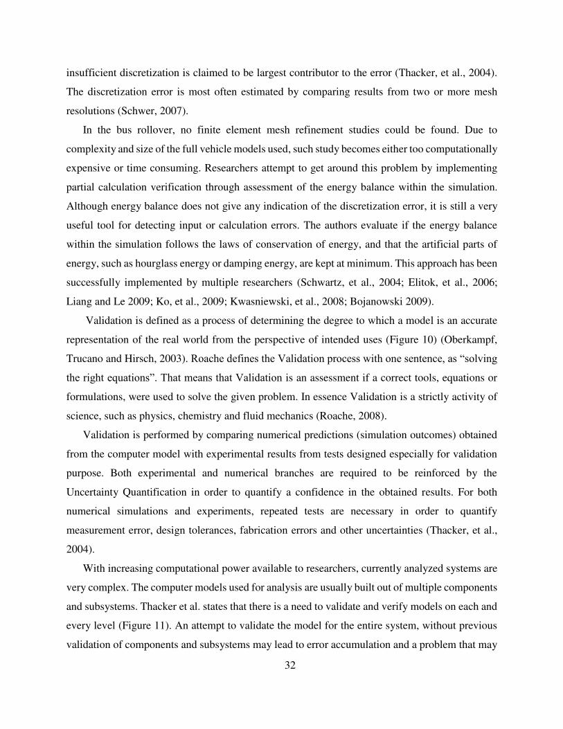
32
insufficient discretization is claimed to be largest contributor to the error (Thacker, et al., 2004).
The discretization error is most often estimated by comparing results from two or more mesh
resolutions (Schwer, 2007).
In the bus rollover, no finite element mesh refinement studies could be found. Due to
complexity and size of the full vehicle models used, such study becomes either too computationally
expensive or time consuming. Researchers attempt to get around this problem by implementing
partial calculation verification through assessment of the energy balance within the simulation.
Although energy balance does not give any indication of the discretization error, it is still a very
useful tool for detecting input or calculation errors. The authors evaluate if the energy balance
within the simulation follows the laws of conservation of energy, and that the artificial parts of
energy, such as hourglass energy or damping energy, are kept at minimum. This approach has been
successfully implemented by multiple researchers (Schwartz, et al., 2004; Elitok, et al., 2006;
Liang and Le 2009; Ko, et al., 2009; Kwasniewski, et al., 2008; Bojanowski 2009).
Validation is defined as a process of determining the degree to which a model is an accurate
representation of the real world from the perspective of intended uses (Figure 10) (Oberkampf,
Trucano and Hirsch, 2003). Roache defines the Validation process with one sentence, as “solving
the right equations”. That means that Validation is an assessment if a correct tools, equations or
formulations, were used to solve the given problem. In essence Validation is a strictly activity of
science, such as physics, chemistry and fluid mechanics (Roache, 2008).
Validation is performed by comparing numerical predictions (simulation outcomes) obtained
from the computer model with experimental results from tests designed especially for validation
purpose. Both experimental and numerical branches are required to be reinforced by the
Uncertainty Quantification in order to quantify a confidence in the obtained results. For both
numerical simulations and experiments, repeated tests are necessary in order to quantify
measurement error, design tolerances, fabrication errors and other uncertainties (Thacker, et al.,
2004).
With increasing computational power available to researchers, currently analyzed systems are
very complex. The computer models used for analysis are usually built out of multiple components
and subsystems. Thacker et al. states that there is a need to validate and verify models on each and
every level (Figure 11). An attempt to validate the model for the entire system, without previous
validation of components and subsystems may lead to error accumulation and a problem that may
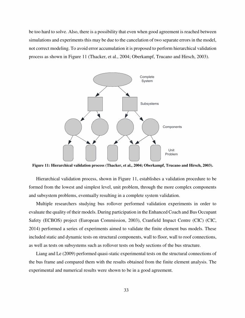
33
be too hard to solve. Also, there is a possibility that even when good agreement is reached between
simulations and experiments this may be due to the cancelation of two separate errors in the model,
not correct modeling. To avoid error accumulation it is proposed to perform hierarchical validation
process as shown in Figure 11 (Thacker, et al., 2004; Oberkampf, Trucano and Hirsch, 2003).
Figure 11: Hierarchical validation process (Thacker, et al., 2004; Oberkampf, Trucano and Hirsch, 2003).
Hierarchical validation process, shown in Figure 11, establishes a validation procedure to be
formed from the lowest and simplest level, unit problem, through the more complex components
and subsystem problems, eventually resulting in a complete system validation.
Multiple researchers studying bus rollover performed validation experiments in order to
evaluate the quality of their models. During participation in the Enhanced Coach and Bus Occupant
Safety (ECBOS) project (European Commission, 2003), Cranfield Impact Centre (CIC) (CIC,
2014) performed a series of experiments aimed to validate the finite element bus models. These
included static and dynamic tests on structural components, wall to floor, wall to roof connections,
as well as tests on subsystems such as rollover tests on body sections of the bus structure.
Liang and Le (2009) performed quasi-static experimental tests on the structural connections of
the bus frame and compared them with the results obtained from the finite element analysis. The
experimental and numerical results were shown to be in a good agreement.

34
Guler et al (2009), Tech and Iturrioz (2009) and Elitok et al. (2006) performed a similar
validation study, by examining experimentally roof, breast and floor knots (connections). In all the
cases authors presented a good agreement between the experimental and numerical results, but no
uncertainty quantification was performed in neither of the cases.
Bojanowski, Kwasniewski and Wekezer (2009; 2008) established and presented a
comprehensive validation program for paratransit buses. This validation program has become a
part of the Florida Standard for Crashworthiness and Safety Evaluation of Paratransit Buses
(FDOT Standard) and it is presented in Figure 9. The FDOT Standard requires, for every finite
element model of a paratransit bus tested, to undergo a hierarchical validation procedure. Starting
from unit problem level, which contains material testing for structural components, through
component level which includes static and dynamic tube testing, as well as composite bending
tests, to a subsystem level including elements of bus cage such as wall to floor, wall to roof
connections testing, and side panel impact. On the system level the full vehicle model is validated
through comparison of the Center of Gravity (COG) location.
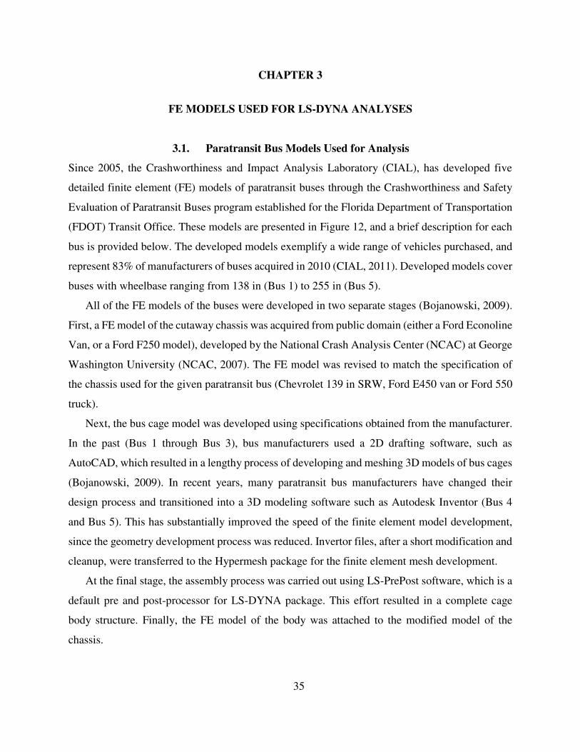
35
CHAPTER 3
FE MODELS USED FOR LS-DYNA ANALYSES
3.1. Paratransit Bus Models Used for Analysis
Since 2005, the Crashworthiness and Impact Analysis Laboratory (CIAL), has developed five
detailed finite element (FE) models of paratransit buses through the Crashworthiness and Safety
Evaluation of Paratransit Buses program established for the Florida Department of Transportation
(FDOT) Transit Office. These models are presented in Figure 12, and a brief description for each
bus is provided below. The developed models exemplify a wide range of vehicles purchased, and
represent 83% of manufacturers of buses acquired in 2010 (CIAL, 2011). Developed models cover
buses with wheelbase ranging from 138 in (Bus 1) to 255 in (Bus 5).
All of the FE models of the buses were developed in two separate stages (Bojanowski, 2009).
First, a FE model of the cutaway chassis was acquired from public domain (either a Ford Econoline
Van, or a Ford F250 model), developed by the National Crash Analysis Center (NCAC) at George
Washington University (NCAC, 2007). The FE model was revised to match the specification of
the chassis used for the given paratransit bus (Chevrolet 139 in SRW, Ford E450 van or Ford 550
truck).
Next, the bus cage model was developed using specifications obtained from the manufacturer.
In the past (Bus 1 through Bus 3), bus manufacturers used a 2D drafting software, such as
AutoCAD, which resulted in a lengthy process of developing and meshing 3D models of bus cages
(Bojanowski, 2009). In recent years, many paratransit bus manufacturers have changed their
design process and transitioned into a 3D modeling software such as Autodesk Inventor (Bus 4
and Bus 5). This has substantially improved the speed of the finite element model development,
since the geometry development process was reduced. Invertor files, after a short modification and
cleanup, were transferred to the Hypermesh package for the finite element mesh development.
At the final stage, the assembly process was carried out using LS-PrePost software, which is a
default pre and post-processor for LS-DYNA package. This effort resulted in a complete cage
body structure. Finally, the FE model of the body was attached to the modified model of the
chassis.

36
Figure 12: FE models developed by CIAL as of July 2014, a) Bus 1, b) Bus 2, c) Bus 3, d) Bus 4, and e) Bus 5
All of the developed FE models of paratransit buses have been equipped with water ballast
dummies in order to simulate passenger load during rollover. Water ballast dummies are visible in
Figure 12 (yellow), and will be discussed further in Chapter 5.
Bus 1
Bus 1 represents the smallest paratransit bus purchased by the State of Florida. With the wheelbase
of 138 in, it provides a room for a driver, seven seated passengers, and two passengers in the
wheelchairs.
Original model, developed in 2009, consisted of over 480,000 finite elements. Increased
computational resources made it feasible for the model to be refined, and the latest, re-meshed
version of Bus 1 model contains over 800,000 finite elements. FE model statistics are presented
below in Table 11. Developed FE model of Bus 1 is shown below in Figure 13.
a) b) c)
d) e)
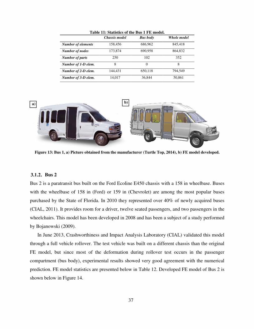
37
Table 11: Statistics of the Bus 1 FE model.
Chassis model Bus body Whole model
Number of elements 158,456 686,962 845,418
Number of nodes 173,874 690,958 864,832
Number of parts 250 102 352
Number of 1-D elem. 8 0 8
Number of 2-D elem. 144,431 650,118 794,549
Number of 3-D elem. 14,017 36,844 50,861
Figure 13: Bus 1, a) Picture obtained from the manufacturer (Turtle Top, 2014), b) FE model developed.
Bus 2
Bus 2 is a paratransit bus built on the Ford Ecoline E450 chassis with a 158 in wheelbase. Buses
with the wheelbase of 158 in (Ford) or 159 in (Chevrolet) are among the most popular buses
purchased by the State of Florida. In 2010 they represented over 40% of newly acquired buses
(CIAL, 2011). It provides room for a driver, twelve seated passengers, and two passengers in the
wheelchairs. This model has been developed in 2008 and has been a subject of a study performed
by Bojanowski (2009).
In June 2013, Crashworthiness and Impact Analysis Laboratory (CIAL) validated this model
through a full vehicle rollover. The test vehicle was built on a different chassis than the original
FE model, but since most of the deformation during rollover test occurs in the passenger
compartment (bus body), experimental results showed very good agreement with the numerical
prediction. FE model statistics are presented below in Table 12. Developed FE model of Bus 2 is
shown below in Figure 14.
a) b)

38
Table 12: Statistics of the Bus 2 FE model.
Chassis model Bus body Whole model
Number of elements 189,083 774,461 963,544
Number of nodes 204,998 808,811 1,013,809
Number of parts 295 82 377
Number of 1-D elem. 6 0 6
Number of 2-D elem. 173,401 695,545 868,946
Number of 3-D elem. 78,916 0 94,592
Figure 14: Bus 2, a) Test vehicle prepared for the rollover test, b) FE model developed.
Bus 3
Bus 3 is a paratransit bus built on the Ford Ecoline E450 chassis with a 158 in wheelbase. It
provides room for a driver, twelve seated passengers, and two passengers in the wheelchairs. This
model has been developed in 2006, and since then it has been refined multiple times.
Over the course of the model development newly available computational resources made it
possible to increase the number of finite elements. The original model, containing 537,839 finite
elements, was expanded to 925,324 finite elements. This allowed major structural parts to be
modeled at a higher resolution (e.g. four shell elements per main tubing width). Finer FE meshes
are especially important at the areas of plastic hinges.
This FE model has been validated through two full scale rollover tests described before in
(Gepner, et al., 2014), and in Chapter 4. The statistics of the developed and updated FE model are
shown in Table 13. The paratransit bus and its FE model are presented in Figure 15.
a) b)
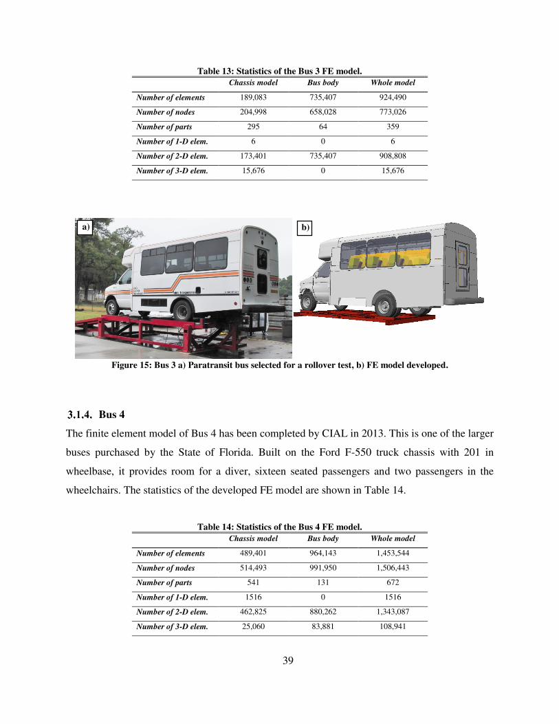
39
Table 13: Statistics of the Bus 3 FE model.
Chassis model Bus body Whole model
Number of elements 189,083 735,407 924,490
Number of nodes 204,998 658,028 773,026
Number of parts 295 64 359
Number of 1-D elem. 6 0 6
Number of 2-D elem. 173,401 735,407 908,808
Number of 3-D elem. 15,676 0 15,676
Figure 15: Bus 3 a) Paratransit bus selected for a rollover test, b) FE model developed.
Bus 4
The finite element model of Bus 4 has been completed by CIAL in 2013. This is one of the larger
buses purchased by the State of Florida. Built on the Ford F-550 truck chassis with 201 in
wheelbase, it provides room for a diver, sixteen seated passengers and two passengers in the
wheelchairs. The statistics of the developed FE model are shown in Table 14.
Table 14: Statistics of the Bus 4 FE model.
Chassis model Bus body Whole model
Number of elements 489,401 964,143 1,453,544
Number of nodes 514,493 991,950 1,506,443
Number of parts 541 131 672
Number of 1-D elem. 1516 0 1516
Number of 2-D elem. 462,825 880,262 1,343,087
Number of 3-D elem. 25,060 83,881 108,941
a) b)
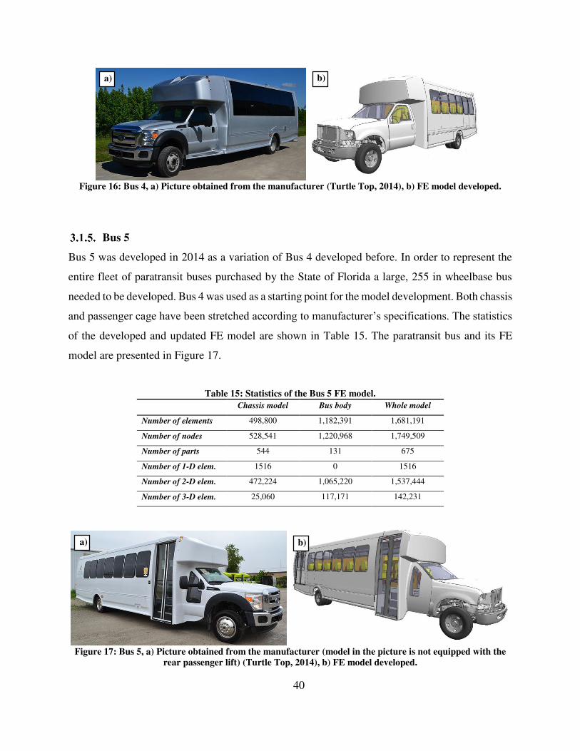
40
Figure 16: Bus 4, a) Picture obtained from the manufacturer (Turtle Top, 2014), b) FE model developed.
Bus 5
Bus 5 was developed in 2014 as a variation of Bus 4 developed before. In order to represent the
entire fleet of paratransit buses purchased by the State of Florida a large, 255 in wheelbase bus
needed to be developed. Bus 4 was used as a starting point for the model development. Both chassis
and passenger cage have been stretched according to manufacturer’s specifications. The statistics
of the developed and updated FE model are shown in Table 15. The paratransit bus and its FE
model are presented in Figure 17.
Table 15: Statistics of the Bus 5 FE model.
Chassis model Bus body Whole model
Number of elements 498,800 1,182,391 1,681,191
Number of nodes 528,541 1,220,968 1,749,509
Number of parts 544 131 675
Number of 1-D elem. 1516 0 1516
Number of 2-D elem. 472,224 1,065,220 1,537,444
Number of 3-D elem. 25,060 117,171 142,231
Figure 17: Bus 5, a) Picture obtained from the manufacturer (model in the picture is not equipped with the
rear passenger lift) (Turtle Top, 2014), b) FE model developed.
a) b)
a) b)
41
3.2. Methodology for FE Analyses – Used Software and Hardware
Research presented in this dissertation has been carried out on two separate High Performance
Computing (HPC) systems. All full vehicle rollover simulations presented in this dissertation have
been completed using Zephyr HPC Cluster at the Transportation Research and Analysis
Computing Center (TRACC) at the Argonne National Laboratory (ANL) (TRACC, 2014). All of
the ERT procedure component tests have been carried out using local Crashworthiness and Impact
Analysis Laboratory (CIAL) Phoenix cluster (CIAL, 2014).
TRACC Zephyr cluster consists of 88 compute nodes, each with two 16-core AMD Interlagos
6273, 2.3GHz CPUs, and 32 GB RAM (TRACC, 2014). All of the rollover runs have been carried
out using two compute nodes (32 cores) and a LS-DYNA Massively Parallel Processing (MPP)
solver version mpp971s R6.1.0. LS-OPT jobs were carried out using LS-OPT version 4.2 on the
two additional login nodes of TRACC Zephyr cluster which have the same system configuration
as the compute nodes. Due to the transient, nonlinear and impact character of the rollover test
simulation explicit time integration solver in LS-DYNA was used for all rollover simulations
(LSTC, 2014).
CIAL Phoenix cluster consists of 3 compute nodes, each with dual 6-core INTEL Xeon 5650,
2.6GHz CPUs and 24 GB RAM. All of the ERT procedure component tests were executed using
one compute node (8 cores) and a LS-DYNA Shared Memory Processing (SMP) solver version
ls971s R6.1.0. LS-OPT jobs were carried out using LS-OPT version 4.2. ERT procedure
simulations have been conducted using both implicit and explicit time integration in LS-DYNA.
Due to transient character Tube and Panel Impact simulations were conducted using an explicit
time integration. Frontal Ring, Rear Wall, Connections and Static Tube Bending test simulations,
due to quasi-static character of the experiments, have been carried out using an implicit time
integration module in LS-DYNA.
The default implicit solution method implemented in the LS-DYNA is a Quasi-Newton method
that forces the global stiffness matrix to be reformed every 11th step. This is a very efficient solution
scheme when no significant amount of contact is involved, or nonlinearity of the problem is
moderate (Bala, 2014). Unfortunately, ERT tests exhibit plastic hinge development, breaking
welds and other highly nonlinear effects, which limit the stability of the default implicit solver
method. In order to increase the stability of the implicit solution a Full-Newton solution scheme
was used. Full-Newton method is executed in LS-DYNA by forcing the solver to perform a global
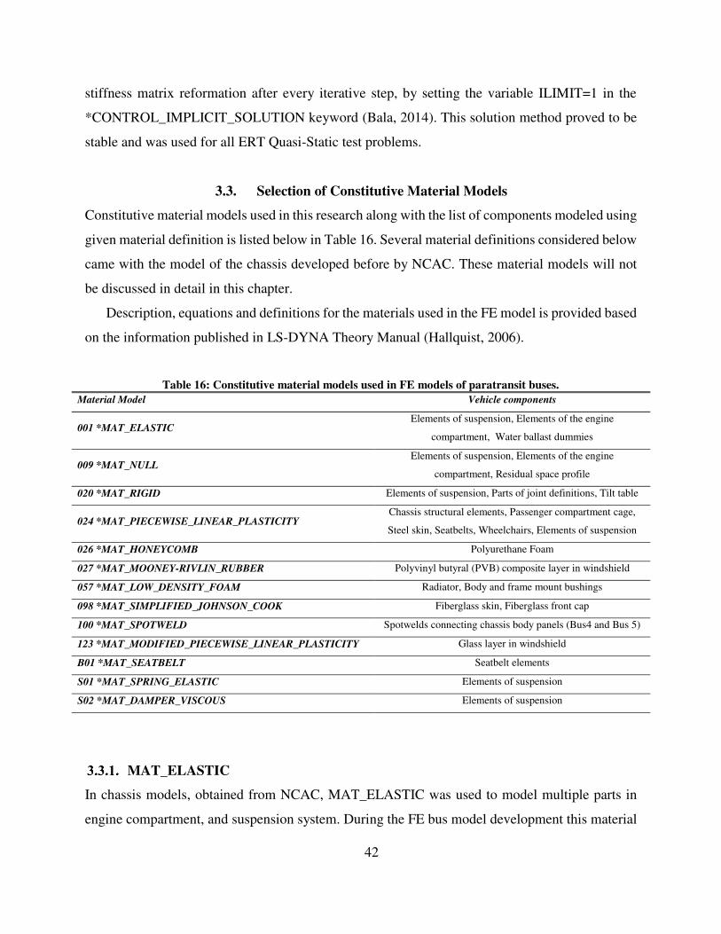
42
stiffness matrix reformation after every iterative step, by setting the variable ILIMIT=1 in the
*CONTROL_IMPLICIT_SOLUTION keyword (Bala, 2014). This solution method proved to be
stable and was used for all ERT Quasi-Static test problems.
3.3. Selection of Constitutive Material Models
Constitutive material models used in this research along with the list of components modeled using
given material definition is listed below in Table 16. Several material definitions considered below
came with the model of the chassis developed before by NCAC. These material models will not
be discussed in detail in this chapter.
Description, equations and definitions for the materials used in the FE model is provided based
on the information published in LS-DYNA Theory Manual (Hallquist, 2006).
Table 16: Constitutive material models used in FE models of paratransit buses.
Material Model Vehicle components
001 *MAT_ELASTIC Elements of suspension, Elements of the engine
compartment, Water ballast dummies
009 *MAT_NULL Elements of suspension, Elements of the engine
compartment, Residual space profile
020 *MAT_RIGID Elements of suspension, Parts of joint definitions, Tilt table
024 *MAT_PIECEWISE_LINEAR_PLASTICITY Chassis structural elements, Passenger compartment cage,
Steel skin, Seatbelts, Wheelchairs, Elements of suspension
026 *MAT_HONEYCOMB Polyurethane Foam
027 *MAT_MOONEY-RIVLIN_RUBBER Polyvinyl butyral (PVB) composite layer in windshield
057 *MAT_LOW_DENSITY_FOAM Radiator, Body and frame mount bushings
098 *MAT_SIMPLIFIED_JOHNSON_COOK Fiberglass skin, Fiberglass front cap
100 *MAT_SPOTWELD Spotwelds connecting chassis body panels (Bus4 and Bus 5)
123 *MAT_MODIFIED_PIECEWISE_LINEAR_PLASTICITY Glass layer in windshield
B01 *MAT_SEATBELT Seatbelt elements
S01 *MAT_SPRING_ELASTIC Elements of suspension
S02 *MAT_DAMPER_VISCOUS Elements of suspension
MAT_ELASTIC
In chassis models, obtained from NCAC, MAT_ELASTIC was used to model multiple parts in
engine compartment, and suspension system. During the FE bus model development this material

43
definition was used to model nonstructural parts of the passenger compartment, such as rubber
door seals, rubber wheel well covers, and water ballast dummies used to compensate for passenger
weight.
MAT_ELASTIC is one of the simplest constitutive material models used in LS-DYNA. The
deviatoric Cauchy stress tensor and pressure are defined as:
∇ + ⁄ = ′ + ⁄ (2)
+ = − + (3)
where:
G – elastic shear modulus,
K – bulk modulus,
V – relative volume (Hallquist, 2006).
MAT_NULL
Shell elements defined with this material are not included into element processing by LS-DYNA
solver (Hallquist, 2006). To take advantage of that feature, the residual space profile (used only
for visualization purposes), was modeled with MAT_NULL definition. In the chassis model
obtained from NCAC several contact surfaces, including surfaces of rigid bodies, have been
defined with this material.
MAT_RIGID
MAT_RIGID presents a very convenient way of defining parts within the model as rigid bodies.
In some applications it is a good choice to approximate a part of the model as a rigid body, since
its definition is bypassed in the element processing and results in increased calculation speed
(Hallquist, 2006). Rigid bodies are also commonly used in LS-DYNA for joint definition such as
JOINT_REVOLUTE and JOINT_CYLINDRICAL keywords. Material properties are necessary
to be defined in this material model in order to calculate sliding interface parameters during contact
with other parts.
Bus FE models developed in CIAL consist of multiple rigid bodies. Several parts of suspension
in chassis models, were defined as rigid in order to define rotational or cylindrical joints, for

44
example wheel hub and axle. Also, tilt table, used for rollover test procedure, was modeled using
the material rigid definition.
MAT_PIECEWISE_LINEAR_PLASTICITY
Most of the steel and aluminum structural elements in the developed FE models were modeled
using MAT_PIECEWISE_LINEAR_PLASTICITY material definition. Elements of the chassis,
such as frame and vehicle body panels, were defined as MAT_024 on the original downloaded
model. Structural elements of the passenger compartment, such as cage frame, and steel bus skin,
were added to the model also using MAT_024 definition.
LS-DYNA Theory Manual states that in implementation of this material model, deviatoric
stresses are updated elastically, same as in MAT_ELASTIC described above, until the yield
function is violated (Hallquist, 2006). Yield function is defined as:
∅ = − � (4)
where:
� = [� + ℎ( )] (5)
where:
β – accounts for rate effects,
ℎ( ) – is a hardening function,
– effective plastic strain.
It is a common practice for metals to specify a hardening function based on the uniaxial tensile
test results. In such case, it needs to be noted that hardening function is a function of effective
plastic strain and experimental results need to be updated through equation:
= − � (6)
where:
– true strain obtained from uniaxial tensile test (LSTC, 2014), � – true stress obtained from uniaxial tensile test (LSTC, 2014),
– Young’s modulus.

45
MAT_024 also allows to account for strain rate effects. Three options are available (Hallquist,
2006).
Cowper-Symonds formulation where yield stress scaling factor β is defined as:
= + � ⁄ (7)
where – is the strain rate,
C, p – are Cowper-Symonds coefficients.
A tabular definition of yield stress scaling factor β versus strain rate.
Different stress strain values defined for various strain rates.
MAT_HONEYCOMB
The State of Florida requires additional isolation to be added to the bus structure in order to
improve its thermal isolation (Siervogel, 2014). Some bus manufacturers use polyurethane spray
on foam on the inner side of the bus frame to isolate the structure. The foam is also used to improve
adhesion between bus skin and structural frame.
MAT_HONEYCOMB, defined also as crushable foam material, is an orthotropic material
model that has two distinctive deformation stages during loading. The first stage represents a
material before compaction, where all of the components of stress tensor are uncoupled. This
means that strain in one direction will not generate strains in other two directions, or simply said
the Poisson’s Ratio for the model before compaction is assumed to be zero (Du Bois and Schwer,
2010). The modulus of elasticity is assumed to vary linearly between uncompacted value and fully
compacted value with respect to the relative volume. Before reaching compacted value of relative
volume elastic and shear moduli is expressed by (Hallquist, 2006):
= + − (8)
= [ + ( − )], for ≠ (9)
where:
= � [ ( −− , ) , ] (10)
– is the elastic modulus of a fully compacted material,
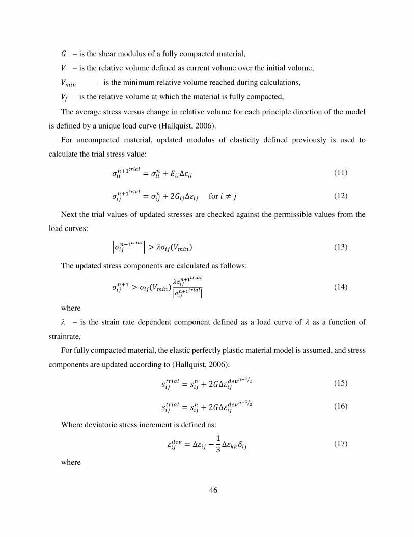
46
– is the shear modulus of a fully compacted material,
– is the relative volume defined as current volume over the initial volume,
– is the minimum relative volume reached during calculations,
– is the relative volume at which the material is fully compacted,
The average stress versus change in relative volume for each principle direction of the model
is defined by a unique load curve (Hallquist, 2006).
For uncompacted material, updated modulus of elasticity defined previously is used to
calculate the trial stress value:
� + �� � = � + ∆ (11)
� + �� � = � + ∆ for ≠ (12)
Next the trial values of updated stresses are checked against the permissible values from the
load curves:
|� + �� � | > � (13)
The updated stress components are calculated as follows:
� + > � �� + �� �|� + �� � | (14)
where
– is the strain rate dependent component defined as a load curve of as a function of
strainrate,
For fully compacted material, the elastic perfectly plastic material model is assumed, and stress
components are updated according to (Hallquist, 2006):
� = + ∆ + ⁄ (15)
� = + ∆ + ⁄ (16)
Where deviatoric stress increment is defined as:
= ∆ − ∆ (17)
where

47
– is the Kronecker delta = { ≠ =
Next, the yield criterion for a fully compacted material is checked, and if the effective trial
stress exceeds the yield stress, the stress components are scaled back to the yield surface.
MAT_MOONEY-RIVLIN_RUBBER
During the full scale bus rollover experiment, it has been noticed that the performance of the
windshield FE model was not satisfactory. Safety glass, a material used for windshields, is a very
difficult material to simulate, (Du Bois, Kolling and Fassnacht, 2003; Timmel, et al., 2007; Sun,
et al., 2005). The structure of safety glass, a layer of PVB composite sandwiched in between two
pieces of glass, adds to this complexity. Although the material properties for glass itself are pretty
well established, the PVB is a more complex material with a high strain rate dependency. The
material model implemented in the existing FE model was based on research done by Du Bois,
Kolling, and Fassnacht (2003) with a Mooney-Rivlin formulation for PVB.
As defined in the LS-DYNA manual, the Mooney-Rivlin material formulation is based on the
strain energy density function defined as:
= − + − + − − + − (18)
where:
= . + (19)
= � − + � −− � (20)
� – Poisson’s ratio, + – shear modulus of elasticity, , , – Invariants of right Cauchy-Green Tensor.
This leads to the expression for engineering stress (Piola-Kirchhoff stress, (Du Bois, Kolling
and Fassnacht, 2003) given by:
= + − � + − − − �− (21)
where:

48
– Piola-Kirchhoff stress tensor,
– Identity matrix, � – Right Cauchy-Green strain tensor,
– Determinant of the deformation gradient.
The values defining the Mooney-Rivlin material formulation proposed by Du Bois, Kolling,
and Fassnacht, (Du Bois, Kolling and Fassnacht, 2003) were: A = 1.60 MPa, and B = 0.06 MPa.
Unfortunately, these results were based on quasi-static experiments for PVB, which made them
difficult to use in the experiments with a higher strain rate. The review of existing papers on PVB
properties (Iwasaki, et al., 2007) allowed identification of material properties for higher strain rates
and their implementation into the Mooney-Rivlin material model. The obtained values were: A =
1.00 MPa, and B = 9.00 MPa.
MAT_SIMPLIFIED_JOHNSON_COOK
Multiple body parts on paratransit buses are built using a spray on fiberglass composite material.
In all five buses, investigated in this study, frontal cap was made out of fiberglass composite. Some
bus manufacturers also used fiberglass components for sidewall and rear wall skin. Due to the
simplicity of material definition, and inclusion of strain rate effects, material Johnson Cook
(Johnson and Cook, 1985) was used to model fiberglass components.
The three key components of Johnson-Cook material model are; strain hardening, strain rate
effects and thermal softening. These components combined in the multiplicative manner give a
form of Johnson-Cook material model (Schwer, 2007). In LS-DYNA this material model is
represented by MAT_015_JOHNSON_COOK:
� = [ + ] + ln [ − ] (22)
where: , , – Material parameters used for definition of plastic stress flow (Static
component).
– Material parameter used for definition of plastic stress flow (Strain rate
dependency component).
– Material parameters used for definition of plastic stress flow (Thermal softening
component)
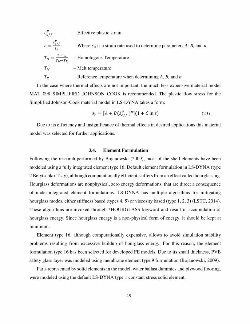
49
– Effective plastic strain.
= ��� – Where is a strain rate used to determine parameters A, B, and n.
= − ��− � – Homologous Temperature
– Melt temperature
– Reference temperature when determining A, B, and n
In the case where thermal effects are not important, the much less expensive material model
MAT_098_SIMPLIFIED_JOHNSON_COOK is recommended. The plastic flow stress for the
Simplified Johnson-Cook material model in LS-DYNA takes a form:
� = [ + ] + ln (23)
Due to its efficiency and insignificance of thermal effects in desired applications this material
model was selected for further applications.
3.4. Element Formulation
Following the research performed by Bojanowski (2009), most of the shell elements have been
modeled using a fully integrated element type 16. Default element formulation in LS-DYNA (type
2 Belytschko-Tsay), although computationally efficient, suffers from an effect called hourglassing.
Hourglass deformations are nonphysical, zero energy deformations, that are direct a consequence
of under-integrated element formulations. LS-DYNA has multiple algorithms for mitigating
hourglass modes, either stiffness based (types 4, 5) or viscosity based (type 1, 2, 3) (LSTC, 2014).
These algorithms are invoked through *HOURGLASS keyword and result in accumulation of
hourglass energy. Since hourglass energy is a non-physical form of energy, it should be kept at
minimum.
Element type 16, although computationally expensive, allows to avoid simulation stability
problems resulting from excessive buildup of hourglass energy. For this reason, the element
formulation type 16 has been selected for developed FE models. Due to its small thickness, PVB
safety glass layer was modeled using membrane element type 9 formulation (Bojanowski, 2009).
Parts represented by solid elements in the model, water ballast dummies and plywood flooring,
were modeled using the default LS-DYNA type 1 constant stress solid element.

50
3.5. Contact Definition
During FEM crash calculations, it is often the case that modeled parts come in contact. In order to
prevent two objects penetrating each other, a contact handling algorithm is necessary to be
implemented into the FEM software. Contact treatment algorithms are critical for large
deformation problems, and accurate contact modeling is very important (LSTC, 2014). Many
contact types are currently available in commercial FEM software. Contact algorithms in LS-
DYNA can be separated into two groups, penalty based contacts and constrained based contacts.
Most of the contacts algorithms, used for crash applications, are penalty based contacts. The
principle of classical penalty contact definition in LS-DYNA requires the user to define “slave”
nodes (ex. node sets, parts, past sets) that should be prevented from penetrating “master” segments
(ex. segment set, parts, part sets). A search algorithm is implemented in LS-DYNA software in
search for possible penetrations. Once a penetration is detected, a penalty force, proportional to
the depth of the penetration is applied to the “slave” node in order to eliminate detected penetration
(LSTC, 2014).
Since the penalty force is proportional to the depth of the penetration, it is often described as a
tension-only spring, attached to the penetrating “slave” node. The resultant reaction force, coming
from the contact spring, is also distributed over neighboring nodes that belong to the “master”
segment in order to follow the laws of conservation of momentum. The contact spring stiffness is
a product of a user defined penalty factor and a stiffness value, defined as a minimum stiffness
from either master segment or slave node (Du Bois and Schewr, 2010).
Currently, AUTOMATIC_SINGLE_SURFACE contact algorithm is the most commonly used
in impact simulations. It considers contact between all parts defined within the slave part set, as
well as their self-contact. This contact is considered to be reliable and accurate (LSTC, 2014).
AUTOMATIC_SINGLE_SURFACE contact algorithm was used to define contact between
all parts in developed FE models. Friction coefficient for this contact type was set equal to 0.15
representing steel to steel contact. A separate contact entity was created for tiers and tilt table
contact with a friction coefficient set to 0.7 representing rubber to steel contact.
Contact AUTOMATIC_SURFACE_TO_ SURFACE_TIEBREAK was used to simulate
adhesive between bus skin and steel cage. During implementation process, it was discovered that
this contact definition is very sensitive to segment orientation. Even though AUTOMATIC contact
types do not have orientation requirements (LSTC, 2014), the use of this contact type led to model
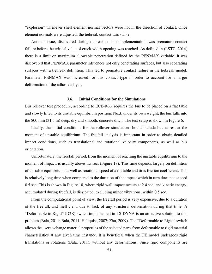
51
“explosion” whenever shell element normal vectors were not in the direction of contact. Once
element normals were adjusted, the tiebreak contact was stable.
Another issue, discovered during tiebreak contact implementation, was premature contact
failure before the critical value of crack width opening was reached. As defined in (LSTC, 2014)
there is a limit on maximum allowable penetration defined by the PENMAX variable. It was
discovered that PENMAX parameter influences not only penetrating surfaces, but also separating
surfaces with a tiebreak definition. This led to premature contact failure in the tiebreak model.
Parameter PENMAX was increased for this contact type in order to account for a larger
deformation of the adhesive layer.
3.6. Initial Conditions for the Simulations
Bus rollover test procedure, according to ECE-R66, requires the bus to be placed on a flat table
and slowly tilted to its unstable equilibrium position. Next, under its own weight, the bus falls into
the 800 mm (31.5 in) deep, dry and smooth, concrete ditch. The test setup is shown in Figure 6.
Ideally, the initial conditions for the rollover simulation should include bus at rest at the
moment of unstable equilibrium. The freefall analysis is important in order to obtain detailed
impact conditions, such as translational and rotational velocity components, as well as bus
orientation.
Unfortunately, the freefall period, from the moment of reaching the unstable equilibrium to the
moment of impact, is usually above 1.5 sec. (Figure 18). This time depends largely on definition
of unstable equilibrium, as well as rotational speed of a tilt table and tires friction coefficient. This
is relatively long time when compared to the duration of the impact which in turn does not exceed
0.5 sec. This is shown in Figure 18, where rigid wall impact occurs at 2.4 sec. and kinetic energy,
accumulated during freefall, is dissipated, excluding minor vibrations, within 0.5 sec.
From the computational point of view, the freefall period is very expensive, due to a duration
of the freefall, and inefficient, due to lack of any structural deformation during that time. A
“Deformable to Rigid” (D2R) switch implemented in LS-DYNA is an attractive solution to this
problem (Bala, 2011; Bala, 2011; Hallquist, 2007; Zhu, 2009). The “Deformable to Rigid” switch
allows the user to change material properties of the selected parts from deformable to rigid material
characteristics at any given time instance. It is beneficial when the FE model undergoes rigid
translations or rotations (Bala, 2011), without any deformations. Since rigid components are
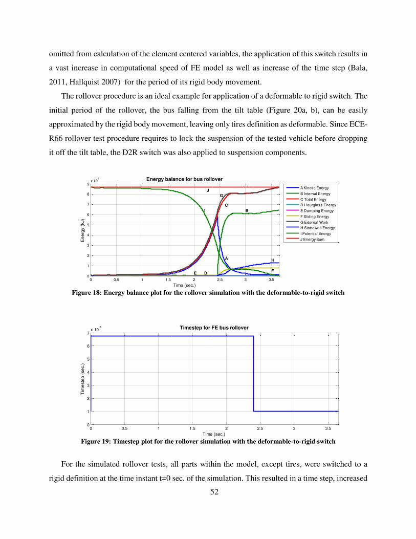
52
omitted from calculation of the element centered variables, the application of this switch results in
a vast increase in computational speed of FE model as well as increase of the time step (Bala,
2011, Hallquist 2007) for the period of its rigid body movement.
The rollover procedure is an ideal example for application of a deformable to rigid switch. The
initial period of the rollover, the bus falling from the tilt table (Figure 20a, b), can be easily
approximated by the rigid body movement, leaving only tires definition as deformable. Since ECE-
R66 rollover test procedure requires to lock the suspension of the tested vehicle before dropping
it off the tilt table, the D2R switch was also applied to suspension components.
0 0.5 1 1.5 2 2.5 3 3.50
1
2
3
4
5
6
7
8
9x 10
7 Energy balance for bus rollover
Time (sec.)
En
erg
y (
kJ)
A
B
C
DEF
G
H
I
J
A Kinetic Energy
B Internal Energy
C Total Energy
D Hourglass Energy
E Damping Energy
F Sliding Energy
G External Work
H Stonewall Energy
I Potential Energy
J Energy Sum
Figure 18: Energy balance plot for the rollover simulation with the deformable-to-rigid switch
0 0.5 1 1.5 2 2.5 3 3.50
1
2
3
4
5
6
7x 10
-6 Timestep for FE bus rollover
Time (sec.)
Tim
este
p (
se
c.)
Figure 19: Timestep plot for the rollover simulation with the deformable-to-rigid switch
For the simulated rollover tests, all parts within the model, except tires, were switched to a
rigid definition at the time instant t=0 sec. of the simulation. This resulted in a time step, increased
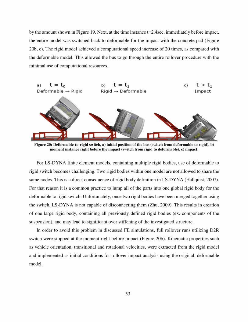
53
by the amount shown in Figure 19. Next, at the time instance t=2.4sec, immediately before impact,
the entire model was switched back to deformable for the impact with the concrete pad (Figure
20b, c). The rigid model achieved a computational speed increase of 20 times, as compared with
the deformable model. This allowed the bus to go through the entire rollover procedure with the
minimal use of computational resources.
Figure 20: Deformable-to-rigid switch, a) initial position of the bus (switch from deformable to rigid), b)
moment instance right before the impact (switch from rigid to deformable), c) impact.
For LS-DYNA finite element models, containing multiple rigid bodies, use of deformable to
rigid switch becomes challenging. Two rigid bodies within one model are not allowed to share the
same nodes. This is a direct consequence of rigid body definition in LS-DYNA (Hallquist, 2007).
For that reason it is a common practice to lump all of the parts into one global rigid body for the
deformable to rigid switch. Unfortunately, once two rigid bodies have been merged together using
the switch, LS-DYNA is not capable of disconnecting them (Zhu, 2009). This results in creation
of one large rigid body, containing all previously defined rigid bodies (ex. components of the
suspension), and may lead to significant over stiffening of the investigated structure.
In order to avoid this problem in discussed FE simulations, full rollover runs utilizing D2R
switch were stopped at the moment right before impact (Figure 20b). Kinematic properties such
as vehicle orientation, transitional and rotational velocities, were extracted from the rigid model
and implemented as initial conditions for rollover impact analysis using the original, deformable
model.
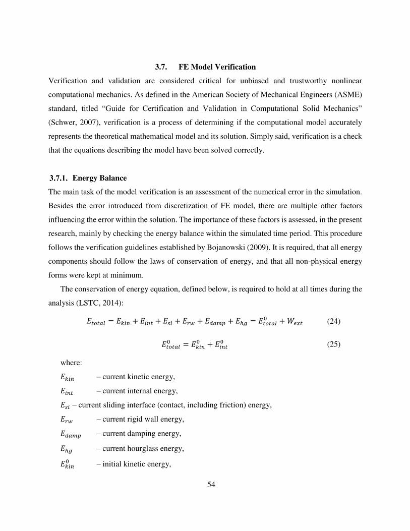
54
3.7. FE Model Verification
Verification and validation are considered critical for unbiased and trustworthy nonlinear
computational mechanics. As defined in the American Society of Mechanical Engineers (ASME)
standard, titled “Guide for Certification and Validation in Computational Solid Mechanics”
(Schwer, 2007), verification is a process of determining if the computational model accurately
represents the theoretical mathematical model and its solution. Simply said, verification is a check
that the equations describing the model have been solved correctly.
Energy Balance
The main task of the model verification is an assessment of the numerical error in the simulation.
Besides the error introduced from discretization of FE model, there are multiple other factors
influencing the error within the solution. The importance of these factors is assessed, in the present
research, mainly by checking the energy balance within the simulated time period. This procedure
follows the verification guidelines established by Bojanowski (2009). It is required, that all energy
components should follow the laws of conservation of energy, and that all non-physical energy
forms were kept at minimum.
The conservation of energy equation, defined below, is required to hold at all times during the
analysis (LSTC, 2014):
� = + + + + � + ℎ = � + (24)
� = + (25)
where:
– current kinetic energy,
– current internal energy,
– current sliding interface (contact, including friction) energy,
– current rigid wall energy, � – current damping energy,
ℎ – current hourglass energy,
– initial kinetic energy,
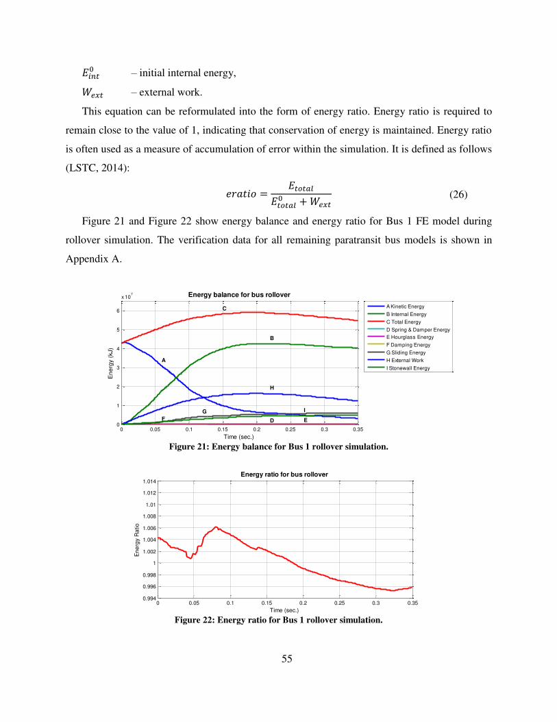
55
– initial internal energy,
– external work.
This equation can be reformulated into the form of energy ratio. Energy ratio is required to
remain close to the value of 1, indicating that conservation of energy is maintained. Energy ratio
is often used as a measure of accumulation of error within the simulation. It is defined as follows
(LSTC, 2014):
� = �� + (26)
Figure 21 and Figure 22 show energy balance and energy ratio for Bus 1 FE model during
rollover simulation. The verification data for all remaining paratransit bus models is shown in
Appendix A.
0 0.05 0.1 0.15 0.2 0.25 0.3 0.350
1
2
3
4
5
6
x 107 Energy balance for bus rollover
Time (sec.)
En
erg
y (
kJ)
A
B
C
D EF
G
H
I
A Kinetic Energy
B Internal Energy
C Total Energy
D Spring & Damper Energy
E Hourglass Energy
F Damping Energy
G Sliding Energy
H External Work
I Stonewall Energy
Figure 21: Energy balance for Bus 1 rollover simulation.
0 0.05 0.1 0.15 0.2 0.25 0.3 0.350.994
0.996
0.998
1
1.002
1.004
1.006
1.008
1.01
1.012
1.014
Energy ratio for bus rollover
Time (sec.)
En
erg
y R
atio
Figure 22: Energy ratio for Bus 1 rollover simulation.

56
For all rollover simulations, performed on the developed FE models, energy balance followed
the laws of conservation of energy and all non-physical forms of energy were kept at minimum.
Energy ratio remained in the close proximity of target value of 1, reaching maximum amount of
error of 4% for Bus 2. For all other bus models error indicated by energy ratio remained below the
value of 4%.
Discretization Error Estimation
Mesh refinement studies are not often found in the publications on numerical investigations of
vehicle crashworthiness. This is often due to the complexity and size of the analyzed models,
where mesh refinement is not feasible or too expensive. Researchers often choose to mitigate this
shortcoming by performing energy balance analysis on the entire model, to gain confidence that
final solution is free of errors. Schwer (Schwer, 2008) highlights this problem, suggesting that
researchers often omit spatial discretization error estimation, and as a consequence, have no idea
if they have obtained a converged solution.
In this research, due to the complexity of the developed FE models, mesh refinement study on
the entire vehicle was not carried out. Instead, a mesh sensitivity analysis was performed on a three
point bending test of a structural tube. This test was selected due to the fact that steel tube is a part
of the bus cage that absorbs the most amount of energy during rollover, and the bending test
deformation pattern closely resembles the tube deformation during rollover. Similar assessment
was performed before by Bojanowski (2009) for a four point tube bending test. A test setup is
shown below in Figure 23. Test results are shown in Figure 24.
Figure 23: A numerical three point bending test used for spatial discretization error estimation with two
elements across the tube.

57
Figure 24: Three point bending test, experiment versus FE simulation with various spatial discretization.
Table 17: Three point bending test results. Experiment versus FE simulation.
# elements Element Size [mm] Max force [N] Energy [J] Error force [%] Error Energy [%]
2 18 16462.8 1346.88 11.97 14.24
4 9 14812.7 1200.97 0.75 1.86
8 4.5 14686.8 1202.22 0.11 1.97
Experiment - 14702.33 1179.03 - -
The results for this study are shown in Table 17. Mesh with two elements across the tube
(Figure 23) is too crude, and results in the FE model being too stiff as compared with the
experiment. The error associated with the two element model was 11.97% for the maximum force
and 14.24% for the energy dissipated by the tube respectively. Four and eight element samples
show a better agreement with the experimental data. Based on the results shown in Table 17 it was
decided to keep the current mesh density (4 elements across the tube) for all developed FE models
of paratransit buses.
3.8. FE Model Validation
The goal of validation is to assess accuracy of the numerical model and its predictive capability by
comparing results from experiments with FE simulations. It is critical to select validation
experiments related to the scenario for which the model will be used. The process of validation for
complex structures should be set up in a hierarchical order. Starting from the basic experiments
and simulations, through more complicated systems of components, and finally by validating the
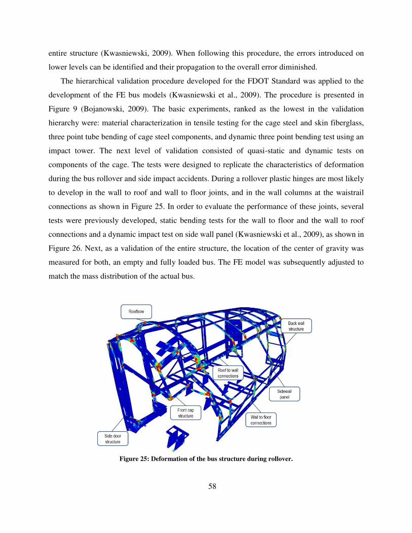
58
entire structure (Kwasniewski, 2009). When following this procedure, the errors introduced on
lower levels can be identified and their propagation to the overall error diminished.
The hierarchical validation procedure developed for the FDOT Standard was applied to the
development of the FE bus models (Kwasniewski et al., 2009). The procedure is presented in
Figure 9 (Bojanowski, 2009). The basic experiments, ranked as the lowest in the validation
hierarchy were: material characterization in tensile testing for the cage steel and skin fiberglass,
three point tube bending of cage steel components, and dynamic three point bending test using an
impact tower. The next level of validation consisted of quasi-static and dynamic tests on
components of the cage. The tests were designed to replicate the characteristics of deformation
during the bus rollover and side impact accidents. During a rollover plastic hinges are most likely
to develop in the wall to roof and wall to floor joints, and in the wall columns at the waistrail
connections as shown in Figure 25. In order to evaluate the performance of these joints, several
tests were previously developed, static bending tests for the wall to floor and the wall to roof
connections and a dynamic impact test on side wall panel (Kwasniewski et al., 2009), as shown in
Figure 26. Next, as a validation of the entire structure, the location of the center of gravity was
measured for both, an empty and fully loaded bus. The FE model was subsequently adjusted to
match the mass distribution of the actual bus.
Figure 25: Deformation of the bus structure during rollover.

59
Figure 26: Components selected for the validation procedure: wall to floor connection (1), wall to roof
connection (2), and sidewall panel (3).
The procedure of FE model development, model verification, and validation, have been
published before and can be found in Kwasniewski et al., (2006), Cichocki and Wekezer, (2007),
Horstemeyer et al., (2007), Li et al., (2007), Kwasniewski et al., (2009), Bojanowski, (2009).
Structural Steel Material Properties
Material properties for structural steel, used in investigated buses, was established based on
uniaxial tensile test results. Uniaxial tensile tests for first three buses (Bus 1, Bus 2, Bus 3) were
performed during previous research according to EN 10002 testing standard (EN BS, 2001;
Bojanowski, 2009), whereas material testing for the other two buses (Bus 4 and Bus 5) was
performed using ASTM E8 standard (ASTM, 1997). Material properties obtained for structural
steel were then implemented into the formulation of the FE models. The implementation process
was repeated for all modeled buses.
MAT_024_PIECEWISE_LINEAR_PLASTICITY was used as a material model for structural
steel. MAT_024 is an elastoplastic material model with arbitrary stress versus strain curve for the
plastic region, and arbitrary strain rate dependency definition. It allows also for a failure criteria
definition based on limiting value of a plastic strain. True stress versus true plastic strain curve is
required as an input data for the MAT_024 material model. This curve was obtained from
experimental data according to LS-DYNA support guidelines (LSTC, 2014). True strain and true
stress are defined as:
= ln + (27)
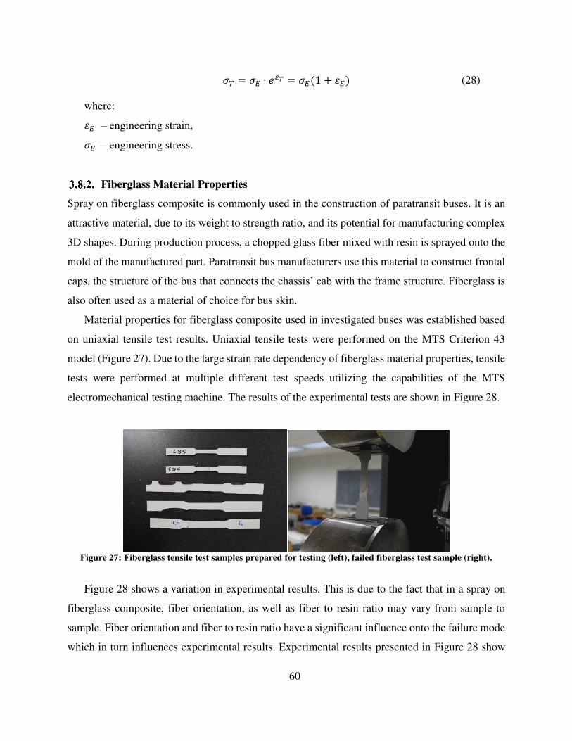
60
� = � ∙ �� = � + (28)
where:
– engineering strain, � – engineering stress.
Fiberglass Material Properties
Spray on fiberglass composite is commonly used in the construction of paratransit buses. It is an
attractive material, due to its weight to strength ratio, and its potential for manufacturing complex
3D shapes. During production process, a chopped glass fiber mixed with resin is sprayed onto the
mold of the manufactured part. Paratransit bus manufacturers use this material to construct frontal
caps, the structure of the bus that connects the chassis’ cab with the frame structure. Fiberglass is
also often used as a material of choice for bus skin.
Material properties for fiberglass composite used in investigated buses was established based
on uniaxial tensile test results. Uniaxial tensile tests were performed on the MTS Criterion 43
model (Figure 27). Due to the large strain rate dependency of fiberglass material properties, tensile
tests were performed at multiple different test speeds utilizing the capabilities of the MTS
electromechanical testing machine. The results of the experimental tests are shown in Figure 28.
Figure 27: Fiberglass tensile test samples prepared for testing (left), failed fiberglass test sample (right).
Figure 28 shows a variation in experimental results. This is due to the fact that in a spray on
fiberglass composite, fiber orientation, as well as fiber to resin ratio may vary from sample to
sample. Fiber orientation and fiber to resin ratio have a significant influence onto the failure mode
which in turn influences experimental results. Experimental results presented in Figure 28 show

61
that this material experiences high strain rate dependency effect resulting in larger ultimate stresses
for higher test rates. This effect needs to be addressed in the FE material model.
The Johnson-Cook constitutive material (Johnson and Cook, 1983) model was selected to
model fiberglass composite. First, the material parameters A, B and n for quasi-static test rate of
0.0005 in/s were calibrated using LS-OPT optimization software. Then strain rate parameter C was
calibrated using test results obtained for higher test rates. The calibrated material parameters
obtained for material Johnson-Cook are shown below in Table 18. The results from the calibrated
MAT_98_SIMPLIFIED_JOHNSON_COOK material model are shown in Figure 28.
Table 18: Parameters optimized for MAT_098_SIMPLIFIED_JOHNSON_COOK.
A [1] B [1] C [1] n [1] � [1/s]
40 2000 0.06788 0.7618 0.002667
Figure 28: Comparison of FE results with experiment for MAT_98 material model definition. True Stress
[MPa] vs True Strain; for a strain rate of 0.0005 in/s (a), strain rate of 0.5in/s (b), strain rate of 1.5in/s (c).
a) b)
c)
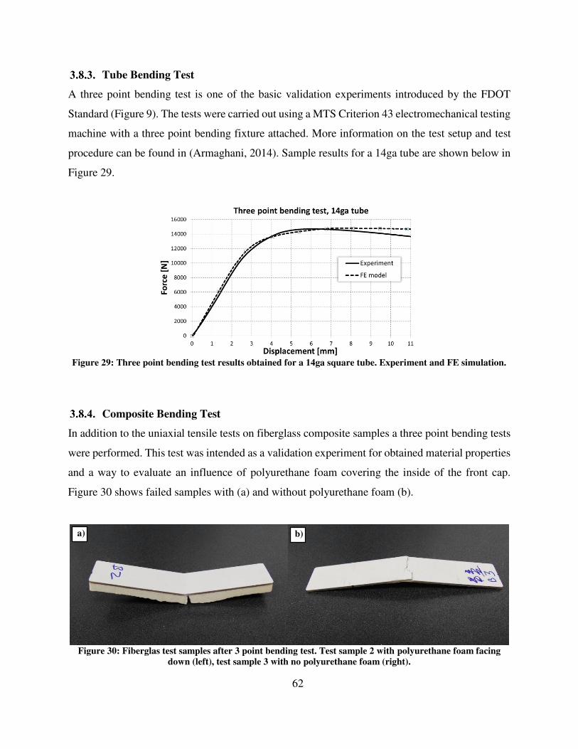
62
Tube Bending Test
A three point bending test is one of the basic validation experiments introduced by the FDOT
Standard (Figure 9). The tests were carried out using a MTS Criterion 43 electromechanical testing
machine with a three point bending fixture attached. More information on the test setup and test
procedure can be found in (Armaghani, 2014). Sample results for a 14ga tube are shown below in
Figure 29.
Figure 29: Three point bending test results obtained for a 14ga square tube. Experiment and FE simulation.
Composite Bending Test
In addition to the uniaxial tensile tests on fiberglass composite samples a three point bending tests
were performed. This test was intended as a validation experiment for obtained material properties
and a way to evaluate an influence of polyurethane foam covering the inside of the front cap.
Figure 30 shows failed samples with (a) and without polyurethane foam (b).
Figure 30: Fiberglas test samples after 3 point bending test. Test sample 2 with polyurethane foam facing
down (left), test sample 3 with no polyurethane foam (right).
a) b)
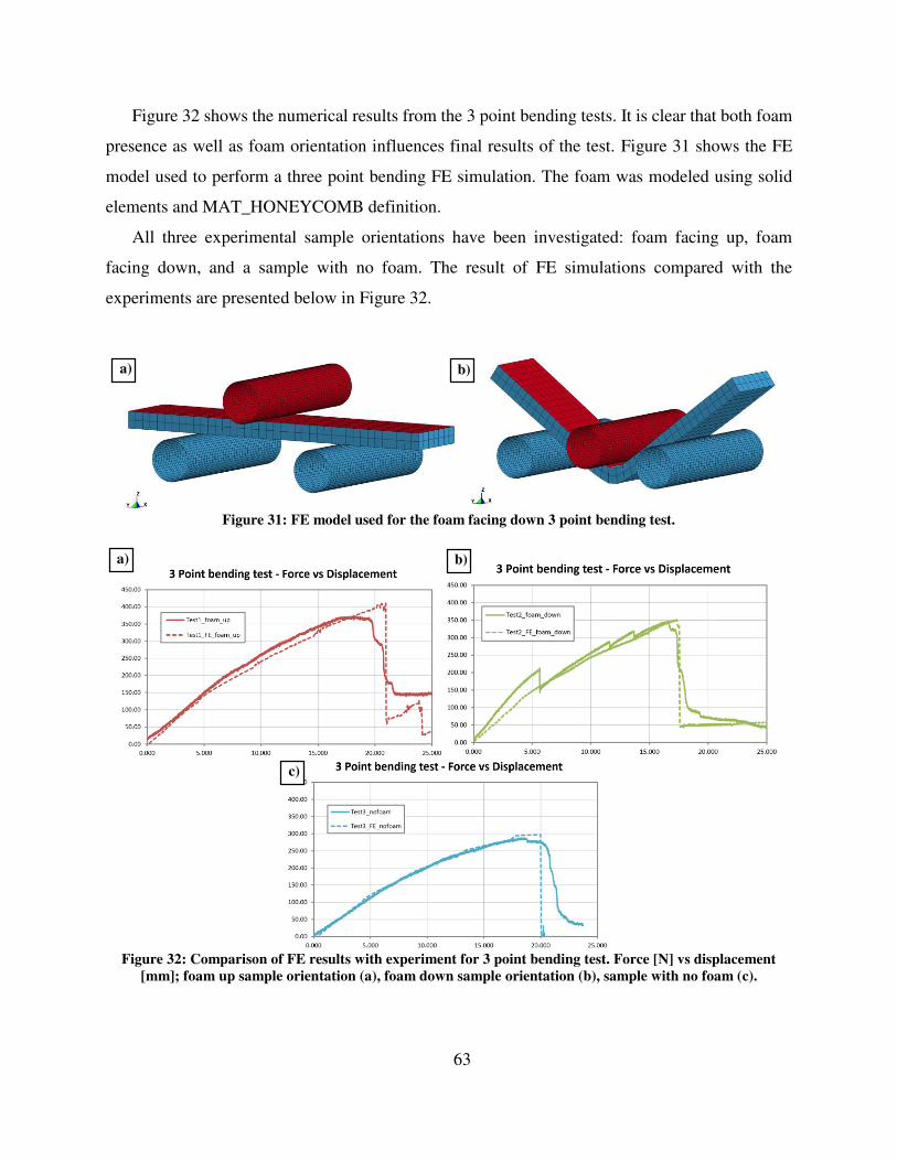
63
Figure 32 shows the numerical results from the 3 point bending tests. It is clear that both foam
presence as well as foam orientation influences final results of the test. Figure 31 shows the FE
model used to perform a three point bending FE simulation. The foam was modeled using solid
elements and MAT_HONEYCOMB definition.
All three experimental sample orientations have been investigated: foam facing up, foam
facing down, and a sample with no foam. The result of FE simulations compared with the
experiments are presented below in Figure 32.
Figure 31: FE model used for the foam facing down 3 point bending test.
Figure 32: Comparison of FE results with experiment for 3 point bending test. Force [N] vs displacement
[mm]; foam up sample orientation (a), foam down sample orientation (b), sample with no foam (c).
a) b)
a) b)
c)
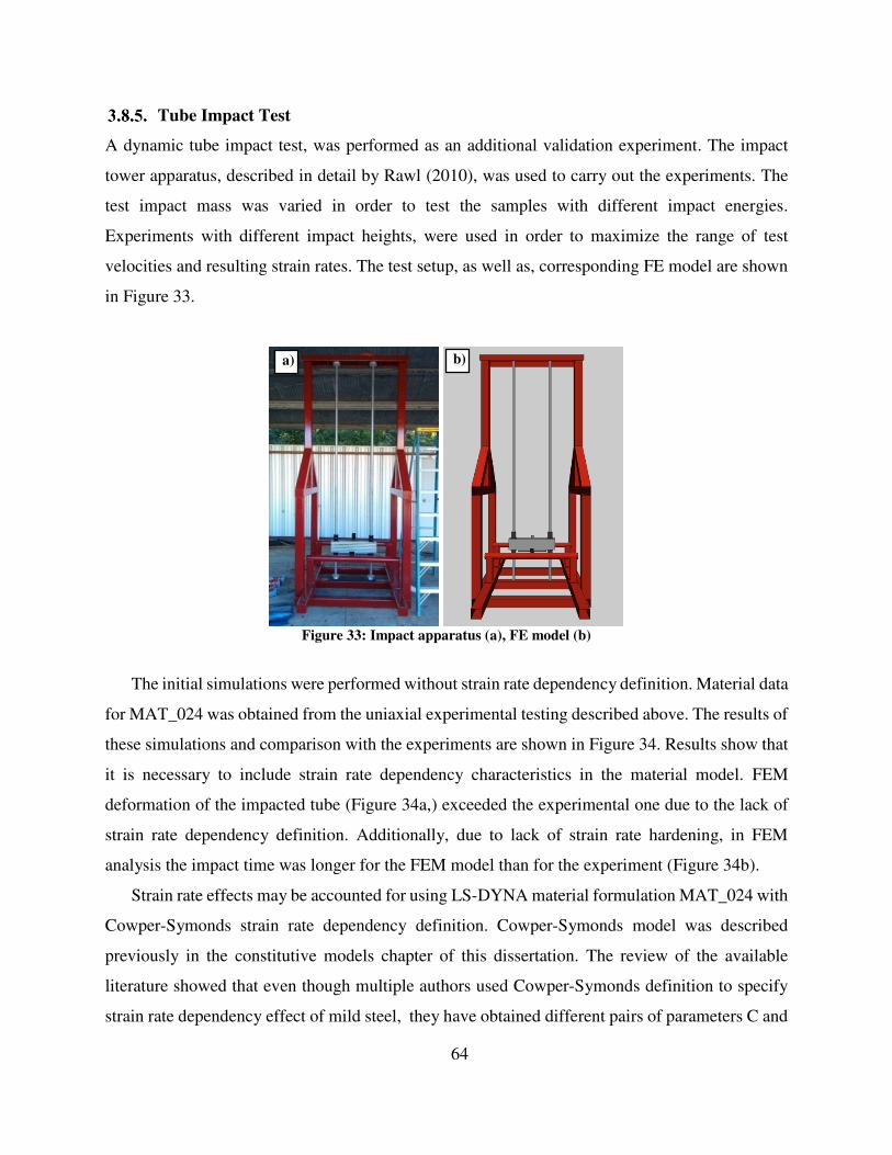
64
Tube Impact Test
A dynamic tube impact test, was performed as an additional validation experiment. The impact
tower apparatus, described in detail by Rawl (2010), was used to carry out the experiments. The
test impact mass was varied in order to test the samples with different impact energies.
Experiments with different impact heights, were used in order to maximize the range of test
velocities and resulting strain rates. The test setup, as well as, corresponding FE model are shown
in Figure 33.
Figure 33: Impact apparatus (a), FE model (b)
The initial simulations were performed without strain rate dependency definition. Material data
for MAT_024 was obtained from the uniaxial experimental testing described above. The results of
these simulations and comparison with the experiments are shown in Figure 34. Results show that
it is necessary to include strain rate dependency characteristics in the material model. FEM
deformation of the impacted tube (Figure 34a,) exceeded the experimental one due to the lack of
strain rate dependency definition. Additionally, due to lack of strain rate hardening, in FEM
analysis the impact time was longer for the FEM model than for the experiment (Figure 34b).
Strain rate effects may be accounted for using LS-DYNA material formulation MAT_024 with
Cowper-Symonds strain rate dependency definition. Cowper-Symonds model was described
previously in the constitutive models chapter of this dissertation. The review of the available
literature showed that even though multiple authors used Cowper-Symonds definition to specify
strain rate dependency effect of mild steel, they have obtained different pairs of parameters C and
a) b)
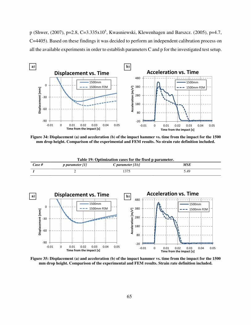
65
p (Shwer, (2007), p=2.8, C=3.335x10⁵, Kwasniewski, Klewenhagen and Barszcz. (2005), p=4.7,
C=4405). Based on these findings it was decided to perform an independent calibration process on
all the available experiments in order to establish parameters C and p for the investigated test setup.
Figure 34: Displacement (a) and acceleration (b) of the impact hammer vs. time from the impact for the 1500
mm drop height. Comparison of the experimental and FEM results. No strain rate definition included.
Table 19: Optimization cases for the fixed p parameter.
Case # p parameter [1] C parameter [1/s] MSE
1 2 1375 5.49
Figure 35: Displacement (a) and acceleration (b) of the impact hammer vs. time from the impact for the 1500
mm drop height. Comparison of the experimental and FEM results. Strain rate definition included.
-90
-60
-30
0
-0.01 0 0.01 0.02 0.03 0.04 0.05
Dis
pla
cem
en
t [m
m]
Time from the impact [s]
Displacement vs. Time
1500mm
1500mm FEM
-20
80
180
280
380
480
-0.01 0 0.01 0.02 0.03 0.04 0.05
Acc
ele
rati
on
(m
/s2)
Time from the impact [s]
Acceleration vs. Time
1500mm
1500mm FEM
-90
-60
-30
0
-0.01 0 0.01 0.02 0.03 0.04 0.05
Dis
pla
cem
en
t [m
m]
Time from the impact [s]
Displacement vs. Time
1500mm
1500mm FEM
-20
80
180
280
380
480
-0.01 0 0.01 0.02 0.03 0.04 0.05
Acc
ele
rati
on
[m
/s2]
Time from the impact [s]
Acceleration vs. Time
1500mm
1500mm FEM
a) b)
a) b)

66
Using Design Optimization software LS-OPT, and results from the experiments the Cowper-
Symonds parameters were calibrated. Parameters C and p were used as calibration variables, and
a Mean Square Error (MSE) estimator of maximum deflection of all test cases was selected as
minimized objective function. The calibrated p and C parameters are shown in Table 19. The
results for the FE model with strain rate dependency parameters and its comparison with the
experiment is shown in Figure 35.
Connection Tests
On a subsystem level, model validation is carried out through the comparison of FE simulations
and experiments performed on bus wall to floor (WF) and wall to roof (WR) connections and side
wall panels. The theoretical groundwork for these tests has been established by Bojanowski (2009),
and refined by Rawl (2010). In connection testing, validation is carried out through comparison of
moment versus rotation curves, whereas for panel impact tests a final specimen deflection after
impact is compared. Validation experiments for Bus 2 have been presented before, and are
described in detail in (Bojanowski, 2009).
Connection testing apparatus is shown below in Figure 36. The load in the experiment is
applied through the cable connected to the aluminum I beam fixed to the tested specimen. The load
is obtained via a load cell connected to the cable. Specimen deformation is recorded using string
potentiometers, often referred to as string transducers, fixed onto the test frame. Moment versus
rotation data is obtained through vector operations, which are extensively covered in (Rawl, 2010).
A specimen prepared for testing and its corresponding FE model are shown below in Figure 37.
Figure 36: A plan of a connection testing apparatus, with a specimen fixed for testing (Rawl, 2010).

67
Figure 37: Connection testing apparatus, experiment (a), and FE simulation (b).
Figure 38 and Figure 39 below show the comparison of the experimental and numerical results
obtained from the connection tests performed for Bus 1. Table 20 shows the maximum moment,
energy absorbed by the connection within the 0-20 deg. range, as well as relative error obtained
for both measurements. The remaining validation data, for all other FE models of paratransit buses
is shown in Appendix A of this dissertation.
0 2 4 6 8 10 12 14 16 18 200
200
400
600
800
1000
1200
1400
1600
1800
2000
2200Wall to Floor Connection Test
Angle of rotation (deg.)
Mo
me
nt
(Nm
)
Experiment
FE Analysis
Figure 38: Wall to floor connection test for Bus 1. Experimental results compared with FE analysis.
a) b)
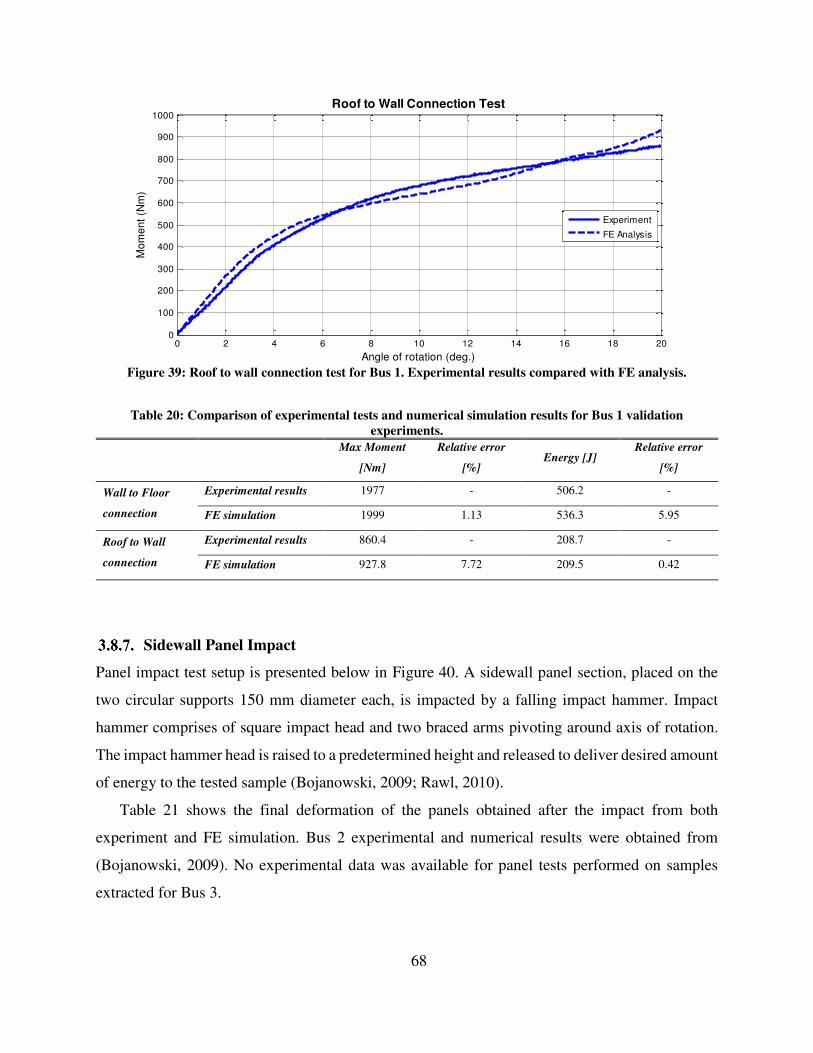
68
0 2 4 6 8 10 12 14 16 18 200
100
200
300
400
500
600
700
800
900
1000Roof to Wall Connection Test
Angle of rotation (deg.)
Mo
me
nt
(Nm
)
Experiment
FE Analysis
Figure 39: Roof to wall connection test for Bus 1. Experimental results compared with FE analysis.
Table 20: Comparison of experimental tests and numerical simulation results for Bus 1 validation
experiments.
Max Moment
[Nm]
Relative error
[%] Energy [J]
Relative error
[%]
Wall to Floor
connection
Experimental results 1977 - 506.2 -
FE simulation 1999 1.13 536.3 5.95
Roof to Wall
connection
Experimental results 860.4 - 208.7 -
FE simulation 927.8 7.72 209.5 0.42
Sidewall Panel Impact
Panel impact test setup is presented below in Figure 40. A sidewall panel section, placed on the
two circular supports 150 mm diameter each, is impacted by a falling impact hammer. Impact
hammer comprises of square impact head and two braced arms pivoting around axis of rotation.
The impact hammer head is raised to a predetermined height and released to deliver desired amount
of energy to the tested sample (Bojanowski, 2009; Rawl, 2010).
Table 21 shows the final deformation of the panels obtained after the impact from both
experiment and FE simulation. Bus 2 experimental and numerical results were obtained from
(Bojanowski, 2009). No experimental data was available for panel tests performed on samples
extracted for Bus 3.

69
Figure 40: Experimental setup for panel impact tests (Bojanowski 2009).
Table 21: Comparison of experimental tests and numerical simulation results for panel impact validation
experiments (Rawl, 2010), (Bojanowski, 2009).
Drop height [mm]
Final Deformation
(Experiment) [mm]
Final Deformation
(Simulation) [mm] Relative error [%]
Bus 1 700 38 37.8 0.53
Bus 2 700 312 298.8 4.23
Bus 3 n/a n/a n/a n/a
Bus 4, Bus 5 580 148 156 5.41
70
CHAPTER 4
FULL SCALE ROLLOVER TESTING
4.1. Limitations of FMVSS220
Currently, there are two standards, as presented in Chapter 2.3, available to be used for rollover
crashworthiness assessment of buses. The FMVSS 220 standard titled: “School bus rollover
protection” (US DOT, 1998) is commonly used in the United States to evaluate rollover
crashworthiness of wide variety of buses. It is also voluntarily used to test smaller, paratransit (cut
away) buses for the integrity of their structure in the absence of a dedicated standard. Its quasi-
static nature offers an attractive, easy to perform test that provides good repeatability of results.
Nevertheless, this procedure may not be the best choice for evaluating the dynamic behavior of a
bus during a rollover accident.
In contrast, the UN-ECE Regulation 66 (UN ECE, 2006) employs a full scale, dynamic,
rollover test as a basic experiment to examine response of buses in rollover accidents. This
regulation has been adopted by over 40 countries in the world. However, the dynamic nature of
this test makes it expensive and difficult to perform.
The main objective of this chapter is to compare the performance of a selected paratransit bus
subjected to these two roof integrity tests, in order to gather better understanding of scope and
limitations of each discussed safety standard. The study is carried out by employing advanced
computational techniques accompanied by selected experiments. This study summarizes a research
effort presented in (Gepner, et al., 2014)
A similar experimental study, on larger transit buses, was conducted by NHTSA (Prasad et al.,
2009) where two “bracket” buses were selected for full scale experimental tests. The comparison
of the testing procedures was inconclusive because both selected buses failed the tests according
to ECE R66 and FMVSS 220. Numerical comparison of both tests, for a large transit bus, was also
performed by Liang and Le (2010). This research showed significant differences in deformation
and energy absorption between both tested buses.
In a presented study the verified and validated model is used to compare the results from two
numerical tests: dynamic rollover according to ECE-R66 and quasi-static roof loading following
the requirements of FMVSS 220. In order to identify the critical elements affecting the response

71
of the bus structure during the two tests a sensitivity analysis was performed using LS-OPT
probabilistic tool (Stander et al., 2008).
Rollover Test Simulation According to the ECE-R66
The verified and validated FE model of Bus 3 was used to simulate rollover test according to the
ECE-R66. The depth of the ditch was set at the level of 800 mm, as required by ECE-R66. The
point in time of maximum deformation in the simulation is presented in Figure 41. The modeled
bus failed the rollover test according to the ECE-R66. The residual space was compromised by the
side wall entering the RS during the test. The Deformation Index calculated according to Equation
(1) (FDOT 2007) reached a peak value of 1.28. Most of the deformation was developed in plastic
hinges located in the frontal part of the body at the waistrail and at the cantrail (located at the wall
to roof connection). Figure 41 indicates that the weakest part of the bus superstructure is the frontal
cap area, which is primarily built of a composite fiber glass material and lacks sufficient
reinforcement. The rear part of the bus cage is much stiffer due to presence of the rear wall, which
plays the role of a shear wall during the torsional deformation of the bus structure.
Figure 41: Residual space compromised by the bus structure. View of complete bus (a), view without skin (b).
Roof Crush Test Simulation According to FMVSS 220
The numerical model as used for ECE-R66 rollover simulation was utilized to simulate the
conditions of FMVSS 220 for quasi-static load resistance of the roof structure. The mass of the
investigated bus was 4,636 kg. The requirement of FMVSS 220 is that the bus has to withstand a
a) b)
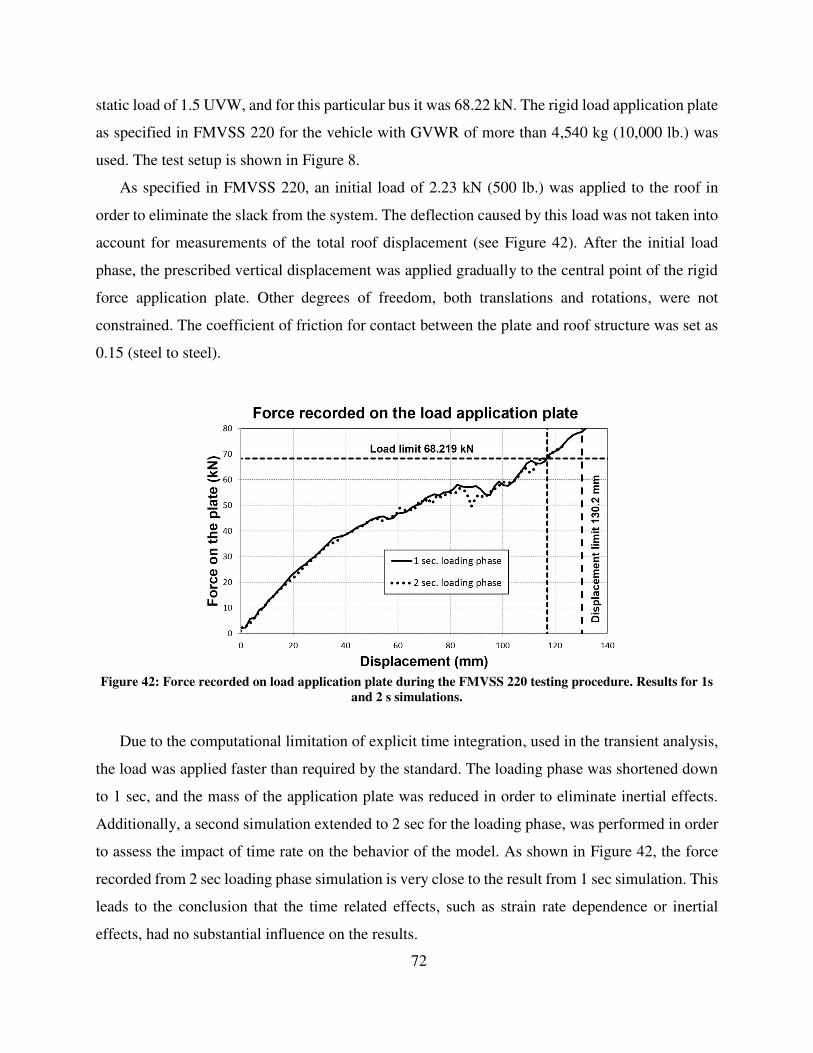
72
static load of 1.5 UVW, and for this particular bus it was 68.22 kN. The rigid load application plate
as specified in FMVSS 220 for the vehicle with GVWR of more than 4,540 kg (10,000 lb.) was
used. The test setup is shown in Figure 8.
As specified in FMVSS 220, an initial load of 2.23 kN (500 lb.) was applied to the roof in
order to eliminate the slack from the system. The deflection caused by this load was not taken into
account for measurements of the total roof displacement (see Figure 42). After the initial load
phase, the prescribed vertical displacement was applied gradually to the central point of the rigid
force application plate. Other degrees of freedom, both translations and rotations, were not
constrained. The coefficient of friction for contact between the plate and roof structure was set as
0.15 (steel to steel).
Figure 42: Force recorded on load application plate during the FMVSS 220 testing procedure. Results for 1s
and 2 s simulations.
Due to the computational limitation of explicit time integration, used in the transient analysis,
the load was applied faster than required by the standard. The loading phase was shortened down
to 1 sec, and the mass of the application plate was reduced in order to eliminate inertial effects.
Additionally, a second simulation extended to 2 sec for the loading phase, was performed in order
to assess the impact of time rate on the behavior of the model. As shown in Figure 42, the force
recorded from 2 sec loading phase simulation is very close to the result from 1 sec simulation. This
leads to the conclusion that the time related effects, such as strain rate dependence or inertial
effects, had no substantial influence on the results.
73
The requirement of emergency exit opening during the test was not addressed in this study.
It can be concluded from the plot in Figure 42, that the bus passed the FMVSS 220 quasi-static
load resistance test of the roof structure. The roof withstood the load of 1.5 UVW without
exceeding the limit value of the deformation. The maximum displacement of the force application
plate was found to be only 118 mm.
Sensitivity Analysis
Bus manufacturers frequently strengthen up the roof structure to pass the FMVSS 220 testing
procedure. The symmetric loading, applied to the roof according to FMVSS 220, is focused mainly
on testing the strength of the roof bows, without applying a meaningful loading on the rest of the
structure. It is still common to find paratransit buses designed with the open cross section wall
columns. In such cases, it is likely that the bus can pass the FMVSS 220 test procedure yet may
perform poorly during a real rollover accident.
The goal of this section is to analyze and rank the significance of individual members of the
structure in the response to the loading experienced in FMVSS 220 and ECE-R66 testing
procedures, applied for the selected bus. The analysis was carried out using LS-OPT 4.1 with
Analysis Of Variance (ANOVA), and Global Sensitivity Analysis (GSA) with Sobol’s approach
(Stander et al., 2008).
Figure 43 shows the passenger compartment frame with ten numbered parts, in no particular
order, selected for the sensitivity analysis. Part thickness was used in the design of experiments
(DOE) study as the design variable. The baseline thickness values for these parts, as well as
assumed lower and upper bounds for the region of interest in the DOE, are listed in Table 22. The
metal sheet thickness is described by discrete gauges. The equivalent metric measurement of the
gauge depends on the material from which the members are built.
The sensitivity was analyzed with respect to the DI for the case of ECE-R66 test. The DI
response in LS-OPT was defined through Equation (1) based on nodal distances in the most
vulnerable cross section of the bus. For the FMVSS 220 test sensitivity was studied with respect
to the resistance force measured from the contact between the rigid plate and the bus roof structure.
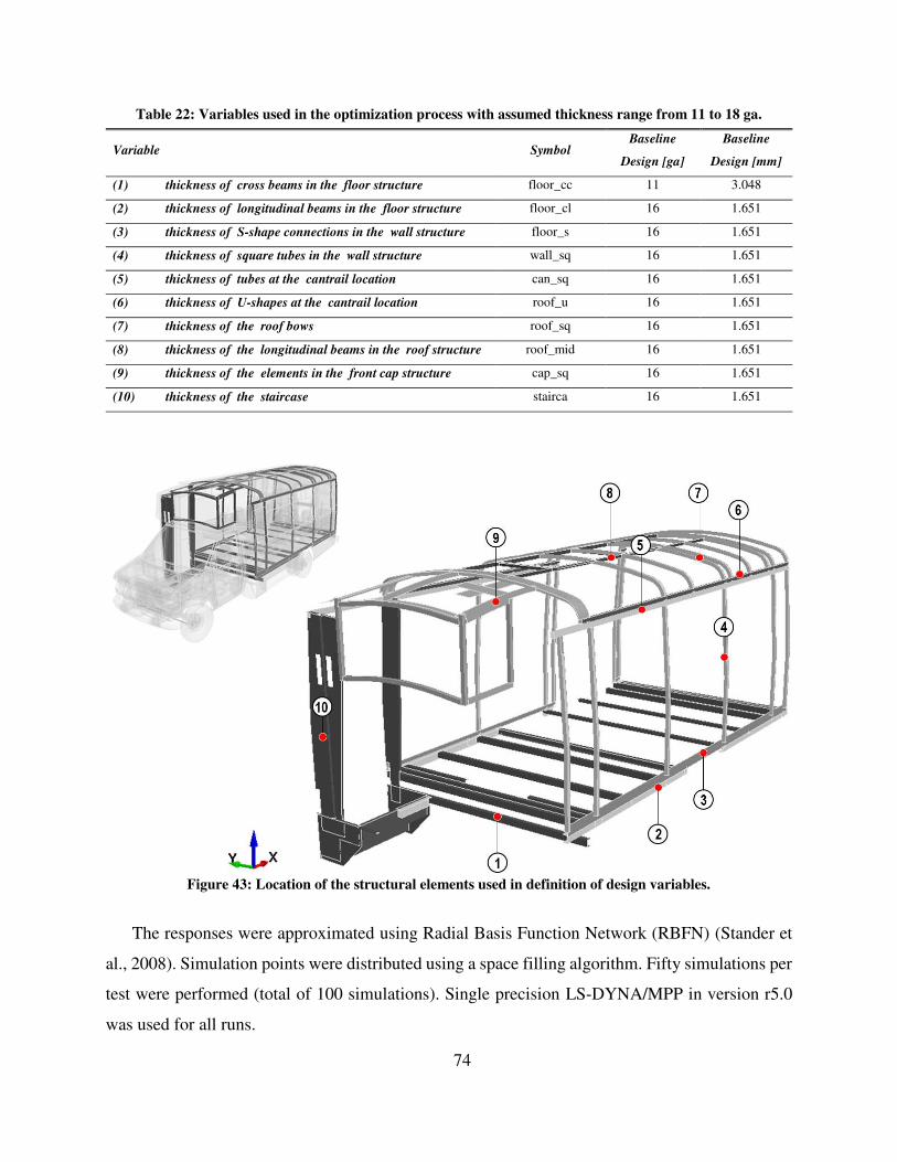
74
Table 22: Variables used in the optimization process with assumed thickness range from 11 to 18 ga.
Figure 43: Location of the structural elements used in definition of design variables.
The responses were approximated using Radial Basis Function Network (RBFN) (Stander et
al., 2008). Simulation points were distributed using a space filling algorithm. Fifty simulations per
test were performed (total of 100 simulations). Single precision LS-DYNA/MPP in version r5.0
was used for all runs.
Variable Symbol Baseline
Design [ga]
Baseline
Design [mm]
(1) thickness of cross beams in the floor structure floor_cc 11 3.048
(2) thickness of longitudinal beams in the floor structure floor_cl 16 1.651
(3) thickness of S-shape connections in the wall structure floor_s 16 1.651
(4) thickness of square tubes in the wall structure wall_sq 16 1.651
(5) thickness of tubes at the cantrail location can_sq 16 1.651
(6) thickness of U-shapes at the cantrail location roof_u 16 1.651
(7) thickness of the roof bows roof_sq 16 1.651
(8) thickness of the longitudinal beams in the roof structure roof_mid 16 1.651
(9) thickness of the elements in the front cap structure cap_sq 16 1.651
(10) thickness of the staircase stairca 16 1.651
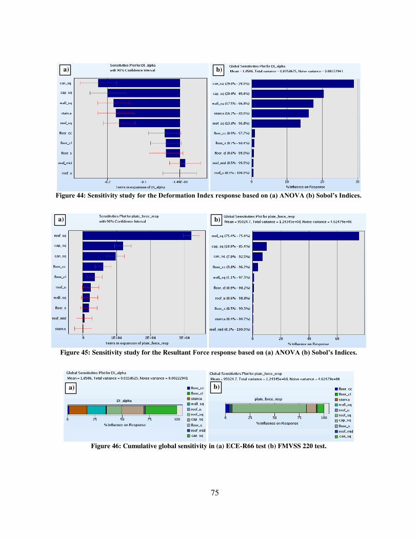
75
Figure 44: Sensitivity study for the Deformation Index response based on (a) ANOVA (b) Sobol’s Indices.
Figure 45: Sensitivity study for the Resultant Force response based on (a) ANOVA (b) Sobol’s Indices.
Figure 46: Cumulative global sensitivity in (a) ECE-R66 test (b) FMVSS 220 test.
a) b)
a) b)
a) b)
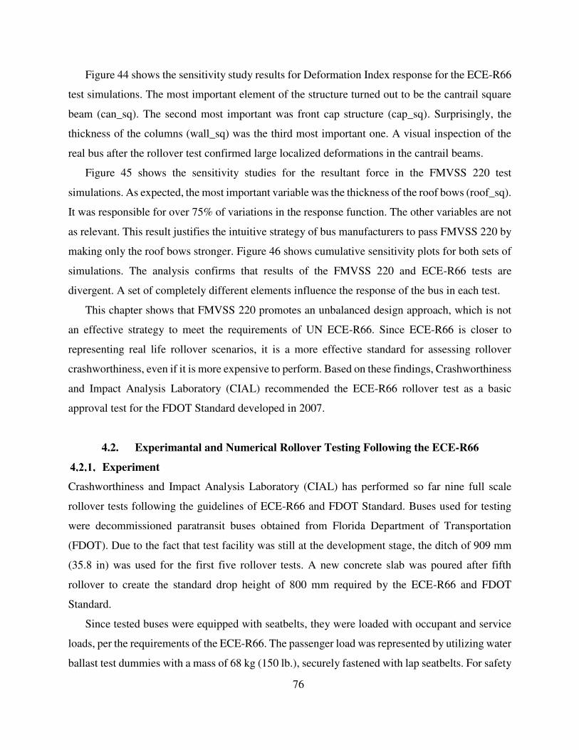
76
Figure 44 shows the sensitivity study results for Deformation Index response for the ECE-R66
test simulations. The most important element of the structure turned out to be the cantrail square
beam (can_sq). The second most important was front cap structure (cap_sq). Surprisingly, the
thickness of the columns (wall_sq) was the third most important one. A visual inspection of the
real bus after the rollover test confirmed large localized deformations in the cantrail beams.
Figure 45 shows the sensitivity studies for the resultant force in the FMVSS 220 test
simulations. As expected, the most important variable was the thickness of the roof bows (roof_sq).
It was responsible for over 75% of variations in the response function. The other variables are not
as relevant. This result justifies the intuitive strategy of bus manufacturers to pass FMVSS 220 by
making only the roof bows stronger. Figure 46 shows cumulative sensitivity plots for both sets of
simulations. The analysis confirms that results of the FMVSS 220 and ECE-R66 tests are
divergent. A set of completely different elements influence the response of the bus in each test.
This chapter shows that FMVSS 220 promotes an unbalanced design approach, which is not
an effective strategy to meet the requirements of UN ECE-R66. Since ECE-R66 is closer to
representing real life rollover scenarios, it is a more effective standard for assessing rollover
crashworthiness, even if it is more expensive to perform. Based on these findings, Crashworthiness
and Impact Analysis Laboratory (CIAL) recommended the ECE-R66 rollover test as a basic
approval test for the FDOT Standard developed in 2007.
4.2. Experimantal and Numerical Rollover Testing Following the ECE-R66
Experiment
Crashworthiness and Impact Analysis Laboratory (CIAL) has performed so far nine full scale
rollover tests following the guidelines of ECE-R66 and FDOT Standard. Buses used for testing
were decommissioned paratransit buses obtained from Florida Department of Transportation
(FDOT). Due to the fact that test facility was still at the development stage, the ditch of 909 mm
(35.8 in) was used for the first five rollover tests. A new concrete slab was poured after fifth
rollover to create the standard drop height of 800 mm required by the ECE-R66 and FDOT
Standard.
Since tested buses were equipped with seatbelts, they were loaded with occupant and service
loads, per the requirements of the ECE-R66. The passenger load was represented by utilizing water
ballast test dummies with a mass of 68 kg (150 lb.), securely fastened with lap seatbelts. For safety
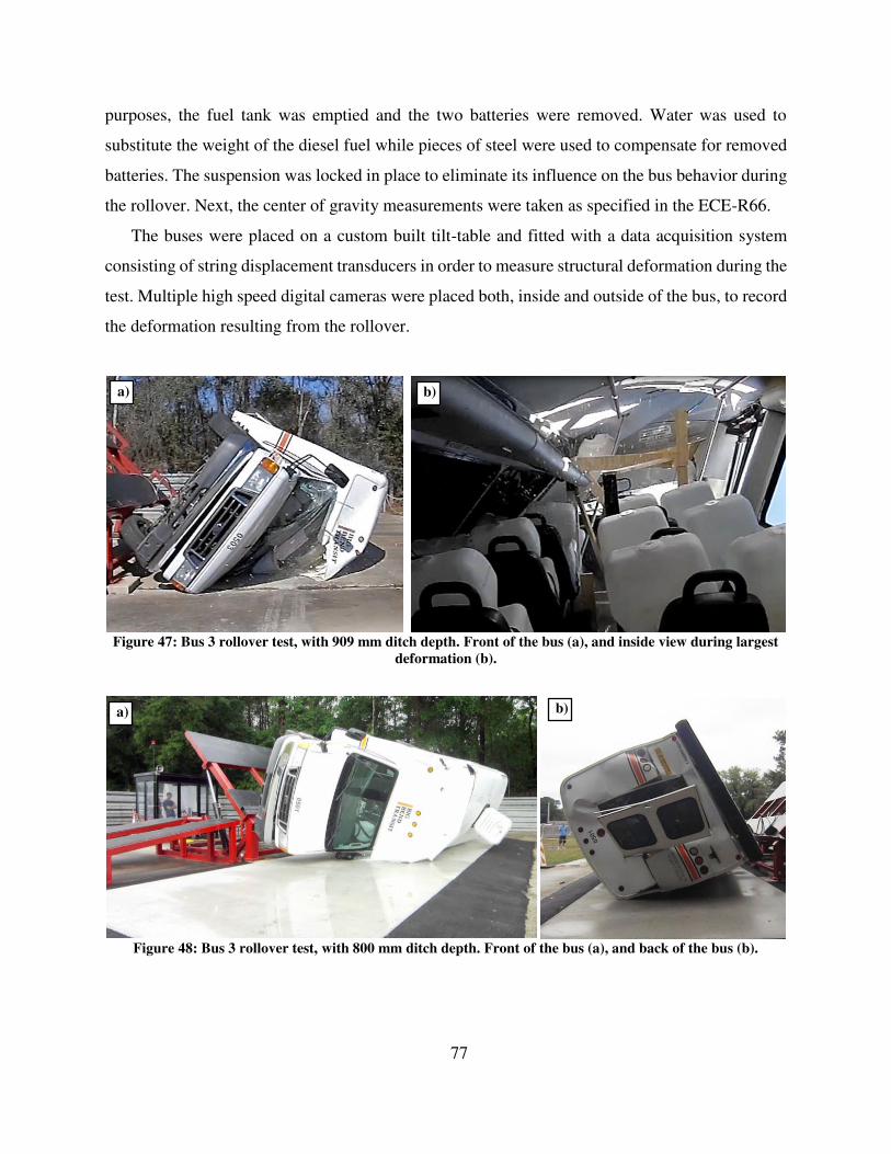
77
purposes, the fuel tank was emptied and the two batteries were removed. Water was used to
substitute the weight of the diesel fuel while pieces of steel were used to compensate for removed
batteries. The suspension was locked in place to eliminate its influence on the bus behavior during
the rollover. Next, the center of gravity measurements were taken as specified in the ECE-R66.
The buses were placed on a custom built tilt-table and fitted with a data acquisition system
consisting of string displacement transducers in order to measure structural deformation during the
test. Multiple high speed digital cameras were placed both, inside and outside of the bus, to record
the deformation resulting from the rollover.
Figure 47: Bus 3 rollover test, with 909 mm ditch depth. Front of the bus (a), and inside view during largest
deformation (b).
Figure 48: Bus 3 rollover test, with 800 mm ditch depth. Front of the bus (a), and back of the bus (b).
a) b)
a) b)
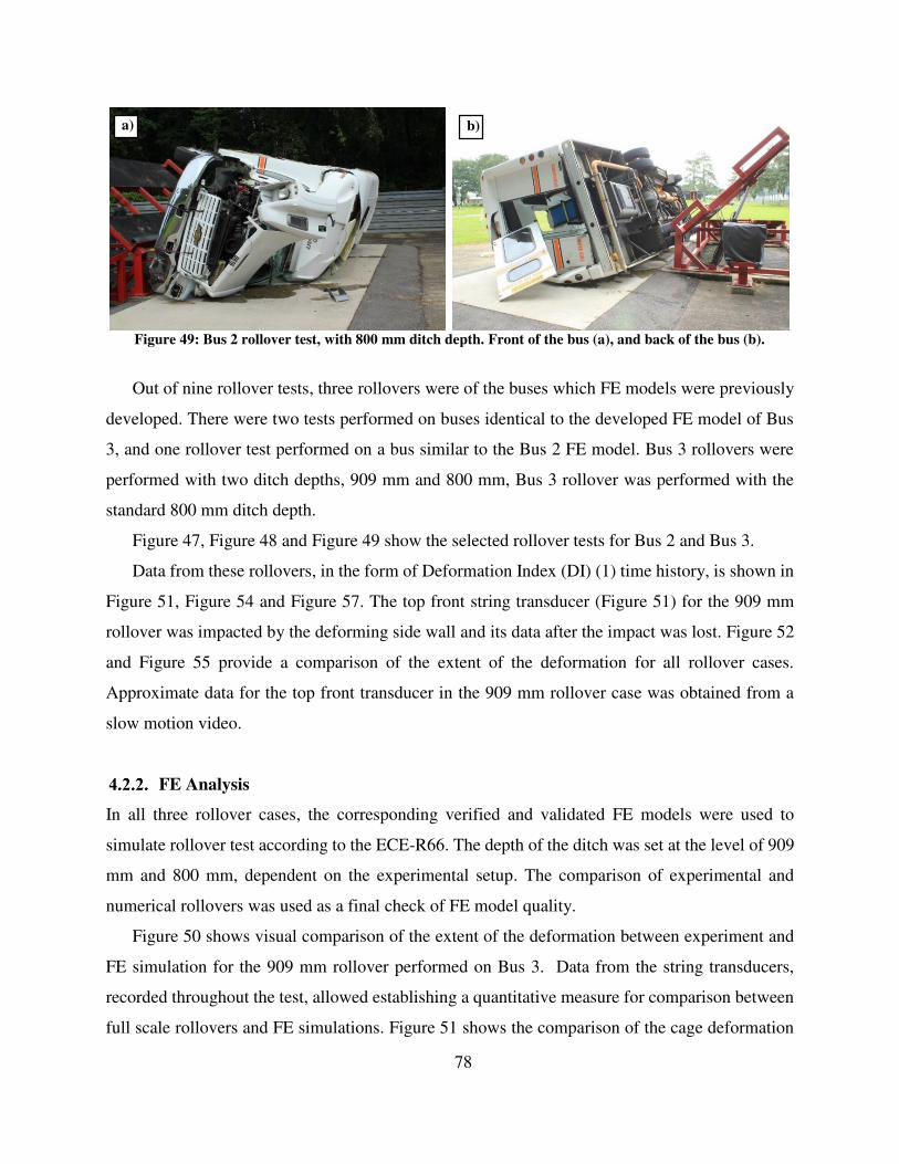
78
Figure 49: Bus 2 rollover test, with 800 mm ditch depth. Front of the bus (a), and back of the bus (b).
Out of nine rollover tests, three rollovers were of the buses which FE models were previously
developed. There were two tests performed on buses identical to the developed FE model of Bus
3, and one rollover test performed on a bus similar to the Bus 2 FE model. Bus 3 rollovers were
performed with two ditch depths, 909 mm and 800 mm, Bus 3 rollover was performed with the
standard 800 mm ditch depth.
Figure 47, Figure 48 and Figure 49 show the selected rollover tests for Bus 2 and Bus 3.
Data from these rollovers, in the form of Deformation Index (DI) (1) time history, is shown in
Figure 51, Figure 54 and Figure 57. The top front string transducer (Figure 51) for the 909 mm
rollover was impacted by the deforming side wall and its data after the impact was lost. Figure 52
and Figure 55 provide a comparison of the extent of the deformation for all rollover cases.
Approximate data for the top front transducer in the 909 mm rollover case was obtained from a
slow motion video.
FE Analysis
In all three rollover cases, the corresponding verified and validated FE models were used to
simulate rollover test according to the ECE-R66. The depth of the ditch was set at the level of 909
mm and 800 mm, dependent on the experimental setup. The comparison of experimental and
numerical rollovers was used as a final check of FE model quality.
Figure 50 shows visual comparison of the extent of the deformation between experiment and
FE simulation for the 909 mm rollover performed on Bus 3. Data from the string transducers,
recorded throughout the test, allowed establishing a quantitative measure for comparison between
full scale rollovers and FE simulations. Figure 51 shows the comparison of the cage deformation
a) b)
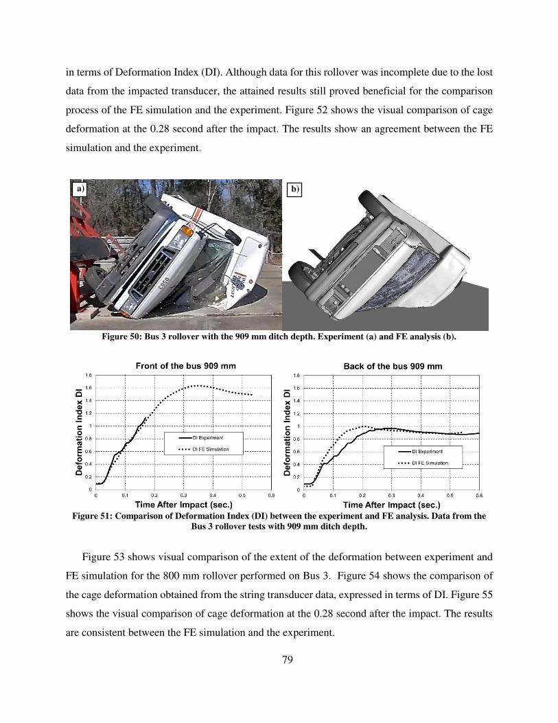
79
in terms of Deformation Index (DI). Although data for this rollover was incomplete due to the lost
data from the impacted transducer, the attained results still proved beneficial for the comparison
process of the FE simulation and the experiment. Figure 52 shows the visual comparison of cage
deformation at the 0.28 second after the impact. The results show an agreement between the FE
simulation and the experiment.
Figure 50: Bus 3 rollover with the 909 mm ditch depth. Experiment (a) and FE analysis (b).
Figure 51: Comparison of Deformation Index (DI) between the experiment and FE analysis. Data from the
Bus 3 rollover tests with 909 mm ditch depth.
Figure 53 shows visual comparison of the extent of the deformation between experiment and
FE simulation for the 800 mm rollover performed on Bus 3. Figure 54 shows the comparison of
the cage deformation obtained from the string transducer data, expressed in terms of DI. Figure 55
shows the visual comparison of cage deformation at the 0.28 second after the impact. The results
are consistent between the FE simulation and the experiment.
a) b)

80
Figure 52: Experimental and FE results for the Bus 3, 909 mm rollover. Cage deformation at t=0.28 s.
Figure 53: Bus 3 rollover with the 800 mm ditch depth. Experiment (a) and FE analysis (b).
Figure 56 shows visual comparison of the extent of the deformation between experiment and
FE simulation for the 800 mm rollover performed on Bus 2. The bus obtained for the experimental
testing was built on a different chassis than the original FE model developed. The FE model of
Bus 2 was based on the Ford Ecoline E450 chassis with 158 in wheelbase, whereas the bus used
in the experimental rollover was built on the Chevrolet GM C4500 chassis with 165.5 in
wheelbase. Even though the two buses were based on different chassis, the passenger cage built
for both of these buses was of the same design. The bus chassis and driver’s cab do not experience
large deformation bus rollover test. It was decided to use existing model, without recreating new
a) b)
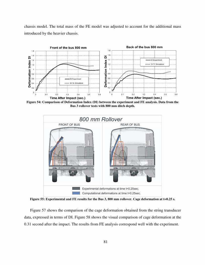
81
chassis model. The total mass of the FE model was adjusted to account for the additional mass
introduced by the heavier chassis.
Figure 54: Comparison of Deformation Index (DI) between the experiment and FE analysis. Data from the
Bus 3 rollover tests with 800 mm ditch depth.
Figure 55: Experimental and FE results for the Bus 3, 800 mm rollover. Cage deformation at t=0.25 s.
Figure 57 shows the comparison of the cage deformation obtained from the string transducer
data, expressed in terms of DI. Figure 58 shows the visual comparison of cage deformation at the
0.31 second after the impact. The results from FE analysis correspond well with the experiment.

82
Figure 56: Bus 2 rollover with the 800 mm ditch depth. Front view - experiment (a) and FE analysis (b), back
view - experiment (c) and FE analysis (d).
Figure 57: Comparison of Deformation Index (DI) between the experiment and FE analysis. Data from the
Bus 2 rollover tests with 800 mm ditch depth.
The results for the front of the bus, in all rollover cases, showed a better agreement between
experiments and FE simulations than the results obtained for the back of the bus. This is because
the behavior of the back wall is highly dependent on brittle failure of local connections between
skin and cage, breaking welds and rivets. It also acts as a shear wall during a rollover, absorbing
large amounts of energy and experiencing weld snap failures. All of these factors contribute to the
complexity of the simulated event.
a) b)
c) d)
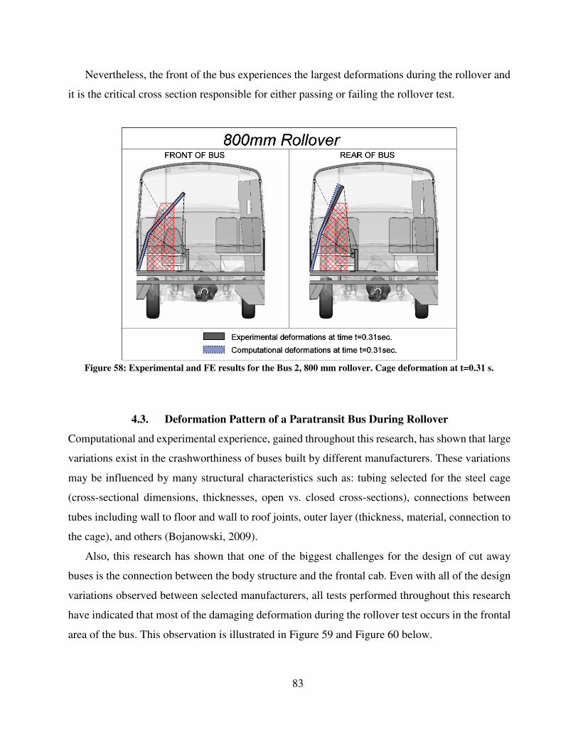
83
Nevertheless, the front of the bus experiences the largest deformations during the rollover and
it is the critical cross section responsible for either passing or failing the rollover test.
Figure 58: Experimental and FE results for the Bus 2, 800 mm rollover. Cage deformation at t=0.31 s.
4.3. Deformation Pattern of a Paratransit Bus During Rollover
Computational and experimental experience, gained throughout this research, has shown that large
variations exist in the crashworthiness of buses built by different manufacturers. These variations
may be influenced by many structural characteristics such as: tubing selected for the steel cage
(cross-sectional dimensions, thicknesses, open vs. closed cross-sections), connections between
tubes including wall to floor and wall to roof joints, outer layer (thickness, material, connection to
the cage), and others (Bojanowski, 2009).
Also, this research has shown that one of the biggest challenges for the design of cut away
buses is the connection between the body structure and the frontal cab. Even with all of the design
variations observed between selected manufacturers, all tests performed throughout this research
have indicated that most of the damaging deformation during the rollover test occurs in the frontal
area of the bus. This observation is illustrated in Figure 59 and Figure 60 below.
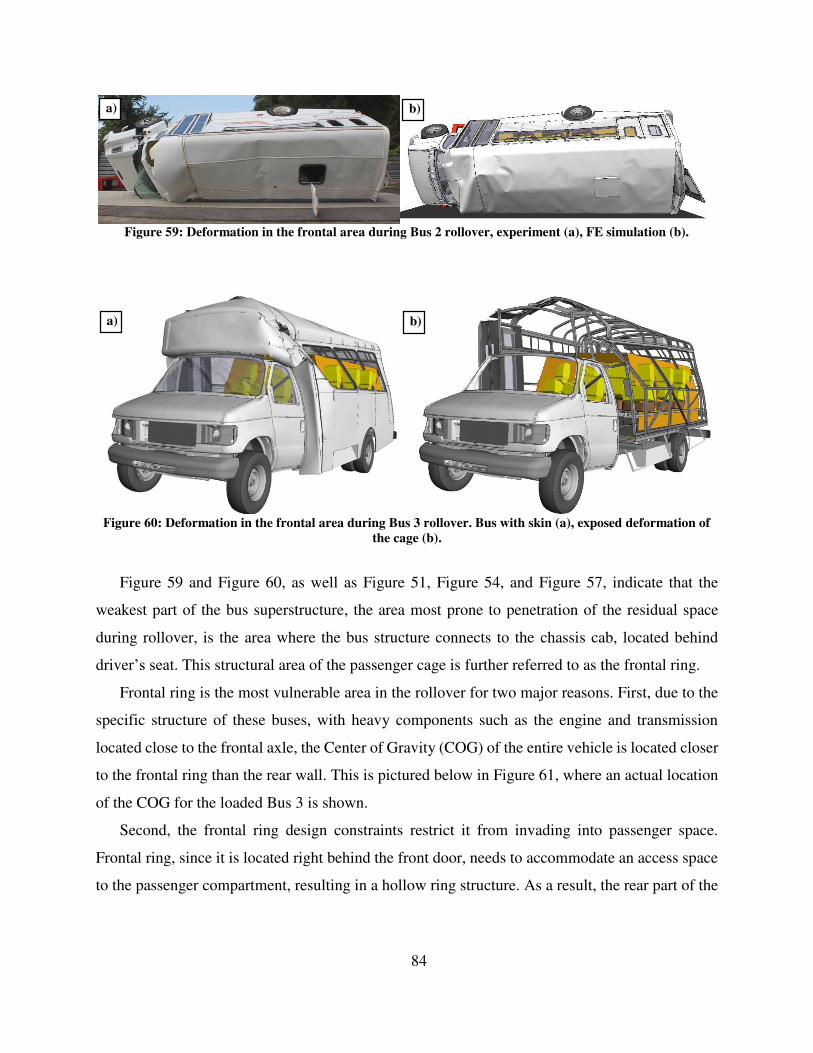
84
Figure 59: Deformation in the frontal area during Bus 2 rollover, experiment (a), FE simulation (b).
Figure 60: Deformation in the frontal area during Bus 3 rollover. Bus with skin (a), exposed deformation of
the cage (b).
Figure 59 and Figure 60, as well as Figure 51, Figure 54, and Figure 57, indicate that the
weakest part of the bus superstructure, the area most prone to penetration of the residual space
during rollover, is the area where the bus structure connects to the chassis cab, located behind
driver’s seat. This structural area of the passenger cage is further referred to as the frontal ring.
Frontal ring is the most vulnerable area in the rollover for two major reasons. First, due to the
specific structure of these buses, with heavy components such as the engine and transmission
located close to the frontal axle, the Center of Gravity (COG) of the entire vehicle is located closer
to the frontal ring than the rear wall. This is pictured below in Figure 61, where an actual location
of the COG for the loaded Bus 3 is shown.
Second, the frontal ring design constraints restrict it from invading into passenger space.
Frontal ring, since it is located right behind the front door, needs to accommodate an access space
to the passenger compartment, resulting in a hollow ring structure. As a result, the rear part of the
a) b)
a) b)
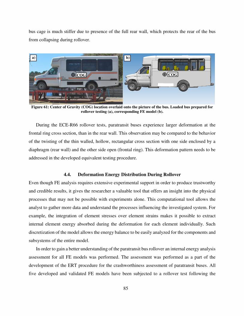
85
bus cage is much stiffer due to presence of the full rear wall, which protects the rear of the bus
from collapsing during rollover.
Figure 61: Center of Gravity (COG) location overlaid onto the picture of the bus. Loaded bus prepared for
rollover testing (a), corresponding FE model (b).
During the ECE-R66 rollover tests, paratransit buses experience larger deformation at the
frontal ring cross section, than in the rear wall. This observation may be compared to the behavior
of the twisting of the thin walled, hollow, rectangular cross section with one side enclosed by a
diaphragm (rear wall) and the other side open (frontal ring). This deformation pattern needs to be
addressed in the developed equivalent testing procedure.
4.4. Deformation Energy Distribution During Rollover
Even though FE analysis requires extensive experimental support in order to produce trustworthy
and credible results, it gives the researcher a valuable tool that offers an insight into the physical
processes that may not be possible with experiments alone. This computational tool allows the
analyst to gather more data and understand the processes influencing the investigated system. For
example, the integration of element stresses over element strains makes it possible to extract
internal element energy absorbed during the deformation for each element individually. Such
discretization of the model allows the energy balance to be easily analyzed for the components and
subsystems of the entire model.
In order to gain a better understanding of the paratransit bus rollover an internal energy analysis
assessment for all FE models was performed. The assessment was performed as a part of the
development of the ERT procedure for the crashworthiness assessment of paratransit buses. All
five developed and validated FE models have been subjected to a rollover test following the
COG COG
a) b)
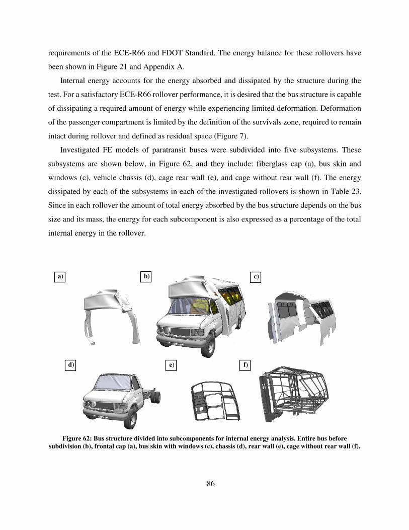
86
requirements of the ECE-R66 and FDOT Standard. The energy balance for these rollovers have
been shown in Figure 21 and Appendix A.
Internal energy accounts for the energy absorbed and dissipated by the structure during the
test. For a satisfactory ECE-R66 rollover performance, it is desired that the bus structure is capable
of dissipating a required amount of energy while experiencing limited deformation. Deformation
of the passenger compartment is limited by the definition of the survivals zone, required to remain
intact during rollover and defined as residual space (Figure 7).
Investigated FE models of paratransit buses were subdivided into five subsystems. These
subsystems are shown below, in Figure 62, and they include: fiberglass cap (a), bus skin and
windows (c), vehicle chassis (d), cage rear wall (e), and cage without rear wall (f). The energy
dissipated by each of the subsystems in each of the investigated rollovers is shown in Table 23.
Since in each rollover the amount of total energy absorbed by the bus structure depends on the bus
size and its mass, the energy for each subcomponent is also expressed as a percentage of the total
internal energy in the rollover.
Figure 62: Bus structure divided into subcomponents for internal energy analysis. Entire bus before
subdivision (b), frontal cap (a), bus skin with windows (c), chassis (d), rear wall (e), cage without rear wall (f).
a) b) c)
d) e) f)

87
The main structural component dissipating most energy during rollover for all buses was the
structural steel cage. The cage and the rear wall accounted for over 55% of internal energy
dissipated within the structure of all investigated buses. Fiberglass frontal cap accounted for
around 10%, whereas the skin accounted for 10% to 20% of internal energy dissipated during
rollover. Vehicle chassis dissipated from 10% to 15% of rollover energy. In all FE models other
components such as seat rails, seats and doors accounted for less than 10% of energy.
Energy distribution shown in Table 23 was used as a theoretical basis and a starting point for
the ERT procedure development summarized in the next chapter of this dissertation
Table 23: Internal energy distribution within the developed bus FE models during ECE-R66 rollover.
Bus 1 Bus 2 Bus 3 Bus 4 Bus 5
Energy
[kJ] [%]
Energy
[kJ] [%]
Energy
[kJ] [%]
Energy
[kJ] [%]
Energy
[kJ] [%]
Fiberglass Cap 4.78 11.8 4.24 8.6 6.21 10.6 13.43 15.0 14.24 14.0
Skin 4.53 11.2 7.04 14.3 11.64 19.9 8.48 9.5 10.08 9.9
Chassis 6.62 16.3 4.54 9.2 4.82 8.3 12.23 13.7 12.48 12.2
Rear wall 7.39 18.2 7.77 15.8 8.22 14.1 13.93 15.6 14.01 13.7
Cage 15.34 37.9 22.9 46.5 22.78 39.0 36.86 41.2 44.71 43.9
Other 1.86 4.6 2.75 5.6 4.7 8.1 4.45 5.0 6.39 6.3
Total 40.51 100.0 49.24 100.0 58.38 100.0 89.38 100.0 101.92 100.0
88
CHAPTER 5
EQUIVALENT ROLLOVER TESTING PROCEDURE
5.1. Introduction
In 2010 the State of Florida purchased over 40 different types of paratransit buses. Purchased buses
ranged in floor/wheelbase/chassis configurations depending on intended use, and came from
multiple different bus manufacturers (CIAL, 2011). This variety of purchased vehicles creates a
difficult situation for safety approval procedure performed by FDOT.
FDOT Standard requires a bus manufacturer to comply with its requirements within two years
from the date the bus was sold to the state. The approval procedure requires for a bus manufacturer
to subject its’ buses to either the full scale rollover test, defined by the standard, or to cooperate
with CIAL in developing the detailed FE model, and test it through the use of computational
mechanics.
Since paratransit bus manufacturers are typically small companies, with the production number
as low as 1000 buses per year, they cannot afford expensive research and development procedures,
observed in the automotive industry. Additionally, these companies offer a wide variety of
available models which further complicates their crashworthiness assessment. In case of the buses
purchased by the state of Florida in 2010, it would require to test 40 different vehicles within two
years, not accounting for buses purchased in 2011 and 2012. This scenario is impossible to fulfill
within the available resources of the FDOT.
An attractive, alternative approval path is established by the use of FE analysis. Unfortunately,
the process of development, validation and verification of FE models for all purchased vehicles is
an overwhelming task for a research institution such as CIAL. It became apparent that the full
scale experimental rollover tests and the process of developing FE model for computer simulations
are too expensive and time consuming to be effectively used in the current situation.
This situation calls for an update of an approval procedure. There is a need for a simplified
assessment tool that will allow reasonably accurate safety evaluation of a given paratransit bus
within reasonable time and budget. A new assessment protocol, which is a topic of this dissertation,
developed for this purpose is further referred to as the Equivalent Rollover Testing (ERT)
procedure.
89
The ERT procedure is conceived as an alternative approval method for the experimental or
virtual full scale testing defined in the previous version of the FDOT Standard (FDOT, 2007). It
is assumed that a safe bus in terms of rollover crashworthiness is a bus that complies with the
requirements of the regulation ECE R66 rollover. This observation forms the basis of the ERT
procedure. A bus structure will be considered to be crashworthy and safe if it passes all required
tests defined in the ERT procedure. It means that with high level of confidence its residual space
(Figure 7) would be neither compromised through intrusion nor by projection during a full scale
rollover test defined in the FDOT Standard (FDOT, 2007).
Based on the accumulated knowledge the components tests defined in the ERT procedure
include:
- Frontal ring test
- Rear wall test
- Wall to floor connection test
- Wall to roof connection test
- Panel impact test
- Static tube testing
- Dynamic tube testing
Each test needs to be defined through a detailed description of the testing procedure,
measurements, and calculations of acceptable pass/fail (Threshold Values) criterion which specify
requirements for passing each test. The testing procedures and the calculation of the test
requirements (Threshold Values) is based on the accumulated experience from experimental
testing and computer simulations conducted thus far at CIAL. The detailed description of the tests
is given in Chapter 5.8.
The ERT procedure is thought out to use relatively simple experimental tests on individual bus
components (defined above) in order to evaluate if the investigated bus will pass the rollover test
defined by the FDOT Standard. The tests are intended to evaluate the rollover crashworthiness of
structural cage built by the bus manufacturer. In order to maintain the simplicity of benchmark
experiments most of them were designed as static push over tests, on the individual components
extracted from the cage structure. Although this approach simplifies final testing procedures it
requires an introduction of several reduction coefficients. The development, and assumption of
necessary reduction coefficients is summarized in the following chapter.

90
5.2. Goals and Expected Benefits
The main goal for development of the ERT procedure is to replace the expensive and time
consuming full-scale tests (actual or virtual) with a set of relatively simple, experimental tests.
Expected benefits to the industry and society include:
increased safety of paratransit buses,
faster evaluation of new buses,
implementation of the ERT procedure by the manufactures.
5.3. General Assumptions
Development of the ERT procedure has been based on the following assumptions:
The bus is considered safe and crashworthy in terms of roof integrity if it satisfies the
requirements of the Regulation ECE-R66 for full scale rollover test.
The ERT procedure is intended to ensure that the evaluated bus will meet requirements of
ECE-R66.
The ERT procedure is designed to reduce cost and time and allows for evaluation without
experimental or numerical full-scale tests.
The ERT procedure is based on experimental component testing and relatively simple
calculations of the pass/fail criterion (Threshold Values).
Safety requirements must be satisfied by the steel cage, regardless how robust are other
nonstructural components, e.g. seats, internal skin etc.
The ERT procedure is addressing the integrity of the entire bus superstructure.
All required tests must be satisfied.
There is no extra credit for successful outcome of the single component test. Very good
performance of some tested components cannot overcome the one that failed.
The ERT procedure test sequence should help to identify weak elements of the bus
structure.
The ERT procedure tests are not intended to and cannot precisely replicate the behavior of
the components during rollover.
ERT procedure tests are develop to help in differentiating good from bad designs.

91
5.4. ERT Procedure Development Summary
This subchapter summarizes the process of the ERT procedure development, further described in
Chaper 5.
The development of the ERT procedure was initiated by introducing the energy concept
summarized in Chapter 5.5. The idea behind the energy concept was to understand the energy
transfer in the paratransit bus structure during the rollover experiment. First, the total energy
delivered to the system was defined. This was done through the analysis of the potential energy
stored in the bus due to its position in the gravitational field at the point of unstable equilibrium,
when compared to its position at the point of maximum deformation.
Next, the amount of the energy dissipated by the entire bus structure during rollover, was
evaluated based on the available literature, past experience and FE rollover analysis performed on
all five available FE models. The conclusion was that only 75% of energy is transferred to the bus
structure. The amount of energy absorbed by the bus structure was defined as Total Reference
Energy.
The assumptions of the ERT procedure state that the safety requirements must be satisfied by
the structural cage, regardless of other nonstructural components. This assumption requires a
division of the Total Reference Energy among the structural cage and other nonstructural elements.
This task was carried out through the analysis of the energy distribution during rollover, observed
in all five available FE models of paratransit buses. It was concluded that reduction coefficients
for fiberglass frontal cap, chassis, rear wall, and skin need to be introduced into the analysis in
order to distribute the energy. The following energy reduction resulted in defining the energy
attributed to the structural cage.
Once the energy attributed to structural cage was established, it was necessary to subdivide it
further into the energies attributed to individual components in order to establish energy threshold
values. Due to the characteristic deformation pattern, observed during the paratransit bus rollover
experiment (Chapter 4.3), the cage was subdivided in a series of rings for the purpose of energy
distribution. Next, a theoretical formula was established in order to distribute the cage energy
among the structural rings. The formula was designed to take into account the critical importance
of the frontal ring structure, deformation pattern, and the differences in the ring design along the
length of the bus.
92
During initial implementation of the ERT procedure it was observed that calculated threshold
values were substantially higher than the energies absorbed by the tested components extracted
from the buses passing the FDOT rollover test. The original ERT procedure was too strict, and
required from the bus components to absorb more energy than necessary. It was identified that
since most of the ERT procedure component tests were thought out as static test on individual
component, they do not fully represent the bus structure during rollover. There is a substantial
difference in the energy absorption when the structure is subjected to the dynamic rollover test,
and compared with the static push over experiment. This characteristic was identified in the
Chapter 5.6 and resulted in introduction of the new reduction coefficient accounting for eliminated
inertial effects.
The ERT procedure is intended to evaluate the rollover crashworthiness of the entire bus from
the series of relatively simple tests on bus components. For this reason, once the rollover energy
was distributed into individual rings, the methodology for the division of the energy within the
ring structure was developed. The energy distribution to individual components within the ring
structure was based on the idea of the plastic chain concept. The plastic chain concept is described
in detail in Chapter 5.7.
The plastic chain concept assumes that the deformation within the individual rings during
rollover is limited to a series of plastic hinges, and the energy assigned to each plastic hinge is
proportional to its deformation. Additionally, three deformation patterns were assumed in order to
cover a wide range of possible deformation scenarios. Finally, based on the summarized
considerations, Chapter 5.8 lists proposed experiments and threshold values to be used in the ERT
procedure.
5.5. Energy Concept
The ERT procedure is based on the concept of energy transfer throughout the rollover test. This
concept is further described in this subchapter. First, the total reference energy is defined as the
total potential energy accumulated in the system. The reference height for the potential energy is
defined as the height difference between the location of the bus Center of Gravity (COG) at the
moment of unstable equilibrium and its location at the moment when the residual space is
compromised by deforming sidewall. The equations necessary to calculate the lowest COG height
are established and presented in this subchapter. Next, based on the experience gathered from the
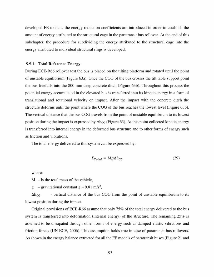
93
developed FE models, the energy reduction coefficients are introduced in order to establish the
amount of energy attributed to the structural cage in the paratransit bus rollover. At the end of this
subchapter, the procedure for subdividing the energy attributed to the structural cage into the
energy attributed to individual structural rings is developed.
Total Reference Energy
During ECE-R66 rollover test the bus is placed on the tilting platform and rotated until the point
of unstable equilibrium (Figure 63a). Once the COG of the bus crosses the tilt table support point
the bus freefalls into the 800 mm deep concrete ditch (Figure 63b). Throughout this process the
potential energy accumulated in the elevated bus is transferred into its kinetic energy in a form of
translational and rotational velocity on impact. After the impact with the concrete ditch the
structure deforms until the point where the COG of the bus reaches the lowest level (Figure 63b).
The vertical distance that the bus COG travels from the point of unstable equilibrium to its lowest
position during the impact is expressed by ΔhCG (Figure 63). At this point collected kinetic energy
is transferred into internal energy in the deformed bus structure and to other forms of energy such
as friction and vibrations.
The total energy delivered to this system can be expressed by:
� = ∆ℎ (29)
where:
M – is the total mass of the vehicle,
g – gravitational constant g = 9.81 m/s2, ∆h - vertical distance of the bus COG from the point of unstable equilibrium to its
lowest position during the impact.
Original provisions of ECE-R66 assume that only 75% of the total energy delivered to the bus
system is transferred into deformation (internal energy) of the structure. The remaining 25% is
assumed to be dissipated through other forms of energy such as damped elastic vibrations and
friction forces (UN ECE, 2006). This assumption holds true in case of paratransit bus rollovers.
As shown in the energy balance extracted for all the FE models of paratransit buses (Figure 21 and

94
Appendix A), the internal energy absorbed by the bus during rollover is very close to the
established 75%. The detailed energy ratios are shown below in Table 24.
Figure 63: Energy transfer during the bus rollover. Bus at the moment of unstable equilibrium (a), bus
during concrete ditch impact, with COG at its lowest position (b).
Table 24: The percentage of total energy absorbed by the bus structure during rollover.
Bus 1 Bus 2 Bus 3 Bus 4 Bus 5 Avg.
Energy
[kJ] [%]
Energy
[kJ] [%]
Energy
[kJ] [%]
Energy
[kJ] [%]
Energy
[kJ] [%] [%]
Total Energy 54.9 79.7 64.3 119.2 135.4
Internal Energy 40.3 73.4 58.3 73.1 49.2 76.6 89.3 74.9 101.8 75.2 74.6
It is assumed that the Total Reference Energy ET estimates the amount of energy hypothetically
absorbed by a bus during a rollover test. It was decided that the level of 75% of energy transfer
upon impact established by the ECE-R66 is applicable for the paratransit bus rollover. Total
Reference Energy (ET) is defined therefore by Equation (30):
= . ∆ℎ (30)
where all variables used were defined before in Equation (29): ∆h is defined as a vertical distance between an elevation of the vehicle COG at its starting,
unstable position and its location at its lowest level during the impact (Figure 63). For the purpose
of establishing Total Reference Energy it is assumed that the maximum deformation of the bus
ΔhCG
COG
COG
a) b)

95
structure occurs at the moment when the residual space is compromised at the frontal ring cross
section (see Figure 64). ∆h is defined as follows:
∆ℎ = ∆ℎ � − .− − (31)
where: ∆h ax – is the vertical distance between the height of the vehicle COG projection onto the
frontal ring plane in its starting, unstable position and at the moment when the residual space is
compromised at the frontal ring cross section (Figure 64),
– is a distance between the front axle and the rear wall of the bus (Figure 64),
– is a distance between the front axle and the frontal ring of the bus (Figure 64),
– is a distance between the front axle and the COG of the bus (Figure 64).
Figure 64: Assumed deformation throughout the length of the bus.
This equation accounts for linear distribution of deformation throughout the length of the bus
(Figure 59 and Figure 60). Since both ECE-R66 and FDOT Standard limit the allowable
deformation during the rollover test to the point when the residual space becomes compromised,
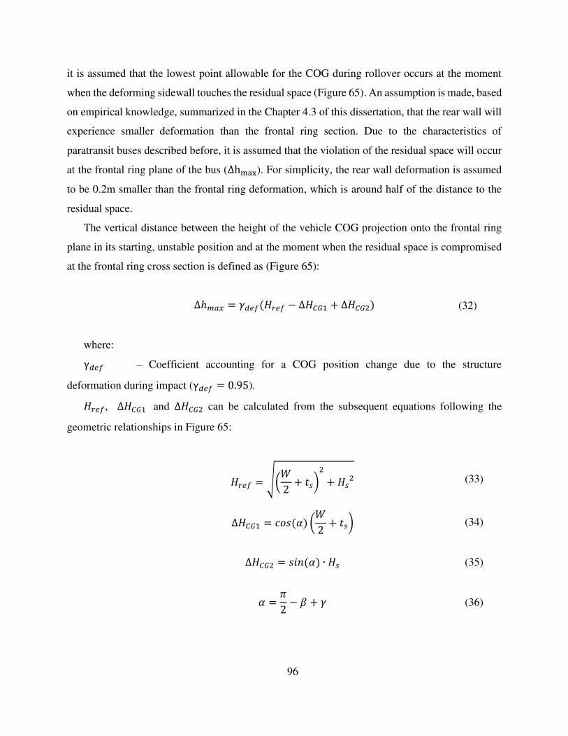
96
it is assumed that the lowest point allowable for the COG during rollover occurs at the moment
when the deforming sidewall touches the residual space (Figure 65). An assumption is made, based
on empirical knowledge, summarized in the Chapter 4.3 of this dissertation, that the rear wall will
experience smaller deformation than the frontal ring section. Due to the characteristics of
paratransit buses described before, it is assumed that the violation of the residual space will occur
at the frontal ring plane of the bus (∆h ax). For simplicity, the rear wall deformation is assumed
to be 0.2m smaller than the frontal ring deformation, which is around half of the distance to the
residual space.
The vertical distance between the height of the vehicle COG projection onto the frontal ring
plane in its starting, unstable position and at the moment when the residual space is compromised
at the frontal ring cross section is defined as (Figure 65):
∆ℎ � = − ∆ + ∆ (32)
where: γ – Coefficient accounting for a COG position change due to the structure
deformation during impact (γ = . ).
, ∆ and ∆ can be calculated from the subsequent equations following the
geometric relationships in Figure 65:
= √( + ) + (33)
∆ = ( + ) (34)
∆ = ∙ (35)
= � − + (36)
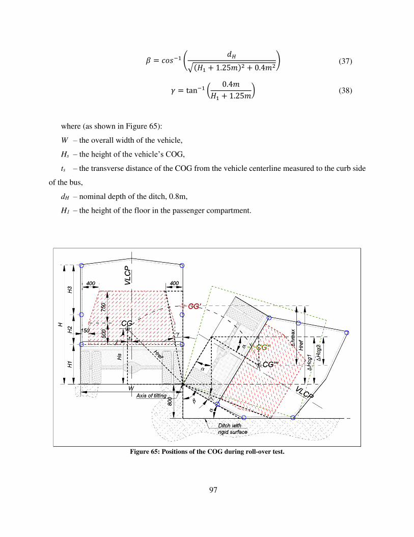
97
= − √ + . + . (37)
= t�n− ( .+ . ) (38)
where (as shown in Figure 65):
W – the overall width of the vehicle,
Hs – the height of the vehicle’s COG,
ts – the transverse distance of the COG from the vehicle centerline measured to the curb side
of the bus,
dH – nominal depth of the ditch, 0.8m,
H1 – the height of the floor in the passenger compartment.
Figure 65: Positions of the COG during roll-over test.
98
The coefficient γ is assumed in Equation (32) based on the computational mechanic studies
performed on all five bus FE models used for rollover. The model presented in Figure 65 assumes
that during the rollover impact the location of the bus COG does not change its location relative to
the bus floor. This assumption would hold true in case if the bus would not experience any
deformation during impact, but this is not true in case of the bus rollover. During the rollover
impact the structure of the bus experiences large deformation (Figure 60), and large portion of its
mass associated with sidewalls, roof, and passenger mass is pushed to one side of the structure.
This results in translation of the COG away from the impacted wall and reduction of ∆ℎ � . This
effect is compensated by the introduction of the γ coefficient.
For paratransit buses the transverse offset of the COG ts will typically be positive due to heavy
doors and a lift placed on the curb side. Following the guidelines of the ECE-R66, it is assumed
that the reference mass of the vehicle M - is equal to the unladen curb mass of the vehicle if there
are no occupant restraints, or, total effective vehicle mass with the mass of passengers when
occupant restraints are fitted. Mass of an individual occupant, is assumed as 75 kg. Since FDOT
requires all of the buses purchased by the state to be equipped with seatbelts, all buses are tested
with the total effective vehicle mass.
Energy Attributed to Structural Cage
Results presented in Table 23 suggest that structural cage (including rear wall) accounts for around
50-60% of energy dissipated by the bus structure during rollover test. This is not a surprising
finding, given the fact that the cage mounted on the vehicle chassis is the principal component
responsible for protecting passengers from the collapsing structure. In the initial stages of the ERT
procedure development, it has been assumed that the safety requirements must be satisfied by the
steel cage, regardless how robust are other nonstructural components. Simply said, a well built bus
must have a proper structural cage designed to withstand the requirements of the ECE-R66 rollover
test.
With the amount of Total Reference Energy ET that is absorbed by the entire bus structure
during rollover, established in the previous chapter, there is a need to establish reduction
coefficients required to evaluate the amount of energy required to be dissipated by the cage alone.
99
Data from the Table 23 is used as an initial indication for the energy distribution within the bus
during rollover test.
Table 23 shows that for all rollover cases for five buses considered, fiberglass front cap
absorbed from 10-15% of internal energy. The bus skin, either sheer metal of fiberglass composite,
was responsible for 10-20%, where the vehicle chassis together with the driver’s cab dissipated
from 10-15% of internal energy.
Fiberglass Front Cap and Bus Chassis Reduction Coefficients
Based on these results (Table 23) it was decided to establish reduction coefficients in order to
reduce Total Reference Energy dissipated by the bus to the energy dissipated by the cage only.
The values assumed for initial analysis were: = . – energy reduction coefficient accounting for the internal energy dissipated
by the frontal fiberglass cap, = . . – energy reduction coefficient accounting for the internal energy dissipated
by the chassis and drivers cab.
Skin Reduction Coefficient
Even though, according to the data presented in Table 23, the skin of the bus accounts only for 10-
20% of the energy dissipated during rollover it is a very important part of the bus structure. A
strong skin, with a good bond to the steel cage, creates a composite effect, where the additional
layer of skin changes the moment of inertia of considered cross section, and protects the tube from
developing a plastic hinge. A strong skin, well connected with the cage, allows also to transfer
energy between different cross sections of the bus, distributing it more evenly throughout the
structure and protecting the bus from a sudden collapse through the failure of a single cross section.
This might not be the case for a weak skin structure, or insufficient connection of skin layer with
the structural cage.
A study of the skin influence onto the rollover performance of the paratransit bus was
performed previously in (Bojanowski, 2009). The finding was that, even though skin accounted
for around 10% of internal energy dissipation, its contribution to limiting the deformation was
substantial. Comparing buses during rollover, with and without skin, has shown that the resultant
deformation has increased by 89.8% for the case of the bus without skin.

100
For these reasons it has been decided that it is necessary for the skin reduction coefficient to
be based on experiments, rather than on the pre-formulated fixed coefficients. This requirement
has violated one of the original assumptions of ERT procedure, that all of the pass/fail criteria
(Threshold Values) should be calculated without any experimental tests. Nevertheless, it has been
found that a pre-test evaluating skin reduction coefficient is necessary in order to cover a wide
range of skin designs observed throughout paratransit bus manufacturers.
Existing experimental setup was used to evaluate quality of the skin and its connection to the
bus frame. Sidewall panel impact test, described in Chapter 3.8.7, was chosen as the most
applicable test. The idea behind evaluating the skin reduction coefficient is to compare two panel
impact tests, both of the performed with the same impact energy of 1.5 kJ, one conducted on the
panel with skin and one conducted on the panel without skin. Since one of the assumptions of the
ERT procedure was that the crashworthiness of the bus should be evaluated based on its structural
cage, it was decided to limit the skin reduction coefficient to the maximum value of 0.3.
Skin reduction coefficient � can be calculated following the given equation:
� = ∆ . − ∆ .∆ . . (39)
where: ∆ . – is the experimentally determined permanent deformation angle of a
sidewall panel with skin resulting from the panel impact with the energy of 1.5 kJ, ∆ . – is the experimentally determined permanent deformation angle of a
sidewall panel without skin resulting from the panel impact with the energy of 1.5 kJ.
Rear Wall Reduction Coefficient
Table 23 shows that the energy absorbed by the rear wall structure during rollover test varies from
10% to 20%. An interesting observation has been made that the percentage of energy dissipated
by the rear wall is inversely proportional to the bus size. For a small bus (Bus 1) with a wheelbase
of 138 in the energy dissipated by the rear wall accounted for 18.2%, and for the large bus (Bus 5)
with the wheelbase of 255 in it accounted for only 13.7%.
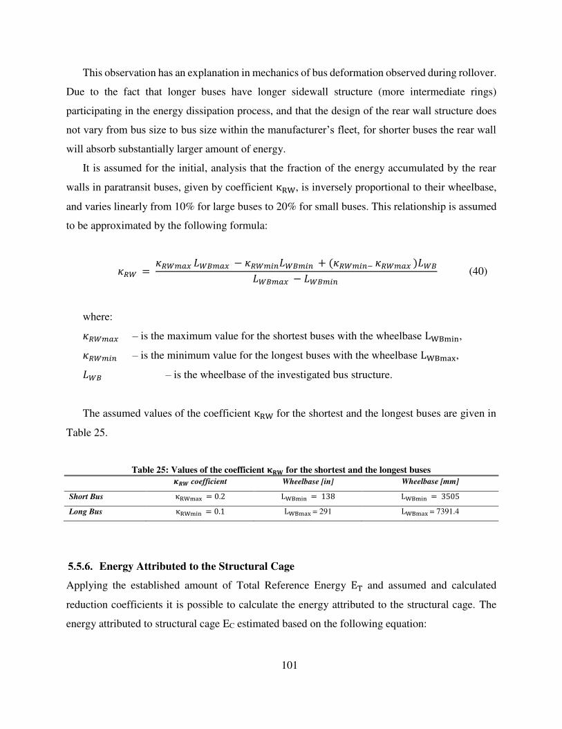
101
This observation has an explanation in mechanics of bus deformation observed during rollover.
Due to the fact that longer buses have longer sidewall structure (more intermediate rings)
participating in the energy dissipation process, and that the design of the rear wall structure does
not vary from bus size to bus size within the manufacturer’s fleet, for shorter buses the rear wall
will absorb substantially larger amount of energy.
It is assumed for the initial, analysis that the fraction of the energy accumulated by the rear
walls in paratransit buses, given by coefficient κRW, is inversely proportional to their wheelbase,
and varies linearly from 10% for large buses to 20% for small buses. This relationship is assumed
to be approximated by the following formula:
= � � − + − � � − (40)
where: � – is the maximum value for the shortest buses with the wheelbase LW , – is the minimum value for the longest buses with the wheelbase LW ax,
– is the wheelbase of the investigated bus structure.
The assumed values of the coefficient κRW for the shortest and the longest buses are given in
Table 25.
Table 25: Values of the coefficient ��� for the shortest and the longest buses
� coefficient Wheelbase [in] Wheelbase [mm]
Short Bus κRW ax = . LW = LW =
Long Bus κRW = . LW ax = 291 LW ax = 7391.4
Energy Attributed to the Structural Cage
Applying the established amount of Total Reference Energy ET and assumed and calculated
reduction coefficients it is possible to calculate the energy attributed to the structural cage. The
energy attributed to structural cage EC estimated based on the following equation:
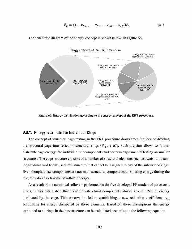
102
= − � − − − (41)
The schematic diagram of the energy concept is shown below, in Figure 66.
Figure 66: Energy distribution according to the energy concept of the ERT procedure.
Energy Attributed to Individual Rings
The concept of structural cage testing in the ERT procedure draws from the idea of dividing
the structural cage into series of structural rings (Figure 67). Such division allows to further
distribute cage energy into individual subcomponents and perform experimental testing on smaller
structures. The cage structure consists of a number of structural elements such as; waistrail beam,
longitudinal roof beams, seat rail structure that cannot be assigned to any of the subdivided rings.
Even though, these components are not main structural components dissipating energy during the
test, they do absorb some of rollover energy.
As a result of the numerical rollovers performed on the five developed FE models of paratransit
buses, it was established that these non-structural components absorb around 15% of energy
dissipated by the cage. This observation led to establishing a new reduction coefficient κNR
accounting for energy dissipated by these elements. Based on these assumptions the energy
attributed to all rings in the bus structure can be calculated according to the following equation:
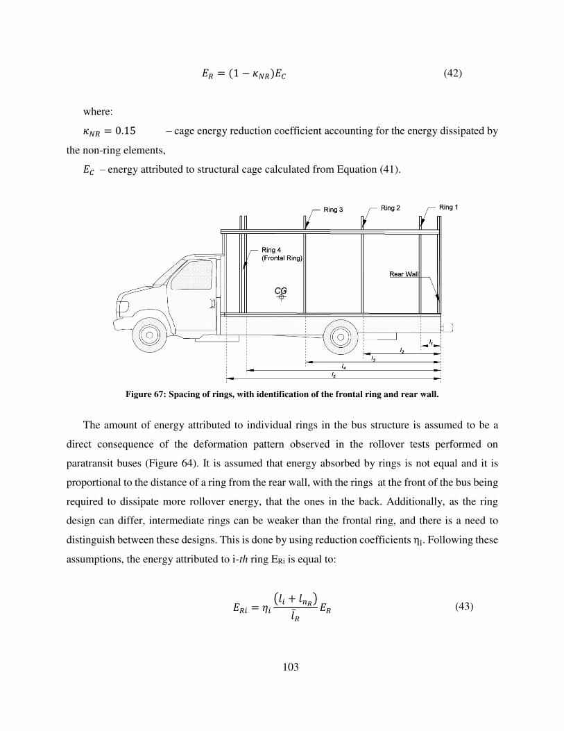
103
= − (42)
where: = . – cage energy reduction coefficient accounting for the energy dissipated by
the non-ring elements,
– energy attributed to structural cage calculated from Equation (41).
Figure 67: Spacing of rings, with identification of the frontal ring and rear wall.
The amount of energy attributed to individual rings in the bus structure is assumed to be a
direct consequence of the deformation pattern observed in the rollover tests performed on
paratransit buses (Figure 64). It is assumed that energy absorbed by rings is not equal and it is
proportional to the distance of a ring from the rear wall, with the rings at the front of the bus being
required to dissipate more rollover energy, that the ones in the back. Additionally, as the ring
design can differ, intermediate rings can be weaker than the frontal ring, and there is a need to
distinguish between these designs. This is done by using reduction coefficients η . Following these
assumptions, the energy attributed to i-th ring ERi is equal to:
= � ( + �) (43)
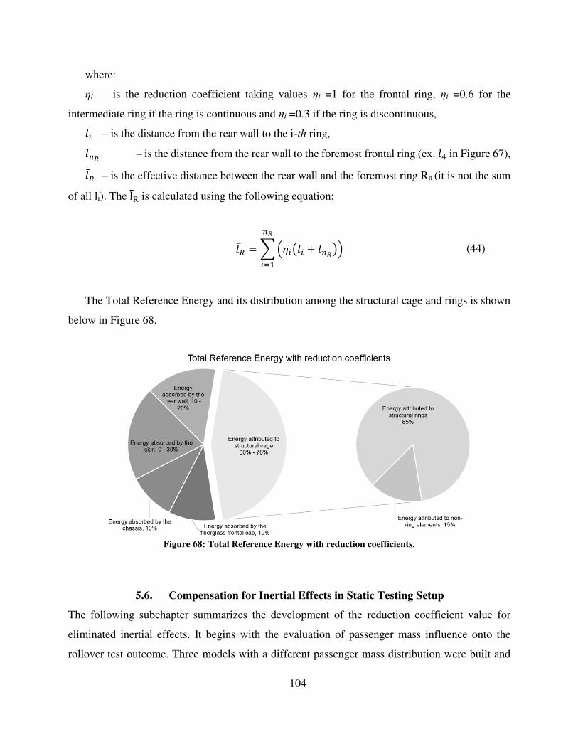
104
where:
ηi – is the reduction coefficient taking values ηi =1 for the frontal ring, ηi =0.6 for the
intermediate ring if the ring is continuous and ηi =0.3 if the ring is discontinuous,
– is the distance from the rear wall to the i-th ring,
� – is the distance from the rear wall to the foremost frontal ring (ex. in Figure 67), – is the effective distance between the rear wall and the foremost ring Rn (it is not the sum
of all li). The lR is calculated using the following equation:
= ∑ � ( + �)�= (44)
The Total Reference Energy and its distribution among the structural cage and rings is shown
below in Figure 68.
Figure 68: Total Reference Energy with reduction coefficients.
5.6. Compensation for Inertial Effects in Static Testing Setup
The following subchapter summarizes the development of the reduction coefficient value for
eliminated inertial effects. It begins with the evaluation of passenger mass influence onto the
rollover test outcome. Three models with a different passenger mass distribution were built and

105
analyzed. Diverging outcomes for three considered cases are shown and discussed. Next, a
comparison between a rollover and a static push over test is performed, and used as a basis for the
formulation of the reduction coefficient.
As described in the previous chapter the ERT procedure is based on the idea of energy transfer
throughout the rollover test. During the experiment, the tested bus starts to freefall from the tilting
platform at the point of unstable equilibrium (Figure 6b), transferring gathered potential energy
into kinetic energy until the moment of impact.
Let us consider a simplified model of a bus structure during a rigid wall impact. The model is
shown in Figure 69a. A deforming, energy absorbing bus structure is presented here as a
combination of a spring (k1) and a damper (c1). Spring represents an elastic component of the
deformation upon impact such as elastic strain in the structural cage, whereas the damper
represents the plastic component of the deformation including plastic deformation, crack
development and propagation, failing welds and rivets, friction, and damped vibrations.
In the case of ECE-Regulation 66 bus rollover, as shown in Figure 70, the kinetic energy is
absorbed mainly by a plastic component (damper), whereas the energy absorbed by the elastic
component (spring) is substantially smaller.
A model presented in Figure 69a, assumes that all of the mass, distributed within the bus is
rigidly connected to the deforming structure, and there is no internal energy dissipation. This is
not true in case of the full scale paratransit bus rollover.
Figure 69: Simplified model of a bus structure during a rigid wall impact, a) Spring-damper model without
internal energy dissipation, b) Spring-damper model with internal energy dissipation.
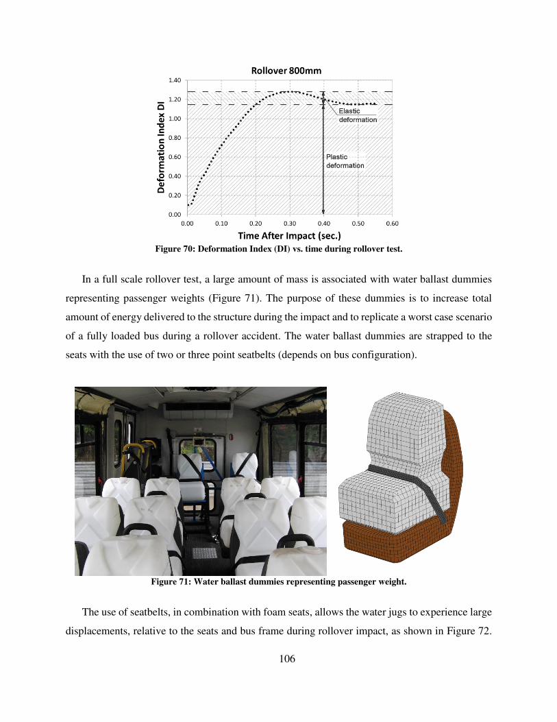
106
Figure 70: Deformation Index (DI) vs. time during rollover test.
In a full scale rollover test, a large amount of mass is associated with water ballast dummies
representing passenger weights (Figure 71). The purpose of these dummies is to increase total
amount of energy delivered to the structure during the impact and to replicate a worst case scenario
of a fully loaded bus during a rollover accident. The water ballast dummies are strapped to the
seats with the use of two or three point seatbelts (depends on bus configuration).
Figure 71: Water ballast dummies representing passenger weight.
The use of seatbelts, in combination with foam seats, allows the water jugs to experience large
displacements, relative to the seats and bus frame during rollover impact, as shown in Figure 72.

107
This mechanism acts like an internal damper (c2), spring (k2) configuration, as presented in Figure
69b. In this case, the damper (c2) dissipates a part of total energy delivered to the bus during the
impact, without contributing to the global deformation of its structure.
Figure 72: Large displacement of water ballast dummies relative to the seats during rollover test.
Another important factor in the mechanics of bus rollover, differentiating it from the static ring
based component tests, is the mass distribution of passenger weights during the impact. As shown
in Figure 73a, passenger mass and seats (m) are connected to the sidewall by the seat mounting
rail. During rollover test, this setup generates an additional inertial force (Fm). This results in a
modified bending moment in the wall to floor (MWFS) and wall to roof (MWRS) connection. As a
result, the bending moment diagram within the sidewall column is different than the one obtained
during ring based static experiment (Figure 73b).
Dependent on the stiffness of selected bus cage components and percentage of total mass
associated with the mass of passengers, this configuration may lead to the failure at the waistrail
location, instead of the failure of wall to floor connection (Figure 60b). It needs to be noted, that
the bending moment diagrams (Figure 73) are simplified and presented here only for visualization
purposes. The actual distribution of moments will vary with time during the impact and will
change with the development of plastic hinges throughout the cross section of the ring.

108
Figure 73: Inertial forces and bending moment diagrams in a) rollover test, b) ring based static experiment.
Even though dynamic rollover test and static ring based experimental tests are not directly
comparable, there is a correlation between them that can be quantified. Both of the effects
described above require introduction of additional reduction coefficients in order to maintain the
concept of energy transfer.
In order to evaluate the effect of these factors, a reduced, generic Finite Element model of the
bus has been created (Figure 74a). The simplified model includes all of the major components of
the original bus cage structure, such as: back wall, frontal ring, intermediate rings and skin. The
nonessential structural components that do not participate in overall rollover crashworthiness of
the bus, such as: side wall bracing, roof bracing, and window frames have been excluded from the
model in order to reduce calculation time and simplify overall analysis.
Figure 74: Generic model of a paratransit bus passenger compartment prepared for rollover testing, a) Cage
#1, b) Cage #2, c) Cage #3.
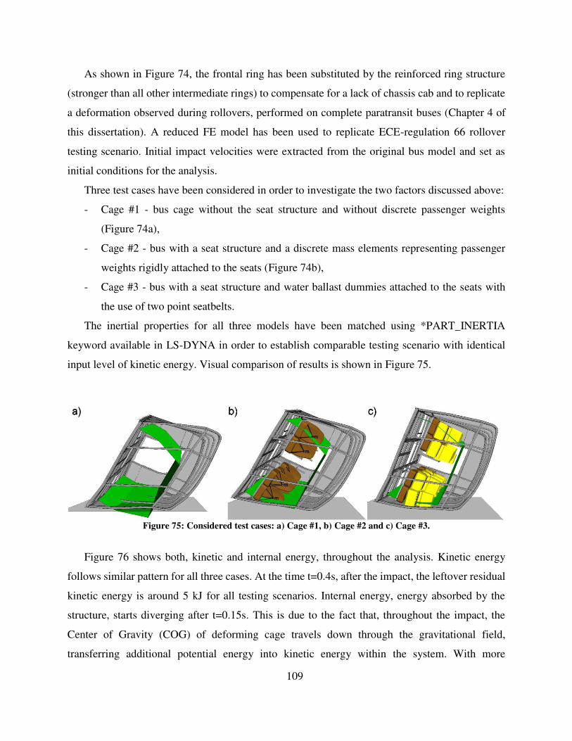
109
As shown in Figure 74, the frontal ring has been substituted by the reinforced ring structure
(stronger than all other intermediate rings) to compensate for a lack of chassis cab and to replicate
a deformation observed during rollovers, performed on complete paratransit buses (Chapter 4 of
this dissertation). A reduced FE model has been used to replicate ECE-regulation 66 rollover
testing scenario. Initial impact velocities were extracted from the original bus model and set as
initial conditions for the analysis.
Three test cases have been considered in order to investigate the two factors discussed above:
- Cage #1 - bus cage without the seat structure and without discrete passenger weights
(Figure 74a),
- Cage #2 - bus with a seat structure and a discrete mass elements representing passenger
weights rigidly attached to the seats (Figure 74b),
- Cage #3 - bus with a seat structure and water ballast dummies attached to the seats with
the use of two point seatbelts.
The inertial properties for all three models have been matched using *PART_INERTIA
keyword available in LS-DYNA in order to establish comparable testing scenario with identical
input level of kinetic energy. Visual comparison of results is shown in Figure 75.
Figure 75: Considered test cases: a) Cage #1, b) Cage #2 and c) Cage #3.
Figure 76 shows both, kinetic and internal energy, throughout the analysis. Kinetic energy
follows similar pattern for all three cases. At the time t=0.4s, after the impact, the leftover residual
kinetic energy is around 5 kJ for all testing scenarios. Internal energy, energy absorbed by the
structure, starts diverging after t=0.15s. This is due to the fact that, throughout the impact, the
Center of Gravity (COG) of deforming cage travels down through the gravitational field,
transferring additional potential energy into kinetic energy within the system. With more
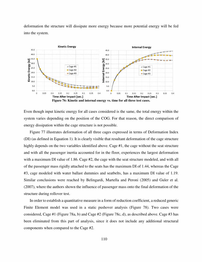
110
deformation the structure will dissipate more energy because more potential energy will be fed
into the system.
Figure 76: Kinetic and internal energy vs. time for all three test cases.
Even though input kinetic energy for all cases considered is the same, the total energy within the
system varies depending on the position of the COG. For that reason, the direct comparison of
energy dissipation within the cage structure is not possible.
Figure 77 illustrates deformation of all three cages expressed in terms of Deformation Index
(DI) (as defined in Equation 1). It is clearly visible that resultant deformation of the cage structure
highly depends on the two variables identified above. Cage #1, the cage without the seat structure
and with all the passenger inertia accounted for in the floor, experiences the largest deformation
with a maximum DI value of 1.86. Cage #2, the cage with the seat structure modeled, and with all
of the passenger mass rigidly attached to the seats has the maximum DI of 1.44, whereas the Cage
#3, cage modeled with water ballast dummies and seatbelts, has a maximum DI value of 1.19.
Similar conclusions were reached by Belingardi, Martella and Peroni (2005) and Guler et al.
(2007), where the authors shown the influence of passenger mass onto the final deformation of the
structure during rollover test.
In order to establish a quantitative measure in a form of reduction coefficient, a reduced generic
Finite Element model was used in a static pushover analysis (Figure 78). Two cases were
considered, Cage #1 (Figure 78a, b) and Cage #2 (Figure 78c, d), as described above. Cage #3 has
been eliminated from this part of analysis, since it does not include any additional structural
components when compared to the Cage #2.
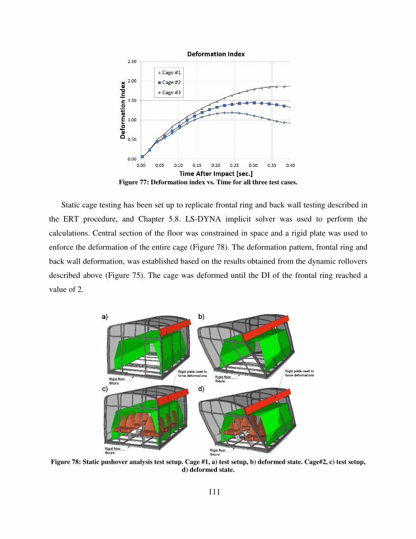
111
Figure 77: Deformation index vs. Time for all three test cases.
Static cage testing has been set up to replicate frontal ring and back wall testing described in
the ERT procedure, and Chapter 5.8. LS-DYNA implicit solver was used to perform the
calculations. Central section of the floor was constrained in space and a rigid plate was used to
enforce the deformation of the entire cage (Figure 78). The deformation pattern, frontal ring and
back wall deformation, was established based on the results obtained from the dynamic rollovers
described above (Figure 75). The cage was deformed until the DI of the frontal ring reached a
value of 2.
Figure 78: Static pushover analysis test setup. Cage #1, a) test setup, b) deformed state. Cage#2, c) test setup,
d) deformed state.
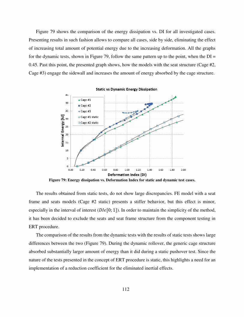
112
Figure 79 shows the comparison of the energy dissipation vs. DI for all investigated cases.
Presenting results in such fashion allows to compare all cases, side by side, eliminating the effect
of increasing total amount of potential energy due to the increasing deformation. All the graphs
for the dynamic tests, shown in Figure 79, follow the same pattern up to the point, when the DI =
0.45. Past this point, the presented graph shows, how the models with the seat structure (Cage #2,
Cage #3) engage the sidewall and increases the amount of energy absorbed by the cage structure.
Figure 79: Energy dissipation vs. Deformation Index for static and dynamic test cases.
The results obtained from static tests, do not show large discrepancies. FE model with a seat
frame and seats models (Cage #2 static) presents a stiffer behavior, but this effect is minor,
especially in the interval of interest ( �[ ; ]). In order to maintain the simplicity of the method,
it has been decided to exclude the seats and seat frame structure from the component testing in
ERT procedure.
The comparison of the results from the dynamic tests with the results of static tests shows large
differences between the two (Figure 79). During the dynamic rollover, the generic cage structure
absorbed substantially larger amount of energy than it did during a static pushover test. Since the
nature of the tests presented in the concept of ERT procedure is static, this highlights a need for an
implementation of a reduction coefficient for the eliminated inertial effects.

113
In order to estimate reduction coefficient for eliminated inertial effects κ , a ratio of
absorbed energy obtained for dynamic rollover test and static push over test, was used. The Cage
#3 was selected as a representative case for a dynamic rollover test, since it contains the most parts
found in the complete bus. Cage #1 was selected as a representative case for ERT procedure
testing. Using results obtained before:
κ = � # − � # �� # = . − .. = . (45)
From above we assume a reduction coefficient for eliminated inertial effects κ = .
5.7. Plastic Chain Concept
The following subchapter summarizes the development and implementation of the plastic chain
concept, used to distribute the internal energy within the structural rings.
Paratransit bus manufacturers often use steel tubing with a slender cross sections in order to
meet the restrictive vehicle weight requirements. Because of this, the deformation of the cage
during rollover test occurs through the development of localized plastic hinges. A plastic hinge
develops due to a local buckling of the material within the steel member and results in lost stability
and large deformations. An example of the plastic hinge developed in the bus during rollover is
shown in Figure 80.
Figure 80: Plastic hinge developed in the bus during rollover.
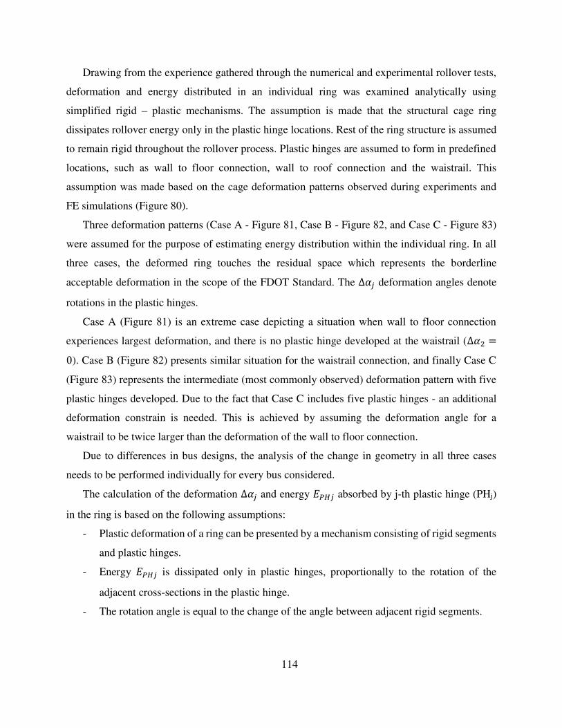
114
Drawing from the experience gathered through the numerical and experimental rollover tests,
deformation and energy distributed in an individual ring was examined analytically using
simplified rigid – plastic mechanisms. The assumption is made that the structural cage ring
dissipates rollover energy only in the plastic hinge locations. Rest of the ring structure is assumed
to remain rigid throughout the rollover process. Plastic hinges are assumed to form in predefined
locations, such as wall to floor connection, wall to roof connection and the waistrail. This
assumption was made based on the cage deformation patterns observed during experiments and
FE simulations (Figure 80).
Three deformation patterns (Case A - Figure 81, Case B - Figure 82, and Case C - Figure 83)
were assumed for the purpose of estimating energy distribution within the individual ring. In all
three cases, the deformed ring touches the residual space which represents the borderline
acceptable deformation in the scope of the FDOT Standard. The ∆ deformation angles denote
rotations in the plastic hinges.
Case A (Figure 81) is an extreme case depicting a situation when wall to floor connection
experiences largest deformation, and there is no plastic hinge developed at the waistrail (∆ =). Case B (Figure 82) presents similar situation for the waistrail connection, and finally Case C
(Figure 83) represents the intermediate (most commonly observed) deformation pattern with five
plastic hinges developed. Due to the fact that Case C includes five plastic hinges - an additional
deformation constrain is needed. This is achieved by assuming the deformation angle for a
waistrail to be twice larger than the deformation of the wall to floor connection.
Due to differences in bus designs, the analysis of the change in geometry in all three cases
needs to be performed individually for every bus considered.
The calculation of the deformation ∆ and energy absorbed by j-th plastic hinge (PHj)
in the ring is based on the following assumptions:
- Plastic deformation of a ring can be presented by a mechanism consisting of rigid segments
and plastic hinges.
- Energy is dissipated only in plastic hinges, proportionally to the rotation of the
adjacent cross-sections in the plastic hinge.
- The rotation angle is equal to the change of the angle between adjacent rigid segments.
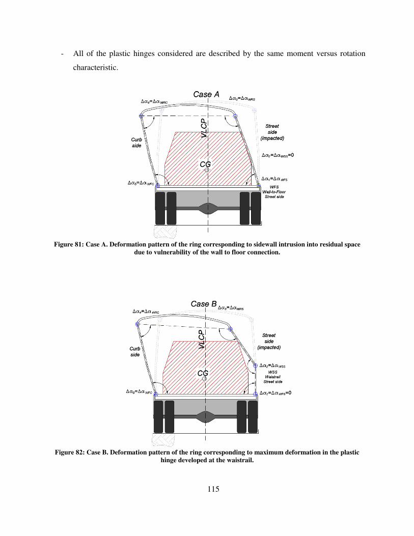
115
- All of the plastic hinges considered are described by the same moment versus rotation
characteristic.
Figure 81: Case A. Deformation pattern of the ring corresponding to sidewall intrusion into residual space
due to vulnerability of the wall to floor connection.
Figure 82: Case B. Deformation pattern of the ring corresponding to maximum deformation in the plastic
hinge developed at the waistrail.
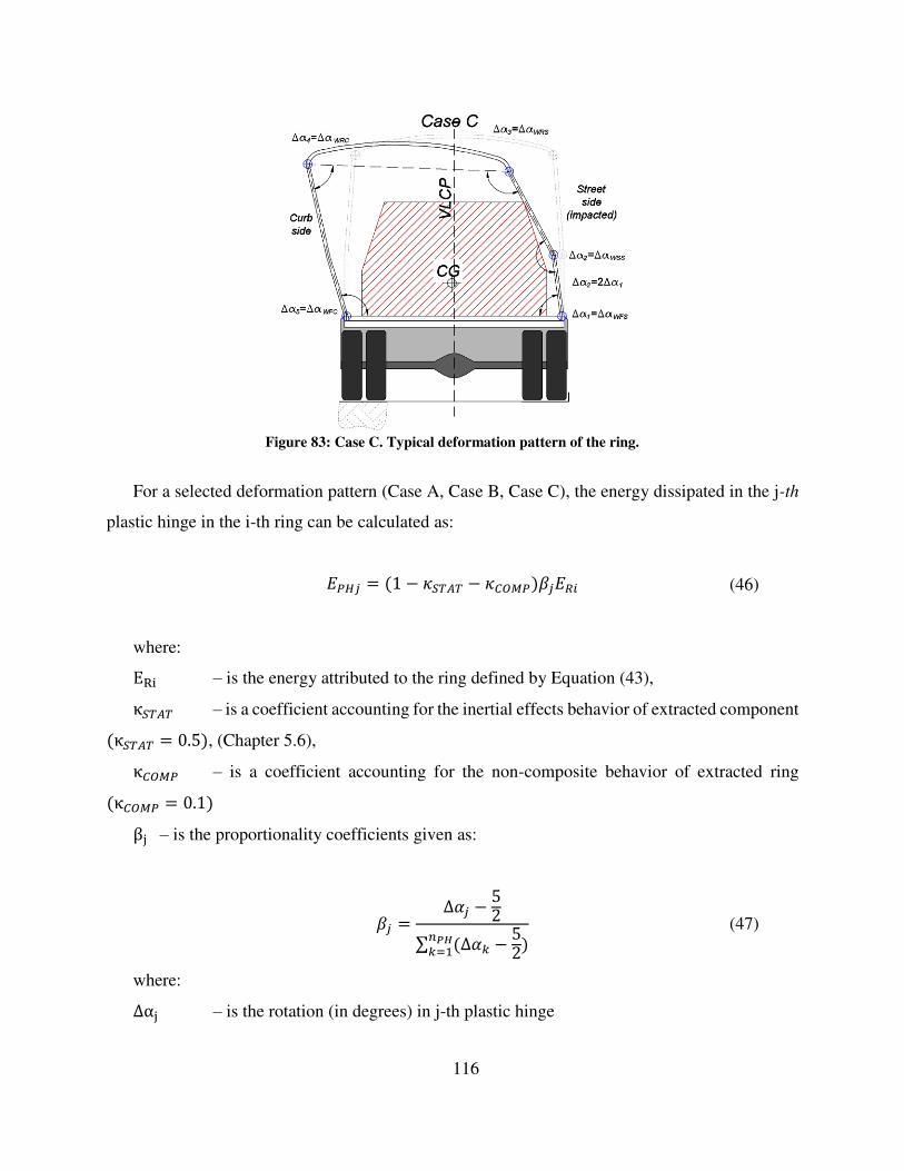
116
Figure 83: Case C. Typical deformation pattern of the ring.
For a selected deformation pattern (Case A, Case B, Case C), the energy dissipated in the j-th
plastic hinge in the i-th ring can be calculated as:
= − − (46)
where: ER – is the energy attributed to the ring defined by Equation (43), κ – is a coefficient accounting for the inertial effects behavior of extracted component κ = . , (Chapter 5.6), κ – is a coefficient accounting for the non-composite behavior of extracted ring κ = .
– is the proportionality coefficients given as:
= ∆ −∑ ∆ −��= (47)
where: ∆ – is the rotation (in degrees) in j-th plastic hinge
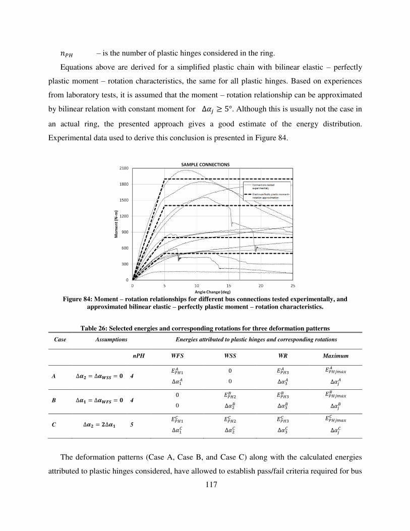
117
– is the number of plastic hinges considered in the ring.
Equations above are derived for a simplified plastic chain with bilinear elastic – perfectly
plastic moment – rotation characteristics, the same for all plastic hinges. Based on experiences
from laboratory tests, it is assumed that the moment – rotation relationship can be approximated
by bilinear relation with constant moment for ∆ °. Although this is usually not the case in
an actual ring, the presented approach gives a good estimate of the energy distribution.
Experimental data used to derive this conclusion is presented in Figure 84.
Figure 84: Moment – rotation relationships for different bus connections tested experimentally, and
approximated bilinear elastic – perfectly plastic moment – rotation characteristics.
Table 26: Selected energies and corresponding rotations for three deformation patterns
Case Assumptions Energies attributed to plastic hinges and corresponding rotations
nPH WFS WSS WR Maximum
A ∆� = ∆� = 4 ∆
0
∆
� ∆
B ∆� = ∆� � = 4
0
∆
∆
� ∆
C ∆� = ∆� 5 ∆
∆
∆
� ∆
The deformation patterns (Case A, Case B, and Case C) along with the calculated energies
attributed to plastic hinges considered, have allowed to establish pass/fail criteria required for bus
118
cage subcomponents. These values are defined in Table 26 and they will be used as the Threshold
Values for experimental testing. In Table 26 the last column refers to the maximum energies and
corresponding rotations, calculated for each case.
5.8. Experimental Testing in ERT
Chapter below summarizes the experimental procedures required to be performed in order to carry
out ERT procedure.
The experimental testing procedures and the calculation of the test requirements (Threshold
Values) is based on experimental experience, and theoretical considerations summarized
previously in this chapter. Following the energy concept, the evaluation of the inertial effects in
the rollover and plastic chain concept, several experimental tests were proposed to form the ERT
procedure requirements. These tests include:
- Pretest – panel test with and without skin (required for establishing the value of � ), - Frontal ring test,
- Rear wall test,
- Wall to floor connection test,
- Wall to roof connection test,
- Panel impact test,
- Static tube testing,
- Dynamic tube testing.
Threshold Values are established as the pass/fail criteria for the ERT procedure. These values
have been established based on the theoretical investigation carried out in this dissertation. The
bus structure is required to satisfy all of the proposed experiments by meeting or exceeding
established Threshold Values.
Pretest – Panel Test With and Without Skin
The ERT procedure starts from the pretest in which two panels, with and without skin, are tested
using impacting arm with energy equal to 1.5 kJ. The test procedure is described in detail in the
Panel Test section. Comparing results of two tests on panels with and without skin, the
dimensionless coefficient � is established as defined in Equation (39).
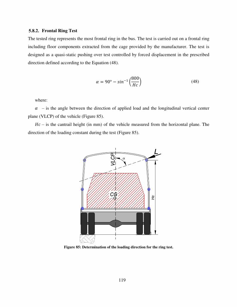
119
Frontal Ring Test
The tested ring represents the most frontal ring in the bus. The test is carried out on a frontal ring
including floor components extracted from the cage provided by the manufacturer. The test is
designed as a quasi-static pushing over test controlled by forced displacement in the prescribed
direction defined according to the Equation (48).
= ° − − ( ) (48)
where:
– is the angle between the direction of applied load and the longitudinal vertical center
plane (VLCP) of the vehicle (Figure 85).
– is the cantrail height (in mm) of the vehicle measured from the horizontal plane. The
direction of the loading constant during the test (Figure 85).
Figure 85: Determination of the loading direction for the ring test.
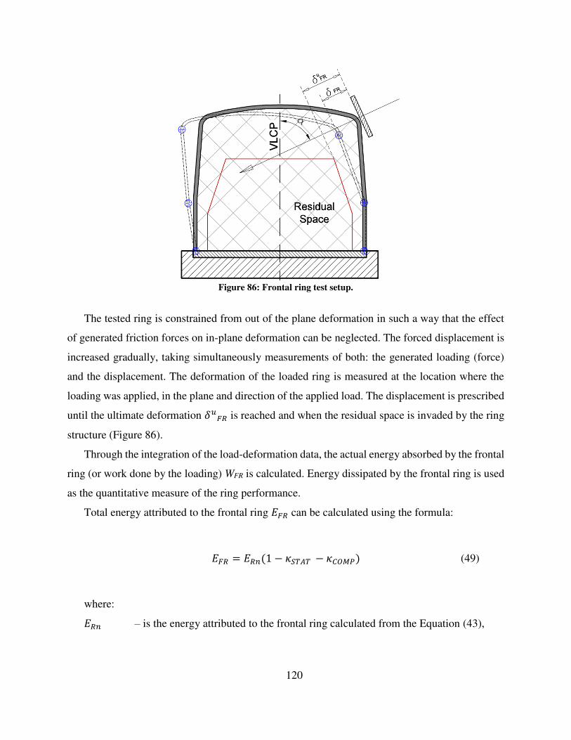
120
Figure 86: Frontal ring test setup.
The tested ring is constrained from out of the plane deformation in such a way that the effect
of generated friction forces on in-plane deformation can be neglected. The forced displacement is
increased gradually, taking simultaneously measurements of both: the generated loading (force)
and the displacement. The deformation of the loaded ring is measured at the location where the
loading was applied, in the plane and direction of the applied load. The displacement is prescribed
until the ultimate deformation is reached and when the residual space is invaded by the ring
structure (Figure 86).
Through the integration of the load-deformation data, the actual energy absorbed by the frontal
ring (or work done by the loading) WFR is calculated. Energy dissipated by the frontal ring is used
as the quantitative measure of the ring performance.
Total energy attributed to the frontal ring can be calculated using the formula:
= − − (49)
where:
– is the energy attributed to the frontal ring calculated from the Equation (43),
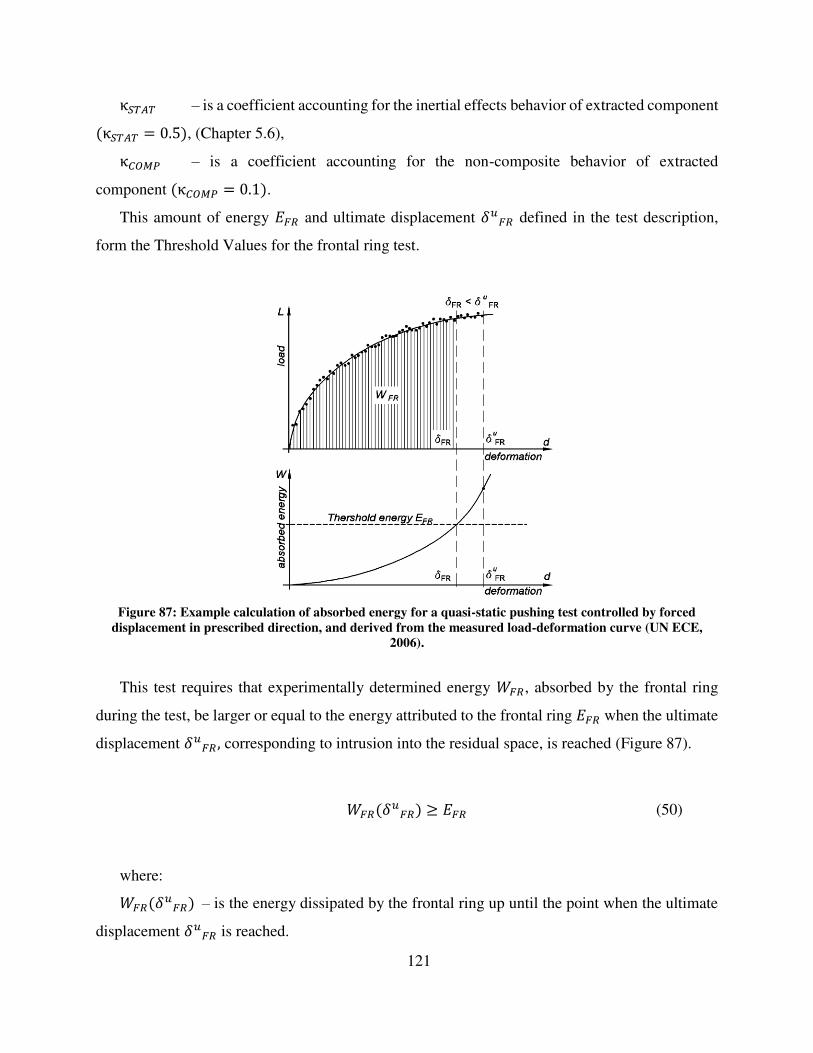
121
κ – is a coefficient accounting for the inertial effects behavior of extracted component κ = . , (Chapter 5.6), κ – is a coefficient accounting for the non-composite behavior of extracted
component κ = . .
This amount of energy and ultimate displacement defined in the test description,
form the Threshold Values for the frontal ring test.
Figure 87: Example calculation of absorbed energy for a quasi-static pushing test controlled by forced
displacement in prescribed direction, and derived from the measured load-deformation curve (UN ECE,
2006).
This test requires that experimentally determined energy , absorbed by the frontal ring
during the test, be larger or equal to the energy attributed to the frontal ring when the ultimate
displacement , corresponding to intrusion into the residual space, is reached (Figure 87).
(50)
where:
– is the energy dissipated by the frontal ring up until the point when the ultimate
displacement is reached.
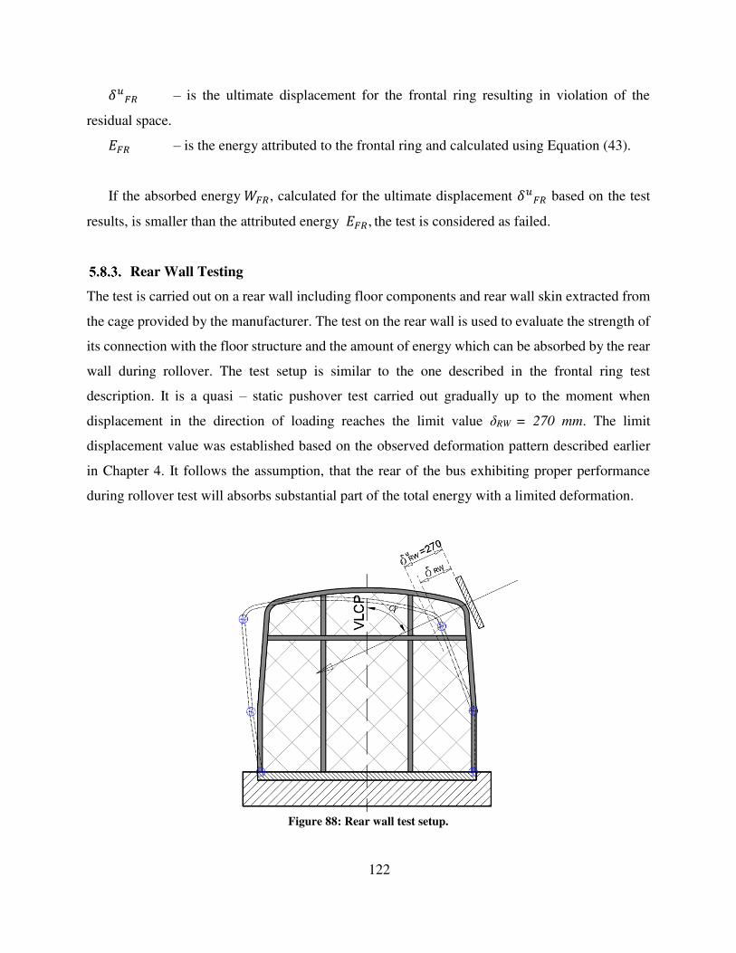
122
– is the ultimate displacement for the frontal ring resulting in violation of the
residual space.
– is the energy attributed to the frontal ring and calculated using Equation (43).
If the absorbed energy , calculated for the ultimate displacement based on the test
results, is smaller than the attributed energy , the test is considered as failed.
Rear Wall Testing
The test is carried out on a rear wall including floor components and rear wall skin extracted from
the cage provided by the manufacturer. The test on the rear wall is used to evaluate the strength of
its connection with the floor structure and the amount of energy which can be absorbed by the rear
wall during rollover. The test setup is similar to the one described in the frontal ring test
description. It is a quasi – static pushover test carried out gradually up to the moment when
displacement in the direction of loading reaches the limit value δRW = 270 mm. The limit
displacement value was established based on the observed deformation pattern described earlier
in Chapter 4. It follows the assumption, that the rear of the bus exhibiting proper performance
during rollover test will absorbs substantial part of the total energy with a limited deformation.
Figure 88: Rear wall test setup.
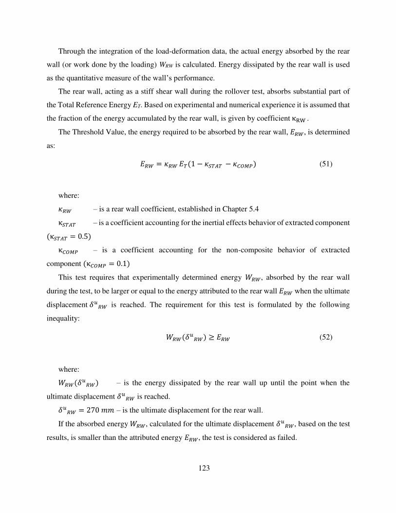
123
Through the integration of the load-deformation data, the actual energy absorbed by the rear
wall (or work done by the loading) WRW is calculated. Energy dissipated by the rear wall is used
as the quantitative measure of the wall’s performance.
The rear wall, acting as a stiff shear wall during the rollover test, absorbs substantial part of
the Total Reference Energy ET. Based on experimental and numerical experience it is assumed that
the fraction of the energy accumulated by the rear wall, is given by coefficient κRW . The Threshold Value, the energy required to be absorbed by the rear wall, , is determined
as:
= − − (51)
where: – is a rear wall coefficient, established in Chapter 5.4 κ – is a coefficient accounting for the inertial effects behavior of extracted component κ = . κ – is a coefficient accounting for the non-composite behavior of extracted
component κ = .
This test requires that experimentally determined energy , absorbed by the rear wall
during the test, to be larger or equal to the energy attributed to the rear wall when the ultimate
displacement is reached. The requirement for this test is formulated by the following
inequality:
(52)
where:
– is the energy dissipated by the rear wall up until the point when the
ultimate displacement is reached. = – is the ultimate displacement for the rear wall.
If the absorbed energy , calculated for the ultimate displacement , based on the test
results, is smaller than the attributed energy , the test is considered as failed.

124
Connections
Connection tests on wall-to-floor (WF) and wall-to-roof (WR) connections, implemented into the
ERT procedure, have been previously established for the purpose of the validation of the finite
element models. These tests are described in Chapter 2 of this dissertation, and the test setup is
presented in Figure 36. The tested connection consists of the steel structural elements only, and is
extracted from the cage provided by the manufacturer.
The test is carried out until the maximum angle of rotation shall exceed the maximum angle
defined in Table 26 for the given connection. The resulting data, bending moment vs. angle of
rotation, after integration, will result in the actual energy absorbed by the tested connection (or
work done by the loading). Energy dissipated by the connections is used as the quantitative
measure of their performance.
The Threshold Values for connection tests are established based on the plastic chain analysis
presented in this dissertation. For wall to floor (WF) connection the Threshold Value is defined as ∆ from the Table 26 which is the energy attributed to the plastic hinge at the WF location
(identified by the subscript 1), at the maximum rotation of ∆ .
It is required, that in order to avoid the deformation pattern depicted in Figure 81. The energy
dissipated by the WF connection to be larger or equal to the energy attributed to the WF
connection when the ultimate rotation ∆ determined through the analysis of plastic chain
is reached (Table 26).
∆ (53)
where: ∆ – is the energy dissipated by the WF connection up until the point when the
ultimate rotation ∆ is reached. ∆ – is the WF plastic hinge deformation (rotation) determined from the analysis of
plastic chain, Case A (Figure 81). EP – is the energy attributed to the plastic hinge at the WF location for maximum
rotation of ∆ (Table 26, Figure 81).
Similarly, for the wall to roof (WR) connection the Threshold Values are given by ∆ ,
and ∆ , which are the energies attributed to the plastic hinge at the WR location (identified
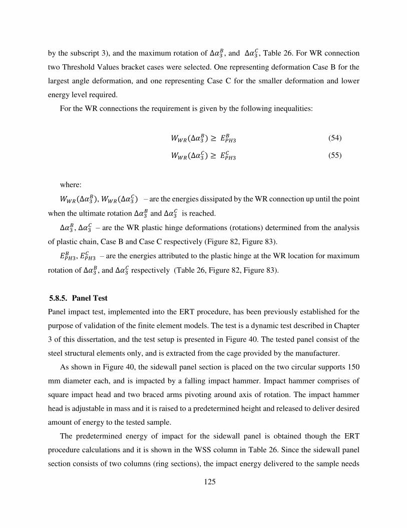
125
by the subscript 3), and the maximum rotation of ∆ , and ∆ , Table 26. For WR connection
two Threshold Values bracket cases were selected. One representing deformation Case B for the
largest angle deformation, and one representing Case C for the smaller deformation and lower
energy level required.
For the WR connections the requirement is given by the following inequalities:
∆ (54)
∆ (55)
where: ∆ , ∆ – are the energies dissipated by the WR connection up until the point
when the ultimate rotation ∆ and ∆ is reached. ∆ , ∆ – are the WR plastic hinge deformations (rotations) determined from the analysis
of plastic chain, Case B and Case C respectively (Figure 82, Figure 83).
, – are the energies attributed to the plastic hinge at the WR location for maximum
rotation of ∆ , and ∆ respectively (Table 26, Figure 82, Figure 83).
Panel Test
Panel impact test, implemented into the ERT procedure, has been previously established for the
purpose of validation of the finite element models. The test is a dynamic test described in Chapter
3 of this dissertation, and the test setup is presented in Figure 40. The tested panel consist of the
steel structural elements only, and is extracted from the cage provided by the manufacturer.
As shown in Figure 40, the sidewall panel section is placed on the two circular supports 150
mm diameter each, and is impacted by a falling impact hammer. Impact hammer comprises of
square impact head and two braced arms pivoting around axis of rotation. The impact hammer
head is adjustable in mass and it is raised to a predetermined height and released to deliver desired
amount of energy to the tested sample.
The predetermined energy of impact for the sidewall panel is obtained though the ERT
procedure calculations and it is shown in the WSS column in Table 26. Since the sidewall panel
section consists of two columns (ring sections), the impact energy delivered to the sample needs
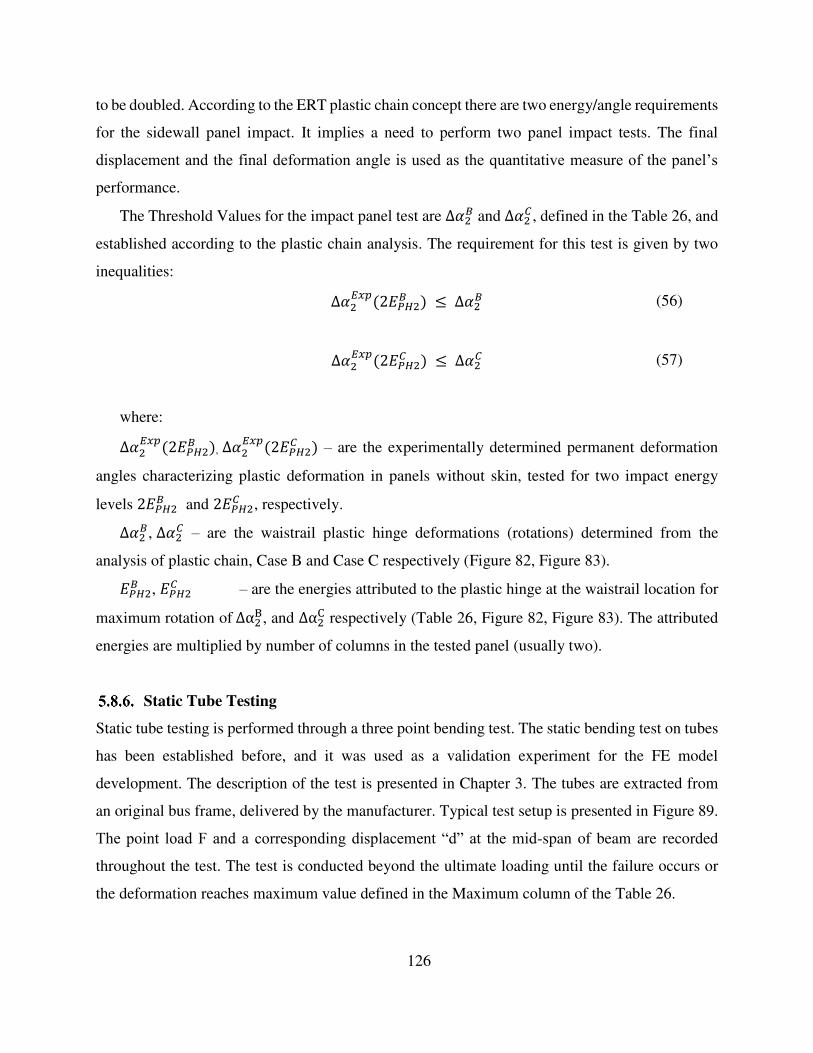
126
to be doubled. According to the ERT plastic chain concept there are two energy/angle requirements
for the sidewall panel impact. It implies a need to perform two panel impact tests. The final
displacement and the final deformation angle is used as the quantitative measure of the panel’s
performance.
The Threshold Values for the impact panel test are ∆ and ∆ , defined in the Table 26, and
established according to the plastic chain analysis. The requirement for this test is given by two
inequalities:
∆ ∆ (56)
∆ ∆ (57)
where: ∆ , ∆ – are the experimentally determined permanent deformation
angles characterizing plastic deformation in panels without skin, tested for two impact energy
levels and , respectively. ∆ , ∆ – are the waistrail plastic hinge deformations (rotations) determined from the
analysis of plastic chain, Case B and Case C respectively (Figure 82, Figure 83).
, – are the energies attributed to the plastic hinge at the waistrail location for
maximum rotation of ∆ , and ∆ respectively (Table 26, Figure 82, Figure 83). The attributed
energies are multiplied by number of columns in the tested panel (usually two).
Static Tube Testing
Static tube testing is performed through a three point bending test. The static bending test on tubes
has been established before, and it was used as a validation experiment for the FE model
development. The description of the test is presented in Chapter 3. The tubes are extracted from
an original bus frame, delivered by the manufacturer. Typical test setup is presented in Figure 89.
The point load F and a corresponding displacement “d” at the mid-span of beam are recorded
throughout the test. The test is conducted beyond the ultimate loading until the failure occurs or
the deformation reaches maximum value defined in the Maximum column of the Table 26.

127
The actual energy absorbed by the tube (WTUBE) is obtained through the integration of the load-
deformation data. The energy dissipated by the tube is used as the quantitative measure of its
performance.
Figure 89: Test setup for three point bending with a=300 mm.
The Threshold Values for the static tube testing is established based on the plastic chain
analysis presented in this dissertation. The energy, required to be absorbed by the tube � ,
and a corresponding angle of rotation ∆ � , are defined in the last column of Table 26. This is
the maximum energy attributed to a plastic hinge based on the three deformation patterns, defined
in Figure 81, Figure 82, and Figure 83. Rotation ∆ � is the corresponding rotation (angle) in
the same plastic hinge and for the same deformation pattern. Since two deformation patterns (Case
B, and Case C) generate similar amount of maximum energy, both of them will be considered in
static tube testing.
It is required that the energy dissipated by the tube during static testing to be larger
or equal to the energy attributed to the tube � when the ultimate rotation ∆ � determined
through the analysis of plastic chain is reached (Table 26).
The requirements for this test is given by the following inequalities:
∆ � � (58)
∆ � � (59)
where: ∆ � , ∆ � – are energies dissipated by the tube during static testing
up until the point when the ultimate rotation ∆ � and ∆ � is reached. ∆ � , ∆ � – are the rotations (angles) in the plastic hinges dissipating the biggest amount
of energy for the given deformation pattern (Case B, Figure 82 and Case C, Figure 83).

128
� , � – are the maximum energies defined in the last column in Table 26 for Case
B and Case C.
Dynamic Tube Testing
Dynamic tube testing is designed according to the same principles as the panel test described
above. It is also an impact test, however it is conducted using different testing device. The tube
impact test has been established before, and it was used as a validation experiment for the FE
model development. The description of the test is presented in Chapter 3 and an example of the
drop impact hammer used for tube testing is shown in Figure 33. The linear impact hammer head
is adjustable in mass and it may be raised to a predetermined height and released to deliver desired
amount of energy to the tested sample.
The predetermined energy of impact for the tubes is obtained though the ERT procedure
calculations and it is shown in the Maximum column in Table 26. Two extreme energy/angle pairs
were selected for the dynamic tube testing.
After the impact, the permanent deformation angle ∆ , defined in Figure 90, is measured. The
rotation ∆ is considered as a measure of plastic deformation generated by the impact in the plastic
hinge.
Figure 90: Permanent angle ∆� as a measure of plastic deformation generated by the impact in the plastic
hinge, assumed a=300 mm.
The Threshold Values for the Dynamic tube testing are defined in a similar fashion as for the
panel impact test. The energy required to be absorbed by the tube � and a corresponding
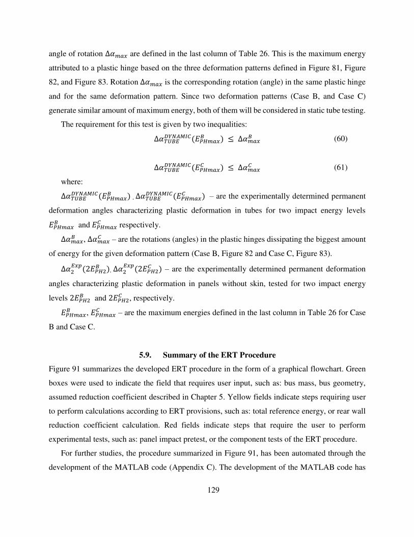
129
angle of rotation ∆ � are defined in the last column of Table 26. This is the maximum energy
attributed to a plastic hinge based on the three deformation patterns defined in Figure 81, Figure
82, and Figure 83. Rotation ∆ � is the corresponding rotation (angle) in the same plastic hinge
and for the same deformation pattern. Since two deformation patterns (Case B, and Case C)
generate similar amount of maximum energy, both of them will be considered in static tube testing.
The requirement for this test is given by two inequalities:
∆ � ∆ � (60)
∆ � ∆ � (61)
where: ∆ � , ∆ � – are the experimentally determined permanent
deformation angles characterizing plastic deformation in tubes for two impact energy levels
� and � respectively. ∆ � , ∆ � – are the rotations (angles) in the plastic hinges dissipating the biggest amount
of energy for the given deformation pattern (Case B, Figure 82 and Case C, Figure 83). ∆ , ∆ – are the experimentally determined permanent deformation
angles characterizing plastic deformation in panels without skin, tested for two impact energy
levels and , respectively.
� , � – are the maximum energies defined in the last column in Table 26 for Case
B and Case C.
5.9. Summary of the ERT Procedure
Figure 91 summarizes the developed ERT procedure in the form of a graphical flowchart. Green
boxes were used to indicate the field that requires user input, such as: bus mass, bus geometry,
assumed reduction coefficient described in Chapter 5. Yellow fields indicate steps requiring user
to perform calculations according to ERT provisions, such as: total reference energy, or rear wall
reduction coefficient calculation. Red fields indicate steps that require the user to perform
experimental tests, such as: panel impact pretest, or the component tests of the ERT procedure.
For further studies, the procedure summarized in Figure 91, has been automated through the
development of the MATLAB code (Appendix C). The development of the MATLAB code has

130
helped to increase the efficiency of the application of the ERT procedure to all of the performed
test cases described in the Chapter 6.
Figure 91: Summary of the ERT procedure.
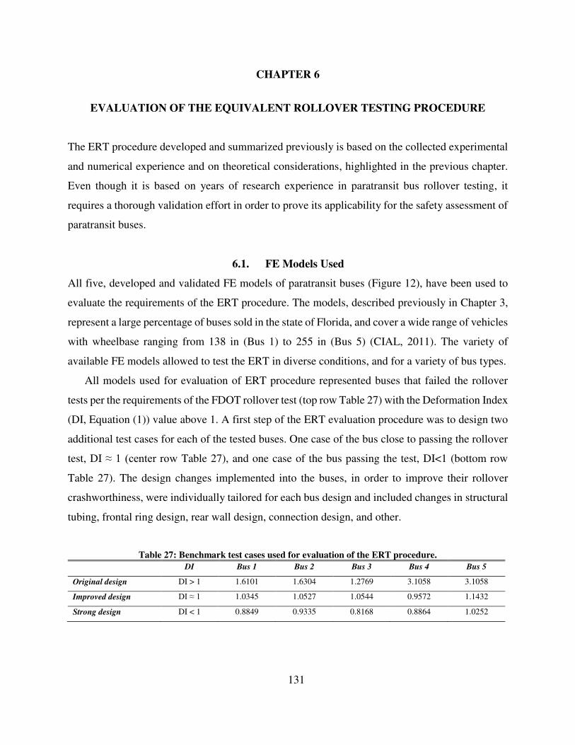
131
CHAPTER 6
EVALUATION OF THE EQUIVALENT ROLLOVER TESTING PROCEDURE
The ERT procedure developed and summarized previously is based on the collected experimental
and numerical experience and on theoretical considerations, highlighted in the previous chapter.
Even though it is based on years of research experience in paratransit bus rollover testing, it
requires a thorough validation effort in order to prove its applicability for the safety assessment of
paratransit buses.
6.1. FE Models Used
All five, developed and validated FE models of paratransit buses (Figure 12), have been used to
evaluate the requirements of the ERT procedure. The models, described previously in Chapter 3,
represent a large percentage of buses sold in the state of Florida, and cover a wide range of vehicles
with wheelbase ranging from 138 in (Bus 1) to 255 in (Bus 5) (CIAL, 2011). The variety of
available FE models allowed to test the ERT in diverse conditions, and for a variety of bus types.
All models used for evaluation of ERT procedure represented buses that failed the rollover
tests per the requirements of the FDOT rollover test (top row Table 27) with the Deformation Index
(DI, Equation (1)) value above 1. A first step of the ERT evaluation procedure was to design two
additional test cases for each of the tested buses. One case of the bus close to passing the rollover
test, DI ≈ 1 (center row Table 27), and one case of the bus passing the test, DI<1 (bottom row
Table 27). The design changes implemented into the buses, in order to improve their rollover
crashworthiness, were individually tailored for each bus design and included changes in structural
tubing, frontal ring design, rear wall design, connection design, and other.
Table 27: Benchmark test cases used for evaluation of the ERT procedure.
DI Bus 1 Bus 2 Bus 3 Bus 4 Bus 5
Original design DI > 1 1.6101 1.6304 1.2769 3.1058 3.1058
Improved design DI ≈ 1 1.0345 1.0527 1.0544 0.9572 1.1432
Strong design DI < 1 0.8849 0.9335 0.8168 0.8864 1.0252
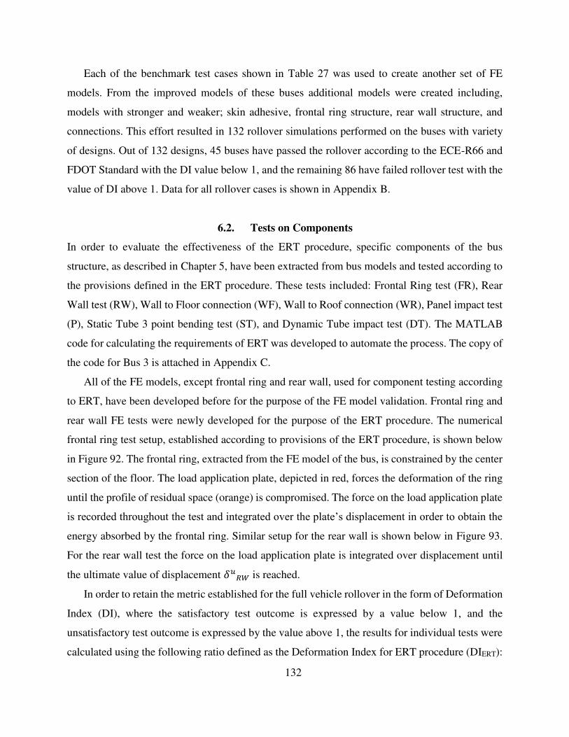
132
Each of the benchmark test cases shown in Table 27 was used to create another set of FE
models. From the improved models of these buses additional models were created including,
models with stronger and weaker; skin adhesive, frontal ring structure, rear wall structure, and
connections. This effort resulted in 132 rollover simulations performed on the buses with variety
of designs. Out of 132 designs, 45 buses have passed the rollover according to the ECE-R66 and
FDOT Standard with the DI value below 1, and the remaining 86 have failed rollover test with the
value of DI above 1. Data for all rollover cases is shown in Appendix B.
6.2. Tests on Components
In order to evaluate the effectiveness of the ERT procedure, specific components of the bus
structure, as described in Chapter 5, have been extracted from bus models and tested according to
the provisions defined in the ERT procedure. These tests included: Frontal Ring test (FR), Rear
Wall test (RW), Wall to Floor connection (WF), Wall to Roof connection (WR), Panel impact test
(P), Static Tube 3 point bending test (ST), and Dynamic Tube impact test (DT). The MATLAB
code for calculating the requirements of ERT was developed to automate the process. The copy of
the code for Bus 3 is attached in Appendix C.
All of the FE models, except frontal ring and rear wall, used for component testing according
to ERT, have been developed before for the purpose of the FE model validation. Frontal ring and
rear wall FE tests were newly developed for the purpose of the ERT procedure. The numerical
frontal ring test setup, established according to provisions of the ERT procedure, is shown below
in Figure 92. The frontal ring, extracted from the FE model of the bus, is constrained by the center
section of the floor. The load application plate, depicted in red, forces the deformation of the ring
until the profile of residual space (orange) is compromised. The force on the load application plate
is recorded throughout the test and integrated over the plate’s displacement in order to obtain the
energy absorbed by the frontal ring. Similar setup for the rear wall is shown below in Figure 93.
For the rear wall test the force on the load application plate is integrated over displacement until
the ultimate value of displacement is reached.
In order to retain the metric established for the full vehicle rollover in the form of Deformation
Index (DI), where the satisfactory test outcome is expressed by a value below 1, and the
unsatisfactory test outcome is expressed by the value above 1, the results for individual tests were
calculated using the following ratio defined as the Deformation Index for ERT procedure (DIERT):
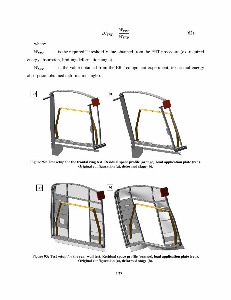
133
= (62)
where:
– is the required Threshold Value obtained from the ERT procedure (ex. required
energy absorption, limiting deformation angle).
– is the value obtained from the ERT component experiment, (ex. actual energy
absorption, obtained deformation angle).
Figure 92: Test setup for the frontal ring test. Residual space profile (orange), load application plate (red).
Original configuration (a), deformed stage (b).
Figure 93: Test setup for the rear wall test. Residual space profile (orange), load application plate (red).
Original configuration (a), deformed stage (b).
a) b)
a) b)
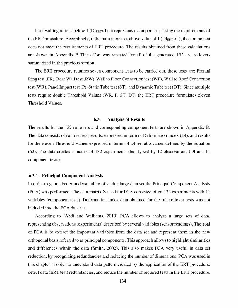
134
If a resulting ratio is below 1 (DIERT<1), it represents a component passing the requirements of
the ERT procedure. Accordingly, if the ratio increases above value of 1 (DIERT >1), the component
does not meet the requirements of ERT procedure. The results obtained from these calculations
are shown in Appendix B This effort was repeated for all of the generated 132 test rollovers
summarized in the previous section.
The ERT procedure requires seven component tests to be carried out, these tests are: Frontal
Ring test (FR), Rear Wall test (RW), Wall to Floor Connection test (WF), Wall to Roof Connection
test (WR), Panel Impact test (P), Static Tube test (ST), and Dynamic Tube test (DT). Since multiple
tests require double Threshold Values (WR, P, ST, DT) the ERT procedure formulates eleven
Threshold Values.
6.3. Analysis of Results
The results for the 132 rollovers and corresponding component tests are shown in Appendix B.
The data consists of rollover test results, expressed in term of Deformation Index (DI), and results
for the eleven Threshold Values expressed in terms of DIERT ratio values defined by the Equation
(62). The data creates a matrix of 132 experiments (bus types) by 12 observations (DI and 11
component tests).
Principal Component Analysis
In order to gain a better understanding of such a large data set the Principal Component Analysis
(PCA) was performed. The data matrix X used for PCA consisted of on 132 experiments with 11
variables (component tests). Deformation Index data obtained for the full rollover tests was not
included into the PCA data set.
According to (Abdi and Williams, 2010) PCA allows to analyze a large sets of data,
representing observations (experiments) described by several variables (sensor readings). The goal
of PCA is to extract the important variables from the data set and represent them in the new
orthogonal basis referred to as principal components. This approach allows to highlight similarities
and differences within the data (Smith, 2002). This also makes PCA very useful in data set
reduction, by recognizing redundancies and reducing the number of dimensions. PCA was used in
this chapter in order to understand data pattern created by the application of the ERT procedure,
detect data (ERT test) redundancies, and reduce the number of required tests in the ERT procedure.

135
The data matrix X used for PCA was preprocessed before the analysis. The columns of X were
centered so that the mean value of each column was 0. Since all of the data in X was normalized
by the application of the DIERT ratio definition following the Equation (62), no additional
normalization was performed on available data.
Principal components are obtained by the use of Singular Value Decomposition (SVD)
performed on the provided data set X. It takes a form of (Abdi and Williams, 2010):
= ∆ (63)
where:
– is the orthogonal matrix which columns are the orthonormal eigenvectors of ,
– is the orthogonal matrix which columns are the orthonormal eigenvectors of , ∆ – is the diagonal matrix of square roots of (nonzero) eigenvalues of and .
Since both matrices P and Q are orthogonal the following applies:
= = = = � (64)
where: � – is the identity matrix.
According to Abdi and Williams, (2010) the matrix of factor scores F, is obtained as:
� = ∆ (65)
The matrix Q, is often referred to as the projection matrix, because multiplying X by Q gives
the projections of the experiments onto the principal components. This is shown by Abdi and
Williams, (2010):
� = ∆= ∆� = ∆ = (66)
Principal Component Analysis for the obtained ERT data was performed using a MATLAB
code. The discussed code is attached in the Appendix D. The results for the 132 sets of ERT
component tests, projected onto the first two principal components, as well eigenvalues obtained
for matrix P and Q, are shown below in Figure 94.
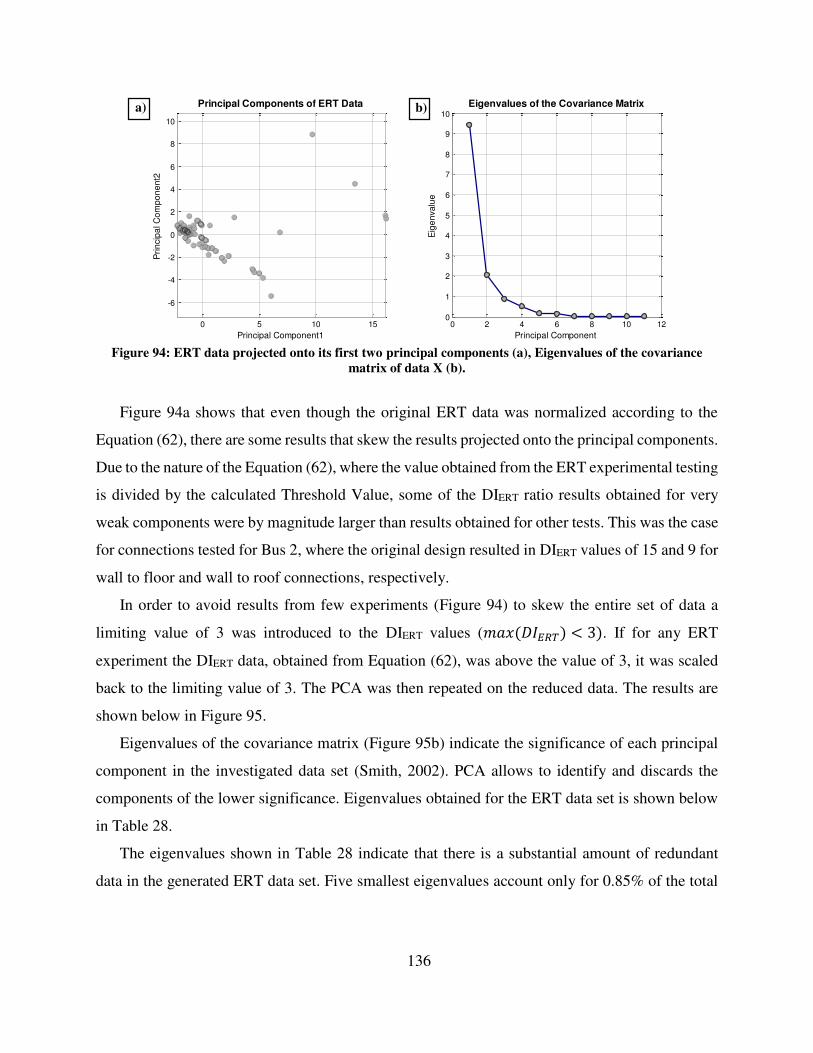
136
0 5 10 15
-6
-4
-2
0
2
4
6
8
10
Principal Components of ERT Data
Principal Component1
Pri
ncip
al C
om
po
ne
nt2
0 2 4 6 8 10 120
1
2
3
4
5
6
7
8
9
10
Eigenvalues of the Covariance Matrix
Principal Component
Eig
en
va
lue
Figure 94: ERT data projected onto its first two principal components (a), Eigenvalues of the covariance
matrix of data X (b).
Figure 94a shows that even though the original ERT data was normalized according to the
Equation (62), there are some results that skew the results projected onto the principal components.
Due to the nature of the Equation (62), where the value obtained from the ERT experimental testing
is divided by the calculated Threshold Value, some of the DIERT ratio results obtained for very
weak components were by magnitude larger than results obtained for other tests. This was the case
for connections tested for Bus 2, where the original design resulted in DIERT values of 15 and 9 for
wall to floor and wall to roof connections, respectively.
In order to avoid results from few experiments (Figure 94) to skew the entire set of data a
limiting value of 3 was introduced to the DIERT values ( � < . If for any ERT
experiment the DIERT data, obtained from Equation (62), was above the value of 3, it was scaled
back to the limiting value of 3. The PCA was then repeated on the reduced data. The results are
shown below in Figure 95.
Eigenvalues of the covariance matrix (Figure 95b) indicate the significance of each principal
component in the investigated data set (Smith, 2002). PCA allows to identify and discards the
components of the lower significance. Eigenvalues obtained for the ERT data set is shown below
in Table 28.
The eigenvalues shown in Table 28 indicate that there is a substantial amount of redundant
data in the generated ERT data set. Five smallest eigenvalues account only for 0.85% of the total
a) b)
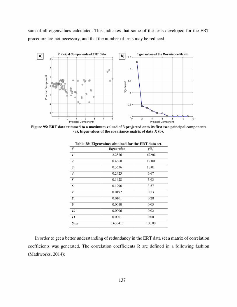
137
sum of all eigenvalues calculated. This indicates that some of the tests developed for the ERT
procedure are not necessary, and that the number of tests may be reduced.
-1 0 1 2 3 4 5
-3
-2
-1
0
1
2
3
Principal Components of ERT Data
Principal Component1
Pri
ncip
al C
om
po
ne
nt2
0 2 4 6 8 10 120
0.5
1
1.5
2
2.5
Eigenvalues of the Covariance Matrix
Principal Component
Eig
en
va
lue
Figure 95: ERT data trimmed to a maximum valued of 3 projected onto its first two principal components
(a), Eigenvalues of the covariance matrix of data X (b).
Table 28: Eigenvalues obtained for the ERT data set.
# Eigenvalue [%]
1 2.2876 62.96
2 0.4360 12.00
3 0.3636 10.01
4 0.2423 6.67
5 0.1428 3.93
6 0.1296 3.57
7 0.0192 0.53
8 0.0101 0.28
9 0.0010 0.03
10 0.0006 0.02
11 0.0001 0.00
Sum 3.633417 100.00
In order to get a better understanding of redundancy in the ERT data set a matrix of correlation
coefficients was generated. The correlation coefficients R are defined in a following fashion
(Mathworks, 2014):
a) b)

138
, = ,√ , , (67)
where: , – covariance between two variables, √ , , √ , – standard deviation of the variable.
The matrix of correlation coefficients is shown below in Table 29.
Correlation coefficients shown in Table 29, highlight that a strong correlation exists (marked
in green) between results of the tests on the same components performed with different amount of
energy (panel, tube impact), or for different deformation angles (static tube, wall to roof connection
test). This data shows that there is no need to duplicate Threshold Values for these tests, and only
the more stringent requirement should be kept. For all the redundant tests, the more rigorous
requirements came from the deformation pattern depicted in Case C (Figure 83), and these
requirements were kept for the final version of the ERT procedure.
Table 29: Correlation coefficients obtained for the Deformation Index (DIRoll) and DIERT data set. FR - frontal
ring, RW – rear wall, WF – wall to floor connection ,WR – wall to roof connection, P – panel impact test, ST
– 3 point static tube bending, DT – tube impact test.
DIRoll FR RW WF WR1 WR2 P1 P2 ST1 ST2 DT1 DT2
DIRoll 1.000 0.651 0.374 0.463 0.472 0.480 0.674 0.662 0.695 0.689 0.582 0.593
FR 1.000 0.180 0.288 0.244 0.237 0.180 0.200 0.198 0.230 0.194 0.207
RW 1.000 0.405 0.408 0.472 0.361 0.358 0.382 0.392 0.368 0.355
WF 1.000 0.692 0.650 0.512 0.533 0.623 0.652 0.478 0.494
WR1 1.000 0.976 0.511 0.552 0.660 0.678 0.667 0.666
WR2 1.000 0.492 0.527 0.650 0.665 0.687 0.684
P1 1.000 0.990 0.869 0.859 0.673 0.687
P2 Sym. 1.000 0.862 0.859 0.709 0.723
ST1 1.000 0.996 0.877 0.885
ST2 1.000 0.878 0.887
DT1 1.000 0.997
DT2 1.000
The first row of Table 29 shows correlation coefficients between individual ERT component
tests, and the rollover test outcome (DIRoll). The highest correlation coefficient is observed for
panel test (P), static tube testing (ST), frontal ring test (FR) and dynamic tube testing (DT). Panel
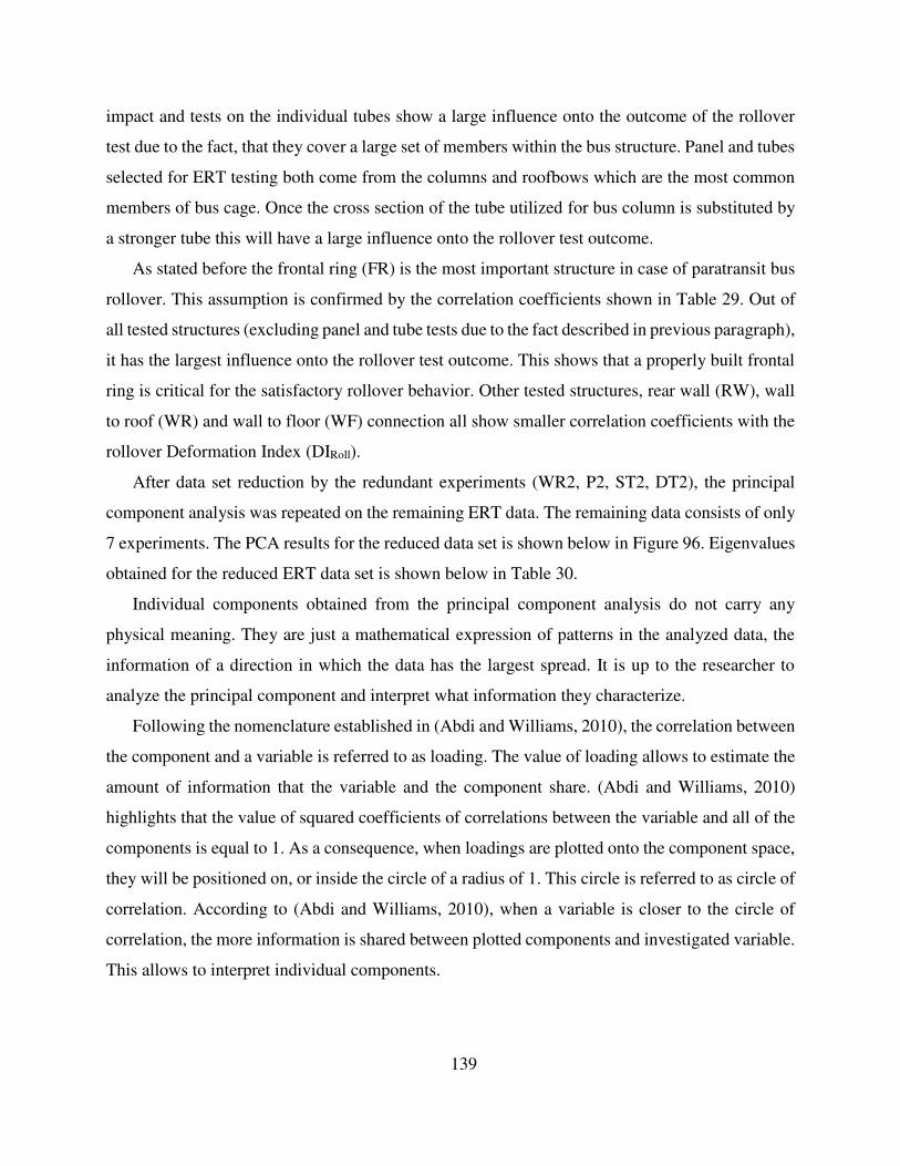
139
impact and tests on the individual tubes show a large influence onto the outcome of the rollover
test due to the fact, that they cover a large set of members within the bus structure. Panel and tubes
selected for ERT testing both come from the columns and roofbows which are the most common
members of bus cage. Once the cross section of the tube utilized for bus column is substituted by
a stronger tube this will have a large influence onto the rollover test outcome.
As stated before the frontal ring (FR) is the most important structure in case of paratransit bus
rollover. This assumption is confirmed by the correlation coefficients shown in Table 29. Out of
all tested structures (excluding panel and tube tests due to the fact described in previous paragraph),
it has the largest influence onto the rollover test outcome. This shows that a properly built frontal
ring is critical for the satisfactory rollover behavior. Other tested structures, rear wall (RW), wall
to roof (WR) and wall to floor (WF) connection all show smaller correlation coefficients with the
rollover Deformation Index (DIRoll).
After data set reduction by the redundant experiments (WR2, P2, ST2, DT2), the principal
component analysis was repeated on the remaining ERT data. The remaining data consists of only
7 experiments. The PCA results for the reduced data set is shown below in Figure 96. Eigenvalues
obtained for the reduced ERT data set is shown below in Table 30.
Individual components obtained from the principal component analysis do not carry any
physical meaning. They are just a mathematical expression of patterns in the analyzed data, the
information of a direction in which the data has the largest spread. It is up to the researcher to
analyze the principal component and interpret what information they characterize.
Following the nomenclature established in (Abdi and Williams, 2010), the correlation between
the component and a variable is referred to as loading. The value of loading allows to estimate the
amount of information that the variable and the component share. (Abdi and Williams, 2010)
highlights that the value of squared coefficients of correlations between the variable and all of the
components is equal to 1. As a consequence, when loadings are plotted onto the component space,
they will be positioned on, or inside the circle of a radius of 1. This circle is referred to as circle of
correlation. According to (Abdi and Williams, 2010), when a variable is closer to the circle of
correlation, the more information is shared between plotted components and investigated variable.
This allows to interpret individual components.
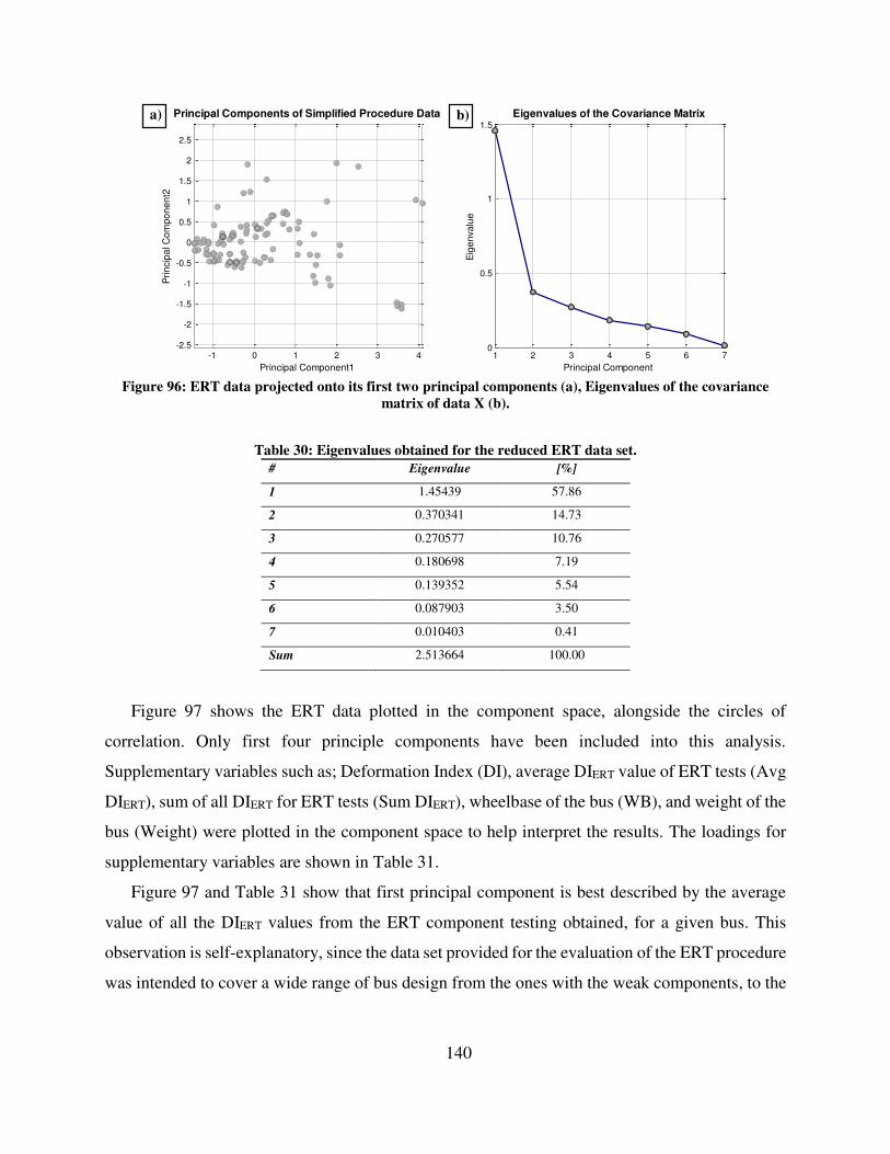
140
-1 0 1 2 3 4-2.5
-2
-1.5
-1
-0.5
0
0.5
1
1.5
2
2.5
Principal Components of Simplified Procedure Data
Principal Component1
Pri
ncip
al C
om
po
ne
nt2
1 2 3 4 5 6 70
0.5
1
1.5
Eigenvalues of the Covariance Matrix
Principal Component
Eig
en
va
lue
Figure 96: ERT data projected onto its first two principal components (a), Eigenvalues of the covariance
matrix of data X (b).
Table 30: Eigenvalues obtained for the reduced ERT data set.
# Eigenvalue [%]
1 1.45439 57.86
2 0.370341 14.73
3 0.270577 10.76
4 0.180698 7.19
5 0.139352 5.54
6 0.087903 3.50
7 0.010403 0.41
Sum 2.513664 100.00
Figure 97 shows the ERT data plotted in the component space, alongside the circles of
correlation. Only first four principle components have been included into this analysis.
Supplementary variables such as; Deformation Index (DI), average DIERT value of ERT tests (Avg
DIERT), sum of all DIERT for ERT tests (Sum DIERT), wheelbase of the bus (WB), and weight of the
bus (Weight) were plotted in the component space to help interpret the results. The loadings for
supplementary variables are shown in Table 31.
Figure 97 and Table 31 show that first principal component is best described by the average
value of all the DIERT values from the ERT component testing obtained, for a given bus. This
observation is self-explanatory, since the data set provided for the evaluation of the ERT procedure
was intended to cover a wide range of bus design from the ones with the weak components, to the
a) b)
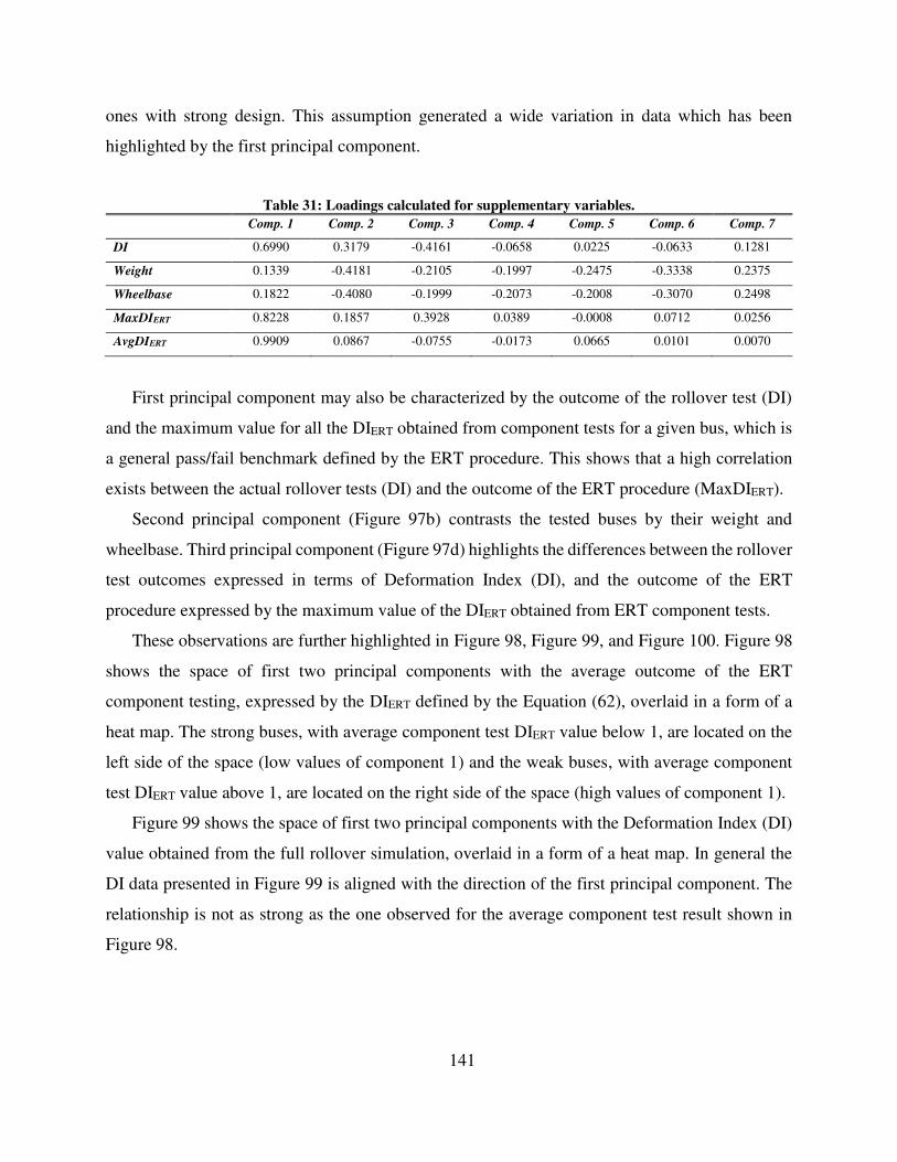
141
ones with strong design. This assumption generated a wide variation in data which has been
highlighted by the first principal component.
Table 31: Loadings calculated for supplementary variables.
Comp. 1 Comp. 2 Comp. 3 Comp. 4 Comp. 5 Comp. 6 Comp. 7
DI 0.6990 0.3179 -0.4161 -0.0658 0.0225 -0.0633 0.1281
Weight 0.1339 -0.4181 -0.2105 -0.1997 -0.2475 -0.3338 0.2375
Wheelbase 0.1822 -0.4080 -0.1999 -0.2073 -0.2008 -0.3070 0.2498
MaxDIERT 0.8228 0.1857 0.3928 0.0389 -0.0008 0.0712 0.0256
AvgDIERT 0.9909 0.0867 -0.0755 -0.0173 0.0665 0.0101 0.0070
First principal component may also be characterized by the outcome of the rollover test (DI)
and the maximum value for all the DIERT obtained from component tests for a given bus, which is
a general pass/fail benchmark defined by the ERT procedure. This shows that a high correlation
exists between the actual rollover tests (DI) and the outcome of the ERT procedure (MaxDIERT).
Second principal component (Figure 97b) contrasts the tested buses by their weight and
wheelbase. Third principal component (Figure 97d) highlights the differences between the rollover
test outcomes expressed in terms of Deformation Index (DI), and the outcome of the ERT
procedure expressed by the maximum value of the DIERT obtained from ERT component tests.
These observations are further highlighted in Figure 98, Figure 99, and Figure 100. Figure 98
shows the space of first two principal components with the average outcome of the ERT
component testing, expressed by the DIERT defined by the Equation (62), overlaid in a form of a
heat map. The strong buses, with average component test DIERT value below 1, are located on the
left side of the space (low values of component 1) and the weak buses, with average component
test DIERT value above 1, are located on the right side of the space (high values of component 1).
Figure 99 shows the space of first two principal components with the Deformation Index (DI)
value obtained from the full rollover simulation, overlaid in a form of a heat map. In general the
DI data presented in Figure 99 is aligned with the direction of the first principal component. The
relationship is not as strong as the one observed for the average component test result shown in
Figure 98.
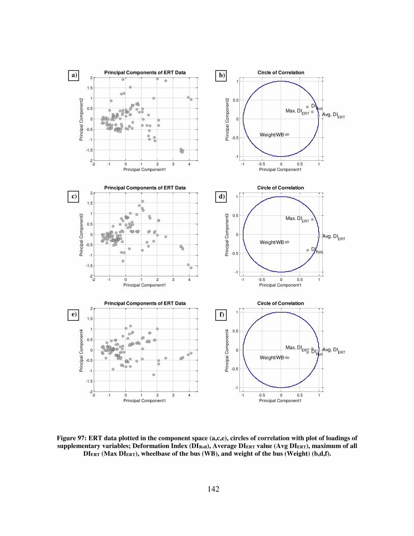
142
-2 -1 0 1 2 3 4-2
-1.5
-1
-0.5
0
0.5
1
1.5
2
Principal Components of ERT Data
Principal Component1
Pri
ncip
al C
om
po
ne
nt2
-1 -0.5 0 0.5 1
-1
-0.5
0
0.5
1
Circle of Correlation
Principal Component1
Pri
ncip
al C
om
po
ne
nt2
DIRoll
Weight/WB
Max. DIERT Avg. DI
ERT
-2 -1 0 1 2 3 4-2
-1.5
-1
-0.5
0
0.5
1
1.5
2
Principal Components of ERT Data
Principal Component1
Pri
ncip
al C
om
po
ne
nt3
-1 -0.5 0 0.5 1
-1
-0.5
0
0.5
1
Circle of Correlation
Principal Component1
Pri
ncip
al C
om
po
ne
nt3
DIRoll
Weight/WB
Max. DIERT
Avg. DIERT
-2 -1 0 1 2 3 4-2
-1.5
-1
-0.5
0
0.5
1
1.5
2
Principal Components of ERT Data
Principal Component1
Pri
ncip
al C
om
po
ne
nt4
-1 -0.5 0 0.5 1
-1
-0.5
0
0.5
1
Circle of Correlation
Principal Component1
Pri
ncip
al C
om
po
ne
nt4
DIRoll
Weight/WB
Max. DIERT Avg. DI
ERT
Figure 97: ERT data plotted in the component space (a,c,e), circles of correlation with plot of loadings of
supplementary variables; Deformation Index (DIRoll), Average DIERT value (Avg DIERT), maximum of all
DIERT (Max DIERT), wheelbase of the bus (WB), and weight of the bus (Weight) (b,d,f).
a) b)
c) d)
e) f)

143
-2 -1 0 1 2 3 4-2
-1.5
-1
-0.5
0
0.5
1
1.5
2
Principal Component1
Pri
ncip
al C
om
po
ne
nt2
Correlation of avreage test result Avg. DIERT
with first and second principal component
Avg.
DI E
RT
0.6
0.8
1
1.2
1.4
1.6
1.8
2
2.2
2.4
2.6
Figure 98: First and second component space, with the heat map of the average DIERT component test result.
-2 -1 0 1 2 3 4-2
-1.5
-1
-0.5
0
0.5
1
1.5
2
Principal Component1
Pri
ncip
al C
om
po
ne
nt2
Correlation of Deformation Index (DIRoll
) with first and second principal component
Defo
rmation I
ndex (
DI R
oll)
Bus 127Bus 130
0.9
1
1.1
1.2
1.3
1.4
1.5
1.6
Figure 99: First and second component space, with the heat map of the rollover Deformation Index (DI)
values.
-2 -1 0 1 2 3 4-2
-1.5
-1
-0.5
0
0.5
1
1.5
2
Principal Component1
Pri
ncip
al C
om
po
ne
nt2
Correlation of Bus Mass with first and second principal component
Mass o
f th
e B
us [
Tons]
5
5.5
6
6.5
7
7.5
8
8.5
9
Figure 100: First and second component space, with the heat map of the mass of a tested bus.
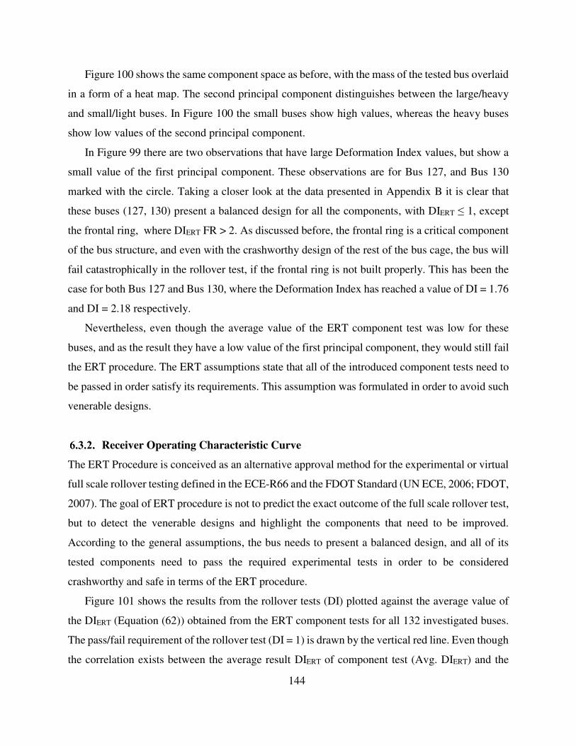
144
Figure 100 shows the same component space as before, with the mass of the tested bus overlaid
in a form of a heat map. The second principal component distinguishes between the large/heavy
and small/light buses. In Figure 100 the small buses show high values, whereas the heavy buses
show low values of the second principal component.
In Figure 99 there are two observations that have large Deformation Index values, but show a
small value of the first principal component. These observations are for Bus 127, and Bus 130
marked with the circle. Taking a closer look at the data presented in Appendix B it is clear that
these buses (127, 130) present a balanced design for all the components, with DIERT ≤ 1, except
the frontal ring, where DIERT FR > 2. As discussed before, the frontal ring is a critical component
of the bus structure, and even with the crashworthy design of the rest of the bus cage, the bus will
fail catastrophically in the rollover test, if the frontal ring is not built properly. This has been the
case for both Bus 127 and Bus 130, where the Deformation Index has reached a value of DI = 1.76
and DI = 2.18 respectively.
Nevertheless, even though the average value of the ERT component test was low for these
buses, and as the result they have a low value of the first principal component, they would still fail
the ERT procedure. The ERT assumptions state that all of the introduced component tests need to
be passed in order satisfy its requirements. This assumption was formulated in order to avoid such
venerable designs.
Receiver Operating Characteristic Curve
The ERT Procedure is conceived as an alternative approval method for the experimental or virtual
full scale rollover testing defined in the ECE-R66 and the FDOT Standard (UN ECE, 2006; FDOT,
2007). The goal of ERT procedure is not to predict the exact outcome of the full scale rollover test,
but to detect the venerable designs and highlight the components that need to be improved.
According to the general assumptions, the bus needs to present a balanced design, and all of its
tested components need to pass the required experimental tests in order to be considered
crashworthy and safe in terms of the ERT procedure.
Figure 101 shows the results from the rollover tests (DI) plotted against the average value of
the DIERT (Equation (62)) obtained from the ERT component tests for all 132 investigated buses.
The pass/fail requirement of the rollover test (DI = 1) is drawn by the vertical red line. Even though
the correlation exists between the average result DIERT of component test (Avg. DIERT) and the
145
actual rollover result (DI), the ERT procedure requires for all the component tests to satisfy its
requirements. The average component test results, even if it is useful in predicting bus rollover
crashworthiness is not a satisfactory measure for ensuring that tested bus will pass the FDOT
rollover test.
0.5 1 1.5 2 2.5 3 3.50.5
1
1.5
2
2.5
3
DIRoll
vs Avg. DIERT
DIRoll
Avg
. D
I ER
T
Avg. DIERT
= 1
DI R
oll =
1
Figure 101: Deformation Index versus the average ERT component test result (Avg DIERT). Results for all 132
buses.
The reason behind this observation is that not all of the component tests carry equal
significance for the full scale rollover testing. As defined in previous sections of this dissertation,
the most important component for rollover crashworthiness in the bus structure is the frontal ring.
For example, a bus with a strong frontal ring (DIERT <1) and a weak wall to floor connection (Bus
23 and Bus 24, in Appendix B) will perform well in the actual rollover test, in contrast to the bus
with a strong wall to floor connection and a weak frontal ring (Bus 127, Bus 130, in Appendix B).
In either case, both of the buses will have a similar average result for all component tests, even
though the actual rollover test results will diverge. This approach could lead to the acceptance of
the buses, in which the critical components are weak, and which would fail the actual rollover test
(bottom right rectangle in Figure 101).
Figure 102 shows the actual, stringent requirements of the ERT procedure, where the
maximum DIERT (Equation (62)) of all the component tests defines a pass/fail criteria. The
requirements of the ERT procedure, listed in Chapter 5, state that in order to pass the ERT
procedure all of the tested components need to demonstrate a satisfactory performance (MaxDIERT
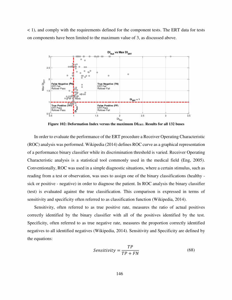
146
< 1), and comply with the requirements defined for the component tests. The ERT data for tests
on components have been limited to the maximum value of 3, as discussed above.
0.5 1 1.5 2 2.5 3 3.50.5
1
1.5
2
2.5
3
DIRoll
vs Max DIERT
DIRoll
Ma
x D
I ER
T
True Positive (TP)
False Negative (FN) True Negative (TN)
False Positive (FP)
DIERT
= 1
DI R
oll =
1
ERT Pass
ERT Fail ERT Fail
ERT PassRollover Pass
Rollover Pass Rollover Fail
Rollover Fail
Figure 102: Deformation Index versus the maximum DIERT. Results for all 132 buses
In order to evaluate the performance of the ERT procedure a Receiver Operating Characteristic
(ROC) analysis was performed. Wikipedia (2014) defines ROC curve as a graphical representation
of a performance binary classifier while its discrimination threshold is varied. Receiver Operating
Characteristic analysis is a statistical tool commonly used in the medical field (Eng, 2005).
Conventionally, ROC was used in a simple diagnostic situations, where a certain stimulus, such as
reading from a test or observation, was uses to assign one of the binary classifications (healthy -
sick or positive - negative) in order to diagnose the patient. In ROC analysis the binary classifier
(test) is evaluated against the true classification. This comparison is expressed in terms of
sensitivity and specificity often referred to as classification function (Wikipedia, 2014).
Sensitivity, often referred to as true positive rate, measures the ratio of actual positives
correctly identified by the binary classifier with all of the positives identified by the test.
Specificity, often referred to as true negative rate, measures the proportion correctly identified
negatives to all identified negatives (Wikipedia, 2014). Sensitivity and Specificity are defined by
the equations:
� = �� + (68)

147
= + � (69)
where: � – number of true positives, observations identified correctly as positives,
– number of true negatives, observations identified correctly as negatives, � – number of false positives, observations identified incorrectly as positives,
– number of false negatives, observations identified incorrectly as negatives.
The ROC curve is constructed by plotting sensitivity versus specificity. Historically the ROC
curve has been mirrored along the vertical axis, and it is common to plot sensitivity versus 1 –
specificity (Eng, 2005). The area under the curve (AUC) is used as the measure of the quality of
the binary classifier. The AUC ranges from 0.5 to 1.0. The AUC = 0.5 represents the inconclusive
test, that generates random classification results, and the AUC = 1.0 represents a test perfectly
distinguishing between positive and negative results.
In case of the ERT procedure the binary classifier is defined as the maximum DIERT (Equation
(62)) value obtained from the ERT component tests (Figure 102). This value will be referred to as
MaxDIERT further in this chapter. If the MaxDIERT value is above 1 then the ERT procedure on the
investigated bus is considered as failed (negative), if on the other hand the MaxDIERT value is
below 1 then the bus passes the ERT procedure (positive). The true classification is defined as the
outcome of the rollover test performed on the full FE model of the investigated bus (DI < 1 – pass,
DI > 1 – fail, Figure 102).
The True Positive (TP) region in Figure 102 represents buses that have satisfied the
requirements of the ERT procedure, and have passed the rollover test per FDOT Standard
requirements. The False Positive (FP) region represents buses that have satisfied the requirements
of the ERT procedure, but have failed the rollover test. The False Negative (FN) region represents
buses that have failed the requirements of the ERT procedure, but have passed the rollover test.
And the True Negative (TN) region represents buses that have failed the requirements of the ERT
procedure, and also have failed the rollover test.
In case of the ERT procedure the discrimination threshold for a binary classifier was initially
set to MaxDIERT = 1. In order to construct Sensitivity and Specificity plots and the ROC curve the
value of MaxDIERT discrimination threshold is varied. This can be interpreted as vertically
repositioning the horizontal red line in Figure 102, and adjusting the number of positive and
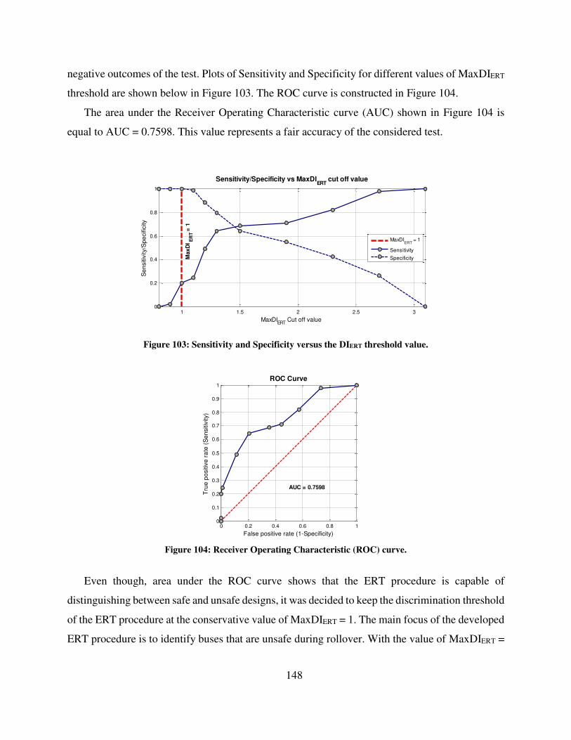
148
negative outcomes of the test. Plots of Sensitivity and Specificity for different values of MaxDIERT
threshold are shown below in Figure 103. The ROC curve is constructed in Figure 104.
The area under the Receiver Operating Characteristic curve (AUC) shown in Figure 104 is
equal to AUC = 0.7598. This value represents a fair accuracy of the considered test.
1 1.5 2 2.5 30
0.2
0.4
0.6
0.8
1
Sensitivity/Specificity vs MaxDIERT
cut off value
MaxDIERT
Cut off value
Se
nsitiv
ity/S
pe
cific
ity
MaxD
IE
RT =
1
MaxDIERT
= 1
Sensitivity
Specificity
Figure 103: Sensitivity and Specificity versus the DIERT threshold value.
0 0.2 0.4 0.6 0.8 10
0.1
0.2
0.3
0.4
0.5
0.6
0.7
0.8
0.9
1ROC Curve
False positive rate (1-Specificity)
Tru
e p
ositiv
e r
ate
(S
en
sitiv
ity)
AUC = 0.7598
Figure 104: Receiver Operating Characteristic (ROC) curve.
Even though, area under the ROC curve shows that the ERT procedure is capable of
distinguishing between safe and unsafe designs, it was decided to keep the discrimination threshold
of the ERT procedure at the conservative value of MaxDIERT = 1. The main focus of the developed
ERT procedure is to identify buses that are unsafe during rollover. With the value of MaxDIERT =
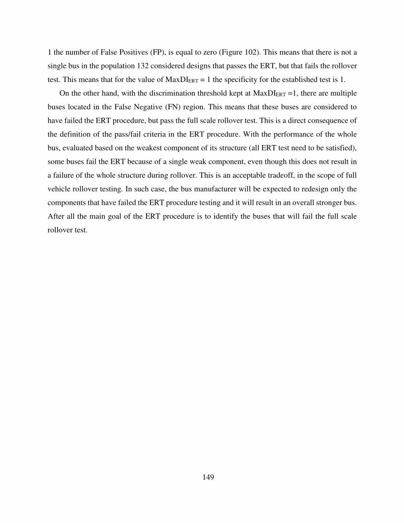
149
1 the number of False Positives (FP), is equal to zero (Figure 102). This means that there is not a
single bus in the population 132 considered designs that passes the ERT, but that fails the rollover
test. This means that for the value of MaxDIERT = 1 the specificity for the established test is 1.
On the other hand, with the discrimination threshold kept at MaxDIERT =1, there are multiple
buses located in the False Negative (FN) region. This means that these buses are considered to
have failed the ERT procedure, but pass the full scale rollover test. This is a direct consequence of
the definition of the pass/fail criteria in the ERT procedure. With the performance of the whole
bus, evaluated based on the weakest component of its structure (all ERT test need to be satisfied),
some buses fail the ERT because of a single weak component, even though this does not result in
a failure of the whole structure during rollover. This is an acceptable tradeoff, in the scope of full
vehicle rollover testing. In such case, the bus manufacturer will be expected to redesign only the
components that have failed the ERT procedure testing and it will result in an overall stronger bus.
After all the main goal of the ERT procedure is to identify the buses that will fail the full scale
rollover test.
150
CHAPTER 7
SUMMARY AND CONCLUSIONS
7.1. Summary
The FDOT testing framework established for the crashworthiness assessment of paratransit buses
has proven to be challenging in a real world applications. A dynamic full scale rollover test or a
development of a detailed FE model for the purpose of the numerical assessment, are either too
expensive or time consuming. In the light of these problems, there is a need for a new, simple and
reliable assessment tool. The objective of this dissertation was to perform a preliminary study on
feasibility of the development of the new simplified safety assessment protocol for
crashworthiness assessment of paratransit buses. The new protocol, the Equivalent Rollover
Testing (ERT) procedure, was developed based on the available resources and gathered
knowledge, and was intended to be relatively simple and economically viable.
This dissertation begins with the analysis of the epidemiological data, available for bus
accidents. The data obtained from FARS database was analyzed and compared with the accident
data from Europe. This comparison shows that the most dangerous accident scenario for buses is
the vehicle rollover. Even though rollover was a rare event, over a half of serious and fatal injuries
occurred when a vehicle rolled over during the accident. This observation has led other researchers
to focus on rollover as the most dangerous accident scenario for bus occupants. This effort resulted
in the introduction of two separate safety standards aiming to improve bus safety in case of the
rollover accident. The discussed standards are the FMVSS 220 used in the United States and
Canada and the ECE-Regulation 66 accepted by over 40 countries in the world. The variation of
the ECE-R66 is also utilized in the test standard developed by the FDOT often referred to as the
FDOT standard.
The two discussed safety standards (FMVSS 220 and ECE-R66) were used in this dissertation
as a starting point for the development of the new testing procedure. First, a case study on one of
the developed paratransit bus FE models was carried out. A selected bus was subjected to the
provisions of FMVSS 220 and ECE-R66. Even though both safety standards were developed for
the same purpose, evaluation of bus rollover crashworthiness, their outcome diverged for the
investigated bus. The tested vehicle passed the FMVSS 220 roof load test but has failed the ECE-
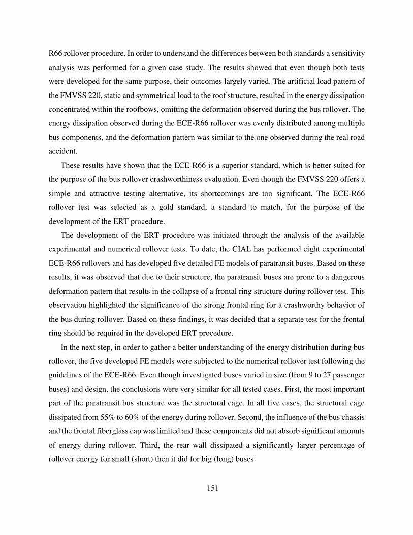
151
R66 rollover procedure. In order to understand the differences between both standards a sensitivity
analysis was performed for a given case study. The results showed that even though both tests
were developed for the same purpose, their outcomes largely varied. The artificial load pattern of
the FMVSS 220, static and symmetrical load to the roof structure, resulted in the energy dissipation
concentrated within the roofbows, omitting the deformation observed during the bus rollover. The
energy dissipation observed during the ECE-R66 rollover was evenly distributed among multiple
bus components, and the deformation pattern was similar to the one observed during the real road
accident.
These results have shown that the ECE-R66 is a superior standard, which is better suited for
the purpose of the bus rollover crashworthiness evaluation. Even though the FMVSS 220 offers a
simple and attractive testing alternative, its shortcomings are too significant. The ECE-R66
rollover test was selected as a gold standard, a standard to match, for the purpose of the
development of the ERT procedure.
The development of the ERT procedure was initiated through the analysis of the available
experimental and numerical rollover tests. To date, the CIAL has performed eight experimental
ECE-R66 rollovers and has developed five detailed FE models of paratransit buses. Based on these
results, it was observed that due to their structure, the paratransit buses are prone to a dangerous
deformation pattern that results in the collapse of a frontal ring structure during rollover test. This
observation highlighted the significance of the strong frontal ring for a crashworthy behavior of
the bus during rollover. Based on these findings, it was decided that a separate test for the frontal
ring should be required in the developed ERT procedure.
In the next step, in order to gather a better understanding of the energy distribution during bus
rollover, the five developed FE models were subjected to the numerical rollover test following the
guidelines of the ECE-R66. Even though investigated buses varied in size (from 9 to 27 passenger
buses) and design, the conclusions were very similar for all tested cases. First, the most important
part of the paratransit bus structure was the structural cage. In all five cases, the structural cage
dissipated from 55% to 60% of the energy during rollover. Second, the influence of the bus chassis
and the frontal fiberglass cap was limited and these components did not absorb significant amounts
of energy during rollover. Third, the rear wall dissipated a significantly larger percentage of
rollover energy for small (short) then it did for big (long) buses.
152
The analysis of energy dissipation within the bus rollover was further analyzed to formulate
the energy concept that forms the theoretical basis of the ERT procedure. A series of reduction
coefficients was either assumed or established through theoretical considerations, acquired
empirical and experimental experience. The developed coefficients accounted for effects such as
the effect of bus skin, eliminated inertial effect from test setup, or the composite action of entire
structure. Based on these studies, a procedure allowing to calculate a required threshold (pass/fail)
values for each tested bus component was established. Seven component tests, required to be
satisfied by the developed provisions of the ERT procedure were; frontal ring test, rear wall test,
wall to floor connection test, wall to roof connection test, panel impact test, static tube testing and
dynamic tube testing.
Since ERT procedure was formulated based on multiple assumptions, it was a necessity to
perform broad testing of the newly developed procedure. This task was carried out using five
developed and validated FE models of paratransit buses. Each model was subjected to multiple
structural changes where a certain component, e.g. wall to floor connection, was modified. This
effort resulted in a set of 132 paratransit buses, each with a different design. Each of the developed
models was further subjected to the rollover test, per ECE-R66 requirements, and to the provisions
of the newly developed ERT procedure. The test outcomes for both groups were further compared
using the analysis of Principal Components (PCA) and the analysis of the Receiver Operating
Characteristics (ROC).
The results show that the ERT procedure fulfills its original assumption, and allows to detect
and separate the buses that would fail the ECE-R66 rollover test. Out of all 132 evaluation cases
there was not a single bus that has satisfied all of the provisions of the ERT procedure but has
failed the ECE-R66 rollover. There were however buses that have failed to satisfy the provisions
of the ERT procedure but have passed the ECE-R66 rollover. This is a direct consequence of the
conservative approach proposed in the assumptions of the ERT procedure, where all of the tested
components need to pass the testing procedure. Some of the bus component, e.g. frontal ring, have
a more significant influence onto the entire structure than other e.g. wall to floor connection. A
strong frontal ring may result in the bus passing the ECE-R66 rollover, even if other components
would fail the ERT procedure. In such case the bus manufacturer would be required to either
improve offending component or subject the bus to a full scale rollover testing to prove that it is
safe.

153
7.2. Objectives
The objective of this dissertation was to develop a series of simple experiments, which combined
together, will result in a set of mathematical formulae for evaluation of the structure of each
individual paratransit bus. The achieved objectives of this dissertation are summarized below and
include:
Development of a new Equivalent Rollover Testing procedure for the assessment of
safety of paratransit buses during rollover accidents.
The ERT procedure was thought out to consist of a series of relatively simple and
inexpensive experimental tests on bus structure components.
Each test has been defined by giving a detailed description of the testing procedure.
The calculation procedures defining Threshold Values, which post requirements for
passing each test, have been developed based on the theoretical considerations,
supported by engineering judgment and gathered experience.
Low cost and simplicity of selected experiments allows more buses to be effectively
tested in a shorter period of time. The ERT procedure will serve as a very useful tool
for assessing vehicle safety for decision makers within purchasing organizations.
The ERT procedure was tested through 132 individual rollover tests, covering the entire
range of the population (weak, strong, small, and large buses).
Due to the provisions of ERT procedure, where the bus is evaluated based on its
weakest component, it is expected that some buses will fail the ERT procedure and pass
FDOT rollover test. In such case, the manufacturer will be expected to strengthen the
offending component, or subject the bus to the ECE-R66 rollover test.
Even though ERT indicated that some of the buses would fail the FDOT Standard
rollover test, when they did not, in all 132 test rollovers there was not a single case of
a bus passing the ERT and failing the rollover. This shows that ERT presents a
conservative approach to the rollover testing of paratransit buses.
154
7.3. Practical Recommendations
Manufacturers are encouraged to use the provisions of the Equivalent Rollover Testing
procedure in order to understand how to build safer paratransit buses.
The two most important component responsible for crashworthy behavior of the bus
during rollover are frontal ring and rear wall.
7.4. Suggestions for Further Research
Presented in this dissertation is the concept of the ERT procedure intended to increase test
efficiency, and to reduce cost associated with full scale rollover testing of paratransit buses. Even
though the ERT procedure was evaluated using five validated FE models of paratransit buses, it
requires to be supplemented by the extensive experimental testing.
First, in order for the ERT to become operational, a new test apparatus for a frontal ring and
the rear wall testing need to be constructed. Currently, this apparatus is in a design development
stage. It is intended that both, frontal ring and the rear wall tests, will be performed using the same
test setup. All other test apparatuses, required by the provisions of ERT, were constructed in the
past research, and no other additional work is required.
Second, the paratransit bus cage structures, obtained from the manufacturers need to be
subjected to the tests defined in the ERT procedure. It is recommended to accept a transition period
during the introduction of the new standard to allow the industry to familiarize itself with
requirements of the ERT standard. This can be achieved by requiring all components of tested
buses to demonstrate component DIERT (Equation (62)) below the value of 1.5 within the first year,
the values below 1.25 within the second year, and to comply with the entire regulation (DIERT < 1)
after two years.
It is recommended to eventually assess the rollover crashworthiness of a paratransit bus,
passing the requirements of the ERT procedure, through the full scale FDOT rollover test.
Comparison of results from these two tests will allow to do a “final check” of the ERT procedure
and highlight areas requiring improvement.
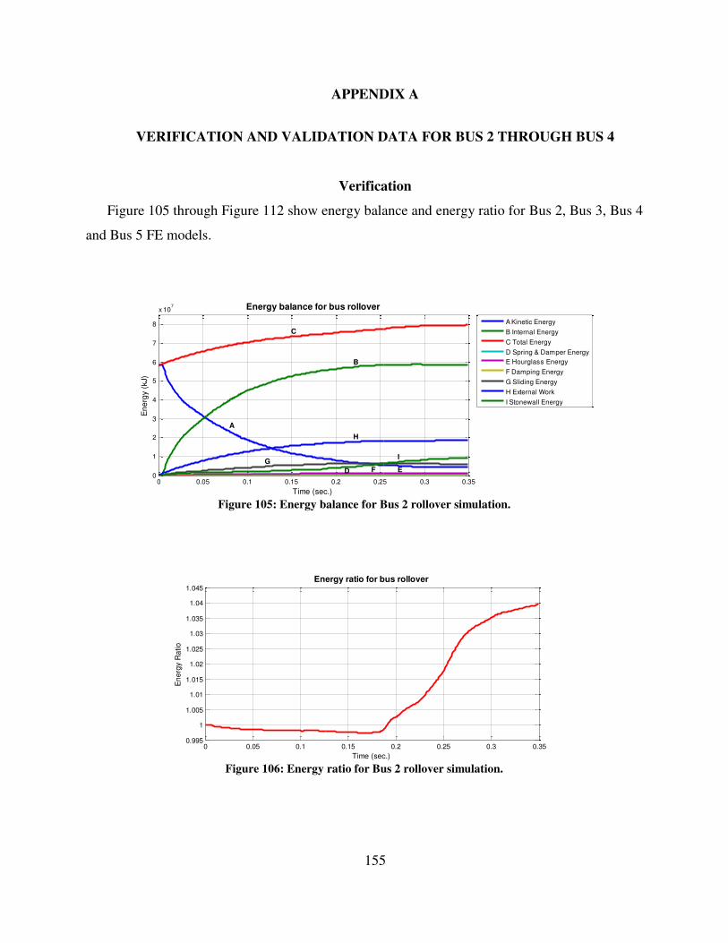
155
APPENDIX A
VERIFICATION AND VALIDATION DATA FOR BUS 2 THROUGH BUS 4
Verification
Figure 105 through Figure 112 show energy balance and energy ratio for Bus 2, Bus 3, Bus 4
and Bus 5 FE models.
Figure 105: Energy balance for Bus 2 rollover simulation.
Figure 106: Energy ratio for Bus 2 rollover simulation.
0 0.05 0.1 0.15 0.2 0.25 0.3 0.350
1
2
3
4
5
6
7
8
x 107 Energy balance for bus rollover
Time (sec.)
En
erg
y (
kJ)
A
B
C
D EFG
H
I
A Kinetic Energy
B Internal Energy
C Total Energy
D Spring & Damper Energy
E Hourglass Energy
F Damping Energy
G Sliding Energy
H External Work
I Stonewall Energy
0 0.05 0.1 0.15 0.2 0.25 0.3 0.350.995
1
1.005
1.01
1.015
1.02
1.025
1.03
1.035
1.04
1.045
Energy ratio for bus rollover
Time (sec.)
En
erg
y R
atio
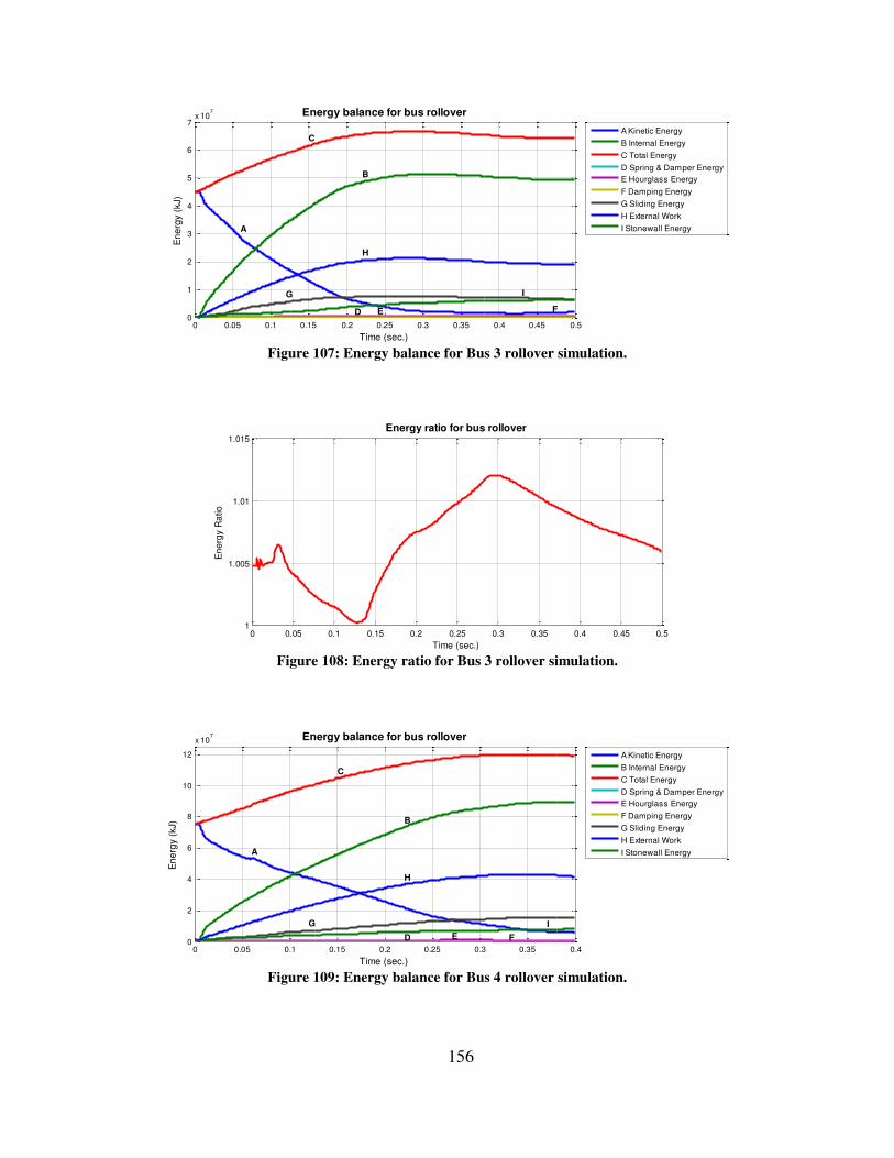
156
Figure 107: Energy balance for Bus 3 rollover simulation.
Figure 108: Energy ratio for Bus 3 rollover simulation.
Figure 109: Energy balance for Bus 4 rollover simulation.
0 0.05 0.1 0.15 0.2 0.25 0.3 0.35 0.4 0.45 0.50
1
2
3
4
5
6
7x 10
7 Energy balance for bus rollover
Time (sec.)
En
erg
y (
kJ)
A
B
C
D E F
G
H
I
A Kinetic Energy
B Internal Energy
C Total Energy
D Spring & Damper Energy
E Hourglass Energy
F Damping Energy
G Sliding Energy
H External Work
I Stonewall Energy
0 0.05 0.1 0.15 0.2 0.25 0.3 0.35 0.4 0.45 0.51
1.005
1.01
1.015
Energy ratio for bus rollover
Time (sec.)
En
erg
y R
atio
0 0.05 0.1 0.15 0.2 0.25 0.3 0.35 0.40
2
4
6
8
10
12
x 107 Energy balance for bus rollover
Time (sec.)
En
erg
y (
kJ)
A
B
C
D E F
G
H
I
A Kinetic Energy
B Internal Energy
C Total Energy
D Spring & Damper Energy
E Hourglass Energy
F Damping Energy
G Sliding Energy
H External Work
I Stonewall Energy
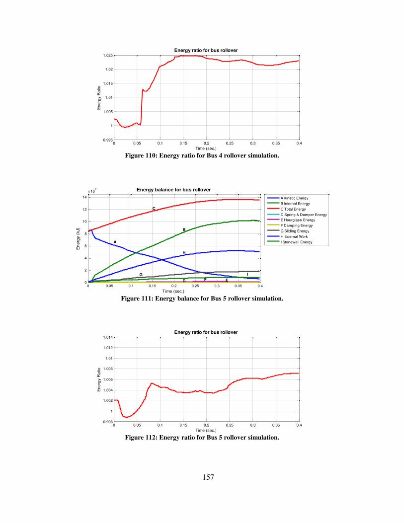
157
Figure 110: Energy ratio for Bus 4 rollover simulation.
Figure 111: Energy balance for Bus 5 rollover simulation.
Figure 112: Energy ratio for Bus 5 rollover simulation.
0 0.05 0.1 0.15 0.2 0.25 0.3 0.35 0.40.995
1
1.005
1.01
1.015
1.02
1.025
Energy ratio for bus rollover
Time (sec.)
En
erg
y R
atio
0 0.05 0.1 0.15 0.2 0.25 0.3 0.35 0.40
2
4
6
8
10
12
14
x 107 Energy balance for bus rollover
Time (sec.)
En
erg
y (
kJ)
A
B
C
D EF
G
H
I
A Kinetic Energy
B Internal Energy
C Total Energy
D Spring & Damper Energy
E Hourglass Energy
F Damping Energy
G Sliding Energy
H External Work
I Stonewall Energy
0 0.05 0.1 0.15 0.2 0.25 0.3 0.35 0.40.998
1
1.002
1.004
1.006
1.008
1.01
1.012
1.014
Energy ratio for bus rollover
Time (sec.)
En
erg
y R
atio

158
Validation Experiments
Bus 2
Figure 113 and Figure 114 show the comparison of the experimental and numerical results
obtained from the connection tests performed for Bus 2. Table 32 shows the maximum moment,
energy absorbed by the connection within the 0-20 deg. range, as well as relative error obtained
for both measurements. Validation of Bus 2 FE model was presented before and is published in
[Bojanowski 2010].
Figure 113: Wall to floor connection test for Bus 2. Experimental results compared with FE analysis.
Figure 114: Roof to wall connection test for Bus 2. Experimental results compared with FE analysis.
0 2 4 6 8 10 12 14 16 18 200
50
100
150
200
250
300
350
400
450
500Wall to Floor Connection Test
Angle of rotation (deg.)
Mo
me
nt
(Nm
)
Experiment
FE Analysis
0 2 4 6 8 10 12 14 16 18 200
50
100
150
200
250Roof to Wall Connection Test
Angle of rotation (deg.)
Mo
me
nt
(Nm
)
Experiment
FE Analysis
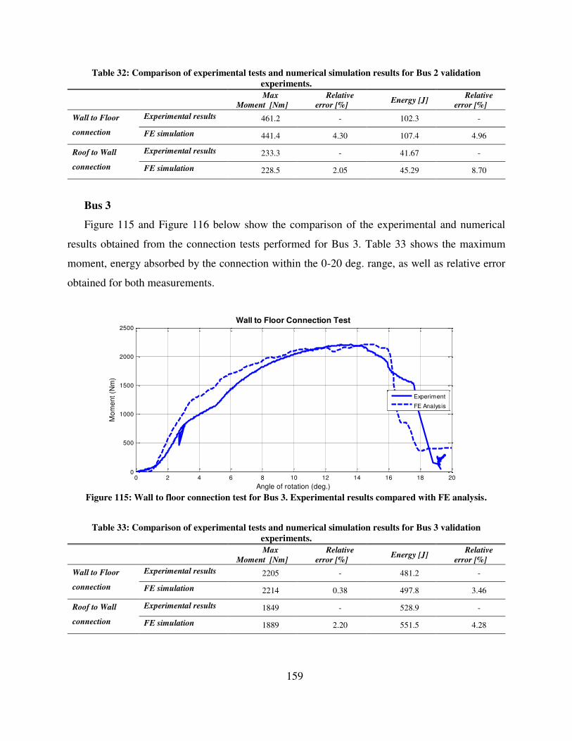
159
Table 32: Comparison of experimental tests and numerical simulation results for Bus 2 validation
experiments.
Max
Moment [Nm]
Relative
error [%] Energy [J]
Relative
error [%]
Wall to Floor
connection
Experimental results 461.2 - 102.3 -
FE simulation 441.4 4.30 107.4 4.96
Roof to Wall
connection
Experimental results 233.3 - 41.67 -
FE simulation 228.5 2.05 45.29 8.70
Bus 3
Figure 115 and Figure 116 below show the comparison of the experimental and numerical
results obtained from the connection tests performed for Bus 3. Table 33 shows the maximum
moment, energy absorbed by the connection within the 0-20 deg. range, as well as relative error
obtained for both measurements.
Figure 115: Wall to floor connection test for Bus 3. Experimental results compared with FE analysis.
Table 33: Comparison of experimental tests and numerical simulation results for Bus 3 validation
experiments.
Max
Moment [Nm]
Relative
error [%] Energy [J]
Relative
error [%]
Wall to Floor
connection
Experimental results 2205 - 481.2 -
FE simulation 2214 0.38 497.8 3.46
Roof to Wall
connection
Experimental results 1849 - 528.9 -
FE simulation 1889 2.20 551.5 4.28
0 2 4 6 8 10 12 14 16 18 200
500
1000
1500
2000
2500Wall to Floor Connection Test
Angle of rotation (deg.)
Mo
me
nt
(Nm
)
Experiment
FE Analysis

160
Figure 116: Roof to wall connection test for Bus 3. Experimental results compared with FE analysis.
Bus 4 and Bus 5
Figure 117 and Figure 118 below show the comparison of the experimental and numerical
results obtained from the connection tests performed for Bus 4 and Bus 5. Due to the fact that Bus
4 and Bus 5 are built using the same design, differing only in wheelbase, validation experiments
for both buses are performed on the same samples. Table 33 shows the maximum moment, energy
absorbed by the connection within the 0-20 deg. range, as well as relative error obtained for both
measurements.
Figure 117: Wall to floor connection test for Bus 4 and Bus 5. Experimental results compared with FE
analysis.
0 2 4 6 8 10 12 14 16 18 200
500
1000
1500
2000
2500Roof to Wall Connection Test
Angle of rotation (deg.)
Mo
me
nt
(Nm
)
Experiment
FE Analysis
0 2 4 6 8 10 12 14 16 18 200
200
400
600
800
1000
1200Wall to Floor Connection Test
Angle of rotation (deg.)
Mo
me
nt
(Nm
)
Experiment
FE Analysis
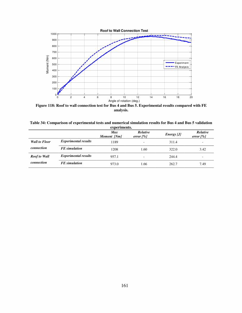
161
Figure 118: Roof to wall connection test for Bus 4 and Bus 5. Experimental results compared with FE
analysis.
Table 34: Comparison of experimental tests and numerical simulation results for Bus 4 and Bus 5 validation
experiments.
Max
Moment [Nm]
Relative
error [%] Energy [J]
Relative
error [%]
Wall to Floor
connection
Experimental results 1189 - 311.4 -
FE simulation 1208 1.60 322.0 3.42
Roof to Wall
connection
Experimental results 957.1 - 244.4 -
FE simulation 973.0 1.66 262.7 7.49
0 2 4 6 8 10 12 14 16 18 200
100
200
300
400
500
600
700
800
900
1000Roof to Wall Connection Test
Angle of rotation (deg.)
Mo
me
nt
(Nm
)
Experiment
FE Analysis
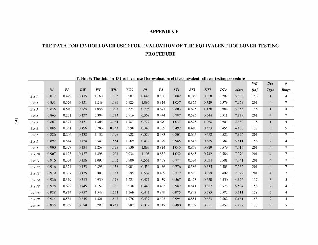
APPENDIX B
THE DATA FOR 132 ROLLOVER USED FOR EVALUATION OF THE EQUIVALENT ROLLOVER TESTING
PROCEDURE
Table 35: The data for 132 rollover used for evaluation of the equivalent rollover testing procedure
DI FR RW WF WR1 WR2 P1 P2 ST1 ST2 DT1 DT2 Mass
WB
[in]
Bus
Type
#
Rings
Bus 1 0.817 0.429 0.415 1.160 1.102 0.907 0.645 0.568 0.882 0.742 0.858 0.707 5.985 158 1 4
Bus 2 0.851 0.324 0.431 1.249 1.186 0.923 1.093 0.824 1.037 0.853 0.729 0.579 7.659 201 4 7
Bus 3 0.858 0.810 0.285 1.056 1.003 0.825 0.795 0.697 0.803 0.675 1.136 0.964 5.956 158 1 4
Bus 4 0.863 0.201 0.437 0.904 1.173 0.916 0.569 0.474 0.787 0.595 0.644 0.511 7.879 201 4 7
Bus 5 0.867 0.377 0.431 1.866 2.164 1.787 0.777 0.690 1.037 0.878 1.068 0.904 5.950 158 1 4
Bus 6 0.885 0.361 0.496 0.786 0.953 0.998 0.347 0.369 0.492 0.410 0.553 0.455 4.868 137 3 5
Bus 7 0.886 0.206 0.432 1.132 1.196 0.928 0.579 0.483 0.801 0.605 0.652 0.522 7.826 201 4 7
Bus 8 0.892 0.814 0.754 2.543 1.554 1.269 0.437 0.399 0.985 0.843 0.685 0.582 5.611 158 2 4
Bus 9 0.900 0.327 0.434 1.258 1.195 0.930 1.093 0.824 1.045 0.859 0.729 0.579 7.715 201 4 7
Bus 10 0.907 0.173 0.437 1.498 1.203 0.934 1.105 0.832 1.052 0.865 0.742 0.586 7.770 201 4 7
Bus 11 0.916 0.374 0.436 1.093 1.152 0.900 0.561 0.468 0.774 0.584 0.634 0.501 7.741 201 4 7
Bus 12 0.916 0.374 0.433 0.893 1.156 0.903 0.559 0.466 0.776 0.586 0.635 0.503 7.762 201 4 7
Bus 13 0.919 0.377 0.435 0.888 1.153 0.895 0.569 0.469 0.772 0.583 0.629 0.499 7.729 201 4 7
Bus 14 0.926 0.319 0.515 0.930 1.176 1.225 0.471 0.439 0.567 0.473 0.650 0.550 4.826 137 3 5
Bus 15 0.928 0.692 0.745 1.157 1.161 0.938 0.440 0.403 0.982 0.841 0.687 0.578 5.594 158 2 4
Bus 16 0.928 0.814 0.757 2.543 1.554 1.269 0.441 0.399 0.985 0.843 0.685 0.582 5.611 158 2 4
Bus 17 0.934 0.584 0.645 1.821 1.546 1.276 0.437 0.403 0.994 0.851 0.683 0.582 5.661 158 2 4
Bus 18 0.935 0.359 0.679 0.782 0.947 0.992 0.329 0.347 0.490 0.407 0.551 0.453 4.838 137 3 5
162

Table 35 - continued
DI FR RW WF WR1 WR2 P1 P2 ST1 ST2 DT1 DT2 Mass
WB
[in]
Bus
Type
#
Rings
Bus 19 0.939 0.674 0.494 0.784 0.949 0.994 0.341 0.362 0.491 0.408 0.552 0.453 4.850 137 3 5
Bus 20 0.940 0.327 0.434 1.258 1.195 0.930 1.093 0.824 1.045 0.859 0.729 0.579 7.715 201 4 7
Bus 21 0.941 0.988 0.420 1.255 1.192 0.980 0.709 0.613 0.955 0.803 0.957 0.807 5.604 138 1 3
Bus 22 0.941 0.326 0.428 2.049 1.183 0.921 1.089 0.821 1.035 0.851 0.732 0.580 7.642 201 4 7
Bus 23 0.951 0.595 0.758 2.553 1.538 1.270 0.436 0.400 0.989 0.847 0.679 0.578 5.633 158 2 4
Bus 24 0.957 0.324 0.431 1.249 1.186 0.923 1.093 0.824 1.037 0.853 0.729 0.579 7.659 201 4 7
Bus 25 0.961 0.606 0.515 0.929 0.575 0.600 0.477 0.438 0.566 0.473 0.660 0.548 4.818 137 3 5
Bus 26 0.961 0.608 0.515 0.928 0.575 0.600 0.476 0.437 0.566 0.473 0.652 0.550 4.818 137 3 5
Bus 27 0.962 0.602 0.514 0.930 0.558 0.581 0.454 0.446 0.567 0.473 0.650 0.548 4.826 137 3 5
Bus 28 0.964 0.594 0.514 0.858 0.576 0.601 0.449 0.442 0.567 0.473 0.650 0.545 4.823 137 3 5
Bus 29 0.970 0.345 0.555 0.885 1.209 1.286 0.470 0.437 1.134 0.946 1.447 1.169 4.821 137 3 5
Bus 30 0.971 0.630 0.517 1.296 0.575 0.599 0.493 0.458 0.566 0.472 0.652 0.547 4.813 137 3 5
Bus 31 0.973 0.762 0.670 2.535 1.162 0.938 0.435 0.393 0.982 0.841 0.655 0.568 5.594 158 2 4
Bus 32 0.978 0.354 0.565 1.622 2.574 2.764 0.455 0.466 1.127 0.940 1.415 1.162 4.794 137 3 5
Bus 33 0.978 1.491 0.508 1.868 2.166 1.788 0.778 0.691 1.037 0.878 1.074 0.903 5.917 158 1 4
Bus 34 0.978 0.342 0.429 1.245 2.568 2.149 1.090 0.823 1.034 0.850 0.730 0.578 7.631 201 4 7
Bus 35 0.982 0.185 0.425 2.215 2.679 2.191 1.420 1.295 1.545 1.271 2.142 1.755 7.699 201 4 7
Bus 36 0.983 0.642 0.522 2.270 0.574 0.599 0.459 0.472 0.565 0.472 0.659 0.545 4.809 137 3 5
Bus 37 0.983 0.477 0.534 0.677 0.923 0.982 0.358 0.331 0.867 0.723 1.043 0.859 4.804 137 3 5
Bus 38 0.984 0.605 0.514 0.927 1.171 1.220 0.468 0.436 0.565 0.472 0.659 0.551 4.808 137 3 5
Bus 39 0.989 0.610 0.519 0.925 0.813 0.853 0.484 0.456 0.564 0.471 0.660 0.547 4.799 137 3 5
Bus 40 0.991 0.886 0.419 1.155 1.097 0.902 0.633 0.563 0.878 0.739 0.845 0.702 5.956 158 1 4
Bus 41 0.992 0.645 0.421 0.952 0.860 0.706 0.495 0.453 0.696 0.585 0.637 0.529 5.983 158 1 7
Bus 42 0.993 0.358 2.132 0.780 0.945 0.990 0.341 0.360 0.488 0.406 0.551 0.456 4.826 137 3 5
Bus 43 0.997 0.209 0.418 0.960 1.246 0.973 0.601 0.505 0.836 0.632 0.684 0.544 9.354 254 5 9
163

Table 35 - continued
DI FR RW WF WR1 WR2 P1 P2 ST1 ST2 DT1 DT2 Mass
WB
[in]
Bus
Type
#
Rings
Bus 44 0.998 0.358 1.094 0.780 0.945 0.991 0.341 0.360 0.489 0.406 0.551 0.456 4.830 137 3 5
Bus 45 0.998 0.357 0.570 2.528 4.132 4.419 0.425 0.445 1.125 0.939 1.420 1.160 4.784 137 3 5
Bus 46 1.005 0.612 0.525 0.925 1.615 1.604 0.475 0.470 0.564 0.470 0.645 0.541 4.793 137 3 5
Bus 47 1.013 0.209 0.417 1.178 1.242 0.970 0.596 0.500 0.834 0.630 0.683 0.540 9.326 254 5 9
Bus 48 1.016 0.684 0.420 1.008 0.910 0.747 0.528 0.479 0.737 0.620 0.684 0.553 5.977 158 1 6
Bus 49 1.019 0.816 0.650 2.550 1.557 1.272 0.441 0.399 0.988 0.846 0.685 0.582 5.626 158 2 4
Bus 50 1.023 0.324 0.431 1.249 1.186 0.923 1.093 0.824 1.037 0.853 0.729 0.579 7.659 201 4 7
Bus 51 1.023 0.213 0.417 0.979 1.270 0.986 0.620 0.519 0.851 0.643 0.698 0.555 9.310 254 5 9
Bus 52 1.025 0.214 0.413 1.199 1.266 0.983 0.609 0.506 0.848 0.641 0.691 0.553 9.282 254 5 9
Bus 53 1.025 1.037 0.424 1.296 0.905 0.711 0.484 0.449 0.669 0.557 0.610 0.501 5.993 158 1 4
Bus 54 1.029 0.740 0.746 1.161 1.554 1.269 0.441 0.399 0.985 0.843 0.685 0.582 5.612 158 2 4
Bus 55 1.033 0.621 0.553 0.882 1.204 1.281 0.480 0.436 1.130 0.942 1.435 1.165 4.804 137 3 5
Bus 56 1.035 0.621 0.553 0.882 1.204 1.281 0.480 0.436 1.130 0.942 1.435 1.165 4.804 137 3 5
Bus 57 1.035 0.344 0.425 2.182 2.636 2.157 1.395 1.264 1.521 1.252 2.082 1.707 7.581 201 4 7
Bus 58 1.042 0.802 0.420 1.183 1.068 0.877 0.630 0.569 0.865 0.728 0.832 0.693 5.966 158 1 5
Bus 59 1.046 0.655 0.562 1.616 2.564 2.753 0.457 0.458 1.123 0.937 1.423 1.161 4.776 137 3 5
Bus 60 1.046 0.341 0.412 1.342 1.275 0.992 1.156 0.881 1.114 0.916 0.786 0.622 9.087 254 5 9
Bus 61 1.049 0.216 0.411 2.469 1.263 0.980 0.610 0.498 0.846 0.639 0.691 0.550 9.258 254 5 9
Bus 62 1.050 0.887 0.397 1.156 1.098 0.904 0.647 0.565 0.879 0.739 0.844 0.704 5.936 158 1 4
Bus 63 1.053 0.814 0.757 2.543 1.554 1.269 0.441 0.399 0.985 0.843 0.685 0.582 5.611 158 2 4
Bus 64 1.053 0.182 0.417 1.608 1.291 1.002 1.161 0.896 1.129 0.929 0.798 0.629 9.207 254 5 9
Bus 65 1.054 0.886 0.419 1.155 1.097 0.902 0.633 0.563 0.878 0.739 0.845 0.702 5.935 158 1 4
Bus 66 1.054 0.886 0.419 1.155 1.097 0.902 0.633 0.563 0.878 0.739 0.845 0.702 5.956 158 1 4
Bus 67 1.054 0.886 0.419 1.155 1.097 0.902 0.633 0.563 0.878 0.739 0.845 0.702 5.956 158 1 4
Bus 68 1.057 0.928 0.416 1.644 1.097 0.903 0.654 0.573 0.878 0.738 0.842 0.708 5.949 158 1 4
164

Table 35 - continued
DI FR RW WF WR1 WR2 P1 P2 ST1 ST2 DT1 DT2 Mass
WB
[in]
Bus
Type
#
Rings
Bus 69 1.060 0.667 0.567 2.519 4.114 4.398 0.422 0.440 1.121 0.935 1.420 1.153 4.767 137 3 5
Bus 70 1.067 0.621 0.553 0.882 1.204 1.281 0.480 0.436 1.130 0.942 1.435 1.165 4.804 137 3 5
Bus 71 1.070 1.647 0.431 2.010 2.330 1.923 0.853 0.744 1.117 0.945 1.214 1.021 5.568 138 1 3
Bus 72 1.071 1.534 0.417 1.295 0.905 0.711 0.479 0.448 0.668 0.555 0.610 0.501 5.988 158 1 4
Bus 73 1.072 0.994 0.415 2.657 1.133 0.932 0.653 0.584 0.906 0.762 0.888 0.741 5.944 158 1 4
Bus 74 1.075 0.952 0.416 1.263 1.199 0.986 0.714 0.620 0.960 0.808 0.967 0.810 6.288 176 1 4
Bus 75 1.077 0.321 1.373 1.237 1.175 0.914 1.084 0.816 1.027 0.845 0.727 0.574 7.584 201 4 7
Bus 76 1.077 0.389 0.415 0.949 1.229 0.960 0.603 0.495 0.825 0.623 0.676 0.536 9.227 254 5 9
Bus 77 1.077 0.884 0.462 1.152 1.095 0.900 0.629 0.561 0.876 0.737 0.844 0.705 5.962 158 1 4
Bus 78 1.078 0.836 0.766 2.543 10.09 7.081 0.441 0.399 0.985 0.843 0.685 0.582 5.611 158 2 4
Bus 79 1.079 0.946 0.426 1.173 1.528 1.275 0.650 0.579 0.891 0.750 0.869 0.722 5.948 158 1 4
Bus 80 1.086 0.321 1.420 1.236 1.174 0.913 1.078 0.814 1.026 0.844 0.725 0.574 7.579 201 4 7
Bus 81 1.094 0.883 0.517 1.151 1.093 0.899 0.629 0.561 0.875 0.736 0.844 0.705 5.956 158 1 4
Bus 82 1.095 0.879 0.753 15.37 1.554 1.269 0.441 0.399 0.985 0.843 0.685 0.582 5.611 158 2 4
Bus 83 1.099 0.943 0.412 1.264 1.201 0.988 0.711 0.625 0.962 0.809 0.966 0.810 6.571 190 1 5
Bus 84 1.100 0.223 0.411 1.168 3.177 2.658 0.585 0.488 0.826 0.624 0.677 0.536 9.245 254 5 9
Bus 85 1.116 0.944 0.758 7.083 6.183 4.671 0.438 0.400 0.985 0.843 0.673 0.577 5.611 158 2 4
Bus 86 1.123 0.886 0.419 1.155 1.097 0.902 0.633 0.563 0.878 0.739 0.845 0.702 5.956 158 1 4
Bus 87 1.124 0.814 0.757 2.543 1.554 1.269 0.441 0.399 0.985 0.843 0.685 0.582 5.592 158 2 4
Bus 88 1.137 0.883 0.530 1.151 1.093 0.899 0.629 0.561 0.875 0.736 0.844 0.705 5.944 158 1 4
Bus 89 1.143 0.341 0.412 1.342 1.275 0.992 1.156 0.881 1.114 0.916 0.786 0.622 9.086 254 5 9
Bus 90 1.146 0.295 2.358 2.133 3.592 3.814 0.504 0.508 1.216 1.019 2.069 1.616 4.728 137 3 5
Bus 91 1.149 0.799 0.724 1.135 1.549 1.648 0.590 0.563 1.454 1.213 2.272 1.832 4.804 137 3 5
Bus 92 1.163 0.194 0.405 2.372 2.870 2.347 1.520 1.425 1.655 1.362 2.426 1.997 9.107 254 5 9
Bus 93 1.174 0.338 1.361 1.330 1.264 0.983 1.149 0.874 1.105 0.908 0.779 0.619 9.007 254 5 9
165
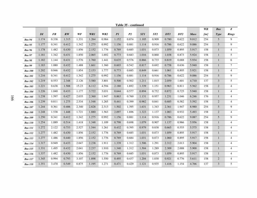
Table 35 - continued
DI FR RW WF WR1 WR2 P1 P2 ST1 ST2 DT1 DT2 Mass
WB
[in]
Bus
Type
#
Rings
Bus 94 1.174 0.338 1.315 1.331 1.264 0.984 1.152 0.874 1.105 0.909 0.780 0.622 9.012 254 5 9
Bus 95 1.177 0.341 0.412 1.342 1.275 0.992 1.156 0.881 1.114 0.916 0.786 0.622 9.086 254 5 9
Bus 96 1.178 1.482 0.430 1.856 2.152 1.776 0.769 0.685 1.031 0.873 1.059 0.895 5.917 158 1 4
Bus 97 1.181 1.342 0.431 1.850 2.065 1.692 0.773 0.683 1.016 0.860 1.038 0.873 5.924 158 1 5
Bus 98 1.182 1.144 0.431 1.576 1.760 1.441 0.635 0.576 0.866 0.733 0.819 0.688 5.934 158 1 6
Bus 99 1.183 1.080 0.432 1.488 1.661 1.360 0.603 0.542 0.817 0.692 0.758 0.636 5.940 158 1 7
Bus 100 1.202 0.946 0.432 1.854 2.153 1.777 0.773 0.685 0.849 0.661 1.061 0.895 5.921 158 1 4
Bus 101 1.216 0.341 0.412 1.342 1.275 0.992 1.156 0.881 1.114 0.916 0.786 0.622 9.086 254 5 9
Bus 102 1.219 0.553 2.348 2.126 3.580 3.801 0.500 0.502 1.211 1.015 2.059 1.601 4.710 137 3 5
Bus 103 1.221 0.638 1.508 15.23 6.112 4.594 2.180 1.692 1.339 1.151 0.963 0.811 5.562 158 2 4
Bus 104 1.226 1.040 0.433 1.177 3.722 3.031 0.644 0.577 0.894 0.752 0.872 0.725 5.940 158 1 4
Bus 105 1.238 1.597 0.427 2.035 2.360 1.947 0.863 0.760 1.131 0.957 1.231 1.046 6.246 176 1 4
Bus 106 1.239 0.811 1.275 2.534 1.548 1.265 0.441 0.399 0.982 0.841 0.685 0.582 5.592 158 2 4
Bus 107 1.244 0.361 0.406 2.340 2.828 2.313 1.502 1.395 1.631 1.343 2.361 1.947 8.980 254 5 9
Bus 108 1.248 1.538 1.448 1.721 1.880 1.563 2.097 1.696 1.323 1.137 1.083 0.932 5.493 158 2 4
Bus 109 1.250 0.341 0.412 1.342 1.275 0.992 1.156 0.881 1.114 0.916 0.786 0.622 9.087 254 5 9
Bus 110 1.254 1.089 0.514 1.418 1.348 1.109 0.798 0.698 1.079 0.907 1.137 0.966 5.956 158 1 4
Bus 111 1.272 2.122 0.753 2.527 1.544 1.261 0.432 0.395 0.979 0.838 0.665 0.555 5.575 158 2 4
Bus 112 1.277 1.482 0.430 1.856 2.152 1.776 0.769 0.685 1.031 0.873 1.059 0.895 5.917 158 1 4
Bus 113 1.277 1.486 0.440 1.856 2.152 1.776 0.769 0.684 1.031 0.873 1.060 0.895 5.917 158 1 4
Bus 114 1.317 0.949 0.433 2.047 2.238 1.911 1.339 1.312 1.506 1.291 2.312 2.013 5.904 158 1 4
Bus 115 1.331 1.495 0.432 2.041 2.237 1.910 1.340 1.312 1.504 1.289 2.309 2.008 5.900 158 1 4
Bus 116 1.337 1.482 0.430 1.856 2.152 1.776 0.769 0.685 1.031 0.873 1.059 0.895 5.917 158 1 4
Bus 117 1.345 0.994 0.793 3.107 1.898 1.550 0.495 0.437 1.204 1.030 0.921 0.776 5.611 158 2 4
Bus 118 1.351 3.470 0.549 0.875 1.195 1.271 0.471 0.429 1.121 0.935 1.416 1.154 4.766 137 3 5
166
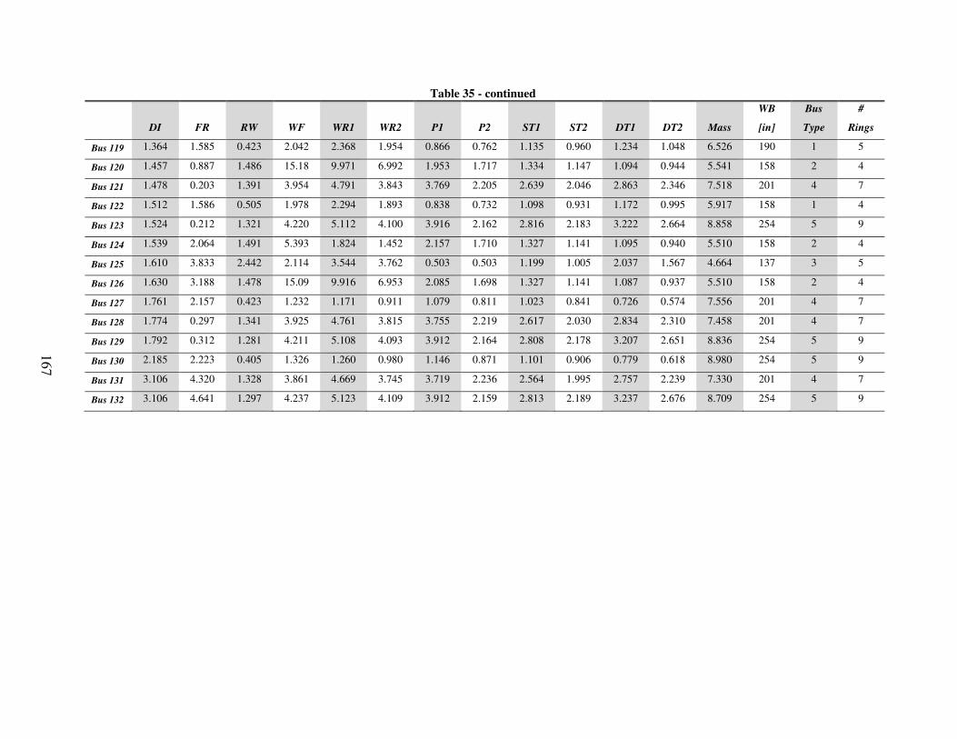
Table 35 - continued
DI FR RW WF WR1 WR2 P1 P2 ST1 ST2 DT1 DT2 Mass
WB
[in]
Bus
Type
#
Rings
Bus 119 1.364 1.585 0.423 2.042 2.368 1.954 0.866 0.762 1.135 0.960 1.234 1.048 6.526 190 1 5
Bus 120 1.457 0.887 1.486 15.18 9.971 6.992 1.953 1.717 1.334 1.147 1.094 0.944 5.541 158 2 4
Bus 121 1.478 0.203 1.391 3.954 4.791 3.843 3.769 2.205 2.639 2.046 2.863 2.346 7.518 201 4 7
Bus 122 1.512 1.586 0.505 1.978 2.294 1.893 0.838 0.732 1.098 0.931 1.172 0.995 5.917 158 1 4
Bus 123 1.524 0.212 1.321 4.220 5.112 4.100 3.916 2.162 2.816 2.183 3.222 2.664 8.858 254 5 9
Bus 124 1.539 2.064 1.491 5.393 1.824 1.452 2.157 1.710 1.327 1.141 1.095 0.940 5.510 158 2 4
Bus 125 1.610 3.833 2.442 2.114 3.544 3.762 0.503 0.503 1.199 1.005 2.037 1.567 4.664 137 3 5
Bus 126 1.630 3.188 1.478 15.09 9.916 6.953 2.085 1.698 1.327 1.141 1.087 0.937 5.510 158 2 4
Bus 127 1.761 2.157 0.423 1.232 1.171 0.911 1.079 0.811 1.023 0.841 0.726 0.574 7.556 201 4 7
Bus 128 1.774 0.297 1.341 3.925 4.761 3.815 3.755 2.219 2.617 2.030 2.834 2.310 7.458 201 4 7
Bus 129 1.792 0.312 1.281 4.211 5.108 4.093 3.912 2.164 2.808 2.178 3.207 2.651 8.836 254 5 9
Bus 130 2.185 2.223 0.405 1.326 1.260 0.980 1.146 0.871 1.101 0.906 0.779 0.618 8.980 254 5 9
Bus 131 3.106 4.320 1.328 3.861 4.669 3.745 3.719 2.236 2.564 1.995 2.757 2.239 7.330 201 4 7
Bus 132 3.106 4.641 1.297 4.237 5.123 4.109 3.912 2.159 2.813 2.189 3.237 2.676 8.709 254 5 9
167
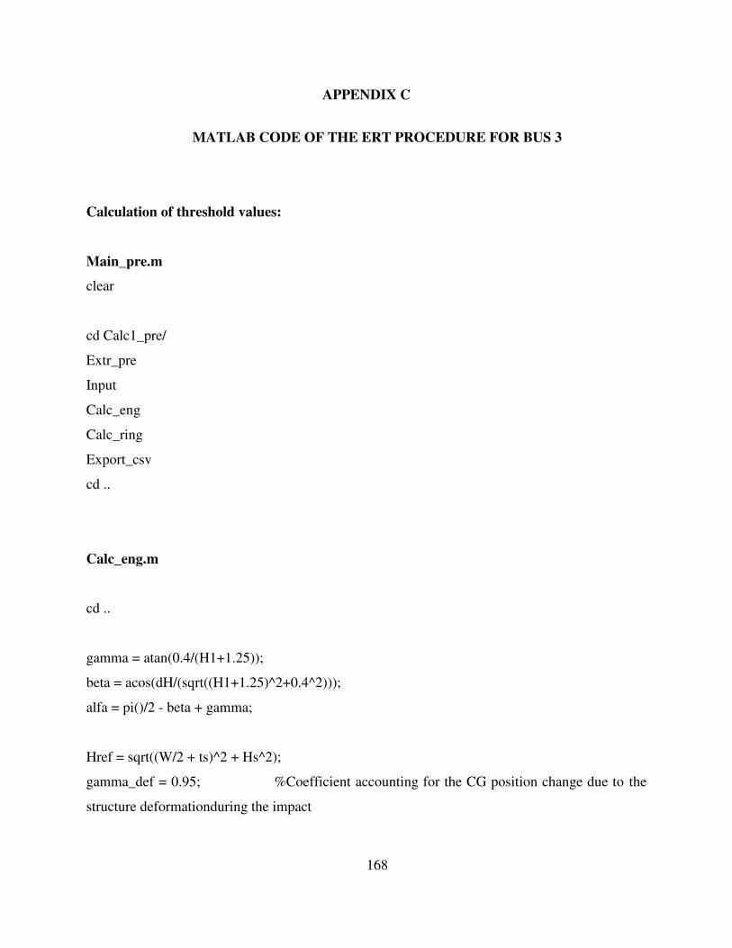
168
APPENDIX C
MATLAB CODE OF THE ERT PROCEDURE FOR BUS 3
Calculation of threshold values:
Main_pre.m
clear
cd Calc1_pre/
Extr_pre
Input
Calc_eng
Calc_ring
Export_csv
cd ..
Calc_eng.m
cd ..
gamma = atan(0.4/(H1+1.25));
beta = acos(dH/(sqrt((H1+1.25)^2+0.4^2)));
alfa = pi()/2 - beta + gamma;
Href = sqrt((W/2 + ts)^2 + Hs^2);
gamma_def = 0.95; %Coefficient accounting for the CG position change due to the
structure deformationduring the impact

169
Dhmax = gamma_def * Href - cos(alfa)*(W/2 + ts) + sin(alfa)*Hs;
Dhpre = Href -(W+2*ts)/(2*H)*sqrt(H^2-dH^2) + dH*Hs/H;
DhCG = Dhmax - (Dhmax - Dhpre)/2/(LRW - LFR)*(Ls - LFR);
Ee = M * g *DhCG;
Et = 0.75 * Ee;
%Rear wall reduction coefficient
K_RW = (K_RW_max * LWB_max - K_RW_min * LWB_min + (K_RW_min -
K_RW_max)*LWB)/(LWB_max-LWB_min);
if K_skin > 0.3 ; %Max allowable skin reduction 0.3
K_skin = 0.3;
end
Ec = (1-K_skin - K_RW - K_NS - K_FC)*Et;
Er = (1 - K_NR)*Ec;
cd Calc1_pre
Calc_ring.m
cd ..
lR = 0;
for i = 1:4
lR = lR + n(i)*(l(i)+l(4));
170
end
for i = 1:4
ERr(i) = (n(i)*(l(i)+l(4)))/lR*Er; %eNERGY DISTRIBUTION ONTO THE RINGS
end
ER_check = 0;
for i = 1:4
ER_check = ER_check +ERr(i);
end
ERr;
WRr_inv = ERr(rn - 1)*(1-K_NC);
ER_check;
for i = 1:5
BA(i) = (DAa(i)-5/2)/(DAa(1)+DAa(2)+DAa(3)+DAa(4)+DAa(5) - 4*5/2);
end
BA(2) = 0;
for i = 1:5
BB(i) = (DBa(i)-5/2)/(DBa(1)+DBa(2)+DBa(3)+DBa(4)+DBa(5) - 4*5/2);
end
171
BB(1) = 0;
for i = 1:5
BC(i) = (DCa(i)-5/2)/(DCa(1)+DCa(2)+DCa(3)+DCa(4)+DCa(5) - 5*5/2);
end
BA;
BB;
BC;
WFR = ERr(rn)*(1-K_NC);
WRW = K_RW*Et*(1-K_NC);
WWF = WRr_inv*BA(1);
WWR(1) = WRr_inv*BC(3);
WWR(2) = WRr_inv*BB(3);
WP_eng(1) = WRr_inv*BC(2);
WP_eng(2) = WRr_inv*BB(2);
WP_ang(1) = DCa(2);
WP_ang(2) = DBa(2);
WST_eng(1) = WWR(1);
WST_eng(2) = WWR(2);
WDT_eng(1) = WWR(1);
WDT_eng(2) = WWR(2);
172
WDT_ang(1) = DCa(3);
WDT_ang(2) = DBa(3);
WFR;
WRW;
WWF ;
WWR;
WP_eng;
WP_ang;
WST_eng;
WDT_eng;
WDT_ang;
cd Calc1_pre
Export_csv.m
cd ..
%Create energy input values for the 2_Final_testing simulations
for i = 1:2 %Loop creating input value matrix
Export(i,1) = i;
Export(i,2) = 2*WP_eng(i);
Export(i,3) = WDT_eng(i);
end

173
cd 2_Final_testing
Export;
header1=['Point,P_Energ,TD_Energ']; %Writing to the csv file with lsopt format
header2=['sk,dv,dv'];
outid = fopen('Eng_input.csv', 'w+');
fprintf(outid, '%s\n', header1);
fprintf(outid, '%s\n', header2);
fclose(outid);
dlmwrite ('Eng_input.csv',Export,'roffset',0,'-append')
cd ..
Threshold(1) = 1.000;
Threshold(2) = WFR*1000;
Threshold(3) = WRW*1000;
Threshold(4) = 2*WWF*1000;
Threshold(5) = 2*WWR(1)*1000;
Threshold(6) = 2*WWR(2)*1000;
Threshold(7) = WP_ang(1);
Threshold(8) = WP_ang(2);
Threshold(9) = WST_eng(1)*1000;
Threshold(10) = WST_eng(2)*1000;
Threshold(11) = WDT_ang(1);
Threshold(12) = WDT_ang(2);
Threshold;
174
header1=['Threshold_DI,Threshold_FR,Threshold_RW,Threshold_WF,Threshold_WR1,Thresh
old_WR2,Threshold_P1,Threshold_P2,Threshold_ST1,Threshold_ST2,Threshold_DT1,Threshol
d_DT2']; %Writing to the csv file with lsopt format
outid = fopen('Threshold.csv', 'w+');
fprintf(outid, '%s\n', header1);
fclose(outid);
dlmwrite ('Threshold.csv',Threshold,'roffset',0,'-append')
cd Calc1_pre
Extr_pre.m
%Read The Input data for the Simplified Procedure
cd ..
cd 0_Rollover/ROLLOVER_800mm/1.1/
log = dir('log*');
log = {log.name};
ix = regexp(log,'log\d+');
ix = ~cellfun('isempty',ix);
log = log(ix);
log1=log{1};
TheString = fileread(log1);
T = regexp(TheString,'physical mass=\s*(\S+)','tokens');
if isempty(T)
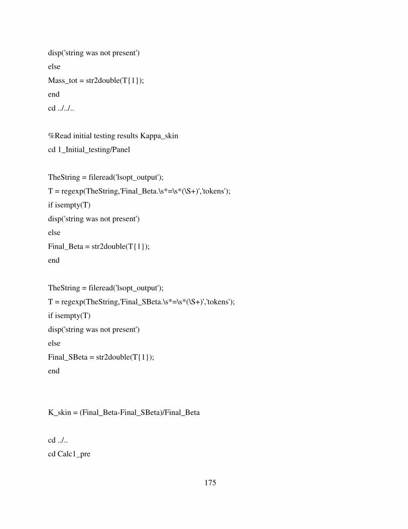
175
disp('string was not present')
else
Mass_tot = str2double(T{1});
end
cd ../../..
%Read initial testing results Kappa_skin
cd 1_Initial_testing/Panel
TheString = fileread('lsopt_output');
T = regexp(TheString,'Final_Beta.\s*=\s*(\S+)','tokens');
if isempty(T)
disp('string was not present')
else
Final_Beta = str2double(T{1});
end
TheString = fileread('lsopt_output');
T = regexp(TheString,'Final_SBeta.\s*=\s*(\S+)','tokens');
if isempty(T)
disp('string was not present')
else
Final_SBeta = str2double(T{1});
end
K_skin = (Final_Beta-Final_SBeta)/Final_Beta
cd ../..
cd Calc1_pre
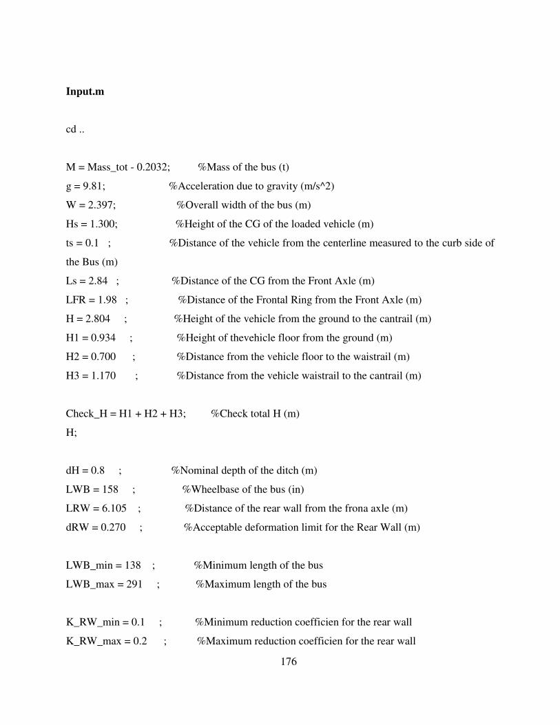
176
Input.m
cd ..
M = Mass_tot - 0.2032; %Mass of the bus (t)
g = 9.81; %Acceleration due to gravity (m/s^2)
W = 2.397; %Overall width of the bus (m)
Hs = 1.300; %Height of the CG of the loaded vehicle (m)
ts = 0.1 ; %Distance of the vehicle from the centerline measured to the curb side of
the Bus (m)
Ls = 2.84 ; %Distance of the CG from the Front Axle (m)
LFR = 1.98 ; %Distance of the Frontal Ring from the Front Axle (m)
H = 2.804 ; %Height of the vehicle from the ground to the cantrail (m)
H1 = 0.934 ; %Height of thevehicle floor from the ground (m)
H2 = 0.700 ; %Distance from the vehicle floor to the waistrail (m)
H3 = 1.170 ; %Distance from the vehicle waistrail to the cantrail (m)
Check_H = H1 + H2 + H3; %Check total H (m)
H;
dH = 0.8 ; %Nominal depth of the ditch (m)
LWB = 158 ; %Wheelbase of the bus (in)
LRW = 6.105 ; %Distance of the rear wall from the frona axle (m)
dRW = 0.270 ; %Acceptable deformation limit for the Rear Wall (m)
LWB_min = 138 ; %Minimum length of the bus
LWB_max = 291 ; %Maximum length of the bus
K_RW_min = 0.1 ; %Minimum reduction coefficien for the rear wall
K_RW_max = 0.2 ; %Maximum reduction coefficien for the rear wall
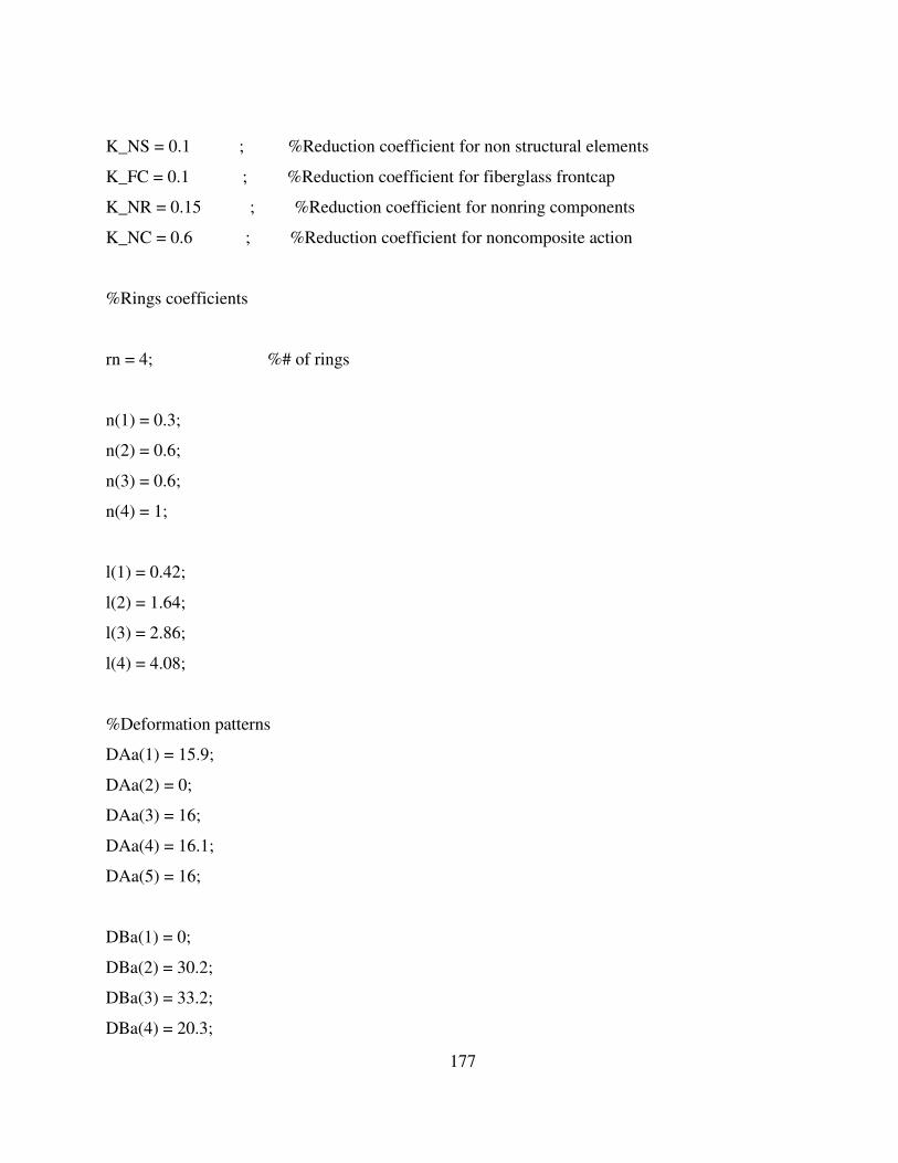
177
K_NS = 0.1 ; %Reduction coefficient for non structural elements
K_FC = 0.1 ; %Reduction coefficient for fiberglass frontcap
K_NR = 0.15 ; %Reduction coefficient for nonring components
K_NC = 0.6 ; %Reduction coefficient for noncomposite action
%Rings coefficients
rn = 4; %# of rings
n(1) = 0.3;
n(2) = 0.6;
n(3) = 0.6;
n(4) = 1;
l(1) = 0.42;
l(2) = 1.64;
l(3) = 2.86;
l(4) = 4.08;
%Deformation patterns
DAa(1) = 15.9;
DAa(2) = 0;
DAa(3) = 16;
DAa(4) = 16.1;
DAa(5) = 16;
DBa(1) = 0;
DBa(2) = 30.2;
DBa(3) = 33.2;
DBa(4) = 20.3;
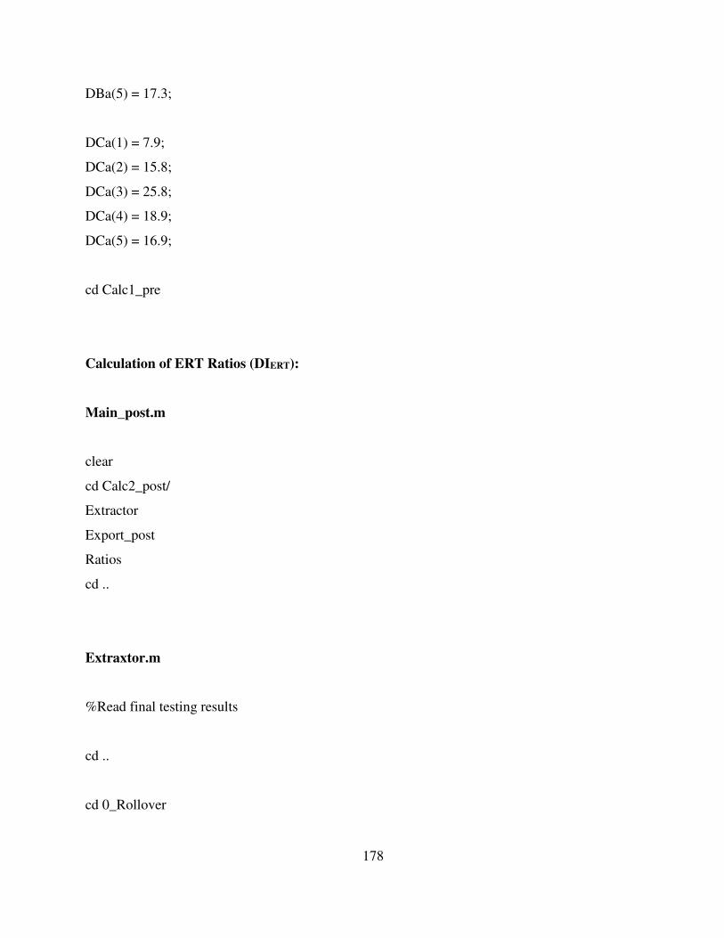
178
DBa(5) = 17.3;
DCa(1) = 7.9;
DCa(2) = 15.8;
DCa(3) = 25.8;
DCa(4) = 18.9;
DCa(5) = 16.9;
cd Calc1_pre
Calculation of ERT Ratios (DIERT):
Main_post.m
clear
cd Calc2_post/
Extractor
Export_post
Ratios
cd ..
Extraxtor.m
%Read final testing results
cd ..
cd 0_Rollover
179
TheString = fileread('lsopt_output');
%Read Frontal Ring Test
T = regexp(TheString,'SDI_alpha\s+(\S+)','tokens');
if isempty(T)
disp('string was not present')
else
DI_index = str2double(T{1});
end
cd ..
cd 2_Final_testing
TheString = fileread('lsopt_output');
%Read Frontal Ring Test
T = regexp(TheString,'FR_Energy1\s+(\S+)','tokens');
if isempty(T)
disp('string was not present')
else
FR_Energy1 = str2double(T{1});
end
%Read Back Wall Test
T = regexp(TheString,'BW_Energy1\s+(\S+)','tokens');
if isempty(T)
disp('string was not present')
else
BW_Energy1 = str2double(T{1});
end
180
%Read Wall-to-floor Test
T = regexp(TheString,'WF_Energy1\s+(\S+)','tokens');
if isempty(T)
disp('string was not present')
else
WF_Energy1 = str2double(T{1});
end
%Read Roof-to-wall Test
T = regexp(TheString,'RW_Energy1\s+(\S+)','tokens');
if isempty(T)
disp('string was not present')
else
RW_Energy1 = str2double(T{1});
end
T = regexp(TheString,'RW_Energy2\s+(\S+)','tokens');
if isempty(T)
disp('string was not present')
else
RW_Energy2 = str2double(T{1});
end
%Read Panel impact Test
T = regexp(TheString,'P_Final_Beta\s+(\S+)','tokens');
if isempty(T)
disp('string was not present')
else
P_Final_Beta1 = str2double(T{1});
end
181
T = regexp(TheString,'P_Final_Beta\s+\S+\s+(\S+)','tokens');
if isempty(T)
disp('string was not present')
else
P_Final_Beta2 = str2double(T{1});
end
%Read Tube static Test
T = regexp(TheString,'TS_Energy_abs_for_25_8\s+(\S+)','tokens');
if isempty(T)
disp('string was not present')
else
TS_Energy_1 = str2double(T{1});
end
T = regexp(TheString,'TS_Energy_abs_for_33_2\s+(\S+)','tokens');
if isempty(T)
disp('string was not present')
else
TS_Energy_2 = str2double(T{1});
end
%Read Tube Dynamic Test
T = regexp(TheString,'TD_Final_Beta\s+(\S+)','tokens');
if isempty(T)
disp('string was not present')
else
TD_Final_Beta1 = str2double(T{1});
end
182
T = regexp(TheString,'TD_Final_Beta\s+\S+\s+(\S+)','tokens');
if isempty(T)
disp('string was not present')
else
TD_Final_Beta2 = str2double(T{1});
end
cd ..
cd Calc2_post
Export_post.m
cd ..
Results(1) = DI_index;
Results(2) = FR_Energy1;
Results(3) = BW_Energy1;
Results(4) = WF_Energy1;
Results(5) = RW_Energy1;
Results(6) = RW_Energy2;
Results(7) = P_Final_Beta1;
Results(8) = P_Final_Beta2;
Results(9) = TS_Energy_1;
Results(10) = TS_Energy_2;
Results(11) = TD_Final_Beta1;
Results(12) = TD_Final_Beta2;
Results;
183
header1=['Results_DI,Results_FR,Results_RW,Results_WF,Results_WR1,Results_WR2,Results
_P1,Results_P2,Results_ST1,Results_ST2,Results_DT1,Results_DT2']; %Writing to the csv
file with lsopt format
outid = fopen('Results.csv', 'w+');
fprintf(outid, '%s\n', header1);
fclose(outid);
dlmwrite ('Results.csv',Results,'roffset',0,'-append')
cd Calc2_post
Ratios.m
cd ..
Results = dlmread('Results.csv',',',1,0);
Threshold = dlmread('Threshold.csv',',',1,0);
for i = 1:12 %Loop calculating threshold ratios
Ratio(i) = Threshold(i)/Results(i);
end
Ratio(1) = Results(1)/Threshold(1);
Ratio(7) = Results(7)/Threshold(7);
Ratio(8) = Results(8)/Threshold(8);
Ratio(11) = Results(11)/Threshold(11);
Ratio(12) = Results(12)/Threshold(12);
184
header1=['Ratio_DI,Ratio_FR,Ratio_RW,Ratio_WF,Ratio_WR1,Ratio_WR2,Ratio_P1,Ratio_P
2,Ratio_ST1,Ratio_ST2,Ratio_DT1,Ratio_DT2']; %Writing to the csv file with lsopt format
outid = fopen('Ratio.csv', 'w+');
fprintf(outid, '%s\n', header1);
fclose(outid);
dlmwrite ('Ratio.csv',Ratio,'roffset',0,'-append')
header1=['DI,FR,RW,WF,WR1,WR2,P1,P2,ST1,ST2,DT1,DT2']; %Writing to the csv file
with lsopt format
outid = fopen('Combine.csv', 'w+');
fprintf(outid, '%s\n', header1);
fclose(outid);
dlmwrite ('Combine.csv',Threshold,'roffset',0,'-append')
dlmwrite ('Combine.csv',Results,'roffset',0,'-append')
dlmwrite ('Combine.csv',Ratio,'roffset',0,'-append')
cd Calc2_post
185
APPENDIX D
PRINCIPAL COMPONENT ANALYSIS AND RECEIVER OPERATING
CHARACTERISTIC CURVE MATLAB CODES
Principal component analysis
clear
RatioGlobal = dlmread('Combine_gl_MTWB.csv',',',1,0);
RatioTrim = unique(RatioGlobal,'rows');
% RatioDI1 = [RatioTrim(:,2:12)];
% RatioDI1 = min(RatioDI1,3);
RatioDI1 = [RatioTrim(:,2:5)];
RatioDI11 = [RatioTrim(:,7)];
RatioDI12 = [RatioTrim(:,9)];
RatioDI13 = [RatioTrim(:,11)];
RatioDI1 = [RatioDI1,RatioDI11,RatioDI12,RatioDI13];
RatioDI1 = min(RatioDI1,3);
Bus_char1 = [RatioTrim(:,1)];
Bus_char2 = [RatioTrim(:,13)];
Bus_char3 = [RatioTrim(:,14)];
Bus_char4 = [max(RatioDI1,[],2)];
Bus_char5 = [sum(RatioDI1,2)];
Bus_char1T = min(Bus_char1,1.6);
Bus_char = [Bus_char1,Bus_char2,Bus_char3,Bus_char4,Bus_char5];
186
RatioDI2 = [Bus_char1,RatioDI1];
CrA = cronbach(RatioDI2);
CorDI = corrcoef(RatioDI2);
[pc,score,latent,tsquare] = princomp(RatioDI1);
[M,N] = size(RatioDI1);
stdR = std(Bus_char);
stdS = std(score);
std = stdR.' * stdS;
covRS = (1 / (M-1) * Bus_char.' * score);
loadings = covRS./std;
cd Figures
x = 0:0.01:3.5;
y = 1+0.000000001*x;
y1 = 0:0.01:3;
x1 = 1+0.000000001*y1;
figure('Position', [300, 400, 1000, 400]);
subplot(1,2,1);
plot(score(:,1),score(:,2),'o','MarkerEdgeColor' , [.2 .2 .2] , ...
'MarkerFaceColor' , [.7 .7 .7], 'LineWidth',1,'MarkerSize',6);
hTitle = title('Principal Components of ERT Data');
hXLabel = xlabel('Principal Component1'); % x-axis label;
hYLabel = ylabel('Principal Component2'); % y-axis label;
187
axis equal
grid on
set( gca , ...
'FontName' , 'Helvetica' );
set([hTitle, hXLabel, hYLabel], ...
'FontName' , 'AvantGarde');
set([hXLabel, hYLabel] , ...
'FontSize' , 10 );
set( hTitle , ...
'FontSize' , 12 , ...
'FontWeight' , 'bold' );
subplot(1,2,2);
plot(latent,'b-o','MarkerEdgeColor' , [.2 .2 .2] , ...
'MarkerFaceColor' , [.7 .7 .7], 'LineWidth',1.5,'Color', [0 0 .5]);
grid on
hTitle = title('Eigenvalues of the Covariance Matrix');
hXLabel = xlabel('Principal Component'); % x-axis label;
hYLabel = ylabel('Eigenvalue'); % y-axis label;
set( gca , ...
'FontName' , 'Helvetica' );
set([hTitle, hXLabel, hYLabel], ...
'FontName' , 'AvantGarde');
set([hXLabel, hYLabel] , ...
'FontSize' , 10 );
set( hTitle , ...
'FontSize' , 12 , ...
188
'FontWeight' , 'bold' );
set(gcf, 'PaperPositionMode', 'auto');
print -dmeta PCA8_Trim3_1.emf
xCenter = 0;
yCenter = 0;
theta = 0 : 0.01 : 2*pi;
radius = 1;
x = radius * cos(theta) + xCenter;
y = radius * sin(theta) + yCenter;
figure('Position', [100, 100, 1000, 1250]);
for n=1:3
subplot(3,2,2*n-1);
plot(score(:,1),score(:,n+1),'o','MarkerEdgeColor' , [.2 .2 .2] , ...
'MarkerFaceColor' , [.7 .7 .7], 'LineWidth',1,'MarkerSize',6);
grid on
xlim([-2 4.5])
ylim([-2 2.0])
str = strcat('Principal Component',' ',num2str(n+1));
hTitle = title('Principal Components of ERT Data');
hXLabel = xlabel('Principal Component1'); % x-axis label;
hYLabel = ylabel(str); % y-axis label;
set( gca , ...
'FontName' , 'Helvetica' );
189
set([hTitle, hXLabel, hYLabel], ...
'FontName' , 'AvantGarde');
set([hXLabel, hYLabel] , ...
'FontSize' , 10 );
set( hTitle , ...
'FontSize' , 12 , ...
'FontWeight' , 'bold' );
subplot(3,2,2*n);
plot(x,y,'g','LineWidth',2,'Color', [0 0 .5]);
hold on
plot(loadings(:,1),loadings(:,n+1),'o','MarkerEdgeColor' , [.2 .2 .2] , ...
'MarkerFaceColor' , [.7 .7 .7], 'LineWidth',1,'MarkerSize',6);
axis equal
grid on
xlim([-1.1 1.1])
ylim([-1.1 1.1])
hTitle = title('Circle of Correlation');
hXLabel = xlabel('Principal Component1'); % x-axis label;
hYLabel = ylabel(str); % y-axis label;
hText1 = text(loadings(1,1)+0.1,loadings(1,n+1),{'DI_{Roll}'},...
'FontSize',12);
hText2 = text(loadings(2,1)+0.1,loadings(2,n+1),{'Weight/WB'},...
'FontSize',12);
hText3 = text(loadings(3,1)+0.1,loadings(3,n+1),{'DI_{Roll}' 'Weight/WB' '' 'Max.
DI_{ERT}' 'Avg. DI_{ERT}'},...
'FontSize',12);

190
hText4 = text(loadings(4,1)+0.1,loadings(4,n+1),{'DI_{Roll}' 'Weight/WB' '' 'Max.
DI_{ERT}' 'Avg. DI_{ERT}'},...
'FontSize',12);
set( gca , ...
'FontName' , 'Helvetica' );
set([hTitle, hXLabel, hYLabel], ...
'FontName' , 'AvantGarde');
set([hXLabel, hYLabel] , ...
'FontSize' , 10 );
set( hTitle , ...
'FontSize' , 12 , ...
'FontWeight' , 'bold' );
end
set(gcf, 'PaperPositionMode', 'auto');
print -dmeta PCA8_Trim3_2.emf
figure('Position', [100, 100, 1000, 400]);
scatter(score(:,1),score(:,2),50,Bus_char1T,'fill', 'MarkerEdgeColor' , [.2 .2 .2]); colorbar;
grid on
xlim([-2 4.5])
ylim([-2 2.0])
set(gca,'Box', 'on')
hTitle = title('Correlation of Deformation Index (DI_{Roll}) with first and second principal
component');
hXLabel = xlabel('Principal Component1'); % x-axis label;
hYLabel = ylabel('Principal Component2'); % y-axis label;
hText = text(5.3, -0.9,'Deformation Index (DI_{Roll})');
191
set( gca , ...
'FontName' , 'Helvetica' );
set([hTitle, hXLabel, hYLabel], ...
'FontName' , 'AvantGarde');
set([hXLabel, hYLabel] , ...
'FontSize' , 10 );
set( hTitle , ...
'FontSize' , 12 , ...
'FontWeight' , 'bold' );
set( [hText], ...
'FontSize' , 10 );
set(hText, 'rotation', 90)
set(gcf, 'PaperPositionMode', 'auto');
print -dmeta PCA8_Trim3_3.emf
figure('Position', [100, 100, 1000, 400]);
scatter(score(:,1),score(:,2),50,Bus_char2,'fill', 'MarkerEdgeColor' , [.2 .2 .2]); colorbar;
grid on
xlim([-2 4.5])
ylim([-2 2.0])
set(gca,'Box', 'on')
hTitle = title('Correlation of Bus Mass with first and second principal component');
hXLabel = xlabel('Principal Component1'); % x-axis label;
hYLabel = ylabel('Principal Component2'); % y-axis label;
hText = text(5.3, -0.9,'Mass of the Bus [Tons]');
set( gca , ...

192
'FontName' , 'Helvetica' );
set([hTitle, hXLabel, hYLabel], ...
'FontName' , 'AvantGarde');
set([hXLabel, hYLabel] , ...
'FontSize' , 10 );
set( hTitle , ...
'FontSize' , 12 , ...
'FontWeight' , 'bold' );
set( [hText], ...
'FontSize' , 10 );
set(hText, 'rotation', 90)
set(gcf, 'PaperPositionMode', 'auto');
print -dmeta PCA8_Trim3_4.emf
figure('Position', [100, 100, 1000, 400]);
scatter(score(:,1),score(:,2),50,Bus_char5/N,'fill', 'MarkerEdgeColor' , [.2 .2 .2]); colorbar;
grid on
xlim([-2 4.5])
ylim([-2 2.0])
set(gca,'Box', 'on')
hTitle = title('Correlation of avreage test result Avg. DI_{ERT} with first and second principal
component');
hXLabel = xlabel('Principal Component1'); % x-axis label;
hYLabel = ylabel('Principal Component2'); % y-axis label;
hText = text(5.3, -0.2,'Avg. DI_{ERT}');
set( gca , ...
'FontName' , 'Helvetica' );
193
set([hTitle, hXLabel, hYLabel], ...
'FontName' , 'AvantGarde');
set([hXLabel, hYLabel] , ...
'FontSize' , 10 );
set( hTitle , ...
'FontSize' , 12 , ...
'FontWeight' , 'bold' );
set( [hText], ...
'FontSize' , 10 );
set(hText, 'rotation', 90)
set(gcf, 'PaperPositionMode', 'auto');
print -dmeta PCA8_Trim3_5.emf
figure('Position', [100, 100, 1000, 400]);
scatter(score(:,1),score(:,2),50,Bus_char1T,'fill', 'MarkerEdgeColor' , [.2 .2 .2]); colorbar;
hold on
scatter(-0.18,1.22,1000, 'MarkerEdgeColor', [0 0 .5], 'LineWidth',4);
grid on
xlim([-2 4.5])
ylim([-2 2.0])
set(gca,'Box', 'on')
hTitle = title('Correlation of Deformation Index (DI_{Roll}) with first and second principal
component');
hXLabel = xlabel('Principal Component1'); % x-axis label;
hYLabel = ylabel('Principal Component2'); % y-axis label;
hText = text(5.3, -0.9,'Deformation Index (DI_{Roll})');
hText2 = text(0.1, 1.28,'Bus 127');
hText3 = text(0.1, 1.10,'Bus 130');
194
set( gca , ...
'FontName' , 'Helvetica' );
set([hTitle, hXLabel, hYLabel], ...
'FontName' , 'AvantGarde');
set([hXLabel, hYLabel] , ...
'FontSize' , 10 );
set( hTitle , ...
'FontSize' , 12 , ...
'FontWeight' , 'bold' );
set( [hText,hText2,hText3], ...
'FontSize' , 10 );
set(hText, 'rotation', 90)
set(gcf, 'PaperPositionMode', 'auto');
print -dmeta PCA8_Trim3_6.emf
cd ..
Receiver operating characteristic curve
clear
RatioGlobal = dlmread('Combine_gl_MTWB.csv',',',1,0);
RatioTrim = unique(RatioGlobal,'rows');
% RatioDI1 = [RatioTrim(:,2:12)];
% RatioDI1 = min(RatioDI1,3);
RatioDI1 = [RatioTrim(:,2:5)];
RatioDI11 = [RatioTrim(:,7)];
RatioDI12 = [RatioTrim(:,9)];
RatioDI13 = [RatioTrim(:,11)];
RatioDI1 = [RatioDI1,RatioDI11,RatioDI12,RatioDI13];

195
RatioDI1 = min(RatioDI1,3);
Bus_char1 = [RatioTrim(:,1)];
Bus_char2 = [RatioTrim(:,13)];
Bus_char3 = [RatioTrim(:,14)];
Bus_char4 = [max(RatioDI1,[],2)];
Bus_char5 = [sum(RatioDI1,2)];
Bus_char = [Bus_char1,Bus_char2,Bus_char3,Bus_char4,Bus_char5];
RatioDI2 = [Bus_char1,RatioDI1];
[M,N] = size(RatioDI1);
k = 0;
% CutP = [0.8:0.1:3.1];
CutP = [0.8, 0.9, 1.0, 1.1, 1.2, 1.3, 1.5, 1.9, 2.3, 2.7, 3.1];
% CutP = [0.8, 0.9, 1.0, 1.1, 1.2, 1.3, 2.7, 3.1];
[O,P] = size(CutP);
Cutpoint = 1;
TruePositive1 = 0;
FalseNegative1 = 0;
FalsePositive1 = 0;
TrueNegative1 = 0;
for n = 1:M;
if Bus_char1(n) < 1;
if Bus_char4(n) < Cutpoint;
196
TruePositive1 = TruePositive1 + 1;
else
FalseNegative1 = FalseNegative1 +1;
k = k + 1;
RatioDI1FNeg(k,:) = RatioDI1(n,:);
end
else
if Bus_char4(n) < Cutpoint;
FalsePositive1 = FalsePositive1 + 1;
else
TrueNegative1 = TrueNegative1 +1;
end
end
end
for Cp = 1:P;
Cutpoint = CutP(Cp);
TruePositive = 0;
FalseNegative = 0;
FalsePositive = 0;
TrueNegative = 0;
for n = 1:M;
if Bus_char1(n) < 1;
if Bus_char4(n) < Cutpoint;
TruePositive = TruePositive + 1;
else
FalseNegative = FalseNegative +1;
197
k = k + 1;
RatioDI1FNeg(k,:) = RatioDI1(n,:);
end
else
if Bus_char4(n) < Cutpoint;
FalsePositive = FalsePositive + 1;
else
TrueNegative = TrueNegative +1;
end
end
end
Sensitivity(Cp) = TruePositive/(TruePositive + FalseNegative);
Specificity(Cp) = TrueNegative/(TrueNegative + FalsePositive);
FPrate(Cp) = 1 - Specificity(Cp);
Pospv(Cp) = TruePositive/(TruePositive + FalsePositive);
Negpv(Cp) = TrueNegative/(TrueNegative + FalseNegative);
end
for Cp = 1:P;
Poslike(Cp) = Sensitivity(Cp) / FPrate(Cp);
Neglike(Cp) = (1 - Sensitivity(Cp)) / Specificity(Cp);
end
AUC = trapz(FPrate,Sensitivity);
cd Figures
x = [1,1];
198
y = [0,1];
figure('Position', [100, 400, 800, 400]);
plot(x,y,'r--','LineWidth',3)
hold on
plot(CutP,Sensitivity,'b-o','MarkerEdgeColor' , [.2 .2 .2] , ...
'MarkerFaceColor' , [.7 .7 .7], 'LineWidth',1.5,'Color', [0 0 .5])
plot(CutP,Specificity,'g--o','MarkerEdgeColor' , [.2 .2 .2] , ...
'MarkerFaceColor' , [.7 .7 .7], 'LineWidth',1.5,'Color', [0 0 .5]);
axis equal
grid on
xlim([0.8 3.1])
ylim([0.0 1])
hTitle = title ('Sensitivity/Specificity vs MaxDI_{ERT} cut off value');
hXLabel = xlabel('MaxDI_{ERT} Cut off value' );
hYLabel = ylabel('Sensitivity/Specificity' );
hText = text(1.06, 0.4,'MaxDI_{ERT} = 1');
% hLegend = legend([Sensitivity, Specificity], 'Sensitivity' , 'Specificity', 'location',
'NorthWest' );
hLegend = legend('MaxDI_{ERT} = 1','Sensitivity', 'Specificity', 'location', 'East' );
set( gca , ...
'FontName' , 'Helvetica' );
set([hTitle, hXLabel, hYLabel], ...
'FontName' , 'AvantGarde');
set([hLegend, gca] , ...
'FontSize' , 9 );

199
set([hXLabel, hYLabel] , ...
'FontSize' , 10 );
set( hText , ...
'FontSize' , 10 , ...
'FontWeight' , 'bold' );
set(hText, 'rotation', 90)
set( hTitle , ...
'FontSize' , 12 , ...
'FontWeight' , 'bold' );
set(gcf, 'PaperPositionMode', 'auto');
print -dmeta ROC1.emf
x = [0,1];
y = [0,1];
figure('Position', [1000, 400, 400, 400]);
plot(x,y,'r--','LineWidth',2);
hold on
plot(FPrate,Sensitivity,'-o','MarkerEdgeColor' , [.2 .2 .2] , ...
'MarkerFaceColor' , [.7 .7 .7], 'LineWidth',1.5,'Color', [0 0 .5]);
axis equal
grid on
xlim([0.0 1])
ylim([0.0 1])
hTitle = title ('ROC Curve');
hXLabel = xlabel('False positive rate (1-Specificity)' );
hYLabel = ylabel('True positive rate (Sensitivity)' );
hText = text(0.5, 0.25,'AUC = 0.7598');

200
set( gca , ...
'FontName' , 'Helvetica' );
set([hTitle, hXLabel, hYLabel, hText], ...
'FontName' , 'AvantGarde');
set([hLegend, gca] , ...
'FontSize' , 9 );
set([hXLabel, hYLabel] , ...
'FontSize' , 10 );
set( hText , ...
'FontSize' , 10 , ...
'FontWeight' , 'bold' );
set( hTitle , ...
'FontSize' , 12 , ...
'FontWeight' , 'bold' );
set(gcf, 'PaperPositionMode', 'auto');
print -dmeta ROC2.emf
x = 0:0.01:3.5;
y = 1+0.000000001*x;
y1 = 0:0.01:3;
x1 = 1+0.000000001*y1;
figure('Position', [300, 400, 1000, 400]);
plot(x,y,'r--','LineWidth',3)
hold on
plot(x1,y1,'r--','LineWidth',3)
plot(Bus_char1,Bus_char4,'o','MarkerEdgeColor' , [.2 .2 .2] , ...
'MarkerFaceColor' , [.7 .7 .7], 'LineWidth',1,'MarkerSize',6);
201
grid on
xlim([0.5 3.5])
ylim([0.5 3.0])
hTitle = title('DI_{Roll} vs Max DI_{ERT}')
hXLabel = xlabel('DI_{Roll}') % x-axis label;
hYLabel = ylabel('Max DI_{ERT}') % y-axis label;
hText1 = text(0.52, 0.85,'True Positive (TP)');
hText2 = text(0.52, 1.8,'False Negative (FN)');
hText3 = text(1.52, 1.8,'True Negative (TN)');
hText4 = text(1.52, 0.85,'False Positive (FP)');
hText5 = text(2.22, 1.1,'DI_{ERT} = 1');
hText6 = text(1.06, 0.55,'DI_{Roll} = 1');
hText11 = text(0.52, 0.75,'ERT Pass');
hText21 = text(0.52, 1.7,'ERT Fail');
hText31 = text(1.52, 1.7,'ERT Fail');
hText41 = text(1.52, 0.75,'ERT Pass');
hText12 = text(0.52, 0.65,'Rollover Pass');
hText22 = text(0.52, 1.6,'Rollover Pass');
hText32 = text(1.52, 1.6,'Rollover Fail');
hText42 = text(1.52, 0.65,'Rollover Fail');
set( gca , ...
'FontName' , 'Helvetica' );
set([hTitle, hXLabel, hYLabel], ...
'FontName' , 'AvantGarde');
set([hXLabel, hYLabel] , ...
'FontSize' , 10 );
202
set( [hText1,hText2,hText3,hText4,hText5,hText6], ...
'FontSize' , 10 , ...
'FontWeight' , 'bold' );
set(hText6, 'rotation', 90)
set( hTitle , ...
'FontSize' , 12 , ...
'FontWeight' , 'bold' );
set(gcf, 'PaperPositionMode', 'auto');
print -dmeta ROC_DIvsMAX.emf
figure('Position', [300, 400, 1000, 400]);
plot(x,y,'r--','LineWidth',3)
hold on
plot(x1,y1,'r--','LineWidth',3)
plot(Bus_char1,Bus_char5/N,'o','MarkerEdgeColor' , [.2 .2 .2] , ...
'MarkerFaceColor' , [.7 .7 .7], 'LineWidth',1,'MarkerSize',6);
grid on
xlim([0.5 3.5])
ylim([0.5 3.0])
hTitle = title('Deformation Index (DI) vs average value obtained from the ERT tests')
hXLabel = xlabel('Deformation Index (DI)') % x-axis label
hYLabel = ylabel('Avg of ERT') % y-axis label
hText1 = text(3.12, 1.1,'Avg. ERT = 1');
hText2 = text(1.06, 2.60,'DI = 1');
set( gca , ...
'FontName' , 'Helvetica' );
set([hTitle, hXLabel, hYLabel], ...
'FontName' , 'AvantGarde');
set([hXLabel, hYLabel] , ...

203
'FontSize' , 10 );
set( [hText1,hText2], ...
'FontSize' , 10 , ...
'FontWeight' , 'bold' );
set(hText2, 'rotation', 90)
set( hTitle , ...
'FontSize' , 12 , ...
'FontWeight' , 'bold' );
set(gcf, 'PaperPositionMode', 'auto');
print -dmeta ROC_DIvsAVG.emf
cd ..
204
LIST OF REFERENCES
Abdi, H. & Williams, L.J. 2010, "Principal component analysis", Wiley Interdisciplinary
Reviews: Computational Statistics, vol. 2, no. 4, pp. 433-459.
AIAA 1998, Guide for the Verification and Validation of Computational Fluid Dynamics
Simulations, American Institute of Aeronautics and Astronautics, Reston, VA.
Albertsson, P. & Falkmer, T. 2005, "Is there a pattern in European bus and coach incidents? A literature analysis with special focus on injury causation and injury mechanisms", Accident
Analysis & Prevention, vol. 37, no. 2, pp. 225-233.
Amputee coalition 2012, Fact Sheet - Paratransit Services. Available: http://www.amputee-coalition.org/fact_sheets/paratransit.html [2014, 07/23].
Armaghani, S.B. 2014, Behavior of plywood and fiberglass steel composite tube structures
subjected to impact loading, Florida State University.
Astm E8 1997, "Standard test methods for tensile testing of metallic materials.", Annual book of
ASTM standards, vol. 3.
Bala Suri 2014, Deformability Switching in LSDYNA [Homepage of D3View], [Online]. Available:http://blog.d3view.com/2006/09/13/deformability-switching-in-ls-dyna/ [2011, 07/14].
Bala Suri 2014, Full-Newton and Quasi-Newton Iterative Schemes [Homepage of D3View], [Online]. Available:http://blog2.d3view.com/full-newton-and-quasi-newton-iterative-schemes/ [2014, 08/01].
Bala Suri 2014, MPP and Deformable to Rigid Switching [Homepage of D3View], [Online]. Available:http://blog.d3view.com/2007/02/19/mpp-and-deformable-to-rigid-switching/ [2011, 07/14].
Belingardi, G., Gastaldin, D., Martella, P. & Peroni, L. 2003, "Multibody analysis of M3 bus rollover: structural behaviour and passenger injury risk", Proceeding of 18th International
Technical Conference on the Enhanced Safety of Vehicles (ESV), Nagoya (Japan).
Belingardi, G., Martella, P. & Peroni, L. 2006, "Analysis of the coach rollover scenario", Vehicle
System Dynamics, vol. 44, no. sup1, pp. 455-467.
Belingardi, G., Martella, P. & Peroni, L. 2005, "Coach passenger injury risk during rollover: influence of the seat and the restraint system", 19th International Technical Conference on
the Enhanced Safety of Vehicles–ESV.
205
Boada, B., Gauchia, A., Boada, M. & Diaz, V. 2007, "A genetic-based optimization of a bus structure as a design methodology", 12th IFToMM World Congress, Besancon, pp. 18.
Board, N. 1999, "Highway Special Investigation Report–Bus Crashworthiness Issues", vol.PB99-
917006, NTS Board, Ed.: NTIS.
Bojanowski, C. 2009, Verification, validation and optimization of finite element model of bus
structure for rollover test, Florida State University.
Bojanowski, C., Gepner, B., Kwasniewski, L., Rawl, C. & Wekezer, J. 2011, "Roof crush resistance and rollover strength of a paratransit bus", 8th European LS-DYNA User’s Conference.
Bojanowski, C. & Kulak, R.F. 2011, "Multi-objective optimisation and sensitivity analysis of a paratransit bus structure for rollover and side impact tests", International Journal of
Crashworthiness, vol. 16, no. 6, pp. 665-676.
Bojanowski, C., Kwasniewski, L. & Wekezer, J.W. 2013, "Comprehensive rollover testing of paratransit buses", International journal of heavy vehicle systems, vol. 20, no. 1, pp. 76-98.
Borkowski, W. & Hryciów, Z. 2006, "Modeling of the bus superstructure in order to confirm requirements of 66 ECE Regulation", Journal of KONES Powertrain and Transport, vol. 13, no. 1.
Champion Bus 2014, Champion Bus [Homepage of Champion Bus], [Online]. Available: http://www.championbus.com/[2014, 07/02].
Cichocki, K. & Wekezer, J.W. 2007, "Structural response of paratransit buses in rollover accidents", International Journal of Crashworthiness, vol. 12, no. 3, pp. 217-225.
Cranfield Impact Centre 2014, Cranfield Impact Centre [Homepage of Cranfield Impact Centre], [Online]. Available:http://www.cranfieldimpactcentre.com/ [2014, 08/01].
Crashworthiness and Impact Analysis Laboratory (CIAL) 2014, Crashworthiness and Impact
Analysis Laboratory (CIAL)[Homepage of CIAL], [Online]. Available: https://www.eng.fsu.edu/~wekezer/research.html [2014, 08/01].
Crashworthiness and Impact Analysis Laboratory FAMU-FSU College of Engineering July 15, 2011, "Statistical analysis of paratransit buses aquired using the FDOT trips program 11/3/2009 to 9/29/2010 ".
Deshmukh, P.S. 2006, Rollover and roof crush analysis of low-floor mass transit bus, Wichita State University.
Deutermann, W. 2002, Characteristics of fatal rollover crashes, NHTSA, http://www-nrd.nhtsa.dot.gov/.
206
Digges, K.H. & Eigen, A.M. 2004, "Crash attributes that influence the severity of rollover crashes", PROGRESS IN TECHNOLOGY, vol. 101, pp. 299-308.
Du Bois, P., Kolling, S. & Fassnacht, W. 2003, "Modelling of safety glass for crash simulation", Computational materials science, vol. 28, no. 3, pp. 675-683.
Du Bois, P. & Schwer, L. 2010, Modeling & Simulation with LS-DYNA, Class material.
Elitok, K., Dr Guler, M., Bayram, B. & Stelzmann, U. 2006, "An investigation on the rollover crashworthiness of an intercity coach, influence of seat structure and passenger weight", 9th
International LS-DYNA Users Conference.
EN, B. 2001, "10002-1: 2001. Tensile testing of metallic materials. Method of test at ambient temperature", British Standards Institution.
Eng, J. 2005, "Receiver Operating Characteristic Analysis: A Primer", Academic Radiology, vol. 12, no. 7.
European Commission 2003, ECBOS – Enhanced Coach and Bus Occupant Safety , European Commission, http://ec.europa.eu.
European Parliament 2001, Directive, 2001/85/EC.
Florida Department of Transportation August 10, 2007, Crash and Safety Testing Standard for
Paratransit Buses Acquired by the State of Florida.
Gepner, B., Bojanowski, C., Kwasniewski, L. & Wekezer, J. 2014, "Effectiveness of ECE R66 and FMVSS 220 standards in rollover crashworthiness assessment of paratransit buses", International Journal of Automotive Technology, vol. 15, no. 4, pp. 581-591.
Guler, M.A., Elitok, K., Bayram, B. & Stelzmann, U. 2007, "The influence of seat structure and passenger weight on the rollover crashworthiness of an intercity coach∗", International
Journal of Crashworthiness, vol. 12, no. 6, pp. 567-580.
Gürsel, K.T. & GÜRSESLİ, S. 2010, "Analysis of the Superstructure of a Designed Bus in Accordance with Regulations ECE R 66", Gazi University Journal of Science, vol. 23, no. 1, pp. 71-80.
Hallquist, J.O. 2007, "LS-DYNA keyword user’s manual", Livermore Software Technology
Corporation, vol. 970.
Hallquist, J.O. 2006, "LS-DYNA theory manual", Livermore Software Technology
Corporation, vol. 3.

207
Horstemeyer, M.F., Li, H., Siervogel, J., Kwasniewski, L., Wekezer, J., Christiana, B. & Roufa, G. 2007, "Material and structural crashworthiness characterization of paratransit buses", International Journal of Crashworthiness, vol. 12, no. 5, pp. 509-520.
Iskandar, A. & Li, Q. 2013, "Ageing Effect on Crashworthiness of Bus Rollover", 9th European
LS-DYNA Users' Conference.
Iwasaki, R., Sato, C., Latailladeand, J. & Viot, P. 2007, "Experimental study on the interface fracture toughness of PVB (polyvinyl butyral)/glass at high strain rates", International
Journal of Crashworthiness, vol. 12, no. 3, pp. 293-298.
Johnson, G.R. & Cook, W.H. 1985, "Fracture characteristics of three metals subjected to various strains, strain rates, temperatures and pressures", Engineering Fracture Mechanics, vol. 21, no. 1, pp. 31-48.
Kahane, C.J. 1989, An Evaluation of Door Locks and Roof Crush Resistance of Passenger Cars,
Federal Motor Vehicle Safety Standards 206 and 216, US Department of Transportation, National Highway Traffic Safety Administration.
Ko, H., Shin, K., Jeon, K. & Cho, S. 2009, "A study on the crashworthiness and rollover characteristics of low-floor bus made of sandwich composites", Journal of mechanical
science and technology, vol. 23, no. 10, pp. 2686-2693.
Kwasniewski, L. 2009, "On practical problems with verification and validation of computational models", Archives of Civil Engineering, vol. LV, no. no. 3, pp. 323-346.
Kwasniewski, L., Li, H., Nimbalkar, R. & Wekezer, J. 2006, "Crashworthiness assessment of a paratransit bus", International Journal of Impact Engineering, vol. 32, no. 5, pp. 883-888.
Kwaśniewski, L., Klewenhagen, J. & Barszcz, Z. 2005, "Niesprężyste zginanie belki spowodowane uderzeniem spadającej masy", Inżynieria i Budownictwo, vol. 61, pp. 624-626.
Kwasniewski, L., Bojanowski, C., Siervogel, J., Wekezer, J.W. & Cichocki, K. 2009, "Crash and safety assessment program for paratransit buses", International Journal of Impact
Engineering, vol. 36, no. 2, pp. 235-242.
Li, H., Bojanowski, C., Siervogel, J., Wekezer, J.W. & Kwasniewski, L. 2007, "Laboratory Testing Program For F. E. Crash Analyses Of Paratransit Buses", 20th International
Technical Conference on the Enhanced Safety of Vehicles (ESV),U. S. Department of Transportation National Highway Traffic Safety Administration, , pp. Paper. No. 07-6539. 2007.
LI, Q., SHEN, F., YU, H., ZHU, L. & HAN, D. 2011, "Influence of Bus Skin on Rollover Crash Simulation Outcomes [J]", Journal of Highway and Transportation Research and
Development, vol. 2, pp. 025.
208
Li, Y., Lan, F. & Chen, J. 2012, "Numerical study on the influence of superstructure configuration on coach rollover resistance performance", International Journal of
Crashworthiness, vol. 17, no. 6, pp. 637-654.
Liang, C.C. & Le, G.N. 2010, "Analysis of bus rollover protection under legislated standards using LS-DYNA software simulation techniques", International Journal of Automotive
Technology, vol. 11, no. 4, pp. 495-506.
Liang, C. & Le, G. 2010, "Optimization of bus rollover strength by consideration of the energy absorption ability",International journal of automotive technology, vol. 11, no. 2, pp. 173-185.
LSTC 2014, Contact Modeling in LS-DYNA [Homepage of LSTC], [Online]. Available:http://www.dynasupport.com/tutorial/contact-modeling-in-ls-dyna [2014, 07/18].
LSTC 2014, From engineering to true strain, true stress [Homepage of LSTC], [Online]. Available:http://www.dynasupport.com/howtos/material/from-engineering-to-true-strain-true-stress [2014, 07/19].
LSTC 2014, Hourglass [Homepage of LSTC], [Online]. Available: http://www.dynasupport.com/howtos/element/hourglass[2014, 07/19].
LSTC 2014, Time integration [Homepage of LSTC], [Online]. Available: http://www.dynasupport.com/tutorial/ls-dyna-users-guide/time-integration [2014, 7/18].
Malliaris, A. & Digges, K. 1987, "Crash protection offered by safety belts", International
Technical Conference on Research Safety Vehicles, 11 (31).
Martínez, L., Aparicio, F., García, A., Páez, J. & Ferichola, G. 2003, "Improving occupant safety in coach rollover",International journal of crashworthiness, vol. 8, no. 2, pp. 121-132.
Mathworks 2014, Documentation Center [Homepage of Mathworks], [Online]. Available:http://www.mathworks.com/help/matlab/ref/corrcoef.html [2014, 08/05].
Matolcsy, M. 2003, "Unusual statistics about rollover accident of buses", 85th GRSG Working
Party on General Safety Provisions, .
Matolcsy, M. 2007, "The severity of bus rollover accidents", ESV Paper, vol. 989.
Matolcsy, M. 2003, "Lessons and conclusions-learned from the analysis of bus rollover accidents", International Conference on Science and Motor Vehicles.
Mayrhofer, E., Steffan, H. & Hoschopf, H. 2005, Enhanced coach and bus occupant safety, na.
209
National Highway Traffic Safety Administration 2014, Crash Injury Research
(CIREN) [Homepage of National Highway Traffic Safety Administration], [Online]. Available: http://www.nhtsa.gov/CIREN [2014, 06/24].
National Highway Traffic Safety Administration 2014, Fatality Analysis Reporting System
(FARS) [Homepage of National Highway Traffic Safety Administration], [Online]. Available: http://www.nhtsa.gov/FARS [2014, 06/24].
National Highway Traffic Safety Administration 2014, National Automotive Sampling System
(NASS) [Homepage of National Highway Traffic Safety Administration], [Online]. Available: http://www.nhtsa.gov/NASS [2014, 06/24].
National Highway Traffic Safety Administration 2014, TRAFFIC SAFETY FACTS 2012, National Highway Traffic Safety Administration.
National Highway Traffic Safety Administration 2013, 2012 Fatality Analysis Reporting System
(FARS) and National Automotive Sampling System (NASS) General Estimates System (GES)
Coding and Validation Manual, National Highway Traffic Safety Administration, http://www.nhtsa.gov/.
National Highway Traffic Safety Administration 2013, NHTSA Announces Final Rule Requiring
Seat Belts on Motorcoaches[Homepage of NHTSA], [Online]. Available:http://www.nhtsa.gov/About+NHTSA/Press+Releases/NHTSA+Announces+Final+Rule+Requiring+Seat+Belts+on+Motorcoaches[2014, 08/01].
National Highway Traffic Safety Administration 2013, TRAFFIC SAFETY FACTS 2011, National Highway Traffic Safety Administration.
National Highway Traffic Safety Administration 2012, TRAFFIC SAFETY FACTS 2010, National Highway Traffic Safety Administration.
National Highway Traffic Safety Administration 2005, Federal Motor Vehicle Safety
Standards, Roof Crush Resistance 49 CFR Part 571, National Highway Traffic Safety Administration.
NCAC 2014, Finite Element Model Archive [Homepage of NCAC], [Online]. Available: http://www.ncac.gwu.edu/vml/models.html [2010, June 25, 2010].
Oberkampf, W.L., Trucano, T.G. & Hirsch, C. 2003, "Verification, validation, and predictive capability in computational engineering and physics", Applied Mechanics Reviews, vol. 57, no. 5, pp. 345-384.
Özcanli, M. & Yilmaz, M. 2014, "Effect of foam application in bus structure for conservation of residual space during rollovers",International journal of heavy vehicle systems, vol. 21, no. 1, pp. 56-63.
210
Prasad, A., Sutula, D., Saul, R., Hinch, J., Hott, C., Valvo, L., Beretzky, S. & Sword, M.L. 2009, " Status of NHTSA Motorcoach Safety Plan ", .
Rawl, C.F. 2010, Impact Performance of Steel Connections Used in Paratransit Buses, Florida State University.
Roache, P.J. 1998, Verification and validation in computational science and
engineering, Hermosa.
RONA Kinetics and Associates Ltd 2002, Evaluation of occupant protection in
buses, https://tc.gc.ca/.
Saul, R. 2007, "NHTSA’s approach to motorcoach safety", National Highway Traffic Safety
Administration, US Department of Transportation.
Schlesinger, S., Crosbie, R.E., Gagné, R.E., Innis, G.S., Lalwani, C., Loch, J., Sylvester, R.J., Wright, R.D., Kheir, N. & Bartos, D. 1979, "Terminology for model credibility", Simulation, vol. 32, no. 3, pp. 103-104.
Schwartz, W., Kvocic, C., Lesti, K., Schott, K. & Vaculin, O. 2004, "Simulations with LS-DYNA for Registration Approval of a Coach according to ECE R66 Regulation", Int.Cong.Center, Dresden, Germany.
Schwer, L. 2007, "Optional Strain-rate forms for the Johnson Cook Constitutive Model and the Role of the parameter Epsilon_0", LS-DYNA Anwenderforum.
Schwer, L.E. 2008, "Is your mesh refined enough? Estimating discretization error using GCI", LS-DYNA Forum.
Siervogel, J. 2014, Personal conversation with FDOT.
Smith, L.I. 2002, "A tutorial on principal components analysis", Cornell University, USA, vol. 51, pp. 52.
Stander, N., Roux, W., Goel, T., Eggleston, T. & Craig, K. 2008, "LS-OPT user’s manual", Livermore Software Technology Corporation.
Su, R., Gui, L. & Fan, Z. 2011, "Multi-objective optimization for bus body with strength and rollover safety constraints based on surrogate models", Structural and Multidisciplinary
Optimization, vol. 44, no. 3, pp. 431-441.
Subic, A. & He, J. 1997, "Improving bus rollover design through modal analysis", International
Journal of Crashworthiness,vol. 2, no. 2, pp. 139-152.
211
Sun, D., Andrieux, F., Ockewitz, A., Klamser, H. & Hogenmüller, J. 2005, "Modelling of the failure behaviour of windscreens and component tests", 5th European LS-DYNA Users
Conference, pp. 26.
Tech, T.W. & Iturrioz, I. 2009, "Structural optimization of a bus in rollover conditions", SAE
Technical Paper, , no. 2009-36-013.
Technical University Graz August 2003, ECBOS – Enhanced Coach and Bus Occupant
Safety , Technical University Graz.
Thacker, B.H., Doebling, S.W., Hemez, F.M., Anderson, M.C., Pepin, J.E. & Rodriguez, E.A. 2004, Concepts of model verification and validation, .
The Federal Highway Administration (FHWA) 2014, Highway Statistics, The Federal Highway Administration (FHWA).
The Transportation Research and Analysis Computing Center (TRACC) 2014, , TRACC
wiki [Homepage of TRACC], [Online]. Available: https://wiki.anl.gov/tracc/TRACC [2014, 08/01].
Timmel, M., Kolling, S., Osterrieder, P. & Du Bois, P. 2007, "A finite element model for impact simulation with laminated glass", International Journal of Impact Engineering, vol. 34, no. 8, pp. 1465-1478.
Turtle Top 2014, , Turtle Top [Homepage of Turtle Top], [Online]. Available: http://www.turtletop.com/ [2014, 07/02].
U.S. Department of Labor. 1990, "Americans with Disabilities Act of 1990".
United Nations Economic Commission for Europe Feb, 22, 2006, Regulation 66, Addendum 65,
Uniform technical prescriptions concerning the approval of large passenger vehicles with
regard to the strength of their superstructure.
United Nations Economic Commission for Europe 21- 24 April 2008, REPORT OF THE
IG/R.66 MEETING, [UNECE] United Nations Economic Commission for Europe, Madrid, Spain.
United Nations Economic Commission for Europe 21 – 24 October 2008, Proposal for draft
amendments to Regulation No. 66 , [UNECE] United Nations Economic Commission for Europe.
United Nations Economic Commission for Europe 11-14 October 2005, Rollover situation for
coaches – a serious risk for injuries , [UNECE] United Nations Economic Commission for Europe.

212
US Department of Transportation 1998, Federal Motor Vehicle Safety Standards and
Regulations FMVSS 220 School Bus Rollover Protection.
Valladares, D., Miralbes, R. & Castejon, L. 2010, "Development of a Numerical Technique for Bus Rollover Test Simulation by the FEM", Proceedings of the World Congress on
Engineering.
Wikipedia 2014, Receiver operating characteristic [Homepage of Wikipedia], [Online]. Available: http://en.wikipedia.org/wiki/Receiver_operating_characteristic [2014, 08/01].
Zhang, G.S., Wang, W., Piao, S.A. & Dong, X. 2012, "The Study of Bus Superstructure Strength Based on ECE R66",Advanced Materials Research, vol. 430, pp. 1799-1804.
Zhu, L. 2009, "Development of guidelines for deformable and rigid switch in LS-Dyna simulation", Mechanical (and Materials) Engineering--Dissertations, Theses, and Student
Research, pp. 3.
213
BIOGRAPHICAL SKETCH
Bronislaw Gepner received his Master of Science degree from the Warsaw University of
Technology in Civil Engineering in the spring of 2009. For two years, during his Masters program
he worked as a structural engineer in the Pro-Invest structural design office in Warsaw, Poland. In
the fall of 2009 he entered the PhD program at the Florida State University. Since then he has
worked as a research assistant at the Crashworthiness and Impact Analysis Laboratory supervised
by Dr. Jerry Wekezer and was assigned to work on “Crashworthiness Evaluation of Paratransit
Buses” Florida Department of Transportation project. Most of his work pertains to the Finite
Element Analysis related to paratransit bus safety.
Refereed journal publications:
Gepner, B., Bojanowski, C., Kwasniewski, L. & Wekezer, J. 2014, "Effectiveness of ECE
R66 and FMVSS 220 standards in rollover crashworthiness assessment of paratransit
buses", International Journal of Automotive Technology, vol. 15, no. 4, pp. 581-591.
Reviewed proceedings and symposia articles:
Gepner, B., Siervogel, J., Wekezer, J. Crashworthiness evaluation of paratransit buses.
UTC Conference for the Southeastern Region March 2014, Atlanta, Ga., USA.
Gepner, B., Rawl, C., Bojanowski, C., Kwasniewski, L., Wekezer, J. Comparison of ECE-
R66 and FMVSS 220 Tests for a Selected Paratransit Bus. TRB 2011, Paper: 11-1802.
Bojanowski, C., Gepner, B., Kwasniewski, L., Rawl, C., Wekezer, J. Roof crush resistance
and rollover strength of a paratransit bus. In Proceedings of the 8th European LS-DYNA
User's Conference. 2012, Strasbourg, France.
Kwasniewski, L., Wekezer, J. Gepner, B., Siervogel, J. Development of simplified safety
assessment procedure for paratransit buses. Computer Methods in Mechanics 9–12 May
2011, Warsaw, Poland.