arX

iv:1

103.

0976

v2 [

gr-q

c] 2

8 M

ar 2

011

IFT-UAM/CSIC-09-24Version 29th March 2011

The role of shell crossing on the existence and stability of trapped matter shells

in spherical inhomogeneous Λ-CDM models

Morgan Le Delliou∗

Instituto de Física Teórica UAM/CSIC,Facultad de Ciencias, C-XI,

Universidad Autónoma de MadridCantoblanco, 28049 Madrid SPAIN

Filipe C. Mena†

Centro de MatemáticaUniversidade do Minho

Campus de Gualtar, 4710-057 Braga, Portugal

José P. Mimoso‡

Departamento de Física, Faculdade de Ciências da Universidade de LisboaCentro de Astronomia e Astrofísica,Universidade de Lisboa,Campo Grande, Edifício C8 P-1749-016 Lisboa, Portugal

(Dated: Received...; Accepted...)

We analyse the dynamics of trapped matter shells in spherically symmetric inhomogeneous Λ-CDM models. The investigation uses a Generalised Lemaître-Tolman-Bondi description with initialconditions subject to the constraints of having spatially asymptotic cosmological expansion, initialHubble-type flow and a regular initial density distribution. We discuss the effects of shell crossingand use a qualitative description of the local trapped matter shells to explore global properties ofthe models. Once shell crossing occurs, we find a splitting of the global shells separating expansionfrom collapse into, at most, two global shells: an inner and an outer limit trapped matter shell.In the case of expanding models, the outer limit trapped matter shell necessarily exists. We alsostudy the role of shear in this process, compare our analysis with the Newtonian framework andgive concrete examples using density profile models of structure formation in cosmology.

PACS numbers: 98.80.-k, 98.80.Cq, 98.80.Jk, 95.30.Sf , 04.40.Nr, 04.20.Jb

I. INTRODUCTION

Studies of non-linear structure formation in cosmology,namely spherical top hat collapse models, often assumethat there is no influence of the cosmological backgroundon a finite domain which has disconnected from the back-ground dynamics (see e.g. [1–4]).

We have looked at this problem in more detail inRef. [5] and found local conditions under which such sep-aration could be justified for inhomogeneous cosmologi-cal models. In particular, we have studied the possibil-ity for perfect fluid solutions to exhibit locally definedseparating shells between collapsing and the expanding(cosmological) regions.

The simplest examples given in [5] were set in an inho-mogeneous universe of dust with a positive cosmologicalconstant and the nature of the dust spherical shells al-lowed the system to be entirely determined from its initialconditions, at least, until the eventual occurrence of shellcrossing.

∗ Also at Centro de Física Teórica e Computacional, Universi-dade de Lisboa, Av. Gama Pinto 2, 1649-003 Lisboa, Portugal;Morgan.LeDelliou@uam.es, delliou@cii.fc.ul.pt

† fmena@math.uminho.pt‡ jpmimoso@cii.fc.ul.pt

However, shell crossings or caustics are expected tohappen in these settings with more general initial condi-tions than in [5] and an interesting question is whetherour previous results are robust with respect to the occur-rence of shell crossing. This is the main concern in thispaper, which can be regarded a natural follow up of ourprevious work [5].

Shell crossing in spherical symmetry has already beenstudied in several past works, although in contexts differ-ent from the one of present paper. For Lemaître-Tolman-Bondi (hereafter LTB) spacetimes shell crossing condi-tions were established by Hellaby and Lake [6] in termsof the metric data and more recently re-written by Suss-man in terms of quasi-local scalars [8, 9]. Goncalves [10],has shown that shell crossing exists for Λ-LTB spacetimeswith charge. In [11], it has been shown that shell-crossingoccurs for a large class of initial conditions in models offormation of voids and some cases of fluids with pressuregradients.

There were also several works about the strength ofshell crossing singularities, with the general conclusionthat it is a weak singularity in the sense of Tipler [12].This then raised the question of the continuity of themetric across these singularities and, very interestingly,solutions of dynamical extension through shell crossingsingularities of LTB have been proved to exist, by Nolan[13], while the case including a cosmological constant and

2

electric charges has been discussed by Gonçalves [10].

A complementary treatment was given by Nunez et al.[14] for metric extensions through shell crossing basedon the interactions between shells, which translate in aconservation relation between mass and momenta, fortimelike massive shells. Physically, this conservation re-lation summarises the microphysics of the fluid, howeverfor dust, only purely gravitational interaction occurs be-tween crossing shells, hence the rest mass of each shell isconserved [15].

Here, we shall not deal with the problem of metric ex-tensions after shell crossing and, motivated by the aboveresults, we shall assume the validity of the field equationsin between shell crossing events and the continuity of theradial coordinates. Our main concern here will be tostudy the effects of shell crossing on the existence and sta-bility of separating shells in spherical symmetry. In thispaper, we shall also discuss the role of shear in the forma-tion of shells which separate expanding from collapsingregions, we shall compare our results with Newtoniancases and give a concrete example of initial data whichdevelops shell crossing and exhibits separating shells in aΛ-dust model.

The models considered in this paper obey the followingproperties: (a) spherically symmetric dust (the rest massof infinitesimal pressureless shells is conserved under shellcrossing) with a cosmological constant in GeneralisedLTB (GLTB) system ; (b) Lagrangian treatment of theradial coordinates (assume there are metric extensionsthrough shell crossings); (c) asymptotic spatial cosmolog-ical behaviour (Friedmann-Lemaître-Robertson-Walker,hereafter FLRW, at spatial infinity); (d) initial Hubble-type flow (outgoing initial velocities); (e) regular initialdensity distribution (no finite mass for infinitely thinshell, and no singularity or zero density at the centre).

The paper is organized as follows: in a first part (II) werecall the conditions for the existence of matter trappedshells and study the role of shear on the existence of thoseshells in Λ-LTB models. Section (III) is devoted to thestudy of the effect of shell crossing in Λ-LTB models. Inparticular, we perform a dynamical analysis and separatethis study into a local and global effects. We give con-crete examples in section (IV) before presenting the finalconclusions.

II. TRAPPED MATTER SHELLS IN Λ-CDM

A. Conditions for the existence of trapped matter

shells

In this section, we briefly recall some results of ourprevious paper [5] which did not consider shell-crossings.

The GLTB system proposed in Refs. [5, 16], has the fol-lowing simple form for the case of a Λ-dust model whereP ′ = 0 and P = Pdust = 0 (here we set G = 1 = c, Λ > 0,α is the lapse function, r (T,R) the areal radius and E

the energy of spatial hypersurfaces1)

ds2 = −α(t, R)2dt2 +(∂Rr)

2

1 + E(t, R)dR2 + r2dΩ2. (1)

The Bianchi identities projected along and orthogonal tothe timelike flow n = ∂t yield (P is the pressure, ρ thedensity, the prime ′ denotes ∂R, a dot ˙ stands for ∂t andΘ is the expansion along the flow)

ρ =− (ρ+ P ) 3Θ, (2)

− P ′

ρ+ P=α′

α= 0 ⇒ αdt = dt∗ ⇒ α = 1, (3)

and the Einstein Field Equations (M is the Misner-Sharp

mass [17], defined as M =´ R

04πρr2r′dR)

Er′ =− 2r1 + E

ρ+ PP ′ = ∓2

1 + E

ρ+ PP ′α

√

2M

r+

1

3Λr2 + E

(4)

⇒ E =0, E = E(R), unless there is shell crossing, (5)

M =− r4πPr2 = ∓4πPr2α

√

2M

r+

1

3Λr2 + E = 0

(6)

⇒ M =M(R), unless there is shell crossing, (7)

r2 =2M

r+

1

3Λr2 + E. (8)

2Time derivation of Eq. (8) gives a Raychaudhuri equa-tion related to the gTOV function of Ref. [5]:

gTOV =M

r2− Λ

3r = −r. (9)

The dynamical analysis detailed in Ref. [5] yields themotion of separated non-crossing shells in their respectiveeffective potential

E = V (r) ≡− 2M

r− Λ

3r2, (10)

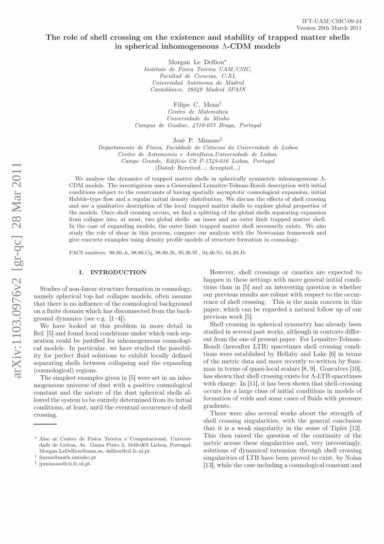
where the unstable saddle point, for which gTOV = 0,gives a local separating shell (see [5], figures 1 and 2, andrepeated in Fig. 1), in the case when the shell’s energyreaches its critical value. This separating (or "cracking",by analogy with Herrera et al. [18]) shell is characterisedby

rlim =3

√

3M

Λ, (11)

Elim =− (3M)2

3 Λ1

3 = −Λr2lim, (12)

1 Actually, 3R = −2 (Er)′

r2so E is related to the 3-curvature.

2 In case of shell crossing, E can be nonzero as r′ = 0 and M getschanged by the loss or gain of the mass from infinitesimal shellcrossings, so E = E(t, R) and M = M(t, R), in that case.

3

r3√

3MΛ

E>

Elim− (3M )

23

3√

Λ

E<

(

−2Mr

−Λ3r

2)

r

r

Figure 1. Effective potential kinematic analysis (left) and phase space analysis (right) from [5]. The kinematic analysis fora given shell of constant M and E depict the fate of the shell, depending on E relative to Elim. It either remains bound(E< < Elim) or escapes and cosmologically expands (E> > Elim). There exists a critical behavior where the shell will forever

expand, but within a finite, bound radius (E = Elim, r ≤ rlim). The maximum occurs at rlim = 3√

3M/Λ. The corresponding

phase space behaviour follows, the scales are set by the value of rlim = 3√

3M/Λ while the actual kinematic of the shell is givenby E.

while the energy follows

E =r2 + V (r). (13)

Definition 1. Local trapped matter shells in Λ-LTB aredefined in GLTB coordinates as the locus R⋆ such that

Θ

3+ a ≡ r

r= 0 and Ln

(Θ

3+ a

)

≡(r

r

)

= 0. (14)

This definition follows from Eqs. (3.11) and (3.16) of [5]applied to dust with Λ.

In Λ-LTB, conditions (14) are reached by shellsat time-infinity which are characterised by Eqs. (8)and (12) so that (see footnote 2) E (t = ∞, R⋆) =Elim (t = ∞, R⋆) (defining R⋆) i.e.3

(Θ

3+ a

)2

=2M (R⋆)

r3 (T,R⋆)+

1

3Λ− (3M (R⋆))

2

3 Λ1

3

r2 (T,R⋆). (15)

So, since here the Misner-Sharp mass M and energy E ofeach shell is conserved in time (without shell crossing),and E is thus set by initial M(R) and ri(R) profiles, onecan characterise local trapped matter, or limit, shell bythe intersections E = Elim (see [5], for details). Globalshells emerge from the neighbourhood behaviour aroundthose intersections which local study we give in Secs. III Aand III C.

3 Erratum: Eq. (3.14) of [5] has a sign typo. It should read

gTOV = −r

[

Ln

(

Θ

3+ a

)

+

(

Θ

3+ a

)2]

.

Before studying the occurrence of shell-crossing we willnow examine more carefully the role of shear in thesesettings.

B. The role of shear in the existence of trapped

matter shells

In Ref. [5], we derived the relation between expansionand shear (see Eq. III.10) and found that, in the presentlystudied model, the shear could be put in the form

a = ∓ 1

6√

E + 2Mr + Λ

3 r2×

×[(

E′

r′− 2E

r

)

+2

r

(M ′

r′− 3M

r

)]

. (16)

In the latter equation the terms within the brackets mea-sure the departures from the profiles E = E(t) r2 andM = M(t) r3 that one would expect from a homoge-neous, uniformly curved models . Indeed, in FLRW mod-els E = kr2 and M ∝ ρ(t)r3. Moreover, we should stressthat Eq. (16) yields the shear in terms of non-local (in-tegral) quantities (E and M). We can now evaluate theexpansion and shear at the limit shell defined by settingEqs. (8) and (9) to zero at time infinity in Ref. [5], which,with the conservation of E and M , is simply defined byEqs. (8) and (12). Combining those equations yields

E′ =− 2M ′

rlim. (17)

4

First on the limit shell we can write, setting E = Elim,

a = ∓

2M ′

r′

(1r − 1

rlim

)

+ 2Λr2lim

r

(1− rlim

r

)

6

√

Λ3

(

2r3lim

r + r2 − 3r2lim

) . (18)

With the definition of mass issued from Ref. [5]’s Eq. II.27in GLTB coordinates so

M ′ =4πρr2r′, (19)

we then express the shear of the limit shell as

alim = ∓√√√√

Λ

3(

rrlim

)3

1− 4πρ(r)Λ

(r

rlim

)3

√

2 + rrlim

, (20)

which in the limit of time infinity simplifies into

alim∞ = ∓Λ− 4πρ(rlim)

3√Λ

. (21)

This quantity does not vanish in general. Since at thatlocus we have Θ = 3

(rr − a

), the expansion then reads

Θlim = ±√√√√

3Λ(

rrlim

)3

√

2− 3r

rlim+

(r

rlim

)3

+1− 4πρ(r)

Λ

(r

rlim

)3

√

2 + rrlim

, (22)

which in the limit of time infinity simplifies into

Θlim∞ = ±Λ− 4πρ(rlim)√Λ

. (23)

We shall now use a particular form of initial data in orderto study in more detail the role of shear in the appearanceof the diving shell. In the examples below we shall assumeM > 0, ρ > 0,Λ > 0 and E < 0 around the origin.

So, consider analytic initial data for Λ-LTB as in [19,20]4:

M(R) = R3∞∑

i=0

miRi, m0 > 0 (24)

E(R) = R2∞∑

i=0

EiRi, E0 < 0

4 This data ensures that the solution approaches FLRW at theorigin which is therefore regular.

then, from the expressions above, we derive

alim(R) = ±Λ1/2

(

1

3− 2

32/3

(

m1

3

0 +2m1

m2/30

R+ (3m2

m2/30

− m21

m5/30

)R2 +O(R3)

))

rlim(R) = (3

Λ)

1

3

(

m1

3

0 R+m1

3m2/30

R2 +O(R3)

)

Elim(R) = −32

3Λ1

3

(

m2

3

0 R2 +

2m1

3m1/30

R3 +O(R4)

)

(25)

also, for the re-scaling r(t0, R) = R, we get an expressionfor the initial shear distribution as (see also [21]):

a(t0, R) = ±E1 + 2m1

6AR

± 1

6

(2E2 + 4m2

A− (E1 + 2m1)

2

2A3

)

R2 +O(R3)

with A(R) =√

E0 + Λ/3 + 2m0.

It is interesting to see that for a fixed shell R nearthe centre, bigger M (i.e. bigger m3) means smallerinitial shear but bigger |Elim| and rlim for that shell.On the other hand, since bigger initial shear impliessmaller |Elim| (i.e. smaller departures from Elim = 0)and smaller rlim, one can argue that, at least around theorigin (and for the above initial data), shear contributesto the appearance of "cracking" limit shells. This is inagreement with the results of Herrera et al. [18]. Wesummarize this result as:

Result 1. Consider a neighbourhood U of the originwhere the Λ-LTB initial data can be written as (24).Then, bigger values of the initial shear |a(t0, R)| in U , im-ply smaller |Elim| and favour the occurrence of trappedmatter shells in U .

For data which is asymptotically Friedmann at infinitywe take functions which, at infinity, can be expanded inthe form5:

M(R) =

+∞∑

i=1

miR3

i , E(R) =

+∞∑

i=1

EiR2

i

with m1 6= 0 and E1 6= 0.By taking asymptotic expan-

5 Note that we only assume this data form at infinity and notaround the origin. Otherwise, we would have a non-regular ori-gin.

5

R

Elim

R⋆i

︷ ︸︸ ︷ ︷ ︸︸ ︷

E = E<(R < R⋆i) E = E>(R > R⋆i)

E E = Elim(R⋆i)︸ ︷︷ ︸

Bound shells

Unbound shells

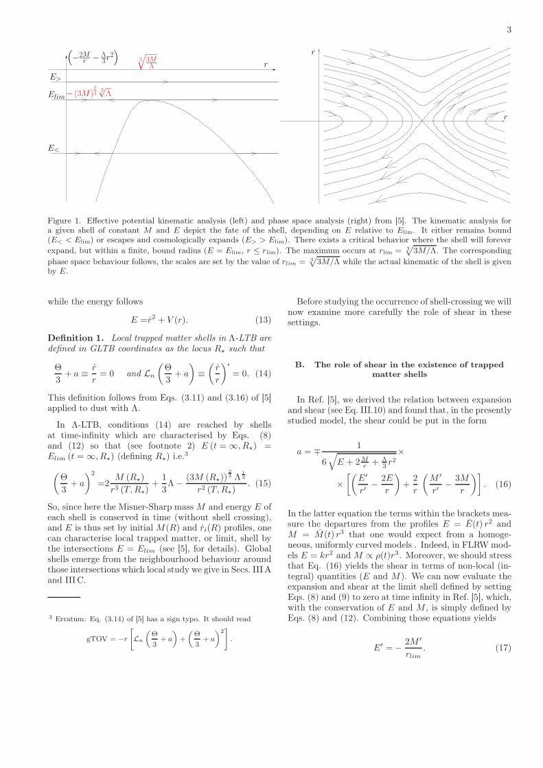
Figure 2. Overcoming local configuration of E intersectingElim. Phase space and effective potential trajectories fromdynamical analysis of [5] give the local qualitative behaviour,emphasised on the radial axis. Inner shells on bound tra-jectories and outer shells on unbound paths forecast no shellcrossing locally. Considering Elim as corresponding to theNewtonian zero radial velocity axis in [24, 25], this configura-tion is analogous to, e.g., figure 1 of [26].

sions we find :

rlim(R) =

(3

Λ

) 1

3

(

m1

3

1 R+m2

3m2

3

1

(1

R

) 1

2

+O(1

R)

)

Elim(R) = −32

3Λ1

3

(

m2

3

1 R2 +

2

3

m2

m1

3

1

R1

2 +2

3

m3

m1

3

1

+O(1

R1

4

)

)

(26)

while the initial shear is:

a(t0, R) = ∓ E2

2√3√3E1 + Λ+ 6m1

1

R+O(

1

R4

3

)

So, again, bigger values of the initial shear |a(t0, R)| nearinfinity, imply smaller |Elim| and favour the occurrenceof trapped matter shells.

We shall return to this issue in section IV where westudy other examples in more detail.

III. SHELL-CROSSING AND TRAPPED

MATTER SHELLS

A. Sufficient conditions for shell-crossing

In terms of the comoving coordinates of metric (1),shell-crossing is defined as a surface for which ∂Rr = 0

and the density diverges6. In geometrical terms, at shell-crossing there is a discontinuity both in the extrinsic cur-vature Kij and in the spacetime metric. For the space-times considered here, those discontinuities are finite andthe magnitude of the jump in Kij can be read from theexpressions derived in [15, 23].

Hellaby and Lake [6] (see also [7]) have derived nec-essary and sufficient conditions for the occurrence ofshell-crossing in LTB, in terms of the free initial data.Other works have used other type of conditions whichare sufficient to avoid shell crossing7 and therefore imply∂Rr 6= 0. For example, in the case of LTB, Landau andLifshitz [27] simply assume ∂Rr > 0 and, in [28], Hellabyand Lake impose the condition for a simultaneous bigbang in their local analysis around the initial singularity.

Here, we shall take a different point of view and writesufficient conditions for the occurrence of shell-crossingin terms of the local behaviour of M and E in the neigh-bourhood of some intersection, when it exists, of the en-ergy E with the critical energy Elim. In order to dothat we first observe that two local configurations arepossible in the neighbourhood of the intersection: eitherE′ > E′

lim or E′ < E′lim.

In the case E′ > E′lim, shells just inside the inter-

section radius will have a lower E than their respectiveElim and will therefore be trapped in closed trajecto-ries, following the dynamical analysis presented in Fig.1. In that case, shells just outside the intersection willdisplay higher E than their respective Elim and will ac-cordingly be free to escape to infinity on unbound trajec-tories. That shell distribution will lead to the separationof neighbouring shells, those inside the intersection beingbound to a finite region while those outside will escapeto infinity. This case doesn’t entail neighbouring shellcrossings and is presented on Fig. 2.

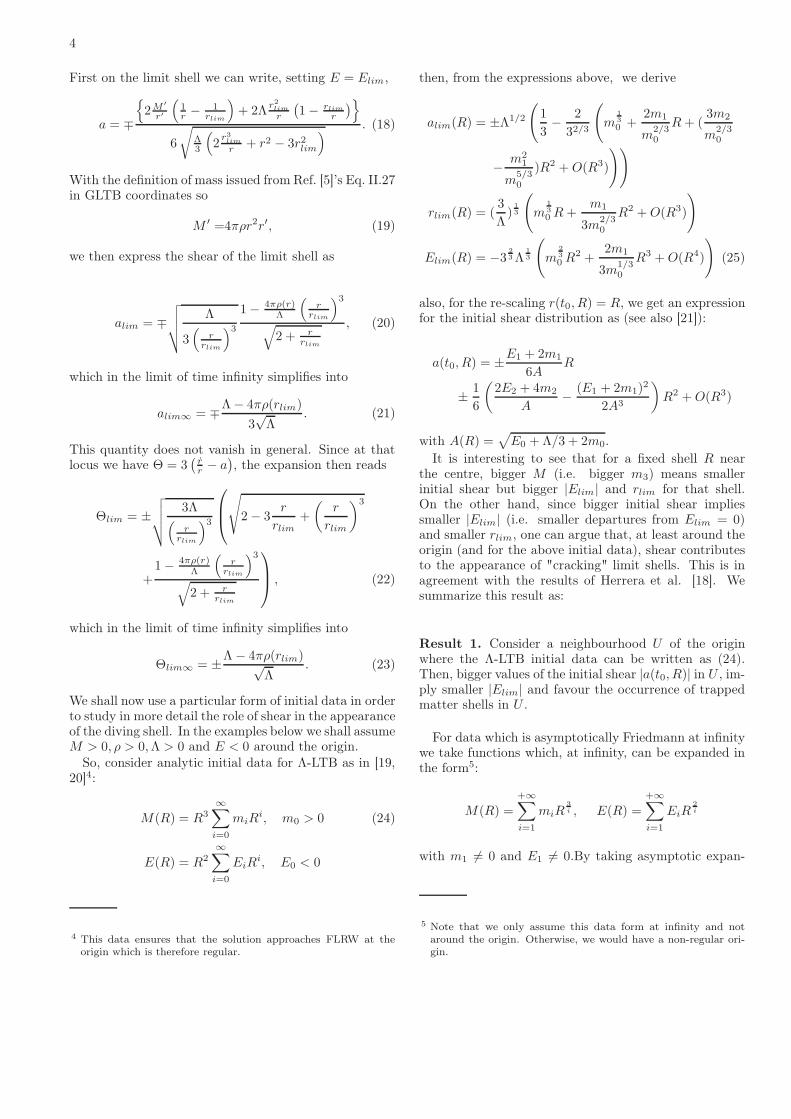
On the contrary, in the case E′ < E′lim, shells just

inside the intersection will have a higher E than theirrespective Elim and will accordingly be free to escapeto infinity on unbound trajectories whereas shells justoutside the intersection will display a lower E than theirrespective Elim and will therefore be trapped in closedtrajectories. Because of the configuration of that shelldistribution, shell crossings of neighbouring shells occur:those inside the intersection escaping to infinity will haveto cross those outside which are bound to a finite region.This case is presented on Fig. 3. We summarize thisresult as:

Result 2. Let ∆ = E − Elim and consider a Λ-LTBspacetime where there is R⋆ such that ∆|R⋆

= 0. Then,

6 There can exist cases where ∂Rr = 0 and the density does notdiverge. At those regular extrema, the extrinsic curvature isdiscontinuous while the metric is continuous and finite [6, 22].

7 A comment on the occurrence of caustics when using a syn-chronous reference frame can be found in Ref. [27] (§97). Wemust notice though that the latter assumes that the strong en-ergy condition holds, whereas in our present case the cosmologi-cal constant evades that assumption.

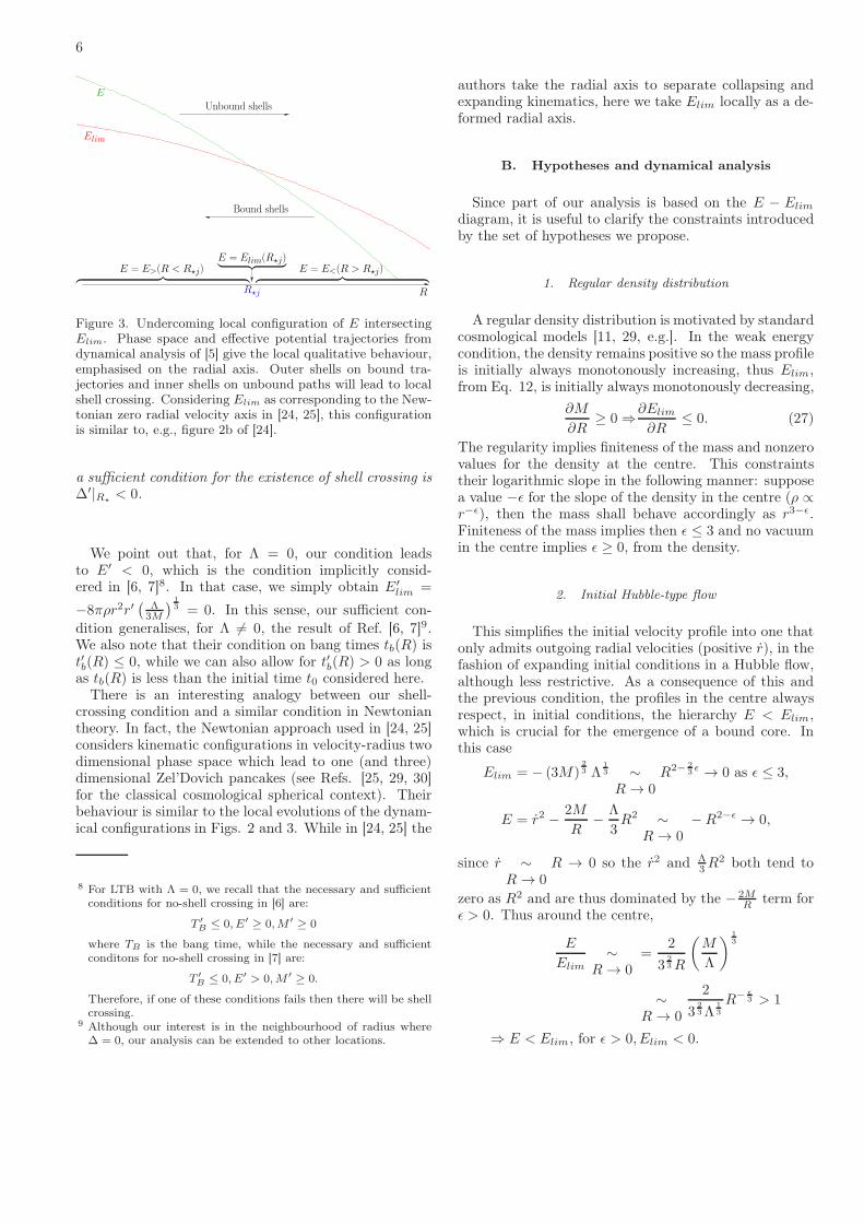
6

E

Elim

︷ ︸︸ ︷︷ ︸︸ ︷E = E>(R < R⋆j) E = E<(R > R⋆j)

R⋆j

E = Elim(R⋆j)︸ ︷︷ ︸

R

Unbound shells

Bound shells

Figure 3. Undercoming local configuration of E intersectingElim. Phase space and effective potential trajectories fromdynamical analysis of [5] give the local qualitative behaviour,emphasised on the radial axis. Outer shells on bound tra-jectories and inner shells on unbound paths will lead to localshell crossing. Considering Elim as corresponding to the New-tonian zero radial velocity axis in [24, 25], this configurationis similar to, e.g., figure 2b of [24].

a sufficient condition for the existence of shell crossing is∆′|R⋆

< 0.

We point out that, for Λ = 0, our condition leadsto E′ < 0, which is the condition implicitly consid-ered in [6, 7]8. In that case, we simply obtain E′

lim =

−8πρr2r′(

Λ3M

) 1

3 = 0. In this sense, our sufficient con-

dition generalises, for Λ 6= 0, the result of Ref. [6, 7]9.We also note that their condition on bang times tb(R) ist′b(R) ≤ 0, while we can also allow for t′b(R) > 0 as longas tb(R) is less than the initial time t0 considered here.

There is an interesting analogy between our shell-crossing condition and a similar condition in Newtoniantheory. In fact, the Newtonian approach used in [24, 25]considers kinematic configurations in velocity-radius twodimensional phase space which lead to one (and three)dimensional Zel’Dovich pancakes (see Refs. [25, 29, 30]for the classical cosmological spherical context). Theirbehaviour is similar to the local evolutions of the dynam-ical configurations in Figs. 2 and 3. While in [24, 25] the

8 For LTB with Λ = 0, we recall that the necessary and sufficientconditions for no-shell crossing in [6] are:

T ′B ≤ 0, E′ ≥ 0,M ′ ≥ 0

where TB is the bang time, while the necessary and sufficientconditons for no-shell crossing in [7] are:

T ′B ≤ 0, E′ > 0,M ′ ≥ 0.

Therefore, if one of these conditions fails then there will be shellcrossing.

9 Although our interest is in the neighbourhood of radius where∆ = 0, our analysis can be extended to other locations.

authors take the radial axis to separate collapsing andexpanding kinematics, here we take Elim locally as a de-formed radial axis.

B. Hypotheses and dynamical analysis

Since part of our analysis is based on the E − Elim

diagram, it is useful to clarify the constraints introducedby the set of hypotheses we propose.

1. Regular density distribution

A regular density distribution is motivated by standardcosmological models [11, 29, e.g.]. In the weak energycondition, the density remains positive so the mass profileis initially always monotonously increasing, thus Elim,from Eq. 12, is initially always monotonously decreasing,

∂M

∂R≥ 0 ⇒∂Elim

∂R≤ 0. (27)

The regularity implies finiteness of the mass and nonzerovalues for the density at the centre. This constraintstheir logarithmic slope in the following manner: supposea value −ǫ for the slope of the density in the centre (ρ ∝r−ǫ), then the mass shall behave accordingly as r3−ǫ.Finiteness of the mass implies then ǫ ≤ 3 and no vacuumin the centre implies ǫ ≥ 0, from the density.

2. Initial Hubble-type flow

This simplifies the initial velocity profile into one thatonly admits outgoing radial velocities (positive r), in thefashion of expanding initial conditions in a Hubble flow,although less restrictive. As a consequence of this andthe previous condition, the profiles in the centre alwaysrespect, in initial conditions, the hierarchy E < Elim,which is crucial for the emergence of a bound core. Inthis case

Elim = − (3M)2

3 Λ1

3 ∼R → 0

R2− 2

3ǫ → 0 as ǫ ≤ 3,

E = r2 − 2M

R− Λ

3R2 ∼

R → 0−R2−ǫ → 0,

since r ∼R → 0

R → 0 so the r2 and Λ3R

2 both tend to

zero as R2 and are thus dominated by the − 2MR term for

ǫ > 0. Thus around the centre,

E

Elim∼

R → 0=

2

32

3R

(M

Λ

) 1

3

∼R → 0

2

32

3Λ1

3

R− ǫ

3 > 1

⇒ E < Elim, for ǫ > 0, Elim < 0.

7

In the peculiar case of a constant central density (ǫ = 0),we have M ∼

R → 0

4π3 ρ0R

3, r ∼R → 0

∂Rr0R = HcR so

E =(H2

c − 8π3 ρ0 − Λ

3

)R2 =

(H2

c − 8π3 (ρ0 + ρΛ)

)R2. In

that case, the Hubble-type flow needs to remain moderatein the centre to respect the constraint

∂Rr0 < 4π

(

ρ2

3

0 (2ρΛ)1

3 +2

3(ρ0 + ρΛ)

)

.

In the rest of the paper, we assume the conditions forE < Elim in the centre are met.

3. Asymptotic spatial cosmological behaviour

If we restrict our explorations to asymptotically cos-mological (FLRW) solutions, this implies that at radialinfinity the mass and velocity initial profiles, constrainingthe energy and Elim profiles for all time, shall obey

M −→R → ∞

4π

3ρbR

3 with3M

4πR3−→

R → ∞ρb = ρb(t)

⇒ Elim −→R → ∞

− (4πρb)2

3 Λ1

3R2,

ri(R) −→R → ∞

HiR ⇒ E −→R → ∞

−K R2. (28)

We note that the value of the curvature K of theasymptotic FLRW solution compared with the equiva-

lent (4πρb)2

3 Λ1

3 FLRW critical curvature will determine,together with the central constraint E < Elim, the oc-curence of, at least, one intersection of E and Elim of theE′ > E′

lim kind, not inducive of shell crossing (see Sec.III A).

Definition 2. Supposing there exists n ∈ N shells veri-fying equation (15), we order them by initial radius anddenote them R⋆i, i ∈ [1, n],• R⋆out ≡ R⋆n the outermost intersections E = Elim ofthe initial profiles• R⋆in ≡ R⋆1 the innermost initial intersections E =Elim of the initial profiles.

4. Local mass conservation and Lagrangian frame

Since in our system, the cosmological constant is inertby definition and dust purely interacts gravitationally,we assume, as in [15], that the rest mass of each crossinginfinitesimal shell is conserved. The shell crossing eventcan thus be viewed as an infinitesimal exchange of therelative positions and integrated masses while each shellconserves its own velocity.

As shell masses M and energies E are conserved be-tween shell crossing events, Eq. (8) will govern the mo-tion of individual shells. Keeping initial R = r(0, R)

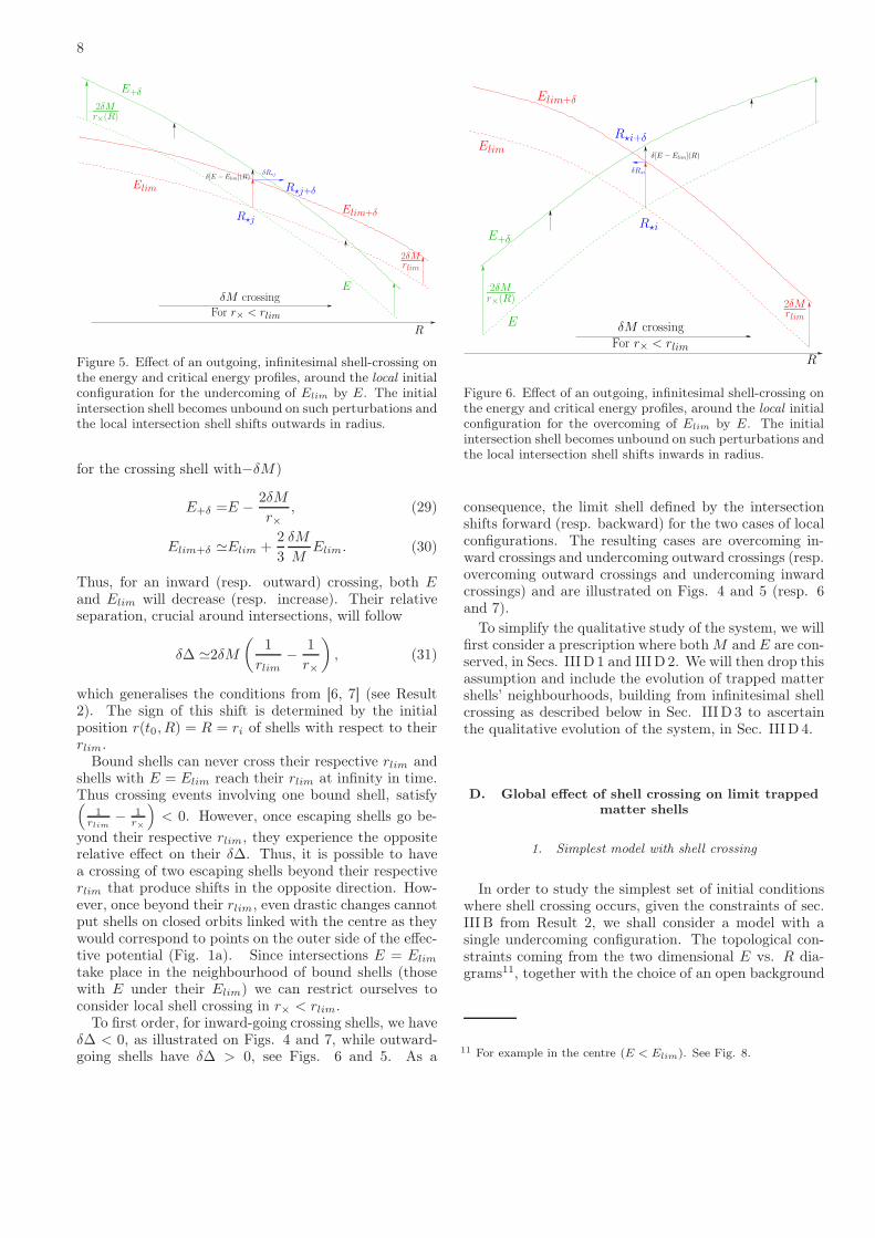
δM crossingFor r× < rlim

δR⋆i

R⋆i

δ[E − Elim](R)

E+δ

Elim+δ

Elim

E

R

− 2δMr×(R) −2δM

rlim

R⋆i+δ

Figure 4. Effect of an ingoing, infinitesimal test shell-crossingon the energy and critical energy profiles, around the localinitial configuration for the overcoming of Elim by E. Theinitial intersection shell becomes bound on such perturbationsand the local intersection shell shifts outwards in radius.

as Lagrangian labels, we can follow the dynamics of theshells using a the simple prescription obtained abovewithout the need to reorder the radial labels as wouldrequire a metric extension. Instead, we keep the initiallabels all throughout and follow each shell’s evolutionusing Eq. (8) and the shell crossing prescription of Sec.III B 4, as e.g. in Ref [24, 29].

C. Local effects of shell crossing on trapped matter

shells

In this section, we will detail how a test crossing shellaffects locally the values of E and Elim around trappedmatter shells.

Since each shell conserves its infinitesimal mass, thelocal effect of an elementary crossing of a system’s shellby a test, neighbouring, shell will just exchange theirnon-local mass in the exchange of their positions10. As aconsequence, their values of E and Elim will also change.The change of E, in Eq. (4), is allowed by the shell cross-ing event.

A shell crossed at some r× by an infinitesimal mass δM(δM > 0 for inward crossing, < 0 for outward crossing)will see its values shifted as follow (the reciprocal is true

10 In this process the other shells of the system, not involved, willremain unaffected and conserve their masses.

8

R

δM crossing

2δMr×(R)

For r× < rlim

Elim+δ

Elim

δR⋆jδ[E − Elim](R)

E

2δMrlim

E+δ

R⋆j+δ

R⋆j

Figure 5. Effect of an outgoing, infinitesimal shell-crossing onthe energy and critical energy profiles, around the local initialconfiguration for the undercoming of Elim by E. The initialintersection shell becomes unbound on such perturbations andthe local intersection shell shifts outwards in radius.

for the crossing shell with−δM)

E+δ =E − 2δM

r×, (29)

Elim+δ ≃Elim +2

3

δM

MElim. (30)

Thus, for an inward (resp. outward) crossing, both Eand Elim will decrease (resp. increase). Their relativeseparation, crucial around intersections, will follow

δ∆ ≃2δM

(1

rlim− 1

r×

)

, (31)

which generalises the conditions from [6, 7] (see Result2). The sign of this shift is determined by the initialposition r(t0, R) = R = ri of shells with respect to theirrlim.

Bound shells can never cross their respective rlim andshells with E = Elim reach their rlim at infinity in time.Thus crossing events involving one bound shell, satisfy(

1rlim

− 1r×

)

< 0. However, once escaping shells go be-

yond their respective rlim, they experience the oppositerelative effect on their δ∆. Thus, it is possible to havea crossing of two escaping shells beyond their respectiverlim that produce shifts in the opposite direction. How-ever, once beyond their rlim, even drastic changes cannotput shells on closed orbits linked with the centre as theywould correspond to points on the outer side of the effec-tive potential (Fig. 1a). Since intersections E = Elim

take place in the neighbourhood of bound shells (thosewith E under their Elim) we can restrict ourselves toconsider local shell crossing in r× < rlim.

To first order, for inward-going crossing shells, we haveδ∆ < 0, as illustrated on Figs. 4 and 7, while outward-going shells have δ∆ > 0, see Figs. 6 and 5. As a

E

Elim

Elim+δ

δ[E − Elim](R)

δM crossing

2δMr×(R) 2δM

rlim

δR⋆i

For r× < rlimR

E+δ

R⋆i+δ

R⋆i

Figure 6. Effect of an outgoing, infinitesimal shell-crossing onthe energy and critical energy profiles, around the local initialconfiguration for the overcoming of Elim by E. The initialintersection shell becomes unbound on such perturbations andthe local intersection shell shifts inwards in radius.

consequence, the limit shell defined by the intersectionshifts forward (resp. backward) for the two cases of localconfigurations. The resulting cases are overcoming in-ward crossings and undercoming outward crossings (resp.overcoming outward crossings and undercoming inwardcrossings) and are illustrated on Figs. 4 and 5 (resp. 6and 7).

To simplify the qualitative study of the system, we willfirst consider a prescription where both M and E are con-served, in Secs. III D 1 and III D 2. We will then drop thisassumption and include the evolution of trapped mattershells’ neighbourhoods, building from infinitesimal shellcrossing as described below in Sec. III D 3 to ascertainthe qualitative evolution of the system, in Sec. III D 4.

D. Global effect of shell crossing on limit trapped

matter shells

1. Simplest model with shell crossing

In order to study the simplest set of initial conditionswhere shell crossing occurs, given the constraints of sec.III B from Result 2, we shall consider a model with asingle undercoming configuration. The topological con-straints coming from the two dimensional E vs. R dia-grams11, together with the choice of an open background

11 For example in the centre (E < Elim). See Fig. 8.

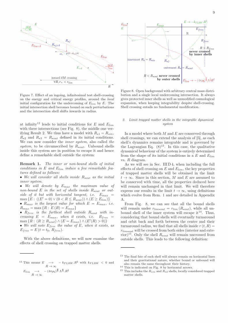
9

Elim

E

−2δMrlim

Elim+δ

δR⋆jδ[E − Elim](R)

∀R, r× < rlim

R

inward δM crossing

E+δ

− 2δMr×(R)

R⋆j

R⋆j+δ

Figure 7. Effect of an ingoing, infinitesimal test shell-crossingon the energy and critical energy profiles, around the localinitial configuration for the undercoming of Elim by E. Theinitial intersection shell becomes bound on such perturbationsand the intersection shell shifts inwards in radius.

at infinity12 leads to initial conditions for E and Elim

with three intersections (see Fig. 8), the middle one ver-ifying Result 2. We thus have a model with R⋆1 = R⋆in,R⋆2 and R⋆3 = R⋆out defined in its initial conditions.We can now consider the inner system, also called thesystem, to be circumscribed by R⋆out. Unbound shellsinside this system are in position to escape it and hencedefine a remarkable shell outside the system:

Remark 1. The inner or non-bound shells of initialconditions in E and Elim induce a few remarkable fea-tures defined as follows:• We will consider all shells inside R⋆out as the initialinner system.• We will denote by Emax the maximum value ofnon-bound E in the set of shells inside R⋆out or out-side of it but with horizontal tangent, i.e. Emax =max E : ((E′ = 0) ∨ (0 < R ≤ R⋆out)) ∧ (E ≥ Elim)• Rmax is the largest value for which E = Emax, i.e.Rmax = max R : E (R) = Emax• Rfree is the furthest shell outside R⋆out with in-creasing E = Emax, when it exists, i.e. Rfree =max R : (R ≥ R⋆out) ∧ (E = Emax) ∧ (E′(R) > 0)• We will note Efree the value of E, when it exists, asEfree = E (t = t0, Rfree).

With the above definitions, we will now examine theeffects of shell crossing on trapped matter shells.

12 This means E −→

R → ∞

− kFLRW .R2 with kFLRW < 0 and

Elim −→

R → ∞

− (4πρb)2

3 Λ1

3 .R2

ElimE

innermost R⋆ = R⋆in

outermost R⋆ = R⋆out

R < R⋆out never crossedby outer shells

R

E → −kFLRW .R2

Rfree

by inner shellsnever crossed

R > Rfree

Efree

Elim → − (4πρb)23 Λ

13R2

R⋆2

Emax

Figure 8. Open background with arbitrary central mass distri-bution and a single local undercoming intersection. It alwaysgives protected inner shells as well as unmodified cosmologicalexpansion, when keeping integrability despite shell-crossing.Shell crossing entails no fundamental modification.

2. Limit trapped matter shells in the integrable dynamicalsystem

In a model where both M and E are conserved throughshell crossings, we can extend the analysis of [5], as eachshell’s dynamics remains integrable and is governed bythe Lagrangian Eq. (8)13. In this case, the qualitativedynamical behaviour of the system is entirely determinedfrom the shape of its initial conditions in a E and Elim

vs. R diagram.As we will see in Sec. III D 4, when including the full

effects of shell crossing on E and Elim, the key propertiesof trapped matter shells will be obtained in the limitt → ∞. Since in this section, M and E are assumed tobe conserved with time, all the properties deduced herewill remain unchanged in that limit. We will thereforeexpress our results in the limit t → ∞, using definitionswhich evolve from Rem. 1 and are detailed in AppendixA.

From Fig. 8, we can see that all the bound shellswill remain under rlim⋆out = rlim (R⋆out), while all un-bound shell of the inner system will escape it14. Thus,considering that bound shells will eventually turnaroundand orbit back and forth between the centre and theirturnaround radius, we find that all shells inside r (t, R) =rlim⋆out will be crossed from both sides (interior and exte-rior)15. Only the shell R⋆out will remain uncrossed fromoutside shells. This leads to the following definition:

13 The final fate of each shell will always remain on horizontal linesand their gravitational nature, whether bound or unbound willalso remain the same throughout their history.

14 This is indicated on Fig. 8 by horizontal arrows.15 This includes the R⋆in and R⋆2 shells, locally considered trapped

matter shells.

10

Definition 3. The outer limit trapped matter shellRt⋆out∞ verifies Def. 1 in the limit t → ∞, in addi-tion to being the outermost such shell which locally is notshell-crossing inducive16 i.e.

Rt⋆out∞ = R : max R⋆∞ ∧ (E′ (t → ∞) > E′lim (t → ∞))

Note, from Def. 2, that R⋆out: verifies Def. 3; definesRt⋆out, if E′ > E′

lim; and verifies Rt⋆out = Rt⋆out∞ in thelimit t → ∞.

Remark 2. In Λ-LTB with asymptotic cosmologicalevolution (FLRW at radial infinity) and initial Hubble-like flow (outwards going) for which shell crossingoccurs, the outer limit trapped matter shell is a surfaceS with the following properties:• The matter exterior to S follows trapped geodesics,remaining in that exterior.• The matter inside S can expand and collapse protectedfrom the crossing of outside shells.• S is the shell with largest R for which the energyE intersects the critical energy Elim, from bound tounbound shells.

The condition for existence of Rt⋆out∞, follows fromthe properties of Rt⋆out, so we obtain the following result:

Result 3. Sufficient conditions for the existence of anouter limit trapped matter shell are:• The FLRW curvature of the background kFLRW <

(4πρb)2

3 Λ1

3 , or• Rt⋆out exists, or• The local configuration around R⋆out is such thatE′

⋆out > E′lim⋆out.

Proof. kFLRW < (4πρb)2

3 Λ1

3 ⇒ E (R → ∞) >Elim (R → ∞) so the last intersection E (R) = Elim (R)is such that E′ > E′

lim from a corollary to Bolzano-Weierstrass theorem and the Definition 3 is verified.

We show, in Fig. 8, a diagram with data such that theinner limit trapped matter shell Rt⋆out is at R⋆out. Theexterior of the system will include all the unbound shellsescaping to infinity. However, the dynamics from Eq. (8)allows us to study under what conditions unbound sys-tem’s shells will never cross shells located in the exteriorof the system17. Take two different shells R1 < R2, even-tually crossing each other at a given radius18 r×, andwith the outer shell more open than the inner shell (i.e.

16 Recall that R⋆∞is defined by solutions in initial R of Eq. 15taken at t → ∞.

17 Their escape velocity at infinity should never exceed that of ex-terior shells.

18 This radius is allowed to tend to radial infinity.

E1 < E2 for M1 < M2):

E1 =v21 −Λ

3r2× − 2M1

r×, with E1 <E2,

(32)

E2 =v22 −Λ

3r2× − 2M2

r×and M1 <M2,

(33)

⇒ ∆v2 =∆E +2∆M

r×> 0 and (34)

∆v2 ∼r× → ∞

∆E > 0 ⇒ ∀t, v22 >v21 .

(35)

Thence shells with E1 < E2 and M1 < M2 will al-ways remain in the same radial order and the shell withE = Emax will then escape all other system’s shells.It then appears that, when Rfree exists, all shells withE > Efree will never be crossed by any shell inside Rfree.The counterpart to Def. 3 can thus be formulated bydefining first Emax. In turn, the condition for the exis-tence of Emax is that E ≥ Elim, in the limit t → ∞.Thus, Rem. 1 can be adapted here as19

Definition 4. Suppose Emax∞ exists and is defined, inthe initial conditions, as

Emax∞ = max

E|(t→∞) : ((E′ = 0)

∨ (0 < R ≤ R⋆out∞)) ∧ (E ≥ Elim)(t→∞)

. (36)

Then, inner limit trapped matter shells are defined as thelocus Rfree∞ such that

Rfree∞ = max R : (R ≥ R⋆out∞) ∧ (E = Emax∞)t→∞

∧ (E′(t → ∞, R) > 0) . (37)

Remark 3. In Λ-LTB with asymptotic cosmologicalevolution (FLRW at radial infinity) and initial Hubble-like flow (outwards going) for which shell crossing occurs(and Emax∞ is defined), the inner limit trapped mattershell is a surface S with the following properties:• The matter interior to S follows trapped geodesics whichremain in that interior.• The matter exterior to S expands, protected from thecrossing of inside shells.• S is the shell outside the system (defined with R⋆out∞)with energy equal to that of the highest E of non-boundshells, and starting inside of the system, or outside it butwith horizontal tangent.

The conditions for existence of Rfree∞ combine theexistence of Emax∞ with constraints on the background:

19 The following can be formulated also in terms of gauge invariantLie derivatives, expansion and shear, as seen in appendix B.

11

Result 4. Sufficient conditions for the existence of aninner limit trapped matter shell are (a) the existence ofEmax∞ and (b) the existence of Efree∞:(a) • There exist initially a non-bound, system shell,or a non-bound shell with horizontal tangent: ∃R :(0 < R ≤ R⋆out ∨E′ = 0) ∧E (R) ≥ Elim(R), or

• R⋆out∞ exists, or• There exist at least one R⋆i

(b) • Emax∞ < E (R → ∞), or• ∃R : R ≥ R⋆out∞ ∧ E (t → ∞, R) = Emax∞ ∧

E′(R) > 0

Proof. (a) 1/ If we have R such that(0 < R ≤ R⋆out ∨E′ = 0) ∧ E (R) > Elim(R), then,either it is a maximum so Emax exists and, by timeevolution of its neighbourhood, Emax∞ exists, or, bycontinuity, in the case when it is not a shell withE′ = 0 (local maximum), there is a shell with largerE which satisfies Rem. 1 for Emax and thus one in itsneighbourhood satisfying Def. 5 for Emax∞.2/ If R⋆out∞ exists, it is not bound at time infinity andis inside the system, therefore, even if it is the onlyunbound system shell, it can at least define Emax∞.3/ If there is only one R∗, then it is R⋆out by Def. 2.We are then in the case 2/ above as this guarantees theexistence of R⋆out∞.

(b) Since: (i) Emax∞ is, by definition, the largest valueof E reached at time infinity by inner or outer local max-ima shells,(ii) uncrossed outer shells have their E conserved,(iii) asymptotic cosmological conditions render Emonotonous near infinity,(iv) evolution of the inner shell Rmax∞ follows Eqs. 35,(v) the energy profile is continuous,therefore, E⋆out∞ ≤ Emax∞ and by continu-ity, since Emax∞ < E (R → ∞), exterior shellswill obey E ∈ [E⋆out∞, E (t → ∞, R → ∞)[ k[Emax∞, E (t → ∞, R → ∞)[, thus there exist at leastone shell at time infinity with E = Emax∞.Moreover, for the outermost exterior shell Rxmax∞ =max R : R ≥ R∗out∞, E (R) = Emax∞ with E =Emax∞, since Emax∞ < E (R → ∞), by continuity, allshells outside of it will verify E > Emax∞. ThereforeE′(Rxmax∞) > 0 and Rxmax∞ = Rfree∞ is fulfilling Def.4.

We show a diagram in Fig. 8 where we indicatethe outer limit trapped matter shell for which Rfree =Rfree∞, in the model where both E and M are conservedbetween shell crossings. We thus have found, for thatmodel, that extending the analysis of [5] in the contextof shell crossing leads to the emergence of two remark-able shells: an inner limit trapped matter shell and anouter limit trapped matter shell. From their definitions 3and 4, we can deduce other properties depending on thebackground cosmological model, namely:

From Result 3, any background with E > Elim willadmit an outer limit trapped matter shell. This includessome closed models and all flat and open models.

From Result 4, and under the assumptions of this sec-tion, any closed background in our models cannot fosteran inner limit trapped matter shell as the finite value ofEmax∞ is always larger than its energy at radial infin-ity. Conversely, open models always have an inner limittrapped matter shell (see the example of section IV) andonly flat models with moderate enough energy fluctua-tions (i.e. for which Emax < 0 = E (R → ∞)) can allowthe existence of an inner limit trapped matter shell. Insummary:

Summary 1. Consider a Λ-LTB spacetime with asymp-totic cosmological evolution (FLRW at radial infinity)and initial Hubble-like flow (outwards going) for whichshell crossing occurs. Then:

1. The global limit trapped matter shell found in theno-shell crossing Λ-LTB examples of [5] is split, ifshell crossing occurs, into at most, two global shells,namely an inner limit trapped matter shell and anouter limit trapped matter shell.

2. For open or flat expanding spacetimes,

(a) there exists always an outer limit trapped mat-ter shell at Rt⋆out∞.

(b) The inner limit trapped matter shell exists inflat backgrounds for sufficiently small initialvelocities inside the system limited by R⋆out∞.

3. For closed spacetimes, outer limit trapped matter

shells are present if kFLRW < (4πρb)2

3 Λ1

3 and innerlimit trapped matter shells cannot be defined if shellcrossing occurs, with our definitions.

4. In the Λ-CDM examples of global limit trapped mat-ter shell found in [5], inner and outer limit trappedmatter shells reduce to one single surface.

Proof. 1: Direct from Definitions 3 and 4 and Result 2which leads to shell crossings at some R⋆ .2(a): From Result 3.2(b): Direct from Result 4, as open and flat expandingspacetimes admit E (R → ∞) ≥ 0. Some flat spacetimescan exhibit Efree∞ > 0 while their E −→

R → ∞0. For

those cases, Definition 4 is never verified.3: Using Result 3, for closed spacetimes, E −→

R → ∞−

∞ ≪ Efree∞, so from Result 4 , Definition 4 is neververified.4: Applying Definitions 3 and 4 to configurations wherethere is only one intersection R⋆ = R⋆1 = R⋆out verifyingE′ > E′

lim, no shell crossing occurs. Thus all E valuesare constant over time so R⋆out = Rt⋆out∞, and given theopen background, Efree = E⋆out, so Rfree∞ = R⋆out =Rt⋆out∞.

In this section, we have assumed that E and M were con-served through shell crossings. In the next section, wedrop this assumption and investigate whether our previ-ous results remain true.

12

3. Global effect of shell crossing

Since the sign of ∆ = E−Elim determines the bindingproperty of the system, it is useful to give the final valuesof E and Elim for each shell, labeled i, in terms of theinitial Ri and Mi, reaching areal radius r after crossingshells, with

M(r(R, t), t) = Mi +

ˆ

dMin −ˆ

dMout = Mi +∆Mi

where the index in refers to inward crossing, out to out-ward crossing, j to the shells crossing shell i.

Using definition (12) and integrating Eq. (29) over allcrossing shells, we get

Elim(r) =Elim(Ri)−[(

1 +∆Mi

Mi

) 2

3

− 1

]

3Mi

rlim(Ri),

(38)

E(r) =E(Ri)− 8π

[ˆ

drj,in −ˆ

drj,out

]ρ (rj) r

2j

r×i (rj),

(39)

where r×i is a crossing radius. Because of their qualita-tively simple shell crossing histories, we can look at thechanges for three peculiar shells, singled out on Fig. 8:the innermost limit shell, the outermost limit shell andthe maximum E shell initially lying in the interior of theoutermost limit shell.

The innermost limit shell will only be crossed by morebound shells exterior to it, so ∆M1 > 0 and

E(r(R⋆1)) =E(R⋆1)− 8π

ˆ

drj,inρ (rj) r

2j

r×1 (rj). (40)

Since

1

3

(∆M1

M1

)2

+

(2

3

∆M1

M1

)3

> 0 (41)

⇔[(

1 +∆M1

M1

) 2

3

− 1

]

<2

3

∆M1

M1(42)

and

− 1

r×1(rj)<− 1

max [r×1(rj)]< − 1

rlim(R⋆1), (43)

as the innermost limit shell becomes a bound shell, weget that

∆ [E − Elim]1 <2∆M1

[1

rlim(R⋆1)− 1

max [r×1(rj)]

]

< 0.

(44)

Thus, the innermost limit shell will globally shift out-wards, following the qualitative analysis of Fig. 4.

innermost R⋆ = R⋆in

R, r.ai/a∞

Elim → − (4πρb)23 Λ

13R2

Emax

by outer shells

R⋆2

E → −kFLRW .R2

Elim

E∞

E

Elim∞

outermost R⋆∞ = R⋆out∞R < R⋆out∞ never crossed

outermost R⋆ = R⋆out

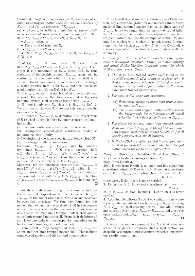
Figure 9. Illustration, on an open background with arbitrarycentral mass distribution, of the effect of shell crossing on theinner global limit shell previously defined as the outermostlocal limit shell. The time variation of the locus of the outer-most local limit shell leads to defining it as the time infinityoutermost limit shell: this is shown on the extrapolated timeinfinity energy profiles and linked to the initial energy profileby a connecting curve. The global inner limit shell is thenjust shifted inwards, compared with the integrable analysis.

In turn, the outermost limit shell will be only crossedby all the unbound shells interior to it, so

E(r(R⋆out)) =E(R⋆out) + 8π

ˆ

drj,outρ (rj) r

2j

r×out (rj)

≡E(R⋆out) + 2∆Mout

〈r×out〉 (R⋆out), (45)

where ∆Mout is the positive mass loss of the outermostlimit shell and 〈r×〉 is a reduced crossing radius. Notethat, by construction, Mout > M(R⋆out, t → ∞) =Mout −∆Mout > 0.

Now, supposing the density distribution remains finitewe can decompose the crossing of the outermost limitshell by all escaping inner shells into a series of infinites-imal shell crossings. Thus following Eq. (31) we get

d [E − Elim] = −8πdrj,outρ (rj,out) r2j,out

×(

1

rlim(M⋆out(t×j))− 1

r×out(rj,out)

)

. (46)

As all shells cross outwards20 and

1

〈r×out〉 (R⋆out)>

1

rlim(〈r×out〉)≥ 1

rlim(R⋆out), (47)

20 Note that R⋆out starts as a marginally bound shell well insideits limit radius.

13

ElimE

Elim → − (4πρb)23 Λ

13R2

innermost R⋆ = R⋆in

R

E → −kFLRW .R2

never crossedby inner shells

Efree∞Rfree∞

R⋆2

R⋆out∞

R > Rfree∞

outermost R⋆ = R⋆out

Emax∞

Emax

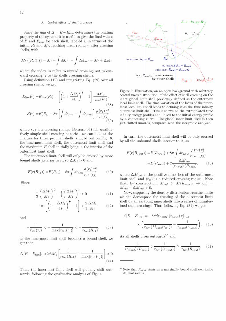
Figure 10. Illustration, on an open background with arbi-trary central mass distribution, of the effect of shell crossingon the outer global limit shell previously defined as the outershell with same energy function as the inner shells’ maximum.The time variations of the inner shells’ maximum energy func-tion from shell crossings lead to defining it as the outer shellwith same energy as the time infinity inner shells’ maximumenergy function E: this is shown with the highest of extrapo-lated time infinity Es of inner shells peaks. The global outerlimit shell is then just shifted inwards, compared with theintegrable analysis.

then, in this case, we have

∆ [E − Elim]out =

2∆Mout

[1

〈r×out〉 (R⋆out)− 1

rlim(R⋆out)

]

> 0. (48)

Thus, the outermost limit shell will shift relatively in-wards, following the qualitative analysis of Fig. 6.

Finally, the maximum E shell initially inside R⋆out, orwith horizontal tangent (its initial radius is Rmax), willbe only crossed inwards by all the shells starting withradii above it and having an E below E(Rmax, t → ∞),at the moment of crossing. This shell will then follow

∆ [E − Elim]max < 2∆Mmax

×[

1

rlim(Rmax)− 1

max [r×max(rj)]

]

< 0, (49)

similarly as for the innermost limit shell.We summarize the main result of this section as:

Result 5. Consider a Λ-LTB spacetime where shellcrossing exists. Then the metric and extrinsic curvatureare discontinuous and the discontinuity in E is given by(29). Furthermore, at R⋆out, ∆ [E − Elim]out > 0 and,at Rmax, ∆ [E − Elim]max < 0.

4. Qualitative analysis of limit trapped matter shells

In this section, we argue that the results contained inSummary 1 remain true for the case where M and E arenot conserved through shell crossing.

–1

–0.8

–0.6

–0.4

–0.2

0

0.2

0.4

500 1000 1500 2000 2500 3000r

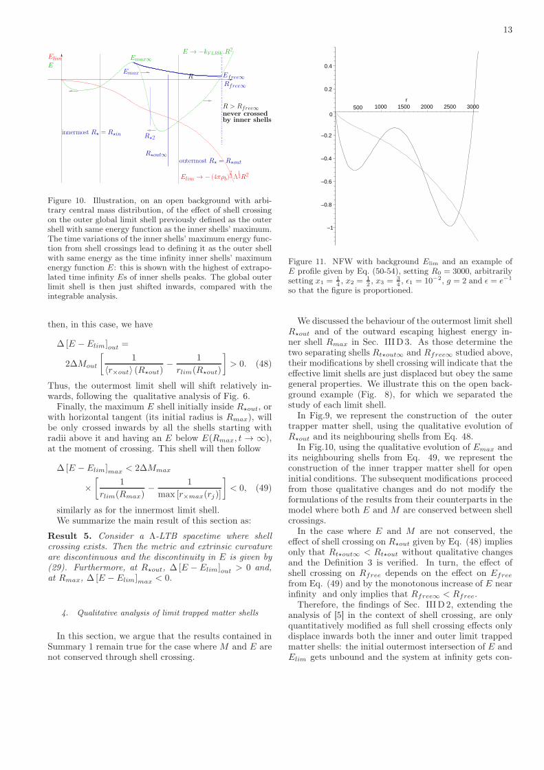
Figure 11. NFW with background Elim and an example ofE profile given by Eq. (50-54), setting R0 = 3000, arbitrarilysetting x1 = 1

4, x2 = 1

2, x3 = 3

4, ǫ1 = 10−2, g = 2 and ǫ = e−1

so that the figure is proportioned.

We discussed the behaviour of the outermost limit shellR⋆out and of the outward escaping highest energy in-ner shell Rmax in Sec. III D 3. As those determine thetwo separating shells Rt⋆out∞ and Rfree∞ studied above,their modifications by shell crossing will indicate that theeffective limit shells are just displaced but obey the samegeneral properties. We illustrate this on the open back-ground example (Fig. 8), for which we separated thestudy of each limit shell.

In Fig.9, we represent the construction of the outertrapper matter shell, using the qualitative evolution ofR⋆out and its neighbouring shells from Eq. 48.

In Fig.10, using the qualitative evolution of Emax andits neighbouring shells from Eq. 49, we represent theconstruction of the inner trapper matter shell for openinitial conditions. The subsequent modifications proceedfrom those qualitative changes and do not modify theformulations of the results from their counterparts in themodel where both E and M are conserved between shellcrossings.

In the case where E and M are not conserved, theeffect of shell crossing on R⋆out given by Eq. (48) impliesonly that Rt⋆out∞ < Rt⋆out without qualitative changesand the Definition 3 is verified. In turn, the effect ofshell crossing on Rfree depends on the effect on Efree

from Eq. (49) and by the monotonous increase of E nearinfinity and only implies that Rfree∞ < Rfree.

Therefore, the findings of Sec. III D 2, extending theanalysis of [5] in the context of shell crossing, are onlyquantitatively modified as full shell crossing effects onlydisplace inwards both the inner and outer limit trappedmatter shells: the initial outermost intersection of E andElim gets unbound and the system at infinity gets con-

14

–10

–8

–6

–4

–2

0

2

4

6

8

2 4 6 8 10 12x

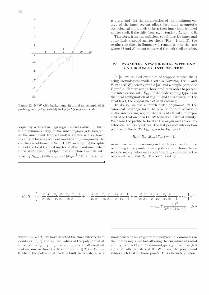
Figure 12. NFW with background Elim and an example of Eprofile given by Eq. (50-54) in log (−E)-log (−R) scale.

sequently reduced in Lagrangian initial radius. In turn,the maximum energy of the inner regions gets lowered,so the inner limit trapped matter surface is also drawninwards. This displacement modifies only marginally theconclusions obtained in Sec. III D 2, namely: (i) the split-ting of the local trapped matter shell is maintained whenthose shells exist. (ii) Open, flat and closed models with

existing Rt⋆out (with kFLRW < (4πρb)2

3 Λ1

3 ) all retain an

Rt⋆out∞ and (iii) the modification of the maximum en-ergy of the inner regions allows just more asymptoticcosmological flat models to keep their inner limit trappedmatter shell, if the shift from Emax tends to Emax∞ < 0.

Therefore, from the sufficient conditions for inner andouter limit trapped matter shells (Res. 4 and 3), theresults contained in Summary 1 remain true in the casewhere M and E are not conserved through shell crossing.

IV. EXAMPLES: NFW PROFILES WITH ONE

UNDERCOMING INTERSECTION

In [5], we studied examples of trapped matter shellsusing cosmological models with a Navarro, Frenk andWhite (NFW) density profile [31] and a simple parabolicE profile. Here we adapt those profiles in order to presentone intersection with Elim of the undercoming type as inthe local configuration of Fig. 3, and thus ensure, at thelocal level, the appearance of shell crossing.

To do so, we use a fourth order polynomial in thecanonical Lagrange form, to provide for the behaviourin the intersecting region, that we cut off with an expo-nential so that an open FLRW term dominates at infinity.We chose the profile to be 0 at the origin and at a char-acteristic radius R0 set near the last possible intersectionpoint with the NFW Elim given by Eq. (4.21) of [5],

R0 ≤ R−1,Elim(R−1) = −1,

so as to secure the crossings in the physical region. Theremaining three points of interpolation are chosen to beset alternately below and above the Elim curve inside theregion set by 0 and R0. The form is set by

E(R) =

m1x

x1

x− x2

x1 − x2

x− x3

x1 − x3

x− 1

x1 − 1+m2

x

x2

x− x1

x2 − x1

x− x3

x2 − x3

x− 1

x2 − 1+m3

x

x3

x− x1

x3 − x1

x− x2

x3 − x2

x− 1

x3 − 1+ ǫ1x

e−x

− k∞R2 ǫ0x2

(x2 − 1) ǫ0 + 1, (50)

where x = R/R0, we have denoted the three intermediatepoints as x1, x2 and x3, the values of the polynomial atthose points by m1, m2 and m3, ǫ1 is a small constantmaking sure we have the freedom to fit E(R0) = E(0) =0 where the polynomial itself is built to vanish, ǫ0 is a

small constant making sure the polynomial dominates inthe interesting range but allowing the curvature at radialinfinity to be set by a Friedmann-type k∞. The form (50)automatically vanishes at 0. We chose the polynomialvalues such that at those points, E is alternately below,

15

above and again below Elim, the last one making sure it remains above -1:

E(R0) =0 = ǫ1e−1 − k∞R2

0ǫ0, ⇒ ǫ0 =ǫ1

k∞R20e

, (51)

E(R1) =gElim(R1) = (m1 + ǫ1x1) e−x1 − k∞R2

0

ǫ0x41

(x21 − 1) ǫ0 + 1

= (m1 + ǫ1x1) e−x1 − ǫ1x

41

e− (1− x21)

ǫ1k∞R2

0

⇒ m1 =gElim(R1)ex1

+ ǫ1x1

(

x31e

x1

e− (1− x21)

ǫ1k∞R2

0

− 1

)

, (52)

E(R2) =Elim(R2)

g= (m2 + ǫ1x2) e

−x2 − k∞R20

ǫ0x42

(x22 − 1) ǫ0 + 1

= (m2 + ǫ1x2) e−x2 +

ǫ1x42

e− (1− x22)

ǫ1k∞R2

0

⇒ m2 =Elim(R2)

gex2

+ ǫ1x2

(

x32e

x2

e− (1− x22)

ǫ1k∞R2

0

− 1

)

, (53)

E(R3) =Elim(R3)− (Elim(R3) + 1) (1− ǫ)

= (Elim(R3) + 1) ǫ− 1 = (m3 + ǫ1x3) e−x3 − k∞R2

0

ǫ0x43

(x23 − 1) ǫ0 + 1

= (m3 + ǫ1x3) e−x3 +

ǫ1x43

e− (1− x23)

ǫ1k∞R2

0

⇒ m3 = [(Elim(R3) + 1) ǫ− 1] ex3

+ ǫ1x3

(

x33e

x3

e− (1− x23)

ǫ1k∞R2

0

− 1

)

.

(54)

We illustrate this in Figs. (11) and (12) after choosingthe values of the density profile identical to those in [5].The cut off leaves the region under R0 almost unaffectedby the Friedmann term, so the value of k∞ is not veryrelevant there but we set it to -1.

We summarize the result of this section as:

Result 6. For NFW density and initial data given by(50-54), the Λ-LTB spacetime has three shells R⋆ suchthat E|R⋆

= Elim|R⋆. Furthermore, for this data, there

is shell crossing and R⋆out − R⋆out∞ < 0 and Rfree −Rfree∞ < 0.

V. CONCLUSIONS

We have studied the effects of shell crossing on theexistence of trapped matter shells in Λ-LTB spacetimes.In particular, we have considered initial conditions suchthat: (i) our models approach a FLRW solution at radialinfinity and have an initial outgoing Hubble-type flow(ii) the shell crossing of dust remains pressureless andthe mass of infinitely thin shells remains finite.

We have shown that the local trapped matter shellsdiscussed in Ref. [5] split in two shells: one outer limittrapped matter shell and one inner limit trapped mattershell.

We have established sufficient conditions for the exis-tence of such shells in Λ-LTB spacetimes, in terms of ini-tial data for which shell crossing occurs. Furthermore, wehave derived a number of properties for those shells usinga qualitative approach inspired in newtonian-like frame-works of cosmological kinematical models, as in [24, 25].

We have also studied the role of shear in these set-tings and concluded, as in [18], that shear favours theemergence of trapped matter shells.

Finally, we have given concrete examples where shellcrossing occurs and the inner and outer limit trappedmatter shells emerge, using NFW data.

As potential applications of our models we note that (i)Due to mass conservation and integrability in the absenceof shell crossing at the boundary, the background asymp-totic conditions remain FLRW over all time. Therefore,this gives an interesting setting to study the extendabil-ity of Birkhoff’s theorem to cosmological expanding back-grounds; (ii) Extensions of this work to unsmooth distri-

16

butions of mass should be possible and might give sup-port to current structure formation analyses using thespherical top hat collapse model, in the case of ΛCDM.

ACKNOWLEDGMENTS

The work of MLeD is supported by CSIC (Spain) un-der the contract JAEDoc072, with partial support fromCICYT project FPA2006-05807, at the IFT, UniversidadAutonoma de Madrid, Spain. Financial support fromthe Portuguese Foundation for Science and Technology(FCT) under contract PTDC/FIS/102742/2008 and con-tract CERN/FP/109381/2009 is gratefully acknowledgedby J. P. M.. F. C. M. is supported by CMAT, Univ.Minho, through FCT plurianual funding, Project No.PTDC/MAT/108921/2008 and CERN/FP/116377/2010and Grant No. SFRH/BSAB/967/2010.

Appendix A: Time infinity definitions

Definition 5. The inner or non-bound shells of initialconditions in E and Elim, in the limit t → ∞, induce afew remarkable features defined as follows:• R⋆∞ ≡ R⋆i (t → ∞) is the intersections numberi between E (t → ∞) = Elim (t → ∞) taken at timeinfinity but singled out by its radius in the initial profileof E; in particular we note R⋆out∞ ≡ R⋆n (t → ∞) forthe outermost intersection and Rt⋆out∞ ≡ R⋆out∞ whenwe add the condition (E′ (t → ∞) > E′

lim (t → ∞))• We will note Emax∞ the maximum value taken attime infinity, but singled out in the initial profile, ofnon-bound E in the set of shells inside R⋆out∞ oroutside but with initial horizontal tangent, i.e. Emax∞ =E,max (E (t → ∞)) ∧ ((E′ = 0) ∨ (0 < R ≤ R⋆out∞))∧ (E ≥ Elim)• Rmax∞ is the largest value for which E = Emax∞, i.e.Rmax∞ = max R, E (R) = Emax∞• Rfree∞, if it exists, is the furthest shell outside R⋆out∞

with an increasing E at E = Emax∞, i.e. Rfree∞ =max R, (R ≥ R∗⋆out∞) ∧ (E = Emax∞) ∧ (E′(R) > 0)• We will note Efree∞ the value of E, if it exists, suchas Efree∞ = E (T = 0, Rfree∞).

Appendix B: Gauge invariant definitions for inner

limit trapped matter shells

We can rewrite E in terms of gauge invariant quantitieswith Eqs. (9, 8, 14, 12 and 11)

Ln

(Θ

3+ a

)

≡(r

r

)

=1

r2

(rlimr

Elim − E)

⇔ E(R) =rlimR

Elim −R2Ln

(Θ

3+ a

)

= r2(Elimrlim

r3− Ln

(Θ

3+ a

))

,

so the condition of existence for Emax, that E ≥ Elim,translates into initial condition with the inequality

Ln

(Θ

3+ a

)

=

(rlimR − 1

)Elim

R2+

1

R2(Elim − E)

≤(rlimR − 1

)Elim

R2< 0,

or at time infinity into

Ln

(Θ

3+ a

)∣∣∣∣(t→∞)

≤(rlimr − 1

)Elim

r2

∣∣∣∣∣(t→∞)

< 0.

We get then Rmax and Emax from

Rmax = max

R,E

R2= −min

Ln

(Θ

3+ a

)

−ElimrlimR3

∧((E′ = 0) ∨ (0 < R ≤ R∗out))∧(

Ln

(Θ

3+ a

)

≤(rlimR − 1

)Elim

R2< 0

)

⇒ Emax = −R2maxmin

Ln

(Θ

3+ a

)

− ElimrlimR3

= max

R2

(Elimrlim

R3− Ln

(Θ

3+ a

))

,

((E′ = 0) ∨ (0 < R ≤ R∗out))

∧(

Ln

(Θ

3+ a

)

≤(rlimR − 1

)Elim

R2< 0

)

.

Taken at t → ∞, this translates into

Rmax∞ = max

R, E = max

−r2(

Ln

(Θ

3+ a

)

−ElimrlimR3

)∣∣∣∣(t→∞)

∧ ((E′ = 0) ∨ (0 < R ≤ R∗out∞))

∧(

Ln

(Θ

3+ a

)

≤(rlimr − 1

)Elim

r2< 0

)∣∣∣∣∣(t→∞)

17

⇒ Emax∞ = max

r2(Elimrlim

r3− Ln

(Θ

3+ a

))∣∣∣∣(t→∞)

,

((E′ = 0) ∨ (0 < R ≤ R∗out∞))

∧(

Ln

(Θ

3+ a

)

≤(rlimr − 1

)Elim

r2< 0

)∣∣∣∣∣(t→∞)

.

Thus, Def. 4 can be rewritten as

Definition 6. Suppose that Emax∞ defined as

Emax∞ = max

r2(Elimrlim

r3− Ln

(Θ

3+ a

))∣∣∣∣(t→∞)

,

((E′ = 0) ∨ (0 < R ≤ R∗out∞))

∧(

Ln

(Θ

3+ a

)

≤(rlimr − 1

)Elim

r2< 0

)∣∣∣∣∣(t→∞)

,

(B1)

exists. Then, inner limit trapped matter shells are de-fined, in the models considered with GLTB coordinates,as the locus Rfree∞ such that

Rfree∞ = max

R, (R ≥ R∗out∞)

∧(

Θ

3+ a =

√

Emax∞

r2+ 2

M

r3+

1

3Λ

)

t→∞

∧ (E′(t → ∞, R) > 0)

. (B2)

[1] F. Bernardeau, S. Colombi, E. Gaztanaga andR. Scoccimarro, Phys. Rept. 367 (2002) 1[arXiv:astro-ph/0112551].

[2] D. F. Mota and C. van de Bruck, Astron. Astrophys. 421(2004) 71 [arXiv:astro-ph/0401504].

[3] M. Le Delliou, JCAP, 0601 (2006) 021[arXiv:astro-ph/0506200].

[4] I. Maor, Int. J. Theor. Phys. 46 (2007) 2274[arXiv:astro-ph/0602441].

[5] J. P. Mimoso, M. Le Delliou & F. C. Mena, Phys. Rev. D81 (2010) 123514 arXiv:0910.5755 [gr-qc].

[6] C. Hellaby & K. Lake, Astrophysical Journal 290 (1985)381-387

[7] A. Meszaros, MNRAS, 253 (1991) 619[8] R. Sussman, Class. Quantum Grav. 27 (2010) 175001.[9] R. A. Sussman & G. Izquierdo, A dynamical sys-

tems study of the inhomogeneous Lambda-CDM model,preprint arXiv:1004.0773

[10] S. M. C. Goncalves, Phys. Rev. D 63 (2001) 124017[arXiv:gr-qc/0107087].

[11] K. Bolejko, A. Krasinski & C. Hellaby, MNRAS 362

(2005) 213[12] R. P. A. C. Newman, Class. Quantum Grav. 3 (1986) 527[13] B.C. Nolan, Class. Quant. Grav. 20 (2003) 575

[arXiv:gr-qc/0301028].[14] D. Nunez, H. P. de Oliveira and J. Salim, Class. Quant.

Grav. 10 (1993) 1117 [arXiv:gr-qc/9302003].[15] S. M. C. Goncalves, Phys. Rev. D 66 (2002) 084021

[arXiv:gr-qc/0212124].[16] P. D. Lasky, & A. W. C. Lun, Phys. Rev. D 74 (2006)

084013[17] C. W. Misner and D. H. Sharp, Phys. Rev. B 136, 571

(1964).

[18] A. Di Prisco, L. Herrera, E. Fuenmayor and V. Varela,Phys. Lett. A 195 (1994) 23; A. Abreu, H. Hernandez,and L. A. Nunez, Classical Quantum Gravity 24 (2007)4631; A. Di Prisco, L. Herrera, and V. Varela, Gen. Rela-tiv. Gravit. 29 (1997) 1239; L. Herrera and N. O. Santos,Phys. Rep. 286 (1997) 53.

[19] S. S. Deshingkar, S. Jhingan, A. Chamorro & P. S. Joshi,Phys. Rev. D 63 (2001) 124005

[20] S. M. C. Gonçalves, Phys. Rev. D 63 (2001) 064017[21] F. C. Mena, B. Nolan and R. Tavakol, Phys. Rev. D, 70

(2004) 084030[22] Y. B. Zeldovich & L. P. Grishchuk, MNRAS 207 (1984)

23[23] K. Lake, Phys. Rev D 29 (1984) 1861[24] S. F. Shandarin, & Ya. B. Zel’Dovich, Rev.Mod.Phys.

61, (1989) 185[25] P. Sikivie, I. I. Tkachev, & Y. Wang, Phys.Rev.D, 56

(1997) 1863[26] P. Sikivie, Phys. Rev. D 60 (1999) 063501

[arXiv:astro-ph/9902210].[27] L. D. Landau, & E. M. Lifshitz, The Classical Theory of

Fields (New York: Pergamon, 1975).[28] C. Hellaby & K. Lake, Astrophysical Journal 282 (1984)

1-10.[29] M. Le Delliou,2001, PhD Thesis, Queen’s University,

Kingston, Canada.[30] M. Le Delliou, A.&A 490 (2008) L43 [arXiv: 0705.1144].[31] J. F. Navarro, C. S. Frenk and S. D. M. White, Astro-

phys. J. 462 (1996) 563.