arX

iv:0

809.

0202

v2 [

hep-

ph]

22

Mar

200

9

IISc-CHEP/02/08

Role of polarization in probing anomalous gaugeinteractions of the Higgs boson

Sudhansu S. Biswal1, Debajyoti Choudhury2, Rohini M. Godbole1 and Mamta3

1Centre for High Energy Physics, Indian Institute of Science, Bangalore 560 012, India2Department of Physics and Astrophysics, University of Delhi, Delhi 110 007, India

3Department of Physics and Electronics, S.G.T.B. Khalsa College,

University of Delhi, Delhi 110 007, India

Abstract

We explore the use of polarized e+/e− beams and/or the information on final statedecay lepton polarizations in probing the interaction of the Higgs boson with a pair ofvector bosons. A model independent analysis of the process e+e− → f fH, where f isany light fermion, is carried out through the construction of observables having identicalproperties under the discrete symmetry transformations as different individual anomalousinteractions. This allows us to probe an individual anomalous term independent of theothers. We find that initial state beam polarization can significantly improve the sen-sitivity to CP -odd couplings of the Z boson with the Higgs boson (ZZH). Moreover,an ability to isolate events with a particular τ helicity, with even 40% efficiency, can im-prove sensitivities to certain ZZH couplings by as much as a factor of 3. In addition,the contamination from the ZZH vertex contributions present in the measurement ofthe trilinear Higgs-W (WWH) couplings can be reduced to a great extent by employingpolarised beams. The effects of initial state radiation (ISR) and beamstrahlung, whichcan be relevant for higher values of the beam energy are also included in the analysis.

1 Introduction

Although the Standard Model (SM) has been highly successful in describing all the availableexperimental data, the precise mechanism of the breaking of the SU(2)⊗U(1) gauge symmetryand consequent generation of masses for all the elementary particles is still very much an openquestion. In the SM, the symmetry is broken spontaneously giving rise to masses for all theelementary particles via the Higgs mechanism thereby requiring the presence of a spin-0 CP-even particle, namely the Higgs boson [1–4]. However, so far, there exists no direct experimentalevidence for the the same. Not surprisingly, therefore, the search for the Higgs boson and thestudy of its various properties, comprise one of the major aims of all the current and futurecolliders [5]. The Large Hadron Collider (LHC), soon to go into operation, is expected to shedlight on the mechanism of electroweak symmetry breaking (EWSB). It is designed to be capableof finding the SM Higgs boson over most of the theoretically allowed range for its mass [6].

Direct searches at the LEP gives a lower bound on the mass of the SM Higgs boson: mH >114.4 GeV [7]. On the other hand, electroweak precision measurements put an upper bound

1

on its mass of about 182 GeV at the 95% confidence level (CL) [8]. Note, though, that thesemass bounds are model-dependent and various extensions of the SM admit different allowedranges of mH . For example, the lower bound can be relaxed in generic two-Higgs doubletmodels (2HDM) [9] and more spectacularly in multi-Higgs models with CP violation [10, 11].As a matter of fact, even in the Minimal Supersymmetric extension of the Standard Model(MSSM) [12], once additional CP-violation is admitted in the scalar sector [10], direct searchesat LEP and elsewhere still allow a Higgs boson mass as low as 10 GeV [13]. Similarly, the non-minimal supersymmetric standard model admits very light spin-0 states even without invokingadditional sources of CP violation [14]. In certain extensions, the upper bound on the mass ofthe (lightest) Higgs boson may also be substantially higher [15]. A more detailed discussion ofthe subject may be found in Refs. [4, 14].

While the SM contains only a single CP-even scalar state, in general, various extensions ofthe SM mentioned above contain more than one Higgs boson and some, possibly, with differentCP properties. For example, the 2HDM—of which the MSSM is a particular case—consistsof five spin zero particles: two CP-even neutrals, a CP-odd neutral and a pair of chargedscalars. If the MSSM parameters admit CP violation, the neutral particles may no longer beCP eigenstates. The aforementioned dilution of the experimental lower limits is, generically,the result of a reduced coupling of the lightest spin-0 state with the Z due to the mixing of theSM higgs with the other (pseudo)scalars in the model.

Thus, even after the LHC sees a signal for a Higgs boson, a study of its properties (includingCP) and precise measurements of its interactions would be necessary to establish the natureof electroweak symmetry breaking. Such a detailed study of this sector may also providethe footprints of new physics beyond the SM. This, though, would be possible only at theInternational e+e− Linear Collider (ILC) [16, 17] and combined information from the ILC andLHC [18,19], will be required to establish it as the SM Higgs boson. A key step in this directionis the determination of the tensor structure of the coupling of the spin-0 state with the differentSM particles. A model independent analysis would, then, incorporate the most general formfor this tensor structure as allowed by symmetry principles, the anomalous parts having beenassumed to have come from effects of high scale physics. The couplings of the Higgs boson witha pair of gauge bosons V (V = γ, W and Z) as well as that with a tt pair have been studied verythoroughly in the context. The tensor structure can be inferred from kinematical distributionsand polarisation measurements for various final state particles. In this study, we concentrateon the trilinear Higgs-Z (ZZH) and Higgs-W (WWH) coupling, in particular focusing on theutility of beam polarisation, measurement of the final state particle polarisation as well as theuse of higher beam energies, for the process e+e− → f fH .

At an e+e− collider, the Z boson produced in the process e+e− → ZH is, at high energies,longitudinally polarised when produced in association with a CP-even Higgs boson and trans-versely polarised in case of a CP-odd Higgs boson. The angular and energy distribution of the Zboson can, thus, provide a wealth of information about the ZZH coupling [20,21]. The shapesof the threshold excitation curve in the processes e+e− → ZH [22, 23] and e+e− → ttH [24]constitute model independent probes of the tensor structure of the ZZH and the ttH cou-pling respectively. Many detailed studies of how kinematical distributions for the processese+e− → f fH , proceeding via vector boson fusion and Higgs-strahlung can be used to probethe ZZH vertex exist [25, 26]. The anomalous ZZH vertex, in the context of higher dimen-sional operators has been studied in Refs. [26–35] for a Linear Collider (LC). Ref. [31] is oneof the pioneering studies and contains a very extensive analysis, using the optimal observable

2

technique [36], to probe ZZH and γZH couplings, whereas Refs. [32–34] use asymmetriesconstructed using differences in the kinematical distributions of the decay products.

The ZZH vertex could be probed at the LHC in a similar fashion, again using kinematicdistributions, threshold behaviour as well as asymmetries in the Higgs decays [37–43]. This,alongwith the WWH vertex, can also be studied through vector boson fusion at the LHC [44,45].Angular distributions of the decay products have been used in Ref. [46] to study the V V H(where V = Z/W ) vertex in the process γγ → H → W+W−/ZZ.

In Ref. [34], an exhaustive set of asymmetries, which could probe each of the ZZH anoma-lous coupling independent of the others, were constructed. Defining kinematical observableswhich are either odd or even under the different discrete symmetry transformations, the saidasymmetries are the expectation values of the sign of these observables. In the approxima-tion of small contribution from anomalous parts (which amounts to retaining terms only uptothe linear order in the anomalous couplings), these asymmetries are then proportional to thecoefficient of the term in the Lagrangian with the corresponding transformation properties.However, many of these asymmetries turned out to be proportional to the difference betweenthe squared right and left handed couplings of the fermion to the Z boson (viz. l2f − r2

f), andconsequently were rather small, on account of the electrons (charged leptons) being involved.It follows then that the sensitivity of these asymmetries to the anomalous couplings could beenhanced by either using the polarized beams or through a measurement of the polarization ofthe final state particles.

In the unpolarized case, the determination of the anomalous WWH coupling suffers alarge contamination from the contribution from the s–channel diagram, arising from the ZZHcoupling. We look at the possibility of reducing this contamination by the use of polarisedbeams. For completely polarized e+ and e− beams, σLR receives contributions from boththe Bjorken (s-channel) and fusion (t-channel) diagrams, whereas only the s-channel diagramcontributes to σRL. Thus, beam polarisation may also be used to enhance the sensitivity toWWH anomalous couplings, and this constitutes part of our investigations. Furthermore, wealso study the dependence of the sensitivities on the beam energy; again with an aim to enhancethe t channel contribution and hence the sensitivity to the WWH couplings. Effects of bothinitial state radiation (ISR) [47] and beamstrahlung [48,49] have been included in this study asthey ought to be.

The rest of the paper is organized as follows: in Sec. 2 we discuss possible sources ofanomalous V V H couplings. Various kinematical cuts on final state particles used to suppressthe background are discussed in Sec. 3. The ZZH vertex is examined in detail in Sec. 4,with the various observables being defined in Sec. 4.1, the effects of beam polarization beingdiscussed in Sec. 4.2 and the use of final state τ -polarization in Sec. 4.3. In Sec. 4.4 we discussthe improvements possible in the reach for the anomalous ZZH coupling using final state τmeasurement with polarised initial beams. In Sec. 5 we construct some observables using thepolarisation of initial beams to constrain the WWH couplings. In Sec. 6 we present resultson the dependence of the sensitivities to different couplings to the beam energy, including theeffects of ISR and beamstrahlung. Finally we summarize our results in Sec. 7.

3

2 The VVH Couplings

Within the SM/MSSM, the only interaction term involving the Higgs boson and a pair of gaugebosons arises from the Higgs kinetic term in the Lagrangian. However, once we accept the SMto be only an effective low-energy theory, higher-dimensional (and hence non-renormalizable)terms are allowed. The most general V V H vertex, consistent with Lorentz invariance andcurrent conservation1 can be written as

Γµν = gV

[aV gµν +

bV

m2V

(k1νk2µ − gµν k1 · k2) +bV

m2V

ǫµναβ kα1 kβ

2

](1)

where ki denote the momenta of the two W ’s (Z’s). Here

gSMW = e cot θW MZ , gSM

Z = 2 eMZ/ sin 2θW ,

θW being the weak-mixing angle and ǫµναβ the antisymmetric tensor with ǫ0123 = 1. Withinthe SM, aZ = aW = 1 and bV = bV = 0 at tree level. Anomalous parts may arise on account ofhigher order contributions in a renormalizable theory [50] or from higher dimensional operatorsin an effective theory [51]. While the imposition of SU(2)L ⊗ U(1)Y invariance relates the WWHcouplings to the ZZH ones, such an assumption restricts the nature of the physics beyond theSM. Instead, we view them purely as phenomenological inputs and study their effect on variousfinal state observables in collider processes.

In general, each of these couplings can be complex, reflecting final state interactions, orequivalently, absorptive parts of the loops either within the SM or from some new physics beyondthe SM. However, for each of the observables that we construct for the process e+e− → f fH ,one overall phase can always be rotated away and we may choose that to be corresponding toeither aZ or aW . In our analysis, we choose aZ to be real and allow the others to be complex.Further we also assume aZ and aW to be close to there SM value i.e. aV = 1 + ∆aV .

For a generic multi-doublet model, supersymmetric or otherwise, couplings of the neutralHiggs bosons to a pair of vector bosons (V = Z, W ) obey a sum rule [52–54]:

∑

i

a2V V Hi

= 1. (2)

Although aV V Hifor a given Higgs boson in different models, such as MSSM, can be significantly

smaller than the SM value, the presence of higher SU(2)L multiplets or more complicatedsymmetry breaking structures (such as those within higher-dimensional theories) [54] wouldlead to more complicated sum rules.

The terms containing aV and bV in Eq. 1 constitute the most general coupling of a CP -even Higgs boson with two vector bosons whereas the bV term corresponds to the CP -odd one.Simultaneous presence of both sets would indicate CP -violation. A non-vanishing value foreither ℑ(bV ) or ℑ(bV ) destroys the hermiticity of the effective theory.

In the context of SU(2)L ⊗ U(1)Y symmetry, the couplings bV and bV can be realized as firstorder corrections arising from dimension-six operators such as FµνF

µνΦ†Φ or FµνFµνΦ†Φ where

Φ is the usual Higgs doublet, Fµν the field strength tensor and Fµν its dual [51]. Of course,higher-order terms may also contribute. Equivalently, the relevant coupling constants may be

1Terms not respecting current conservation make vanishing contributions once a gauge boson couples to lightfermions, as at least one of them must in realistic experimental situations.

4

thought of as momentum dependent form factors. However, for a theory with a cut-off scale Λlarge compared to the energy scale at which the scattering experiment is to be performed, theform-factor behaviour would be very weak and hence can be neglected for our study. Keeping inview the purported higher-order nature of the anomalous couplings, we shall retain only termsup to the linear order in all our expressions.

It is worthwhile to note here that, while our Eq. 1 is the most general expression for theV V H vertex, consistent with Lorentz invariance and current conservation, the process underconsideration, namely e+e− → Hff , can, in fact, receive anomalous/non-SM contributionsfrom additional possible operators in an effective theory. Examples include contact interactionssuch as the dimension-6 ffV H operator [55]

λF

Λ2(Φ†DµΦ) (FγµF)

where F(∋ f/e) denotes a SU(2) multiplet. Even dimension-8 terms such as

gef

Λ4(Φ†Φ) (eγµe) (fγµf)

could contribute. The second term can arise from ultraviolet-complete theories, such as a theorywith a Z ′ and accommodating a Z ′Z ′H vertex in the limit of a very heavy Z ′. The first one,on the other hand, would require a Z ′ZH vertex as well. Other constructions, such as theoriesliving in higher dimensions, could also lead to such terms in an appropriate approximation [54].While the gef terms can be neglected in an effective theory approach, the λF terms obviouslyhave to be included in the most general analysis of the process e+e− → f fH [56–58]. Luckily,the contributions of such terms, arising say from a Z ′ exchange, to the e+e− → f fH amplitude,have the same structure as that due to some of the terms in our anomalous vertex (Eq. 1), aslong as λF are flavour universal. For a generic theory—say, with a Z ′ whose couplings tofermions are not flavour universal—the two contributions may be distinguished from each otherby a comparison of possible differences in different channels. In the present work we desist fromdoing so and thus implicitly assume a flavour universality of the underlying UV-completion(say, the Z ′ couplings). The only remaining dimension-6 operator that is relevant to the given

process is of the form(ℓ Dµ e

)(Dµφ), where ℓ and e are fermionic SU(2) doublet and singlet

respectively. However, owing to a different chirality structure, it does not interfere with the SMamplitude for a massless fermion and hence the corresponding contribution is highly suppressed(∼ Λ−4).

Various terms in the effective V V H vertex have definite properties under the discrete trans-formations CP and T , where T stands for the pseudo-time reversal transformation, one whichreverses particle momenta and spins but does not interchange initial and final states. Table 1shows the behaviour under the transformations, CP and T of various operators in the effectiveLagrangian, involving different coefficients given in the table.

3 Kinematics and cuts

In this analysis, we largely consider the case of ILC operating at a center of mass energy of500 GeV and focus on the case of an intermediate mass Higgs boson (2mb ≤ mH ≤ 140 GeV),for which H → bb is the dominant decay mode with a branching fraction >∼ 0.68 [59]. To be

5

aV ℜ(bV ) ℑ(bV ) ℜ(bV ) ℑ(bV )CP + + + − −T + + − − +

Table 1: Transformation properties of the various operators (identified by their coefficients) inthe effective Lagrangian.

specific, we choose the mass of the Higgs boson to be 120 GeV and the b-tagging efficiency tobe 0.7.

To be detectable, each of the final state particles in the process e+e− → f fH(bb), musthave a minimum energy and a minimum angular deviation from the beam pipe. Moreover,to be recognized as different entities, they need to be well separated. On the other hand, ifthe final state contains neutrinos, then the event must be characterized by a minimum missingtransverse momentum. Quantitatively, the requirements are

Ef ≥ 10 GeV for each visible outgoing fermion

5◦ ≤ θ0 ≤ 175◦ for each visible outgoing fermion

pmissT ≥ 15 GeV for events with ν ′s

∆Rjj ≥ 0.7 for each pair of jets

∆Rℓℓ ≥ 0.2 for each pair of charged leptons

∆Rlj ≥ 0.4 for jet-lepton isolation .

(3)

Here (∆R)2 ≡ (∆φ)2 + (∆η)2, ∆φ and ∆η being the separation between the two entities inazimuthal angle and rapidity respectively.

In addition, cuts may be imposed on the invariant mass of the f f system to enhance(suppress)the contributions coming from s-channel Z-exchange process, namely

R1 ≡∣∣∣mff − MZ

∣∣∣ ≤ 5 ΓZ =⇒ select Z-pole ,

R2 ≡∣∣∣mff − MZ

∣∣∣ ≥ 5 ΓZ =⇒ de-select Z-pole ,(4)

where ΓZ is the width of the Z boson. For the ννH final state, the same goal may be reachedinstead by demanding

R1′ ≡ E−H ≤ EH ≤ E+

H ,

R2′ ≡ EH < E−H or EH > E+

H ,(5)

where E±H = (s + m2

H − (mZ ∓ 5ΓZ)2)/(2√

s).As described earlier, given that the anomalous couplings (Bi) correspond to operators that

are notionally suppressed by some large scale, we need retain terms only upto the linear order.So, any observable O may be expressed as

O({Bi}) = OSM +∑

Oi Bi.

The possible sensitivity of these observables to Bi, at a given degree of statistical significance f ,can be obtained by demanding that |O({Bi}) −OSM| ≤ f ∆O. Here O({0}) = OSM is the SM

6

value of O and ∆O is the fluctuation in the measurement of O, obtained by adding statisticaland systematic errors in quadrature. For example, for O being the total cross section (σ) orsome asymmetry (A), we have

(∆σ)2 = σ/L + ǫ2 σ2,

(∆A)2 =1 − A2

σL +ǫ2

2(1 − A2)2.

(6)

Here, L is the integrated luminosity of the e+e− collider and ǫ is the fractional systematic errorin cross section measurements. Throughout our analysis, we shall take f = 3 and ǫ = 0.01. Inthe approximation of retaining only terms upto linear order in anomalous couplings, the SMvalues for σ and A are to be used in Eqs. 6.

It may be noted here that in certain cases, such as when

σSM >1

Lǫ2

the fluctuations are dominated by the systematic error and thus

(∆σ)2 ≈ σ2ǫ2 .

For example, the cross sections with the R2′-cut for neutrino final state that are used toconstrain WWH couplings in Sec. 5 satisfy this condition and hence the bounds on thesecouplings are dominated by systematic errors.

4 Anomalous ZZH Couplings

The analysis of Ref. [34] for the case of unpolarised beams had revealed that various asymmetriesprobing the ZZH anomalous couplings were in fact proportional to (l2f−r2

f ) where lf (rf) denotethe coupling of a Z boson to a left-(right-)handed fermion. Use of polarised beams or detectionof a τ with a specific polarisation in the final state can then avoid the cancellation betweenthese two terms and may lead to an enhancement in sensitivity. In this section, we analysevarious observables that can be constructed with the use of these two quantities.

4.1 Observables

Starting from various kinematical quantities Ci constructed as various combinations of thedifferent particle momenta and their spins, we define observables Oi, as expectation values ofthe signs of Ci, i.e. Oi = 〈sign(Ci)〉 (Ci’s, i 6= 1). Each of these observables transform in awell-defined manner under C, P and T , and within the aforementioned linear approximation,may be used to probe the contribution of a given operator(s) in the effective Lagrangian withthe same transformation properties2. In fact, the observables listed here are the same ones asconsidered in Ref. [34], but here we use them for a specific polarisation of initial beams andfinal state τ ’s. Needless to say, we concentrate on the cases where use of polarisation affords adistinct gain in sensitivity. Table 2 lists some of these observables (cross sections and variousasymmetries), their transformation properties and the anomalous coupling they may constrain;and, below, we give a description of the same:

2Henceforth, we shall interchangeably use the terminology “transformation properties of anomalous cou-plings” for those of the corresponding operator in the effective Lagrangian.

7

ID Ci C P CP T CP TObserva-ble(Oi)

Coupling

1 1 + + + + + σ az,ℜ(bz)

2 ~Pe · ~pH − + − + − AFB ℑ(bz)

3 ( ~Pe × ~pH) · ~Pf + − − − + AUD ℜ(bz)

4 [ ~Pe · ~pH ] ∗ [( ~Pe × ~pH) · ~Pf ] − − + − − Acomb ℑ(bz)

5 [ ~Pe · ~pf ] ∗ [( ~Pe × ~pH) · ~Pf ] ⊗ − ⊗ − ⊗ A′comb ℑ(bz),ℜ(bz)

Table 2: Various possible Ci’s, their transformation properties, the associated observables Oi

and the anomalous couplings on which they provide information. The symbol ⊗ indicates thelack of a definitive transformation property. Here, ~Pe ≡ ~pe− − ~pe+, ~Pf ≡ ~pf − ~pf and ~pH is themomentum of Higgs boson (to be deduced from the measurement of its decay products).

1. O1 is nothing but the total cross section as obtained with a specific choice of polarisationfor the initial beams and/or that for a final state τ . As we retain contributions onlyupto the lowest non-trivial order in the anomalous couplings (keeping in view the higherdimensional nature of their origin), the differential cross section can be expressed as

dσ =∑

V =Z,W

[(1 + 2 ℜ(∆aV ))dσ0V + ℑ(∆aV )dσ′0V + ℜ(bV )dσ1V

+ ℜ(bV )dσ2V + ℑ(bV )dσ3V + ℑ(bV )dσ4V ]. (7)

where, as in Ref. [34], we have assumed that the Higgs is SM-like and hence

aV ≡ 1 + ∆aV (8)

is close to its SM value. As stated before we choose aZ to be real, hence ℑ(∆aZ) = 0 andwe denote ℜ(∆aZ) = ∆aZ .

2. O2 is simply the forward-backward(FB) asymmetry with respect to polar angle of the Higgsboson, namely

AFB(cos θH) =σ(cos θH > 0) − σ(cos θH < 0)

σ(cos θH > 0) + σ(cos θH < 0)(9)

Since C2 ≡ ~Pe · ~pH is odd under CP and even under T transformation, this observablewould thus be proportional to ℑ(bz).

3. O3 is the up-down(UD) asymmetry defined in terms of the momentum of the final statefermion f with respect to the H-production plane:

AUD =σ(sin φ > 0) − σ(sin φ < 0)

σ(sin φ > 0) + σ(sin φ < 0). (10)

As C3 ≡ ( ~Pe × ~pH) · ~Pf is odd under both CP and T , one may use this to probe ℜ(bZ).

8

4. C4 ≡ [ ~Pe · ~pH ] ∗ [( ~Pe × ~pH) · ~Pf ] is even under CP and odd under T and thus expected to besensitive to ℑ(bZ). The corresponding observable O4 is a particular combination of thepolar and azimuthal asymmetries (designed to increase sensitivity) and is defined as

Acomb =σFU + σBD − σFD − σBU

σFU + σBD + σFD + σBU, (11)

where F, B, U and D refer to the restricted phase space as mentioned above in O2 andO3. Thus σFU refers to the cross section with Higgs boson restricted to be produced inforward hemi-sphere with respect to the initial state electron and the final state fermionis produced above the H-production plane.

5. O5 is yet another asymmetry derived from a combination of polar and azimuthal distribu-tions and is given by:

A′comb =

σF ′U + σB′D − σF ′D − σB′U

σF ′U + σB′D + σF ′D + σB′U

. (12)

Here F′ (B′) refer to the production of f in forward (backward) hemi-sphere with respectto the initial state e−, whereas U and D are the same as defined before. This being bothP - and T -odd and with no specific C transformation, can be used to probe both ℑ(bZ)and ℜ(bZ).

Note that the asymmetries O3, O4 and O5 require charge measurement of the final state particlesand hence events with light quarks in the final state can not be considered for these observables.

4.2 Effect of Beam Polarization

For longitudinally polarized beams, the cross section can be written as

σ(Pe−,Pe+) =1

4

[(1 + Pe−)(1 + Pe+)σRR + (1 + Pe−)(1 −Pe+)σRL

]

+1

4

[(1 −Pe−)(1 + Pe+)σLR + (1 − Pe−)(1 − Pe+)σLL

],

where σLR corresponds to the case of the electron (positron) beams being completely left(right)polarized respectively, i.e. , Pe− = −1, Pe+ = +1. σRR, σRL and σLL are defined analogously.While the ideal case of complete polarisation is impossible to achieve, values of 80%(60%)polarisation for e−(e+) seem possible at the ILC [17]. Taking these to be our default values, wedenote:

σ−,+ = σ(Pe− = −0.8,Pe+ = 0.6) (13)

and similarly for other combinations, viz. σ+,+, σ+,− and σ−,−. We concentrate here on theobservables discussed in the Sec. 4.1 for specific polarization combinations. We would find thatpolarization plays a crucial role in probing the CP-odd ZZH couplings, while the improvementin sensitivity in the others is only marginal.

We quote all our results for an integrated luminosity of 500 fb−1 and a degree of statisticalsignificance f = 3 assuming the fractional systematic error to be 1% i.e. ǫ of Eq. 6 to be 0.01.Denoting the four possible polarization combinations by

a : (−, +) , b : (+,−) ,c : (−,−) , d : (+, +) ,

(14)

9

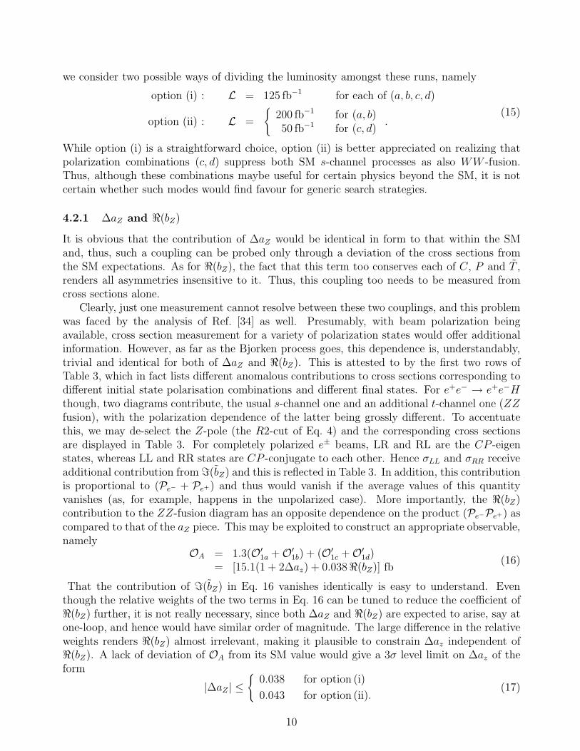
we consider two possible ways of dividing the luminosity amongst these runs, namely

option (i) : L = 125 fb−1 for each of (a, b, c, d)

option (ii) : L =

{200 fb−1 for (a, b)50 fb−1 for (c, d)

.(15)

While option (i) is a straightforward choice, option (ii) is better appreciated on realizing thatpolarization combinations (c, d) suppress both SM s-channel processes as also WW -fusion.Thus, although these combinations maybe useful for certain physics beyond the SM, it is notcertain whether such modes would find favour for generic search strategies.

4.2.1 ∆aZ and ℜ(bZ)

It is obvious that the contribution of ∆aZ would be identical in form to that within the SMand, thus, such a coupling can be probed only through a deviation of the cross sections fromthe SM expectations. As for ℜ(bZ), the fact that this term too conserves each of C, P and T ,renders all asymmetries insensitive to it. Thus, this coupling too needs to be measured fromcross sections alone.

Clearly, just one measurement cannot resolve between these two couplings, and this problemwas faced by the analysis of Ref. [34] as well. Presumably, with beam polarization beingavailable, cross section measurement for a variety of polarization states would offer additionalinformation. However, as far as the Bjorken process goes, this dependence is, understandably,trivial and identical for both of ∆aZ and ℜ(bZ). This is attested to by the first two rows ofTable 3, which in fact lists different anomalous contributions to cross sections corresponding todifferent initial state polarisation combinations and different final states. For e+e− → e+e−Hthough, two diagrams contribute, the usual s-channel one and an additional t-channel one (ZZfusion), with the polarization dependence of the latter being grossly different. To accentuatethis, we may de-select the Z-pole (the R2-cut of Eq. 4) and the corresponding cross sectionsare displayed in Table 3. For completely polarized e± beams, LR and RL are the CP -eigenstates, whereas LL and RR states are CP -conjugate to each other. Hence σLL and σRR receiveadditional contribution from ℑ(bZ) and this is reflected in Table 3. In addition, this contributionis proportional to (Pe− + Pe+) and thus would vanish if the average values of this quantityvanishes (as, for example, happens in the unpolarized case). More importantly, the ℜ(bZ)contribution to the ZZ-fusion diagram has an opposite dependence on the product (Pe−Pe+) ascompared to that of the aZ piece. This may be exploited to construct an appropriate observable,namely

OA = 1.3(O′1a + O′

1b) + (O′1c + O′

1d)= [15.1(1 + 2∆az) + 0.038ℜ(bZ)] fb

(16)

That the contribution of ℑ(bZ) in Eq. 16 vanishes identically is easy to understand. Eventhough the relative weights of the two terms in Eq. 16 can be tuned to reduce the coefficient ofℜ(bZ) further, it is not really necessary, since both ∆aZ and ℜ(bZ) are expected to arise, say atone-loop, and hence would have similar order of magnitude. The large difference in the relativeweights renders ℜ(bZ) almost irrelevant, making it plausible to constrain ∆az independent ofℜ(bZ). A lack of deviation of OA from its SM value would give a 3σ level limit on ∆az of theform

|∆aZ | ≤{

0.038 for option (i)

0.043 for option (ii).(17)

10

Observable Description σ0Z σ1Z σ4Z

O1a σ−,+(R1; µ, q) 23.9 226 0O1b σ+,−(R1; µ, q) 17.9 169 0O′

1a σ−,+(R2; e) 4.04 1.46 0.122O′

1b σ+,−(R2; e) 2.64 0.715 −0.122O′

1c σ−,−(R2; e) 3.29 −1.34 0.855O′

1d σ+,+(R2; e) 3.09 −1.45 −0.855

Table 3: Various anomalous contributions (as defined in Eq. 7) to the cross sections σ(R1; µ, q)(for µ± and light quarks in the final state with R1-cut) and σ(R2; e) (for e± in the final statewith R2-cut) for the four polarisation states. The rates are in femtobarns, for

√s = 500 GeV.

The smallness of the difference in the two limits is but a consequence of the larger error barsresulting from smaller luminosities assigned to polarization combinations (c, d). Note thatthe limits are only marginally different from that obtained with unpolarised beams with L =500 fb−1, namely of |∆aZ | <∼ 0.04 [34]3. More importantly, though, unlike the bound of Ref. [34],the constraint of Eq. 17 is independent of ℜ(bZ).

-0.015

-0.01

-0.005

0

0.005

0.01

0.015

-0.04 -0.02 0 0.02 0.04

Re(

b Z)

∆aZ

ΟA

ΟB

-0.015

-0.01

-0.005

0

0.005

0.01

0.015

-0.04 -0.02 0 0.02 0.04

Re(

b Z)

∆aZ

ΟC

-0.015

-0.01

-0.005

0

0.005

0.01

0.015

-0.04 -0.02 0 0.02 0.04

Re(

b Z)

∆aZ

∆χ2 = 11.83

Figure 1: The regions in the ∆aZ −ℜ(bZ) plane consistent with 3σ variations in the observablesOA,B,C respectively. The region enclosed by all the three sets reflect the overall constraints. Theellipse represents the region corresponding to ∆χ2 = 11.83 obtained using all polarised crosssections listed in Table 3. An integrated luminosity of 125 fb−1 for each of the polarisation statei.e. option (i) of Eq. 15 has been used. The limits for option (ii) are very similar.

A different linear combination of the same observables, namely,

OB = O1a + O1b − 6.6(O′1c + O′

1d)

= [−0.31(1 + 2∆aZ) + 413ℜ(bZ)] fb(18)

3Note that the results quoted here for the unpolarised beams differ from those of the Ref. [34] because ofthe difference in the value of branching fraction of H → b b decay mode used there. We have used the value ofbranching fraction to be 0.68 whereas in Ref. [34] it was taken to be 0.9

11

is equally useful as this enhances the ℜ(bZ) contribution, while essentially getting rid of ∆aZ .This leads to

|ℜ(bZ)| ≤{

0.012 for option (i)

0.018 for option (ii)(19)

virtually independent of ∆aZ . Finally, using the information from the R1-cut alone, we have

OC = O1a + O1b

= [41.8(1 + 2∆az) + 395ℜ(bZ)] fb(20)

leading to a correlated constraint in the ∆aZ–ℜ(bZ) plane as displayed in Fig. 1. Of the sixcross sections of Table 3, one may be used to eliminate ℑ(bZ), leaving behind five constraintsin this plane. Note that we have already used three linearly independent combinations. Wemay, nonetheless, use all five to construct a χ2-test. The resultant 3σ ellipse (correspondingto ∆χ2 = 11.83) is also displayed in Fig. 1. That this ellipse protrudes slightly beyond theset of straight lines is not surprising, for the latter denote the 3σ constraint on a particularcombination of the two variables (with complete disregard for the orthogonal combination),while the ellipse gives the corresponding bound on the plane. Furthermore, the size and theshape of the ellipse demonstrates that the three combinations identified above represent thestrongest constraints with very little role played by the remaining two.

Finally, recollect that, for completely polarized e± beams, LL and RR states are CP -conjugate to each other. Hence the difference of σLL and σRR can be used to probe CP -oddcouplings. Thus, using

OD ≡ O′1c −O′

1d =[0.2 (1 + 2∆az) + 0.11ℜ(bZ) + 1.71ℑ(bZ)

]fb , (21)

one obtains

|ℑ(bZ)| ≤ 0.4 for L = 125 fb−1. (22)

However, a better constraint can be obtained on this coupling with the use of FB-asymmetrywith respect to polar angle of Higgs boson and a discussion of this follows.

4.2.2 ℜ(bZ) and ℑ(bZ)

Next we focus on the role of beam polarisation in exploring both the real and imaginary parts ofbZ . As discussed earlier, the independent experimental probes for these couplings, namely theasymmetries AFB and AUD, are proportional to the quantity (l2e −r2

e) for the case of unpolarisedbeams [34]. For maximally polarized beams, on the other hand, the squared matrix elementis either proportional to r2

e or to ℓ2e and hence the suppression factor is not so severe even for

moderate polarization. Since ℓ2e > r2

e , the cross sections are somewhat larger for the polarizationcombination a ≡ (−, +), and hence the corresponding constraints would turn out to be a littlestronger.

Imposing the various kinematical cuts of Eq. 3, along-with the R1-cut of Eq. 4 to selectZ-pole contribution, the forward-backward (referring to the Higgs polar angle) asymmetry fordifferent final states and with different polarisation states of the initial beams, can be written,

12

keeping terms up to linear order in anomalous couplings, as

A−,+FB (R1 − cut) =

0.174 ℜ(bZ) − 6.14 ℑ(bZ)

1.48(e+e−H)

−6.07 ℑ(bZ)

1.46(µ+µ−H)

−92.8 ℑ(bZ)

22.4(qqH)

(23)

and

A+,−FB (R1 − cut) =

−0.0911 ℜ(bZ) + 4.43 ℑ(bZ)

1.11(e+e−H)

4.4 ℑ(bZ)

1.09(µ+µ−H)

67.2 ℑ(bZ)

16.8(qqH)

(24)

Here, each of the numerical factors denote cross-sections in femtobarns with the denominatorbeing the SM cross section. Understandably, the FB asymmetry is identical for the case of theZ going into muons or a qq pair, and thus the two channels can be added up to obtain the totalsensitivity. As for the e+e−H channel, the coupling ℜ(bZ) makes an appearance on account ofthe interference of the t-channel diagram with the absorptive part of the s-channel SM one.

The FB-asymmetry with final state µ’s and q’s get contribution only from ℑ(bZ). Hence wedefine the following observable

OFB(R1; µ, q) = A−,+FB (R1; µ) + A−,+

FB (R1; q) − A+,−FB (R1; µ) − A+,−

FB (R1; q)

= − 16.3ℑ(bZ) (25)

which leads to

|ℑ(bZ)| ≤{

0.011 for option (i)0.0089 for option (ii).

(26)

In Fig. 2, the vertical lines represent the above bounds for option (i).Similarly, the up-down asymmetries, with respect to azimuthal angle of final state fermions,

are given by

A−,+UD (R1 − cut) =

−1.43 ℜ(bZ) − 0.286 ℑ(bZ)

1.48(e+e−H)

−1.49 ℜ(bZ)

1.46(µ+µ−H)

(27)

and

A+,−UD (R1 − cut) =

1.12 ℜ(bZ) − 0.161 ℑ(bZ)

1.11(e+e−H)

1.08 ℜ(bZ)

1.09(µ+µ−H)

(28)

Since the determination of this asymmetry requires charge measurement of the final stateparticles, we do not consider it for quarks in the final states. Once again, ℑ(bZ) makes an

13

appearance for the e+e−H case on account of the aforementioned interference. Combining bothpolarisation states (−, +) and (+,−) for final state muons we construct a observable, namely,

OUD(R1; µ) ≡ A−,+UD (R1; µ) − A+,−

UD (R1; µ) = − 2.01ℜ(bZ) , (29)

we may constrain

|ℜ(bZ)| ≤{

0.17 for option (i)0.13 for option (ii).

(30)

Clearly, one expects a nontrivial effect of the beam poalrisation only for asymmetries con-structed with the R1-cut. For the sake of completeness, we also present the up-down asymme-tries with the R2-cut (de-selecting the Z-pole) for the eeH final state, namely

A−,+UD (R2; e) =

4.3ℜ(bZ) + 0.227ℑ(bZ)

4.04,

A+,−UD (R2; e) =

3 ℜ(bZ) − 0.227ℑ(bZ)

2.64,

A−,−UD (R2; e) =

4.01ℜ(bZ) + 1.59ℑ(bZ)

3.29,

A+,+UD (R2; e) =

3.82ℜ(bZ) − 1.59ℑ(bZ)

3.09.

(31)

With LL and RR initial states being CP -conjugate to each other, it is understandable thatAUD receives additional contribution4 from ℑ(bZ). Defining

OUD(R2; e) = 2 A−,+UD (R2; e) + A+,−

UD (R2; e) + A−,−UD (R2; e) + A+,+

UD (R2; e)

= 5.72ℜ(bZ) − 0.005ℑ(bZ)(32)

one may get rid of this contribution, and thereby constrain

|ℜ(bZ)| ≤{

0.067 for option (i)0.074 for option (ii)

(33)

at the 3σ level. The bounds for option (i) are represented by horizontal lines in Fig. 2.It is instructive to compare the above sensitivities (see Table 4) with those possible with

unpolarised beams [34]. As one can see, for asymmetries with R1-cut, the enhancement ofsensitivity to both the CP -odd couplings ℜ(bZ) and ℑ(bZ) on using longitudinally polarizedbeams for option (ii)(option (i)) of Eqs. 15) is nearly by a factor of 7(5–6), a feat unachievablewithout polarisation. This improvement is indeed due to the circumvention of the vanishinglysmall vector coupling of electron to the Z boson. Our results are compatible with the morestringent limits of Ref. [33], when we remove the effect of kinematical cuts as well as of the useof the bb final state and finite b–tagging efficiency, implemented in our analysis. Of course, asimilar enhancement for ℜ(bz) may also be possible even with unpolarised beams, when AUD

for the eeH final state is considered alongwith the R2-cut. It is, nonetheless, interesting to havetwo different measurements measure the same coupling to the same accuracy. Of course, thisin addition to the big enhancement in sensitivity to the CP -odd couplings ℜ(bZ) and ℑ(bZ) asmentioned above; this, in fact, is not achievable with the R1-cut.

4This is analogous to the appearance of ℑ(bZ) in the total cross sections in Sec.4.2.1.

14

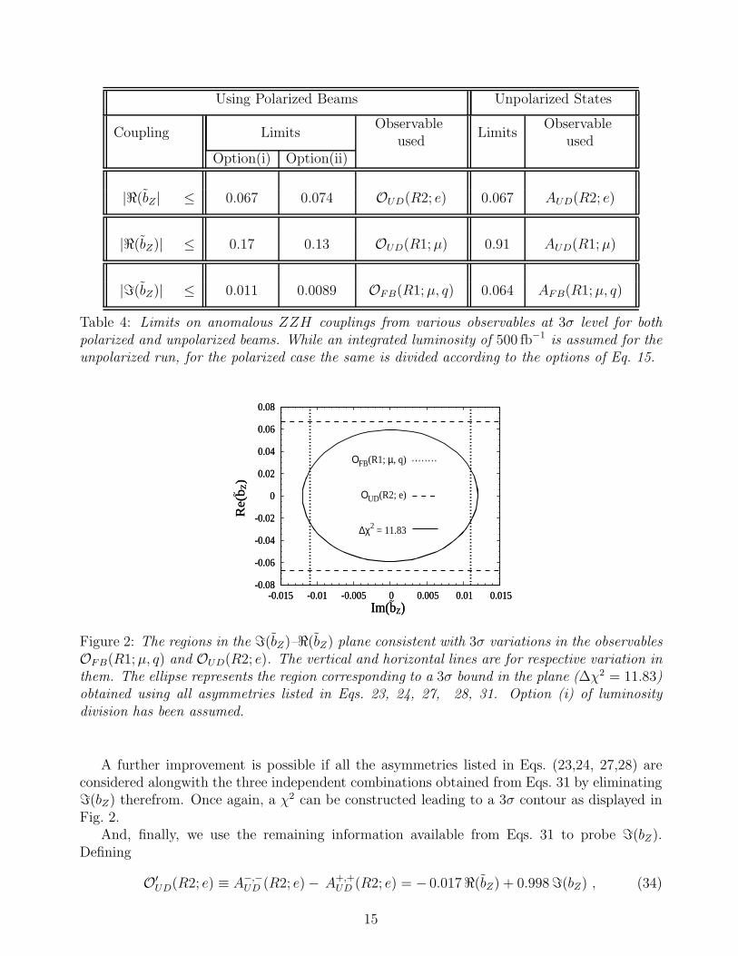
Using Polarized Beams Unpolarized States

Coupling LimitsObservable

usedLimits

Observableused

Option(i) Option(ii)

|ℜ(bZ| ≤ 0.067 0.074 OUD(R2; e) 0.067 AUD(R2; e)

|ℜ(bZ)| ≤ 0.17 0.13 OUD(R1; µ) 0.91 AUD(R1; µ)

|ℑ(bZ)| ≤ 0.011 0.0089 OFB(R1; µ, q) 0.064 AFB(R1; µ, q)

Table 4: Limits on anomalous ZZH couplings from various observables at 3σ level for bothpolarized and unpolarized beams. While an integrated luminosity of 500 fb−1 is assumed for theunpolarized run, for the polarized case the same is divided according to the options of Eq. 15.

-0.08

-0.06

-0.04

-0.02

0

0.02

0.04

0.06

0.08

-0.015 -0.01 -0.005 0 0.005 0.01 0.015

Re(

~ b Z)

Im(~bZ)

ΟFB(R1; µ, q)

ΟUD(R2; e)

-0.08

-0.06

-0.04

-0.02

0

0.02

0.04

0.06

0.08

-0.015 -0.01 -0.005 0 0.005 0.01 0.015

Re(

~ b Z)

Im(~bZ)

∆χ2 = 11.83

Figure 2: The regions in the ℑ(bZ)–ℜ(bZ) plane consistent with 3σ variations in the observablesOFB(R1; µ, q) and OUD(R2; e). The vertical and horizontal lines are for respective variation inthem. The ellipse represents the region corresponding to a 3σ bound in the plane (∆χ2 = 11.83)obtained using all asymmetries listed in Eqs. 23, 24, 27, 28, 31. Option (i) of luminositydivision has been assumed.

A further improvement is possible if all the asymmetries listed in Eqs. (23,24, 27,28) areconsidered alongwith the three independent combinations obtained from Eqs. 31 by eliminatingℑ(bZ) therefrom. Once again, a χ2 can be constructed leading to a 3σ contour as displayed inFig. 2.

And, finally, we use the remaining information available from Eqs. 31 to probe ℑ(bZ).Defining

O′UD(R2; e) ≡ A−,−

UD (R2; e) − A+,+UD (R2; e) = − 0.017ℜ(bZ) + 0.998ℑ(bZ) , (34)

15

we may impose

|ℑ(bZ)| ≤ 0.22 for L = 125 fb−1. (35)

This limit is only marginally different than the one obtained with unpolarised beams using thecombined asymmetry Acomb of Sec. 4.1 with R1-cut. We shall see in the next section that abetter constraint may be obtained on this coupling from the combined asymmetry if the finalstate τ helicity is measured.

4.3 Use of Final State τ Polarization with Unpolarised Beams.

In this section we report on the use of selecting final states with τ ’s in a given helicity state. Asimilar idea was employed in the optimal variable analysis of Ref. [31]. A detailed measurementof the decay pion energy distribution [60] or a simpler measurement of the inclusive singlepion spectrum [61], can yield information on τ polarisation. Discussions exist in literatureon how this can be utilized to sharpen search strategies for charged Higgs boson [60–66] orsupersymmetric partners [67] and even for the measurement of SUSY parameters [68,69]. In asimilar vein, one can also construct observables using the final state τ polarisation to probe ZZHcouplings. We construct asymmetries for τ with definite polarisation which can be measured insimple counting experiments and which can catch the essence of the above mentioned optimalobservable analysis.

As discussed in Ref. [34], for unpolarized initial and final states, the combined polar-azimuthal asymmetry Acomb is proportional to (ℓ2

e + r2e)(r

2f − ℓ2

f) and the up-down asymmetry,AUD(φ) is proportional to (ℓ2

e − r2e)(r

2f − ℓ2

f ). Thus, for leptonic final states, both these asym-metries suffer a suppression (this is particularly important for both AUD and Acomb which areimpossible to measure with hadronic final states). Hence, the measurement of the final state τpolarisation would lead to an enhancement in these symmetries with a consequent improvementin the sensitivity to both of the T -odd anomalous couplings, namely ℑ(bZ) and ℜ(bZ). Further,since ℓ2

τ > r2τ , one gets a slightly higher gain in sensitivity with final state τ in a negative

helicity state.To demonstrate this, we construct various asymmetries (listed in Table 2) for both left- and

right-handed τ in the final state. These are the same as described in Sec. 4.1 but defined for aparticular helicity of τ rather than for a specific initial beam polarisation state (for this analysiswe take the initial state to be unpolarised). Again, after imposing the kinematical cuts of Eq. 3

16

alongwith the R1-cut, these read

ALUD(R1; τ) =

−0.527 ℜ(bZ)

0.495,

ARUD(R1; τ) =

0.388 ℜ(bZ)

0.365,

ALcomb(R1; τ) =

−1.37 ℑ(bZ)

0.495,

ARcomb(R1; τ) =

1.01 ℑ(bZ)

0.365,

A′Lcomb(R1; τ) =

1.18 ℑ(bZ) − 0.3 ℜ(bZ)

0.495,

A′Rcomb(R1; τ) =

−0.868 ℑ(bZ) − 0.221 ℜ(bZ)

0.365.

(36)

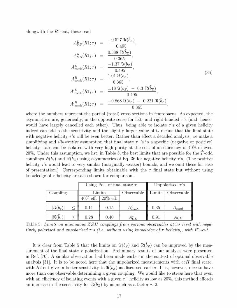
where the numbers represent the partial (total) cross sections in femtobarns. As expected, theasymmetries are, generically, in the opposite sense for left- and right-handed τ ’s (and, hence,would have largely cancelled each other). Thus, being able to isolate τ ’s of a given helicityindeed can add to the sensitivity and the slightly larger value of lτ means that the final statewith negative helicity τ ’s will be even better. Rather than effect a detailed analysis, we make asimplifying and illustrative assumption that final state τ−’s in a specific (negative or positive)helicity state can be isolated with very high purity at the cost of an efficiency of 40% or even20%. Under this assumption, we list, in Table 5, the best limits that are possible for the T -oddcouplings ℑ(bz) and ℜ(bZ) using asymmetries of Eq. 36 for negative helicity τ ’s. (The positivehelicity τ ’s would lead to very similar (marginally weaker) bounds, and we omit these for easeof presentation.) Corresponding limits obtainable with the τ final state but without usingknowledge of τ helicity are also shown for comparison.

Using Pol. of final state τ− Unpolarised τ ’s

Coupling Limits Observable Limits Observable40% eff. 20% eff.

|ℑ(bz)| ≤ 0.11 0.15 ALcomb 0.35 Acomb

|ℜ(bz)| ≤ 0.28 0.40 ALUD 0.91 AUD

Table 5: Limits on anomalous ZZH couplings from various observables at 3σ level with nega-tively polarised and unpolarised τ ’s (i.e. without using knowledge of τ helicity), with R1-cut.

It is clear from Table 5 that the limits on ℑ(bZ) and ℜ(bZ) can be improved by the mea-surement of the final state τ polarization. Preliminary results of our analysis were presentedin Ref. [70]. A similar observation had been made earlier in the context of optimal observableanalysis [31]. It is to be noted here that the unpolarized measurements with eeH final state,with R2-cut gives a better sensitivity to ℜ(bZ) as discussed earlier. It is, however, nice to havemore than one observable determining a given coupling. We would like to stress here that evenwith an efficiency of isolating events with a given τ− helicity as low as 20%, this method affordsan increase in the sensitivity for ℑ(bZ) by as much as a factor ∼ 2.

17

-0.2

-0.15

-0.1

-0.05

0

0.05

0.1

0.15

0.2

-0.3 -0.2 -0.1 0 0.1 0.2 0.3

Im(b

Z)

Re(~bZ)

A’Lcomb(R1; τ)

-0.2

-0.15

-0.1

-0.05

0

0.05

0.1

0.15

0.2

-0.3 -0.2 -0.1 0 0.1 0.2 0.3

∆χ2

ALcomb(R1; τ)

ALUD (R1; τ)

(a)

-0.2

-0.1

0

0.1

0.2

-0.3 -0.2 -0.1 0 0.1 0.2 0.3

Im(b

Z)

Re(~bZ)

A’Rcomb(R1; τ)

-0.2

-0.1

0

0.1

0.2

-0.3 -0.2 -0.1 0 0.1 0.2 0.3

∆χ2

ARcomb(R1; τ)

ARUD (R1; τ)

(b)

-0.4

-0.2

0

0.2

0.4

-0.4 -0.3 -0.2 -0.1 0 0.1 0.2 0.3 0.4

(c)

Im(b

Z)

Re(~bZ)

∆χ2(τunpol) = 11.83∆χ2(τL; τR) = 11.83

Figure 3: 3σ blind regions in the ℜ(bZ) − ℑ(bZ) for a τ -helicity isolation efficiency of 40%.and an integrated luminosity of 500 fb−1. Panel a (b) is for left-(right-)handed τ−’s. Thehorizontal, vertical and oblique lines correspond to Acomb, AUD and A′

comb respectively. Theellipse combines all three and represents the blind region in the plane. The inner ellipse ofpanel (c) combines both sets, and the outer represents the constraints without using τ -helicityinformation.

Fig. 3 displays the region in ℜ(bZ)−ℑ(bZ) plane that can be probed using the asymmetriesof Eq. 36 for τ−’s in a specific helicity state, for an isolation efficiency of 40%. Once again,a χ2 test can be constructed trivially. Note that the constraint from A′

comb are in oppositesense for left- and right-handed τ ’s, resulting in a rotation of the two 3σ ellipses with respect toeach other. One may then combine the information obtained from the two final states and theresults thereof are shown in the last panel. The fact of the two individual ellipses being onlyslightly rotated with respect to the ℜ(bZ) axes means that this exercise of combining the twoleads to only a moderate improvement. It is interesting, though, to compare the result with thecorresponding region when the τ -helicity information is unavailable. The difference is obvious.

4.4 Use of final state τ polarisation for polarised beams

Having established that each of beam polarization and measurement of τ -helicity can lead tosubstantial improvements, the natural question relates to the combination of the two effects.Recall that the up-down asymmetry AUD is proportional to (l2e−r2

e) (l2τ −r2τ ) while the combined

asymmetry Acomb is proportional to (l2e + r2e) (l2τ − r2

τ ). Thus, while the isolation of events witha final state τ in a definite helicity state would enhance both, the use of polarised beams willonly enhance AUD. Hence in this section, we concentrate on the improvement in sensitivity toℜ(bZ) (which is probed by AUD).

The up-down(UD) asymmetry for τ ’s in negative helicity state, with negatively polarizede− and positively polarized e+ beams (i.e. the polarisation state ‘a’ as mentioned in Sec. 4.2)is given by

A−,+UD (R1; τL) =

−5.66 ℜ(bZ)

0.836. (37)

Once again, assuming that τL’s can be isolated with an efficiency of 40% (20%), the associated 3σ limits on ℜ(bZ) from this single measurement alone for an integrated luminosity L = 200 fb−1

18

(i.e. using only part of the data available for option (ii) of the luminosity divide) reads

|ℜ(bZ)| ≤{

0.054 for 40% efficiency

0.077 for 20% efficiency.(38)

Comparing this to Table 4, the large gain in sensitivity is obvious. And that too with only partof the data. This is significantly better than the maximal sensitivity available for unpolarizedbeams, namely |ℜ(bZ)| ≤ 0.067 obtainable for the e+e−H final state with R2-cut and isolating τ -helicities with a 40% efficiency. Once the data for the other combinations of beam polarizationsand the τ -helicity, viz.

A+,−UD (R1; τL) =

4.1 ℜ(bZ)

0.627.

A−,+UD (R1; τR) =

4.17 ℜ(bZ)

0.617.

A+,−UD (R1; τR) =

−3.02 ℜ(bZ)

0.462.

(39)

are taken into account (using a χ2 test), one obtains, for a 40% isolation efficiency,

|ℜ(bZ)| ≤{

0.032 for option (i)

0.040 for option (ii) ,(40)

with the numbers for an isolation efficiency of 20% being a little worse. The combined use ofbeam polarisation and τ -helicity measurement thus plays a very productive role,

To summarize the entire section, we have demonstrated that the CP-odd and T -odd ZZHcouplings can be probed far better by the use of polarised beams and/or the information of finalstate polarisation. The sensitivity to CP-even and T -even anomalous ZZH couplings, (∆aZ

and ℜ(bZ)), on the other hand, show only a marginal improvement in their sensitivity limits.However, use of polarised beams helps to constrain these couplings independent of each other.

5 Beam Polarization and the WWH Couplings

A study of the anomalous WWH couplings is possible via the process e+e− → ννH . However,since it receives contributions from both the t-channel WW fusion diagram and the s-channelBjorken diagram, this determination needs knowledge of the anomalous ZZH couplings, whichfortunately, can be measured well from measurements of other final states. It may be arguedthat, for completely polarized e± beams, the cross section σLR gets contribution from both theBjorken and fusion diagrams, whereas only the first contributes to σRL, and hence it should bepossible to use cross sections with different polarisation combinations to reduce the contam-ination due to the anomalous ZZH couplings. It should be noted however, that in realisticsituations one would not have 100% beam polarisation, and thus this effect cannot be entirelyneutralized.

Apart from this possible contamination, the determination of WWH anomalous couplingsuffers from one more limitation. The presence of a pair of neutrinos deprives us of the fullknowledge of the momenta of the final state fermions and, thus, does not allow construction ofT -odd observables. Total rates and forward-backward asymmetry with respect to polar angle of

19

the Higgs boson (each for different combinations of beam polarisations) are the only observablesavailable in the present case. Using the notation of Eq. 14 for the polarisation states, the states‘c’ and ‘d’ do not contribute to the process e+ e− → ννH , for the case of 100% polarisation.Even with the assumed values of 80% and 60% polarisation for the e− and e+ beams respectively,these two combinations will correspond to rather small cross sections. Therefore, we restrictourselves to the data accrued from the other two polarisation combinations viz. a and b. Onimposition of the R1′- or the R2′-cut, the cross sections are now given by5

σ−,+(R1′; ν) = [9.09 + 17.6 ∆aZ + 0.60 ℜ(∆aW ) + 83.8 ℜ(bZ) − 3.62 ℑ(bZ)

− 0.48 ℑ(∆aW ) + 0.90 ℜ(bW ) + 1.51 ℑ(bW )] fb

σ+,−(R1′; ν) = [6.63 + 13.2 ∆aZ + 0.02 ℜ(∆aW ) + 63.4 ℜ(bZ) − 0.10 ℑ(bZ)− 0.01 ℑ(∆aW ) + 0.03 ℜ(bW ) + 0.04 ℑ(bW )] fb

σ−,+(R2′; ν) = [102 − 0.45 ∆aZ − 17.6 ℜ(bZ) − 0.31 ℑ(bZ)+ 205 ℜ(∆aW ) − 38.3 ℜ(bW )] fb

σ+,−(R2′; ν) = [3.23 + 0.78 ∆aZ + 4.31 ℜ(bZ) + 5.68 ℜ(∆aW ) − 1.06 ℜ(bW )] fb

(41)

That the WWH couplings make a small contribution for the (+,−) case is easy to under-stand. Furthermore, the contributions from ℑ(bW,Z) are small as these have to be proportionalto the absorptive part of the Z-propagator in Bjorken diagram. As can be expected, the sensi-tivity to the WWH couplings is enhanced if one can successfully eliminate the contribution ofthe Z-diagram (this has the further advantage of eliminating the νµ and ντ events). However,since even the R2′-cut (see Eq. 5) cannot eliminate the Z diagram entirely, as is seen fromEq. 41, we consider a particular linear combination of the cross sections, namely

O2 νA≡ σ−,+(R2′; ν) + 4 σ+,−(R2′; ν)= [η1 + 115 + 228 ℜ(∆aW ) − 42.5 ℜ(bW )] fb,

η1 ≡ 2.66 ∆aZ − 0.36 ℜ(bZ) − 0.31 ℑ(bZ).

(42)

Thus the contamination from ZZH couplings is contained entirely in η1. Using the analysisof the previous section (which did not involve the ννH final state), we have |η1| ≤ 0.13(0.14)respectively for options (i) and (ii) of the luminosity division (Eqs. 15). In other words, theuncertainty due to a lack of precise knowledge of the ZZH couplings is reduced to negligibleproportions enabling us to constrain a combination of ℜ(∆aW ) and ℜ(bW ) virtually independentof ZZH couplings:

|2 ℜ(∆aW ) − 0.37 ℜ(bW )| ≤ 0.040 (0.036) (43)

for the two choices of luminosity division among different polarisation modes concerned (seeFig. 4). The relatively small difference between the sensitivities indicates that the luminositydivision is not very crucial as long as a sufficiently large fraction is devolved into the canonicalchoices of (+,−) and (−, +). It may be also noted here that due to large value of SM crosssection, the fluctuation in the cross section with R2′-cut given by Eq. 6 is dominated by thesystematic error as mentioned in Sec. 3. Thus small changes in luminosity or cross section is

5 As stated earlier in Sec. 2, we may choose aZ to be real, without any loss of generality. But once we makethis choice, all the WWH couplings (including ∆aW ) may be complex.

20

not going to make much difference to the sensitivity limits of the couplings that are probed bycross section σ−,+(R2′; ν) or O2 νA

.While it is true that we can only probe a combination of these two couplings using O2 νA

,use of beam polarization clearly helps to reduce contamination from ZZH couplings to thisdetermination. It is to be noted that since only a particular linear combination of ℜ(∆aW ) andℜ(bW ) can be probed, limits on them are strongly correlated. Of course, it is possible to derivea constraint on the orthogonal combination from the data of Eq. 41, but it is too weak to be ofany relevance. If we make a further assumption of only one of these couplings being non-zero,we would obtain

|ℜ(∆aW )| ≤ 0.020 (0.018) for ℜ(bW ) = 0|ℜ(bW )| ≤ 0.110 (0.095) for ℜ(∆aW ) = 0

(44)

with the two limits corresponding to options (i) and (ii) of Eqs. 15. Although a comparison withthe results obtained earlier [34] shows only a marginal improvement in the individual limits, thedetermination is now free of uncertainty coming from contamination from the ZZH couplings.

-0.4

-0.3

-0.2

-0.1

0

0.1

0.2

0.3

0.4

-0.04 -0.03 -0.02 -0.01 0 0.01 0.02 0.03 0.04

Re(

b W) ∆aZ

∆aZ

Re(∆aW)

Ο2νA(R2’; ν)

ΟA(R2; e)

Figure 4: The region in the ℜ(∆aW ) − ℜ(bW ) plane consistent with 3σ variations in O2 νAfor

an integrated luminosity of 125 fb−1. The vertical line shows the sensitivity limit on ∆aZ fromFig. 1

At this stage, it is intriguing to consider the consequences of an additional assumption(made in Ref. [34]) of ∆aW = ∆aZ , which is found to be true in some cases [71] and wouldbe motivated by SU(2) × U(1) invariance of the effective theory. By itself, this would imposea bound on ∆aW , courtesy Eq. 17 and hence that would lead to a closed area as shown inFig. 4. However, one should also note that SU(2) × U(1) invariance would further equate bW

and bZ , and that the correlation between constraints in the ℜ(bW )–ℜ(∆aW ) plane (Fig. 4) isin the opposite sense to that in the ℜ(bZ)–∆aZ plane (Fig. 1). Thus, an assumption of such aninvariance would lead to far stronger constraints. In particular, the improvement is dramaticfor ℜ(bW ).

As for the other CP-even WWH couplings, namely ℑ(∆aW ) and ℑ(bW ), note that theircontributions arise from the interference of the WW -fusion diagram with the absorptive part

21

of the Z-propagator in the Bjorken diagram. Hence the corresponding terms appear only intotal rate with R1′-cut and being proportional to the width of Z-boson, are very small. Sincethe presence of two neutrinos in the final state does not allow us to construct any T -oddobservables, this study is virtually insensitive to these two couplings. Of course, an assumptionof SU(2) × U(1) invariance would change matters drastically.

What remains is to investigate bW , and this being a CP-odd coupling, can be probed throughthe forward-backward (FB) asymmetry with respect to the polar angle of Higgs boson. Theseasymmetries, R1′- or and R2′-cuts can be expressed as

A−,+FB (R1′; ν) =

1

9.09

[−2.29 ℜ(bZ) − 36.9 ℑ(bZ) + 0.57 ℜ(bW ) − 0.47 ℑ(bW )

],

A+,−FB (R1′; ν) =

1

6.63

[−0.064 ℜ(bZ) + 27.1 ℑ(bZ) + 0.02 ℜ(bW ) − 0.01 ℑ(bW )

],

A−,+FB (R2′; ν) =

1

102

[5.17 ℑ(bZ) + 7.83 ℑ(bW )

],

A+,−FB (R2′; ν) =

1

3.23

[2.1 ℑ(bZ) + 0.22 ℑ(bW )

].

(45)

where the numbers once again represent the corresponding cross sections in femtobarns. Withthe last two of Eqs. 45 involving just a single WWH coupling, these can be combined toeliminate the remaining dependence on the ZZH anomalous couplings to leave us

A2mix≡ 13 A−,+

FB (R2′; ν) − A+,−FB (R2′; ν)

= 0.009 ℑ(bZ) + 0.93 ℑ(bW ).(46)

The contribution to A2mixfrom ℑ(bZ) (which, incidentally, can be probed very accurately, see

Table 4) may be neglected, leading to

|ℑ(bW )| ≤ 0.50 (0.44) (47)

for L = 125 (200) fb−1 for each of the (+,−) and (−, +) polarization combinations. Whileit may seem that the improvement is marginal when compared to the sensitivity achievablewith unpolarised beams— |ℑ(bW )| ≤ 0.46 for a total luminosity of 500 fb−1 [34]—note that,unlike the older analysis, the current sensitivity is independent of any other coupling. In otherwords, the use of beam polarisation has allowed construction of an observable that can isolatethe contribution of ℑ(bW ).

The anomalous coupling ℜ(bW ) being a T -odd coupling has no contribution to FB asymme-tries with R2′-cut and only a small contribution to FB asymmetries with R1′-cut through theinterference of the WW -fusion diagram with the absorptive part of Bjorken diagram. Hencethese asymmetries are not a good probe of ℜ(bW ). Thus the process under consideration cannot be used to probe any of the T -odd couplings in the WWH vertex.

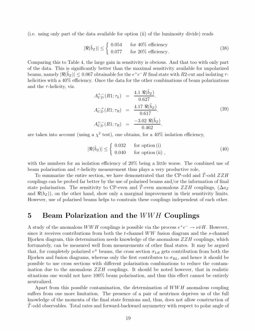
To summarize the results of this section: use of beam polarisation allows us to obtainlimits on T -even couplings ℜ(∆aW ), ℜ(bW ) and ℑ(bW ) independent of the ZZH couplings,these being listed in Table 6. Using linear combinations of our observables corresponding todifferent polarisation combinations for initial states, the contamination from ZZH coupling canbe reduced to negligible amount, something that was not possible with the unpolarised beams.Further, even though this measurement uses only two of the combinations, an equal division of

22

Using Polarized Beams Unpolarized States

Coupling Limits (for given L)Observables

usedLimits

Observablesused

200 fb−1 125 fb−1

|ℜ(∆aW )| ≤ 0.018 0.020 O2 νA0.019 σunpol(R2′; ν)

|ℜ(bW )| ≤ 0.095 0.11 O2 νA0.10 σunpol(R2′; ν)

|ℑ(bW )| ≤ 0.44 0.50 A2mix0.40 Aunpol

FB (R2′; ν)

Table 6: 3 σ limits on anomalous WWH couplings from various observables with polarized andunpolarized beams.

the total luminosity among all four already gives optimal results. The limits on ℜ(∆aW ) andℜ(bW ) are highly correlated whereas ℑ(bW ) is constrained independent of any other coupling.There is no observable to constrain the T -odd couplings and thus we conclude that this processis not a good probe for these couplings. Hence one has to look to other processes to probe thesecouplings. For example, this problem may be overcome in the e γ collider as shown in Ref. [72].The WWH couplings are not contaminated by the ZZH couplings in the process studied thereviz. (e−γ → ν W− H). Using this process in conjunction with the P T conjugate process, theauthors were able to construct observables that depend only on one of the anomalous WWHcouplings and hence the limits obtained on each of the WWH couplings were independent ofthe others. The anomalous VVH couplings at e γ collider have been also studied in Ref. [73].Finally, an assumption of SU(2) × U(1) invariance would drastically improve the constraintsfor virtually all the couplings, whether they be WWH or ZZH .

6 Dependence on√

s and inclusion of ISR/Beamstrahlung

Effects

All our analysis so far has been performed for a fixed centre of mass energy, namely√

s =500 GeV. Clearly, the total cross section is a function of energy, and the functional formmay depend on the presence of (and the identity of) any anomalous coupling, owing to theirhigher-dimensional nature. Thus, the sensitivities could, in principle, depend on the choiceof

√s. Furthermore, for the processes involving both s- and t-channel diagrams, the relative

importance of these two parts of the amplitude is, in fact, energy dependent, and the genericenhancement of the t–channel cross section with increasing beam energies may, in principle, leadto an improvement in the sensitivity to those couplings primarily constrained using observableswith R2-(R2′)-cut.

Even for a nominally fixed beam energy, the√

s available to an individual hard scatter-

23

ing event is generically less than this value owing to the ubiquitous initial state radiation(ISR)— which is nothing but the bremsstrahlung radiation by the incoming particles—or beam-strahlung, which is a name for the radiation from the beam particles due to its interaction withthe (strong) electromagnetic fields caused by the dense bunches of the opposite charge in a col-lider environment. Consequently, it is important to investigate the possibly detrimental effectsof such eventualities.

0

50

100

150

200

250

300

350

400

500 1000 1500 2000 2500 3000

Coe

ffic

ient

of

vari

ous

coup

ling

s in

σ(R

2) [

fb]

Ecm[Gev]

50*σ0Z(R2; e)

σ0W(R2’; ν)

- σ1W(R2’; ν)

Figure 5:√

s-variation of (σ0Z(R2; e) (the SM part in the cross section σ(R2; e) = σ(e+e− →e+e−H) with R2-cut), σ0W (R2′; ν) and σ1W (R2′; ν) (the coefficients of ℜ(∆aW ) and ℜ(bW )respectively in the cross section for e+e− → ννH with R2′-cut).

To this end, we begin by studying the√

s-dependence of the observables used in this paper.For simplicity, we shall restrict ourselves, in this section, to unpolarised scattering, with theresults for polarised beams expected to be similar. Moreover, we shall concentrate on observ-ables defined with the R2-(R2′)-cut. For example, the ZZH coupling ∆aZ is best probed bythe total cross section with R2-cut for electron final state i.e. σ(R2; e) = σ(e+e− → e+e−H)with R2-cut. Fig. 5 shows the variation of the SM part of this cross section (σ0Z of Eq. 7)with

√s.6 Recall that ∆aZ simply rescales the SM part of the cross section (Eq. 7) and hence

the sensitivity is determined simply by the corresponding number of events, namely it scales asN

−1/2

0Z . With σ0Z(R2; e) having a maximum at√

s ≈ 1.1 TeV, this would be the optimal beamenergy to probe ∆aZ , with the maximal improvement (compared to the results quoted above)being by about 40%.

Fig. 5 also shows the√

s-variation of the SM and ℜ(bW ) contributions (i.e. σ0W and σ1W

respectively) to the cross section σ(R2′; ν) = σ(e+e− → ννH) with R2′-cut which is the bestprobe for the WWH couplings ℜ(∆aW ) and ℜ(bW ). While the monotonic increase in σ1W wouldseem to suggest that increasing

√s would readily lead to an improvement in the sensitivity to

ℜ(bW ), note that this increase saturates and, furthermore, that σ0W increases at least as fast.Consequently, for moderate changes in

√s, any improvement or otherwise is expected to be

marginal at best.

6Note that σ0Z has been scaled by a factor of 50 to fit in the same figure.

24

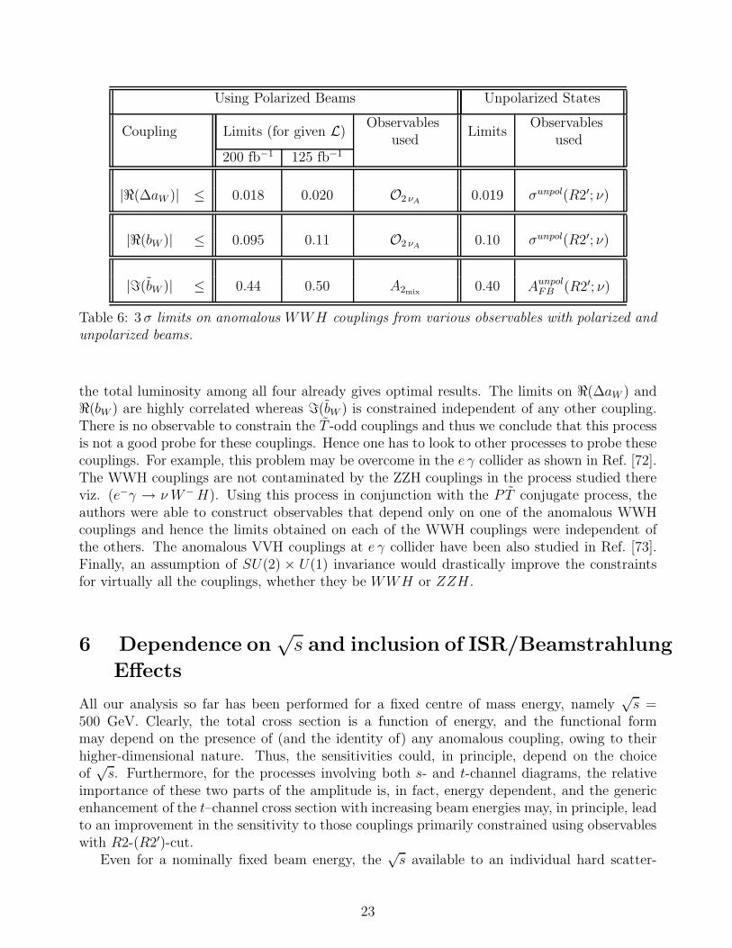
Moving to asymmetries, the up-down asymmetry AUD(R2; e) of the final state fermionwith respect to the H-production plane, and the forward-backward asymmetry with respectto polar angle of the Higgs boson, AFB(R2′; ν) have been used to constrain ℜ(bZ) and ℑ(bW )respectively [34]. Expressing these as

AUD(R2; e) = AaUD ℜ(bZ)

AFB(R2′; ν) = AbFB ℑ(bZ) + Ac

FB ℑ(bW ) (48)

the coefficients AaUD and Ac

FB are plotted in Fig. 6 as a function of√

s. The figure clearly shows

0

1

2

3

4

5

6

7

8

500 1000 1500 2000 2500 3000

Coe

ffic

ient

of

vari

ous

coup

ling

s in

the

asy

mm

etry

Ecm[Gev]

AaUD(R2; e)

100*AcFB(R2’; ν)

Figure 6:√

s-variation of the coefficients AaUD in up-down asymmetry and the Ac

FB in forward-backward asymmetry as defined in Eq. 48 of the text. Both plots are with R2-(R2′)-cut (de-selecting Z pole) imposed.

that the sensitivity to ℜ(bZ) is expected to improve at higher√

s, while,√

s = 500 GeV is anoptimal choice for ℑ(bW ) and higher energies would only tend to deteriorate the sensitivity.The arguments above are reflected by Table 7 which summarizes the sensitivity limits at the3 σ level, with an integrated luminosity of 500 fb−1, for different center of mass energies.

The above analysis did not take into account either of ISR and beamstrahlung. We nowproceed to do so, using the structure function formalism [48] to incorporate these effects. Thedifferential scattering cross section for a given process e−(p1)+e+(p2) → X(γ) can be expressedas:

dσ[e+e− → X(γ)] = fe/e(x1) fe/e(x2) dσ[e+e− → X](s) ,

where the electron luminosity function fe/e(x) describes the probability of finding an electronwith a momentum fraction x of the nominal beam energy, or, in other words, the probabilitywith which an electron energy E =

√s/2 emits one or more photons with total energy (1−x)E

resulting in the reduction of its energy to Ee = xE. Hence the square of the effective c.m.energy s can be expressed as: s ≃ x1x2s.

Using the Weiszacker-Williams approximation, one can write down the luminosity functionfor ISR as [47]

f ISRe/e (x) =

β

16

[(8 + 3β)(1 − x)β/2−1 − 4(1 + x)

], (49)

25

Coupling3 σ limit at√

s = 0.5TeV

3 σ limit at√s = 1TeV

3 σ limit at√s = 3TeV

Observableused

|∆aZ | ≤ 0.040 0.030 0.049 σ(R2; e)

0.043 0.031 0.039 σISR+Beam.(R2; e)

|ℜ(bZ)| ≤ 0.067 0.028 0.015 AUD(R2; e)

0.075 0.032 0.018 AISR+Beam.UD (R2; e)

|ℜ(∆aW )| ≤ 0.019 0.016 0.016 σ(R2′; ν)

0.019 0.017 0.016 σISR+Beam.(R2′; ν)

|ℜ(bW )| ≤ 0.10 0.082 0.084 σ(R2′; ν)

0.11 0.084 0.083 σISR+Beam.(R2′; ν)

|ℑ(bW )| ≤ 0.40 0.42 0.89 AFB(R2′; ν)

0.43 0.41 0.71 AISR+Beam.FB (R2′; ν)

Table 7: Individual sensitivity limits (assuming only the relevant coupling to be non-zero) at the3σ level for an integrated luminosity of 500 fb−1 on various anomalous couplings at differentc.m. energies without and with the inclusion of ISR and beamstrahlung effects. The resultscorrespond to unpolarised beams.

where

β =2αem

π

(log

s

m2e

− 1

), (50)

and αem is the fine-structure constant.The beamstrahlung spectrum depends on electron beam energy E, and the parameters such

as the number of electrons per bunch Ne, the bunch dimensions (for a Gaussian bunch profile) inboth the longitudinal direction (σz) as well as in the transverse directions (σy,x). It is convenientto introduce a “beamstrahlung parameter” Υ [49] given by:

Υ =5 r2

e E Ne

6 αem σz (σx + σy) me,

where re is the classical electron radius, and me its mass. The electron spectrum fbeame/e (x)

describing the effects of beamstrahlung, can be written in a closed analytical form for Υ <∼ 10[49]. Armed with all these, the expression for the electron spectrum function, including bothISR and beamstrahlung effects, may be written as [48]:

fe|e(x) =∫ 1

x

dξ

ξf ISR

e|e (ξ) fbeame|e

(ξ−1 x

), (51)

26

where f ISRe|e (ξ) is as given in Eq. 49 above, whereas fbeam

e|e (ξ−1 x) is that given by Eq. 22 ofRef. [49].

We now analyse how the ISR and beamstrahlung effects modify the sensitivity limits ofℜ(bZ), for which we had observed an improvement in sensitivity at higher

√s as listed in

Table 7. In our analysis we use the beamstrahlung parameters to be [74]

σz = 30 µm for all energies,

Υ = 0.3, 1.0 and 8.1 for Ecm = 0.5, 1.0, and 3.0 TeV respectively. (52)

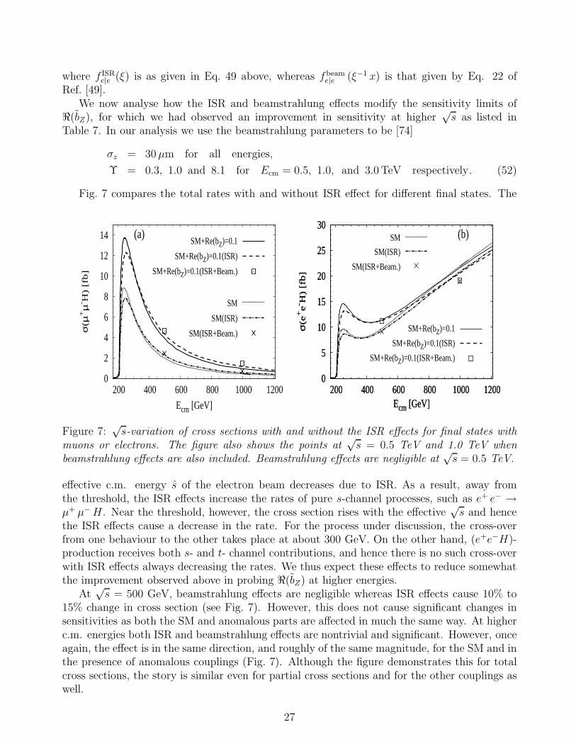
Fig. 7 compares the total rates with and without ISR effect for different final states. The

0

2

4

6

8

10

12

14

200 400 600 800 1000 1200

(a)

σ(µ

+µ

- H)

[fb]

Ecm [GeV]

SM+Re(bZ)=0.1

SM+Re(bZ)=0.1(ISR)

SM+Re(bZ)=0.1(ISR+Beam.)

SM

SM(ISR)

SM(ISR+Beam.)

0

5

10

15

20

25

30

200 400 600 800 1000 1200

(b)

σ(e

+e

- H)

[fb]

Ecm [GeV]

SM

SM(ISR)

SM(ISR+Beam.)

0

5

10

15

20

25

30

200 400 600 800 1000 1200

σ(e

+e

- H)

[fb]

Ecm [GeV]

SM+Re(bZ)=0.1

SM+Re(bZ)=0.1(ISR)

SM+Re(bZ)=0.1(ISR+Beam.)

Figure 7:√

s-variation of cross sections with and without the ISR effects for final states withmuons or electrons. The figure also shows the points at

√s = 0.5 TeV and 1.0 TeV when

beamstrahlung effects are also included. Beamstrahlung effects are negligible at√

s = 0.5 TeV.

effective c.m. energy s of the electron beam decreases due to ISR. As a result, away fromthe threshold, the ISR effects increase the rates of pure s-channel processes, such as e+ e− →µ+ µ− H . Near the threshold, however, the cross section rises with the effective

√s and hence

the ISR effects cause a decrease in the rate. For the process under discussion, the cross-overfrom one behaviour to the other takes place at about 300 GeV. On the other hand, (e+e−H)-production receives both s- and t- channel contributions, and hence there is no such cross-overwith ISR effects always decreasing the rates. We thus expect these effects to reduce somewhatthe improvement observed above in probing ℜ(bZ) at higher energies.

At√

s = 500 GeV, beamstrahlung effects are negligible whereas ISR effects cause 10% to15% change in cross section (see Fig. 7). However, this does not cause significant changes insensitivities as both the SM and anomalous parts are affected in much the same way. At higherc.m. energies both ISR and beamstrahlung effects are nontrivial and significant. However, onceagain, the effect is in the same direction, and roughly of the same magnitude, for the SM and inthe presence of anomalous couplings (Fig. 7). Although the figure demonstrates this for totalcross sections, the story is similar even for partial cross sections and for the other couplings aswell.

27

Since the constraints on ℜ(bZ) are the only ones to improve significantly with increasing√

s(see Table 7), we concentrate on the effects of ISR and beamstrahlung on this coupling. Withℜ(bZ) being best probed by the up-down asymmetry (with R2-cut) for electrons in (e+e−H)production, the ISR and beamstrahlung effects can be summarised as listed in Table 8.

√s UD-asymmetry(AUD(R2; e))

No ISR & Beam. With ISR With ISR & Beam.

0.5 TeV 1.16 ℜ(bZ) 1.13 ℜ(bZ) 1.1 ℜ(bZ)

1 TeV 2.00 ℜ(bZ) 1.94 ℜ(bZ) 1.85 ℜ(bZ)

3 TeV 6.29 ℜ(bZ) 5.60 ℜ(bZ) 4.23 ℜ(bZ)

Table 8: Up-down asymmetry for final state electron for R2-cut(AUD(R2; e)) with and withoutISR and beamstrahlung effects at different

√s’s.

As is readily seen, the effects are almost negligible even for√

s = 1 TeV, and only marginallyimportant for

√s = 3 TeV. The consequent shift in the sensitivities are summarised in Table

7. The smallness of the effects can be understood by realizing that, on the imposition of theR2-cut (de-selecting the Z-pole), the energy dependence of the cross sections (total or partial)is only logarithmic. Further, both SM and anomalous parts have a similar dependence. Hencealthough the cross sections are affected significantly there is little effect on the sensitivity limitsof the anomalous parts after inclusion of ISR and beamstrahlung effects.

We conclude this section by making a few general observations :

• With increasing energy, the observables with the R2-cut imposed gain more in sensitivityas compared to those defined with the R1-cut.

• Observables with R1-cut (selecting Z-pole) are affected more by ISR and beamstrahlungcorrections because of the usual s-channel suppression, whereas the observables with R2-cut (de-selecting Z-pole) have only logarithmic

√s-dependence and hence do not suffer

as significant corrections.

• By using higher c.m. energies, we gain significantly in the sensitivity to ℜ(bZ) (upto afactor of 2 at

√s = 1 TeV as compared to the case of 500 GeV). Neither the ISR nor the

beamstrahlung effects change the sensitivity significantly.

• There is no significant gain in the sensitivity to anomalous WWH couplings even at veryhigh energies.

• In totality, we do not gain much in the sensitivity by going to higher c.m. energies. Thus,running the collider at lower energies (say

√s = 500 GeV), but with polarised beams is

more beneficial for the study of anomalous VVH couplings.

28

7 Summary

With the plethora of the gauge boson couplings with a Higgs that an effective theory allows,it is always going to be a complicated task to unravel these. It was shown in Ref. [34] thatit is possible to construct observables with definite CP and T transformation properties thatare sensitive to a single anomalous coupling (the one with matching CP and T properties) andhence these observables may be used to obtain robust constraints on the couplings in a modelindependent way. With polarised beams, we have the possibility of constructing even moresuch observables.

We have performed our analysis by imposing kinematical cuts on different final state particlesto reduce backgrounds. In addition, we also include the reduction (in the event rates) causedby considering only the events wherein the H decays into a bb pair (with branching fraction∼ 0.68), with a realistic b-tagging efficiency of 70%. This renders, to a great extent, ourestimates of sensitivity quite realistic.

Almost all of the asymmetries pertaining to the probe of the ZZH vertex, that were con-structed in Ref. [34] for unpolarised beams and neglecting the polarisation of the final stateparticles, are proportional to the difference between the squared right and left handed couplingof the Z to charged leptons. Consequently, one expects the sensitivity to the correspondinganomalous couplings to be enhanced once one uses a specific polarisation, thereby overcomingthis cancellation between the (almost) equal left and right handed couplings of the Z boson toleptons. Indeed, we observe this. For example, the use of beam polarization alone leads on theone hand, to the disentangling of the couplings ∆aZ and ℜ(bZ) (not possible for unpolarisedbeams), and on the other, to an improvement in the sensitivities to CP -odd ZZH couplingsby a factor of upto 5-7.

With the helicity of a τ in the final state decipherable from the momentum distribution ofthe charged prongs in its decay, one can construct asymmetries pertaining to τ ’s with a specifichelicity. Assuming that it would be possible to isolate events with τ ’s in a definite helicitystate with an efficiency of (say) 40%, we use such asymmetries to demonstrate that sensitivityto ℑ(bZ) and ℜ(bZ) could be improved by a factor of about 3. While an earlier optimalobservable analysis [31] had indeed investigated the use of τ helicity, our analysis differs in thatwe have constructed an observable that can be measured in a simple counting experiment andcatches the essence of the optimal observable. Also worth noting is that the use of final state τmeasurement along with polarised beams, allows us to improve on the sensitivity for ℜ(bZ) bya factor of about 2.

As far as the constraints on the anomalous WWH couplings are concerned, the problem ofa smaller number of observables due to the presence of missing neutrinos in the the ννH(bb)still exists. However, by constructing new observables that are combinations of the observablescorresponding to different polarisation states, the contamination from the anomalous ZZHcouplings is highly reduced in case of T -even WWH couplings which is a great advantageover the use of unpolarised beams. For T -odd WWH couplings though, we conclude that thisprocess is not a good probe for them because of non-availability of any T -odd observable. Henceone has to look to other processes to probe these couplings.

We have also investigated possible gains in sensitivity by going to higher centre of massenergies. This though renders ISR and the beamstrahlung effects progressively more important.As a matter of fact, even for

√s = 500 GeV, the ISR effects can affect cross sections with the

R1-cut by 10–15%. Fortunately, the ISR and beamstrahlung effects on sensitivity limits is very

29

modest, as both the standard model and the anomalous contributions change by similar amountscausing only small numerical effects, especially on the asymmetries. As for the variation insensitivity with

√s ranging from 300 GeV to 3 TeV, the observables with the R1-cut (selecting

the Z-pole) are naturally associated with a larger cross section (and, hence, better limits)for lower energies. Thus, a machine operating at

√s = 350 GeV would do even better for

certain couplings than the present case. This is in agreement with the findings of Ref. [34].For observables constructed with the R2-cut, however, one can obtain an improvement in thesensitivity limit (say) for ℜ(bZ) by upto a factor of 2 at c.m. energy 1 TeV compared to theones possible at 500 GeV [34].

In conclusion, we find that use of beam polarisation and final state τ polarisation can resultin significant advances in the search for anomalous ZZH couplings at the ILC. For WWHcouplings, though there is no significant change in the sensitivity limits, the T -even ones canbe now probed virtually independent of the anomalous ZZH couplings. The inclusion of ISRand beamstrahlung effects, changes the individual cross sections but has very little effect onthe sensitivities. Further, going to higher beam energies, leads to only modest improvements.Thus, as far as this sector of the theory is concerned, there is a strong case for use of beampolarisation and measurement of final state fermion polarisations wherever possible, but thereis no real gain in going to higher energies.

Acknowledgments

We thank R. K. Singh for collaboration in the initial phase of this project. DC & M ac-knowledge partial support from the Department of Science and Technology(DST), India undergrants SR/S2/RFHEP-05/2006 and SR/S2/HEP-12/2006 respectively and infrastructural sup-port from the IUCAA Reference Centre, Delhi. R.M.G. wishes to acknowledge the DST underGrant No. SR/S2/JCB-64/2007. RMG also wishes to acknowledge support from the IndoFrench Centre for Promotion of Advanced Scientific Research under project number 3004-2.

Note: During the last stages of finalising our manuscript, a paper dealing with related issuescontaining a very detailed analysis [75] on probing the coefficients of the CP-even, dimension 6operators in the anomalous V V H vertices has appeared.

References

[1] P.W. Higgs, Phys. Rev. Lett. 13 (1964) 508; Phys. Rev. 145 (1966) 1156; F. Englert andR. Brout, Phys. Rev. Lett. 13 (1964) 321; G.S. Guralnik, C.R. Hagen and T. Kibble, Phys.Rev. Lett. 13 (1964) 585.

[2] J. Gunion, H. Haber, G. Kane, and S. Dawson, The Higgs Hunter’s Guide, Addison–Wesley,Reading (USA), 1990.

[3] M. Gomez-Bock et al., J. Phys. Conf. Ser. 18, 74 (2005) [arXiv:hep-ph/0509077].

30

[4] A. Djouadi, Phys. Rept. 457, 1 (2008) [arXiv:hep-ph/0503172]; Phys. Rept. 459, 1 (2008)[arXiv:hep-ph/0503173].

[5] For a review, see for example, R. M. Godbole, [arXiv:hep-ph/0205114], Volume 4, JubileeIssue of the Indian Journal of Physics, pp. 44-83, 2004, Guest Editors: A. Raychaudhuriand P. Mitra.

[6] ATLAS Collaboration, Technical Design Report, CERN–LHCC–99–14 and CERN–LHCC–99–15; CMS Collaboration, Technical Design Report, CMS–LHCC–2006–21.

[7] ALEPH, DELPHI, L3 and OPAL Collaborations, The LEP WorkingGroup for Higgs Boson Searches, Phys. Lett. B565, 61 (2003); see alsohttp://lephiggs.web.cern.ch/LEPHIGGS/

[8] LEP Electroweak Working Group, http://lepewwg.web.cern.ch/LEPEWWG/ J. Alcarazet al. [LEP Collaborations], CERN-PH-EP/2007-039, arXiv:0712.0929 [hep-ex].

[9] R. Akers et al. [OPAL Collaboration], Z. Phys. C61, 19 (1994); D. Buskulic et al. [ALEPHCollaboration], Z. Phys. C62, 539 (1994); M. Acciarri et al. [L3 Collaboration], Z. Phys.C62, 551 (1994); P. Abreu et al. [DELPHI Collaboration], Z. Phys. C67, 69 (1995);D. Antreasyan et al. [Crystal Ball Collaboration], Phys. Lett. B251, 204 (1990); P. Franziniet al., Phys. Rev. D35, 2883 (1987); J. Kalinowski and M. Krawczyk, Phys. Lett. B361, 66(1995) [arXiv:hep-ph/9506291]; D. Choudhury and M. Krawczyk, Phys. Rev. D55, 2774(1997) [arXiv:hep-ph/9607271].

[10] M. Carena, J. R. Ellis, A. Pilaftsis and C. E. M. Wagner, Nucl. Phys. B586, 92 (2000).

[11] A. Mendez and A. Pomarol, Phys. Lett. B279, 98 (1992); J. F. Gunion, H. E. Haberand J. Wudka, Phys. Rev. D43, 904 (1991); J. F. Gunion, B. Grzadkowski, H. E. Haberand J. Kalinowski, Phys. Rev. Lett. 79, 982 (1997) [hep-ph/9704410]; I. F. Ginzburg,M. Krawczyk and P. Osland, hep-ph/0211371; I. F. Ginzburg and M. Krawczyk, Phys.Rev. D 72, 115013 (2005).

[12] See e.g. M. Drees, R.M. Godbole and P. Roy, Theory and phenomenology of sparticles,World Scientific, 2005; H. Baer and X. Tata, “Weak scale Supersymmetry: From superfieldsto scattering events,” Cambridge, UK: Univ. Pr. (2006) .

[13] G. Abbiendi et al. [OPAL Collaboration], Eur. Phys. J. C 37, 49 (2004)[arXiv:hep-ex/0406057]; ALEPH, DELPHI, L3 and OPAL Collaborations, The LEPWorking Group for Higgs Boson Searches, LHWG-Note 2004-01, CERN-PH-EP-2006-001; S. Schael et al. [ALEPH Collaboration], Eur. Phys. J. C 47 (2006) 547[arXiv:hep-ex/0602042].

[14] E. Accomando et al., Report of “Workshop on CP studies and non-standard Higgs physics,”CERN-2006-009, arXiv:hep-ph/0608079.

[15] See for example, J. R. Forshaw, Pramana 63, 1119 (2004) and discussion therein; seealso D. Choudhury, T. M. P. Tait and C. E. M. Wagner, Phys. Rev. D65, 053002 (2002)[arXiv:hep-ph/0109097].

31

[16] E. Accomando et al., Phys. Rept. 299 (1998) 1 [arXiv:hep-ph/9705442]; J. Aguilar-Saavedra et al., hep-ph/0106315; T. Abe et al., hep-ex/0106055-58; K. Abe et al.,hep-ph/0109166.

[17] J. Brau et al., SLAC-R-857; A. Djouadi et al., arXiv:0709.1893 [hep-ph].

[18] G. Weiglein et al. [LHC/LC Study Group], Phys. Rept. 426, 47 (2006)[arXiv:hep-ph/0410364].

[19] For a review, see, e.g., R. M. Godbole et al., arXiv:hep-ph/0404024 and references therein.

[20] V. D. Barger et al., Phys. Rev. D 49 (1994) 79 [arXiv:hep-ph/9306270], A. Skjold andP. Osland, Phys. Lett. B 311 (1993) 261 [arXiv:hep-ph/9303294]; Nucl. Phys. B 453(1995) 3 [arXiv:hep-ph/9502283].

[21] A. Djouadi and B. Kniehl, Correlations in Higgs production and decay as a probe of CP-violation in the scalar sector, published in the Proceedings of the Workshop on “e+e−

Collisions”, Report DESY–93–123C.

[22] D. J. Miller et al., Phys. Lett. B 505 (2001) 149 [arXiv:hep-ph/0102023].

[23] M. T. Dova, P. Garcia-Abia and W. Lohmann, arXiv:hep-ph/0302113.

[24] P. S. Bhupal Dev et al., Phys. Rev. Lett. 100, 051801 (2008) [arXiv:0707.2878 [hep-ph]];arXiv:0710.2669 [hep-ph].

[25] R. M. Godbole and P. Roy, Phys. Rev. Lett. 50 (1983) 717; P. Kalyniak, J. N. Ng, P. Za-karauskas, Phys. Rev. D 29, 502 (1984), J. C. Romao and A. Barroso, Phys. Lett. B185, 195 (1987). W. Kilian, M. Kramer and P. M. Zerwas, Phys. Lett. B 373, 135 (1996)[arXiv:hep-ph/9512355] and referneces therein.

[26] K. Hagiwara and M. L. Stong, Z. Phys. C 62 (1994) 99 [arXiv:hep-ph/9309248].

[27] R. Rattazzi, Z. Phys. C 40 (1988) 605.

[28] H. J. He, Y. P. Kuang, C. P. Yuan and B. Zhang, Phys. Lett. B 554, 64 (2003)[arXiv:hep-ph/0211229].

[29] K. Hagiwara, S. Ishihara, R. Szalapski and D. Zeppenfeld, Phys. Rev. D 48, 2182(1993); K. Hagiwara, R. Szalapski and D. Zeppenfeld, Phys. Lett. B 318, 155 (1993)[arXiv:hep-ph/9308347].

[30] G. J. Gounaris, F. M. Renard and N. D. Vlachos, Nucl. Phys. B 459, 51 (1996)[arXiv:hep-ph/9509316].

[31] K. Hagiwara, S. Ishihara, J. Kamoshita and B. A. Kniehl, Eur. Phys. J. C 14, 457 (2000)[arXiv:hep-ph/0002043].

[32] D. Chang, W. Y. Keung and I. Phillips, Phys. Rev. D 48 (1993) 3225[arXiv:hep-ph/9303226].

32

[33] T. Han and J. Jiang, Phys. Rev. D 63, 096007 (2001) [arXiv:hep-ph/0011271].

[34] S. S. Biswal, R. M. Godbole, R. K. Singh and D. Choudhury, Phys. Rev. D 73, 035001(2006) [Erratum-ibid. D 74, 039904 (2006)] [arXiv:hep-ph/0509070].

[35] S. S. Biswal, D. Choudhury, R. M. Godbole and R. K. Singh, Pramana 69, 777 (2007).

[36] D. Atwood and A. Soni, Phys. Rev. D 45, 2405 (1992).

[37] S. Y. Choi, D. J. Miller, M. M. Muhlleitner and P. M. Zerwas, Phys. Lett. B 553 (2003)61 [arXiv:hep-ph/0210077].

[38] C. P. Buszello, I. Fleck, P. Marquard and J. J. van der Bij, Eur. Phys. J. C 32 (2004)209 [arXiv:hep-ph/0212396]; C. P. Buszello and P. Marquard, in Ref. [14]; C. P. Buszello,P. Marquard and J. J. van der Bij, arXiv:hep-ph/0406181.

[39] M. Bluj, Acta Phys. Polon. B 38, 739 (2007).

[40] R. M. Godbole, D. J. Miller, S. Moretti and M. M. Muhlleitner, Pramana 67 (2006) 617;ibid. in Ref. [14].

[41] B. Zhang, Y. P. Kuang, H. J. He and C. P. Yuan, Phys. Rev. D 67, 114024 (2003)[arXiv:hep-ph/0303048].

[42] S. M. Lietti, A. A. Natale, C. G. Roldao and R. Rosenfeld, Phys. Lett. B 497 (2001) 243[arXiv:hep-ph/0009289].

[43] R. M. Godbole, D. J. Miller and M. M. Muhlleitner, JHEP 0712, 031 (2007)[arXiv:0708.0458 [hep-ph]].

[44] T. Plehn, D. L. Rainwater and D. Zeppenfeld, Phys. Rev. Lett. 88, 051801 (2002)[arXiv:hep-ph/0105325].

[45] C. P. Buszello and P. Marquard, arXiv:hep-ph/0603209.

[46] P. Niezurawski, A. F. Zarnecki and M. Krawczyk, Acta Phys. Polon. B 36, 833 (2005)[arXiv:hep-ph/0410291].

[47] E. A. Kuraev and V. S. Fadin, Sov. J. Nucl. Phys. 41, 466 (1985) [Yad. Fiz. 41, 733(1985)].

[48] M. Drees and R. M. Godbole, Z. Phys. C 59, 591 (1993) [arXiv:hep-ph/9203219].

[49] P. Chen, Phys. Rev. D 46, 1186 (1992).

[50] B. A. Kniehl, Nucl. Phys. B 352, 1 (1991); Nucl. Phys. B 357, 439 (1991)

[51] M. C. Gonzalez-Garcia, Int. J. Mod. Phys. A 14, 3121 (1999) [arXiv:hep-ph/9902321];V. Barger et al., Phys. Rev. D 67, 115001 (2003) [arXiv:hep-ph/0301097].

[52] J. F. Gunion, H. E. Haber and J. Wudka, Phys. Rev. D 43 (1991) 904.

33

[53] A. Mendez and A. Pomarol, Phys. Lett. B 272, 313 (1991).

[54] D. Choudhury, A. Datta and K. Huitu, Nucl. Phys. B 673, 385 (2003)[arXiv:hep-ph/0302141].

[55] W. Buchmuller and D. Wyler, Nucl. Phys. B 268, 621 (1986).

[56] B. Grzadkowski and J. Wudka, Phys. Lett. B 364, 49 (1995) [arXiv:hep-ph/9502415].

[57] W. Kilian, M. Kramer and P. M. Zerwas, Phys. Lett. B 381, 243 (1996)[arXiv:hep-ph/9603409].

[58] K. Rao and S. D. Rindani, Phys. Lett. B 642, 85 (2006) [arXiv:hep-ph/0605298]; Phys.Rev. D 77, 015009 (2008) [arXiv:0709.2591 [hep-ph]]

[59] A. Djouadi, J. Kalinowski and M. Spira, Comput. Phys. Commun. 108, 56 (1998)[arXiv:hep-ph/9704448].

[60] K. Hagiwara, A. D. Martin and D. Zeppenfeld, Phys. Lett. B 235, 198 (1990).

[61] D. P. Roy, Phys. Lett. B 277 (1992) 183.

[62] B. K. Bullock, K. Hagiwara and A. D. Martin, Phys. Rev. Lett. 67 (1991) 3055.

[63] B. K. Bullock, K. Hagiwara and A. D. Martin, Nucl. Phys. B 395 (1993) 499.

[64] S. Raychaudhuri and D. P. Roy, Phys. Rev. D 52 (1995) 1556.

[65] S. Raychaudhuri and D. P. Roy, Phys. Rev. D 53 (1996) 4902.

[66] G. Bella, Nucl. Phys. Proc. Suppl. 40 (1995) 475.

[67] M. Guchait and D. P. Roy, arXiv:0808.0438 [hep-ph].

[68] M. M. Nojiri, Phys. Rev. D51 (1995) 6281.

[69] R. M. Godbole, M. Guchait and D. P. Roy, Phys. Lett. B 618, 193 (2005)[arXiv:hep-ph/0411306].

[70] S. S. Biswal, D. Choudhury, R. M. Godbole and Mamta, arXiv:0710.2735 [hep-ph].

[71] A. Pilaftsis and C. E. M. Wagner, Nucl. Phys. B553, 3 (1999); M. Carena, H. E. Haber,H. E. Logan and S. Mrenna, Phys. Rev. D 65, 055005 (2002).

[72] D. Choudhury and Mamta, Phys. Rev. D74 (2006) 115019 [arXiv:hep-ph/0608293]; Pra-mana 69, 795 (2007).

[73] I. Sahin, Phys. Rev. D 77, 115010 (2008) [arXiv:0802.0293 [hep-ph]].

[74] R. W. Assmann et al., SLAC-REPRINT-2000-096.

[75] S. Dutta, K. Hagiwara, and Yu Matsumoto, arXiv:0808.0477v1 [hep-ph].

34