Robust set-point regulation for ecological models with multiple

management goals

Chris Guiver∗ Markus Mueller∗ Dave Hodgson† Stuart Townley∗

Preprint submitted to Journal of Mathematical Biology, July 2014

Abstract

Population managers will often have to deal with problems of meeting multiple goals, for ex-ample, keeping both the total population and population densities in given stage classes at specificlevels. In control engineering, such set-point regulation problems are often tackled using multi-input, multi-output PI (proportional and integral) controllers. Building on our recent results forpopulation management with single goals, we develop a PI control approach in a context of multi-objective population management. We show that robust set-point regulation is achieved by using amodified PI controller with saturation and anti-windup elements. Our results apply more generallyto linear systems with positive state variables, including a class of infinite-dimensional systems,and thus have broad appeal.

Keywords: integral control, PI control, population ecology, positive system, anti-windup methods

MSC-2010: 93C55, 93D15, 93B03, 92D25, 92D40

1 Introduction

The development of a mathematical theory of control systems and control engineering is predicatedon a need to describe and understand feedback. Feedback is a phenomenon that arises in numerousareas of science and engineering; such as acoustics, electrical circuits, aviation and biological systems.Ubiquitous to the design and synthesis of modern control systems are (P)roportional, (I)ntegral,(D)erivative controllers. PID controllers are widely used in industrial processes (Lunze, 1989; Astromand Hagglund, 1995) and have been described as one of the “Success Stories in Control” (Samad andAnnaswamy, 2011, p. 103).

Integral control was developed in the 1970s as a technique for regulating the output of a stable linearsystem to a fixed set point. Early contributions to the theory of PI control include Davison (1975,1976), Lunze (1985), Morari (1985) and Grosdidier et al. (1985). Applications of integral control aremultiple and varied. Established examples in engineering are complemented by emerging examples inbiology, such as the regulation of blood sugar by insulin (Saunders et al., 1998), bacterial chemotaxisin living cells (Yi et al., 2000), calcium homeostasis (El-Samad et al., 2002) and, recently, managingecological populations (Guiver et al., 2014b). PID control, and feedback control schemes in general,are appealing to users and in applications because of (a) their ease of implementation and requirementof very little knowledge of the to-be-controlled system and (b) their inherent robustness to various formof uncertainty present. These facets make PID control ideally suited for management of populationsdescribed by noisy and highly uncertain models.

∗Environment and Sustainability Institute, College of Engineering Mathematics and Physical Sciences, Uni-versity of Exeter, Penryn Campus, Cornwall, TR10 9FE, UK, c.guiver@ex.ac.uk, m.mueller@ex.ac.uk,

s.b.townley@ex.ac.uk.†Centre for Ecology and Conservation, College of Life and Environmental Sciences, University of Exeter, Penryn

Campus, Cornwall, TR10 9FE, UK, d.j.hodgson@ex.ac.uk.

1

Positive systems, or positive input systems, are systems where the state and input variables take(componentwise) nonnegative values and form the appropriate framework for a variety of physicallymeaningful mathematical models. The theory of linear positive systems is well-developed with text-books by; for example, Berman et al. (1989), Krasnosel′skij et al. (1989) and Farina and Rinaldi(2000). Recently, the attention of the present authors has been drawn to (linear) systems where onlythe state need take componentwise nonnegative values, so-called positive state systems, considered inGuiver et al. (2014a). Interest in positive state systems is motivated by population ecology and thesituation where the removal of individuals is naturally permitted, provided that a nonnegative numberor distribution remains. Such a framework allows the modelling of control actions (or disturbances)such as harvesting, culling or predation; actions which, importantly, fall outside the existing positivesystems theory.

As already mentioned a version of PI control, called low-gain PI control, has recently been consideredin Guiver et al. (2014b) for structured population models, namely matrix (P)opulation (P)rojection(M)odels (Caswell, 2001; Cushing, 1998) and (I)ntegral (P)rojection (M)odels (Easterling et al., 2000;Ellner and Rees, 2006; Briggs et al., 2010). Matrix PPMs and IPMs are both examples of discrete-time,componentwise nonnegative linear systems. The term low-gain refers to a positive scalar parameterin the PI controller that is required to be small. Guiver et al. (2014b) consider regulation of scalarobservations or measurements to a prescribed reference, or, in population modelling parlance, achievesa single management objective. It is reasonable to request, however, that more than one measurementof the population is regulated, and that more than one per time-step management action is permitted.For example, in managing a declining plant population, regulating total abundance may not be asbeneficial as thought when the decomposition of the resulting stratified population is dominated bythe seed stage-class, say. It may be more desirable to control both total abundance and abundance ofa given stage class, for instance, flowering plants.

Solutions to the above multi-objective PI control problem are well-known when there are no compo-nentwise nonnegativity constraints; but low-gain PI control need not preserve componentwise nonnega-tivity. Moreover, demanding componentwise nonnegativity of the state and additionally incorporatingsaturation on the input (the management strategy in this instance), to reflect limited per time-stepresources, adds complexity. For example, under the restriction of nonnegative states it is clear thatnot every nonnegative vector with more than one component is a feasible set-point target; if one mea-surement is always larger than another (as in the plant example mentioned above), then this orderingmust be preserved in any desired set-point.

Here we develop low-gain PI control with multiple management goals (so-called multi-input, multi-output systems) for discrete-time, positive state systems. These inclusions are, as far is known bythe authors, novel to positive state systems more generally and applicable to examples outside ofpopulation ecology. The material is an extension of that presented in Guiver et al. (2014b), where anexisting suite of low-gain control tools was drawn upon and further developed to address the nuancedsituation of positive state variables and input constraints. Analogously, in regulating multiple outputswith multiple saturating inputs, we need to develop a different set of tools, described in the manuscript,and in particular draw upon recent positive state results in Guiver et al. (2014a) and ideas from “anti-windup” Johanastrom and Rundqwist (1989).

The manuscript is organised as follows. Section 2 contains a brief overview of low-gain PI controland motivates the present contribution by highlighting the difficulties caused by the componentwisenonnegativity, saturating the input and the need to describe feasible reference choices. Section 3presents a low-gain PI control solution to the multiple management objective problem and containsour main results. Section 4 contains worked examples and Section 5 is a discussion. In order to extendthe appeal of this contribution to as broad, possibly non-mathematical, audience as possible, we havedeliberately placed proofs of all novel results in Appendix B. Appendix A contains mathematicalnotation and material required for the proofs of our results.

2

2 Preliminaries and mathematical problem formulation

We provide a brief overview of multi-input, multi-output low-gain PI control, Section 2.1, and motivateand formulate the present problem, Section 2.2. We refer the reader to Guiver et al. (2014b) for amore thorough overview of integral control in the context of population models and particularly howintegral control compares and contrasts with other theoretical approaches to population managementavailable in the literature.

Notation: Most mathematical notation we use is standard, or is defined as it is introduced. We letN0, N, R and C denote the sets of nonnegative integers, positive integers, real and complex numbers,respectively. For n ∈ N, we let Rn and Cn denote real and complex n-dimensional Euclidean space,respectively, equipped with the usual 2-norm, always denoted by ‖ · ‖. As usual we let R1 = R andC1 = C. For positive integers n and m, Rn×m and Cn×m denote the sets of n×m matrices with realand complex entries, respectively. The notation ‖ · ‖ also denotes the operator 2-norm induced from‖ · ‖ on Cn or Rn. The sets Rn

+ and Rn×m+ denote the sets of componentwise nonnegative vectors and

matrices, respectively.

2.1 Multi-input, multi-output low-gain PI control

Throughout the manuscript we consider the discrete-time linear model

x(t+ 1) = Ax(t) +Bu(t), x(0) = x0 ,

y(t) = Cx(t),

}t ∈ N0 , (2.1)

where in the first instance(A,B,C) ∈ R

n×n × Rn×m × R

p×n, (2.2)

for n,m, p ∈ N and given x0 ∈ Rn. The variables u, x and y denote the state, input and outputrespectively. Although our primary applications of interest are population models where the input,state and output have clear biological interpretations, here we are describing the more general situation.In particular, PI control does not require nonnegativity assumptions on A,B or C. We shall imposeadditional structure on (2.1)–(2.2) in Section 2.2.

We denote the spectral radius of A by r(A) which, recall, is given by

r(A) = sup{|λ| : λ ∈ σ(A) } ,

where σ(A) denotes the spectrum of A, and is simply the set of eigenvalues of A when A is a matrix.The state of the uncontrolled model

x(t+ 1) = Ax(t) , x(0) = x0 , t ∈ N0 , (2.3)

converges to zero or diverges to infinity when r(A) < 1 or r(A) > 1, respectively (the latter at leastfor some nonzero initial states x0).

The transfer function G of the linear system (2.1) (also of the triple (A,B,C)) is defined as

G : C → Cp×m , z 7→ G(z) := C(zI −A)−1B , (2.4)

which is certainly defined for every complex z that is not an eigenvalue of A. The function G providesa relationship between an input u and the resulting output y given by (2.1). More details on G arecontained in Appendix B, but for our present purposes it is sufficient to note that if r(A) < 1 thenG(1) is well-defined and moreover if u has a limit, u∞, then for any initial state x0, y in (2.1) has thelimit

limt→∞

y(t) = C(I −A)−1Bu∞ . (2.5)

The set-point regulation objective throughout the manuscript is to generate an input u such that theresulting outputs y of (2.1) converge to a prescribed reference r ∈ Rp, independently of the initialstate x0, with only knowledge of y (and later also in the presence of possible uncertainty in A,B andC).

3

Remark 2.1. We comment on the roles of the dimensions of the input and output spaces, m andp respectively. In the case that r(A) < 1, from (2.5) we see that the range of possible asymptoticoutputs is equal to the image of G(1), which is at most m-dimensional. For every r ∈ Rp to belongto this image then necessarily we require that m ≥ p (and that G(1) surjects). That is, as manycontrol actions are needed as output components are to be regulated. When m > p then there is someredundancy, or non-uniqueness, in the choice of inputs.

Still assuming for the moment that r(A) < 1, the internal model principle (Francis and Wonham,1976) dictates that in order to achieve the control objective via feedback control, the control strategymust contain an integrator, that is, a dynamical system of the form:

xc(t+ 1) = xc(t) + gK(r − Cx(t)), xc(0) = x0c ,

yc(t) = xc(t),

}t ∈ N0 , (2.6)

where K ∈ Rm×p and g > 0 are design parameters. The notation xc, with xc(t) ∈ Rm for each t ∈ N0,denotes the state of the integral controller, which is also equal to the output of the integral controller.The initial controller state, x0c , is free to be chosen by the modeller.

Let (I) (for integrator) denote the feedback system (2.1), (2.6) and connection

u = yc = xc . (2.7)

The following low-gain result for integral control is well-known (see, for example, Logemann andTownley (1997, Theorem 2.5, Remark 2.7)). The term “low-gain” is motivated by the fact that (I)requires the positive parameter g in (2.6) (often called a“gain”) to be sufficiently small.

Theorem 2.2. Suppose that the feedback system (I) with m = p satisfies

(A1) r(A) < 1, and;

(A2) K and G(1) are such that every eigenvalue of the product KG(1) has positive real part.

Then, there exists g∗ > 0 such that for all g ∈ (0, g∗), all r ∈ Rp and all (x0, x0c) ∈ Rn × Rm thesolution (x, xc) of (I) has the properties:

(a) limt→∞

xc(t) = x∞c := G(1)−1r;

(b) limt→∞

x(t) = x∞ := (I −A)−1BG(1)−1r;

(c) limt→∞

y(t) = limt→∞

Cx(t) = r.

Remark 2.3. (i) Assumption (A2) can be more succinctly written as; K and G(1) are such thatσ(KG(1)) ⊆ C

+0 , where C

+0 denotes the (open) right-half complex plane composed of all z ∈ C

with Re z > 0. The spectrum condition implies that KG(1) is invertible, as zero is not aneigenvalue of KG(1).

(ii) Assumption (A2) implies that G(1) is injective because if G(1)v = 0 for some v ∈ Rm thenKG(1)v = 0 and thus v = 0. Therefore, by the rank-nullity theorem, m ≤ p. In order for everyreference r ∈ Rp to be a candidate limit of the output, we require that G(1) surjects and hencem ≥ p (see Remark 2.1). Combined we see that necessarily m = p. Therefore, m = p and (A2)together imply that G(1) is invertible, and hence the inverses in parts (a) and (b) of Theorem2.2 make sense. Consequently, the spectrum condition (A2) implies that K = KG(1) · G(1)−1

is invertible as well.

(iii) Conversely, in the (usual) case that m = p and G(1) is invertible assumption (A2) is notrestrictive. For instance, a candidate K is G(1)−1 which clearly satisfies σ(KG(1)) = σ(I) ={1} ⊆ C

+0 . We note that K = G(1)−1 requires knowledge of G(1). If G(1) is not known

exactly then K can be based on an estimate of (the inverse of) G(1). We comment more on thisrobustness in Section 3.3.

4

When r(A) ≥ 1 then integral control as presented above fails, but the feedback system (I) can bemodified by including a (P)roportional component so that (2.7) is replaced by

u = −F1x+ xc , (2.8)

if the state x is known and available to the modeller, or by

u = −F2y + xc , (2.9)

when only the output is available. The matrices F1 ∈ Rm×n and F2 ∈ Rm×m are additional designparameters. We denote by (PI1) and (PI2) the combinations of (2.1), (2.6) and (2.8) or (2.1), (2.6)and (2.9), respectively.

Straightforward calculations show that (PI1) simplifies to the form of (I), with A replaced by A−BF1,and (PI2) simplifies to (I) with A replaced by A−BF2C. Theorem 2.2 is applicable to (PI1) providedthat F1 can be chosen such that A − BF1 satisfies (A1) and K can be chosen such that K and thetransfer function of (A1, B, C) together satisfy (A2). In usual situations the crucial requirements is thechoice of F1 such that r(A−BF1) < 1, as here a suitable K in (2.6) is given by K = (C(I−A1)

−1B)−1

(see Remark 2.3). The analogous statements are true for (PI2).

2.2 Multi-input, multi-output low-gain PI control for positive systems

Having recapped low-gain PI control for linear systems in Section 2.1 we now introduce additionalstructure that arises from considering positive linear systems and seek to motivate the challenges theseinclusions create. Specifically, we additionally assume that (A,B,C) in (2.1) satisfy

(A,B,C) ∈ Rn×n+ × R

n×m+ × R

p×n+ , (2.10)

and all initial states x0 are componentwise nonnegative, so that x0 ∈ Rn+. As in Theorem 2.2, in our

low-gain PI control results we shall assume that m = p (see Remarks 2.1 and 2.3 for motivation ofthis choice).

The framework (2.1) and (2.10) includes matrix PPMs where the input, state and output of (2.1)denote the control action, the stage- or age-structured population abundances, and some measurementor observation of the population, respectively.

We seek a version of Theorem 2.2 for asymptotic tracking of a chosen nonnegative reference r ∈ Rm+ .

Of course, for a meaningful model we require that x(t) ∈ Rn+ for each time-step t, and thus also that

x∞ ∈ Rn+. Therefore, we expect constraints on the choice of which r can be tracked. For example, if

C =

[1 1 10 0 1

], so that y(t) =

[y1(t)y2(t)

]=

[x1(t) + x2(t) + x3(t)

x3(t)

],

then for x(t) ∈ R3+, necessarily y1(t) ≥ y2(t).

Somewhat problematically, there is no a priori reason why the state x of the feedback system (I) or (PI)should remain in Rn

+; the integrator (2.6) can produce negative signals which are then added to thestate. As state components denote abundance or density of an age- or stage-class, negative entries aremeaningless. Moreover, in practical situations, it is unlikely to prove popular to remove individualsfrom a possibly endangered population when the ultimate goal is conservation. Additionally, thecontrol strategy (2.6) can produce values too large for practical implementation, given limited financialor labour resources.

The problem of negative and larger-than-permitted control signals can be treated by saturating theinput — replacing negative control signals by zero and replacing signal components larger than aprescribed quantity by that quantity. However, in contrast to the single-input, single-output case con-sidered in Guiver et al. (2014b), saturating a multi-input control signal can be inherently destabilising,preventing control objectives from being achieved. Loosely speaking, the control signal gets ‘stuck’

5

in the saturating region, and the resulting failure is attributed to what is called “actuator satura-tion” or “integrator windup” in control engineering literature (Johanastrom and Rundqwist, 1989).Anti-windup control refers to the study of mechanisms to alleviate or remove windup in PI controllersand is a well-studied topic; the (already almost 20 year old) chronological bibliography Bernstein andMichel (1995) contains 250 references. We refer the reader to Tarbouriech and Turner (2009) for arecent overview of anti-windup control, but here append the PI controller considered with a simpleanti-windup component. We reiterate that although our results are aimed at population models, theyapply to any positive state linear system.

Therefore, in designing PI control with input saturation for positive state systems with multiple inputsand outputs we need to address the following problems:

P1 Which nonnegative references can be tracked asymptotically?

P2 How can integrator windup be prevented when input saturation is included in the controllermodel?

Our main result of the manuscript is Theorem 3.7 (and its infinite-dimensional counterpart Theorem3.19), which is similar in appearance to Theorem 2.2, but which includes solutions to (P1) and (P2).

3 Multi-input, multi-output low-gain PI control for positive systems

with input saturation and anti-windup

3.1 Feasible reference choices

In this section we answer the question P1: which nonnegative references can the output y of (2.1),(2.10) converge to? Although we shall apply these results to inputs u generated by PI control, fornow it suffices to consider inputs that converge, and not worry about how these signals are generated.For that reason we do not need to impose the restriction m = p in this section. We introduce somenotation.

Definition 3.1. For (A,B,C) as in (2.2) we say that r ∈ Rp is trackable if there exists a convergentinput u such that the output y of (2.1) converges to r as t tends to infinity. Supposing further that(A,B,C) satisfy (2.10) we say that r ∈ R

p+ is trackable with positive state if r is trackable and moreover

the state x(t) of (2.1) is componentwise nonnegative for every t ∈ N0. We call the set of such r theset of trackable outputs of (A,B,C) with positive state.

We seek to characterise the set of trackable outputs of (A,B,C) with positive state. For X ∈ Rs×t+ ,

where s, t ∈ N, the set 〈X〉+ denotes all nonnegative linear combinations of the columns of X, whichis a subset of Rs

+. We also denote componentwise nonnegativity of a matrix X or vector v by X ≥ 0or v ≥ 0 (respectively, also 0 ≤ X and 0 ≤ v).

We remind the reader that proofs of all the subsequent claims are located in Appendix B.

Lemma 3.2. Suppose that (A,B,C) are given by (2.10) and that r(A) < 1. Then

(a) GCAB(1) = C(I −A)−1B ≥ 0;

(b) for each F ∈ Rn×m, F ≥ 0 such that A1 := A−BF ≥ 0, the set of trackable outputs of (A,B,C)with positive state contains 〈GCA1B(1)〉+.

Next we recall an assumption from Guiver et al. (2014a)1, which is applied to a pair (A,B) ∈ Rn×n+ ×

Rn×m+ :

1Assumption (H) was labelled (A) in Guiver et al. (2014a), which has been changed to (H) to avoid confusion with(A1) and (A2).

6

(H) There exists F ≥ 0 such that A := A−BF ≥ 0 and for any v ∈ Rn+ and w ∈ Rm, if Av+Bw ≥ 0

then w ≥ 0.

Assumption (H) describes the situation when A and B are such that for any nonnegative x it ispossible to choose negative u such that Ax + Bu is “as small as possible”, yet still nonnegative.Indeed, the choice of u that achieves this is u = −Fx. The easiest example to illustrate assumption(H) is when B = b = ei, the i

th standard basis vector, and the required F = fT is the ith row of A.We let the superscript T denote both matrix and vector transposition. For instance, if

A =

f1 f2 f3g1 s2 00 g2 s3

≥ 0 , and B = e1 =

100

,

then F = fT =[f1 f2 f3

]≥ 0 gives

A = A− bfT =

0 0 0g1 s2 00 g2 s3

≥ 0 ,

and so if Av + bw ≥ 0 then by inspection of the first component, necessarily w ≥ 0. More generally,assumption (H) always holds for any A ∈ R

n×n+ if B = ei, for any i ∈ {1, 2, . . . , n}, or when B =[

ci1ei1 . . . cikeik]for some distinct ij ∈ {1, 2, . . . , n} with cij > 0 for each j. Furthermore, Guiver

et al. (2014a, Lemma 2.1) contains a constructive algorithm for checking whether assumption (H)holds for any pair (A,B), and determines the required F (which is unique) when it exists.

If the (A,B) component of (2.1) satisfy (H) then there exists an exact characterisation of the set oftrackable outputs of (A,B,C) with positive state.

Proposition 3.3. Suppose that (A,B,C) are given by (2.10), that r(A) < 1 and additionally that thepair (A,B) satisfy assumption (H). Then the set of trackable outputs of (A,B,C) with positive stateis precisely equal to 〈GCAB(1)〉+, where A is as in (H).

The next result provides a recipe for enlarging the guaranteed set of possible trackable outputs withpositive state, particularly in the case that assumption (H) fails.

Lemma 3.4. Suppose that (A,B,C) are given by (2.10) and that r(A) < 1. If F ∈ Rn×m+ is such that

A1 := A−BF ≥ 0 then

(a) I −GFA1B(1) is invertible, and;

(b) 〈GCAB(1)〉+ ⊆ 〈GCA1B(1)〉+ .

Remark 3.5. A straightforward adjustment to the proof of Lemma 3.4 demonstrates that the sets〈GCAB(1)〉+ have a monotonically decreasing nested structure with respect to the partial ordering ofcomponentwise nonnegativity on A, in that

0 ≤ A1 ≤ A2 ⇒ 〈GCA2B(1)〉+ ⊆ 〈GCA1B(1)〉+ ,

where A1 ≤ A2 means by definition that 0 ≤ A2 − A1. The largest possible set that can be achievedby this process is 〈CB〉+, which the set of trackable outputs of (A,B,C) with positive state must becontained in when F ≥ 0 can be chosen such that A − BF = 0. Proposition 3.3 demonstrates that,when assumption (H) holds, 〈GCAB(1)〉+ is the largest possible set for tracking with positive state.

3.2 Saturating the control signal and integrator windup

We reconsider the integral control system (I). To avoid negative control signals and to bound the controlsignal u generated by (2.6) and (2.7) it is natural to include saturation on the input. Specifically, for

7

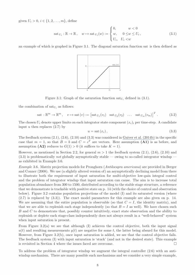
given Ui > 0, i ∈ {1, 2, . . . ,m}, define

sat Ui: R → R , w 7→ sat Ui

(w) :=

0, w < 0

w, 0 ≤w ≤ Ui ,

Ui, Ui <w

(3.1)

an example of which is graphed in Figure 3.1. The diagonal saturation function sat is then defined as

0 Ui

Ui

satUi(w)

w

Figure 3.1: Graph of the saturation function satUidefined in (3.1).

the combination of satUias follows:

sat : Rm → Rm , v 7→ sat (v) :=

[sat U1

(v1) sat U2(v2) . . . sat Um

(vm)]T

. (3.2)

The chosen Ui denote upper limits on each integrator state component (xc)i per time-step. A candidateinput u then replaces (2.7) by

u = sat (xc) , (3.3)

The feedback system (2.1), (2.6), (2.10) and (3.3) was considered in Guiver et al. (2014b) in the specificcase that m = 1, so that B = b and C = cT are vectors. Here assumption (A1) is as before, andassumption (A2) reduces to G(1) > 0 (it suffices to take K = 1).

However, as mentioned in Section 2.2, for general m > 1 the feedback system (2.1), (2.6), (2.10) and(3.3) is problematically not globally asymptotically stable — owing to so-called integrator windup —as exhibited in Example 3.6.

Example 3.6. Matrix projection models for Pronghorn (Antilocapra americana) are provided in Bergerand Conner (2008). We use (a slightly altered version of) an asymptotically declining model from thereto illustrate both the requirement of input saturation for multi-objective low-gain integral controland the problem of integrator windup that input saturation can cause. The aim is to increase totalpopulation abundance from 300 to 1500, distributed according to the stable stage structure, a referencethat we demonstrate is trackable with positive state on p. 14 (with the choice of control and observationbelow). Figure 3.2 contains population projections of the model (I) and its saturated version (where(2.7) is replaced by (3.3)). The exact model parameters for this example are also given on p. 14.We are assuming that the entire population is observable (so that C = I, the identity matrix), andthat we are able to replenish each stage independently (so that B = I as well). We have chosen suchB and C to demonstrate that, possibly counter intuitively, exact state observation and the ability toreplenish or deplete each stage-class independently does not always result in a “well-behaved” systemwhen input saturation is present.

From Figure 3.2(a) we see that although (I) achieves the control objective, both the input signalu(t) and resulting measurements y(t) are negative for some t, the latter being absurd for this model.However, from Figure 3.2(b), once input saturation is added, we see that the control objective fails.The feedback system (I) with input saturation is ‘stuck’ (and not in the desired state). This exampleis revisited in Section 4 where the issues faced are overcome. �

To address the problem of integrator windup we augment the integral controller (2.6) with an anti-windup mechanism. There are many possible such mechanisms and we consider a very simple example,

8

0 100 200 300−400

−300

−200

−100

0

100

200

300

t

ui(t)

u∞1

u∞2

u∞3

0 100 200 300−200

0

200

400

600

800

1000

1200

r1

r2

r3

t

yi(t)

(a)

0 100 200 3000

10

20

30

40

50

60

70

80

u∞1

u∞2

u∞3

t

ui(t)

0 100 200 3000

200

400

600

800

r1

r2

r3

t

yi(t)

(b)

Figure 3.2: Simulations of integral control for the Pronghorn model considered in Example 3.6. (a)Without input saturation (b) With input saturation. In both figures, the left and right panels containthe input and output signals, respectively. The variables corresponding to stage classes one, two andthree are plotted in solid, dashed and dashed-dotted lines, respectively. The dotted lines are thedesired references.

the advantages of which are that it is straightforward to implement, it possesses demonstrable robust-ness to model uncertainty and can be extended to a class of infinite-dimensional systems. We replace(2.6) by the integral controller with (static) anti-windup

xc(t+ 1) = xc(t) + gK(r − Cx(t))− E(xc(t)− sat (xc(t))), xc(0) = x0c ,

yc(t) = xc(t),

}t ∈ N0 , (3.4)

where E ∈ Rm×m is another design parameter. We denote by (Iaw) the feedback system (2.1),(2.10), (3.4) and connection (3.3). Intuitively, the term in (3.4) involving E acts as a correctionterm, activating at time-steps t when the integral control state xc(t) saturates meaning that xc(t) 6=sat (xc(t)). When the control signal is not saturating, then sat (xc(t)) = xc(t) and thus the extraterm in (3.4) is zero and plays no role. In this region the system is behaving as though there is nosaturation and, loosely speaking, Theorem 2.2 applies. Our main result is Theorem 3.7 below, whichmirrors Theorem 2.2, and guarantees asymptotic tracking of a reference with positive state under the(same) assumptions (A1) and (A2) and a known choice of E.

9

Theorem 3.7. Suppose that (Iaw) satisfies (A1) and (A2) and choose

E := gKG(1) , (3.5)

where g > 0 is as in (3.4). Then, there exists g∗ > 0 such that for all g ∈ (0, g∗), all r ∈ 〈G(1)〉+ suchthat

r = G(1)u+, for some u+ ∈ Rm+ with u+ ≤ U , (3.6)

and all (x0, x0c) ∈ Rn+ × Rm

+ , the solution (x, xc) of (Iaw) satisfies x(t) ≥ 0 for each t ∈ N0 and hasproperties:

(a) limt→∞

xc(t) = x∞c := G(1)−1r;

(b) limt→∞

x(t) = x∞ := (I −A)−1BG(1)−1r;

(c) limt→∞

y(t) = limt→∞

Cx(t) = r.

By appealing to the results of Section 3.1, including a proportional component in the feedback law(3.3) gives rise a larger set of possible target references. Let (PI1aw) denote the feedback system (2.1),(2.10), (3.4) and connection

u = −F1x+ sat (xc) . (3.7)

Let (PI2aw) denote the feedback system (2.1), (2.10), (3.4) and connection

u = −F2y + sat (xc) . (3.8)

The terms F1 ∈ Rm×n and F2 ∈ Rm×m in (3.7) and (3.8), respectively, are additional design parame-ters.

Corollary 3.8. The PI systems (PI1aw) and (PI2aw) specified by (A,B,C) satisfying (2.10) areequal to (Iaw) specified by (A1, B, C) and (A2, B, C), where A1 := A − BF1 and A2 := A − BF2C,respectively. If F1 is such that A1 ≥ 0 and (A1, B, C) satisfy (A1) and (A2) then the conclusions ofTheorem 3.7 apply to (Iaw) specified by (A1, B, C), and similarly for F2.

Remark 3.9. (i) Although no F1 or F2 component is required to apply Theorem 3.7 when r(A) < 1,the use of (PI1aw) or (PI2aw) often results in faster convergence, as is the case in Example 3.6on p. 4. Moreover, if F1 ∈ Rn×n is such that

0 ≤ A−BF1 ≤ A ,

then Lemma 3.4 (b) implies that there is a larger choice of possible references achievable by(PI1aw) than by (Iaw), which thus encourages the use of PI control even in the case that r(A) < 1.Similar comments apply to F2 for the (PI2aw) system.

(ii) The conclusions of Theorem 3.7 hold with E = 0, that is, with no anti-windup component, ifK and G(1) are such that KG(1) is positive semi-definite. Although the choice K = G(1)−1

guarantees this condition, such a choice requires exact knowledge of G(1) and the requirementthat KG(1) is positive semi-definite is very non-robust to parameter uncertainty. The lattermotivates our insistence on including an anti-windup component E(xc − sat (xc)) in (3.4).

3.3 Robustness

The material presented thus far is predicated on the assumption that we have perfect knowledge aboutthe system to be controlled, and that there are no disturbance (or noise) signals affecting the dynamics.In practice both of these assumptions are likely to be violated and thus it is important to quantify towhat extent low-gain PI control is robust to noisy dynamics or lack of system information. These tworespective issues are addressed in the subsequent subsections.

10

3.3.1 Disturbance estimates and disturbance rejection

Here we extend the original controlled and observed model (2.1) to include disturbance signals bywriting

x(t+ 1) = Ax(t) +Bu(t) + d1(t), x(0) = x0 ,

y(t) = Cx(t) + d2(t),

}t ∈ N0 , (3.9)

where d1, d2 are unknown. In a population model d1 denotes a disturbance to the population such as(unmodelled) immigration, emigration or predation and d2 denotes some form of sampling error. Areasonably general framework is to assume that d1 and d2 are bounded, and of course are such thatx and y remain nonnegative. The impacts of nonnegative disturbances on populations modelled bymatrix PPMs have been explored in Eager et al. (2014).

When only boundedness of d1 and d2 is assumed then we cannot in general expect the same convergenceof the feedback system (3.9), (2.10), (3.4) and (3.3) as exhibited by (Iaw) (or the PI versions (PI1aw)and (PI2aw)). The next result provides an upper bound on the difference of the state and outputfrom their respective references in terms of the initial error and the maximum values of d1 and d2.The result is an (I)nput to (S)tate (S)tability estimate, and we refer the reader to Sontag (2008) formore background on ISS.

Proposition 3.10. Suppose that the disturbed feedback system (3.9), (2.10), (3.4) and (3.3) withbounded disturbances d1 and d2 satisfies (A1) and (A2), and choose E := gKG(1) where g > 0is as in (3.4). Then, there exists g∗ > 0 such that for all g ∈ (0, g∗), all r as in (3.6) and all(x0, x0c) ∈ Rn

+ × Rm+ , the solution (x, xc) of (Iaw) satisfies

∥∥∥∥∥∥

x(t)− x∞

xc(t)− x∞cy(t)− r

∥∥∥∥∥∥≤M0γ

t

∥∥∥∥[x0 − x∞

x0c − x∞c

]∥∥∥∥+M1 maxj∈N0

j≤t−1

‖d1(j)‖+M2 maxj∈N0

j≤t−1

‖d2(j)‖ , t ∈ N , (3.10)

for some constant γ ∈ (0, 1) and M0,M1,M2 > 0 and where x∞c and x∞ are as in (a) and (b) ofTheorem 2.2, respectively. The constants γ,M0,M1 and M2 depend on A,B,C, g and K, but not onr, x0, x0c , d1 or d2. Furthermore, g∗ is independent of the disturbances d1 and d2.

Low-gain PI control without saturation or positivity constraints is known to have the desirable propertythat convergent disturbances in the input (d1 = Bδ1 in (3.9) for some δ1) are rejected by the output,so that the output still converges to the reference. Similarly, convergent disturbances in the output(d2 in (3.9)) result in asymptotic tracking of the output to the reference offset by the limit of thedisturbance. The next corollary demonstrates that, broadly speaking, the same is true in the presenceof input saturation and anti-windup.

Corollary 3.11. Suppose that the disturbed feedback system (3.9), (2.10), (3.4) and (3.3) with boundeddisturbances d1 = Bδ1 and d2 satisfies (A1) and (A2), and choose E := gKG(1) where g > 0 is asin (3.4). Suppose that δ1 and d2 have respective limits δ∞1 and d∞2 . Then, there exists g∗ > 0 suchthat for all g ∈ (0, g∗), all r ∈ Rm

+ such that

r − d∞2 = G(1)(u+ + δ∞1 ) , 0 ≤ u+ ≤ U , (3.11)

and all (x0, x0c) ∈ Rn+ × Rm

+ , the solution (x, xc) of (Iaw) satisfies

(a) limt→∞

xc(t) = G(1)−1(r − d∞2 ) = u+ + δ∞1 ,

(b) limt→∞

x(t) = (I −A)−1BG(1)−1(r − d∞2 ) = (I −A)−1B(u+ + δ∞1 ),

(c) limt→∞

y(t) = limt→∞

Cx(t) = r − d∞2 .

The constant g∗ is independent of δ1 and d2.

11

3.3.2 Uncertain steady state gains

Here we consider the situation where there is uncertainty in the steady-state gain matrix G(1). As-suming that r(A) < 1, from the definition

G(1) = C(I −A)−1B = C(I +A+A2 + . . . )B ,

and the limit relationship (2.5) it follows that the (i, j)th entry of G(1) is the eventual ith measurementwhen the jth input variable is one for all time. The interpretation is somewhat similar to that of thefundamental matrix in Caswell (2001, p.112). In engineering applications, such as electrical circuits,it is sometimes possible to obtain an estimate of G(1) by conducting controlled experiments (Lunze,1985; Penttinen and Koivo, 1980), although this is likely not to be possible in population management.

Knowledge of G(1) is used in two separate situations: first, in determining K in (3.4) to satisfy(A2) and second, in determining E that also appears in (3.4). Both of the components K and E arerequired to ensure that low-gain PI control as presented is effective. Recall that the choiceK = G(1)−1

is sufficient for satisfying (A2) and E = gKG(1) is sufficient to ensure that the conclusions of Theorem3.7 (and Corollary 3.8, Proposition 3.10 and Corollary 3.11) hold.

Uncertainty in G(1) typically arises from uncertainty in the parameters or even the dimensions ofA,B or C. Throughout this section we shall assume that the unknown transfer function G can bedecomposed as

G = G+∆G , (3.12)

where G is known and ∆G is expected to be “small”. More generally, in this section variables withhats shall always denote known quantities and capital deltas denote uncertain terms.

Lemmas 3.12–3.14 below are technical preliminary results gathering sufficient conditions for the mainresult of the section, Corollary 3.16. This latter result states that if a known nominal estimate G isclose to the unknown G, meaning that ‖G− G‖∞ is small, then basing the design of K and E on thenominal estimate G(1) of G(1) is sufficient for low-gain PI control to succeed.

We first demonstrate how the decomposition (3.12) arises out of uncertainty in A,B and C. We letρ(A) = C \σ(A) denote the resolvent set of A, (when A is a matrix then ρ(A) is the set of all complexnumbers that are not eigenvalues of A).

Lemma 3.12. Suppose that (A,B,C) ∈ Rn×n×Rn×m×Rm×n for m,n ∈ N admit the decompositions

A = A+∆A , B = B +∆B , C = C +∆C ,

then

GCAB(z) = C(zI −A)−1B = GCAB

(z) + ∆C(zI − A)−1(B +∆B) + C(zI − A)−1∆B

+ (C +∆C)(zI −A)−1∆A(zI − A)−1(B +∆B) , (3.13)

which is defined for all z ∈ C ∩ ρ(A) ∩ ρ(A) and is in the form (3.12) with G = GCAB

and ∆G thesum of the remaining three terms on the right hand side of (3.13).

Lemma 3.13. Suppose that G admits the decomposition (3.12) and that G(1) is invertible. ChooseK = QG(1)−1, where Q ∈ Cm×m is such that σ(Q) ⊆ C

+0 . Then assumption (A2) is satisfied for K

and G(1) if

‖QG(1)−1∆G(1)‖ < 1

supω∈R ‖(ωi +Q)−1‖ . (3.14)

If Q = I, the m×m identity matrix, then K and G(1) satisfy (A2) if

min{‖∆G(1)G(1)−1‖, ‖G(1)−1∆G(1)‖

}< 1 . (3.15)

A sufficient condition for (3.15) is that

‖∆G(1)‖ < 1

‖G(1)−1‖. (3.16)

12

Lemma 3.14. Let X denote a bounded operator on a Hilbert space (such as a square matrix with realor complex entries), with −1 ∈ ρ(X), so that I +X is invertible. Then the conditions

(a) ‖X‖ < 12 , or;

(b) ‖X‖ ≤ 1 and ‖(I −X)(I +X)−1‖ ≤ 1 ;

are sufficient for‖(I +X)−1X‖ < 1 . (3.17)

Remark 3.15. An estimate of the form (3.17) appears as a condition on X in Corollary 3.16 below,hence the inclusion of sufficient conditions here. We comment that (a) and (b) do not imply oneanother as X = −1

4I satisfies (a) but not (b) and X = I satisfies (b) but not (a).

Corollary 3.16. Suppose that the (A,B,C) as in (2.10) satisfy (A1) and the associated transferfunction G admits the decomposition (3.12), where G is known and K and G together satisfy (A2)and choose

E := gKG(1) , (3.18)

where g > 0 is as in (3.4). Then, there exists M∗ > 0 and g∗ > 0 (which in general depends on M∗)such that for all ∆G in (3.12) with

‖∆G‖∞ < M∗ , (3.19)

and ∥∥∥[I + G(1)−1∆G(1)]−1 · [G(1)−1∆G(1)]∥∥∥ < 1 , (3.20)

all g ∈ (0, g∗), all r ∈ 〈G(1)〉+ as in (3.6) and all (x0, x0c) ∈ Rn+ × Rm

+ , the solution (x, xc) of (Iaw)satisfies x(t) ≥ 0 for each t ∈ N0 and has the properties (a), (b) and (c) of Theorem 2.2.

Remark 3.17. Corollary 3.16 can easily be extended to the PI systems (PI1aw) or (PI2aw), consideredin Corollary 3.8, by replacing A by A1 and A2 as appropriate.

3.4 Extension to infinite-dimensional systems

In this manuscript we have so far we have focussed on applying low-gain PI control to finite-dimensionallinear systems with positive state, with both multiple inputs and outputs, and with input saturation;motivated by the management of ecological populations modelled by matrix PPMs. However, inthis section we demonstrate that many of the results presented extend to a class of discrete-time,infinite-dimensional linear systems that includes as an example IPMs, introduced in Easterling et al.(2000).

Consider the controlled and observed linear system (2.1) where now

A : X → X , B : Rm → X , C : X → Rm , (3.21)

are bounded, linear operators and X is a real Banach space, equipped with a partial order denoted by≤ (also ≥). The state-space X may now be infinite-dimensional, but the input and output spaces arestill Rm. Since B and C are bounded and finite-rank, then necessarily they can be written

Bu =m∑

i=1

biui , ∀ u =[u1 . . . um

]T ∈ Rm , (3.22)

and (Cx)j = cjx , ∀ j ∈ {1, 2, . . . ,m} , x ∈ X , (3.23)

for some bi ∈ X and cj : X → R, linear functionals on X .

We let K denote the positive cone of X , which is the set of all x ∈ X such that x ≥ 0. The positivecone K is a convex cone, with 0 ∈ K and satisfies αK = K for every α > 0. Intuitively, when X = Rn

for n ∈ N and ≥ denotes usual componentwise nonnegativity, then K = Rn+. For two real, partially

ordered Banach spaces X1,X2 with respective positive cones K1,K2, we say that a bounded linearoperator T : X1 → X2 is positive if T (K1) ⊆ K2, that is, positive elements of X1 are mapped topositive elements of X2.

13

Example 3.18. Let X denote a real, partially ordered Banach space with positive cone K and let B andC denote the bounded, linear, finite-rank operators defined in (3.22) and (3.23), respectively. Then Bis positive if, and only if, bi ∈ K for every i ∈ {1, 2, . . . ,m}. Similarly, C is positive if, and only if, cjis positive for every j ∈ {1, 2, . . . ,m} , here meaning that cj(K) ⊆ R+. �

The integral controller with anti-windup is still defined by (3.4), with design parameters E,K ∈ Rm×m,g > 0 and x0c ∈ Rm. The expression (2.4) for the transfer function G is still well-defined when A,Band C are as in (3.21), and thus assumptions (A1) and (A2) are as before.

To design a (P)roportional feedback in (3.7) or (3.8) requires bounded linear operators

F1 : X → X or F2 : Rm → X .

For brevity, we note here that the PI (state-)feedback system (2.1), (3.4) and (3.7) specified by A,B,Creduces to the feedback system (2.1), (3.4) and (3.3) specified by A1, B, C with

A1 : X → X , A1 := A−BF1 .

The operator A1 is bounded as the composition and difference of bounded operators. Similarly, thePI (output-)feedback system (2.1), (3.4) and (3.8) specified by A,B,C reduces to the feedback system(2.1), (3.4) and (3.3) specified by A2, B, C with

A2 : X → X , A2 := A−BF2C ,

again a bounded operator.

The main result of this section demonstrates that the low-gain results derived so far extend to theabove class of systems. By noting the above simplifications, the next result includes both the stateand output feedback cases, when the feedbacks F1 or F2 are chosen such that A1 and A2 are positiveoperators, respectively.

Theorem 3.19. Assume that the integral control feedback system with anti-windup (2.1), (3.4) and(3.3) specified by the positive operators A,B,C as in (3.21) satisfies assumptions (A1) and (A2) withE = gKG(1) in (3.4). Then, there exists g∗ > 0 such that for all g ∈ (0, g∗), all r as in (3.6) and all(x0, x0c) ∈ K × Rm

+ , the solution (x, xc) of (2.1), (3.4) and (3.3) has the properties (a), (b) and (c) ofTheorem 2.2 and furthermore x(t) ∈ K for every t ∈ N0.

The robustness results Proposition 3.10, Corollary 3.11 and Corollary 3.16 also apply when (2.1), (3.4)and (3.3) are specified by the positive operators A,B,C as in (3.21).

The proof of the above theorem is exactly the same as the earlier named results; none of the argumentsused required that X is finite-dimensional.

Remark 3.20. We comment on the results of Section 3.1, on feasible positive references, in the situationwhen X is a Banach space. The results do translate across; again none of the proofs explicitly usethat X is finite-dimensional. However, assumption (H) should be replaced by

(H′) Let X denote a real, partially ordered Banach space with positive cone K. Given the pair ofbounded, linear, positive operators A : X → X , B : Rm → X , there exists a bounded, positiveoperator F : X → Rm such that defining A := A−BF it follows that A is positive and for anyv ∈ K and w ∈ Rm, if Av +Bw ∈ K then w ∈ Rm

+ .

Importantly, the constructive characterisation (Guiver et al., 2014a, Lemma 2.1) does not hold in thegeneral Banach space case, however, as that is truly a finite-dimensional result.

4 Examples

Example 3.6 continued: The purpose of this example is to demonstrate a physical situation whereusual low-gain integral control is problematic as componentwise nonnegativity is not maintained, but

14

simply adding input saturation introduces another problem, that of integrator windup. These issuesare obviated by considering the feedback systems (Iaw) and (PIaw), and the solution to set-pointregulation problem is guaranteed by Theorem 3.7 and Corollary 3.8.

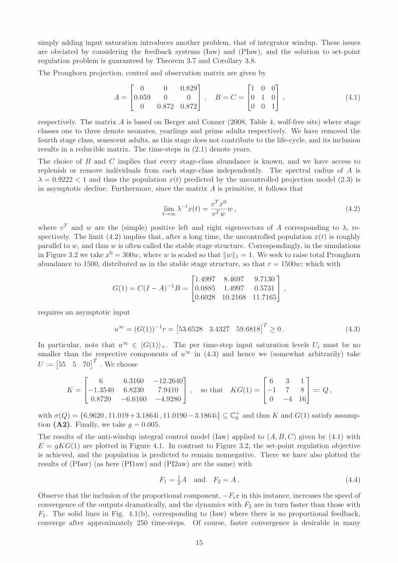
The Pronghorn projection, control and observation matrix are given by

A =

0 0 0.8290.059 0 00 0.872 0.872

, B = C =

1 0 00 1 00 0 1

, (4.1)

respectively. The matrix A is based on Berger and Conner (2008, Table 4, wolf-free site) where stageclasses one to three denote neonates, yearlings and prime adults respectively. We have removed thefourth stage class, senescent adults, as this stage does not contribute to the life-cycle, and its inclusionresults in a reducible matrix. The time-steps in (2.1) denote years.

The choice of B and C implies that every stage-class abundance is known, and we have access toreplenish or remove individuals from each stage-class independently. The spectral radius of A isλ = 0.9222 < 1 and thus the population x(t) predicted by the uncontrolled projection model (2.3) isin asymptotic decline. Furthermore, since the matrix A is primitive, it follows that

limt→∞

λ−tx(t) =vTx0

vTww , (4.2)

where vT and w are the (simple) positive left and right eigenvectors of A corresponding to λ, re-spectively. The limit (4.2) implies that, after a long time, the uncontrolled population x(t) is roughlyparallel to w, and thus w is often called the stable stage structure. Correspondingly, in the simulationsin Figure 3.2 we take x0 = 300w, where w is scaled so that ‖w‖1 = 1. We seek to raise total Pronghornabundance to 1500, distributed as in the stable stage structure, so that r = 1500w; which with

G(1) = C(I −A)−1B =

1.4997 8.4697 9.71300.0885 1.4997 0.57310.6028 10.2168 11.7165

,

requires an asymptotic input

u∞ = (G(1))−1r =[53.6528 3.4327 59.6818

]T ≥ 0 . (4.3)

In particular, note that u∞ ∈ 〈G(1)〉+. The per time-step input saturation levels Ui must be nosmaller than the respective components of u∞ in (4.3) and hence we (somewhat arbitrarily) take

U :=[55 5 70

]T. We choose

K =

6 6.3160 −12.2640−1.3540 6.8230 7.94100.8720 −6.6160 −4.9280

, so that KG(1) =

6 3 1−1 7 80 −4 16

=: Q ,

with σ(Q) = {6.9620 , 11.019+3.1864i , 11.0190−3.1864i} ⊆ C+0 and thus K and G(1) satisfy assump-

tion (A2). Finally, we take g = 0.005.

The results of the anti-windup integral control model (Iaw) applied to (A,B,C) given by (4.1) withE = gKG(1) are plotted in Figure 4.1. In contrast to Figure 3.2, the set-point regulation objectiveis achieved, and the population is predicted to remain nonnegative. There we have also plotted theresults of (PIaw) (as here (PI1aw) and (PI2aw) are the same) with

F1 =12A and F2 = A . (4.4)

Observe that the inclusion of the proportional component, −Fix in this instance, increases the speed ofconvergence of the outputs dramatically, and the dynamics with F2 are in turn faster than those withF1. The solid lines in Fig. 4.1(b), corresponding to (Iaw) where there is no proportional feedback,converge after approximately 250 time-steps. Of course, faster convergence is desirable in many

15

0 20 40 60 80 1000

20

40

60

80

100

t

ui(t)

Pronghorn stage input levels

u∗

1

u∗

2

u∗

3u∗

1

u∗

2

u∗

3u∗

1

u∗

2

u∗

3

(a)

0 10 20 30 40 500

200

400

600

800

1000

t

yi(t)

Pronghorn stage adundances

r1

r2

r3

r1

r2

r3

r1

r2

r3

(b)

Figure 4.1: Projections of the restocking scheme for the three-stage matrix PPM of Pronghorn of Ex-ample 3.6. See the main text for more description. In both panels the solid, dashed and dashed-dottedlines are the feedback system (PIaw) specified by (A,B,C), (A1, B, C) and (A2, B, C), respectively(see (4.1) and (4.4)). The dotted lines are the references and are labelled on the right hand sides ofthe figures.

contexts, such as conservation, but does introduce another practical consideration. As exhibited inFig. 4.1(a), the faster response follows from acting more quickly, here meaning adding more individualsper time-step. Consequently, the per time-step saturation levels need to be larger, which of coursemay not be feasible in practice.

We seek to explain this mathematically. Let A1 := A− F1 =12A and A2 := A− F2 = 0. The limiting

inputs of (Iaw) and the two (PIaw) systems specified by (A,B,C), (A1, B, C) and (A2, B, C) are

u∞ , −F1r + u∞1 and − F2r + u∞2 ,

respectively. However, as r(A) < 1, it can be demonstrated that the above three quantities are equaland as F2 ≥ F1 the terms u∞, u∞1 and u∞2 must satisfy

u∞ ≤ u∞1 ≤ u∞2 .

Indeed, in this example (to 3 sig. figs.)

u∞ =

53.73.4359.7

≤ u∞1 =

37123.8413

≤ u∞2 =

68944.1767

,

The terms u∞, u∞1 and u∞2 are those subject to input saturation and so the per time-step saturationlevels must be larger than these levels to ensure convergence. Indeed, for the feedback systems (PIaw)specified by (A1, B, C) and (A2, B, C) we have taken saturation levels 1.2u∞1 and 1.2u∞2 , respectively.�

Example 4.1. Matrix projection models for the sustainable harvesting of two species of palm trees inMexico are considered in Olmsted and Alvarez-Buylla (1995). We use a matrix PPM from there of thepalm species Coccothrinax readii to demonstrate how a potential harvesting and conservation strategy

16

could be based on a low-gain PI control law. The projection matrix A is given by

A =

0.35 0 0 0 0 0 0 0 55.80.18 0.8 0 0 0 0 0 0 00 0.1 0.89 0 0 0 0 0 00 0 0.07 0.94 0 0 0 0 00 0 0 0.06 0.92 0 0 0 00 0 0 0 0.08 0.94 0 0 00 0 0 0 0 0.06 0.94 0 00 0 0 0 0 0 0.06 0.94 00 0 0 0 0 0 0 0.06 0.95

. (4.5)

The nine stages denote seedlings, saplings I and II, juveniles I–V, and adult trees and the time-stepscorrespond to years. We refer the reader to Olmsted and Alvarez-Buylla (1995) for details on thephenology of Coccothrinax readii.

The spectral radius of A in (4.5) is 1.0549 > 1, so that the uncontrolled population (2.3) is predictedto grow asymptotically. Unlike the previous example, we assume that we do not know the entirepopulation distribution at each time-step exactly and instead only have access to some part of thestate. For simplicity, we consider the case where just two per time-step measurements are made andcorrespondingly have access to two stages for replenishment. We assume that the seedlings and adulttree stage classes may be restocked and harvested, respectively, leading to the B matrix

B =

[1 0 0 0 0 0 0 0 0 00 0 0 0 0 0 0 0 0 1

]T.

Furthermore, we assume that we are able to measure the abundances of the final two stages; thelargest juvenile trees and adult trees so that

C =

[0 0 0 0 0 0 0 0 1 00 0 0 0 0 0 0 0 0 1

].

The set-point regulation objective is to determine a feedback F in (3.8) and reference r such thatthe PI control system (PIaw2) drives the population to some non-zero level, and to determine theresulting adult tree harvest. Here the control signal u(t) is given by

u(t) =

[u1(t)u2(t)

]= −FCx(t) + sat (xc(t)) , t ∈ N0 . (4.6)

In this example, u1(t) denotes the number of seedlings planted at time-step t ∈ N0, and is desiredto be nonnegative. Similarly, u2(t) denotes the number of adult trees harvested at time-step t ∈ N0,and should be negative. Indeed, we do not want to harvest seedlings or plant adult trees. Roughlyspeaking, the negative term −FCx on the right hand side of (4.6) determines the harvesting yieldand the positive term sat (xc) from the integral control law determines the replanting scheme.

We require F ∈ R2×2 such that

A0 := A−BFC ∈ R9×9+ and r(A0) < 1 . (4.7)

Then, for each r =[r1 r2

]T= GCA0B(1)v ∈ R2

+ for v ∈ R2+, the following asymptotic yields are

obtained

population distribution: x∞ = (I −A0)−1Bv , (4.8)

harvesting/planting effort: u∞ = −Fr + v = (−FGCA0B(1)(1) + I)v , (4.9)

measured abundances: x∗8 = r1 and x∗9 = r2 . (4.10)

First, we construct F ∈ R2×2 to satisfy (4.7). By considering the product BFC, we seek to replacethe ninth row of A by zero, which necessitates

F =

[0 0f1 f2

]:=

[0 0

0.06 0.95

], (4.11)

17

and yields

A0 = A−BFC =

0 0 0 0 0 0 0 0 55.80.18 0.8 0 0 0 0 0 0 00 0.1 0.89 0 0 0 0 0 00 0 0.07 0.94 0 0 0 0 00 0 0 0.06 0.92 0 0 0 00 0 0 0 0.08 0.94 0 0 00 0 0 0 0 0.06 0.94 0 00 0 0 0 0 0 0.06 0.94 00 0 0 0 0 0 0 0 0

, with r(A0) = 0.94 < 1 .

(4.12)Choosing F as in (4.11) satisfies (4.7) from which we compute

GCA0B(1) =

[γ1 γ20 1

]:=

[1.4685 81.9441

0 1

].

It remains to determine r, or equivalently v. In terms of components the reference r = G(1)v is givenby

r1 = γ1v1 + γ2v2 and r2 = v2 . (4.13)

Of the four quantities r1, r2, v1 and v2, two are free to be chosen, provided that 0 ≤ v1 ≤ U1 and0 ≤ v2 ≤ U2, and the remaining two are determined by (4.13).

Rewriting (4.9) in components gives

[u∞1u∞2

]=

(−[0 0f1 f2

] [γ1 γ20 1

]+

[1 00 1

])[v1v2

]

⇒ u∞1 = v1 and u∞2 = −f1γ1v1 + (1− f1γ2 − f2)v2 . (4.14)

Therefore, from (4.14) we see that v1 ≥ 0 is the asymptotic replanting level, and from (4.13) thatv2 = r2 is the desired asymptotic adult tree density. For given v1, v2, the expression u∞2 ≤ 0 in (4.14)determines the asymptotic number of adult trees harvested per time-step. The asymptotic abundanceof the penultimate stage is r2. These relations are summarised in Table 4.1.

Table 4.1: Summary of the roles ofr1, r2, v1 and v2 in Example 4.1.

Quantity Interpretation

v1 Asymptotic planting levelv2 = r2 Asymptotic adult tree abundancer1 Asymptotic final juvenile stage class abundance

For the following numerical simulation we suppose an initial population distribution with no adulttrees, so that

x0 = 2[160 120 80 91 79 68 57 45 0

]T,

As an example, we take

v =[10 8

]T ⇒ r = G(1)v =[670.24 8

]Tand u∞ =

[10 −39.8

]T,

meaning that, asymptotically, per time-step 10 seedlings are planted, almost 40 adult trees are har-vested with eight adult trees remaining in the population. Of course, in practice only an integernumber of trees can be harvested per year and we believe that the 39.8 = −u∞2 is an artifact of themodel considered. The asymptotic harvest yield can be altered by tuning v1 and v2 as explainedabove. To see the role of input saturation, we take

U =[50 40

]T,

18

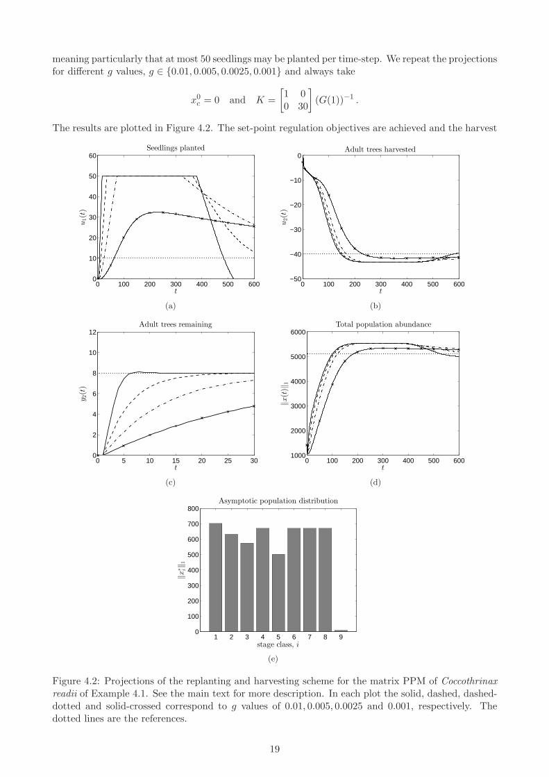
meaning particularly that at most 50 seedlings may be planted per time-step. We repeat the projectionsfor different g values, g ∈ {0.01, 0.005, 0.0025, 0.001} and always take

x0c = 0 and K =

[1 00 30

](G(1))−1 .

The results are plotted in Figure 4.2. The set-point regulation objectives are achieved and the harvest

0 100 200 300 400 500 6000

10

20

30

40

50

60

t

u1(t)

Seedlings planted

(a)

0 100 200 300 400 500 600−50

−40

−30

−20

−10

0

tu2(t)

Adult trees harvested

(b)

0 5 10 15 20 25 300

2

4

6

8

10

12

t

y2(t)

Adult trees remaining

(c)

0 100 200 300 400 500 6001000

2000

3000

4000

5000

6000

t

‖x(t)‖

1

Total population abundance

(d)

1 2 3 4 5 6 7 8 90

100

200

300

400

500

600

700

800

stage class, i

‖x∗ i‖1

Asymptotic population distribution

(e)

Figure 4.2: Projections of the replanting and harvesting scheme for the matrix PPM of Coccothrinaxreadii of Example 4.1. See the main text for more description. In each plot the solid, dashed, dashed-dotted and solid-crossed correspond to g values of 0.01, 0.005, 0.0025 and 0.001, respectively. Thedotted lines are the references.

19

of adult trees increases from zero to (almost) 40 per year, peaking at approximately 43 trees per year.Furthermore, although not specified as a management objective, the total tree abundance rises from‖x0‖1 = 1400 to 5100. We note that the resulting dynamics are rather slow; the time-steps here denoteyears. This is, in part we suspect, because of the admittedly somewhat limited control actions of onlyadding to the first stage class and removing from the last. The uncontrolled dynamics themselves areslow as mathematically the matrix A has nearly ones on the diagonal and very small entries on thesub diagonal. Biologically, the species Coccothrinax readii is long lived; Olmsted and Alvarez-Buylla(1995) estimate the maximal life span as over 145 years, yet the model is a size based model. Thatsaid, the speed of convergence could be increased by allowing more control actions and measurementsand adding a ‘larger’ proportional part F to the control law. In this case the explanation of the roles ofr and v related by r = G(1)v become more complicated. It is also the case that we have not exploredthe roles of tuning K and g further, or of the initial controller state x0c ; all of which can affect thetransient dynamics of the model.

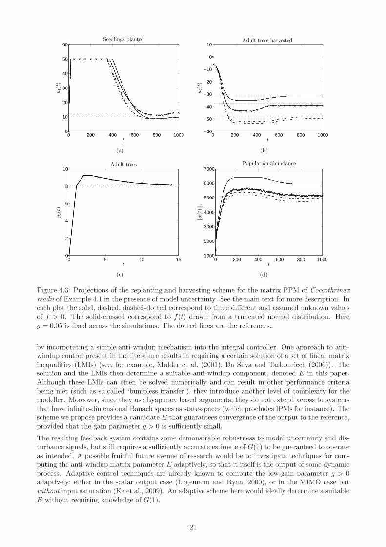
To demonstrate robustness of the PI controller, we now assume that the recruitment of the populationis not fixed at 55.8, but unknown and denoted by f . We have relegated proofs of the subsequentclaims to Appendix B. If f ≥ 0 is constant, then owing to the particular structure of this modeland the uncertainty, the reference r is still tracked asymptotically. This is an example of convergentdisturbance rejection, Corollary 3.11. Moreover, a calculation shows that

G(1) =

[γ1 γ1f

0 1

], (4.15)

and hence the relations (4.14) and (4.13) hold with γ2 replaced by γ1f . The key interpretations thatv1 is the asymptotic planting level and r2 = v2 is the asymptotic abundance of adult trees hold asbefore and are thus independent of f . Figure 4.3 contains three simulations with randomly chosen,but positive f . Here we have fixed v1 and v2 as before, so that now r1 and the asymptotic harvestyield varies as f and thus G(1) does.

A more appropriate model may be to consider the situation where f is time varying with valuesf(t), t ∈ N0, the inclusion of which reflects environmental or demographic stochasticity. It can bedemonstrated that the second output y2, denoting adult trees, still converges to r2. The populationabundances x, planting/harvesting quantities u and abundance of largest juvenile trees need notconverge in general. However, the ISS estimate of Proposition 3.10 applies. Figure 4.3 contains asimulation where f(t) is drawn from a pseudo-random truncated normal with mean 55.8 and variance 4.We note that, as predicted, the second output, number of adult trees present, rejects the disturbancesto the model and is the same across all simulations. �

5 Discussion

Low-gain PI control has been extended to nonnegative, discrete-time linear systems where multiple out-puts are regulated to desired, but constrained, references. The theory holds for both finite-dimensionaland a class of infinite-dimensional systems. Our motivating application is population management,and it is in this context that we have posed much of the present material and our examples. Thepresent contribution can be viewed as the sequel to Guiver et al. (2014b), where the problem wasfirst considered, but only scalar control and observation was permitted. Although conceptually verysimilar, there are additional mathematical difficulties in extending these results to the natural situ-ation where many management objectives are specified (that is, multi-input, multi-output (MIMO)systems with input saturation). Particularly, two problems had to be overcome. First, the set ofpossible reference targets needed to be described, which was addressed in Section 3.1 and reflectedin our main results, Theorem 3.7 and Corollary 3.8. In summary, the set of trackable outputs withpositive state includes the nonnegative linear span of G(1), the transfer function evaluated at one,and is enlarged by incorporating a proportional component to the feedback law. Second, the problemof integrator windup, whereby the control objective failed, needed to be avoided, which was achieved

20

0 200 400 600 800 10000

10

20

30

40

50

60

t

u1(t)

Seedlings planted

(a)

0 200 400 600 800 1000−60

−50

−40

−30

−20

−10

0

10

t

u2(t)

Adult trees harvested

(b)

0 5 10 150

2

4

6

8

10

t

y2(t)

Adult trees

(c)

0 200 400 600 800 10001000

2000

3000

4000

5000

6000

7000

t

‖x(t)‖

1

Population abundance

(d)

Figure 4.3: Projections of the replanting and harvesting scheme for the matrix PPM of Coccothrinaxreadii of Example 4.1 in the presence of model uncertainty. See the main text for more description. Ineach plot the solid, dashed, dashed-dotted correspond to three different and assumed unknown valuesof f > 0. The solid-crossed correspond to f(t) drawn from a truncated normal distribution. Hereg = 0.05 is fixed across the simulations. The dotted lines are the references.

by incorporating a simple anti-windup mechanism into the integral controller. One approach to anti-windup control present in the literature results in requiring a certain solution of a set of linear matrixinequalities (LMIs) (see, for example, Mulder et al. (2001); Da Silva and Tarbouriech (2006)). Thesolution and the LMIs then determine a suitable anti-windup component, denoted E in this paper.Although these LMIs can often be solved numerically and can result in other performance criteriabeing met (such as so-called ‘bumpless transfer’), they introduce another level of complexity for themodeller. Moreover, since they use Lyapunov based arguments, they do not extend across to systemsthat have infinite-dimensional Banach spaces as state-spaces (which procludes IPMs for instance). Thescheme we propose provides a candidate E that guarantees convergence of the output to the reference,provided that the gain parameter g > 0 is sufficiently small.

The resulting feedback system contains some demonstrable robustness to model uncertainty and dis-turbance signals, but still requires a sufficiently accurate estimate of G(1) to be guaranteed to operateas intended. A possible fruitful future avenue of research would be to investigate techniques for com-puting the anti-windup matrix parameter E adaptively, so that it itself is the output of some dynamicprocess. Adaptive control techniques are already known to compute the low-gain parameter g > 0adaptively; either in the scalar output case (Logemann and Ryan, 2000), or in the MIMO case butwithout input saturation (Ke et al., 2009). An adaptive scheme here would ideally determine a suitableE without requiring knowledge of G(1).

21

To some audiences, the term control theory will be synonymous with optimal control theory, where acontrol action is chosen to minimise some prescribed functional; typically denoting the cost or effortof the management strategy in ecological applications. We have used a feedback control to robustlymanage a population and not addressed the subject of costs here. As we sought to motivate in Guiveret al. (2014b), optimal control is not always robust to various forms of uncertainty (and so-thoughtoptimal controls can have disastrous performance when applied to an uncertain model). We refer thereader to Guiver et al. (2014b) for a more detailed discussion of the relative merits of robust vs. optimalcontrol. Needless to say, as we believe that ecological models are naturally prone to uncertainty, andindeed as there are some existing optimal-type-control results available in the literature for populationmanagement, we have sought to further develop the set of robust feedback control tools for populationmanagement. We acknowledge the demands placed on population managers by limited resources,and a desire to use those resources wisely. Certainly, more research is required in combining optimalcontrol with robust control in this subject field.

Acknowledgements Chris Guiver is fully supported and Dave Hodgson and Stuart Townley arepartially supported by the UK Engineering and Physical Sciences Research Council (EPSRC) grantEP/I019456/1.

Appendix

A The Z-transform, transfer functions and convolutions

We collect more notation that shall be required for some of the proofs. First, for B a Banach spacewith norm ‖ · ‖ and p ∈ [1,∞] we let ℓp = ℓp(N0;B) denote the usual sequence space of B-valuedsequences v such that

‖v‖ℓp = ‖v‖p :=

∑

j∈N0

‖v(j)‖p

1p

<∞ , p ∈ (1,∞) or ‖v‖ℓ∞ = ‖v‖∞ = supt∈N0

‖v(t)‖ <∞ ,

For each sequence v, t ∈ N0 and p ∈ [1,∞), the quantity ‖v‖ℓp(0,t) denotes

t∑

j=0

‖v(j)‖p

1p

,

with an analogous definition for ‖v‖ℓ∞(0,t). If H is a Hilbert space with norm ‖ · ‖ induced from aninner-product, then ℓ2(N0;H) is itself a Hilbert space. For a sequence v ∈ ℓ2, the Z-transform of v,denoted v, is a H-valued function of a complex variable given by

z 7→ v(z) =∑

j∈N0

v(j)

zj, z ∈ C , (A.1)

defined wherever the summation converges absolutely, and can be thought of as a discrete-time Laplacetransform. We let E := {z ∈ C : |z| > 1} denote the exterior of the unit complex disc and circle andlet H2 = H2(E;H) denote the Hardy space of bounded, analytic H-valued functions on E with finiteHardy norm

‖w‖H2 = supr>1

(∫

|z|=1‖w(rz)‖2 dz

)12

.

If v ∈ ℓ2 then v ∈ H2 and furthermore the Parseval equivalence of norms holds

‖u‖2 = ‖u‖H2, ∀ u ∈ ℓ2 . (A.2)

The above claims are well-known see; for example, Staffans (2005, p.699).

22

If r(A) < 1 and u ∈ ℓ2 then applying the Z-transform to (2.1) and eliminating x(z) yields that

y(z) = C(zI −A)−1x0 + C(zI −A)−1Bu(z) = C(zI −A)−1x0 +G(z)u(z) , (A.3)

so that when x0 = 0y(z) = G(z)u(z) , ∀ z ∈ E . (A.4)

For two sequences u, v we let u ∗ v denote the (discrete) convolution of u and v, with terms given by

(u ∗ v)(t) :=t∑

j=0

u(t− j)v(j) , t ∈ N0 ,

and record the following fact regarding the Z-transform of convolutions

(u ∗ v)(z) = u(z) · v(z) , ∀ u, v ∈ ℓ2 , ∀ z ∈ E . (A.5)

We shall also require the following ℓ2 and pointwise estimates for convolutions, respectively

‖u ∗ v‖2 ≤ ‖u‖1 · ‖v‖2 , ∀ u ∈ ℓ1 , ∀ v ∈ ℓ2 . (A.6)

and‖(u ∗ v)(t)‖ ≤ ‖u‖2 · ‖v‖2 , ∀ u, v ∈ ℓ2 , ∀ t ∈ N0 . (A.7)

A proof of (A.6) may be found in Desoer and Vidyasagar (1975, p.244) and (A.7) follows from theCauchy-Schwarz inequality (equivalently, the Holder inequality with exponents p = q = 2). Let Xdenote a Banach space and

A : X → X , B : Rs → X , C : X → Rs ,

denote bounded, linear operators with r(A) < 1. Then the function

z 7→ G(z) = C(zI −A)−1B, z ∈ E ,

(as defined in (2.4)) is equal to the Z-transform of the sequence h defined by

h(t) = CAtB : Rm → Rm , t ∈ N0 , (A.8)

that is,h(z) = G(z) , ∀ z ∈ E . (A.9)

Since r(A) < 1 it follows that h ∈ ℓp(N0;Rm×m) for every p ≥ 1. Furthermore, combining (A.2), (A.5)

and (A.9) we obtain the crucial estimate for u ∈ ℓ2 and h as in (A.8)

‖h ∗ u‖2 = ‖(h ∗ u)‖H2 = ‖h · u‖H2 = ‖G · u‖H2 ≤ ‖G‖∞ · ‖u‖H2 = ‖G‖∞ · ‖u‖2 . (A.10)

For any finitely nonzero sequence v, v = PT v, for some T ∈ N where PT is the truncation operator

(PTw)(j) =

{w(j) j ∈ {0, 1, . . . , T} ,0 j ≥ T + 1 .

Clearly, PT v ∈ ℓ2 for every T ∈ N, and applying estimate (A.10) above yields the truncated version

‖h ∗ v‖ℓ2(0,T ) ≤ ‖G‖∞ · ‖v‖ℓ2(0,T ) , (A.11)

that we shall also require for the proofs in the following appendix.

23

B Proofs of results

Proof of Lemma 3.2: (a): Since by assumption r(A) < 1, the Neumann series

(I −A)−1 =∑

j∈N0

Aj ,

holds (and converges absolutely) and thus as A, B and C are nonnegative

GCAB(1) =∑

j∈N0

CAjB ∈ Rp×m+ , as required.

(b): A useful ingredient in the following proof is that with A = A1 + BF , since B,F ≥ 0 it followsthat A1 ≤ A and so (by, for example, Berman and Plemmons (1994, p.27))

r(A1) ≤ r(A) < 1 . (B.1)

A consequence of (B.1) is that GCA1B(1) is well-defined and from (a), GCA1B(1) ∈ Rp×m+ . Choose

r ∈ im+GCA1B(1), so that there exists u+ ∈ Rm+ such that

r = GCA1B(1)u+ .

Consider the state–feedback input

u(t) := −Fx(t) + u+ , t ∈ N0 , (B.2)

which when inserted into (2.1) gives rise to the closed–loop system

x(t+ 1) = Ax(t) +Bu(t) = A1x(t) +Bu+ , t ∈ N0 . (B.3)

Note that as A1, B, u+ ≥ 0 it follows from (B.3) that x(t) ≥ 0 for each t ∈ N0. Invoking (B.1) yieldsthat x is convergent, with limit

x∞ = (I −A1)−1Bu+ . (B.4)

Consequently, the input u given by (B.2) is also convergent as is the output y, which therefore satisfies

limt→∞

y(t) = limt→∞

Cx(t) = Cx∞ = C(I −A1)−1Bu+ = GCA1B(1)u+ = r ,

whence r ∈ Rp+ is trackable with positive state. �

Proof of Proposition 3.3: It suffices to prove that the set of trackable outputs of (A,B,C) with pos-itive state is contained in 〈GCAB(1)〉+, as the converse inclusion was established in Lemma 3.2 (b).Assume that r ∈ R

p+ is trackable with positive state, so that there exists a convergent input (itself not

necessarily nonnegative) such that the state x(t) is nonnegative for each t ∈ N0 and furthermore theoutput converges to r. Thus for each t ∈ N0

0 ≤ x(t+ 1) = Ax(t) +Bu(t) = Ax(t) +B(u(t) + Fx(t)) , (B.5)

so that by assumption (H), u(t) + Fx(t) ≥ 0. Furthermore as u, and thus x, are convergent

u(t) + Fx(t) → u ≥ 0, as t→ ∞,

yielding thatr = lim

t→∞Cx(t) = C(I − A)−1Bu ∈ 〈GCAB(1)〉+ . �

24

Proof of Lemma 3.4: (a): It is well-known that

1 ∈ σ(A1 +BF ) ⇐⇒ 1 ∈ σ(GFA1B(1)) ⇐⇒ 0 ∈ σ(I −GFA1B(1)) .

As r(A1+BF ) = r(A) < 1, the above equivalences yield that 0 6∈ σ(I−GFA1B(1)), proving the claim.

(b): A calculation using the Sherman–Woodbury–Morrison Formula (see, for example, Hager (1989))gives that

GCAB(1) = C(I −A)−1B = C((I −A1)−BF )−1B

= GCA1B(1) +GCA1B(1) [I −GFA1B(1)]−1GFA1B(1) = GCA1B(1) [I −GFA1B(1)]

−1

= GCA1B(1)∑

k∈N0

(GFA1B(1))k , (B.6)

where we have used part (a) for the existence of the inverse of I −GFA1B(1). Claim (b) follows from(B.6) once we note that the Neumann series appearing in (B.6) is nonnegative. �

Proof of Theorem 3.7: The choice of r in (3.6) ensures that there exists v ∈ Rm such that

r = G(1)sat (v) . (B.7)

We note that v need not be unique. From its definition, the saturation function has the idempotentproperty that

sat (sat (w)) = sat (w) , ∀ w ∈ Rm . (B.8)

We define the shifted function sat : Rm → Rm by

sat : Rm → Rm , sat (w) := sat (w + sat (v))− sat (v) , (B.9)

which from (B.8) satisfies sat (0) = 0, and introduce the shifted co-ordinates x and xc by

x(t) := x(t)− x∞ , t ∈ N0 , (B.10a)

and xc(t) := xc(t)− sat (v), t ∈ N0 , (B.10b)

where x∞ is as in Theorem 3.7 (b). For notational convenience we introduce the (so-called deadzone)nonlinearity Ψ by

Ψ : Rm → Rm , Ψ(w) := w − sat (w) , (B.11)

which, it is routine to verify, satisfies the linear estimate

‖Ψ(w)‖ ≤ ‖w‖ , ∀ w ∈ Rm . (B.12)

An elementary sequence of calculations shows that x and xc have dynamics given by[x(t+ 1)xc(t+ 1)

]=

[A B

−gKC I

] [x(t)xc(t)

]−[B

E

]Ψ

([0 I

] [ x(t)xc(t)

]), t ∈ N0 , (B.13)

which after introducing

ξ :=

[x

xc

], A :=

[A B

−gKC I

], B := −

[B

E

]and C :=

[0 I

], (B.14)

is rewritten asξ(t+ 1) = Aξ(t) + BΨ(Cξ(t)) , ξ(0) = ξ0 , t ∈ N0 . (B.15)

Our aim is to demonstrate that our choice of E = gKG(1) ∈ Rp×m in (3.5) ensures that zero is aglobally asymptotically stable equilibrium of (B.15) for all sufficiently small, but positive, g. To thatend, as in Theorem 2.2 (see Logemann and Townley (1997, Theorem 2.5, Remark 2.7)), assumptions(A1) and (A2) (particularly the choice of K) imply that there exists g > 0 such that

r(A) < 1 , ∀ g ∈ (0, g) . (B.16)

25

For such g ∈ (0, g), we consider the transfer function Gg of the triple (A,B, C), which is given by

z 7→ Gg(z) = C(zI −A)−1B = −[0 I

] [zI −A −BgKC (z − 1)I

]−1 [B

E

], z ∈ C , |z| ≥ 1 .

By using blockwise inversion and subsituting our choice of E = gKG(1), it follows that Gg reduces to

Gg(z) = ((z − 1)I + gKG(z))−1(gKG(z)− gKG(1)) . (B.17)

We seek to establish the following claim: there exists a g∗ ∈ (0, g) and ρ ∈ (0, 1) such that for allg ∈ (0, g∗)

‖Gg‖∞ ≤ ρ . (B.18)

In what follows we let T denote the complex unit circle T = {z ∈ C : |z| = 1}. We note that for everyg ∈ (0, g) and z ∈ T, zI −A is invertible (as r(A) < 1), as is

[zI −A −BgKC (z − 1)I

],

and hence by, for example, Zhang (2005, Theorem 1.2), it follows that the Schur complement

T (z) := (z − 1)I + gKG(z) ,

is invertible as well. For z ∈ T we define

Q(z) := gK(G(z)−G(1)) ,

so thatGg(z) = T (z)−1Q(z) , z ∈ T . (B.19)

Consider the following chain of equivalences: fix ρ ∈ (0, 1)

‖Gg‖∞ ≤ ρ ⇐⇒ supz∈T

‖Gg(z)‖ ≤ ρ ⇐⇒ ‖Gg(z)‖ ≤ ρ , ∀ z ∈ T ,

⇐⇒ ‖(Gg(z))∗‖ ≤ ρ , ∀ z ∈ T ,

where superscript ∗ denotes the Hilbert space adjoint operator, and we have used in the last equivalencethat a bounded operator on a Hilbert space has the same operator norm as its adjoint. Therefore

‖Gg‖∞ ≤ ρ ⇐⇒ ‖(Gg(z))∗u‖2 ≤ ρ2‖u‖2, ∀ z ∈ T, ∀ u ∈ C

m . (B.20)

Expressing the right hand side of (B.20) in terms of the inner-product 〈·, ·〉 on Cm and using thedecomposition (B.19) yields that

‖Gg‖∞ ≤ ρ ⇐⇒ 〈(Gg(z))∗u, (Gg(z))

∗u〉 ≤ ρ2〈u, u〉 , ∀ z ∈ T, ∀ u ∈ Cm ,

⇐⇒ 〈(Q(z))∗(T (z))−∗u, (Q(z))∗(T (z))−∗u〉 ≤ ρ2〈u, u〉 , ∀ z ∈ T, ∀ u ∈ Cm ,

⇐⇒ 〈(Q(z))∗v, (Q(z))∗v〉 ≤ ρ2〈(T (z))∗v, (T (z))∗v〉 , ∀ z ∈ T, ∀ v ∈ Cm ,

where we have set v = (T (z))−∗u, and noted that as T (z) is bijective, v ∈ Cm ranges across all of Cm

as u ∈ Cm does. Therefore,

‖Gg‖∞ ≤ ρ ⇐⇒ ‖(Q(z))∗v‖2 ≤ ρ2‖(T (z))∗v‖2 , ∀ z ∈ T, ∀ v ∈ Cm ,

⇐⇒ ‖(Q(z))∗v‖ ≤ ρ‖(T (z))∗v‖ , ∀ z ∈ T, ∀ v ∈ Cm . (B.21)

We seek to establish that the right hand side of (B.21) holds, which, written out in full claims thatthere exists g∗ > 0 and ρ ∈ (0, 1) such that for all g ∈ (0, g∗)

∥∥g(KG(z)−KG(1))∗v∥∥ ≤ ρ

∥∥[(z − 1)I + g(KG(z))∗]v∥∥ , ∀ z ∈ T, ∀ v ∈ C

m , (B.22)

26

where for w ∈ C, w denotes its complex conjugate. The arguments that follow are based on thoseused in the proof of Logemann and Townley (1997, Theorem 2.5), although adapted for our pur-poses. Seeking a contradiction, suppose that the above claim is false. Therefore, there exist sequences(gn)n∈N ⊆ (0,∞), (zn)n∈N ⊆ T and (vn)n∈N ⊆ Cm such that gn ց 0 as n→ ∞, but

∥∥gn(KG(zn)−KG(1))∗vn∥∥ >

(1− 1

n

)∥∥[(zn − 1)I + gn(KG(zn))∗]vn

∥∥ , ∀ n ∈ N . (B.23)

The inequality (B.23) necessitates that vn 6= 0 for each n ∈ N and so (by multiplying both sides of(B.23) by a positive constant if necessary) we may assume that

‖vn‖ = 1 , n ∈ N . (B.24)

Arguing similarly, inequality (B.23) also necessitates that zn 6= 1 for each n ∈ N and, as zn ∈ T, itfollows that

Re zn < 1 , ∀ n ∈ N . (B.25)

Since the sequences (zn)n∈N ⊆ T and (vn)n∈N ⊆ Cm are both bounded, we may pass to a subsequence(not relabelled) along which both (zn)n∈N ⊆ T and (vn)n∈N ⊆ Cm converge. We denote the limitsof these sequences by z∞ ∈ T and v∞ ∈ Cm, respectively, and note that (zn)n∈N has limit z∞. Theequalities (B.24) imply that

‖v∞‖ = 1 and so v∞ 6= 0 .

Since (KG(zn))n∈N is bounded, taking the limit n→ ∞ in (B.23) yields that

0 ≥ ‖(z∞ − 1)v∞‖ =∣∣z∞ − 1

∣∣ · ‖v∞‖ =∣∣z∞ − 1

∣∣ ≥ 0 ,

and hence z∞ = 1 = z∞. Dividing both sides of (B.23) by gn > 0, we obtain the following estimatesfor n ∈ N, n ≥ 2

‖(KG(zn)−KG(1))∗vn‖ >(1− 1

n

)∥∥∥∥[zn − 1

gnI + (KG(zn))

∗

]vn

∥∥∥∥ , (B.26)

≥ 1

2

∥∥∥∥[zn − 1

gnI + (KG(zn))

∗

]vn

∥∥∥∥ ,

≥ 1

2

∥∥∥∥(zn − 1

gn

)vn

∥∥∥∥−1

2‖(KG(zn))∗vn‖ ,

so that

0 ≤∣∣∣∣zn − 1

gn

∣∣∣∣ =∥∥∥∥(zn − 1

gn

)vn

∥∥∥∥ ≤ 2‖(KG(zn)−KG(1))∗vn‖+ ‖(KG(zn))∗vn‖ ≤ Γ , (B.27)

for some constant Γ > 0. Therefore, the sequence ( zn−1gn

)n∈N is bounded and hence has a convergentsubsequence, which we pass to without relabelling, and denote the limit by l∞. Taking the limitn→ ∞ in (B.26) yields that

0 ≥ ‖l∞v∞ + (KG(1))∗v∞‖ ≥ 0 ,

whence(KG(1))∗v∞ = −l∞v∞ . (B.28)

In particular, as v∞ 6= 0 we conclude from (B.28) that −l∞ ∈ σ((KG(1))∗) ⊆ C+0 , since

σ((KG(1))∗) = σ(KG(1)) ⊆ C+0 = C

+0 .

Therefore, Re (−l∞) ≥ 2α > 0, for some α > 0 and hence there exists N ∈ N such that

Re1− zn

gn= Re

1− zn

gn≥ α > 0 , n ∈ N , n ≥ N . (B.29)

27

Define z′n = 1 + i Im zn for n ∈ N and using (B.25) and |zn| = 1 we compute

|z′n − zn||1− zn|

=1− Re zn√

2(1− Rezn) + |zn|2 − 1=

1√2

√(1− Re zn) → 0 , as n→ ∞. (B.30)

Now for each n ∈ N1− z′ngn

=1− zn

gn+zn − z′n1− zn

· 1− zn

gn,

and thus

Re1− z′ngn

= Re

(1− zn

gn+zn − z′n1− zn

· 1− zn

gn

)= Re

(1− zn

gn

)+Re

(zn − z′n1− zn

· 1− zn

gn

)

≥ Re

(1− zn

gn

)−∣∣∣∣zn − z′n1− zn

∣∣∣∣ ·∣∣∣∣1− zn

gn

∣∣∣∣ . (B.31)

Inserting (B.27), (B.29) and (B.30) into (B.31) implies that

lim infn→∞

(Re

1− z′ngn

)≥ α

2> 0 ,

which is a contradiction, since by construction

Re1− z′ngn

= 0, n ∈ N .

The inequality (B.18) is sufficient for us to invoke a small-gain proof. From (B.15) we have that foreach t ∈ N

ξ(t) = Atξ(0) +t−1∑

j=0

At−1−jBΨ(Cξ(j)) ⇒ Cξ(t) = CAtξ(0) +t−1∑

j=0

CAt−1−jBΨ(Cξ(j)) . (B.32)

Since r(A) < 1, (and B and C are bounded) it follows that the sequences a and h with terms a(t) = CAt

and h(t) = CAtB , t ∈ N0, respectively, both belong to ℓ2. Therefore, we estimate from (B.32) forT ∈ N

‖Cξ‖ℓ2(0,T ) ≤ ‖a‖ℓ2(0,T ) · ‖ξ(0)‖+ ‖h ∗Ψ(Cξ)‖ℓ2(0,T−1) ≤ ‖a‖ℓ2(0,T ) · ‖ξ(0)‖+ ‖Gg‖∞ · ‖Ψ(Cξ)‖ℓ2(0,T ) ,

≤ ‖a‖ℓ2(0,T ) · ‖ξ(0)‖+ ‖Gg‖∞ · ‖Cξ‖ℓ2(0,T ) , (B.33)

where we have used the linear bound (B.12) for Ψ and the convolution bound (A.11). Invoking theestimate (B.18) we rearrange (B.33)

‖Cξ‖ℓ2(0,T ) ≤‖a‖ℓ2(0,T ) · ‖ξ(0)‖

1− ‖Gg‖∞≤ ‖a‖ℓ2 · ‖ξ(0)‖

1− ‖Gg‖∞. (B.34)

The bound (B.34) holds for every T ∈ N, and we hence conclude that xc = Cξ ∈ ℓ2 and thus claim (a)holds, that is,

xc(t) → 0 , as t→ ∞ ⇒ xc(t) → sat (v) = G(1)−1r , as t→ ∞. (B.35)

From (B.15) it follows that x has dynamics

x(t+ 1) = Ax(t) +Bsat (xc(t)) , x(0) = x0 − x∞ , t ∈ N0 ,

whence, as r(A) < 1 and by (B.35)

x(t) = Atx(0) +t−1∑

j=0

At−1−jBsat (xc(t)) → 0 , as t→ ∞ ,

proving parts (b) and (c). �

28

Proof of Corollary 3.8: We only prove the result for (PI1aw), as the proof for (PI2aw) is very similarand is omitted. With F1 chosen as in the statement of the result, the conjunction of (2.1) and (3.7)yields that

x(t+ 1) = Ax(t) +Bu(t) = Ax(t) +Bsat (xc(t))−BF1x(t)

= (A−BF1)x(t) +Bsat (xc(t)) , x(0) = x0 , t ∈ N0 , (B.36)

so that (PI1aw) specified by (A,B,C) is in fact an instance of (Iaw) specified by (A1, B, C). Byassumption A1 := A − BF1 ∈ R

n×n+ , so that (A1, B, C) satisfy (2.10), (A1) and (A2) hold for

(A1, B, C) and thus the result follows by applying Theorem 3.7 to (Iaw) specified by (A1, B, C).�

Proof of Proposition 3.10: The proof is based on that of Theorem 3.7. Introducing the shifted co-ordinates x and xc as in (B.10a) and (B.10b), respectively, then the disturbed feedback system can bewritten as[x(t+ 1)xc(t+ 1)

]=

[A B

−gKC I

] [x(t)xc(t)

]−[B

E

]Ψ

([0 I

] [ x(t)xc(t)

])+

[d1(t)

−gKd2(t)

], t ∈ N0 , (B.37)

which after introducing

ξ :=

[x

xc

], D :=

[d1

−gKd2

], A :=

[A B

−gKC I

], B := −

[B

E

]and C :=

[0 I

], (B.38)

we rewrite asξ(t+ 1) = Aξ(t) + BΨ(Cξ(t)) +D(t) , ξ(0) = ξ0 , t ∈ N0 . (B.39)

The solution ξ of (B.39) can be expressed as

ξ(t) = Atξ(0) +t−1∑

j=0

At−1−jBψ(Cξ(j)) +t−1∑

j=0

At−1−jD(j) , t ∈ N . (B.40)

From the proof of Theorem 3.7 there exists g∗ > 0 such that for all g ∈ (0, g∗)

r(A) < 1 and ‖Gg‖∞ = supz∈T

‖C(zI −A)−1B‖ < 1 ,

(see (B.16) and (B.18), respectively). Therefore, by continuity for each g ∈ (0, g∗) there exists µ > 1such that

r(µA) = µr(A) < 1 and ‖Gg,µ‖∞ = supz∈T

‖C(zI − µA)−1B‖ < 1 . (B.41)

Multiplying (B.40) by µt−1 and setting η(t) := µt−1ξ(t), t ∈ N0 gives

η(t) = (µA)tη(0) +t−1∑

j=0

(µA)t−1−jBψ(Cξ(j))µj +t−1∑

j=0

(µA)t−1−jD(j)µj , t ∈ N , (B.42)

and applying C to (B.42) produces

Cη(t) = C(µA)tη(0) +

t−1∑

j=0

C(µA)t−1−jBψ(Cξ(j))µj +t−1∑

j=0

C(µA)t−1−jD(j)µj , t ∈ N . (B.43)

Introduce the sequences hµ, aµ, s(µ, ξ) and Dµ with respective terms

hµ(t) = C(µA)tB , aµ(t) = C(µA)t , s(µ, ξ)(t) = Ψ(Cξ(t))µt , Dµ(j) = D(j)µj , t ∈ N0 .

29

The property r(µA) < 1 from (B.41) implies that aµ, hµ ∈ ℓ1 ∩ ℓ2. We estimate (B.43) in a similarmanner to as in (B.33), yielding that

‖Cη‖ℓ2(0,t) ≤ ‖aµ‖ℓ2(0,t) · ‖η(0)‖+ ‖hµ ∗ s(µ, ξ)‖ℓ2(0,t−1) + ‖hµ ∗ Dµ‖ℓ2(0,t−1)

≤ c1‖ξ(0)‖+ ‖Gg,µ‖∞ · ‖s(µ, ξ)‖ℓ2(0,t) + ‖hµ‖ℓ1(0,t−1) · ‖Dµ‖ℓ2(0,t−1) ,

≤ c1‖ξ(0)‖+ ‖Gg,µ‖∞ · ‖Cη‖ℓ2(0,t) + c2‖Dµ‖ℓ2(0,t−1) , t ∈ N , (B.44)

where c1 = ‖aµ‖2, c2 = ‖hµ‖1, we have used the convolution estimate (A.6), the linear estimate (B.12)and the definition of η. Rearranging (B.44) gives

‖Cη‖ℓ2(0,t) ≤ c3‖η(0)‖+ c4‖Dµ‖ℓ2(0,t−1) , t ∈ N , (B.45)

with constantsc3 =

c1

1− ‖Gg,µ‖∞, c4 =

c2

1− ‖Gg,µ‖∞.

Taking norms in (B.42) gives that

‖η(t)‖ ≤ ‖(ρA)tη(0)‖+

∥∥∥∥∥∥

t−1∑

j=0

(µA)t−1−jBψ(Cξ(j))µj∥∥∥∥∥∥+

∥∥∥∥∥∥

t−1∑

j=0

(µA)t−1−jD(j)µj

∥∥∥∥∥∥, t ∈ N . (B.46)

The second and third terms on the right hand side of (B.46) are convolutions, which we bound fromabove using (A.7) to give

‖η(t)‖ ≤ c5‖η(0)‖+(

t−1∑

k=0

‖(µA)kB‖2)1

2

· ‖s(µ, ξ)‖ℓ2(0,t−1) +

(t−1∑

k=0

‖(µA)k‖2)1

2

· ‖Dµ‖ℓ2(0,t−1)

where c5 := ‖aµ‖∞. As r(µA) < 1 and B is bounded, there exist constants c6 and c7 such that

‖η(t)‖ ≤ c5‖η(0)‖+ c6‖s(µ, ξ)‖ℓ2(0,t−1) + c7‖Dµ‖ℓ2(0,t−1) ≤ c5‖η(0)‖+ c6‖Cη‖ℓ2(0,t) + c7‖Dµ‖ℓ2(0,t−1)

≤ (c5 + c6c3)︸ ︷︷ ︸=:c8

‖η(0)‖+ (c7 + c6c4)︸ ︷︷ ︸=:c9

‖Dµ‖ℓ2(0,t−1) , t ∈ N , (B.47)

where we have inserted (B.45). We compute that

‖Dµ‖ℓ2(0,t−1) =

t−1∑

j=0

‖µjD(j)‖2

12

≤

t−1∑

j=0

µ2j

12

‖D‖ℓ∞(0,t−1) =

(µ2(µ2t − 1)

µ2 − 1

)12‖D‖ℓ∞(0,t−1)

≤ c10µt‖D‖ℓ∞(0,t−1) , t ∈ N ,

which, when substituted into (B.47) produces

‖η(t)‖ ≤ c8‖η(0)‖+ c9c10µt‖D‖ℓ∞(0,t−1) , t ∈ N .

Recalling that η(t) = µt−1ξ(t) we obtain

‖ξ(t)‖ ≤ c8µ−t‖ξ(0)‖+ c9c10µ‖D‖ℓ∞(0,t−1)

≤ c8µ−t‖ξ(0)‖+ c11‖d1‖ℓ∞(0,t−1) + c12‖d2‖ℓ∞(0,t−1) , t ∈ N ,

from the definition of D in (B.38). We have established the first two estimates in (3.10). To acquire theestimate for y(t)−r, we repeat the above calculation from (B.46), but now estimate y(t)−r = [ C 0 ] ξ(t)instead of ξ(t). The proof is the same as above, as

[C 0

]is bounded. In summary, we have established

(3.10) with γ = 1µ∈ (0, 1) and constantsM0,M1 andM2 relabelled from the cj constants appropriately.

�

30

Proof of Corollary 3.11: The proof of the result borrows heavily from the proof of (3.10) in Proposition3.10. For given δ∞1 and d∞2 let r and u+ be as in (3.11), and note that

u+ = sat (v) ,

for some v ∈ Rm+ (not necessarily unique). Define

w∞ := (I −A)−1B(sat (v) + δ∞1 ) , (B.48)

Define the shifted co-ordinates x and xc by

x(t) := x(t)− w∞ , xc(t) := xc(t)− sat (v), t ∈ N0 .

An elementary sequence of calculations shows that x and xc have dynamics given by[x(t+ 1)xc(t+ 1)

]=

[A B

−gKC I

] [x(t)xc(t)

]−[B

E

]Ψ

([0 I

] [ x(t)xc(t)

])+

[B(δ1(t)− δ∞1 )

−gK(d2(t)− d∞2 )

], t ∈ N0 ,

(B.49)which can be written as (B.39) with

D(t) =

[B(δ1(t)− δ∞1 )

−gK(d2(t)− d∞2 )

], t ∈ N0 . (B.50)

In deriving Proposition 3.10 we established the existence of a g∗ > 0 such that for all g ∈ (0, g∗) andall initial states (x0, x0c) ∈ Rn

+×Rm+ , there exists µ > 1 and constants C1, C2 > 0 such that the solution

ξ =[

x−w∞

xc−sat (v)

]of (B.39) satisfies the estimate

‖ξ(t)‖ ≤ C1µ−t‖ξ(0)‖+ C2µ‖D‖ℓ∞(0,t−1) , t ∈ N . (B.51)

Since D in (B.50) is convergent, it is bounded and hence the inequality (B.51) implies that ξ isbounded. A straightforward time-invariance argument yields that for every T ∈ N0

‖ξ(t+ T )‖ ≤ C1µ−t‖ξ(T )‖+ C2µ‖D‖ℓ∞(T,T+t−1) , t ∈ N . (B.52)

By construction D(t) → 0 as t → ∞, which coupled with the boundedness of ξ and (B.52) impliesthat ξ(t) → 0 as t→ ∞, proving the corollary. �

Proof of Lemma 3.12: The proof is elementary using the follow identity

(V +W )−1 = V −1 − (V +W )−1WV −1 ,

for both V and V +W boundedly invertible, which itself follows from rearranging (V +W )−1(V +W ) =I. As such, for z ∈ C ∩ ρ(A) ∩ ρ(A)

(zI −A)−1 = ((zI − A)−∆A)−1 = (zI − A)−1 + ((zI − A)−∆A)−1(∆A)(zI − A)−1 . (B.53)

The result now follows by multiplying (B.53) by C = C +∆C and B = B +∆B on the left and righthand sides respectively, expanding and collecting together terms as suggested. �

Proof of Lemma 3.13: The proof makes use of the complex stability radius developed by Hinrichsenand Pritchard (1986a,b). For given Q ∈ Cm×m with σ(Q) ⊆ C

+0 , then clearly σ(−Q) ⊆ C

−0 , with C

−0

the open left-half complex plane. For assumption (A2) we require that

−KG(1) = −KG(1)−K∆G(1) = −Q−K∆G(1) ,

also has spectrum contained in C−0 . Viewing −K∆G(1) as a structured perturbation to −Q, by

Hinrichsen and Pritchard (1986b, Proposition 2.1) it follows that σ(−KG(1)) ⊆ C−0 if

‖ −K∆G(1)‖ = ‖K∆G(1)‖ < 1

supω∈R ‖(ωi +Q)−1‖ ,

31

which, noting that K = QG(1)−1, is (3.14). In the case that Q = I then

supω∈R

‖(ωi +Q)−1‖ = supω∈R

‖(ωi + 1)−1I‖ = supω∈R

1

|ωi + 1| = 1 ,

yielding one ingredient of the inequality (3.15). When Q = I, so that K = G(1)−1, then we also notethat

−G(1)K = −G(1)K −∆G(1)K = −I −∆G(1)K ,

and thus σ(−G(1)K) ⊆ C−0 if

‖ −∆G(1)K‖ = ‖∆G(1)K‖ < 1

supω∈R ‖(ωi + I)−1‖ = 1 ,

which is the second ingredient in establishing (3.15). Here we have used that σ(−G(1)K) ⊆ C−0 if,

and only if, σ(−KG(1)) ⊆ C−0 , which follows from the fact that the non-zero eigenvalues of −KG(1)

are precisely equal to those of −G(1)K. That (3.16) is sufficient for (3.15) follows immediately fromthe fact that the matrix 2–norm satisfies

‖∆G(1)G(1)−1‖ , ‖G(1)−1∆G(1)‖ < ‖G(1)−1‖ · ‖∆G(1)‖ . �

Proof of Lemma 3.14: If (a) holds then we simply estimate

‖(I +X)−1X‖ ≤ ‖(I +X)−1‖ · ‖X‖ =

∥∥∥∥∥∥

∑

j∈N0

(−X)j

∥∥∥∥∥∥· ‖X‖ ≤

∑

j∈N0

‖X‖j · ‖X‖

=‖X‖

1− ‖X‖ < 1 ⇐⇒ ‖X‖ < 1

2,

as required. We claim that (b) implies that X + X∗ < 0, where P < 0 or 0 4 P both denotepositive definiteness of P (as opposed to the usual P ≥ 0 or 0 ≤ P , which in this manuscript denotescomponentwise nonnegativity of P ). Denote Y = (I −X)(I +X)−1, and note that (b) implies that‖Y ‖2 ≤ 1 or, in other words, I − Y ∗Y < 0. From here we compute that

0 4 I − Y ∗Y = I − (I +X)−∗(I −X)∗(I −X)(I +X)−1

= (I +X)−∗ [(I +X)∗(I +X)− (I −X)∗(I −X)] (I +X)−1

= 2(I +X)−∗ [X +X∗] (I +X)−1

⇒ 0 4 X +X∗ , (B.54)

as claimed. The inequality ‖X‖ ≤ 1 implies that ‖X∗‖ ≤ 1 and thus, letting H denote the Hilbertspace on which X is defined

〈X∗v,X∗v〉 ≤ 〈v, v〉 = ‖v‖2 , ∀ v ∈ H . (B.55)

We combine (B.54) and (B.55) and estimate for v ∈ H and ρ2 ∈ (12 , 1)

0 ≤ (2ρ2 − 1)〈v, v〉+ ρ2〈(X +X∗)v, v〉 ≤ ρ2〈v, v〉+ (ρ2 − 1)〈X∗v,X∗v〉+ ρ2〈(X +X∗)v, v〉⇒ 〈X∗v,X∗v〉 ≤ ρ2〈(I +X)∗v, (I +X)∗v〉 ,

and taking u = (I +X)∗v ∈ H yields that

〈X∗(I +X)−∗u,X∗(I +X)−∗u〉 ≤ ρ2〈u, u〉 ⇒ ‖X∗(I +X)−∗u‖ ≤ ρ‖u‖ . (B.56)

Since v ∈ H and hence u ∈ H was arbitrary, we conclude from (B.56) that

‖(I +X)−1X‖ = ‖X∗(I +X)−∗‖ = supu∈Hu 6=0

‖X∗(I +X)−∗u‖‖u‖ ≤ ρ < 1 ,

as required. �

32

The next lemma is a technical result that prepares the proof of Corollary 3.16. The lemma demon-strates that the assumptions of Corollary 3.16 are sufficient for the (unknown) transfer function Gg

associated with the feedback system (Iaw) to satisfy

‖Gg‖∞ < 1 , (B.57)

for all perturbations ∆G that are not too large in norm. Once (B.57) is established, then the proofof Corollary 3.16 is identical to the latter part of the proof of Theorem 3.7. Establishing (B.57) isachieved in part by choosing g > 0 sufficiently small, and hence we obtain a low-gain result. However,the value of Gg(1) is independent of g, indeed

‖Gg‖∞ ≥ ‖Gg(1)‖ = ‖[I + G(1)∆G(1)]−1 · [G(1)∆G(1)]‖ ,

and hence condition (3.19) (see also (B.58) below) is necessary for (B.57) to hold.

Lemma B.1. Suppose that G = G+∆G ∈ H∞ where G ∈ H∞ and K ∈ Rm×m is such that K andG(1) satisfy σ(KG(1)) ⊆ C

+0 . Then, there exists ρ ∈ (0, 1), M∗ > 0 and g∗ > 0 (which depends on

M∗) such that for all ∆G in (3.12) with

‖∆G‖∞ < M∗ and∥∥∥[I + G(1)−1∆G(1)]−1 · [G(1)−1∆G(1)]

∥∥∥ < 1 , (B.58)

and all g ∈ (0, g∗), the function

z 7→ Gg(z) := ((z − 1)I + gKG(z))−1(gKG(z)− gKG(1)) , z ∈ C , |z| ≥ 1 ,

belongs to H∞ and‖Gg‖∞ ≤ ρ . (B.59)

Proof. First note that as σ(KG(1)) ⊆ C+0 is a finite set and eigenvalues depend continuously on

bounded perturbations, we may choose N > 0 such that

‖∆G‖∞ < N ⇒ σ(KG(1)) ⊆ C+α , (B.60)

for some α > 0. The spectrum condition (B.60) implies that G(1) = G(1) + ∆G(1) is invertible (seeRemark 2.3), as is G(1). Hence

I + G(1)−1∆G(1) = G(1)−1 ·G(1) ,

is also invertible, and thus the operator that appears in the second estimate in (B.58) is well-definedwhenever ‖∆G‖∞ < N .

We seek to establish the existence of M > 0 and g > 0 such that for all ∆G with ‖∆G‖∞ ≤ M andfor all g ∈ (0, g) it follows that Gg ∈ H∞. By inspection of Gg, it suffices to prove that for ∆G and gas above

E ∪ T ∋ z 7→ T (z) := (z − 1)I + gKG(z) ,

satisfies T−1 ∈ H∞, as then Gg ∈ H∞ as the product of H∞ functions. Boundedness of gKG impliesthat

‖T (z)v‖ ≥ κ‖v‖ , ∀ v ∈ Cm , ∀z ∈ T ∪ E , |z| ≥ R , (B.61)

for some R sufficiently large. The function T−1 is analytic if

T ∪ E ∋ z 7→ det(T (z)) ,

has no zeros in T ∪ E. The function z 7→ det(T (z)) is itself analytic, and thus can only have at mostfinitely many zeros (since by (B.61) it is not identically zero), and we seek to prove that it has none.

The spectrum condition (B.60) implies that T (z) is invertible at z = 1 for any g > 0 and ∆G with‖∆G‖ < N . Therefore, by continuity, there exists r > 0, M1 > 0 (with M1 < N) and g1 > 0 suchthat for all ∆G with ‖∆G‖∞ ≤ M1, and for all g ∈ (0, g1)

det(T (z)) 6= 0 , ∀ z ∈ B(1, r) , (B.62)

33

where B(1, r) is the complex ball of radius r and centre one. Moreover, we estimate that

‖T (z)‖ = ‖(z − 1)I + gKG(z)‖ ≥ r

2− g‖KG(z)‖ , ∀ z ∈ (E ∪ T) \B

(1, r2),

and hence there exists ε > 0, M2 > 0 (again with M2 < N) and g2 > 0 such that for all ∆G with‖∆G‖∞ ≤ M2, and for all g ∈ (0, g2)

‖T (z)‖ ≥ ε , ∀ z ∈ (E ∪ T) \B(1, r2). (B.63)

The lower bound (B.63) implies that T is injective and thus invertible on (E ∪ T) \ B(1, r2). Taking

M = min{M1, M2} and g = min{g1, g2} and combining (B.62) and (B.63) we have proven that thereexists M > 0 and g > 0 such that for all ∆G with ‖∆G‖ < M and all g ∈ (0, g) then T−1 ∈ H∞ andhence Gg ∈ H∞ as well.

To prove the norm estimate (B.59) we argue by contradiction and suppose that the claim is false.Then, there exists sequences (Mn)n∈N, (gn)n∈N ⊆ (0,∞) and (∆nG)n∈N such that gn,Mn ց 0 asn→ ∞,

‖∆nG‖∞ < Mn and∥∥∥[I + G(1)−1∆G(1)]−1 · [G(1)−1∆G(1)]

∥∥∥ < 1 , ∀ n ∈ N , (B.64)

but

‖Ggn‖∞ > 1− 1

n,

where for n ∈ N

z 7→ Ggn(z) = ((z − 1)I + gnK(G(z) + ∆nG(z)))−1gnK(G(z) + ∆nG(z)− G(1)) , z ∈ T ∪ E .

Arguing as in the proof of Theorem 3.7, particularly between (B.18) and (B.23), the above suppositioncan be expressed as the existence of (zn)n∈N ⊆ T and (vn)n∈N ⊆ Cm, with ‖vn‖ = 1 such that

∥∥gn(G(zn)+∆nG(zn)−G(1))∗K∗vn∥∥ >

(1− 1

n

)∥∥[(zn−1)I+gn(G(zn)+∆nG(zn))∗K∗]vn

∥∥ , ∀n ∈ N .

(B.65)As the sequences (zn)n∈N and (vn)n∈N are bounded, we may pass to a subsequence, without relabelling,along which (zn)n∈N and (vn)n∈N converge to respective limits z∞ ∈ T and v∞ ∈ Cm. We notethat ‖v∞‖ = 1 and thus v∞ 6= 0. The norm estimate (B.64) certainly implies that the sequence(∆nG(zn))n∈N is bounded and so taking a limit n→ ∞ in (B.65) gives

0 ≥∥∥(z∞ − 1)v∞

∥∥ =∣∣z∞ − 1

∣∣ ·∥∥v∞

∥∥ ≥ 0 .

We deduce that z∞ = 1 = z∞. Dividing both sides of (B.65) by gn > 0, we obtain the followingestimates

‖(G(zn) + ∆nG(zn)− G(1))∗K∗vn‖ >(1− 1

n

)∥∥∥∥[(zn − 1)

gnI + (KG(zn))

∗

]vn

∥∥∥∥ , (B.66)

≥ 1

2

∥∥∥∥[zn − 1

gnI + (KG(zn))

∗

]vn

∥∥∥∥ , n ≥ 2

≥ 1

2

∥∥∥∥(zn − 1

gn

)vn

∥∥∥∥−1

2‖(KG(zn))∗vn‖ ,

so that

0 ≤∣∣∣∣zn − 1

gn

∣∣∣∣ =∥∥∥∥(zn − 1

gn

)vn

∥∥∥∥ ≤ 2‖(G(zn)+∆nG(zn)−G(1))∗K∗vn‖+‖(KG(zn))∗vn‖ ≤ Γ , (B.67)

for some constant Γ > 0. Therefore, the sequence ( zn−1gn

)n∈N is bounded and hence has a convergentsubsequence, which we pass to without relabelling, and denote the limit by l∞.

34

We note that the norm estimate (B.64) implies that

∆nG(zn) → 0 , as n→ ∞ ,

and so taking the limit n→ ∞ in (B.66) yields that

0 ≥ ‖l∞v∞ + (KG(1))∗v∞‖ ≥ 0 ,

whence(KG(1))∗v∞ = −l∞v∞ . (B.68)

In particular, as v∞ 6= 0 we conclude from (B.68) that −l∞ ∈ σ((KG(1))∗) ⊆ C+0 , since

σ((KG(1))∗) = σ(KG(1)) ⊆ C+0 = C

+0 .

Therefore, Re (−l∞) ≥ 2α > 0, for some α > 0 and hence there exists N ∈ N such that

Re1− zn

gn= Re

1− zn

gn≥ α > 0 , n ∈ N , n ≥ N . (B.69)

However, zn ∈ T and if zn = 1 for any n ∈ N with n ≥ N then Re 1−zngn

= 0, contradicting theuniformly positive estimate (B.69). Therefore, it suffices to suppose that

Re zn < 1 , ∀ n ∈ N . (B.70)

The proof now finishes identically to that of Theorem 3.7, arguing from the line after (B.29). �

Proof of Corollary 3.16: The hypotheses of the corollary ensure that Lemma B.1 applies and thereforefor g ∈ (0, g∗) the estimate (B.57) (or (B.59)) holds. The proof of the corollary is now the same asthat of Theorem 3.7, following from the paragraph preceding equation (B.32). �

Example 3.6 continued: For the robustness arguments we first replace the (1,9)th entry of A in (4.5)by f > 0 and let f = 55.8 so that the original A is denoted by A. Therefore

A = A+ e1(f − f)eT9 =: A+ e1δeT9 ,

where ei is the ith standard basis vector, and thus also

A0 = A−BFC = A−BFC + e1δeT9 =: A0 + e1δe

T9 .

Appealing to the block structure of A0, it follows that σ(A0) = σ(A0) is independent of f . Conse-quently, A satisfies (A) for every f > 0. Similarly, from (4.15) a calculation shows that

G(1) = C(I −A)−1B =

[γ1 γ1f

0 1

],

and hence the known choice

K =

[1 00 30

]G(1)−1 =

[γ−11 −γ1f0 30

],

is such that K and G(1) satisfy (A2) for every f > 0. We claim that the y2 dynamics, which recallare those of the 9th stage-class, are independent of δ. To see this we note that the dynamics for thestate x are

x(t+ 1) = A0x(t) +Bsat (xc(t)) + e1eT9 δx(t) , x(0) = x0 , t ∈ N0 ,

which by inspection of the 9th component yields that

y2(t) = x9(t) = sat U2(x(2)c (t)) .

35

Moreover, from the integral control update law

x(2)c (t+ 1) = x(2)c (t) + 30g(r2 − x9(t))− 30g(x(2)c (t)− sat U2(x(2)c (t)))

= (1− 30g)︸ ︷︷ ︸<1

x(2)c (t) + gr2 , t ∈ N0 .

Therefore, x(2)c (t) and thus y2(t) converge as t→ ∞ (the latter to r2), independently of δ. The above

argument holds if f = f(t) is time-varying. Now writing

A(t) = A+ e1(f(t)− f)eT9 = A+B

[0 f(t)− f

0 0

]C =: A+B∆(t)C ,

the whole state dynamics are given by

x(t+ 1) = A(t)x(t) +Bu(t) = Ax(t)−BFCx(t) +Bsat (xc(t)) = A0x(t) +Bsat (xc(t)) +B∆(t)Cx(t)

= A0x(t) +Bsat (xc(t)) +B

[(f(t)− f)y2(t)

0

]

︸ ︷︷ ︸=:d(t)

, x(0) = x0 , t ∈ N0 .

If f(t) is constant then d(t) is convergent, and hence the disturbance to x(t) is rejected by the output,by Corollary 3.11. If f(t) is time-varying then the ISS estimates of Proposition 3.10 apply.

References

K. J. Astrom and T. Hagglund. PID Controllers: Theory, Design, and Tuning. Instrument Societyof America, Research Triangle Park, North Carolina, 1995.

K. M. Berger and M. M. Conner. Recolonizing wolves and mesopredator suppression of coyotes:impacts on pronghorn population dynamics. Ecological Applications, 18(3):599–612, 2008.

A. Berman and R. J. Plemmons. Nonnegative matrices in the mathematical sciences, vol-ume 9 of Classics in Applied Mathematics. Society for Industrial and Applied Mathematics(SIAM), Philadelphia, PA, 1994. ISBN 0-89871-321-8. doi: 10.1137/1.9781611971262. URLhttp://dx.doi.org/10.1137/1.9781611971262.

A. Berman, M. Neumann, and R. J. Stern. Nonnegative matrices in dynamic systems. Pure andApplied Mathematics (New York). John Wiley & Sons Inc., New York, 1989. ISBN 0-471-62074-2.A Wiley-Interscience Publication.

D. S. Bernstein and A. N. Michel. A chronological bibliography on saturating actuators. InternationalJournal of robust and nonlinear control, 5(5):375–380, 1995.

J. Briggs, K. Dabbs, M. Holm, J. Lubben, R. Rebarber, B. Tenhumberg, and D. Riser-Espinoza.Structured population dynamics. Mathematics Magazine, 83(4):243–257, 2010.

H. Caswell. Matrix population models : construction, analysis, and interpretation. Sinauer Associates,2001.

J. M. Cushing. An introduction to structured population dynamics. SIAM, 1998.

J. G. Da Silva and S. Tarbouriech. Anti-windup design with guaranteed regions of stability fordiscrete-time linear systems. Systems & Control Letters, 55(3):184–192, 2006.

E. J. Davison. Multivariable tuning regulators: the feedforward and robust control of a generalservomechanism problem. In Proceedings of the IEEE Conference on Decision and Control includingthe 14th Symposium on Adaptive Processes (Houston, Tex., 1975), pages 180–187. Inst. Electr.Electron, Engrs., New York, 1975.

36

E. J. Davison. Multivariable tuning regulators: the feedforward and robust control of a generalservomechanism problem. IEEE Trans. Automatic Control, AC-21(1):35–47, 1976. ISSN 0018-9286.

C. A. Desoer and M. Vidyasagar. Feedback systems: input-output properties. Academic Press [HarcourtBrace Jovanovich Publishers], New York, 1975. Electrical Science.

E. A. Eager, C. Guiver, D. Hodgson, R. Rebarber, I. Stott, and S. Townley. Bounds on the dynamicsof sink populations with noisy immigration. Theoretical Population Biology, 92:88–96, 2014.

M. Easterling, S. Ellner, and P. Dixon. Size-specific sensitivity: applying a new structured populationmodel. Ecology, 81(3):694–708, 2000.

H. El-Samad, J. P. Goff, and M. Khammash. Calcium homeostasis and parturient hypocalcemia:an integral feedback perspective. J. Theoret. Biol., 214(1):17–29, 2002. ISSN 0022-5193. doi:10.1006/jtbi.2001.2422. URL http://dx.doi.org/10.1006/jtbi.2001.2422.

S. Ellner and M. Rees. Integral projection models for species with complex demography. The AmericanNaturalist, 167(3):410–428, 2006.

L. Farina and S. Rinaldi. Positive linear systems. Pure and Applied Mathematics (New York).Wiley-Interscience, New York, 2000. ISBN 0-471-38456-9. doi: 10.1002/9781118033029. URLhttp://dx.doi.org/10.1002/9781118033029. Theory and applications.

B. Francis and W. Wonham. The internal model principle of control theory. Automat-ica, 12(5):457 – 465, 1976. ISSN 0005-1098. doi: 10.1016/0005-1098(76)90006-6. URLhttp://www.sciencedirect.com/science/article/pii/0005109876900066.

P. Grosdidier, M. Morari, and B. R. Holt. Closed-loop properties from steady-state gain information.Industrial & engineering chemistry fundamentals, 24(2):221–235, 1985.

C. Guiver, D. Hodgson, and S. Townley. Positive state controllability of positive linear systems.Systems Control Lett., 65:23–29, 2014a. ISSN 0167-6911. doi: 10.1016/j.sysconle.2013.12.002. URLhttp://dx.doi.org/10.1016/j.sysconle.2013.12.002.

C. Guiver, H. Logemann, R. Rebarber, A. Bill, B. Tenhumberg, D. Hodgson, and S. Townley. Integralcontrol for population management. Journal of Mathematical Biology, pages 1–49, 2014b. ISSN 0303-6812. doi: 10.1007/s00285-014-0789-4. URL http://dx.doi.org/10.1007/s00285-014-0789-4.

W. W. Hager. Updating the inverse of a matrix. SIAM Rev., 31(2):221–239, 1989. ISSN 0036-1445.doi: 10.1137/1031049. URL http://dx.doi.org/10.1137/1031049.

D. Hinrichsen and A. J. Pritchard. Stability radii of linear systems. Systems Con-trol Lett., 7(1):1–10, 1986a. ISSN 0167-6911. doi: 10.1016/0167-6911(86)90094-0. URLhttp://dx.doi.org/10.1016/0167-6911(86)90094-0.

D. Hinrichsen and A. J. Pritchard. Stability radius for structured perturbations and the algebraicRiccati equation. Systems Control Lett., 8(2):105–113, 1986b. ISSN 0167-6911. doi: 10.1016/0167-6911(86)90068-X. URL http://dx.doi.org/10.1016/0167-6911(86)90068-X.

K. Johanastrom and L. Rundqwist. Integrator windup and how to avoid it. In American ControlConference, 1989, pages 1693–1698. IEEE, 1989.

Z. Ke, H. Logemann, and S. Townley. Adaptive sampled-data integral control of stable infinite-dimensional linear systems. Systems Control Lett., 58(4):233–240, 2009. ISSN 0167-6911. doi:10.1016/j.sysconle.2008.10.015. URL http://dx.doi.org/10.1016/j.sysconle.2008.10.015.

M. A. Krasnosel′skij, J. A. Lifshits, and A. V. Sobolev. Positive linear systems, volume 5 of SigmaSeries in Applied Mathematics. Heldermann Verlag, Berlin, 1989. ISBN 3-88538-405-1. The methodof positive operators, Translated from the Russian by Jurgen Appell.

37

H. Logemann and E. P. Ryan. Time-varying and adaptive discrete-time low-gain control of infinite-dimensional linear systems with input nonlinearities. Math. Control Signals Systems, 13(4):293–317,2000. ISSN 0932-4194. doi: 10.1007/PL00009871. URL http://dx.doi.org/10.1007/PL00009871.

H. Logemann and S. Townley. Discrete-time low-gain control of uncertain infinite-dimensional systems.IEEE Trans. Automat. Control, 42(1):22–37, 1997. ISSN 0018-9286. doi: 10.1109/9.553685. URLhttp://dx.doi.org/10.1109/9.553685.

J. Lunze. Determination of robust multivariable I-controllers by means of experiments and simulation.Systems Anal. Modelling Simulation, 2(3):227–249, 1985. ISSN 0232-9298.

J. Lunze. Robust multivariable feedback control. Prentice Hall International Series in Systems andControl Engineering. Prentice Hall International, Englewood Cliffs, NJ, 1989. ISBN 0-13-781949-8.

M. Morari. Robust stability of systems with integral control. IEEE Trans. Automat.Control, 30(6):574–577, 1985. ISSN 0018-9286. doi: 10.1109/TAC.1985.1104012. URLhttp://dx.doi.org/10.1109/TAC.1985.1104012.

E. F. Mulder, M. V. Kothare, and M. Morari. Multivariable anti-windup controller synthesis usinglinear matrix inequalities. Automatica, 37(9):1407–1416, 2001.

I. Olmsted and E. R. Alvarez-Buylla. Sustainable harvesting of tropical trees: demography and matrixmodels of two palm species in mexico. Ecological Applications, 5(2):484–500, 1995.

J. Penttinen and H. Koivo. Multivariable tuning regulators for unknown systems. Automatica, 16(4):393 – 398, 1980. ISSN 0005-1098. doi: http://dx.doi.org/10.1016/0005-1098(80)90023-0. URLhttp://www.sciencedirect.com/science/article/pii/0005109880900230.

T. Samad and A. Annaswamy, editors. The Impact of Control Technology. IEEE Control SystemsSociety, 2011. Available at http://ieeecss.org/general/impact-control-technology.

P. T. Saunders, J. H. Koeslag, and J. A. Wessels. Integral rein control in physiology. Journal ofTheoretical Biology, 194(2):163–173, 1998.

E. D. Sontag. Input to state stability: basic concepts and results. In Nonlinear and optimal controltheory, volume 1932 of Lecture Notes in Math., pages 163–220. Springer, Berlin, 2008.

O. Staffans. Well-posed linear systems, volume 103 of Encyclopedia of Mathematics and its Applica-tions. Cambridge University Press, Cambridge, 2005. ISBN 978-0-521-82584-9; 0-521-82584-9. doi:10.1017/CBO9780511543197. URL http://dx.doi.org/10.1017/CBO9780511543197.

S. Tarbouriech and M. Turner. Anti-windup design: an overview of some recent advances andopen problems. IET Control Theory Appl., 3(1):1–19, 2009. ISSN 1751-8644. doi: 10.1049/iet-cta:20070435. URL http://dx.doi.org/10.1049/iet-cta:20070435.

T.-M. Yi, Y. Huang, M. I. Simon, and J. Doyle. Robust perfect adaptation in bacterial chemotaxisthrough integral feedback control. Proceedings of the National Academy of Sciences, 97(9):4649–4653, 2000.

F. Zhang, editor. The Schur complement and its applications, volume 4 of Numerical Methods andAlgorithms. Springer-Verlag, New York, 2005. ISBN 0-387-24271-6. doi: 10.1007/b105056. URLhttp://dx.doi.org/10.1007/b105056.

38