Robust Demographic Inference from Genomic and SNPDataLaurent Excoffier1,2*, Isabelle Dupanloup1,2, Emilia Huerta-Sanchez , Vitor C. Sousa , Matthieu Foll3 1,2 1,2,4

1 CMPG, Institute of Ecology and Evolution, Berne, Switzerland, 2 Swiss Institute of Bioinformatics, Lausanne, Switzerland, 3 Center for Theoretical Evolutionary Genomics,

Department of Integrative Biology, University of California, Berkeley, Berkeley, California, United States of America, 4 School of Life Sciences, Ecole Polytechnique Federale

de Lausanne, Lausanne, Switzerland

Abstract

We introduce a flexible and robust simulation-based framework to infer demographic parameters from the site frequencyspectrum (SFS) computed on large genomic datasets. We show that our composite-likelihood approach allows one to studyevolutionary models of arbitrary complexity, which cannot be tackled by other current likelihood-based methods. Forsimple scenarios, our approach compares favorably in terms of accuracy and speed with LaLi, the current reference in thefield, while showing better convergence properties for complex models. We first apply our methodology to non-codinggenomic SNP data from four human populations. To infer their demographic history, we compare neutral evolutionarymodels of increasing complexity, including unsampled populations. We further show the versatility of our framework byextending it to the inference of demographic parameters from SNP chips with known ascertainment, such as that recentlyreleased by Affymetrix to study human origins. Whereas previous ways of handling ascertained SNPs were either restrictedto a single population or only allowed the inference of divergence time between a pair of populations, our framework cancorrectly infer parameters of more complex models including the divergence of several populations, bottlenecks andmigration. We apply this approach to the reconstruction of African demography using two distinct ascertained human SNPpanels studied under two evolutionary models. The two SNP panels lead to globally very similar estimates and confidenceintervals, and suggest an ancient divergence (.110 Ky) between Yoruba and San populations. Our methodology appearswell suited to the study of complex scenarios from large genomic data sets.

Citation: Excoffier L, Dupanloup I, Huerta-Sanchez E, S usa VC, Foll M (2013) Robust Demographic Inference from Genomic and SNP Data. PLoS Genet 9(10):e1003905. doi:10.1371/journal.pgen.1003905

Editor: Joshua M. Akey, University of Washington, United States of America

Received February 28, 2013; Accepted September 11, 2013; Published October 24, 2013

Copyright: � 2013 Excoffier et al. This is an open-access article distributed under the terms of the Creative Commons Attribution License, which permitsunrestricted use, distribution, and reproduction in any medium, provided the original author and source are credited.

Funding: This work was supported by Swiss NSF grants No 3100-126074, 31003A-143393, and CRSII3_141940 to LE. The funders had no role in study design,data collection and analysis, decision to publish, or preparation of the manuscript.

Competing Interests: The authors have declared that no competing interests exist.

* E-mail: laurent.excoffier@iee.unibe.ch

Introduction

Reconstructing the past history of a given species is important

not only for its own sake, but for disentangling demographic from

selective effects [1,2]. Demography is indeed often estimated on a

set of markers and the best neutral model is used as a null for

evidencing markers under selection [3,4] or for finding global

patterns of selection across the genome [e.g. 5]. Various methods

have been proposed to estimate demography from genetic data,

including full-likelihood methods [6–9], summary-statistics likeli-

hood based methods [10,11], or different flavours of Approximate

Bayesian Computation [12–16]. With some exceptions, these

methods are relatively slow and do not scale up very well with new

genomic data, as computation time increases with the number of

loci. In contrast, recently developed composite-likelihood methods

based on the site frequency spectrum [SFS, 17] have computing

times that do not depend on the amount of available genomic data

[18–21], and several approaches have been proposed to estimate

demographic parameters from the SFS [e.g. 11,17,20,21–24].

Among these latter methods, the most widely used is LaLi [21],

which estimates the expected joint site frequency spectrum for an

arbitrary set of parameters by a diffusion approach. Whereas the

estimation of the expected SFS is relatively fast, the optimization of

the parameters is still time-consuming, which prevents LaLi to

tackle models with more than three populations at the same time.

While some methods can extract demographic information from

single whole-genomes per population [25,26], SFS-based methods,

when applied to multiple individuals, do not require whole

genome data because correct estimates of the SFS can be obtained

from a few Mb [21]. However, with few exceptions [11], the

accuracy of SFS-based methods has not been properly assessed,

and their ability to infer demographic parameters has been

questioned [27].

One advantage of SFS-based inference methods is that they can

handle large next generation sequencing (NGS) data sets [28–30].

However, the computation of the SFS from NGS data is not

always trivial. An empirical Bayes approach has been proposed to

estimate the joint 2D SFS from low coverage data [31] and an

unbiased maximum likelihood approach has been developed to

recover the SFS for a single population [32]. SFS obtained from

low-coverage genomic data often show a deficit of rare alleles

because a given allele needs to be observed in several individuals to

exclude read errors [28,33]. These missing low frequency variants

can lead to imprecisions and biases in population genetic

inferences [34]. Several approaches have been proposed to correct

for this bias [32,35], either during the process of genotype calling

PLOS Genetics | www.plosgenetics.org 1 October 2013 | Volume 9 | Issue 10 | e1003905

o

itself [e.g. 31,36,37] or later by applying quality filters on called

genotypes [e.g. 38]. Gravel et al. [28] have also proposed to

predict the SFS from low-coverage data by using an overlapping

subset of high quality data to derive a generalized correction of the

SFS. It appears likely that SFS estimation will improve with higher

coverage NGS data, and that such data will become increasingly

available and used in the near future.

As an alternative to deep sequencing, one could use information

from a few tens of thousands SNP scattered over the whole

genome to make demographic inference, but most SNP chips have

complex and often unknown ascertainment schemes that bias the

SFS if not properly taken into account [39–41]. However, a new

SNP chip has recently been introduced [42,43], which implements

a known and simple ascertainment scheme where SNPs are

selected at random from sites that are heterozygous in a single

individual of a given population. Whereas this ascertainment

scheme has no major effect on statistics designed to infer

admixture [42], it biases the site frequency spectrum [44,45] and

thus potentially alters the estimation of other parameters. Using

simple combinatorics, the SFS can be unbiased [44] in a single

population, and this strategy could be extended to unbias joint SFS

under complex models involving more populations. A diffusion

approach has been recently proposed to estimate divergence times

between two populations based on the fraction of SNPs having

occurred recently in the ascertained population [45], but this

approach is currently restricted to the sole estimation of divergence

time and cannot be applied if gene flow occurred between

populations.

In this paper, we introduce a flexible and robust way to estimate

demographic parameters from the SFS inferred from sequence or

SNP chip data that we implemented in the fastsimcoal2 software.

Our method is based on Nielsen’s approach [17], which estimates

the expected SFS from simulations under any demographic model.

We compare the performance of this approach to LaLi [21] under

a variety of evolutionary models with simulated data, and we show

that it can successfully handle models including more than three

populations. We also show how this approach can be extended to

deal with ascertained SNP panels by explicitly modelling the

ascertainment bias and computing likelihoods based on expected

ascertained SFSs. We first apply our method to a large human

genomic data set from which we estimate the demography of four

populations, and then to two separate Affymetrix ascertained SNP

panels [43] from which we estimate the demography of two

African populations.

Results

Comparison between fastsimcoal2 and LaLiWe performed parameter estimations for 10 data sets generated

under each of the 3 evolutionary scenarios shown in Figures 1A–

1C. We took two approaches for estimating demography: our new

approach based on a composite multinomial likelihood where the

expected SFS is obtained using coalescent simulations and LaLi[21], which computes a composite Poisson likelihood where the

expected SFS is obtained by a diffusion approximation. The two

approaches have a very similar accuracy under a simple bottleneck

scenario (Figure S4) and under a scenario of population isolation

with migration [46] (IM model, Figure S5). For both approaches

we report the estimates leading to the maximum likelihood

obtained among 50 independent runs. Under these conditions,

LaLi leads to extremely accurate estimations for most data sets.

However, in a few cases (1/10 for the bottleneck scenario, and 2/

10 for the IM model), the best likelihood obtained from 50 LaLiruns led to very divergent estimates, which were not reported in

Figures S4, S5. For those cases, the log likelihood appeared orders

of magnitude smaller than those inferred for other data sets and

could be easily spotted. Although it is possible to recognize that

additional LaLi runs are necessary to get meaningful estimates, we

did not follow this procedure here, as we wanted to allocate similar

resources to the two programs and get results using an automated

procedure not requiring further user tweaks. Contrastingly,

fastsimcoal2 estimations seem to converge to correct values for all

data sets in Figure S4 and S5, even though the variances of the

estimators are slightly larger than LaLi’s for those cases where both

approaches agree on the correct demographic model.

Parameter estimations under the more complex scenario of

Figure 1C, mimicking a simple model of human evolution, are

reported in Figure 2. In this case, results obtained by fastsimcoal2

are again very accurate and close to the true values for all 10 data

sets. With LaLi, we report results for only 8 data sets due to

potential lack of convergence, as explained above. However, even

for these 8 data sets, the best estimates can be quite far from the

true parameters, especially for parameters related to the ancestral

bottleneck. It suggests that for complex scenarios involving three

populations and more than 5 parameters, LaLi needs to be run

from many more than 50 initial conditions and that some iterative

refinements of search ranges might be necessary to obtain correct

solutions (R. Gutenkunst, personal communication). Note that a

lack of robustness of LaLi under certain conditions (e.g. high

migration rates between populations) had already been reported

before [11,24].

Estimation of parameters under a scenario with morethan 3 populations

We have estimated parameters for the more complex hierar-

chical continent-island model shown in Figure 1D, involving

samples from 10 different populations (islands), a model that LaLicannot handle. Continent-island models are equivalent to infinite

islands models, and have been used to model recent spatial

expansions [see e.g. 47]. This model could therefore represent two

successive spatial expansions, the first one stemming from an

ancestral refuge area, and the second one starting more recently

from a single deme belonging to the first expansion wave. The

parameters of interest are here the immigrations rates in each

Author Summary

We present a new likelihood-based method to infer thepast demography of a set of populations from largegenomic datasets. Our method can be applied toarbitrarily complex models as the likelihood is estimatedby coalescent simulations. Under simple scenarios, ourmethod behaves similarly to a widely used diffusion-basedmethod while showing better convergence properties. Inaddition, our approach can be applied to very complexmodels including as many as a dozen populations, and stillretrieve parameters very accurately in a reasonable time.We apply our approach to estimate the past demographyof four human populations for which non-coding wholegenome diversity is available, estimating the degree ofEuropean admixture of a southwest African Americanpopulation and that of a Kenyan population with anunsampled East African population. We also show theversatility of our framework by inferring the demographichistory of African populations from SNP chip data withknown ascertainment bias, and find a very old divergencetime (.110 Ky) between Yorubas from Western Africa andSans from Southern Africa.

Demographic Inference from Genomic and SNP Data

PLOS Genetics | www.plosgenetics.org 2 October 2013 | Volume 9 | Issue 10 | e1003905

sampled deme, the timing of the spatial expansions and the

ancestral population size. As shown in Figure 3, all these parameters

are extremely well estimated by fastsimcoal2 when we maximize the

multiple pairwise composite-likelihood shown in eq. (7). We note

that we can also recover very well the immigration rate to the

unsampled deme (rightmost column in Fig. 3) from which the

second expansion started. The accuracy of the immigration rate

estimations is quite remarkable, given that they span over two orders

of magnitude and that we specified the same search intervals

covering four orders of magnitude for each parameter.

Estimation of human demography from non-codinggenomic data

We first applied our methodology to the problem of estimating

the past demography of two African, one European and one

African-American populations. The multidimensional SFS for

these 4 populations was estimated from more than 220,000 non-

coding SNPs, each located more than 5 Kb away from its closest

neighbour, such as to minimize linkage disequilibrium between

SNPs. We examined three evolutionary scenarios shown in

Figure 4 to explain observed patterns of diversity. In the first

and simplest scenario (Figure 4A), the South Western African

American population (ASW) was assumed to have been formed 16

generations ago (around 1600 AD) with initial input from one

European (CEU) and two Niger-Congo speaking African popu-

lations (Yoruba from Nigeria: YRI; Luhya from Kenya: LWK)

having diverged earlier. In order to calibrate the other parameters,

we assumed that the European population diverged from the

ancestral African population 50 Ky ago [28,48]. Under this

scenario, we find that the ASW population would have initially

received 16% (CI95% = [15–17%]) of its gene pool from the CEU

population, 83.8% from the YRI population and almost nothing

(0.2%) from the LWK population (see Table 1, Model A). This

European contribution is in line with previous estimates obtained

from SNP-chip allele frequencies (17% for Southwest African

Americans [49]). Under model A, the two Niger-Congo popula-

tions would have diverged very recently (70 generations ago,

CI95% = [56–197]), and the CEU and YRI populations have the

smallest effective population sizes (around 4000 individuals),

whereas the ASW population has the largest (NASW = 170,000

individuals). The inferred human ancestral population size is

relatively small (about 8000 individuals) and there is no real signal

of an ancestral bottleneck since the estimated bottleneck size

(NBOT = 7083) is only 12% smaller than the ancestral size, in line

with recent results showing no evidence for a strong Pleistocene

bottleneck in humans [50].

Figure 1. Tested demographic models. A) One population with bottleneck B) Isolation of two populations with asymmetric migration C) Threepopulation divergence with migration and bottleneck. This model corresponds roughly to a model of human differentiation, where N1 would be thesize of an African population, and TDIV would correspond to the exit of a population diverging into Asian and European populations growingexponentially and still exchanging migrants at rate m. We assume that the current size of the expanding population is known and equal to 1 milliondiploids. D) Divergence of two continent-islands. We assume that two Continent-Island systems were created TCI1 and TCI2 generations ago, with theyoungest continent stemming from one of the island of Continent 2. The parameters of interest are the per generation number of migrant genes(M = 2Nm) from each continent to each island, the age of the continents and the ancestral population size NA. The island population sizes were set to500 diploids and M changed due to immigration rates m that could differ for each island.doi:10.1371/journal.pgen.1003905.g001

Demographic Inference from Genomic and SNP Data

PLOS Genetics | www.plosgenetics.org 3 October 2013 | Volume 9 | Issue 10 | e1003905

Figure 2. Three population divergence and growth model. fastsimcoal2 results are in black and LaLi’s results (8/10) are in blue. Trueparameters values are shown as red dots. fastsimcoal2 required 4–5 h for a single estimation based on 40 ECM cycles over parameters, whereas a runof LaLi requires on average 34 hours on a similar CPU.doi:10.1371/journal.pgen.1003905.g002

Figure 3. Hierarchical islands model. Boxplots showing the distribution parameters estimated from 10 data sets simulated under the samescenario. True parameter values are shown as red dots. fastsimcoal2 required 35–40 hours for a single estimation based on 30 ECM cycles overparameters, using 50 thousand simulations to estimate the expected SFS under a given set of parameters.doi:10.1371/journal.pgen.1003905.g003

Demographic Inference from Genomic and SNP Data

PLOS Genetics | www.plosgenetics.org 4 October 2013 | Volume 9 | Issue 10 | e1003905

Figure 4. Demographic models of four human populations. A: Simple model of African American (ASW) admixture supposed to haveoccurred 16 generations ago, with contributions from 3 potential sources (Europeans : CEU; Yoruba: YRI; Luhya: LWK. The European population isassumed to have diverged 2000 generations ago (50 Kya, [28]) from Africa. B1: More realistic demographic scenario (dark grey) of African Americanadmixture and population differentiation, based on continent-island models used to depict spatially arranged populations after range expansions[see e.g. 47]. B2: same as B1 but with an additional possible admixture of Luhya from an unsampled (possibly East African) population. The extraparameters and population of model B2 are shown with a lighter shade of gray and with dashed arrows, respectively. The models and theirparameters are further described in the Material and Methods section.doi:10.1371/journal.pgen.1003905.g004

Table 1. Inferred parameters of human demography under model B1 and B2 defined in Figure 4B.

Model B1 Model B2

Point estimation 95% CIaPoint estimation 95% CIa

Parameters Lower bound Upper bound Lower bound Upper bound

NANC 13405 12075 15923 12386 10986 14875

NAFR 27519 23246 38250 25536 22054 35939

NASW 38287 10470 41812 9219 9906 44026

NCEU 27070 3673 44075 38623 8842 43883

NLWK 26793 15395 44540 10711 13288 41103

NYRI 6635 5546 12003 22835 14809 44010

NEUR 16689 12818 40709 14530 11792 25615

IBEURb 0.432 0.395 0.472 0.418 0.375 0.450

NNC 164535 41032 401691 56697 33872 414434

IBNCb 0.026 0.019 0.071 0.027 0.011 0.040

2NmC 2.08 0.03 13.56 0.05 0.04 26.57

2NmY 8.66 0.04 19.37 0.52 0.04 22.83

2NmL 10.93 0.03 29.40 5.18 0.03 35.68

TNC 793 567 1814 797 509 1981

TBOT 10059 8526 12932 9971 8900 12834

aE 0.16 0.15 0.18 0.17 0.16 0.18

NEA 228516 95844 451516

TEA 2230 1479 3386

aEA 0.17 0.08 0.19

aParametric bootstrap estimates obtained by parameter estimation from data sets simulated according to CML estimates shown in the point estimation column.bBottleneck intensity is equal to bottleneck duration (100 generations) divided by the bottleneck population size (NBEUR or NBNC).Conditions for fastsimcoal2 point estimations were: 50–250,000 simulations per likelihood estimation (-n50000, -N250000), 30 ECM cycles (-L30), 50 runs per data set.Conditions for fastsimcoal2 CI estimations were: 100,000 simulations per likelihood estimation (-N100000), 30 ECM cycles (-L30), 10 runs per data set.doi:10.1371/journal.pgen.1003905.t001

Demographic Inference from Genomic and SNP Data

PLOS Genetics | www.plosgenetics.org 5 October 2013 | Volume 9 | Issue 10 | e1003905

Whereas model A captures some obvious features of the past

demography of these populations (see Table S1), it seems relatively

unrealistic for some other features (i.e. a direct contribution of the

CEU and YRI populations to ASW). We therefore investigated a

more realistic but more complex and parameter-rich model

involving several other unsampled populations, as shown in

Figure 4B (see Material and Methods for a complete description of

this model). The multiple continent-island model B1 assumes that

the ASW population was founded by migrants originating from a

Niger-Congo and from a European metapopulations, from which

the two Niger-Congo and the CEU populations currently receive

migrants. It also assumes that the Niger-Congo and the European

metapopulations passed through a bottleneck when they diverged

from an ancestral African population. An even more complex

scenario B2 includes a potential admixture of the Luhya

population (a Niger-Congo speaking population from Kenya)

with an unsampled (potentially East-African) population, which

also diverged earlier ago from the ancestral African population.

The model parameters estimates and their confidence intervals

obtained by a parametric bootstrap approach are listed in Table 1.

The two models show overall very congruent values and

overlapping 95% confidence intervals for their common param-

eters. The agreement is especially good for the human ancestral

size (NANC = 12–13,000 individuals), the ancestral African popu-

lation size (NAFR = 25–27,000), the continental European size

(NEUR = 14,500–16,500 individuals), the European strong bottle-

neck intensity (IBEUR = tB=(2NB) = 0.42–0.43, where tB is the

bottleneck duration, and NB is the bottleneck size), the Niger-

Congo milder bottleneck intensity (INC = 0.027–0.028), the diver-

gence time of the Niger-Congo metapopulation (TNC = 793–797

generations), the time to the shift to the ancestral human

population size (TBOT,10,000 generations), and the European

contribution to the ASW population (aE = 0.16–0.17). The other

parameters show different point estimates but all have overlapping

confidence intervals.

We have plotted the marginal SFS for each of the four

populations in Figure S6, to visualize the fit of the expected and

observed SFS for each model. Whereas the expected population

specific marginal SFSs show some discrepancies with the

observation for the four populations under model A, the fit is

much better for model B1, except for LWK, which still shows an

underestimation of singletons and doubletons. Model B2, which

allows for LWK admixture, leads to a much better fit for the LWK

population, as shown by the cumulative distribution of differences

between the expected and observed marginal SFS (see 3rd row in

Figure S6). Under this model B2, we estimate the LWK

population to have 17% admixture from an unspecified but

probably East African (see e.g. Figure 1 in ref. [51]) population.

This East African population would have diverged from the

ancestral African population more than 2200 generations ago

(95% CI 1274–3586), thus potentially before the out-of-Africa

dispersal. Even though the different models can be conveniently

compared on the basis of their marginal SFSs, these 1D SFSs only

capture a small fraction of the total (multidimensional) SFS.

Therefore the models are better compared on the basis of their

likelihood. This is formalized here by a model comparison

procedure based on AIC [52], revealing that the relative likelihood

wi of models A and B1 are almost 0 as compared to that of model

B2 (see Table S2).

Estimation of African demography from ascertained SNPpanels

We estimated the parameters of African past demographies

shown in Figure 5 based on Yoruba and San samples for which we

have independent SNP panels (see Methods section). In model A

(shown in Figure 5A), we assumed that the Yoruba and San samples

were taken from large populations that expanded after their

divergence, and we allowed for a single pulse of gene flow between

them at a given time Ta in the past. The model B (shown in

Figure 5B) includes the divergence of two-continent island

metapopulations, and assume that the sampled populations are

each an island attached to these continents and that the two

continents exchanged migrants some time ago in a single pulse of

gene flow, like in model A, but also earlier in time (see Figure 5B and

material and methods for a complete description of the model).

The point estimates of the two models and their associated 95%

confidence intervals (CI) inferred from 100 parametric bootstraps

Figure 5. Alternative demographic models for two African populations. A) Simple model of population divergence. The San and Yorubapopulations are assumed to have split from an ancestral African population and to have gone through a recent populations size increase. They alsohad a single pulse of asymmetrical gene flow (admixture) Ta generations ago. B) More complex scenario, where the San and Yoruba demes belong totwo distinct continent-island structures, which have also admixed asymmetrically Ta generations ago. The ancestral Yoruba and San populationswould have gone through exponential growth at different times, and have exchanged genes just after their divergence until TEY generations ago. Inboth models, we assumed that the Denisova population diverged from the ancestral human population 16,000 generations ago, as estimated in [58]based on an ancestral population size of 10,000 diploids (see Table S11.2 in Suppl. Mat. of ref. [58]). This date would correspond to <400,000 yearsassuming a generation time of 25 y. The models and their parameters are further described in the Material and Methods section.doi:10.1371/journal.pgen.1003905.g005

Demographic Inference from Genomic and SNP Data

PLOS Genetics | www.plosgenetics.org 6 October 2013 | Volume 9 | Issue 10 | e1003905

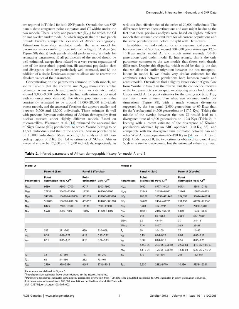
are reported in Table 2 for both SNP panels. Overall, the two SNP

panels show congruent point estimators and CI widths under the

two models. There is only one parameter (NAY) for which the CI

do not overlap under model A, which suggests that the two panels

provide broadly compatible scenarios of African demography.

Estimations from data simulated under the same model for

parameter values similar to those inferred in Figure 5A show (see

Figure S8) that i) both panels should perform very similarly for

estimating parameters, ii) all parameters of the model should be

well estimated, except those related to a very recent expansion of

one of the ascertained population, iii) ancestral population sizes

and divergence times are particularly well estimated, and iv) the

addition of a single Denisovan sequence allows one to recover the

absolute values of the parameters.

Concentrating on the parameters common to both models, we

see in Table 2 that the ancestral size NANC shows very similar

estimates across models and panels, with an estimated value

around 9,000–9,500 individuals (in line with estimates obtained

with non-ascertained data set). The African population size is also

consistently estimated to be around 18,000–28,000 individuals

across models, and the ancestral Yoruban size appears smaller and

between 5,500 and 13,000 individuals. These estimates fit well

with previous Bayesian estimations of African demography from

nuclear markers under slightly different models. Based on

microsatellites, Wegmann et al. [13] estimated the ancestral size

of Niger-Congo (NC) populations (to which Yoruba belong) to be

12,500 individuals and that of the ancestral African population to

be 15,000 individuals. More recently, the analysis of 40 non-

coding regions of 2 Kb [53] led to estimates of NC and African

ancestral size to be 17,500 and 11,000 individuals, respectively, as

well as a San effective size of the order of 20,000 individuals. The

differences between these estimations and ours might be due to the

fact that these previous analyses were based on slightly different

models that assumed constant sizes for all current populations and

the same population size before the split with Denisovans.

In addition, we find evidence for some asymmetrical gene flow

between San and Yoruba, around 500–600 generations ago (12.5–

15 Kya) under model A, and much more recently (60–80

generations ago) under model B. Interestingly, this is the only

parameter common to the two models that shows such drastic

difference. Despite this disparity, which could be due to the fact

that we allow for earlier migration between the two metapopu-

lations in model B, we obtain very similar estimates for the

admixture rates between populations both between panels and

across models. Overall, we find a slightly larger extent of gene flow

from Yoruba to San than the reverse, but the confidence intervals

of the two parameters seem quite overlapping under both models.

Under model A, the point estimates for the divergence time TDIV

are much more different than what was obtained under our

simulations (Figure S8), with a much younger divergence

suggested by the San panel (2,600 generations or 65 Kya) than

for the Yoruba panel (4,700 generations or 117.5 Kya). Taking the

middle of the overlap between the two CI would lead to a

divergence time of 4,500 generations or 112.5 Kya (Table 2), in

keeping with a recent estimate of the divergence of Khoisan

populations obtained by an ABC approach [110 Ky, 53], and

compatible with the divergence time estimated between San and

other West African population (65–120 Ky in [54], or ,100 Ky in

[55]). Under model B, the two estimates obtained for panel 4 and

5, show a similar discrepancy, but the estimated values are much

Table 2. Inferred parameters of African demographic history for model A and B.

Model A Model B

Panel 4 (San) Panel 5 (Yoruba) Panel 4 (San) Panel 5 (Yoruba)

ParametersPointestimation 95% CIab

Pointestimation 95% CIab Parameters

Pointestimation 95% CIab

Pointestimation 95% CIab

NANC 9680 9300–10700 9017 8500–9900 NANC 9612 8977–10424 9013 8384–10146

NAFR 27835 26400–33500 17746 16800–20700 NAFR 23849 21634–44081 21762 15867–46813

NSAN 741378 166700–811800 532609 139900–873500 NCS 180,771 16598–411442 224,695 38694–446151

NYRI 517893 106600–890100 463052 124200–941000 NCY 96,071 2464–461785 251,150 67722–428360

NAS 8473 2400–10300 11140 8900–13900 NDS 3,704 412–6996 5187 2,000–5,700

NAY 5528 2000–7800 13087 11200–14800 NAY 10251 2456–461785 5480 1730–15823

NDY 644 85–4553 3654 517–4680

2NmS 5.9 4.6–14 3.7 3.4–18

2NmY 37.4 5–77 36.8 25–88

Ta 523 271–766 650 310–868 Ta 59 10–100 77 16–95

aYS 0.16 0.04–0.22 0.19 0.12–0.22 aYS 0.19 0.04–0.28 0.08 0.03–0.19

aSY 0.11 0.06–0.15 0.10 0.06–0.13 aSY 0.08 0.04–0.18 0.16 0.06–0.25

mSY 4.45E-05 2.3E-06–9.9E-04 2.56E-04 3.1E-06–1.0E-03

mYS 1.11E-04 1.2E-05–6.3E-04 1.53E-04 6.2E-06–2.4E-04

TEY 32 20–260 113 38–249 TEY 170 101–691 298 162–567

TES 63 54–480 232 73–401

TDIV 2599 999–3834 4689 3716–5013 TDS 5,530 2482–9710 10,330 5358–12561

Parameters are defined in Figure 5.aPopulation size estimates have been rounded to the nearest hundred.bParametric bootstrap estimates obtained by parameter estimation from 100 data sets simulated according to CML estimates in point estimation columns.Estimates were obtained from 100,000 simulations per likelihood and 20 ECM cycle.doi:10.1371/journal.pgen.1003905.t002

Demographic Inference from Genomic and SNP Data

PLOS Genetics | www.plosgenetics.org 7 October 2013 | Volume 9 | Issue 10 | e1003905

higher (5,530 and 10,330 generations for panels 4 and 5,

respectively), which can also be due to the fact that we authorize

some gene flow between the two metapopulations after their

divergence. If we again take the middle of the overlap between the

two CI, we obtain a value of 7,500 generations (180 Kya),

substantially larger than the value obtained under model A (4,500

generations).

An examination of the parameters restricted to model B suggests

that the Yoruban continent expanded recently 170–300 genera-

tions ago (4250–7500 ya), from a relatively small population of

600–3600 individuals, and that the Yoruban island receives more

migrants (around 18 per generation) than the San island (2–3

individuals per generation). The age of the expansion is slightly

older than the divergence time between two Western Niger-Congo

populations estimated previously (140 generations, [13]), and

intermediate between the age of the Niger-Congo languages

(,10 Kya, [56]), and that of the Bantu expansion (,5 Kya, [57]).

The larger immigration rate seen in Yorubans is compatible with

the fact that farmer populations generally maintain higher levels of

gene flow with their neighbours than hunter-gatherers due to their

larger effective size [47]. Note however that all parameter

estimates mentioned above assume that the Denisova divergence

time is correctly estimated at 16,000 generations or 400 Kya [58],

even though there is still a large uncertainty attached to this

divergence time, which could range from 230 to 650 Kya [58] or

even between 170 and 700 Kya in a more recent study [59].

Reported estimates and CI in Table 2 do not take this uncertainty

into account, and should thus be rescaled if a different divergence

time between Denisovans and Humans was proposed.

Like in the case of non-ascertained data, we find that the more

complex model is much better supported by the data. Even though

this better fit is barely visible when considering the marginal 1D

expected SFS (see Figure S10), this is more exactly quantified by

an AIC analysis (Table S3) revealing that the relative likelihood of

model A is close to zero for both panels when compared to model

B.

Discussion

Estimation of demographic parameters from genomicdata

We have introduced a new and flexible simulation-based

approach to estimating demographic parameters. For the tested

scenarios, our composite-likelihood approach is as precise as LaLi[21], which is the current standard in the field. Our approach

seems more robust than LaLi since it is more likely to converge

towards the correct solution when starting from the same number

(50) of initial conditions (see Figures 2, 3, S4, S5). In terms of

computational speed, point estimates are very quickly obtained by

LaLi for simple models (on average 15 seconds and 6 minutes for

models in Fig. 1A and 1B, respectively, compared to 15 minutes

and 2h30 for fastsimcoal2, respectively). However, fastsimcoal2 is

much faster for more complex models with three populations and

migration (4–5 h per run for fastsimcoal2 for model on Fig. 1C,

compared to 34 h on average for LaLi). By maximizing the fit of

two-dimensional SFS, fastsimcoal2 can also explore very complex

models involving more than 10 populations with migration, which

cannot be tackled by any other current method. Since fastsimcoal2

and LaLi use a very similar likelihood function (see Figure S3), it

seems that the improved convergence of our approach lies in the

use of the ECM optimization scheme, which compensates for the

use of non-optimal approximate likelihoods. Note that our robust

ECM maximization technique and the maximization of the

product of pairwise composite likelihoods could also be used by

methods deriving the SFS analytically or by a diffusion approx-

imation (like LaLi), thus potentially enabling the analysis of models

as complex as those studied here. Also note that recent progress in

the computation of joint SFS using coalescent or diffusion

approaches [18,23] have led to the development of promising

demographic inference methods applied to the study of relatively

complex evolutionary models [see e.g. 24].

Even though different demographic trajectories can lead to

exactly the same SFS in a single population [27], we do not find

any evidence of parameter non-identifiability in our investigated

cases. This is probably because we restricted our search to a

limited set of possible histories, defined by few-parameter models.

Our results confirm that if the true history lies within the models

considered, the parameters of relatively complex scenarios can be

well recovered from the (joint) SFS. However, we must keep in

mind that histories outside our model family might have identical

likelihoods.

One disadvantage of our method (and of any other simulation-

based method) is that we are approximating the likelihood,

implying that two runs from identical initial parameter values can

results in different estimations (see Figure S2). Using more

simulations for the estimation of the likelihood would lessen but

not totally suppress this problem, but our results show that our

maximization procedure leads to almost completely unbiased

estimates and converges to correct values. Another disadvantage of

our approach is its dependence on composite likelihoods. More

powerful full likelihood approaches explicitly take into account

linkage disequilibrium (LD) between sites [60], and therefore

might reveal useful to infer recent migration events (see e.g. [61]).

That being said, our applied data sets consist of SNPs randomly

distributed across the whole genome, and so patterns of LD

between sites are minimal. Whereas confidence intervals of

demographic parameters based on composite likelihood ratios

should in principle be too narrow (see e.g. [21,60,62,63]), a study

based on short stretches of DNA sequences has empirically shown

that they were extremely similar to those obtained by explicitly

modeling patterns of recombination [54]. This appears unlikely to

be true in general, and certainly not if products of pairwise

composite likelihoods were used (as with eq. (7), which was actually

not used for our test cases). Similarly, the use of composite

likelihoods in model tests based on AIC can overestimate the

support for the most likely model [64]. However, the composite

likelihoods in our test cases are quasi likelihoods due to the global

independence between SNPs, and the differences in relative

likelihood of alternative models are so huge (see Tables S2 and S3)

that some residual patterns of LD are unlikely to change our

conclusions.

As an alternative to our composite likelihood maximization

approach, Garrigan [22] has proposed to integrate an approxi-

mate likelihood computed in a way similar to ours into an MCMC

algorithm, allowing him to get posterior distributions and credible

intervals. Whereas MCMC algorithms generally assume that the

likelihood is computed accurately, it has been shown that MCMC

procedure should lead to correct posterior distributions even if the

likelihood is approximated, provided that there is no systematic

error in its computation [65,66]. This Bayesian approach could be

worth exploring as a possible extension of our likelihood

maximization procedure. However, our current implementation

has the advantage of quickly getting point estimates, around which

CIs can be obtained later by repeating the estimation on

bootstrapped samples. For instance, a point estimate for the IM

model shown in Figure 1B is obtained in about 2h30 on a single

core machine, whereas 40–80 h are necessary to get posterior

distributions for the parameters of a similar IM model from a

Demographic Inference from Genomic and SNP Data

PLOS Genetics | www.plosgenetics.org 8 October 2013 | Volume 9 | Issue 10 | e1003905

single MCMC run using a specialized coalescent program on a

multi-core machine [see 22].

Handling ascertained SNP data setsThe additional versatility of our simulation-based likelihood

approach is well exemplified by its handling of ascertained SNP

chips, and the inference of several parameters from the SFS under

complex demographic scenarios. Previous ways of handling ascer-

tained SNP chips either consisted in removing the bias induced by the

ascertainment [44] or taking it into account in the estimation

procedure [39,45]. However, these methods are usually not as

general as our implementation, as they are either restricted to models

including a single population [44], or to the case of the sole estimation

of divergence time between two populations [45]. Contrastingly, our

method can be applied to various types of demographic models

including several populations, bottlenecks and migration.

Our simulation results suggest that parameters of complex

models can be correctly recovered when the ascertainment consists

of randomly chosen SNPs heterozygous in a single individual

(Figures S8 and S9). Interestingly, we find that some parameters of

unascertained populations that diverged a long time ago either

with (Figure S8) or without (Figure S9) admixture can also be quite

well estimated when the model is well specified. This suggests that

a given ascertainment panel of the GWHO Affymetrix chip could

be used to infer parameters in several related populations. It is also

worth noting that our calibration of parameters relied on the

assumption that the divergence time with an outgroup population

was known, but a different divergence time would only require a

rescaling of the estimated parameters. The use of an outgroup

species with fixed divergence time is a standard way to calibrate

mutation rates (as e.g. in [21]), but we note it could also be used

within species for DNA sequence data when some uncertainty

exist on mutation rates, which is currently the case in humans

[67,68].

Most parameters inferred from real African populations have

very similar estimates and confidence intervals irrespective of

which SNP panel is used (Figure 5, Table 2), which agrees with our

simulation results (Figures S8, S9). However, a few parameters

seem to provide relatively divergent estimates, like the Yoruba and

the African ancestral size, as well as the Yoruba-San divergence

time, a discrepancy that is not really expected from the

simulations. This discrepancy could stem from either an unknown

source of ascertainment, from a misspecification of the model for

one of the two ascertained population, or from an ascertained

individual that is not representative of its population, the latter

case being possibly due to inbreeding or admixture. It currently

appears difficult to disentangle these cases, and the inclusion of

additional parameters in model B only seems to marginally

improve the fit of the expected SFS to the data. It suggests that our

models still do not capture all aspect of the true demography of

these populations, which might also affect our ability to reproduce

the ascertained SFS, and have a negative impact on our

estimations. We note however that previous estimates of African

demography [e.g. 53] are more in line with those inferred from the

Yoruba than from the San panel, which could suggest that our

demographic models are more appropriate for the Yoruba than

for the San population. Overall, our results nevertheless show that

meaningful demographic estimates can be obtained from ascer-

tained SNP chips, suggesting a useful and cheap alternative to

large scale sequencing for demographic inference.

Application to complex demographic modelsOur methodology has the potential to infer demographic

parameters from large scale genomic data under a much wider

range of neutral evolutionary models than either the current

implementation of LaLi, current Approximate Bayesian Compu-

tation (ABC) implementations [69], summary statistics based

approaches [11], or other existing likelihood-based methods [22].

Whereas ABC has the potential to be applied to genomic data, it

has rarely been done since it usually requires the simulations of

data sets as large as those analysed, which is computationally very

costly. Our approach could thus be seen as a powerful likelihood-

based alternative to the study of complex evolutionary models,

which are usually only tackled by ABC approaches [see e.g.

16,70,71], with the additional advantage of not having to choose

which summary statistics to use for the inference, which is often a

problem in ABC [e.g. 13,72,73,74]. Our approach can indeed

tackle complex evolutionary models with a relatively large number

of populations (see Figs. 1D, 4B and 5B). For instance, the model

shown in Figure 4B includes 4 sampled populations, as well as four

other unsampled populations, whose demography also needs to be

reconstructed. AIC analysis reveals that the cost associated to

increasing model complexity is rewarded by a much better fit to

the data. One should however make a distinction between the

inclusion of additional parameters for a given number of

populations (e.g. adding the possibility to have gene flow between

populations), and the inclusion of additional populations. The

addition of unsampled or ghost populations can not only modify

parameter estimations but also alter our interpretation of the

results (see e.g. [75,76]). For instance, the inclusion of continents

from which sampled populations received migrants (which is an

attempt at taking into account the spatial structure of African

populations) in Figure 4B improved the fit of expected SFS (see

Table S2), without really modifying our estimation of the level of

European admixture, but it radically changed our interpretation of

the relationships between African Americans and extant African

and European populations. As expected, the inclusion of a

potential source of admixture for the Luhya population in model

B2 improved the fit of the model and it allowed us to make

inference about this ghost population, but it also modified

estimated parameter values of this and other populations. These

observations suggest that complex models are better studied by

considering all populations simultaneously, and that a strategy

consisting in estimating population-specific parameters and fixing

them when incorporating additional populations would not be

optimal.

There are still some limits to the complexity of models that can

be studied, and AIC-like approaches can be used to study which

modifications sufficiently improve the model to be preserved.

However, the question of whether our best model is the true model

is not addressed by model comparisons such as likelihood ratios or

AIC. One would ideally like to assess how well the model explains

the data, which is usually done by some posterior predictive check

in a Bayesian setting [77], or by getting the data p-value under a

frequentist approach. We have implemented such an approach,

where the model p-value was evaluated by comparing an observed

G-test statistic [3,62] to its model distribution. As expected, this

approach leads to non-significant p-values when applied to

simulated data sets (Figure S11). However, the p-values for all

models shown in Figures 4 and 5 are highly significant (p = 0,

Figures S12 and S13) suggesting that our implemented models of

human evolution are still overly simplistic. This is not surprising

given the high-dimensionality of the parameter space and the large

amount of SNPs at hand giving us high power to reject inaccurate

hypotheses. Since models are generally expected to be wrong, the

question is at what point is a model so wrong that it is no longer

useful [78, p. 74]. The fact that the addition of plausible source of

realism into our models significantly improves the fit to the data

Demographic Inference from Genomic and SNP Data

PLOS Genetics | www.plosgenetics.org 9 October 2013 | Volume 9 | Issue 10 | e1003905

(Tables S2 and S3) is reassuring in the sense that we have a

methodology to refine our still imperfect evolutionary scenarios.

Methods

Simulation-based site frequency spectrum andlikelihoood

Nielsen [17] has shown that one could estimate the likelihood of

a demographic model L X ,hð Þ, where X is the site frequency

spectrum, on the basis of coalescent simulations. This is because

the probability pi of a given derived allele frequency i is simply a

ratio of branch lengths of the coalescent tree expected under

model h as [17]:

pi~E(ti Dh)=E(T Dh), ð1Þ

where ti is the total length of a set Bi~fbijg of branches directly

leading to i terminal nodes, and T is the total tree length. This

probability can then be estimated with arbitrary precision on the

basis of Z simulations as [62]

ppi~XZ

k

Xj[Bi

bijk

,XZ

k

Tk: ð2Þ

where bijk is the length of the j-th compatible branch in simulation

k (see Figure S1A). Note that the estimator shown in eq. (2)

implicitly weights simulations according to the probability that a

mutation occurs on the simulated tree. Note that an estimator of

the form ppi~PZ

k

Pj[Bi

bijk=Tk (as used by Garrigan [22] to

estimate the expected SFS) would give each tree the same weight

and would thus give an excessive weight to genomic regions with

shallow coalescent trees, which can be a problem for recently

bottlenecked populations. If some simulated entries of the SFS

were zero (becausePZ

k

Pj[Bi

bijk~0), ppi was set to an arbitrarily

small values [as in 22] chosen here as min(ppj Dppjw0)=100.

We have empirically checked that our procedure gives the correct

SFS under two simple scenarios for which the expected SFS can be

obtained exactly by the method developed by Chen [18] for cases

involving up to two populations and no migration. These scenarios

were (i) a bottleneck model (as in Fig. 1A) and (ii) a divergence model

without migration (as in Fig. 1B but without migration). We show in

Figures S14 and S15 for scenarios i) and ii), respectively, the fit of the

SFSs entries (estimated by our approach for different numbers of

coalescent simulations) to the true SFS entries. As expected the fit

improves with the number of simulations, and the estimated SFS

entries are distributed symmetrically around the true values without

any visible bias for these two scenarios.

Composite likelihoodsProbabilities inferred from the simulations and eq. (2) can then

be used to compute the composite likelihood of a given model as

[20]

CL~Pr(X Dh)!PL{S0 (1{P0)S P

n{1

i~1ppi

mi : ð3Þ

where X~fm1, . . . ,mn{1g is the SFS in a single population

sample of size n, S is the number of polymorphic sites, L is the

length of the studied sequence, and P0 is the probability of no

mutation on the tree, obtained as P0~e{mT assuming a Poisson

distribution of mutations occurring at rate m.

This formulation can be extended for the joint SFS of two

populations as

CL12!PL{S0 (1{P0)S P

n1

i~0Pn2

j~0ppij

mij , ð4Þ

and one can define a v-dimensional SFS for more than two (v)

populations as

CL1:::v!PL{S0 (1{P0)S P

n1

i1

Pn2

i2

. . .Pnv

ivppW

mW ð5Þ

where W~i1 i2 . . . iv{1 iv is a composite index. However, when

the number of populations in the model is larger than 2 and

sample sizes are relatively large, the number of entries in the v-

dimensional SFS can be huge, implying that most entries of the

observed SFS will be either zero or a very small number and that

the expected values for these low-count entries will be difficult to

estimate precisely. In that case, we have chosen to estimate the v-

dimensional CL1...v by collapsing all entries with observed SFS less

than a predefined threshold e as

CL1:::v!PL{S0 (1{P0)S P

obsSFSi§eppi

mi

� �

X1vobsSFSjve

ppj

0@

1A

P1vobsSFSjve

mj

:

ð6Þ

When v.4, this approach will also prove computationally difficult,

and in that case we have chosen to compute a composite

composite-likelihood (C2L) obtained by multiplying all pairwise

CL’s, as

C2L1:::v

! Pivj

CLij , ð7Þ

where CLij is given by eq. (4).

Maximizing the likelihoodAs the likelihood is obtained by simulations, which incurs some

approximation, we cannot use optimization methods based on

partial derivatives. Even though other methods would be possible,

we have chosen to use a conditional maximization algorithm

[ECM, 79], which is an extension of the EM algorithm where each

parameter of the model is maximized in turn, keeping the other

parameters at their last estimated value. The maximization of each

parameter was done using Brent’s [80, Chapter 5] algorithm,

which is a root-finding algorithm using a combination of bisection,

secant and inverse quadratic interpolation [see e.g. 81]. We start

with initial random parameter values, and perform a series of

ECM optimization cycles until estimated values stabilize or until

we have reached a specified maximum number of ECM cycles

(usually 20–40). Unless specified otherwise, we used 100,000

coalescent simulations for the estimation of the expected SFS and

likelihood for a given set of demographic parameters. Even though

a higher precision could be reached with a larger number of

simulations, especially for complex models, this number appears

like a good compromise between computational efficiency and

likelihood estimation accuracy (see Figure S2). Note that the

imprecision on the likelihood estimation might also prevent an

efficient optimization of our parameters, as a sub-optimal

parameter might give by chance a better likelihood than the

Demographic Inference from Genomic and SNP Data

PLOS Genetics | www.plosgenetics.org 10 October 2013 | Volume 9 | Issue 10 | e1003905

optimal one during an ECM cycle. Because the composite

likelihood surface might have several local maxima and be

difficult to explore [e.g. 60], several independent optimizations are

performed (between 20 and 40 depending on the model and

computation time), each starting from different initial conditions,

and the overall maximum composite likelihood solution is

retained.

Coalescent simulations, estimation of the SFS, likelihood

computations and its maximization were all done with fastsimcoal2,

a modified version of the fastsimcoal program [82]. fastsimcoal2 input

file format and command lines arguments are briefly described in

Supplementary Text S1, and examples of input files are provided

in Supplementary Text S2.

Tested demographic models without ascertainmentWe have tested our program ability to recover demographic

parameters from DNA sequence data in four relatively plausible

but distinct scenarios of population differentiation involving one to

ten populations with migration (see Figure 1). In all cases, we

simulated with fastsimcoal2 400,000 unlinked regions of 50 bp, thus

totaling 20 Mb of DNA sequences, assuming a mutation rate of

2.561028 bp21 per generation and an infinite-site model. Pseudo-

observed SFS were also directly computed with fastsimcoal2.

Parameters were estimated independently from ten data sets

generated under each model. For each data set generated under

models with one to three populations, we performed 50 parameter

estimations via ECM maximization, and each time retained the

parameter set with maximum likelihood. For the model with 10

populations we only performed 20 estimations per data sets, and

used 50,000 simulations instead of 100,000 for the other models to

estimate the expected SFS due to long computation times. We

describe the four tested models in Figure 1, and the used

parameter values are showed as red dots in Figures 2, 3, S4 and

S5. Absolute numbers (generations, population sizes) were

obtained by assuming that the mutation rate of 2.561028 bp21

per generation was known.

As a benchmark, we used LaLi to infer the demographic

parameters in scenarios shown in Figure 1A–1C involving up to

three populations. For each generated data set, we performed 50

parameter estimations using the Broyden-Fletcher-Goldfarb-

Shanno (BFGS) optimization method implemented in LaLi, and

we retained the parameters associated with the maximum

likelihood. We followed LaLi’s manual specification to set

reasonable upper and lower bounds of the search ranges of the

parameter. In all cases, the expected SFS was estimated by

extrapolating the SFS inferred from 3 grid sizes set to 40, 50 and

60, which are in all cases larger than our maximum samples sizes

(30 in the IM model case). The composite likelihood was

computed using LaLi’s multinomial model, which is in fact a

product of Poisson likelihoods, where the expected model entries

are scaled to sum up to 1. This likelihood also ignores information

about the expected and observed numbers of monomorphic and

polymorphic sites used in our likelihood formulation (as well as in

[20]). Therefore, the ratio CLLaLi=CLfastsimcoal should be equal to

SSe{S�

PL{S0 (1{P0)S Pi mi!

� �showing that barring the P0

terms, the two CLs differ by a single constant value. The difference

between likelihoods computed with fastsimcoal and LaLi is

illustrated in Figure S3 for the case of the bottleneck scenarios

shown in Figures 1A. It shows that when monomorphic sites are

not taken into account, fastsimcoal and LaLi indeed produce

essentially identical likelihood profiles around true parameters.

However, when monomorphic sites are used in the likelihood, the

shape of the likelihood profiles differs, making it more or less peaky

depending on the parameter. There is thus no clear advantage in

using one or the other likelihood form for this scenario, but our use

of monomorphic sites allows us to directly get absolute values of

the parameters. We report in Figures 2, S4 and S5 only the results

obtained for data sets for which LaLi’s best log likelihood was less

than 10% lower than the largest log-likelihood obtained with the

other data sets, and we considered LaLi not to have converged for

the discarded data sets.

Estimating demographic parameters from an ascertainedSNP array

Recently, Affymetrix developed a new SNP array including

,629,000 SNPs with known ascertainment scheme for population

inference (Axiom Genome-Wide Human Origins 1 Array, http://

www.affymetrix.com/support/technical/byproduct.

affx?product = Axiom_GW_HuOrigin) [43]. This array, abbrevi-

ated hereafter GWHO, is made up of SNPs defined in 13

discovery panels. In the first 12 panels, SNPs have been identified

by comparing the two chromosomes of an individual from a

known population, further quality checks and validation on a large

population sample [43]. The 13th panel contains SNPs that are

polymorphic when comparing the Denisovan sequence and a

random San chromosome. Raw genotypes from 943 unrelated

individuals from more than 50 worldwide populations are freely

available on ftp://ftp.cephb.fr/hgdp_supp10/.

The ascertainment scheme of this array is simple and

homogeneous over a given panel. However, the SFS inferred

from this array is biased as only mutations that occur in the

ancestry of the two compared chromosomes will be considered (see

Figure S1B). We show in Figure S7 the difference between the

ascertained and non-ascertained SFS under a few basic demo-

graphic scenarios in a single population. The differences between

the two SFS can be quite dramatic, implying that the estimation of

demographic parameters on ascertained data sets without taking

the ascertainment into account is bound to lead to biased

estimates. Nielsen et al. [44] have shown how to correct the

expected SFS within a given population under such a simple

ascertainment scheme, and the ascertained joint SFS could be

unbiased in a similar way by taking into account ascertainment

probabilities in the ascertained populations. Rather than unbiasing

the SFS, we have chosen here to incorporate the bias in the model

and to infer demographic parameters directly from the ascertained

(joint) SFS, a strategy similar in spirit to that used by Gravel et al.

[28] to account for biases in the SFS obtained from low-coverage

next-generation sequencing data. It implies we need to model the

ascertainment scheme in the coalescent simulations such as to infer

the expected ascertained SFS for a given demography. In order to

estimate the SFS when SNPs are defined as being sites

heterozygous in a given individual, we use the following

procedure: 1) we perform conventional coalescent simulations

under a given demography, 2) we choose two lineages at random

in the ascertained population, 3) we identify the subtree relating

the chosen lineages to their most recent common ancestor

(MRCA) (highlighted in blue in Figure S1B), 4) we update the

numerator in eq. (2) by summing up branch lengths of the blue

subtree that are ancestral to i1 lineages in population 1, i2 lineages

in population 2, …, iv lineages in population v, 5) The

denominator of eq. (2) is updated by summing up the total length

of the blue subtree.

Parameter optimization is then performed similarly to the

unascertained case, except that the terms depending on the

number of monomorphic sites (PL{S0 (1{P0)S ) in eq. (6) are

removed from the likelihood since only polymorphic sites are

reported on the ascertained chip, which implies that we cannot use

a molecular clock. Therefore, parameter absolute estimation

Demographic Inference from Genomic and SNP Data

PLOS Genetics | www.plosgenetics.org 11 October 2013 | Volume 9 | Issue 10 | e1003905

should be done relative to an arbitrarily fixed or known parameter

(e.g. population size, divergence time). Note however that a

molecular clock could be used if the fraction of sites found

heterozygous were known in ascertained individuals, as in this case

the expected fraction of monomorphic sites would then simply be

P0A~e{m TA , where TA would be the total length of the expected

ascertained tree (shown in blue in Figure S1B).

Applications to human demographyNon-ascertained human genomic data set. We illustrate

the potential of our method to inferring demographic parameters

from more than three populations by investigating the past

demography of four populations analyzed by Complete Genomics,

which sequenced the whole genome of 54 unrelated individuals

from 11 populations at a depth of 51-89X per genome [83]. This

data set was chosen as we could assume that heterozygous

positions were recovered unambiguously due to the high coverage,

and because it covered non-genic regions that are less sensitive to

selection, and thus to bias in the site frequency spectrum [5,84].

We thus considered autosomal SNPs found outside genic regions

(as defined by Ensembl version 71, April 2013 [85], and outside

CpG islands (as defined on the UCSC platform, [86]). The derived

and ancestral states of the SNPs were inferred from the

comparison with the chimpanzee and orangutan genomes, using

the syntenic net alignments between hg19 and panTro2, and

between hg19 and ponAbe2, both available on the UCSC

platform [86]. We then kept the SNPs found to be polymorphic

in 27 individuals from 4 samples representing African Americans

(5 African Americans from Southwest United States), 2 African

populations (4 Luhya from Webuye, Kenya; 9 Yoruba from

Ibadan, Nigeria) and a European population (9 Utah residents

with Northern and Western European ancestry from the CEPH

collection). The multidimensional SFS for these four populations

was inferred from a total of 239,120 independent SNPs located

more than 5 Kb apart from each other, to minimize linkage

disequilibrium.

We then considered several demographic scenarios accounting

for the pattern of genomic diversity found in these samples (see

Figure 4). The first investigated scenario A is shown in Figure 4A.

It is a relatively simple scenario, with 12 parameters, which

assumes a divergence between the European and an ancestral

African population to have occurred 50 Kya [28,48], and this date

is used to calibrate the other parameters. The two Niger-Congo

(NC) speaking populations (YRI and LWK) are assumed to have

diverged TNC generations ago, and each NC population has a

different constant effective size since then. The two African

populations are then assumed to have contributed to the founding

of the African-American population (ASW) 16 generations ago

(around 1800, assuming 25 years per generation). The African

population is also considered to have gone through a bottleneck

TBOT generations ago with a reduced population size NBOT for

100 generations (as it is the bottleneck intensity NBOT/100 and not

its duration that conditions genetic diversity).

We have also considered two alternative and more realistic

scenarios of human evolution, but requiring more parameters to

estimate (16 and 19 for models B1 and B2 in Figure 4, respectively)

and additional unsampled populations (3 and 4, respectively). The

main difference with the previous model A is that we assume that

the European and the two NC samples belong to two different

subdivided populations modeled here as continent-island systems.

These continent-island models are equivalent to infinite-island

models [e.g. 87], and have been shown to well approximate

patterns of diversity after range expansions [47]. In this model, the

CEU population receives migrants from a European continent,

which is also the source of admixture of the African-American

ASW population. The ASW population has also received an initial

genetic contribution 16 generations ago from a Niger-Congo

‘‘continent’’, which is also the source of gene flow to the two NC

populations. These two continents are assumed to have diverged

some time ago from an African population, and here again this

time is fixed to 2000 generations for the European continent,

whereas this time is estimated for the NC continent. For simplicity,

all islands are assumed to have been formed 100 generations ago,

which is thus the assumed duration of the scattering phase sensu

Wakeley [88]. It implies that in the backward coalescent process,

all genes remaining in the islands are transferred to the continents

100 generations ago. Note that we also allow for bottlenecks of size

(NBNC and NBEUR) to have occurred for 100 generations in the

NC and European continents, respectively. Like in the model

shown in Figure 4A, we allow for a different population size

(NANC) of the ancestral population some TBOT generations ago. In

our most complex model B2, we include a potential admixture of

the Luhya population with an unsampled (potentially East African)

population, which contributed with a proportion aEA to the initial

Luhya population 100 generations ago. In the simpler model B1,

the Luhya population is not considered as admixed and only

receives genes from the NC continent, and this model thus has 3

parameters less (16) than our model B1 (19).

Parameter estimations were performed from the multidimen-

sional SFS, without considering the number of monomorphic sites,

which were not available in the VCF files from Complete

Genomics. Fixing African-European divergence time and Afri-

can-American admixture times nevertheless allowed us to get

absolute values for the other parameters. In addition to ignoring

terms in P0 from equation (6) (command line option –0 of

fastsimcoal2), we also collapsed all SFS entries less than 5 in a

single category (command line option –C5 of fastsimcoal2).

Maximum CL parameters were obtained after 40 cycles of the

ECM algorithm, starting with 50,000 coalescent simulations per

likelihood estimations, and ending with 250,000 simulations per

likelihood estimation.

SNP chip data sets with known ascertainment. We

applied our approach to infer the demographic history from

ascertained SNP chips to the case of the divergence between two

African populations, the Yoruba from Ibadan (Nigeria) and a

hunter-gatherer San population from Southern Africa, where one

individual from each population was included in the Affymetrix

ascertainment panels. We can thus use the Affymetrix panel 4 (San

ascertained) and panel 5 (Yoruba ascertained) to perform separate

estimations that can be compared to each other. The assumed

models of African population divergence we analysed are shown in

Figure 5. In the simple model shown in Figure 5A, the 12 San and

44 Yoruban individuals were assumed to be drawn from two

currently large populations that expanded recently from two

ancestral populations that diverged TDIV generations ago. We also

allowed the Yoruba and San populations to have had a single

pulse of bi-directional and potentially asymmetrical gene flow. As

mentioned above, the use of SNPs does not allow us to get absolute

dates due to the absence of a mutation clock. We therefore

included the Denisova population (and its SNP data) in our model,

and assumed that it diverged 400,000 years ago [58] (or 16,000

generations assuming a 25 y generation time) to calibrate our

estimates. Note that an absolute dating would have also been

possible if the total number of heterozygous sites per ascertained

individual had been know or made available. In model B shown in

Figure 5B, we use a more complex scenario describing the

divergence of two continent-island metapopulations, in a way

similar to models in Figure 5B. In this case we assume that the

Demographic Inference from Genomic and SNP Data

PLOS Genetics | www.plosgenetics.org 12 October 2013 | Volume 9 | Issue 10 | e1003905

Yoruba and San sampled populations receive 2 Nm genes per

generation from their respective continents, which diverged TDS

generations ago. At that time the San population began an

exponential growth, whereas the exponential growth of the

Yoruban continent was allowed to start later, TEY generations

ago. Note also that in Model B, the Ancestral Yoruban population

and the San population can continuously exchange migrants

during the period between TEY and TDS.

Panels 4 and 5 originally contained 163,313 and 124,125 SNPs,

respectively. From this we discarded all CpG SNPs potentially

target of multiple hits (N. Patterson, personal communication), as

well as all SNP positions with missing data in either Denisova,

Yoruba or San samples, which finally left us with 109,020 and

81,383 SNPs in panels 4 and 5, respectively. The SNP ancestral

states were assumed to be those present in the chimpanzee

outgroup, as provided in the HGDP data set. With this choice, it is

possible that some ancestral states are mis-specified (due to

recurrent mutations or incomplete lineage sorting in both humans

and chimps). Such misspecifications can artificially increase the

observation of high-frequency derived allele classes, a signal that

can wrongly be taken as the effect of selection [63]. However, this

problem is relatively unlikely here, as such mis-identification

should be more frequent at CpG SNPs, which were removed from

our data set. Moreover, the observed SFS for both panels do not

show a particular excess of high frequency derived alleles (see

Figure S10). Parameter confidence intervals were obtained 100

parametric bootstrap, simulating SFS with the same number of

SNPs from the CML estimates and re-estimating parameters each

time. Parameters were estimated from 30 starting conditions for

each original data set as well as for the 100 bootstrapped SFS data

sets. Parameters associated with the maximum CL computed from

eq. (6) without terms in P0 were retained after 20 cycles of the

ECM algorithm were retained. One hundred thousand coalescent

simulations were used to estimate the expected joint ascertained

SFSs, and a threshold e value of 2 was used for pooling rarely

observed SFS entries in a single category, as in eq. (6) above.

Assessing the accuracy of estimations from ascertained

SNP panels. In order to see if the 12 parameters of model A

could be correctly recovered by our approach, we simulated 10

data sets under the model shown in Figure 5A using fixed

parameter values, as reported in Figure S8. We simulated 20 Mb

of DNA sequence data under the selected scenario and retained all

SNPs that were heterozygous in an arbitrary individual from the

ascertained population (pseudo-San or pseudo-Yoruba), adjusting

the mutation rate to get approximately 100,000 SNPs to match the

observed data. We also simulated ascertained SNP data sets under

a slightly simpler scenario, removing any admixture event between

Yoruba and San ancestors, as shown in Figure S9.

Parameters were estimated for the 10 data sets generated for

each panel and results were reported in Figures S8 and S9.

Model comparisonsAs mentioned in the next section on model test, it might be

difficult to accept a simple model with a G-test based on tens of

thousands of polymorphic sites, but in that case, it might be better

to establish a procedure allowing one to improve models, by

progressively adding some realism to simple models [89]. Our

likelihood-based approach would in principle lend itself to model

comparison through likelihood-ratios for nested models or through

Akaike Information Criterion (AIC, [52]) for other model

comparisons. However, we are here confronted with two distinct

problems. The first one affects all composite likelihood approaches

and due to the fact that the distribution of the composite likelihood

ratio test (CLRT) is generally unknown. When the SFS is obtained

from DNA sequences with relatively large levels of linkage

disequilibrium, it has been proposed to obtain an empirical

distribution of the CLRT by simulation of DNA sequences with

recombination (e.g. [54,90]). In the case of the AIC, Varin and

Vidoni [91] have proposed to replace the number of parameter d of

a given model in AIC~2d{2 ln(lhood) by an effective number of

parameters de that needs to be computed from a sensitivity matrix

and Godambe Information matrix, which might be difficult to do in

practice. We note however that in our two applied examples the

SFS is computed from a collection of SNPs randomly distributed

across the genome, such that we shall conservatively assume that the

CL computed from the multidimensional SFS is close to a true

likelihood. Note that this assumption would not be valid if one had

computed a composite likelihood based on the product of pairwise

composite likelihoods, like in eq. (7). The second problem is linked

to the fact that we estimate the likelihood with some error (Figure

S2). As noted previously, this can prevent us to efficiently optimize

our parameters, but it also means that the likelihood ratios or AIC

statistics are imprecisely estimated. To address this problem, we

have compared models on the basis of the maximum value of the

likelihood obtained over 100 estimations performed for the ML

parameters obtained by our optimization procedure. We then

calculated the relative likelihood or the Akaike’s weight of evidence

in favor of the i-th model as (see e.g. [89])

wi~exp({0:5Di)PRr exp({0:5Dr)

where Di~AICi{AICmin.

Model testEven though we can estimate parameters under any model, it

can be useful to check how data fit the chosen model. To this aim

we use an approach based on a likelihood ratio G-statistic [3,62] of

the form CLR~log10(CLO=CLE), where CL0 is the observed

maximum composite likelihood where the expected SFS is

replaced by the relative observed SFS in eqs. 3, 5 or 7, and CLE

is the estimated composite maximum likelihood computed using

the procedure described above. We obtain the null distribution of

the CLR statistic by the same parametric bootstrap procedure used

to infer confidence intervals, where we generate by simulation a

number of data sets using the estimated maximum-likelihood

parameters of the model, and each time perform parameter

estimations and estimate the CLR statistic. We can compute the p-

value of the observed CLR statistic from this null distribution.

Note that this type of G-test has been used before to find genomic

regions under selection [3,62].

We report in Figure S11 the null distributions of the CLR and the

p-values of two data sets generated under models shown in

Figure 1A and 1B. In both cases, the p-values are not significant

confirming that the data sets are compatible with the tested models.

Note however that a non-significant p-value is not an absolute

proof that the tested model is correct, as there could be a large

number of models leading to similar SFSs, as was shown

previously [27], but it is an indication that the observed SFS is

well explained by the model.

However, in applied cases, we actually expect that this test leads

to very significant values, since the true history of the populations

is completely unspecified and our models are certainly overly

simple and potentially far from reality.

Demographic Inference from Genomic and SNP Data

PLOS Genetics | www.plosgenetics.org 13 October 2013 | Volume 9 | Issue 10 | e1003905

Supporting Information

Figure S1 Estimation of the SFS by a ratio of branch lengths on

a coalescent tree. A) Case without ascertainment bias. All branches

of a given genealogy can be used to estimate the site frequency

spectrum. Here we have highlighted in red the branches

contributing to the SFS 2 entry. B) In case of ascertainment, only

mutations occurring along the subtree (shown in blue) connecting

the ascertained alleles can be observed. Therefore only branches

along the blue subtree can contribute to the ascertained SFS.

(PDF)

Figure S2 Effect of the number of coalescent simulation on the

precision of the estimated likelihood for different evolutionary

models. The three evolutionary models considered here are those

shown in Figures 1A, 1B and 1C. For each model we plot the

distribution of 100 composite log-likelihoods computed with either

10,000, 100,000, 200,000, or 1 million simulations, shown as

brown, orange, blue and black lines, respectively. In each case, the

distributions are centered on their median value (shown below the

x-axis for the 1 million simulation case), and the x axis units

express deviation from the median in log10 likelihood units. As

expected, we gain precision with increasing number of simulations

performed per likelihood simulation, but the precision also

decreases with the complexity of the model for the same number

of simulations. Note that for computation time issues, 100,000

simulations per likelihood estimation were used for the optimiza-

tions done in the paper.

(PDF)

Figure S3 Comparison of likelihood profiles between fastsim-

coal2 and LaLi for the simple bottleneck scenario shown in

Figure 1A. For each pane, we computed the likelihood of the

model by varying only one parameter around its true value (blue

vertical line), and keeping the other parameters of the model

constant. The fourth parameter of the model, which is the

ancestral population size NA was explicitly set to its true value

(10,000) in fastsimcoal2 and set as the reference parameter in LaLi,as LaLi does not allow one to specify the value of the reference

parameter, which might explain the small discrepancies between

the blue and grey curves. The bottleneck duration was set to 100

generations for both fastsimcoal2 and LaLi. The orange and blue

lines represent the scaled likelihoods computed by fastsimcoal2

with and without the monomorphic sites, respectively, whereas the

grey line represents the likelihood profile obtained with LaLi.Likelihood profiles are computed around the current population

size NCUR = 10000 (A), the bottleneck size NBOT = 100 (B), and

the age of the bottleneck TBOT = 1000 generations (C). One

million simulations were used to compute the likelihoods of each

point with fastsimcoal2. We see that when the number of

monomorphic sites is not used by fastsimcoal, fastsimcoal and

LaLi produce essentially the same likelihood up to a constant term.

The use of the number of polymorphic sites makes the profile

likelihood curve peakier for NBOT but flatter for TBOT and NCUR.

(PDF)

Figure S4 Single population bottleneck model. fastsimcoal2

results are in black and LaLi’s results (9/10) are in blue. True

parameters values are shown as red dots. fastsimcoal2 required

15 minutes for a single estimation based on 40 ECM cycles over

parameters, whereas LaLi requires on average 15 seconds on a

similar CPU.

(PDF)

Figure S5 IM model. fastsimcoal2 results are in black and LaLi’sresults (8/10) are in blue. True parameters values are shown as red

dots. fastsimcoal2 required about2h30 for a single estimation based

on 40 ECM cycles over parameters, whereas LaLi requires on

average 6 minutes on a similar CPU.

(PDF)

Figure S6 Marginal SFS obtained under the three models

defined in Figure 4. Black lines: Observed SFS; Blue line: Fitted

SFS. Gray circles: Cumulative absolute difference between

observed and expected SFS.

(PDF)

Figure S7 Effect of ascertainment on the SFS in a single

population. A: Stationary population. B: Population demographic

expansion by a factor 100, 5000 generations ago, NCUR = 50,000

diploids, NANC = 500; C: Population contraction of a factor 100,

1000 generations ago, NCUR = 500 diploids, NANC = 50,000; D:

Population bottleneck according to scenario shown in Figure 2A.

Expected SFS were obtained from 1 million coalescent simulations.

The ascertainment consisted here in selecting SNPs that were

heterozygous in a single individual, like in the Affymetrix SNP array.

(PDF)

Figure S8 ML estimation of the model parameters shown in

Figure 5. Parameters estimated from the simulated for the pseudo-

Yoruba ascertained panel are shown in black, and the parameters

estimated from the pseudo-San ascertained panels are shown in

blue. For each panel, we generated 10 data sets according to

parameters shown in red.

(PDF)

Figure S9 Estimation of parameters under a simpler model of

population divergence between Yoruba and San. A: Demographic

model and parameter definition. B: Parameters estimated from the

Yoruba ascertained panel are in shown black, and parameters

estimated from the San ascertained panels are shown in blue. True

simulated parameter values are shown in red.

(PDF)

Figure S10 Observed and expected marginal SFS in San,

Yoruba and Denisvova samples inferred from panel 4 and 5 for

models A and B of Figure 5. Gray line = observed, dashed blue

line = expected under model A of Figure 5; dashed orange

line = expected under model B of Figure 5. ML estimates are

reported in Table 2. Note that the fit for the expected SFS was

done on the three dimensional joint SFS, and that the Denisova

1D SFS has only two entries at zero or 1.

(PDF)

Figure S11 Model tests performed for one data set generated

under scenarios in Figures 1A (A) and 1B (B). The black line

represents the distribution of CLRs obtained for data sets

generated by parametric bootstraps from simulations done with

the maximum composite likelihood parameters obtained for each

data set (see Materal and Methods). The p-value of each model is

then computed as the fraction of data sets with a CLR larger than

or equal to the observed CLR (red line).

(PDF)

Figure S12 Model tests performed on scenartios of human history

shown in Figure 4. The black line represents the distribution of

CLRs obtained for data sets generated by parametric bootstraps

from simulations done with the maximum composite likelihood

parameters obtained for each data set and shown in Table 1. The p-

values of each model are then computed as the fraction of data sets

with a CLR larger than or equal to the observed CLR (red line), and

are zero for all models. Note that the demographic models used for

parameter estimations are clearly rejected for both SNP panels,

which imply that these models cannot exactly reproduce the

observed data. Note however, the shift of the red line to the right for

Demographic Inference from Genomic and SNP Data

PLOS Genetics | www.plosgenetics.org 14 October 2013 | Volume 9 | Issue 10 | e1003905

Model B1 and B2, suggesting a much better fit to the data in line

with the AIC results shown in Table S2.

(PDF)

Figure S13 Model tests performed on scenarios of African history

shown in Figure 5 for the San and Yoruba SNP panels. The black

line represents the distribution of CLRs obtained for data sets

generated by parametric bootstraps from simulations done with the

maximum composite likelihood parameters obtained for each data

set and shown in Table 2. The p-values of each model are then

computed as the fraction of data sets with a CLR larger than or

equal to the observed CLR (red line). The demographic models

used for parameter estimations are clearly rejected for both SNP

panels (p-value = 0 for all models), which imply that these models

cannot exactly reproduce the observed data. Note however, the shift

of the red line to the right for Model B, suggesting a much better fit

to the data in line with the AIC results shown in Table S3.

(PDF)

Figure S14 Fit of the SFS approximation obtained with

fastsimcoal2 to the expected SFS for a bottleneck model similar to

that shown in Fig. 1A. The expected SFS was obtained by

implementing eqs. 2–9 from Chen [18] in Mathematica ver 9.0.1.0.

We considered a scenario with the following fixed parameter values:

2NCUR = 10000, 2NBOT = 100, and 2NA = 10000. The sample size

was fixed to n = 20. We examined the effect of varying the age of the

bottleneck TBOT, as 10, 1000, and 10000 generations, which

corresponds to a scaled times of 0.001, 0.1, and 1.0 in units of 2NA,

and the effect of varying the number of simulations per SFS

estimation (between 1 thousand and 1 million). A–C) Direct

comparison of the SFS entries (in log scale), where we report

fastsimcoal2 results for 100 replicated runs. As can be seen, the higher

the number of simulations the better the approximation, as the

points get closer to the diagonal. D–F) Relative Error of the

fastsimcoal2 SFS approximation, defined as ((SFS fastsimcoal2-exact

SFS)/exact SFS). As expected, increasing the number of simulations

decreases the relative error. Interestingly, the error distributions are

symmetrically distributed around zero suggesting that the fastsim-

coal2 approximation is essentially unbiased.

(PDF)

Figure S15 Fit of the SFS approximation obtained with fastsimcoal2

to the expected SFS for a divergence model similar to that in Fig. 1B

but without migration. The expected SFS was obtained by

implementing eqs. 2–9 from Chen [18] in Mathematica ver 9. We

considered a scenario where two populations of different sizes

2N1 = 10000 and 2N2 = 1000 diverged TDIV generations ago from

and an ancestral population of size 2NA = 10000. The number of

sampled genes are n1 = 20 and n2 = 30 for populations 1 and 2,

respectively. We examined the effect of using 1 thousand to 1 million

simulations to estimate the SFS for varying TDIV values of 0.001, 0.1,

and 10, expressed in units of 2NA generations. A–C) Direct

comparison of the SFS entries (in log scale), where we report

fastsimcoal2 results for 100 replicated runs. Note that we do not show

SFS entries estimated by fastsimcoal2 that have a value of zero, but these

entries correspond to extremely low expected values. As can be seen,

the higher the number of simulations the better the approximation, as

the points get closer to the diagonal. D–F) Relative Error of the

fastsimcoal2 SFS approximation in log scale. The density curves were

obtained after exclusion of outliers (values smaller or larger than the1%

and 99% quantiles, respectively). As expected, increasing the number

of simulations decreases the relative error. Interestingly, the error

distributions are symmetrically distributed around zero suggesting that

the fastsimcoal2 approximation is essentially unbiased.

(PDF)

Table S1 Inferred parameters of human demography under

model A of Figure 4A.

(PDF)

Table S2 Relative likelihood of the different models shown in

Figure 4.

(PDF)

Table S3 Relative likelihood of the different models shown in

Figure 5 for SNP chip panels 4 and 5.

(PDF)

Text S1 Input file format and fastsimcoal2 command lines.

(PDF)

Text S2 Examples of input files used in the paper.

(PDF)

Acknowledgments

We are very grateful to Rasmus Nielsen for interesting discussions and

sharing of code for unbiasing the site frequency spectrum distributions used

to check the validity of our simulations, to Christoph Leuenberger for

statistical insights and critical comments, to Ryan Gutenkunst for advices

on the use of hahi, and to Nick Patterson to send us the list of CpG SNPs

for al panels. We are also indebted to David Reich and Nick Patterson for

introducing us to the problem of ascertained SNP chips and making

available unpublished data sets. We also thank three anonymous reviewers

for their critical and helpful comments and Isabel Alves for discussing

various aspects of African demography. The program fastsimcoal2 is freely

available on http://cmpg.unibe.ch/software/fastsimcoal2.

Author Contributions

Conceived and designed the experiments: LE MF. Performed the

experiments: LE ID EHS VCS. Analyzed the data: LE ID EHS MF

VCS. Contributed reagents/materials/analysis tools: LE ID EHS MF

VCS. Wrote the paper: LE ID EHS MF VCS.

References

1. Nielsen R, Hellmann I, Hubisz M, Bustamante C, Clark AG (2007) Recent and

ongoing selection in the human genome. Nat Rev Genet 8: 857–868.

2. Kelley JL, Madeoy J, Calhoun JC, Swanson W, Akey JM (2006) Genomic

signatures of positive selection in humans and the limits of outlier approaches.

Genome Res 16: 980–989.

3. Nielsen R, Williamson S, Kim Y, Hubisz MJ, Clark AG, et al. (2005) Genomic

scans for selective sweeps using SNP data. Genome Res 15: 1566–1575.

4. Beaumont MA, Nichols RA (1996) Evaluating loci for use in the genetic analysis of

population structure. Proceedings of the Royal Society London B 263: 1619–1626.

5. Boyko AR, Williamson SH, Indap AR, Degenhardt JD, Hernandez RD, et al.

(2008) Assessing the evolutionary impact of amino acid mutations in the human

genome. PLoS Genet 4: e1000083.

6. Kuhner MK, Beerli P, Yamato J, Felsenstein J (2000) Usefulness of Single

Nucleotide Polymorphism Data for Estimating Population Parameters. Genetics

156: 439–447.

7. Beerli P, Felsenstein J (2001) Maximum likelihood estimation of a migration

matrix and effective population sizes in n subpopulations by using a coalescent

approach. Proceedings of the National Academy of Sciences USA 98: 4563–

4568.

8. Hey J, Nielsen R (2007) Integration within the Felsenstein equation for improved

Markov chain Monte Carlo methods in population genetics. Proc Natl Acad

Sci U S A 104: 2785–2790.

9. Hey J (2010) Isolation with migration models for more than two populations.

Mol Biol Evol 27: 905–920.

10. Becquet C, Przeworski M (2007) A new approach to estimate parameters of

speciation models with application to apes. Genome Res 17: 1505–1519.

11. Naduvilezhath L, Rose LE, Metzler D (2011) Jaatha: a fast composite-likelihood

approach to estimate demographic parameters. Mol Ecol 20: 2709–2723.

12. Leuenberger C, Wegmann D (2010) Bayesian computation and model selection

without likelihoods. Genetics 184: 243–252.

Demographic Inference from Genomic and SNP Data

PLOS Genetics | www.plosgenetics.org 15 October 2013 | Volume 9 | Issue 10 | e1003905

13. Wegmann D, Leuenberger C, Excoffier L (2009) Efficient approximate Bayesiancomputation coupled with Markov chain Monte Carlo without likelihood.

Genetics 182: 1207–1218.

14. Beaumont MA, Cornuet J-M, Marin J-M, Robert CP (2009) Adaptive

approximate Bayesian computation. Biometrika 96: 983–990.

15. Excoffier L, Estoup A, Cornuet J-M (2005) Bayesian Analysis of an Admixture

Model With Mutations and Arbitrarily Linked Markers. Genetics 169: 1727–

1738.

16. Beaumont MA, Zhang W, Balding DJ (2002) Approximate Bayesian

computation in population genetics. Genetics 162: 2025–2035.

17. Nielsen R (2000) Estimation of population parameters and recombination ratesfrom single nucleotide polymorphisms. Genetics 154: 931–942.

18. Chen H (2012) The joint allele frequency spectrum of multiple populations: a

coalescent theory approach. Theor Popul Biol 81: 179–195.

19. Marth GT, Czabarka E, Murvai J, Sherry ST (2004) The Allele Frequency

Spectrum in Genome-Wide Human Variation Data Reveals Signals of

Differential Demographic History in Three Large World Populations. Genetics166: 351–372.

20. Adams AM, Hudson RR (2004) Maximum-likelihood estimation of demo-

graphic parameters using the frequency spectrum of unlinked single-nucleotidepolymorphisms. Genetics 168: 1699–1712.

21. Gutenkunst RN, Hernandez RD, Williamson SH, Bustamante CD (2009)

Inferring the joint demographic history of multiple populations frommultidimensional SNP frequency data. PLoS genetics 5: e1000695.

22. Garrigan D (2009) Composite likelihood estimation of demographic parameters.

BMC genetics 10: 72.

23. Lukic S, Hey J, Chen K (2011) Non-equilibrium allele frequency spectra via

spectral methods. Theoretical population biology 79: 203–219.

24. Lukic S, Hey J (2012) Demographic inference using spectral methods on SNPdata, with an analysis of the human out-of-Africa expansion. Genetics 192: 619–

639.

25. Li H, Durbin R (2011) Inference of human population history from individual

whole-genome sequences. Nature 475: 493–496.

26. Gronau I, Hubisz MJ, Gulko B, Danko CG, Siepel A (2011) Bayesian inference

of ancient human demography from individual genome sequences. Nat Genet

43: 1031–1034.

27. Myers S, Fefferman C, Patterson N (2008) Can one learn history from the allelic

spectrum? Theoretical population biology 73: 342–348.

28. Gravel S, Henn BM, Gutenkunst RN, Indap AR, Marth GT, et al. (2011)Demographic history and rare allele sharing among human populations. Proc

Natl Acad Sci U S A 108: 11983–11988.

29. Tennessen JA, Bigham AW, O’Connor TD, Fu W, Kenny EE, et al. (2012)Evolution and functional impact of rare coding variation from deep sequencing

of human exomes. Science 337: 64–69.

30. Sousa V, Hey J (2013) Understanding the origin of species with genome-scaledata: modelling gene flow. Nat Rev Genet 14: 404–414.

31. Yi X, Liang Y, Huerta-Sanchez E, Jin X, Cuo ZX, et al. (2010) Sequencing of

50 human exomes reveals adaptation to high altitude. Science 329: 75–78.

32. Nielsen R, Korneliussen T, Albrechtsen A, Li Y, Wang J (2012) SNP calling,

genotype calling, and sample allele frequency estimation from New-Generation

Sequencing data. PloS one 7: e37558.

33. Durbin RM, Abecasis GR, Altshuler DL, Auton A, Brooks LD, et al. (2010) A

map of human genome variation from population-scale sequencing. Nature 467:

1061–1073.

34. Crawford JE, Lazzaro BP (2012) Assessing the accuracy and power of population

genetic inference from low-pass next-generation sequencing data. Front Genet 3:

66.

35. Nielsen R, Paul JS, Albrechtsen A, Song YS (2011) Genotype and SNP calling

from next-generation sequencing data. Nat Rev Genet 12: 443–451.

36. Lynch M (2009) Estimation of allele frequencies from high-coverage genome-

sequencing projects. Genetics 182: 295–301.

37. Kim SY, Lohmueller KE, Albrechtsen A, Li Y, Korneliussen T, et al. (2011)

Estimation of allele frequency and association mapping using next-generation

sequencing data. BMC Bioinformatics 12: 231.

38. Johnson PL, Slatkin M (2006) Inference of population genetic parameters in

metagenomics: a clean look at messy data. Genome Res 16: 1320–1327.

39. Wollstein A, Lao O, Becker C, Brauer S, Trent RJ, et al. (2010) Demographichistory of Oceania inferred from genome-wide data. Current biology : CB 20:

1983–1992.

40. Albrechtsen A, Nielsen FC, Nielsen R (2010) Ascertainment biases in SNP chipsaffect measures of population divergence. Mol Biol Evol 27: 2534–2547.

41. Clark AG, Hubisz MJ, Bustamante CD, Williamson SH, Nielsen R (2005)

Ascertainment bias in studies of human genome-wide polymorphism. GenomeRes 15: 1496–1502.

42. Patterson N, Moorjani P, Luo Y, Mallick S, Rohland N, et al. (2012) Ancient

admixture in human history. Genetics 192: 1065–1093.

43. Lu Y, Patterson N, Zhan Y, Mallick S, Reich D (2011) Technical design

document for a SNP array that is optimized for population genetics. Available:

ftp://ftp.cephb.fr/hgdp_supp10/8_12_2011_Technical_Array_Design_Document.pdf

44. Nielsen R, Hubisz MJ, Clark AG (2004) Reconstituting the Frequency Spectrum

of Ascertained Single-Nucleotide Polymorphism Data. Genetics 168: 2373–

2382.

45. Pickrell JK, Patterson N, Barbieri C, Berthold F, Gerlach L, et al. (2012) Thegenetic prehistory of southern Africa. Nature communications 3: 1143.

46. Wakeley J, Hey J (1997) Estimating ancestral population parameters. Genetics

145: 847–855.

47. Excoffier L (2004) Patterns of DNA sequence diversity and genetic structure

after a range expansion: lessons from the infinite-island model. Mol Ecol 13:

853–864.

48. Fagundes NJ, Ray N, Beaumont M, Neuenschwander S, Salzano FM, et al.

(2007) Statistical evaluation of alternative models of human evolution. Proc Natl

Acad Sci U S A 104: 17614–17619.

49. Zakharia F, Basu A, Absher D, Assimes TL, Go AS, et al. (2009) Characterizingthe admixed African ancestry of African Americans. Genome Biol 10: R141.

50. Sjodin P, Sjostrand AE, Jakobsson M, Blum MG (2012) Resequencing data

provide no evidence for a human bottleneck in Africa during the penultimateglacial period. Mol Biol Evol 29: 1851–1860.

51. Henn BM, Gignoux CR, Jobin M, Granka JM, Macpherson JM, et al. (2011)

Hunter-gatherer genomic diversity suggests a southern African origin formodern humans. Proc Natl Acad Sci U S A 108: 5154–5162.

52. Akaike H (1974) New Look at Statistical-Model Identification. Ieee Transactions

on Automatic Control Ac19: 716–723.

53. Veeramah KR, Wegmann D, Woerner A, Mendez FL, Watkins JC, et al. (2012)

An early divergence of KhoeSan ancestors from those of other modern humans

is supported by an ABC-based analysis of autosomal resequencing data.Molecular biology and evolution 29: 617–630.

54. Hammer MF, Woerner AE, Mendez FL, Watkins JC, Wall JD (2011) Genetic

evidence for archaic admixture in Africa. Proc Natl Acad Sci U S A 108: 15123–

15128.

55. Schlebusch CM, Skoglund P, Sjodin P, Gattepaille LM, Hernandez D, et al.

(2012) Genomic Variation in Seven Khoe-San Groups Reveals Adaptation and

Complex African History. Science 338: 374–379.

56. Dimmendaal GJ (2008) Language Ecology and Linguistic Diversity on the

African Continent. Language and Linguistics Compass: 840–858.

57. Ehret C (2001) Bantu expansions: Re-envisioning a central problem of earlyAfrican history. International Journal of African Historical Studies 34: 5–41.

58. Reich D, Green RE, Kircher M, Krause J, Patterson N, et al. (2010) Genetic

history of an archaic hominin group from Denisova Cave in Siberia. Nature 468:1053–1060.

59. Meyer M, Kircher M, Gansauge MT, Li H, Racimo F, et al. (2012) A high-

coverage genome sequence from an archaic Denisovan individual. Science 338:222–226.

60. Auton A, McVean G (2007) Recombination rate estimation in the presence of

hotspots. Genome Research 17: 1219–1227.

61. Jenkins PA, Song YS, Brem RB (2012) Genealogy-based methods for inference

of historical recombination and gene flow and their application in Saccharo-

myces cerevisiae. PloS one 7: e46947.

62. Nielsen R, Hubisz MJ, Hellmann I, Torgerson D, Andres AM, et al. (2009)

Darwinian and demographic forces affecting human protein coding genes.

Genome Res 19: 838–849.

63. Hernandez RD, Williamson SH, Bustamante CD (2007) Context dependence,

ancestral misidentification, and spurious signatures of natural selection. Mol Biol

Evol 24: 1792–1800.

64. Varin C, Reid N, Firth D (2011) An Overview of Composite Likelihood

Methods. Statistica Sinica 21: 5–42.

65. Beaumont MA (2003) Estimation of population growth or decline in genetically

monitored populations. Genetics 164: 1139–1160.

66. Andrieu C, Roberts GO (2009) The Pseudo-Marginal Approach for Efficient

Monte Carlo Computations. Annals of Statistics 37: 697–725.

67. Kong A, Frigge ML, Masson G, Besenbacher S, Sulem P, et al. (2012) Rate of de

novo mutations and the importance of father’s age to disease risk. Nature 488:

471–475.

68. Scally A, Durbin R (2012) Revising the human mutation rate: implications forunderstanding human evolution. Nature reviews Genetics 13: 745–753.

69. Li S, Jakobsson M (2012) Estimating demographic parameters from large-scale

population genomic data using Approximate Bayesian Computation. BMCgenetics 13: 22.

70. Csillery K, Blum MG, Gaggiotti OE, Francois O (2010) Approximate Bayesian

Computation (ABC) in practice. Trends in ecology & evolution 25: 410–418.

71. Lopes JS, Beaumont MA (2010) ABC: a useful Bayesian tool for the analysis of

population data. Infection, genetics and evolution : journal of molecular

epidemiology and evolutionary genetics in infectious diseases 10: 826–833.

72. Aeschbacher S, Beaumont MA, Futschik A (2012) A novel approach for

choosing summary statistics in approximate Bayesian computation. Genetics

192: 1027–1047.

73. Nunes MA, Balding DJ (2010) On optimal selection of summary statistics for

approximate Bayesian computation. Statistical applications in genetics and

molecular biology 9: Article34.

74. Sousa VC, Fritz M, Beaumont MA, Chikhi L (2009) Approximate bayesian

computation without summary statistics: the case of admixture. Genetics 181:

1507–1519.

75. Beerli P (2004) Effect of unsampled populations on the estimation of population

sizes and migration rates between sampled populations. Mol Ecol 13: 827–836.

76. Slatkin M (2005) Seeing ghosts: the effect of unsampled populations on

migration rates estimated for sampled populations. Mol Ecol 14: 67–73.

Demographic Inference from Genomic and SNP Data

PLOS Genetics | www.plosgenetics.org 16 October 2013 | Volume 9 | Issue 10 | e1003905

77. Gelman A, Meng XL, Stern H (1996) Posterior predictive assessment of model

fitness via realized discrepancies. Statistica Sinica 6: 733–760.78. Box GEP, Draper NR (1987) Empirical model-building and response surfaces.

New York; Chichester etc.: J. Wiley. XIV, 669 pp.

79. Meng XL, Rubin DB (1993) Maximum likelihood estimation via the ECMalgorithm: A general framework. Biometrika 80: 267–278.

80. Brent RP (1973) Algorithms for Minimization without Derivatives. EnglewoodCliffs, NJ: Prentice-Hall.

81. Press WH, Teukolsky SA, Vetterling WT, Flannery BP (2007) Numerical

Recipes in C++: The Art of Scientific Computing. Cambridge: CambridgeUniversity Press. 1256 p.

82. Excoffier L, Foll M (2011) fastsimcoal: a continuous-time coalescent simulator ofgenomic diversity under arbitrarily complex evolutionary scenarios. Bioinfor-

matics 27: 1332–1334.83. Drmanac R, Sparks AB, Callow MJ, Halpern AL, Burns NL, et al. (2010)

Human genome sequencing using unchained base reads on self-assembling DNA

nanoarrays. Science 327: 78–81.

84. O’Fallon B (2013) Purifying selection causes widespread distortions of

genealogical structure on the human6chromosome. Genetics 194: 485–492.85. Birney E, Andrews D, Bevan P, Caccamo M, Cameron G, et al. (2004) Ensembl

2004. Nucleic acids research 32: D468–470.

86. Karolchik D, Hinrichs AS, Kent WJ (2012) The UCSC Genome Browser.Current protocols in bioinformatics/editoral board, Andreas D Baxevanis [et al]

Chapter 1: Unit1 4.87. Beaumont MA (2004) Recent developments in genetic data analysis: what can

they tell us about human demographic history? Heredity 92: 365–379.

88. Wakeley J (1999) Nonequilibrium migration in human history. Genetics 153:1863–1871.

89. Johnson JB, Omland KS (2004) Model selection in ecology and evolution.Trends in ecology & evolution 19: 101–108.

90. Zhu L, Bustamante CD (2005) A composite-likelihood approach for detectingdirectional selection from DNA sequence data. Genetics 170: 1411–1421.

91. Varin C, Vidoni P (2005) A note on composite likelihood inference and model

selection. Biometrika 92: 519–528.

Demographic Inference from Genomic and SNP Data

PLOS Genetics | www.plosgenetics.org 17 October 2013 | Volume 9 | Issue 10 | e1003905