Robust control of fed-batch cultures of Escherichia coli
263
Thèse de doctorat NNT: 2021UPASG072 Robust control of fed-batch cultures of Escherichia coli Commande robuste de cultures fed-batch de Escherichia coli Thèse de doctorat de l’Université Paris-Saclay École doctorale n ◦ 580, Sciences et Technologies de l’Information et de la Communication (STIC) Spécialité de doctorat: Automatique Unité de recherche : Université Paris-Saclay, CNRS, CentraleSupélec, Laboratoire des signaux et systèmes, 91190, Gif-sur-Yvette,France Référent : Faculté des sciences d’Orsay Thèse présentée et soutenue à Paris Saclay, le 20 Octobre 2021, par Merouane ABADLI Composition du Jury Antoine CHAILLET Président Professeur, CentraleSupélec/L2S Rudibert KING Rapporteur & Examinateur Professeur, Technische Universität Berlin Jesus PICO Rapporteur & Examinateur Professeur, Universitat Politècnica de València Anne-Lise HANTSON Examinatrice Professeur, Université de Mons Direction de la thèse Sihem TEBBANI Directrice de thèse Professeur, CentraleSupélec/L2S Alain VANDE WOUWER Directeur de thèse Professeur, Université de Mons/FPMs Didier DUMUR Co-encadrant & invité Professeur, CentraleSupélec/L2S Invités Laurent DEWASME Invité Docteur ingénieur, Université de Mons/FPMs
-
Upload
khangminh22 -
Category
Documents
-
view
0 -
download
0
Transcript of Robust control of fed-batch cultures of Escherichia coli

Thès
e de
doc
tora
tNNT:2021UPA
SG072
Robust control of fed-batchcultures of Escherichia coli
Commande robuste de culturesfed-batch de Escherichia coli
Thèse de doctorat de l’Université Paris-Saclay
École doctorale n 580, Sciences et Technologies del’Information et de la Communication (STIC)
Spécialité de doctorat: AutomatiqueUnité de recherche : Université Paris-Saclay, CNRS, CentraleSupélec,Laboratoire des signaux et systèmes, 91190, Gif-sur-Yvette, France
Référent : Faculté des sciences d’Orsay
Thèse présentée et soutenue à Paris Saclay,le 20 Octobre 2021, par
Merouane ABADLI
Composition du Jury
Antoine CHAILLET PrésidentProfesseur, CentraleSupélec/L2SRudibert KING Rapporteur & ExaminateurProfesseur, Technische Universität BerlinJesus PICO Rapporteur & ExaminateurProfesseur, Universitat Politècnica de ValènciaAnne-Lise HANTSON ExaminatriceProfesseur, Université de Mons
Direction de la thèse
Sihem TEBBANI Directrice de thèseProfesseur, CentraleSupélec/L2SAlain VANDE WOUWER Directeur de thèseProfesseur, Université de Mons/FPMsDidier DUMUR Co-encadrant & invitéProfesseur, CentraleSupélec/L2S
Invités
Laurent DEWASME InvitéDocteur ingénieur, Université de Mons/FPMs


Robust control of fed-batch cultures ofEscherichia coli
THESE DE DOCTORATsoumise a
L’UNIVERSITE DE MONSpour l’obtention du grade de
DOCTEUR EN SCIENCES DE L’INGENIEUR ET TECHNOLOGIE
These presentee et soutenue a Gif-sur-Yvette, le 20 Octobre 2021, par:
Merouane ABADLI
Composition du Jury
Antoine CHAILLET PresidentProfesseur, CentraleSupelec/L2SLaurent DEWASME SecretaryDocteur ingenieur, Universite de Mons/FPMsJesus PICO Reviewer & ExaminerProfesseur, Universitat Politecnica de ValenciaRudibert KING Reviewer & ExaminerProfesseur, Technische Universitat BerlinAnne-Lise HANTSON ExaminerProfesseur, Universite de MonsPhilippe BOGAERTS ExaminerProfesseur, Universite Libre de Bruxelles
Direction de la these
Sihem TEBBANI SupervisorProfesseur, CentraleSupelec/L2SAlain VANDE WOUWER SupervisorProfesseur, Universite de Mons/FPMsDidier DUMUR Co-supervisorProfesseur, CentraleSupelec/L2S


Important information
This work is a joint PhD thesis of Universite de Paris-Saclay (France) and Universite deMons (Belgium). The jury members are:
Antoine CHAILLET PresidentProfessor, CentraleSupelec/L2SLaurent DEWASME SecretarySenior Researcher and part-time Lecturer, Universite de MonsJesus PICO ReviewerProfessor, Universitat Politecnica de ValenciaRudibert KING ReviewerProfessor, Technische Universitat BerlinAnne-Lise HANTSON ExaminerProfessor, Universite de MonsPhilippe BOGAERTS ExaminerProfessor, Universite Libre de BruxellesSihem TEBBANI SupervisorProfessor, CentraleSupelec/L2SAlain VANDE WOUWER SupervisorProfessor, Universite de Mons/FPMsDidier DUMUR Co-supervisorProfessor, CentraleSupelec/L2S
The thesis was first presented in a private defense, held at Universite of Mons on the 22ndof September 2021 in the presence of all jury members.
A public defense was held at Universite Paris-Saclay on 20th of October 2021.
The roles of the jury members was adapted in the cover page of this manuscript in accor-dance with the regulation of each university. Consequently, they may differ for the twouniversities, but it is emphasized that the actual composition of the jury was the same.


i
“So the problem is ... not so much to see what nobody has yet seen, as to think what nobodyhas yet thought concerning that which everybody sees. ”
Arthur Schopenhauer”Parerga und Paralipomena” , 1851
“If I have seen further it is by standing on the shoulders of Giants ”
Isaac Newtonletter to Robert Hooke, 1675


iii
AcknowledgementsThis thesis is the fruit of the collaboration between the L2S laboratory at Cen-
traleSupelec, and the SECO laboratory of the polytechnic faculty of Mons.I would like begin by thanking the jury members who were more than gener-
ous with their extreme patience and precious time. Their expertise and feedbackon my work will surely contribute to my professional and personal development.I thank my committee chairman Pr. Antoine Chaillet for his support, patience, andgood advice throughout the defense process. A special thanks to the reviewers Pr.Rudibert King and Pr. Jesus Pico for the countless hours of reflecting, reading,and examining my manuscript. I thank them for the constructive feedback on thedifferent aspect of the thesis and their precious advice on the improvement of thepresented work. Thank you Pr. Anne-Lise Hantson, Pr. Philippe Bogaerts and Dr.Laurent Dewasme for agreeing to examine my work and to be part of my jury andmy committee. Your advice and comments helped me to advance on this researchproject and finalize my thesis.
I would like to express all my gratitude to my supervising team, Pr. SihemTebbani and Didier Dumur from CentraleSupelec, and Pr. Alain Vande Wouwerfrom the Polytechnic faculty of Mons. I thank them for guiding me throughout mythesis with professionalism, rigor, patience, availability, and generosity. I extendmy sincere gratitude to them for their constant support, encouragement and theprecious time they have given me during the thesis.
I would like to thank Sihem and Didier for their warm welcome to the lab andthe automation department, for the trust they placed in me, for their kindness andcare during difficult times, and for the precious opportunity they gave me to beable to participate in teaching activities at the department.
I thank Alain, for the warm welcome he always given me on each of my visits toMons. I thank him for his constant support, good advice, regular encouragementand patience during my experiments. I also thank him for motivating me to learnand explore new concepts.
My deepest gratitude to Dr. Laurent Dewasme, without whom finishing thisresearch project wouldn’t have been possible. I thank him for his participation andguidance during the experiments, his implication in scientific writing process, andhis discussions and feedback that were vital for finalizing this thesis.
I am also grateful to Pr. Anne-Lise Hantson for welcoming me to the depart-ment of Applied Chemistry and Biochemistry in order to carry out the fermenta-tion experiments that were essential to the conclusion of this work. I would like tothank her for the availability, the advice, and the support during my stays at thebiochemical lab.
I would like to thank my colleagues for creating a warm working atmospherethat allowed me to finish this doctoral PhD project. My sincere thanks to:
• The doctors and doctoral students of the Automation Department of Cen-traleSupelec for all the good times we shared.
• My colleagues in the automation service at the Polytechnic Faculty of Mons.

iv
• The doctoral students and reaserchers of the Chimical and Biochimical of thePolytechnic Faculty of Mons.
I would like to thank my friends, without whom I would not have made itthrough the difficult moments of this research project. Mehdi, Abdelhak, Mo-hamed, Abdou, and Mourad for always being there for me when I needed themthe most. Sarah and Fawzi for providing company, encouragement, and generos-ity. Amira, Katia, and Amina for their motivation, availability, and helpful adviceand guidance. Mokrane and Aladdin for our daily interactions and discussionsthat helped motivate and lift the spirit of each one of us. Tiziri for providing con-stant support especially during my stays at Mons. And all my friends from ENPand CAP.
Most importantly, I am grateful for my family’s unconditional, unequivocal,and loving support. I would like to pay homage to parents Kamel and Saıdafor their love, wise counsel and sympathetic ear. Without your sacrifices I wouldnever have had so many opportunities. My deepest gratitude to my brothers Sofi-ane and Badreddine and my sister Yasmine for the constant encouragement andsupport. I would like to thank all my family members, especially my grandmotherwho shaped the man I am today.
Finally, I dedicate this work to the memory of those we lost during the pan-demic and in the recent years. Particularly: My grandparents, my uncle Hamid,and my teacher/friend/mentor Pr. Abdelkrim Bouchouata.

v
AbstractEscherichia coli is a widespread cellular host for the industrial production of
protein-based biopharmaceutical products considering its physiological and bio-logical features. This production is mostly operated in fed-batch mode due to thescalable process, the low operational costs, and the relatively simple media con-ditions. One key challenge to maximize the bioprocess productivity is related tothe production of acetate, a metabolic byproduct inhibiting the cell respiratory ca-pacity and affecting the cells metabolic performance. This production must bemaintained as low as possible.
In this thesis, model-based control strategies are considered to avoid acetate ac-cumulation, thus maximizing biomass productivity, and to drive the culture nearthe optimal metabolic operating conditions. In addition, software sensors are de-veloped to estimate the evolution of the non-measured key variables required toimplement the control strategies.
To this end, three control strategies are proposed. First, the generic model con-trol method is investigated within an adaptive framework in order to regulatethe biomass growth rate to a desired reference. Secondly, a robust version of thegeneric model control strategy is developed to regulate the acetate concentrationto a low value. Finally, the last part of the thesis focuses on the implementation ofa nonlinear model predictive controller to limit acetate accumulation and comparethe performance with the previously described control methods. Furthermore, anUnscented Kalman filter estimating the glucose and acetate concentrations basedon the biomass measurements is implemented and coupled to the previously men-tioned control schemes.
The bioprocess is a complex, nonlinear, uncertain, and time-varying system.Thereby, the developments in this study are focused on the robustness of the im-plemented methods towards model uncertainties and unpredicted dynamics.
The performance and robustness of the control and estimation strategies aretested and tuned by means of different scenarios of simulation runs. Fed-batchcultures of E. coli BL21(DE3) strain are successfully carried on a lab-scale biore-actor, highlighting the potential of the proposed strategies in real-time conditions.Theoretical developments and experimental results allow to assess the advantagesof the different proposed approaches and show their tractability for further appli-cations in an industrial framework.
The proposed control strategies presented in this thesis lead to an average gainof up to 20% in biomass productivity compared to the conventional operatingmode.


ResumeEscherichia coli est un hote cellulaire tres repandu pour la production indus-
trielle de produits biopharmaceutiques a base de proteines, compte tenu de sescaracteristiques physiologiques et biologiques. Cette production est generalementrealisee en mode fed-batch en raison de l’evolutivite du procede, des faibles coutsoperationnels et des conditions de milieu de culture relativement simples a mettreen œuvre. Un defi majeur pour maximiser la productivite du bioprocede est lie ala production d’acetate, un produit metabolique inhibant la capacite respiratoiredes cellules et affectant leur performance metabolique. Des lors, il s’agit de limiterau maximum sa production par les microorganismes.
Dans cette these, des strategies de commande a base de modeles sont en-visagees pour eviter l’accumulation d’acetate, maximisant ainsi la productivitede la biomasse. Ces strategies ont pour objectif d’operer la culture en restant leplus proche possible des conditions operatoires optimales. En outre, des capteurslogiciels sont developpes pour estimer l’evolution des variables cles non mesureesnecessaires a la mise en œuvre des lois de commande.
A cette fin, trois strategies de commande sont developpees. La methode decommande par modele generique est tout d’abord mise en œuvre dans un cadreadaptatif afin de reguler le taux de croissance de la biomasse a une referencedesiree. Ensuite, une version robuste de la strategie de commande par modelegenerique est developpee afin de reguler la concentration d’acetate a une valeurrestant faible. Enfin, la derniere partie de la these s’interesse a la mise en œuvred’une structure de commande predictive non lineaire pour limiter l’accumula-tion d’acetate et comparer les performances avec les methodes de commandedecrites precedemment. De plus, un filtre de Kalman sans parfum (Un-scented Kalman Filter) estimant les concentrations de glucose et d’acetate a partirdes mesures de biomasse est implemente et couple aux schemas de commandementionnes precedemment. Enfin, la derniere partie de la these se concentre surl’implementation d’un controleur predictif base sur un modele non-lineaire pourlimiter l’accumulation d’acetate et comparer les performances avec les methodesde controle decrites precedemment.
Le bioprocede est un systeme complexe, non lineaire, incertain, variant dans letemps. Aussi, les developpements presentes dans cette these se focalisent sur larobustesse des methodes mises en œuvre vis-a-vis des incertitudes de modele etdes dynamiques non modelisees. La performance et la robustesse des schemas decommande et d’estimation sont testees et ajustees au travers de differents scenariosde simulation. Des cultures en mode Fed-batch de la souche E. coli BL21(DE3)sont realisees avec succes sur un bioreacteur de laboratoire, mettant en evidence lepotentiel des strategies proposees dans un contexte de conditions operatoires entemps reel. Les developpements theoriques et resultats experimentaux permettenten outre de mettre en evidence les avantages des differentes approches proposees,et illustrent egalement la generalisation envisageable a des procedes industriels deplus grande echelle. Les strategies de commande proposees dans cette these per-mettent un gain moyen jusqu’a 20% de la productivite de la biomasse par rapportau mode de fonctionnement conventionnel.

viii

ix
Contents
Acknowledgements iii
List of Figures xviii
List of Tables xx
1 General aspects of Escherichia coli as a host cell 11.1 Introduction . . . . . . . . . . . . . . . . . . . . . . . . . . . . . . . . 11.2 E. coli as a host cell . . . . . . . . . . . . . . . . . . . . . . . . . . . . 21.3 E. Coli strains . . . . . . . . . . . . . . . . . . . . . . . . . . . . . . . 31.4 E. coli physiology . . . . . . . . . . . . . . . . . . . . . . . . . . . . . 31.5 E. coli metabolism . . . . . . . . . . . . . . . . . . . . . . . . . . . . . 41.6 Overflow metabolism . . . . . . . . . . . . . . . . . . . . . . . . . . . 81.7 Bioprocess cultivation and operating modes . . . . . . . . . . . . . . 101.8 Conclusion . . . . . . . . . . . . . . . . . . . . . . . . . . . . . . . . . 14
2 Dynamic modeling of E. coli fed-batch cultures 172.1 Introduction . . . . . . . . . . . . . . . . . . . . . . . . . . . . . . . . 172.2 General aspects of bioprocess modeling . . . . . . . . . . . . . . . . 18
2.2.1 Reaction schemes . . . . . . . . . . . . . . . . . . . . . . . . . 182.2.2 General dynamic model . . . . . . . . . . . . . . . . . . . . . 192.2.3 Kinetic models . . . . . . . . . . . . . . . . . . . . . . . . . . 20
The Monod model . . . . . . . . . . . . . . . . . . . . . . . . 20The Haldane model (Haldane, 1930) . . . . . . . . . . . . . . 21Contois model (Contois, 1959) . . . . . . . . . . . . . . . . . 22Herbert model (Herbert, 1958) . . . . . . . . . . . . . . . . . 23Product inhibition model . . . . . . . . . . . . . . . . . . . . 24
2.2.4 Gas transfer models . . . . . . . . . . . . . . . . . . . . . . . 252.3 Macroscopic model of fed-batch E. coli cultures . . . . . . . . . . . . 26
2.3.1 E. coli mechanistic models . . . . . . . . . . . . . . . . . . . . 262.3.2 Reaction scheme . . . . . . . . . . . . . . . . . . . . . . . . . 272.3.3 Kinetic model . . . . . . . . . . . . . . . . . . . . . . . . . . . 282.3.4 Macroscopic model . . . . . . . . . . . . . . . . . . . . . . . . 30
2.4 Model Simulation . . . . . . . . . . . . . . . . . . . . . . . . . . . . . 322.5 Conclusion . . . . . . . . . . . . . . . . . . . . . . . . . . . . . . . . . 36
x
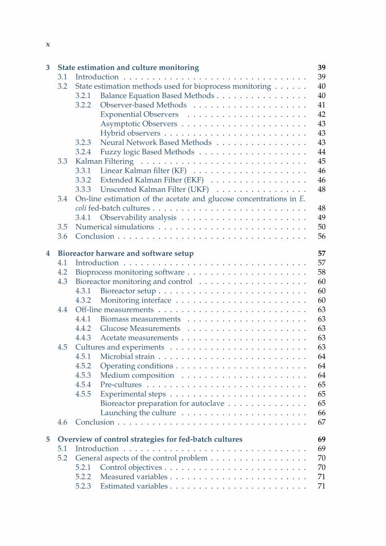
3 State estimation and culture monitoring 393.1 Introduction . . . . . . . . . . . . . . . . . . . . . . . . . . . . . . . . 393.2 State estimation methods used for bioprocess monitoring . . . . . . 40
3.2.1 Balance Equation Based Methods . . . . . . . . . . . . . . . . 403.2.2 Observer-based Methods . . . . . . . . . . . . . . . . . . . . 41
Exponential Observers . . . . . . . . . . . . . . . . . . . . . 42Asymptotic Observers . . . . . . . . . . . . . . . . . . . . . . 43Hybrid observers . . . . . . . . . . . . . . . . . . . . . . . . . 43
3.2.3 Neural Network Based Methods . . . . . . . . . . . . . . . . 433.2.4 Fuzzy logic Based Methods . . . . . . . . . . . . . . . . . . . 44
3.3 Kalman Filtering . . . . . . . . . . . . . . . . . . . . . . . . . . . . . 453.3.1 Linear Kalman filter (KF) . . . . . . . . . . . . . . . . . . . . 463.3.2 Extended Kalman Filter (EKF) . . . . . . . . . . . . . . . . . 463.3.3 Unscented Kalman Filter (UKF) . . . . . . . . . . . . . . . . 48
3.4 On-line estimation of the acetate and glucose concentrations in E.coli fed-batch cultures . . . . . . . . . . . . . . . . . . . . . . . . . . . 483.4.1 Observability analysis . . . . . . . . . . . . . . . . . . . . . . 49
3.5 Numerical simulations . . . . . . . . . . . . . . . . . . . . . . . . . . 503.6 Conclusion . . . . . . . . . . . . . . . . . . . . . . . . . . . . . . . . . 56
4 Bioreactor harware and software setup 574.1 Introduction . . . . . . . . . . . . . . . . . . . . . . . . . . . . . . . . 574.2 Bioprocess monitoring software . . . . . . . . . . . . . . . . . . . . . 584.3 Bioreactor monitoring and control . . . . . . . . . . . . . . . . . . . 60
4.3.1 Bioreactor setup . . . . . . . . . . . . . . . . . . . . . . . . . . 604.3.2 Monitoring interface . . . . . . . . . . . . . . . . . . . . . . . 60
4.4 Off-line measurements . . . . . . . . . . . . . . . . . . . . . . . . . . 634.4.1 Biomass measurements . . . . . . . . . . . . . . . . . . . . . 634.4.2 Glucose Measurements . . . . . . . . . . . . . . . . . . . . . 634.4.3 Acetate measurements . . . . . . . . . . . . . . . . . . . . . . 63
4.5 Cultures and experiments . . . . . . . . . . . . . . . . . . . . . . . . 634.5.1 Microbial strain . . . . . . . . . . . . . . . . . . . . . . . . . . 644.5.2 Operating conditions . . . . . . . . . . . . . . . . . . . . . . . 644.5.3 Medium composition . . . . . . . . . . . . . . . . . . . . . . 644.5.4 Pre-cultures . . . . . . . . . . . . . . . . . . . . . . . . . . . . 654.5.5 Experimental steps . . . . . . . . . . . . . . . . . . . . . . . . 65
Bioreactor preparation for autoclave . . . . . . . . . . . . . . 65Launching the culture . . . . . . . . . . . . . . . . . . . . . . 66
4.6 Conclusion . . . . . . . . . . . . . . . . . . . . . . . . . . . . . . . . . 67
5 Overview of control strategies for fed-batch cultures 695.1 Introduction . . . . . . . . . . . . . . . . . . . . . . . . . . . . . . . . 695.2 General aspects of the control problem . . . . . . . . . . . . . . . . . 70
5.2.1 Control objectives . . . . . . . . . . . . . . . . . . . . . . . . . 705.2.2 Measured variables . . . . . . . . . . . . . . . . . . . . . . . . 715.2.3 Estimated variables . . . . . . . . . . . . . . . . . . . . . . . . 71

xi
5.2.4 Control inputs and variables . . . . . . . . . . . . . . . . . . 715.3 Overview of control strategies for fed-batch cultivation . . . . . . . 72
5.3.1 Predetermined feeding control . . . . . . . . . . . . . . . . . 725.3.2 Adaptive control . . . . . . . . . . . . . . . . . . . . . . . . . 735.3.3 Model predictive control . . . . . . . . . . . . . . . . . . . . . 755.3.4 Fuzzy control . . . . . . . . . . . . . . . . . . . . . . . . . . . 765.3.5 Artificial neural networks . . . . . . . . . . . . . . . . . . . . 775.3.6 Probing control . . . . . . . . . . . . . . . . . . . . . . . . . . 785.3.7 Statistical control . . . . . . . . . . . . . . . . . . . . . . . . . 795.3.8 Discussion . . . . . . . . . . . . . . . . . . . . . . . . . . . . . 80
5.4 Control of fed-batch E. coli cultures . . . . . . . . . . . . . . . . . . . 825.5 Conclusion . . . . . . . . . . . . . . . . . . . . . . . . . . . . . . . . . 83
6 Generic Model Control of the biomass concentration 856.1 Introduction . . . . . . . . . . . . . . . . . . . . . . . . . . . . . . . . 856.2 Generic Model Control . . . . . . . . . . . . . . . . . . . . . . . . . . 86
6.2.1 GMC principle . . . . . . . . . . . . . . . . . . . . . . . . . . 876.3 Application of the GMC scheme to E. coli Cultures . . . . . . . . . . 89
GMC Design Using the Full-Order Model . . . . . . . . . . . 91GMC Design Using a Reduced Model . . . . . . . . . . . . . 93
6.4 Adaptive GMC . . . . . . . . . . . . . . . . . . . . . . . . . . . . . . 956.4.1 Constant evolution of γ . . . . . . . . . . . . . . . . . . . . . 956.4.2 Ramp evolution of γ . . . . . . . . . . . . . . . . . . . . . . . 966.4.3 Kalman filtering . . . . . . . . . . . . . . . . . . . . . . . . . 96
6.5 Numerical simulations . . . . . . . . . . . . . . . . . . . . . . . . . . 976.5.1 Parameter estimation . . . . . . . . . . . . . . . . . . . . . . . 986.5.2 GMC performance . . . . . . . . . . . . . . . . . . . . . . . . 986.5.3 Robustness of the control scheme . . . . . . . . . . . . . . . . 1006.5.4 Comparison with classical control strategies . . . . . . . . . 104
6.6 Experimental results . . . . . . . . . . . . . . . . . . . . . . . . . . . 1066.7 Conclusion . . . . . . . . . . . . . . . . . . . . . . . . . . . . . . . . . 110
7 Robust Generic Model Control of the acetate concentration 1137.1 Introduction . . . . . . . . . . . . . . . . . . . . . . . . . . . . . . . . 1137.2 GMC control of the acetate concentration . . . . . . . . . . . . . . . 115
7.2.1 Control objective . . . . . . . . . . . . . . . . . . . . . . . . . 1157.2.2 Control design . . . . . . . . . . . . . . . . . . . . . . . . . . 116
7.3 Robust control design . . . . . . . . . . . . . . . . . . . . . . . . . . . 1177.3.1 Robustness constraints . . . . . . . . . . . . . . . . . . . . . . 1197.3.2 Performance constraints . . . . . . . . . . . . . . . . . . . . . 120
7.4 Numerical simulations . . . . . . . . . . . . . . . . . . . . . . . . . . 1227.4.1 Comparison with the classical GMC . . . . . . . . . . . . . . 127
7.5 Experimental results and discussion . . . . . . . . . . . . . . . . . . 1287.5.1 Culture evolution . . . . . . . . . . . . . . . . . . . . . . . . . 1317.5.2 Acetate and glucose estimation . . . . . . . . . . . . . . . . . 1327.5.3 GMC control performance . . . . . . . . . . . . . . . . . . . . 133

xii
7.5.4 Discussion . . . . . . . . . . . . . . . . . . . . . . . . . . . . . 1337.6 Conclusion . . . . . . . . . . . . . . . . . . . . . . . . . . . . . . . . . 136
8 Nonlinear model predictive control of the acetate concentration 1398.1 Introduction . . . . . . . . . . . . . . . . . . . . . . . . . . . . . . . . 1398.2 Principles of Nonlinear Model Predictive Control . . . . . . . . . . 1418.3 Nonlinear Model predictive control applied to E. coli cultures . . . 143
8.3.1 Determination of the reference feed-rate profile . . . . . . . 1448.3.2 Control design . . . . . . . . . . . . . . . . . . . . . . . . . . 145
8.4 Numerical simulations . . . . . . . . . . . . . . . . . . . . . . . . . . 1498.5 Experiment results and discussion . . . . . . . . . . . . . . . . . . . 1548.6 Comparative study . . . . . . . . . . . . . . . . . . . . . . . . . . . . 1588.7 Conclusions . . . . . . . . . . . . . . . . . . . . . . . . . . . . . . . . 163
9 General conclusions and perspectives 1659.1 Conclusions . . . . . . . . . . . . . . . . . . . . . . . . . . . . . . . . 1659.2 Recommendations for future research . . . . . . . . . . . . . . . . . 169
9.2.1 Experimental implementation . . . . . . . . . . . . . . . . . 169Hardware & software . . . . . . . . . . . . . . . . . . . . . . 169Biological aspects . . . . . . . . . . . . . . . . . . . . . . . . . 169
9.2.2 Model and Estimation . . . . . . . . . . . . . . . . . . . . . . 1699.2.3 Control . . . . . . . . . . . . . . . . . . . . . . . . . . . . . . 170
Control objectives . . . . . . . . . . . . . . . . . . . . . . . . 170Control methods . . . . . . . . . . . . . . . . . . . . . . . . . 170
A Kalman Filter algorithms 173A.1 Linear Kalman Filter . . . . . . . . . . . . . . . . . . . . . . . . . . . 173A.2 Kalman filter algorithm . . . . . . . . . . . . . . . . . . . . . . . . . . 174
Prediction: . . . . . . . . . . . . . . . . . . . . . . . . . . . . . 174Update: . . . . . . . . . . . . . . . . . . . . . . . . . . . . . . 174Extended Kalman filter . . . . . . . . . . . . . . . . . . . . . 175Prediction: . . . . . . . . . . . . . . . . . . . . . . . . . . . . . 176Update: . . . . . . . . . . . . . . . . . . . . . . . . . . . . . . 176
A.3 The Unscented Kalman filter . . . . . . . . . . . . . . . . . . . . . . 177The unscented transform (UT): . . . . . . . . . . . . . . . . . 177Prediction . . . . . . . . . . . . . . . . . . . . . . . . . . . . . 178Update . . . . . . . . . . . . . . . . . . . . . . . . . . . . . . . 178
B Culture monitoring 181B.1 Biomass concentration measurements . . . . . . . . . . . . . . . . . 181
B.1.1 Biomass probe calibration . . . . . . . . . . . . . . . . . . . . 181B.2 Glucose concentration measurements . . . . . . . . . . . . . . . . . 182
DNS reagent preparation . . . . . . . . . . . . . . . . . . . . 182Sample preparation and measurement procedure . . . . . . 183Calibration . . . . . . . . . . . . . . . . . . . . . . . . . . . . . 183
B.3 Acetate concentration measurements . . . . . . . . . . . . . . . . . . 184

Calibration . . . . . . . . . . . . . . . . . . . . . . . . . . . . . 185
C GMC biomass regulation parameters 187C.1 Closed-loop response and parameter tuning . . . . . . . . . . . . . 187C.2 Expressions of the αj coefficients . . . . . . . . . . . . . . . . . . . . 188
D Sensitivity analysis 189
Bibliography 193


xv
List of Figures
1 Commande GMC couplee au filtre de Kalman . . . . . . . . . . . . xxxiii2 Evolution de la biomasse mesuree, du profil de reference, des con-
centrations de glucose et d’acetate, et du debit d’alimentation . . . xxxiv3 Evolution de la biomasse mesuree, des concentrations estimees et
mesurees de glucose et d’acetate, et du debit d’alimentation . . . . xxxviii4 Evolution de la biomasse mesuree, des concentrations du glucose
et d’acetate (mesurees hors ligne et estimees en ligne) et du debitd’alimentation. . . . . . . . . . . . . . . . . . . . . . . . . . . . . . . xliv
1.1 The E. coli cell structure (Moulton, 2014) . . . . . . . . . . . . . . . . 41.2 A simplified central aerobic pathway of Escherichia coli (Moulton,
2014) . . . . . . . . . . . . . . . . . . . . . . . . . . . . . . . . . . . . 61.3 A simplified central pathway of Escherichia coli growth under lim-
ited oxygen conditions (Moulton, 2014) . . . . . . . . . . . . . . . . 71.4 Representation of the bottleneck principle (Crabtree, 1929) in the
case of E. coli cultures . . . . . . . . . . . . . . . . . . . . . . . . . . . 91.5 General scheme of a continuous stirred-tank bioreactor . . . . . . . 111.6 The different operating modes of a continuous stirred-tank bioreactor 14
2.1 Evolution of the Monod model µ(S) . . . . . . . . . . . . . . . . . . 212.2 Evolution of the Haldane model µ(S) . . . . . . . . . . . . . . . . . 222.3 Evolution of the Contois model µ(X) . . . . . . . . . . . . . . . . . . 232.4 Evolution of the Herbert model µ(S) . . . . . . . . . . . . . . . . . . 242.5 . . . . . . . . . . . . . . . . . . . . . . . . . . . . . . . . . . . . . . . 252.6 Operating regimes of the E. coli cell according to the Bottleneck as-
sumption . . . . . . . . . . . . . . . . . . . . . . . . . . . . . . . . . . 292.7 Experiment 1: Simulation of E. coli model with experimental data
from (Retamal et al., 2018). Plot of the state variables (ξ = [X S A])and the feed-rate (Fin) . . . . . . . . . . . . . . . . . . . . . . . . . . 34
2.8 Experiment 1: Simulation of E. coli model with experimental datafrom (Retamal et al., 2018). Plot of the specific growth rates([µ1 µ2 µ3]). . . . . . . . . . . . . . . . . . . . . . . . . . . . . . . . . 34
2.9 Experiment 2: Simulation of E. coli model with experimental datafrom (Retamal et al., 2018). Plot of the state variables (ξ = [X S A])and the feed-rate (Fin) . . . . . . . . . . . . . . . . . . . . . . . . . . 35
2.10 Experiment 2: Simulation of E. coli model with experimental datafrom (Retamal et al., 2018). Plot of the specific growth rates([µ1 µ2 µ3]). . . . . . . . . . . . . . . . . . . . . . . . . . . . . . . . . 36

xvi
3.1 Observer block diagram . . . . . . . . . . . . . . . . . . . . . . . . . 423.2 State estimation in E. coli process . . . . . . . . . . . . . . . . . . . . 513.3 EKF and UKF applied to the E. coli fed-batch process. Estimation of
the glucose and acetate concentrations in the ideal model case . . . 533.4 EKF and UKF applied to the E. coli fed-batch process. Estimation of
the glucose and acetate concentrations in the model mismatch case 543.5 EKF and UKF applied to the E. coli fed-batch process. Comparison
with experimental data from (Retamal et al., 2018) . . . . . . . . . . 55
4.1 Front panel of the data aquisition interface . . . . . . . . . . . . . . 614.2 Real-time implementation diagram . . . . . . . . . . . . . . . . . . . 624.3 Picture of the bioreactor and the feeding system . . . . . . . . . . . 62
5.1 General scheme of the control strategy of a fed-batch process . . . . 72
6.1 GMC structure . . . . . . . . . . . . . . . . . . . . . . . . . . . . . . . 886.2 Biomass productivity (blue) and acetate production (magenta) for
different µset values . . . . . . . . . . . . . . . . . . . . . . . . . . . . 916.3 GMC combined with the Kalman filter . . . . . . . . . . . . . . . . . 976.4 γ estimation based on biomass measurement using both constant
and ramp exogenous models . . . . . . . . . . . . . . . . . . . . . . 986.5 State variable evolutions with the full-order model (Right) and the
reduced model (Left) . . . . . . . . . . . . . . . . . . . . . . . . . . . 996.6 Biomass tracking error with the full-order model (Right) and the
reduced model (Left) . . . . . . . . . . . . . . . . . . . . . . . . . . . 1006.7 Flow rate evolution: full-order model (Right) and reduced model
(Left) . . . . . . . . . . . . . . . . . . . . . . . . . . . . . . . . . . . . 1006.8 Histogram of the parameter k11 during 500 Monte Carlo runs . . . 1016.9 State variables and feed-rate evolution during 500 Monte Carlo runs 1016.10 mean root mean square tracking errors for different values of k11 . 1026.11 Closed loop response to a disturbance on the biomass signal at t = 5 h1036.12 Closed-loop response to a set-point change µset= 0.18 h−1 and µset=
0.22 h−1 . . . . . . . . . . . . . . . . . . . . . . . . . . . . . . . . . . . 1046.13 Comparison of the GMC performance with a first order controller
(FOC) and a PID controller . . . . . . . . . . . . . . . . . . . . . . . . 1066.14 Experiment 1: Time evolution of the measured biomass, reference
profile, glucose, acetate concentrations, and feed-rate . . . . . . . . 1086.15 Experiment 1: Time evolution of pO2, acid and base concentrations,
pH, and Stirring . . . . . . . . . . . . . . . . . . . . . . . . . . . . . . 1086.16 Experiment 2: Time evolution of the measured biomass, reference
profile, glucose, acetate concentrations, and feed-rate . . . . . . . . 1096.17 Experiment 2: Time evolution of pO2, acid and base concentrations,
pH, and Stirring . . . . . . . . . . . . . . . . . . . . . . . . . . . . . . 1096.18 γ estimation during experiment 1 (left) and experiment 2 (right) . . 110

xvii
7.1 Generic model control applied to fed-batch E. coli cultures to regu-late the acetate concentration . . . . . . . . . . . . . . . . . . . . . . 116
7.2 Robust control scheme . . . . . . . . . . . . . . . . . . . . . . . . . . 1197.3 Representation of the region S(ρ, r, Θ) . . . . . . . . . . . . . . . . . 1217.4 Plot of the pole location (blue) and the imposed region S (red) . . . 1247.5 Biomass and substrate concentrations in 50 runs with kinetic pa-
rameter deviations (up to 15%) and a measurement noise standarddeviation of 0.1 g/L using the robust GMC control strategy. . . . . 124
7.6 Acetate concentration and feed flow-rate in 50 runs with kinetic pa-rameter deviations (up to 15%) and a measurement noise standarddeviation of 0.1 g/L using the robust GMC control strategy. . . . . 125
7.7 kinetic parameter θ evolution with random parameter variationsand measurement noise (std = 0.1 g/L) . . . . . . . . . . . . . . . . . 125
7.8 Productivity levels of the 50 runs with random parameter variationsusing the robust GMC strategy . . . . . . . . . . . . . . . . . . . . . 126
7.9 Coupled UKF-GMC with random parameter values (±15% varia-tion) and a white measurement noise (std =0.1 g/L)). . . . . . . . . 126
7.10 Comparison between the classical and robust tuning of the GMCstrategy, with increasing levels of parameter variation. . . . . . . . 128
7.11 Experiment 1: Time evolution of the measured biomass, the esti-mated and measured glucose and acetate concentrations, and thefeed-rate . . . . . . . . . . . . . . . . . . . . . . . . . . . . . . . . . . 129
7.12 Experiment 1: Time evolution of the pO2, acid and base concentra-tions, pH and stirring . . . . . . . . . . . . . . . . . . . . . . . . . . . 130
7.13 Experiment 2: Time evolution of the measured biomass, the esti-mated and measured glucose and acetate concentrations, and thefeed-rate . . . . . . . . . . . . . . . . . . . . . . . . . . . . . . . . . . 130
7.14 Experiment 2: Time evolution of the pO2, acid and base concentra-tions, pH and stirring . . . . . . . . . . . . . . . . . . . . . . . . . . . 131
7.15 Comparison between the control approaches in the ideal modelcase, and in the presence of parametric variation. Plot of the statevariables and the feed-rate. . . . . . . . . . . . . . . . . . . . . . . . 135
7.16 Comparison between the control approaches in the ideal modelcase, and in the presence of parametric variation. Plot of the spe-cific biomass growth rates. . . . . . . . . . . . . . . . . . . . . . . . . 135
8.1 Illustration of the receding horizon principle . . . . . . . . . . . . . 1448.2 Principle of the CVP approach . . . . . . . . . . . . . . . . . . . . . . 1488.3 Ideal model case. Left: Closed loop evolution of the state variables,
X, S, A, and feed flow rates Fin and Fref with prediction horizonNp = 10, λ = 0.05 and a noise standard deviation of 0.02 [g/L].Right: Zoom over 2h. . . . . . . . . . . . . . . . . . . . . . . . . . . . 150
8.4 Plant/model mismatch case. Closed-loop evolution of the statevariables X, S, and A with noise standard deviation of 0.02 g/L.Profiles of the 100 Monte Carlo experiments. . . . . . . . . . . . . . 151

xviii
8.5 Histograms of the plant parameters qS max, qO max, kX2, and kA2, thebiomass production and productivity during the MC simulations. . 152
8.6 Coupled UKF-NMPC numerical simulations with measurementnoise and parametric uncertainties. . . . . . . . . . . . . . . . . . . . 153
8.7 Comparison of the NMPC and GMC strategies. Plot of the statevariables and the control inputs. . . . . . . . . . . . . . . . . . . . . 154
8.8 Comparison of the NMPC and GMC strategies. Plot of the statevariables and the control inputs. Zoom over 2h. . . . . . . . . . . . 155
8.9 Experimental results: Time evolution of the measured biomass,glucose, acetate concentrations (offline and online estimation), andfeed-rate . . . . . . . . . . . . . . . . . . . . . . . . . . . . . . . . . . 157
8.10 Experimental results: Time evolution of the pO2, acid and base con-centrations, pH, and stirring . . . . . . . . . . . . . . . . . . . . . . . 157
8.11 Comparison between the experimental results and the processmodel predictions . . . . . . . . . . . . . . . . . . . . . . . . . . . . . 158
8.12 Evolution of the state variables in the ideal model case for the threecontrol methods . . . . . . . . . . . . . . . . . . . . . . . . . . . . . . 160
8.13 Evolution of the state variables in the model mismatch case for thethree control methods . . . . . . . . . . . . . . . . . . . . . . . . . . 161
B.1 Biomass concentration calibration curve from the optical densitymeasurements . . . . . . . . . . . . . . . . . . . . . . . . . . . . . . . 182
B.2 Biomass concentration calibration curve from the optical densitymeasurements . . . . . . . . . . . . . . . . . . . . . . . . . . . . . . . 183
B.3 Glucose concentration calibration curve from the optical densitymeasurements . . . . . . . . . . . . . . . . . . . . . . . . . . . . . . . 184
B.4 Acetate concentration calibration curve from the Optical densitymeasurements . . . . . . . . . . . . . . . . . . . . . . . . . . . . . . . 185
C.1 GMC biomass tracking response specification with parameters forfor different values of ξ for the E. coli BL21 model. . . . . . . . . . . 187
C.2 GMC biomass tracking response specification for for different val-ues of tr for the E. coli BL21 model. . . . . . . . . . . . . . . . . . . . 188
D.1 Evolution of the state variables X, S, A, and V, and the growth ratesµ1, µ2, and µ3, in oxydo-fermentative mode. . . . . . . . . . . . . . 190
D.2 Normalized sensitivity functions - influence on the biomass concen-tration X . . . . . . . . . . . . . . . . . . . . . . . . . . . . . . . . . . 190
D.3 Normalized sensitivity functions influence on the substrate concen-tration S . . . . . . . . . . . . . . . . . . . . . . . . . . . . . . . . . . 191
D.4 Normalized sensitivity functions influence on the acetate concentra-tion A . . . . . . . . . . . . . . . . . . . . . . . . . . . . . . . . . . . . 191

xix
List of Tables
1 L’effet de la variation des parametres sur la performance de la com-mande . . . . . . . . . . . . . . . . . . . . . . . . . . . . . . . . . . . xxxix
2 Productivite de biomasse des methodes de commande durant 500simulations MC . . . . . . . . . . . . . . . . . . . . . . . . . . . . . . xlv
2.1 Yield coefficients values of E.coli model(Retamal et al., 2018) . . . . . . . . . . . . . . . . . . . . . . . . . . . 32
2.2 Kinetic coefficients values of E.coli model(Retamal et al., 2018) . . . . . . . . . . . . . . . . . . . . . . . . . . . 32
3.1 EKF and UKF covariance matrices, tuning parameters, and initialconditions . . . . . . . . . . . . . . . . . . . . . . . . . . . . . . . . . 52
3.2 error of EKF and UKF in the ideal model case. . . . . . . . . . . . . 533.3 error of EKF and UKF in the model mismatch case. . . . . . . . . . 55
4.1 Set-points of the operating conditions . . . . . . . . . . . . . . . . . 644.2 Composition of the LB media used during preparations . . . . . . . 654.3 Composition of the M9 medium (Rocha, 2003) . . . . . . . . . . . . 664.4 Composition of the HDF media (DeLisa et al., 2001) . . . . . . . . . 67
5.1 Summary of the requirements and benefits of the presented controlstrategies (Mears et al., 2017). . . . . . . . . . . . . . . . . . . . . . . 81
6.1 αj values and Sset solutions for µset = 0.18 h−1 and Xset = 10 gL−1. . 926.2 Theoritical dependency of kij parameters. . . . . . . . . . . . . . . . 946.3 Control and estimation parameters . . . . . . . . . . . . . . . . . . . 976.4 Root Mean Square error (RMSE) comparison between the constant
and ramp exogenous models . . . . . . . . . . . . . . . . . . . . . . 986.5 Root mean square tracking errors for different values of k11 . . . . . 1026.6 Control and estimation parameters used in the experiments . . . . 107
7.1 UKF covariance matrices, sigma point tuning parameters, and ini-tial conditions . . . . . . . . . . . . . . . . . . . . . . . . . . . . . . . 122
7.2 Results of 100 Monte Carlo simulations comparing the classical androbust GMC strategies . . . . . . . . . . . . . . . . . . . . . . . . . . 128
7.3 Control & estimation parameters and initial conditions used in theexperiments . . . . . . . . . . . . . . . . . . . . . . . . . . . . . . . . 129
7.4 Control & estimation parameters and initial conditions used in theexperiments . . . . . . . . . . . . . . . . . . . . . . . . . . . . . . . . 131
7.5 Experimental study - UKF estimation mean square errors (in g/L) . 133

xx
7.6 Initial conditions and control parameters for the comparison simu-lations . . . . . . . . . . . . . . . . . . . . . . . . . . . . . . . . . . . 134
7.7 The effect of parameter variation on the control performance . . . . 135
8.1 UKF covariance matrices, sigma points tuning parameters, and ini-tial conditions . . . . . . . . . . . . . . . . . . . . . . . . . . . . . . . 149
8.2 Comparison between the computation time required for solving thedifferent NMPC problems . . . . . . . . . . . . . . . . . . . . . . . . 152
8.3 UKF parameters used in the experiments . . . . . . . . . . . . . . . 1558.4 NMPC control parameters used in the experiments . . . . . . . . . 1568.5 Initial conditions and control parameters . . . . . . . . . . . . . . . 1598.6 Biomass productivity of the control methods during 500 MC simu-
lations . . . . . . . . . . . . . . . . . . . . . . . . . . . . . . . . . . . 1628.7 Biomass production of the control methods during 500 MC simula-
tions . . . . . . . . . . . . . . . . . . . . . . . . . . . . . . . . . . . . . 1628.8 Root mean square errors of the control methods during 500 MC sim-
ulations . . . . . . . . . . . . . . . . . . . . . . . . . . . . . . . . . . . 1628.9 Computation time (between 2 sampling steps) of the control meth-
ods during 500 MC simulations . . . . . . . . . . . . . . . . . . . . . 162
B.1 Calibration of the biomass concentration from the optical densitymeasurements . . . . . . . . . . . . . . . . . . . . . . . . . . . . . . . 182
B.2 Calibration of the glucose measurements using the DNS procedure 184B.3 Calibration of the acetate measurements using the enzymatic kit . . 185
D.1 Ranking of the model parameters according to their respective in-fluence on the state variables (From most to least influent) . . . . . 192

xxi
List of Abbreviations
TCA Tricarboxylic Acid CyclePEP PhosphoenolpyruvatePDH Pyruvate DehydrogenasePTA PhosphotransacetylaseACKA Acetate KinaseACS Acetyl-coa SynthetasePoxB Pyruvate DehydrogenasePFL Pyruvate Formate LyaseCSTR Continuously Stirred Tank ReactorFIA Flow Injection AnalysisVISA Virtual Instrument Software ArchitectureDCU Digital Control UnitDO Dissolved OxygenDLL Dynamic Library FilesOD Optical DensityDCW Dry Cell WeightMRAC Model Reference Adaptive ControlOTR Oxygen Transfer RateCTR Carbon Dioxide Transfer RateMPC Model Predictive ControlNMPC Nonlinear Model Predictive ControlANN Artificial Neural NetworkPCA Principle Component AnalysisPLS Partial Least SquaresGMC Generic Model ControlODE Ordinary Differential EquationFOC First Order Linearizing ControllerPID Proportional Integral Derivative ControllerEKF Extended Kalman FilterUKF Unscented Kalman Filter


xxiii
Preface
Context and motivation:
Escherichia coli is one of the most popular cellular hosts for the industrial produc-tion of protein-based drugs via non-microbial systems. Indeed, a vast array of bio-pharmaceutical products have been produced through E. coli fermentation, such asinsulin, somatotropin, human parathyroid hormone, and others (Ferrer-Miralles etal., 2009). Escherichia coli is preferred for its physiological and biological features,such as flexible culture conditions, fast growth, and high production yields (Lee,1996; Pontrelli et al., 2018).
Fed-batch cultivation of genetically modified strains of E. coli is the most com-mon method that rapidly and efficiently produces high-quality proteins whilemaintaining industrial processes economic viability (Lee, 1996; Pontrelli et al.,2018). The advantage is the scalable process, the low operational costs, and therelatively simple media conditions.
However, some obstacles are still being faced to reach high cell densities inthese bioprocesses, particularly stemming from host cells metabolic performance(Chou, 2007). The main challenge to ensure the process efficiency and productiv-ity is the accumulation of acetate, a metabolic by-product inhibiting cell growth(Luli and Strohl, 1990). Acetate formation occurs when the capacity for energygeneration within the cell is exceeded due to high flux into the main metabolicpathways caused by an excess in the carbon source (Han et al., 1992; Van De Walleand Shiloach, 1998). This mechanism is referred to as ”overflow metabolism” or”Crabtree effect” (Crabtree, 1929).
Acetate presence in high concentration causes the inhibition of the cell res-piratory capacity, leading to the decrease of biomass production yield and con-sequently the decrease of the recombinant protein production (Riesenberg et al.,1991; Rothen et al., 1998).
The goal of the work presented in this thesis is to propose and develop practicalsolutions to avoid overflow metabolism and maximize the biomass productivityin fed-batch E. coli cultures. This objective is achieved by closed-loop control andestimation strategies that drive the culture near the optimal metabolic operatingconditions. In this manuscript, we attempt to answer the following questions:
• Is there a mathematical representation of the fed-batch E. coli process thataccurately describes overflow metabolism and acetate production? Is thereenough data to properly utilize this model to develop and test the controlstrategies?
• Which key components are available for on-line measurement? And is itpossible to estimate the non-measured variables and parameters, based onthese measurements?

xxiv
• What are the available materials and hardware for this study? Is the reactorequipped for closed-loop operation? What software solutions are requiredto implement our control strategies?
• How can we translate the biological objectives into a defined control objec-tive? What are the control variables? And which control method should beused depending on the available materials and measurements?
• What is the difference between the control methods in terms of metabolicperformance? Difficulty of implementation? Control performance?
Outline:
This thesis is organized as follows:An introduction to Escherichia coli, the bacterial system studied in this thesis, is
given in chapter 1 . The physiological and metabolic aspects of the microorganismare presented and discussed. The chapter also discusses the overflow metabolismphenomenon and acetate excretion via the fermentation pathways. The chapterincludes a general presentation of a bioprocess and its main components, alongwith the different operating modes used for cell cultivation.
In chapter 2, a macroscopic representation of the dynamics and the kinetics ofbioprocesses is presented. These dynamic models use reaction schemes and massbalance principles to derive a state-space representation of the biological system.Additionally, kinetic models used to describe the different reaction rates are pre-sented in this chapter. Lastly, the state-space model for fed-batch E. coli culturesis obtained using the general modeling approach. The model dynamics are illus-trated in simulation runs showcasing the different metabolic regimes of the bio-process.
Chapter 3 is dedicated to state estimation. The different software sensor con-figurations found in the literature are introduced. Then the estimation of the statevariables and kinetic parameters in the studied bioprocess is discussed. For thistask, the Kalman filtering methods are presented and then implemented to esti-mate the acetate and glucose concentrations based on the biomass concentration.The efficiency of these algorithms is illustrated in simulation runs.
Chapter 4 includes a presentation of the developed closed-loop system for thelab-scale bioreactor. This system comprises a real-time monitoring software solu-tion, control and estimation blocks, and a peristaltic pump control interface. Thisprogram allows the testing and validation of the algorithms presented in this the-sis. The chapter also includes a description of the bioprocess hardware, materials,methods, and protocols used during the experiments.
The different control strategies found in the literature for fed-batch biopro-cesses are presented in chapter 5. This presentation highlights the difference be-tween the control methods depending on the requirements, complexity, and con-trol objectives in order to provide a guide for choosing the appropriate methodfor the studied bioprocess. The chapter then discusses the control objectives of the

xxv
current study on fed-batch E. coli cultures. The available hardware setup and theavailability of a reliable process model guided the control strategies presented inthe following chapters.
Chapter 6 introduces an adaptive biomass regulation strategy based on theGeneric Model Control method (GMC). The GMC algorithm is presented and thenapplied to the E. coli model to track a predefined biomass concentration trajectorycorresponding to a specific growth rate chosen to satisfy the control objectives andavoid acetate accumulation. A model order reduction is applied to avoid using thekinetic terms and ensure low feeding rates. Parameter adaptation is performedusing the linear Kalman filter to estimate the unmeasured kinetic terms and adaptfor unpredictable dynamics. The strategy is validated through simulation runsand experiments using the BL21(DE3) E. coli strain.
Chapter 7, a robust variation of the Generic Model Control strategy is pre-sented and applied to regulate the acetate concentration at a defined low level.A robust design procedure using the LMI formalism is presented to account formodel mismatch while ensuring the desired closed-loop transient response. Therobust GMC controller is combined with the state estimation by the UKF, and thestrategy is validated both in simulation runs and through Fed-batch experiments.
Chapter 8 discusses implementing the nonlinear model predictive control(NMPC) strategy to regulate the acetate concentration to a low level. A controlvector parametrization (CVP) approach is used to reduce the complexity of theoptimization problem and improve the calculation efficiency. The NMPC strategyis coupled to the UKF estimator and validated through simulations and fed-batchexperiments on the lab-scale reactor. A comparison with the robust GMC structureis given in this chapter.
Finally, Chapter 9 draws the main conclusions and perspectives of this work.
Contributions:
The main contributions of this work are:
• The development of three control strategies for fed-batch E. coli cultures withthe objective of avoiding acetate accumulation and driving the culture nearthe optimal operating conditions. The strategies varied from linearizing con-trol to nonlinear predictive control.
• The transformation of the lab-scale bioreactor from an open-loop process toa reliable closed-loop system with flexible monitoring tools allowing the ac-quisition of several measurements from different manufacturers. The sameinterface includes tools that facilitate the integration of advanced control andestimation algorithms, and feeding flow rate manipulation.
• The experimental validation of the proposed regulation strategies on lab-scale fed-batch BL21(DE3) E. coli cultures. Providing a proof of concept forfuture implementations on higher scale reactors.

xxvi
Publications:
The thesis work has resulted in the following publications to international journaland conferences:
Journal articles
Abadli, Merouane, Laurent Dewasme, Sihem Tebbani, Didier Dumur, and AlainVande Wouwer (July 2020). “Generic model control applied to E. coliBL21(DE3) Fed-batch cultures”. In: Processes 8.7, p. 772. ISSN: 22279717.
Abadli, Merouane, Laurent Dewasme, Sihem Tebbani, Didier Dumur, and AlainVande Wouwer (2021). “An Experimental Assessment of Robust control andEstimation of Acetate Concentration in Escherichia coli BL21 (DE3) Fed-batchCultures”. In: Biochemical Engineering Journal, p. 108103.
Conferences with proceedings
Abadli, Merouane, Laurent Dewasme, Didier Dumur, Sihem Tebbani, and AlainVande Wouwer (Oct. 2019). “Generic model control of an Escherichia coli fed-batch culture”. In: 2019 23rd International Conference on System Theory, Controland Computing, ICSTCC 2019 - Proceedings. Institute of Electrical and ElectronicsEngineers Inc., pp. 212–217. ISBN: 9781728106991.
Conferences with abstracts
Abadli, Merouane, Sihem Tebbani, Didier Dumur, Laurent Dewasme, and AlainVande Wouwer (Mar. 2018a). “Nonlinear model predictive control of Es-cherichia coli culture”. In: 37th Benelux Meeting on Systems and Control. Soester-berg, Netherlands.
Presentations
Abadli, Merouane, Sihem Tebbani, Didier Dumur, Laurent Dewasme, and AlainVande Wouwer (June 2018b). “Nonlinear model predictive control of Es-cherichia coli cultures”. In: Groupe de travail sur le theme de : La CommandePredictive Non Lineaire. Chatillon, France.

xxvii
Resume en francais
Contexte et motivations
Escherichia coli est la cellule hote la plus utilisee dans la production biopharma-ceutique industrielle. Jusqu’a un tiers des proteines therapeutiques approuveessont produites par la fermentation fed-batch a haute densite cellulaire de souchesgenetiquement modifiees de E. coli (Baeshen et al., 2015). Cela decoule desdifferentes proprietes biologiques de ce micro-organisme. La souplesse des con-ditions de culture, la rapidite de la croissance, le rendement eleve et la facilitede mise a l’echelle du procede ont fait de E. coli l’hote principal dans l’industriebiotechnologique (Lee, 1996; Pontrelli et al., 2018).
Escherichia coli est une bacterie heterotrophe de la famille des enterobacteries.Elle peut effectuer des metabolismes complexes et survivre dans des conditionsde stress et de culture difficiles. Elle peut se developper a differentes conditionsde temperature de pH et se multiplier en utilisant diverses sources de carboneen presence d’une quantite elevee ou limitee d’oxygene. Le glucose est considerecomme la principale source de carbone dans le metabolisme de l’E. coli.
En cas de croissance aerobique sur le glucose, les cellules d’E. coli peuvent pro-duire de l’acetate par la voie fermentative. Cependant, des complications peu-vent survenir pendant la phase de croissance exponentielle. La secretion d’acetatedans le milieu de culture peut inhiber la croissance cellulaire a des concentrationselevees (Eiteman and Altman, 2006). L’inhibition provient de la diminution del’efficacite respiratoire en cas d’exces de glucose. Ce phenomene est connu sousle nom de metabolisme de debordement ou effet Crabtree bacterien (Crabtree,1929; De Deken, 1966; Doelle et al., 1982). Par consequent, il est indispensablede determiner une strategie d’alimentation qui favorise la croissance des celluleset evite l’accumulation de l’acetate dans le milieu de culture.
Le but du travail presente dans cette these est de proposer et de developperdes solutions pratiques pour eviter le metabolisme de debordement et maximiserla productivite de la biomasse dans les cultures fed-batch de E. coli. Cet objectifest atteint a travers des strategies de commande et d’estimation en boucle fermeeen determinant le taux d’alimentation approprie qui conduit la culture pres desconditions metaboliques optimales.
Modele dynamique des cultures fed-batch de E. coli
Le modele macroscopique de la croissance de Escherichia coli est presente ci-apres.Le schema reactionnel qui decrit la croissance cellulaire de E. coli sur le glucose

xxviii
en conditions aerobiques est compose de trois voies cataboliques (Retamal et al.,2018; Rocha and Ferreira, 2002) :
S + kO1Oµ1 X−−→ kX1X + kC1C (1a)
S + kO2Oµ2 X−−→ kX2X + kA2A + kC2C (1b)
A + kO3Oµ3 X−−→ kX3X + kC3C (1c)
ou
• S, O, X, C, et A representent respectivement les concentrations de glucose(substrat), d’oxygene, de biomasse, de dioxyde de carbone et d’acetate.
• kξi (ξ = [X S A O C]>; i = 1, 2, 3) sont les coefficients pseudo-stoechiometriques.
• µj (j = 1, 2, 3) sont les taux de croissance specifiques.
La croissance des cellules E. coli est modelisee suivant la theorie du goulotd’etranglement de Sonnleitner et Kappeli (Sonnleitner and Kappeli, 1986). Latheorie du goulot d’etranglement suppose que les cellules sont susceptibles dechanger leur metabolisme en raison de leur capacite respiratoire limitee, ce quientraıne un metabolisme de debordement controle par le niveau de substrat.
Si la concentration en substrat est superieure au seuil critique correspondant ala capacite oxydative disponible (S > Scrit), l’acetate est produit par les cellules parla voie metabolique fermentaire. La culture est dite en regime oxydo-fermentaire(reactions (1a) et (1b)).
D’autre part, l’acetate (s’il est present dans le milieu de culture) est consommelorsque la concentration en substrat est inferieure au niveau critique (S < Scrit), etla culture est dite en regime oxydatif (reactions (1a) et (1c)).
Lorsque la concentration en substrat est au niveau critique et remplit exacte-ment la capacite respiratoire, la culture est optimale, correspondant a la limite en-tre les deux regimes de fonctionnement, et l’acetate n’est ni produit ni consomme.Le modele cinetique pour les taux specifiques est base sur ces regimes de fonction-nement :
µ1 = min(qs, qscrit) (2a)µ2 = max(0, qs − qscrit) (2b)µ3 = max(0, qAC) (2c)
ou µ1, µ2, et µ3 sont les taux specifiques lies aux reactions cataboliques decrivantl’oxydation du substrat (1a), la production d’acetate (fermentation) (1b), et l’oxy-dation de l’acetate (1c) (Bastin and Dochain, 1990).

xxix
Les termes cinetiques lies aux taux de consommation qj sont definis par :
qs(S) = qsmax
SKs + S
(3a)
qscrit(A) = qOmax
KiA
KiA + A(3b)
qAC(S, A) = (qscrit − qs)A
KA + A(3c)
ou
• qs et qAC representent respectivement les taux de consommation du substratet de l’acetate.
• qscrit represente le taux de consommation critique du substrat.
• qS max represente le taux de consommation maximal de glucose.
• qOmax represente la valeur maximale de la capacite respiratoire.
En analysant le bilan massique du schema reactionnel (1), on obtient les equationsdifferentielles suivantes (Retamal et al., 2018) :
X = (kX1µ1 + kX2µ2 + kX3µ3)X − D X (4a)
S = −(µ1 + µ2)X − D (S − Sin) (4b)
A = (kA2µ2 − µ3)X − D A (4c)
O = −(kO1µ1 + kO2µ2 + kO3µ3)X − D O + OTR (4d)
C = (kC1µ1 + kC2µ2 + kC3µ3)X − D C − CTR (4e)
V = Fin (4f)
ou
• V est le volume du milieu de culture.
• Fin est le debit d’alimentation d’entree.
• D est le taux de dilution (D =Fin
V).
• Sin est la concentration en glucose dans le milieu d’alimentation.
• µ1,2,3 sont les taux specifiques donnes par equations (2) and (3c),.
Les taux de transfert de gaz OTR et CTR peuvent etre modelises par lesequations suivantes :
OTR = kLaO (Osat − O) (5)CTR = kLaC (C − Csat) (6)
ou

xxx
• kLaO et kLaC sont respectivement les coefficients de transfert volumetriquedes concentrations d’oxygene et de dioxyde de carbone dissous.
• Osat et Csat sont respectivement les concentrations d’oxygene et de dioxydede carbone dissous a saturation.
Commande adaptative par modele generique (GMC) dela concentration en biomasse
Le metabolisme de debordement et l’accumulation d’acetate conduisent a ladiminution du rendement de la production de biomasse et par consequent a ladiminution de la production de proteines recombinantes (Riesenberg et al., 1991;Rothen et al., 1998).
Selon la theorie du goulot d’etranglement, afin de maximiser la productivitede la biomasse et d’eviter un metabolisme de debordement, la concentration ensubstrat doit etre maintenue a un certain seuil critique correspondant a la capacitecritique d’oxydation des cellules (Jana and Deb, 2005). Pour atteindre cet objec-tif, une strategie d’alimentation en boucle fermee est necessaire pour maintenir lebioprocede pres des conditions de fonctionnement optimales.
Une formulation simple du probleme de commande consiste a reguler les con-centrations de substrat ou d’acetate a de faibles valeurs. Cependant, le manqued’outils fiables de mesure en ligne des concentrations d’acetate et de glucose con-stitue un obstacle majeur a l’application de ces strategies, puisque le niveau cri-tique de la concentration de glucose dans les cultures d’E. coli est tres faible parrapport a la sensibilite des sondes disponibles sur le marche.
Nous proposons une strategie de commande adaptative basee sur lalinearisation des equations du modele non lineaire, appelee Commande parModele Generique (GMC) (Lee and Sullivan, 1988). L’objectif est de beneficierde la mesure en ligne de la concentration de la biomasse afin de developper etd’implementer un algorithme GMC pour controler la productivite de la biomassedans une fermentation fed-batch de E. coli.
Dans cette strategie de commande que nous proposons, une trajectoirepredefinie de biomasse correspondant a une production limitee d’acetate est im-posee par le regulateur. Les avantages de cette approche sont l’inclusion dumodele non lineaire du bioprocede dans la conception de loi de commande et lacompensation des incertitudes du modele par une adaptation en ligne utilisant unestimateur de parametres.
Une mise en œuvre experimentale de la strategie de commande est effectueesur un bioreacteur de laboratoire afin de tester ses performances et sa robustessedans des conditions reelles d’exploitation.

xxxi
Commande par modele generique (GMC)
La commande par modele generique est basee sur la linearisation par retour desortie, incluant les non-linearites du systeme dans la conception de la loi de com-mande. L’objectif principal du schema de commande est de suivre une trajec-toire nominale de sortie desiree (Peter and Lee, 1993). Considerons le systeme nonlineaire suivant :
x = f (x) + g(x)u (7)y = h(x) (8)
ou
• x ∈ Rn est le vecteur d’etat
• u ∈ R est l’entree de commande
• y ∈ R est la sortie du systeme.
• f : Rn → Rn, g : Rn → Rn sont des fonctions non lineaires des etats x,
• h : Rn → R est la fonction de sortie.
D’apres Equation (8), la dynamique de la sortie est donnee par (Isidori et al., 1995):
y =∂h∂x
[ f (x) + g(x)u] = L f h(x) + Lgh(x)u (9)
ou
• L f h(x) = ∂h∂x f (x) est la derivee de Lie de h le long de f .
• Lgh(x) = ∂h∂x g(x) est la derivee de Lie de h le long de g.
Dans la procedure de conception de la GMC, la sortie y est comparee a une trajec-toire de reference predeterminee yre f . L’equation de sortie peut alors etre definie al’aide d’un regulateur proportionnel-integral sous la forme :
y = u = G1(yre f − y) + G2
∫ t
0(yre f − y)∂τ (10)
ou G1 et G2 sont des gains de commande (constants par rapport au temps).Leur reglage est effectue en fonction du comportement dynamique souhaite. SiLgh(x) 6= 0 (c’est-a-dire que le systeme est de degre relatif 1), la commande satis-faisant equations (9) and (10) est derivee de l’equation suivante :
u =1
Lgh(−L f h + u
)(11)
La reponse desiree de la boucle fermee est definie en fixant le coefficient d’amor-tissement ξ et la pulsation propre ω0. G1 et G2 sont regles de maniere a confererles ξ et ω0 desires.

xxxii
Application de la strategie GMC aux cultures de E. coli
L’objectif de la commande de la culture fed-batch de E. coli est de favoriser la pro-duction de biomasse, d’atteindre des densites cellulaires elevees et de maximiserla productivite de la biomasse.
Nous proposons de reguler le taux de croissance de la biomasse en suivant unetrajectoire sous-optimale predeterminee satisfaisant les objectifs de commande etmaintenant la culture proche des conditions optimales. L’avantage de cette ap-proche est son faible cout d’exploitation et sa praticite, puisqu’elle repose unique-ment sur la mesure en ligne de la biomasse qui est fournie par la sonde tur-bidimetrique avec un faible bruit de mesure.
Le taux de croissance cible µset correspond a une concentration de substratinferieure a la valeur critique (Sset < Scrit), et a une concentration initiale en acetateegale a zero. Cette trajectoire de fonctionnement permet au procede d’evoluerpres de la limite entre les modes oxydatif et oxydo-fermentatif, avec une margede securite pour eviter les commutations metaboliques et favoriser la croissancecellulaire.
L’application directe de la GMC au modele macroscopique souleve quelquesproblemes. La determination precise des taux de croissance specifiques est dif-ficile, car la cinetique est basee sur le principe du metabolisme de debordementrepresente par des commutations metaboliques entre les deux regimes. De plus,une trajectoire imposee de biomasse pourrait eventuellement conduire a desvaleurs elevees du debit d’alimentation.
Conception de la commande GMC a l’aide d’un modele reduit
Une commande basee sur un modele reduit est developpee en appliquant la tech-nique de perturbation singuliere : la dynamique du substrat, de l’oxygene et dudioxyde de carbone est consideree plus rapide que celle de la biomasse et del’acetate. Ainsi, les variables rapides sont considerees comme etant en quasi-etatd’equilibre et leur dynamique est mise a zero.Sous ces hypotheses, l’equation suivante est obtenue pour la concentration de labiomasse :
X = − ¯k11Fin
VSin − ¯k12 OTR + ¯k13 CTR − Fin
VX (12)
ou les parametres ¯k11, ¯k12, et ¯k13 sont des fonctions des parametres du modele. Enappliquant le schema de la GMC, on obtient la loi de commande suivante :
Fin =− ¯k12 OTR + ¯k13CTR − F
X + ¯k11 SinV (13)
F = G1(Xre f − X) + G2
∫ t
0(Xre f − X)∂τ (14)
En supposant que X + ¯k11 Sin 6= 0, ce qui est satisfait en general.

xxxiii
L’avantage de la reduction du modele est que la condition de fonctionnementdesiree (faible concentration de substrat) est directement integree dans l’algo-rithme de commande.
Etant donne que OTR et CTR ne sont pas disponibles pour une mesure enligne dans notre montage experimental et que la biomasse X est la seule variablemesuree, une strategie adaptative de la GMC est developpee. Les signaux nondisponibles sont reconstruits a base de mesures, en adaptant egalement la loi decommande soumise a l’incertitude des parametres.
GMC adaptative
La loi de commande de (14) comporte la variable non mesurable et incertaine suiv-ante : − ¯k12 OTR + ¯k13CTR. Le dispositif experimental n’etant pas equipe d’analy-seurs de gaz, un algorithme d’estimation des parametres cinetiques est developpe.L’equation de la dynamique de la biomasse (12) peut etre reecrite comme suit :
X = γ − D (X + ¯k11Sin) (15)
ou D = FinV , et γ est le parametre incertain et non mesurable variant dans le temps
donne par :γ = − ¯k12 OTR + ¯k13CTR (16)
A condition que X∗ = X + ¯k11Sin soit disponible pour une mesure en ligne, γ peutetre estime a l’aide d’un filtre de Kalman lineaire de la meme maniere que cellepresentee dans (Gonzalez et al., 2016).
Un filtre de Kalman discret (Welch and Bishop, 1995) peut etre applique pourestimer l’evolution de X∗ et de γ . La structure de commande mise a jour estdecrite dans la Figure 1.
Xre fCorrecteur PI
ε Commandelinearisante
u = F u = Fin X
Filtre de Kalman
γ , X
−
FIGURE 1: Commande GMC couplee au filtre de Kalman
La loi de commande, apres inclusion du parametre estime γ devient :
Fin =γ − F
X + ¯k11 SinV (17)

xxxiv
Resultats experimentaux
Des experiences fed-batch sont realisees pour tester la strategie de commande dansdes conditions experimentales reelles. Les parametres de commande G1 et G2 ontete regles en simulation, le temps de reponse choisi tr est egal a 1 h (ω0 = 3rad/h),et le rapport d’amortissement est fixe a ξ = 1.
Les concentrations en biomasse, glucose, acetate, ainsi que le debit d’alimenta-tion sont representes dans la Figure 2. La concentration de biomasse commence apartir de 0.3 g/L et atteint 1.5-1.7 g/L a la fin de la phase batch, caracterisee parun epuisement du glucose. La phase de fed-batch commence a 6 h, et l’algorithmede commande est lance.
0 5 10 150
2
4
Control start
temps (h)
Biom
asse
(g/L
) Sortie y
Reference yre f
Biomasse (hors ligne)
0 5 10 150
2
4
6
temps (h)
Glu
cose
(g/L
)
0 5 10 150
1
2
temps (h)
Ace
tate
(g/L
)
0 5 10 150
2
4
6
·10−2
temps (h)
Deb
it(L
/h)
FIGURE 2: Evolution de la biomasse mesuree, du profil de reference,des concentrations de glucose et d’acetate, et du debit d’alimentation
La taux de croissance de reference impose est µset = 0, 18 h −1. Dans la Fig-ure 2, la biomasse maintient une croissance exponentielle proche de la trajectoirede reference montrant que la regulation est efficace. La concentration en glucosereste proche de zero et presque constante pendant la phase d’alimentation desdeux experiences, confirmant l’hypothese de dynamique rapide presentee dans lasection de reduction du modele (S = 0).
La concentration d’acetate reste inferieure a 2 g/L pendant l’experience.L’evolution indique un basculement metabolique entre les modes oxydatif etoxydo-fermentatif, et lorsque le glucose est presque epuise a t = 5h, la concen-tration d’acetate commence a diminuer, c’est-a-dire que la culture est en regimeoxydatif.
Les performances du regulateur a modele generique, en termes de robustesse,sont satisfaisantes. Le controleur est capable de maintenir l’erreur de poursuitede la biomasse proche de zero dans les deux experiences malgre l’inadequation

xxxv
du modele resultant des incertitudes de modelisation. Le regulateur parvient as’adapter aux variations du signal de la biomasse en agissant sur le debit d’ali-mentation.
Discussion
Les experiences ont montre que la combinaison de la commande par modelegenerique et de l’adaptation des parametres permet d’atteindre les objectifs decommande en temps reel. Le suivi de la trajectoire de la biomasse est effectuede maniere adequate malgre la presence de perturbations et d’incertitudes sur lesparametres du modele.
La strategie combinee GMC-Kalman presente plusieurs caracteristiquesinteressantes. Tout d’abord, les couts de developpement et de conception sontassez minimes. Un autre avantage est le fait que la loi de commande est cal-culee a l’aide d’equations algebriques simples, et ne necessite pas la resolutionen temps reel d’equations differentielles non lineaires complexes. Cette car-acteristique reduit la complexite de calcul du schema de commande et le rendfacilement integrable dans la plupart des bioreacteurs.
La disponibilite des mesures de la biomasse rend le schema de commandetres pratique. L’estimation des variables d’etat n’est pas necessaire puisquela variable mesuree est la variable commandee, et l’estimation des parametresest effectuee a l’aide d’un filtre de Kalman lineaire. L’adaptation en ligne desparametres cinetiques renforce la robustesse du systeme en boucle fermee face auxdynamiques imprevisibles.
Cependant, malgre ses caracteristiques interessantes, la strategie de commandepresente certaines limites concernant les performances metaboliques. La com-mande vise a reguler la concentration de biomasse avec un taux de croissancedefini inferieur au taux critique pour eviter le metabolisme de debordement. Selonla theorie du goulot d’etranglement, ce taux de croissance sous-optimal peut corre-spondre aux regimes oxydatif ou oxydo-fermentatif. Cependant, le comportementobserve est que les cellules fonctionnent principalement en regime oxydatif.
Bien que l’accumulation d’acetate soit evitee en fonctionnant dans ce mode, lesecarts par rapport au taux de croissance de reference (dus a une forte inadequationdu modele, a une variation des parametres due aux conditions d’oxygenationou a de fortes perturbations des mesures de la biomasse) peuvent entraıner unebaisse du rendement de production de la biomasse et de la productivite de labiomasse par rapport aux valeurs theoriques attendues. De plus, cette deviationpeut egalement provoquer une accumulation d’acetate si la culture passe en modeoxydo-fermentatif sans aucune indication en ligne pour l’utilisateur sur le signalde la biomasse.
Une solution pratique a ce probleme est de reguler la concentration d’acetate aune faible valeur, car elle est directement liee au taux de croissance optimal. Cetteapproche necessite une estimation robuste des variables d’etat, ce qui augmentela complexite de la strategie de commande, mais ameliore en revanche la produc-tivite du procede.

xxxvi
Commande robuste par modele generique (GMC) de laconcentration d’acetate
Cibler un faible taux de croissance de biomasse offre une solution pour eviter l’ac-cumulation d’acetate. Cependant, cela ne permet pas d’atteindre le potentiel dubioprocede car ce choix entraıne une faible productivite et un temps de cultureeleve (Srinivasan et al., 2001). Une alternative consiste a reguler la concentrationde glucose ou d’acetate a des niveaux specifiques (Dewasme et al., 2011a,b; Santoset al., 2012a). Le principal defi dans les cultures fed-batch de E. coli est la difficultede mise en œuvre en raison de l’exigence de mesures precises a faibles concentra-tions d’acetate et/ou de glucose.
Commande GMC de la concentration d’acetate
Nous proposons une autre solution pour eviter le metabolisme de debordementen regulant la concentration d’acetate autour d’une valeur basse Are f . Cette valeurdoit etre choisie aussi proche de zero que possible afin de maintenir le bioprocedepres de la limite metabolique optimale. D’autre part, une marge de securite doitetre prise pour eviter les commutations metaboliques entre les regimes operatoire(Dewasme et al., 2011a).
Comme la variable commandee (acetate) n’est pas disponible pour la mesureen ligne, un algorithme d’estimation d’etat est necessaire. Un filtre de Kalman nonparfume (UKF) est mis en œuvre pour estimer les concentrations d’acetate et deglucose a base du modele du procede et des mesures de biomasse.
Le schema de la GMC presente precedemment est applique pour reguler laconcentration d’acetate dans des cultures fed-batch de E. coli. En considerant laconcentration d’ acetate comme la sortie controlee, et en supposant sa disponibilitepour la mesure (y = A), la loi de commande suivante est obtenue :
Fin = Vu + (kA2µ1 + µ3) X
kA2Sin − A(18)
u = G1(Are f − A) + G2
∫ t
0(Are f − A)∂τ (19)
ou θ = (kA2µ1 + µ3) est un terme cinetique suppose incertain.
Conception d’une commande robuste
Les incertitudes structurelles et parametriques ainsi que les erreurs d’estimationpeuvent etre regroupees dans une erreur parametrique globale :
δ = θ − θ (20)
ou δ est une fonction non lineaire de (S, A, O) representant les eventuellesdeviations des termes non lineaires dues aux incertitudes du modele, et θ

xxxvii
represente la valeur nominale exacte (inconnue). Suivant une approche similairea celle developpee dans (Dewasme et al., 2011a), le parametre incertain δ est sup-pose borne et appartenant a l’ensemble ∆ defini par :
∆ := δ : δ ≤ δ ≤ δ (21)
avec δ et δ representant respectivement les valeurs minimale et maximale de l’en-semble polytopique borne ∆.
Les parametres de commande G1 et G2 sont concus pour assurer certaines car-acteristiques de robustesse et performance du systeme global en boucle fermee.
Contraintes de robustesse
Le probleme de conception de la commande robuste consiste a determiner lesparametres du correcteur G1 et G2 de maniere a minimiser la norme infinie dela fonction de transfert en boucle fermee (Chilali and Gahinet, 1996).
Le lemme borne reel (Chilali and Gahinet, 1996) pour les systemes conti-nus donne une formulation equivalente en LMI (inegalite matricielle lineaire) duprobleme de commande. La resolution de cette LMI permet de reconstruire levecteur de retour d’etat K qui stabilise le systeme en boucle fermee et compense laperturbation bornee δ.
Contraintes de performance
En plus d’assurer la robustesse de la boucle fermee, il est desire d’obtenir cer-taines performances en termes de reponse transitoire (par exemple, amortisse-ment, temps de reponse, etc.). En d’autres termes, des contraintes sont ajouteessur l’emplacement des poles de la boucle fermee.
Les contraintes de placement des poles peuvent etre exprimees a l’aidede regions LMI, qui sont connues pour avoir des proprietes geometriquesinteressantes (convexite, symetrie, ...) (Chilali and Gahinet, 1996). Une regionappropriee satisfaisant ce critere est l’intersection du demi-plan s < −ρ < 0, dudisque de rayon r et du secteur conique defini par un angle Θ. La region corre-spondante S(ρ, r, Θ) est definie comme suit :
S(ρ, r, Θ) = a < −ρ < 0, |s = a + jb| < r, a tan(Θ) < −|b| (22)
De cette facon, il est possible de fixer un taux de convergence minimal ρ, unrapport d’amortissement minimal ζ = cos(Θ), et une pulsation propre amortiemaximale ωd = rsin(Θ) (Wood, 1972). Notre probleme de conception de la com-mande consiste alors a trouver un gain de retour d’etat K qui :
• garantit la performance H∞.
• place les poles en boucle fermee dans la region LMI S(ρ, r, Θ) definie par(22).

xxxviii
Resultats experimentaux
Des experiences de commande ont ete realisees pour tester les performances etla robustesse de la strategie GMC robuste developpee dans un environnement entemps reel. Chaque experience comprenait une phase batch suivie d’une phasefed-batch (phase de commande). Les resultats d’une experience sont presentesdans la Figure 3, qui illustre l’evolution de la biomasse mesuree (en ligne & horsligne), des concentrations de glucose et d’acetate (hors ligne), et leurs estimations,ainsi que le debit d’alimentation (sortie du regulateur).
0 2 4 6 80
2
4
6
8
temps (h)
Biom
asse
(g/L
) Biomasse (en ligne)
Biomasse (hors ligne)
0 2 4 6 80
1
2
3
4
temps (h)
Glu
cose
(g/L
) S
S
0 2 4 6 80
0.5
1
temps (h)
Ace
tate
(g/L
)
A
A
0 2 4 6 80
2
4
6
·10−2
temps (h)
Deb
it(L
/h)
FIGURE 3: Evolution de la biomasse mesuree, des concentrations es-timees et mesurees de glucose et d’acetate, et du debit d’alimentation
.
Apres avoir atteint les conditions operatoires desirees, le reacteur est inoculeavec la preculture, et la phase batch commence. Comme le montre Figure 3, labiomasse suit une croissance exponentielle et atteint jusqu’a 2 g/L. Comme laconsommation de glucose entraıne la production d’acetate, la culture est en moderespiro-fermentaire.
La phase batch a dure 4 heures apres la consommation de la majorite du glu-cose dans le milieu. La phase de fed-batch a commence juste apres la mesured’une faible concentration de glucose. Le controleur GMC est lance apres la miseen place de la reference acetate et des parametres de commande. La solution d’al-imentation est injectee par le controleur et les cellules reprennent leur croissance.La phase de fed-batch se poursuit jusqu’a atteindre la limite de saturation de lasonde turbidimetrique (autour d’une concentration de biomasse de 8 g/L).
La mesure en ligne de la concentration de la biomasse fournie par la sondeturbidimetrique, et le modele cinetique avec les valeurs des parametres identifiesdu (Retamal et al., 2018) sont utilises pour estimer les concentrations d’acetate et

xxxix
de glucose en utilisant l’UKF. L’estimation est lancee pendant la phase batch apresavoir atteint une concentration de biomasse mesuree superieure a 0,2 g/L pourgarantir une bonne precision d’estimation.
Les performances de l’UKF dans la phase fed-batch sont satisfaisantes, malgreles erreurs d’initialisation et les incertitudes du modele. Les estimations du glu-cose et de l’acetate correspondent tres bien aux mesures hors ligne pendant laperiode de commande, et la convergence est atteinte en moins d’une heure. Lesvaleurs de l’erreur quadratique moyenne de l’estimation pour chaque etat estime(le substrat et l’acetate) sont du meme niveau de la sensibilite de la mesure (0,1g/L).
Comme on peut le voir dans Figure 3, l’accumulation d’acetate est evitee, etla concentration est limitee a moins de (1 g/L) pendant la phase fed-batch. Laconcentration estimee en acetate converge vers la reference desiree, en respectantle temps de stabilisation choisi.
Discussion
La strategie de commande presentee constitue une approche pratique pour eviterle metabolisme de debordement dans les cultures fed-batch de E. coli. Cepen-dant, elle offre une solution sous-optimale, car la regulation de la concentrationde substrat au niveau critique n’est pas pratique en raison du manque de mesuresprecises en ligne.
Afin d’evaluer l’efficacite de l’approche proposee, une comparaison est ef-fectuee en simulation avec la strategie de regulation du taux de croissancepresentee dans la section precedente. A cette fin, nous avons regle la regulationde la biomasse pour suivre un taux de croissance defini µset choisi a 90% de lavaleur maximale theorique (µmax = 0,26 L/h), correspondant a la concentration cri-tique de substrat et a la capacite oxydative maximale. D’autre part, nous fixons laregulation de l’acetate pour suivre une reference de 0,5 g/L. Nous supposons quela concentration d’acetate est mesuree avec un bruit blanc additif d’une deviationstandard de 0,05 g/L.
Tout d’abord, nous supposons que les parametres du modele et le taux de crois-sance maximal µmax sont parfaitement connus. Ensuite, nous introduisons unevariation fixe de la capacite oxydative maximale qOmax qui est directement liee a lavaleur du taux de croissance maximal.
TABLE 1: L’effet de la variation des parametres sur la performance dela commande
Variation de qOmaxµX
µmax% (GMC-X)
µX
µmax% (GMC-A) Scrit (g/L)
0% 89% 81% 0.037510% 81% 85% 0.04620% 75% 89% 0.052930% 70% 93% 0.0628

xl
Dans le cas du modele ideal (aucune variation parametrique), la regulationde la croissance de la biomasse (GMC-X) presente une performance globalelegerement superieure. En revanche, la regulation de la concentration en acetate(GMC-A) a 0.5 L/h conduit a un taux de croissance de la biomasse de 0,21 h−1
correspondant a 81% de la valeur maximale comme on peut le voir dans Table 1.Ce resultat montre que la presence d’acetate dans le milieu reduit le taux de crois-sance de la biomasse, en raison d’un taux de consommation de substrat plus faiblecause par l’activation des voies de consommation de l’acetate selon la theorie dugoulot d’etranglement. Cependant, le maintien de l’acetate a une faible concen-tration reduit son effet inhibiteur, et maintient la culture proche des conditionsoptimales. L’introduction d’une variation de 20 % de qOmax entraıne une augmen-tation de la concentration critique de substrat Scrit et par consequent du taux decroissance maximal µmax.
Malgre l’inadequation du modele, la regulation du taux de croissance de labiomasse presente une bonne performance dans le suivi du taux de reference.Cependant, elle ne correspond qu’a 75% de la nouvelle valeur maximale, et laproductivite de la biomasse est donc egalement inferieure a sa valeur optimalepar rapport au cas nominal. Ceci est du a l’augmentation de l’ecart entre le tauxde reference µset et le nouveau taux de croissance maximal µmax.
La regulation de l’acetate, en revanche, offre une performance plus coherente,et donne un meilleur rapport de taux de croissance (89%). De plus, le rapportde taux de croissance est plus eleve avec une variation croissante de la capaciteoxydative maximale, comme on peut le voir dans Table 1.
Ce resultat met en evidence un probleme lie au choix d’un taux de croissancespecifique comme objectif de commande, car il necessite une determination precisede la valeur maximale, puis de cibler un taux de croissance plus faible pour eviterl’accumulation d’acetate. C’est une tache difficile en raison de la nature incertainedes bioprocedes, car la variation des parametres depend de plusieurs facteurs telsque la variation des conditions operatoires entre les cultures. Si le taux de crois-sance maximal est sous-estime, la productivite sous-optimale de la biomasse quien resulte est inferieure a celle desiree. Si le taux de croissance maximal est sures-time, une regulation a 90% de cette valeur pourrait conduire a une accumulationd’acetate et a des commutations metaboliques, et donc a une inhibition de la crois-sance.
D’autre part, la regulation de la concentration d’acetate et son maintien a unefaible valeur offrent un meilleur compromis pratique, puisque l’accumulation estevitee, et le taux de croissance obtenu est coherent dans le cas d’une inadequationdu modele. Il s’agit d’un resultat interessant car l’approche de regulation del’acetate est robuste face aux changements des conditions d’exploitation et n’estpas specifique a la souche bacterienne. La strategie pourrait etre appliquee a unesouche differente tout en assurant le meme niveau de performance sans avoir be-soin d’estimer µmax avec precision.

xli
Commande predictive non lineaire de la concentrationd’acetate
La commande predictive non lineaire (NMPC) est souvent envisagee pour lesproblemes de regulation de procedes suite a ses nombreux avantages et a salarge utilisation dans les applications industrielles (Forbes et al., 2015; Qin andBadgwell, 2000). La NMPC est une strategie de commande a base de modeledeveloppee pour les procedes non lineaires. Elle consiste a resoudre un problemed’optimisation en ligne sous un ensemble de contraintes. La NMPC peut predire,en utilisant un modele dynamique non lineaire du procede, l’effet des valeurs decommande sur les variables commandees sur un horizon fini. Une formulationgenerale du probleme NMPC consiste a minimiser une fonction quadratique (fonc-tion cout) sur un horizon fini.
Dans cette section, la NMPC est appliquee pour maximiser la productivite dela biomasse dans des cultures fed-batch de E. coli, en regulant la concentrationd’acetate a une faible valeur. L’algorithme NMPC est implemente dans un envi-ronnement en temps reel, et l’effort de calcul est reduit grace a la technique deparametrisation du vecteur de commande (CVP) (Banga et al., 2005).
Le filtre de Kalman non parfume (UKF) est utilise pour fournir des estimationsdes concentrations d’acetate et de glucose sur la base de la mesure de la biomasse.
Commande predictive non lineaire appliquee aux cultures de E.coli
De la meme maniere que pour la strategie de commande precedente, nous desironsmaintenir la concentration d’acetate a une valeur de consigne faible Are f poureviter son accumulation durant la culture. Cette regulation est obtenue en agis-sant sur le debit d’alimentation Fin, egalement contraint de suivre une trajectoirede reference pre-calculee Fre f afin de lisser le comportement de la commande.
Conception de la commande
Dans ce qui suit, une expression equivalente en temps discret du modele continude E. coli est utilisee pour mettre en œuvre la strategie de commande predictive.En considerant un temps d’echantillonnage constant Ts, le modele discret est definipar :
ξk+1 = F(ξk, Fink
)zk = Hξk
(23)
ou
• ξk = [Xk Sk Ak Vk]T et zk = Ak sont respectivement l’etat discret la sortie
echantillonnes au temps kTs.
• F est la fonction de transition non lineaire

xlii
• H =[
0 0 1 0]
est la matrice de mesure.
• Fin est l’entree de commande, parametree a l’aide d’une approximation con-stante par morceaux.
Le suivi de trajectoire est realise a l’aide de la strategie de commande predictivenon lineaire (NMPC). En se basant sur le modele (23) et des objectifs de commandedefinis precedemment, la fonction cout de la NMPC peut etre defini comme suit :
Φ(ξ?, Fin•
)=
Np
∑i=1
(Ak+i − Are f k+i
)2+ λ
Nc
∑i=1
(Fink+i − Fre fk+i−1
)2(24)
ou A est la concentration d’acetate predite, et Fre f est le profil d’alimentationde reference pre-calcule. Np et Nc sont respectivement les horizons de predictionet de commande, et λ > 0 est le gain de penalite de commande.
La formulation du probleme NMPC consiste a minimiser la fonction coutΦ(ξ?, Fin•
)a l’instant k comme suit :
minAk ...Ak+Np−1,Fink
...Fink+Nc−1
Φ(ξ?, Fin•
)(25)
sous des contraintes liees a la dynamique predite du systeme :
s.t. ξk+i+1 = F(ξk+i, Fink+i
), i = 0, Np − 1 (26a)
Ak+i+1 = HF(ξk+i, Fink+i
), i = 0, Np − 1 (26b)
0 6 Fink+i 6 Fmax, i = 0, Nc − 1 (26c)
0 6 ξk+i 6 ξmax, i = 0, Np − 1 (26d)
Afin d’eviter de resoudre le probleme d’optimisation sous contraintes, cedernier est transforme en un probleme de programmation non lineaire (NLP)a l’aide de la technique de parametrisation des vecteurs de commande (CVP)presentee dans (Banga et al., 2005). De plus, un changement de variable Fin = ev
vise a eliminer les contraintes de positivite sur Fin et ameliore le conditionnementdu probleme d’optimisation. La fonction de cout correspondante s’ecrit :
Φ(ξ?, v•
)=
Np
∑i=1
(Ak+i − Are f k+i
)2+ λ
Np
∑i=1
(evre f
k+i−1 − evk+i−1
)2(27)
et la formulation du probleme NMPC se reduit a resoudre a chaque instant kTe:
minevk ...e
vk+Np−1Φ(ξ?, v•
)(28)

xliii
Resultats experimentaux
Pour valider la strategie de commande combinee du NMPC et l’estimation desconcentrations d’acetate et de glucose par l’UKF, des experiences en fed-batch sontrealisees en utilisant la souche E. coli. BL21(DE3).
L’horizon de prediction Np et le parametre de penalite λ ont ete regles en sim-ulation par essais et erreurs afin d’atteindre les objectifs de la commande tout enempechant une deviation excessive de Fin par rapport au profil d’alimentation dereference Fre f . L’evolution de la biomasse, du glucose, des concentrations d’acetateet du debit d’alimentation dans l’une des experiences est illustree dans la Figure 4.
La premiere experience est realisee en deux phases, un batch suivi d’un fed-batch. La phase batch est realisee pour atteindre une concentration minimale debiomasse de 1 g/L et s’assurer que les cellules sont en phase exponentielle au mo-ment de lancement de la regulation et d’injection du milieu d’alimentation. L’es-timation par l’UKF est lancee pendant cette phase apres l’initialisation du vecteurd’etat.
La phase fed-batch commence apres la consommation totale du glucose. Leregulateur NMPC est lance apres la configuration de la reference d’acetate et desparametres de commande. Le regulateur genere un profil d’alimentation expo-nentiel, et la concentration d’acetate estimee converge vers la reference desiree enmoins de 30 min et reste dans l’intervalle 0,33-0,5 L/h jusqu’a la fin de la culture.En meme temps, la concentration de substrat reste dans un etat quasi-stationnaire.
Apres la fin de la premiere experience, un rafraıchissement de la culture esteffectue. Un volume de la culture est extrait a l’aide d’une pompe peristaltique,laissant 500 mL de culture de volume. Ensuite, 3L d’un milieu sterilise en auto-clave sont injectes par une pompe peristaltique, et la phase batch de la secondeexperience commence.
La deuxieme experience suit le meme protocole que la premiere, la phase batchdure 2 h, et le glucose est rapidement consomme par les cellules. La consigne deconcentration en acetate est fixee a 1,5 g/L, l’alimentation suit une courbe expo-nentielle, et la concentration en acetate converge vers la reference imposee. A t=12h, un changement de point de consigne est introduit et Are f est fixe a 0, 7 g/L.La commande NMPC adapte le debit d’alimentation en fonction de la nouvellereference, et la concentration d’acetate estimee suit la nouvelle reference en 20minutes.
Les performances de la strategie NMPC-UKF sont tres satisfaisantes. L’UKFestime avec precision les concentrations d’acetate et de glucose en presence debruit de mesure sur la concentration de la biomasse. Les erreurs quadratiquesmoyennes des concentrations en substrat et en acetate sont respectivement de0,089 g/L et 0,068 g/L, ce qui est coherent avec la sensibilite des mesures et lesniveaux de bruit (0,1 g/L).
La commande NMPC regule la concentration d’acetate estimee a la consignefixee, et la convergence est atteinte en 20 minutes. La concentration d’acetate restedans une plage acceptable pendant la duree de la fermentation, et les conditionsde culture sont bien adaptees a la croissance de la biomasse.

xliv
0 5 10 150
5
10
15rafraıchissement
temps (h)
Biom
asse
(g/L
) Biomasse (En ligne)
Biomasse (hors ligne)
0 5 10 150
1
2
3
temps (h)
Glu
cose
(g/L
) S
S
0 5 10 150
1
2
temps (h)
Ace
tate
(g/L
)
A
A
Are f
0 5 10 150
2
4
6
8
·10−2
temps (h)
Feed
rate
(L/h
)
FIGURE 4: Evolution de la biomasse mesuree, des concentrations duglucose et d’acetate (mesurees hors ligne et estimees en ligne) et du
debit d’alimentation.
Etude comparative
Afin d’evaluer les performances des strategies de commande presentees dans cettethese, une etude en simulation est effectuee et presentee dans cette section. Lestrois methodes de commande sont comparees dans les memes conditions de fonc-tionnement et avec un reglage de commande similaire.
Les commandes NMPC et GMC robuste (GMC-A) sont parametrees poursuivre une reference d’acetate de Are f = 0, 7 g/L. D’autre part, la regulation dutaux de croissance de la biomasse a l’aide de la strategie GMC (GMC-X) est regleepour suivre un profil de reference correspondant a cette valeur de concentrationen acetate.
La simulation est realisee sur 10 h en supposant que le vecteur d’etat estdisponible pour la mesure, avec un bruit de mesure ajoute de 0,05 g/L et 0,02g/L sur les concentrations de biomasse et d’acetate.
Tout d’abord, les strategies de commande sont comparees dans le cas dumodele ideal, ou tous les parametres du modele sont supposes etre parfaitementconnus. Ensuite, 500 simulations de Monte Carlo (MC) sont effectuees en ten-ant compte des incertitudes du modele. Les parametres du modele sont choisisaleatoirement avec une variation maximale de 30 % autour de leur valeur nomi-nale suivant une distribution normale.

xlv
Les resultats des simulations de Monte Carlo donnent un apercu des perfor-mances des methodes de commande. La productivite de la biomasse sur 10 hpendant les 500 simulations est resumee dans le tableau 2.
On peut voir que le NMPC surpasse les commandes GMC en moyenne etdonne une meilleure productivite. On peut egalement observer que la regulationd’acetate a une valeur moyenne et maximale plus elevee. Le regulateur debiomasse vise un taux de croissance specifique, et ainsi, lorsque le procede est ca-pable d’atteindre des taux de croissance plus eleves, la regulation de la biomassemaintient le taux de croissance plus proche de la reference specifiee, ce qui conduita une productivite de biomasse plus faible. Comme prevu, toutes les comman-des developpees donnent de meilleurs resultats que la boucle ouverte, avec uneamelioration moyenne de 20 % de la productivite de biomasse.
TABLE 2: Productivite de biomasse des methodes de commande du-rant 500 simulations MC
Methode Moyenne Min Max UniteeBoucle ouverte 0,0161 0,0079 0,0183 g/(h · g de substrat)
GMC-X 0,0187 0,0176 0,0208 g/(h · g de substrat)GMC-A 0,0190 0,0184 0,0206 g/(h · g de substrat)NMPC 0,0192 0,0185 0,0206 g/(h · g de substrat)


1
Chapter 1
General aspects of Escherichia coli asa host cell
1.1 Introduction . . . . . . . . . . . . . . . . . . . . . . . . . . . . . . . 1
1.2 E. coli as a host cell . . . . . . . . . . . . . . . . . . . . . . . . . . . 2
1.3 E. Coli strains . . . . . . . . . . . . . . . . . . . . . . . . . . . . . . 3
1.4 E. coli physiology . . . . . . . . . . . . . . . . . . . . . . . . . . . . 3
1.5 E. coli metabolism . . . . . . . . . . . . . . . . . . . . . . . . . . . 4
1.6 Overflow metabolism . . . . . . . . . . . . . . . . . . . . . . . . . 8
1.7 Bioprocess cultivation and operating modes . . . . . . . . . . . . 10
1.8 Conclusion . . . . . . . . . . . . . . . . . . . . . . . . . . . . . . . 14
1.1 Introduction
Escherichia coli has become one of the best characterized cellular organisms onearth, and the predominant organism in research and production laboratories.
E. coli rise to fame in metabolic engineering and synthetic biology stems fromits numerous traits. The simple culture conditions, the rapid growth, and themetabolic flexibility have made E. coli one of the most studied host organisms,leading to a significant biochemical and physiological knowledge of the cellu-lar system and a broad set of developed genetic and genomic engineering tools.Hence, the different non-pathogenic strains of E. coli can be found in the produc-tions of pharmaceuticals, food, chemicals, and fuels.
The rapid progress in metabolic engineering and synthetic biology allowedovercoming many limitations of the bacterial system. New engineered phenotypesin E. coli have proven to surpass traditional native producers. A demonstration ofthis can be found in (Gusyatiner et al., 2017), where a bio-engineered strain of E.coli has been utilized for the industrial production of amino acids, traditionallyachieved using the Corynebacterium glutamicum. Another example is the produc-tion of n-butanol, where E. coli demonstrated a similar efficiency to that achievedwith the natural producer Clostridia (Ohtake et al., 2017; Shen et al., 2011).

2 Chapter 1. General aspects of Escherichia coli as a host cell
E. coli is also the preferred proof-of-concept model organism and among thetop choices as a host when no natural producer exists. Successful examples ofindustrial production of lysine, 1,3-propanediol (PDO), and 1,4 butanediol usingE. coli can be found in (Burgard et al., 2016; Kojima et al., 2000; Sabra et al., 2016;Sanford et al., 2016).
As such, E. coli is the most preferred micro-organism for research purposes anda key player in developing modern biological engineering and industrial microbi-ology.
This chapter introduces E. coli, the bacterial system chosen for this study, andwe present the general aspects of bioprocesses. It is thereby divided into two mainsections. We first start by describing the E. coli cell, its physiology, and the mainstrains used in laboratory applications. Additionally, we examine the aerobic andanaerobic metabolism of E. coli, with a focus on acetate production and overflowmetabolism.
Finally, we present and discuss the general definition of a bioprocess, its maincomponents and the different kinds of cultures used for cell cultivation.
1.2 E. coli as a host cell
The choice of E. coli for this study is motivated by its interesting traits as a host cell.E. coli strains can be easily cultured under a variety of growth conditions. In addi-tion, E. coli can be easily enhanced genetically, allowing the extensive physiolog-ical analysis and the engineering of new phenotypes, thus significantly reducingindustrial development costs (Meyer and Schmidhalter, 2012).
Various chemicals such as tryptophan, phenylalanine, threonine, lysine, andothers have been produced on the industrial scale using E. coli strains. As forbiopharmaceutical applications, recombinant proteins are the main product of E.coli fermentations. It was reported that 34% of recombinant proteins in US andEuropean markets are expressed in E. coli (Meyer and Schmidhalter, 2012).
Nevertheless, using E. coli as a host has some limitations. E. coli is incapable ofproducing proteins that require complex assembly or proteins with high numbersof disulfide bonds (Meyer and Schmidhalter, 2012).
Furthermore, culture conditions that favor contamination resistance (high andlow pH, high temperatures) are not suitable for E. coli growth (Bhalla et al., 2013;Hasunuma and Kondo, 2012; Tao et al., 2005; Wernick et al., 2016). Phage attackis also a significant concern to industrial production using bacterial strains in non-sterile conditions (Melo et al., 2018; Samson and Moineau, 2013).
Despite these drawbacks, E. coli maintains it’s position as one the most versatileorganisms used on the industrial scale. The large knowledge of its physiology,genetics and metabolism has enabled a big progress in metabolic engineering andsynthetic biology using E. coli. This progress lead to overcoming many limitationand to the development of new phenotypes engineered in E. coli (Pontrelli et al.,2018).

1.3. E. Coli strains 3
1.3 E. Coli strains
To date, more than 700 serotypes of E. coli have been identified (Liu, 2019). Cur-rent biotechnology research is focused on the strains E. coli B (BL21) and E. coli K(MG109), and E. coli W (ATCC 9637).
The K strains (K-12) are used in recombinant protein production, in laboratoryand industrial scale. K-12 strains are characterized by lower reducing power inthe cytoplasm to form disulfide bonds better. They are frequently chosen as a hostfor plasmid DNA production (Phue et al., 2008).
Most common applications using E. coli are carried using K-12 strains. How-ever, BL21 and its derivatives quickly became preferable for biopharmaceuticalproductions (Pontrelli et al., 2018). The strains B and K and their derivatives havebeen extensively studied. Their response under high glucose concentrations intheir growth media is significantly different (Lee, 1996).
The difference in the metabolism resides within the glycolytic pathway andthe tricarboxylic acid cycle (TCA) cycle. The B and K strains process glucose andpyruvate at different rates and thus generate more or less acetate production andconsumption. The acetate production and consumption rates are crucial to thegrowth and recombinant protein production efficiency using E. coli (Shiloach andRinas, 2009).
Hence, applications that require high protein expression are mostly achievedusing BL21 as a host because of the lower sensitivity to high glucose concentrations(Meyer and Schmidhalter, 2012). The reduced sensitivity leads to reduced acetateproduction and high growth rates, and efficient glucose consumption (Phue et al.,2008).
W strains are known for the extensive substrate range, less acetate production,and higher product tolerance (Prieto et al., 1996). The W strain (ATCC 9637) is bestknown for ethanol production (Park et al., 2011) .
1.4 E. coli physiology
Escherichia coli is named after the German bacteriologist Theodor Escherich whoisolated the type species in the human colon in 1885 (Feng et al., 2002). It is a non-spore-forming, Gram-negative heterotrophic bacterium from the Enterobacteriafamily.
The E. coli forms a rod-shaped cell composed of a fimbria and a cell wall. Itincludes a protective outer membrane, a periplasmic space with a peptidoglycanlayer, and an inner cytoplasmatic cell membrane. The cell is about 2.0-6.0 µm inlength and 0.25–1.0 µm in diameter, with a cell volume of 0.7 µm3 (Nelson andCox, 2017).
The cytoplasmatic membrane and the layers outside it constitute the cell en-velope (Figure 1.1). The plasma membrane consists of a thin bilayer of lipidmolecules and proteins. The cytoplasm contains about 15,000 ribosomes, thou-sands of different enzymes, numerous metabolites and cofactors, and various in-organic ions. The nucleoid contains a single, circular molecule of DNA, and the

4 Chapter 1. General aspects of Escherichia coli as a host cell
cytoplasm contains one or smaller plasmids. The outer membrane provides a bar-rier to toxins and certain antibiotics (e.g., penicillin) (Nelson and Cox, 2017).
E. coli has an extremely simple cell structure, with only one chromosomal DNAand a plasmid. However, it can perform complicated metabolisms and surviveunder stress and difficult culture conditions. It can grow at temperatures from 8-48 C and pH values ranging from 4.4 to 10. It is a facultative anaerobic bacteriumsince it can grow with various carbon sources in the presence or absence of oxygen.
FIGURE 1.1: The E. coli cell structure (Moulton, 2014)
1.5 E. coli metabolism
The cell activities are performed through a set of biochemical reactions takingplace inside the cell itself. The sum of these chemical transformations is calledmetabolism. These reactions are catalyzed by enzymes and organized in metabolicpathways and are regulated according to the cell’s need and function. Metabolismprovides energy for vital processes and the synthesis of organic material. The prin-cipal metabolism components are the carbon source, the metabolic products, thebiomass constituents, the intercellular metabolites, and the enzymes.
This section presents a brief description of the most important metabolic path-ways of E. coli, under aerobic and anaerobic conditions. Figures 1.2 and 1.3 rep-resent the central metabolic pathways under aerobic and anaerobic conditions,respectively, considering only the carbon fluxes. The aerobic metabolic growth

1.5. E. coli metabolism 5
is composed of two main pathways: glycolysis and the tricarboxylic acid cycle(TCA). During these transformations, part of the energy released is converted tothe cofactors ATP and NADH (Nelson and Cox, 2017).
Glucose is considered as the primary carbon source in E. coli metabolism. Un-der aerobic conditions, glucose is catabolized through glycolysis. Glycolysis is themetabolic route where glucose is converted to phosphoenolpyruvate (PEP) andpyruvate through a series of enzymatic reactions, releasing some energy in theform of ATP and NADH.
Then, pyruvate is oxidized to acetyl-CoA and CO2 by the pyruvate dehydro-genase (PDH) enzyme. This pathway involves five coenzymes and three enzymesand links the glycolysis to the TCA cycle. The TCA cycle (also known as the Krebscycle) is a catabolic phase of aerobic respiration, where oxygen is used as the fi-nal electron acceptor to generate ATP and cofactors. The TCA cycle pathway hasthe role of energy production and conservation. Acetyl-CoA is metabolized in theTCA cycle, and a variety of biosynthesis products are generated (Nelson and Cox,2017).
In aerobic growth, acetate is produced through two main pathways. The firstpathway is the breakdown of acetyl-CoA by phosphotransacetylase (PTA) and ac-etate kinase (ACKA). This pathway is called the overflow pathway since it rapidlyconverts acetyl-CoA to acetate via acetyl phosphate. The overflow pathway is re-versible, where the acetate can be converted back to acetyl-CoA via the acetyl-CoAsynthetase (ACS) enzyme (Phue et al., 2008).
The second pathway for acetate production is the pyruvate oxidation by the en-zyme pyruvate dehydrogenase (PoxB), generating acetate and CO2. This pathwayhas lower energy conservation compared to the overflow pathway (Kirkpatrick etal., 2001).

6 Chapter 1. General aspects of Escherichia coli as a host cell
glucose
PEP
pyruvate LDHPD
H
PFL
lactate
formate
acetateacetyl-CoA
CO2
ethanol
citrate
isocitrateCO2
α-ketoglutarate
succynil-CoACO2
succynate
fumarate
malate
oxaloacetate
Gly
coly
sis
TCA cycle
FIGURE 1.2: A simplified central aerobic pathway of Escherichia coli(Moulton, 2014)
The cells growth occurs also under limited oxygen and active respiratory path-ways. Under these conditions, the growth is characterized by limited ATP pro-duction, leading to the downregulation of the TCA cycle and incomplete glucoseoxidation (Koebmann et al., 2002).
Fermentation by-products are excreted during anaerobic growth. The list in-cludes succinate, formate, acetate, lactate, and ethanol. These by-products areproduced with ratios that allow the cell to regulate redox balance and ATP for-mation (Xu et al., 2014).

1.5. E. coli metabolism 7
Acetate is produced from acetyl-COA, and the reaction generates one ATP.However, different enzymes are involved compared to aerobic growth. The pyru-vate formate lyase (PFL) intervenes in the generation of acetyl-COA and formatefrom pyruvate (Xu et al., 2014).
glucose
PEP
pyruvate
PFL
LDH
acetyl-CoAPTA ADH
acetyl-P
AC
KA
acetaldehyde
AD
H
ethanolacetate
lactate
succinate
formateFHL
CO2
H2O
Gly
coly
sis
FIGURE 1.3: A simplified central pathway of Escherichia coli growthunder limited oxygen conditions (Moulton, 2014)

8 Chapter 1. General aspects of Escherichia coli as a host cell
1.6 Overflow metabolism
Under aerobic growth on glucose, acetate is excreted by E. coli cells through thefermentative pathway. However, complications can arise during the exponentialgrowth phase. The secretion of acetate into the surrounding media can inhibit cellgrowth at higher concentrations (Eiteman and Altman, 2006).
The respiration efficiency in the case of excess glucose can decrease due to theproduction of acetate. This phenomenon is known as overflow metabolism orbacterial Crabtree effect. It was reported that up to 15% of glucose is convertedto acetate under these conditions. (Crabtree, 1929; De Deken, 1966; Doelle et al.,1982; Wolfe, 2005).
Overflow metabolism can also cause the decoupling of transmembrane pH gra-dients, thus affecting osmotic pressure, intracellular pH, and amino acid synthesis.Adding to that, the excretion of acetate causes the acetogenesis of the E. coli cell.
Overflow metabolism is likely caused by an imbalance between fast glucosemetabolism and the TCA cycle’s limited capacity or respiration (Holms, 1986;Kadir et al., 2010; Shin et al., 2009). The repression of many TCA promoters andgenes that encode enzymes leads to enzymatic limitations, and the lack of regu-lation in the maximum glucose uptake rate velocity (Luli and Strohl, 1990; Phueet al., 2008; Vemuri et al., 2006).
In the case of the aerobic excretion of acetate, the cell metabolism depends onthe limited oxidative capacity (represented by a bottleneck) and the available glu-cose in the medium. Six possible scenarios presented in (Luli and Strohl, 1990; Xuet al., 2014) are summarized in Figure 1.4:

1.6. Overflow metabolism 9
Case A Case B Case C
Case D Case E Case F
Oxydative capacity acetate glucose
acetate
FIGURE 1.4: Representation of the bottleneck principle (Crabtree,1929) in the case of E. coli cultures
• Case A: the oxidative capacity is completely filled by the glucose availablein the culture medium.
• Case B: the available quantity of glucose is lower than the oxidative capacity.
• Case C: the available quantity of glucose is higher than the oxidative capac-ity. A portion of the glucose corresponding to the oxidative capacity is des-tined for cell growth, and the remaining amount is transformed into acetatethrough the fermentation metabolic pathway.
• Case D: the glucose completely fills the oxidative capacity despite the pres-ence of acetate in the culture medium.

10 Chapter 1. General aspects of Escherichia coli as a host cell
• Case E: the sum of the glucose and acetate quantities is lower than the ox-idative capacity.
• Case F: the glucose is not present in the culture medium, so the acetate usesall the oxidative capacity.
Despite the presence of oxygen, the cells have a limited respiration capacity.The high glucose concentration causes an inhibition of the oxidative metabolicpathway. When the oxidative capacity is saturated, the cell can no longer oxi-dize the glucose, and the excess is directed to the fermentative catabolic pathway.Otherwise, two operating regimes that describe overflow metabolism can be dis-tinguished:
• The oxidative regime: where the substrate concentration is lower than acritical threshold, corresponding to the maximal oxidative capacity of thecell. Acetate (if present in the medium) is also oxidized. (Cases B, E, and F).
• The oxido-fermentative regime where the substrate (glucose) concentrationis higher than the critical threshold. The glucose excess is converted to ac-etate through the fermentative pathway. (Case C).
These two operating regimes are detailed in the chapter 2. They are the basisof the dynamic model of the fed-batch E. coli cultures considered in this work.
1.7 Bioprocess cultivation and operating modes
A bioprocess is defined as the structure developed to cultivate living micro-organisms (bacteria, yeast, fungi, etc.) or enzymes using a medium containingcertain nutrients (carbon source, vitamins, minerals, etc.) under specific operatingconditions (temperature, pH, oxygenation, etc.). The cultivation goal is to trans-form the substrates into desired products yielding from the cell’s metabolism. Bio-processes can be found in various applications, such as food processing, biomedi-cal, pollution control, and energy production (Doran, 2013).
Cultivating micro-organisms in bioreactors depends on several factors: Theproduct of interest, the micro-organism strain, the culture medium, and the avail-able material means. Thereby, bioprocess design is a crucial step in the cultiva-tion of micro-organisms. The design consists of choosing the suitable strain forthe application, the bioreactor size and shape, the culture and the feeding mediumcompositions, and the appropriate operating conditions (temperature, pH, airflow,etc.). The cultivation mode is also an essential part of the design, as it dependsmainly on the application objectives.
In this study, the continuously stirred tank reactor (CSTR) is considered. TheCSTR is a tank reactor equipped with a mixing device to provide efficient agitation.This class of reactors is composed of several components (illustrated in Figure 1.5):
• A thermal water jacket composed of inner and outer walls, allowing tem-perature regulation at a constant value through hot/cold water circulation.

1.7. Bioprocess cultivation and operating modes 11
• An agitator that ensures the homogeneity of the cells and an adequate trans-port of nutrients and gases.
• A sparger used in aerobic cultivations to continuously supply the oxygen tothe growing cells.
• Probes connections for on-line measurements of main variables (pH, tem-perature, dissolved gases, etc.), and the concentrations of vital components(e.g., biomass).
Motor
Probes
FeedWithdrawal
Water jacket
Medium
AgitatorSparger
FIGURE 1.5: General scheme of a continuous stirred-tank bioreactor
Four main operating modes are distinguished in continuously stirred tank re-actor (CSTR) cultures (Dochain, 2010), depending on the inlet (Fin) and outlet (Fout)feed-rate configuration, Figure 1.6 shows a diagram of these operating modes:
• Batch mode: In batch mode, all the nutrients and media are added at thebeginning of the culture. The cells are inoculated, and the culture is oper-ated without any addition or withdrawal of the culture medium. The batchprocess is a closed system, where the biomass and products are recovered atthe end of the culture.

12 Chapter 1. General aspects of Escherichia coli as a host cell
The inlet feed-rate and outlet feed rate in batch mode are equal to zero (Fin =Fout = 0). Therefore the culture volume is approximately constant.
Note that there is a slight variation of the volume throughout the cultivationdue to base and acid (pH regulation), antifoam additions, . Sample with-drawal also slightly alters the culture volume. However, these variations areconsidered negligible compared to the total culture volume.
This batch mode is appropriate for fast experimentations such as strain char-acterization or optimization of culture medium. The advantages of culturesoperated in batch mode are the short culture time, the low chance of con-tamination, and the ease of operation and management. This mode’s disad-vantages include the limited biomass and product yields, the short exponen-tial growth periods, and the necessity of additional treatment to retrieve theproducts.
• Fed-batch mode: In fed-batch mode, the nutrients are supplied continu-ously during the cultivation to avoid the carbon source or other nutrientslimitation. In this mode, a feed containing are injected until the end of theculture, with no medium withdrawal (Fin > 0, Fout = 0). Hence, the mediumvolume increases all along with the cell’s growth.
The culture ends when the objectives are met (quantity of biomass, quantityof products, culture time, etc.) or when the maximum volume is reached.As in batch mode, the biomass and products are harvested at the end of theculture.
The advantage of the fed-batch mode is the higher obtainable productivityby reaching higher biomass and product yields. The cells are continuouslydoubling, and the exponential growth phase is extended. Other advantagesare the possibility to change the substrate mid-culture and the variety of ap-plications using different feeding strategies. The disadvantages of the fed-batch process include the build-up of inhibitory products and the higher riskof contamination.
Fed-batch processes are widely used in biotechnological applications, partic-ularly for the production of recombinant proteins and antibiotics.
• Continuous mode: The continuous mode describes the cultures operatedwith continuous addition and withdrawal of the culture medium. In thismode, the volume is kept constant by maintaining equal inlet and outlet rates(Fin = Fout 6= 0).
Continuous processes reduce product inhibition and improve the space-timeyield, leading to longer cultivations than the fed-batch mode. However, thecontamination risk and long-term changes in the cultures are significantlyhigher.

1.7. Bioprocess cultivation and operating modes 13
Continuous cultivation is an ideal tool for a better understanding of the stud-ied process since it is operated around a fixed operating point (called steady-state). The plant parameters remain constant for a considerable period oftime in continuous mode.
The challenge of continuous reactors is the determination of optimal operat-ing conditions (Optimal operating points), that maximize culture efficiencyand productivity.
• Perfusion mode: The perfusion mode is a particular variation of continuousmode, where the feed and substraction rates are non-zero. The main differ-ence is that the outflow stream is filtered and the biomass is kept inside thereactor. Thereby, only the culture medium is renewed. This operating modeis used for animal cell cultures.
The addition of the fresh nutrients and the withdrawal of the toxic and in-hibiting products in perfusion mode provide a suitable environment for cellgrowth. As such, this mode leads to higher productivity and higher biomassand product yields.
However, despite the advantages of the perfusion mode, it shares the samedrawbacks of the continuous process. Fed-batch remains the most widelyused mode for biotechnological production, mainly for the excellent char-acterization of the process due to the accumulated expertise within the in-dustry. The experiments carried out in this work will consider the fed-batchmode for E. coli cultivation. The aim is to maximize the biomass productivityand cell growth since pharmaceutical and vaccine manufacturing requiresmaximal cell and protein production.
A detailed description of the fed-batch bioreactor and the different materialsand methods used in this work is given in chapter 4.

14 Chapter 1. General aspects of Escherichia coli as a host cell
Batch mode(Fin = Fout = 0)
Fed-batch mode(Fin = F > 0; Fout = 0)
Continuous mode(Fin = Fout = F > 0)
Perfusion mode(Fin = Fout = F > 0)
Fin
Fin
Fout
Fin
Fout
Filter
FIGURE 1.6: The different operating modes of a continuous stirred-tank bioreactor
1.8 Conclusion
In this chapter, Escherichia coli is presented as a versatile micro-organism and awidely studied bacterial system in biotechnological applications. First, the vari-ous physiological features of E. coli are described and discussed. Then, the cellcatabolism in aerobic and anaerobic conditions is summarized, considering the

1.8. Conclusion 15
central metabolic pathways. The focus is on the overflow metabolism and the pro-duction of acetate due to the byproduct’s inhibitory effect, which will be of interestin the next chapters of this work.
The second part of this chapter discussed the biochemical processes and theirbasic composition and components. The different operating modes used in the cul-tivation of micro-organisms are presented, highlighting the fed-batch cultivationused in this study’s experiments.
The following chapters will discuss the control and estimation of the E. colifed-batch process, with the general objective of biomass productivity maximiza-tion. The closed-loop methods used throughout the work require a mathematicaldescription of the system. Thereby, a macroscopic mathematical model for the E.coli fed-batch process is needed.
In the next chapter, a macroscopic dynamic model describing E. coli growthon glucose is presented. The model is based on overflow metabolism and thebottleneck assumption to describe the acetate dynamics during the fermentation.


17
Chapter 2
Dynamic modeling of E. colifed-batch cultures
2.1 Introduction . . . . . . . . . . . . . . . . . . . . . . . . . . . . . . . 17
2.2 General aspects of bioprocess modeling . . . . . . . . . . . . . . 18
2.2.1 Reaction schemes . . . . . . . . . . . . . . . . . . . . . . . . 18
2.2.2 General dynamic model . . . . . . . . . . . . . . . . . . . . 19
2.2.3 Kinetic models . . . . . . . . . . . . . . . . . . . . . . . . . 20
2.2.4 Gas transfer models . . . . . . . . . . . . . . . . . . . . . . 25
2.3 Macroscopic model of fed-batch E. coli cultures . . . . . . . . . . 26
2.3.1 E. coli mechanistic models . . . . . . . . . . . . . . . . . . . 26
2.3.2 Reaction scheme . . . . . . . . . . . . . . . . . . . . . . . . 27
2.3.3 Kinetic model . . . . . . . . . . . . . . . . . . . . . . . . . . 28
2.3.4 Macroscopic model . . . . . . . . . . . . . . . . . . . . . . . 30
2.4 Model Simulation . . . . . . . . . . . . . . . . . . . . . . . . . . . 32
2.5 Conclusion . . . . . . . . . . . . . . . . . . . . . . . . . . . . . . . 36
2.1 Introduction
Designing the bioprocess and choosing the appropriate cultivation mode is an es-sential step in culture optimization. The next challenge is to develop efficient on-line monitoring tools for the process.
For that purpose, the mathematical modeling of bioprocesses is a powerfultool that provides a comprehensive understanding of the evolution of living cells.Thereby, it can offer a good prediction of the process dynamics. The model is alsothe basis for adequate optimization and control applications.
The dynamic model’s role is to describe the transfer phenomena of the maincomponents, the metabolic reaction rates, and their stoichiometry based on thebioprocess operating mode and conditions.
Several steps are required to establish a dynamic model. First, a general reac-tion scheme describing the evolution of the main components is defined. The next

18 Chapter 2. Dynamic modeling of E. coli fed-batch cultures
step is to select the appropriate kinetic model structure for the bioprocess. Finally,mass balance principles are applied to derive the differential equations. The re-sulting model quality depends on the available experimental data at hand for theparametric identification procedure.
Edwards and Wilke defined some essential properties that biological modelsmust have (Schugerl and Bellgardt, 2014): (a) represent all the culture phases, (b)be flexible enough to use different data types (c) be easy to operate once the pa-rameters are identified (d) have parameters with a physical significance.
Biosystems usually have complex attributes. Therefore the model must pro-vide a compromise between a faithful and detailed representation of the processand a simple structure with the use of few parameters to simplify the identifica-tion procedure. In this chapter, we introduce a general structure of mathematicalmodels of bioprocesses. This model is the backbone of the estimation and controlstrategies presented in the subsequent chapters.
The dynamic model structure is then utilized to derive the state space repre-sentation of the E. coli fed-batch culture.
2.2 General aspects of bioprocess modeling
Mathematical models can offer viable information about the dynamics of vitalcomponents of the culture and provide insight into the process evolution in vari-ous conditions.
These models are used to have a better understanding of the process and its op-timal operating conditions. They can be used to implement monitoring tools andsoftware sensors to predict non-measurable variables. Models are also essentialto develop control strategies to reach the optimal conditions and design softwaresensors capable of estimating unmeasurable variables.
Modeling a process should balance a faithful representation of its dynamicsand a structural simplicity to simplify the parameter identification procedure, con-trol and estimation design phases, and provide a reasonable computational effort.
In this section, we introduce the dynamical models of cultivation in CSTRbioreactors. Thereby, the culture medium and components are supposed to behomogeneous.
2.2.1 Reaction schemes
The mechanistic model approach is based on macroscopic reactions, where onlythe significant reactants, catalysts, and products are considered. The reactionscheme is analogous to chemical reactions but not equivalent, as it is a qualitativerepresentation of the macroscopic reactions.
Considering a bioprocess with a set of nϕ reactions involving Rr reactants andPr products. The corresponding reaction scheme is described as follows (Bastinand Dochain, 1990):

2.2. General aspects of bioprocess modeling 19
∑i∈Rr
ki,rξiϕr→ ∑
j∈Pr
k j,rξ j r ∈[1, . . . , nϕ
](2.1)
where
• ki,r and k j,r are the pseudo-stoichiometric coefficients or yield coefficients.
• ϕr is the reaction rate of reaction r.
• ξi is the ith macroscopic component (reactant or product).
• Rr (Pr) is the set of reactants (products) in reaction r.
• nϕ is the number of reactions.
The reaction scheme is a qualitative representation of the relationship of themain components, and does not represent the chemical stoichiometry. The reac-tions do not necessarily satisfy elementary mass balances, thus the coefficient ki,rand k j,r are called the pseudo-stoichiometric coefficients. These coefficients (alsocalled yield coefficients)
The components ξi are generally the population of micro-organisms or biomass(X), internal and external substrates (S), products (P), and enzymes. Other usefulchemical components can be integrated into the reaction scheme.
The reaction scheme is not a detailed description of the process, and mass con-servation is not always respected. However, it allows the combination of chemicaland biochemical representations in one scheme and offers a valuable tool for de-riving the process dynamical model.
2.2.2 General dynamic model
In this section, a general class of state-space models is presented. This model isderived from the reaction scheme and can describe a broad class of bioprocessesin a CSTR (Bastin and Dochain, 1990).
Applying mass balances to the reaction scheme yields the following set of non-linear differential equations, written in a matrix form:
dξ
dt= Kϕ − Dξ + F + Q (2.2)
wherewhere ξk ∈ Rnξ and zk ∈ Rnz are the system state and output vectors at the time
step k, respectively. Fink ∈ RnF the input. F is the nonlinear transition function,and H is the measurement matrix.
•
•

20 Chapter 2. Dynamic modeling of E. coli fed-batch cultures
•
• feed, acid/base, and antifoam. V is the medium volume.
•
•
2.2.3 Kinetic models
The reaction rate vector ϕ describes the kinetics of biological reactions. In the caseof microbial growth, the reaction rate vector is related to the biomass, and thespecific rate of the reaction µ:
ϕ = µX (2.3)
The kinetic laws are used to model these specific rates (µ). They describe inparticular the phenomena of activation, limitation, and inhibition. These specificrate models are usually a function of main component concentrations ξi, and a setof kinetic parameters.
The models describe the activation or the inhibition by a substrate (S), the acti-vation by the biomass (X) or the inhibition by a metabolic product (P). The mostcommon kinetic models for the specific rates are presented below.
The Monod model
The Monod model is mostly used for growth rate modeling. This model describesthe growth rate as a function of the substrate concentration:
µ(S) = µmaxS
KS + S(2.4)
where
• KS is the half saturation constant.
• µmax is the maximal specific growth rate.
The Monod law is an extension of the Michaelis-Menten model that de-scribes the growth rate of a single substrate enzyme-catalyzed reaction (Michaelis,Menten, et al., 1913). It reflects the phenomenon of growth limitation due to lack ofsubstrate S without considering its inhibitory effect. An illustration of the Monodlaw is given in Figure 2.1.

2.2. General aspects of bioprocess modeling 21
0 0.05 0.1 0.15 0.2 0.25 0.3 0.35 0.4 0.45 0.50
0.05
0.1
0.15
0.2
0.25
0.3
0.35
0.4
µmax = 0.4, Ks = 0.015
Substrate S (g/L)
Gro
wth
rate
µ(1
/h)
Monod model
FIGURE 2.1: Evolution of the Monod model µ(S)
The Haldane model (Haldane, 1930)
The Haldane model is used to describe the substrate inhibition on microbialgrowth:
µ(S) = µmaxS
S + KS + S2/KI(2.5)
where
• KS is the half saturation constant.
• µmax is the maximal specific growth rate.
• KI is the substate inhibition constant.
The Haldane model is an empirical model first introduced for enzymatic reactions.It was extended by Andrews to model the growth of living organisms. An exampleof the Haldane law is illustrated in Figure 2.2.

22 Chapter 2. Dynamic modeling of E. coli fed-batch cultures
0 0.05 0.1 0.15 0.2 0.25 0.3 0.35 0.4 0.45 0.50
0.05
0.1
0.15
0.2
0.25
0.3
0.35
0.4
µmax = 0.4, Ks = 0.002, KI = 0.35
Substrate S (g/L)
Gro
wth
rate
µ(1
/h)
Haldane model
FIGURE 2.2: Evolution of the Haldane model µ(S)
Contois model (Contois, 1959)
The Contois model describes the growth slowdown under high biomass X con-centrations:
µ(X, S) = µmaxS
kcX + S(2.6)
where
• µmax is the maximal specific growth rate.
• kc is the biomass inhibition constant.
This law is similar to the Monod model, with a consideration of the possible in-hibitory effect of X. Figure 2.3 shows a plot of the Contois model.

2.2. General aspects of bioprocess modeling 23
0 1 2 3 4 5 6 7 8 9 100
0.05
0.1
0.15
0.2
0.25
0.3
0.35
0.4
µmax = 0.4, Kc = 1, S = 1
Biomass X (g/L)
Gro
wth
rate
µ(1
/h)
Contois model
FIGURE 2.3: Evolution of the Contois model µ(X)
Herbert model (Herbert, 1958)
µ(S) = µmaxS
KS + S− m (2.7)
where
• KS is the half saturation constant.
• µmax is the maximal specific growth rate.
• m is a maintenance/mortality coefficient.
An illustration of the Herbert law is given in Figure 2.4.

24 Chapter 2. Dynamic modeling of E. coli fed-batch cultures
0 0.05 0.1 0.15 0.2 0.25 0.3 0.35 0.4 0.45 0.50
0.05
0.1
0.15
0.2
0.25
0.3
0.35
0.4
µmax = 0.4, Ks = 0.015, m = 0.1
Substrate S (g/L)
Gro
wth
rate
µ(1
/h)
Herbert model
Monod modelHerbert model
FIGURE 2.4: Evolution of the Herbert model µ(S)
Product inhibition model
The growth inhibition by a by-product is a common phenomenon in alcoholic fer-mentations. To describe product inhibition, the following factor is added to thegrowth rate:
µ(S, P) = µmaxS
KS + SKP
KP + P(2.8)
where
• KS is the half saturation constant.
• µmax is the maximal specific growth rate.
• P is the product concentration.
• KP is the product inhibition constant.
A plot illustrating the product inhibition is shown in Figure 2.5.

2.2. General aspects of bioprocess modeling 25
0 1 2 3 4 5 6 7 8 9 100
0.05
0.1
0.15
0.2
0.25
µmax = 0.4, Ks = 0.25KP = 2, S = 0.4 g/L
Product P (g/L)
Gro
wth
rate
µ(1
/h)
Product inhibition model
FIGURE 2.5:
In the case of fed-batch cultures of E. coli, the kinetics are described by Monoddynamics and product inhibition models.
2.2.4 Gas transfer models
The gas transfers in bioprocesses mainly concern oxygen, carbon dioxide, and ni-trogen. In the case of aerobic cultures, such as bacteria and yeast, oxygen is arequired substrate for cell growth. The accumulation of oxygen in a culture can berepresented as follows:
dOdt
= OTR − OUR − D O (2.9)
where
• OTR is the oxygen transfer rate from the gas phase to the liquid phase
• OUR is the oxygen uptake rate
• D is the dilution rate
The OTR classical model is based on Henry’s law:
OTR = kLaO (Osat − O) (2.10)
where

26 Chapter 2. Dynamic modeling of E. coli fed-batch cultures
• kLaO is the volumetric oxygen transfer coefficient of the liquid phase
• Osat is the oxygen saturation constant in the culture medium.
OUR depends on the growth of the micro-organism. It can be modeled as:
OUR = kOµX (2.11)
where
• kO is the yield coefficient associated with the consumption of oxygen perbiomass produced.
The carbon dioxide mass balance follows a similar approach. The transfer rateof carbon dioxide from the liquid to the gaseous phase is noted CTR and is mod-eled by:
CTR = kLaC (C − Csat) (2.12)
where
• kLaC is the volumetric carbon dioxide transfer coefficient of the liquid phase.
• Csat is the saturation constant of carbon dioxide in the medium of culture.
2.3 Macroscopic model of fed-batch E. coli cultures
The dynamic modeling concepts presented in the previous section will now be ap-plied to a process of Escherichia coli fed-batch cultures. The first step is to definethe specific reaction scheme related to this micro-organism. This reaction schemewill be used to establish the mechanistic model describing E. coli growth on glu-cose under aerobic conditions. Finally, the kinetic model based on the bottlenecktheory is presented.
2.3.1 E. coli mechanistic models
Various mechanistic models in literature were used to describe overflowmetabolism and acetate dynamics in fed-batch E. coli cultures.
Substrate consumption is the most described fermentation phenomenon in E.coli metabolism. The Monod model is the simplest representation of the substrateconsumption rate. Despite being an empirical model, the Monod expression canadequately describe the substrate consumption dynamics. To model the inhibitionby substrate or products, an inhibition term is often added to the Monod model(Cockshott and Bogle, 1999). The internal usage and partitioning of glucose as asubstrate in E. coli cultures are studied in (Insel et al., 2007), an extensive mecha-nistic model describing E. coli metabolism is presented.

2.3. Macroscopic model of fed-batch E. coli cultures 27
In fed-batch fermentation, the oxygenation conditions are mostly favorable forgrowth, and thereby the cells are assumed to be in exponential phase with a lowdeath rate. The death rate factor is considered negligible in most mechanistic mod-els (Horowitz et al., 2010).
Models describing acetate production and overflow metabolism can take var-ious forms (Ko et al., 1994; Lin et al., 2001; Neubauer et al., 2003; Peebo et al.,2015; Rocha and Ferreira, 2002; Xu et al., 1999). In most approaches, overflowmetabolism is divided into two distinct phases: The overflow phase, where ac-etate is produced, followed by the substrate limitation phase, where the acetate isconsumed. (Xu et al., 1999) modeled acetate production and consumption usingthe bottleneck assumption. The culture switches between the two processes andthe cells consume the accumulated acetate after substrate depletion. In (Insel et al.,2007), the acetate is also consumed after the substrate depletion, and the acetateproduction rate is modeled by a constant fraction of the substrate conversion effi-ciency. (Cockshott and Bogle, 1999) considered a constant parameter to model thespecific acetate production rate. This parameter is estimated from experimentaldata. In (Ko et al., 1994), the acetate production rate is represented by an algebraicequation function of the specific growth rate, the biomass concentration, and thefraction of carbon flux to the Embden-Meyerhof-Parnas (EMP) pathway. The mod-els based on the bottleneck theory are able to describe acetate evolution in E. colifermentations adequately. However, the expressions used to model these dynam-ics are discrete conditional statements and discontinuous functions, presenting ahurdle for implementing advanced control laws and optimization algorithms.
Advanced proteomic analysis and system biology approaches were performedin (Peebo et al., 2015; Valgepea et al., 2010) to show that the intracellular produc-tion and consumption of acetate in E. coli metabolism is a continuous and simulta-neous process called acetate cycling. As a result, the extracellular acetate excretionyields from an offset of the intracellular production and consumption equilibrium.
The transition from glucose to acetate consumption in E. coli batch cultures isinstantaneous, suggesting that the acetate is already consumed in the backgroundalong with the glucose, and the acetate consumption pathways are already acti-vated (Bernal et al., 2016; Enjalbert et al., 2015).
(Anane et al., 2017) presented a promising modeling approach of the E. colifed-batch process based on the acetate cycling principle. The presented modelis composed of continuous functions for the acetate and glucose kinetics. Thisdevelopment opens doors for the implementation of complex optimization andcontrol algorithms in E. coli processes.
2.3.2 Reaction scheme
The reaction scheme that describes E. coli cell growth is based on the cellularmetabolism presented in chapter 1. The scheme is composed of three catabolic

28 Chapter 2. Dynamic modeling of E. coli fed-batch cultures
pathways detailed below (Retamal et al., 2018; Rocha and Ferreira, 2002):
S + kO1Oµ1 X−−→ kX1X + kC1C (2.13a)
S + kO2Oµ2 X−−→ kX2X + kA2A + kC2C (2.13b)
A + kO3Oµ3 X−−→ kX3X + kC3C (2.13c)
where
• S, O, X, C, and A represent the glucose (substrate), oxygen, biomass, carbondioxide, and acetate concentrations, respectively.
• the parameters kξi (ξ = [X S A O C]>; i = 1, 2, 3) are the pseudo-stoichiometric coefficients.
• µj (j = 1, 2, 3) are the specific growth rates.
Each reaction describes a specific catabolic pathway. Reaction (2.13a) corre-sponds to the oxidation of glucose under aerobic conditions. This reaction is exer-gonic: it releases a form of energy that allows the cellular components biosynthe-sis.
Reaction (2.13b) describes the fermentation of glucose. It takes place either inanaerobic conditions, in the presence of excess glucose.
Reaction (2.13c) corresponds to acetate’s oxidation, which is degraded toacetyl-CoA, and the latter allows the activation of the TCA cycle.
It is important to note that in reactions (2.13a and 2.13b), the yield coefficientsare normalized with respect to substrate concentration, and in reaction (2.13c) withrespect to the acetate concentration.
2.3.3 Kinetic model
As presented in chapter 1, the growth of E. Coli cells is modeled following the bot-tleneck assumption by Sonnleitner and Kappeli (Sonnleitner and Kappeli, 1986),applied to Saccharomyces cerevisiae.
The bottleneck theory assumes that the cells are likely to change theirmetabolism due to their limited oxidative capacity, leading to overflowmetabolism controlled by the substrate level. Figure 2.6 illustrates the operatingregimes depending on the substrate concentration.
If the substrate concentration is higher than the critical threshold correspond-ing to the available oxidative capacity (S > Scrit), acetate is produced by the cellsthrough the fermentative metabolic pathway. The culture is said in the oxido-fermentative regime (reactions (2.13a) and (2.13b)).
On the other hand, acetate (if present in the culture medium) is consumedwhen the substrate concentration is lower than the critical level (S < Scrit), andthe culture is said in the oxidative regime (reactions (2.13a) and (2.13c)).

2.3. Macroscopic model of fed-batch E. coli cultures 29
When the substrate concentration is at the critical level and fills exactly therespirative capacity, the culture is optimal, corresponding to the edge between thetwo operating regimes, and acetate is neither produced nor consumed.
S < Scrit
Oxidativeregime
S = Scrit
Optimal operatingconditions
S > Scrit
Oxydo-fermentativeregime
Oxydative capacity acetate glucose
acetate
FIGURE 2.6: Operating regimes of the E. coli cell according to the Bot-tleneck assumption
The kinetic model for the specific rates is based on these operating regimes:
µ1 = min(qs, qscrit) (2.14a)µ2 = max(0, qs − qscrit) (2.14b)µ3 = (0, qAC) (2.14c)
where µ1, µ2, and µ3 are the specific rates related to the catabolic reactions de-scribing substrate oxidation (2.13a), acetate production (fermentation) (2.13b), andacetate oxidation (2.13c) Bastin and Dochain, 1990. Their proposed kinetic struc-tures read (Retamal et al., 2018):

30 Chapter 2. Dynamic modeling of E. coli fed-batch cultures
The kinetic terms related to consumption rates qj are defined by:
qs(S) = qsmax
SKs + S
(2.15a)
qscrit(A) = qOmax
KiA
KiA + A(2.15b)
qAC(S, A) = (qscrit − qs)A
KA + A(2.15c)
where
• qs and qAC represent the substrate and acetate consumption rates respec-tively.
• qscrit represents the substrate critical consumption rate.
• qS max represents the maximal glucose consumption rate.
• qOmax represents the maximal value of the respiratory capacity.
µ1 = qs = qscrit (2.16)µ2 = 0 (2.17)µ3 = 0 (2.18)
Equation (2.18) leads to:
qOmax
kOS= qs = qsmax
SKs + S
(2.19)
Scrit =KSqOmax
kOSqsmax − qOmax
(2.20)
2.3.4 Macroscopic model
Applying component-wise mass balances to the reaction scheme (2.13), the follow-ing differential equations are derived (Retamal et al., 2018):
X = (kX1µ1 + kX2µ2 + kX3µ3)X − D X (2.21a)
S = −(µ1 + µ2)X − D (S − Sin) (2.21b)
A = (kA2µ2 − µ3)X − D A (2.21c)
O = −(kO1µ1 + kO2µ2 + kO3µ3)X − D O + OTR (2.21d)
C = (kC1µ1 + kC2µ2 + kC3µ3)X − D C − CTR (2.21e)
V = Fin (2.21f)

2.3. Macroscopic model of fed-batch E. coli cultures 31
where
• V is the culture medium volume.
• Fin is the inlet feed rate.
• D is the dilution rate (D =Fin
V).
• Sin is the glucose concentration in the feed medium.
• µ1,2,3 are the specific rates given by equations (2.14) and (2.15c),.
The state space model (2.21) can be written in the matrix form, following thestructure of the general dynamic model (2.2):
dξ
dt= Kϕ − Dξ + F + Q (2.22)
dVdt
= DV = Fin (2.23)
where:
ξ> = [X, S, A, O, C] (2.24)
ϕ> = [ϕ1 ϕ2 ϕ3] = [µ1 X µ2 X µ3 X] (2.25)
F> =[
0 DSin 0 0 0]
(2.26)
Q> =[
0 0 0 OTR −CTR]
(2.27)
K =
kX1 kX2 kX3−1 −1 00 kA2 −1
−kO1 −kO2 −kO3kC1 kC2 kC3
(2.28)
The gas transfer rates OTR and CTR can be modeled with the classical equa-tions:
OTR = kLaO (Osat − O) (2.29)CTR = kLaC (C − Csat) (2.30)

32 Chapter 2. Dynamic modeling of E. coli fed-batch cultures
where
• kLaO and kLaC are respectively the volumetric transfer coefficients of the dis-solved oxygen and the carbon dioxide concentrations.
• Osat and Csat are respectively the dissolved oxygen and carbon dioxide con-centrations at saturation.
2.4 Model Simulation
Two numerical simulations of the E. coli mechanistic model are presented here-after. The model parameters used in these simulations and the rest of the workwere estimated in a previous study (Retamal et al., 2018), performed on fed-batchcultures of E. coli BL21(DE3) strain. Tables 2.1 and 2.2 list the values of the kineticand stoichiometric parameters.
The goal behind these simulations is to show the model ability to translatethe different dynamics of the bioprocess and the cells behaviour under differentsubstrate conditions. Furthermore, the simulation are designed to illustrate themetabolic switch between the operating regimes illustrated in Figure 2.6.
TABLE 2.1: Yield coefficients values of E.coli model(Retamal et al., 2018)
Yield coefficients Values UnitskX1 0.184 g of X/g of SkX2 0.289 g of X/g of SkX3 0.041 g of X/g of AkA2 0.432 g of A/g of SkO1 0.737 g of O2/g of SkO2 0.319 g of O2/g of SkO3 1.341 g of O2/g of AkC1 0.760 g of CO2/g of SkC2 0.105 g of CO2/g of SkC3 0.846 g of CO2/g of A
TABLE 2.2: Kinetic coefficients values of E.coli model(Retamal et al., 2018)
Kinetic coefficients Values UnitsqOmax 1.403 h−1
qSmax 3.281 h−1
KS 0.050 g of S/LKA 0.392 g of A/LKiA 2.041 g of A/L

2.4. Model Simulation 33
The profiles of the measured state variables and feed rate (X, S, A, Fin) with thecorresponding model predictions are plotted in Figures 2.7 and 2.9. The specificgrowth rates are shown in Figures 2.8 and 2.10. The experiments were designedto trigger metabolic switches and observe the cells reaction to different operatingconditions from substrate excess to starvation.
The first experiment is composed of a batch phase followed by a fed-batch onewith exponential and constant feeding (Figure 2.7).
In the first part of the batch phase (A), we observe an exponential growth ofthe cells and the consumption of the main substrate (glucose). Acetate is producedduring this phase, indicating that the cells are in oxido-fermentative regime (RF).This can be seen in the specific growth rates evolution (Figure 2.8). The specificrate µ3 associated with acetate consumption is kept at zero, unlike its counterpartsµ1 and µ2, indicating that only the first two reactions are active (equations (2.13a)and (2.13b)).
The second half of the batch phase (B) illustrates the cell’s behavior in the caseof lack of glucose. , and the acetate becomes the new substrate. The culture is nowin the oxidative regime. The specific growth rates confirm this metabolic switch, asshown in Figure 2.8. µ2 is kept at zero while µ3 and µ1 are active (equations (2.13a)and (2.13c)).
The fed-batch phase starts with an exponential feeding (C) with µset = 0.18h−1, followed by a break of 1h (D). The feeding is performed in (E) with the sameµset.
During (C), the cells reprise their growth, and the biomass increases exponen-tially. The glucose concentration remains constant and close to zero. Acetate is notproduced during this phase, indicating that the culture is operating in the oxida-tive regime. This can be confirmed by the fact that the glucose concentration islower than the critical threshold (Scrit) and the specific growth rate µ2 is equal tozero. µ3 is also equal to zero because the acetate is not available in the medium tobe consumed by the cells. This shows that the growth rate reference µset is lowerthan the optimal growth rate.
The biomass concentration remains constant when the feeding is stopped (D).The cells start growing again after the feeding is reprised with the same set value(E). The culture operates in the same regime (oxidative), and the substrate concen-tration is lower than Scrit. A constant feeding is applied in (F). The cells continuegrowing with a lower growth rate. The specific growth rate µ1 decreases to a lowervalue when the glucose supply falls to a value below 0.02 L/h. This indicates thatthe culture is still in suboptimal conditions in the oxidative regime.

34 Chapter 2. Dynamic modeling of E. coli fed-batch cultures
0 5 10 15 200
5
10
15
A B C
D
E F
time (h)
Biomass
(g/L)
Model
Measurements
0 5 10 15 200
2
4
6
time (h)
Glucose
(g/L)
Model
Measurements
5 10 15 200
2
4
6·10−2
Scrit
A B C D
E F
0 5 10 15 200
0.5
1
1.5
A B C D E F
time (h)
Acetate
(g/L)
Model
Measurements
0 5 10 15 200
5
10
15·10−2
A B C D E F
time (h)
Fin
(L/h)
FIGURE 2.7: Experiment 1: Simulation of E. coli model with exper-imental data from (Retamal et al., 2018). Plot of the state variables
(ξ = [X S A]) and the feed-rate (Fin)
0 5 10 15 200
1
2
3
4
A B C D E F
time (h)
µ1(h
−1)
Model
Measurements
0 5 10 15 200
2
4
A B C D E F
time (h)
µ2(h
−1)
Model
Measurements
0 5 10 15 200
0.2
0.4
0.6
A B C D E F
time (h)
µ3(h
−1)
Model
Measurements
FIGURE 2.8: Experiment 1: Simulation of E. coli model with experi-mental data from (Retamal et al., 2018). Plot of the specific growth
rates ([µ1 µ2 µ3]).

2.4. Model Simulation 35
The second experiment follows a similar path to the first one. A batch phasefollowed by exponential feeding with different µset values and constant feeding.
During the batch phase, the cells consume the available substrate to multiply,producing acetate in the process due to the excess of glucose (A). The culture is inoxido-fermentative regime as can be seen in Figure 2.10 (µ1, µ2 6= 0 µ3 = 0). Inthe second half (B), biomass stabilization is observed due to the absence of glucose,and acetate is consumed. The culture switches to the oxidative regime (µ1, µ3 6=0 µ2 = 0).
The fed-batch phase starts with exponential feeding with a higher µset = 0.22h−1. The cells reprise their growth, and biomass concentration increases expo-nentially. The glucose concentration remains constant but higher than the criticalvalue Scrit causing acetate accumulation. This triggers a metabolic switch to theoxido-fermentative regime (µ1, µ2 6= 0 µ3 = 0).
The feeding stops for 30 min (D), causing the drop of the growth rate, the glu-cose depletion, and consequently the switch to the oxidative regime. Reprising thefeeding (E) with µset = 0.18 h−1 causes the cells to reprise their metabolism, butthe low feeding rate puts the culture in oxidative mode (µ1 6= 0 µ2, µ3 = 0) andleads to the consumption of the acetate. The constant feeding (F) causes a drop inthe growth rate, but it does not change the culture operating mode.
0 5 10 15 200
5
10
A B CD
E F
time (h)
Biomass
(g/L)
Model
Measurements
0 5 10 15 200
2
4
time (h)
Glucose
(g/L)
Model
Measurements
0 5 10 15 200
2
4
6
8·10−2
Scrit
A B C
D
E
F
0 5 10 15 200
2
4
A B C
D
E F
time (h)
Acetate
(g/L)
Model
Measurements
0 5 10 15 200
5
10
·10−2
A B C D E F
time (h)
Fin
(L/h)
FIGURE 2.9: Experiment 2: Simulation of E. coli model with exper-imental data from (Retamal et al., 2018). Plot of the state variables
(ξ = [X S A]) and the feed-rate (Fin)

36 Chapter 2. Dynamic modeling of E. coli fed-batch cultures
0 5 10 15 200
2
4
A B C D E F
time (h)
µ1(h
−1)
Model
Measurements
0 5 10 15 200
2
4
A B (C) (D) E F
time (h)
µ2(h
−1)
Model
Measurements
0 5 10 15 200
0.5
1
1.5
A B (C) (D) E F
time (h)
µ3(h
−1)
Model
Measurements
FIGURE 2.10: Experiment 2: Simulation of E. coli model with exper-imental data from (Retamal et al., 2018). Plot of the specific growth
rates ([µ1 µ2 µ3]).
The simulations show an overall good fit between the model prediction andthe experimental data. The model adequately describes the metabolic behaviourof the cells under various feeding conditions.
Nevertheless, the identified model presents some parametric uncertaintyshown in Figure 2.8 indicating a possible mismatch in the parameters which isvery common in bioprocess models. Therefore, the developed control and estima-tion strategies must consider the model mismatch in the design procedure.
2.5 Conclusion
In this chapter, we present a general representation of mathematical models usedto describe the dynamics and the kinetics of bioprocesses. A dynamic model isa macroscopic approach based on chemical and biological reactions that illustratethe major components interactions.
Mass balance principles are then applied to the reaction scheme to obtain thestate-space model. The model also includes a kinetic representation of the reactionrates depending on the empirical relations between the process components. Apresentation of the main kinetic models used in bioprocesses models is given.
Lastly, the general dynamic model is applied to the case of fed-batch E. colicultures, and a state space representation of the studied bioprocess is given. Thismodel is then illustrated with a series of numerical simulations to highlight thedifferent operating mode in E. coli metabolism.

2.5. Conclusion 37
The mechanistic model presented in this chapter is used to implement softwaresensors in order to estimate the non-measured variables. The next chapter willpresent the estimation scheme developed to predict the acetate concentration infed-bacth E. coli cultures.


39
Chapter 3
State estimation and culturemonitoring
3.1 Introduction . . . . . . . . . . . . . . . . . . . . . . . . . . . . . . . 39
3.2 State estimation methods used for bioprocess monitoring . . . . 40
3.2.1 Balance Equation Based Methods . . . . . . . . . . . . . . . 40
3.2.2 Observer-based Methods . . . . . . . . . . . . . . . . . . . 41
3.2.3 Neural Network Based Methods . . . . . . . . . . . . . . . 43
3.2.4 Fuzzy logic Based Methods . . . . . . . . . . . . . . . . . . 44
3.3 Kalman Filtering . . . . . . . . . . . . . . . . . . . . . . . . . . . . 45
3.3.1 Linear Kalman filter (KF) . . . . . . . . . . . . . . . . . . . 46
3.3.2 Extended Kalman Filter (EKF) . . . . . . . . . . . . . . . . 46
3.3.3 Unscented Kalman Filter (UKF) . . . . . . . . . . . . . . . 48
3.4 On-line estimation of the acetate and glucose concentrations inE. coli fed-batch cultures . . . . . . . . . . . . . . . . . . . . . . . 48
3.4.1 Observability analysis . . . . . . . . . . . . . . . . . . . . . 49
3.5 Numerical simulations . . . . . . . . . . . . . . . . . . . . . . . . 50
3.6 Conclusion . . . . . . . . . . . . . . . . . . . . . . . . . . . . . . . 56
3.1 Introduction
The main advances in biotechnological processes mainly include , bioprocess op-timization, control, fault detection, and diagnosis. An essential common require-ment in all these engineering tools is the necessity of reliable real-time informationof viable process variables. Thereby, efficient bioprocess monitoring is an essentialcomponent for successful bioprocess operation.
Despite the recent advances in optical, ion-selective, and enzymatic sensors,reliable on-line measurement of many essential variables in bioprocesses is notpossible. The available on-line measurement tools are either expensive or mainlyconcern pH, temperature, and dissolved gases. Nevertheless, many informative

40 Chapter 3. State estimation and culture monitoring
variables such as the metabolic products and intracellular metabolite concentra-tions are not easily measured on-line. The absence of on-line measurements ofthe internal process variables represents a limitation for the effective operation ofbioprocesses.
This information could provide a more comprehensive description of the pro-cess and improve the cultivation. Furthermore, incorporating this estimated infor-mation to develop novel control strategies can improve the process performanceand productivity (Bastin and Dochain, 1990). In addition to control applications,variable and parameter estimation can be integrated into other engineering appli-cations such as optimization, fault detection, and diagnosis.
In this chapter, a brief presentation of the estimation methods developed forbioprocess monitoring is described, focusing on the Kalman filtering algorithmsince it is the estimation technique used in the various applications presentedthroughout the thesis.
Later in this chapter, the problem of acetate and glucose estimation in fed-batchE. coli cultures is discussed. The Kalman filter algorithm is applied to the mecha-nistic model presented in the previous chapter. A series of numerical simulationsare performed to illustrate the developed estimation schemes.
3.2 State estimation methods used for bioprocessmonitoring
On-line estimation of non-measured process variables and parameters providesa tool for better monitoring of bioreactors. The estimation methods are used todeliver a reliable real-time estimation of the internal process variables (called statevariables) or parameters based on the knowledge of the process and the availablemeasurements.
The incorporation of estimated signals of unknown process variables in thecontrol strategies has significant advantages as it complements conventional sen-sor data and delivers new feedback signals for control and regulation purposes.The estimation can also provide viable information to compensate model mis-match and parametric uncertainties, thus improving the control performance andthe process productivity (Bastin and Dochain, 1990).
In this section, the main state and parameter estimation methods used in bio-process monitoring are presented and classified into different categories, includingmethods based on balance equations, observers, neural networks, and fuzzy logic-based estimation. The list of methods is not exhaustive but it is a presentation ofthe main estimation methods encountered in bioprocess monitoring
3.2.1 Balance Equation Based Methods
The balance equation methods are based on the theoretical and empirical relation-ships between the measurable and unmeasurable variables.

3.2. State estimation methods used for bioprocess monitoring 41
This empirical approach neglects the measurement noise and model uncertain-ties and only relies on the mathematical relationship between variables. Therefore,the estimation is performed through simple calculations, and the required compu-tational cost is low.
Several bioprocess applications considered balance equation-based estimation.In (Zabriskie and Humphrey, 1978), the estimation of the biomass concentrationand the biomass growth rate in aerobic batch fermentation processes were per-formed based on the dissolved oxygen measurements and mass balance equations.The method is validated on a bakers yeast culture.
(Grosz et al., 1984) introduced the relationship between the respiratory quo-tient and the product yield in fermentation processes. The respiratory quotientand the heat evolutions measurements are used to reconstruct the product yieldfor on-line identification and control purposes. The theoretical results are vali-dated through simulations and experimental data of yeast and E. coli fermenta-tions.
Another on-line estimation of Streptomyces avermitilis fermentation based onthe oxygen measurements and mass balances is presented by (Gbewonyo et al.,1989). The biomass estimation is also investigated by (Beluhan et al., 1995) wheremaintenance equations are used to estimate the biomass concentration in baker’syeast fermentation. The on-line estimation is used in a feedback control scheme.
Mass balance estimation methods are based on input-output relations betweenthe process state variables and parameters. They involve simple calculations andcan provide important insight into the evolution of key variables.
However, the disadvantage of these techniques is that they do not consider sys-tem uncertainties or measurement noises, leading to significant estimation errors.
3.2.2 Observer-based Methods
State observers are model-based estimation schemes used to predict the evolu-tion of the process parameters and variables. The mathematical model of the bio-process and the available on-line measurements are used to reconstruct the non-measurable signals. The observer is provided with the system input u and outputy to estimate the real process vector ξ and calculate the estimated state vector ξ (aspresented in Figure 3.1).
The state observers are based on a mathematical model to provide the stateand parameter estimation, and they can effectively deal with deterministic andstochastic, linear, and non-linear processes. Observers can also incorporate distur-bances and uncertainties, making them a powerful tool for bioprocess monitoring.However, developing an accurate process model is a major task, and the quality ofthe estimation is linked to model structure and the identified parameters. Severaltypes of observers have been developed and implemented for biotechnologicalapplications; a detailed description of observers designed for bioprocesses can befound in (Bogaerts and Vande Wouwer, 2003).

42 Chapter 3. State estimation and culture monitoring
SensorsProcessu ξ y
Measurement noise
ξObserver
FIGURE 3.1: Observer block diagram
The observer type and design depend on the model structure (linear/non-linear), the model uncertainty, the measurement nature (discrete/continuous), thesensor noise, and the estimation objectives.
Various observer-based estimation methods have been bioprocess monitoring.Each method has some advantages and drawbacks depending on the application.The main differences are:
• The ability to consider measurement noise and errors.
• The ability to consider model uncertainties.
• The aptitude to handle nonlinear dynamics or the need for local lineariza-tion.
• The convergence rate of the observer
• The observer convergence depending on the culture conditions (e.g.metabolic switches).
A brief description of the main observer types is given hereafter:
Exponential Observers
Exponential observers reconstruct the state vector based on a process model andon-line sensor measurements. In linear systems, the system observability condi-tion must be guaranteed to design an exponential observer. As for nonlinear mod-els, the local observability condition is the minimal requirement to implement thistype of observers (Kwakernaak and Sivan, 1974).
The exponential observer uses the measurements in a closed-loop feedbackstructure. The estimation error is driven to zero, and the estimated state convergesexponentially to the real process state. The observer parameters are tuned to adjustthe convergence rate and improve the estimation quality. Examples of exponen-tial observers are the Luenberger observer, the Kalman filter, the moving horizonobserver, and the high-gain observer (Bogaerts and Vande Wouwer, 2003).
The specific case of Kalman filtering is detailed in section 3.3 since this filter isan essential part of the control strategies presented in this thesis.

3.2. State estimation methods used for bioprocess monitoring 43
Asymptotic Observers
Asymptotic observers have an open-loop structure, where only a part of the pro-cess model is used, and the missing part is compensated by the continuous andnoise-free measurements. Unlike the exponential observer, the asymptotic ob-server does not include a correction term between the estimated state and themeasurement. The advantage of the asymptotic observers is the possibility to es-timate the state vector without the need to model the reaction kinetics. However,the estimation error convergence rate depends heavily on the operating conditions(Bastin and Dochain, 1990).
A recent example of asymptotic observers developed for bioprocesses can befound in (Dochain and Rapaport, 2018). The asymptotic observer is designed forsystems that are unobservable on a subset domain boundary. The observer is ap-plied to a batch microbial fermentation system with a single biogas measurementto estimate the biomass concentration. The results showed a guaranteed conver-gence and better overall performance compared to the Luenberger observer.
Hybrid observers
Hybrid observers provide a combination of the previous method features: the ad-justable conversion rate of the exponential observers and the robustness towardsthe reaction kinetics of the asymptotic observers.
This technique consists in defining a confidence level in the mathematicalmodel, and the observers switch between two extreme cases depending on thisconfidence level. When the model is assumed to be perfectly known, the exponen-tial structure is used. Conversely, when the uncertainty level is high, the asymp-totic structure is considered (Bogaerts, 1999).
Examples of hybrid observers applied to bioprocesses can be found in (Bo-gaerts and Coutinho, 2014; Hulhoven et al., 2006a). A hybridization parameterthat reflects the kinetic model confidence is generally considered.
3.2.3 Neural Network Based Methods
Artificial neural networks (ANN) are computing systems composed of several lay-ers of highly interconnected nodes. The network maps a set of input patterns tocorresponding output patterns by learning from a series of a defined set of input-output examples from past data. Then, the neural network applies this learnedinformation to new inputs to generate an appropriate predicted output.
In the case of state and parameter estimation, the inputs to the network estima-tor consist of the measured process variables and the process inputs. The processoutputs act as a teacher signal that trains the neural network. The difference be-tween the predicted output by the network and the process states is called theprediction error. The trained neural network performs iterations to minimize theprediction error so that the predicted states converges to the real process ones.

44 Chapter 3. State estimation and culture monitoring
Artificial neural networks provide the possibility to estimate states and param-eters of nonlinear processes and do not require developing and validating rigor-ous process models (black box models). The application of neural networks forstate estimation and parameter identification for bioprocesses increased in recentyears. A neural network-based estimation and prediction of bioprocess variablespresented in (Karim and Rivera, 1992). The network was trained on available en-vironmental and physiological data sets using the conjugate gradient method withunconstrained optimization.
In (Murugan and Natarajan, 2019), a Multiphase Artificial Neural Network(MANN) based estimator was developed to predict the biomass concentration infed-batch Trichoderma cultures in the presence of insoluble substrates. The esti-mator comprises three nonlinear Auto Regressive with eXogenous input (NARX)models to capture the three phases of the microorganism. The proposed MANN-based estimator demonstrated good performance with acceptable deviation.
A three-layer feed-forward back propagation ANN was employed to esti-mate the biomass concentration in a microalgae cultivation with various nutrientsources (Ansari et al., 2020). The proposed ANN structure achieved high predic-tive performance for the waste-water treatment process.
In (Ahmad et al., 2016), an ANN model was proposed to estimate the biosurfac-tants yield, the surface tension reduction, and the emulsification index in Klebsiellasp. FKOD36 cultures. The ANN model used temperature, pH, incubation period,and gas measurements as inputs. The estimation scheme showed an efficient pre-diction of the variables compared to experimental data.
Neural networks are very adaptive and can provide efficient results in the pres-ence of measurement noise and incomplete data. However, the training range re-stricts the generalization to different operating conditions, and new training datais usually required.
3.2.4 Fuzzy logic Based Methods
Fuzzy logic is a mathematical approach to handle uncertain, semi-qualitative, andlinguistic information. The fuzzy set theory describes and manipulates impreciseand vague physical phenomena through a set of graded membership functions. Aset of fuzzy if-then rules and an inference mechanism are used to determine theinput-output mapping of the system (Zadeh, 1994).
The advantage of the fuzzy logic approach is the greater flexibility to captureincomplete and imperfect aspects of the process. Several bioprocess parametersand state estimation algorithms based on fuzzy logic were developed. In (Dohnal,1985), a fuzzy-logic-based model was used to estimate the specific yield in a fer-mentation process, based on the dilution rate and the growth rate signals. A re-view of fuzzy logic systems application for estimation and control purposes inbiological applications can be found in (Birle et al., 2013).
A stable linear matrix inequality-based fuzzy observer for fermentation pro-cesses is proposed in (Marquez-Vera et al., 2018). The fuzzy rules used are the

3.3. Kalman Filtering 45
linear, mechanistic submodels. The observer is set to estimate the biomass concen-tration and is integrated into a state-feedback regulation of the product concen-tration. In (Boiocchi et al., 2015), a fuzzy logic-based estimation scheme has beenimplemented for the diagnosis and control of a Complete Autotrophic NitrogenRemoval (CANR) process. The estimation is based on the nitrogen concentrationin the influent and in the effluent measurements.
The fuzzy logic-based estimation is a practical alternative for complex pro-cesses, where the development of an accurate model is not straightforward. How-ever, they require a good understanding of the bioprocess to establish a compre-hensive rule base.
3.3 Kalman Filtering
The classical Kalman filter has been used in various applications for more than 50years due to its low computational requirement and status as the best estimatorfor linear systems with Gaussian error statistics (Anderson et al., 2008).
The Kalman filter provides optimal estimates of the state variables for linearsystems, based on the noisy measurement and a mathematical model of the pro-cess. The estimate provided by the Kalman filter is the maximum likelihood esti-mate conditioned on all observations up to that instant of time.
There are different variations of the Kalman filter, depending on the natureof system dynamics (continuous or discrete, linear or not) and measurements(discrete or continuous) assuming gaussian distribution of the process and mea-surement noises. In the case of biochemical systems, the measurements are usu-ally available at large sampling periods, leading to the consideration of discretemeasurements. However, most bioprocess models are continuous, so consideringKalman filter for continuous dynamics is generally preferred. Nevertheless, in thiswork, since the system dynamics are slow compared to the sensor’s characteristictimes, it will be discretized, leading to an estimation problem for a discrete-timesystem with discrete-time measurements.
Furthermore, most bioprocesses are inherently nonlinear, therefore modelingtheir dynamics with a nonlinear mapping that reflects the essential structure of theprocess is more beneficial. Consequently, the estimation algorithms developed forbioprocesses should be based upon the nonlinear model structure or approximatethe dynamics using a linearization of the model with some adaptation.
The Kalman filter algorithm has been appended for nonlinear systems in vari-ous forms. The Extended Kalman filter (EKF) is an estimation technique based onthe linear Kalman filter equations used for the estimation of states and parametersin nonlinear processes. The EKF algorithm is based on linearizing the nonlinearequations around the current estimate and . This approximation may introduceestimation errors, especially in the case of strong nonlinearities.
An alternative to the EKF is the Unscented Kalman Filter (UKF) (Julier andUhlmann, 1997). The UKF is a derivative-free estimation method based on a deter-ministic sampling approach called the Unscented transformation. This techniqueallows for better estimation in inherently nonlinear systems.

46 Chapter 3. State estimation and culture monitoring
This section aims to present the Kalman filter equations for linear and non-linear systems. The algorithms presented in the following are used throughoutthe thesis in both simulations and experiments for state and parameter estimationpurposes.
In the case of nonlinear systems, the Extended Kalman filter (EKF) and theUnscented Kalman Filter (UKF) are tested and compared in simulation using thefed-batch E. coli process model presented in the previous chapter.
3.3.1 Linear Kalman filter (KF)
The Kalman filtering approach consists of minimizing the estimation error vari-ance using an algorithm with two recursive steps. First, the process model is usedto propagate the initial state estimates until a new measurement is available (pre-diction step). In the second step, the propagated model estimates are combinedwith the measurements to update or correct the estimates (Lewis et al., 2007).
Several studies considered the Kalman filter for bioprocess monitoring pur-poses. (Cha and Hitzmann, 2004) have employed the Kalman filter for noise fil-tering and prediction of the biomass, glucose, and ethanol concentrations in S.cerevisiae batch cultivation. In (Holmberg and Olsson, 1985), the Kalman filter wasemployed in an open aerator system for the on-line estimation of the oxygen trans-fer rate and the respiration rate, using air flow rate and dissolved oxygen mea-surements. Similarly, (Howell and Sodipo, 1985) presented a Kalman filter-basedalgorithm to estimate respiration and aeration rates in a sludge aeration basin us-ing the measurement of dissolved oxygen concentration only. Other examples ofstate estimation in bacterial and microbial cell cultures using the Kalman filter canbe found in (Chattaway and Stephanopoulos, 1989).
The classical Kalman filter addresses the general problem of state estimation inlinear stochastic processes with Gaussian error statistics. The algorithm describingthe prediction and update steps of the Kalman filter is presented in appendix A.
3.3.2 Extended Kalman Filter (EKF)
The classical Kalman filtering is applied to a variety of systems described by linearstochastic equations. However, most practical applications and processes (includ-ing bioprocesses) are described by nonlinear models.
The Extended Kalman filter (EKF) is the standard method for most nonlinearstate and parameter estimation problems. In the EKF scheme, the nonlinear modelequations are linearized around the current estimate, and the classical Kalmanfilter scheme is applied to the linearized model.
Various applications of the EKF have been derived for state and parameter esti-mation for biotechnological processes. (Lee et al., 1991) applied the EKF to a batchculture of E. coli to filter the noise on the dissolved oxygen measurements and im-prove the DO control strategy. (Cha and Hitzmann, 2004) presented an experimen-tal study where the EKF was implemented to a fed-batch culture of S. cerevisiae

3.3. Kalman Filtering 47
to filter the glucose measurements and estimate the biomass and glucose concen-trations as well as a kinetic parameter (µmax). The glucose measurements wereprovided by a special flow injection analysis (FIA) system, and the estimated vari-ables were used in a feedback glucose control scheme. In another study, the EKFwas implemented to filter the dilution rate and dissolved oxygen measurementsin fed-batch cultivation of S. cerevisiae (Patnaik, 2005).
(Dewasme et al., 2013b) have studied the glucose and acetate concentrationsestimation in fed-batch E. coli cultures using the EKF with various measurementconfigurations. The observability analysis on a mechanistic model and experi-mental data showed that the biomass measurement is sufficient for the states andgrowth rate estimations. (Rocha et al., 2006) have studied the parameter, and stateestimation by the EKF on the same process using dissolved and exhaust oxygenand carbon dioxide measurements.
(Soons et al., 2007) have applied the EKF to a fed-batch cultivation of Bordetellapertussis to estimate the specific growth rate, biomass concentration, and oxygenmass transfer coefficient based on dissolved oxygen measurements. (Kramer andKing, 2016) employed the EKF to a fed-batch culture of S. cerevisiae to predict thesubstrate and biomass concentrations using a mass balance model with Monodkinetics and the biomass measurements with NIR spectrometer. Another studyon the same bioprocess considered the EKF to estimate the ethanol concentrationbased on temperature and dissolved oxygen measurements (Lisci et al., 2020).
An on-line estimation of the biomass, xylose, and ethanol concentrations infed-batch E. coli cultures using the EKF is presented in (Hilaly et al., 1992). Theestimation is based on the CO2 evolution and alkali addition rate. The state es-timation is combined with an optimization control scheme to maximize ethanolproductivity.
In (Markana et al., 2018), the EKF was combined to an economic model pre-dictive control strategy with multiple objectives (substrates and productivity) in afed-batch bioreactor. The estimation of the state variables is based on the nutrientand foreign protein concentration measurements. The EKF was integrated in theshrinking horizon MPC algorithm, and results showed improved efficiency of thecontrol scheme.
The EKF is one of the most used algorithm for state estimation problems innonlinear stochastic and uncertain systems. The simplicity and the reasonableperformance made the EKF a standard in several fields. A presentation of the EKFalgorithm is given in appendix A.
Nevertheless, the EKF strategy have some drawbacks and limitations. The EKFin general is not an optimal estimator like the linear Kalman filter, because only themean is propagated through the nonlinear model (Julier and Uhlmann, 1997). Fur-thermore, the linearization procedure in the EKF algorithm may introduce someestimation errors and can lead to the divergence of the algorithm. Especially in thecase of bad initial estimate of the state, and incorrect process model.
An alternative to some of these drawbacks is the Unscented Kalman filter(UKF) (Julier and Uhlmann, 1997), presented in the next section.

48 Chapter 3. State estimation and culture monitoring
3.3.3 Unscented Kalman Filter (UKF)
The Unscented Kalman filter (UKF) is introduced as an EKF alternative. It is aderivative free nonlinear variation of the Kalman filter that utilizes the unscentedtransformation to approximate the statistics of stochastic variables with Gaussiandistribution (Julier and Uhlmann, 2004).
(Tebbani et al., 2013) employed the UKF in a Chlamydomonas reinhardtii microal-gae culture to estimate the biomass, carbon dioxide, and oxygen concentrationsbased on a molar fraction in the output gas measurements. The estimation is vali-dated through simulations and experiments on a lab-scale photobioreactor.
(Simutis and Lubbert, 2017) presented a hybrid version of the UKF applied toa recombinant therapeutic protein production process using E. coli. The UKF wasemployed to estimate the biomass growth rate and the state variables.
(Marafioti et al., 2009) applied the UKF for state and parameter estimation of aPorphyridium purpureum microalgae culture. The biomass concentration is recon-structed based on the total inorganic carbon measurement. The UKF producedbetter performance in comparison to the EKF when applied to the experimentaldata.
(Fernandes et al., 2015) presented an EKF and a UKF algorithm applied to ahybridoma cell culture to estimate the glutamine and glucose concentrations fromthe biomass, lactate, and ammonia measurements in fed-batch and continuouscultures. The UKF outperformed the EKF in terms of estimation accuracy.
(Dewasme et al., 2015) has applied the UKF as a part of a nonlinear model pre-dictive control (NMPC) scheme in fed-batch cultures of hybridoma cells to pro-duce monoclonal antibodies (MAb). The combined closed-loop scheme showed asatisfactory robust response.
(Wang et al., 2010a) have presented a robust version of the UKF, applied forestimating the biomass and substrate concentrations in fed-batch cultures of S.cerevisiae using the measurements of dissolved oxygen and carbon dioxide. Theresults show that the proposed approach presents better accuracy and stability onthe state estimation than the strong tracking filter and classical UKF algorithm.
Contrarily to the EKF, the UKF algorithm (presented in appendix A) does notinclude any linearization procedure and the Jacobian matrices are not required.Thereby, the implementation of the UKF is more flexible, since the nonlinear mapcan be changed without altering the algorithm structure. The EKF and UKF per-formance is compared in the simulation in the following sections.
3.4 On-line estimation of the acetate and glucose con-centrations in E. coli fed-batch cultures
In order to develop the control strategies presented in this thesis, it is necessaryto determine the acetate concentration on-line. Since the available sensors in themarket are either expensive or not precise in the working concentration range, theacetate concentration is estimated on-line from the biomass measurements.

3.4. On-line estimation of the acetate and glucose concentrations in E. colifed-batch cultures 49
3.4.1 Observability analysis
Before proceeding to the acetate and glucose concentrations estimation, the E. colidynamic model observability has to be verified for the available measurements.
Observability is a structural system property that depends on the input signalin nonlinear systems, it relates to the possibility of estimating the state variableson the basis of the available measurement information.
The observability analysis of the E. coli model structure is detailed in (Dewasmeet al., 2013b). The analysis is performed on the substrate and acetate concentra-tions, considering various measurement setups. The acetate observability analysisis summuarized in this section. First, the model is put in the following canonicalform introduced in (Gauthier and Kupka, 1994; Zeitz, 1984):
∀i ∈ 1, . . . , q, ξi ∈ Rni , n1 > n2 > . . . > nq, ∑16i6q
ni = N = dim ξ,
ξ =
ξ1ξ2...
ξq−1ξq
=
f1 (ξ1, ξ2)f2 (ξ1, ξ2, ξ3)
fq−1(ξ1, . . . , ξq−1, ξq
)fq(ξ1, . . . , ξq−1, ξq
)
y = ξ1
(3.1)
where
• ξ is the state vector.
• y the vector of measurements.
• fi is a partition of the nonlinear state equations
• q the number of partitions.
The system (3.1) (also called a Lower Hessenberg System) is said globally observ-able if the following condition is satisfied:
rank∂ fi
∂ξi+1= ni+1 ∀i ∈ 1, . . . , q − 1 (3.2)
To assess if the E. coli process is observable, the dynamic model must be put inthe canonical form of (3.1).
Under controlled operating conditions, several simplifications of the model arepossible. The substrate concentration could be kept close to zero under controlledconditions (S ≈ 0, S ≈ 0). In addition, ample oxygenation is provided (O = 0)(Dewasme et al., 2013b). Under these assumptions, the system (2.21) can be writtenin the canonical form (3.1) using the following partition:

50 Chapter 3. State estimation and culture monitoring
ξ =
[ξ1ξ2
]=
[XA
]=
[f1 (X, A)f2 (X, A)
]y = X
(3.3)
Assuming that the biomass concentration is measured, the condition (3.2) reducesto:
rank∂ f1
∂ξ26= 0 (3.4)
which is verified if the biomass concentration do not vanish (X 6= 0).Similarly, assuming that the acetate concentration is regulated (A = 0 and
KiA >> A) and ample oxygenation is provided (O = 0) the system (2.21) canbe written in the following form:
ξ =
[ξ1ξ2
]=
[XS
]=
[f1 (X, S)f2 (X, S)
]y = X
(3.5)
The condition (3.2) becomes:
rank∂ f1
∂ξ26= 0 (3.6)
This condition is also verified if the biomass concentration do not vanish (X 6= 0).
Remark. The observability analysis presented in the chapter considers the operating con-ditions of the fed-batch phase of the studied bioprocess (substrate in quasi-steady-state).More rigorous analysis should be performed under a higher substrate and acetate range.
From equations (3.3) and (3.5), the bioprocess model is observable, and welladapted for the estimation of acetate and glucose concentrations based on thebiomass measurement. The EKF and UKF strategies can then be applied to thesystem, following the structure illustrated in Figure 3.2.
3.5 Numerical simulations
In this section, several numerical simulations are achieved to test and compare theestimation of the acetate and glucose concentrations using the EKF and the UKF.
The process and measurement noise covariance matrices Q and R are chosenempirically by trial and error to ensure a good compromise between the filter sta-bility, convergence rate, and estimation accuracy. In the following, they are de-noted as follows:
Q = diag(σ2X, σ2
S, σ2A, σ2
V) R = r2X

3.5. Numerical simulations 51
E. coli processξ = (X, S, A, V)
X
EKF orUKF
(S, A)
Fin
FIGURE 3.2: State estimation in E. coli process
where σ? and rX are respectively the state and measurement standard deviations.The initial state covariance matrix P0 is chosen according to the deviation in
the process initial conditions. Table 3.1 summarizes the filters parameters andmatrices. The UKF specific tuning parameters (α,β, and κ) were determined fromthe literature (Fernandes et al., 2015; Julier and Uhlmann, 2004).

52 Chapter 3. State estimation and culture monitoring
TABLE 3.1: EKF and UKF covariance matrices, tuning parameters,and initial conditions
Initial conditionsX0 0.1 g/LS0 5 g/LA0 0.1 g/LV0 3.15 Lµset 0.25 h−1
Sin 500 g/LSampling time
Ts 3 mnUKF parameters
σX 0.01 g/LσS 0.1 g/LσA 0.1 g/LσV 0.001 LrX 0.1 g/LP0 10−4 × I4 g/Lα 1 -β 2 -κ 0 -
EKF parametersσX 0.05 g/LσS 0.005 g/LσA 0.02 g/LσV 0.001 LrX 0.1 g/LP0 10−4 × I4 g/L
The EKF and UKF are first compared in the ideal model case, where no modeluncertainties or mismatch are considered. A robustness study of the filters per-formance is carried out, considering uncertainties on the simulated process modelparameters.
The convergence of the Kalman filters is first tested with erroneous initial con-ditions. Figure 3.3 shows the performance of the EKF and the UKF in estimatingglucose and acetate concentrations based on the biomass concentration measure-ment affected by additive white noise with zero mean and a standard deviation of0.1 g/L.
A predefined feeding profile is applied to the system, consisting of a batchphase of 6h followed by a fed-batch phase of 9h with an exponential feeding pro-file.

3.5. Numerical simulations 53
After a transient phase of 3 h, both states are well estimated, and the conver-gence is achieved. Both filters manage to estimate the glucose and acetate con-centrations accurately based on the on-line biomass concentration measurement.Moreover, the filters are not affected by the change in the feeding-rate at 12 h, andthe estimated glucose and acetate concentrations converge to the real values.
The EKF and UKF performances are similar in the nominal case. They bothmanage to reconstruct the acetate and glucose concentration signals adequately.Nevertheless, the UKF performance in terms of convergence rate and accuracy isslightly better, as shown in Table 3.2. The root mean square errors of the substrate(eS) and acetate (eA) estimates during this test include the initial transient phaseand are coherent with the measurements’ sensitivity and the noise levels (0.1 g/L).
0 5 10 150
2
4
6
8
10
time (h)
X(g/L)
Process
EKF
UKF
0 5 10 150
2
4
time (h)
S(g/L)
Process
EKF
UKF
5 10 150
2
4
6·10−2
0 5 10 150
1
2
time (h)
A(g/L)
Process
EKF
UKF
0 5 10 150
5
10
15·10−2
time (h)
Fin
(L/h)
FIGURE 3.3: EKF and UKF applied to the E. coli fed-batch process. Es-timation of the glucose and acetate concentrations in the ideal model
case
TABLE 3.2: error of EKF and UKF in the ideal model case.
EKF UKFeS (g/L) 0.203 0.196eA (g/L) 0.153 0.107
The Kalman filters robustness with respect to model uncertainties is analyzedhereafter. The initial deviations, covariance matrices, and filter parameters are thesame as those considered in the ideal model case.

54 Chapter 3. State estimation and culture monitoring
We consider deviations of up to 15% around the nominal value in the plantkinetic and stoichiometric parameters (these deviations are randomly generatedaccording to a Gaussian distribution). Figure 3.4 shows the evolution of the esti-mated and real process state variables during this test.
Both filters managed to predict the non-measured glucose and acetate con-centrations. However, estimation errors are significantly higher than the perfectmodel case, especially at the end of the culture. This is an expected result withexponential observers, as they highly depend on the model quality. A practicalsolution is to increase the value of Q and lower the confidence in the model. How-ever, it is not easy to guarantee the filter stability with high values of Q.
It can be noticed that the UKF provides a closer estimated value to the processvalues compared to the EKF. This stems from the strong non-linearity in the pro-cess kinetic model and the linear approximation of the EKF algorithm. Leading tohigher estimation errors, as shown in Table 3.3 when using the latter filter.
The UKF performance is better than the EKF in the model mismatch case. How-ever, both approaches are highly dependent on the model quality. Therefore, anyimplementation of these estimation strategies must consider model mismatch inthe design procedure and the parameters choice.
0 5 10 150
2
4
6
8
10
time (h)
X(g/L)
Experiment
EKF
UKF
0 5 10 150
2
4
time (h)
S(g/L)
Experiment
EKF
UKF
5 10 150
2
4
6·10−2
0 5 10 150
1
2
time (h)
A(g/L)
Experiment
EKF
UKF
0 5 10 150
5
10
15·10−2
time (h)
Fin
(L/h)
FIGURE 3.4: EKF and UKF applied to the E. coli fed-batch process. Es-timation of the glucose and acetate concentrations in the model mis-
match case

3.5. Numerical simulations 55
TABLE 3.3: error of EKF and UKF in the model mismatch case.
EKF UKFeS (g/L) 0.227 0.225eA (g/L) 0.183 0.157
0 2 4 6 8 100
5
10
time (h)
X(g/L)
Experiment
EKF
UKF
0 2 4 6 8 100
1
2
3
4·10−1
time (h)S(g/L)
Experiment
EKF
UKF
0 2 4 6 8 100
2
4
time (h)
A(g/L)
Experiment
EKF
UKF
0 2 4 6 8 100
5
10
15·10−2
time (h)
Fin
(L/h)
FIGURE 3.5: EKF and UKF applied to the E. coli fed-batch process.Comparison with experimental data from (Retamal et al., 2018)
Figure 3.5 illustrates the filters performance under real operating conditions,compared to experimental data from (Retamal et al., 2018). The model and thefilters are initialized with the off-line measurements and the experimental feed-rate is applied as the model and estimators input. The Kalman filters showed agood performance in estimating the glucose and acetate concentrations, especiallyin the latter case where the model prediction is far from the measurements at 8hand 9h.
In the following chapters, the UKF is preferred for state estimation problemssince it provides better performance than the EKF. An experimental validation ofthe UKF is performed using new data. Nevertheless, it still depends on the modelaccuracy, which should be addressed in control design using bioprocess models.

56 Chapter 3. State estimation and culture monitoring
3.6 Conclusion
In this chapter, a brief overview of the estimation methods used for bioprocessmonitoring is presented. The estimation method choice depends on several fac-tors: The application in question, the required prediction accuracy, the conver-gence rate, the computational cost, the availability of previous data, and the avail-ability of a detailed process model.
A focus is then placed on the Kalman filter due to its practicality and wide usefor state and parameter estimation problems in biotechnological applications.
Due to the inherent nonlinear nature of bioprocesses, a nonlinear variation ofthe Kalman filter is considered for state estimation. The Extended and UnscentedKalman filters are applied to the E. coli fed-batch process to estimate the glucoseand acetate concentrations based on the biomass measurements and the mecha-nistic model.
The filters performance is put to the test through numerical simulations. Bothfilters accurately predicted the glucose and acetate concentrations, with a slightlybetter performance of the UKF, especially when considering modelling errors anduncertainties. However, they both rely on the quality of the process model.
In the following chapters, the UKF is implemented on-lined and combinedwith the developed control strategies.

57
Chapter 4
Bioreactor harware and softwaresetup
4.1 Introduction . . . . . . . . . . . . . . . . . . . . . . . . . . . . . . . 57
4.2 Bioprocess monitoring software . . . . . . . . . . . . . . . . . . . 58
4.3 Bioreactor monitoring and control . . . . . . . . . . . . . . . . . . 60
4.3.1 Bioreactor setup . . . . . . . . . . . . . . . . . . . . . . . . . 60
4.3.2 Monitoring interface . . . . . . . . . . . . . . . . . . . . . . 60
4.4 Off-line measurements . . . . . . . . . . . . . . . . . . . . . . . . 63
4.4.1 Biomass measurements . . . . . . . . . . . . . . . . . . . . 63
4.4.2 Glucose Measurements . . . . . . . . . . . . . . . . . . . . 63
4.4.3 Acetate measurements . . . . . . . . . . . . . . . . . . . . . 63
4.5 Cultures and experiments . . . . . . . . . . . . . . . . . . . . . . . 63
4.5.1 Microbial strain . . . . . . . . . . . . . . . . . . . . . . . . . 64
4.5.2 Operating conditions . . . . . . . . . . . . . . . . . . . . . . 64
4.5.3 Medium composition . . . . . . . . . . . . . . . . . . . . . 64
4.5.4 Pre-cultures . . . . . . . . . . . . . . . . . . . . . . . . . . . 65
4.5.5 Experimental steps . . . . . . . . . . . . . . . . . . . . . . . 65
4.6 Conclusion . . . . . . . . . . . . . . . . . . . . . . . . . . . . . . . 67
4.1 Introduction
Experimental validation of the developed control and estimation strategies re-quires efficient monitoring and utilizing the available hardware and software. Oneof the main obstacles to implement advanced optimization and control algorithmsin bioprocesses is interacting efficiently with the hardware. The diversity of thesensor configurations and the closed environment of commercial monitoring soft-ware are significant problems.

58 Chapter 4. Bioreactor harware and software setup
A first step in the experimental validation of the algorithms presented in thiswork is implementing a closed-loop structure in one main program since the biore-actor is conceived to operate in open-loop mode. The developed program shouldcontain all the available measurements from the reactor’s control unit and ad-ditional measurements in one interface. This information should be available inreal-time and can be manipulated by the control and estimation algorithms. Thedeveloped program should also be able to actuate the system input represented bythe pump’s feed-rate.
The monitoring and control of the bioreactor main variables during the fed-batch cultures is described in this chapter. The reactor setup and main compo-nents are presented, as well as the digital control unit and on-line sensors. Finally,the off-line measurements and analysis performed during the experiments are de-scribed.
4.2 Bioprocess monitoring software
The efficient operation of bioprocesses requires the availability of on-line measure-ments for the operator. This information should be easily manipulated, visualized,and recorded in real-time.
In addition to the lack of reliable sensors for several essential components, it isoften challenging to incorporate the available measurements in on-line control andestimation schemes due to the diversity of sensor configurations and connectiv-ity. Main variables like pH, temperature, dissolved oxygen, airflow, and agitationspeed are measured and controlled by the bioreactor integrated units. These com-ponents are often specific to the manufacturer. Their communication protocols arenot universal and require dedicated commercial software.
Some examples of commercial software for bioprocess monitoring are: UBI-CON (Universal Bioprocess Control System) by Software Electronic Systems De-sign, (Germany); AFS (Advanced Fermentation Software), by New Brunswick Sci-entific Inc. (USA); BioCommand FermExpert software by BioExpert Ltd. (Estonia).
Most programs allow data-acquisition and control for the main variables, datarecording, visualization, and open-loop control of the feeding rate. However, sev-eral works reported the limited applications of these programs: (Shin et al., 2009;Soccol et al., 2012).
The commercial software’s main disadvantage is the specificity to the manu-facturer’s hardware and the difficulty of manipulating the measurements outsidethe software defined environement.
A solution to these setbacks is developing dedicated software in a programinglanguage (C++, C#, Python . . . ). This approach advantage is integrating advancedcontrol and estimation algorithms, manipulating measured variables, and flexibil-ity in terms of data manipulation. However, this approach is time-consuming andrequires knowledge of different communication protocols. Examples of dedicatedprograms developed for data acquisition and control can be found in (Jaen et al.,2017; Pablos et al., 2014).

4.2. Bioprocess monitoring software 59
The MFCS program from B.Braun Biotech International (Germany) is an exclu-sive software for Biostat bioreactors. The MFCS has several features allowing dataacquisition and control of the digital control unit of the bioreactor. However, itdoes not allow the implementation of user control algorithms and integration ofexternal measurement devices. Examples of applying the MFCS for monitoringand control of E. coli fermentation can be found in (Huang et al., 1995; Tomsonet al., 1995).
In most cases, the MFCS is used for data acquisition and saving, and addi-tional measurements are implemented and visualized in a separate program. Ifthe bioreactor control unit is not equipped with a specific measurement input (e.g.light intensity measurements), the operator is obliged to use separate software tovisualize and record the new measurements. This increases the difficulty of imple-menting control and estimation schemes based on these measurements, especiallywhen using multiple sensors from different manufacturers.
(Rocha, 2003) found the MFCS program inadequate for acetate regulation infed-batch E. coli cultures due to the difficulty to integrate the additional measure-ments from a Flow Injection Analysis (FIA) system, and to implement adaptivecontrol algorithms. A LabView program was developped to acquire on-line mea-surements of the acetate concentration from the FIA measurement system as wellas the main reactor measurements. This information is then integrated into aclosed-loop adaptive control scheme. The approach used to develop this programrequired setting up the communication protocols with the reactor measurementsfor every variable.
In this chapter, we present a data acquisition and control solution developedin the framework of this thesis in the LabView programming environment. In thisprogram, communication is established directly between the MFCS software andthe LabView program, allowing to port the measurements to the program in real-time using shared library nodes.
Labview is a visual object-oriented programing language dedicated to data ac-quisition and monitoring systems. It allows the development of virtual instru-ments and communication with several types of hardware with various commu-nication protocols.
A LabView virtual instrument (VI) comprises three main parts: The front panel,the block diagram, and the connector. The front panel represents the user interface.It contains the main controls in the form of buttons, knobs, and sliders. It can dis-play the data in the form of numerical indicators, graphs, charts, and other forms.The block diagram is the main code of the VI. It contains a vast library of dedicatedblocks for various applications (Signal analysis, communication, mathematical ex-pressions . . . ) connected by virtual wire. The connector is responsible for dataflow between subroutines. Every VI can be integrated as a subVI in another VIby specifying the Input-Output map, making the applications modular and theworkflow easy.
LabView has a dedicated serial communication library called VISA (Virtual In-strument Software Architecture) that offers a programming interface for serial portcommunication with most instruments’ interfaces (RS232/485, Ethernet, USB).

60 Chapter 4. Bioreactor harware and software setup
LabView has been widely used for bioprocess data acquisition purposes. Exam-ples of LabView applications for fermentation supervision can be found in (Johns-son et al., 2013; Stratz and Dittrich, 2015).
In the following sections, the data-acquisition solution implemented in Lab-View environment is described. The goal is to integrate the different on-line mea-surements from the bioreactor Digital Control Unit (DCU) and the biomass probein one main interface.
4.3 Bioreactor monitoring and control
4.3.1 Bioreactor setup
The cultivations were performed in a Bioreactor consisting of a 5L jacketed glassvessel and a digital control unit or (DCU) (BIOSTAT B plus, Sartorius StedimBiotech, Germany). The reactor is equipped with a water jacket and an agitationmotor.
The monitoring of the cultures is possible thanks to a potentiometric pH sensor(Hamilton, Switzerland), dissolved oxygen (DO) probe (Hamilton, Switzerland),and a temperature sensor (Sartorius, Germany). These probes are directly con-nected to the DCU which allows the control and regulation of the main variables.
Also, biomass concentration is available on-line via an absorption-based pho-tometric turbidity probe (Fundalux II, Sartorius, Germany). However, this probecannot be connected to the DCU due to the lack of a suitable connection in theDCU configuration.
4.3.2 Monitoring interface
All the programs presented in this chapter were conducted in NI LabView 2016environment. The computer used for the experiments has an Intel I3 3.2 Ghz pro-cessor with 8Gb of ram running on Windows 10.
As stated before, the main process variables (pH, temperature, pO2, . . . ) arecontrolled by the DCU and monitored on-line via the MFCS software. This real-time information can be ported to LabView using the shared-library nodes. Thesenodes allow to execute functions in dynamic library files (DLL), provided the func-tion definition and configuration. Luckily, this information is provided by theMFCS, and the functions used to retrieve the values of the variables are well de-fined. Hence, all variables contained in the MFCS can be displayed, manipulated,and saved in LabView. An immediate advantage of this method is the flexibilityof the sampling and recording rate since the MFCS rate is locked at 5 mn. Thefront panel representing the user interface of the LabView program is shown inFigure 4.1.

4.3. Bioreactor monitoring and control 61
FIGURE 4.1: Front panel of the data aquisition interface
The biomass signal is measured separately by a data acquisition device fromnational instruments (NI USB-6000USB Multifunction DAQ Device, National In-struments, USA) and squired in the same LabView program using DAQMax li-brary. The advantage of the programing in Labview is the combination of variousmeasurements from different sources in the same environment and the ability tofix an appropriate sampling rate for these measurements and apply signal analysistools (Filtering, FFT . . . ).
All the individual measurements are integrated into one program that displaysthe variable values, plots chosen variables, and saves them in a spreadsheet witha specified recording time. Additionally, the program controls external peristalticpumps and manipulates the feed-rate in real-time via the VISA module, thus creat-ing a closed-loop structure. Furthermore, thanks to the network shared variablesfeature of LabView, these measurements are shared via the network and can beaccessed in real-time by authorized computers or servers on the same network.This feature allows the remote supervision and control of the reactor and the im-plementation of complex algorithms on a separate powerful computer.
The control and simulation algorithms were coded in Matlab for simulationsand implemented on-line in LabView using shared-library and MathScript nodes.
A diagram of the experimental setup showing all the devices described in thischapter is shown Figure 4.2, and a picture of the experimental setup is shown inFigure 4.3.

62 Chapter 4. Bioreactor harware and software setup
Reactor
TurbiditypH
pO2T
Stirring
Feed-rate
peristaltic pump
MFCS
NI-6000USB
FIGURE 4.2: Real-time implementation diagram
FIGURE 4.3: Picture of the bioreactor and the feeding system

4.4. Off-line measurements 63
4.4 Off-line measurements
In order to validate the on-line measurements of the biomass concentration, andthe estimation quality of the glucose and acetate concentrations, several off-lineanalyses were performed on the samples. In the following sections, a brief de-scription of the off-line analysis methods used during the cultures is provided.
4.4.1 Biomass measurements
Off-line biomass measurements were determined by measuring the optical density(OD) at 600 nm in a UV spectrophotometer (Shimadzu, Pharmacia Biotech, USA).Samples were diluted with deionized water to obtain OD in the linear range (0-0.3 absorbance units), and then correlated with dry cell weight (DCW) using acalibration curve. The calibration method and curve can be found in appendix B.
4.4.2 Glucose Measurements
Glucose concentration was determined using the di-nitrosalicylic acid (DNS)method. A reagent is prepared according to the procedure described in (Retamalet al., 2018; Rocha, 2003).
The glucose concentration is correlated using a calibration curve performedwithin the range 0.1-2 g/L. The measurement and calibration procedure are pre-sented in appendix B. The sensitivity level of the measurements is consideredaround 0.1 gL−1.
4.4.3 Acetate measurements
Acetate concentration measurements were performed with an enzymatic kit(Megazyme, Ireland) according to the manufacturer’s instructions. The ab-sorbance measurements were carried out in a Sunrise moduler absorbance mi-croplate reader (Tecan, Austria). The calibration curve for acetate measurementsis presented in appendix B. The sensitivity level of the measurements is consideredaround 0.1 gL−1.
4.5 Cultures and experiments
The fermentations performed throughout this work were operated in batch andfed-batch modes. Initial batch cultures of V = 3.5L were pre-equilibrated to theappropriate operating conditions (pH, temperature, DO) before inoculation with5% v/v seed culture, where the initial OD600 in the fermenter reaches 0.3-0.6. Ster-ile filtered anti-foam was added via a peristaltic pump when necessary throughoutthe cultivations. The batch-phase is monitored during the day. The flag for the be-ginning of the feeding was the increase of the dissolved oxygen resulting from theexhaust of the glucose and acetate in the medium. Once the glucose is nearly de-pleted, the fed-batch phase starts, and the feeding solution is added with a rate

64 Chapter 4. Bioreactor harware and software setup
determined by the controller, and applied by a Reglo-digital peristaltic pump (Is-matec, Germany).
4.5.1 Microbial strain
The E. coli BL21 (DE3) strain was used for all fermentations. This strain is moresuitable for high cell density cultivation due to low acetate production and lowersensitivity to varying growth conditions compared to other strains (Muller et al.,2018).
4.5.2 Operating conditions
The batch and fed-batch fermentations were conducted under controlled condi-tions summarized in Table 4.1. These set-points were determined according toliterature (Retamal et al., 2018; Rocha, 2003). The pH is regulated by titration of12.5% ammonium hydroxide (base) and phosphoric acid 0.5 M (acid). Dissolvedoxygen was maintained above 30% air saturation by a two-level controller, increas-ing the agitation rate when the oxygen demand of the cells increases. When themaximal agitation rate is reached, the manipulated variable shifts to the airflow.Minimum values for airflow and agitation were imposed (1 L-min−1 and 200 rpm,respectively).
The temperature is controlled by the DCU at 37 C using a heating water jacket.
TABLE 4.1: Set-points of the operating conditions
Variable Setpoint Controller
Temperature 37C PIDpH 7 PID
Dissolved Oxygen 30% Two-level
4.5.3 Medium composition
The composition of the pre-cultures, batch, and feed medium is given in Tables 4.2and 4.4. The mediums were prepared according to the protocol cited in (DeLisaet al., 2001; Rocha, 2003). During the preparation, solutions were filtered and ster-ilized in the autoclave to avoid contamination.
A minimal M9 medium with addition of trace metals and vitamins was usedfor the biomass regulation experiments. The M9 medium was applied to fed-batchcontrol experiments of E. coli cultures by (Rocha, 2003). It has the advantage ofbeing cheap and has a very low autofluorescence. During the acetate regulationexperiments, a defined high-density fermentation medium (HDF) (DeLisa et al.,2001) was used. This medium allows high density and growth rates.
In all experiments, the salts and glucose solution of the batch medium wassterilized in the autoclave for 120 mn at 120-200 C with a total volume of 2.9 L.

4.5. Cultures and experiments 65
A 100 mL of the trace mineral solution was filter sterilized using acrodisc syringefilters (from Pall Corp., USA) and injected in the bioreactor using peristaltic pumpprior to the batch phase.
4.5.4 Pre-cultures
Bacteria from frozen cryotubes were transferred into a petri dishes containing (perliter) 25 g of LB medium (Table 4.2) and 15 g of Agar, the dishes are incubated at37C for 24h. A single colony is transfered to 250 mL shaker flask containing 50mL of LB medium, incubated at 37C for 8h.
A volume of 10 mL of this culture was then inoculated into two 500 mL shakeflasks containing 250mL of the application medium (Tables 4.3 and 4.4) , and incu-bated over night (14− 16h) at 37C (DeLisa et al., 2001). This culture (500 mL) wasused to innoculate the bioreactor to a final volume of 3.5 L, the minimal volume toensure the complete immersion of the biomass probe.
TABLE 4.2: Composition of the LB media used during preparations
Component Concentration(g/L)
Peptone 10Yeast extract 5
NaCl 6
4.5.5 Experimental steps
In order to ensure reproducibility of the experiments, the following sequence ofoperating steps was performed during all the cultures:
Bioreactor preparation for autoclave
1. Prepare 2.9L of the salt media (M9 or HDF) and add it to the reactor vessel.
2. Turn on the stirrer and set it to 150 rpm to ensure the medium homogeneity.
3. Calibrate the dissolved oxygen probe 0 % with using a 2.0 M sodium sulfite(Na2SO3) solution.
4. Calibrate the dissolved oxygen probe 100 % by sparging the bioreactor witha maximal airflow (10 L-min−1) and a maximal stirring (800 rpm).
5. Calibrate the pH probe with pH 4 and 7 standards and insert it into the biore-actor.
6. Prepare the tubing for the airflow, acid-base, feeding, and anti-foam.
7. Autoclave the bioreactor overnight.

66 Chapter 4. Bioreactor harware and software setup
TABLE 4.3: Composition of the M9 medium (Rocha, 2003)
Components Batch medium Feeding solution(./L) (./L)
Glucose 5–10 g 500 gSalts solution
Na2HPO4 6 g -KH2PO4 3 g -NH4Cl 1 g 10gNaCl 0.5 g -
MgSO4 · 7H2O 0.12 g 4gTrace metals and vitamin solution
FeCl3 27 mg -ZnCl2 2.0 mg -CoCl2 2.0 mg -
NaMoO4 2.0 mg -CaCl2 1.0 mg -CuCl2 1.0 mg -H3BO3 0.50 mg -
HCl 100 mg -Kanamicin 5 mg -
Tiamine 3.4 mg -
Launching the culture
1. After sterilization, connect the different tubing and probes, and prepare thefeeding system (vessel, pump).
2. Sterile addition of 100 mL trace and vitamin solution.
3. Initialize temperature control and wait for stable readings.
4. Initialize pH control.
5. Initialize the cascade control of dissolved oxygen.
6. Launch MFCS and the LabView data acquisition and application (Control,Estimation) interfaces.
7. Inoculate for beginning the batch phase.
8. When the on-line flags for glucose depletion appear (sudden increase of pO2,pH increase), begin the fed-batch phase.

4.6. Conclusion 67
TABLE 4.4: Composition of the HDF media (DeLisa et al., 2001)
Components Batch medium Feeding solution(./L) (./L)
Glucose 5 g 500. 0gSalts solution
KH2PO4 13.3 g −(NH4)2 HPO4 4.0 g −
MgSO4 · 7 H2O 1.2g 20.0gCitric acid 1.7 g −
Trace metals and vitamin solutionEDTA 8.4 mg 13.0 mg
CoCl2 · 6H2O 2.5 mg 4.0 mgMnCl2 · 4H2O 15.0 mg 23.5 mgCuCl2 · 4H2O 1.5 mg 2.5 mg
H3BO3 3.0 mg 5.0 mgNa2MoO4 · 2H2O 2.5 mg 4.0 mg
Zn (CH3COO)2 · 2H2O 13.0 mg 16.0 mgFeIIICitrate 100.0 mg 40.0 mg
Thiamine ·HCl 4.5 mg −
4.6 Conclusion
In order to efficiently operate the bioreactor, and implement the control and es-timation methods presented throughout the thesis, a data-acquisition program isdeveloped in the LabView environment.
This program provides the communication with the MFCS software, allowingreal-time measurements in the LabView environment with more flexibility (samplerate, recording, exporting, real-time plotting of data . . . ).
The program also allows integrating several measurements in one environmentand is flexible for a hardware upgrade. Network-shared variables feature in Lab-View offers the possibility of sharing the same information between computers onthe same network. Meaning that the closed-loop system does not require a pow-erful computer to operate. The data acquisition interface can share the variablesin real-time, and the complex calculation can be performed in another powerfulcomputing machine or a server in another room.
Another advantage is the possibility to integrate modular control and estima-tion algorithms. The modular structure of the program allows modifying thesealgorithms quickly. The user can swap a component with another without theneed to build a new program. The user-friendly interface facilitates the operationof the program.
The different materials and methods used in this work are presented in thischapter, including the bioreactor structure and hardware, the bacterial strain, themediums, and the culture operation steps.

68 Chapter 4. Bioreactor harware and software setup
The following chapters describe the control and estimation strategies to max-imize biomass production yield and promote cell growth in fed-batch E. coli cul-tures.

69
Chapter 5
Overview of control strategies forfed-batch cultures
5.1 Introduction . . . . . . . . . . . . . . . . . . . . . . . . . . . . . . . 69
5.2 General aspects of the control problem . . . . . . . . . . . . . . . 70
5.2.1 Control objectives . . . . . . . . . . . . . . . . . . . . . . . . 70
5.2.2 Measured variables . . . . . . . . . . . . . . . . . . . . . . . 71
5.2.3 Estimated variables . . . . . . . . . . . . . . . . . . . . . . . 71
5.2.4 Control inputs and variables . . . . . . . . . . . . . . . . . 71
5.3 Overview of control strategies for fed-batch cultivation . . . . . 72
5.3.1 Predetermined feeding control . . . . . . . . . . . . . . . . 72
5.3.2 Adaptive control . . . . . . . . . . . . . . . . . . . . . . . . 73
5.3.3 Model predictive control . . . . . . . . . . . . . . . . . . . . 75
5.3.4 Fuzzy control . . . . . . . . . . . . . . . . . . . . . . . . . . 76
5.3.5 Artificial neural networks . . . . . . . . . . . . . . . . . . . 77
5.3.6 Probing control . . . . . . . . . . . . . . . . . . . . . . . . . 78
5.3.7 Statistical control . . . . . . . . . . . . . . . . . . . . . . . . 79
5.3.8 Discussion . . . . . . . . . . . . . . . . . . . . . . . . . . . . 80
5.4 Control of fed-batch E. coli cultures . . . . . . . . . . . . . . . . . 82
5.5 Conclusion . . . . . . . . . . . . . . . . . . . . . . . . . . . . . . . 83
5.1 Introduction
Fed-batch fermentation is the most common cultivation mode in industrial pro-cesses (Birol et al., 2002; Bodizs et al., 2007). This mode is preferred for large-scaleproduction of several products such as chemicals, enzymes, pharmaceuticals andfood products (Doran, 2013).
The progress in engineering tools developed for biotechnological applicationsfocused on improving the productivity of the processes, improving the produc-tion yields, and reaching optimal operating conditions. These objectives can be

70 Chapter 5. Overview of control strategies for fed-batch cultures
achieved by multiple approaches like genetic and genomic engineering of hoststrains, or by designing efficient control and optimization strategies (Pontrelli etal., 2018).
Several control strategies were developed throughout the years for biopro-cesses. These types of systems have indeed specific features such as the strongnon-linearities, the parametric uncertainties, and the multiple metabolic operatingmodes.
In this chapter, the main strategies based on feed rate manipulation in fed-batchcultures are presented and discussed. In all strategies, the goal is to determineand maintain an optimal feeding profile corresponding to the desired objectivesbehind the fermentation. The main difficulty is to define this optimal feed-rate,since it depends on several variables of the bioprocess, as well as the operatingconditions.
Manipulating the feed-rate has a direct impact on the metabolism of the micro-organisms, since the variation in the substrate concentration affects the growthrate, the products formation rate, the oxygen uptake rate, and other kinetic vari-ables. Furthermore, a variation of the feed-rate directly changes the mass andvolume dynamics, thereby affecting the bioprocess variables, and especially theoxygen dynamics due to the change in viscosity.
Closed-loop control schemes can maintain the optimal feed-rate correspondingto the desired objectives, and in most cases adapts to disturbances affecting themetabolism of the cells and measurement noise.
The list of the control strategies presented in this chapter is not exhaustive, butit may provide a guide to choose the appropriate control method to develop andimplement, based on the available materials, process knowledge, or the amount ofavailable data. The list considers the most widely used control strategies currentlyimplemented either through industrial applications or lab-scale experiments.
5.2 General aspects of the control problem
5.2.1 Control objectives
The objective behind implementing a control scheme usually depends on eco-nomic drivers of the bioprocess. For example, the production of recombinant pro-teins and pharmaceutical products requires the maximization of the biomass con-centration and the biomass production yield. Other objectives include: Maximiz-ing/minimizing the product concentration, maximizing the process yield, maxi-mizing the productivity, and maintaining an oxygen uptake rate profile.
Due to the exponential growth rates, metabolic shifts, varying volume dynam-ics, nonlinear kinetics, and feed disturbances, fed-batch processes dynamics areinherently nonlinear. Therefore, a major challenge to reach the defined controlobjective is the constantly changing nature of the optimal operating points in non-linear dynamics.

5.2. General aspects of the control problem 71
5.2.2 Measured variables
A major obstacle for efficient and advanced control of fed-batch cultures is the lim-ited number of on-line measurement devices. The standard measurements foundin fed-batch cultivations include temperature, pH, dissolved oxygen, and carbondioxide. Adding to these list, we find the on-line measurements of the agitationspeed, and inlet gas rates (Alford, 2006; Sonnleitner, 2013).
Other advanced probes like spectroscopic sensors can be found on the market(Cervera et al., 2009), however they are not widely used on the industrial scale dueto the lack of robust measurements at low concentrations of key variables, such assubstrate or by-products concentrations.
5.2.3 Estimated variables
The lack of efficient sensors for key variables is a major challenge in industrialfermentations (Luttmann et al., 2012; Montague et al., 1989), since the process op-timization and control requires robust on-line data. Thereby, software sensors canprovide an alternative tool to include additional variables in the developed strate-gies based on the available measurements.
As described in chapter 3, software sensors use the available on-line data fromthe physical sensors and the process knowledge (in the form of dynamic modelsor historical data sets) to efficiently reconstruct and estimate the non-measuredvariables (Bogaerts and Vande Wouwer, 2003; Montague et al., 1989). Hence, es-timation strategies are not only a powerful tool for on-line process monitoring,but also provide additional data to implement advanced control and optimizationstrategies (Luttmann et al., 2012; Sagmeister et al., 2013).
5.2.4 Control inputs and variables
In the case of control strategies designed for fed-batch cultures presented in thischapter, the control input is the inlet feeding flow rate. The controlled variablecan be a measured variable (pH, oxygen, biomass . . . ), an estimated variable (by-product, substrate, . . . ), or a calculated term from the measured and estimatedvariables (growth rate, uptake rate, . . . ). The control strategy can also includemultiple controlled variables, and multiple inputs. A general scheme of the maincomponents of a control strategy is shown in Figure 5.1.
The control design procedure must take into consideration the parametric un-certainties and disturbances. Furthermore, the robustness of the developed strate-gies towards batch-to-batch variations, initial conditions errors, and measurementnoise must be evaluated.

72 Chapter 5. Overview of control strategies for fed-batch cultures
Controller
Soft sensors
ControllerControl input
Estimated variables
Measured variablesFeed-rate
Bioprocess
FIGURE 5.1: General scheme of the control strategy of a fed-batchprocess
5.3 Overview of control strategies for fed-batch culti-vation
This section describes the most used control strategies developed for fed-batchprocesses. This presentation is not exhaustive but is intended to provide guidance.
5.3.1 Predetermined feeding control
Predetermined feeding control (also called open-loop control or non-feedback con-trol) is the most used operating strategy in the fermentation industry (Oliveira etal., 2004). In this method, the control actions are independent from the process out-puts and the manipulated variables. Thus, a feedback is not required to determinethe controller actions. Non-feedback control is employed to apply a pre-calculatedfeeding profile to the process, based on the initial states and the operating condi-tions of the culture.
In fed-batch cultures, a pre-calculated exponential feed-rate profile is usuallyconsidered to achieve reproducibility of batches at the end of the exponentialgrowth phase. Exponential feeding allows the cells to grow at a constant specificgrowth rate (Lee et al., 1999). This feeding method is usually applied to cells thatexhibit overflow metabolism. In order to avoid cell growth inhibition and productformation, the growth rate is usually regulated below the maximal value.
The feeding profile is generated based on the initial conditions, and specificparameters such as the maximum specific growth rate (µmax). An example of the

5.3. Overview of control strategies for fed-batch cultivation 73
feeding profile is given by Equation (5.1) (Dochain, 2010; Lee et al., 1999), de-rived from mass balances with the assumption of a constant cell yield and constantgrowth rate.
F(t) =µset · X0V0
YXS · Sineµsett (5.1)
where µset < µmax is the set-point growth rate. YXS the yield of biomass on sub-strate, X0 and V0 are respectively the initial biomass concentration and culturevolume.
The non-feedback control is used to reduce the variability between batchescaused mainly by variations in initial biomass concentration (Jenzsch et al., 2006a).Examples of open-loop applications to fed-batch processes can be found in (Henesand Sonnleitner, 2007; Jenzsch et al., 2006a; Wechselberger et al., 2012).
The main advantage of this method is that it doesn’t require any on-line mea-surements of the key variables and its implementation is fairly easy. However, as adirect consequence, it does not allow to regulate process variables, or reach most ofthe control objectives. Furthermore, process disturbances and system nonlinearityare major issues, especially when cell growth does not match the predeterminedprofile due to overfeeding or under feeding. Exponential growth of the cells leadsto significant deviations in biomass profile from its reference (Lee et al., 1999).
5.3.2 Adaptive control
Adaptive control is a nonlinear control strategy, where the model parameters areestimated and adapted in real-time. Adaptive control covers a wide range of meth-ods, but they all rely on changing a defined set of parameters in the control lawin order to achieve a better response in presence of disturbances or uncertaintiesin the process. The adaptive controller types vary depending on the parameteradaptation method.
A simple scheme of adaptive control is the gain scheduling method. Gainscheduling techniques are also called ”open-loop” adaptive strategies since thecontroller gain is adapted based on prior knowledge of the system to account forvarying dynamics. A preprogrammed tuning is calculated and applied based ondata from previous cultures. An example of the application of the gain schedulingmethod to fed-batch cultures can be found in (Hisbullah et al., 2001; Yuan et al.,2009). Gain scheduling strategies gained interest due to their simplicity to imple-ment on specific manufacturers hardware. However, they lack robustness towardsmodel uncertainties and disturbances.
Closed-loop adaptive control strategies can be divided into two main cate-gories: direct or indirect, depending on the parameter tuning method. In directadaptive control, the controller variables are adapted directly based on systemmeasurements. In other words, the tracking error between the process and a ref-erence model is used to directly modify a parameter in the control law.
In a variant of direct adaptive control, the optimal control action is designed tominimize the error between an ideal model and the process outputs. This method

74 Chapter 5. Overview of control strategies for fed-batch cultures
refers to model reference adaptive control (MRAC), and has been applied in sev-eral fed-batch control applications by feed-rate manipulation (Oliveira et al., 2005,2004; Soons et al., 2006a). The desired response of the system is defined by a model,that has optimal response to input disturbances. The minimization of the errorbetween the actual response and the desired one is used to tune the controllerparameters (Landau et al., 2011).
In indirect adaptive methods, the measurements are used to update the modelparameters to reduce the error between the system response and the desired one.Then the controller parameter values are calculated based on the updated modelparameters.
Nonlinear control methods such as feedback linearization and backsteppingcontrol are usually employed to bioprocesses with the addition of an adaptationof a set of parameters in the control scheme. These parameters are estimated on-line based on the measurements and the process model. The controller is then ableto adapt to unpredictable system dynamics. The measurements are processed topredict and update a state variable or a system parameter, before their use in theadaptation algorithm. There is a big interest for adaptive control schemes based ontraditional nonlinear controllers in fermentation applications due to the nonlinearand uncertain nature of bioprocesses (Bastin and Dochain, 1990; Gonzalez et al.,2015; Rocha and Ferreira, 2002; Smets et al., 2004).
In (Dewasme et al., 2011a), adaptive control is applied to control the by-productconcentration P to a low predefined setpoint in fed-batch E.coli and S. cerevisiaecultures. A robust linearizing adaptive control law is implemented to estimateand adapt a kinetic parameter θ. The robustness of the closed-loop is ensuredusing the LMI formulation. The control scheme is compared to classic adaptivestrategy developed in (Rocha, 2003), and the results showed a better performancein the presence of modeling errors and disturbances.
In (Oliveira et al., 2004), an indirect MRAC algorithm was applied to regulatethe dissolved oxygen concentration and maximize the Oxygen transfer rate (OTR)in penicillin-G fermentation. First, a model identification is carried out from mea-sured variables, then, the error from the reference model output is used to updatethe control parameters.
With the same control objective, the MRAC was used on an industrial 50L fed-batch fermentation of P. pastoris in (Oliveira et al., 2005). The OTR signal wasestimated from the available state variable signals to reduce the measurement de-lays. The strategy allowed reaching a high cell density, with a biomass up to 670 gof wet weight/L.
(Soons et al., 2006b) applied a direct MRAC to regulate the growth rate µ toa defined set-point in a 5L B. pertussis fed-batch cultures. The method is basedon a mechanistic model with two substrates compared to a reference model. Thecontroller gains are calculated based on the updated state variables (µ, X and V).
Adaptive control is suitable to fermentation systems with high disturbance lev-els and unpredictable system dynamics (Landau et al., 2011). A general challengefor adaptive control is the determination of the Parameter Adaptation Algorithm(PAA) used to adapt the control parameters to reach optimal operating points and

5.3. Overview of control strategies for fed-batch cultivation 75
ensure a stable system response. Another challenge is the need of sufficiently richsignals for the parameter and state estimation.
5.3.3 Model predictive control
Model predictive control (MPC) is an advanced control strategy used for a va-riety of control problems (Forbes et al., 2015), since it is based on on-line opti-mization and is known for handling complex multivariate dynamics and systemconstraints. These features allow the MPC strategies to be applied in a wide rangeof industrial fields (Qin and Badgwell, 2003).
The basic principle behind the MPC is to simulate the model up to a definedtime in the future (called prediction horizon) in order to predict the current outputand the future evolution of the system. The prediction is evaluated to define theaction required at the current time, based on optimization of a cost function and agiven defined prediction window (Stanke and Hitzmann, 2013).
The MPC scheme has been extended to nonlinear systems (NMPC), and usedfor a variety of control objectives. A cost function can be defined to maximize theproduction, minimize the costs, or to follow a trajectory for a certain variable (Se-borg et al., 1989). The optimization is carried out up to a predetermined point inthe future, and the algorithm is then repeated at the next time interval. The opti-mization of the cost function can also be subject to a set of operational constraints(Seborg et al., 1989).
The main difference between the different MPC implementations in fermen-tation applications is the choice of the cost function. Some applications aim tofollow a defined trajectory for a specific variable, such as biomass concentration,X (Kuprijanov et al., 2013a; Zhang and Lennox, 2004) or substrate concentrationS (Craven et al., 2014). In other examples, the objective is to maximize a certainprocess variable (Chang et al., 2016; Kovarova-Kovar et al., 2000a; Santos et al.,2010), rather than follow a determined trajectory.
The MPC is based on a mechanistic or data driven model of the system, there-fore the efficiency of this control strategy depends heavily on the quality and ac-curacy of the model. Furthermore, the method is considered to have an expensivecomputational cost, especially when handling uncertain steep nonlinear dynamics(Laurı et al., 2014).
The MPC strategy is considered as a standard method in several industrialfields, however its application in industrial bioprocesses is not as wide, due to thelack of robust process models and the heavy computational cost.
In (Zhang and Lennox, 2004), the MPC strategy was employed to regulate thebiomass trajectory in a penicillin fed-batch process. The biomass concentrationwas estimated using a Multivariate Partial Least Squares method based on 20 pre-vious batches.
(Kuprijanov et al., 2013b) applied an adaptive MPC scheme to reproduce an op-timal biomass profile obtained from a golden batch. The method relied on off-linemeasurements of the biomass and substrate concentrations inputs. An application

76 Chapter 5. Overview of control strategies for fed-batch cultures
to an industrial 10 L culture of E. coli allowed reaching a high cell density and afinal biomass concentration over 55 g/kg.
A nonlinear MPC (NMPC) strategy was applied to a mammalian fed batchculture in (Craven et al., 2014). The control objective is to maintain the substrateconcentration (glucose) at a defined setpoint. The controller was tuned in simu-lation and then implemented on a 15L bioreactor. The glucose concentration wassuccessfully regulated at 11 mM with a setpoint change to 15 mM after 100 h.
In (Santos et al., 2012b) an NMPC strategy was presented to control fed-batchE. coli cultures. The cost function is defined to maximize glucose oxidation rateand minimize the glucose fermentation rate, in order to avoid growth inhibitiondue to overflow metabolism. The advantage of this approach is the ability to trackan unknown optimal operating point corresponding to the critical substrate con-centration.
(Kovarova-Kovar et al., 2000b) presented a combination of the MPC with anartificial neural network (ANN) applied to B. subtilis fed-batch fermentation. TheANN is applied to predict the product formation, due to the lack of a reliablemechanistic model. The cost function aimed at maximizing the total product quan-tity and the product yield. The results showed a 10% increase of the product yieldcompared to previous batches.
(Chang et al., 2016) applied the MPC strategy to S. cerevisiae cultures, with agoal of regulating the dissolved oxygen to a defined set-point using a dynamicflux balance model.
The advantages of the MPC schemes are the full exploitation of the process dy-namics, the simple control policy for complex systems, the consideration of opera-tional constraints, and the on-line optimization procedure. On the other hand theyrequire rigorous model identification, and come with a high computation load.
5.3.4 Fuzzy control
Fuzzy control is a method based on fuzzy logic theory (Zadeh, 1994), designedto bypass the use of complex models and to deal with the uncertainty aspect ofprocesses. This property made fuzzy control suitable for fermentation processesknown for their non-linear dynamics (Lee et al., 1999). Unlike model-based meth-ods, fuzzy logic controllers do not rely on the initial knowledge of the system dy-namics, since the control parameters are calculated relying on the user experienceto evaluate the current state of the process. Fuzzy control is based on convertingthe quantitative data into qualitative parameters. The method relies on the follow-ing definitions:
• Fuzzy set: A linguistic term defining the properties of a variable.
• Membership function: A value between 0 and 1 translating the degree towhich a variable belongs to the fuzzy set.
In fuzzy control, numerical data are converted based on their degree of fittingin a fuzzy set using the membership function. This operation is called fuzzifica-tion. The ensemble of the fuzzy sets is then used to determine the current state of

5.3. Overview of control strategies for fed-batch cultivation 77
the process, which allows the definition of a control action. A set of conditionalrules (If/else/then) is defined based on the a-priori knowledge of the system.These rules are applied to the interpreted condition or state of the process, andused to calculate a numerical output that represents the controller output. Thisstep is called the defuzzification (Seborg et al., 1989).
Fuzzy control methods can provide some insight into complex nonlinearsystem dynamics without the need for model identification (Babuska and Ver-bruggen, 1996). However, despite its benefits, there are some limitations to fuzzycontrol applications as it depends entirely on the user knowledge and expertise.The fuzzy sets are often defined on a set of operating conditions, and the controllerperformance is affected outside these conditions.
Several works considered the fuzzy logic for control problems in fed-batch cul-tures. In (Zhang et al., 1994) two fuzzy sets were used in a baker’s yeast fermen-tation for different phases of the culture. In the first phase (alcohol productionphase), a set of rules was used to regulate the tracking errors. In the second phase,the growth rate µX became the new regulated variable and was controlled to reachthe optimal growth rate µmax.
(Horiuchi and Hiraga, 1999) applied the fuzzy control to a large-scale recom-binant protein production process. The controller was employed to identify thecurrent process phase in a four operating phases process. A trapezoid member-ship function was assigned to each state variable, and the manipulated variableswere the pH and the feed-rate. The total product increased up to 16% after theimplementation of the fuzzy controller compared to a manual control method.
In (Hisbullah et al., 2003), a hybrid fuzzy and PI control strategy with sched-uled gain was implemented in a baker’s yeast cultures. The objective is to regulatethe oxygen and carbon dioxide evolution rates to predefined set-points based onbiomass measurements. The controller managed to reduce the oscillations and theset point tracking offset compared to conventional controllers.
Fuzzy logic-based controllers combine the user knowledge of the process andhistorical data in a relatively simple structure. Adaptation for different processesand scales is also a big advantage since the method relies on linguistic rules ratherthan mathematical representation. On the other hand, the definition of the rules isnot straightforward and requires a deep knowledge of the process.
5.3.5 Artificial neural networks
Artificial Neural Network (ANN) is a data driven control method that can describea complex non-linear system without the need for explicit equations. ANN relieson past process data to predict the outcomes of the process inputs. Consequently,ANN can be found in various industrial applications (Glassey et al., 1994; Lubbertand Simutis, 1994).
In ANNs, the input data are processed by weighted functions to predict theoutputs. These outputs are defined by basic functions that may be sigmoidal orstep functions (Lee et al., 1999; Stanke and Hitzmann, 2013). ANN training is

78 Chapter 5. Overview of control strategies for fed-batch cultures
commonly done using the back propagation algorithm (Rumelhart et al., 1986), asshown by (Boskovic and Narendra, 1995; Peng et al., 2013).
To utilize ANN in a control strategy, an optimal value of a chosen process vari-able must be set, and then an optimization algorithm (such as the genetic algo-rithm (Holland, 1984)) is used to optimize ANN outputs for the given data set andsolve the optimization problem.
Controllers based on ANNs have been applied successfully to fed-batch fer-mentation applications. In some set point tracking applications, ANN is used topredict a variable of interest, and then feed it to a closed loop control algorithm(Ferreira et al., 2001). Alternatively, ANN can be used directly in solving opti-mization problems, and determine an optimal solution (Chen et al., 2004; Peng etal., 2013).
The main drawback of ANN controllers is that the network cannot be usedto get some understanding of the process or the relationship between variables.Furthermore, the performance depends heavily on the operating conditions of thetraining data (Babuska and Verbruggen, 1996).
Few examples of ANN control of industrial fed-batch processes exist. (Chenet al., 2004) employed a cascade recurrent neural network for fed batch S. cerevisiaeprocess to maximize the biomass concentration. The controller is composed oftwo network blocks where the feed-rate and the volume were used to estimatethe dissolved oxygen in the first block. The second block uses the DO as an inputto predict the biomass concentration. A genetic algorithm is used to optimize asmooth feed profile.
Another ANN implementation can be found in (Peng et al., 2013) based on datafrom 6 batches of B. casei fed-batch cultures. An optimal trajectory was createdusing a genetic algorithm. The strategy showed an improvement in the productsynthesis over 25 batches.
(Ferreira et al., 2001) presented a multilayer ANN used to control the substrateconcentration in fed-batch fermentation. The network was used to interpret theglucose and sucrose measurements. The ANN was coupled to a PI controller toregulate the substrate concentration to a predefined set-point of 10 g/L.
5.3.6 Probing control
Probing control is a control method where perturbations are applied to the processinputs, in order to get a response in the controlled variable and base the controldecisions on this response. Probing control is employed when the regulation set-points and the reference trajectories are unknown.
In fed-batch fermentation, a perturbation is applied to the feed-rate and the re-sponse of a kinetic variable signal is analyzed to calculate the feed rate for the nextsampling time. Examples of applications of probing control in fed-batch fermen-tation are given in (Henes and Sonnleitner, 2007; Johnsson et al., 2013; Velut et al.,2007).
Self-optimizing control and extremum seeking control are the main forms ofprobing control used in bioprocesses (Dochain et al., 2011). They are used to solve

5.3. Overview of control strategies for fed-batch cultivation 79
optimization problems. Self-optimizing control is based on maintaining controlparameters at a constant value in order to reach near-optimal operating conditionswith acceptable loss. Extremum seeking control is employed to find an unknownoptimal operating point that maximizes or minimizes a cost function. This strat-egy is appropriate to situations where the optimum is unknown, but the optimalcondition is known.
In most applications, the determination of the optimal feed rate is difficult,therefore probing control is an interesting alternative since it does not refer to set-point knowledge, but it finds the optimal point and adapts to its changes. Thisadvantage makes probing control suitable for fed-batch fermentations, where theobjective is to maximize a certain variable, while avoiding feeding excess (De-wasme et al., 2011b; Henes and Sonnleitner, 2007; Johnsson et al., 2013). Anotheradvantage is the adaptation to disturbance rejection and different initial condi-tions.
In (Johnsson et al., 2013), probing control was applied to fed-batch B. licheni-form cultures. The goal was to maximize the oxidative metabolism, whilst avoid-ing overflow metabolism. The frequency response of the DO signal was analyzedto interpret the system state. The biomass concentration at 10 h was 24% greaterthan the reference batch.
(Henes and Sonnleitner, 2007) employed the probing control strategy to E. coli,S. cerevisiae, and P. pastoris fed-batch cultures. The relative change in DO was usedto determine the controller actions. An exponential feeding profile was used as areference, and an adaptive strategy was used to reach the optimal feeding profileby manipulating the specific growth rate µ in the used model.
In (Velut et al., 2007), probing control was applied to E. coli cultures to regulateand limit the Oxygen Uptake Rate (OUR). The probing controller was combined toa temperature control loop in cascade, and the feed-rate is adapted in proportion tothe response, and the temperature is varied to maintain the oxygen concentrationto the defined set-point.
The main advantage of probing control is the tracking of unknown and varyingoptimal conditions. This requires a knowledge of the optimum nature and on-lineaccess to signals affecting it. These signals are not always available, which limitsthe control objectives handled by probing control.
5.3.7 Statistical control
Statistical control approaches are based on evaluating the current process statecompared to past performances using statistical multivariate methods. Hence,past cultures data is used to form an empirical model (Nomikos and MacGregor,1994), rather than relying on process knowledge. It is applied to monitor the pro-cess and identify the deviation from a given optimal state.
Correlation between variables can be identified by multivariate analysis (Olkinand Sampson, 2001), two main methods are used: principle component analysis(PCA) (Nomikos and MacGregor, 1994) and partial least squares (PLS) (Nomikosand MacGregor, 1995).

80 Chapter 5. Overview of control strategies for fed-batch cultures
Despite the challenge of the development of a separate model for each pro-cess and scale, statistical process control is applied to a variety of fed-batch con-trol problems. Examples of multivariate analysis methods application for processmodeling and monitoring, and control can be found in (Albert and Kinley, 2001;Doan and Srinivasan, 2008; Duran-Villalobos et al., 2016a; Ferreira et al., 2007;Glassey, 2013; Mears et al., 2016).
In (Albert and Kinley, 2001), an industrial application of multivariate analy-sis to provide on-line process control of fed-batch tysoline cultures. The PCA isapplied to 144 batches, and 65 high yield batches are found desirable.
In (Duran-Villalobos et al., 2016b), a PLS model was developed and appliedto maximize the biomass formation in fed-batch cultures. The PLS was combinedwith an optimization algorithm to determine the optimal manipulated variablesfor future batches based on their initial conditions.
5.3.8 Discussion
In the previous sections, various control schemes implemented on fed-batch pro-cesses are presented. Each method has some advantages and drawbacks depend-ing on several factors. A classification of these factors may provide an insight intochoosing the appropriate method for the desired application.
The presented strategies can be classified into three main categories: model-based, historical data based, or user experience-based. Table 5.1 shows a summaryof the different aspects of each control method.
Before choosing a control strategy for the fed-batch culture, the user must con-sider several aspects related to the studied bioprocess. The number of availablemeasurements is a first deciding factor. These measurements should be accurate,reliable, with minimal noise in order to be applicable in a control or estimationloop.
The available data prior to the application of any control method is another de-ciding factor. If a reliable process model is available, it should describe accuratelythe studied process in order to provide a basis for eventual model-based controlscheme. In the case of the lack of a model and the difficulty to identify a new setof model parameters, the user may refer to historical data from previous fermen-tations, and choose a control method that doesn’t rely on the explicit descriptionof the system.
Another aspect to analyze is the complexity of the control method. Ideallythe control strategy should be as simple as possible, in terms of parameter tuning,software requirements, and hardware implementation. Development and runningcosts should also be evaluated before choosing a control strategy.
Methods such as fuzzy control and probing control provide some interestingadvantages, as they do not require a process model, and a big amount of datafrom previous cultivations. They also handle unpredictable dynamics and processdisturbances. However, they rely heavily on the process knowledge and the choiceof control objectives is constrained to this aspect.

5.3. Overview of control strategies for fed-batch cultivation 81
TABLE 5.1: Summary of the requirements and benefits of the pre-sented control strategies (Mears et al., 2017).
PF Adaptive MPC ANN Fuzzy Probing SPCR
equi
rem
ents
Historicaldata sets
ProcessModel
Userexperience
Adv
anta
ges
Handlesnonlineardynamics
Adaptation tounpredictible
dynamics
Providesprocess insight
Flexibleobjectivedefinition
In the case where a process model is available, it is valuable to opt for a model-based control strategy due to flexibility, versatility, and the relatively low develop-ment time. Model-based methods (especially the MPC) can be applied for a widerange of control objectives. Predictive control covers most of the advantages ofother methods, and the flexibility to define objective functions and the possibilityto include operational constraints. However, the implementation difficulty andthe computational cost are higher than other methods.
If a reliable process model exists, model-based approaches provide a vast num-ber of possibilities, . However, their main drawback is the quality of the model interms of uncertainty and sensitivity. Therefore, the model development time, theuncertainty analysis, and the robust design of the control strategy must be consid-ered.
Another aspect of the control strategies is the gained insight of the process,since it’s very valuable from an industrial point of view. Model-based methods,fuzzy control, and probing control provide information for the user about the pro-cess state and behavior under different conditions.
The development and implementation costs of the control strategies are oneof the deciding factors of the industrial application of the control strategies. Thecost/benefit ratio is a standard quantifier of the bioprocess performance. The costsinclude the model development, the industrial software licenses, and the specificprogram development (Lubbert and Bay Jorgensen, 2001). In terms of benefits of

82 Chapter 5. Overview of control strategies for fed-batch cultures
considering a control approach, the increase of the product yield or the productiv-ity is usually the main focus area. Other benefits are the reduced variance in thevariables and the reduced variability between batches, in order to stay as close aspossible to the optimal operating conditions (Moulton, 2014).
Furthermore, the implementation costs should be minimized, meaning that thechosen method complexity should be as low as possible. Methods that require ex-tensive user training and operation and constant operator presence lead to addi-tional working hours and thereby increasing running costs.
5.4 Control of fed-batch E. coli cultures
In the context of this thesis, we consider the control of fed-batch E. coli cultures.The main goal behind the control strategies is to favor the biomass production,reach high cell densities, and maximize the biomass productivity, while avoidingacetate accumulation.
As mentioned in the previous chapters, in order to maintain the process inthe optimal conditions, the culture must be driven to the boundary between therespiro-fermentative and the respirative modes, where the substrate concentrationis neither limiting nor in excess (S = Scrit and qs = qscrit).
A straightforward approach to reach this optimal condition is to control thesubstrate concentration accurately at the critical level corresponding to the criticaloxidative capacity of the cells. Another suboptimal approach is to regulate thebyproduct (acetate) concentration at a low value to stay close to the metabolicedge and avoid the growth inhibition due to byproduct accumulation.
The main obstacles facing these approaches are the metabolic switch betweenthe operating modes in the neighborhood of the critical substrate concentration,which may disturb the cells growth and cause uncontrolled fluctuations and la-tencies. Another major obstacle is the resolution and sensitivity of the availableacetate and substrate measurement devices at low levels.
Indeed, the glucose critical level is very low (O (10−2) gL−1) and a small mea-surement error of this vital variable can increase the metabolic switches or causethe accumulation of acetate throughout the culture. On the other hand, the acetateconcentration at the optimum is equal to zero, and regulating it at this level isimpractical since the culture can operate in respirative mode at this concentrationcausing a drop in the biomass production yield. Thereby, robust soft sensors withhigh estimation accuracy are required to implement these approaches.
A reliable process model was developed in a previous study (Retamal et al.,2018) on the same process. The model parameters were identified based on a setof fed-batch experiments designed to trigger metabolic switches between the op-erating modes.
Model-based methods are therefore considered since they provide flexibility indefining control objectives. The chosen control method should achieve the desiredobjectives while remaining simple to develop and easy to implement on a lab-scalereactor setup. The method should also take into consideration modeling errors anduncertainties.

5.5. Conclusion 83
The measurement setup of the studied process includes traditional probes (pH,pO2, temperature . . . ) in addition to the agitation and airflow measurements.The biomass concentration can be measured on-line using the turbidimetric probe.This measurement is reliable and therefore can be used in an output-feedback con-trol scheme.
Taking into account all the previous points, a biomass regulation strategy basedon the direct measurements of the biomass concentration is presented in the fol-lowing chapter. The controller is based on feedback linearization with the additionof parameter adaptation. The control objective is to track a predefined biomass tra-jectory corresponding to a defined growth rate chosen lower than the maximal onein order to avoid acetate accumulation.
The biomass concentration measurement can also be used to implement a stateestimation strategy, provided the availability of sufficient data for parameter tun-ing. The state estimation allows the implementation of state-feedback controlstrategies which increases the number of possible control objectives.
5.5 Conclusion
The main differences between the control methods are the requirements, complex-ity, process operation, and the control objectives. The goal of this presentation is toprovide a basis and a guide to formulate the control problems depending on theavailable materials, methods, and objectives.
In the context of this thesis, we consider the control of fed-batch E. coli cultures.The control objective is to maximize biomass concentration and biomass produc-tivity while avoiding acetate accumulation.
Several control strategies were developed for this bioprocess. However, mostof the research studies are performed in simulation. The control strategies pre-sented in the following chapters are tested and validated in simulations and onthe lab-scale bioreactor.
The availability of a reliable process model and on-line biomass measurementsallows for the consideration of an adaptive model-based biomass growth rate con-trol strategy. The advantage being the easiness of implementation on the lab-scalereactor.
The next chapter discusses implementing an adaptive generic model control(GMC) strategy to regulate the biomass concentration tracking the desired biomasstrajectory.


85
Chapter 6
Generic Model Control of thebiomass concentration
6.1 Introduction . . . . . . . . . . . . . . . . . . . . . . . . . . . . . . . 85
6.2 Generic Model Control . . . . . . . . . . . . . . . . . . . . . . . . 86
6.2.1 GMC principle . . . . . . . . . . . . . . . . . . . . . . . . . 87
6.3 Application of the GMC scheme to E. coli Cultures . . . . . . . . 89
6.4 Adaptive GMC . . . . . . . . . . . . . . . . . . . . . . . . . . . . . 95
6.4.1 Constant evolution of γ . . . . . . . . . . . . . . . . . . . . 95
6.4.2 Ramp evolution of γ . . . . . . . . . . . . . . . . . . . . . . 96
6.4.3 Kalman filtering . . . . . . . . . . . . . . . . . . . . . . . . 96
6.5 Numerical simulations . . . . . . . . . . . . . . . . . . . . . . . . 97
6.5.1 Parameter estimation . . . . . . . . . . . . . . . . . . . . . . 98
6.5.2 GMC performance . . . . . . . . . . . . . . . . . . . . . . . 98
6.5.3 Robustness of the control scheme . . . . . . . . . . . . . . . 100
6.5.4 Comparison with classical control strategies . . . . . . . . 104
6.6 Experimental results . . . . . . . . . . . . . . . . . . . . . . . . . . 106
6.7 Conclusion . . . . . . . . . . . . . . . . . . . . . . . . . . . . . . . 110
6.1 Introduction
As presented in chapter 1, a major challenge in reaching high cell densities in fed-batch E. coli fermentation is the overflow metabolism and the accumulation of ac-etate during the culture (Han et al., 1992; Van De Walle and Shiloach, 1998). Thismetabolic phenomenon leads to the decrease of the biomass production yield andconsequently the decrease of the recombinant protein production (Riesenberg etal., 1991; Rothen et al., 1998).
According to the bottleneck theory, in order to maximize the biomass produc-tivity and avoid overflow metabolism, the substrate concentration must be main-tained at a certain critical threshold corresponding to the critical cell oxidation

86 Chapter 6. Generic Model Control of the biomass concentration
capacity (Jana and Deb, 2005). To achieve this objective, a closed-loop feedingstrategy is required to maintain the process near optimal operating conditions.Several possible formulations of the control objective and strategy have been de-veloped throughout the years, examples of control schemes developed for similarfed-batch processes presenting overflow metabolism can be found in (Benattia etal., 2015; Dewasme et al., 2011a,b; Gonzalez et al., 2016; Santos et al., 2012a).
A straightforward formulation of the control problem is to regulate the sub-strate or acetate concentrations at low values. Achieving this control objectivesputs the process closer to the metabolic edge between the respirative and therespiro-fermentative modes, and allocates the majority of the available substrateto biomass production. Some application of this control approach can be found in(Dewasme et al., 2010; Hafidi et al., 2008; Renard et al., 2006; Rocha and Ferreira,2002).
A major practical hurdle facing the experimental application of these methodsis the lack of reliable on-line monitoring tools of acetate and glucose concentra-tions. The critical level of the glucose concentration in E. coli cultures is very lowcompared to the sensitivity of the available probes on the market. Furthermore,the strong nonlinearities exhibited by the process and the need for an accurate de-termination of the stoichiometry and the kinetics present additional obstacles inthe implementation of these control strategies. Therefore, developing an adaptivecontrol scheme with minimum reliance on stoichiometry can be an attractive al-ternative, especially if it does not require on-line measurements of substrate andacetate concentrations.
In this chapter, we propose an adaptive control strategy based on feedback lin-earization of the nonlinear model equations called Generic Model Control (GMC)(Lee and Sullivan, 1988). The objective is to take advantage of the on-line measure-ment of the biomass concentration to develop and implement a GMC algorithm tocontrol biomass productivity during the fed-batch fermentation of recombinant E.coli. In this control strategy, a pre-defined biomass trajectory corresponding to alimited acetate production is imposed by the controller. The advantages of this ap-proach are the inclusion of the process nonlinear model in the control design andthe compensation of the model inaccuracies by online adaptation using a param-eter estimator. In addition, the on-line integration of the process model (i.e. thenumerical solution of the mass balance ODEs) is not required, which leads to aneasy experimental implementation. An experimental implementation of the con-trol strategy is carried on a lab-scale bioreactor in order to test its performance androbustness under real operating conditions.
6.2 Generic Model Control
Generic Model Control (GMC) was developed by Lee and Sullivan (Lee and Sul-livan, 1988) and is a control strategy based on feedback linearization, embeddingthe process nonlinearities in the design of the control law.

6.2. Generic Model Control 87
GMC was used in various process control applications, among which we cancite for instance (DeLisa et al., 2001), where GMC ensured the tracking of the for-eign protein level reference trajectory in E. coli fermentations, (Costello et al., 1989)where it was applied to anaerobic digestion, and (Douglas et al., 1994) where GMCwas used to control dual product composition in an industrial high purity distilla-tion column. More specifically, in relation with the present study, the GMC strat-egy was applied in (Jenzsch et al., 2006b) to control the specific biomass growthrate in recombinant E. coli fed-batch cultures to an experimentally defined specificgrowth rate reference µre f (t). A model simplification was carried out during thecontrol design and a state estimation using the Extended Kalman Filter was carriedout. In the same spirit, a control strategy was developed in (Bastin and Dochain,1990) and applied in (Rocha, 2003), based on an adaptive linearizing control law,regulating the acetate concentration with the dilution rate as manipulated variable.
Hereafter, the GMC is applied to regulate the biomass concentration in fed-batch E. coli cultures, and track a predefined biomass trajectory corresponding tothe desired metabolic performance.
6.2.1 GMC principle
Generic Model Control (GMC) is based on the feedback linearization of the non-linear dynamics of the system. The main objective of the control scheme is to tracka desired output nominal trajectory (Lee and Sullivan, 1988; Peter and Lee, 1993).Consider the following nonlinear process:
x = f (x) + g(x)u (6.1)y = h(x) (6.2)
where
• x ∈ Rn is the state vector
• u ∈ R is the manipulated input
• y ∈ R is the system output.
• f : Rn → Rn g : Rn → Rn are nonlinear functions of the states x,
• h : Rn → R is the output map.
From Equation (6.2), the output dynamics is given by (Isidori et al., 1995):
y =∂h∂x
[ f (x) + g(x)u] = L f h(x) + Lgh(x)u (6.3)
where
• L f h(x) = ∂h∂x f (x) is the Lie derivative of h along f .
•

88 Chapter 6. Generic Model Control of the biomass concentration
In the GMC strategy, the performance of the system is measured using the timederivative of the output y and an arbitrary specification function (Lee and Sullivan,1988):
y = u (6.4)
where u is an arbitrary function used to specify the desired closed-loop perfor-mance.
In the GMC design procedure, the output y is compared against a prescribedreference trajectory yre f . When the process output is away from its desired refer-ence yre f , we would like the process to return towards steady-state with a definedconvergence rate. In addition, we would like to have zero offset. Hence, the speci-fication signal u can then be defined using a proportional-integral controller in theform:
y = u = G1(yre f − y) + G2
∫ t
0(yre f − y)∂τ (6.5)
where G1 and G2 are tuning gains (constant with respect to time), whose values canbe chosen to achieve a variety of responses. Their tuning is performed accordingto the desired dynamic behavior as detailed later. If Lgh(x) 6= 0 (i.e., the system isof relative degree 1), the control input satisfying equations (6.3) and (6.5) is derivedfrom the following equation:
u =1
Lgh(−L f h + u
)(6.6)
The resulting closed-loop transfer function (Figure 6.1) is given by:
Y(s)Yre f (s)
= (6.7)
where
• Y(s) and Yre f (s) are respectively the Laplace transforms of y and yre f .
• s is the Laplace variable.
yre fPI Controller
ε Linearizing lawuProcess
Fin y−
FIGURE 6.1: GMC structure

6.3. Application of the GMC scheme to E. coli Cultures 89
The desired closed-loop response is defined by setting the damping ratio ξ andthe natural frequency ω0, G1 and G2 are then chosen as follows:
G1 = 2ξω0G2 = ω2
0(6.8)
Although the controlled system response is different from the classic second-ordersystem due to uncertainties strong nonlinearities, similar plots of the closed-loopresponse for different values of ξ and ω0 can be achieved. An example is given inFigures C.1 and C.2 in appendix C with multiple responses for the studied process.G1 and G2 can be tuned so as to confer the desired damping ratio ξ and a naturalfrequency ω0 in the following steps:
• Choose ξ according to the desired response shape.
• Choose an appropriate rise time tr and the corresponding ω0 = 3tr
.
• Calculate G1 and G2 using Equation (6.8).
The nonlinear closed-loop stability and the performance analysis of the GMCare detailed in (Zhou et al., 1992). Nominal stability is ensured for any positivevalues of G1 and G2. The proof is based on finding a strict Lyapunov functionfor the nominal process and applying a perturbation theorem. Another stabilityproof for a similar control structure with kinetic parameter estimation is given in(Gonzalez et al., 2016).
An anti-windup mechanism is also added to the integral term of u to avoidintegration accumulation under input saturation:
u = G1(Xre f − X) + G2
∫ t
0[(Xre f − X) + uω]dτ
uω = Kω(usat − u)(6.9)
where Kω is the anti-windup gain, . In the following, Kω is determined by trialand error.
6.3 Application of the GMC scheme to E. coli Cultures
As presented in the previous chapters, our goal behind controlling fed-batch fer-mentation of E. coli is to favor the biomass production, reach high cell densities,and maximize the biomass productivity. Acetate accumulation and its growth in-hibiting effect must be taken into consideration during the control design.
In this chapter, we propose regulating the biomass growth rate by tracking apredetermined suboptimal biomass trajectory. The idea is to reproduce a theo-retical biomass profile reference satisfying the control objectives and maintainingthe culture as close as possible to the optimal conditions. The advantage of this

90 Chapter 6. Generic Model Control of the biomass concentration
approach is the low operating cost and practicality, since it relies only on the on-line biomass measurement which is provided by the turbidimetric probe with lowmeasurement noise.
The reference biomass profile must satisfy the previously described control ob-jectives. First, an exponential feeding reference Finre f profile given in (Retamal etal., 2018) is applied to the system:
Finre f =µset
kXS
X0V0eµset t
Sin(6.10)
where µset is the setpoint specific growth rate, and kXS is the yield coefficient de-fined as grams of produced biomass per grams of consumed substrate.
An important step of the control design is to choose the reference growth rateµset. We seek to track an exponential biomass reference trajectory correspondingto a constant growth rate, an initial substrate concentration lower than the criticalvalue (S∗ < Scrit), and an initial acetate concentration equal to zero. This operat-ing trajectory allows the process to evolve close to the edge between the respira-tive and respiro-fermentative modes, with a safety net that avoids the metabolicswitches and favor cell growth.
The reference growth rate µset should be carefully selected below the criticalvalue µset ≤ µ?
X, where µ?X is the optimal growth rate. Figure 6.2 shows a simula-
tion of the biomass productivity and acetate production for different values of µset.The biomass productivity is defined by the following equation:
PX =1t f
V(t f)
X(t f)− V0X0
Sin(V(t f)− V0
) (6.11)
Biomass productivity increases for increasing µset values until µset = 0.24 h−1.For the sake of security with respect to possible model uncertainties offsetting µX,µset will be selected in the range [0.18, 0.22] in order to avoid acetate accumulation.

6.3. Application of the GMC scheme to E. coli Cultures 91
0.15 0.2 0.25 0.33
3.5
4
4.5
5
5.5·10−3
Biom
ass
prod
ucti
vity
(gh−
1 )/(
gof
subs
trat
e)
Productivity
0.15 0.2 0.25 0.30
5
10
15
µset (h−1)
acet
ate
conc
entr
atio
n(g
L−
1 )
Acetate
FIGURE 6.2: Biomass productivity (blue) and acetate production (ma-genta) for different µset values
GMC Design Using the Full-Order Model
The GMC scheme presented in the previous section is applied to the mechanisticmodel of the E. coli culture considering the biomass as the sole online measurement(y = X). Applying Equation (6.6), we obtain the following control law:
Fin =VX((kX1µ1 + kX2µ2 + kX3µ3)X − F
)(6.12)
provided that X 6= 0. In this expression, F is given by the following:
F = G1(Xre f − X) + G2
∫ t
0(Xre f − X + Fω)dτ
Fω = Kω(Fsat − Fin)(6.13)
where Kω is the anti-windup gain, and Fsat is the value of the saturation on thefeed-rate Fin.
Unfortunately, the straightforward application of the GMC to the mechanisticmodel raises some problems. Accurate determination of the specific growth ratesis difficult, since the kinetics are based on the overflow metabolism paradigm andare represented by metabolic switches. Moreover, an imposed biomass trajectorycould possibly lead to high values of the flow-rate.
The biomass differential equation in respiro-fermentative mode is given by thefollowing:
X = µXX − Fin
VX (6.14)

92 Chapter 6. Generic Model Control of the biomass concentration
whereµX = (kX1 − kX2)qscrit + kX2qs (6.15)
If the imposed biomass trajectory is exponential with a constant growth rate µset,the correspondent feeding profile is given by:
Fin = (µX − µset)V|X=Xset(6.16)
The substrate dynamics is assumed to be fast and, therefore, in quasy-steady state(S = Sset, S = 0) during the control period, implying the following:
S = µSX − Fin
V(S − Sin) = 0 (6.17)
where
µS = qsmax
SKs + S
∣∣∣∣S=Sset
(6.18)
which leads to the following feed-rate profile:
Fin =µS
(Sin − S)XV∣∣∣∣S=Sset
(6.19)
Assuming a low production of acetate, equations (6.16) and (6.19) show that thereference feeding trajectory depends on the pair (Xset,Sset):
µS
(Sin − S)
∣∣∣∣Xset,Sset
= (µX − µset
X)
∣∣∣∣Sset,Xset
(6.20)
For each value of Xset, two possible solutions for Sset are obtained:
Sset = (α1 + α2Xset ±√
α3 + α4Xset + α5X2set)/α6 (6.21)
The expressions of the αj coefficients are given in appendix C. A numerical exam-ple with µset=0.18 h−1 and Xset=10 gL−1 is presented in Table 6.1. The first solutionSset1 is a low value of S, while the second solution Sset2 is rejected because it corre-sponds to a high value and physically non-achievable operating condition.
TABLE 6.1: αj values and Sset solutions for µset = 0.18 h−1 and Xset =10 gL−1.
α1 = −1.5602 × 10⁴ α2 = 164.0900α3 = 2.4338 × 10⁸ α4 = −5.1201 × 10⁶
α5 = 2.6926 × 10⁴ α6 = −62.4058Sset1 = 0.0294 gL−1 Sset2 = 447.4088 gL−1
The GMC controller based on the mechanistic model can reproduce the correct

6.3. Application of the GMC scheme to E. coli Cultures 93
biomass profile corresponding to the reference growth rate µset. However, the sys-tem can converge to the undesired and unrealistic operating point correspondingto the high feed-rate. To avoid this behavior, a reduced model taking into accountthe low substrate concentration (during the control period) is presented hereafter.
GMC Design Using a Reduced Model
A control design based on a reduced model is developed by applying the singularperturbation technique (Rocha and Ferreira, 2002): the dynamics of substrate, oxy-gen, and carbon dioxide are considered much faster than the dynamics of biomassand acetate. Thus, the fast variables are considered to be in quasi steady-state andtheir dynamics are set to zero.A fast-slow state partition is therefore proposed as follows:
ξ f =
SOC
ξs =
(XA
)(6.22)
with indices f and s being respectively related to fast and slow dynamics. Thedynamic system for the fast variables can be written from the system model:
SOC
︸ ︷︷ ︸
ξ f
=
−1 −1 0−kO1 −kO2 −kO3kC1 kC2 kC3
︸ ︷︷ ︸
K f
ϕ1ϕ2ϕ3
︸ ︷︷ ︸
ϕ
−D
SOC
︸ ︷︷ ︸
ξ f
+
DSinOTR−CTR
︸ ︷︷ ︸
Ff +Q f
(6.23)
where
• D is the dilution factor (D =Fin
V).
• K f is the stoichiometric matrix.
• ϕ is the reaction rate vector defined as ϕ =(µ1X µ2X µ3X
)T
Since the dynamics of these variables (ξ f = 0) as well as the dilution effects (Dξ f =0) are neglected, which are often several orders of magnitude smaller than thereaction terms, the following equation holds approximately:
K f ϕ + Ff + Q f = 0 (6.24)
If K f is full rank, Equation (6.24) can be rewritten as follows:
ϕ = K−1f (−Q f − Ff ) (6.25)

94 Chapter 6. Generic Model Control of the biomass concentration
The state space dynamics of the reduced model considering only slow variablesis given by the following:
(XA
)︸ ︷︷ ︸
ξs
=
(kX1 kX2 kX30 kA1 −1
)︸ ︷︷ ︸
Ks
ϕ1ϕ2ϕ3
︸ ︷︷ ︸
ϕ
−Fin
V
(XA
)︸ ︷︷ ︸
ξs
(6.26)
Replacing the expression of ϕ from (6.25) in (6.26) yields the following:
ξs = K(−Q f − Ff )−Fin
Vξs (6.27)
where
K = KsK−1f =
( ¯k11 ¯k12 ¯k13¯k21 ¯k22 ¯k23
)(6.28)
The following equation is for the biomass:
X = − ¯k11Fin
VSin − ¯k12 OTR + ¯k13 CTR − Fin
VX (6.29)
where the parameters ¯k11, ¯k12, and ¯k13 are functions of the yield coefficients shownin Table 6.2.
TABLE 6.2: Theoritical dependency of kij parameters.
Parameter Expression
¯k111δ(kX3(kC1kO2)− kC2kO1 − kX2(kC1kO3 − kC3kO1) + kC3kO2) + kX1(kC2kO3 − kc3kO2)
¯k121δ(kC3kX1)− (kC3kX2)− (kX3(kC1 − kC2))
¯k131δ(kO3kX1)− (kO3kX2)− kX3(kO1kO2))
δ (kC1kO3 − kC3kO1 − kC2kO3 + kC3kO2)
OTR and CTR can be calculated using the on-line measurements of the oxygenand carbon dioxide concentration using gas analyzers. The expressions of OTRand CTR under controlled conditions are given by (Retamal et al., 2018):
OTR = (kO1µ1 + kO2µ2 + kO3µ3)X (6.30)CTR = (kC1µ1 + kC2µ2 + kC3µ3)X (6.31)
From equations (6.3), (6.13) and (6.29), the following control law is obtained:
Fin =− ¯k12 OTR + ¯k13CTR − F
X + ¯k11 SinV (6.32)
where F is still given by Equation (6.13) and assuming that X + ¯k11 Sin 6= 0, whichis satisfied in general.

6.4. Adaptive GMC 95
The advantage of the model reduction is that the desired operating condition(low substrate concentration) is directly embedded in the control algorithm.
Since OTR and CTR are not available for on-line measurement in our experi-mental setup and the biomass X is the sole measured variable, an adaptive GMCstrategy is developed in the next section to reconstruct the unavailable signals, alsoadapting the control law subject to parameter uncertainty.
6.4 Adaptive GMC
The control law from Equation (6.32) contains the following unmeasurable anduncertain quantity: − ¯k12 OTR + ¯k13CTR. Since the experimental setup is notequipped with gas analyzers, a kinetic parameter estimation scheme is developedand presented in this section. The biomass dynamics equation (6.29) can be rewrit-ten as:
X = γ − D (X + ¯k11Sin) (6.33)
where D = FinV , and γ is the uncertain and unmeasurable time-varying parameter
given by:γ = − ¯k12 OTR + ¯k13CTR (6.34)
We desire to model the dynamics of γ in order to apply a parameter estimationscheme. Let:
X∗ = X + ¯k11Sin (6.35)
Hence, Equation (6.33) can be written in a compact form, assuming that Sin isconstant:
X∗ = γ − D X∗ (6.36)
Provided X∗ = X + ¯k11Sin is available for on-line measurement, γ can be estimatedusing a linear Kalman filter in the same way as presented in (Gonzalez et al., 2016),where the production rate of lactic acid is estimated in continuous mode.
Two estimation approaches are presented in the following, based on the classi-cal discrete Kalman filter which offers simplicity and easy implementation.
6.4.1 Constant evolution of γ
First, γ is assumed to be constant, which is described by an exogeneous system:X∗ = γ − DX∗
γ = 0 (6.37)
As biomass measurements are collected at discrete time (sampling time Ts), it canbe convenient to discretize Equation (6.37) using, for instance, the Euler scheme

96 Chapter 6. Generic Model Control of the biomass concentration
(assuming a sufficiently small value of Ts):[X∗
k+1γk+1
]=
[−DkTs + 1 Ts
0 1
] [X∗
kγk
]+
[v1,kv2,k
](6.38)
X∗k =
[1 0
] [X∗k
γk
]+ wk (6.39)
where Dk is the dilution rate at the time instant tk (Dk =Fink
Vk), assumed to be piece-
wise constant. vk and wk are respectively the process and measurement noises, as-sumed to be centered Gaussian white noises with covariance matrices Qconst andRconst, respectively. The covariance matrix of the estimation error on the state vec-tor [Xk γk]
T is denoted Pconst.
6.4.2 Ramp evolution of γ
Considering a ramp evolution of γ, Equation (6.37) becomes:X∗ = γ − DX∗
Γ = γ = 0 (6.40)
As in the previous case, the model is discretized using Euler scheme and additivenoises are considered:X∗
k+1γk+1Γk+1
=
−DkTs + 1 Ts 00 1 Ts0 0 1
X∗k
γkΓk
+
v1,kv2,kv3,k
(6.41)
X∗k =
[1 0 0
] X∗k
γkΓk
+ wk (6.42)
The covariance matrices of vk and wk, as well as the error on the state vector[Xk γk Γk]
T are denoted QLin, RLin, and PLin respectively.
6.4.3 Kalman filtering
After modeling the dynamics of γ, a discrete Kalman filter (Welch and Bishop,1995) can be applied to estimate the evolution of X∗ and γ . The updated controlstructure is summarized in Figure 6.3.

6.5. Numerical simulations 97
Xre fPI Controller
ε Linearizing lawu = F u = Fin X
Kalman Filter
γ , X
−
FIGURE 6.3: GMC combined with the Kalman filter
The updated control law, after including the estimated parameter γ becomes:
Fin =γ − F
X + ¯k11 SinV (6.43)
The performances of both exogenous models will be compared in the next sec-tion.
6.5 Numerical simulations
This section highlights the control scheme performance using numerical simula-tions, based on the mechanistic model presented in chapter 2. The initial condi-tions and the different control and estimation parameters are given in Table 6.3.
TABLE 6.3: Control and estimation parameters
Initial conditions
X0S0A0V0
=
1.42 gL−1
0.5 gL−1
0.5 gL−1
3.15 L
Ts = 0.05 h
Control parameters G1= 6, G2= 9, kω = 0.2ξ = 1, tr = 1 h
ω0 = 3tr= 3 rad/h
Reference characteristics Finre f =µset
kXS
V0X0eµsett
Sinµset = 0.18 h−1, kXS = 0.2
Estimator parameters PLin = diag([0.1 1 1])QLin = diag([0.01 0.1 0.1])
PConst = diag([0.1 1])QConst = diag([0.01 0.1])
RConst = RLin = 0.1

98 Chapter 6. Generic Model Control of the biomass concentration
6.5.1 Parameter estimation
First, the Kalman filter is tested with both the constant and ramp exogenous mod-els for γ. Figure 6.4 shows the evolution of the variable γ constructed with thecomputation of OTR and CTR, and its estimate using both the constant and rampexogenous models. The estimator convergence is achieved in 20 mn after a tran-sient phase. Both exogenous models yield good performance of the Kalman filter.However, the ramp model presents a better performance regarding the initializa-tion error as shown in Table 6.4. In the following (and in the experiments), theramp model is applied to estimate the kinetic parameter γ.
0 1 2 3 4 5 6 7 8 9 10
−0.6
−0.4
−0.2
0
0.2
0.4
0.6
0.8
1
1.2
1.4
time (h)
γ(g
L−
1 h−1 )
γ estimation
RealConstant modelRamp model
FIGURE 6.4: γ estimation based on biomass measurement using bothconstant and ramp exogenous models
TABLE 6.4: Root Mean Square error (RMSE) comparison between theconstant and ramp exogenous models
Model Constant RampRMSE (gL−1h−1) 0.0139 0.0030
6.5.2 GMC performance
Next, the control strategy is tested assuming that the variables are directly mea-surable (no parameter adaptation). Figures 6.5 to 6.7 show the simulation resultsof the GMC strategy based on the nominal and reduced models. The initial con-ditions and control parameters are the same in both scenarios, and all the statevariables are assumed to be measurable. In both cases, the biomass is regulated

6.5. Numerical simulations 99
and the exponential reference trajectory is tracked after 0.8 h, the convergence timeis identical for the two models as can be seen in Figure 6.6. The offset due to ini-tialization and model mismatch is forced to zero by the integral term in the GMCcontrol formulation.
However, in the case of the controller based on the full-order model, simulationshows that the feed-rate reaches unrealistic high values, as well as the substrateconcentration which gets close to Sin. Indeed, as established in the previous sec-tions, for every set biomass value Xset, two possible substrate concentrations canbe obtained from the model, and only one corresponds to realistic growth condi-tions.
Conversely, in the case of the control law derived from the reduced model for-mulation, the system converges to the desired trajectory corresponding to lowsubstrate concentration. The substrate and the acetate concentrations are in theexpected practical range, and the calculated flow rate is more realistic.
While the full-order system may indeed converge to both substrate solutions,the reduced model, established under the assumption of low dilution rates, i.e.Dξ f = 0 and therefore Fin will always converge to the expected realistic trajectory.
0 2 4 6 8 100
2
4
6
8
biom
ass
(gL−
1 ) ProcessReference
0 2 4 6 8 100
2
4
6·10−2
Subs
trat
e(g
L−
1 )
0 2 4 6 8 100
0.2
0.4
0.6
time (h)
Ace
tate
(gL−
1 )
0 1 2 3 4 5 6 7 80
2
4
6
biom
ass
(g/L
) ProcessReference
0 2 4 6 8 100
200
400
Subs
trat
e(g
/L)
0 2 4 6 8 100
2
4
6
8
10
time (h)
Ace
tate
(g/L
)
FIGURE 6.5: State variable evolutions with the full-order model(Right) and the reduced model (Left)

100 Chapter 6. Generic Model Control of the biomass concentration
0 2 4 6 8 10−0.2
−0.1
0
0.1
0.2
time (h)
X−
Xre
f
0 2 4 6 8 10−0.2
−0.1
0
0.1
0.2
time (h)
X−
Xre
f
FIGURE 6.6: Biomass tracking error with the full-order model (Right)and the reduced model (Left)
0 2 4 6 8 100
2
4
6·10−2
time (h)
F in
(Lh−
1 )
0 2 4 6 8 100
1,000
2,000
3,000
4,000
time (h)
F in
(Lh−
1 )
FIGURE 6.7: Flow rate evolution: full-order model (Right) and re-duced model (Left)
6.5.3 Robustness of the control scheme
The GMC controller and the Kalman filter are now combined. To test further therobustness of the proposed controller, a sequence of Monte Carlo simulations isachieved, with 15% relative uncertainty on the plant parameters following a nor-mal distribution, with the same control setting as the previous simulations. 500Monte Carlo (MC) simulations were performed, and the histogram of the parame-ter k11 during the MC runs is shown in Figure 6.8. The biomass, substrate, acetate,and flow rate time evolutions are presented in Figure 6.9.
In all the runs, the corresponding reference substrate concentration Sset isreached, and the acetate concentration is equal to zero at the end of the culture,ending in respiratory mode. However, parameter variations imply a distributionof the final biomass concentration. Nevertheless, the goal of reaching high biomassconcentrations while keeping the culture in good operating conditions is achievedin all experiments.

6.5. Numerical simulations 101
−0.4 −0.35 −0.3 −0.25 −0.2 −0.15 −0.10
5
10
15
20
25
30
k11
Num
ber
ofru
ns
FIGURE 6.8: Histogram of the parameter k11 during 500 Monte Carloruns
FIGURE 6.9: State variables and feed-rate evolution during 500 MonteCarlo runs

102 Chapter 6. Generic Model Control of the biomass concentration
TABLE 6.5: Root mean square tracking errors for different values ofk11
Deviation Value min(eX) mean(eX) max(eX)-30% -0.1759 0.1444 0.0994 0.1591-20% -0.201 0.1456 0.1148 0.1661-10% -0.2261 0.1463 0.1337 0.1569
nominal -0.2512 0.1481 0.1365 0.1636+10% -0.2764 0.1515 0.1381 0.1658+20% -0.3015 0.1533 0.139 0.1804+30% -0.3266 0.1575 0.144 0.2179
−0.34 −0.32 −0.3 −0.28 −0.26 −0.24 −0.22 −0.2 −0.18
0.1
0.11
0.12
0.13
0.14
k11
mean(e
X)
FIGURE 6.10: mean root mean square tracking errors for differentvalues of k11
Comparably to the set-point change illustrated in Figure 6.12, the same simula-tion is achieved with a trajectory change from µset= 0.18 h−1 to µset= 0.22 h−1 at t=3 h, before returning to µset = 0.18 h−1 at t= 6 h. Obviously, the controller is ableto handle all of these types of disturbances, providing a fast and robust behavior.

6.5. Numerical simulations 103
0 2 4 6 8 10
2
4
6
8
time (h)bi
omas
s(g
/L) X
Xre f
0 2 4 6 8 100
2
4
6
8
10·10−2
time (h)
gluc
ose
(g/L
)
0 2 4 6 8 100
0.2
0.4
0.6
time (h)
acet
ate
(g/L
)
0 2 4 6 8 100
2
4
·10−2
time (h)
F in
(Lh
-1)
0 1 2 3 4 5 6 7 8 9 10−0.15
−0.1
−5 · 10−2
0
5 · 10−2
0.1
0.15
0.2
0.25
0.3
time (h)
X−
Xre
f
FIGURE 6.11: Closed loop response to a disturbance on the biomasssignal at t = 5 h

104 Chapter 6. Generic Model Control of the biomass concentration
0 2 4 6 8 100
2
4
6
8
time (h)
biom
ass
(g/L
) XXref
0 2 4 6 8 100
2
4
6
8
10·10−2
time (h)
gluc
ose
(g/L
)0 2 4 6 8 10
0
0.2
0.4
0.6
time (h)
acet
ate
(g/L
)
0 2 4 6 8 100
2
4
·10−2
time (h)F i
n(L
h-1
)
0 1 2 3 4 5 6 7 8 9 10−0.2
−0.1
0
0.1
0.2
0.3
0.4
0.5
time (h)
X−
Xre
f
FIGURE 6.12: Closed-loop response to a set-point change µset= 0.18h−1 and µset= 0.22 h−1
6.5.4 Comparison with classical control strategies
In order to compare the performance of the proposed GMC strategy with otherregular control schemes, a simulation is performed with a GMC controller, a firstorder linearizing controller (FOC) (Bastin and Dochain, 1990; Rocha, 2003) and aPID controller. A reference profile is imposed with µset = 0.18 h−1, and the processparameter are considerer to have a 15 % variation around their nominal values.The first order linearizing controller has the same structure as the GMC but with-out the integral term as in:
F = G1(Xre f − X
)(6.44)

6.5. Numerical simulations 105
The PID controller has the following transfer function:
C(s) = Kp + Ki1s+ Kd
s1 + Tf s
(6.45)
The PID parameters are chosen to have an overall dynamic behaviour close tothe one obtained by the GMC, the parameters values are: Kp = 0.07 L2g−1h−1,Ki = 0.01 L2g−1h−2, Kd = 0.01 L2g−1, Tf = 0.5 h. The first order controller gain G1is chosen equal to the GMC proportional gain.
It is noteworthy to point out that in the case of the PID controller, a metabolicswitch from the respirative to the respiro-fermentative mode occurred at t=13 h,leading to acetate formation due to substrate excess (S > Scrit), and thus the con-trol output (feed-rate) strayed from its initial exponential curve.

106 Chapter 6. Generic Model Control of the biomass concentration
0 2 4 6 8 10 12 140
5
10
15
time (h)
biom
ass
(g/L
)GMCFOCPIDyre f
0 2 4 6 8 10 12 140
0.2
0.4
0.6
time (h)
gluc
ose
(g/L
)
GMCFOCPID
0 2 4 6 8 10 12 140
0.2
0.4
0.6
time (h)
acet
ate
(g/L
)
GMCFOCPID
0 2 4 6 8 10 12 140
5
10
·10−2
time (h)
F in
(Lh
-1)
GMCFOCPID
0 1 2 3 4 5 6 7 8 9 10 11 12 13 14 15−0.7
−0.6
−0.5
−0.4
−0.3
−0.2
−0.1
0
0.1
time (h)
y−
yref
GMCFOCPID
FIGURE 6.13: Comparison of the GMC performance with a first ordercontroller (FOC) and a PID controller
6.6 Experimental results
Two fed-batch experiments were performed to challenge the controller under realexperimental conditions. The control and estimation parameters are given in Ta-ble 7.4. The control parameters G1 and G2 were tuned in simulation, the chosen

6.6. Experimental results 107
response time tr is equal to 1 h (ω0 = 3rad/h), and the damping ratio is fixed atξ = 1. As far as the parameter γ estimation, the ramp model was used during theexperiments.
Biomass, glucose, acetate concentrations, as well as the feed flow rate areshown in Figures 6.14 and 6.16. Operating conditions are also shown in Fig-ures 6.15 and 6.17.
TABLE 6.6: Control and estimation parameters used in the experi-ments
Sampling time Ts = 0.05 h
GMC parameters G1= 6, G2= 9ξ = 1, tr = 1 h, ω0 = 3 rad/h
Reference Finre f =µset
kXS
V0X0eµsett
Sinµset = 0.18 h −1, kXS = 0.22
Estimator covariance matrices PLin = diag([0.1 1 1])QLin = diag([0.01 0.1 0.1])
RLin = 0.1
During the fermentations, the initial biomass concentration ranged from 0.1-0.3 gL−1 and reached 1.5-1.7 gL−1 by the end of the batch phase, characterized byglucose depletion. The on-line flag for the end of the batch phase is the suddenincrease of the pH, and consequently the decrease of base addition, as can be seenin Figures 6.15 and 6.17. The fed-batch phase starts around 6-8 h of culture time,and the control algorithm is launched. During this period, the RPM increases dueto the important glucose oxidation inducing an increasing cell demand for oxygen.Base is added to compensate the pH decrease.

108 Chapter 6. Generic Model Control of the biomass concentration
0 5 10 150
2
4
Control start
time (h)
Biom
ass
(g/L
)
Output y
Reference yre f
Biomass (Offline)
0 5 10 150
2
4
6
time (h)
Glu
cose
(g/L
)0 5 10 15
0
1
2
time (h)
Ace
tate
(g/L
)
0 5 10 150
2
4
6
·10−2
time (h)
Feed
rate
(L/h
)
FIGURE 6.14: Experiment 1: Time evolution of the measuredbiomass, reference profile, glucose, acetate concentrations, and feed-
rate
0 2 4 6 8 10 12
20
40
60
time (h)
pO2
(%)
0 2 4 6 8 10 120
0.2
0.4
0.6
0.8
1
time (h)
Aci
d(m
L)
0
20
40Ba
se(m
L)
0 2 4 6 8 10 12
6.6
6.8
7
time (h)
pH
0 2 4 6 8 10 12
200
400
600
time (h)
Stir
ring
(RPM
)
FIGURE 6.15: Experiment 1: Time evolution of pO2, acid and baseconcentrations, pH, and Stirring

6.6. Experimental results 109
0 5 100
2
4
Control start
time (h)
Biom
ass
(gL−
1 ) Output y
Reference yre f
Biomass (Offline)
0 5 100
2
4
6
time (h)
Glu
cose
(g/L
)0 5 10
0
1
2
time (h)
Ace
tate
(g/L
)
0 5 100
2
4
6
8·10−2
time (h)Fe
edra
te(L
/h)
FIGURE 6.16: Experiment 2: Time evolution of the measuredbiomass, reference profile, glucose, acetate concentrations, and feed-
rate
0 2 4 6 8 10 12
20
40
60
time (h)
pO2
(%)
0 2 4 6 8 10 120
0.2
0.4
0.6
0.8
1
time (h)
Aci
d(m
L)
0
20
40
60
80
Base
(mL)
0 2 4 6 8 10 126.7
6.8
6.9
7
7.1
time (h)
pH
0 2 4 6 8 10 12
200
400
600
time (h)
Stir
ring
(RPM
)
FIGURE 6.17: Experiment 2: Time evolution of pO2, acid and baseconcentrations, pH, and Stirring

110 Chapter 6. Generic Model Control of the biomass concentration
8 10 12 14−1
−0.5
0
0.5
time (h)
γ(g
h−1 )
Exp
1
6 8 10 12 14
−2
−1
0
1
time (h)
γ(g
h−1 )
Exp
1
FIGURE 6.18: γ estimation during experiment 1 (left) and experiment2 (right)
The imposed reference trajectory is µset = 0.18 h −1 and the algorithm islaunched with an initial biomass concentration lower than the measured one toavoid excessive feeding at the start of the fed-batch. In Figures 6.14 and 6.16, thebiomass maintains an exponential growth close to the reference trajectory show-ing that the regulation is efficient. The glucose concentration remains close to zeroand almost constant during the fed-batch phase of both experiments, confirmingthe fast dynamics assumption presented in the model reduction section (S = 0).
The acetate concentration remains under 2 gL−1 during both experiments.The evolution indicates a metabolic switch between respirative and respiro-fermentative modes, as can be seen in Figure 6.14 where the acetate concentrationincreases from 0.5 to 1.7 gL−1 due to overflow, and when the glucose is nearlydepleted at t=4h, the acetate concentration starts to decrease, i.e the culture is inrespirative mode. This behavior is reproduced during experiment 2 (Figure 6.16).
The Generic Model Controller performance, in terms of robustness, is quite sat-isfactory. The controller is able to maintain the biomass tracking error close to zeroin both experiments despite the model mismatch resulting from modeling uncer-tainties and the use of basic minimal growth media (M9). The controller managesto adapt to the variations in the biomass signal by acting on the feed flow rate. Wecan see in experiment 1 (Figure 6.14) that the flow rate follows an exponential ratebut is, however heavily distorted, due to the noisy biomass measurements. Wecan see in Figure 6.18 that measurement noise indeed affects γ estimation and, inturn, the calculated controller input. In the following experiments, a low pass filteris applied to the turbidimetric probe to reduce the measurement noise caused byairflow injection, leading to smoother profiles.
6.7 Conclusion
In this chapter, we presented a control strategy to regulate the biomass concen-tration in fed-batch E. coli BL21 (DE3) cultures. The considered control strategy isthe Generic Model Control, based on input-output linearization of the nonlinearoutput equation and a proportional-integral control law.

6.7. Conclusion 111
Model reduction is applied to the mechanistic model presented in chapter 2, inorder to obtain a control law which is independent of the kinetic terms (specificgrowth rates), and to avoid high feeding rates. A parameter estimation is coupledwith the controller to predict the unmeasured kinetic terms in the control law, andadapt to model uncertainties and unpredicted dynamics.
Numerical simulations are carried out to test and tune the control and esti-mation algorithms. Results show that the accuracy and robustness of the pro-posed control strategy are quite satisfactory. The adaptation law was able to recon-struct the unmeasured dynamics, however, the closed-loop system is vulnerableto model mismatch and strong disturbances. A robust control design is requiredto take into account the effect of parametric uncertainties.
Fed-batch experiments of a BL21(DE3) E. coli strain are achieved with a lab-scale bioreactor and results show that the biomass concentration profile correctlytracks the given reference, and the controller manages to keep the culture in suit-able growth conditions.
The experiments on the real lab-scale process showed that the combination ofthe Generic Model Control and the parameter adaptation is able to achieve thecontrol objectives under real-time conditions. The biomass trajectory tracking isperformed adequately despite the presence of disturbances and model mismatch.
The combined GMC-Kalman strategy has several interesting features. First,the development and design cost are fairly minimal, making its implementationon complex or old experimental setups simple and effective. The integration ofthe control scheme on an existing process does not require heavy modificationsof the hardware and software configurations. In the present setup, only on-linebiomass measurements are used, but the availability of a gas analyzer could pro-vide missing information on OTR and CTR leading to a simplification of the con-trol law. The proposed strategy can also be used to reproduce “golden batches”while adapting to disturbances due to the change in culture conditions.
Another advantage is the fact that the control law is calculated through simplealgebraic equations, and doesn’t require real-time solving of complex nonlineardifferential equations. This feature lowers the computation complexity of the con-trol scheme, and makes it easily integrable in most monitoring hardware.
The availability of the biomass measurements makes the control scheme verypractical. The estimation of the state variables is not required since the measuredvariable is the controlled variable, and the parameter estimation is performed us-ing a linear Kalman filter.
Finally, the addition of on-line kinetic parameter adaptation strengthens therobustness of the closed-loop system towards unpredictable dynamics.
However, despite its interesting features, the control strategy has some lim-itations concerning the metabolic performance. The controller aims at regulat-ing the biomass concentration with a defined growth rate lower than the criticalone to avoid overflow metabolism. According to the bottleneck theory, this sub-optimal targeted growth rate can correspond to either the respirative or respiro-fermentative regimes. However, the observed behavior is that the cells operatemainly in respirative regime.

112 Chapter 6. Generic Model Control of the biomass concentration
While the acetate accumulation is avoided by operating in this mode, devia-tions from the reference growth rate (due to strong model mismatch, parametervariation due to oxygenation conditions, or strong disturbances on the biomassmeasurements) can lead to a drop in the biomass production yield and biomassproductivity compared to the expected theoretical values. Furthermore, this devi-ation can also cause an accumulation of the acetate if the culture switches to therespiro-fermentative mode without any informative on-line indication for the useron the biomass signal.
A practical solution to this problem is to regulate the acetate concentration ata low value, as it is directly linked to the growth rate. This approach requiresrobust state estimation, raising the complexity of the control strategy, but on theother hand improving the process productivity. The next chapter presents a robustGMC control strategy to regulate the acetate concentration at a defined low value.

113
Chapter 7
Robust Generic Model Control of theacetate concentration
7.1 Introduction . . . . . . . . . . . . . . . . . . . . . . . . . . . . . . . 113
7.2 GMC control of the acetate concentration . . . . . . . . . . . . . 115
7.2.1 Control objective . . . . . . . . . . . . . . . . . . . . . . . . 115
7.2.2 Control design . . . . . . . . . . . . . . . . . . . . . . . . . 116
7.3 Robust control design . . . . . . . . . . . . . . . . . . . . . . . . . 117
7.3.1 Robustness constraints . . . . . . . . . . . . . . . . . . . . . 119
7.3.2 Performance constraints . . . . . . . . . . . . . . . . . . . . 120
7.4 Numerical simulations . . . . . . . . . . . . . . . . . . . . . . . . 122
7.4.1 Comparison with the classical GMC . . . . . . . . . . . . . 127
7.5 Experimental results and discussion . . . . . . . . . . . . . . . . 128
7.5.1 Culture evolution . . . . . . . . . . . . . . . . . . . . . . . . 131
7.5.2 Acetate and glucose estimation . . . . . . . . . . . . . . . . 132
7.5.3 GMC control performance . . . . . . . . . . . . . . . . . . . 133
7.5.4 Discussion . . . . . . . . . . . . . . . . . . . . . . . . . . . . 133
7.6 Conclusion . . . . . . . . . . . . . . . . . . . . . . . . . . . . . . . 136
7.1 Introduction
Acetate accumulation in fed-batch Escherichia coli cultivations affects the biopro-cess efficiency and the biomass productivity (Han et al., 1992; Luli and Strohl, 1990;Van De Walle and Shiloach, 1998). Acetate presence in high concentrations causesthe inhibition of the cell respiratory capacity, leading to the decrease of biomassproduction yield and consequently the decrease of the recombinant protein pro-duction (Riesenberg et al., 1991; Rothen et al., 1998).
Operating the process with a sufficiently low feed rate is a straightforward so-lution to avoid acetate accumulation. However, it does not allow reaching the fullpotential of the bioprocess since it leads to low productivity and high cultivation

114 Chapter 7. Robust Generic Model Control of the acetate concentration
time. It is therefore required to determine a closed-loop feeding strategy that max-imizes biomass productivity while avoiding overflow metabolism (Srinivasan etal., 2001).
Several optimization schemes and process control architectures have been de-veloped to reduce or avoid overflow metabolism (Dewasme et al., 2011a,b; Gon-zalez et al., 2016; Hulhoven et al., 2006b; Jana and Deb, 2005; Rocha, 2003; Santoset al., 2012a; Valentinotti et al., 2003).
Two main control approaches can be categorized. The first approach, presentedin the previous chapter, consists of regulating the specific biomass growth rate(Abadli et al., 2020; Jenzsch et al., 2006b) and imposing a reference biomass evo-lution profile. This type of control is made possible by the availability of reliableon-line biomass probes which allows convenient real-time implementation. How-ever, the definition of a biomass reference profile is not straightforward as it relieson prior process knowledge (i.e., a growth model based on past experimental ob-servations), and in practice, a suboptimal solution is often selected by targeting areference slightly lower than the maximal growth rate, in order to ensure sufficientmargin of security.
As seen in the previous chapter, limiting the specific growth rate presents somepractical and metabolic limitations since its maximal level depends on the cells’ ox-idative capacity, which is by essence, uncertain. Therefore, targeting a growth rateclose to its maximal value could lead to several uncontrolled metabolic switchesprovoking latencies. An example can be found in (Kleman and Strohl, 1994) wherethe glucose and oxygen consumption rates and CO2 evolution rate suddenly andreproducibly decreased, causing a break of the metabolism for a period of 40 minand a drop in the biomass productivity.
The second approach consists of regulating either the substrate or the by-product concentration at specific levels (Dewasme et al., 2011a,b; Santos et al.,2012a). The substrate concentration should be close to a threshold correspondingto the critical oxidative capacity, while the by-production concentration should beclose to zero. This approach was considered for several biological processes char-acterized with overflow metabolism such as Saccharomyces cerevisiae (Pico et al.,2009). The main challenge in E. coli fed-batch cultures is the difficulty of on-lineimplementation due to the requirement of accurate measurements of low-levelconcentrations of acetate and/or glucose.
This chapter proposes a control strategy combining the Generic Model Controlwith a software sensor to monitor and regulate the acetate concentration on-line.The approach is tested and validated through experimental runs on a lab-scalebioreactor.
An experimental implementation of linearizing control to fed-batch cultures ofEscherichia coli cultures is published in (Rocha, 2003), where the acetate concentra-tion is regulated to a pre-defined set-point. However, the control strategy relieson accurate knowledge of the model parameters, which is a significant drawbacksince a bioprocess model is always uncertain. Parameter adaptation strategies areusually applied to compensate the uncertainty in the kinetic terms of the process

7.2. GMC control of the acetate concentration 115
model. However, stability is not guaranteed in the presence of unmodeled dynam-ics and high noise levels, this is why we propose a robust control design procedure,which will alleviate this difficulty.
Moreover, the control loop developed in (Rocha, 2003) is based on a flow in-jection analysis (FIA) device, whose market distribution has been disrupted, andno other similar device has been (re)developed in the meantime. The use of stateestimation, or software sensors, seems therefore the most appropriate solution toavoid the burden of complex, unreliable sensing techniques. The results reportedin (Rocha, 2003) show that exponential growth could not be sustained in the ex-perimental studies, which might be an indication of the lack of accuracy of theFIA device. In this study, we propose an Unscented Kalman Filter (UKF) for theon-line reconstruction of the acetate concentration.
In this chapter, a robust version of the Generic Model Control (GMC) strategy isdeveloped to control the acetate concentration to a low pre-defined value. LMIsare considered in the control synthesis to derive the GMC control gains. The con-trol design includes performance requirements using the regional pole placementtechnique. The approach ensures both the robust stability of the process in thepresence of model uncertainties and process and measurement noise, and the de-sired transient performance of the closed-loop system.
Experimental implementation of the proposed strategy on a lab-scale reactoris performed to validate the control and estimation performance. Finally, a com-parative discussion with the growth regulation strategy developed in chapter 6 ispresented at the end of this chapter.
7.2 GMC control of the acetate concentration
7.2.1 Control objective
As described in previous chapters, the goal behind the control strategies is to drivethe culture near the optimal operating conditions to maximize the biomass pro-ductivity. These conditions lie at the boundary of the respiro-fermentative andrespirative modes (Dewasme et al., 2011a; Rocha, 2003), where all the availablesubstrate is assumed to be allocated for biomass production, and the acetate isneither produced nor consumed.
Maintaining the culture at the edge between the respirative and respiro-fermentative modes requires controlling the substrate concentration to the criticalvalue Scrit. An efficient on-line substrate measurement around this value is re-quired, but the concentration level is below the resolution of currently availableglucose probes (Dewasme et al., 2011a).
In the previous chapter, we proposed a solution to avoid acetate accumulationby regulating the biomass growth rate at a defined value, chosen slightly lowerthan the maximal growth rate. This choice was motivated by the availability ofreliable biomass measurements, and the lack of on-line substrate and acetate mea-surements at low levels.

116 Chapter 7. Robust Generic Model Control of the acetate concentration
In this chapter, we propose another solution to avoid overflow metabolism byregulating the acetate concentration around a low value Are f . This value shouldbe chosen as close to zero as possible in order to maintain the process near theoptimal metabolic edge. On the other hand, a safety margin should be taken toavoid metabolic switches between the operating regime and the accuracy of theestimation procedure (around 0.1 g/L) (Dewasme et al., 2011a).
It is reported in (Pinhal et al., 2019) that industrially relevant inhibitory levels ofacetate concentration are on the order of 100 mM (6 g/L). The authors studied theeffect of acetate presence in the culture medium on E. coli metabolism and showedthat a concentration of 16.67 mM (1 g/L) corresponds to less than 20% drop in thegrowth rate compared to its maximal value.
Based on these elements, the control objective will be the tracking of a definedlow acetate concentration reference Are f chosen between 0.3-2 g/L.
7.2.2 Control design
The GMC paradigm presented in the previous chapter is applied to regulate theacetate concentration in fed-batch E. coli cultures. The control structure is illus-trated in Figure 7.1. Considering acetate concentration as the controlled output,and assuming its availability for measurement (y = A).
Are fGMC
e Fin A
[X, S, A, V]
−
FIGURE 7.1: Generic model control applied to fed-batch E. coli cul-tures to regulate the acetate concentration
We recall the E. coli model equations presented in chapter 2:
X = (kX1µ1 + kX2µ2 + kX3µ3)X − D X (7.1a)
S = −(µ1 + µ2)X − D (S − Sin) (7.1b)
A = (kA2µ2 − µ3)X − D A (7.1c)
V = Fin (7.1d)
As the theoretical value of Scrit is very small (below 0.1 g/L) and assuming aquasi-steady state of S (i.e. no accumulation of glucose in the neighborhood of

7.3. Robust control design 117
the optimal operating conditions), the small quantity of substrate VS is almostinstantaneously consumed by the cells ( d(VS)
dt ≈ 0 and S ≈ 0), and Equation (7.1b)yields:
µ2X = −µ1X + DSin (7.2)
where µ1 and µ2 are nonlinear functions of S, A and O. Replacing µ2X by Equa-tion (7.2), the mass balance equation of A (Equation (7.1c)) can be expressed as:
A = −kA2µ1X − µ3X − u (A − kA2Sin) (7.3)
where u = D = FinV is the control input. Applying the GMC scheme introduced in
chapter 6 yields:
A = u = G1(Are f − A) + G2
∫ t
0(Are f − A)∂τ (7.4)
Equating (7.3) and (7.4), the following control law is obtained:
Fin = Vu + (kA2µ1 + µ3) X
kA2Sin − A(7.5)
u = G1(Are f − A) + G2
∫ t
0(Are f − A)∂τ (7.6)
where (kA2µ1 + µ3) is an assumed uncertain kinetic term. The next section there-fore explores a robust control design in order to compensate this uncertainty.
7.3 Robust control design
The linearizing control law obtained in the previous section can be written in thefollowing form:
Fin = Vu + θX
kA2Sin − A
u = G1(Are f − A) + G2
∫ t
0(Are f − A)∂τ
(7.7)
where θ is the kinetic term given by:
θ = kA2µ1 + µ3 (7.8)

118 Chapter 7. Robust Generic Model Control of the acetate concentration
Structural and parametric uncertainties as well as estimation errors can be lumpedinto a global parametric error:
δ = θ − θ (7.9)
where δ is a nonlinear function of (S, A, O) representing possible inexact cancel-lations of nonlinear terms due to model uncertainties, and θ represents the hypo-thetical exact (unknown) value. Rewriting the control law in Equation (7.7) usingthe new expression of the kinetic term from Equation (7.9), we obtain:
Fin = Vu + θX − δXkA2Sin − A
(7.10)
which corresponds to the perturbed reference system:
A = u − δX (7.11)
Following a similar approach to the one developed in (Dewasme et al., 2011a), thetime-varying parameter δ is assumed bounded and belonging to the set ∆ definedby:
∆ := δ : δ ≤ δ ≤ δ (7.12)
with δ and δ respectively representing the minimal and maximal values of theassumed bounded polytopic set.
The control parameters G1 and G2 are designed to ensure some robustness andtracking performance to the overall closed-loop system. To this end, the acetatetracking error (A1 = Are f − A) dynamics can be modeled by the following aug-mented system, illustrated in Figure 7.2:
˙A1 =ddt(Are f − A) = −u + δX
˙A2 = Are f − A = A1
(7.13)
Considering the state vector x = A =[A1 A2
]T, the performance output e =
A1 = (Are f − A) and the disturbance w = [X Are f ]T, the control problem can be
formulated as a state feedback controller (u = Kx,K = [G1 G2]) applied to theaugmented system M:
M :
x = AMx + Bww + Buue = Cex + Deww + Deuu
(7.14)

7.3. Robust control design 119
Mw
u
e
x
K
FIGURE 7.2: Robust control scheme
The state-space matrices are given by:
AM =
[0 01 0
]Bw =
[δ 00 0
]Bu =
[−10
]Ce = [1 0] Dew = [0 0] Deu = 0
(7.15)
and the representation of the closed-loop system is therefore given by:[xe
]=
[A f B fC f D f
] [xw
]=
[AM + BuK BwCe + DeuK Dew
] [xw
](7.16)
7.3.1 Robustness constraints
The control design problem consists in determining the controller parame-ters G1 and G2 so as to limit the infinity norm of the closed-loop transferfunction within a predefined performance index (Chilali and Gahinet, 1996),(∥∥∥T(s) = D f + C f
(sIn − A f
)−1 B f
∥∥∥∞< γ∞), where s is the Laplace variable. First,
the following assumptions on the plant parameters are considered:
Assumption 1. The pair (AM, Bu) and (AM, Ce) are respectively stabilizable and de-tectable
Assumption 2. Deu = One,nu
Under the previous assumptions, the Bounded Real Lemma (Chilali andGahinet, 1996) for continuous-time systems gives an equivalent LMI formula-tion of the control problem:
Lemma 1. The H∞ norm of the continuous-time transfer function T(s) associated to theclosed-loop system (7.16) is strictly smaller than γ∞ if and only if there exists a symmetricpositive definite matrix Q∞ verifying:
Q∞ > 0 A f Q∞ + Q∞ ATf B f Q∞CT
fBT
f −γ∞Inw DTf
C f Q∞ D f −γ∞Ine
< 0(7.17)

120 Chapter 7. Robust Generic Model Control of the acetate concentration
According to the bounded real lemma, the closed-loop system (7.16) is stable ifand only if there exists: Q∞ = QT
∞ > 0 verifying: AQ∞ + BuKQ∞ + Q∞ AT + Q∞KTBTu Bw Q∞CT
e + Q∞KTDTeu
BTw −γ∞Inw DT
ewCeQ∞ + DeuKQ∞ Dew −γ∞Ine
< 0
(7.18)
Considering L = KQ∞, the following LMI is obtained: AQ∞ + BuL + Q∞ AT + LTBTu Bw Q∞CT
e + LTDTeu
BTw −γ∞Inw DT
ewCeQ∞ + DeuL Dew −γ∞Ine
< 0 (7.19)
and the controller given by K = LQ−1∞ ensures a level of robustness w.r.t the
bounded uncertainty δ. Next, the desired performance constraints are defined andadded to the robustness condition (7.19).
7.3.2 Performance constraints
Besides ensuring the robustness of the closed-loop, it is desirable to achieve someperformance in terms of the transient response (e.g. damping, response time, etc.).In other words, constraints are added to the location of closed-loop poles of system(7.16).
For a second-order system with poles λ = −ζωn ± jωd, the step response ischaracterized by the undamped natural frequency ωn = |λ|, the damping ratioζ, and the damped natural frequency ωd. To ensure a desired transient response,specific bounds are imposed on these quantities, thus constraining the closed-looppoles λ in a prescribed region of the complex plane. Pole placement constraints canbe expressed using LMI regions, which are known to have interesting geometricproperties for control purposes (convexity, symmetry, ...) (Chilali and Gahinet,1996). A suitable region satisfying this criterion is the intersection of the half-planes < −ρ < 0, the disk of radius r and the conic sector defined by an angle Θ. Thecorresponding region S(ρ, r, Θ) (Figure 7.3) is defined as follows:
S(ρ, r, Θ) = a < −ρ < 0, |s = a + jb| < r, a tan(Θ) < −|b| (7.20)
In this way, it is possible to set a minimum decay rate ρ, a minimum damp-ing ratio ζ = cos(Θ), and a maximum damped natural frequency ωd = rsin(Θ)(Wood, 1972).
The poles of the closed-loop system (7.16) are contained in the region S(ρ, r, Θ),if there exists a symmetric positive definite matrix Q = QT verifying (Chilali andGahinet, 1996):

7.3. Robust control design 121
r
Θ
ρ
S
FIGURE 7.3: Representation of the region S(ρ, r, Θ)
A f Q + QATf + 2ρQ < 0[
−rQ A f QQAT
f −rQ
]< 0 sin Θ
(A f Q + QAT
f
)cos Θ
(A f Q − QAT
f
)cos Θ
(QAT
f − A f Q)
sin Θ(
A f Q + QATf
) < 0
(7.21)
Our control design problem consists then in finding a state-feedback gain Kthat:
• guarantees the H∞ performance ‖T(s)‖∞ < γ∞.
• places the closed-loop poles in the LMI region S(ρ, r, Θ) defined by Equa-tion (7.20).
The first criterion (robustness) is ensured by solving Equation (7.19), and com-puting the matrix Q∞. On the other hand, a sufficient condition to ensure theperformance constraints given by Equation (7.21) is to take Q = Q∞ (Chilali andGahinet, 1996), yielding:
A f Q∞ + Q∞ ATf + 2ρQ∞ < 0[
−rQ∞ A f Q∞Q∞ AT
f −rQ∞
]< 0 sin Θ
(A f Q∞ + Q∞ AT
f
)cos Θ
(A f Q∞ − Q∞ AT
f
)cos Θ
(Q∞ AT
f − A f Q∞
)sin Θ
(A f Q∞ + Q∞ AT
f
) < 0
(7.22)

122 Chapter 7. Robust Generic Model Control of the acetate concentration
The robust GMC control design procedure based on LMIs is summarized inthe following steps:
• Step1: Select a suitable range for the uncertain variable δ.
• Step2: Determine the values of ρ, r, Θ in order to meet a suitable transientperformance.
• Step3: Solve (off-line) the bounded real lemma (Equation (7.19)) and theperformance LMI (Equation (7.22)) simultaneously, to compute the gainK = [G1 G2], and obtain the robust GMC controller parameters G1 and G2.
7.4 Numerical simulations
In this section, a set of numerical simulations is achieved to validate the perfor-mance and robustness of the GMC scheme before the experimental validation.The cultures are achieved in a 5-L bioreactor and the kinetic and stoichiometricparameters are those estimated in a previous work (Retamal et al., 2018). TheGMC regulation is first tested assuming the acetate concentration is available formeasurement, and then coupled to the UKF estimator presented in chapter 3.
The UKF tuning parameters (α, β, κ), the process and measurement noise co-variance matrices Q and R, and the initial state covariance matrix P0 are given inTable 7.1.
TABLE 7.1: UKF covariance matrices, sigma point tuning parameters,and initial conditions
Parameter Value Unit
σX 0.01 g/LσS 0.1 g/LσA 0.1 g/LσV 0.001 g/LrX 0.01 g/LP0 10−4 × I4 g/L
[α, β, κ] [1, 2, 0] -X0 0.1 g/LS0 5 g/LA0 0.1 g/LV0 3.5 LSin 500 g/L
First, the performance of the robust GMC design based on the LMI approachwith the regional pole assignment is tested. The control objective is to regulatethe acetate set-point Are f , chosen sufficiently low to approach the neighborhoodof the optimal trajectory but also sufficiently high to stay within the limit of the

7.4. Numerical simulations 123
observation sensitivity (0.1 g/L) and maintain the culture in respiro-fermentativemode. The acetate concentration is assumed available on-line for feedback, withthe consideration of measurement noise.
The first step in our design approach is to define upper and lower bounds forthe parametric uncertainty δ. The expression of the kinetic parameter θ is givenby:
θ = kA2µ1 + µ3 (7.23)
The expression of the uncertain term θ, and the kinetic terms µ1 and µ3 contain theparameters kA2, Ks, KiA, kOS, KA. Additionally the GMC control law contains theparameter kA2. These parameters can deviate from their nominal values, therebydeviations of maximum 15% are considered. In addition, the parametric sensitiv-ity study presented in appendix D shows that the parameters qS max, qO max, kX2,have an influence on the acetate concentration. Consequently, the range ∆ can bedefined by δ = 0 and δ = 0.1.
Regarding the performance constraints, we desire to enforce a maximal settlingtime Ts =
4ζωn
= 4ρ equal to 2 h, and to prevent fast controller dynamics.
To this end, we characterize the section S(ρ, r, θ) as the intersection of the half-plane x < −ρ = − 4
Tswith the disk of radius r = 4 centered at the origin, and the
conic section defined by Θ = π2 rad.
In light of these constraints, the LMIs (Equations (7.19) and (7.22)) are solvednumerically using the solver SeDuMi (Sturm, 1999) and the following results areobtained:
Q∞ =
[0.143 −0.034−0.034 0.015
]KT =
[G1 = 5.61G2 = 9.55
](7.24)
corresponding to the following damping ratio and natural frequency:
ζ = 0.91 ωn = 3.09 rad/h (7.25)
satisfying the performance constraints regarding the settling time Ts = 4ζωn
=
1.43 h. It can be seen in Figure 7.4 that the obtained poles are located in the chosenregion of the complex plane.

124 Chapter 7. Robust Generic Model Control of the acetate concentration
s−5.5 −5 −4.5 −4 −3.5 −3 −2.5 −2 −1.5 −1 −0.5 0 0.5 1
−4
−2
0
2
4
real axis
imag
inar
yax
is
Pole map
FIGURE 7.4: Plot of the pole location (blue) and the imposed regionS (red)
Figures 7.5 and 7.6 show the closed-loop response of biomass, substrate, acetateconcentrations, and the corresponding feed flow-rate in 50 different runs, withAre f = 0.5 g/L and kinetic parameter deviations. A white noise is added to theacetate concentration measurement with zero mean and a standard deviation of0.1 g/L. In all the runs, biomass follows a similar exponential growth in the firsthours, while the model errors show their effect in the final hours. Nevertheless, themodel uncertainties have a minor influence on the controller performance as canbe observed in the acetate evolution, where the set-point is regulated and robustconvergence is achieved by the controller. The noisy acetate signal has a meanvalue of 0.49 g/L and the tracking error (Are f − A) has a RMSE of 0.0314 g/Lwhich is lower than the measurement noise amplitude (0.1 g/L). Note that themaximal 2 h settling time condition is also satisfied.
FIGURE 7.5: Biomass and substrate concentrations in 50 runs withkinetic parameter deviations (up to 15%) and a measurement noisestandard deviation of 0.1 g/L using the robust GMC control strategy.

7.4. Numerical simulations 125
FIGURE 7.6: Acetate concentration and feed flow-rate in 50 runs withkinetic parameter deviations (up to 15%) and a measurement noisestandard deviation of 0.1 g/L using the robust GMC control strategy.
Figure 7.7 illustrates an example of the kinetic parameter θ variation in thefirst run, compared to the theoretical real value θ in the presence of measurementnoise. The parametric uncertainties create a bias (δ) to the θ value. Nevertheless,the robust design of the controller allows to compensate for this error.
0 1 2 3 4 5 6 7 8 9 100.4
0.45
0.5
0.55
0.6
0.65
0.7
time (h)
θ
θ
θ
FIGURE 7.7: kinetic parameter θ evolution with random parametervariations and measurement noise (std = 0.1 g/L)
The different biomass productivity levels in all runs are shown in Figure 7.8,where the productivity remains higher than 90 % of the nominal value in 90% ofthe runs, which is satisfactory from an operational point of view.

126 Chapter 7. Robust Generic Model Control of the acetate concentration
88 89 90 91 92 93 94 95 96 97 98 99 1000
2
4
6
8
10
12
Productivity/Productivity-max [%]
Num
ber
ofru
ns
FIGURE 7.8: Productivity levels of the 50 runs with random parame-ter variations using the robust GMC strategy
0 2 4 6 8 100
5
10
time (h)
biom
ass
(g/L
)
0 2 4 6 8 100
0.2
0.4
time (h)
gluc
ose
(g/L
) SS
0 2 4 6 8 100
0.5
1
time (h)
acet
ate
(g/L
)
AA
0 2 4 6 8 100
2
4
6
8
10·10−2
time (h)
F in
(L/h
)
FIGURE 7.9: Coupled UKF-GMC with random parameter values(±15% variation) and a white measurement noise (std =0.1 g/L)).
Finally, the UKF and robust GMC are coupled, and their overall performance

7.4. Numerical simulations 127
assessed in a new set of numerical simulations. The UKF initial conditions are se-lected randomly with a maximum deviation of 20% from the real values. Kineticparameter variations of ±15% of the nominal values and a white measurementnoise with a standard deviation of 0.1 g/L are considered. As shown in Figure 7.9,the UKF behaves very well and converges in the first hours to the real state trajec-tories. We can observe small estimation errors with peaks and troughs around thereal substrate value when the substrate (glucose) concentration reaches a criticallevel of Scrit. Fortunately, this is not too detrimental for the controller which is stillable to track the acetate concentration reference set-point.
7.4.1 Comparison with the classical GMC
In order to test further the performance and robustness of the control approach, acomparison is achieved with the classical GMC algorithm presented in (Lee andSullivan, 1988). The parameter tuning is performed by selecting a desired rise timetr. In the presented simulations, the following parametrization for the classicalapproach is chosen:
ξ = 1, tr = 2 h, G1 = 3, G2 = 2.25
The classical and the robust controllers are tested in the ideal model case (noparameter variation), and in the case of a random variation in all model parame-ters up to ±30% of their nominal value. We assume that the acetate concentrationis available for measurements, with additive centered white noise with a standarddeviation of 0.05 g/L. A series of 100 Monte Carlo (MC) simulations is performedand the results are summarized in Table 7.2.
The results of one simulation are shown in Figure 7.10, where both approachesperform similarly in the ideal model case. However, we can see that with increas-ing levels of parameter variation, the robust GMC performs better in terms of ref-erence tracking. The mean square errors (eA) and the mean acetate concentration(A) summarized in Table 7.2 show that the robust tuning of the parameters allowsthe controller to achieve the control objective accurately. We can also observe thata ±30% variation is the breakpoint of both methods, with a slight advantage to therobust GMC design. Note that the robust GMC design was performed assuming amaximum of 15% variation of the plant parameters.

128 Chapter 7. Robust Generic Model Control of the acetate concentration
0 5 10 150.4
0.5
0.6
0.7
time (h)
acetate
(g/L)
0% variation (ideal model)
Robust GMCClassic GMC
0 5 10 150.4
0.5
0.6
0.7
time (h)
acetate
(g/L)
10% variation
Robust GMCClassic GMC
0 5 10 150.4
0.5
0.6
0.7
time (h)
acetate
(g/L)
20% variation
Robust GMCClassic
0 5 10 150
0.2
0.4
0.6
time (h)
acetate
(g/L)
30% variation
Robust GMCClassic GMC
FIGURE 7.10: Comparison between the classical and robust tuning ofthe GMC strategy, with increasing levels of parameter variation.
TABLE 7.2: Results of 100 Monte Carlo simulations comparing theclassical and robust GMC strategies
A (Classic) A (Robust) eA (Classic) eA (Robust)0% 0.4996 0.4996 0.0226 0.0192
10% 0.4968 0.4989 0.0293 0.020015% 0.5009 0.5001 0.0343 0.020720% 0.4992 0.4998 0.0456 0.022425% 0.4885 0.4974 0.0643 0.026130% 0.4744 0.4944 0.0843 0.029435% 0.4741 0.4913 0.0889 0.0418
7.5 Experimental results and discussion
Two control experiments were performed to test the tracking performance and ro-bustness of the developed UKF-GMC strategy in a real-time environment. Eachexperiment consisted of a batch phase followed by a fed-batch phase (control

7.5. Experimental results and discussion 129
phase). The evolution of the measured biomass (on-line & off-line), glucose, ac-etate concentrations (off-line), and their estimates, as well as the feed flow-rate(controller output), are shown in Figures 7.11 and 7.13. The operating conditionsare also illustrated in Figures 7.12 and 7.14.
TABLE 7.3: Control & estimation parameters and initial conditionsused in the experiments
Experiment 1 Experiment 2Sampling time Ts = 3 min Ts = 3 min
Acetate reference Are f = 0.5 g/L Are f = 0.7 g/LQ diag[10−4, 10−2, 10−2, 10−8] g/L diag[10−4, 10−2, 10−2, 10−8] g/LR 10−4 g/L 10−4 g/LP0 10−4 × I4 g/L 10−4 × I4 g/L
[α, β, κ] [1, 2, 0] [1, 2, 0]
0 2 4 6 80
2
4
6
8
time (h)
Biom
ass
(g/L
) Biomass (Online)
Biomass (Offline)
0 2 4 6 80
1
2
3
4
time (h)
Glu
cose
(g/L
) Estimated S
Measured S
0 2 4 6 80
0.5
1
time (h)
Ace
tate
(g/L
)
Estimated A
Measured A
0 2 4 6 80
2
4
6
·10−2
time (h)
Feed
rate
(L/h
)
FIGURE 7.11: Experiment 1: Time evolution of the measuredbiomass, the estimated and measured glucose and acetate concentra-
tions, and the feed-rate

130 Chapter 7. Robust Generic Model Control of the acetate concentration
0 2 4 6 8
20
40
60
80
100
time (h)
pO2
(%)
0 2 4 6 8
−0.5
0
0.5
1
time (h)
Aci
d(m
L)
0
20
40
Base
(mL)
0 2 4 6 8
6.6
6.8
7
time (h)
pH
0 2 4 6 8
200
400
600
800
time (h)
Stir
ring
(RPM
)
FIGURE 7.12: Experiment 1: Time evolution of the pO2, acid and baseconcentrations, pH and stirring
0 2 4 6 8 100
2
4
6
8
time (h)
Biom
ass
(g/L
) Biomass (Online)
Biomass (Offline)
0 2 4 6 8 100
1
2
3
4
time (h)
Glu
cose
(g/L
) Estimated S
Measured S
0 2 4 6 8 100
0.5
1
1.5
time (h)
Ace
tate
(g/L
)
Estimated A
Measured A
0 2 4 6 8 100
2
4
6
·10−2
time (h)
Feed
rate
(L/h
)
FIGURE 7.13: Experiment 2: Time evolution of the measuredbiomass, the estimated and measured glucose and acetate concentra-
tions, and the feed-rate

7.5. Experimental results and discussion 131
0 2 4 6 8
20
40
60
80
time (h)
pO2
(%)
0 2 4 6 8
−0.5
0
0.5
1
time (h)
Aci
d(m
L)
0
5
10
15
Base
(mL)
0 2 4 6 8
6.6
6.8
7
time (h)
pH
0 2 4 6 8
200
400
600
800
time (h)St
irri
ng(R
PM)
FIGURE 7.14: Experiment 2: Time evolution of the pO2, acid and baseconcentrations, pH and stirring
7.5.1 Culture evolution
The control parameters and acetate references for each experiment, as well as thevalues for the measurement and process noise covariance matrices are given inTable 7.4.
TABLE 7.4: Control & estimation parameters and initial conditionsused in the experiments
Experiment 1 Experiment 2Ts 3 min 3 min
Are f 0.5 g/L 0.7 g/LσX 0.01 g/L //σS 0.1 g/L //σA 0.1 g/L //σV 0.001 g/L //rX 0.01 g/L //P0 10−4 × I4 g/L //
After reaching the desired operating conditions, the reactor is inoculated withthe seed culture, and the batch phase begins. As shown in Figures 7.11 and 7.13,the initial biomass concentration in the reactor ranges from 0.1-0.2 g/L. Duringthis phase, the biomass follows an exponential growth and reaches up to 2 g/L.Since glucose consumption leads to acetate production, the culture is in respiro-fermentative mode. Note that the estimation algorithm is launched during thebatch phase.

132 Chapter 7. Robust Generic Model Control of the acetate concentration
The batch phase lasts for 4-5 h, and ends after the consumption of the glucose inthe medium. On-line indicators of the glucose depletion are the sudden decreaseof the stirring speed due to the decrease of cell demand for oxygen, the suddenincrease of the pH combined with the stagnation of injected base volume. .
Practically, the feeding (control) should be launched slightly before the com-plete depletion of glucose, to prevent the interruption of cell growth, and avoid apossible metabolic switch (acetate consumption) as small delays in reprising thegrowth have been observed in previous experiments. These delays can affect thecontrol performance at the beginning of the fed-batch phase, leading to undesiredtransitory behaviors. To this end, off-line glucose measurements are performed atevery sampling point (1 h), and the control algorithm is launched when the glu-cose level is below 0.5 g/L.
In experiment 1 (Figure 7.12), the batch phase lasted for 4 h after the almostcomplete consumption of the glucose in the medium. The fed-batch phase startedright after measurement of a low glucose concentration. The first on-line appearedaround 5 h, as the pH increase, stirring speed decrease, and base stagnation indi-cate the consumption of acetate and the drop of the glucose concentration belowthe critical level. This occurrence of the metabolic switch during the control phasegives the controller the ability to adjust the feeding depending on the culture con-ditions.
Similarly in experiment 2 (Figure 7.14), the batch phase lasted 5h due to thelower initial biomass concentration, and higher initial acetate concentration. Thefeeding started while the glucose was not completely consumed and the acetateconcentration was higher than the setpoint. A peak can be observed at 5 h indicat-ing an adaptation of the feed by the controller to reduce the acetate and glucoseconcentrations. The online flags of glucose depletion and metabolic switch can beobserved right after the start of the fed-batch phase.
The GMC controller is launched after setting up the acetate reference and thecontrol parameters. The feed solution is injected by the controller and the cellsresume their growth, resulting in an increase of the stirring speed due to the glu-cose oxidation, and the decrease of pH due to CO2 emission which requires baseaddition to maintain the pH around its set-point.
The fed-batch phase continues until reaching the saturation limit of the turbidi-metric probe (around a biomass concentration of 8 g/L). The maximum attainablecell density depends on the oxygenation limitation related to the bioreactor scaleas can be observed in several studies (Dewasme et al., 2010; Retamal et al., 2018;Rocha, 2003). Therefore, the end of the fed-batch phase is forced by either an ex-hausted feed medium, or the limiting oxygenation conditions.
7.5.2 Acetate and glucose estimation
As presented in the simulation section, the on-line biomass concentration mea-surement provided by the turbidimetric probe, and the kinetic model with identi-fied parameter values from (Retamal et al., 2018) are used to estimate the acetateand glucose concentrations using the UKF. The estimation is launched during the

7.5. Experimental results and discussion 133
batch phase after reaching a measured biomass concentration higher than 0.2 g/Lto ensure a good estimation accuracy.
The measurement noise affecting the biomass concentration signal is consid-ered as a centered white noise with a standard deviation of 0.1 g/L. On the otherhand, the degree of confidence in the model regarding the substrate and acetateconcentration signals is lower compared to the biomass concentration.
The initialization of the estimated state vector remains a challenge. Thebiomass and glucose concentrations can be measured every hour, and thereforeaccurate initial conditions for these variables is possible. The acetate concentra-tion on the other hand is measured after the end of the culture and therefore ini-tialization errors are significantly higher for this variable. Nevertheless, the UKFmanages to correctly estimate the acetate concentration.
In both experiments, the UKF performance in the fed-batch phase is satisfac-tory, despite the initialization errors and the model uncertainties. The glucose andacetate estimations fit very well with the off-line measurements during the con-trol period, and the convergence is achieved in less than 1 h. Table 7.5 shows theestimation mean square error values for each estimated state (i.e., substrate andacetate ) during the fed-batch phase of both experiments, which are on par withthan the measurement sensitivity (0.1 g/L).
TABLE 7.5: Experimental study - UKF estimation mean square errors(in g/L)
eS(g/L) eA(g/L)Experiment 1 0.0885 0.0679Experiment 2 0.0381 0.1132
7.5.3 GMC control performance
The control objective, as explained in previous sections, is to regulate the acetateconcentration to a predefined set-point, and maintain the culture in the respiro-fermentative mode close to the optimal limit. As can be seen in Figures 7.11and 7.13, acetate accumulation is avoided in both cultures, and the concentrationis limited to less than (1 g/L) during the fed-batch phase.
In the first experiment (Figure 7.11), the estimated acetate concentration is reg-ulated and converges to the desired reference, respecting the chosen settling time.The second experiment (Figure 7.13) presents the same performance regarding theGMC algorithm convergence, with a different set-point and a longer control time.
7.5.4 Discussion
The presented control method provides a practical approach to avoid overflowmetabolism in E. coli fed-batch cultures. However, it offers a suboptimal solution,since regulating the substrate concentration at the critical level is impractical dueto the lack of accurate on-line measurements.
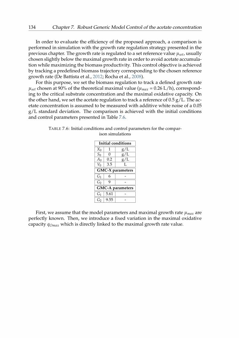
134 Chapter 7. Robust Generic Model Control of the acetate concentration
In order to evaluate the efficiency of the proposed approach, a comparison isperformed in simulation with the growth rate regulation strategy presented in theprevious chapter. The growth rate is regulated to a set reference value µset, usuallychosen slightly below the maximal growth rate in order to avoid acetate accumula-tion while maximizing the biomass productivity. This control objective is achievedby tracking a predefined biomass trajectory corresponding to the chosen referencegrowth rate (De Battista et al., 2012; Rocha et al., 2008).
For this purpose, we set the biomass regulation to track a defined growth rateµset chosen at 90% of the theoretical maximal value (µmax = 0.26 L/h), correspond-ing to the critical substrate concentration and the maximal oxidative capacity. Onthe other hand, we set the acetate regulation to track a reference of 0.5 g/L. The ac-etate concentration is assumed to be measured with additive white noise of a 0.05g/L standard deviation. The comparison is achieved with the initial conditionsand control parameters presented in Table 7.6.
TABLE 7.6: Initial conditions and control parameters for the compar-ison simulations
Initial conditionsX0 1 g/LS0 0 g/LA0 0.2 g/LV0 3.5 LGMC-X parametersG1 6 -G2 9 -GMC-A parametersG1 5.61 -G2 9.55 -
First, we assume that the model parameters and maximal growth rate µmax areperfectly known. Then, we introduce a fixed variation in the maximal oxidativecapacity qOmax which is directly linked to the maximal growth rate value.

7.5. Experimental results and discussion 135
Ideal model case
0 5 10 150
10
20
time (h)
biomass
(g/L)
GMC-AGMC-X
0 5 10 150
0.2
0.4
0.6
time (h)
glucose
(g/L)
GMC-AGMC-X
0 5 10 150
0.2
0.4
0.6
0.8
1
time (h)
acetate
(g/L)
GMC-AGMC-X
0 5 10 150
5
10
15
20
·10−2
time (h)
Fin
(L/h)
GMC-AGMC-X
30% variation in qOmax
0 5 10 150
10
20
30
40
time (h)
biomass
(g/L)
GMC-AGMC-X
0 5 10 150
0.5
1
time (h)
glucose
(g/L)
GMC-AGMC-X
0 5 10 150
0.2
0.4
0.6
0.8
1
time (h)
acetate
(g/L)
GMC-AGMC-X
0 5 10 150
0.2
0.4
0.6
time (h)
Fin(L/h)
GMC-AGMC-X
FIGURE 7.15: Comparison between the control approaches in theideal model case, and in the presence of parametric variation. Plot
of the state variables and the feed-rate.
Ideal model case
0 2 4 6 8 10 12 140
5 · 10−2
0.1
0.15
0.2
0.25
0.3
0.35
time (h)
Growth
rateµX
µX GMC-AµX GMC-Xµmaxµset
30% variation in qOmax
0 2 4 6 8 10 12 140
0.1
0.2
0.3
0.4
0.5
0.6
time (h)
Growth
rateµX
µX GMC-AµX GMC-Xµmaxµset
FIGURE 7.16: Comparison between the control approaches in theideal model case, and in the presence of parametric variation. Plot
of the specific biomass growth rates.
TABLE 7.7: The effect of parameter variation on the control perfor-mance
Variation in qOmaxµX
µmax% (GMC-X)
µX
µmax% (GMC-A) Scrit
0% 89% 81% 0.037510% 81% 85% 0.04620% 75% 89% 0.052930% 70% 93% 0.0628

136 Chapter 7. Robust Generic Model Control of the acetate concentration
Simulation results are shown in Figures 7.15 and 7.16. In the ideal model case(no parameter variation), the biomass growth regulation (GMC-X) has a slightlybetter overall performance. The reference growth rate is tracked accurately at 0.23h−1 corresponding to 89% of its maximal value. On the other hand, regulatingthe acetate concentration (GMC-A) at 0.5 L/h leads to a biomass growth rate of0.21 h−1 corresponding to 81% of the maximal value as can be seen in Table 7.7.This result shows that the presence of acetate in the medium reduces the biomassgrowth rate, due to lower substrate consumption rate caused by the activation ofthe acetate consumption pathways according to the bottleneck theory. However,keeping the acetate at a low concentration reduces its inhibitory effect, and keepsthe culture close to the optimal conditions.
The introduction of 20% variation in qOmax leads to an increase of the criticalsubstrate concentration Scrit and consequently the maximal growth rate µmax. De-spite the model mismatch, the biomass growth rate regulation presents a goodperformance in tracking the reference rate. However, it corresponds to only 75%of the new maximal value, and therefore the biomass productivity is also lowerthan its optimal value compared to the nominal case. This is due to the increase inthe gap between the reference µset and new maximal growth rate µmax.
The acetate regulation on the other hand offers a more consistent performance,and gives a better growth rate ratio (89%). Furthermore, the growth rate ratio ishigher with increasing variation in the maximal oxidative capacity as can be seenin Table 7.7.
This result highlights a problem with targeting a specific growth rate as a con-trol objective, as it requires accurate determination of the maximal value, and thentarget a lower growth rate to avoid acetate accumulation. This is a difficult taskdue to the uncertain nature of bioprocesses, as parameter variation depends onseveral factors such as the variation in operating conditions between batches. If themaximal growth rate is underestimated, the resulting suboptimal biomass produc-tivity is lower than the desired one. If the maximal growth rate is overestimated,a regulation at 90% of this value could lead to acetate accumulation and metabolicswitches, and thereby a growth inhibition.
On the other hand, regulating the acetate concentration and maintaining it at alow value offers a better practical trade-off, since the accumulation is avoided, andthe obtained growth rate is consistent in the case of model mismatch. This is an in-teresting result since the acetate regulation approach is robust towards the changein operating conditions, and is not specific to the bacterial strain. The strategycould be applied to a different strain while ensuring the same level of performancewithout the need to estimate µmax accurately.
7.6 Conclusion
In this chapter, a robust Generic Model Control strategy is presented and appliedto drive fed-batch cultures of E. coli BL21 (DE3) near the optimal operating condi-tions.

7.6. Conclusion 137
The control objective of this proposed strategy is to regulate the acetate con-centration at a defined low level. This approach has several advantages comparedto the growth rate regulation presented in the previous chapter.
Although it provides a suboptimal solution, maintaining the acetate concentra-tion is a practical alternative to avoid overflow metabolism. The regulation of thesubstrate at the critical level is impractical since accurate measurements at a lowlevel are not possible via the available sensors on the market.
Furthermore, targeting the optimal operating conditions and the critical sub-strate concentration causes fluctuations and metabolic switches between the ox-idative and oxido-fermentative regimes. Thereby, maintaining the acetate concen-tration at a low level provides a safety margin and a practical solution to avoid cellstress caused by the repetitive switches.
Due to the uncertain nature of the bioprocess model, a robust design procedureusing the LMI formalism is carried out, to compensate the model mismatch, dis-turbances, and measurement noise. Performance constraints are also formulatedwith LMIs to ensure desired properties of the closed-loop transient response.
Since the controlled variable (acetate) is not available for on-line measurement,a state estimation algorithm is required and an Unscented Kalman Filter (UKF)is implemented. The robust GMC controller and the state estimation by the UKFwere validated both through simulation runs and in real-time experimental con-ditions.
Finally, fed-batch experiments with a lab-scale reactor were performed in orderto validate the efficiency of the coupled GMC-UKF strategy in driving the culturesnear the optimal operating conditions.
The results showed that the proposed control strategy is not restricted to thestudied strain since accurate determination of the maximal growth rate is not re-quired. It is also adaptable to different control objectives such as substrate regula-tion at high concentrations in order to promote the product formation.
An improvement of the proposed control scheme is tracking a successively de-creasing set-point calculated by numerical on-line optimization based on the esti-mation of the maximal growth rate. An experimental validation of this approachin future works could improve the process productivity since it provides a goodtrade-off between practicality and best achievable sub-optimality.
A performance comparison of the robust GMC with advanced control strate-gies developed for the same objective would give an insight about the practicalefficiency of the proposed solution. To this end, a nonlinear model predictive con-troller (NMPC) is presented and implemented to the studied process in the nextchapter. The NMPC has several interesting features like the explicit use of thenonlinear model and the on-line optimization procedure.


139
Chapter 8
Nonlinear model predictive control ofthe acetate concentration
8.1 Introduction . . . . . . . . . . . . . . . . . . . . . . . . . . . . . . . 139
8.2 Principles of Nonlinear Model Predictive Control . . . . . . . . 141
8.3 Nonlinear Model predictive control applied to E. coli cultures . 143
8.3.1 Determination of the reference feed-rate profile . . . . . . 144
8.3.2 Control design . . . . . . . . . . . . . . . . . . . . . . . . . 145
8.4 Numerical simulations . . . . . . . . . . . . . . . . . . . . . . . . 149
8.5 Experiment results and discussion . . . . . . . . . . . . . . . . . . 154
8.6 Comparative study . . . . . . . . . . . . . . . . . . . . . . . . . . . 158
8.7 Conclusions . . . . . . . . . . . . . . . . . . . . . . . . . . . . . . . 163
8.1 Introduction
As mentioned in previous chapters, several solutions to avoid growth inhibitioncaused by overflow metabolism have been developed, ranging from genetic mod-ifications of the strains to closed-loop control and optimization of the bioprocess.The common objective behind the control strategies is to maintain the substrateconcentration at a critical threshold, corresponding to the maximal oxidation ca-pacity (Jana and Deb, 2005). Various nonlinear control methods of processes ex-hibiting overflow metabolism have been proposed in the literature (Abadli et al.,2020; Benattia et al., 2015; Dewasme et al., 2011a,b; Gonzalez et al., 2016; Santoset al., 2012a).
Among these studies, Nonlinear Model Predictive Control (NMPC) is oftenconsidered following its several advantages and wide use in industrial applica-tions (Forbes et al., 2015; Qin and Badgwell, 2000). NMPC is an advanced model-based control strategy developed for nonlinear processes. It consists in solving anoptimization problem on-line under a set of defined constraints. NMPC can pre-dict, using a nonlinear dynamic model of the process, the effect of control stepson controlled variables over a finite horizon. A general formulation of the NMPC

140 Chapter 8. Nonlinear model predictive control of the acetate concentration
problem consists in minimizing the quadratic objective function over a finite mov-ing horizon.
Various structures of the NMPC strategy have been developed throughout theyears for numerous control purposes (Findeisen et al., 2007). The difference be-tween the NMPC schemes lies in the definition of the cost function and the con-straints. An overview of the nonlinear model predictive methods can be found in(Allgower and Zheng, 2012). Hereafter, the main NMPC approaches are brieflypresented.
Explicit NMPC (E-NMPC) is an offline NMPC variation based on the paramet-ric programming technique, where the control law is pre-calculated offline (Bem-porad et al., 2002). The E-NMPC does not require significant computational re-sources and is suited for control problems for systems with fast dynamics. Otherstructures focus on the stability of the closed-loop by approximating an infinite-horizon optimization problem. The list includes Finite-horizon NMPC with ter-minal equality constraint (Keerthi and Gilbert, 1988), Finite-horizon NMPC withterminal inequality constraint (Morari and Lee, 1999; Scokaert et al., 1999), Finite-horizon NMPC with terminal cost (Bitmead et al., 1990), and the Quasi-infinitehorizon NMPC (Chen and Allgower, 1998). Another variation is the EconomicNMPC (E-NMPC), where the objective function is an economically-oriented costfunction of the state variables and the control inputs (Diehl et al., 2010).
Robust MPC schemes are designed to account for a set of bounded uncertain-ties and disturbances in the process model while satisfying the control objectives.There are several approaches to robust NMPC: In Min-max MPC, the optimizationis performed with respect to all possible evolutions of the bounded model uncer-tainty (Scokaert and Mayne, 1998). The variations of the uncertainty related to theprocess model parameters is included in the cost function to be optimized.
Another robust NMPC approach is the Linear parameter varying NMPC (LVP),which is based on the reformulation of the process nonlinear model with a linearparameter-varying model (LPV), mostly using linear and bilinear matrix inequal-ities (LMI/BMI) in the control. H∞-NMPC approaches consider the implementa-tion of the H∞ problem in a receding horizon framework, by considering a partic-ular choice of the objective function (Gautam et al., 2013; Wang et al., 2009, 2010b).
Robust NMPC approaches are designed to handle model mismatch and para-metric uncertainties, which make them appropriate for bioprocess models. How-ever, they are known to carry a high computational burden as the size of the op-timization problem increases with the number of uncertainties and the predictionhorizon. This may explain the fewer experimental implementations of the MPCstrategies for fed-batch bioprocesses.
The NMPC scheme can be found in various industrial fields such as chemicalplants, oil refineries, power electronics, automotive industry, biochemistry, andmany others (Qin and Badgwell, 2003). However, only a few industrial applica-tions of NMPC exist in biotechnology (Stanke and Hitzmann, 2013). The reasonsstem from the difficulties of developing reliable dynamic models of bioprocesses,the high computational costs, and the absence of efficient real-time monitoringsolutions.

8.2. Principles of Nonlinear Model Predictive Control 141
Among the experimental studies on lab-scale bioprocesses, the NMPC strategyhave been applied to a variety of micro-organism cultures such as mammaliancell cultures (Aehle et al., 2012; Craven et al., 2014), yeast cultures (Cochraneand Alamir, 2018; Preuß et al., 2000), hybridoma cell cultures (Dewasme et al.,2013a, 2015), fungi (Ashoori et al., 2009), microalgae (Del Rio-Chanona et al., 2015;Gorrini et al., 2020) and bacterial cultures (Rio-Chanona et al., 2016; Santos et al.,2012b; Tebbani et al., 2010; Ulonska et al., 2018).
These studies are usually conducted in fed-batch mode, where an inlet feed-rate is the sole manipulated input used to regulate variables such as substrates orspecific rates to defined set-points (Aehle et al., 2012; Craven et al., 2014; Dewasmeet al., 2015). Other control objectives may also aim at maximizing substrate oxi-dation rates while minimizing product fermentation rates (Santos et al., 2012a), orregulating/limiting byproduct formation (Dewasme et al., 2010; Logist et al., 2011;Tebbani et al., 2010; Valentinotti et al., 2004). Multiple input (feed rates) MPC poli-cies are also examined in (Amribt et al., 2014; Ashoori et al., 2009; Rio-Chanonaet al., 2016).
This chapter focuses on the experimental implementation and validation ofthe NMPC to maximize the biomass productivity in fed-batch E. coli BL21(DE3)cultures, by regulating the acetate concentration at a low value and limiting theoverflow metabolism effect. The NMPC algorithm is implemented in a real-timeenvironment, and the computing effort is reduced through the control vectorparametrization (CVP) technique (Banga et al., 2005).
As discussed in the previous chapter, the unscented Kalman filter (UKF) isused to provide estimates of the acetate and glucose concentrations based on thebiomass measurement. This choice is motivated by the good results obtained inthe previous experiments.
The chapter is organized as follows. A general description of the NMPC ba-sic principles is presented. These principles are then applied to the specific caseof acetate concentration regulation in fed-batch E. coli cultures. A set of numeri-cal simulations is presented to showcase the performance of the proposed NMPCstrategy in the nominal case (no model mismatch), and in presence of parametricuncertainty in the process model. Finally, the NMPC and UKF algorithms are im-plemented in real-time to a lab-scale bioreactor for experimental validations. Thechapter ends with final remarks and future work directions.
8.2 Principles of Nonlinear Model Predictive Control
Nonlinear model predictive control (NMPC) is an optimization-based feedbackcontrol strategy applied for nonlinear systems. It is applied for a variety of controlobjectives including stabilization, trajectory tracking, optimum seeking, and manyother control problems.
The NMPC strategy is based on the receding horizon principle, where the op-timal control problem is solved over a finite horizon at each sampling point. Theoptimized control input is applied to the process, and the optimization problem issolved again at the next sampling point.

142 Chapter 8. Nonlinear model predictive control of the acetate concentration
The NMPC shares the same basic philosophy as the linear MPC. However, ithas some major differences such as the explicit use of nonlinear models for the pre-diction and the inclusion of state and input constraints. Furthermore, the NMPCallows the online minimization of the cost function, and requires the availability ofthe state variables for the prediction either through measurements or estimation.
The basic principles of the NMPC problem are described hereafter (Allgowerand Zheng, 2012). We consider the following discrete-time state-space nonlinearsystem:
ξk+1 = F(ξk, Fink
)zk = Hξk
(8.1)
where ξk ∈ Rnξ and zk ∈ Rnz are the system state and output vectors at the timestep k, respectively. Fink ∈ RnF the input. F is the nonlinear transition function,and H is the measurement matrix.
A general formulation of the NMPC problem consists in minimizing thequadratic cost function Φ at the instant k over a finite moving horizon:
minξk ...ξk+Np−1,Fink
...Fink+Nc−1
Φ(ξ?, Fin•
)(8.2)
s.t
ξk+i+1 = F(ξk+i, Fink+i
), for i = 0, Np − 1
ξk = ξk(8.3)
where
• Φ is the cost function evaluated at instant k.
• Np and Nc represent the prediction horizon and the control horizon respec-tively. They are not necessarily equal ( i.e. Np ≥ Nc ≥ 1
)in order to reduce
the computational load.
• ξk+i is the predicted state vector at time instant k + i, i = 0, Np − 1.
• ξk is the initial condition which is the plant state at time instant k.
The classical NMPC strategy is implemented in a moving horizon framework.At current time step k, the optimization problem (equations (8.2) and (8.3)) is ini-tialized by the current state vector ξk and solved over the prediction horizon Np.The first element of the resulting input vector Fink is applied to the system (8.1). Atthe next sampling time k + 1, the optimization problem is solved again with theupdated state vector ξk+1 as the initial condition.
The NMPC is a model-based control strategy. A mathematical representationof the system is required to predict the evolution of each state variable. Therefore,the efficiency of the control scheme is directly linked to the model used for the

8.3. Nonlinear Model predictive control applied to E. coli cultures 143
predictions. The choice of the model structure and the parameter identificationprocedure have a decisive role in the controller performance.
In the case of trajectory and set-point tracking problems, the cost function Φ tobe optimized is a quadratic nonnegative function measuring the distance betweenthe predicted model state ξ and a determined known reference sequence ξre f overthe horizon window. Another quadratic function weighting the control effort isadded to achieve the control objective. The general expression for the cost functionin this case is given by the following:
Φ(ξ?, Fin•
)=
Np
∑i=1
∥∥∥ξk+i − ξre fk+i
∥∥∥2
αi+
Nc
∑i=1
∥∥∥Fink+i−1 − Fre fk+i−1
∥∥∥2
βi(8.4)
where
• ξre f represents the reference trajectory or setpoint chosen to specify a desiredclosed-loop behavior.
• Fre f represents the reference feeding trajectory corresponding to ξre f .
• αi ≥ 0 ∈ Rnξ×nξ and βi ≥ 0 ∈ RnF×nF are the weighting matrices for thestate tracking error and the control inputs, respectively.
The tuning parameters are implemented to penalize the deviations of the pre-dicted controlled state vector ξ from the reference ξre f , as well as the control inputdeviations at every sampling point in the prediction horizon. These parametersare tuned to avoid instability and to reach the desired transient performance ofthe closed-loop.
In addition to the cost function, constraints on the states and inputs can bedefined:
ξmin ≤ ξk+i ≤ ξmax, i = 0, Np − 1. (8.5)
Fmin ≤ Fink+j ≤ Fmax, j = 0, Nc − 1 (8.6)
(8.7)
However, this addition increases the complexity of the optimization problem,and the solution cannot be obtained explicitly as in the unconstrained case. An il-lustration of the receding horizon principle in the SISO case is shown in Figure 8.1.
8.3 Nonlinear Model predictive control applied to E.coli cultures
Reminding the objective behind the control strategy, that is to drive the processcloser to the boundary of the respiro-fermentative and respirative regimes. Simi-larly, to the previous chapter, we desire to maintain the acetate concentration at a

144 Chapter 8. Nonlinear model predictive control of the acetate concentration
Past Future
Closed-loopinput Fin
Closed-loopstate ξ
Setpoint
Predicted input Fin
Predictedstate ξ
k k + 1 k + Nc k + Np
Control horizon Nc
Prediction horizon Np
FIGURE 8.1: Illustration of the receding horizon principle
predefined low set-point to avoid its accumulation during the culture. To main-tain the acetate concentration at a constant value, the bioprocess operates in therespiro-fermentative regime to compensate the dilution effect which tends to de-crease the acetate concentration with time. Nevertheless, a low acetate concentra-tion keeps the process close to the optimal metabolic edge (Dewasme et al., 2010;Rocha, 2003). In the proposed control strategy, the acetate concentration is regu-lated to the pre-defined set-point Are f . This regulation is achieved by acting on thefeed rate Fin, also constrained to track a pre-calculated reference trajectory Fre f inorder to smooth the control behavior.
8.3.1 Determination of the reference feed-rate profile
In order to implement the NMPC strategy on the E. coli process, a reference feedingtrajectory Fre f corresponding to the acetate reference must be pre-calculated basedon the model equations defined by:
X = (kX1µ1 + kX2µ2 + kX3µ3)X − Fin
VX (8.8a)
S = −(µ1 + µ2)X − Fin
V(S − Sin) (8.8b)
A = (kA2µ2 − µ3)X − Fin
VA (8.8c)
V = Fin (8.8d)

8.3. Nonlinear Model predictive control applied to E. coli cultures 145
Considering a constant acetate concentration (A = Are f 6= 0, A = 0), the differ-ential equation (8.8c) leads to the following feed-rate:
Fin =µA
AXV∣∣∣
A=Are f(8.9)
where µA = (kA2µ2 − µ3) = kA2(qs–qscrit) in respiro-fermentative mode.Generating the feeding profile using Equation (8.10) requires the availability of
the substrate concentration. Assuming that there is no accumulation of the sub-strate concentration in the neighborhood of the optimal conditions, so that it isinstantaneously consumed by the cells. The substrate is considered to be in quasi-steady state near the critical value (S = Sset, S = 0).
From Equation (8.8b) we obtain the following equation:
Fin =µS
(Sin − S)XV∣∣∣∣S=Sset
(8.10)
where µS = −(µ1 + µ2) = qS in respiro-fermentative mode. The substrate concen-tration Sset corresponding to the reference acetate concentration Are f can then becalculated from the following equation:
qS
(Sin − S)
∣∣∣∣S=Sset
=µA
A
∣∣∣A=Are f
(8.11)
From equations (8.8a) and (8.8d) the following differential equation is obtained:
d(XV)
dt= µXXV (8.12)
hence:
XV = X0V0eµXt (8.13)
where X0 and V0 are the initial conditions for the biomass concentration and theculture volume respectively, and µX = kX1µ1 + kX2µ2 + kX3µ3.
Finally, the expression of the reference trajectory Fre f for the pair(
Are f , Sset)
can be generated by the following equation:
Fre f =µA
AX0V0eµXt
∣∣∣A=Are f ,S=Sset
=qS
(Sin − S)X0V0eµXt
∣∣∣∣A=Are f ,S=Sset
(8.14)
8.3.2 Control design
In the following, a discrete-time equivalent expression of the continuous E. colimodel (8.8) is used to implement the predictive control strategy. Considering a

146 Chapter 8. Nonlinear model predictive control of the acetate concentration
constant sampling time Ts, the discrete model is defined as follows:
ξk+1 = F(ξk, Fink
)zk = Hξk
(8.15)
where
• ξk = [Xk Sk Ak Vk]T and zk = Ak are the discrete state and sampled output
vectors at time kTs, respectively.
• F is the nonlinear transition function
• H =[
0 0 1 0]
is the measurement matrix.
• Fin is the control input, parametrized using a piecewise constant approxima-tion.
The trajectory tracking is achieved using the nonlinear model predictive con-trol (NMPC) strategy. Based on the model (8.15) and the control objectives definedearlier, the NMPC objective cost can be defined as follows:
Φ(ξ?, Fin•
)=
Np
∑i=1
(Ak+i − Are f k+i
)2+ λ
Nc
∑i=1
(Fink+i − Fre fk+i−1
)2(8.16)
where A is the predicted acetate concentration, and Fre f is the pre-calculatedreference feeding profile. Np and Nc are the prediction and control horizons re-spectively, and λ > 0 is the control penalty gain.
The NMPC problem formulation minimizes the quadratic cost functionΦ(ξ?, Fin•
)at the instant k and reads:
minAk ...Ak+Np−1,Fink
...Fink+Nc−1
Φ(ξ?, Fin•
)(8.17)
under constraints related to the predicted dynamics of the system:
s.t. ξk+i+1 = F(ξk+i, Fink+i
), i = 0, Np − 1 (8.18a)
Ak+i+1 = HF(ξk+i, Fink+i
), i = 0, Np − 1 (8.18b)
0 6 Fink+i 6 Fmax, i = 0, Nc − 1 (8.18c)
0 6 ξk+i 6, i = 0, Np − 1 (8.18d)
A classical NMPC strategy follows the receding horizon principle, where theoptimization problem (8.17 and 8.18) is solved online at instant k. The first elementof the input vector is then applied to the system, and the optimization problem is
8.3. Nonlinear Model predictive control applied to E. coli cultures 147
solved again with the updated initial state and input vectors at the next samplingpoint.
However, solving the constrained nonlinear optimization problem (8.17 and8.18) raises two major difficulties. The first difficulty lies in the discretization of thecontinuous nonlinear system (8.8). The sampling period needs to be sufficientlysmall compared to the system’s time constants such as the discrete model remainsrelevant compared to its the continuous counterpart. An appropriate choice of thesampling time in this case is in the order of 0.5-1 min, since the doubling time ofE. coli is around 20 minutes and the response time is in the order of several tens ofminutes. This leads to very long prediction horizons and an increase in the num-ber of the decision variables of the optimization problem. Furthermore, it posesa practical problem for the on-line implementation of the control strategy due tothe different operations executed between two sampling points (measurement, es-timation, calculation of the control law).
The second difficulty is the nonlinear constraints (8.18), which increases theon-line computation time of the optimization procedure involved in the NMPCstrategy.
In order to avoid to solve the constrained optimization problem, the optimiza-tion problem is transformed into a nonlinear programing problem (NLP) using theControl Vector Parametrization (CVP) technique presented in (Banga et al., 2005).
The CVP method is based on the discretization of the control variables only,and the control sequence is approximated by a piecewise constant function be-tween two sampling instants. The advantage of this transformation is that it is nolonger necessary to discretize the continuous model, and the predicted states areobtained by the integration of the continuous differential system (8.8).
Consequently, the sampling period required for the prediction can be muchlarger, and the constraints related to the state variables are removed from the op-timization problem, since they are taken into account in an implicit way duringthe prediction of the states via the CVP method. Furthermore, the control hori-zon Nc can be chosen equal to the prediction horizon Np, since the control vectoris the only decision variable for the optimization problem. The CVP principle isillustrated in Figure 8.2.
The new formulation of the optimization problem is therefore given by:
minvk ...vk+Np−1
Φ(ξ?, Fin•
)(8.19)
Under the constraints:
0 6 Fink 6 Fmax, k = 1, Np (8.20a)
In addition, a change of variable Fin = ev aims at removing the positivity con-straints on Fin and improves the conditioning of the optimization problem. The

148 Chapter 8. Nonlinear model predictive control of the acetate concentration
Discretized control sequence
predicted states
uk
tk
ξk
tk
Te 2Te Np Te
Te 2Te Np Te
FIGURE 8.2: Principle of the CVP approach
corresponding cost function reads:
Φ(ξ?, v•
)=
Np
∑i=1
(Ak+i − Are f k+i
)2+ λ
Np
∑i=1
(evre f
k+i−1 − evk+i−1
)2(8.21)
and the formulation of the NMPC problem is reduced to solving at each time kTe:
minevk ...e
vk+Np−1Φ(ξ?, v•
)(8.22)
The constraint on the upper bound of the control input is removed from theoptimization problem. The optimal input solution of the problem (8.18) is thenlimited to its upper bound before its application to the process.
This transformation of the initial optimization problem (8.17) to an uncon-strained optimization problem is very beneficial for the implementation of thecontrol strategy on the real process. A comparison between the classical and un-constrained NMPC formulations is presented in the simulations section.
In the following, the UKF estimated state ξk is used in the NMPC scheme.

8.4. Numerical simulations 149
8.4 Numerical simulations
The combined UKF-NMPC strategy is first assessed through numerical simula-tions, considering the fed-batch E. coli model presented in chapter 2. The initialplant conditions as well as UKF and controller parameters are given in Table 8.1.
Estimates initial conditions are randomly chosen using a normal distributioncentred at the nominal state values with a standard deviation of 15%. The covari-ance matrix of measurement noise R depends on the quality of the turbidimetricprobe signal. On the other hand, the covariance matrix of the model noise Q rep-resents the confidence level in the model.
TABLE 8.1: UKF covariance matrices, sigma points tuning parame-ters, and initial conditions
Initial conditionsX0 1.0 g/LS0 0.1 g/LA0 1 g/LV0 3.5 LSin 500 g/L
UKF parametersσX 0.01 g/LσS 0.1 g/LσA 0.1 g/LσV 0.001 g/LrX 0.01 g/LP0 10−4 × I4 g/Lα 1 -β 2 -κ 0 -Control parametersNp 10 -λ 0.05 -
Sampling timeTs 3 min -
The acetate concentration regulation achieved by the NMPC is assessed, firstconsidering a perfectly known model (no parametric uncertainty), and then a morerealistic case with plant-model parameter mismatch. In both cases, the acetate con-centration is supposed to be measured with a measurement noise level of 0.02g/L.
The optimization is performed by the LSQNONLIN optimizer under MATLABR2018b environment on a 3.2 Ghz PC with 8Gb of ram. The optimization problemis solved using the ’trust-region-reflective’ algorithm .
Figure 8.3 shows the closed-loop profiles of the state and control variables forthe ideal model case (no modeling errors or parameter uncertainties), with pre-diction horizon Np = 10 and penalty parameter equal to λ = 0.05. λ was tunedby trial and error to prevent excessive deviation of Fin from the reference feedingprofile Fre f .

150 Chapter 8. Nonlinear model predictive control of the acetate concentration
0 1 2 3 4 5 6 7 8 9 100
2
4
6
8
10bi
omas
s(g
/L)
0 1 2 3 4 5 6 7 8 9 100
2
4
6
8
10·10−2
gluc
ose
(g/L
)
0 1 2 3 4 5 6 7 8 9 100.6
0.7
0.8
0.9
1
acet
ate
(g/L
)
AAref
0 1 2 3 4 5 6 7 8 9 100
2
4
6
·10−2
time (h)
F in
(L/h
)
Fin
F refin
0 0.5 1 1.5 20
0.5
1
1.5
2
0 0.5 1 1.5 20
2
4
6
8
10·10−2
0 0.5 1 1.5 20.6
0.7
0.8
0.9
1
0 0.5 1 1.5 20
0.5
1
1.5
·10−2
time (h)
FIGURE 8.3: Ideal model case. Left: Closed loop evolution of thestate variables, X, S, A, and feed flow rates Fin and Fref with predictionhorizon Np = 10, λ = 0.05 and a noise standard deviation of 0.02
[g/L]. Right: Zoom over 2h.
It may be observed in Figure 8.3 that the regulation of the acetate concentra-tion is achieved successfully. The biomass growth follows a typical exponentialtrajectory, and the substrate quickly reaches an a priori unknown and constantsteady-state, assumed to be greater than the critical level since, to keep the acetateconcentration constant, the cells must evolve in respiro-fermentative regime, com-pensating the dilution effects from the feed rate by a small acetate production.
The convergence to the steady-state is achieved in 25 minutes and the biomassat t = 10 h is 32.5 g.
In view of analyzing the NMPC robustness to plant-model mismatch, a simu-lation is performed by varying the most influential parameters on the acetate con-centration. The parametric sensitivity study presented in appendix D shows thatthe most influential parameters on the acetate concentration A are qS max, qO max,kX2, and kA2.
During the simulation, the values of these parameters are randomly chosenfollowing a normal distribution centred at their nominal values with a standarddeviation of 15%. A set of 100 Monte Carlo (MC) simulations is performed using

8.4. Numerical simulations 151
the same control settings as previously for the ideal model (Table 8.1).Figure 8.5 shows the histograms of the runs as functions of the randomly cho-
sen values. The corresponding closed-loop profiles are represented in Figure 8.4.The acetate concentration is maintained at the reference in all runs, with a meanvalue of 0.7 g/L. The tracking error (Are f − A) has a RMSE of 0.0314 g/L, which isstill satisfactory. The convergence to the desired steady-state is still 25 minutes inaverage.
0 2 4 6 8 100
2
4
6
8
10
biom
ass
(g/L
)
0 2 4 6 8 100
2
4
6
8
10·10−2
gluc
ose
(g/L
)
0 2 4 6 8 10
0.7
0.8
0.9
1
acet
ate
(g/L
)
0 2 4 6 8 100
2
4
6
·10−2
time (h)
F in
(L/h
)
FIGURE 8.4: Plant/model mismatch case. Closed-loop evolution ofthe state variables X, S, and A with noise standard deviation of 0.02
g/L. Profiles of the 100 Monte Carlo experiments.
Histograms of the final biomass productions and productivities are also shownin Figure 8.5. Biomass production is, in average, slightly lower than in the idealcase (31.2g), nevertheless it stays above 30g in 96% of the MC experiments (Fig-ure 8.5). In most of the cases, biomass productivity is higher than 90% of the max-imal attained level.
To illustrate the advantages of the CVP method, a series of simulations is per-formed comparing the computation time required to solve the optimization prob-lems before and after using the CVP technique.
The simulation consists in regulating the acetate concentration to the definedsetpoint of Are f = 0.7 g/L, with the same initial values for the state variables andcontrol parameters described in Table 8.1.
Three methods were compared: The initial constrained NMPC problem (8.17),the NMPC problem with the CVP method (8.19), and the unconstrained NMPC

152 Chapter 8. Nonlinear model predictive control of the acetate concentration
3.2 3.3 3.40
5
10
15
20
qsmax
Number
ofruns
1.34 1.36 1.38 1.4 1.42 1.440
5
10
qOmax
Number
ofruns
0.28 0.29 0.30
5
10
15
20
KX2
Number
ofruns
0.42 0.43 0.44 0.450
5
10
KA2
Number
ofruns
85 90 95 1000
5
10
Productivity/Produtivity-max [%]
Number
ofruns
29 30 31 32 330
5
10
15
Biomass production (g)
Number
ofruns
FIGURE 8.5: Histograms of the plant parameters qS max, qO max, kX2,and kA2, the biomass production and productivity during the MC
simulations.
problem (8.22) with the variable change (VC) Fin = ev. A total of 10 simulations isperformed for each method, and the computation time δt required for solving theoptimization problem for one time step (kTe) is shown in Table 8.2.
The results show that the introduction of the CVP method offers a significantgain in the computation time, while achieving the same control problem objec-tives. Even though the variable change (VC) gives a close performance, it improvesthe conditioning of the optimization problem. This shows the advantage of theproposed method for the on-line implementation of the NMPC on bioprocesses.The low computation time offers the opportunity to consider lower sampling pe-riods, and to couple the NMPC with other components in a more advanced controlstructure.
TABLE 8.2: Comparison between the computation time required forsolving the different NMPC problems
min(δt) (s) max(δt) (s) mean(δt) (s)Constrained NMPC 2.423 11.779 5.863NMPC + CVP + VC 0.018 0.733 0.037
NMPC + CVP 0.019 0.793 0.038
The NMPC is now coupled to the UKF estimator, considering the estimatedacetate concentration as the regulated variable. The same parameter uncertainty aswell as biomass measurement noise level are considered. As shown in Figure 8.6,the UKF is able to correctly estimate the acetate concentration in the presence of

8.4. Numerical simulations 153
model and measurement noise, and the acetate regulation is performed accuratelyas both the estimated and actual states converge to the desired acetate value.
0 1 2 3 4 5 6 7 8 9 100
2
4
6
8
biomass
(g/L)
0 1 2 3 4 5 6 7 8 9 100
2
4
6
8
10·10−2
glucose
(g/L)
0 1 2 3 4 5 6 7 8 9 100.6
0.8
1
acetate
(g/L)
A
AAref
0 1 2 3 4 5 6 7 8 9 100
2
4
6·10−2
time (h)
Fin
(L/h)
Fin
Fref
FIGURE 8.6: Coupled UKF-NMPC numerical simulations with mea-surement noise and parametric uncertainties.
In order to compare the performance of the NMPC and the GMC strategies,simulations are performed testing their performance in regulating the acetate con-centration at Are f = 0.7 g/L. The initial conditions for the simulation are the sameof the previous simulations given in Table 8.1. The GMC parameters are the sameused in the previous chapter (G1 = 5.61, G2 = 9.55) (Equation (7.24)). Theseparameters were determined using the robust design method, for a maximal pa-rameter variation of 15%. Figure 8.7 shows the evolution of the state variables andthe feed-rate using the two control strategies: NMPC and GMC, and Figure 8.8shows a zoom over the first two hours.
The simulation shows that both control strategies achieved good regulation ofthe acetate concentration at the reference value Are f = 0.7 g/L. As seen in the pre-vious chapter, the GMC strategy is able to achieve the control objective. However,it induces a longer transient phase, a higher overshoot, and a longer convergence

154 Chapter 8. Nonlinear model predictive control of the acetate concentration
time compared to the NMPC. Furthermore, the biomass quantity obtained withthe NMPC strategy is marginally higher than that obtained using the GMC.
In conclusion, both the NMPC and the GMC strategies achieve the control ob-jectives adequately, however the NMPC is better than the GMC regarding the tran-sient performance, and this has a direct effect on the final biomass quantity.
0 1 2 3 4 5 6 7 8 9 100
2
4
6
8
10
time (h)
biomass
(g/L) NMPC
GMC
0 1 2 3 4 5 6 7 8 9 100
2
4
6
8
10·10−2
time (h)
glucose
(g/L) NMPC
GMC
0 1 2 3 4 5 6 7 8 9 100.6
0.7
0.8
0.9
1
time (h)
acetate
(g/L) NMPC
GMCAref
0 1 2 3 4 5 6 7 8 9 100
2
4
6·10−2
time (h)
Fin
(L/h)
NMPCGMC
FIGURE 8.7: Comparison of the NMPC and GMC strategies. Plot ofthe state variables and the control inputs.
8.5 Experiment results and discussion
To validate the combined NMPC control strategy and the estimation of the acetateand glucose concentrations by the UKF, two fed-batch experiments are carried outusing the strain E. coli BL21(DE3) according to the protocol described in chapter 4.The UKF parameters during the experiments are given in Table 8.3, and the UKFalgorithm is presented in appendix A.
The NMPC parameters used in both experiments are given in Table 8.4. Theprediction horizon and penalty parameter λ were tuned in simulation by trial anderror in order to achieve the control objectives while preventing excessive devia-tion of Fin from the reference feeding profile Fre f .
The evolution of the biomass, glucose, acetate concentrations, and the feed flowrate in both experiments are illustrated in Figure 8.9, and the operating conditionsare shown in Figure 8.10.

8.5. Experiment results and discussion 155
0 0.2 0.4 0.6 0.8 1 1.2 1.4 1.6 1.8 21.4
1.6
1.8
2
time (h)
biomass
(g/L) NMPC
GMC
0 0.2 0.4 0.6 0.8 1 1.2 1.4 1.6 1.8 20
5
10
·10−2
time (h)
glucose
(g/L) NMPC
GMC
0 0.2 0.4 0.6 0.8 1 1.2 1.4 1.6 1.8 2
0.6
0.8
1
time (h)
acetate
(g/L) NMPC
GMCAref
0 0.2 0.4 0.6 0.8 1 1.2 1.4 1.6 1.8 20
0.5
1
1.5·10−2
time (h)
Fin
(L/h)
NMPCGMC
FIGURE 8.8: Comparison of the NMPC and GMC strategies. Plot ofthe state variables and the control inputs. Zoom over 2h.
TABLE 8.3: UKF parameters used in the experiments
UKF parametersσX 0.01 g/LσS 0.1 g/LσA 0.1 g/LσV 0.001 g/LrX 0.01 g/LP0 10−4 × I4 g/Lα 1 -β 2 -κ 0 -
The first experiment is carried in two phases, a batch followed by a fed-batch.The batch phase is performed to reach a minimal biomass concentration of 1 g/Land ensure that the cells are in the exponential phase when initiating the regulationand injecting the feed media. The UKF estimation is launched during this phaseafter initializing the state vector.
The fed-batch phase starts after the near depletion of glucose. Even though theglucose concentration measurement is not available, on-line flags of the glucosedepletion can be detected, consisting of a sudden drop in the stirring speed due to

156 Chapter 8. Nonlinear model predictive control of the acetate concentration
TABLE 8.4: NMPC control parameters used in the experiments
NMPC parametersSampling time Ts = 3 min
Acetate reference Are f = 0.5 − 1.5 g/LNMPC parameters Np= 10, λ= 0.05
the low cell demand for oxygen (Figure 8.10), coupled with an increase in the pHvalue due to the decrease of CO2 released by the cells.
The NMPC controller is launched after setting up the acetate reference and thecontrol parameters. The controller outputs an exponential feeding profile, and theestimated acetate concentration converges to the desired reference in less than 30min and remains in the range 0.33-0.5 L/h until the end of the culture. At the sametime, the substrate concentration remains in a quasi-steady state.
After the end of the first experiment, a culture refresh is performed. A vol-ume of the culture is extracted using a peristaltic pump, leaving 500 mL of theculture of volume. Then, 3L of an autoclave sterilized HDF medium is injected bya peristaltic pump, and the batch phase of the second experiment starts.
The second experiment follows the same protocol as the first one, the batchphase lasts for 2 h, and the glucose is quickly consumed by the cells. The con-troller is launched as soon as the stirring drops significantly, indicating a dropin glucose oxidation. The acetate concentration set-point is fixed at 1.5 g/L, thefeeding follows an exponential curve, and the acetate concentration converges tothe imposed reference. At t=12 h, a set-point change is introduced and Are f is setequal to 0.7 g/L.The NMPC controller adapts the feed-rate according to the newreference, and the estimated acetate concentration tracks the new reference in 20min.
The NMPC-UKF strategy performance is highly satisfying. The UKF accu-rately estimates the acetate and glucose concentrations in the presence of measure-ment noise on the biomass concentration. The mean square errors of the substrateand acetate concentrations are eS = 0.089 g/L and eA = 0.068 g/L respectively,which is consistent regarding the sensitivity of the measurements and the noiselevels (0.1 g/L). The NMPC controller regulates the estimated acetate concentra-tion to the fixed set-point, and the convergence is achieved in 20 min. The acetateconcentration remains at an acceptable range during the fermentation time, andthe culture conditions are well suited for biomass growth.

8.5. Experiment results and discussion 157
0 5 10 150
5
10
15Refresh time
time (h)
Biom
ass
(g/L
) Biomass (Online)
Biomass (Offline)
0 5 10 150
1
2
3
time (h)
Glu
cose
(g/L
) Estimated S
Measured S
0 5 10 150
1
2
time (h)
Ace
tate
(g/L
)
Estimated A
Measured A
Are f
0 5 10 150
2
4
6
8
·10−2
time (h)
Feed
rate
(L/h
)
FIGURE 8.9: Experimental results: Time evolution of the measuredbiomass, glucose, acetate concentrations (offline and online estima-
tion), and feed-rate
0 5 10
20
40
60Refresh time
time (h)
pO2
(%)
0 5 10
−5
0
5
10·10−1
time (h)
Aci
d(m
L)
0
1
2
·102
Base
(mL)
0 5 10
6.6
6.8
7
time (h)
pH
0 5 10
5
10
·102
time (h)
Stir
ring
(RPM
)
FIGURE 8.10: Experimental results: Time evolution of the pO2, acidand base concentrations, pH, and stirring

158 Chapter 8. Nonlinear model predictive control of the acetate concentration
0 5 10 150
5
10
15Refresh time
time (h)
Biom
ass
(g/L
) Measured X
Model
0 5 10 150
1
2
3
time (h)
Glu
cose
(g/L
) Estimated S
Model
0 5 10 150
2
4
6
8
time (h)
Ace
tate
(g/L
)
Estimated A
Model
Are f
0 5 10 150
2
4
6
8
·10−2
time (h)
Feed
rate
(L/h
) FinFre f
FIGURE 8.11: Comparison between the experimental results and theprocess model predictions
In order to compare the deviation of real process response from the model pre-dictions, a simulation is performed using the experimental data and the processmodel used in the control and estimation algorithms.
The model is simulated in open-loop with the same operating conditions andthe initial values for the state variables from the experiments. The obtained exper-imental feed-rate is applied to the model input.
The results presented in Figure 8.11 show a deviation between the model pre-dictions and the measured and estimated state variables. The experimental feed-rate deviates from the reference trajectory, indicating the presence of a model mis-match. On the other hand, the acetate concentration is accumulated in the modelsimulation due the high glucose concentration resulting from the high feed-ratelevels.
Consequently, the acetate presence leads to a lower growth rate than in theexperiments and a low biomass concentration. The experimental and simulationresults show the efficiency of the proposed predictive strategy to achieve the con-trol objectives despite the model mismatch.
8.6 Comparative study
In order to evaluate the performance of the control strategies presented in thisthesis, a simulation study is performed and presented in this section. The threecontrol methods are compared under the same initial operating conditions and asimilar control setting.

8.6. Comparative study 159
The NMPC and robust GMC (GMC-A) controllers are set to track an acetate ref-erence of Are f = 0.7 g/L. On the other hand, the biomass growth rate regulationusing the GMC strategy (GMC-X) is set to track a reference profile correspond-ing to this acetate concentration value. To this end, the glucose concentration Ssetcorresponding to Are f is calculated using Equation (8.11). Then, using the pair(Sset, Are f ), the reference biomass growth rate µset is calculated from kinetic modelequations.
The simulation is performed over 10 h assuming that the state vector is avail-able for measurement, with an added measurement noise of 0.05 g/L and 0.02g/L on the biomass and acetate concentrations. The initial conditions, referencevariables, and control parameters values are summarized in table Table 8.5.
TABLE 8.5: Initial conditions and control parameters
Initial conditionsX0 1.0 g/LS0 0.1 g/LA0 1 g/LV0 3.5 LSin 500 g/L
Reference variablesAre f 0.01 g/LSset 0.0234 g/Lµset 0.1925 h−1
Fmax 0.2 L/h
NMPC parametersNp 10 -λ 0.05 -
GMC-X parametersG1 = 2.25 -G2 = 9 -GMC-A parametersG1 = 5.61 -G2 = 9.55 -
Sampling timeTe 3 min
First, the control strategies are compared in the ideal model case, where all themodel parameters are assumed to be perfectly known. Then, 500 Monte Carlosimulations are performed considering model uncertainties. The model parame-ters are randomly chosen with a maximal variation of ±30% around their nominalvalue following a normal distribution.
In the ideal model case (Figure 8.12), the biomass trajectories are almost iden-tical for the three methods. This behavior is expected since the simulation is de-signed to have the same setting for the three methods.
The acetate and glucose concentrations, on the other hand, have different dy-namics. The NMPC and the GMC-A strategies regulate the acetate concentrationat the reference Are f . On the other hand, the biomass regulation (GMC-X) leads toa decrease in the acetate concentration to reach a zero value after 7.5 hours.
The feed rates have similar behavior, where the main difference between thecontrollers is the delays due to the transitory phase. The acetate dynamics affectthe metabolic operating mode and the biomass evolution and, consequently, therequired feed rate to reach the desired growth rate.
In the model mismatch case, the parameter variation leads to different re-sponses of the controllers. An example of a mismatch simulation is shown inFigure 8.13. The biomass profiles in this case are different for each control strategy.

160 Chapter 8. Nonlinear model predictive control of the acetate concentration
0 2 4 6 8 100
2
4
6
time (h)
X(g/L)
NMPC
GMC-A
GMC-X
0 2 4 6 8 100
5
10
·10−2
time (h)
S(g/L)
2 4 6 8 100
2
4
6·10−2
0 2 4 6 8 100
0.5
1
time (h)
A(g/L)
NMPC
GMC-A
GMC-X
0 2 4 6 8 100
2
4
6·10−2
time (h)
Fin
(L/h)
NMPC
GMC-A
GMC-X
FIGURE 8.12: Evolution of the state variables in the ideal model casefor the three control methods
The GMC-A and NMPC have higher final biomass concentration compared tothe GMC-X with an advantage for the NMPC. This is due to the difference in thecontrol objective definition.
The biomass regulation targets a specific growth rate and manages to repro-duce the biomass profile in the case of model mismatch, leading to similar per-formance compared to the nominal case. However, since the optimal metabolicoperating point is linked to the critical substrate concentration and the critical ox-idative capacity, which is by nature uncertain.
The targeted growth rate is usually defined by setting it 5-10% lower than themaximal growth rate to avoid acetate accumulation. In the case where the maximalvalue changes due to the model mismatch, targeting µset leads to a lower metabolicperformance due to underfeeding.
This strategy is useful for reproducing experiments and results with high yieldsand final product quality (“golden batches”), thanks to its consistent results. Fur-thermore, the operational advantage of the method is the availability of reliablebiomass probes making its implementation fairly easy. However, this requiresa knowledge of the bioprocess and a sufficient amount of historical data. Thebiomass growth regulation strategy is not the best fit for productivity maximiza-tion, especially in the case of uncertain optimal conditions or unreliable models.
On the other hand, acetate regulation offers a solution to this problem. Tar-geting an acetate concentration close to zero maintains the culture closer to the

8.6. Comparative study 161
0 2 4 6 8 100
2
4
6
8
time (h)
X(g/L)
NMPC
GMC-A
GMC-X
0 2 4 6 8 100
5
10
·10−2
time (h)
S(g/L)
2 4 6 8 100
2
4
6·10−2
0 2 4 6 8 100
0.5
1
time (h)
A(g/L)
NMPC
GMC-A
GMC-X
0 2 4 6 8 100
2
4
6
8·10−2
time (h)
Fin
(L/h)
NMPC
GMC-A
GMC-X
FIGURE 8.13: Evolution of the state variables in the model mismatchcase for the three control methods
optimum with consistent metabolic performance. In the case where the optimumis unknown and uncertain, acetate fermentation is directly linked to the oxidativecapacity, and therefore the metabolic performance is better thanks to the adapta-tion to the new maximal growth rate value.
The NMPC strategy leads to higher biomass quantity compared to the GMC-A.This is mainly due to the longer transitory phase in the GMC case and the morefrequent fluctuations around the regulated acetate concentration value. This resultcan be explained by the fact that the NMPC uses the nonlinear model implicitlyin the prediction phase, while the GMC algorithm includes linearization of thenonlinear dynamics leading to tracking errors and unpredicted dynamics.
The results of the Monte Carlo simulations give a performance overview of thecontrol methods. The biomass productivity and productions over 10 h during the500 runs are summarized in tables 8.6 and 8.7.
It can be seen that the NMPC outperforms the GMC controllers on average andgives higher productivity and biomass quantities. It can also be seen that acetateregulation has a higher average and maximal value. The biomass regulator targetsa specific growth rate by design, and thereby, when the process is able to reachhigher growth rates, the biomass regulation maintains the growth rate closer tothe specified reference, leading to a lower biomass productivity. As expected, allthe developed controllers lead to better results than the open-loop trajectory withan average improvement of 20% in the biomass productivity.

162 Chapter 8. Nonlinear model predictive control of the acetate concentration
TABLE 8.6: Biomass productivity of the control methods during 500MC simulations
Method Mean Min Max UnitOpen-loop 0.0161 0.0079 0.0183 g/(h · g of substrate)
GMC-X 0.0187 0.0176 0.0208 g/(h · g of substrate)GMC-A 0.0190 0.0184 0.0206 g/(h · g of substrate)NMPC 0.0192 0.0185 0.0206 g/(h · g of substrate)
TABLE 8.7: Biomass production of the control methods during 500MC simulations
Method Mean Min Max UnitOpen-loop 22.864 22.0472 26.776 g
GMC-X 25.3944 18.4881 39.0349 gGMC-A 25.7305 20.7225 56.4224 gNMPC 26.6117 19.4120 57.1957 g
TABLE 8.8: Root mean square errors of the control methods during500 MC simulations
Method Mean Min Max UnitOpen-loop 0.941 0.139 1.3821 g/L
GMC-X 0.1400 0.0744 0.8976 g/LGMC-A 0.0623 0.0503 0.1531 g/LNMPC 0.0560 0.0466 0.0888 g/L
TABLE 8.9: Computation time (between 2 sampling steps) of the con-trol methods during 500 MC simulations
Method Mean Min Max UnitOpen-loop 0.0165 0.01413 0.0401 (×10−3) s
GMC-X 0.0265 0.1413 0.0401 (×10−3) sGMC-A 0.0274 0.2854 0.0535 (×10−3) sNMPC 0.0210 0.8095 0.0968 s
Concerning the tracking performance, the root-mean-square errors of the con-trolled variable (y–yre f ) are given in Table 8.8. It can be seen that the NMPC hasthe lowest tracking error compared to the GMC-A regulation. The acetate controlstrategies provide better tracking performance than biomass regulation due to theexponential evolution of the biomass concentration.
As for the computation load (Table 8.9), The GMC methods have the lowesttime required to calculate the control law. This result is expected since the GMClaw is computed by a simple algebraic equation and does not require the integra-tion of a nonlinear differential equation.
As for the NMPC, the computation time can sum up to 0.8 seconds between

8.7. Conclusions 163
sampling points, which is a good result compared to the sampling period (Ts = 3min). However, this result is obtained by implementing a CVP method to simplifythe optimization problem making it better conditioned. Considering constraints,a complex cost function or a robust variation of the NMPC (min-max NMPC, forexample) can significantly raise the computation load. A computation time of theorder of several seconds combined with the different delays in the LabView envi-ronment can sum up to several minutes. This may be a challenge, especially if alower sampling time is required for the NMPC prediction to be accurate. Imple-menting time-saving strategies in the NMPC schemes is a necessary step beforeinvestigating advanced predictive variations.
8.7 Conclusions
In this chapter, an implementation of the nonlinear model predictive control strat-egy on the fed-batch E. coli process is presented. This strategy is experimentallyimplemented and validated on lab-scale fed-batch E. coli BL21(DE3) cultures. Thegoal behind the control scheme is to maximize the biomass production and fa-vorize cell growth, by avoiding overflow metabolism and the accumulation of theacetate during the culture.
The control objective is to regulate the acetate concentration to a low value.This reference needs to be as close to zero as possible in order to maintain theprocess closer to the metabolic edge between the operating regimes. On the otherhand, the reference value should be high enough to account for the measurementand estimation sensitivities, and to avoid cell stress caused by metabolic switchesin the neighborhood of optimal operating conditions. Furthermore, the feed-rateis also set to track a specified feeding trajectory, precalculated offline dependingon the couple (Are f , Sset) in order to prevent excessive deviations from the optimaltrajectory.
The NMPC strategy has several advantages, like the implicit use of the non-linear model equations for the prediction, and the inclusion of state and controlconstraints. However, this comes with an additional computational cost, which isa major hurdle for experimental implementation of the NMPC.
To this end, the optimization problem was transformed into a nonlinear pro-gramming problem using the control vector parametrization (CVP) approach, anda variable change. This transformation allowed a significant reduction in the com-plexity of the optimization problem, and the obtention of an unconstrained non-linear problem.
Simulations were achieved testing the proposed NMPC strategy to achieve thecontrol objectives assuming an ideal model with no parameter uncertainty. Theresults showed a good performance to track the desired acetate concentration withrelatively short transients. The feed-rate also follows the pre-calculated trajectoryvery well. The robustness of the strategy was tested using a set of Monte Carlosimulations, assuming a random variation of the model parameters around theirnominal values. The results showed that the NMPC is able to achieve the control

164 Chapter 8. Nonlinear model predictive control of the acetate concentration
objectives and regulate the acetate concentration to the low reference value, witha small deviation from the reference feeding trajectory.
Finally, the NMPC strategy was coupled to the UKF estimator. The acetateconcentration is estimated by the pre-tuned UKF based on the biomass signal. TheNMPC is then set to regulate the estimated acetate concentration. Results showedthat the same level of performance is obtained by the combined control and esti-mation algorithms.
The performance of the NMPC was compared to that obtained with robustgeneric model control (GMC). The comparison was performed for identical sce-narios, under nominal model assumption. The NMPC outperformed the GMC inachieving the control objectives of trajectory tracking. The NMPC strategy providebetter transient response, and a higher biomass quantity. Furthermore, the NMPCdesign includes the explicit use of the nonlinear model for the prediction, whilethe GMC strategy requires a model reduction to avoid using the kinetic structure,and to prevent deviations of the feed-rates leading to excessive and high values.
The main contribution of this chapter is the experimental implementation ofthe proposed NMPC strategy. The NMPC algorithm was deployed on the con-trol structure presented in the previous chapters, to regulate the estimated acetateconcentration in a lab-scale fed-batch culture of E. coli BL21(DE3). The experimentswere conducted according to the protocol presented in chapter 3. The results val-idated the combined NMPC-UKF strategy in regulating the acetate concentrationdespite the model mismatch. Furthermore, the experiments validated that regulat-ing the acetate concentration to a low level leads to higher biomass concentrationsand lower cultivation time, and consequently higher biomass productivity.
A possible improvement of the proposed NMPC strategy is to consider a costfunction that includes a term accounting for bounded parameter uncertainty. Thistransformation may improve the NMPC robustness with respect to model mis-match especially when implemented on other strains with higher level of uncer-tainty. This may lead to an increase in the computational burden, but the proposedtransformation using the CVP method provides a significantly low computationtime compared to the sampling time, allowing a margin to include more objec-tives.

165
Chapter 9
General conclusions and perspectives
9.1 Conclusions
The work presented in this thesis aims at developing and implementing a practi-cal solution to overflow metabolism in fed-batch Escherichia coli cultures throughclosed-loop control and estimation strategies. The objective behind the regulationof the bioprocess is to maximize bacterial growth and drive the culture near theoptimal operating conditions. Another objective is to evaluate and test controland estimation algorithms developed for the bioprocess under realistic conditionsin the lab-scale bioreactor.
Along with the developed strategies, the experimental setup is transformedinto a reliable closed-loop system with a flexible monitoring and control softwaresolution. This transformation allows to successfully implementing and validat-ing the proposed control strategies on the real bioprocess, providing a frameworkfor more validations of future works considering different control objectives andstrategies. This thesis covered several steps to achieve these objectives:
– A presentation of the bacterial system used in this thesis: Escherichia coli, witha description of its physiological and metabolic features under aerobic andanaerobic conditions. The focus is then put on acetate production through theoverflow metabolism mechanism, considering its inhibitory effect on bacterialgrowth. The different cultivation modes of bioprocesses are also presented,with a highlight on the fed-batch mode used in the framework of this thesis.
– A presentation of the macroscopic mathematical model of the fed-batch E.coli bioprocess. The model is based on the reaction scheme describing themetabolism of E. coli. The kinetic model is determined according to the bot-tleneck theory describing the overflow metabolism mechanism in the form oftwo metabolic regimes. The presented model is the basis of the estimation andcontrol schemes implemented in this thesis.
– In order to implement the control and estimation strategies presented in thisthesis, a closed-loop interactive system is developed for a lab-scale bioreac-tor. This system is composed of a data-acquisition LabView program gatheringthe real-time measurements from the various sensors with different acquisitionsoftware. Furthermore, the program has a modular structure for deploying the

166 Chapter 9. General conclusions and perspectives
estimation and control algorithms, making it flexible for software and hardwareupgrade and changing the control structure and objectives. Finally, the controlof the feed rate is made possible using peristaltic pumps, turning the bioreactorfrom an open-loop to a reliable closed-loop system.
– The developed control strategies require the on-line availability of the mainstate variables concentrations (Biomass, Glucose, Acetate). However, thebiomass concentration is the only variable available for on-line measurement.To overcome this practical hurdle, software sensors are considered for state andkinetic parameter estimations. In the case of our process, the linear Kalman fil-ter and the Unscented Kalman filter are implemented to estimate the glucoseand acetate concentrations and other kinetic parameters based on the measuredbiomass concentration. These algorithms are tested and tuned in simulation,based on previous data from the bioprocess, and validated in the control exper-iments.
– The different control strategies developed and implemented in fed-batch fer-mentation by feed-rate manipulation are presented. The main differences be-tween the control methods are the requirements, complexity, process operation,and control objectives. This presentation provides a basis and a guide to formu-late the control problems depending on the available materials, methods, andobjectives.
This thesis focused on maximizing the biomass productivity and avoid acetateaccumulation in fed-batch E. coli cultures. The availability of a reliable processmodel and on-line biomass measurements lead to the consideration of model-based methods to regulate the biomass growth rate and develop state estimatorsbased on biomass measurement. Three strategies control are developed:
– First, an adaptive biomass regulation strategy is developed based on theGeneric Model Control algorithm. A model order reduction is applied to ob-tain a control law independent from kinetic terms and avoid high flow rates.Parameter adaptation based on the linear Kalman filter is coupled to the con-troller to estimate the unmeasured terms of the control law and adapt to modelmismatch.
The controller is set to track a defined growth rate reference chosen slightlylower than the maximal growth rate to avoid acetate accumulation whilemaximizing biomass productivity. The performance of the proposed strat-egy is tested in simulation, and validated through fed-batch experiments of aBL21(DE3) E. coli strain were achieved on a lab-scale bioreactor.
– Secondly, a robust variation of the Generic Model Control strategy is developedand applied to regulate the acetate concentration at a defined low level in fed-batch cultures of E. coli BL21 (DE3). A robust design procedure using the LMI

9.1. Conclusions 167
formalism is carried out to account for model mismatch, disturbances, and mea-surement noise. Performance constraints are also formulated with LMIs toensure desired properties of the closed-loop transient response.
The robust GMC controller combined with the state estimation by the UKF isvalidated both in simulation runs and in real-time experimental conditions.
– Finally, an implementation of the nonlinear model predictive control strategyon the fed-batch E. coli is considered to regulate the acetate concentration to alow value. The NMPC strategy is chosen for its several advantages, like theimplicit use of the nonlinear model equations for the prediction and state andcontrol constraints.
To improve the computation performance and reduce the complexity of theoptimization problem, the latter is transformed into a nonlinear programmingproblem using the control vector parametrization (CVP) approach.
The NMPC strategy coupled to the UKF estimator is validated through simula-tions and experiments on the lab-scale reactor. The experiments also validatedthat regulating the acetate concentration to a low level leads to higher biomassconcentrations, lower cultivation time, and higher biomass productivity.
This thesis presented practical control solutions to growth inhibition by acetateaccumulation in fed-batch E. coli cultures. These control methods, along with mon-itoring and estimation solutions, were tested on real-time conditions in a lab-scalebioreactor. The obtained results highligthed the efficiency of the proposed strate-gies, and their benefits in comparison to open-loop strategy (increase of biomassproductivity of about 20% over 10 h).
The difference between the proposed control strategies can be summarized intwo main categories: Control objective and the method type and complexity.
Regarding the control objectives, two main approaches were investigated. Reg-ulating the biomass concentration at a targeted reference growth rate and regulat-ing the acetate concentration at a low level.
The biomass regulation is performed by tracking a generated biomass profilecorresponding to a specified growth rate. The operational advantage of this ap-proach is that it does not require state estimation, thanks to reliable biomass mea-surements. Another advantage is the reproducibility of results, even under modelmismatch (assuming that the control method is robust).
The main issue lies in the definition of the control problem. The method re-lies on defining a distance from the maximal growth rate, which is an uncertainvariable linked to the cells critical capacity. Underestimating the maximal valuecan lead to uncontrolled overflow and acetate accumulation due to overfeeding.This could be a problem at high cell densities where a slight increase in the sub-strate concentration can provoke acetate fermentation. Overestimating the max-imal value, on the other hand, leads to underfeeding and long cultivation time.The resulting biomass yield is even lower than its maximal value.

168 Chapter 9. General conclusions and perspectives
The acetate concentration, on the other hand, is directly linked to the metabolicoptimum. Acetate is produced when the cell’s oxidative capacity is exceeded. Ide-ally, acetate should be equal to zero, but practically this can lead to uncontrolledmetabolic switches causing cell stress and slowing their metabolism. Further-more, an acetate concentration equal to zero can also be achieved by underfeeding,which is not ideal for a biomass yield maximization objective.
One could target the critical substrate concentration, but this value is very low(0.0375 g/L), and any small fluctuations around this value can cause a switch be-tween respirative and respiro-fermentative regimes. In addition, no reliable mea-surement or estimation solutions exist for this concentration range.
Therefore, regulating the acetate concentration to a low value close to zero ismore practical. This value is linked to the maximal oxidative capacity, and if thelatter is uncertain, the metabolic performance is preserved. Another advantage isthat acetate provides an on-line indicator of the culture metabolic state.
The challenge raised by this approach is the necessity of accurate acetate es-timation, which requires a reliable process model, and experimental data. Re-garding the control methods, this thesis investigated feed-back linearization andpredictive methods.
The GMC offers a straightforward solution to the control problem with mini-mal computation burden. This feature makes the GMC a good candidate for real-time implementations of set-point and trajectory tracking problems. However, thiscomes with the cost of long transient phases and tracking errors caused by modeluncertainties.
Considering a robust design and adaptive schemes can improve the controlperformance with uncertain models and unpredicted dynamics. The NMPC con-troller allows the inclusion of state and input constraints, flexibility in the defini-tion of the control law, and implicit use of the nonlinear model. These featureslead to better tracking performance and lower transient phases. Consequently, thebiomass productivity and metabolic performance of the cells is higher when usingthe NMPC compared to the GMC.
However, the implementation of the NMPC comes with a high computationalburden due to the strong nonlinearities in bioprocess models, especially when sev-eral operational constraints are considered. Furthermore, the robust design of theNMPC is not as straightforward as the GMC and raises the calculation complex-ity. Time-saving strategies can reduce the computation load while maintaining thebenefits of the predictive strategies.
Finally, model-based strategies offer the opportunity to investigate severaldeveloped solutions from control theory. However, the performance is directlylinked to the process model parameters. The uncertain nature of bioprocess andthe complexity of the biological dynamics requires rigorous parameter estimationschemes.

9.2. Recommendations for future research 169
9.2 Recommendations for future research
The work that has been undertaken during this thesis has underlined several ar-eas for further research. These include further investigation and improvement inexperiments, modeling, estimation, and control.
9.2.1 Experimental implementation
Hardware & software
Regarding implementing the closed-loop system, several improvements can bemade regarding the hardware setup and the computation efficiency. Developinga dedicated bioprocess control library in LabView would be extremely useful toimprove the efficiency of the current solution and easily implement other controlstructures and algorithms. Furthermore, it will provide a useful platform for ex-periments on different bioprocesses such as Microalgae and Hybridoma cells.
On this topic, using the shared libraries function in LabView allows the in-tegration of Dynamic Link Libraries (DLL). This provides a significant gain incomputation time since dynamic libraries contain compiled dynamic functionsmainly developed in C or C++. Several efficient and open-source libraries ded-icated to nonlinear integration and optimization can be found for these languages,such as libIntegrate, OptimLib, ACADO, and many others. Thereby, creating adedicated bioprocess modeling, control, and estimation library based on sharedlibraries function can open doors for testing several algorithms.
Biological aspects
An area of improvement on the biological aspects of the experiments would betesting the same control algorithm on different strains of E. coli, and comparingthe results to showcase the robustness towards the model kinetic and yield pa-rameters.
Another perspective is testing and validating the strategies on higher bioreac-tor scales since the lab-scale reactor presented a limitation for testing the perfor-mance under higher cell densities.
The application of the developed algorithms and monitoring tools on othermicroorganisms exhibiting overflow metabolism would be an interesting area toexplore. An example is the regulation of ethanol concentration in Saccharomycescerevisiae cultures.
9.2.2 Model and Estimation
Regarding the process model, considering the differentiable E. coli model pre-sented in (Anane et al., 2017) can lead to several improvements, especially regard-ing the state estimation. This model is based on the acetate cycling principle andcontains continuous functions for the glucose and acetate kinetics. The consider-ation of this model requires carrying a new set of cultures using gas analyzers.

170 Chapter 9. General conclusions and perspectives
These experiments dedicated to model identification would be beneficial for de-veloping new model-based strategies.
The soft sensors area can be improved by developing a joint parameter-stateestimation strategy. For example, the on-line estimation of the maximal growthrate can improve the state estimation accuracy and the control efficiency. .
On the other hand, it would be interesting to develop and implement a mov-ing horizon estimator (MHE) (Allgower et al., 1999) coupled with the NMPC con-troller. The MHE is an optimization-based state-estimation method that shares thesame algorithmic structure as the MPC. Thereby, it allows the explicit use of non-linear models leading to higher estimation quality than Kalman filtering methods.Another advantage of the MHE is the possibility to incorporate constraints on theestimated variables and the flexibility in the definition of the cost function. Fur-thermore, several robust variations of the MHE have been developed for uncertainsystems, making it an appropriate choice for bioprocesses. The main challenge fac-ing this implementation would be reducing the calculation complexity for reliablereal-time results.
9.2.3 Control
Control objectives
Regarding the biological aspects of the control schemes, it would be interesting toconsider the maximization of the glucose oxidation while minimizing the acetateformation. This concept is presented in a simulation study (Santos et al., 2012b),and achieved by optimizing a cost function in an NMPC framework. A recom-mendation for the real-time implementation is to add a safety margin from theoptimum (metabolic edge) in order to avoid repetitive switches. A combinationwith the Receding Horizon Estimator with parameter and state estimation wouldbe ideal for this type of control.
Control methods
The control schemes presented in this thesis managed to achieve the control objec-tives, but improvements on the strategies could be made. Implementing a robustpredictive scheme using a min-max NMPC (Scokaert and Mayne, 1998) or a TubeNMPC (Langson et al., 2004) would improve the robustness, especially on highercell densities. However, these strategies must be followed with computation time-saving methods (sensitivity analysis, efficient optimization algorithms, ...).
Another area is to consider probing methods such as Extremum seeking (ES)(Ariyur and Krstic, 2003), where a cost function is minimized, and the unknownoptimum is tracked on-line without the need for a process model. A problem fac-ing this implementation is the necessity of substrate measurements at low levels.This problem can be solved by robust substrate estimation or by combining the Ex-tremum seeking algorithm with the probing control structure presented in (Kessonet al., 2001), where the dissolved oxygen measurements were used to detect and

9.2. Recommendations for future research 171
avoid overflow metabolism. A robust formulation of the ES algorithm would alsobe beneficial for higher performance.


173
Appendix A
Kalman Filter algorithms
A.1 Linear Kalman Filter
The classical Kalman filter addresses the general problem of state estimation inlinear stochastic processes. We consider the following discrete-time recursivestochastic system:
ξk = Ak−1ξk−1 + Bk−1uk−1 + vk−1 (A.1a)yk = Ckξk + wk (A.1b)
where ξ ∈ Rn is the state vector, u ∈ Rm is the system input, y ∈ Rp is themeasurement vector.
The matrix Ak ∈ Rn×n in Equation (A.1a) relates the state ξ at instant k, and thematrix Bk ∈ Rn×m relates the control input u to the state ξ. The matrix Ck ∈ Rp×n
in Equation (A.1b) relates the state ξ to the measurement yk.vk and wk represent the process and measurement noise, respectively. They are
assumed to be non-correlated, have a zero mean and normal probability distribu-tions:
v ∼ N (0, Q)w ∼ N (0, R)
(A.2)
where
• Q is covariance matrix of process noise vk.
• R is covariance matrix of measurement noise wk.
The process noise vk is used to model the confidence in the system model, whilethe measurement noise wk is used to model the measurement quality.
Given the knowledge of the process evolution prior to the instant k, we definethe a priori state estimate at step k as ξ−k ∈ Rn. Similarly, given the measurementyk at instant k, the a posteriori state estimate is refered to as ξk ∈ Rn.

174 Appendix A. Kalman Filter algorithms
Definition: The a priori and a posteriori estimation errors are defined as follows(Welch and Bishop, 1995):
e−k , ξk − ξ−kek , ξk − ξk
(A.3)
The a priori and a posteriori covariance matrices of the estimation errors aredefined as:
P−k = E
[e−k e−T
k
](A.4)
Pk = E⌊
ekeTk
⌋(A.5)
where E is the mathematical expectation.
A.2 Kalman filter algorithm
The Kalman filter algorithm consist in two major phases: a prediction phase be-tween instants k − 1 and k, and an update phase at instant k.
First, the initial estimated state vector and covariance matrix are initialized:
ξ0 = E [ξ0]
P0 = E[e0 eT
0
] (A.6)
where P0 represents the initial covariance matrix of the estimation error, and ξ0and ξ0 represent the initial state and the initial state estimate, respectively.
Prediction:
In this step, the model and the covariance P−k−1 are used to calculate the estimated
a priori state ξ−k .
ξ−k = Ak−1ξk−1 + Bk−1uk−1
P−k = Ak−1Pk−1AT
k−1 + Q(A.7)
Update:
At instant k, the available measurement yk is used to update the a posteriori esti-mated state ξk and the covariance matrix Pk.

A.2. Kalman filter algorithm 175
Ωk = P−k CT
k
(CkP−
k CTk + R
)−1(A.8)
Pk = (I − ΩkCk) P−k (A.9)
ξk = ξ−k + Ωk(yk − Ck ξ−k
)(A.10)
where Ω is called the Kalman gain, it minimizes the trace of the covariancematrix of the a posteriori estimation error presented in equation Equation (A.9). Theterm
(yk − Ck ξ−k
)is called the residual or the measurement innovation term.
The prediction and update steps are repeated at the next sampling point. Thealgorithm is initialized with the previous a posteriori estimates and covariance ma-trix. These are then used as initial variables in a new prediction step to calculatethe new a priori estimates.
Tuning the Kalman filter
The tuning of the filter parameters is performed prior to the initialization of thefilter using the process noise Q and the measurement noise R covariance matrices.
The measurement noise covariance R is chosen depending on the measure-ment quality and the sensor characteristics. The process covariance matrix Q isusually tuned to model the uncertainty of the process model on each state vari-able. Adding sufficient uncertainty to the matrix Q improves the filter estimationquality in the case of uncertain systems.
Extended Kalman filter
The EKF is applied to systems represented by nonlinear differential equations,where a linearization is performed around the current state using the partialderivatives of the process and measurement functions to compute estimates. Letus consider the following stochastic continuous nonlinear system:
ξ(t) = f (ξ(t), u(t)) + v(t)y(t) = h(ξ(t)) + w(t)
(A.11)
where ξ ∈ Rn is the state vector, u ∈ Rp is the input vector, y ∈ Rm is themeasurement vector, f (·) and h(·) are nonlinear functions. v ∼ N (0, Q) is theprocess noise vector, w ∼ N (0, R) is the measurement noise vector. They areassumed to be non-correlated.
The extended Kalman filter applied to the system (A.11) is an extension of theclassical Kalman filter in the linear case. It requires to linearize the nonlinear stateand measurement equations around the estimated trajectories.
In the context of bioprocess monitoring, the concentration measurements areobtained at discrete times due to sampling or processing delays in the sensors. Onthe other hand, as presented in chapter 2, the dynamic models of bioprocesses are

176 Appendix A. Kalman Filter algorithms
continuous. Thus, a continuous-discrete of formulation of the Extended KalmanFilter is considered (Sarkka, 2007), where the state dynamics are modeled as con-tinuous time process, and the measurements are obtained at discrete times.
The EKF algorithm follows the same steps as the linear Kalman filter: the pre-diction phase between instants k − 1 and k, and the update phase at instant k. Theinitialization step also remains the same (Equation (A.6)).
The prediction phase uses the continuous model to obtain the a priori esti-mated state and covariance matrix, and the update phase uses the classical discreteKalman filter equations.
Prediction:
The a priori prediction of the state, ξ−k , and the a priori covariance matrix P−k are
obtained by solving:
˙ξ(t) = f (ξ(t), u(t))P(t) = AP(t) + P(t)A> + Q(t)
(A.12)
with
ξ−k = ξ (tk)
P−k = P (tk)
(A.13)
The matrix A is obtained by linearizing the dynamics around the current stateestimate ξk−1
A =∂ f (ξ, u)
∂ξ
∣∣∣∣ξ=ξk−1
(A.14)
Update:
The measurement yk is used to update the prediction and calculate the a posterioriestimate ξk:
Ωk = P−k CT
k
(CP−
k CT + Rk
)−1(A.15)
Pk = (I − ΩkC) P−k (A.16)
ξk = ξ−k + Ωk(yk − h
(ξ−k))
(A.17)
where the matrix C is obtained by linearizing the measurement function aroundthe current state estimate:
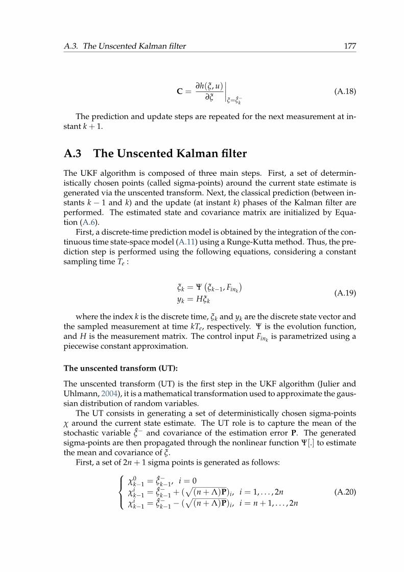
A.3. The Unscented Kalman filter 177
C =∂h(ξ, u)
∂ξ
∣∣∣∣ξ=ξ−k
(A.18)
The prediction and update steps are repeated for the next measurement at in-stant k + 1.
A.3 The Unscented Kalman filter
The UKF algorithm is composed of three main steps. First, a set of determin-istically chosen points (called sigma-points) around the current state estimate isgenerated via the unscented transform. Next, the classical prediction (between in-stants k − 1 and k) and the update (at instant k) phases of the Kalman filter areperformed. The estimated state and covariance matrix are initialized by Equa-tion (A.6).
First, a discrete-time prediction model is obtained by the integration of the con-tinuous time state-space model (A.11) using a Runge-Kutta method. Thus, the pre-diction step is performed using the following equations, considering a constantsampling time Te :
ξk = Ψ(ξk−1, Fink
)yk = Hξk
(A.19)
where the index k is the discrete time, ξk and yk are the discrete state vector andthe sampled measurement at time kTe, respectively. Ψ is the evolution function,and H is the measurement matrix. The control input Fink is parametrized using apiecewise constant approximation.
The unscented transform (UT):
The unscented transform (UT) is the first step in the UKF algorithm (Julier andUhlmann, 2004), it is a mathematical transformation used to approximate the gaus-sian distribution of random variables.
The UT consists in generating a set of deterministically chosen sigma-pointsχ around the current state estimate. The UT role is to capture the mean of thestochastic variable ξ− and covariance of the estimation error P. The generatedsigma-points are then propagated through the nonlinear function Ψ[.] to estimatethe mean and covariance of ξ.
First, a set of 2n + 1 sigma points is generated as follows:χ0
k−1 = ξ−k−1, i = 0χi
k−1 = ξ−k−1 + (√(n + Λ)P)i, i = 1, . . . , 2n
χik−1 = ξ−k−1 − (
√(n + Λ)P)i, i = n + 1, . . . , 2n
(A.20)

178 Appendix A. Kalman Filter algorithms
where
• ξ−k−1Rn the a priori estimated state at instant k − 1.
• χik−1 is the ith generated sigma point at instant k − 1.
• P is the covariance of the estimation error.
• Λ is a scaling parameter defined as Λ = α2(n + κ)− n.
The corresponding weights of the sigma points are computed as follows:ω0
m = Λn+Λ
ω0c = Λ
n+Λ +(1 − α2 + β
)ωi
m = ωic =
12(n+Λ)
, i = 1, . . . , 2n(A.21)
where
• ωim and ωi
c represent respectively the weights of the mean and the covari-ance.
• α, κ, and β are positive constants tuned to set the appropriate spread of thesigma points.
Prediction
The prediction phase (between k and k + 1) consists in computing the a priori pre-dicted state ξ−k and the predicted a priori covariance matrix P−
k .The sigma vectors are propagated through the nonlinear function Ψ, and the
predicted value and covariance of the prediction error are computed using theweights ωi.
χi−k = Ψ
(χi
k−1
)(A.22)
ξ−k =2n
∑i=0
ωimχi−
k (A.23)
P−k =
2n
∑i=0
ωic
[χi−
k − ξ−k
] [χi−
k − ξ−k
]T+ Q (A.24)
where
• χi−k the a priori generated sigma point at instant k.
Update
The update step (at k + 1) consists in using the measurements at time k to correctthe estimated state ξ−k and covariance of the estimation error P−
k obtained in theprevious step.

A.3. The Unscented Kalman filter 179
The predicted measurement yk is calculated by propagating the predictedsigma points through the measurement function H[.]:
Yik = H
(χi−
k−1
)(A.25)
yk =2n
∑i=0
ωimYi
k (A.26)
The measurement covariance matrix Pyk yk and the cross covariance matrix Pxyykare then computed:
Pyk yk =2n
∑i=0
ωic
[Yi
k − yk
] [Yi
k − yk
]T+ R (A.27)
Pxkyk =2n
∑i=0
ωic
[χi−
k − ξ−k
] [Yi(k) − yk
]T(A.28)
(A.29)
Finally, the measurement update is performed using the Kalman filter equations:
Ωk = Pxkyk P−1yk yk
(A.30)
ξk = ξ−k + Ωk (yk − yk) (A.31)
Pk = P−k − ΩkPyk yk ΩT
k (A.32)
where Ωk is the Kalman gain, and Pk is the a posteriori estimated state andcovariance of the estimation error.


181
Appendix B
Culture monitoring
B.1 Biomass concentration measurements
The biomass concentration was obtained by determining the cell dry weight of aselected set of samples at different concentrations, then correlated with the opticaldensity (OD) measurements. The procedure is summarized in the following steps:
• Place the filters (45 µm) at 105C overnight.
• Weight the filters using an analytical balance.
• Prepare standard solutions at different dilutions from a sample.
• Measure the OD of the prepared samples.
• Filter 10 mL of the samples and store them overnight at 105C.
• Weight the filtered samples using an analytical balance.
• Calculate the biomass concentration Xsample using:
Xsample =Average Cell Dry Weight
Filtered Volume
• Build a chart of the biomass concentration Xsample versus the optical density(OD) in the linear range
The results of one of the dry weight and calibration experiments are given inTable B.1 and illustrated in Figure B.1.
B.1.1 Biomass probe calibration
The calibration is carried out using the off-line biomass measurements and theoptical density obtained from the Turibidimetric probe (Fandalux, Germany) (Fig-ure B.2). Several calibration methods were tested (linear, exponential) and thepolynomial curve presented the best trade off between data fit in high densities,and stability under airflow disturbances.

182 Appendix B. Culture monitoring
TABLE B.1: Calibration of the biomass concentration from the opticaldensity measurements
Filter Weight (g) Optical Density Xsample
Sample Filter Filter + Biomass Biomass (abs) (g/L)0 0.301 0.301 0 0.098 01 0.280 0.300 0.0198 5.420 1.9802 0.349 0.361 0.0170 3.097 1.1702 0.302 0.311 0.008 2.587 0.8004 0.301 0.306 0.005 1.805 0.5405 0.366 0.369 0.003 1.234 0.370
0 0.5 1 1.5 2 2.5 3 3.5 4 4.5 5 5.50
0.2
0.4
0.6
0.8
1
1.2
1.4
1.6
1.8
2y = 0.3796x− 0.0911
R2 = 0.9911
OD (abs)
Xsam
ple
(g/L
)
FIGURE B.1: Biomass concentration calibration curve from the opticaldensity measurements
B.2 Glucose concentration measurements
The glucose measurements were performed using the dinitrosalysilic acid (DNS)method, described hereafter:
DNS reagent preparation
• Dissolve 1.00 g of DNS in 20 mL of NaOH 2 M
• Dissolve 30 g of Potassium sodium tartrate tetrahydrate (Rochelle salt) in50mL of distilled water.

B.2. Glucose concentration measurements 183
0 0.2 0.4 0.6 0.8 1 1.2 1.4 1.6 1.8 2 2.2 2.40
2
4
6
8
10 y = 0.2137e1.5996x
R2 = 0.9903
Turbidity (abs)
Biomass
(g/L)
FIGURE B.2: Biomass concentration calibration curve from the opticaldensity measurements
• Stir until complete dissolution then mix the prepared solutions.
• Heat and mix to homogenize.
• Fill with distilled water for a final volume of 100 mL.
• Store in amber bottle at 4C.
Sample preparation and measurement procedure
• Add 1mL of culture supernatant and 1mL of DNS reagent.
• Boil the mix in a 100C water bath for 5 min.
• Add 8 mL of distilled water after cooling to room temperature.
• Homogenize and read the absorbance at 540nm in the spectrophotometer.
The blank solution follows the same procedure as the samples, but the culturesupernatant is replaced with distilled water.
Calibration
An example of glucose calibration results is given in Table B.2. Figure B.3 showsa calibration curve obtained during this experiment. The data fit is linear in therange of 0 to 1 g/L with a correlation coefficient of 0.996.

184 Appendix B. Culture monitoring
TABLE B.2: Calibration of the glucose measurements using the DNSprocedure
Sample Concentration OD 1 OD 2 OD 3g/L abs abs abs
1 0 0.044 0.046 0.0422 0.2 0.165 0.168 0.1663 0.4 0.260 0.276 0.2664 0.5 0.341 0.341 0.3565 0.8 0.487 0.491 0.4806 1 0.637 0.629 0.635
0.1 0.2 0.3 0.4 0.5 0.60
0.2
0.4
0.6
0.8
1y = 1.7169 x− 0.0701
R2 = 0.9961
OD (abs)
Glucose
(g/L)
FIGURE B.3: Glucose concentration calibration curve from the opticaldensity measurements
B.3 Acetate concentration measurements
Acetate concentration measurements were performed with an enzymatic kit(Megazyme, Ireland) according to the manufacturer’s instructions. The calibra-tion of the measurements was performed using the standard solution providedwith the measurement kit. The concentrations are obtained by measuring the op-tical density (OD) of the samples and a calibration curve.
The acetate calibration is carried out by triplicate. Table B.3 and Figure B.4show one of the calibration curves performed during the study. The methoddemonstrated linearity in a range of 0 to 0.25 g/L with a correlation coefficientof 0.98.

B.3. Acetate concentration measurements 185
Calibration
TABLE B.3: Calibration of the acetate measurements using the enzy-matic kit
Sample OD C(nM/µL) C(g/L)0 0.257 0.012714777 0.0150161512 0.322 0.035051546 0.0413958764 0.421 0.069072165 0.0815742276 0.542 0.110652921 0.13068118 0.708 0.167697595 0.198050859
10 0.816 0.204810997 0.241881787
0.2 0.3 0.4 0.5 0.6 0.7 0.80
2 · 10−2
4 · 10−2
6 · 10−2
8 · 10−2
0.1
0.12
0.14
0.16
0.18
0.2
0.22y = 0.3379x− 0.0727
R2 = 0.9833
Acetate (g/L)
OD
(abs)
FIGURE B.4: Acetate concentration calibration curve from the Opticaldensity measurements


187
Appendix C
GMC biomass regulation parameters
C.1 Closed-loop response and parameter tuning
A closed loop response showcasing the closed-loop behavior for different tuningvalues of the damping ratio ξ and the response time tr are shown in Figures C.1and C.2. These variables are used to set the GMC control parameters for thebiomass regulation presented in chapter 6.
0 0.5 1 1.5 2 2.5 3 3.5 4 4.5 5−8 · 10−2
−6 · 10−2
−4 · 10−2
−2 · 10−2
0
2 · 10−2
4 · 10−2
6 · 10−2
8 · 10−2
0.1
time (h)
y−
yref
ξ = 0.700ξ = 0.900ξ = 1.100ξ = 1.300ξ = 1.500
tr = 1 h
FIGURE C.1: GMC biomass tracking response specification with pa-rameters for for different values of ξ for the E. coli BL21 model.

188 Appendix C. GMC biomass regulation parameters
0 0.5 1 1.5 2 2.5 3 3.5 4 4.5 5−0.15
−0.1
−5 · 10−2
0
5 · 10−2
0.1
time (h)
y−
yref
tr = 0.500 htr = 1.000 htr = 1.500 htr = 2.000 htr = 2.500 h
ξ = 1
FIGURE C.2: GMC biomass tracking response specification for fordifferent values of tr for the E. coli BL21 model.
C.2 Expressions of the αj coefficients
Theoretical expression of the αj coefficients presented in chapter 5, calculated us-ing Matlab Symbolic Toolbox:
α1 = 9SinKOS − 9KSKOS + 50KSkX1qOmax − 50KSkX2qOmax − 50SinkX1qOmax
+ 50SinkX2qOmax − 50SinKOSkX2qSmax
α2 = +50KOSqSmax
α3 = 81K2SK2
OS − 900K2SKOSkX1qOmax + 900K2
SKOSkX2qOmax + 2500K2Sk2
X1q2Omax
− 5000K2SkX1kX2q2
Omax+ 2500K2
Sk2X2q2
Omax− 900KSSinK2
OSkX2qSmax
+ 162KSSinK2OS + 5000KSSinKOSkX1kX2qOmax qSmax − 1800KSSinKOSkX1qOmax
− 5000KSSinKOSk2X2qOmax qSmax + 1800KSSinKOSkX2qOmax + 5000KSSink2
X1q2Omax
− 10000KSSinkX1kX2q2Omax
+ 5000KSSink2X2q2
Omax− 900KSXsetK2
OSqSmax
+ 5000KSXsetKOSkX1qOmax qSmax − 5000KSXsetKOSkX2qOmax qSmax + 2500S2inK2
OSk2X2q2
Smax
− 900S2inK2
OSkX2qSmax + 81S2inK2
OS + 5000S2inKOSkX1kX2qOmax qSmax − 900S2
inKOSkX1qOmax
− 5000S2inKOSk2
X2qOmax qSmax + 900S2inKOSkX2qOmax + 2500S2
ink2X1q2
Omax
− 5000S2inkX1kX2q2
Omax+ 2500S2
ink2X2q2
Omax
α4 = 5000SinK2OSkX2q2
Smax+ 900SinK2
OSqSmax − 5000SinKOSkX1qOmax qSmax
+ 5000SinKOSkX2qOmax qSmax
α5 = 2500K2OSq2
Smax
α6 = 2(9KOS − 50kX1qOmax + 50kX2qOmax − 50KOSkX2qSmax)

189
Appendix D
Sensitivity analysis
In view of analyzing the robustness of the control strategies to plant-model mis-match, the most influencing parameters are determined by a parametric sensitivitystudy. The influence of a parameter θj on the model output xi can be quantifiedby:
ddt
(∂xi
∂θj
)=
∂
∂θj
(dxi
dt
)(D.1)
The expressions of the parametric sensitivities for the E. coli model are thereforegiven by:
ddt
(∂xi
∂θj
)=
∂F i
∂θj+
∂F i
∂X∂X∂θj
+∂F i
∂S∂S∂θj
+∂F i
∂A∂A∂θj
+∂F i
∂V∂V∂θj
(D.2)
where F i represents the n differential equations of the state variables xi, and θj
represents the parameters (j = 1, 9) from the following vector:
θ = [kX1 kX2 kX3 kA2 qSmax qOmax Ks KiA Ka] (D.3)
Figure D.1 shows a simulation of model in open-loop over 2 h, with initialconditions : [X0 S0 A0 V0]
T = [0.1 g/L 0 g/L 0 g/L 3.5 L]T and Fin = 0.02 L/h. Thegrowth rate µ3 = 0 confirms that the culture is maintained in oxydo-fermentativemode.
Figures D.2 to D.4 shows the normalized parameter sensitivity functions for thebiomass, substrate, and acetate concentrations. Table D.1 summuarizes the degreeof influence of the model parameters on each variable.

190 Appendix D. Sensitivity analysis
0 1 2 30
0.2
0.4
0.6
0.8
1
time (h)
biom
ass
(g/L
)
0 1 2 30
2
4
time (h)
gluc
ose
(g/L
)
0 1 2 30
0.5
1
time (h)
acet
ate
(g/L
)
0 1 2 33.5
3.52
3.54
3.56
time (h)
volu
me
(L)
0 0.2 0.4 0.6 0.8 1 1.2 1.4 1.6 1.8 2 2.2 2.4 2.6 2.8 30
0.5
1
1.5
2
2.5
time (h)G
row
thra
tes
µ1µ2µ3
FIGURE D.1: Evolution of the state variables X, S, A, and V, and thegrowth rates µ1, µ2, and µ3, in oxydo-fermentative mode.
Influence on biomass X
0 1 2 30
0.2
0.4
0.6
kX1 ∂X/∂kX1
0 1 2 30
0.5
1
1.5
2
kX2 ∂X/∂kX2
0 1 2 3−1
−0.5
0
0.5
1
kX3 ∂X/∂kX3
0 1 2 30
2
4
·10−2kA2 ∂X/∂kA2
0 1 2 30
1
2
3
qsmax ∂X/∂qsmax
0 1 2 3
−0.4
−0.3
−0.2
−0.1
0
qomax ∂X/∂qomax
0 1 2 3−10−8−6−4−20
·10−2Ks ∂X/∂Ks
0 1 2 3
−4
−2
0·10−2
KiA ∂X/∂KiA
0 1 2 3−1
−0.5
0
0.5
1
KA ∂X/∂KA
FIGURE D.2: Normalized sensitivity functions - influence on thebiomass concentration X

Appendix D. Sensitivity analysis 191
Influence on substrate S
0 1 2 3−2
−1.5
−1
−0.5
0
kX1 ∂S/∂kX1
0 1 2 3−4
−3
−2
−1
0
kX2 ∂S/∂kX2
0 1 2 3−1
−0.5
0
0.5
1
kX3 ∂S/∂kX3
0 1 2 3−10−8−6−4−20
·10−2KA2 ∂S/∂KA2
0 1 2 3−10
−5
0
qSmax ∂S/∂qSmax
0 1 2 30
0.5
1
qOmax ∂S/∂qOmax
0 1 2 30
0.1
0.2
0.3
0.4
KS ∂S/∂KS
0 1 2 30246810
·10−2KiA ∂S/∂KiA
0 1 2 3−1
−0.5
0
0.5
1
KA ∂S/∂KA
FIGURE D.3: Normalized sensitivity functions influence on the sub-strate concentration S
Influence on acetate A
0 1 2 30
0.2
0.4
0.6
kx1∂A/∂kx1
0 1 2 30
0.5
1
1.5
kx2∂A/∂kx2
0 1 2 3−1
−0.5
0
0.5
1
kx3∂A/∂kx3
0 1 2 30
0.5
1
kA2∂A/∂kA2
0 1 2 30
1
2
3
4
qSmax∂A/∂qSmax
0 1 2 3−1
−0.8−0.6−0.4−0.2
0
qOmax∂A/∂qOmax
0 1 2 3
−10
−5
0·10−2
KS∂A/∂KS
0 1 2 3−15
−10
−5
0·10−2
KiA∂A/∂KiA
0 1 2 3−1
−0.5
0
0.5
1
KA∂A/∂KA
FIGURE D.4: Normalized sensitivity functions influence on the ac-etate concentration A

192 Appendix D. Sensitivity analysis
TABLE D.1: Ranking of the model parameters according to their re-spective influence on the state variables (From most to least influent)
Influence on X Influence on S Influence on AkX2 qs max qs max
qs max kX2 kX2kX1 kX1 kA2KS qO max qO maxKiA Ks kX1kA2 kA2 KiA
qO max KiA KS

193
Bibliography
Abadli, Merouane, Laurent Dewasme, Didier Dumur, Sihem Tebbani, and AlainVande Wouwer (Oct. 2019). “Generic model control of an Escherichia coli fed-batch culture”. In: 2019 23rd International Conference on System Theory, Controland Computing, ICSTCC 2019 - Proceedings. Institute of Electrical and ElectronicsEngineers Inc., pp. 212–217. ISBN: 9781728106991.
Abadli, Merouane, Laurent Dewasme, Sihem Tebbani, Didier Dumur, and AlainVande Wouwer (July 2020). “Generic model control applied to E. coliBL21(DE3) Fed-batch cultures”. In: Processes 8.7, p. 772. ISSN: 22279717.
Abadli, Merouane, Laurent Dewasme, Sihem Tebbani, Didier Dumur, and AlainVande Wouwer (2021). “An Experimental Assessment of Robust control andEstimation of Acetate Concentration in Escherichia coli BL21 (DE3) Fed-batchCultures”. In: Biochemical Engineering Journal, p. 108103.
Abadli, Merouane, Sihem Tebbani, Didier Dumur, Laurent Dewasme, and AlainVande Wouwer (Mar. 2018a). “Nonlinear model predictive control of Es-cherichia coli culture”. In: 37th Benelux Meeting on Systems and Control. Soester-berg, Netherlands.
Abadli, Merouane, Sihem Tebbani, Didier Dumur, Laurent Dewasme, and AlainVande Wouwer (June 2018b). “Nonlinear model predictive control of Es-cherichia coli cultures”. In: Groupe de travail sur le theme de : La CommandePredictive Non Lineaire. Chatillon, France.
Aehle, Mathias, Kaya Bork, Sebastian Schaepe, Artur Kuprijanov, RudigerHorstkorte, Rimvydas Simutis, and Andreas Lubbert (2012). “Increasing batch-to-batch reproducibility of CHO-cell cultures using a model predictive controlapproach”. In: Cytotechnology. ISSN: 09209069.
Ahmad, Zulfiqar, David Crowley, Ninoslav Marina, and Sunil Kr Jha (2016). “Es-timation of biosurfactant yield produced by Klebseilla sp. FKOD36 bacteriausing artificial neural network approach”. In: Measurement: Journal of the Inter-national Measurement Confederation. ISSN: 02632241.
Albert, S. and R.D. Kinley (2001). “Multivariate statistical monitoring of batchprocesses: An industrial case study of fermentation supervision”. In: Trends inBiotechnology 19.2, pp. 53–62.
Alford, J.S. (2006). “Bioprocess control: Advances and challenges”. In: Computersand Chemical Engineering 30.10-12, pp. 1464–1475.
Allgower, Frank, Thomas A Badgwell, Joe S Qin, James B Rawlings, and StevenJ Wright (1999). “Nonlinear predictive control and moving horizon estima-tion—an introductory overview”. In: Advances in control, pp. 391–449.
Allgower, Frank and Alex Zheng (2012). Nonlinear model predictive control. Vol. 26.Birkhauser.
194 Bibliography
Amribt, Zakaria., Laurent. Dewasme, Alain. Vande Wouwer, and Philippe Bo-gaerts (2014). “Optimization and robustness analysis of hybridoma cell fed-batch cultures using the overflow metabolism model”. In: Bioprocess and Biosys-tems Engineering. ISSN: 16157605.
Anane, Emmanuel, Diana C. Lopez C, Peter Neubauer, and M. Nicolas Cruz Bour-nazou (2017). “Modelling overflow metabolism in Escherichia coli by acetatecycling”. In: Biochemical Engineering Journal. ISSN: 1873295X.
Anderson, Brian D. O., John B. Moore, and Mansour Eslami (2008). “Optimal Fil-tering”. In: IEEE Transactions on Systems, Man, and Cybernetics. ISSN: 0018-9472.
Ansari, Faiz Ahmad, Mahmoud Nasr, Ismail Rawat, and Faizal Bux (2020). “Artifi-cial neural network and techno-economic estimation with algae-based tertiarywastewater treatment”. In: Journal of Water Process Engineering. ISSN: 22147144.
Ariyur, Kartik B and Miroslav Krstic (2003). Real time optimization by extremum seek-ing control. Wiley Online Library.
Ashoori, Ahmad, Behzad Moshiri, Ali Khaki-Sedigh, and Mohammad RezaBakhtiari (2009). “Optimal control of a nonlinear fed-batch fermentation pro-cess using model predictive approach”. In: Journal of Process Control. ISSN:09591524.
Babuska, R. and H.B. Verbruggen (1996). “An overview of fuzzy modeling for con-trol”. In: Control Engineering Practice 4.11, pp. 1593–1606.
Baeshen, Mohammed N., Ahmed M. Al-Hejin, Roop S. Bora, Mohamed M.M.Ahmed, Hassan A.I. Ramadan, Kulvinder S. Saini, Nabih A. Baeshen, and El-rashdy M. Redwan (2015). Production of biopharmaceuticals in E. Coli: Currentscenario and future perspectives.
Banga, Julio R, Eva Balsa-Canto, Carmen G Moles, and Antonio A Alonso (June2005). “Dynamic optimization of bioprocesses: efficient and robust numericalstrategies”. In: Journal of biotechnology 117.4, pp. 407–419. ISSN: 0168-1656.
Bastin, G. and D. Dochain (1990). “On-line estimation and adaptive control ofbioreactors”. In: Process Measurement and Control 1.
Beluhan, D., D. Gosak, N. Pavlovic, and M. Vampola (1995). “Biomass estimationand optimal control of the baker’s yeast fermentation process”. In: Computersand Chemical Engineering. ISSN: 00981354.
Bemporad, Alberto, Manfred Morari, Vivek Dua, and Efstratios N Pistikopoulos(2002). “The explicit linear quadratic regulator for constrained systems”. In:Automatica 38.1, pp. 3–20.
Benattia, S.E., S. Tebbani, and D. Dumur (2015). “Hierarchical Control Strategybased on Robust MPC and Integral Sliding mode - Application to a ContinuousPhotobioreactor”. In: IFAC-PapersOnLine 48.23, pp. 212–217.
Bernal, Vicente, Sara Castano-Cerezo, and Manuel Canovas (2016). Acetatemetabolism regulation in Escherichia coli: carbon overflow, pathogenicity, and beyond.
Bhalla, Aditya, Namita Bansal, Sudhir Kumar, Kenneth M. Bischoff, and Rajesh K.Sani (2013). Improved lignocellulose conversion to biofuels with thermophilic bacteriaand thermostable enzymes.
Birle, S., M. A. Hussein, and T. Becker (2013). Fuzzy logic control and soft sensingapplications in food and beverage processes.

Bibliography 195
Birol, G., C. Undey, and A. Cinar (2002). “A modular simulation package for fed-batch fermentation: Penicillin production”. In: Computers and Chemical Engi-neering 26.11, pp. 1553–1565.
Bitmead, Robert R, Michel Gevers, and Vincent Wertz (1990). “Adaptive optimalcontrol the thinking man’s GPC”. In.
Bodizs, L., M. Titica, N. Faria, B. Srinivasan, D. Dochain, and D. Bonvin (2007).“Oxygen control for an industrial pilot-scale fed-batch filamentous fungal fer-mentation”. In: Journal of Process Control 17.7, pp. 595–606.
Bogaerts, Ph. and D. Coutinho (2014). “Robust nonlinear state estimation of biore-actors based on H∞ hybrid observers”. In: Computers and Chemical Engineering.ISSN: 00981354.
Bogaerts, Ph. and A. Vande Wouwer (2003). “Software sensors for bioprocesses”.In: ISA Transactions 42.4, pp. 547–558.
Bogaerts, Philippe (1999). “A hybrid asymptotic-Kalman observer for biopro-cesses”. In: Bioprocess Engineering 20.3, pp. 249–255.
Boiocchi, R., M. Mauricio-Iglesias, A. K. Vangsgaard, K. V. Gernaey, and G. Sin(2015). “Aeration control by monitoring the microbiological activity usingfuzzy logic diagnosis and control. Application to a complete autotrophic ni-trogen removal reactor”. In: Journal of Process Control. ISSN: 09591524.
Boskovic, J.D. and K.S. Narendra (1995). “Comparison of linear, nonlinear andneural-network-based adaptive controllers for a class of fed-batch fermenta-tion processes”. In: Automatica 31.6, pp. 817–840.
Burgard, Anthony, Mark J. Burk, Robin Osterhout, Stephen Van Dien, and HarryYim (2016). Development of a commercial scale process for production of 1,4-butanediol from sugar.
Cervera, A.E., N. Petersen, A.E. Lantz, A. Larsen, and K.V. Gernaey (2009). “Appli-cation of near-infrared spectroscopy for monitoring and control of cell cultureand fermentation”. In: Biotechnology Progress 25.6, pp. 1561–1581.
Cha, Young-Lok and B. Hitzmann (2004). “Ultrasonic Measurements and its Eval-uation for the Monitoring of Saccharomyces cerevisiae Cultivation”. In.
Chang, L., X. Liu, and M.A. Henson (2016). “Nonlinear model predictive controlof fed-batch fermentations using dynamic flux balance models”. In: Journal ofProcess Control 42, pp. 137–149.
Chattaway, Thomas and Gregory Stephanopoulos (1989). “Adaptive estimation ofbioreactors: monitoring plasmid instability”. In: Chemical Engineering Science.ISSN: 00092509.
Chen, Hong and Frank Allgower (1998). “A quasi-infinite horizon nonlinear modelpredictive control scheme with guaranteed stability”. In: Automatica 34.10,pp. 1205–1217.
Chen, L., S.K. Nguang, X.D. Chen, and X.M. Li (2004). “Modelling and optimiza-tion of fed-batch fermentation processes using dynamic neural networks andgenetic algorithms”. In: Biochemical Engineering Journal 22.1, pp. 51–61.
Chilali, Mahmoud and Pascal Gahinet (1996). “H∞ design with pole placementconstraints: An LMI approach”. In: IEEE Transactions on Automatic Control. ISSN:00189286.

196 Bibliography
Chou, C. Perry (2007). Engineering cell physiology to enhance recombinant protein pro-duction in Escherichia coli.
Cochrane, Jodie A. and Mazen Alamir (2018). “Model Predictive Control andParameter Estimation applied to Gene Expression in Yeast”. In: IFAC-PapersOnLine. ISSN: 24058963.
Cockshott, A. R. and I. D.L. Bogle (1999). “Modelling the effects of glucose feed-ing on a recombinant E. coli fermentation”. In: Bioprocess Engineering. ISSN:0178515X.
Contois, DE (1959). “Kinetics of bacterial growth: relationship between populationdensity and specific growth rate of continuous cultures”. In: Microbiology 21.1,pp. 40–50.
Costello, D. J., P. L. Lee, and P. F. Greenfield (1989). “Control of anaerobic digestersusing Generic Model Control”. In: Bioprocess Engineering. ISSN: 0178515X.
Crabtree, H.G. (1929). “Observations on the carbohydrate metabolism of tu-mours”. In: Biochem J 23, pp. 536–545.
Craven, S., J. Whelan, and B. Glennon (2014). “Glucose concentration control of afed-batch mammalian cell bioprocess using a nonlinear model predictive con-troller”. In: Journal of Process Control 24.4, pp. 344–357.
De Battista, Hernan, Jesus Pico, and Enric Pico-Marco (2012). “Nonlinear PI controlof fed-batch processes for growth rate regulation”. In: Journal of Process Control.ISSN: 09591524.
De Deken, R.H. (1966). “The Crabtree effect: a regulatory system in yeast.” In: Jour-nal of general microbiology 44.2, pp. 149–156.
Del Rio-Chanona, Ehecatl Antonio, Pongsathorn Dechatiwongse, Dongda Zhang,Geoffrey C. Maitland, Klaus Hellgardt, Harvey Arellano-Garcia, and Vassil-ios S. Vassiliadis (2015). “Optimal Operation Strategy for Biohydrogen Produc-tion”. In: Industrial and Engineering Chemistry Research. ISSN: 15205045.
DeLisa, M., H. Chae, W. Weigand, J. Valdes, G. Rao, and W. Bentley (Sept. 2001).“Generic model control of induced protein expression in high cell density culti-vation of Escherichia coli using on-line GFP-fusion monitoring”. In: Bioprocessand Biosystems Engineering 24.2, pp. 83–91.
Dewasme, L., Z. Amribt, L. O. Santos, A. L. Hantson, Ph Bogaerts, and A. VandeWouwer (2013a). “Hybridoma cell culture optimization using nonlinear modelpredictive control”. In: IFAC Proceedings Volumes (IFAC-PapersOnline). ISBN:9783902823588.
Dewasme, L., D. Coutinho, and A. Vande Wouwer (2011a). “Adaptive and robustlinearizing control strategies for fed-batch cultures of microorganisms exhibit-ing overflow metabolism”. In: Lecture Notes in Electrical Engineering. Vol. 89LNEE. Springer, Berlin, Heidelberg, pp. 283–305. ISBN: 9783642195389.
Dewasme, L., S. Fernandes, Z. Amribt, L. O. Santos, Ph Bogaerts, and A. VandeWouwer (2015). “State estimation and predictive control of fed-batch culturesof hybridoma cells”. In: Journal of Process Control. ISSN: 09591524.

Bibliography 197
Dewasme, L., G. Goffaux, A. L. Hantson, and A. Vande Vande Wouwer (Feb.2013b). “Experimental validation of an Extended Kalman Filter estimating ac-etate concentration in E. coli cultures”. In: Journal of Process Control. Vol. 23. 2,pp. 148–157.
Dewasme, L., A. Richelle, P. Dehottay, P. Georges, M. Remy, Ph. Bogaerts, and A.Vande Wouwer (2010). “Linear robust control of S. cerevisiae fed-batch culturesat different scales”. In: Biochemical Engineering Journal 53.1, pp. 26–37.
Dewasme, L., B. Srinivasan, M. Perrier, and A. Vande Wouwer (2011b).“Extremum-seeking algorithm design for fed-batch cultures of microorganismswith overflow metabolism”. In: Journal of Process Control 21.7, pp. 1092–1104.
Diehl, Moritz, Rishi Amrit, and James B Rawlings (2010). “A Lyapunov functionfor economic optimizing model predictive control”. In: IEEE Transactions onAutomatic Control 56.3, pp. 703–707.
Doan, X.-T. and R. Srinivasan (2008). “Online monitoring of multi-phase batch pro-cesses using phase-based multivariate statistical process control”. In: Computersand Chemical Engineering 32.1-2, pp. 230–243.
Dochain, D. and A. Rapaport (2018). “An asymptotic observer for batch processeswith single biogas measurement”. In: IFAC-PapersOnLine. ISSN: 24058963.
Dochain, Denis (2010). Bioprocess Control. London: Wiley. ISBN: 9780470611128.Dochain, Denis, Michel Perrier, and Martin Guay (2011). “Extremum seeking con-
trol and its application to process and reaction systems: A survey”. In: Mathe-matics and Computers in Simulation 82.3, pp. 369–380. ISSN: 0378-4754.
Doelle, Horst W., Ken N. Ewings, and Neil W. Hollywood (1982). “Regulation ofglucose metabolism in bacterial systems”. In.
Dohnal, Mirko (1985). “Fuzzy bioengineering models”. In: Biotechnology and Bio-engineering. ISSN: 10970290.
Doran, P.M. (2013). “Bioprocess development: an interdisciplinary challenge”. In:Bioprocess Engineering Principles, pp. 3–11.
Douglas, P. L., P. S. Fountain, G. R. Sullivan, and W. Zhou (1994). “Model basedcontrol of a high purity distillation column”. In: The Canadian Journal of ChemicalEngineering. ISSN: 1939019X.
Duran-Villalobos, C.A., B. Lennox, and D. Lauri (2016a). “Multivariate batchto batch optimisation of fermentation processes incorporating validity con-straints”. In: Journal of Process Control 46, pp. 34–42.
Duran-Villalobos, Carlos A., Barry Lennox, and David Lauri (2016b). “Multivariatebatch to batch optimisation of fermentation processes incorporating validityconstraints”. In: Journal of Process Control 46, pp. 34–42. ISSN: 0959-1524.
Eiteman, Mark A. and Elliot Altman (2006). Overcoming acetate in Escherichia colirecombinant protein fermentations.
Enjalbert, Brice, Muriel Cocaign-Bousquet, Jean Charles Portais, and FabienLetisse (2015). “Acetate exposure determines the diauxic behavior of Es-cherichia coli during the glucose-acetate transition”. In: Journal of Bacteriology.ISSN: 10985530.

198 Bibliography
Feng, Peter, Stephen Weagant, Michael Grant, and William Burkhardt (2002). “Bac-teriological Analytical Manual : Enumeration of Escherichia coli and the Col-iform Bacteria”. In: Bacteriological Analytical Manual.
Fernandes, Sofia, Anne Richelle, Zakaria Amribt, Laurent Dewasme, Philippe Bo-gaerts, and Alain Vande Wouwer (2015). “Extended and Unscented KalmanFilter design for hybridoma cell fed-batch and continuous cultures”. In: IFAC-PapersOnLine.
Ferreira, A.P., J.A. Lopes, and J.C. Menezes (2007). “Study of the application ofmultiway multivariate techniques to model data from an industrial fermenta-tion process”. In: Analytica Chimica Acta 595.1-2 SPEC. ISS. Pp. 120–127.
Ferreira, L.S., M.B. De Souza Jr, and R.O.M. Folly (2001). “Development of an alco-hol fermentation control system based on biosensor measurements interpretedby neural networks”. In: Sensors and Actuators, B: Chemical 75.3, pp. 166–171.
Ferrer-Miralles, Neus, Joan Domingo-Espın, Jose Corchero, Esther Vazquez, andAntonio Villaverde (2009). Microbial factories for recombinant pharmaceuticals.
Findeisen, Rolf, Frank Allgower, and Lorenz T Biegler (2007). Assessment and futuredirections of nonlinear model predictive control. Vol. 358. 7. Springer.
Forbes, M.G., R.S. Patwardhan, H. Hamadah, and R.B. Gopaluni (2015). “Modelpredictive controlin industry: Challenges and opportunities”. In: IFAC-PapersOnLine 28.8, pp. 531–538.
Gautam, Ajay, Yun-Chung Chu, and Yeng Chai Soh (2013). “Robust H∞ recedinghorizon control for a class of coordinated control problems involving dynam-ically decoupled subsystems”. In: IEEE Transactions on Automatic Control 59.1,pp. 134–149.
Gauthier, J.P. and I.A.K. Kupka (1994). “Observability and observers for nonlinearsystems”. In: SIAM Journal on Control and Optimization 32.4, pp. 975–994.
Gbewonyo, K., D. Jain, G. Hunt, S. W. Drew, and B. C. Buckland (1989). “On-lineanalysis of avermectin fermentation cell growth kinetics in an industrial pilotplant”. In: Biotechnology and Bioengineering. ISSN: 10970290.
Glassey, J. (2013). “Multivariate data analysis for advancing the interpretation ofbioprocess measurement and monitoring data”. In: Advances in Biochemical En-gineering/Biotechnology 132, pp. 167–191.
Glassey, J., G.A. Montague, A.C. Ward, and B.V. Kara (1994). “Enhanced super-vision of recombinant E. coli fermentation via artificial neural networks”. In:Process Biochemistry 29.5, pp. 387–398.
Gonzalez, Karen, Sihem Tebbani, Filipa Lopes, Aurore Thorigne, Sebastien Givry,Didier Dumur, and Dominique Pareau (2016). “Regulation of lactic acid con-centration in its bioproduction from wheat flour”. In: Control Engineering Prac-tice 54, pp. 202–213.
Gonzalez, Karen Vanessa, Sihem Tebbani, Didier Dumur, Filipa Lopes, DominiquePareau, Aurore Thorigne, and Sebastien Givry (2015). “Adaptive Control ofLactic Acid Production Process from Wheat Flour”. In: IFAC-PapersOnLine 48.8,pp. 1087–1092.
Gorrini, Federico Alberto, Jesus Miguel Zamudio Lara, Silvina Ines Biagiola, JoseLuis Figueroa, Hector Hernandez Escoto, Anne-Lise Hantson, and Alain Vande

Bibliography 199
Wouwer (2020). “Experimental Study of Substrate Limitation and Light Accli-mation in Cultures of the Microalgae Scenedesmus obliquus—Parameter Iden-tification and Model Predictive Control”. In: Processes 8.12, p. 1551.
Grosz, Ron, Gregory Stephanopoulos, and K. Y. San (1984). “Studies on on-linebioreactor identification. III. Sensitivity problems with respiratory and heatevolution measurements”. In: Biotechnology and Bioengineering. ISSN: 10970290.
Gusyatiner, M. M., Y. G. Rostova, M. Y. Kiryukhin, and A. Y. Romkina (2017).“Method for producing an L-amino acid using a bacterium of the family En-terobacteriaceae having a disrupted putrescine degradation pathway”. In: U.S.Patent 9840725B2.
Hafidi, G., S. Tebbani, D. Dumur, and A. Vande Wouwer (2008). “Nonlinear ModelPredictive Control applied to E. Coli Cultures”. In: IFAC Proceedings Volumes41.2, pp. 14570–14575.
Haldane, JBS (1930). “Union of enzymes with substrate”. In: Enzymes, 1st Edition.Longmans, Green & Co., London, pp. 28–53.
Han, Keehyun, Henry C. Lim, and Juan Hong (1992). “Acetic acid formation in es-cherichia coli fermentation”. In: Biotechnology and Bioengineering 39.6, pp. 663–671. ISSN: 10970290.
Hasunuma, Tomohisa and Akihiko Kondo (2012). Consolidated bioprocessing and si-multaneous saccharification and fermentation of lignocellulose to ethanol with thermo-tolerant yeast strains.
Henes, B. and B. Sonnleitner (2007). “Controlled fed-batch by tracking the maximalculture capacity”. In: Journal of Biotechnology 132.2, pp. 118–126.
Herbert, DENIS (1958). “Some principles of continuous culture”. In: Recent progressin microbiology 1.
Hilaly, A. K., M. N. Karim, and J. C. Linden (1992). “Real time application of ex-tended Kalman filtering in estimation and optimization of a recombinant Es-cherichia coli fermentation”. In: IFAC Symposia Series. ISBN: 0080417108.
Hisbullah, M.A. Hussain, and K.B. Ramachandran (2001). “Comparative evalua-tion of various control schemes for fed-batch fermentation”. In: Bioprocess andBiosystems Engineering 24.5, pp. 309–318.
Hisbullah, M.A. Hussain, and K.B. Ramachandran (2003). “Design of a fuzzy logiccontroller for regulating substrate feed to fed-batch fermentation”. In: Food andBioproducts Processing: Transactions of the Institution of of Chemical Engineers, PartC 81.2, pp. 138–146.
Holland, J.H. (1984). “Genetic algorithms and adaptation”. In: Adaptive Control ofIll-Defined Systems, pp. 317–333.
Holmberg, Ulf and Gustaf Olsson (1985). “Simultaneous On-Line Estimation ofOxygen Transfer Rate and Respiration Rate”. In: IFAC Proceedings Volumes.ISSN: 14746670.
Holms, W. H. (1986). “The Central Metabolic Pathways of Escherichia coli: Rela-tionship between Flux and Control at a Branch Point, Efficiency of Conversionto Biomass, and Excretion of Acetate”. In: Current Topics in Cellular Regulation.

200 Bibliography
Horiuchi, J.-I. and K. Hiraga (1999). “Industrial application of fuzzy control tolarge-scale recombinant vitamin B2 production”. In: Journal of Bioscience andBioengineering 87.3, pp. 365–371.
Horowitz, Joseph, Mark D. Normand, Maria G. Corradini, and Micha Peleg (2010).“Probabilistic model of microbial cell growth, division, and mortality”. In: Ap-plied and Environmental Microbiology. ISSN: 00992240.
Howell, J.A. and B.O. Sodipo (1985). “On-line Respirometry and Estimation ofAeration Efficiencies in an Activated Sludge Aeration Basin from DissolvedOxygen Measurements”. In: IFAC Proceedings Volumes. ISSN: 14746670.
Huang, Yu Liang, Titus J. Foellmer, Koon Chye Ang, Soo Beng Khoo, and Mi-randa G.S. Yap (1995). “Characterization and application of an on-line flowinjection analysis/wall-jet electrode system for glucose monitoring during fer-mentation”. In: Analytica Chimica Acta. ISSN: 00032670.
Hulhoven, X., A. Vande Vande Wouwer, and Ph Bogaerts (2006a). “Hybrid ex-tended Luenberger-asymptotic observer for bioprocess state estimation”. In:Chemical Engineering Science. ISSN: 00092509.
Hulhoven, Xavier, Frederic Renard, Sandrine Dessoy, Ph Dehottay, Ph Bogaerts,and A Vande Wouwer (2006b). “Monitoring and control of a bioprocess formalaria vaccine production”. In: IFAC Proceedings Volumes 39.9, pp. 143–148.
Insel, G., G. Celikyilmaz, E. Ucisik-Akkaya, K. Yesiladali, Z. P. Cakar, C. Tamer-ler, and D. Orhon (2007). “Respirometric evaluation and modeling of glucoseutilization by Escherichia coli under aerobic and mesophilic cultivation condi-tions”. In: Biotechnology and Bioengineering. ISSN: 00063592.
Isidori, Alberto, M. Thoma, E. D. Sontag, B. W. Dickinson, A. Fettweis, J. L. Massey,and J. W. Modestino (1995). Nonlinear Control Systems. 3rd. Berlin, Heidelberg:Springer-Verlag. ISBN: 3540199160.
Jaen, Karim E, Juan-Carlos Sigala, Roberto Olivares-Hernandez, Karsten Niehaus,and Alvaro R Lara (2017). “Heterogeneous oxygen availability affects the titerand topology but not the fidelity of plasmid DNA produced by Escherichiacoli”. In: BMC biotechnology 17.1, pp. 1–12.
Jana, S. and J. K. Deb (2005). Strategies for efficient production of heterologous proteinsin Escherichia coli.
Jenzsch, M., S. Gnoth, M. Beck, M. Kleinschmidt, R. Simutis, and A. Lubbert(2006a). “Open-loop control of the biomass concentration within the growthphase of recombinant protein production processes”. In: Journal of Biotechnol-ogy 127.1, pp. 84–94.
Jenzsch, Marco, Rimvydas Simutis, and Andreas Luebbert (2006b). “Genericmodel control of the specific growth rate in recombinant Escherichia coli culti-vations”. In: Journal of Biotechnology 122.4, pp. 483–493.
Johnsson, O., J. Andersson, G. Liden, C. Johnsson, and T. Hagglund (2013). “Feedrate control in fed-batch fermentations based on frequency content analysis”.In: Biotechnology Progress 29.3, pp. 817–824.
Julier, Simon J. and Jeffrey K. Uhlmann (1997). “New extension of the Kalman filterto nonlinear systems”. In: Signal Processing, Sensor Fusion, and Target RecognitionVI. ISBN: 0819424838.

Bibliography 201
Julier, Simon J. and Jeffrey K. Uhlmann (2004). “Unscented filtering and nonlinearestimation”. In: Proceedings of the IEEE.
Kadir, Tuty A.A., Ahmad A. Mannan, Andrzej M. Kierzek, Johnjoe McFadden, andKazuyuki Shimizu (2010). “Modeling and simulation of the main metabolismin Escherichia coli and its several single-gene knockout mutants with experi-mental verification”. In: Microbial Cell Factories. ISSN: 14752859.
Karim, M. N. and S. L. Rivera (1992). Artificial neural networks in bioprocess stateestimation.
Keerthi, SS a and Elmer G Gilbert (1988). “Optimal infinite-horizon feedback lawsfor a general class of constrained discrete-time systems: Stability and moving-horizon approximations”. In: Journal of optimization theory and applications 57.2,pp. 265–293.
Kesson, M., P. Hagander, and J.P. Axelsson (2001). “Avoiding acetate accumula-tion in Escherichia coli cultures using feedback control of glucose feeding”. In:Biotechnology and Bioengineering 73.3, pp. 223–230.
Kirkpatrick, Christopher, Lisa M. Maurer, Nikki E. Oyelakin, Yuliya N. Yoncheva,Russell Maurer, and Joan L. Slonczewski (2001). “Acetate and formate stress:Opposite responses in the proteome of Escherichia coli”. In: Journal of Bacteriol-ogy. ISSN: 00219193.
Kleman, G. L. and W. R. Strohl (1994). “Acetate metabolism by Escherichia coliin high-cell-density fermentation”. In: Applied and Environmental Microbiology.ISSN: 00992240.
Ko, Yun-Fei -F, William E. Bentley, and William A. Weigand (1994). “A metabolicmodel of cellular energetics and carbon flux during aerobic Escherichia colifermentation”. In: Biotechnology and Bioengineering. ISSN: 10970290.
Koebmann, Brian J., Hans V. Westerhoff, Jacky L. Snoep, Dan Nilsson, and PeterR. Jensen (2002). “The glycolytic flux in Escherichia coli is controlled by thedemand for ATP”. In: Journal of Bacteriology. ISSN: 00219193.
Kojima, Hiroyuki, Yuri Ogawa, Kazue Kawamura, and Konosuke Sano (2000).“Method of producing L-lysine by fermentation”. In: U.S. Patent 6040160A.
Kovarova-Kovar, K., S. Gehlen, A. Kunze, T. Keller, R. Von Daniken, M. Kolb, andA.P.G.M. Van Loon (2000a). “Application of model-predictive control based onartificial neural networks to optimize the fed-batch process for riboflavin pro-duction”. In: Journal of Biotechnology 79.1, pp. 39–52.
Kovarova-Kovar, Karin, Stefan Gehlen, Axel Kunze, Thoralf Keller, Ralph vonDaniken, Michael Kolb, and Adolphus P.G.M. van Loon (2000b). “Applicationof model-predictive control based on artificial neural networks to optimize thefed-batch process for riboflavin production”. In: Journal of Biotechnology 79.1,pp. 39–52. ISSN: 0168-1656.
Kramer, Dominik and Rudibert King (2016). “On-line monitoring of substratesand biomass using near-infrared spectroscopy and model-based state estima-tion for enzyme production by S. cerevisiae”. In: IFAC-PapersOnLine. ISSN:24058963.

202 Bibliography
Kuprijanov, A., S. Schaepe, R. Simutis, and A. Lubbert (2013a). “Model predictivecontrol made accessible to professional automation systems in fermentationtechnology”. In: Biosyst. Inf. Technol. 2, pp. 26–31.
Kuprijanov, A., S. Schaepe, R. Simutis, and A. Lubbert (2013b). “Model predictivecontrol made accessible to professional automation systems in fermentationtechnology”. In: Biosyst. Inf. Technol 2.1, pp. 26–31.
Kwakernaak, H. and R. Sivan (1974). “Linear Optimal Control Systems”. In: IEEETransactions on Automatic Control. ISSN: 15582523.
Landau, I.D., R. Lozano, M. M’Saad, and A. Karimi (2011). “Adaptive regula-tion—Rejection of unknown disturbances”. In: Communications and Control En-gineering 9780857296634, pp. 477–497.
Langson, Wilbur, Ioannis Chryssochoos, SV Rakovic, and David Q Mayne (2004).“Robust model predictive control using tubes”. In: Automatica 40.1, pp. 125–133.
Laurı, D., B. Lennox, and J. Camacho (2014). “Model predictive control for batchprocesses: Ensuring validity of predictions”. In: Journal of Process Control 24.1,pp. 239–249.
Lee, J., S.Y. Lee, S. Park, and A.P.J. Middelberg (1999). “Control of fed-batch fer-mentations”. In: Biotechnology Advances 17.1, pp. 29–48.
Lee, P.L. and G.R. Sullivan (1988). “Generic model control (GMC)”. In: Computers& Chemical Engineering 12.6, pp. 573–580.
Lee, Sang Yup (1996). “High cell-density culture of Escherichia coli”. In: Trends inBiotechnology 14.3, pp. 98–105.
Lee, Seung Chul, Young Bo Hwang, Ho Nam Chang, and Yong Keun Chang(1991). “Adaptive control of dissolved oxygen concentration in a bioreactor”.In: Biotechnology and Bioengineering. ISSN: 10970290.
Lewis, Frank l., Lihua Xie, and Dan Popa (2007). Optimal and Robust Estimation:With an Introduction to Stochastic Control Theory. ISBN: 9781420008296.
Lin, H. Y., B. Mathiszik, B. Xu, S. O. Enfors, and P. Neubauer (2001). “Determi-nation of the maximum specific uptake capacities for glucose and oxygen inglucose-limited fed-batch cultivations of Escherichia coli”. In: Biotechnology andBioengineering. ISSN: 00063592.
Lisci, Silvia, Massimiliano Grosso, and Stefania Tronci (2020). “A geometricobserver-assisted approach to tailor state estimation in a bioreactor for ethanolproduction”. In: Processes. ISSN: 22279717.
Liu, D. (2019). “Escherichia coli”. In: Encyclopedia of Microbiology. ISBN:9780128117378.
Logist, Filip, Boris Houska, Moritz Diehl, and Jan F. Van Impe (2011). “Ro-bust multi-objective optimal control of uncertain (bio)chemical processes”. In:Chemical Engineering Science. ISSN: 00092509.
Lubbert, A. and S. Bay Jorgensen (2001). “Bioreactor performance: A more scien-tific approach for practice”. In: Journal of Biotechnology 85.2, pp. 187–212.
Lubbert, A. and R. Simutis (1994). “Using measurement data in bioprocess mod-elling and control”. In: Trends in Biotechnology 12.8, pp. 304–311.

Bibliography 203
Luli, G. W. and W. R. Strohl (1990). “Comparison of growth, acetate production,and acetate inhibition of Escherichia coli strains in batch and fed-batch fermen-tations”. In: Applied and Environmental Microbiology 56.4, pp. 1004–1011. ISSN:00992240.
Luttmann, R. et al. (2012). “Soft sensors in bioprocessing: A status report and rec-ommendations”. In: Biotechnology Journal 7.8, pp. 1040–1048.
Marafioti, Giancarlo, Sihem Tebbani, Dominique Beauvois, Giuliana Becerra, Ar-sene Isambert, and Morten Hovd (2009). “Unscented Kalman filter state andparameter estimation in a photobioreactor for microalgae production”. In: IFACProceedings Volumes (IFAC-PapersOnline). ISBN: 9783902661548.
Markana, Anilkumar, Nitin Padhiyar, and Kannan Moudgalya (2018). “Multi-criterion control of a bioprocess in fed-batch reactor using EKF based economicmodel predictive control”. In: Chemical Engineering Research and Design. ISSN:02638762.
Marquez-Vera, M. A., L. E. Ramos-Velasco, and B. D. Balderrama-Hernandez(2018). “Stable fuzzy control and observer via LMIs in a fermentation process”.In: Journal of Computational Science. ISSN: 18777503.
Mears, L., R. Nørregard, G. Sin, K.V. Gernaey, S.M. Stocks, M.O. Albaek, and K.Villez (2016). “Functional unfold principal component regression methodologyfor analysis of industrial batch process data”. In: AIChE Journal 62.6, pp. 1986–1994.
Mears, Lisa, Stuart M. Stocks, Gurkan Sin, and Krist V. Gernaey (2017). “A reviewof control strategies for manipulating the feed rate in fed-batch fermentationprocesses”. In: Journal of Biotechnology 245, pp. 34–46. ISSN: 0168-1656.
Melo, Alessandra Goncalves de, Sebastien Levesque, and Sylvain Moineau (2018).Phages as friends and enemies in food processing.
Meyer, Hans-Peter and Diego R Schmidhalter (2012). “Microbial Expression Sys-tems and Manufacturing from a Market and Economic Perspective”. In: Inno-vations in Biotechnology.
Michaelis, Leonor, Maud L Menten, et al. (1913). “Die kinetik der invertin-wirkung”. In: Biochem. z 49.333-369, p. 352.
Montague, G.A., A.J. Morris, and A.C. Ward (1989). “Fermentation monitoring andcontrol: A perspective”. In: Biotechnology and Genetic Engineering Reviews 7.1,pp. 147–188.
Morari, Manfred and Jay H Lee (1999). “Model predictive control: past, presentand future”. In: Computers & Chemical Engineering 23.4-5, pp. 667–682.
Moulton, Gus G. (2014). Fed-Batch Fermentation: A Practical Guide to Scalable Recom-binant Protein Production in Escherichia Coli. ISBN: 9781908818331.
Muller, Matthias, Wolfram Meusel, Ute Husemann, Gerhard Greller, and MatthiasKraume (Jan. 2018). “Application of heat compensation calorimetry to an E. colifed-batch process”. In: Journal of Biotechnology 266, pp. 133–143. ISSN: 18734863.
Murugan, Chitra and Pappa Natarajan (2019). “Estimation of fungal biomass usingmultiphase artificial neural network based dynamic soft sensor”. In: Journal ofMicrobiological Methods. ISSN: 18728359.

204 Bibliography
Nelson, David L. and Michael M. Cox (2017). “Lehninger Principles of Biochem-istry 7th”. In: W.H. Freeman and Company. ISSN: 00063568.
Neubauer, P., H. Y. Lin, and B. Mathiszik (2003). “Metabolic load of recombinantprotein production: Inhibition of cellular capacities for glucose uptake and res-piration after induction of a heterologous gene in Escherichia coli”. In: Biotech-nology and Bioengineering. ISSN: 00063592.
Nomikos, P. and J.F. MacGregor (1994). “Monitoring batch processes using multi-way principal component analysis”. In: AIChE Journal 40.8, pp. 1361–1375.
Nomikos, P. and J.F. MacGregor (1995). “Multi-way partial least squares in moni-toring batch processes”. In: Chemometrics and Intelligent Laboratory Systems 30.1,pp. 97–108.
Ohtake, Toshiyuki, Sammy Pontrelli, Walter A. Lavina, James C. Liao, Sastia P.Putri, and Eiichiro Fukusaki (2017). “Metabolomics-driven approach to solvinga CoA imbalance for improved 1-butanol production in Escherichia coli”. In:Metabolic Engineering. ISSN: 10967184.
Oliveira, R., J.J. Clemente, A.E. Cunha, and M.J.T. Carrondo (2005). “Adaptive dis-solved oxygen control through the glycerol feeding in a recombinant Pichiapastoris cultivation in conditions of oxygen transfer limitation”. In: Journal ofBiotechnology 116.1, pp. 35–50.
Oliveira, R., R. Simutis, and S. Feyo De Azevedo (2004). “Design of a stable adap-tive controller for driving aerobic fermentation processes near maximum oxy-gen transfer capacity”. In: Journal of Process Control 14.6, pp. 617–626.
Olkin, Ingram and Allan R Sampson (2001). “Multivariate analysis: overview”. In.Pablos, Tania E, Juan Carlos Sigala, Sylvie Le Borgne, and Alvaro R Lara (2014).
“Aerobic expression of Vitreoscilla hemoglobin efficiently reduces overflowmetabolism in Escherichia coli”. In: Biotechnology journal 9.6, pp. 791–799.
Park, Jin Hwan, Yu Sin Jang, Jeong Wook Lee, and Sang Yup Lee (2011). “Es-cherichia coli W as a new platform strain for the enhanced production of L-Valine by systems metabolic engineering”. In: Biotechnology and Bioengineering.ISSN: 00063592.
Patnaik, Pratap R. (2005). “The extended Kalman filter as a noise modulator forcontinuous yeast cultures under monotonic, oscillating and chaotic condi-tions”. In: Chemical Engineering Journal. ISSN: 13858947.
Peebo, Karl, Kaspar Valgepea, Andres Maser, Ranno Nahku, Kaarel Adamberg,and Raivo Vilu (2015). “Proteome reallocation in Escherichia coli with increas-ing specific growth rate”. In: Molecular BioSystems. ISSN: 17422051.
Peng, J., F. Meng, and Y. Ai (2013). “Time-dependent fermentation control strate-gies for enhancing synthesis of marine bacteriocin 1701 using artificial neuralnetwork and genetic algorithm”. In: Bioresource Technology 138, pp. 345–352.
Peter, Ed. and L. Lee (1993). Nonlinear Process Control: Applications of Generic ModelControl. London Ltd. UK: Springer-Verlag.
Phue, Je Nie, Jun Lee Sang, Loc Trinh, and Joseph Shiloach (2008). “Modified Es-cherichia coli B (BL21), a superior producer of plasmid DNA compared withEscherichia coli K (DH5α)”. In: Biotechnology and Bioengineering. ISSN: 00063592.

Bibliography 205
Pico, J, F Garelli, H De Battista, and RJ Mantz (2009). “Geometric invariance andreference conditioning ideas for control of overflow metabolism”. In: Journal ofProcess Control 19.10, pp. 1617–1626.
Pinhal, Stephane, Delphine Ropers, Johannes Geiselmann, and Hidde De Jong(2019). “Acetate metabolism and the inhibition of bacterial growth by acetate”.In: Journal of Bacteriology. ISSN: 10985530.
Pontrelli, Sammy, Tsan-Yu Chiu, Ethan I. Lan, Frederic Y.-H. Chen, PeichingChang, and James C. Liao (2018). “Escherichia coli as a host for metabolic en-gineering”. In: Metabolic Engineering 50, pp. 16–46.
Preuß, Karlheinz, Marie Veronique Le Lann, Jacques Proth, and Herve Pingaud(2000). “Modelling and predictive control of fed-batch yeast growth on indus-trial pilot plant scale”. In: Chemical Engineering Journal. ISSN: 13858947.
Prieto, Marıa A., Eduardo Dıaz, and Jose L. Garcıa (1996). “Molecular characteri-zation of the 4-hydroxyphenylacetate catabolic pathway of Escherichia coli W:Engineering a mobile aromatic degradative cluster”. In: Journal of Bacteriology.ISSN: 00219193.
Qin, S. Joe and Thomas A. Badgwell (2000). “An Overview of Nonlinear ModelPredictive Control Applications”. In: Nonlinear Model Predictive Control.
Qin, S.J. and T.A. Badgwell (2003). “A survey of industrial model predictive controltechnology”. In: Control Engineering Practice 11.7, pp. 733–764.
Renard, F., A. Vande Wouwer, S. Valentinotti, and D. Dumur (2006). “A practicalrobust control scheme for yeast fed-batch cultures – An experimental valida-tion”. In: Journal of Process Control 16.8, pp. 855–864.
Retamal, C., L. Dewasme, A. L. Hantson, and A. Vande Wouwer (July 2018). “Pa-rameter estimation of a dynamic model of Escherichia coli fed-batch cultures”.In: Biochemical Engineering Journal 135, pp. 22–35. ISSN: 1873295X.
Riesenberg, D., V. Schulz, W.A. Knorre, H.-D. Pohl, D. Korz, E.A. Sanders, A. Roß,and W.-D. Deckwer (1991). “High cell density cultivation of Escherichia coli atcontrolled specific growth rate”. In: Journal of Biotechnology 20.1, pp. 17–27.
Rio-Chanona, Ehecatl Antonio del, Dongda Zhang, and Vassilios S. Vassiliadis(2016). “Model-based real-time optimisation of a fed-batch cyanobacterial hy-drogen production process using economic model predictive control strategy”.In: Chemical Engineering Science. ISSN: 00092509.
Rocha, I. and E.C. Ferreira (2002). “Model-based Adaptive Control Of Acetate Con-centration During The Production Of Recombinant Proteins With E. Coli”. In:IFAC Proceedings Volumes 35.1, pp. 461–466.
Rocha, I., Ana Veloso, and Eugenio Ferreira (Feb. 2006). “Design of estimators forspecific growth rate control in a fed-batch E. coli fermentation”. In.
Rocha, Isabel (2003). Model-based strategies for computer-aided operation of recombinantE. coli fermentation.
Rocha, Isabel, Ana Veloso, Sonia Carneiro, Eugenio Ferreira, and Rafael Costa(2008). “Implementation of a specific rate controller in a fed-batch E.coli fermentation”. In: IFAC Proceedings Volumes (IFAC-PapersOnline). ISBN:9783902661005.

206 Bibliography
Rothen, S. A., M. Sauer, B. Sonnleitner, and B. Witholt (1998). “Growth characteris-tics of Escherichia coli HB101[pGEc47] on defined medium”. In: Biotechnologyand Bioengineering 58.1, pp. 92–100.
Rumelhart, D.E., G.E. Hinton, and R.J. Williams (1986). “Learning representationsby back-propagating errors”. In: Nature 323.6088, pp. 533–536.
Sabra, W, C Groeger, An-Ping Zeng, Antonino Baez, Kwang Myung Cho, andJames C Liao (2016). “Microbial Cell Factories for Diol Production”. In: Bioreac-tor Engineering Research and Industrial Applications I: Cell Factories. Ed. by Qin Ye,Jie Bao, and Jian-Jiang Zhong. Berlin, Heidelberg: Springer Berlin Heidelberg,pp. 165–197. ISBN: 978-3-662-49161-4.
Sagmeister, P., P. Wechselberger, M. Jazini, A. Meitz, T. Langemann, and C. Her-wig (2013). “Soft sensor assisted dynamic bioprocess control: Efficient tools forbioprocess development”. In: Chemical Engineering Science 96, pp. 190–198.
Samson, Julie E. and Sylvain Moineau (2013). Bacteriophages in food fermentations:New frontiers in a continuous arms race.
Sanford, Karl, Gopal Chotani, Nathan Danielson, and James A. Zahn (2016). Scal-ing up of renewable chemicals.
Santos, L.O., L. Dewasme, D. Coutinho, and A. Vande Wouwer (2012a). “Nonlinearmodel predictive control of fed-batch cultures of micro-organisms exhibitingoverflow metabolism: Assessment and robustness”. In: Computers & ChemicalEngineering 39, pp. 143–151. ISSN: 0098-1354.
Santos, L.O., L. Dewasme, D. Coutinho, and A. Vande Wouwer (2012b). “Non-linear model predictive control of fed-batch cultures of micro-organisms ex-hibiting overflow metabolism: Assessment and robustness”. In: Computers andChemical Engineering 39, pp. 143–151.
Santos, L.O., L. Dewasme, and A. Vande Wouwer (2010). “Nonlinear model predic-tive control of fed-batch cultures of E. coli: performance and robustness analy-sis”. In: IFAC Proceedings Volumes 43.14, pp. 1046–1051.
Sarkka, Simo (2007). “On unscented Kalman filtering for state estimation ofcontinuous-time nonlinear systems”. In: IEEE Transactions on Automatic Control.ISSN: 00189286.
Schugerl, K. and K.H. Bellgardt (2014). Bioreaction Engineering: Modeling and Con-trol. ISBN: 9780874216561.
Scokaert, Pierre OM and David Q Mayne (1998). “Min-max feedback model pre-dictive control for constrained linear systems”. In: IEEE Transactions on Auto-matic control 43.8, pp. 1136–1142.
Scokaert, Pierre OM, David Q Mayne, and James B Rawlings (1999). “Suboptimalmodel predictive control (feasibility implies stability)”. In: IEEE Transactions onAutomatic Control 44.3, pp. 648–654.
Seborg, D.E., T.F. Edgar, and D.A. Mellichamp (1989). In: Process Dynamics and Con-trol.
Shen, Claire R, Ethan I Lan, Yasumasa Dekishima, Antonino Baez, Kwang MyungCho, and James C Liao (2011). “Driving Forces Enable High-Titer Anaerobic 1-Butanol Synthesis in ¡span class=”named-content genus-species” id=”named-content-1”¿Escherichia coli¡/span¿”. In: Applied and Environmental Microbiology.

Bibliography 207
Shiloach, Joseph and Ursula Rinas (2009). “Glucose and Acetate Metabolism inE. coli – System Level Analysis and Biotechnological Applications in ProteinProduction Processes”. In: Systems Biology and Biotechnology of Escherichia coli.Ed. by Sang Yup Lee. Dordrecht: Springer Netherlands, pp. 377–400. ISBN: 978-1-4020-9394-4.
Shin, Sooan, Dong Eun Chang, and Jae Gu Pan (2009). “Acetate consumption activ-ity directly determines the level of acetate accumulation during Escherichia coliW3110 growth”. In: Journal of Microbiology and Biotechnology. ISSN: 10177825.
Simutis, Rimvydas. and Andreas. Lubbert (2017). “Hybrid approach to state esti-mation for bioprocess control”. In: Bioengineering. ISSN: 23065354.
Smets, I.Y., J.E. Claes, E.J. November, G.P. Bastin, and J.F. Van Impe (2004). “Op-timal adaptive control of (bio)chemical reactors: Past, present and future”. In:Journal of Process Control 14.7, pp. 795–805.
Soccol, Carlos Ricardo, Michele Rigon Spier, Luciana Porto de Souza Vanden-berghe, Adriane Bianchi Pedroni Medeiros, Luiz Alberto Junior Letti, andWilerson Sturm (2012). “Data acquisition systems in bioprocesses”. In: Dataacquisition applications. Rijeka (Croatia): InTech, pp. 79–106.
Sonnleitner, B. (2013). “Automated measurement and monitoring of bioprocesses:Key elements of the M3C strategy”. In: Advances in Biochemical Engineer-ing/Biotechnology 132, pp. 1–33.
Sonnleitner, B. and O. Kappeli (1986). “Growth of Saccharomyces cerevisiae is con-trolled by its limited respiratory capacity: Formulation and verification of ahypothesis”. In: Biotechnology and Bioengineering 28.6, pp. 927–937.
Soons, Z. I.T.A., J. Shi, L. A. Van Der Pol, G. Van Straten, and A. J.B. Van Boxtel(2007). “Biomass growth and kLa estimation using online and offline measure-ments”. In: IFAC Proceedings Volumes (IFAC-PapersOnline). ISBN: 9783902661616.
Soons, Z.I.T.A., J.A. Voogt, G. van Straten, and A.J.B. van Boxtel (2006a). “Con-stant specific growth rate in fed-batch cultivation of Bordetella pertussis usingadaptive control”. In: Journal of Biotechnology 125.2, pp. 252–268.
Soons, Z.I.T.A., J.A. Voogt, G. van Straten, and A.J.B. van Boxtel (2006b). “Constantspecific growth rate in fed-batch cultivation of Bordetella pertussis using adap-tive control”. In: Journal of Biotechnology 125.2, pp. 252–268. ISSN: 0168-1656.
Srinivasan, B. W., B. Sedghi, and D Bonvin (2001). “Terminal-cost optimization ofa class of hybrid systems”. In: EEC.
Stanke, M. and B. Hitzmann (2013). “Automatic control of bioprocesses”. In: Ad-vances in Biochemical Engineering/Biotechnology 132, pp. 35–63.
Stratz, Simone and Petra S Dittrich (2015). “A Microfluidic Device forImmunoassay-Based Protein Analysis of Single E. coli Bacteria”. In: Single CellProtein Analysis. Springer, pp. 11–25.
Sturm, Jos F (1999). “Using SeDuMi 1.02, a MATLAB toolbox for optimization oversymmetric cones”. In: Optimization methods and software 11.1-4, pp. 625–653.
Tao, F., J. Y. Miao, G. Y. Shi, and K. C. Zhang (2005). “Ethanol fermentation by anacid-tolerant Zymomonas mobilis under non-sterilized condition”. In: ProcessBiochemistry. ISSN: 00329592.

208 Bibliography
Tebbani, S., D. Dumur, G. Hafidi, and A. Vande Wouwer (2010). “Nonlinear Predic-tive Control of Fed-Batch Cultures of Escherichia coli”. In: Chemical Engineering& Technology 33.7, pp. 1112–1124.
Tebbani, Sihem., Mariana. Titica, Sergiu Caraman, and Lionel Boillereaux (2013).“Estimation of chlamydomonas reinhardtii growth in a torus photobioreactor”.In: IFAC Proceedings Volumes (IFAC-PapersOnline).
Tomson, K., T. Paalme, P. S. Laakso, and R. Vilu (1995). “Automatic laboratory-scale fed-batch procedure for production of recombinant proteins using in-ducible expression systems of Escherichia coli”. In: Biotechnology Techniques.ISSN: 0951208X.
Ulonska, Sophia, Daniel Waldschitz, Julian Kager, and Christoph Herwig (2018).“Model predictive control in comparison to elemental balance control in an E.coli fed-batch”. In: Chemical Engineering Science. ISSN: 00092509.
Valentinotti, S., C. Cannizzaro, B. Srinivasan, and D. Bonvin (2004). “An Opti-mal Operating Strategy for Fed-Batch Fermentations by Feeding the OverflowMetabolite”. In: IFAC Proceedings Volumes 37.1, pp. 365–371. ISSN: 1474-6670.
Valentinotti, S., B. Srinivasan, U. Holmberg, D. Bonvin, C. Cannizzaro, M. Rhiel,and U. von Stockar (2003). “Optimal operation of fed-batch fermentations viaadaptive control of overflow metabolite”. In: Control Engineering Practice. ISSN:09670661.
Valgepea, Kaspar, Kaarel Adamberg, Ranno Nahku, Petri Jaan Lahtvee, LiisaArike, and Raivo Vilu (2010). “Systems biology approach reveals that over-flow metabolism of acetate in Escherichia coli is triggered by carbon cataboliterepression of acetyl-CoA synthetase”. In: BMC Systems Biology. ISSN: 17520509.
Van De Walle, Michele and Joseph Shiloach (1998). “Proposed mechanism of ac-etate accumulation in two recombinant Escherichia coli strains during highdensity fermentation”. In: Biotechnology and Bioengineering.
Velut, S., L. de Mare, and P. Hagander (2007). “Bioreactor control using a probingfeeding strategy and mid-ranging control”. In: Control Engineering Practice 15.2,pp. 135–147.
Vemuri, G. N., E. Altman, D. P. Sangurdekar, A. B. Khodursky, and M. A. Eiteman(2006). “Overflow metabolism in Escherichia coli during steady-state growth:Transcriptional regulation and effect of the redox ratio”. In: Applied and Envi-ronmental Microbiology. ISSN: 00992240.
Wang, Jianlin, Xuying Feng, Liqiang Zhao, and Tao Yu (2010a). “Unscented trans-formation based Robust Kalman filter and its applications in fermentation pro-cess”. In: Chinese Journal of Chemical Engineering. ISSN: 10049541.
Wang, Rui, Guo-Ping Liu, Wei Wang, David Rees, and Yun-Bo Zhao (2009). “H∞Control for Networked Predictive Control Systems Based on the Switched Lya-punov Function Method”. In: IEEE transactions on industrial electronics 57.10,pp. 3565–3571.
Wang, Rui, Bo Wang, Guo-Ping Liu, Wei Wang, and David Rees (2010b). “H∞ Con-troller Design for Networked Predictive Control Systems Based on the AverageDwell-Time Approach”. In: IEEE Transactions on Circuits and Systems II: ExpressBriefs 57.4, pp. 310–314.

Wechselberger, P., P. Sagmeister, H. Engelking, T. Schmidt, J. Wenger, and C. Her-wig (2012). “Efficient feeding profile optimization for recombinant protein pro-duction using physiological information”. In: Bioprocess and Biosystems Engi-neering 35.9, pp. 1637–1649.
Welch, Greg and Gary Bishop (1995). An Introduction to the Kalman Filter. ChapelHill, NC, USA: University of North Carolina at Chapel Hill.
Wernick, David G., Sammy P. Pontrelli, Alexander W. Pollock, and James C. Liao(2016). “Sustainable biorefining in wastewater by engineered extreme alka-liphile Bacillus marmarensis”. In: Scientific Reports. ISSN: 20452322.
Wolfe, Alan J. (2005). “The Acetate Switch”. In: Microbiology and Molecular BiologyReviews. ISSN: 1092-2172.
Wood, Richard (1972). “Automatic control systems”. In: Water Research. ISSN:00431354.
Xu, Bo, Mehmedalija Jahic, and Sven Olof Enfors (1999). “Modeling of overflowmetabolism in batch and fed-batch cultures of Escherichia coli”. In: Biotechnol-ogy Progress. ISSN: 87567938.
Xu, Youqiang, Haipei Chu, Chao Gao, Fei Tao, Zikang Zhou, Kun Li, Lixiang Li,Cuiqing Ma, and Ping Xu (2014). “Systematic metabolic engineering of Es-cherichia coli for high-yield production of fuel bio-chemical 2,3-butanediol”.In: Metabolic Engineering. ISSN: 10967176.
Yuan, J.Q., Y.F. Xue, K.L. Hu, H.T. Wu, and Q. Jia (2009). “On-line application ori-ented optimal scheduling for penicillin fed-batch fermentation”. In: ChemicalEngineering and Processing: Process Intensification 48.2, pp. 651–658. ISSN: 0255-2701.
Zabriskie, Dane W. and Arthur E. Humphrey (1978). “Real-time estimation of aer-obic batch fermentation biomass concentration by component balancing”. In:AIChE Journal. ISSN: 15475905.
Zadeh, Lotfi A. (1994). “Soft Computing and Fuzzy Logic”. In: IEEE Software. ISSN:07407459.
Zeitz, M. (1984). “Observability canonical (phase-variable) form for non-lineartime-variable systems”. In: International Journal of Systems Science 15.9, pp. 949–958.
Zhang, H. and B. Lennox (2004). “Integrated condition monitoring and control offed-batch fermentation processes”. In: Journal of Process Control 14.1, pp. 41–50.
Zhang, X.-C., A. Visala, A. Halme, and P. Linko (1994). “Functional state model-ing and fuzzy control of fed-batch aerobic baker’s yeast process”. In: Journal ofBiotechnology 37.1, pp. 1–10.
Zhou, Weibiao, Peter L. Lee, and Gerald R. Sullivan (1992). “Robust stability anal-ysis of Generic Model Control”. In: Chemical Engineering Communications 117.1,pp. 41–72.


Titre: Commande robuste de cultures fed-batch de Escherichia coli
Mots clés: Escherichia coli, Commande robuste, Biotechnologie, Fed-batch
Résumé: Escherichia coli est un hôte cellu-
laire très répandu pour la production indus-
trielle de produits bio-pharmaceutiques à base
de protéines. Cette production, principale-
ment opérée en mode fed-batch, vise à max-
imiser la productivité de la biomasse. Cepen-
dant, l'accumulation d'acétate durant la cul-
ture inhibe la capacité respiratoire des cel-
lules et diminue leur performance métabolique.
Dans cette thèse, des stratégies de commande
de l'alimentation sont envisagées pour éviter
l'accumulation d'acétate et maximiser la pro-
ductivité de la biomasse. A cette n, des sché-
mas de commande et d'estimation à base de
modèle sont développés pour réguler le taux de
croissance de la biomasse et la concentration en
acétate. Les méthodes de commande vont du
contrôle par modèle générique au contrôle pré-
dictif par modèle non linéaire, et les variables
non mesurées sont estimées à l'aide du ltre
de Kalman sans parfum . Les développe-
ments ont porté sur la robustesse des méthodes
proposées en raison de la nature incertaine du
bioprocédé. La performance et la robustesse
des schémas de commande et d'estimation sont
testées et ajustées au travers de diérents scé-
narios de simulation. Des cultures en mode
Fed-batch de la souche E. coli BL21(DE3) sont
réalisées avec succès sur un bioréacteur de lab-
oratoire, mettant en évidence le potentiel des
stratégies proposées dans un contexte de condi-
tions opératoires en temps réel. Les stratégies
de commande proposées dans cette thèse per-
mettent un gain moyen jusqu'à 20% de la pro-
ductivité de la biomasse par rapport au mode
de fonctionnement conventionnel.
Title: Robust control of fed-batch cultures of Escherichia coli
Keywords: Escherichia coli, Robust Control, Biotechnology, Fed-batch
Abstract: Escherichia coli is a widespread
cellular host for the industrial production of
protein-based biopharmaceuticals. This produc-
tion, mainly operated in fed-batch mode, aims
to maximize biomass productivity. However,
the accumulation of acetate during the culture
inhibits the cells respiratory capacity and low-
ers their metabolic performance. In this thesis,
closed-loop feeding control strategies are consid-
ered to avoid acetate accumulation and maxi-
mize biomass productivity. To this end, model-
based control and estimation schemes are devel-
oped to regulate the biomass growth rate and
the acetate concentration. The control meth-
ods ranged from the Generic Model Control
and Nonlinear Model Predictive Control, and
the non-measured variables are estimated us-
ing the Unscented Kalman Filter. The devel-
opments focused on the robustness of the pro-
posed methods due to the uncertain nature of
the bioprocess. The performance and robust-
ness of the control and estimation strategies are
tested and tuned by means of dierent scenar-
ios of simulation runs. Fed-batch cultures of
E. coli BL21(DE3) strain are successfully car-
ried on a lab-scale bioreactor, highlighting the
potential of the proposed strategies in real-time
conditions. The proposed control strategies pre-
sented in this thesis lead to an average gain of
up to 20% in biomass productivity compared to
the conventional operating mode.
Université Paris-SaclayEspace Technologique / Immeuble DiscoveryRoute de l’Orme aux Merisiers RD 128 / 91190 Saint-Aubin, France