Robotics Force/Torque Control for Manufacturing Operations
214
HAL Id: tel-03675191 https://tel.archives-ouvertes.fr/tel-03675191v2 Submitted on 23 May 2022 HAL is a multi-disciplinary open access archive for the deposit and dissemination of sci- entific research documents, whether they are pub- lished or not. The documents may come from teaching and research institutions in France or abroad, or from public or private research centers. L’archive ouverte pluridisciplinaire HAL, est destinée au dépôt et à la diffusion de documents scientifiques de niveau recherche, publiés ou non, émanant des établissements d’enseignement et de recherche français ou étrangers, des laboratoires publics ou privés. Robotics Force/Torque Control for Manufacturing Operations Noelie Ramuzat To cite this version: Noelie Ramuzat. Robotics Force/Torque Control for Manufacturing Operations. Automatic. INSA de Toulouse, 2022. English. NNT: 2022ISAT0004. tel-03675191v2
-
Upload
khangminh22 -
Category
Documents
-
view
0 -
download
0
Transcript of Robotics Force/Torque Control for Manufacturing Operations
HAL Id: tel-03675191https://tel.archives-ouvertes.fr/tel-03675191v2
Submitted on 23 May 2022
HAL is a multi-disciplinary open accessarchive for the deposit and dissemination of sci-entific research documents, whether they are pub-lished or not. The documents may come fromteaching and research institutions in France orabroad, or from public or private research centers.
L’archive ouverte pluridisciplinaire HAL, estdestinée au dépôt et à la diffusion de documentsscientifiques de niveau recherche, publiés ou non,émanant des établissements d’enseignement et derecherche français ou étrangers, des laboratoirespublics ou privés.
Robotics Force/Torque Control for ManufacturingOperationsNoelie Ramuzat
To cite this version:Noelie Ramuzat. Robotics Force/Torque Control for Manufacturing Operations. Automatic. INSAde Toulouse, 2022. English. �NNT : 2022ISAT0004�. �tel-03675191v2�
THÈSETHÈSEEn vue de l’obtention du
DOCTORAT DE L’UNIVERSITÉ DETOULOUSE
Délivré par :l’Institut National des Sciences Appliquées de Toulouse (INSA de Toulouse)
Présentée et soutenue le 18/02/2021 par :Noëlie RAMUZAT
Contrôle en force/couple pour des opérations industriellesRobotics Force/Torque Control for Manufacturing
Operations
JURYVincent PADOIS Directeur de Recherche Président du JuryPhilippe FRAISSE Professeur des Universités RapporteurAndrea DEL PRETE Assistant Professeur ExaminateurChristian OTT Directeur de Département ExaminateurSerena IVALDI Chargée de Recherche ExaminatriceOlivier STASSE Directeur de Recherche Directeur de ThèseSébastien BORIA Ingénieur R&D Encadrant de Thèse
École doctorale et spécialité :EDSYS : Robotique 4200046
Unité de Recherche :LAAS - Laboratoire d’Analyse et d’Architecture des Systèmes (UPR 8001)
Directeur(s) de Thèse :Olivier STASSE
Rapporteurs :Philippe FRAISSE et Vincent PADOIS


i
There are no safe paths in this part of the world.Remember you are over the Edge of the Wild now,
and in for all sorts of fun wherever you go.
J. R. R. Tolkien(The Hobbit, or There and Back Again)
ii
Remerciements
Je voudrais remercier en premier lieu mon directeur de thèse Olivier Stasse qui m’aguidée et accompagnée durant ma thèse. Je le remercie pour sa disponibilité et sonaide qui m’ont permis de réaliser mes travaux, même dans des domaines nouveauxpour l’équipe. Merci de m’avoir soutenue constamment pendant ces trois annéesassez particulières.Merci également à Sébastien Boria, mon tuteur entreprise, et Damien Van Dammepour leur soutien côté entreprise. Je vous remercie pour vos échanges d’idées etvotre aide afin que ma thèse se passe sans encombre au sein d’Airbus.
Je remercie Philippe Fraisse et Vincent Padois d’avoir accepté d’être mes rap-porteurs et de m’avoir apportée beaucoup d’éléments de réflexion et de correctionsur mon manuscrit. Merci pour votre lecture approfondie et de votre bienveillancependant ma soutenance. Merci aussi à Christian Ott, Serena Ivaldi et Andrea DelPrete pour avoir fait partie de mon jury de thèse et pour vos retours constructifslors de ma soutenance. Merci encore à Andrea pour son soutien sur TSID et mercià Vincent Bonnet pour son aide pour mon premier papier.
Je souhaite remercier tout spécialement l’équipe Gepetto, qui a été un environ-nement de travail et de vie incroyable. Je vous remercie pour toute la joie, la bonneambiance et l’entraide dont l’équipe déborde ; pour les temps de pause autour d’ungâteau, d’un café ou d’un jeu de carte. Un grand merci à tout mon bureau et à sesinvités, j’ai eu la chance d’être dans le meilleur bureau du monde.Merci enfin à ma famille et mes ami.e.s, mes soeurs et ma mère en particulier, et àmon partenaire Axel pour m’avoir soutenue et supportée jusqu’à la fin.
Table of Contents
List of Figures vii
List of Tables xi
List of Theorems xiii
List of Algorithms xiii
1 Context of the thesis 11.1 Introduction . . . . . . . . . . . . . . . . . . . . . . . . . . . . . . . . 21.2 ROB4FAM . . . . . . . . . . . . . . . . . . . . . . . . . . . . . . . . 31.3 Objectives and Contributions of the Thesis . . . . . . . . . . . . . . . 41.4 The robotics platforms: TALOS, TIAGo and MSDR . . . . . . . . . 41.5 Scientific Context . . . . . . . . . . . . . . . . . . . . . . . . . . . . . 101.6 Frameworks and Libraries . . . . . . . . . . . . . . . . . . . . . . . . 141.7 Summary of the Chapters . . . . . . . . . . . . . . . . . . . . . . . . 161.8 Publications . . . . . . . . . . . . . . . . . . . . . . . . . . . . . . . . 17
2 State of the Art 192.1 Humanoid Robot Model . . . . . . . . . . . . . . . . . . . . . . . . . 212.2 Centroidal Dynamics . . . . . . . . . . . . . . . . . . . . . . . . . . . 252.3 Actuator Model . . . . . . . . . . . . . . . . . . . . . . . . . . . . . . 302.4 Motion and Locomotion Planning . . . . . . . . . . . . . . . . . . . . 332.5 Real-time Whole Body Control . . . . . . . . . . . . . . . . . . . . . 372.6 Stability Analysis: Convergence toward an equilibrium . . . . . . . . 482.7 Force Control for Manipulation . . . . . . . . . . . . . . . . . . . . . 532.8 Model Predictive Control . . . . . . . . . . . . . . . . . . . . . . . . . 612.9 Learning approach . . . . . . . . . . . . . . . . . . . . . . . . . . . . 642.10 Human-Robot Collaboration . . . . . . . . . . . . . . . . . . . . . . . 64
3 Identification, Modeling and Protection of the Robotic Chains 673.1 Introduction . . . . . . . . . . . . . . . . . . . . . . . . . . . . . . . . 68
iii
iv TABLE OF CONTENTS
3.2 Modeling of the Rigid Chain Actuators . . . . . . . . . . . . . . . . . 693.3 Identification of the Rigid Chain Actuators . . . . . . . . . . . . . . . 713.4 Differential Dynamic Programming Optimal Control Scheme . . . . . 733.5 Results . . . . . . . . . . . . . . . . . . . . . . . . . . . . . . . . . . . 763.6 Conclusion . . . . . . . . . . . . . . . . . . . . . . . . . . . . . . . . . 86
4 Whole Body Control 874.1 Introduction . . . . . . . . . . . . . . . . . . . . . . . . . . . . . . . . 894.2 Inverse Kinematics Quadratic Program . . . . . . . . . . . . . . . . . 904.3 Inverse Dynamics Quadratic Program . . . . . . . . . . . . . . . . . . 914.4 Comparison of the Control Schemes . . . . . . . . . . . . . . . . . . . 944.5 Application on Human-Robot Collaboration for Navigation . . . . . . 1114.6 Experiments realized on the real robot using the controllers . . . . . . 1204.7 Conclusion of the Chapter . . . . . . . . . . . . . . . . . . . . . . . . 126
5 Energy Analysis and Passivity of the Robotic System 1275.1 Introduction . . . . . . . . . . . . . . . . . . . . . . . . . . . . . . . . 1285.2 Passivity Theory . . . . . . . . . . . . . . . . . . . . . . . . . . . . . 1295.3 Formulation using Energy Tank in TSID . . . . . . . . . . . . . . . . 1315.4 Simulations . . . . . . . . . . . . . . . . . . . . . . . . . . . . . . . . 1385.5 Discussion . . . . . . . . . . . . . . . . . . . . . . . . . . . . . . . . . 1455.6 Conclusion . . . . . . . . . . . . . . . . . . . . . . . . . . . . . . . . . 147
6 Adapting the solution to industrial context 1496.1 Introduction . . . . . . . . . . . . . . . . . . . . . . . . . . . . . . . . 1506.2 Whole Body Control Formulation . . . . . . . . . . . . . . . . . . . . 1516.3 Interface between the robot low-level and our controller . . . . . . . . 1546.4 Drilling Process Solution . . . . . . . . . . . . . . . . . . . . . . . . . 1556.5 Conclusion . . . . . . . . . . . . . . . . . . . . . . . . . . . . . . . . . 157
Conclusion 159
Appendices 163Appendix 1: Complete Scheme of the Walking Pattern Generator and the
Dynamic Filter . . . . . . . . . . . . . . . . . . . . . . . . . . . . . . 163Appendix 2: Differential Dynamics Programming Algorithm . . . . . . . . 164Appendix 3: Frameworks of the different controllers . . . . . . . . . . . . . 165Appendix 4: TALOS Hip Flexibility Identification and Control . . . . . . . 169Appendix 5: Proof of positivity of the potential energy S . . . . . . . . . . 172
Bibliography 175

TABLE OF CONTENTS v
Glossary 194

vi TABLE OF CONTENTS
List of Figures
1.1 From HRP2 to TALOS. . . . . . . . . . . . . . . . . . . . . . . . . . 51.2 Kinematic structure of TALOS . . . . . . . . . . . . . . . . . . . . . 61.3 Pyrène head with the LIDAR and the two cameras. . . . . . . . . . . 71.4 Left: Humanoid robot TALOS. Right: Manipulator robot TIAGo . . 81.5 Airbus automated fuselage structure assembly line at Hamburg . . . . 91.6 Middle Size Drilling Robot. . . . . . . . . . . . . . . . . . . . . . . . 101.7 Overall approach of the motion generation problem (WP) . . . . . . . 121.8 Parallel between the control architecture of a humanoid robot and
manipulator robots: TALOS stack of tasks (WP). . . . . . . . . . . . 131.9 Parallel between the control architecture of a humanoid robot and
manipulator robots: Manipulators stack of tasks (WP). . . . . . . . . 131.10 ROS-Control framework with the ROS-Control SoT interface . . . . . 151.11 SoT framework . . . . . . . . . . . . . . . . . . . . . . . . . . . . . . 16
2.1 Contact properties illustration on HRP-2 . . . . . . . . . . . . . . . . 242.2 Scheme of the contact forces at points pi for each foot and their
contact wrench cones and the ZMP in the support polygon. . . . . . 272.3 Link between the ZMP (in blue), the support contact positions (in
green and red) and the CoM (in orange) . . . . . . . . . . . . . . . . 272.4 TALOS Actuator illustration . . . . . . . . . . . . . . . . . . . . . . . 312.5 Scheme of the locomotion problem for humanoid robots. . . . . . . . 342.6 Scheme illustrating the Walking Pattern Generator and the Dynamic
Filter . . . . . . . . . . . . . . . . . . . . . . . . . . . . . . . . . . . . 352.7 Framework of the multicontact-locomotion-planning . . . . . . . . . . 362.8 Left: WALK-MAN. Center: TORO. Right: HRP4. . . . . . . . . . . 462.9 Left: JAXON. Center: Atlas. Right: Gazelle. . . . . . . . . . . . . . 462.10 Simple Analysis of the passivity of a robotic system. . . . . . . . . . . 512.11 Simple Admittance Control Scheme. . . . . . . . . . . . . . . . . . . . 562.12 Simple Cartesian Impedance Control Scheme. . . . . . . . . . . . . . 572.13 Simple Stiffness Control Scheme. . . . . . . . . . . . . . . . . . . . . 582.14 Example of Hybrid Control Scheme. . . . . . . . . . . . . . . . . . . . 592.15 Example of Parallel Control Scheme. . . . . . . . . . . . . . . . . . . 60
vii
viii LIST OF FIGURES
2.16 Scheme illustrating the DDP algorithm . . . . . . . . . . . . . . . . . 63
3.1 Scheme of the retained mechanical model. . . . . . . . . . . . . . . . 693.2 Equivalent electric model of the simple actuator thermal model. . . . 713.3 Thermal parameter identification . . . . . . . . . . . . . . . . . . . . 773.4 Results of the fitting of motor and joint torques used for the identifi-
cation process. . . . . . . . . . . . . . . . . . . . . . . . . . . . . . . . 783.5 Results of the joint torques identification . . . . . . . . . . . . . . . . 803.6 Experiment where TALOS is holding 34kg at 5 cm of the elbow joint. 813.7 Simulated state trajectory illustrating the angular exponential barrier. 823.8 Comparison between simulated trajectories with and without load. . . 823.9 Simulated control trajectories with and without an additional load. . 833.10 Simulated state and control trajectories in loaded case but without
control input limitation. . . . . . . . . . . . . . . . . . . . . . . . . . 833.11 Experiments - State trajectory illustrating the angular exponential
barrier. . . . . . . . . . . . . . . . . . . . . . . . . . . . . . . . . . . . 843.12 Experiments - State trajectories with and without a 34kg load. . . . . 853.13 Experiments - Control trajectories with and without a 34kg load. . . 85
4.1 Walking on Uneven Terrain and Climbing Stairs. . . . . . . . . . . . 954.2 Position control schemes: IK and TSID. The OR block is used to
activate only one controller at a time. . . . . . . . . . . . . . . . . . . 964.3 TSID torque control scheme. . . . . . . . . . . . . . . . . . . . . . . . 974.4 ZMP estimation of the 20 cm step walk. . . . . . . . . . . . . . . . . 1014.5 DCM estimation of the 20 cm step walk. . . . . . . . . . . . . . . . . 1014.6 Z-axis left foot force of the 20 cm step walk. . . . . . . . . . . . . . . 1024.7 Feet, CoM, DCM and ZMP of the 60 cm step walk. . . . . . . . . . . 1034.8 AM behaviour during the 60 cm step walk in torque. . . . . . . . . . 1034.9 ZMP estimation of the tilted platforms simulation. . . . . . . . . . . . 1044.10 Z-axis left foot force of the tilted platforms simulation. . . . . . . . . 1054.11 ZMP estimation of stairs climbing. . . . . . . . . . . . . . . . . . . . 1064.12 Simulation on Gazebo and RViz of the robot executing a predicted
trajectory. . . . . . . . . . . . . . . . . . . . . . . . . . . . . . . . . . 1114.13 Description of the whole framework of the Human-Robot Collabora-
tion for Navigation . . . . . . . . . . . . . . . . . . . . . . . . . . . . 1124.14 Representation of the 3 scenarios of the Human-Robot Collaboration
for Navigation study . . . . . . . . . . . . . . . . . . . . . . . . . . . 1134.15 RViz simulation of a collaborative navigation using the NMPC. . . . 1154.16 Tracking of the CoM and Feet trajectories in the Gazebo simulation
where the robot is synchronized with the human (scenario 2). . . . . 117
LIST OF FIGURES ix
4.17 Simulation of the robot executing a predicted trajectory behind thehuman. . . . . . . . . . . . . . . . . . . . . . . . . . . . . . . . . . . . 117
4.18 Tracking of the CoM and Feet trajectories in the Gazebo simulationwhere the robot is behind the human (scenario 1). . . . . . . . . . . . 118
4.19 Experiments - Push recovery of the TALOS robot with one foot raised.1214.20 Experiments - On spot walking with the TALOS robot. . . . . . . . . 1224.21 Failed experiment using torque control for a postural task. . . . . . . 1254.22 Successful experiment using torque control for a postural task. . . . . 126
5.1 Simulations with Passivity: Left: Contact-Force Task - Right: Walkof 20cm steps. . . . . . . . . . . . . . . . . . . . . . . . . . . . . . . . 129
5.2 Port-based modeling of the subsystems and their relative power vari-ables. . . . . . . . . . . . . . . . . . . . . . . . . . . . . . . . . . . . . 131
5.3 TSID torque control scheme with global energy tank. . . . . . . . . . 1375.4 Reference and measured forces of the pushing task. . . . . . . . . . . 1405.5 Energy tank and coefficients evolution during the force simulation. . . 1405.6 Energy derivative H and its bound −vNT τ during the removal of the
bloc and the task. The result when no energy tank is added is alsopresented. . . . . . . . . . . . . . . . . . . . . . . . . . . . . . . . . . 141
5.7 Energy tank and coefficients of the passive walk of 20cm steps. . . . . 1425.8 CoM tracking on the y-axis of the passive walk of 20cm steps. . . . . 1435.9 Feet tracking on the z-axis of the passive walk of 20cm steps. . . . . . 1445.10 H constraint of the passive walk of 20cm steps. . . . . . . . . . . . . 1445.11 H evolution with respect to SCoM and Sfeet, on the passive walk of
20cm steps. . . . . . . . . . . . . . . . . . . . . . . . . . . . . . . . . 145
6.1 How to transfer the solution from TALOS to the MSDR ?Example of the process of drilling a metal plane. . . . . . . . . . . . . 151
6.2 Whole control scheme for the MSDR using our solution. . . . . . . . 1556.3 Drilling operation with 10 holes between two reference holes (R1, R2). 155
6.4 Detailed Scheme illustrating the Walking Pattern Generator and theDynamic Filter . . . . . . . . . . . . . . . . . . . . . . . . . . . . . . 163
6.5 Framework of sot-talos-balance in position mode. . . . . . . . . . . . 1666.6 Framework of sot-torque-control in position mode. . . . . . . . . . . . 1676.7 Framework of sot-torque-control in torque mode. . . . . . . . . . . . . 1686.8 Scheme to illustrate the identification of the flexibility . . . . . . . . . 170

x LIST OF FIGURES
List of Tables
2.1 Comparison of Humanoid robots specifications. . . . . . . . . . . . . 45
3.1 Results of the identification process and comparison with manufac-turer data. . . . . . . . . . . . . . . . . . . . . . . . . . . . . . . . . . 78
4.1 Set of tasks used for the IK control scheme. . . . . . . . . . . . . . . 964.2 Set of tasks used for the TSID position and torque control schemes. . 974.3 Tasks gains of the control schemes to compare. . . . . . . . . . . . . . 994.4 ZMP error of the 20 cm step walk simulation. . . . . . . . . . . . . . 1004.5 CoM and Feet error of the 60 cm step walk. . . . . . . . . . . . . . . 1034.6 ZMP error of the tilted platforms simulation. . . . . . . . . . . . . . . 1054.7 ZMP error of the stairs simulation. . . . . . . . . . . . . . . . . . . . 1064.8 Results of the specific cost of transport. . . . . . . . . . . . . . . . . . 1074.9 Results of the PGM on three gait stages. . . . . . . . . . . . . . . . . 1074.10 Comparison of the execution time. . . . . . . . . . . . . . . . . . . . . 1084.11 Set of tasks for the torque control scheme on the posture task. . . . . 1244.12 Tasks gains of the torque control scheme for the posture task. . . . . 124
5.1 Set of tasks used in the contact simulation. . . . . . . . . . . . . . . . 1385.2 Tasks gains of the control scheme. . . . . . . . . . . . . . . . . . . . . 1395.3 Set of tasks used in the walking simulation. . . . . . . . . . . . . . . . 141
6.1 Set of tasks that can be implemented for the MSDR using Task SpaceInverse Dynamics (TSID). . . . . . . . . . . . . . . . . . . . . . . . . 152
6.2 Set of steps performed by a manipulator robot for drilling operation. 156
xi

xii LIST OF TABLES
List of Theorems
1 Definition (Lyapunov local asymptotic stability) . . . . . . . . . . . . 482 Definition (Lyapunov global asymptotic stability) . . . . . . . . . . . 493 Definition (Passive System) . . . . . . . . . . . . . . . . . . . . . . . 501 Property (Passivity Storage Function) . . . . . . . . . . . . . . . . . . 50
4 Definition (Real symmetric semi-positive definite matrix) . . . . . . . 1725 Definition (Quadratic form semi-positive definition) . . . . . . . . . . 1722 Property . . . . . . . . . . . . . . . . . . . . . . . . . . . . . . . . . . 1723 Property (Matrix congruent to a symmetric matrix) . . . . . . . . . . 1726 Definition (Toeplitz decomposition) . . . . . . . . . . . . . . . . . . . 1731 Theorem (Eigenvalues majorization of Ky Fan) . . . . . . . . . . . . 174
List of Algorithms
1 DDP Solver . . . . . . . . . . . . . . . . . . . . . . . . . . . . . . . . 164
xiii

xiv LISTS OF THEOREMS AND ALGORITHMS
Chapter 1
Context of the thesis
Contents1.1 Introduction . . . . . . . . . . . . . . . . . . . . . . . . . . 21.2 ROB4FAM . . . . . . . . . . . . . . . . . . . . . . . . . . . 31.3 Objectives and Contributions of the Thesis . . . . . . . . 41.4 The robotics platforms: TALOS, TIAGo and MSDR . . 4
1.4.1 Humanoid robot TALOS . . . . . . . . . . . . . . . . . . 41.4.1.a The flexibility on the hip of TALOS . . . . . . . 6
1.4.2 Wheeled Manipulator robot TIAGo . . . . . . . . . . . . 71.4.3 Middle Size Drilling Robot . . . . . . . . . . . . . . . . . 8
1.5 Scientific Context . . . . . . . . . . . . . . . . . . . . . . . 101.6 Frameworks and Libraries . . . . . . . . . . . . . . . . . . 14
1.6.1 Pinocchio Library . . . . . . . . . . . . . . . . . . . . . . 141.6.2 Stack-of-Tasks (SoT) Framework . . . . . . . . . . . . . . 14
1.6.2.a Dynamic Graph . . . . . . . . . . . . . . . . . . 141.6.2.b ROS-Control SoT . . . . . . . . . . . . . . . . . 141.6.2.c SoT Core . . . . . . . . . . . . . . . . . . . . . . 151.6.2.d Overall scheme for real-time control . . . . . . . 15
1.6.3 Task Space Inverse Dynamics (TSID) Library . . . . . . . 161.7 Summary of the Chapters . . . . . . . . . . . . . . . . . . 161.8 Publications . . . . . . . . . . . . . . . . . . . . . . . . . . . 17
In this chapter, some of the figures presented were realized for the Work-Package(WP) reports in the scope of the joint-laboratory Robots For the Future of AircraftManufacturing (ROB4FAM). They are indicated to be part of these reports by notingWP in their captions. Moreover, Louise Scherrer has kindly authorized us to usesome of her figures from her Master report Scherrer [1] to illustrate some principles
1
2 CHAPTER 1. CONTEXT OF THE THESIS
1.1 Introduction
Robotics consists in the study of machines able to perform tasks that were previ-ously executed manually. In an industrial context, it is often repetitive and drainingtasks, which may lead to safety and health issues (such as musculoskeletal disorders).Thus, machines, called robots, are studied in terms of design and control in orderto execute these types of industrial applications. These operations belong to semi-structured environments, often known a-priori, and their realizations by a robot iscalled automation. Generally, industrial robots can be separated in two groups:one where the robot is used for mass production and needs only to have satisfy-ing execution repeatability to efficiently execute tasks. And another one where theindustrial process favors robots with high position accuracy over repeatability capa-bility; and even versatility to be able to realize different tasks. In aircraft industry,a robot which can react and adapt to unknown environments and unplanned eventsis desirable. Indeed, some parts of the aircraft production process are closed tounstructured environments and adaptation of the solution would allow to maintainthe production process even when failure occurs, which is often a point of concern.
However, adaptability is rarely completely achieved in industry, as the robotneeds to process the information given by its sensors to react accordingly to aplanned or unplanned situation. Moreover, it is not always the most importantor prioritized part of the process. For instance, when the industrial process consistsin manufacturing a huge amount of identical products, the predictable quality ofthe repeatability process is more relevant than the ability to adapt. In general, arobot is programmed to execute a task, and various programs can be implementedto allow the robot to switch between them and fit with the manufacturing process.For instance, a robot can first drill a hole, then change its end-effector (versatility ofthe solution) and switch automatically to another task program such as deburringthe hole. However, this type of programming cannot be called "adaptable" as itdoes not use actively the robot sensors to react to unplanned event. This scenariois currently the most common in industry Siciliano et al. [2]. Online path and so-lution modifications for the robot when unplanned events occur often require highcomputation resources and more complex algorithms.
In the industrial context, the robots are commonly rigid manipulators with sixDegrees of Freedom (DoFs) but also parallel robots (Stewart Gough platform) orhybrid robots (for instance, a robot with 3 parallel DoFs and 2 serial DoFs). In par-ticular, these robots are fixed to the ground or to a fixed structure integrating aux-iliary axis (to add redundancy to the system). However, they can also be assembledon a mobile base to augment their reachable workspace. This design choice comesfrom the structured working environment where they perform tasks. Consideringthat the environment is well identified, the level of autonomy needed by the robot isless important compared to the expected quality results (such as the precision or re-peatability). However, when the adaptability criterion becomes dominant, advancedrobotics solutions are needed. For instance, if a human operator is not available oris not safe in the working environment, how can a robot still perform the task ?Some disaster or emergency-response scenarios have been addressed in the DARPA(Defense Advanced Research Projects Agency) Robotics Challenge (DRC) [3] (June2015), which presents complex tasks in dangerous, degraded, human-engineered en-vironments. These scenarios included for instance walking on debris or remove them
1.2. ROB4FAM 3
from a blocked entryway, climbing industrial ladders and walking across industrialwalkways or using a tool to break through a concrete panel. Even for non disasterscenarios, adaptability is a desirable ability to safely work in such environments andalongside humans.
In the scientific domain, researches on advanced robotics solutions lead to morediverse type of robots: from rigid to compliant, from manipulators to drones, fromquadruped and biped to humanoids. In particular, the literature presents multiplesolutions on humanoid robots as they are complex systems designed to operatein the same environment than humans and perform the same tasks. Humanoidrobots were the most represented type of robots in the DRC, indeed, one of theirinteresting purposes is to achieve tasks that can be dangerous for humans. Thehumanoid robots offer two main challenges to the literature, represented by theirtwo main capabilities: the locomotion and the manipulation. By addressing thepotential issues of the robotic domain on these complex systems, the literatureproposes exhaustive solutions that cover most of the simpler systems’ needs. Inparticular, a solution developed for a humanoid robot can be transposed to anindustrial 6 DoFs robot by simplifying the formulation of the problem. This is why,in this thesis, we focus on designing solutions for a humanoid robot to then transferthem onto an industrial manipulator robot arm.
1.2 ROB4FAM
On the 21st May 2019, a joint lab between Airbus Operations SAS and the Labora-tory for Analysis and Architecture of Systems (LAAS) is inaugurated. It is namedROB4FAM and creates a collaboration between the Airbus Commercial AircraftMechatronics and Robotics team and the LAAS-CNRS Gepetto team. Its goal is todevelop innovative robotics solutions to achieve reactive manufacturing operationsin a manufacturing plant environment, while evolving closed to human operators.The idea is to deploy the scientific toolset developed by the Gepetto team on indus-trial robots, so that these robots can take their environment into account to detectanomalies (uncertainties or environment changes) and adapt to them, continuously(in real time). Moreover, the proposed solutions must ensure that the robots’ behav-iors are stable, safe and robust in order to interact with the surrounding environmentand in particular humans.
The robotics platforms used by the Gepetto team during my thesis are two robotsmade by the PAL-Robotics company: the humanoid robot TALOS and the wheeledmanipulator robot TIAGo (see Fig.1.4). One advantage of these two robots is thatthey are built aiming modularity and cross platform compatibility. The hardwareand software of the robots are close enough such that the developed solutions onTALOS can be easily transferred to TIAGo (see Section 1.4). After the validation onthese research platforms, the implemented solutions must be adapted and deployedon their industrial counterpart, such as the Middle Size Drilling Robot (MSDR), seeChapter 6.
My thesis is part of the ROB4FAM joint lab, focusing on the implementationof a torque whole-body control on the humanoid robot TALOS for manufacturingoperations. The results of this joint-lab are open-source, under the license BSD-v2.
4 CHAPTER 1. CONTEXT OF THE THESIS
1.3 Objectives and Contributions of the Thesis
This thesis is a CIFRE, realized within the Airbus Operations SAS company inpartnership with the LAAS. It is one of the two first thesis launched in the scopeof the ROB4FAM joint-lab. The thesis tries to answer the issue of robotics whole-body control for manufacturing operations. One major concern is to ensure thesafety of the operation for the robot and for its environment, for instance humans.Indeed, the current robotic systems implemented in factories are separated from theworkers by safety fences. It requires a huge space compared to what a human needsand when a failure occurs it is necessary to stop the production chain to check theproblem in the cell. A smaller and safer solution is thus targeted, which must beadaptable to the robotic platform and able to react to unplanned events. Thus,the thesis focuses on the development of innovative solutions on the more adaptablerobots available in the laboratory, in particular the humanoid robot TALOS (seeSection 1.4). This robot has high capabilities, can be controlled in torque and iscommercially available; a part of the realized works contribute toward the robotevaluation on locomotion and multi-contact scenarios.
The aim is for the robot to succeed manufacturing operations such as drilling,tightening or deburring. Each of these operations requires high precision and a forceapplication using a specific tool. Therefore, during this thesis the question of whichtype of control to use has been addressed. Applying a specific amount of force canbe achieved by different methods, the most common being position control usingforce sensors and direct torque control. The chosen solution has moreover to respectthe safety concern. To resume, this thesis address the following problems:� How to efficiently control a humanoid robot during manufacturing operations:
using torque or position control;� How to ensure the safety of the solution, by studying the stability and conver-
gence of the solution toward an equilibrium.
To answer these problems and fulfill the objectives this thesis proposes the fol-lowing contributions: firstly the design of a controller protecting the robotic systemusing a Model Predictive Control (MPC), secondly the benchmarking and imple-mentation of three different humanoid robots control architectures, thirdly the ap-plication of one of this controller in a context of human-robot collaboration. Andfinally, the design of a novel passive whole-body controller, validated through aforce application simulation, with the proof of its stability to ensure the safety androbustness of the solution.
1.4 The robotics platforms: TALOS, TIAGo andMSDR
1.4.1 Humanoid robot TALOS
The humanoid robot TALOS has been designed and built by the Spanish companyPAL-Robotics following the call to tender of the LAAS. Thus, the requirements andspecifications of the robot have been made jointly with the laboratory Stasse et al.
1.4. THE ROBOTICS PLATFORMS: TALOS, TIAGO AND MSDR 5
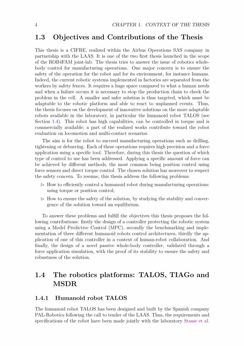
Figure 1.1: From HRP2 to TALOS.
[4], aiming to create a successor to the robot HRP-2 Kaneko et al. [5] developedby the National Institute of Advanced Industrial Science and Technology (AIST).The goal was to create a robot capable of dexterous bi-handed manipulation whichcan involve high payload, with better locomotion performances and with size andmass better suited to work in human environment. This is why TALOS is taller andheavier than HRP-2 (see Fig.1.1) and has torque and temperature sensors.
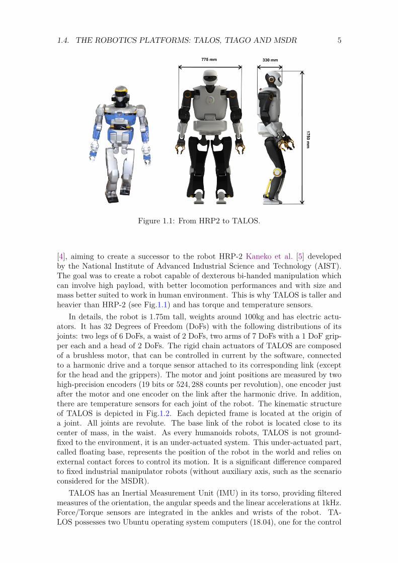
In details, the robot is 1.75m tall, weights around 100kg and has electric actu-ators. It has 32 Degrees of Freedom (DoFs) with the following distributions of itsjoints: two legs of 6 DoFs, a waist of 2 DoFs, two arms of 7 DoFs with a 1 DoF grip-per each and a head of 2 DoFs. The rigid chain actuators of TALOS are composedof a brushless motor, that can be controlled in current by the software, connectedto a harmonic drive and a torque sensor attached to its corresponding link (exceptfor the head and the grippers). The motor and joint positions are measured by twohigh-precision encoders (19 bits or 524, 288 counts per revolution), one encoder justafter the motor and one encoder on the link after the harmonic drive. In addition,there are temperature sensors for each joint of the robot. The kinematic structureof TALOS is depicted in Fig.1.2. Each depicted frame is located at the origin ofa joint. All joints are revolute. The base link of the robot is located close to itscenter of mass, in the waist. As every humanoids robots, TALOS is not ground-fixed to the environment, it is an under-actuated system. This under-actuated part,called floating base, represents the position of the robot in the world and relies onexternal contact forces to control its motion. It is a significant difference comparedto fixed industrial manipulator robots (without auxiliary axis, such as the scenarioconsidered for the MSDR).
TALOS has an Inertial Measurement Unit (IMU) in its torso, providing filteredmeasures of the orientation, the angular speeds and the linear accelerations at 1kHz.Force/Torque sensors are integrated in the ankles and wrists of the robot. TA-LOS possesses two Ubuntu operating system computers (18.04), one for the control
6 CHAPTER 1. CONTEXT OF THE THESIS
Figure 1.2: Kinematic structure of TALOS Scherrer [1]
(patched with the Linux Real-Time Preempt) and one for the vision processes. Thecontrol computer is connected to all the actuators and sensors of the robot by anEtherCAT bus [6]. It uses the middle-ware Robot Operating System (ROS) Stan-ford Artificial Intelligence Laboratory et al. [7] and reaches a control-loop frequencyof 2kHz. This high-frequency allows to obtain a quick reaction time necessary forreal time complex behaviors. Because of the ROS architecture it is possible touse MoveIt! Coleman et al. [8], Chitta et al. [9] to plan the robot motions, andthe Gazebo simulator Koenig and Howard [10] to simulate dynamically the robotTALOS. PAL-Robotics has additionally implemented a specific simulator for theirrobot which simulates its actuators dynamics.
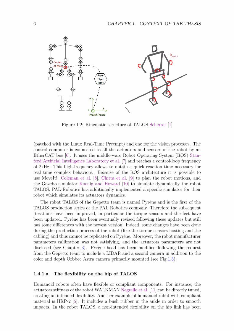
The robot TALOS of the Gepetto team is named Pyrène and is the first of theTALOS production series of the PAL Robotics company. Therefore the subsequentiterations have been improved, in particular the torque sensors and the feet havebeen updated. Pyrène has been eventually revised following these updates but stillhas some differences with the newest version. Indeed, some changes have been doneduring the production process of the robot (like the torque sensors hosting and thecabling) and thus cannot be replicated on Pyrène. Moreover, the robot manufacturerparameters calibration was not satisfying, and the actuators parameters are notdisclosed (see Chapter 3). Pyrène head has been modified following the requestfrom the Gepetto team to include a LIDAR and a second camera in addition to thecolor and depth Orbbec Astra camera primarily mounted (see Fig.1.3).
1.4.1.a The flexibility on the hip of TALOS
Humanoid robots often have flexible or compliant components. For instance, theactuators stiffness of the robot WALKMAN Negrello et al. [11] can be directly tuned,creating an intended flexibility. Another example of humanoid robot with compliantmaterial is HRP-2 [5]. It includes a bush rubber in the ankle in order to smoothimpacts. In the robot TALOS, a non-intended flexibility on the hip link has been
1.4. THE ROBOTICS PLATFORMS: TALOS, TIAGO AND MSDR 7
Figure 1.3: Pyrène head with the LIDAR and the two cameras.
observed and impacts meaningfully the control of its legs and, therefore, its balanceand locomotion. Indeed, this flexibility (not modeled in the simulator) leads toerrors in the landing positions of the feet on the real robot. However, the deflectionis not directly measurable by the encoders and cannot be directly modified. Thissubject is more detailed in the Appendix 4.
1.4.2 Wheeled Manipulator robot TIAGo
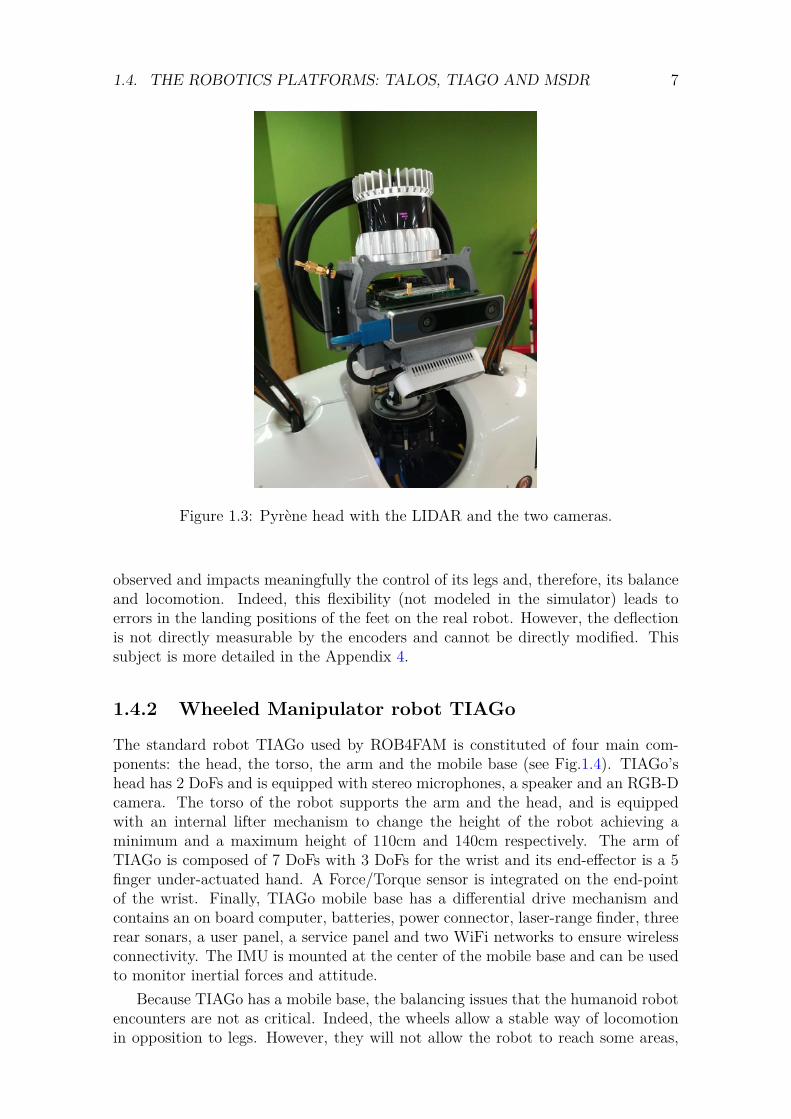
The standard robot TIAGo used by ROB4FAM is constituted of four main com-ponents: the head, the torso, the arm and the mobile base (see Fig.1.4). TIAGo’shead has 2 DoFs and is equipped with stereo microphones, a speaker and an RGB-Dcamera. The torso of the robot supports the arm and the head, and is equippedwith an internal lifter mechanism to change the height of the robot achieving aminimum and a maximum height of 110cm and 140cm respectively. The arm ofTIAGo is composed of 7 DoFs with 3 DoFs for the wrist and its end-effector is a 5finger under-actuated hand. A Force/Torque sensor is integrated on the end-pointof the wrist. Finally, TIAGo mobile base has a differential drive mechanism andcontains an on board computer, batteries, power connector, laser-range finder, threerear sonars, a user panel, a service panel and two WiFi networks to ensure wirelessconnectivity. The IMU is mounted at the center of the mobile base and can be usedto monitor inertial forces and attitude.
Because TIAGo has a mobile base, the balancing issues that the humanoid robotencounters are not as critical. Indeed, the wheels allow a stable way of locomotionin opposition to legs. However, they will not allow the robot to reach some areas,
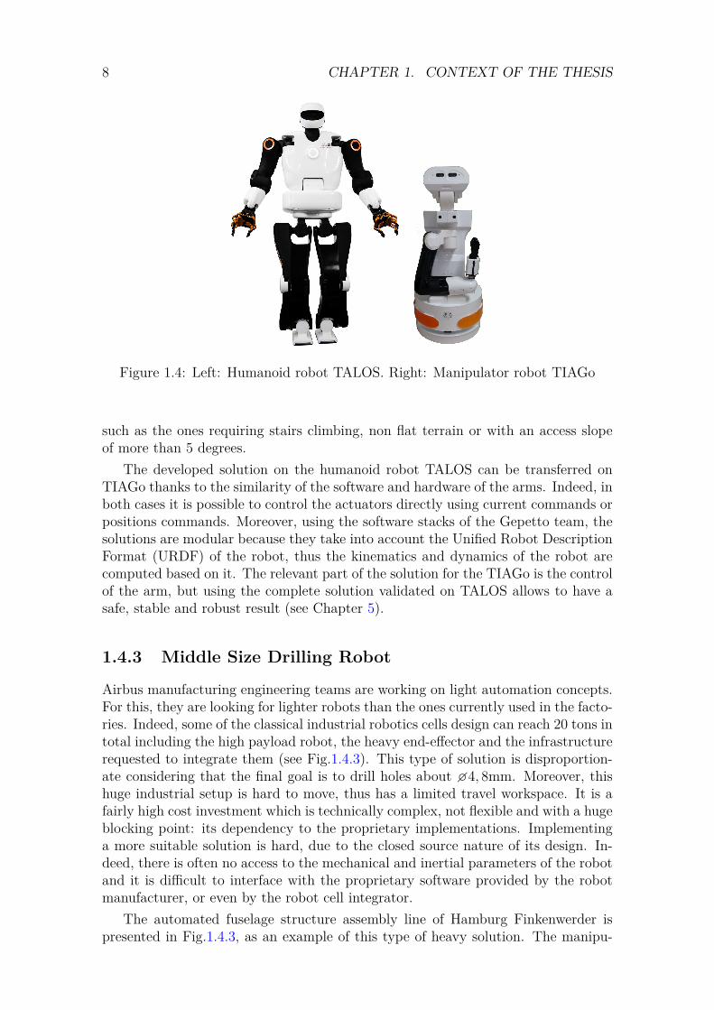
8 CHAPTER 1. CONTEXT OF THE THESIS
Figure 1.4: Left: Humanoid robot TALOS. Right: Manipulator robot TIAGo
such as the ones requiring stairs climbing, non flat terrain or with an access slopeof more than 5 degrees.
The developed solution on the humanoid robot TALOS can be transferred onTIAGo thanks to the similarity of the software and hardware of the arms. Indeed, inboth cases it is possible to control the actuators directly using current commands orpositions commands. Moreover, using the software stacks of the Gepetto team, thesolutions are modular because they take into account the Unified Robot DescriptionFormat (URDF) of the robot, thus the kinematics and dynamics of the robot arecomputed based on it. The relevant part of the solution for the TIAGo is the controlof the arm, but using the complete solution validated on TALOS allows to have asafe, stable and robust result (see Chapter 5).
1.4.3 Middle Size Drilling Robot
Airbus manufacturing engineering teams are working on light automation concepts.For this, they are looking for lighter robots than the ones currently used in the facto-ries. Indeed, some of the classical industrial robotics cells design can reach 20 tons intotal including the high payload robot, the heavy end-effector and the infrastructurerequested to integrate them (see Fig.1.4.3). This type of solution is disproportion-ate considering that the final goal is to drill holes about �4, 8mm. Moreover, thishuge industrial setup is hard to move, thus has a limited travel workspace. It is afairly high cost investment which is technically complex, not flexible and with a hugeblocking point: its dependency to the proprietary implementations. Implementinga more suitable solution is hard, due to the closed source nature of its design. In-deed, there is often no access to the mechanical and inertial parameters of the robotand it is difficult to interface with the proprietary software provided by the robotmanufacturer, or even by the robot cell integrator.
The automated fuselage structure assembly line of Hamburg Finkenwerder ispresented in Fig.1.4.3, as an example of this type of heavy solution. The manipu-
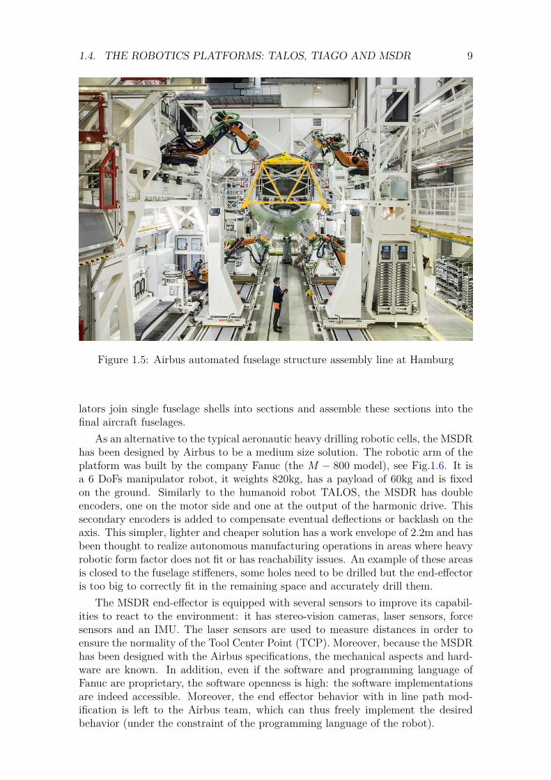
1.4. THE ROBOTICS PLATFORMS: TALOS, TIAGO AND MSDR 9
Figure 1.5: Airbus automated fuselage structure assembly line at Hamburg
lators join single fuselage shells into sections and assemble these sections into thefinal aircraft fuselages.
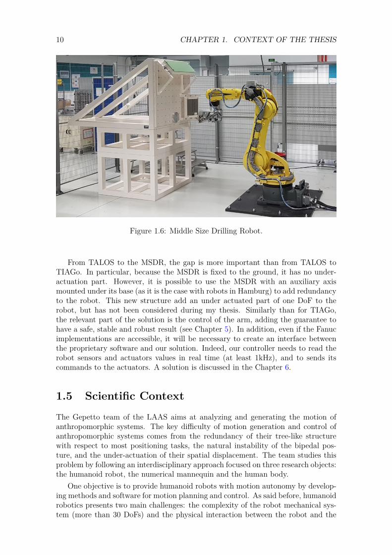
As an alternative to the typical aeronautic heavy drilling robotic cells, the MSDRhas been designed by Airbus to be a medium size solution. The robotic arm of theplatform was built by the company Fanuc (the M − 800 model), see Fig.1.6. It isa 6 DoFs manipulator robot, it weights 820kg, has a payload of 60kg and is fixedon the ground. Similarly to the humanoid robot TALOS, the MSDR has doubleencoders, one on the motor side and one at the output of the harmonic drive. Thissecondary encoders is added to compensate eventual deflections or backlash on theaxis. This simpler, lighter and cheaper solution has a work envelope of 2.2m and hasbeen thought to realize autonomous manufacturing operations in areas where heavyrobotic form factor does not fit or has reachability issues. An example of these areasis closed to the fuselage stiffeners, some holes need to be drilled but the end-effectoris too big to correctly fit in the remaining space and accurately drill them.
The MSDR end-effector is equipped with several sensors to improve its capabil-ities to react to the environment: it has stereo-vision cameras, laser sensors, forcesensors and an IMU. The laser sensors are used to measure distances in order toensure the normality of the Tool Center Point (TCP). Moreover, because the MSDRhas been designed with the Airbus specifications, the mechanical aspects and hard-ware are known. In addition, even if the software and programming language ofFanuc are proprietary, the software openness is high: the software implementationsare indeed accessible. Moreover, the end effector behavior with in line path mod-ification is left to the Airbus team, which can thus freely implement the desiredbehavior (under the constraint of the programming language of the robot).
10 CHAPTER 1. CONTEXT OF THE THESIS
Figure 1.6: Middle Size Drilling Robot.
From TALOS to the MSDR, the gap is more important than from TALOS toTIAGo. In particular, because the MSDR is fixed to the ground, it has no under-actuation part. However, it is possible to use the MSDR with an auxiliary axismounted under its base (as it is the case with robots in Hamburg) to add redundancyto the robot. This new structure add an under actuated part of one DoF to therobot, but has not been considered during my thesis. Similarly than for TIAGo,the relevant part of the solution is the control of the arm, adding the guarantee tohave a safe, stable and robust result (see Chapter 5). In addition, even if the Fanucimplementations are accessible, it will be necessary to create an interface betweenthe proprietary software and our solution. Indeed, our controller needs to read therobot sensors and actuators values in real time (at least 1kHz), and to sends itscommands to the actuators. A solution is discussed in the Chapter 6.
1.5 Scientific Context
The Gepetto team of the LAAS aims at analyzing and generating the motion ofanthropomorphic systems. The key difficulty of motion generation and control ofanthropomorphic systems comes from the redundancy of their tree-like structurewith respect to most positioning tasks, the natural instability of the bipedal pos-ture, and the under-actuation of their spatial displacement. The team studies thisproblem by following an interdisciplinary approach focused on three research objects:the humanoid robot, the numerical mannequin and the human body.
One objective is to provide humanoid robots with motion autonomy by develop-ing methods and software for motion planning and control. As said before, humanoidrobotics presents two main challenges: the complexity of the robot mechanical sys-tem (more than 30 DoFs) and the physical interaction between the robot and the
1.5. SCIENTIFIC CONTEXT 11
real world.The research activities of the Gepetto team can be described in three levels:� The fundamental research level concerns theoretical developments related to
system modeling and motion generation. The modeling part includes the me-chanics of robotics systems, the mathematics of new representations and op-erators, and the recording and analysis of the human motion. The motiongeneration part ranges from the global trajectory planning to the local move-ment control (considered under different kinds of constraints).
� The integration level integrates the theoretical developments in software pack-ages. These ones are maintained and made accessible to the whole roboticscommunity (using standard formats and tools, see Section 1.6).
� The application level concerns the contribution to different domains such asassistive robotics, industrial robotics (specifically the factory of the future),actuator design, human movement imitation and understanding.
My thesis is part of the motion generation research studies of the team and inparticular the control stage. For a given mission and a given robot, a control vectorhas to be computed and sent to the robot motors in a timely manner. This problemis in general complex. More precisely, considering the problem of moving to find anobject in an unknown environment is NP −hard Boyd and Vandenberghe [12]. TheROB4FAM joint-lab focuses on the following operational challenges:
� Climbing stairs with an heavy handled tool (designed for humans)� Manufacturing tasks applied on a real structure such as drilling or screwing
Climbing stairs imposes to switch from one contact to another in order to makethe humanoid robot TALOS move while handling an heavy object. This impliestaking into account balance with multiple contacts, the geometry and the dynamicaleffect of the tool to handle. The robot has to take into account possible driftdue to contact slip, spring back effect from the material part and vibrations whenperforming the tasks. On the other hand, drilling and screwing mostly involve wholebody motion to perform a force control based behavior.
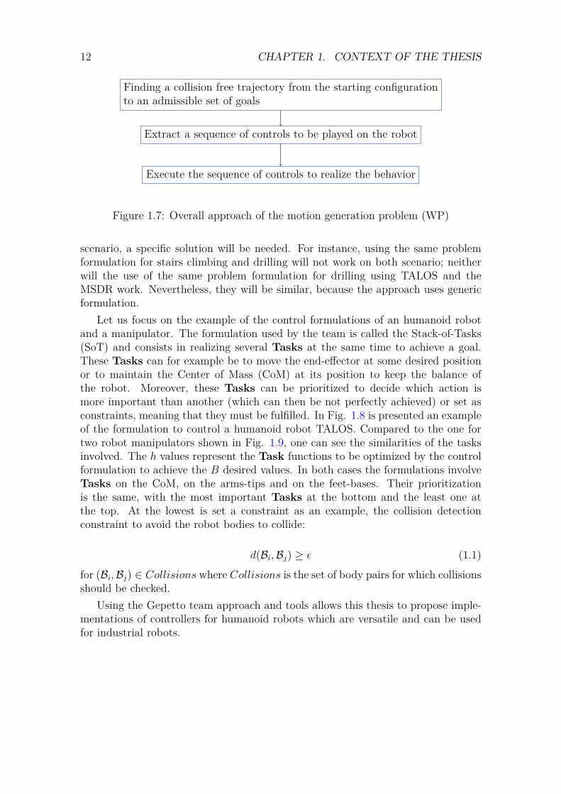
In order to produce a feasible motion, the robot has to decide where to interactwith the environment to be able to move and perform its actions. Consideringthe climbing case, the robot has to locate where to put its feet and possibly itshand. Once this is decided, it needs to find a feasible motion for each of its bodiesto generate the overall motion. When a feasible solution is found (i.e. avoidingcollision, joint limits, ...) this solution needs to be executed on the robot. Thisis usually not trivial as discrepancies between the model and reality will affect theresult. It is therefore necessary to modify these motions and to create a final controlcommand for the robot in order to make sure that the plan is followed.
These three stages: global trajectory planning, local planning for control, controlof the robot (illustrated in Fig. 1.7) are the ones considered by the Gepetto teamto realize motion generation.
This approach is generic and allows to formulate solutions for different robotsand scenarios. However, the way the problem is solved is dependant on the robotand the scenario, meaning that a solution cannot be reused on a different robot or
12 CHAPTER 1. CONTEXT OF THE THESIS
Finding a collision free trajectory from the starting configurationto an admissible set of goals
Extract a sequence of controls to be played on the robot
Execute the sequence of controls to realize the behavior
Figure 1.7: Overall approach of the motion generation problem (WP)
scenario, a specific solution will be needed. For instance, using the same problemformulation for stairs climbing and drilling will not work on both scenario; neitherwill the use of the same problem formulation for drilling using TALOS and theMSDR work. Nevertheless, they will be similar, because the approach uses genericformulation.
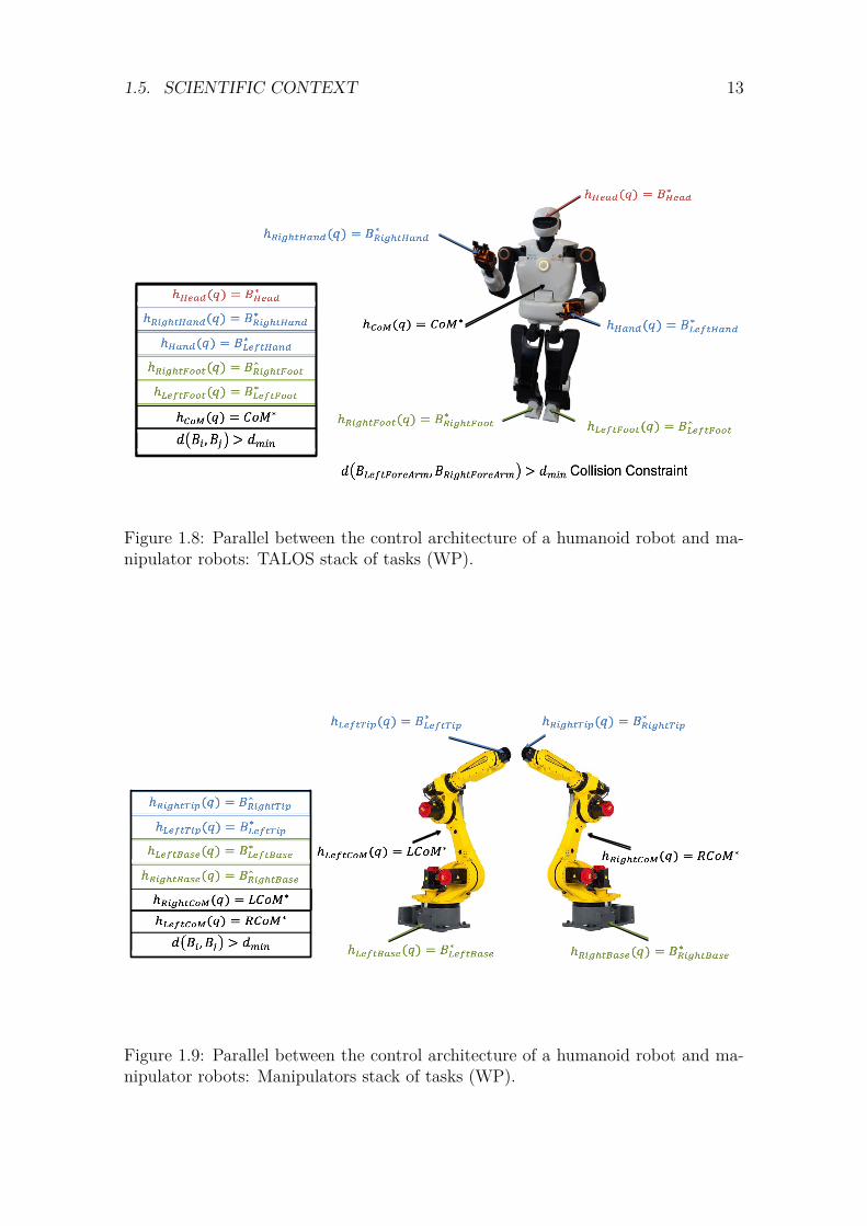
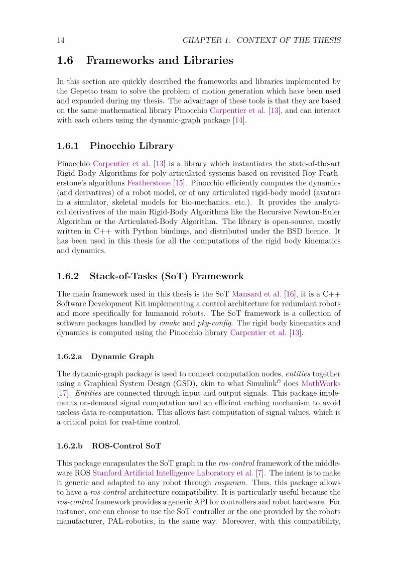
Let us focus on the example of the control formulations of an humanoid robotand a manipulator. The formulation used by the team is called the Stack-of-Tasks(SoT) and consists in realizing several Tasks at the same time to achieve a goal.These Tasks can for example be to move the end-effector at some desired positionor to maintain the Center of Mass (CoM) at its position to keep the balance ofthe robot. Moreover, these Tasks can be prioritized to decide which action ismore important than another (which can then be not perfectly achieved) or set asconstraints, meaning that they must be fulfilled. In Fig. 1.8 is presented an exampleof the formulation to control a humanoid robot TALOS. Compared to the one fortwo robot manipulators shown in Fig. 1.9, one can see the similarities of the tasksinvolved. The h values represent the Task functions to be optimized by the controlformulation to achieve the B desired values. In both cases the formulations involveTasks on the CoM, on the arms-tips and on the feet-bases. Their prioritizationis the same, with the most important Tasks at the bottom and the least one atthe top. At the lowest is set a constraint as an example, the collision detectionconstraint to avoid the robot bodies to collide:
d(Bi,Bj) ≥ ε (1.1)
for (Bi,Bj) ∈ Collisions where Collisions is the set of body pairs for which collisionsshould be checked.
Using the Gepetto team approach and tools allows this thesis to propose imple-mentations of controllers for humanoid robots which are versatile and can be usedfor industrial robots.
1.5. SCIENTIFIC CONTEXT 13
Figure 1.8: Parallel between the control architecture of a humanoid robot and ma-nipulator robots: TALOS stack of tasks (WP).
Figure 1.9: Parallel between the control architecture of a humanoid robot and ma-nipulator robots: Manipulators stack of tasks (WP).
14 CHAPTER 1. CONTEXT OF THE THESIS
1.6 Frameworks and Libraries
In this section are quickly described the frameworks and libraries implemented bythe Gepetto team to solve the problem of motion generation which have been usedand expanded during my thesis. The advantage of these tools is that they are basedon the same mathematical library Pinocchio Carpentier et al. [13], and can interactwith each others using the dynamic-graph package [14].
1.6.1 Pinocchio Library
Pinocchio Carpentier et al. [13] is a library which instantiates the state-of-the-artRigid Body Algorithms for poly-articulated systems based on revisited Roy Feath-erstone’s algorithms Featherstone [15]. Pinocchio efficiently computes the dynamics(and derivatives) of a robot model, or of any articulated rigid-body model (avatarsin a simulator, skeletal models for bio-mechanics, etc.). It provides the analyti-cal derivatives of the main Rigid-Body Algorithms like the Recursive Newton-EulerAlgorithm or the Articulated-Body Algorithm. The library is open-source, mostlywritten in C++ with Python bindings, and distributed under the BSD licence. Ithas been used in this thesis for all the computations of the rigid body kinematicsand dynamics.
1.6.2 Stack-of-Tasks (SoT) Framework
The main framework used in this thesis is the SoT Mansard et al. [16], it is a C++Software Development Kit implementing a control architecture for redundant robotsand more specifically for humanoid robots. The SoT framework is a collection ofsoftware packages handled by cmake and pkg-config. The rigid body kinematics anddynamics is computed using the Pinocchio library Carpentier et al. [13].
1.6.2.a Dynamic Graph
The dynamic-graph package is used to connect computation nodes, entities togetherusing a Graphical System Design (GSD), akin to what Simulink© does MathWorks[17]. Entities are connected through input and output signals. This package imple-ments on-demand signal computation and an efficient caching mechanism to avoiduseless data re-computation. This allows fast computation of signal values, which isa critical point for real-time control.
1.6.2.b ROS-Control SoT
This package encapsulates the SoT graph in the ros-control framework of the middle-ware ROS Stanford Artificial Intelligence Laboratory et al. [7]. The intent is to makeit generic and adapted to any robot through rosparam. Thus, this package allowsto have a ros-control architecture compatibility. It is particularly useful because theros-control framework provides a generic API for controllers and robot hardware. Forinstance, one can choose to use the SoT controller or the one provided by the robotsmanufacturer, PAL-robotics, in the same way. Moreover, with this compatibility,

1.6. FRAMEWORKS AND LIBRARIES 15
Figure 1.10: ROS-Control framework with the ROS-Control SoT interface
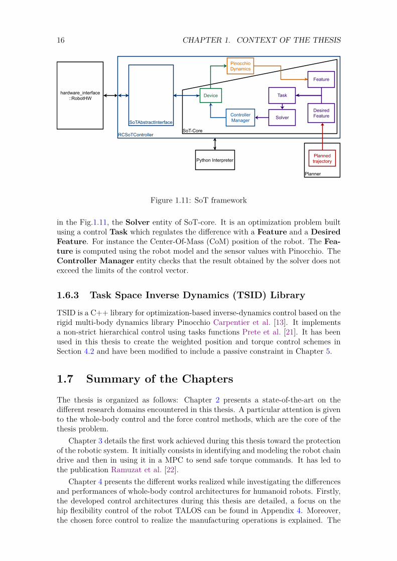
it is possible to use the Gazebo simulator of ros-control. The software developedfor the real robot can then be tested in simulation with the same architecture.However, one issue of the generic ROS API is highlighted when specific componentsare used in the robot hardware. Indeed, if the actuators have specific sensors, suchas temperature ones as the robot TALOS does, it is not handled by the architecture.Thus, the roscontrol-sot package [18] has been modified to take these sensors intoaccount. This package is represented by the dark blue blocks in the SoT Frameworkscheme of Figure.1.11. It creates an abstract interface to communicate with thehardware interface of ros-control, its integration in the whole ros-control frameworkis displayed in Fig.1.10 in purple, based on [19].
1.6.2.c SoT Core
SoT-core [20] is the package in charge of the control architecture. The package im-plements hierarchical control using the task-based inverse kinematics described inMansard et al. [16] (see Section 4.2). The robots can be loaded from their URDFmodel. The rigid body dynamics is provided through the Pinocchio library Car-pentier et al. [13]. It has been used in this thesis to compare hierarchical positioncontrol to weighted position and torque control in Section 4.2.
1.6.2.d Overall scheme for real-time control
In the Fig.1.11 is presented the general SoT flow chart, where the SoT-Core purpleblocks can be replaced by another task-based controller (for instance a controllerusing TSID) and the Planner block can be any planning algorithm giving theappropriate references. Real-time control system are usually driven by a cyclic com-putational node which needs to send a control reference value to each motors of arobot. To compute this control reference values, sensor values need to be provided.In the SoT, special entities called Device are used to provide an abstract interfaceto the hardware. The Device has specific inputs which contains the control vec-tor. This control vector is the result of a computation solving a control problem,
16 CHAPTER 1. CONTEXT OF THE THESIS
RCSoTControllerSoT-Core
hardware_interface::RobotHW
SoTAbstractInterface
Device
PinocchioDynamics
Feature
Solver
Task
DesiredFeature
Python Interpreter
Planner
Plannedtrajectory
ControllerManager
Figure 1.11: SoT framework
in the Fig.1.11, the Solver entity of SoT-core. It is an optimization problem builtusing a control Task which regulates the difference with a Feature and a DesiredFeature. For instance the Center-Of-Mass (CoM) position of the robot. The Fea-ture is computed using the robot model and the sensor values with Pinocchio. TheController Manager entity checks that the result obtained by the solver does notexceed the limits of the control vector.
1.6.3 Task Space Inverse Dynamics (TSID) Library
TSID is a C++ library for optimization-based inverse-dynamics control based on therigid multi-body dynamics library Pinocchio Carpentier et al. [13]. It implementsa non-strict hierarchical control using tasks functions Prete et al. [21]. It has beenused in this thesis to create the weighted position and torque control schemes inSection 4.2 and have been modified to include a passive constraint in Chapter 5.
1.7 Summary of the Chapters
The thesis is organized as follows: Chapter 2 presents a state-of-the-art on thedifferent research domains encountered in this thesis. A particular attention is givento the whole-body control and the force control methods, which are the core of thethesis problem.
Chapter 3 details the first work achieved during this thesis toward the protectionof the robotic system. It initially consists in identifying and modeling the robot chaindrive and then in using it in a MPC to send safe torque commands. It has led tothe publication Ramuzat et al. [22].
Chapter 4 presents the different works realized while investigating the differencesand performances of whole-body control architectures for humanoid robots. Firstly,the developed control architectures during this thesis are detailed, a focus on thehip flexibility control of the robot TALOS can be found in Appendix 4. Moreover,the chosen force control to realize the manufacturing operations is explained. The
1.8. PUBLICATIONS 17
targeted application is the drilling of a metal plate, requiring high precision and theapplication of huge forces.
Secondly, three controllers are compared: one solving torque commands and twoposition commands. The aim is to choose the most appropriate scheme for therobot TALOS, these controllers are compared in terms of tracking error, energyconsumption and computational time by using Gazebo simulations of the robotwalking on flat horizontal ground, tilted platforms, and stairs. This work has led tothe publication Ramuzat et al. [23].
Thirdly, the efficiency of the previous whole-body torque controller is exposed ina context of human-robot collaboration. The goal is to make the robot proactivelywalk alongside a human. The results have been obtained during a collaboration withanother PhD student of the Gepetto team, Isabelle Maroger and have been publishedin Maroger et al. [24]. This work combines an optimal control prediction model ofthe human trajectory, a Walking Pattern Generator (WPG) based on non-linearMPC and the previous real-time whole-body torque controller.
Finally, the last section describes the experiments realized on the real robot, usingthe presented controllers. This section discusses the different difficulties encounteredand the approaches we tried to implement to solve them, leading to the publicationRamuzat et al. [25].
Chapter 5 details the second work realized during this thesis toward the safetyof the robotic system. It describes a new passivity-based inverse dynamics (ID)controller, based on the torque controller of Chapter 4 and the passivity theory.The control approach allows to achieve a safe multi-contact scenario on a torquecontrolled humanoid robot, using a global energy tank. This work has led to thepublication Ramuzat et al. [26].
Chapter 6 describes the expected challenges that will be encountered when trans-posing the obtained results from the TALOS robot to the MSDR or another indus-trial robot. It highlights the benefits and drawbacks of my complex and state-of-the-art solution compared to the classical proposal for manipulator robots.
Finally the last chapter presents the conclusions of my works and the perspectivesand future aims.
1.8 Publications
Journal
Maroger et al. [24] I. Maroger, N. Ramuzat, O. Stasse and B. Watier, "HumanTrajectory Prediction Model and Its Coupling With a Walking Pattern Generatorof a Humanoid Robot". In IEEE Robotics and Automation Letters with IEEE/RSJInternational Conference on Intelligent Robots and Systems (IROS) option, October2021, vol. 6, no. 4, pp. 6361-6369.
Ramuzat et al. [25] N. Ramuzat, O. Stasse and S. Boria, "Benchmarking WholeBody controllers on TALOS". In Frontiers Robotics and AI, January 2022.
Ramuzat et al. [26] N. Ramuzat, S. Boria and O. Stasse, "Passive Inverse Dynam-ics Control using a Global Energy Tank for Torque-Controlled Humanoid Robots
18 CHAPTER 1. CONTEXT OF THE THESIS
in Multi-Contact". In IEEE Robotics and Automation Letters with IEEE/RAS Int.Conf. on Robotics and Automation (ICRA) option, April 2022, vol. 7, no. 2, pp.2787-2794.
Conference
Ramuzat et al. [22] N. Ramuzat, F. Forget, V. Bonnet, M. Gautier, S. Boria andO. Stasse, "Actuator Model, Identification and Differential Dynamic Programmingfor a TALOS Humanoid Robot". In IFAC - 2020 European Control Conference(ECC), May 2020, pp. 724-730.
Ramuzat et al. [23] N. Ramuzat, G. Buondonno, S. Boria and O. Stasse, "Com-parison of Position and Torque Whole Body Control Schemes on the HumanoidRobot TALOS". In 20th International Conference on Advanced Robotics (ICAR),December 2021, pp. 785-792.
Chapter 2
State of the Art
Contents2.1 Humanoid Robot Model . . . . . . . . . . . . . . . . . . . 21
2.1.1 Robot Model . . . . . . . . . . . . . . . . . . . . . . . . . 212.1.2 Contacts properties . . . . . . . . . . . . . . . . . . . . . 232.1.3 Task Space and Workspace . . . . . . . . . . . . . . . . . 24
2.2 Centroidal Dynamics . . . . . . . . . . . . . . . . . . . . . 252.2.1 Zero Moment Point . . . . . . . . . . . . . . . . . . . . . 262.2.2 Linear Inverted Pendulum Model . . . . . . . . . . . . . . 262.2.3 Equilibrium Criteria . . . . . . . . . . . . . . . . . . . . . 28
2.2.3.a Divergent Component of Motion . . . . . . . . . 282.2.3.b CoM Admittance Control . . . . . . . . . . . . . 29
2.2.4 Angular Momentum . . . . . . . . . . . . . . . . . . . . . 302.3 Actuator Model . . . . . . . . . . . . . . . . . . . . . . . . 30
2.3.1 General formulation . . . . . . . . . . . . . . . . . . . . . 312.3.2 Friction . . . . . . . . . . . . . . . . . . . . . . . . . . . . 312.3.3 Parameters Identification . . . . . . . . . . . . . . . . . . 312.3.4 Actuator Control . . . . . . . . . . . . . . . . . . . . . . . 32
2.3.4.a Position control . . . . . . . . . . . . . . . . . . 322.3.4.b Torque control . . . . . . . . . . . . . . . . . . . 33
2.4 Motion and Locomotion Planning . . . . . . . . . . . . . 332.4.1 Walking Pattern Generator . . . . . . . . . . . . . . . . . 332.4.2 Multicontact-locomotion-planning . . . . . . . . . . . . . 35
2.5 Real-time Whole Body Control . . . . . . . . . . . . . . . 372.5.1 Introduction . . . . . . . . . . . . . . . . . . . . . . . . . 372.5.2 Whole-body controller . . . . . . . . . . . . . . . . . . . . 37
2.5.2.a Introduction: Task Function . . . . . . . . . . . 372.5.2.b QP Formulation: Task space velocity or acceler-
ation control . . . . . . . . . . . . . . . . . . . . 38
19

20 CHAPTER 2. STATE OF THE ART
2.5.2.c HQP and Weighted Sum . . . . . . . . . . . . . 422.5.3 Recent Humanoid Robots Whole Body Controllers . . . . 45
2.6 Stability Analysis: Convergence toward an equilibrium 482.6.1 Introduction . . . . . . . . . . . . . . . . . . . . . . . . . 482.6.2 Lyapunov Theory . . . . . . . . . . . . . . . . . . . . . . . 482.6.3 Passivity Theory . . . . . . . . . . . . . . . . . . . . . . . 49
2.6.3.a Definition . . . . . . . . . . . . . . . . . . . . . . 492.6.3.b Analysis of a robotic system . . . . . . . . . . . 512.6.3.c Energy Tank . . . . . . . . . . . . . . . . . . . . 512.6.3.d State-of-the-art . . . . . . . . . . . . . . . . . . . 52
2.7 Force Control for Manipulation . . . . . . . . . . . . . . . 532.7.1 Introduction . . . . . . . . . . . . . . . . . . . . . . . . . 532.7.2 Admittance Control . . . . . . . . . . . . . . . . . . . . . 552.7.3 Impedance Control . . . . . . . . . . . . . . . . . . . . . . 562.7.4 Stiffness/Compliance Control . . . . . . . . . . . . . . . . 572.7.5 Hybrid Control . . . . . . . . . . . . . . . . . . . . . . . . 582.7.6 Parallel Control . . . . . . . . . . . . . . . . . . . . . . . . 60
2.8 Model Predictive Control . . . . . . . . . . . . . . . . . . 612.8.1 Differential Dynamics Programming Formulation . . . . . 62
2.9 Learning approach . . . . . . . . . . . . . . . . . . . . . . . 642.10 Human-Robot Collaboration . . . . . . . . . . . . . . . . . 64
2.10.1 Proactive human-robot interactions . . . . . . . . . . . . 652.10.2 Human trajectories during gait . . . . . . . . . . . . . . . 65
In this chapter, some parts of the state-of-the-art presented were elements ofthe works realized for the Work-Package (WP) reports in the scope of the joint-laboratory ROB4FAM. Some of the figures presented are thus indicated of part ofthese reports (WP). The presented section on human-robot collaboration is part of thepaper [24] realized in collaboration with Isabelle Maroger. Moreover, Louise Scherrerhas kindly authorized us to use some of her figures from her master report Scherrer[1] to illustrate some principles and the Walking Pattern Generator of Naveau et al.[27].
2.1. HUMANOID ROBOT MODEL 21
2.1 Humanoid Robot Model
2.1.1 Robot Model
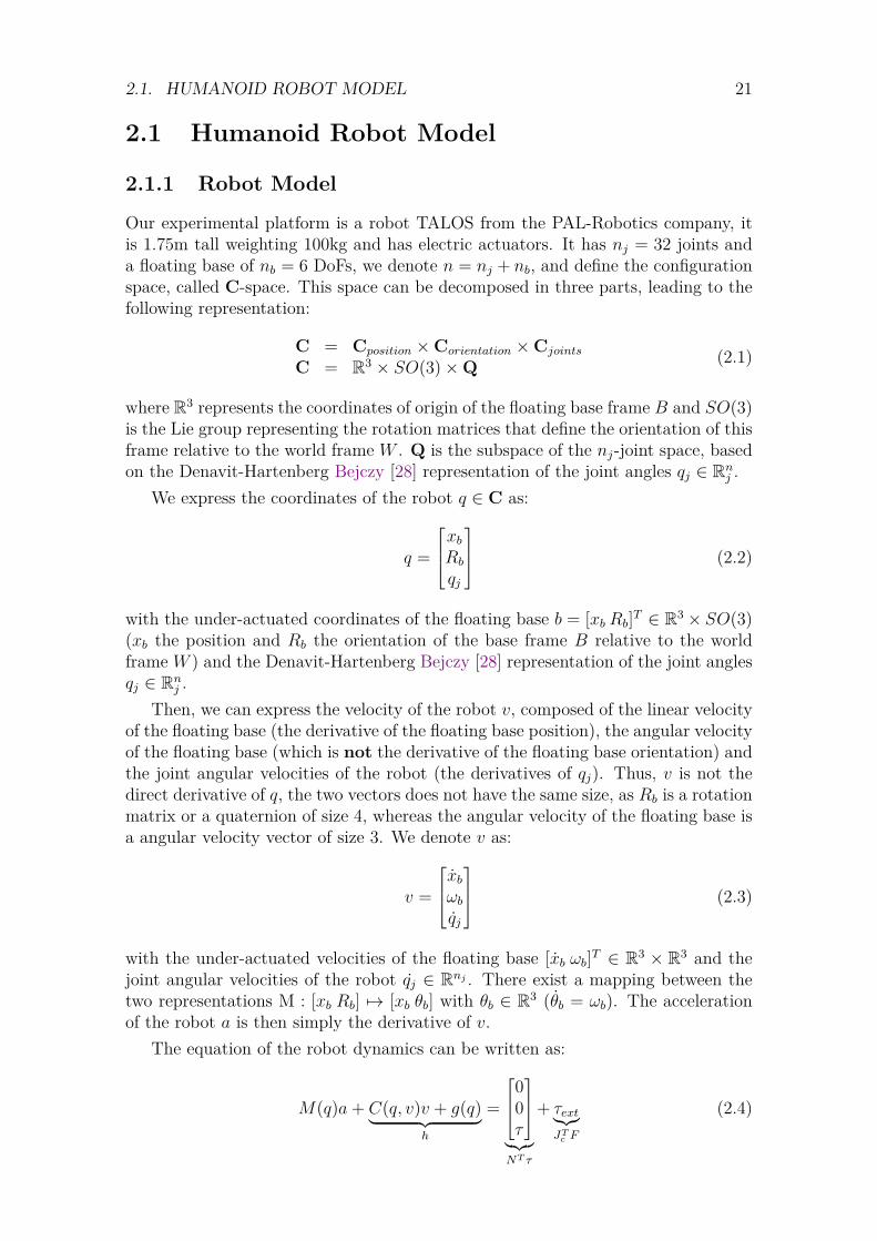
Our experimental platform is a robot TALOS from the PAL-Robotics company, itis 1.75m tall weighting 100kg and has electric actuators. It has nj = 32 joints anda floating base of nb = 6 DoFs, we denote n = nj + nb, and define the configurationspace, called C-space. This space can be decomposed in three parts, leading to thefollowing representation:
C = Cposition ×Corientation ×Cjoints
C = R3 × SO(3)×Q (2.1)
where R3 represents the coordinates of origin of the floating base frame B and SO(3)is the Lie group representing the rotation matrices that define the orientation of thisframe relative to the world frame W . Q is the subspace of the nj-joint space, basedon the Denavit-Hartenberg Bejczy [28] representation of the joint angles qj ∈ Rn
j .We express the coordinates of the robot q ∈ C as:
q =
xbRb
qj
(2.2)
with the under-actuated coordinates of the floating base b = [xb Rb]T ∈ R3 × SO(3)(xb the position and Rb the orientation of the base frame B relative to the worldframe W ) and the Denavit-Hartenberg Bejczy [28] representation of the joint anglesqj ∈ Rn
j .Then, we can express the velocity of the robot v, composed of the linear velocity
of the floating base (the derivative of the floating base position), the angular velocityof the floating base (which is not the derivative of the floating base orientation) andthe joint angular velocities of the robot (the derivatives of qj). Thus, v is not thedirect derivative of q, the two vectors does not have the same size, as Rb is a rotationmatrix or a quaternion of size 4, whereas the angular velocity of the floating base isa angular velocity vector of size 3. We denote v as:
v =
xbωbqj
(2.3)
with the under-actuated velocities of the floating base [xb ωb]T ∈ R3 × R3 and thejoint angular velocities of the robot qj ∈ Rnj . There exist a mapping between thetwo representations M : [xb Rb] 7→ [xb θb] with θb ∈ R3 (θb = ωb). The accelerationof the robot a is then simply the derivative of v.
The equation of the robot dynamics can be written as:
M(q)a+ C(q, v)v + g(q)︸ ︷︷ ︸h
=
00τ
︸︷︷︸NT τ
+ τext︸︷︷︸JTc F
(2.4)
22 CHAPTER 2. STATE OF THE ART
M ∈ Rn×n the symmetric and positive definite inertia matrix, C ∈ Rn×n the Coriolismatrix and g ∈ Rn the gravity vector. qj ∈ Rnj is the joint configuration of the robot.a, v, q ∈ Rn are the accelerations, velocities and positions of the joint configurationof the robot including the base (free-flyer). The free-flyer information are estimatedwith a base-estimator from the configuration, IMU and force sensors of the robot(we use in the thesis the one persented in Flayols et al. [29]). τ ∈ Rnj are the jointtorques of the actuators and τext ∈ Rn are the external torques. N is a selectormatrix associated to the actuated joints N = [0nb , 1nj ], such that NT ∈ Rn×nj .
A notable property of the dynamic model is that the choice for the Coriolismatrix C is not unique. A particular choice is to define this matrix such that:12M(q) = C(q, v) + C(q, v)T
2 Siciliano et al. [2]. Indeed, with this formulation, thematrix M(q)− 2C(q, v) is skew-symmetric, thus their quadratic form is null, i.e. forany vector x ∈ Rn:
xT [M(q)− 2C(q, v)]x = 0 (2.5)
It is an important property that is often used for simplifications.Using the force contacts F , we can write that τext = JTc F = ∑nc
i=1 JTi Fi with nc
the number of contacts and Ji the Jacobian of the contact point xic (with the contactframe Vi) according to the robot coordinate vector q:
Ji = [J iu J ia]
=[T (Vi, B) ∂xic
∂qj
] (2.6)
where J iu is the "Jacobian" of the under-actuated part: it is the transformation Tbetween the contact frame and the base frame Siciliano et al. [2]. And J ia is theclassical Jacobian of the actuated part.
By denoting qj, qj the velocity and acceleration of the joints and xb, ωb the linearand angular velocities of the floating base frame we can decompose Eq.2.4, to haveHenze et al. [30]:
M(q)
xbωbqj
︸ ︷︷ ︸a
+ C(q, v)
xbωbqj
︸ ︷︷ ︸v
+ g(q) = NT τ + τext (2.7)
If all the external forces act at the end-effector frames Vi with i = 1...ψ, with ψthe number of end-effector frames, then we can write:
τext =ψ∑i=1
[I 0xbi I
]J iTa
Fi (2.8)
with J ia the actuated Jacobian matrix of the end-effector i making the contact pointxi (see Eq.2.6), Fi = [fTi τTi ]T the effector wrench. xbi is the cross-product matrixof the vector xbi = xi− xb: the configuration-dependent lever arm between the end-effector frame Vi and the base frame B (defining Ju = T (Vi, B) the transformationof Eq.2.6).
2.1. HUMANOID ROBOT MODEL 23
For balancing it is interesting to replace the floating base frame by the CoM onewhich has the same orientation as the base link. The equations are similar withc, wcom, xcom,i instead of xb, ωb, xbi and using the transformation matrix T: c
ωcomqj
=
I −xb,com Jb,com0 I 00 0 I
︸ ︷︷ ︸
T
xbωbqj
(2.9)
We obtain the following simplified equation Wieber et al. [31], denoting vcom =[cT ωTcom]T :
M
[vcomqj
]+ C
[vcomqj
]+[m g0
0
]=[0τ
]+ τext (2.10)
We have M(q) ∈ R(nj+nb)× (nj+nb), C(q, v) ∈ R(nj+nb)× (nj+nb), τ ∈ Rnj and τext ∈R(nj+nb). Here one can notice that the gravity vector g is projected as the robotweight in its base frame. It is a major difference compared to fixed based robotswhere this simplification is not possible.
2.1.2 Contacts properties
Using friction model of Coulomb Kajita et al. [32], the slippage is avoided whenHenze et al. [30], Ramos et al. [33]:
‖ f‖ ‖ ≤ µ |f⊥| (2.11)
with f‖ and f⊥ the tangential and normal components of the contact forces (in ourcase for each of the ith end-effector). µ is the coefficient of friction, an empiricalproperty of the contacting materials. Similarly a constraint can be added on thetorque to limit the friction:
‖ τ‖ ‖ ≤ µ |τ⊥| (2.12)To avoid the interpenetration of the end-effector and the surface at the contactpoints xc (for instance between the foot and the ground) the Signorini conditionshave to be met, called the complementarity constraints:
f⊥ ≥ 0xc⊥ ≥ 0
xc⊥ f⊥ = 0(2.13)
These equations can be simplified by fulfilling the condition of positivity to guaranteethe contact:
f⊥ ≥ fmin⊥ xc⊥ = 0⇐⇒
fmin⊥ ≥ 0 Jc a+ Jc v = 0(2.14)
because xc⊥ = Jc v, with Jc the Jacobian matrix of the contact point xc (as definedin Eq.2.6).
Finally to prevent the end-effector from tilting, the Center of Pressure (CoP)p ∈ R3, can be restricted as follow to lie in the contact surface:
p⊥ ∈[pmin⊥ , pmax⊥
](2.15)
24 CHAPTER 2. STATE OF THE ART
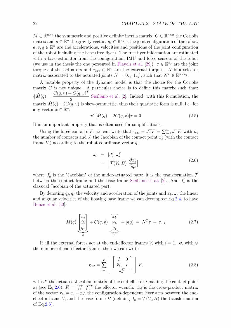
p1
f1,zp2
f2,z
c f1,y
f1,z
f1,x
f1
p1
Figure 2.1: (left) The HRP-2 humanoid robot walking on a non-flat terrain. Oneach contact pi a wrench (fi, τi) is applied. For sake of clarity all the componentsare not represented. This figure is part of the WP reports.(right) A graphical representation of the Coulomb Friction constraint applied to theright foot of the humanoid robot with f1 = [f1,x f1,y f1,z]T and µf 2
1,z > f 21,x + f 2
1,y(Eq.2.11).
These constraints define the allowed force at the contact points, which representsa friction cone defined by an axis along the surface normal and a semi-angle θ =arctanµ (see Fic.2.1 for an illustration of the friction cone).
2.1.3 Task Space and Workspace
It is common to distinguish two spaces from the configuration space of the robot(C-space linked to q). These spaces are denoted the task space and theworkspace(usually defined for the end-effectors of the robot).
The task space is a space in which a task performed by the robot can be naturallyexpressed. For instance, to control the 3D position of the CoM of the robot, the taskspace would be R3. However, if one want to control the posture of the robot (thepositions of each joint angles), then the task space corresponds to the configurationspace. The task space is linked to the configuration space with the Jacobian matrixassociated to the task Orin et al. [34]. One can switch between one space to anotherusing the relation: x = Jaqj where x is the task point position in the task space,qj the velocities of the joint configuration and Ja the Jacobian of the task pointaccording to the robot state vector Ja = ∂x
∂q. Using the Eq.2.6, we can also define
the relation x = Jv with v the velocity vector of the robot including its floatingbase.
The workspace defines the reachability space of the robot, i.e the set of configu-rations reachable by the robot end-effectors. This definition is independent of anytask and is characterized by the robot structure.
A point in the task space or in the workspace may be achievable by more than one
2.2. CENTROIDAL DYNAMICS 25
robot configuration, meaning that the point is not a full specification of the robot’sconfiguration. Conversely, some points in the task space may not be reachable atall by the robot. By definition, however, all points in the workspace are reachableby at least one configuration of the robot Lynch and Park [35].
In this thesis, we use and focus on solutions designing the desired motions ofthe robot in the task spaces rather than in the configuration one. This approachis called the task-function approach Khatib [36], Samson et al. [37], Escande et al.[38]. The objectives to be performed by the robot are expressed in their respectivetask spaces, using reference trajectories given by the motion planning (for instancethe CoM, end-effectors, feet or head desired trajectories). The planning algorithmcomputes references respecting the reachability space of the robot.
2.2 Centroidal Dynamics
The under-actuated part of the whole-body dynamics of a robot is called the cen-troidal dynamics, that is the dynamics of the CoM. It is possible to project theentire robot dynamics on it. Considering the robot as a rigid body, one can usethe Newton-Euler equations of motion to couple the variations of the centroidalmomentum with the contact forces Orin et al. [34] (using Eq.2.10):{
mc = ∑i fi +mg = lc
mc×(c− g) + L = ∑i(pi − ci)× fi + τi = kc
(2.16)
with c, c, c the CoM position, velocity and acceleration, L = ∑k[RkIkwk −
Rk(Ikwk)×wk] and g = [0, 0, −9.81]T , where Rk ∈ SO(3) is the rotation matrixbetween the kth body frame and the inertial coordinate frame, Ik its inertial matrix,wk its angular velocity, m is the mass of the robot, fi ∈ R3 the vector of contactforces at contact point i, pi ∈ R3 their positions and τi ∈ R3 their contact torque(represented at the inertial coordinate frame). lc and kc ∈ R3 are the linear andangular momentum around the CoM. The operator × denotes the cross productbetween two terms.
Solving this problem can be complex mostly due to the term c×c. Because ofthis term, the dynamics of the system is not linear.Over a receding horizon this termgenerates polynomials which might be either convex or concave. In general solvingsuch problem is known to be NP −Hard Boyd and Vandenberghe [12].
Several questions need to be answered to make a robot evolve on any terrainbased only on these equations:� How to choose the contact location pi ∈ R ?� What are the CoM trajectory c ∈ R3 and the equivalent forces trajectories
fulfilling Eq.2.16 ?� How to take into account constraints on L, pi, fi ?
In order to simplify the problem one might consider the resulting wrench of theexternal forces fext acting on the CoM and its application point p, called the CoP.
{mc = fext +mg
mc×(c− g) + L = p×fext + τext(2.17)
26 CHAPTER 2. STATE OF THE ART
with c = [cx cy cz]T , c = [cx cy cz]T , L = [Lx Ly Lz]T .This is equivalent to pose:
fext =nc∑i=0
fi
p×fext =nc∑i=0
pi × fi(2.18)
This model is also called the free wheel model, or the inertia wheel model.
2.2.1 Zero Moment Point
The Zero Moment Point (ZMP) has first been introduced in Surla et al. [39]. In 2D,the ZMP is a point where the moment of the ground reaction force is zero (giving thename of the point), while in 3D it specifies the point where the total of horizontalinertia and gravity forces is null Kajita et al. [40]. The concept assumes planarcontact area (pz = 0) with high friction to avoid feet sliding.
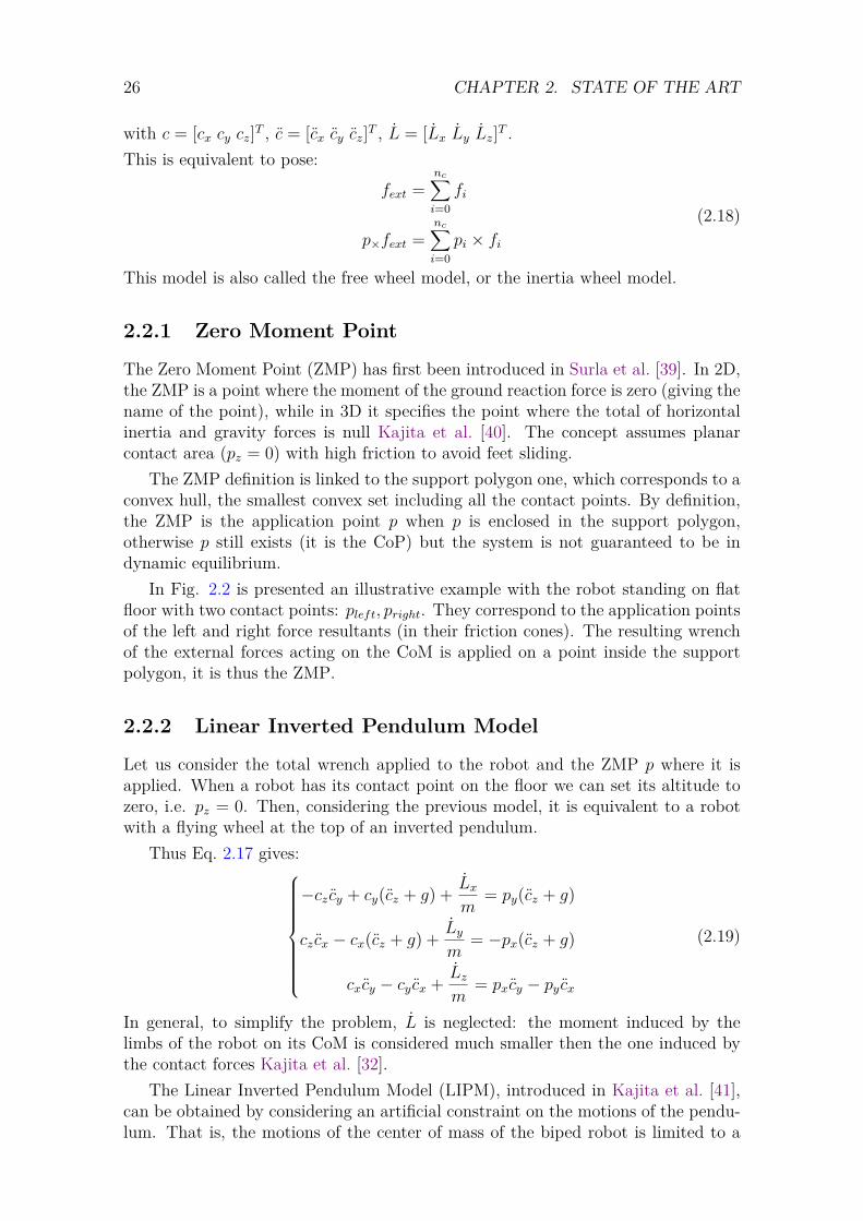
The ZMP definition is linked to the support polygon one, which corresponds to aconvex hull, the smallest convex set including all the contact points. By definition,the ZMP is the application point p when p is enclosed in the support polygon,otherwise p still exists (it is the CoP) but the system is not guaranteed to be indynamic equilibrium.
In Fig. 2.2 is presented an illustrative example with the robot standing on flatfloor with two contact points: pleft, pright. They correspond to the application pointsof the left and right force resultants (in their friction cones). The resulting wrenchof the external forces acting on the CoM is applied on a point inside the supportpolygon, it is thus the ZMP.
2.2.2 Linear Inverted Pendulum Model
Let us consider the total wrench applied to the robot and the ZMP p where it isapplied. When a robot has its contact point on the floor we can set its altitude tozero, i.e. pz = 0. Then, considering the previous model, it is equivalent to a robotwith a flying wheel at the top of an inverted pendulum.
Thus Eq. 2.17 gives:
−cz cy + cy(cz + g) + Lxm
= py(cz + g)
cz cx − cx(cz + g) + Lym
= −px(cz + g)
cxcy − cy cx + Lzm
= pxcy − py cx
(2.19)
In general, to simplify the problem, L is neglected: the moment induced by thelimbs of the robot on its CoM is considered much smaller then the one induced bythe contact forces Kajita et al. [32].
The Linear Inverted Pendulum Model (LIPM), introduced in Kajita et al. [41],can be obtained by considering an artificial constraint on the motions of the pendu-lum. That is, the motions of the center of mass of the biped robot is limited to a
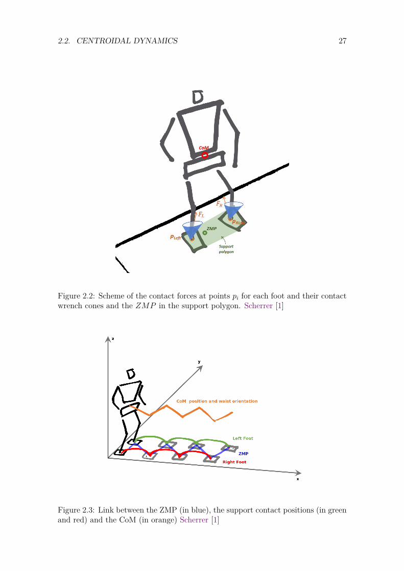
2.2. CENTROIDAL DYNAMICS 27
Figure 2.2: Scheme of the contact forces at points pi for each foot and their contactwrench cones and the ZMP in the support polygon. Scherrer [1]
Figure 2.3: Link between the ZMP (in blue), the support contact positions (in greenand red) and the CoM (in orange) Scherrer [1]
28 CHAPTER 2. STATE OF THE ART
plan whose normal vector is[kx ky −1
]Tand z intersection is zc. This constraint
can be formulated as :cz = kxcx + kycy + zc (2.20)
and by successive derivation :
cz = kxcx + ky cy (2.21)
To retrieve the equations of the LIPM of Kajita et al. [32] it is common to simplifythe problem by considering the planar constraint to be horizontal, i.e. kx = ky = 0and then cz = 0. In addition to that hypothesis, the part of Angular Momentum(AM), depicted as L previously, is neglected in front of the influence of the centerof mass motion (induced by the contact forces).
Thus, from the eq. 2.19, the following linear relationship can be written betweenthe CoM and the ZMP:
px = cx −zcgcx = cx −
czgcx
py = cy −zcgcy = cy −
czgcy
(2.22)
It is important to notice that the two equations are decoupled. Therefore, using theLIPM formulation, one can solve separately the equations along the x and the yaxis.
Since the ZMP position is imposed by the contact forces and contact positions,one can use the LIPM equations to deduce the CoM trajectory from the ZMP one(see Fig.2.3 for an illustration). This is a common implementation in WPG Naveauet al. [27], Kajita et al. [32], Herdt et al. [42], creating the path of the CoM to respectthe constraints on the contact forces, thus maintaining the contacts necessary fora balanced motion. Moreover, keeping the ZMP inside the support polygon with acertain margin is also often implemented in WPG, to obtain a safer balancing of therobot (reduce the risk of fall).
2.2.3 Equilibrium Criteria
2.2.3.a Divergent Component of Motion
We recall that the problem considers the planar constraint to be horizontal, i.e.cz = 0 and thus cz = constant. One can rewrite the eq.2.22 by noting ω =
√g/cz
as follows:cx = ω2(cx − px) (2.23)
And, setting X = [cx cx]T in eq.2.23, one can obtain the following system of equa-tions:
X =(
0 1ω2 0
)X +
(0
−ω2px
)= AX + b (2.24)
This matrix A can be decomposed as :
A = 12
(1 1−ω ω
)(−ω 00 ω
)(1 − 1
ω
1 1ω
)= 1
2P(−ω 00 ω
)P−1 (2.25)
2.2. CENTROIDAL DYNAMICS 29
It is then possible to make a change of variables:
X =
ζxξx
= P−1X =
1 − 1ω
1 1ω
cxcx
=
cx −cxω
cx + cxω
(2.26)
The dynamics of the LIPM can therefore be divided in two: the upper part which isnaturally converging, and the lower part which is diverging. The diverging part iscalled the Divergent Component of Motion (DCM), and its definition is given by:
ξx = cx + cxω
(2.27)
The DCM has been introduced first in Pratt et al. [43] under the name "CapturePoint", while the presentation given here is the one provided by Takenaka et al. [44]from Honda, and popularized by the work of Englsberger et al. [45] on the humanoidrobot TORO.
2.2.3.b CoM Admittance Control
The net contact wrench (that is the contact wrench expressed at the level of theCoM) can be computed indirectly by defining the ZMP position that will producethe said contact wrench. Under the assumptions of the LIPM, one can retrieve thefollowing two coupled first-order equations Englsberger et al. [45], Takenaka et al.[46]:
c = ω(ξ − c)ξ = ω(ξ − p)ξ = c+ c
ω
(2.28)
with p, ξ respectively the ZMP and DCM and ω =√g/cz.
These equations show that the DCM diverges from the ZMP, while the CoMconverges to the DCM. Thus, the DCM can be controlled to control the CoM devi-ations and stabilize the system Englsberger et al. [45], Kajita et al. [47], Sugihara[48], Mesesan et al. [49]. This strategy is called the admittance control of the CoM.
From a CoM reference trajectory provided by a planner, a reference DCM canbe defined as well. This reference, along with a measure of the DCM (based on theestimation of the base position of the robot) can be used in a Proportional–Integral(PI) controller. This controller has been presented in Caron et al. [50] (the integralterm is used to eliminate the steady-state error):
ξ = ξ∗ +KPdcm(ξ∗ − ξ) +KIdcm
∫(ξ∗ − ξ) (2.29)
with ξ∗ the desired DCM given by the planning, ξ the estimated DCM andKPdcm, KIdcm the proportional and integral gains. In terms of ZMP (see Eq.2.28),the obtained control law is Caron et al. [50]:
p∗ = pref −[1 + KPdcm
ω
](ξref − ξ) + KZdcm
ω(pref − p)− KIdcm
ω
∫(ξref − ξ)
(2.30)with pref , ξref the respective ZMP and DCM reference values, given by the planning.And KZdcm the proportional gain on the ZMP.
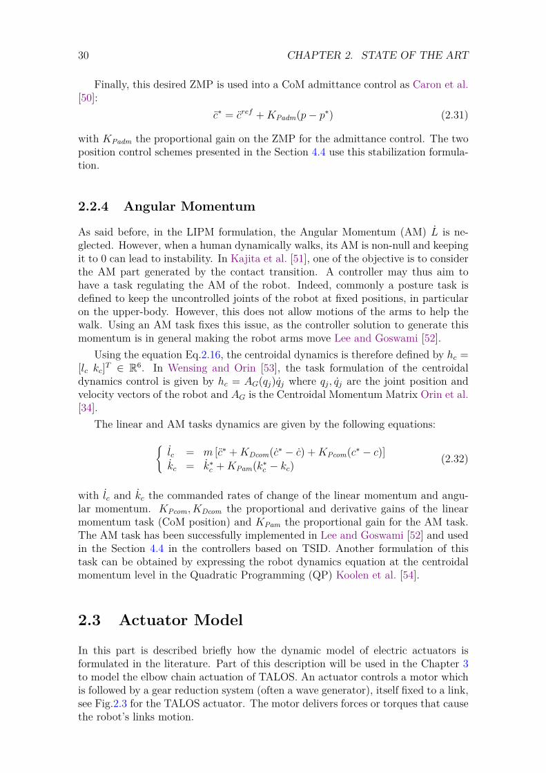
30 CHAPTER 2. STATE OF THE ART
Finally, this desired ZMP is used into a CoM admittance control as Caron et al.[50]:
c∗ = cref +KPadm(p− p∗) (2.31)
with KPadm the proportional gain on the ZMP for the admittance control. The twoposition control schemes presented in the Section 4.4 use this stabilization formula-tion.
2.2.4 Angular Momentum
As said before, in the LIPM formulation, the Angular Momentum (AM) L is ne-glected. However, when a human dynamically walks, its AM is non-null and keepingit to 0 can lead to instability. In Kajita et al. [51], one of the objective is to considerthe AM part generated by the contact transition. A controller may thus aim tohave a task regulating the AM of the robot. Indeed, commonly a posture task isdefined to keep the uncontrolled joints of the robot at fixed positions, in particularon the upper-body. However, this does not allow motions of the arms to help thewalk. Using an AM task fixes this issue, as the controller solution to generate thismomentum is in general making the robot arms move Lee and Goswami [52].
Using the equation Eq.2.16, the centroidal dynamics is therefore defined by hc =[lc kc]T ∈ R6. In Wensing and Orin [53], the task formulation of the centroidaldynamics control is given by hc = AG(qj)qj where qj, qj are the joint position andvelocity vectors of the robot and AG is the Centroidal Momentum Matrix Orin et al.[34].
The linear and AM tasks dynamics are given by the following equations:{lc = m [c∗ +KDcom(c∗ − c) +KPcom(c∗ − c)]kc = k∗c +KPam(k∗c − kc)
(2.32)
with lc and kc the commanded rates of change of the linear momentum and angu-lar momentum. KPcom, KDcom the proportional and derivative gains of the linearmomentum task (CoM position) and KPam the proportional gain for the AM task.The AM task has been successfully implemented in Lee and Goswami [52] and usedin the Section 4.4 in the controllers based on TSID. Another formulation of thistask can be obtained by expressing the robot dynamics equation at the centroidalmomentum level in the Quadratic Programming (QP) Koolen et al. [54].
2.3 Actuator Model
In this part is described briefly how the dynamic model of electric actuators isformulated in the literature. Part of this description will be used in the Chapter 3to model the elbow chain actuation of TALOS. An actuator controls a motor whichis followed by a gear reduction system (often a wave generator), itself fixed to a link,see Fig.2.3 for the TALOS actuator. The motor delivers forces or torques that causethe robot’s links motion.
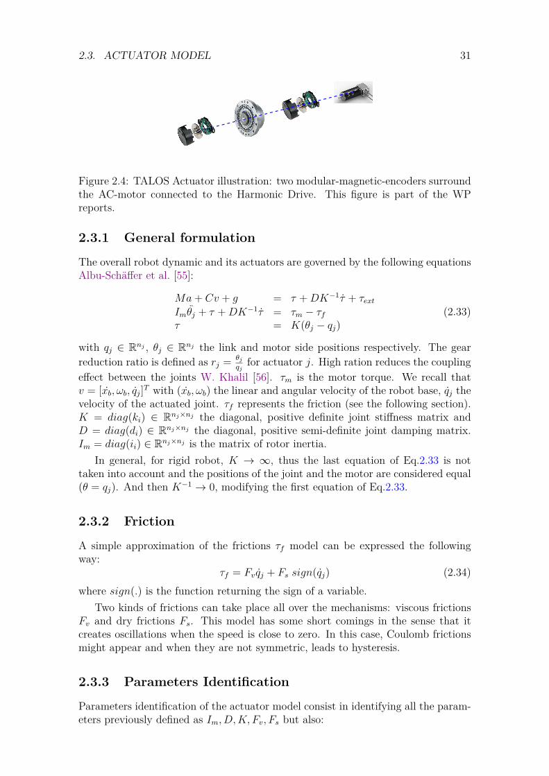
2.3. ACTUATOR MODEL 31
Figure 2.4: TALOS Actuator illustration: two modular-magnetic-encoders surroundthe AC-motor connected to the Harmonic Drive. This figure is part of the WPreports.
2.3.1 General formulation
The overall robot dynamic and its actuators are governed by the following equationsAlbu-Schäffer et al. [55]:
Ma+ Cv + g = τ +DK−1τ + τextImθj + τ +DK−1τ = τm − τfτ = K(θj − qj)
(2.33)
with qj ∈ Rnj , θj ∈ Rnj the link and motor side positions respectively. The gearreduction ratio is defined as rj = θj
qjfor actuator j. High ration reduces the coupling
effect between the joints W. Khalil [56]. τm is the motor torque. We recall thatv = [xb, ωb, qj]T with (xb, ωb) the linear and angular velocity of the robot base, qj thevelocity of the actuated joint. τf represents the friction (see the following section).K = diag(ki) ∈ Rnj×nj the diagonal, positive definite joint stiffness matrix andD = diag(di) ∈ Rnj×nj the diagonal, positive semi-definite joint damping matrix.Im = diag(ii) ∈ Rnj×nj is the matrix of rotor inertia.
In general, for rigid robot, K → ∞, thus the last equation of Eq.2.33 is nottaken into account and the positions of the joint and the motor are considered equal(θ = qj). And then K−1 → 0, modifying the first equation of Eq.2.33.
2.3.2 Friction
A simple approximation of the frictions τf model can be expressed the followingway:
τf = Fv qj + Fs sign(qj) (2.34)where sign(.) is the function returning the sign of a variable.
Two kinds of frictions can take place all over the mechanisms: viscous frictionsFv and dry frictions Fs. This model has some short comings in the sense that itcreates oscillations when the speed is close to zero. In this case, Coulomb frictionsmight appear and when they are not symmetric, leads to hysteresis.
2.3.3 Parameters Identification
Parameters identification of the actuator model consist in identifying all the param-eters previously defined as Im, D,K, Fv, Fs but also:
32 CHAPTER 2. STATE OF THE ART
� The geometrical parameters of the robot,� the gear reduction ratio rj for actuator j, defined by rj = θj
qj,
� the motor constant relating current ij to motor torque τm,j for each actuatorj such that τm,j = Km,jij.
� the Center-Of-Mass position for each link cj,
This is realized by generating trajectories which are maximizing the observabilityof the parameters W. Khalil [56], called optimal exciting motions (OEM) Bonnetet al. [57]. On TALOS it is possible to measure the joint positions, the motorpositions, the current and the external torque (qj, θ, i, τext). From this, the gearratio rj and the motor constant Km,j can be identified.
For Im, D,K, Fv, Fs a common approach is to solve a Least Square Problem(LSP), based on Eq.2.33. Note that most of the non-linear parts of the equationsare related to quantities which can be measured. Therefore while the equations arenon-linear, the Least Square Problem is not. More precisely all the parameters npar(for each actuator) to be identified are put together in a vector of free variablescalled X ∈ Rn×npar . All the measurements nmeas are stack together to obtain avector Y . The theoretical relationship is then Y = AX with A ∈ Rnmeas×npar .A large number of measurements will make this equality over-constrained, thus toidentify the parameters, the following LSP is solved Gautier and Jubien [58]:
minX ||Y − AX|| (2.35)
When the measured variables are not precise or compromised, it is possible to usea Ransac (RANdom SAmple Consensus) algorithm or another iterative method tostill estimate the parameters of the model.
2.3.4 Actuator Control
In general, the whole body controller provides a control vector u to the robot in twopossible forms (see Section 2.5):� q∗j , q∗j , or q∗j a desired position or velocity or acceleration for each actuator,� τ ∗ a desired torque for each joint.
However, the real control variable that is provided by the power electronics ofthe robot is the motor current. Thus, one have to add a layer of control creating arelationship between the output of the controller and the motor current Lynch andPark [35]. For the first form of u one can use a position control, while for the secondform one will need to implement a torque control. In the following sections, for eachmotor j the current is noted ij.
2.3.4.a Position control
The position control is usually done by a simple Proportional Integral Derivative(PID) embedded in the electronic board of the robot:
ij = Pj(q∗j − qj) + Ij
∫ t
0(q∗j (h)− qj(h))dh+Dj(q∗j − qj) (2.36)

2.4. MOTION AND LOCOMOTION PLANNING 33
with q∗j , qj the desired and measured joint j positions, Pj the proportional gain,Dj the derivative gain and Ij the integral one. Proportional gains for this kind ofcontrol are typically very high (10000 for Pj), with Ij often very small (0.1) or equalto zero. This is making the robot extremely rigid, but it is quite simple to deploy.
On TALOS and TIAGO this low level control is realized at 10 kHz by the Elmoboard sending the current to the motors.
2.3.4.b Torque control
On the other hand to have a robot which is compliant, one would like to control thetorque applied τj and not the position.
There is a non linear relationship between the joint torque and the motor currentwhich depends on the actuator model (see Section 2.3):
f :R 7→ R (2.37)ij → τj (2.38)
Once the chain actuation is modeled and its parameters identified, one can expressthis relationship in a low-level controller to directly send current commands fromdesired torques to the robot. Chapter 3 presents one implementation of such acontroller for the elbow of the TALOS robot.
2.4 Motion and Locomotion Planning
During this thesis, two distinct planning approaches have been used to compute thereference trajectories used by our controllers: a Walking Pattern Generator WPGStasse et al. [59], [60] and a multi-contact locomotion framework Carpentier et al.[61], [62]. Because motion planning is not the core of our research subject, onlythis two approaches are described in this section. They have been chosen becausethey are part of the algorithms developed by the Gepetto team and can thus easilybe connected to our architectures. But, we could have used any other methodsproviding reference trajectories for the CoM and the feet. Moreover, the two usedapproaches meet the requirements and needs of the thesis context: allowing to planreal-time locomotion solution for the first approach and multi-contact scenarios forthe second one. Finally they are state-of-the-art solutions. We quickly present theirposition in the literature in this section.
2.4.1 Walking Pattern Generator
The generation of a stable humanoid robot gait, on flat floor without obstacles, isa commonly tackled issue in robotics. Introduced by Kajita et al. [41], the LIPMis widely used to approximate the non linear dynamics of a humanoid robot CoMduring gait as a function of the CoP. Indeed, the CoP is a relevant variable to controlas the CoP has to stay within the support polygon of the robot at all time to ensurethe humanoid robot balance Wieber [63].
In Kajita et al. [64], the authors present a CoP preview control which computesthe CoM of the humanoid robot over a prediction horizon from imposed footsteps
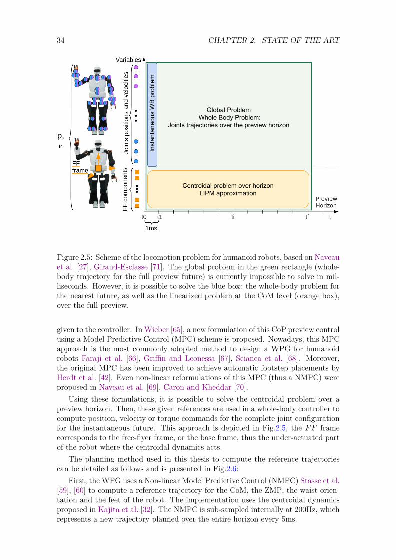
34 CHAPTER 2. STATE OF THE ART
Figure 2.5: Scheme of the locomotion problem for humanoid robots, based on Naveauet al. [27], Giraud-Esclasse [71]. The global problem in the green rectangle (whole-body trajectory for the full preview future) is currently impossible to solve in mil-liseconds. However, it is possible to solve the blue box: the whole-body problem forthe nearest future, as well as the linearized problem at the CoM level (orange box),over the full preview.
given to the controller. In Wieber [65], a new formulation of this CoP preview controlusing a Model Predictive Control (MPC) scheme is proposed. Nowadays, this MPCapproach is the most commonly adopted method to design a WPG for humanoidrobots Faraji et al. [66], Griffin and Leonessa [67], Scianca et al. [68]. Moreover,the original MPC has been improved to achieve automatic footstep placements byHerdt et al. [42]. Even non-linear reformulations of this MPC (thus a NMPC) wereproposed in Naveau et al. [69], Caron and Kheddar [70].
Using these formulations, it is possible to solve the centroidal problem over apreview horizon. Then, these given references are used in a whole-body controller tocompute position, velocity or torque commands for the complete joint configurationfor the instantaneous future. This approach is depicted in Fig.2.5, the FF framecorresponds to the free-flyer frame, or the base frame, thus the under-actuated partof the robot where the centroidal dynamics acts.
The planning method used in this thesis to compute the reference trajectoriescan be detailed as follows and is presented in Fig.2.6:
First, the WPG uses a Non-linear Model Predictive Control (NMPC) Stasse et al.[59], [60] to compute a reference trajectory for the CoM, the ZMP, the waist orien-tation and the feet of the robot. The implementation uses the centroidal dynamicsproposed in Kajita et al. [32]. The NMPC is sub-sampled internally at 200Hz, whichrepresents a new trajectory planned over the entire horizon every 5ms.
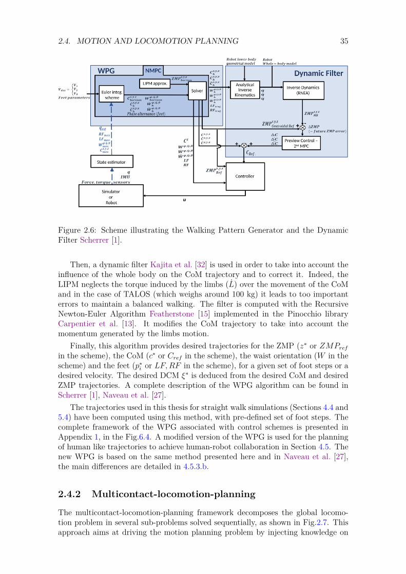
2.4. MOTION AND LOCOMOTION PLANNING 35
Figure 2.6: Scheme illustrating the Walking Pattern Generator and the DynamicFilter Scherrer [1].
Then, a dynamic filter Kajita et al. [32] is used in order to take into account theinfluence of the whole body on the CoM trajectory and to correct it. Indeed, theLIPM neglects the torque induced by the limbs (L) over the movement of the CoMand in the case of TALOS (which weighs around 100 kg) it leads to too importanterrors to maintain a balanced walking. The filter is computed with the RecursiveNewton-Euler Algorithm Featherstone [15] implemented in the Pinocchio libraryCarpentier et al. [13]. It modifies the CoM trajectory to take into account themomentum generated by the limbs motion.
Finally, this algorithm provides desired trajectories for the ZMP (z∗ or ZMPrefin the scheme), the CoM (c∗ or Cref in the scheme), the waist orientation (W in thescheme) and the feet (p∗i or LF,RF in the scheme), for a given set of foot steps or adesired velocity. The desired DCM ξ∗ is deduced from the desired CoM and desiredZMP trajectories. A complete description of the WPG algorithm can be found inScherrer [1], Naveau et al. [27].
The trajectories used in this thesis for straight walk simulations (Sections 4.4 and5.4) have been computed using this method, with pre-defined set of foot steps. Thecomplete framework of the WPG associated with control schemes is presented inAppendix 1, in the Fig.6.4. A modified version of the WPG is used for the planningof human like trajectories to achieve human-robot collaboration in Section 4.5. Thenew WPG is based on the same method presented here and in Naveau et al. [27],the main differences are detailed in 4.5.3.b.
2.4.2 Multicontact-locomotion-planning
The multicontact-locomotion-planning framework decomposes the global locomo-tion problem in several sub-problems solved sequentially, as shown in Fig.2.7. Thisapproach aims at driving the motion planning problem by injecting knowledge on
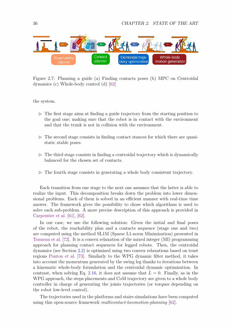
36 CHAPTER 2. STATE OF THE ART
Figure 2.7: Planning a guide (a) Finding contacts poses (b) MPC on Centroidaldynamics (c) Whole-body control (d) [62]
the system.
� The first stage aims at finding a guide trajectory from the starting position tothe goal one; making sure that the robot is in contact with the environmentand that the trunk is not in collision with the environment.
� The second stage consists in finding contact stances for which there are quasi-static stable poses.
� The third stage consists in finding a centroidal trajectory which is dynamicallybalanced for the chosen set of contacts.
� The fourth stage consists in generating a whole body consistent trajectory.
Each transition from one stage to the next one assumes that the latter is able torealize the input. This decomposition breaks down the problem into lower dimen-sional problems. Each of them is solved in an efficient manner with real-time timeanswer. The framework gives the possibility to chose which algorithms is used tosolve each sub-problem. A more precise description of this approach is provided inCarpentier et al. [61], [62].
In our case, we use the following solution: Given the initial and final posesof the robot, the reachability plan and a contacts sequence (stage one and two)are computed using the method SL1M (Sparse L1-norm Minimization) presented inTonneau et al. [72]. It is a convex relaxation of the mixed integer (MI) programmingapproach for planning contact sequences for legged robots. Then, the centroidaldynamics (see Section 2.2) is optimized using two convex relaxations based on trustregions Ponton et al. [73]. Similarly to the WPG dynamic filter method, it takesinto account the momentum generated by the swing leg thanks to iterations betweena kinematic whole-body formulation and the centroidal dynamic optimization. Incontrast, when solving Eq. 2.16, it does not assume that L = 0. Finally, as in theWPG approach, the steps placements and CoM trajectory are given to a whole bodycontroller in charge of generating the joints trajectories (or torques depending onthe robot low-level control).
The trajectories used in the platforms and stairs simulations have been computedusing this open-source framework multicontact-locomotion-planning [62].
2.5. REAL-TIME WHOLE BODY CONTROL 37
2.5 Real-time Whole Body Control
2.5.1 Introduction
The goal of this section is to report the existing solutions on real-time whole bodycontroller. From a mathematical viewpoint, a real-time whole body controller aimsto find a control vector u ∈ Rnj for each motor of a robot (nj = 32 for TALOS,and nj = 10 for TIAGo), for a given set of tasks, at high frequency (for instance1kHz). The controller is said to be instantaneous and corresponds to the blue blockof Fig.2.5.
In all the thesis, we assume that u can take only three values:� u = v, i.e. the control problem is solved considering the free variables as being
velocities.
� u = a, i.e. the control problem is solved considering the free variables as beingaccelerations.
� u = τ , i.e. the control problem is solved considering the free variables as beingjoint torques.
For the first and second case, the robot is position controlled and the low-levelservo control transform the commanded joint positions into motor currents with aPID at high frequency (typically 2 kHz for TALOS, see Section 2.3.4). This meansthat the output of the optimization is integrated one or two times before being sentto the low level system of the robot. In general, for locomotion scenarios, those twocontrols give the most efficient walk, achieving the fastest results with less trackingerrors along the trajectories Caron et al. [50].
Torque control, in another hand, requires a low level controller able to transformthe desired joint torques into motor currents (see Sections 2.3.4,2.3). To performthis transformation, the low level controller needs the model of the robot’s chain ac-tuation. This model can be given by the robot’s manufacturer, or the manufacturercan directly provide the low-level controller. However, this model often presentsinaccuracies and the identification of the robot inertial parameters and the motor’schain drive is required to correct it. This issue is partially why torque control wasless popular until recently, the transition from the simulations (which often do notmodel the actuators dynamics) to the real robot proving to be much harder thanposition control Mesesan et al. [49], Englsberger et al. [74].
2.5.2 Whole-body controller
2.5.2.a Introduction: Task Function
The most widely-used technique to generate whole-body motions is to design themotion in a space dedicated to the task, rather than directly at the whole-bodylevel (i.e. in configuration space, see Section 2.1.3). Indeed, it is easier to designthe reference motion in the task space, and then transcript this reference to theconfiguration space.
Once the planning has computed reference trajectories for the CoM and feet
38 CHAPTER 2. STATE OF THE ART
positions, they are given to the controller as desired features noted s∗. The taskfunctions Khatib [36], Samson et al. [37], Escande et al. [38] are defined as errorse between the current features s and the desired ones and are often non-linear.For instance, the geometric relationship between the configuration space and theEuclidean space of the end effector (hands or feet) is non-linear. In particular, therecan be multiple configurations possible to reach a desired end effector position.
Therefore, the task functions are usually computed as an optimization problem:
minq||s− s∗|| (2.39)
with the relation between s and q defined by the differentiable function f such that:
f : C → Sq 7→ s
(2.40)
with C the configuration space and S the task space (for example the Special Eu-clidian group SE(3)).
This problem is solved iteratively using a gradient descent approach Chevallereauand Khalil. [75]. Once expressed as an optimization problem, it is interesting to seethat this opens up an incremental approach where constraints can be added, andvarious formulations of equivalent problems can be considered.
To generate a complex motion on a humanoid robot, several tasks have to becombined, sequentially Mansard et al. [76] or simultaneously. The simultaneousexecution of two tasks on a robot can be achieved in two ways: by setting respectiveweights between the tasks, or by imposing a strict hierarchy. Recently, a solutionhas been proposed to handle both strict and non-strict priorities of an arbitrarynumber of tasks Liu et al. [77]. These first two solutions have been implemented inthe Gepetto Stack-of-Task (SoT) software (see Section 1.6):� The library implementing the task formulation in velocity domain using a strict
hierarchy as in Mansard et al. [16], Mansard and Chaumette [78] is SoT-Core[20],
� The library implementing the task formulation in torque using weights andinequalities is SoT-Torque-Control [79] (C++ wrapper of TSID [80] usingthe dynamic-graph [14]).
2.5.2.b QP Formulation: Task space velocity or acceleration control
IntroductionGenerally these optimization problems involving multiple tasks and constraints aresolved using Quadratic Programming. A QP is a convex optimization problemwith a convex objective function (cost function) which is quadratic and constraintfunctions which are affine Boyd and Vandenberghe [12]. A famous unconstrainedQP is the Least Square Problem (LSP), for instance the Eq.2.39 is a LSP, which hasan analytical solution (given by using pseud-inverse).
However, a QP with equality and inequality constraints is not easily solved. Onemethod to solve these optimization problem is to use active set solvers Nocedaland Wright [81]. These solvers use the Lagrangian multipliers formulation and the

2.5. REAL-TIME WHOLE BODY CONTROL 39
Karush-Kuhn-Tucker (KKT) conditions Boyd and Vandenberghe [12], Nocedal andWright [81]. They project the free variables of the problem in the null space of theequality and inequality constraints. Then, the objective function is minimized inthis subspace. Such solvers guarantee that the constraints are properly fulfilled, butmight be computationally expensive, in particular when the matrix of the linearconstraints is ill-conditioned.
Another way to cope with the constraints is to reformulate a new optimizationproblem with all the constraints as tasks inside the objective function. Therefore, theconstraints might not be fulfilled. This new problem is mathematically equivalent tothe one with constraints but it means that the related tasks might not be completelyperformed Hofmann et al. [82]. This can be helpful for tasks that are subject to theenvironment disturbances.
Therefore, an important question is to decide which constraints need to strictlybe respected (equality constraints), and which constraints can be relaxed (costfunction). In general the constraints related to the physical laws are strictlyenforced because any violation would induce damages to the robot. Constraintsrelated to tasks such as the position of the right hand might be performed at best.It is important to notice that some tasks, such as foot contact with the ground,while being subject to modifications from the environment, may have a strongimpact on the robot if they are not fulfilled correctly.
Mathematical formulation for velocity controlLet us simplify the motion equation based on the rigid body dynamics (see Eq.2.4)when there is no contacts:
Ma+ h = NT τ (2.41)with h = C(q, v)v + g(q).
If we have a task e regulating a feature s, the dynamics of the task can beimposed, for instance as an exponential decay (last equation):
e = s s∗e = s− s∗e = −λe = −λ(s− s∗) (2.42)
with the difference operator in the task space, for instance the operator of the Liegroup. λ the control gain of the task, which can be constant, or adaptive in order tocontrol the speed of convergence to the desired feature. The task is realized when ereaches 0 or is close to 0.
Using the previous function f such that s = f(q) one can define the relationshipbetween s and v using the Jacobian of s Lynch and Park [35] and the formulationgiven in Eq.2.6 for the under-actuated part:
s = [Ju Ja]v = Jv (2.43)
One can notice that the Jacobian for the task error e is the same one as its features, because s∗ depends only on the time and not on the configuration. It is thuspossible to compute v with Eq.2.43 as:
v = J†s (2.44)
40 CHAPTER 2. STATE OF THE ART
with J† the Moore-Penrose pseudo-inverse of J , since J can be non square and thusnot invertible.
It is possible to reformulate Eq.2.42 to obtain the dynamics of the feature andthen the desired joint velocities:
s = s∗ + e⇔ Jv = s∗ − λ(s s∗)⇔ v = J†(s∗ − λ(s s∗))
(2.45)
One can introduce a slack variable w (an implicit optimization variable) to expressthe realization of the task, then the solver will optimize this variable instead of theerror directly, allowing a relaxation of the problem if no solution is found (fromEq.2.42):
w = e+ λew = Jv − (s∗ − λ(s− s∗)) (2.46)
A simple formulation of the QP problem can then be expressed as:
minv,τ
‖w‖2
s.t. Ma+ h = NT τ(2.47)
Where the free variables are the robot velocity v and the torque τ .
Mathematical formulation for acceleration/torque controlIn this thesis, we also used the formulation of the task errors at the second order toachieve acceleration control. In Eq.2.42 one can define the dynamics of the secondderivative of the error e (third equation) Lynch and Park [35]:
e = s− s∗s = Ja+ Jve = −2λ e− λ2 e
(2.48)
And thus, similarly as before one can obtain the desired joint acceleration and theslack variable w as:
a = J†(s∗ − Jv − 2λ e− λ2 e)w = e+ 2λ e+ λ2 ew = Ja+ Jv − (s∗ − 2λ e+ λ2 e)
(2.49)
Leading to the following QP:
mina,τ
‖w‖2
s.t. Ma+ h = NT τ(2.50)
Where the free variables are the accelerations a and the torque τ . It is possible towork only on one type of variables (to achieve acceleration or torque control on therobot) by substitution.
2.5. REAL-TIME WHOLE BODY CONTROL 41
Formulation with contactsIf the system is in contact with the environment, its dynamics must account forcontact forces fext. If contacts are soft, measured/estimated contact forces fext canbe easily included:
mina,τ
‖w‖2
s.t. Ma+ h = NT τ + JTc fext(2.51)
with Jc the Jacobian of the contact points xc according to the robot state vector, asdefined in Eq.2.6.
But if contacts are rigid, they constrain the motion. They can be implementedas nonlinear functions, which are differentiated twice:
xc = 0 ⇔ Contact point does not moveJTc v = 0 ⇔ Contact point velocity is zero
JTc a+ Jc v = 0 ⇔ Contact point acceleration is zero(2.52)
This representation leads to the following optimization problem:
mina,f,τ
‖w‖2
s.t. Jc 0 0M −JTc −ST
afτ
= −Jc v−h
(2.53)
These optimization problems represent Equality-Constrained Least-Square Problem(ECLSP) because they only have equality constraints. Unconstrained LSP can bedirectly solved using the Moore-Penrose pseudo-inverse Boyd and Vandenberghe [12](if J is surjective). For instance, for a fully actuated robot (q = qj, v = qj, a = qj),if the desired feature does not move (s∗ = 0) and using Eq.2.49 one can find thesolution:
qj = −J†(2λ e+ λ2 e+ J qj
)(2.54)
The ECLSP can also be resolved with pseudo-inverse by using null-space projectorBoyd and Vandenberghe [12]. But the main benefit of QP solver is that they canhandle inequality-constraints. It is mainly used to define boundaries of the systemsuch as torque, velocity or joint limits; and also friction cones for the contacts:
τmin ≤ τ ≤ τmaxqminj ≤ qj ≤ qmaxj
qminj ≤ qj ≤ qmaxj
fmin ≤ f ≤ fmax
(2.55)
42 CHAPTER 2. STATE OF THE ART
2.5.2.c HQP and Weighted Sum
Complex robots are typically redundant with respect to the main task they mustperform, this redundancy can be used to execute secondary tasks. This multi-objective optimization can be achieved by setting respective weights between thetasks, or by imposing a strict hierarchy between them (cascade of QP or HQP)Kanoun et al. [83].
We assume that the robot must perform N tasks, each defined by a task functionand its optimization variable wi:
gi = ‖wi‖2 (2.56)
In the following we chose to use the formulation of Eq.2.49 for wi.
Weighted SumThe easiest strategy is to sum all functions using user-defined weights µi:
mina,f,τ
N∑i=0
µi gi
s.t. Jc 0 0M −JTc −ST
afτ
= −Jc v−h
τmin ≤ τ ≤ τmax
qminj ≤ qj ≤ qmaxj
qminj ≤ qj ≤ qmaxj
fmin ≤ f ≤ fmax
(2.57)
This problem remains standard computationally-efficient (compared to LSP). But,finding proper weights is hard and too extreme weights can lead to numerical issues.It is easier to find the priority of a task than its weight, but a cascade of QP canquickly become too computationally expensive if computed in a naive way. For thisreason several teams working on humanoid robots are using this formulation fortheir controllers:� In Koolen et al. [54], the IHMC whole body controller is described. The
tracking of the feet position and the foot contact wrenches tasks are consideredas strict equalities, whereas the momentum rate is tracked at best inside thecost function.
� In Bouyarmane et al. [84], the JRL/IDH team is using strict inequalities tomaintain the physical constraints: joint limits, velocity limit, accelerationlimit, and strict equality to maintain the dynamical consistency. All the othertasks are tracked at best in the cost function.
The weighted approach tends to imply new gains when considering newapplications. Finding these new gains is not straightforward and often require time-consuming tuning and expertise. However some procedures exist to automaticallytuned these gains, such as in Pucci et al. [85] for a momentum based controller orin Teshnehlab and Watanabe [86] by using learning approach. Penco et al. [87]
2.5. REAL-TIME WHOLE BODY CONTROL 43
proposes a multi-objective optimization approach to learn the gains and also thepriorities (strict and soft) of a controller.
Lexicographical HierarchyThe alternative strategy is to use strict priorities to order the task functions, whichmeans to solve a cascade of QP problems:
g∗i = mina,f,τ
gi
s.t. Jc 0 0M −JTc −ST
afτ
= −Jc v−h
gj = g∗j ∀j < i
τmin ≤ τ ≤ τmax
qminj ≤ qj ≤ qmaxj
qminj ≤ qj ≤ qmaxj
fmin ≤ f ≤ fmax
(2.58)
The following works have investigated the use of strict inequalities on humanoidrobots:� In Hoffman et al. [88], the IIT team of WALKMAN presents a scheme to
perform Cartesian Impedance Control in a hierarchical manner. The new taskat level i is performed at best, while preserving the integrity of previous tasks.The dynamics is preserved through its formulation as a task equality.
� In Henze et al. [89], the DLR team describes a whole body controller to performcontact control. In this work, the authors use 4 levels of hierarchy. The firstlevel is used to maintain contact with the environment and to make sure thatthe planned external wrench is applied to the robot. The second level containsthe tracking tasks of the end-effectors not used for the balancing. The thirdlevel is used to control the CoM and the fourth level is used to control theposture. This controller is moreover passive (see Section 2.6.3)
To illustrate this last solution with inequalities, let us take two tasks with priorityorder e1 ≺ e2 and bounds e1, e1 and e2, e2 respectively. When there is no contacts,the expression of the Lexicographical QP applied on inverse kinematics (see theprevious velocity formulation of Section 2.5.2.b: e−Jv = w) can be written as Saabet al. [90]:
H1 = minv,w1
‖w1‖2
s.t. e1∗ ≤ J1 v + w1 ≤ e1
∗
H2 = minv,w2
‖w2‖2
s.t. e1∗ ≤ J1 v + w∗1 ≤ e1
∗
e2∗ ≤ J2 v + w2 ≤ e2
∗
with w∗1 = arg minw1
H1
(2.59)
A naive implementation would be to solve the second problem H2 in the samespace than H1, i.e. v ∈ Rn. However by working in the base of the null space
44 CHAPTER 2. STATE OF THE ART
of H1, the computation becomes extremely efficient Nocedal and Wright [81]. InSection 4.4 is presented a hierarchical controller which exploit this specific structureto keep its control frequency higher than 1kHz in average with 4 hierarchy levels(see Section 4.4.4). Note however that when the tasks are compatible the projectionin null space is useless. In addition, when a constraint is activated it means thatthe robot is working at one of its limit which is rarely desirable. The main interestof strict inequalities is the guarantee that a constraint is never violated and that atask of lower priority will not interfere.
Once the QP solver find a solution (using for example the active sets methodNocedal and Wright [81]), the desired joint torques/accelerations or velocities aresent to the robot. However, most robots such as TALOS or HRP-2 ultimatelycontrols their motor in current (electric motors). Thus the low-level controller musttransform these commands into motor in current, this can be done by two generalapproaches: position control or torque control (see Section 2.3.4).
2.5. REAL-TIME WHOLE BODY CONTROL 45
TALOS WALK-MAN TORO HRP-4 JAXON Atlas GazelleDate 2018 2018 2014 2010 2015 2016 2020Actuation Electric Electric/ Electric/ Electric Electric Hydraulic Electric
Compliant CompliantDoFs 32 32 39 34 32 28 13Size 1.75m 1.85m 1.74m 1.51m 1.88m 1.50m 1.30mWeight 100kg 102kg 76.4kg 39kg 127kg 75kg 60kgTorque 22 22 25 0 32 28 13sensorsF/T Ankle/ Ankle/ Ankle Ankle/ Ankle/ Ankle/ Anklesensors Wrist Wrist Wrist Wrist WristIMU/ 1 2 2 1 1 1 1Accelero.Cameras 2 1 3 4 1 2 0LIDAR 1 1 0 0 1 1 0/Laser
Table 2.1: Comparison of Humanoid robots specifications.
2.5.3 Recent Humanoid Robots Whole Body Controllers
In this section, a short presentation of recent humanoid robots and their controlschemes is given. A review on the hardware design of humanoid robots can be foundin Ficht and Behnke [91]. The aim is to highlight the particularities of the robotTALOS and investigate the promising control schemes compatible for our robot.PAL Robotics demonstrated, during IROS 2018, an accurate whole-body balancingcontrol on TALOS PAL-Robotics [92], however it is only position controlled.
In the Table.2.1 are presented some specifications of 6 humanoid robots anda biped. The robot Gazelle is presented in this section because it can be entirelytorque controlled and achieves great results while walking on uneven terrain becauseof its hardware composition and control Jeong et al. [93]. One has to notice that theTORO robot has more DoFs than the other robots because its 39 DoFs include itshands (6 DoFs each). The only robot presented here which does not have electricactuation is the Atlas robot, with hydraulic actuation using valve current (howeverother hydraulic robots exist such as HYDROïD from LISV and Hydra from theAIST). The HRP-4 robot has no torque sensors to achieve torque control but maybe controlled in current.
The robot WALK-MAN (see Fig.2.8) was first presented by the IIT in 2015 andhas then been updated to reach the presented final version. The humanoid robothas been design to operate in damaged buildings and hostile environment Tsagarakiset al. [94]. It can be torque controlled. Recently a two strict hierarchy whole-bodycontroller has been implemented, using energy shaping Subburaman et al. [95] tocontrol a falling-over scenario. It is an interesting strategy because it allows tocontrol the energy of the system, as energy shaping is an approach close to the oneof the passivity Folkertsma and Stramigioli [96].
TORO (see Fig.2.8) was made specifically for torque control Englsberger et al.[97] by the DLR, it was first presented in 2013 but the project begun in 2010.
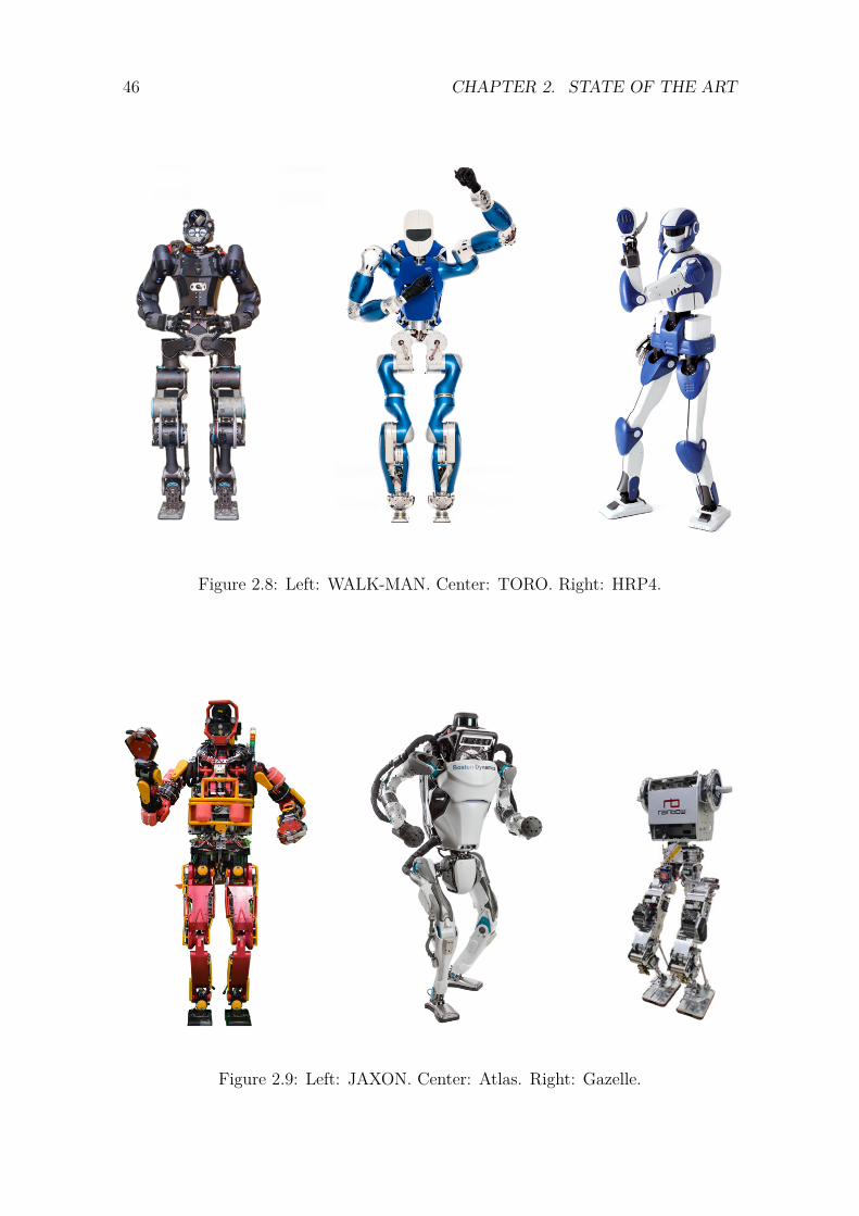
46 CHAPTER 2. STATE OF THE ART
Figure 2.8: Left: WALK-MAN. Center: TORO. Right: HRP4.
Figure 2.9: Left: JAXON. Center: Atlas. Right: Gazelle.
2.5. REAL-TIME WHOLE BODY CONTROL 47
This humanoid robot is robust to walking, balancing and multi-contact scenarios,Henze et al. [89] presents a passivity-based whole body controller to perform multi-contact balancing. This work has led this thesis to investigate the passivity theoryto ensure the stability of the whole-body controllers. Englsberger et al. [74] presentsa weighted whole-body controllers with DCM control on TORO, and Englsbergeret al. [98] describes an implementation proving the Lyapunov and passivity stabilityeven for conflicting sub-tasks.
The HRP-4 robot (see Fig.2.8) is the follow up of the HRP-2 robot designed bythe Kawada Industries and AIST. It is a light-weighted robot which is designed tocollaborate with humans, and able to react to external forces. The recent papersare from the common laboratory of the CNRS-AIST JRL realized at the LIRMM.In Caron et al. [50] the HRP-4 robot succeed stairs climbing in Airbus Plant, usinga whole-body admittance controller with strict hierarchy. The CoM admittancecontrol used in this paper is similar to what is described in Section 2.2.3.b. Thestabilization of the control is based on the LIPM and feet wrench distributions. Therobot is controlled in position, while the QP is solved for accelerations free variables,thus the command is integrated two times. In Bouyarmane et al. [84] is presenteda weighted whole body controller achieving task force control with multi-robot. Italso uses admittance control and the robot is controlled in position.
TORO and HRP-4 have been used in Kheddar et al. [99] to achieve some man-ufacturing tasks in an assembly line. The results of a complete solution embeddingvisual tracking, localization, planning and control is impressive. One can noticethat HRP-4 is used for tasks which do not require force application and have lim-ited contact. When multi-contact is needed or to realize the manufacturing appli-cations, the torque controlled robots TORO and HRP-2Kai are used. Compared towhat is achieved, we want to answer the first limiting factor encounter in this study,which is the security of the robotic platform. The repeated falls and weakness ofthe humanoid robots lead to damages during the experiments. Thus, we want toensure the stability of our solution while conserving the robot capabilities to achievedemanding tasks (such as applying huge torque for drilling).
The robot JAXON (see Fig.2.9) from the JSK laboratory is also a humanoidrobot designed for torque control, to perform disaster relief assistance. In Shiraiet al. [100] is presented a whole body torque controller which can absorb impulsivedisturbances. Associated with an online walking controller, the framework demon-strates high robustness to strong collision with the robot’s legs. This robot is howeverthe heaviest.
The robot Atlas (see Fig.2.9) from Boston Dynamics and the MIT is a humanoidrobot using state-of-the-art hardware which demonstrates human-level agility. How-ever, the hardware specifications of this robot are not disclosed. In Koolen et al. [54]is detailed a momentum based whole body torque control, using a soft hierarchy.This formulation controls the AM of the robot and achieve impressive results withthe robot while walking on different terrains (tilted cylinder blocks, rubble) and faston flat one (0.43m/s). These results confirmed our interest to add a control on theAM of the robot for our control schemes.
Finally, the robot GAZELLE (see Fig.2.9) was recently designed by the KAIST,aiming to build a fast and reliable biped platform for walking experiments. Assaid before, the paper Jeong et al. [93] presents the results obtained with this new
48 CHAPTER 2. STATE OF THE ART
platform. The controller split the control between a CoM task and ankles forcetasks. It controls the damping of the CoM and then solves the Inverse Kinematicsto obtain the desired joint configuration; while using the F/T sensors to regulatethe torques on the ankles and send directly a torque command for them. Thisarchitecture allows the biped robot to walk fast on uneven terrain and to be robustto external pushes.
Compared to the robots in the literature, TALOS has average capabilities, how-ever, it is the only robot commercially available (and not too expensive). It ispossible to implement torque or position control, and it has been built to be able tosustain heavy load for a long duration and to apply high torques/forces to completemanufacturing operations.
2.6 Stability Analysis: Convergence toward anequilibrium
2.6.1 Introduction
Humanoid robots are meant to act in the same environment than humans, interact-ing with it, but this environment can be unknown and subject to disturbances. Evenperforming simple tasks in fixed environment can lead to instabilities, the authorsencountered this problem while testing a classical torque control scheme using inversedynamics on the robot TALOS on a simple postural task. After some repetitionsof a sinusoidal motion on the robot arm, the system diverged brutally and blockedsome of its harmonic drives. The gains tuned in simulation (simulating the rigidchain actuators) were too high for the real robot. Thus, even with gains tuned on aproper simulator modeling the actuators, we cannot expect the solution to remainstable (i.e. remains in a bounded distance from an equilibrium). To provide a safeand reliable interaction with the environment and possibly humans, it is necessaryto ensure the stability of the robotic system. This problem is commonly tackled inthe community using two strategies: the Lyapunov analysis or the passivity-basedanalysis. In this section, we first present briefly the Lyapunov theory and recentworks proving the Lyapunov stability of humanoid robots whole-body controllers.Then, the passivity theory is described with more details as this analysis is used inthe Chapter 5 to prove the stability of our new controller.
2.6.2 Lyapunov Theory
The Lyapunov theory consists in analysing the stability of an equilibrium, lookingif the solution remains in a bounded distance from the equilibrium or convergesasymptotically (Asymptotic stability) or exponentially (Exponential stability) Bac-ciotti and Rosier [101]. This analysis ensures that the controller will not find adiverging solution. We have the following definitions for local and global strictasymptotic stability Bacciotti and Rosier [101]:
Definition 1 (Lyapunov local asymptotic stability). For a system with the statespace model of x = f(x) (x ∈ Rn) and an equilibrium state x∗ = 0. If there exists
2.6. STABILITY ANALYSIS 49
a Lyapunov function V : Rn → R such that: V is continuous, has continuousfirst derivatives, is locally positive definite and its time derivative is locally negativedefinite, i.e:
V (0) = 0V (x) ∈ C1 onBV (x) > 0 ∀x ∈ B\{0}V (x) = ∇V (x).f(x)V (x) < 0 ∀x ∈ B\{0}
(2.60)
where B is the local neighborhood of the origin. Then the equilibrium is proven tobe locally asymptotically stable (local Lyapunov stability).
Definition 2 (Lyapunov global asymptotic stability). For a system with the statespace model of x = f(x) (x ∈ Rn) and an equilibrium state x∗ = 0. If thereexists a Lyapunov function V respecting the local Lyapunov stability (Definition 1),with B = Rn and radially unbounded then the equilibrium is proven to be globallyasymptotically stable (global Lyapunov stability).
We recall, V radially unbounded if: ‖x‖ → ∞ =⇒ V (x)→∞
From these definitions, one can obtain the exponential stability by majoratingV by an exponentially converging function.
In the control literature, Lyapunov functions are often built based on the relativekinetic and potential energy of the system to prove its stability. Recently, Navaet al. [102] proposed a momentum-based QP with two strict hierarchies and provedits Lyapunov stability by using integral gains in the task functions. In a similar way,Cisneros et al. [103] adds an integral term to the computed torque while using it inthe constraints of their QP to prove the Lyapunov stability. Finally, Englsbergeret al. [98] has designed a new controller creating separate Lyapunov functions foreach task and proving the overall stability and passivity of the system.
2.6.3 Passivity Theory
The passivity-based analysis consists in investigating the energy flows within a sys-tem Schaft [104]. It is also possible to directly control the system energy withoutproving the passivity, which requires an analysis of the energy derivative of thesystem. For instance, Joseph et al. [105] proposes a formulation of a kinetic en-ergy constraint in a QP to prevent a manipulator robot from transferring dangerousamounts of this energy during an impact. Yet, it has been proven in Camlibel et al.[106] that when a robot interacts with its environment, a passively-controlled robotis a necessary condition for stability Folkertsma and Stramigioli [96]. Using thederivative of the energy in the system, the passivity can be analyzed to ensure thatthe system converges to the desired equilibrium or to detect which components havean unbounded energy consumption.
2.6.3.a Definition
The principle of passivity comes from the concept of dissipative dynamical systemWillems [107], in particular proving that the internal power of the system is less
50 CHAPTER 2. STATE OF THE ART
than or equal to the power transferred to the system through its port. This conceptis associated with the Port-Hamiltonian System theory; which is an energy-basedformulation of the physical systems Schaft [104].
The Hamiltonian H is the sum of the potential and kinetic energy of the system.Using the Poisson framework representation (input-state-output representation), onecan obtain the following formulation:
For a state vector x ∈ Rn, u, y ∈ Rm:
x =[J(x)−R(x)
]∂H∂x
(x) + g(x)u
y = gT (x)∂H∂x
(x)(2.61)
with J(x) = −JT (x), R(x) = RT (x) ≥ 0. g represents the interconnection, andtherefore effect, of the port variables on the state variables and vice versa. Thematrix J is a power-continuous interconnection and is skew-symmetric, whereas Rmodels pure resistive losses of the system. The latter property is obtain by takingthe time derivative of the Hamiltonian:
H = ∂HT
∂x(x)x
= ∂HT
∂x(x)[J(x)−R(x)
]∂H∂x
(x) + ∂HT
∂x(x)g(x)u
= −∂HT
∂x(x)R(x)∂H
∂x(x) + yTu
(2.62)
using the fact that J is skew-symmetric (∂HT∂x
(x)J(x)∂H∂x
(x) = 0). Thus, H is thepower supplied through the port yTu, minus the power lost to friction, quadratic onR(x) Schaft [104].
Using the dissipative definition, a system is defined as a passive system Schaft[104] if it respects the following definition:
Definition 3 (Passive System). A system with the state space model of x = f(x, y)with initial state x(0) = x0 ∈ Rn, input vector u ∈ Rm and output y = h(x, u) issaid to be passive, if there exists a positive semi-definite function H : Rn → R+,called storage function, such that:
H(x(T ))−H(x(0)) ≤∫ T
0yT (t)u(t)dt (2.63)
∀y : [0, T ]→ Rm, x0 ∈ Rn and T > 0.
One can see that by choosing H = H, the storage function is the energy in thesystem and the supply rate yTu is the power transferred to the system through itsport. If R = 0, there is no dissipation and the system is conservative.
From the Definition. 3, the passivity of the system can equivalently be provenby finding an appropriate storage function H(x) respecting the property 1:
Property 1 (Passivity Storage Function). A system with the state space model ofx = f(x, y) with initial state x(0) = x0 ∈ Rn, input vector u ∈ Rm and output
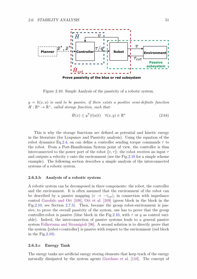
2.6. STABILITY ANALYSIS 51
RobotController
Passivesubsystem
Planner
Prove passivity of the blue or red subsystem
Environment
Figure 2.10: Simple Analysis of the passivity of a robotic system.
y = h(x, u) is said to be passive, if there exists a positive semi-definite functionH : Rn → R+, called storage function, such that:
H(x) ≤ yT (t)u(t) ∀(x, y) ∈ Rn (2.64)
This is why the storage functions are defined as potential and kinetic energyin the literature (for Lyapunov and Passivity analysis). Using the equation of therobot dynamics Eq.2.4, on can define a controller sending torque commands τ tothe robot. From a Port-Hamiltonian System point of view, the controller is thusinterconnected to the power port of the robot {v, τ}: the robot receives an input τand outputs a velocity v onto the environment (see the Fig.2.10 for a simple schemeexample). The following section describes a simple analysis of the interconnectedsystems of a robotic system.
2.6.3.b Analysis of a robotic system
A robotic system can be decomposed in three components: the robot, the controllerand the environment. It is often assumed that the environment of the robot canbe described by a passive mapping (v → −τext), in connection with impedancecontrol Garofalo and Ott [108], Ott et al. [109] (green block in the block in theFig.2.10, see Section 2.7.3). Then, because the group robot-environment is pas-sive, to prove the overall passivity of the system, one has to prove that the groupcontroller-robot is passive (blue block in the Fig.2.10, with τ or q as control vari-able). Indeed, the interconnection of passive systems leads to a general passivesystem Folkertsma and Stramigioli [96]. A second solution is to directly prove thatthe system {robot+controller} is passive with respect to the environment (red blockin the Fig.2.10).
2.6.3.c Energy Tank
The energy tanks are artificial energy storing elements that keep track of the energynaturally dissipated by the system agents Giordano et al. [110]. The concept of
52 CHAPTER 2. STATE OF THE ART
virtual energy tank is to give an energy budget to the controller and to changethe behavior of the controller in function of it. The tank monitors the energy flowof the system to guarantee the passivity. The energy stored in this tank can bere-used to accomplish different goals without violating the passivity of the system.By augmenting one control architecture with a virtual energy tank Folkertsma andStramigioli [96], it is possible to limit the energy generated by the system andthen make it passive. For instance, in the case of a controller with multiple tasks,one can introduce an energy tank in the framework to store the energy dissipatedby these tasks. The tank will then be used to transfer the stored energy when atask needs more energy to be completed. On the contrary, if the tank is empty,it will be used to deteriorate the tracking of this task to ensure the passivity ofthe system Folkertsma and Stramigioli [96]. For instance, if a robot lifts a massits actuators consume potential energy (the energy flows through them) thus thisenergy is removed from the tank. In contrary, if someone pulls the mass down whilethe robot lifts it, the actuators extract energy from the system and the energy flowsback to the tank. When the tank is empty, the controller is forbidden to inject energyinto the system: the robot stops lifting the mass and the system is guaranteed tobe passive Folkertsma and Stramigioli [96]. The energy tank is commonly definedas a virtual storage element with flow variable s and effort variable s such that:
Etank = 12s
2 (2.65)
The flow variable s is often defined by the damping energy of the tasks Garofaloand Ott [108], Dietrich et al. [111, 112] and then integrated to find the energy valuein the tank. It is possible to create a global tank monitoring the energy of all thetasks, or one tank for each task Dietrich et al. [112]. According to the value of thetank, the tracking of a task (or all tasks in the case of a global tank) is deterioratedto ensure the passivity of the system. This can be achieved by different ways:� By using a Dirac structure to link the flow, effort and control variables Dietrich
et al. [111, 112] (this method is not used in our case because of the complexityof the structure that will be involved)
� By modifying the dynamics of the controller states according to the energy inthe tank Garofalo and Ott [108]
� By computing coefficients based on the tank value to directly regulate thetasks Dietrich et al. [112], Shahriari et al. [113].
An elegant way of using the first method on manipulators has been presented formulti-tasks in a strict-hierarchy using null-space projection in Dietrich et al. [111].Moreover, regulating the size and flow of the energy tank are challenges that havebeen expressed in the domain Dietrich et al. [112], Tadele et al. [114]. Providing toomuch energy to the system may lead the controller to diverge from the equilibriumor to over-accumulate this energy. Likewise, an uncontrolled sharp release of thetank energy might lead to dangerous motions Shahriari et al. [113].
2.6.3.d State-of-the-art
For manipulator robots with flexible joints, Ott et al. [109], Albu-Schäffer et al. [115]present a passive framework using impedance control. Another method, successfully
2.7. FORCE CONTROL FOR MANIPULATION 53
implemented in Giusti et al. [116], couples Inverse Dynamics (ID) and passivity-based control by modifying the ID formulation to exploit the passivity-properties ofthe robot model.
However, using these approaches on humanoid robots is not straightforward.Indeed, humanoids robots are not ground-fixed to the environment, they are under-actuated systems. This under-actuated part, called floating base, prevents fromusing the full feedback linearization of the underlying system Acosta and Lopez-Martinez [117]. Moreover, it relies on external contact forces to control its motion.Besides, the penalization of the tracking tasks used in Dietrich et al. [112], Shahriariet al. [113] can compromise the balance of the robot. Thus, passivity-based controlon humanoid robots is still an open-problem. In Garofalo and Ott [108], the methodof Dietrich et al. [112] has been extended for a fully actuated humanoid robot forlimit cycle control. Thus, this solution does not guarantee the passivity when con-straints are activated in the QP due to the under-actuation of the humanoid robot.
The passivity method using impedance control has been first implemented onhumanoid robots by Cheng et al. [118] and has lately been extended on the DLRrobot TORO, leading to impressive results in multi-contact scenarios in Henze et al.[119]. Finally, Englsberger et al. [98] has designed a new controller respecting theLyapunov stability and proving the passivity of the system even for conflicting sub-tasks, for fully actuated robots. This controller covers the complete range betweenInverse Dynamics (with non-strict hierarchy) and Proportional Derivative with feed-forward (PD+) Control. However, as in Garofalo and Ott [108], for under-actuatedrobot, if a constraint becomes active, the passivity is no longer guaranteed. Nonethe-less, it achieves great results with the humanoid robot TORO.
2.7 Force Control for Manipulation
2.7.1 Introduction
In order to perform an operation involving interactions of the robot arm with theenvironment it is needed to implement a specific control. Force control consists inusing the force information given by the robot sensors in the controller. It allows toincrease the robot adaptability to uncertain environments and to monitor the contactforces. Thus, force feedback can be used to enforce the safety of the control, avoidinghuge contact forces which may lead to damages. This is particularly important formanufacturing and assembly tasks such as drilling or deburring where the amount offorce required to perform the operation is important. Moreover, the controller usedfor these operations must also control the position of the arm or mechanical toolused by the robot. Indeed, the manipulation requires contact with the environmentat precise position. Thus, the motion of the robot arm is constrained by this contact,constraints represented by the interaction forces.
In this section are presented the most common force control schemes present inthe literature. These schemes have been mostly developed for manipulator robotsand then adapted to robots with more DoFs. In particular, for humanoid robots,the solutions presented can be used on the end-effectors of the robot, for instanceas specific tasks in the whole-body controller.
54 CHAPTER 2. STATE OF THE ART
In the case of the robot TALOS, the forces are measured by the force sensorsconnected to the wrists and ankles of the robot. These force sensors can accuratelyprovide forces along six DoFs. This vector Fm consists of the three orthogonal forcecomponents and the three orthogonal torque components operating at the end-effector with respect to the fixed Cartesian coordinate system (named the worldW ). Similarly, the position of the end-effector x in the constraint or task space isa six DoFs vector with three orthogonal displacements (distance between the end-effector and the world) and three angles (orientation of the end-effector with respectto the world). The Denavit-Hartenberg Bejczy [28] representation of the joint anglesare set in the variable qj and the generalized joint torques are given by τ .
To achieve manipulation operations with both position and force requirementsthe researchers have implemented solutions which create a dynamic relationship be-tween position and force variables in addition to the control of one variable. Indeed,it is not possible to simultaneously impose force and position values on the environ-ment. The two most common solutions are dual, one performing a direct closed-loopforce control, the other performing an open-loop force control, and are the followingSiciliano et al. [2]:
� The admittance control: Commands a force reference and builds a relationshipbetween the end-effector motion and the error from the reference force Albu-Schäffer et al. [115], Keemink et al. [120], Yu and Perrusquía [121]. Thissolution allows to control the contact force to a desired value, with an open-loop position control (see Fig.2.11).
� The impedance control: Commands a position reference and builds a rela-tionship between the external forces and the error from the reference positionLu and Meng [122], Anderson and Spong [123], Albu-Schaffer and Hirzinger[124], Schindlbeck and Haddadin [125]. This solution allows to control theposition of the end-effector to a desired value, with an open-loop force control(see Fig.2.12). The resulting impedance can be linear or nonlinear (if there isa force feedback).
These two control strategies are complementary, they implement opposed so-lutions to achieve the same goal and thus behave well in different situations: thetwo controllers exhibit opposite stability characteristics depending on the stiffnessof the environment. The admittance control is better suited for interactions withsoft environments or operations in free space (see Section 2.7.2) and the impedancecontrol is better suited for dynamic interactions with stiff environments (see Section2.7.3).
Both methods aim to implement a task-space relationship following a mechanicalimpedance Siciliano et al. [2]:
∆x = xm − x∗Fext = Mx∆x+Dx∆x+Kx∆x
(2.66)
where x∗, xm are the desired and measured positions of the end-effector, Fext theaimed external force measured at the end-effector,Mx is a mass matrix, Dx a damp-ing matrix and Kx a stiffness matrix. Because the measurement of the accelerationxm can be noisy, the mass term is often neglected and set to 0.
2.7. FORCE CONTROL FOR MANIPULATION 55
Others strategies have been implemented to combine the advantages of the ad-mittance and impedance control or of the position and force control. The first oneis called the hybrid position/force control Anderson and Spong [123], Raibert andCraig [126], and more recently the hybrid admittance-impedance control Ott et al.[127], Kim et al. [128] (see Section 2.7.5). The second one is the parallel force/position control Chiaverini and Sciavicco [129], Siciliano [130] described in Section2.7.6.
2.7.2 Admittance Control
In the admittance control approach the robot is position controlled. The environ-ment is assumed to behave as an impedance system, with elastic and dissipativecomponents while the robot behaves as an admittance system. This method usesclosed-loop force control and open-loop position control. It presents interestingproperties when creating contact with compliant surfaces (direct control on theforce and little use of position control) or when the environment is used to guidethe end-effector. A simple control scheme is presented in Fig.2.11. In this schemethe mass term of Eq.2.66 is neglected and the desired force F ∗ to apply is related toa reference position xref = Kc(F ∗ − Fm) where Kc is the compliance (or stiffness)matrix Salisbury [131]. Thus, Eq.2.66 is simplified in Siciliano et al. [2]:
KxKc(F ∗ − Fm) = Dx∆x+Kx∆x (2.67)
And the close-loop can be done by a PD+ on the end-effector velocity (see Eq.2.68). The PD+ control can be of different forms, it can take an inner close-loopin position control with the term proportional on the position error ∆x = x∗ − xm(modified admittance control) or not.
In the example given in the Fig.2.11, we set Dx = I and choose the gains of thePD+ to be KxKc = Dadm, Kx = Padm. Thus we obtain the following equations andnotations:
ef = F ∗ − Fm
x∗ = xm +Dadmef − Padm∆x (2.68)
with F ∗, Fm respectively the desired and measured forces at the end-effector, x∗, xmrespectively the desired and measured velocities of the end-effector, Padm, Dadm theproportional and derivative gains for the admittance control, q∗, qm respectively thedesired and measured joint positions, q∗, qm respectively the desired and measuredjoint velocities and i the motor currents.
Then in the example, the desired end-effector velocity is saturated in the exampleand then v∗, q∗ are computed using the Inverse Kinematics. The position controllerto obtain the motor current is usually done by a simple PID:
i = P (q∗ − qm) + I∫ t
0(q∗(h)− qm(h))dh+D(q∗ − qm) (2.69)
with P, I,D the respective proportional, integral and derivative gains. Proportionalgains for this kind of control are often very high, and integral ones small or equal tozero. This is making the robot extremely rigid, but the solution is simple to deploy.
An overview of admittance control for physical interactions with human can befound in Keemink et al. [120], which proposes guidelines to achieve high-performance
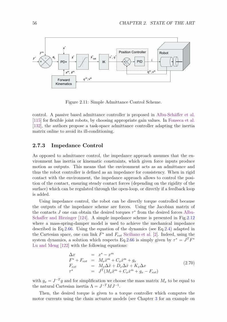
56 CHAPTER 2. STATE OF THE ART
RobotPosition Controller
+-
iv*, q*
IKPD+
ẋ*sat
PID
qm,𝓿m
ẋ*ef
q m,𝓿m
Forward Kinematics
+-
F m
F *
xm, ẋm
x*
Figure 2.11: Simple Admittance Control Scheme.
control. A passive based admittance controller is proposed in Albu-Schäffer et al.[115] for flexible joint robots, by choosing appropriate gain values. In Fonseca et al.[132], the authors propose a task-space admittance controller adapting the inertiamatrix online to avoid its ill-conditioning.
2.7.3 Impedance Control
As opposed to admittance control, the impedance approach assumes that the en-vironment has inertia or kinematic constraints, which given force inputs producemotion as outputs. This means that the environment acts as an admittance andthus the robot controller is defined as an impedance for consistency. When in rigidcontact with the environment, the impedance approach allows to control the posi-tion of the contact, ensuring steady contact forces (depending on the rigidity of thesurface) which can be regulated through the open-loop, or directly if a feedback loopis added.
Using impedance control, the robot can be directly torque controlled becausethe outputs of the impedance scheme are forces. Using the Jacobian matrix ofthe contacts J one can obtain the desired torques τ ∗ from the desired forces Albu-Schaffer and Hirzinger [124]. A simple impedance scheme is presented in Fig.2.12where a mass-spring-damper model is used to achieve the mechanical impedancedescribed in Eq.2.66. Using the equation of the dynamics (see Eq.2.4) adapted inthe Cartesian space, one can link F ∗ and Fext Siciliano et al. [2]. Indeed, using thesystem dynamics, a solution which respects Eq.2.66 is simply given by τ ∗ = JTF ∗
Lu and Meng [122] with the following equations:
∆x = x∗ − xmF ∗ + Fext = Mxx
m + Cxxm + gx
Fext = Mx∆x+Dx∆x+Kx∆xτ ∗ = JT (Mxx
m + Cxxm + gx − Fext)
(2.70)
with gx = J−Tg and for simplification we choose the mass matrix Mx to be equal tothe natural Cartesian inertia Λ = J−TMJ−1.
Then, the desired torque is given to a torque controller which computes themotor currents using the chain actuator models (see Chapter 3 for an example on
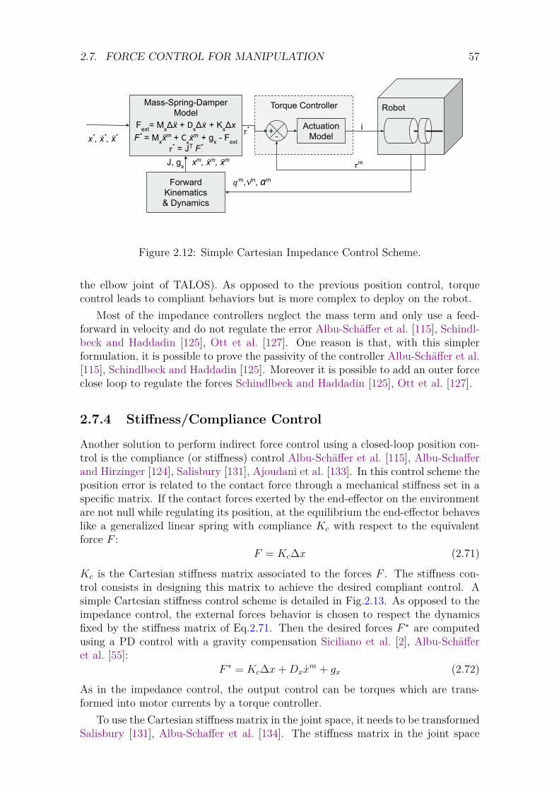
2.7. FORCE CONTROL FOR MANIPULATION 57
RobotTorque Controller
+-
Actuation Model
𝜏m
𝜏* i
q m,𝓿m, am
Mass-Spring-Damper Model
Fext
= MxΔẍ + D
xΔẋ + K
xΔx
F* = Mxẍm + C
xẋm + g
x - F
ext𝜏* = JT F*
Forward Kinematics& Dynamics
xm, ẋm, ẍm
x*, ẋ*, ẍ*
J, gx
Figure 2.12: Simple Cartesian Impedance Control Scheme.
the elbow joint of TALOS). As opposed to the previous position control, torquecontrol leads to compliant behaviors but is more complex to deploy on the robot.
Most of the impedance controllers neglect the mass term and only use a feed-forward in velocity and do not regulate the error Albu-Schäffer et al. [115], Schindl-beck and Haddadin [125], Ott et al. [127]. One reason is that, with this simplerformulation, it is possible to prove the passivity of the controller Albu-Schäffer et al.[115], Schindlbeck and Haddadin [125]. Moreover it is possible to add an outer forceclose loop to regulate the forces Schindlbeck and Haddadin [125], Ott et al. [127].
2.7.4 Stiffness/Compliance Control
Another solution to perform indirect force control using a closed-loop position con-trol is the compliance (or stiffness) control Albu-Schäffer et al. [115], Albu-Schafferand Hirzinger [124], Salisbury [131], Ajoudani et al. [133]. In this control scheme theposition error is related to the contact force through a mechanical stiffness set in aspecific matrix. If the contact forces exerted by the end-effector on the environmentare not null while regulating its position, at the equilibrium the end-effector behaveslike a generalized linear spring with compliance Kc with respect to the equivalentforce F :
F = Kc∆x (2.71)
Kc is the Cartesian stiffness matrix associated to the forces F . The stiffness con-trol consists in designing this matrix to achieve the desired compliant control. Asimple Cartesian stiffness control scheme is detailed in Fig.2.13. As opposed to theimpedance control, the external forces behavior is chosen to respect the dynamicsfixed by the stiffness matrix of Eq.2.71. Then the desired forces F ∗ are computedusing a PD control with a gravity compensation Siciliano et al. [2], Albu-Schäfferet al. [55]:
F ∗ = Kc∆x+Dxxm + gx (2.72)
As in the impedance control, the output control can be torques which are trans-formed into motor currents by a torque controller.
To use the Cartesian stiffness matrix in the joint space, it needs to be transformedSalisbury [131], Albu-Schaffer et al. [134]. The stiffness matrix in the joint space
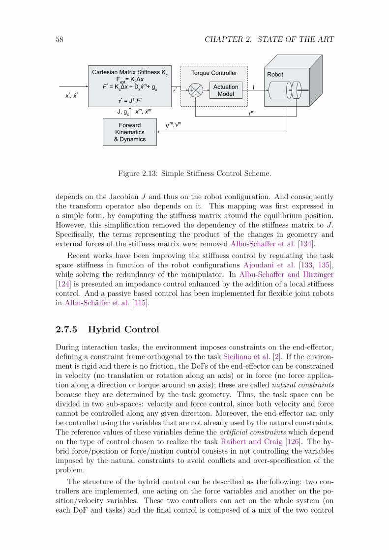
58 CHAPTER 2. STATE OF THE ART
RobotTorque Controller
+-
Actuation Model
𝜏m
𝜏* i
q m,𝓿m
Cartesian Matrix Stiffness Kc
Fext
= KcΔx
F* = KcΔx + D
xẋm+ g
x
𝜏* = JT F*
Forward Kinematics& Dynamics
xm, ẋmJ, gx
x*, ẋ*
Figure 2.13: Simple Stiffness Control Scheme.
depends on the Jacobian J and thus on the robot configuration. And consequentlythe transform operator also depends on it. This mapping was first expressed ina simple form, by computing the stiffness matrix around the equilibrium position.However, this simplification removed the dependency of the stiffness matrix to J .Specifically, the terms representing the product of the changes in geometry andexternal forces of the stiffness matrix were removed Albu-Schaffer et al. [134].
Recent works have been improving the stiffness control by regulating the taskspace stiffness in function of the robot configurations Ajoudani et al. [133, 135],while solving the redundancy of the manipulator. In Albu-Schaffer and Hirzinger[124] is presented an impedance control enhanced by the addition of a local stiffnesscontrol. And a passive based control has been implemented for flexible joint robotsin Albu-Schäffer et al. [115].
2.7.5 Hybrid Control
During interaction tasks, the environment imposes constraints on the end-effector,defining a constraint frame orthogonal to the task Siciliano et al. [2]. If the environ-ment is rigid and there is no friction, the DoFs of the end-effector can be constrainedin velocity (no translation or rotation along an axis) or in force (no force applica-tion along a direction or torque around an axis); these are called natural constraintsbecause they are determined by the task geometry. Thus, the task space can bedivided in two sub-spaces: velocity and force control, since both velocity and forcecannot be controlled along any given direction. Moreover, the end-effector can onlybe controlled using the variables that are not already used by the natural constraints.The reference values of these variables define the artificial constraints which dependon the type of control chosen to realize the task Raibert and Craig [126]. The hy-brid force/position or force/motion control consists in not controlling the variablesimposed by the natural constraints to avoid conflicts and over-specification of theproblem.
The structure of the hybrid control can be described as the following: two con-trollers are implemented, one acting on the force variables and another on the po-sition/velocity variables. These two controllers can act on the whole system (oneach DoF and tasks) and the final control is composed of a mix of the two control
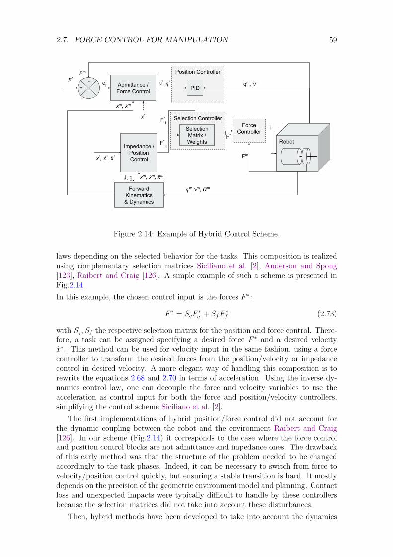
2.7. FORCE CONTROL FOR MANIPULATION 59
Robot
Selection Controller
Fm
F*q
i
q m,𝓿m, am
Impedance / Position Control
Forward Kinematics& Dynamics
xm, ẋm, ẍm
x*, ẋ*, ẍ*
J, gx
Position Controller
F*f
+-
F m
F *
Admittance / Force Control
v*, q*
PIDqm, 𝓿m
Selection Matrix / Weights
Force Controller
F*
ef
xm, ẋm
x*
Figure 2.14: Example of Hybrid Control Scheme.
laws depending on the selected behavior for the tasks. This composition is realizedusing complementary selection matrices Siciliano et al. [2], Anderson and Spong[123], Raibert and Craig [126]. A simple example of such a scheme is presented inFig.2.14.In this example, the chosen control input is the forces F ∗:
F ∗ = SqF∗q + SfF
∗f (2.73)
with Sq, Sf the respective selection matrix for the position and force control. There-fore, a task can be assigned specifying a desired force F ∗ and a desired velocityx∗. This method can be used for velocity input in the same fashion, using a forcecontroller to transform the desired forces from the position/velocity or impedancecontrol in desired velocity. A more elegant way of handling this composition is torewrite the equations 2.68 and 2.70 in terms of acceleration. Using the inverse dy-namics control law, one can decouple the force and velocity variables to use theacceleration as control input for both the force and position/velocity controllers,simplifying the control scheme Siciliano et al. [2].
The first implementations of hybrid position/force control did not account forthe dynamic coupling between the robot and the environment Raibert and Craig[126]. In our scheme (Fig.2.14) it corresponds to the case where the force controland position control blocks are not admittance and impedance ones. The drawbackof this early method was that the structure of the problem needed to be changedaccordingly to the task phases. Indeed, it can be necessary to switch from force tovelocity/position control quickly, but ensuring a stable transition is hard. It mostlydepends on the precision of the geometric environment model and planning. Contactloss and unexpected impacts were typically difficult to handle by these controllersbecause the selection matrices did not take into account these disturbances.
Then, hybrid methods have been developed to take into account the dynamics
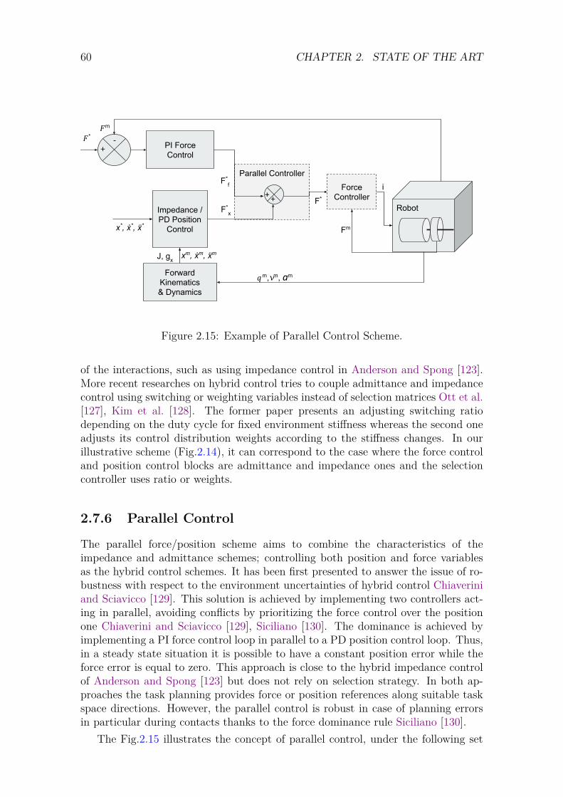
60 CHAPTER 2. STATE OF THE ART
Robot
Parallel Controller
Fm
F*x
i
q m,𝓿m, am
Impedance / PD Position
Control
Forward Kinematics& Dynamics
xm, ẋm, ẍmJ, gx
F*f
+-
F m
F *
PI Force Control
Force ControllerF*
+ +
x*, ẋ*, ẍ*
Figure 2.15: Example of Parallel Control Scheme.
of the interactions, such as using impedance control in Anderson and Spong [123].More recent researches on hybrid control tries to couple admittance and impedancecontrol using switching or weighting variables instead of selection matrices Ott et al.[127], Kim et al. [128]. The former paper presents an adjusting switching ratiodepending on the duty cycle for fixed environment stiffness whereas the second oneadjusts its control distribution weights according to the stiffness changes. In ourillustrative scheme (Fig.2.14), it can correspond to the case where the force controland position control blocks are admittance and impedance ones and the selectioncontroller uses ratio or weights.
2.7.6 Parallel Control
The parallel force/position scheme aims to combine the characteristics of theimpedance and admittance schemes; controlling both position and force variablesas the hybrid control schemes. It has been first presented to answer the issue of ro-bustness with respect to the environment uncertainties of hybrid control Chiaveriniand Sciavicco [129]. This solution is achieved by implementing two controllers act-ing in parallel, avoiding conflicts by prioritizing the force control over the positionone Chiaverini and Sciavicco [129], Siciliano [130]. The dominance is achieved byimplementing a PI force control loop in parallel to a PD position control loop. Thus,in a steady state situation it is possible to have a constant position error while theforce error is equal to zero. This approach is close to the hybrid impedance controlof Anderson and Spong [123] but does not rely on selection strategy. In both ap-proaches the task planning provides force or position references along suitable taskspace directions. However, the parallel control is robust in case of planning errorsin particular during contacts thanks to the force dominance rule Siciliano [130].
The Fig.2.15 illustrates the concept of parallel control, under the following set
2.8. MODEL PREDICTIVE CONTROL 61
of equations Chiaverini and Sciavicco [129], Siciliano [130] with force control input(acceleration input can be defined similarly):
F ∗ = F ∗f + F ∗xF ∗f = Kfef +Ki
∫ t0 efdt
F ∗x = Mxx∗ +Dx∆x+Kx∆x
(2.74)
One can choose a simpler impedance control as explained before by simply settingF ∗x = Kx∆x−Dxx
m Siciliano et al. [2].In the Chapter 4 is presented the solution implemented for our whole-body con-
troller to achieve a force operation task. It is close to a parallel force/position schemewith the addition of Coulomb contact constraints (see Section 4.3.4).
2.8 Model Predictive Control
It is possible to create controllers which consider a time horizon on a short timewindow instead of an instantaneous control. This type of control is called Modelpredictive control (MPC) Rawlings et al. [136] and is becoming an important fieldof research in robotics because it can handle non-linearity, constraints and systemdynamics Huba [137]. The MPC is part of the branch of applied mathematicscalled Optimal Control. This method is able to predict the future behavior ofthe robot over a receding finite-time horizon, using the mathematical model of thesystem dynamics Rawlings et al. [138], Findeisen and Allgöwer [139]. Because of itsprediction capability, MPC can for instance explicitly take into account stability.Passivity can be implemented by using the value function as a storage function andthe optimal feedback as an output of the system, or by adding a sate constraintover the trajectory to respect the passivity inequality Raff et al. [140]. It is alsopossible to explicitly change the tasks which are activated inside the time horizonand to ensure state smoothness. Thus, using MPC, one can formulate and solvea sequence of controllers Todorov et al. [141] to handle complex problems. RecentMPC formulations are based on explicit discrete variables of the problem, in orderto be able to choose contact phases Dai et al. [142].
The two main problems of the MPC approach are its computational cost andits limited time preview window (which is short, typically 2 − 3 s). Indeed, as theOptimal Control Problem (OCPs) are often non-convex due to the robot modelnon-linearity, they lead to high computational load and to local minimum Boydand Vandenberghe [12]. This is why the MPC has first been applied on simplifiedmodel Kajita et al. [32], Kim et al. [143] or systems with few DoFs Neunert et al.[144], Grandia et al. [145]. A first solution was to use the OCP to re-plan trajectoriesat low frequency while the robot was controlled by another controllerNeunert et al.[144].
For a system state x ∈ Rn and a control u ∈ Rm, such that x = f(x, u), one canformulate the OCP as follows Mayne [146], Dantec et al. [147]:
minx,u
T−1∑t=0
lt(x(t), u(t))dt+ lT (x(T ))
s.t. x(0) = x0
∀t ∈ [0, T ], x(t) = f t(x(t), u(t))
(2.75)

62 CHAPTER 2. STATE OF THE ART
with T the horizon time where is made the prediction, lt, lT are the running andterminal cost functions and x0 is the initial state.
The cost functions are used to define the robot tasks, to regularize the state andcontrol trajectories. The system constraints (such as the joint, velocity or torquelimits) can be added in the cost as well or be put as constraints of the problem.Thus, the cost functions are often non-linear. During an iteration of control, therobot state is estimated and a new OCP is solved over the finite horizon betweenthe estimated state and the future shifted from one sampling period.
In order to efficiently use a whole-body MPC directly as the main robot controllerone will want to tackle the following problems:� The computational time: To solve this problem one will need to use an OCP
algorithm working at high frequency Carpentier et al. [13], Featherstone [15],or to rewrite the OCP to obtain a more efficient formulation in terms of com-putation.
� The number of iterations before convergence: To reduce this number, one canuse a convex formulation Majumdar et al. [148], or a warm start.
To answer the first issue, shooting methods like Differential Dynamic Program-ming (DDP) Tassa et al. [149] have been introduced. In Bertsekas [150], Tassa et al.[151], Xie et al. [152] are presented efficient solvers able to deal with non linearcosts, constraints and dynamics (see the following Section 2.8.1). Because of thisproblem of computational time, it was not possible to connect the MPC directly tothe low-level servo controller Englsberger et al. [74], Herzog et al. [153] until Dantecet al. [147]. Indeed, to connect the two controllers it is necessary to evaluate theMPC at a compatible high frequency (at least 100Hz).
To find a good warm start for the second issue, Diehl et al. [154] proposes touse the solution from the previous iteration, but this heuristic is not robust to dis-turbances. Mansard et al. [76] uses the learning approach and specifically offlinereinforcement learning (see Section 2.9) to find a warm start. In Dantec et al. [147]is presented the first successful experiment implementing whole-body model predic-tive control with state feedback on a torque-controlled humanoid robot, running at100Hz. The control scheme is able to do whole-body target tracking, control thebalance in front of strong external perturbations and avoid collision with an externalobject.
2.8.1 Differential Dynamics Programming Formulation
The DDP algorithm considers the OCP of Eq.2.75 in discrete form and denotesthe control and state variables along the time horizon T as U = {u0, u1, ..., uT−1}and X = {x0, x1, ..., xT , U}. To minimize the cost function of Eq.2.75, the DDPuses the “Bellman’s principle of optimality” to transform the general problem intoa sequence of simpler sub-problems. Indeed, this principle states that the remainingdecisions of an optimal policy constitute an optimal policy with respect to the firstdecisions resulting state (in the absence of disturbances) Bellman [155]. For the DDPalgorithm, it is used to proceed backward in time from T − 1 to 0 while evaluatingthe optimal cost function at every node in the discretized state-time space. The
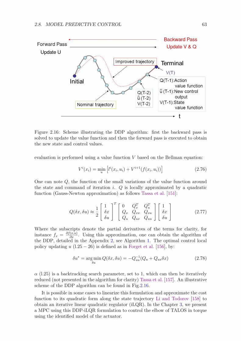
2.8. MODEL PREDICTIVE CONTROL 63
Figure 2.16: Scheme illustrating the DDP algorithm: first the backward pass issolved to update the value function and then the forward pass is executed to obtainthe new state and control values.
evaluation is performed using a value function V based on the Bellman equation:
V i(xi) = minu
[li(xi, ui) + V i+1(f(xi, ui))
](2.76)
One can note Q, the function of the small variations of the value function aroundthe state and command of iteration i. Q is locally approximated by a quadraticfunction (Gauss-Newton approximation) as follows Tassa et al. [151]:
Q(δx, δu) ≈ 12
1δxδu
T 0 QT
x QTu
Qx Qxx Qxu
Qu Qux Quu
1δxδu
(2.77)
Where the subscripts denote the partial derivatives of the terms for clarity, forinstance fx = ∂f(x,u)
∂x. Using this approximation, one can obtain the algorithm of
the DDP, detailed in the Appendix 2, see Algorithm 1. The optimal control localpolicy updating u (l.25− 26) is defined as in Forget et al. [156], by:
δu∗ = arg minδu
Q(δx, δu) = −Q−1uu (Qu +Quxδx) (2.78)
α (l.25) is a backtracking search parameter, set to 1, which can then be iterativelyreduced (not presented in the algorithm for clarity) Tassa et al. [157]. An illustrativescheme of the DDP algorithm can be found in Fig.2.16.
It is possible in some cases to linearize this formulation and approximate the costfunction to its quadratic form along the state trajectory Li and Todorov [158] toobtain an iterative linear quadratic regulator (iLQR). In the Chapter 3, we presenta MPC using this DDP-iLQR formulation to control the elbow of TALOS in torqueusing the identified model of the actuator.
64 CHAPTER 2. STATE OF THE ART
2.9 Learning approach
This thesis uses a model base approach to solve the different algorithms, relyingon the kinematics and dynamics models of the robot. Another method is to usemachine learning techniques, which propose new solutions in the robotics field, suchas control, modeling or planning. We briefly expose their principles in this section.Two major approaches are Reinforcement learning Sutton and Barto [159] and DeepLearning LeCun et al. [160]. The former is a methodological approach which aimsat finding a policy π to maximize a reward function assuming a value function.The value function V (x, u) based on state and control provides a way to evaluatethe cost to achieve a behavior. It can use a parametric functional space to findan appropriate control law and/or the model to be controlled Sutton and Barto[159], Jemin Hwangbo and Hutter [161]. Deep learning is a supervised approachwhich has recently gained a large popularity in computer vision LeCun et al. [160].A current method is to use Convolutional Neural Network (used in Deep Learning)in the context of Reinforcement Learning Esteban et al. [162]. Interestingly, in orderto discover the policy a large part of these works are using MPC Todorov et al. [141].More generally, the assumptions related to optimal control are used in the differentlearning approaches Bottou and Bousquet [163].
An important part of the learning method is to generate an action and to evaluateits corresponding reward. The exploration of the controlled system and its specificenvironment is in general time consuming and very costly on a real robot. For thisreason simulations are often used in a pre-exploration phase, which can require highcomputing performance. For instance, Reinforcement Learning can be used on thephysical parameters of the robot to learn a model in simulation (see Section 2.3).The training of the control policy has to satisfy the physical constraints such as thejoint limits. The main problem is then to deploy the trained policy on the physicalsystem. Indeed, the methodology implies to perform some run on the real robot totake into account the differences between the simulation model and the real one.Recent works (Hwangbo et al. [164], Tan et al. [165]) demonstrate great results onquadruped robots, however, it is unclear how this can be realized on humanoid robotwhich are much more unstable than quadruped robots. This impossibility to realizenumerous tests on the real robotic platforms has lead to develop specific learningalgorithms which require few training data, called one-shot and few-shot learningVinyals et al. [166], Snell et al. [167], James et al. [168].
2.10 Human-Robot Collaboration
Interactions between humanoid robots and humans raise great challenges as hu-manoid robots are complex systems due to their numerous DoFs and natural insta-bility. During collaborative interactions, the tasks are generally performed by thehuman while the robot is passively following or assisting K. et al. [169]. However,by anticipating and predicting the human behavior and motions the robot would beable to perform its task more efficiently. To achieve this aim, cobotic applicationsrequire a good knowledge of the human behaviour. For example, to make a humanand a humanoid robot perform a co-navigation or a co-manipulation task, a modelof human walking trajectories is essential to make the robot follow or even anticipate
2.10. HUMAN-ROBOT COLLABORATION 65
the human movements Maroger et al. [170].In this section is presented a short state-of-the-art on the prediction processes
and human-likeness trajectory planning methods used to proactively interact withhumans. This section focuses on the literature used in the paper [24] realized incollaboration with Isabelle Maroger, presented in Section 4.5.
2.10.1 Proactive human-robot interactions
To proactively collaborate with a human, a humanoid robot needs to predict, or atleast guess, its partner’s future actions Jarrassé et al. [171]. The first experimentwhere a humanoid robot proactively interacts with a human was performed in Bussyet al. [172]. In this work, motion primitives like Stop, Side, Turn and Walk/Turnwere used to generate the robot locomotion according to the human velocity. Sincethen, collaborative tasks are often aimed to be as proactive as possible in order tosmooth the human-robot interactions.
For example, in Otani et al. [173], a co-manipulation task is aimed. To achievethis goal, the authors design a robot controller which can generate optimal motionsin real time equivalent to those generated by a human. As this controller takes intoaccount a whole-body dynamics of the human, it allows a more proactive interactionbetween the humanoid-robot and the human.
Furthermore, proactive co-navigation tasks have already been well studied. In-deed, in Teja S. and Alami [174], the authors propose a reactive trajectory plannerfor robots which takes into account the human predicted motions and goals to han-dle human-robot co-navigation. The estimation of the human movement is basedon its current velocity and three different navigation modes are presented to makethe robot move forward without colliding with the human. In this work, the goal isto smoothly avoid the human partner.
In Lanini et al. [175] and Lanini et al. [176], the authors target a collaborativehandling task while walking, where the humanoid robot identifies its human part-ner’s intentions. To guess future human motions, a training of a multiclass classifierof human intentions was performed using measurements collected from a human-human handling collaboration. The results of this training, namely the optimalfeatures to discriminate a set of human motions, was then used to predict humanintentions. Machine learning Aarno and Kragic [177] Kelley et al. [178] Li et al.[179] and probabilistic state machines Awais and Henrich [180] have already beenstudied to guess human intentions. In Maroger et al. [24], an OCP model is pro-posed to predict the human partner’s future trajectory (briefly described in Section4.5). A real-time approach is more complex but gives more versatility for futureworks. Indeed, optimisation problems allow to incrementally add obstacles or newconstraints by adding new terms to the cost function.
2.10.2 Human trajectories during gait
Healthy human gait is a well studied field in bio-mechanics Winter [181]. However,the focus of those works is rarely on the modeling and the simulation of humanwalking trajectories. Nevertheless, in robotics, some authors studied this problem

66 CHAPTER 2. STATE OF THE ART
to generate human-like paths for a robot to follow. Thus, models of human walkingtrajectories using parametric curves called clothoids Raković et al. [182] or OCPmodels Papadopoulos et al. [183], Arechavaleta et al. [184], Mombaur and Laumond[185] have been designed.
In Maroger et al. [186], the authors assessed those models according to a metricsevaluating the linear and angular distances between human trajectories and gener-ated trajectories. The most human-like model was the one introduced in Mombaurand Laumond [185] which approximates the human by a holonomic system insteadof a non-holonomic one. Indeed, a holonomic model allows lateral and oblique mo-tions which better fits human locomotion. This is why a new OCP model, inspiredfrom Mombaur and Laumond [185], is defined in Maroger et al. [187]. This modelgives an accurate approximation of human behaviour. This OCP model is detailedand used in the Section 4.5.
Chapter 3
Identification, Modeling andProtection of the Robotic Chains
Contents3.1 Introduction . . . . . . . . . . . . . . . . . . . . . . . . . . 683.2 Modeling of the Rigid Chain Actuators . . . . . . . . . . 69
3.2.1 Mechanical Model . . . . . . . . . . . . . . . . . . . . . . 693.2.2 Actuator Thermal model . . . . . . . . . . . . . . . . . . 70
3.3 Identification of the Rigid Chain Actuators . . . . . . . . 713.3.1 Identification of chain drive and segment inertial parameters 71
3.4 Differential Dynamic Programming Optimal ControlScheme . . . . . . . . . . . . . . . . . . . . . . . . . . . . . . 73
3.4.1 DDP State space representation . . . . . . . . . . . . . . 733.4.2 Treatment of Constraints . . . . . . . . . . . . . . . . . . 733.4.3 Iterative Linear Quadratic Regulator (iLQR) . . . . . . . 743.4.4 State space partial derivatives . . . . . . . . . . . . . . . . 743.4.5 Cost function . . . . . . . . . . . . . . . . . . . . . . . . . 75
3.5 Results . . . . . . . . . . . . . . . . . . . . . . . . . . . . . . 763.5.1 Identifying the thermal model . . . . . . . . . . . . . . . . 763.5.2 Identifying the chain drive and inertial parameters . . . . 773.5.3 Controlling the actuator . . . . . . . . . . . . . . . . . . . 79
3.5.3.a Simulation . . . . . . . . . . . . . . . . . . . . . 793.5.3.b Experiments . . . . . . . . . . . . . . . . . . . . 81
3.6 Conclusion . . . . . . . . . . . . . . . . . . . . . . . . . . . 86
In this chapter are detailed the results obtained in the publication Ramuzat et al.[22].
67
68 CHAPTER 3. IDENTIFICATION, MODELING & PROTECTION
3.1 Introduction
Having torque control on a humanoid robot is interesting for safe interaction withthe environment and for its potential impact on cobotic applications. Historically,most of the humanoid robots are controlled in position and few robots, such as theTORO robot Englsberger et al. [97] or the DYROS-JET robot Park et al. [188], aretorque controlled. Recently, a new generation of humanoid robots, including theTALOS robot, have shown the possibility to use their actuators either in position orin torque control modes Stasse et al. [189]. Several whole-body control architectureshave been proposed (Cisneros et al. [103], Khatib et al. [190]) to compute and followdesired joint torques. However regulating joint torques is still an opened problem,which requires a low level controller able to follow a desired joint torque (see Section2.3.4). In particular, some humanoid robots do not provide access to their low levelcontroller (HRP-2 for instance), as well as a majority of industrial robots. In thissituation, Khatib et al. [191] proposed a controller which takes in input a desiredtorque and provides a desired position to reflect the desired torque at the actuator. Ina similar spirit, Prete et al. [192] implemented a torque control and inverse-dynamicscontrol on the HRP-2 robot, originally designed for position control. They estimatethe joint torques from the force sensors and the IMU by using the method proposedfor the iCub robot by Nori et al. [193].
In this chapter, we present a solution which takes advantage of the capabilitiesof the commercially available TALOS robot. Its industrial standard EtherCat busallows to gather numerous information about the actuators at a very high frequency(∼ 2kHz). Thus, information related to the chain drive, the motor and joint posi-tions or the joint torques can be read simultaneously. We would like to be able togenerate extreme but safe motions, such as carrying heavy object or applying hugeforces (∼ 600N) for manufacturing operations (like drilling), without breaking orcausing damages to the motor. This event may occur if a large torque is sustainedfor an extended period of time or when the robot is carrying a large additional pay-load. To avoid it, the current drawn in an actuator can be limited by adapting itsmotion. Moreover, the motor current can be saturated by the joint controller if thedesired joint torque is above its limit.
Ideally, this could be done using a MPC (see Section 2.8). The use of a DDPas MPC allows to cope with the actuator flexibility while meeting the control looptiming constraints. However, such a controller requires the knowledge of the inertialparameters of the robot, of the motor chain drive and to have a well calibratedjoint torque sensor. As said before, these parameters may not be provided by themanufacturer of the robot or may be inaccurate. Indeed, for TALOS, the chaindrive parameters are not disclosed, to protect industrial conception, and they donot take into account the element modifying the inertia (such as cabling, gluedelements or protection covers). Fortunately, the literature in system identificationof serial manipulators proposes methods that allow to identify the joint drive gainsand inertial parameters at once Bonnet et al. [57], Gautier and Jubien [58], Gautierand Briot [194] (see Section 2.3).
Alternatively, Reinforcement Learning algorithms can be used on the physicalparameters of the robot to learn a model in simulation. The training of the controlpolicy beware to satisfy the physical constraints such as the joint limits. The main
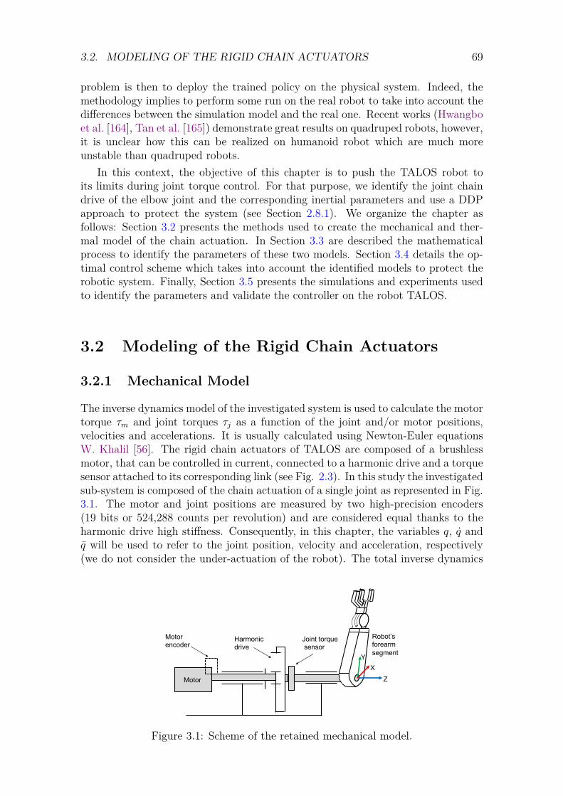
3.2. MODELING OF THE RIGID CHAIN ACTUATORS 69
problem is then to deploy the trained policy on the physical system. Indeed, themethodology implies to perform some run on the real robot to take into account thedifferences between the simulation model and the real one. Recent works (Hwangboet al. [164], Tan et al. [165]) demonstrate great results on quadruped robots, however,it is unclear how this can be realized on humanoid robot which are much moreunstable than quadruped robots.
In this context, the objective of this chapter is to push the TALOS robot toits limits during joint torque control. For that purpose, we identify the joint chaindrive of the elbow joint and the corresponding inertial parameters and use a DDPapproach to protect the system (see Section 2.8.1). We organize the chapter asfollows: Section 3.2 presents the methods used to create the mechanical and ther-mal model of the chain actuation. In Section 3.3 are described the mathematicalprocess to identify the parameters of these two models. Section 3.4 details the op-timal control scheme which takes into account the identified models to protect therobotic system. Finally, Section 3.5 presents the simulations and experiments usedto identify the parameters and validate the controller on the robot TALOS.
3.2 Modeling of the Rigid Chain Actuators
3.2.1 Mechanical Model
The inverse dynamics model of the investigated system is used to calculate the motortorque τm and joint torques τj as a function of the joint and/or motor positions,velocities and accelerations. It is usually calculated using Newton-Euler equationsW. Khalil [56]. The rigid chain actuators of TALOS are composed of a brushlessmotor, that can be controlled in current, connected to a harmonic drive and a torquesensor attached to its corresponding link (see Fig. 2.3). In this study the investigatedsub-system is composed of the chain actuation of a single joint as represented in Fig.3.1. The motor and joint positions are measured by two high-precision encoders(19 bits or 524,288 counts per revolution) and are considered equal thanks to theharmonic drive high stiffness. Consequently, in this chapter, the variables q, q andq will be used to refer to the joint position, velocity and acceleration, respectively(we do not consider the under-actuation of the robot). The total inverse dynamics
Joint torquesensor
Motorencoder
Harmonicdrive
Robot’sforearmsegment
Motor ZX
Y
Figure 3.1: Scheme of the retained mechanical model.
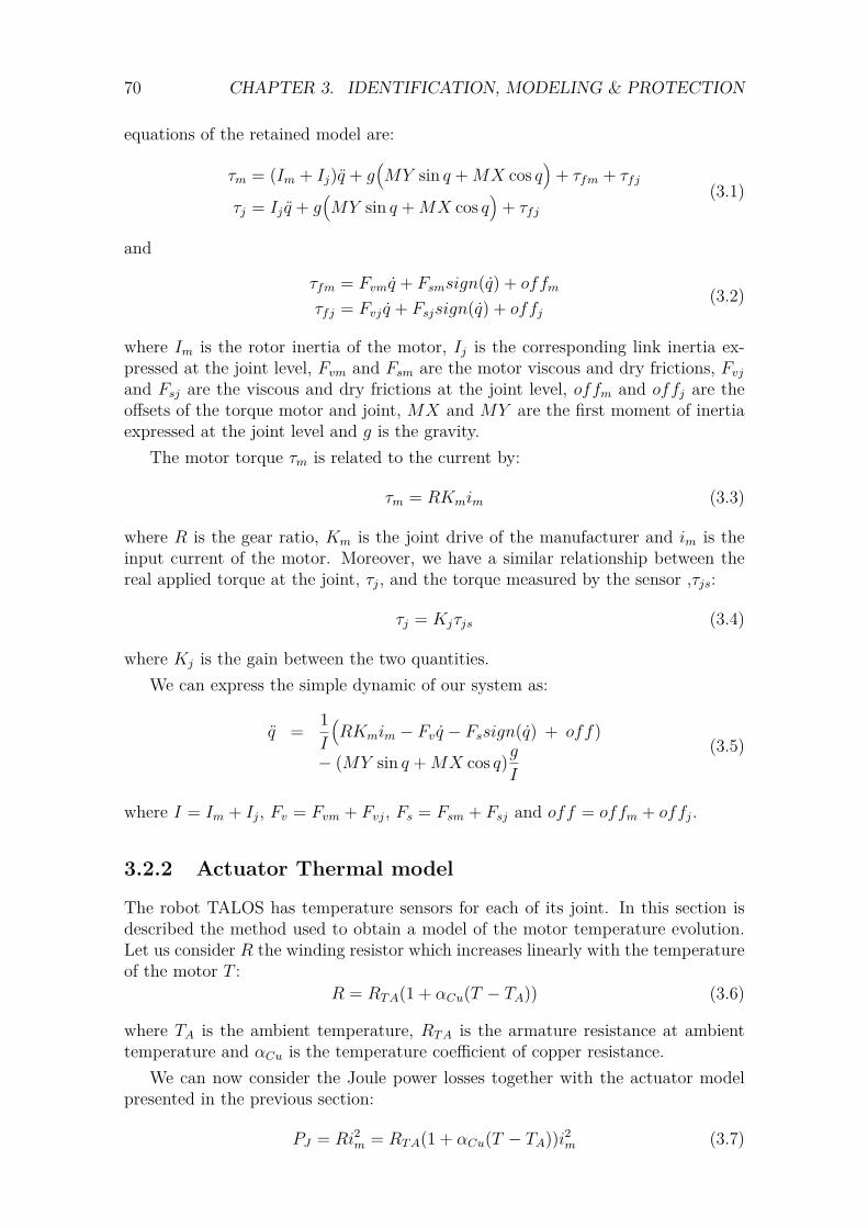
70 CHAPTER 3. IDENTIFICATION, MODELING & PROTECTION
equations of the retained model are:
τm = (Im + Ij)q + g(MY sin q +MX cos q
)+ τfm + τfj
τj = Ij q + g(MY sin q +MX cos q
)+ τfj
(3.1)
and
τfm = Fvmq + Fsmsign(q) + offm
τfj = Fvj q + Fsjsign(q) + offj(3.2)
where Im is the rotor inertia of the motor, Ij is the corresponding link inertia ex-pressed at the joint level, Fvm and Fsm are the motor viscous and dry frictions, Fvjand Fsj are the viscous and dry frictions at the joint level, offm and offj are theoffsets of the torque motor and joint, MX and MY are the first moment of inertiaexpressed at the joint level and g is the gravity.
The motor torque τm is related to the current by:
τm = RKmim (3.3)
where R is the gear ratio, Km is the joint drive of the manufacturer and im is theinput current of the motor. Moreover, we have a similar relationship between thereal applied torque at the joint, τj, and the torque measured by the sensor ,τjs:
τj = Kjτjs (3.4)
where Kj is the gain between the two quantities.We can express the simple dynamic of our system as:
q = 1I
(RKmim − Fv q − Fssign(q) + off)
− (MY sin q +MX cos q)gI
(3.5)
where I = Im + Ij, Fv = Fvm + Fvj, Fs = Fsm + Fsj and off = offm + offj.
3.2.2 Actuator Thermal model
The robot TALOS has temperature sensors for each of its joint. In this section isdescribed the method used to obtain a model of the motor temperature evolution.Let us consider R the winding resistor which increases linearly with the temperatureof the motor T :
R = RTA(1 + αCu(T − TA)) (3.6)
where TA is the ambient temperature, RTA is the armature resistance at ambienttemperature and αCu is the temperature coefficient of copper resistance.
We can now consider the Joule power losses together with the actuator modelpresented in the previous section:
PJ = Ri2m = RTA(1 + αCu(T − TA))i2m (3.7)
3.3. IDENTIFICATION OF THE RIGID CHAIN ACTUATORS 71
Figure 3.2: Equivalent electric model of the simple actuator thermal model.
In this model, some terms are neglected due to their small impact on the con-sidered problem: The friction losses because the type of motor is DC brushless, there-magnetization losses and the Eddy current losses.
We consider that casing conducts the temperature well enough. Therefore, theouter side of the casing (where we measure the temperature) is considered to havethe same temperature as the windings, i.e. RTA = Rth. This allows us to have avery simple model of the motor temperature evolution, depicted in Fig.3.2.2:
CthT = PJ −1Rth
(T − TA) (3.8)
with Cth is the thermal capacity, Rth is the thermal resistance. We set Rth = R.
3.3 Identification of the Rigid Chain Actuators
3.3.1 Identification of chain drive and segment inertial pa-rameters
Usually the segment mass, center of mass and inertia are provided by the robot’smanufacturer with a relatively good accuracy, whereas the friction and chain driveparameters are unknown. The provided current gain drive Km is known to have 10to 15% of inaccuracy Gautier and Briot [194]. Finally, the joint torque sensor shouldbe calibrated prior to be used for control applications. Thus, we propose to use theinverse dynamics model and a total least square approach Gautier and Jubien [58]to identify the system described in Fig. 3.1 and its chain drive at once. To do so,two experiments were performed with and without using an additional payload.When the inertial parameters of the dynamic model are expressed at the joint level,the model is linear, thus Eq.(3.1) becomes:[
τmτj
]=[RKmimKjτjs
]= WΦ =
[cos(q) sin(q) D Dcos(q) sin(q) 0 D
]Φ (3.9)
where D = [q q sign(q) 1] and W is the so-called regressor matrix. As quicklyexplained in Section 2.3.3, we need to create a vector containing all the parametersto be identified. This vector is φ, it contains the inertial parameters to be identified
72 CHAPTER 3. IDENTIFICATION, MODELING & PROTECTION
and is defined as φ = [MX MY Im Fvm Fsm offm Fvj Fsj offj].The TALOS robot embeds motor current and joint torque sensors, thus the regressormatrix W is full rank and the parameters can be identified separately.
To identify the current drive and the torque sensor gains, it is necessary to insertthem into the vector φ Gautier and Jubien [58]. To do so, two regressor matricesthat contain observations from two experiments have to be considered: W0 for theexperiment without payload, and W1 for the one with a known payload at theend-effector. The Eq.(3.9) can be reformulated as:
−W0 im 0 0 0−W0 0 τjs 0 0−W1 im 0 −Wup −Wkp
−W1 0 τjs −Wup −Wkp
φRKm
Kj
φupφkp
= 0 (3.10)
WtotΦtot = 0 (3.11)
where Wup and Wkp are the observation matrices corresponding respectively to theunknown and known payload inertial parameters.
As noted by Gautier et al. Gautier and Jubien [58] Wtot is a full rank ma-trix because of the measurement perturbations. Therefore, the system described inEq.(3.11) is modified to the closest compatible one with respect to the Frobeniusnorm:
WtotΦtot = 0 (3.12)
where Wtot is the closest rank deficient matrix from Wtot and is calculated usingthe singular value decomposition of Wtot = USV T .
The solution Φtot is given by the last column of V and is scaled Gautier andJubien [58] using the known position of the center of mass of the payload along theY-axis (see Fig.3.1).
The success of the inertial parameters identification relies on maintaining themexcited using optimal motions Bonnet et al. [57]. An exciting joint trajectory isdefined using a double S-curve spanning the whole range of motion of the elbowjoint. The duration of each phase (acceleration, constant velocity and deceleration)of the S-curve is set to be equal. The velocity plateau is increased by steps of 20% upto its maximal value. A video illustrating the exciting joint trajectories of the armsis available at the following link: https://peertube.laas.fr/videos/watch/ae07428c-f25a-4637-a998-7e6885db3986.
Joint derivatives are obtained to fulfill the regressor matrix using centered differ-ences from the measured joint positions. All the recorded data are low-pass filteredat 5Hz (Butterworth filter, zero-phase lag order 5) and the number of sample isdecimated to reduce the noise influence Gautier [195]. The S-curve motions are con-sidered exciting since the condition number of the base parameter regressor matrixis low (cond(Wb) = 36).
3.4. DIFFERENTIAL DYNAMIC PROGRAMMING OPTIMAL CONTROL SCHEME73
3.4 Differential Dynamic Programming OptimalControl Scheme
This section presents the optimal control scheme used to find the control sequencesrequired to perform the desired motion. In Section 2.8 is presented the DDP formu-lation (see Algorithm.1), we use a modified version here. In this chapter, we use theformulation given in Forget et al. [156], Kumar Hari Shankar Lal Das et al. [196],which maximizes the performance of the desired motion with respect to the controlunder the actuator physical limitations constraints.
3.4.1 DDP State space representation
In state space, we denote the state vector x = [q, q] and the command vector u = [im].We then represent the direct dynamics model (Eq.3.5) as the following:
x = f(x, u) = f(q, q, im) = q
1I
(RKmim − Fv q − Fssign(q) + off)− (MY sin q +MX cos q)g
I
(3.13)
3.4.2 Treatment of Constraints
In comparison to the work achieved in Forget et al. [156], we do not solve a box QPproblem to bound the command vector. As introduced in Kumar Hari Shankar LalDas et al. [196], we have instead considered the joint and actuator mechanical limitsas constraints on the state and control space in the cost function formulation. Theretained constraints functions are expressed by the following equations, referred as’exponential barrier’, at each time-step t:
max(ct) = 1− λ(cmax − ct)min(ct) = 1− λ(ct − cmin)
Cs(ct) = eλmax(ct) + eλmin(ct)
(3.14)
where cmin, cmax are the corresponding lower and upper mechanical limits on angularposition, velocity and torque, i.e. ct ∈ {x(t), u(t)}. λ is a positive constant whichdefines the smoothness of the function. The higher it is, the quicker the cost willincrease when approaching the limits (depending on the difference between the limitand the current state).
With these constraints, the total cost function will increase and reach a veryhigh cost near the limits, keeping the system safe, in its mechanical bounds.
The control problem formulation is expressed as an open-loop control u =u(t, x) ∈ U which can minimize or maximize a cost function along a given timeinterval t ∈ [0, T ] and from an initial state x(0) = x0 value. The most genericexpression for the cost function can be written as follows:
J(x0) = Cf + Cr + Cs (3.15)
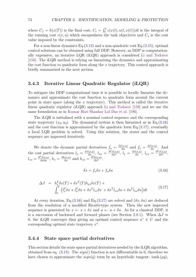
74 CHAPTER 3. IDENTIFICATION, MODELING & PROTECTION
where Cf = h(x(T )) is the final cost, Cr =∫ T
0 c(x(t), u(t, x(t)))dt is the integral ofthe running cost c(x, u) which encapsulates the task objectives and Cs is the costvalue imposed by the constraints.
For a non-linear dynamics Eq.(3.13) and a non-quadratic cost Eq.(3.15), optimalcontrol solutions can be obtained using full DDP. However, as DDP is computation-ally expensive, an iterative LQR (iLQR) approach is considered Li and Todorov[158]. The iLQR method is relying on linearizing the dynamics and approximatingthe cost function to quadratic form along the x trajectory. This control approach isbriefly summarized in the next section.
3.4.3 Iterative Linear Quadratic Regulator (iLQR)
To mitigate the DDP computational time it is possible to locally linearize the dy-namics and approximate the cost function to quadratic form around the currentpoint in state space (along the x trajectory). This method is called the iterativelinear quadratic regulator (iLQR) approach Li and Todorov [158] and we use thesame formulation as in Kumar Hari Shankar Lal Das et al. [196].
The iLQR is initialized with a nominal control sequence and the correspondingstate trajectory (x0, u0). The dynamical system is then linearized as in Eq.(3.16)and the cost function is approximated by the quadratic form Eq.(3.17), eventuallya local LQR problem is solved. Using this solution, the states and the controlsequence are improved iteratively.
We denote the dynamic partial derivatives fu = ∂f(x,u)∂u
and fx = ∂f(x,u)∂x
. Andthe cost partial derivatives lu = ∂J(x,u)
∂u, luu = ∂2J(x,u)
∂u2 , lx = ∂J(x,u)∂x
, lxx = ∂2J(x,u)∂x2 ,
lxu = ∂2J(x,u)∂x∂u
, hx = ∂h(x,u)∂x
and hxx = ∂2h(x,u)∂x2 .
˙δx = fxδx+ fuδu (3.16)
∆J = hTx δx(T ) + δxT (T )hxxδx(T ) +∫ T
0
(lTx δx+ lTu δu+ δxT lxxδx + δxT lxuδu+ δuT luuδu
)dt
(3.17)
At every iteration, Eq.(3.16) and Eq.(3.17) are solved and (δx, δu) are deducedfrom the resolution of a modified Ricatti-type system. Then the new improvedsequence is generated by x ← x + δx and u ← u + δu. As for a classical DDP, itis a succession of backward and forward phases (see Section 2.8.1). When ∆J ≈0, the iLQR converges thus giving an optimal control sequence u∗ ∈ U and thecorresponding optimal state trajectory x∗.
3.4.4 State space partial derivatives
This section details the state space partial derivatives needed by the iLQR algorithm,obtained from eq. (3.13). The sign() function is not differentiable in 0, therefore wehave chosen to approximate the sign(q) term by an hyperbolic tangent: tanh (µq),
3.4. DDP CONTROL SCHEME: ILQR FORMULATION 75
where µ = 1000. We obtain the following new equation for the dynamic of thesystem:
f(x, u) =
q
1I
(RKmim − Fv q − Fs tanh (µq) + off)
− (MY sin q +MX cos q)gI
(3.18)
The partial derivative in u can be directly computed because the function islinearly dependent in im:
fu =[0.0 1
IRKm
]T(3.19)
Concerning the derivative in x, we have non-linear dependencies between q andq, and q and q. Moreover the relationship between q and q is not explicit. Thereforewe use the spatial finite difference discretization of the equation to obtain fx at eachiteration i:
xi+1 = f(xi, ui) (3.20)
fx =
f([qi + h/2
qi
], ui)− f(
[qi − h/2
qi
], ui)
h
f([
qiqi + h/2
], ui)− f(
[qi
qi − h/2
], ui)
h
(3.21)
3.4.5 Cost function
This section presents the cost function used in our system and the cost partial deriva-tives needed by the iLQR algorithm, obtained from the equation (3.13). Consideringthe actual state vector x, the desired state vector x∗, the actual command vector uand the actual torque on the elbow motor τm, we use the following cost function:
J = (x− x∗)TQ (x− x∗) + uTR u+CT
s (x)W Cs(x) + CTs (τm) P Cs(τm) (3.22)
Q =[
40.0 0.00.0 0.01
]R = 0.0001
W =[
1.0 0.00.0 0.1
]P = 10.0
(3.23)The weighting matrix Q,W,R and P have been chosen to give a hierarchy from
the most important error to control to the lesser one. Using the lexicographicalorder we have: q �� τm, τm �� q, q �� q, q �� q �� u. Where c, c are thecorresponding lower and upper mechanical limits. The tracking of the trajectory (inposition) is the prioritized task, followed by the one controlling the torque bounds.
76 CHAPTER 3. IDENTIFICATION, MODELING & PROTECTION
We obtain the following cost partial derivatives lu = ∂J(x,u)∂u
, luu = ∂2J(x,u)∂u2 , lx =
∂J(x,u)∂x
, lxx = ∂2J(x,u)∂x2 , lxu = ∂2J(x,u)
∂x∂u:
lu = 2Ru+ 2 dCs(τm)Tdu
WCs(τm) (3.24)
luu = 2R + 2[d2Cs(τm)T
du2 WCs + dCs(τm)Tdu
WdCs(τm)du
](3.25)
dCs(τm)du
= λ(τm)2 RKm
(eλ(τm)max(τm) − eλ(τm)min(τm)
)(3.26)
d2Cs(τm)du2 = λ(τm)4 (RKm)2 Cs(τm) (3.27)
lx = 2Q (x− x∗) + 2 dCs(x)Tdx
WCs (3.28)
lxx = 2Q+ 2[d2Cs(x)Tdx2 Cs + dCs(x)T
dxWdCs(x)dx
](3.29)
dCs(x)dx
= diag( λ(q)2
[eλmax(q) − eλmin(q)
)λ(q)2
(eλmax(q) − eλmin(q)
) ) (3.30)
d2Cs(x)dx2 =
[λ(q)4 Cs(q) 0.0
0.0 0.0
][
0.0 0.00.0 λ(q)4 Cs(q)
] (3.31)
with λ(τm) = 0.5, λ(q) = 10 and λ(q) = 1. These parameters have been chosenaccordingly to the explanation on the λ of the section 3.4.2. The ’exponentialbarrier’ on the position bounds will be sharper than the two others. It also dependson the difference between the limit and the current state. For instance the maximaldifference in current is 12A whereas the one in position is 2.35rad, then the λ(τm)do not need to be as big as the λ(q).
3.5 Results
3.5.1 Identifying the thermal model
The room temperature (26◦C during the experiment) is never the same as the ambi-ent temperature for the motor. Indeed, the robot drives release a lot of heat, heatingthe motor to approximately 43◦C even when it is unused. The experimental setupis the following: the robot is controlled in position, a sinusoidal command is sent tothe elbow actuators and a heavy charge is put on the arm of the robot (Fig.3.6).
As represented in Fig.3.3, during the heating sequence of the experiment, theidentified function fits the measured temperature evolution. On the other hand,

3.5. RESULTS 77
Figure 3.3: Thermal parameter identification
in the cooling part, the estimated and measured curves tend to diverge. The heatof the drives may cause the problem. Indeed, the temperature of the drives alsoincreases during the experiment. But the drives and the motor are really close toone another, meaning that the temperature of the drives can not be set aside whilestudying the temperature of the motors: it makes the motors cool down slower.Nevertheless, results show that holding 20 kg at 5 cm of the elbow is not a problemfor this specific joint in terms of temperature. As the chain actuators are similar foreach joint of the robot TALOS, one can conclude that overheating the actuators ofthe robot during experiments is unlikely.
3.5.2 Identifying the chain drive and inertial parameters
Fig. 3.4 shows the results of the least square identification. It shows the fitting of themeasured motor and joint torque when no payload was used. The correspondingRoot Mean Square Difference (RMSD) was 0.6 N.m showing an excellent fitting.Fig. 3.6.c shows the estimate of joint torque from the current of the motor that isof importance for the proposed dynamic controller.Table 1 details the comparison between the identified parameters and their valuesas provided by the manufacturer.
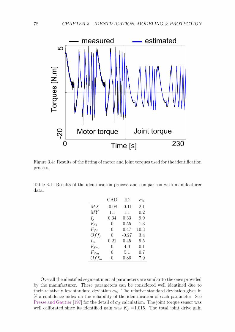
78 CHAPTER 3. IDENTIFICATION, MODELING & PROTECTION
Time [s]0 230
measured estimated
5-2
0To
rque
s [N
.m]
Motor torque Joint torque
Figure 3.4: Results of the fitting of motor and joint torques used for the identificationprocess.
Table 3.1: Results of the identification process and comparison with manufacturerdata.
CAD ID σ%
MX -0.08 -0.11 2.1MY 1.1 1.1 0.2Ij 0.34 0.33 9.9FSj 0 0.55 1.3FV j 0 0.47 10.3Offj 0 -0.27 3.4Im 0.21 0.45 9.5FSm 0 4.0 0.1FV m 0 5.1 0.7Offm 0 0.86 7.9
Overall the identified segment inertial parameters are similar to the ones providedby the manufacturer. These parameters can be considered well identified due totheir relatively low standard deviation σ%. The relative standard deviation gives in% a confidence index on the reliability of the identification of each parameter. SeePresse and Gautier [197] for the detail of σ% calculation. The joint torque sensor waswell calibrated since its identified gain was Kj =1.015. The total joint drive gain
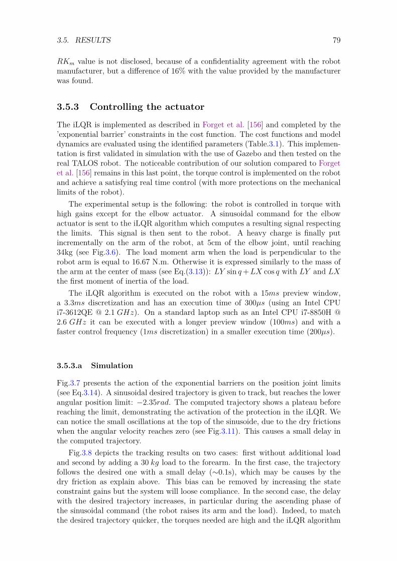
3.5. RESULTS 79
RKm value is not disclosed, because of a confidentiality agreement with the robotmanufacturer, but a difference of 16% with the value provided by the manufacturerwas found.
3.5.3 Controlling the actuator
The iLQR is implemented as described in Forget et al. [156] and completed by the’exponential barrier’ constraints in the cost function. The cost functions and modeldynamics are evaluated using the identified parameters (Table.3.1). This implemen-tation is first validated in simulation with the use of Gazebo and then tested on thereal TALOS robot. The noticeable contribution of our solution compared to Forgetet al. [156] remains in this last point, the torque control is implemented on the robotand achieve a satisfying real time control (with more protections on the mechanicallimits of the robot).
The experimental setup is the following: the robot is controlled in torque withhigh gains except for the elbow actuator. A sinusoidal command for the elbowactuator is sent to the iLQR algorithm which computes a resulting signal respectingthe limits. This signal is then sent to the robot. A heavy charge is finally putincrementally on the arm of the robot, at 5cm of the elbow joint, until reaching34kg (see Fig.3.6). The load moment arm when the load is perpendicular to therobot arm is equal to 16.67 N.m. Otherwise it is expressed similarly to the mass ofthe arm at the center of mass (see Eq.(3.13)): LY sin q+LX cos q with LY and LXthe first moment of inertia of the load.
The iLQR algorithm is executed on the robot with a 15ms preview window,a 3.3ms discretization and has an execution time of 300µs (using an Intel CPUi7-3612QE @ 2.1 GHz). On a standard laptop such as an Intel CPU i7-8850H @2.6 GHz it can be executed with a longer preview window (100ms) and with afaster control frequency (1ms discretization) in a smaller execution time (200µs).
3.5.3.a Simulation
Fig.3.7 presents the action of the exponential barriers on the position joint limits(see Eq.3.14). A sinusoidal desired trajectory is given to track, but reaches the lowerangular position limit: −2.35rad. The computed trajectory shows a plateau beforereaching the limit, demonstrating the activation of the protection in the iLQR. Wecan notice the small oscillations at the top of the sinusoide, due to the dry frictionswhen the angular velocity reaches zero (see Fig.3.11). This causes a small delay inthe computed trajectory.
Fig.3.8 depicts the tracking results on two cases: first without additional loadand second by adding a 30 kg load to the forearm. In the first case, the trajectoryfollows the desired one with a small delay (∼0.1s), which may be causes by thedry friction as explain above. This bias can be removed by increasing the stateconstraint gains but the system will loose compliance. In the second case, the delaywith the desired trajectory increases, in particular during the ascending phase ofthe sinusoidal command (the robot raises its arm and the load). Indeed, to matchthe desired trajectory quicker, the torques needed are high and the iLQR algorithm
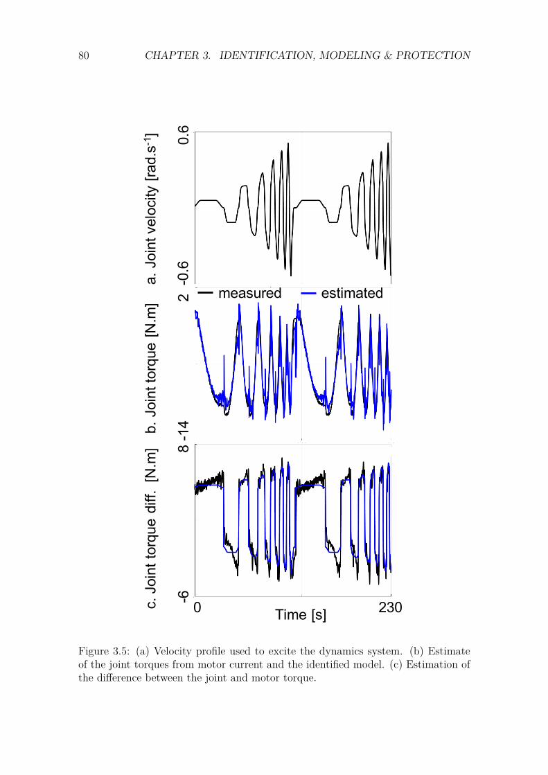
80 CHAPTER 3. IDENTIFICATION, MODELING & PROTECTION
Time [s]0 230
a. J
oint
vel
ocity
[rad.
s-1] 0.6
-0.6
b. J
oint
torq
ue [N
.m] 2
-14
8-6c. J
oint
torq
ue d
iff.
[N.m
]
measured estimated
Figure 3.5: (a) Velocity profile used to excite the dynamics system. (b) Estimateof the joint torques from motor current and the identified model. (c) Estimation ofthe difference between the joint and motor torque.
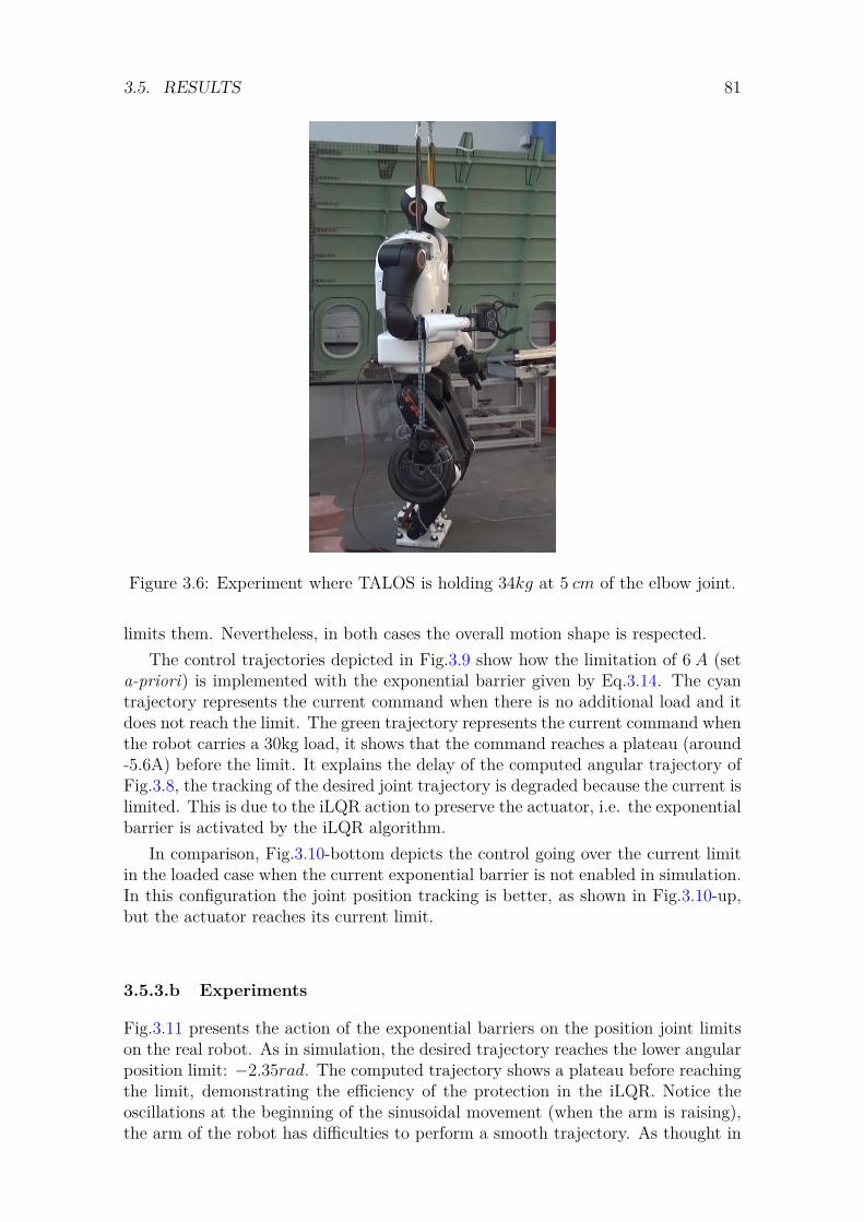
3.5. RESULTS 81
Figure 3.6: Experiment where TALOS is holding 34kg at 5 cm of the elbow joint.
limits them. Nevertheless, in both cases the overall motion shape is respected.The control trajectories depicted in Fig.3.9 show how the limitation of 6 A (set
a-priori) is implemented with the exponential barrier given by Eq.3.14. The cyantrajectory represents the current command when there is no additional load and itdoes not reach the limit. The green trajectory represents the current command whenthe robot carries a 30kg load, it shows that the command reaches a plateau (around-5.6A) before the limit. It explains the delay of the computed angular trajectory ofFig.3.8, the tracking of the desired joint trajectory is degraded because the current islimited. This is due to the iLQR action to preserve the actuator, i.e. the exponentialbarrier is activated by the iLQR algorithm.
In comparison, Fig.3.10-bottom depicts the control going over the current limitin the loaded case when the current exponential barrier is not enabled in simulation.In this configuration the joint position tracking is better, as shown in Fig.3.10-up,but the actuator reaches its current limit.
3.5.3.b Experiments
Fig.3.11 presents the action of the exponential barriers on the position joint limitson the real robot. As in simulation, the desired trajectory reaches the lower angularposition limit: −2.35rad. The computed trajectory shows a plateau before reachingthe limit, demonstrating the efficiency of the protection in the iLQR. Notice theoscillations at the beginning of the sinusoidal movement (when the arm is raising),the arm of the robot has difficulties to perform a smooth trajectory. As thought in
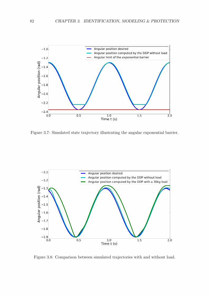
82 CHAPTER 3. IDENTIFICATION, MODELING & PROTECTION
Figure 3.7: Simulated state trajectory illustrating the angular exponential barrier.
Figure 3.8: Comparison between simulated trajectories with and without load.
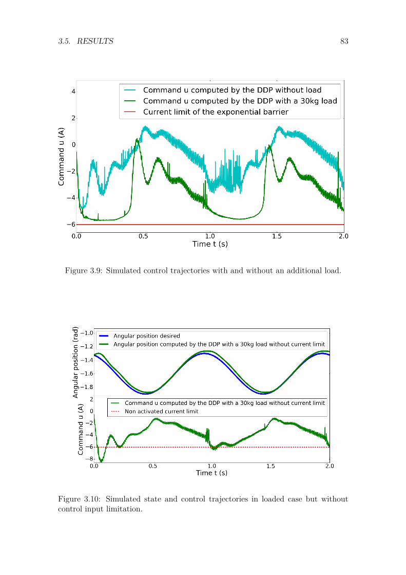
3.5. RESULTS 83
Figure 3.9: Simulated control trajectories with and without an additional load.
Figure 3.10: Simulated state and control trajectories in loaded case but withoutcontrol input limitation.
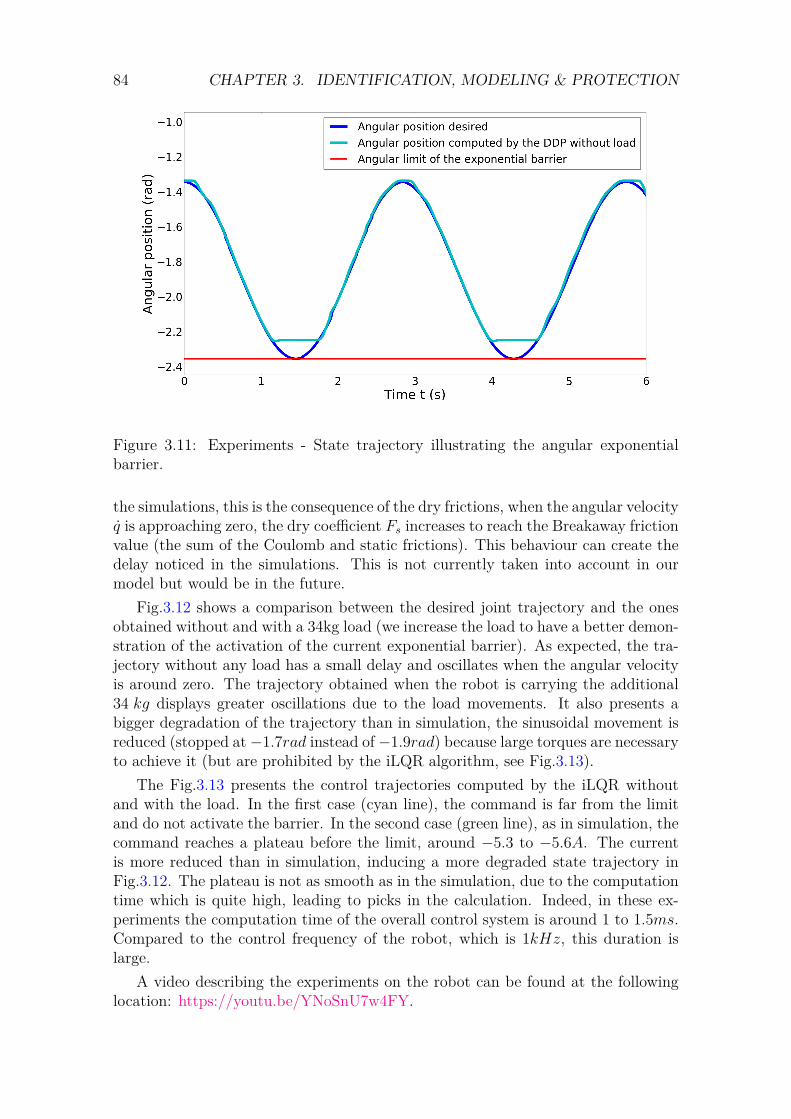
84 CHAPTER 3. IDENTIFICATION, MODELING & PROTECTION
Figure 3.11: Experiments - State trajectory illustrating the angular exponentialbarrier.
the simulations, this is the consequence of the dry frictions, when the angular velocityq is approaching zero, the dry coefficient Fs increases to reach the Breakaway frictionvalue (the sum of the Coulomb and static frictions). This behaviour can create thedelay noticed in the simulations. This is not currently taken into account in ourmodel but would be in the future.
Fig.3.12 shows a comparison between the desired joint trajectory and the onesobtained without and with a 34kg load (we increase the load to have a better demon-stration of the activation of the current exponential barrier). As expected, the tra-jectory without any load has a small delay and oscillates when the angular velocityis around zero. The trajectory obtained when the robot is carrying the additional34 kg displays greater oscillations due to the load movements. It also presents abigger degradation of the trajectory than in simulation, the sinusoidal movement isreduced (stopped at −1.7rad instead of −1.9rad) because large torques are necessaryto achieve it (but are prohibited by the iLQR algorithm, see Fig.3.13).
The Fig.3.13 presents the control trajectories computed by the iLQR withoutand with the load. In the first case (cyan line), the command is far from the limitand do not activate the barrier. In the second case (green line), as in simulation, thecommand reaches a plateau before the limit, around −5.3 to −5.6A. The currentis more reduced than in simulation, inducing a more degraded state trajectory inFig.3.12. The plateau is not as smooth as in the simulation, due to the computationtime which is quite high, leading to picks in the calculation. Indeed, in these ex-periments the computation time of the overall control system is around 1 to 1.5ms.Compared to the control frequency of the robot, which is 1kHz, this duration islarge.
A video describing the experiments on the robot can be found at the followinglocation: https://youtu.be/YNoSnU7w4FY.
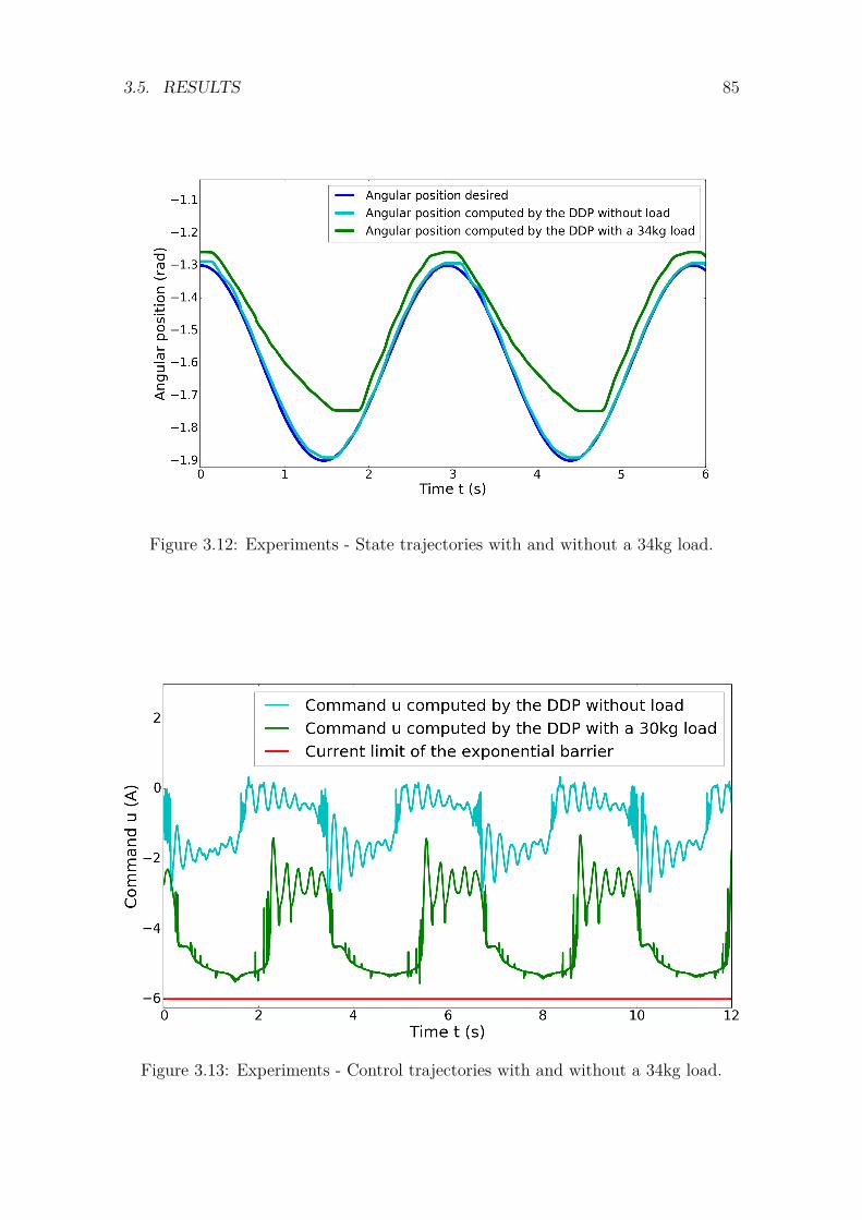
3.5. RESULTS 85
Figure 3.12: Experiments - State trajectories with and without a 34kg load.
Figure 3.13: Experiments - Control trajectories with and without a 34kg load.
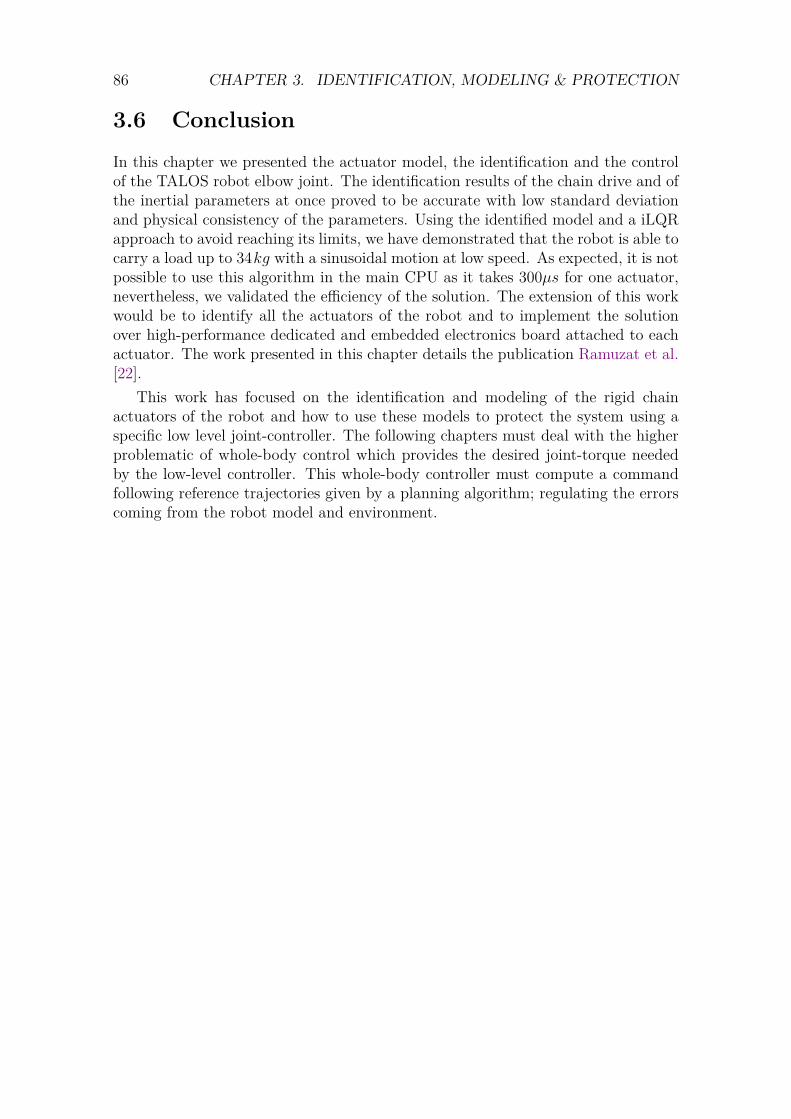
86 CHAPTER 3. IDENTIFICATION, MODELING & PROTECTION
3.6 Conclusion
In this chapter we presented the actuator model, the identification and the controlof the TALOS robot elbow joint. The identification results of the chain drive and ofthe inertial parameters at once proved to be accurate with low standard deviationand physical consistency of the parameters. Using the identified model and a iLQRapproach to avoid reaching its limits, we have demonstrated that the robot is able tocarry a load up to 34kg with a sinusoidal motion at low speed. As expected, it is notpossible to use this algorithm in the main CPU as it takes 300µs for one actuator,nevertheless, we validated the efficiency of the solution. The extension of this workwould be to identify all the actuators of the robot and to implement the solutionover high-performance dedicated and embedded electronics board attached to eachactuator. The work presented in this chapter details the publication Ramuzat et al.[22].
This work has focused on the identification and modeling of the rigid chainactuators of the robot and how to use these models to protect the system using aspecific low level joint-controller. The following chapters must deal with the higherproblematic of whole-body control which provides the desired joint-torque neededby the low-level controller. This whole-body controller must compute a commandfollowing reference trajectories given by a planning algorithm; regulating the errorscoming from the robot model and environment.
Chapter 4
Whole Body Control
Contents4.1 Introduction . . . . . . . . . . . . . . . . . . . . . . . . . . 894.2 Inverse Kinematics Quadratic Program . . . . . . . . . . 90
4.2.1 Motion Task . . . . . . . . . . . . . . . . . . . . . . . . . 904.2.2 Contact Constraints . . . . . . . . . . . . . . . . . . . . . 904.2.3 Quadratic Programming Formulation . . . . . . . . . . . 91
4.3 Inverse Dynamics Quadratic Program . . . . . . . . . . . 914.3.1 Motion Task . . . . . . . . . . . . . . . . . . . . . . . . . 914.3.2 Angular Momentum Task . . . . . . . . . . . . . . . . . . 924.3.3 Contact Constraints . . . . . . . . . . . . . . . . . . . . . 924.3.4 Cartesian Force-Contact task . . . . . . . . . . . . . . . . 934.3.5 Quadratic Programming Formulation . . . . . . . . . . . 94
4.4 Comparison of the Control Schemes . . . . . . . . . . . . 944.4.1 Control Schemes . . . . . . . . . . . . . . . . . . . . . . . 95
4.4.1.a Lexicographical Quadratic Programming . . . . 954.4.1.b Task Space Inverse Dynamics (TSID) . . . . . . 964.4.1.c Remark on the state feedback . . . . . . . . . . 98
4.4.2 Locomotion Planning and Estimator . . . . . . . . . . . . 984.4.3 Energetic Comparison Criteria . . . . . . . . . . . . . . . 98
4.4.3.a Energy cost . . . . . . . . . . . . . . . . . . . . . 984.4.3.b Passivity Gait Measure . . . . . . . . . . . . . . 99
4.4.4 Simulation Results . . . . . . . . . . . . . . . . . . . . . . 1004.4.4.a Straight walk of 20 cm steps . . . . . . . . . . . 1004.4.4.b Straight walk of 60 cm steps in torque control . 1024.4.4.c Walk on the tilted platforms: Uneven terrain . . 1044.4.4.d Climbing Stairs . . . . . . . . . . . . . . . . . . 1054.4.4.e Energy cost and Passivity Gait Measure . . . . . 1054.4.4.f Execution time of the control schemes . . . . . . 108
87
88 CHAPTER 4. WHOLE BODY CONTROL
4.4.5 Discussion . . . . . . . . . . . . . . . . . . . . . . . . . . . 1084.4.6 Conclusion . . . . . . . . . . . . . . . . . . . . . . . . . . 109
4.5 Application on Human-Robot Collaboration for Navi-gation . . . . . . . . . . . . . . . . . . . . . . . . . . . . . . 111
4.5.1 Introduction . . . . . . . . . . . . . . . . . . . . . . . . . 1114.5.2 Scenarios . . . . . . . . . . . . . . . . . . . . . . . . . . . 1124.5.3 Framework Description . . . . . . . . . . . . . . . . . . . 112
4.5.3.a Prediction Model . . . . . . . . . . . . . . . . . 1124.5.3.b Walking Pattern Generator . . . . . . . . . . . . 1134.5.3.c Coupling of the Prediction Process and the WPG 1144.5.3.d Whole-body controller . . . . . . . . . . . . . . . 114
4.5.4 Simulation Results . . . . . . . . . . . . . . . . . . . . . . 1164.5.5 Discussion . . . . . . . . . . . . . . . . . . . . . . . . . . . 1164.5.6 Conclusion . . . . . . . . . . . . . . . . . . . . . . . . . . 119
4.6 Experiments realized on the real robot using the con-trollers . . . . . . . . . . . . . . . . . . . . . . . . . . . . . . 120
4.6.1 Position Control . . . . . . . . . . . . . . . . . . . . . . . 1204.6.1.a Static stabilization . . . . . . . . . . . . . . . . . 1204.6.1.b Dynamic stabilization . . . . . . . . . . . . . . . 1204.6.1.c Fixed compensation of the flexibility . . . . . . . 122
4.6.2 Torque Control . . . . . . . . . . . . . . . . . . . . . . . . 1234.6.2.a PAL robotics low-level controller . . . . . . . . . 1234.6.2.b Experiment Results on a Posture Task . . . . . 124
4.7 Conclusion of the Chapter . . . . . . . . . . . . . . . . . . 126
In this chapter are detailed the results obtained in the publications Ramuzat et al.[23] and Maroger et al. [24]. The second publication is a collaboration with the PhDIsabelle Maroger of the Gepetto Team. Not all this paper is detailed, my contributionon the whole-body controller and the simulations is the main part that is presented.
4.1. INTRODUCTION 89
4.1 Introduction
One of the major issue involving the whole-body motion and control of humanoidrobots is their locomotion. Bipedal locomotion of humanoid robots is still consid-ered as a difficult problem, because of the complexity of the robots dynamics, thenumerous constraints of the motion and the unknown environment. Indeed, to makea humanoid robot stand and walk it is necessary to find a solution involving balanc-ing, contacts creation or removal and contacts stability while performing motionsadapted to the environment. To achieve the locomotion of such complex systems,the problem can be decomposed in four stages (see Fig.2.7): guide planning, contactssequence generation, centroidal trajectory optimization and whole-body control.
Some solutions for the planning stages have been presented in Section 2.4. Mostof the trajectory planning methods use the centroidal dynamics to generate consis-tent behaviors for a legged robot. In addition, the concepts of Divergent Componentof Motion (DCM) Englsberger et al. [45] and Capture Point (CP) Pratt et al. [43] as-sociated to reduced dynamics models such as the Linear Inverted Pendulum (LIPM)Kajita et al. [47] allow to simplify the trajectory generation. Our work focuses onthe last stage of the problem: the whole-body control. Most control architecturesfor legged locomotion are either torque or position controlled.
In the recent literature there is a growing number of implementation of torquecontrol algorithms to solve locomotion problems Lee and Goswami [52], Koolenet al. [54], Englsberger et al. [97], Herzog et al. [153]. Indeed, due to the intrinsiccompliance of the torque control formulation, it is more suitable for interactionswith humans and for multi-contact problems where external interactions and severalcontact points are needed. However, the transition from the simulations to the realexperiments are harder due to the necessity to take into account the model of theactuation chain of the robot Ramuzat et al. [22].
This chapter details the works realized to create whole-body controllers able tocope locomotion problems. Indeed, locomotion and manufacturing operations bothconsist in creating contacts and applying forces in a certain manner while balancing.The capabilities designed for the controllers to realize locomotion with the robotTALOS are the same one needed to achieve the force operations. Moreover, theGepetto team core subject of study is the anthropomorphic motions, thus the teamhas already numerous solutions of complex locomotion trajectories. This allows usto quickly test our implementations on these problems. This chapter presents thedifferent aspects and steps needed to create a complete solution. For instance, theDCM approach can be used in the control stage, for admittance control on theCoM Mesesan et al. [49], Caron et al. [50] to improve the stability of the robot(as described in Section 2.2.3.b). We successfully implement three controllers, twoposition controlled and one torque controlled.
We then investigate the differences and performances of our torque and positioncontrol schemes to choose the most appropriate one for the robot TALOS. We testthe most promising controller on a specific application of human-robot collaborationfor navigation. Finally, the results of the experiments performed on TALOS arepresented.
The chapter is organized as follows: Sections 4.2 and 4.3 detail the formulationsused for the position and torque QPs used by our whole-body controllers. Then, the
90 CHAPTER 4. WHOLE BODY CONTROL
next sections explain the process implemented to benchmark the controllers: Sec-tion 4.4 details the three task-space whole-body control schemes to be compared.Section 4.4.2 presents the planning methodologies and the state estimator used forthe simulations. Section 4.4.3 describes the energy criteria used for the controllersbenchmarking. Section 4.4.4 presents the simulations results and Section 4.4.5 dis-cusses them. In Section 4.5 is detailed the application of our torque controller inthe scope of a human-robot co-navigation, this work was realized in collaborationwith Isabelle Maroger. Finally, the last section describes the intermediate experi-ments realized on the real robot and the difficulties we faced, using the presentedcontrollers.
4.2 Inverse Kinematics Quadratic Program
The first controller created during this thesis is a Hierarchical Quadratic Program-ming (HQP) (see Section 2.5.2.c). It solves a task-based inverse velocity kinematicsdescribed in Mansard et al. [16] and outputs a velocity command. It implementsa strict hierarchy between the tasks and has been implemented using the packageSoT-Core [20]. For the remaining of the manuscript, the inverse velocity kinematicsis directly called inverse kinematics or IK.
4.2.1 Motion Task
In this controller, the task errors e to be reduced in the cost function are implementedas velocity-based tracking laws in the Lie group SE(3). Having the robot coordinatevector q and its velocity v as control input, a task-function is a derivable functionx(q) whose space is named the task-space. And the task errors e ∈ Rl are expressedas in the Section 2.5.2.b:
e(q, t) = x(q)− x∗(t)x(q) = Jv
(4.1)
with x∗, x∗ the desired position and velocity of the task, l is the dimension of the taskerror (for instance, for the 3D acceleration error on the CoM l = 3), J = [Ju Ja] =[T (S,B) ∂e
∂q] = [T (S,B) ∂x
∂q] the Jacobian according to the robot coordinates vector.
Ju is the "Jacobian" of the under-actuated part: it is the transformation T betweenthe task/error frame S and the base frame B (see Eq.2.6).
A first-order linear dynamics is imposed on these errors (see Section 2.5.2.b):
e(q, t) = KP (x(q) x∗(q))⇔ x(q) = x∗(t) +KP (x(q) x∗(q)) (4.2)
with the difference operator of Lie group.
4.2.2 Contact Constraints
In SoT-Core, the contact constraints are implemented as tasks with the higherpriorities. The velocity of the task is null and the position is kept constant, i.e. for
4.3. INVERSE DYNAMICS QUADRATIC PROGRAM 91
a contact point xc and its Jacobian Jc:xic = xi+1
c
xc = 0⇔ JTc v = 0
(4.3)
4.2.3 Quadratic Programming Formulation
Using the similar formulation as Section 2.5.2.b and Section 2.5.2.c, with gi = ‖wi‖for each task i ∈ N , it is possible to formulate the QP formulation of our controlleras follows:
g∗i = minv,gi
gi
s.t. JTc v = 0gj = g∗j ∀j < i
(4.4)
with Jc the Jacobian associated to the c contact points Xc = {xc1...xcc}. Herewe differentiate the contact tasks from the other one but they can be also put asfunction g0 with the higher priority 0.
This strict hierarchy can be solved by using the orthogonal projection operator Pon the null-space of the Jacobian J . The tasks with lower priorities are solved at bestin the remaining space of the previous tasks solutions. With J† the pseudo-inverseof J , one can write for N tasks such that e1 ≺ e2 ≺ ... ≺ eN :
q = J†1e1 +N∑k=2
J†k(k−1∏l=1
Pl)ek (4.5)
In SoT-Core, this QP is solved using the method presented in Mansard andChaumette [78].
4.3 Inverse Dynamics Quadratic Program
The second and third controllers created during this thesis use a Weighted QuadraticProgramming (WQP) called TSID [80]. It sums selected task functions in a generalcost function using weights to define their priorities (see Section 2.5.2.c). It thenoptimizes this sum subject to several constraints. It has been successfully used on aHRP-2 robot to realize torque control in Prete et al. [21]. The controllers have beenimplemented in the package SoT-Torque-Control [79].
4.3.1 Motion Task
Most of the task-function errors of TSID are expressed as motion task errors e.They are implemented as acceleration-based tracking laws in the Lie group SE(3).Having the robot coordinates vector q and the acceleration a as control input, atask-function is a second-order derivable function x(q) whose space is named thetask-space. And the motion task errors e ∈ Rl (with l the dimension of the errortask for instance 3 for the CoM task) are expressed as in the Section 2.5.2.b:
e(q, t) = x(q)− x∗(t)e(q, t) = (Ja+ Jv)− x∗(t) (4.6)
92 CHAPTER 4. WHOLE BODY CONTROL
with x∗, x∗ the desired position and acceleration of the task, J the Jacobian accordingto the robot state vector as defined previously and in Eq.2.6.
The following dynamics is imposed on these errors (see Section 2.5.2.b):
e(q, t) = KP (x(q) x∗) +KD(x(q)− x∗(t))⇔ x(q) = x∗(t) +KP (x(q) x∗(t))+
KD(x(q)− x∗(t))(4.7)
with the difference operator of Lie group. To simplify notations, in the following,we will use the usual difference operator instead of and we will not write the stateor time dependencies of the terms. Using Eq.4.6 and Eq.4.7 leads to the genericformulation for a motion task-function:
J︸︷︷︸O
a︸︷︷︸y
= x∗ − Jv +KP e+KDe︸ ︷︷ ︸o
(4.8)
4.3.2 Angular Momentum Task
The Angular Momentum (AM) dynamics is expressed in TSID using the equationdefined in Section 2.2.4, recalled here:
kc = k∗c +KPam(k∗c − kc) (4.9)
with kc the commanded rates of change of the angular momentum and KPam theproportional gain for the AM task. The linear component follows the motion taskdefined in Eq.4.8, called CoM task.
4.3.3 Contact Constraints
The inverse dynamics of the robot is solved in rigid contact with the environmentHerzog et al. [153], thus, these contacts constrain the motion. They are implementedin TSID as nonlinear functions, which are differentiated twice (with Jc the Jacobianat the contact point). The Eq.2.52 is recalled here for clarity:
c(q) = 0 ⇔ Contact point does not moveJTc v = 0 ⇔ Contact point velocity is zero
JTc a+ Jc v = 0 ⇔ Contact point acceleration is zero(4.10)
The equation of the dynamics is formulated as an equality constraint with τext re-placed by the forces applied at each contact, and these forces are optimized (seeEq.4.14). In this chapter, we use the unilateral rectangular plane contact formula-tion of TSID. The contact is defined as a 6D motion task (Eq.4.8), an inequalityconstraint on the force bounds and a direct force task:
T Tf = f ∗ (4.11)
with the force-generator matrix T T ∈ R6×12 mapping the forces at the vertices of thecontact surface, f ∈ R12 (four 3D forces), to a 6D resultant force at the contact point(center of the surface). f ∗ ∈ R6 the desired force for the contact. T creates the mapbetween the two representations: τcontact = JTT Tf . However in our formulation wedo not use this direct force task, letting the QP optimize freely the forces at thecontact, except for the Cartesian Force-Contact case.
4.3. INVERSE DYNAMICS QUADRATIC PROGRAM 93
4.3.4 Cartesian Force-Contact task
The context of my thesis is the validation of a solution for manufacturing opera-tions. These operations, mainly drilling or tightening, need precision while applyinga certain amount of force on a structure. To achieve these operations with our devel-oped whole-body controllers we need to implement a new force task. The targetedapplication is the drilling of a metal plate, requiring the application of huge forces(∼ 600N). Following the study of the state-of-the art realized on the force control formanipulations (see Section 2.7), and based on the formulation of the tasks in TSID,we choose to implement a parallel force/position control. This task is composed oftwo parts: the force application and the position control of the contact. Thus, itcombines two tasks, a motion task defined in Eq.4.8 for the control of the position,and a force task for the application of the force.
The force task is defined as a Proportional Integral with a feed-forward (PI+)and an anti-windup, inspired by Shahriari et al. [113]:
ef = F ∗ − FextT TF︸︷︷︸O
FF︸︷︷︸y
= F ∗ + PF ef + IF
∫ t
0efds︸ ︷︷ ︸
o
(4.12)
with F ∗, Fext ∈ R6, respectively the desired and measured or estimated externalwrenches and PF , IF ∈ R6×6 the task gains. TF is the force-generator matrix definedas in the previous paragraph and FF is the constrained wrench.
In TSID, as explained in Eq.2.52,4.11, the forces in the equation of the dynamicsare expressed at the contacts. Thus, the force task is linked to its appropriate contacttask (see previous paragraph, Section 4.3.4). In the library, the task is called task-contact-force, it implements the force task of Eq.4.12 and the position control partof the task is done by the 6D motion task of the associated contact (Eq.4.8).
Thus, we implemented a parallel force/position control which also respects thecoulomb constraints as the position control is done by the contact constraint of theprevious section (Section 4.3.3). Considering that our system has c contacts and theCartesian Force-Contact task, we can replace τext by:
τext =c∑
k=1JTk T
Tk fk − JTF T TF FF (4.13)
which is in fact the JTc F term defined in Eq.2.4.
94 CHAPTER 4. WHOLE BODY CONTROL
4.3.5 Quadratic Programming Formulation
TSID sums all the task functions gi(y) using user-defined scalar weights λi, ∀i ∈ Ntasks, subject to constraints such as the rigid contacts and the dynamics. It leadsto the same formulation defined in Eq.2.57 replacing ωi with the tasks functions(Eq.4.8):
gi(y) = ‖Oiy − oi‖2
miny=[a,f ]
N∑i=0
λi gi
s.t. Jc 0 0M −JTc −NT
afτ
= −Jc v−h
τmin ≤ τ ≤ τmax
qminj ≤ qj ≤ qmaxj
qminj ≤ qj ≤ qmaxj
fmin ≤ f ≤ fmax
(4.14)
Where the free variables are the acceleration a and the force F . The QP is formulatedto solve the acceleration and the forces and to then retrieve the torque using Eq.2.4.It has only two strict layers: the constraint layer (priority 0) and the cost layer(priority I).
The solver used in TSID is eiquadprod [198], it implements the algorithm ofGoldfarb and Idnani Goldfarb and Idnani [199] for the solution of a convex QPproblem by means of a dual method.
For x = [a, F ], the problem is of the form :
minx 12x
TGx+ g0xs.t. CETx+ ce0 = 0
CITx+ ci0 ≥ 0(4.15)
with G the symmetric Hessian of the Cholesky factorization of the cost function,g0 the Lagrange multipliers of the cost function, CE the generalized matrix of theequality constraints and ce0 their associated vectors and similarly CI the generalizedmatrix of the inequality constraints and ci0 their associated vectors.
4.4 Comparison of the Control Schemes
This section focus on the implementation and comparison of three real-time whole-body controllers using the task-function approach Samson et al. [37], Escande et al.[38]. The objectives to be performed by the robot are expressed in their respectivetask spaces, using reference trajectories given by the planning. Complex motionscombine several nonlinear tasks and constraints. Quadratic Programming prob-lems (QP) are instantaneous optimization techniques used to solve such nonlinearproblems, employing the whole-body kinematics or dynamics of the robot. In thissection two types of QP are compared, a Hierarchical QP which imposes a stricthierarchy between the tasks Hoffman et al. [88], Henze et al. [89], Herzog et al.
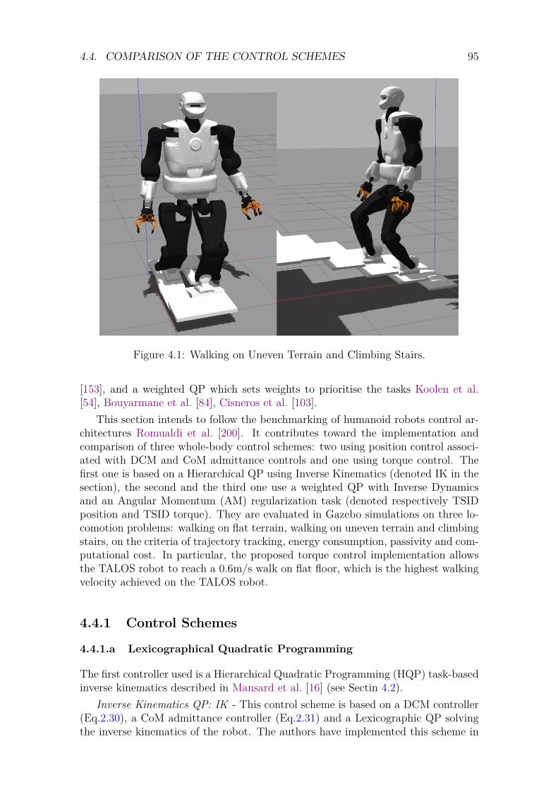
4.4. COMPARISON OF THE CONTROL SCHEMES 95
Figure 4.1: Walking on Uneven Terrain and Climbing Stairs.
[153], and a weighted QP which sets weights to prioritise the tasks Koolen et al.[54], Bouyarmane et al. [84], Cisneros et al. [103].
This section intends to follow the benchmarking of humanoid robots control ar-chitectures Romualdi et al. [200]. It contributes toward the implementation andcomparison of three whole-body control schemes: two using position control associ-ated with DCM and CoM admittance controls and one using torque control. Thefirst one is based on a Hierarchical QP using Inverse Kinematics (denoted IK in thesection), the second and the third one use a weighted QP with Inverse Dynamicsand an Angular Momentum (AM) regularization task (denoted respectively TSIDposition and TSID torque). They are evaluated in Gazebo simulations on three lo-comotion problems: walking on flat terrain, walking on uneven terrain and climbingstairs, on the criteria of trajectory tracking, energy consumption, passivity and com-putational cost. In particular, the proposed torque control implementation allowsthe TALOS robot to reach a 0.6m/s walk on flat floor, which is the highest walkingvelocity achieved on the TALOS robot.
4.4.1 Control Schemes
4.4.1.a Lexicographical Quadratic Programming
The first controller used is a Hierarchical Quadratic Programming (HQP) task-basedinverse kinematics described in Mansard et al. [16] (see Sectin 4.2).
Inverse Kinematics QP: IK - This control scheme is based on a DCM controller(Eq.2.30), a CoM admittance controller (Eq.2.31) and a Lexicographic QP solvingthe inverse kinematics of the robot. The authors have implemented this scheme in
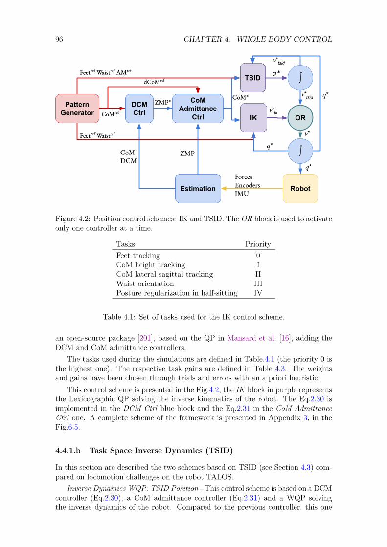
96 CHAPTER 4. WHOLE BODY CONTROL
𝓿*
𝓿*tsid
CoMref
CoM Admittance
Ctrl
DCMCtrl
IK
PatternGenerator
RobotEstimation
ForcesEncodersIMU
Feetref Waistref
ZMPCoMDCM
CoM*ZMP*
dCoMref
OR𝓿*Ik
𝑞*
TSIDFeetref Waistref AMref
∫a*
∫𝑞*
𝑞*
𝓿*tsid
Figure 4.2: Position control schemes: IK and TSID. The OR block is used to activateonly one controller at a time.
Tasks PriorityFeet tracking 0CoM height tracking ICoM lateral-sagittal tracking IIWaist orientation IIIPosture regularization in half-sitting IV
Table 4.1: Set of tasks used for the IK control scheme.
an open-source package [201], based on the QP in Mansard et al. [16], adding theDCM and CoM admittance controllers.
The tasks used during the simulations are defined in Table.4.1 (the priority 0 isthe highest one). The respective task gains are defined in Table 4.3. The weightsand gains have been chosen through trials and errors with an a priori heuristic.
This control scheme is presented in the Fig.4.2, the IK block in purple representsthe Lexicographic QP solving the inverse kinematics of the robot. The Eq.2.30 isimplemented in the DCM Ctrl blue block and the Eq.2.31 in the CoM AdmittanceCtrl one. A complete scheme of the framework is presented in Appendix 3, in theFig.6.5.
4.4.1.b Task Space Inverse Dynamics (TSID)
In this section are described the two schemes based on TSID (see Section 4.3) com-pared on locomotion challenges on the robot TALOS.
Inverse Dynamics WQP: TSID Position - This control scheme is based on a DCMcontroller (Eq.2.30), a CoM admittance controller (Eq.2.31) and a WQP solvingthe inverse dynamics of the robot. Compared to the previous controller, this one
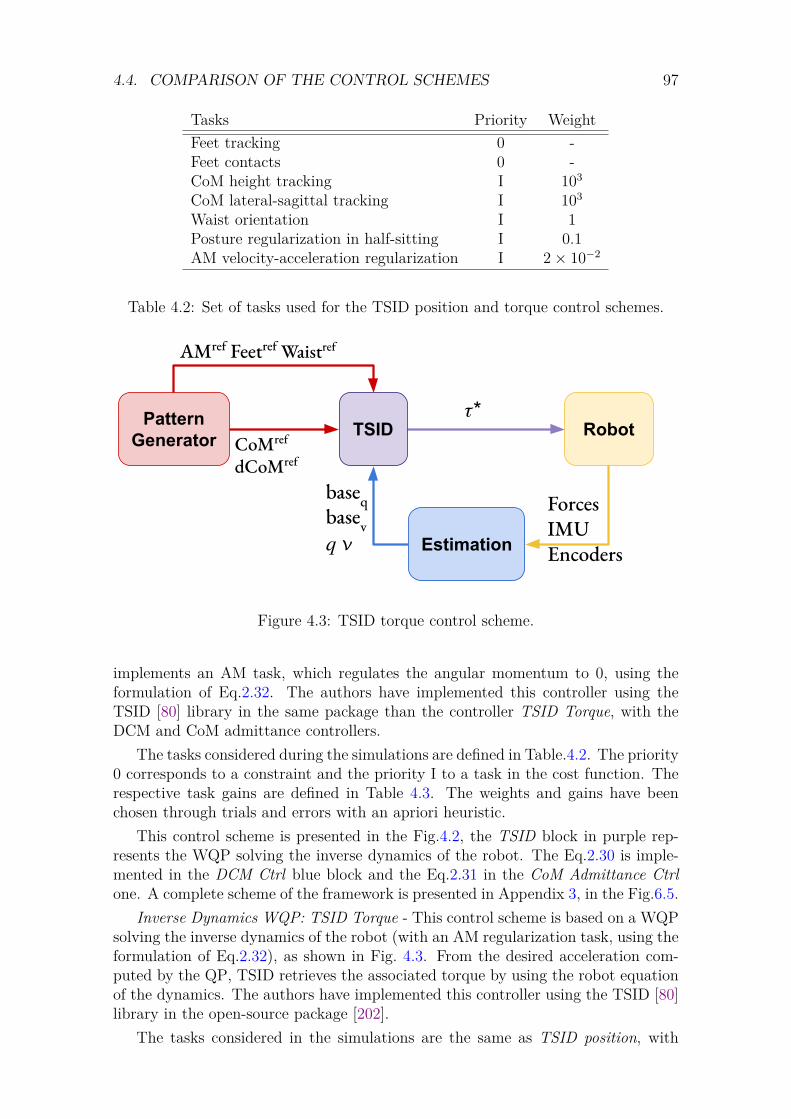
4.4. COMPARISON OF THE CONTROL SCHEMES 97
Tasks Priority WeightFeet tracking 0 -Feet contacts 0 -CoM height tracking I 103
CoM lateral-sagittal tracking I 103
Waist orientation I 1Posture regularization in half-sitting I 0.1AM velocity-acceleration regularization I 2× 10⁻²
Table 4.2: Set of tasks used for the TSID position and torque control schemes.
CoMref dCoMref
TSIDPatternGenerator
Robot
Estimation
ForcesIMUEncoders
AMref Feetref Waistref
baseqbasev 𝑞 𝓿
𝜏*
Figure 4.3: TSID torque control scheme.
implements an AM task, which regulates the angular momentum to 0, using theformulation of Eq.2.32. The authors have implemented this controller using theTSID [80] library in the same package than the controller TSID Torque, with theDCM and CoM admittance controllers.
The tasks considered during the simulations are defined in Table.4.2. The priority0 corresponds to a constraint and the priority I to a task in the cost function. Therespective task gains are defined in Table 4.3. The weights and gains have beenchosen through trials and errors with an apriori heuristic.
This control scheme is presented in the Fig.4.2, the TSID block in purple rep-resents the WQP solving the inverse dynamics of the robot. The Eq.2.30 is imple-mented in the DCM Ctrl blue block and the Eq.2.31 in the CoM Admittance Ctrlone. A complete scheme of the framework is presented in Appendix 3, in the Fig.6.5.
Inverse Dynamics WQP: TSID Torque - This control scheme is based on a WQPsolving the inverse dynamics of the robot (with an AM regularization task, using theformulation of Eq.2.32), as shown in Fig. 4.3. From the desired acceleration com-puted by the QP, TSID retrieves the associated torque by using the robot equationof the dynamics. The authors have implemented this controller using the TSID [80]library in the open-source package [202].
The tasks considered in the simulations are the same as TSID position, with
98 CHAPTER 4. WHOLE BODY CONTROL
different gains (see Table 4.3). A complete scheme of the framework is presented inAppendix 3, in the Fig.6.5.
4.4.1.c Remark on the state feedback
For position control, it is needed to integrate the result of the QP (one time for IKand two times for TSID position, see Fig.4.2) to obtain the desired command. Toavoid instabilities, the control loop of both QP use these integrated values in the nextiteration instead of the measured ones. The measured position and velocity of therobot are only used to compute the CoM, DCM and ZMP for the admittance controlin the position schemes. In contrary, the torque control scheme uses the measuredvalues at each iteration of the QP (see Fig.4.3) and in particular the position andvelocity of the robot base (or free-flyer).
4.4.2 Locomotion Planning and Estimator
In this section the two locomotion planning methods presented in Section 2.4 havebeen used. First, the WPG has computed the trajectories for the walk on flatfloor simulations (20cm and 60cm), with pre-defined set of foot steps. The WPGis plugged to the whole body controller using the dynamic-graph package in or-der to get the next reference point of the trajectories in real-time. Secondly, themulticontact-locomotion-planning is used to obtain the trajectories for the platformsand stairs simulations. Here the references are computed offline and then a file con-taining the trajectories is read during the simulation.
Finally, for every simulations, the estimation of the base (free-flyer) of the robothas been realized using the approach presented in Flayols et al. [29]. The free-flyerinformation are estimated using robot joints configurations and velocities, the IMUand the force sensors of the robot. It allows the whole-body controller to have accessto the whole state vector, including the position and velocity of the base, necessaryto compute the CoM on an under-actuated system.
4.4.3 Energetic Comparison Criteria
4.4.3.a Energy cost
Based on Torricelli et al. [203], a relevant criterion to compare the energy consump-tion of the control schemes is the cost of transport. It can be computed as theenergetic cost of transport Cet using the whole mechanical work of the actuationsystem Em or as the mechanical cost of transport Cmt using only the positive oneEm+.
Cet = EmmgD
Cmt = Em+
mgDEm =
∫ T
0
N∑i=0|τi(t)ωi(t)|dt
(4.16)with m the mass of the system, g the gravity constant, D the distance traveled bythe system and τi, ωi the respective torque and velocity of each robot joint for all(N) joints.
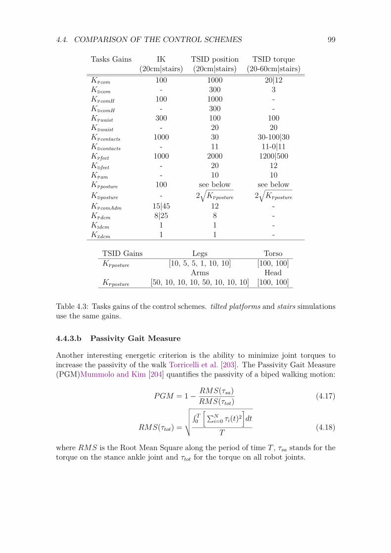
4.4. COMPARISON OF THE CONTROL SCHEMES 99
Tasks Gains IK TSID position TSID torque(20cm|stairs) (20cm|stairs) (20-60cm|stairs)
Kpcom 100 1000 20|12Kdcom - 300 3KpcomH 100 1000 -KdcomH - 300 -Kpwaist 300 100 100Kdwaist - 20 20Kpcontacts 1000 30 30-100|30Kdcontacts - 11 11-0|11Kpfeet 1000 2000 1200|500Kdfeet - 20 12Kpam - 10 10Kpposture 100 see below see belowKdposture - 2
√Kpposture 2
√Kpposture
KpcomAdm 15|45 12 -Kpdcm 8|25 8 -Kidcm 1 1 -Kzdcm 1 1 -
TSID Gains Legs TorsoKpposture [10, 5, 5, 1, 10, 10] [100, 100]
Arms HeadKpposture [50, 10, 10, 10, 50, 10, 10, 10] [100, 100]
Table 4.3: Tasks gains of the control schemes. tilted platforms and stairs simulationsuse the same gains.
4.4.3.b Passivity Gait Measure
Another interesting energetic criterion is the ability to minimize joint torques toincrease the passivity of the walk Torricelli et al. [203]. The Passivity Gait Measure(PGM)Mummolo and Kim [204] quantifies the passivity of a biped walking motion:
PGM = 1− RMS(τsa)RMS(τtot)
(4.17)
RMS(τtot) =
√√√√√∫ T0[∑N
i=0 τi(t)2]dt
T(4.18)
where RMS is the Root Mean Square along the period of time T , τsa stands for thetorque on the stance ankle joint and τtot for the torque on all robot joints.
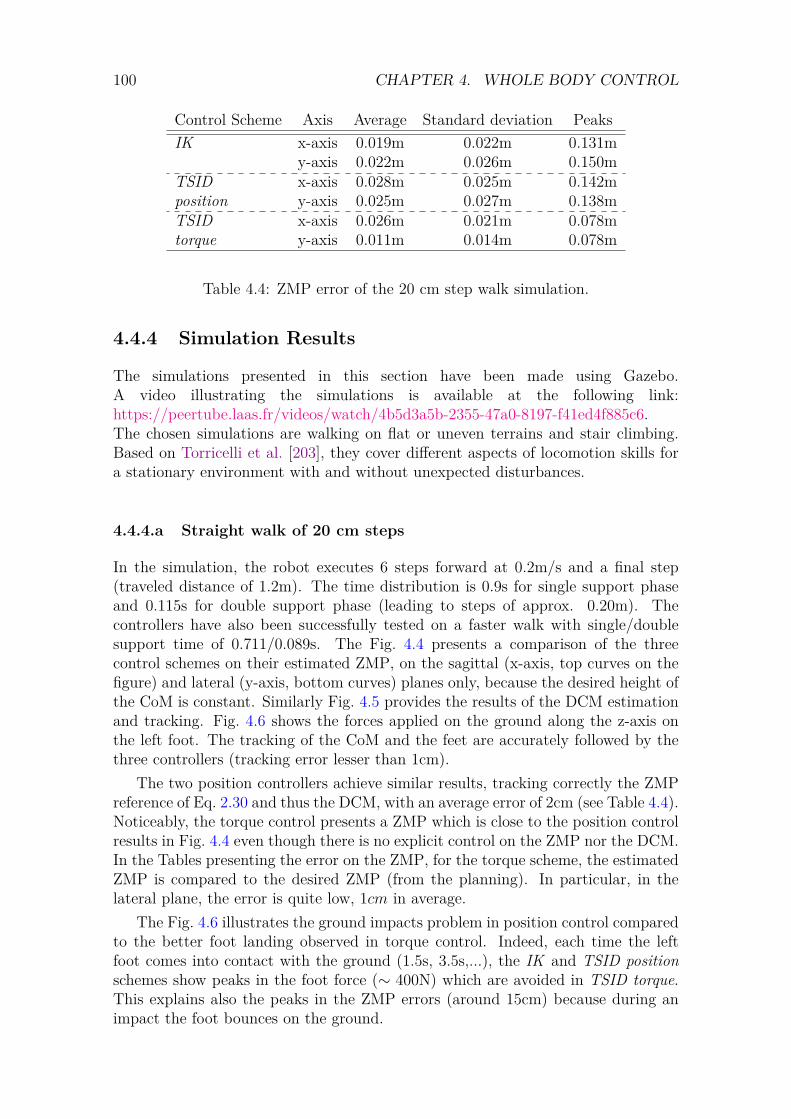
100 CHAPTER 4. WHOLE BODY CONTROL
Control Scheme Axis Average Standard deviation PeaksIK x-axis 0.019m 0.022m 0.131m
y-axis 0.022m 0.026m 0.150mTSID x-axis 0.028m 0.025m 0.142mposition y-axis 0.025m 0.027m 0.138mTSID x-axis 0.026m 0.021m 0.078mtorque y-axis 0.011m 0.014m 0.078m
Table 4.4: ZMP error of the 20 cm step walk simulation.
4.4.4 Simulation Results
The simulations presented in this section have been made using Gazebo.A video illustrating the simulations is available at the following link:https://peertube.laas.fr/videos/watch/4b5d3a5b-2355-47a0-8197-f41ed4f885c6.The chosen simulations are walking on flat or uneven terrains and stair climbing.Based on Torricelli et al. [203], they cover different aspects of locomotion skills fora stationary environment with and without unexpected disturbances.
4.4.4.a Straight walk of 20 cm steps
In the simulation, the robot executes 6 steps forward at 0.2m/s and a final step(traveled distance of 1.2m). The time distribution is 0.9s for single support phaseand 0.115s for double support phase (leading to steps of approx. 0.20m). Thecontrollers have also been successfully tested on a faster walk with single/doublesupport time of 0.711/0.089s. The Fig. 4.4 presents a comparison of the threecontrol schemes on their estimated ZMP, on the sagittal (x-axis, top curves on thefigure) and lateral (y-axis, bottom curves) planes only, because the desired height ofthe CoM is constant. Similarly Fig. 4.5 provides the results of the DCM estimationand tracking. Fig. 4.6 shows the forces applied on the ground along the z-axis onthe left foot. The tracking of the CoM and the feet are accurately followed by thethree controllers (tracking error lesser than 1cm).
The two position controllers achieve similar results, tracking correctly the ZMPreference of Eq. 2.30 and thus the DCM, with an average error of 2cm (see Table 4.4).Noticeably, the torque control presents a ZMP which is close to the position controlresults in Fig. 4.4 even though there is no explicit control on the ZMP nor the DCM.In the Tables presenting the error on the ZMP, for the torque scheme, the estimatedZMP is compared to the desired ZMP (from the planning). In particular, in thelateral plane, the error is quite low, 1cm in average.
The Fig. 4.6 illustrates the ground impacts problem in position control comparedto the better foot landing observed in torque control. Indeed, each time the leftfoot comes into contact with the ground (1.5s, 3.5s,...), the IK and TSID positionschemes show peaks in the foot force (∼ 400N) which are avoided in TSID torque.This explains also the peaks in the ZMP errors (around 15cm) because during animpact the foot bounces on the ground.
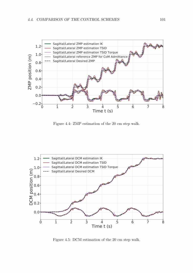
4.4. COMPARISON OF THE CONTROL SCHEMES 101
0 1 2 3 4 5 6 7 8Time t (s)
0.2
0.0
0.2
0.4
0.6
0.8
1.0
1.2
ZMP
posit
ion
(m)
Sagittal/Lateral ZMP estimation IKSagittal/Lateral ZMP estimation TSIDSagittal/Lateral ZMP estimation TSID TorqueSagittal/Lateral reference ZMP for CoM AdmittanceSagittal/Lateral Desired ZMP
Figure 4.4: ZMP estimation of the 20 cm step walk.
0 1 2 3 4 5 6 7 8Time t (s)
0.0
0.2
0.4
0.6
0.8
1.0
1.2
DCM
pos
ition
(m)
Sagittal/Lateral DCM estimation IKSagittal/Lateral DCM estimation TSIDSagittal/Lateral DCM estimation TSID TorqueSagittal/Lateral Desired DCM
Figure 4.5: DCM estimation of the 20 cm step walk.
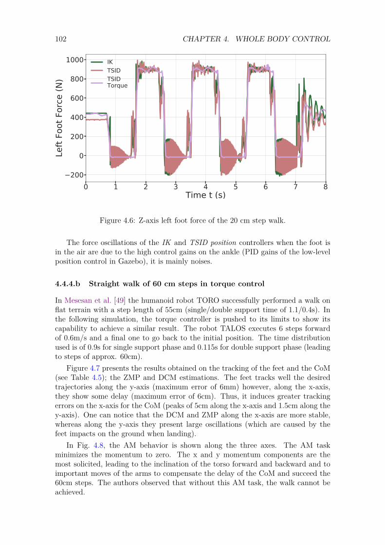
102 CHAPTER 4. WHOLE BODY CONTROL
0 1 2 3 4 5 6 7 8Time t (s)
200
0
200
400
600
800
1000Le
ft Fo
ot F
orce
(N)
IKTSIDTSIDTorque
Figure 4.6: Z-axis left foot force of the 20 cm step walk.
The force oscillations of the IK and TSID position controllers when the foot isin the air are due to the high control gains on the ankle (PID gains of the low-levelposition control in Gazebo), it is mainly noises.
4.4.4.b Straight walk of 60 cm steps in torque control
In Mesesan et al. [49] the humanoid robot TORO successfully performed a walk onflat terrain with a step length of 55cm (single/double support time of 1.1/0.4s). Inthe following simulation, the torque controller is pushed to its limits to show itscapability to achieve a similar result. The robot TALOS executes 6 steps forwardof 0.6m/s and a final one to go back to the initial position. The time distributionused is of 0.9s for single support phase and 0.115s for double support phase (leadingto steps of approx. 60cm).
Figure 4.7 presents the results obtained on the tracking of the feet and the CoM(see Table 4.5); the ZMP and DCM estimations. The feet tracks well the desiredtrajectories along the y-axis (maximum error of 6mm) however, along the x-axis,they show some delay (maximum error of 6cm). Thus, it induces greater trackingerrors on the x-axis for the CoM (peaks of 5cm along the x-axis and 1.5cm along they-axis). One can notice that the DCM and ZMP along the x-axis are more stable,whereas along the y-axis they present large oscillations (which are caused by thefeet impacts on the ground when landing).
In Fig. 4.8, the AM behavior is shown along the three axes. The AM taskminimizes the momentum to zero. The x and y momentum components are themost solicited, leading to the inclination of the torso forward and backward and toimportant moves of the arms to compensate the delay of the CoM and succeed the60cm steps. The authors observed that without this AM task, the walk cannot beachieved.
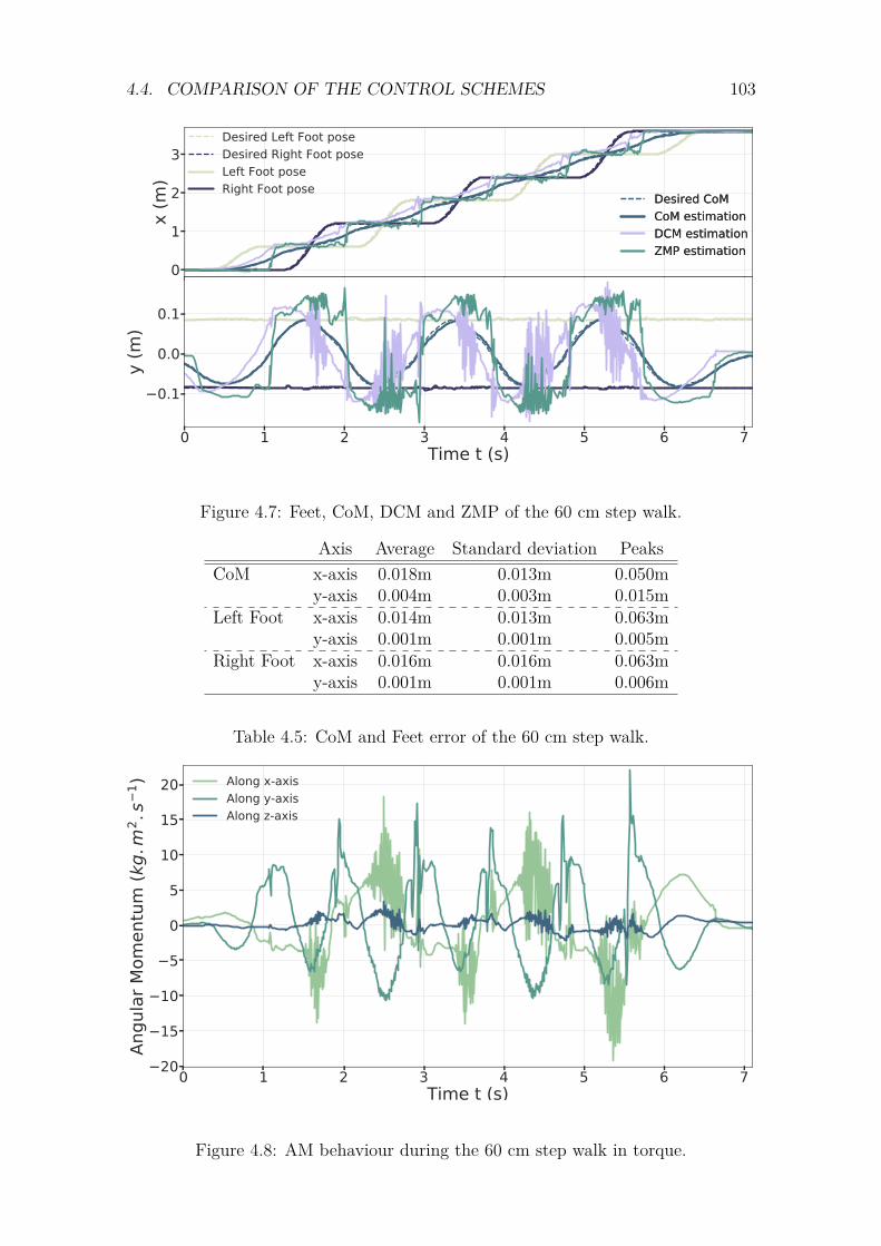
4.4. COMPARISON OF THE CONTROL SCHEMES 103
0
1
2
3x
(m)
Desired Left Foot poseDesired Right Foot poseLeft Foot poseRight Foot pose
Desired CoMCoM estimationDCM estimationZMP estimation
Desired CoMCoM estimationDCM estimationZMP estimation
0 1 2 3 4 5 6 7Time t (s)
0.1
0.0
0.1
y (m
)
Figure 4.7: Feet, CoM, DCM and ZMP of the 60 cm step walk.
Axis Average Standard deviation PeaksCoM x-axis 0.018m 0.013m 0.050m
y-axis 0.004m 0.003m 0.015mLeft Foot x-axis 0.014m 0.013m 0.063m
y-axis 0.001m 0.001m 0.005mRight Foot x-axis 0.016m 0.016m 0.063m
y-axis 0.001m 0.001m 0.006m
Table 4.5: CoM and Feet error of the 60 cm step walk.
0 1 2 3 4 5 6 7Time t (s)
20
15
10
5
0
5
10
15
20
Angu
lar M
omen
tum
(kg.
m2 .
s1 ) Along x-axis
Along y-axisAlong z-axis
Figure 4.8: AM behaviour during the 60 cm step walk in torque.
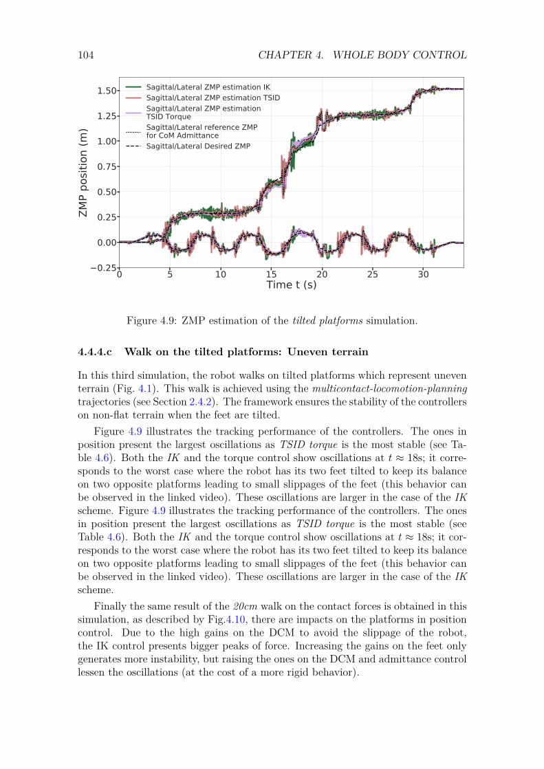
104 CHAPTER 4. WHOLE BODY CONTROL
0 5 10 15 20 25 30Time t (s)
0.25
0.00
0.25
0.50
0.75
1.00
1.25
1.50ZM
P po
sitio
n (m
)Sagittal/Lateral ZMP estimation IKSagittal/Lateral ZMP estimation TSIDSagittal/Lateral ZMP estimation TSID TorqueSagittal/Lateral reference ZMP for CoM AdmittanceSagittal/Lateral Desired ZMP
Figure 4.9: ZMP estimation of the tilted platforms simulation.
4.4.4.c Walk on the tilted platforms: Uneven terrain
In this third simulation, the robot walks on tilted platforms which represent uneventerrain (Fig. 4.1). This walk is achieved using the multicontact-locomotion-planningtrajectories (see Section 2.4.2). The framework ensures the stability of the controllerson non-flat terrain when the feet are tilted.
Figure 4.9 illustrates the tracking performance of the controllers. The ones inposition present the largest oscillations as TSID torque is the most stable (see Ta-ble 4.6). Both the IK and the torque control show oscillations at t ≈ 18s; it corre-sponds to the worst case where the robot has its two feet tilted to keep its balanceon two opposite platforms leading to small slippages of the feet (this behavior canbe observed in the linked video). These oscillations are larger in the case of the IKscheme. Figure 4.9 illustrates the tracking performance of the controllers. The onesin position present the largest oscillations as TSID torque is the most stable (seeTable 4.6). Both the IK and the torque control show oscillations at t ≈ 18s; it cor-responds to the worst case where the robot has its two feet tilted to keep its balanceon two opposite platforms leading to small slippages of the feet (this behavior canbe observed in the linked video). These oscillations are larger in the case of the IKscheme.
Finally the same result of the 20cm walk on the contact forces is obtained in thissimulation, as described by Fig.4.10, there are impacts on the platforms in positioncontrol. Due to the high gains on the DCM to avoid the slippage of the robot,the IK control presents bigger peaks of force. Increasing the gains on the feet onlygenerates more instability, but raising the ones on the DCM and admittance controllessen the oscillations (at the cost of a more rigid behavior).
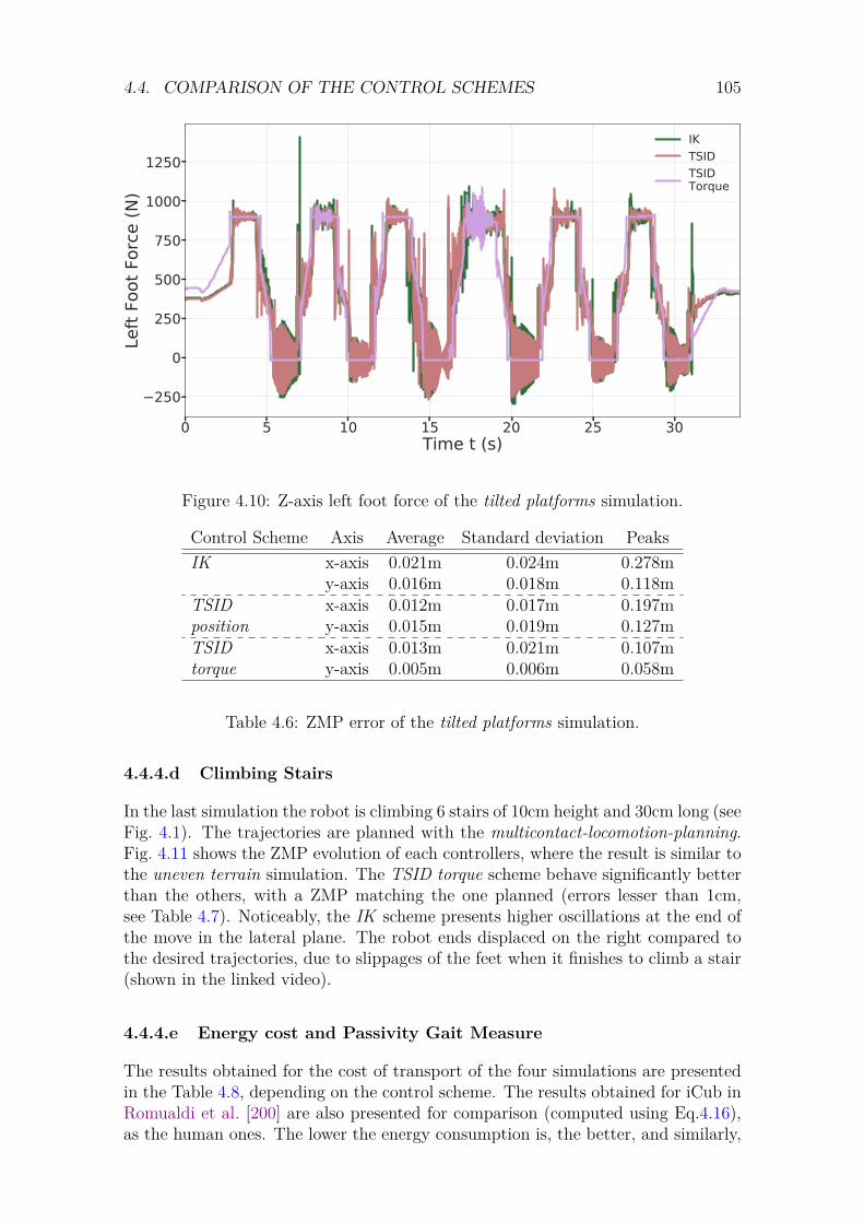
4.4. COMPARISON OF THE CONTROL SCHEMES 105
0 5 10 15 20 25 30Time t (s)
250
0
250
500
750
1000
1250
Left
Foot
For
ce (N
)IKTSIDTSIDTorque
Figure 4.10: Z-axis left foot force of the tilted platforms simulation.
Control Scheme Axis Average Standard deviation PeaksIK x-axis 0.021m 0.024m 0.278m
y-axis 0.016m 0.018m 0.118mTSID x-axis 0.012m 0.017m 0.197mposition y-axis 0.015m 0.019m 0.127mTSID x-axis 0.013m 0.021m 0.107mtorque y-axis 0.005m 0.006m 0.058m
Table 4.6: ZMP error of the tilted platforms simulation.
4.4.4.d Climbing Stairs
In the last simulation the robot is climbing 6 stairs of 10cm height and 30cm long (seeFig. 4.1). The trajectories are planned with the multicontact-locomotion-planning.Fig. 4.11 shows the ZMP evolution of each controllers, where the result is similar tothe uneven terrain simulation. The TSID torque scheme behave significantly betterthan the others, with a ZMP matching the one planned (errors lesser than 1cm,see Table 4.7). Noticeably, the IK scheme presents higher oscillations at the end ofthe move in the lateral plane. The robot ends displaced on the right compared tothe desired trajectories, due to slippages of the feet when it finishes to climb a stair(shown in the linked video).
4.4.4.e Energy cost and Passivity Gait Measure
The results obtained for the cost of transport of the four simulations are presentedin the Table 4.8, depending on the control scheme. The results obtained for iCub inRomualdi et al. [200] are also presented for comparison (computed using Eq.4.16),as the human ones. The lower the energy consumption is, the better, and similarly,
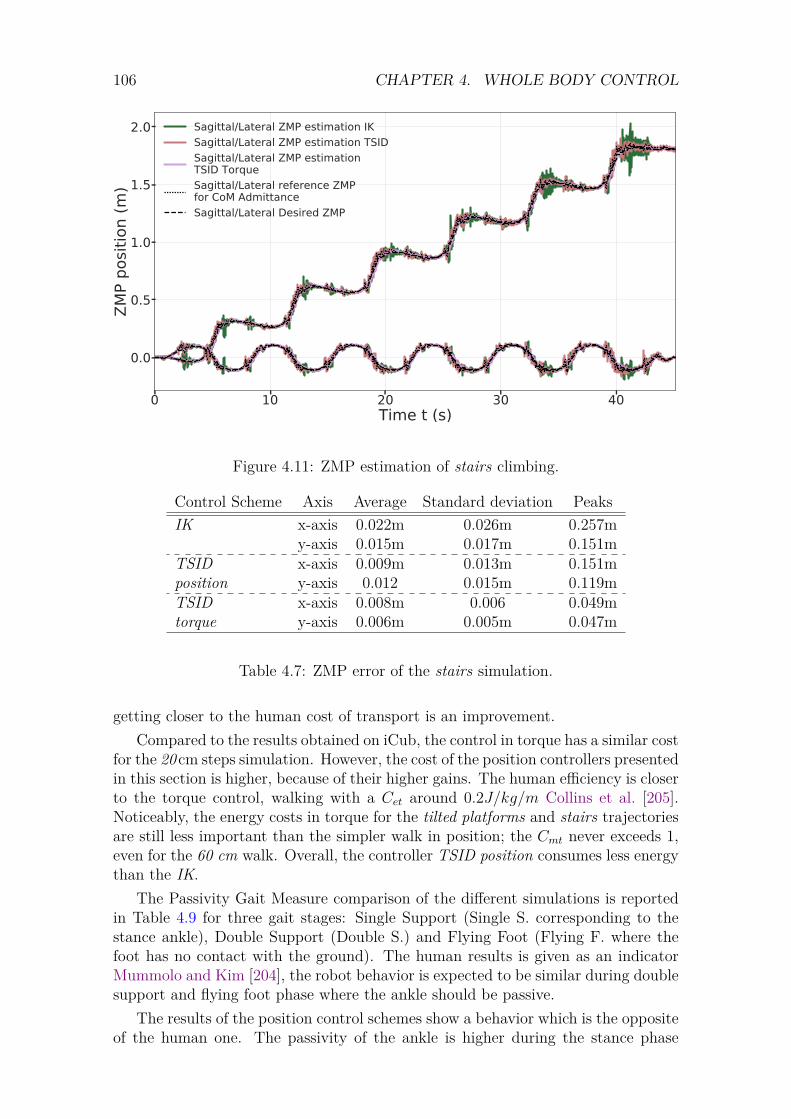
106 CHAPTER 4. WHOLE BODY CONTROL
0 10 20 30 40Time t (s)
0.0
0.5
1.0
1.5
2.0ZM
P po
sitio
n (m
)Sagittal/Lateral ZMP estimation IKSagittal/Lateral ZMP estimation TSIDSagittal/Lateral ZMP estimation TSID TorqueSagittal/Lateral reference ZMP for CoM AdmittanceSagittal/Lateral Desired ZMP
Figure 4.11: ZMP estimation of stairs climbing.
Control Scheme Axis Average Standard deviation PeaksIK x-axis 0.022m 0.026m 0.257m
y-axis 0.015m 0.017m 0.151mTSID x-axis 0.009m 0.013m 0.151mposition y-axis 0.012 0.015m 0.119mTSID x-axis 0.008m 0.006 0.049mtorque y-axis 0.006m 0.005m 0.047m
Table 4.7: ZMP error of the stairs simulation.
getting closer to the human cost of transport is an improvement.Compared to the results obtained on iCub, the control in torque has a similar cost
for the 20 cm steps simulation. However, the cost of the position controllers presentedin this section is higher, because of their higher gains. The human efficiency is closerto the torque control, walking with a Cet around 0.2J/kg/m Collins et al. [205].Noticeably, the energy costs in torque for the tilted platforms and stairs trajectoriesare still less important than the simpler walk in position; the Cmt never exceeds 1,even for the 60 cm walk. Overall, the controller TSID position consumes less energythan the IK.
The Passivity Gait Measure comparison of the different simulations is reportedin Table 4.9 for three gait stages: Single Support (Single S. corresponding to thestance ankle), Double Support (Double S.) and Flying Foot (Flying F. where thefoot has no contact with the ground). The human results is given as an indicatorMummolo and Kim [204], the robot behavior is expected to be similar during doublesupport and flying foot phase where the ankle should be passive.
The results of the position control schemes show a behavior which is the oppositeof the human one. The passivity of the ankle is higher during the stance phase
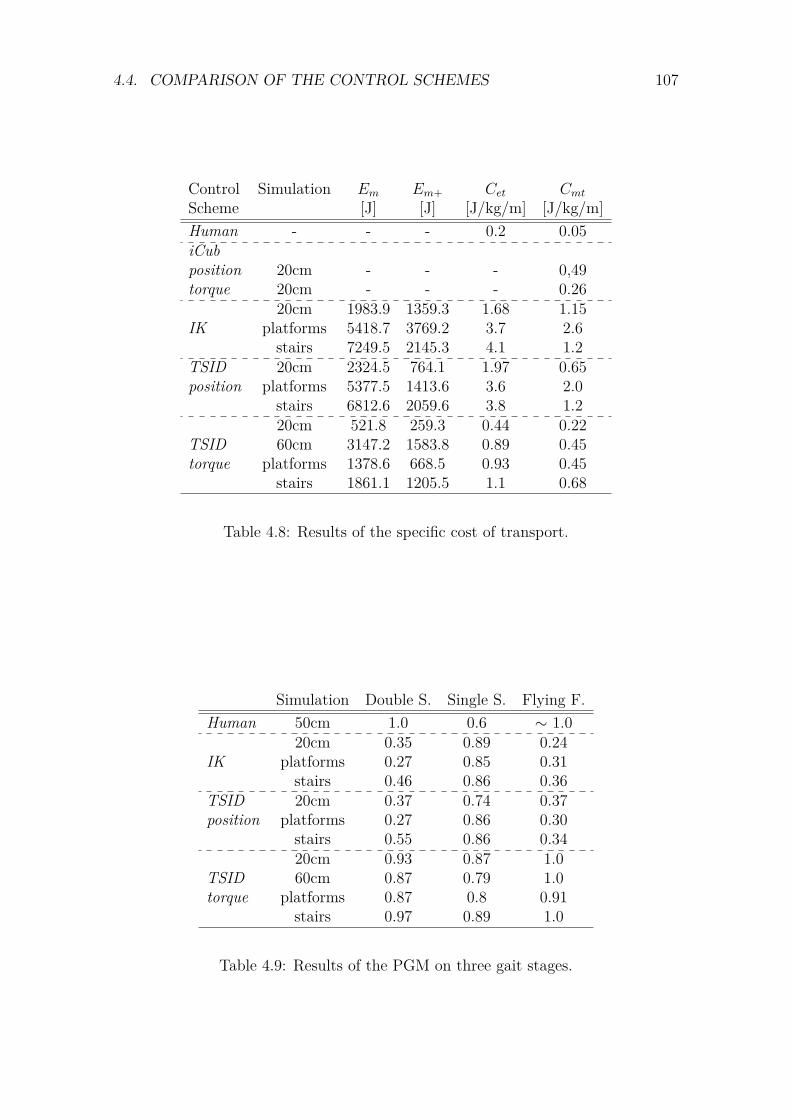
4.4. COMPARISON OF THE CONTROL SCHEMES 107
Control Simulation Em Em+ Cet CmtScheme [J] [J] [J/kg/m] [J/kg/m]Human - - - 0.2 0.05iCubposition 20cm - - - 0,49torque 20cm - - - 0.26
20cm 1983.9 1359.3 1.68 1.15IK platforms 5418.7 3769.2 3.7 2.6
stairs 7249.5 2145.3 4.1 1.2TSID 20cm 2324.5 764.1 1.97 0.65position platforms 5377.5 1413.6 3.6 2.0
stairs 6812.6 2059.6 3.8 1.220cm 521.8 259.3 0.44 0.22
TSID 60cm 3147.2 1583.8 0.89 0.45torque platforms 1378.6 668.5 0.93 0.45
stairs 1861.1 1205.5 1.1 0.68
Table 4.8: Results of the specific cost of transport.
Simulation Double S. Single S. Flying F.Human 50cm 1.0 0.6 ∼ 1.0
20cm 0.35 0.89 0.24IK platforms 0.27 0.85 0.31
stairs 0.46 0.86 0.36TSID 20cm 0.37 0.74 0.37position platforms 0.27 0.86 0.30
stairs 0.55 0.86 0.3420cm 0.93 0.87 1.0
TSID 60cm 0.87 0.79 1.0torque platforms 0.87 0.8 0.91
stairs 0.97 0.89 1.0
Table 4.9: Results of the PGM on three gait stages.
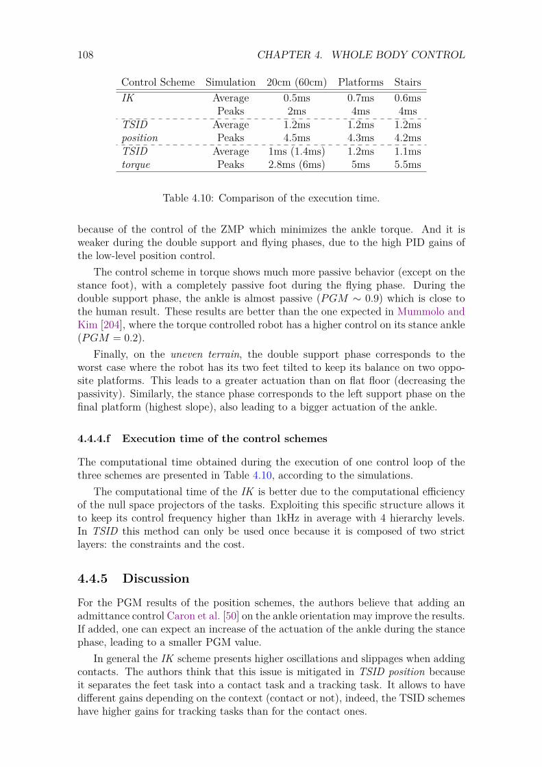
108 CHAPTER 4. WHOLE BODY CONTROL
Control Scheme Simulation 20cm (60cm) Platforms StairsIK Average 0.5ms 0.7ms 0.6ms
Peaks 2ms 4ms 4msTSID Average 1.2ms 1.2ms 1.2msposition Peaks 4.5ms 4.3ms 4.2msTSID Average 1ms (1.4ms) 1.2ms 1.1mstorque Peaks 2.8ms (6ms) 5ms 5.5ms
Table 4.10: Comparison of the execution time.
because of the control of the ZMP which minimizes the ankle torque. And it isweaker during the double support and flying phases, due to the high PID gains ofthe low-level position control.
The control scheme in torque shows much more passive behavior (except on thestance foot), with a completely passive foot during the flying phase. During thedouble support phase, the ankle is almost passive (PGM ∼ 0.9) which is close tothe human result. These results are better than the one expected in Mummolo andKim [204], where the torque controlled robot has a higher control on its stance ankle(PGM = 0.2).
Finally, on the uneven terrain, the double support phase corresponds to theworst case where the robot has its two feet tilted to keep its balance on two oppo-site platforms. This leads to a greater actuation than on flat floor (decreasing thepassivity). Similarly, the stance phase corresponds to the left support phase on thefinal platform (highest slope), also leading to a bigger actuation of the ankle.
4.4.4.f Execution time of the control schemes
The computational time obtained during the execution of one control loop of thethree schemes are presented in Table 4.10, according to the simulations.
The computational time of the IK is better due to the computational efficiencyof the null space projectors of the tasks. Exploiting this specific structure allows itto keep its control frequency higher than 1kHz in average with 4 hierarchy levels.In TSID this method can only be used once because it is composed of two strictlayers: the constraints and the cost.
4.4.5 Discussion
For the PGM results of the position schemes, the authors believe that adding anadmittance control Caron et al. [50] on the ankle orientation may improve the results.If added, one can expect an increase of the actuation of the ankle during the stancephase, leading to a smaller PGM value.
In general the IK scheme presents higher oscillations and slippages when addingcontacts. The authors think that this issue is mitigated in TSID position becauseit separates the feet task into a contact task and a tracking task. It allows to havedifferent gains depending on the context (contact or not), indeed, the TSID schemeshave higher gains for tracking tasks than for the contact ones.
4.4. COMPARISON OF THE CONTROL SCHEMES 109
One major point to discuss is the transition from the simulations to the realexperiments. For torque control, in the Gazebo simulator, the joint torque controlis almost perfect because the dynamics of the motor is completely neglected. How-ever, not taking these dynamics into account will lead to unrealistic and dangerousbehaviors on the real robot. The authors are currently testing the simulations onthe simulator of the TALOS constructor, PAL robotics, which models the actua-tor dynamics of the robot. To do so, the torque control scheme is plugged to theconstructor low-level controller, which computes a new command respecting the ac-tuator dynamics. Only some tuning of the task gains seems to be needed to achievegood results.
Another concern is that the real robot is subject to imperfections such as errorsin the chain actuation model, sensor noise, limited torque bandwidth or delays. Inthe presented implementation some actions against the possible problems have beenimplemented Englsberger et al. [74], such as adding filters on the signals retrievedfrom the robot and using the force sensors on the feet to improve the robustness ofthe base-estimator. Moreover, a PD+ controller has been implemented for the torquecontroller, to stiff the ankles, improving the quality of the feet landing. However, insimulation, this PD+ only increases the rigidity because of the feedback in positionand velocity, and decreases the PGM, thus it has not been presented.
For position control, the simulations are dependent of the low-level control PID ofthe Gazebo plugin. These gains however have been modified to fit the real behaviorof the motors. Thus, the position controllers should not need important modifi-cations to be tested on the real robot. Yet, because the robot TALOS presents aflexibility in the hips which is not measured by the encoders, the simulations can-not be entirely realized on the real robot. The Appendix 4 describes the solutionsdeveloped to compensate this non-measurable hip flexibility of the robot TALOS(mentioned in Section 1.4). This flexibility leads to errors in the landing positionsof the feet which cannot be compensated without a proper identification and mod-eling of the flexibility. In torque control however, this issue is mitigated because theflexibility is considered by the control system as external disturbances. Nonetheless,to achieve the experiments, it will be necessary control this flexibility; the solutionpresented in Villa et al. [206] is currently tested on the robot TALOS and our con-trollers will be adapted to take it into account. It is important to mention that thefinal real robot implementations will require slightly different gains and weights.
4.4.6 Conclusion
Three whole-body control implementations are compared in this chapter. Two ofthem are position based (with DCM and CoM admittance control): a LexicographicQP using inverse kinematics and a WQP using TSID with an AM task. The last oneis a WQP using TSID in torque with an AM task. They are evaluated in Gazeboon flat, uneven terrains and stairs climbing; on the criteria of trajectory tracking,energy consumption, passivity and computational cost.
In general, both position control schemes present the same results, with lessenergy consumption and higher passivity for the TSID position controller. A bettertuning of the tasks gains may improve its results on the ZMP tracking.
On the other hand, the TSID torque controller shows better results in terms of
110 CHAPTER 4. WHOLE BODY CONTROL
smoothness of the trajectory tracking, energy consumption, passivity of the walk -without impacts and can achieve a 60cm walk with steps of 1s in simulation. Thisconfirms the high capabilities of a torque control scheme coupled with an angu-lar momentum regularization (see for instance Atlas in DARPA robotics challengeKoolen et al. [54]). In average, the TSID controllers reach the 1kHz of control loop,necessary for real-time control, nonetheless, the IK scheme has the best computa-tional time.
For our future work, we plan to control the hip flexibility of TALOS based onthe identification work done in Villa et al. [206], so that we can evaluate the threecontrollers on the real robot.

4.5. APPLICATION ON HUMAN-ROBOT COLLABORATION 111
4.5 Application on Human-Robot Collaborationfor Navigation
4.5.1 Introduction
This section exposes the efficiency of the previous whole-body torque controller in acontext of human-robot collaboration. It presents the results obtained during a col-laboration with another PhD student of the Gepetto team, Isabelle Maroger, wherethe robot proactively walks alongside a human. The resulting paper Maroger et al.[24] is part of a French project, called ANR-COBOT, which aims at a collaborationbetween a human and a TALOS humanoid robot to carry and move a table. Tosmoothly achieve such a handling task, a good knowledge of the human dynamicswhile walking with a table is needed to allow the robot to anticipate and proactivelyfollow the human movements. For now, the problem of walking with a table hasbeen put aside and the issue has been reduced to the proactive tracking of a walkinghuman by a humanoid robot. Thus, the paper focuses on the real-time predictionof human walking trajectory and its coupling with a Walking Pattern Generator(WPG) for a TALOS humanoid robot.
The paper presents a prediction model of human trajectory during gait and itscoupling with a WPG which generates a TALOS humanoid robot CoM and footstepsalong the predicted trajectory. This coupling allows a proactive tracking of a walkinghuman by a humanoid robot, instead of a passive one, in order to ease every potentialinteractions during gait. The whole framework is assessed in simulation on Gazebo,as Fig.4.12 shows, and is described on Fig.4.13. This framework is designed tohelp a humanoid robot to predict the spontaneous human trajectory during gaitaccording to its real-time CoM observation. This aims to allow the robot to movein accordance with its human partner. Thus, if the human accelerates, slows downor stops, the robot should act similarly while following the same trajectory as itspartner.
This section focuses on the part of the paper corresponding to my work. Itconsists in the adaptation of the torque whole-body controller presented in Section4.4.4 to successfully simulate the coupling of the WPG with the prediction model
Figure 4.12: Simulation on Gazebo (left) of the robot executing a predicted trajec-tory. The CoM, footsteps (desired in red, real in blue) and human trajectories (ingreen) are also displayed in RViz (right) for comparison.
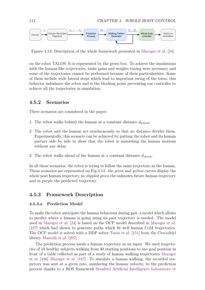
112 CHAPTER 4. WHOLE BODY CONTROL
Human RecordedTrajectory
PredictionProcess
Walking PatternGeneratorHuman Whole body
controller
*
Robot onsimulation
Figure 4.13: Description of the whole framework presented in Maroger et al. [24]
on the robot TALOS. It is represented by the green box. To achieve the simulationswith the human-like trajectories, tasks gains and weights tuning were necessary andsome of the trajectories cannot be performed because of their particularities. Someof them include wide lateral steps which lead to important swing of the torso, thisbehavior imbalance the robot and is the blocking point preventing our controller toachieve all the trajectories in simulation.
4.5.2 Scenarios
Three scenarios are considered in the paper:
1. The robot walks behind the human at a constant distance dbehind.
2. The robot and the human act synchronously so that no distance divides them.Experimentally, this scenario can be achieved by putting the robot and its humanpartner side by side to show that the robot is mimicking the human motionswithout any delay.
3. The robot walks ahead of the human at a constant distance dahead.
In all those scenarios, the robot is trying to follow the same trajectory as the human.Those scenarios are represented on Fig.4.14: the green and yellow curves display thewhole past human trajectory, in stippled green the unknown future human trajectoryand in purple the predicted trajectory.
4.5.3 Framework Description
4.5.3.a Prediction Model
To make the robot anticipate the human behaviour during gait, a model which allowsto predict where a human is going using its past trajectory is needed. The modelused in Maroger et al. [24] is based on the OCP model described in Maroger et al.[187] which had shown to generate paths which fit well human CoM trajectories.The OCP model is solved with a DDP solver Tassa et al. [151] from the Crocoddyllibrary Mastalli et al. [207].
The prediction process needs a human trajectory as an input. We used trajecto-ries of 10 healthy subjects walking from 40 starting positions to one goal position infront of a table collected as part of a study of human walking trajectories Marogeret al. [186] Maroger et al. [187]. To simulate a human walking, the recorded tra-jectory was sent at a given rate, simulating the human velocity, to the predictionprocess thanks to a ROS framework Stanford Artificial Intelligence Laboratory et
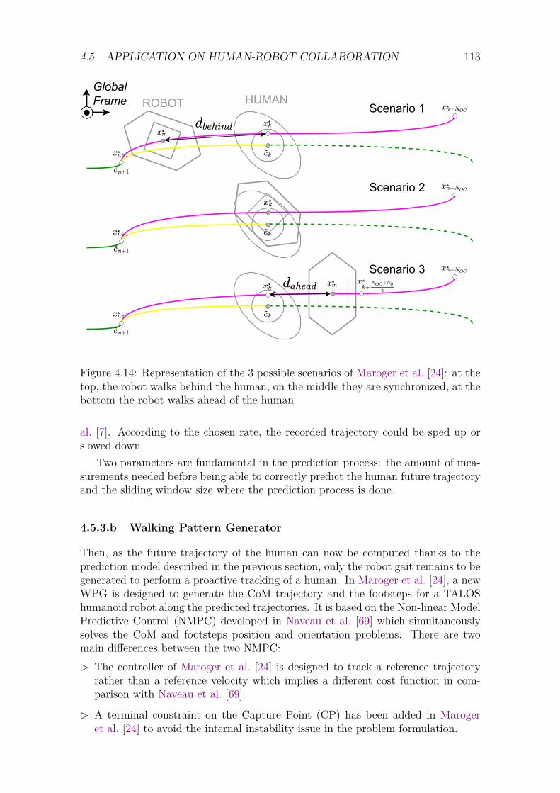
4.5. APPLICATION ON HUMAN-ROBOT COLLABORATION 113
ROBOT HUMAN
*
*
*
*
*
*
*
* *
GlobalFrame Scenario 1
*
*
*Scenario 2
Scenario 3
Figure 4.14: Representation of the 3 possible scenarios of Maroger et al. [24]: at thetop, the robot walks behind the human, on the middle they are synchronized, at thebottom the robot walks ahead of the human
al. [7]. According to the chosen rate, the recorded trajectory could be sped up orslowed down.
Two parameters are fundamental in the prediction process: the amount of mea-surements needed before being able to correctly predict the human future trajectoryand the sliding window size where the prediction process is done.
4.5.3.b Walking Pattern Generator
Then, as the future trajectory of the human can now be computed thanks to theprediction model described in the previous section, only the robot gait remains to begenerated to perform a proactive tracking of a human. In Maroger et al. [24], a newWPG is designed to generate the CoM trajectory and the footsteps for a TALOShumanoid robot along the predicted trajectories. It is based on the Non-linear ModelPredictive Control (NMPC) developed in Naveau et al. [69] which simultaneouslysolves the CoM and footsteps position and orientation problems. There are twomain differences between the two NMPC:� The controller of Maroger et al. [24] is designed to track a reference trajectory
rather than a reference velocity which implies a different cost function in com-parison with Naveau et al. [69].
� A terminal constraint on the Capture Point (CP) has been added in Marogeret al. [24] to avoid the internal instability issue in the problem formulation.
114 CHAPTER 4. WHOLE BODY CONTROL
4.5.3.c Coupling of the Prediction Process and the WPG
The purpose of the paper Maroger et al. [24] is to design a whole architecture thatallows a humanoid robot to smoothly follow a human who walks to an a prioriunknown goal while predicting his future trajectory. This tracking is aimed to beproactive as a prediction process estimates the human future trajectory so that thefuture steps of the robot planned by the WPG are already in the right direction.This may cancel the reaction time of the robot and make the tracking smoother.The coupling of the prediction process and the WPG for a TALOS humanoid robotdescribed in Sec.1.4 is a first step towards this purpose.
This coupling can be described as follows, it corresponds to the blue boxes repre-sented in Fig.4.13. First, a pre-recorded human trajectory is streamed and retrievedby the prediction process. Then, it sends the predicted trajectory to the WPG whichcomputes, thanks to a NMPC, the robot CoM and feet positions and orientationsover the preview horizon with respect to the human velocity (the CoM orientationis in fact the robot base one). All those data are shared through a ROS frameworkand displayed on the RViz software as shown on Fig.4.15 for a specific trajectory. Inthis figure, the chosen scenario is the second one on Fig.4.14, namely the synchro-nization of a robot and a human. In the next section, the last steps of the processare detailed, namely the whole-body controller (the green box on Fig.4.13) and thesimulations on the TALOS robot on Gazebo are presented.
All the results and simulations resulting of this coupling are reproducible as allthe libraries are open-source and the source code and the data are available on:https://github.com/imaroger/human_walking_trajectory_prediction.
4.5.3.d Whole-body controller
The whole-body controller computes a stable command from the reference trajecto-ries and the actual state of the robot. In the paper Maroger et al. [24], we used thecontroller described in Section 4.4.1.b: it is a Weighted Quadratic Program (WQP),which solves the inverse dynamics of a robot in rigid contact with the environmentHerzog et al. [153]. It has been successfully tested on the humanoid robot TALOSin simulations in Ramuzat et al. [23], the results are presented in Section 4.4.4. Thecontroller takes as inputs the CoM position, the base (free-flyer) orientation and thefeet positions and orientations reference trajectories of the WPG. It implements taskfunctions with them, as acceleration-based tracking law (see Section 4.3). The con-troller optimises its cost function using these tasks, prioritised with weights, whilerespecting constraints such as the robot dynamics and feet contacts. The weightsand gains used in the paper are the same as the one of the torque controller pre-sented in Section 4.4.4, except for the CoM and Angular Momentum (AM) tasksgains: the CoM proportional gains were raised to 800 and the AM ones decreasedto 2.5. This gains tuning were needed to make the controller successfully performthe trajectory wide side steps found by the WPG.
Moreover, the orientation of the free-flyer given by the WPG was changing alot and impacted the walking. As it was computed to be the mean of the feetorientations on each component in the WPG of Maroger et al. [24], we implementedit directly as this mean in our torque controller given the reference feet values. Thissolved the problem and we had a smoother orientation of the free-flyer, however the
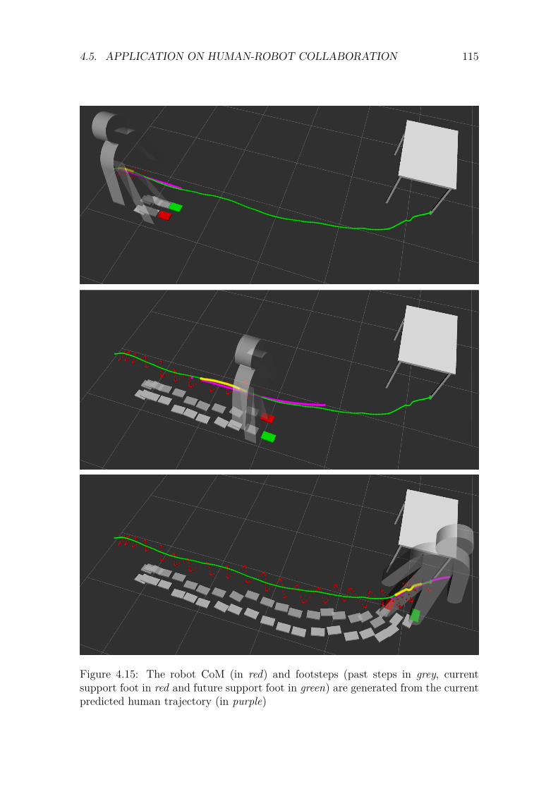
4.5. APPLICATION ON HUMAN-ROBOT COLLABORATION 115
Figure 4.15: The robot CoM (in red) and footsteps (past steps in grey, currentsupport foot in red and future support foot in green) are generated from the currentpredicted human trajectory (in purple)
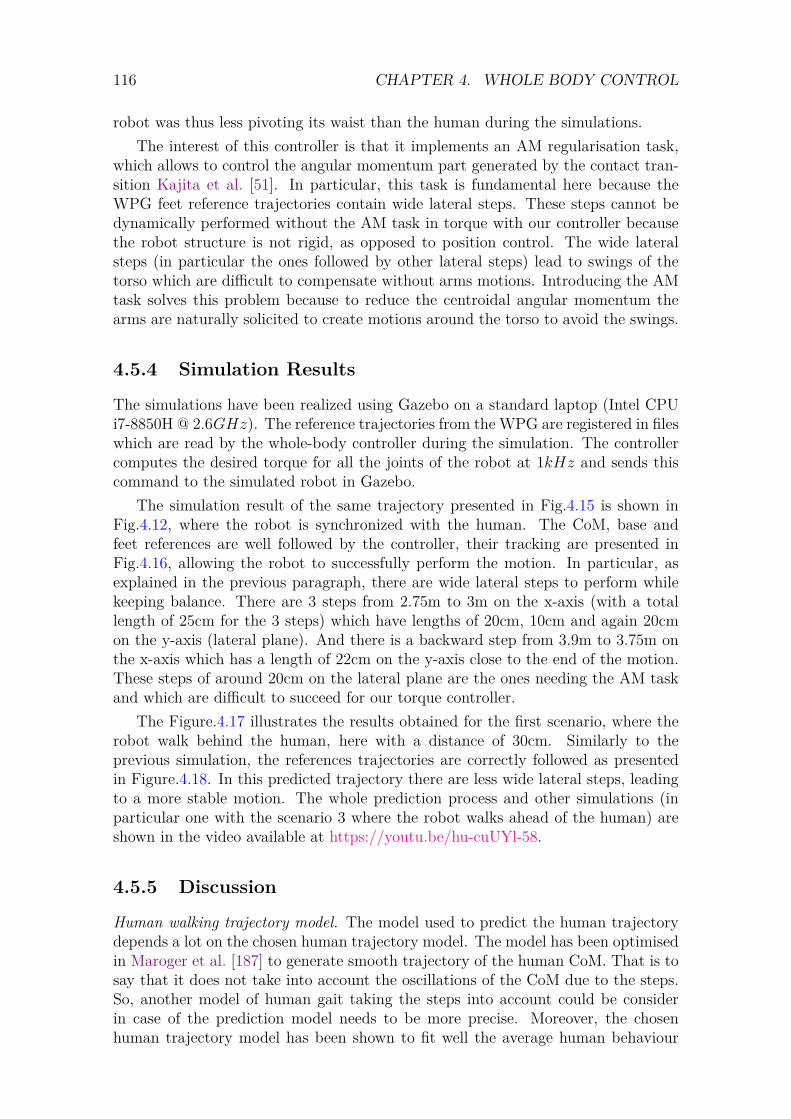
116 CHAPTER 4. WHOLE BODY CONTROL
robot was thus less pivoting its waist than the human during the simulations.The interest of this controller is that it implements an AM regularisation task,
which allows to control the angular momentum part generated by the contact tran-sition Kajita et al. [51]. In particular, this task is fundamental here because theWPG feet reference trajectories contain wide lateral steps. These steps cannot bedynamically performed without the AM task in torque with our controller becausethe robot structure is not rigid, as opposed to position control. The wide lateralsteps (in particular the ones followed by other lateral steps) lead to swings of thetorso which are difficult to compensate without arms motions. Introducing the AMtask solves this problem because to reduce the centroidal angular momentum thearms are naturally solicited to create motions around the torso to avoid the swings.
4.5.4 Simulation Results
The simulations have been realized using Gazebo on a standard laptop (Intel CPUi7-8850H @ 2.6GHz). The reference trajectories from the WPG are registered in fileswhich are read by the whole-body controller during the simulation. The controllercomputes the desired torque for all the joints of the robot at 1kHz and sends thiscommand to the simulated robot in Gazebo.
The simulation result of the same trajectory presented in Fig.4.15 is shown inFig.4.12, where the robot is synchronized with the human. The CoM, base andfeet references are well followed by the controller, their tracking are presented inFig.4.16, allowing the robot to successfully perform the motion. In particular, asexplained in the previous paragraph, there are wide lateral steps to perform whilekeeping balance. There are 3 steps from 2.75m to 3m on the x-axis (with a totallength of 25cm for the 3 steps) which have lengths of 20cm, 10cm and again 20cmon the y-axis (lateral plane). And there is a backward step from 3.9m to 3.75m onthe x-axis which has a length of 22cm on the y-axis close to the end of the motion.These steps of around 20cm on the lateral plane are the ones needing the AM taskand which are difficult to succeed for our torque controller.
The Figure.4.17 illustrates the results obtained for the first scenario, where therobot walk behind the human, here with a distance of 30cm. Similarly to theprevious simulation, the references trajectories are correctly followed as presentedin Figure.4.18. In this predicted trajectory there are less wide lateral steps, leadingto a more stable motion. The whole prediction process and other simulations (inparticular one with the scenario 3 where the robot walks ahead of the human) areshown in the video available at https://youtu.be/hu-cuUYl-58.
4.5.5 Discussion
Human walking trajectory model. The model used to predict the human trajectorydepends a lot on the chosen human trajectory model. The model has been optimisedin Maroger et al. [187] to generate smooth trajectory of the human CoM. That is tosay that it does not take into account the oscillations of the CoM due to the steps.So, another model of human gait taking the steps into account could be considerin case of the prediction model needs to be more precise. Moreover, the chosenhuman trajectory model has been shown to fit well the average human behaviour
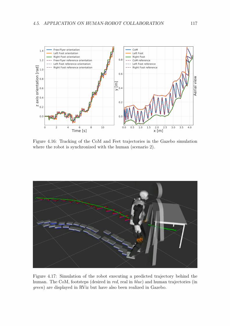
4.5. APPLICATION ON HUMAN-ROBOT COLLABORATION 117
Figure 4.16: Tracking of the CoM and Feet trajectories in the Gazebo simulationwhere the robot is synchronized with the human (scenario 2).
Figure 4.17: Simulation of the robot executing a predicted trajectory behind thehuman. The CoM, footsteps (desired in red, real in blue) and human trajectories (ingreen) are displayed in RViz but have also been realized in Gazebo.
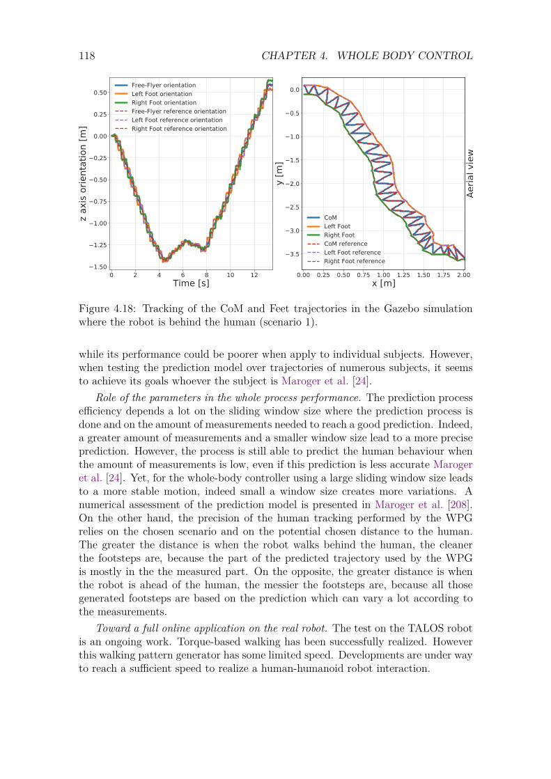
118 CHAPTER 4. WHOLE BODY CONTROL
Figure 4.18: Tracking of the CoM and Feet trajectories in the Gazebo simulationwhere the robot is behind the human (scenario 1).
while its performance could be poorer when apply to individual subjects. However,when testing the prediction model over trajectories of numerous subjects, it seemsto achieve its goals whoever the subject is Maroger et al. [24].
Role of the parameters in the whole process performance. The prediction processefficiency depends a lot on the sliding window size where the prediction process isdone and on the amount of measurements needed to reach a good prediction. Indeed,a greater amount of measurements and a smaller window size lead to a more preciseprediction. However, the process is still able to predict the human behaviour whenthe amount of measurements is low, even if this prediction is less accurate Marogeret al. [24]. Yet, for the whole-body controller using a large sliding window size leadsto a more stable motion, indeed small a window size creates more variations. Anumerical assessment of the prediction model is presented in Maroger et al. [208].On the other hand, the precision of the human tracking performed by the WPGrelies on the chosen scenario and on the potential chosen distance to the human.The greater the distance is when the robot walks behind the human, the cleanerthe footsteps are, because the part of the predicted trajectory used by the WPGis mostly in the the measured part. On the opposite, the greater distance is whenthe robot is ahead of the human, the messier the footsteps are, because all thosegenerated footsteps are based on the prediction which can vary a lot according tothe measurements.
Toward a full online application on the real robot. The test on the TALOS robotis an ongoing work. Torque-based walking has been successfully realized. Howeverthis walking pattern generator has some limited speed. Developments are under wayto reach a sufficient speed to realize a human-humanoid robot interaction.
4.5. APPLICATION ON HUMAN-ROBOT COLLABORATION 119
4.5.6 Conclusion
In this section is presented the work realized in collaboration with Isabelle Marogerin a context of human-robot collaboration. The aim is to ease the tracking of ahuman by a humanoid robot by helping the robot to predict, and thus anticipate,its partner behaviour. To this end, three contributions have been made in Marogeret al. [24]: First, a prediction OCP model is designed based on a human trajectorymodel, which generates the future trajectory of a human from its recent past tra-jectory. Then, a WPG is designed to generate a TALOS humanoid robot CoM andfootsteps along the predicted trajectory in real time. Finally the CoM and footstepstrajectories resulting from the WPG are given to a torque whole-body controllerwhich computes a stable command for the robot to follow. This whole frameworkhas been successfully tested in real-time simulation. Thus, in this work, we achieveto develop and assess the capabilities of a whole framework aiming to control a sim-ulated TALOS humanoid robot in order to make him proactively walk along with ahuman partner.
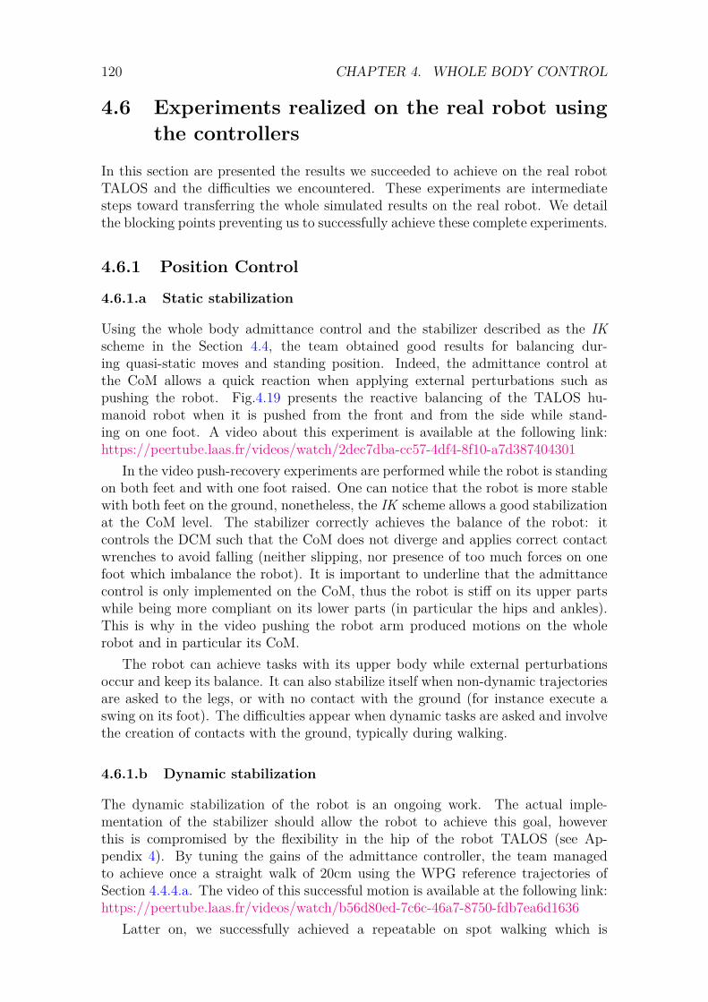
120 CHAPTER 4. WHOLE BODY CONTROL
4.6 Experiments realized on the real robot usingthe controllers
In this section are presented the results we succeeded to achieve on the real robotTALOS and the difficulties we encountered. These experiments are intermediatesteps toward transferring the whole simulated results on the real robot. We detailthe blocking points preventing us to successfully achieve these complete experiments.
4.6.1 Position Control
4.6.1.a Static stabilization
Using the whole body admittance control and the stabilizer described as the IKscheme in the Section 4.4, the team obtained good results for balancing dur-ing quasi-static moves and standing position. Indeed, the admittance control atthe CoM allows a quick reaction when applying external perturbations such aspushing the robot. Fig.4.19 presents the reactive balancing of the TALOS hu-manoid robot when it is pushed from the front and from the side while stand-ing on one foot. A video about this experiment is available at the following link:https://peertube.laas.fr/videos/watch/2dec7dba-cc57-4df4-8f10-a7d387404301
In the video push-recovery experiments are performed while the robot is standingon both feet and with one foot raised. One can notice that the robot is more stablewith both feet on the ground, nonetheless, the IK scheme allows a good stabilizationat the CoM level. The stabilizer correctly achieves the balance of the robot: itcontrols the DCM such that the CoM does not diverge and applies correct contactwrenches to avoid falling (neither slipping, nor presence of too much forces on onefoot which imbalance the robot). It is important to underline that the admittancecontrol is only implemented on the CoM, thus the robot is stiff on its upper partswhile being more compliant on its lower parts (in particular the hips and ankles).This is why in the video pushing the robot arm produced motions on the wholerobot and in particular its CoM.
The robot can achieve tasks with its upper body while external perturbationsoccur and keep its balance. It can also stabilize itself when non-dynamic trajectoriesare asked to the legs, or with no contact with the ground (for instance execute aswing on its foot). The difficulties appear when dynamic tasks are asked and involvethe creation of contacts with the ground, typically during walking.
4.6.1.b Dynamic stabilization
The dynamic stabilization of the robot is an ongoing work. The actual imple-mentation of the stabilizer should allow the robot to achieve this goal, howeverthis is compromised by the flexibility in the hip of the robot TALOS (see Ap-pendix 4). By tuning the gains of the admittance controller, the team managedto achieve once a straight walk of 20cm using the WPG reference trajectories ofSection 4.4.4.a. The video of this successful motion is available at the following link:https://peertube.laas.fr/videos/watch/b56d80ed-7c6c-46a7-8750-fdb7ea6d1636
Latter on, we successfully achieved a repeatable on spot walking which is
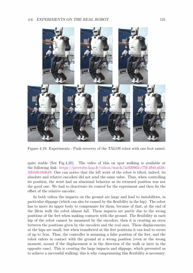
4.6. EXPERIMENTS ON THE REAL ROBOT 121
Figure 4.19: Experiments - Push recovery of the TALOS robot with one foot raised.
quite stable (See Fig.4.20). The video of this on spot walking is available atthe following link: https://peertube.laas.fr/videos/watch/1a920902-c75f-4fb0-a638-33bb9b48d649. One can notice that the left wrist of the robot is tilted, indeed, itsabsolute and relative encoders did not send the same value. Thus, when controllingits position, the wrist had an abnormal behavior as its returned position was notthe good one. We had to deactivate its control for the experiment and then fix theoffset of the relative encoder.
In both videos the impacts on the ground are large and lead to instabilities, inparticular slippage (which can also be caused by the flexibility in the hip). The robothas to move its upper body to compensate for them, because of that, at the end ofthe 20cm walk the robot almost fall. These impacts are partly due to the wrongpositions of the feet when making contacts with the ground. The flexibility in eachhip of the robot cannot be measured by the encoders, then it is creating an errorbetween the positions given by the encoders and the real ones. These displacementsat the hips are small, but when transferred at the feet positions it can lead to errorsof up to 5cm. Thus, the controller is assuming a false position of the feet, and therobot enters in contact with the ground at a wrong position (even at the wrongmoment, sooner if the displacement is in the direction of the walk or later in theopposite case). This is creating the large impacts and slippage, which prevented usto achieve a successful walking; this is why compensating this flexibility is necessary.
122 CHAPTER 4. WHOLE BODY CONTROL
Figure 4.20: Experiments - On spot walking with the TALOS robot.
In the next subsection, the experiment realized to compensate it with a fixed valueis presented.
An additional way to cope with the stabilization problem would be to reschedulethe footsteps and their location according the landing time.
4.6.1.c Fixed compensation of the flexibility
As described in the Appendix 4 we first tried to compensate the flexibility by using afeed-forward on the commanded position of the hip taking into account the torsionalstiffness and the measured torque. However, because of the noises on the torquesensors, we had to filter it, which leads the compensation to be applied with delays.We also tried to activate this compensation only on single support phases and noton double support ones to avoid accumulation of internal efforts (on double supportthe robot will try to correct its hip position while having its feet in contact with theground and thus not moving, leading to this accumulation of energy). Even withsuch modifications the results were not enough to successfully perform repeatablewalk.
Thus, we then tried to impose a fix compensation of the flexibility with-out taking into account the measured torque. With a leg of 1m weighting20kg, we fixed the compensation on the hip to ∆qhip = 20
K≈ 20
973 = 0.021rad. Only a repeatable one step froward walk in position control has beensuccessfully achieved with this method, see the video at the following link:https://peertube.laas.fr/videos/watch/08db3177-372b-43cc-85da-2009a267b5c9.
As the robot locomotion was not the core subject of my thesis and that we suspectthe flexibility would be a less important issue for the robot during torque control;we stopped the work on the flexibility until the postdoctoral researcher NahuelVilla came in the team. Then, he properly modeled this flexibility, as describedin Appendix 4 and has recently achieved walking results on the robot using a CoPwhole-body controller.
4.6. EXPERIMENTS ON THE REAL ROBOT 123
4.6.2 Torque Control
4.6.2.a PAL robotics low-level controller
To achieve torque control on the real robot, as explained in the Section 2.3.3 andin conclusion of the Section 4.4.4, it is needed to transform the joint torque com-mands to motor currents. We decided to use the PAL robotics constructor low-levelcontroller, which computes new commands respecting the robot actuators dynam-ics. This low-level controller is a proprietary black-box, which use a ros-controlhardware interface to communicate with the robot (see Fig.1.10). To interface ourcontrol scheme (based on the SoT with the WPG), we had to create a new version ofthe roscontrol-sot package, presented in Section 1.6.2.b. Indeed, our control schemeneeds no more to communicate directly with the robot but with the PAL roboticscontroller, which implements different functions and formulations. One of the majordifficulty is that the proprietary code source is not available, we only had access toits C++ headers and some basic tutorials. Developing this interface to keep all thefunctionalities implemented in the roscontrol-sot package (for instance to keep therecording of the logs and creating all the necessary signals needed by the SoT in thedynamic-graph structure), take us months of work (including the following remark).
Moreover, the robot has a modified operating system called ferrum (which is anequivalent to ubuntu). In order to have exactly the same environment as the oneon the robot to test our codes, we created a Docker [209] container. Installing theSoT packages on this environment was not trivial as some packages had conflictingdependencies with the PAL robotics packages. Finally, we succeeded to test in thisDocker container our interface and our torque controller using the PAL simulatoravailable on ferrum. An additional difficulty is that the simulator (based on RViz) isslowed down when using our control scheme; i.e. the displayed behavior is estimatedas five times slower than the real one. Therefore, a small and slow oscillation seenin the simulator is in reality a high frequency one on the robot and can lead todangerous behaviors.
One has to note that, in Dantec et al. [147], the MPC is not embedded on therobot and is interfaced with the PAL robotics low-level controller via ROS top-ics. This simpler architecture choice was made because it is a stand-alone package(no SoT or dynamic-graph framework) and does not imply sending commands athigh frequency (200Hz). ROS topics may induce latency and do not allow to sendhigh frequency commands leading to real-time issues. To avoid the troubles I en-counter to interface my control scheme with the PAL robotics low-level controller,the CoP whole-body controller of Nahuel Villa (not relying on the SoT nor dynamic-graph framework) compensating the flexibility was directly implemented in the PALrobotics control scheme.
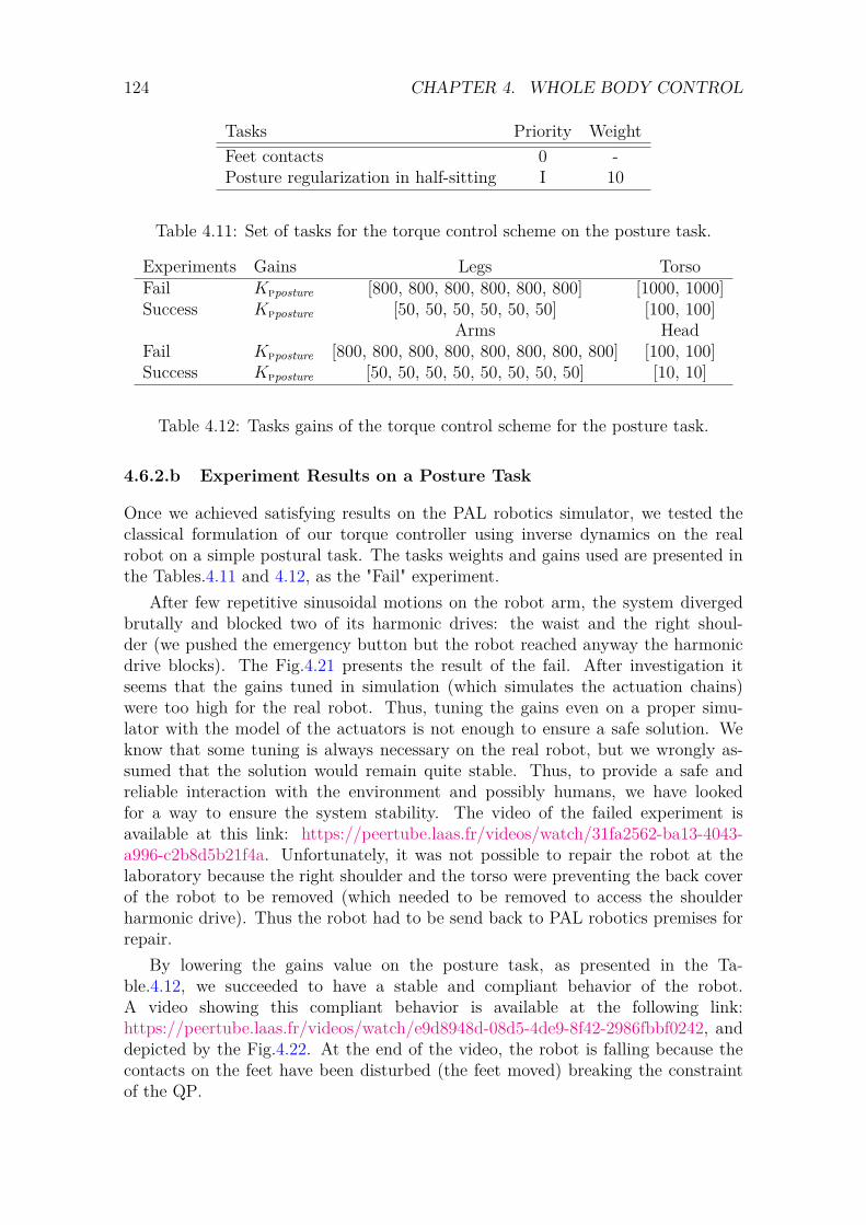
124 CHAPTER 4. WHOLE BODY CONTROL
Tasks Priority WeightFeet contacts 0 -Posture regularization in half-sitting I 10
Table 4.11: Set of tasks for the torque control scheme on the posture task.
Experiments Gains Legs TorsoFail Kpposture [800, 800, 800, 800, 800, 800] [1000, 1000]Success Kpposture [50, 50, 50, 50, 50, 50] [100, 100]
Arms HeadFail Kpposture [800, 800, 800, 800, 800, 800, 800, 800] [100, 100]Success Kpposture [50, 50, 50, 50, 50, 50, 50, 50] [10, 10]
Table 4.12: Tasks gains of the torque control scheme for the posture task.
4.6.2.b Experiment Results on a Posture Task
Once we achieved satisfying results on the PAL robotics simulator, we tested theclassical formulation of our torque controller using inverse dynamics on the realrobot on a simple postural task. The tasks weights and gains used are presented inthe Tables.4.11 and 4.12, as the "Fail" experiment.
After few repetitive sinusoidal motions on the robot arm, the system divergedbrutally and blocked two of its harmonic drives: the waist and the right shoul-der (we pushed the emergency button but the robot reached anyway the harmonicdrive blocks). The Fig.4.21 presents the result of the fail. After investigation itseems that the gains tuned in simulation (which simulates the actuation chains)were too high for the real robot. Thus, tuning the gains even on a proper simu-lator with the model of the actuators is not enough to ensure a safe solution. Weknow that some tuning is always necessary on the real robot, but we wrongly as-sumed that the solution would remain quite stable. Thus, to provide a safe andreliable interaction with the environment and possibly humans, we have lookedfor a way to ensure the system stability. The video of the failed experiment isavailable at this link: https://peertube.laas.fr/videos/watch/31fa2562-ba13-4043-a996-c2b8d5b21f4a. Unfortunately, it was not possible to repair the robot at thelaboratory because the right shoulder and the torso were preventing the back coverof the robot to be removed (which needed to be removed to access the shoulderharmonic drive). Thus the robot had to be send back to PAL robotics premises forrepair.
By lowering the gains value on the posture task, as presented in the Ta-ble.4.12, we succeeded to have a stable and compliant behavior of the robot.A video showing this compliant behavior is available at the following link:https://peertube.laas.fr/videos/watch/e9d8948d-08d5-4de9-8f42-2986fbbf0242, anddepicted by the Fig.4.22. At the end of the video, the robot is falling because thecontacts on the feet have been disturbed (the feet moved) breaking the constraintof the QP.
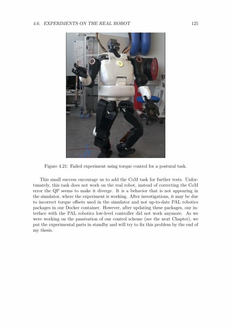
4.6. EXPERIMENTS ON THE REAL ROBOT 125
Figure 4.21: Failed experiment using torque control for a postural task.
This small success encourage us to add the CoM task for further tests. Unfor-tunately, this task does not work on the real robot, instead of correcting the CoMerror the QP seems to make it diverge. It is a behavior that is not appearing inthe simulator, where the experiment is working. After investigations, it may be dueto incorrect torque offsets used in the simulator and not up-to-date PAL roboticspackages in our Docker container. However, after updating these packages, our in-terface with the PAL robotics low-level controller did not work anymore. As wewere working on the passivation of our control scheme (see the next Chapter), weput the experimental parts in standby and will try to fix this problem by the end ofmy thesis.
126 CHAPTER 4. WHOLE BODY CONTROL
Figure 4.22: Successful experiment using torque control for a postural task.
4.7 Conclusion of the Chapter
In this chapter we presented the evaluations realized to achieve an efficient whole-body controller for the humanoid robot TALOS, able to follow correctly the referencetrajectories given by the planning in real-time while keeping a low energy consump-tion. We detailed the force task implemented to achieve manufacturing operations.Finally, we prove the adaptability our torque controller by using it in different lo-comotion contexts such as walking in collaboration with a human, using a similargait.
However, these evaluations have been made only on locomotion problems in sim-ulations. Because the torque controller has proven to be adaptable, energy efficientand capable of quite high speed locomotion we choose to focus on this solution. Yet,when we tried our torque implementation on the real robot the system eventuallydiverges and the robot reaches its limits abruptly, blocking its harmonic drives. Theinvestigation of the problem leads to decrease the controller tasks gains, however thequestion of the stability of our scheme was raised. Recalling the results obtained byHenze et al. [30] and other passive controllers, we decide to consider a way to makeour controller respect the passivity of the system.
Thus, the following chapter presents the works realized in order to analyse theenergy flow and passivity of our system. We detail the achieved results which modifythe previous torque controller with a global energy tank to force the passivity of thesystem. The new scheme is tested in a multi-contact scenario employing the designedforce task of Section 4.3.4 as a first step for manufacturing operations.
Chapter 5
Energy Analysis and Passivity ofthe Robotic System
Contents5.1 Introduction . . . . . . . . . . . . . . . . . . . . . . . . . . 1285.2 Passivity Theory . . . . . . . . . . . . . . . . . . . . . . . . 129
5.2.1 Recall of the definitions . . . . . . . . . . . . . . . . . . . 1295.2.2 Analysis of our System . . . . . . . . . . . . . . . . . . . . 130
5.3 Formulation using Energy Tank in TSID . . . . . . . . . 1315.3.1 Choosing Etank for a set of tasks . . . . . . . . . . . . . . 1315.3.2 Including protection and valve . . . . . . . . . . . . . . . 133
5.3.2.a Proof with valves for the power port {−Nv, τ} . 1355.3.2.b Proof with valves for the power port {v, τext} . . 135
5.3.3 Modified passive QP formulation . . . . . . . . . . . . . . 1365.4 Simulations . . . . . . . . . . . . . . . . . . . . . . . . . . . 138
5.4.1 Pushing task with unplanned contact removal simulation 1385.4.2 Walk of 20cm steps . . . . . . . . . . . . . . . . . . . . . . 141
5.5 Discussion . . . . . . . . . . . . . . . . . . . . . . . . . . . . 1455.6 Conclusion . . . . . . . . . . . . . . . . . . . . . . . . . . . 147
In this chapter are detailed the results obtained in the submission Ramuzat et al.[26].
127
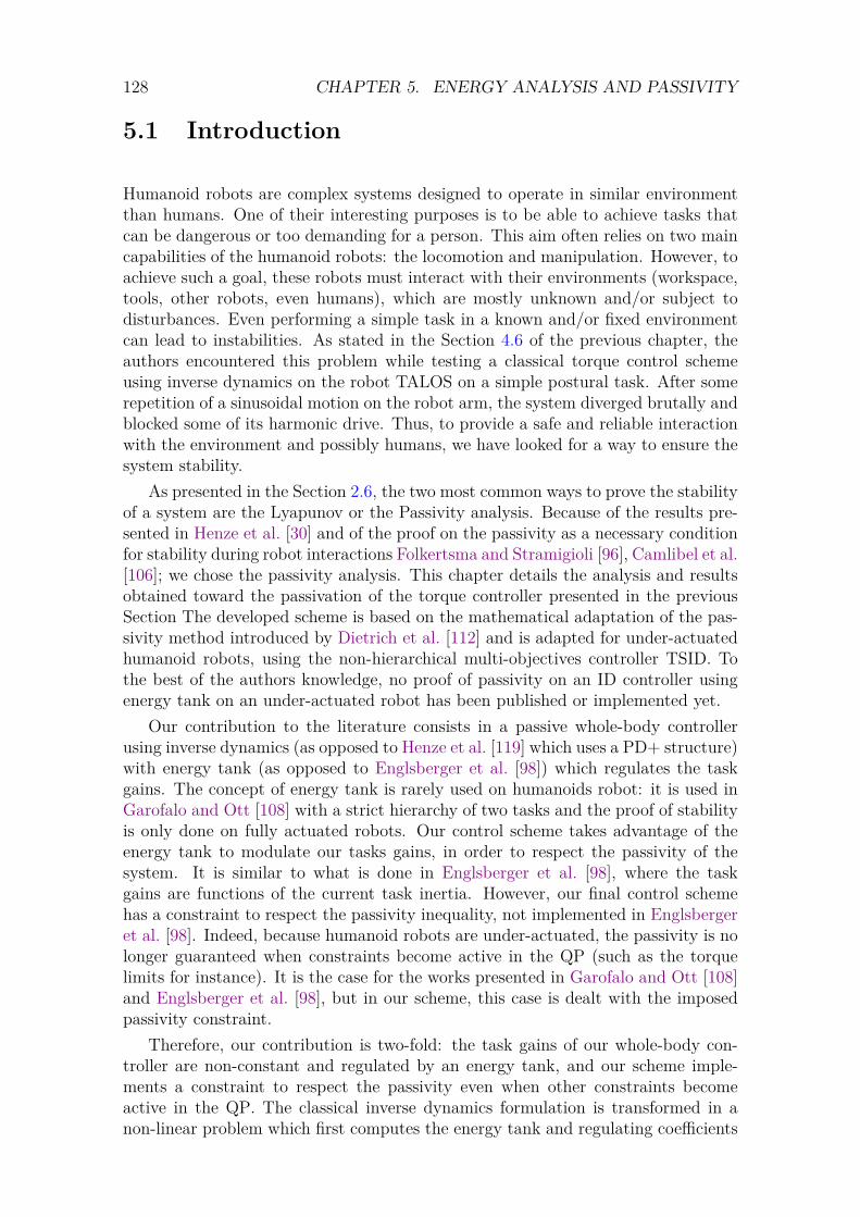
128 CHAPTER 5. ENERGY ANALYSIS AND PASSIVITY
5.1 Introduction
Humanoid robots are complex systems designed to operate in similar environmentthan humans. One of their interesting purposes is to be able to achieve tasks thatcan be dangerous or too demanding for a person. This aim often relies on two maincapabilities of the humanoid robots: the locomotion and manipulation. However, toachieve such a goal, these robots must interact with their environments (workspace,tools, other robots, even humans), which are mostly unknown and/or subject todisturbances. Even performing a simple task in a known and/or fixed environmentcan lead to instabilities. As stated in the Section 4.6 of the previous chapter, theauthors encountered this problem while testing a classical torque control schemeusing inverse dynamics on the robot TALOS on a simple postural task. After somerepetition of a sinusoidal motion on the robot arm, the system diverged brutally andblocked some of its harmonic drive. Thus, to provide a safe and reliable interactionwith the environment and possibly humans, we have looked for a way to ensure thesystem stability.
As presented in the Section 2.6, the two most common ways to prove the stabilityof a system are the Lyapunov or the Passivity analysis. Because of the results pre-sented in Henze et al. [30] and of the proof on the passivity as a necessary conditionfor stability during robot interactions Folkertsma and Stramigioli [96], Camlibel et al.[106]; we chose the passivity analysis. This chapter details the analysis and resultsobtained toward the passivation of the torque controller presented in the previousSection The developed scheme is based on the mathematical adaptation of the pas-sivity method introduced by Dietrich et al. [112] and is adapted for under-actuatedhumanoid robots, using the non-hierarchical multi-objectives controller TSID. Tothe best of the authors knowledge, no proof of passivity on an ID controller usingenergy tank on an under-actuated robot has been published or implemented yet.
Our contribution to the literature consists in a passive whole-body controllerusing inverse dynamics (as opposed to Henze et al. [119] which uses a PD+ structure)with energy tank (as opposed to Englsberger et al. [98]) which regulates the taskgains. The concept of energy tank is rarely used on humanoids robot: it is used inGarofalo and Ott [108] with a strict hierarchy of two tasks and the proof of stabilityis only done on fully actuated robots. Our control scheme takes advantage of theenergy tank to modulate our tasks gains, in order to respect the passivity of thesystem. It is similar to what is done in Englsberger et al. [98], where the taskgains are functions of the current task inertia. However, our final control schemehas a constraint to respect the passivity inequality, not implemented in Englsbergeret al. [98]. Indeed, because humanoid robots are under-actuated, the passivity is nolonger guaranteed when constraints become active in the QP (such as the torquelimits for instance). It is the case for the works presented in Garofalo and Ott [108]and Englsberger et al. [98], but in our scheme, this case is dealt with the imposedpassivity constraint.
Therefore, our contribution is two-fold: the task gains of our whole-body con-troller are non-constant and regulated by an energy tank, and our scheme imple-ments a constraint to respect the passivity even when other constraints becomeactive in the QP. The classical inverse dynamics formulation is transformed in anon-linear problem which first computes the energy tank and regulating coefficients
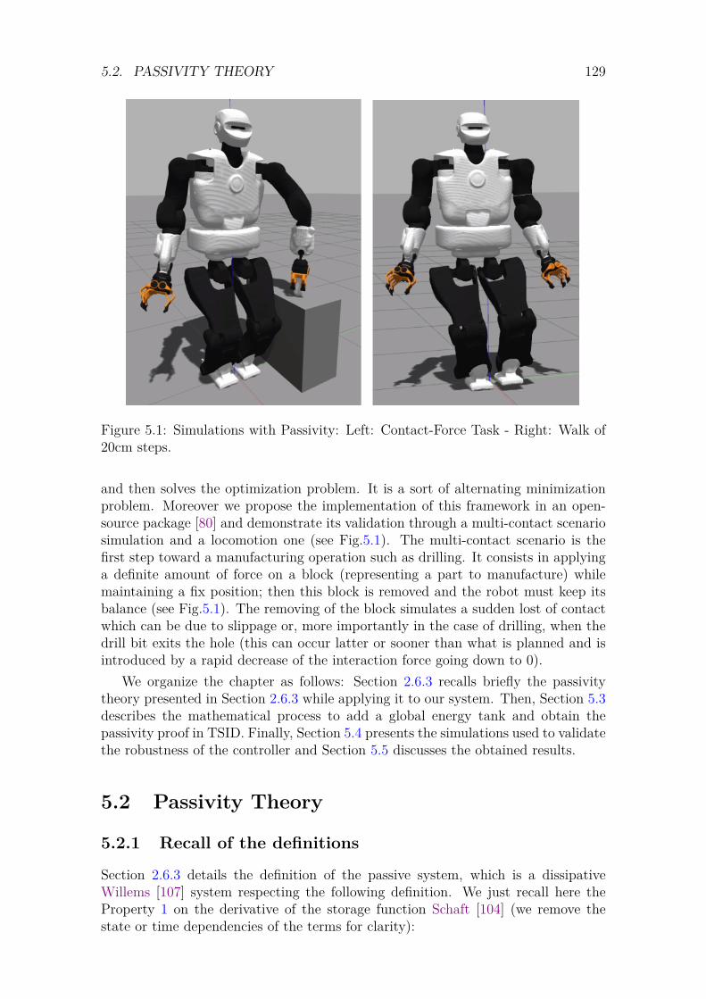
5.2. PASSIVITY THEORY 129
Figure 5.1: Simulations with Passivity: Left: Contact-Force Task - Right: Walk of20cm steps.
and then solves the optimization problem. It is a sort of alternating minimizationproblem. Moreover we propose the implementation of this framework in an open-source package [80] and demonstrate its validation through a multi-contact scenariosimulation and a locomotion one (see Fig.5.1). The multi-contact scenario is thefirst step toward a manufacturing operation such as drilling. It consists in applyinga definite amount of force on a block (representing a part to manufacture) whilemaintaining a fix position; then this block is removed and the robot must keep itsbalance (see Fig.5.1). The removing of the block simulates a sudden lost of contactwhich can be due to slippage or, more importantly in the case of drilling, when thedrill bit exits the hole (this can occur latter or sooner than what is planned and isintroduced by a rapid decrease of the interaction force going down to 0).
We organize the chapter as follows: Section 2.6.3 recalls briefly the passivitytheory presented in Section 2.6.3 while applying it to our system. Then, Section 5.3describes the mathematical process to add a global energy tank and obtain thepassivity proof in TSID. Finally, Section 5.4 presents the simulations used to validatethe robustness of the controller and Section 5.5 discusses the obtained results.
5.2 Passivity Theory
5.2.1 Recall of the definitions
Section 2.6.3 details the definition of the passive system, which is a dissipativeWillems [107] system respecting the following definition. We just recall here theProperty 1 on the derivative of the storage function Schaft [104] (we remove thestate or time dependencies of the terms for clarity):
130 CHAPTER 5. ENERGY ANALYSIS AND PASSIVITY
A system with the state space model of x = f(x, y) with initial state x(0) = x0 ∈Rn, input vector u ∈ Rm and output y = h(x, u) is said to be passive, if there existsa positive semi-definite function H : Rn → R+, called storage function, such that:
H ≤ yTu ∀(x, y) (5.1)
The passivity is a stability criterion based on the power flow exchanged by thecomponents of the system. H(x) is often chosen as the energy of the system, then,the system internal power (H: derivative of the energy in the system) is lesser orequal to the power transferred to the system through its port (yTu).
This property will be used in the following sections to prove the passivity of ourcontrol scheme. Then, let us recall the definition of a virtual energy tank, as thecontrol framework will be augmented by a global one to store the energy dissipatedby the tasks. The tank can be used to transfer the stored energy when a taskbecomes active (the task needs more energy to be completed). In opposition, whenthe tank is empty, it can be used to deteriorate the tracking of this task to ensurethe passivity of the system. The energy tank is defined as a virtual storage elementwith flow variable s and effort variable s such that Giordano et al. [110], Dietrichet al. [111, 112]:
Etank = 12s
2 (5.2)
5.2.2 Analysis of our System
Our system is composed of three components: the robot, the controller and theenvironment. As in Section 2.6.3, we assume that the environment of the robotcan be described by a passive mapping (v → −τext), in connection with impedancecontrol Garofalo and Ott [108], Ott et al. [109]. Then, the group robot-environmentis passive, so we have to make the group controller-robot passive. As in Ott et al.[109], the input of our controller is the velocity of the robot, with the joint angularvelocity measured by the encoders and the free-flyer velocity calculated by the base-estimator. And the output of the controller is the control joint torque τ . Becausethe interconnection of passive systems leads to a general passive system we havetwo solutions: we can impose the passive mapping (−Nv → τ) between the robotand the controller, then because the group robot-environment is passive the overallsystem will be passive. Or, we can impose the passive mapping (v → τext) betweenthe system {robot+controller} and the environment, see Fig.5.2.
Note that because NT ∈ Rn×nj is the selector matrix we have (taking the pseudo-inverse) N † ∈ Rnj×n = NT , N †T = N and N †Tv = Nv = qj by definition (butv 6= NT qj).
Then, as described in Section 2.6.3 (see Garofalo and Ott [108]), we have to finda storage function H such that:
H ≤ −(N †Tv)T τ = −qTj τ = −vTNT τ (5.3)Or a storage function Hext such that:
Hext ≤ vT τext (5.4)
5.3. FORMULATION USING ENERGY TANK IN TSID 131
RobotTSID QPController
Passivesubsystem
Planner
Force passivity of the blue or red subsystem
Environment
Figure 5.2: Port-based modeling of the subsystems and their relative power variables.
In the following, we prove the passivity of the system by building H. Then weaugment this function to obtain a Hext satisfying Eq.5.4.
5.3 Formulation using Energy Tank in TSID
5.3.1 Choosing Etank for a set of tasks
In this part we look at the proof of the passivity for a set of N motion tasks (seeEq.4.8). In this set of tasks, there must be at least a postural task regularization andone contact task with the environment. We consider here only one level of hierarchy(the cost, priority I), and assume that several tasks at this level can be put togetheras if it was only one task.
For one motion task x (see Eq.4.8), we define S the potential energy of the task:
S = 12eTΛKP e
S = eTΛKP e+ 12eT ΛKP e
Λ = (JM−1JT )†J† = UD−1V T
(5.5)
where KP is the proportional gain of the task regularization in the controller(Eq.4.8), J† is the Moore-Penrose pseudo-inverse of J , with U , D and V respec-tively the left singular vectors, the diagonal matrix of singular values and the rightsingular vectors of J (using the Singular Value Decomposition), e = (x− x∗) and Λis the semi-positive definite Cartesian space inertia matrix (multiplication propertyof the positive semi-definite matrix M , see Prop.2).
ΛKp is semi-positive definite if Kp has equal positive elements (see Table.4.3)or under some specific conditions described in an open access document Ramuzat[210] which have been added in the Appendix 5 of the manuscript. Then, becauseS = eTΛKP e is a quadratic form of ΛKp, S is always positive.
We then define the storage function for one task as:
H = S + Etank (5.6)
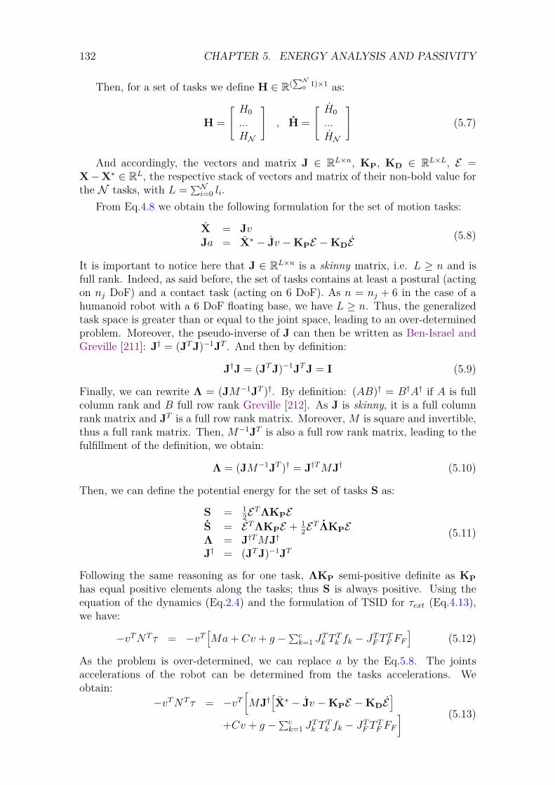
132 CHAPTER 5. ENERGY ANALYSIS AND PASSIVITY
Then, for a set of tasks we define H ∈ R(∑N
0 1)×1 as:
H = H0...HN
, H = H0...HN
(5.7)
And accordingly, the vectors and matrix J ∈ RL×n, KP, KD ∈ RL×L, E =X−X∗ ∈ RL, the respective stack of vectors and matrix of their non-bold value forthe N tasks, with L = ∑N
i=0 li.From Eq.4.8 we obtain the following formulation for the set of motion tasks:
X = JvJa = X∗ − Jv −KPE −KDE
(5.8)
It is important to notice here that J ∈ RL×n is a skinny matrix, i.e. L ≥ n and isfull rank. Indeed, as said before, the set of tasks contains at least a postural (actingon nj DoF) and a contact task (acting on 6 DoF). As n = nj + 6 in the case of ahumanoid robot with a 6 DoF floating base, we have L ≥ n. Thus, the generalizedtask space is greater than or equal to the joint space, leading to an over-determinedproblem. Moreover, the pseudo-inverse of J can then be written as Ben-Israel andGreville [211]: J† = (JTJ)−1JT . And then by definition:
J†J = (JTJ)−1JTJ = I (5.9)
Finally, we can rewrite Λ = (JM−1JT )†. By definition: (AB)† = B†A† if A is fullcolumn rank and B full row rank Greville [212]. As J is skinny, it is a full columnrank matrix and JT is a full row rank matrix. Moreover, M is square and invertible,thus a full rank matrix. Then, M−1JT is also a full row rank matrix, leading to thefulfillment of the definition, we obtain:
Λ = (JM−1JT )† = J†TMJ† (5.10)
Then, we can define the potential energy for the set of tasks S as:
S = 12E
TΛKPES = ETΛKPE + 1
2ET ΛKPE
Λ = J†TMJ†J† = (JTJ)−1JT
(5.11)
Following the same reasoning as for one task, ΛKP semi-positive definite as KPhas equal positive elements along the tasks; thus S is always positive. Using theequation of the dynamics (Eq.2.4) and the formulation of TSID for τext (Eq.4.13),we have:
−vTNT τ = −vT[Ma+ Cv + g −∑c
k=1 JTk T
Tk fk − JTF T TF FF
](5.12)
As the problem is over-determined, we can replace a by the Eq.5.8. The jointsaccelerations of the robot can be determined from the tasks accelerations. Weobtain:
−vTNT τ = −vT[MJ†
[X∗ − Jv −KPE −KDE
]+Cv + g −∑c
k=1 JTk T
Tk fk − JTF T TF FF
] (5.13)
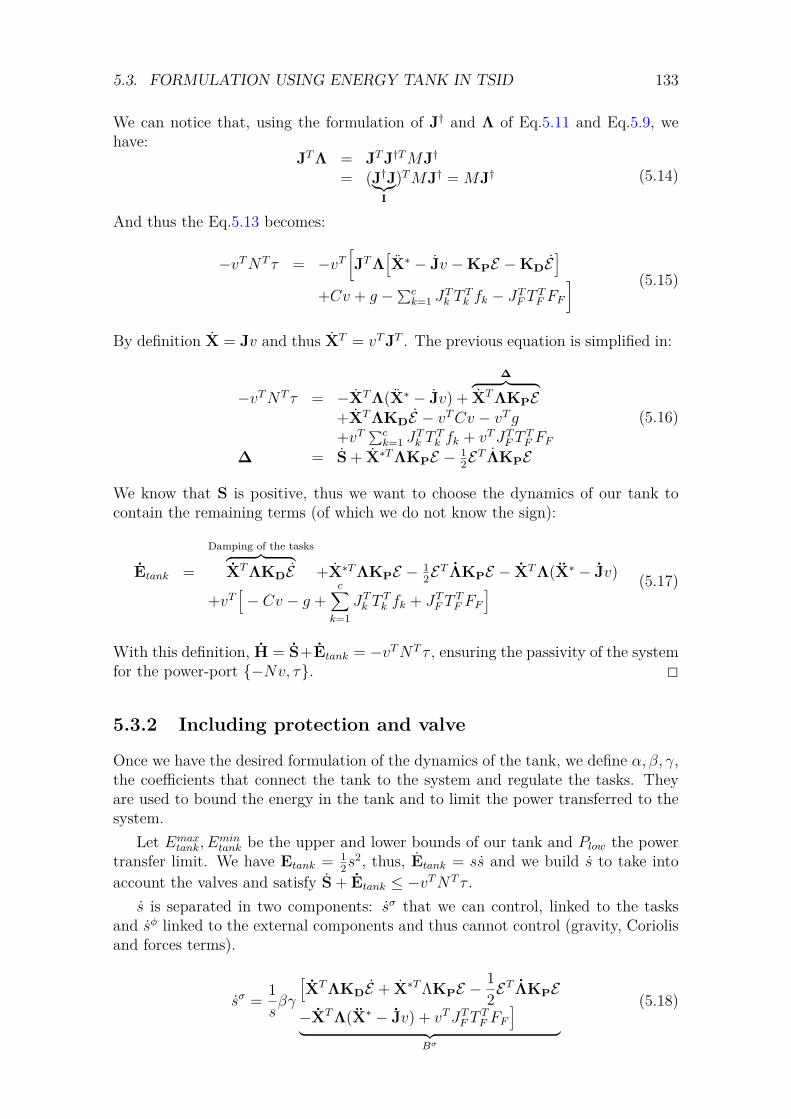
5.3. FORMULATION USING ENERGY TANK IN TSID 133
We can notice that, using the formulation of J† and Λ of Eq.5.11 and Eq.5.9, wehave:
JTΛ = JTJ†TMJ†= (J†J︸︷︷︸
I
)TMJ† = MJ† (5.14)
And thus the Eq.5.13 becomes:
−vTNT τ = −vT[JTΛ
[X∗ − Jv −KPE −KDE
]+Cv + g −∑c
k=1 JTk T
Tk fk − JTF T TF FF
] (5.15)
By definition X = Jv and thus XT = vTJT . The previous equation is simplified in:
−vTNT τ = −XTΛ(X∗ − Jv) +∆︷ ︸︸ ︷
XTΛKPE+XTΛKDE − vTCv − vTg+vT ∑c
k=1 JTk T
Tk fk + vTJTF T
TF FF
∆ = S + X∗TΛKPE − 12E
T ΛKPE
(5.16)
We know that S is positive, thus we want to choose the dynamics of our tank tocontain the remaining terms (of which we do not know the sign):
Etank =Damping of the tasks︷ ︸︸ ︷
XTΛKDE +X∗TΛKPE − 12E
T ΛKPE − XTΛ(X∗ − Jv)
+vT[− Cv − g +
c∑k=1
JTk TTk fk + JTF T
TF FF
] (5.17)
With this definition, H = S+Etank = −vTNT τ , ensuring the passivity of the systemfor the power-port {−Nv, τ}. 2
5.3.2 Including protection and valve
Once we have the desired formulation of the dynamics of the tank, we define α, β, γ,the coefficients that connect the tank to the system and regulate the tasks. Theyare used to bound the energy in the tank and to limit the power transferred to thesystem.
Let Emaxtank, E
mintank be the upper and lower bounds of our tank and Plow the power
transfer limit. We have Etank = 12s
2, thus, Etank = ss and we build s to take intoaccount the valves and satisfy S + Etank ≤ −vTNT τ .
s is separated in two components: sσ that we can control, linked to the tasksand sφ linked to the external components and thus cannot control (gravity, Coriolisand forces terms).
sσ = 1sβγ
[XTΛKDE + X∗TΛKPE −
12E
T ΛKPE
−XTΛ(X∗ − Jv) + vTJTF TTF FF
]︸ ︷︷ ︸
Bσ
(5.18)
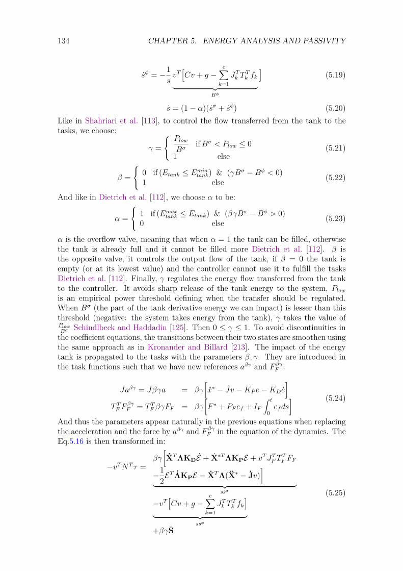
134 CHAPTER 5. ENERGY ANALYSIS AND PASSIVITY
sφ = −1svT[Cv + g −
c∑k=1
JTk TTk fk︸ ︷︷ ︸
Bφ
](5.19)
s = (1− α)(sσ + sφ) (5.20)Like in Shahriari et al. [113], to control the flow transferred from the tank to thetasks, we choose:
γ =
PlowBσ
ifBσ < Plow ≤ 01 else
(5.21)
β =
0 if (Etank ≤ Emintank) & (γBσ −Bφ < 0)
1 else (5.22)
And like in Dietrich et al. [112], we choose α to be:
α =
1 if (Emaxtank ≤ Etank) & (βγBσ −Bφ > 0)
0 else (5.23)
α is the overflow valve, meaning that when α = 1 the tank can be filled, otherwisethe tank is already full and it cannot be filled more Dietrich et al. [112]. β isthe opposite valve, it controls the output flow of the tank, if β = 0 the tank isempty (or at its lowest value) and the controller cannot use it to fulfill the tasksDietrich et al. [112]. Finally, γ regulates the energy flow transferred from the tankto the controller. It avoids sharp release of the tank energy to the system, Plowis an empirical power threshold defining when the transfer should be regulated.When Bσ (the part of the tank derivative energy we can impact) is lesser than thisthreshold (negative: the system takes energy from the tank), γ takes the value ofPlowBσ
Schindlbeck and Haddadin [125]. Then 0 ≤ γ ≤ 1. To avoid discontinuities inthe coefficient equations, the transitions between their two states are smoothen usingthe same approach as in Kronander and Billard [213]. The impact of the energytank is propagated to the tasks with the parameters β, γ. They are introduced inthe task functions such that we have new references aβγ and F βγ
F :
Jaβγ = Jβγa = βγ[x∗ − Jv −KP e−KDe
]T TF F
βγF = T TF βγFF = βγ
[F ∗ + PF ef + IF
∫ t
0efds
] (5.24)
And thus the parameters appear naturally in the previous equations when replacingthe acceleration and the force by aβγ and F βγ
F in the equation of the dynamics. TheEq.5.16 is then transformed in:
−vTNT τ =βγ[XTΛKDE + X∗TΛKPE + vTJTF T
TF FF
−12E
T ΛKPE − XTΛ(X∗ − Jv)]
︸ ︷︷ ︸ssσ
−vT[Cv + g −
c∑k=1
JTk TTk fk
]︸ ︷︷ ︸
ssφ
+βγS
(5.25)
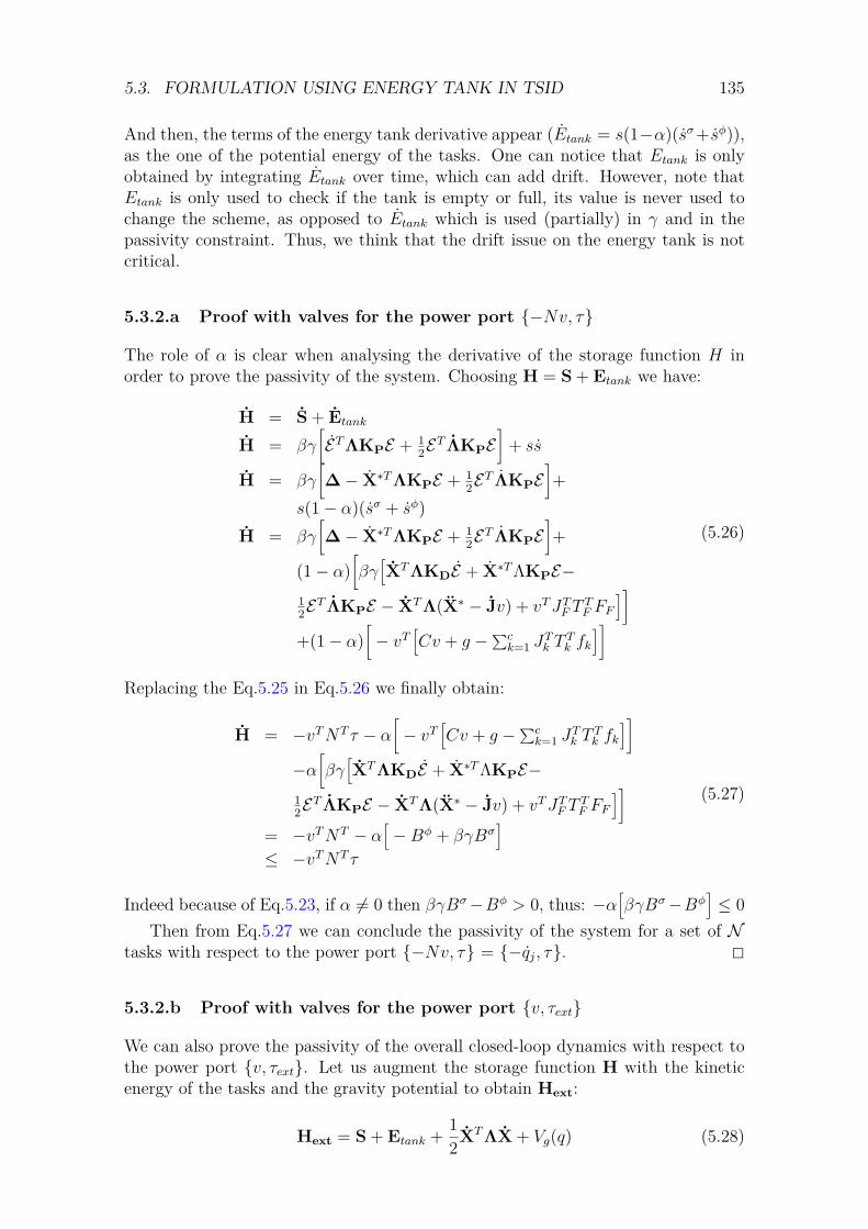
5.3. FORMULATION USING ENERGY TANK IN TSID 135
And then, the terms of the energy tank derivative appear (Etank = s(1−α)(sσ+sφ)),as the one of the potential energy of the tasks. One can notice that Etank is onlyobtained by integrating Etank over time, which can add drift. However, note thatEtank is only used to check if the tank is empty or full, its value is never used tochange the scheme, as opposed to Etank which is used (partially) in γ and in thepassivity constraint. Thus, we think that the drift issue on the energy tank is notcritical.
5.3.2.a Proof with valves for the power port {−Nv, τ}
The role of α is clear when analysing the derivative of the storage function H inorder to prove the passivity of the system. Choosing H = S + Etank we have:
H = S + Etank
H = βγ[ETΛKPE + 1
2ET ΛKPE
]+ ss
H = βγ[∆− X∗TΛKPE + 1
2ET ΛKPE
]+
s(1− α)(sσ + sφ)H = βγ
[∆− X∗TΛKPE + 1
2ET ΛKPE
]+
(1− α)[βγ[XTΛKDE + X∗TΛKPE−
12E
T ΛKPE − XTΛ(X∗ − Jv) + vTJTF TTF FF
]]+(1− α)
[− vT
[Cv + g −∑c
k=1 JTk T
Tk fk
]]
(5.26)
Replacing the Eq.5.25 in Eq.5.26 we finally obtain:
H = −vTNT τ − α[− vT
[Cv + g −∑c
k=1 JTk T
Tk fk
]]−α
[βγ[XTΛKDE + X∗TΛKPE−
12E
T ΛKPE − XTΛ(X∗ − Jv) + vTJTF TTF FF
]]= −vTNT − α
[−Bφ + βγBσ
]≤ −vTNT τ
(5.27)
Indeed because of Eq.5.23, if α 6= 0 then βγBσ−Bφ > 0, thus: −α[βγBσ−Bφ
]≤ 0
Then from Eq.5.27 we can conclude the passivity of the system for a set of Ntasks with respect to the power port {−Nv, τ} = {−qj, τ}. 2
5.3.2.b Proof with valves for the power port {v, τext}
We can also prove the passivity of the overall closed-loop dynamics with respect tothe power port {v, τext}. Let us augment the storage function H with the kineticenergy of the tasks and the gravity potential to obtain Hext:
Hext = S + Etank + 12XTΛX + Vg(q) (5.28)
136 CHAPTER 5. ENERGY ANALYSIS AND PASSIVITY
We have by definition, g(q) =(∂Vg(q)
∂q
)T, leading to:
∂Vg(q)dt
= ∂Vg(q)∂q
∂q
dt=(∂qdt
∂Vg(q)∂q
)T= vTg(q) (5.29)
Let us write the formulation of the equation of the dynamics for one task in theCartesian space:
Λx+ µx = J†T (−g +NT τ + τext) (5.30)
With µ = J†TCJ† − ΛJJ†. Then, for a set of N tasks we have, Z designating thestack of µ:
ΛX + ZX = J†T (−g +NT τ + τext) (5.31)
By taking the derivative of Eq.5.28 and substituting Eq.5.31, we can write:
Hext = S + Etank + vTg + 12XT ΛX+
XT[J†T︸ ︷︷ ︸
vT
(−g +NT τ + τext)− ZX]
(5.32)
Using the fact that the Coriolis matrix is defined such that: 12M(q) = C(q,v)+C(q,v)T
2 ,we have XT (1
2Λ− Z)X = 0 (skew-symmetric property, recall of the eq.2.5).Finally we obtain, using the Eq.5.27:
Hext = S + Etank︸ ︷︷ ︸≤−vTNT τ
+vTNT τ + vT τext
Hext ≤ −vTNT τ + vTNT τ + vT τextHext ≤ vT τext
(5.33)
Delivering the proof of passivity for the port {v, τext}. 2
5.3.3 Modified passive QP formulation
The classical inverse dynamics formulation is transformed in a non-linear problemwith two stages. It is a sort of alternating minimization problem. The first stage(1) computes the energy tank dynamics and the regulating coefficients and then thesecond stage (2) solves the QP modified by these coefficients. One can notice thatthe first stage finds the coefficients for a torque which does not take into accountthe constraints of the QP. Thus as in Englsberger et al. [98], if a constraint becameactive, the passivity is no longer guaranteed because the computation used for theenergy tank is not the same as the one of the QP. This is why we add a newconstraint in the QP formulation, similarly to Joseph et al. [105], enforcing theinequality H ≤ −vTNT τ to maintain the passivity in any situation. The general
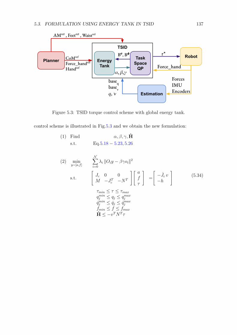
5.3. FORMULATION USING ENERGY TANK IN TSID 137
Figure 5.3: TSID torque control scheme with global energy tank.
control scheme is illustrated in Fig.5.3 and we obtain the new formulation:
(1) Find α, β, γ, Hs.t. Eq.5.18− 5.23, 5.26
(2) miny=[a,f ]
N∑i=0
λi ‖Oiy − βγoi‖2
s.t. Jc 0 0M −JTc −NT
afτ
= −Jc v−h
τmin ≤ τ ≤ τmaxqminj ≤ qj ≤ qmaxj
qminj ≤ qj ≤ qmaxj
fmin ≤ f ≤ fmaxH ≤ −vTNT τ
(5.34)
138 CHAPTER 5. ENERGY ANALYSIS AND PASSIVITY
5.4 Simulations
In this section are detailed the simulations realized on Gazebo to demonstrate thevalidity of our implementation. The tests are performed on a humanoid robot TA-LOS. The chosen simulations are a force application task performed by the left handand a walk of 20cm steps on flat ground. These simulations allow to cover multi-contact and locomotion skills in stationary environment. The set of tasks consideredduring the first simulation are presented in the Table.5.1, and in the Table.5.3 forthe second one. The task gains are defined in Table 5.2. The authors have imple-mented this controller using the TSID [80] library in the open-source package [202].The design parameters of the global energy tank are set as follows: Emax
tank = 5J,Emintank = 0.1J and Plow = −0.5W. They are set as low values in order to keep small
the contribution of the tank energy compared to the overall energy of the system. Inthe simulations, we use the robot base-estimator of Flayols et al. [29]. The base in-formation is estimated using robot joints configurations and velocities, the IMU andthe force sensors of the robot. For the force task simulation, no planning methodswere used as the robot remains in the same configuration. The force references werecreated by linear interpolation between the actual and desired force to be appliedon the block. The reference trajectories of the 20cm step walk were computed withthe multicontact-locomotion-planning framework [62] (see Section 2.4).
5.4.1 Pushing task with unplanned contact removal simula-tion
In this simulation the robot makes a contact between a tool and a surface and appliesa 30N force along the z-axis. In Gazebo, the tool is simulated by a cylinder and thesurface is a simple square block, shown in Fig.5.1. This set-up is a first step towardmore complex operations, requiring contact and a force application, such as drilling.It exposes the problem of unexpected broken contact that can be due to slippage,disturbances or when the drill bit exits the hole. In this simulation, the referenceforce is raised in two steps, the first one reaches 10N to stabilize the contact, inFig.5.4 some oscillations can be seen in the first slope, leading to some instabilityin the tank coefficients in Fig.5.5. Then it is set to 30N, and at 32.3s the block isremoved. The energy tank is initialized at 3J.
As shown in Fig.5.4, the measured force along the z-axis falls to 0N when theblock is removed. We first try a simulation without the energy tank and the passivity
Tasks Priority WeightFeet contacts I 100CoM tracking I 50Cartesian Force-Contact I 10Waist orientation I 1Posture regularization in half-sitting I 0.1AM regularization to 0 I 2× 10⁻²
Table 5.1: Set of tasks used in the contact simulation.
5.4. SIMULATIONS 139
Tasks Gains KP KD KI
CoM [50, 50, 50] [5, 5, 5] -Waist [100, 100, 100] 2
√KP -
Feet Contacts [30, 30, 30, 30, 30, 30] 2√KP -
Feet Motions [100, 100, 100, [5, 5, 5, -(walk simulation) 100, 100, 100] 5, 5, 5] -Force-Contact (force simulation) [10, 10, 10, 10, 10, 10] - 0.5KP
AM [10, 10, 10] 2√KP -
Posture Legs Torso Arms HeadKP [80, 80, 80, [80, 80] [80, 80, 80, 80, [80, 80]
80, 80, 80] 80, 80, 80, 80]KD 2
√KP 2
√KP 2
√KP 2
√KP
Table 5.2: Tasks gains of the control scheme.
constraint. As a result, the robot quickly falls and cannot react in time to try tobalance itself or to remove the force task when detecting the loss of the contact. Onthe contrary, with the formulation presented previously, when the block is removedthe robot does not fall immediately. Indeed, as presented in Fig.5.5, the α and γcoefficients are triggered. With the γ closes to 0, the force task is highly penalizedand thus the hand slowly comes down. As a result, the system has the time to detectthe loss of the contact and remove the task, leading to the pick in the consumptionof the energy tank at 34.4s. By removing the task, the robot goes back to its initialposition because of the postural task and thus raises its hand, going against thegravity and consuming energy. On can notice a continuous growth of energy duringthe steady state between 20 and 30 s. We think that this growth is due to theremaining error of the postural task which desired position is set to the half-sittingof the robot and not the contact configuration.
Because the energy constraint is enforced in the TSID constraints, the QP ensuresthat the passivity holds, i.e. H ≤ −vT τ . The Fig.5.6 presents the evolution ofthe potential function derivative H during the removal of the block (at 32.2s) andthe task. We also display the results without energy tank, when the robot falls.We can see that the mechanical power of the system is controlled in the passiveimplementation case whereas it presents peaks in the simple case, leading to thefall. One can notice that around second 34 − 35 the tank energy slope is muchsteeper than −0.5 W (corresponding to the value of Plow). This is because the taskis removed and the robot goes back to the postural task position (straighten up),acting against the gravity. Keep in mind that Etank = s(1− α)(ssigma + sphi), thuswhile ssigma is regulated by γ, sphi is not as we cannot control it. Thus, the highvalues of H correspond to the power delivered by the gravity, Coriolis and contactforces terms.
For the moment to remove the task we use a hand-programmed emergency action,but it should be implemented in a better way in the QP. Or for instance, having afinite-state-machine which would tell the QP which tasks should be added/removedin function of the energy tank parameters.
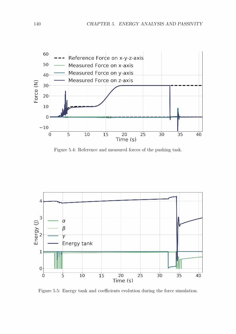
140 CHAPTER 5. ENERGY ANALYSIS AND PASSIVITY
Figure 5.4: Reference and measured forces of the pushing task.
Figure 5.5: Energy tank and coefficients evolution during the force simulation.
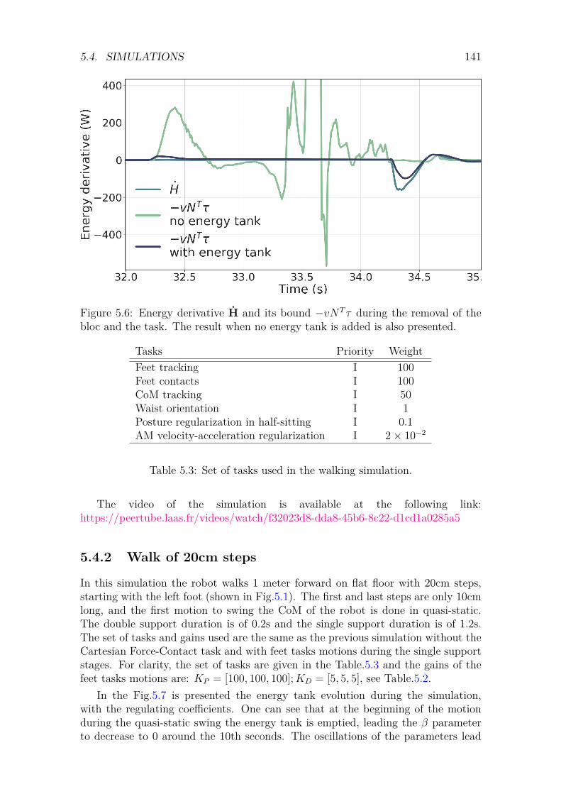
5.4. SIMULATIONS 141
Figure 5.6: Energy derivative H and its bound −vNT τ during the removal of thebloc and the task. The result when no energy tank is added is also presented.
Tasks Priority WeightFeet tracking I 100Feet contacts I 100CoM tracking I 50Waist orientation I 1Posture regularization in half-sitting I 0.1AM velocity-acceleration regularization I 2× 10⁻²
Table 5.3: Set of tasks used in the walking simulation.
The video of the simulation is available at the following link:https://peertube.laas.fr/videos/watch/f32023d8-dda8-45b6-8c22-d1cd1a0285a5
5.4.2 Walk of 20cm steps
In this simulation the robot walks 1 meter forward on flat floor with 20cm steps,starting with the left foot (shown in Fig.5.1). The first and last steps are only 10cmlong, and the first motion to swing the CoM of the robot is done in quasi-static.The double support duration is of 0.2s and the single support duration is of 1.2s.The set of tasks and gains used are the same as the previous simulation without theCartesian Force-Contact task and with feet tasks motions during the single supportstages. For clarity, the set of tasks are given in the Table.5.3 and the gains of thefeet tasks motions are: KP = [100, 100, 100];KD = [5, 5, 5], see Table.5.2.
In the Fig.5.7 is presented the energy tank evolution during the simulation,with the regulating coefficients. One can see that at the beginning of the motionduring the quasi-static swing the energy tank is emptied, leading the β parameterto decrease to 0 around the 10th seconds. The oscillations of the parameters lead
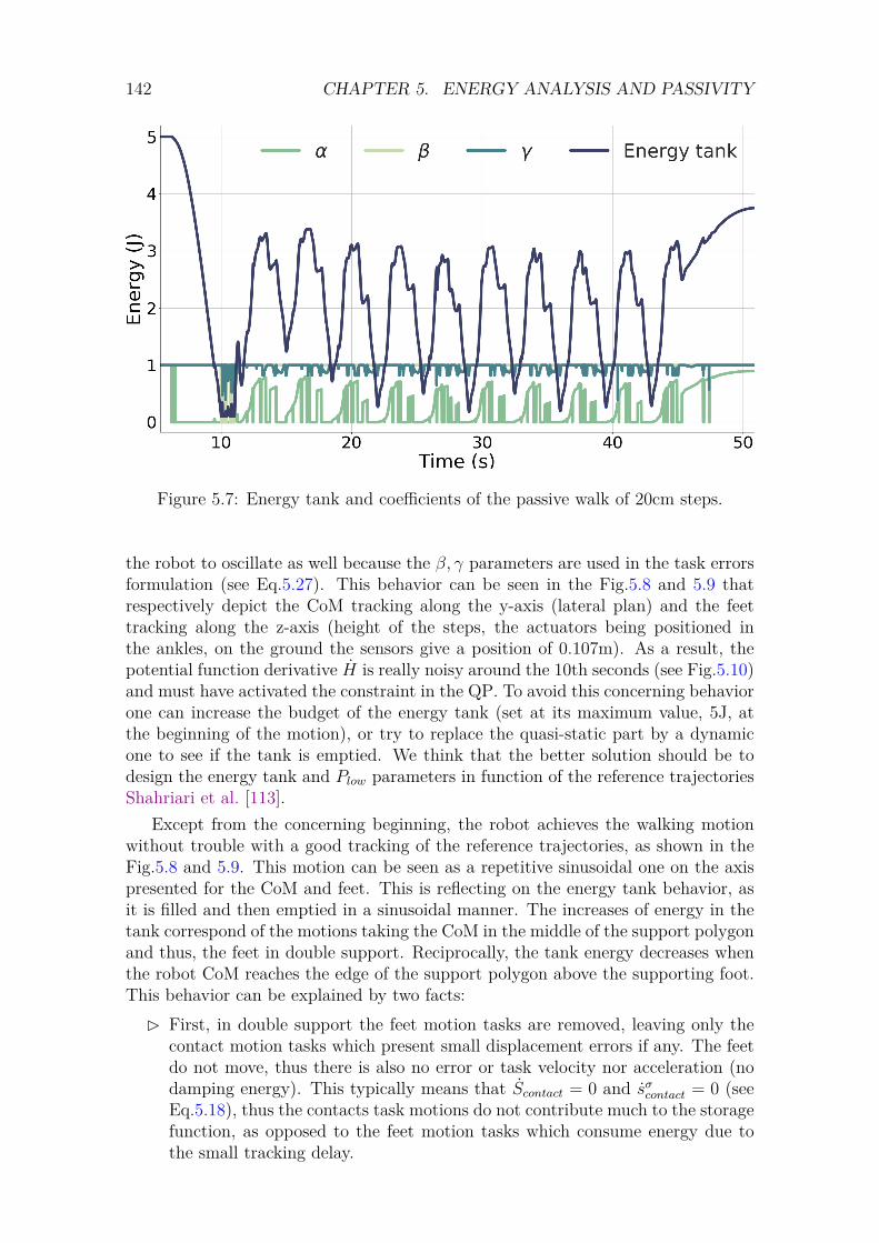
142 CHAPTER 5. ENERGY ANALYSIS AND PASSIVITY
Figure 5.7: Energy tank and coefficients of the passive walk of 20cm steps.
the robot to oscillate as well because the β, γ parameters are used in the task errorsformulation (see Eq.5.27). This behavior can be seen in the Fig.5.8 and 5.9 thatrespectively depict the CoM tracking along the y-axis (lateral plan) and the feettracking along the z-axis (height of the steps, the actuators being positioned inthe ankles, on the ground the sensors give a position of 0.107m). As a result, thepotential function derivative H is really noisy around the 10th seconds (see Fig.5.10)and must have activated the constraint in the QP. To avoid this concerning behaviorone can increase the budget of the energy tank (set at its maximum value, 5J, atthe beginning of the motion), or try to replace the quasi-static part by a dynamicone to see if the tank is emptied. We think that the better solution should be todesign the energy tank and Plow parameters in function of the reference trajectoriesShahriari et al. [113].
Except from the concerning beginning, the robot achieves the walking motionwithout trouble with a good tracking of the reference trajectories, as shown in theFig.5.8 and 5.9. This motion can be seen as a repetitive sinusoidal one on the axispresented for the CoM and feet. This is reflecting on the energy tank behavior, asit is filled and then emptied in a sinusoidal manner. The increases of energy in thetank correspond of the motions taking the CoM in the middle of the support polygonand thus, the feet in double support. Reciprocally, the tank energy decreases whenthe robot CoM reaches the edge of the support polygon above the supporting foot.This behavior can be explained by two facts:� First, in double support the feet motion tasks are removed, leaving only the
contact motion tasks which present small displacement errors if any. The feetdo not move, thus there is also no error or task velocity nor acceleration (nodamping energy). This typically means that Scontact = 0 and sσcontact = 0 (seeEq.5.18), thus the contacts task motions do not contribute much to the storagefunction, as opposed to the feet motion tasks which consume energy due tothe small tracking delay.
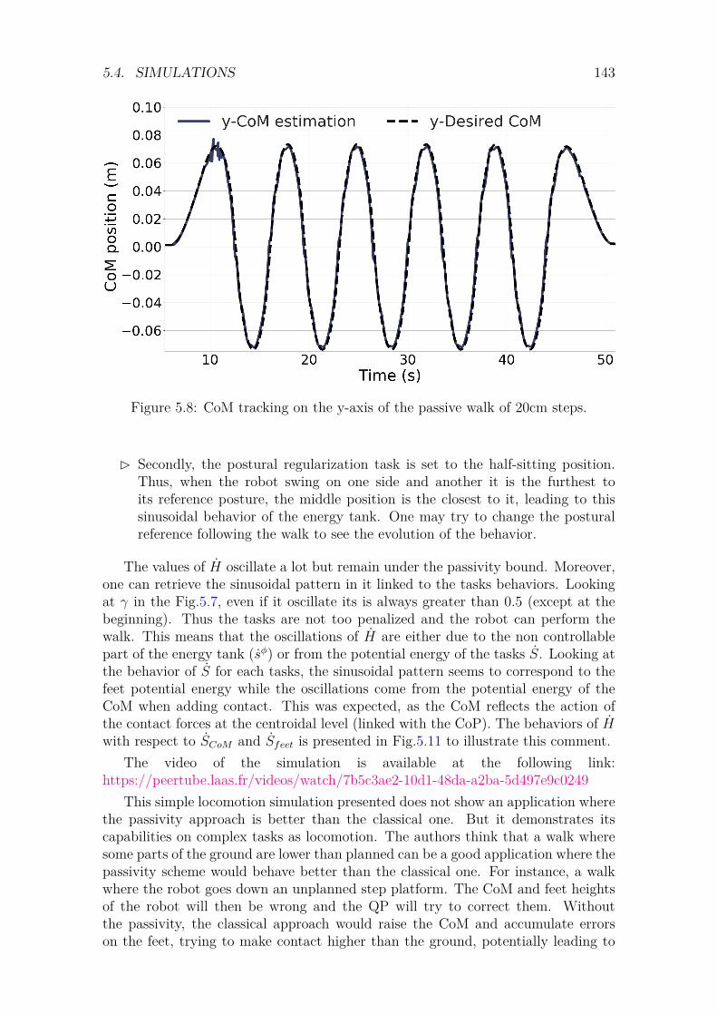
5.4. SIMULATIONS 143
Figure 5.8: CoM tracking on the y-axis of the passive walk of 20cm steps.
� Secondly, the postural regularization task is set to the half-sitting position.Thus, when the robot swing on one side and another it is the furthest toits reference posture, the middle position is the closest to it, leading to thissinusoidal behavior of the energy tank. One may try to change the posturalreference following the walk to see the evolution of the behavior.
The values of H oscillate a lot but remain under the passivity bound. Moreover,one can retrieve the sinusoidal pattern in it linked to the tasks behaviors. Lookingat γ in the Fig.5.7, even if it oscillate its is always greater than 0.5 (except at thebeginning). Thus the tasks are not too penalized and the robot can perform thewalk. This means that the oscillations of H are either due to the non controllablepart of the energy tank (sφ) or from the potential energy of the tasks S. Looking atthe behavior of S for each tasks, the sinusoidal pattern seems to correspond to thefeet potential energy while the oscillations come from the potential energy of theCoM when adding contact. This was expected, as the CoM reflects the action ofthe contact forces at the centroidal level (linked with the CoP). The behaviors of Hwith respect to SCoM and Sfeet is presented in Fig.5.11 to illustrate this comment.
The video of the simulation is available at the following link:https://peertube.laas.fr/videos/watch/7b5c3ae2-10d1-48da-a2ba-5d497e9c0249
This simple locomotion simulation presented does not show an application wherethe passivity approach is better than the classical one. But it demonstrates itscapabilities on complex tasks as locomotion. The authors think that a walk wheresome parts of the ground are lower than planned can be a good application where thepassivity scheme would behave better than the classical one. For instance, a walkwhere the robot goes down an unplanned step platform. The CoM and feet heightsof the robot will then be wrong and the QP will try to correct them. Withoutthe passivity, the classical approach would raise the CoM and accumulate errorson the feet, trying to make contact higher than the ground, potentially leading to
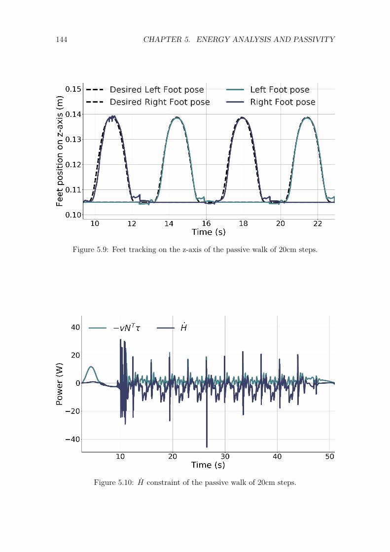
144 CHAPTER 5. ENERGY ANALYSIS AND PASSIVITY
Figure 5.9: Feet tracking on the z-axis of the passive walk of 20cm steps.
Figure 5.10: H constraint of the passive walk of 20cm steps.
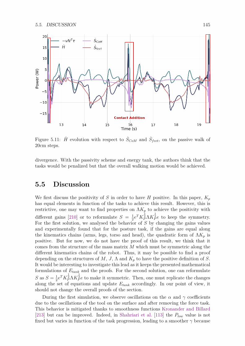
5.5. DISCUSSION 145
Figure 5.11: H evolution with respect to SCoM and Sfeet, on the passive walk of20cm steps.
divergence. With the passivity scheme and energy tank, the authors think that thetasks would be penalized but that the overall walking motion would be achieved.
5.5 Discussion
We first discuss the positivity of S in order to have H positive. In this paper, Kp
has equal elements in function of the tasks to achieve this result. However, this isrestrictive, one may want to find properties on ΛKp to achieve the positivity withdifferent gains [210] or to reformulate S = 1
2eTK
12PΛK
12P e to keep the symmetry.
For the first solution, we analysed the behavior of S by changing the gains valuesand experimentally found that for the posture task, if the gains are equal alongthe kinematics chains (arms, legs, torso and head), the quadratic form of ΛKp ispositive. But for now, we do not have the proof of this result, we think that itcomes from the structure of the mass matrix M which must be symmetric along thedifferent kinematics chains of the robot. Thus, it may be possible to find a proofdepending on the structures of M , J , Λ and Kp to have the positive definition of S.It would be interesting to investigate this lead as it keeps the presented mathematicalformulations of Etank and the proofs. For the second solution, one can reformulateS as S = 1
2eTK
12PΛK
12P e to make it symmetric. Then, one must replicate the changes
along the set of equations and update Etank accordingly. In our point of view, itshould not change the overall proofs of the section.
During the first simulation, we observe oscillations on the α and γ coefficientsdue to the oscillations of the tool on the surface and after removing the force task.This behavior is mitigated thanks to smoothness functions Kronander and Billard[213] but can be improved. Indeed, in Shahriari et al. [113] the Plow value is notfixed but varies in function of the task progression, leading to a smoother γ because
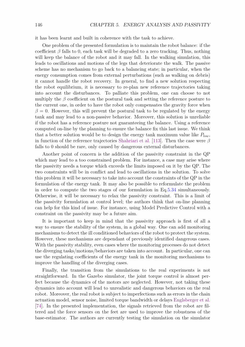
146 CHAPTER 5. ENERGY ANALYSIS AND PASSIVITY
it has been learnt and built in coherence with the task to achieve.One problem of the presented formulation is to maintain the robot balance: if the
coefficient β falls to 0, each task will be degraded to a zero tracking. Thus, nothingwill keep the balance of the robot and it may fall. In the walking simulation, thisleads to oscillations and motions of the legs that deteriorate the walk. The passivescheme has no mechanism to go back to a balancing state; in particular, when theenergy consumption comes from external perturbations (such as walking on debris)it cannot handle the robot recovery. In general, to find a new solution respectingthe robot equilibrium, it is necessary to re-plan new reference trajectories takinginto account the disturbances. To palliate this problem, one can choose to notmultiply the β coefficient on the postural task and setting the reference posture tothe current one, in order to have the robot only compensates the gravity force whenβ = 0. However, this will prevent the postural task to be regulated by the energytank and may lead to a non-passive behavior. Moreover, this solution is unreliableif the robot has a reference posture not guaranteeing the balance. Using a referencecomputed on-line by the planning to ensure the balance fix this last issue. We thinkthat a better solution would be to design the energy tank maximum value like Plow,in function of the reference trajectories Shahriari et al. [113]. Then the case were βfalls to 0 should be rare, only caused by dangerous external disturbances.
Another point of concern is the addition of the passivity constraint in the QPwhich may lead to a too constrained problem. For instance, a case may arise wherethe passivity needs a torque which exceeds the limits imposed on it by the QP. Thetwo constraints will be in conflict and lead to oscillations in the solution. To solvethis problem it will be necessary to take into account the constraints of the QP in theformulation of the energy tank. It may also be possible to reformulate the problemin order to compute the two stages of our formulation in Eq.5.34 simultaneously.Otherwise, it will be necessary to relax the passivity constraint. This is a limit ofthe passivity formulation at control level; the authors think that on-line planningcan help for this kind of issue. For instance, using Model Predictive Control with aconstraint on the passivity may be a future aim.
It is important to keep in mind that the passivity approach is first of all away to ensure the stability of the system, in a global way. One can add monitoringmechanisms to detect the ill conditioned behaviors of the robot to protect the system.However, these mechanisms are dependant of previously identified dangerous cases.With the passivity stability, even cases where the monitoring processes do not detectthe diverging tasks/motions/behaviors are taken into account. In particular, one canuse the regulating coefficients of the energy tank in the monitoring mechanisms toimprove the handling of the diverging cases.
Finally, the transition from the simulations to the real experiments is notstraightforward. In the Gazebo simulator, the joint torque control is almost per-fect because the dynamics of the motors are neglected. However, not taking thesedynamics into account will lead to unrealistic and dangerous behaviors on the realrobot. Moreover, the real robot is subject to imperfections such as errors in the chainactuation model, sensor noise, limited torque bandwidth or delays Englsberger et al.[74]. In the presented implementation, the signals retrieved from the robot are fil-tered and the force sensors on the feet are used to improve the robustness of thebase-estimator. The authors are currently testing the simulation on the simulator
5.6. CONCLUSION 147
of the TALOS constructor, PAL robotics, which models the actuator dynamics ofthe robot.
5.6 Conclusion
In this chapter a novel control formulation for the passivation of an inverse dynam-ics framework is presented. It involves a global energy tank which monitors theexchange of energy between a set of tasks and regulates their gains. This method isclose to the passive hierarchical impedance control relying on a strict hierarchy andnull-space projection of Dietrich et al. [112]. It adds a protection valve for powerflow variations and is transposed in a case of a non-strict hierarchy on an under-actuated humanoid robot. The robustness of the controller is evaluated in simula-tions on Gazebo through a multi-contact scenario and 20cm walk involving six andfive tasks. Thus, the proposed method extends the repertoire of multi-objectivesnon-hierarchical controllers for applications requiring physical interactions with theenvironment or a human. Its passive formulation ensures a stable, safe and robustbehavior of the system.
For our future works, we plan to improve the behavior of the coefficients, in par-ticular, the one on the power flow regulation can be computed as in Shahriari et al.[113], to vary in function of the task progression. The impact of these coefficients onthe balance of the robot will be evaluated, indeed, for now, the robot may falls if allthe system is penalized to respect the passivity. Finally, our new control formulationwill be evaluated on the real robot.
In this chapter our passive torque controller implementing a contact-force taskhas been successfully tested in simulation on the humanoid robot TALOS. However,one can wonder how to apply this solution to an industrial context and industrialrobots such as the MSDR. The transfer of the solution is not straightforward, asstated in the context of this thesis (see Section 1.4.3), the MSDR has no ROSinterface, thus one will be needed to plug our solution to the low-level controller ofthe robot. The transfer of our state-of-the-art controller onto the MSDR industrialrobot is discussed in the next chapter.

148 CHAPTER 5. ENERGY ANALYSIS AND PASSIVITY
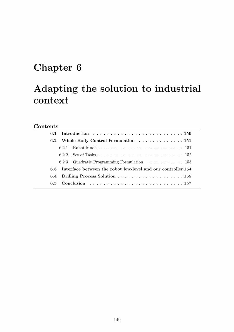
Chapter 6
Adapting the solution to industrialcontext
Contents6.1 Introduction . . . . . . . . . . . . . . . . . . . . . . . . . . 1506.2 Whole Body Control Formulation . . . . . . . . . . . . . 151
6.2.1 Robot Model . . . . . . . . . . . . . . . . . . . . . . . . . 1516.2.2 Set of Tasks . . . . . . . . . . . . . . . . . . . . . . . . . . 1526.2.3 Quadratic Programming Formulation . . . . . . . . . . . 153
6.3 Interface between the robot low-level and our controller 1546.4 Drilling Process Solution . . . . . . . . . . . . . . . . . . . 1556.5 Conclusion . . . . . . . . . . . . . . . . . . . . . . . . . . . 157
149
150 CHAPTER 6. ADAPTING THE SOLUTION TO THE MSDR
6.1 Introduction
This chapter describes the challenges that may arise when we will transfer the passivetorque controller presented in the previous section on an industrial robot. Theindustrial robot MSDR considered has been presented in Section 1.4.3, as it is thesolution designed by Airbus to achieve autonomous manufacturing operations (seeFig.6.1).
As stated before, the first issue to tackle is the difference of model between therobot TALOS and the MSDR: one is under-actuated while the other is not becauseit is fixed to the ground (for the initial setup considered in this thesis). Thus, therelevant part of our control solution can be seen as the application of a passivecontact-force task on the robot arm. Using our formulation of the passivity, thecontrol formulation will guarantee safe, stable and robust behaviors of the robotonto the environment. One can thus formulate a new set of tasks in our previoustorque controller to take into account only the relevant parts of the complex problempresented on the humanoid robot.
Secondly, the MSDR uses the Fanuc proprietary software architecture which doesnot implement a ROS interface. The difficulty here lies in reading sensors and writingcommands (joint position or torque vector) within a guaranteed deterministic timeboundary in order to update the system information in real time. The frequencyneeded to achieve a correct behavior is at least 250Hz, our torque scheme achievesa control loop at 1kHz. Thus, one will need to implement an interface to connectthe low-level control board of the MSDR to our high level solution.
Once these issues are solved, one can highlights the benefits and drawbacks of ourstate-of-the-art solution compared to the classical proposal for manipulator robots.The proposal on how our solution will work on the MSDR is done on a drillingprocess for a fuselage metal plate.
This Chapter is organized as follows: The first Section 6.2 details the change tobe made in the formulations of the robot model, controller set of tasks and controllaw and how it will affect the results. Then, Section 6.3 presents an abstract methodto create the interface between the robot low-level and our controller. Finally, theapplication proposal of our passive scheme compare to a classical drilling process isdone in Section 6.4
6.2. WHOLE BODY CONTROL FORMULATION 151
Figure 6.1: How to transfer the solution from TALOS to the MSDR ?Example of the process of drilling a metal plane.
6.2 Whole Body Control Formulation
6.2.1 Robot Model
Because the MSDR is fixed to the ground, it has no under-actuated part. It cannonetheless be put on a forklift truck to be moved in the fuselage cell. Then, astate estimation is necessary to check the base position of the robot and correctpossible errors by updating the frame placements. In some specific setup, additionalauxiliary axis mounted within the end-effector might be considered as source ofunder actuated parts. They are not considered here as the concept behind theMSDR is closely related to simple end-effector without additional axis modifying itsabsolute position.
Consequently, in this chapter, the variables q, q and q will be used to refer to thejoint position, velocity and acceleration, respectively (as there is no under-actuatedpart).
The MSDR robot has stiffer joints (by design) than traditional industrial robots,as opposed to the flexible manipulators of Albu-Schäffer et al. [55]. Then, theequation of the robot dynamics (Eq.2.4) can be re-written as:
M(q)q + C(q, q)q + g(q)︸ ︷︷ ︸h
= τ + τext︸︷︷︸JTc F
(6.1)
with M ∈ Rnj×nj the symmetric and positive definite inertia matrix, C ∈ Rnj×nj
the Coriolis matrix and g ∈ Rnj the gravity vector. q ∈ Rnj is the the Denavit-Hartenberg Bejczy [28] representation of the robot joint angles. q, q ∈ Rnj are theaccelerations and velocities of the joint configuration of the robot. τ ∈ Rnj are thejoint torques of the actuators and τext ∈ Rnj are the external torques.
The main difference from the humanoid robot formulation is that the acceler-ations a is replaced by the joint accelerations q and thus the section matrix Ndisappears.
152 CHAPTER 6. ADAPTING THE SOLUTION TO THE MSDR
Tasks Priority WeightEnd-Effector contact I 100Cartesian Force-Contact I 50Posture regularization I 0.1
Table 6.1: Set of tasks that can be implemented for the MSDR using TSID.
6.2.2 Set of Tasks
As explained in the Section 1.5, the stack of tasks used for a humanoid robot andfor manufacturing robots are similar (see Fig.1.9). Because the base of the robotis fixed, one can neglect to add a task keeping the base joint at the same posi-tion. Moreover, controlling the CoM of classical robot manipulators is usually nota major concern. Indeed, for robot manipulators, static stability is ensured sincethey are fixed to the ground and that the gravity effects on the joint torques aregenerally compensated for, either actively or using passive mechanical devices Albu-Schäffer et al. [55], Schindlbeck and Haddadin [125]. Unfortunately, most of thetime these compensations are implemented by the industrial robots manufacturerswithout providing access to their algorithms or intrinsic parameters.
The order of priority of the tasks is set using their weights, indeed, each task isput in the cost function (see Table.6.1). One can set the contact task as a constraintbut it can be avoided as we will implement additional constraints on the force andit can over-constrain the problem. Nonetheless, the contact task is set as the higherpriority (with the higher gain) as it is necessary to remain in contact with theplate to drill and the position precision is important. Then, the force task is setas the second most important task to follow accurately the force profile in order tosuccessfully drill the plate. Finally, a posture regularization task can be added tocontrol the remaining DoFs of the robot. Table.6.1 presents the tasks that seemappropriate to implement to realize a force manufacturing operation.
The end-effector contact task is necessary to control the position of the cuttingtool while drilling. Indeed, even if the robot is quite stiff, spring effects can stillappear in the joints of the robot and the robot parts can wrap while applying hugeforces. Moreover, spring back effects can be propagated due to the mechanicalproperties of the aircraft part material. This can lead to deflect in the position ofthe end-effector. In the actual industrial process, two strategies are implemented totackle this issue unplanned displacement: the use of a clamping force and slippagethreshold.� Clamping force: To avoid any unexpected movement during drilling opera-
tion the end effector must be stuck against the aircraft part all along drillingcycle. To achieve this, the robot must apply a clamping thrust against theaircraft part. The clamping force is dependant on the stiffness of the surface.However, in the process of clamping, the robot can slip over the surface.
� Slippage avoidance: As stated Eq.2.11, to avoid the end-effector slippagealong the parallel axis of the surface, it is necessary to have a the norm of theperpendicular force greater or equal than the norm of the normal one timesthe friction coefficient of the surface. However, this formulation leads to huge
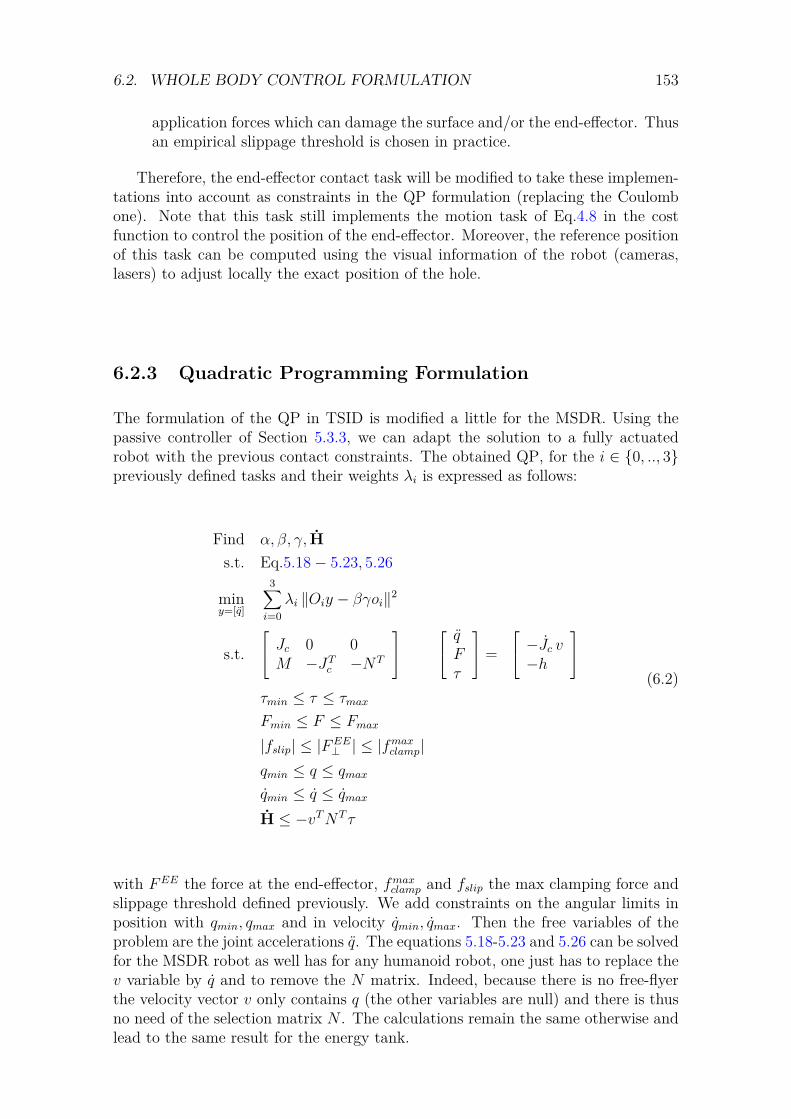
6.2. WHOLE BODY CONTROL FORMULATION 153
application forces which can damage the surface and/or the end-effector. Thusan empirical slippage threshold is chosen in practice.
Therefore, the end-effector contact task will be modified to take these implemen-tations into account as constraints in the QP formulation (replacing the Coulombone). Note that this task still implements the motion task of Eq.4.8 in the costfunction to control the position of the end-effector. Moreover, the reference positionof this task can be computed using the visual information of the robot (cameras,lasers) to adjust locally the exact position of the hole.
6.2.3 Quadratic Programming Formulation
The formulation of the QP in TSID is modified a little for the MSDR. Using thepassive controller of Section 5.3.3, we can adapt the solution to a fully actuatedrobot with the previous contact constraints. The obtained QP, for the i ∈ {0, .., 3}previously defined tasks and their weights λi is expressed as follows:
Find α, β, γ, Hs.t. Eq.5.18− 5.23, 5.26
miny=[q]
3∑i=0
λi ‖Oiy − βγoi‖2
s.t. Jc 0 0M −JTc −NT
qFτ
= −Jc v−h
τmin ≤ τ ≤ τmax
Fmin ≤ F ≤ Fmax
|fslip| ≤ |FEE⊥ | ≤ |fmaxclamp|
qmin ≤ q ≤ qmax
qmin ≤ q ≤ qmax
H ≤ −vTNT τ
(6.2)
with FEE the force at the end-effector, fmaxclamp and fslip the max clamping force andslippage threshold defined previously. We add constraints on the angular limits inposition with qmin, qmax and in velocity qmin, qmax. Then the free variables of theproblem are the joint accelerations q. The equations 5.18-5.23 and 5.26 can be solvedfor the MSDR robot as well has for any humanoid robot, one just has to replace thev variable by q and to remove the N matrix. Indeed, because there is no free-flyerthe velocity vector v only contains q (the other variables are null) and there is thusno need of the selection matrix N . The calculations remain the same otherwise andlead to the same result for the energy tank.

154 CHAPTER 6. ADAPTING THE SOLUTION TO THE MSDR
6.3 Interface between the robot low-level and ourcontroller
Once the problem is re-formulated for the MSDR, the QP can compute a torquecommand respecting the passivity of the system. However, it needs the robot ac-tuators angular position and velocity and the forces measured at the end-effectorlevel. This data must be retrieved in a timely manner to be able to execute the QPin real time. In the case of the MSDR, to have access to this data it is necessary touse the Fanuc software.
In the control scheme implemented on the TALOS robot, the data transfer isperformed by the ros-control framework of the middle-ware ROS Adolfo RodríguezTsouroukdissian [19]. Recalling the scheme of the Fig.1.10, the roscontrol-sot pack-age can communicate with the hardware interface of ros-control to retrieve the low-level information. Thus, to solve the issue of communication between the hardwareof the MSDR and our control scheme, one can create the ROS robot hardwareinterface of the MSDR to communicate with the Fanuc software and retrieve theinformation. Tutorials exist online to implement your own hardware interface, itis however important to notice that the data of the MSDR can be internal sensorsembedded within the robot (encoders, current, force sensors) or external sensors ofthe end-effector (lasers for normality, cameras, IMU, force sensors).
One issue that may arise is the importance of the delay between the readingof the sensors/actuators data by the Fanuc software and its transmission to theinterface and to the controller. And vice-versa, if the delay between the commandsent by the controller toward the Fanuc software and its application on the robot istoo important it can lead to precision issues. One has to notice that in any case, thecommunication within the robot manufacturer’s controller interfaces is mainly besteffort and not real-time (∼ 250Hz), as it is not the prioritized process. However,to reduce the delays, it can be appropriate to have the Fanuc software implementsa quick regulation control loop which takes the high-level controller input at a lowfrequency depending of the delay (for instance 500Hz). Its role will be to regulatethe high-level commands for the low-level until reaching the defined time to read thenew high-level control input. This regulating controller can for instance be achievedby a PD+ (as the controller used by the PAL-Robotics company) or a RegulationSensitivity and Tracking (RST) polynomial controller (more common in industryfor digital control). The RST is a robust control able to track reference trajectoriesas well as to regulate the control during disturbances. The PID is a particular formof RST, with a particular choices of the polynomials R, S and T.
In Fig.6.2 is presented an example of complete solution incorporating all theelements from the planning to the control of the robot. In yellow are depicted thethe visual processes to detect the holes (object recognition) and localize the metalplate and the robot (using for instance the Simultaneous Localization And Mapping(SLAM) approach). In red are presented the planning algorithms, which followsthe stages detailed in Fig.2.7: first plan the motion, then find the contact posesand finally optimize the trajectory with a MPC. The motion can be decomposedin several sub-motions or states, which can be organized in a finite-state-machine.The state will present different constraints or tasks such as the presence or absenceof contact for instance. The current state is thus given to the whole-body controller
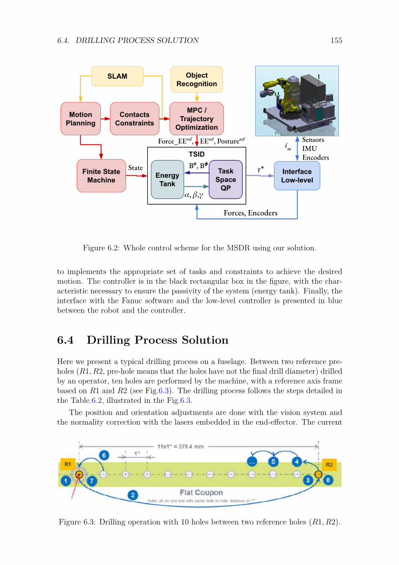
6.4. DRILLING PROCESS SOLUTION 155
Force_EEref, EEref, Postureref
MPC / Trajectory
Optimization
Forces, Encoders
𝜏*
TSID
EnergyTank
Task Space
QP𝛼, 𝛽,𝛾
B𝞂, B𝟇
Object Recognition
Motion Planning
ContactsConstraints
SLAM
Finite State Machine
InterfaceLow-level
State
imSensorsIMUEncoders
Figure 6.2: Whole control scheme for the MSDR using our solution.
to implements the appropriate set of tasks and constraints to achieve the desiredmotion. The controller is in the black rectangular box in the figure, with the char-acteristic necessary to ensure the passivity of the system (energy tank). Finally, theinterface with the Fanuc software and the low-level controller is presented in bluebetween the robot and the controller.
6.4 Drilling Process Solution
Here we present a typical drilling process on a fuselage. Between two reference pre-holes (R1, R2, pre-hole means that the holes have not the final drill diameter) drilledby an operator, ten holes are performed by the machine, with a reference axis framebased on R1 and R2 (see Fig.6.3). The drilling process follows the steps detailed inthe Table.6.2, illustrated in the Fig.6.3.
The position and orientation adjustments are done with the vision system andthe normality correction with the lasers embedded in the end-effector. The current
Figure 6.3: Drilling operation with 10 holes between two reference holes (R1, R2).
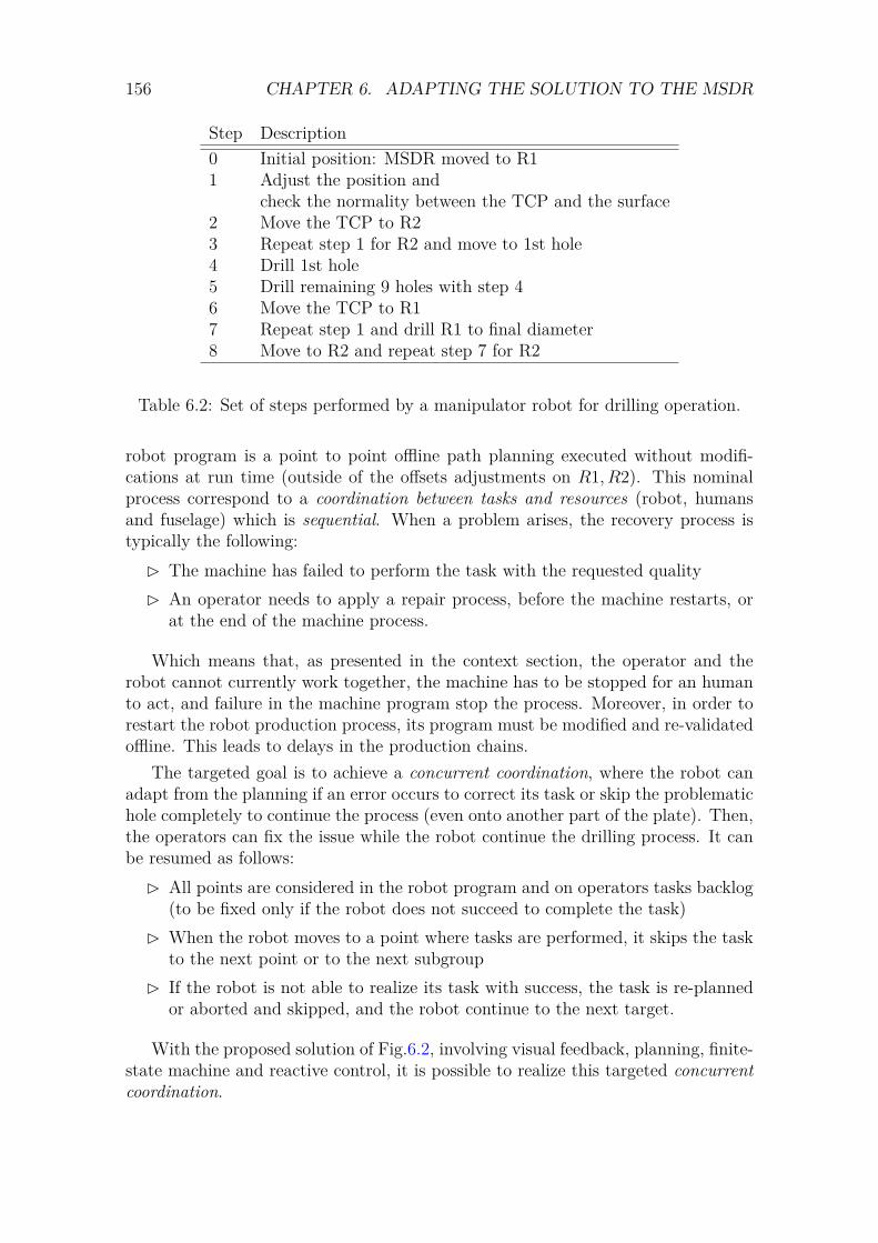
156 CHAPTER 6. ADAPTING THE SOLUTION TO THE MSDR
Step Description0 Initial position: MSDR moved to R11 Adjust the position and
check the normality between the TCP and the surface2 Move the TCP to R23 Repeat step 1 for R2 and move to 1st hole4 Drill 1st hole5 Drill remaining 9 holes with step 46 Move the TCP to R17 Repeat step 1 and drill R1 to final diameter8 Move to R2 and repeat step 7 for R2
Table 6.2: Set of steps performed by a manipulator robot for drilling operation.
robot program is a point to point offline path planning executed without modifi-cations at run time (outside of the offsets adjustments on R1, R2). This nominalprocess correspond to a coordination between tasks and resources (robot, humansand fuselage) which is sequential. When a problem arises, the recovery process istypically the following:� The machine has failed to perform the task with the requested quality� An operator needs to apply a repair process, before the machine restarts, or
at the end of the machine process.
Which means that, as presented in the context section, the operator and therobot cannot currently work together, the machine has to be stopped for an humanto act, and failure in the machine program stop the process. Moreover, in order torestart the robot production process, its program must be modified and re-validatedoffline. This leads to delays in the production chains.
The targeted goal is to achieve a concurrent coordination, where the robot canadapt from the planning if an error occurs to correct its task or skip the problematichole completely to continue the process (even onto another part of the plate). Then,the operators can fix the issue while the robot continue the drilling process. It canbe resumed as follows:� All points are considered in the robot program and on operators tasks backlog
(to be fixed only if the robot does not succeed to complete the task)� When the robot moves to a point where tasks are performed, it skips the task
to the next point or to the next subgroup� If the robot is not able to realize its task with success, the task is re-planned
or aborted and skipped, and the robot continue to the next target.
With the proposed solution of Fig.6.2, involving visual feedback, planning, finite-state machine and reactive control, it is possible to realize this targeted concurrentcoordination.
6.5. CONCLUSION 157
Another point of interest is the safety of the robotic solution, indeed, with theconcurrent solution (and even with the sequential one), the operators can performmanual tasks very close to the robot. Thus, the collision shall be avoided to ensurehuman safety. For now, the solution implemented is to progressively decrease thespeed of the robot when the robot get closer to humans or the fuselage. What canbe used in our proposed solution is the reactive planning of “collision free” paththat can be computed on demand, while executing the initial path. Moreover, usingour passive torque controller allows to benefit from the natural compliance of torquecontrol and from the passivity of the system. This means that, subject to unplanneddisturbances, the control will be penalized to ensure the safety of the whole system(environment, humans and robot), see Chapter 5. Thus, the tasks performed willbe degraded or aborted in favor of the security. However, the qualification of thissafety process for production will be difficult.
6.5 Conclusion
In this chapter is presented the two challenges that we think may arise when wewill transfer our passive torque controller onto the MSDR. The reformulation ofthe optimization problem to match the robot fully-actuated model and new forceconstraints has been presented. Then, the issue of interfacing the hardware andlow-level control of the robot to our solution has been discussed, a ROS hardwareinterface between the Fanuc software and our control scheme is possible. Finally,a proposal of complete control scheme using some of the Gepetto team works andthe passive controller has been presented. Its application on a drilling process hasbeen explored and the benefit of it stated. In particular, our solution improve theadaptability, reactivity and safety of the robotic solution.
The future works consist in implementing the proposed solutions on the MSDRrobot and test them on the drilling process. This will however require a consequentamount of time to create a self-sufficient "tool-box" from the Gepetto team software.Moreover, the certification of the programs termination (analysis of time complexity)and robustness is an important security process for Airbus, which is not currentlyachievable. Despite this blocking point, Airbus is interested to transfer the developedsolution of this thesis on the MSDR. A first step could be to directly implementa simple passive PD+ control using the Fanuc software. A second step may beto implement the complete solution as a "tool-box" in the scope of the joint-labROB4FAM.

158 CHAPTER 6. ADAPTING THE SOLUTION TO THE MSDR
Conclusion
Summary
This thesis aims to answer the issue of robotics whole-body control for manufacturingoperations. During the development of my solutions, two major objectives had tobe considered, the safety of the operation for the robot and for its environment,and the capabilities of the whole-body controller to achieve force application whilekeeping its balance.
A state-of-the-art is first presented in the Chapter 2. It details the robot modeland centroidal dynamics formulation used in my thesis, the different type of controldesigned on humanoids robots for locomotion and manipulation scenarios and thestability criteria considered in my works.
Secondly, a process for identifying and modeling the elbow chain actuator ofthe robot TALOS is described in the Chapter 3. This model and the identifiedparameters are used to design a low level current controller to protect the roboticsystem using a MPC. The process of identification can be applied on any rigid chainactuator (for any robot) to retrieve its inertial parameters, it is only subject tocorrectly model the chain actuation. Even if the MPC is computationally slow,it allows TALOS to carry high payload (up to 34 kg on one arm) while realizingmotions and protects the system.
The Chapter 4 details the three whole-body controllers implemented in this the-sis, two in position and one in torque. Their respective tasks functions and for-mulations are presented to achieve locomotion and manipulation scenarios. Thischapter compare them in simulations on complex locomotion problems such as stairclimbing and walking on non flat terrain. These simulations have yet to be tested onthe real robot using the modeling of the hip flexibility of TALOS. The intermediatesteps performed on the real robot are detailed as well as the blocking points prevent-ing us to successfully achieve the experiments. Because the torque controller hasproven to be energy efficient, capable of quite high speed locomotion and adaptableto uncommon scenarios (such as navigating in collaboration with a human, whileusing similar gait); I chose to focus on this solution for the next developments ofthe thesis.
Yet, using this controller on the real TALOS robot leads to instabilities in thesolution on the simplest scenario. Thus, to realize the objective of safe operations,stability analysis and in particular the passivity analysis methods are investigatedin the Chapter 5. I implemented a novel formulation for my torque control schemeto obtain a passive system (a dissipative system), ensuring a stable, safe and robustbehavior of the system. My whole-body control scheme embeds an energy tank
159
160 CHAPTER 6. ADAPTING THE SOLUTION TO THE MSDR
monitoring the exchanged power in the system. The tank regulates the controllertasks gains in function of the input-output system power. This new scheme istested in two simulations. First on a multi-contact scenario employing a parallelposition/force task as a first step for manufacturing operations. Secondly on asimple locomotion scenario, a walk of 20cm steps on flat ground.
Finally, the Chapter 6 presents the expected difficulties to consider when transfer-ring the passive solution from the humanoid robot TALOS to the manipulator robotMSDR. The two main aspects to consider are the reformulation of the optimizationproblem to match specific force constraints and the creation of an interface betweenthe Fanuc software and my controller. This chapter also highlights the benefits thatmy solution and, in a more global approach, the planning and visual methods of theGepetto team, can bring. The team hopes to improve the adaptability, reactivityand safety of the industrial robotics solution.
Future Work
Identification and Modeling of the Whole Chain ActuationThe extension of the work presented in the Chapter 3 would be to identify all
the actuators of the robot and to implement the solution over high-performancededicated and embedded electronics board attached to each actuator of the robot.However, due to the sanitary crisis this identification process has been delayed.
Moreover, with the model and parameters of each of the actuator it will bepossible to implement a torque controller mapping the desired joint torques of theQP controller to motor currents and send them directly to the robot. This way,there will be no need to use the PAL-Robotics company low-level controller to trymy simulations on the real robot. For now, this proprietary controller is a black boxand I encounter some problems to interface my complete solution with it even if ituses a ros-control architecture, as presented in Section 4.6. This is why, currently,even the simulation of the contact-force has not be tested on the real robot, whilethe flexibility of the robot is not a blocking point. It is a known difficulty of torquecontrol implementations to successfully transfer the simulation results on the realrobot. I should have started to work on the interface with the PAL-Robotics low-level controller sooner to solve this problem. Or, it might have been quicker to try tocreate a simple PD+, validated in the PAL-Robotics simulator, to transform my de-sired joint torques to motor currents and completely bypass the black-box controller.
Interfacing my Controller with the Flexibility Compensation ModelTo finalize the work presented in the Chapter 4 and test the walking simulations
on the real robot, it would be necessary to implement the flexibility compensation ofVilla et al. [206] in my controllers. In this paper, the hip bending is estimated fromthe commanded torque and the elastic deflection (θ) is added to the measured hipconfiguration qhip. The same is done for the derivative of the deflection. The newvalues of the hip configuration and joint velocities are then replaced in the coordinateand velocity vectors q and v and are used by the base-estimator and the controller.Because the implementations done in Villa et al. [206] have been made using TSID, itshould be easy to join my controllers with them and then test the simulations on the
6.5. CONCLUSION 161
real robot. Be aware that for torque control, the previous point still holds and theproblem with the PAL-Robotics low-level controller must be solved. Furthermore,in Villa et al. [206], the modified coordinate and velocity vectors q and v taking intoaccount the deflection are also used in a locomotion planner to compute coherentreference trajectories. An interesting future step would be to use this planner intandem with my controllers to adequately take into account the hip flexibility of therobot TALOS.
Finally, with the modified torque controller using the flexibility compensation,one would want to continue the collaboration with Isabelle Maroger on theANR-COBOT project. The aim would be to test the whole developed frameworkfor human-robot co-navigation in real time on the robot TALOS. In particular,using the contact-force task added in my torque controller and the passivityimplementation, it would be amazing to have TALOS successfully carry and movea table in collaboration with a human. Thus, the stability of the system would beguaranteed and it would be possible to control the amount of force the robot hasto apply on the table (currently only the control of the robot hands positions ispossible).
Improving the Energy Tank Shaping and Regulating CoefficientsTo improve the results obtained in the Chapter 5 on the passivation of the
control scheme, one would revise the definitions of the budget of the energy tankand of the regulating coefficients. Indeed, for now, the robot may falls if all thesystem is penalized to respect the passivity, because the coefficients β, γ are actingon every tasks. However, as discussed before, the passivity proof will not hold ifthese coefficients only act on some of the tasks. One can try to implement anenergy tank for the tasks responsible of the robot balancing, such as the CoM, thefeet contacts and the posture ones and another tank for the other tasks. Then, ifthe activation of the system does not come from the balancing tasks, they will notbe penalized and the robot would keep its balance.
Moreover, it would be interesting to design the budget and the maximal valueallocated to the energy tank in function of the reference trajectories. The upperbound of the tank might then increase or decrease in function of the planning. Forinstance, while moving on flat floor the robot does not need too much energy, butif it has to climb an obstacle the necessary amount may rise. Thus, one wouldincrease the maximum value of the tank a little before-hand to store energy toanticipate the climb. Similarly, the coefficient on the power flow regulation γ canbe computed as in Shahriari et al. [113] to vary in function of the task progression,close to what I described before for the maximal value of the tank, using thereference trajectories. Finally, one would want to use the regulating coefficients ofthe energy tank in higher level monitoring mechanisms to improve the handling ofthe diverging cases.
Reformulating the QP Formulation or Developing the Passivity Criterionon a MPC
Another way to improve the results obtained in the Chapter 5 would be to refor-mulate the alternate minimization problem of Eq.5.34 to solve the energy parametersconcurrently to the complete optimization problem (subject to constraints). Then,
162 CHAPTER 6. ADAPTING THE SOLUTION TO THE MSDR
the passivity as a constraint in the QP will not be necessary as the energy parame-ters will be optimized on the same problem formulation than the QP (including theconstraints of the system). For now, the addition of the passivity constraint in theformulation can lead to a too constrained problem and it is possible that it entersin conflict with another constraint and lead to oscillations in the solution.
A second possibility could be to implement the passivity criterion in a MPC,for instance the one developed by Dantec et al. [147] which has achieved greatresults recently. The passivity can be implemented by using the value function ofthe Optimal Control as the storage function and constraining it. Or it is possible toreformulate the problem and to add a sate constraint over the trajectory to respectthe passivity inequality Raff et al. [140].
Testing the Complete Approach in a FactoryFinally, one of the future goal would be to bring the TALOS and TIAGo robots
to an Airbus factory and test in real conditions the overall approach includinglocalization, visual-servoing and control. This aim was first expected by the endof my thesis, but due to the sanitary crisis, we accumulate delays and could onlysuccessfully test the localization and navigation stack of the robot TIAGo. Oncesome of the previous points are fixed, one would try to demonstrate the developedsolutions in the industrial environment. This is a future goal for the ROB4FAMjoint-lab, which could be achieved before or in parallel with the implementation ofthe results on the MSDR.
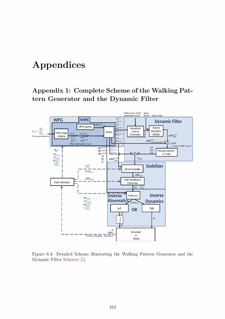
Appendices
Appendix 1: Complete Scheme of the Walking Pat-tern Generator and the Dynamic Filter
Figure 6.4: Detailed Scheme illustrating the Walking Pattern Generator and theDynamic Filter Scherrer [1].
163
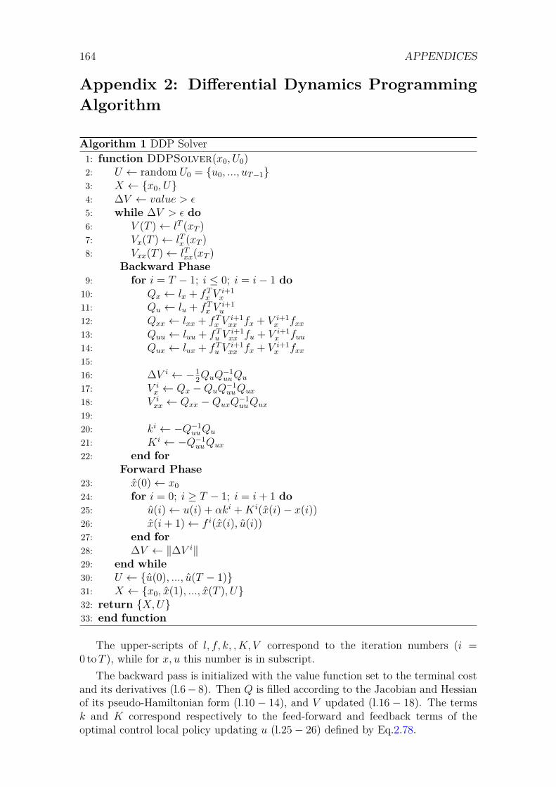
164 APPENDICES
Appendix 2: Differential Dynamics ProgrammingAlgorithm
Algorithm 1 DDP Solver1: function DDPSolver(x0, U0)2: U ← random U0 = {u0, ..., uT−1}3: X ← {x0, U}4: ∆V ← value > ε5: while ∆V > ε do6: V (T )← lT (xT )7: Vx(T )← lTx (xT )8: Vxx(T )← lTxx(xT )
Backward Phase9: for i = T − 1; i ≤ 0; i = i− 1 do10: Qx ← lx + fTx V
i+1x
11: Qu ← lu + fTx Vi+1u
12: Qxx ← lxx + fTx Vi+1xx fx + V i+1
x fxx13: Quu ← luu + fTu V
i+1xx fu + V i+1
x fuu14: Qux ← lux + fTu V
i+1xx fx + V i+1
x fxx15:16: ∆V i ← −1
2QuQ−1uuQu
17: V ix ← Qx −QuQ
−1uuQux
18: V ixx ← Qxx −QuxQ
−1uuQux
19:20: ki ← −Q−1
uuQu
21: Ki ← −Q−1uuQux
22: end forForward Phase
23: x(0)← x024: for i = 0; i ≥ T − 1; i = i+ 1 do25: u(i)← u(i) + αki +Ki(x(i)− x(i))26: x(i+ 1)← f i(x(i), u(i))27: end for28: ∆V ← ‖∆V i‖29: end while30: U ← {u(0), ..., u(T − 1)}31: X ← {x0, x(1), ..., x(T ), U}32: return {X,U}33: end function
The upper-scripts of l, f, k, ,K, V correspond to the iteration numbers (i =0 toT ), while for x, u this number is in subscript.
The backward pass is initialized with the value function set to the terminal costand its derivatives (l.6− 8). Then Q is filled according to the Jacobian and Hessianof its pseudo-Hamiltonian form (l.10 − 14), and V updated (l.16 − 18). The termsk and K correspond respectively to the feed-forward and feedback terms of theoptimal control local policy updating u (l.25− 26) defined by Eq.2.78.

165
Appendix 3: Frameworks of the different con-trollers
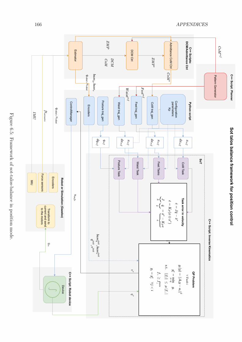
166 APPENDICES
Sot talos balance framew
ork for position control
Device
Robot or Sim
ulation (Gazebo)
Transform to
current and sendto the m
otors
Encoders
C++ Script: R
obot device
Python script
CoM
traj_gen
Posture traj_gen
Waist traj_gen
C++ Script: Inverse K
inematics
CoM
Task
Posture Task
Waist Task
Configuration
parameters:
Kp
ControlM
anager
SoT
Encoders
QP Problem
Task error in velocity
C++ Scripts:
DC
M/A
dmittance C
trl
DC
M C
trl
Admittance C
oM C
trl
Estimator
IMU
Force sensors
Pattern Generator
C++ Script: Planner
Feet traj_gen
Feet Tasks
Figure6.5:
Framework
ofsot-talos-balancein
positionmode.
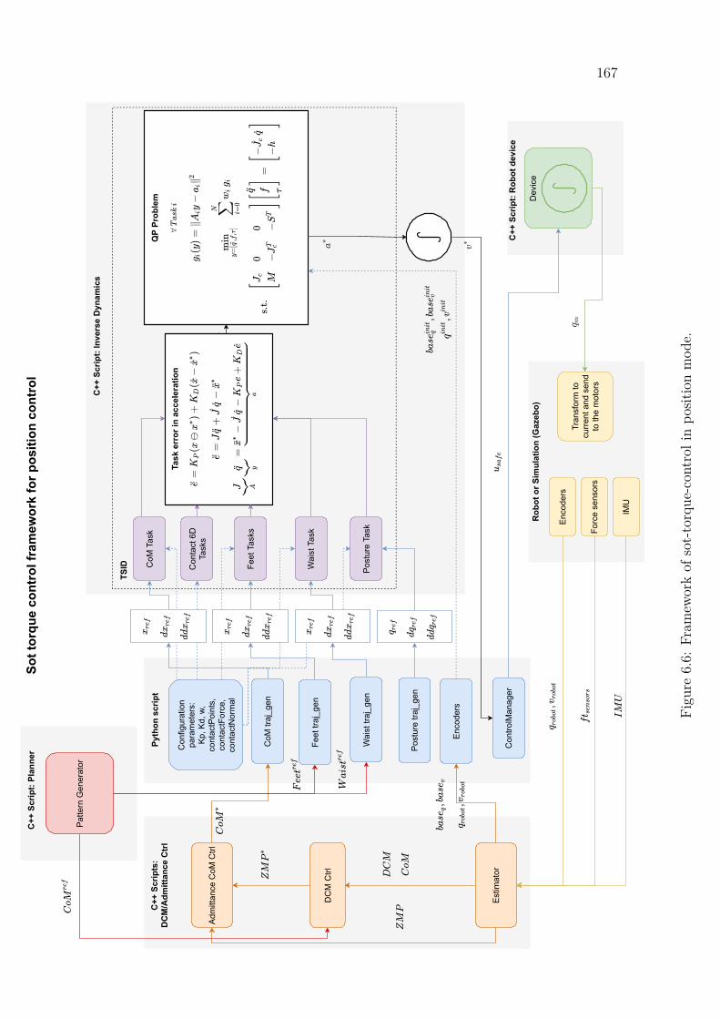
167
Sot t
orqu
e co
ntro
l fra
mew
ork
for p
ositi
on c
ontr
ol
Dev
ice
Rob
ot o
r Sim
ulat
ion
(Gaz
ebo)
Tran
sfor
m to
curre
nt a
nd s
end
to th
e m
otor
s
Enco
ders
C++
Scr
ipt:
Rob
ot d
evic
e
Pyth
on s
crip
t
CoM
traj
_gen
Post
ure
traj_
gen
Wai
st tr
aj_g
en
C++
Scr
ipt:
Inve
rse
Dyn
amic
s
Con
tact
6D
Task
s
CoM
Tas
k
Post
ure
Task
Wai
st T
ask
Con
figur
atio
npa
ram
eter
s:Kp
, Kd,
w,
cont
actP
oint
s,co
ntac
tFor
ce,
cont
actN
orm
al
Con
trolM
anag
er
TSID
Enco
ders
QP
Prob
lem
Task
err
or in
acc
eler
atio
n
C++
Scr
ipts
:D
CM
/Adm
ittan
ce C
trl
DC
M C
trl
Adm
ittan
ce C
oM C
trl
Estim
ator
IMU
Forc
e se
nsor
s
Patte
rn G
ener
ator
C++
Scr
ipt:
Plan
ner
Feet
traj
_gen
Feet
Tas
ks
Figu
re6.6:
Fram
eworkof
sot-torque-con
trol
inpo
sitionmod
e.
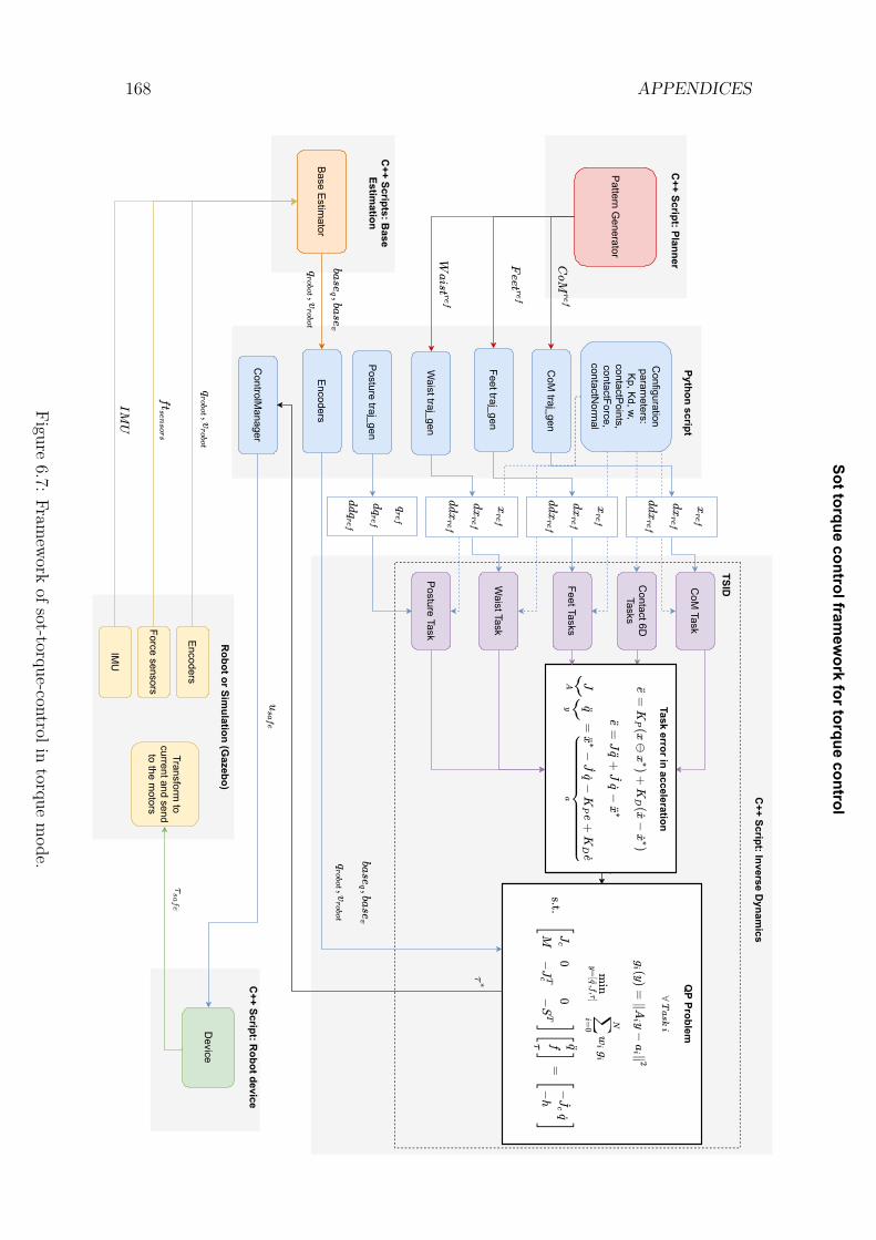
168 APPENDICES
Sot torque control framew
ork for torque control
Device
Robot or Sim
ulation (Gazebo)
Transform to
current and sendto the m
otors
Encoders
C++ Script: R
obot device
Python script
CoM
traj_gen
Posture traj_gen
Waist traj_gen
C++ Script: Inverse D
ynamics
Contact 6DTasks
CoM
Task
Posture Task
Waist Task
Configuration
parameters:
Kp, Kd, w,contactPoints,contactForce,contactN
ormal
ControlM
anager
TSID
Encoders
QP Problem
Task error in acceleration
C++ Scripts: B
aseEstim
ation
Base Estimator
IMU
Force sensors
Pattern Generator
C++ Script: Planner
Feet traj_gen
Feet Tasks
Figure6.7:
Framework
ofsot-torque-controlintorque
mode.
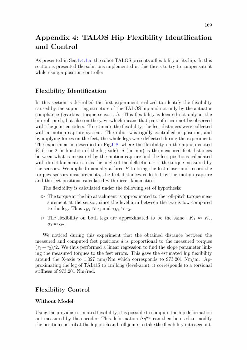
169
Appendix 4: TALOS Hip Flexibility Identificationand Control
As presented in Sec.1.4.1.a, the robot TALOS presents a flexibility at its hip. In thissection is presented the solutions implemented in this thesis to try to compensate itwhile using a position controller.
Flexibility Identification
In this section is described the first experiment realized to identify the flexibilitycaused by the supporting structure of the TALOS hip and not only by the actuatorcompliance (gearbox, torque sensor ...). This flexibility is located not only at thehip roll-pitch, but also on the yaw, which means that part of it can not be observedwith the joint encoders. To estimate the flexibility, the feet distances were collectedwith a motion capture system. The robot was rigidly controlled in position, andby applying forces on the feet, the whole legs were deflected during the experiment.The experiment is described in Fig.6.8, where the flexibility on the hip is denotedK (1 or 2 in function of the leg side), d (in mm) is the measured feet distancesbetween what is measured by the motion capture and the feet positions calculatedwith direct kinematics. α is the angle of the deflection, τ is the torque measured bythe sensors. We applied manually a force F to bring the feet closer and record thetorques sensors measurements, the feet distances collected by the motion captureand the feet positions calculated with direct kinematics.
The flexibility is calculated under the following set of hypothesis:� The torque at the hip attachment is approximated to the roll-pitch torque mea-
surement at the sensor, since the level arm between the two is low comparedto the leg. Thus τK1 ≈ τ1 and τK2 ≈ τ2.
� The flexibility on both legs are approximated to be the same: K1 ≈ K2,α1 ≈ α2.
We noticed during this experiment that the obtained distance between themeasured and computed feet positions d is proportional to the measured torques(τ1 + τ2)/2. We thus performed a linear regression to find the slope parameter link-ing the measured torques to the feet errors. This gave the estimated hip flexibilityaround the X-axis to 1.027 mm/Nm which corresponds to 973.201 Nm/m. Ap-proximating the leg of TALOS to 1m long (level-arm), it corresponds to a torsionalstiffness of 973.201 Nm/rad.
Flexibility Control
Without Model
Using the previous estimated flexibility, it is possible to compute the hip deformationnot measured by the encoder. This deformation ∆qhip can then be used to modifythe position control at the hip pitch and roll joints to take the flexibility into account.
170 APPENDICES
Figure 6.8: Scheme to illustrate the identification of the flexibility
The new position command is then defined by:
∆qhip = τhip
K
qhipcmd = qhipdes + ∆qhip(6.3)
However, the noise in torque sensors requires filtering, which introduces impor-tant delays. Unfortunately, previous experiences with such a technique carried outwith the robot gave poor performances. Only a repeatable one step walk experimenton TALOS in position control was achieved using fixed flexibility compensation (seeSection 4.6). In torque control however, this issue is mitigated because the flexibilityis considered by the control system as external disturbances. Nonetheless, to achieverobust experiments, it will be necessary to take into account this flexibility whichcannot be compensated without a proper identification and modeling.
With Model
A second method has been tested to control the hip flexibility in Villa et al. [206],relying on the use of a specific model for the flexibility. It uses the standard model
171
defined by Nakaoka et al. [214], introducing passive joints in the waist-leg connec-tion, where the link cross-section is reduced, as the link deflections of the robotconcentrate there. The torque on each passive joint is related to its deflection θ asa spring-damper:
τf = −kfθ − df θ, (6.4)
with link stiffness kf and damping df coefficients.As the stiffness is coming for the vertical linkage, only the flexibility along pitch
and roll deflections is modeled, which produce the main impact on foot placement.As a result, the model for the robot TALOS is augmented to reach 42 DoFs composedby 32 actuated joints, 4 elastic passive joints and the robot free-flyer. The obtainedresults in Villa et al. [206] are quite satisfying, see the video at the following link:https://peertube.laas.fr/videos/watch/9a3c5258-e5b7-49a5-a153-02e804a06f65.
With this modeling a new value of the stiffness flexibility has been identified. Itis important to notice that between the identification experiments the legs have beenunmounted and a backlash in the knees have been corrected. The second experimentconsists in lifting a leg and putting the CoM at the center of the support foot, tomatch the CoP position computed from the F/T sensors, it allows to identify thestatic stiffness. For the left foot, without compensation, the CoP does not equal theCoM, it is naturally going toward the outside of the robot. With the compensationand a stiffness set at 3000 Nm/rad, the CoP and CoM nearly match. With a lowerstiffness, the CoP goes toward the inside of the robot.
This observation is confirmed by checking the torque measured by the ankle F/Tsensors. There should be no torque around the X-axis once the reference is reached,but there is ∼ 20Nm toward the outside of the robot without compensation. Usingthe flexibility compensation model with a stiffness of 3000 Nm/rad the torque islowered to ∼ 5Nm and decreasing the stiffness makes the torque goes to the oppositedirection. Thus, the second estimation of the stiffness flexibility found a value of∼ 3000 Nm/rad on the left leg. For the right leg a value of ∼ 4750 Nm/rad hasbeen identified.
It is a work in progress to interface the controllers developed in this thesis andthe compensation model implemented in the paper Villa et al. [206].
172 APPENDICES
Appendix 5: On the semi-positive definition of thepotential energy S
This Appendix details the results presented in the open-access document Ramuzat[210].
Problem statement: We have Λ a real symmetric semi-positive definitematrix and Kp a real positive diagonal matrix (thus also symmetric). We definedin Chapter 5 the potential energy of a task as S = 1
2eTΛKP e. The product ΛKp is
a square matrix but non-symmetric. We want to prove that ΛKp is semi-positivedefinite with respect to the Definition 5.
If the elements of the diagonal Kp are equal, i.e. Kp = aI with a ∈ R+\{0},then the product ΛKp = aΛ is a real symmetric semi-positive definite matrix. Thus,for a diagonal Kp with equal elements we have directly xTΛKpx ≥ 0∀x ∈ Rn\{0}.
For different elements on the diagonal, we have the following results:
− The eigenvalues of ΛKp are real and non-negatives
− If ΛKp+(ΛKp)T2 has non-negative eigenvalues, then the quadratic form of
ΛKp is semi-positive definite
Proof. Let us recall some useful matrix definitions and properties:
Definition 4 (Real symmetric semi-positive definite matrix). A is a real symmetricmatrix (its eigenvalues are thus real): A is semi-positive definite ⇐⇒ all itseigenvalues are non-negatives.
Definition 5 (Quadratic form semi-positive definition). A matrix A is semi-positivedefinite ⇐⇒ xTAx ≥ 0, ∀x ∈ Rn\{0}
Property 2. If A is a real semi-positive definite matrix, then BTAB is semi-positivedefinite for any matrix B.
Property 3 (Matrix congruent to a symmetric matrix). Any matrix congruent to asymmetric matrix is again symmetric: If A is a symmetric matrix then so is BTABfor any matrix B.
Proof that the eigenvalues of ΛKp are real and non-negatives
Because Kp is diagonal and positive we can write Kp = K12p K
12p , K
12p is also real
positive and symmetric thus invertible. Let us reformulate the matrix ΛKp:
ΛKp = ΛK12p K
12p
= K− 1
2p (K
12p ΛK
12p )K
12p
(6.5)
173
It corresponds to a change of basis of K12p . Because the eigenvalues (denoted λ) are
invariant to change of basis we have:
λ(ΛKp) = λ(K12p ΛK
12p ) (6.6)
Using the Properties. 2 and 3, because Λ is a real symmetric semi-positive definitematrix, (K
12p )TΛK
12p = K
12p ΛK
12p is a real symmetric semi-positive definite matrix.
Thus its eigenvalues are real and non-negatives (Definition.4) and so are the ones ofΛ because of Eq.6.6. Then we have proven our first result: the eigenvalues of ΛKp
are real and non-negatives.
Semi-positive definition of ΛKp
In this part we look at a way to prove the semi-positive definition of ΛKp by studyingits symmetric part in the Toeplitz decomposition:
Definition 6 (Toeplitz decomposition). Every square matrix A can be decomposeduniquely as the sum of two matrices U and V , where U is symmetric and V isskew-symmetric.
A = U + V = 12(A+ AT ) + 1
2(A− AT ) (6.7)
In our case A = ΛKp and U = 12(ΛKp + (ΛKp)T ) is symmetric.
We recall the fact that the quadratic form of a skew-symmetric matrix equals tozero. Indeed, by definition V T = −V and thus xTV x = (xTV Tx)T = −xTV x whichholds only if it equals to zero. Thus, the quadratic form of xTΛKpx is the same oneof xTUx, i.e:
xTΛKpx = xT (ΛKp + (ΛKp)T2 )x (6.8)
One can thus prove the semi-positive definition of the symmetric matrix U toprove the semi-positive definition of ΛKp. Indeed, if xTUx ≥ 0, ∀x ∈ Rn\{0},using Eq.6.8, we obtain xTΛKpx ≥ 0, ∀x ∈ Rn\{0}: proving of the semi-positivedefinition of ΛKp.
One way to prove the semi-positive definition of U is to look at its eigenvalues.Because U is symmetric, if its eigenvalues are non-negatives then U is semi-positivedefinite (see Definition 4). This gives our second result: if U has non-negativeeigenvalues, then ΛKp is semi-positive definite.
On the eigenvalues of U
One may notice that we have further information on the eigenvalues of U withrespect to the ones of ΛKp. Using the following theorem of Fan on matrices [215](Chapter 10, Theorem 10.28):
174 APPENDICES
Theorem 1 (Eigenvalues majorization of Ky Fan). Let A be an n× n matrix witheigenvalues λ1(A), ..., λn(A) and Reλi(A) their real parts. Then:
n∑i=1Reλi(A) ≤
n∑i=1
λi(A+ AT
2)
(6.9)
Then, because the eigenvalues of ΛKp are real and non-negatives (as proven in thefirst part), we have using the Theorem 1:
0 ≤n∑i=1
λi(ΛKp) ≤n∑i=1
λi(U) (6.10)
Thus, we know that the sum of the eigenvalues of U is non-negative, however toprove the semi-positive definition of U it is needed to prove that all its eigenvaluesare non-negatives.
Bibliography
[1] Louise Scherrer. Reactive walking for the humanoid robot pyrène. In HALopen archive, 2021. 1, 6, 20, 27, 35, 163
[2] Bruno Siciliano, Lorenzo Sciavicco, Luigi Villani, and Giuseppe Oriolo.Robotics: Modelling, Planning and Control. Springer Publishing Company,Incorporated, 1st edition, 2008. ISBN 1846286417. 2, 22, 54, 55, 56, 57, 58,59, 61
[3] Matthew Spenko, Stephen Buerger, and Karl Iagnemma. The DARPARobotics Challenge Finals: Humanoid Robots To The Rescue. 01 2018. ISBN978-3-319-74665-4. doi: 10.1007/978-3-319-74666-1. 2
[4] O. Stasse, T. Flayols, R. Budhiraja, K. Giraud-Esclasse, J. Carpentier,J. Mirabel, et al. Talos: A new humanoid research platform targeted forindustrial applications. In IEEE-RAS ICHR, 2017. 4, 5
[5] K. Kaneko, F. Kanehiro, S. Kajita, H. Hirukawa, T. Kawasaki, M. Hirata,K. Akachi, and T. Isozumi. Humanoid robot hrp-2. In IEEE InternationalConference on Robotics and Automation, 2004. Proceedings. ICRA ’04. 2004,volume 2, pages 1083–1090 Vol.2, 2004. doi: 10.1109/ROBOT.2004.1307969.5, 6
[6] International Electrotechnical Commission. Industrial communicationnetworks–fieldbus specifications–part 3–12: data-link layer service definition–part 4–12: datalink layer protocol specification–type 12 elements. IEC, 2007.6
[7] Stanford Artificial Intelligence Laboratory et al. Robotic operating system.URL https://www.ros.org. 6, 14, 112, 113
[8] David Coleman, Ioan Sucan, Sachin Chitta, and Nikolaus Correll. Reducingthe barrier to entry of complex robotic software: a moveit! case study. arXivpreprint arXiv:1404.3785, 2014. 6
[9] Sachin Chitta, Ioan Sucan, and Steve Cousins. Moveit![ros topics]. IEEERobotics & Automation Magazine, 19(1):18–19, 2012. 6
[10] Nathan Koenig and Andrew Howard. Design and use paradigms for gazebo, anopen-source multi-robot simulator. In 2004 IEEE/RSJ International Confer-ence on Intelligent Robots and Systems (IROS)(IEEE Cat. No. 04CH37566),volume 3, pages 2149–2154. IEEE, 2004. 6
175
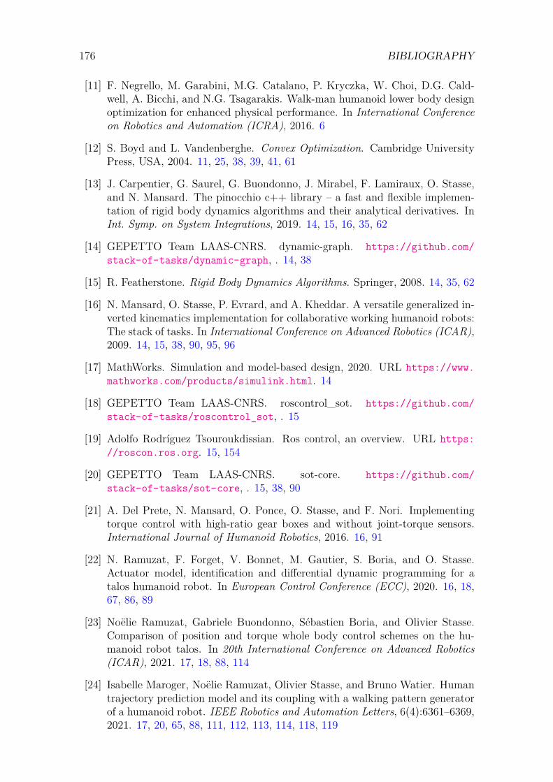
176 BIBLIOGRAPHY
[11] F. Negrello, M. Garabini, M.G. Catalano, P. Kryczka, W. Choi, D.G. Cald-well, A. Bicchi, and N.G. Tsagarakis. Walk-man humanoid lower body designoptimization for enhanced physical performance. In International Conferenceon Robotics and Automation (ICRA), 2016. 6
[12] S. Boyd and L. Vandenberghe. Convex Optimization. Cambridge UniversityPress, USA, 2004. 11, 25, 38, 39, 41, 61
[13] J. Carpentier, G. Saurel, G. Buondonno, J. Mirabel, F. Lamiraux, O. Stasse,and N. Mansard. The pinocchio c++ library – a fast and flexible implemen-tation of rigid body dynamics algorithms and their analytical derivatives. InInt. Symp. on System Integrations, 2019. 14, 15, 16, 35, 62
[14] GEPETTO Team LAAS-CNRS. dynamic-graph. https://github.com/stack-of-tasks/dynamic-graph, . 14, 38
[15] R. Featherstone. Rigid Body Dynamics Algorithms. Springer, 2008. 14, 35, 62
[16] N. Mansard, O. Stasse, P. Evrard, and A. Kheddar. A versatile generalized in-verted kinematics implementation for collaborative working humanoid robots:The stack of tasks. In International Conference on Advanced Robotics (ICAR),2009. 14, 15, 38, 90, 95, 96
[17] MathWorks. Simulation and model-based design, 2020. URL https://www.mathworks.com/products/simulink.html. 14
[18] GEPETTO Team LAAS-CNRS. roscontrol_sot. https://github.com/stack-of-tasks/roscontrol_sot, . 15
[19] Adolfo Rodríguez Tsouroukdissian. Ros control, an overview. URL https://roscon.ros.org. 15, 154
[20] GEPETTO Team LAAS-CNRS. sot-core. https://github.com/stack-of-tasks/sot-core, . 15, 38, 90
[21] A. Del Prete, N. Mansard, O. Ponce, O. Stasse, and F. Nori. Implementingtorque control with high-ratio gear boxes and without joint-torque sensors.International Journal of Humanoid Robotics, 2016. 16, 91
[22] N. Ramuzat, F. Forget, V. Bonnet, M. Gautier, S. Boria, and O. Stasse.Actuator model, identification and differential dynamic programming for atalos humanoid robot. In European Control Conference (ECC), 2020. 16, 18,67, 86, 89
[23] Noëlie Ramuzat, Gabriele Buondonno, Sébastien Boria, and Olivier Stasse.Comparison of position and torque whole body control schemes on the hu-manoid robot talos. In 20th International Conference on Advanced Robotics(ICAR), 2021. 17, 18, 88, 114
[24] Isabelle Maroger, Noëlie Ramuzat, Olivier Stasse, and Bruno Watier. Humantrajectory prediction model and its coupling with a walking pattern generatorof a humanoid robot. IEEE Robotics and Automation Letters, 6(4):6361–6369,2021. 17, 20, 65, 88, 111, 112, 113, 114, 118, 119
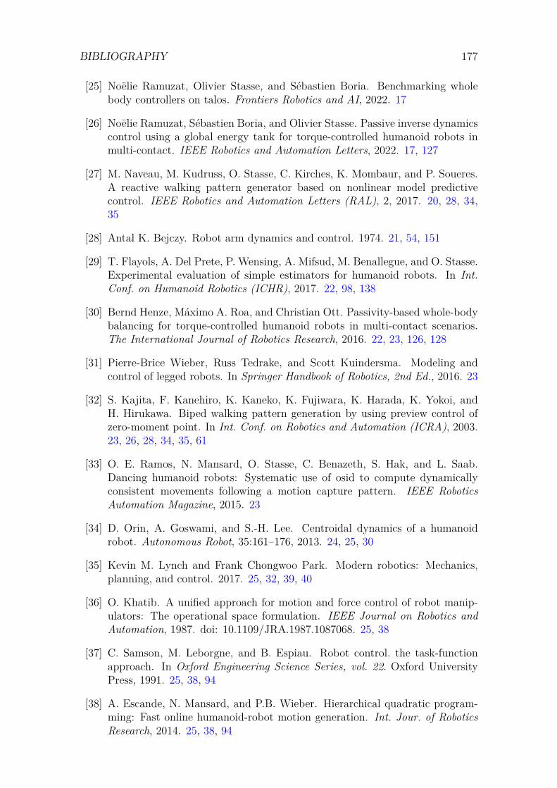
BIBLIOGRAPHY 177
[25] Noëlie Ramuzat, Olivier Stasse, and Sébastien Boria. Benchmarking wholebody controllers on talos. Frontiers Robotics and AI, 2022. 17
[26] Noëlie Ramuzat, Sébastien Boria, and Olivier Stasse. Passive inverse dynamicscontrol using a global energy tank for torque-controlled humanoid robots inmulti-contact. IEEE Robotics and Automation Letters, 2022. 17, 127
[27] M. Naveau, M. Kudruss, O. Stasse, C. Kirches, K. Mombaur, and P. Soueres.A reactive walking pattern generator based on nonlinear model predictivecontrol. IEEE Robotics and Automation Letters (RAL), 2, 2017. 20, 28, 34,35
[28] Antal K. Bejczy. Robot arm dynamics and control. 1974. 21, 54, 151
[29] T. Flayols, A. Del Prete, P. Wensing, A. Mifsud, M. Benallegue, and O. Stasse.Experimental evaluation of simple estimators for humanoid robots. In Int.Conf. on Humanoid Robotics (ICHR), 2017. 22, 98, 138
[30] Bernd Henze, Máximo A. Roa, and Christian Ott. Passivity-based whole-bodybalancing for torque-controlled humanoid robots in multi-contact scenarios.The International Journal of Robotics Research, 2016. 22, 23, 126, 128
[31] Pierre-Brice Wieber, Russ Tedrake, and Scott Kuindersma. Modeling andcontrol of legged robots. In Springer Handbook of Robotics, 2nd Ed., 2016. 23
[32] S. Kajita, F. Kanehiro, K. Kaneko, K. Fujiwara, K. Harada, K. Yokoi, andH. Hirukawa. Biped walking pattern generation by using preview control ofzero-moment point. In Int. Conf. on Robotics and Automation (ICRA), 2003.23, 26, 28, 34, 35, 61
[33] O. E. Ramos, N. Mansard, O. Stasse, C. Benazeth, S. Hak, and L. Saab.Dancing humanoid robots: Systematic use of osid to compute dynamicallyconsistent movements following a motion capture pattern. IEEE RoboticsAutomation Magazine, 2015. 23
[34] D. Orin, A. Goswami, and S.-H. Lee. Centroidal dynamics of a humanoidrobot. Autonomous Robot, 35:161–176, 2013. 24, 25, 30
[35] Kevin M. Lynch and Frank Chongwoo Park. Modern robotics: Mechanics,planning, and control. 2017. 25, 32, 39, 40
[36] O. Khatib. A unified approach for motion and force control of robot manip-ulators: The operational space formulation. IEEE Journal on Robotics andAutomation, 1987. doi: 10.1109/JRA.1987.1087068. 25, 38
[37] C. Samson, M. Leborgne, and B. Espiau. Robot control. the task-functionapproach. In Oxford Engineering Science Series, vol. 22. Oxford UniversityPress, 1991. 25, 38, 94
[38] A. Escande, N. Mansard, and P.B. Wieber. Hierarchical quadratic program-ming: Fast online humanoid-robot motion generation. Int. Jour. of RoboticsResearch, 2014. 25, 38, 94
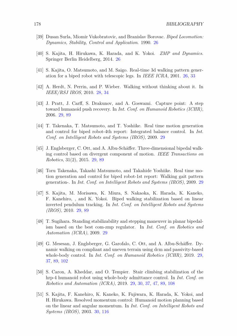
178 BIBLIOGRAPHY
[39] Dusan Surla, Miomir Vukobratovic, and Branislav Borovac. Biped Locomotion:Dynamics, Stability, Control and Application. 1990. 26
[40] S. Kajita, H. Hirukawa, K. Harada, and K. Yokoi. ZMP and Dynamics.Springer Berlin Heidelberg, 2014. 26
[41] S. Kajita, O. Matsumoto, and M. Saigo. Real-time 3d walking pattern gener-ation for a biped robot with telescopic legs. In IEEE ICRA, 2001. 26, 33
[42] A. Herdt, N. Perrin, and P. Wieber. Walking without thinking about it. InIEEE/RSJ IROS, 2010. 28, 34
[43] J. Pratt, J. Carff, S. Drakunov, and A. Goswami. Capture point: A steptoward humanoid push recovery. In Int. Conf. on Humanoid Robotics (ICHR),2006. 29, 89
[44] T. Takenaka, T. Matsumoto, and T. Yoshiike. Real time motion generationand control for biped robot-4th report: Integrated balance control. In Int.Conf. on Intelligent Robots and Systems (IROS), 2009. 29
[45] J. Englsberger, C. Ott, and A. Albu-Schäffer. Three-dimensional bipedal walk-ing control based on divergent component of motion. IEEE Transactions onRobotics, 31(2), 2015. 29, 89
[46] Toru Takenaka, Takashi Matsumoto, and Takahide Yoshiike. Real time mo-tion generation and control for biped robot-1st report: Walking gait patterngeneration-. In Int. Conf. on Intelligent Robots and Systems (IROS), 2009. 29
[47] S. Kajita, M. Morisawa, K. Miura, S. Nakaoka, K. Harada, K. Kaneko,F. Kanehiro, , and K. Yokoi. Biped walking stabilization based on linearinverted pendulum tracking. In Int. Conf. on Intelligent Robots and Systems(IROS), 2010. 29, 89
[48] T. Sugihara. Standing stabilizability and stepping maneuver in planar bipedal-ism based on the best com-zmp regulator. In Int. Conf. on Robotics andAutomation (ICRA), 2009. 29
[49] G. Mesesan, J. Englsberger, G. Garofalo, C. Ott, and A. Albu-Schäffer. Dy-namic walking on compliant and uneven terrain using dcm and passivity-basedwhole-body control. In Int. Conf. on Humanoid Robotics (ICHR), 2019. 29,37, 89, 102
[50] S. Caron, A. Kheddar, and O. Tempier. Stair climbing stabilization of thehrp-4 humanoid robot using whole-body admittance control. In Int. Conf. onRobotics and Automation (ICRA), 2019. 29, 30, 37, 47, 89, 108
[51] S. Kajita, F. Kanehiro, K. Kaneko, K. Fujiwara, K. Harada, K. Yokoi, andH. Hirukawa. Resolved momentum control: Humanoid motion planning basedon the linear and angular momentum. In Int. Conf. on Intelligent Robots andSystems (IROS), 2003. 30, 116
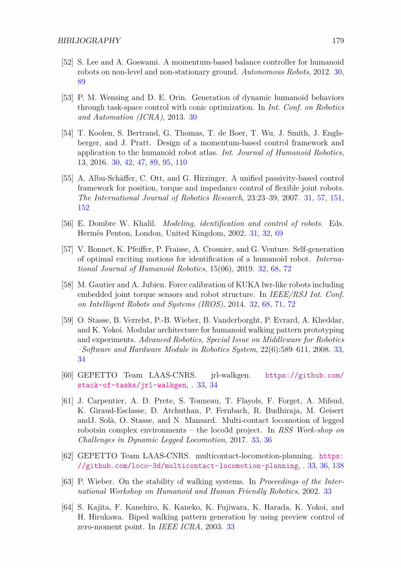
BIBLIOGRAPHY 179
[52] S. Lee and A. Goswami. A momentum-based balance controller for humanoidrobots on non-level and non-stationary ground. Autonomous Robots, 2012. 30,89
[53] P. M. Wensing and D. E. Orin. Generation of dynamic humanoid behaviorsthrough task-space control with conic optimization. In Int. Conf. on Roboticsand Automation (ICRA), 2013. 30
[54] T. Koolen, S. Bertrand, G. Thomas, T. de Boer, T. Wu, J. Smith, J. Engls-berger, and J. Pratt. Design of a momentum-based control framework andapplication to the humanoid robot atlas. Int. Journal of Humanoid Robotics,13, 2016. 30, 42, 47, 89, 95, 110
[55] A. Albu-Schäffer, C. Ott, and G. Hirzinger. A unified passivity-based controlframework for position, torque and impedance control of flexible joint robots.The International Journal of Robotics Research, 23:23–39, 2007. 31, 57, 151,152
[56] E. Dombre W. Khalil. Modeling, identification and control of robots. Eds.Hermès Penton, London, United Kingdom, 2002. 31, 32, 69
[57] V. Bonnet, K. Pfeiffer, P. Fraisse, A. Crosnier, and G. Venture. Self-generationof optimal exciting motions for identification of a humanoid robot. Interna-tional Journal of Humanoid Robotics, 15(06), 2019. 32, 68, 72
[58] M. Gautier and A. Jubien. Force calibration of KUKA lwr-like robots includingembedded joint torque sensors and robot structure. In IEEE/RSJ Int. Conf.on Intelligent Robots and Systems (IROS), 2014. 32, 68, 71, 72
[59] O. Stasse, B. Verrelst, P.-B. Wieber, B. Vanderborght, P. Evrard, A. Kheddar,and K. Yokoi. Modular architecture for humanoid walking pattern prototypingand experiments. Advanced Robotics, Special Issue on Middleware for Robotics–Software and Hardware Module in Robotics System, 22(6):589–611, 2008. 33,34
[60] GEPETTO Team LAAS-CNRS. jrl-walkgen. https://github.com/stack-of-tasks/jrl-walkgen, . 33, 34
[61] J. Carpentier, A. D. Prete, S. Tonneau, T. Flayols, F. Forget, A. Mifsud,K. Giraud-Esclasse, D. Atchuthan, P. Fernbach, R. Budhiraja, M. GeisertandJ. Solà, O. Stasse, and N. Mansard. Multi-contact locomotion of leggedrobotsin complex environments – the loco3d project. In RSS Work-shop onChallenges in Dynamic Legged Locomotion, 2017. 33, 36
[62] GEPETTO Team LAAS-CNRS. multicontact-locomotion-planning. https://github.com/loco-3d/multicontact-locomotion-planning, . 33, 36, 138
[63] P. Wieber. On the stability of walking systems. In Proceedings of the Inter-national Workshop on Humanoid and Human Friendly Robotics, 2002. 33
[64] S. Kajita, F. Kanehiro, K. Kaneko, K. Fujiwara, K. Harada, K. Yokoi, andH. Hirukawa. Biped walking pattern generation by using preview control ofzero-moment point. In IEEE ICRA, 2003. 33
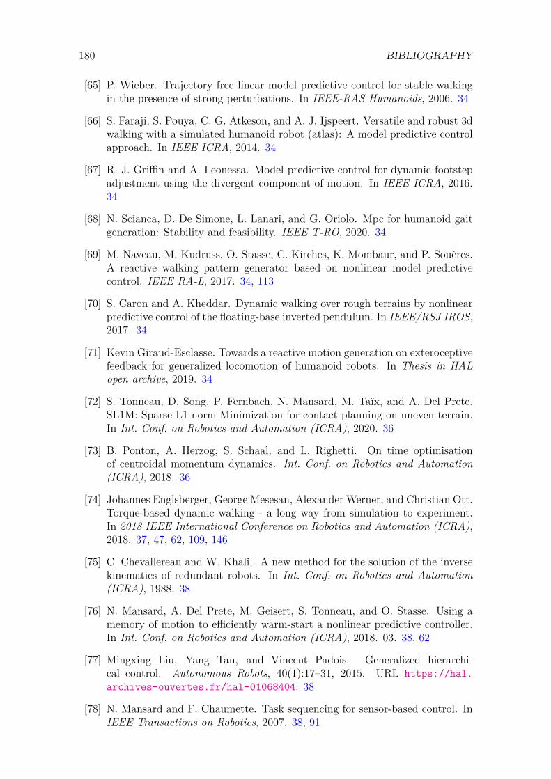
180 BIBLIOGRAPHY
[65] P. Wieber. Trajectory free linear model predictive control for stable walkingin the presence of strong perturbations. In IEEE-RAS Humanoids, 2006. 34
[66] S. Faraji, S. Pouya, C. G. Atkeson, and A. J. Ijspeert. Versatile and robust 3dwalking with a simulated humanoid robot (atlas): A model predictive controlapproach. In IEEE ICRA, 2014. 34
[67] R. J. Griffin and A. Leonessa. Model predictive control for dynamic footstepadjustment using the divergent component of motion. In IEEE ICRA, 2016.34
[68] N. Scianca, D. De Simone, L. Lanari, and G. Oriolo. Mpc for humanoid gaitgeneration: Stability and feasibility. IEEE T-RO, 2020. 34
[69] M. Naveau, M. Kudruss, O. Stasse, C. Kirches, K. Mombaur, and P. Souères.A reactive walking pattern generator based on nonlinear model predictivecontrol. IEEE RA-L, 2017. 34, 113
[70] S. Caron and A. Kheddar. Dynamic walking over rough terrains by nonlinearpredictive control of the floating-base inverted pendulum. In IEEE/RSJ IROS,2017. 34
[71] Kevin Giraud-Esclasse. Towards a reactive motion generation on exteroceptivefeedback for generalized locomotion of humanoid robots. In Thesis in HALopen archive, 2019. 34
[72] S. Tonneau, D. Song, P. Fernbach, N. Mansard, M. Taïx, and A. Del Prete.SL1M: Sparse L1-norm Minimization for contact planning on uneven terrain.In Int. Conf. on Robotics and Automation (ICRA), 2020. 36
[73] B. Ponton, A. Herzog, S. Schaal, and L. Righetti. On time optimisationof centroidal momentum dynamics. Int. Conf. on Robotics and Automation(ICRA), 2018. 36
[74] Johannes Englsberger, George Mesesan, Alexander Werner, and Christian Ott.Torque-based dynamic walking - a long way from simulation to experiment.In 2018 IEEE International Conference on Robotics and Automation (ICRA),2018. 37, 47, 62, 109, 146
[75] C. Chevallereau and W. Khalil. A new method for the solution of the inversekinematics of redundant robots. In Int. Conf. on Robotics and Automation(ICRA), 1988. 38
[76] N. Mansard, A. Del Prete, M. Geisert, S. Tonneau, and O. Stasse. Using amemory of motion to efficiently warm-start a nonlinear predictive controller.In Int. Conf. on Robotics and Automation (ICRA), 2018. 03. 38, 62
[77] Mingxing Liu, Yang Tan, and Vincent Padois. Generalized hierarchi-cal control. Autonomous Robots, 40(1):17–31, 2015. URL https://hal.archives-ouvertes.fr/hal-01068404. 38
[78] N. Mansard and F. Chaumette. Task sequencing for sensor-based control. InIEEE Transactions on Robotics, 2007. 38, 91
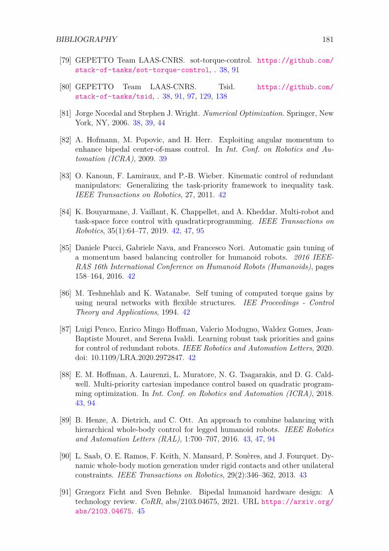
BIBLIOGRAPHY 181
[79] GEPETTO Team LAAS-CNRS. sot-torque-control. https://github.com/stack-of-tasks/sot-torque-control, . 38, 91
[80] GEPETTO Team LAAS-CNRS. Tsid. https://github.com/stack-of-tasks/tsid, . 38, 91, 97, 129, 138
[81] Jorge Nocedal and Stephen J. Wright. Numerical Optimization. Springer, NewYork, NY, 2006. 38, 39, 44
[82] A. Hofmann, M. Popovic, and H. Herr. Exploiting angular momentum toenhance bipedal center-of-mass control. In Int. Conf. on Robotics and Au-tomation (ICRA), 2009. 39
[83] O. Kanoun, F. Lamiraux, and P.-B. Wieber. Kinematic control of redundantmanipulators: Generalizing the task-priority framework to inequality task.IEEE Transactions on Robotics, 27, 2011. 42
[84] K. Bouyarmane, J. Vaillant, K. Chappellet, and A. Kheddar. Multi-robot andtask-space force control with quadraticprogramming. IEEE Transactions onRobotics, 35(1):64–77, 2019. 42, 47, 95
[85] Daniele Pucci, Gabriele Nava, and Francesco Nori. Automatic gain tuning ofa momentum based balancing controller for humanoid robots. 2016 IEEE-RAS 16th International Conference on Humanoid Robots (Humanoids), pages158–164, 2016. 42
[86] M. Teshnehlab and K. Watanabe. Self tuning of computed torque gains byusing neural networks with flexible structures. IEE Proceedings - ControlTheory and Applications, 1994. 42
[87] Luigi Penco, Enrico Mingo Hoffman, Valerio Modugno, Waldez Gomes, Jean-Baptiste Mouret, and Serena Ivaldi. Learning robust task priorities and gainsfor control of redundant robots. IEEE Robotics and Automation Letters, 2020.doi: 10.1109/LRA.2020.2972847. 42
[88] E. M. Hoffman, A. Laurenzi, L. Muratore, N. G. Tsagarakis, and D. G. Cald-well. Multi-priority cartesian impedance control based on quadratic program-ming optimization. In Int. Conf. on Robotics and Automation (ICRA), 2018.43, 94
[89] B. Henze, A. Dietrich, and C. Ott. An approach to combine balancing withhierarchical whole-body control for legged humanoid robots. IEEE Roboticsand Automation Letters (RAL), 1:700–707, 2016. 43, 47, 94
[90] L. Saab, O. E. Ramos, F. Keith, N. Mansard, P. Souères, and J. Fourquet. Dy-namic whole-body motion generation under rigid contacts and other unilateralconstraints. IEEE Transactions on Robotics, 29(2):346–362, 2013. 43
[91] Grzegorz Ficht and Sven Behnke. Bipedal humanoid hardware design: Atechnology review. CoRR, abs/2103.04675, 2021. URL https://arxiv.org/abs/2103.04675. 45
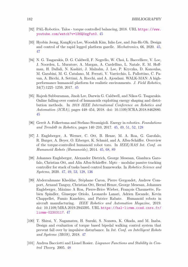
182 BIBLIOGRAPHY
[92] PAL-Robotics. Talos - torque controlled balancing, 2018. URL https://www.youtube.com/watch?v=lX6Q0zgFut0. 45
[93] Hyobin Jeong, KangKyu Lee, Wooshik Kim, Inho Lee, and Jun-Ho Oh. Designand control of the rapid legged platform gazelle. Mechatronics, 66, 2020. 45,47
[94] N. G. Tsagarakis, D. G. Caldwell, F. Negrello, W. Choi, L. Baccelliere, V. Loc,J. Noorden, L. Muratore, A. Margan, A. Cardellino, L. Natale, E. M. Hoff-man, H. Dallali, N. Kashiri, J. Malzahn, J. Lee, P. Kryczka, D. Kanoulas,M. Garabini, M. G. Catalano, M. Ferrati, V. Varricchio, L. Pallottino, C. Pa-van, A. Bicchi, A. Settimi, A. Rocchi, and A. Ajoudani. WALK-MAN: A high-performance humanoid platform for realistic environments. J. Field Robotics,34(7):1225–1259, 2017. 45
[95] Rajesh Subburaman, Jinoh Lee, Darwin G. Caldwell, and Nikos G. Tsagarakis.Online falling-over control of humanoids exploiting energy shaping and distri-bution methods. In 2018 IEEE International Conference on Robotics andAutomation (ICRA), pages 448–454, 2018. doi: 10.1109/ICRA.2018.8462880.45
[96] Gerrit A. Folkertsma and Stefano Stramigioli. Energy in robotics. Foundationsand Trends® in Robotics, pages 140–210, 2017. 45, 49, 51, 52, 128
[97] J. Englsberger, A. Werner, C. Ott, B. Henze, M. A. Roa, G. Garofalo,R. Burger, A. Beyer, O. Eiberger, K. Schmid, and A. Albu-Schäffer. Overviewof the torque-controlled humanoid robot toro. In IEEE/RAS Int. Conf. onHumanoid Robots (Humanoids), 2014. 45, 68, 89
[98] Johannes Englsberger, Alexander Dietrich, George Mesesan, Gianluca Garo-falo, Christian Ott, and Alin Albu-Schäeffer. Mptc – modular passive trackingcontroller for stack of tasks based control frameworks. In Robotics Science andSystems, 2020. 47, 49, 53, 128, 136
[99] Abderrahmane Kheddar, Stéphane Caron, Pierre Gergondet, Andrew Com-port, Arnaud Tanguy, Christian Ott, Bernd Henze, George Mesesan, JohannesEnglsberger, Máximo A Roa, Pierre-Brice Wieber, François Chaumette, Fa-bien Spindler, Giuseppe Oriolo, Leonardo Lanari, Adrien Escande, KevinChappellet, Fumio Kanehiro, and Patrice Rabate. Humanoid robots inaircraft manufacturing. IEEE Robotics and Automation Magazine, 2019.doi: 10.1109/MRA.2019.2943395. URL https://hal-lirmm.ccsd.cnrs.fr/lirmm-02303117. 47
[100] T. Shirai, Y. Nagamatsu, H. Suzuki, S. Nozawa, K. Okada, and M. Inaba.Design and evaluation of torque based bipedal walking control system thatprevent fall over by impulsive disturbance. In Int. Conf. on Intelligent Robotsand Systems (IROS), 2018. 47
[101] Andrea Bacciotti and Lionel Rosier. Liapunov Functions and Stability in Con-trol Theory. 2005. 48
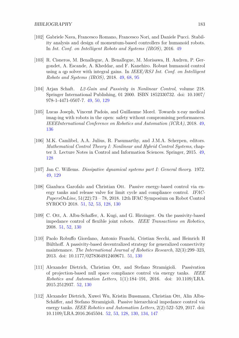
BIBLIOGRAPHY 183
[102] Gabriele Nava, Francesco Romano, Francesco Nori, and Daniele Pucci. Stabil-ity analysis and design of momentum-based controllers for humanoid robots.In Int. Conf. on Intelligent Robots and Systems (IROS), 2016. 49
[103] R. Cisneros, M. Benallegue, A. Benallegue, M. Morisawa, H. Audren, P. Ger-gondet, A. Escande, A. Kheddar, and F. Kanehiro. Robust humanoid controlusing a qp solver with integral gains. In IEEE/RSJ Int. Conf. on IntelligentRobots and Systems (IROS), 2018. 49, 68, 95
[104] Arjan Schaft. L2-Gain and Passivity in Nonlinear Control, volume 218.Springer International Publishing, 01 2000. ISBN 1852330732. doi: 10.1007/978-1-4471-0507-7. 49, 50, 129
[105] Lucas Joseph, Vincent Padois, and Guillaume Morel. Towards x-ray medicalimag-ing with robots in the open: safety without compromising performances.IEEEInternational Conference on Robotics and Automation (ICRA), 2018. 49,136
[106] M.K. Camlibel, A.A. Julius, R. Pasumarthy, and J.M.A. Scherpen, editors.Mathematical Control Theory I: Nonlinear and Hybrid Control Systems, chap-ter 3. Lecture Notes in Control and Information Sciences. Springer, 2015. 49,128
[107] Jan C. Willems. Dissipative dynamical systems part I: General theory. 1972.49, 129
[108] Gianluca Garofalo and Christian Ott. Passive energy-based control via en-ergy tanks and release valve for limit cycle and compliance control. IFAC-PapersOnLine, 51(22):73 – 78, 2018. 12th IFAC Symposium on Robot ControlSYROCO 2018. 51, 52, 53, 128, 130
[109] C. Ott, A. Albu-Schaffer, A. Kugi, and G. Hirzinger. On the passivity-basedimpedance control of flexible joint robots. IEEE Transactions on Robotics,2008. 51, 52, 130
[110] Paolo Robuffo Giordano, Antonio Franchi, Cristian Secchi, and Heinrich HBülthoff. A passivity-based decentralized strategy for generalized connectivitymaintenance. The International Journal of Robotics Research, 32(3):299–323,2013. doi: 10.1177/0278364912469671. 51, 130
[111] Alexander Dietrich, Christian Ott, and Stefano Stramigioli. Passivationof projection-based null space compliance control via energy tanks. IEEERobotics and Automation Letters, 1(1):184–191, 2016. doi: 10.1109/LRA.2015.2512937. 52, 130
[112] Alexander Dietrich, Xuwei Wu, Kristin Bussmann, Christian Ott, Alin Albu-Schäffer, and Stefano Stramigioli. Passive hierarchical impedance control viaenergy tanks. IEEE Robotics and Automation Letters, 2(2):522–529, 2017. doi:10.1109/LRA.2016.2645504. 52, 53, 128, 130, 134, 147
184 BIBLIOGRAPHY
[113] Erfan Shahriari, Lars Johannsmeier, Elisabeth Jensen, and Sami Haddadin.Power flow regulation, adaptation, and learning for intrinsically robust virtualenergy tanks. IEEE Robotics and Automation Letters, 5(1):211–218, 2020. doi:10.1109/LRA.2019.2953662. 52, 53, 93, 134, 142, 145, 146, 147, 161
[114] Tadele Shiferaw Tadele, Theo De Vries, and Stefano Stramigioli. Combiningenergy and power based safety metrics in controller design for domestic robots.In Int. Conf. on Robotics and Automation (ICRA), 2014. 52
[115] A. Albu-Schäffer, C. Ott, and G. Hirzinger. A unified passivity-based controlframework for position, torque and impedance control of flexible joint robots.The international journal of robotics research, 2007. 52, 54, 56, 57, 58
[116] Andrea Giusti, Jörn Malzahn, Nikolaos G. Tsagarakis, and Matthias Al-thoff. On the combined inverse-dynamics/passivity-based control of elastic-joint robots. IEEE Transactions on Robotics, 2018. 53
[117] J. A Acosta and M. Lopez-Martinez. Constructive feedback linearization ofunderactuated mechanical systems with 2-dof. In Decision and Control, 2005and 2005 European Control Conference. CDC-ECC ’05. 44th IEEE Conferenceon, 2006. 53
[118] Gordon Cheng, Sang-ho Hyon, Jun Morimoto, Ales Ude, Glenn Colvin, WaycoScroggin, and Stephen C. Jacobsen. Cb: A humanoid research platform forexploring neuroscience. In 2006 6th IEEE-RAS ICHR, 2006. 53
[119] Bernd Henze, Máximo A. Roa, and Christian Ott. Passivity-based whole-bodybalancing for torque-controlled humanoid robots in multi-contact scenarios.Int. Jour. of Robotics Research, 2016. 53, 128
[120] Arvid QL Keemink, Herman van der Kooij, and Arno HA Stienen. Admittancecontrol for physical human–robot interaction. The International Journal ofRobotics Research, 37(11):1421–1444, 2018. doi: 10.1177/0278364918768950.54, 55
[121] Wen Yu and Adolfo Perrusquía. Simplified stable admittance control usingend-effector orientations. Int. J. Soc. Robotics, 12:1061–1073, 2020. 54
[122] W.-S. Lu and Q.-H. Meng. Impedance control with adaptation for roboticmanipulations. IEEE Transactions on Robotics and Automation, 7(3):408–415, 1991. doi: 10.1109/70.88152. 54, 56
[123] R.J. Anderson and M.W. Spong. Hybrid impedance control of robotic manip-ulators. IEEE Journal on Robotics and Automation, 4(5):549–556, 1988. doi:10.1109/56.20440. 54, 55, 59, 60
[124] A. Albu-Schaffer and G. Hirzinger. Cartesian impedance control techniquesfor torque controlled light-weight robots. In Proceedings 2002 IEEE Inter-national Conference on Robotics and Automation (Cat. No.02CH37292), vol-ume 1, pages 657–663 vol.1, 2002. doi: 10.1109/ROBOT.2002.1013433. 54,56, 57, 58
BIBLIOGRAPHY 185
[125] Christopher Schindlbeck and Sami Haddadin. Unified passivity-based carte-sian force/impedance control for rigid and flexible joint robots via task-energytanks. In 2015 IEEE International Conference on Robotics and Automation(ICRA), pages 440–447, 2015. doi: 10.1109/ICRA.2015.7139036. 54, 57, 134,152
[126] M. H. Raibert and J. J. Craig. Hybrid Position/Force Control of Manipulators.Journal of Dynamic Systems, Measurement, and Control, 103(2):126–133, 061981. doi: 10.1115/1.3139652. URL https://doi.org/10.1115/1.3139652.55, 58, 59
[127] Christian Ott, Ranjan Mukherjee, and Yoshihiko Nakamura. A hybrid systemframework for unified impedance and admittance control. Journal of Intelli-gent and Robotic Systems, 78, 06 2014. doi: 10.1007/s10846-014-0082-1. 55,57, 60
[128] Hyomin Kim, Jaesung Kwon, Yonghwan Oh, Bum Jae You, and WoosungYang. Weighted hybrid admittance-impedance control with human intentionbased stiffness estimation for human-robot interaction. In 2018 IEEE/RSJInternational Conference on Intelligent Robots and Systems (IROS), pages1–6, 2018. doi: 10.1109/IROS.2018.8594435. 55, 60
[129] S. Chiaverini and L. Sciavicco. The parallel approach to force/position controlof robotic manipulators. IEEE Transactions on Robotics and Automation, 9(4):361–373, 1993. doi: 10.1109/70.246048. 55, 60, 61
[130] Bruno Siciliano. Parallel force/position control of robot manipulators. InGeorges Giralt and Gerhard Hirzinger, editors, Robotics Research, pages 78–89, London, 1996. Springer London. 55, 60, 61
[131] J. Kenneth Salisbury. Active stiffness control of a manipulator in cartesiancoordinates. In 1980 19th IEEE Conference on Decision and Control includingthe Symposium on Adaptive Processes, pages 95–100, 1980. doi: 10.1109/CDC.1980.272026. 55, 57
[132] M.d.P.A. Fonseca, B.V. Adorno, and P. Fraisse. Task-space admittance con-troller with adaptive inertia matrix conditioning. Journal of Intelligent RobotSystem, 41, February 2021. doi: https://doi.org/10.1007/s10846-020-01275-0.56
[133] Arash Ajoudani, Nikos G. Tsagarakis, Jinoh Lee, Marco Gabiccini, and An-tonio Bicchi. Natural redundancy resolution in dual-arm manipulation usingconfiguration dependent stiffness (cds) control. In 2014 IEEE InternationalConference on Robotics and Automation (ICRA), pages 1480–1486, 2014. doi:10.1109/ICRA.2014.6907047. 57, 58
[134] A. Albu-Schaffer, M. Fischer, G. Schreiber, F. Schoeppe, and G. Hirzinger.Soft robotics: what cartesian stiffness can obtain with passively compliant,uncoupled joints? In 2004 IEEE/RSJ International Conference on IntelligentRobots and Systems (IROS) (IEEE Cat. No.04CH37566), volume 4, pages3295–3301 vol.4, 2004. doi: 10.1109/IROS.2004.1389925. 57, 58
186 BIBLIOGRAPHY
[135] Arash Ajoudani, Nikos G. Tsagarakis, and Antonio Bicchi. On the role ofrobot configuration in cartesian stiffness control. In 2015 IEEE InternationalConference on Robotics and Automation (ICRA), pages 1010–1016, 2015. doi:10.1109/ICRA.2015.7139300. 58
[136] J. Rawlings, D. Mayne, and M. Diehl. Model Predictive Control: Theory,Computation and Design. Nob Hill Publishing, 2017. 61
[137] Mikulas Huba. Selected Topics on Constrained and Nonlinear Control, pages87–185. 01 2011. ISBN 978-80-968627-4-0. 61
[138] J. Rawlings, E. Meadows, and K. Muske. Nonlinear model predictive control:A tutorial and survey. IFAC Advanced Control of Chemical Processes, 1994.61
[139] Rolf Findeisen and Frank Allgöwer. An introduction to nonlinear model pre-dictive control. In Conference: 21st Benelux Meeting on Systems and Control,2002. 61
[140] T. Raff, C. Ebenbauer, and P. Allgöwer. Nonlinear Model Predictive Control:A Passivity-Based Approach, pages 151–162. Springer, 2007. 61, 162
[141] E. Todorov, T. Erez, and Y. Tassa. Mujoco: A physics engine for model-basedcontrol. In Int. Conf. on Intelligent Robots and Systems (IROS), 2012. 61, 64
[142] H. Dai, A. Valenzuela, and R. Tedrake. Optimization-based locomotion plan-ning, estimation, and control design for the atlas humanoid robot. In Int.Conf. on Humanoid Robotics (ICHR), 2014. 61
[143] Donghyun Kim, Jared Di Carlo, Benjamin Katz, Gerardo Bledt, and SangbaeKim. Highly dynamic quadruped locomotion via whole-body impulse controland model predictive control. CoRR, abs/1909.06586, 2019. URL http://arxiv.org/abs/1909.06586. 61
[144] Michael Neunert, Cédric de Crousaz, Fadri Furrer, Mina Kamel, FarbodFarshidian, Roland Siegwart, and Jonas Buchli. Fast nonlinear model pre-dictive control for unified trajectory optimization and tracking. In 2016IEEE International Conference on Robotics and Automation (ICRA), page1398–1404. IEEE Press, 2016. doi: 10.1109/ICRA.2016.7487274. URLhttps://doi.org/10.1109/ICRA.2016.7487274. 61
[145] Ruben Grandia, Farbod Farshidian, Rene Ranftl, and Marco Hutter. Feedbackmpc for torque-controlled legged robots. In EEE/RSJ International Con-ference on Intelligent Robots and Systems, pages 4730–4737, 11 2019. doi:10.1109/IROS40897.2019.8968251. 61
[146] David Mayne. A second-order gradient method for determining optimal tra-jectories of non-linear discrete-time systems. International Journal of Control,3(1):85–95, 1966. 61
BIBLIOGRAPHY 187
[147] Ewen Louis Dantec, Rohan Budhiraja, Adria Roig, Teguh Lembono, Guil-hem Saurel, Olivier Stasse, Pierre Fernbach, Steve Tonneau, Sethu Vijayaku-mar, Sylvain Calinon, Michel Taïx, and Nicolas Mansard. Whole BodyModel Predictive Control with a Memory of Motion: Experiments on aTorque-Controlled Talos. In International Conference on Robotics and Au-tomation (ICRA 2021), 2021. URL https://hal.archives-ouvertes.fr/hal-02995796. 61, 62, 123, 162
[148] A. Majumdar, G. Hall, and A. A. Ahmadi. Recent scalability improvementsfor semidefinite programming with applications in machine learning, control,and robotics. 2020. 62
[149] Y. Tassa, T. Erez, and W. D. Smart. Receding horizon differential dynamicprogramming. In Advances in Neural Information Processing Systems, 2008.62
[150] D. P. Bertsekas. Dynamic Programming and Optimal Control. Athena Scien-tific, 2017. 62
[151] Y. Tassa, N. Mansard, and E. Todorov. Control-limited differential dynamicprogramming. In IEEE ICRA, 2014. 62, 63, 112
[152] Z. Xie, C. K. Liu, and K. Hauser. Differential dynamic programming withnonlinear constraints. In Int. Conf. on Robotics and Automation (ICRA),pages 695–702, 2017. 62
[153] A. Herzog, N. Rotella, S. Mason, F. Grimminger, S. Schaal, and L. Righetti.Momentum control with hierarchical inverse dynamics on a torque-controlledhumanoid. Autonomous Robots, 2014. 62, 89, 92, 94, 95, 114
[154] M. Diehl, H. G. Bock, , and J. P. Schlödre. A real-time iteration schemefor nonlinear optimization in optimal feedback control. In SIAM Journal oncontrol and optimization, 2005. 62
[155] Richard Bellman. On the theory of dynamic programming. Proceedings of theNational Academy of Sciences, 38(8):716–719, 1952. doi: 10.1073/pnas.38.8.716. 62
[156] F. Forget, K. Giraud-Esclasse, R. Gelin, N. Mansard, and O. Stasse. Im-plementation, identification and control of an efficient electric actuator forhumanoid robots. In International Conference on Informatics in Control, Au-tomation and Robotics, ICINCO, 2018. 63, 73, 79
[157] Yuval Tassa, Nicolas Mansard, and Emo Todorov. Control-limited differentialdynamic programming. In icra, 2014. 63
[158] W. Li and E. Todorov. Iterative linearisation methods for approximatelyoptimal control and estimation of non-linear stochastic system. Int. Jour. ofControl, 2007. 63, 74
[159] R. S. Sutton and A. G. Barto. Reinforcement Learning: An Introduction,second edition. The MIT Press, 2018. 64
188 BIBLIOGRAPHY
[160] Y. LeCun, Y. Bengio, and G. Hinton. Deep learning. Nature, 521:436–444,2015. 64
[161] Roland Siegwart Jemin Hwangbo, Inkyu Sa and Marco Hutter. Control of aquadrotor with reinforcement learning. IEEE Robotics and Automation Letters2096–2103, 2017. 64
[162] D. Esteban, L. Rozo, and D. G. Caldwell. Learning deep robot controllersby exploiting successful and failed executions. In Int. Conf. on HumanoidRobotics (ICHR), 2018. 64
[163] L. Bottou and O. Bousquet. Optimization for Machine Learning, chapter TheTradeoffs of Large Scale Learning, page 351–368. Cambridge: MIT Press,2012. 64
[164] J. Hwangbo, J. Lee, A. Dosovitskiy, D. Bellicoso, V. Tsounis, V. Koltun, andM. Hutter. Learning agile and dynamic motor skills for legged robots. ScienceRobotics, 2019. 64, 69
[165] J. Tan, T. Zhang, E. Coumans, A. Iscen, Y. Bai, D. Hafner, S. Bohez, andV. Vanhoucke. Sim-to-real: Learning agile locomotion for quadruped robots.In Robotics: Science and Systems, 2018. 64, 69
[166] Oriol Vinyals, Charles Blundell, Timothy Lillicrap, koray kavukcuoglu, andDaan Wierstra. Matching networks for one shot learning. In D. Lee,M. Sugiyama, U. Luxburg, I. Guyon, and R. Garnett, editors, Advances inNeural Information Processing Systems. Curran Associates, Inc., 2016. 64
[167] Jake Snell, Kevin Swersky, and Richard Zemel. Prototypical networks for few-shot learning. In I. Guyon, U. V. Luxburg, S. Bengio, H. Wallach, R. Fergus,S. Vishwanathan, and R. Garnett, editors, Advances in Neural InformationProcessing Systems. Curran Associates, Inc., 2017. 64
[168] Stephen James, Michael Bloesch, and Andrew J. Davison. Task-embeddedcontrol networks for few-shot imitation learning. ArXiv, 2018. 64
[169] Kosuge K., Yoshida H., and Fukuda T. Dynamic control for robot-humancollaboration. In Proceedings of 1993 2nd IEEE International Workshop onRobot and Human Communication., 1993. 64
[170] Isabelle Maroger, Olivier Stasse, and Bruno Watier. Inverse Optimal Con-trol to Model Human Trajectories During Locomotion. Computer Methodsin Biomechanics and Biomedical Engineering, 2021. doi: 10.1080/10255842.2021.1962311. URL https://hal.laas.fr/hal-03142655. 65
[171] N. Jarrassé, V. Sanguineti, and E. Burdet. Slaves no longer: review on roleassignment for human–robot joint motor action. Adaptive Behavior, SAGEPublications, 2013. 65
[172] Antoine Bussy, Pierre Gergondet, Abderrahmane Kheddar, Francois Keith,and Andre Crosnier. Proactive behavior of a humanoid robot in a haptictransportation task with a human partner. In IEEE RO-MAN, 2012. 65

BIBLIOGRAPHY 189
[173] K. Otani, K. Bouyarmane, and S. Ivaldi. Generating assistive humanoid mo-tions for co-manipulation tasks with a multi-robot quadratic program con-troller. In IEEE ICRA, 2018. 65
[174] P. Teja S. and R. Alami. Hateb-2: Reactive planning and decision making inhuman-robot co-navigation. In IEEE RO-MAN, 2020. 65
[175] J. Lanini, A. Duburcq, H. Razavi, C.G. Le Goff, and A. Ijspeert. Interactivelocomotion: Investigation and modeling of physically-paired humans whilewalking. PLoS ONE, 2017. 65
[176] J. Lanini, H. Razavi, J. Urain, and A. Ijspeert. Human intention detectionas a multiclass classification problem: Application in physical human–robotinteraction while walking. IEEE RA-L, 2018. 65
[177] Daniel Aarno and Danica Kragic. Motion intention recognition in robot as-sisted applications. Robotics and Autonomous Systems, 2008. 65
[178] R. Kelley, M. Nicolescu, A. Tavakkoli, M. Nicolescu, C. King, and G. Bebis.Understanding human intentions via hidden markov models in autonomousmobile robots. In ACM/IEEE HRI, 2008. 65
[179] Q. Li, Z. Zhang, Y. You, Y. Mu, and C. Feng. Data driven models for humanmotion prediction in human-robot collaboration. IEEE Access, 2020. 65
[180] M. Awais and D. Henrich. Human-robot collaboration by intention recognitionusing probabilistic state machines. In RAAD, 2010. 65
[181] David A. Winter. Biomechanics and motor control of human gait. InWaterloo,Ont. : University of Waterloo Press, 1991. 65
[182] Mirko Raković, Srdjan Savić, José Santos-Victor, Milutin Nikolić, andBranislav Borovac. Human-inspired online path planning and biped walkingrealization in unknown environment. Frontiers in Neurorobotics, 2019. 66
[183] Alessandro Papadopoulos, Luca Bascetta, and Gianni Ferretti. Generation ofhuman walking paths. In IEEE IROS, 2013. 66
[184] Gustavo Arechavaleta, Jean-Paul Laumond, Halim Hicheur, and AlainBerthoz. On the nonholonomic nature of human locomotion. AutonomousRobots, 2008. 66
[185] K. Mombaur and J.-P. Laumond. From human to humanoid locomotion - aninverse optimal control approach. Autonomous Robots, 2010. 66
[186] Isabelle Maroger, Olivier Stasse, and Bruno Watier. Walking human trajectorymodels and their application to humanoid robot locomotion. In IEEE/RSJIROS, 2020. 66, 112
[187] Isabelle Maroger, Olivier Stasse, and Bruno Watier. Inverse optimal controlto model human trajectories during gait. In HAL open archive, 2021. 66, 112,116
190 BIBLIOGRAPHY
[188] S. Park, J. Sim, and J. Park. System design of humanoid robot dyros-jet. InIEEE/SICE International Symposium on System Integration (SII), 2019. 68
[189] O. Stasse, T. Flayols, R. Budhiraja, K. Giraud-Esclasse, J. Carpentier, and al..Talos: A new humanoid research platform targeted for industrial applications.In IEEE/RAS Int. Conf. on Humanoid Robots (Humanoids), 2017. 68
[190] O. Khatib, L. Sentis, J. Park, and J. Warren. Whole-body dynamic behaviorand control of human-like robots. International Journal of Humanoid Robotics,2004. 68
[191] O. Khatib, P. Thaulad, T. Yoshikawa, and J. Park. Torque-position trans-former for task control of position controlled robots. In IEEE/RAS Int. Conf.on Robotics and Automation (ICRA), 2008. 68
[192] A. Del Prete, N. Mansard, O. Ponce O., Stasse, and F. Nori. Implementingtorque control with high-ratio gear boxes and without joint-torque sensors.International Journal of Humanoid Robotics, 2015. 68
[193] F. Nori, S. Traversaro, J. Eljaik, F. Romano, A. Del Prete, and D. Pucci. icubwhole-body control through force regulation on rigid non-coplanar contacts.Frontiers in Robotics and AI, 2015. 68
[194] M. Gautier and S. Briot. Global identification of joint drive gains and dynamicparameters of robots. ASME Journal of Dynamic Systems, 2014. 68, 71
[195] M. Gautier. Dynamic identification of robots with power model. ICRA, 1997.72
[196] G. Kumar Hari Shankar Lal Das, B. Tondu, F. Forget, J. Manhes, O. Stasse,and P. Soueres. Controlling a multi-joint arm actuated by pneumatic muscleswith quasi-ddp optimal control. In IEEE/RSJ Int. Conf. on Intelligent Robotsand Systems (IROS), 2016. 73, 74
[197] C. Presse and M. Gautier. New criteria of exciting trajectories for robotidentification. In IEEE/RAS Int. Conf. on Robotics and Automation (ICRA),1993. 78
[198] GEPETTO Team LAAS-CNRS. eiquadprog. https://github.com/stack-of-tasks/eiquadprog, . 94
[199] Donald Goldfarb and Ashok U. Idnani. A numerically stable dual method forsolving strictly convex quadratic programs. Mathematical Programming, 27:1–33, 1983. 94
[200] G. Romualdi, S. Dafarra, Y. Hu, P. Ramadoss, F. Andrade Chavez, S. Traver-saro, and D. Pucci. A benchmarking of dcm based architectures for position,velocity and torque controlled humanoid robots. Int. Journal of HumanoidRobotics, 2019. 95, 105
[201] GEPETTO Team LAAS-CNRS. sot-talos-balance. https://github.com/loco-3d/sot-talos-balance, . 96
BIBLIOGRAPHY 191
[202] GEPETTO Team LAAS-CNRS. talos-torque-control. https://github.com/stack-of-tasks/talos-torque-control, . 97, 138
[203] D. Torricelli, J. Gonzalez-Vargas, J. Veneman, K. Mombaur, N. Tsagarakis,A. del Ama, A. Gil-Agudo, J. Moreno, and J. Pons. Benchmarking bipedallocomotion: A unified scheme for humanoids, wearable robots, and humans.IEEE Robotics Automation Magazine, 2015. 98, 99, 100
[204] C. Mummolo and J. H. Kim. Passive and dynamic gait measures for bipedmechanism: formulation and simulation analysis. In Robotica, 2012. 99, 106,108
[205] S. Collins, A. Ruina, R. Tedrake, and M. Wisse. Efficient bipedal robots basedon passive-dynamic walkers. Science, 2005. 106
[206] Nahuel A. Villa, Pierre Fernbach, Nicolas Mansard, and Olivier Stasse. Ad-dressing flexibility in biped locomotion with robust control and closed-loopmodel-predictive control. In IEEE/RAS Int. Conf. on Robotics and Automa-tion (ICRA), submitted in 2022. 109, 110, 160, 161, 170, 171
[207] C. Mastalli, R. Budhiraja, W. Merkt, G. Saurel, B. Hammoud, M. Naveau,et al. Crocoddyl: An efficient and versatile framework for multi-contact opti-mal control. In IEEE ICRA, 2020. 112
[208] Isabelle Maroger, Olivier Stasse, and Bruno Watier. Metrics to assess a humantrajectory prediction model during gait. In HAL open archive, 2021. 118
[209] Dirk Merkel. Docker: lightweight linux containers for consistent developmentand deployment. Linux journal, 2014(239):2, 2014. 123
[210] Noëlie Ramuzat. On the semi-positive definition of the product of a positivediagonal matrix and a symmetric semi-positive definite matrix. working pa-per or preprint, January 2022. URL https://hal.archives-ouvertes.fr/hal-03434195. 131, 145, 172
[211] Adi Ben-Israel and Thomas N.E. Greville. Generalized Inverses: Theory andApplications. Springer, 2003. ISBN 0-387-00293-6. 132
[212] T. N. E. Greville. Note on the generalized inverse of a matrix product. SIAMReview, 8(4):518–521, 1966. doi: 10.1137/1008107. 132
[213] Klas Kronander and A. Billard. Passive interaction control with dynamicalsystems. IEEE Robotics and Automation Letters (RAL), 2016. 134, 145
[214] Shin’ichiro Nakaoka, Shizuko Hattori, Fumio Kanehiro, Shuuji Kajita, and Hi-rohisa Hirukawa. Constraint-based dynamics simulator for humanoid robotswith shock absorbing mechanisms. In 2007 IEEE/RSJ International Confer-ence on Intelligent Robots and Systems, pages 3641–3647. IEEE, 2007. 171
[215] Fuzhen Zhang. Matrix theory: basic results and techniques. Springer, 2011.173

192 BIBLIOGRAPHY
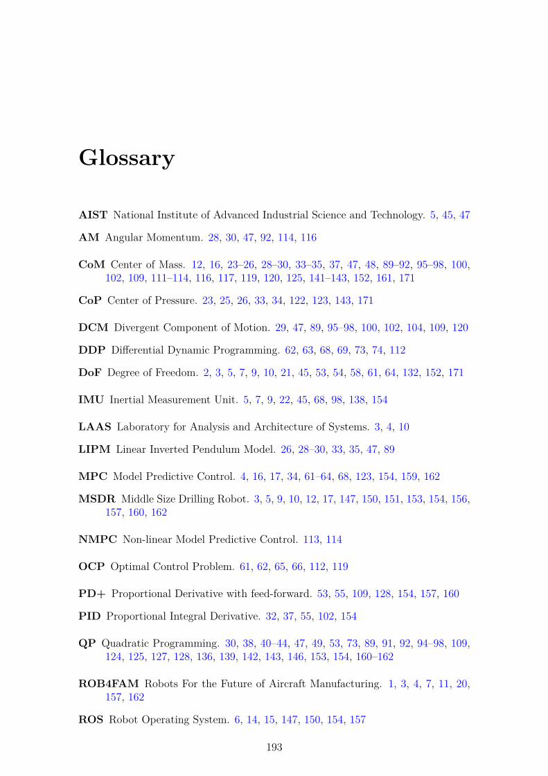
Glossary
AIST National Institute of Advanced Industrial Science and Technology. 5, 45, 47
AM Angular Momentum. 28, 30, 47, 92, 114, 116
CoM Center of Mass. 12, 16, 23–26, 28–30, 33–35, 37, 47, 48, 89–92, 95–98, 100,102, 109, 111–114, 116, 117, 119, 120, 125, 141–143, 152, 161, 171
CoP Center of Pressure. 23, 25, 26, 33, 34, 122, 123, 143, 171
DCM Divergent Component of Motion. 29, 47, 89, 95–98, 100, 102, 104, 109, 120
DDP Differential Dynamic Programming. 62, 63, 68, 69, 73, 74, 112
DoF Degree of Freedom. 2, 3, 5, 7, 9, 10, 21, 45, 53, 54, 58, 61, 64, 132, 152, 171
IMU Inertial Measurement Unit. 5, 7, 9, 22, 45, 68, 98, 138, 154
LAAS Laboratory for Analysis and Architecture of Systems. 3, 4, 10
LIPM Linear Inverted Pendulum Model. 26, 28–30, 33, 35, 47, 89
MPC Model Predictive Control. 4, 16, 17, 34, 61–64, 68, 123, 154, 159, 162
MSDR Middle Size Drilling Robot. 3, 5, 9, 10, 12, 17, 147, 150, 151, 153, 154, 156,157, 160, 162
NMPC Non-linear Model Predictive Control. 113, 114
OCP Optimal Control Problem. 61, 62, 65, 66, 112, 119
PD+ Proportional Derivative with feed-forward. 53, 55, 109, 128, 154, 157, 160
PID Proportional Integral Derivative. 32, 37, 55, 102, 154
QP Quadratic Programming. 30, 38, 40–44, 47, 49, 53, 73, 89, 91, 92, 94–98, 109,124, 125, 127, 128, 136, 139, 142, 143, 146, 153, 154, 160–162
ROB4FAM Robots For the Future of Aircraft Manufacturing. 1, 3, 4, 7, 11, 20,157, 162
ROS Robot Operating System. 6, 14, 15, 147, 150, 154, 157
193
194 Glossary
RST Regulation Sensitivity and Tracking. 154
SoT Stack-of-Tasks. 12, 14, 15, 123
TSID Task Space Inverse Dynamics. xi, 15, 16, 38, 91–94, 96, 128, 129, 152, 153,160
URDF Unified Robot Description Format. 8, 15
WPG Walking Pattern Generator. 17, 28, 33–36, 98, 111, 113, 114, 116, 118–120,123
ZMP Zero Moment Point. 26, 28–30, 34, 35, 98, 100, 102, 105, 108, 109
RésuméLes robots humanoïdes ne sont pas encore capables de travailler en sécurité dans
un environnement fait pour l’Homme et d’effectuer les mêmes tâches. L’objectif decette thèse est d’étudier des algorithmes de contrôle corps-complet pour robots hu-manoïdes afin d’effectuer des opérations de productions de structures avions tellesque le perçage. Cette thèse s’inscrit dans le cadre du laboratoire commun entre leLAAS-CNRS et la société Airbus Operations SAS. Les travaux et études présen-tés appartiennent aux domaines scientifiques de l’optimisation pour le contrôle desystèmes dynamiques et de l’analyse de leur stabilité.
Les contributions majeures de cette thèse sont la conception et l’implémentationde nouveaux algorithmes de contrôle temps-réel pour des robots humanoïdes, in-tégrés sur le robot TALOS. Les applications présentées traitent de la locomotiondu robot et de la réalisation d’opérations nécessitant l’application de force. Pre-mièrement, les paramètres de la chaîne d’actionnement du robot sont identifiés afinde commander directement le robot en courant tout en garantissant la protectiondu système. La solution proposée confirme les capacités du robot TALOS contrôléen couple lors de la manipulation d’une charge élevée. Ainsi, des algorithmes decontrôle temps-réel en couple pour le corps-complet du robot sont ensuite étudiés.Trois contrôleurs sont implémentés et comparés, deux en position et un en couple.Leur analyse est effectuée sur des scénarios de locomotion complexes en utilisantplusieurs critères comme le suivi de trajectoires et la dépense énergétique. Le con-trôleur corps-complet en couple est validé en simulation et ses avantages par rapportaux schémas en position confirment le choix de l’implémenter pour des opérationsde productions. Cependant, les premiers tests réalisés sur le robot réel ont conduità une dangereuse divergence de la solution. C’est pourquoi, une analyse de sta-bilité a été effectuée pour assurer la sécurité et la robustesse de la solution pourdes applications industrielles. La solution développée est basée sur la théorie dela passivité, augmentant le contrôleur en couple avec un réservoir d’énergie con-trôlant les transmissions d’énergie au sein du système. Ce nouveau contrôleur passifest validé en simulation sur des scénarios de locomotion et de multi-contacts avecl’environnement. Ce dernier met en place une tâche d’application de force commepremière étape vers des opérations de productions.
Les résultats de cette thèse ont été intégrés dans la suite logicielle Stack-of-Tasksdu LAAS-CNRS.
Mots clés : Contrôle corps-complet, Robots humanoïdes, Contrôle en force/couple
AbstractHumanoids robots are not yet able to safely work in similar environment than
humans and to perform the same tasks. The objective of this thesis is to studywhole-body control algorithms for humanoids robots in order to perform aircraftmanufacturing operations such as drilling. This thesis is part of the joint-lab be-tween the LAAS-CNRS laboratory and the Airbus Operations SAS company. Thepresented research and innovative studies rely on recent advances on control theory,optimization and stability analysis.
The main contributions of this thesis are the design and implementation of newreal-time controllers for humanoid robot, integrated on the robot TALOS. The il-lustrated applications are locomotion and force task operations. First, the chainactuation parameters of the robot are identified in order to directly control therobot in current while having low level protection mechanisms. The proposed so-lution confirms the capabilities of the robot TALOS to achieve torque control incomplex scenario with high payload. Thus, real-time whole-body torque controllersare then investigated. Three controllers are implemented and benchmarked, twoin position and one in torque. Their comparison is performed on complex loco-motion scenarios using several metrics including trajectory tracking and energeticcriteria. The whole-body torque controller is validated in simulations and its ad-vantages compared to the position schemes confirms the decision to implement itfor manufacturing operations. However, the first tests realized on the real robot ledto a dangerous divergence of the solution. Thus, a stability analysis was performedto ensure the safety and robustness of the solution for industrial applications. Thedeveloped solution is based on passivity theory, augmenting the whole-body torquecontrol scheme with a global energy tank monitoring the power flow of the system.This new passive scheme is validated in simulations on locomotion and multi-contactscenarios. The latter involves force applications as a first step toward manufacturingoperations.
The results of this thesis have been integrated in the Stack-of-Tasks frameworkof the LAAS-CNRS.
Keywords: Humanoid Whole-Body Control, Humanoids Robots, Force/TorqueControl