FORAGING STRATEGIES, DIET AND COMPETITION IN OLIVE

BABOONS

Robert A. Barton

A Thesis Submitted for the Degree of PhD

at the University of St. Andrews

1990

Full metadata for this item is available in Research@StAndrews:FullText

at: http://research-repository.st-andrews.ac.uk/

Please use this identifier to cite or link to this item:

http://hdl.handle.net/10023/2767

This item is protected by original copyright

_

FORAGING STRATEGIES, DIET AND COMPETITION IN OLIVE BABOONS

Robert A. Barton

Thesis submitted for the degree of Doctor of Philosophy,University of St. Andrews, 1989.

ACKNOWLEDGEMENTS-

This thesis has seen the light of day only through the greathelp, support and encouragement I have received from manyquarters. I would particularly like to thank Liz Anderson,who has helped in so many ways and provided emotional,intellectual and practical support throughout the last fouryears. Andy Whiten has been the most patient, diligent andgenerous of supervisors, and has headed off innumerable criseswith typical pragmatism and skill, while I flapped andfloundered. I would also like to thank both Andy and SusyWhiten for the warm hospitality they have extended to me on somany occasions. The fieldwork would simply not have beenpossible without the assistance of Shirley Strum, who kindlyallowed me to join the Uaso Ngiro Baboon Project, gave meideas for data-collection, and provided vital logisticalsupport throughout. I also thank Shirley for welcoming mydishevelled, field-weary self into her home on my visits toNairobi, and for stimulating discussions about baboons,philosophy, and soul music. My second supervisor, Dick Byrne,has been instrumental in sharpening up some of my ideas andprose, and has given over much time to sorting out all thelittle wrangles and administrative details that haveinevitably arisen. Josiah Musau and Hudson Oogh helped incrucial ways in the field, and kept me going at the beginningwhen it all seemed impossible. Debbie Lochhead helped withthe collection of demographic and ecological data, andtolerated my little domestic foibles and oddities atGeoffrey's House.

A number of other people have helped along the way. Inparticular, David and Anne Perrett have shown incomparablekindness and hospitality, which I have shamelessly exploitedfor far too long. Mary English conducted the phytochemicalanalysis, and computing assistance was given by Alan Milne,Phil Benson, Phil Robertson and Darryl Davies. Usefulcomments on research proposals and drafts of the thesis havebeen provided by Shirley Strum, Robin Dunbar, and Jeff Graves.

I thank the Office of the President, Kenya, for granting mepermission to conduct research in that country, and theInstitute of Primate Research, Nairobi, to whom I wasaffilited during the period of fieldwork. Jim Else was aparticular help in sorting out administrative details.Financial support was provided by a studentship from theScience and Engineering Council of Great Britain:

Finally, I would like once again to thank my parents,Catherine Peters and Anthony Storr, who have provided thesecure base and encouragement which have enabled me to keepgoing through dissapointments and lean times.

ABSTRACT

Savannah baboons are amongst the most intensively studied taxa

of primates, but our understanding of their foraging

strategies and diet selection, and the relationship of these

to social processes is still rudimentary. These issues were

addressed in a 12-month field study of olive baboons (Papio

anubis) on the Laikipia plateau in Kenya.

Seasonal fluctuations in food availability were closely

related to rainfall patterns, with the end of the dry season

representing a significant energy bottleneck. The

distribution of water and of sleeping sites were the

predominant influences on home range use, but certain

vegetation zones were occupied preferentially in seasons when

food availability within them was high.

The influence of rainfall on monthly variation in dietary

composition generally mirrored inter-population variation.

Phytochemical analysis revealed that simplistic dietary

taxonomies can be misleading in the evaluation of diet

quality. Food preferences were correlated with nutrient and

secondary compound content. The differences between males and

females in daily nutrient intakes were smaller than expected

on the basis of the great difference in body size; this was

partly attributable to the energetic costs of reproduction,

and possibly also to greater energetic costs of

thermoregulation and lower digestive efficiency in females.

A strongly linear dominance hierarchy was found amongst the

adult females. Dominance rank was positively correlated with

food ingestion rates and daily intakes, but not with time

spent feeding or with dietary quality or diversity. In a

provisioned group, high-ranking females occupied central

positions, while low-ranking females were more peripheral and

were supplanted more frequently. In the naturally-foraging

group, the intensity of competition was related to the pattern

of food distribution, but not to food quality, and was greater

in the dry season than in the wet season. The number of

neighbours and rates of supplanting were correlated with rank,

and evidence was presented that high-rankers monopolised

arboreal feeding sites.

PAGE

1

1111111516181920

CONTENTS

CHAPTER 1: INTRODUCTION

CHAPTER 2: STUDY SITE AND METHODSGeographyGeology, topography and vegetationClimate and seasonalityFaunaLivestock and human activitiesBaboons at ChololoMethods

CHAPTER 3: VEGETATION, FOOD AVAILABILITY AND HABITAT USE 44Introduction 44Relative abundance of habitat types 47Seasonal variation in food availability 49Implications of seasonality for baboons 54Spatial distribution patterns of food andthe problem of patchiness 58Patterns of ranging and habitat use 64

CHAPTER 4: FEMALE DOMINANCE RELATIONS, REPRODUCTIVEPROFILES AND BODY CONDITION

101Introduction

101Social organisation among females

104Reproduction and body condition

128

CHAPTER 5: DIET SELECTION

136Introduction

136Phytochemistry

139Diet

153Phytochemical determinants ofdietary preferences

176

CHAPTER 6: NUTRIENT INTAKESIntroductionEffects of month, sexSeasonal variationSex differencesThe influence ofNutrient intakesThe influence ofDiscussion

196196

and reproductive state 198200207212216222224

reproductive statein comparative perspectivedominance rank amongst females

CONTENTS, cont.

CHAPTER 7: THE DYNAMICS AND SEASONALITY OF FEEDINGCOMPETITION 244Introduction 244Competition and spatial deployment: anexperiment 245Seasonal variation in the intensity ofcompetition 252The influence of food quality and distribution 256Dominance rank, spatial deployment andsupplanting 261Discussion 266

CHAPTER 8: CONCLUDING DISCUSSION 279Ecological contrasts between males and females 279Feeding competition, predation and socialevolution 287

APPENDICES: SPECIES LIST OF MAMMALS SIGHTEDLIST OF FOODSPROXIMATE COMPOSITION OF CHOLOLO PLANTS

1

CHAPTER 1: INTRODUCTIONYe.

The study of primate social behaviour has been characterised

by something of a thematic schism. On the one hand, many

researchers have been interested in the relationship between

animals' environments and their mating systems and demography,

an area of study known generally as socioecology. This was

chiefly stimulated by pioneering comparative work on birds by

Orians (1961) and, in particular, by Crook (1964), who later

extended the approach to primates (Crook and Gartlan, 1966).

On the other hand, some researchers, notably Robert Hinde and

colleagues, have carried out extensive investigations into the

complex nature and dynamics of social interactions and

relationships (Hinde, 1969, 1976, 1979, 1983a; Hinde and

Simpson, 1975; Hinde and Stevenson-Hinde, 1976; Datta, 1981),

and into the relations between inter-individual processes and

social structure (Seyfarth, 1977, 1978; Colvin, 1982). A

little more recently, some attempts have been made to

integrate these two disparate trends, in order to produce

coherent models of primate social evolution (Wrangham, 1979,

1980, 1983; Dunbar, 1988; van Schaik, 1989). The aim of

this thesis is both to advance the study of primate ecology,

and, specifically, to continue the trend of interpreting

social relationships from an ecological point of view.

The Papio baboons have been perhaps the most intensively

studied of all primate genera (e.g. Zuckerman, 1932; DeVore

and Washburn, 1963; Crook and Aldrich-Blake, 1968; Rowell,

1966; Altmann and Altmann, 1970; Smuts, 1985; Strum, 1987).

To some, it might therefore seem difficult to justify further

2

studies; do we not know all we want to know? In fact, the-

advanced state of our knowledge about some aspects of baboon

behaviour makes continued study all the more interesting,

because it enables us increasingly to interrelate social,

life-history, demographic and ecological variables. By

integrating such information, it may eventually be possible to

construct a socioecological model for the genus which is

unique in its completeness.

The Papio baboons inhabit a wide range of habitats (mainly in

sub-Saharan Africa, but extending north as far as Saudi Arabia

in the case of P.hamadryas), including forest, swampy

woodland, savannah, desert, and high montane slopes (DeVore

and Hall, 1965; Rowell, 1966a; Kummer, 1968; Altmann and

Altmann, 1970; Jouventin, 1975; Hamilton et al., 1976;

Stammbach, 1987; Norton et al., 1987; Whiten et al., 1987;

Dunbar, 1988). This has contributed to their reputation as

ecological generalists, a reputation consolidated by studies

of their feeding behaviour, which have characterised them as

omnivores with diverse and seasonally variable diets. Thus

baboons are known to eat grass blades, leaves, flowers, fruit,

seeds, roots, bulbs, tubers, corms, gum, bark and vertebrate

and invertebrate animals, and all of these foods appear in the

diets of some individual groups or populations (DeVore and

Hall, 1965; Crook and Aldrich-Blake, 1968; Altmann and

Altmann, 1970; Hamilton et al., 1978; Post, 1978; Sharman,

1980; Norton et al., 1987; Whiten et al., 1987). Dunbar

(1988) argues that, excluding the forest-dwelling mandrill

(Papio mandrillus) and drill (Papio leucophaeus), variation in

diet between populations reflects purely the constraints of

3

local habitats, rather than species-specific adaptations.

Dunbar has shown that, while there is much dietary variance

between species, this is not significantly different from the

amount of variance within them, and he has therefore suggested

that this group constitutes an ecologically flexible, but

homogenous taxon. Indeed, the so-called common or savannah

baboons (P.anubis, P.cynocephalus, P.ursinus and P.papio) may

be best regarded as a single superspecies (Thorington and

Groves, 1970).

This ecological flexibility within the Papio baboons is

paralleled by variation in demography and social organisation.

Small, one-male units are found at low population densities in

high-altitude montane populations of P.ursinus (Whiten et al.,

1987), and in P.hamadryas inhabiting arid and semi-arid

regions of Ethiopia and Saudi Arabia (Kummer, 1968, Kummer et

al., 1985). In Ethiopia, P.hamadryas one-male units are

nested within larger bands, which appear to be homologous with

savannah baboon groups (Dunbar, 1988). Dunbar (op. cit.)

argues that this substructuring into one-male units is a

consequence of poor food availability combined with low or

moderate predation pressure. Bands coalesce at sleeping

sites, probably because of a shortage of suitable refuges

(Kummer, 1968). Regular migration between one-male units by

females is known in P.hamadryas, and suspected in montane

P.ursinus (Sigg et al., 1982; Anderson, 1982; Whiten et al.,

1987).

Amongst woodland- and savannah-dwelling populations, by

contrast, densities are generally higher, and groups rarely

4

break down into smaller units (an exception being P.papio -Id,

see Dunbar, 1988, for details), resulting in large, cohesive,

multimale groups, within which females generally remain

throughout their lives (Altmann and Altmann, 1970; Harding,

1973; Rasmussen, 1981; Moore, 1984; Stammbach, 1986; Dunbar,

1988 - but see also McCuskey, 1975; Hamilton and Bulger,

1987). In these groups, females have strongly differentiated,

enduring networks of social relationships, characterised by

grooming bonds, especially between close kin, and linear

dominance hierarchies (Rowell, 1966a; Hausfater et al., 1982,

1987; Collins, 1984; Smuts, 1985; Strum, 1987). The situation

seems to be similar amongst montane populations of P.ursinus

living at relatively low altitude and high population density

(Seyfarth, 1976; Whiten et al., 1987; Byrne et al., 1989).

Close relatives support one another in aggressive

interactions, resulting in the phenomenon of rank

"inheritance" (Seyfarth, 1976; Walters, 1980; Hausfater et

al., 1982; Strum, 1987), a pattern also commonly found amongst

female macaques (see Gouzoules and Gouzoules, 1986, for a

review). In the large multi-male groups found in woodland and

savannah habitats, males form exclusive but transient

consortships with sexually receptive females (Hausfater, 1975;

Bercovitch, 1984; Smuts, 1985). However, there are also more

lasting affiliative bonds, formed between particular males and

females, which may be homologous with the one-male units found

in P.hamadryas (Dunbar, 1988). These persist outside the

period of female sexual receptivity, and extend to friendly

and protective behaviour by males towards females' juvenile

offspring (e.g. Smuts, 1985).

5

Both long-term projects and targeted field studies of Papiovl.,

baboons have thus provided a wealth of information about the

nature of social organisation, the dynamics of social

relationships, demography, and, to some extent, about life

history variables (see Altmann et al., 1977; Altmann, 1980;

Hausfater et al., 1982; Nicolson, 1982; Altmann et al., 1985;

Bulger and Hamilton, 1987; Smuts, 1985; Strum, 1987; see

Dunbar, 1988, for a synthesis). A certain amount is also

known about their ecology (see DeVore and Washburn, 1963;

Crook and Aldrich-Blake, 1968; Altmann and Altmann, 1970;

Altmann, 1974; Hamilton et al., 1978; Post, 1978; Sharman,

1980; Strum and Western, 1982; Whiten et al., 1987; Dunbar,

1988). There are, however, significant gaps in our ecological

knowledge. Little work has been done on the determinants of

dietary selectivity (Hausfater and Bearce, 1976; Hamilton et

al., 1978; Whiten et al., in press), and in this respect,

studies of baboons, and indeed of cercopithecines generally,

have somewhat lagged behind studies of colobine primates and

ungulates (e.g. Field, 1976; Stanley Price, 1977; Hoppe, 1977;

Hladik, 1977; McKey et al., 1981; Waterman, 1984; Davies et

al., 1987; Hay and van Hoven, 1989). We also know virtually

nothing about nutrition and energy requirements, or their

seasonal and individual variation (Stacey, 1986 - see also

Iwamoto, 1979, on Theropithecus gelada). Similarly, we have

only a fairly rudimentary understanding of the availability

and distribution of the relevant resources, their seasonal

variation, and relationships with demography, ranging

patterns, and reproductive activity.

7

Research in primate socioecology has been chiefly concerned

with correlations between environmental features and group

parameters, such as group size, gross social structure, and

territoriality, and falls within Rasmussen's (1981) category

of "proximate social ecology"; group-level variation in

social behaviour is described and adaptive arguments are

either explicitly made or implied, but are not related

functionally to the interests of individuals. Thus the

predominant unit of socioecological study has been the group,

rather at the expense of understanding individual strategies

and intragroup processes (interactions and relationships). In

Rasmussen's words, "The "social" bit of social ecology has

been largely left out". This matters because, in accordance

with the sociobiological perspective, social structure is to

be seen as the outcome of reproductive strategies pursued by

individuals, rather than by groups (Maynard Smith, 1964, 1976;

Wilson, 1975; Dunbar, 1988; Crook, 1989).

On this view, the building blocks of adaptive explanations for

social organisation must be studies which document the

consequences of individuals' ecological strategies for theirinclusive fitness, or at least for correlates thereof, an area

of investigation which Rasmussen (1981) has termed "functional

social ecology".

These considerations lead to the conclusion that the

functional significance of demography and social structure

cannot be fully appreciated without understanding the adaptive

nature of individuals' involvement in relationships, a

principle which has been at the heart of theoretical work by

8

Richard Wrangham (1979, 1980, 1983, 1986). He argues that,WOO.

because the constraints operating on reproductive success in

males and females are different, it is necessary to construct

adaptive arguments on the basis of their divergent strategies;

for females, the critical constraint is expected to be

nutrition, because this limits physiological investment in

offspring, and hence reproductive rate and infant mortality

(Murphy and Coates, 1966; Sadleir, 1969; Buss and Reed, 1970;

Belonje and Niekerk, 1975; Dittus, 1975; Altmann et al.,

1977). The direct physiological costs of reproduction for

males are minimal by comparison, so the chief constraint on

male success is expected to be access to receptive females.

The social structure of groups can then be seen as an emergent

property of the interplay between male and female strategies.

Thus, large, matrilocal, female-bonded groups, such as those

found in savannah baboons, are thought by Wrangham (1980) to

be founded on alliances formed between females for the

cooperative defense of patchily distributed resources.

Wrangham's (1980) model has been criticised by some authors

for its complete reliance on feeding competition between

females as the explanation for the evolution of female-bonded

groups (van Schaik, 1983, 1989; van Schaik and van Hoof, 1983;

Dunbar, 1988). These authors argue that, while feeding

competition can have a profound impact on social organisation

within groups, the tendency of diurnal primates to live in

groups in the first place may be best understood with

reference to predation pressure. Wrangham (1983) has

supported his model by pointing out that it is the only one

which simultaneously explains both group-living and the

.9

internal structure of groups. Parsimony is not always the

best criterion for choosing between moders, however, and there

is no reason in principle why a unitary functional explanation

for group-living and female-bondedness is necessaiily the

correct one.

Despite doubts about the adequacy of feeding competition as an

explanation for group-living per se, there has been

considerable interest in the idea that it is related to the

internal structure of primate groups (van Schaik, 1989). In

particular, aspects of relationships between females have been

interpreted as the outcomes of individuals' social foraging

strategies for the enhancement of reproductive performance,

through the medium of nutritional status (Dittus, 1979; Post

et al., 1980; Wrangham and Waterman, 1981; Wrangham, 1983;

Whitten, 1983; Harcourt, 1987, 1989; van Schaik, 1989).

Thus, competition amongst adult females is an important focus

of the present study. It is not possible to measure

reproductive success in a short-term study of a long-lived

species, and I concentrate on the direct nutritional

implications of competition; it is then the task of

longitudinal projects to establish whether the presumed link

between individuals' nutritional and reproductive profiles

actually exists.

Relatively few studies of primate ecology have involved

attempts to estimate absolute rates of nutrient intake, mainly

because of the methodological difficulties (see Chapter 6).

Such estimates would be useful, both for analysing comparative

nutritional trends across species, and for examining seasonal

10

trends and differences between individuals within groups.

Feeding time budgets are appropriate where the concern is

expressly with the allocation of time to different activities

or areas of the home range, but, in the evaluation of

nutritional variation, estimates of actual intakes are

preferable. For example, where researchers have failed to

find correlations between dominance and foraging success,

using only feeding time budgets as measures of the latter (see

Harcourt, 1987, 1989, for reviews), the possibility always

exists that feeding rate or the quality of food garnered are

the crucial variables mediating rank-related effects on

nutrition. Similarly, the significance of seasonal variation

in the amount of time spent feeding is difficult to interpret,

because it will be unclear whether increases reflect greater

food availability or lower feeding efficiency. This latter

problem is also exacerbated by the lack of information on

overall food availability, a subject tackled in Chapter 3.

In summary, the aims of this thesis are to investigate the

behavioural and social ecology of a group of olive baboons

(Papio anubis), using detailed quantification of both

environmental parameters and behaviour. Analyses of group-

level phenomena, such as ranging, habitat use and diet, will

be complemented by examination of intragroup differences in

feeding and nutrition, with particular reference to the

implications of sexual dimorphism, the physiological costs of

reproduction, and competition between adult females.

11

CHAPTER 2: STUDY SITE AND METHODS

1. GEOGRAPHY

The study site is located about 40 km north of Nanyuki on the

eastern edge of the Laikipia plateau of central Kenya (see map

in fig. 2.1). Much of the district is privately owned

ranchland, the rest belonging to local pastoralists. The Uaso

Ngiro Baboon Project is based at Chololo Ranch, owned by the

Jessel family. It ranges in altitude between 5300-5600 ft.

above sea-level and covers an area of 15000 acres. It is

bounded to the north, south and west by other private ranches,

and to the east by the Ndorobo Reserve, a tribally owned area

inhabited by Samburu and Ndorobo pastoralists. However,

access to these areas is not restricted by fencing, and the

home range of the study troop straddled the intersection of

the boundaries of Chololo Ranch, Male Ranch to the north, and

the Reserve to the east.

2. GEOLOGY, TOPOGRAPHY AND VEGETATION

The main study area (i.e. approximately the home range of the

study troop) encompassed the eastern edge of Chololo Ranch,

the south-western section of Mbale Ranch, and the Western edge

of the Ndorobo Reserve (henceforth referred to simply as "the

reserve") where it borders with the private ranchland. The

area comprises about 50 km 2 of undulating dry woodland and

wooded and bushed grassland l , dominated by various Acacia

1 In describing the habitat I follow the nomenclatureestablished by Pratt et al. (1966).

STUDY

SITE

OP

SERVE

MBALERANCH

SLEEPING SITES OF STT

HIGH RIDGES AND KOPJES

DIRT ROADS

WATERCOURSES S DAMS

& thief,

CENTRAL AND SOUTHERN KENYA

FIGURE 2.1: MAP OF THE STUDY AREA

12

species, and punctuated by large granitic inselbergs or

"kopjes". The soils are chiefly clay barns and gravelly clay

barns developed on basement complex metamorphic rocks

(gneisses, migmatites and granites) 2 but there is considerable

variation in the condition and fertility of the soils within

the study area, due principally to local differences in slope

gradients and grazing pressure. Three main geovegetational

associations can be differentiated2:

1. The major part of Chololo Ranch itself, and Male Ranch

to the north, consists of gently rolling non-dissected plains

with low ridges and smooth valleys. The soils are well

drained, moderately deep to deep clay barns with high natural

fertility and medium to high water capacity. The vegetation

almost throughout consists of Acacia etbaica and Acacia

mellifera woodland and wooded grassland (with

KyllingalCynodon/Tragus understory), grading in places to open

Kyllinga grassland. Other common Acacias in the area are

A.tortilis (on well drained slopes), A.seyal (around gullies),

A.nilotica and A.brevispicata (both widespread). Whistling

thorns (A.drepanolobium) occur chiefly in extensive stands

outside the main study area, but some small patches exist

within it. Common shrubs are Lycium europaeum, which in

places forms dense thickets, the abundant "sodom apple"

Solanum incanum, Grewia tembensis and Asparagus africanus.

The understory is dominated by short and medium height

perennials, principally Kyllinga alba, K.alata, Cynodon

plectostachyus, C.dactylon, Tragus bertorianus, Michrochloa

2 Information from Kenya Soil Survey

13

kuntii, Aristida kenyensis and Pennisetum-and Era grostis

species. In places where the soil has been disturbed, such as

at the long-disused sites of human settlement, the corm-

bearing sedge Cyperus blysmoides tends to dominate. Narrow

strips of Acacia etbaica groundwater forest, with stands of

Acacacia seyal occasionally interspersed, are associated with

a system of seasonal watercourses draining westwards to the

Uaso Ngiro River. In three places the watercourses have been

dammed to provide a year-round source (barring extreme

droughts) of water for cattle, and around the two lower-lying

of these dams, more extensive patches of forest have grown up.

The understory vegetation is sparser in these areas, with

Cynodon plectostachyus, Chloris roxburghiana and Penissetum

mezianum predominating. There are several kopjes in the area,

used as sleeping sites by baboons. They consist of large,

steep-sided blocks of exfoliating granite whose ledges and

cracks support a few fig trees (Ficus ingens). Scattered

stands of the giant spurge Euphorbia nyikae are localized

particularly around the bases of these kopjes and in other

well drained rocky places.

2. The second area comprises the south-eastern corner of

Chololo, overlapping onto the western part of the Reserve. It

consists of a system of high, steep ridges with massive

outcrops and boulder-strewn footslopes. On its northern side

it is dissected by two valleys containing vertical-sided sandy

gullies up to twenty-five feet deep. The soils are

excessively drained, shallow and very shallow gravelly and

loamy soils on the upper slopes, becoming deeper , less

14

gravelly and more water-retentive as gradients flatten out

lower down. Tree cover is relatively sparse, with Acacia

etbaica and A.mellif era the dominant species (with Themeda

triandra/Eragrostris spp. understory). A few clumped stands

of Euphorbia nyikae are present. There has been considerable

gullying and erosion damage on the north-eastern slopes, and

here there are extensive patches of bare soil. Along the

gullies there are strips of Acacia etbaica groundwater forest.

3. To the east of the private ranchland is the Ndorobo

Reserve. The topography here is generally intermediate

between the previous two areas, consisting of rolling hills

and valleys with rock outcrops on ridges. The inselbergs tend

to be lower and less steep than in the second area, but there

are several massive rock outcrops. The main distinction is in

the condition of the soils and the vegetation. The soils are

well drained friable clay barns and gravelly clay loams that

have been seriously affected by water erosion (partly as a

result of heavy grazing pressure from pastoralists'

livestock). In most places, over one half of the surface

layer has been removed. In others, erosion has proceeded into

the subsoil, and on some slopes the bedrock has been exposed.

The vegetation is generally more arid-adapted than in the rest

of the study area: Acacia etbaica and Acacia mellifera still

dominate in many places, the former particularly around

gullies and and on lower slopes, the latter frequently forming

dense thickets; but dry Acacia tortilis woodland and wooded

grassland and stoneland is widespread on well drained slopes.

The understory is sparser, with the xerophytic plant

Sansavieria intermedia abundant, and Tragus bertorianus and

15

Eragrostis spp. the dominant grasses. In some places the

compacted gravelly soil is bare of any plants. Several

patches of the introduced prickly pear cactus (Opuntia

vulgaris) exist. A system of seasonal watercourses drains

northwards, forming deep-cut gullies, along which there are a

number of stands of large fever trees (Acacia xanthophloea).

Once again, but this time in greater numbers, Euphorbia nyikae

trees are found in clusters along the ridges and around rock

outcrops.

3. CLIMATE AND SEASONALITY

Rainfall and maximum and minimum temperatures were recorded

daily. The study site falls into the category of "dry

savannah", which is defined as having an annual rainfall of

between 300 and 900 mm. (Delany and Happold, 1979). This

habitat type is prone to considerable variability in annual

rainfall: total precipitation in the twelve months from

October 1985 was 544 mm., whereas it was only 386 mm. in the

following twelve months. During the study year (January-

December 1986 inclusive) 580 mm. of rain fell.

As in many parts of East Africa, rainfall is concentrated in

two wet seasons, in this case roughly March through to July,

and November/December (see Fig. 2.2). Maximium daily

temperatures are greatest during the dry seasons (Fig 2.3):

they reached a mean of 37.2°C in February of the study year,

topping 40°C on the hottest days. At these times insolation

is intense and the evapotranspiration gradient steep.

Consequently, in the absence of rejuvenating showers, the

herb-layer vegetation dies back rapidly (see chapter 3). This

r---k

JAN FEB

1MAR APR MAY

1-1---In, riJUN JUL AUG Se OCT NOV CEC

1

FIGURE 2.2: MONTHLY PRECIPITATION DURING STUDY YEAR

200

100 -

MONTH(1986)

FIGURE 2.3: MEAN MINIMUM AND MAXIMUM DAILY TEMPERATURES

40

—o— MINIMUM

—4-- MAXIMIUM

a 1 1 'II II g Tr 1 1JAN FEB MAR APR MAY JUN JUL AUG 933 CCT Ne."/ CEC

MONTH

E ' — v t1 — s , 1 1 _ I i — 4 r - — is

16

seasonality has great implications for baboon behavioural*OP

ecology, as the herb- layer is the source of many favoured

foods.

Standing water was available in every month of the study from

the four dams within the study area. During the wet season,

the baboons drank from pools that accumulated in the beds of

seasonal watercourses and other gullies and depressions. As

the dry season progresses these pools gradually dry out, but

water continues to be available beneath the sandy beds of the

watercourses: the baboons both dug their own holes and

exploited those made by humans.

4. FAUNA

A species list of all mammals observed in the study area is

given in Appendix I. The private ranchland supports a wide

range of mammals, many of which - especially the larger

herbivores - seem to be effectively absent from the reserve.

This is probably due to a combination of the disadvantages of

greater human activity, lower plant biomass and higher density

of domestic herbivore competitors. Some species were present

for short periods only: elephants pass through on migration

(about 200 were present for a few days in June) and wild dogs

have been reported only once.

(a) Interspecific competition

Because of the great breadth of their diet (e.g. Hamilton et

a/.,1978, Post, 1978, Norton et a/.,1987), baboons may be

17

susceptible to competition from a wide range of herbivores,

and such competition may significantly affect their life

history profiles (Strum and Western, 1982). Thus at Chololo

baboons may compete for herbs and grasses with grazers such as

zebra, eland and warthog, and for leaves, flowers and fruits

of trees and shrubs with browsers like giraffe and gerenuk.

Grazing cattle and browsing goats presumably exert similar

pressure (see below). Competition from birds may even be a

significant factor at certain times: von der Decken's

hornbills were observed feeding on Acacia pods, and helmeted

guineafowl used the same grass-corm sites as the baboons.

Finally judging from studies of vervet monkeys in other areas

of Kenya (Wrangham and Waterman, 1981, Whitten, 1983), the

groups living in the east of the study troop's range

presumably had extensive dietary overlap with them.

(b) Predation

All the large African felids (lion, leopard and cheetah) were

seen in the study area, though they occurred at relatively low

densities (lower, for instance, than at the yellow baboon

study site at Mikumi, Tanzania - personal observation - but,

except for leopards, higher than at Gilgil - Harding, 1973;

Strum, pers. comm.). Predator alarms occured most frequently

as the troop penetrated dense thickets and woodland, and

involved barking, running back and climbing into trees.

Hyaenas have been recorded to take baboons (Stelzner and

Strier,1981), and spotted hyenas were a relatively common

cause of alarms at Chololo. No actual predations on baboons

were observed, though one adult female died after receiving

injuries consistent with a predator attack. Local people

18

..n10

owned dogs, and these have been known to harass baboons at at

least one other site (Harding, 1973), though no interactions

were observed at this one. In principle large raptors could

be a threat to juvenile animals, but the study troop never

showed any reaction even to martial eagles. Likewise, the

troop's lack of reaction to smaller carnivores like black-

backed jackals suggested that these were not a threat.

5. LIVESTOCK AND HUMAN ACTIVITIES

Due to the poor rains at the end of 1985 and a consequent

shortage of forage, all cattle were removed from Chololo Ranch

by the manager, and so were not present at the start of this

study. However, in June (during the long rains) 550 head of

cattle were brought to the ranch and remained throughout the

rest of the study period. Both goats and cows were present on

Male Ranch and on the reserve, and goats in particular were

commonly observed eating many of the foods exploited by

baboons. The study troop avoided local people, and there was

very little direct interaction: people were most frequently

encountered when herding their livestock, and the baboons

occasionally suffered ranging displacements of up to about 400

metres as a result. The baboons are thought to occasionally

predate domestic goats, but no incidents were recorded during

the study period.

No crops were being cultivated within the study area, and

consequently antagonism towards baboons was minimal compared

to that in many areas of Kenya (such as previously at Gilgil).

19

...The highly habituated animals in the translocated troops (see

below) occasionally caused problems by hanging around

manyattas and attempting to raid food stores, but this was not

the case with STT.

In summary, direct interactions between STT and humans were

infrequent and the only likely significant influence of human

activity on the baboons was through the impact of pastoralism

on the environment, viz, soil erosion on the reserve affecting

the vegetational profile, feeding competition with livestock,

and the provision of permanent standing water from dams on the

private ranchland.

6. BABOONS AT CHOLOLO

The Uaso Ngiro Baboon Project was established at Chololo in

1984 by Dr. Shirley Strum. Chololo was selected by Strum

following extensive enquiries and survey work aimed at finding

a suitable site for relocation of the Gilgil Baboon Project,

situated until then near Nakuru, in the Rift Valley.

Translocation to Chololo of two study troops (PHG and MLK) of

olive baboons numbering 57 and 36 animals respectively was

successfully undertaken in September 1984. Details of the

objectives and methods of the translocation project can be

found elsewhere (Strum, 1987, 1988; Strum et al., 1986; Eleyet al., 1989). In establishing their new home ranges, bothtroops moved off the ranch onto the reserve, the larger troop -

ending up several kilometres to the east and never returning

to Chololo, the smaller troop settling around Chololo's

20

eastern border, frequently coming back onto the ranch and

sleeping at the Rough Rocks site favoured by STT. Thus, apart

from during a short period of provisioning PUG and MLK on

Chololo during January 1986, the home range of the study troop

during the study period overlapped extensively with that of

the smaller translocated troop, but not at all with that of

the larger one. Both translocated troops appeared to become

well integrated into the local population; dominance relations

with local troops did not appear to be excessively weighted in

either direction, and intertroop transfers occurred. No very

obvious differences in the morphology or general behaviour

patterns of the local and translocated baboons were observed.

Olive baboons observed at this study site occur in multimale

troops numbering between 25 and 120 individuals (Berger (1972)

found a mean troop size of 96.5 in a survey of Laikipia

baboons). Following preliminary observations and survey work

by Josiah Musau and assistants prior to my arrival, a large

local troop known as Soitoitache (STT) was selected for

habituation and study. The troop was selected because of

frequent sightings and the proximity of some of its sleeping

sites to the research base.

7. METHODS

(a) Following and habituating baboons

I began following STT in January 1986. The baboons were

usually located at their sleeping site around 7.00 a.m. and

followed on foot until 18.00-18.30 p.m., or until it was clear

21

where they would spend the night. Initially I recorded

ranging data, made preliminary observatlons on feeding, and

began distinguishing individuals. Censuses were attempted

whenever possible, though occasions when visibilty was good

enough to ensure a complete census were extremely rare (a

demographic breakdown derived from knowledge of all

individuals except juveniles is presented in Table 2.1). At

the start, the flight distance was 40-100 metres, depending on

the animal concerned (in general, adult males allowed me

closer than females and juveniles), and this factor in

combination with the large size of the troop and the density

of the vegetation in many areas made scan sampling of

activities and diet effectively impossible. However, during

the next two months the flight distance decreased to 10-20

metres, and in March I considered habituation to be good

enough to begin focal animal sampling (Altmann,1974).

(b) Focal animal sampling

(i) Selection of subjects and sampling strategy.

For reasons outlined in Chapter 1, I focussed chiefly on adult

females, though some males were also sampled in order to

provide a comparison group and to balance the analysis of

overall group patterns of diet and habitat use. Females were

defined as adult after the birth of their first infant, at

about 5-6 years of age. Males were defined as adult when they

had reached full size and developed a cape of hair on the

upper back and shoulders. Definitions of all age-sex classes

follow Gilgil/Uaso Ngiro project protocols, also used in

Nicolson (1982) and Smuts (1985, p.21). By mid-March I could

recognise most adult females, of which there were 27 (assuming

22

AO.

TABLE 2.1: DEMOGRAPHIC BREAKDOWN FOR STT (December 1986).

ADULT FEMALES 26

ADULT MALES 16

SUBADULT FEMALES 8

SUBADULT MALES 7

JUVENILES 29

INFANT FEMALES 4

INFANT MALES 12

TOTAL 103

23

no change between then and April), and several adult males, ofta.•

which there were about 16. Several adult females remained

very unapproachable, and these were avoided as focal subjects

(subsequently there was no evidence that this significantly

biased my selection on the basis of obvious characteristics

like age and dominance rank). Initially eight females and

three males were selected for study, this sample being

gradually expanded as other individuals became more

approachable. By the beginning of May I had established a

final sample size of nineteen adult females and seven adult

males, and it is from this date onwards that analyses of

individual differences in diet and behaviour proceed; prior to

that, analyses are restricted to age-sex class differences and

overall group patterns. One female was later dropped from the

sample due to persistently poor habituation, and replaced with

another more amenable to my proximity. Details of total focal

sample times for each month are given in Table 2.2.

Five time-zones were delimited for sampling purposes: 07.00-

09.15, 09.15-11.30, 11.30-13.45, 13.45-1600, 16.00-18.15.

Individuals were sampled for an approximately equal duration

in each time-zone each month by keeping a running record of

which animals had been sampled when, and selecting

individuals according to which were needed to keep the tallies

even. Focal samples were 30 minutes in duration, and I

attempted to collect at least one of these per time-zone for

every individual in each month (a total of 2.5 hours per

individual per month). In this way I avoided unequal

distribution of samples across time-zones and between _

24

TABLE 2.2: MONTHLY FOCAL SAMPLE DURA'tIONS (TOTAL MINUTES).

Month Adult females N* Adult males N*

March 1610 9 760 3

April 950 14 370 5

May 1738 19 1162 7

June 2381 19 976 7

July 1377 19 678 7

August 1614 19 828 7

September 2468 19 1183 7

October 3216 19 1403 7

November 1556 19 702 7

December 2654 19 1159 7

TOTAL(mins) 19564 9221 -

TOTAL(hours) 326 153 -

* N=number of focal animals

25

...

individuals. A focal animal was never sampled twice on the

same day, and only on successive days when a sample was

particularly needed (usually towards the end of a month). The

sampling strategy represents a compromise between selecting

individuals at random, and selecting them according to a

strict rota. The former is likely to lead to bias through

oversampling of the most visible individuals, whilst the

latter would have involved an unacceptable amount of time

devoted to searching for animals, due to the large size of the

group and the frequently dense vegetation.

(ii) Data collection and handling. All focal animal samples

were collected using a Hewlett-Packard HP-71 miniature

microcomputer equipped with extra memory modules to provide a

total storage capacity of 32K. The HP-71 was programmed in

BASIC as an event-recorder with two elements: Continuous

recording of feeding bouts (duration, number of bites, bite-

rate and food species and part), tree occupancy (bout

duration, canopy size and tree species), feeding supplants

(direction of supplant, identity of interactant and food type)

and other social interactions (see Table 2.3 for details).

Feeding bouts began when the focal animal first made contact

with the food, and were terminated when the animal moved two

paces without continuing to feed, or ceased orienting visually

toward the food plant (after Post, 1981). Instantaneous

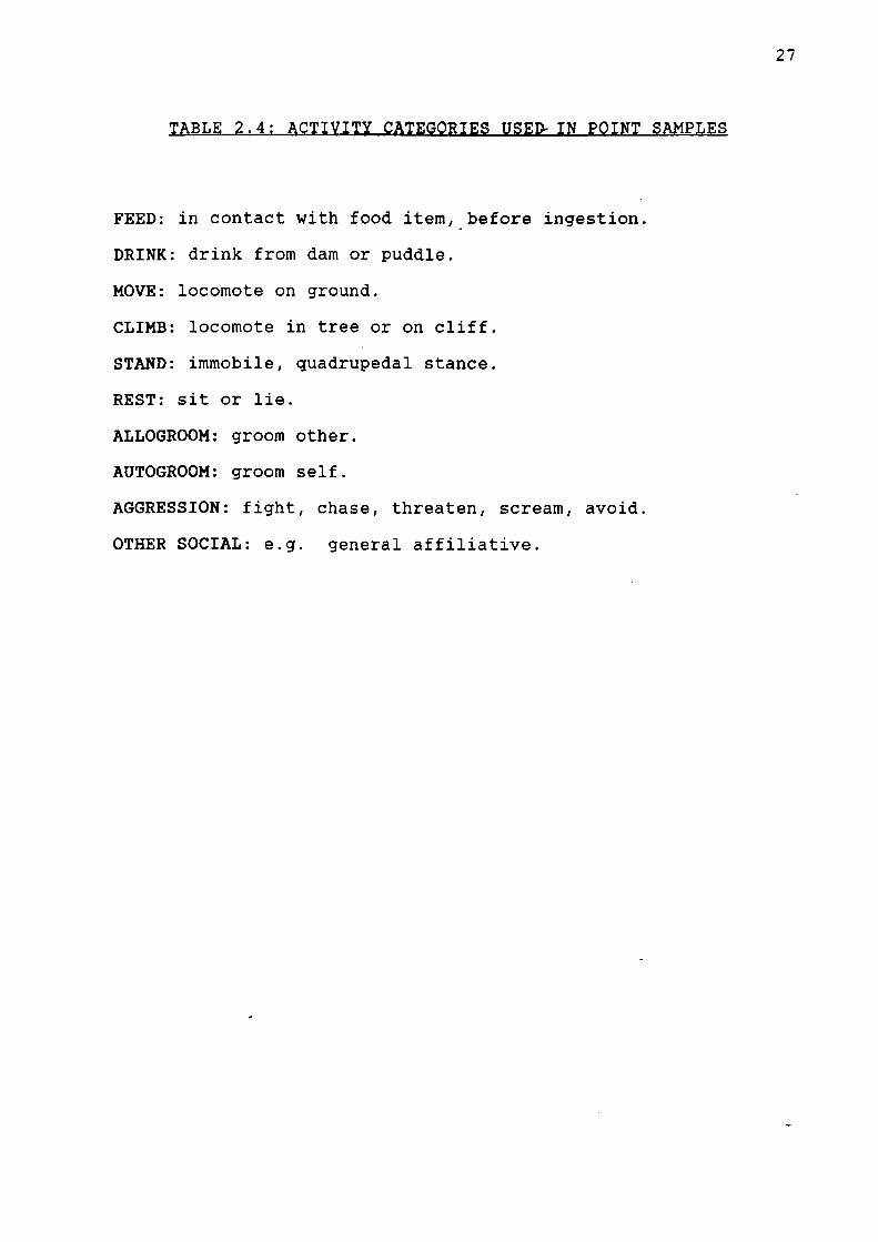
recording of point sample data at 120-second intervals;

activity (see Table 2.4), shade (fully in shade, half in

shade, in full sunshine or sky overcast), nearest neighbour

26

Ige•

TABLE 2.3: SOCIAL AND SEXUAL INTERACTION CATEGORIES

A. Instantaneous behaviours

Affiliative approach: approach with lipsmack,embrace etc.

Lipsmack: rapid and repeated smacking of lips, with orwithout vocalisation.

Threaten: hand slap, eyelid flash, vocalisation,lunge.

Attack: grab, bite, wrestle.

Avoid/grimace: physically or visually avoid, feargrimace.

Scream: fearful, high-pitched vocalisation.

Solicit aid: glance from solicitee to aggressor/aggressee. (i) Succesful (ii) Unsuccessful.

Give aid: attack or chase aggressor/aggressee ofthird party.

Sociosexual: inspect, present, mount, copulate.

Feeding supplant: actor occupies feeding site(within 1 metre) following avoidance byrecipient.

Other supplant: same as above, but not over feedingsite.

B. Timed behaviours

Allogrooming: manual sheafing/searching through fur ofother animal.

Interrupted allogrooming: bouts terminated by third-party intervention.

27

TABLE 2.4: ACTIVITY CATEGORIES USED-IN POINT SAMPLES

FEED: in contact with food item, before ingestion.

DRINK: drink from dam or puddle.

MOVE: locomote on ground.

CLIMB: locomote in tree or on cliff.

STAND: immobile, quadrupedal stance.

REST: sit or lie.

ALLOGROOM: groom other.

AUTOGROOM: groom self.

AGGRESSION: fight, chase, threaten, scream, avoid.

OTHER SOCIAL: e.g. general affiliative.

28

-(identity, activity and distance), number of other individuals

within a ten-metre radius of focal, and habitat type (see

below for details of latter). If the activity was 'feeding',

then the food species and part were also recorded.

Though the data recorded in point samples were instantaneous

samples of behaviour (and therefore had no duration), point

samples took some time to complete and were therefore assigned

a fixed duration of thirty seconds. Thus, each focal sample

consisted of 1380 seconds (1 x 120 s + 14 x 90 s) of

continuous sampling and 450 seconds (15 x 30 s) of point

samples. Point samples interrupted recording of feeding bouts

since it was not possible to keep track of feeding and record

point sample data simultaneously. Feeding bouts in progress

after termination of a point sample were treated as new bouts,

even if they were carried over from a bout that started before

the point sample. Thus, it is not possible to analyse feeding

bout lengths. Tree occupancy and grooming bouts, the other

behaviours for which durations were recorded, were not treated

as interrupted by point samples.

Up to about 16 focal animal samples could be stored in the

memory of the HP-71, and this was more than sufficient

capacity for one full day's data collection (the greatest

number of 30-minute samples I ever managed to collect in a day

was 14). On return to the research house each evening, the

data were transferred onto 130K magnetic microcassettes using

a Hewlett-Packard battery-powered cassette drive. Transfer

from microcassette to mainframe VAX computer in St. Andrews

29

following completion of fieldwork was accomplished using aW.

Hewlett-Packard interface device. Finally, two BASIC programs

(one for point samples and one for continuous samples) were

written to sort the sequentially-recorded data for analysis

using the SPSSX and ALICE statistical packages. Further

details of programming and applications can be found in Whiten

and Barton (1988)

(c) Ad libitum records

To supplement data on social relationships, records were kept

of affiliative and aggressive interactions observed between

identified individuals outside of focal animal samples. These

records involved the same interaction categories as used in

the latter. In addition, ad libitum records were kept of

actual or attempted predations on or by baboons, intertroop

encounters, and new foods eaten.

(d) Ranging

Using a relief map traced from a 1:250 000 scale ordnance

survey map, I recorded occupancy of numbered 1/4 km 2 grid

squares. Every fifteen minutes I assessed which square the

main part of the troop was occupying, and recorded this on a

checksheet throughout the day. The data were subsequently

used in two ways. First, the length of the day journey (day

range length) was estimated by calculating the sum of the

vectors joining the centre of each square successively

occupied. Secondly, the frequency of use of each quadrat was -

30

summed for each month to provide information on the intensity

of use of different parts of the home range.

(e) Demographic records

The following data were collected every day, or failing that,

as often as possible: female sexual state and body condition

(see Tables 2.5 and 2.6), consortships (identities and

behaviour of consort pair, male followers, takeovers), births,

deaths, emigrations and immigrations.

(f) Ecological monitoring

Three days per month were spent monitoring plant phenology and

productivity by a composite of techniques, similar to those

used by Byrne et al. (in press) in their study of mountain

baboons (Papio ursinus). Permanent transects were

established, two of 2 km and one of 1 km in length. These

were located in such a way as to provide a reasonably

representative sample of habitat types. Transects were

oriented either north-south or east-west, and cairns were

built at 200 m. intervals along them to provide a total of 28

permanent sampling points. Provisional unmarked transects

were established in May, the cairns being built with the

assistance of E. Anderson in June and July. Sampling

techniques were as follows.

31

V,

TABLE 2.5: FEMALE SEXUAL STATE CATEGORIES

A. SWOLLEN*

Numbers 1-5 represent increasing degrees of swellingof the sexual skin as the cycle progresses. Ovulation occursin the later stages of swelling, but there issubstantial individual and seasonal variation in themaximum size reached.

1: Vaginal enlargement with or without slightswelling.

2: Downward expansion of swelling to bottom ofischial callosities.

3: Backward expansion, visible from side.

4: Lateral expansion, with or without furtherdescent. .

5: More expanded version of 4.

6: Detumescent.

B. MENSTRUATING: menstrual blood visible prior toswelling.

C. PREGNANT: backdated to last day of detumescence.

D. LACTATIONAL AMENORRHEA: prior to resumption of cycles

1: Infant with natal coat colour (black).

2: Infant with transitional coat colour.

3: Infant brown.

* . .Gilgil/Uaso Ngiro Project protocols

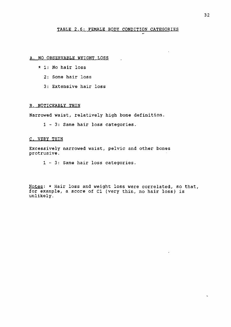
32

TABLE 2.6: FEMALE BODY CONDITION CATEGORIES -

A. NO OBSERVABLE WEIGHT LOSS

* 1: No hair loss

2: Some hair loss

3: Extensive hair loss

B. NOTICEABLY THIN

Narrowed waist, relatively high bone definition.

1 - 3: Same hair loss categories.

C. VERY THIN

Excessively narrowed waist, pelvic and other bonesprotrusive.

1 - 3: Same hair loss categories.

Notes: * Hair loss and weight loss were correlated, so that,for example, a score of Cl (very thin, no hair loss) isunlikely.

33

-

(i) Total herb-laver green biomass. Fluctuations in the gross

biomass of green herbiage were assessed using the pin-frame

method described by McNaughton (1979). Briefly, a count is

made of the number of contacts between green plant material

and four angled wire pins slotted down through holes in the

ridge-piece of a wooden frame. In this case, the procedure

was repeated eight times at each of five grassland plots by

members of the UNBP, as part of their long-term ecological

monitoring. Green biomass was then computed from the mean

number of hits per pin using the following equation:

b=6.3+16.93(h) (McNaughton, 1979)

where b is green biomass in grams dry weight per square metre,

and h is mean hits per pin. Ideally, because of differences

in vegetation structure, the equation should be calibrated

with clipped biomass figures from the particular study site.

However, the calibration is the same for Serengeti and

Amboseli, with widely divergent habitats and rainfall (D.

Western, pers. comm.). Furthermore, since the main concern is

with temporal variation within the site, rather than with the

absolute values of the biomass figures, this is not critical.

These data, collected at approximately six-weekly intervals,

have been made available to me by Dr. Strum. They provide

background information on general food availability for a

greater period than the more detailed quadrat data (see

below). In addition, I collected pin-frame data every month,

between August and December, at six plots on my transects (two

per transect). These (admittedly limited) data could then be

34

compared directly with the quadrat data to give an idea of the-

efficacy of the pin-frame method in estimating an

environmental parameter of relevance to baboon ecology.

(ii) Herb-laver baboon foods. The biomass of baboon foods

found in the herb-layer or loose on the ground was assessed

each month using 0.25 m 2 quadrats. These were placed on the

ground adjacent to marker pegs one metre to either side of of

the cairns, giving a total of 56 quadrats each month

(equivalent to a sample area of 14 m2 ). The number of items

of each food type was counted within each quadrat, including

non-growing items that the baboons picked up from the ground,

such as dried Acacia flowers and seeds. Sampling was carried

out at the same spots each month to avoid introducing "noise"

due to spatial variation in assesssments of temporal

variation. This meant that biomass could not be measured

directly by removing baboon foods for weighing. Instead,

items were collected for drying, weighing and phytochemical

analysis from other sites. The dry weights per item thus

obtained for each food type were then multiplied by the number

of items counted within quadrats to give estimates of biomass.

In many cases, where items comprise discrete units (such as

with individual flowers, fruits and leaves) this procedure was

straightforward. In the case of grass blades, however,

estimates were a little cruder, because it was not considered

feasible to count each individual blade. I therefore counted

the number of average-sized baboon bites available, based on

my observations of the animals feeding, and multiplied these

figures by the dry weights of the average baboon bite. The

35

latter was estimated for each grass and sedge species by

collecting at least one hundred "bites" in a manner as similar

as possible to that observed in the baboons (these estimates

were also used to calculate food intake by focal animals).

Subsequently, the accuracy of the technique was checked for

two grass species by counting bites available in quadrats away

from the transects, predicting the biomass by multiplying the

number of bites by the average dry weight per bite, and then

harvesting, drying and weighing all the available blades

considered edible (coarse, older blades were not generally

eaten by the baboons). The predicted and actual biomass

values were in close agreement for both samples (Cynodon

dactylon, error=7.3%; Cynodon plectostachyus, error=4.9%).

Herb-layer quadrat data are available for the eight-month

period May-December.

(iii) Trees and shrubs. The biomass of baboon foods available

from trees and shrubs was also assessed every month. The

method involved estimating the average weight of food items

per tree or shrub of a given species and size category, and

multiplying this by the density of such individuals within the

home range. Initially I intended to assess density using the

point-centred quarter (PCQ) method developed by Cottam and

Curtis (1956). At each cairn along the transects, four

quadrants were delineated, defined by the intersections of

bearings to the four main points of the compass. The distance

to the nearest tree 3 and to the nearest shrub (at least 50 cm

high) within each quadrant was measured. These were also then -

assigned as "focals" for phenological monitoring by marking

36

with string. Focal trees and shrubs were examined every

month, and scored for percentage presence (0%, 1-25%, 25-50%,

50-75%, 75-100%) of leaves, flowers and fruits or pods. In

the case of known or suspected baboon foods, the total numbers

of items (flowers, pods etc.) were counted, or estimated when

numbers were too great to count directly. These estimates

were obtained in two ways. For shrubs and smaller trees, the

number of items on several branches were counted, the average

number per branch calculated, and this figure multiplied by

the total number of branches. For trees too large to make

counting of every branch feasible, the number of branches in a

vertical section, two arm-spans in width, was counted and

multiplied by the number of these sections in the tree.

Given the problematic nature of estimating absolute densities

from PCQ data where habitats are patchy (Cottam and Curtis,

1956), and the relatively small number of PCQs in the sample,

it was ultimately decided to measure densities more directly,

using appropriately-sized quadrats. At each of the 28 cairns,

quadrats measuring 30 x 30 m were staked out, and the number

of trees and shrubs of each species and size category counted.

Thus the density data were calculated from a total sampling

area of 25,200 m 2 . No Euphorbia nyikae trees appeared in any

of the quadrats because their distribution is very clumped.

Therefore I counted the total number of these trees within the

3 Immature trees, defined as those not exceeding head-height,were ignored. These did not produce significant amounts ofbaboon foods.

37

home range, and calculated density by dividing by the home

range size. Phenological data were not collected for this

species, but the total number of edible stem segments, or

"pads", was estimated in September by counting the number

present on fifteen individuals. Biomass is then given by

b=w(n)/HRS

where w is the mean dry weight of pads

(grams), n is the estimated number of segments within the home

range, and HRS is the home range size (m2 ). In using the same

biomass estimate for each month I assume that availability did

not vary during the study period. This is probably not wholly

warranted, although there were no visually obvious changes in

the condition of trees, apart from a few that became decimated

by baboons, and the food was eaten in nine out of ten study

months (June was the exception). The biomass estimate arrived

at in September is considered to be a maximum value, since all

segments that looked remotely edible were counted, despite the

fact that some of these were probably not acceptable to

baboons. Despite this, the biomass figure arrived at is a

small proportion of the total figures for each month (1.75%

and 0.49% in the months of lowest and greatest total biomass

respectively), so fluctuations in availability, whatever their

magnitude, could not have had an important impact On total

food availability.

(iv) Sedge corms and other underground items. Assessment of

underground food items is highly problematic: the obvious way

is to dig up quadrats and extract , dry and weigh all food

38

items found. Quadrats could not be disrupted in this study

because I returned to monitor the same sites each month.

Partly visible semi-underground items, such as the leaf bases

of sedges, were counted directly in the quadrats, though

variations in their condition could not be directly assessed.

The bases of Mariscus amauropus and Sanseviera intermedia were

eaten in every study month and seemed to be resistant to the

effects of dehydration: samples taken away from quadrats

revealed that the mean wet weight of bases per plant was

greater in the wet season than in the dry (M. amauropus:

wet=0.098 grms., dry=0.076 grms., t=3.63, df=5, P<0.05;

S.intermedia: wet=1.822 grms., dry=1.736 grms., t=2.98, df=6,

P<0.05), but dry weight appears unaffected (M.amauropus:

wet=0.033 grms., dry=0.036 grms, t=0.34, P>0.05; S.intermedia:

wet=0.178, dry=0.190, t=1.01, P>0.05). However, not all bases

are edible (baboons appear very selective about which ones

they pull up, and even then may discard some) so the counts

made were corrected by assessing the proportion of bases in a

random sample that were edible - it is not difficult for an

experienced human observer to distinguish bases which are

obviously inedible from those which are at least fairly

edible.

The corms of the sedge Cyperus blysmoides, an important food

in the baboons diet in the second dry season, are entirely

subterranean and could not therefore be counted in herb-layer

quadrats. Instead, the density of plants was assessed from

the quadrats in June (when new green growth was present). The

mean number of corms per plant was estimated by counting the

39

-,number of plants in a small quadrat (0.1 m 4 ) away from the

transects, digging this up to a depth of six inches, passing

the soil through a fine wire mesh, and counting the number of

corms thus extracted. Finally, corms were collected for

weighing and phytochemical analysis in the dry season by D.

Lochhead and S. Whiten. The biomass of corms within the home

range is then estimated as:

b=w(dn)

where w is the mean

dry weight of corms, d the density of plants, and n the number

of corms per plant. No attempt has been made to assess

variations in the availability of corms, though such

variations are likely to be substantial for the following

reasons. Firstly, the main sites where corms were eaten are

concentrated patches of C.blysmoides, mostly associated with

ancient sites of human settlement; these "corming sites" may

become depleted with extensive use, towards the end of

prolonged dry seasons. Secondly, during the rainy season, the

plants presumably divert nutrients stored in the corms into

the new green growth above ground. During this time it may

also be physically more difficult to dig corms out, due to the

relative profusion of impeding vegetation. In fact, during

this study, C.blysmoides corms were eaten only in the dry

season (August to October) and the short rains (November and

December). In compiling the total baboon food biomass

estimates I have therefore assumed that the corms were

available in those months only. While this assumption is

unlikely to be wholly realistic, including the corm estimate

in the calculation of total biomass for other months does not

40

change the overall rank ordering of months - it simply.....

increases the disparity between wet season and dry season (see

Chapter 3). Furthermore, it is a moot point as to whether a

food can validly be thought of as exerting an influence on

behaviour (such as ranging) at times when it is not actually

eaten. The_only real problem comes in analysing determinants

of what is and what is not eaten at particular times - this is

not something I attempt here.

(q) Weather

Daily precipitation and minimum and maximum shade temperatures

were recorded by members of the UNBP.

(h) Plant material collection and Phvtochemistrv

Samples of plant material were collected whenever possible.

In the case of baboon foods, the number of items or bites was

counted as the plants were harvested. The samples were

immediately sealed in plastic bags and weighed. Samples were

subsequently dried to constant weight under a gas-fired grill

on the minimum setting, a procedure which took a variable

amount of time according to the size and nature of the

material, but not less than 2-3 hours. For each sample a

record was kept of the collection date, the fresh weight, the

dry weight and the number of items or bites. The samples were

tied up in fresh plastic bags and stored in a canvas sack

41

inside a dry, dark cupboard. They were checked periodicallyvt.

for signs of dampness or degradation.

On my return to St. Andrews in February 1987, M. English

carried out analyses of acid detergent fibre (ADF), total

phenolics (tannic acid equivalents), and condensed tannins

(quebracho tannin equivalents) on all samples, and of lipids

(ether extract), and alkaloids (by reaction with Dragendorf's

reagent - see Whiten et al., in press) on some samples.

Subsequently, the samples were also analysed for nitrogen

content by the Panmure Trading Company, Monikie Granary,

Dundee, using the micro-Kjeldahl method; protein content is

then estimated by N 2 /6.25 (Crampton and Harris, 1979). The

results are given in Appendix III.

(i) Habitat map

A bipartite system for classifying habitat types within the

study area was established on the basis of the density and

species dominance of trees and shrubs. Further distinctions

were made according to whether habitats were associated with

watercourses or dams, or had a sparse or relatively abundant

herb-layer. Kopjes were distinguished as a habitat - type in

their own right since they have a distinctive vegetative make-

up. No attempt was made to classify habitat types on the

basis of the species composition of the herb-layer. The

habitat classification system is detailed in Figure 2.4.

, lll llll ...........

2. Open: grasses and herbs dominant, tree/shrub cover 0-25%.

3. Light bush: tree/shrub cover 25-50%, canopy overla p rare.8. Light bush: with stony/rocky ground (at least 50% of

surface).

4. Thick bush; tree/shrub cover 50-75%, canopy overlap frequent.7. Thick bush: In strips along watercourses.

9. Thick bush: with stony/rocky ground.

r-..... Q.C? Y....

5. Forest: tree/shrub cover 75-100%, canopy overlap extensive.6. Forest: in strips along watercourses.

10. Kopjes and rocky ridges.

Habitat subtypes by dominant tree/shrub

a. Acacia etbaica b. A. mellifera c. A.etbaica/A.mellifera

d. A.tortilis e. A.brevispicata f. Lycium europaeum

j. A.nilotica k. Commiphora coricea/C.schimperi

m. A.xanthophloea n. A. seyal.

Figure 2.4: Habitat Classification System, Each density typeis split into sub-types accordirm to the dominanttree or shrub. Missing sub-types from the table(g,h,i,l)are those that occurred only in very smallpatches, beneath the resolution of the habitat map.

42

Having defined habitat types the scheme was used in two ways.Ir•

Firstly, the habitat type occupied by the focal animal was

recorded in point samples, and breakdowns of habitat occupancy

in different months were then compiled. Secondly, a habitat

map was produced in order to estimate the percentage of the

home range covered by each of the habitat types. The two sets

of results could then be put together to calculate habitat

selectivity (Chapter 3). The habitat map was drawn up by

tracing vegetation boundaries, viewed by walking along ridges

and other high points, onto a transparency overlying the

topographical map of the area. Each vegetation zone was

labelled. The resulting map was subsequently analysed by D.

Davies using a 3-dour plane "Pluto" graphics workstation.

The procedure involved reproducing the map on a colour monitor

by tracing the outline of each vegetation zone using

interactive graphics procedures, and uniquely labelling each

zone type with an assigned colour. A program to count the

number of pixcels of each colour was then run, producing a

breakdown of the relative area of each habitat type (see

Chapter 3 for results).

li) Statistical methods

Parametric tests have been used in preference to nonparametric

tests wherever possible, due to their greater power (Sokal and

Rolf, 1981). This has, in many cases, necessitated

transforming the raw data in ways appropriate to the

assumptions of particular tests. Facilities for checking

assumptions within SPSSX routines were used (e.g. the

"condescriptive" routine for assessment of departure from the

43

normal distribution, and procedures for analysis of residuals

in regression). Where assumptions were not met by the raw

data, I have followed Sokal and Rolf (1981), who recommend

data transformations appropriate to particular problems. In

general, logarithmic transformation was found to be effective

in linearising relationships in correlations and regressions,

and in normalising positively skewed distributions and

stabilising variances correlated with means in ANOVAs. Where

data were expressed as percentages or proportions, the arcsine

transformation was routinely used. In t-tests, separate

variance estimates were used wherever variances showed

significant heterogeneity. Finally, where data were

inherently ranked (e.g. as in dominance rank), or where

transformation was ineffective in satisfying assumptions,

nonparametric methods were used. Tests of significance are

all two-tailed, unless otherwise stated.

N.B. In the continuous focal sampling of feeding, bites offoods which varied in size, such as bunches of grass blades,were differentiated according to their size (small, medium andlarge). Specific estimates of the dry weight per bite werethen generated for each size category of each of these foods.One bite constituted one hand-to-mouth action.

44

CHAPTER 3: VEGETATION, FOOD AVAILABILITY AND HABITAT USEW.

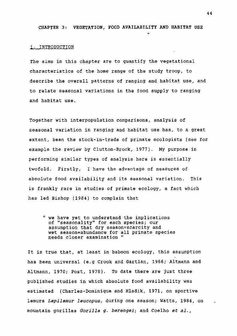
1. INTRODUCTION

The aims in this chapter are to quantify the vegetational

characteristics of the home range of the study troop, to

describe the overall patterns of ranging and habitat use, and

to relate seasonal variations in the food supply to ranging

and habitat use.

Together with interpopulation comparisons, analysis of

seasonal variation in ranging and habitat use has, to a great

extent, been the stock-in-trade of primate ecologists (see for

example the review by Clutton-Brock, 1977). My purpose in

performing similar types of analysis here is essentially

twofold. Firstly, I have the advantage of measures of

absolute food availability and its seasonal variation. This

is frankly rare in studies of primate ecology, a fact which

has led Bishop (1984) to complain that

n we have yet to understand the implicationsof "seasonality" for each species; ourassumption that dry season=scarcity andwet season=abundance for all primate speciesneeds closer examination "

It is true that, at least in baboon ecology, this assumption

has been universal (e.g Crook and Gartlan, 1966; Altmann and

Altmann, 1970; Post, 1978). To date there are just three

published studies in which absolute food availability was

estimated (Charles-Dominique and Hladik, 1971, on sportive

lemurs Lepilemur leucopus, during one season; Watts, 1984, on

mountain gorillas Gorilla g. berengel; and Coelho et al.,

45

1976, on howler monkeys Alouatta villosa and spider monkeys

Ateles geoffroyi). There is one study on mountain chacma

baboons (Papio ursinus) in which overall food availability was

measured (Byrne, Whiten and Henzi, in press), which, indeed,

laid the methodological groundwork for this study. To my

knowledge, however, there have been no previous studies of

savannah baboons in which plant food biomass was measured,

despite the great potential value of such data in comparative

work, and, excepting the three-month study by Charles-

Dominique and Hladik (op cit.) no studies of any primate in

which monthly variation in plant food biomass was quantified.

Perhaps some of the responsibility lies with Clutton-Brock

(1977), who has stated that

...it is (and may always be) virtuallyimpossible to measure variation in overallfood availability. "

Having tried it, I believe Clutton-Brock's assertion to be

overly pessimistic (and I thank my supervisors, Andy Whiten

and Dick Byrne, for persuading me of both the possibility and

the desirabilty of such measurement, while Shirley Strum

introduced me to the pin-frame method of estimating total

herb-layer green biomass). These measures permit a more

rigorous, quantitative approach to the analysis of temporal

covariation between behaviour and environment, although it

should be stressed that my conclusions will of necessity be

somewhat limited by the relatively short period of my study

(twelve months of the six-weekly pin-frame estimates, but only

eight months of actual baboon food biomasses). Analyses will

be extended in future publications by incorporating data

46

collected using the same methods in subsbquent years (by D.

Lochhead and others).

-Clutton-Brock (op cit.) warns that, even if it is feasible to

measure availability of foods selected, this may be a poor

estimate of overall availability if feeding becomes less

selective when food is short - presumably the point is that

marginal foods will not have been included in the earlier

estimates, hence rendering comparisons problematic. However,

this can probably be dealt with by incorporating all items

which it seems likely or possible will be eaten at some stage.

Of course, no monitoring system can be perfect, and,

inevitably, certain foods will not be sampled adequately or at

all. But so long as availability of most foods, and of all

the important ones, is adequately measured, it will be valid

to calculate estimates of overall biomass and to assess

seasonal variation.

The second purpose of including analyses of food availability

and behavioural correlates is to inform the analysis of

individual differences in behaviour and foraging strategies,

issues central to this study, by setting these in ecological

context. There is the general point that, in trying to

understand the adaptive significance of individual behaviour,

it is important to know as much as possible about the

ecological constraints acting on the social unit as a whole.

The interpretation of sex differences in nutrition, for

example (see Chapter 6), depends on our understanding of what

foods are available and in what quantities. More

specifically, the issues of seasonality and of social

47

strategies are directly related, at leaft with respect to one

major theoretical model of the ecology of primate social

structure (Wrangham, 1980) - this link will be explored in

Chapter 7.

In the analyses that follow, I begin by assessing the habitat

structure of the home range, and seasonal variation in food

availability. I examine the influence of rainfall and address

the issue of the wet season/dry season dichotomy.

Subsequently I describe ranging patterns and habitat use, and

relate seasonal variations in these to variations in the food

supply.

2. RELATIVE ABUNDANCE OF HABITAT TYPES

The percentage of the home range covered by each habitat type,

assessed by the method described in Chapter 2, is given in

Table 3.1. This demonstrates the overwhelming preponderance

of Acacia dominated woodland and wooded grassland.

A.mellifera, A.etbaica and A.tortilis zones predominate,

principally at medium densities, together making up about 81%

of the home range. The habitat map in Figure 3.1 indicates

that A.tortilis zones are found principally in the east of

the home range (as suggested in Chapter 2), being associated

with dryer, well-drained slopes. The denser woodlands tend to

be associated with seasonal watercourses and with dams. Note

that missing species (e.g Ficus ingens) occurred in patch

sizes beyond the resolution of the habitat map. The data in

48

TABLE 3.1: PERCENTAGES OF HOME RANGE COVERED BY EACH

SPECIES

HABITAT TYPE

TYPE

•nn•

DENSITY

TYPE 2 3 4 5 6 7 8 TOTAL

A 0.86 9.30 13.42 0.13 0.99 1.10 0.29 26.09

B 2.92 20.65 8.40 0.80 0.28 0.27 33.32

C 0.59 3.18 3.77

D 0.63 18.69 2.77 0.01 0.12 0.06 0.11 22.39

E 0.04 0.18 0.22

F 0.06 0.06

J 0.04 0.04

K 0.10 0.15 0.25

M 0.67 0.67

N 1.09 1.09

OTHER 2.26 1.05 2.46 0.06 0.06 0.56 6.45

KOPJE 6.06

TOTAL 6.67 50.42 30.48 1.00 2.06 2.58 1.14 100

Notes: A=Acacia etbaica; E=A.mellifera; C=A.etbaica/melliferamixed; D=A.tortilis; E=A.brevispicata; F=Lyciumeuropaeum; J=A.nilotica; K=Commiphora coricea/schimperimixed; M=A.xanthophloea; N=A.seyal.2=Open; 3=light bush; 4=thick bush; 5=forest;6=forest along watercourse; 7=thick bush alongwatercourse; 8=light bush, stony ground.

• 31(4

ii 414• 49II14c• 40• 4E• 4K• S• SAIsm

KEY:

f---- 1 Km

• 2 160• 2 A128120

•68•unMum3 • 7

FIGURE 3.1: HABITAT MAP 130 70138 17811 3C 170

See Table 3.1 (P.48) for legend to key 130 711131 • a

118A88

• 8D• 8EW OW AKE

49

Table 3.1 are used to calculate habitat selection ratios in

section 5(ii).

3. SEASONAL VARIATION IN FOOD AVAILABILITY

Estimates of food availability during the study period are

plotted in Figures 3.2 and 3.3. In the first graph, three

types of biomass estimate are shown; the total biomass of

green herb-layer vegetation on grassland plots (six-weekly

pin-frames, courtesy of U.N.B.P., January-December), the total

biomass of green herb-layer vegetation on transects (monthly

pin-frames, August-December), and the biomass of . baboon foods

(monthly quadrats, May-December). In Figure 3.3, the quadrat

data are replotted on a larger scale, for greater clarity, and

divided into the protein and non-protein components.

Preliminary inspection suggests that rainfall was a strong

influence on biomass of both total herb-layer vegetation and

of baboon foods - herb-layer biomass peaked in June, in the

second half of the rainy season, then declining until the

start of the short rains in November. Biomass of baboon

foods, sampled over a shorter period, shows the same pattern

of decline during the dry season (August-November) followed by

an increase during the short rains. On average, baboon food

biomass was greater in wet months than in dry months (Figure

3.4), though the difference is not quite significant (t=2.54,

df=4, p=0.064). However, when protein biomass alone is

considered, the difference is significant (t=3.08, df=4,

0

-

41

nn••

FIGURE 3.2: VARIATION IN BIOMASS OF TOTAL HERB-LAYERVEGETATION AND BABOON FOODS

80

JAN FEB MAR APR MAY JUN JUL AUG SEP OCT NOV DEC

MONTH

D=Dry seasonW=Wet season

• U.N.B.P. PIN-FRAMES

• TRANSECT PIN-FRAMES

II QUADRATS

Pin-frames measure totalherb-layer green biomass(6-weekly, Jan-Dec).Quadrats measure totalavailable baboon food(monthly, May-Dec).

MEI

FIGURE 3.3: VARIATION IN TOTAL AND PROTEIN BIOMASS OF BABOON FOODS

W=Wet seasonD=Dry season

E2 PROTEIN

0 NON-PROTEIN

Total dry weight andprotein weight ofbaboon foods measuredwithin 30x30m.quadrats (trees andshrubs), and0.5x0.5m. quadrats(herb layer).

MAY JUN JUL AUG SEP OCT Nat EECMONTH

(1986)

1

7A

e

nn•••••

FIGURE 3A: S ASONAL DIFFERENCE IN TOTAL ANDPROTEIN BIOMASS OF BABOON FOODS

WET DRYSEASON(1986)

PROTEIN

0 NON-PROTEIN

Average dry weight

and protein weightof baboon foods in

5 wet and 3 dry season

months (methods as in

Figure 3.3).

50

p=0.037). It is therefore possible to confirm that variation-

in food availability conforms to the common assumption of dry

season scarcity and wet season abundance. Nevertheless, the

overall difference is perhaps not as clear-cut as might be

expected, and this is apparently because a time-lag effect

slightly complicates the picture: November was the month of

lowest food availability despite ranking third out of the

eight months in terms of total rainfall. Conversely,

December, which had less rain than November, ranked second

overall in terms of baboon food biomass. This is not

surprising because sampling was carried out in the middle of

each month, so the effect of each month's rainfall could only

be partially apparent in the corresponding biomass estimate.

The correlation between baboon food biomass and monthly

rainfall (r=0.588, df=6, p=0.069) is not as strong as that

between the former and rainfall in the previous month

(r=0.607, df=6, p=0.055). There is also likely to be a

cumulative effect of rainfall, wherein biomass gradually

increases as plants continue to grow and produce reproductive

parts: indeed, the correlation between biomass and the

rainfall total for the previous two months is stronger still

(r=0.670, df=6, p=0.035).

In comparing the pin-frame and quadrat data, it is clear that

total herb-layer green biomass while being considerably

greater (especially on grassland plots), follows the same

pattern of seasonal variation as the more fine-grained baboon

food biomass estimates. There is a high correlation between

quadrat data and the pin-frame data taken at the same plots

for the period August-December (r=0.970, df=3, p=0.003). This

51

suggests that the major factor in the aNiailability of baboon

foods is the condition of the herb-layer, a notion supported

by inspection of Figure 3.5, which shows that variation in

fresh herb-layer foods (grass blades, herb leaves, shoots,

flowers and fruits) effectively swamps variation in other

foods; in the wet season, by far the majority of the biomass

was made up of this element, and when it died back in the dry

season, the availability of foods like Acacia flowers and

pods, which are less tied to immediate rainfall patterns, was

not sufficient to compensate.

As noted in Chapter 2, I have made the rather unrealistic

assumption that Cyperus blysmoides corms, a major dry season

food, are available only in months when they were eaten

substantially (more than 1% of time spent feeding). Thus, in

the biomass estimates, corms only contribute to the totals in

five out of eight months (August-December), three of which

were dry season months. There is a possibility that corm

availability actually changed very little, and that the

baboons simply became less selective in the dry season.

However, corms were eaten in December, when overall food

availability was high, suggesting that a reduction in

selectivity cannot be the only reason for corm eating.

Nevertheless, it is worth examining the effect of relaxing the

assumption that corms were available only in months when

eaten. The main effect would be to increase the wet

season/dry season disparity, thereby strengthening the case

for the importance of rainfall. Similarly, if the assumption

that corm availability did not decrease through depletion

during the dry season was relaxed, this would also increase

1 0

FIGURE 3.5: VARIATION IN COMPONENTS OF BIOMASS OF AVAILABLE FOOD

MAY JUN JUL AUG SEP OCT NOV DEC

MONTH(1986)

W=Wet season

D=Dry season

0 CORMSII TREESANDSHRUBS11 HERB-LAYER(DRY)

0 HERB-LAYER(FRESH)Area graph displaying

monthly variation in majorcomponents of baboon foodbiomass (methods as for

Figure 3.3).

.--. 6.0 -

LU

X

4 .0 -›-cC

4 2 .0 -0co

' 1 • 1 • 1 • 1 • IMAY JUN JUL AUG SEP OCT NOV DEC

MONTH

(1986)

0.0

FIGURE 3.6: VARIATION IN AVAILABILITY OF FOOD TYPES

W=Wet season

D=Dry season

D an-ER

El ACACIA SEEDS/PODS

El ACACIA FLOWERS

El CORMS

O SEDGE BASES

n HERB FLOVVERS

• SHRUB FRUITS

El HERB FRUITS

O GRASS SEEDHEADS

el SHRUB LEAVES

IN HERB LEAVES

O GRASS BLADES

Area graph displaying monthlyvariation in biomass of

major food types (methods as

for Figure 3.3).

52

the disparity. In summary, the simplifying assumptions made

are conservative with respect to the dichotomy between dry

season scarcity and wet season abundance, though this

obviously does not help us to understand the observed

variation in corm consumption.

The general validity of the wet/dry dichotomy might be

challenged on the basis that the period for which baboon foods

were sampled was only eight months - not even a full annual

cycle. Things might be different in the long dry season

(January-March), or in different years. What if some dry

seasons see the simultaneous production of large amounts of

Acacia flowers and pods, for example? Two main arguments can

be advanced against this. Firstly, it appears that the

phenology of other plants is also to some extent affected by

immediate rainfall patterns. Table 3.2 displays correlations

between the biomass of particular food types and rainfall (a)

for the same month, (b) for the previous month, and (c) for

the previous two months. It can be seen that rainfall has a

strong impact on herb-layer foods as expected, but also to an

extent on production of shrub leaves. The correlations

between biomass and rainfall in the previous two months are

positive, though not significant, for shrub frUits and Acacia

leaves. These trends will tend to emphasize the impact of

rainfall. The only significant negative correlation is

between biomass of Acacia flowers and rainfall in the previous

month, reinforcing the impression that these are produced

mainly in the dry season. This could be the result of a

longer time-lag, with rainfall stimulating the initiation of

reproductive cycles which culminate in the production of

53

TABLE 3.2: PEARSON CORRELATIONS BETWEEN RAINFALL ANDBIOMASS OF BABOON FOODS

SAME

MONTH

PREVIOUS PREVIOUS TWO

TOTAL BIOMASS 0.587 0.617* 0.670*

HERB/GRASS FOLIAGE 0.793 ** 0.889** 0.815**

HERB FRUITS 0.640* 0.561 0.803**

HERB FLOWERS 0.381 0.554 0.795**

SHRUB FOLIAGE 0.370 0.595* 0.172

SHRUB FRUITS -0.404 -0.043 0.349

ACACIA FLOWERS -0.541 -0.635* -0.547

ACACIA PODS -0.041 0.153 0.031

ACACIA FOLIAGE -0.036 0.440 0.385

* p<0.05 ** p<0.02

flowers and pods some months later. This idea is supported by

the observation that production of A.etbaica flowers failed

almost entirely in September 1987 following poor rains

(D.Lochhead, unpublished data).

Given that the production of Acacia reproductive parts is by

no means restricted to the wet season, what is the likelihood

that in some dry seasons, in particular the long dry season

between January and March, these compensate for the paucity of

herb-layer and other vegetation? Firstly, data from the year

following my study do not support this idea (D.Lochhead, in

prep.). Secondly, in the long dry season of 1986, A.mellifera

and A.tortilis both flowered and then produced seed pods, but

asynchronously, and A.mellifera pod production did not peak

until the following wet season (information from field notes).

54

A.etbaica did not flower. Thus, at no time was there a single.e.

synchronised peak of production that could have made a

substantial difference to the conclusion that dry seasons are

times of relative scarcity.

4. IMPLICATIONS OF SEASONALITY FOR BABOONS

I have argued that food availability for the study troop was

strongly related to patterns of rainfall distribution. This

will perhaps come as no surprise to savannah ecologists, since

" It is well known that there is a relationshipbetween rainfall and primary production inarid and savannah habitats " (Delaney andHappold, 1979).

However, this is the first formal demonstration that the

relationship applies within the range of items eaten by

baboons. I do not wish to overstate the case for a simple

distinction between wet and dry seasons; after all, the

definition of seasons is arbitrary, and, as we have seen,

there are time-lag effects whose magnitude probably varies

according to the type and size of plant (new grass growth

appears within one or two weeks of the onset of rain, while

Acacia reproductive cycles are more likely to be influenced by

cumulative rainfall over a period of months, and perhaps even

years).

One important implication of these findings is that they

suggest that seasonal energy bottlenecks may occur. Such

bottlenecks can only be validly defined in terms of effects on

55

baboons, and the demonstration of fluctuations in food

availability does not in itself tell us -much about constraints

on baboons; it is possible that, even during the dry season,

animals are not significantly energy-limited (Coelho et al.,

1976; but c.f. Cant, 1980). This could be the case, for

example, if the primary regulator of population density was

predation. Also, characteristic of baboons is that they are

well equipped to ameliorate the effects of seasonal

bottlenecks by their ability to utilise a very wide range of

food types, from the tops of the trees to below ground

(Altmann and Altmann, 1970; Hamilton et al., 1978; Post, 1978;

Norton et al. 1987; Whiten et al., 1987). In fact, as I willshow, there are very good reasons for believing that, in STT,

females in particular face significant energetic constraints

which increase in severity during the dry season. This seems

to be true to some extent even in a "normal" year, when there

are two good rainy seasons (as during my study), minimising

the extent of the dry season hiatus - there was approximately

a three-and-a-half-fold difference in biomass between the

months of greatest and lowest food availability. It is

therefore no surprise that the effective failure of the short

rains at the end of 1987 resulted in dramatically reduced body

condition and increased mortality amongst adult females and

their infants (I.Saunders, unpublished data). It is possible

that such droughts are a factor of major importance in the

ecology and population dynamics of these baboons.

The use of space and time are central considerations in the

evaluation of ecological constraints acting on animals

(MacArthur and Pianka, 1966; Altmann, 1974; Krebs, 1978). An

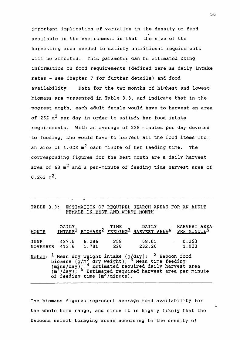
56

important implication of variation in the density of food

available in the environment is that the size of the

harvesting area needed to satisfy nutritional requirements

will be affected. This parameter can be estimated using

information on food requirements (defined here as daily intake

rates - see Chapter 7 for further details) and food

availability. Data for the two months of highest and lowest

biomass are presented in Table 3.3, and indicate that in the

poorest month, each adult female would have to harvest an area

of 232 m2 per day in order to satisfy her food intake

requirements. With an average of 228 minutes per day devoted

to feeding, she would have to harvest all the food items from

an area of 1.023 m 2 each minute of her feeding time. The

corresponding figures for the best month are a daily harvest

area of 68 m2 and a per-minute of feeding time harvest area of

0.263 m2.

TABLE 3.3: ESTIMATION OF REQUIRED SEARCH AREAS FOR AN ADULTFEMALE IN BEST AND WORST MONTH

DAILY TIME DAILY HARVEST AUAMONTH 3NTAKE1 BIOMASS2 FEEDING— HARVEST AREAS PER MINUTE2

JUNE 427.5 6.286 258 68.01 . 0.263NOVEMBER 413.6 1.781 228 232.20 1.023

Notes: 1 Mean dry w0ght intake (g4day); 2 Baboon foodbiomass (g/m4 dry weight); 3 Mean time feeding(4ns/day); 4 Estimated required daily harvest area(m 4 /day); 3 Estimated required harvest area per minuteof feeding time (m4/minute).

The biomass figures represent average food availability for

the whole home range, and since it is highly likely that the

baboons select foraging areas according to the density of

57

resources, the data in Table 3.3 probably overestimate

required harvest areas, and hence time-budgeting constraints.

Set against this, however, is the certainty that individuals

do not harvest every item within the area in which they

forage; some are inevitably missed, and some may be rejected

because they are nutritionally sub-optimal in terms of what

else is available and what else is needed to balance the

animal's diet that day. Because of these factors, it is not

possible to assess the absolute accuracy of the harvesting

area estimates, but the data serve to emphasise the.likely

effects of variation in food availability on ranging and

activity budgets. Note, however, that the prediction of a

seasonal difference in the harvesting area needed to satisfy

intake requirements depends on the assumption that overall

changes in biomass are at least partly a function of changes

in the density of food items within patches, and not simply of

a reduction in the number or size of patches (this is

discussed in the next section). It may seem puzzling that the

amount of time spent feeding was lower in November than in

June, thereby apparently further increasing the harvesting

area needed for each minute of feeding time. Why did the

baboons not "try harder" when conditions were worse? The

answer is that they may have done; this can only be evaluated

by reference to time spent foraging, since the feeding time

budget only reflects actual manipulation and ingestion of

food, not searching. This subject is taken up in Chapter 5,

while seasonal variation in ranging is examined in succeeding

sections of this Chapter.

58

5. SPATIAL DISTRIBUTION PATTERNS OF FOOD AND THE PROBLEM OFPATCHINESS

Vl. 0

In addition to gross abundance, much attention has been

devoted by primatologists to the relevance of spatial

distribution patterns of foods to a number of demographic and

behavioural variables. These include group size, composition

and stability, territoriality, ranging patterns and inter- and

intragroup social relations (e.g.Crook and Gartlan, 1966;

Altmann, 1974; Clutton-Brock, 1974; Klein and Klein, 1977;

Waser, 1977; Lindburg, 1977; Dunbar, 1977; Wrangham, 1977,

1980,1986; Clutton-Brock and Harvey, 1977a; Whitten, 1983).

In particular these and other authors have referred to the

"patchiness" of resources. However, variables such as

"patchiness", "patch size" and "inter-patch distance" are

notoriously difficult to quantify (Wrangham, 1983; Krebs and

McCleery, 1984). It is rare that clear patch boundaries exist

in natural situations, so the definition and measurement of

patches will always be somewhat arbitrary and subjective. One

solution to the problem of patch size is to measure the

"survival time" between animals entering and leaving patches,

controlling for the number of animals involved (White, 1989).

The amount of time taken to exhaust patches can then be used

as a measure of relative patch size, at least within a

species. This approach suffers from essentially the same

problem encountered in measuring a patch directly; where (and

when) does the patch start and finish? The problem may be

minimal for animals feeding mostly or exclusively in trees,

since each separate tree can often be considered an individual

patch. For baboons, which gather a great deal of their food -

from the herb-layer and beneath, the approach would not be

59

viable. Indeed, it is a moot point whether the concept of

patches is a useful one at all in this context, because it

seems inevitable that "patches" will tend to be contiguous,

overlapping and even concentric.

These methodological and conceptual problems with patches seem

to rule out comprehensive quantitative analysis involving

unitary measures of patchiness. This is not to say that

spatial heterogeneity is unimportant, for this or any other

population of primate, nor even that attempts should not be

made to assess it in some way. It is clearly crucial to

understanding variation in patterns of intragroup competition,

for example (see Chapter 7). Extensive investigation of

seasonal variation in heterogeneity is outside the scope of

this project, so this discussion will be based largely on

qualitative observations supplemented by data on spatial

variance in food density.

During the wet season the major food sources were grasses,

herbs and shrubs, with a variable amount (0.2-10.0%) being

derived from trees. In the dry season dietary diversity was

lower (see Chapter 6) and the major food sources were Acacia

trees (flowers and pods) and sedge corms (Cyperus blysmoides)

and bases (Mariscus amauropus). The pads of the succulent

tree (Euphorbia nyikae) were an important food in-the first

dry season.

The first point to make is that, assuming that the

distribution of particular plant species is not entirely

homogenous, it is reasonable to expect that a reduction in the

60

number of available food species will automatically result in

an increase in patchiness. Secondly, wet season foods appear

to be intrinsically more evenly distributed than the dry

season foods; the grasses and herbs that provided the

foliage, flowers and fruit eaten" extensively in the wet season

covered the ground almost everywhere, and in many places

occurred in large meadows capable of accomodating the whole

troop, even when individuals were spread widely apart. In

contrast, flowering and fruiting Acacia trees could often be

clumped in distribution because, while extensive woodlands of

the three main food species occurred in many parts of the home

range, the production of reproductive parts was to an extent

asynchronous. This meant that "rich pickings" were frequently

restricted to relatively small groves within particular areas,

and even to individual trees. The leaf bases of Mariscus

amauropus did not appear to be a clumped resource, on any

scale, but the corms of the other important sedge, Cyperus

blysmoides, did. The latter were dug almost exclusively from

relatively well-defined, isolated patches of ground, between

about 30 and 75 metres in diameter; these "corming sites"

appeared to occur at the old and long-disused sites of

settlement by nomadic pastoralists. Finally, specimens of

Euphorbia nyikae occurred in fairly large clumps, mostly

associated with kopjes and other rocky outcrops, and were

entirely absent from large tracts of the home range.

A more formal way of examining these trends is to compare the

average biomass for the home range with the maximum biomass

within food patches. I have estimated the latter by

extracting data for individual herb-layer quadrats (0.25 m2)

61

and for individual trees. The month of greatest average

biomass, at the height of the wet seasoh, was June, with 6.286

g/m 2 ; the maximum biomasses at this time, recorded from the

top two quadrats, were 40.588 g/m 2 and 32.374 g/M 2 . Thus,

within-patch biomass was 5-6.5 times greater than the average

biomass. Assuming that fresh herb-layer vegetation made a

negligble contribution to the biomass and diet at the height

of the second dry season (see Figure 3.6 and Chapter 6), it is

valid to concentrate on Acacia products and corms for this

period (biomass data are not available for the first dry

season). Within patch-biomass of Acacia flowers is obtained

by

Biomass = wn/a

where w is the dry weight of

the average flower, n is the number of flowers in the tree and

a is the canopy area of the tree (diameters of all sampled

trees were measured when transects were established).

The two greatest recorded within-patch biomasses for A.etbaica

flowers in September (approximately 60% of the diet) were

38.011 g/m2 and 36.256 g/m2 (13.2-13.8 times greater than the

average). For A.tortilis flowers (30% Of the diet in October)

they were 35.774 g/m2 and 32.386 g/m2 (14.6-16.2 times greater

than the average). The average biomass of corms of Cyperus

blysmoides at sites used by the baboons was 42.901 g/m 2 (14.1-

19.4 times the overall biomass during dry season.months).

These data suggest seasonal variability in the extent to which

available resources were spatially clumped; although overall

biomass was up to 3.5 times greater in the wet season than in

62

the dry season, the maximum biomass within patches of the most

important foods was actually very consistent.

So far no attempt has been made to assess the scale of spatial

heterogeneity. The significance of the observation that

biomass is distributed more patchily in the dry season is

difficult to interpret without knowing something about the

size of patches (real or abstracted) and the distance between

them. If local concentrations of biomass are large but spaced

widely apart, this may affect ranging but not intragroup

competition. Conversely, if such concentrations are small

relative to troop size, both variables may be affected. If

patches are both small and close together, then neither

ranging nor competition may be significantly affected.

The solution to the problem of scale is not at all obvious.

Whitten (1983) related the extent of feeding competition

within troops of vervet monkeys (Cercopithecus aethiops) to

the non-randomness of distribution of food species. She

assessed the latter as the ratio of the variance to the mean

number of individuals per sample point. This is a good

measure of the extent to which particular species occur in

clumps, but it is difficult to interpret its relevance to

behaviour because it is entirely dimensionless; "clumping" by

this definition is an abstract concept unrelated ' to the scale

at which the monkeys operated. It is therefore not surprising

that Whitten felt it necessary to support her arguments with

qualitative descriptions. For example, in her study doum

palms (Hyphaena coriacea) were randomly distributed according

to the criterion used, yet rank-related differences in feeding

63

were apparent. The anomaly was explained by the observation

that fruits were clumped on a smaller scale, within individual

trees. This is perfectly convincing, but it serves to

illustrate the problematic nature of scaleless measures of

spatial heterogeneity.

Perhaps the problem of rigorous quantification is

insurmountable. However, the observation that spatial

heterogeneity varies between seasons, at least in an abstract

sense, is a useful starting point, since it allows for the

possibility that behaviour is affected, although from thispoint on I am restricted to subjective evaluations. What

evidence is there that increased patchiness in the dry season

was of a scale that would influence (a) ranging, and (b)

intragroup feeding competition?

My strong impression was that, during the dry season, more

time was spent by the baboons traveling between localised food

sources such as Acacia groves, corming sites and waterholes,

with little or no feeding on the way. In the wet season,

bouts of feeding and moving appeared less distinguishable, the

large expanses of herb-layer greenery providing a rich

substrate for continuous "travel-feeding" (Whiten et al.,1987). The data already presented on within-patch biomasses

suggest that, contrary to the conclusions derived from Table

3.3, the required harvesting areas would not necessarily

increase as average biomass decreased. Therefore, seasonal

changes in day range length, evaluated in the next section,

are most likely to be principally related to effects on the

between-patch travel component.

64

With respect to intragroup interactions, there is also

evidence that "effective" patchiness increased during the dry

season, resulting in greater levels of competition. Some of

the groves of flowering Acacias visited by the baboons were

extensive, with many trees simultaneously in flower. Others,

however, comprised just a few trees, often with one or two

larger individuals plainly being the richest source of food,

and attracting high densities of baboons. Fallen flowers,

which accumulated on the ground in small drifts, were also

eaten. As already mentioned, corms of Cyperus blysmoides were

concentrated in relatively discrete patches 30-75 metres in

diameter - not large relative to the size of the troop - and

spatial clustering of feeding animals was greater for this

food than for any other. Seasonal differences in feeding

competition and their relationship with resource

characteristics are explored further in Chapter 7.

6. PATTERNS OF RANGING AND HABITAT USE

(a) Home range size

The size of the home range (HRS) was estimated by summing the

km2total number of 1/4 K quadrats entered throughout the 12-

month study period (January-December, 1986). These formed a

coextensive block, enclosing only one quadrat which was never

seen to be entered. The HRS given by this method was 43.75

km2 . To check that this estimate represents the asymptotic

function of study time, I have plotted the cumulative estimate

obtained for each month in the method of Sharman (1981). This

shows that the final estimate does indeed represent a near-

50

40-

30-

20-

10 -

0 - , I I I I I- I I I 1 I

JAN FEB MAR APR MAYJUN JUL AUG SEP OCT NOV CEO

MONTH(1986)

FIGURE 3.7: MONTHLY CHANGES IN HOME RANGE SIZE ESTIMATES

Cumulative home range

size estimated by

summing the area of

quadrats entered by the

end of each month.

65

asymptotic value, vindicating the assumption that the study...

duration was sufficient to yield a reliable HRS, at least

given the general ecological conditions, population density

and group size in the study period. Of course these variables

are not entirely static and, indeed, when STT split during a

drought in 1987, HRS changed substantially for at least one of

the sub-groups (D.Lochhead, in prep.).

The HRS of 43.75km2 is certainly large compared to other

populations, and this is true even when group size has been

taken into account. In Figure 3.8 I have plotted the HRS of

19 populations of Papio baboons against their respective group

sizes, and fitted the curve for the logarithmic function of

the relationship (which gives a better fit than a straight

line, while preserving the original scale for ease of

interpretation). Data were extracted from Sharman (1981) and

Sharman and Dunbar (1982) - the value for P.papio was not

included because the extremely large group size of 247

conceals the fact that troops split into smaller parties while

foraging, and because the asymptotic HRS was not known

(Sharman, 1981). Thirty-six percent of the variance in home

range size is explained by the regression. It can be seen

that the value for STT falls somewhat above the line, implying

a larger HRS than expected. However, caution should be

exercised in interpreting this result given the relatively

small sample size and a certain diversity of methodology

underlying the published estimates.

80 y = 4.9921e-2 * x"1.3540 R A2 = 0.361

0

20

40

60 80

1 00

GROUP SIZE

1401 20

FIGURE 3.8: RELATIONSHIP BETWEEN GROUP SIZE AND HOME RANGE SIZE IN PAPIO BABOONS

Data from Sharman and Dunbar (1982): 18 populationsplus SIT. Best —fit curvilinear regressiondetermined using "CRICKET" graphics package.

66

(b) Mean day range length

The mean day range length (DRL) for the 12-month study period,

calculated as the mean of monthly means, was 5.637 km

(standard deviation=1.553). In Figure 3.9 the mean DRL is

plotted against group size for SiT and 16 other populations of

Papio baboons, using the same sources of data and curve-

fitting procedure as for HRS. This shows that the DRL is

significantly related to group size, a result also obtained by

Sharman and Dunbar (1982), with 48% of the variance explained.

The DRL obtained for STT is clearly not grossly unusual for a

troop of its size.

The mean value actually conceals a bimodal distribution of

DRLs; the distances travelled on days when the baboons

changed sleeping sites was significantly greater than when

they returned to the same sleeping site (t= - 2.91, df=9,

p=0.017; mean return DRL = 5071 m., mean intersite

DRL = 6480 m.). This needs to be taken into account in the

interpretation of seasonal differences in DRL.

(c) Seasonal variation in day range length

Day range length varied significantly between months (Kruskal-

Wallis test; H=23.09, df=7, p<0.01), though the overall

difference between wet months and dry months was not

significant (t=1.89, df=7, p=0.103). As noted in section 3.3,

the simple wet/dry dichotomy reflects seasonal variation in

food availability imperfectly, at least in part because of

time-lags between rainfall and biomass peaks. Accordingly, I

have calculated correlations between day range length and the

20 40 60 80

100

120

140

GROUP SIZE

0.15826 • x"0.80432 RA2 = 0.481

FIGURE 3.9: RELATIONSHIP BETWEEN GROUP SIZE ANDPAY RANGE LENGTH IN PAPIO BABOONS

Data and methods as for Figure 3.8.

67

following variables: monthly rainfall, rainfall for previous

two months, total herb-layer green biomass and baboon food

biomass. Sample sizes vary according to the following

constraints: ranging and rainfall data are available for

twelve separate months; herb-layer biomass data (grassland

pin-frame plots) are also available for the whole period, but

only as six-weekly measurements (n=7), and it was therefore

necessary to calculate mean day ranges for the equivalent

intervals; baboon food biomass data are available only for

eight separate months. Correlation coefficients are displayed

in Table 3.4.

TABLE 3.4: ENVIRONMENTAL CORRELATES OF DAY RANGE LENGTH

L1 n Period

1.RAINFALLa)Monthly 0.230 12 12 MONTHSb)Previous 2 months -0.536* 12 12 MONTHS

2.TOTAL GREEN BIOMASSa)All day ranges -0.917** 7 12 MONTHSb)Return day ranges 2 -0.825** 7 12 MONTHSc)Intersite day ranges 3 - 0.791 * 7 12 MONTHS

3.BABOON FOOD BIOMASSa)All day ranges -0.467 8 8 MONTHSb)Return day ranges 2 -0.510 8 8 MONTHSc)Intersite day ranges 3 -0.412 8 8 MONTHS

Notes: 1 Pearson correlation coefficients2 Return to same sleeping site .5 Move sleeping site* P<0.05 ** P<0.01

There is a highly significant negative correlation between

total green biomass and DRL, and this correlation holds when

the data are split into "return" and "intersite" day ranges.

As a corollary to this, there is no significant correlation

between the total green biomass and the proportion of

intersite day ranges (r=0.290, df=5, p>0.05). Thus the

N

FIGURE 3.10: RELATIONSHIP BETWEEN TOTAL HERB-LAYER GREEN BIOMASS AND DAY RANGE LENGTH

8

y . 8.5922 * xA-0.15825 RA2 . 0.734

7 -

6 -

05

0

1

20

40

BIOMASS

1

60 80

0

Data points are means of day journeys for 7six-weekly periods in 1986; herb-layer greenbiomass measured by pin-frame method, regressiondetermined using "CRICKET" graphics package.

68

observed variation in DRL is not simply a function of changesY."

in the frequency with which the baboons moved to new sleeping

sites. Instead, the baboons showed a general tendency to

travel further when biomass was low, supporting the prediction

made in the previous section. However, the difference between

the average DRLs in the two most extreme periods is only about

half that predicted by the difference in biomass - it will be

recalled that biomass in the "best" month was about 3.5 times

greater than that in the "worst" month, whereas mean DRL

differed only by a factor of about 1.6 (7.4 km vs 4.3 km).

The fact that a significant negative correlation exists

between rainfall for the previous two months and DRL, but not

for monthly rainfall and DRL, lends further support to the

notion of a time-lag effect. The correlations with baboon

food biomass are negative, but not significant, a fact which

may seem surprising given that this parameter is theoretically

a measure of more direct relevance to the behaviour of the

baboons than is total herb-layer green biomass. However, it

must be remembered that baboon food biomass was only sampled

for the last eight months of the study, entirely missing out

the relatively extreme conditions of the first dry season.

The data suggest that, through their direct influence on food

availability, rainfall patterns were an important determinant

of ranging. This notion can be pursued further by analysis of

comparative data. The question is whether the longitudinal

patterns of temporal covariation in this population are

mirrored by patterns of interpopulation covariation. The

assumption needs to be made that, just as seasonal rainfall

69

patterns determine variation in biomass, differences between

study sites in mean annual rainfall refrêct differences in

mean annual productivity. This is a reasonable assumption

(Phillipson, 1975; Delaney and Happold, 1979), though there

are obviously other factors that are also likely to influence

productivity. As we have seen, DRL is significantly related to

group size (Sharman and Dunbar,1982, and analysis above), so

it is desirable to control for the latter variable in

assessing the relationship between DRL and rainfall. Once

again using data from Sharman and Dunbar (op cit.), I have

carried out a multiple regression with log DRL as the

dependent variable and log rainfall and log group size as the

independent variables. A summary of the results is presented

in Table 3.5.

TABLE 3.5: MULTIPLE REGRESSION ANALYSIS OF INTERPOPULATIONVARIATION IN DAY RANGE LENGTH

*INDEPENDENT VARIABLE BETA— T SIG T

Rainfall -0.589 -3.04 0.008Group size 0.654 4.07 0.001

F=13.32 df=14 p<0.001 adjusted /1=0.625

Notes: * standardised regression coefficient

The regression is highly significant, with 62% of the variance

in DRL explained. DRL is independently related to" rainfall

(negatively) and group size (positively). Thus, both seasonal

patterns observed in the study of STT, and variation between

study populations, support the contention that baboons have to

travel further each day to find sufficient food when

availability is low.

70

Ye.

(d) Discussion of day range length variation

It has been established that the distance travelled by the

baboons each day varied significantly between months, and that

this variation correlates with changes in food availability,

itself related to rainfall patterns. The initial hypothesis

suggested to explain the relationship between DRL and biomass

was that the harvesting area needed to satisfy nutritional

requirements is directly proportional to the average density

of food within the home range. However, it was subsequently

found that food density within the most productive patches was

substantially similar during the months of highest and lowest

biomass, and therefore that changes in biomass are to a great

extent a function of changes in the spatial uniformity of food

distribution, rather than in overall food density. Thus, it

appears that increased patchiness of resources in the dry

season is the main reason for day ranges being longer,

although comprehensive data on spatial heterogeneity of

resources are required before this issue can be completely

resolved.

Dry season food patches, such as flowering Acacias and corming

sites, are likely to be less diverse sources of nutrients than

comparably-sized feeding areas in the wet season. ' In general,

there seemed to be a greater tendency for particular areas to

be visited for specific food types in the dry season, with the

whole troop sometimes spending several hours exploiting

essentially one food. The situation was rather different in

the wet season, when a large number of different foods

71

(foliage, flowers, fruits and sometimes invertebrates) were

available in relatively small areas of the herb-layer, and

there would presumably have been less need to move on to

entirely new feeding areas. This seems to have been the case,

since it was not an infrequent oecurrence at this time for the

troop to spend the whole day within about one kilometre of the

sleeping site. Water was more widely available during the wet

season, both because foods contained more, and because

temporary rain pools were abundant. The main sources of water

in the dry season (dams on Chololo Ranch and holes dug in the

sandy beds of dry watercourses) were localised, and this could

have been an additional pressure forcing the baboons to travel

further each day.

There has been a considerable lack of uniformity in the

results of studies examining seasonal variation in day range

lengths of primates. Several studies, including two on Papio

baboons, found no significant seasonal variation (Papio

cynocephalus; Post, 1978: Papio papio; Sharman, 1981:

Cercocebus albigena; Waser, 1977: Indri indri; Pollock, 1977).

Two studies of baboons, including this one, and two on other

Old World monkeys, have reported a negative association

between DRL and food availability, although the latter is

invariably inferred , rather than measured (Papio anubis; Lee,

1983, and this study: hecaca mulatta; Lindburg, 1977: Colobus

badius: Clutton-Brock, 1975). Altmann and Muruthi (1988)

found that DRL of a semi-provisioned troop of yellow baboons

(Papio cynocephalus) was significantly less than that of wild-

feeding groups. A study of Sifakas (Propithecus verrauxii)

found that DRL was lower when food was assumed to be less

72

abundant, in the dry season (Richard, 1977). Chivers (1977)

and Bennett (1986) also suggested that 15RL was reduced when

food was scarce, in studies of siamang (Symphalangus

syndactylus) and banded langurs (Presbytis melalophos)

respectively, but in the latter case it appeared that

abundance was positively correlated with patchiness. Two

studies, both on New World monkeys, have argued specifically

that DRL increased in seasons when food was most clumped

(Brachyteles: Strier, 1987. Saimiri sciurus and Cebus:

Terborgh, 1983) though, as in this study, differences in

spatial distribution patterns were inferred rather than

directly measured.

There is plainly a need for a more quantitative approach to

the evaluation of ecological influences on ranging, with

respect to both seasonal variation and differences between

populations and species. From the evidence available to date

it seems that DRLs are probably strongly related to patchiness

of resources, with overall availability perhaps being a

secondary factor (Lee, 1983). Where seasonal variation in

baboons has been observed, DRL seems to be negatively

associated with availability, and perhaps positively with

patchiness. However, until these variables are Properly

quantified it will be impossible to confidently evaluate their

relative importance.

(e) Habitat use

There have been many studies relating differential use of

areas of the home range to resource distribution. Waser

73

(1977) found that the areas used most intensively by mangabeys

(Cercocebus albigena) were centred on fruiting trees.

Lindburg (1977) identified water sources as the most important

determinant of differential range use by rhesus monkeys

(Macaca mulatta). Seasonal shifts in range use have been

related to food availability in gelada Theropithecus gelada

(Dunbar, 1977), chimpanzees Pan troglodytes (Wrangham, 1977)

and mountain gorillas Gorilla g. berengei (Goodall, 1977).

These are just a few of the published observations, but little

would be gained by multiplying examples. Importantly,

however, there seems to have been a singular lack of formal

statistical treatment, arising perhaps from a certain

reluctance to quantify the relevant ecological and habitat

variables. Instead, authors have generally relied on

qualitative assessments of associations between range use and

resource distribution. While this may be sufficient in many

cases for interpreting gross patterns of range use, the

approach is extremely limited when it comes to evaluating the

importance of a number of influences, and there will always be

the danger posed by confounding variables. With regard to

studies of baboons, there are at least three exceptions, in

which attempts were made to separate the influences of

environmental variables (Post, 1978; Sigg and Stolba, 1981;

Stelzner, 1988). The results of these studies will be

discussed alongside the following analyses.

The habitat types used for the analyses are as defined in

Chapter 2 and quantified in Table 3.1. The approach taken is

to consider habitat use according to species dominance and

tree/shrub density independently, and to then assess whether

74

the observed influences of these factors are genuinelylee•

independent of one another. It is important to distinguish

between the overall importance of particular habitat types, in

terms of the time spent within them (time-habitat budgets),

and the extent to which they are selected (evaluated by

taking relative abundance into account). These two issues are

considered separately below.

(i) Summary of time-habitat budgets

The percentage of time spent in each habitat type, calculated

from focal point samples, are presented in Table 3.6.

Equivalent density categories (3 and 8, and 4, 7 and 9 - see

Figure 2.1) have been collapsed, since some of these represent

only very small proportions of the home range. Note also that

some of the minor species/density sub-types occupied do not

appear in the habitat breakdown (Table 3.1), due to the

relatively low resolution of the habitat map. Because of this

lack of resolution, detailed consideration of use of species

types is restricted to the three major ones - Acacia etbaica,

A.mellifera and A.tortilis. The following observations can be

made:

(a) The three most abundant species types were also the

three most occupied, together accounting for 78% of the

animals' time.

(b) Nearly half the animals' time was spent in A.etbaica

habitats.

(c) Similarly, the two most abundant density types (light

and thick bush) were the most frequently occupied, together

accounting for 74% of the animals' time.

75

tluo

TABLE 3.6: PERCENT OCCUPANCY OF HABITAT TYPES

DENSITY TYPE

SPECIES 2 3/8 4/7/9 5/6 OTHER TOTALTYPE

A 1.51 17.36 18.44 4.39 0.84 42.54

1.68 16.35 6.62 0.85 0.23 25.73

0.05 0.64 0.22 0.91

1.20 6.13 2.75 0.11 0.13 10.32

0.04 0.59 0.10 1.30 2.03

0.14 0.28 0.21 0.63

0.63 2.32 0.80 0.09 0.18 4.02

0.03 0.37 0.01 0.02 0.34 0.77

0.36 0.62 0.45 1.43

0.13 0.13

OTHER 0.15 0.55 0.53 10.96 12.19

TOTAL 5.43 44.59 29.33 6.92 14.43k 100

Notes: * Includes 6.19% in type 10 (kopjes). A=Acaciaetbaica; B=A.mellifera; C=A.etbaica/mellifera mixed;D=A.tortilis; E=A.brevispicata; F=Lycium europaeum;J=A.nilotica; K=Commiphora coricea/schimperi mixed;M=A.xanthophloea; N=A.seyal. 2=Open; 3=light bush; 4=thickbush; 5=forest; 6=forest along watercourse; 7=thick bush alongwatercourse; 8=light bush, stony ground; 9=thick bush, stonyground.

76

(d) Reference to Table 3.1 suggests that species type and

density type are confounded (most A.etba-ica habitat is thick

bush, whereas most A.mellifera and A.tortilis habitat is light

bush).

Thus, in terms of the overall time-habitat budgets, medium-

density zones (light and thick bush) dominated by A.etbaica,

A.mellifera and A.tortilis were the most important types.

However, because species dominance and density are confounded,

interpretation of the patterns of habitat selectivity demands

that each variable be controlled in considering the influence

of the other.

(ii) Habitat selectivity

In order to examine selectivity in habitat use, observed

frequencies of occupancy of habitat types are compared with

frequencies expected on the basis of their relative abundance

(percentage of the home range). Selection ratios (% time

divided by % area) are presented in table 3.7, and the

separate influences of species dominance and tree density on

habitat selection are considered below. Statistical analyses

of the influence of species dominance are restricted to the

three major types (see Table 3.1 for key).

TABLE 3.7: HABITAT SELECTION RATIOS'

DENSITY TYPESPECIES 2 3/8 4/7/9 5/6 TOTALTYPEA 1.76 1.81 1.27 3.92 1.63B 0.58 0.79 0.76 0.79 0.77D 1.90 0.33 0.97 0.85 0.46

TOTAL 0.81 0.87 0.89 2.26 1.00

77

Species dominance: Frequencies of occupancy of different

species types departs significantly from those predicted on

the basis of relative abundance .(X 2 =39.2, df=7, p<0.001; only

one point from each focal sample used, to preserve

independence). Table 3.7 shows that A.etbaica habitats were

positively selected, while A.mellifera and A.tortilis habitats

were occupied less frequently than expected. The consistency

of these patterns across density types, at least for A.etbaica

and A.mellifera, suggests that patterns of selectivity are not

simply a result of the confounding effects of selectivity for

correlated density types. When observed and expected

frequencies are analysed using the Wilcoxan matched-pairs

signed-ranks test (Siegel, 1956), the trends are consistent

enough across density types to be significant for A.etbaica

(T=0, n=7, p<0.05) and A.mellifera (T=1, n=7, p<0.05), but not

for A.tortilis (T=5, n=7, p>0.05). However, the overall

selection ratio for the latter habitat was the smallest of the

three major types, because of the particularly low frequency

of occupation of the abundant A.torti/is-dominated light bush

(see Tables 3.1 and 3.6). In contrast, A.torti/is-dominated

open habitat was strongly positively selected. Whether this

represents a genuine case of interaction between the effects

of species dominance and density, or simply error in

measurement of the relative abundance of density types within

the category of A.tortilis habitats, is not known, but in the

absence of supporting evidence, it is probably safest to

assume the latter.

Tree/shrub density: Frequencies of occupation of different

density types also departed significantly from those predicted

78

ta,

from relative abundance (X 2 =25.6, df=4, p<0.001; one point

from each focal sample). The data in Table 3.7 suggest that,

overall selection ratios are positively correlated with

density (r5 =1.0, which, according to Siegel (1956), can be

considered as significant at the 5% level with a sample size

as small as four). However, deviations of observed from

expected occupancy were consistent enough across species types

to be significant only in the case of positive selection for

forested zones (open;T=6, n=6, p>0.06: light bush;T=19, n=8,

p>0.05: thick bush; T=15, n=8, p>0.05: forest; T=6, n=9,

p<0.05). Therefore, the apparent association between density

and selection may be partly due to the confounding effect of

species composition, though this cannot explain the preference

for forested habitat.

Kopies: As noted, kopjes constituted a distinct habitat type,

and no attempt was made to sub-classify them according to

species dominance or tree/shrub density. Occupancy was at

almost exact parity with abundance (selection ratio=1.02).

(iii) Determinants of habitat selectivity

In the preceding section, an overall preference for A.etbaica-

dominated habitat, and a positive association between

selectivity and tree density were noted. A number of

possibilities need to be considered in trying to explain these

preferences. Firstly, preference for particular species types

might reflect intensive dietary utilisation by the baboons of

food items from that species. Secondly, it is possible that

tree-species dominance and tree density reflect

79

wider characteristics of the vegetational association, which

bear on overall productivity. For example, A.tortilis trees

tend to be associated with relatively dry, well-drained soils

(see chapter 2), having implications for herb-layer

productivity. Thirdly, there could be systematic or

coincidental spatial associations between habitat types and

other important features of the home range, such as sleeping

sites and water sources (see for example Sharman, 1981; Sigg

and Stolba, 1981; Lindburg, 1977; Post, 1978; Crompton and

Andau, 1987; Chapman, 1988). Finally, as a "last resort"

explanation, apparent selectivity could conceivably be an

artefact of error in estimating the relative abundance of each

habitat type.

Biomass differences between habitat types: Utilisation of

A.etbaica products (mainly flowers, but also pods, leaves,

thorns and exudate) cannot explain why above-parity selection

ratios for that species type were maintained throughout the

year (see Table 3.10a), even in months when it made a

negligible contribution to the diet. The possibility remains

that general productivity of the habitat was greater than in

the other two main species types.

Extraction of separate biomass estimates reveals that biomass

of quadrats within A.etbaica habitat was higher than that of

quadrats within A.tortilis habitat, but about the same as that

of quadrats within A.mellifera habitat (means of monthly

means: A.etbaica=3.518 g/m2 , A.tortilis=2.915 g/m2,

A.mellifera=3.359 g/m2 ). Overall, the differences between the

three sets of eight monthly means were not significant

80

(F=1.013, p>0.05). Similarly, the differences between biomass

estimates extracted separately for each density type were not

significant (F=0.887, p>0.05).

,

These results suggest that average biomass differences between

habitat types are insufficient to explain apparent

selectivity. However, it must be cautioned that the means for

each habitat type are in some cases derived from dubiously

small samples; there were 10 points (20 quadrats) in

A.etbaica habitat, and 11 points (22 quadrats) in A.mellifera

habitat, but only 2 points (4 quadrats) within A.tortilis

habitat. The same proviso applies to the separate estimates

for density types, there being only 1 point (2 quadrats) in

the case of open habitat. It may therefore be premature to

conclude that habitats did not differ in their productivity.

Spatial associations between habitat types, sleeping sites and

dams: Sleeping sites surrounded by A.etbaica habitat were

used on 56% of known occasions, while the corresponding

figures for sites surrounded by A.mellifera and A.tortilis are

10.9% and 20.2% respectively. Similarly, three of the four

permanent dams used by the troop for drinking were located

within A.etbaica habitat, the fourth being surrounded by

A.mellif era woodland. Since foraging routes inevitably

converge on and diverge out from these resources, it is

possible that the preference for A.etbaica habitat is an

incidental effect of this spatial association. With regard to

tree density, three of the main sleeping sites (accounting for

78% of nights) were situated at the boundaries of light and

thick bush zones, while the fourth was entirely surrounded by

81

light bush. Two of the four dams (the most frequently used

ones) were surrounded by forest, the other two principally by

thick bush. No sleeping sites or dams were close to open

habitat. '

It seems, then, that apparent preferences could have more to

do with the geography of the home range than with inherent

properties of the habitat types themselves. Against this it

could be argued that the direction of causality goes the other

way - that selection of particular sleeping sites and dams is

contingent on their proximity to preferred habitats. The only

way of resolving this is by examining the influences of each

variable on differential range use while statistically

controlling the influences of the other variables. This is

the approach taken in the following section.

Multiple regression analysis of quadrat use: In order to

evaluate the independent influences of (a) inherent properties

of habitat types associated with species dominance and tree

density, and (b) associations between habitat types and

proximity to sleeping sites and dams, I have performed

multiple regression analyses of quadrat use. Each 25 hectare

quadrat in the home range (see Chapter 2) was scored for

percent coverage of each of the three major species types,

estimated by eye from the habitat map. As predicted by the

selection ratios, the frequency of occupation of quadrats

correlates positively with A.etbaica coverage (r=0.219, df=75

1-tailed p=0.049). However, the correlations with the other

two species types are not significant (A.mellifera; r=0.089,

p=0.255: A.tortilis; r=-0.049, p=0.361). Quadrats were also

82

scored for percent coverage by different density types, and

these data were combined into single density indices for each

quadrat, using arbitrary weightings in the formula:

DI = %open+(%light bush*2)+(%thick bush*3)+(%forest*4) 400

DI correlates positively with occupancy, as expected (r=0.351,

1-tailed p=0.003).

The second step in the analysis was to measure the distances

from the centre of each quadrat to the nearest sleeping site

and to the nearest dam (in millimetres on the ranging map).

Using arcsine transformations of percentages, and then

logarithmic transformation of all variables (to improve

linearity), a stepwise multiple regression was performed on

the pooled data for the whole study period, with quadrat

occupancy as the dependent variable. Strictly, the

independent variables in such an analysis should be

statistically independent, because multicolinearities make

valid estimation of beta weights and values of r 2 problematic

(Marascuilo and Levin, 1983). However, in the SPSSX program

used, candidate variables are evaluated for their "tolerance"

(the amount of their variance not explained by the other

independent variables in the regression equation) before

qualifying for inclusion. If the tolerance of a-variable

exceeds the permitted level, a warning is printed. A solution

at this stage is to perform principal component rotations on

the variables to eliminate linear dependencies. However, this

was not necessary in the present analysis because tolerance

levels were not exceeded. The results, summarised in Table

83

3.8, indicate that, overall, the regression was significant,

with about 60% of the variance in quadrat occupancy explained.

Proximity to sleeping sites and to dams were significantly

related to intensity of quadrat use, whereas neither the

density index nor percent coverage by any of the three species

types were.

Since the dependent variable was the total number of 15-minute

point samples recorded for each quadrat, the significant

influences of sleeping site and dam proximity could be due to

more frequent use of quadrats, to longer stays in quadrats, or

to both. Thus, although it has been established that the

TABLE 3.8: MULTIPLE REGRESSION ANALYSIS OF OUADRAT OCUPANCY

INDEPENDENT VARIABLE BETA-1 T SIG T

Distance to sleeping site -0.697 - 6.340 <0.0001Distance to dam -0.367 -3.105 0.0001

A.etbaica coverage 0.085 0.771 0.4447A.mellifera coverage 0.006 0.078 0.8862A.tortilis coverage - 0.091 - 0.121 0.7836Density index 0.035 0.399 0.6915

F=44.33 p<0.001 Adjusted r2=0.603

Notes: * Standardized regression coefficient

baboons' ranging patterns centred on sleeping sites and dams,

there is still the question of whether this simply reflects

the tendency for day ranges to converge on these essential

resources or whether the areas around them were genuinely used

more intensively by the baboons. If the latter is the case

then quadrat bout length (the average duration of stays within-

a quadrat) should also be related to the distance measures.

84

In addition, analysis of quadrat bout length might reveal a

relationship between differential range use and the habitat

variables, concealed in the first analysis.

Another multiple regression was performed, this time with

quadrat bout duration as the dependent variable (Table 3.9).

The regression was significant, but only 7% of the variance

was explained. The only variable which exerted a significant

influence on the duration of stays within quadrats was

distance to the nearest dam, indicating that the effect of

sleeping site proximity found in the previous analysis was due

TABLE 3.9: MULTIPLE REGRESSION ANALYSIS OF MEAN QUADRATBOUT DURATION

INDEPENDENT VARIABLE BETA T SIG T

Distance to dam -0.285 -2.225 0.030

Distance to sleeping site - 0.083 - 0.634 0.529A.etbaica coverage -0.041 - 0.249 0.805A.mellifera coverage 0.013 0.180 0.912A.tortilis coverage -0.097 -0.256 0.788Density index 0.058 0.437 0.664

F=4.949 p=0.030 Adjusted r 2 = 0.068

simply to the higher frequency with which quadrats near the

convergence-divergence points of day ranges were entered.

In summary these analyses indicate that the discrepancies

between observed and expected time-habitat budgets are best

explained by the spatial associations between habitat type and

sleeping sites and dams, rather than by inherent properties of

the habitats themselves. However, the conclusion that habitat

characteristics exerted no influence on the ranging of the

85

baboons would be premature for two reasons. Firstly, the

admittedly rather crude methods of habitat classification and

estimation of abundance within quadrats could be obscuring

genuine relationships. In particular, explicit account was

not taken of characteristics of the herb layer (though, as

noted, these probably correlate to some extent with density

and species dominance of trees and shrubs). Secondly, and

perhaps more importantly, the effects of seasonal variation

have not yet been taken into account; it is likely that any

seasonally-dependent selectivity that existed would have been

obscured by pooling data for the whole study period. This

possibility is followed up in the next section.

(iv) Seasonal variation in habitat use and its determinants

Table 3.10 shows monthly variation in habitat use (time-

habitat budgets and selection ratios) for the three major

species types and for the collapsed density types. Also shown

(in 3.10b) are values for the density selection index, which

is analagous to the density index, and is calculated using

percentage of time spent within each density category,

according to the formula:

DSI = %open+(lilight bush*2)+(%thick bush*3)+(%forest*4) 400

Species dominance: Month of observation was significantly

associated with allocation of time to species types (X2=58.3,

df=14, p<0.001; data are one point per focal sample). As

already noted, the selection ratio for

86

TABLE 3.10: MONTHLY VARIATION IN TIME-HABITAT BUDGETS

AND HABITAT SELECTION RATIOS

(a) Major species types

MAYA.etbaica A.mellifera A.tortilis

% 46.4 28.6 3•3SR 1.78 0.88 0.15

JUNE% 35.6 24.4 8.5SR 1.37 0.75 0.38

JULY% 40.3 30.8 12.4SR 1.55 0.95 0.55

AUG% 36.6 26.0 5.4SR 1.40 0.80 0.24

SEP% 64.4 15.4 3.9SR 2.47 0.47 0.17

OCT% 33.6 19.5 26.4SR 1.29 0.60 1.18

NOV% 52.3 25.2 3.2SR 2.0 0.78 0.14

DEC% 33.8 37.8 12.6SR 1.30 1.16 0.56

87

TABLE 3.10

(b) Density

MAY

cont.

types

2 _aLa 4/7/9

VY.

5/6 'DSI

% 18.4 49.9 18:6 10.2 0.55SR 2.76 0.97 0.56 4.34

JUNE% 5.2 47.0 31.3 3.7 0.59SR 0.78 0.91 0.95 1.57

JULY% 2.1 47.2 34.5 8.7 0.63SR 0.31 0.92 1.04 3.70

AUG% 1.0 50.3 17.8 7.1 0.60SR 0.15 0.98 0.54 3.02

SEP% 0.1 37.3 33.3 11.3 0.67SR 0.01 0.72 1.01 4.81

OCT% 1.6 42.1 36.7 4.9 0.64SR 0.24 0.82 1.11 2.08

NOV% 3.6 25.3 47.9 8.4 0.68SR 0.54 0.49 1.45 3.57

DEC% 6.3 56.6 23.2 2.0 0.56SR 0.94 1.10 0.70 0.85

Notes: % = % of point samples SR = selection ratio DSI =Density selection index

88

A.etbaica habitat was maintained above parity throughout the

study period, while ratios for A.mellifera and A.tortilis were

below parity for seven out of eight months in both cases.

The proportion of time spent in each species type is

significantly or near-significantly correlated with the

proportion of feeding time devoted to that species (A.etbaica;

r=0.675, p=0.033: A.mellifera; r=0.733, p=0.019: A.tortilis;

r=0.594, p=0.054: n=8 in each case). Thus diet and

differential habitat use do appear to be linked. This

association could be a side-effect of some independent factor

influencing ranging; whatever caused the troop to be in a

particular area at a particular time, diet would be

constrained by what was available there. That this is not

the case (i.e. that the baboons actively selected habitat

types on the basis of food availability) is strongly suggested

by the fact that the proportion of time spent in each species

type is also significantly correlated with productivity (g/m2

dry weight of food) of the given species (A.etbaica; r=0.658,

p=0.041: A.mellifera; r=0.870, p=0.008: A.tortilis; r=0.876,

p=0.006: n=8).

Despite any differences that might exist in the structure and

composition of the herb layer in species types, there were no

significant correlations between the proportion of time spent

in the latter and average herb layer biomass (A.etbaica; r=-

0.429, p=0.145: A.mellifera, r=0.469, p=0.120: A.tortilis, r=-

0.072, p=0.433: n=8).

89

Tree/shrub density: Month of observation was also

significantly associated with allocation of time amongst

density types (X2=87.6, df=21, p<0.001). Once again, however,

a potential problem is that species dominance and density may

be confounded; the DSI is near-significantly correlated with

the percentage of time spent in A.etbaica habitat (r=0.584,

df=6, p=0.097) and in A.mellifera habitat (r= - 0.639, df=6,

p=0.064), though not with time in A.tortilis habitat (r=-

0.036, df=6, p=0.616). Thus, increases in time spent in more

densely wooded areas might simply reflect increases in

preference for A.etbaica habitat, and vice versa. However, if

similar trends of monthly variation in occupancy of the

different species types exist within density types, it would

be valid to conclude that density has some independent

influence on ranging. This possibility was examined by

testing for concordance of monthly variation within density

types: monthly allocation of time to density types was

significantly concordant across species types for open areas

(w=0.6687, x2=14.482, p=0.047), but not for light bush

(w=0.5027, x 2 =10.556, p=0.159), thick bush (w=0.3348,

x 2=9.376, p=0.227) or forest (w=0.4162, x 2=5.826, p=0.560).

Thus it seems that there is variation in use of open areas

independent of variation in selection for species type, but

that variation in other density types is largely or entirely

linked to species type selection. This makes it difficult to

interpret seasonal variation in habitat use, but the

correlations between time spent in species types and the

productivity and intensity of utilisation of these species

suggests that species dominance per se is an important factor.

SPECIESTYPE

PEARSON rHLB TB

A.etbaica -0.741* 0.290A.mellifera - 0.336 -0.164A.tortilis 0.600° 0.041

PARTIAL rHLB TBu

-0.7"g

0.1

- 0.349 -0.101

0.626° 0.228

90

What other evidence is there that density has independent

influences on ranging? There is a significant negative

correlation between DSI and biomass of herb layer foods (r=-

0.699, df=6, p=0.042), but no correlation between T1SI and

biomass of tree foods (r=0.306, df=6, p=0.460), implying that

the baboons spent more of their time in relatively open

habitats when herb layer productivity was high. When the

effect of tree food biomass is controlled, the correlation

between DSI and herb layer food biomass remains significant

(partial r= - 0.672, df=5, p=0.050). Conversely, the

correlation between DSI and tree food biomass remains non-

significant when the effect of herb layer food biomass is

controlled (partial r=0.212, df=5, p=0.324).

To control for the effect of variation in species type

utilisation, these analyses were repeated individually for the

three main species types. The matrix of correlations is

presented in Table 3.11.

TABLE 3.11: PEARSON AND PARTIAL CORRELATIONS BETWEEN DENSITYSELECTION INDEX AND BIOMASS OF FOODS IN HERBLAYER AND IN TREES

HLB = Herb layer food biomass TB = Tree food biomass

* p<0.05 ° p<0.07

91

The results indicate an interaction between the influences of

species dominance and tree density, in terms of responses to

herb layer biomass fluctuations: the expected negative

correlation between herb layer biomass and DSI is"found within

A.etbaica habitat, but is not significant within A.mellifera

habitat. In contrast, within A.tortilis habitat, there is a

near-significant positive correlation between DSI and herb

layer food biomass. These patterns remain when the effects of

tree food biomass are partialled out.

Multiple regression analysis of quadrat use in four seasons:

At the end of section (iii) it was noted that the conclusion

that habitat composition of quadrats did not influence the

intensity of their utilisation by the baboons was premature

because seasonality had not been taken into account.

Subsequently it was shown that the amount of time spent in

particular habitats varied significantly across months, and,

in the case of species types, correlated with the productivity

and intensity of use of the relevant species. In this section

the theme of seasonal variation in differential range use is

pursued by examining quadrat occupancy separately for two wet

seasons (April-July and November/December) and two dry seasons

(January-March and August-October). The main question

concerns whether or not there are seasonally-dependent

influences on quadrat utilisation that were obscured in the

analysis of pooled data.

Stepwise multiple regressions were performed on the four data

sets, with total, rather than average, quadrat occupancy as

92

the dependent variable (data were too sparse to permit use of-

the latter). The results are presented in Table 3.12.

Regressions were significant in each case, with between 37%

and 68% of the variance explained. The results reflect those

for the pooled data (Table 3.8) in that distance to sleeping

sites and dams were significant influences on quadrat

occupancy in all four seasons. In addition, tree density (as

measured by the TDI) was a significant positive influence in

the first dry season, as was percent A.etbaica coverage in the

second dry season. None of the habitat variables were

significant influences in either wet season.

Splitting the analysis of quadrat use in this way has revealed

some seasonally-dependent selectivity in habitat use obscured

in the analysis of pooled data. Thus, evidence has been

obtained that habitat composition does have some influence on

ranging, independently of the spatial associations between

habitat type and sleeping sites and dams. Specifically, the

idea that more densely-wooded habitats are preferred when herb

layer biomass is low has received limited support. The

positive association between quadrat use and A.etbaica

coverage in the second dry season reflects the intensive

utilisation of the species as a food source at that time.

Perhaps surprisingly, the influence of distance to the nearest

dam persisted in the two wet seasons, despite the wider

availability of water.

While habitat composition had no discernible influence on

quadrat use in the two wet seasons, this should not be taken -

as definitive evidence for there being no habitat preferences

93

TABLE 3.12: MULTIPLE REGRESSION ANALYSES OF TOTALQUADRAT OCCUPANCY IN FOUR SEASONS

DRY 1

INDEPENDENT VARIABLEDistance to sleeping siteTree density indexDistance to dam

BETA T SIG T

- 0.420 - 3.433 0.0011

0.408 3.314 0.0016=0.327 =2.164 0.0132

F = 10.573 p<0.001 adjusted r 2 = 0.351

Variables not in the equation: A.etbaica, A.mellifera,A.tortilis coverage.

DRY 2

INDEPENDENT VARIABLE

BETA-1T SIG TDistance to sleeping site -0.627 - 7.195 <0.0001Distance to dam

- 0.355 -4.082 0.0001A.etbaica coverage

0.204 2.132 0.0021

F = 40.411 •p<0.001 adjusted r 2 = 0.680

Variables not in the equation: A.mellifera, A.tortiliscoverage, tree density index.

WET 1

INDEPENDENT VARIABLEDistance to sleeping siteDistance to dam

BETA T SIG T-0.579 - 5.749 <0.0001

=0.266 =2.639 0.0108

F = 23.280 p<0.001 adjusted r 2 = 0.439

Variables not in the equation: A.etbaica, A.mellifera,A.tortilis coverage, tree density index.

WET 2

INDEPENDENT VARIABLEDistance to sleeping siteDistance to dam

BETA!.T SIG T

- 0.545 - 5.123 <0.0001=0.237 =2.226 0.0302

F = 18.070 p<0.0001 adjusted r2 = 0.375

Variables not in the equation: A.etbaica, A.mellifera,A.tortilis coverage, tree density index.

Notes: * standardised regression coefficient

94

at all at that time. It is important to stress again the

somewhat crude methods of habitat classification and

quantification within quadrats; a more fine-grained approach,

beyond the scope of this project, might have enabled the

identification of further relevaht parameters influencing

differential range use by the baboons. Given this, the

significant effects found within the two dry seasons are

encouraging and provide a basis for future work.

(v) Discussion of differential range use

The baboons use of space was evidently not random; ranging

patterns were centred on sleeping sites and dams throughout

the year, and there were seasonal changes in preferences for

particular habitat types related to changes in food

availability.

The influence of sleeping site proximity on total quadrat

occupancy is unsurprising, given that ranging routes must

inevitably converge on and diverge out from these points, and

when the average duration of stays was considered, no effect

was apparent.

In contrast, proximity of dams did influence average quadrat

bout duration, as well as total utilisation. It is, of

course, very difficult to entirely separate the effects of

water proximity and vegetation by statistical means, because

they are, to an extent, inherently associated with one

another; that is, the presence of water will inevitably

influence the composition of the local vegetation. I have

95

only quantified the abundance of gross habitat types, which

ignores the possible effects of subtle vegetational

differences. However, the presence of subterranean water

along the network of dry wadis, which covered the'whole home

range, apparently had a very similar influence on vegetation,

so that the effects of vegetation and of drinking water are,

to a degree, separable. Furthermore, the baboons did not

particularly concentrate their feeding activities in the

immediate vicinity of the dams (i.e. within the few metres

directly affected by the presence of the water). They did, on

the other hand, regularly come to dams to drink. It seems,

therefore, quite safe to conclude that the need for drinking

water per se influenced the ranging patterns of the troop.

This fits with qualitative observations that water

availability determines both what areas baboons can survive

in, and where they go within their home range (Altmann, 1974;

Sharman,1981 refs.). Lindburg (1977) came to a similar

conclusion in his study of rhesus monkeys (hacaca mulatta)

inhabiting dry woodland in India. To my knowledge, the

results reported here are the first quantitative demonstration

of a relationship between water distribution and differential

range use. Since the actual process of drinking enough to

satisfy requirements takes up relatively little time, the

relationship is probably largely a consequence of baboons

preferring to forage in areas conveniently close to water

sources, rather than directly related to use of the resource

itself. Water has a more restricted distribution in the dry

season, and this may have contributed to the corresponding

increase in day range lengths found in the present study.

96

The importance of water for baboons is probably due in part to

the thermoregulatory requirements of life in savannahs. While

moving about in the open during the middle of the day, animals

are exposed to intense insolation and radiation of heat from

the ground (any fieldworker will testify to this!). Baboons

maintain core temperatures by sweating and panting (Funkhouser

et al., 1967), both of which involve evaporation of water.

Hiley (1976) found that cutaneous water loss in captive

baboons subjected to heat exposure at 40°C increased by about

360%. Behavioural thermoregulation has the advantage that

water loss is not incurred, and several workers have reported

that baboons rest in the shade during the hottest part of the

day (Altmann and Altmann, 1970; Stolz and Saymann, 1970). It

would be interesting to see whether the extent to which this

strategy is used in different populations is related to water

availability.

Use of shade as a form of behavioural thermoregulation could

have implications for differential range use, if certain areas

provide better cover than others. I do not have the data to

answer this, but the question has been addressed by Stelzner

(1988) in one of the few published multivariate analyses of

range use in primates. Using general linear modelling of

quadrat choice in relation to shade availability and heat

load, controlling for time of day, Stelzner found that

intensity of quadrat use by yellow baboons (Papio

cynocephalus) in Amboseli National Park was unrelated to the

shade-giving characteristics of the vegetation. Instead,

animals used shade opportunistically by slowing rates of

97

travel and spending more time resting when they encountered

shaded areas. SW'

Sharman (1981) reported that availability of shade influenced

the frequency with which quadrats were entered by troops of

Guinea baboons (Papio papio). As in the present study, he

also found that differential home range use was related to

sleeping site proximity, and also to topography, visibility,

and habitat type. However, these results are difficult to

interpret because no attempt was made to evaluate the

independent contributions of each variable with the effects of

the other variables statistically controlled. It seems

particularly likely, for example, that shade availability and

visibility were confounded, and the same goes for topography

and habitat type.

The use of multiple regression analysis here has revealed the

importance of statistical control of confounding variables in

the analysis of differential range use. Had only the habitat

selection ratios or the bivariate correlations between quadrat

use and habitat composition been considered, for example, this

would have led to the erroneous conclusion that there was an

overall preference for A.etbaica habitat, and perhaps, given

enough deliberation and imagination, it would have been

possible to concoct a spurious explanation based on some

inherent property of the habitat. As mentioned above, there

have been few attempts of any kind to control confounding

variables in studies of range use in primates; indeed, many

studies have resorted to mere qualitative evaluation of

98

bivariate relationships between ranging and resource

distribution.

Two other studies, both on baboons, have been carried out, in

which some attempt was made to evaluate the independent

influences of more than one habitat variable on differential

range use. Sigg and Stolba (1981) controlled for distance

from the sleeping site by comparing the frequency of use of

quadrats assigned to one of three habitat types within four

concentric distance rings. Using this procedure, it was found

that wadis were preferred to high plains. Sigg and Stolba

argued that the reason for this preference was the lower risk

of finding no food in wadis. In another study, Post (1978)

used multiple regression to investigate the influence of

habitat composition on quadrat use in yellow baboons (Papio

cynocephalus). Similarly to the analyses presented here,

overall frequency of use of quadrats was regressed on

percentage cover values for the different habitat types. The

overall regression was significant, although the coefficients

for particular habitat types did not correlate well with

measures of habitat value. The influence of sleeping site and

waterhole proximity were not evaluated in the regression;

instead, Post examined the residuals for quadrats containing

these features, finding a significant effect of presence of

sleeping sites but not of waterholes (though the non-

significant effect was in the predicted direction). The

latter may seem surprising given the results obtained in the

present study. However, the procedure used by Post is likely

to be relatively insensitive, since only effects on the actual

quadrat containing the waterholes were considered.

99

-

(f) Arborealitv

Focal animals (therefore not juveniles) spent a mean of 9.69%

of their active day off the ground in trees (mean of monthly

means). This is less than the 14.5% figure for Sharman's

(1981) Papio papio study population (calculated from his data

as %feeding records in trees multiplied by proportion of time

spent feeding), probably a reflection of the fact that

Sharman's Senegal study site was relatively thickly wooded.

Dunbar and Dunbar (1974) reported that 27.9% of their

sightings of Papio anubis at a study site in Ethiopia were

animals in trees, but this may overestimate the amount of time

spent in trees, since it is likely that such animals are more

visible than those on the ground.

Monthly variation in the mean percentage of time spent in

trees is negatively correlated with herb layer biomass

(r= - 0.745, df=6, p=0.034), but, perhaps surprisingly, the

correlation with tree food biomass, though in the expected

direction, is not significant (r=0.508, df=6, p=0.200). The

correlation with herb layer food biomass remains significant

when the effect of tree food biomass is held constant (partial

r= - 0.750, df=5, p=0.048). The correlation with tree food

biomass remains non-significant when the effect of herb layer

food biomass is held constant (partial r=0.520, df=5,

p=0.232). Thus the baboons' arboreality seems to have been

most strongly affected by the availability of terrestrial

foods.

100

The percentage of time spent in trees in each month is shown

separately for males and females in Figure 3.11. Females

spent more time in trees than did males, except in September,

and the difference is significant (paired t= - 3.11; df=7,

p=0.017). There are at least thtee possible explanations for

this difference in arboreality. Firstly, male baboons are

nearly twice the weight of females, and the relative energetic

cost of climbing increases with body size (Peters, 1983).

Secondly, males' greater weight will inevitably limit their

ability to climb about on terminal branches and twigs.

Thirdly, an alternative way in which trees were exploited by

the baboons was by plucking food items from branches pulled

down and held onto from a position on the ground; males'

greater strength and weight must have made this easier. The

tendency for larger individuals to spend less time feeding in

terminal branches, or more time feeding on the ground, has

been observed in a number of species, including Papio

hamadryas, Cercocebus albigena, Colobus badius, Symphalangus

syndactylus, and Gorilla g. berengei (reviewed by Clutton-

Brock, 1977, pp. 544-545). As we shall see, however, this

difference iss not necessarily associated with dietary

divergence (Chapters 5 and 6).

W

D

W

50

40 -

30 -

20 -

10 -

W=Wet seasonD=Dry season

—9-- MALES—9-- FEMALES

FIGURE 3.11: PERCENTAGE OF TIME SPENT IN TREES BY MALES AND FEMALES

MAY JUN JUL AUG SEP OCT NOV CEO

MONTH (1986)

101

CHAPTER 4: FEMALE DOMINANCE RELATIONS, REPRODUCTIVEPROFILES, AND BODY CONDITION

1. INTRODUCTION

This chapter lays the groundwork for the analyses of female

ecological and social strategies developed in the succeeding

chapters. The particular interest in females derives from two

related sources. Firstly, female mammals are confronted by

considerable physiological costs associated with gestation and

especially lactation (Payne and Wheeler, 1968; Hanwell and

Peaker, 1977; Sadleir, 1973), and how these translate into

constraints on diet, energy intake and time-budgeting is of

central importance in understanding the relationship between

ecology and patterns of reproductive investment (e.g. Altmann,

1980; Lee, 1987; Dunbar and Dunbar, 1988). Secondly,

because of these costs, female reproductive success is

probably constrained importantly by nutritional status, and

thus by foraging efficiency; social structure is therefore

expected to be intimately linked to female foraging stategies

and patterns of dispersion (Bradbury and Vehrencamp, 1977;

Emlen and Oring, 1977; Wrangham, 1979, 1980; Greenwood, 1980;

Wittenberger, 1980; Ims, 1988). In this chapter I provide a

basic description of social relationships among females, and

examine trends in their reproductive investment and body

condition.

In most cercopithecine monkeys, females form the core of

society, invariably remaining in their natal troop to breed,

and forming well-differentiated, stable, long-term

102

relationships with one another, in which agonistic dominance

is an important component (e.g. Kawai, 1958; Wrangham, 1980;

Hausfater et a/.,1982; Sade, 1972a; Cheney et al,. 1981; Chism

and Rowell, 1986; but c.f. Moore, 1984). Richard Wrangham has

argued that this type of social organisation is associated

with a particular set of ecological conditions promoting

intraspecific feeding competition (Wrangham, 1980). The gist

of this model is that "female-bonded" groups evolve in

response to a particular pattern of food distribution; if

food occurs in relatively high-quality, defendable patches, at

least during part of the year, it may be worthwhile for

individuals to form permanent alliances in order to gain

exclusive access to those patches when they are encountered.

However, the cost of enhanced access to patches is competition

within the group (Wrangham, op cit. pp.267 and 283), and

whenever feeding sites are limited in number or variable in

quality, competitive exclusion will result in certain

individuals doing better than others. It is argued that so-

called dyadic dominance, which may actually be dependent on

alliances formed with other group members (Cheney, 1977;

Walters, 1980; Datta, 1983; Berman, 1983; Harcourt and

Stewart, 1987), will influence individuals' foraging success,

in a way which parallels the effects of intergroup dominance.

The twin needs to cooperate against other groups, and to

compete within the group, are seen as the driving forces

behind the development of highly differentiated relationships

among females. Wrangham's claim, therefore, is that the model

explains both the evolution of group-living and the internal

structure of the groups so formed.

103

The model has been criticised on the basis that it discounts

an important role for predation pressurt in the evolution of

group-living (van Schaik, 1983, 1989; Dunbar, 1988). Wrangham

has argued that the ability of his model to account for both

the occurrence and the form of group life makes it preferable

to a predation model, which only accounts for the former

(though see van Schaik, 1989). The reason for this view is

not entirely clear; as noted in Chapter 1, whatever the

ecological pressures responsible for the evolution of groups,

it seems perfectly plausible that female-bonding and male

dispersal could have been secondary responses to this. The

theory that female-bonding is functionally related to feeding

competition does not depend on group-living per se having

evolved for the same reason.

These considerations suggest that the issue of group-living,

and the issue of groups' internal organisation, can be

decoupled. Evaluation of models of the evolution of groups is

outside the scope of the present project, but the functional

significance of female social relationships within groups is a

central concern of it. In particular, I shall focus on the

behavioural and nutritional implications of dominance, an

approach taken by a number of previous researchers (Dittus,

1979; Jones, 1980; Post et al., 1980; Wrangham, 1981; Wrangham

and Waterman, 1982; Whitten, 1983; van Noordwijk 'and van

Schaik, 1987; Janson, 1988). The concept of dominance amongst

primates is, however, not uncontroversial (Gartlan, 1968;

Rowell, 1974; Altmann, 1981; Strum, 1982; see Dunbar, 1988

pp.206-208, for a summary), and it is not valid to simply

assume that a linear hierarchy exists if this has not been

104

tested. There may be considerable ecologically- and

demographically-related variation in the importance and

structure of intragroup competition, both within and between

species (Chapais and Schulman, 1980; Datta, 1988; van Schaik,

1989). Consequently, the nature and distribution of

affiliative behaviours are also likely to vary. Part of this

chapter is therefore concerned with examining patterns of

dominance and affiliation within the cohort of 26 adult

females in the study group, and in particular with the

question of whether a linear hierarchy best accounts for the

observed distribution of interactions.

The oestrous cycles and reproductive behaviour of Papio

baboons have been described before (Rowell, 1969; Hendrikx and

Kraemer, 1969; Saayman, 1971a; Scott, 1984), and it is not my

intention to analyse these phenomena in detail. However,

basic data on the timing of reproduction during the study year

will be presented, and related to ecological constraints

(bearing in mind the severe limitations of a short study), and

to body condition.

2) SOCIAL ORGANISATION AMONGST FEMALES

The following sections provide a basic description of the

dominance structure and patterning of agonistic and

affiliative interactions amongst the adult females. Both ad

libitum observations on all 26 adult females and focal data on

the subset of 19 sampled females are used. The scope of the

analysis is fairly modest, concentrating on the essential

105

features relevant to competition. Because of this, I amto,

probably only scratching the surface of the social complexity

(for more comprehensive analyses of the dynamics and

determinants of social relationships in baboons, macaques and

other species, see Hinde, 1983b).

(a) Female dominance hierarchy

The following analysis utilises 532 observations of dyadic

agonistic interactions between adult females. These comprise

361 ad libitum observations, and 171 observations extracted

from focal samples. Excepting supplants over food, all types

of agonistic and approach/avoid interactions (see Chapter 2)

were pooled and scored according to winner and loser (food

supplants are analysed separately in Chapter 7).. Using these

data it was possible to determine the direction of dominance

for 212 of the 325 dyads (65%). Appleby (1983) presents a

method for evaluating the linearity of hierarchies, based on

the estimated number of circular triads. Using this procedure

it is found that a significantly linear hierarchy existed

among the STT females (d=442.75, x 2 =107.77, df=32.2, p<0.001).

The coefficient of linearity is only K=0.392, lower than any

of those presented for four study groups of savannah baboons

in the review by Jackson and Winnegrad (1988). However, this

cannot be taken as evidence for relatively low linearity in

the STT cohort, because the value of K is inversely related to

the proportion of undetermined dyads; in the present study

this was 34.7%, whereas Jackson and Winnegrad excluded data

sets having more than 20% of dyads undetermined.

106

The significant result obtained permits the construction of aIge

linear dominance hierarchy, with individuals arranged so as to

minimise the number of circular triads. When this is done,

(Figure 4.1), 17 of the observed interactions, or 3.2%, are

reversals "against" the hierarchy. Of these 17, 12 were

between individuals no more than three ranks apart, and 5 were

between adjacently ranked individuals. Fifteen of these

reversals occurred between animals in the bottom half of the

hierarchy, suggesting that dominance relations may have been

more stable in the top half. In two relationships, dominance

runs counter to the hierarchy. One of these (LE and KH) is

based on only one interaction. The other is between ET and

HO, who were only 3 ranks apart.

Although I did not try to evaluate dominance relations during

the course of the fieldwork, it is probably inevitable that

subjective impressions will be formed by simple virtue of

making the observations. Because it is conceivable that

initial impressions bias subsequent observations towards

reinforcement of putative dominance relations, I have

performed an inter-observer reliability test. A high

correlation exists between the hierarchy in Figure 4.1 and

that constructed from an entirely independent data set by

D.Lochhead, from her 1987 study (r 5=0.983, df=24, p<0.001) I

did not discuss my subjective impressions with Lochhead, nor

show her my results until the conclusion of her fieldwork.

This both validates the hierarchy, and indicates some

stability between years. The only differences between the two

hierarchies were found amongst the bottom ten positions, which-

is perhaps further evidence for less stability than amongst

EU MA PR TR KH DI AT CT MR SH GR ML Cl FT NI LE OP TK ET TW CH HO BI LA EL AQEU

*5 3 2 1 2 5 3 5 3 3 1 3 3 1 .2 1 1 5 2233

MA*

--21312 1121 5 1 114 1 1 1PR

*-- 1 1 5 1 1 3 1 1 1 2

TR 1 5 4 1 1 1 1 1 2 1 2KH --26 1 1 3 3 ' 1 21 1 111

DI -- 6 3 1 2 1 2 2 1 4 1 2 '3AT --11 2 4 1 7 4 2 2 1 2411 1CT --11 . 1 1 1MR --11 13 134 3111SH

*1 -- 7 8 41 1 26 2

GR*

1 722 1 41ML* 1 1 4 4 2 3 1 3 2 23 1Cl 2 2 5 1 3FT* -- 2 5 3 5 5 1 1 1 4NI* -- 3 4 1 2 6 4 2 1 3 2LE* 1 1 --32721 5142 OP* 1 -- 1 1 211 2 3 8TK 1 1 2 2 1 31ET* 1 --2 1 124 TW

*1-- 721 5 1

CH* 1 1 1 1 4 4HO* 1 4 1 3 1Ea* 1 2 2LA

*1 -- 1 1

EL* 3AQ--

* Focal animals

FIGURE 4.1: DISTRIBUTION OF AGONISTIC INTERACTIONS (ADULT FEMALES)

Numbers are totals of observed agonistic interactionsfor each dyad, with individual on vertical axisscored as winner. Combined focal and ad lib. data,excluding feeding supplants

107

the higher positions. When the troop split in 1987, theI•e•

division separated the bottom third of the hierarchy fairly

neatly from the top two-thirds (Lochhead, pers. comm.).

(b) Distribution of agonistic and affiliative interactions among females

In this section I examine the broad distribution patterns of

social interactions in relation to dominance and the magnitude

of differences in rank between dyad members. To a certain

extent this discussion is tangential to the main thrust of the

study, in that it does not bear directly on the issue of

resource competition. It is, however, justifiable on the

following count. Knowledge of the distribution patterns of

social interactions may be helpful in eventually coming to

understand the polyadic nature of resource competition. Thus,

since competition generates cooperation between individuals

(e.g. Hall and DeVore, 1965; Alexander, 1974; Packer, 1977;

Cheney, 1977; Wrangham, 1980; Dunbar, 1984a, 1988),

establishing with whom individuals compete and with whom they

cooperate will ultimately be an important element in

understanding the way that competitive processes operate

within groups.

In the female-bonded primates studied to date, it has been

found that, because mothers assist daughters in acquiring

ranks similar to their own, kinship and rank differences are

confounded (Macaques: Kawai, 1958; Sade, 1965; Missakian,

1972. Vervets: Horrocks and Hunte, 1983. Baboons: Cheney,

1977; Walters, 1980). The genetic relatedness of adult

108

females in the present study is not known, but there is noUtr•

reason to suspect that STT are any different from other

groups, and this must be borne in mind in interpreting the

following findings.

Also examined below are the influences of reproductive state

on the various interaction rates. , There were generally

insufficient data to compare state-specific rates for

individual months. Therefore, the approach taken is to

examine relationships between reproductive profiles of

different females during the whole study period, and their

overall rates of interaction. The variables used are the

percentage of months spent cycling, and whether or not females

had a black infant for at least three months during the study

period (both sexual receptivity and the presence of young

infants have been shown to influence interaction rates among

females in previous studies (Seyfarth, 1976; Wasser, 1983;

Dunbar, 1978). Since the percentage of months spent cycling

was uncorrelated with dominance rank (r 5 =0.062, df=16,

p=0.806), and since, of the three females with black infants

during the main study period, one was high-ranking, one middle

ranking and one low-ranking, it is unlikely that any observed

effects of rank or reproductive state will be due simply to

the confounding influence of the other. However, because

relationships with these variables could obscure one another,

I have calculated Kendall partial rank correlation

coefficients, controlling for rank and percentage of months

cycling alternately (Table 4.1). Unfortunately, the sampling

distribution of this statistic is not known (Siegel, 1956), so

the results only give a rough indication of the change in the

109

degree of correlation when the effects of one variable are

held constant (like Kendall's tau, coefficients range from +1

to -1).

The analyses of interaction rates presented below are based on

the focal sample data, with sample sizes as follows:

agonistic n=171 interactions; affiliative approach n=160

interactions; grooming n=90 bouts; 18 adult females - DI

excluded due to insufficient data. I concentrate on the

effects of dominance rank on overall rates of interaction, and

on the influence on interaction rates of the difference in

rank between members of dyads. In the case of the latter I

have permitted a minimum sample size of 5 dyads for

calculation of mean interaction rates, giving an overall

sample size for correlations of 21 (since the total number of

adult females in the cohort was 26).

(i) Agonistic interactions: Not surprisingly, high-ranking

females (HRFs) received aggression from or avoided other

females at lower rates than did low-ranking females (LRFs)

(r5 = - 0.659, one-tailed p=0.003), and HRFs were aggressive

towards or avoided by other females more frequently than were

LRFs (r5=0.765, p<0.001). However, rank was not significantly

related to the overall rates at which individuals participated

in these interactions with other females (r s = - 0.335, p=0.174).

The magnitude of the difference in ranks between the members

of a dyad strongly influenced the frequency with which they

engaged in agonistic interactions (r 5 = - 0.835, p<0.001). Thus,

110

most agonism occurred between adjacently-ranked individuals

(Figure 4.2).

With respect to the reproductive profiles of focal females,

there were no significant associations between the percentage

of months spent cycling during the study period and the rate

of receipt of aggression from other females (rate of receiving

aggression/avoiding; r s=0.163, p=0.517: rate of directing

aggression at others/being avoided; r s = - 0.025, p=0.922: total

rate of agonistic encounters with other females; r5=0.017,

p=0.948). Nor does the strength of these associations change

much when the effect of rank is partialled out (Table 4.1).

Females that had black infants during part of the study period

directed aggression at or were avoided by others at a higher

rate than those that did not (t= - 2.34, df=16, p=0.032), but

the two groups did not differ in the rate at which they

received aggression from or avoided other females (t=0.82,

df=16, p=0.424), nor in the total rate of aggressive

encounters (t= - 1.84, df=16, p=0.084).

Adult males were more frequently aggressors of or avoided by

adult females than were other adult females (n=70 and 54

interactions respectively). These frequencies depart

significantly from those expected on the basis of the number

of potential interactees of each sex present in the group (X2=

10.61, df=1, p<0.01). Breaking this down further, there was

no difference in the frequencies with which focal females

received aggression from adult males and from other adult

females (48 interactions in each case; X 2 =2.53, df=1, p>0.10,

FIGURE 4.2: RELATIONSHIP BETWEEN RANK DIFFERENCE AND RATE OF AGONISTIC INTERACTIONS

0.14

1 2 3 4 5 6 7 8 9 101112191415161718192021

DIFFERENCE IN RANK

* Rates determined from focal samples

111

with expected frequencies according to numbers of males and

females present). we

However, with the limited data available, it appears that

focal females more frequently avoided males than they did

other females (22 versus 6, X 2=15.62, df=1, p<0.001 - the low

overall rates of these subtle interactions are probably

attributable to the observation methods, which involved close

visual scrutiny of feeding). The frequency with which females

received aggression from males was unrelated to either rank

(r5 = - 0.137, p=0.653) or percentage of months cycling (rs=-

0.269, p=0.332; see also Table 4.1).

(ii) Affiliative approaches: Dominance rank was not

significantly associated with the frequency with which focal

females received affiliative approaches from other females

(r5=0.073, p=0.773), the frequency with which they made such

approaches (r5 = - 0.257, p=0.303), or the total frequency of

approaching and being approached (r 5 = - 0.042, p=0.868). The

lack of associations appears to remain when the effect of

percentage of months cycling is partialled out (Table 4.1).

Nor was there an appreciable difference in the frequencies

with which affiliative approaches were made "up" the

hieararchy rather than down it (54% and 46% respectively,

X2 =2.24, df=1, p>0.10).

As with agonistic interactions, the difference in rank between

members of dyads strongly influenced the rate at which

affiliative approaches were made, closely ranked females

approaching one another more frequently than distantly ranked -

females (r 5 = - 0.824, p<0.001 - see Figure 4.3).

0.06

MO5-

0.04

0.03

0.02

0.01

MOO

FIGURE 4.3: RELATIONSHIP BETWEEN RANK DIFFERENCE ANDRATE OF AFFILIATIVE APPROACHES*

1 2 9 4 5 6 7 8 9 101112131415161718192021

RANK DIFFERENCE

PrI• r Pdr p

Pr r

dAA g AA4.4A•Ad• Ad.

* Rates determined from focal samples

112

le,

TABLE 4.1: MATRIX OF KENDALL CORRELATIONS AND PARTIAL CORRELATIONS BETWEEN INTERFEMALE INTERACTION RATES, DQMINANCE RANK, AND PERCENTAGE OF MONTHS CYCLING

Interaction -RAnk Rank CvclesR2

Agonistica) Recipient -0.543 ** -0.546 0.109 0.147b) Actor 0.621 ** 0.622 -0.014 0.005c) Total 0.216 0.215 -0.027 0.023

Approachesa) Recipient 0.020 0.039 - 0.624 ** -0.624b) Actor - 0.203 -0.202 0.068 0.064c) Total - 0.021 -0.011 - 0.366 * 0.367

Groominga) Recipient 0.119 0.120 - 0.473 ** -0.474b) Actor -0.046 -0.043 0.149 0.148c) Total -0.059 -0.071 - 0.312 -0.314

** p<0.001 * p<0.05

1 Correlation with rank, percentage of months cyclingpartialled out.

2 Correlation with percentage of months cycling, rankpartialled out.

Reproductive profiles of females and rates at which they

received affiliative approaches from other females were

strongly related. The percentage of months cycling is

negatively correlated with the rate at which focal females

were approached (r 5 = - 0.773, p<0.001), but uncorrelated with

the rate at which they approached other females (r5=0.078,

p=0.758). The correlation between percentage of months

cycling and total rate of affiliative approaching is near-

significant (r 5 = - 0.466, p=0.051). Conversely, females which

had black infants received affiliative approaches at a

significantly higher rate than those that did not (t=-4.77,

113

df=16, p<0.001), while there was no difference in the rate at

which they made affiliative approaches €t=0.04, df=16,

p=0.970), nor in the overall rate of affiliative approaching

(t= - 1.84, df=16, p=0.084).

Females made affiliative approaches to each other far more

than they did to males (1.04/hour, compared to 0.02/hour; Chi-

square test on raw frequencies, X 2=226.2, df=1, p<0.001).

They were also rarely approached in this manner by males

(0.06/hour). Thus, the behaviour appears to be particularly

associated with interfemale relationships, and rates of male-

female approaches were far too low (18 interactions in total)

to permit analysis by rank or reproductive state.

(iii) Grooming: Rank was unrelated to the percentage of time

focal females spent being groomed by other females (r5=0.158,

p=0.530), the percentage of time grooming them (r5=0.053,

p=0.836), and the percentage of total time involved in

grooming with them (r 5=0.102, p=0.686). Neither was rank

significantly related to the ratio of grooming received to

grooming given in interactions with other, adult females

(r5 =0.288, p=0.246). This lack of associations between rank

and grooming time does not appear to be affected when

percentage of months cycling is partialled out (Table 4.1).

However, the amount of grooming within dyads was strongly

influenced by the difference in rank, more occurring between

closely ranked females than between distantly ranked females

(r5 =0.848, p<0.001 - see Figure 4.4).

——

0.01 2 3 4 5 6 7 8 9 101112131415161718192021

DIFFERENCEINRANK

FIGURE 4.4: RELATIONSHIP BETWEEN RANK DIFFERENCE AND PERCENT TIME GROOMING

* Percentage of total activity budget

114

There is a significant negative relationship between the-

percentage of months cycling and the overall amount of time

being groomed by other females (r 5 = - 0.601, p=0.008). However,

females that spent more of the study period cycling do not

appear to have significantly reduced the amount of time they

spent grooming other females (r 5 =0.181, p=0.473), resulting in

a near-significant negative correlation between percentage of

months cycling and the ratio of grooming received to grooming

given in bouts with other females (r 5=0.467, p=0.051).

Females that had black infants during the study received

significantly more grooming overall than those that did not

(t= - 5.69, p<0.001), but there was no significant difference in

the amount of grooming given by them (t=0.03, df=16, p=0.973).

In consequence, females having black infants had superior

ratios of grooming received to grooming given in bouts with

other females (t= - 2.80, df=16, p=0.013), and spent

significantly more time grooming with them overall (t=-2.34,

df=16, p=0.032).

Focal females spent slightly more of their time grooming with

other adult females than they did with adult males (5.2%

versus 3.8%). However, there were fewer potential male than

female partners available, and when expected durations are

calculated, these match the observed values almost exactly

(5.4% and 3.6% respectively). Males received slightly more

grooming from females than they gave, (54.3% of all male-

female grooming). To examine this trend further, each focal

animal was scored according to the relative durations of male-

female and female-male grooming; in 19 out of the 26 cases,

115

the predominant direction of grooming favoured males

(x 2 =5.538, df=1, p<0.05). There was a mear-significant

positive correlation between the dominance rank of focal

females and the amount of time they spent grooming with adult

males (r 5 =0.421, p=0.082), and this association does appear to

be increased by holding constant the effect of percentage of

months cycling (Kendall's tau: r=0.467, partial rmc=0.504).

Similarly, percentage of months cycling and time spent

grooming with males are positively correlated (r5=0.545,

p=0.019).

(iv) Coalitions and aiding: The data on alliances between

females are very sparse, consisting of 15 interactions

occurring in focal samples during the main period May-December

(about 1 every 13.7 hours of observation) and 18 ad libitum

observations. Because of this, statistical analysis is not

possible, and no firm conclusions can be drawn, but it is

nevertheless worth pointing out some suggestive trends in the

data. None of these interactions appeared to be directly

related to disputes over resources. Of the 33 interactions,

the female receiving aid was in the top half of the hierarchy

on 14 occasions and in the bottom half on 16; on three

occasions it was unclear which individual had aided the other.

The female receiving aid ranked higher than the female giving

it in 11 and lower in 19 out of the 30 interactions where

roles could be assigned. There was a tendency for coalition

partners to be close in rank; the mean rank difference of

coalition partners was 3.95, and in 20 of the 30 interactions

(67%) coalition partners were three or less ranks apart.

116

However, coalitions between individuals far apart in rank were

observed on four occasions, in each case aid being received by

the dominant (rank differences of +9,+10,+16 and ,+21). In

summary, the paucity of the data notwithstanding, reasonable

evidence exists to suggest that closely ranked individuals (or

close kin) were preferred alliance partners, while aid was

occasionally given to relatively high-ranking individuals,

presumed not to be close kin.

Out of the 30 coalitions, aid was given to cycling females on

15 occasions, to lactating females on 9 occasions, and to

pregnant females on 6 occasions. These frequencies do not

differ from those expected if aid was given randomly according

to the number of "female months" in each reproductive state

(X 2 =4.566, df=2, p>0.05). The same is true when the

reproductive states of donors is considered (X2=2.44,df=2,

p>0.20). Note, however, that, because it was necessary to

combine ad lib and focal observations to get a reasonable

sample size, it was not possible to control for differences in

focal sampling time in these calculations.

In focal female samples, coalitions were more frequently made

with males than with other females, but rates were still low

(n=27, or about one every 7.6 hours, compared with one every

13.7 hours between females). Aid was given to HRFs and LRFs

at similar rates (0.06/hour and 0.07/hour).

117

(c) Discussion of social organisation among femalestie•

The findings of these analyses can be summarised as follows:

1) Dominance relations were found to be consistent,

and the 26 adult females in the troop could be ranked in a

linear hierarchy. The top-ranking female was never observed

to lose a dyadic interaction with other females, while the

bottom-ranking female was never observed to win one.

2) HRFs acted aggressively or were avoided more

frequently than LRFs, and they received aggression or avoided

less frequently. There was no apparent relationship between

dominance rank and the rate of receiving aggression from and

avoiding adult males. Rank was also unrelated to the rates at

which focal females affiliatively approached others or were

approached by them, and to the amount of time being groomed by

other females, the amount of time grooming them, and the ratio

of grooming given to grooming received. However, HRFs tended

to spend more time than LRFs in grooming with males.

Coalition formation between females was infrequent, and no

clear pattern of distribution with respect to rank could be

discerned. As far as the sparse data can reveal, when

coalitions were formed between females not closely related,

aid tended to be given "up the hierarchy", to relatively high-

ranking females.

3) The difference in rank between adult females (which

is assumed to also estimate the degree of relatedness) had a

pervasive influence on the distribution of interactions.

118

Closely-ranking females were involved in more agonistic

interactions, spent more time grooming each other,

affiliatively approached each other more frequently, and

perhaps formed coalitions together more frequently.

4) The reproductive profiles of females during the

study period also had important influences on the distribution

of interactions. The percentage of months that focal females

were cycling was positively correlated with the amount of time

they spent grooming with males, but negatively correlated with

the amount of grooming received from other females and with

the rate at which other females made affiliative approaches to

them; however, the amount of time they spent grooming other

females, and the rate at which they affiliatively approached

them were not significantly affected. Rates of agonistic

interactions with both females and males were unrelated to the

percentage of months cycling. Females which had black infants

during the study period were aggressive to or avoided by other

females more frequently than those that did not, but there was

no difference in the rate at which they received aggression or

avoided; these females also received more grooming from other

females, and had superior ratios of grooming received to

grooming given.

5) Females groomed each other slightly more than they

groomed males, though this difference disappeared once the

discrepancy in partner availability was taken into account.

Females tended to groom males more than males groomed them.

119

The above findings are in general agreement with previous

studies on baboons and other cercopithecine monkeys. Although

authors rarely test statistically for linearity in primate

hierarchies, the review by Jackson and Winnegrad (1988)

suggests that linearity is the norm, at least amongst cohorts

of adult females. The implication of this is that some kind

of resource competition is occurring. Agonistic interactions

may not always be directly related to resource acquisition,

and I specifically excluded feeding supplants from the

analyses. The significance of many interactions probably lies

in the establishment and maintenance of dominance relations

which determine priority of access through their effects on

spatial organisation and the tendency of subordinates to avoid

conflict with dominants (Rowell, 1966; Robinson,1981;

Furuichi, 1983 Collins, 1984). While this kind of view has

sometimes been criticised on the basis that "dominance" is

actually only an abstraction of patterns of interaction

(Rowell, 1974; Hinde, 1978), having no substrate in the minds

of the animals themselves, there is now evidence that

individuals, on some level, understand their own and others'

rank relations (Seyfarth, 1981; Seyfarth and Cheney, 1988;

Dasser, 1988). The issues of differential resource

acquisition and the mechanisms of competetive exclusion are

explored in Chapters 5-7.

One respect in which the findings did not reflect those in

other studies was the failure to demonstrate rank-related

attractiveness in the distribution of affiliative

interactions. A number of authors have found, for example,

that, in matrilocal multifemale groups, high-ranking female

120

engage in a disproportionately large amount of grooming

(Macaques: Bernstein and Sharpe, 1966; S;de, 1972b; Oki and

Maeda, 1973; Rhine, 1972; Silk et al., 1981. Baboons; Hall,

1967; Seyfarth, 1976, 1977; Stammbach, 1978. Vervets:

Seyfarth, 1980; Fairbanks, 1980). Seyfarth (1976, 1980) has

developed a model of affiliative relations amongst females,

based on the principle of attraction to high rank combined

with competitive exclusion, which explains both this finding

and the tendency amongst cercopithecines for most grooming to

occur between closely-ranking individuals (Seyfarth, ops cit.;

Kawai, 1958; Sade, 1965, 1967; Koyama, 1967; Bramblett, 1970;

Lindburg, 1971; Oki and Maeda, 1973; Collins, 1981; Fairbanks,

1980; Silk et al., 1981; Colvin, 1983b). However, this rank-

adjacency effect can also be explained in terms of attraction

to kin (either due to kin selection or to the benefits of

familiarity, or both - see Colvin, 1983a). Furthermore, a

number of studies apart from the current one have failed to

demonstrate rank-related attractiveness (Rowell, 1966;

Rosenblum et al., 1966; Bernstein, 1970; Lindburg, 1973;

Altmann, 1980; Dunbar, 1980; Collins, 1981). Dunbar (ibid),

for example, found that most female-female grooming in gelada

(Theropithecus gelada) occurred between putative kin, and

found no evidence for competition to groom HRFs, and Collins

(1981), working on wild yellow baboons (P.cynocephalus), found

that grooming rates among adult females were unrelated to

dominance rank. Neither has it been possible to confirm the

prediction of Seyfarth's model that the ratio of grooming

received to that given will be positively correlated with

rank, and that the degree of reciprocity will be greater

between closely-ranking individuals (Seyfarth, 1980). Thus,

121

at best, the principle of attraction to high rank appears not

to operate universally amongst female cercopithecines.

Seyfarth (1983; Walters and Seyfarth, 1986) points to

demographic variation as a possible cause of this"lack of

consistency, arguing that rank-related attraction will, in

fact, be most important in populations where females disperse

(such as in Papio hamadryas), rather than in matrilocal or

female-bonded groups, or else where groups are small, so that

individuals tend to have fewer close kin with whom to

interact. As Walters and Seyfarth (1986) point out, however,

preference for HRFs has not been universally demonstrated even

within such groups. One question that needs to be answered is

the extent to which the greater amount of grooming received by

HRFs (in studies where this has been found) is simply due to

the confounding effect of matriline size; if high-ranking

matrilines are larger than low-ranking matrilines (as found

for macaques by Sade et al. 1976; Drickamer, 1974), then HRFs

will have more relatives with which to groom than will LRFs.

Admittedly this cannot explain Seyfarth's (1976) finding that,

within the majority of dyads, the subordinate individual did

most of the grooming, nor the finding by Sade (1972b) that the

amount of grooming received by individuals was more closely

correlated with her rank than with the size of her family.

While Wrangham (1980) cited Seyfarth's principle of rank-

related attraction as evidence for feeding competition

mediated by dominance, there is no necessary relation between

the two phenomena. The argument suggests that subordinates

can improve or consolidate their positions by obtaining aid

from dominants with whom they form strong affiliative

122

relationships. Seyfarth and Cheney (1984) have shown that

vervet monkeys pay more attention to requests for aid from

unrelated individuals who have recently groomed them than from

unrelated individuals who have not, so grooming could perhaps

be "used" by subordinates to enlist the support of socially

powerful allies. However, it seems most likely that

individuals will distribute aid optimally in terms of

maintaining or improving their own hierarchical position, and

that of their relatives, rather than simply in terms of who

grooms them; of course the two may coincide to a great

extent, because kin selection (Hamilton, 1964) enhances

benefits of cooperation when partners are related. In

addition, familiarity, which is engendered by kinship, can

facilitate cooperative behaviour (Colvin, 1983a). Within

dyads of adjacently-ranked females, the value of'each as a

coalition partner is theoretically unrelated to rank, because

each is dominant to the same number of individuals outwith the

dyad (i.e. their relative power - Datta, 1983 - is

equivalent). Therefore, the prediction concerning the

predominant direction of grooming should only apply to

individuals more than one rank apart.

The conclusion to be drawn, on both empirical and theoretical

grounds, is that high-ranking animals are not necessarily the

most attractive as grooming partners. This does not preclude

them from being important as allies of subordinates, but this

should be the case only in circumstances that benefit HRFs

"politically" (sensu de Waal, 1982. See also Noe, 1986, for

discussion of game-theoretic approach to modelling the

distribution of coalitions in male baboons). In the present

123

case, the data seem to provide more support for a model of

affiliation networks based on attraction-to kin, or to

familiar individuals (see Colvin, 1983a), than for a

competetive exclusion model, although caution is required due

to the rather small sample sizes. Relevant to this is the

finding by Colvin (1983b) for age cohorts of immature male

rhesus monkeys (1.1caca mulatta); not only was the amount of

grooming strongly related to rank similarity or kinship, but

amongst adjacently ranked dyads, most grooming occurred within

those in which the individuals were particularly closely

related.

Like Seyfarth (1976), I found that coalition formation among

females was rare (33 observations in 10 months, compared to

Seyfarth's total of 32 in 15 months);

a number of other authors (reviewed by

that coalitions were most often formed

individuals, suggesting kinship as the

again. Resource competition was never

also like Seyfarth, and

Silk, 1986a), I found

between closely-ranking

primary factor once

directly implicated in

these interactions. It may be that active coalitions occur

mainly when dominance relations become unstable, perhaps

because of demographic changes. There is evidence from both

macaques and baboons that escalated polyadic aggression does

indeed increase at such times (Chance et al., 1977;

Gouzoules, 1980; Samuels and Hendrickson, 1983; Mardt and

Bernstein., 1986; Samuels et al., 1987). For the rest of the

time, coalitions may influence resource competition only

rather indirectly, by the implicit threat of aggression

against subordinates should they try to supplant dominants.

105

features relevant to competition. Because of this, I am

probably only scratching the surface of the social complexity

(for more comprehensive analyses of the dynamics and

determinants of social relationships in baboons, macaques and

other species, see Hinde, 1983b).

(a) Female dominance hierarchy

The following analysis utilises 532 observations of dyadic

agonistic interactions between adult females. These comprise

361 ad libitum observations, and 171 observations extracted

from focal samples. Excepting supplants over food, all types

of agonistic and approach/avoid interactions (see Chapter 2)

were pooled and scored according to winner and loser (food

supplants are analysed separately in Chapter 7). Using these

data it was possible to determine the direction of dominance

for 212 of the 325 dyads (65%). Appleby (1983) presents a

method for evaluating the linearity of hierarchies, based on

the estimated number of circular triads. Using this procedure

it is found that a significantly linear hierarchy existed

among the STT females (d=442.75, x 2=107.77, df=32.2, p<0.001).

The coefficient of linearity is only K=0.392, lower than any

of those presented for four study groups of savannah baboons

in the review by Jackson and Winnegrad (1988). However, this

cannot be taken as evidence for relatively low linearity in

the STT cohort, because the value of K is inversely related to

the proportion of undetermined dyads; in the present study

this was 34.7%, whereas Jackson and Winnegrad excluded data

sets having more than 20% of dyads undetermined.

124

Interestingly, the distribution of aggressive and approach-

retreat interactions among the STT females showed the same

pattern as that for affiliative interactions; rates were

highest between individuals close in rank, which is perhaps

counterintuitive, since these ar6 also likely to have been

kin. There are two possible explanations. Firstly, because

of the relatively small difference in power (sensu Datta,

1983), it is less risky and more worthwhile for subordinates

to challenge dominants just above them in the hierarchy, and

therefore more crucial for dominants to assert their position.

A second, more prosaic, explanation, is simply that the rate

of interactions between individuals is directly related to the

amount of time they spend in proximity to one another.

Relevant to this suggestion is the fact that most of these

interactions were of the approach-retreat type (83%), rather

than the escalated aggression likely where dominance is at

stake.

I found little evidence for systematic persecution of

subordinates by gangs of dominants, as in the reproductive

competition reported for yellow baboons (Papio cynocephalus)

by Wasser (1983; Wasser and Starling, 1986), and for gelada

(Theropithecus gelada) by Dunbar (1980). Overall rates of

agonistic interactions were unrelated to the reproductive

profiles of females, except that females which had- black

infants were avoided or were aggressors more frequently than

were other females. Only five episodes of apparent "bullying"

were observed during the study, in which an individual was

repeatedly threatened, chased and bitten by other females.

The targets of this aggression were females in the detumescent

125

phase of the oestrous cycle in two cases, two females whose

perineal skin was in the early stages of-swelling, and one

pregnant female. The episodes lasted between about five

minutes and thirty minutes, and in one case the aggression

recurred at intervals throughout . the day. It is possible that

these incidents were associated with reproductive competition,

but the rates were so low that a significant impact on

reproductive profiles of females in the group generally is

doubtful. In no case was it possible to link disruption of

sexual cycling or pregnancy to these attacks.

Because male baboons are so much larger than females, they may

have particular importance both as allies and as potential

aggressors, compared to the situation in other species (Smuts,

1985, Dunbar, 1988). Amongst non-human primates, "special.

relationships" (Ransom and Ransom, 1971) between adult females

and males, that persist throughout the reproductive cycle,

have been found in baboons, macaques and woolly spider monkeys

(Brachyteles arachnoides), but not in vervets (Smuts, 1985).

The benefits of such relationships for females (see Smuts,

1983) may result in the somewhat unusual situation of females

competing amongst themselves for access to males (see Dunbar

and Sharman, 1983). Seyfarth (1976) found that in 31% of

approach-retreat interactions, and in 93% of actively

aggressive interactions between adult females, competition

over males was implicated (data from Seyfarth's Table IV).

In her study of Papio anubis at Gilgil, Kenya, Smuts (1985)

found that HRFs had more male friends than did LRFs, and that

rank was related to the age and residency status of male..-

friends. She also found that females groomed males more

126

frequently than they were groomed by them, regardless of

reproductive state (76-87% of bouts), a result which has also

been obtained in a number of studies of Old World monkeys

(Baboons: Hall, 1962; Saayman, 1971a; Hausfater, 1975.

Macaques: Kaufman, 1965; Lindburg, 1967; Oki and Maeda, 1973;

Sugiyama, 1971; Angst, 1975. Mangabeys: Chalmers, 1968.

Guenons; Rowell, 1974). In the present study it was found

that female rank correlated positively, though weakly, with

the amount of time spent grooming with males. The bias

towards females grooming males more than the reverse was also

apparent, though the effect was not so strong as in Smuts'

study. There was a positive association between the percentage

of months cycling and the amount of time spent grooming with

males; this can be explained by the fact that much grooming

occurs between males and females when the latter are sexually

receptive, during consortships. Conversely, the negative

association between percentage of months cycling and the

amount of time being groomed by other females suggests that

time taken up by relationships with males during consortships

compromises time investment in other relationships.

Nevertheless, the amount of time focals spent grooming other

females was unrelated to the percentage of months cycling,

whereas the total amount of time spent grooming all partners

was positively correlated with this variable, a pattern

parallelled by the variation in rates of affiliative

approaches; this raises the possibility that cycling females

increase the level of their investment in affiliation

generally, in order to maintain important relationships that

would otherwise suffer from lack of "servicing" during periods

of sexual activity.

127

Byrne et al. (in press) compared female-female and female-male

bonding in mountain chacma baboons (Papio ursinus), finding

that the latter was stronger than the former; rates of

affiliative interactions across matriline boundaries were low

and the distribution of grooming was significantly male-biased

compared to the expected (random) distribution. Byrne et al.

argued for a clear distinction between matrilocality (females

remain in natal troop) and female-bonding (groups are founded

on female-female affiliative networks). They suggested that

all baboons are better classified as "cross-sex-bonded" than

female-bonded, in contrast to other Old World monkeys, such as

vervets (Cercopithecus aethiops), which do not show strong

male-female affiliative relationships. In the present study,

females groomed each other more than they groomed males, but

the distribution was not biased when the difference in

availability of partners of each sex was taken into account.

Affiliation between females was strongly related to closeness

in rank, or relatedness, and no evidence could be found for

specific attraction to high-ranking individuals. Thus it

could be argued that the group was cross-sex-bonded rather

than female-bonded. However, the taxonomy proposed by Byrne

et al. does not necessarily constitute a hard-and-fast

dichotomy; there is no reason why groups should not be both

female-bonded and female-male bonded. Indeed, it is possible

that the two types of bonding are closely related, in that, as

mentioned, the large size of male baboons may make them

particularly valuable as allies for females in competition

with one another. The results presented in this chapter

indicate the occurrence of such competition, and subsequent

128

chapters demonstrate its ecological importance. Further work,

may eventually reveal a role for males jr' the regulation of

this competition, thus perhaps explaining the lack of female-

male bonding in some undimorphic species.

3) REPRODUCTION AND BODY CONDITION

In this section I present data on variation in the number of

females in different reproductive states during the course of

the study, and on monthly and reproductive-state specific

variation in body condition. The study was too short to

permit any extensive examination of variables like the

duration of post-partum amenorrhea and interbirth intervals,

or the influences of resource availability and dominance rank

on these - such analysis must await long-term data. However,

the data that are available will be discussed in relation to

findings from long-term studies on other populations.

(a) The timing of reproduction

Changes in the number of females in each reproductive state

(cycling, pregnant and post-partum amenorrhea), and the number

of births in each month between March 1986 and November 1987

are shown in Figure 4.5. (additional data from D.Lochhead).

It can be seen from this that there was no strict seasonality

in the timing of reproduction. However, there does seem to

have been something of a birth peak between December 1986 and

FIGURE 4.5: REPRODUCTIVE PROFILE OF STUDY TROOP (1986/87)

60

D=Dry season

50- I A A 1 W=Wet season

El BIRTHS0—CYCLING

PREGNANTR- LACTATING

11111 F,-

MAR APR MAY JUN JUL AUG SS' OCT NOV EEC JAN FEB MAR

MONTH(1986)

129

March 1987. The two females that gave birth prior to that

period, in June 1986, were both young, Rrimiparous animals.

The duration of post-partum amenorrhea is known for six

individuals; the mean was 11.0 months (standard

deviation=1.41). This figure is slightly less than those

reported from other populations (Altmann et al., 1988;

Amboseli = 12months. Nicolson, 1982; Gilgil = 14 months).

The month of infant pelage transition from black to more than

50% mottled brown was also recorded for 6 individuals; in four

cases this occurred in month five after parturition, and in

two cases during month six (mean=5.33 months, standard

deviation=0.52). This accords with observations on infants at

Amboseli, for which the transition occurs between months 3-6

(Altmann, 1980). For this parameter the Gilgil data again

suggest relatively retarded development, with the transition

reported to occur around month seven. These parameters

however are not fixed within populations, but probably depend

to a great extent on food availability at particular times

(e.g Strum and Western, 1982).

(b) Female and infant mortality

It is not valid to calculate mortality rates for such a short

study duration. The main study period was probably a time of

comparatively low environmental stress for the baboons

(judging by drought periods immediately before and since), and

only two females died or disappeared during the ten months

between March-December 1986. One of these disappeared at the

end of the first dry season, when a number of animals,

including this one, did appear to be in poor condition. The

130

other female died about 24 hours after receiving severe

injuries, in the form of bruising, lacerations, and suspected

fractures, perhaps as a result of an encounter with a

predator. Similarly, only two infants died or disappeared

between March 1986 and March 1987: one of these was an infant

of 5-6 months (transitional pelage), in May 1986; the other,

born in February 1987, was only two days old, being one of

three successive neonatal casualties of the female KH (she was

observed carrying a dead neonate at the beginning of the

study, in January, 1986, and again in March 1988 - presumably

some congenital problem is implicated here).

(c) Female body condition

Figure 4.6 shows changes in the mean body condition of females

in each reproductive state for the period April-December 1986

(no data are available for the early part of 1987). Pregnant

females were, according to the index, at or near peak

condition throughout, whilst cycling and lactating females

show a sustained gradual improvement from the post-drought low

at the beginning of the sampled period, through to December.

Lactating females (or, at least, those in post-partum

amenorrhea) were initially worse off than cycling females, but

had caught up by September.

Figure 4.7 plots mean body conditions of females for each

month of the reproductive cycle, between eight months before

parturition (about two months before conception) and 12 months

after that time. Data for females in the top and bottom

halves of the hierarchy are plotted separately. There is an

indication that females only became pregnant after reaching a -

W=Wet seasonD=Dry season

CYCUNG

--A-- PREGNANT

--IF— LACTATING

Body condition

assessed according

to thinness and

hair loss, on a

scale from 2-6

(see Table 2.6).

FIGURE 4.6: BODY CONDITION CHANGES OF FEMALES

4.0 1-1-1•1•1•1 . 1• •1•1-1•1•1• •1•1•1•1

A M J J A S 0 N D

NKNITH

(1986)

—ID-- HIGH RANKING

• LOW RANKING

See Table 2.6 and

Figure 4.6 for

details of scoring

6.0 -

5.0 -

FIGURE 4.7: BODY CONDITION CHANGES OVER REPRODUCTIVE CYCLE

FOR HIGH AND LOW RANKING FEMALES

4.0 'I•I• I • I'I'l • I '1•1*-1'1'

-10 - 8 -6 -4 -2 0 2 4 6 8 10 12 1 4

MONTH (FROM PARTURITION)

131

certain level of body condition. Subsequently, throughout

pregnancy, a high level was maintained. _Starting at three to

four months after parturition, there was a visible decline in

condition, continuing until month seven. After this,

condition rises towards pre-conception levels. No consistent

effect of dominance rank is apparent.

Discussion of reproduction and body condition

Baboons, along with some macaques, chimpanzees and gorillas

are not obligate seasonal breeders (Lancaster and Lee, 1965;

Altmann, 1983). This is probably because they exceed the

maximum body size permitting interbirth intervals of one year

or less (body size and interbirth interval are positively

correlated across species - Harvey and Clutton-Brock, 1985).

The body size difference between baboons and vervets, which

often occupy very similar habitats and have overlapping home

ranges, may explain why the latter are seasonal breeders

(Whitten, 1983; Cheney et al., 1988), while the former are

not. In fact, since interbirth intervals are often close to

two years in baboons (19-28 months at Gilgil; Strum and

Western, 1982. 21 months at Amboseli; Altmann, 1983) it is a

moot point as to why there is not a biennial cycle, with some

individuals giving birth one year, and others the next. It is

possible that lack of predictability in the phenology of

baboon plant foods is the answer; as we have seen in Chapter

3, the availability of food is closely linked to rainfall, and

annual rainfall is known to vary considerably from year to

132

year in savannah ecosystems (Delaney and Happold, 1979). For

this argument to hold water, however, it.would be necessary to

show that the foods eaten by seasonally-breeding vervets are

more predictable than those eaten by baboons. Perhaps the

most likely explanation, therefore, is simply that any

benefits of synchronising the major energetic costs of

reproduction with seasonal food peaks are offset by the cost

that would be engendered by delaying the next pregnancy. This

delay would amount to 7 months in the present case, assuming

that it takes 17 months from conception to weaning (6 months

pregnant plus 11 months of lactational amenorrhea).

Altmann (1983) noted that the seasonal pattern of food

availability nevertheless resulted in a tendency towards birth

seasonality in yellow baboons (Papio cynocephalus) at Amboseli

National Park, Kenya. Females tended to conceive more readily

in the rainy season, when food was assumed to be relatively

abundant; this meant that they tended to give birth at a time

of low availability, but that the stage of probable maximium

energetic stress (around six months after parturition)

coincided with the following rainy season, when food

availability was again presumed to be high. In the present

study, the majority of conceptions occurred at the end of the

long rainy season and beginning of the ensuing dry season,

resulting in a birth peak during the dry season between

January and March. The trough in body condition which STT

females experienced around months six to seven supports

Altmann's suggestion that this is a critical point for mothers

and infants. This point would be reached in June or July,

during the long rains, for females giving birth in January and

133

February. There is therefore also limited support for

Altmann's suggestion that seasonal birth peaks are linked to

food availability at critical periods of the reproductive

cycle. Lee (1987) has also shown that the period of peak

lactation in vervet monkeys (Cercopithecus aethiops) coincides

with the period of peak food availability. However, the birth

peak in the present case was quite extended, with an equal

number occurring in May as in January, for example (Lochhead,

pers. comm.); these mothers would have experienced maximum

stress around October/November, when overall food availability

could be expected to be at its lowest (although diet quality

at this time was high - see Figure 6.4). It is therefore

perhaps more likely that these slight birth peaks result

directly from a tendency of females to conceive subsequent

only to exceeding some threshold of body condition.

Functionally, it makes no sense for a female to resume sexual

cycling and to become pregnant again if she does not have

sufficient reserves to bear the physiological stress involved.

Studies on a number of species, including humans, have shown a

relationship between nutritional status and the probability of

ovulation or conception (Sadleir, 1969; Belonje and van

Niekerk, 1975; Frisch, 1982), and STT females became pregnant

only in the upper range of body condition values.

The data on changes in body condition during the.course of the

reproductive cycle confirm Altmann's (1981, 1983) suspicion

that females are unable to compensate entirely for the

energetic costs of lactation by increasing the amount of time

spent feeding. Similarly, Hazama (1964) found that female

Japanese macaques (Macaca fuscata) steadily lost weight during-

134

lactation. The data presented here also suggest, however,.......,

that the extent to which females are affected is dependent on

environmental factors, since seasonal changes in food

availability also influenced body condition. The two females

which gave birth in the middle of the study, and whose period

of maximum stress therefore coincided with high food

availability, exhibited barely any decline in condition. In

contrast, mortality during the drought of 1988 was

concentrated among females with young infants (Saunders, pers.

comm.), an observation supported by more long-term patterns at

Amboseli (Altmann et al., 1988). Experimental work, on

baboons in captivity, also suggests a relationship between

resource availability and the ability of females to maintain

condition during lactation; mothers given 80% of their ad

libitum intake maintained their milk output at normal levels

and lost little weight, while those on 60% of the ad libitum

diet showed reduced milk output and substantial decline in

weight (Roberts et al., 1985). Growth rates of captive baboon

infants studied by Buss and Reed (1979) were related to

experimentally manipulated protein levels in maternal diets.

In white-tailed deer (Odocoilus virginianus) mortality of

fawns varied according to the amount of protein in the diet of

mothers; those on low-protein diets usually experienced

complete lactational failure (Murphy and Coates,_ 1966).

Further work is required, involving more precise measurements

of nutritional status, to evaluate the influence of

environmental variation on the tendency of nursing mothers to

lose condition.

135

Mori (1979) found that the offspring of high-ranking female

Japanese macaques were heavier and had higher survival rates

than those of LRFs. The amount of body fat on female rhesus

monkeys (hacaca mulatta) was found by Small (1981) to be

related to dominance rank, and d similar result was obtained

for body weights of female vervet monkeys (Cercopithecus

aethiops) by Whitten (1983). In the present study, High- and

low-ranking females did not differ significantly in their mean

values for body condition through the reproductive cycle.

However, the sample sizes were small, and it was not possible

to control for confounding effects of age and parity. Long-

term data should answer the question of whether or not HRFs in

this population are generally able to maintain better

condition, and thereby reduce interbirth intervals and/or

extend their reproductive lifetimes. However, strong

indications on this issue could be obtained from an analysis

of individual differences in diet and nutrient intake rates;

is there any relationship between dominance and nutrition, and

if so, what? These questions are amongst those examined in

the following chapters.

136

CHAPTER 5: DIET SELECTION

1. INTRODUCTION

Primates are selective feeders; they eat a relatively small

proportion of the plants that are available to them (Clutton-

Brock, 1977). The principle reason for this is that potential

food items vary in their chemical composition and

digestibility. Protein, simple sugars and storage

carbohydrates have been associated with positive selection,

whilst fibre and secondary compounds such as condensed tannins

and perhaps some alkaloids seem to be avoided (Hladik, 1978;

Wrangham and Waterman, 1981; Waterman, 1984). However, there

. may be considerable species differences in what can be

incorporated into the diet; gorillas, for example, are

probably unique in consuming large quantities of rotten wood

(Gooda11,1977). Furthermore, within the range of food items

taken by a given species, there may be great variation in the

suitability (quality) of items, stemming from differences in

the relative proportions of constituent compounds. However,

the profitability of particular items will be a function not

only of their nutritional quality, but also of the associated

time and energy costs of obtaining them (Krebs, 1978). High-

quality items should always be taken when encountered (Krebs

et al., 1977), but they may not be encountered very often.

Abundance may influence representation in the diet both

through random encounter rates, and through active "decision

rules" (Krebs, 1978) based on the profitability of foraging

for specific foods. Thus, relative abundance should play an

137

important role in determining the composition of primate diets

(Gaulin, 1979).

What primates eat, and why, has been the subject of

considerable interest. In part this is due to the hope that

comparative studies will help us to understand the ecology and

behaviour of early hominids, and perhaps even of Homo sapiens

sapiens (e.g. Jolly, 1970; Dunbar, 1984b; Gaulin and Konner,

1977; Harding and Teleki, 1981; Kinzey, 1987; Sussman, 1987).

More generally,. diet and dietary selectivity are seen as

underlying species differences in other aspects of behaviour

and demography, such as territoriality, ranging patterns, and

the size, structure and internal organisation of social groups

(Crook and Gartlan, 1966; Eisenberg et al., 1972; Clutton-

Brock and Harvey, 1977; Wrangham, 1979, 1980). Thus the study

of diet is integral to understanding the adaptive principles

governing socioecological systems. In the context of the

present study, its particular importance derives from two

major sources.

(i) Characterising baboon diets: While a considerable

amount of research has been conducted on the determinants of

diet in certain species, notably the colobine monkeys ( e.g.

McKey et al., 1981 ; Davies et al., 1988; Waterman et al.,

1988), relatively little is known about this in baboons, or

indeed in monogastric primates generally. The high proportion

of plant reproductive parts in the diets of many

cercopithecines (Clutton-Brock and Harvey, 1977) has led to

the widespread assumption that, as a taxon, they can be

characterised with reasonable accuracy by the label

"frugivore". The Papio baboons are recognised as being

138

ecologically quite different, the great breadth of their diet

being reflected in their usual categorisation as "omnivores"

(Altmann and Altmann, 1970; Gaulin and Konner, 1977; Hamilton

et al., 1978; Post, 1982; Norton et al., 1987). It is also

true, however, that emphasis is sometimes placed on a supposed

tendency to frugivory. For example, Richard (1985) states

that "olive baboons are frugivorous" in parts of their range,

whilst Dunbar (1988) describes the genus as being omnivorous

"with a marked preference for fruit", and contrasts the diet

of gelada (Theropithecus gelada) with the "more frugivorous

diet of Papio baboons" (Dunbar, 1977). These statements are,

of course, quite correct given the dietary classifications

currently used by primatologists. If such classifications are

to make sense, however, we need to be sure that the categories

have reasonable botanical and phytochemical homogeneity. In

the case of "fruit", the usual implication is that we are

talking about the fleshy, fructose-containing varieties

(mainly berries and drupes) which "want" to be eaten in order

to have their seeds dispersed, and which are a rich source of

energy (Richard, 1985). In comparative studies (e.g. Clutton-

Brock and Harvey, 1977; Sailer et al., 1985), however, these

are rarely, if ever, differentiated from the drier, less

digestible achenes and capsules, or , for that matter, from

leguminous pods and seeds, all of which enter into the diets

of baboons (Harding, 1973; Hamilton et al., 1978; Post, 1982;

Norton et al., 1987). A further point to make here is that

the characterisation of the Papio baboons as generalists has

tended to obscure the fact that they are also highly selective

(Post, 1981, Norton et al., 1987; Whiten et al., 1987).

139

(ii) Investigation of individual differences: Analysis

of the chemical composition of dietary items, and the factors

affecting selection, facilitate the evaluation of nutritional

differences between males and females, and the identification

of constraints operating on females at different stages of the

reproductive cycle. These analyses also provide a framework

for interpreting the effects of competition between

individuals, investigated in Chapter 6.

In what follows I begin by presenting data on the chemical

composition of items, and evaluate common assumptions

concerning differences in the "quality" of particular classes

of food. Unfortunately it has not been possible to analyse

levels of simple sugars, but a gross botanical classification

of fruits, separating, among other things, sugary from non-

sugary types, is possible. I also examine the relationship

between abundance and nutritional composition of different

foods, since any such relationship is expected to influence

the relative profitability of items for males and females

(Demment, 1983). I then describe the overall composition and

diversity of the diet and seasonal variation in these factors.

The relationships between diet diversity and dominance rank,

gender and reproductive effort are analysed. Finally, I

examine the phytochemical determinants of dietary. selectivity.

2. PHYTOCHEMISTRY

The raw phytochemistry data are presented in Appendix 2.

These data are summarised in Tables 5.1 (water, protein, fibre

140

and lipids) and 5.2 (secondary compounds), in which averagele,

percentages are given for the major food classes. Table 5.3

contains details of the species and parts containing

alkaloids. The main uses of these data are in building

nutritional profiles for individuals by gender, reproductive

state and rank, for the assessment of seasonal trends in

nutrition, and for analysing the determinants of diet

selection. These topics will be pursued in the following

sections and chapters. It is, however, worth making two

points before moving on; these concern the nutritionalquality of particular food types, and the relationship between

quality and abundance.

(a) Nutritional quality

Assumptions about the nutritional quality of different food

types abound in the primatological literature. In comparative

studies foliage is usually considered to be the least

nutritious component of diets, notwithstanding the occasional

bit of bark or soil, and the proportion of foliage in the diet

has been found to be positively correlated with body size

(Clutton-Brock and Harvey, 1977; Sailer et al., 1985). Fruitsand other reproductive parts are often assigned an

intermediate position between leaves and animal matter (Sailer

et al., 1985; Hamilton et al., 1978), and thefolivore/frugivore dichotomy has been widely used in

ecological classifications of primate species (Clutton-Brock

and Harvey, 1977a,b,1981; Martin, 1981). It has been argued,

for example, that folivores are likely to have relatively low

basal metabolic rates, because energy capture

141

TABLE 5.1: WATER1 AND NUTRIENT2 CONTENT OF MAJOR FOOD CLASSES

A. Photosynthetic parts

Grass blades

Grass stolon meristem

Herb leaves

Shrub leaves

Acacia leaves

Tree leaves

B. Storage parts

Sedge bulb

Sedge corm

Herb root

Herb bulb

Sansevieria leaf base

C. Flowers

Grass flower

Herb flower

Acacia flower

Water

78.7(4.3)80.0(-)

84.2(8.3)86.2(6.7)75.0(-)

77.8(-)

82.1(5.5)39.0(-)

71.4(0.8)84.9(-)

93.2(-)

71.3(7.6)87.8(3.4)71.7(5.8)

Protein

24.4(8.2)30.4(-)

27.6(6.3)28.2(9.6)42.8(-)

27.1(-)

9.1(0.7)5.8(-)5.8(0.9)18.3(-)

15.8(-)

12.6(2.3)19.5(6.2)22.2(5.7)

Fibre

24.9(4.2)17.6(-)

16.6(6.6)11.4(3.8)10.2(-)

10.4(-)

16.6(2.6)1.3(-)

26.8(4.2)12.7(-)

16.9(-)

29.0(7.5)17.4(1.9)11.9(3.6)

'

Lipid

7.6(1.9)9.0(-)n.a.(-)n.a.(-)8.0(-)n.a.(-)

5.0(2.8)3.0(-)6.0(-)6.0(-)8.0(-)

n.a.(-)

10.5(-)8.1(1.2)

N3

4

1

6

3

1

1

2

1

2

1

1

3

5

3

142

TABLE 5.1, cont.

Water Protein Fibre Lipid N3

D. Fruits/seeds

Berries 80.6 - 12.3 27.4 3.5 4(8.9) (0.9) (14.7) (3.5)

Dry fruits (achenes,capsules etc.)

69.2(7.9)

15.5(5.1)

28.8(10.8)

5.6(4.5)

9

Acacia

a. Dehiscent podsfresh pods+seeds 68.7 23.5 26.4 3.9 3

(9.1) (5.8) (4.2) (0.6)dry seeds 12.5 37.4 16.9 12.5 1

b. Indehiscent podsfresh pods-seeds *

(-)

64.6

(-)

12.3

(-)

26.3

(-)

4.0 3(5.1) (1.9) (13.5) (1.4)

fresh seeds 66.4 28.7 15.3 3.5 2(4.1) (1.1) (3.4) (0.7)

fresh seed kernels 74.5 47.7 3.7 9.5 2(0.1) (0.9) (1.1) (2.8)

fresh seed skins * 66.9 13.5 22.2 3.5 2(0.2) (2.2) (0.7) (0.7)

E. Other

Euphorbia stems 89.9 9.9 21.2 9.0 2(1.2) (3.3) (7.0) (1.4)

Mushrooms 66.7 9.2 n.a. n.a. 1(-) (-) (-) (-)

Acacia green thorns 78.1 26.2 15.1 n.a. 1(-) (-) (-) (-)

Aloe flower stem 90.6 8.4 24.7 n.a. 1(-) (-) (-) (-)

Notes:Figures are means for food classes, figures in brackets aretandard deviations.

-; Percentage of total weight, Percentage of dry weight

J Number of species sampled* Part usually rejected

143

SECONDARY 1 OF MAJOR FOOD CLASSESTABLE 5.2: COMPOUND CONTENT

Tannins 2 Phenolics 3 Alkaloids 4 N5

A. Photosynthetic parts

Grass blades 0.5 1.4 0 4(0.9) (0.1)

Grass stolon meristem 0.0 1.2 0 1(-) (-)

Herb leaves 1.8 2.4 + 6(1.7) (1.3)

Shrub leaves 0.0 1.9 0 3(0.0) (2.3)

Acacia young leaves 5.3 10.5 + 1(-) (-)

Tree young leaves 1.4 0.9 0 1(-) (-)

B. Storage parts

Sedge bulb 6.4 1.0 0 2(1.3) (0.1)

Sedge corm 0.9 0.4 0 1(-) (-)

Herb root 3.2 7.8 0 2(2.0) (0.9)

Herb bulb 0.0 2.9 + 1(-) (-)

Sansevieria leaf base 0.0 0.7 n.a. 1(-) (-)

C. Flowers

Grass flower 0.8 1.4 0 3(1.1) (0.9)

Herb flower 1.6 3.6 0 6(2.3) (2.8)

Acacia flower 3.0 4.8 + 3(1.2) (1.5)

D. Fruits/seeds

Berries

Dry fruits (achenes,capsules etc.)

Acaciaa. Dehiscent pods

fresh pods+seeds

dry seeds (ground)

E. Other

Euphorbia stems

Mushrooms

Acacia green thorns

Aloe flower stem

144

TABLE 5.2, cont. MR

Tannins 2 Phenolics 3 Alkaloids 4 N5

b. Indehiscent podsfresh pods-seeds

*

fresh seeds

fresh seed kernels

fresh seed skins *

0.3 2.0 + 4(0.6) (0.9)0.3 1.1 0 9(0.6) (0.6)

8.9 4.8 + 3(7.5) (3.2)1.0 0.7 n.a. 1(-) (-)

6.1 6.4 + 3(3.3) (0.8)6.9 2.7 0 2(3.7) (1.2)0.6 0.5 0 2(0.2) (0.1)15.0 8.0 0 2(4.2) (0.2)

0.0 1.5 0 2(0.0) (1.0)0.0 0.0 n.a. 1(-) (-)0.0 5.6 n.a. 1(-) (-)0.0 0.8 0 1(-) (-)

Notes:Figures are means for food classes, figures in brackets aretandard deviations1 Percentage of dry weight2 Condensed tannin3 Total phenolics4 Presence or absence: +=present in at least one sample;

0=not present in any samples5 Number of species sampled* Part usually rejectedn.a. Information not available

145

TABLE 5.3: PLANT FOODS CONTAINING ALKALOIDS

Acacia brevispicaImmature leaf +++Fresh pod (dehiscent) with seeds +

Acacia niloticaFresh pod (indehiscent) no seeds ++Flowers +

Acacia melliferaFresh pod (dehiscent) with seeds +Flowers ++

Ammocharis tinneanaLeaf +++

Solanum incanumGreen fruit +Ripe fruit ++

Herb spp.Bulb

+

+++ = high levels, ++ = medium levels, + = low levels* Not eaten

146

from leaves is expected to be less efficient than that from

fruits (Martin, 1981; McNab, 1980; Muller et al., 1983). With

regard to other plant parts, Sailer et al. (1985) assume

storage and structural parts to be inferior in their analysis

of the relationship between body size and diet quality. On an

intraspecific level, Demment (1983), argues that foliage

represents a relatively high-fibre food for baboons, and is

therefore eaten less by females than by the larger-bodied

males.

What evidence, then, is there that the foliage eaten by STT

represented a high-fibre, low-quality resource compared to

fruits and other reproductive parts? The fibre (ADF)

measurements for the various types of foliage range from a

mean of 10.24%, for Acacia leaves, to a mean of 24.9% for

grass blades. The mean values for berries and for dry fruits

are both above this range of variation (27.4% and 28.8%

respectively). The maximum ADF value for any foliage item

eaten by the baboons is 28.5% (for the leaves of the vine

Neonotonia wightii) whereas for fruits it is 48.45%, for the

achenes of Osteospermum vaillantii. Moreover, five out of the

ten commonly eaten species of fruit have ADF values over 30%.

Reference to Table 3.1 reveals that foliage was relatively

high in protein; in terms of both protein and fibre levels,

individual Acacia seeds are clearly the highest quality food

(assuming protein to be "good" and fibre to be "bad" - see

section 5.4 below). The whole dehiscent pods of the species

in which these were eaten, however, are, if anything, inferior

to the foliage samples.

147

tal.•

These results do not support the belief that foliage eaten by

baboons is generally a high-fibre (and therefore low-quality)

food in comparison with fruits. Demment's (1983) calculations

of the proportion of the diets of adult male and female

baboons that was made up of high-fibre items was based on the

assumption that grass blades and the leaves of herbs, shrubs

and trees were high in fibre, whilst flowers, fruits, Acacia

seeds, exudate, grass seedheads, grass and sedge corms, roots

and animal matter were assumed to be low in fibre. It appears

that these assumptions are extremely questionable, especially

considering that there is substantial overlap between major

plant species utilised by baboons in Post's study and by those

in my own study (6 genera and 7 species). Of the items

supposed by Demment to be low in fibre, only Acacia seeds,

exudate and perhaps corms are clearly likely to have been

lower in fibre than foliage. Corms are also a problematic

category in this respect; the way the term is used by

researchers at Amboseli (Altmann, pers. comm.) appears to

include bulbs (swollen leaf bases) as well as true corms

(swollen stems), and these two have rather different

phytochemical profiles (Table 5.1). Corms are extremely low

in fibre, but bulbs are equivalent to herb leaves in my sample

(therefore intermediate between grass blades and foliage of

larger plants): Neither corms nor bulbs contain as much

protein as the foliage samples, although, being storage

organs, they are presumably rich in starch (Waterman, 1984).

Phytochemistry data have recently become available for plant -

foods at Amboseli (Altmann et al., 1987). Conversion of their

148

protein results from percentage of wet weight to percentage of.10

dry weight reveals fairly good agreement between their results

and those obtained here for the same species and parts. For

example, the mean protein content of 20.7% for Acacia tortilis

flowers calculated from Table 1 in Altmann et al. corresponds

to a value of 19.1% obtained here (Appendix X). Their value

of 29.5% protein for the stolon node meristem of Cynodon

dactylon is very close to my value of 30.4% for the item. Notall our results are in such close agreement, but the

discrepancies are generally reasonably small. In the case of

fibre, the measure obtained by Altmann et al. was crude fibre,

which is not directly comparable to ADF. Nevertheless,

evaluation of differences within their sample generally

supports the conclusions arrived at above; leaf foods are

generally higher in protein, and often lower in fibre, than

fruits and some corms.

Perhaps a better indication of the overall quality of food

items can be obtained by combining phytochemical measures into

single indices. McKey et al. (1981) showed that the ratio

protein/(fibre+condensed tannins) correlated better with

selection in Colobus satanas than did any of the constituents

on their own. Previewing the results in section 5.3 below, a

similar situation obtains in the present case. There is

therefore at least some validity in assessing the relative

quality of items according to this ratio. In Table 5.4 I

present ratios for each of the major food types under the

categories of reproductive, photosynthetic, storage and

structural parts. The average ratios for each category

149

TABLE 5.4: FOOD QUALITY RATIOS (PROTErN/(FIBRE+CONDENSEDTANNINS)) FOR DIFFERENT PLANT PARTS.

REPRODUCTIVE PHOTOSYNTHETIC STORAGE STRUCTURAL1)11.09 9) 2.76 15) 2.64 20) 1.742) 2.09 10) 2.47 16) 1.44 21) 0.473) 1.49 11) 2.30 17) 0.93 22) 0.344) 1.03 12) 1.73 18) 0.405) 0.67 13) 1.50 19) 0.196) 0.53 14) 0.967) 0.428) 0.42

MEAN 2.22 1.95 1.12 0.88S.D 3.63 0.67 0.98 0.77

1=Acacia seed kernels, 2=Acacia dry seeds, 3=Acacia flowers,4=Herb flowers, 5=Acacia indehiscent pods+seeds, 6=dry fruits,7=grass flowers, 8=berries, 9=Acacia young leaves, 10=shrubleaves, 11=tree leaves, 12=grass stolon meristems, 13=herbleaves, 14=grass blades, 15=sedge corms, 16=herb bulbs,17=Sansevieria bases, 18=sedge bulb, 19=herb root, 20=Acaciagreen thorns, 21=Euphorbia fleshy stems, 22=A1oe flowerstems.

suggest the following descending rank-order; reproductive

parts, photosynthetic parts, storage parts, structural parts.

If Acacia seed kernels, which are an extreme outlier, are

removed from the calculation, this relegates reproductive

parts to a position intermediate between storage and

structural parts. Variation between groups in the ratios

(with storage parts removed due to small sample size) is not

significant (Kruskal-Wallis test; X 2=3.938, p=0.140. Non-

parametric test used because variances could not be stabilised

by data transformation).

It is clear that there are grounds for questioning common

assumptions about the relative quality of different food

items, at least within the dietary range of savannah baboons:

This does not mean, of course, that we should simply turn the

150

usual dichotomy around, and consider fruits to be a low-.r.

quality category. For one thing, as noted, it all depends on

what type of fruit is concerned; the fruits eaten by arboreal

guenons and ceboids, for example, mostly are the fleshy sugar-rich variety (Coelho et al., 1976; Gaulin and Konner, 1977;Gautier, 1988), whereas the leaves eaten by colobines are

undoubtedly higher in fibre and lower in protein than those

analysed here (c.f. data in Mckey et al., 1981; Waterman etal., 1988; Davies et al., 1988). Perhaps really definitivestatements about species differences in diet quality and

nutrient intake must await the production of phytochemical

profiles across a range of species. With respect to

intraspecific trends, another complication is with the notion

of a unitary dimension of quality; while the assumption that

protein=good and fibre=bad probably has general validity, this

should not obscure the fact that animals require a variety of

nutrients, including also lipids, carbohydrates, vitamins and

minerals, and these may be obtained from a wide array of food

types. Relatively recently, the importance of dietary fibre

for health in humans has been highlighted (Burkitt, 1975;

Gaulin and Konner, 1977). Thus, the usefulness of rank-

ordering food types along a unitary dimension of quality may

be limited. On the basis of these results, however, Demment's

(1983) argument concerning fibre levels in male and female

diets can be questioned, and in Chapter 6 I re-examine his

hypothesis using data from the current study.

151

(b) Relationship between food quality and abundance

It is often suggested that an inverse relationship exists

between the nutritive value of potential food items and their

abundance (Jarman, 1968; Bell,.. 1971; Demment, 1983: Demment

and van Soest 1985). Thus the fibrous structural tissue of

plants (i.e. woody stems) comprises a large proportion of the

biomass, particularly in densely wooded or forested areas,

photosynthetic parts rather less, and reproductive and storage

organs least of all. Because energy is lost from ecological

systems at each successive higher trophic level (Odum, 1968;

Whittaker, 1975) animal matter, generally considered the

highest quality, lowest fibre item available to primates (e.g

Sailer et al., 1985) will be less abundant than plant matter.

It is this inverse relationship between abundance and quality,

coupled with the negative allometry of metabolic rate, that

has been given as the explanation for observed relationships

between body size and diet (Jarman, 1968; Bell, 1971; Clutton-

Brock and Harvey, 1977a,b; Gaulin, 1979; Sailer et al., 1985);

small-bodied species have high mass-specific metabolic rates

but lower overall requirements, so are expected to concentrate

on high-quality resources which are relatively rare. Larger

species have higher total requirements, so should eat

relatively low-quality but abundant foods.

Demment (1983; Demment and van Soest, 1985) extends these

arguments to predict sex differences in the feeding of male

and female baboons; as noted in the previous section, males

are expected to have relatively high-fibre diets, because

digestive efficiency relative to metabolic requirements

152

increases with body size, while high-fibre items are thought

to be commonest amongst the available roods.

In order to test the hypothesis that a relationship exists

between abundance and quality of food items, I have calculated

correlations between mean monthly biomass and phytochemical

measures for the food classes listed in Table 5.1. None of

these are significant (Protein; r=0.085, p=0.369: Fibre;r=-

0.075, p=0.384: Condensed tannins; r= -0.254, p=0.154:

Protein/(ADF+condensed tannins); r= -0.067, p=0.395).

These results may seem a little surprising, but it is

important to bear in mind that the correlations pertain

specifically to the range of items eaten by the baboons, not

to plant matter within the environment more generally. As

Demment and van Soest (1985) argue, his curve of crude fibre

content against biomass (p.648) may have relevance for

understanding differences between herbivores of greatly

different size, but application to the intraspecific situation

depends on the relationship holding good across the relatively

small part of the curve within which baboon foods fall.

Interpolation into Demment and van Soest's fibre curve of the

ADF values obtained for baboon foods here reveals that those

foods occupy only the low-fibre end (<50%), over which the

relationship with biomass appears to be weak or absent. This

is basically because baboons do not eat tree trunks and

branches, or other excessively fibrous and abundant material.

The scale of the ecological relationship represented by

Demment and van Soest's fibre curve is too broad to be readily_

applied to the intraspecific situation.

153

.4..Some high-quality (low-fibre) foods are nevertheless obviously

relatively scarce and/or hard to process. Examples include

the individual seed kernels of Acacia trees, and animal

matter. The latter did not enter into the correlations above,

because biomass estimates were not available, but there seems

little reason for doubting that it is comparatively rare, and

it is undoubtedly high in protein and low in fibre (Hladik,

1977; Gaulin and Konner, 1977). It is possible, then, that

females concentrate on such foods more than males do, and the

question of differences in diet quality is pursued in Chapter

6.

3. DIET

a) Dietary diversity

During the twelve month study-period, the baboons were

observed to eat 108 foods from 76 plant species (72 identified

to genus, 64 to species). In addition, 7 vertebrates and

various unidentified invertebrates were eaten. These foods

are listed in Appendix II.

TABLE 5.5: SUMMARY OF FOOD SPECIES DIVERSITY IN SEVENSTUDIES OF PAPIO BABOONS.

% time on top Total number2spp. 5spp. of species

P.anubis l , 26.2 41.6 76P.cynocephalus 4 50.0 >60.0 30P.cynoceplialus 3 n.a n.a. 180P.ursinws 433.4 63.1* n.a.P.papio 323.5 45.4 58

Rainfall Months

580 mm 10

300 mm 11

842 mm 60

457 mm ?

1000 mm 12

1 This study; 2 Post (1978); 3 Norton et al. (1987); 4Hamilton et al. (1978); 5 Sharman (1981).

154

In Table 5.5, data from this and other studies on the

percentage of time spent feeding on the top 2 and top 5 food

species, and on the total number of species utilised are

presented. Dietary diversity must be at least partly a

function of study duration and the amount of observation time,

but three studies - this one, and those by Post and by Sharman

- were of approximately equal duration (10-12 months), so

enable valid comparisons. In terms of the percentages of time

spent feeding on the top two and top five species, the results

from the present study and those from Sharman's study of

P.papio in Senegal are very similar. The total number of

species utilised are also not too dissimilar. In contrast,

the results obtained by Post for P.cynocephalus in Kenya

indicate considerably lower diversity; greater percentages of

feeding time were spent on the most favoured species, and the

total number utilised was only 30. The most likely

explanation is that the Amboseli habitat is relatively

depauperate; rainfall was only 300 mm, at the bottom end of

the range for semi-arid savannah (Delaney and Happold, 1975),

and, prior to Post's study, the habitat had been transforming

into a halophytic, xeromorphic one (Post, 1978). In their

five-year study of diet in P.cynocephalus at Mikumi, Tanzania,

Norton et al. (1987) observed the utilisation of 180 species,

and argued that this great diversity was due to habitat

richness as well as to the long duration of their study.

Unfortunately they did not provide the data to test this

hypothesis, but they did estimate that about 700 plant species

were available, and rainfall at Mikumi is relatively high

(842 mm.).

155

.NOL

Dietary diversity can be quantified using the Shannon-Weiner

index (Harvey, 1977; Oates, 1977; Post, 1977). This is

calculated as

H = -E pi ( loge pi)

where p i is the proportion

of time spent feeding on each food type. I have calculated

dietary diversity according to this index, using the

proportions of dry weight intake made up by each of the major

food types; intake, rather than feeding time is considered

more appropriate, because it reflects nutrition more closely,

but, in this case, it makes no difference to the overall

conclusions. Post (1978) used the same index, but, as he

notes, comparisons between studies is problematic because the

value of the index depends on the way in which foods are

classified; clearly, the grosser the classification, the

lower the apparent diversity will tend to be. So the fact

that the mean value of 1.848 obtained by him (calculated from

his Table 24) is greater than the 1.55 obtained in the present

study probably reflects the fact that he used 24 food

categories, whereas I used only 16 in this analysis. This is

illustrated by the fact that calculation of the index across

all food species and parts, without pooling data into

categories, yields the markedly higher figure of 2.69.

b) Seasonal variation in dietary diversity

Variation in the diversity index during the ten-month period

is plotted in Figure 5.1. Diversity tended to be higher in -

wet season months (mean=1.71) than in dry season months

FIGURE 5.1: MONTHLY VARIATION IN DIETARY

DIVERSITY (SHANNON-WEINER INDEX)

D=Dry seasonD W D W2.25 - W=Wet season

1.75 -LI

11

1.25 -

.

0.75-

0.251111111111MAR APR MAY JUN JUL AUG SEP OCT NOV GEC

MONTH(1986)

156

(mean=1.36), but this difference was not significant (t=1.1,

df=3, p=0.32). Post (1978) found that- diversity was non-

significantly correlated with monthly rainfall, but

significantly with rainfall for the previous month.

Correlations with rainfall and food biomass in the present

study are presented in Table 5.6: all are in the expected

direction (positive), and the coefficients for rainfall in

preceding months is higher than that for the same month;

none, however, are significant.

TABLE 5.6: CORRELATIONS BETWEEN DIETARY DIVERSITY ANDFOOD BIOMASS AND RAINFALL

FOOD BIOMASS

RAINFALLSAME MONTHPREVIOUS MONTHSAME + PREVIOUSSAME + TWO PREVIOUS

r n p0.433 8 0.284

0.380 10 0.2790.467 10 0.1740.488 10 0.1510.508 10 0.134

The results of this analysis are suggestive, but not

conclusive; there is some indication that rainfall has an

effect on dietary diversity, but the pattern is not completely

clear. The low diversity of the diet in July, towards the end

of the wet season, reflects the intensive utilisation of herb

fruits and grass seeds, which together made up 79.4% of the

diet at that time (section 5.2.f). In the following month,

availability of these foods had declined (Figure 3.6), and

dietary diversity increased. The situation appears to be a

complex one, and the causal relationships are not clear. On

the other hand, the sample size is small, and, as noted, Post_

did obtain significant correlations.

157

.••

c) Effects of gender and reproductive state on diversity

Individual differences in foraging behaviour and dietary

profile may reflect variation in biological constraints

(Clutton-Brock, 1977; Demment, 1983), variation in competence

(Whiten, 1988), competitive exclusion (e.g. Wrangham, 1980;

Dittus, 1979; Post et al. 1980; Van Schaik, 1987), or all

three. This topic is pursued with respect to nutrient intakes

and troop spatial organisation in Chapters 6 and 7.

Diversity, however, is also a relevant parameter - Post (1978,

Table 29) found that the diets of adult females were less

diverse than those of adult males. His sample, however,

consisted of only four individuals. Here I extend his

analysis, using my larger sample of 19 females and seven

males, and also examine the implications of females'

reproductive states.

Comparison of average diversity indices for males and females

in each study month indicates no significant difference (t=-

0.08, df=6, p=0.936). It is possible, however, that variation

exists within the female sample due to the constraints of

different reproductive states. Perhaps surprisingly, there is

a positive correlation between the number of months spent

cycling by females and their mean diversity indices (r=0.420,

df=17, p=0.037), indicating that females' diets are less

diverse when they are pregnant and/or lactating. The mean

monthly diversity indices are 1.811 for cycling females, 1.732

for lactating females, 1.593 for pregnant females, and 1.590-

for males. Thus, far from females having less diverse diets

158

than males, as in Post's (1978) study, their diets were ifwa•

anything more diverse. The differences amongst these groups

are not, however, statistically significant overall (F=0.688,

df=3,28, p=0.567). Examining the picture within individual

months, cycling females had more diverse diets than pregnant

females in 7 out of 8 months, and more diverse diets than

lactating females, also in 7 out of 8 months, but more diverse

diets than males in only 5 months. Likewise, male diets were

more diverse than those of pregnant and lactating females in 5

out of 8 months. The differences amongst the groups were

significant in only two (July: F=4.233, df=3,23, p=0.019;

September: F=3.865, df=3,20, p=0.025). Post hoc tests reveal

that the values for cycling females were significantly higher

than those for pregnant females (Tukey test; Q=4.272, p=0.031)

in July, and significantly higher than those for males in

September (Tukey test; Q=5.181, p=0.017). Experimentwise

error rates (e.g. Harris, 1975) are a potential problem here,

since, given n repeated tests of a hypothesis, one would

expect n(0.05) significant results on a random basis (assuming

the usual significance value of 5%). In the present case

8(0.05)=0.4 significant results expected by chance, compared

to the two actually obtained, so it looks as though the

trends, though weak, are real.

Why might pregnant and lactating females have less diverse

diets than cycling females? One explanation is that they may

be more constrained in their diet selection because of a need

to avoid toxic secondary compounds capable of damaging the

foetus or the suckling infant (Janzen, 1978). This hypothesis

159

is evaluated with respect to the alkaloid intake of females inuNIN.

Chapter 6.

It is difficult to suggest plausible reasons for the lack of

agreement between this study and Post's (1978) findings, as

regards an overall sex difference in dietary diversity. As

noted, however, Post collected data on only two individuals of

each sex. In addition, the females were pregnant or lactating

for 73% of the study period, but the possible influence of

reproductive state was not taken into account.

(d) Relationship between dominance and dietary diversityamongst adult females

If high-ranking females dominate access to preferred foods,

low-ranking females might be forced to expand their diet to

include other, more marginal foods (suggested by Hamilton et

al., 1978); under these conditions we would expect a negative

correlation between dominance and diversity. On the other

hand, high-ranking females might exclude low-rankers

specifically from rarely-encountered "special" foods,

suggesting, perhaps, a positive correlation between rank and

diversity (suggested by Post, 1978). There are therefore no

strong theoretical reasons for making a prediction one way

rather than another.

In fact, there is no significant correlation between females'

dominance ranks and their average dietary diversity (r=0.139,

df=17, p=0.572). This is also true within each of the eight-

main study months (May, r 5=0.009; June, r 5=0.158; July,

160

r 5 =0.039; August, r5 = - 0.141; September, r 5 = - 0.059; October,

r5 =0.241; November, r5 =0.038; December-7 r5=0.094 - all p>0.05

with df=16-17). It is possible that a real relationship is

being obscured by the confounding effect of reproductive

state. In order to test this, I regressed mean diversity on

the number of months spent cycling, and correlated the

residual values from the regression with dominance rank; the

correlation is not significant (r 5 = - 0.170, df=19, p=0.486).

e) Annual composition

In Table 5.7 information is presented on the utilisation of

the top 30 foods, in terms of both percentage of dry weight

intake and percentage of feeding time (means of results for 10

months, March-December inclusive). Although the two types of

measure are well correlated overall (r=0.858, df=187, p<0.001)

there are a few important differences. For example, the

fleshy stems of Euphorbia nyikae ranked third in terms of dry

weight intake, at 7.92%, but only eighth, with 3.82%, in terms

of feeding time. Conversely, corms of the sedge Cyperus

blysmoides ranked only thirtieth on dry weight intake (0.53%),

but tenth in terms of feeding time, providing confirmation for

Post's suspicion that the large amount of time devoted to corm

harvesting by P.cynocephalus at Amboseli overestimated actual

intake. Here, time spent feeding also considerably

overestimates intake for the bulbs of Mariscus amauropus.

Little would be gained by multiplying examples; suffice to

say that, as noted by Konner and Gaulin (1977), percentage

time, the usual measure in primate ecology, will not always

161

TABLE 5.7: PERCENTAGE OF TIME SPENT FEEDING ON TOP 30 FOODS

% feeding time cumulative %Acacia etbaica flowers 12.56 12.56Marsicus amauropus bulbs - 9.65 22.21Tribulus terrestris achenes 7.98 30.19Lycium europaeum leaves 5.78 35.97Cynodon plectostachyus foliage *

5.63 41.60Acacia tortilis flowers 4.83 46.43Tragus bertorianus flowers 4.93 51.36Euphorbia nyikae fleshy stems 3.82 55.18Acacia etbaica dry seeds 2.98 58.16Cyperus blysmoides corms 2.86 61.02Penissetum spp. foliage 2.78 63.80Cynodon dactylon foliage * 2.28 66.08Acacia mellifera fresh pods 1.88 67.96Trachyandra saltii leaves 1.78 69.74Osteospermum vailantii capsules 1.74 71.48Acacia seyal fresh seed kernels 1.45 72.93Tribulus terrestris leaves 1.41 74.34Euphorbia spp. fleshy stems 1.39 75.73Sansevieria intermedia bulbs 1.19 76.92Ipomoea mombassana achenes 1.09 78.01Kyllinga nervosa bulbs 1.06 . 79.07Commelina erecta flower buds 1.04 80.11Cyperus merkeri bulbs 1.04 81.15Acacia etbaica fresh pods 1.02 82.17Polichia campestris berries 1.01 83.18Acacia tortilis seed kernels 0.90 84.08Acacia mellifera flowers 0.88 84.96Asparagus africanus leaves 0.87 85.83Oxygonum sinuatum leaves 0.79 86.63Acacia mellifera exudate 0.78 87.41

Blades and meristems

162

TABLE 5.8: PERCENTAGE OF DRY WEIGHT - INTAKE MADE UP BY TOP30 FOODS

% INTAKE CUMULATIVE %Acacia etbaica flowers 15.58 15.58Cynodon plectostachyus foliage- 9.25 24.83Euphorbia nyikae fleshy stems 7.92 32.75Tribulus terrestris achenes 5.67 38.42Acacia mellif era fresh pods 5.48 43.90Tragus bertorianus flowers 5.34 49.24Acacia tortilis flowers 5.27 54.51*Cynodon dactylon foliage* 4.68 59.19Pe nissetum spp. foliage 4.25 63.44Lycium europaeum leaves 3.55 66.99Tribulus terrestris leaves 3.35 70.34Trachyandra saltii leaves 2.64 72.98Mariscus amauropus bulbs 2.43 75.41Acacia etbaica dry seeds 1.97 77.38Osteospermum vaillantii capsules 1.56 78.94Solanum incanum green fruits 1.47 80.41Acacia brevispica fresh pods 1.46 81.87Euphorbia spp. fleshy stems 1.37 83.24Acacia mellifera flowers 1.15 84.39Pelargonium quinguelobatum roots 1.12 85.51Cyperus merkeri bulbs 0.76 86.27Acacia brevispica leaves 0.72 86.99Sansevieria intermedia bulbs 0.72 87.71Acacia seyal fresh seed kernels 0.70 88.41Ipomoea mombassana achenes 0.63 89.04Kyllinga nervosa bulbs 0.63 89.67Asparagus africanus leaves 0.58 90.25Acacia mellif era dry seeds 0.58 90.83Ipomoea obscura achenes 0.56 91.39Cyperus blysmoides corms 0.53 91.92

Blades and meristems

163

accurately reflect actual intake. The different measures will

be appropriate for different types of analysis; percentage,

time will be most appropriate where the concern is with time-

budgeting, such as in the explanation of variation in habitat

preferences (Chapter 3), whereas percentage intake is more

useful when considering nutrition and diet selection (this

chapter, and Chapter 6).

The percentages of dry weight intake and of time spent

feeding for the major food classes are presented in Table

5.9. Several features of the dietary breakdown deserve

attention.

(i) Underground items The percentage of feeding time on

underground items, at 15%, is quite low in comparison to

populations of Papio baboons studied elsewhere; data collated

by Dunbar (1988 - Table 13.2), with additions from Norton et

al. (1987) and from the present study, indicate a range from

1.4% (P.anubis at Bole, Ethiopia) to 53.4% (P.ursinus in the

Drakensberg mountains, South Africa), with a mean of 23.4%

(Table 5.10). The percentage of the diet made up of grass and

sedge corms is considerably lower in the present study (even

when sedge bulbs are included - see section 5.1(a)) than in

Post's (1978) study, in which subjects spent over 30% of their

feeding time on this item. Mention has already been made of

the low rainfall and relatively depauperate nature of the

habitat at Amboseli, and subterranean foods are thought by

some researchers to constitute a "fall-back", or "bottleneck"

164

TABLE 5.9: PERCENTAGE OF TIME SPENT FEEDING AND OF DRYWEIGHT INTAKE FOR MAJOR FOOD CLASSES.

FOODMean of monthly percentage% Time % Dry weight

Sedge bulbs 11.37 (8.00) 4.31 (3.68)Sedge corms 2.86 (3.19) 0.97 (1.44)Roots 0.96 (1.17) 1.47 (1.97)Grass foliage 13.99 (13.06) 19.96 (15.47,Other foliage 12.84 (9.81) 12.43 (11.91)Acacia flowers 18.01 (27.94) 22.00 (31.56)Grass flowers/seedheads 8.92 (9.80) 5.82 (11.74)Other flowers 2.56 (2.97) 0.87 (1.27)Acacia seeds/pods 8.92 (8.98) 9.66 (10.39)Berries 1.93 (2.77) 1.99 (2.61)Dry fruits 11.66 (15.65) 9.48 (12.32)Succulents 5.21 (8.40) 9.29 (12.50)Animal 0.95 (1.84) 0.67 (1.13)

Notes: Figures in brackets are standard deviations

food when availability of preferred items is low (Post, 1978;

Whiten et al., 1987); although in some cases they may be quitehigh quality (see Table 5.1), the time and energy costs of

digging are likely to be high. Rainfall data for most of the

study sites listed in Dunbar (1987) are available from Sharman

and Dunbar (1982). Adding data from the present study, and

from the study by Norton et al. (1987) the correlation betweenmean annual rainfall and percentage of the diet made up by

underground items is actually positive and not significant

(r=0.182, df=9, p=0.592). The Drakensberg site of Whiten etal. (1987) is, however atypical. It is a montane, rather thana savannah habitat, with high rainfall, but low productivity;

baboon food biomass, assessed using similar methodology to my

own, varied between only 0.552 - 0.800 g/m 2 , compared to the

mean of 3.51g/m2 in the present study. The rainfall figure

listed by Sharman and Dunbar for Ruaha is somewhat anomalous;-

it is given as 1680 mm, and, while Ruaha is described as being

"comparatively open... .savannah" (Collins, 1984), 1600mm is

165

the approximate isohyet marking the transition from savannah

to forest (Delaney and Happold, 1975).- When these two sites

are removed from the analysis, we find a significant negative

correlation between rainfall and utilisation of underground

items (r= - 0.699, df=7, p=0.036). If it is assumed that food

availability is lower in drier habitats, this provides some

confirmation for the idea that in general they represent a

sub-optimal food class relative to above-ground items.

TABLE 5.10: RAINFALL AND DIET OF BABOON POPULATIONS

PERCENTAGE OF TIME FEEDING ONRAIN* UNDERGROUND FRUITS FLOWERS LEAVES ANIMALS

1. 580 15.0 23.2 21.0 27.3 0.92. 1105 1.5 40.8 11.7 41.1 3.93. 690 27.0 9.5 2.6 52.9 1.94. 1380 6.6 48.6 2.2 13.9 13.15. 300 32.5 27.1 4.7 15.2 0.66. 1680 51.6 15.5 1.4 18.7 8.77. 842 11.7 42.6 20.3 13.9 ?8. 700 39.0 43.3 7.3 8.0 2.69. 631 16.0 42.0 12.0 25.0 2.510. 1197 53.4 2.5 14.3 25.7 3.911. 941 3.1 73.5 8.6 8.5 1.4MEAN 913 23.4 33.5 9.6 22.7 3.9S.D. 399 18.6 20.4 6.9 13.9 4.0

Notes: * mean annual rainfall (mm).Papio anubis; 1. Present study; 2. Bole, Ethiopia; 3. Gilgil,Kenya; 4. Gombe, Tanzania. Papio cynocephalus; 5. Amboseli,Kenya; 6. Ruaha, Tanzania; 7. Mikumi, Tanzania. Papioursinus; 8. Suikerbosrand, S.Africa; 9. Cape Reserve,S.Africa; 10. Drakensberg, S.Africa. Papio papio; 11. Mt.Assirik, Senegal

(ii) Fruit Most of the fruit consumption by the baboons

involved dry and fibrous varieties rather than berries. Of

the latter, most were unripe fruits of Solanum incanum, which

is not sweet, but extremely "bitter and inedible, and is more

or less poisonous" (Watt and Breyer-Brandwijk, 1962). Post

166

(1978) lists it as a common plant avoided by baboons at

Amboseli. Altmann and Altmann (1970: p.148) mention that it

was eaten for a short time during their initial study there,

although, curiously, Altmann (1982) later refers to it as

"deadly and rejected". The genus Solanum is generally

characterised by the bitter gluco-alkaloid solanine (Watt and

Breyer-Brandwijk, 1962; Waterman,1985), and the alkaloid

assay used here did give positive results for both ripe and

unripe fruit, though less strongly so in the case of the

latter (Table 5.3). The significance of the utilisation of

this plant is discussed in relation to alkaloid content in

section 5.3.b(ii).

The only sweet-tasting berries eaten in significant quantities

were those of Polichia campestris and Grewia tembensis,

together making up 1.4% of feeding time and 0.9% of dry weight

intake. This lack of sweet, fleshy fruits in the diet is most

likely to have been due to their scarcity, rather than to

their not being a preferred item; when the baboons encountered

them, they fed avidly on them, and this is reflected in high

selection ratios (mean=4.13 - see section 5.3). Similar

observations have been made on baboons at other study sites

(Altmann and Altmann, 1970; Hamilton et al., 1978), so there

seems some justification for the idea that, as a genus, they

do exhibit a tendency to frugivory (Dunbar, 1988). It is then

availability which determines the expression of this tendency

in terms of the composition of the diet. Since availability

is probably often fairly low (Post, 1981; this study), diet

composition data may not suggest that frugivory is a

characteristic of baboons, at least once the proper

167

distinctions have been made between types of fruit. Confusion

could perhaps be avoided by making a clear distinction between

dietary preferences and dietary composition. At the moment,

for baboons, we have quite a lot of information on the latter,

but very little on the former.

Across populations there is no correlation between rainfall

and the proportion of fruit and seeds in the diet (r=-0.067,

df=9, p=0.844). The correlation improves, but remains non-

significant, when the two aberrant populations are removed

(r=0.503, df=7, p=0.168). The lack of correlation is none too

surprising, given the pooling of all types of fruit and seeds.

Possibly the most relevant environmental determinant of fruit

consumption would be tree cover, because this can be expected

to influence availability both of grasses (negatively) and of

large, fleshy tree fruits (positively) - c.f Whiten et al.

(1987, p.383). To the extent that rainfall determines tree

cover, then, it may affect the proportion of berries and

drupes in the diet; perhaps this goes some way towards

explaining the high figure of 73.5% and 48.6% fruit at Mt.

Assirik and Gombe respectively, both of which had relatively

dense tree cover.

(iii) Flowers Since trees potentially yield large numbers of

flowers, the proportion of flowers in the diet might also be

expected to correlate with tree coverage, and therefore, by

proxy, rainfall. Once again, however, there is no correlation

with rainfall (r= - 0.298, df= 9, p=0.372; with Drakensberg and

Ruaha removed, r= - 0.159, df=7, p=0.682). The greatest degree

of florivory of all the populations in Table 5.10 was found

168

in the present study, but of the 21% total, the great majority

was comprised by Acacia flowers (18%) whereas, in at least

three of the other studies in Table 5.10 , this was not the

case (Sharman, 1981; Whiten, et al., 1987; Norton et al.,

1987).

(iv) Foliage Leafy matter made up about 27% of the diet, as

time spent feeding, or 32% of dry weight intake, well below

the 53% recorded by Harding (1976) at Gilgil, but slightly

above the mean for all the populations in Table 5.10. There

is no correlation with rainfall (r= - 0.067, df=9, p=0.844),

even with the two "aberrant" populations removed (r=-0.035,

df=7, p=0.913). Once again, to the extent that tree cover is

determined by rainfall, we might expect to find a negative

correlation with grass blade consumption, and a positive

correlation with tree leaf consumption, when these two are

differentiated, and, indeed, the former relationship was

demonstrated by Dunbar (1984b).

(v) Succulents One important food class in the present

study was that of succulents (5% of feeding time, and 9% of

intake). Principally this involved two spurges; Euphorbia

nyikae (a tree-sized plant from which the baboons broke off

large segments of the fleshy stem nodes), and an unidentified

Euphorbia (a small, herb-sized plant, possibly E.heterochroma,

from which the sharp spines were removed with hands and teeth

before consumption of the finger-like stems). Both of these

contained latex, which is reputed to be poisonous (Watt and

Breyer-Brandwijk, 1962), and which was observed to flow

copiously from the broken stumps after the baboons had fed.

169

Similar observations have been made by Lock (1972), for Papio

anubis feeding on E.candelabrum (another tree-like species) in

Uganda, and for P.cynoceohalus by Norton et al. (1987), but no

previous study has reported such intensive utilisation. In

the very dry period January-February 1986, before I had begun

collecting detailed data, E.nyikae appeared to be the single

most important component of the diet, with the possible

exception of dry Acacia seeds picked from the ground. It may

therefore be a "bottleneck" food, perhaps functionally akin to

corms at Amboseli (Post, 1981). Apart from the latex, which

is reputed to be quite toxic to some animals (Watt and Breyer-

Brandwijk, 1962), these plants contain little protein, but

much water, especially in comparison to other major dry season

foods, such as Acacia flowers and dry seeds (Table 5.1). It

grew mainly in the drier, eastern half of the home range,

where no permanent standing water was available, so it may

have provided an important water source when the baboons

travelled in this area during the dry season (against this it

must be said that the baboons also got water by digging in the

dried-out sandy beds of gullies).

(vi) Animal matter Consumption of animal matter was

relatively low in the present study (0.9% of feeding time,

compared to the mean of 3.9% in Table 5.10). Across

populations, rainfall is positively correlated ' with the

proportion of the diet comprised of animal matter (r=0.804,

df=9, p=0.006; with Drakensberg and Ruaha removed, r=0.815,

df=7, p=0.014). The relationship is perhaps against

expectations, since rates of predation by baboons generally-

increase during the dry season (Dunbar, 1984b; Strum, 1981).

MAR APR MAY JUN JUL AUG SEP OCT NZN DEC

MONTH

(1986)

•mamma 000 Nam mm111111.111111r40,"

'

FIGURE 5.2: MONTHLY VARIATION IN DIETCOMPOSITION (INTAKE)

EU OTHFR

E3 ANIMAL

0 SUCCULENTS

0 ROOTS

• SEDGE CORMS

II BUM

El GRASS SEEDS

0 FRUIT

o ACACIASEEDSMODS

O ACACIA FLOWERS

el ROWERS

El LEAVES

0 GRASS BLADES

D=Dry seasonW=Wet season

Area graph diplaying percentage of dry weightintake made up by major food types in eachmonth.

100

0

FIGURE 5.3: MONTHLY VARIATION IN DIET COMPOSITION (FEEDING TIME)

MAR APR MAY JUN JUL AUG SEP OCT NOV EEC

MONTH(1986)

0 OTHER

0 ANIMAL

0 suipoulms

0 Roars

• SEDGE CORMS

• BULBS

El GRASS SEEDS

FRUF

o ACACIA SEEDS/PODS

E3 ACACIA FLOWERS

El RAMPS

• LEAVES

0 GRASS BLADES

D=Dry seasonW=Wet season

Area graph displaying percentage of feedingtime on major food types in each month.

170

The latter results, however, concern vertebrate prey, whereas•n••

the major proportion of the values in Table 5.10 may represent

invertebrates; vertebrates made up only 0.01% of the 0.9%

total for Chololo. Many invertebrates, such as caterpillars,

are likely to be more abundant in wet conditions, because they

depend directly on the availability of green vegetation for

food. In turn, invertebrate predators, such as scorpions,

which were also eaten by the baboons in the present study,

will depend on the availability of herbivorous invertebrates.

This also suggests a seasonal pattern related to rainfall, and

this is indeed evident (see below).

One final comment on the subject of overall diet composition

is necessary. Results in the present study are based on

observations over a period of less than a year (ten months),

and most of the studies in Table 5.11 were of roughly similar

duration. The study by Norton et al. (1987), however, is anexception which raises a question about the validity of

characterising baboon diets on the basis of these relatively

short observation periods. Norton et al. present data for afive-year period, arguing that had they been restricted to a

single annual cycle they would have gained a rather misleading

picture of long-term dietary composition. Thus, one dry

season or one wet season is not necessarily like another

This is probably more true of baboons than of other primates,

because of the flexible nature of their ecological niche and

the breadth of their diet. We therefore need to exercise a

certain amount of caution in the weight we give to the details

of dietary profiles derived from shorter-term studies. In the

171

present case, the population concerned appears to be unusual

in the lack of reliance on corms, but— consumption of this item

was more substantial in the following year (Lochhead, pers.

comm.). Elucidation of the principles underlying these long-

term fluctuations will be a task for future research.

c) Monthly variation in diet composition

Figures 5.2 and 5.3 show monthly variation in the proportions

of time spent feeding and of dry weight intake for the major

food classes. Table 5.11 shows that, in general, variation

TABLE 5.11: CORRELATIONS BETWEEN BIOMASS AND PROPORTIONOF DRY WEIGHT INTAKE FOR MAJOR FOOD TYPES

FOOD TYPE r p (1-tailed)

Grass bladesHerb leavesShrub leavesAcacia leavesSedge bulbsGrass flowers/seedsHerb flowersAcacia flowersHerb fruitsAcacia podsAcacia dry seeds

0.6180.7650.8320.0050.0650.8150.8970.8960.6410.6290.719

0.0500.0130.0050.4950.4390.0070.0010.0010.0440.0470.022

for each category was positively correlated with variation in

its availability (dry weight biomass). The two exceptions are

sedge bulbs and Acacia leaves. In both of these there are

problems associated with sampling error. Sedge bulb

172

availability was evaluated on the basis of what was visible

above ground, though this is inevitably a problematic

procedure. Alternatively, the lack of correlation might

indicate that sedge bulbs were not eaten in acOordance with

their availability, but were used as a low-quality fall-back

food when general food availability was low. If this were the

case we would expect a negative correlation between overall

food biomass and the proportion of the diet made up by sedge

bulbs; in fact the correlation is positive, but not

significant (r=0.597, df=8, p=0.118; controlling for effect of

sedge bulb availability, partial r=0.595, df=7, p=0.160).

Acacia leaves are represented by only one species,

A.brevispica, which was relatively uncommon, and therefore not

sampled very adequately for the purposes of this analysis.

In Chapter 3 it was shown that the availability of certain

foods, notably the various types of foliage, was positively

correlated with rainfall. Given that availability is a

proximal influence on consumption, we would therefore expect

rainfall to emerge as the distal cause of seasonal variation

in dietary profiles. Correlations between rainfall and the

proportion of dry weight intake made up by each food type are

presented in Table 5.12. A problem with these analyses is

that the probability of obtaining "significant" results by

chance increases in direct relation to the number of tests

carried out. Since a large number of correlation coefficients

are presented in Table 5.12, there is a correspondingly high

chance of erroneously rejecting the general null hypothesis

that rainfall has some effect on intake of some foods. The

expected rate of making such errors (known as the

173

TABLE 5.12: CORRELATIONS BETWEEN RALNFALL AND PERCENTAGECONTRIBUTION TO THE DIET

Shrub leavesGrass blades Herb leaves .r P r P r P

Same month 0.238 0.508" 0.490 0.150 -0.174 0.630Previous 0.659 0.045* 0.756 0.012 * 0.170 0.636Same+previous -0.036 0.922 0.721 0.018

* 0.003 0.992Same+2 previous - 0.267 0.456 0.566 0.088 0.292 0.443

Tree leaves Grass flowers Herb flowersr p r P r p

Same month -0.071 0.846 - 0.137 0.706 0.268 0.454Previous 0.163 0.652 0.470 0.170 0.544 0.104Same+previous 0.057 0.876 0.203 0.584 0.473 0.168Same+2 previous - 0.162 0.652 0.847 0.002 ** 0.793 0.006**

Acacia flowers Herb fruits Shrub fruitsr P r P r P

Same month -0.564 0.090 0.018 0.960 -0.338 0.340Previous -0.548 0.100 0.573 0.084 -0.032 0.913Same+previous -0.640 0.046 * 0.350 0.322 0.207 0.548Same+2 previous - 0.436 0.208 0.809 0.004 ** 0.329 0.354

Acacia pods1 Acacia seeds2 Succulents

Same monthr P

0.016 0.966r P

0.491 0.150r P ,

0.681 0.030-Previous -0.159 0.660 - 0.344 0.330 -0.067 0.854Same+previous -0.087 0.810 0.071 0.846 0.341 0.336Same+2previous - 0.584 0.076 -0.698 0.024 * - 0.267 0.456

Sedge bulbs Sedge corms Rootsr P r P r P

Same month 0.392 0.164 - 0.552 0.098 0.022 0.950Previous 0.547 0.102 - 0.361 0.306 0.403 0.248Same+previousSame+2previous

0.542 0.1060.604 0.064

- 0.344 0.330- 0.438 0.206

0.252 0.4820.759 0.010**

Animal matterr P

Same month 0.469 0.172Previous 0.663 0.036

*

Same+previous 0.655 0.040*Same+2previous 0.383 0.272

Notes: 1 Dehiscent pods eaten whole 2 Seeds extracted frompods

174

experimentwise error rate - see section 2(c) above) is equal

60(0.05)=3; we would expect 3 "significant" results by

chance, whereas there are in fact 12. Likewise', at p=0.01 we

would expect 60(0.01)=0.6 results, in contrast to the 5

obtained. It therefore seems reasonable to conclude that

rainfall patterns did indeed influence dietary composition.

As expected, consumption of at least some classes of foliage

(grass blades and herb leaves) was generally positively

correlated with rainfall, in the case of grass blades, with

rainfall for the same month, and in the case of herb leaves,

most strongly with rainfall in the previous month. These

results correspond with those obtained by Post (1978).

Reproductive parts not surprisingly showed more of a time lag

in getting into the diet, reflecting the fact that foliage

tends to be produced first, with flowers and fruits emerging

later (see Table 3.2); thus consumption of herb flowers and

herb fruits correlated most strongly with rainfall for the

previous two months. Consumption of dry Acacia seeds picked

up from the ground, and of Acacia flowers, however, correlated

negatively with rainfall (in the previous two months and in

the previous month, respectively). Consumption of fresh pods

and seeds was uncorrelated with rainfall.

For practical reasons, monthly variation in the biomass of

succulents, roots, sedge corms and invertebrates was not

measured. Consumption of succulents correlated positively

with rainfall for the same month, rather going against the

175

idea that they are utilised principally as a dry season food.

The proportion of dry weight intake made up by roots was also

positively correlated with rainfall in the two previous

months, possibly because it is easier to find them and pull

them up once green growth has appeared above ground. Not all

underground items, therefore, can be considered dry season

fall-back foods. Sedge corms, by contrast, do seem to fill

this role, consumption being negatively correlated with

rainfall. As Post (1978) has pointed out, however, corms are

probably also less nutritious in the wet season (since

nutrients are transferred into stem and leaf growth at this

time) so variation in food value may contribute to the

seasonal patterns observed. Finally, consumption of

invertebrate prey was positively correlated with rainfall

(previous month and same+previous month), replicating the

findings of Sharman (1981). This seasonal pattern mirrors the

association between annual rainfall and time spent feeding on

animal matter by different populations of baboons, supporting

the idea that prey availability is higher in relatively wet

conditions.

The absence of significant correlations in the cases of some

food types does not mean that no relationship with rainfall

exists; it is highly likely that both availability and

consumption are ultimately linked to rainfall patterns for all

food types (as well as to inter- and intraspecific competition

- Strum and Western, 1982). The difficulty lies in

establishing the exact nature of the relationship between

temporal patterns of rainfall and the responses of different_

kinds of plants. Trees obviously tend to respond more slowly

176

than do grasses and herbs, for exampler Elucidation of these

longer-term phenological patterns must await data collected

over a period of years, rather than months.

4. PHYTOCHEMICAL DETERMINANTS OF DIETARY PREFERENCES

In a review of the literature on primate feeding selectivity

in relation to plant chemistry, Waterman (1984) stated that

"Selection appears to correlate with bothpositive and negative factors in leaves,with protein being the most significantnutrient. The same is probably true forflowers and perhaps for seeds. In fruits,other nutrients, notably simple sugars, willbe important positive factors."

The studies that have been conducted suggest that the

proportion of fibre (cell wall polysaccharides) present in

foliage are an important determinant of selection in both

colobines and ruminants (Field, 1976; Stanley Price, 1977;

Hoppe, 1977; Oates et al., 1980; Choo et al., 1981; Waterman,

1984; Davies et al., 1988). Both these taxa have evolved

digestive specialisations for breaking down fibre. In

ruminants, the stomach has evolved into a multi-chambered

vessel in which cellulose is fermented by a cellulase-

producing microflora (Waterman, 1984). In the colobines, the

fore-gut has been modified in a similar way (Chivers and

Hladik, 1980), and in both groups volatile fatty acids are

produced by a process of fermentation (Bauchop, 1978;

Waterman, 1984). The howler monkey (Alouatta palliata) is

another specialised folivore, in this case showing

177

modifications to the mid-gut; leaf selection in howlers, as in

colobines and ruminants, also appears to be negatively

correlated with fibre content (Milton, 1979).

Comparatively little is known about the principles underlying

food selection in monogastric primates, such as the baboon.

There is evidence that, like species specialised for a fibrous

diet, they also possess populations of gut microflora enabling

the breakdown of cellulose (Clemens and Phillips, 1980).

However, because gut passage rates are considerably retarded

by the fermentation process, its efficiency as a method of

nutrient capture in monogastric species may be limited

(Waterman, 1984). Furthermore, it appears that tannins may

play a more important role in deterring feeding in monogastric

primates than in colobines (Wrangham and Waterman, 1981).

Finally, the ability to detoxify poisons found in many plant

materials is thought to be less well developed in monogastric

primates than in the colobines (Hladik, 1977).

These considerations suggest that primates probably vary, in

some respects, in the rules underlying their dietary

preferences. Unfortunately, it is currently difficult to say

anything definitive about monogastric primates, due to the

paucity of studies on them. Wrangham and Waterman (1981)

examined diet selection in vervet monkeys (Cercopithecus

aethiops), but focussed on the negative implications of

condensed tannins. Until recently, very little was known,

though occasionally quite a lot was assumed, about food

preferences in the genus Papio. Data on phytochemical

composition of baboon foods is now becoming available (Lock,

178

1972; Hausfater and Bearce, 1976; Hamilton et al., 1978;

Altmann et al., 1987), but the work by-Whiten et al. (in

press) is the first comprehensive study of the rules

underlying selective foraging in baboons. Their findings will

be discussed subsequently, alongside results obtained here.

(a) Differences between foods and non-foods

The most common approach used in studies of determinants of

food selection is to examine differences between foods and

non-foods in the levels of various chemical constituents;

some of these may have positive effects, and others may have

negative effects. I have a relatively limited sample of non-

foods for this type of analysis, mainly consisting of Acacia

products. Thus, like Wrangham and Waterman (1981), I

concentrate on selection amongst different parts and species

of Acacia.

Phytochemical profiles for Acacia foods and non-foods are

presented in Table 5.13, in the form of five matched samples.

Thus, the seed kernels of each species in which these were

eaten are paired with means for the two parts of the same

species that were rejected (seed skins and pods), whereas

means for whole dehiscent pods in species eaten are paired

with means for the same parts in species not utilised. In

general, protein content is higher in eaten items, while

levels of fibre, condensed tannins and total phenolics are

lower. The differences are significant in the case of protein

(t=3.72, df=4, p=0.020), and total phenolics (t= - 14.19, df=4,

p<0.001). The differences are near-significant for fibre (t=-

179

TABLE 5.13: PHYTOCHEMISTRY OF ACACIA FOODS AND NON-FOODS

Protein Fibre

Species/part Food Non-food Food Non-food

A.seyal seeds/pods 49.2 18.6 4.2 30.3

A.nilotica seeds/pods 47.0 11.8 3.1 16.6

A.tortilis seed/pods 39.9 10.8 10.1 29.6

Whole dehiscent pods 24.3 17.5 24.4 29.1

Flowers 22.2 12.8 13.1 12.2

Condensed tannins Total phenolics

Species/part Food Non-food Food Non-food

A.seyal seeds/pods 0.4 8.6 0.5 6.5

A.nilotica seeds/pods 0.7 15.4 0.6 7.5

A.tortilis seeds/pods 1.2 10.2 0.4 6.4

Whole dehiscent pods 8.9 ? 3.2 8.1

Flowers 2.7 3.6 4.4 10.7

180

WO,

2.59, df=4, p=0.060) and condensed tannins (t= - 2.72, df=3,

p=0.072), and if one argues that, since there is a strong

prediction of the difference being in a particular direction

(lower levels in foods than non-foods) a one-tailed

significance test should be used here, the differences are

significant. Note also the reduced sample size necessary in

comparing tannin levels, due to the absence of an estimate for

non-food whole dehiscent pods. It is interesting

nevertheless, that the negative effect of total phenolics

emerges more clearly than that of condensed tannins (the

former theoretically includes the latter, but the two assays

are based on different standards, so results cannot be

directly compared).

Only crude quantitative assessments of alkaloid content are

available. Of the seven food items, no alkaloids were

detected in three, low levels were found in three, and medium

levels in one. Of the seven non-food items, no alkaloids were

found in five, low levels were found in one, and medium levels

in one. In two other food items analysed, high alkaloid levels

were found (Table 5.3). There is no evidence here, therefore,

that alkaloids had a deterrent effect in terms of what items

were incorporated into the diet. It is important to point

out, however, that the assay method used did not distinguish

between different types of alkaloids. The latter are a

diverse group of chemicals with varying structure and activity

(Waterman, 1984). It is therefore possible that particular

types deter feeding, while others do not. It is worth noting

that amongst the sample of pods that were not eaten, a

181

positive result (medium levels) was obtained for the pods of

A.nilotica; this item had a surprisingly low fibre content

(11.5%, compared to 29.6% and 37.9% for the pods of A.tortilis

and A.seyal respectively), so perhaps an alkaloid is used by

the plant as an alternative deterrant to herbivores.

Non-food counterparts of two other foods were also collected

and analysed (Table 5.14). Ripe fruits of Solanum incanum,

which were not eaten, had very similar levels of protein and

fibre to unripe fruits, which were eaten. Neither contained

any condensed tannins, but ripe fruits had marginally higher

levels of total phenolics. The alkaloid assay indicated

higher levels in ripe fruits than in unripe fruits, the

reverse of the usual pattern found in the genus Solanum

(Waterman, 1984). Corms of the sedge Cyperus blysmoides were

usually dehusked by the baboons; the limited analysis that

was possible on the small sample (about one gram) of corms

with husks demonstrates higher fibre and tannin content than

in dehusked corms. This accords with the comparisons between

corms and corm "sheaths" in Altmann et al. (1987).

These analyses strongly suggest a positive effect of protein

and a negative effect of total phenolics in determining which

items will be incorporated into the diet. Low fibre and

condensed tannin content were also associated with selection,

if somewhat more weakly. No clear effect of alkaloid content

could be demonstrated. It has, however, been argued by Whiten

et al. (in press) that a distinction should be made between

the rules underlying dietary selection and the actual dietary

composition which the animals get as a result. Whiten et al.

182

(ibid) used a multivariate technique, discriminant analysis,to determine the weightings of the relevant constituents

differentiating foods and non-foods. Though desirable, such

an approach is not applicable to my small sample. size; the

conclusions of Whiten et al., however, do not depart

substantially from those suggested by the results reported

here (see section 5.3 for further discussion).

(b) Preferences amongst food items

In this section I consider the influence of phytochemical

composition on the degree to which different food items were

preferred. I begin by examining selectivity across a broad

array of food types and then narrow the focus to selectivity

within particular types. Since predictions are being made

about the direction of influence of the various factors, one-

tailed significance tests are used unless otherwise stated.

The possible role of alkaloids in determining feeding

preferences is considered separately, since results of assays

are expressed only on an ordinal scale.

(i) Nutrients and digestion inhibitors

It has aleady been shown that seasonal changes in the

abundance of particular food classes influenced .the

contribution they made to the baboons' diet. The appropriate

measure for assessing dietary preferences is therefore likely

to be one that expresses preferences in terms of departure

from the level of utilisation expected on the basis of

abundance. The simplest and most commonly used such measure -

183

is the selection ratio - simply the proportion of the diet

divided by the proportion of the biomaqs.

Table 5.14 shows that, across all the major food types for

which adequate biomass estimates are available (i.e. excluding

herb roots and bulbs, and animal matter), the expected

positive correlation between dietary percentage (mean of

monthly percentage contribution to dry weight intake) and mean

biomass is obtained. In contrast, none of the correlations

between dietary percentages and phytochemistry are

significant. Thus, differences in availability explain much

of the variance in utilisation. When selection ratios are

considered, however, significant correlations with protein

content (positive) and fibre content (negative) emerge. If

protein content is divided by fibre content (after Mckey et

al., 1981), this protein-fibre ratio correlates markedly

better with selection ratios than do either protein or fibre

on their own.

These results provide support for the conclusions of the

preceding section; as expected, protein is positively

associated with selection, while fibre is a negative factor.

In order to examine whether secondary compounds or water

content correlate with residual variation in preferences, I

have calculated partial correlations between these variables

and selection ratios, controlling for the effect of protein-

fibre ratios. This yields a non-significant result for

tannins (r= - 0.084, df=15, p=0.375), for total phenolics (r=-_

0.155, df=15, p=0.276), and for the residual portion

184

40.

TABLE 5.14: CORRELATES OF SELECTION AMONGST MAJOR FOOD TYPES

MEAN % INTAKE SELECTION RATIOr P r P

MEAN BIOMASS 0.528 0.012 * - -

PROTEIN -0.167 0.254 0.483 0.021*

FIBRE 0.300 0.113 -0.436 0.035*

TANNINS -0.184 0.232 -0.159 0.265

PHENOLICS -0.123 0.313 -0.155 0.367

PROTEIN/FIBRE -0.279 0.131 0.829 <0.001**

PROTEIN/(FIBRE+TANNINS) -0.262 0.147 0.853 <0.001**

RESIDUAL -0.006 0.490 0.174 0.244

WATER 0.274 0.135 0.058 0.410

** *p<0.01 p<0.05

185

(r= - 0.081, df=15, p=0.379), but a significant positive

correlation for water (r=0.479, df=15, p=0.026). Thus it

appears that water content may be a secondary factor

underlying foraging preferences.

Waterman (1984) has emphasised that selection rules may vary

according to the category of food under consideration, and

most previous investigations of primates have focussed on leaf

selection. Nevertheless, Wrangham and Waterman (1981)

demonstrated the ubiquity of tannin avoidance across a range

of Acacia products eaten by vervet monkeys (Cercopithecus

aethiops). Recently, Whiten et al. (in press) found in their

study of mountain baboons (Papio ursinus) that protein and

fibre were consistent discriminators of foods and non-foods

within all categories examined (see below for discussion of

their findings). The results reported here provide further

evidence for the generality of food selection principles,

notwithstanding the lack of effects of secondary compounds.

It may nevertheless be the case that these principles are

modified when it comes to choices between food items of the

same general type, so it is worthwhile to examine trends

within types.

Data are available for ten types of foliage, ten types of non-

sugary fruit (the latter including seeds/pods of two Acacia

species), and six types of flower. Three bulbs and two

succulents constitute an additional, "other" category.

Correlations between biomass and dietary percentage are_

positive in each case, though not significant for flowers

186

TABLE 5.15: CORRELATES OF SELECTION RATIOS WITHIN FOOD TYPES

A. FOLIAGE(n=10)

2

PROTEIN 0.597 0.034 *

FIBRE - 0.486 0.077TANNIN 0.173 0.316PHENOLICS 0.514 0.064PROTEIN/FIBRE 0.616 0.025*PROTEIN/(FIBRE+TANNIN) 0.640 0.023*RESIDUAL - 0.287 0.210WATER 0.038 0.462

B. FRUIT(N=10)

PROTEIN 0.070 0.424FIBRE - 0.330 0.176TANNINS 0.198 0.292PHENOLICS 0.245 0.250PROTEIN/FIBRE 0.408 0.121PROTEIN/(FIBRE+TANNIN) 0.149 0.348RESIDUAL 0.096 0.389WATER 0.271 0.178

C. FLOWERS(n=6)

PROTEIN 0.557 0.126FIBRE -0.197 0.354TANNINS - 0.163 0.379PHENOLICS 0.674 0.071PROTEIN/FIBRE 0.244 0.321PROTEIN/(FIBRE+TANNIN) 0.388 0.206RESIDUAL - 0.143 0.393WATER - 0.100 0.425

D. BULBS+SUCCULENTS(n=5)

PROTEIN 0.397 0.254FIBRE -0.194 0.377TANNINS -0.448 0.224PHENOLICS -0.172 0.391PROTEIN/FIBRE 0.757 0.069PROTEIN/(FIBRE+TANNIN) 0.666 0.110RESIDUAL 0.137 0.413WATER 0.838 0.038*

p<0.05

187

(leaves, r=0.661, df=8, p=0.036; fruits, r=0.920, df=8,

p<0.001; flowers, r=0.112, df=4, p=0. ; bulbs+succulents,

r=0.867, df=3, p=0.028). Correlations between phytochemistry

and selection ratios are presented in Table 5.15. In the

foliage sample, selection ratios are positively correlated

with protein content, and negatively, though not significantly

with fibre content. As in the preceding analysis, the

strongest correlation is with protein-fibre and protein-

fibre+tannin ratios. No further relationships emerge when the

effect of protein-fibre ratio is partialled out (tannins, r=-

0.275; phenolics, r=0.187; residual, r= - 0.065; water, r=0.161;

p>0.05 in each case).

The influences of protein and fibre on selection within the

other three food types is less clear; all the correlations

are in the predicted direction (positive for protein, negative

for fibre, and positive for protein-fibre ratios), but none

are significant. For bulbs and succulents, the correlation

with protein-fibre ratio is particularly close to significance

(p=0.067). The residual proportion of dry weight was not

significantly correlated with selection ratios in any of the

food types.

Water content was positively correlated with selection ratios

in the sample of bulbs and succulents. Partial correlations

were therefore computed, holding constant the effect of water,

to see if relationships then emerged with any of the other

components; they did not (protein, r=0.611, p=0.194; fibre,

r= - 0.438, p=0.281; tannins, r=0.509, p=0.245; phenolics,

188

r=0.434, p=0.283; protein/fibre, r=0.709, p=0.145;

protein/(fibre+tannin), r=0.492, p=0.25,4; residual, r=-0.476,p=0.262; df=2 in each case).

(ii) Alkaloids

Only seven foods were found to contain alkaloids, and, of

these, adequate biomass data are available for only five.

Table 5.16 shows that selection ratios for these five were

generally lower than for foods yielding a negative result on

the assay. The mean selection ratio for the three low-

alkaloid foods was, in turn, considerably greater than for the

higher-alkaloid items. Interestingly, the two foods with high

and medium levels of alkaloid (young leaves of Acacia

brevispica and flowers of A.mellifera respectively) also

contained substantially more protein. One other food, the

leaves of Ammocharis tinneana (for which biomass data are not

adequate to compute selection ratios), also had high levels of

alkaloids, and was also high in protein (31%). Thus, although

caution must be exercised in the absence of larger sample

sizes and the lack of information on the nature of the

particular alkaloids involved, preliminary indications are

that these chemicals had some effect on the food preferences

of the baboons. Furthermore, it appears that plants producing

growth rich in protein, and therefore of potentially high

value to herbivores, may protect themselves with alkaloids.

189

TABLE 5.16: SELECTION RATIOS AND PROTEIN CONTENT FOR FOODS WITH VARYING LEVELS OF ALKALOIDS

ALKALOID LEVEL MEAN SELECTION RATIO MEAN % PROTEIN N

HIGH 0.910 42.8 1MEDIUM 0.780 34.6 1LOW 2.711 - 19.6 3NONE 3.390 20.6 32

(c) Discussion of food preferences in relation toPhvtochemistrv

The results presented in this section have shown that diet

choice was related to phytochemistry once relative abundance

had been taken into account. As in the study of mountain

chacma baboons (Papio ursinus) by Whiten et al: (in press),

the positive influence of protein was particularly consistent,

being apparent both in the differentiation of foods and non-

foods, and in the degree of preference shown between foods.

Levels of digestion-inhibitors (fibre, condensed tannins and

total phenolics) were lower in foods than in non-foods, but

correlations with selection ratios were generally not

significant (the exception being fibre in the analysis

conducted across food types). Nevertheless, correlations with

protein-fibre ratios were mostly higher than those for protein

on its own. In these respects, the findings suggest that

rules governing dietary preferences were similar to those

elucidated in colobines.

Whiten et al. (in press) found that a combination of positive

factors (protein content) and negative factors (fibre,

190

alkaloid and total phenolics content) discriminated most

effectively between foods and non-foods, There was some

variation between food types in the discriminating factors,

however; lipids emerged as a positive factor for sedge bases,

whereas phenolics and alkaloids were not a problem for the

subterranean items. The negative effect of fibre was less

consistent than the positive effect of protein. Within food

types in the present study, significant correlations between

selection ratios and phytochemistry were restricted largely to

the foliage sample. In part this may be a function of small

sample sizes, and perhaps also of error in estimating

biomasses of some foods, but it is also plausible that

relevant aspects of phytochemistry have not been measured; a

more comprehensive analysis would incorporate estimates for

lipids, starch and simple sugars.

The lack of correlation between selection ratios and levels of

condensed tannins and total phenolics is somewhat puzzling

given that foods had significantly less of both than non-

foods; it is worth bearing in mind the warning of Whiten etal. (in press) that demonstrating such differences is not

equivalent to demonstrating the basis of selection, because it

may be other, covarying, factors which are important. In the

present case, significant differences were also obtained for

both protein and fibre, and it may have been these alone that

were determining selection. Nevertheless, the difference was

more marked for phenolics (p<0.001) than it was for protein,

fibre, or for protein-fibre ratios (0.05>p>0.01 in each case).

Furthermore, Whiten et al. (in press) found that totalphenolics did significantly improve discriminant functions in

191

their analysis, so it would seem premature to conclude that

these compounds exerted no influence in the present case.

Note that the near-significant positive correlations between

selection ratios and phenolics within the sample of foliage

can be explained by the fact that protein content and phenolic

content were positively correlated in this type (r=0.636,

df=9, p=0.021). This suggests both that plants protected

leaves and flowers according to their protein content (and

hence attractiveness to herbivores), and that the baboons were

little deterred, if at all, by these phytochemical defenses.

The implication is that plant defenses in this ecosystem are

principally adaptations to the feeding activities of organisms

other than baboons. In this context, Janzen (1978) has

suggested that, at least in some habitats, insects are

probably the driving force behind the evolution of

phytochemical defenses.

The results obtained here provide the first demonstration that

water content can exert a positive influence on diet selection

in primates. In part this may be because it has infrequently

been looked at, and Waterman (1984) states that, because the

water content of leaves and fruit flesh is usually over 80%,

water is not expected to be much of a problem. This is likely

to be true for arboreal species living in forests, especially

since the thermoregulatory burden of exposure to direct

insolation will be largely absent (see Chapter 3). Gaulin

(1979) argues that, because water takes up space in the gut

that might otherwise contain nutrient-bearing material, high

water content may actually deter feeding. Baboons both

occupy environments exposing them to high temperatures and

192

prolonged insolation, and eat foods low in water (sedge corms

and dry seeds are good examples). Whiten et al. (in press)

did not find that water discriminated foods from non-foods,

but their study population was living at high altitude, where

temperatures were quite low and rainfallabundant (Whiten et

al., 1987). Wrangham (1981), however, observed vervet monkeys

(Cercopithecus aethiops) at Amboseli subject to water stress

in the dry season, and Wrangham and Waterman (1981) argued

that this was due to the combination of low water availability

and the high water requirements exerted by a diet rich in

condensed tannins. Since standing water was available to

subjects in the present study, it may seem surprising that

water content played a part in food preferences. Waterholes

were, however, sparsely distributed within the home range (see

Chapter 3), and periods of several days were sometimes spent

without utilising them; an interesting follow-up analysis

would be to compare the water content of diets on days away

from waterholes with those on days when waterholes were used.

An important feature of the results obtained by Whiten et al.

(in press) was the negative influence of alkaloids in

distinguishing foods from non-foods. Although the data were

limited, results presented here also suggest avoidance of

alkaloids. These findings tend to support the idea that,

while the alimentary specialisations of colobines may

facilitate detoxification of harmful substances, monogastric

primates will be less capable of dealing with them (Hladik,

1977; Waterman, 1984). Nevertheless, some foods containing

high levels of alkaloids were consumed (see Table 5.3). As

noted above, prominent amongst these were the unripe fruits of

193

Solanum incanum. Alkaloids are usually withdrawn from fruit

as it ripens (Mckey, 1974; Waterman, 1984), yet baboons often

harvest immature fruits, bitter to human taste and avoided by

other animals (Hamilton et al., 1878). Ripe fruit of

S.incanum has been fed to goats, sheep and rabbits without ill

effect, but, in the rabbit, unripe fruit was found to cause

acute catarrhal gastritis, haemorrages, emphysima of the lungs

and dilation of coronary ventricles (Watt and Breyer-

Brandwijk, 1962). The juice of the fruit is used in some

areas as an arrow poison, but also as a remedy for pleurisy,

pneumonia, toothache, ringworm, abdominal pains, and venereal

diseases (Watt et al.). Perhaps it is the latter human

applications that provide a clue for understanding the

utilisation of this item by the baboons.

The view that some plant feeding in primates might be

medicinal in function has been expressed by Janzen (1978), who

notes, for example, that pomegranate (Punicum granatum) roots

contain an alkaloid that is highly toxic to tapeworms, and

that colobines in Kibale forest, which eat a leaf diet

relatively high in secondary compounds, have lower levels of

infestation than do sympatric monkeys which are more

omnivorous. Wrangham and Nishida (1983) report possible

medicinal usage of Aspilia leaves in chimpanzees (Pan

troglodytes), and Phillips-Conroy (1986) argues that leaves

and berries of Balanites aegyptica may have been eaten by

baboons (Papio hamadryas) as a prophylactic agent against

schistosomiasis. Huffman and Seifu (1989) have recently

reported a case-study of an ill female chimpanzee apparently

treating herself by chewing the pith of Vernonia amygdalina

194

and swallowing the astringent, bitter-tasting juice, which is

also used by humans to treat intestinal_cholic.

Solanum incanum was a very common plant at the study site, but

its fruits were not particularly highly selected (selection

ratio=0.85, where 1=unity between relative intake and relative

biomass). They contained little protein (12.5% of dry

weight), a medium amount of fibre (25%) and lipids (5.0%), and

presumably small quantities of simple sugars. I often

observed foraging baboons to walk straight past groves of

S.incanum bushes with abundant unripe fruits. When

individuals did feed on them, they appeared to take relatively

few of the fruits available in the immediate vicinity; the

maximum number I recorded eaten in a single bout was 27, by an

adult male. Of course these observations do not preclude the

possibility that the fruits were eaten for some nutritional

benefits, and that individuals were simply constrained from

eating too many by their toxicity. I would tentatively

suggest, however, that this feeding pattern, coupled with what

is known about their toxic properties and use by humans (Watt

and Breyer-Brandwijk, 1962), may indicate a medicinal

function. The most likely target would be gut parasites, such

as nematodes and cestodes, with which baboons are invariably

infested (Hausfater and Watson, 1976; Appleton et al., 1986).

The idea is speculative on the basis of the current evidence,

and confirmation would require experiments demonstrating that

the fruits, or extracts thereof, did indeed suppress or kill

gut parasites. Perhaps the best evidence would be that

baboons select fruits in response to experimental infection,

195

but data from the field on seasonal variation in diet and in

parasite load would also be useful.

196

CHAPTER 6: NUTRIENT INTAKES

4de

1. INTRODUCTION

Little is known about the nutritional requirements of free-

ranging primates. This is certainly due in part to the

methodological difficulties involved in measuring food intake.

Close observation of feeding on identified foods, with some

way of estimating quantities ingested, is necessary, and this

may be impossible for most arboreal and cryptic species.

Nevertheless, Hladik (1977) has emphasized the importance of

measuring food intake, arguing that "time spent feeding cannot

be accepted as an estimate of food intake, since feeding rate

may differ considerably...". He has estimated daily intakes

over 1-2 day periods for free-ranging howler monkeys Alouatta

palliata (Hladik and Hladik, 1969) and langurs (Presbytis

senex and P.entellus; Hladik, 1977). Gaulin and Gaulin (1982)

also noted the difficulties of measuring food intake, but were

able, in their lengthier study, to produce estimates for

howler monkeys (A. seniculus) which were in close accord with

the results obtained by Hladik and Hladik (1969). Whitten

(1982), however, was able to measure food intake of gibbons

(Hylobates klossii) only in one animal, under exceptional

conditions, on a single day. Chivers (1974) was able to

estimate intake rates of some, but not all foods in siamangs

(Symphalangus syndactylus), due to poor visibility.

The difficulties are ameliorated in species which are largely

terrestrial. Thus Watts (1988) measured daily dry weight

intake in highly habituated mountain gorillas (Gorilla gorilla

beringei). The visibility afforded in studies of largely

197

terrestrial, open-country cercopithecines, makes them ideal

subjects for such work. Iwamoto (1979restimated dry weight

and energy intake in four adult gelada (Theropithecus gelada),

while Stacey (1986) compared the energy balances of three

different-sized groups of yellow baboons (Papio cynocephalus).

These successful studies suggest that estimation of food

intakes in free-ranging primates is viable, and several issues

remain to be addressed. In this chapter, I construct

nutritional profiles by combining continuous feeding records

with the data on phytochemistry and dry weights per bite (see

Chapter 2 for methods). Daily food intakes were calculated

assuming an active day length of 10.75 hours, which was the

median observed duration (measured to the nearest quarter-

hour) between descent from and ascent to the sleeping site

(since the study site is close to the Equator, variation in

daylength is minimal; range of monthly medians of active day

= 0.5 hours; monthly variation in duration of active day was

not significant; F=0.827, df=9,52, p>0.05). I also examine

ingestion rates (intake of nutrients and secondary compounds

per minute of feeding time). This information is then used to

evaluate seasonal and sex differences in nutrition,

nutritional costs associated with reproduction, and the

influence of feeding competition (as reflected by dominance

rank) amongst adult females. Average daily food intakes are

also compared with predictions derived from allometric

equations, and with measurements made in other studies of

free-ranging primates.

198

2. EFFECTS OF MONTH, SEX, AND REPRODUUIVE STATE ON FOODINTAKE

Since the number of females in each reproductive, state varied

markedly between months (see Chapter 4), variation in feeding

rates due to seasonal trends on the one hand, and to

reproduction on the other, are likely to be confounded. One

method of controlling these effects would be to calculate the

mean of the monthly means for each reproductive state, and to

then use reproductive state as the replicator variable for

one-way ANOVAs investigating the effect of month, and,

conversely, month as the replicator variable in a separate set

of ANOVAs investigating the effect of reproductive state.

This procedure has the disadvantages of being cumbersome, and

of sacrificing information by pooling data for ' the calculation

of means. A more economical (and more powerful) way of

analysing the data is to enter the monthly values for each

individual, assigned to cells according to reproductive state,

into two-way ANOVAs, thereby analysing the effects of month

and reproduction simultaneously.

Differences between females and males are also examined in

this analysis; thus, for the purpose of the ANOVAs, "male"

constitutes a reproductive state. Two additional dependent

variables are also analysed; the ratio of protein to fibre

ingested, and the percentage of time spent feeding. Results

are presented in Table 6.1.

Each of the ANOVAs yielded significant overall F-values.

Monthly variation was significant for ingestion rates of all

food components (total dry weight, protein, fibre, tannins,

199

TABLE 6.1: RESULTS OF TWO-WAY ANOVAs TO INVESTIGATE THE EFFECTS OF MONTH AND REPRODUCTIVE STATE ONNUTRIENT INTAKE RATES, DIET QUALITY (PROTEIN/ FIBRE), AND PERCENTAGE OF TIME SPENT FEEDING.

a)Ingestion rate (grams dry weight per minute feeding time-1).

Main effects:F value

MonthF value

Repro stateF value

InteractionF value

Total 6.62*** 9.02 *** 0.94 1.97 *

Protein 11.53*** 16.00 *** 1.84 1.53FibreTanninsResidual

3.482*::26.44*„.7.68*A^

4.79 ***32.47 ***10.58 ***

0.461.560.98

2.09**1.081.93*

b)Daily intake (grams dry weight per 24 hours-1).

Main effects:F value

MonthF value

Repro stateF value

InteractionF value

Total 1.98* 1.86 2.45* 0.75Protein 3.99*** 5.01*** 2.48 * 0.66Fibre 2.68 ** 3.11 ** 1.69 0.85Tannins 17.21*** 22.09*** 3.25* 0.95Residual 2.15* 2.09* 2.97* 0.95

c)Proportional composition and protein/fibre ratio of foodingested

Main effects:F value

Month Repro stateF value F value

InteractionF value

% protein 11.86 ***% fibre 31.60***% tannins 11.38***% residual 15.91* **

P/F ratio 11.48***

16.59***44.93***14.74***22.42 ***

16.15***

1.711.751.630.931.71

0.831.621.031.261.38

d)Percentage of time spent feeding

% Time 3.55*** 2.33* 5.67 *** 0.91

*** p<0.001 ** p<0.01 p<0.05

Notes: All rates and ratios log-transformed, percentagesarcsine-transformed. Sexual states = cycling,pregnant, lactating, male. Months = May - December.Degrees of freedom = 10,3,7 (main effects), 21(interactions).

200

and the residual portion), and also for- daily intakes of each,

excepting total dry weight. There was also significant

monthly variation in diet quality (protein ingested/fibre

ingested) and in the percentage of time spent feeding.

Ingestion rates did not vary significantly between

reproductive states, for any of the food components. Daily

intake of total dry weight, protein, tannin, and the residual

portion, however, did show significant variation. Diet

quality did not vary significantly between reproductive

states, but the percentage of time spent feeding did.

These results, along with further analyses, will now be

discussed in separate sections on seasonal variation, sex

differences, and the influence of reproductive state.

3. SEASONAL VARIATION

Figure 6.1 presents monthly variation in ingestion rates per

minute of feeding time for protein, fibre, condensed tannins,

and the residual portion. The top line on the graph therefore

represents variation in total dry weight ingestion rates. The

data points were calculated by averaging the monthly means for

males and lactating, pregnant and cycling females. Similar

data are presented in Figure 6.2, only in this Case, values

represent daily intake rates. In Figure 6.3, the data are re-

expressed as percentage of dry weight intake made up by each

component, and in Figure 6.4, protein/fibre ingestion ratios

are presented.

D

w

D iW

N.1 %/II

N.N.N.lee/

\ \ N. N. N. \eee.leed. , ee

'se

%

• • •N.

es.

%

e%

e 01 \ \ N• el ee% ,.. s. 1 % 1 \ %

ere%N.

e

800

W D

600 -

D

1 1 1 1 1 I 1 I

MAR APR MAY JUN JUL AUG SEP OCT NOV DEC

FIGURE 6.1: MONTHLY VARIATION IN FOOD INGESTION RATES

3.0

2.5 -

2.0 -

1.5 -

1 .0 -

0.5 -

0.0

m I I I I IMAR APR MAY JUN JUL AUG SEP OCT NOV CM

MONTH(1986)

Ingestion rate is grams dry weight per

minute of feeding time.

D=Dry season

W=Wet season

IN TANNIN

D Fl3RE

03 PROTEIN'

CI RESIDUAL

FIGURE 6.2: MONTHLY VARIATION IN DAILY FOOD INTAKES

MONTH(1986)

Daily intake is grams dry weight per

24 hours.

D=Dry season

W=Wet season

• TANNINS

O FIBRE

0:1 PROTEN

El RESIDUAL

'b. FIBRE CONTENT

D=Dry

season

W=Wet

season

30 -

25 -

20 -

15 -

c. CONDENSED TANNIN CONTENT

D

0.5 MAR APR MAY JUN JUL AUG SEP OCT NOV DM

, MONTH(102A1

FIGURE 6.3: MONTHLY VARIATION IN PROPORTIONAL

COMPOSITION OF FOOD

30

a. PROTEIN CONTENT

10 I .1MAR APR MAY JUN JUL AUG SEP OCT Nail DEC

MONTH(1986)

MAR APR MAY JUN JUL AUG SEP OCT ND/ CE

MONTH

(1986)

D=Dry seasonW=Wet season

I 1MAR APR MAY JUN JUL AUG SEP OCT NDV DEC

MONTH(1986)

FIGURE 6.4: MONTHLY VARIATION IN PROTEIN-FIBRE RATIO OF FOOD

Cu-cc1.9

at1.7

1.5

W0cc

at

1.3

c) 1.1

cc 0.9

0.7

0.5

201

It has already been noted, from the results of the ANOVAs,

that ingestion rates of all food components varied

significantly on a monthly basis. Total daily dry weight

intake, however, did not. It seems, therefore, that the

baboons may have kept their daily intakes relatively constant,

despite fluctuations in the rates at which nutrients could be

harvested. If this were so, we would expect that they would

have compensated for low harvesting rates by increasing the

amount of time spent feeding; this idea is supported by a

significant negative correlation between dry weight ingestion

rate and percentage of time spent feeding (r= -0.728, df=8,

p=0.022). Of course, dry weight intake only corresponds

approximately to nutrient intake, because a proportion of it

is indigestible, and the correlation is enhanced when we_

consider only the non-fibre, (hence digestible) portion of dry

weight intake (r= - 0.834, p=0.005). Nevertheless, presumably

because the chemical composition of foods varied

substantially, this was not enough to prevent there being

significant variation in daily protein intake (Figure 6.3).

One might expect to find increases in total daily intake to

compensate for decreases in protein content, but,

surprisingly, the reverse pattern is found (correlation

between percentage protein content of diet and daily dry

weight intake; r=0.917, df=8, p<0.001). Similarly, the ratio

of protein to fibre ingested was positively correlated with

daily intakes (r=0.781, df=8, p=0.009).

There is little evidence that these variations were related to

overall seasonal productivity during the study period in any

straightforward fashion; Table 6.2 shows that daily dry

weight intake and dry weight ingestion rate were not

202

correlated with either baboon food biomass or rainfall.

There were also no significant differehces between dry months

(March, August, September and October) and wet months (April,

May, June and July) when the data were pooled accordingly

(daily intake; t=0.72, df=8, p=0.492: ingestion rate; t=0.49,

df=8, p=0.637). This lack of correlation must, however, be

viewed in the context of the small sample size of eight

months.

TABLE 6.2: CORRELATIONS BETWEEN FOOD INTAKE RATES ANDENVIRONMENTAL PARAMETERS

Rainfall in month

a. Daily intake

(i) Dry weight

Same Previous Previous two Food biomass

Pearson r -0.043 - 0.106 -0.200 0.313df 8 8 8 6

p(ii) Protein

0.908 0.772 0.580 0.450

Pearson r -0.053 - 0.223 -0.561 0.124df 8 8 8 6P 0.884 0.528 0.088 0.728

b. Ingestion rate

(i) Dry weightPearson r -0.096 -0.049 -0.199 0.250

df 8 8 8 6P

(ii) Protein0.792 0.892 0.580 0.550

Pearson r -0.129 - 0.338 -0.259 0.071df 8 8 8 6P 0.722 0.350 0.554 0.840

Notes:Daily intake in grams dry weight per 24 hours -1 , ingestionrate in grams dry weight per minute -1 , (log-transforms).

Were variations in the chemical composition of the diet

related to extrinsic seasonal parameters? Table 6.3 displays

203

correlations with the proportion of the diet composed of

protein, fibre, tannins, and the residual portion, and with

the ratio of protein to fibre ingested. Three are

significant, and although this is not particularly impressive

given that we would expect 0.0(20) = 1 "significant" result

by chance, they are what we might expect given the

phytochemical data in combination with the relationships

between diet and rainfall reported in Chapter 5; percentage

protein is positively correlated with rainfall for the

previous month, reflecting high foliage consumption, while

percentage fibre is positively correlated, and protein-fibre

ratio negatively correlated, with rainfall for the previous

two months, reflecting high consumption of herb fruits and

grass inflorescences.

Differences in dietary composition between wet and dry months

were non-significant for protein content (t=1.40, df=8,

p=0.199), fibre content (t=0.97, df=8, p=0.361), and tannin

content (t=0.12, df=8, p=0.905), but the residual portion was

significantly greater in the dry season than in the wet season

(dry season mean = 60.42%, wet season mean = 55.5%, t=2.47,

df=8, p=0.039). The difference in protein-fibre ratios was

not significant (t=0.11, df=8, p=0.914).

If energy expenditure on activities were determining daily

food requirements, we might expect dry weight intake to be

correlated with day range length and with components of the

activity budget. The correlation with day range length is

positive, but not significant (r=0.352, df=8, one-tailed

p=0.159), and the same goes for the correlation with

204

percentage of time spent moving (r=0.252, df=8, one-tailed

p=0.271). The same is found when considering intake of only

the non-fibre (hence relatively digestible) portion of food

(day range length; r=0.368, df=8, one-tailed p=0.142: time

spent moving; r=0.418, df=8, one-tailed p=0.119).

TABLE 6.3: CORRELATIONS BETWEEN PROPORTIONAL COMPOSITION OFFOODS AND ENVIRONMENTAL PARAMETERS

Rainfall in monthSame Previous Previous two Food biomass

ProteinPearson r 0.167 0.660* 0.364 0.185

df 8 8 8 6p 0.644 0.044 0.301 0.660

FibrePearson r 0.232 0.559 0.645* 0.423

df 8 8 8 6p 0.518 0.092 0.044 0.296

TanninsPearson r 0.062 -0.423 -0.513 -0.313

df 8 8 8 6p 0.864 0.224 0.130 0.450

ResidualPearson r - 0.371 -0.544 -0.342 -0.521

df 8 8 8 6p 0.292 0.104 0.334 0.186

Protein/Fibre ratioPearson r -0.110 -0.381 -0.641* -0.236

df 8 8 8 6p 0.762 0.278 0.048 0.574

p<0.05

In the absence of clear statistical associations with

environmental seasonality, some indication of the determinants

of daily intakes and ingestion rates may perhaps be gained bi

a qualitative examination of trends during the study period.

205

If we look at Figure 6.1, it is apparent that both ingestion

rates and daily intakes fluctuated considerably within seasons

as well as between them. Thus, ingestion rates started at the

low-point for the study period, in the first dry season,

rising to a peak in the middle of the first wet season. They

then dropped to another low point, before rising again in the

following dry season. After a slight drop at the start of the

second wet season, they reached the peak for the study period

towards the end of it.

Daily dry weight intakes show a similar pattern, (although

damped down by compensating changes in time spent feeding),

and the two measures are highly correlated (r=0.880, df=8,

p<0.001). The correlation could arise either because the

animals fed faster when, for some unknown reason, daily energy

requirements were high, or, perhaps more likely, daily intakes

were partially constrained by the rate at which animals could

feed. This could happen, for instance, if the animals were

unable to entirely compensate for low feeding rates due to

hitting a ceiling on feeding time (other activities, such as

moving and socialising, must, to a degree, be conserved -

Dunbar, 1988; Dunbar and Dunbar, 1989). Ingestion rate

itself is presumably a composite function of the local biomass

of food within patches and the speed with which it is

processed. As an example, in Chapter 3 it was suggested that

Acacia flowers occur in dense patches. Furthermore, Acacia

flowers appeared to be simple to process, requiring no special

processing technique. It is not surprising, then, that

ingestion rates were relatively high when the baboons fed on

this item (mean=2.446 grams dry weight minute -1 , compared to

206

the mean for all foods of 2.026 grams dry weight minute-1).0.

This can also explain the high overall ingestion rates (and

hence daily intakes) in September and October, when a large

proportion of the diet was composed of this item. Note that,

although within-patch density may have been high at this time,

overall biomass within the home range was low. Conversely,

the two other peaks in ingestion rate both occurred during

periods of relatively intensive utilisation of foliage, in the

two wet seasons, when overall biomass was high.

We must conclude that ingestion rates are not related in any

simple way to gross environmental fluctuations, but depend on

both the local biomasses of particular food types and the

speed with which they can be processed. To the extent that

changes in time spent feeding only incompletely compensated

for this variation, daily intakes are influenced by the same

parameters. It is important to re-emphasize, however, that

the seasonal variance sampled in the present study was

limited, a point which is pursued in the discussion.

In Chapter 5 it was argued that foliage does not represent a

low-quality, or high-fibre diet, in comparison with fruits.

This is supported by the finding that monthly variation in the

protein proportion of dry weight ingested correlates

positively with the proportion of the diet made up by foliage

(r=0.752, df=8, p=0.012), and negatively with the proportion

of the diet made up by fruits (excluding leguminous seeds;

r=-0.672, df=8, p=0.034). Conversely, the fibre proportion of

ingested dry weight is uncorrelated with the proportion of -

foliage in the diet (r=0.143, df=8, p=0.662), but positively

207

correlated with the proportion of fruit in the diet (r=0.783,

df=8, p=0.008). Finally, levels of tannin ingestion were also

uncorrelated with the proportion of foliage in the diet (r=-

0.059, df=8, p=0.876), but negatively correlated with the

proportion of fruit in the diet (r=-0.662, df=8, p=0.037).

4. SEX DIFFERENCES

Mean daily intake rates and intake rates per minute of feeding

time for males and females are presented in Table 6.4. In

order to test for overall sex differences in nutrient intake

rates, I have calculated monthly means for males and females

and performed paired t-tests, with month as the replicator

variable. In terms of daily intake rates, there was no

significant difference for total dry weight (t=1.69, df=7,

p=0.135), fibre (t=1.19, df=7, p=0.272), tannins (t=0.26,df=7,

p=0.801), or the residual portion (t=0.98, df=7, p=0.384).

The difference in daily protein intake, which favoured males,

verged on significance (t=2.25, df=7, p=0.059). Total dry

weight intake by females was 90.0% that of males. The general

lack of differences in daily intake is reflected in high mass-

specific intakes by females: body weights of males and

females are estimated at 23.95 kg and 13.38 kg respectively

(means of values for P.anubis given by Dunbar, in press, Table

I), which implies daily dry weight intakes for males and

females of 21.3 grams per kg. -1 and 34.4 grams per kg.

respectively, and daily protein intakes of 4.6 grams per kg.

and 7.2 grams per kg. respectively.

208

TABLE 6.4: MEAN INTAKE RATES PER DAY AND PER MINUTE OFFEEDING TIME IN ADULT MALES AND FEMALES

a. INTAKE PE?24 HOURS'

INTAKE IN GRAMS OFDRY WEIGHT PROTEIN FIBRE TANNINS

MALES 511.3 110.2 100.9 6.2S.D. (99.8) (38.1) (25.8) (3.9)

FEMALES 460.1 95.9 94.0 6.4S.D.

b. INTAKE PER MIN-1

(77.4) (31.6) (18.7) (3.9)

OF FEEDING TIMEMALES 2.120 0.453 0.416 0.027S.D. (0.476) (0.160) (0.099) (0.016)

FEMALES 2.027 0.425 0.414 0.028S.D. (0.415) (0.150) (0.080) (0.016)

Notes: Means and standard deviations (in brackets) are basedon eight monthly values in each case.

In terms of ingestion rates (intake per minute of feeding

time), again, no significant differences were found for total

dry weight (t=1.10, df=7, p=0.308), fibre (t=0.09, df=7,

p=0.928), tannins (t=1.02, df=7, p=0.340), or the residual

portion (t=1.46, df=7, p=0.189). The difference in protein

intake, once again favouring males, was significant (t=2.65,

df=7, p=0.033), suggesting that the food eaten by males was

marginally higher in protein than that selected by females.

Despite this, the difference in the ratio of protein to fibre

consumed was not significant (t=0.88, df=7, p=0.409).

A potential problem with the analysis of sex differences

in feeding rates is that bite-size may have been greater

for the larger-bodied males, for foods such as leaves and

grass blades, where each bite is comprised of a sheaf

gathered into the hand in successive plucking motions. Bites

of such foods were differentiated according to size category,

209

but this is perhaps a rather crude way of controlling for the

presumed confounding effect of body size. It was therefore

deemed desirable to repeat the above analyses, including only

foods for which bite size was universal, such as individual

fruits, pods, seeds, flowers, Euphorbia stems, bulbs, corms

and roots.

Dry weight intake of foods with universal bite sizes comprised

58.9% of the total intake of all individuals. Total daily

dry weight intake of these foods by females was 92.6% that by

males, which is actually a slightly larger proportion than the

one calculated for total intake. Not surprisingly, then,

when paired t-tests are computed with month as the replicator

variable, the difference in daily dry weight intake is still

not significant (t=1.20, df=6, p=0.272). In terms of dry

weight ingestion rates per minute of feeding time, there was

once again no significant difference (t=1.03, df=7, p=0.340).

Assuming that these results are representative of total

intakes, it seems that the lack of sex differences is not an

artefact of a failure to control for differences in bite size.

In order to examine whether sex differences were more marked

in particular periods of the study, uncorrelated t-tests were

performed for each month, using individuals' monthly feeding

rate scores. In terms of daily intake rates, there were no

significant differences for any of the four components (dry

weight, protein, fibre and tannins) in any of the eight

months.

210

In the two-way ANOVAs (Table 6.1), there were significant

interactions between the effects of month and reproductive

state for ingestion rates of total dry weight, of fibre, and

of the residual portion. Breaking the results down by month,

males had higher rates for all fourcomponents in six out of

eight months, but the differences were significant only for

protein in September (t=2.52, df=22, p=0.019), and for total

dry weight (t=2.17, df=23, p=0.045) and protein (t=2.38,

df=23, p=0.048) in November. Females, however, ingested fibre

at a near-significantly faster rate than males in September

(t=2.05, df=18.73, p=0.054, separate variance estimate due to

heterogeneity of variances). Overall, there may thus have

been a slight tendency for males to eat faster than females;

the differences in protein and fibre consumption per minute of

feeding time in September is reflected in the fact that males

had superior protein-fibre ratios in that month (t=2.48,

df=22, p=0.021). Out of the other seven months, males'

protein-fibre ratios were greater in six, but non-

significantly so.

A word of warning, concerning experimentwise error rates, is

appropriate once again; in the above analyses broken down by

month, 72 t-tests were computed, giving rise to a total of 3

results significant at the 0.05 level. This is similar to the

0.05(72) = 3.6 expected by chance, so the idea'that males in

general tend to eat faster than females should be treated with

great caution.

In conclusion, the evidence for overall sex differences in the

rates of food processing, in terms of both total daily intakes

211

and feeding speed, is, at best, slight. Males appear to have

consumed marginally more protein, but this is not attributable

to higher total food intake. Instead, the fact that protein,

but not fibre or tannins, was ingested at a slightly higher

rate per minute of feeding time . by males, indicates that the

quality of their diet may have been somewhat greater than that

of females. Differences in protein-fibre ratios, however,

were marginal, and were significant in only one month out of

eight.

Possible reasons for the rather surprising lack of sex

differences in food consumption rates and diet quality are

taken up fully in the discussion at the end of this chapter.

Meanwhile, it can be noted that, while pregnancy and,

particularly, lactation are expected to be energetically

costly for females, no account has yet been taken of their

effects on food intake. This comprises the subject of the

following section.

5. THE INFLUENCE OF REPRODUCTIVE STATE

In this section I examine the relationship between nutrient

requirements and reproductive activity. Firstly, did the

nutritional profiles of individual females reflect their

reproductive histories during the study period? The answer

appears to be yes; there are significant positive correlations

between the percentage of months spent lactating and mean dry

weight intake (p=0.492, df=16, one-tailed p=0.019), protein

intake (0.444, df=16, one-tailed p=0.032), tannin intake

(r=0.408, df=16, one-tailed p=0.047), intake of the residual

212

portion of dry weight (r=0.521, df=16, one-tailed p=0.013),

and percentage of time spent feeding (f=0.863, df=16, one-

tailed p<0.001). The correlation with fibre intake was not

significant (r=0.311, df=16, one-tailed p=0.105) '. Ingestion

rates, however, were not correlated with the percentage of

months lactating (dry weight; r= - 0.228, df=16, p=0.362:

protein; r= - 0.259, df=16, p=0.298: fibre; r= - 0.357, df=16,

p=0.146: tannins; r=0.009, df=16, p=0.970: residual portion;

r= - 0.149, df=16, p=0.556). Similarly, correlations between

mean proportional composition of food ingested and the

percentage of months lactating were not significant, although

that for the residual portion nears significance (protein; r=-

0.169, df=16, p=0.502: fibre; r= - 0.390, df=16, p=0.110:

tannins; r= - 0.066, df=16, p=0.796: residual portion; r=0.465,

df=16, p=0.052).

In accordance with the results presented above, the two-way

ANOVAs (Table 6.1) indicated significant differences among

reproductive states in daily intakes. Thus the high mass-

specific daily intakes of females might reflect elevated

nutritional requirements only at certain stages of the

reproductive cycle. Tukey post-hoc tests on the ANOVAS

yielding significant F-ratios (Table 6.1) are given in Table

6.5.

Table 6.5 shows that lactating females and males both had

significantly higher daily total dry weight and protein

intakes than pregnant and cycling females. Lactating females

and males were not, however, significantly different from one _

another in these respects. The differences between pregnant

213

and cycling females were not significant either. Lactating

and pregnant females each had significantly higher daily

TABLE 6.5: RESULTS OF TUKEY TESTS FOR DIFFERENCES AMONGREPRODUCTIVE STATES-IN DAILY INTAKES AND PERCENTAGE OF TIME SPENT FEEDING.

a. TOTAL DRY WEIGHTMales P.females C.females

L. females

0.091

3.630 *3.780*

Males

3.701 *3.811*

P. females

0.151

b. PROTEINL.females P.females C.females

Males 0.535 3.722 * 3.986 *

L.females 3.693* 3.718 *

P.females 0.993

C. TANNINSP. females

Males

C. femalesL. females

1.499

2.665

5.662 ***

P. females

1.166

4.163*Males

2.988

d. RESIDUALMales P.females C.females

L. femalesMalesP. females

e. % TIME FEEDINGL.females Males P.females C.females

L.females 2.272 4.673 ** 5.959 ***

Males 2.401 3.687*

P.females 1.286

Notes: ***p<0.05 ** p<0.01 p<0.001L=Lactating; P=Pregnant; C=Cycling. Values in table arevalues of Tukey's Q statistic. Only variables for which theANOVAs showed significant effects of reproductive state areincluded. Order of entries indicates descending rank order ofmeans. For example, in (a), lactating females had highestintakes, followed by males, pregnant females and cyclingfemales.

214

intakes of condensed tannins than did dircling females.

Finally, lactating females spent the highest percentage of

time feeding (mean=43.0%), the differences with Pregnant

females (mean=35.4%) and cycling females (mean=34.5%), but not

with males (mean=38.5%), being significant. Daily food

intakes for females in each reproductive state are presented

in Table 6.6.

TABLE 6.6: MEAN DAILY INTAKE RATES FOR FEMALES IN EACHREPRODUCTIVE STATE (GRAMS DRY WEIGHT PER 24 HRS=1)

LACTATINGS .D.

PREGNANTS.D

CYCLINGS.D

INTAKE IN GRAMS OFDRY WEIGHT PROTEIN FIBRE TANNINS

518.8 105.4 101.4 7.7

(129.0) (30.8) (15.5) (4.3)

454.4 96.0 96.1 5.9

(196.1) (38.9) (56.8) (3.8)

442.5 88.4 86.1 5.3

(102.3) (40.6) (23.4) (4.1)

Notes: Means and standard deviations (in brackets) are basedon eight monthly means for each reproductive state.

These results confirm that there are tangible nutritional

costs associated with lactation, if not with pregnancy. They

also show that sex differences in daily nutrient intakes do

exist, but are contingent on the reproductive states of

females. Intriguingly, nutrient intakes of males and

lactating females were remarkably similar, despite the great

disparity in body size; the implications of this finding are

taken up in the discussion.

Some toxins have been shown to have detrimental effects on

foetuses when ingested by pregnant females, and even to appear-

in the milk of lactating animals (Watt and Breyer-Brandwijk,

215

1962; Janzen, 1978). Measures of the absolute quantity of

alkaloids in plant foods are not available, but an indication

of amounts ingested can be obtained by examining the

percentages of food eaten which yielded a positive alkaloid

test (see Table 5.3). Data are - presented in Table 6.7.

TABLE 6.7: ALKALOID INTAKE ACCORDING TO REPRODUCTIVE STATE

MEAN PERCENTAGE OF FOOD WITH:HIGH ALKALOID LEVELS ANY ALKALOIDS

CYCLING 1.31 25.13

S.D. (1.89) (22.85)PREGNANT 0.41 19.28

S.D. (1.04) (20.34)LACTATING 0.92 26.74

S.D. (1.50) (23.76)MALES 2.22 33.19

S.D. (4.13) (24.68)

Notes:Values are means and standard deviations of monthly means(n=8) for each reproductive state.

It can be seen that, whether one considers all alkaloid-

containing foods or only foods containing high levels,

pregnant animals consumed the smallest proportional amounts,

and males the largest proportional amounts. Differences

between lactating and cycling females were not clear-cut, the

former consuming slightly less high-alkaloid food, but more

alkaloid-bearing food generally. The differences among

reproductive states (including males) in the percentage of

intake made up by all alkaloid-bearing foods are significant

(repeated-measures ANOVAs with month as replicator variable:

high-alkaloid foods; F=3.143, df=3,21, p=0.049).

216

Tukey post-hoc tests reveal that percentage'intake was

significantly greater in males than in,pregnant females

(Q=4.420, p=0.024), but that none of the other differences

were significant (males vs. lactating females; Q=2.195,

p=0.426: males vs. cycling females; Q=2.210, p=0.464: cycling

females vs. lactating females; Q=0.511, p=0.900). Due to the

large number of cells containing zeros, a similar analysis of

intake of high-alkaloid foods was not viable.

6. NUTRIENT INTAKES IN COMPARATIVE PERSPECTIVE

This section is concerned with two questions. Firstly, how do

the estimates of daily nutrient intake compare with

predictions derived from allometric equations? Secondly, do

the limited data already available for free-ranging primates

show a regular relationship with body size, and therefore

imply that methodologies are sufficiently accurate and robust

to validate future comparative studies?

a. Comparison of observed and predicted nutrient intakes

Basal metabolic rates of mammals are described by the

allometric equation:

BMR = 317 0 .75

(1)

(Kleiber, 1961; Linstedt and Boyce, 1985), where BMR is inkJ • day-1 , and W is body weight in kilograms. Using mean body

weights of olive baboons calculated from Dunbar (in press,

217

Table I) the BMRs of males and females can thus be estimated

as:

Male BMR = 317 23.95 0.75 = 3432 kJdav-1 (2)Female BMR = 317 13.38 0 - 75 = 2218 kJJ-dav-1 (3)

Unfortunately, energy values of foods eaten have not been

determined in the present study. Stacey (1986), however,

estimated the physiological fuel value (PFV) of foods in his

study of yellow baboons (P.cynocephalus); since there is

considerable overlap in the diets of these two populations

(see Chapter 5), it seems reasonable to assume similar energy

values. The mean PFV in Stacey's study was 13.98 kJ per gram

dry weight-1 (calculated from his Table 3). Interpolating the

intake values in Tables 6.2 and 6.4 yields daily energy

intakes of 7144 kJ for males, and 6432 for females. These

values imply total energy requirements greater than BMRs by

factors of 2.08 and 2.90 respectively, consistent with the

conclusion of Peters (1983) that daily energy expenditure in

homeotherms are approximately " two to three times basal ".

Breaking the female data down according to reproductive state

(Table 6.4) yields daily energy intake values of 7242 kJ for

lactating females (3.3 times basal), 6347 kJ for pregnant

females (2.9 times basal), and 6179 kJ for cycling females

(2.8 times basal).

Allometric equations describing energy intake are provided by

Peters (1983; citing Farlow, 1976). For homeotherms, energy

intake is predicted as:

El = 10.7 W° .703 J . sec -1 , or 924.4 W° .7 ° 3 kJ . day-1 . (4)

218

Again interpolating the body weights in equation 1, predicted

daily intakes are 8620 kJ for males and 5725 kJ for females.

Observed values (above) were lower in males, but higher in

females, and the mean of the predicted values is tolerably

close to the mean of the observed values (7173 kJ and 6788 kJ

respectively). While the mean intake of lactating females, at

7242 kJ, was considerably higher than predicted, that of

cycling females, at 6179 kJ, was only about 1.1 times greater.

Voluntary nitrogen intake is described by the equation:

N2 = 1.60 W° .75 grams . day-1(5)

(Peters, 1983; citing Evans and Miller, 1968). Assuming a

conversion factor of N 2 *6.25 (Crampton and Harris, 1979),

predicted protein intakes are:

Male PI = 10.0 23.95 0.75 = 108.3 gramsdav=1 (6)Female PI = 10.0 13.38 0.75 = 69.9 cframsdav=1 (7)

The prediction for males is remarkably close to the observed

value of 110.2 grams-day -1 , while the prediction for females

is somewhat below the range of observed values for females in

different reproductive states (88.4-105.4 grams-day-1).

In conclusion, two main observations can be made. Firstly,

estimated energy and protein intakes were much as predicted

from comparative data, with energy intakes roughly two to

three times the requirements dictated by basal metabolism;

this encourages the idea that reasonably accurate estimations

of these parameters can be obtained in studies of free-ranging

219

animals. Secondly, energy and protein intakes by females were

higher than the predicted values, and Darkedly so in lactating

females, emphasising once again the nutritional costs of

reproduction.

(b) Allometrv of dry weight intakes in free-ranging primates

Six published studies were located in which food intakes were

measured. Body weights were extracted from Stacey (1986),

Iwamoto (1979), Dunbar (in press), and from a data-base kindly

made available to me by Professor R.D. Martin. This

information, along with results from the current study, is

presented in Table 6.8. Unfortunately, separate food intake

estimates for males and females are provided in only one other

study (Iwamoto, 1979, on Theropithecus gelada). In the study

of mountain gorillas (G. gorilla berengei) by Watts (1988),

only data for females were published. In all other cases,

means of male and female body weights are used, and food

intakes for T.gelada and P.anubis are also means of values for

males and females.

TABLE 6.8: DAILY DRY WEIGHT INTAKES OF FREE-RANGING PRIMATES

SPECIES BODY WEIGHT(kg) INTAKE(g. 24 hours-1)

1.Alouatta seniculus 7.3 2662.Papio anubis 18.7 .4923.Papio cynocephalus 14.8 4084.Theropithecus gelada 18.5 8985.Presbytis entellus 12.8 3216.Presbytis senex 8.2 1887.Gorilla g. berengei 93.0 2955

Sources: 1 - Gaulin and Gaulin (1982); 2 - present study; 3- Stacey (1986); 4 - Iwamoto (1979); 5+6 - Hladik (1977); 7- Watts (1988).

220

Figure 6.5 displays the least-squares regression of daily dry

weight intake on body weight, after logarithmic transformation

of both variables. The regression is highly significant, with

over 90% of the variance in daily intake accounted for. The

equation describing the relationship is:

log intake = 1.05 . 1og body weight + 1.421 (8)

The relationship appears to be approximately linear; clearly,

more data are required before any firm emphasis can be placed

on the value of the scaling exponent (1.05 in equation 8), but

it is interesting to note that Nagy's (1987) analysis of field

metabolic rates, measured by the doubly-labelled water

technique, indicated a scaling exponent for eutherian mammals

significantly greater, at 0.813, than the 0.75 expected on the

basis of scaling of basal metabolic rates (Kleiber, 1961;

Peters, 1983). Nagy and Milton (1979) examined field

metabolic rates of howler monkeys using the doubly-labelled

water method, and also found a least-squares regression

scaling exponent close to unity. The slope of the line in

allometric analyses is known to be influenced by the method

used, and the major axis and reduced major axis are considered

preferable to model 1 regression (Harvey and Mace, 1982; Pagel

and Harvey, 1988). Model 1 regression, however, tends to

underestimate the slope relative to that obtained by the other

methods (e.g. Martin and Harvey, 1985).

The most noticeable deviation from the regression line in

Figure 6.5 is the point for T. gelada. While the mean body

weight of the gelada is very similar to that of olive baboons

0..v 3.2 -co`C

>. 3.0 -

co

2.8-Eno_c

• 1 • 1 1 " I • 1 •

1.0 1.2 1.4 1.6

Log body weight

1 .8 2.0

FIGURE 6.5: RELATIONSHIP BETWEEN DAILY FOOD INTAKE AND

BODY WEIGHT IN PRIMATES

Daily intake in grams dry weight per 24 hours,

Body weight in kilograms. Regression determined

using "CRICKET" graphics package.

221

(18.7 versus 18.8 kilograms), estimated food intakes were 1.8

times greater. Perhaps the most plauLble explanation for

this is the metabolic cost of thermoregulation. Iwamoto's

study group lived at high altitude (about 4000 metres above

sea-level), and night-time temperatures dropped to 0°C in the

dry season. Mean temperatures were only 6-9°C. Iwamoto and

Dunbar (1983) found a positive correlation between altitude

and time spent feeding among populations of gelada, and

concluded that this reflected differences in the energetic

costs of thermoregulation. Low diet quality may also be a

contributory factor to large food intake in this species

(Dunbar, 1988). Comparative data on dry weight intake from

other primate populations living in extreme climatic

conditions, as well as information on phytochemistry of gelada

foods, are needed to evaluate these hypotheses.

Interestingly, Whiten et al. (1987) report that chacma baboons

(Papio ursinus) inhabiting a high-altitude sub-alpine habitat

similar to the lower zones of the gelada's, were "at the high

end of the foraging-time distribution" for baboons, although

they attribute this to the heavy dependence on underground

foods, which require extensive processing time.

In conclusion, it appears that the estimates of daily food

intake, made by different researchers working independently,

show a regular relationship with body size. This finding

provides further encouragement for the view that accurate

determinations of intake are possible, opening up the

possibility of future comparative analyses of the effects of

parameters such as diet and temperature.

222

7. THE INFLUENCE OF DOMINANCE RANK AMONGST FEMALES

This section addresses the question of whether the nutritional

profiles of individual adult females were influenced by their

status in the dominance hierarchy (see Chapter 4). The ways

in which such influence might operate are then examined in

Chapter 7.

Mean intake rates were computed for each of the 18 adult

females, as the average of their monthly values for the period

May-December. Using these means, with df=16, significant

positive correlations are found between dominance rank and

daily intakes of total dry weight (r 5=0.540, p=0.020), protein

(r5 =0.527, p=0.024), fibre (r 5=0.552, p=0.018), and the

residual portion (r 5=0.486, P=0.040), but not tannins

(r 5 =0.224, p=0.372).

Looking at the magnitude of these effects, the mean daily dry

weight intake of the three top-ranking females was 559 grams,

compared to a mean of 393 grams for the three bottom-ranking

females. Low rank, by this criterion, was therefore

associated with a 30% depression in food intake. This

compares with differences between top- and bottom-ranking

female vervets (Cercopithecus aethiops) and capuchins (Cebus

capuchinus) of 16% and 30% respectively (Janson and van

Schaik, 1988).

The mean percentage of time spent feeding was not correlated_

with dominance rank (r 5 =0.065, p=0.399), suggesting that the

223

intake differentials resulted from differences in ingestion

rates (per minute of feeding time). This is confirmed;

dominance rank was positively correlated with ingestion rates,

in the cases of total dry weight (r s =0.754, p<0:001), protein

(r 5 =0.624, p=0.006), fibre (r 5=0.542, p=0.020), and the

residual portion (rs=0.756, P<0.001 ), but again not tannins

(r 5 =0.133, p=0.598).

Dominance rank was not correlated with the proportional

chemical composition of food ingested (protein; r=-0.304,

p=0.220: fibre; r 5=0.205, p=0.414: tannins; r5=-0.195,

p=0.438: residual portion; r 5 =0.349, p=0.158). Nor was there

a significant correlation between dominance rank and mean

protein-fibre ratio (r s = - 0.100, p=0.346).

As we have seen, daily intakes correlated significantly with

the percentage of months spent lactating during the study

period. There is, however, no association between rank and

the percentage of months lacatating (r 5=0.095, p=0.708).

Furthermore, if the influence of reproductive costs is

controlled by correlating rank with the residuals from

regressions of daily intakes on percentage of months spent

lactating, there is no substantial departure from the findings

reported above (dry weight; r5=0.511, p=0.030: 'protein;

r5=0.488, p=0.046: fibre; r 5=0.548, p=0.018: residual

portion; r5=0.521, P=0.026). This is also true when the sa e

type of analysis is performed for ingestion rates (dry weight;

r5=0.736, p<0.001: protein; r 5=0.695, p=0.002: fibre;

r8 =0.620, p=0.006: residual portion; r 5 =0.713, P<0.001 ).

224

In conclusion, this section provides clear evidence for a

positive relationship between dominance rank and nutrient

intake rates, mediated by ingestion rates rather than

percentage of time spent feeding, but no evidence for rank-

related differences in the quality of food ingested.

8. DISCUSSION

a) Seasonal variation and some comparative trends in nutrition

There was marked seasonal variation in ingestion rates, and

reciprocal variation in the percentage of time spent feeding;

thus daily intakes remained relatively constant. I have

suggested that ingestion rate nevertheless partially

constrains daily intake, because of limits on the extent to

which feeding time can be increased to compensate; this

requires verificaton. Neither ingestion rate nor daily intake

bore any simple relation to extrinsic seasonality as measured

(rainfall and food biomass). There was also substantial

seasonal variation in the chemical composition of the diet,

and this did show some relationship with the measured

environmental variables.

There is only one other published study examining seasonal

variation in nutrient intakes of free-ranging primates. This

is the study by Hladik (1977), comparing the feeding

strategies of two colobines, Presbytis entellus and Presbytis

senex. As in the present study, there was substantial monthly

variation in chemical composition of the diet, though P.senex

225

varied less than P.entellus. The protein proportion of the

diet was fairly constant at around 11% in P.senex, and—

fluctuating between 10-16% in P.entellus. In contrast, 16%

was the seasonal low-point for the baboons, rising as high as

27% at the end of the study period. This difference reflects

the evolutionary divergence of colobines and cercopithecines,

the former developing foregut specialisations for digesting

relatively low-quality, high-fibre foods via fermentation, the

latter retaining a simple foregut, and capable of only limited

fermentation (Clemens and Phillips, 1980; Waterman, 1984).

Hladik (summarised in Richard, 1985, pp.155-159) has also

published average chemical compositions of diets for several

other haplorhine species. In the howler monkey (Alouatta

palliata), protein made up 9.6% of the diet, and this species

also has morphological specialisations for folivory (Milton,

1981). Spider monkey (Ateles geoffroyi) diet was also low in

protein (7.4%), but high in readily digestible simple sugars

(34%). Cebus monkeys (Cebus capuchinus) consumed more protein

(14% - about the same as P.entellus), and also quite high

levels of simple sugars (26%). None of these species had .

cellulose components anywhere near those in the diets of the

two colobines. Unfortunately, the figures for cellulose in

these studies are not directly comparable with the figures for

fibre (ADF) in the present one, but it is evident that baboons

pursue a "high-protein" strategy, with simple sugars almost

certainly being a less important component than for the

cebids, but with a fibre intake lower than the colobines.

226

Hladik (1977) noted that protein consumption was highest

during the rainy season, when immature foliage comprised a

large part of the diet, whereas simple sugar intake followed

seasonal variation in availability of fruits and flowers. I

found a similar correlation (between protein/fibre content of

the diet and utilisation of foliage), and this was related to

rainfall, through the effects of the latter on the production

of new young foliage, much favoured by the baboons.

The lack of association found between environmental parameters

and both ingestion rates and daily intakes in this study,

should not be considered conclusive. The period during which

feeding data were collected (March - December) was not one of

very great seasonal fluctuations, since it excluded most of

the first dry season, which was considerably more severe than

the second one. Since ranging data were collected from

January, it is not surprising that day range length displayed

more environmentally-related variance, reflecting dry season

shortages, (Chapter 3) than did feeding. Subsequently,

collection of feeding, ranging and ecological data has

continued into the medium-to-long term, so it should

eventually be possible to perform more comprehensive analyses

of the interrelationships between these variables over periods

incorporating more seasonal variance.

b) Sex differences: the energetic impacts of reproduction, thermorequlation and activities, and the implications of diet quality.

Previous findings have suggested, though not conclusively

demonstrated, that the food intakes of male and female

primates of dimorphic species are unexpectedly similar. It

227

has often been found that females spend scarcely less timeoale

feeding than males, or even that they spend more time feeding

(Clutton-Brock, 1977; Post et al., 1980; Post, 1981; Harcourt

and Stewart, 1984; Watts, 1988; Rhine, in prep.). A similar

finding has been made by Clutton-Brock et al. (1982) in red

deer (Cervus elephus). These observations, however, suffer

from the problem that they take no account of feeding rates,

and hence may not reflect nutrient ingestion. This would be

the case, for example, if females for some reason fed less

efficiently than males, as suggested by Clutton-Brock (1977).

The results presented here circumvent the problem, and

demonstrate that the difference in nutrient intakes is far

less than that expected on the basis of the scaling laws

linking energy requirements to body size. Similar findings

can be extrapolated from the data presented by Iwamoto (1979),

who recorded daily dry weight intakes of 971.4 g. and 825.3 g.

respectively for male and female gelada (Theropithecus

gelada), suggesting that female intakes were about 85% those

of males. Using Iwamoto's body weight estimates of 23 kg. and

14 kg., we can calculate that, according to Kleiber's law,

female intakes "should" have been (14/23) 0.75 = 68.9% of male

intakes. Likewise, in Watts' study of gorillas (Gorilla g.

berengei), females fed for only slightly less time than

silverback males, and the latter did not have higher ingestion

rates. Finally, van Schaik and van Noordwijk (1986) found

that the rates of fruit ingestion by long-tailed macaques

(Macaca fascicularis) differed little between adult males and

females.

228

In the present study, female intakes were about 90% those of

males. Possible reasons for this small difference are:

physiological costs of reproduction; some other energetic cost

disproportionately related to body size, such as

thermoregulation; greater energy expenditure by females on

activity; relatively low diet quality in females. These

hypotheses will be dealt with individually below.

(i) Reproduction

The physiological costs of reproduction evidently did elevate

the nutrient intakes of females. It has been suggested that,

in mammals, basal energy requirements increase by factors of

about 15-25% during pregnancy (Portman, 1970; Clapp et al.,

1971; Begley et al., 1980; Bronson, 1985) and about 30-50%

during lactation (Hytten and Thomson, 1961; Portman, 1970;

Bronson, 1985) . In the present study, estimated daily energy

intakes were on average 168 kJ and 1063 kJ lower in cycling

females than in pregnant and lactating females respectively.

Against the estimated basal metabolic rate of 2218 kJ-day-1,

this represents increases of about 7.5% and 48%.

Data on the energetics of lactation in baboons are available

for comparison from laboratory studies. In a review, Oftedal

(1984) reports that at peak lactation daily milk energy output

in P.cycnocephalus is 162 kJ 0 .75 . For our typical 13.38 kg

female olive baboon, this implies a daily energy output of

1133 kJ, equivalent to a 51% increment of basal metabolic

rate. Roberts et al. (1985) determined energy intakes in

captive P.cynocephalus and P.anubis. The average total

energy intake by females during lactation was 17.6% higher

229

than during the non-reproductive weight-maintaining phase,—

being remarkably close to the difference of 17.2% between

lactating and cycling females in the present study. Total

energy intakes were, however, slightly lower in the study by

Roberts et al., despite the fact that their animals were

heavier (about 20 kg) than most wild females (this is not too

surprising given the lower energy requirements for activity

and thermoregulation in the captive setting).

The increase in food intake by lactating females was clearly

within the range expected, while that for pregnant females was

much less than expected; indeed, the differences between

pregnant and cycling females were not significant. Altmann

(1980) and Dunbar (1988) have explored the time-budgetting

costs of lactation in wild baboons (P.cynocephalus) and gelada

(Theropithecus gelada). Their data suggest that, at peak

lactation, females' feeding budgets are elevated by between

40% (Altmann's data) and 79% (Dunbar's data; estimated from

his Figure 2), to values well above the time spent feeding by

adult males. These figures compare with an overall difference

of 23% more time spent feeding by lactating females than by

cycling females in the present study.

Here, then, we have at least a partial explanation for the

small difference in average food intakes of males and females;

the requirements of the latter are, during the phase of peak

energetic costs, raised to a level which is at least equal to,

and probably greater, than those of males. It is important to

bear in mind that I have not estimated food intake at peak

lactation, though this will inevitably be higher than the

230

average value given in Table 6.4. This is not the whole

story, however, because it is yet to be explained why females

start from such a high baseline; the intake of cycling

females, at 86% that of males, is still "too high", compared

to the expected value (according to Kleiber's law) of

(13.38/23.95)0.75=65%.

One answer to the problem is that it is perhaps incorrect to

view mature females as ever being in a non-reproductive state.

Despite increasing food intake, lactating females tend to lose

body condition (see Chapter 4, and Roberts et al., 1985), and

can be expected to have declined to a low point around the

time they resume sexual cycling (although there may be some

delay between cessation of lactation and resumption of

cycling). Figure 4.7 indicates that they then gradually build

up condition prior to the next pregnancy, and there is

evidence that poor feeding conditions and malnutrition can

inhibit ovulation in mammals (Ransom, 1967; Short, 1976).

This being so, cycling females will not often be simply

maintaining weight, but will be actively increasing it,

ecological circumstances permitting, to the point when they

can again become pregnant. Males, in contrast, displayed no

variance at all in body condition as measured; they always had

"perfect" scores of 6. Of course, this ceiling effect does

imply a lack of sensitivity inherent in the method of

estimating condition, but it also suggests that males were

able to maintain a fairly constant weight relative to the

fluctuations shown by females. Thus, even cycling females

are, in some sense, having to bear energetic costs of

reproduction. This may also explain the minimal (and non-

231

significant) elevation of food intakes in females when they

were pregnant. Silk (1986b), however,,has made a detailed

examination of feeding behaviour in pregnant baboons

(P.cynocephalus) at Amboseli, finding that time spent feeding

increases progressively during pregnancy. It is intended that

subsequent analysis of the present data set will involve

partitioning reproductive phases, including pregnancy, more

finely, thus elucidating whether food intake follows the same

trend as feeding time budgets in Silk's study.

(ii) Thermorequlation

Another possible explanation for the apparently small sex-

difference in food requirements is that there is some other

energetic cost of living which is disproportionately related

to body size. One obvious candidate for such a role is

thermoregulation. It is well known that homeothermic animals

increase metabolic heat production to offset heat loss when

the ambient temperature drops below a critical level, and that

this critical level is related to body size (e.g. Peters,

1983; Schmidt-Nielsen, 1984). The equation given by Peters

(1983) relates the two parameters as:

Tic = Tb_ 14.6 w0.182

where T ic is the lower critical temperature, Tb is core body

temperature (both in degrees centigrade), and W is body weight

in kilograms. Body temperatures of baboons at rest are

approximately 38° C (Funkhouser et al., 1967). T ic of males

and females can therefore be estimated as 11.97° C and 14.59°

C respectively. Minimum night-time temperatures at Chololo -

232

ranged between 9-17° C, with an annual mean of 12.33° C. If

the conservative assumption that the cut-offs in recorded

temperatures were 12° C for males and 14° C for females,

females would have spent a part of the night with raised

metabolic rates on 317 occasions (87%), whereas males would

have done so on only 192 occasions (53%).

The actual frequencies may differ considerably from these

estimates, but the calculations serve to emphasize that

females would always be more likely to incur thermoregulatory

costs. In addition, once below T ic , the increase in metabolic

rate required to offset temperature loss is proportionately

greater in small animals than in large ones (Peters, 1983).

Behavioural thermoregulation can ameliorate physiological

costs; the baboons were observed to huddle together on the

sleeping rocks, and it is possible that females did so more

than males. It would be interesting to know whether high-

ranking females have priority of access to the central

positions in such clusters, thereby exposing themselves to the

minimum heat loss to the environment and the maximum heat gain

from neighbouring bodies. This would result in energy

balances even more favourable than those suggested simply by

the rank-related differences in food intake.

At the other end of the temperature scale, heat stress can

also have energetic consequences, Studies have demonstrated

the existence of upper critical temperatures (T uc analagous to

Tic, above which active metabolic processes aid cooling

(Peters, 1983). Funkhouser et al. (1976) found that baboons

exposed to a temperature of 45 0 C markedly increased oxygen

233

consumption after about 60 minutes. Shade temperatures did

not reach this level at Chololo (the maximum recorded was 400

C), but temperatures in the sun must have exceeded it

considerably (e.g. see Delaney and Happold, 1979; Sharman,

1981). The importance of water availability for

thermoregulation, and the impact on the use of shade has

already been discussed (Chapter 3), but no mention was made of

the energetic implications of heat stress. Unfortunately, no

reliable allometric equations describing T uc exist, but there

is evidence that, once again, body size is inversely related

to the proportional energy costs of thermoregulation at high

ambient temperatures. Females could compensate by spending

more of their time in the shade, but preliminary analysis of

the data does not support this idea; females and males spent

27.4% and 29.1% of their time in the shade respectively.

Females spent slightly more time in deep shade than males, but

the difference is marginal (4.0% versus 3.3%).

Notwithstanding behavioural strategies, then, the proportional

energetic costs of thermoregulation are likely to have been

higher for females than for males, and this may have

contributed to the relatively high food intakes by former.

(iii) Activities

Did females also expend more energy on activities? This

question cannot be fully addressed without extremely detailed

information on activity budgets, and some knowledge of the

energy costs of each behaviour. These measures are not

available in the present case, but some indication can be

obtained by comparing the amount of time spent moving (as

234

opposed to feeding, resting, grooming or other socialising).

Males and females spent averages of 33-9% and 34.0% moving,

and the difference was not significantly different (correlated

t-test, with month as replicator variable; t=0.162, df=6,

p=0.876). These data, as far as they go, therefore provide no

evidence that females engaged more than males in energetically

expensive activity, but, plainly, a more adequate test of the

hypothesis would be helpful.

(iv) Diet quality and food intake

Although the subject of age-sex class ecological variability

in primates has attracted attention (e.g. Clutton-Brock, 1977;

Harrison, 1983) there have been no thoroughgoing attempts to

compare diets at the level of chemistry. The 2-way ANOVAs at

the beginning of this chapter revealed no differences between

reproductive states, including males as a category, in the

proportional chemical composition, or in the ratio of protein

to fibre, in food ingested. In only one month out of eight

was an overall sex difference in diet quality uncovered, when

males consumed protein at a higher rate than did females,

consequently having superior protein-fibre ratios. These data

therefore contradict Demment's (1983) hypothesis that female

baboons should have higher-quality, lower-fibre diets than

males (see also Chapter 5).

Demment's argument is based on the observation that, while

metabolic rate (MR) increases as a fractional power of body

weight, gut capacity (GC) increases linearly. Therefore, the

ratio MR/GC will be lower in males than in females, allowing

males to retain food in their guts longer, and hence to digest

235

it more completely. Thus, the finding that male and female

diets were no different in quality is,perhaps surprising; how

do females extract sufficient nutrients from food presumably

rendered less digestible by their shorter retention times?

It is possible that this problem, and the one of small

differences between males and cycling females in food intake,

are mutually resolvable. It may simply be easier for females

to compensate for the smaller nutritional return they get from

each gram of food by consuming relatively large amounts,

rather than by searching for higher quality items. Demment's

model (op cit.) assumes that an inverse relationship exists

between fibre content and abundance of foods, and that it pays

females more than it does males to concentrate on the rarer

low-fibre items. One or both of these assumptions may be

incorrect. Firstly, I could find no relationship between

phytochemistry and biomass of plant foods (Chapter 5).

Secondly, the model does not take account of the potential

costs of foraging in a group. Group-living in most primates

may be a response to predator pressure (van Schaik, 1983;

Dunbar, 1988; c.f. Wrangham, 1980), and baboons are known to

be eaten by a number of carnivores, including lions, leopards

and hyaenas (DeVore and Hall, 1965; Altmann and Altmann,

1970; Altmann, 1980; Stelzner and Strier, 1981).

Individuals are therefore likely to be constrained in their

diet choice by the necessity of staying and moving with the

group, a point also made by Norton (1986). This may be

particularly true for the smaller females, who probably gain

protection through keeping close to males (Smuts, 1983, 1985)._

The roles of different individuals in determining troop

236

movements among baboons are not yet clear, but it seems thatnn••

females are certainly not always responsible (Norton, 1986;

Strum, 1987). This potentially limits the extent to which

females can determine their own foraging paths. Furthermore,

the effects of this constraint on female feeding are likely to

be exacerbated by competition with males, who are always

dominant to females in dyadic interactions (Smuts, 1985;

Strum, 1987; personal observations).

The relationship between body size and diet quality is, in

contrast, comparatively well documented in the case of

interspecific variation (Bell, 1971; Jarman, 1974; Clutton-

Brock and Harvey, 1977a; Gaulin, 1979; Sailer et al., 1985).

I suggest that, because of the constraints of group foraging,

and because there is not necessarily a relationship between

food quality and abundance within the range of items utilised

by a single species, the intraspecific pattern may frequently

differ from the interspecific one. In particular, females may

respond to their lesser digestive ability by consuming

surprisingly large amounts. In other species, sex differences

in diet choice have been found, but no clear pattern emerges

in the absence of phytochemical information; Colobus badius

males were reported to eat more fruit and less foliage than

females (Clutton-Brock, 1977), while, in Cercocebus albigena,

males spent proportionately more time feeding on fruit and

less time foraging for insects (Waser, 1977); whether these

examples represent cases of divergent ecological strategies or

simply competetive exclusion is not known. Van Schaik and van

Noordwijk (1986) found that adult male long-tailed macaques

(Macaca fascicularis) tended to eat larger fruits than adult

237

females, and suggested that this might be related to proteinw•

content, but they also mentioned that strength could have been

a constraint. Male orang utans (Pongo pygmaeus) studied by

Rodman (1977) apparently ate less fruit and more bark than

females, and this example fulfils the assumptions of Demment's

model rather well; orang utans are highly dimorphic, and they

forage solitarily. In addition, bark is clearly a high-fibre

and abundant resource compared with fruit.

Other examples of sexually dimorphic diets are given by

Clutton-Brock (1977), but these are not easy to interpret. In

some cases, differences in body weight may lead to dietary

differences through the use of different strata and

substrates; in the present study, females spent more time

foraging in trees than did males (Chapter 3), but this

apparently had minimal impact on dietary composition, probably

because males could often feed on flowers and fruits from the

ground, either by reaching up and pulling down smaller

branches, or by picking up fallen items. In other cases,

differences in sheer physical strength may enable the larger

sex to exploit foods not available to the smaller one (see

also Waser, 1977; p.207; Clutton-Brock, 1977). The large

roots of one Sansevieria species, which required considerable

efforts to extract, were eaten by the male baboons at Chololo,

and not by females, but this comprised a very small proportion

of the diet (<0.1%).

(iiil Conclusions

Previous studies have tended to emphasize dietary divergence

between males and females (see Clutton-Brock, 1977, for a

238

review). It must be emphasized that I have not demonstrated

that there were no sex differences in- the present case; onlythe overall feeding rates and chemical composition of diets

was examined. The possibility remains to be investigated that

differences existed in dietary composition with respect to

species and parts of plants eaten. Post (1978) for example,

did find that the diets of male and female yellow baboons

(P.cynocephalus) were distinct, in terms of both composition

and overall diversity. I also examined diversity (Chapter 5),

but could find no significant difference (though females

appeared to differ according to reproductive state). Post

(op. cit.) suggested that sex differences should be least

marked when food abundance is high, because of the reduction

in competition, and this may go some way towards explaining

the discrepancy in our results. It is worth reiterating,

however, that Post's sample consisted of just four

individuals, raising the possibility that sex differences and

individual differences due to other factors were confounded.

One interesting aspect of the results reported here is' the

similarity in the daily food intakes of lactating females and

of males. Demment (1983) noted that, assuming an increment in

basal metabolic rate of about 50% during lactation, females in

that state would have quite similar requirements to tho ge of

males. He suggested that female body size is limited by the

same factors limiting male size, with the addition of the

energetic costs of lactation. This perspective is an

intriguing departure from the traditional view of the

evolution of sexual dimorphism, which emphasizes sexual

selection for large size and fighting ability in males

-rly L)

239

(pa _c71; Clutton-Brock et al., 1977; Balls, 1977;

Ale der et al., 1979; Clutton-BrOck, 1985). The idea is

deg erving ^f farther attention, especially in the light of the

findinc!s b liner and Martin (1985), which imply that sexual

ates evolved through a process of reduction

fP- a, -her than by increases in male size.

Ecc -nolutionary implications of size dimorphism

are ,F-se her in Chapter 8.

kave m= sol siAggestioLc as to why male. -d cycling

femal s di_ fered so little Th daily food intake.

Specifically, I argued the_ the need to rc:lain

prie r to pregnar7y, disprer

c 9gts, and low fa' are al'

gPf .

des - - these explanati. is

c9r ct; th i - e detail' 'r ?is of

Wei(Sr .ntake and

ass_ a, und regimes of teaiperature and diet

chig lity, du g eaen _ .0.ce of rt17,roductive cycle.

9.1 Panic infller-es -'emale food intake

UOLerstanding the functional significance of dominance

r%lationships amongst female primates, such as those I have

4%cribed in Chapter 4, is a prerequisite for a proper account

ct the evolution of sociality (Wrangham, 1980; Dunbar, 1984;

Schaik, 1989). A number of studies have focussed on the

maritional implications of dominance, on the well-founded

aeasumption that, while nutrition limits reproductive success

Sadleir, 1969; Bongaarts, 1980; Lunn et al., 1984; Lee,

240

1987), living in groups is likely to give rise to feeding

competition (Devore and Hall, 1965; -Altmann, 1974;

Alexander, 1974; Waser, 1977; van Schaik and van Noordwijk,

1986; Janson and van Schaik, 1988; Dunbar, 1988; van

Schaik, 1989). A substantial proportionof the studies on

feeding competition which have been done, however, have relied

on rather indirect measures of nutrient intake.

The percentage of time spent feeding, in total, and on

particular food types, has often been used to measure the

nutritional impact of competition between individuals.

Altmann (1980) and Post et al. (1980), for yellow baboons

(P.cynocephalus), Wrangham and Waterman (1981) for vervets

(Cercopithecus aethiops), and van Noordwijk and van Schaik

(1987) for long-tailed macaques (hacaca fascicularis), found

no relationship between overall time spent feeding and

dominance rank. However, amongst female yellow baboons

feeding at a rubbish dump, a correlation between feeding time

and rank was found (Altmann and Muruthi, 1988). In addition,

Dittus (1979) for toque macaques (hacaca sinica), and Wrangham

and Waterman (1981) and Whitten (1983, 1988), for vervet

monkeys (Cercopithecus aethiops), detected influences of rank

on the percentage of time spent feeding on preferred food

items.

Individual differences in feeding time budgets are difficult

to interpret; it is often assumed that, where feeding time

and food intake are correlated, more time feeding will reflect

greater food intake (Post et al., 1980; Whitten, 1983;

Janson and van Schaik, 1988). Altmann (1980), however, took

241

the opposite view, assuming that feeding competition would be

reflected in a negative correlation between feeding time and

rank, because low-ranking females were expected to forage less

efficiently, and hence compensate by feeding for longer. The

only sure way to quantify the effects of competition is

therefore to examine the actual intake of nutrients.

Recently there have been a few attempts to do just this. Van

Noordwijk and van Schaik (1987) showed that fruit-picking

rates by female long-tailed macaques were positively

correlated with rank. While overall food intake appeared to

be unrelated to rank, high-ranking females acquired their food

at less energetic cost. This implies that the effects of

competition will sometimes only be revealed when both halves

of the energy equation (intake and expenditure) are taken into

account. Similarly, Janson (1985, 1988) reported positive

correlations between rank and ingestion rates amongst capuchin

monkeys (Cebus apella).

Van Noordwijk and van Schaik (1987) argue that "in the

baboons, feeding on dispersed foods, competition is more

likely to be for safe central positions". There may indeed be

competition for positions with the lowest risk from predation,

but, as is made clear in Chapter 7, these two types of

competition are likely to interact. Furthermore, it is

evident from the present study that, when the appropriate

methodology is used, competition for food is apparent. A

general concensus has emerged that the level of intragroup

competition is determined by the distribution patterns of

resources (Whitten, 1983; Janson, 1985; van Schaik and van

242

Noordwijk, 1986; Harcourt, 1989). All of these authors

argue, and present data to demonstrate, that competition, and

hence rank-based differentials, will be most marked where

resources are clumped. It appears, then, that"at least some

of the foods utilised by the baboons at Chololo were

sufficiently clumped to elicit competition between

individuals, resulting in sizeable differences between high-

and low-ranking females in daily intake .

What has not been demonstrated in the present study is that

the nutritional advantages of high rank translate into

reproductive advantages; this is unavoidable with a short-

term study on a large, slow-growing species. That high rank

can be associated with enhanced reproduction amongst female

primates is evident from other studies. These have been

reviewed by Harcourt (1987, 1989), who noted that, in 13 out

of 14 studies that have found a difference, dominants either

had lower ages at first reproduction or had higher birth

rates. Harcourt also noted, however, that most populations

which have been studied show no clear difference; for

example, during 25 years of intensive study of Old World

monkeys, higher reproductive performance in dominant animals

has been demonstrated for only five populations.

Harcourt (1989), following Wrangham (1980), and Whitten

(1983), suggests that the reason for inconsistency in the

relationship between dominance and reproductive success is

variation in the degree to which resources are clumped; where

food is concentrated in discrete, defensible patches,

individuals compete for access, leading to nutritional and

243

hence ultimately reproductive differences between high- and**"

low-ranking animals (this does, of course, leave open the

question of what functional significance dominance

relationships have where food is not so distributed - c.f.

Dunbar, 1988, and Wasser and Starling, 1988). While

Harcourt's argument is plausible, and while there is some

evidence to support it (Wrangham, 1981; Whitten, 1983; van

Noordwijk and van Schaik, 1987; Altmann and Muruthi, 1988),

we still have little knowledge about the nature of the

competitive processes underlying rank-based differences. It

is this that forms the subject of Chapter 7.

244

CHAPTER 7: THE DYNAMICS AND SEASONALITY OF FEEDING COMPETITION

1. INTRODUCTION

It was established in the preceding chapter that dominance

rank influenced foraging success; high-ranking females ate

faster and had higher daily intakes than low-ranking females.

While these correlations may reveal something about the

functional significance of dominance relations, they do not in

themselves tell us much about the actual mechanisms of

competition. In this chapter I am concerned with the way in

which the competitive process operates through social

interaction and patterns of spatial deployment.

Recently, a distinction has been made between "contest" and

"scramble" modes of feeding competition in primates, which can

occur between individuals within groups, or between groups

(Post, 1978; Janson and van Schaik, 1988; following Nicholson,

1954). Within-group contest competition "occurs when

aggression or displacements between group members lead to

reduced food intake for some individuals...(whereas)...within

group...scramble competition is the result of some individuals

removing limited food supplies from an area before other group

members have a chance to feed" (Janson and van Schaik, op

cit.). It seems likely that there will often be a mixture of

these two modes, their relative importance being determined by

the spatial distribution of particular resources. Janson and

van Schaik (op cit.) state that within-group contest

245

competition has no discernible effect in baboons (citing Post

et al. (1980), a reference which has also been used - by

Wrangham, 1983 - to argue the reverse!), but this is evidently

not true in the present case, and it is this type of

competition which I focus on here.

While, in certain circumstances, contest competition may be

manifested in overt aggressive interactions (e.g. Klein and

Klein, 1975; Dittus, 1977; Janson, 1985; Belzung and

Anderson, 1986), in others, the mechanisms of resource

partitioning may be more subtle, involving the avoidance of

direct confrontation, and discernible only by observation of •

patterns of a group's spatial organisation (Robinson, 1981;

Sugiyama and Ohsawa, 1982; Furuichi, 1983; Belzung and

Anderson, 1986; van Noordwijk and van Schaik, 1987). Whitten

(1983) found that the rates of aggressive supplants by vervet

monkeys (Cercopithecus aethiops) did not reflect variation in

the intensity of competition for between different foods, or

between different groups. It is therefore of value to

determine how individuals differ in the spatial locations that

they take up spontaneously, out of "respect" (sensu Kummer et

al., 1978) for the ownership by dominant animals of particular

positions or feeding sites.

2. COMPETITION AND SPATIAL DEPLOYMENT: AN EXPERIMENT

In January 1986, while I was habituating the indigenous baboon

troop prior to detailed data collection, an opportunity arose

to conduct an intensive short-term study of the social

246

dynamics of feeding competition amongst females in a-

provisioned group. The group, known as Malaika (MLK), had

been translocated to the study area in September 1984, and was

highly habituated (see Chapter 2 for further details). Due to

the low rainfall over the preceding months, and the

consequently poor feeding conditions, these animals, unlike

their indigenous counterparts, were failing to find enough

natural foods to survive, and some were near starvation. The

decision was therefore taken by the director of the site to

provision them temporarily, to tide them over until conditions

improved.

Each morning for about two weeks, cubes of "monkey chow" were

scattered over a small area of about 15 metres in diameter,

close to the sleeping rocks. Although formal measurements

were not made, it was clear that these artificial patches

contained a density of food far greater than any of the

natural foods within the animals' home range. Furthermore,

the patches were small enough such that the whole troop could

not be easily accommodated, and relatively high levels of

aggression were immediately observed. The baboons would

gather round, and feed avidly for about 90 minutes, until all

the cubes had been eaten.

These artificial conditions seemed ideal for an analysis of

the social processes mediating competition. It is highly

probable that interaction rates and the effects of competitive

exclusion would be elevated above the usual levels in the

natural situation, as has been found in provisioned Macaca

fuscata (Sugiyama and Ohsawa, 1982), and in baboons feeding at

247

a rubbish dump (Altmann and Muruthi, 1988). If intragroupYe,

contest competition is a significant feature of baboons (which

the preceding chapter indicates it is), then it should

certainly be discernible under such conditions. There is no

reason to suppose, however, that qualitatively abnormal

patterns of behaviour would arise. Indeed, the situation

closely resembled that observed amongst the indigenous troops

at "corming" sites, which were also spatially concentrated

food sources (see sections 3-5, below). Another advantage of

the artificial situation was that the whole troop was in view,

allowing the use of measures of spatial deployment not

otherwise possible. Subsequently, the cubes were scattered

over a wider area in order to reduce competition and allow

low-ranking animals to feed more easily, so the study was

restricted to the initial two-week period.

Each of the nine adult females in the group were sampled.

Individuals' food ingestion rates and rates of supplanting and

being supplanted were measured continuously, as described for

the rest of the study. In addition, I employed two measures

of spatial positioning (Figure 7.1). The proximity index (PI)

estimates the area of unoccupied space surrounding the focal

animal, calculated as the sum of the areas circumscribed by

the distance to the nearest neighbour in each of four

quadrants surrounding the focal animal. The centre-periphery

index (CPI) is a measure of the focal's location within the

troop, and is calculated as the weighted sum of frequencies of

occupation of four radial zones, divided by the total number

of instantaneous samples; the innermost circle is weighted by

multiplying frequencies by four, the middle segment is

A

Pl. itc412

1.4

- II" • 2nL. 3nc +4%nA+nenc+no

FIGURE7.1:MEASURES OF FOCAL'S SPATIAL POSITION IN TROOP. A - TheProximity Index, which estimates the area of unoccupiedspace surrounding F, the focal animal, with referenceto the nearest neighbour in each of four quadrants.B - The Centre-periphery Index, a measure of thelocation of the focal animal within the troop.

248

multiplied by three, and so on. The PI has some resemblance

to a "domain of danger" spatial measure developed

independently by Busse (1984) in his study of chacma baboons

(P.ursinus), while the CPI is similar to measures of

centrality used by Robinson (1981) on capuchin monkeys (Cebus

nigrivittatus), Collins (1984) on yellow baboons

(P.cynocephalus), and Waser (1985) on mangabeys (Cercocebus

albigena). Both measures were recorded as an instantaneous

sample every 30 seconds.

The duration of focal samples was fixed at ten minutes, so

that each of the nine adult females in the group could be

sampled once within each provisioning episode. Clearly it is

to be expected that ingestion rates would decline as the cubes

were depleted, so it was important to ensure that the sampling

order was unbiased. Accordingly, I generated a sampling order

randomly (by picking names out of a bag); the order was

varied by moving one place down the order each day, such that

the second individual from the previous day was sampled first,

and the first individual from the previous day was sampled

last. Samples were collected on nine days; thus the rotating

order ensured that each female was sampled once in each

position, yielding ninety minutes of samples per individual.

Although the dominance ranks of all the females in the group

were being monitored by Dr. Strum's research group, they were

not made known to me until after completion of the study.

Table 7.1 displays correlations amongst ingestion rates,

spatial measures, supplant rates and dominance rank. Firstly,

mean ingestion rate is positively correlated with dominance

249

rank, replicating the findings of the previous chapter for the

natural situation. Secondly, both the spatial measures are

also highly correlated with dominance rank; the negative

correlation for PI indicates that high-ranking females (HRFs)

had smaller areas of unoccupied space around them, while the

positive correlation for CPI indicates that HRFs showed a

strong tendency to occupy the central positions in the group.

Associations with supplant rates are weaker, being significant

only in the case of the negative correlation between rank and

the rate of receiving supplants. The overall supplant rate

was quite low, there being on average one event every 2.22

minutes.

TABLE 7.1: CORRELATIONS AMONGST RANK, FOOD INTAKE, SPATIALMEASURES AND SUPPLANTING

INGESTION RATERANK

INGESTION RATE 0.783*

SPATIAL MEASURESa. PROXIMITY INDEX -0.917*** 0.800**

b. CENTRE-PERIPHERY INDEX 0.863** 0.742*

SUPPLANT RATESa. GIVE SUPPLANTS 0.122 0.140b. RECEIVE SUPPLANTS -0.709* -0.658c. GIVE/RECEIVE RATIO 0.051 0.026

Notes: Tabulated values are Spearman rank correlation***coefficients. p<0.001 ** p<0.01 p<0.05, DF=7.

The spatial measures appear to show the strongest associations

with food intake, while also being highly correlated with

rank. This perhaps suggests that intake was determined

proximately by the spatial positions of individuals, which

were in turn determined by rank, rather than rank having a

direct effect on intake. The idea could be tested by

250

examining the relationship between spatial measures and

ingestion rate, with the effect of rink partialled out, and

conversely, the relationship between rank and ingestion rates

with spatial measures partialled out. Strictly, a

nonparametric test should be used, since one of the variables

consists inherently of rank-order data. Unfortunately, the

sampling distribution is unknown for the only nonparametric

partial correlation method that exists (Siegel, 1956). I have

therefore relaxed usual distributional assumptions, and used

parametric partial correlations to give an idea of the pattern

of associations. The correlation between ingestion rate and

rank is not significant when the effects of either the CPI or

the PI are partialled out (partial r cpi=0.223, df=6, p=0.298:

partial rp1 =0.071 1 df=6, p=0.434). Conversely, when the

effect of rank is partialled out, the correlations between

ingestion rate and spatial measures are higher, being

significant for PI (partial rrank= - 0.703, df=6, p=0.026),

though not for CPI (partial rrank=0.356, df=6, p=0.194).

Did supplants play any role in regulating spatial position?

Table 7.2 shows that only the rate of receiving supplants was

significantly correlated with the spatial measures, and that

even this association disappears when the effect of rank is

partialled out. It is important to remember, however, that

supplants may be used primarily when the group first

encounters a patch, as dominant animals establish their

positions. Thereafter, assuming that dominance relations are

clear-cut, subordinates would do better to avoid direct

conflicts, so as not to waste energy or risk injury when the

probability of obtaining food was low. Under these

,

FIGURE 7.2: RELATIONSHIP BETWEEN SUPPLANT RATE AND ELAPSED TIME

FROM START OF PROVISIONING (Data points are means for5-minute blocks)

20 40 60 80 100

TIME FROM START OF FIRST SAMPLE (MINUTES)

251

TABLE 7.2: CORRELATIONS BETWEEN SUPPLANT RATES ANDSPATIAL MEASURES

PARTIAL RANKEI CPI PI CPI

SUPPLANT RATESa. GIVEb. RECEIVEc. GIVE/RECEIVE RATIO

-0.2270.819

- 0.269

** 0.172- 0.6900.225

* -0.3730.204

-0.187

-0.123-0.117-0.389

Notes: ** p<0.01 * p<0.05, df=7 for zero-order correlations,df=6 for partial correlations.

conditions, then, we would expect to observe a relatively high

rate of supplants initially, followed by a period during which

spatial deployment patterns were maintained primarily by

avoidance by subordinates. This is confirmed by examination

of the changes in supplant rates over time (Figure 7.2).

Thus the evidence • suggests that the proximate determinant of

food intake was spatial location within the troop, which was

itself related to rank. The correlations indicate a

"dominance gradient", with the highest-ranking females at the

centre of the troop, monopolising access to the best feeding

sites, and the lowest-ranking females at the periphery. The

lower PIs of high-rankers was presumably a direct reflection

of their centrality. Aggressive supplants appeared to play

little direct role in regulating spatial deployment. These

findings will later be discussed in relation to patterns of

competition in the natural setting, which are described below.

252

3. SEASONAL VARIATION IN THE INTENSITY OF COMPETITION-

Because of relatively poor visibility during observations in

the natural situation, I was unable to employ either of the

spatial measures used in the provisioning study. Instead, I

recorded the number of individuals within a 10-metre radius of

the focal animal (excluding dependent infants), at every

point-sample. Although I recorded this whatever the activity

of the animal, for the purpose of these analyses I include

only point-samples in which it was feeding. This measure is

used together with rates of supplanting, to evaluate the

intensity and nature of competition in each month of the study

period. The rationale is as follows: having a large number

of neighbours while feeding should reflect a relatively high

level of competition; such clustering could be due to the use

of clumped resources, to increased risk of predation at

certain times of year, or to both. Similarly, while it is

possible that supplanting is not an important strategy for

getting food, any variation in rates is nevertheless likely to

be related to the degree to which individuals are clustered.

Because feeding supplant rates were low (mean = 1 supplant

every 29.9 minutes of feeding time), there were insufficient

data to permit analyses broken down by both individual and

month, as was possible for the number of neighbours data.

Previous studies have found that the number of individuals in

close proximity to a female baboon, and her spatial location

with respect to the group, are influenced by her reproductive

state (Rowell, 1969, 1972; Rhine, 1975; Seyfarth, 1976;

Altmann, 1980; Collins, 1984). The former statement is _

supported in the present case; a two-way analysis of variance

253

was performed, revealing that the mean number of neighbours

differed significantly according to both reproductive state

(excluding males) and month (Table 7.3). Lactating females

had the highest average (2.61), followed by cycling females

(2.49) and pregnant females (2.37). It is therefore not

surprising that the mean number of neighbours for each focal

female during the study period is positively correlated with

the percentage of months spent lactating (r=0.512, df=16,

p=0.024).

TABLE 7.3: RESULTS OF TWO-WAY ANOVA TO INVESTIGATE THEEFFECTS OF REPRODUCTIVE STATE AND MONTH ONTHE NUMBER OF NEIGHBOURS (FEMALES ONLY).

F-RATIO DF PMAIN EFFECTS 5.148 9 <0.001REPRODUCTIVE STATE 5.196 2 0.007MONTH 6.156 7 <0.001

INTERACTION 1.265 14 0.240

These results accord with previous findings that female

baboons with young infants are particularly attractive to

other group members (De yore, 1963; Rowell et al., 1968;

Seyfarth, 1976; Altmann, 1980), and tend more than cycling and

pregnant females to be found near the centre of the group

(Busse, 1984; Collins, 1984), while pregnant females are the

least socially active and most peripheral class (Saayman,

1971b; Rowell, 1972; Collins, 1984). It is obvious therefore,

that characteristics of the resource being exploited are not

the only influence on the number of neighbours, and that

analysis of seasonal variation should control for the effects

of reproductive state.

254

Monthly variation in the mean number of neighbours within ten

metres while feeding is presented in Figure 7.3., and

variation in overall supplant rates is shown in Figure 7.4.,

both calculated as the mean of values for each reproductive

state. Variations in these two parameters are not

significantly correlated (r=0.341, df=8, p=0.336).

One of the ecological conditions specified by Wrangham (1980)

in his model of female-bonded primate groups is that, during

periods of scarcity, a switch to foods occurring in large,

low-quality patches should occur, allowing individuals to

spread out and reduce competition with other group members.

The opposite appears to obtain in the present case. Firstly,

number of neighbours and supplant rate are negatively, not

positively, correlated with biomass and rainfall, although

only one of the correlations is significant (Table 7.4).

TABLE 7.4: CORRELATIONS BETWEEN ENVIRONMENTAL PARAMETERS ANDNUMBER OF NEIGHBOURS AND SUPPLANT RATE

RAINFALL IN MONTH:FOOD BIOMASS SAME PREVIOUS SAME+PREVIOUS

NEIGHBOURS -0.556 -0.345 -0.583 -0.538

SUPPLANT RATE -0.631 -0.286 -0.730* -0.594

Notes: * p<0.05, df=6 for biomass, df=8 for rainfall.

Secondly, collapsing the monthly number of neighbours data

into two categories, wet months and dry months, and performing_

a two-way ANOVA similar to the one above, shows that the mean

0.5 I I • I • I • I I • I • 1 I • I

MAR APR MAY JUN JUL AUG SEP OCT NDV EECMONTH

(1986)

• • • • 1 "MAR APR MAY JUN JUL AUG SEP OCT NOV EEC

MONTH(1986)

D=Dry season

W=Wet season

FIGURE 7.3: MONTHLY VARIATION IN MEAN NUMBER OFNEIGHBOURS WHILE FEEDING

D=Dry seasonW=Wet season

Number ofneighbours=number within 10m.radius.

FIGURE 7.4: MONTHLY VARIATION IN MEAN SUPPLANT RATE

0.08

0.07

UI 0.06 -LIJ

UI 0.05 -

0.04

a.0.03 -

O.

0.02 -

Lai 0.012

0.00

255

was significantly higher in the dry season than in the wet

season (F=13.176, df=1, p<0.001; mean dry season = 2.13, mean

wet season = 1.73; Tukey test, Q=4.823, p<0.001). The same

type of analysis cannot be performed on supplant rates, as

explained above, but the mean was again higher in the dry

season than in the wet (2.49 per hour versus 1.51 per hour),

and a t-test on these data indicates a significant difference

(t=2.31, df=8, p=0.050).

It has already been suggested that the intensity of

competition will be related to the spatial distribution of the

resource being exploited, and we might expect to find

correlations between the mean number of neighbours or supplant

rate, and the monthly percentage of feeding time devoted to

clumped foods versus dispersed foods. As discussed in Chapter

3, objective measures of clumping on a scale relevant to the

behaviour of the animals being studied are difficult to

acquire. Subjectively, it seemed reasonably clear that corms

of the sedge Cyperus blysmoides, and some Acacia products,

occurred in dense patches with limited feeding sites (see

discussion in Chapter 3). Table 7.5 shows that, in each of

these cases, feeding time was correlated with one, but not

both, measures of competition. Feeding time on other food

types, however, showed no significant correlations.

In conclusion, the observed variation in the degree to which

the baboons fed in clusters and in the rates at which feeding

supplants occurred, suggests that the level of contest

competition was higher in the dry season, when food was

relatively scarce. This was probably due to an increased

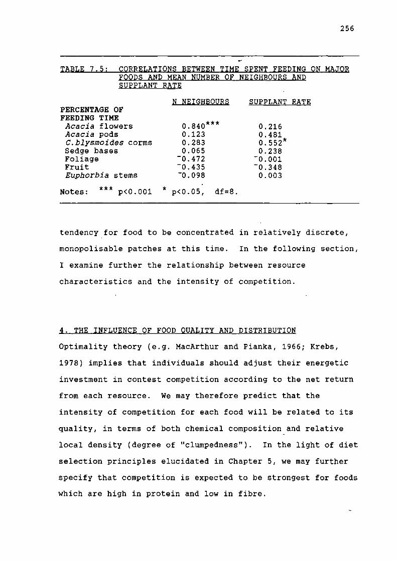
256

we'

TABLE 7.5: CORRELATIONS BETWEEN TIME SPENT FEEDING ON MAJORFOODS AND MEAN NUMBER OF NEIGHBOURS ANDSUPPLANT RATE

SUPPLANT RATEPERCENTAGE OFFEEDING TIME

N NEIGHBOURS

Acacia flowers 0.840*** 0.216Acacia pods 0.123 0.481C.blysmoides corms 0.283 0.552*Sedge bases 0.065 0.238Foliage -0.472 -0.001Fruit -0.435 -0.348Euphorbia stems -0.098 0.003

***Notes: p<0.001 * p<0.05, df=8.

tendency for food to be concentrated in relatively discrete,

monopolisable patches at this time. In the following section,

I examine further the relationship between resource

characteristics and the intensity of competition.

4. THE INFLUENCE OF FOOD QUALITY AND DISTRIBUTION

Optimality theory (e.g. MacArthur and Pianka, 1966; Krebs,

1978) implies that individuals should adjust their energetic

investment in contest competition according to the net return

from each resource. We may therefore predict that the

intensity of competition for each food will be related to its

quality, in terms of both chemical composition and relative

local density (degree of "clumpedness"). In the light of diet

selection principles elucidated in Chapter 5, we may further

specify that competition is expected to be strongest for foods

which are high in protein and low in fibre.

257

Empirically, however, there is already reason to doubt that...

the prediction of an association between phytochemistry and

the intensity of competition will be confirmed; high-ranking

females had greater daily intakes, but not better-quality

diets. Because of this, we may predict that the spatial

distribution of foods is the primary determinant of the levels

of competition they evoke. Unfortunately, as explained above,

no meaningful quantitative measures of clumping or of patch

size are available. Therefore, in the following correlational

analysis of relationships between competition and resource

characteristics, measures of the latter include only chemical

composition and dry weight ingestion rate. Shopland (1987)

performed a similar analysis, and also encountered the problem

of quantifying food distribution. Her solution was to class

food types as either clumped or uniformly distributed, on a

scale appropriate to groups of foraging baboons:

" A food was considered clumped if it was distributed inpatches that could accommodate several baboons but not thewhole group, and within which the density of food units washigh.. .A food was scored as uniformly distributed if itoccurred in large stands that could accommodate the entirebaboon group without crowding: the density of food unitswithin the stand could be high or low" (Shopland, 1987).

Note that Shopland's dichotomy actually concerns "patch size"

as much as it does general spatial heterogeneity. In the

absence of any obvious improvement on this method, I have

adopted the same procedure, and I have retained her

terminology for convenience. According to this definition,

six foods for which sufficient data were available were scored

as clumped: Cyperus blysmoides corms, Acacia tortilis

flowers, Acacia etbaica flowers (but only those collected from

drifts on the ground; flowering trees themselves often

occurred in large groves), Acacia nilotica pods, Acacia

258

mellifera pods, and Euphorbia nyikae fleshy stems. A seventhOh.

food type, Lycium europaeum leaves, was difficult to classify,

and so was excluded from the analysis.

A comparison of clumped versus dispersed foods shows that both

the mean number of neighbours and the mean supplant rate were

greater when animals were feeding on the former (number of

neighbours; t=4.19, df=23, p<0.001: supplant rate; t=2.24,

df=23, p=0.032), indicating a link between resource

distribution and the intensity of competition. A problem with

the procedure, however, is that clumped foods were also foods

obtained from trees in 3 out of the 5 cases, whereas non-

clumped foods were obtained from trees in only 2 out of 22

cases; this means that "clumped food" and "three-dimensional

substrate" are confounded. There is no clear reason in

principle to expect supplant rates to be higher in a three-

dimensional situation, but clearly the number of neighbours

are likely to be greater, without any concomitant increase in

the level of competition, because of the greater number of

feeding sites per square metre. Comparing tree foods and non-

tree foods, number of neighbours were significantly greater

for the former (t=4.57, df=24, p<0.001), whereas, as

predicted, there was no difference in supplant rate (t=0.17,

df=24, p=0.870).

The present data set does not permit a rigorous separation of

the influences of these factors on the number of neighbours,

because there were only two clumped non-tree foods. However,

in the case of one of the latter, Cyperus blysmoides corms,

both the mean number of neighbours (7.9) and the mean supplant

259

rate were greater (0.231 per minute) than for any other food.

In the case of fallen Acacia etbaica flowers, the other

clumped non-tree food, the two parameters were also relatively

high (4.4 neighbours and 0.057 supplants per minute, compared

with the mean for all clumped foods of 4.7 neighbours and

0.085 supplants per minute, and means for all non-clumped

foods of 1.6 neighbours and 0.032 supplants per minute).

Conversely, for the two non-clumped tree foods, the numbers of

neighbours were fairly high, while supplant rates were low

(number of neighbours; 2.8 and 4.6: supplant rates; 0.026 and

0.011: foods are pods of Acacia seyal and A.mellifera

respectively). Thus, the available evidence does suggest

that, while spatial deployment was influenced by the use of

arboreal versus terrestrial sources of food, it was also

independently influenced by the degree to which foods were

clumped, whereas supplant rates were influenced only by the

latter.

Next I turn to the relationship between chemical composition

and the intensity of competition. In order to control for the

effects of food distribution and substrate, I have excluded

the 9 foods which were either clumped or obtained from trees.

Correlations are displayed in Table 7.7; none are

significant. Number of neighbours and supplant rate are,

however, significantly correlated with each other (r=0.514,

df=25, p=0.008), suggesting that they do indeed reflect

aspects of the same underlying behavioural process.

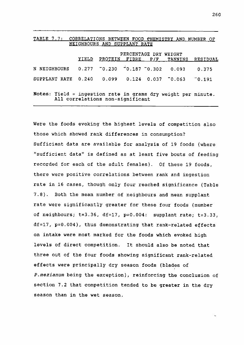
260

TABLE 7.7: CORRELATIONS BETWEEN FOOD eHEMISTRY AND NUMBER OFNEIGHBOURS AND SUPPLANT RATE

PERCENTAGE DRY WEIGHTYIELD PROTEIN FIBRE P/F TANNINS RESIDUAL

N NEIGHBOURS 0.277 - 0.230 - 0.187 - 0.302 0.093 0.375

SUPPLANT RATE 0.240 0.099 0.124 0.037 - 0.063 -0.191

Notes: Yield = ingestion rate in grams dry weight per minute.All correlations non-significant

Were the foods evoking the highest levels of competition also

those which showed rank differences in consumption?

Sufficient data are available for analysis of 19 foods (where

"sufficient data" is defined as at least five bouts of feeding

recorded for each of the adult females). Of these 19 foods,

there were positive correlations between rank and ingestion

rate in 16 cases, though only four reached significance (Table

7.8). Both the mean number of neighbours and mean supplant

rate were significantly greater for these four foods (number

of neighbours; t=3.36, df=17, p=0.004: supplant rate; t=3.33,

df=17, p=0.004), thus demonstrating that rank-related effects

on intake were most marked for the foods which evoked high

levels of direct competition. It should also be noted that

three out of the four foods showing significant rank-related

effects were principally dry season foods (blades of

P.mezianum being the exception), reinforcing the conclusion of

section 7.2 that competition tended to be greater in the dry

season than in the wet season.

261

TABLE 7.8: CORRELATIONS BETWEEN DOMINANCE RANK AND INGESTIONRATE, AND MEAN NUMBER OF NEIGHBOURS AND SUPPLANT RATE, FOR 19 FOODS.

FOOD 1 2 3

Acacia etbaica flowers (tree) 0.514* 3.80 0.019Acacia etbaica flowers (ground) 0.456* 4.38 0.027Acacia tortilis flowers (tree) 0.199 4.40 0.022Commelina erecta buds -0.252 0.85 0.000Cynodon dactylon blades 0.288 1.86 0.034Cynodon plectostachyus blades 0.197 1.63 0.009Cyperus blysmoides corms 0.611 ** 7.86 0.231Cyperus merkeri bases -0.029 1.84 0.030Ipomoea mombassana fruits 0.050 1.47 0.090Lycium europaeum leaves 0.253 1.81 0.037Mariscus amauropus bases 0.139 0.99 0.017Osteospermum vaillantii fruits 0.147 0.59 0.034Penissetum mezianum blades 0.509* 2.67 0.046Penissetum spp. blades 0.442 1.18 0.000Sansevieria intermedia bases -0.204 0.98 0.032Trachyandra saltii leaves 0.230 1.23 0.018Tragus bertoriana inflorescences -0.252 1.54 0.020Tribulus terrestris leaves 0.418 1.69 0.018Tribulus terrestris fruits 0.206 •2.28 0.012

Notes: 1; pearson correlation coefficient between rank andingestion rate (** p<0.01, p<0.05, df=16). Foodsincluded are those for which 5 or more feedingbouts were recorded for each female.

2; mean number of neighbours within 10 metres.3; number of supplants per minute.

5. DOMINANCE RANK, SPATIAL DEPLOYMENT AND SUPPLANTING

The evidence of section 7.2 suggested that the nutritional

advantages of high rank in a provisioned group were mediated

by spatial deployment, with supplants apparently being of

little direct importance. In this section I evaluate whether

the tendency of high-rankers to occupy central positions, or -

to otherwise monopolise feeding sites, was also a feature of

262

the naturally-foraging group. Two parameters are examined

here: the number of neighbours, as a-surrogate for the

proximity index, and the use of trees, which simplifies the

definition of patches. Finally, correlations between

dominance rank and supplant rates are presented.

(a) Number of neighbours

If high-ranking females (HRFs) monopolise the best feeding

sites within patches, and thus tend to occupy central

positions in a way similar to HRFs in the provisioned group,

this is likely to be reflected in the number of animals in

close proximity to them while feeding. I have collapsed data

for individual females into three rank categories, high medium

and low, and performed a one-way repeated measures ANOVA,

with food type as the replicator variable. This procedure

reveals that the number of neighbours differed significantly

between rank categories (F=3.372, df=2,38, p=0.045: means;

high=2.05, medium=1.79, low=1.58), with high-rankers having

significantly more than low-rankers (Tukey test: Q=3.642,

p=0.037).

To pursue the influence of dominance further, and to

investigate the possibility that the effect is due simply to

the tendency for HRFs to be more attractive (Seyfarth, 1977;

Gouzoules and Gouzoules, 1986; Walters and Seffarth, 1986),

or to have larger families (Sade et al., 1976; Silk, 1986a),

I compare the influence of rank during feeding with that

during other activities; if effects during feeding, but not

during other activities, are apparent, this would support the

263

idea that differences were due directly to competition for

feeding sites, rather than to attractfveness or family size.

Correlations between rank and the number of neighbours within

10 metres, broken down by food type, are displayed in Table

7.9. All of the 10 correlations are positive, with three

being significant, indicating that HRFs tended to have more

close neighbours when feeding than LRFs did. Rank was,

however, uncorrelated with the number of neighbours in the

other major activities (moving; r5 = - 0.091, p=0.710: standing;

r5 = - 0.089, p=0.716: resting; r5=0.119, p=0.627: grooming;

r5 = - 0.004, p=0.988: df=17 in each case).

TABLE 7.9: CORRELATIONS BETWEEN RANK AND THE NUMBER OFNEIGHBOURS, BROKEN DOWN BY FOOD TYPE

FOODAcacia etbaica flowers (tree) 0.47Acacia etbaica flowers (ground) 0.03Acacia tortilis flowers (tree) 0.15Cynodon dactylon blades 0.18Cyperus blysmoides corms 0.61**Euphorbia nyikae fleshy stems 0.46*Lycium europaeum leaves 0.32Mariscus amauropus bases 0.19Tragus bertoriana inflorescences 0.24Tribulus terrestris fruits 0.14

Notes: tabulated values are Spearman's rank correlationcoefficients (* p<0.05, df=16). Foods included arethose eaten in >5 point samples by each female..

(b) Use of trees

I have suggested that the nutritional advantages emjcatw%dillny

high-ranking females are likely to be mediated by prisoiriittzacri

access to feeding sites or patches containing rellattiillzihjigjh

densities of food. What evidence is there for this?? Whia%t

264

there is frequent talk in primate behavioural ecology of the

significance of "patches", in practice, these phenomena are

extremely difficult to define, let alone to measure (Wrangham,

1983), and no attempt was made in the present study to do so.

Trees, however, are a class of patch which it is relatively

easy to measure and delineate the boundaries of. Accordingly,

in this section I evaluate the evidence that HRFs had priority

of access to foods obtained from trees.

Animals sometimes fed on tree products by reaching up from

the ground, but this appeared to be less efficient than when

they climbed into the tree. This subjective impression can be

tested by comparing the feeding rates of individuals when they

were in trees with their feeding rates when outside the tree.

In the case of A.etbaica, feeding rates were significantly

higher when individuals were in trees than when they were

outside them (correlated t-test, individual as replicator

variable; t=2.59, df=18, p=0.019, means = 49.3 and 44.7 bites

per minute respectively); in the case of A.tortilis there was

no significant difference (t=1.21, df=12, p=0.250, means =

47.6 and 50.5 bites per minute), but the number of non-tree

bouts recorded for each individual is small (mean=2.7), so the

test is not very reliable. In general, then, feeding on

Acacia flowers was less efficient when individuals harvested

them from a terrestrial position. The next question is

whether there were rank-related differences in the extent to

which individuals fed in and out of trees.

Unfortunately, there are insufficient data to analyse trends

for the two Acacia species separately, so I have pooled the

265

data. While rank is uncorrelated with the overall percentage

of time spent in Acacia trees (rs=-0.±85, df=16, p=0.464),

there is a significant positive correlation between rank and

the proportion of feeding time on Acacia flowers that was

spent actually in the tree, as opposed to picking the flowers

from a position on the ground (r 5=0.472, df=16, p=0.048). The

same type of analysis cannot be performed on any other tree

species, due to a lack of data, but the same trend is apparent

in the context of feeding on Euphorbia nyikae fleshy stems;

high-rankers spent 63.5% of their feeding time on this item

actually in the tree, while for medium-rankers the figure is

exactly 50%, and for low-rankers 0%.

Acacia trees utilised by the baboons varied substantially in

size; each time the focal animal climbed into a tree I

estimated the canopy diameter as being less than 5 metres, 5-

10 metres, 10-15 metres, or 15-20 metres. Figure 7.5 clearly

shows that, for a number of Acacia species, the duration of

feeding visits to trees, and hence presumably patch richness,

was a positive function of crown diameter. This suggests that

crown diameter may be used as an index of patch quality; did

HRFs monopolise the larger trees?

Figures 7.6 and 7.7 display the average percentages of feeding

time spent in A.etbaica and A.tortilis that was allocated to

different sizes of tree by high-, medium-, and low-ranking

females. In the case of A.etbaica there appears to be a clear

relationship between rank and the size of trees selected, with

HRFs feeding more in larger trees. No such relationship is

apparent for A.tortilis, however. In Figure 7.8 I have

800

a0z0(..) 600 -uiw

z0I=< 400 -ccD0

I—

Eh5200 -z

<La2

I I I

<6 <10

<15

20

_...._

A.etbalca

A.tortilis

A.mellifera

A.nilotica

A.seyal

FIGURE 7.5: RELATIONSHIP BETWEEN CANOPY DIAMETERAND DURATION OF VISITS TO ACACIA TREES

CANOPY DIAMETER (METRES)

Duration of visits = time in secondsbetween entering and leaving tree.

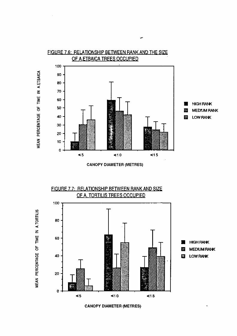
• HIGH RAM(

• MEDIUM RANK

• LOW RAN<

100

90

80

70

60

50

40

30

20

10

o

• HIGH RAM(

• MEDIUM RANK

LOW RANK

100

80

60

40

20

o

FIGURE 7,6: RELATIONSHIP BETWEEN RANK AND THE SIZE

OF A.ETBAICA TREES OCCUPIED

<5

<10

<15

CANOPY DIAMETER (METRES)

FIGURE 7.7: RELATIONSHIP BETWEEN RANK AND SIZE

OF A. TORTILIS TREES OCCUPIED

<5

<10

<15

CANOPY DIAMETER (METRES)

266

plotted the relative frequencies of the different size

categories for each species. Larger trees are evidently lesswrIll0

common, yet they are clearly selected; this is shown by

calculating selection ratios (percentage of feeding time

allocated to each size category, divided by percentage

abundance) for the two species; these are plotted in Figure

7.9. Larger trees may also be less defendable, and this could

account for the smaller differences between rank categories at

the largest size. For one species, then, but not for the

other, HRFs may have monopolised the larger (hence richer) and

rarer trees.

(c) Supplanting

Rates of feeding supplants were calculated for each of the

focal adult females. Unlike in the provisioned group, rank

was positively correlated with the rate at which supplants

were given (r 5=0.659, df=16, p=0.002), but uncorrelated with

the rate at which they were received (rs= - 0.248, df=16,

p=0.320). The ratio of supplants given to supplants received

was positively correlated with rank (r 5 =0.699, df=16, p=0.001)

6. DISCUSSION

I have attempted to document some of the behavioral processes

mediating the relationship between ecology and 'social

organisation amongst females. Specifically, I have shown that

the spatial locations of foraging individuals within the group

were related to their dominance ranks, and that, under certain

conditions of food distribution, high-rankers had priority of_

access to the best feeding sites. Competition was most

FIGURE 7.8: RELATIVE FREQUENCIES OF DIFFERENT SIZED ACACIAS

loo

80

60

40

20

0

:

-

/

•111

A.etbaica

A.tortilis

t ,

< 5 < 1 0

<15

CANOPY DIAMETER (METRES)

* Frequencies estimated from 30 m. quadrats.

0I-4ix

z0P0w_1wCl)

El A. etbaica

EI A. tortilis

FIGURE 7.9: SELECTION OF DIFFERENT SIZES OF ACACIAS

<5 m. <10 m. <15 m.

CANOPY DIAMETER

267

intense, and the influence of rank on ingestion rates was most

apparent, for foods which occurred in -high-density clumps.

These were primarily foods eaten in the dry season.

a. Competition, resource charactersitics and seasonality

The patterns of competitive exclusion were extremely clear-cut

in the provisioned group, for which food was supplied in a

single, high-density "super-patch". Similar patterns were

observed by Belzung and Anderson (1986) in an experimental

study of feeding competition in rhesus macaques (Macaca

mulatta); high-rankers ate first and ate most, whereas low-

rankers tended to remain on the periphery and ate little.

Other authors working on female cercopithecines have also

noted an exacerbation of competition amongst provisioned

animals (Sugiyama and Ohsawa, 1982, Fairbanks and McGuire,

1984; Altmann and Muruthi, 1988). Harcourt (1987) argues that

"it is probably the distribution of food that is important,

not its abundance". Thus the potential for despotism is, in

theory, inversely related to the degree to which food is

dispersed, irrespective of how much there is of it.

Harcourt's argument is supported in the present case, since

the highest levels of competition in the naturally-foraging

group were evoked by foods occurring in high-density clumps.

However, the idea that competition tends to be greatest during

periods of relative scarcity (e.g. Post et al., 1980;

Gouzoules et al., 1982) also received some support, probably

because foods which were eaten in the dry season also happened

to be relatively clumped in distribution.

268 •

I have stressed that inferences about seasonal patterns in the

behavioural ecology of these baboons are subject to the

qualification that a fairly limited period has been sampled

(12 months for ranging, 10 months for feeding, 'and only 8

months for biomass estimates and detailed behavioural data on

separate individuals). There is, however, evidence from other

sources supporting the claim that, amongst baboons,

competition tends to be most intense in the dry season. Post

(1978) found, as I have done, that the rate of feeding

supplants was significantly higher in the dry season than in

the wet season, and also that monthly rates were inversely

related to cumulative rainfall. Whitten's (1983) study

suggests that the situation is the same in vervet monkeys

(Cercopithecus aethiops); most rank-related dietary

differences were found in the dry season (although this was

not when supplant rates were highest). In the present case, a

period of drought and drastically reduced food availability in

the year following the study culminated in the group

splitting, possibly as a result of exacerbated intra-group

competition.

What are the implications of this tendency for competition to

increase with declining food availability? An obvious one is

that dominance rank may influence female fitness primarily

through effects on survival, particularly infant survival,

rather than through effects on fecundity. It is intended

that long-term data from Chololo will eventually be used to

test the hypothesis, but in the meantime, evidence bearing on

it is available from other studies. Busse (1982) reported a

correlation between female rank and infant survival in chacma

269

baboons (P.ursinus), and Bulger and Hamilton (1987) found

that, at large group sizes, high-ranking females of the same

species had significantly greater offspring survival than did

low-rankers. Altmann et al. (1988) found that ,offspring

survival to age 6 years among -P.cynocephalus was an

interactive function of offspring sex and female rank; the

sons of high-rankers were more vulnerable than their

daughters, whereas the reverse was found for low-rankers.

High-rankers' daughters survived better than low-rankers'

daughters, but high-rankers' sons survived less well than low-

rankers' sons. The pattern of survivorship can be summarised

as follows:

HRF daughters > LRF sons > LRF daughters > HRF sonsp=0.47 p=0.33 p=0.25 p=0.00n=15 n=9 n=4 n=5

Where p is the probability of surviving to age 6, and n is thenumber of offspring in the sample.

In terms of actual numbers, this corresponds to 1 surviving

offspring per female for HRFs and 0.57 for LRFs, but the

parameter "surviving offspring" is obviously partly a function

of the number of births. These data do not, therefore, give a

clear indication as to whether there is a general relationship

between rank and offspring survival, and, as Altmann et al.

(op. cit.) stress, firm conclusions must await more data.

What was clear from the available evidence, was that rank

strongly influenced the age at which a female reproduced for

the first time. This component of lifetime reproductive

success is presumably a function of pre-pubertal growth rates,

and so could equally be influenced by a young females' ability

270

to make the most of good conditions as by her ability to

ameliorate the effects of periods of food scarcity.

Cheney et al. (1988) found no correlation between female rank

and overall infant survivorship among vervet monkeys

(Cercopithecus aethiops), but low-ranking females and their

offspring were more likely than high-rankers to die during

periods of food shortage. This did not translate into overall

mortality differences because high-rankers were more

susceptible to predation, the reason for which was unclear.

There was no evidence that competition lowered the fecundity

of low-ranking animals. In contrast, vervets studied by

Whitten (1983) in a different area did show a positive

association between rank and fecundity, high-rankers breeding

earlier and having higher birth rates than low-rankers.

Offspring survival was not significantly related to rank. In

macaques (hracaca), however, associations between rank and

mortality rates have been documented (M.sinica; Dittus, 1979:

M.fuscata; Sugiyama and Ohsawa, 1982: M.mulatta; Drickamer,

1974; Wilson et al., 1978: M.fascicularis; Silk et al., 1981:

M.sylvanus; Paul and Thommen, 1984: see also Harcourt, 1987).

To summarise, there is good evidence for an association

between dominance rank and mortality in at least some

populations of cercopithecine monkeys. Nevertheless, it is

also the case that some populations exhibit a relationship

between rank and fecundity (see Harcourt, 1987, 1989, for

reviews).

271

Which component of female fitness is most affected by rank

will presumably depend on ecological Qircumstances; where

resources are most clumped during periods of scarcity, rank

may affect survival more than it does fecundity ,. The

situation is complicated, however, by the fact that infant

mortality and interbirth interval (IBI) are related; IBIs are

reduced where infant mortality is high, because females

quickly become pregnant again when an infant dies (Harcourt,

1987, 1989). Thus, if the offspring of HRFs survive better

than those of LRFs, any tendency for the former to be more

fecund may be overidden. Conversely, where rank does not

influence infant mortality, effects on fecundity may emerge.

Clearly, further study is needed of the relationships between

seasonal clumping of resources, feeding competition, and

patterns of reproduction and mortality.

Like Shopland (1987) I was unable to demonstrate a

relationship between food quality and rates of supplanting or

spatial clustering. Shopland did, however, find that the

probability of an attempted supplant being unsuccessful (pu)

was higher when the yield (amount harvested per unit time) was

low; she interpreted this result as indicating that

individuals were less willing to give up their position when

feeding on items that were hard to process, because the cost

in wasted time and energy was greater. If this-is so, then it

can be further predicted that p u will be positively related to

the elapsed time spent attempting to extract items (such as

underground corms and roots) prior to the attempted

interruption; this remains to be tested.

272

The present study and the one by Shopland (op cit.) produced

contrasting results concerning the effect of resource clumping

on the intensity of competition in baboons. Shopland found

no difference between clumped and dispersed foods in either

the associated supplant rate or the number of neighbours.

Elsewhere, experiments on captive macaques (hacaca mulatta)

have demonstrated that clumping of food results in high levels

of aggression (Southwick, 1967; Belzung and Anderson, 1986;

Boccia et al., 1988). Monaghan and Metcalfe (1985) observed

a similar phenomenon amongst wild brown hares (Lepus

europaeus). During the provisioning experiment at Chololo,

individuals in MLK group engaged in supplants at a rate of 1

every 2.5 minutes, which contrasts strongly with the mean of 1

every 29.9 minutes for the naturally-foraging group; the only

natural food which evoked supplants at a rate approaching that

seen during provisioning was Cyperus blysmoides corms (1 every

4.33 minutes). These were highly clumped in distribution (see

Chapter 3), but they also took considerable time (and

presumably energy) to dig up, and it is to this latter factor

that Altmann (1980) attributed the high supplant rates evoked

by corms at Amboseli, where they do not occur in clumps.

Altmann's explanation, however, seems to conflict with the

lack of any association between yield or processing value and

supplant rate in Shopland's study.

It is to be expected that seasonal variability in levels of

competition are mirrored by geographic variability, although

one then has the additional factor of group size and

demography to take into consideration. Unfortunately,

differences between study sites in the reported rates of_

273

supplants are probably not a very reliable indicator of

variation in the level of competition. Even when very similarOM,

behavioural definitions are used, there are likely to be

observer differences in sensitivity and attention to

particular behaviours. In the.present study, for example, the

detailed recording of feeding must surely have compromised the

detection of subtle interactions. This "observer effect" is

suggested by comparing rates reported from a single study

site, Amboseli (the species being P.cynocephalus), by

different workers. Post (1978) recorded an average feeding

supplant rate for adult females of 1 every 11.8 minutes

(calculated from his Table 45), whereas Altmann (1980)

observed a range of between about 1 every 17 minutes and 1

every 100 minutes, also amongst adult females (estimated from

her Figure 27). Finally, Shopland recorded a mean of 1 every

6.9 minutes; this higher rate may be partly attributable to

the fact that her subjects were juveniles, but also probably

to the fact that feeding supplants were a major focus of her

observations. Because of this inevitable variation, it is not

possible to make direct comparisons with any confidence.

Where differences are extreme, however, these may be taken as

indicative of real population variability. Amongst mountain

baboons (P.ursinus) studied in the Drakensberg region of South

Africa, feeding supplants were observed at a rate of only 1

every 100 hours! (R. Byrne, pers. comm.); here group size was

small, foods were mostly widely dispersed, and there were no

predators forcing foraging groups to bunch together for

protection. Intra-group competition in that case can

therefore be presumed to have been minimal.

274

b. Spatial deployment, supplants, feeding, and predation

I have argued that dominance influenced foraging success

through the medium of spatial deployment; high-rankers

monopolised the richest feeding sites, and were thus able to

achieve relatively high ingestion rates. Similar associations

between rank and spatial positioning have been found in other

work on baboons. Collins (1984), working on yellow baboons

(P.cynocephalus) found that HRFs spent more time in clusters,

whereas LRFs were more often in peripheral positions. Busse

(1984) found that HRFs amongst chacma baboons (P.ursinus) had

smaller "domains of danger" (the area containing all points

nearer to the individual than to any other potential prey

animal), and that, in one group, rank was positively

correlated with the mean number of neighbours within 5 metres.

More generally, much debate has surrounded the issue of

whether baboon troops are coherently organised during group

movements in such a way that the more vulnerable members are

protected (e.g. DeVore and Washburn, 1963; Rowell, 1969;

Rhine, 1975; Rhine et al., 1979, 1980, 1981; Rhine and

Westlund, 1981; Harding, 1977; Altmann, 1979).

Whereas these authors have mostly emphasised the anti-predator

significance of spatial deployment, I, in common with a number

of other authors, have been concerned with its-relevance for

feeding. Imanishi (1957) and Yamada (1966) reported that

high-ranking individuals in groups of Japanese macaques

(Macaca fuscata) tended to occupy the centre of the group,

where they monopolised resources. In a study of baboons

(P.cynocephalus), Collins (1984) suggested that the greater

275

propensity of HRFs than LRFs to be found in clusters might be

the result of the latter suffering competitive exclusion.

Robinson (1981) found that the dominant female and the

dominant male in a group of capuchins (Cebus nigrivittatus)

occupied the centre-front positions during foraging, and thus

accrued significant foraging advantages. A relationship

between spatial position and foraging success has also been

documented for woodpigeons (Columba palumbas) foraging in

flocks (Murton et al., 1971), although in that example

individuals near the front of the flock were at a

disadvantage, due to continual displacement by the individuals

behind. Finally, van Noordwijk and van Schaik (1987) studied

groups of long-tailed macaques (Placaca fascicularis) which

formed foraging sub-groups during the day. Here, low-ranking

females were more prone than high-rankers to avoid direct

competition, by splitting off from the main group into small

foraging parties. When they did remain in the main group,

they suffered a depression in the rate at which they harvested

fruit.

The anti-predator and feeding implications of spatial

positioning may, however, be interdependent. Hamilton (1971)

argued that vulnerability to predators will, in general, be

greatest for those individuals which are distant from

neighbours and for those at the edge of the group. The

tendencies of HRFs to be located in central positions, to be

surrounded by less unoccupied space, and to feed more in

trees, could reduce their susceptibility to predation. This,

in turn, could reduce the amount of time needed for

vigilance, and hence increase the harvesting rate. An inverse

276

relationship between vigilance time and harvesting rate has

been demonstrated in several species of birds (e.g. Powell,

1974; Lazarus, 1979; Caraco et al., 1980), as has a tendency

for peripheral individuals to spend more time in vigilance

(Horn, 1968; Jennings and Evans, 1980; Inglis and Lazarus,

1981).

The only published study of the interaction between spatial

positioning, vigilance and foraging success in a primate is

Robinson's (1981) study of capuchins. In these monkeys, as in

birds, occupation of central positions was associated with

less time spent in vigilance and greater foraging success. In

their study of long-tailed macaques, Van Noordwijk and Van

Schaik (1987) found that low-ranking females maintained their

foraging success at a level comparable to that of high-rankers

only by moving outside the main party, thereby increasing

their vulnerability to predators. These authors also

suggested that competition within baboon groups might be

primarily for "safe positions", but neither the existence of

such safe positions, nor a trade-off between vigilance and

foraging, has been empirically demonstrated; for a genus

whose adaptations are thought by many to have been extensively

moulded by predation (e.g. Hall and DeVore, 1965; Crook and

Gartlan, 1966; Altmann and Altmann, 1970; Dunbar, 1988),

this is surely an omission.

Some authors have argued that supplants directly suppress the

foraging success of subordinates (Slatkin and Hausfater, 1977;

Post, 1978; Post et al., 1980), while others have emphasised

the importance of spatial deployment patterns that result from

277

subordinates avoiding direct competition with dominants

(Robinson, 1981; Furuichi, 1983; Whitten, 1983; van

Noordwijk and van Schaik, 1987). It should be noted that the

first set of references given are all for the ,same species

(Papio cynocephalus), and from the same study site at that.

Thus the difference of emphasis may reflect genuine species-

or population-differences. On the other hand, it could also

reflect the simple fact that spatial deployment has been

little studied at Amboseli.

Variation in predation pressure could perhaps result in

variation in the degree to which individuals cluster together

(van Schaik, 1989), hence influencing the rates of direct

confrontation; where predators are scarce, low-rankers could

spread out and find alternative feeding sites. The problem

with this idea is that it implies that the vervets in

Whitten's study were less vulnerable to predation than the

(much larger) baboons at Amboseli, an unlikely possibility,

and one for which there is no evidence.

Like Post (1978) and Altmann (1980), I found that supplant

rates were related to dominance rank. It has not been

possible here to specify what direct effects this had on

foraging success. Although the rates were rather low (on

average, about 1 every 30 minutes of feeding time), if they

were used to gain initial access to rich food patches, they

could still have had an important direct impact on spatial

positioning and foraging success. Supplant rates were not

clearly related to spatial position in the provisioned group

once the group had settled at the food patch, but it was

278

argued that supplants could have served to establish those

positions initially. Other authors ..have suggested that

feeding supplants are often used as a form of "pure

interference" (Shopland, 1987), to reinforce dominance

relations even at some energetic cost to the supplanter

(Johnson, in prep.). As yet we have no idea of the relative

frequency of "genuine" feeding supplants and "social" feeding

supplants.

279

CHAPTER 8: CONCLUDING DISCUSSION

sle•

Having already discussed each set of results in detail, I will

confine myself here to the implications of two general themes

which have been pervasive.

1. ECOLOGICAL CONTRASTS BETWEEN MALES AND FEMALES

It has long been appreciated that unequal material

contributions by males and females to the production of

offspring will theoretically lead to the evolution of

morphological, physiological and behavioural differences

associated with the divergent reproductive strategies of the

two sexes (Bateman, 1948; Trivers, 1972; Wade, 1979).

Amongst mammals, females make a far greater material

contribution than do males. Hence females' reproductive

success should be primarily limited by their ability to

channel resources into rearing offspring, while males will be

primarily limited by the number of females to which sexual

access can be gained.

These conclusions have a number of implications, two of which

are considered here. Firstly, the divergent selection

pressures associated with reproduction in females and males

are thought to underlie the evolution of sexual dimorphism in

body size (e.g. Clutton-Brock, 1985). The primary emphasis of

discussion, however, has been on only one half of the story;

the effects of sexual selection on male size (e.g. Darwin,

1871; Clutton-Brock et al., 1977; Clutton-Brock, 1985;

280

Alexander, 1979; but see Rails, 1977). Progress in

understanding the evolution of dimorphism therefore demands

consideration of the likely role of reproductive selection

pressures in determining female size. It has also been argued

that, whatever the precise explanations for the phenomenon,

body size dimorphism may have secondary influences on

behavioural ecology (Clutton-Brock, 1977), and primatologists

have been particularly interested in sex differences in

dietary composition. In sum, we can expect dimorphism to have

important ecological implications. Secondly, we might expect

female behavioural strategies to reflect the paramount

importance of nutrient-acquisition, while males may compromise

foraging efficiency by investing time and energy in gaining

and maintaining access to fertile females; while generally

valid, this kind of thinking may have led to an

underestimation of the importance of nutrition in males. The

two issues are addressed separately below.

(a) Ecological implications of sexual dimorphism

Baboons are strongly dimorphic in body size (Dunbar, in

press). Nevertheless, in the present study, lactating females

had daily food intakes very similar to those of males,

suggesting that male and female body sizes are limited by

common ecological-energetic constraints, with the addition of

reproductive costs in females. The idea that sexual

dimorphism in animals may in part reflect energetic strategies

by reproducing females has been discussed before (Jones, 1973;

Wiley, 1974; Downhower, 1976; Ralls, 1977; Demment, 1983;

Price, 1984; Saether and Haagenrud, 1985). Price (1984) for_

example, suggests that both males and females may be held off

281

the survival optima for body size, the former by sexual

selection (usually for larger size), the latter by fertility

selection (usually for smaller size). He argues that

evaluation of mortality rates can reveal which' sex is closer

to the survival optimum. In a population of Darwin's finches

(Geospiza fortis), Price (op. cit.) found a fertility

advantage accruing to small females, but a survival advantage

to large individuals (hence to males) during a drought. The

degree of dimorphism within mated pairs bore no relationship

to reproductive success, arguing against the niche separation

hypothesis for the evolution of size differences.

Dimorphism in baboons may be related to mortality and

fertility in similar ways. The ability to survive periods of

food shortage (fasting endurance) is theoretically a positive

function of body size in mammals, because metabolic rate

increases with body size more slowly than do fat reserves

(Lindstedt and Boyce, 1985). This is likely to have important

demographic consequences for baboons, because of the marked

seasonality and occurrence of energy bottlenecks in savannah

environments (see Chapter 3). Indeed, higher mortality in

females than in males during food shortages has been reported

for baboons (Hamilton, 1985; Altmann et al., 1988). However,

the picture is complicated by the fact that females' smaller

size means they are also subordinate to males; ' hence,

differences in survivorship through seasonal bottlenecks may

be related to inter-sexual competition (Hamilton, 1985), as

well as to energetic implications of size. A further

complication in evaluating the implications of dimorphism for

sex-specific mortality rates in matrilocal populations is that

282

males are exposed to additional risks during migration between

groups (Dunbar, 1988). At present, therefore, it is not

possible to draw firm conclusions concerning the nature and

causes of sex differences in mortality.

Variation among baboon populations in body weight and

dimorphism has been examined by Popp (1983), and, with a more

extensive data set, by Dunbar (in press). Both authors found

a relationship between mean annual rainfall and male weight.

Dunbar also found a relationship between female weight and

rainfall, but the correlation was weaker than in the case of

male weight. Conversely, ambient temperature was found to be

a stronger influence on female weight than it was for male

weight. Overall, however, female weight showed less variance

across populations than male weight did. Dunbar suggested

that these differences reflect differences in reproductive

strategies, arguing that, while large size is crucially

important for males, resulting in a delay in the onset of

breeding, females should start to reproduce as early as

possible. Hence males may take advantage of better quality

habitats by growing larger, while females take advantage by

reaching menarche earlier. The stronger influence of

temperature on females was explained by the fact that, since

males are larger anyway, they will be less prone to variation

in thermoregulatory energy costs; this makes sense because

the crucial factor is probably the amount of time at night

spent below the lower critical temperature (see Chapter 6).

These arguments lead to the suggestion that female size _

represents a compromise between selection for low basal energy

283

requirements during reproduction (hence small body size), and

selection for factors such as temperature tolerance, digestive

capability (see Demment, 1983) and fasting endurance (hence

large size). Large size in males may be promoted by sexual

selection acting on competitive ability, and/or the same

factors promoting large size in females; the problem is then

to determine what constrains males from growing even larger.

One answer, suggested by Demment (1983), is that male size is

limited at the upper end by competition with ruminants, which

are more efficient at digesting the fibrous foods that would

have to be incorporated into the diet to satisfy increased

energy requirements. The situation in baboons appears to

differ from that in populations of the Norwegian moose (Alces

alces), where the onset of reproduction is apparently

determined by age rather than by size, female weight varies

more than male weight does, and dimorphism is more closely

correlated with variation in female weight than it is with

variation in male weight (Saether and Haagenrud, 1985).

Dietary sex differences have been interpreted both as a

function of dimorphism, in the sense that dimorphism has

evolved under selection for niche separation, and as a

secondary consequence of it (Selander, 1966; Clutton-Brock,

1977; Post, 1978; Price, 1985). For example, in reviewing

field studies of primates, Clutton-Brock (1977) suggested that

sex differences might be a result of body size constraints,

the physiological impact of reproduction on females, or the

need to avoid excluding mates from valuable resources. A

fourth possibility, alternative to the third, is that sex

differences directly reflect competitive exclusion of the less

284

powerful sex. In general, inter-individual variance in diet

in the present study, at the level of-gross nutrient

composition, was surprisingly low. This conflicts with a

reasonable body of data in the literature on primates which

suggests both that competition leads to rank-related

differences in diet quality (e.g. Dittus, 1979; Wrangham and

Waterman, 1981; Whitten, 1983) and that males and females eat

different diets (Clutton-Brock, 1977; Post, 1978; Demment,

1983).

In fact, the evidence supporting claims for dietary sex

differences is generally rather flimsy, because it is often

the case that too few individuals (particularly males) are

sampled to allow generalisations to be made with confidence.

For example, in three out of the four published studies cited

by Clutton-Brock (1977) as demonstrating sex differences in

plant feeding, only two males were sampled (Pollock, 1977;

Rodman, 1977; Fossey and Harcourt, 1977); in the fourth

study, three males were sampled (Waser, 1977). Post's use of

two males and two females in his study of baboons

(P.cynocephalus) was mentioned in Chapter 5, and these sample

sizes also apply to Demment's (1983) calculations, since he

used Post's data. Studies by Harrison (1983) on green monkeys

(Cercopithecus sabaeus) and by Watts (1984) on gorillas

(Gorilla g. berengei) involved larger samples, and so provide

stronger claims for real sex differences. However, it is not

yet possible to discern any general trends in terms of what

types of food or nutrient are implicated. Further extensive

study would be required to establish whether marked sex

differences are the norm, in which species and under what

285

conditions they are most likely to occur, and, where they do

occur, what their nature and functiona/ significance is.

In the present case, in which seven males and nineteen females

were sampled, no strong differences in either diversity or

nutritional composition of the diet were found, despite a

tendency of females to spend more time foraging in trees.

This lack of dietary sex differences coupled with the failure

to demonstrate clear trends within the primates generally,

suggests that the idea of niche separation may have been

overemphasized. A question that remains for future analysis

is whether the composition of diets nevertheless differed in

terms of plant species and parts; if so, this would suggest

that males and females were able to arrive at similar

nutritional endpoints via different dietary routes. It is

possible, for example, that females were forced by competition

with males to utilise items which were harder to find and/or

process, but which were phytochemically similar. The fact

that sex differences in total nutrient intake and in time

spent feeding correspond quite closely (Chapter 6) does,

however, argue against this suggestion.

(b) Implications of foraging and nutrition in miles

In the present study, the importance of nutrient-acquisition

for females was indicated by the occurrence of tangible

competition. I did not, however, evaluate whether this was

also true of males, and research on feeding competition _

elsewhere has also tended to focus on females (e.g. Wrangham,

286

1980, 1983; Whitten, 1983, 1988; van Noordwijk and van

Schaik, 1987; Harcourt, 1989: but see also Dittus, 1979; Post

et al., 1980).

The idea that, amongst males, foraging strategies are less

important than mate-acquisition strategies (e.g Wrangham,

1980) is, however, perhaps a little too simplistic. The

reason for this is that the outcome of reproductive

competition between males may itself be influenced by

nutrition. Firstly, gaining and maintaining access to fertile

females in multimale baboon troops can be extremely

energetically expensive (Hausfater, 1975; Bercovitch, 1984;

Smuts, 1985; Strum, 1987; pers. obs..), and an undernourished

or otherwise weak male would no doubt be at a considerable

disadvantage. Secondly, sperm competition is thought to be

intense amongst male primates living in multimale groups,

since females frequently consort with several males

sequentially during oestrous (Smuts, 1985; Strum, 1987; pers

obs.), and males show morphological adaptations for producing

large amounts of sperm (Short, 1981; Harcourt et al., 1981;

Harvey and May, 1989); anything which affects the quantity

or motility of sperm is therefore likely to affect

insemination success. Little has been published on the

relationship between nutrition and sperm production, but

amongst domestic cattle sperm counts are positively correlated

with caloric intake (Moustegaard, 1977). These considerations

suggest that the influence of foraging strategies and

nutrition on reproductive success amongst male baboons

deserves examination, and that it may not make sense to speak

287

of fertile females as being "uniquely valuable" resources

(Wrangham, 1980). =V,

2. FEEDING COMPETITION, PREDATION AND SOCIAL EVOLUTION

At the beginning of this thesis I commented on the recent

valuable rapprochement between the two previously rather

disparate areas of primate behavioural ecology and

socioecology on the one hand, and the study of social

relationships on the other. It is thus, I suggested, that our

understanding of the processes of social evolution can be

advanced. I will now try to link the work that I have

presented here with attempts to produce comprehensive

ecological models of primate social organisation and

relationships.

Relationships between individuals are the building blocks of

societies (Hinde, 1976b, Dunbar, 1989), and it is the

recognition of this that has guided much recent work in

primate socioecology. The most influential attempt, at least

until recently, to explain variation in social relationships

has been Wrangham's (1980) model of female-bonded groups,

which was predicated on certain patterns of feeding

competition (see also Chapter 1). How do savannah baboons fit

in with the ecological conditions specified by Wrangham?

Wrangham (1980) envisaged the diets of female-bonded primate

groups as consisting of two components, the "growth" diet,

288

eaten during periods of abundance, when populations are

expanding, and the "subsistence" diet, eaten during periods of

scarcity, when populations are declining. Subsistence diets,

Wrangham argued, should consist of low-quality.food found in

large, uniform patches, allowing group members to coexist with

minimal competition when food is scarce. Then, when rich

patches of high-quality food become available, these can be

exploited by the whole group, insofar as it is able to exclude

neighbouring groups. It is these "rich pickings" that, in

Wrangham's model, provide the raison d'etre for female-bonded

groups.

The conditions specified in Wrangham's model do not appear to

be met amongst baboons, because, as noted, competition

increases during the dry season. Wrangham correctly noted

that savannah-dwelling populations do not rely extensively on

fleshy fruits, and that the seeds, pods and flowers which are

utilised "tend to be available for short periods at restricted

locations, where aggressive competition occurs for access to

feeding sites" (Wrangham, 1980). What may be incorrect about

this part of Wrangham's argument is the contention that such

foods make up the so-called growth diet; as we have seen

(Chapter 5), in the present study they were available and

eaten principally in the dry season. During the period of

abundance (the wet season), much of the diet was made up of

grass blades and other foliage, as in Post's study (1978), and

these foods are relatively homogenous in their disribution.

Wrangham (p.274), however, assumed that they represent

subsistence foods.

289

The implication of this reversal of the conditions specified

by Wrangham is that the functional significance of group

living in these baboons is either related to survival through

seasonal bottlenecks, rather than to exploiting growth foods

when conditions are good, or to some factor other than feeding

competition, such as predation (c.f. van Schaik, 1983, 1989;

Dunbar, 1988). It is important, as Janson and van Schaik

(1988) have emphasised, to maintain a clear distinction

between intra- and inter-group competition. Since I have not

measured the latter, I cannot be sure that the two processes

display similar seasonal trends (or even that inter-group

competition was significant). Thus, theoretically, it is

still possible that groups competed with each other more in

the wet season. In fact little is known about inter-group

competition in primates (see Janson and van Schaik, 1988; van

Schaik, 1989), let alone in baboons, and this will be an

important area for future investigations aiming to test

functional hypotheses about social organisation.

Recently, the topic of ecological influences on social

relationships in female primates has been reassessed by van

Schaik (1989), who, contrary to Wrangham, emphasizes the

likely role played by predation. Van Schaik begins with the

proposition that there are essentially three types of

competition affecting female relationships; scramble

competition within groups, contest competition within groups,

and contest competition between groups (see also Introduction

to Chapter 7). In gregarious species or populations, strong

inter-group contest competition should result in egalitarian

hierarchies, rather than the despotic variety observed, for -

290

example, amongst baboons and macaques. This is because•10.

subordinate females would be expected to leave the group,

thereby reducing its ability to compete with other groups,

wherever the subordinates suffered excessively from contest

competition with dominants. Thus, under these conditions,

dominants should refrain from exerting their full power.

Van Schaik contrasts this situation with the one in which

there is little inter-group contest competition and marked

intra-group contest competition. Intra-group competition is

expected where high predator pressure forces groups to be

cohesive. Where intra-group competition is of the scramble

variety - because food is either dispersed or occurs in

patches large enough to feed the whole group - aggression over

food will be ineffectual in enhancing individuals' intakes,

and dominance hierarchies will be generally weak and

egalitarian. It is therefore suggested by van Schaik that

despotic, linear hierarchies reflect strong intra-group

contest competition, and relatively weak inter-group contest

competition. This pattern could, however, result from intra-

group contest for positions with low predation risk, rather

than from contest for food, if food is dispersed. Earlier,

van Noordwijk and van Schaik (1987) argued that "The vervets,

living in cohesive groups, competed mainly for food and

perhaps also for safe positions, whereas in the baboons,

feeding on dispersed foods, competition is more likely to be

for safe central positions". Janson and van Schaik (1988)

stated that no intra-group contest competition for food is

discernible in baboons. Given the results of the present _

291

study, in which females' dominance ranks strongly influenced

their foraging success, this position.should now be modified.

As noted in the previous chapter, competition for safe

positions and competition for foodmay be interdependent.

Thus, in the long-tailed macaques (Macaca fascicularis)

studied by van Noordwijk and van Schaik (1987), competition

for clumped food within the main party forced subordinates to

forage in smaller sub-groups, in which predation rates were

higher. This led the authors to conclude that "safety

monopolization was the predominant mode of competition". In

fact we may differentiate two types of "safety competition".

Firstly, there is pure safety competition, unrelated to

feeding; an example of this would be monopolisation of

central positions in baboon groups during movements across

open ground, or when feeding on dispersed food. Secondly,

there is indirect safety competition, which is essentially

competition for feeding sites resulting in peripheralisation,

and hence increased vulnerability, of subordinates. Note that

where pure safety competition occurs, this may still have the

effect of lowering feeding rates in subordinates, by

increasing their need for vigilance. Under such conditions as

these, then, subordinates are subject to two conflicting

forces; feeding competition from within the group tends to

push them out to the margins, while predation risk has the

opposite effect. It is the balance of these two forces which

will determine the cohesiveness of the group. Where the risk

of predation is low relative to the costs of feeding

competition (but not necessarily low in absolute terms),

groups will be less cohesive and may fission into separate

292

foraging parties at times when feeding competition is

particularly intense, enabling low-rankers to forage

relatively undisturbed (e.g. van Noordwijk and van Schaik,

1987). We can expect that the major costs of competition for

subordinates in these circumstances will be increased foraging

effort (time and/or energy expended), which is just what van

Noordwijk and Van Schaik (op. cit.) found. Conversely, where

predation risk is high relative to the costs of feeding

competition, individuals should endure the depression in

feeding rates engendered by remaining close to other troop

members; the costs which result here will be primarily

reduced food intake, as opposed to increased foraging effort.

It is this latter scenario which seems to best fit Chololo

baboons; its general applicability to savannah baboons would

be most effectively addressed by comparative studies assessing

inter-population covariation in predation pressure, group

cohesion and the impact of competition on individuals'

foraging profiles.

The fact that, in the present study, correlations were found

between rank and the number of neighbours while feeding on

clumped foods, but not while moving or performing other

activities, suggests that competition was primarily for food,

and that monopolisation of safe positions, if it occurred at

all, was therefore indirect. Given the crudensss with which

number of neighbours measures spatial deployment, however,

further detailed study would be required to confirm this.

Rather damaging for any safety competition hypothesis,

however, is the finding that predation of vervet monkeys_

(Cercopithecus aethiops) at Amboseli was concentrated amongst

293

high-ranking rather than low-ranking females (Cheney et al.,

1988).

A final point concerns a limitation of this study. I am aware

that, in focussing on the ecological implications of dominance

rank amongst adult females, I have merely scratched the

surface of baboon social complexity (see for example Strum,

1982, 1988; de Waal, 1986). Dominance amongst females is,

after all, only one dimension of one type of relationship, and

there is more to social organisation than simply resource

competition among females. As van Schaik has warned, to try

to account for variability in relationships purely in terms of

ecology is to oversimplify, since "interactions between male

and female strategies may result in different female

relationships from those found in the absence of any male .

influence" (van Schaik, 1989, p.196). Smuts (1983, 1985), for

example, has begun exploration of the functional implications

of the "special relationships" (Strum, 1975) between males and

females, which are commonly observed amongst baboons,

speculating that individual females may benefit from such

associations by an amelioration of intra-sexual competition,

while males benefit by reproductive cooperation. Females

appear to compete for access to particular males (Dunbar and

Sharman, 1983; Smuts, 1985; Strum, pers. comm.). The precise

costs and benefits of such relationships, however, have yet to

be quantified.

REFERENCESIste•

Alexander, R. D. 1974. The evolution of social behaviour.Ann. Rev. Ecol. Syst. 5:325-383.

Alexander, R. D., J. L. Hoogland, R. D. Howard, K. M.Sherman, and P. W. Noonan. 1979. Sexual dimorphism andbreeding system in pinnipeds, ungulates, primates, and humans.In:"Evolutionary biology and human social behaviour: ananthropological perspective", N. A. Chagnon and W. Irons, eds,Duxbury Press, Mass.

Altmann, J. 1980. "Baboon mothers and infants". HarvardUniversity Press, Cambridge, Mass.

Altmann, J. 1983. Cost of reproduction in baboons.In:"Behavioral energetics: vertebrate costs of survival",Aspey, W.P. and Lustick, S. I., eds., Ohio State Uni. Press,Columbus, Ohio. pp. 67-88.

Altmann, J., and S. Alberts. 1987. Body mass and growthrates in a wild primate population. Oecologia. 72:15-20

Altmann, J., Altmann, S. A., and Hausfater, G. 1986.Determinants of reproductive success in savannah baboons(Papio cynocephalus). In: "Reproductive Success", T.H.Clutton-Brock, ed., Chicago University Press.

Altmann, J., Altmann, S. A., Hausfater, G. and McCluskey, S.S. 1977. Life history of yellow baboons: infant mortality,physical development, and reproductive parameters. Primates.18:315-330.

Altmann, J., and A. Samuels. 1987. Socio-ecology of infantmortality and maturation in baboons. Int. J. Primatol.8:465.

Altmann, J., G. Hausfater, and S. A. Altmann. 1985.Demography of Amboseli baboons, 1963-1983. Am. J. Primatol.8:113-125

Altmann, J., G. Hausfater, and S. A. Altmann. 1988.Determinants of reproductive success in savannah baboons Papiocynocephalus. In: "Reproductive success", Clutton-Brock,T.H., ed., Uni. of Chicago Press, Chicago. pp. 403-418.

Altmann, J., and P. Muruthi. 1988. Differences in daily lifebetween semi-provisioned and wild-feeding baboons. Am. J.Primatol. 15:213-221.

Altmann, S. A. 1974. Baboons, time, space and energy. Am.Zool. 14:221-248.

Altmann, S. A. 1979. Baboon progressions: order or chaos? Astudy of one-dimensional group geometry. Anim. Behav. 27:46-80.

Altmann, S. A. 1981. Dominance relationships: the Cheshirecat's grin? Behav. Brain Sci. 4:430-431.

Altmann, S. A. 1982. The consequences of selective foragingby baboons. Int. J. Primatol. 3:256.

Altmann, S. A. 1987. The impact of locomotor , energetics onmammalian foraging. J. Zool., London. 211:215-225

Altmann, S. A. and Altmann, J. 1970. "Baboon Ecology".University of Chicago Press, Chicago.

Altmann, S. A., D. G. Post, and D. F. Klein. 1987. Nutrientsand toxins of plants in Amboseli, Kenya. Afr. J. Ecol.25:279-293.

Anderson, C. M. 1982. Baboons below the Tropic of Capricorn.J. Hum. Evol. 11:205-217.

Anderson, C. M. 1987. Desert, mountain and savannah baboons:a comparison with special reference to the Suikerbosrandpopulation. Int. J. Primatol. 8:465.

Angst, W. 1975. Basic data and concepts in the socialorganisation of Macaca fascicularis. In:"Primate Behaviour",L. A. Rosenblum, ed., Academic Press, New York.

Appleby, M. C. 1983. The probability of linearity inhierarchies. Anim. Behav. 31:600-608.

Appleton, C. C. , S. P. Henzi, A. Whiten, and R. W. Byrne.1986. The gastrointestinal parasites of Papio ursinus fromthe Drakensberg Mountains, Republic of South Africa. Int. J.Primatol. 7:449-456.

Barrette, C., and D. Vandal. 1986. Social rank, dominance,antler size, and access to food in snow-bound wild woodlandcaribou. Behaviour. 97:118-146.

Bateman, A. J. 1948. Intra-sexual selection in Drosophila.Heredity. 2:349-368.

Bauchop, T. 1978. Digestion of leaves in vertebratearboreal folivores. In:"The ecology of arboreal folivores",C.G. Montgomery, ed., Smithsonian Institute Press, Washington.pp. 193-204.

Begley, D. J., J. A. Firth, and J. R. S. Hoult. 1980."Human reproduction and developmental biology", Macmillan,London.

Bell, R. H. V. 1971. A grazing ecosystem in the Serengetti.Sci. Am. 225:86-93.

Belonje, P. C., and C. H. Van Niekerk. 1975. A review of theinfluence of nutrition upon the oestrous cycle and earlypregnancy in the mare. J. Reprod. Fertil., Suppl. 23:167-169.

Belzung, C., and J.R. Anderson. 1986. Social rank andresponse to feeding competition in rhesus monkeys. Behav.Processes. 12:307-316.

Bennett, E. L. 1986. Environmental correlates of rangingbehaviour in the banded langur, Presbytis melalophos. Foliaprimatol. 47:26-38.

Bercovitch, F. B. 1984. Time budgets and consortships inolive baboons. Folia primatol. 41:180-190.

Berman, C. M. 1983. Influence of close female relatives onpeer-peer rank acquisition. In: Primate SocialRelationships", R.A. Hinde, ed., Blackwells. pp. 157-160.

Bernstein, I. S. 1970. Primate status hierarchies.In:"Primate Behaviour", vol. 1, L. A. Rosenblum, ed., AcademicPress, New York.

Bernstein, I. S., and L. G. Sharpe. 1966. Social roles in arhesus monkey group. Behaviour. 26:91-104.

Bishop, N. H. 1984. Patterns of female behaviour.In:"Female Primates: Studies by Women Primatologists.Monographs in Primatology", Small, M. F., ed., Alan R Liss,Inc., New York. pp.

Boccia, M. L., M. Laudenslager, and M. Rete. 1988. Fooddistribution, dominance, and aggressive behavior in bonnetmacaques. Am. J. Primatol. 16:123-130.

Bongaarts, J. 1980. Does malnutrition affect fecundity?Science. 208:564-569.

Bradbury J. W. and S. L. Vehrencamp 1977. Socialorganisation and foraging in emballonurid bats. III. Matingsytems. Behav. Ecol. Sociobiol.. 2:1-17.

Bramblett, C. A. 1970. Coalitions among gelada baboons.Primates. 11:327-334.

Bronson, F. H. 1985. Mammalian reproduction: an ecologicalperspective. Biol. Reprod. 32:1-26.

Bulger, J., and W. J. Hamilton. 1987. Rank and densitycorrelates of inclusive fitness measures in a natural chacmababoon population. Int. J. Primatol. 8:635-650.

Burkitt, D. P. 1973. Fibre deficiency and colonic tumours.In:"Fibre deficiency and colonic disorders", R. W. Reilly andJ. B. Kirsner, eds, Plenum, New York.

Buss, D. H. and 0. M. Reed. 1970. Lactation of baboons fed alow protein maintenance diet. Lab. Anim. Care. 20:709-712.

Busse, C. D. 1982. Social dominance and offspring mortalityamong female chacma baboons. Int. J. Primatol. 3:267.

Busse, C. D. 1984. Spatial structure of chacma baboongroups. Int. J. Primatol. 5:247-261.

Byrne, R. W., A. Whiten, and S. P. Henzi (in press).Measuring the food constraints on mountain baboons. Proc.XIIth Congr. Int. Primat. Soc.

Cant, J. H. G. 1980. What limits primates? Primates.21:538-544.

Caraco, T., S. Martindale, and H. R. Pulliam. 1980. Avianflocking in the presence of a predator. Nature (Lond.).285:400-401.

Chalmers, N. R. 1968. The social behaviour of free-livingmangabeys in Uganda. Folia Primatol. 8:263-281.

Chance, M., G. Emory, and R. Payne. 1977. Status referentsin long-tailed macaques (Macaca fascicularis): precursors andeffects of female rebellion. Primates 18:611-632.

Chapais, B., and S. R. Schulman. 1980. An evolutionary modelof female dominance relations in primates. J. Theoret. Biol.82:48-89.

Chapman, C. 1988. Patterns of foraging and range use bythree species of neotropical primates. Primates. 29:177-194.

Charles-Dominique, P., and C. M. Hladik. 1971. Le lepilemurdu sud de le Madagascar: ecologie, alimentation et viesociale. Terre Vie. 25:3-66.

Cheney, D. L. 1977. The acquisition of rank and thedevelopment of reciprocal alliances among free-rangingimmature baboons. Behav. Ecol. Sociobiol. 2:303-318.

Cheney, D. L., P. C. Lee, and R. M. Seyfarth. 1981.Behavioural correlates of non-random mortality among free-ranging female vervet monkeys. Behav. Ecol. Sociobiol.9:153-161.

Cheney, D. L., R. M. Seyfarth., S. J. Andelman and P. C. Lee.1986. Factors affecting reproductive success in vervetmonkeys. In: "Reproductive Success", T.H. Clutton-Brock, ed.,Chicago University Press. pp. 384-402.

Chism, J. B., and T. E. Rowell. 1986. Mating and residencepatterns of male patas monkeys. Ethology. 72:31-39.

Chivers, D. 1974. "The siamang in Malaya". Karger, Basel.

Chivers, D. 1977. The feeding behaviour of siamang(Symphalangus syndactylus). In: "Primate Ecology", Clutton-Brock, T. H., ed., Academic Press, London. pp. 355-382.

Chivers, D. J. 1984. Feeding and ranging in gibbons: asummary.In: "The Lesser Apes", Preuschoft, H., Chivers, D.J.,Brockelman, W. Y., and Creel, N., eds. EdinburghUniversity Press.

Chivers, D. J., and C. M. Hladik. 1980. Morphology of thegastro-intestinal tract of primates: comparisons with othermammals in relation to diet. J. Morphol. 166:337-386.

Choo, G. M., P. G. Waterman, D. B. McKey, and J. S. Gartlan.1981. A simple enzyme assay for dry matter digestibility andits value in studying food selection by generalist herbivores.Oecologia. 49:170-178.

Clapp, J. F., R. M. Abrams, D. Caton, J. R. Cotter, and D.H. Barron. 1971. Fetal oxygen consumption in late gestation.Q. J. Exp. Physiol. 56:137-146.

Clemens, E., and B. Phillips. 1980. Organic acid productionand digesta movement in the gastrointestinal tract of thebaboon and the sykes monkey. Comp. biochem. physiol.66a:529-532.

Clutton-Brock, T. H. 1974. Primate social organisation andecology. Nature 250:539-542.

Clutton-Brock, T. H. 1975. Ranging behaviour of red colobus(Colobus badius tephrosceles) in the Gombe National Park.Anim. Behav. 23:706-722.

Clutton-Brock, T. H. 1977. Some aspects of intra-specificvariation in feeding and ranging behaviour in primates.In:"Primate Ecology", Clutton-Brock, T. H., ed., AcademicPress, London. pp.539-556.

Clutton-Brock, T. H. 1985. Size, sexual dimorphism, andpolygyny in primates. In:"Size and scaling in primatebiology", W. L. Jungers, ed., Plenum Press, New York. pp.51-59

Clutton-Brock, T. H., and P. Harvey. 1977a. Speciesdifferences in feeding and ranging behaviour in primates. In:"Primate Ecology", Clutton-Brock, T. H., ed., Academic Press,London. pp. 557-579.

Clutton-Brock, T. H., and P. Harvey. 1977b. Primate ecologyand social organisation. J. Zool. (London). 183:1-39.

Clutton-Brock, T. H., and P. Harvey. 1980. Primates, brainsand ecology. J. Zool. (Lond.). 190:309-323.

Clutton-Brock, T. H., P. Harvey, and B. Rudder. 1977.Sexual dimorphism, socionomic sex ratio, and body weight inprimates. Nature (Lond.). 269:797-799.

Clutton-Brock, T. H., G. R. Iason, S. D. Albon, and F. E.Guinness. 1982. Effects of lactation on feeding behaviourand habitat use in wild red deer hinds. J. Zool.(Lond.)198:227-236.

Coelho, A. M. 1974. Socio-bioenergetics and sexualdimorphismin primates. Primates. 15:263.

Coelho, A. M., C. A. Bramblett, L. B. Quick, and S. S.Bramblett. 1976. Resource availability and populationdensity in primates: a sociobioenergetic analysis of theenergy budgets of the Guatemalan howler and spider monkeys.Primates. 17:63-80.

Collins, D. A. 1984. Spatial patterns in a group of yellowbaboons (Papio cynocephalus) in Tanzania. Anim Behav.32:536-553.

Colvin, J. D. 1982. Social integration and emigration ofimmature male rhesus macaques. Ph.D. thesis, CambridgeUniversity.

Colvin, J. D. 1983a. Familiarity, rank and the structure ofrhesus male peer networks. In: "Primate SocialRelationships", R.A. Hinde, ed., Blackwells, Oxford. pp.190-199.

Colvin, J. D. 1983b. Rank influences rhesus male peerrelationships. In: "Primate Social Relationships", R.A.Hinde, ed., Blackwells, Oxford. pp. 20-27.

Cottam, G., and J. T. Curtis. 1956. The use of distancemeasures in phytosociological sampling. Ecology.37:449-460.

Crampton, E. W., and L. E. Harris. 1979. "Applied animalnutrition". Freeman, San Francisco.

Crompton, R. H., and P. M. Andau. 1987. Ranging, activityrhythms, and sociality in free-ranging Tarsius bancanus: apreliminary report. Int. J. Primatol. 8:43-72.

Crook, J. H. 1964. The evolution of social organisation andvisual communication in the weaver birds (Ploceinae). Behav.suppl. vol. 10.

Crook, J. H. 1989. Introduction: Socioecological paradigms,evolution and history: perspective for the 1990s. In:"Comparative Socioecology: the behavioural ecology of humansand other animals", Standen, V. and Foley, R., eds., BlackwellScientific Publications, Oxford. pp. 1-36.

Crook, J.H., and Aldrich-Blake, P. 1968. Ecological andbehavioural contrasts between sympatric groun dwellingprimates in Ethiopia. Folia Primatol. 8:192-227.

Crook, J. H., and J. S. Gartlan. 1966. Evolution of primatesocieties. Nature. 210:1200-1203

Darwin, C. 1871. "The descent of man and selection inrelation to sex". Murray, London.

Dasser, V. 1988. Mapping social concepts in monkeys.In:"Machiavellian intelligence", R. W. Byrne and A. Whiten,eds, Oxford University Press. pp. 85-93.

Datta, S. B. 1981. Dynamics of Dominance Among RhesusFemales. Ph.D. thesis, Cambridge University.

Datta, S. B. 1983. Relative power and the maintenance ofdominance. In: "Primate Social Relationships", R.A. Hindeied., Blackwells, Oxford. pp. 103-112.

Datta, S. B. 1988. Demographic influences on dominancestructure among female primates. Primate Eye. 35:11-12.

Davies, A. G., Bennett, E. L., and Waterman, P. G. 1988.Food selection by two South-east Asian colobine monkeys(Presbytis rubicunda and Presbytis melapholos) in relation toplant chemistry. Biol. J. Linn. Soc.. 34:35-56.

Delany, M. J., and D. C. D. Happold. 1979. "Ecology ofAfrican Mammals". Longman, London.

Demment, M. W. 1983. Feeding ecology and the evolution ofbody size of baboons. Journal of Ecology. 21:219-233.

Demment, M. W., and P. J. van Soest. 1985. A nutritionalexplanation for body-size patterns of ruminant and nonruminantherbivores. Am. Nat. 125:641-672.

Denham, W. W. 1971. Energy relations and some basicproperties of primate social organisation. Am. Anthropol.73:77-95.

DeVore, I. 1963. Mother-infant relations in free-rangingbaboons. In:"Maternal behaviour in mammals", H. L. Reingold,ed., John Wiley, New York. pp. 305-335.

DeVore, I., and K. R. L. Hall. 1965. Baboon ecology.In:"Primate Behaviour", I. DeVore, ed., Holt, Rinehart andWinston, New York. pp. 20-52.

Devore, I., and Washburn, S. 1963. Baboon ecology and humanevolution. In: "African Ecology and Human Evolution", Howell,F.C. and Bourliere, F., eds., Viking Fund Publ. Anthropology,Chicago. pp.335-367.

DeWaal, F. B. M. 1986. Yhe integration of dominance andsocialbonding in primates. Q. Review of Biology. 61:459.

De Waal, F. B. M. 1988. A new look at the olddominanceconcept. American Journal of Primatology. vol. June1988.

Dittus, W. P. J. 1975. Population dynamics of the toquemonkey, Macaca sinica. In:"Socioecology and Psychology ofPrimates", Tuttle, R.H., ed, Mouton, The Hague. pp. 125-151.

Dittus, W. P. J. 1977. The social regulation of populationdensity and age-specific distribution j,11 the toque monkey.Behaviour. 63:281-322.

Dittus, W. P. J. 1979. The evolution of behavioursregulating density and age-specific sex ratios in a primatepopulation. Behaviour. 69:265-302.

Dittus, W. P. J. 1987. Group fusion among wild toquemacaques:an extreme case of inter-group resourcecompetition.Behaviour. 100:247.

Dougall, H. W., V. M. Drysdale, and P. E. Glover. 1964. Thechemical composition of Kenya browse and pasture herbage.E.Afr. Wildl. J. 2:82.

Dougall, H. W., and P. E. Glover. 1964. On thechemicalcomposition of Themeda triandra and Cynodon dactylon.E. Afr. Wildl. J. 2:67-70.

Downhower, J. F. 1976. Darwin's finches and the evolution ofsexual dimorphism in body size. Nature (Lond.). 263:558-563.

Drickamer, L. C. 1974. A ten year summary of reproductivedata for free-ranging Macaca mulatta. Folia Primatol. 21:61-80.

Dunbar, R. I. M. 1977. Feeding ecology of gelada baboons: apreliminary report. In: "Primate Ecology", Clutton-Brock, T.H., ed., Academic Press, London. pp. 250-273.

Dunbar, R. I. M. 1978. Sexual behaviour and socialrelationships among gelada baboons. Anim. Behav. 26:167-178.

Dunbar, R. I. M. 1980. Determinants and evolutionaryconsequences of dominance among female gelada baboons. Behav.Ecol. Sociobiol. 7:253-265.

Dunbar, R. I. M. 1984a. Reproductive decisions: an economicanalysis of gelada baboon social strategies. PrincetonUniversity Press.

Dunbar, R. I. M. 1984b. Theropithecines and hominids:contrasting solutions to the same ecological problems. J.Hum. Evol. 12:647-658.

Dunbar, R.I.M. 1988. "Primate Social Systems". Croom Helm,London.

Dunbar, R.I.M. 1989(a). Social systems as optimal strategysets: the costs and benefits of socilaity. In: "ComparativeSocioecology: the behavioural ecology of humans and otheranimals", Standen, V. and Foley, R., eds., BlackwellScientific Publications, Oxford. pp. 131-150.

Dunbar, R.I.M. In press, Environmental determinants ofintraspecific variation in body weight in baboons (Papio spp.)J.Zool. (London).

Dunbar, R.I.M. and Dunbar, P. 1974. Ecological relations andniche separation between sympatric terrestrial primates inEthiopia. Folia Primatol. 21:36-60.

Dunbar, R.I.M. and M. Sharman. 1983. Female competition foraccess to males affects birth rate in baboons. Behav. Ecol.Sociobiol. 13:157-159.

Ehardt, C. L. and I. S. Bernstein. 1986. Matrilinealoverthrows in rhesus monkey groups. Int. J. Primatol. 7:157-181.

Eisenberg, J. F., N. A. Muckenhirn, and S. A. Rudran. 1972.The relation between ecology and social structure in primates.Science. 176:863-874.

Eley, R. M., S. C. Strum, G. Muchemi, and G. D. F. Read.1989. Nutrition, body condition, activity patterns andparasitism of free-ranging troops of olive baboons (Papioanubis) in Kenya. Am. J. Primatol. 18:209-220.

Emlen, S. T. and L. Oring. 1977. Ecology, sexual selectionand the evolution of mating systems. Science. 197:215-213.

Evans, E. and D. S. Miller. 1968. Comparative nutrition,growth and longevity. Proc. Nutr. Soc. 27:121-129.

Fairbanks, L. A. 1980. Relationships among adult females incaptive vervet monkeys: testing a model of rank-relatedattractiveness. Anim. Behav. 28:853-859.

Fairbanks, L. A., and M. T. McGuire. 1984. Determinants offecundity and reproductive success in captive vervets. Am. J.Primatol. 7:27-38.

Farlow, J. 0. 1976. A consideration of the trophic dynamicsof a late Cretaceous large dinosaur community (Oldmanformation). Ecology. 57:841-857.

Fedigan, L. M., L. Fedigan, S. Gouzoules, H. Gouzoules, andN.Koyama. 1986. Lifetime reproductive success in femaleJapanesemacaques. Folia primatol. 47:143-157.

Field, C. R. 1976. Palatability factors and nutritivevalues of the food of buffaloes (Syncerus caffer) in Uganda.E.Afr.Wildl.J. 14:181-201.

Fossey, D., and A. H. Harcourt. 1977. Feeding ecology offree-ranging mountain gorillas (Gorilla gorilla berengei).In: "Primate Ecology", Clutton-Brock, T. H., ed., AcademicPress, London. pp. 415-447.

Frisch, R. E. 1982. Malnutrition and fertility. Science.169:397-399.

Funkhouser, G. E., E. A. Higgins, T. Adam, and C. C. Snow.(1967). The response of the savannah baboon (Papiocynocephalus) to thermal stress. Life Sci. Oxford. 6:1615-1620.

Furuichi, T. 1983. Interindividual distance and influence ofdominance on feeding in a natural Japanese macaque troop.Primates. 24:445-455.

Gartlan, J. S. 1968. Structure and function in primatesociety. Folia Primatol. 8:89-120.

Gartlan, J. S. and C. K. Brain. 1968. Ecology and socialvariability in Cercopithecus aethiops and C.mitis. In:"Primates: Studies in adaptation and variability", P. Jay, ed.Holt, Rinehart, and Winston, New York. pp. 253-292.

Gaulin, S. J. C. 1979. A Jarman/Bell model of primatefeeding niches. Human Ecology. 7:1-19.

Gaulin, S. J., and M. Konner. 1977. On the natural diet ofprimates, including humans. In: "Nutrition and the brain.vol.1", Wurtman, J. J., ed., Raven press, New York.

Gaulin, S. J. C., and L. Sailer. 1985. Are females theecological sex? American Anthropology. 87:111-119.

Gaulin, S. J. C., and C. K. Gaulin. 1982. Behaviouralecology of Alouatta seniculus in Andean cloud forest. Int. J.Primatol. 3:1-32.

Gautier, A. 1988. Feeding, ranging and grouping behaviourin guenons. Primate Eye. 35:8.

Goodall, A. G. 1977. Feeding and ranging behaviour of amountain gorilla group (Gorilla gorilla berengei) in theTshibinda-Kahuzi region (Zaire). In: "Primate Ecology",Clutton-Brock, T. H., ed., Academic Press, New York. pp. 449-479.

Gouzoules, H. 1980. A description of genealogical rankchanges in a troop of Japanese monkeys (Macaca fuscata).Primates. 21:262-267.

Gouzoules, H., and S. Gouzoules. 1986. Kinship. In:"Primate Societies", Smuts, B.B., Cheney, D.L., Seyfarth,R.M., Wrangham, R.W., and Struhsaker, T.T., University ofChicago Press. pp. 299-305.

Gouzoules, H., S. Gouzoules, and L. Fedigan. 1982.Behavioural dominance and reproductive success in femaleJapanese monkeys (Macaca fuscata). Anim. Behav. 32:182-193.

Greenberg, L. D. 1970. Nutritional requirements of macaquemonkeys. In:"Feeding and Nutrition of Nonhuman Primates",R.S. Harris, ed., Academic Press, New York. pp. 117-157.

Greenwood, P. J. 1980. Mating systems, philopatry, anddispersal in birds and mammals. Anim. Behav. 28:1140-1162.

Gwynne, M. D. 1969. The nutritive values of Acacia pods inrelation to Acacia seed distribution by ungulates. E. Afr.Wildl. J. 7:176-178.

Hall, K. R. L. 1962. The sexual, agonistic, and derivedsocial behaviour patterns of the wild chacma baboon (Papioursinus). Proc. Zool. Soc. Lond. 13:283-327.

Hall, K. R. L. 1967. Social interactions of the adult maleand adult females of a patas monkey group. In:"Socialcommunication among primates", S.A. Altmann, ed., Universityof Chicago Press. pp. 261-280.

Hall, K. R. L., and I. DeVore. 1965. Baboon behaviour. In:"Primate Behaviour", I. DeVore, ed., Holt, Rinehart andWinston, New York. pp. 53-110.

Hamilton, W. D. 1964. The genetical evolution of socialbehaviour. J. Theoret. Biol. 7:1-52.

Hamilton, W. D. 1971. Geometry for the selfish herd. J.Theoret. Biol. 7:295-311.

Hamilton, W. J. 1985. Demographic consequences of a food andwater shortage to desert chacma baboons, Papio ursinus. Int.J. Primatol. 6:451-462.

Hamilton, W. J., and J. Bulger. 1987. Interpretations ofone-male savanna baboon troops. Int. J. Primatol. 8:466.

Hamilton, W. J., R. E. Buskirk, and W. H. Buskirk. 1978.Omnivory and utilization of food resources by chacma baboons,Papio ursinus. American Naturalist. 112:911-924.

Hanwell, A., and M. Peaker. 1977. Physiological effects oflactation on the mother. Symp. Zool. Soc. Lond. 41:297-312.

Harcourt, A. H. 1987. Dominance and fertility among femaleprimates. J. Zool., London. 213:471-497.

Harcourt, A. H. 1989. Environment, competition andreproductive performance of female monkeys. Trends Ecol.Evol. 4:101-105.

Harcourt, A., H., P. H. Harvey, S. G. Larsen, and R. V. Short.1981. Testis weight, body weight and breeding system inprimates. Nature, Lond. 293:55-57.

Harcourt, A. H., and K. Stewart. 1984. Gorilla's timefeeding: aspects of methodology, body size, competition anddiet. Afr. J. Ecol. 22:207-215.

Harcourt, A. H., and K. J. Stewart. 1987. The influence ofhelp in contests on dominance rank in primates: hints fromgorillas. Anim. Behav. 35:182-190.

Harding, R. S. 0. 1973. Range utilisation by a troop ofolive baboons (Papio anubis). Ph.D. thesis, University ofCalifornia, Berkely.

Harding, R. S. O. 1976. Ranging patterns of a troop ofbaboons (Papio anubis) in Kenya. Folia Primatol. 25:143-185.

Harding, R. S. O. 1977. Patterns of movement in open countrybaboons. Am. J. Phys. Anth. 47:349-354.

Harding, R. S. O., and G. Teleki. "Omnivorous Primates:gathering and hunting in human evolution". Colombia UniversityPress, New York.

Harris, R. J. 1975. "A primer of multivariate statistics".Academic Press, New York.

Harrison, M. J. 1983. Age and sex differences in the dietand feeding strategies of the green monkey, Cercopithecussabaeus. Anim. Behav. 31:969-977.

Harvey, P. H. 1977. The measurement of dietetic diversity.In: "Primate Ecology", Clutton-Brock,-T. H., ed., AcademicPress, London. pp. 591-594.

Harvey, P. H., and T. H. Clutton-Brock. 1985. Life historyvariation in primates. Evolution. 39:559-581:

Harvey, P. H., and G. M. Mace: 1982. Comparisons betweentaxa and adaptive trends: problems of methodology.In:"Current Problems in Sociobiology", King's CollegeSociobiology Group, eds., Cambridge University Press. pp.343-362.

Harvey, P. H., and R. M. May. 1989. Out for the spermcount. Nature (Lond.). 508-509.

Hauser, M. D., D. L. Cheney, and R. M. Seyfarth. 1986. Groupextinction and fusion in free-ranging vervet monkeys.Am. J.Primatol. 11:63-77.

Hausfater, G. 1975. "Dominance and reproduction in baboons(Papio cynocephalus)". Karger, Basel.

Hausfater, G., J. Altmann, and S. A. Altmann. 1982. Long-term consistency of dominance relations among female baboons(Papio cynocephalus). Science. 217:752-755.

Hausfater, G., and W. H. Bearce. 1976. Acacia tree exudates:their composition and use as a food source by baboons. E.Afr. Wildl. J. 14:241-243.

Hausfater, G., and W. H. Bearce. 1976. Acacia tree exudates:their composition and use as a food source by baboons. E.Afr. Wildl. J. 14:241-243.

Hausfater, G., and D. F. Watson. 1976. Social andreproductive correlates of parasite ove emissions by baboons.Nature (Lond.). 262:688-689.

Hay, L., and W. van Hoven. 1989. Tannins and digestibilityin the steenbok (Raphicerus campestris).

Hazama, N. 1964. Weighing wild Japanese monkeys inArashiyama. Primates. 5:81-104.

Hendrickx, A . G., and D. G. Kramer. 1969. Observations onthe menstrual cycle, optimal mating time and pre-implantationembryos of the baboon, Papio anubis and Papio cynocephalus.J. Reprod. Fertil. Suppl. 6:119-128.

Hiley, P. H. 1976. The thermoregualatory responses of thegalago (Galago crassicaudatus), the baboon (Papiocynocephalus), and the chimpanzee (Pan satyrus) to heatstress. J. Physiol. (Lond.). 254:657-671.

Hinde, R. A. 1969. Analyzing the roles of the partners in abehavioural interaction - mother-infant relations in rhesus -macaques. Ann.N.Y.Acad.Sci. 159;651-667.

Hinde, R. A. 1976a. On describing relationships. Journal ofChild Psychology. 17:1-19.

Hinde, R. A. 1976b. Interactions, relationships and socialstructure. Man. 11:1-17.

Hinde, R. A. 1978. Dominance and role - two concepts withdual meaning. J. Soc. Biol. Struct. 1:27-38.

Hinde, R. A. 1979. "Towards understanding relationships".Academic Press, London.

Hinde, R. A. 1983a. A conceptual framework. In: "PrimateSocial Relationships", Hinde, R. A., ed., Blackwells, Oxford:1-7

Hinde, R. A. 1983b. "Primate Social Relationships",Blackwells, Oxford.

Hinde, R. A. and Simpson, M.J.A. 1975. Qualities of mother-infant relationships in monkeys. Parent-infant Interactions,Ciba Foundation Symposium 33;39-68.

Hinde, R. A., and J. Stevenson-Hinde. 1976. _Towardsunderstanding relationships: dynamic stability. In "GrowingPoints in Ethology", P.P.G. Bateson and R.A. Hinde, eds.,Cambridge University Press. pp. 451-479.

Hladik, A., and Hladik, C. M. 1969. Rapports trophiquesentre vegetation et primates dans le fort de Barro Colorado(Panama). La terre et la vie. 23:25-117.

Hladik, C. M. 1977. A comparative study of the feedingstrategies of two sympatric species of leaf monkey: P. sennexand Presbytis entellus. In: "Primate Ecology", Clutton-Brock,T. H., ed., Academic Press, London. pp. 324-353.

Hladik, C. M. 1978. Adaptive strategies of primates inrelation to leaf eating. In: "The Ecology of ArborealFolivores", Montgomery, G. G., ed., Smithsonian InstitutionPress.

Hoppe, P.P. 1977. Comparison of voluntary food and waterconsumption and digestion in Kirk's dik-dik and suni. E. Afr.Wildl. J. 15:41-48.

Horn, H. S. 1968. The adaptive significance of colonialnesting in the Brewer's blackbird (Euphagus cyanocephalus).Ecology. 49:682-694.

Horrocks, J. and W. Hunte. 1983. Maternal rank andoffspring rank in vervet monkeys: an appraisal of themechanism of rank acquisition. Anim. Behav. 31:772-781.

Hoshino, J. 1985. Feeding ecology of mandrills (hrandrillussphynx) in Campo Animal Reserve, Cameroon. Primates. 26:248-273.

Huffman, M. A., and M. Seifu. 1989. Observations on theillness and consumption of a possibly medicinal plant Vernoniaamygdalina (Del.), by a wild chimpanzee in the MahaleMountains National Park, Tanzania. Primates. 30:51-63.

Hytten, F. E., and A. M. Thomson. 1961. Nutrition of thelactating woman. In:"The mammary gland and its secretion", S.K. Kon and A. T. Cowie, eds,

Ihobe, H. 1989. How social relationships influence amonkey's choice of feeding sites in the troop of Japanesemacaques on Koshima Islet. Primates. 30:17-25.

Imanishi, K. 1957. Social behaviour in Japanese monkeysMacaca fuscata. Psychologia. 1:47-54.

Ims, R. A. 1988. Spatial clumping of sexually receptivefemales induces space sharing among male voles. Nature.335:541-543.

Inglis, I. R., and J. Lazarus. 1981. Vigilance and flocksize in brent geese: the edge effect. Z. tierpsychol.57:193-200.

Iwamoto, T. 1979. Feeding ecology. In: "Ecological andsocioecological studies of gelada baboons", Kawai, M. ed., S.Karger, Basel. pp. 280-330.

Iwamoto, T., and Dunbar, R. I. M. 1983. Thermoregulation,habitat quality and the behavioural ecology of gelada baboons.J. Anim. Ecol. 52:357-366.

Jackson, W. M., and R. L. Winnegrad. 1988. Linearity indominance hierarchies: a second look at the individualattributes model. Anim. Behav. 36:1237-1241.

Janson, C. H. 1985. Aggression and individual foodconsumption in wild brown capuchin monkeys (Cebus apella).Behav. Ecol. Sociobiol. 18:125-138.

Janson, C. H. 1987. Ecological correlates of aggression inbrown Capuchin monkeys. Int. J. , Primatol. 8:431.

Janson, C. H. 1988. Food competition in brown capuchinmonkeys (Cebus apella): quantitative effects of group size andtree productivity. Behaviour 105:53-76.

Janson, C. H., and C. P. van Schaik. 1988. Recognizing themany faces of primate food competition: methods. Behaviour.105:165-186.

Janzen, D. H. 1978. Complications in interpreting thechemical defenses of trees against tropical arboreal plant-eating vertebrates. In: "Ecology of Arboreal Folivores",Montgomery,G. G., ed., Smithsonian Institution Press,Washington.

Jarman, P. J. 1974. The social organization of antelope inrelation to their ecology. Behaviour. 48:215-267.

Jennings, T., and S. M. Evans. 1980. Influence of positionin the flock and flock size on vigilance in the starling,(Sturnus vulgaris). Anim. Behav. 28:634-635.

Jolly, C. J. 1970. The seed-eaters: a new model of hominiddifferentiation based on a baboon analogy. Man. 4:5-26.

Jones, C. B. 1980. The function of status in the mantledhowler monkey, Alouatta palliata Gray: intraspecificcompetition for group membership in a folivorous neotropicalprimate. Primates. 21:389-405.

Jorde, L. B., and Spuhler, J. N. 1974. A statisticalanalysis of selected aspects of primate demography, ecology,and social behaviour. J. Anthropol. Res. 30:199-224.

Jouventin, P. 1975. Observations sur le socio-ecologie dumandrill. Terre Vie. 29:493-532.

Kaufmann, J. H. 1965. A three-year study of mating behaviourin a free-ranging band of rhesus monkeys. Ecology. 40:500-512.

Kawai, M. 1958. On the rank system in a natural group ofJapanese monkeys. Primates. 1:111-148.

Kinzey, W. G. 1987. "The evolution of human behaviour:primate models". SUNY press, New York.

Kleiber, M. 1961. "The fire of life". John Wiley and Sons,New York.

Klein, L. L. and D. J. Klein. 1975. Social and ecologicalcontrasts between four taxa of neotropical primates.In:"Scioecology and psychology of primates", R. Tuttle, ed.,Mouton, The Hague.

Klein, L. L. and D. J. Klein. 1977. Feeding behaviour of theColombian spider monkey. In: "Primate Ecology", Clutton-Brock, T. H., ed., Academic Press, London. pp. 153-181.

Koyama, N. 1967. On dominance rank and kinship of a wildJapanese monkey troop in Arashiyama. Primates. 8:189-216.

Krebs, J. 1978. Optimal foraging: decision rules forpredators.In: "Behavioural Ecology: an evolutionary approach",Krebs, J. and Davies, N. B., eds., Blackwells. pp. 23-63.

Krebs, J. R., J. T. Erichson, M. I. Webber, and E. L.Charnov. 1977. Optimal prey selection in the great tit(Parus major). Anim. Behav. 25:30-38.

Krebs, J. R., and R. H. McCleery. 1984. Optimisation inbehavioural ecology. In: "Behavioural Ecology: an evolutionaryapproach", second edtition, Krebs, J. and Davies, N. B., eds.,Blackwells. pp.91-121.

Kummer, H. 1968. "Social Organisation of Hamadryas Baboons".University of Chicago Press, Chicago.

Kummer, H., J. J. Abegglen, Ch. Bac/1111'án, J. Falett, and H.Sigg. 1978. Grooming relationships and object competitionamong hamadryas baboons. In:"Recent advances in primatology",vol. 1, D. J. Chivers and J. Herbert, eds, Academic Press,London.

Kummer, H., A. Banaja, A. Abo-Khatwa, and A. Ghandour. 1985.Differences in social behaviour between Ethiopian and Arabianhamadryas baboons. Folia Primatol. 45:1-8.

Kurland, J. A., and S. J. C. Gaulin. 1987. Comparabilityamong measures of primate diets. Primates. 28:71-77.

Lahm, S. A. 1986. Diet and habitat preference of Mandrillussphinx in Gabon. Am. J. Primatol. 11:9-26.

Lancaster, J. B. and R. B. Lee. 1965. The annualreproductive cycle in monkeys and apes. In:"PrimateBehaviour", I. DeVore, ed., Holt, Rinehart and Winston, NewYork. pp. 486-513.

Lazarus, J. 1979. The early warning function of flocking inbirds: an experimental study with captive Quelea. Anim.Behav. 27:855-865.

Lee, P. C. 1983. Ecological influences on relationships andsocial structure. In:"Primate Social Relationships", R.A.Hinde, ed., Blackwells, Oxford. pp.225-229.

Lee, P. C. 1987. Nutrition, fertility and maternalinvestment in primates. J. Zool., London. 213:409-421.

Lind, E. M., and M. E. S. Morrison. 1974. "East AfricanVegetation". Longmans, London.

Lindburg, D. G. 1969. Rhesus monkeys: mating season mobilityof adult males. Science. 166:1176-1178.

Lindburg, D. G. 1971. The rhesus monkey in north India: anecological and behavior study. In:"Primate Behavior", L.A.Rosenblum, ed., vol. 1. Academic Press, New York. pp. 1-106.

Lindburg, D. G. 1973. Grooming behaviour as a regulator ofsocial interactions in rhesus monkeys. In:"Behaviouralregulators of behaviour in primates". C. R. Carpenter, ed.,Bucknell University Press, Cranbury, New Jersey.

Lindburg, D. G. 1977. Feeding behaviour of rhesus monkeys(Pfacaca mulatta) in a Siwalik forest in north India. In:"Primate Ecology", Clutton-Brock, T. H., ed., Academic Press,London. pp. 223-249.

Lindstedt, S. L., and M. S. Boyce. 1985. Seasonality,fasting endurance, and body size in mammals. Am. Nat.125:873-878.

Lock, J. M. 1972. Baboons feeding on Euphorbia candelabrum.E. Afr. Wildl. J. 10:73-76.

Lunn, P. G., S. Austin, A. M. Prentice, and R. G. Whitehead.1984. The effects of improved nutrition on plasma prolactinconcentration and postpartum infertility in lactating Gambianwomen. Am. J. din. Nutr. 39:227-235.

MacArthur, R. H., and E. R. Pianka. 1966. On the optimal useof a patchy environment. Amer. Nat. 100:603-609.

McCuskey, S. A. 1975. Demography and behavior of one-malegroups of yellow baboons (Papio cynocephalus). M.Sc. thesis,University of Virginia.

McKey, D. B., J. S. Gartlan, P. G. Waterman, and G. M. Choo.1981. Food selection by black colobus monkeys (Colobussatanas) in relation to plant chemistry. Biol. J. Linn. Soc.16:115-146.

McNab, B. K. 1980. Food habits, energetics, and thepopulation biology of mammals. Am. Nat. 116:106-124.

Marascuilo, L. A., and J. R. Levin. 1983. "Multivariatestatistics in the social sciences". Brooks/Cole, Monterey.

Martin, P., and P. P. G. Bateson. 1986. "MeasuringBehaviour". Cambridge University Press.

Martin, R. D. 1981. Field studies of primate behaviour.Symp. Zool. Soc. Lond. 46:287-336.

Martin, R. D., and P. H. Harvey. 1985. Brain sizeallometry: ontogeny and phylogeny. In:"Size and scaling inprimate biology", W. L. Jungers, ed., Plenum Press, New York.pp.147-206.

McNaughton, S. J. 1979. Grassland-herbivore dynamics. In:"Serengetti: Dynamics of an ecosystem", A.R.E. Sinclair and M.Norton-Griffiths, eds., University of Chicago Press. pp. 46-81

Maynard Smith, J. 1964. Group selection and kin selection.Nature. 201:1145-1147.

Maynard Smith, J. 1976. Group selection. Q. Rev. Biol.51:277-283.

Meikle, D. B., and S. H. Vessey. 1988. Maternal dominancerank and lifetime survivorship of male and female rhesusmonkeys. Behav. Ecol. Sociobiol. 22:379-383 .

Milton, K. 1979. Factors influencing leaf choice by howlermonkeys: a test of some hypotheses of food selection bygeneralist herbivores. Am. Nat. 114:362-378.

Milton, K. 1981. Food choice and digestive strategies of twosympatric primate species. Am. Nat. 117:496-505.

Milton, K., and M. L. May. 1976. Body weight, diet, and homerange area in primates. Nature. 259:459-462. _

Missakian, E. A. 1972. GenealogicaLand cross-genealogicaldominance relations in a group of free-ranging rhesus monkeys(PMcaca mulatta) on Cayo Santiago. Primates. 13:169-180.

Monaghan, P., and N. B. Metcalfe. 1985. Group foraging inwild brown hares: effects of resource distribution and socialstatus. Anim. Behav. 33:993-999.

Moore, J. 1984. Female transfer in primates. Int. J.Primatol. 5:537-589.

Mori, A. 1979. Analysis of population changes by measurementof body weight in the Koshima troop of Japanese monkeys.Primates. 20:371-397.

Moustegaard, J. 1977. Nutrition and reproduction in domesticanimals. In:"Reproduction in domestic animals", vol. 2, H. H.Cole and P. T. Cupps, eds, Academic Press, New York. pp. 170-223.

Muller, E. F., J. M. Z. Kamau, and G. M. 0. Maloiy. 1983. Acomparative study of basal metabolism and thermoregulation ina folivorous (Colobus guereza) and an omnivorous(Cercopithecus mitis) primate species. J. Comp. Physiol.74A:319-322

Murphy, D. A., and J. A. Coates. 1966. Effects of dietaryprotein on deer. Trans. N. Am. Wildl. Nat. Resour. Conf.31:129-139.

Murton, R. K., A. J. Isaacson, and N. J. Westwood. 1971.The significance of gregarious behaviour and adrenal stress ina population of wood-pigeons Columba palumbas. J. Zool.(Lond.). 165:53-84.

Nagy, K. A. 1987. Field metabolic rate and food requirementscaling in mammals and birds. Ecological Monographs. 57:111-128.

Nagy, K. A., and K. Milton. 1979. Energy metabolism and foodconsumption by wild howler monkeys (Aloutta palliata).Ecology. 60:475-480.

Newton, P. N. 1988. The variable social organisation ofHanuman langurs (Presbytis entellus), infanticide, and themonopolisation of females. Int. J. Primatol. 9:59-78.

Nicholson, A. J. 1954. An outline of the dynamics of animalpopulations. Aust J. Zool. 2:9-65.

Nicolson, N. 1982. Weaning and the development ofindependence in olive baboons. Ph.d. thesis, HarvardUniversity.

Noe, R. 1986. Lasting alliances among adult male savannahbaboons. In:"Primate ontogeny, cognition and socialbehaviour", J. Else and P. Lee, eds., Cambridge UniversityPress. pp. 381-392.

Norton, G. W. 1986. Leadership: decision processes of groupmovement in yellow baboons. In:"Primate ecology andconservation", J. Else and P. Lee, eds., Cambridge UnivesityPress. pp. 145-156.

Norton, G. W., R. J. Rhine, G. W. Wynn, and R. D. Wynn. 1987.Baboon diet: a five year study of stability and variability inthe plant feeding and habitat of the yellow baboons (Papiocynocephalus) of Mikumi National Park, Tanzania. Foliaprimatol. 48:78-120.

Oates, J. F. 1977. The guereza and its food. In: "PrimateEcology", Clutton-Brock, T. H., ed., Academic Press, London.pp. 275-321.

Oates, J. F., P. G. Waterman, and G. M. Choo. 1980. Foodselection by the south Indian leaf-monkey (Presbytis johnii),in relation to leaf chemistry. Oecologia. 45:45-56.

Odum, E. P. 1968. Energy flow in ecosystems: a historicalreview. 11-18.

Oftedal, 0. T. 1984. Milk composition, mik yield and energyoutput at peak lactation: a comparative review. Symp. Zool.Soc. Lond. 51:33-85.

Oki, J, and Y. Maeda. 1973. Grooming as a regulator ofbehaviour in Japanese macaques. In:"Behavioural regulators ofbehaviour in primates". C. R. Carpenter, ed., BucknellUniversity Press, Cranbury, New Jersey.

Packer, C. 1977. Reciprocal altruism in Papio anubis.Nature. 265:441-443.

Pagel, M. D., and P. H. Harvey. 1989. Recent developmentsin the analysis of comparative data. Q. Rev. Biol.

Paul, A., and D. Thommen. 1984. Timing of birth, femalereproductive success and infant sex ratio in semifree-rangingBarbary macaques (Hacaca sylvanus). Folia primatol. 42:2-16.

Payne, P. R., and E. F. Wheeler. 1968. Comparative nutritionin pregnancy and lactation. Proc. Nutr. Soc. 27:129-138.

Peters, R. H. 1983. "The ecological implications of bodysize". Cambridge University Press.

Phillips-Conroy, J. E. 1986. Baboons diet and disease: foodselection and schistosomiasis. In:"Current perspectives inprimate social dynamics", D. M. Taub and F. A. King, eds, VanNostrand Reinhold, New York. pp. 287-304.

Pollock, J. I. 1977. The ecology and sociology of feedingin Indri indri. In: "Primate Ecology", Clutton-Brock, T. H.,ed., Academic Press, London. pp. 37-68.

Popp, J. 1983. Ecological determinism in the life history ofbaboons. Primates. 24:198-210.

Portman, 0. W. 1970. Nutritional requirements of nonhumanprimates. In:"Feeding and Nutrition of Nonhuman Primates",R.S. Harris, ed., Academic Press, New York. pp. 87-115.

Portman, 0. W. 1972. Nutrient requirements of the monkey.In:"Nutrient Requirements of Laboratory Animals", NaturalAcademyof Sciences, Washington D.C..

Post, D. G. 1978. Feeding and ranging behaviour of theyellow baboon (Papio cynocephalus). Ph.D. thesis, YaleUniversity.

Post, D. G. 1982. Feeding ecology of yellow baboons (Papiocynocephalus) in the Amboseli National Park, Kenya. Int. J.Primatol. 3:403-430.

Post, D. G., G. Hausfater and S.A. McCuskey. 1980. Feedingbehaviour of yellow baboons (Papio cynocephalus) in relationto age, gender, and dominance rank. Folia Primatol. 34:170-195.

Powell, G. V. N. 1974. Experimental analysis of the socialvalue of flocking by starlings (Sturnus vulgaris) in relationto predation and foraging. Anim. Behav. 22:501-505.

Pratt, D. J., P. J. Greenaway, and M. D. Gwynne. 1966. Aclassification of East African rangeland, with an appendix onterminology. J. Appl. Ecol. 3:369-382.

Price, T. D. 1984. The evolution of sexual size dimorphismin Darwin's finches. Am. Nat. 123:500-517.

Rails, K. 1977. Sexual dimorphism in mammals: avian modelsand unanswered questions. Am. Nat. 111:917-938.

Ransom, A. B. 1967. Reproductive biology of white-taileddeer in Manitoba. J. Wildl Manage. 31:114-123.

Ransom, T. W. and B. S. Ransom. 1971. Adult male-infantrelations among baboons (Papio anubis). Folia Primatol.16:179-195.

Rasmussen, D. R. 1981. Evolutionary, proximate andfunctional primate social ecology. In: "Perspectives inEthology. vol.4", Bateson, P. P. G. and Klopfer, P. H., eds.,Plenum.

Rhine, R. J. 1972. Changes in the social structure of twogroups of stump-tail macaques. Primates. 13:181-194.

Rhine, R. J. 1975. The order of movement of yellow baboons(Papio cynocephalus). Folia Primatol. 23:72-104.

Rhine, R. J. in prep. Baboon plant feeding.

Rhine, R. J., D. L. Forthman, R. Stillwell-Barnes, B. J.Westlund and H. D. Westlund. 1979. Movement patterns ofyellow baboons (Papio cynocephalus): the location of sub-adult males. Folia Primatol. 32:241-251.

Rhine, R. J., D. L. Forthman, R. Stillwell-Barnes, B. J.Westlund and H. D. Westlund. 1981. Movement patterns ofyellow baboons (Papio cynocephalus): sex differences injuvenile development toward adult patterns. Am. J. Phys.Anthrop. 55:473-484.

Rhine, R. J., H. M. Hendy, R. Stilwell-Barnes, and H. D.Wetslund. 1980. Movement patterns of yellow baboons (Papiocynocephalus): central position of walking infants. Am. J.Phys. Anthrop. 53:159-167.

Rhine, R. J., and B. J. Westlund. 1981. Adult malepositioning in baboon progressions: order and chaos revisited.Folia Primatol. 35:77-116.

Richard, A. 1974. Intraspecific variation in the socialorganisation and ecology of Propithecus verrauxi. Foliaprimatologica. 22:178-207.

Richard, A. 1977. The feeding behaviour of Propithecusverrauxi. In: "Primate Ecology", Clutton-Brock, T. H., ed.,Academic Press, London. pp. 72-96.

Richard, A. 1985. "Primates in Nature". W. H. Freeman, SanFrancisco.

Roberts, S. B., T. J. Cole, and W. A. Coward. . 1985.Lactation performance in relation to energy intake in thebaboon. Am. J. din. Nutr. 41:1270-1276.

Robinson, J. G. 1981. Spatial structure in foraging groupsof wedge-capped capuchin monkeys, Cebus nigrivittatus. Anim.Behav. 29:1036-1057.

Rodman, P. S. 1977. Feeding behaviour of orang-utans of theKutai Reserve, East Kalimantan. In: "Primate Ecology",Clutton-Brock, T. H., ed., Academic Press, New York. pp. 383-413.

Rosenblum, L. A., I. C. Kaufman, and A. J. Stynes. 1966.Some characteristics of adult social and autogrooming patternsin two species of macaque. Folia Primatol. 4:438-451.

Rowell, T. E. 1966. Forest living baboons in Uganda.J.Zool. (London). 159:344-364.

Rowell, T. E. 1969. Intra-sexual behaviour and femalereproductive cycles of baboons (Papio anubis).- Anim. Behav.17:159-167.

Rowell, T. E. 1972. Female reproduction cycles and socialbehaviour in primates. Adv. Study Behav. 4:69-105.

Rowell, T. E. 1974. The concept of social dominance. Behav.Biol. 11:131-154.

Rowell, T. E., N. A. Din, and A. Omar. 1968. Socialdevelopment of baboons in their first three months. J. Zool.(Lond.). 155:461-483.

Saayman, G. S. 1970. The menstrual cycle and sexualbehaviour in a troop of free-living chacma baboons (Papioursinus). Folia Primatol. 12:81-110.

Saayman, G. S. 1971a. Grooming behaviour in a troop of free-ranging chacma baboons (Papio ursinus). Folia"Primatol.16:161-168.

Saayman, G. S. 1971b. Baboons' responses to predators. Afr.Wild Life. 25:46-49.

Sade, S. D. 1967. Determinants of dominance in a group offree-ranging rhesus monkeys. In: "Social communication amongprimates", S.A. Altmann, ed., University of Chicago Press.pp. 99-114.

Sade, S. D. 1972a. A longitudinal study of social behaviourof rhesus monkeys. In:"The Functional and evolutionarybiology of primates", R. Tuttle, ed., Aldine, Chicago. pp.378-398.

Sade, S. D. 1972b. Sociometrics of Macaca mulatta. I.Linkages and cliques in grooming matrices. Folia Primatol.18:196-223.

Sade, S. D., K. Cushing, P. Cushing, J. Dunaid, A. Figueroa,J. Kaplan, C. Lauer, D. Rhodes, and J. Schneider. 1976.Population dynamics in relation to social structure on CayoSantiago. Ybk Phys. Anthropol. 20:253-262.

Sadleir, R. M. F. S. 1969. "The ecology of reproduction inwild and domestic mammals". Methuen, London.

Sadleir, R. M. F. S. 1973. Intake and requirements of energyand protein for the breeding of wild mice. J. Reprod. Fertil.Suppl. 19:237-247.

Saether, B.-E., and H. Haagenrud. 1985. Geographicalvariation in body weight and sexual size-dimorphism ofNorwegian moose (Aloes alces). J. Zool. (Lond.). 206:83-96.

Sailer, L. D., S. J. C. Gaulin, J. S. Boster, and J. A.Kurland. 1985. Measuring the relationship between dietaryquality and body size in primates. Primates. 26:14-27.

Samuels, A. and R. V. Hendrickson. 1983. Outbreak of severeaggression in captive Macaca mulatta. Am. J. Primatol.5:277-281.

Samuels, A., J. B. Silk, and J. Altmann. 1987. Continuityand change in dominance relations among female baboons. Anim.Behav. 35:785-793.

Schmidt-Nielson, K. 1984. "Scaling: why is animal size soimportant?" Cambridge University Press.

Schoener, T. W. 1971. Theory of feeding strategies. Ann.Rev. Ecol. Syst. 2:369-404.

Scott, L. M. 1984. Reproductive behaviour of adolescentfemale baboons (Papio anubis) in Kenya. In:"Female primates:studies by women primatologists", M. Small, ed., Alan Liss,New York. pp. 77-100.

Selander, R. K. 1966. Sexual dimorphism and differentialniche utilization in birds. Condor. 68:113-151.

Seyfarth, R. M. 1976. Social relationships among adult femalebaboons. Anim. Behav. 24:917-938.

Seyfarth, R. M. 1977. A model of social grooming among adultfemale monkeys. J.Theoret.Biol. 65:671-698.

Seyfarth, R. M. 1978. Social relatioships among adult maleand female baboons. II. Behaviour throughout the femalereproductive cycle. Behaviour. 64:227-247.

Seyfarth, R. M. 1980. The distribution of grooming andrelated behaviours among adult female vervet monkeys. Anim.Behav. 28:798-813.

Seyfarth, R. M. 1981. Do monkeys rank each other? Behav.Brain Sci. 4:447-448.

Seyfarth, R. M. 1983. Grooming and social competition inprimates. In:"Primate Social Relationships", R.A. Hinde, ed.,Blackwells, Oxford. pp. 182-190.

Seyfarth, R., and D. Cheney. 1984. Grooming alliances andreciprocal altruism in vervet monkeys. Nature, London.308:541-543.

Seyfarth, R., and D. Cheney. 1988. Do monkeys understandtheir relations? In:"Machiavellian intelligence", R. W. Byrneand A. Whiten, eds, Oxford University Press. pp.69-84.

Sharman, M. J. 1981. Feeding, ranging and socialorganisation of the guinea baboon. Ph.D. Thesis, Universityof St. Andrews.

Sharman, M. J. and R.I.M. Dunbar. 1982. Observer bias inselection of study group in baboon field studies. Primates.23:567-573.

Shopland, J. M. 1987. Food quality, spatial deployment andthe intensity of feeding interference in yellow baboons (Papiocynocephalus). Behav. Ecol. Sociobiol. 21:149-156.

Short, R. V. 1976. The evolution of human reproduction.Proc. R. Soc. Lond. B. Biol. Sci. 195:3-24.

Short, R. V. 1981. In:"Reproductive biology of the greatapes", C. E. Graham, ed., Academic Press, New York. pp. 319-341.

Sigg, H. and A. Stolba. 1981. Home range and daily marchin a hamadryas baboon troop. Folia Primatol. 36:40-75.

Siegel, S. 1956. "Nonparametric statistics for thebehavioural sciences". McGraw-Hill, New York.

Silk, J. B. 1986a. Social behaviour in evolutionaryperspective. In: "Primate Societies", Smuts, B.B., Cheney,D.L., Seyfarth, R.M., Wrangham, R.W., and Struhsaker, T.T.,University of Chicago Press. pp. 318-329.

Silk, J. B. 1986b. Eating for two: behavioural andenvironmental correlates of gestation length among free-ranging baboons (Papio cynocephalus). Int. J. Primatol.7:583-602.

Silk, J. B., A. Samuels, and P. S. Rodman. 1981a. Theinfluence of kinship, rank and sex on affiliation andaggression betwen adult female and immature bonnet macaques(hracaca radiata). Behaviour. 78:111-137.

Silk, J. B., C. B. Clarke-Wheatley, P. S. Rodman, and A.Samuels. 1981b. Differential reproductive success andfacultative adjustment of sex ratios among captive femalebonnet macaques. Anim. Behav. 29:1106-1120.

Slatkin, M. and G. Hausfater. 1976. A note on the activitiesof a solitary male baboon. Primates. 17:311-322.

Small, M. F. 1981. Body fat, rank and nutritional status ina captive group of rhesus macacques. Int. J. Primatol. 2:91-96

Smuts, B. 1983. Special relationships between adult male andfemale olive baboons: selective advantages. In: "PrimateSocial Relationships", Hinde, R. A., ed., Blackwells, Oxford.pp. 262-266.

Smuts, B. B. 1985. "Sex and Friendship in Baboons". Aldine,New York.

Sokal, R. R., and F. J. Rohlf. 1969. "Biometry". W HFreeman and Co., San Francisco.

Southwick, C. H. 1967. An experimental study of intra-groupagonistic behaviour in rhesus monkeys. Behaviour. 28:182-209.

Srivastava, A. 1987. Is displacement behaviour resourcerelated in the hanuman langur? Int. J. Primatol. 8:501.

Stacey, P.B. 1986. Group size and foraging efficiency inyellow baboons. Behav. Ecol. Sociobiol. 18:175-187.

Stanley Price, M. R. 1977. Estimation of food intake, andits seasonal variation, in the hartebeest. E. Afr. Wildl. J.15:107-124.

Stammbach, E. 1978. On social differentiation in groups ofcaptive female hamadryas baboons. Behaviour. 67:322-328.

Stammbach, E. 1986. Desert, forest, And montane baboons:multilevel societies. In: "Primate Societies", Smuts, B.B.,Cheney, D.L., Seyfarth, R.M., Wrangham, R.W., and Struhsaker,T.T., University of Chicago Press. pp. 112-120.

Stelzner, J. 1988. Thermal effects on movement patterns ofyellow baboons. Primates. 29:91-105.

Stelzner, J., and K. Strier. 1981. Hyena predation on anadult male baboon. Mammalia. 45:259-260

Stoltz, L. and G.S. Saayman. 1970. Ecology and behaviourof baboons in the Transvaal. Ann. Transvaal. Mus. 26:99-143.

Strier, K. B. 1987. Ranging behavior of woolly spidermonkeys, or muriquis (Brachyteles arachnoides). Int. J.Primatol. 8:575-592.

Strum, S. C. 1975. Life with the Pumphouse Gang: newinsights into baboon behavior. Nat. Geogr. 147:672-691.

Strum, S. C. 1981. Processes and products of change: baboonpredatory behavior at Gilgil, Kenya. In:"Omnivorous Primates:Gathering and Hunting in Human Evolution", R.S. Harding and G.Teleki, eds, Colombia University Press. pp. 255-302.

Strum, S. C. 1982. Agonistic dominance in male baboons: analternative view. Int. J. Primatol. 3:175-202.

Strum, S. C. 1987. "Almost Human". Random House, New York.

Strum, S. C. and Western, D. 1982. Variations in fecunditywith age and environment in olive baboons (Papio anubis).Am.J.Primatol. 3:61-76.

Strum, S. C., J. Musau, H. Oyaro, T. Kingwa, D. Ooga, and L.Kinyanjui. 1986. Progress report:translocation of Gilgilbaboons; conservation implications. Unpub. M.S., Institute OfPrimate Research, Nairobi, Kenya.

Struhsaker, T. T. and J. F. Oates. 1975. Comparison of thebehaviour and ecology of red colobus monkeys in Uganda: asummary. In:"Socioecology and Psychology of Primates", Tuttle,R.H., ed, Mouton, The Hague. pp. 103-123.

Sugiyama, Y. 1971. Characteristics of the social life ofbonnet macaques (Macaca radiata). Primates. 12:247-266.

Sugiyama, Y., and H. Ohsawa. 1982. Population dynamics ofJapanese monkeys with special reference to the effect ofartificial feeding. Folia Primatol. 39:238-263.

Sussman, R. 1987. Species-specific dietary patterns andhuman dietary adaptations. In:"The evolution of humanbehaviour: primate models", W. G. Kinzey, ed., SUNY press, NewYork. pp. 151-179.

Terborgh, J. 1983. "Five New World primates." PrincetonUniversity Press.

Thorington, R. W., and C. P. Groves. 1970. An annotatedclasssification of the Cercopithecoidea. In:"Old Worldmonkeys: evolution, systematics and behaviour", J. R. Napier,ed., Academic Press, New York.- pp.629-647.

Trivers, R. L. 1972. Parental investment and sexualselection. In:"Sexual selection and thr descent of man", B.Campbell, ed., Aldine, Chicago. pp. 136-179.

Van Noordwijk, M. A., and C. P. Van Schaik. 1987.Competition among female long-tailed macaques, Macacafascicularis. Anim. Behav. 35:577-589.

Van Schaik, C. P. 1983. Why are diurnal primates living ingroups? Behaviour. 87:120-144.

Van Schaik, C. P. 1989. The ecology of social relationshipsamongst female primates. In: "Comparative Socioecology: thebehavioural ecology of humans and other animals", Standen, V.and Foley, R., eds., Blackwell Scientific Publications,Oxford. pp. 195-218.

Van Schaik, C. P., and J. van Hoof. 1983. On the ultimatecauses of primate social systems. Behaviour. 87:91-117.

Van Schaik, C. P., and M. A. Van Noordwijk. 1986. The hiddencosts of sociality: intra-group variation in feedingstrategies in Sumatran long-tailed macaques (Macacafascicularis). Behaviour 99:296-315.

de Waal, F. 1982. "Chimpanzee politics". Allen and Unwin,London.

de Waal, F. 1986. The integration of dominance and socialbonding in primates. Q. Rev. Biol. 61:459-479.

Wade, M. J. 1979. Sexual selection and variance inreproductive success. Am. Nat. 114:742-746.

Walters, J. R. 1980. Interactions and the development ofdominance relationships in female baboons. Folia Primatol.34:61-89.

Walters, J. R., and R. M. Seyfarth. 1986. Conflict andcooperation. In "Primate Societies", Smuts, B.B., Cheney,D.L., Seyfarth, R.N., Wrangham, R.W., and Struhsaker, T.T.,University of Chicago Press. pp. 306-317.

Waser, P. M. 1977. Feeding, ranging, and group size in themangabey, Cercocebus albigena. In: "Primate Ecology", Clutton-Brock, T. H., ed., Academic Press, London. pp. 182-222.

Waser, P. M. 1985. Spatial structure in mangabey groups.Int. J. Primatol. 6:569-580. .0.,

Wasser, S. K. 1983. Reproductive competition and cooperationamong female yellow baboons. In: "Social behaviour in femaleVertebrates", Wasser, S. K., ed., Academic Press, London.pp.349-390.

Wasser, S. K., and A. K. Starling. 1988. Proximate andultimate causes of reproductive suppression among femaleyellow baboons at Mikumi National Park, Tanzania. Am. J.Primatol. 16:97-122.

Waterman, P. G. 1984. Food acquisition and processing as afunction of plant chemistry. In: "Food Acquisition andprocessing in primates", Chivers, D., Wood, B., andBilborough,A., eds., Plenum Press, New York. pp.177-211.

Waterman, P. G., J. A. M. Ross, E. L. Bennet, and A. G.Davies. 1988. A comparison of the floristics and leafchemistry of the tree flora in two Malaysian rain forests andthe influence of leaf chemistry on populations of colobinemonkeys in the Old World. Biol. J. Linn. Soc. 34:1-32.

Watt, J. M., and M. G. Breyer-Brandwijk. 1962. "Themedicinal and poisonous plants of southern and easternAfrica". Livingstone, London.

Watts, D. P. 1984. Composition and variability of mountaingorilla diets in the central Virungas. Am. J. Primatol.7:323-356.

Watts, D. P. 1988. Environmental influences on mountaingorilla time budgets. Am. J. Primatol. 15:195-211.

White, F. 1989.In:"Comparative Socioecology: the behavioural ecology ofhumans and other animals", Standen, V. and Foley, R., eds.,Blackwell Scientific Publications, Oxford.

Whiten, A. 1988. Acquisition of foraging techniques ininfant olive baboons. Int. J. Primatol. 8:469

Whiten, A. and Barton, R. A. 1988. Demise of thechecksheet: using off-the-shelf miniature hand-held computersfor remote fieldwork applications. Trends Ecol. Evol. 3:146-148.

Whiten, A., R. W. Byrne and S. P. Henzi. 1987. Thebehavioural ecology of mountain baboons. Int. J. Primatol.8:367-388.

Whiten A. R. W. Byrne and S. P. Henzi. 1989. Proc. Int.Primate Soc. in press

Whittaker, R. H. 1975. "Communities and ecosystems".Macmillan, New York.

Whitten, A. H. 1982. Diet and feeding behaviour of Kloss'gibbons on Siberut Island, Indonesia. Folia Primatol.37:177-208.

Whitten, P. L. 1983. Diet and dominance among . female vervetmonkeys (Cercopithecus aethiops). Am. J. Primatol. 5:139-159.

Whitten, P. L. 1988. Effects of patch quality and feedingsubgroup size on feeding success in vervet monkeys(Cercopithecus aethiops). Behaviour. 105:35-52.

Wiley, R. H. 1974. Evolution of social organisation and lifehistory patterns among grouse (Ayes: Tetraonidae). Q. Rev.Biol. 49:201-227.

Wilson, E. 0. 1975. "Sociobiology: the new synthesis".Belknap, Cambridge, Mass.

Wilson, M. E., T. P. Gordon, and I. S. Bernstein. 1978.Timing of births and reproductive success in rhesus monkeysocial groups. J. Med. Primatol. 7:202-212.

Wilner, L., and R. D. Martin. 1985. Some basic principlesof mammalian sexual dimorphism. In:"Human sexual dimorphism",J. Ghesquiere, R. D. Martin and F. Newcombe, eds, Taylor andFrancis, London. pp. 1-19.

Wittenberger, J. F. 1980. Group size and polygamy in socialmammals. Amer. Nat. 115:197-222.

Wrangham, R. W. 1977. Feeding behaviour of chimpanzees inthe Gombe National Park, Tanzania. In: "Primate Ecology",Clutton-Brock, T. H., ed., Academic Press, London. pp. 503-538.

Wrangham, R. W. 1979. On the evolution of ape socialsystems. Soc. Sci. Inf. 18:335-368.

Wrangham, R. W. 1980. An ecological model of female-bondedprimate groups. Behaviour. 75:262-300.

Wrangham, R. W. 1981. Drinking competition in vervetmonkeys. Anim. Behav. 29:904-910.

Wrangham, R. W. 1983. Ultimate factors determining socialstructure. In: "Primate Social Relationships",'Hinde, R. A.,ed., Blackwells. 255-261.

Wrangham, R. W. 1986. Evolution of social structure. In"Primate Societies", Smuts, B.B., Cheney, D.L., Seyfarth,R.M., Wrangham, R.W., and Struhsaker, T.T., University ofChicago Press. 282-296.

Wrangham, R. W., and T. Nishida. 1983. Aspilia spp. leaves:a puzzle in the feeding behaviour of wild chimpanzees. _Primates. 24:276-282.

Wrangham, R. W., and P. G. Waterman. 1981. Feeding behaviourof vervet monkeys on Acacia tortilis and_Acacia xanthophloeawith special reference to reproductive strategies andcondensed tannin production. Journal of Animal Ecology.50:715-731.

Yamada, M. 1966. Five natural troops of Japanese monkeys inShodoshima Island. I. Distribution of social organisation.Primates. 7:315-362.

Zuckerman, S. 1932. "The social life of monkeys and apes".Harcourt, Brace, New York.

APPENDIX I: SPECIES LIST OF MAMMALS SIGHTED

ChiropteraYellow-winged bat (Lavia frons)Spp. (Pipistrellus?)

RodentiaCrested porcupine (Hystrix spp.)Pallid ground squirrel (Xerus rutilus)Mouse spp. (Pfurinae)

LagomorphaCape hare (Lepus capensis)

PrimatesLesser bushbaby (Galago senegalensis)Vervet monkey (Cercopithecus aethiops)Olive baboon (Papio cynocephalus)

CarnivoraDwarf mongoose (Helogale parvula)White -tailed mongoose (Ichneumia albicauda)Slender mongoose (Herpestes sanguineus)Common genet (Genetta genetta)Black -backed jackal (Canis mesomalis)Bat -eared fox (Otocyon megalotis)Wild dog (Lycaon pictus)*Aardwolf (Proteles cristatus)Spotted hyaena (Crocuta crocuta)Cheetah (Acinonyx jubatus)Leopard (Panthera pardus)Lion (Panthera leo)

Probosc ideaElephant (Loxodonta africana)*

ArtiodactylaKirk's dik -dik (Rhynchotragus kirki)Grimm's duiker (Sylvicapra grimmia)Oribi (Ourebi ourebi)Steenbok (Raphicerus campestris)Klipspringer (Oreotragus oreotragus)Gerenuk (Litocranius walleri)Kongoni (Alcelaphus busephalus)Beisa oryx (Oryx beisa)Cape eland (Taurotragus oryx)Impala (Aepyceros melampus)Thomson's gazelle (Gazella thomsoni)Grant's gazelle (Gazella granti)Buffalo (Syncerus caffer)Reticulated giraffe (Giraffa camelopardalis)Warthog (Phacochoerus aethiopicus)

PerissodactylaGrevy's zebra (Equus grevyi)Burchell's zebra (Equus burchelli)

* Transient

APPENDIX II: LIST OF FOODS

Grasses and Sedges

Chloris roxburghianaCynodon dactylonCynodon plectostachyusCyperus blysmoidesCyperus merkeriCyperus obtusiflorusCyperus spp.Dactyloctenium aegyptiumKyllinga alataKyllinga albaKyllinga nervosaMariscus amauropusPanicum maximumPenissetum mezianumPenissetum spp.Sporobolus spp.Tragus bertorianus

Parts eaten

Blade basesBlades, meristemsBlades, meristemsBlades, cormsSwollen leaf basesSwollen leaf basesSwollen leaf basesFlowerFlowerFlowerSwollen leaf basesSwollen leaf basesBlades (distal portion)BladesBladesSeed headsFlowers

Herbs

Amaranth us graezicansAmmocharis tinneanaBecium spp.Cissus rotundifoliaCoccinea gradisCommeline erectaCommelina reptansCommelina spp.Commicarpus helenaeConostomium quadrangulareFarsetia steropteraIpomoea kituensisIpomoea mombassanaIpomoea wightiiIpomoea obscurajasminum fluminenseLantana viburnoidesMonsonia angustifoliaNotonia picticaulusOcimum suaveOsteospermum vaillantiiOxygonum sinuatumPelargonium quinguelobatumPolichia campestrisTrachyandra sal tiiTribulus terrestrisSpp.Spp.

LeavesLeavesInflorescencesDried leavesLeaves and stemsFloral budsStem bases, rootsLeavesFruitsInflorescencesInflorescencesFlowersFlowers, fruitsFlowersFlowers, fruitsLeavesFruitsRootsLeavesLeaves+stemsFruitsLeavesRootsFruitsLeavesLeaves, flowers, fruitsBulbPods

Appendix II cont.

Shrubs

Asparagus africanusGrewia tembensisHibiscus flavifoliusHibiscus spp.Hibiscus spp.Lycium europaeumSansevieria intermediaSansevieria spp.Solanum incanumSolanum nigrumSolanum spp.

LeafletsFruits, flowersFruitsFruitsFlowersLeavesSwollen bases, fruitsRootsUnripe fruitsFruitsFruits

Acacias

Acacia brevispicataAcacia etbaica

Acacia drepanalobiumAcacia melliferaAcacia niloticaAcacia tortilis

Acacia seyal

Acacia xanthophloea

Other trees

Canthium phyllanthoideumCommiph era coriceaFicus ingensRhus natalensis

Succulents

Aloe spp.Euphorbia gossypinaEuphorbia nyikaeEuphorbia spp.(heterechroma?)Euphorbia spp.Opuntia vulgaris

Leaflets, whole podsFlowers, soft green thorns,(whole pods)(Ant galls)Young leaves, flowers, whole podsGreen seed kernels, dried seedsFlowers, green seed kernels,dried seedsFlowers, green seed kernels,exudateFlowers, green seed kernels

FruitsYoung leavesFruitsFruits

Floral stemsStem tipsFleshy stem segmentsFleshy stemsWhole young plantFleshy pads

Animal matter

CaterpillarCoccoon spp.FrancolinWhite-bellied bustardPasserine spp.Passerine spp.

WholeContentsEggs, adultEggsEggsAdult

Appendix II cont.

Animal matter

GrasshopperCape hare (Lepus capensis)Dik-dik (Rhynchotragus kirki)Gazelle (Gazella granti)Scorpion spp.Snail

WholeWhole, except furWhole, except furWhole juvenile, except furWhole, except stingWhole

APPENDIX III: PROXIMATE COMPOSITION OF CHOLOLO PLANTS

a. Water, protein, fibre and lipid.

WATER% DRY WEIGHT

PROTEIN FIBRE LIPID

1.GRASSES AND SEDGES .Cynodon dactylon green blades 76.1 19.1 28.3 5.0C.plectostachyus young green blades 74.3 36.0 18.7 11.0

II green blades 84.8 22.5 21.1 8.011 stolon node meristem 80.0 30.4 17.6 9.0

Cyperus blysmoides green blades 81.7 15.5 26.7 9.0II II II 11 84.0 15.4 24.2 8.0II II corms (+husks) -- -- 13.311 II 11 (-husks) 39.0 5.8 1.3 3.0

C.merkeri swollen leaf bases 85.9 8.6 14.7 7.0Kyllinga alba flowers 75.0 10.1 23.9 --Mariscus amauropus swollen leaf bases 78.6 7.6 16.1 3.0

11 11 11 11 u 80.0 8.7 20.211 11 u u u 75.9 12.5 19.1

Penissetum spp. green blades 74.2 26.5 26.9 8.011 u u H 83.1 31.6 27.3 7.0

Sporobolus spp. seed heads 62.5 13.2 37.6Tragus bertorianus flowers 76.3 14.6 25.5

2.HERBSAmaranthus graezicans leaves 85.6 31.9 12.3Ammocharis tinneana leaves - 87.3 30.9 12.7Becium spp. infl. 81.9 19.5 18.9Commelina erecta floral buds 90.0 -- 26.5Commicarpus helenae fruits 61.6 20.8 24.8Conostomium quadrangualare infl. 90.0 14.6 15.9Ipomoea mombassana flowers 87.5 15.6 17.3 7.0

II II 11 87.9 15.7 14.5 14.0II II fruits (+hull) 72.5 18.8 26.9II 11 11 II 19.0 28.911 11 II (-hull) 24.8 19.9

I. obscura fruits (+hull) 77.8 18.1 19.9II II II (-hull) 21.0 16.1II II II (hull only) 13.8 38.3 --I. spp. flowers 88.3 15.8 11.8 12.0Neonotonia wightii leaves 69.0 19.9 28.5 --Monsonia angustifolia roots 66.7 6.6 25.3 6.0

II II II 75.0 5.1 35.6Osteospermum vaillantii fruits(+bract) 78.8 11.6 38.6

It II u (-bract) 71.1 12.3 48.5 9.0Oxygonum sinuatum leaves 86.3 20.3 10.4Pelargonium quinguelobatum root 72.0 -- 23.1Polichia campestris fruits 66.1 11.3 12.2Trachyandra saltii leaves 94.0 26.4 20.4

II II II 92.5 24.8 16.911 11 u 91.0 30.4 19.911 11 infl. 89.3 28.2 16.3

Tribulus terrestris leaves 83.2 35.1 17.3II II soft green fruits 82.2 18.2 29.1 3.011 11 green fruits 82.5 15.6 55.6

Spp. bulb 84.9 18.3 12.7 6.0

APPENDIX Ufa, cont.

3.SHRUBSAloe spp. flower stem 90.6 8.4 24.7Asparagus africanus leaflets 78.6 30.8 13.5

II II II 81.5 -- 12.7Grewia tembensis green fruits 85.0 12.7 46.8Hibiscus flavifolius fruits 70.6 15.1 36.5H. spp. fruits 58.3 -- 32.5Lycium europaeum leaves 82.6 37.7 12.2

II II II 87.9 34.9 16.1Sanasavieria intermedia swollen bases 93.2 15.8 16.9 8.0

II II fruits -- 10.1 13.3 --Solanum incanum green fruits 84.3 12.9 23.0 6.0

II II II II 80.9 12.2 24.3 5.0II II ripe fruits -- 12.5 26.3 7.0

S. spp. unripe fruits 75.0 12.9 34.3

Spp. leaves 93.3 17.6 7.1

4.ACACIASAcacia brevispicata leaflets 75.0 42.8 10.2 8.0

ii young pods 60.3 20.9 23.9 4.0A.etbaica young pods 67.4 17.3 31.2 5.0

II 19.5 25.7 4.0II mature pods 65.5 15.2 36.4 4.0II Ii II 75.7 18.0 23.0 6.0ii flowers (+pedicel) 68.9 19.1 11.3 9.0ii flowers (-pedicel) 65.2 18.7 10.9 9.0ii flowers (-pedicel) 18.7 9.5 10.0

soft green thorns 78.1 26.2 15.1 --A.mellifera young pods 79.5 33.8 21.5 4.0

it II ii 79.2 29.6 26.5 3.0Ii 79.4 27.0 24.0 3.0

mature pods 82.6 21.1 31.8 2.027.0 20.6 3.0

dry seeds 1K2 39.9 16.9 12.0Ii ii II 6.7 34.9 16.9 13.0SI flowers (-pedicel) 76.4 34.6 9.6 8.0ii dry flowers (-pedicel) 36.4 22.8 15.1 8.0

A.nilotica pods (-seeds) 11.6 11.5 12.0fresh seed kernels 76.7 47.0 2.5 11.0

72.3 3.6 12.0II fresh seed skins 50.0 12.0 21.4 4.0II II II IS 67.0 12.0 22.1 4.0i i flowers (+pedicel) 60.5 12.8 12.2 3.6

A.tortilis pods (-seeds) 61.0 10.8 29.6 3.0fresh seeds (+skins) 63.2 27.9 17.7 3.0flowers (+pedicel) 73.5 19.1 16.7 7.0

A.seyal pods (-seeds) 68.2 14.4 37.9 5.0u fresh seeds (+skins) 71.1 29.4 12.9 4.0is fresh seed kernels 74.4 48.3 3.4 8.0II St 11 73.6 50.0 5.1 7.0II fresh seed skins 66.7 15.1 22.7 3.0

APPENDIX IIIa, cont.

5.0THER TREESCan thium phyllanthoidium fruits 67.1 7.2 22.8Commiphora coricea leaves 77.8 27.1 10.4

6.EUPHORBIASEuphorbia nyikae fleshy stems 89.1 7.6 26.1 8.0E. spp. (heterochroma?) stems 90.8 10.8 17.3 10.0

11 88.9 13.7 15.3

7.MISCELLANEOUSMushrooms spp.Caterpillars spp.

b. Secondary compounds

66.7 9.285.7

% dry weightTOTAL CONDENSED

PHENOLICS TANNINS ALKALOID:1.GRASSES

Cynodon dactylon green blades 1.3 0.0 0C.plectostachyus young green blades 1.6 0.0 0

II green blades- 1.3 0.0 -II stolon node meristem 1.2 0.0 -

Cyperus blysmoides green blades 1.4 2.3 -II II II 1.6 2.8 -II corms (+husks) 0.8 1.8 0II II II (-husks) 0.4 0.9 -

C.merkeri swollen leaf bases 0.9 7.3 0Kyllinga alba flowers 1.1 0.0 0Mariscus amauropus swollen leaf bases 1.0 3.1 0

II II II II II 0.9 5.6 -II II II II II 1.0 7.9 -

Penissetum spp. green blades 1.3 0.0 -II II II II 1.5 0.0 -

Sporobolus spp. seed heads 2.4 2.4 0Tragus bertorianus flowers 0.8 0.0

2.HERBSAmaranthus graezicans leaves 1.6 0.7 0Ammocharis tinneana leaves 4.2 3.4 +++Becium spp. infl. 7.6 5.6 0Commelina erecta floral buds -- -- 0Commicarpus helenae fruits 1.5 0.0 0Conostomium quadrangualare infl. 1.8 0.0 0Ipomoea mombassana flowers 1.6 0.6 -

II II II 1.6 0.8 -II II fruits (+hull) 0.8 0.0 -II II II II 1.0 0.0 -II II n (-hull) 0.8 0.0 0

I. obscura fruits (+hull) 0.7 0.0 -II II II (-hull) 0.9 0.0 0II II II (hull only) 1.0 0.0I. spp. flowers 0.7 0.7

APPENDIX IIIb, cont.--

Neonotonia wightii leaves 1.5 0.7 0Monsonia angustifolia roots 8.1 1.1 0

II II II 6.6 1.4 -Osteospermum vaillantii fruits(+bract) 0.6 •0.0 -

II II II (-bract) 0.5 0.0 -Oxygonum sinuatum leaves 3.9 2.0 -Pelargonium quinguelobatum root 8.5 4.1 0Polichia campestris fruits 2.6 0.0 0Trachyandra saltii leaves 1.7 0.0 -

I, II 1.9 0.0 -II II II 1.3 0.0 -II u infl. 3.6 0.0 -

Tribulus terrestris leaves 1.4 0.0 011 II soft green fruits ' 0.5 0.0 0II 11 green fruits 0.4 0.0 -

Spp. bulb 2.9 0.0 0

3. SHRUBS

Aloe spp. flower stem 0.8 0.0 0Asparagus africanus leaflets 3.8 0.0 0

II It 5.3 0.0 -Grewia tembensis green fruits, 1.6 1.3 0Hibiscus flavifolius fruits 1.1 0.7 0H. spp. fruits 0.8 0.5 0Lycium europaeum leaves 0.6 0.0 0

11 II II 0.7 0.0Sanasavieria intermedia swollen bases 0.7 0.0

11 II fruits 1.0 1.7 -Solanum incanum green fruits 2.5 0.0 +

II II II II 2.8 0.0 -It It ripe fruits 3.3 0.0 ++

S. spp. unripe fruits 0.9 0.0 -

Spp. leaves 0.6 0.0 0

4.ACACIASAcacia brevispicata leaflets 10.5 5.3 +++

II II young pods 4.8 15.2 -A.etbaica young pods 9.1 * 0

II 11 11 6.7 * -II mature pods 7.8 * 0II II II 8.6 * -II flowers (+pedicel) 5.6 2.2 -II flowers (-pedicel) 5.2 1.9 +II flowers (-pedicel) 6.4 1.9 -II soft green thorns 5.6 0.0 0

A.mellif era young pods 2.0 3.4 +11 II II 1.0 1.3 +11 II 11 1.5 3.1 -II mature pods 1.2 2.5 +ii 11 II 1.9 3.3 -ti dry seeds 0.6 0.9II 11 it 0.7 1.2

APPENDIX IIIb, cont.4..

A.mellifera flowers (-pedicel) 2.7 2.3 +11 dry flowers (-pedicel) 2.2 0.9 -

A.nilotica pods (-seeds) 7.2 7.6 ++11 fresh seed kernels 0.5 '0.7 0u 11 11 H 0.7 0.8 0u fresh seed skins 8.2 14.3 0II u II 11 7.3 21.6 -u flowers (+pedicel) 10.7 3.0 +

A.tortilis pods (-seeds) 6.4 8.5 -II fresh seeds (+skins) 1.8 3.9 0u flowers (+pedicel) 4.9 4.5 0

A.seyal pods (-seeds) 5.6 2.3 0u fresh seeds (+skins) 3.6 9.8 _u fresh seed kernels 0.4 0.0 0it u 11 11 0.6 0.8 -11 fresh seed skins 7.5 12.1 0

5.0THER TREESCanthium phyllanthoidium fruits 0.9 0.0 0Commiphora coricea leaves 0.9 1.4 0

6.EUPHORBIASEuphorbia nyikae fleshy stems 2.1 1.4 0E. spp. (heterochroma?) stems 0.8 0.0 0

11 11 11 0.9 0.0 _

7.MISCELLANEOUSMushrooms spp. 0.1

0.0 _

Caterpillars spp. 1.2

0.0 _

Notes: composition determined as follows; water by drying toconstant weight, protein by micro-Kjeldahl method, fibre byacid-detergent method, lipids by ether extraction, phenolicsby Folin-Denis method (tannic acid equivalents), tannins bymodified butanol-HCL method (quebracho tannin equivalents),alkaloids according to strength of reaction to Dragendorf'sreagent (see Whiten et al., in press).