RoadEng Civil Engineer Tutorial - Softree
178
Tutorial for Civil Applications Version 9 Softree Technical Systems Inc.
-
Upload
khangminh22 -
Category
Documents
-
view
2 -
download
0
Transcript of RoadEng Civil Engineer Tutorial - Softree

Tutorial for Civil Applications
Version 9 Softree Technical Systems Inc.

P A G E | 2
Document Version - December 17, 2019
The software described in this document is furnished under a license agreement or non-disclosure agreement. The
software may be used or copied only in accordance with the terms of that agreement. No part of this manual may be
reproduced or transmitted in any form or by any means, electronic or mechanical, including photocopying and recording, for
any purpose other than the purchaser's personal use without the written permission of Softree Technical Systems Inc.
No warranty is expressed or implied as to the documented function or performance of the software described. The user of
the software is expected to make the final evaluation of the results in the context of his /her own application.
Copyright Softree Technical Systems Inc. 2019. All rights reserved.
Trade Marks
AutoCAD and Civil 3D are registered trademarks of Autodesk.
Criterion and LaserSoft are registered trademarks of Laser Technology, Inc.
Microsoft Windows 7, 8, 10, Microsoft Word, and Microsoft Excel are trademarks of Microsoft Corporation
Terrain Tools® and RoadEng® are registered trademarks of Softree Technical Systems Inc.
Suite 215 - 1000 Roosevelt Crescent
North Vancouver, BC
Canada V7P 344

Table of Contents
P A G E | 3
Table of Contents GETTING STARTED ......................................................................................................................... 6
Installation .............................................................................................................................................. 6 Documents ................................................................................................................................................................. 6 Don’t Save Files (in most cases) ............................................................................................................................... 7 Defaults and Layouts ................................................................................................................................................. 7 Function Groups ......................................................................................................................................................... 8 On-line Help ................................................................................................................................................................ 9 Tutorial Units .............................................................................................................................................................. 9
Screen Layouts ....................................................................................................................................... 9 Conventions ............................................................................................................................................................. 10
FUNCTIONAL OVERVIEW ............................................................................................................... 11
Survey/Map Module ............................................................................................................................. 11
Terrain Module ..................................................................................................................................... 12
Typical RoadENG Work Flow for Designing a Road ............................................................................... 13
IMPORTING ASCII SURVEY FILES .................................................................................................. 14
A Typical Data File ................................................................................................................................. 14
Setting Up an Import Format ................................................................................................................ 15
CREATING A DTM WITH CONTOURS ............................................................................................... 22
Contour Specification ........................................................................................................................... 23
Limiting Triangles .................................................................................................................................. 25
MOVING AROUND IN THE PLAN WINDOW ....................................................................................... 27
Selecting Features with the Mouse ...................................................................................................... 27
Zooming and Panning ........................................................................................................................... 28
MOVING AROUND IN THE 3D WINDOW ........................................................................................... 30 Rotating the 3D image ............................................................................................................................................ 30 3D Window Options ................................................................................................................................................. 30
FINDING / REPAIRING DTM PROBLEMS ........................................................................................ 32
Removing a Bad Point From the Model ................................................................................................ 33
Defining Breaklines .............................................................................................................................. 33
CREATING BREAKLINES ............................................................................................................... 36
Selecting Features by Name ................................................................................................................. 36 Joining Points to Create a Polyline Feature ............................................................................................................ 38 Modifying Feature Formatting ................................................................................................................................ 38
Creating a New Feature ........................................................................................................................ 40
Drawing with the Mouse ....................................................................................................................... 40
WORKING WITH LIDAR ................................................................................................................. 44
Size and Accuracy Considerations ........................................................................................................ 44
Importing LiDAR in ASCII format ........................................................................................................... 44
Setting up a Linear Corridor Feature .................................................................................................... 45
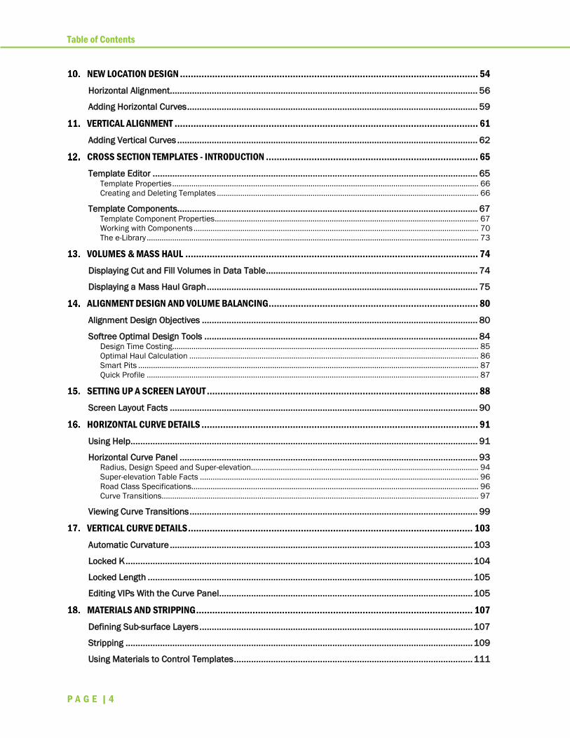
Table of Contents
P A G E | 4
NEW LOCATION DESIGN ............................................................................................................... 54
Horizontal Alignment............................................................................................................................. 56
Adding Horizontal Curves ...................................................................................................................... 59
VERTICAL ALIGNMENT ................................................................................................................. 61
Adding Vertical Curves .......................................................................................................................... 62
CROSS SECTION TEMPLATES - INTRODUCTION ............................................................................... 65
Template Editor .................................................................................................................................... 65 Template Properties ................................................................................................................................................ 66 Creating and Deleting Templates ........................................................................................................................... 66
Template Components.......................................................................................................................... 67 Template Component Properties ............................................................................................................................ 67 Working with Components ...................................................................................................................................... 70 The e-Library ............................................................................................................................................................ 73
VOLUMES & MASS HAUL ............................................................................................................. 74
Displaying Cut and Fill Volumes in Data Table ...................................................................................... 74
Displaying a Mass Haul Graph .............................................................................................................. 75
ALIGNMENT DESIGN AND VOLUME BALANCING .............................................................................. 80
Alignment Design Objectives ................................................................................................................ 80
Softree Optimal Design Tools ............................................................................................................... 84 Design Time Costing ................................................................................................................................................ 85 Optimal Haul Calculation ........................................................................................................................................ 86 Smart Pits ................................................................................................................................................................ 87 Quick Profile ............................................................................................................................................................ 87
SETTING UP A SCREEN LAYOUT ..................................................................................................... 88
Screen Layout Facts ............................................................................................................................. 90
HORIZONTAL CURVE DETAILS ....................................................................................................... 91
Using Help ............................................................................................................................................. 91
Horizontal Curve Panel ......................................................................................................................... 93 Radius, Design Speed and Super-elevation ........................................................................................................... 94 Super-elevation Table Facts ................................................................................................................................... 96 Road Class Specifications....................................................................................................................................... 96 Curve Transitions ..................................................................................................................................................... 97
Viewing Curve Transitions ..................................................................................................................... 99
VERTICAL CURVE DETAILS .......................................................................................................... 103
Automatic Curvature ........................................................................................................................... 103
Locked K ............................................................................................................................................. 104
Locked Length .................................................................................................................................... 105
Editing VIPs With the Curve Panel....................................................................................................... 105
MATERIALS AND STRIPPING ....................................................................................................... 107
Defining Sub-surface Layers ............................................................................................................... 107
Stripping ............................................................................................................................................. 109
Using Materials to Control Templates ................................................................................................. 111

Table of Contents
P A G E | 5
TEMPLATE ASSIGNMENTS .......................................................................................................... 114
Assigning a Roadside Barrier to a Range of Stations ......................................................................... 114 Creating a New Template ...................................................................................................................................... 114
Assigning the Template....................................................................................................................... 115
TEMPLATE PARAMETER OVERRIDES ............................................................................................ 117 Creating a Turning Lane ........................................................................................................................................ 117
TEMPLATES – DISPLAY AND REPORTING ...................................................................................... 119 Surfaces ................................................................................................................................................................. 119 Codes ..................................................................................................................................................................... 119
Display and Reporting of Template Layers ......................................................................................... 120 Formatting Template Layers ................................................................................................................................. 120
Display and Reporting of Ditch Lines .................................................................................................. 123 Reporting template point codes ........................................................................................................................... 123
CULVERTS ................................................................................................................................ 127
Changing Fill Material ......................................................................................................................... 130
LABELS .................................................................................................................................... 132
Label Classes ...................................................................................................................................... 132 Class Label Formatting ......................................................................................................................................... 132
User Definable Labels ......................................................................................................................... 140
Point Label Formatting ....................................................................................................................... 143 Editing Labels with the Mouse .............................................................................................................................. 143 Floating Labels ...................................................................................................................................................... 145 Profile Sub View Labels ......................................................................................................................................... 146
MULTI-PLOT REPORT BUILDER.................................................................................................... 149
Multi-Plot Introduction ........................................................................................................................ 149 Creating and Positioning Sub-Views ..................................................................................................................... 149 Configuring Your Page Size ................................................................................................................................... 150 Configuring our Chapter ........................................................................................................................................ 151 Adding Graphic Sub-views .................................................................................................................................... 152 Grid Options ........................................................................................................................................................... 153 Adding a Scale Bar ................................................................................................................................................ 154 Adding Rectangle Sub-View Items ........................................................................................................................ 155 Multi-Plot Plan Rotation ........................................................................................................................................ 157
Multi-Plot Chapters ............................................................................................................................. 158 Copy and Paste of Multi-Plot Items ...................................................................................................................... 158 Add a Legend ......................................................................................................................................................... 160 Add a Curve Table ................................................................................................................................................. 162 Saving Layouts ...................................................................................................................................................... 163
FIXED SECTION EDITOR .............................................................................................................. 164 Editing Layer of Individual Cross Sections: .......................................................................................................... 165
Fixed Section Volume Calculations ..................................................................................................... 166 Fixed Ranges ......................................................................................................................................................... 168
CREATING A COMPOSITE SURFACE ............................................................................................. 169
Exporting Designed Surfaces .............................................................................................................. 169
Merging Terrains ................................................................................................................................. 172
Iterative Alignment Design .................................................................................................................. 173
Chapter 1 - Getting Started
P A G E | 6
Getting Started This manual is formatted as a hands-on tutorial, which can be used by novice or experienced users.
Step-by-step examples use prepared documents and data files to illustrate tools needed for common
RoadEng® tasks. The document is set out as if you were doing a road design project from original
ground survey to completed construction documents.
Installation
The tutorial files referred to in the following examples can be installed from Softree’s Support web
site:
• Go to the Support-Documentation Updates page on Softree’s web site:
https://support.softree.com/product-updates/Documentation-Tutorials.
• Once SoftreeTutorials.exe has been successfully downloaded.
• Double-click on the file to begin installation.
During the installation you will be prompted to select which content to install, we recommend
installing all the available tutorial options.
Documents
The tutorial files (data sets) will be installed in the folder below by default:
C:\Users\Public\Documents\softree\training90\RoadEngCivil
We will refer to this folder as <RoadEngCivil> in the examples below. It is possible to change this
folder at install time; you can also copy it to a new location afterwards if you wish.
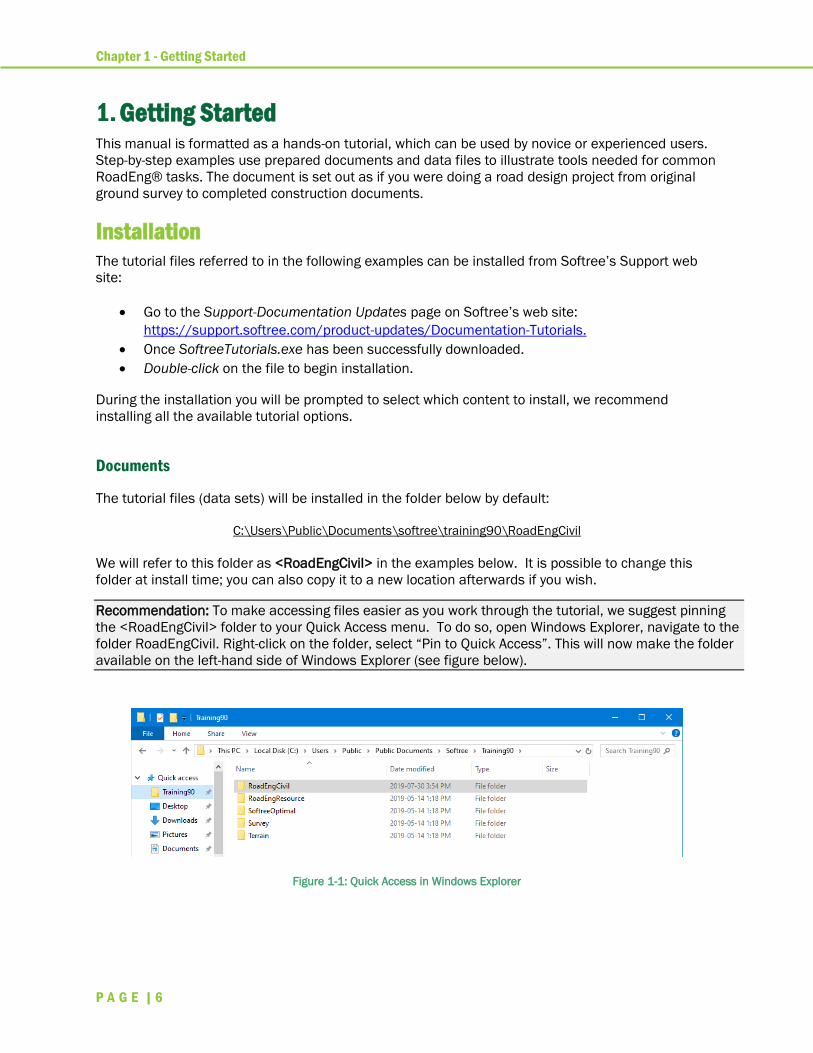
Recommendation: To make accessing files easier as you work through the tutorial, we suggest pinning
the <RoadEngCivil> folder to your Quick Access menu. To do so, open Windows Explorer, navigate to the
folder RoadEngCivil. Right-click on the folder, select “Pin to Quick Access”. This will now make the folder
available on the left-hand side of Windows Explorer (see figure below).
Figure 1-1: Quick Access in Windows Explorer

Chapter 1 - Getting Started
P A G E | 7
Don’t Save Files (in most cases)
Most of the following examples end with the phrase: “… do not save changes”. If you modify the
tutorial files, they will no longer work with the steps in the exercise; this will prevent you, or someone
else, coming back and doing the exercise again.
If a file gets modified, delete the files in the training folder. Then re-install the tutorial files (per the
original steps).
C:\Users\Public\Documents\softree\training90\RoadEngCivil
Defaults and Layouts
The setup and layout files are stored the folder below by default:
C:\ProgramData\Softree\RoadEng
It is possible to change this folder, so we will refer to it as <Defaults and Layouts> in the examples
below. A folder containing training specific files has also been added to this location:
<Defaults and Layouts>\
Note: You can always determine the actual <Defaults and Layouts> folder by running the Terrain
Module, selecting menu Setup | Location Setup | Install tab.
If Softree Optimal is installed after RoadEng, the default folder will be:
C:\ProgramData\Softree\SoftreeOptimal\

Chapter 1 - Getting Started
P A G E | 8
Function Groups
Some RoadEng® and Terrain Tools® products have certain features; we classify these optional
features by function group.
To view the features enabled with your license:
1. Select Setup | Module Setup and click on the General tab.
2. Click on the Menus… to open the Menu Customization Dialogue box.
Figure 1-2: Function Groups Displayed in the Menu Customisation Dialogue
Note: Specific function groups are required to do certain examples
All required function groups are listed prior to each example in this manual. If you do not have
permission to use all the required function groups, you may wish to skip the example. Also note that
some function groups may be disabled even if you have permission to use them – this is so users with a
lesser license can still do the example.

Chapter 1 - Getting Started
P A G E | 9
On-line Help
Help information is available by choosing the Help menu or pressing <F1> on your keyboard. The
On-line Help includes detailed technical information about menus, dialogue boxes, and operation of
the program. It may be useful to refer to the On-line Help while working through the examples in this
manual.
Additional help is available through the Softree Knowledge Base:
https://www.support.softree.com/knowledge-base
Tutorial Units
Most examples in this tutorial are in Imperial Units (feet). To correctly follow the examples, ensure
Imperial (ft) units are enabled in the Setup |Setup Module Setup | Units tab | Units: Imperial (ft). If
other units are used, they will be specified at the start of the example. The procedures and concepts
described apply to all unit systems.
Screen Layouts
Screen layouts are small files that save display options (window positions, labels, scales etc). Many
of the examples in this training manual include a step to retrieve a screen layout; this change
provides multiple view options in one quick step.
The screen layout drop-down control can be found in the Standard toolbar in all modules (figure
below), View | Screen Layout:
Figure 1-3: Accessing Screen Layouts Group
With the drop-down expanded, you can:
• <Right-click> on a screen layout in the Screen Layouts tool bar item to:
o Change Properties
o Delete
o Copy
o Save
• <Right-click> on a folder (Softree or Custom) in the Screen Layouts tool bar item to:
o Change properties (only the Custom folder can be changed here)
o Paste a screen layout that was recently copied
o Save new layout (define name and description)
The Custom folder is often defined on a network drive so that the layouts are accessible to all users.
Chapter 1 - Getting Started
P A G E | 10
• The Save screen layout button allows you to save a screen layout anywhere but only
those in the Custom or Softree folders will appear in the Screen Layouts tool bar.
• The Retrieve screen layout button allows you to open a screen layout file anywhere
including those in the Custom, Training or Softree folders.
• The Delete screen layout button opens up the screen layout folder where you can multiple
layouts to delete.
• You can change the Softree folder from the menu Module | Setup, Install tab. Do not do this
unless you understand the consequences; more than just screen layouts are stored in this
folder. The most common change is to put Settings and Layouts into your Documents folder
(private to one user only).
Note: Screen layouts were updated in Version 9. Softree recommends ‘updating’ any legacy user screen
layouts to update their behavior. Version 9 layouts work better when moved between monitors of
differing screen resolutions.
To ‘update’ your screen layouts:
If your legacy screen layout contains multi-plot information, please open your legacy screen layout in the
multi-plot window first:
Select Multi-Plot tab | Add New ▼ | Retrieve Other Layout. Select Multi-Plot Old Screen Layout (.dlt)
from the file type drop-down in the Retrieve Screen Layout Dialog. Select your legacy layout. Once open,
press Save Chapter in the Multi-Plot ribbon.
Conventions
The following conventions are used throughout the manual:
• Menu functions are delimited by a line “|”. File | Open means to click on Location File
button in the corner of the menu bar and then select Open from the drop-down menu.
Dialogue box control (like buttons) and heading names are italicized.
• The symbols “< >” contain keyboard functions. For example, < shift-enter> means: hold
down the Shift key and press the Enter key.
• File names and path names are bold.

Chapter 2 - Functional Overview
P A G E | 11
Functional Overview Softree software solutions are sold as modular products. Depending on the product you have
purchased, it could include up to three modules:
1. Survey/Map
2. Terrain
3. Location
Figure 2-1: Relationship Between the Modules
Each of the modules can be started from the Windows Start menu, a desktop shortcut or from the
Setup tab within either of the other modules.
Survey/Map Module
This module is used primarily to type paper survey notes into the computer. Azimuths, distances and
slopes are entered and reduced to coordinates. Facilities exist to add perpendicular side shots to a
traverse so that a ground terrain, suitable for a road design, can be easily captured with basic survey
instruments.
Survey/Map also contains tools for adjusting traverses with respect to each other or to known
coordinates.

Chapter 2 - Functional Overview
P A G E | 12
Terrain Module
The Terrain Module provides basic CAD facilities for assembling and manipulating 2D and 3D points
and features. Information can be imported from external sources like survey files, CAD files and
image files. Three dimensional coordinates can be incorporated into a digital terrain model (DTM).
DTMs can be used for:
• Contour generation
• Section and profile display
• Volume calculations
• Pad, pit and site design (grading)
• 3D viewing
• Original ground for road design (Location module)
The Terrain module is also a capable mapping tool with control of line types, colors, symbols,
hatching and labelling styles.
Chapter 2 - Functional Overview
P A G E | 13
Location Module
This is the module used to design road alignments. Location requires an original ground terrain
(provided by the Survey/Map and/or Terrain modules). The designer controls cross section
templates, alignment location and curves. Location provides real time feedback of volumes, mass
haul, road footprint, cross sections, grades, etc.
Location can also export designed surfaces back to the terrain module where they can be merged
into a composite surface. This is the most common way to prepare the original ground for an
intersection design.
Typical RoadENG Work Flow for Designing a Road
1. The Terrain module is used to import and verify survey data of existing conditions. Possible
data sources include total station (XYZ files), LiDAR, or GIS maps (shape, dwg, dgn etc.).
2. Using the Terrain module, break-lines and other linear features are identified and
connected. A TIN (Triangular Irregular Network) surface representing original ground (OG) is
created. The resulting linework and TIN surface is saved in a *.TERX file. NOTE: it may be
useful to create several terrain files (e.g. one with the TIN model and one with planimetric
linework).
3. A new design is created in the Location module, based on an OG surface (.TERX file from
step 2).
4. The road cross section is created or adjusted using the Template Editor.
5. A horizontal alignment is created or adjusted using the mouse or explicitly in the Horizontal
Alignment Panel.
6. A vertical alignment is created or adjusted using the mouse or explicitly in the Vertical
Alignment Panel. Vertical optimization (Softree Optimal) can also be used in this step.
7. Steps 4-6 are repeated until the designer is satisfied with the result. In addition to Plan,
Profile and Cross Section views, various reporting tools provide the designer with feedback.
This includes volumes, mass haul diagram, and cost reporting.
8. Construction documentation is prepared using the Multi-Plot window. This documentation is
printed directly or exported to CAD (*.dwg).
9. LandXML or ASCII files can be saved for construction staking.

Chapter 3 - Importing ASCII Survey Files
P A G E | 14
Importing ASCII Survey Files The Terrain Module will accept a variety of different ASCII files by allowing the user to configure the
import format. This example illustrates the use of the import functions to read a topographic survey
file created by a total station data collector.
Note: section for file install folders (<RoadEngCivil> and <Defaults and Layouts>).
A Typical Data File
The file (excerpt below) consists of a sequence number, X, Y, Z and code separated by tabs.
1 329591.7666 2195715.037 1172.736 SPOT
2 329570.0566 2195516.997 1158.295 PP
3 329625.9166 2195555.797 1159.534 SPOT
4 329573.4966 2195594.317 1161.31 SPOT
5 329552.9966 2195554.887 1160.682 SPOT
6 329561.9466 2195602.537 1164.661 SPOT
7 329531.5866 2195563.567 1166.9 SPOT
8 329527.9066 2195628.777 1177.279 SPOT
9 329500.6266 2195578.507 1177.822 SPOT
10 329482.4666 2195641.327 1190.244 SPOT
11 329456.7666 2195598.247 1192.141 SPOT
12 329433.7266 2195654.027 1204.384 SPOT
13 329407.6066 2195614.587 1206.786 SPOT
14 329396.5866 2195673.697 1216.893 SPOT
15 329374.2266 2195630.877 1218.22 SPOT
16 329347.4766 2195697.547 1231.632 SPOT
17 329321.3566 2195653.237 1235.406 SPOT
18 329296.9066 2195704.397 1242.378 SPOT
19 329276.1266 2195665.097 1244.316 SPOT
20 329247.7166 2195711.457 1248.812 SPOT
Figure 3-1: Excerpt from Survey1.txt
Chapter 3 - Importing ASCII Survey Files
P A G E | 15
Setting Up an Import Format
1. Open the Terrain Module.
2. Setup | Module Setup | Units tab, Units: Imperial (ft). The import software cannot detect
units from the information in an ASCII file.
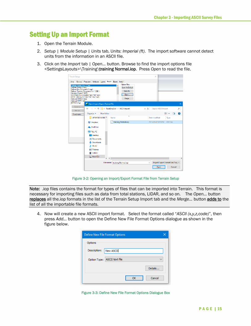
3. Click on the Import tab | Open… button. Browse to find the import options file
<SettingsLayouts>\Training\training Normal.iop. Press Open to read the file.
Figure 3-2: Opening an Import/Export Format File from Terrain Setup
Note: .iop files contains the format for types of files that can be imported into Terrain. This format is
necessary for importing files such as data from total stations, LIDAR, and so on. The Open… button
replaces all the.iop formats in the list of the Terrain Setup Import tab and the Merge… button adds to the
list of all the importable file formats.
4. Now will create a new ASCII import format. Select the format called “ASCII (x,y,z,code)”, then
press Add… button to open the Define New File Format Options dialogue as shown in the
figure below.
Figure 3-3: Define New File Format Options Dialogue Box
Chapter 3 - Importing ASCII Survey Files
P A G E | 16
Note: When you create a new import format, it will initially be a copy of the one selected when you press
the Add… (“ASCII (x,y,z,code)” in this case).
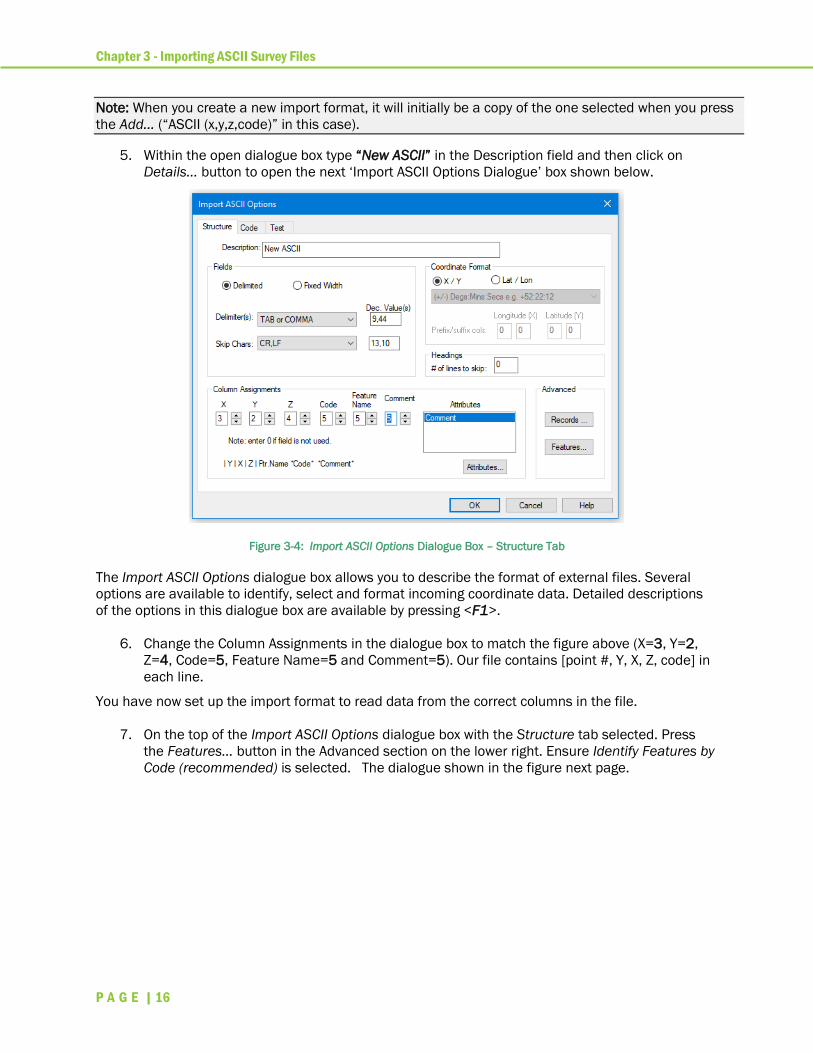
5. Within the open dialogue box type “New ASCII” in the Description field and then click on
Details… button to open the next ‘Import ASCII Options Dialogue’ box shown below.
Figure 3-4: Import ASCII Options Dialogue Box – Structure Tab
The Import ASCII Options dialogue box allows you to describe the format of external files. Several
options are available to identify, select and format incoming coordinate data. Detailed descriptions
of the options in this dialogue box are available by pressing <F1>.
6. Change the Column Assignments in the dialogue box to match the figure above (X=3, Y=2,
Z=4, Code=5, Feature Name=5 and Comment=5). Our file contains [point #, Y, X, Z, code] in
each line.
You have now set up the import format to read data from the correct columns in the file.
7. On the top of the Import ASCII Options dialogue box with the Structure tab selected. Press
the Features… button in the Advanced section on the lower right. Ensure Identify Features by
Code (recommended) is selected. The dialogue shown in the figure next page.

Chapter 3 - Importing ASCII Survey Files
P A G E | 17
Figure 3-5: Feature Detection Method Dialogue Box
8. The dialogue box above allows you to limit the length of polyline features by defining a
termination character to be found in the point code. An exclamation point, “!”, is defined as
the termination character in the Feature Detection Method dialogue box. If you refer to the
Survey1.txt (see figure at start of this exercise), you will see many of the point codes end with
“!”; this means that a connected feature breaks after this point and a new feature will be
created when the next point of this type is encountered. The EP polyline code (defined above)
will import as two breaklines (left and right) because of a strategically placed “!” in the survey
point codes.
9. Press OK to exit the Feature Detection Method dialogue box.
10. Within the existing dialogue box and select the Code tab (figure next page). Here you can
assign properties, symbols and line-types to the incoming points. For example, when
importing survey data you may can to connect center line or edge of road points.
Chapter 3 - Importing ASCII Survey Files
P A G E | 18
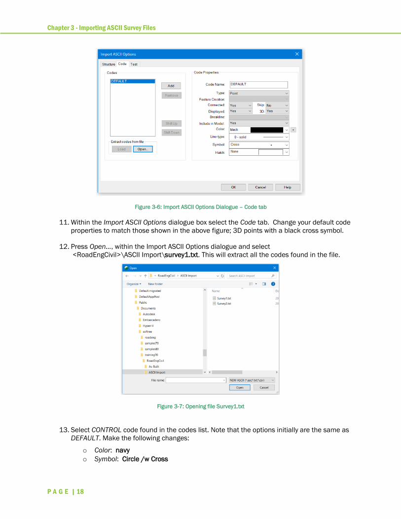
Figure 3-6: Import ASCII Options Dialogue – Code tab
11. Within the Import ASCII Options dialogue box select the Code tab. Change your default code
properties to match those shown in the above figure; 3D points with a black cross symbol.
12. Press Open…, within the Import ASCII Options dialogue and select
<RoadEngCivil>\ASCII Import\survey1.txt. This will extract all the codes found in the file.
Figure 3-7: Opening file Survey1.txt
13. Select CONTROL code found in the codes list. Note that the options initially are the same as
DEFAULT. Make the following changes:
o Color: navy
o Symbol: Circle /w Cross

Chapter 3 - Importing ASCII Survey Files
P A G E | 19
14. Select EP (Edge Pavement) in the code list and type in * beside EP, eg. ‘EP*’, in the Code
Name. The “*” is a wild card – any code starting with “EP” will fall into this category. Make
the following changes:
o Type: Polyline
o Feature Creation: Connect All by Code
o Breakline: Yes
o Color: blue
o Symbol: None
Points with the EP code will be connected (in the order found in the file) and made into a blue
breakline. The Connect All by Code property ensures that codes like EPL and EPR form separate
features even though they both fit the EP* specification.
15. Select code name CLP (Center Line Pavement) in the code list. Make the following changes:
o Type: Polyline
o Feature Creation: Connect All
o Breakline: Yes
o Color: red
o Line-type: 3-dash-dot
16. To test the specification, go to the Test tab (see Figure 3-8):
Figure 3-8: Import ASCII Options Dialogue – Test tab
17. Click Open File and open <RoadEngCivil>\ASCII Import\Survey1.txt.
18. Press Next Record several times. At the bottom of the dialogue box the values of X, Y, Z and
comment are displayed. Confirm that the incoming fields are being correctly interpreted; if
not return to the other tabs to modify the format.
19. When satisfied, press OK to return to the Terrain Setup dialogue box.

Chapter 3 - Importing ASCII Survey Files
P A G E | 20
20. To save the new import specifications for future use Setup | Module Setup | Import tab |
Save As… button. Normally, you would choose Normal.IOP and write over it (to update your
default settings) – do this only if you are working on a computer used for tutorial or training,
otherwise save as new training.iop or press Cancel to avoid changing your defaults.
21. Press OK to close the Terrain Setup dialogue box. Now we’ll use the import format we’ve
created to open the survey data file.
22. File | Open. Change dropdown menu in lower right-hand corner to New ASCII (*.asc, *.txt,
*.csv) (at the bottom of the list). Open <RoadEngCivil>\ASCII Import\Survey1.txt. You will be
presented with the Import Options dialogue box to allow last minute changes. Press OK to
import the file.
23. Softree Warning appears: “Incoming coordinate system and units are undefined. OK to
continue without conversion?” Click Continue.
24. Select the View| Screen Layouts | select training Normal.ilt from the dropdown menu. This
will set up your options and windows to look like the Figure 3-9.
Figure 3-9: Plan Window after Importing Survey1.txt.
Note: The right EP feature is selected (note the properties displayed in the status window). Also note that
there are many point codes that have not been formatted or connected to form breaklines. In the next
steps, we will re-read the same data with a prepared import format.
Turn on the feature labels:
25. <Right-click> in the Plan window | Select Feature(s)>All, <right-click> | select Modify
Selected Feature(s) | Labels…
26. <Double-click> on ‘Comments (at feature points)’ and ‘Feature Name’. Press OK.
To reduce the size of the labels:
27. Zoom in by scrolling with the mouse wheel until the label font size is smaller and readable.
Chapter 3 - Importing ASCII Survey Files
P A G E | 21
28. Press the Scale Lock . Now zoom out by rolling the wheel on the mouse. The labels will
remain the size of what they were when they were locked.
We will now open the same file, with more point codes defined:
29. File | Open. Change Files of type to ASCII 2 (#,y,x,z,code).
30. Open <RoadEngCivil>\ASCII Import\Survey1.txt. When prompted to save changes, choose
No.
31. This will open the Import Options dialogue; click on the Code tab to see the extra codes
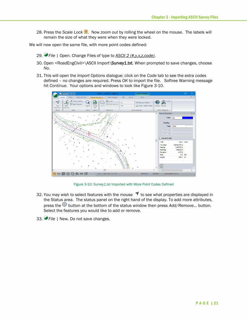
defined – no changes are required. Press OK to import the file. Softree Warning message
hit Continue. Your options and windows to look like Figure 3-10.
Figure 3-10: Survey1.txt Imported with More Point Codes Defined
32. You may wish to select features with the mouse to see what properties are displayed in
the Status area. The status panel on the right hand of the display. To add more attributes,
press the button at the bottom of the status window then press Add/Remove… button.
Select the features you would like to add or remove.
33. File | New. Do not save changes.
Chapter 4 - Creating a DTM with Contours
P A G E | 22
Creating a DTM with Contours In this exercise, you will open a file containing 3D data (imported in the Importing ASCII Survey Files
exercise) and create a Digital Terrain Model (DTM). You will also generate major and minor contour
lines.
Note: The digital model is represented by a Triangular Irregular Network (TIN); for this reason, menus,
documentation and help files often refer to a Digital Terrain Model as TIN model.
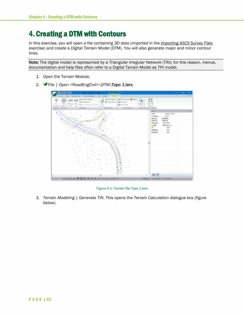
1. Open the Terrain Module.
2. File | Open <RoadEngCivil>\DTM\Topo 1.terx.
Figure 4-1: Terrain file Topo 1.terx
3. Terrain Modeling | Generate TIN. This opens the Terrain Calculation dialogue box (figure
below).

Chapter 4 - Creating a DTM with Contours
P A G E | 23
Figure 4-2: Digital Terrain Calculation Dialogue Box with
Both Major and Minor Contours Enabled.
Contour Specification
4. Ensure the Labeling box is checked in the Major Contours tabs. Clicking on the button
adjacent to the Major or Minor Contours check boxes, allows you to change the color and line
type used for the contour lines. Optional contour Smoothing (controlled by Thinning distance)
rounds the corners where contours cross triangle sides – smoothed contours do not match
the model elevation exactly.
Note: Default contour line types and colors are stored in the Normal.ilt screen layout. Any changes made
after a new document is created are saved with the document.
5. Click on the Major Contours tab and set the Interval: 10 and check the Labeling box as
shown above. You also need to an even number before the start of calculated range. Set the
elevation Start: 1150.
Click on the Minor Contours tab and set the Interval: 2 and make sure Labeling box is unchecked.
You also need to set the Start elevation to be a multiple of 2, Start: 1150. Press OK to generate both
TIN and contours.

Chapter 4 - Creating a DTM with Contours
P A G E | 24
Figure 4-3: Contours Generated without Boundary or Length Limitation. Underlying Triangles Shown on Right
6. To display triangles in the model first delete the contours: Terrain Modelling | Delete TIN |
select Delete Contours box | OK. Then, <right-click> in plan view select Active Window (Plan)
Option…| Surface tab | check Triangle outlines box.
Figure 4-4: Contour Formation from TIN model. Elevations between known Elevation Points are Interpolated. Enabling
Contour Smoothing causes Contours to be Less Angular
Chapter 4 - Creating a DTM with Contours
P A G E | 25
Limiting Triangles
In this example, the triangles (and resulting contours) on the upper right and lower left of the model
are unrealistic – elevations are being interpolated between points very far apart. There are two ways
to prevent these unrealistic triangles:
• Create a boundary polygon (with property TIN boundary).
• Limit triangle length.
A boundary polygon will limit triangle formation to an area of interest – this can also be useful when
your data set is very large or when you wish to merge a small DTM into a larger one. TIN boundaries
will be covered in other exercises.
In this example, we will limit the triangle length.
7. If triangles are still displayed, turn them off: <Right-click> in plan view | Active Window (Plan)
Options… | Surface tab | uncheck Triangle outlines box | OK.
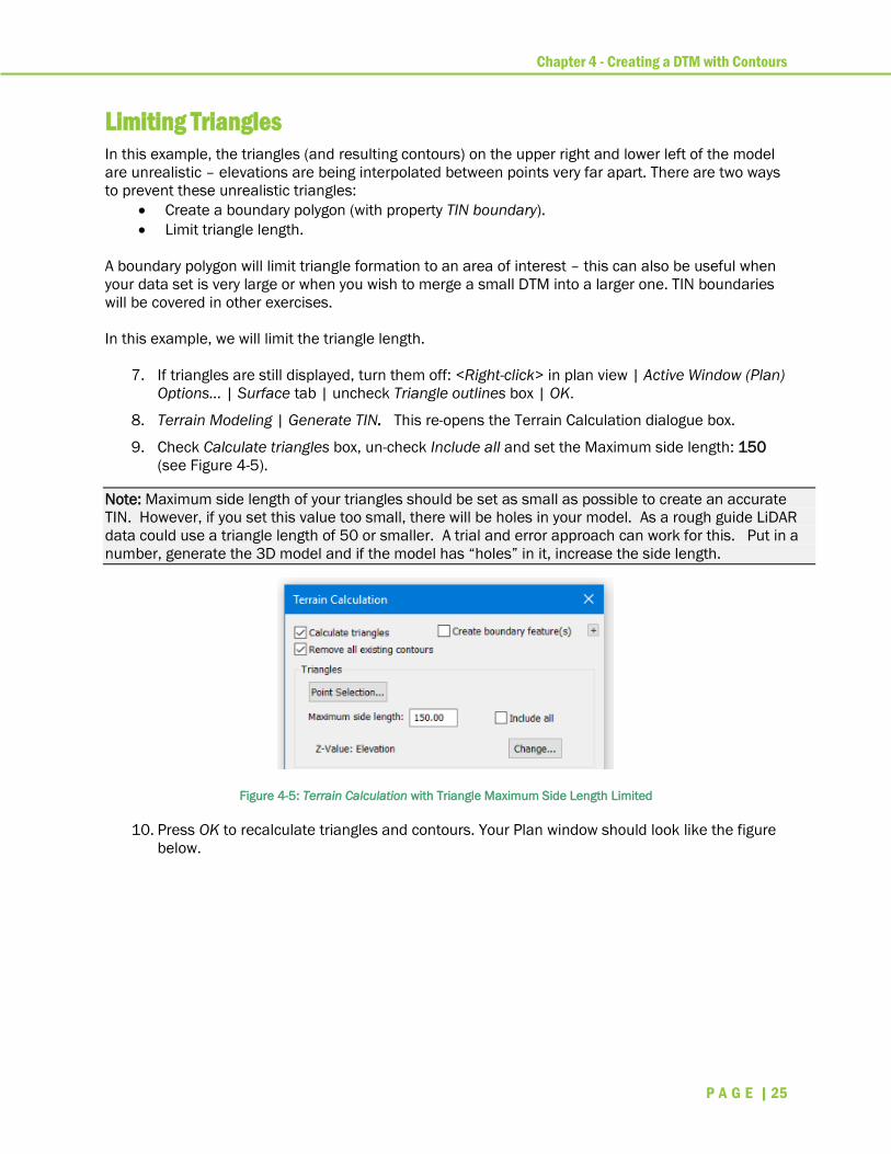
8. Terrain Modeling | Generate TIN. This re-opens the Terrain Calculation dialogue box.
9. Check Calculate triangles box, un-check Include all and set the Maximum side length: 150
(see Figure 4-5).
Note: Maximum side length of your triangles should be set as small as possible to create an accurate
TIN. However, if you set this value too small, there will be holes in your model. As a rough guide LiDAR
data could use a triangle length of 50 or smaller. A trial and error approach can work for this. Put in a
number, generate the 3D model and if the model has “holes” in it, increase the side length.
Figure 4-5: Terrain Calculation with Triangle Maximum Side Length Limited
10. Press OK to recalculate triangles and contours. Your Plan window should look like the figure
below.
Chapter 4 - Creating a DTM with Contours
P A G E | 26
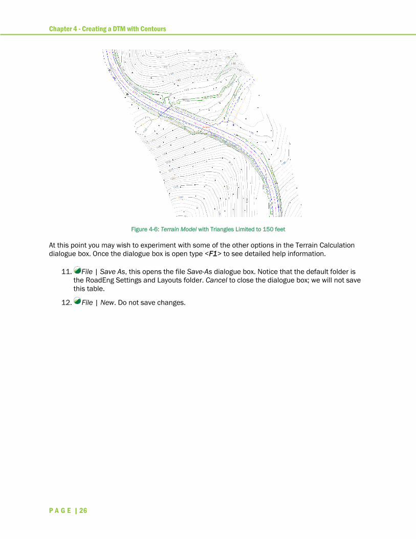
Figure 4-6: Terrain Model with Triangles Limited to 150 feet
At this point you may wish to experiment with some of the other options in the Terrain Calculation
dialogue box. Once the dialogue box is open type <F1> to see detailed help information.
11. File | Save As, this opens the file Save-As dialogue box. Notice that the default folder is
the RoadEng Settings and Layouts folder. Cancel to close the dialogue box; we will not save
this table.
12. File | New. Do not save changes.
Chapter 5 - Moving Around in the Plan Window
P A G E | 27
Moving Around in the Plan Window In this exercise, you will use the Zooming and Panning functions to change the Plan view. You will
also select features with the mouse to examine their properties in the Status window. Many of these
functions work in other graphics window types.
Note: section for file install folders (<RoadEngCivil> and <Defaults and Layouts>).
1. Open the Terrain Module.
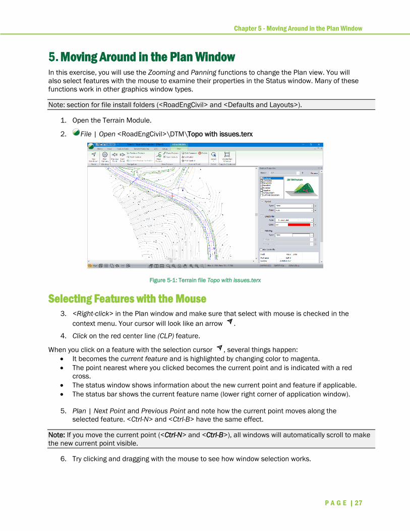
2. File | Open <RoadEngCivil>\DTM\Topo with issues.terx
Figure 5-1: Terrain file Topo with issues.terx
Selecting Features with the Mouse
3. <Right-click> in the Plan window and make sure that select with mouse is checked in the
context menu. Your cursor will look like an arrow .
4. Click on the red center line (CLP) feature.
When you click on a feature with the selection cursor , several things happen:
• It becomes the current feature and is highlighted by changing color to magenta.
• The point nearest where you clicked becomes the current point and is indicated with a red
cross.
• The status window shows information about the new current point and feature if applicable.
• The status bar shows the current feature name (lower right corner of application window).
5. Plan | Next Point and Previous Point and note how the current point moves along the
selected feature. <Ctrl-N> and <Ctrl-B> have the same effect.
Note: If you move the current point (<Ctrl-N> and <Ctrl-B>), all windows will automatically scroll to make
the new current point visible.
6. Try clicking and dragging with the mouse to see how window selection works.

Chapter 5 - Moving Around in the Plan Window
P A G E | 28
7. Hold the <shift> key and click on a feature. This allows you to add and remove features from
a selection set.
Zooming and Panning
View | Zoom allows you to zoom in, zoom out, zoom to window, end zoom, zoom extents and pan
respectively. The function of these tools is mostly self- evident with a little experimentation.
The middle roller mouse button is dedicated to zoom and pan functions. If these functions do not
work as described below, it is likely because of mouse software that has been configured to override
the default behavior – check your control panel.
8. Move your mouse cursor over the Plan window and click and drag with the middle mouse
button; even a roller button can be “clicked”. Note that the mouse cursor changes into the
Pan hand, and the plan image moves with your mouse.
Note: The dedicated middle mouse Pan function can be much more convenient than scroll bars. You can
turn scroll bars off to save space (<Right-click> | Active Window (Plan) Window Options… | General tab |
check Scroll Bars).
9. Move your mouse cursor to a point of interest then roll the middle mouse button away from
you. Note how the image zooms in and how the point of interest stays under the mouse. If
you use the Zoom 200% the center of the screen is always in the same location.
10. Similarly, use the middle roller mouse to zoom out by rolling towards you.
11. Practice zooming and panning while you look for interesting features of the model. Note that
the scale changes (tool bar) every time you zoom in or out. Also note that the text remains
the same size (although this is an option) and that the symbol sizes and line thickness
remain unchanged (Figure 5-2).
Figure 5-2: Before and After Zoom Operation with Scale Un-locked
12. Set the scale to 1200 in the toolbar (note this is a natural scale, the same as 1" = 100").
Chapter 5 - Moving Around in the Plan Window
P A G E | 29
Note: The mouse roller will change the scale box in the tool bar once you have selected it. This can be
confusing. See step 14 below.
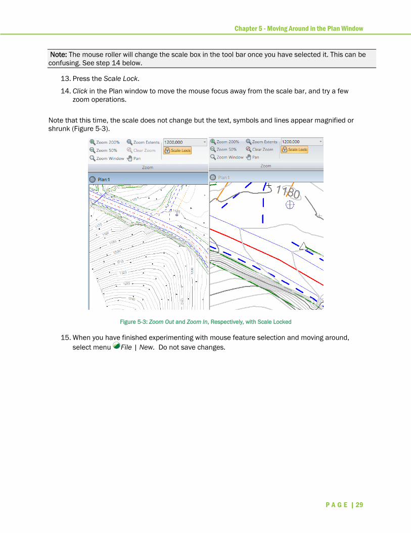
13. Press the Scale Lock.
14. Click in the Plan window to move the mouse focus away from the scale bar, and try a few
zoom operations.
Note that this time, the scale does not change but the text, symbols and lines appear magnified or
shrunk (Figure 5-3).
Figure 5-3: Zoom Out and Zoom In, Respectively, with Scale Locked
15. When you have finished experimenting with mouse feature selection and moving around,
select menu File | New. Do not save changes.

Chapter 6 - Moving Around in the 3D Window
P A G E | 30
Moving Around in the 3D Window In this exercise, you will use the Zoom, Pan and Rotation functions to change the 3D view. You will
also use the current point to help navigate in the 3D window and to help to find corresponding points
in Plan and 3D views.
Note: Refer to Getting Started section for file install folders (<RoadEngCivil> and <Defaults and
Layouts>).
1. Open the Terrain Module.
2. File | Open <RoadEngCivil>\DTM\Topo with issues.terx
3. Select View | New Window | 3D. A 3D window will appear on your screen. The rendered
surface should be visible; if it is not, press Zoom Extents in the View tab of the tool bar (this
does not always work if your model contains stray points).
4. View | Tile Vertically to show Plan and 3D windows side by side (see figure below).
Figure 6-1: 3D and Plan Windows depicting file Topo with issues.terx
Now we need to move around in the two windows to find problems with the model. In the 3D window,
Zooming and Panning behave in a similar way to the Plan window (see previous exercise Moving
Around in the Plan Window).
5. Use the zoom tools in the tool bar or the middle mouse wheel button to move around in the
3D window.
Rotating the 3D image
The 3D window also allows you to rotate the image.
6. In the 3D window, Click and drag with the left mouse and notice how the 3D view changes. It
may take a little practice to get the hang of it.
3D Window Options
Chapter 6 - Moving Around in the 3D Window
P A G E | 31
7. Make sure you have a current point defined by clicking with the selection cursor on a feature
in the Plan Window. Note that the current point is represented by a three-dimensional red
cross in the 3D window.
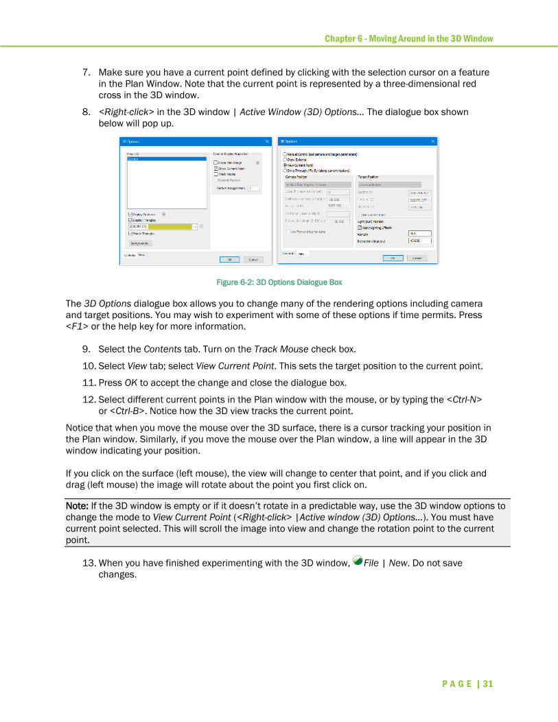
8. <Right-click> in the 3D window | Active Window (3D) Options... The dialogue box shown
below will pop up.
Figure 6-2: 3D Options Dialogue Box
The 3D Options dialogue box allows you to change many of the rendering options including camera
and target positions. You may wish to experiment with some of these options if time permits. Press
<F1> or the help key for more information.
9. Select the Contents tab. Turn on the Track Mouse check box.
10. Select View tab; select View Current Point. This sets the target position to the current point.
11. Press OK to accept the change and close the dialogue box.
12. Select different current points in the Plan window with the mouse, or by typing the <Ctrl-N>
or <Ctrl-B>. Notice how the 3D view tracks the current point.
Notice that when you move the mouse over the 3D surface, there is a cursor tracking your position in
the Plan window. Similarly, if you move the mouse over the Plan window, a line will appear in the 3D
window indicating your position.
If you click on the surface (left mouse), the view will change to center that point, and if you click and
drag (left mouse) the image will rotate about the point you first click on.
Note: If the 3D window is empty or if it doesn’t rotate in a predictable way, use the 3D window options to
change the mode to View Current Point (<Right-click> |Active window (3D) Options…). You must have
current point selected. This will scroll the image into view and change the rotation point to the current
point.
13. When you have finished experimenting with the 3D window, File | New. Do not save
changes.

Chapter 7 - Finding / Repairing DTM Problems
P A G E | 32
Finding / Repairing DTM Problems In this exercise, you will use the 3D window to help find problems with a DTM. You will also remove
bad data points from the model and tag critical features as breaklines. It is possible to find all the
problems with this model by looking carefully at the contours (especially as they are closely spaced).
However, the 3D window often makes this task quicker and easier.
You should already be familiar with moving around in the Plan and 3D windows (previous two
exercises).
Note: Refer to Getting Started section for file install folders (<RoadEngCivil> and <Defaults and
Layouts>).
1. Open the Terrain Module.
2. File | Open <RoadEngCivil>\DTM\Topo with issues.terx.
3. View | New Window | 3D from dropdown. A 3D window will appear on your screen.
4. Use menu View | Tile Vertically to show 3D and Plan windows side by side.

Chapter 7 - Finding / Repairing DTM Problems
P A G E | 33
Removing a Bad Point From the Model
5. Adjust the Plan and 3D views until you can see the bad elevation point shown below.
Figure 7-1: Bad Elevation Point Displayed in 3D, Plan and Feature Properties Windows
6. Select the bad point in the Plan window or the 3D window with the mouse . You know
you’ve selected the correct point when the 3D window shows the current point on top of the
anomalous spike (figure above). Note that the Status window shows that this point is a 3D
modeled point – it is part of the TIN surface.
At this point you could delete the feature but then there will be no record of this point. Instead we will
remove it from the TIN model.
7. In the Feature Properties panel, clear the Modelled property so the point feature will no
longer be part of the model. Press Apply.
8. When warned that “existing triangles will be cleared” respond OK.
Note: The above procedure is typical of most Terrain Module operations:
First, select features of interest (sometimes the current feature and current point are important).
Second, use the Modify Selected Feature(s) menu to do something to the selection set.
9. Select the Terrain Modeling | Generate TIN in the tool bar to open the Terrain Calculation
dialogue box (see Creating a DTM with Contours exercise above). The settings for this
dialogue box were configured when this file was created; you don’t need to adjust anything.
10. Press OK to recalculate the DTM and the contours. Note that the anomalous spike in the
model has disappeared.
Defining Breaklines
11. Adjust the Plan and 3D views until you can see along the curve in the road shown below.
Chapter 7 - Finding / Repairing DTM Problems
P A G E | 34
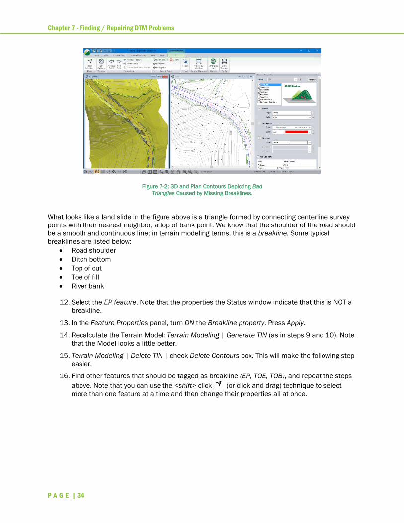
Figure 7-2: 3D and Plan Contours Depicting Bad
Triangles Caused by Missing Breaklines.
What looks like a land slide in the figure above is a triangle formed by connecting centerline survey
points with their nearest neighbor, a top of bank point. We know that the shoulder of the road should
be a smooth and continuous line; in terrain modeling terms, this is a breakline. Some typical
breaklines are listed below:
• Road shoulder
• Ditch bottom
• Top of cut
• Toe of fill
• River bank
12. Select the EP feature. Note that the properties the Status window indicate that this is NOT a
breakline.
13. In the Feature Properties panel, turn ON the Breakline property. Press Apply.
14. Recalculate the Terrain Model: Terrain Modeling | Generate TIN (as in steps 9 and 10). Note
that the Model looks a little better.
15. Terrain Modeling | Delete TIN | check Delete Contours box. This will make the following step
easier.
16. Find other features that should be tagged as breakline (EP, TOE, TOB), and repeat the steps
above. Note that you can use the <shift> click (or click and drag) technique to select
more than one feature at a time and then change their properties all at once.
Chapter 7 - Finding / Repairing DTM Problems
P A G E | 35
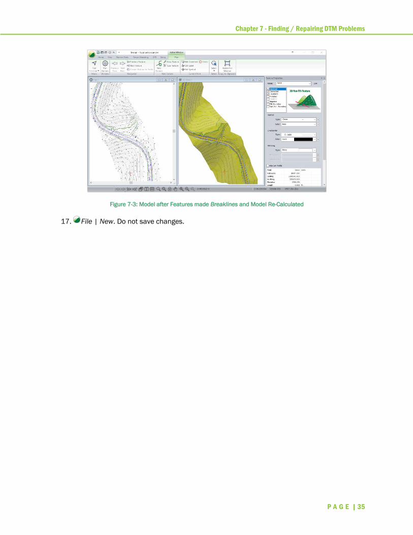
Figure 7-3: Model after Features made Breaklines and Model Re-Calculated
17. File | New. Do not save changes.

Chapter 8 - Creating Breaklines
P A G E | 36
Creating Breaklines We have seen in the Chapter, Importing ASCII Survey Files, breaklines can be created automatically.
Sometimes, however, it is easier to simply connect the dots. In this exercise, you will add some
breaklines to a data set that consists of nothing but points.
To perform this task, you will learn about the following Terrain functions:
• Select features by name.
• Join points to create a polyline feature.
• Create a new feature.
• Draw and edit features with the mouse.
• Format feature colors, symbols and line styles.
Note: Refer to Getting Started section for file install folders (<RoadEngCivil> and <Defaults and
Layouts>).
1. Open the Terrain Module.
2. File | Open <RoadEngCivil>\DTM\Topo no breaklines.terx.
Figure 8-1: 3D and Plan Windows, File: Topo no breaklines.terx.
Notice that the road is not well defined. As shown in the previous exercise, breaklines are required to
define the surface realistically. It would also be nice to see other surveyed features like pavement
edges and the road center line. Fortunately, the survey data for this file was imported so that
features are named by the survey point code.
Selecting Features by Name
3. Hover your mouse cursor over a point in the Plan window and note the information tooltip
window that appears after a moment (see figure above). This is a subset of the Status
information available after you select a point (lower portion of Feature Properties panel).
4. Zoom in and select or hover over points to find out their names. You will notice that the road
center line points are named “CLP”.
Chapter 8 - Creating Breaklines
P A G E | 37
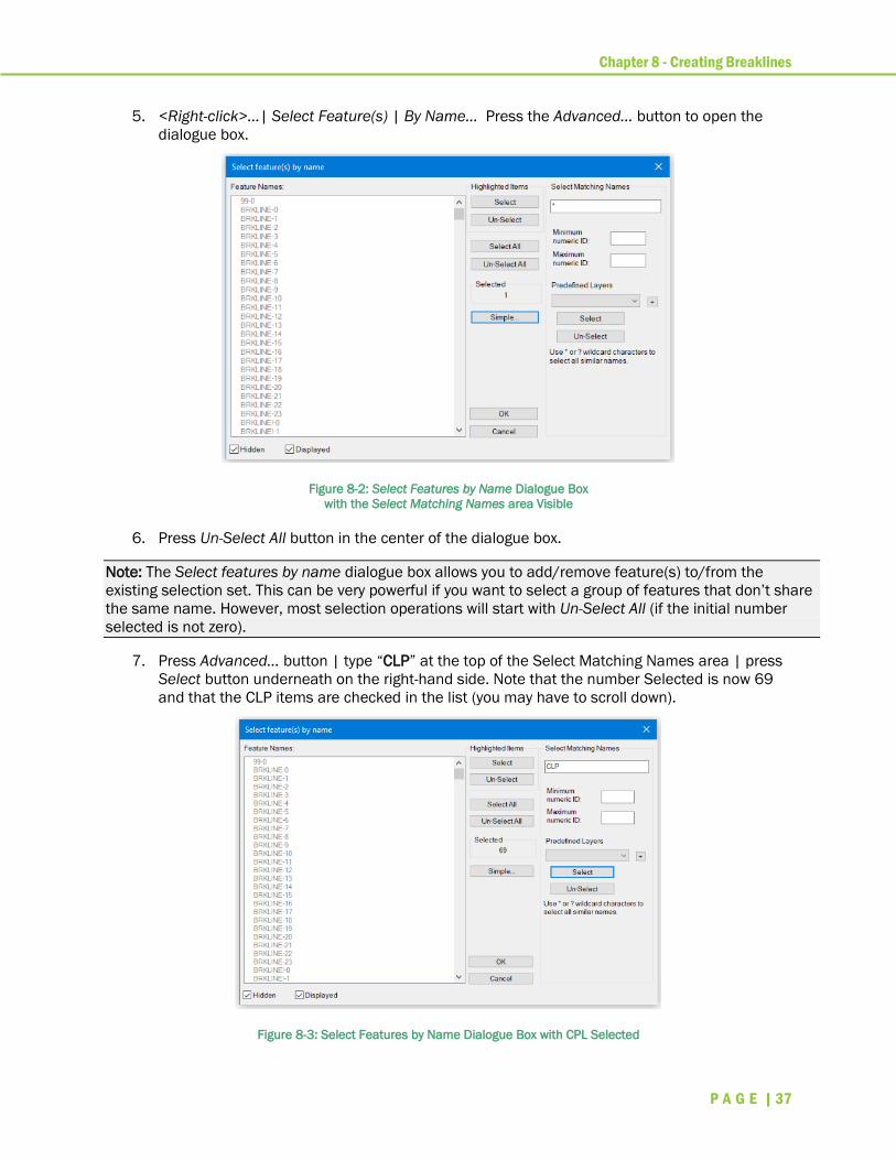
5. <Right-click>…| Select Feature(s) | By Name… Press the Advanced… button to open the
dialogue box.
Figure 8-2: Select Features by Name Dialogue Box
with the Select Matching Names area Visible
6. Press Un-Select All button in the center of the dialogue box.
Note: The Select features by name dialogue box allows you to add/remove feature(s) to/from the
existing selection set. This can be very powerful if you want to select a group of features that don’t share
the same name. However, most selection operations will start with Un-Select All (if the initial number
selected is not zero).
7. Press Advanced… button | type “CLP” at the top of the Select Matching Names area | press
Select button underneath on the right-hand side. Note that the number Selected is now 69
and that the CLP items are checked in the list (you may have to scroll down).
Figure 8-3: Select Features by Name Dialogue Box with CPL Selected

Chapter 8 - Creating Breaklines
P A G E | 38
8. Press OK to accept the change and close the dialogue box.
Joining Points to Create a Polyline Feature
Now that the CLP points are selected (highlighted magenta) we can connect them together and
format the resulting polyline.
9. Feature Tools | Join or <Ctrl-J>, to connect all the CLP points into one polyline feature. When
warned, “existing triangles will be cleared”, respond OK button.
Modifying Feature Formatting
10. <Right-click> in plan view| Modify Selected Feature(s) | Linetypes, Symbols or <Ctrl-L>, to
display the dialogue box below. Alternatively, you could use the Feature Properties Panel.
Figure 8-4: Feature Formatting Dialogue Box
11. Within the Plan Window Feature Formatting set Symbol Type: None, the Line/Border Type: 3-
dash-dot and the Color: red as shown in the figure above.
12. Press OK to accept the change and close the dialogue box.
The center line is now visible and represented by a polyline as desired. It should also be a breakline
as it represents the crown of the pavement.
13. Use Feature Properties panel to set the CLP feature as a Breakline (as in the Finding and
Repairing DTM problems exercise above). Press Apply.
14. Now let’s try the same process with the edge of pavement (EP) points.
15. As in step 5 above, use the Select features by name dialogue box to select all EP points.
16. Again use <Ctrl-J> to join them. The results are pictured below.

Chapter 8 - Creating Breaklines
P A G E | 39
Figure 8-5: Pavement Edges Connected using the Join Function
The polyline created above connects one side of the road to the other; the join function connects
each point to its nearest neighbour. If the points had been coded EPL (left) and EPR (right) then this
procedure would have produced satisfactory results (in two operations).
In this case, it is easier to connect the dots. We will make the EP points easy to find and then create
a new breakline feature to connect them manually.
17. Use the undo button or <Ctrl-Z> to restore the loose points.
18. As in step 10 above, use the formatting dialogue box <Ctrl-L> to change the EP points to a
distinctive color and symbol (as below).
Figure 8-6: Formatting can Make it Easier to Locate Points of a Given Type

Chapter 8 - Creating Breaklines
P A G E | 40
19. Select the Terrain Modeling | Delete TIN. Check the Delete Contours box and press OK
button. This will make the following steps easier.
Creating a New Feature
20. Home | New Feature.
Figure 8-7: The Feature Properties Dialogue used to Prepare a New Feature
21. Change the Name: EP-BL and check the Breakline property box as well as the others shown
in the figure above.
22. Within the Feature Properties dialogue box press Mouse button to close the dialogue box and
create the new feature.
23. When you are prompted to define the Elevation value, just press OK; keep Default elevation:
100.0. We will be snapping to existing points and picking up their elevations.
Drawing with the Mouse
When you are in Edit/Insert points mode, the mouse cursor will change to indicate what will happen
when you click the mouse.
New point is added at either end of the current
feature.
New point is inserted in between existing points
of the current feature.
Existing point is captured for editing.
24. Your mouse cursor has changed to a pencil indicating that you are in Edit/Insert points
mode. Left click anywhere in the Plan window (mouse down and up again) to create a new
point. Your cursor changes to a cross.
25. Move the cross over an EP point the cursor changes to indicate you are ready to snap.
Click a second time to anchor the new point. Note that the Elevation shown in the Status
window is the elevation of the EP survey point (if it is 100, then the snap failed – you may
have been too far from the EP point).
Chapter 8 - Creating Breaklines
P A G E | 41
Note: Snap to Point is an option set in the Plan window options <Right-click> | Active Window (Plan)
Options | General tab). Settings like this are saved in the document and in screen layouts.
26. Continue adding points to your new break line:
a) Click with the pencil cursor to create a new point.
b) Move the red cross over an EP point and click a second time to anchor the new point.
27. Try editing a point:
a) Move your mouse over an existing point in the new feature; note that the cursor
changes to a box .
b) Click the mouse the capture the point.
c) Move the red cross to a new position and click a second time to re-anchor the point.
28. Delete a point:
a) Move your mouse over an existing point in the new feature; note that the cursor
changes to a box .
b) Click the mouse the capture the point.
c) Type the <delete> key.
29. Insert a point:
a) Move your mouse over an existing segment in the new feature; note that the cursor
changes to a pencil with a cross .
b) Click the mouse to create a new point.
c) Move the red cross to a desired position and click a second time to anchor the point.
30. Stop when you have done enough points to get the hang of editing with the mouse. Make
sure you have tried deleting and inserting points as well as adding new ones at the end of
the feature.
Note: You can edit the points of any feature. First select the feature, then <Right-click> and select menu
Edit/Insert points with mouse (you can also choose the pencil button in the Home tab| Mode group |
Tool Selection button | Edit/Insert Points with Mouse from dropdown menu.
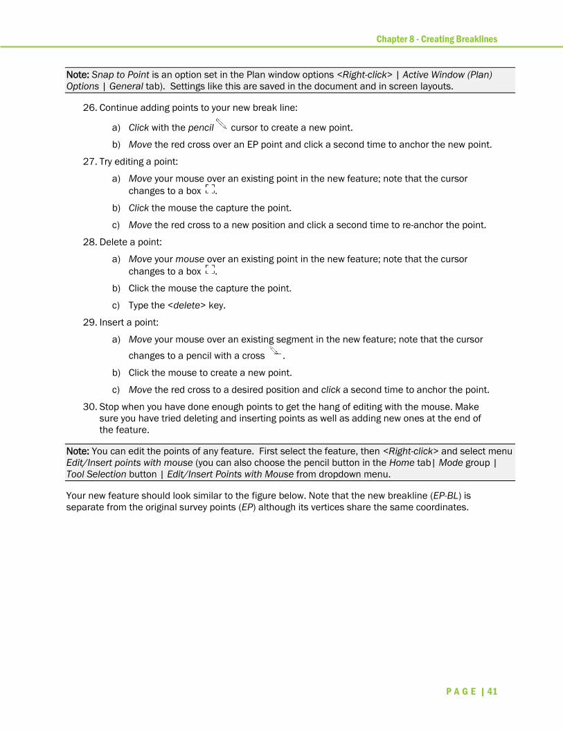
Your new feature should look similar to the figure below. Note that the new breakline (EP-BL) is
separate from the original survey points (EP) although its vertices share the same coordinates.
Chapter 8 - Creating Breaklines
P A G E | 42
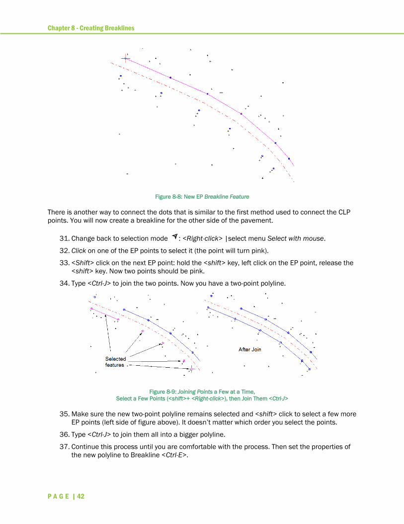
Figure 8-8: New EP Breakline Feature
There is another way to connect the dots that is similar to the first method used to connect the CLP
points. You will now create a breakline for the other side of the pavement.
31. Change back to selection mode : <Right-click> |select menu Select with mouse.
32. Click on one of the EP points to select it (the point will turn pink).
33. <Shift> click on the next EP point: hold the <shift> key, left click on the EP point, release the
<shift> key. Now two points should be pink.
34. Type <Ctrl-J> to join the two points. Now you have a two-point polyline.
Figure 8-9: Joining Points a Few at a Time,
Select a Few Points (<shift>+ <Right-click>), then Join Them <Ctrl-J>
35. Make sure the new two-point polyline remains selected and <shift> click to select a few more
EP points (left side of figure above). It doesn’t matter which order you select the points.
36. Type <Ctrl-J> to join them all into a bigger polyline.
37. Continue this process until you are comfortable with the process. Then set the properties of
the new polyline to Breakline <Ctrl-E>.

Chapter 8 - Creating Breaklines
P A G E | 43
If time permits you may wish to create breaklines for other point types using any of the methods
above.
38. File | New. Do not save changes.

Chapter 9 - Working with LiDAR
P A G E | 44
Working with LiDAR LiDAR (Light Detection And Ranging) surveys produce very large amounts of relatively accurate three
dimensional point data. The data includes points representing laser light scattered from the ground
(bare earth), foliage, buildings, transmission lines and other objects. This data is usually broken into
tiles, each containing a few million points.
Size and Accuracy Considerations
• The 32-bit version of RoadEng® is limited to approximately 5 million points. The 64-bit
version of RoadEng® can handle more points depending on the speed of the user’s CPU
processor and amount RAM, 10 million points is reasonable.
• Interpolating the LiDAR into regular grid format is not recommended, because this creates
points by interpolation (lost accuracy). For accuracy purposes, it is better to work with the raw
data points.
• When importing LiDAR data, it is very important to group points together instead of making
feature for every point. Features require a significant amount of memory (much more that a
point) so it is best to store thousands of points per feature.
It is not uncommon to have data sets with hundreds of millions of points (well exceeding the
recommended maximum of 10 million points). This limitation is generally not a problem for most
corridor projects, if points outside the area of interest are thinned. Consider a relatively large road
project say 20 kilometers (~ 12 miles). Assume that your LiDAR horizontal resolution is 1 meter (3
feet) and that you have identified a corridor that is 200 meters (~656 ft.) wide along a preliminary
alignment. This yields about 4 million data points.
Importing LiDAR in ASCII format
Large data sets need to be loaded in such a way that they use the least amount of memory possible.
In the next section, you will load a prepared LiDAR import format from a *.IOP (Input/Output
Parameters) file.
Note: If your data is in LAS format, many of the steps in the next section are not required. However, the
corridor thinning technique is required for both formats. LAS format is the preferred format for LiDAR, as
it is compact and loads fast.
1. Open the Terrain module.
2. File | Open <RoadEngCivil>\LiDAR\Empty.terx
3. Setup | Module Setup button. This opens a Terrain Setup dialogue box.
4. Select the Import tab.
5. Check if LiDAR (x,y,z,code) already existing in the dropdown menu. If that format in not
present press Merge… button and browse to find the import options file.
<RoadEngCivil>\LIDAR \Lidar2.iop. See figure below. IOP files are Import/Export File
Formats were previously created.

Chapter 9 - Working with LiDAR
P A G E | 45
Figure 9-1: Changing Import Options by Opening an IOP File
6. Press Open (if it was not present in your list) and press OK to close the Module Setup
dialogue box.
Setting up a Linear Corridor Feature
Now you will read in a proposed center line and later use it to create an area of interest.
7. Home | Insert File. Ensure your file type drop-down is set to Shape (Arc) (*.shp) – should be
at the bottom of the list. Browse for file <RoadEngCivil>\LiDAR\ ProposedAlignment.SHP.
Press Ok.
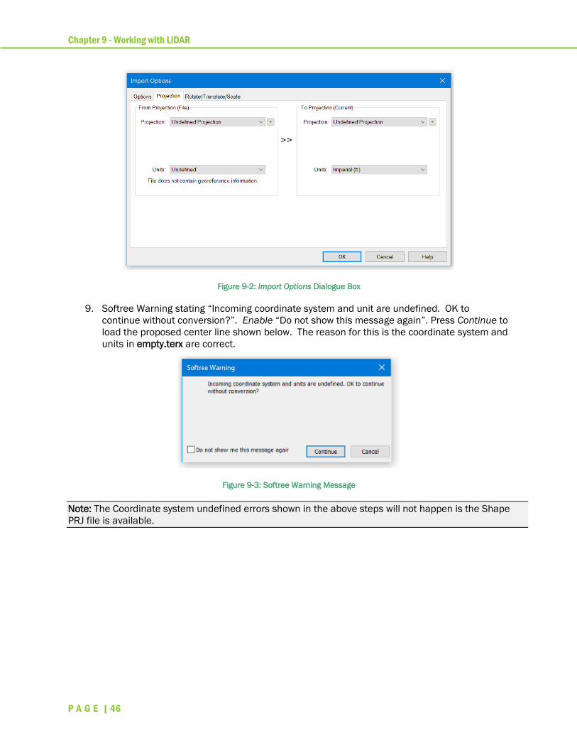
8. The Import options dialogue box below appears. Press OK.
Chapter 9 - Working with LiDAR
P A G E | 46
Figure 9-2: Import Options Dialogue Box
9. Softree Warning stating “Incoming coordinate system and unit are undefined. OK to
continue without conversion?”. Enable “Do not show this message again”. Press Continue to
load the proposed center line shown below. The reason for this is the coordinate system and
units in empty.terx are correct.
Figure 9-3: Softree Warning Message
Note: The Coordinate system undefined errors shown in the above steps will not happen is the Shape
PRJ file is available.

Chapter 9 - Working with LiDAR
P A G E | 47
Figure 9-4: Proposed Road Center Line
Now that the road center line has been brought in, we can bring in the LiDAR data. This example
only contains approximately 700,000 points to save download and file read time. This example use
*.txt files but could be other file types. A common LiDAR file format it *.LAS.
In the following steps, we will read in the data at full resolution in the area of interest (AOI) and skip
some points outside this area. In addition, we will follow some important guidelines to prevent slow
draw times and memory overload.
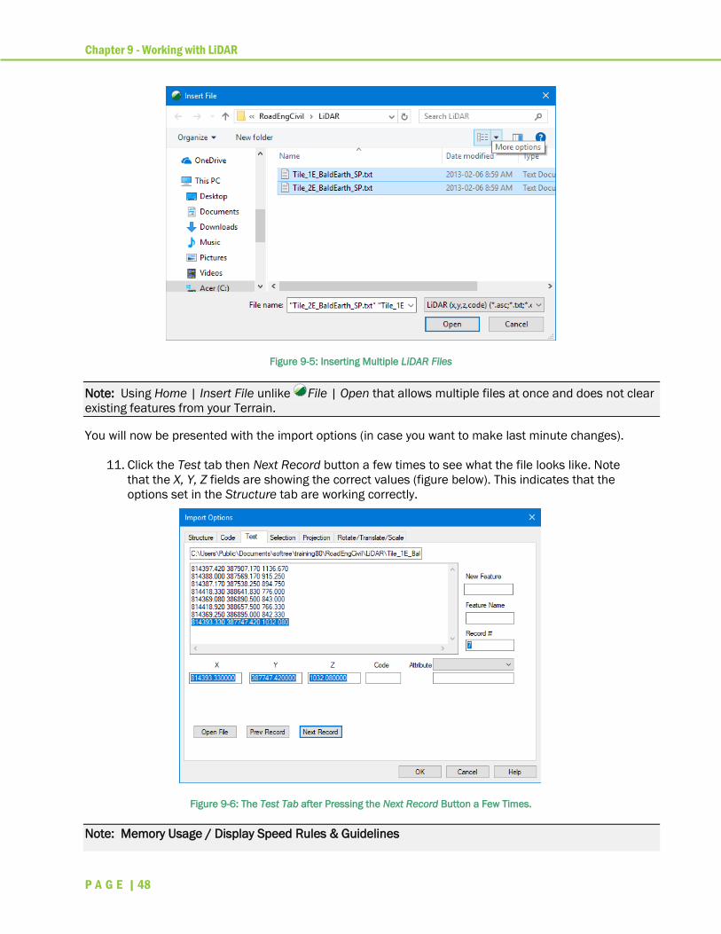
Bring in the LiDAR data: Home | Insert File button. Set the file type drop-down to ASCII Lidar
(x,y,z). (This is the one at the bottom of the list.)
10. Select both TXT files included with this example. Press Open. Tile_1E_BaldEarth_SP.txt;
Tile_2E_BaldEarth_SP.txt
Chapter 9 - Working with LiDAR
P A G E | 48
Figure 9-5: Inserting Multiple LiDAR Files
Note: Using Home | Insert File unlike File | Open that allows multiple files at once and does not clear
existing features from your Terrain.
You will now be presented with the import options (in case you want to make last minute changes).
11. Click the Test tab then Next Record button a few times to see what the file looks like. Note
that the X, Y, Z fields are showing the correct values (figure below). This indicates that the
options set in the Structure tab are working correctly.
Figure 9-6: The Test Tab after Pressing the Next Record Button a Few Times.
Note: Memory Usage / Display Speed Rules & Guidelines

Chapter 9 - Working with LiDAR
P A G E | 49
Other Import Options have been setup to avoid using more memory than necessary and to make the
resulting Terrain display manageable. The following rules are necessary when importing large data sets:
A. Do not attach comments or other attributes to every point.
B. Do not allow very large numbers of points in features.
C. Do not make every point into a separate feature.
D. Do not attach symbols to every point.
E. Do not turn on labels (such as Elevation) that will display at every point.
If you use the standard LiDAR import options these guidelines will be taken care of for you.
12. Click on the Structure tab. Notice that there are no Attributes defined in the Column
Assignments section (Rule A).
Figure 9-7: The Structure Tab defines the Location of the X,Y,Z Coordinates
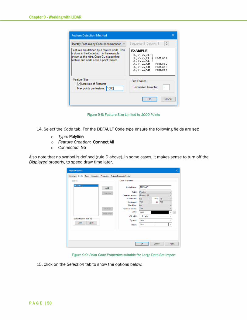
13. Press the Features… button in the Advanced section (lower right).
o Enable Limit size of Features.
o Set Max points per feature: 1000.
o OK.
The reason for this is when LiDAR points are grouped in features the program works better.
Chapter 9 - Working with LiDAR
P A G E | 50
Figure 9-8: Feature Size Limited to 1000 Points
14. Select the Code tab. For the DEFAULT Code type ensure the following fields are set:
o Type: Polyline
o Feature Creation: Connect All
o Connected: No
Also note that no symbol is defined (rule D above). In some cases, it makes sense to turn off the
Displayed property, to speed draw time later.
Figure 9-9: Point Code Properties suitable for Large Data Set Import
15. Click on the Selection tab to show the options below:
Chapter 9 - Working with LiDAR
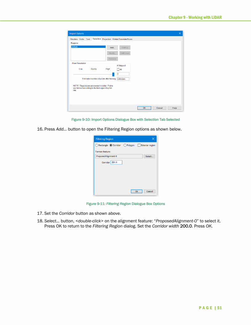
P A G E | 51
Figure 9-10: Import Options Dialogue Box with Selection Tab Selected
16. Press Add… button to open the Filtering Region options as shown below.
Figure 9-11: Filtering Region Dialogue Box Options
17. Set the Corridor button as shown above.
18. Select… button, <double-click> on the alignment feature: “ProposedAlignment-0” to select it.
Press OK to return to the Filtering Region dialog. Set the Corridor width 200.0. Press OK.
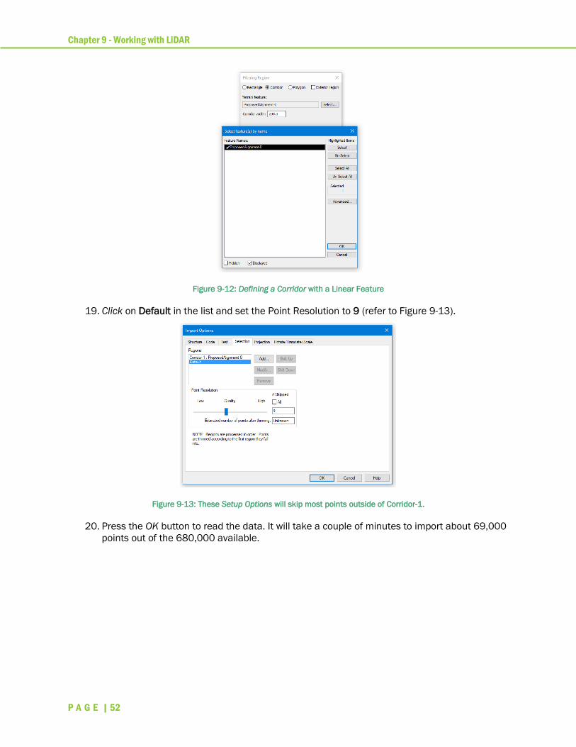
Chapter 9 - Working with LiDAR
P A G E | 52
Figure 9-12: Defining a Corridor with a Linear Feature
19. Click on Default in the list and set the Point Resolution to 9 (refer to Figure 9-13).
Figure 9-13: These Setup Options will skip most points outside of Corridor-1.
20. Press the OK button to read the data. It will take a couple of minutes to import about 69,000
points out of the 680,000 available.
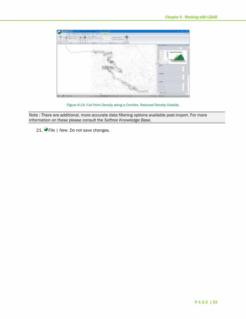
Chapter 9 - Working with LiDAR
P A G E | 53
Figure 9-14: Full Point Density along a Corridor, Reduced Density Outside.
Note : There are additional, more accurate data filtering options available post-import. For more
information on these please consult the Softree Knowledge Base.
21. File | New. Do not save changes.

Chapter 10 - New Location Design
P A G E | 54
New Location Design In this exercise, a short road alignment will be created.
Note: See Getting Started section for file install folders (<RoadEngCivil> and <Defaults and Layouts>).
Open the Location Module or if you are running the Terrain Module, use the Setup | Open Location
Module Button.
Figure 10-1: Setup Tab | Open Modules Group | Location Button
To create a new road alignment in the Location module, you first need to create an original ground
DTM. This is usually done by reading survey data into the Terrain module, and then creating a
surface with contours (see previous exercises). However, it is possible to import DTM surfaces from
other applications by using LandXML or DWG (3D faces) file formats.
1. Open the Location Module. File | New File.
2. Select Terrain Surface, and press the Browse… button and open
<RoadEngCivil>\Location\Topo.terx. Press OK.
Figure 10-2: File | New File – Opening File to Define the Original Ground
3. The Initial Alignment dialogue box will appear. This allows you to select a start coordinate or
to import an existing alignment.
Location
Module
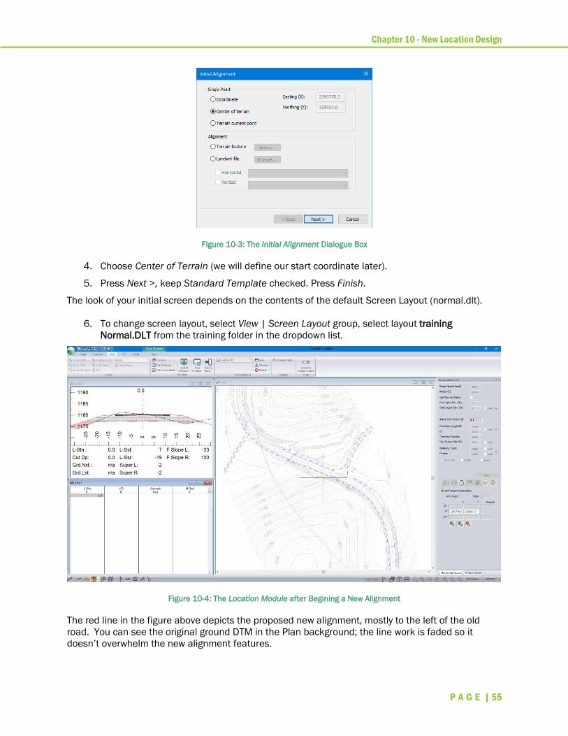
Chapter 10 - New Location Design
P A G E | 55
Figure 10-3: The Initial Alignment Dialogue Box
4. Choose Center of Terrain (we will define our start coordinate later).
5. Press Next >, keep Standard Template checked. Press Finish.
The look of your initial screen depends on the contents of the default Screen Layout (normal.dlt).
6. To change screen layout, select View | Screen Layout group, select layout training
Normal.DLT from the training folder in the dropdown list.
Figure 10-4: The Location Module after Begining a New Alignment
The red line in the figure above depicts the proposed new alignment, mostly to the left of the old
road. You can see the original ground DTM in the Plan background; the line work is faded so it
doesn’t overwhelm the new alignment features.
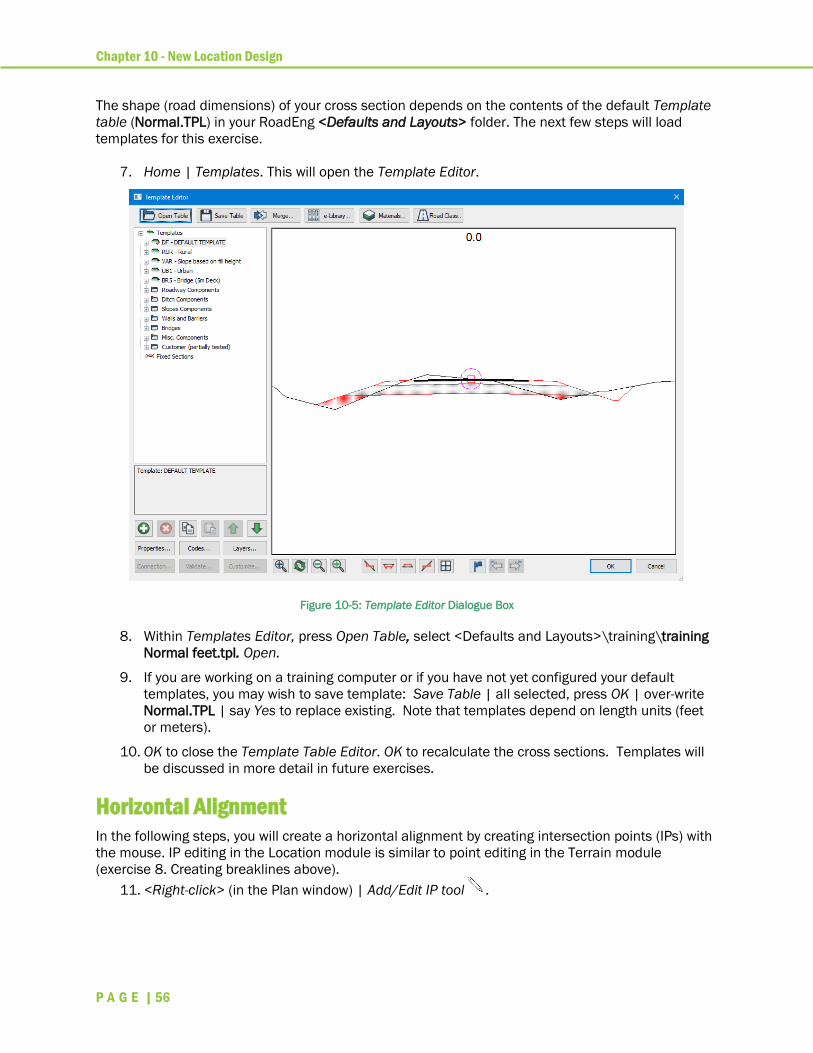
Chapter 10 - New Location Design
P A G E | 56
The shape (road dimensions) of your cross section depends on the contents of the default Template
table (Normal.TPL) in your RoadEng <Defaults and Layouts> folder. The next few steps will load
templates for this exercise.
7. Home | Templates. This will open the Template Editor.
Figure 10-5: Template Editor Dialogue Box
8. Within Templates Editor, press Open Table, select <Defaults and Layouts>\training\training
Normal feet.tpl. Open.
9. If you are working on a training computer or if you have not yet configured your default
templates, you may wish to save template: Save Table | all selected, press OK | over-write
Normal.TPL | say Yes to replace existing. Note that templates depend on length units (feet
or meters).
10. OK to close the Template Table Editor. OK to recalculate the cross sections. Templates will
be discussed in more detail in future exercises.
Horizontal Alignment
In the following steps, you will create a horizontal alignment by creating intersection points (IPs) with
the mouse. IP editing in the Location module is similar to point editing in the Terrain module
(exercise 8. Creating breaklines above).
11. <Right-click> (in the Plan window) | Add/Edit IP tool .
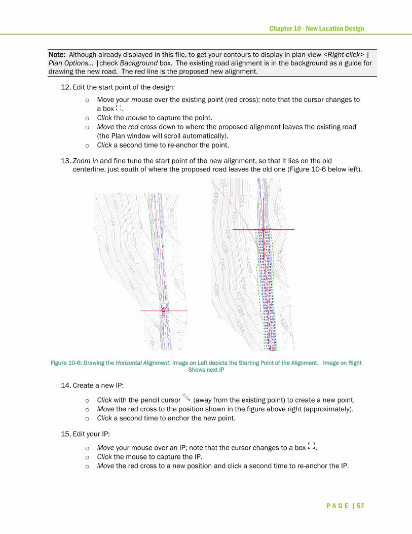
Chapter 10 - New Location Design
P A G E | 57
Note: Although already displayed in this file, to get your contours to display in plan-view <Right-click> |
Plan Options… |check Background box. The existing road alignment is in the background as a guide for
drawing the new road. The red line is the proposed new alignment.
12. Edit the start point of the design:
o Move your mouse over the existing point (red cross); note that the cursor changes to
a box .
o Click the mouse to capture the point.
o Move the red cross down to where the proposed alignment leaves the existing road
(the Plan window will scroll automatically).
o Click a second time to re-anchor the point.
13. Zoom in and fine tune the start point of the new alignment, so that it lies on the old
centerline, just south of where the proposed road leaves the old one (Figure 10-6 below left).
Figure 10-6: Drawing the Horizontal Alignment. Image on Left depicts the Starting Point of the Alignment. Image on Right
Shows next IP
14. Create a new IP:
o Click with the pencil cursor (away from the existing point) to create a new point.
o Move the red cross to the position shown in the figure above right (approximately).
o Click a second time to anchor the new point.
15. Edit your IP:
o Move your mouse over an IP; note that the cursor changes to a box .
o Click the mouse to capture the IP.
o Move the red cross to a new position and click a second time to re-anchor the IP.

Chapter 10 - New Location Design
P A G E | 58
16. Insert an IP:
o Move your mouse over a segment between IPs; note that the cursor changes to a
pencil with cross .
o Click the mouse to create a new IP.
o Move the red cross to the desired position (not important) and click a second time to
anchor the IP.
17. Delete an IP:
o Move your mouse over the IP created above; note that the cursor changes to a box
.
o Click the mouse to capture the IP.
o Type the <delete> key to remove the IP.
Continue this process until you have an alignment similar to the one in the figure below on the left.
Note: Don’t forget Undo command, <Ctrl-Z> or undo button.
Figure 10-7: Horizontal Alignment Before and After Curves Applied

Chapter 10 - New Location Design
P A G E | 59
Adding Horizontal Curves
To create a horizontal curve, you identify an IP then you define a curve between the tangents it
defines. Horizontal curves are created and edited using the horizontal curve panel.
If it is not open, you can open a new curve panel using the Horizontal Curve Panel button in the
window navigation toolbar.
Figure 10-8: Horizontal Curve Panel
18. If not already shown, press the Activate Horizontal Curve Panel button using the Window
Tools toolbar in the lower left part of the screen (figure above).
19. Use the Previous IP or Next IP buttons to move to the second IP in the alignment
(watch the Plan window).

Chapter 10 - New Location Design
P A G E | 60
20. Press Get Default Curve button to set up the parameters as shown in the Figure 10-8:
Horizontal Curve Panel, above.
Note: The curve panel controls are disabled until the current is point is an IP between two tangents. Most
of the controls are still disabled until you either select Circle or Spiral or press the Get Default Curve
button .
Default curves and associated tables are stored with your template table. The default template table is
Normal.TPL.
21. Press the Apply button to create the first curve.
22. Use the Next IP button to move to the third IP in the alignment and repeat to the steps
above to create the second curve.
23. Return to the Plan window and edit one of the curve IPs. Notice that when the IP is captured,
the curves update dynamically as you move the mouse. Also notice that you aren’t allowed to
overlap the curves or to push a curve off the end of the road.
Note: The current cross section is shown in the Plan window as a red cross. When you have finished
editing a curve, the current cross section is the End Curve (EC) point.
24. Go back to the curve panel and increase the radius of the two curves:
o Use the Previous IP or Next IP button to select a curve.
o Type a new radius (it must be small enough to fit or you will see an error message).
o Press the Apply button.
25. Modify the IP locations and continue adjusting the radius and see if you can get the new
alignment to line up with the proposed alignment in the background.
26. File | Close. Do not save changes.

Chapter 11 - Vertical Alignment
P A G E | 61
Vertical Alignment This exercise follows on from the previous. You must create a horizontal alignment before you can
create vertical alignment.
In the following steps, you will create a vertical alignment by creating vertical intersection points
(VIPs) with the mouse. VIP editing in the Profile window is similar to IP editing in the Plan window.
Note: Refer to Getting Started section for file install folders (<RoadEngCivil> and <Defaults and
Layouts>).
1. File | Open <RoadEngCivil>\Location\Align stage 1.dsnx in the Location Module. This
should look just like your design at the end of the previous exercise.
2. View | Retrieve <Defaults and Layouts>\Training\training Profile.dlt.
This will set up your screen to look like the figure below.
Figure 11-1: No Vertical Alignment, Profile Window Shows the Ground Line Only
3. <Right-click> in the Profile window and select the Add/Edit IP tool .Click anywhere to the
right of station 0+00 to create a new Vertical intersection point (VIP). Move the captured
point to a desired position and click again to anchor the point.
As in the previous horizontal alignment exercise, we can use the mouse to:
• Create a new VIP at the end of the existing alignment.
• Edit an existing VIP.
• Insert a VIP between existing VIPs.
• Delete a VIP.
There are a few subtle differences between editing in the Plan and Profile windows:
• In the profile, you can’t have a backwards segment (if you insert a point between two existing
VIPs, you are restricted to that station range).
• In the profile, you can insert a point no matter where your mouse is (in the Plan you must
mouse over a segment).
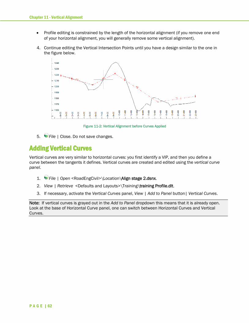
Chapter 11 - Vertical Alignment
P A G E | 62
• Profile editing is constrained by the length of the horizontal alignment (if you remove one end
of your horizontal alignment, you will generally remove some vertical alignment).
4. Continue editing the Vertical Intersection Points until you have a design similar to the one in
the figure below.
Figure 11-2: Vertical Alignment before Curves Applied
5. File | Close. Do not save changes.
Adding Vertical Curves
Vertical curves are very similar to horizontal curves: you first identify a VIP, and then you define a
curve between the tangents it defines. Vertical curves are created and edited using the vertical curve
panel.
1. File | Open <RoadEngCivil>\Location\Align stage 2.dsnx.
2. View | Retrieve <Defaults and Layouts>\Training\training Profile.dlt.
3. If necessary, activate the Vertical Curves panel, View | Add to Panel button| Vertical Curves.
Note: If vertical curves is grayed out in the Add to Panel dropdown this means that it is already open.
Look at the base of Horizontal Curve panel, one can switch between Horizontal Curves and Vertical
Curves.
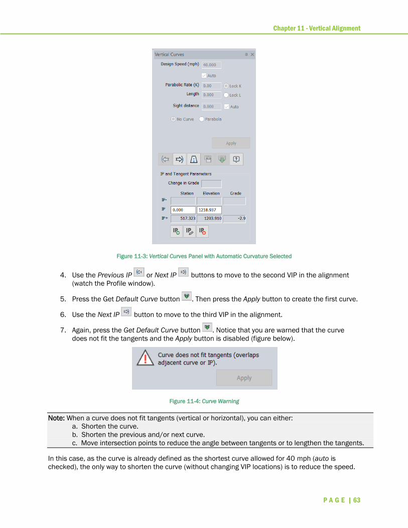
Chapter 11 - Vertical Alignment
P A G E | 63
Figure 11-3: Vertical Curves Panel with Automatic Curvature Selected
4. Use the Previous IP or Next IP buttons to move to the second VIP in the alignment
(watch the Profile window).
5. Press the Get Default Curve button . Then press the Apply button to create the first curve.
6. Use the Next IP button to move to the third VIP in the alignment.
7. Again, press the Get Default Curve button . Notice that you are warned that the curve
does not fit the tangents and the Apply button is disabled (figure below).
Figure 11-4: Curve Warning
Note: When a curve does not fit tangents (vertical or horizontal), you can either:
a. Shorten the curve.
b. Shorten the previous and/or next curve.
c. Move intersection points to reduce the angle between tangents or to lengthen the tangents.
In this case, as the curve is already defined as the shortest curve allowed for 40 mph (auto is
checked), the only way to shorten the curve (without changing VIP locations) is to reduce the speed.
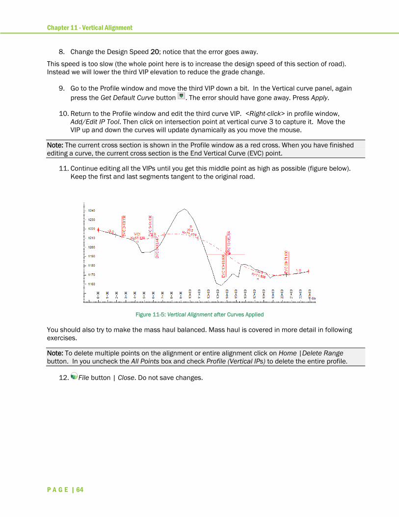
Chapter 11 - Vertical Alignment
P A G E | 64
8. Change the Design Speed 20; notice that the error goes away.
This speed is too slow (the whole point here is to increase the design speed of this section of road).
Instead we will lower the third VIP elevation to reduce the grade change.
9. Go to the Profile window and move the third VIP down a bit. In the Vertical curve panel, again
press the Get Default Curve button . The error should have gone away. Press Apply.
10. Return to the Profile window and edit the third curve VIP. <Right-click> in profile window,
Add/Edit IP Tool. Then click on intersection point at vertical curve 3 to capture it. Move the
VIP up and down the curves will update dynamically as you move the mouse.
Note: The current cross section is shown in the Profile window as a red cross. When you have finished
editing a curve, the current cross section is the End Vertical Curve (EVC) point.
11. Continue editing all the VIPs until you get this middle point as high as possible (figure below).
Keep the first and last segments tangent to the original road.
Figure 11-5: Vertical Alignment after Curves Applied
You should also try to make the mass haul balanced. Mass haul is covered in more detail in following
exercises.
Note: To delete multiple points on the alignment or entire alignment click on Home |Delete Range
button. In you uncheck the All Points box and check Profile (Vertical IPs) to delete the entire profile.
12. File button | Close. Do not save changes.

Chapter 12 - Cross Section Templates - Introduction
P A G E | 65
Cross Section Templates - Introduction Cross section templates allow you to set parameters such as road width, surfacing depths,
shoulders, ditches and cut/fill slopes.
Templates interact with topography, super-elevation, sub-surfaces, and alignment(s) to produce final
design cross sections. It is important to understand that templates are not static; they adapt to each
cross section.
Users will typically create a set of standard templates for use in common design situations.
Templates, template components and road class specifications are stored in a template table.
This example will introduce you to templates and the Template Table Editor.
Template Editor
Note: Refer to Getting Started section for file install folders (<RoadEngCivil> and <Defaults and
Layouts>).
1. In the Location module, open <RoadEngCivil> \Location2\bluff_road.dsnx.
2. Home | Templates, to open the Template Table Editor shown below.
3. Click on slope right (to the right of the graphic) to prepare for the following section.
Figure 12-1: Template Table Editor Dialogue Box
4. Click on the + beside the template RUR-Rural to view its components as shown in the
figure above.
The template editor shows you the templates contained in a table and the components
contained in each template. These are the items you commonly work with.

Chapter 12 - Cross Section Templates - Introduction
P A G E | 66
Template Properties
5. <Right-click> on the RUR-Rural template and choose Properties…
Figure 12-2: Template Properties Dialogue Box
There are relatively few controls in the Template Properties, most template flexibility is at the
Component level. Aside from the template Name and Description, the most commonly used
properties are the cross-fall slopes.
6. Change the Crown/Super Slope to -5% on the left and +5% on the right. Press OK.
Notice how the Roadway component is altered by the new crown slopes – this is what happens when
this template is applied inside a curve with 5% super-elevation (the template property Override with
Curve Super must be enabled). Some components are designed to adjust themselves to the
prevailing crown or super-elevation slope.
7. <Right-click> on the RUR-Rural template and choose Undo Modify to restore the initial
settings.
Creating and Deleting Templates
Although there is an Add button (and context menu), you will find the most intuitive way to create a
new template is to copy an existing template, paste it back into the table and then re-name and
modify it.
8. <Right-click> on the RUR-Rural template and select Copy.
9. <Right-click> | Paste > | As New. The new template will appear at the bottom of the list.

Chapter 12 - Cross Section Templates - Introduction
P A G E | 67
10. Select the new xx0-Rural template and use the Shift Up button to move it up the list.
You could also open the properties and rename the template to RUR2 or similar. You would also
want to change at least one property or component to make the template different in a useful way.
Note: The fewer templates you have the easier it is to maintain them.
11. <Right-click> on the new xx0-Rural template and select Delete to remove it.
Template Components
There are four types of template components:
• Custom
• Roadway
• Ditches
• Slopes
Roadway, Ditches, and Slopes components are included for backward compatibility and their
behavior is mostly self-explanatory (and there is always <F1>). Custom components have replaced
and improved upon their features. You can tell when you are looking at an old-style component – the
properties dialogue boxes are quite different from the Custom components properties (figures
below).
In this document, we will work exclusively with Custom components.
Template Component Properties
Template components have parameters allowing you to configure the object for your specific design.
Template parameters can be any one of the following:
User This is the most common type of parameter. It can be a
numerical value (usually distance) or a slope percent.
Reference Feature
X Offset
Allows you to specify an optional horizontal alignment instead
of a numerical offset from center-line. See Reference Features
for more information.
Reference Feature
X Offset
Allows you to specify an optional horizontal alignment instead
of a numerical offset from center-line. See Reference Features
for more information.
Reference Feature
Y Offset
Allows you to specify an optional vertical alignment instead of
a numerical offset from center-line. See Reference Features
for more information.
Reference Surface Allows you to specify a surface (rarely used).
12. <Right-click> on the Rural Paved-left component of the RUR-Rural template | select
Properties… to open the Template Component Properties dialogue box (Figure 12-3).

Chapter 12 - Cross Section Templates - Introduction
P A G E | 68
Figure 12-3: Rural Paved Roadway Component Properties
This component allows you to change various parameters such as pavement thickness, lane width
shoulder width, and various thicknesses and slopes.
13. Change the lane width:
o Select ACP_WIDTH in the Parameters list; note the pavement highlight in the graphic.
o Change the Default value to 16.0; note that the graphic updates immediately.
Figure 12-4: Template Graphic Depicting the Effect of Changing the ACP_WIDTH Variable While the Component Properties
Dialogue is Open
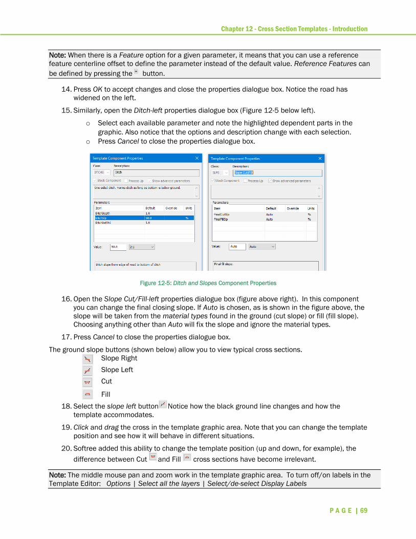
Chapter 12 - Cross Section Templates - Introduction
P A G E | 69
Note: When there is a Feature option for a given parameter, it means that you can use a reference
feature centerline offset to define the parameter instead of the default value. Reference Features can
be defined by pressing the button.
14. Press OK to accept changes and close the properties dialogue box. Notice the road has
widened on the left.
15. Similarly, open the Ditch-left properties dialogue box (Figure 12-5 below left).
o Select each available parameter and note the highlighted dependent parts in the
graphic. Also notice that the options and description change with each selection.
o Press Cancel to close the properties dialogue box.
Figure 12-5: Ditch and Slopes Component Properties
16. Open the Slope Cut/Fill-left properties dialogue box (figure above right). In this component
you can change the final closing slope. If Auto is chosen, as is shown in the figure above, the
slope will be taken from the material types found in the ground (cut slope) or fill (fill slope).
Choosing anything other than Auto will fix the slope and ignore the material types.
17. Press Cancel to close the properties dialogue box.
The ground slope buttons (shown below) allow you to view typical cross sections.
Slope Right
Slope Left
Cut
Fill
18. Select the slope left button Notice how the black ground line changes and how the
template accommodates.
19. Click and drag the cross in the template graphic area. Note that you can change the template
position and see how it will behave in different situations.
20. Softree added this ability to change the template position (up and down, for example), the
difference between Cut and Fill cross sections have become irrelevant.
Note: The middle mouse pan and zoom work in the template graphic area. To turn off/on labels in the
Template Editor: Options | Select all the layers | Select/de-select Display Labels

Chapter 12 - Cross Section Templates - Introduction
P A G E | 70
21. Click on the split screen view button . The screen shown below will appear showing four
typical ground situations at the same time. Each template position can be adjusted with a
mouse click and drag.
Figure 12-6: Split Screen View Showing the 4 Typical Sections
22. Click on the station button on the right-hand side of the screen, and enter the value 300.
Press OK.
On the screen, you will see the template applied to station 300 of the design. This allows you to
quickly see how the template will appear before it is assigned.
Working with Components
Template components are interchangeable building blocks. A template table can also contain
optional folders containing re-usable components.
23. Click on the slope right button to prepare for the following section.
24. Scroll down the template tree list and open the Slopes Components folder (Figure 12-7).
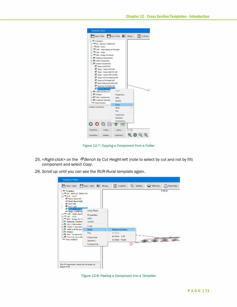
Chapter 12 - Cross Section Templates - Introduction
P A G E | 71
Figure 12-7: Copying a Component from a Folder
25. <Right-click> on the Bench by Cut Height-left (note to select by cut and not by fill)
component and select Copy.
26. Scroll up until you can see the RUR-Rural template again.
Figure 12-8: Pasting a Component Into a Template

Chapter 12 - Cross Section Templates - Introduction
P A G E | 72
27. <Right-click> on the Slope Cut/Fill-left component in the RUR-Rural template and
choose menu Paste | Replace Existing (figure above).
You will be prompted with the dialogue box shown below. This allows you to copy parameters
between similar components. In this case we just want to overwrite the component not the
parameters.
Figure 12-9: Paste Options when Replacing an Existing Template Component
28. Leave the Overwrite parameters only option unchecked (as shown in the figure above) and
press OK.
29. Click and drag the template down until you can see the cut benches – figure below (you may
also need to zoom out).
Figure 12-10: The New Slopes Component is only on the Leftside
At this point you might want to change the new component’s properties. Is the bench wide enough?
Are the steps high enough?
30. Open the properties dialogue box for the new component and change BenchWidth to 15.
Press OK to commit the change.

Chapter 12 - Cross Section Templates - Introduction
P A G E | 73
31. Notice that the cut bench component is only on the left side. We will copy it (with its new
bench width) to the right:
o <Right-click> on Slope Cut/Fill-right and choose menu Delete.
o <Right-click> on Bench by Cut Height-left and select Copy.
o <Right-click> again Bench by Cut Height-left and select Paste | As New - Right.
Notice the template now has cut benches on both sides.
Note: The order of components is important; components should be arranged from the center line out.
The left/right order is unimportant.
32. Use the Shift Up button to move your cut bench component to the top of the list. Notice
what happens to the drawing.
33. Restore the order.
The e-Library
Softree maintains a library of template components on the web.
34. If you are connected to the web, press the e-Library button, within the template editor, to
open the dialogue box in the figure below:
Figure 12-11: Component Folders available from Softree’s Website
35. Press the Web Info… button. The Template Resource page lists the available components
and their parameters.
Note: If you are using components it is always best to load or reload them directly from the e-Library.
36. Press Cancel to close the dialogue box.
37. File | Close. Do not save changes.

Chapter 13 - Volumes & Mass Haul
P A G E | 74
Volumes & Mass Haul
Note: Getting started section for file install folders (<RoadEngCivil> and <Defaults and Layouts>).
1. File | Open <RoadEngCivil>\Location\Align stage 3.dsnx.
2. View | Retrieve Screen Layout <Defaults and Layouts>\training\training Profile Only.dlt. This
will set up your screen to look like the figure below.
Figure 13-1: Location Design - training Profile Only.dlt Screen Layout
Displaying Cut and Fill Volumes in Data Table
3. Activate a new Data Window from the bottom navigation toolbar.
Change the columns displayed in the data window:
4. <Right-click> | Data Options…
5. Click the plus next to Point Types (Rows), this will open the Point Type Selection dialogue.
6. De-select any current selected point types (<double-click>).
7. <Double-click> on Auto interval points (xx.000 ft). If the interval is not currently set to 20.0 ft,
press Properties… to configure. Adjust the Interval to 20.0 ft. Press OK to return to the
previous dialogue.
8. Press OK to return to the Data Window Options main dialogue.
9. Press Columns…. Add the following fields as shown in the figure below:
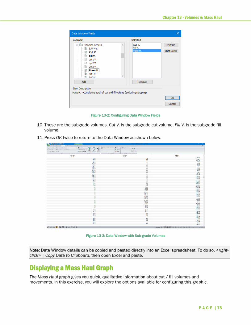
Chapter 13 - Volumes & Mass Haul
P A G E | 75
Figure 13-2: Configuring Data Window Fields
10. These are the subgrade volumes. Cut V. is the subgrade cut volume, Fill V. is the subgrade fill
volume.
11. Press OK twice to return to the Data Window as shown below:
Figure 13-3: Data Window with Sub-grade Volumes
Note: Data Window details can be copied and pasted directly into an Excel spreadsheet. To do so, <right-
click> | Copy Data to Clipboard, then open Excel and paste.
Displaying a Mass Haul Graph
The Mass Haul graph gives you quick, qualitative information about cut / fill volumes and
movements. In this exercise, you will explore the options available for configuring this graphic.

Chapter 13 - Volumes & Mass Haul
P A G E | 76
Mass Haul is a graphic representation of accumulated volume; at any station, the value is the
accumulated cut volume minus the accumulated fill volume up to that point. The difference in Mass
Haul between two points indicates the volume of surplus (positive difference) or deficit (negative
difference).
The default setting for mass haul includes only sub-grade material, however it is possible to select
specific materials to be included.
12. Activate the Profile window from the bottom navigation toolbar.
13. <<Right-click>> in the Profile window | select Profile Options… to open the dialogue box
shown below left.
14. Press Select… at the bottom of the Sub-Windows area. This will display the two-list dialogue
box shown below on the right.
Figure 13-4: Profile Sub-Windows to Display
15. Select Mass Haul, press Add (or <Double-click>) to add it to the Selected list as shown
above.
Note: The profile sub-windows area can display multiple items. All sub-windows will share the same
horizontal axis (station) with the profile window.
16. Press OK button twice to accept changes and close the dialogue boxes.
Figure 13-5: Mass-Haul Displayed in a Profile Sub-Window.
17. Move your mouse over the divider between the main profile window and the mass haul; when
it changes to the sizing cursor , click and drag up to make more room for the mass haul.
18. <Right-click> in the mass haul window | select Mass Haul Options… to open the dialogue
box shown in the figure below.
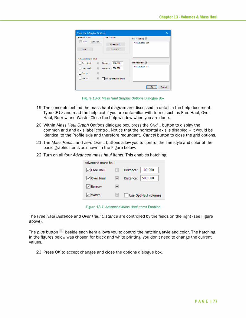
Chapter 13 - Volumes & Mass Haul
P A G E | 77
Figure 13-6: Mass Haul Graphic Options Dialogue Box
19. The concepts behind the mass haul diagram are discussed in detail in the help document.
Type <F1> and read the help text if you are unfamiliar with terms such as Free Haul, Over
Haul, Borrow and Waste. Close the help window when you are done.
20. Within Mass Haul Graph Options dialogue box, press the Grid… button to display the
common grid and axis label control. Notice that the horizontal axis is disabled – it would be
identical to the Profile axis and therefore redundant. Cancel button to close the grid options.
21. The Mass Haul… and Zero Line… buttons allow you to control the line style and color of the
basic graphic items as shown in the Figure below.
22. Turn on all four Advanced mass haul items. This enables hatching.
Figure 13-7: Advanced Mass Haul Items Enabled
The Free Haul Distance and Over Haul Distance are controlled by the fields on the right (see Figure
above).
The plus button beside each item allows you to control the hatching style and color. The hatching
in the figures below was chosen for black and white printing; you don’t need to change the current
values.
23. Press OK to accept changes and close the options dialogue box.

Chapter 13 - Volumes & Mass Haul
P A G E | 78
Figure 13-8: Mass Haul with Advanced Features Turned On
Note: That the hatch styles are different from the ones on your screen so that we can print this
document in black and white.
Free Haul
Material which is pushed or pulled a distance less than
the Free Haul distance (100 ft.).
Over Haul
Material moved beyond Free Haul Distance (100 ft.)
and less than the Overhaul Distance (500 ft.).
Borrow
Material which must be trucked in from outside the
road project.
Waste
Material which must be trucked outside the road
project (End haul).
24. It is possible to modify the mass haul to account for borrow and waste. We will add a new
Borrow pit:
o Home | Assign by Range.
o Select the Pits tab.
o Add... Set the access station to 450. Press Ok.
o Select Borrow and uncheck the Variable volume (smart pit).
o In the Volume (Cu. Yd.) capacity box enter 8000.
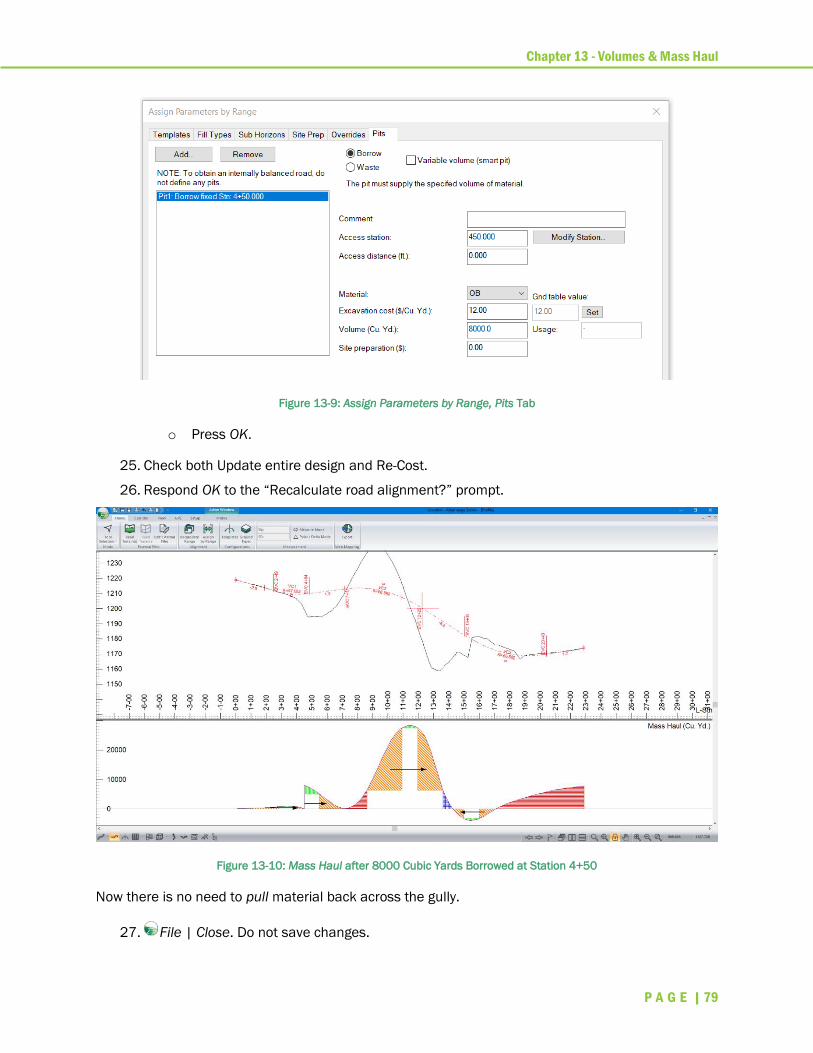
Chapter 13 - Volumes & Mass Haul
P A G E | 79
Figure 13-9: Assign Parameters by Range, Pits Tab
o Press OK.
25. Check both Update entire design and Re-Cost.
26. Respond OK to the “Recalculate road alignment?” prompt.
Figure 13-10: Mass Haul after 8000 Cubic Yards Borrowed at Station 4+50
Now there is no need to pull material back across the gully.
27. File | Close. Do not save changes.
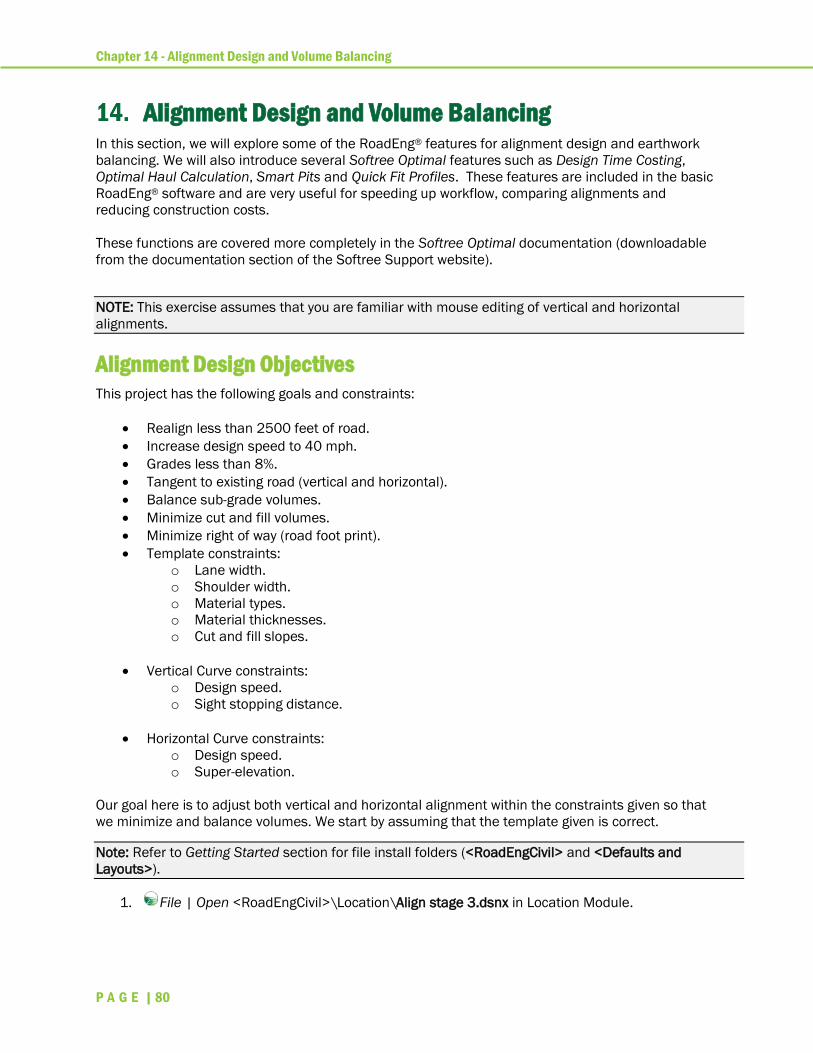
Chapter 14 - Alignment Design and Volume Balancing
P A G E | 80
Alignment Design and Volume Balancing In this section, we will explore some of the RoadEng® features for alignment design and earthwork
balancing. We will also introduce several Softree Optimal features such as Design Time Costing,
Optimal Haul Calculation, Smart Pits and Quick Fit Profiles. These features are included in the basic
RoadEng® software and are very useful for speeding up workflow, comparing alignments and
reducing construction costs.
These functions are covered more completely in the Softree Optimal documentation (downloadable
from the documentation section of the Softree Support website).
NOTE: This exercise assumes that you are familiar with mouse editing of vertical and horizontal
alignments.
Alignment Design Objectives
This project has the following goals and constraints:
• Realign less than 2500 feet of road.
• Increase design speed to 40 mph.
• Grades less than 8%.
• Tangent to existing road (vertical and horizontal).
• Balance sub-grade volumes.
• Minimize cut and fill volumes.
• Minimize right of way (road foot print).
• Template constraints:
o Lane width.
o Shoulder width.
o Material types.
o Material thicknesses.
o Cut and fill slopes.
• Vertical Curve constraints:
o Design speed.
o Sight stopping distance.
• Horizontal Curve constraints:
o Design speed.
o Super-elevation.
Our goal here is to adjust both vertical and horizontal alignment within the constraints given so that
we minimize and balance volumes. We start by assuming that the template given is correct.
Note: Refer to Getting Started section for file install folders (<RoadEngCivil> and <Defaults and
Layouts>).
1. File | Open <RoadEngCivil>\Location\Align stage 3.dsnx in Location Module.

Chapter 14 - Alignment Design and Volume Balancing
P A G E | 81
The outermost lines on either side of the alignment are the slope stakes or catch points
(configurable in the Plan Options dialogue box). The area inside the slope stakes is the footprint of
the road that must lie within the right of way.
Figure 14-1: Green Dot Slope Stakes (catch point) Lines in
the Plan Indicates the Footprint of the Design
2. Press the Activate Profile Window button , in windows toolbar, to open the Profile window
using in the windows toolbar and notice shape of the ground and the quantities indicated by
the mass haul diagram (figure below).
3. Enter selection mode (<Right-click> | choose Selection Tool) then click on the alignment
to view a cross section in the middle of the through cut (red cross in the profile shown
below).
Toe of Fill
Toe of Cut
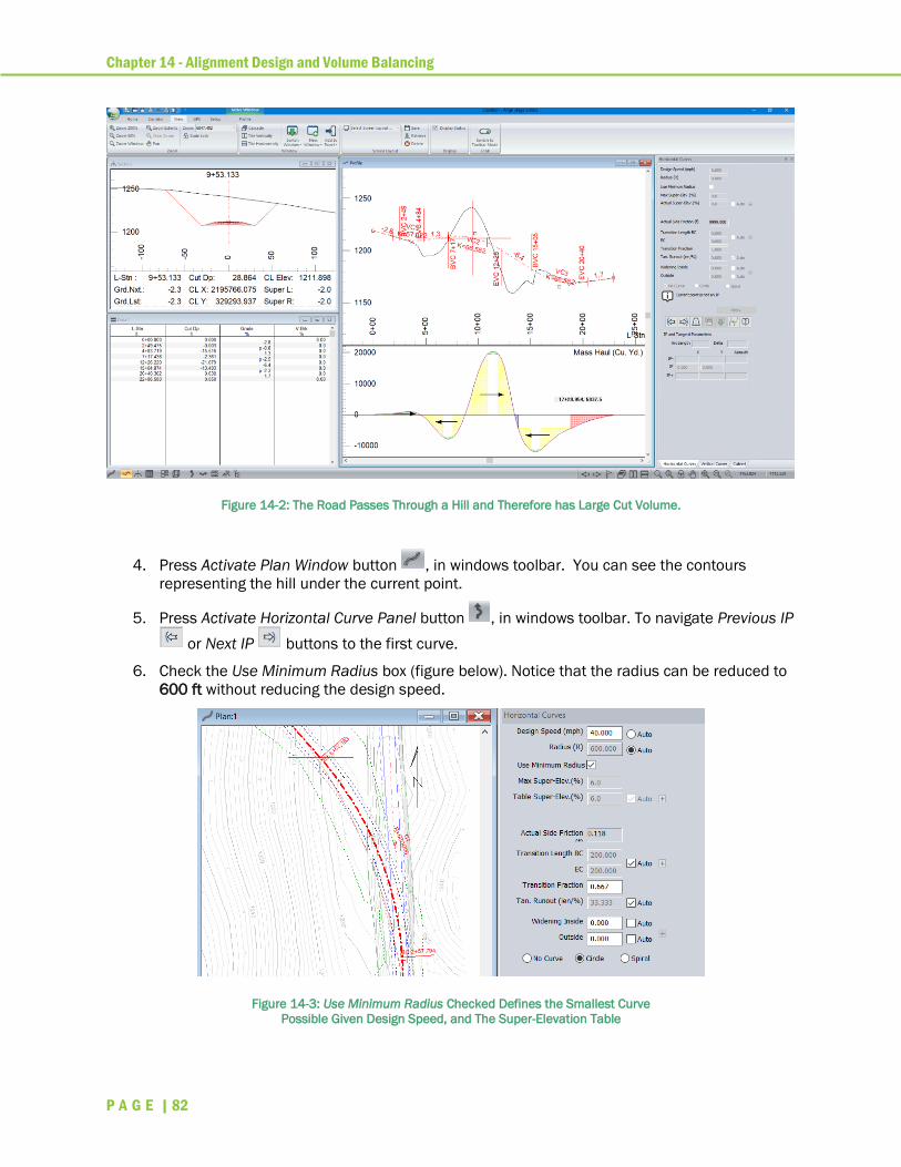
Chapter 14 - Alignment Design and Volume Balancing
P A G E | 82
Figure 14-2: The Road Passes Through a Hill and Therefore has Large Cut Volume.
4. Press Activate Plan Window button , in windows toolbar. You can see the contours
representing the hill under the current point.
5. Press Activate Horizontal Curve Panel button , in windows toolbar. To navigate Previous IP
or Next IP buttons to the first curve.
6. Check the Use Minimum Radius box (figure below). Notice that the radius can be reduced to
600 ft without reducing the design speed.
Figure 14-3: Use Minimum Radius Checked Defines the Smallest Curve
Possible Given Design Speed, and The Super-Elevation Table

Chapter 14 - Alignment Design and Volume Balancing
P A G E | 83
7. Apply the smaller 600 ft radius to both curves. This will give you some room to move the
horizontal alignment, so it is not so far up the hill.
8. Change to edit mode ; <Right-click> choose Add/Edit IP Tool.
9. In the Plan window, move C1 (the IP for the South curve) North and move C2 (the IP for the
North curve) South (both while maintaining tangency with the old road).
If you move the C2 too far south, the cross section will extend beyond the edge of the surface model
(figure below). Be sure that the fill areas of the road do not fall off the topographic surface. You will
never be able to balance the mass haul diagram this way.
Figure 14-4: Plan and Section Windows Depicting What Occurs When The Road Section Extends Beyond the Original
Ground Surface Model
10. Note that a captured curve IP will stop moving (and there will be an audible beep if you have
sounds on) when the curves bump into each other and become an S curve.
11. Open Activate Profile Window button and notice the new shape of the ground (figure
below).
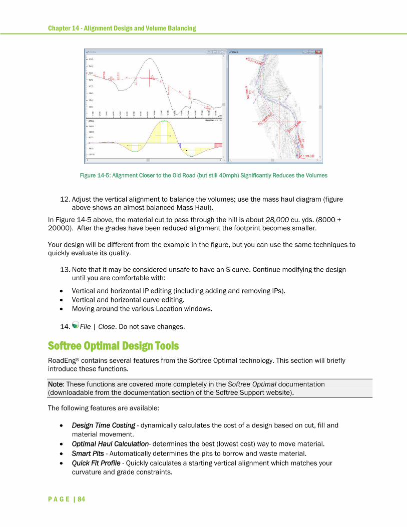
Chapter 14 - Alignment Design and Volume Balancing
P A G E | 84
Figure 14-5: Alignment Closer to the Old Road (but still 40mph) Significantly Reduces the Volumes
12. Adjust the vertical alignment to balance the volumes; use the mass haul diagram (figure
above shows an almost balanced Mass Haul).
In Figure 14-5 above, the material cut to pass through the hill is about 28,000 cu. yds. (8000 +
20000). After the grades have been reduced alignment the footprint becomes smaller.
Your design will be different from the example in the figure, but you can use the same techniques to
quickly evaluate its quality.
13. Note that it may be considered unsafe to have an S curve. Continue modifying the design
until you are comfortable with:
• Vertical and horizontal IP editing (including adding and removing IPs).
• Vertical and horizontal curve editing.
• Moving around the various Location windows.
14. File | Close. Do not save changes.
Softree Optimal Design Tools
RoadEng® contains several features from the Softree Optimal technology. This section will briefly
introduce these functions.
Note: These functions are covered more completely in the Softree Optimal documentation
(downloadable from the documentation section of the Softree Support website).
The following features are available:
• Design Time Costing - dynamically calculates the cost of a design based on cut, fill and
material movement.
• Optimal Haul Calculation- determines the best (lowest cost) way to move material.
• Smart Pits - Automatically determines the pits to borrow and waste material.
• Quick Fit Profile - Quickly calculates a starting vertical alignment which matches your
curvature and grade constraints.

Chapter 14 - Alignment Design and Volume Balancing
P A G E | 85
Figure 14-6: Softree Optimal Features.
Design Time Costing
Cost reporting and feedback is useful at all stages of design (preliminary, detailed and construction
estimation).
Design Time Cost Reporting is the ability to accurately evaluate the cost of a particular design
interactively before it is complete. Softree Optimal provides interactive and automated feedback to
report earthwork costs. This functionality is extremely useful for manual design and is a prerequisite
for optimization.
Earthwork cost calculations are based on material excavation, embankment, movement and
borrow/waste locations.
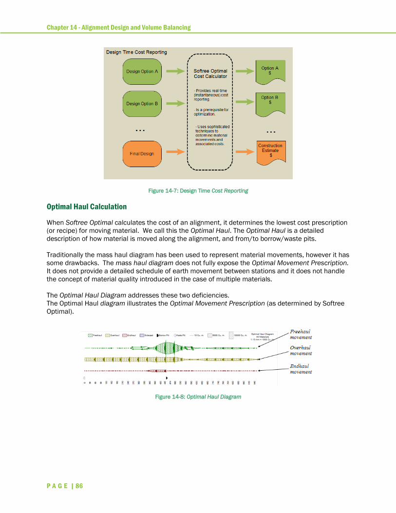
Chapter 14 - Alignment Design and Volume Balancing
P A G E | 86
Figure 14-7: Design Time Cost Reporting
Optimal Haul Calculation
When Softree Optimal calculates the cost of an alignment, it determines the lowest cost prescription
(or recipe) for moving material. We call this the Optimal Haul. The Optimal Haul is a detailed
description of how material is moved along the alignment, and from/to borrow/waste pits.
Traditionally the mass haul diagram has been used to represent material movements, however it has
some drawbacks. The mass haul diagram does not fully expose the Optimal Movement Prescription.
It does not provide a detailed schedule of earth movement between stations and it does not handle
the concept of material quality introduced in the case of multiple materials.
The Optimal Haul Diagram addresses these two deficiencies.
The Optimal Haul diagram illustrates the Optimal Movement Prescription (as determined by Softree
Optimal).
Figure 14-8: Optimal Haul Diagram
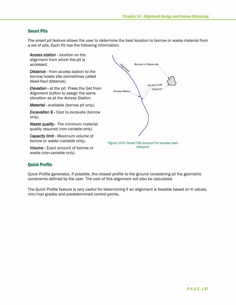
Chapter 14 - Alignment Design and Volume Balancing
P A G E | 87
Smart Pits
The smart pit feature allows the user to determine the best location to borrow or waste material from
a set of pits. Each Pit has the following information:
Access station - location on the
alignment from which the pit is
accessed.
Distance - from access station to the
borrow/waste site (sometimes called
dead-haul distance).
Elevation - at the pit. Press the Get from
Alignment button to assign the same
elevation as at the Access Station.
Material - available (borrow pit only).
Excavation $ - Cost to excavate (borrow
only).
Waste quality - The minimum material
quality required (non-variable only).
Capacity limit - Maximum volume of
borrow or waste (variable only).
Volume - Exact amount of borrow or
waste (non-variable only).
Figure 14-9: Smart Pits account for access road
distance
Quick Profile
Quick Profile generates, if possible, the closest profile to the ground considering all the geometric
constraints defined by the user. The cost of this alignment will also be calculated.
The Quick Profile feature is very useful for determining if an alignment is feasible based on K values,
min/max grades and predetermined control points.
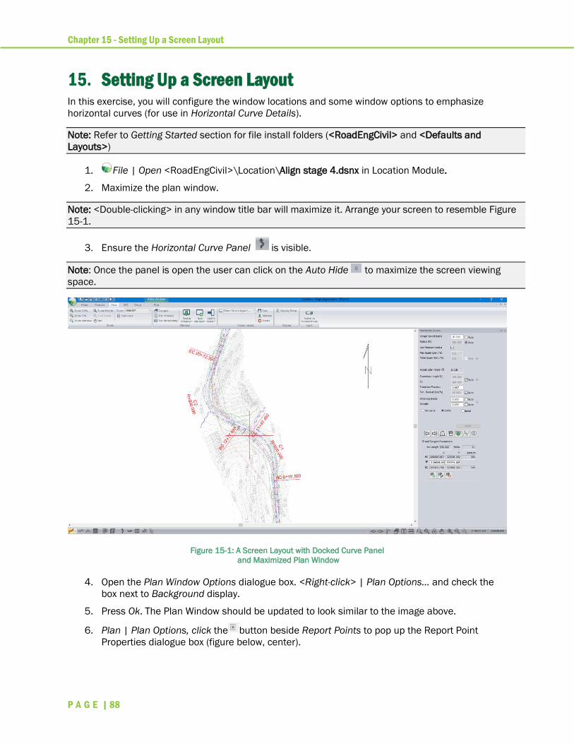
Chapter 15 - Setting Up a Screen Layout
P A G E | 88
Setting Up a Screen Layout In this exercise, you will configure the window locations and some window options to emphasize
horizontal curves (for use in Horizontal Curve Details).
Note: Refer to Getting Started section for file install folders (<RoadEngCivil> and <Defaults and
Layouts>)
1. File | Open <RoadEngCivil>\Location\Align stage 4.dsnx in Location Module.
2. Maximize the plan window.
Note: <Double-clicking> in any window title bar will maximize it. Arrange your screen to resemble Figure
15-1.
3. Ensure the Horizontal Curve Panel is visible.
Note: Once the panel is open the user can click on the Auto Hide to maximize the screen viewing
space.
Figure 15-1: A Screen Layout with Docked Curve Panel
and Maximized Plan Window
4. Open the Plan Window Options dialogue box. <Right-click> | Plan Options… and check the
box next to Background display.
5. Press Ok. The Plan Window should be updated to look similar to the image above.
6. Plan | Plan Options, click the button beside Report Points to pop up the Report Point
Properties dialogue box (figure below, center).
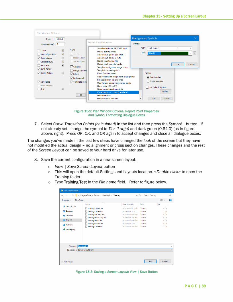
Chapter 15 - Setting Up a Screen Layout
P A G E | 89
Figure 15-2: Plan Window Options, Report Point Properties
and Symbol Formatting Dialogue Boxes
7. Select Curve Transition Points (calculated) in the list and then press the Symbol… button. If
not already set, change the symbol to Tick (Large) and dark green (0,64,0) (as in figure
above, right). Press OK, OK, and OK again to accept changes and close all dialogue boxes.
The changes you’ve made in the last few steps have changed the look of the screen but they have
not modified the actual design – no alignment or cross section changes. These changes and the rest
of the Screen Layout can be saved to your hard drive for later use.
8. Save the current configuration in a new screen layout:
o View | Save Screen Layout button
o This will open the default Settings and Layouts location. <Double-click> to open the
Training folder.
o Type Training Test in the File name field. Refer to figure below.
Figure 15-3: Saving a Screen Layout: View | Save Button

Chapter 15 - Setting Up a Screen Layout
P A G E | 90
o Press Save button
9. You will be prompted with a reminder about save locations for screen layouts. Press OK to
continue.
10. You have just created a screen layout that will appear in your Screen Layouts tool bar item
for easy retrieval. Training Test.dlt is now in the dropdown menu within the training folder.
11. View | Select Screen Layout (dropdown) to retrive another screen layout: training Curve H.dlt
(located in the Training folder).
12. Try opening some of the other screen layouts available.
Note: When accessing screen layouts or opening new windows (Profile, Plan, Section, Data, 3D, Multi-
Plot) window can get lost behind one another or minimized. Using View | Cascade or Tile Vertically can
be useful find open windows.
Screen Layout Facts
• The Custom folder is often defined on a network drive so that the layouts are accessible to all
users.
• You can change the Softree folder (RoadEng Settings and Layouts folder) from the menu
Setup | Location Setup | Install tab. Do not do this unless you understand the
consequences; more than just screen layouts are stored in this folder. The most common
change is to put Defaults and Layouts Folder into your Documents folder (private to one user
only).
13. When you have finished experimenting with screen layouts, File | Close, do not save
changes.
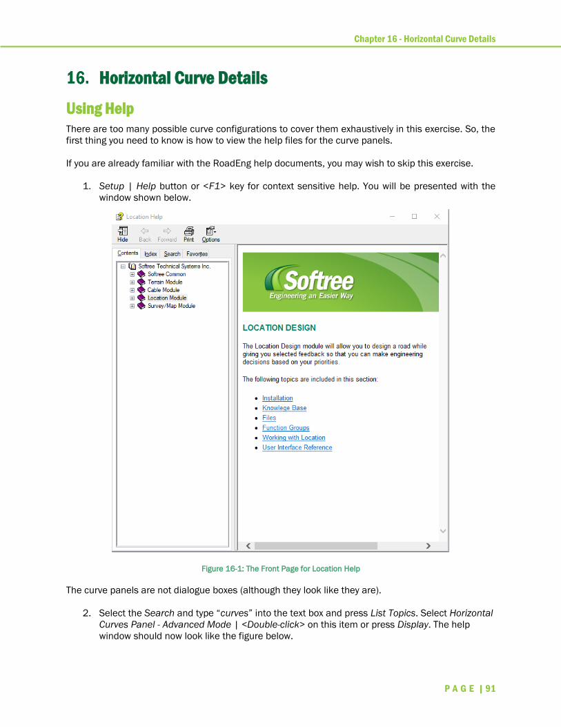
Chapter 16 - Horizontal Curve Details
P A G E | 91
Horizontal Curve Details
Using Help
There are too many possible curve configurations to cover them exhaustively in this exercise. So, the
first thing you need to know is how to view the help files for the curve panels.
If you are already familiar with the RoadEng help documents, you may wish to skip this exercise.
1. Setup | Help button or <F1> key for context sensitive help. You will be presented with the
window shown below.
Figure 16-1: The Front Page for Location Help
The curve panels are not dialogue boxes (although they look like they are).
2. Select the Search and type “curves” into the text box and press List Topics. Select Horizontal
Curves Panel - Advanced Mode | <Double-click> on this item or press Display. The help
window should now look like the figure below.

Chapter 16 - Horizontal Curve Details
P A G E | 92
Figure 16-2: Horizontal Curves Panel - Advanced Mode Help Page
This page has information about all the controls in the horizontal curve panel. It also has many links
to related topics.
3. Click on Vertical Curves Panel - Advanced Mode in the list to display its help page.
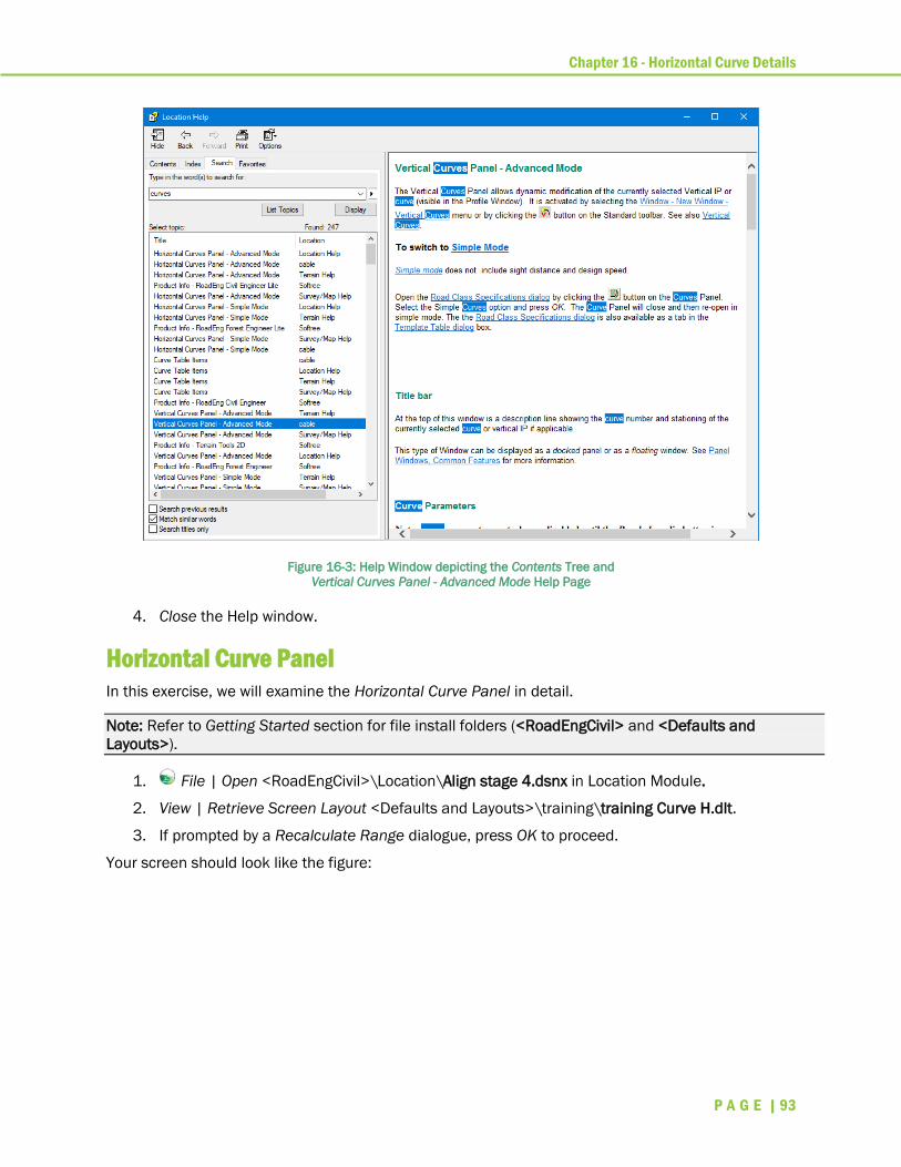
Chapter 16 - Horizontal Curve Details
P A G E | 93
Figure 16-3: Help Window depicting the Contents Tree and
Vertical Curves Panel - Advanced Mode Help Page
4. Close the Help window.
Horizontal Curve Panel
In this exercise, we will examine the Horizontal Curve Panel in detail.
Note: Refer to Getting Started section for file install folders (<RoadEngCivil> and <Defaults and
Layouts>).
1. File | Open <RoadEngCivil>\Location\Align stage 4.dsnx in Location Module.
2. View | Retrieve Screen Layout <Defaults and Layouts>\training\training Curve H.dlt.
3. If prompted by a Recalculate Range dialogue, press OK to proceed.
Your screen should look like the figure:
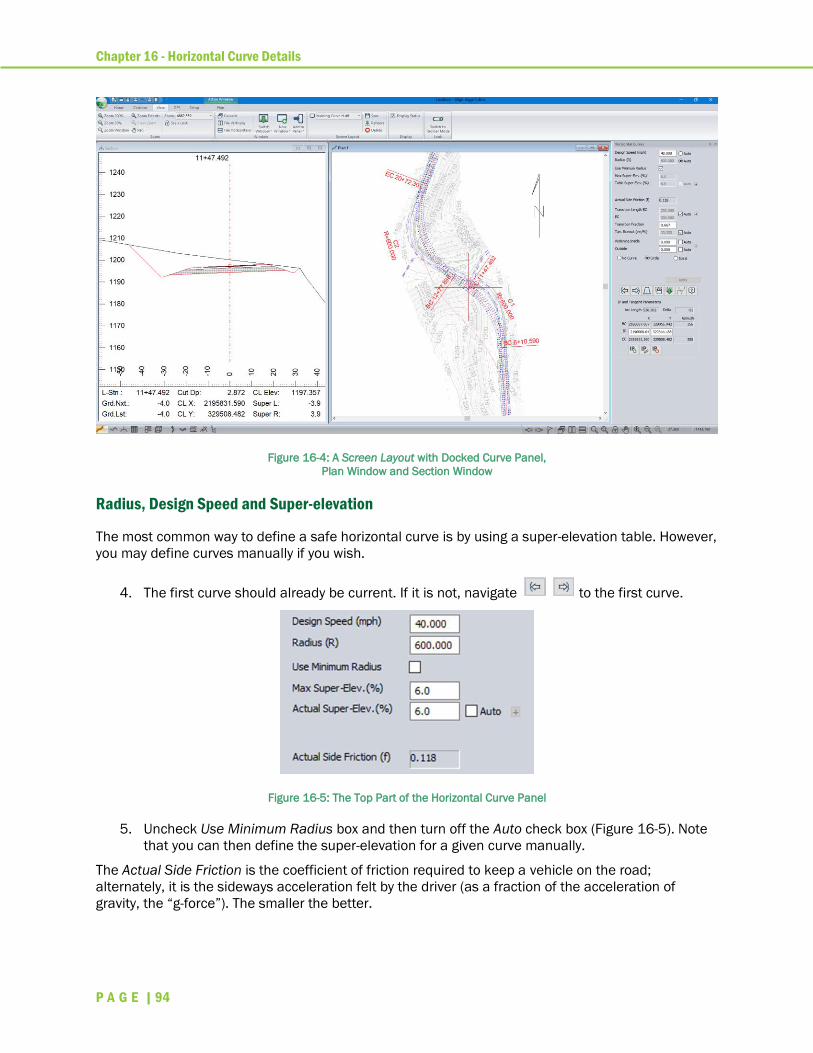
Chapter 16 - Horizontal Curve Details
P A G E | 94
Figure 16-4: A Screen Layout with Docked Curve Panel,
Plan Window and Section Window
Radius, Design Speed and Super-elevation
The most common way to define a safe horizontal curve is by using a super-elevation table. However,
you may define curves manually if you wish.
4. The first curve should already be current. If it is not, navigate to the first curve.
Figure 16-5: The Top Part of the Horizontal Curve Panel
5. Uncheck Use Minimum Radius box and then turn off the Auto check box (Figure 16-5). Note
that you can then define the super-elevation for a given curve manually.
The Actual Side Friction is the coefficient of friction required to keep a vehicle on the road;
alternately, it is the sideways acceleration felt by the driver (as a fraction of the acceleration of
gravity, the “g-force”). The smaller the better.

Chapter 16 - Horizontal Curve Details
P A G E | 95
Design Speed
(mph)
Radius
(feet)
Super-
Elevation (%)
Side
Friction
40 600 6 0.118
40 600 0 0.178
40 1200 3 0.059
30 600 3 0.07
Figure 16-6: Side friction factor for various speeds, curve radii and super-elevation values.
6. Turn the Auto check box back ON and press the plus button beside it to open the Auto
Super Elevation Options dialogue box (Figure 16-7).
Figure 16-7: Auto Super Elevation Options Dialogue Box
The use of the side friction factor method is defined in the AASHTO 2001 handbook. It relies on a
table of “safe” side friction factors to calculate maximum speed given radius (or minimum radius
given speed) using physical principals. It is possible to use this method to calculate the values for a
super-elevation table; the two methods need not give different results. The side friction factor
method is discussed in the help text and will not be discussed further here.
7. Press the Select Table button to open the Lookup Table dialogue box (Figure 16-8).
Figure 16-8: Super Elevation Lookup Table Dialogue Box
Chapter 16 - Horizontal Curve Details
P A G E | 96
Super-elevation Table Facts
• The blank area of the table represents unsafe combinations of radius and speed.
• The top of each column in the body of the table is the maximum super-elevation. Given a
speed, the corresponding radius is the minimum allowed; given a radius, the corresponding
speed is the maximum allowed.
• Super-elevation is defined by rise over run – the tangent of the angle (not %).
• Interpolation means that if the speed or radius is in between table entries, the super-
elevation value will be linearly interpolated between the values in the body of the table.
• This table is stored in the template table (inside a design document or in an external file).
• Super-elevation tables can be imported/exported from/to simple text files (comma or tab
delimited). Spreadsheet programs can also import and export these files.
• Lines starting with “#” characters are excluded from the table when importing text files – the
comments at the top of the table in the figure above were marked in this way.
• Softree does not (as of this printing) provide officially approved tables. However, there are
metric and English versions included in the RoadEng install (<Defaults and
Layouts>\Superelevation EMax 06.tbl and Superelevation EMax 06 - Feet.tbl, respectively).
Note: *.tbl files can be viewed and edited using notepad.
8. Press Cancel to close the table and Cancel again to close the Auto Super Elevation Options
dialogue box.
Sometimes when your options are limited, it is best to design alignment with the smallest safe radius
– you can always increase the radius later if you have room.
9. Check the Use Minimum Radius box and then check the Auto button beside Radius. In this
mode, you can type a desired Design Speed and the software will use the super-elevation
table to find the minimum safe radius. Try a few values.
10. If you type a speed outside the table (20 mph for example) you will see the error message
below (top). If you type a speed greater than 40 mph (45 mph for example) you will see the
warning below (bottom). You can ignore the warning and apply the curve anyway if you wish.
Figure 16-9: Curve Error Messages
Road Class Specifications
Each curve has its own Design Speed; the maximum design speed for the entire road is specified in
the Road Class Specifications.
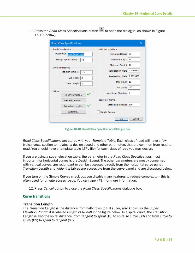
Chapter 16 - Horizontal Curve Details
P A G E | 97
11. Press the Road Class Specifications button to open the dialogue, as shown in Figure
16-10 (below).
Figure 16-10: Road Class Specifications Dialogue Box
Road Class Specifications are stored with your Template Table. Each class of road will have a few
typical cross section templates, a design speed and other parameters that are common from road to
road. You should have a template table (.TPL file) for each class of road you may design.
If you are using a super-elevation table, the parameter in the Road Class Specifications most
important for horizontal curves is the Design Speed. The other parameters are mostly concerned
with vertical curves, are redundant or can be accessed directly from the horizontal curve panel.
Transition Length and Widening tables are accessible from the curve panel and are discussed below.
If you turn on the Simple Curves check box you disable many features to reduce complexity – this is
often used for private access roads. You can type <F1> for more information.
12. Press Cancel button to close the Road Class Specifications dialogue box.
Curve Transitions
Transition Length The Transition Length is the distance from half-crown to full super, also known as the Super
Elevation Runoff; it is labeled Length of Runoff in the figure below. In a spiral curve, the Transition
Length is also the spiral distance (from tangent to spiral (TS) to spiral to circle (SC) and from circle to
spiral (CS) to spiral to tangent (ST).

Chapter 16 - Horizontal Curve Details
P A G E | 98
Figure 16-11: Cross Fall Behavior when Entering a Curve
13. Clear the Auto box beside the two Transition Length values and note that you can now
manually enter a different value for BC (begin curve) and EC (end curve), shown in the figure
below:
Figure 16-12: Manually Configuring Transition Length
14. Re-check the Auto box beside the two Transition Length values then press the associated
plus button. The table shown below will be displayed.
Figure 16-13: Transition Length Table.

Chapter 16 - Horizontal Curve Details
P A G E | 99
When Transition Length is automatic, you are forced to use the same length for begin and end of
curve. Like the super-elevation table, this table can be imported/exported from/to an external text
file. To make changes, export, edit and re-import.
15. Press Cancel to close the Transition Length Lookup Table.
Transition Fraction For a circular curve, the Super Elevation Runoff may start before the curve BC and end after;
similarly, at the end of the curve, the transition starts before the EC and ends after. The Transition
Fraction is the amount of transition that happens outside the curve (before BC and after EC).
For example, if Transition Length = 90 feet:
• If Transition Fraction is 1.0, the Super Elevation Runoff starts 90 feet before the BC point
and full super-elevation is reached at BC.
• If Transition Fraction is 0.667, a common standard, the Super Elevation Runoff starts 60 feet
before BC and full super-elevation is reached 30 feet beyond BC.
In a spiral curve, the Transition Fraction is not used (the Super Elevation Runoff always happens in
the spiral section).
Tangent Runout Length Tangent Runout length is the distance from full crown to half crown (see cross fall behavior figure
above).
16. Clear the Auto check box associated with Tan. Runout (len/%). Note that you can now enter a
length manually.
17. Re-check the Auto check box associated with Tan. Runout (length). Now the caption reads
len./%; the automatic value displayed is the tangent runout length for each % of crown (if
your crown is 2%, you multiply this number by two to get the total length). When set to
automatic, the Tangent Runout happens at the same rate as the Super-Elevation Runoff.
Curve Widening Small radius curves require lane widening to accommodate large vehicle off tracking. The Widening
fields allow you to define a different widening distance for inside and outside lanes.
Note: Your cross-section template must have curve widening built-in for these values to have any effect.
18. As with other curve parameters, you can extract widening values from a table by setting the
Auto check box. If time permits, you may wish to experiment with this feature. There is a
widening table called: <RoadEngCivil>\Location\WideningFeet.tbl.
19. File |Close, do not save changes.
Viewing Curve Transitions
Now we will look more closely at the curves we have created to see how the super elevation is
applied along the alignment.
1. File| Open to open <RoadEngCivil>\Location\Align stage 4.dsnx in Location Module.
2. Use the Screen Layouts tool bar control to retrieve <Defaults and Layouts>\training\training
Curve H.dlt.
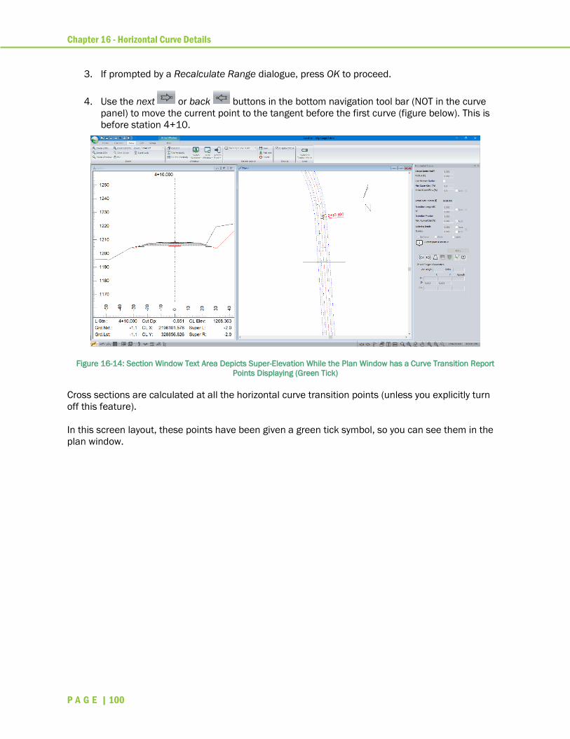
Chapter 16 - Horizontal Curve Details
P A G E | 100
3. If prompted by a Recalculate Range dialogue, press OK to proceed.
4. Use the next or back buttons in the bottom navigation tool bar (NOT in the curve
panel) to move the current point to the tangent before the first curve (figure below). This is
before station 4+10.
Figure 16-14: Section Window Text Area Depicts Super-Elevation While the Plan Window has a Curve Transition Report
Points Displaying (Green Tick)
Cross sections are calculated at all the horizontal curve transition points (unless you explicitly turn
off this feature).
In this screen layout, these points have been given a green tick symbol, so you can see them in the
plan window.
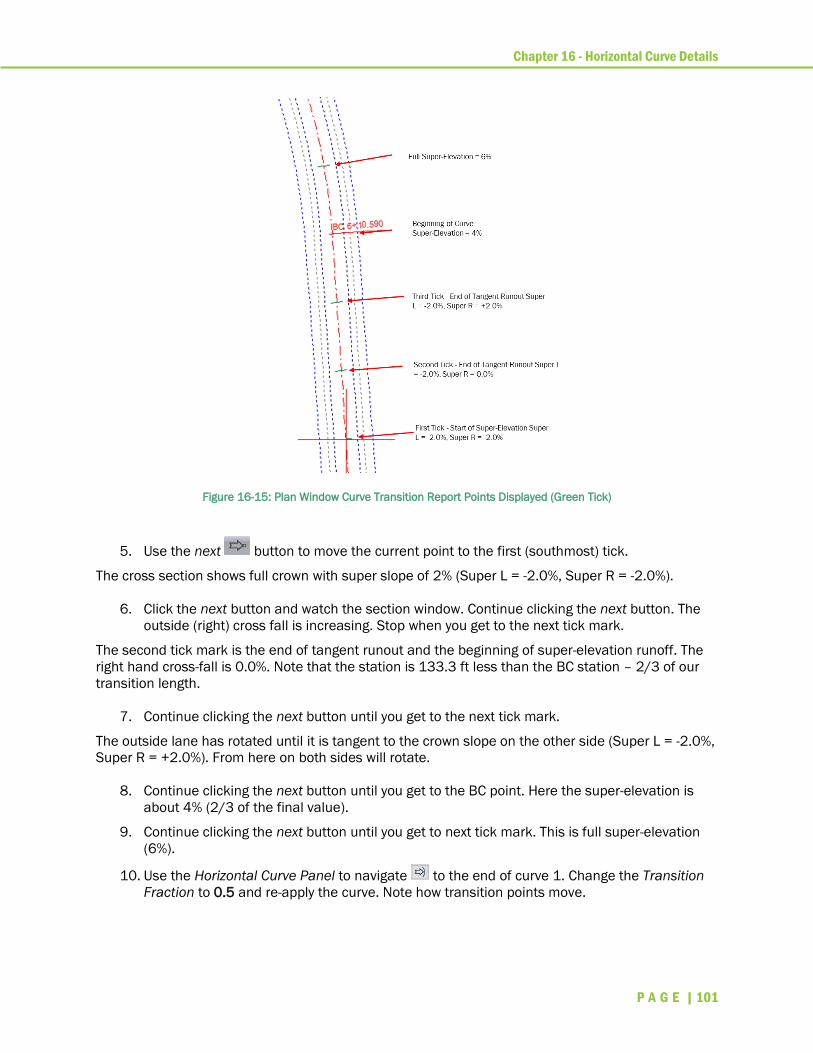
Chapter 16 - Horizontal Curve Details
P A G E | 101
Figure 16-15: Plan Window Curve Transition Report Points Displayed (Green Tick)
5. Use the next button to move the current point to the first (southmost) tick.
The cross section shows full crown with super slope of 2% (Super L = -2.0%, Super R = -2.0%).
6. Click the next button and watch the section window. Continue clicking the next button. The
outside (right) cross fall is increasing. Stop when you get to the next tick mark.
The second tick mark is the end of tangent runout and the beginning of super-elevation runoff. The
right hand cross-fall is 0.0%. Note that the station is 133.3 ft less than the BC station – 2/3 of our
transition length.
7. Continue clicking the next button until you get to the next tick mark.
The outside lane has rotated until it is tangent to the crown slope on the other side (Super L = -2.0%,
Super R = +2.0%). From here on both sides will rotate.
8. Continue clicking the next button until you get to the BC point. Here the super-elevation is
about 4% (2/3 of the final value).
9. Continue clicking the next button until you get to next tick mark. This is full super-elevation
(6%).
10. Use the Horizontal Curve Panel to navigate to the end of curve 1. Change the Transition
Fraction to 0.5 and re-apply the curve. Note how transition points move.
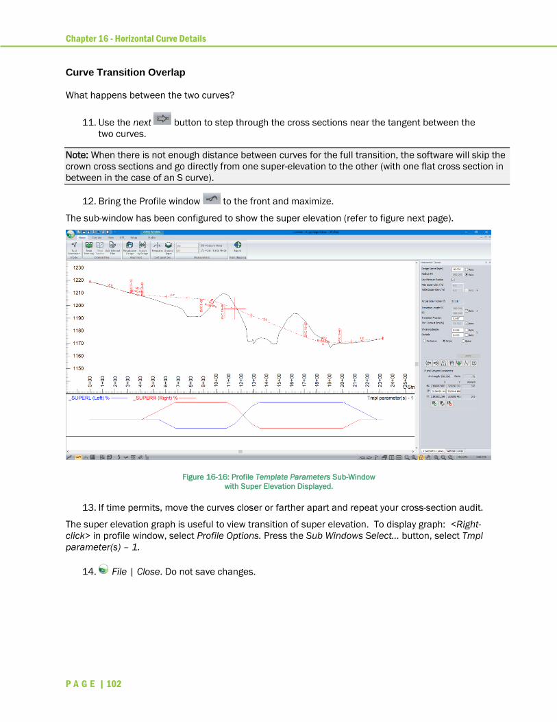
Chapter 16 - Horizontal Curve Details
P A G E | 102
Curve Transition Overlap
What happens between the two curves?
11. Use the next button to step through the cross sections near the tangent between the
two curves.
Note: When there is not enough distance between curves for the full transition, the software will skip the
crown cross sections and go directly from one super-elevation to the other (with one flat cross section in
between in the case of an S curve).
12. Bring the Profile window to the front and maximize.
The sub-window has been configured to show the super elevation (refer to figure next page).
Figure 16-16: Profile Template Parameters Sub-Window
with Super Elevation Displayed.
13. If time permits, move the curves closer or farther apart and repeat your cross-section audit.
The super elevation graph is useful to view transition of super elevation. To display graph: <Right-
click> in profile window, select Profile Options. Press the Sub Windows Select… button, select Tmpl
parameter(s) – 1.
14. File | Close. Do not save changes.

Chapter 17 - Vertical Curve Details
P A G E | 103
Vertical Curve Details In this exercise, we will examine the Vertical Curve Panel in detail.
Note: Refer to Getting Started section for file install folders (<RoadEngCivil> and <Defaults and
Layouts>).
1. In Location, File| Open <RoadEngCivil>\Location\Align stage 4.dsnx.
2. Use the Screen Layouts tool bar control to retrieve <Defaults and Layouts>\training\training
Curve V.dlt.
Your screen should look like Figure 17-1.
Figure 17-1: Vertical Alignment with Docked Vertical Curve Panel
3. Use the Previous IP and Next IP buttons within the vertical curve panel to move to
the first vertical curve.
Automatic Curvature
4. This curve has been configured to find the smallest possible curve that has a safe sight
stopping distance. Ensure the Auto check box for Sight distance is enabled and check
Parabola button.
5. Change the Design Speed to 30. Notice how the sight stopping distance drops, as does K
and the length of curve.
6. Set the Design Speed back to 40.
7. Press the Road Class Specifications button to open the dialogue box shown below.

Chapter 17 - Vertical Curve Details
P A G E | 104
Figure 17-2: Road Class Specifications Dialogue Box
When Sight distance (stopping) is automatic in the vertical curve panel, it is calculated from the
steepest grade in the curve and the following values from the Road Class Specifications:
• Design Speed
• Reaction time
• Deceleration
When curvature, K, is automatic in the vertical curve panel, it is calculated from the required Sight
distance and the following values from the Road Class Specifications:
• Eye Height
• Object Height
Note: You can type <F1> for more information.
8. Press Cancel to close the Road Class Specifications dialogue box.
9. <Right-click> in profile window, select Add/Edit IP Tool>move cursor to capture the vertical
intersection point for this curve. Move it up and down.
Notice how the values in the curve panel are kept up to date. With the curvature set to automatic,
both the length and the curvature (K) change as the VIP is moved.
Locked K
10. Clear the Auto check box below the design speed. Make sure the Lock K button is selected
and press Apply.
11. Repeat the experiment from step 9. Now the K value is constant and the length changes as
you move the VIP up and down. Notice that the “K is too small for desired sight distance”
warning appears and disappears (larger grades require longer stopping distances and
therefore larger K values).

Chapter 17 - Vertical Curve Details
P A G E | 105
Locked Length
12. Select the Lock L button and Apply your change. Again, capture the VIP and move it with the
mouse. Curves with constant length will never bump into one another when you raise or
lower the VIP; however, the curvature changes dramatically.
13. File | close. Do not save changes.
Editing VIPs With the Curve Panel
So far, we have created and edited intersection points only with the mouse (both vertical and
horizontal). The curve panels also allow you to create and edit IPs.
1. File button | Open <RoadEngCivil>\Location\Align stage 4.dsnx.
2. Retrieve screen layout <Defaults and Layouts>\training\training Curve V.dlt.
3. Use the Previous IP and Next IP buttons to move to the second vertical curve.
Figure 17-3 : The Bottom Part of The Vertical Curve Panel
4. Change the elevation of the IP to 1210 (shown as 1204.550 in the figure above) and Apply
your change. Note how the curve moves vertically.
Note: You can fine tune your alignment by making small changes to the VIP Station, Elevation values.
5. Press the Modify IP button to open the Modify Vertical IP dialogue box (Figure 17-4).

Chapter 17 - Vertical Curve Details
P A G E | 106
Figure 17-4: The Modified Vertical IP Dialogue Box Allows the User to Set
the Grade of the Previous Tangent (Among Other Things)
6. Type “2” into the Grade % field (Figure 17-4) and press OK to close the dialogue box.
Your Elevation value in the curve panel has been updated.
7. Press Apply in vertical curve panel to change the curve.
Note: You can also edit horizontal alignment curves in the Horizontal curve panel in an analogous way.
8. File | Close. Do not save changes.

Chapter 18 - Materials and Stripping
P A G E | 107
Materials and Stripping So far, our “Align Stage” design has ignored the quality of the material in the original ground. If you
looked a little closer, you would find that all subgrade cut and fill material is classified as OB
(overburden). This is a common practice and produces acceptable results (provided that you assign a
reasonable expansion factor to OB so that the Mass Haul is approximately correct).
In this exercise, we will add some more realism to our design by defining materials in the original
ground and in the subgrade fill. We will also strip topsoil from the original ground before applying
templates.
Defining Sub-surface Layers
1. File | Open <RoadEngCivil>\Location\Align stage 4.dsnx.
2. Select Home | Ground Types.
3. Create a new ground type for use in subgrade fill:
o Select the FR Fractured Rock item.
o Press the New… button to open the New Ground Type dialogue box (figure below
right). Note that we start with a copy of the selected item.
o Fill in the ID RR and Description Rip Rap.
o Press OK.
Figure 18-1: The Available Ground and Subgrade Fill
Materials in the Ground Types Editor.
Note: The Composite Material option can be used for uncertain or mixed materials found in the original
ground – F1 for help.
Note that the RR fill angle is set to 100% (1:1); this is suitable for our purposes, so there is no need
to change it. The cut angle is not important as we will not assign this material as native ground.
4. Create another material called CS-Clay Silt with cut slope of 1:1 and fill slope 3:1.
Note: The default ground table is called NORMAL.GDX.

Chapter 18 - Materials and Stripping
P A G E | 108
5. Press OK to accept changes and close the Ground Types Editor. Respond Cancel to the
recalculate prompt (we didn’t change anything that is in use).
Assign original ground materials to a station range:
6. Home | Assign by Range
7. Select the Sub Horizons tab (Figure 18-2 below left).
Figure 18-2: Defining Materials in The Original Ground.
8. Press the button beside the Ground Layers field to open the Ground Layers dialogue box
(Figure 18-2 above right).
Note: If you define reference surfaces (Terrain files with a DTM) you can use them to define the C/L
depth values. This would require bore hole data or like create enough subsurface points to make surface
models.
9. Select the three subsurface layers shown above (OB, CS, FR) and then set the layer depths
(1, 5).
10. Press OK to close the dialogue box and fill the Ground Layers field in the Sub-Horizons
dialogue box.
Figure 18-3: Sub-Horizons Have Been Applied to The Entire Alignment

Chapter 18 - Materials and Stripping
P A G E | 109
11. Leave the From/To Stn. values as “..” and press the Add/Edit button. This will apply the new
layer arrangement to the entire alignment.
Note: The most common mistake made in the assignments dialogue box is to skip the Add/Edit step. If
you Press OK before the ranges are updated, nothing happens.
12. Press OK to accept changes and close the dialogue box.
13. Respond OK to the Re-calculate Range prompt.
14. Select a cross section that has some cut in it (ie stn 17+25). Notice that the new ground
layers are displayed.
Figure 18-4: Ground Layers Depicted in The Section Window.
The design total volumes haven’t changed because of the new ground layers. However, the program
is now keeping track of three categories of cut volume which can be reported separately.
15. File | Close. Do not save changes.
Stripping
Now we will remove the top layer before building each cross section.
1. File | Open <RoadEngCivil>\Location\Align stage 5.dsnx.
2. Home | Assign by Range. Select the Site Prep tab (figure below).
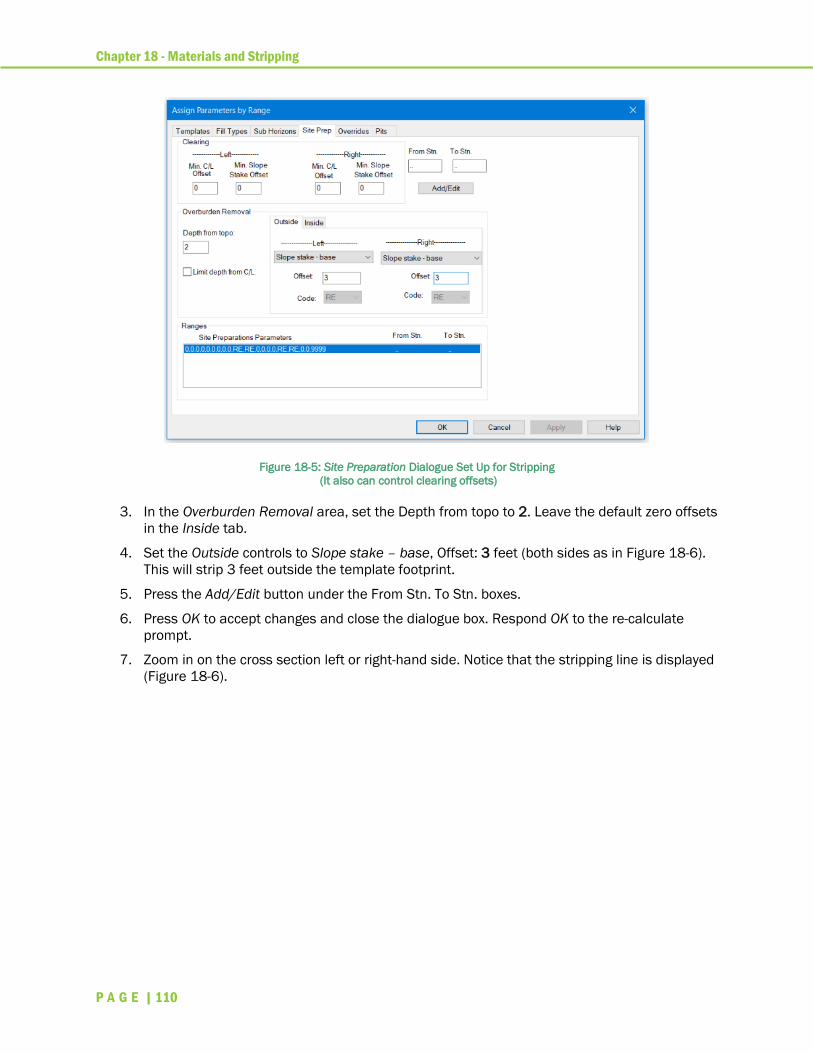
Chapter 18 - Materials and Stripping
P A G E | 110
Figure 18-5: Site Preparation Dialogue Set Up for Stripping
(It also can control clearing offsets)
3. In the Overburden Removal area, set the Depth from topo to 2. Leave the default zero offsets
in the Inside tab.
4. Set the Outside controls to Slope stake – base, Offset: 3 feet (both sides as in Figure 18-6).
This will strip 3 feet outside the template footprint.
5. Press the Add/Edit button under the From Stn. To Stn. boxes.
6. Press OK to accept changes and close the dialogue box. Respond OK to the re-calculate
prompt.
7. Zoom in on the cross section left or right-hand side. Notice that the stripping line is displayed
(Figure 18-6).

Chapter 18 - Materials and Stripping
P A G E | 111
Figure 18-6: The Top Ground Layer has to been Stripped Off
The total volume of cut will have been reduced and fill increased. The OB cut volume will now be zero
and there is now a non-zero Stripping volume available for reporting.
Some important facts about stripping:
• Stripped material is excluded from the mass haul – it is assumed to be unsuitable for fill.
• The depth stripped will be the value assigned in the Site Prep dialogue or the top surface
layer thickness, whichever is least. In the above example, the top layer (OB) is only 1 foot
thick so that is the stripped depth.
• Stripping happens before the template is applied to a cross section.
8. File | Close. Do not save changes.
Using Materials to Control Templates
The templates we have used so far have fixed cut and fill slopes. In the following steps, we will
change the final slopes component so that it extracts slopes from the materials in the ground or in
the fill.
1. File | Open <RoadEngCivil>\Location\Align stage 6.dsnx.
2. Home | Assign by Range. Select the Templates tab (Figure 18-7).

Chapter 18 - Materials and Stripping
P A G E | 112
Figure 18-7: Assigning the RUR Rural Template to The Entire Alignment.
3. In Template Name, choose RUR Rural. Leave the default “..” in the From/To fields.
4. Press the Add/Edit button, this will apply the new template to the entire alignment. The
dialogue box should appear as in the figure above.
Note: The most common mistake made in the assignments dialogue box is to skip the Add/Edit step. If
you Press OK before the ranges are updated, nothing happens.
5. Press OK to return to the main screen. Respond OK to “Recalculate road alignment”.
6. Click on the section window window to select it. Section | Jump to Station type in <Ctrl-J>
and type station 1675. Press OK to update the current section.
Figure 18.8: Template on The Left has Fixed Slope Values, while
The One on The Right Has Slopes Set to Auto

Chapter 18 - Materials and Stripping
P A G E | 113
7. The RUR Rural template has the cut and fill slope parameters set to automatic. The result of
this change is to significantly reduce the cut material due to the steeper cut angle in the
deeper FR layer.
This technique is used in the Culverts exercise later.
8. File | Close. Do not save changes.
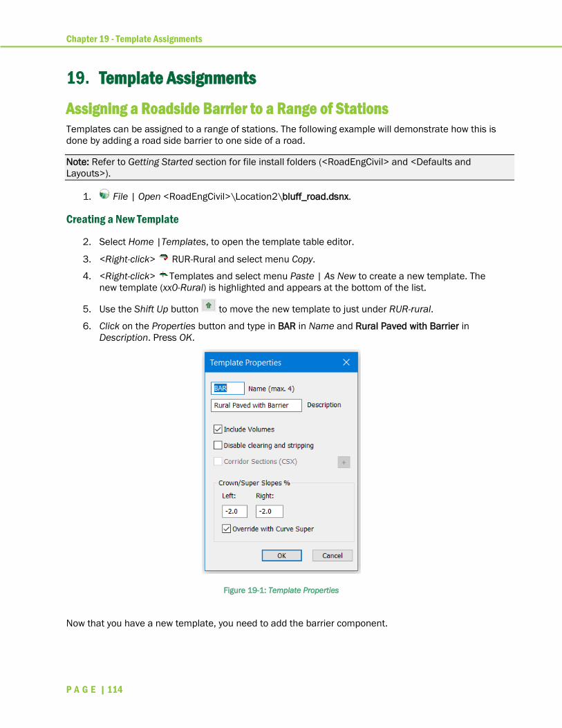
Chapter 19 - Template Assignments
P A G E | 114
Template Assignments
Assigning a Roadside Barrier to a Range of Stations
Templates can be assigned to a range of stations. The following example will demonstrate how this is
done by adding a road side barrier to one side of a road.
Note: Refer to Getting Started section for file install folders (<RoadEngCivil> and <Defaults and
Layouts>).
1. File | Open <RoadEngCivil>\Location2\bluff_road.dsnx.
Creating a New Template
2. Select Home |Templates, to open the template table editor.
3. <Right-click> RUR-Rural and select menu Copy.
4. <Right-click> Templates and select menu Paste | As New to create a new template. The
new template (xx0-Rural) is highlighted and appears at the bottom of the list.
5. Use the Shift Up button to move the new template to just under RUR-rural.
6. Click on the Properties button and type in BAR in Name and Rural Paved with Barrier in
Description. Press OK.
Figure 19-1: Template Properties
Now that you have a new template, you need to add the barrier component.
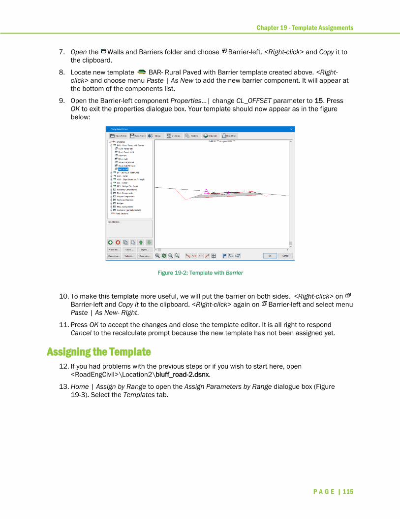
Chapter 19 - Template Assignments
P A G E | 115
7. Open the Walls and Barriers folder and choose Barrier-left. <Right-click> and Copy it to
the clipboard.
8. Locate new template BAR- Rural Paved with Barrier template created above. <Right-
click> and choose menu Paste | As New to add the new barrier component. It will appear at
the bottom of the components list.
9. Open the Barrier-left component Properties…| change CL_OFFSET parameter to 15. Press
OK to exit the properties dialogue box. Your template should now appear as in the figure
below:
Figure 19-2: Template with Barrier
10. To make this template more useful, we will put the barrier on both sides. <Right-click> on
Barrier-left and Copy it to the clipboard. <Right-click> again on Barrier-left and select menu
Paste | As New- Right.
11. Press OK to accept the changes and close the template editor. It is all right to respond
Cancel to the recalculate prompt because the new template has not been assigned yet.
Assigning the Template
12. If you had problems with the previous steps or if you wish to start here, open
<RoadEngCivil>\Location2\bluff_road-2.dsnx.
13. Home | Assign by Range to open the Assign Parameters by Range dialogue box (Figure
19-3). Select the Templates tab.
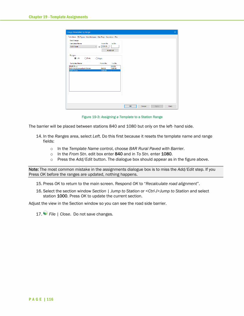
Chapter 19 - Template Assignments
P A G E | 116
Figure 19-3: Assigning a Template to a Station Range
The barrier will be placed between stations 840 and 1080 but only on the left- hand side.
14. In the Ranges area, select Left. Do this first because it resets the template name and range
fields:
o In the Template Name control, choose BAR Rural Paved with Barrier.
o In the From Stn. edit box enter 840 and in To Stn. enter 1080.
o Press the Add/Edit button. The dialogue box should appear as in the figure above.
Note: The most common mistake in the assignments dialogue box is to miss the Add/Edit step. If you
Press OK before the ranges are updated, nothing happens.
15. Press OK to return to the main screen. Respond OK to “Recalculate road alignment”.
16. Select the section window Section | Jump to Station or <Ctrl-J>Jump to Station and select
station 1000. Press OK to update the current section.
Adjust the view in the Section window so you can see the road side barrier.
17. File | Close. Do not save changes.

Chapter 20 - Template Parameter Overrides
P A G E | 117
Template Parameter Overrides The previous section demonstrated how an entire template can be assigned to a range of stations.
To do this a new template was created and assigned to a station range.
It is often desirable to change a single template parameter such as road or shoulder width, ditch
depth, etc. for a range of stations. Template Parameter Overrides provides an easy way to do this.
Creating a Turning Lane
This example will demonstrate parameter overrides by creating a turning lane at an approach to an
intersection.
Note: Refer to Getting Started section for file install folders (<RoadEngCivil> and <Defaults and
Layouts>).
1. File | Open <RoadEngCivil>\Location2\bluff_road.dsnx.
2. Home | Assign by Range | Select the Overrides tab.
Figure 20-1: The Assign Parameters By Range with Overrides Tab Selected
3. In the Parameter control, choose ACP_WIDTH (left).
4. Click on the first entry in the override list (Station 0+00) and press the Modify… button. Turn
off Use Default and set the Value to 30.0 (figure below left). Press OK.
5. Press Add… another Value of 30 at Station 110. Also change the Description to read “Turn
lane end” (figure below right). Press OK.
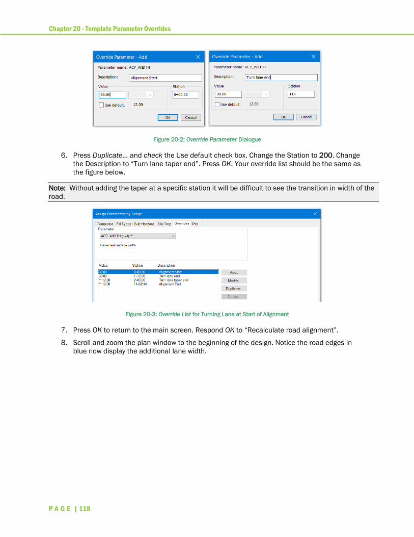
Chapter 20 - Template Parameter Overrides
P A G E | 118
Figure 20-2: Override Parameter Dialogue
6. Press Duplicate… and check the Use default check box. Change the Station to 200. Change
the Description to “Turn lane taper end”. Press OK. Your override list should be the same as
the figure below.
Note: Without adding the taper at a specific station it will be difficult to see the transition in width of the
road.
Figure 20-3: Override List for Turning Lane at Start of Alignment
7. Press OK to return to the main screen. Respond OK to “Recalculate road alignment”.
8. Scroll and zoom the plan window to the beginning of the design. Notice the road edges in
blue now display the additional lane width.
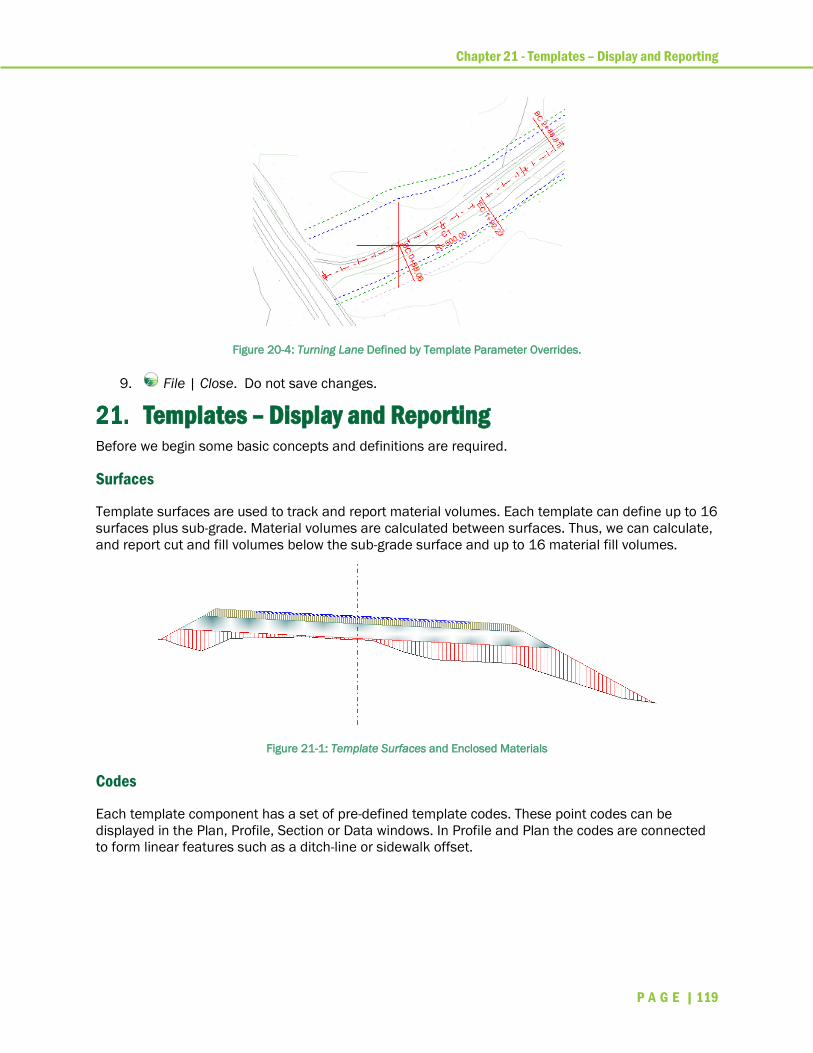
Chapter 21 - Templates – Display and Reporting
P A G E | 119
Figure 20-4: Turning Lane Defined by Template Parameter Overrides.
9. File | Close. Do not save changes.
Templates – Display and Reporting Before we begin some basic concepts and definitions are required.
Surfaces
Template surfaces are used to track and report material volumes. Each template can define up to 16
surfaces plus sub-grade. Material volumes are calculated between surfaces. Thus, we can calculate,
and report cut and fill volumes below the sub-grade surface and up to 16 material fill volumes.
Figure 21-1: Template Surfaces and Enclosed Materials
Codes
Each template component has a set of pre-defined template codes. These point codes can be
displayed in the Plan, Profile, Section or Data windows. In Profile and Plan the codes are connected
to form linear features such as a ditch-line or sidewalk offset.
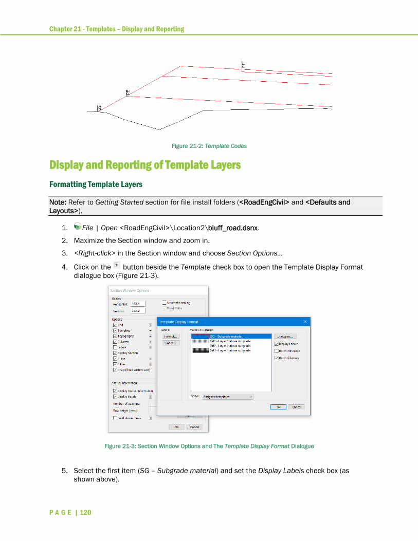
Chapter 21 - Templates – Display and Reporting
P A G E | 120
Figure 21-2: Template Codes
Display and Reporting of Template Layers
Formatting Template Layers
Note: Refer to Getting Started section for file install folders (<RoadEngCivil> and <Defaults and
Layouts>).
1. File | Open <RoadEngCivil>\Location2\bluff_road.dsnx.
2. Maximize the Section window and zoom in.
3. <Right-click> in the Section window and choose Section Options…
4. Click on the button beside the Template check box to open the Template Display Format
dialogue box (Figure 21-3).
Figure 21-3: Section Window Options and The Template Display Format Dialogue
5. Select the first item (SG – Subgrade material) and set the Display Labels check box (as
shown above).
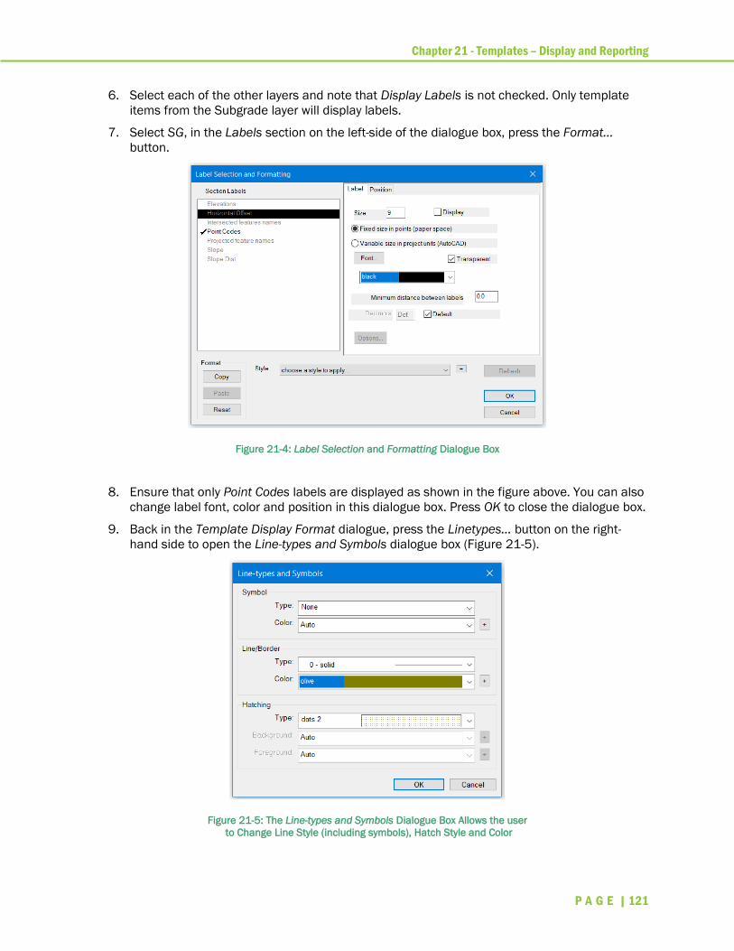
Chapter 21 - Templates – Display and Reporting
P A G E | 121
6. Select each of the other layers and note that Display Labels is not checked. Only template
items from the Subgrade layer will display labels.
7. Select SG, in the Labels section on the left-side of the dialogue box, press the Format…
button.
Figure 21-4: Label Selection and Formatting Dialogue Box
8. Ensure that only Point Codes labels are displayed as shown in the figure above. You can also
change label font, color and position in this dialogue box. Press OK to close the dialogue box.
9. Back in the Template Display Format dialogue, press the Linetypes… button on the right-
hand side to open the Line-types and Symbols dialogue box (Figure 21-5).
Figure 21-5: The Line-types and Symbols Dialogue Box Allows the user
to Change Line Style (including symbols), Hatch Style and Color
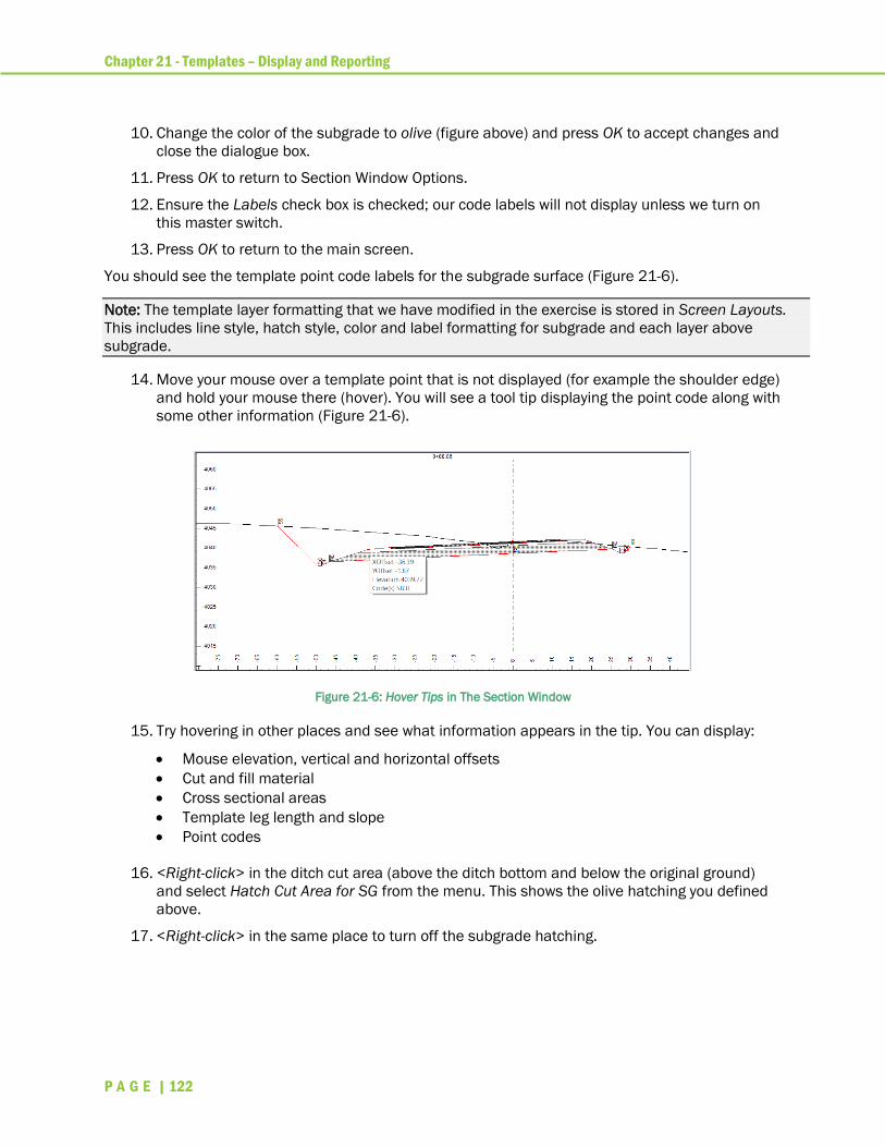
Chapter 21 - Templates – Display and Reporting
P A G E | 122
10. Change the color of the subgrade to olive (figure above) and press OK to accept changes and
close the dialogue box.
11. Press OK to return to Section Window Options.
12. Ensure the Labels check box is checked; our code labels will not display unless we turn on
this master switch.
13. Press OK to return to the main screen.
You should see the template point code labels for the subgrade surface (Figure 21-6).
Note: The template layer formatting that we have modified in the exercise is stored in Screen Layouts.
This includes line style, hatch style, color and label formatting for subgrade and each layer above
subgrade.
14. Move your mouse over a template point that is not displayed (for example the shoulder edge)
and hold your mouse there (hover). You will see a tool tip displaying the point code along with
some other information (Figure 21-6).
Figure 21-6: Hover Tips in The Section Window
15. Try hovering in other places and see what information appears in the tip. You can display:
• Mouse elevation, vertical and horizontal offsets
• Cut and fill material
• Cross sectional areas
• Template leg length and slope
• Point codes
16. <Right-click> in the ditch cut area (above the ditch bottom and below the original ground)
and select Hatch Cut Area for SG from the menu. This shows the olive hatching you defined
above.
17. <Right-click> in the same place to turn off the subgrade hatching.
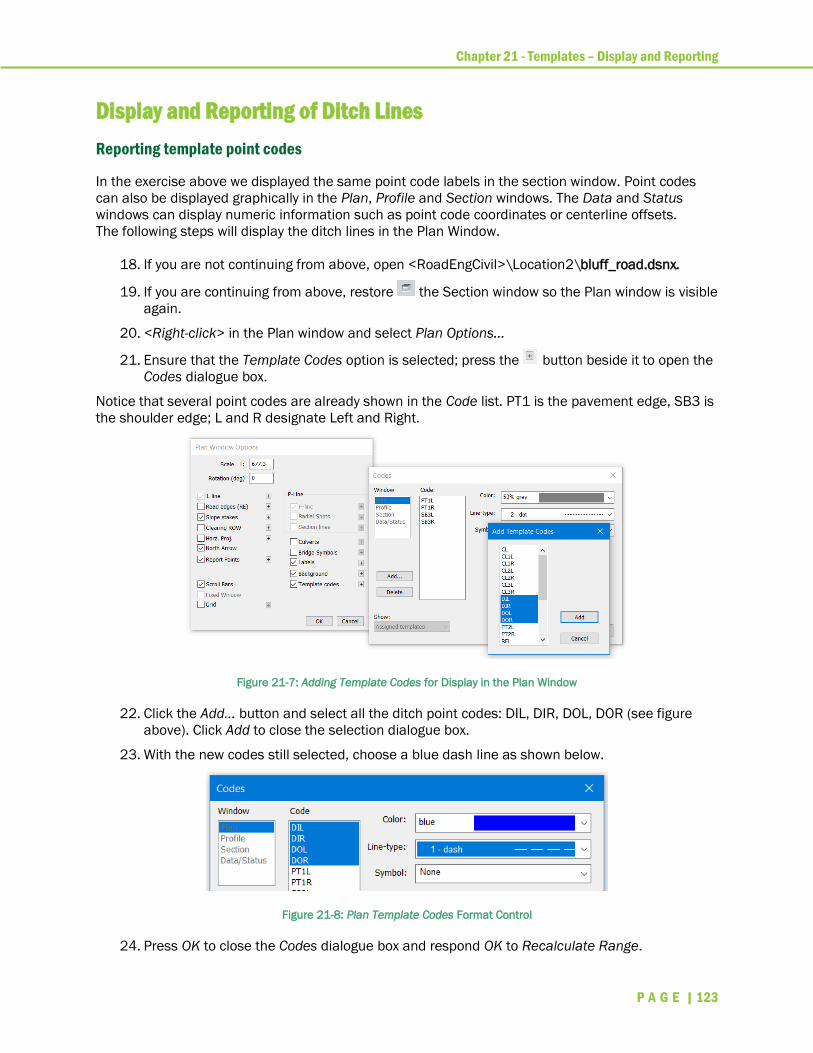
Chapter 21 - Templates – Display and Reporting
P A G E | 123
Display and Reporting of Ditch Lines
Reporting template point codes
In the exercise above we displayed the same point code labels in the section window. Point codes
can also be displayed graphically in the Plan, Profile and Section windows. The Data and Status
windows can display numeric information such as point code coordinates or centerline offsets.
The following steps will display the ditch lines in the Plan Window.
18. If you are not continuing from above, open <RoadEngCivil>\Location2\bluff_road.dsnx.
19. If you are continuing from above, restore the Section window so the Plan window is visible
again.
20. <Right-click> in the Plan window and select Plan Options...
21. Ensure that the Template Codes option is selected; press the button beside it to open the
Codes dialogue box.
Notice that several point codes are already shown in the Code list. PT1 is the pavement edge, SB3 is
the shoulder edge; L and R designate Left and Right.
Figure 21-7: Adding Template Codes for Display in the Plan Window
22. Click the Add… button and select all the ditch point codes: DIL, DIR, DOL, DOR (see figure
above). Click Add to close the selection dialogue box.
23. With the new codes still selected, choose a blue dash line as shown below.
Figure 21-8: Plan Template Codes Format Control
24. Press OK to close the Codes dialogue box and respond OK to Recalculate Range.

Chapter 21 - Templates – Display and Reporting
P A G E | 124
25. Press OK again to close the Plan Window Options dialogue.
26. Adjust the Plan Window view so you can see the new ditch lines.
Figure 21-9: Ditch lines in Plan View
Note: Template point code display options we have changed in this exercise are saved in the Template
Table.
27. Next, we will set up the data window. With the Data Window active, Data | Data Options.
28. First set up the desired spacing of data rows:
o Click the button next to Point Types to open the Point Type Selection dialogue box
(Figure 21-10 below left).
Figure 21-10: Setting the Data Window to Display Information every 50 ft
o Ensure that only the Auto Interval points are checked for display (as in figure above
left).
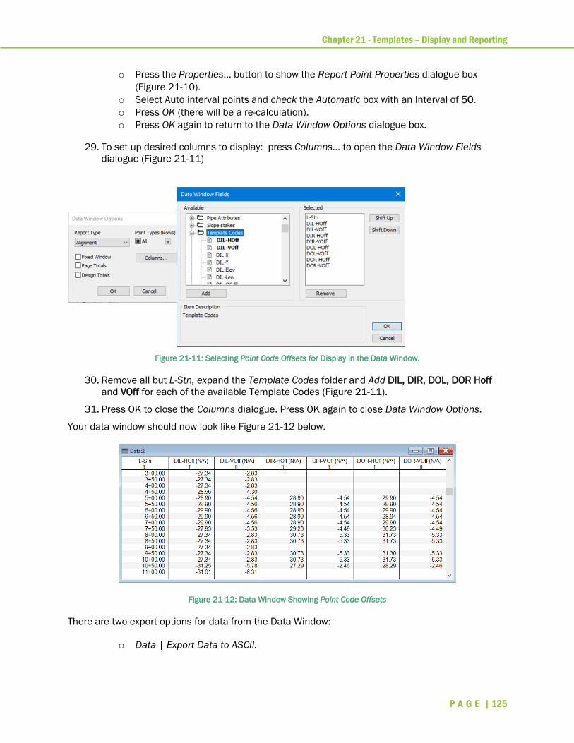
Chapter 21 - Templates – Display and Reporting
P A G E | 125
o Press the Properties… button to show the Report Point Properties dialogue box
(Figure 21-10).
o Select Auto interval points and check the Automatic box with an Interval of 50.
o Press OK (there will be a re-calculation).
o Press OK again to return to the Data Window Options dialogue box.
29. To set up desired columns to display: press Columns… to open the Data Window Fields
dialogue (Figure 21-11)
Figure 21-11: Selecting Point Code Offsets for Display in the Data Window.
30. Remove all but L-Stn, expand the Template Codes folder and Add DIL, DIR, DOL, DOR Hoff
and VOff for each of the available Template Codes (Figure 21-11).
31. Press OK to close the Columns dialogue. Press OK again to close Data Window Options.
Your data window should now look like Figure 21-12 below.
Figure 21-12: Data Window Showing Point Code Offsets
There are two export options for data from the Data Window:
o Data | Export Data to ASCII.

Chapter 21 - Templates – Display and Reporting
P A G E | 126
o Data can be copied to clipboard: (Data | Visible Window or <Right-click> | Copy Data
to Clipboard or use the hotkey <Ctrl+C>). This tabular data can be read by a spread
sheet application.
You can also add the point code offsets to your Section window:
32. In the Section Window Status area (below the graphic). <Right-click> in the Section window
and choose Section Options; press the Fields… button. Here you can add and remove fields
for reporting.
33. Press OK to close the Section Window Status Fields dialogue. And OK again to close Section
Window Options.
34. File | Close. Do not save changes.
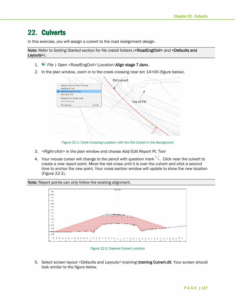
Chapter 22 - Culverts
P A G E | 127
Culverts In this exercise, you will assign a culvert to the road realignment design.
Note: Refer to Getting Started section for file install folders (<RoadEngCivil> and <Defaults and
Layouts>).
1. File | Open <RoadEngCivil>\Location\Align stage 7.dsnx.
2. In the plan window, zoom in to the creek crossing near stn 14+00 (figure below).
Figure 22-1: Creek Crossing Location; with the Old Culvert in the Background
3. <Right-click> in the plan window and choose Add/Edit Report Pt. Tool
4. Your mouse cursor will change to the pencil with question mark . Click near the culvert to
create a new report point. Move the red cross until it is over the culvert and click a second
time to anchor the new point. Your cross section window will update to show the new location
(Figure 22-2).
Note: Report points can only follow the existing alignment.
Figure 22-2: Desired Culvert Location
5. Select screen layout <Defaults and Layouts>\training\training Culvert.dlt. Your screen should
look similar to the figure below.
Old culvert
Toe of Fill
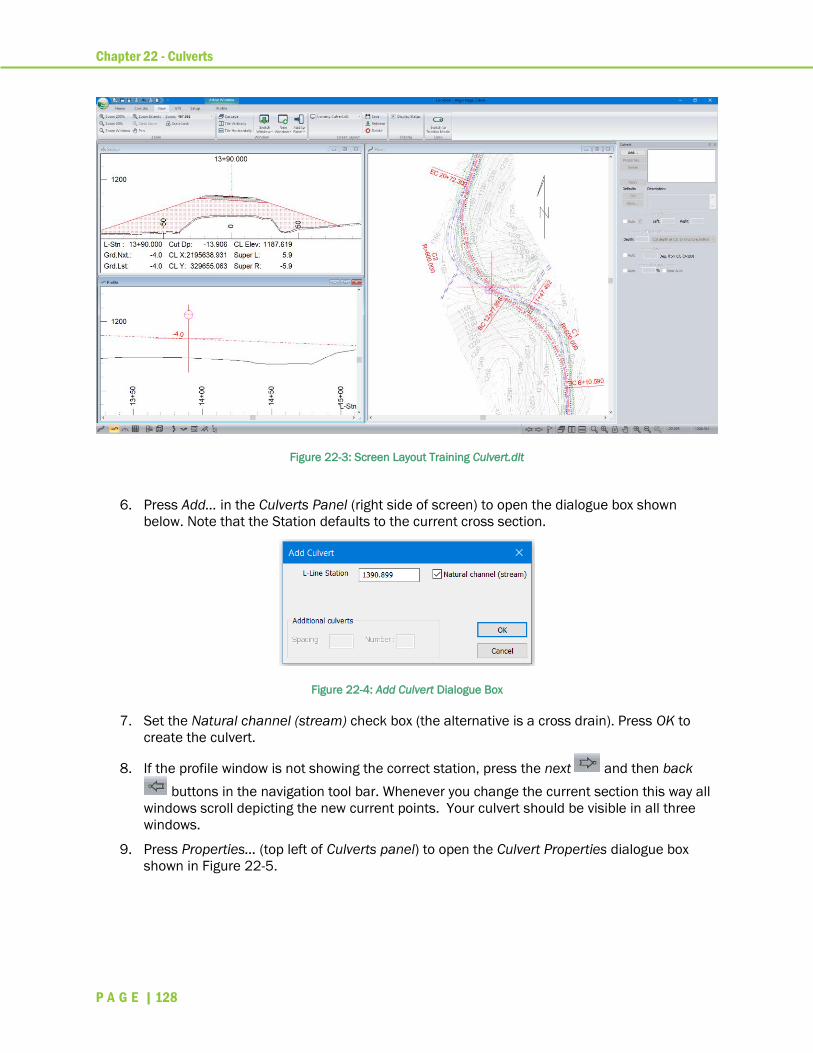
Chapter 22 - Culverts
P A G E | 128
Figure 22-3: Screen Layout Training Culvert.dlt
6. Press Add… in the Culverts Panel (right side of screen) to open the dialogue box shown
below. Note that the Station defaults to the current cross section.
Figure 22-4: Add Culvert Dialogue Box
7. Set the Natural channel (stream) check box (the alternative is a cross drain). Press OK to
create the culvert.
8. If the profile window is not showing the correct station, press the next and then back
buttons in the navigation tool bar. Whenever you change the current section this way all
windows scroll depicting the new current points. Your culvert should be visible in all three
windows.
9. Press Properties… (top left of Culverts panel) to open the Culvert Properties dialogue box
shown in Figure 22-5.
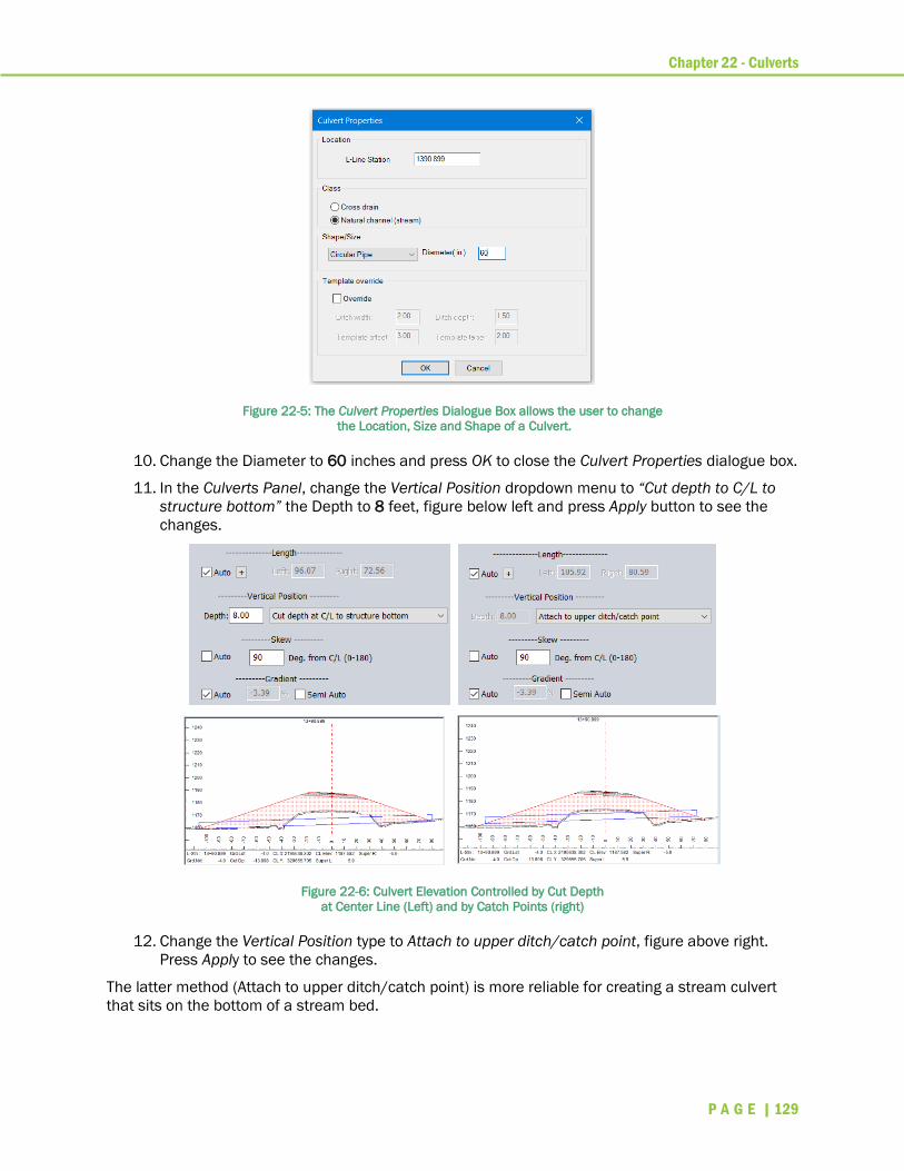
Chapter 22 - Culverts
P A G E | 129
Figure 22-5: The Culvert Properties Dialogue Box allows the user to change
the Location, Size and Shape of a Culvert.
10. Change the Diameter to 60 inches and press OK to close the Culvert Properties dialogue box.
11. In the Culverts Panel, change the Vertical Position dropdown menu to “Cut depth to C/L to
structure bottom” the Depth to 8 feet, figure below left and press Apply button to see the
changes.
Figure 22-6: Culvert Elevation Controlled by Cut Depth
at Center Line (Left) and by Catch Points (right)
12. Change the Vertical Position type to Attach to upper ditch/catch point, figure above right.
Press Apply to see the changes.
The latter method (Attach to upper ditch/catch point) is more reliable for creating a stream culvert
that sits on the bottom of a stream bed.

Chapter 22 - Culverts
P A G E | 130
13. Press the Save… in the culverts panel. Uncheck the Save to disk for future designs box and
respond OK to the save stream default prompt. The next time you create a Natural Channel
culvert this will be the initial configuration.
Changing Fill Material
Now we will change the road fill material to rip rap so that we can
• Steepen the fill and shorten the culvert
• Reduce the amount of fill required
• Reduce the footprint in the wetland (and the right of way)
• Prevent scouring
14. Home | Assign by Range, select the Fill Types tab.
Figure 22-7: Applying Special Fill (Rip Rap) Near the Culvert
15. Choose fill material RR Rip Rap (this comes from your ground types table) and set the station
range from 1300 -1500. Press the Add/Edit button.
16. Press the button next to SG Fill Material type to open the Ground Types editor. You can
add materials here if you wish. Press Cancel to close the Ground Types editor again.
17. Press OK to close the dialogue box. Respond OK to the recalculate prompt.
Figure 22-8: The Creek Crossing with Rip Rap Fill, Steeper Slopes Resulting in a Shorter Culvert

Chapter 22 - Culverts
P A G E | 131
As shown in Figure 22-8, the length of the culvert has been reduced. You can also see the change in
the road footprint in the plan window.
Note that the template applied here has a fill slope defined as Automatic; if the template was set up
with a fixed slope, you would have to change the fill slope for the desired station range using: Home
| Assign by Range| Overrides tab. Refer to section Template Parameter Overrides.
18. File | Close. Do not save changes.
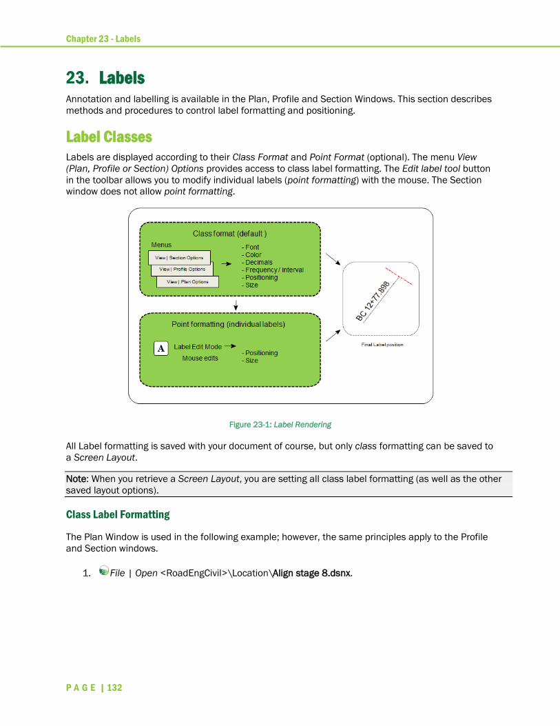
Chapter 23 - Labels
P A G E | 132
Labels Annotation and labelling is available in the Plan, Profile and Section Windows. This section describes
methods and procedures to control label formatting and positioning.
Label Classes Labels are displayed according to their Class Format and Point Format (optional). The menu View
(Plan, Profile or Section) Options provides access to class label formatting. The Edit label tool button
in the toolbar allows you to modify individual labels (point formatting) with the mouse. The Section
window does not allow point formatting.
Figure 23-1: Label Rendering
All Label formatting is saved with your document of course, but only class formatting can be saved to
a Screen Layout.
Note: When you retrieve a Screen Layout, you are setting all class label formatting (as well as the other
saved layout options).
Class Label Formatting
The Plan Window is used in the following example; however, the same principles apply to the Profile
and Section windows.
1. File | Open <RoadEngCivil>\Location\Align stage 8.dsnx.

Chapter 23 - Labels
P A G E | 133
Figure 23-2: Align Stage 8.dsnx
This example demonstrates how to display:
• Station labels at reporting points (set at 200ft intervals)
• Horizontal curve labels at the IPs
• Culvert description labels.
These label types are representative; other labels behave in a similar way.
To create labels at equal intervals, you need to set up Report Points to generate cross sections
where you want your labels. Most labels can only be displayed at existing cross sections.
2. In the plan window, <Right-click> | Plan Options… click on the button next to Report
Points. This will open the Report Point Properties dialogue box.
3. Select Auto Interval Points 2 to create points on 200 ft intervals (figure below). Press OK
twice to return to the main screen.

Chapter 23 - Labels
P A G E | 134
Figure 23-3: Report Point Properties Dialogue
4. Set up station label options:
o <Right-click>, select Plan Options…
o Click on the button beside Labels to open the Label Selection and Formatting
dialogue box.
o Turn on LStn Report Points (Intervals) by <Double-clicking> (or select, then set the
Display check box).
Note: LStn stands for Location Station
o Set the Interval spacing to 200 (Figure 23-4).
o Press OK twice to return to the main screen.

Chapter 23 - Labels
P A G E | 135
Figure 23-4: Plan Window Label Selection and Formatting
After the Plan window refreshes the screen should appear with stationing every 200 feet.
5. The format of the stationing (xx+yy in this case) is controlled in Setup | Location Setup |
Units tab | Stationing: Traditional S+dd e.g. 12+01 from dropdown.
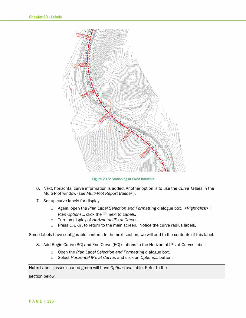
Chapter 23 - Labels
P A G E | 136
Figure 23-5: Stationing at Fixed Intervals
6. Next, horizontal curve information is added. Another option is to use the Curve Tables in the
Multi-Plot window (see Multi-Plot Report Builder ).
7. Set up curve labels for display:
o Again, open the Plan Label Selection and Formatting dialogue box. <Right-click> |
Plan Options… click the next to Labels.
o Turn on display of Horizontal IP's at Curves.
o Press OK, OK to return to the main screen. Notice the curve radius labels.
Some labels have configurable content. In the next section, we will add to the contents of this label.
8. Add Begin Curve (BC) and End Curve (EC) stations to the Horizontal IP's at Curves label:
o Open the Plan Label Selection and Formatting dialogue box.
o Select Horizontal IP's at Curves and click on Options… button.
Note: Label classes shaded green will have Options available. Refer to the
section below.
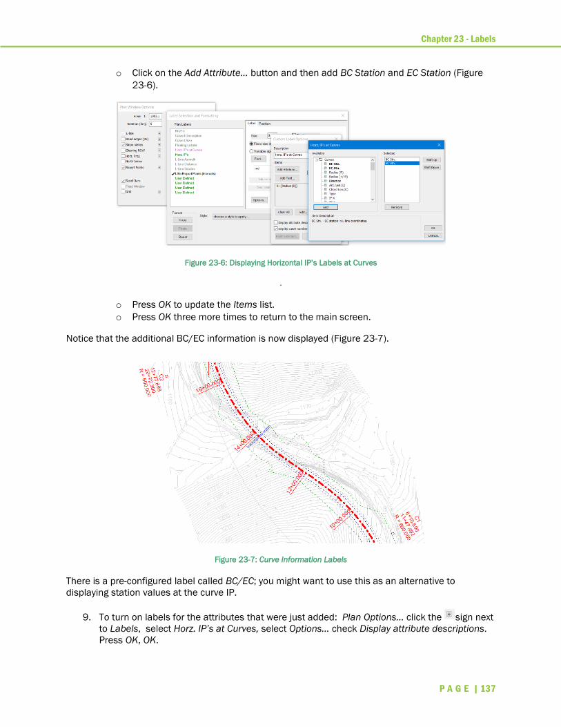
Chapter 23 - Labels
P A G E | 137
o Click on the Add Attribute… button and then add BC Station and EC Station (Figure
23-6).
Figure 23-6: Displaying Horizontal IP’s Labels at Curves
.
o Press OK to update the Items list.
o Press OK three more times to return to the main screen.
Notice that the additional BC/EC information is now displayed (Figure 23-7).
Figure 23-7: Curve Information Labels
There is a pre-configured label called BC/EC; you might want to use this as an alternative to
displaying station values at the curve IP.
9. To turn on labels for the attributes that were just added: Plan Options… click the sign next
to Labels, select Horz. IP’s at Curves, select Options… check Display attribute descriptions.
Press OK, OK.

Chapter 23 - Labels
P A G E | 138
Now we will display a label at the culvert just before station 14+00. We will also look briefly at the
Position formatting.
10. Add a culvert information label:
o Open the Plan Label Selection and Formatting dialogue box.
o Select (<double-click>) Culvert Description class.
o Select the Position tab (Figure 23-8).
o Change the Connector combo box to Circle.
o Press OK twice to return to the main screen.
Figure 23-8: Culvert Information Labels

Chapter 23 - Labels
P A G E | 139
Figure 23-9: Culvert Pipe Display
11. At this point you may want to experiment with some of the Position options to see how they
modify the label formatting; see also <F1> help.
Note: It is possible to use Point Label Formatting (see section below) to modify the Position settings for
the class.
12. File | Close. Do not save changes.
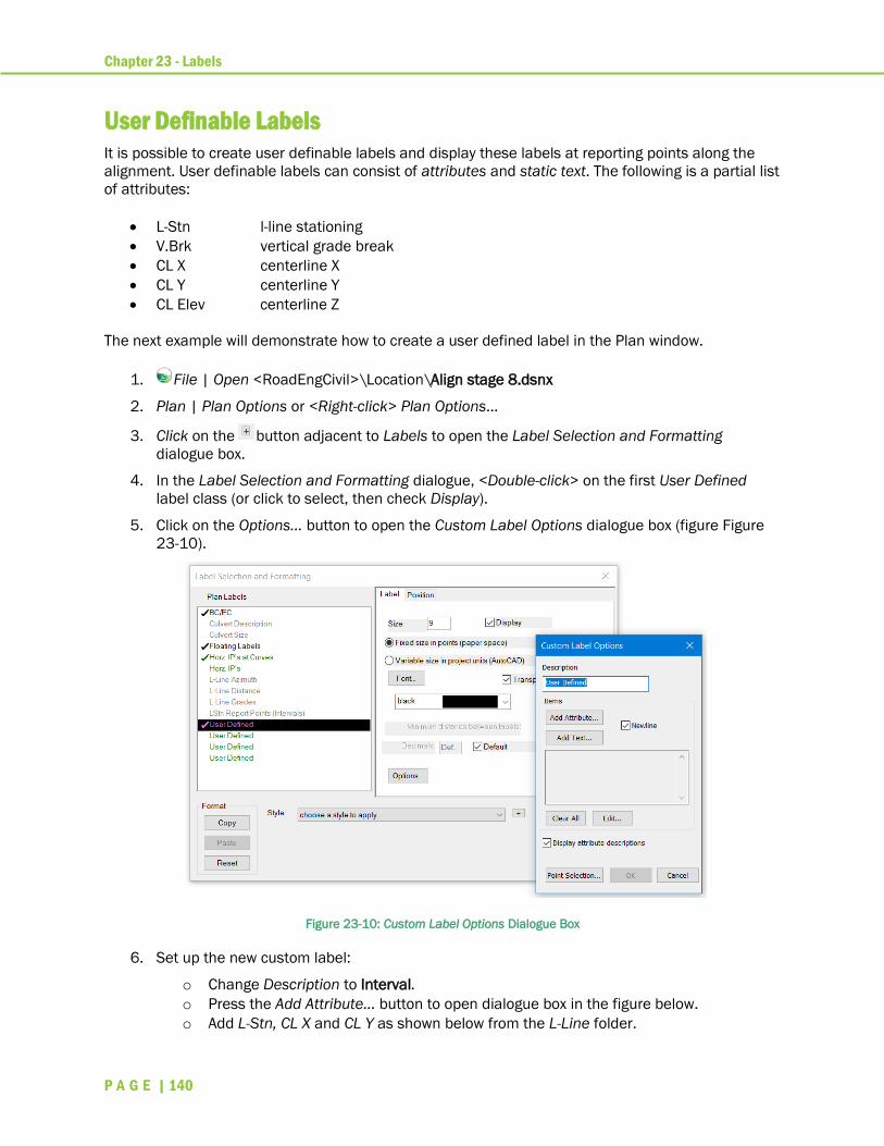
Chapter 23 - Labels
P A G E | 140
User Definable Labels
It is possible to create user definable labels and display these labels at reporting points along the
alignment. User definable labels can consist of attributes and static text. The following is a partial list
of attributes:
• L-Stn l-line stationing
• V.Brk vertical grade break
• CL X centerline X
• CL Y centerline Y
• CL Elev centerline Z
The next example will demonstrate how to create a user defined label in the Plan window.
1. File | Open <RoadEngCivil>\Location\Align stage 8.dsnx
2. Plan | Plan Options or <Right-click> Plan Options…
3. Click on the button adjacent to Labels to open the Label Selection and Formatting
dialogue box.
4. In the Label Selection and Formatting dialogue, <Double-click> on the first User Defined
label class (or click to select, then check Display).
5. Click on the Options… button to open the Custom Label Options dialogue box (figure Figure
23-10).
Figure 23-10: Custom Label Options Dialogue Box
6. Set up the new custom label:
o Change Description to Interval.
o Press the Add Attribute… button to open dialogue box in the figure below.
o Add L-Stn, CL X and CL Y as shown below from the L-Line folder.
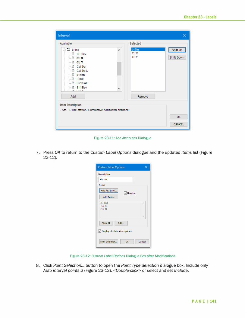
Chapter 23 - Labels
P A G E | 141
Figure 23-11: Add Attributes Dialogue
7. Press OK to return to the Custom Label Options dialogue and the updated Items list (Figure
23-12).
Figure 23-12: Custom Label Options Dialogue Box after Modifications
8. Click Point Selection… button to open the Point Type Selection dialogue box. Include only
Auto interval points 2 (Figure 23-13). <Double-click> or select and set Include.

Chapter 23 - Labels
P A G E | 142
Figure 23-13: Point Type Selection Dialogue Box
Auto interval points 2 is set to 200 ft; you can change this value by clicking on the Properties button.
9. Press OK three time to return to the main screen.
Your Plan window should appear as shown below.
Figure 23-14: User Defined Labels (Stn, X, Y at 200' Spacing)
The text before the numeric value (e.g. “L-Stn =”) is included because Display attribute descriptions
was set in the options (refer to figure above).
10. If you are not satisfied with these descriptions, clear this check box and enter your own:
o <Right-click> Plan Options…
o next to Labels
o Select Interval
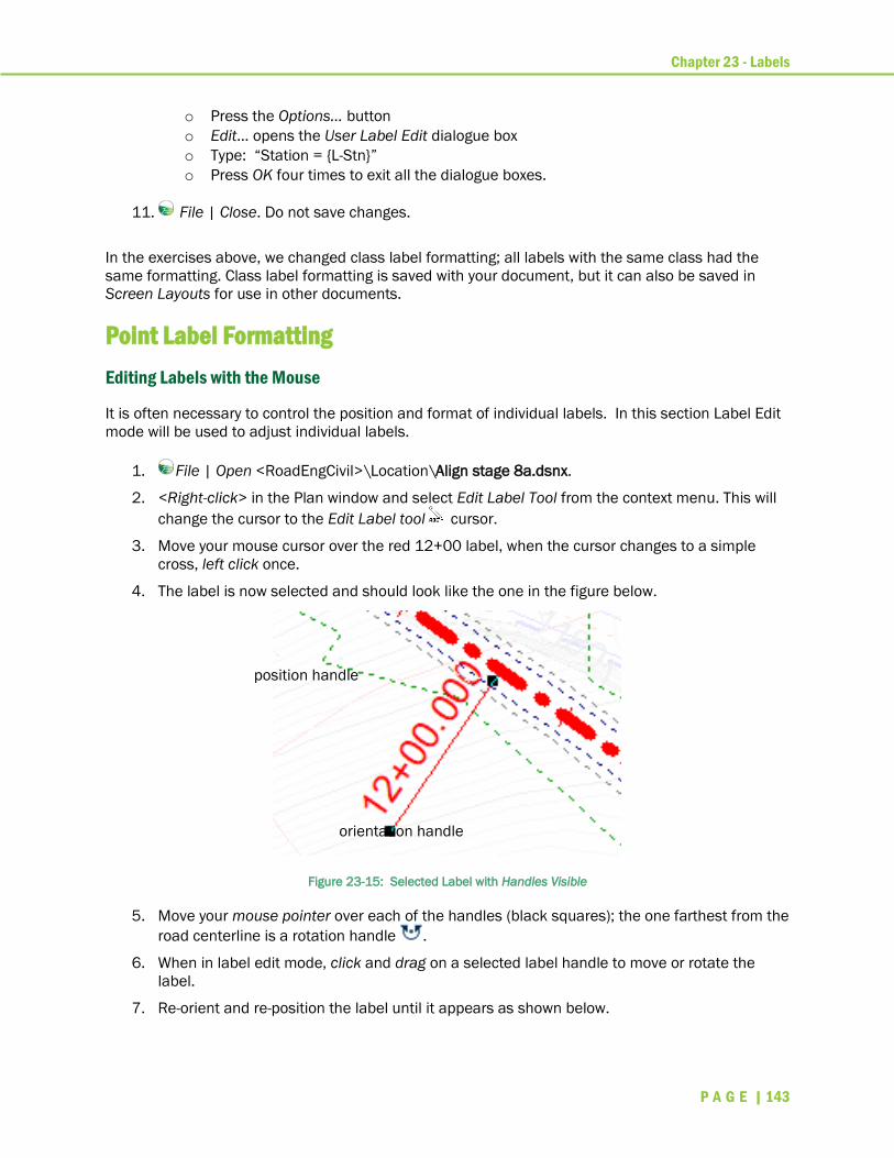
Chapter 23 - Labels
P A G E | 143
o Press the Options… button
o Edit… opens the User Label Edit dialogue box
o Type: “Station = {L-Stn}”
o Press OK four times to exit all the dialogue boxes.
11. File | Close. Do not save changes.
In the exercises above, we changed class label formatting; all labels with the same class had the
same formatting. Class label formatting is saved with your document, but it can also be saved in
Screen Layouts for use in other documents.
Point Label Formatting
Editing Labels with the Mouse
It is often necessary to control the position and format of individual labels. In this section Label Edit
mode will be used to adjust individual labels.
1. File | Open <RoadEngCivil>\Location\Align stage 8a.dsnx.
2. <Right-click> in the Plan window and select Edit Label Tool from the context menu. This will
change the cursor to the Edit Label tool cursor.
3. Move your mouse cursor over the red 12+00 label, when the cursor changes to a simple
cross, left click once.
4. The label is now selected and should look like the one in the figure below.
Figure 23-15: Selected Label with Handles Visible
5. Move your mouse pointer over each of the handles (black squares); the one farthest from the
road centerline is a rotation handle .
6. When in label edit mode, click and drag on a selected label handle to move or rotate the
label.
7. Re-orient and re-position the label until it appears as shown below.
position handle
orientation handle

Chapter 23 - Labels
P A G E | 144
Figure 23-16: Label after Re-Positioning
8. <Double-click> on the text of the label you just edited. This opens the Label Selection and
Formatting dialogue box.
Figure 23-17: Label Selection and Formatting Dialogue Box
9. Select Set as class default label formatting. Press OK.
10. Unlock the scale by clicking on the lock scale button and zoom extents in the
windows toolbar.
Your Plan window should now appear as shown below.

Chapter 23 - Labels
P A G E | 145
Figure 23-18: Plan View after Change to Class Format
Floating Labels
Floating Labels can be added anywhere in the Plan or Profile Windows. Floating Labels can have
their anchor point moved.
11. The Edit Label tool cursor should still be enabled. If not, <right-click> in the Plan window
and select Edit Label Tool.
12. <Right-click> anywhere in the Plan Window. Select Plan Options. Press the plus button
beside Labels. <Double-click> on Floating Labels to turn then on. Press OK twice to return to
the main screen.
13. With the label edit tool , click the left mouse button anywhere in the Plan Window to open
the Label Selection and Formatting dialogue box.
14. Change “xxxxxxxx” to “Rock cut section”. Click on the Position tab and change the Leader to
have a 28mm Offset and an Arrow Connector.
15. Press OK; the floating label will appear where you first clicked the mouse.
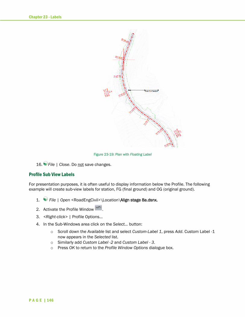
Chapter 23 - Labels
P A G E | 146
Figure 23-19: Plan with Floating Label
16. File | Close. Do not save changes.
Profile Sub View Labels
For presentation purposes, it is often useful to display information below the Profile. The following
example will create sub-view labels for station, FG (final ground) and OG (original ground).
1. File | Open <RoadEngCivil>\Location\Align stage 8a.dsnx.
2. Activate the Profile Window .
3. <Right-click> | Profile Options…
4. In the Sub-Windows area click on the Select… button:
o Scroll down the Available list and select Custom-Label 1, press Add. Custom Label -1
now appears in the Selected list.
o Similarly add Custom Label -2 and Custom Label - 3.
o Press OK to return to the Profile Window Options dialogue box.
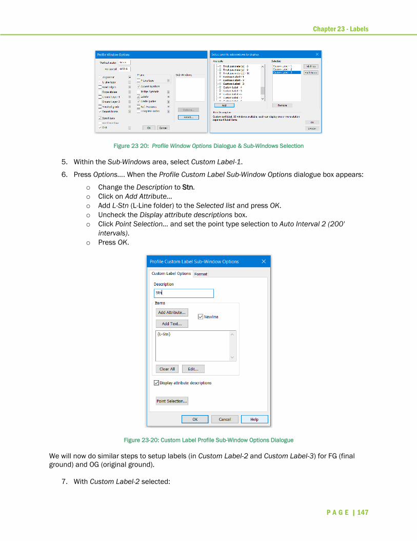
Chapter 23 - Labels
P A G E | 147
Figure 23 20: Profile Window Options Dialogue & Sub-Windows Selection
5. Within the Sub-Windows area, select Custom Label-1.
6. Press Options…. When the Profile Custom Label Sub-Window Options dialogue box appears:
o Change the Description to Stn.
o Click on Add Attribute…
o Add L-Stn (L-Line folder) to the Selected list and press OK.
o Uncheck the Display attribute descriptions box.
o Click Point Selection… and set the point type selection to Auto Interval 2 (200'
intervals).
o Press OK.
Figure 23-20: Custom Label Profile Sub-Window Options Dialogue
We will now do similar steps to setup labels (in Custom Label-2 and Custom Label-3) for FG (final
ground) and OG (original ground).
7. With Custom Label-2 selected:

Chapter 23 - Labels
P A G E | 148
o Click on Options….
o Change the Description to FG
o Click on the Add Attribute… button.
o Add CL-Elev (L-Line folder) to the Selected list and press OK.
o Uncheck Display attribute descriptions.
o Click on Point Selection… and make sure the point type selection is set to be Auto
Interval 2 (200' intervals).
o Press OK twice.
8. With Custom Label-3 selected:
o Click on Options….
o Change the Description to OG
o Click on the Add Attribute… button.
o Add GND-Elev (Ground Layers folder) to the Selected list and press OK.
o Uncheck Display attribute descriptions.
o Click on Point Selection… and make sure the point type selection is set to be Auto
Interval 2 (200' intervals).
o Press OK three times to return to the main screen.
Figure 23-21: Profile Sub-View Labels
9. File | Close. Do not save changes.
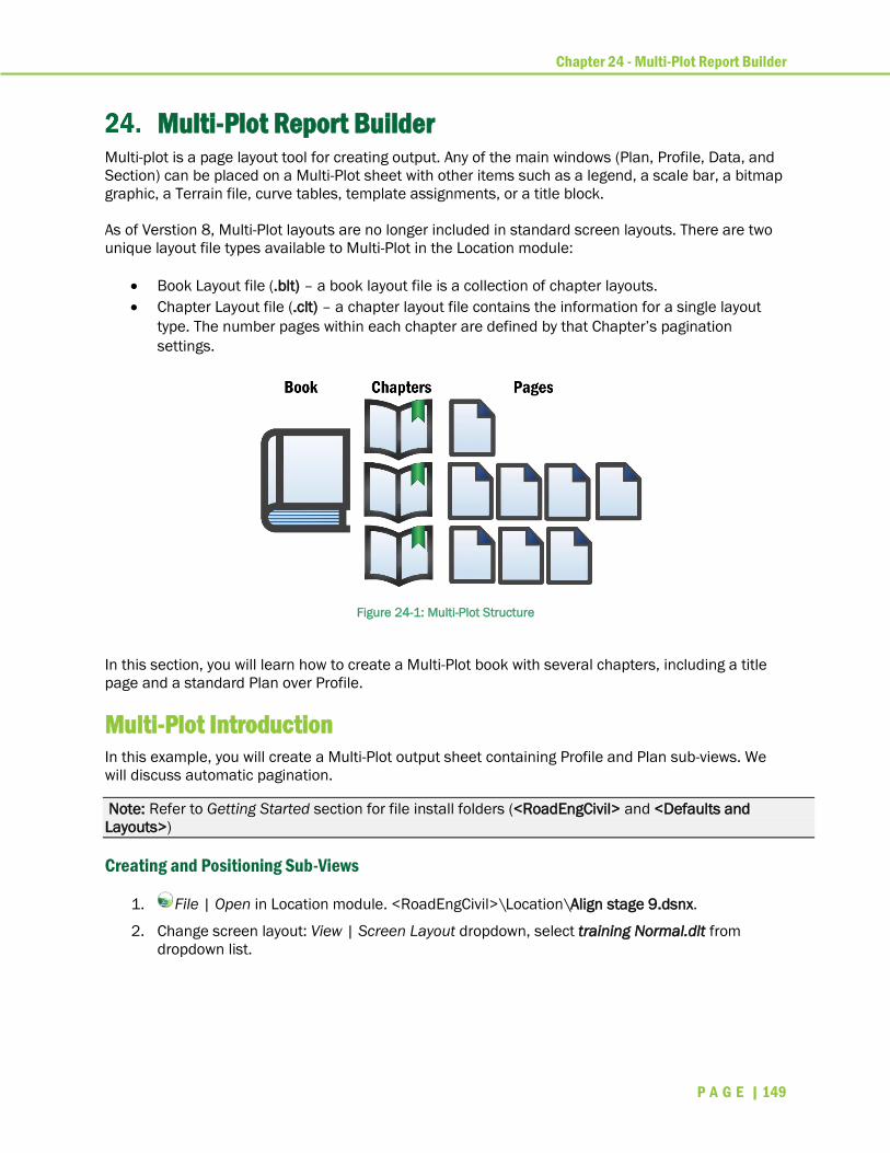
Chapter 24 - Multi-Plot Report Builder
P A G E | 149
Multi-Plot Report Builder Multi-plot is a page layout tool for creating output. Any of the main windows (Plan, Profile, Data, and
Section) can be placed on a Multi-Plot sheet with other items such as a legend, a scale bar, a bitmap
graphic, a Terrain file, curve tables, template assignments, or a title block.
As of Verstion 8, Multi-Plot layouts are no longer included in standard screen layouts. There are two
unique layout file types available to Multi-Plot in the Location module:
• Book Layout file (.blt) – a book layout file is a collection of chapter layouts.
• Chapter Layout file (.clt) – a chapter layout file contains the information for a single layout
type. The number pages within each chapter are defined by that Chapter’s pagination
settings.
Figure 24-1: Multi-Plot Structure
In this section, you will learn how to create a Multi-Plot book with several chapters, including a title
page and a standard Plan over Profile.
Multi-Plot Introduction In this example, you will create a Multi-Plot output sheet containing Profile and Plan sub-views. We
will discuss automatic pagination.
Note: Refer to Getting Started section for file install folders (<RoadEngCivil> and <Defaults and
Layouts>)
Creating and Positioning Sub-Views
1. File | Open in Location module. <RoadEngCivil>\Location\Align stage 9.dsnx.
2. Change screen layout: View | Screen Layout dropdown, select training Normal.dlt from
dropdown list.
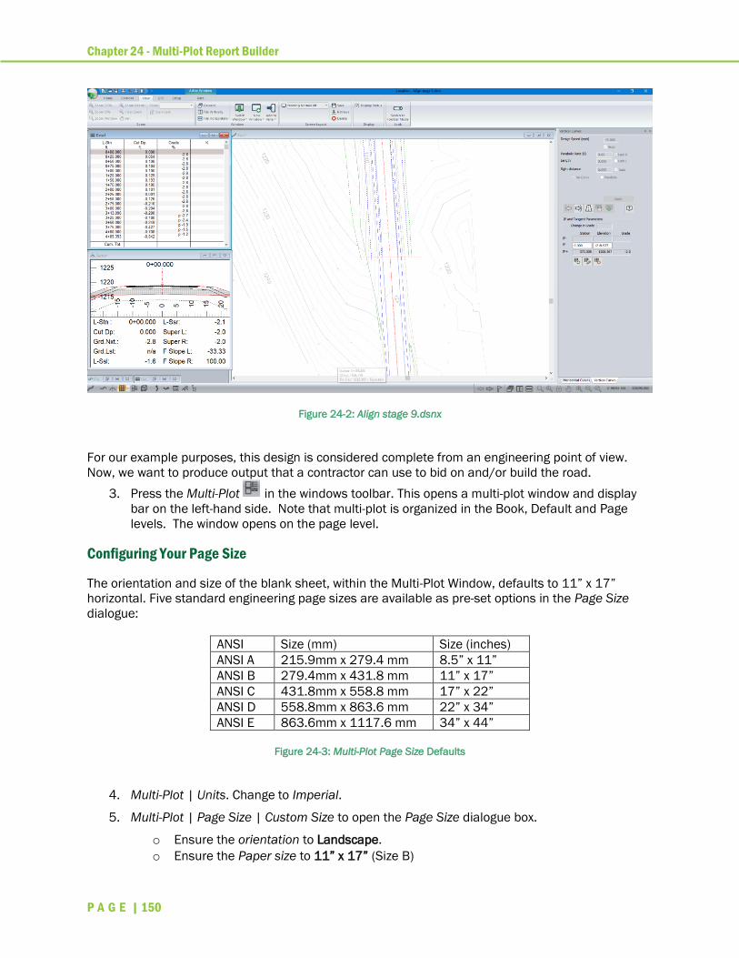
Chapter 24 - Multi-Plot Report Builder
P A G E | 150
Figure 24-2: Align stage 9.dsnx
For our example purposes, this design is considered complete from an engineering point of view.
Now, we want to produce output that a contractor can use to bid on and/or build the road.
3. Press the Multi-Plot in the windows toolbar. This opens a multi-plot window and display
bar on the left-hand side. Note that multi-plot is organized in the Book, Default and Page
levels. The window opens on the page level.
Configuring Your Page Size
The orientation and size of the blank sheet, within the Multi-Plot Window, defaults to 11” x 17”
horizontal. Five standard engineering page sizes are available as pre-set options in the Page Size
dialogue:
ANSI Size (mm) Size (inches)
ANSI A 215.9mm x 279.4 mm 8.5” x 11”
ANSI B 279.4mm x 431.8 mm 11” x 17”
ANSI C 431.8mm x 558.8 mm 17” x 22”
ANSI D 558.8mm x 863.6 mm 22” x 34”
ANSI E 863.6mm x 1117.6 mm 34” x 44”
Figure 24-3: Multi-Plot Page Size Defaults
4. Multi-Plot | Units. Change to Imperial.
5. Multi-Plot | Page Size | Custom Size to open the Page Size dialogue box.
o Ensure the orientation to Landscape.
o Ensure the Paper size to 11” x 17” (Size B)

Chapter 24 - Multi-Plot Report Builder
P A G E | 151
o Press OK.
Note: the screen view is determined by the Page Size and Page Orientation controls in the ribbon toolbar.
When printing, the printer setup must be confirmed to match the screen setup.
6. File| Printer Setup to open the Print Setup dialogue. Set the paper size and orientation to
match our screen size and layout (11x17” and landscape). This is the paper size that
governs in the print preview. This depends on the type of printer and paper size the printer
can handle.
Configuring our Chapter
The first chapter we will create is a Plan over Profile layout.
7. <Right-click> on the Default chapter, this should allow you to edit its name. Select
Rename Chapter, change the name to PlanProfile.
The Location Multi-Plot Window can automatically produce as many pages as are required to show
the entire design. Before we insert a Sub-View, it would be more appropriate to set the number of
pages to avoid any potential rework. In this section, we will explore some of the pagination options.
2. Multi-plot | Pagination:
• Make sure Fixed is selected as Length of road (Stations) per page.
• Enter a value of 800 Feet.
• Enter an overlap value of 0% as seen below in Figure 24-4.
• Press OK to accept these Pagination Options.
Figure 24-4: Pagination Options
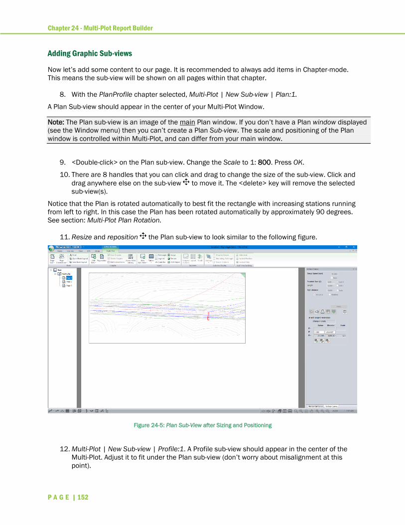
Chapter 24 - Multi-Plot Report Builder
P A G E | 152
Adding Graphic Sub-views
Now let’s add some content to our page. It is recommended to always add items in Chapter-mode.
This means the sub-view will be shown on all pages within that chapter.
8. With the PlanProfile chapter selected, Multi-Plot | New Sub-view | Plan:1.
A Plan Sub-view should appear in the center of your Multi-Plot Window.
Note: The Plan sub-view is an image of the main Plan window. If you don’t have a Plan window displayed
(see the Window menu) then you can’t create a Plan Sub-view. The scale and positioning of the Plan
window is controlled within Multi-Plot, and can differ from your main window.
9. <Double-click> on the Plan sub-view. Change the Scale to 1: 800. Press OK.
10. There are 8 handles that you can click and drag to change the size of the sub-view. Click and
drag anywhere else on the sub-view to move it. The <delete> key will remove the selected
sub-view(s).
Notice that the Plan is rotated automatically to best fit the rectangle with increasing stations running
from left to right. In this case the Plan has been rotated automatically by approximately 90 degrees.
See section: Multi-Plot Plan Rotation.
11. Resize and reposition the Plan sub-view to look similar to the following figure.
Figure 24-5: Plan Sub-View after Sizing and Positioning
12. Multi-Plot | New Sub-view | Profile:1. A Profile sub-view should appear in the center of the
Multi-Plot. Adjust it to fit under the Plan sub-view (don’t worry about misalignment at this
point).
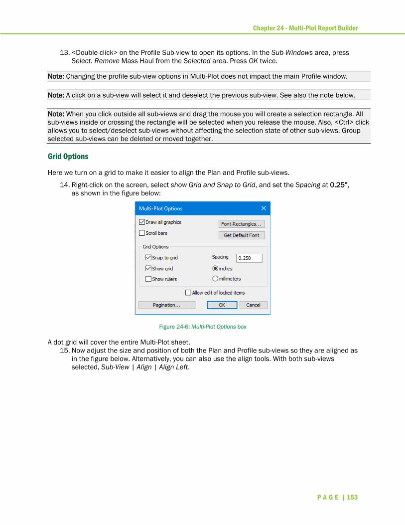
Chapter 24 - Multi-Plot Report Builder
P A G E | 153
13. <Double-click> on the Profile Sub-view to open its options. In the Sub-Windows area, press
Select. Remove Mass Haul from the Selected area. Press OK twice.
Note: Changing the profile sub-view options in Multi-Plot does not impact the main Profile window.
Note: A click on a sub-view will select it and deselect the previous sub-view. See also the note below.
Note: When you click outside all sub-views and drag the mouse you will create a selection rectangle. All
sub-views inside or crossing the rectangle will be selected when you release the mouse. Also, <Ctrl> click
allows you to select/deselect sub-views without affecting the selection state of other sub-views. Group
selected sub-views can be deleted or moved together.
Grid Options
Here we turn on a grid to make it easier to align the Plan and Profile sub-views.
14. Right-click on the screen, select show Grid and Snap to Grid, and set the Spacing at 0.25”,
as shown in the figure below:
Figure 24-6: Multi-Plot Options box
A dot grid will cover the entire Multi-Plot sheet.
15. Now adjust the size and position of both the Plan and Profile sub-views so they are aligned as
in the figure below. Alternatively, you can also use the align tools. With both sub-views
selected, Sub-View | Align | Align Left.
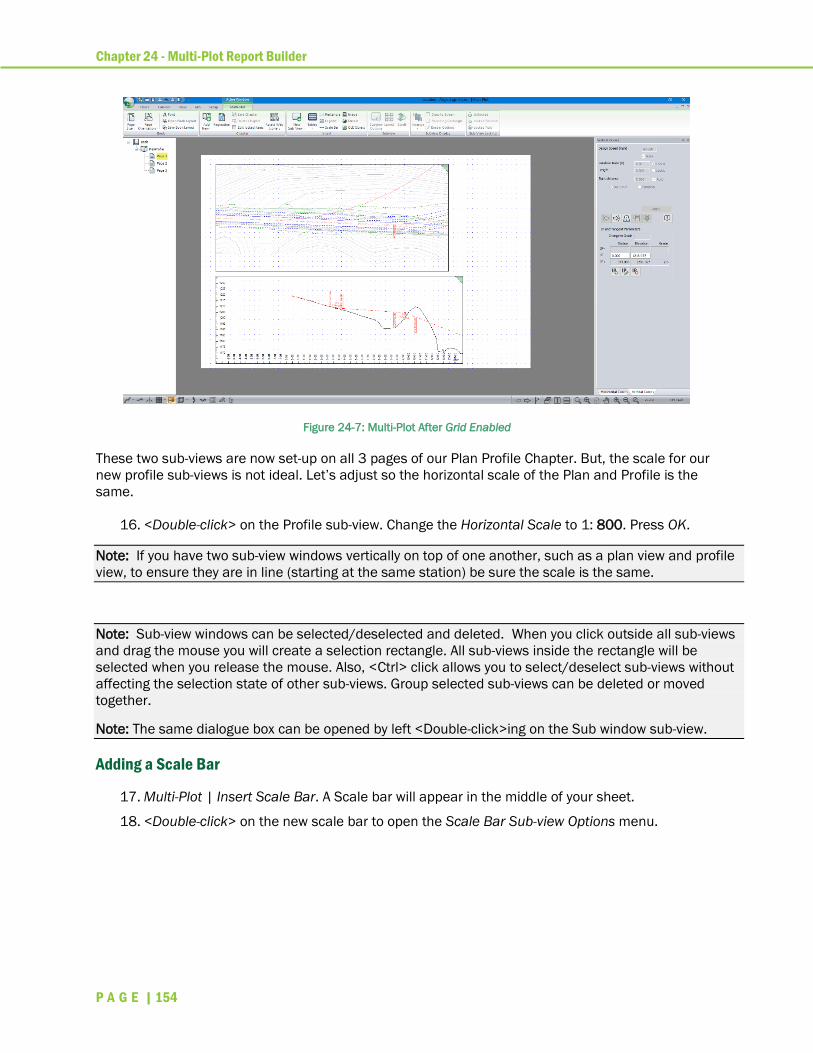
Chapter 24 - Multi-Plot Report Builder
P A G E | 154
Figure 24-7: Multi-Plot After Grid Enabled
These two sub-views are now set-up on all 3 pages of our Plan Profile Chapter. But, the scale for our
new profile sub-views is not ideal. Let’s adjust so the horizontal scale of the Plan and Profile is the
same.
16. <Double-click> on the Profile sub-view. Change the Horizontal Scale to 1: 800. Press OK.
Note: If you have two sub-view windows vertically on top of one another, such as a plan view and profile
view, to ensure they are in line (starting at the same station) be sure the scale is the same.
Note: Sub-view windows can be selected/deselected and deleted. When you click outside all sub-views
and drag the mouse you will create a selection rectangle. All sub-views inside the rectangle will be
selected when you release the mouse. Also, <Ctrl> click allows you to select/deselect sub-views without
affecting the selection state of other sub-views. Group selected sub-views can be deleted or moved
together.
Note: The same dialogue box can be opened by left <Double-click>ing on the Sub window sub-view.
Adding a Scale Bar
17. Multi-Plot | Insert Scale Bar. A Scale bar will appear in the middle of your sheet.
18. <Double-click> on the new scale bar to open the Scale Bar Sub-view Options menu.

Chapter 24 - Multi-Plot Report Builder
P A G E | 155
Figure 24-8: Scale Bar Sub-View Options Dialogue Box
19. Keep the Type: Plan Scale, ensure the Scale is set to 800. Add in the optional Title: Distance
in Feet. Press OK.
20. Resize and reposition the Scale Bar sub-view, until it appears as in the figure below (also see
notes below).
Figure 24-9 : Scale Bar in Lower Left Corner of Plan Sub-View
Adding Rectangle Sub-View Items
Rectangles can hold typed text or many pre-defined text items.
21. Multi-Plot | Insert Rectangle. A Rectangle will appear in the middle of your sheet with the
options dialogue box as shown below.
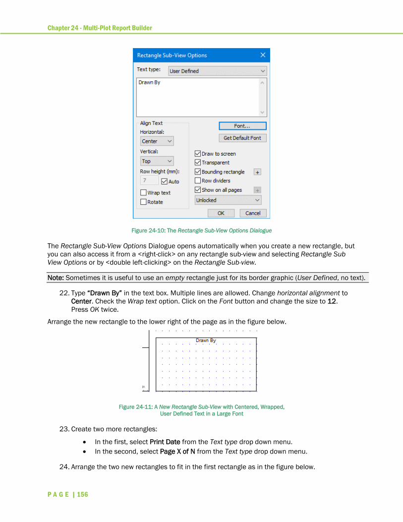
Chapter 24 - Multi-Plot Report Builder
P A G E | 156
Figure 24-10: The Rectangle Sub-View Options Dialogue
The Rectangle Sub-View Options Dialogue opens automatically when you create a new rectangle, but
you can also access it from a <right-click> on any rectangle sub-view and selecting Rectangle Sub
View Options or by <double left-clicking> on the Rectangle Sub-view.
Note: Sometimes it is useful to use an empty rectangle just for its border graphic (User Defined, no text).
22. Type “Drawn By” in the text box. Multiple lines are allowed. Change horizontal alignment to
Center. Check the Wrap text option. Click on the Font button and change the size to 12.
Press OK twice.
Arrange the new rectangle to the lower right of the page as in the figure below.
Figure 24-11: A New Rectangle Sub-View with Centered, Wrapped,
User Defined Text in a Large Font
23. Create two more rectangles:
• In the first, select Print Date from the Text type drop down menu.
• In the second, select Page X of N from the Text type drop down menu.
24. Arrange the two new rectangles to fit in the first rectangle as in the figure below.
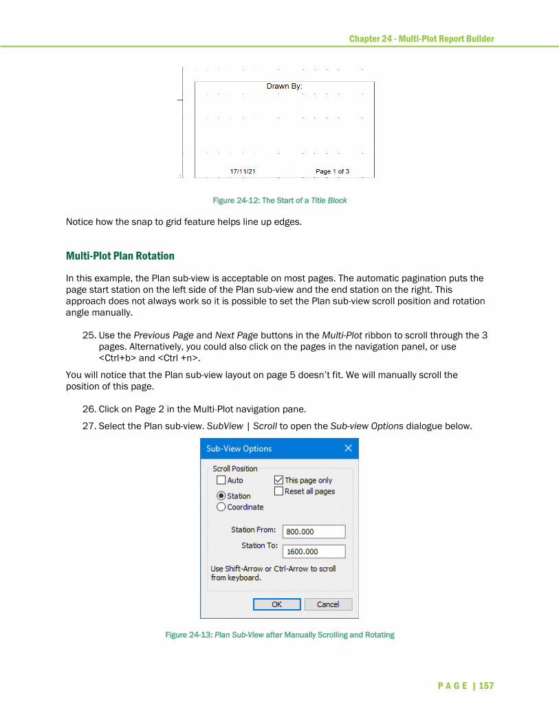
Chapter 24 - Multi-Plot Report Builder
P A G E | 157
Figure 24-12: The Start of a Title Block
Notice how the snap to grid feature helps line up edges.
Multi-Plot Plan Rotation
In this example, the Plan sub-view is acceptable on most pages. The automatic pagination puts the
page start station on the left side of the Plan sub-view and the end station on the right. This
approach does not always work so it is possible to set the Plan sub-view scroll position and rotation
angle manually.
25. Use the Previous Page and Next Page buttons in the Multi-Plot ribbon to scroll through the 3
pages. Alternatively, you could also click on the pages in the navigation panel, or use
<Ctrl+b> and <Ctrl +n>.
You will notice that the Plan sub-view layout on page 5 doesn’t fit. We will manually scroll the
position of this page.
26. Click on Page 2 in the Multi-Plot navigation pane.
27. Select the Plan sub-view. SubView | Scroll to open the Sub-view Options dialogue below.
Figure 24-13: Plan Sub-View after Manually Scrolling and Rotating

Chapter 24 - Multi-Plot Report Builder
P A G E | 158
28. Clear the Auto check box and check This Page Only (as above). Press OK.
Note the Plan position has not yet changed; we didn’t change coordinates or rotation angle yet.
29. Type <Shift + arrow> to scroll. Respond OK to the manual scroll prompt.
30. Use <Shift + arrow> to adjust the Plan sub-view so that the curve is fully visible and no longer
located below the scale bar. Try to get the Plan sub-view to look like the one in the figure
below.
Figure 24-14: Plan Sub-View after Manually Scrolling and Rotating
Note: Manual alterations to the Plan or Profile position and orientation can also be done by selecting the
window and then pressing <shift + arrows>. A prompt may remind you that Your Plan/Profile sub-view is
set to scroll with the current page station range. Do you wish to scroll manually instead? This operation
will disable the Auto check box as in step 28 above. <Shift + arrows > will scroll the plan or profile in the
direction of the arrow. <Ctrl + arrows> will rotate the Plan sub-view around its center.
31. File | Close. Do not save changes.
Multi-Plot Chapters In these exercises, we will create and retrieve Chapter layouts, copy and paste multi-plot items,
explore a couple of new sub-views and save the result for future use.
Copy and Paste of Multi-Plot Items
This exercise will add a title block to a Multi-Plot sheet. We will do this by opening an additional the
current Multi-Plot with a commonly used title block screen layout.
1. File | Open <RoadEngCivil>\Location\Align Stage 10.dsnx.
2. Select and <delete> the existing title block items so that only the Plan, Profile, scale bar
remain.
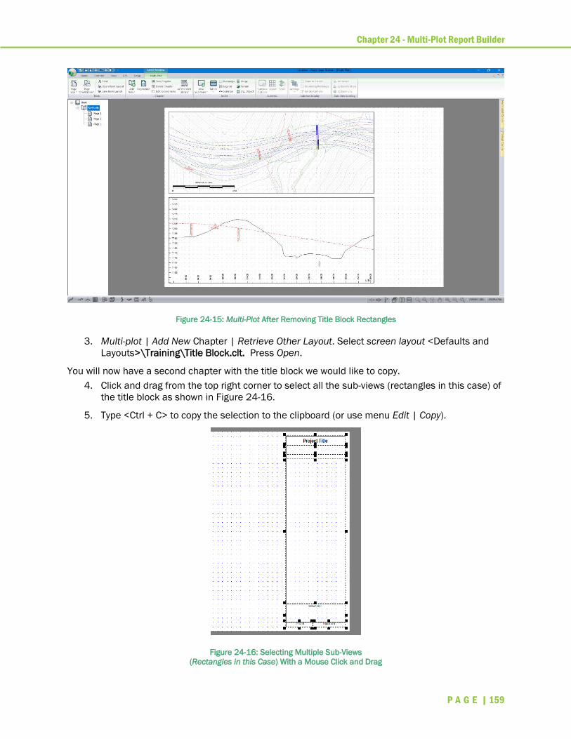
Chapter 24 - Multi-Plot Report Builder
P A G E | 159
Figure 24-15: Multi-Plot After Removing Title Block Rectangles
3. Multi-plot | Add New Chapter | Retrieve Other Layout. Select screen layout <Defaults and
Layouts>\Training\Title Block.clt. Press Open.
You will now have a second chapter with the title block we would like to copy.
4. Click and drag from the top right corner to select all the sub-views (rectangles in this case) of
the title block as shown in Figure 24-16.
5. Type <Ctrl + C> to copy the selection to the clipboard (or use menu Edit | Copy).
Figure 24-16: Selecting Multiple Sub-Views
(Rectangles in this Case) With a Mouse Click and Drag

Chapter 24 - Multi-Plot Report Builder
P A G E | 160
6. Click on the PlanProfile chapter. Type <Ctrl + V> to Paste the title block on your page (or use
menu Edit | Paste).
Your screen should appear as shown below:
Figure 24-17: Updated Title Block
7. We can save our new Plan profile chapter layout for future use: Multi Plot | Save Chapter to
open the Save Chapter dialogue. (optional)
8. We no longer need the Default chapter. Click on Default in the navigation panel, <right-click>
select Delete Chapter.
Add a Legend
In this section, we will create a legend sub-view item and examine some of its options.
9. With the PlanProfile chapter selected, select menu Multi-Plot | Insert Legend to create a
legend item.
Most of the legend items created automatically need to be removed; some of those remaining will
need to be renamed.
10. <Double-click> on the legend to open Legend Sub-View Options.
11. Click on the Items tab of the Legend Sub-View dialogue box.
12. Select and Remove all but the items shown below on the top. Multiple select is allowed use
<Ctrl + Click> or <Shift + Click>.
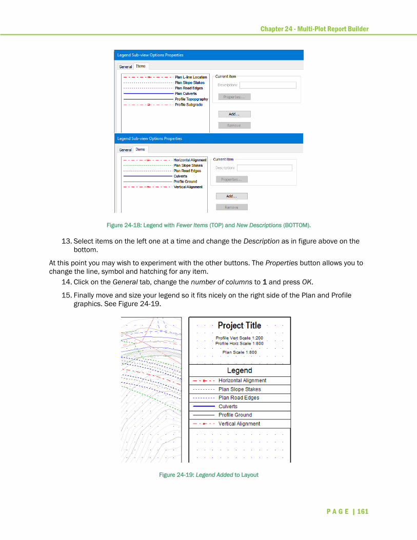
Chapter 24 - Multi-Plot Report Builder
P A G E | 161
Figure 24-18: Legend with Fewer Items (TOP) and New Descriptions (BOTTOM).
13. Select items on the left one at a time and change the Description as in figure above on the
bottom.
At this point you may wish to experiment with the other buttons. The Properties button allows you to
change the line, symbol and hatching for any item.
14. Click on the General tab, change the number of columns to 1 and press OK.
15. Finally move and size your legend so it fits nicely on the right side of the Plan and Profile
graphics. See Figure 24-19.
Figure 24-19: Legend Added to Layout

Chapter 24 - Multi-Plot Report Builder
P A G E | 162
Add a Curve Table
In this section, we will create a horizontal Curve Table sub-view and examine some of its options.
16. With the PlanProfile chapter selected, Multi-Plot | Tables | Horizontal Curves to create the
table.
17. Move and size the table until it fits on the right of the Plan and Profile graphics. We can make
further adjustments to its layout and content:
o <Double-click> on the Horizontal Curve Sub-View table to open Curve Table Options.
o Change the Column Width to 25mm.
o Select Design Points All to include points of intersection (IPs) with no curve attached.
o Press the Add/Remove button to open the Curve Table Fields dialogue box shown in
the Figure below on the right.
Figure 24-20: Horizontal Curves Table Options Dialogue Boxes
18. Add and Remove items (<double-click> works) until you have only Radius (R), IP Stn, IP X and
IP Y in the Selected column as in Figure 24-20.
19. Press OK in both dialogue boxes to see the results as shown below.

Chapter 24 - Multi-Plot Report Builder
P A G E | 163
Figure 24-21: Horizontal Curve Table after Configuration
Saving Layouts
If you only have one chapter, you can save the layout as an individual chapter layout file (.clt): Multi-
Plot | Save Chapter button.
If you have multiple chapters and want to use their layouts together in a future file, you can save the
layout as an book layout file (.blt): Multi-Plot | Save Book button.
32. File | Close. Do not save changes.

Chapter 25 - Fixed Section Editor
P A G E | 164
Fixed Section Editor Fixed sections are cross section at set stationing along the alignment of the road. These can be
useful for determining cut/fill volumes and slope.
Fixed sections allow you to explicitly change the geometry of the cross-section. They can be used to
quickly create specific design elements. However, fixed sections will not respond to alignment
changes; therefore, they should only be used after the alignment has been finalized or for calculating
existing (as-built) quantities.
1. File | Open <RoadEngCivil>\Location\Align stage 2.dsnx
2. Retrieve screen layout: View | Screen Layout, select training Normal.dlt from dropdown
menu.
3. Open section editor: press the section editor button in the window navigation toolbar.
Figure 25-1 – Screen Layout for Cross Sections
4. To allow cross sections volume calculations to be based on equal end area calculation,
check the box Ignore Points Between Fixed Sections in the lower part of Cross Section Editor
panel.
5. Press the Add Section… in the Cross Section panel.
Within the Add Fixed Cross Section dialogue, enable Station Range, check Whole Road and
check Start of Range.
The next step is to assign the station interval where you would like the cross sections:
6. Press the next to Point Types. Press Select All button. Uncheck Include box.
7. <Double-click> on Auto interval points (25.000 Ft).

Chapter 25 - Fixed Section Editor
P A G E | 165
8. Press Properties… button. Ensure Automatic is checked, set the Interval to 20.0. Press OK
three times to exit all the dialogues.
9. Each section will be displayed in Cross Section panel. Refer to Figure 25-2.
Figure 25-2 Cross Section Panel
One can now select each cross section and view it in the section panel.
Editing Layer of Individual Cross Sections:
10. Maximize the Section window.
11. In the Cross Section Editor panel, click on the station you would like to edit, in this example
we will edit 0+40.000.
12. Press the next to the section. Click on the plus next to SG. Select polyline, 7-point refer
to Figure 25-3.
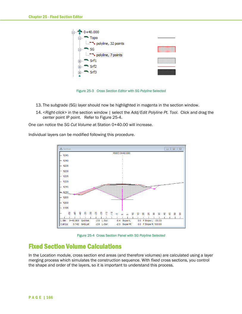
Chapter 25 - Fixed Section Editor
P A G E | 166
Figure 25-3 Cross Section Editor with SG Polyline Selected
13. The subgrade (SG) layer should now be highlighted in magenta in the section window.
14. <Right-click> in the section window | select the Add/Edit Polyline Pt. Tool. Click and drag the
center point IP point. Refer to Figure 25-4.
One can notice the SG Cut Volume at Station 0+40.00 will increase.
Individual layers can be modified following this procedure.
Figure 25-4 Cross Section Panel with SG Polyline Selected
Fixed Section Volume Calculations
In the Location module, cross section end areas (and therefore volumes) are calculated using a layer
merging process which simulates the construction sequence. With fixed cross sections, you control
the shape and order of the layers, so it is important to understand this process.
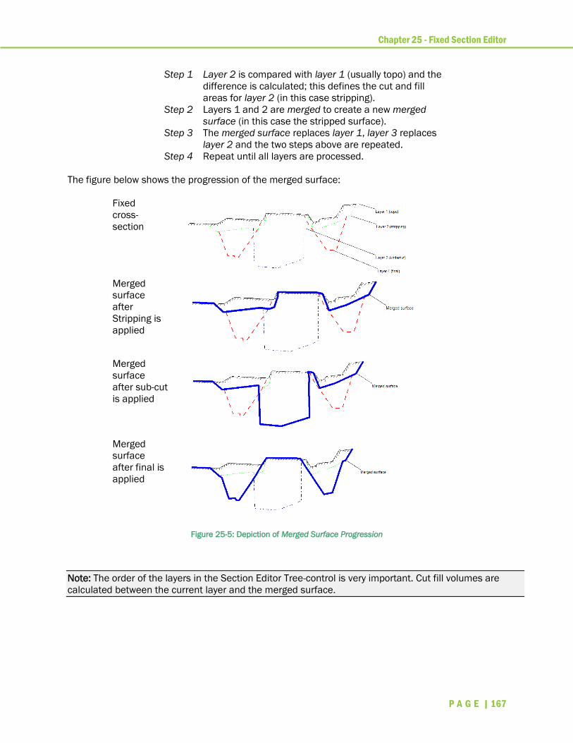
Chapter 25 - Fixed Section Editor
P A G E | 167
Step 1 Layer 2 is compared with layer 1 (usually topo) and the
difference is calculated; this defines the cut and fill
areas for layer 2 (in this case stripping).
Step 2 Layers 1 and 2 are merged to create a new merged
surface (in this case the stripped surface).
Step 3 The merged surface replaces layer 1, layer 3 replaces
layer 2 and the two steps above are repeated.
Step 4 Repeat until all layers are processed.
The figure below shows the progression of the merged surface:
Fixed
cross-
section
Merged
surface
after
Stripping is
applied
Merged
surface
after sub-cut
is applied
Merged
surface
after final is
applied
Figure 25-5: Depiction of Merged Surface Progression
Note: The order of the layers in the Section Editor Tree-control is very important. Cut fill volumes are
calculated between the current layer and the merged surface.
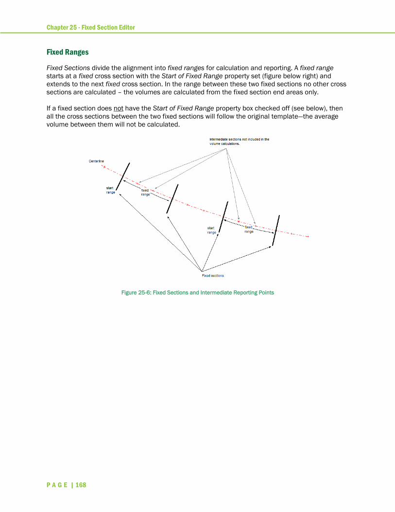
Chapter 25 - Fixed Section Editor
P A G E | 168
Fixed Ranges
Fixed Sections divide the alignment into fixed ranges for calculation and reporting. A fixed range
starts at a fixed cross section with the Start of Fixed Range property set (figure below right) and
extends to the next fixed cross section. In the range between these two fixed sections no other cross
sections are calculated – the volumes are calculated from the fixed section end areas only.
If a fixed section does not have the Start of Fixed Range property box checked off (see below), then
all the cross sections between the two fixed sections will follow the original template—the average
volume between them will not be calculated.
Figure 25-6: Fixed Sections and Intermediate Reporting Points
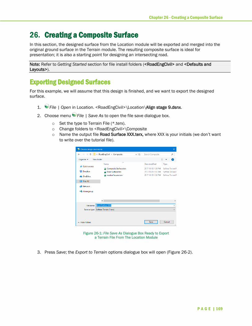
Chapter 26 - Creating a Composite Surface
P A G E | 169
Creating a Composite Surface In this section, the designed surface from the Location module will be exported and merged into the
original ground surface in the Terrain module. The resulting composite surface is ideal for
presentation; it is also a starting point for designing an intersecting road.
Note: Refer to Getting Started section for file install folders (<RoadEngCivil> and <Defaults and
Layouts>).
Exporting Designed Surfaces
For this example, we will assume that this design is finished, and we want to export the designed
surface.
1. File | Open in Location. <RoadEngCivil>\Location\Align stage 9.dsnx.
2. Choose menu File | Save As to open the file save dialogue box.
o Set the type to Terrain File (*.terx).
o Change folders to <RoadEngCivil>\Composite
o Name the output file Road Surface XXX.terx, where XXX is your initials (we don’t want
to write over the tutorial file).
Figure 26-1: File Save As Dialogue Box Ready to Export
a Terrain File From The Location Module
3. Press Save; the Export to Terrain options dialogue box will open (Figure 26-2).
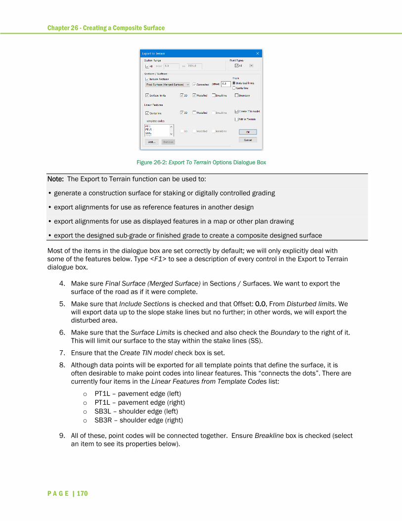
Chapter 26 - Creating a Composite Surface
P A G E | 170
Figure 26-2: Export To Terrain Options Dialogue Box
Note: The Export to Terrain function can be used to:
• generate a construction surface for staking or digitally controlled grading
• export alignments for use as reference features in another design
• export alignments for use as displayed features in a map or other plan drawing
• export the designed sub-grade or finished grade to create a composite designed surface
Most of the items in the dialogue box are set correctly by default; we will only explicitly deal with
some of the features below. Type <F1> to see a description of every control in the Export to Terrain
dialogue box.
4. Make sure Final Surface (Merged Surface) in Sections / Surfaces. We want to export the
surface of the road as if it were complete.
5. Make sure that Include Sections is checked and that Offset: 0.0, From Disturbed limits. We
will export data up to the slope stake lines but no further; in other words, we will export the
disturbed area.
6. Make sure that the Surface Limits is checked and also check the Boundary to the right of it.
This will limit our surface to the stay within the stake lines (SS).
7. Ensure that the Create TIN model check box is set.
8. Although data points will be exported for all template points that define the surface, it is
often desirable to make point codes into linear features. This “connects the dots”. There are
currently four items in the Linear Features from Template Codes list:
o PT1L – pavement edge (left)
o PT1L – pavement edge (right)
o SB3L – shoulder edge (left)
o SB3R – shoulder edge (right)
9. All of these, point codes will be connected together. Ensure Breakline box is checked (select
an item to see its properties below).

Chapter 26 - Creating a Composite Surface
P A G E | 171
10. Next add the ditch bottom features: DIL; DIR; DOL; DOR to the list of Template codes. Press
the Add… button to open the dialogue box shown below. These codes represent ditch inside,
outside left and right as shown in the figure above (use <Ctrl + click> to select/deselect
multiple items).
Figure 26-3: Add Template Codes Dialogue Box after
Selecting Ditch Bottom Point Codes.
11. Select all the new items and set the Breakline check box.
We have finished setting the options for export. It is useful to note that these options are saved with
the Location design when you save it.
12. Press the OK button to export the Terrain file.
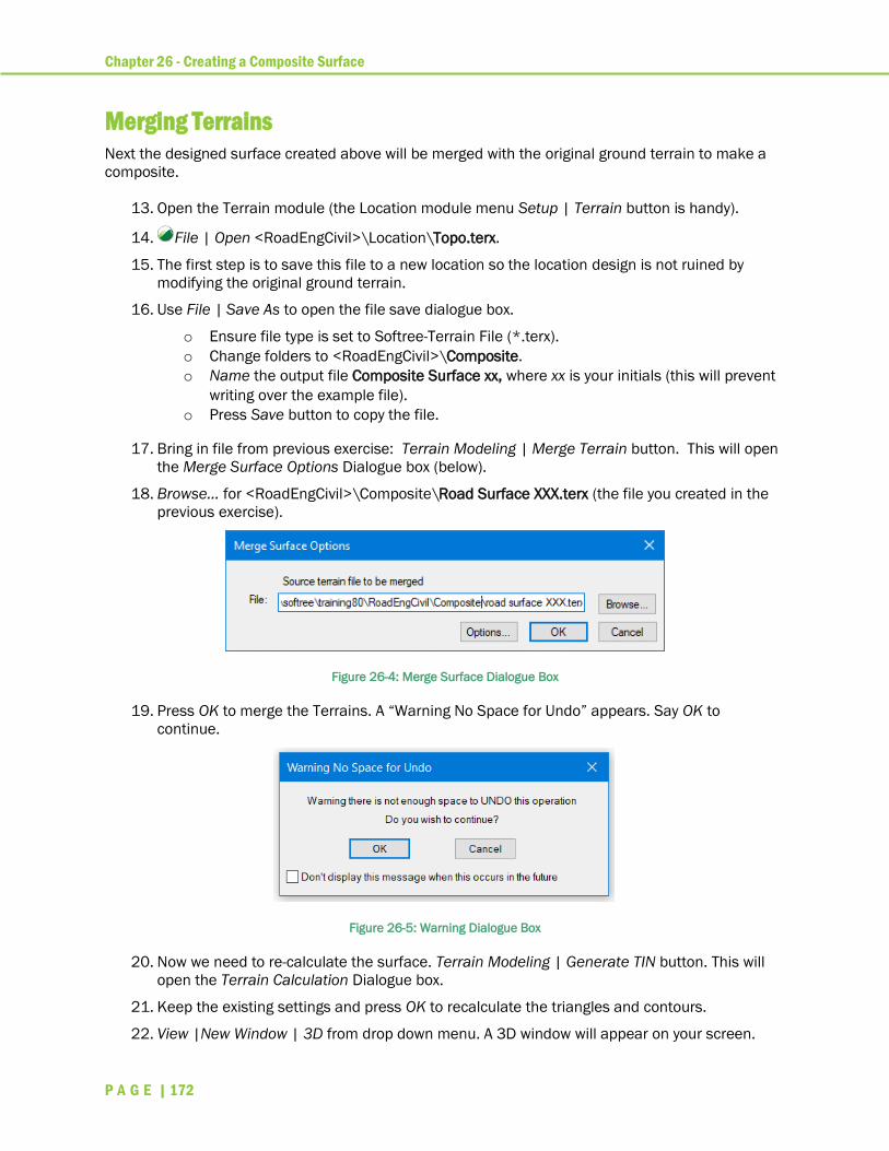
Chapter 26 - Creating a Composite Surface
P A G E | 172
Merging Terrains Next the designed surface created above will be merged with the original ground terrain to make a
composite.
13. Open the Terrain module (the Location module menu Setup | Terrain button is handy).
14. File | Open <RoadEngCivil>\Location\Topo.terx.
15. The first step is to save this file to a new location so the location design is not ruined by
modifying the original ground terrain.
16. Use File | Save As to open the file save dialogue box.
o Ensure file type is set to Softree-Terrain File (*.terx).
o Change folders to <RoadEngCivil>\Composite.
o Name the output file Composite Surface xx, where xx is your initials (this will prevent
writing over the example file).
o Press Save button to copy the file.
17. Bring in file from previous exercise: Terrain Modeling | Merge Terrain button. This will open
the Merge Surface Options Dialogue box (below).
18. Browse… for <RoadEngCivil>\Composite\Road Surface XXX.terx (the file you created in the
previous exercise).
Figure 26-4: Merge Surface Dialogue Box
19. Press OK to merge the Terrains. A “Warning No Space for Undo” appears. Say OK to
continue.
Figure 26-5: Warning Dialogue Box
20. Now we need to re-calculate the surface. Terrain Modeling | Generate TIN button. This will
open the Terrain Calculation Dialogue box.
21. Keep the existing settings and press OK to recalculate the triangles and contours.
22. View |New Window | 3D from drop down menu. A 3D window will appear on your screen.

Chapter 26 - Creating a Composite Surface
P A G E | 173
23. View | Tile Vertically Button to see the 3D and Plan windows side by side.
24. File | New do not save changes.
Figure 26-6: Composite Surface Showing Designed
Road Merged with Original Ground.
Iterative Alignment Design
This composite surface model could now be used as the original ground surface for a new Location
design. This could be used to design an intersecting road, driveway or overpass. This would ensure
grade elevations are coincident (or grade separation in the case of an overpass) and would avoid any
double counting of volumes. We might also wish to design the other direction for a divided highway.
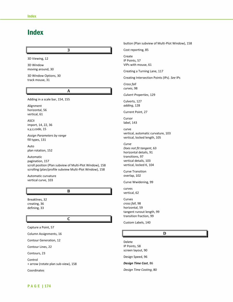
Index
P A G E | 174
Index
3
3D Viewing, 12
3D Window moving around, 30
3D Window Options, 30 track mouse, 31
A
Adding in a scale bar, 154, 155
Alignment horizontal, 56 vertical, 61
ASCII import, 14, 22, 36 x,y,z,code, 15
Assign Parameters by range fill types, 131
Auto plan rotation, 152
Automatic pagination, 157 scroll position (Plan subview of Multi-Plot Window), 158 scrolling (plan/profile subview Multi-Plot Window), 158
Automatic curvature vertical curve, 103
B
Breaklines, 32 creating, 36 defining, 33
C
Capture a Point, 57
Column Assignments, 16
Contour Generation, 12
Contour Lines, 22
Contours, 23
Control + arrow (rotate plan sub-view), 158
Coordinates
button (Plan subview of Multi-Plot Window), 158
Cost reporting, 85
Create IP Points, 57 VIPs with mouse, 61
Creating a Turning Lane, 117
Creating Intersection Points (IPs). See IPs
Cross fall curves, 98
Culvert Properties, 129
Culverts, 127 adding, 128
Current Point, 27
Cursor label, 143
curve vertical, automatic curvature, 103 vertical, locked length, 105
Curve Does not fit tangent, 63 horizontal details, 91 transitions, 97 vertical details, 103 vertical, locked K, 104
Curve Transition overlap, 102
Curve Wwidening, 99
curves vertical, 62
Curves cross fall, 98 horizontal, 59 tangent runout length, 99 transition fraction, 99
Custom Labels, 140
D
Delete IP Points, 58 screen layout, 90
Design Speed, 96
Design Time Cost, 86
Design Time Costing, 80
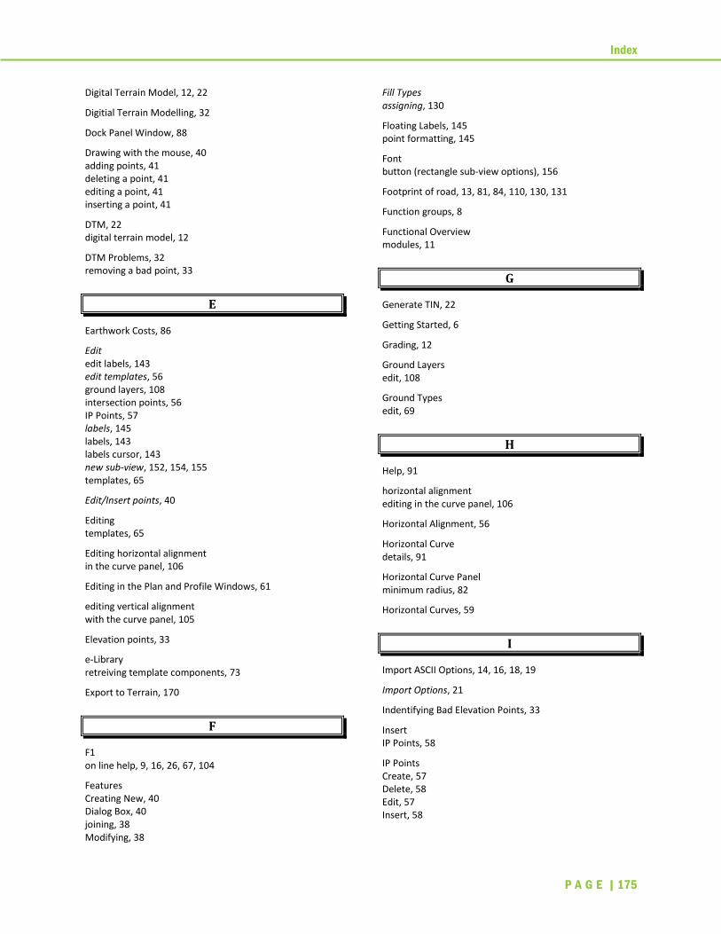
Index
P A G E | 175
Digital Terrain Model, 12, 22
Digitial Terrain Modelling, 32
Dock Panel Window, 88
Drawing with the mouse, 40 adding points, 41 deleting a point, 41 editing a point, 41 inserting a point, 41
DTM, 22 digital terrain model, 12
DTM Problems, 32 removing a bad point, 33
E
Earthwork Costs, 86
Edit edit labels, 143 edit templates, 56 ground layers, 108 intersection points, 56 IP Points, 57 labels, 145 labels, 143 labels cursor, 143 new sub-view, 152, 154, 155 templates, 65
Edit/Insert points, 40
Editing templates, 65
Editing horizontal alignment in the curve panel, 106
Editing in the Plan and Profile Windows, 61
editing vertical alignment with the curve panel, 105
Elevation points, 33
e-Library retreiving template components, 73
Export to Terrain, 170
F
F1 on line help, 9, 16, 26, 67, 104
Features Creating New, 40 Dialog Box, 40 joining, 38 Modifying, 38
Fill Types assigning, 130
Floating Labels, 145 point formatting, 145
Font button (rectangle sub-view options), 156
Footprint of road, 13, 81, 84, 110, 130, 131
Function groups, 8
Functional Overview modules, 11
G
Generate TIN, 22
Getting Started, 6
Grading, 12
Ground Layers edit, 108
Ground Types edit, 69
H
Help, 91
horizontal alignment editing in the curve panel, 106
Horizontal Alignment, 56
Horizontal Curve details, 91
Horizontal Curve Panel minimum radius, 82
Horizontal Curves, 59
I
Import ASCII Options, 14, 16, 18, 19
Import Options, 21
Indentifying Bad Elevation Points, 33
Insert IP Points, 58
IP Points Create, 57 Delete, 58 Edit, 57 Insert, 58

Index
P A G E | 176
J
Joining Features, 38
Joining points, 38, 42
L
Label edit, 145 edit point formatting dialog box, 144 option (Plan options), 140
Labels, 132
Labels class format, 132
Labels point format, 132
Labels user defined, 140
Labels edit, 143
Labels floating, 145
Limiting Triangles TIN model, 25
Location Design create short road alignment, 54 new, 54
Location Module, 13 overview, 13
locked K, 104
locked length verticasl curve, 105
M
Mass Haul Borrow, 78 Cut and fill volumes, 75 diagram, 81 Free haul, 78 free haul distance, 77 options, 77 Over haul, 78 over haul distance, 77 Waste
End Haul, 78
Materials and Stripping, 107
Menu Customization, 8
Merging multi-plot layouts, 158
Merging Terrains, 169, 172
Metric Units, 9
Modify IP button, 105
Modifying Features, 38
Module setup units, 15
Modules functional overview, 11 location, 11, 13 survey/map, 11 terrain, 11, 12 Terrain, 34, 54, 108
Multi-plot options, 153
Multi-Plot, 149 auto plan rotation, 152 creating subviews, 149
Multi-plot Output Grid options, 153 Pagination, 151 screen layouts, 158
Multi-plot Output, 149
N
New sub-view, 152
O
On, 77
On-line Help F1, 9
Optimal Haul Calculation, 80, 84, 86
Option plan, 140
Output, 149
P
Plan rotation, 157 scale, 155 window options, 140
Plan Window, 30, 89, 124, 145 moving around in, 27

Index
P A G E | 177
Point Codes display and reporting, 120, 123
Point Label Formatting, 143
Position Tab label selection and formating, 145
Q
Quick Fit Profile, 84
Quick Profile, 87
R
Red Cross current point, 27
Reporting template point codes, 123
Reporting points, 133, 140, 168
Road Class Specification, 103
Road Class Specifications, 96
Rotating the 3D Image, 30
S
Save screen layout, 90
Scale bar, 29 Sub-view, 155
Screen Layout, 55 change properties, 90 copy, 90 custom folder, 90 delete, 90 retrieve, 89, 163 save, 90 setting up, 88
Scroll Bars Turn Off, 28
Selecting or deselecting multiple sub-views, 153, 154
Selecting Features by name, 36 using the mouse, 27
Shift + arrow (scroll plan or profile sub-view), 158
Side Friction Factor definition, 95
slopes
set to Auto, 112
Smart Pits, 80, 84, 87
Smoothing contours, 24
Snap to Point Plan Window Option, 41
Softree Optimal Documentation, 80, 84
Spiral Curve transition length, 97
Stationing at fixed intervals, 135, 140
Stripping, 109
Subgrade Cut and Fill OB (overburden), 107
sub-horizons defining, 107
Sub-view adding new, 152
Super-elevation table, 94, 96
Super-elevation Runoff, 97
Super-elevation Table, 96
Survey Import ASCII, 14
Survey Notes, 11
Survey/Map Module, 11 overview, 11
T
Tangent Runout Length curves, 99
Template Codes, 119
Template Component properties, 67
Template Components, 67
Template Editor, 65
Template Surfaces, 119
Template Table, 56
templates component copy and paste, 114 components, copy and paste, 70 slopes set to Auto, 112
Templates

Index
P A G E | 178
assigning, 115 components from the e-Library, 73 creating a turning lane, 117 creating and deleting, 66 creating new, 114 display and reporting, 119 introduction, 65 parameter overrides, 117 point codes, 120, 123 properties, 66
Terrain Functions, 36
Terrain Modeling merging terrains, 172
Terrain Module, 12, 15 importing ASCII files, 14 overview, 12 setup, 15
Terrains merging, 169
TIN Model limiting triangles, 25
Toolbar Mode tools, 41 Windows Tools, 59 zoom tools, 28
Transition Fraction curves, 99
Transition length curves, 97
Triangular Irregular Network (TIN) TIN Model, 22
Tutorial files, 7
Tutorial Units setup, 9
U
User Definable Labels, 140
V
vertical alignment editing with the curve panel, 105
Vertical Alignment, 61
vertical curve locked K, 104 locked length, 105
Vertical Curve details, 103
Vertical curves, 62
Vertical Interection Points Creating. See VIPs
View plan options, 140
Volume Calculations, 12
Volume Optimization realignment design, 80
W
Wild Card, 19
Window dock panel, 88 new window/graphics
3D, 30
Wrap Text in rectangle multi-plot, 156
Z
Zooming and Panning, 27, 30 Toolbar
middle roller mouse button, 28