Risk Measures and Insurance Premium

Principles

Zinoviy Landsman

Department of Statistics,

University of Haifa

Mount Carmel, Haifa, 31905, Israel

E-mail: landsman@stat.haifa.ac.il

Michael Sherris

Faculty of Commerce and Economics,

University of New South Wales,

Sydney, NSW, Australia, 2052

Email m.sherris@unsw.edu.au

Abstract

Risk measures based on distorted probabilities have been recently

developed in actuarial science and applied to insurance rate making.

An example is the proportional hazards transform. A risk measure

should satisfy the properties of risk aversion and diversi�cation for

both insurance and asset allocation decisions. The risk measure based

on distorted probabilities is not consistent with the change of measure

used in �nancial economics for pricing. This measure is also not con-

sistent in its treatment of insurance and investment risks. We propose

a risk measure that has the properties of risk aversion and diversi-

�cation, is additive and consistent in its treatment of insurance and

investment risks.

1

1 Introduction

Models are used in actuarial science for both quantifying risks and for pricing

risks. Quantifying risk requires a risk measure to convert a random future

gain or loss into a certainty equivalent that can then be used to order dif-

ferent risks and for decision making purposes. In order to quantify risk it is

necessary to specify the probability distributions of the risks involved and to

apply a preference function to these probability distributions. Thus this pro-

cess involves both statistical assumptions and economic assumptions. The

resulting risk measure should satisfy desirable properties. These properties

include risk aversion, which is fundamental to insurance, and diversi�cation,

which is fundamental to portfolio theory and investment selection.

In order to determine a price or premium for a risk it is necessary to

convert the random future gain or loss into �nancial terms. As well as a

probability distribution for the gain or loss, a premium or pricing principle

is also required. Pricing a risk uses this premium principle to convert the

random gain or loss into a premium or price. Thus the components of a model

required to price risks are a statistical model for the risks, an economic model

for preferences and pricing or premium principles to convert risk measures

into monetary terms.

Prices or premiums must also satisfy some basic properties. The model

used should produce consistent and sensible results. These include consis-

tency with observed behavior in �nancial or insurance markets and the con-

sistent treatment of di�erent risks. It is also important to have a consistent

treatment of asset and liability (or insurance) gains and losses.

Many di�erent premium principles have been proposed in actuarial sci-

ence. Goovaerts [4] discusses various premium principles and examines var-

ious properties that these premium principles should satisfy. In �nancial

economics the principle of no-arbitrage is an important requirement for a

consistent �nancial model. Panjer et al [8] cover both equilibrium pricing

and no-arbitrage pricing in �nancial models. Wang [10] proposes a premium

principle based on a proportional transformation of the hazard function. This

premium principle corresponds to the certainty equivalent of the dual the-

ory of expected utility developed by Yaari [14]. These approaches to pricing

insurance contracts treat insurance losses as positive random variables and

produce premiums that are higher than the expected value of the insurance

loss.

2

2 Assumptions and notation

Random gains and losses, arising from insurance losses and investment deci-

sions, are denoted by the random variables Xi. For each random gain or loss,

denote the probability distribution function by Fi(x) = Pr fXi � xg and the

decumulative distribution function by F i(x) = Pr fXi > xg. The inverse ofthe decumulative distribution function is de�ned as

F�1(q) = inf

nx : F (x) � q

o; 0 � q < 1; F

�1(1) = 0

We take the perspective of an individual so that for an insurance loss Xi will

be non-positive. The pay-o� on an insurance policy in the event of a claim is

denoted by Yi, and will be non-negative. For an investment in an asset, Xi

will be bounded below for limited liability securities. Usually insurance will

cover the loss of value of an asset arising from prede�ned insurable events.

In this case an individual will usually also hold the asset and will be subject

to investment risk arising from uctuations caused by economic and other

factors. The total risk for the asset includes both economic uctuations in

value and losses from insurable events.

We assume that any model used to quantify risk and to determine prices

and premiums should have the properties that individual risk preferences

exhibit risk aversion and portfolio diversi�cation. Both of these properties

are considered essential properties for a �nancial model used for pricing and

asset allocation. Most real world �nancial decisions including the purchase

of insurance and investment decisions are consistent with risk aversion and

portfolio diversi�cation. Portfolio diversi�cation implies risk aversion for

expected utility models. However risk aversion is not su�cient to imply

portfolio diversi�cation for general preference functions (Dekel [2]).

We de�ne risk aversion and diversi�cation as follows:

De�nition 1 Risk aversion - preferences exhibit risk aversion when the ex-

pectation of a risk is preferred to the risk i.e. actuarially fair gambles are

unacceptable.

De�nition 2 Diversi�cation - preferences exhibit portfolio diversi�cation if

a convex combination of risks is preferred to any single risk, assuming all

risks are identical.

3

A preference relation � is assumed to exist over probability distributions

with the symbol � indicating strict preference and � indicating indi�erence.

For example F1 � F2 indicates that the random gain or loss X1 with proba-

bility distribution function F1 is strictly preferred to the random gain or loss

X2, with probability distribution function F2.

3 Expected Utility

An axiomatic approach to the derivation of a risk preference function for

ordering risks using expected utility was given by von Neumann and Mor-

genstern [9]. The axioms are also found in Wang and Young [12]. The key

axiom is the so-called independence axiom. This axiom states that if X � Y

and Z is any risk then

f(�;X); (1 � �;Z)g � f(�; Y ); (1 � �;Z)g

for all � such that 0 � � � 1 where f(�;X); (1 � �;Z)g is the probabilisticmixture with

Ff(�;X);(1��;Z)g(x) = �FX(x) + (1� �)FZ(x)

or equivalently

F f(�;X);(1��;Z)g(x) = �FX(x) + (1� �)FZ(x):

We can write this as

�FX(x) + (1 � �)FZ(x) � �FY (x) + (1 � �)FZ(x):

Assume that an individual has initial wealth W . From the axioms it is

possible to show that there exists a utility function u such that F1 � F2 if

and only if E [u(W +X1)] > E [u(W +X2)]. Properties and applications of

utility functions are covered in the survey paper by Gerber and Pafumi [3].

Since we assume risk aversion, u(X) is an increasing concave function

of X and is at least twice di�erentiable with u0(X) > 0 and u00(X) < 0.

Utility functions are only unique up to a positive a�ne transformation so

that u�(X) = au(X) + b will produce the same ordering of risks as would

u(X). Utility functions can be standardized by taking u(k) = 0 and u0(k) = 1

for some point k:

4

For an insurance loss Xi will be negative. If we write the loss as a positive

random variable Y = �X then E [u(X)] = E [u(�Y )] :For risk aversion, we have

E [u(X)] � u(E [X])

since u is concave, and this holds for all risks whereX is negative for insurance

losses. Alternatively we have

u�1[E [u(X)]] � E [X]

for risk aversion. For insurance losses, taking Y = �X where Y is a non-

negative random variable, this is the same as

�u�1[E [u(�Y )]] � E [Y ]

The certainty equivalent of a risk is de�ned as follows.

De�nition 3 If an individual is indi�erent between a risk and receiving an

amount with certainty then this certain amount is the certainty equivalent

for the risk.

Denote the certainty equivalent of risk X by CX. For an individual with

current wealth W we have

u(W + CX) = E [u(W +X)]

so that

CX = u�1 [E [u(W +X)]]�W

For an insurance risk, if we consider the loss amount Y = �X and �Y as

the certainty equivalent then

u(W � �Y ) = E [u(W � Y )]

or

�Y = W � u�1 [E [u(W � Y )]]

Note that

�C�Y = �Y

5

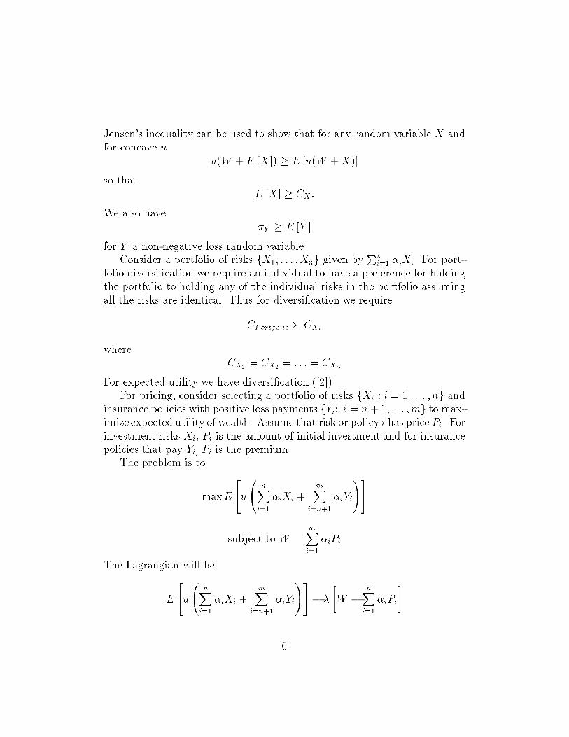
Jensen's inequality can be used to show that for any random variable X and

for concave u

u(W + E [X]) � E [u(W +X)]

so that

E [X] � CX :

We also have

�Y � E [Y ]

for Y a non-negative loss random variable.

Consider a portfolio of risks fX1; : : : ;Xng given byPn

i=1 �iXi. For port-

folio diversi�cation we require an individual to have a preference for holding

the portfolio to holding any of the individual risks in the portfolio assuming

all the risks are identical. Thus for diversi�cation we require

CPortfolio � CXi

where

CX1= CX2

= : : : = CXn

For expected utility we have diversi�cation ([2]).

For pricing, consider selecting a portfolio of risks fXi : i = 1; : : : ; ng andinsurance policies with positive loss payments fYi: i = n + 1; : : : ;mg to max-

imize expected utility of wealth. Assume that risk or policy i has price Pi. For

investment risks Xi; Pi is the amount of initial investment and for insurance

policies that pay Yi; Pi is the premium.

The problem is to

maxE

24u0@ nXi=1

�iXi +mX

i=n+1

�iYi

1A35

subject to W =mXi=1

�iPi

The Lagrangian will be

E

24u0@ nXi=1

�iXi +mX

i=n+1

�iYi

1A35� �

"W �

nXi=1

�iPi

#

6

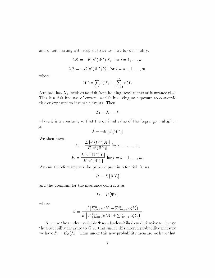
and di�erentiating with respect to �i we have for optimality,

�Pi = �E [u0 (W �)Xi] for i = 1; : : : ; n:

�Pi = �E [u0 (W �)Yi] for i = n + 1; : : : ;m:

where

W � =nXi=1

��iXi +mX

i=n+1

��iYi

Assume that X1 involves no risk from holding investments or insurance risk.

This is a risk free use of current wealth involving no exposure to economic

risk or exposure to insurable events. Then

P1 = X1 = k

where k is a constant, so that the optimal value of the Lagrange multiplier

is b� = �E [u0 (W �)]

We then have

Pi =E [u0 (W �)Xi]

E [u0 (W �)]for i = 1; : : : ; n:

Pi =E [u0 (W �) Yi]

E [u0 (W �)]for i = n+ 1; : : : ;m:

We can therefore express the price or premium for risk Xi as

Pi = E [Xi]

and the premium for the insurance contracts as

Pi = E [Yi]

where

=u0�Pn

i=1 ��

iXi +Pm

i=n+1 ��

iYi�

Ehu0�Pn

i=1 ��

iXi +Pm

i=n+1 ��

iYi�i

Now use the random variable as a Radon-Nikodym derivative to change

the probability measure to Q so that under this altered probability measure

we have Pi = EQ [Xi]. Thus under this new probability measure we have that

7

each risk is priced at its expectation so that we can refer to this Q measure

as the risk neutral measure. See also [3] for a derivation of a similar result in

the context of a Pareto optimal risk exchange.

Premiums for insurance contracts using this change of measure are ad-

ditive for all risks. Thus they will satisfy our requirement for consistent

treatment of risks.

4 Dual Utility Theory and Distortion Func-

tions

The dual theory of Yaari [14] develops an alternative to expected utility using

an axiomatic approach where the independence axiom for expected utility is

replaced with the dual independence axiom. The dual independence axiom

states that if X � Y and Z is any risk then

�F�1

X (q) + (1� �)F�1

Z (q) � �F�1

Y (q) + (1� �)F�1

Z (q)

for all � such that 0 � � � 1:

These axioms imply that there exists a continuous nondecreasing function

g, such that F1 � F2 if and only if

�Z 1

0g(q)dF

�1

1 (q) > �Z 1

0g(q)dF

�1

2 (q)

Letting q = Fi(x) we have that

�Z 1

0g(q)dF

�1

i (q) =

Z1

0g(Fi(x))dx

Yaari [14] notes that UXi=

R1

0 g(Fi(x))dx is a utility which assigns the

certainty equivalent to a random variable. Thus a decision maker would be

indi�erent between receiving UXifor certain and the risk Xi.

Wang ([10], [11]) proposes pricing insurance risks using a distortion func-

tion based on the proportional hazards transform. For an insurance risk

Y , a non-negative random variable, with decumulative distribution func-

tion F Y (x) = Pr fY > xg, Wang proposes the premium principle Hr(X) =R1

0 (Fi(x))rdx with 0 � r � 1. Hr(X) is used to calculate risk-adjusted

premiums. Note that g(x) = xr; 0 � r � 1; is a concave function.

8

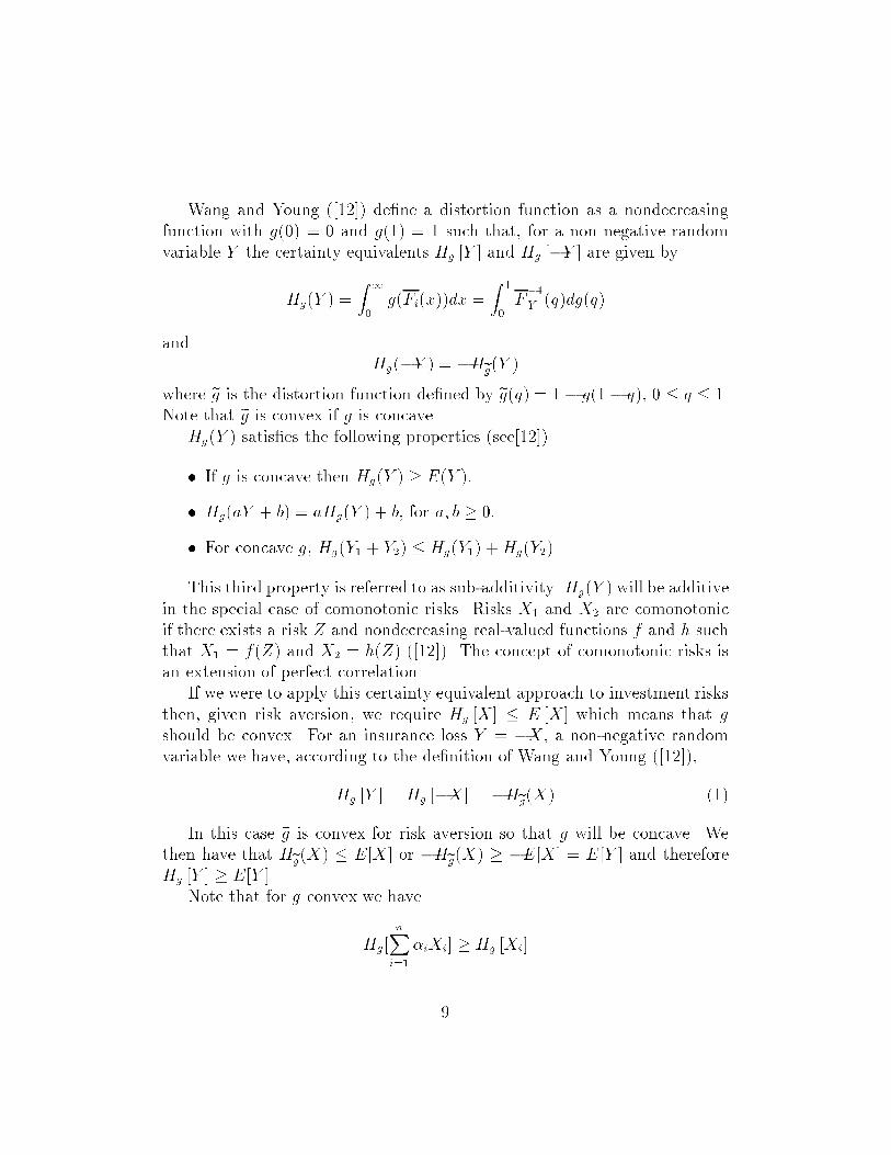
Wang and Young ([12]) de�ne a distortion function as a nondecreasing

function with g(0) = 0 and g(1) = 1 such that, for a non negative random

variable Y the certainty equivalents Hg [Y ] and Hg [�Y ] are given by

Hg(Y ) =

Z1

0g(Fi(x))dx =

Z 1

0F�1

Y (q)dg(q)

and

Hg(�Y ) = �Heg(Y )where eg is the distortion function de�ned by eg(q) = 1� g(1� q); 0 � q � 1.

Note that eg is convex if g is concave.Hg(Y ) satis�es the following properties (see[12])

� If g is concave then Hg(Y ) � E(Y ):

� Hg(aY + b) = aHg(Y ) + b; for a; b � 0:

� For concave g, Hg(Y1 + Y2) � Hg(Y1) +Hg(Y2)

This third property is referred to as sub-additivity. Hg(Y ) will be additive

in the special case of comonotonic risks. Risks X1 and X2 are comonotonic

if there exists a risk Z and nondecreasing real-valued functions f and h such

that X1 = f(Z) and X2 = h(Z) ([12]). The concept of comonotonic risks is

an extension of perfect correlation.

If we were to apply this certainty equivalent approach to investment risks

then, given risk aversion, we require Hg [X] � E [X] which means that g

should be convex. For an insurance loss Y = �X, a non-negative random

variable we have, according to the de�nition of Wang and Young ([12]),

Hg [Y ] = Hg [�X] = �Heg(X) (1)

In this case eg is convex for risk aversion so that g will be concave. We

then have that Heg(X) � E[X] or �Heg(X) � �E[X] = E[Y ] and therefore

Hg [Y ] � E[Y ].

Note that for g convex we have

Hg[nXi=1

�iXi] � Hg [Xi]

9

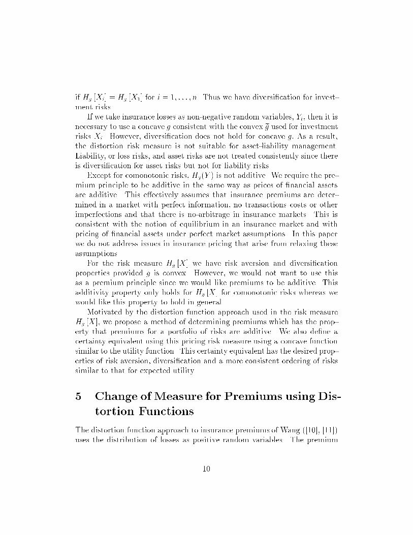
if Hg [Xi] = Hg [X1] for i = 1; : : : ; n. Thus we have diversi�cation for invest-

ment risks.

If we take insurance losses as non-negative random variables, Yi, then it is

necessary to use a concave g consistent with the convex eg used for investment

risks Xi. However, diversi�cation does not hold for concave g: As a result,

the distortion risk measure is not suitable for asset-liability management.

Liability, or loss risks, and asset risks are not treated consistently since there

is diversi�cation for asset risks but not for liability risks.

Except for comonotonic risks, Hg(Y ) is not additive. We require the pre-

mium principle to be additive in the same way as prices of �nancial assets

are additive. This e�ectively assumes that insurance premiums are deter-

mined in a market with perfect information, no transactions costs or other

imperfections and that there is no-arbitrage in insurance markets. This is

consistent with the notion of equilibrium in an insurance market and with

pricing of �nancial assets under perfect market assumptions. In this paper

we do not address issues in insurance pricing that arise from relaxing these

assumptions.

For the risk measure Hg [X] we have risk aversion and diversi�cation

properties provided g is convex. However, we would not want to use this

as a premium principle since we would like premiums to be additive. This

additivity property only holds for Hg [X] for comonotonic risks whereas we

would like this property to hold in general.

Motivated by the distortion function approach used in the risk measure

Hg [X], we propose a method of determining premiums which has the prop-

erty that premiums for a portfolio of risks are additive. We also de�ne a

certainty equivalent using this pricing risk measure using a concave function

similar to the utility function. This certainty equivalent has the desired prop-

erties of risk aversion, diversi�cation and a more consistent ordering of risks

similar to that for expected utility.

5 Change of Measure for Premiums using Dis-

tortion Functions

The distortion function approach to insurance premiums of Wang ([10], [11])

uses the distribution of losses as positive random variables. The premium

10

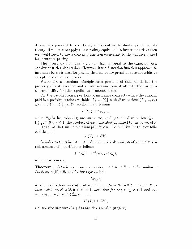
derived is equivalent to a certainty equivalent in the dual expected utility

theory. If we were to apply this certainty equivalent to investment risks then

we would need to use a convex eg function equivalent to the concave g used

for insurance pricing.

The insurance premium is greater than or equal to the expected loss,

consistent with risk aversion. However, if the distortion function approach to

insurance losses is used for pricing then insurance premiums are not additive

except for comonotonic risks.

We require a premium principle for a portfolio of risks which has the

property of risk aversion and a risk measure consistent with the use of a

concave utility function applied to insurance losses.

For the payo�s from a portfolio of insurance contracts where the amount

paid is a positive random variable fY1; :::; Yng with distributions (F1; :::; Fn)

given by Y� =Pn

i=1 �iYi. we de�ne a premium

�r(Y�) = EPn;rY�;

where Pn;r is the probability measure corresponding to the distribution Fn;r =Qni=1 F

ri ; 0 < r � 1; the product of each distribution raised to the power of r.

It is clear that such a premium principle will be additive for the portfolio

of risks and

�r(Y�) � EY�:

In order to treat investment and insurance risks consistently, we de�ne a

risk measure of a portfolio as follows

Ur(Y�) = u�1(EPn;ru(Y�));

where u is concave.

Theorem 1 Let u be a concave, increasing and twice di�erentiable nonlinear

function, u0(0) > 0, and let the expectations

EPn;rYj

be continuous functions of r at point r = 1 from the left hand side: Then

there exists an r� with 0 < r� < 1; such that for any r� � r < 1 and any

� = (�1; :::; �n); withPk

i=1 �i = 1;

Ur(Y�) � EY�;

i.e. the risk measure Ur(�) has the risk aversion property.

11

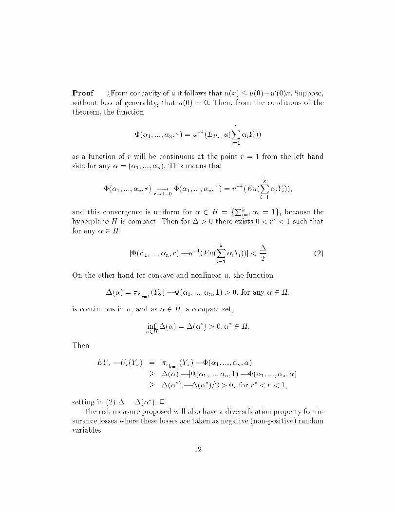
Proof. >From concavity of u it follows that u(x) � u(0)+u0(0)x: Suppose,

without loss of generality, that u(0) = 0: Then, from the conditions of the

theorem, the function

�(�1; :::; �n; r) = u�1(EPn;ru(kXi=1

�iYi))

as a function of r will be continuous at the point r = 1 from the left hand

side for any � = (�1; :::; �n): This means that

�(�1; :::; �n; r) �!r!1�0

�(�1; :::; �n; 1) = u�1(Eu(kXi=1

�iYi));

and this convergence is uniform for � 2 H = fPk

i=1 �i = 1g; because the

hyperplane H is compact. Then for � > 0 there exists 0 < r� < 1 such that

for any � 2 H

j�(�1; :::; �n; r)� u�1(Eu(kXi=1

�iYi))j <�

2(2)

On the other hand for concave and nonlinear u; the function

�(�) = �rjr=1 (Y�)� �(�1; :::; �n; 1) > 0, for any � 2 H;

is continuous in �; and as � 2 H; a compact set,

inf�2H

�(�) = �(��) > 0; �� 2 H:

Then

EY� � Ur(Y�) = �rjr=1 (Y�)� �(�1; :::; �n; �)

� �(�)� j�(�1; :::; �n; 1)� �(�1; :::; �n; �)j

� �(��)��(��)=2 > 0; for r� < r < 1;

setting in (2) � = �(��): 2

The risk measure proposed will also have a diversi�cation property for in-

surance losses where these losses are taken as negative (non-positive) random

variables.

12

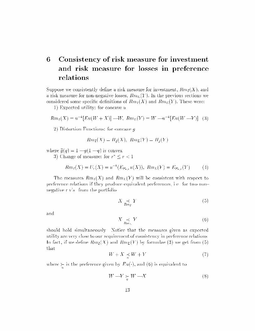
6 Consistency of risk measure for investment

and risk measure for losses in preference

relations.

Suppose we consistently de�ne a risk measure for investment, RmI(X), and

a risk measure for non-negative losses, RmL(Y ): In the previous sections we

considered some speci�c de�nitions of RmI(X) and RmL(Y ): These were:

1) Expected utility: for concave u

RmI(X) = u�1[Eu(W +X)]�W; RmL(Y ) = W � u�1[Eu(W � Y )] (3)

2) Distortion Functions: for concave g

RmI(X) = H~g(X); RmL(Y ) = Hg(Y )

where eg(q) = 1� g(1 � q) is convex.

3) Change of measure: for r� � r < 1

RmI(X) = Ur(X) = u�1(EPn;ru(X)); RmL(Y ) = EPn;r (Y ) (4)

The measures RmI(X) and RmL(Y ) will be consistent with respect to

preference relations if they produce equivalent preferences, i.e. for two non-

negative r.v's. from the portfolio

X �RmI

Y (5)

and

X �RmL

Y (6)

should hold simultaneously. Notice that the measures given as expected

utility are very close to our requirement of consistency in preference relations.

In fact, if we de�ne RmI(X) and RmL(Y ) by formulae (3) we get from (5)

that

W +X �uW + Y (7)

where �uis the preference given by Eu(�), and (6) is equivalent to

W � Y �uW �X (8)

13

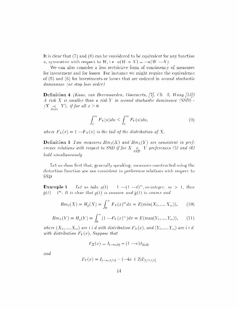
It is clear that (7) and (8) can be considered to be equivalent for any function

u; symmetric with respect to W; i.e. u(W +X) = �u(W �X).

We can also consider a less restrictive form of consistency of measures

for investment and for losses. For instance we might require the equivalence

of (5) and (6) for investments or losses that are ordered in second stochastic

dominance (or stop loss order).

De�nition 4 (Kaas, van Heerwaarden, Goovaerts, [7], Ch. 3, Wang [13])

A risk X is smaller than a risk Y in second stochastic dominance (SSD) -

(X �SSD

Y ), if for all x � 0

Z1

x

�FX(u)du �Z1

x

�FY (u)du; (9)

where �FX(x) = 1 � FX(x) is the tail of the distribution of X:

De�nition 5 Two measures RmI(X) and RmL(Y ) are consistent in pref-

erence relations with respect to SSD if for X �SSD

Y preferences (5) and (6)

hold simultaneously.

Let us show �rst that, generally speaking, measures constructed using the

distortion function are not consistent in preference relations with respect to

SSD.

Example 1 . Let us take g(t) = 1 � (1 � t)m;m-integer, m > 1; then

~g(t) = tm: It is clear that g(t) is concave and ~g(t) is convex and

RmI(X) = Hg(X) =

Z1

0

�FX(x)mdx = E(min(X1; :::;Xm)); (10)

RmL(Y ) = Hg(Y ) =

Z1

0(1� FY (x)

m)dx = E(max(Y1; :::; Ym)); (11)

where (X1; :::;Xm) are i.i.d with distribution FX(x); and (Y1; :::; Ym) are i.i.d.

with distribution FY (x): Suppose that

�FX(x) = I(�1;0) + (1� x)I[0;1];

and�FY (x) = I(�1;1=4)+ (�4x+ 2)I[1=4;1=2]

14

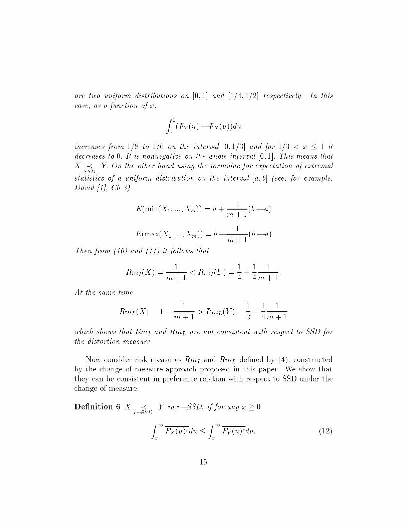
are two uniform distributions on [0; 1] and [1=4; 1=2] respectively. In this

case, as a function of x, Z 1

x( �FY (u)� �FX(u))du

increases from 1=8 to 1=6 on the interval [0; 1=3] and for 1=3 < x � 1 it

decreases to 0: It is nonnegative on the whole interval [0; 1]: This means that

X �SSD

Y: On the other hand using the formulae for expectation of extremal

statistics of a uniform distribution on the interval [a; b] (see, for example,

David [1], Ch.3)

E(min(X1; :::;Xm)) = a+1

m+ 1(b� a)

E(max(X1; :::;Xm)) = b�1

m+ 1(b� a)

Then from (10) and (11) it follows that

RmI(X) =1

m+ 1< RmI(Y ) =

1

4+1

4

1

m+ 1:

At the same time

RmL(X) = 1�1

m+ 1> RmL(Y ) =

1

2�1

4

1

m+ 1

which shows that RmI and RmL are not consistent with respect to SSD for

the distortion measure.

Now consider risk measures RmI and RmL de�ned by (4), constructed

by the change of measure approach proposed in this paper. We show that

they can be consistent in preference relation with respect to SSD under the

change of measure:

De�nition 6 X �r�SSD

Y in r�SSD, if for any x � 0

Z1

xFX(u)rdu �

Z1

xFY (u)rdu: (12)

15

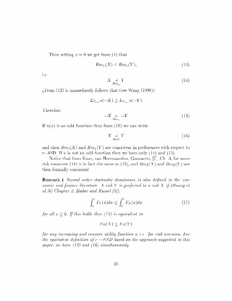
Then setting x = 0 we get from (4) that

RmL(X) � RmL(Y ); (13)

i.e

X �RmL

Y (14)

>From (12) it immediately follows that (see Wang (1998))

EPn;ru(�X) � EPn;ru(�Y )

Therefore

�X �RmI

�Y (15)

If u(x) is an odd function then from (15) we can write

X �RmI

Y (16)

and then RmI(X) and RmL(Y ) are consistent in preferences with respect to

r�SSD. If u is not an odd function then we have only (14) and (15).

Notice that from Kaas, van Heerwaarden, Goovaerts, [7], Ch. 3, for some

risk measures (14) is in fact the same as (15), and RmI(X) and RmL(Y ) are

then formally consistent.

Remark 1 Second order stochastic dominance is also de�ned in the eco-

nomic and �nance literature. A risk Y is preferred to a risk X if (Huang et

al [6] Chapter 2, Hadar and Russel [5]),Z x

0FY (u)du �

Z x

0FX(u)du (17)

for all x � 0: If this holds then (17) is equivalent to

Eu(X) � Eu(Y )

for any increasing and concave utility function u i.e. for risk aversion: For

the equivalent de�nition of r � SSD based on the approach suggested in this

paper, we have (13) and (16) simultaneously.

16

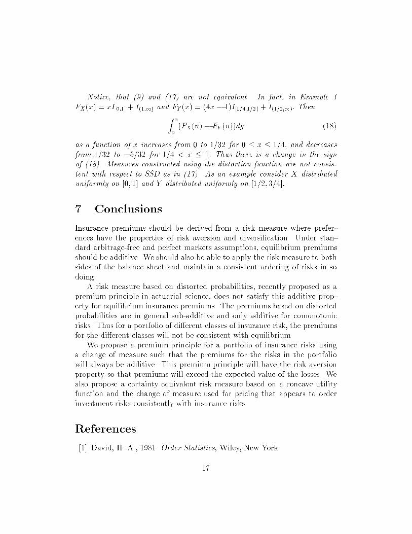
Notice, that (9) and (17) are not equivalent. In fact, in Example 1

FX(x) = xI[0;1] + I(1;1) and FY (x) = (4x� 1)I[1=4;1=2g+ I(1=2;1): ThenZ x

0(FX(u)� FY (u))dy (18)

as a function of x increases from 0 to 1=32 for 0 � x � 1=4; and decreases

from 1=32 to �5=32 for 1=4 < x � 1: Thus there is a change in the sign

of (18). Measures constructed using the distortion function are not consis-

tent with respect to SSD as in (17). As an example consider X distributed

uniformly on [0; 1] and Y distributed uniformly on [1=2; 3=4]:

7 Conclusions

Insurance premiums should be derived from a risk measure where prefer-

ences have the properties of risk aversion and diversi�cation. Under stan-

dard arbitrage-free and perfect markets assumptions, equilibrium premiums

should be additive. We should also be able to apply the risk measure to both

sides of the balance sheet and maintain a consistent ordering of risks in so

doing.

A risk measure based on distorted probabilities, recently proposed as a

premium principle in actuarial science, does not satisfy this additive prop-

erty for equilibrium insurance premiums. The premiums based on distorted

probabilities are in general sub-additive and only additive for comonotonic

risks. Thus for a portfolio of di�erent classes of insurance risk, the premiums

for the di�erent classes will not be consistent with equilibrium.

We propose a premium principle for a portfolio of insurance risks using

a change of measure such that the premiums for the risks in the portfolio

will always be additive. This premium principle will have the risk aversion

property so that premiums will exceed the expected value of the losses. We

also propose a certainty equivalent risk measure based on a concave utility

function and the change of measure used for pricing that appears to order

investment risks consistently with insurance risks.

References

[1] David, H. A., 1981. Order Statistics, Wiley, New York.

17

[2] Dekel, E., 1989, Asset Demands Without the Independence Axiom,

Econometrica, Vol 57, No 1, 163-169.

[3] Gerber, H. U., and G. Pafumi, 1998, Utility Functions: >From Risk

Theory to Finance, North American Actuarial Journal, 2 (3), 74-100.

[4] Goovaerts, M. J., F de Vlyder and J Haezendonck, 1984, Insurance

Premiums, Theory and Applications, North Holland, Amsterdam.

[5] Hadar, J. and Russel R.R., 1969, Rules for Ordering Uncertain

Prospects. American Economic Review, 59, 25-34.

[6] Huang, Chi-fu and R. H. Litzenberger, 1988, Foundations for Financial

Economics, North-Holland, New York.

[7] Kaas, R., van Heerwaarden, A.E., Goovaerts, M.J., 1994. Ordering of

Actuarial Risk. CAIRE, Brussels (Education series)

[8] Panjer, H. H. (Editor), P.P. Boyle, S. H. Cox, D. Dufresne, H. U. Ger-

ber, H. H. Mueller, H. W. Pedersen. S. R. Pliska, M. Sherris, E. S. Shiu,

K. S. Tan, 1998, Financial Economics with Applications to Investments,

Insurance and Pensions, The Actuarial Foundation, Schaumburg, Illi-

nois.

[9] von Neumann, J., and O. Morgenstern, 1944, Theory of Games and Eco-

nomic Behaviour, Princeton University Press, Princeton (3rd Edition,

1953).

[10] Wang, S. ,1995, Insurance pricing and increased limits ratemaking

by proportional hazard transforms, Insurance: Mathematics and Eco-

nomics, 17, 43-54.

[11] Wang, S. 1996, Premium Calculation by Transforming the Layer Pre-

mium Density, Astin Bulletin, 26, 71-92.

[12] Wang, S and Young, V. R., 1997, Ordering Risks: Utility Theory versus

Yaari's Dual Theory of Risk, IIPR Research Report 97-08, University of

Waterloo.

[13] Wang, S, 1998, An Actuarial index of right-tail risk, North American

Actuarial Journal, 2, (2), 88-101.

18

[14] Yaari, M. E., 1987, The Dual Theory of Choice Under Risk, Economet-

rica, 55, 95-115.

19