Risk Analysis of Organic Cropping Systems in Minnesota

Paul R. Mahoney, Kent D. Olson, Paul M. Porter, David R. Huggins, Catherine A. Perrilo, and Kent Crookston

Mahoney, Olson, and Porter are at the University of Minnesota; Huggins and Perilloare at Washington State University; and Crookston is Brigham Young University, Utah.

Abstract: When all strategies received conventional market prices, 4-year croppingsequences had greater net returns than 2-year sequences, and the organic input, 4-yearstrategy had the highest net return. Adding 50% of the estimated organic premium, the4-year, organic strategy dominated all low- and high-purchased input strategies.

Presented at the American Agricultural Economics Association Meeting

Chicago, IL August 5-8, 2001

Copyright 2001 by Mahoney, Olson, Porter, Huggins, Perillo, and Crookston. All rights reserved.Readers may make verbatim copies of this document for non-commercial purposes by any means,

provided that this copyright notice appears on all such copies.

1Mahoney, Olson, and Porter are at the University of Minnesota; Huggins and Perillo are at Washington StateUniversity; and Crookston is Brigham Young University, Utah.

1

Risk Analysis of Organic Cropping Systems in Minnesota

Paul R. Mahoney, Kent D. Olson, Paul M. Porter, David R. Huggins, Catherine A. Perrilo, and Kent Crookston1

In recent years there has been a growing interest in organic agriculture by both

consumers and producers, but the majority of Minnesota and Midwestern farmers still use

traditional, conventional practices to produce corn and soybeans in a 2-year rotation. Therefore,

this study was conducted to evaluate whether organic agriculture is less profitable and/or

involves greater risk than conventional production systems in southern Minnesota. More

specifically, this study compared three different management strategies in both 2 and 4 year

cropping sequences on land with prior management strategies similar to those used in Minnesota

and the upper Midwest. The three management strategies were high purchased inputs (HI), low

purchased inputs (LI), and organic inputs (OI). The cropping sequences were corn-soybeans and

corn- soybeans-oats-alfalfa. Data from the Variable Input Crop Management System Study

(VICM.S), established by the University of Minnesota in 1989 near Lamberton, Minnesota, was

used. Average net returns were based on actual field input operations and yields using annual

cost estimates and prices received by farmers in the area. Stochastic dominance techniques were

used to compare the risk of the net returns from the management strategies and cropping

sequences. Yield distributions were estimated using plot data from the experiment; price

distributions were based on historical data from the same time period.

Previous studies have analyzed the relative profitability, sustainability, and yields of

alternative or organic farming practices, and have shown that generally alternative and organic

2

systems can be as, or more profitable than, conventional systems. (Chase and Duffy, 1991;

Dabbert and Madden, 1986; Diebel et al., 1995; Hanson et al., 1997; Helmers et al., 1986;

Lockeretz et al., 1978; Posner et al., 1995; Shearer et al., 1981; Smolik and Dobbs, 1991; Smolik

et al., 1995). However, the research also found that the alternative systems were not necessarily

without potential pitfalls and not necessarily for every farmer and farm site. In his recent review

of the research of the economics of organic production, Welsh (1999) found that “the price

premiums paid for organic products, although they increase profitability, are not always

necessary for organic systems to be competitive with or outperform conventional systems” (p.

40). However, Welsh adds, “growing organic grains and soybeans in a longer rotation may not

always be the most profitable [Welsh’s italics] alternative for farmers” (p.40).

The studies mentioned above primarily focus their economic evaluation of alternative

systems on profitability of respective alternative systems in comparison to a conventional

system. In a literature review of 58 recent studies comparing alternative crop production

strategies, Roberts and Swinton (1996) mention profitability as the primary method of evaluation

in economic comparisons. They also suggest that comparisons that ignore risk and use

profitability as the single measure of evaluation are insufficient, since income stability over time

is also an important economic measure.

STUDY LOCATION AND DESIGN

The Variable Input Crop Management Study is situated at the University of Minnesota's

Southwest Research and Outreach Center (SWROC) near Lamberton, about 150 miles southwest

of Minneapolis-St. Paul. The study was started in the 1989 crop year. The research plots are on

dark colored Mollisol soils developed from calcareous glacial till. This paper analyzes the results

from the VICMS II site that has been cropped according to University recommendations since

3

1959, resulting in high soil fertility levels and low weed populations. Since the common soil

condition in this part of Minnesota is high fertility and low weed pressure, results from VICMS

II are important for producers interested in the transition from conventional practices to low-

purchased inputs or organic practices.

A companion research site, VICMS I, is located on land which, prior to the Center acquiring

the land in 1988, had a history of minimum inputs. No insecticides had been used on this land,

herbicide use was very minimal, and neither commercial nor natural fertilizers had been applied.

Consequently, weed pressure was high and soil test levels were very low. So, even though the same

treatments were used, the data from VICMS I were not used in this paper since the soil conditions

for VICMS I are not very similar to those commonly found in southwest Minnesota.

This research focuses on the VICMS II site and the three management strategies and two

cropping sequences most relevant to current farmers. The three management strategies are

described below.

1. Low-Purchased Inputs (LI): Chemical applications were minimized by banding of

fertilizers, banding of post-emergent herbicides (if needed), utilization of

mechanical weed control, use of insecticides only if prescribed, and similar

practices. A realistic yield goal was used to determine fertilizer rates. The yield

goal is based on soil type, water availability, growing season length, and past

maximum yield produced. The yield goal was “realistic” in that it was based on

actual recorded yields in the past, not an optimistic view of the soils potential.

2. High Purchased Inputs (HI): Chemical applications were not necessarily minimized.

Broadcast (no banding) fertilizers and insecticides were used according to

University recommendations. Pre-emergent herbicides were often used. Other

2 In the area of Minnesota where the research station is located, crop production began in the 1870s with wheatgrown almost exclusively. From the 1900s until the 1960s, corn, small grains, and pasture predominated. Since the1960s, this region has been farmed almost exclusively with corn and soybean. Currently, corn and soybean aregrown on more than 90% of the cropped land in Southwest Minnesota (Minnesota Agricultural Statistics Service,1996).

4

practices are selected on the basis of what is considered the best conventional

practices for this region. An optimistic yield goal was used to determine fertilizer

rates. Once again the yield goal was “realistic” in that it was based on actual

recorded yields in the past, not an optimistic view of the soils potential

3. Organic Inputs (OI): No synthetic chemical applications were allowed. Organic

sources of nutrients, such as manure, and mechanical weed control were utilized.

This strategy incorporates the best organic practices for the region so the crops

grown could be certified as organically produced. Data was collected from the 1st

year of the transition to organic certification standards. Potential premiums are

not applied until certification was possible under the Minnesota organic

certification standards (i.e. the third crop). Note, however, rotation restrictions do

not allow the certification of a 2-year corn-soybean rotation as organically

produced.

The organic practices followed in the agronomic part of this study are based on the

Minnesota organic certification standards that were in place prior to the final rules set by the

USDA’s National Organic Project (NOP). Although the Minnesota standards followed in the

study were in place prior to the national standards, all practices outlined above in the NOP

organic crop production standards were met.

These three strategies are carried out in two cropping sequences: the popular two-year

sequence2 (corn-soybean) and a four-year sequence (corn-soybean-oat/alfalfa-alfalfa). Every

5

crop was grown every year under each strategy, so all treatments were present each year. Each

treatment was replicated three times.

DATA COLLECTED AND ANALYSIS METHODS

Detailed records have been maintained on field operations, labor used, rainfall, plant

growth, weed counts (broadleaf and grasses separately), earthworm species and counts,

mycorrhiza in the soil and plants, and crop yield (including oat straw yield). Soil P and K

fertility levels were determined in the fall, and soil nitrate levels were determined in one-foot

increments to 5 deep feet following alfalfa and soybeans.

For each management strategy, cropping sequence, and year, net returns were calculated

as: NRijt = Σk wjk{Po*Pkt* Yijkt - Cijkt} (1)

where NRijt = net return to land, management, indirect labor, and other indirect costs per

acre for the ith management strategy and jth cropping sequence in the tth year; wjk = the proportion

of the kth crop in the jth cropping sequence; Po = potential organic premium expressed as a ratio to

the conventional price; Pkt = price of the kth crop in the tth year; Yijkt = average yield per acre of

the kth crop in the ith management strategy, jth cropping sequence, and tth year; and Cijkt = direct

production costs per acre for the kth crop in the ith management strategy, jth cropping sequence,

and tth year. The value of corn, soybean, oat, oat straw, and alfalfa is included in the net return

for the 4-year sequence and corn and soybean for the 2-year sequence.

Crop prices were the typical cash prices received at harvest time in each year by the

members of the Southwestern Minnesota Farm Business Management Association (Table 1)

(various years, e.g., Olson et al., 1992). Crop yields in each year were the average of the three

replications for each management strategy and cropping sequence within VICMS.

6

Production costs were estimated for each year using the actual cultural operations and

equipment used, as listed in the field records. Total crop production costs are the sum of tillage,

planting, fertilizer, pest control, and harvesting costs. The cost of each operation was calculated

using University of Minnesota Extension Service’s estimates of machinery costs which include

fuel, maintenance, repairs, operator labor and overhead costs (various years, e.g., Fuller et al.,

1992). Market prices were used for inputs except for herbicides. Seed prices were taken from

Southwestern Minnesota Farm Business Management Association records (various years, e.g.,

Olson et al., 1992), and herbicide prices were taken from University of Minnesota Extension

Service’s weed control report (various years, e.g., Durgan et al., 1992).

Producers growing crops under the OI system can potentially receive organic premiums

after becoming certified organic producers. Due to insufficient information for Minnesota,

organic price premiums for corn, soybeans, and oats listed in Table 2 were estimated using

Dobbs and Pourier’s (1999) information on organic price quotes and the conventional U.S. cash

prices for 1995-1998. Over these four years, the average organic price premium ratio (compared

to the U.S. cash price) was 1.60 for corn, 2.36 for soybeans, and 1.63 for oats. Note that,

although organic price ratios were given in South Dakota cash prices (which may be similar to

Minnesota cash prices) in addition to U.S. cash prices, the U.S. cash price ratios were used for

several reasons. First, the organic prices Dobbs and Pourier used in their calculations of the

ratios are those reported for the U.S. as a whole, and therefore the U.S. cash price ratios were

used. Second, the U.S. cash price ratios were smaller, and thus a more conservative estimate of

organic crop price premiums. These average ratios were used for all years and crops considered

to be potentially certified as organic. Due to insufficient data, no price premium was considered

for either organic alfalfa or organic oat straw.

7

To be certified organic, the land on which organic crops are grown, must, among other

rules, be free of restricted chemical inputs for at least 36 months. After certification, producers

are allowed to market their commodities as certified organic. This is generally in the third year

after switching to organic methods. Because it would not meet current organic certification

standards concerning crop sequences, organic premiums were not applied to the products from

the 2-year organic management strategy.

Potential organic premiums vary from year to year and are also dependent on each

individual producer's marketing strategies or abilities. To reflect this variability, three price

scenarios were used. In the first scenario, every crop in every management strategy received the

conventional market price. Organic products did not receive any premiums in this scenario. This

scenario reflects the possibility of a large supply of organic production relative to the demand for

organic production. This first scenario can also be useful for those skeptical of being able to

obtain any premium. In the second scenario, organic products in the 4-year organic management

strategy received 100% of the estimated organic premiums starting in the third year after the

required transition period. In the third scenario, organic products in the 4-year organic

management strategy received 50% of the estimated organic premium (or, conversely, 50% of

the organic products received the estimated organic premium) after the transition period. In the

last two scenarios, organic premiums were not applied in the first two years of production, but

were applied in the third and following years to simulate the transition a conventional farmer

would have to go through to sell organically produced crops as certified organic. In all three

price scenarios, the 2-year organic management strategy and non-organic products from the HI

and LI strategies received conventional market prices.

8

The net return calculated in equation (1) was the net return to the farmer’s land,

management, all labor (other than operator labor included in machinery costs), and other costs.

The cost of land was not subtracted because it was highly variable between farms and would be

the same for every management strategy and cropping sequence. Also, the costs of the farmer’s

management, labor (other than operator labor included in machinery costs), and other costs such

as farm insurance, interest, marketing, and general farm expenses were not subtracted for the

same reasons. While it can provide a very good estimate of the relative profitability of each

strategy and cropping sequence, the estimated net return does not account for the potential

differences in labor and management potentially required in different management strategies.

For example, the organic alternative may require more scouting, prospective market searching,

selling time, etc.; collection of this information was not part of the VICMS study, and thus is not

included in the calculation of ANR.

To measure risk, the cumulative distribution functions (CDFs) of ANRs were calculated

based on the yields, market prices, input costs, potential organic premiums, correlations between

crop yields, and correlations between crop yield and market price. The CDFs were calculated

using a program called Crystal Ball © (CB) which is an add-in program that functions within

Microsoft’s Excel ©. Crystal Ball forecasts the entire range of results for a given situation based

on data the user puts into the program. In the case of this study CB develops a probability

distribution of net returns based on the averages and distributions of yields and market prices,

average input costs, average potential organic premiums, correlations between crop yields, and

correlations between crop yields and market prices.

Using equation (1), CDFs of ANRs were calculated for all management strategies and

cropping sequences. To simulate the probability of a given outcome of crop yield and prices,

9

probability distributions were assigned to each individual crop with in each strategy and

sequence, along with the respective market price for each crop. The distribution assigned to

each individual crop within each strategy and sequence was based on actual recorded yield data

with the Kolmogrov-Smirnov (K-S) test used to determine the best fitting distribution (Ostle and

Mensing, 1975, p.489-490). Eleven distributions (Normal, Lognormal, Weibull, Triangular,

Uniform, Beta, Exponential, Gamma, Logistic, Pareto, and Extreme Value) were considered

when using the best fit option of CB to determine which distribution best fits the actual recorded

data. The CB best-fit option ranks all the distributions from one (being the best) to eleven (being

the worst) based on the recorded yield data. Each top ranked best fitting distribution were also

visually compared to the distribution of the actual yields, as were the second and third ranked

best fitting distribution to compare visually the goodness-of-fit of the top three distributions. For

crop yield, 30 yield observations (3 reps/crop for 10 years) from each crop were used in fitting

the distributions. With the exact same methods used in the distribution fitting of yields, 10 years

of crop prices (Table 1), from 1990 through 1999, were also assigned distributions.

The total input cost of each crop in the risk analysis of the study was assumed a constant

based on the actual historical 10-year average of input costs. Average projected costs were used

since historical input prices, actual yields, and field operations were used in the calculation of the

yearly input costs. By using the10-year average of input costs, it more accurately reflects the

relationships and actual decisions made historically. Input costs in this part of the analysis were

held constant because this is most likely the way individual farmers would represent their own

costs in a similar forecasting or budgeting scenario. Potential organic premiums (i.e. ratios of

organic prices to U.S. cash prices) (Table 2) were also considered constants due to the lack of

adequate data to estimate a sound distribution based on the historical data.

10

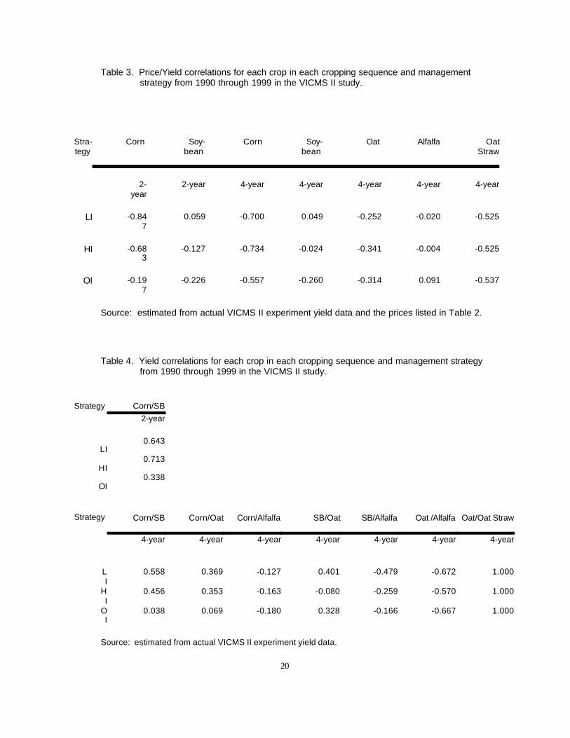
Correlations between crop yield and price were calculated using actual crop yields and

their respective crop prices (Table 3). Correlations between crops were also calculated using the

actual recorded crop yields from the VICMS II data correlating the corn yield to other crops in

the sequence (i.e. soybeans in the 2-year sequence and soybeans, oats, and alfalfa in the 4-year

sequence; Table 4).

Using the assigned distributions of crop yields and crop market prices, CB calculated 500

different possible random draw combinations of crop yields and prices. Using these 500

possible outcomes of yield and price, in addition to input costs, potential organic premiums, and

correlations, 500 possible outcomes of ANR for each input strategy and cropping sequence were

also calculated. The 500 estimated ANRs for each cropping sequence and input strategy are then

used to develop their respective CDFs.

Since risk preferences among individual farmers are difficult to measure, first-degree

stochastic dominance (FSD) and second-degree stochastic dominance (SSD) are used in the

analysis. The methods outlined below follow those described by Hardaker et al. (1997,p.138-

153).

First-degree stochastic dominance assumes the decision-maker always has a positive

marginal utility (i.e., more is preferred to less) for the performance measure being analyzed (i.e.,

ANR for this study). Using this method, the cumulative distribution function (CDF) of the

outcomes (e.g., ANR) of different decisions or actions (e.g., input strategies) can be compared to

measure risk between input strategies. The measurement of risk is based on the distributions of

net returns for the different input strategies, and the strategy with the least risk (under FSD) is

the one with the highest ANR at each probability point. In other words the strategy that lies

strictly below and to the right of all others. For example, if two input strategies FA(x) and FB(x)

11

are considered, and if the cumulative distribution of FA(x)≤ FB(x) for all x, with the inequality

holding for at least one outcome level, then FA(x) is preferred over FB(x), under FSD.

Graphically, if the CDF of FA(x) is strictly below and to the right of the CDF of FB(x), A is said

to be dominant over B by FSD. If the two cross at any point, neither is said to be dominant by

FSD, and SSD can be used to compare the riskiness of the alternatives.

Since several of the CDFs of the outcomes from the VICMS II data do cross, SSD

was also used in the risk analysis. SSD has a higher discriminatory power than FSD because of

an additional restriction on the utility function, which is that the decision maker must be risk

adverse for all values of x. Thus, the decision maker will have a utility function with positive

but decreasing marginal utility. Graphically under SSD, the simplest way to evaluate the

distributions of two different outcomes of input strategies is to compare the areas under the two

individual CDFs. The distribution with the smallest total area under the CDF is said to be

dominant by SSD if the CDF of the distribution with the smaller total area does not lie to the left

of the alternative (larger total area) distribution(s) at low probability levels.

The methods of FSD and SSD may not be able to determine the input strategy and

cropping sequence with the least risk, but these methods can determine which strategies may be

preferred by reducing the efficient set, and thus, narrow down the number of decision choices

between strategies. By reducing the choices to an efficient set of strategies, individual producers

may be able use this information in their decision making process when considering the

conversion to an organic production system.

12

RESULTS

Since they encompassed the production practices commonly used by farmers in

southwest Minnesota, the HI and LI management strategies were used as benchmarks to evaluate

the results from the OI strategy. Also, since it is so dominant in Southwestern Minnesota, the 2-

year cropping sequence was used as the benchmark to compare the results from the 4-year

sequence. Discussed below are: 1) crop yields and production costs by management strategy, 2)

net returns under the three price scenarios, and 3) risk under the same three price scenarios.

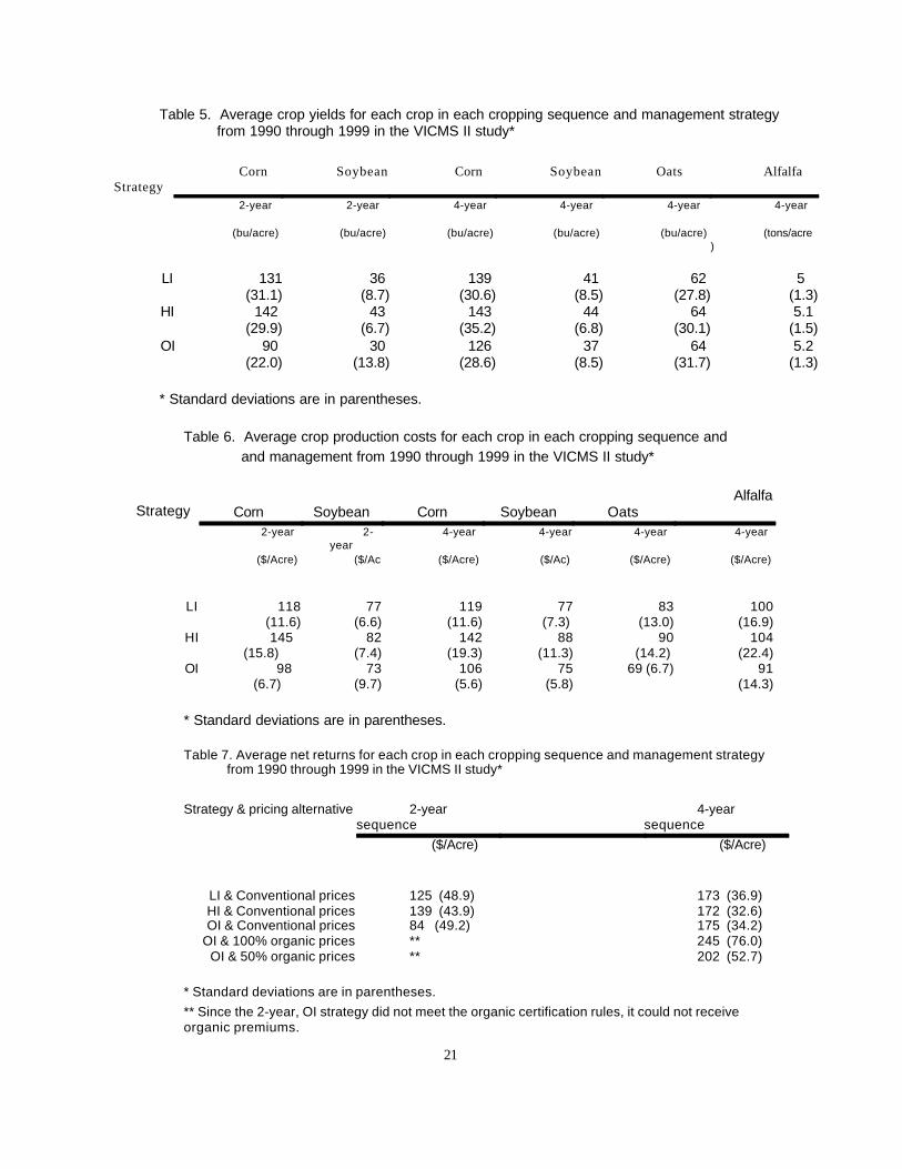
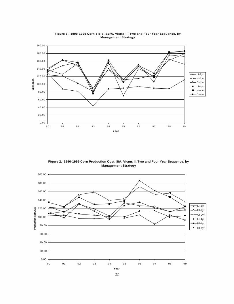
Crop Yields. Across 10 years (1990 through 1999) of the VICMS II study, the HI

strategy under the 4-year sequence had both the highest average corn yield (143 bu/acre) and the

highest average soybean yield (44 bu/acre; Table 5). However, the HI yields were not higher

than the yields in the other strategies in every year. For example, corn yields for the LI-2-year,

LI-4-year, and HI-4-year strategies were higher than the HI-2-year corn yield in several years but

were lower in others (Figure 1). The soybean yields for the 4-year sequence were typically

higher than yields in the 2-year sequence. The OI strategy had a slightly higher alfalfa yield,

while the oat yield for the OI and HI were equal across the 10 year period. Comparing the

different input strategies for oat and alfalfa shows the yields of all input strategies for both crops

were very similar in all the years. In almost every year, the 2-year sequence with either the LI or

“OI” management strategy had the lowest corn and soybean yields. Under current rules, the 2-

year crop sequence could not be certified as organic even though the production practices follow

the organic guidelines. However, since the corn-soybean sequence is so dominant in

Southwestern Minnesota, the 2-year organic strategy results are reported for comparison to the

non-organic practices. For all crops, the impact of annual weather patterns was easily observed,

as yield,s tended to move together regardless of cropping sequence and management strategy.

13

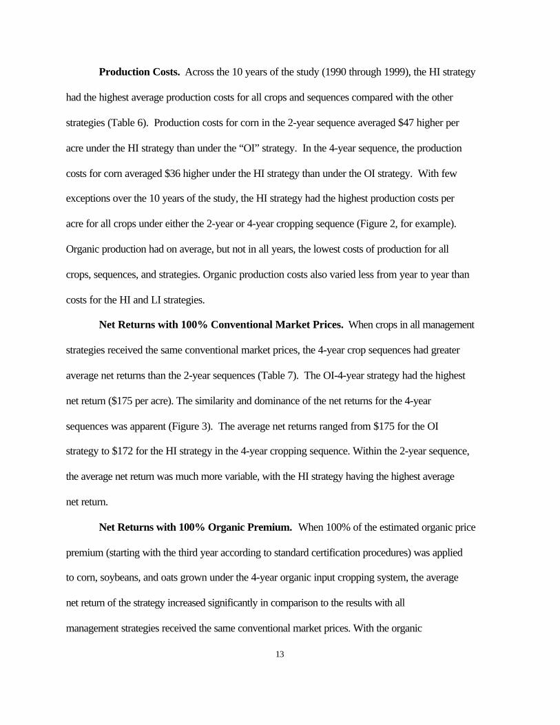
Production Costs. Across the 10 years of the study (1990 through 1999), the HI strategy

had the highest average production costs for all crops and sequences compared with the other

strategies (Table 6). Production costs for corn in the 2-year sequence averaged $47 higher per

acre under the HI strategy than under the “OI” strategy. In the 4-year sequence, the production

costs for corn averaged $36 higher under the HI strategy than under the OI strategy. With few

exceptions over the 10 years of the study, the HI strategy had the highest production costs per

acre for all crops under either the 2-year or 4-year cropping sequence (Figure 2, for example).

Organic production had on average, but not in all years, the lowest costs of production for all

crops, sequences, and strategies. Organic production costs also varied less from year to year than

costs for the HI and LI strategies.

Net Returns with 100% Conventional Market Prices. When crops in all management

strategies received the same conventional market prices, the 4-year crop sequences had greater

average net returns than the 2-year sequences (Table 7). The OI-4-year strategy had the highest

net return ($175 per acre). The similarity and dominance of the net returns for the 4-year

sequences was apparent (Figure 3). The average net returns ranged from $175 for the OI

strategy to $172 for the HI strategy in the 4-year cropping sequence. Within the 2-year sequence,

the average net return was much more variable, with the HI strategy having the highest average

net return.

Net Returns with 100% Organic Premium. When 100% of the estimated organic price

premium (starting with the third year according to standard certification procedures) was applied

to corn, soybeans, and oats grown under the 4-year organic input cropping system, the average

net return of the strategy increased significantly in comparison to the results with all

management strategies received the same conventional market prices. With the organic

14

premium, the average net return for the 4-year, OI strategy increased to $245 per acre (from

$175 using conventional prices) which was $106 more per acre than the 2-year, HI strategy and

$73 more than the 4-year, HI strategy.

Net Returns with 50% Organic Premium. If 50% of the estimated organic premium

was received (or only half of the production received the premium), the 4-year, OI strategy still

had a higher average net return ($202 per acre) than all other management strategies and crop

sequences (Table 7). The impact of this smaller organic premium was still very evident when it

starts in the third year of production (Figure 4).

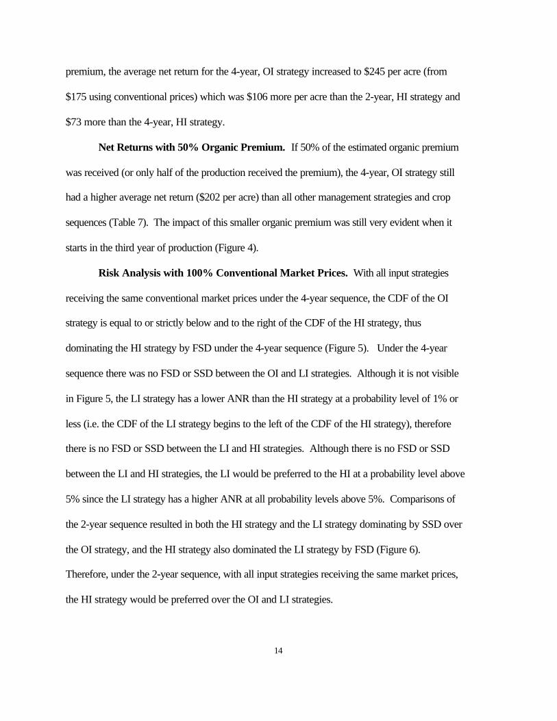
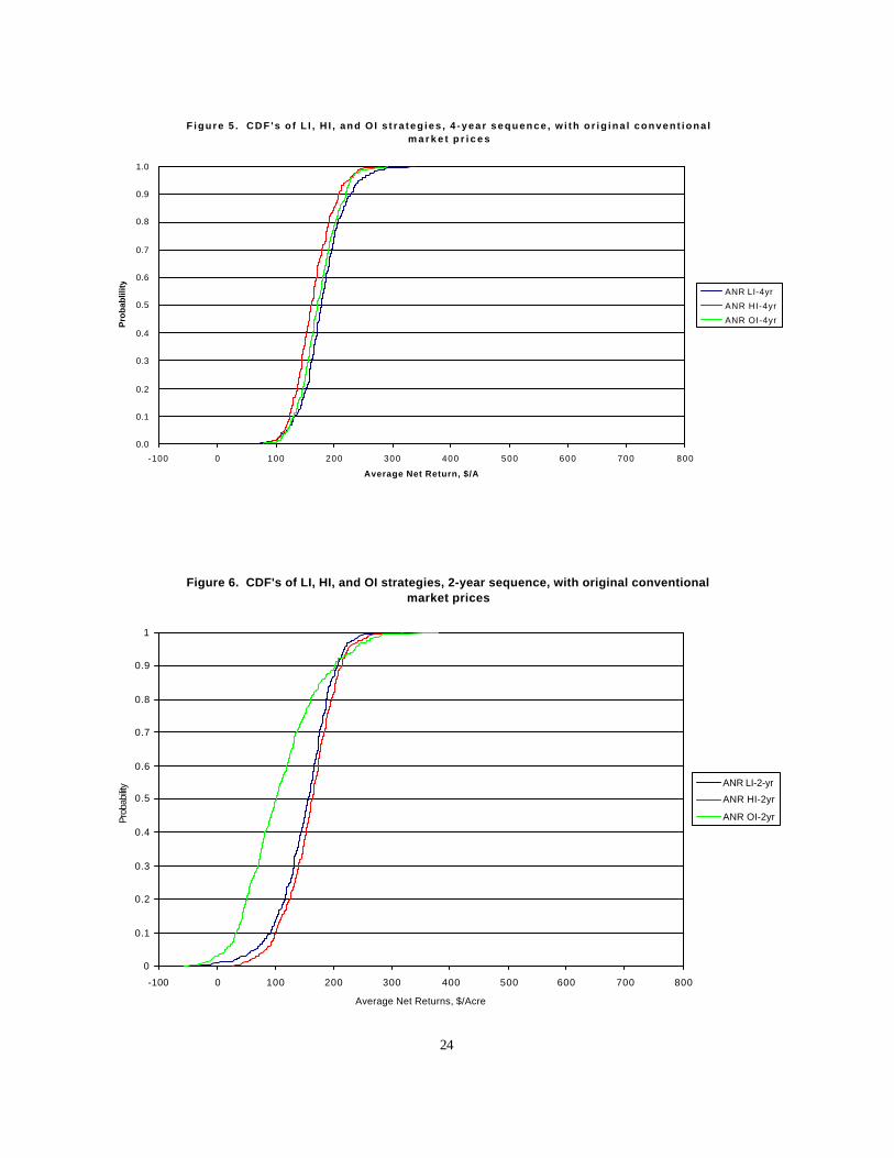
Risk Analysis with 100% Conventional Market Prices. With all input strategies

receiving the same conventional market prices under the 4-year sequence, the CDF of the OI

strategy is equal to or strictly below and to the right of the CDF of the HI strategy, thus

dominating the HI strategy by FSD under the 4-year sequence (Figure 5). Under the 4-year

sequence there was no FSD or SSD between the OI and LI strategies. Although it is not visible

in Figure 5, the LI strategy has a lower ANR than the HI strategy at a probability level of 1% or

less (i.e. the CDF of the LI strategy begins to the left of the CDF of the HI strategy), therefore

there is no FSD or SSD between the LI and HI strategies. Although there is no FSD or SSD

between the LI and HI strategies, the LI would be preferred to the HI at a probability level above

5% since the LI strategy has a higher ANR at all probability levels above 5%. Comparisons of

the 2-year sequence resulted in both the HI strategy and the LI strategy dominating by SSD over

the OI strategy, and the HI strategy also dominated the LI strategy by FSD (Figure 6).

Therefore, under the 2-year sequence, with all input strategies receiving the same market prices,

the HI strategy would be preferred over the OI and LI strategies.

15

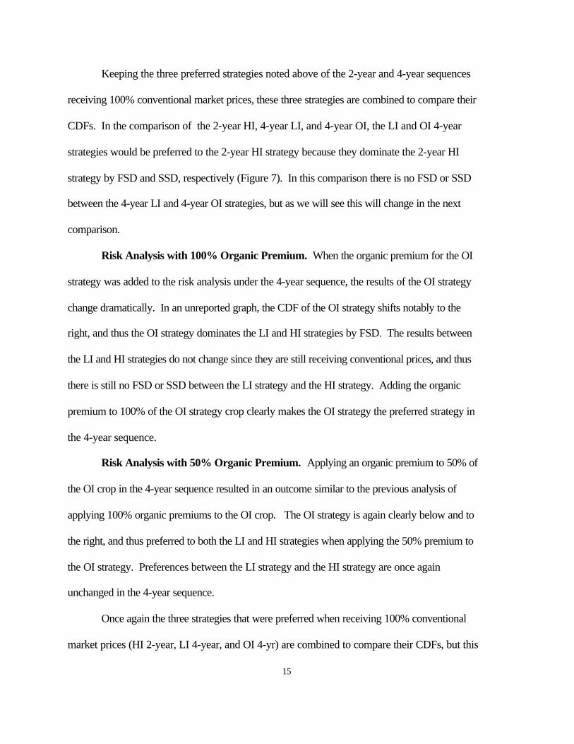
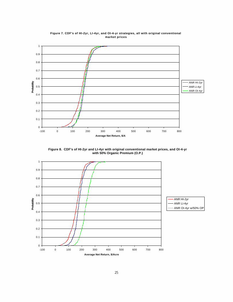
Keeping the three preferred strategies noted above of the 2-year and 4-year sequences

receiving 100% conventional market prices, these three strategies are combined to compare their

CDFs. In the comparison of the 2-year HI, 4-year LI, and 4-year OI, the LI and OI 4-year

strategies would be preferred to the 2-year HI strategy because they dominate the 2-year HI

strategy by FSD and SSD, respectively (Figure 7). In this comparison there is no FSD or SSD

between the 4-year LI and 4-year OI strategies, but as we will see this will change in the next

comparison.

Risk Analysis with 100% Organic Premium. When the organic premium for the OI

strategy was added to the risk analysis under the 4-year sequence, the results of the OI strategy

change dramatically. In an unreported graph, the CDF of the OI strategy shifts notably to the

right, and thus the OI strategy dominates the LI and HI strategies by FSD. The results between

the LI and HI strategies do not change since they are still receiving conventional prices, and thus

there is still no FSD or SSD between the LI strategy and the HI strategy. Adding the organic

premium to 100% of the OI strategy crop clearly makes the OI strategy the preferred strategy in

the 4-year sequence.

Risk Analysis with 50% Organic Premium. Applying an organic premium to 50% of

the OI crop in the 4-year sequence resulted in an outcome similar to the previous analysis of

applying 100% organic premiums to the OI crop. The OI strategy is again clearly below and to

the right, and thus preferred to both the LI and HI strategies when applying the 50% premium to

the OI strategy. Preferences between the LI strategy and the HI strategy are once again

unchanged in the 4-year sequence.

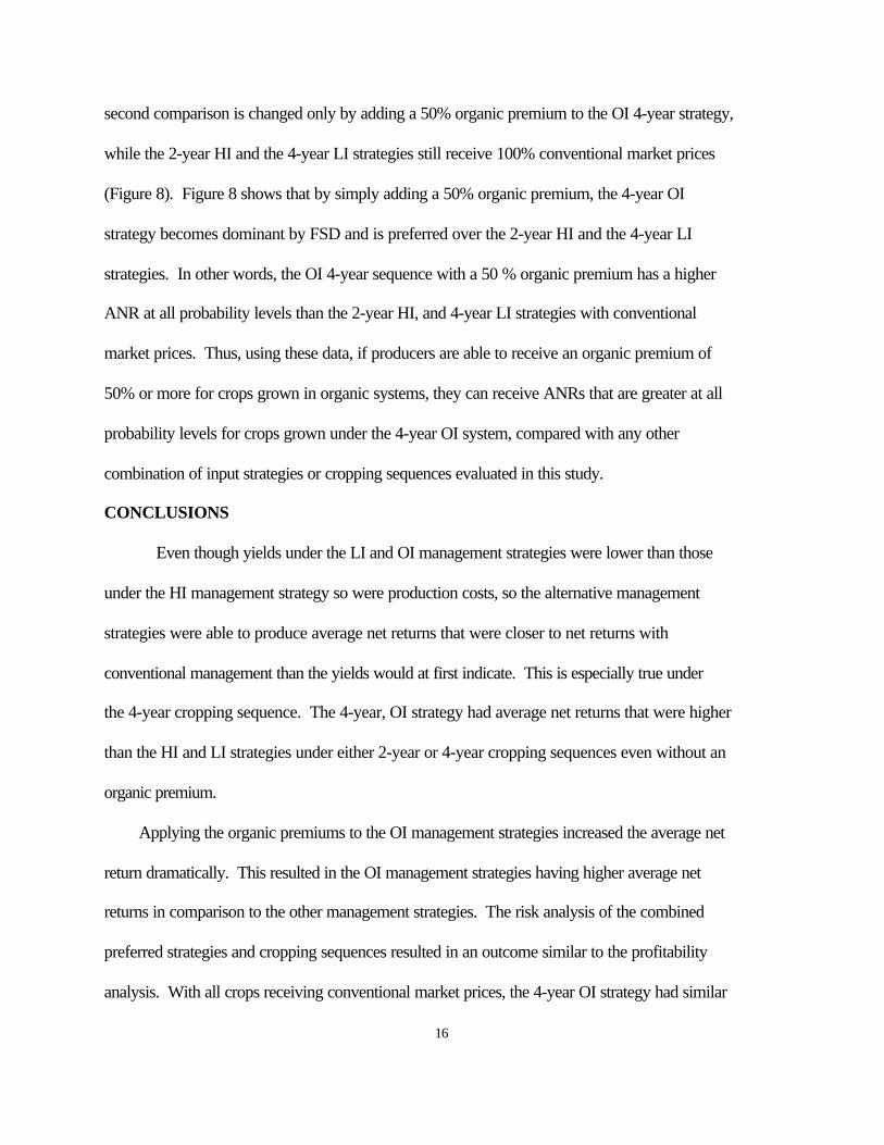
Once again the three strategies that were preferred when receiving 100% conventional

market prices (HI 2-year, LI 4-year, and OI 4-yr) are combined to compare their CDFs, but this

16

second comparison is changed only by adding a 50% organic premium to the OI 4-year strategy,

while the 2-year HI and the 4-year LI strategies still receive 100% conventional market prices

(Figure 8). Figure 8 shows that by simply adding a 50% organic premium, the 4-year OI

strategy becomes dominant by FSD and is preferred over the 2-year HI and the 4-year LI

strategies. In other words, the OI 4-year sequence with a 50 % organic premium has a higher

ANR at all probability levels than the 2-year HI, and 4-year LI strategies with conventional

market prices. Thus, using these data, if producers are able to receive an organic premium of

50% or more for crops grown in organic systems, they can receive ANRs that are greater at all

probability levels for crops grown under the 4-year OI system, compared with any other

combination of input strategies or cropping sequences evaluated in this study.

CONCLUSIONS

Even though yields under the LI and OI management strategies were lower than those

under the HI management strategy so were production costs, so the alternative management

strategies were able to produce average net returns that were closer to net returns with

conventional management than the yields would at first indicate. This is especially true under

the 4-year cropping sequence. The 4-year, OI strategy had average net returns that were higher

than the HI and LI strategies under either 2-year or 4-year cropping sequences even without an

organic premium.

Applying the organic premiums to the OI management strategies increased the average net

return dramatically. This resulted in the OI management strategies having higher average net

returns in comparison to the other management strategies. The risk analysis of the combined

preferred strategies and cropping sequences resulted in an outcome similar to the profitability

analysis. With all crops receiving conventional market prices, the 4-year OI strategy had similar

17

if not greater ANRs at all probability levels when comparing it to the HI and LI strategies under

either 2-year or 4-year cropping sequences. By simply adding a 50% premium to the 4-year OI

strategy, it clearly becomes the preferred input strategy and cropping sequence.

Thus, using the data in this study, if producers are able to receive an organic premium of

50% or more, ANRs are greater at all probability levels for crops grown under a 4-year OI

system compared to other combinations of input strategies or cropping sequences. Therefore,

based the conditions of this study and on the resulting profitability and risk analysis, the

perception that organic agriculture is less profitable and/or involves greater risk, is not true.

Results of this study show that organic and alternative systems can compete with

conventional systems, but three issues need mentioning. First, the OI strategies seem to

encountering weed control problems. Unless this can be corrected, the subsequent yield loss will

decrease profitability of the OI strategies.

The second is the potential market impact of a large shift to other crops if farmers

switched from the dominant corn-soybean cropping sequence by adding other crops. For

example, Minnesota farmers harvested 6.6 million harvested acres of corn for grain in Minnesota

and 6.9 million acres of soybeans in 1999 (Minnesota Agricultural Statistics Service, 2000).

These acreages overshadow the 0.3 million harvested acres of oats and 1.6 million harvested

acres of alfalfa hay. Any significant shift away from the popular corn-soybean sequence will

have large price impacts on other markets as well as on the corn and soybean markets

themselves. That is, if farmers shifted even a relatively small portion of their current corn and

soybean acreage to oats, the increase in oat production would have a tremendous negative effect

on the oat price and thus oat revenue. A similar negative impact would occur for alfalfa.

Conversely, any shift away from corn and soybean production will increase the prices for those

18

products under current demand conditions. Thus, any significant shift in the mix of crop

acreages will change the potential net returns of both the 4-year and 2-year cropping sequence

under any of the three management strategies. The shift to longer cropping sequences will be

possible only to the extent the oat and alfalfa markets can adjust to larger volumes and the corn

and soybean markets can adjust to reduced volumes.

A third concern or hurdle is the potential impact on the organic markets. Even though

organic markets are growing, they are small relative to the whole market, and thus a sudden

increase in the production of organic products will have a very large negative impact on the

potential organic price premium and farm income. Any shift to organic production will have to

be matched by an increase in the organic market demand in order for current expectations of

farm income to be realized.

In summary, many farmers may be considering organic agriculture for its food and

environmental safety attributes, but organic systems must also be profitable and involve

comparable risk to conventional systems for full consideration to occur. Profitability and risk

criteria have been proven through the current research reported in this paper, other published

research, and presence of actual organic producers making their livelihood from organic

production. Farmers considering converting to organic systems must also consider their

individual situations and take other factors (such as soil conditions, machinery needs, labor

needs, crop rotations, production and marketing knowledge and expertise, potential organic

premiums and or market price fluctuations, organic certification requirements, and many other

personal factors) into consideration before converting to organic production systems.

19

Table 1. Typical cash prices received at harvest time by members of the Southwestern MinnesotaBusiness Management Association.

Oat Year Corn Soybeans Oats Alfalfa Straw

($/bush ($/bushel) ($/bushel) ($/Ton) ($/bale)

1990 2.00 5.75 1.25 60.00 1.001991 2.10 5.25 1.00 50.00 1.001992 1.80 5.25 1.00 55.00 1.001993 2.25 6.00 1.25 70.00 1.501994 1.80 5.00 1.10 70.00 1.501995 2.75 5.75 1.50 70.00 1.751996 2.40 7.00 2.00 80.00 2.001997 2.40 6.50 2.00 95.00 2.001998 1.75 5.15 1.20 65.00 1.001999 1.75 5.15 1.20 65.00 1.50

Note: These typical harvest-time prices were chosen each year by the fieldman in the association and published in the annual association reports from each year, e.g.,Olson et.al., 1992

Table 2. Average organic price premium ratios based on organicprice quotes and U.S. cash prices.

Year Corn Soybeans Oats

1995 1.35 2.14 1.35

1996 1.43 1.85 1.59

1997 1.73 2.41 1.73

1998 1.88 3.02 1.83

AVE. 1.60 2.36 1.63

Source: Dobbs, T.L and J.L. Pourier. 1999.

Note:Due to insufficient data on organic prices for alfalfa andoat straw, there were no organic premiums estimated forthese two crop products.

20

Table 3. Price/Yield correlations for each crop in each cropping sequence and management strategy from 1990 through 1999 in the VICMS II study.

Stra-tegy

Corn Soy-bean

Corn Soy-bean

Oat Alfalfa OatStraw

2-year

2-year 4-year 4-year 4-year 4-year 4-year

LI -0.847

0.059 -0.700 0.049 -0.252 -0.020 -0.525

HI -0.683

-0.127 -0.734 -0.024 -0.341 -0.004 -0.525

OI -0.197

-0.226 -0.557 -0.260 -0.314 0.091 -0.537

Source: estimated from actual VICMS II experiment yield data and the prices listed in Table 2.

Table 4. Yield correlations for each crop in each cropping sequence and management strategy from 1990 through 1999 in the VICMS II study.

Strategy Corn/SB2-year

LI 0.643

HI 0.713

OI 0.338

Strategy Corn/SB Corn/Oat Corn/Alfalfa

SB/Oat SB/Alfalfa

Oat /Alfalfa Oat/Oat Straw

4-year 4-year 4-year 4-year 4-year 4-year 4-year

LI

0.558 0.369 -0.127 0.401 -0.479 -0.672 1.000

HI

0.456 0.353 -0.163 -0.080 -0.259 -0.570 1.000

OI

0.038 0.069 -0.180 0.328 -0.166 -0.667 1.000

Source: estimated from actual VICMS II experiment yield data.

21

Table 5. Average crop yields for each crop in each cropping sequence and management strategy from 1990 through 1999 in the VICMS II study*

Strategy Corn Soybean Corn Soybean Oats Alfalfa

2-year 2-year 4-year 4-year 4-year 4-year

(bu/acre) (bu/acre) (bu/acre) (bu/acre) (bu/acre) (tons/acre)

LI 131(31.1)

36 (8.7)

139 (30.6)

41 (8.5)

62 (27.8)

5 (1.3)

HI 142 (29.9)

43 (6.7)

143 (35.2)

44 (6.8)

64 (30.1)

5.1 (1.5)

OI 90 (22.0)

30 (13.8)

126 (28.6)

37 (8.5)

64 (31.7)

5.2 (1.3)

* Standard deviations are in parentheses.

Table 6. Average crop production costs for each crop in each cropping sequence and and management from 1990 through 1999 in the VICMS II study*

Strategy

Corn Soybean

Corn

Soybean

Oats Alfalfa

2-year 2-year

4-year 4-year 4-year 4-year

($/Acre) ($/Ac ($/Acre) ($/Ac) ($/Acre) ($/Acre)

LI 118(11.6)

77(6.6)

119(11.6)

77(7.3)

83(13.0)

100(16.9)

HI 145 (15.8)

82(7.4)

142(19.3)

88(11.3)

90(14.2)

104(22.4)

OI 98 (6.7)

73(9.7)

106(5.6)

75(5.8)

69 (6.7) 91(14.3)

* Standard deviations are in parentheses.

Table 7. Average net returns for each crop in each cropping sequence and management strategy from 1990 through 1999 in the VICMS II study*

Strategy & pricing alternative 2-yearsequence

4-yearsequence

($/Acre) ($/Acre)

LI & Conventional prices 125 (48.9) 173 (36.9)HI & Conventional prices 139 (43.9) 172 (32.6)OI & Conventional prices 84 (49.2) 175 (34.2)

OI & 100% organic prices ** 245 (76.0)OI & 50% organic prices ** 202 (52.7)

* Standard deviations are in parentheses.** Since the 2-year, OI strategy did not meet the organic certification rules, it could not receiveorganic premiums.

22

Figure 1. 1990-1999 Corn Yield, Bu/A, Vicms II, Two and Four Year Sequence, by Management Strategy

0.00

20 .00

40 .00

60 .00

80 .00

100.00

120.00

140.00

160.00

180.00

200.00

9 0 9 1 9 2 9 3 9 4 9 5 9 6 9 7 9 8 9 9

Y e a r

Yie

ld, B

u/A

LI-2yr.

HI-2yr.

OI-2yr.

LI-4yr.

HI-4yr.

OI-4yr.

Figure 2. 1990-1999 Corn Production Cost, $/A, Vicms II, Two and Four Year Sequence, by Management Strategy

0.00

20.00

40.00

60.00

80.00

100.00

120.00

140.00

160.00

180.00

200.00

90 91 92 93 94 95 96 97 98 99

Year

Pro

duct

ion

Cos

t, $/

A

LI-2yr.

HI-2yr.

OI-2yr.

LI-4yr.

HI-4yr.

OI-4yr.

23

Figure 3. 1990-1999 Ave Net Returns $/A, Vicms II, 2&4-year Sequence, by Management Strategy, with Original Market Prices

0

50

100

150

200

250

300

350

400

450

90 91 92 93 94 95 96 97 98 99

Year

Ave

. Net

Ret

urn

s, $

/A

LI-2yr.HI-2yr.OI-2yr.

LI-4yr.HI-4yr.

OI-4yr.

Figure 4. 1990-1999 Ave Net Returns $/A, Vicms II, 2&4-year Sequence, by Management Strategy, with 50% Original Market Prices and 50% Organic Prices

0

50

100

150

200

250

300

350

400

450

90 91 92 93 94 95 96 97 98 99

Year

Ave

. Net

Ret

urn

s, $

/A LI-2yr.

HI-2yr.

OI-2yr.

LI-4yr.

HI-4yr.

OI-4yr.

24

F i g u r e 5 . C D F ' s o f L I , H I , a n d O I s t r a t e g i e s , 4 - y e a r s e q u e n c e , w i t h o r i g i n a l c o n v e n t i o n a l m a r k e t p r i c e s

0.0

0.1

0.2

0.3

0.4

0.5

0.6

0.7

0.8

0.9

1.0

-100 0 100 200 300 400 500 600 700 800

Average Net Return, $/A

Pro

bab

lility ANR LI-4yr

ANR HI-4yr

ANR OI-4yr

Figure 6. CDF's of LI, HI, and OI strategies, 2-year sequence, with original conventional market prices

0

0.1

0.2

0.3

0.4

0.5

0.6

0.7

0.8

0.9

1

-100 0 100 200 300 400 500 600 700 800

Average Net Returns, $/Acre

Prob

abilit

y ANR LI-2-yr

ANR HI-2yr

ANR OI-2yr

25

Figure 7. CDF's of HI-2yr, LI-4yr, and OI-4-yr strategies, all with original conventional market prices

0

0.1

0.2

0.3

0.4

0.5

0.6

0.7

0.8

0.9

1

-100 0 100 200 300 400 500 600 700 800

Average Net Return, $/A

Pro

babi

lity ANR HI-2yr

ANR LI-4yr

ANR OI-4yr

Figure 8. CDF's of HI-2yr and LI-4yr with original conventional market prices, and OI-4-yr with 50% Organic Premium (O.P.)

0

0.1

0.2

0.3

0.4

0.5

0.6

0.7

0.8

0.9

1

-100 0 100 200 300 400 500 600 700 800

Average Net Return, $/Acre

Pro

babi

lity ANR HI-2yr

ANR LI-4yr

ANR OI-4yr w/50% OP

26

REFERENCES

Chase, C., and M. Duffy. 1991. An economic comparison of conventional and reduced chemical farming systems in Iowa. American Journal of Alternative Agriculture,

6(4): 168-73.

Dabbert, S., and P. Madden. 1986. The transition to organic agriculture: A multi-yearsimulation model of a Pennsylvania farm. American Journal of Alternative Agriculture. 1(3): 99-107.

Diebel, P.L., J.R. Williams, and R.V. Llewelyn. 1995. An economic comparison ofconventional and alternative cropping systems for a representative northeast Kansasfarm. Review of Agricultural Economics 17(3): 323-335.

Dobbs, T.L and J.L. Pourier. 1999. Organic Price Premiums for Northern Great Plains and Midwest Crops: 1995 to 1998. Econ. Pamphlet 99-1. South Dakota State University.

Duram, L.A. 1998. Organic Agriculture in the United States: Current Status and Future Regulation. Choices, 13(Second Quarter): 34-38.

Durgan, B.R., J.L. Gunsolus, R.L. Becker and A.G. Dexter. 1992. Cultural and chemical weed control in field crops--1992. AG-BU-3157-S, Minnesota Extension Service,University of Minnesota, St. Paul

Fuller, E., B. Lazarus, L. Carrigan, and G. Green. 1992. Minnesota farm machineryeconomic costs estimates for 1992. AG-FO-2308-C, Minnesota Extension Service,University of Minnesota, St. Paul.

Hanson, C.H., E. Lichtenberg, and S.E. Peters. 1997. Organic verses conventional grainproduction in the mid-Atlantic: An economic and farming system overview. AmericanJournal of Alternative Agriculture. 12(1): 2-9.

Hardaker, J.B., R.B.M Huirne, and J.R. Anderson. 1997. Coping with Risk in

Agriculture. CAB INTERNATIONAL, New York. p. 138-153.

Helmers, G.A., M.R. Langemeier, and J. Atwood. 1986. An economic analysis ofalternative cropping systems for east-central Nebraska. American Journal ofAlternativeAgriculture, 1(4):153-158.

Krissoff, B. 1998. Emergence of U.S. Organic Agriculture-Can We Conpete? Discussion. American Journal of Agricultural Economics, 80 (Number 5): 1130-1133.

Lockeretz, W., G. Shearer, R. Klepper, and S. Sweeney. 1978. Field crop production on organic farms in the Midwest. Journal of Soil and Water Conservation, 33(3):130-134.

27

Minnesota Agricultural Statistics Service. 2000. Minnesota Agricultural Statistics 2000. USDA, National Agricultural Statistics Service. St. Paul, Minnesota.

Olson, K.D., E.J. Weness, D.E. Talley and P.A. Fales. 1992. "1991 Annual Report ofthe Southwestern Minnesota Farm Business Management Association." EconomicReportER92-3, Department of Agricultural and Applied Economics, University of Minnesota,St. Paul.

Olson, K.D., D.R. Huggins, P.M. Porter, P.R. Mahoney, C.A. Perillo, and K.R. Crookston. 2000. Income Trends Durring the Transition to Organic Cropping Systems.Unpublished.

Ostle, B., and R.W. Mensing. 1975. Statistcs in Research, Third Edition. Iowa State University Press. p. 489-490.

Posner, J.L., M.D. Casler, and J.O. Baldock. 1995. The Wisconsin integrated croppingsystems trial: Combining agroecology with production agronomy. American Journal ofAlternative Agriculture, 10: 98-107.

Roberts, W.S., and S.M. Swinton. 1996. Economic methods for comparing alternativecrop production methods: A review of literature. American Journal of AlternativeAgriculture 11(1): 10-16.

Shearer, G., D.H. Kohl, D. Wanner, G. Kuepper, S. Sweeney, and W. Lockeretz. 1981.Crop production costs and returns on midwestern organic farms: 1977 and 1978.American Journal of Agricultural Economics, 63(2): 264-269.

Smolik, J.D., and T.L. Dobbs. 1991. Crop yields and economic returns accompanying thetransition to alternative farming systems. Journal of Production Agriculture, 4(4): 153-161.

Smolik, J.D., T.L. Dobbs, and D.H. Rickerl. 1995. The relative sustainability of alternative, conventional, and reduced-till farming systems. American Journal ofAlternative Agriculture. 10(1): 25-35.

United States Department of Agriculture. Organic Production and Handling Standards FactSheet. 2001. Agricultural Marketing Service. www.ams.usda.gov/nop/.

Welsh, R. 1999. The economics of organic grain and soybean production in themidwestern United States. Policy Studies Report no. 13, Henry A. Wallace Institute forAlternative Agriculture, Greenbelt, Maryland.