Rhythmic Manipulation of Objects with Complex Dynamics: Predictability over Chaos

Rhythmic Manipulation of Objects with ComplexDynamics: Predictability over ChaosBahman Nasseroleslami1¤*, Christopher J. Hasson2, Dagmar Sternad1,3,4,5

1 Department of Biology, Northeastern University, Boston, Massachusetts, United States of America, 2 Department of Physical Therapy, Movement and Rehabilitation

Sciences, Northeastern University, Boston, Massachusetts, United States of America, 3 Department of Electrical and Computer Engineering, Northeastern University,

Boston, Massachusetts, United States of America, 4 Department of Physics, Northeastern University, Boston, Massachusetts, United States of America, 5 Center for the

Interdisciplinary Research on Complex Systems, Northeastern University, Boston, Massachusetts, United States of America

Abstract

The study of object manipulation has been largely confined to discrete tasks, where accuracy, mechanical effort, orsmoothness were examined to explain subjects’ preferred movements. This study investigated a rhythmic manipulationtask, which involved continuous interaction with a nonlinear object that led to unpredictable object behavior. Using asimplified virtual version of the task of carrying a cup of coffee, we studied how this unpredictable object behavior affectedthe selected strategies. The experiment was conducted in a virtual set-up, where subjects moved a cup with a ball inside,modeled by cart-and-pendulum dynamics. Inverse dynamics calculations of the system showed that performing the taskwith different amplitudes and relative phases required different force profiles and rendered the object’s dynamics withdifferent degrees of predictability (quantified by Mutual Information between the applied force and the cup kinematics andits sensitivity). Subjects (n = 8) oscillated the virtual cup between two targets via a robotic manipulandum, paced by ametronome at 1 Hz for 50 trials, each lasting 45 s. They were free to choose their movement amplitude and relative phasebetween the ball and cup. Experimental results showed that subjects increased their movement amplitudes, whichrendered the interactions with the object more predictable and with lower sensitivity to the execution variables. Thesesolutions were associated with higher average exerted force and lower object smoothness, contradicting commonexpectations from studies on discrete object manipulation and unrestrained movements. Instead, the findings showed thathumans selected strategies with higher predictability of interaction dynamics. This finding expressed that humans seekmovement strategies where force and kinematics synchronize to repeatable patterns that may require less sensorimotorinformation processing.

Citation: Nasseroleslami B, Hasson CJ, Sternad D (2014) Rhythmic Manipulation of Objects with Complex Dynamics: Predictability over Chaos. PLoS ComputBiol 10(10): e1003900. doi:10.1371/journal.pcbi.1003900

Editor: Jorn Diedrichsen, University College London, United Kingdom

Received February 25, 2014; Accepted September 11, 2014; Published October 23, 2014

Copyright: � 2014 Nasseroleslami et al. This is an open-access article distributed under the terms of the Creative Commons Attribution License, which permitsunrestricted use, distribution, and reproduction in any medium, provided the original author and source are credited.

Funding: Dagmar Sternad was supported by NIH-R01-HD045639 (www.nih.gov), NSF-DMS-0928587 (www.nsf.gov), and AHA-11SDG7270001. Christopher J.Hasson was supported by NIH-1F32-AR061238 (www.nih.gov). The funders had no role in study design, data collection and analysis, decision to publish, orpreparation of the manuscript.

Competing Interests: The authors have declared that no competing interests exist.

* Email: [email protected], [email protected]

¤ Current address: Academic Unit of Neurology, Trinity College Dublin, Trinity Biomedical Sciences Institute, Dublin, Ireland

Introduction

The behavioral repertoire of humans includes a wide variety of

movements in interaction with objects and the environment.

Grasping and lifting a book involves manual interaction with a

rigid object and turning a key in a keyhole involves moving a rigid

object against a kinematic constraint. Such actions and interac-

tions become particularly intriguing when the objects themselves

have internal degrees of freedom and thereby add complex

dynamics to the interaction. Bringing a cup of coffee to one’s

mouth is one such example: while one moves the cup, the coffee is

only indirectly controlled via moving its container. The dynamics

of the sloshing coffee creates complex interaction forces that the

person has to take into account during control [1,2]. Even though

such complex manipulation of objects and tools are ubiquitous in

human behavior, our understanding of how humans achieve

dexterity in complex object manipulation tasks is still limited.

Given the large number of motor neuroscience studies on goal-

directed movements, relatively few have investigated the manip-

ulation of complex objects. A frequently examined task utilizes the

classic control problem of balancing a pole, where the task of the

controller is to stabilize an inherently unstable system. Several

studies analyzed human trajectories during balancing to infer

properties of the controller, such as intermittent, continuous, or

predictive control with forward or inverse models [3,4]. For

instance, mathematical modeling of the controller [5] and

nonlinear time-series analysis of the trajectory [6] have been used

to study the role of noise and delays to eventually distinguish

between the continuous or intermittent nature of control in pole

balancing tasks [7,8]. Another line of study examined the task of

compressing a buckling spring and focused on multisensory

integration with different time delays, and modeled task perfor-

mance with a simple model displaying a subcritical pitchfork

bifurcation [9]. A final line of studies examined a positioning task,

where the subject placed a mass attached to a spring to a target.

These latter studies posited optimization criteria, such as

generalized kinematic smoothness [10], minimum effort and

maximum accuracy [11], minimum acceleration with constraints

PLOS Computational Biology | www.ploscompbiol.org 1 October 2014 | Volume 10 | Issue 10 | e1003900

http://creativecommons.org/licenses/by/4.0/

www.nih.gov

www.nsf.gov

www.nih.gov

http://crossmark.crossref.org/dialog/?doi=10.1371/journal.pcbi.1003900&domain=pdf

on the center of mass [12], or task-specific criteria such as the

maintenance of adequate safety margins in carrying a virtual cup

of coffee [1].

Given the variety of these theoretical approaches, it has proven

difficult to arrive at a converging answer about the nature of the

human controller in such complex tasks. Probably, not only the

many unknowns in the human control system and the magnitude

and type of noise and delays, but also the complex challenges of

the task itself may have posed hurdles to converge at an answer.

Given these problems, the present study pursued an approach that

makes no assumptions about the human controller. Rather, we

examine the dynamics of the task and the challenges and

opportunities it poses to the human controller. Using a simplified

model of a ‘‘cup of coffee’’, and implementing it in a virtual

environment, we characterize the range of possible object

behaviors for a desired task performance. In simulations, we can

analyze the space of all performances or strategies that satisfy the

task and evaluate them with respect to different criteria. This

approach is consistent with previous work of our group on simpler

tasks, such as throwing or bouncing a ball, where performance

variability was analyzed against the fully known solution space

[13,14].

It is noteworthy that all previous studies on complex object

manipulation examined movements that are essentially discrete

or consist of a sequence of discrete movements. Therefore, the

criteria that describe the preferred manipulation strategies, e.g.

smooth object transport [10], accuracy and effort [11], and

safety margins [1], may not generalize to rhythmic movements.

The present study examined continuous rhythmic interactions

with a complex object, similar to sewing, rowing, or rhythmic

machinery operation. It is important to point out, that in

complex nonlinear object interaction, continuous rhythmic

movements face very different challenges from discrete move-

ments. The continuity of the interaction allows the nonlinear

characteristics to emerge and give rise to complex chaotic or

unpredictable behavior. As extensively discussed in the litera-

ture of nonlinear dynamics [15,16], small changes in (initial)

states and in parameters of a nonlinear system can dramatically

change the long-term behavior of the system [17], leading to

quasi-periodic or chaotic patterns. Given the potential emer-

gence of chaotic or unpredictable behavior in the manipulation

of nonlinear objects, how does this affect humans’ motor

strategies? Answering this question can be highly challenging, as

the interaction with unpredictable dynamics may yield extreme-

ly variable behavior, which makes the analysis and interpreta-

tion onerous. This study attempted to provide an approach and

methods to deal with this challenge.

We expect that the complexity and predictability of the object’s

dynamics play a dominant role in shaping the performer’s

movement strategy. Note that while chaotic behavior is predict-

able in the strict mathematical sense, in most cases it is

unpredictable for a human in practical terms. We hypothesized

that humans avoid chaotic or ‘‘unpredictable’’ solutions and favor

movements that keep the object’s behavior predictable, thereby

simplifying the interactions with the object. If the potential for

unpredictability is high, such as in continuous manipulation of a

complex object, we hypothesize that subjects will prioritize

predictability over other criteria, such as minimizing mechanical

force or effort [18–20], kinematic smoothness [10,21], or other

criteria. Note that predictability of object dynamics affects the

amount of required information processing, unlike other efficiency

criteria, such as force, that tax energy processing in the human

system.

The present study was designed to investigate the role of the

object’s predictability in rhythmic manipulation of an object with

complex dynamics. We chose a model task that mimics the action

of carrying a cup of coffee: moving a cart with a suspended

pendulum. Previous work of our group developed a virtual

implementation of a simple model in two dimensions and

examined movement strategies in discrete displacements [1,22].

This study used the same model, but now asked subjects to

oscillate the ‘‘cup of coffee’’ between two targets. To derive

quantitative predictions for humans’ preferred strategies, we use

inverse dynamics on the model to simulate the space of all

movement strategies that achieved the task. We proceed by

analyzing human movements and compare them to the set of all

solutions. Thereby, we can identify possible strategies in a

rhythmic object manipulation task. If subjects prioritize predict-

ability over other criteria, we expect it to better identify and

explain the human control strategies.

Methods

Model Analysis and Predictions2.1.1. Mathematical model of the object and the

task. The task of moving a cup of coffee was simplified to that

of moving a cup with a ball inside, representing the complex

dynamics of the coffee (Figure 1). The cup was reduced to an arc

in 2D and the cup’s motion was confined to one horizontal

dimension x. The ball’s motion was modeled by a pendulum

suspended from the cart. The arc of the cup corresponded to the

ball’s semi-circular path. In this simplification, the governing

equations of the nonlinear dynamic system were identical to the

well-known model problem of the cart-and-pendulum [23]. The

cup motions were represented by the cart, modeled as a point mass

that moved along the horizontal x- axis. The ball was modeled as a

second point mass attached to a rigid mass-less rod with one

angular degree of freedom. The hand moving the cup is

represented by the force F acting on the cart in the horizontal

direction. This simplification maintains key features of the

dynamics, while allowing an implementation that was easy to

interpret [1,2,20]. The governing equations of the system

Author Summary

Daily actions frequently involve manipulation of tools andobjects, such as stirring soup with a spoon or carrying acup of coffee. Carrying the cup of coffee without spillingcan be challenging as the coffee can only be indirectlycontrolled via moving the cup. Interaction forces betweenthe cup and the coffee can be complex and, due to thenonlinear dynamics, lead to chaotic behavior. If unpredict-able, an individual has to continuously react and compen-sate for the unexpected behavior. We hypothesized thatwhen interacting continuously with such a complex object,humans seek a strategy that keeps the object’s behaviorpredictable to avoid excessive sensorimotor processing.Using a simplified model of the cup of coffee, we analyzedforces and their relation to hand movements for rhythmicmanipulation. Subjects practiced the modeled task in avirtual set-up for 50 trials. Experimental results show thatsubjects establish repeatable and predictable patterns.Importantly, the experiment was set up such that thisincrease in predictability was paralleled by an increase inexerted forces and a decrease in smoothness. Hence, thisresult showed that in complex object manipulationhumans did not prioritize mechanical efficiency, butsought predictable interactions.

Rhythmic Object Manipulation: Predictability over Chaos


dynamics are:

(mzM)€xx~ml(€hh cos h{ _hh2

sin h)zF ð1Þ

l€hh~€xx cos h{g sin h

where h, _hh and €hh are angular position, velocity, and acceleration of

the ball; x, _xx and €xx are the cart/cup position, velocity and

acceleration; F is the external force applied to the cup. Parameters

of the system are m and M representing the masses of ball and

cup, respectively; l is the length of the rod (pendulum length); and

g is the gravitational acceleration. For the simulations, the

parameters m, M, l and g were 0.6 kg, 2.4 kg, 0.25 m and

9.81 m/s2, respectively. This model is equivalent to the one

derived and used in previous studies [1,20].

2.1.2. Kinematic description of the task and

behavior. The cup-and-ball dynamics has two mechanical

degrees of freedom, which requires four state variables to fully

describe the system at each time instance: x, _xx, h, _hh. The applied

force on the cup F (t) represents the input of the forward

dynamics model with cup position x(t) as the output. For the

inverse dynamics model of the object F (t) is the output. For our

analysis and simulations, we did not want to assume a specific

input function or a controller, rather we wanted to infer therequired input force for a kinematically defined task and strategy.

Therefore, inverse dynamics was used to solve Equation (1) to

obtain the force profile F (t) that was required to generate the

oscillatory cup trajectory required by the task. For the analysis of

rhythmic manipulation and inverse dynamics simulations, the full

behavior was simplified to facilitate predictions.

Given the oscillatory nature of the cup movements in the task,

the trajectory of the cup x(t) was approximated by a sine function

with peak-to-peak amplitude A and frequency f :

x(t)~(A=2)sin(2pftzp=2), where t is time. Figure 2 shows

simulated time series based on the sinusoidal cup trajectories.

While x(t) (and _xx(t)) is sinusoidal by assumption, the displacement

of the ball h(t) and _hh(t) was not. The ball kinematics and the shape

of the force profile, required to generate sinusoidal cup trajecto-

ries, depended on the initial values of h and _hh at t~0. The

adjacent experimental data show that the sinusoidal assumption of

the cup displacement is justified. Also, the simulated and measured

force profiles have similar magnitude, although with different

patterns. This is partly due to the fact that the simulation was

initialized at t = 0 with no further modification or correction, while

in the experimental data online corrections were in all likelihood

present.

To facilitate predictions, we simplified the description of the

model’s behavior to four parameters. Assuming sinusoidal

behavior, the kinematic profile of the cup x(t) was fully described

by the parameters amplitude A and frequency f . As long as no

external torque or force was applied to the ball/pendulum, the cup

trajectory was fully determined by the parameters amplitude A

and frequency f ; the initial values of the ball states h0 and _hh0 then

Figure 1. Model of the task and experimental setup. A: The actual task of manipulating a cup of coffee. B: Conceptual model of a cup of coffeeas a ball in a cup. C: Mechanical model of the cart-and-pendulum used as a simplified two-dimensional model for the ball-in-the-cup system. D:Model dynamics. E: Task performed in the virtual environment: the haptic manipulandum provides the real-time mechanical interaction with theobject; the behavior of the system is displayed on a projection screen.doi:10.1371/journal.pcbi.1003900.g001



fully specify the dynamics of the ball. This was demonstrated by

numerically solving the system’s differential equations, Equation

(1), that gave the unique ball trajectories h(t) and _hh(t). Hence, the

full kinematics of the system could be represented by four scalar

values A, f , h0 and _hh0, which were referred to as executionvariables. These scalar execution variables spanned a 4-dimen-

Figure 2. Examples of force profiles and task kinematics in simulation and experiment, with corresponding definitions of the mainvariables. The left column of panels shows the simulations: the cup kinematics x(t) is defined as a pure sine wave with fixed amplitude A and

frequency f ~1=T ; ball angle h(t) and angular velocity _hh(t) are fully defined by their initial values h0 and _hh0 . The force F is found by solving the inverse

dynamics for these kinematic profiles (f = 1.0 Hz, A = 0.2 m, h0 = 1.0rad, _hh0 = 0 rad). The right column shows the experimental kinematics: cup position

x(t), ball angle h(t) and ball angular velocity _hh(t) are used to estimate the frequency fk~1=Tk , amplitude Ak , initial ball angle hk , and initial ball

angular velocity _hhk at each cycle of the trajectories. Red dots and vertical red lines indicate the location and time of the peak cup positions, at which

the initial ball angle and angular velocity values for each cycle were determined, hk and _hhk , marked by blue dots. The experimental force profile is thenet force applied by the subject to the manipulandum.doi:10.1371/journal.pcbi.1003900.g002



sional space of all possible task kinematics and defined the result space.Each point in the result space represents one type of system kinematics,

trajectories of the ball and cup resulting from a force profile applied to

the cup. Each point in result space is referred to as a strategy.2.1.3. Kinematic and force profiles for different task

strategies. Figure 3 (top) shows two example profiles generat-

ed by inverse dynamics calculations with two different initial ball

states that both result in a sinusoidal cup trajectory x(t). The left

force profile F (t) is an example for unpredictable fluctuations,

while the right force profile shows a simple periodic waveform

that is predictable. Both produce a sinusoidal cup displacement,

but are associated with different ball displacements. To charac-

terize and summarize the pattern of force (input) profiles with

respect to the cup kinematics, i.e. the output behavior, we

performed stroboscopic sampling of the force, timed by the

periodic input: for each h0, the force profiles F (t) were strobed at

every peak amplitude of the cup position x(t) (see supporting

Text S1 for more detail). The representative force and kinematic

profiles in the top left figure also show the strobed force values.

All strobed force values were then projected onto the F -axis to

yield a distribution. For this example with h0 = 0.4 rad, the force

values were in the range of 21.37N and 26.59N with little

regularity or predictability in the pattern. In contrast, the

representative time series on the top right shows a periodic

solution, using h0 = 1.0 rad. Here, the system displays simple

periodic behavior with all force values equal to 24.1N. Finally,

for h0 = 21.35rad, the sparse scatter of data between +8.75N and

230.0N represents highly chaotic behavior. To visualize this

changing input-output relationship across different parameters, a

bifurcation diagram summarized the distributions of the strobed

force values as a function of the selected control parameter h0

[15,16]. The diagram shows a pattern similar to the widely

discussed period-doubling behavior of complex systems. Such

emergence of a complex range of behaviors from the relatively

simple object/task dynamics has been widely discussed in the

literature on nonlinear dynamics [5,17,24,25].

While quasi-periodic and chaotic behaviors are predictable in

the exact mathematical sense, they are computationally and

practically unpredictable. Quasi-periodic behavior, or even

periodic behavior with more than one visited value per point of

input cycle (e.g. in period doubling), may appear unpredictable to

the human performer. Thus, most deviations from the single fixed-

value input-output relationships can be considered unpredictable

from the performing subject’s viewpoint.

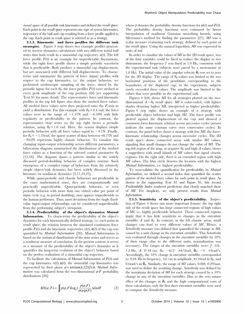
2.1.4. Predictability of the object’s dynamics: Mutual

Information. To characterize the predictability of the object’s

dynamics for each kinematically defined strategy, i.e. each point in

result space, the relation between the simulated continuous force

profile F (t) and the kinematic trajectories x(t), _xx(t) of the cup was

quantified by Mutual Information [26]. Mutual Information is

based on the statistical distributions of the time series and serves as

a nonlinear measure of correlation. In the present context, it serves

as a measure of the predictability of the object’s dynamics as it

quantifies the long-term evolution of the object’s behavior based

on the perfect realization of a sinusoidal cup trajectory.

To facilitate the calculation of Mutual Information of F (t) and

the cup kinematics x(t), _xx(t), the sinusoidal cup kinematics was

represented by their phase Q~arctan( _xx=(2pfx)). Mutual Infor-mation was calculated from the two-dimensional Q-F probability

distributions [26]:

MI(Q; F)~

ððp(Q,F )loge(

p(Q,F )

p(Q)p(F))dQdF ð2Þ

where p denotes the probability density functions for Q(t) and F (t).The probability density functions were estimated by linear

interpolation of nonlinear Gaussian smoothing kernels, using

Silverman’s method for finding the parameters [27]. MI was a

scalar measure evaluating each strategy, defined by each point of

the result space. Using the natural logarithm, MI was expressed in

units of nat.In order to visualize the values of MI in the 2D result space, two

of the four variables could be fixed to reduce the display to two

dimensions: the frequency f was fixed at 1.0 Hz, consistent with

the experimental task (subjects were paced by a metronome at

1.0 Hz). The initial value of the angular velocity _hh0 was set to zero

for the 2D display. The range of h0 values was limited to the two

horizontal positions of the pendulum corresponding to the

boundaries of the displayed cup; in the experiment, subjects

rarely exceeded these values. The amplitude was limited to the

values that were possible in the experimental task.

Figures 4 (left) shows MI for all strategies plotted on the two-

dimensional A{h0 result space. MI is color-coded, with lighter

shades denoting higher MI, interpreted as higher predictability.

Figure 4 (top right) shows an example of a strategy with

predictable object behavior and high MI. The force profile was

plotted against the displacement of the cup and showed a

consistent force-kinematic relation across successive cycles (arrows

indicate the same constant curve over consecutive cycles). In

contrast, the panel below shows a strategy with low MI: the force-

kinematic relationship changes across successive cycles. The 2D

result space shows connected areas with similar MI values,

signaling that small changes do not change the value of MI. The

top left region of the map, at negative h0 and high A values, shows

a ruggedness with small islands of MI values that signal chaotic

regimes. On the right side, there is an extended region with high

MI values. The blue circle denotes the location with the highest

Mutual Information, i.e. highest predictability.

To cross-validate the quantification for predictability by MutualInformation, we defined a second index that quantified the scatter

pattern of the strobed force values for each point in result space. As

shown in the supporting Text S1 and Figure S1, this second

Predictability Index rendered predictions that closely matched those

of MI. For simplicity, we only present results from MutualInformation.

2.1.5. Sensitivity of the object’s predictability. Inspec-

tion of Figure 4 shows one more important feature: the top right

side of the result space has large connected regions of high values

of MI, i.e. highly predictable behavior. These connected regions

imply that it has little sensitivity to changes in the executionvariables A and h0. In contrast, in the left chaotic areas, small

changes can lead to very different values of MI. Hence, a

Sensitivity measure was defined that quantified the change in MI,

caused by a unit change in the execution variables. This Sensitivitywas evaluated through changes in the execution variables by 10%

of their range (due to the different units, normalization was

necessary). The ranges of the execution variables were: f : 0.8–

1.2 Hz, A: 8–44 cm, h0: 2p/2– +p/2rad, _hh0: 23– +3rad/s.

Accordingly, the 10% change in execution variables corresponded

to: 0.04 Hz in frequency, 3.6 cm in amplitude, p/10rad in h0, and

0.6rad/s in _hh0. Similarly, the range of MI values, 0.006–0.295nat,

was used to define the resulting change. Sensitivity was defined by

the maximum deviation of MI for each strategy caused by a 10%

change in any of the execution variables. Due to the very minor

effect of the changes in _hh0 and the high computational costs of

these calculations, only the first three execution variables were used

to compute the Sensitivity measure.



2.1.6. Predictability and limit cycle stability: Global

Lyapunov Exponent. In one further step of cross-validation of

the custom-defined measures, predictability was quantified by the

classical measure of the Global Lyapunov Exponent (GLE). The

GLE could also be considered as a test for the presence of stable

limit cycles: positive GLEs can rule out the presence of stable

behavior [15,16]. While the previous analysis capitalized on the

input-output relation in the system, i.e. on how the desired output

correlates with the required input, the definition of GLE was based

on the kinematic states of the system.

Figure 3. Two profiles of force and cup and ball displacement exemplify unpredictable dynamics (left) and predictable dynamics(right). The strobing procedure is illustrated by the dots and the vertical lines: at every peak of the cup displacement, the value of force is picked; thestrobed force values are then projected onto the vertical axis to show the distribution for each simulation. The left example shows a scattereddistribution, while the right periodic profile only shows one value. The bifurcation diagram summarizes all force distributions as a function of theparameter h0 , the initial ball angle. The vertical axis displays the stroboscopic samples of force values Fk , simulated from a 1.0 Hz sinusoidal cup

displacement x(t) with 10 cm (full peak-to-peak) amplitude and _hh0~0rad/s. The horizontal axis shows the initial ball angle h0. The plot shows thatwhen the simulation starts from the initial angle h0 = 1.0rad, the strobed force values do not change in successive cycles (blue), corresponding to thetime profile on the right. At h0~0:4rad, there is variance in the strobed values of force Fk , corresponding to the plot on the left (purple). The varianceof Fk was used to define a measure for the predictability of object’s dynamics (see Predictability Index in the supporting Text S1).doi:10.1371/journal.pcbi.1003900.g003



To calculate the GLE for each strategy, defined by A, f , h0 and_hh0, the 4D state-space representation of the system’s differential

equations was rewritten for ball states in 2D, as the two states of

the cup were determined by the desired kinematic and acted as

input to the system:

d

dth~ _hh

d

dt_hh~

€xx cos h{g sin h

l

ð3Þ

As for the inverse dynamics calculations above, the cup kinematics

was assumed to be sinusoidal with known A and f . In this

formulation, the sinusoidal movement of the cup was represented

by €xx. Hence, the resulting ball movement was determined by

Equation (3), given the known initial conditions h0 and _hh0. Note

that the force applied on the system F(t) did not directly appear in

the equation, and the cup kinematics and the derived ball

kinematics sufficed for calculating the Global Lyapunov Exponent.

As in a state space analysis of the system for trajectory divergence,

the Jacobian matrix J of the state-space representation was used to

estimate the Global (largest) Lyapunov Exponent:

GLE~(1=n)Loge Jn{1:::J2J1J0ukk k ð4Þ

for n points along the simulated trajectory, estimated in time-steps

of 0.01 s; uk denotes the unit vector (k~1, 2), representing the h

and _hh directions [28]. The GLE was estimated separately for each

of the two unit vectors u1 and u2. Note that for smooth dynamical

systems, the estimation of the GLE does not depend on the chosen

unit vectors uk [29]. Nevertheless, we calculated the GLE for

different choices of uk. The results did not differ. The numerical

integrity of the GLE calculations were further confirmed by

comparing them against the values of the average local Lyapunov

exponents determined for the simulated trajectories. Again, the

results did not differ. It should be emphasized that this measure of

predictability characterizes the object’s behavior, not the control-

ler or human’s control policy [15–17].

Figure 4. Map of Mutual Information in the 2D result space spanned by amplitude A and initial ball angle h0 (left) and examples offorce-kinematics relationship (right). The color map shows that realization of a 1.0 Hz sinusoidal cup trajectory with different amplitudes andinitial angles differ in the resulting predictability of the object dynamics. Mutual Information, coded by color shades, describes the predictability of theobject’s behavior for a 1.0 Hz sinusoidal cup trajectory with different A and h0. The light blue circles indicate the strategies with the highestpredictability of object’s dynamics. The force-cup displacement plots on the right correspond to 2 representative points (strategies) in the resultspace. The profile on the top right shows high Mutual Information with consistent force-kinematic relationship over successive cycles (arrows indicatethe traversal on the same constant curve over consecutive cycles). The profile on the bottom right shows a strategy with low Mutual Information,where the force-kinematic relationship changes in every cycle.doi:10.1371/journal.pcbi.1003900.g004



The estimates of the GLE for each strategy are summarized in

the same 2D result space as for MI, where two of the four variables

were fixed: the frequency was fixed at f = 1.0 Hz, consistent with

the experimental task. Inspection of Figure 5A shows that the

smallest GLE values were found at h0 values between p/4 and p/2

rad, i.e. anti-phase behavior. These strategies presented the most

predictable behavior corresponding to results in Figure 4. The

movement amplitude was very similar to the one for the maximum

MI. Lastly, the rugged changes of GLE in the top left corner,

indicative of chaotic behavior, were very similar to the pattern of

MI. One final important point to note is that all GLE values were

positive. This implies that all strategies were chaotic, even the one

with the smallest GLE, hence ruling out the presence of stable limit

cycles.

2.1.7. Minimization of effort: Mean Squared Force.

Many approaches in motor neuroscience found evidence for

minimization of velocity, force, or more generally speaking, effort

[18,19,30]. To obtain an estimate of the effort exerted for each

strategy, the force profile over the duration of one trial run was

squared and averaged, to quantify the signal power or MeanSquared Force (MSF):

MSF~1

nT

ðnT

0

F (t)2dt ð5Þ

where n denoted the number of cycles and T~1=f the period of

each cycle. Similar to Mutual Information, MSF-values for all

strategies were summarized in the 2D result space. The initial

value of the angular velocity _hh0 was set to zero for the shown

simulation results. However, comparative testing of all initial

values of _hh0 showed that the MSF had little sensitivity to different

values of _hh0.

Figure 5B represents values of the MSF (log-transformed for

better visualization). The movement strategy with minimum force

is found at smaller oscillation amplitudes, where h0 is close to 1 rad

(marked by the green circle). This corresponds to anti-phase

behavior between the cup displacement x and h. However, unlike

MI, this strategy would require a very small movement amplitude.

The irregular pattern in the top left part of the figure indicates that

the boundary from lower to higher values was ragged with islands

of smaller force values interspersed. This area again is identified as

a highly chaotic parameter region of the system.

To evaluate whether the model system afforded a solution at

resonance that required zero force from the subject, linear

analysis of the vibration modes was conducted [31]. The goal

was to identify the modes of the system and its associated

amplitudes. Specifically, the question was whether the system,

as parameterized in the experimental task, allowed a resonance

mode within the task-specified amplitudes. Linear analysis of

the object’s free oscillations showed that, besides the free-

motion mode, the system’s only oscillation mode had anti-

phase relation between x and h (h~20:02x); its natural

frequency was 1.11 Hz. To find the cup’s maximum excursion

at the system’s free oscillation, we exploited the fact that the

displacement of the system’s center of mass was always zero in

the absence of external force: xCM~0. The maximum

excursion therefore satisfied: xCM~MxxMzmxxm. The maxi-

mum horizontal distance between the ball and cup was the

pendulum’s length l, which was the sum of the maximum ball

excursion and maximum cup excursion xxMj jz xxmj j~l. There-

fore, the maximum cup excursion was xxMj j~ml=(mzM) in

both positive and negative directions. For the specific

parameter values, the maximum theoretically possible cup

amplitude in free oscillation was 10 cm.

2.1.8. Maximizing smoothness: jerk. Following the

frequently discussed criterion of smoothness in simple reaching

movements [21] and the findings by Dingwell and colleagues [10],

smoothness or jerk of the trajectories was tested as an alternative

criterion that subjects may have optimized. Due to the complexity

of the object dynamics, jerk could be minimized in cup, ball, and

also force trajectories. In this analysis, only ball and force

trajectories were considered, as the cup trajectory was assumed

to be sinusoidal and thereby smooth by definition.

To assess the smoothness of ball and force trajectories, the mean

absolute jerk was calculated for the simulated profiles of all

strategies, defined in the result space by A, f , h0 and _hh0. The

normalized mean absolute jerk of the ball trajectory was calculated

as:

Figure 5. Predicted values in the 2D result space for alternative criteria. A: Global Lyapunov Exponent. B: Mean Squared Force. C:Normalized Ball Jerk. Note that the maps of the Global Lyapunov Exponent and Mutual Information are remarkably similar, while the Mean SquaredForce and the Ball Jerk maps predict very different preferred regions in the result space.doi:10.1371/journal.pcbi.1003900.g005



Jerk~1

T _€hmax{ _€hminð Þ

ðT

0

_€hj jdt ð6Þ

where the ball’s jerk was normalized by the ball jerk amplitude to

make it dimensionless and, importantly, thereby independent of

movement amplitude [32]. Mean jerk was also calculated for the

simulated force profiles by replacing h with F in Equation (6). The

measures were calculated with, but also without normalization for

verification (see [32] for discussion about normalization and

amplitude dependence of measures). As expected, the 2D result

space for the non-normalized ball jerk and force jerk predicted the

smoothest strategies for the smallest amplitudes. In contrast, when

the mean ball jerk was normalized with respect to ball amplitude,

the strategies with the lowest jerk values were associated with higher

amplitudes. Figure 5C shows the normalized ball jerk in the 2D

result space. The orange dot marks the strategy with the highest

value for smoothness. The regions with the highest smoothness were

associated with in-phase coordination, where h was between –p/4

and –p/2 rad. The mean jerk for the simulated force profiles gave

very similar predictions (not shown).

All simulations were performed with the adaptive integration

algorithm NDSolve with a precision and accuracy goal of 1e-8

using Mathematica v.8.0.4 (Wolfram Research, Inc., Champaign,

IL).

2.1.9. Comparison of predictions and experimental

evaluation. Having computed Mutual Information, GlobalLyapunov Exponent, Mean Squared Force, and Jerk for the

strategies in the A - h0 result space, strategies with maximum

object predictability, minimum mechanical force, and maximum

kinematic smoothness could be identified. Comparison of the

maps in Figures 4 and 5 showed different optima and different

regions in the A - h0 space. The GLE and MI agreed in

predicting highly disjoint, non-smooth, and scattered patterns,

signifying chaotic behavior. In the top right region with positive

h0 and large A values, the MI is high and less sensitive to changes

in A. These strategies with high amplitude and anti-phase

oscillations are marked with a light blue circle and should be

preferred, if predictability of object dynamics is the main criterion

for selection. This contrasts with hypotheses derived from MSF:

in the bottom right region, where h0 is positive and A values are

small, the MSF is at its minimum; predictability of object

dynamics is relatively low and MI is very sensitive to changes in Aand h0. If the mechanical efficiency, e.g. minimization of force, is

the main criterion for selection, these strategies with positive h0

and small A values should be preferred. Finally, the smoothness

criterion predicts the negative h0 and large A values as optimal,

which are associated with chaotic behavior in the predictability

measures.

The simulations highlight that movement amplitude was one

major distinguishing feature between the hypotheses. Hence, to

test what reasons may drive subjects to select certain strategies the

experiment did not specify the movement amplitude or ball’s

motion, but left them free to choose for the subject. Hence, the

measured amplitudes will provide a basis to distinguish between

criteria. However, the task restricted the allowable movement

amplitudes to be between 8 cm and 44 cm to preempt strategies

that exploited free oscillations requiring zero force.

2.2. Experimental MethodsEthics statement. The experiment was approved by the

Northeastern University’s Institutional Review Board (IRB#:

10-06-19). Subjects provided written informed consent before

participation.

2.2.1. Subjects. Eight healthy right-handed adults (6 female,

2 male, age: 33.8612) volunteered for the experiment. None of

them reported any history of neuromuscular disease.

2.2.2. Experimental setup. The dynamics of the two-

dimensional ball-and-cup system was simulated in a virtual

environment (Figure 6). Subjects manipulated the virtual cup-

and-ball system via a robotic arm, which also exerted forces from

the virtual object onto the hand (HapticMASTER, Moog FCS

Control Systems, Nieuw-Vennep, The Netherlands). Custom-

written software in C++ was developed to control the robot and

the visual display based on HapticAPI (Moog FCS Control

Systems). Subjects sat on a chair and grasped the knob at the end

of the robotic arm with their preferred hand to interact with the

virtual environment. The sitting position and the distance to the

manipulandum were adjusted so that the movements remained

within the subject’s workspace limits. The virtual task was

displayed on a rear-projection screen (2.4 m62.4 m) that was at

a distance of 2.15 m in front of the subject. The visual display

consisted of a cup and a ball, shown in white against a black

background. The cup was drawn as a semicircle with an arc length

of 180 deg, along which the ball moved. The visual display gain

between the dimensions in physical displacement of manipulan-

dum and on the visual screen was 4.0. The position, velocity, and

acceleration of the cup and ball and the interaction force between

hand and manipulandum were recorded at 120 Hz.

2.2.3. Task and protocol. Subjects were asked to move the

ball-and-cup system horizontally between two targets in synchrony

with a metronome that played auditory stimuli at 2.0 Hz. Subjects

were instructed to synchronize the right and left excursions with

each metronome sound to achieve an oscillation frequency of

1.0 Hz. If their movements consistently deviated from the

metronome pace, subjects were verbally corrected by the

experimenter. However, this happened very infrequently after

the first few trials. Importantly, the task did not prescribe a specific

amplitude, but rather allowed the subject to choose their preferred

amplitude in the range between 8 cm and 44 cm. In addition, the

instruction explicitly emphasized that respecting the boundaries of

targets was not a priority, i.e. it imposed no spatial accuracy

demands. Guidance for the range of movement amplitudes was

provided by two green target rectangles (Figure 6). As long as the

subject reversed the movement within these long rectangles, the

task was achieved. The ball could not escape from the cup and the

subjects were explicitly informed that they did not have to achieve

particular ball motions. Even though the ball could not escape

from the cup, the ball motions were shown to provide subjects with

visual information about the ball and the forces it exerted onto the

hand. We opted to not constrain the ball movements in the

instructions (contrary to [1,10]) because these additional con-

straints would have interfered and made the task too complex.

Subjects performed 5 blocks of 10 trials each; one trial lasted

45 s. All trials were separated by a 15 s pause and there was a

break of several minutes between each block. Subjects could take

additional breaks between blocks, if they felt fatigued.

2.2.4. Analysis of experimental data: definition of

execution variables. Figure 2 (right) shows examples of the

measured kinematic trajectories and forces, including definitions of

the experimental variables. As the task instructions elicited

trajectories very close to a sinusoid, the cup trajectories were

sufficiently described by amplitude Ak and frequency fk, where the

subscript denotes the estimate at cycle k. At each peak amplitude

of the cup trajectory, the angle and angular velocity of the ball

were strobed to obtain hk and _hhk. These strobed values at cycles k



served as estimates of initial states of the ball for each cup cycle.

The four variables Ak, fk, hk, _hhk were the experimental analogues

to the execution variables A, f , h0, _hh0 in the model simulations. For

each trial, averages of the four execution variables were calculated

over 21 cycles in the time window of 25–45 s. The initial 25 s of

each trial were excluded, as they frequently contained transient

adjustments. Averages were used, because in the experimental

trajectories these estimates could take on different values due to

changes in the applied force. These average values were viewed to

reflect the subject’s intended interaction with the object.

Note that the exemplary profiles in Figure 2 are not meant to

validate the similarity of simulation and experimental data. While

the experimental data show the object’s behavior under subject’s

continuous control, the simulation by definition shows perfect cup

sinusoidal trajectory, with no correction. The force profiles

differed as the cup profiles were different.

2.2.5. Analysis of experimental data: calculation of

strategy measures. To evaluate how the different criteria for

object manipulation can account for the results, measures of

predictability, force, and smoothness were calculated from the

experimental data in two ways. The first method used the average

strobed execution variables Ak, fk, hk, _hhk and looked up the

corresponding Mutual Information and its Sensitivity, Mean

Squared Force, and Mean Jerk from the result space calculated by

the simulations. Note though that the simulations show the

system’s behavior in presence of a perfect realization of the

sinusoidal cup trajectory, without any intermediate correction for

the upcoming cycles. Although this is an idealization, it quantified

the predictability of the object, starting from each cycle.

Therefore, we also applied a second method that was independent

of this assumption and quantified the combined behavior of the

object and human’s applied control directly from the continuous

experimental data.

It needs to be pointed out that in the simulated data, MutualInformation reflects predictability based on the chosen initial

condition, in perfect execution with no intermediate correction.

Evidently, these conditions were not the case in the actual

experiment, where subjects may have continuously corrected for

deviations. Therefore, the experimental MI measure reflects the

consistency and repeatability of the subject’s performance during

interaction with the object. While the simulated measures only

represent the object’s behavior, the experimental measures

characterize the combined effect of the object behavior and the

control of the subject during the experiment, i.e. the property of

object and the controller together.

To calculate MI from experimental data, the continuous force

profile and the continuous cup phase Q~arctan( _xx=(2pfx)) were used

Figure 6. Experimental setup, the robotic arm (HapticMaster), rear-projection screen, and a subject sitting on a chair, while holdingthe manipulandum of the robotic arm. The task instruction was to move the ball-and-cup object rhythmically between the two green targets ata frequency of 1 Hz. As long as the excursion maxima alternated between the wide target regions, the task was satisfied. Hence, the subjects couldchoose their movement amplitude.doi:10.1371/journal.pcbi.1003900.g006



in Equation (2), as in the simulations. The calculation of experimental

MI followed the same procedure as in the simulated MI, except that

the probability density functions were estimated from continuous

experimental data, rather than continuous simulation outputs. To

calculate the Mean Squared Force, the continuous force profile of each

trial was squared and averaged, analogous to the simulated data

(Equation 5). To assess the smoothness in the experimental data, both

normalized and non-normalized mean absolute jerk were calculated to

quantify the smoothness of ball, cup, and force profiles, h, x, and F .

Additionally, the spectral arc-length measure [33], i.e. the arc length of

the normalized spectral density function of the signal’s time history, was

calculated to quantify the smoothness of the experimental data. This

measure has been shown to be more consistent in terms of

normalization requirements [33]. To characterize the smoothness of

the intended/selected strategies rather than the cycle-to-cycle variabil-

ity, the signal profiles were first averaged across the cycles of each trial

and smoothness was estimated on this averaged cycle.

All data analyses were conducted in MATLAB v.2012b (The

Mathworks Inc., Natick, MA).

2.2.6. Statistics. To determine the changes with practice in

the execution variables Ak, fk,hk, _hhk and in the strategy measures,

Mutual Information and its Sensitivity, Mean Squared Force, andMean Jerk, the average values of the first 5 and last 5 trials of each

subject were compared by paired t-tests as representative of early

practice and late practice strategies.

Results

3.1. Execution VariablesFigure 7 shows representative trials of force, cup, and ball

displacements, one set from early and one from late in practice.

While the cup trajectories were generally rhythmic as required by

the task, it is notable that all profiles became more regular with

practice. A third set of trajectories shows an example of an

unpredictable force profiles and ball movements that were

probably highly chaotic. Such chaotic episodes were present in

all subjects, but occurred more frequently during early practice.

The red dots on the cup displacements at each maximum indicate

the strobe points, giving estimates of Ak and fk, the blue dots on

the ball angle indicate the strobed values of hk and _hhk (not shown).

These execution variables of each trial were averaged to represent

the average strategy in each trial (see supporting Figure S2 for an

example distribution before averaging for one subject).

Figure 8 shows how the execution variables develop for all

subjects over the 50 practice trials. The four plots show the mean

values across subjects with the shaded band representing one

standard error around the subject mean. The thin line shows one

representative subject. Subjects improved in performing the task at

the instructed frequency of 1.0 Hz, as seen by the converging line

to fk = 1 Hz and the decrease in the standard error, especially after

trial 30. The fluctuations across trials also decreased in the single

subject, representing the behavior of all other subjects. While the

fluctuations within and across trials decreased, the average

frequencies in the beginning and at the end of practice were

1.0160.06 Hz and 1.0060.01 Hz, respectively, which were not

significantly different (p,0.05). In contrast, movement amplitude

Ak visibly increased with practice, especially until approximately

trial 30, from whereon it asymptoted. The average value increased

from 21.4563.86 cm early in practice to 28.0363.21 cm late in

practice, which was significant (p,0.05). The strobed ball angles

hk (measured at maximum cup position in each cycle) were

positive on average and increased from 0.8560.33rad in early

Figure 7. Representative profiles of raw experimental data from early and late practice. F is the interaction force between the subjectand robot, x is the displacement of the cup (end-effector), and h is the angle of the ball. The time of peak cup positions (shown by red dots) served astime reference to strobe the ball angular displacement h and define hk . Notice that the relatively irregular patterns of cup displacement and especiallyforce in early practice became more regular and also larger in amplitude later in practice. An example of a highly unpredictable or chaotic behavior isshown on the right. Notice the negative values of hk , which indicate the chaotic regime, shown in Figure 4. The Mutual Information measure forthese continuous experimental data are 0.1256nat (early practice), 0.1693nat (late practice), and 0.1295nat (unpredictable behavior).doi:10.1371/journal.pcbi.1003900.g007



practice to 0.9760.24rad in late practice; however, this change

was not significant (p.0.05). By coordinate conventions the cup

movements to the right and clockwise ball movements (to the left)

were defined as positive. Therefore, positive hk values indicate

anti-phase coordination. Trials with negative hk, i.e. in-phase

coordination, corresponded to strategies in the chaotic regions in

Figures 4 and 5. Consequently, performance in these trials was

very variable or unpredictable. The strobed angular velocity of the

ball _hhk showed a rather inconsistent pattern across subjects, but

remained relatively constant across practice. The values at early

practice (20.2360.48 rad/s) and late practice (20.1160.38 rad)

were not significantly different (p.0.05). Importantly, the _hhk

values did not significantly differ from zero, indicating that when

the cup was at maximum excursion with zero velocity, the ball was

also at maximum excursion with zero velocity. This result

confirmed that the assumption _hhk = 0 for plotting the data was

acceptable.

3.2. Preferred Strategies in Result SpaceAlthough the preferred movement strategies were defined in the

4D result space defined by A, f , h0 and _hh0, visualization of

experimental strategies was possible in the 2D subspace as the

frequency was relatively invariant at f ~1Hz due to the

metronome pacing, and the initial cup velocities at maximum

excursion were close to zero ( _hh0~0). Additionally, _hhk had little

effect on the strategy measures Mutual Information and its

Sensitivity, Global Lyapunov Exponent, Mean Squared Force, and

Mean Jerk.

Figure 9 shows all trials of all subjects in result space: Each point

represents the strategy of one trial. The dark and light color

shading corresponds to trials in early and late practice, respec-

tively. The left panels shows that most trials, especially those late in

practice, are in the right half of the map, where h0 is positive and

MI shows extended regions of high values, i.e. low Sensitivity. The

clustering of trials in the regions with higher MI is visibly denser.

The right panel shows the same data, but now separated by

subjects. The arrows connect the average performance in the first

and last 5 trials to highlight the change with practice. It can be

seen that most subjects shifted to higher movement amplitudes and

positive h0 (i.e. anti-phase oscillations), which were associated with

higher MI. While the individual strategy changes were different, 6

out of 8 subjects increased MI, the predictability of interaction; 2

subjects approximately maintained the value, and 7 of 8 subjects

decreased the Sensitivity. To elaborate, 2 subjects improved the

predictability primarily by changes from in-phase towards anti-

phase behavior; the remaining 6 subjects, who were at anti-phase

behavior from the beginning, increased their amplitude and

thereby decreased their sensitivity. This result was consistent with

the hypothesis that predictability is a primary criterion for strategy

selection. The results simultaneously argue against alternative

criteria: None of the subjects moved toward the strategy with

maximum smoothness or minimum force (Figure 5).

3.3. Mutual Information and Sensitivity, Mean SquaredForce, and Smoothness Measures

Figure 10 shows the strategy measures as determined by the two

methods: The panels on the left show the measures based on the

mean estimated execution variables and calculated from the

simulated model data; the panels on the right show the strategy

measures calculated from the continuous experimental data. The

bold lines represent the subject means, the shaded bands indicate

Figure 8. Execution variables across 50 practice trials: frequencyfk of cup displacement shows that the task was mostlyperformed at the instructed frequency of 1.0 Hz, amplitudeof cup displacement Ak showed a significant increase acrosspractice, ball angle at peak cup position hk was approximately

1rad, and ball angular velocity _hhk was close to zero throughoutpractice. The bold lines show the averages across subjects (n = 8); theshaded bands represent one standard error across subject means; thethin lines show one representative subject.doi:10.1371/journal.pcbi.1003900.g008



one standard error. The thin lines represent a representative

subject to show the fluctuations in a single subject.

The top two panels display MI between the force profile and

cup kinematics (blue). The average values of the simulated MI on

the left showed a marginally significant increase from

0.14260.023 nat to 0.15860.004 nat in late practice (0.10,p,

0.05, 6 out of 8 subjects showed an increase). This increase mainly

occurred from trial 1 to 13 and then plateaued until the end of

practice. The experimental MI measure in the right panel showed

a similar trend by increasing from 0.150660.010 nat to

0.159060.007 nat, although this change was not significant (p.

0.05). This increase in MI shows that object’s predictability can

explain the changes in strategies.

The panel in the second row shows the Sensitivity measure

(purple), which could only be derived from the simulated data.

The average value decreased significantly from 2.1260.65 in early

practice to 1.560.27 in late practice (p,0.05). The change

predominantly occurred until about trial 30 and then stayed

relatively constant. This decrease in Sensitivity was additional

support for the hypothesis that object’s predictability can account

for the change and selection in the manipulation strategies.

For all measures, one individual subject was also plotted to

highlight the pattern of variability within a subject. It is

noteworthy that in all measures there were relatively large changes

across trials, which probably reflects the fact that the subject

interacted with a chaotic system. These fluctuations, seen in all

subjects, gave rise to the relatively large standard error.

The next two panels (green) display the simulated and

experimental average Mean Squared Force (MSF) across trials,

i.e. the mean squared interaction force within one trial. The

simulated MSF on the left shows a visible increase from

76.29648.30 N2 in the first 5 trials to 112.71644.53 N2 in the

last 5 trials. However, due to the variability, this increase is non-

significant (p.0.05). In parallel, MSF determined from the

continuous recorded interaction force increased from

50.61631.19 N2 in the first 5 trials to 105.88652.61 N2 in the

last 5 trials, which was significant (p,0.05). The increase was

reached at about trial 30; afterwards, the MSF showed little

change, similar to the sensitivity measure. Note that the effort-

based cost functions predicted that force should be minimized with

practice, i.e. predicted a decrease in exerted force. Hence, both

measures of force reject minimum effort strategies.

Figure 9. Strategies for all subjects and all trials displayed in the 2D result space. The horizontal axis corresponds to the simulation variableh0 or its average experimental estimates hk in each trial. The vertical axis corresponds to the simulation variable A or its average experimentalestimates Ak . Each point represents the average strategy in one 45 s trial. Darker red indicates early practice and lighter red indicates late practice.The left panel shows that subjects explored regions with lower Mutual Information and lower Mean Squared Force; however, the majority of trialsconverged to areas with higher Mutual Information and lower Sensitivity. The right panel shows the same data separated by subject: the red arrowsmark how each subject’s average strategy changed from early practice (first 5 trials) to late practice (last 5 trials). All subjects increased theirmovement amplitude, associated with an increase in overall exerted force. The majority of subjects switched from low- to high-predictability regionsin the result space. None of the subjects moved toward the minimum force strategy.doi:10.1371/journal.pcbi.1003900.g009



Figure 10. Strategy measures Mutual information and its Sensitivity, Mean Squared Force, and Smoothness plotted across all 50 trials.Thick lines are the across-subject average, the shaded bands show one standard error around the subjects’ mean; the thin lines show onerepresentative subject. Left column: model-based strategy measures, simulated at experimental execution variables that at each point show the



Figure 10 (bottom row, in brown) shows one of the smoothness

measures, Normalized Ball Jerk, plotted across the practice trials.

Comparison of the first 5 trials vs. late 5 trials across 8 subjects

(paired t-test, a= 0.10) failed to show a significant decrease. The

same comparison was performed for all other Jerk measures of the

ball trajectory h, cup trajectory x, or force profile F , on the non-

normalized mean absolute jerk, normalized mean absolute jerk, or

spectral arc-length measures. None of the early-late practice

comparisons rendered a significant difference.

Discussion

This study used a virtual task to examine how the complex

nonlinear dynamics of an object, specifically the predictability of

object dynamics, determines preferred manipulation strategies.

Inverse dynamics simulations of the task model rendered insight

into what type of forces are required to achieve the task. It is

important to emphasize that our approach did not assume any

controller. Instead, it calculated the set of all force profiles that

generated the task-required cup trajectories for given parameters

and initial conditions. This approach is consistent with previous

research of our group, where the tasks of throwing and bouncing a

ball were analyzed and solution manifolds derived [34,35].

Determining the manifold of zero-error solutions is comparatively

easy for these discrete tasks, where solutions are fully determined

by a vector of scalar variables. For example in throwing, the error

or task result is a function of position and velocity at release, the

execution variables. Such a relation becomes considerably more

complex, when the task involves continuous interactive control,

such as the current cup-of-coffee task. To afford a compact

overview over all possible solutions to the task, each continuous

strategy was characterized by four scalar execution variables:amplitude, frequency of the cup, and the initial or strobed position

and velocity of the ball. The resulting continuous trajectories were

characterized by different strategy measures or result variables:

predictability of the applied force and the kinematic output

(Mutual Information), and its Sensitivity to small changes in the

execution variables, also expressed in the Global LyapunovExponent, Mean Squared Force, and normalized ball Mean Jerk.

Model simulations rendered the space of solutions and their result

characteristics that served as quantitative criteria to evaluate

human manipulation: maximizing predictability of the object

dynamics, minimizing the exerted force, and maximizing smooth-

ness.

The experimental task was parameterized to dissociate between

the candidate criteria: strategies that maximized predictability

were associated with higher forces, while lower forces were

coupled with less predictability. Similarly, the strategies that

maximized smoothness neither maximized the object predictabil-

ity, nor did they minimize effort. Thereby, experimental data from

humans could dissociate between these criteria.

Results revealed that subjects chose strategies that rendered

their interactions with the object dynamics repeatable and

predictable, even though these strategies demanded higher force

levels and less smooth trajectories. Importantly, these strategies

were not stable limit cycles, but positive Lyapunov exponents

throughout all strategies indicated chaotic solutions. Over 50

practice trials, subjects’ movement amplitudes increased and

thereby the measures of predictability increased and also the

sensitivity of predictability to execution variables decreased.

Although the change in Mutual Information was only marginally

significant, further inspection of the experimental results showed

that many subjects already had reasonably high values in early

practice and practice only helped them to better maintain it.

Additionally, the sensitivity measure showed a significant decrease,

lending further support to the hypothesis that predictability played

a central role. The measure of exerted force increased significantly

across practice. This finding contradicted the dominant role of

force minimization in human motor coordination [18,19], which is

frequently invoked as one of the main optimization costs in

optimal feedback control [11,36]. The analyses also highlighted

the nonlinearity in this continuous object manipulation task: The

result space contained areas of chaotic solutions that were

associated with lower predictability, but they were clearly avoided

by subjects.

Taken together, these results speak against the possibility to

explain the selected strategy based on minimization of force or

maximizing smoothness, nor seeking stable limit cycle solutions.

Instead, the best account for the observed movement strategies

was the notion that humans maximize predictability of object

behavior in rhythmic manipulations. Note that in optimal control

it is always possible and advantageous to combine cost functions as

a weighted sum to arrive at the best possible control solution [37].

While of evident merit in control, this step is scientifically less

appealing as this easily becomes unprincipled fitting of data with

unlimited options.

4.1. Measures of Object PredictabilityEvaluation of subjects’ movement strategies proceeded along

two ways: In a first analysis, the continuous trajectories were

strobed to obtain estimates of the four execution variables that

corresponded to the theoretically derived variables. The average

strobed values per trial could be directly mapped into the

theoretically derived result space. Then, Mutual Informationand its Sensitivity could be looked up in the theoretical map. Note

that these predictions were based on the assumption of perfect

realization of sinusoidal cup trajectories, starting from the current

states, and excluding any online cycle-by-cycle control of the

subject. This simulated condition therefore truly quantified the

object’s long-term predictability. In real performance, however,

subjects constantly applied intermediate online control on the

object during the experiment. Therefore, a second analysis was

based on the measured continuous trajectories and force and

quantified the combined behavior of the object dynamics and the

control applied by the subject. The continuous experimental

Mutual Information showed the same increasing patterns and

confirmed the consistency and repeatability of subject’s interactive

movements.

The map of Mutual Information in result space shows

connected regions of high predictability that are less chaotic and

lead to less unpredictable changes in case of minor changes in

amplitude or ball angle. This feature is quantified by the Sensitivitymeasure. Subjects’ behavior documents that they not only seek

strategies that are predictable, but also those that lower the

sensitivity to small deviations in the parameters, corroborating the

relevance of predictability. As the analysis of the simulated data

rested on the sinusoidal assumption, we also repeated the

calculations with sinusoids that had added harmonics of small

behavior of the object in the upcoming cycle(s) for perfect realization of a sinusoidal cup trajectory. Right column: strategy measures determinedfrom continuous experimental force and kinematics that indicate the combined behavior of the object dynamics and the continuous online controlby subjects. Note that Sensitivity can only be determined based on the simulated maps.doi:10.1371/journal.pcbi.1003900.g010



amplitudes. The results were sufficiently robust with respect to

these added perturbations.

Given the centrality of the concept of predictability, the

theoretical analysis developed two different measures for its

quantification: Mutual Information between the kinematic and

force profiles quantified to what degree the dynamic behavior

differed from simple periodic input-output behavior. A second

measure quantified the normalized average variance of the strobed

force values as plotted in the bifurcation plot. The map of this

Predictability Index is shown in supporting Text S1. While not

exactly identical, the similarity is striking, given that very different

quantifications were used. Hence, their relative congruence can be

considered as cross-validation of the Mutual Information map.

Finally, these input-output measures were verified against a more

classic measure based on system’s kinematic states, the GlobalLyapunov Exponents: as expected, the maps of Mutual Informa-tion and the Global Lyapunov Exponent showed very similar

patterns. It should be emphasized that the predictability measures

do not describe the variability or noise of the kinematics or kinetics

at the end-point. A very smooth force and kinematic profiles may

lead to an unpredictable relationship; conversely, some complex

kinetic and kinematic trajectories with fast fluctuations may form

relatively predictable patterns. It is the mutual correspondence of

the kinematic and kinetic temporal profiles across consecutive

cycles that were captured by the information-theoretic measure,

Mutual Information.

The pattern of the smoothness measure was visibly different

from the predictability and Lyapunov exponent measures. To

corroborate these predictions, Mean Jerk was calculated for force,

ball, and cup profiles and in several different ways: in addition to

calculating Mean Jerk in the time domain, we also calculated a

recently proposed measure for quantifying smoothness: the

spectral arc-length in the frequency domain [33]. Ball trajectory

and force profile variants of smoothness measures (regardless of

normalization) yielded very similar surfaces in the 2D result space.

Comparison of the average experimental measures in early and

late practice showed no significant decrease for any of the h, x, and

F by either of the smoothness measures. This further supported

that subjects did not seek to maximize smoothness in their

preferred movements.

4.2. Alternative Explanations and CriteriaIn the literature on unconstrained movements numerous other

optimization criteria have been proffered as viable candidates for

motor control. However, as this study shows, physical interaction

introduces very specific challenges that potentially override other

criteria that may be relevant for unconstrained motion. We will

discuss potential candidates in turn.

4.2.1. Temporal accuracy. As the task involved synchroni-

zation with the metronome, one potential alternative aspect that

may have affected the outcome is the subjects’ goal to achieve

temporal accuracy and synchrony with the metronome. Note

though that this criterion was not emphasized and there was no

quantitative feedback on timing accuracy. Subjects were only

reminded of this criterion, if they consistently deviated, which only

happened once or twice for each subject. Also, different to typical

tapping synchronization tasks, the haptic feedback was not limited

to the maximum excursion to serve as a salient landmark for

synchronization, such as in tapping movements. Instead, the

interaction forces were continuous and presented complex

fluctuating patterns. Yet, it may be conjectured that the increase

in amplitude was in service of optimizing temporal accuracy.

There is some evidence for this correlation in studies on point-to-

point movements, where small movement amplitudes could

negatively affect temporal accuracy [38]. Further, timing variabil-

ity was shown to decrease with movement velocities and increase

with movement distance [39]. However, these results were

reported for discrete pointing or tapping tasks. The present task

was continuously rhythmic, without a salient touch or contact

event to be synchronized. Discrete and rhythmic movements have

shown to lead to very different effects [40–43], probably due to

different neurophysiological control mechanisms [44]. Hence, the

extrapolations of these results are potentially problematic.

In a study on free rhythmic finger movements, no difference in

the preferred amplitude was found across various un-paced and

paced conditions [45]. This was further supported by a more

recent study, where the arm movement amplitude had no effect on

the timing error variance [46]. Nevertheless, we analyzed our data

to test the hypothesis that temporal accuracy and movement

amplitude were positively related. To this end, the temporal

difference between each metronome beep and the maximum and

minimum excursion of the cup trajectory was determined. To

eliminate transients in each trial, only the cycles in the window

between 20 to 45 s were used. Correlating the average temporal

error with the mean movement amplitude of each trial did not

show any significant relation when all subjects’ data were pooled,

r = 20.064, p = 0.20. Similarly, correlating the standard deviations

of the asynchrony error in each trial with the average amplitude

did not yield any significant correlations, r = 20.019, p = 0.70.

Repeating the correlations for the same two asynchrony measures

for each individual only showed significance for one subject for the

mean asynchrony error. The same results were obtained, even

when the analyses was limited to the final 20 trials, after practice

effects had subsided.

Nevertheless, two additional small experiments were conducted

that probed whether synchronization may have been facilitated at

higher amplitudes. One test presented a small and a large

amplitude target to subjects, while again paced at 1 Hz frequency.

Comparing the temporal error in small and large amplitude

conditions showed no difference, i.e. no advantage for synchro-

nization at the larger amplitudes. A second experiment examined

subjects’ amplitude preference when manipulating a solid object in

synchrony with the metronome, i.e. when the complex dynamics

were removed. Subjects showed a spectrum of amplitudes between

13 and 32 cm, with the mean at 22.466.1 cm. This amplitude was

significantly lower than the preferred movement amplitude during

late practice of the experiment proper (p,0.05, two-sample t-test).

Further, the temporal error was insensitive to the movement

amplitude. For more details on the experiments see supporting

Text S2. Taken together, these findings did not support the

hypothesis that temporal accuracy or precision were responsible

for the observed amplitude increase. Rather, they confirmed that

the object dynamics was the reason for the observed amplitude

increase.

4.2.2. Free oscillation modes and stable limit cycles. A

complex dynamic system has free oscillation modes that may

afford an efficient solution to the task: the free oscillation mode

requires zero applied force. It may be conjectured that subjects

adjusted their amplitudes to seek this efficient mode to satisfy the

task. Indeed, linear analysis of the object’s free oscillations [31]

showed that the system has a free-motion mode (natural frequency

is zero) and an anti-phase oscillation mode with a natural

frequency of 1.11 Hz (h~20:02x). However, given that the center

of mass of the system does not move in free oscillation, the

maximum theoretically possible amplitude of the cup was 10 cm

(assuming the nonlinear characteristics of the system allowed stable

rhythmic movements). This was considerably different from the

experimentally observed amplitudes at any stage of the experiment



and rejected the possibility that the selected amplitudes were

dictated by the free oscillation modes. This result is underscored

by the fact that according to the Global Lyapunov Exponent map,

the positive values in the entire 2D result subspace show that none

of the strategies generated stable limit cycles. This precludes

explanations of the results in terms of stable modes of coupled

oscillators [47–51].

4.2.3. Preference for frequency-amplitude combinations

dictated by stable dynamics. It may be questioned if selecting

a higher amplitude was dictated by ‘‘comfortable’’ frequency-

amplitude combinations due to mechanical properties or neural

control preference [47,52]. The literature on rhythmic movements

has examined the frequency-amplitude relationship in stable paced

and un-paced movements. However, the range of preferred

amplitudes for a given frequency is typically quite high (e.g.

[47,48,52]). In addition, observed increases or decreases in mean

amplitudes were associated with slower or higher frequencies,

respectively. This is congruent with keeping peak velocity at

reasonable values and to keep ‘‘effort’’ low. Our data show an

amplitude change in the opposite direction: for an invariant

frequency, amplitude is increased, which increases peak velocity

and effort.

4.2.4. Kinetic and energetic criteria. Choosing larger

amplitudes and forces implicitly ruled out that subjects minimized

torque change and energy, as both criteria increased simulta-

neously with movement amplitude and force. The force iso-

contours in the 2D result space in Figure 9 also showed that the

regions with larger amplitudes required higher forces. Interesting-

ly, however, subjects reported that their acquired strategies felt

‘‘easier’’ or less forceful than their initial strategies. Unexpected

interaction forces required corrections based on feedback.

Apparently, this additional processing was perceived as more

demanding. This observation underscored that the perceived effort

was smaller in the predictable interactions.

4.2.5. Exploration during practice. It may be speculated

that subjects chose the observed strategies, because they were the

most trivial or available ones and not because of preference over

the other alternatives. It is important to highlight that subjects did

explore different parts of the result space. This can be seen in

Figure 9, where individual trials were scattered across the result

space, especially in the early stage of the experiment. This

indicates that the strategies were not chosen due to limited chance

to discover them. Also, the relatively negligible change in average

strategies from trial 35 to 50 shows that the selected strategies were

relatively consistent and preferred, as opposed to a randomly

visited strategy.

4.3. Information Processing in the Sensorimotor ControlSystem

Rhythmic coordination has been readily associated with stable

limit cycle behavior and a lot of support has been accumulated in

bimanual coordination. For example, two-finger coordination has

been extensively examined and parametric variations in the

experiment, such as frequency scaling, have supported predictions

from coupled oscillator models [51,53,54]. A preference for stable

perception-action dynamics has also been shown in a rhythmic

ball bouncing task, where subjects preferred movement solutions

with dynamic stability [35,55,56]. In this task, the dynamically

stable solution is attained when the racket impacts the ball at the

decelerating segment of the racket trajectory, assuming sinusoidal

racket movements. Importantly, this solution was chosen over the

mechanically more efficient solution of hitting the ball at

maximum velocity of the racket trajectory. Such dynamically

stable solutions can be interpreted as computationally less

demanding, as small perturbations do not require continuous

corrections, but die out by themselves. The same argument can be

made for the present task: the strategies with predictable object

behavior can be considered as the ones that avoid uncertainty [57]

and therefore require little or no error corrections.

The surprising observation in the present task was that rhythmic

performance did not appear to be stable, as inferred from positive

Lyapunov exponents. These results on stability were corroborated

by their match with the predictability estimates. Apparently, the

added complexity from the object dynamics introduced chaos, at

least in the mathematical model. Hence, subjects chose solutions to

the task that offered a surrogate to stability – predictability. Similar

to the argument in the ball bouncing task, it can be argued that

this eases the demands on information processing, while at the

same time increasing the cost of energy processes.

Figure 11 schematizes this information-theoretic interpretation

and its relation to the processing demands of a sensorimotor

control system. If the forces result from motor commands and the

object kinematics and dynamics are translated into sensory

information, the complexity of the object dynamics can be

interpreted as the degree of required sensorimotor processing.

Mutual Information between the force and the object kinematics

quantifies the input-output relation of the system. The less

predictable this sensorimotor information mapping, the more

demands arise for the controller. In contrast, predictable

interactions require less active information processing. This

interpretation is consistent with the finding that during rhythmic

movements fewer cortical and subcortical areas are activated

compared to discrete movements, as revealed by fMRI [44]. It is

Figure 11. Schematic of the control loop between the centralnervous system and the object dynamics. Mutual Informationbetween the force and kinematics quantifies the complexity of theobject dynamics. At the same time, Mutual Information between thesensory information and motor commands quantifies the level of therequired sensorimotor information processing. This can be interpretedas a reflection of the complexity of the sensorimotor informationprocessing required by central nervous system for performing themovement task.doi:10.1371/journal.pcbi.1003900.g011



interesting to contrast this information-processing efficiency with

mechanical efficiency, as an extension of one-way channel

capacity [58,59] to a closed-loop information-theoretic measure

of sensorimotor control (see also [60,61]).4.3.1. Predictability as a control policy. Having demon-

strated that predictability is a priority for human control, the

question arises how to translate this choice into a control policy. At

this point, only speculations are possible. To begin, continuous

‘‘surprises’’ from the interaction are perceived by subjects as

cumbersome and hard to counteract. Therefore, the computa-

tional cost increases. One possibility is to include Local Lyapunov

Exponents or similar measures in the controller’s cost function.

While this is intuitive, a mathematical formulation can be more

challenging, given the potential complexity of the nonlinear

dynamical system.4.3.2. Object characteristics vs. controller characteris-

tics. It needs to be underscored again that in contrast to many

other computational studies, the purpose of the simulations was

not to model the neural control system at every time-step. Many

previous studies investigated models of potential controllers [5], for

example to study the role of delays and noise, or the continuous vs.

intermittent nature of control [7–9]. These studies sought to

identify the details of the human control mechanism; hence, they

have often simplified the object dynamics to facilitate focus on the

complexities of the controller. Our study shifted this emphasis:

maintain the nonlinearity and complexity of the object dynamics

and identify the strategies that are preferred for control, before

modeling the controller and the mechanisms of its neuromecha-

nical implementation [8].

4.4. ConclusionThis study highlighted that interactive tasks with complex object

dynamics may have solutions with different degrees of predictable

or chaotic object behavior. Experimental results supported the

hypothesis that predictability of object’s dynamics and, hence,

interaction between the human and object, is the primary criterion

for strategy selection. Quantification of the predictability of the

human-object interaction expresses that humans seek solutions

where force and kinematics are synchronized into a repeatable

pattern, which most likely has lower demands on sensorimotor

information processing.

Supporting Information

Figure S1 Maps of the Predictability Index (left) and MutualInformation (right). The color maps show that realization of a

1.0 Hz sinusoidal cup trajectory with different amplitudes and

different initial ball angles yielded different predictability of the

object dynamics. Note that the maps of the Predictability Indexand Mutual Information are remarkably similar.

(TIF)

Figure S2 Experimental execution variables Ak, fk, hk, _hhk and

strategy measures (Mutual Information and Sensitivity, MeanSquared Force, and Mean Jerk), plotted for all cycles of all trials for

a representative subject 1.

(EPS)

Text S1 Calculation of the force values in the bifurcation

diagram and Predictability Index of object behavior.

(PDF)

Text S2 Control experiments to assess the role of timing

accuracy or precision demand in selected strategies.

(PDF)

Acknowledgments

We would like to thank Fei Ye for help in collecting experimental data.

Author Contributions

Conceived and designed the experiments: BN DS. Performed the

experiments: BN CJH. Analyzed the data: BN. Contributed reagents/

materials/analysis tools: BN CJH DS. Wrote the paper: BN CJH DS.

Designed and implemented the virtual environment: DS CJH BN.

References

1. Hasson CJ, Shen T, Sternad D (2012) Energy margins in dynamic object

manipulation. J Neurophysiol 108: 1349–1365. doi:10.1152/jn.00019.2012.

2. Mayer HC, Krechetnikov R (2012) Walking with coffee: Why does it spill? PhysRev E 85. doi:10.1103/PhysRevE.85.046117.

3. Mehta B, Schaal S (2002) Forward models in visuomotor control. J Neur-

ophysiol 88: 942–953.

4. Gawthrop P, Lee K-Y, Halaki M, O’Dwyer N (2013) Human stick balancing: an

intermittent control explanation. Biol Cybern 107: 637–652. doi:10.1007/

s00422-013-0564-4.

5. Insperger T, Milton J, Stepan G (2013) Acceleration feedback improves

balancing against reflex delay. J R Soc Interface 10: 20120763. doi:10.1098/rsif.2012.0763.

6. Cluff T, Riley MA, Balasubramaniam R (2009) Dynamical structure of hand

trajectories during pole balancing. Neurosci Lett 464: 88–92. doi:10.1016/j.neulet.2009.08.039.

7. Milton JG, Fuerte A, Belair C, Lippai J, Kamimura A, et al. (2013) Delayed

pursuit-escape as a model for virtual stick balancing. Nonlinear Theory Its ApplIEICE 4: 129–137.

8. Milton JG (2011) The delayed and noisy nervous system: implications for neural

control. J Neural Eng 8: 065005. doi:10.1088/1741-2560/8/6/065005.

9. Venkadesan M, Guckenheimer J, Valero-Cuevas FJ (2007) Manipulating the

edge of instability. J Biomech 40: 1653–1661. doi:10.1016/j.jbiomech.

2007.01.022.

10. Dingwell JB, Mah CD, Mussa-Ivaldi FA (2003) Experimentally confirmed

mathematical model for human control of a non-rigid object. J Neurophysiol 91:

1158–1170. doi:10.1152/jn.00704.2003.

11. Nagengast AJ, Braun DA, Wolpert DM (2009) Optimal control predicts human

performance on objects with internal degrees of freedom. PLoS Comput Biol 5:

e1000419. doi:10.1371/journal.pcbi.1000419.

12. Leib R, Karniel A (2012) Minimum acceleration with constraints of center of

mass: a unified model for arm movements and object manipulation.

J Neurophysiol 108: 1646–1655. doi:10.1152/jn.00224.2012.

13. Sternad D, Huber ME, Kuznetsov N (2014) Acquisition of novel and complexmotor skills: Stable solutions where intrinsic noise matters less. In: Levin MF,

editor. Progress in motor control: Skill learning, performance, health, and injury.

New York, NY, USA: Springer. 277 p.

14. Cohen RG, Sternad D (2008) Variability in motor learning: relocating,channeling and reducing noise. Exp Brain Res 193: 69–83. doi:10.1007/

s00221-008-1596-1.

15. Hilborn R (2001) Chaos and nonlinear dynamics: an introduction for scientistsand engineers. 2nd ed. Oxford University Press.

16. Strogatz S (2001) Nonlinear dynamics and chaos: with applications to physics,

biology, chemistry and engineering. Perseus Books Group. 512 p.

17. Lorenz EN (1995) The essence of chaos. University of Washington Press. 244 p.

18. Prilutsky BI, Zatsiorsky VM (2002) Optimization-based models of muscle

coordination. Exerc Sport Sci Rev 30: 32.

19. Alexander RM (2000) Energy-minimizing choices of muscles and patterns ofmovement. Motor Control 4: 45–47.

20. Hasson CJ, Hogan N, Sternad D (2012) Human control of dynamically complex

objects. Biomedical Robotics and Biomechatronics (BioRob), 2012 4th IEEERAS & EMBS International Conference on. pp. 1235–1240.

21. Flash T, Hogan N (1985) The coordination of arm movements: an

experimentally confirmed mathematical model. J Neurosci 5: 1688–1703.

22. Hasson CJ, Sternad D (2014) Safety margins in older adults increase with

improved control of a dynamic object. Front Aging Neurosci 6: 158.doi:10.3389/fnagi.2014.00158.

23. Ogata K (2010) Modern control engineering. Prentice Hall. 913 p.

24. May RM (1976) Simple mathematical models with very complicated dynamics.

Nature 261: 459–467. doi:10.1038/261459a0.

25. Campbell SA, Belair J, Ohira T, Milton J (1995) Complex dynamics andmultistability in a damped harmonic oscillator with delayed negative feedback.

Chaos Interdiscip J Nonlinear Sci 5: 640–645. doi:10.1063/1.166134.

26. Cover TM, Thomas JA (2006) Elements of information theory. John Wiley &Sons. 776 p.



27. Silverman BW (1986) Density estimation for statistics and data analysis. CRC

Press. 176 p.28. Bailey BA, Nychka DW (1995) Local Lyapunov Exponents: Predictability

depends on where you are. In: Barnett WA, Kirman AP, Salmon M, editors.

Nonlinear Dynamics and Economics: Proceedings of the Tenth InternationalSymposium in Economic Theory and Econometrics. Cambridge University

Press. pp. 345–360.29. Oseledets V (2008) Oseledets theorem. Scholarpedia 3: 1846. doi:10.4249/

scholarpedia.1846.

30. Nelson WL (1983) Physical principles for economies of skilled movements. BiolCybern 46: 135–147.

31. Thomson WT, Dahleh MD (1998) Theory of vibration with applications. UpperSaddle River, N.J.: Prentice Hall. 534 p.

32. Hogan N, Sternad D (2009) Sensitivity of smoothness measures to movementduration, amplitude, and arrests. J Mot Behav 41: 529–534. doi:10.3200/35-09-

004-RC.

33. Balasubramanian S, Melendez-Calderon A, Burdet E (2012) A robust andsensitive metric for quantifying movement smoothness. IEEE Trans Biomed Eng

59: 2126–2136. doi:10.1109/TBME.2011.2179545.34. Muller H, Sternad D (2009) Motor learning: changes in the structure of

variability in a redundant task. In: Sternad D, editor. Progress in Motor Control.

Boston, MA: Springer US, Vol. 629. pp. 439–456.35. Wei K, Dijkstra TMH, Sternad D (2008) Stability and variability: indicators for

passive stability and active control in a rhythmic task. J Neurophysiol 99: 3027–3041. doi:10.1152/jn.01367.2007.

36. Todorov E (2004) Optimality principles in sensorimotor control. Nat Neurosci 7:907–915. doi:10.1038/nn1309.

37. Ronsse R, Wei K, Sternad D (2010) Optimal control of a hybrid rhythmic-

discrete task: the bouncing ball revisited. J Neurophysiol 103: 2482–2493.doi:10.1152/jn.00600.2009.

38. Newell KM, Hoshizaki L, Carlton MJ (1979) Movement time and velocity asdeterminants of movement timing accuracy. J Mot Behav 11: 49–58.

39. Jasiewicz J, Simmons RW (1996) Response timing accuracy as a function of

movement velocity and distance. J Mot Behav 28: 224–232. doi:10.1080/00222895.1996.9941747.

40. Spencer RMC, Zelaznik HN, Diedrichsen J, Ivry RB (2003) Disrupted timing ofdiscontinuous but not continuous movements by cerebellar lesions. Science 300:

1437–1439. doi:10.1126/science.1083661.41. Ikegami T, Hirashima M, Taga G, Nozaki D (2010) Asymmetric transfer of

visuomotor learning between discrete and rhythmic movements. J Neurosci 30:

4515–4521. doi:10.1523/JNEUROSCI.3066-09.2010.42. Kennerley SW, Diedrichsen J, Hazeltine E, Semjen A, Ivry RB (2002)

Callosotomy patients exhibit temporal uncoupling during continuous bimanualmovements. Nat Neurosci 5: 376–381. doi:10.1038/nn822.

43. Smits-Engelsman BCM, Van Galen GP, Duysens J (2002) The breakdown of

Fitts’ law in rapid, reciprocal aiming movements. Exp Brain Res 145: 222–230.doi:10.1007/s00221-002-1115-8.

44. Schaal S, Sternad D, Osu R, Kawato M (2004) Rhythmic arm movement is not

discrete. Nat Neurosci 7: 1136–1143. doi:10.1038/nn1322.

45. Balasubramaniam R, Wing AM, Daffertshofer A (2004) Keeping with the beat:

movement trajectories contribute to movement timing. Exp Brain Res 159: 129–

134. doi:10.1007/s00221-004-2066-z.

46. Bienkiewicz MMN, Rodger MWM, Craig CM (2012) Timekeeping strategies

operate independently from spatial and accuracy demands in beat-interception

movements. Exp Brain Res 222: 241–253. doi:10.1007/s00221-012-3211-8.

47. Kay BA, Kelso JA, Saltzman EL, Schoner G (1987) Space-time behavior of

single and bimanual rhythmical movements: data and limit cycle model. J Exp

Psychol Hum Percept Perform 13: 178–192.

48. Kay BA, Saltzman EL, Kelso JA (1991) Steady-state and perturbed rhythmical

movements: A dynamical analysis. J Exp Psychol Hum Percept Perform 17:

183–197. doi:10.1037/0096-1523.17.1.183.

49. Sternad D, Turvey MT, Schmidt RC (1992) Average phase difference theory

and 1:1 phase entrainment in interlimb coordination. Biol Cybern 67: 223–231.

50. Sternad D, Amazeen EL, Turvey MT (1996) Diffusive, synaptic, and synergetic

coupling: an evaluation through in-phase and antiphase rhythmic movements.

J Mot Behav 28: 255–269. doi:10.1080/00222895.1996.9941750.

51. Haken H, Kelso JA, Bunz H (1985) A theoretical model of phase transitions in

human hand movements. Biol Cybern 51: 347–356.

52. Kugler PN, Turvey MT (1987) Information, natural law, and the self-assembly

of rhythmic movement. Hillsdale, NJ, England: Lawrence Erlbaum Associates,

Inc. 481 p.

53. Amazeen EL, Sternad D, Turvey MT (1996) Predicting the nonlinear shift of

stable equilibria in interlimb rhythmic coordination. Hum Mov Sci 15: 521–542.

doi:10.1016/0167-9457(96)00025-5.

54. Kelso JAS, Scholz JP, Schoner G (1986) Nonequilibrium phase transitions in

coordinated biological motion: critical fluctuations. Phys Lett A 118: 279–284.

doi:10.1016/0375-9601(86)90359-2.

55. Sternad D, Duarte M, Katsumata H, Schaal S (2001) Dynamics of a bouncing

ball in human performance. Phys Rev E Stat Nonlin Soft Matter Phys 63:

011902.

56. Sternad D, Duarte M, Katsumata H, Schaal S (2001) Bouncing a ball: Tuning

into dynamic stability. J Exp Psychol Hum Percept Perform 27: 1163–1184.

doi:10.1037/0096-1523.27.5.1163.

57. Kornilova TV (2010) The uncertainty principle in psychology: foundations and

challenges. Psikhologicheskie Issled 3.

58. Fitts PM, Peterson JR (1964) Information capacity of discrete motor responses.

J Exp Psychol 67: 103–112.

59. Fitts PM (1954) The information capacity of the human motor system in

controlling the amplitude of movement. J Exp Psychol 47: 381–391.

60. Tomovic R, Bellman R (1970) A systems approach to muscle control. Math

Biosci 8: 265–277. doi:10.1016/0025-5564(70)90109-4.

61. Lupu MF (2013) Human manual control as an information processing channel.

Ph.D. Thesis, Pittsburgh, Pennsylvania, United States: University of Pittsburgh.



Rhythmic Manipulation of Objects with Complex Dynamics: Predictability over Chaos

Documents

Transcript of Rhythmic Manipulation of Objects with Complex Dynamics: Predictability over Chaos