Revisiting the Glansdorff-Prigogine criterion for stability

within irreversible thermodynamics

Christian Maes1, ∗

1Instituut voor Theoretische Fysica, KU Leuven, Belgium

Glansdorff and Prigogine proposed a decomposition of the entropy production

rate, which has more recently been rediscovered in various constructions of nonequi-

librium statistical mechanics. Their context was irreversible thermodynamics which,

while ignoring fluctuations, still allows a somewhat broader treatment than the one

based on the Master or Fokker-Planck equation. Glansdorff and Prigogine were the

first to introduce a notion of excess entropy production rate δ2EP and they suggested

as sufficient stability criterion for a nonequilibrium macroscopic condition that δ2EP

be positive. In joint work with Karel Netocny we find that their excess entropy

production rate is itself the time-derivative of a deformed free energy functional [18].

The positivity of the excess δ2EP, for which we state a simple sufficient condition,

is therefore equivalent with the monotonicity in time of that functional in the relax-

ation to steady nonequilibrium.

There also appears a relation with recent extensions of the Clausius heat theo-

rem close-to-equilibrium. The positivity of δ2EP immediately implies a Clausius

(in)equality for the excess heat. We have proposed a nonperturbative version [16]

using a modified excess entropy production that we also review.

A final and related question concerns the operational meaning of fluctuation func-

tionals, nonequilibrium free energies, and how they make their entree in irreversible

thermodynamics.

Talk given at the Solvay Workshop (ULBruxelles, Belgium) on the

Thermodynamics of Small Systems 2–4 December 2013.

∗Electronic address: christian.maes@fys.kuleuven.be

2

I. WITHIN IRREVERSIBLE THERMODYNAMICS

For simplicity we consider here a single scalar field ρ(~r, t) on a fixed volume V with smooth

boundary ∂V . It can represent a particle number or mass density profile for some fixed

boundary conditions ρ(~r, t) = ρ(~r), ~r ∈ ∂V . We take the usual approach of thermodynamics

for macroscopic systems in the continuum where the conservation law is expressed via the

continuity equation

∂

∂tρ(~r, t) + ~∇ · ~J(~r, t) = 0

∂

∂tρ(~r, t) + ~∇ · χ(ρ(~r, t))

[~g(~r)−G′(ρ(~r, t))~∇ρ(~r, t)

]= 0 (1)

We see the thermodynamic current or flux ~J(~r, t) =

~J(ρ(~r, t), ~r) = χ(ρ(~r, t)) ~F (~r, t) (2)

in linear relation with the thermodynamic force ~F (~r, t) =

~F (ρ(~r, t), ~r) = ~g(~r)− ~∇G(ρ(~r, t)

= ~g(~r)−G′(ρ(~r, t))~∇ρ(~r, t) (3)

where ~g is an arbitrary forcing not depending on the field ρ and G is an increasing function

(G′ > 0). There can of course still be a part of ~g that is related to an energy function U , in

the form ~g = ~f − ~∇U with non-conservative part ~f . We assume that the mobility χ in (2)

is a positive symmetric matrix so that Onsager reciprocity is locally obeyed [10].

As more microscopic realizations of the previous hydrodynamic set-up with ~g ≡ 0 we

can keep in mind the pure diffusion of independent particles for χ(n) = n and G(n) =

log n, n ≥ 0, and symmetric exclusion walkers where χ(n) = n(1 − n), G(n) = log[n/(1 −

n)], 0 ≤ n ≤ 1: both models give rise to the linear heat equation. For the zero range

model with open boundary conditions we have χ(n) = z(n) and G(n) = log z(n) for some

fugacity z(n), increasing with the local density n ≥ 0, yielding the hydrodynamic equation

∂tρ(x, t) = ∂2xxz(ρ(x, t)) for x ∈ [0, 1] say with boundary conditions ρ(0, t) = ρ−, ρ(1, t) = ρ+

representing left and right particle reservoirs at different densities ρ∓. Note that all these

examples refer to isothermal and isovolumetric conditions.

3

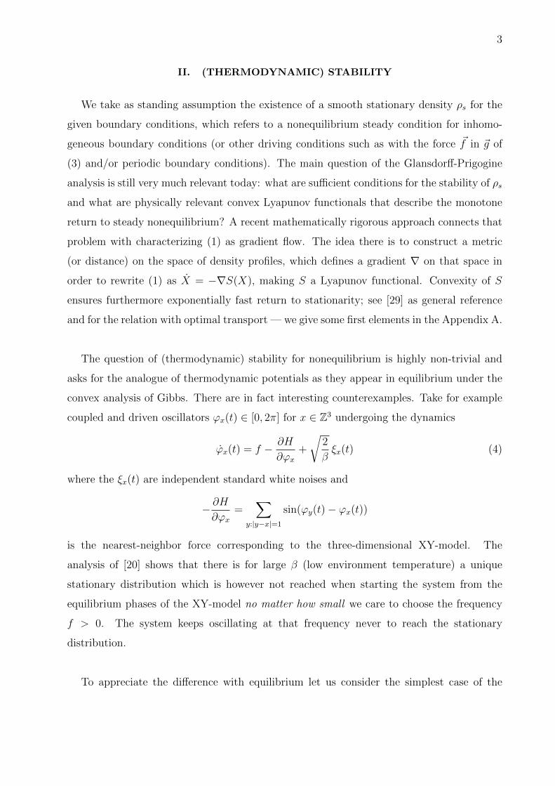
II. (THERMODYNAMIC) STABILITY

We take as standing assumption the existence of a smooth stationary density ρs for the

given boundary conditions, which refers to a nonequilibrium steady condition for inhomo-

geneous boundary conditions (or other driving conditions such as with the force ~f in ~g of

(3) and/or periodic boundary conditions). The main question of the Glansdorff-Prigogine

analysis is still very much relevant today: what are sufficient conditions for the stability of ρs

and what are physically relevant convex Lyapunov functionals that describe the monotone

return to steady nonequilibrium? A recent mathematically rigorous approach connects that

problem with characterizing (1) as gradient flow. The idea there is to construct a metric

(or distance) on the space of density profiles, which defines a gradient ∇ on that space in

order to rewrite (1) as X = −∇S(X), making S a Lyapunov functional. Convexity of S

ensures furthermore exponentially fast return to stationarity; see [29] as general reference

and for the relation with optimal transport — we give some first elements in the Appendix A.

The question of (thermodynamic) stability for nonequilibrium is highly non-trivial and

asks for the analogue of thermodynamic potentials as they appear in equilibrium under the

convex analysis of Gibbs. There are in fact interesting counterexamples. Take for example

coupled and driven oscillators ϕx(t) ∈ [0, 2π] for x ∈ Z3 undergoing the dynamics

ϕx(t) = f − ∂H

∂ϕx+

√2

βξx(t) (4)

where the ξx(t) are independent standard white noises and

− ∂H∂ϕx

=∑

y:|y−x|=1

sin(ϕy(t)− ϕx(t))

is the nearest-neighbor force corresponding to the three-dimensional XY-model. The

analysis of [20] shows that there is for large β (low environment temperature) a unique

stationary distribution which is however not reached when starting the system from the

equilibrium phases of the XY-model no matter how small we care to choose the frequency

f > 0. The system keeps oscillating at that frequency never to reach the stationary

distribution.

To appreciate the difference with equilibrium let us consider the simplest case of the

4

linear heat equation∂

∂tρ(x, t) =

∂2

∂x2ρ(x, t) on x ∈ [0, 1]

with boundary conditions ρ(0, t) = ρ−, ρ(1, t) = ρ+. For equilibrium we require ρ− = ρ+ = m

and then

F [ρ] =

∫ 1

0

dx[ρ(x) log ρ(x)− ρ(x) +m] (5)

is a Lyapunov functional as follows from the calculation

d

dtF [ρt] =

∫ 1

0

dx log(ρ(x, t))∂

∂tρ(x, t)

=

∫ 1

0

dx log(ρ(x, t))∂2

∂x2ρ(x, t)

= −∫ 1

0

dx1

ρ(x, t)

( ∂∂xρ(x, t)

)2 ≤ 0 (6)

where the last equality (partial integration) uses the equilibrium boundary condition;

otherwise (for ρ− 6= ρ+) the monotonicity of F [ρt] in time t generally fails. See more in

Appendix B.

Observe that the functional (5) is an equilibrium free energy corresponding to independent

particles. The computation (6) can be generalized upon considering G as the derivative of

the free energy with respect to the field, δ/δρ(~r)Feq[ρ] = G(ρ(~r)) like the local chemical

potential. One easily checks for (1) with uniform boundary conditions ρ(~r, t) = meq, ~r ∈ ∂V

(and again using partial integration and that ~g ≡ 0) that

Feq[ρ] =

∫d~r

∫ ρ(~r)

meq

dm [G(m)−G(meq)] (7)

(volume integrals are always over V ) is indeed monotone in time under the equilibrium

dynamics:d

dtFeq[ρt] = −

∫d~r ~F (ρ(~r, t)) · χ(ρ(~r, t))~F (ρ(~r, t)) ≤ 0 (8)

The question of thermodynamic stability of macroscopic condition ρs is to find a nonequi-

librium analogue of (8) along the solution of (1), providing in addition fast return to ρs.

5

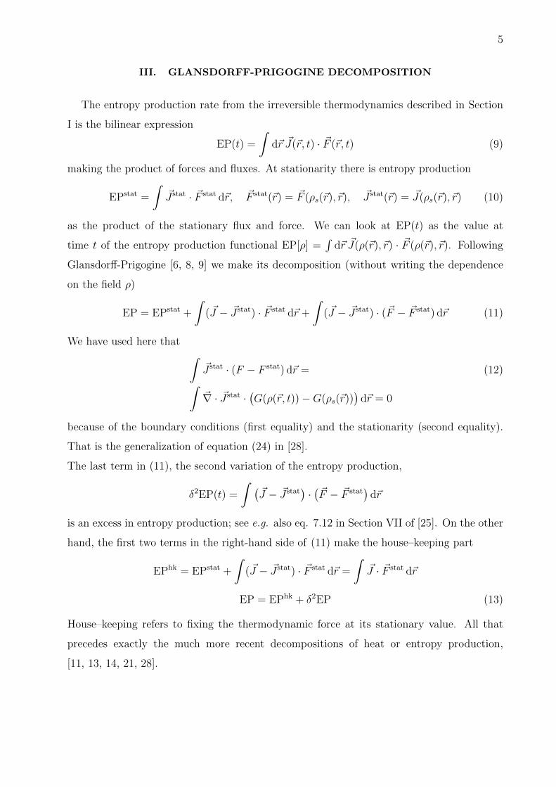
III. GLANSDORFF-PRIGOGINE DECOMPOSITION

The entropy production rate from the irreversible thermodynamics described in Section

I is the bilinear expression

EP(t) =

∫d~r ~J(~r, t) · ~F (~r, t) (9)

making the product of forces and fluxes. At stationarity there is entropy production

EPstat =

∫~J stat · ~F stat d~r, ~F stat(~r) = ~F (ρs(~r), ~r), ~J stat(~r) = ~J(ρs(~r), ~r) (10)

as the product of the stationary flux and force. We can look at EP(t) as the value at

time t of the entropy production functional EP[ρ] =∫

d~r ~J(ρ(~r), ~r) · ~F (ρ(~r), ~r). Following

Glansdorff-Prigogine [6, 8, 9] we make its decomposition (without writing the dependence

on the field ρ)

EP = EPstat +

∫( ~J − ~J stat) · ~F stat d~r +

∫( ~J − ~J stat) · (~F − ~F stat) d~r (11)

We have used here that ∫~J stat · (F − F stat) d~r = (12)∫~∇ · ~J stat ·

(G(ρ(~r, t))−G(ρs(~r))

)d~r = 0

because of the boundary conditions (first equality) and the stationarity (second equality).

That is the generalization of equation (24) in [28].

The last term in (11), the second variation of the entropy production,

δ2EP(t) =

∫ (~J − ~J stat

)·(~F − ~F stat

)d~r

is an excess in entropy production; see e.g. also eq. 7.12 in Section VII of [25]. On the other

hand, the first two terms in the right-hand side of (11) make the house–keeping part

EPhk = EPstat +

∫( ~J − ~J stat) · ~F stat d~r =

∫~J · ~F stat d~r

EP = EPhk + δ2EP (13)

House–keeping refers to fixing the thermodynamic force at its stationary value. All that

precedes exactly the much more recent decompositions of heat or entropy production,

[11, 13, 14, 21, 28].

6

As an aside one should not confuse the above decomposition with the one mentioned in

[10], also under the name of Glansdorff–Prigogine [7], but less interesting for our purposes

(as is also the conclusion in [27]). There one writes

dEP

dt=deFdt

+deJdt

(14)

withdeFdt

=

∫~J · ∂

~F

∂td~r ,

deJdt

=

∫∂ ~J

∂t· ~F d~r (15)

For the time-dependence in eF we have (3) so that

∂ ~F

∂t= −~∇

( ∂∂tG(ρ(~r, t))

)= −~∇

(G′(ρ(~r, t))

∂ρ(~r, t)

∂t

)Therefore,

deFdt

= −∫

~J · ~∇(G′(ρ(~r, t))

∂ρ(~r, t)

∂t

)d~r

= −∫G′(ρ(~r, t))

(∂ρ∂t

)2

d~r ≤ 0

(16)

where the last equality follows from partial integration. Thus, deFdt

, without further physical

meaning, is always non-positive and attains zero if and only if the field becomes stationary.

It is in no way a generalization or an extension of the minimum entropy production principle,

cf. [17]. If however we assume that

~J(ρ(~r, t), ~r) = χ(~r) ~F (ρ(~r, t), ~r)

with χ independent of the field ρ, then

deJdt

=deFdt,

dEP

dt= 2

deFdt≤ 0 (17)

which is a version of the minimum entropy production principle: EP(t) decreases to its

minimum where we find the stationary field. The condition that χ is independent of the

fields amounts to having small gradients, i.e., being close to equilibrium.

IV. EXCESS IS A TIME-DERIVATIVE

The Glansdorff–Prigogine criterion for stability is that δ2EP≥ 0, [8, 9]. We understand

that from observing, [18],

δ2EP(t) = − d

dtG[ρt] (18)

7

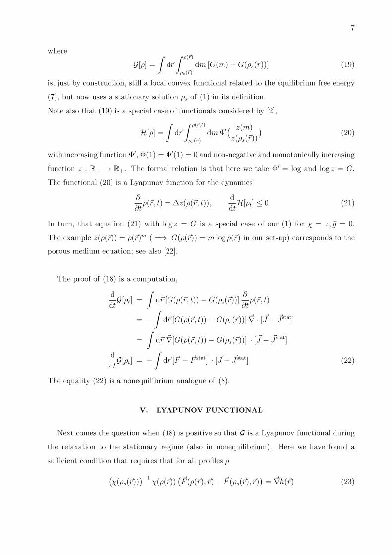
where

G[ρ] =

∫d~r

∫ ρ(~r)

ρs(~r)

dm [G(m)−G(ρs(~r))] (19)

is, just by construction, still a local convex functional related to the equilibrium free energy

(7), but now uses a stationary solution ρs of (1) in its definition.

Note also that (19) is a special case of functionals considered by [2],

H[ρ] =

∫d~r

∫ ρ(~r,t)

ρs(~r)

dmΦ′( z(m)

z(ρs(~r))

)(20)

with increasing function Φ′, Φ(1) = Φ′(1) = 0 and non-negative and monotonically increasing

function z : R+ → R+. The formal relation is that here we take Φ′ = log and log z = G.

The functional (20) is a Lyapunov function for the dynamics

∂

∂tρ(~r, t) = ∆z(ρ(~r, t)),

d

dtH[ρt] ≤ 0 (21)

In turn, that equation (21) with log z = G is a special case of our (1) for χ = z,~g = 0.

The example z(ρ(~r)) = ρ(~r)m ( =⇒ G(ρ(~r)) = m log ρ(~r) in our set-up) corresponds to the

porous medium equation; see also [22].

The proof of (18) is a computation,

d

dtG[ρt] =

∫d~r [G(ρ(~r, t))−G(ρs(~r))]

∂

∂tρ(~r, t)

= −∫

d~r [G(ρ(~r, t))−G(ρs(~r))] ~∇ · [ ~J − ~J stat]

=

∫d~r ~∇[G(ρ(~r, t))−G(ρs(~r))] · [ ~J − ~J stat]

d

dtG[ρt] = −

∫d~r [~F − ~F stat] · [ ~J − ~J stat] (22)

The equality (22) is a nonequilibrium analogue of (8).

V. LYAPUNOV FUNCTIONAL

Next comes the question when (18) is positive so that G is a Lyapunov functional during

the relaxation to the stationary regime (also in nonequilibrium). Here we have found a

sufficient condition that requires that for all profiles ρ(χ(ρs(~r))

)−1χ(ρ(~r))

(~F (ρ(~r), ~r)− ~F (ρs(~r), ~r)

)= ~∇h(~r) (23)

8

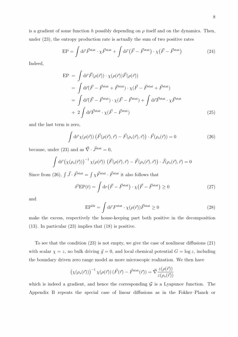
is a gradient of some function h possibly depending on ρ itself and on the dynamics. Then,

under (23), the entropy production rate is actually the sum of two positive rates

EP =

∫d~r ~F stat · χ~F stat +

∫d~r(~F − ~F stat

)· χ(~F − ~F stat

)(24)

Indeed,

EP =

∫d~r ~F (ρ(~r)) · χ(ρ(~r))~F (ρ(~r))

=

∫d~r(~F − ~F stat + ~F stat) · χ(~F − ~F stat + ~F stat)

=

∫d~r(~F − ~F stat) · χ(~F − ~F stat) +

∫d~r ~F stat · χ~F stat

+ 2

∫d~r ~F stat · χ(~F − ~F stat) (25)

and the last term is zero,∫d~r χ(ρ(~r))

(~F (ρ(~r), ~r)− ~F (ρs(~r), ~r)

)· ~F (ρs(~r)) = 0 (26)

because, under (23) and as ~∇ · ~J stat = 0,∫d~r(χ(ρs(~r))

)−1χ(ρ(~r))

(~F (ρ(~r), ~r)− ~F (ρs(~r), ~r)

)· ~J(ρs(~r), ~r) = 0

Since from (26),∫~J · ~F stat =

∫χ~F stat · ~F stat it also follows that

δ2EP(t) =

∫dr(~F − ~F stat

)· χ(~F − ~F stat

)≥ 0 (27)

and

EPhk =

∫d~r F stat · χ(ρ(~r))~F stat ≥ 0 (28)

make the excess, respectively the house-keeping part both positive in the decomposition

(13). In particular (23) implies that (18) is positive.

To see that the condition (23) is not empty, we give the case of nonlinear diffusions (21)

with scalar χ = z, no bulk driving ~g = 0, and local chemical potential G = log z, including

the boundary driven zero range model as more microscopic realization. We then have(χ(ρs(~r))

)−1χ(ρ(~r)) (~F (~r)− ~F stat(~r)) = ~∇ z(ρ(~r))

z(ρs(~r))

which is indeed a gradient, and hence the corresponding G is a Lyapunov function. The

Appendix B repeats the special case of linear diffusions as in the Fokker–Planck or

9

Master equation description where the relationship between the Glansdorff–Prigogine cri-

terion and the monotonicity of the relative entropy has been pointed out first by Schlogl, [24].

In general however, away from equilibrium, there is no a priori reason for (18) or for

(27)–(28) to be non-negative. Similarly, as also reviewed in [30], “the Glansdorff–Prigogine

stability criterion is not necessary, but only sufficient for the local stability of steady states.”

That was earlier discussed in [26] with a general discussion of the Glansdorff–Prigogine

criterion in the light of Lyapunov’s theory. As we review in Section VII there remains

however a nonequilibrium free energy (not necessarily equal to G except for some very

special local equilibrium cases such as the zero range process) which is monotone in time.

As a matter of fact, entropic considerations as too closely related to the Clausius heat

theorem and to the standard entropy production rate of irreversible thermodynamics will be

less relevant for stability far-from-equilibrium, somewhat in the line of [12] writing “that the

second differential of the entropy, which is at the heart of the Glansdorff–Prigogine criterion,

is likely to be relevant for stability questions close to equilibrium only.”

VI. CLAUSIUS HEAT THEOREM

Here we make the dynamics (1) time-dependent, in the sense that the local equilibrium

free energy Feq =∫

d~rΦ(ρ(~r, t), Tt) of (7) depends for example on a time-dependent temper-

ature Tt and that there is a variable control field Ut(~r) vanishing on the boundary, Ut(~r) = 0

for all ~r ∈ ∂V . To be specific, we consider the current in (1) to be now

~J(~r, t) = −χ(ρ(~r, t))~∇( ∂

∂mΦ(ρ(~r, t), Tt) + Ut(~r)

)(29)

where the partial derivative is with respect to the first argument in the local free energy Φ.

We do not have a bulk driving ~g but we assume time-dependent boundary conditions ρ(~r, t)

on ∂V , making a time-dependent boundary chemical potential ∂∂m

Φ(ρ(~r, t), Tt), ~r ∈ ∂V .

Always in the spirit of irreversible thermodynamics there is a balance equation for the

entropy,dStdt

=1

Tt

δQt

dt+ EP(t) (30)

10

where St = −∫∂Φ(ρ(~r, t), Tt)/∂T d~r is the total entropy of the system at time t, δQt

dtis the

total (incoming) heat flux and the entropy production rate is given by

EP(t) =1

Tt

∫~J(~r, t) · χ−1(ρ(~r, t)) ~J(~r, t) d~r ≥ 0 (31)

We refer to [16] for the detailed calculation.

Note that time-integrating (30) is not a good option as there is heat dissipation all the time;

we must renormalize in the way of [13, 14, 21] which in fact follows the Glansdorff–Prigogine

decomposition of Section III:

dStdt

=1

Tt

δQexct

dt+ δ2EP(t) with

1

Tt

δQexct

dt=

1

Tt

δQt

dt− EPhk(t) (32)

Under the Glansdorff–Prigogine criterion δ2EP(t) ≥ 0, integrating (32) directly yields the

Clausius inequality but for the excess heat Qexct :

Sτ − S0 ≥∫ τ

0

1

TtδQexc

t (33)

The equality in (33) is obtained for quasi-stationary time-dependencies by using that δ2EP(t)

is quadratic in the deviation from (instantaneous) stationarity. Again, the stability criterion

δ2EP(t) ≥ 0 (as in (27)) need not be satisfied in general which makes that nonequilibrium

version of the Clausius heat theorem perturbative.

A non-perturbative version (with a modified renormalization) can be obtained along the

lines of [16]. The point is now that EP(t) is a convex quadratic functional of the control

field U for whichδEP(t)

δU(~r)=

2

Tt~∇ · ~J(~r, t) (34)

everywhere in the interior of the volume. Requiring stationarity ~∇ · ~J = 0 for the instan-

taneous field defines a specific profile U∗, for which the entropy production rate is minimal

on the space of all (smooth) fields U , U(~r)|~r∈∂V = 0. We skip further details but we can

thus modify (32) by defining the modified excess heat, removing from the heat its steady

flux corresponding to the reference stationary dynamics under the control field U∗t :

δQmext = δQU

t − δQU∗

t (35)

finally giving rise to a generalized Clausius (in)equality, [16].

11

VII. NONEQUILIBRIUM FREE ENERGIES

Thermodynamics already fails under the microscope. On the other hand statistical me-

chanics renders thermodynamics understandable in more microscopic terms. An early ex-

ample is the macroscopic fluctuation theory of Boltzmann, Planck and Einstein, cf. [4] for

what remains an excellent introduction. Equilibrium free energies appear there as fluctua-

tion functionals for static observables, which allows the understanding of these free energies

both as Lyapunov functions for macroscopic equations (like in (8)) but also as potential for

statistical forces.

What happens in nonequilibrium? Nonequilibrium free energies F are probabilistically de-

fined as the rate functions of static large deviations for the field, defined in the spirit of

Boltzmann’s formula

−F [ρ] = log Prob[ρ] (36)

for a macroscopic profile ρ(~r), ~r ∈ V . The probability is with respect to the stationary dis-

tribution of the locally interacting particle system that creates the profile ρ as a macroscopic

fluctuation while being driven by some time-independent nonconservative forces or by con-

tacts with different external equilibrium reservoirs. When the stationary profile ρs is unique

we must have F [ρs] = 0 while F [ρ] > 0 otherwise, (away from phase coexistence to which we

restrict ourselves). Quite generally there is an associated H-theorem d/dtF [ρt] ≤ 0 for some

good reasons having to do with macroscopic autonomy; see [1–3]. To make the argument of

[3] short, suppose that there is an underlying system of particles with joint configuration at

any time u given by ηu. The macroscopic condition in terms of a density profile is X(ηu), a

particular function (coarse-graining) of the microscopic condition. Writing out (36) in these

terms, by using stationarity,

−F [ρt] = log Prob[X(ηt) ' ρt]

≥ log{Prob[X(ηt) ' ρt|X(ηu) = ρu] Prob[X(ηu) = ρu]}

= −F [ρu] (37)

if we assume for the last equality that Prob[X(ηt) ' ρt|X(ηu) = ρu] ' 1 which is a condition

of macroscopic autonomy for t ≥ u. Conclusion, F [ρt] ≤ F [ρu] when u ≤ t, or F [ρ] is a

Lyapunov function. Note that F does not need to coincide with G of (19) satisfying (18),

but there are cases in which they are equal such as for the zero range model [1, 2]. In fact,

12

there is no reason why ddtF [ρt] has anything to do with the excess entropy production unless

near equilibrium [17, 19], which is another way of understanding the Glansdorff–Prigogine

criterion as just sufficient.

Of course, these nonequilibrium free energies characterize the stationary distribution of the

particle system and hence play a role in specifying the statistical forces on probes that move

on a much slower time-scale than the driven particles [15].

VIII. CONCLUSIONS

The Glansdorff–Prigogine analysis [9] precedes more recently applied decompositions of

the entropy production rate. In particular, the positivity of the excess entropy production

plays an essential role in providing a Lyapunov function for the hydrodynamic evolution

and for obtaining an extended Clausius heat theorem close-to-equilibrium, quite beyond

the treatment in terms of linear diffusions such as the Master equation for reaction

systems. On the other hand, the Glansdorff–Prigogine criterion remains with the local

equilibrium concept of entropy production and need not be satisfied for nonetheless stable

far-from-equilibrium thermodynamics. There convex nonequilibrium free energies appear

from static fluctuation theory, are Lyapunov functions and characterize statistical forces

under time-scale separation. Yet, they do not have a direct interpretation in terms of

entropy production, unless near equilibrium

Acknowledgment I thank the organizers of the Solvay Workshop, P. Gaspard and

C. Van den Broeck, for giving me the opportunity to present our work [18]. It was a special

pleasure to do that in Brussels and with the support of the Solvay Institute, where much of

irreversible thermodynamics was first systematically formulated in the 1940-1970 including

the contributions of Glansdorff and Prigogine that we have revisited in the light of more

recent developments.

13

APPENDIX A: GRADIENT FLOW

The space of macroscopic “values,” such as all the possible mass density profiles in the

volume V , has been called thermodynamic or µ−space and was equipped with extra struc-

ture to serve the purpose. Before the hydrodynamic or thermodynamic limit, the dynamics

is often stochastic to become described by kinetic or hydrodynamic equations in the appro-

priate limit. While considered before, at least since Gibbs found it the appropriate place to

discuss ergodic properties (in contrast with the (microscopic) phase-space), more recently

mathematicians have added metric structure to encode equilibration properties. The point

of departure is adding a distance to the space of profiles to make it into a length space or

Alexandrov space with non-negative curvature. One often calls it the L2−Wasserstein space

W . One then defines gradients ∇ and gradient flows on that space. A major first result was

then to obtain that the gradient flow

∂ν

∂t= −∇S(ν) on W

for the Shannon entropy S(ρd~r) =∫ρ log ρ d~r is given by νt(~r) = ρ(~r, t) d~r where ρ solves

the heat equation ∂ρ∂t

= ∆ρ, [5]. Functional inequalities have been derived e.g. in [23] by

Otto and Villani that resemble the logic and ideas of Glansdorff-Prigogine. In particular,

the convexity of the functional S on W imply equilibration properties of the gradient flow.

For example, a Ricci curvature bound such as Hess S ≥ K implies exponential decay in the

convergence to stationarity with a relaxation time of order 1/K.

APPENDIX B: MASTER EQUATION

The Glansdorff–Prigogine criterion is often used in the case of chemical reactions which

are described in terms of a Markov jump process. Considering independent copies of the

system, the Master equation for the probability density can be considered as a hydrodynamic

equation for the particle density, but of a restricted form

∂

∂tρ(~r, t) + ~∇ · ρ(~r, t)

[~g(~r)− T ~∇ log ρ(~r, t)

]= 0

i.e., for scalar mobility χ(n) = n and with local chemical potential G = T log in (1). In that

case the Glansdorff–Prigogine criterion δ2EP ≥ 0 holds true because (23) is verified, and G

turns out to be the relative entropy which is indeed a Lyapunov function. Assume indeed

14

that χ(ρ(~r)) = D(~r) ρ(~r) > 0 is a scalar proportional to the density and that G = log as for

independent particles; then

χ(ρ(~r))

χ(ρstat(~r))(~F − ~F stat) = ~∇ ρ(~r)

ρstat(~r)(B1)

which realizes (23). That includes the case treated in Section VII (eq. 7.17) of [25]. This

result was first obtained by Schlogl and Schnakenberg [24, 25].

Similarly, the decomposition (13) is analogous (or rather, the generalization) of the Oono-

Paniconi [21] decomposition in terms of excess and house-keeping heat; see also the Hatano-

Sasa “house-keeping heat” as the expectation of formula (16) in [11]. In other contexts it is

the generalization of the “adiabatic rate” of entropy production, e.g. formula (26) in [28] in

the decomposition of Van den Broeck–Esposito.

[1] L. Bertini, A. De Sole, D. Gabrielli, G. Jona-Lasinio, C. Landim, Macroscopic Fluctuation

Theory for Stationary Non-Equilibrium States. J. Stat. Phys. 107, 635–675 (2002).

[2] T. Bodineau, J.L. Lebowitz, C. Mouhot, C. Villani, Lyapunov functionals for boundary-driven

nonlinear drift-diffusions. arXiv:1305.7405 [math.AP].

[3] W. De Roeck, C. Maes and K. Netocny, H-Theorems from Macroscopic Autonomous Equa-

tions. J. Stat. Phys. 123, 571–584 (2006).

[4] A. Einstein, Theorie der Opaleszenz von homogenen Flussigkeiten und Flussigkeitsgemischen

in der Nahe des kritischen Zustandes. Annalen der Physik 33, 1275-1298 (1910).

[5] M. Erbar, The heat equation on manifolds as a gradient flow in the Wasserstein space. Ann.

Inst. H. Poincare Probab. Statist. 46, 1–23 (2010).

[6] P. Glansdorff, G. Nicolis and I. Prigogine, The Thermodynamic Stability Theory of Non-

Equilibrium States. Proc. Nat. Acad. Sci. USA 71, 197–199, (1974).

[7] P. Glansdorff and I. Prigogine, Physica 20, 773 (1954).

[8] P. Glansdorff and I. Prigogine, Non–equilibrium stability theory. Physica 46, 344–366 (1970).

[9] P. Glansdorff and I. Prigogine, Thermodynamic Theory of Structure, Stability, and Fluctua-

tions, Wiley, London (1971).

15

[10] S.R de Groot and P. Mazur, Non-Equilibrium Thermodynamics. Amsterdam: NorthHolland,

1962.

[11] T. Hatano, S.-I. Sasa, Steady-state thermodynamics of Langevin systems. Phys. Rev. Lett.

86, 3463 (2001).

[12] J. Keizer and R. F. Fox, Qualms Regarding the Range of Validity of the Glansdorff-Prigogine

Criterion for Stability of Non-Equilibrium States. Proc. Natl. Acad. Sci. 71, 192-196 (1974).

[13] T. S. Komatsu, N. Nakagawa, S.-I. Sasa, and H. Tasaki: Phys. Rev. Lett. 100, 230602 (2008).

[14] T. S. Komatsu, N. Nakagawa, S.-I. Sasa, and H. Tasaki: J. Stat. Phys. 134, 401 (2009).

[15] C. Maes, On the second fluctuation–dissipation theorem for nonequilibrium baths.

arXiv:1309.3160v1 [cond-mat.stat-mech], to appear in J. Stat. Phys.

[16] C. Maes and K. Netocny, A nonequilibrium extension of the Clausius heat theorem, to appear

in J. Stat. Phys., arXiv:1206.3423v2 [cond-mat.stat-mech] (2013).

[17] C. Maes and K. Netocny, Minimum entropy production principle. Scholarpedia 8(7), 9664

(2013).

[18] C. Maes and K. Netocny, Nonequilibrium free energies in the Glansdorff-Prigogine analysis of

irreversible thermodynamics. In preparation.

[19] C. Maes and K. Netocny and Bram Wynants, Monotonicity of the dynamical activity. J. of

Phys. A: Mathematical and General 45, 455001 (2012).

[20] C. Maes and S. B. Shlosman, Rotating states in driven clock- and XY-models. J. Stat. Phys.

144, 1238-1246 (2011).

[21] Y. Oono and M. Paniconi, Steady State Thermodynamics. Prog. Theor. Phys. Suppl. 130,

29–44 (1998).

[22] F. Otto, The geometry of dissipative evolution equation: the porous medium equation. Comm.

Partial Differential Equations 26, 101-174 (2001).

[23] F. Otto and C. Villani, Generalization of an inequality by Talagrand and links with the

logarithmic Sobolev inequality. J. Funct. Anal. 173, 361-400 (2000).

[24] F. Schlogl, On Stability of Steady States. Z. Phys. 243, 303–310 (1971).

[25] J. Schnakenberg, Network theory of microscopic and macroscopic behavior of master equation

systems. Rev. Mod. Phys. 48, 571–585 (1976).

[26] L. de Sobrino, The Glansdorff-Prigogine thermodynamic stability criterion in the light of

Lyapunov’s theory. J. Theor. Biol. 54(2), 323–333 (1975).

16

[27] H. Tomita, Remarks on Glansdorff and Prigogine’s Theory of Stability. Prog. Theor. Phys.

47, 1052–1054 (1972).

[28] C. Van den Broeck, and M. Esposito, The Three Faces of the Second Law: II. Fokker–Planck

Formulation. Phys. Rev. E 82, 011144 (2010).

[29] C. Villani, Optimal transport, old and new. Lecture notes for the 2005 Saint-Flour summer

school. Springer (2006).

[30] T. Wilhelm and P. Hanggi, What can be stated by the Glansdorff–Prigogine criterion con-

cerning the stability of mass-action kinetic systems? J. Chem. Phys. 110, 6128–6134 (1999).