Revisiting forever gained:Income dynamics in the resettlement

areas of Zimbabwe, 1983-1997

WPS/99-14

Jan Willem Gunning, John Hoddinott, Bill Kinsey and Trudy Owens

March 1999, This version: May 1999

Institutional affiliations: Gunning, University of Oxford and Free University, Amsterdam; Hoddinott,International Food Policy Research Institute; Kinsey, Free University, Amsterdamand University of Zimbabwe; Owens, University of Oxford.

Address for correspodence: John HoddinottInternational Food Policy Research Institute2033 K Street NWWashington DC 20006United States of Americaemail: J.Hoddinott-IFPRI@cgiar.org

Abstract: This paper examines income dynamics for a panel of households resettled on formerwhite-owned farms in the aftermath of Zimbabwe's independence. There are four core findings:(i) there has been an impressive accumulation of assets by these households; (ii) while thisaccumulation has played a role in increases in crop income, increases in returns to these assetshave been especially important in generating the dramatic increase in crop incomes observed inthese households; (iii) differences in initial conditions across these households, such as previousfarming experience, have few persistent effects; and (iv) growth in incomes has been shared acrossall households, with the largest percentage increases in predicted incomes recorded by householdsthat had the lowest predicted incomes at the beginning of the survey.

Funding for data collection under the Rural Household Dynamics Project has been provided in Zimbabwe by1

the British Development Division in Central Africa, UNICEF, and the former Ministry of Lands, Resettlementand Rural Development. Additional support was provided by grants in the United Kingdom from the NuffieldFoundation, the Overseas Development Institute, and the Department for International Development (formerlyODA). Assistance has also been received from the International Food Policy Research Institute, the Food andAgriculture Organization (FAO), the Centre for the Study of African Economies at the University of Oxford,the Free University, Amsterdam, and the Research Board of the University of Zimbabwe.

1

1. Introduction1

Understanding the factors that cause incomes to change over time is important for understandingboth the causes of poverty and for devising appropriate policies to address this poverty. In recentyears, there has been an explosion of interest in this topic, with researchers literally runningmillions of regressions using cross-country data (Salai-i-Martin, 1997). Though interesting, suchanalyses often produce conflicting findings. A well known example is the debate over the impactof various policy, political and institutional factors on long-run average growth in per capita GDP.Levine and Renelt (1992, p. 943) claim that "the cross-country statistical relationships betweenlong-run average growth rates and almost every particular policy indicator considered by theprofession are fragile: small alterations in the 'other' explanatory variables overturn past results."

This paper examines the factors that account for income growth using longitudinalhousehold level data. There are several attractions to such an approach. Conceptually, a coreassumption underlying growth theory - that agents share common technologies - is considerablymore plausible in a rural community than in the case of a cross-country study. The data used herehave been collected, carefully checked, and cleaned by the authors. Consequently, these resultsare less subject to the whims and errors that bedevil national income accounts. Household leveldata more readily lend themselves to consideration of a wide number of econometric concernssuch as endogeneity and the role of unobservables, issue that do not always receive appropriateconsideration in the cross-country growth literature. It is also possible to examine changes in thedistribution of incomes as well as changes in levels.

The data used in this study are drawn from a panel of households resettled on former white-owned farms in the aftermath of Zimbabwe's independence. The paper examines the determinantsof crop incomes in 1982/83 - the first year in which many of these households farmed this newlyacquired land - and compares these results to those derived from data covering the 1995/96agricultural year. There are four core findings: (i) there has been an impressive accumulation ofassets by these households; (ii) while this accumulation has played a role in producing higherlevels of crop income, increases in returns to these assets have been even more important ingenerating the dramatic increase in crop incomes observed in these households. This finding isrobust to a wide variety of econometric concerns; (iii) differences in initial conditions across thesehouseholds, such as previous farming experience, have few persistent effects. Although some ofthese variables affect output in the first year of observation, their impact is virtually non-existentby 1995/96; (iv) growth in incomes has been shared across all households, with the largestpercentage increases in predicted incomes recorded by households that had the lowest predictedincomes at the beginning of the survey.

The paper begins with an introduction to the sample and its characteristics. Section 3outlines the construction of the variables in the study and derives the finding that increases inreturns to assets are the driving factor behind growth in household incomes. Section 4demonstrates that these results are robust to econometric concerns regarding the construction of

2

standard errors, endogeneity, sample selection and fixed, unobserved household characteristics.Section 5 considers the role of initial conditions, while section 6 discusses the distribution of thesechanges across the sample. Section 7 concludes.

2. Background to study(i) Post-independence land resettlement in ZimbabweAccess to land has long been an issue of major economic and political importance in Zimbabwe.Anger at the gross disparities in land ownership between blacks and whites was a major factormotivating armed rebellion against white minority rule. Upon gaining independence, theGovernment of Zimbabwe announced a wide ranging programme of land reform, designed toredress these severe inequalities. A component of the land reform programme was theresettlement of households on farms previously occupied by white commercial farmers. Initially,the supply of land for resettlement was determined by the availability of areas which had beenabandoned during the liberation war and also the general insecurity of European farmers inperipheral areas who were willing to sell. In most cases, these were the commercial farmscontiguous to or generally bordering communal areas.

Criteria for selection into these schemes included: being a refugee or other personsdisplaced by war, including extra-territorial refugees, urban refugees and former inhabitants ofprotected villages; being unemployed; being a landless resident in a communal area or havinginsufficient land to maintain themselves and their families (Kinsey, 1982). At the time ofsettlement, the household heads were also supposed to be married or widowed, aged 25 to 50 andnot in formal employment. Families selected for resettlement were assigned to these schemes, andthe nucleated villages within them, largely on a random basis. Generally, these criteria seem tohave been followed. In this sample, some 90% of households settled in the early 1980s had beenadversely affected by the war for independence in some form or another. Before being resettled,most (66%) had been peasant farmers with the remainder being landless laborers on commercialfarms, workers in the rural informal sector or wage earners in the urban sector.

Individuals settled on these schemes were required to renounce any claim to land elsewherein Zimbabwe. They were not given ownership of the land on which they were settled but insteadwere given permits covering occupancy of homes and for cultivation. Each household wasallocated 5 hectares of arable land for cultivation, with the remaining area in each resettlement sitebeing devoted to communal grazing land. Households were also allocated a residential plot withina planned village. In return for this allocation of land, the Zimbabwean government expected maleheads of households to be farmers. Until 1992, male household heads were not permitted to workon other farms, nor could they migrate to cities, leaving their wives to work these plots. Althoughthis restriction has been relaxed, with male heads being allowed to work off farm (provided thathousehold farm production is judged satisfactory by local government officials), in this sampleagriculture continues to account for at least 80 per cent of household income in non-droughtyears.

(ii) The sampleOver the period, 1982-84, one of the authors (Kinsey) undertook a survey of approximately 400resettled households. The initial sampling frame was all resettlement schemes established in thefirst two years of the programme in Zimbabwe's three agriculturally most important agro-climaticzones. These are Natural Regions II, III and IV and correspond to areas of moderately high,moderate and restricted agricultural potential. One scheme was selected randomly from eachzone: Mupfurudzi in Mashonaland Central (which lies to the north of Harare in NRII), Sengezi

3

in Mashonaland East (which lies south east of Harare in NRIII) and Mutanda in Manicaland(which lies south east of Harare, but farther away than Sengezi and in NRIV). Random samplingwas then used to select villages within schemes, and in each selected village, an attempt was madeto cover all selected households.

These households were first interviewed over the period July-September 1983 to January-March 1984. They are located in 20 different villages (Two additional villages were added to thesample in 1993). Just over half (57%) are found in Mupfurudzi with 18% located in Mutanda and25% found in Sengezi. They were re-interviewed in the first quarter of 1987 and annually, duringJanuary to April, from 1992 to 1998. There is remarkably little sample attrition. Approximately90% of households interviewed in 1983/84 were re-interviewed in 1997. There is no systematicpattern to the few households that drop out. Some were inadvertently dropped during the re-surveys, a few disintegrated (such as those where all adults died) and a small number were evictedby government officials responsible for overseeing these schemes.

Table 1 provides some descriptive statistics for this sample. (The construction of thesevariables is outlined in the next section.) In real terms, gross crop income rises by just under 200per cent between 1982/83 and 1995/96. Although households increase significantly in size, theincrease in per capita gross incomes, approximately 160 per cent, is impressive in the context ofa country in which per capita incomes have been stagnant since 1980. Table 1 also makes clearthat rainfall levels were considerably lower in 1982/83 than they were in 1995/96. The formerwas a drought year, whereas the latter was one of slightly above average rainfall.

Four questions follow. First, to what extent is the difference in incomes between theseyears is a consequence of differences in rainfall levels? Second, once the rainfall factor is takeninto account, what factors explain any remaining changes in crop income. Third, do these incomegains accrue to all households or do these data merely capture enormous gains made by a luckyfew. Fourth, these comparisons are based on gross crop income. Is it legitimate to makeinferences about changes in living standards based on a single component of household income(and one that does not even take into account input costs in crop production)?

A partial answer is provided by other data found in Table 1. It is noteworthy that the stockof capital assets used in crop production, agricultural tools and trained oxen, rise significantly overthis period. Livestock holdings, which play an important buffering role during droughts (Kinsey,Burger and Gunning, 1997) also rise significantly. These increases suggest that the increase inper capita gross crop incomes is not driven solely by rainfall considerations, since it is implausiblethat they could have occurred in the absence of increases in incomes. The fact that virtually allhouseholds now own some livestock is suggestive of broadly distributed gains in wealth. To theextent that capital stock is a proxy for permanent income, and permanent income has somerelation to consumption, these data also are consistent with an increase in household consumptionlevels. That said, it is clearly desirable to move beyond suggestive findings. The next sectionsof this paper address these questions more systematically.

3. Understanding the causes of changes in incomeThis section uses multi-variate analysis to examine the determinants of gross crop incomes andcauses of changes in these incomes over time. Denoting Y to be crop income, explanatoryvariables to be X and parameter estimates, b, the determinants of crop income for the agriculturalyear October 1982 - June 1983 (denoted as "1983") and July 1995 - June 1996 (denoted as"1996"), e to be the disturbance term, yields for the ith household:

Y = b ' @ X + e (1)1983, i 1983, i 1983, i1983, i

Y = b ' @ X + e (2)1996, i 1996, i 1996, i1996, i

4

Analysis begins with a description of the variables that comprise Y and X, before turningto the results of estimating (1) and (2).

(i) Variable constructionIn order to compare the estimates obtained from these regressions, the dependent and independentvariables need to be identical. The 1982/83 survey round contained data on the following: grossrevenues from crop production; the stock of agricultural tools; land used in agriculturalproduction; labor input, as measured by the number of people in the household between the agesof 15 and 64; the number of pairs of oxen owned by the household; the number of extension visitsthe household receives ; and rainfall, by resettlement scheme. All monetary figures are expressedin 1992 Zimbabwe dollars using the CPI as a deflator.

Gross revenues from crop production are calculated by multiplying the physical quantitiesof output multiplied by their unit price. During each interview, households were asked to reportyield, sales and retention, for each crop, for the previous harvest. Unit prices were calculated foreach household by dividing total sales value by the quantity sold. Where a household did not sellany of the crop, its total yield was multiplied by the median price received by farmers in thissample. Unfortunately, the data for the 1982/83 agricultural year do not contain any informationon the costs of inputs such as hired labor and purchased fertilizer and pesticides. This precludesestimates based on net crop income.

There are eight variables that comprise X: the log real value of agricultural tools; logavailable household adult labour; log land used in crop production; the number of ox teams ownedby the household; three extension dummies; and rainfall.

Agricultural tools include ox-ploughs, ox carts, cultivator/harrows, ox-planters, water carts,cotton sprayers, wheelbarrows, tractors and tractor equipment, hoes, axes, spades, machetes andslashers. Valuation of these items is a non-trivial exercise. Throughout the years in which thesehouseholds have been surveyed, respondents have been asked about what items they owned, whenthey were obtained, how much they paid for them, and how much they would cost today.Answers to these questions revealed two problems. First, a number of households did notremember, and therefore could not report, what they had paid for the item. Second, the pricesof virtually identical items were highly variable between households, perhaps due to problems ofrecall or differences in knowledge regarding current prices. Rather than allowing the price ofcapital goods to vary across households, a uniform price is imposed. Specifically, the medianpurchase prices of items both acquired and reported for the crop year 1995/96 were used as abase. (These are assumed to suffer fewer recall problems.) These were deflated using theconsumer price index to derive prices for other survey years, including those used here.

This approach does not take into account depreciation. It could be argued that wear andtear on assets reduces their value. Accordingly, depreciation should be deducted from grossinvestment in order to calculate the increase in capital which is relevant to explaining increasesin output. Alternatively, as argued by Scott (1991), a machine that produces the same quantityof output ceteris paribus, year-in year-out cannot be said to have experienced any depreciation.He argues that capital only depreciates when it becomes obsolete. For this reason, he argues thatcapital stock should be measured in gross terms, not net of depreciation. This argument reflectsthe situation facing households in the sample. Due to the nature of asset ownership within thesample it would lead to a gross underestimate of the level of capital stock if these items weredepreciated. Many households own and still use equipment handed down from previousgenerations. For example, in 1982/83 over 50 percent of households owned and used an ox-plough which was over 10 years old (11 percent of households owned an ox-plough over 30 years

5

old). Therefore to measure the effect of capital these circumstances the appropriate measure ofcapital stock is a gross figure, and not a net figure.

The ideal measure of labor usage would be days worked, by person and activity.Unfortunately, this measure is not available for either of the survey years used here. As a crudeproxy, available family labor supply - defined as the number of people in the household betweenthe ages of 15 and 64 - is used. A related input, ownership of pairs of oxen, is included. Pairsof oxen permit fields to be prepared faster using a plough than by the alternative, individuals usinghoes. They also allow farmers to improve the timing of planting, by ensuring that fields will beprepared in advance of the early season rains and they typically make it possible to break up thesoil to a greater depth.

Visits by extension workers are captured via the inclusion of three dummy variables. Theseare additive in the sense that 'receives at least two extension visits' dummy captures the marginaleffect of a second visit, conditional on the household having received one visit. Finally, levels ofrainfall recorded at the nearest station are included as a regressor. There is one rainfallobservation per settlement scheme.

A final comment is in order. The rather limited information available for the 1982/83agricultural year places restrictions on the extent of this analysis. The absence of data on cropinputs restricts analysis to the determinants of gross, rather than net crop income. It is also makesit impossible to estimate profit functions. Further, detailed data on other sources of income arenot available for 1982/83 either. In light of this, it is helpful to consider the validity of gross cropincome as a measure of the level of household welfare.

With respect to the 1982/83 agricultural year, respondents were asked to rank sources ofincome in terms of their contribution to total household income. Approximately 80 per cent ofhouseholds ranked agriculture as the most important source of income, a figure that rises to 93per cent in the 1985/86 (non-drought) agricultural year. In the case of the 1995/96 data, it ispossible to construct a Spearman correlation coefficient that looks at households ranked by bothgross crop income and total income (gross crop income less input costs plus net income fromwage labor, remittances, gifts and other non-agricultural activities). The coefficient equals 0.90,and rises to 0.96 if we exclude 17 households experiencing the largest change in rank order. Collectively, these data suggest that gross crop income is a good proxy for total householdincome.

(ii) Basic resultsThere are 396 households in the survey that covers the 1982/83 agricultural year. Largely as aconsequence of the drought, 85 do not report any income from crop production. In addition,there is no data on capital stock for 23 households and on household size for 2 households,yielding a sample size of 286 for this year. There are 396 households in the surveys that capturethe 1995/96 agricultural year, of which 2 report no crop income, giving a sample size of 394.These samples are used to generate the results reported below. The obvious selectivity issues arediscussed below.

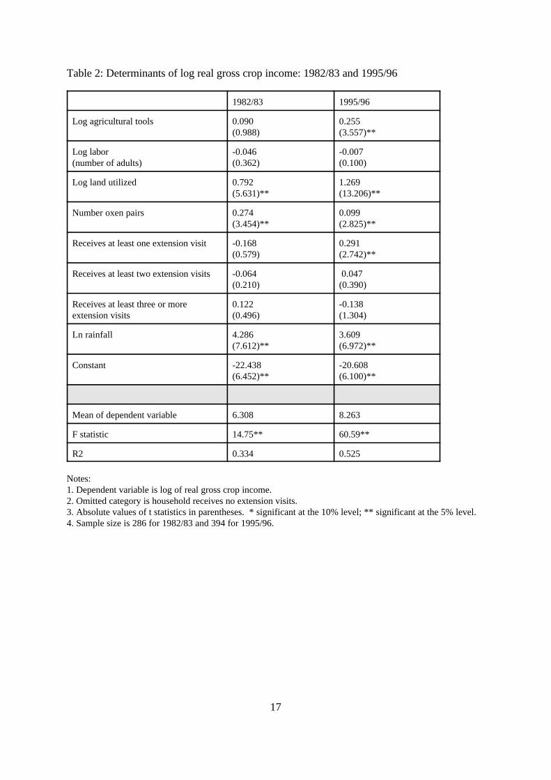
Table 2 presents the estimates of equations (1) and (2) for all households reporting grosscrop revenues greater than zero. The dependent variable, together with capital stock, land, laborand rainfall are all in log terms. Standard errors are corrected for heteroscedasticity using themethod outlined by Huber (1967) and popularized by White (1980).

The mean of the dependent variable, in log terms, rises from 6.308 to 8.263. Recall that the difference in2

logs is approximately equal to the percentage change in value.

A natural interpretation of the labour coefficient in Table 2 is that increasing the family labour force has no3

impact on output - suggesting a situation of 'surplus labour' for these households. Such a finding sits uneasilybeside the fact that few households cultivate all five hectares in any given agricultural year and some complainof labour shortages. However, this 'natural interpretation' is incorrect. Increasing family labour supply has astrong, positive and statistically significant effect on the amount of land these households employ (resultsavailable on request). Two observations follow. The correct interpretation of the labour coefficient is that ithas no effect on output, conditioning on the other regressors. Put another (slightly inaccurately) way, familylabour supply raises output by increasing the amount of land cultivated, but does not have an impact over andabove this. Second, if these households faced well functioning labour markets, there should be no relationshipbetween potential household labour supply and the amount of land used by the household. The fact that such arelationship is observed suggests that such an assumption regarding labour markets is unwarranted here. (Ourthanks to Duncan Thomas who first alerted us to this point.)

There is an intriguing explanation for the decline in the coefficient on trained oxen. Just like people, oxen4

'learn by doing'. Over time, they become used to the commands of the individual leading them and learn whatis required of them. In this sample, as households have accumulated additional oxen, their average age hasdeclined. Consequently, one would expect productivity to fall, precisely what is observed here. (Our thanks toChris Scott who suggested this interpretation.)

6

In real terms, the value of gross production increases by just under 200 per cent. The2

returns to agricultural tools rise by a factor of three. Returns to land increase by about 60 percent. The quantity of household labour available has no statistically significant effect on grosscrop output, controlling for other factors of production. By contrast, although the stock of pairs3

of trained oxen has risen, the impact of this is offset by a reduction in returns to oxen ownership.4

In the first survey round, virtually every household receives at least one visit from an agriculturalextension officer but relative to the few households receiving no visit, this has no effect on output.In 1994-95, extension coverage is much poorer, but receipt of one visit is associated with anincrease in the real value of crop output by 29 per cent. Reassuringly, there is a positive and wellmeasured relationship between rainfall and the value of crop production. Also note that thepredictive power of the model is considerably better for the 1995/96 sample and the parameterstend to be estimated with greater precision.

(iii) Decomposing the causes of changes in incomeAs already noted, rainfall was considerably lower in 1982/83, by about 45 per cent for thehouseholds in this sample. Given the strong relationship between rainfall and output, thisundoubtedly accounts for some of the observed change in incomes. However, given the largechanges in the values of other variables, and the observed changes in the parameter estimates, itwould be useful to separate out the impact of these changes.

Recall that multiplying the coefficients by the means of the explanatory variables generatesthe mean of the dependent variable. Denote means of the dependent variable as ™, 00 as a vectorof means of right hand side variables, and b as a vector of parameter estimates. Accordingly:

ô = b ' @ 0 (3)1983 1983 1983

ô = b ' @ 0 (4)1996 1996 1996

As Neumark (1988) and others have noted, equations (3) and (4) can be manipulated toyield:

Oaxaca and Ransom (1999) issue a cautionary note regarding the contributions of individual variables to the5

wage decomposition. They note that where several sets of dummy variables are employed, the detailed resultsof the decomposition will be sensitive to the omitted group. Although their argument is correct, and applies toboth dummy and slope parameters, the impact of their critique here is minimized by: a) the presence of onlyone set of dummy variables in these regressions (see Oaxaca and Ransom, 1999, p. 156); and b) their ownfinding that in the absence of affine transformations of continuous variables, the role played by these variablesis invariant to the choice of the omitted group.

7

ô - ô = ( 0 - 0 )' @ b + (b - b ) @ 0 ' (5)1996 1983 1996 1983 1996 1996 1983 1983

Equation (5) shows that the difference between mean gross crop incomes in 1982/83 and1995/96 equals changes in the level of income generating assets (the first term) multiplied by thereturn to these assets in 1982/83 plus changes in returns to these assets multiplied by their levelin 1982/83 (the second term). Put crudely, the first term captures the collective impact of changesin the accumulation of factors of production whereas the second term captures changes in theproductivity of inputs. This is commonly referred to as an Oaxaca decomposition (Oaxaca, 1973).However, note that equations (3) and (4) can also be manipulated to yield:

ô - ô = ( 0 - 0 )' @ b + (b - b ) @ 0 ' (6)1996 1983 1996 1983 1983 1996 1983 1996

Although conceptually equation (6) looks similar to equation (5), there is no guarantee thatit will produce the same results. Following standard practice, both (5) and (6) are used in theresults reported below.

Results are reported in Table 3. Note that using either decomposition method yieldsbroadly similar findings. Also note that looking only at the last row, which reports the sums ofthe impact of changes in endowments and changes in returns to endowments, suggests thatchanges in levels of the regressors are the principal cause of increased crop incomes. But a morecareful examination reveals that this finding is generated entirely by the rainfall and constantterms. Abstracting from the role played by rainfall, it is changes in returns to assets (columns (B)and (D)) - especially those associated with agricultural tools and land - that account for much ofthe change in gross crop income.5

It is worth commenting on the factors that may have led to this increase in returns to assets,particularly tools and land. There are a number of possibilities. First, there is entry by a numberof households into the production of higher-value crops such as cotton, groundnuts, andsunflowers. Second, there has been a cumulative capitalization of labor into improving the land.Much of the arable land allocated to the settlers in the early 1980s had lain uncultivated for manyyears. Given that settlement often occurred just a short period before households would have hadto plant their first crops, land thus had to be cleared quickly initially. Inevitably this meant partialclearing was the norm, and very little stumping was done. Without full clearing and thoroughstumping, ox-plowing cannot be done efficiently. Fields have been progressively cleared andstumped over the years. In addition, there has been ongoing investments in soil conservation andwater control and retention measures. Third, the quality of tools is increasing, as is farmers'knowledge regarding their use. One example of this is the cotton sprayer, designed to sprayinsecticide to control bollworms. However, farmers are increasingly using the cotton sprayers toapply pre-emergence herbicide and thus achieving significant labor savings for weeding. A secondexample pertains to the use of ox-drawn ploughs. In the early 1980s, it was not uncommon tosee three people working with an ox team and plough: one handling the plough; one leading the

8

team with a rope; and the third walking alongside with a whip exhorting the oxen to behave anddo what is wanted. Fifteen years later, one sees a single man ploughing by himself and controllingthe animals entirely through whistles and voice commands. More generally, it is entirely likelythat these households have acquired significant 'learning-by doing.' The land these householdssettled on in the early 1980s was entirely unfamiliar to them. Over time, they will have learntwhat crops grow best on which plots, the appropriate methods for growing new crops and so on.

4. How robust are these results?This section considers the finding that increases in gross crop incomes are largely driven byincreases in returns to factors of production in light of a number of econometric concerns:calculation of standard errors; endogeneity of right hand side regressors; the role of unobserved,time invariant characteristics; and selectivity issues.

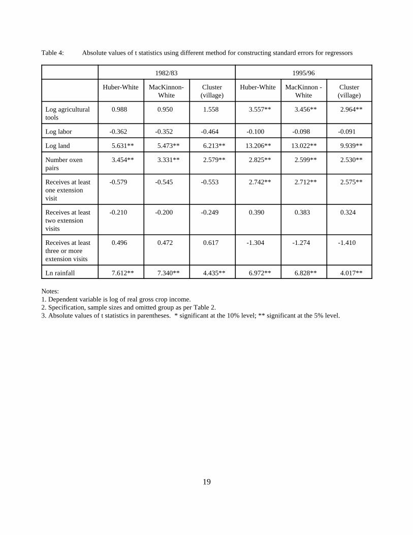
(i) Alternative standard error calculationsThe variance-covariance matrix used to generate the standard errors and t statistics reported inTable 2 uses Huber-White's well-known weighting matrix. However, it has been argued that theseestimates can be adversely affected by a small number of outliers in the weighting matrix. Thomas(1994) argues that this can lead, on occasion, to dramatically understating standard errors andtherefore overstating levels of significance. Deaton (1997) point to a second area of concern.Households in the same village and the same settlement scheme will share some commoncharacteristics. In a statistical sense, therefore, the household level disturbance terms are notindependent.

Table 4 presents three estimates of coefficents' standard errors (reported in terms of theabsolute values of their asymptotic t statistics). The first columns of both the 1982/83 and1995/96 results repeat those results found in Table 2. The second columns report the absolutevalues of asymptotic t statistics based on the variance-covariance matrix outlined by Mackinnonand White (1985) which is robust in the presence of leverage points. The third columns, basedon Rogers (1993) calculates robust standard errors in the presence of intra-cluster correlation atthe village level. Two findings emerge. First, the more conservative estimates produced usingthe MacKinnon-White method produce very small changes in the t statistics. They do not changethe results reported in Table 2 at conventional significance levels. Accounting for the clusterednature of the data does not alter in any substantive way, the household level coefficients. Notsurprisingly, the t statistic on rainfall falls by dramatically, by about 50 per cent, but remainsstatistically significant.

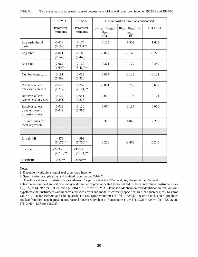
(ii) Two stage least squares resultsA striking feature of the results reported in Table 2 is the relatively large coefficient on the landvariable. One could make the argument that this a consequence of a failure to recognize that forthese households, the amount of land farmed in any one year is a choice variable. (The sameargument does not hold for tools, pairs of oxen and the number of adults resident in thehousehold, which all can be regarded as fixed in the short term.) Since the increase in returns toland is a major factor in the increase in gross crop incomes, this critique represents an importantchallenge to this core finding.

The standard econometric fix to endogeneity concerns is two stage least squares estimation.Its successful application requires: (i) that the instruments be relevant, in the sense that they arecorrelated with the endogenous variable; and (ii) that the instruments are uncorrelated with thedisturbance terms in the structural regression. In the case considered here, it is difficult to think

Further details are available on request.6

The decomposition based on (6) yields almost identical results.7

9

of a variable that would affect the household's use of land, but not affect output. Consequently,the approach taken here was to undertake a somewhat mechanistic search of possible correlatesof land use. In the 1995/96 data, the number of plots available to the household and the soils onthese plots being clay were found to be significant predictors of land. The F statistic testing thehypothesis that these regressors in the first stage regression are jointly zero equals 14.59, a figurecomfortably above the rule of thumb threshold of 10 established by Bound, Jaeger and Baker(1995). These variables also satisfy the over-identification test proposed by Davidson-MacKinnon(1993) on the joint hypothesis that the instruments are uncorrelated with the errors and that thesecond stage regression is correctly specified.

Based on this finding, these two variables are used as instruments for land and equations(1) and (2) are re-estimated. The results are reported in Table 6. There are three notablefeatures. First, these variables are good instruments for the 1995/96 sample, but not for 1982/83(see note 4 for the test statistics). In fact, it proved impossible to find any variables that satisfiedstandard criteria for instruments for the 1982/83 round. Second, the impact of instrumenting isto increase the parameter estimates for land in both years, rendering the returns almost equal. Buttwo stage least squares estimation changes the values of all parameters, not just those on theinstrumented variable. Third, the decomposition of the change in income reveals precisely thesame pattern uncovered in Table 3. The change in income over this period is largely due tochanges in returns to assets. The effect of controlling, albeit imperfectly, for the endogeneity ofthe land variable is to alter the contributions of various variables to this finding - with increasingreturns to agricultural tools now playing a much more important role - but not to overturn thisresult.

(iii) Selectivity issuesThe sample used to generate the parameter estimates reported in Table 2 is restricted to thosehouseholds for whom data are available on the dependent variable and on the regressors. Asnoted, this results in a dramatic reduction in the sample covering the 1982/83 agricultural year.Households reporting zero crop incomes in 1982/83 have, on average, lower levels of capitalstock in the form of agricultural tools, utilized less land and have fewer adults. The differencesin the mean values for these variables are statistically significant. As the households reporting6

zero gross crop incomes are a non-random sub-sample of the survey, the parameter estimatesreported above are likely to be biased. Standard econometric 'fixes' to selectivity problems, suchas the method suggested by Heckman (1979), are not promising solutions. It is difficult to thinkof variables that affect the likelihood of obtaining crop output, but do not affect the level of thatoutput. Further the vast literature on selectivity biases increasingly emphasizes how parameterresults can be especially sensitive to the selectivity fix.

Accordingly, the approach taken here is to consider the sub-sample of households reportingin both rounds, gross crop income greater than zero in both rounds and data on all regressors.This modestly reduces the sample size for 1982/83 from 284 to 267. The reduction in sample sizeis more dramatic for the 1995/96 round, with the sample size falling from 394 to 267. Table 6reports the results of the parameter estimates for these sub-samples, together with variable meansand the decomposition based on equation (5). As in Table 2, standard errors and hence t7

statistics are computed using the Huber-White method. The alternative methods described above

10

yield similar results. Not surprisingly, the 1982/83 results differ little from those reported above.The 1995/96 results indicate that for this sub-sample, returns to agricultural tools are lower thanthey are for the full sample, but this effect is somewhat offset by higher returns to land and trainedoxen. The decomposition reveals exactly the same pattern reported in Table 3. Abstracting fromthe impact of rainfall and the intercept terms, only 19.2% of the difference in mean crop incomesare attributable to differences in levels of assets. Crop income growth is largely attributable toincreased returns to these assets. Selectivity concerns do not alter this core finding.

(iv) The role of fixed, unobservable characteristicsA final econometric concern is that these parameter estimates may be biased by the exclusion offixed, unobserved characteristics that affect farm production. For example, more skillful farmersmay be able to bring more land into production in a given time period or may have better accessto agricultural extension workers. The sub-sample of households who appear in both surveyrounds are an appropriate group to consider this issue. As before, the dependent variable is grosscrop income. Regressors are those described above, together with terms capturing the interactionbetween these explanatory variables and a dummy equaling one if the observation is drawn fromthe 1982/83 survey round. These interaction terms are included to capture the change in returnsto assets that has already been noted. The prior expectation is that these should be negative fortools, land and extension and positive for trained oxen, reflecting the pattern described above.The pooled sample is estimated using ordinary least squares with no account taken of the role ofunobservables, random effects and household fixed effects.

In order to save space, full results are not reported here. (These are available on request.)In brief, a Breusch-Pagan test comparing random effects against an OLS model with no accounttaken of household level unobservables produces a chi-squared statistic with a prob value of only0.27. A Hausman test, comparing the random and fixed effects estimates produces a chi squaredstatistic with a prob value of only 0.32. The F statistic on the household level unobservables hasa prob value of 0.093. At conventional significance levels, it appears that the null hypothesis, thatthese results are not affected by household level unobservables, cannot be rejected. Further, allinteraction terms have their predicted signs, with the coefficients on the land and 'at least oneextension visit' interaction terms significantly different from zero. Recall from Table 3 that thesevariables accounted for about 75 per cent of the difference in mean incomes attributable to factorsother than rainfall. Hence, concerns regarding the role of fixed, unobserved householdcharacteristics do not appear to alter the core results found so far.

5. The role of initial conditionsThe results reported thus far take no account of significant differences in other characteristics atthe time of resettlement. For example, about 40 per cent of household heads had less than fouryears of schooling and about 38 per cent had never been visited by an extension worker. Yet, onemight believe such factors to be important. To the extent that they are relevant determinants ofcrop income, their omission suggests that are results are vulnerable to concerns regarding omittedvariable bias. The large literature on the determinants of cross-country growth stresses that morefavourable initial conditions, in terms of say human or social capital, allows countries to maintainhigher rates of growth over time. Further, suppose that initial conditions are an important,persistent determinant of crop incomes. This would suggest that the distribution of incomes overtime would become increasingly unequal as advantaged households would experience more rapidincreases in incomes, thus producing a increasingly unequal distribution of incomes over time.

11

Denoting fixed initial conditions as Z , their associated parameter estimates as z , and1984

suppressing the i subscript, equations (1) and (2) can be re-written as:

Y = b ' @ X + z ' @ Z + e (1')1984 1984 1984 19841984 1984

andY = b ' @ X + z ' @ Z +e (2')1996 1996 1984 19961996 1996

Table 7 reports the results of including selected initial conditions to equations (1) and (2).These are divided into three categories: initial human capital (years of education of householdhead; household head did 'skilled' work prior to being resettled; household received at least oneextension visit prior to being resettled); location (lived in protected village; lived in town; livedin communal area); and social capital (at least one household member belonged to a politicalorganization). Before discussing the results of these regressors, it is helpful to note the largenumber of variables that were included in preliminary runs, but failed to have any explanatorypower. Those relating to human capital included: dummy variables reflecting different levels ofschooling attainment by the head; average education levels of all household members excludingthe head; and dummy variables reflecting different average household schooling attainment levels.Dummy variables were created describing the activities the household head was engaged inimmediately prior to becoming a settler including: whether the head was farming; working as askilled agricultural worker; a skilled manual laborer; an unskilled laborer; a clerk; involved indomestic service; or serving in the army. Dummies were also tried for the condition that the household was in at the end of the war, these included: whether thehead was unemployed; had house or crops destroyed; cattle killed or stolen; or reported ‘not much affected’. Other variables relating to the social relationships that did not haveexplanatory power were dummies created for the type of organization that households belongedto including: farmers organizations; specialist groups for example, a youth or woman’s group; andlocal or national political organizations. Other variables included a measure of attendance ingroups, whether anyone in the household held an office, and the perceived benefits of belongingto such organizations. Participation in organizations in the area of origin was also considered.Finally, a set of variables was created to reflect whether the household had come with otherfamilies from the same home area, if so, whether they lived nearby, or helped each other. Noneof these proved to be significant.

Table 7 indicates that the parameter estimates on tools, land, labour, oxen and extensionare close to those reported in Table 2, suggesting that the core results are not contaminated bythe omission of these variables. Further, a number of initial condition variables that are significantin 1982/83, such as previously doing skilled work, having previously received extension adviceand having come from a town, have no statistically significant impact on incomes in 1995/96.This suggests that households advantaged in some regard at the time of resettlement initiallyobtain higher incomes, but this effect disappears over time.

There is one striking exception. Households who lived in a 'protected village' during thewar for independence obtained higher incomes both in 1982/83 and 1995/96. Protected villageswere a creation of the white minority government during the war for independence. In areaswhere armed conflict was most prevalent, individual households were forcibly relocated from theirhomesteads to central sites, referred to as "keeps". Individuals were permitted to venture fromthese areas during the day but were required to return to these localities before nightfall. It iswidely acknowledged that the dislocation and repression associated with this forced relocation

A logical extension to this hypothesis would be that those who suffered most during the war were favoured in8

the resettlement process in terms of the amount or quality of land that they received. This is unlikely to becorrect. Both arable and residential plots were allocated through random draws specifically to avoid anychance of favouritism.

As there is only one observation on rainfall per resettlement scheme, it is not possible to include both rainfall9

and scheme dummies in the same model.

12

made living in these protected villages a deeply unpleasant experience but one that may have alsofostered a breakdown in traditional values and compelled education and cooperation.

The impact of having lived in a protected village prior to resettlement on gross cropincomes is large, raising them by more than 40 per cent in both years. One possibility is that thisvariable is capturing some other factor correlated with this characteristic. In particular, allhouseholds reporting having lived in a protected village prior to resettlement are located inMupfurudzi, agro-climatically the area best suited to agriculture. In regressions not reported8

here, these initial conditions variables were re-estimated with the rainfall variable replaced withdummy variables for resettlement schemes. The coefficients on the protected village variables9

fall by about 50 per cent in magnitude and is no longer significant in the 1982/83 sample.However, it retains some explanatory power in the 1995/96 data, with a t statistic of 1.89. Thissuggests that this variable is picking up something more than a pure location effect. It may be thatthis shared experience generated a sense of cohesiveness and common purpose consistent withthe more general notion of social capital.

6. Income changes and changes in povertyA fundamental finding of this study, robust to a number of econometric concerns, is thatsignificant income growth has occurred in these resettlement households even after the droughtconditions of the early 1980s have been taken into account. An important factor in this processhas been improved returns to factors of production. However, there can be no presumption thatthese income gains necessarily translate into reductions in poverty as measured in terms ofconsumption. It might be the case that the largest gains are concentrated amongst a few better-offhouseholds. Gross crop income may be a poor correlate of total household income. Finally, thecorrelation between incomes and consumption may be weak.

An ideal way of examining this issue would be to utilize consumption data for both periods,and after taking into account the impact of the drought in the early 1980s, looking at the incidenceand severity of poverty. Unfortunately such data are not available. There are, however, a numberof inferential points that can be made.

Figure 1 graphs kernel density estimates obtained using an Epanechnikov kernel andoptimal bandwidth. Deaton (1997) describes this technique in detail. Put rather crudely, Figure1 shows the distribution of the log of real per capita gross crop income. The curves can bethought of as histograms in which the 'width' of each bars is narrowed and their tops joinedtogether. The horizontal axis gives the value of this variable, the vertical axis the percentage ofhouseholds to which that value applies. It shows a dramatic rightward shift in the levels of logreal per capita crop incomes, even after excluding the many households in the 1982/83 samplewho reported zero crop income. The distribution also becomes more noticeably peaked,suggesting that crop income inequality is diminishing. Estimated Gini coefficients support thisinterpretation, falling from 0.58 in 1982/83 to 0.49 is 1995/96. But one could argue that this

13

shift is driven by the drought conditions of the early 1980s that were not present in the goodrainfall year of 1995/96.

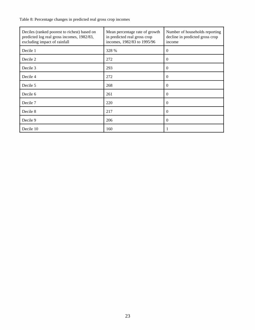
Table 8 takes this possibility into account. Based on the regression coefficients reportedin Table 2, gross crop incomes are predicted for each household for both years, excluding theimpact of rainfall and the constant terms. From these, growth rates are calculated and tabulatedby the households gross per capita crop income rank in 1982/83. There are three key findings.First, growth rates are positive for all deciles. Second, growth rates appear slightly higher forhouseholds that are predicted to be initially poorer, suggesting convergence of gross crop incomesover time. This finding is consistent with the results reported above that initial conditions do nothave, on the whole, persistent effects on gross crop incomes. Third, only one household, in thetop decile, reports a reduction in per capita gross crop incomes. These findings suggest that itis highly likely that the concern that growth has been restricted to a few households is unfounded.Rather, households that were poorer in 1982/83 appear to have experienced the most rapidgrowth in crop incomes.

The correlation between gross crop income and total household income was explored insection 2. There it was argued that these two measures are highly correlated in this sample.Hence, the final issue is the link between income and consumption. One might suspect that thislink would be weakened if there were well functioning credit markets which allowed householdsto follow a consumption path independent of incomes. This issue has been discussed by Kinsey,Gunning and Burger (1997) who examine household responses to the 1991/92 and 1994/95droughts. This study finds that few households had access to credit markets for the purposes ofconsumption smoothing and that many reported reducing the frequency of meals, a copingstrategy indicative of an inability to maintain consumption levels. Such findings, as Morduch(forthcoming) indicates, are consistent with the view that consumption tracks income.Accordingly, it would seem defensible to claim that the rise in income across all households hasled to a rise in consumption and a fall in poverty.

7. ConclusionsThis examination of income dynamics amongst resettlement households in Zimbabwe hasproduced four core findings: (i) there has been an impressive accumulation of assets by thesehouseholds; (ii) while this accumulation has played a role in increases in crop income, it appearsthat increases in returns to these assets have been especially important in generating the dramaticincrease in crop incomes observed in these households. This finding is robust to a wide varietyof econometric concerns; (iii) differences in initial conditions across these households, such asprevious farming experience, have few persistent effects. Although some of these variables affectoutput in the first year of our sample, their impact is virtually non-existent by 1995/96; (iv)growth in incomes has been shared across all households, with the largest percentage increasesin predicted incomes recorded by households that had the lowest predicted incomes at thebeginning of the survey.

These findings are of value in their own right as there are few studies that examine thedynamics of household income change over such a long period of time. They also contribute tothe debate over the merits of land redistribution, both in Zimbabwe and elsewhere in thedeveloping world.

An early paper on resettlement in Zimbabwe was entitled, 'Forever gained: Resettlementand land policy in the context of national development in Zimbabwe' (Kinsey, 1982). The firstpart of the title of that paper, and this one, is taken from a song which rises from the grave ofMkwati, prophet and hero, in Stanlake Samkange's novel Year of the uprising. Mkwati (and

Assessing the full merits of this model of land redistribution takes us beyond the scope of this paper. It is10

helpful to note the following. Over the period considered here, per capita GNP in real Zimbabwe dollars fellby 7 per cent. Within agriculture, livestock production is virtually stagnant. The best direct comparisonbetween this sample and the rest of Zimbabwe relates to crop production. Nationally, this rose by 94 per centbetween 1982/83 and 1995/96, an impressive figure but significantly less that the 195 per cent increase in realgross crop income obtained by these households. National figures are taken from World Bank (1998).

14

Samkange) was urging Zimbabweans to return to their country when they could say: "This is theday, this is the hour / The spirits have risen again, / And from our land from white power /Forever gained." This paper has revisited 'forever gained' in several senses. Literally, it reportsthe results of revisiting households who obtained land formerly occupied by white farmers in theaftermath of Zimbabwe's transition to majority rule. More substantively, it is about revisiting thevision of land resettlement as means of alleviating poverty in rural Zimbabwe. The originalobjectives of this programme included: (i) extending and improving the base for productiveagriculture in the peasant farming sector; (ii) improving the level of living of the largest andpoorest sector of the population; (iii) providing, at the lower end of the scale, opportunities forpeople who have no land; (iv) bringing abandoned or underutilized land into full production; and(v) achieving progress in a country that has only recently emerged from the turmoil of war(Zimbabwe, 1980). The official government critique of resettlement (Zimbabwe, 1993) takes theview that the programme has failed to have a positive impact on agricultural productivity and ruralincomes. The findings of this study question this view. For these households, it may be correctto claim that "forever" was gained.10

References

Bound, J., D. Jaeger and R. Baker, 1995, Problems with instrumental variables estimation whenthe correlation between the instruments and the endogenous explanatory variables is weak,Journal of the American Statistical Association , Vol. 90, pp. 443-450.

Davidson, R. and J. MacKinnon, 1993, Estimation and inference in econometrics, New York:Oxford University Press.

Deaton, A., 1997, The analysis of household surveys, Baltimore: Johns Hopkins University Press.

Heckman, J., 1979, Sample selection bias as specification error, Econometrica Vol. 47, pp. 153-161.

Huber, P., 1967, The behavior of maximum likelihood estimates under non-standard conditionsin Proceedings of the Fifth Berkeley Symposium in Mathematical Statistics and Probability,Berkeley CA: University of California Press.

Kinsey, B, 1982, Forever gained: Resettlement and land policy in the context of nationaldevelopment in Zimbabwe, Africa, Vol. 52, pp. 92-113.

Kinsey, B., K. Burger and J. Gunning, 1998, Coping with drought in Zimbabwe: Survey evidenceon responses of rural households to risk, World Development, Vol. 26, pp. 89-110.

15

MacKinnon, J. and H. White., 1985, Some heteroscedasticity consistent covariance matrixestimators with improved finite sample properties, Journal of Econometrics, Vol. 29, pp. 305-325.

Morduch, J. forthcoming. Between the market and state: Can informal insurance patch the safetynet? World Bank Research Observer.

Neumark, D., 1988, Employers' discriminatory behavior and the estimation of wagediscrimination, Journal of Human Resources, Vol. 23, pp. 279-295.

Oaxaca, R., 1973, Male-female wage differentials in urban labor markets, InternationalEconomic Review, Vol. 14, pp. 693-709.

Oaxaca, R. and M. Ransom, 1999, Identification in detailed wage decompositions. Review ofEconomics and Statistics, Vol. 81, No. 1, pp. 154-157.

Levine, R. and D. Renelt, 1992, A sensitivity analysis of cross-country growth regressions,American Economic Review, Vol. 82, pp. 942-963.

Rogers, W., 1993, Regression standard errors in clustered samples, STATA Technical Bulletin,Vol. 13, pp. 19-23.

Salai-i-Martin, X., 1997, I just ran two million regressions, American Economic Review, Papersand Proceedings, Vol. 87, pp. 178-183.

Scott, M., 1989, A new view of economic growth. Oxford: Clarendon Press.

Thomas, D., 1994, Like father, like son: Like mother, like daughter: Parental resources and childheight, Journal of Human Resources, Vol. 29, pp. 950-988.

White, H., 1980, A heteroscedasticity-consistent covariance matrix and a direct test forheteroscedasticity, Econometrica, Vol. 48, pp. 817-838.

World Bank, 1998, World Development Indicators (CD-ROM), Washington: World Bank.

Zimbabwe, Government of. 1980. Resettlement policies and procedures. Harare: Ministry ofLands, Resettlement and Rural Development.

Zimbabwe, Government of. 1993. Value for money project (special report) of the Comptrollerand Auditor-General on the land acquisition and resettlement programme. Harare: Office of theComptroller and Auditor-General.

16

Table 1: Descriptive statistics

1982/83 1995/96

Log gross crop income 6.31 8.26

Log household size 1.89 2.20

Log per capita gross crop income 4.42 6.06

Log number of adults 1.05 1.52

Log rainfall 6.19 6.64

Log land utilized 1.92 2.07

Log agricultural tools 7.16 7.88

Number oxen pairs 0.77 1.27

Receives at least one extension visit 0.94 0.62

Receives at least two extension visits 0.84 0.42

Receives at least three or more 0.77 0.29extension visits

Percentage of households owning 65.0 90.1livestock

Mean herd size 4.1 10.3

Note1. Income figures for 1982/83 are restricted to households reporting positive gross crop income. 2. Livestock includes the number of bulls, cows, heifers, calves and oxen.

17

Table 2: Determinants of log real gross crop income: 1982/83 and 1995/96

1982/83 1995/96

Log agricultural tools 0.090 0.255(0.988) (3.557)**

Log labor -0.046 -0.007(number of adults) (0.362) (0.100)

Log land utilized 0.792 1.269(5.631)** (13.206)**

Number oxen pairs 0.274 0.099(3.454)** (2.825)**

Receives at least one extension visit -0.168 0.291(0.579) (2.742)**

Receives at least two extension visits -0.064 0.047(0.210) (0.390)

Receives at least three or more 0.122 -0.138extension visits (0.496) (1.304)

Ln rainfall 4.286 3.609(7.612)** (6.972)**

Constant -22.438 -20.608(6.452)** (6.100)**

Mean of dependent variable 6.308 8.263

F statistic 14.75** 60.59**

R2 0.334 0.525

Notes:1. Dependent variable is log of real gross crop income.2. Omitted category is household receives no extension visits.3. Absolute values of t statistics in parentheses. * significant at the 10% level; ** significant at the 5% level.4. Sample size is 286 for 1982/83 and 394 for 1995/96.

18

Table 3: Decomposition of changes in log real gross crop income

Decomposition based on equation (5) Decomposition based on equation (6)

( 0 - 0 ) @ b (b - b ) @ 0 (A) + (B) (0 - 0 ) @ b (b - b ) @ 0 (C) + (D)1996 1983 1996

(A) (B) (C) (D)1996 1983 1983 1996 1983 1983 1996 1983 1996

Log agricultural tools 0.183 1.181 1.364 0.065 1.300 1.365

Log labor -0.003 0.040 0.036 -0.022 0.058 0.037

Log land 0.191 0.916 1.107 0.119 0.988 1.107

Number oxen pairs 0.049 -0.135 -0.085 0.137 -0.222 -0.085

Receives at least one -0.094 0.433 0.339 0.054 0.285 0.339extension visit

Receives at least two -0.019 0.093 0.074 0.026 0.047 0.074extension visits

Receives at least 0.065 -0.199 -0.134 -0.058 -0.076 -0.134three or moreextension visits

Column sums for 0.372 2.330 2.702 0.322 2.380 2.702these regressors (13.8%) (86.2%) (11.9%) (88.1%)

Effect of rainfall and 1.610 -2.357 -0.747 1.912 -2.659 -0.747constant

Totals 1.982 -0.027 1.955 2.234 -0.279 1.955(101.4%) (-1.4%) (114.3%) (-14.3%)

19

Table 4: Absolute values of t statistics using different method for constructing standard errors for regressors

1982/83 1995/96

Huber-White MacKinnon- Cluster Huber-White MacKinnon - ClusterWhite (village) White (village)

Log agricultural 0.988 0.950 1.558 3.557** 3.456** 2.964**tools

Log labor -0.362 -0.352 -0.464 -0.100 -0.098 -0.091

Log land 5.631** 5.473** 6.213** 13.206** 13.022** 9.939**

Number oxen 3.454** 3.331** 2.579** 2.825** 2.599** 2.530**pairs

Receives at least -0.579 -0.545 -0.553 2.742** 2.712** 2.575**one extensionvisit

Receives at least -0.210 -0.200 -0.249 0.390 0.383 0.324two extensionvisits

Receives at least 0.496 0.472 0.617 -1.304 -1.274 -1.410three or moreextension visits

Ln rainfall 7.612** 7.340** 4.435** 6.972** 6.828** 4.017**

Notes:1. Dependent variable is log of real gross crop income.2. Specification, sample sizes and omitted group as per Table 2.3. Absolute values of t statistics in parentheses. * significant at the 10% level; ** significant at the 5% level.

20

Table 5: Two stage least squares estimates of determinants of log real gross crop income: 1982/83 and 1995/96

1982/83 1995/96 Decomposition based on equation (5)

Parameter Parameter ( 0 - 0 ) (b - b ) @ 0 (A) + (B)estimates estimates @ b

1996 1983

1996

(A) (B)

1996 1983

1983

Log agricultural -0.036 0.174 0.125 1.501 1.626tools (0.190) (1.931)*

Log labor -0.021 -0.163 -0.077 -0.148 -0.225(0.140) (1.448)

Log land 2.062 2.129 0.321 0.129 0.450(1.690)* (5.420)**

Number oxen pairs 0.181 0.015 0.007 -0.128 -0.121(1.599) (0.316)

Receives at least -0.529 0.252 -0.081 0.738 0.657one extension visit (1.277) (2.121)**

Receives at least 0.124 -0.041 0.017 -0.138 -0.121two extension visits (0.341) (0.276)

Receives at least 0.013 -0.136 0.064 -0.114 -0.050three or more (0.042) (0.985)extension visits

Column sums for 0.376 1.840 2.216these regressors

Ln rainfall 4.878 4.993(6.175)** (6.750)** 2.228 -2.468 -0.240

Constant -27.358 -30.539(4.775)** (6.114)**

F statistic 10.27** 26.00**

Notes:1. Dependent variable is log of real gross crop income.2. Specification, sample sizes and omitted group as per Table 2.3. Absolute values of t statistics in parentheses. * significant at the 10% level; significant at the 5% level.4. Instruments for land are soil type is clay and number of plots allocated to household. F tests on excluded instruments areF(2, 322) = 14.59** for 1995/96 and F(2, 246) = 2.55* for 1982/83. Davidson-MacKinnon overidentification tests on jointhypotheses that instruments are uncorrelated with errors and model is correctly specified are Chi-squared(1) = 2.64 (probvalue =0.104) for 1995/96 and Chi-squared(1) = 1.87 (prob value =0.171) for 1982/83. F tests on inclusion of predictedresidual from first stage regression on structural model (equivalent to Hausman test) are F(1, 322) = 7.09** for 1995/96 andF(1, 246) = 1.38 for 1982/83.

21

Table 6: Determinants of log real gross crop income 1982/83 and 1995/96 and decomposition of changes using full samples and only households with gross crop incomegreater than zero in both survey rounds

1982/83 1995/96 Decomposition based on equation (5)

Parameter estimates Means Parameter estimates Means ( 0 - 0 ) (b - b ) @ 0 (A) + (B)1996 1983

@ b (A) (B)1996

1996 1983

1983Sample 1 Sample 2 Sample 1 Sample 2 Sample 1 Sample 2 Sample 1 Sample 2

Log agricultural tools 0.090 0.098 7.162 7.172 0.255 0.146 7.880 7.994 0.120 0.348 0.468(0.988) (1.063) (3.557)** (1.666)*

Log labor -0.046 -0.081 1.046 1.033 -0.007 0.094 1.518 1.551 0.049 0.180 0.229(0.362) (0.649) (0.100) (1.061)

Log land 0.792 0.839 1.921 1.925 1.269 1.388 2.071 2.088 0.227 1.058 1.285(5.631)** (5.725) (13.206)* (11.845)*

* *

Number oxen pairs 0.274 0.260 0.771 0.773 0.099 0.150 1.269 1.333 0.084 -0.085 -0.001(3.454)** (3.154) (2.825)** (3.839)**

Receives at least one -0.168 -0.319 0.944 0.947 0.291 0.273 0.622 0.614 -0.091 0.561 0.470extension visit (0.579) (0.998) (2.742)** (2.072)**

Receives at least two -0.064 -0.020 0.836 0.854 0.047 -0.049 0.424 0.401 0.022 -0.025 -0.002extension visits (0.210) (0.062) (0.390) (0.334)

Receives at least three 0.122 0.119 0.766 0.783 -0.138 -0.076 0.294 0.262 0.040 -0.153 -0.114or more extension visits (0.496) (0.462) (1.304) (0.609)

Ln rainfall 4.286 4.398 6.191 6.195 3.609 5.016 6.637 6.657(7.612)** (7.624) (6.972)** (4.336)** 2.318 3.831 6.149

Constant -22.438 -23.121 -20.608 -29.539(6.452)** (6.515)** (6.100)** (3.824)**

F statistic 14.75** 14.21** 60.59** 43.33**

R2 0.334 0.342 0.525 0.540

Sample size 286 267 394 267

Notes:1. Dependent variable is log of real gross crop income.2. Omitted category is household receives no extension visits.3. Absolute values of t statistics in parentheses. * significant at the 10% level; ** significant at the 5% level.4. 'Sample 1' replicates the findings noted in Table 2. 'Sample 2' is restricted to households with gross crop income >0 in both survey rounds.

22

Table 7: The role of initial conditions in determining log real gross crop income

1982/83 1995/96

Log agricultural tools 0.067 0.227(0.743) (2.985)**

Log labor -0.106 0.024(0.541) (0.300)

Log land 0.772 1.189(5.582)** (12.269)**

Number oxen pairs 0.245 0.095(3.178)** (2.405)**

Receives at least one extension visit -0.101 0.194(0.332) (1.731)*

Receives at least two extension visits -0.104 0.014(0.360) (0.120)

Receives at least three or more extension visits 0.028 -0.094(0.124) (0.883)

Ln rainfall 2.613 2.086(3.371)** (2.724)**

Initial conditions: Human capital

Years of education, household head -0.034 0.023(1.450) (1.719)*

Head did 'skilled' work prior to being resettled 0.443 0.061(2.443)** (0.418)

Household received at least one extension visits 0.331 -0.012prior to being resettled (2.308)** (0.131)

Initial conditions: Location

Lived in protected village 0.429 0.401(2.177)** (3.635)**

Lived in town 0.456 0.014(2.278)** (0.096)

Lived in communal area -0.147 -0.164(0.917) (1.518)

Initial conditions: Social capital

Belonged to political organization -0.045 -0.087(0.275) (0.775)

Constant -11.889 -10.295(2.462)** (2.034)**

F statistic 13.31** 37.08**

R2 0.386 0.572

Notes:1. Dependent variable is log of real gross crop income.2. Specification, sample sizes and omitted group as per Table 2.3. Absolute values of t statistics in parentheses. * significant at the 10% level; ** significant at the 5% level.4. Sample sizes are 286 (1982/83) and 353 (1995/96).

23

Table 8: Percentage changes in predicted real gross crop incomes

Deciles (ranked poorest to richest) based on Mean percentage rate of growth Number of households reportingpredicted log real gross incomes, 1982/83, in predicted real gross crop decline in predicted gross cropexcluding impact of rainfall incomes, 1982/83 to 1995/96 income

Decile 1 328 % 0

Decile 2 272 0

Decile 3 293 0

Decile 4 272 0

Decile 5 268 0

Decile 6 261 0

Decile 7 220 0

Decile 8 217 0

Decile 9 206 0

Decile 10 160 1