!"#$%&#'()*+',-

!"#$"%&'(&)*+,-,*."/&+$//$*0&1'/"-2&$*.'*234).3$'*

1

A REVIEW OF UNBALANCED BIDDING MODELS IN

CONSTRUCTION

David W. Cattell1, Paul A. Bowen

2, and Ammar P. Kaka

3

Unbalanced bidding describes an activity otherwise known as item price loading. It is a

common practice used by building contractors to determine the prices that they will

allocate to the individual component items within a project given that they have the

opportunity to manipulate these prices without effecting their overall bid price for a

project. Three types of loading are described, namely those of ‘front-end loading’, ‘back-

end loading’ and ‘quantity error exploitation’ (otherwise known as ‘individual rate

loading’). Several scientists have expressed an interest in this field, starting with Marvin

Gates in 1959. All of these scientific endeavours have entailed the attempt by which to

mathematically determine the optimum method of item pricing. These efforts are seen as

potentially significant given that it has become recognised that this practice can contribute

substantially to a contractor’s profit as well as his risk. Unbalanced bidding has become

commonplace in practice, although there is no published research known to the authors

that describe any practical application as yet of any of these mathematical approaches. A

critical assessment is made of all of the scientific contributions known to the authors that

have been in this field.

CE Database subject headings: bids, optimization models, mathematical models, financial

management, construction costs, construction industry

1 Independent Software Developer, PO Box 21368, Christchurch, New Zealand. E-mail:

dcattell@mweb.co.za

2 Professor and Head of Department, Department of Construction Economics and Management, Faculty of

Engineering and the Built Environment, University of Cape Town, Private Bag X3, Rondebosch

7701, Cape Town, South Africa. E-mail: bowenpa@ebe.uct.ac.za

3 Professor of Construction Economics and Management, School of the Built Environment, Heriot-Watt

University, Edinburgh, UK. E-mail: A.P.Kaka@sbe.hw.ac.uk

2

INTRODUCTION

Unbalanced bidding models are mathematical techniques for use by vendors for the

purposes of benefiting from the uneven distribution of mark-up amongst a project’s

component items. They are typically designed for use by building or engineering

contractors and are also often intended for use in the oil and forestry industries. This

paper is, however, concerned primarily with the use of these models by contractors in the

construction industry although much of this research is relevant to the full spectrum of

the potential use of these models.

A contractor has typically to decide the individual prices of all of a project’s component

items so that in summation they are equal to the tender price. This presents the contractor

with the opportunity (of which many avail themselves, according to McCaffer, 1979;

Green, 1986; Kaka and Price, 1991; and Kenley, 2003) to price some items using a high

mark-up, and others using a low mark-up (to compensate). The incentive for this uneven

distribution of mark-up relies on the role by which the individual item prices form part of

the contract and by which they are used for the valuation of interim payments, escalation

compensation and quantity variations. The manipulation of prices in this way is able to

generate benefits for the contractor which, correspondingly, represent additional expense

and risk to the developer. This practice may also give cause for the contractor, as the

practitioner, to incur additional risk, but it is also possible that contractors can use it as a

technique by which to reduce their risk.

An example of unbalanced bidding would be if a contractor were to apply high prices to

all of the items that are scheduled to arise early in a project. The effect of this would be

for the client to pay the contractor far more in the early stages of a contract than if the bid

were instead a balanced one. These boosted early payments can be of considerable value

(Kenley, 2003) to a contractor in terms of providing the working capital requirements of

the contractor’s.

The objective of unbalanced bidding is for a contractor to derive some advantage at the

expense of the client - most probably without the client initially being aware that they are

being given this exposure. Contractors have the advantage over clients in this regard by

3

having available to them their own confidential information about their estimates of a

project’s cost. Clients don’t have access to this same information, which makes it is far

more difficult for them to determine the existence and / or the extent of any possible

loading in any item prices.

Contractually, clients will typically, in terms of traditional building practice, provide a

specification and design of the project that they wish to have built. Contractors commit

themselves legally to fulfilling these wishes, but they are left entitled to decide their own

approach and technique by which they will accomplish this. These discretionary rights

that contractors have are significant here from the perspective that different contractors

might choose different methods of construction which might lead to different costs.

Furthermore, different contractors have different resources available to them, again with

corresponding differences in cost. For example, one contractor might have available for

a project some plant, such as a crane, which may be very well suited to a project and in

which their long-standing investment is already ‘written-off’ in their books giving them a

cost advantage over their competitors. Different contractors have different suppliers and

sub-contractors or at least might have different relationships with these. Thus, different

contractors will incur different costs if they were all to build the same project, even if

they were to build it at the exact same time, with the exact same set of imposed

conditions (such as the weather). Contractors also differ from one another by way of the

techniques that they use by which they estimate these costs and thus different contractors,

whilst competing for the same job, might reasonably be expected to have estimated item

costs that are quite different from one another. Research by Beeston (1975) has shown

that the variance between contractors in individual, component, estimated item costs far

exceeds the overall variance that lies between contractor’s overall, composite, estimated

project costs.

With these variances in existence, a client might have difficulty being able to differentiate

between a balanced set of item prices and an unbalanced one. Furthermore, if one

recognises from the above that contractors are not all operating off the exact same set of

estimated costs, why is it ethically significant that they should be expected to present a

balanced bid? Should contractors not be entitled to price different items with different

4

mark-ups if only so as simply to recognise their relative, competitive differences from

other contractors, with respect to any such items? For example, if their estimated cost of

their crane were extremely low, perhaps for reason that it was purchased many years ago,

could it not be justified that they might apply a high mark-up to this cost?

A further consideration as regards the ethics of unbalanced bidding relates to a client

being given full disclosure of a contractor’s item prices and hence being given a choice,

prior to the final acceptance of any such bid and prior to the client having to decide on the

final choice of the contractor in preference to any of their competitors.

3 TYPES OF UNBALANCED BIDDING

Currently, it is believed that there are three different, complementary approaches to

unbalanced bidding (see Cattell, 1984, 1987; Green, 1989; and Cattell et al, 2004),

namely, front-end loading, individual rate loading, and back-end loading.

‘Front-end loading’ refers to the loading up of the prices of items that will arise early in

the construction schedule, which will obviously improve a contractor’s cashflow.

‘Back-end loading’, on the other hand, is designed to take advantage of the contractual

mechanism by which contractors may be compensated for inflationary increases in their

expenses by way of escalation. Back-end loading is the process of loading the prices of

items that will arise late in the schedule. It can also entail loading those items that fall

within workgroups (that is, categories of work) that are expected to have a comparatively

high rate of escalation.

The third style of loading is called ‘quantity error exploitation’ or otherwise as

‘individual rate loading’. This process entails loading the price of items whose final

quantities are expected to exceed the initial quantities contained in the tender

documentation.

GATES’ STRATEGY

The practice of unbalanced bidding is believed to have first been commented on by

Marvin Gates (1959, 1967). Gates’ entry into this arena has largely been deemed

5

significant because he proposed an alternative to Friedman’s (1956) (balanced) bidding

model, subsequently coming to criticise the latter (when he became aware of it) for what

he considered to be an incorrect use of mathematics (Gates, 1970). Friedman’s model

pioneered the concept that a contractor might apply mathematics for the purpose of

determining the probability of winning a closed tender bid. This mathematical model

(being a ‘balanced bidding model’ by definition) entails analysis of a contractor’s

competitive environment on the basis that (a) ideally, the contractor has knowledge of

who the competitors are, or (b) that it is only known how many competitors there are, or

(c) worst of all, that it is not even known how many competitors there are. Friedman’s

model provides a basis by which a contractor can utilise this analysis by which to

determine an optimum bid.

Gates’ efforts were largely focused on proposing an alternative mathematical formula by

which to determine this probability. The Gates versus Friedman debate has raged on ever

since with many dozens of researchers falling largely into one or other of these two

camps (see, for example, Skitmore, 2002). Most bidding models are derived from either

Friedman’s or Gates’ original models. Abdel-Razek (1987) is one of those who has

provided a synopsis of the early stages of this conceptual ‘battle’; Crowley (2000)

provides a more recent assessment, and Skitmore (2002) provides a quantitative

comparison.

Whilst the principal area of interest with regards to Gates’ research has been with respect

to this method of determination of the probability of winning (and hence the

determination of an optimum project mark-up), another proposal of his went less well

noticed. He is the first researcher to have commented upon the concept of unbalanced

bidding (Gates, 1959). In the process he came to suggest that unbalanced bidding had

more to offer a contractor in the short-term as a strategy than any other bidding strategy

(Gates, 1959).

He proposed a method that addressed a contractor’s need for an accelerated cashflow as

well as a means to benefit from loading the prices of items whose quantities are

anticipated to increase as a result of a likely variation order. His approach largely steered

6

clear of any sophisticated mathematics and he went so far as to comment that he felt that

unbalanced bidding, at least in so far as the manner in which he advocated it, was the

least mathematically involved of all the bidding strategies that he was then proposing.

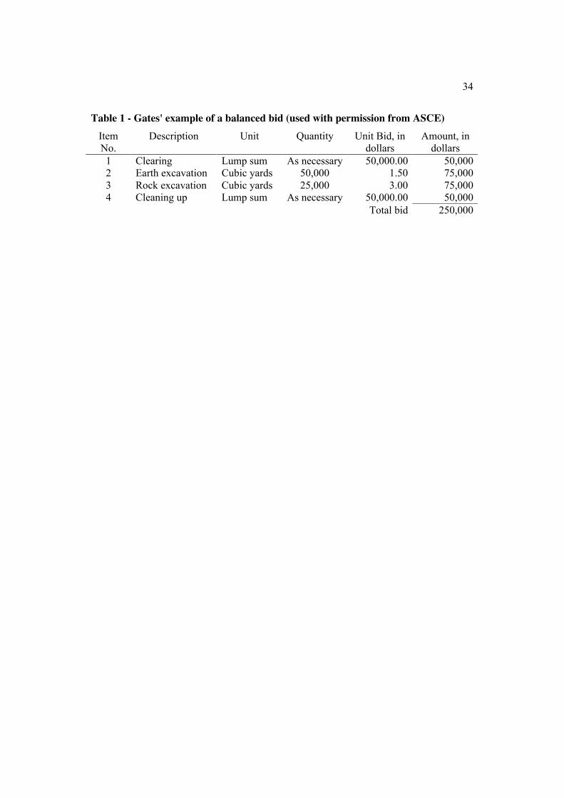
Gates (1967) used the simple 4-item project shown in Table 1 to illustrate this strategy.

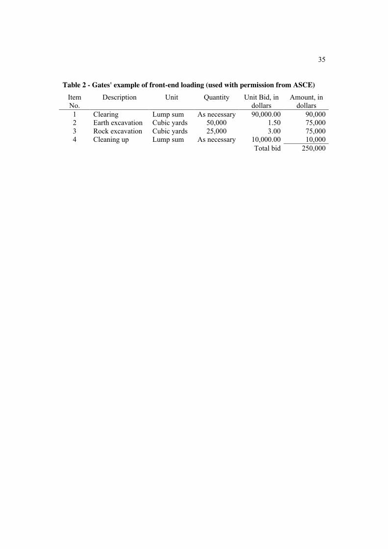
Gates proposed that whilst Table 1 illustrates the item breakdown of a $250,000 project,

as it might be without any loading, Table 2 illustrates how it might appear if its items

were given the treatment of front-end loading.

Gates hence showed how this project could be made to generate an additional $40,000

early on in the project, which clearly is of value to the contractor to finance his

operations.

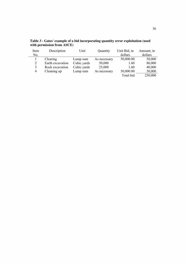
Gates then went on to suggest that another method of unbalanced bidding was to exploit

obvious errors in the project’s initial quantities. He referred to this technique as

“unclassifying”. He illustrated this with the example of a contractor, having done a field

investigation, “having reason to believe” that instead of 50,000 “cubic yards” of earth

excavation, there is more likely to be 70,000 cubic yards; and instead of 25,000 cubic

yards of rock excavation, there is more likely to be only 5,000 cubic yards. He suggested

that this contractor would benefit if they were to load up the price of earth excavation,

and load down the price of rock excavation. He illustrated this with the following

example, shown in Table 3.

The rate for excavation of $1.60 was arrived at solely for the reason that he proposed that

custom dictated that the rate for rock excavation could not be less than the rate for earth

excavation. The rate was calculated as the weighted average based on the contractor’s

“best estimate” of the final quantities of the two items of excavation, as follows:

(70,000 x $1.50) + (5,000 x $3.00) = $1.60 per cubic yard75,000

Gates’ example drew comparison with the (unaltered) balanced bid, as shown in Table 4.

7

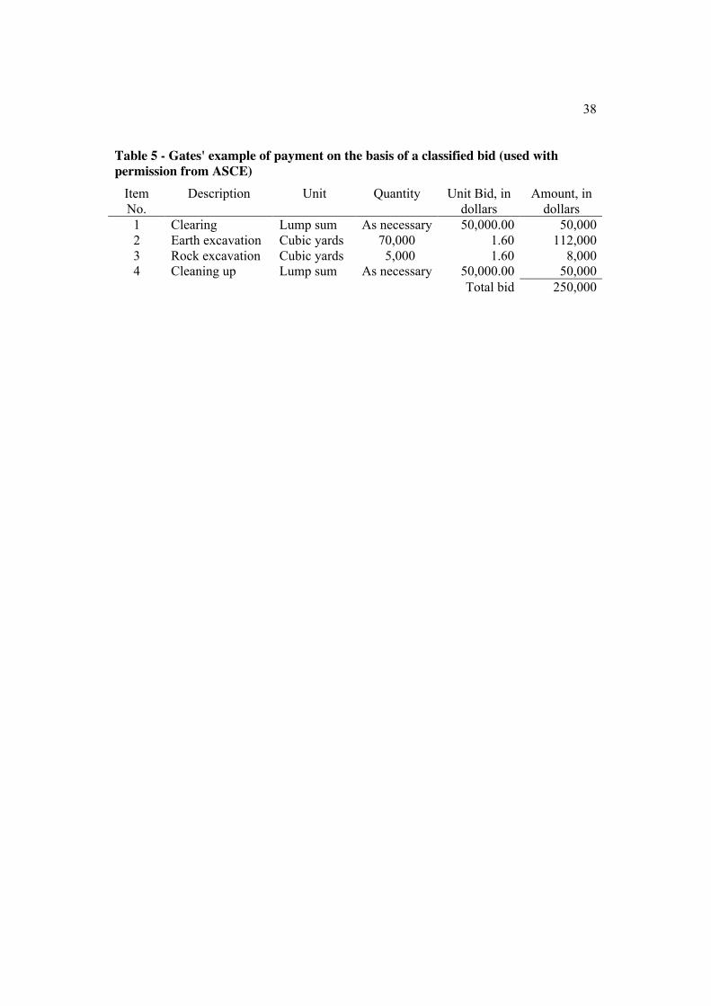
Gates then showed the obvious benefits of his proposed “classified bid”, depicted in

Table 5.

Thus Gates showed that whilst both his examples of a balanced bid and a classified bid

comprised the same tender price of $250,000, the latter unbalanced bid would generate an

additional $30,000 for the contractor provided that his expectation of the variations to the

project’s earthworks were to prove correct.

Gates commented that there was, however, considerable risk for a contractor that his

predictions as regarding the anticipated variations may not be fulfilled. Notwithstanding

this caveat, he did not propose any basis by which to measure or address this risk.

Gates’ work is believed to be important for reason of having identified unbalanced

bidding as a significant strategy. Gates did not, however, succeed with regards to

identifying any mathematical techniques by which to accomplish the potential of this

strategy. He also did not recognise the potential for the use of sophisticated mathematics

for this purpose (Gates, 1967).

STARK’S MODEL

Stark (1968, 1972, 1974) approached the problem largely as Gates had defined it. Unlike

Gates, however, he recognised that there was potential for the application of more

sophisticated mathematics and his approach advocated a linear programming solution.

Stark (1968) recognised that there are the following constraints that govern item pricing:

The bid constraint

This constraint simply ensures that all of the items’ prices add up to the tender price,

which may be stated as follows:

TP = QjPjj=1

J

! Eq.1

where j = item number

J = number of items

8

Qj = bill quantity of item j

Pj = bill price per unit of item j

TP = tender price

Unit bid constraints

Stark suggested that, for reason of “custom”, some item’s prices are governed by other

item’s prices whilst some simply need to be bounded by upper and lower bounds that are

seemingly arbitrarily decided upon.

These two constraints may be expressed as follows:

Pi! P

j" 0 Eq.2

and

Pjl ! Pj ! Pju Eq.3

where i & j = item numbers

Pjl & Pju = lower and upper bounds, respectively, for the price of item j

Stark suggested, as an example, that custom dictated that the excavation of hard rock

should be priced more than the excavation of soft rock, which in turn, should be priced

more than the excavation of earth. He made no attempt, however, to provide any

scientific justification for this nature of constraint. Presumably he meant only for this

constraint to prevent the situation where otherwise it would draw the attention to the

client that the contractor had manipulated the prices.

He also proposed that the upper and lower bounds would be especially useful to limit a

contractor’s risk where the contractor felt less certain of the final quantity of an item. He

did not, however, propose any scientific basis by which to decide these bounds nor did he

suggest a scientific basis by which to identify the items to which to apply this technique.

9

Rate constraints

Stark went on to propose that a contractor may wish to ensure that their anticipated

receipts of interim progress payments remain in some proportion to the rate at which the

work is being done. He suggested that this constraint be described by way of the

following formula:

m

NQjPj = ! QnjPj

n=1

m

"j=1

J

"j=1

J

" Eq.4

where m = a month in the range between 1 and N

N = the estimated duration of the project, in months

! = Stark’s “constant of proportionality”

Qnj = the quantity of item j expected to be built in month n

His suggestion was that a contractor should have an “intuitive” feel for deciding an

appropriate value of ! and that perhaps he should test a range of values within some

bounded limits (also to be arbitrarily decided upon). He indicated that a value of 1

should have the effect that interim payments should keep track with the rate of progress,

such that when for example, 20% of the project is completed (measured in terms of value

completed, as determined by way of the project’s component item prices) then 20% of

the overall project’s value would be paid to the contractor. Values higher than 1 should

have the effect of front-end loading (i.e. that of accelerating the payments) whilst values

of less than 1 should give cause for (a basic form of) back-end loading (i.e. that of

delaying the payments - not that this was something he advocated).

In effect though, the formulation of this constraint appears fundamentally flawed. If this

constraint were to be replicated for all months m then the only basis by which all these

constraints could be satisfied as equalities is in the event of the special case of ! being

equal to 1 and where the rate of progress, and hence the rate of interim progress

payments, of the project was exactly linear. Besides the impracticality of the latter

assumption, this then also negates the effective use of ! for the purpose for which Stark

intended. Thus, it is believed that Stark failed to formulate this intention correctly. It is

10

also noted that although some subsequent research (see Teicholz and Ashley, 1978 and

Diekmann at al, 1982) has made use of other aspects of Stark’s linear programme, they

have not made use of this constraint.

Stark then expressed his “basic model” as having the objective of maximising the present

value (PV ) described as follows, subject to the constraints listed and described above:

PV = Qnj (1+ r)!nPj

n=1

N

"j=1

J

" Eq.5

where r = discount rate of interest, in monthly terms

He described his basic model as being appropriate for those circumstances where the

final quantity of each item will exactly match the bill quantity and where the contractor

has been exactly able to determine the scheduled rate at which each item will be built.

He identified this as a linear programming problem that was capable of being solved

within the practical computing constraints of the time.

This basic model thus only addresses the benefit of front-end loading. Stark then

developed a further derivative of this model for the purposes of also addressing the

benefit of quantity error exploitation and this model (described below) entails the

maximisation of P !V as follows:

P !V = !Qnj (1+ r)"nPj

n=1

!N

#j=1

!J

# Eq.6

where

!J = the estimated final number of items

!N = the estimated final number of months

!Qnj = the estimated final quantity of item j expected to be built in month n

Stark suggested that there are “some circumstances” in which it will be advantageous to

rather optimise the present worth of a project’s future profit (P !!V ), expressed as follows:

11

P !!V = Qnj (1+ r)"n(Pj " Cj )

n=1

N

#j=1

J

# Eq.7

where Cj = the “known” unit cost of item j

He did not describe which circumstances should give cause to encourage this alternative

approach.

This formulation of a project’s profit is simplistic seeing as it does not take account of

many factors that determine that a contractor’s cash outflow in respect of any item will

seldom, if ever, have a simple and continuous linear relationship with the rate at which

the item is built (see, for example, Kaka and Price, 1991; and Kenley, 2003).

Stark illustrated this alternative approach by applying it to his “basic model” (see

equation 5). It would appear, however, that he intended that it should also be applied to

his other model (in which he also incorporates quantity error exploitation - see equation

6).

Stark’s model was limited to only taking account of the combined benefits of cashflow

and quantity estimation errors and it was also limited with respect to its handling of risk.

Furthermore, the effect of his model is largely that items are priced at either the upper or

lower bounds that the contractor will have imposed as constraints. The model’s ultimate

result is thus largely dependent on these arbitrary and subjective inputs, which have to be

decided without the benefit of any suggested scientific aides.

He did, however, agree with Gates (1967) that there was considerable risk attached to any

item price loading strategy. His suggestion was that contractors should test their pricing

models using sensitivity analyses and thereby identify some sense of this risk. This

limited approach to risk may be accountable for his concern about having to design his

model so as to be practical with reference to the limited (and expensive) computing

resources available to contractors at that stage. His model therefore was purely

deterministic in nature.

12

ASHLEY AND TEICHOLZ’S MODELS

Whilst Stark’s (1968, 1972, 1974) efforts took account of the combined benefits of

cashflow and quantity estimation errors, Ashley and Teicholz’s (1977) subsequent

research did not build upon this but rather, seemingly independently, proposed a simple

linear unbalancing model for the sole purpose of improving a contractor’s cashflow. In

this initial research, they recognised that some benefit could be derived from “quantity

error exploitation” but they concluded that it appeared too difficult to model

systematically.

Interestingly, Ashley and Teicholz’s model was developed for the express purposes of

determining, prior to submitting the bid, the extent and manner to which the cashflow of

a project might be manipulated by means of item price loading. They envisaged this

information would aid the decision as to whether or not to bid as well as on what amount

of bid to submit.

They recommended that, whilst having to cope with the limited amount of information

available in the initial stages of a project, that a contractor identify the following three

cashflow curves:

Earnings curve -

representing the value of the contractor’s “work-in-place”, derived from a schedule of

activity for the project priced in terms of the item prices in the Bills of Quantities.

Payments curve -

derived from the earnings curve and adjusted to take account of the retention that is

expected to be withheld by the client. This curve will also be ‘stepped’ (as opposed to

being a continuous ‘smooth’ curve) to take account of the (typically monthly) intervals

between the client’s payments as well as the delays (between when work is executed, and

then measured and then finally paid for). This curve would therefore represent the

contractor’s cash inflow.

13

Cost curve -

representing the contractor’s cash outflow. The cost curve should be derived from the

contractor’s estimate of his costs, matched together with his schedule of activity, and

taking account of any lead or lag between the timing of the activity and the timing of the

expected cash outflow. This curve is also to be derived taking account of the analysis of

each item’s cost, comprising the various types of cost components (labour, materials,

plant, subcontractors, and overheads) and how each of these has a different cash outflow

lead or lag. The cost curve may bear little or no resemblance to the earnings or payments

curves.

Ashley and Teicholz (1977) suggested that the contractor determine the nett cashflow as

being the nett difference between the payments curve and the cost curve. They also

suggested that these differences per period be discounted back to a present value, using

two different discounting rates: one representing the contractor’s cost of borrowings,

being applied to any negative nett cashflow amounts; and the other representing the

contractor’s “corporate rate of return” (being larger than their cost of borrowings) being

applied to any positive nett cashflow amounts. They conclude that the summation of

these periodic (typically monthly) present values would identify the project’s “Nett

Present Worth” – useful as a measure of a project prior to a contractor’s commitment to a

bid as well as to its constituent item prices.

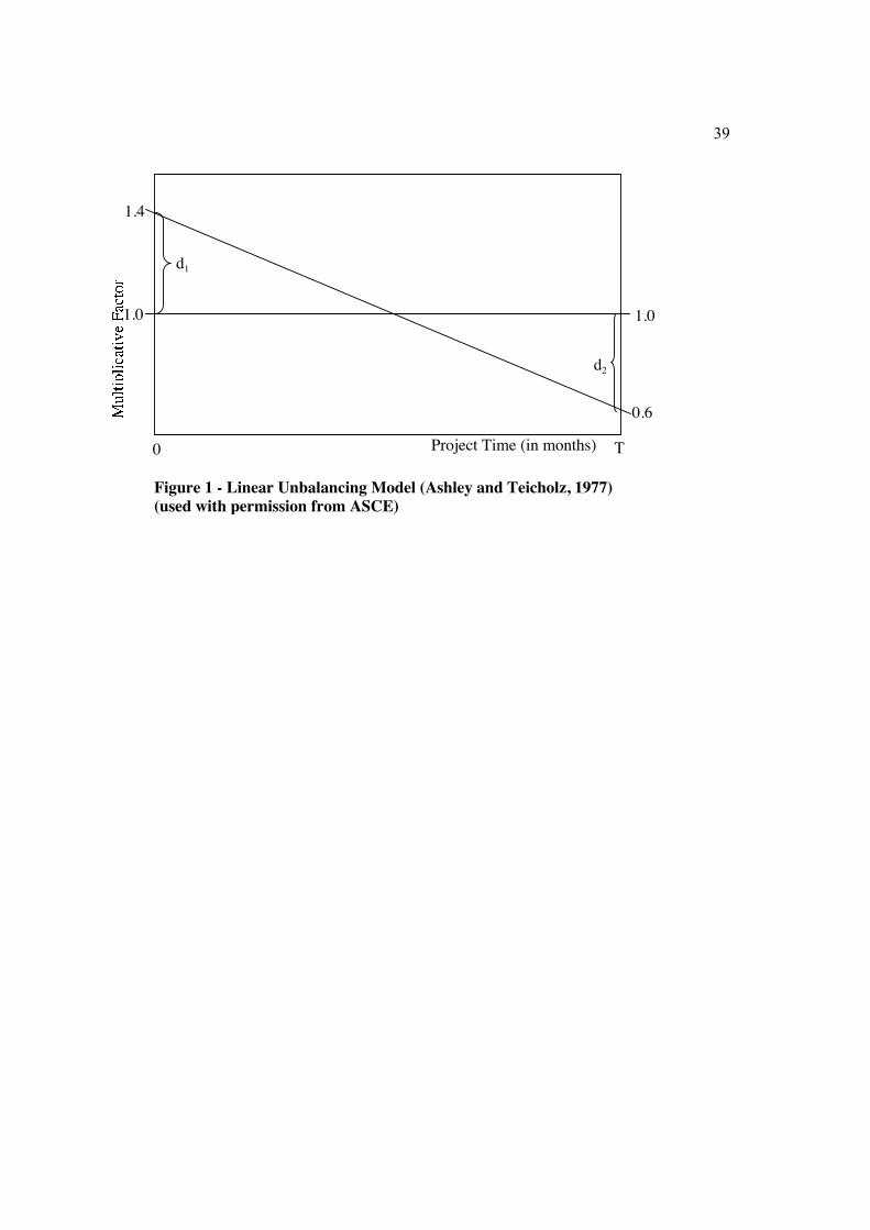
Ashley and Teicholz (1977) then advocated that a contractor measure the effect of the

front-end loading of a project’s item prices using their suggestion of a “linear

unbalancing model”, depicted graphically in Figure 1.

This linear unbalancing model results in all items scheduled for the start of a project

having their prices loaded with the factor d1 (the “Unbalance Factor”). Subsequent items

would be allocated a corresponding lesser factor, derived from the linear equation linking

d1 at the outset of the project with d2 at the end of the project. Various values of d1 can be

tested so as to determine the effect on the contractor’s cashflow as well as on the

project’s “Nett Present Worth”. For each value of d1 a corresponding, compensatory

value of d2 needs to be determined. Ashley and Teicholz (1977) suggested that d2 can be

14

found (by means of an iterative search using a computer) such that the overall unbalanced

bid retain the same simple cumulative value as the balanced bid, i.e. such that the total

“earnings” of the project be kept the same.

Teicholz and Ashley (1978) went on to adopt Stark’s (1974) alternative model with some

minor differences. They proposed that this represented a more sophisticated ‘optimal

model’ which, by comparison to their initial effort (Ashley and Teicholz, 1977), now

included quantity error exploitation.

The essential differences between their model and Stark’s model may be summarised as

follows:

The optimisation of profit

Although Stark had mentioned this as a possible alternative to the optimisation of a

project’s revenue, Teicholz and Ashley (1978) give no explanation why they chose only

to advocate that a contractor should pursue the maximisation of profit.

The probability of execution

Teicholz and Ashley (1978) describe the final quantity of an item as the product of two

forecasts: the “probability of execution” and the contractor’s own estimate of the final

quantity.

Their “probability of execution” refers to the contractor’s estimate of the chance of any

particular item being built. If a contractor believes with certainty that some quantity of a

particular item will finally have to be built as part of a project, then they would assign a

“probability of execution” for this item of 100%. Similarly, if a contractor were of the

opinion that there is only a 50% chance of this item having to be built, then the

“probability of execution” would be 50%.

There seems no reason why the latter estimate should not inherently incorporate the

former probability. On this basis, the “probability of execution” could be considered a

redundant factor. For example, if a contractor were to believe that an item will not finally

15

have to be built, then their estimate of this item’s final quantity could simply be

expressed as being nil.

The analysis of each item’s cost

Stark’s model (in which he seeks to optimise a project’s profit, as opposed to its revenue)

incorporates a simple forecast of each item’s cost. This cost is inherently treated as being

directly proportional to the item’s quantity.

Teicholz and Ashley incorporate the project’s cost estimates somewhat differently. They

break the costs down into three categories: fixed, variable and interest. Their model

seeks to optimise the present value of a project’s “profit” defined as the revenue less the

present value of these three categories of costs. Moreover, they calculate the present

value of the “variable costs” of any item on the basis that it is derived from the final

quantity that the contractor estimates as appropriate for this item. Thus their model

differs slightly from Stark’s by recognising that some items’ costs incorporate fixed

costs, which will not be effected by any variations in the quantities of these items.

The expressed inclusion of the cost of interest

Stark’s model implicitly incorporates the contractor’s cost of interest with the use of

discounted cashflows. Teicholz and Ashley instead expressly incorporate the cost of

interest and yet they advocate, in addition, the use of further discounting.

Their approach therefore has the error of “double counting” the cost of interest, that is,

accounting for it twice when only once is correct. It is also flawed by way of calculating

the cost of interest by treating each project in isolation. Their calculation only includes

the cost of interest in those months when the project’s projected nett cumulative cashflow

is negative; alternatively they advocate that there is no cost of interest (that is, they only

account for interest paid and do not account for interest earned). This approach fails to

recognise that the project being analysed is not one that’s in isolation but rather that it

inevitably forms part of the contractor’s larger ‘portfolio’ of current projects. The cost of

interest to the contractor (incorporating knowledge as to whether the contractor has to

borrow money or not) cannot therefore be determined without taking the contractor’s

16

overall cashflow and level of cash resources into account. One cannot consider a single

project in isolation and make the assumption that if the project has a negative cashflow

that then the contractor’s overall status, inclusive of all his projects, will be such that he

will have a negative cashflow. One project’s negative cashflow could, for instance, be

offset by another project’s concurrent positive cashflow. Similarly if a contractor’s status

at one stage were such that his overall cashflow were considerably negative, they might

be highly dependent, or at very least highly desirous, of as much positive cashflow

contribution at that same stage from any new project. A large positive cashflow

contribution from the new project would be highly valuable to them relative to a much

smaller positive contribution. The former would do very much more to reduce their

overall cost of interest incurred than would the latter. If they were to assess the cost of

interest at an isolated project level, it therefore makes more sense that they account just

the same for the “cost” of interest regardless of whether, at the project level, the nett

cashflow is positive or negative.

The dropping of Stark’s “Rate Constraints”

Teicholz and Ashley’s (1978) approach does not incorporate the need for Stark’s

“constant of proportionality” (! ), which Stark had used as a loading factor to ‘dial up’

the extent of the front-end loading. They have instead been solely reliant on the

discounting rate (which is inherent within the method that they used by which to discount

the cashflow) by which to achieve the desired degree of pricing preference for early

items.

The “Desirability Index” alternative to the use of Linear Programming

Teicholz and Ashley (1978) suggested that the model could be structured as either a

linear programme (as per Stark’s suggestion) or else by using a technique of ranking the

items by way of determining a “desirability index” in respect of each item.

They recognised that the effects of their linear programming model (as with Stark’s) gave

cause for all items, barring one, to be priced at either of the maximum or minimum

pricing limits assigned to each item. Only one item would need to be assigned a price

17

that is not its assigned maximum or minimum limit and this item serves to ensure that the

summation of the priced component items will equate with the overall bid price.

Teicholz and Ashley (1978) therefore identified that there was no need for linear

programming if a contractor could just rank all of a project’s items in terms of their

“desirability”; in other words, in order of their priority status for being awarded or

allocated their maximum-limit price. To start with, this approach allocates all items with

their minimum-limit price. Next, they calculate the total for all of the items priced

accordingly (using the original quantities as listed within the bills of quantities). If one

then deducts this amount from the overall bid amount, one is left with an amount which

can serve to be allocated to those items of greatest “desirability”. Thus, starting at the

item ranked as having the highest Desirability Index, they advocated that one allocates

this item with its maximum limit price. One then needs to make the corresponding

adjustment to what becomes the remaining balance which is still left to be allocated.

Moving down and repeating this process to the next ranked item, and then the next, as the

balance reduces one eventually will come to the one item that is to be assigned neither its

maximum nor its minimum limit price. This item’s price can then be calculated by using

up the remaining balance, and thus the problem (as they defined it) is solved.

Their Desirability Index (DI j ) for each item is calculated as follows:

DI j =

Pj !Qnj (1+ r)"n

n=1

N

#

Qj

Eq.8

Their “probability of execution” factor has been left out when translating their formula

here for the reason (also explained above) that, in order to be consistent with the formulas

throughout this paper, it is considered unnecessary to have both this probability of

execution as well as the estimate of the final quantity. Both can be described by way of

the latter variable alone.

18

Notice that their proposed simplified technique no longer incorporates estimates of each

item’s cost. Each item’s price (barring one) is effectively being decided as either the

minimum or maximum pricing limit influenced by the following three factors:

- the extent to which the item’s quantity is expected to be varied,

- the timing of the item in terms of the project’s schedule, and

- the discounting rate.

This approach inherently overcomes the “double counting” of the cost of interest

discussed above. In effect, this alternative technique of calculation results in a new

model that is substantially different in concept from their linear programming (LP)

model. Inter alia, this new model seeks to maximise the revenue from a project instead

of its profit.

This alternative technique also overcomes the need for the contractor to have to

incorporate into the model all of each item’s estimated fixed and variable costs. This

would appear to be both beneficial and problematic. It is problematic because there is

merit in identifying all of the fixed costs in a project - those that will arise regardless of

variations in the project’s quantities. As long as the model identifies and monitors these

fixed costs (should there be any), the model is able to ensure some protection against the

risk that in the event that an item’s quantity is reduced a proportion of its fixed costs will

not have been compensated for. By not monitoring any item’s costs, this alternative

method of computation loses this advantage.

Besides this advantage, there is no other reason why they should need to incorporate any

costs into their LP model. There is no logical reason why a contractor’s practice of item

pricing should be influenced by knowledge of the individual item costs. By implication,

it is also of no benefit to the function of item pricing, that the contractor should need to

have knowledge of the timing of these costs. The contractor’s costs, as well as the timing

of these costs, will arise regardless of the item price combination chosen by the

contractor. There is no causal-effect relationship between the benefits from item pricing,

19

and any individual item’s cost. Instead, item pricing gives cause for a substantial

influence on a contractor’s revenues, and also of the timing of these revenues.

It follows that any effort to incorporate costs, as well as the timing of these costs, in any

item price loading model is a wasted effort. The only apparent reason for Teicholz and

Ashley (1978) to have incorporated item costs (and their timing) in their model is their

express need to estimate the cost of interest. Their model necessitated estimates of each

item’s cost of interest (and hence, by summation, they would also have estimated the

project’s total cost of interest). It has, however, been shown above (see the earlier

discussion on “double counting” of interest) that, provided that it is to be considered as an

item pricing model, their model had, in fact, no logical need for these cost of interest

estimates.

Ashley and Teicholz’s (1977) original (cashflow planning) model was, however,

presented so as to have a dual purpose: it was firstly said to be intended as a device to

determine the attractiveness of a project to a contractor and hence to aid his decision as to

whether or not to bid, and of how much to bid. It was also said to be a device to decide

appropriate item prices. Given that this model was therefore not solely intended as an

item pricing model, there was originally justified cause to have incorporated

consideration of each item’s cost. In terms of Ashley and Teicholz’s (1977) intention of

being able to assess a project’s ‘attractiveness’, this requires that the contractor be able to

quantify its present worth. This, in turn, requires that the contractor be able to forecast a

project’s nett cashflow, and hence there was the need to incorporate the estimates of each

item’s costs (and also their timing).

However, Teicholz and Ashley’s (1978) subsequent model(s) moved away from being

intended to serve this broader purpose. These subsequent models were designed with the

express sole purpose of identifying what was intended to be ‘optimal’ item prices. When

considering this transition in their intent of purpose, it can be argued that their LP model

no longer had need to incorporate the elaborate analysis of each item’s cost in the manner

in which it had previously done. Their simplified (desirability-index) alternative model

(to their LP model) appears to recognise that this observation is true, notwithstanding that

20

they presented it merely as an alternative, quicker, easier method of calculation, and not

as an alternative new model.

Overall, Teicholz and Ashley can be described as having largely abandoned their prior

“linear unbalancing model” (Ashley and Teicholz, 1977) and instead having adopted

Stark’s model. Despite that they improved and replaced their earlier model, largely

rendering their previous efforts as obsolete, it is their earliest model that is still widely

used in recent research (see for instance, Kenley, 2003).

In summary, although their work had the superficial appearance of being substantially

original and a significant contribution to this field of knowledge, the effective

significance of their work could rather be described as having only identified a quicker

and simpler technique of calculation (that can serve as an alternative to the need for linear

programming) for the application of Stark’s model. It thus did not expand much on what

was originally proposed by Stark.

DIEKMANN, MAYER AND STARK’S MODEL

Diekmann et al. (1982) took Stark’s original deterministic model and added a

probabilistic formulation to take account of risk. All risks, however, were not considered

and the only risk to have been incorporated was the risk that the final item quantities may

be different from what the contractor initially anticipated. They ignored all other risks

(including the risk of variances in all of the variables used in their model), as if they did

not exist. What is, however, of valuable significance as the contribution from this

research is that their model facilitated that a contractor could utilise item price loading for

the purposes of not only maximising their profit but also of controlling their risk (albeit in

the limited manner that they defined it). They thus accomplished the paradigm leap from

all previous research (although they made no reference to the works of Ashley &

Teicholz) that had, up until then, simply identified that the practice of item price loading

was a risk. They recognised that not only could unbalanced bidding contribute to

increased risk, but that it also could be used to manage and reduce risk. Their model

provided the framework for a technique that provided a quantifiable means by which the

practice of item price loading could be pursued whilst “balancing” (their term)

21

profitability against the measurement and manipulation of a project’s risk (no matter that

their definition of what constituted risk was limited).

They ignored all risks other than the risk of a variation in item quantities and also only

loaded prices in the pursuit of the benefits of cashflow and quantity error exploitation.

They therefore ignored the pursuit of increased escalation by way of back-end loading.

Their model was also limited by their assumption that the cash inflows and outflows for

any item arise simply, without any lead or lag, at the time at which the item is built.

Their model thus incorporated the costs of each item but did so without recognising that

the timing of the cash outflows for different items will differ substantially depending on

the nature of the item. It can be argued (see the critique of Teicholz and Ashley’s model

above) that there is no need for this nature of item pricing model to have to incorporate

an item’s estimated costs nor by implication, the timing of these costs. Nevertheless,

Diekmann et al.’s (1982) model does so although it does so in a manner that may be

regarded as simplistic. It does not take account that different items may have

substantially different lead / lag times regarding their associated cash outflows. These

differences in these timings are caused by different items comprise differing proportions

of different types of constituent costs. To forecast any item’s cash outflow should require

that one give consideration to the item’s cost break-down into its constituent components

which may be of many different types (labour, materials, sub-contractors, etc.), each with

substantially different delays / advances between when the item is built and when each of

these costs are having to be paid for.

Whilst their model is derived from Stark’s model, they did not implement Stark’s

“constant of proportionality” (! ) constraint. Incidentally, this constraint was also

ignored in the subsequent work done by Ashley and Teicholz (1977).

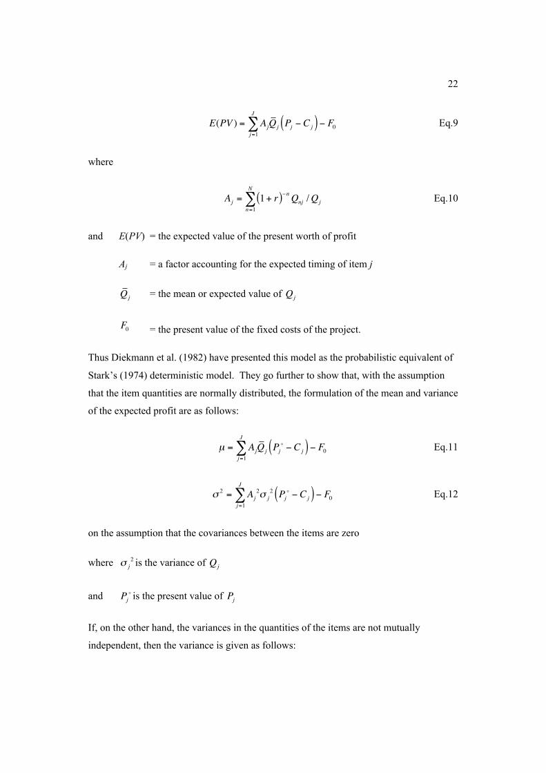
Their model as regards the expected value of PV is given below. Their equation has been

translated (as with all the equations throughout this paper) to a common format in which

the same symbols are used throughout.

22

E(PV ) = AjQj Pj ! Cj( ) ! F0j=1

J

" Eq.9

where

Aj = 1+ r( )!n Qnj /Qj

n=1

N

" Eq.10

and E(PV) = the expected value of the present worth of profit

Aj = a factor accounting for the expected timing of item j

Qj = the mean or expected value of Qj

F0 = the present value of the fixed costs of the project.

Thus Diekmann et al. (1982) have presented this model as the probabilistic equivalent of

Stark’s (1974) deterministic model. They go further to show that, with the assumption

that the item quantities are normally distributed, the formulation of the mean and variance

of the expected profit are as follows:

µ = AjQj Pj! ! Cj( ) ! F0

j=1

J

" Eq.11

! 2 = Aj

2! j

2Pj! " Cj( ) " F0

j=1

J

# Eq.12

on the assumption that the covariances between the items are zero

where !j

2 is the variance of Qj

and Pj

! is the present value of Pj

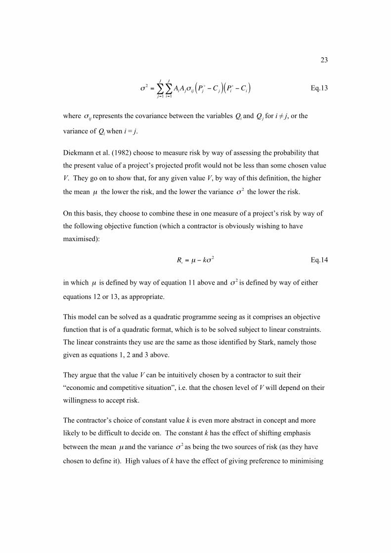
If, on the other hand, the variances in the quantities of the items are not mutually

independent, then the variance is given as follows:

23

! 2 = AiAj! ij Pj! " Cj( ) Pi! " Ci( )

i=1

J

#j=1

J

# Eq.13

where ! ij represents the covariance between the variables Qiand Qj for i ! j, or the

variance of Qiwhen i = j.

Diekmann et al. (1982) choose to measure risk by way of assessing the probability that

the present value of a project’s projected profit would not be less than some chosen value

V. They go on to show that, for any given value V, by way of this definition, the higher

the mean µ the lower the risk, and the lower the variance ! 2 the lower the risk.

On this basis, they choose to combine these in one measure of a project’s risk by way of

the following objective function (which a contractor is obviously wishing to have

maximised):

R!= µ ! k" 2 Eq.14

in which µ is defined by way of equation 11 above and ! 2 is defined by way of either

equations 12 or 13, as appropriate.

This model can be solved as a quadratic programme seeing as it comprises an objective

function that is of a quadratic format, which is to be solved subject to linear constraints.

The linear constraints they use are the same as those identified by Stark, namely those

given as equations 1, 2 and 3 above.

They argue that the value V can be intuitively chosen by a contractor to suit their

“economic and competitive situation”, i.e. that the chosen level of V will depend on their

willingness to accept risk.

The contractor’s choice of constant value k is even more abstract in concept and more

likely to be difficult to decide on. The constant k has the effect of shifting emphasis

between the mean µ and the variance ! 2 as being the two sources of risk (as they have

chosen to define it). High values of k have the effect of giving preference to minimising

24

the project’s projected profit variance, and hence of avoiding the pursuit of quantity error

exploitation, unless the contractor is reasonably certain of the anticipated quantity

variation. Very low values of k, e.g. values approaching zero (bearing in mind that k is

restricted to being a positive value) will cause equation 11 to effectively resemble

equation 9 in the sense that little to no regard will be made of any item’s expected

variance.

Diekmann et al. (1982) appear willing to accept that the contractor’s choice of the values

V and k is difficult and likely to be problematic. In essence they suggest that one

experiment with different values (with there being little guidance available on this matter,

nor that there are any ‘right’ or ‘wrong’ approaches to this) judging to see what effect

different scenarios have on the resultant item prices, as well as on the mean and variance

of the expected profit.

Diekmann et al. (1982) provide an example to illustrate the favourable effect of their

model. Unfortunately, in this example they chose to withhold imposing any upper limits

to the price of each item even though they recommended that in practice these limits are

required. Furthermore, in the manner in which the example is captured as a quadratic

programme, it limits each item’s price to reflect a minimum mark-up of nil. No

explanation is provided as to why some item’s prices are not allowed to be less than the

corresponding estimated item cost.

Without the imposition of upper price limits, this example therefore enjoys greater

freedom by which to pursue its objective. The result is that it does not illustrate at all the

problem that arises when one imposes arbitrarily chosen upper and lower pricing limits

for each item. What happens in the event of upper and lower pricing limits is that all

items barring one will be assigned a price corresponding to either one of these two limits.

Thus, in practice, in accordance with their recommendation (and not in accordance with

their example) it can be argued that there is no greater influence on this model than these

arbitrarily chosen limits. Nevertheless, as with Ashley and Teicholz (1977), Teicholz and

Ashley (1978) and Stark (1968, 1972, 1974), the sophistication of this model does not

extend to addressing this critical issue.

25

In conclusion, one could argue that this model constituted a very significant contribution

to the science of unbalanced bidding. It was the first model to address the management

of both the profitability to be derived from item price loading as well as the risk.

However, although Diekmann et al.’s (1982) model is of far greater mathematical

sophistication than any model that preceded it, it is believed to be flawed for reason of

the following limitations:

- the consideration that a project’s risk is solely related to the risk of variation in

each item’s quantities (with the treatment of all the other variables being in a

deterministic way)

- the unnecessary complexity of the incorporation into the model of having to

forecast a project’s cash outflow (for the purposes of optimising a project’s profit

rather than its revenue)

- the contractor having to decide on values (without any scientific aid) for some

abstract constants (namely, V and k) which have a critical influence on the

model’s outcome

- the effective use of the constant k by which to ‘balance’ the risk vs. return trade-

off, where k is a very arbitrary and abstract measure of this critical decision

- the use of two sets of constraints whereby each item’s price is simplistically a

function of other items’ prices, and also that each item’s price is constrained by

simplistic upper and lower limits (thus it suffers from the same problems as

Ashley and Teicholz’s model as well as Stark’s model), and

- the limitation to the pursuit of front-end loading and quantity error exploitation

only and hence the failure to recognise the benefits of back-end loading.

CATTELL’S MODEL

Cattell (1984) identified all three of the potential benefits from item pricing and he

wrapped them all up in one comprehensive and cohesive formulation. This early work

(1984) did not, however, recognise the risks of item pricing (as commented on by Taylor

26

and Bowen, 1987), and it was only in his subsequent work (1987) that he added to this

the recognition that item pricing has a considerable effect on a project’s risk. He then

formulated a means to measure a project’s risk so that one could quantify,

comprehensively, both the risk and the return factors involved in item pricing. He then

advocated the use of the quadratic programming techniques commonly used in Modern

Portfolio Theory as a novel way by which to manage the decisions regarding the

combination of the risks and returns generated by item pricing.

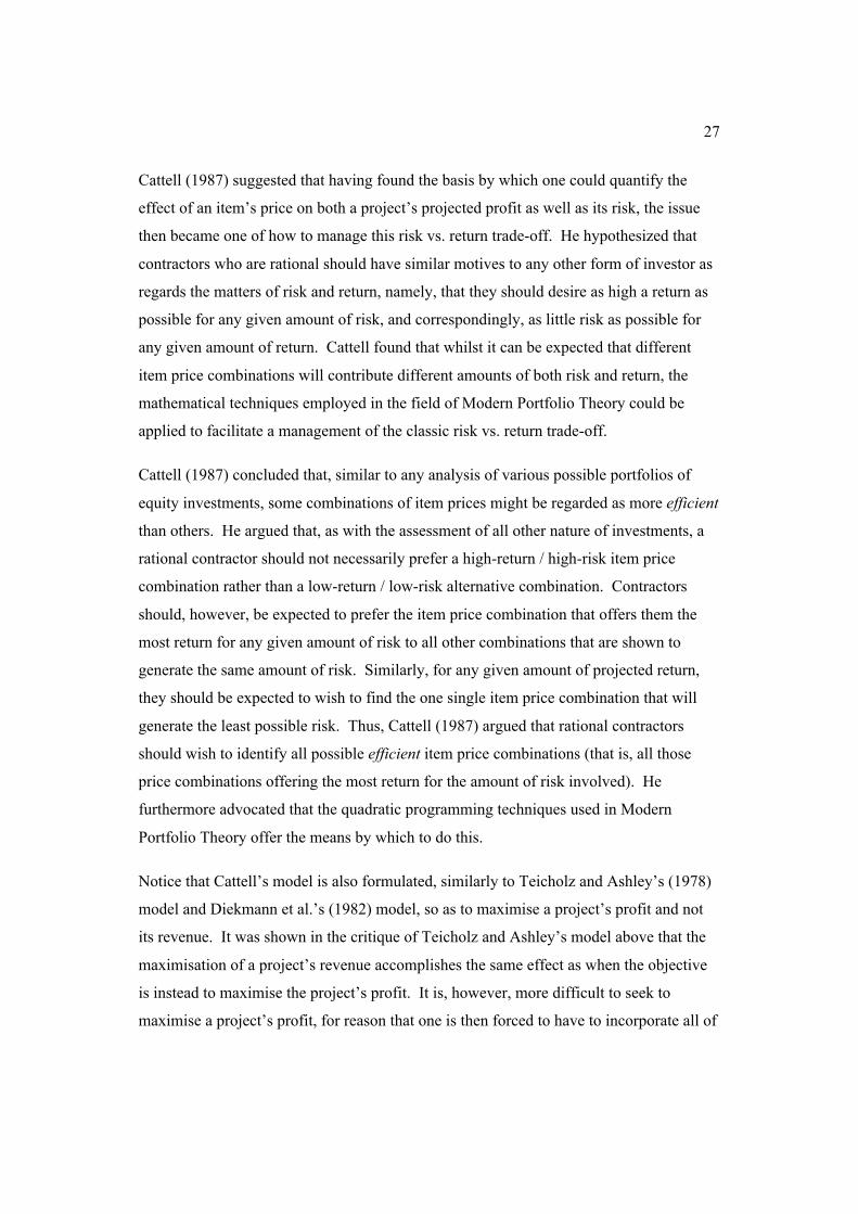
Cattell’s (1987) formulation of the Present Value of a project was described by way of

the following equation:

PV =1

1+ rj

!

"##

$

%&&

n

'Qnj 1( Rn( )Pj (Cj + )nj fPj (Cj( )*+ ,-+ 1+ rr( )nRn 'QnjPj

*+

,-

n=1

N

.j=1

J

. Eq.15

where rj is the discount rate for item j appropriate to the risk of that item

Rnis the proportion retained from payment to the contractor in month n

!nj is the adjustment for escalation / inflation

f is the proportion of the price that’s contractually subject to escalation

rris the interest rate earned on retained funds.

Thus Cattell (1987) had identified a single, comprehensive formulation by which to

determine the contribution to a contractor’s profit by way of any single item’s price. He

reasoned that this formulation comprised numerous variables that are of an uncertain

nature. He argued that the various degrees of uncertainty in all of these variables all

contribute to an uncertainty, or risk, in the projected, formulated profit. He suggested

that it was possible to estimate the variability in each of these variables and also that it

would be necessary to identify any co-variances linking any of the risk factors inherent in

these variables. He then noted that one could use simple mathematics to combine all of

these variances so as to quantify a project’s overall risk.

27

Cattell (1987) suggested that having found the basis by which one could quantify the

effect of an item’s price on both a project’s projected profit as well as its risk, the issue

then became one of how to manage this risk vs. return trade-off. He hypothesized that

contractors who are rational should have similar motives to any other form of investor as

regards the matters of risk and return, namely, that they should desire as high a return as

possible for any given amount of risk, and correspondingly, as little risk as possible for

any given amount of return. Cattell found that whilst it can be expected that different

item price combinations will contribute different amounts of both risk and return, the

mathematical techniques employed in the field of Modern Portfolio Theory could be

applied to facilitate a management of the classic risk vs. return trade-off.

Cattell (1987) concluded that, similar to any analysis of various possible portfolios of

equity investments, some combinations of item prices might be regarded as more efficient

than others. He argued that, as with the assessment of all other nature of investments, a

rational contractor should not necessarily prefer a high-return / high-risk item price

combination rather than a low-return / low-risk alternative combination. Contractors

should, however, be expected to prefer the item price combination that offers them the

most return for any given amount of risk to all other combinations that are shown to

generate the same amount of risk. Similarly, for any given amount of projected return,

they should be expected to wish to find the one single item price combination that will

generate the least possible risk. Thus, Cattell (1987) argued that rational contractors

should wish to identify all possible efficient item price combinations (that is, all those

price combinations offering the most return for the amount of risk involved). He

furthermore advocated that the quadratic programming techniques used in Modern

Portfolio Theory offer the means by which to do this.

Notice that Cattell’s model is also formulated, similarly to Teicholz and Ashley’s (1978)

model and Diekmann et al.’s (1982) model, so as to maximise a project’s profit and not

its revenue. It was shown in the critique of Teicholz and Ashley’s model above that the

maximisation of a project’s revenue accomplishes the same effect as when the objective

is instead to maximise the project’s profit. It is, however, more difficult to seek to

maximise a project’s profit, for reason that one is then forced to have to incorporate all of

28

a project’s costs into such a model. Thus, Cattell’s (1984) model suffers from the same

problem as Teicholz and Ashley’s (1978) model and Diekmann et al.’s (1982) model in

this regard, as being unnecessarily complex. Cattell’s model is therefore believed to best

be simplified and streamlined to leave out all consideration of a project’s costs.

Cattell’s (1984) model also shares the flaw of the other models by also being dependent,

to some degree, on the imposition of maximum and minimum pricing limits for each

item. As with the other researchers, Cattell (1984) failed to recognise the significance of

these arbitrarily chosen limits and hence did not propose any scientific basis by which to

identity the optimum level of these limits.

TONG AND LU’S MODEL

Tong and Lu (1992) developed a method that was focused solely on optimizing the

advantage of what they called ‘error exploitation unbalancing’ (referred to by Green

(1986) as ‘individual rate loading’ and by Cattell (1987) as ‘loading for anticipated

quantity variation orders’). In other words, this method ignored the other benefits in the

areas of cashflow and escalation.

Tong and Lu considered two alternative models – with the same intended effect: one

using linear programming (LP) and the other using a method they called their “minimum-

maximum method”. Their sole motivation and justification for this second method was

due to what they considered the impractical scale of the LP model. They were of the

opinion that the Simplex Algorithm would not cope with being able to solve an LP model

of the size they were envisaging. However, this runs contrary to current popular

computerised usage of the Simplex Algorithm (see Williams, 1993) which manages to

fairly quickly be able to solve models comprising well over a million constraints

(provided that all the variables are continuous and not integral). This incidentally

contrasts with Mixed Integer Linear Programmes (MILP) (where all the variables are not

continuous – some variables, by definition, being integers or binary variables) which take

far longer to solve. It is typically with MILP (or ‘MIP’), rather than with pure LP, where

the size of the model is likely to be of practical concern. In particular, the concern is

typically with regards to the number of integer and binary variables, rather than the

29

number of continuous variables. In the case of Tong and Lu’s LP model (in which all the

variables are, by implication, continuous), it should not present any practical concern that

it shan’t be quick enough. With this being the case, there should not be need to have to

consider their ‘practical’ alternative method.

Tong and Lu’s (1992) alternative model (their ‘minimum-maximum model’ that they

proposed as quicker and easier than their LP model) resembles the ‘Desirability Index’

model from Teicholz and Ashley (1978). Teicholz and Ashley had likewise proposed

their ‘Desirability Index’ model as their alternative to their LP model. Tong and Lu

(1992), however, make no reference to the work of Teicholz and Ashley (1978).

Their ‘minimum-maximum model’ therefore did not present any advance on the model of

Teicholz and Ashley. Their alternative LP model, similarly did not present any practical

advance on the modelling technique proposed by Stark.

DISCUSSION

Item pricing models have commonly been designed as linear programming models.

Linear programming has the restriction that a model may only have one objective

function. This restriction appears to have led to the practice in which early item pricing

models sought only to maximise either a project’s profit or else its revenue. These

models consequently did not incorporate any assessment of a contractor’s risk.

Diekmann et al. (1982) chose instead to use quadratic programming and whilst this

technique again has the restriction of only one objective function, they proposed an

abstract way (facilitated by being able to use a quadratic equation as the objective

function) of pursuing a maximisation of the expected profit together with a minimisation

of the risk. They effectively came to combine these two objectives with the use of a

constant (k) for which the contractor has to arbitrarily choose a value. Different values of

k have the effect of shifting the emphasis of the objective from the maximisation of profit

to the minimisation of risk.

Cattell (1987) also advocated the use of quadratic programming, in this instance so as to

identify the full range of efficient item price combinations (representing different risk vs.

30

return trade-offs), rather than seeking to identify only one optimum combination. He

hypothesized that different rational contractors may have cause to prefer different

efficient combinations (depending on their attitude to risk), but none should wish to adopt

an inefficient combination in preference to an efficient one.

The only other method that has been found to be employed in all of these models by

which to control “the risk” is by means of the use of constraints by which to impose

arbitrarily chosen (upper and lower) limits on each item’s price. These limits, rather than

any other factor, contribute the greatest effect to both the extent to which a project’s

profit can be maximised as well as the extent to which a project’s risk can be minimised.

However, despite the significance of these limits, the decision as regards the choice of

these limits is commonly recommended to be made without any scientific or

mathematical aid. The use of advanced mathematical programming to refine other

aspects of item price loading therefore appears somewhat superfluous as long as the most

influential factor, is by comparison, left to be handled relatively crudely.

In effect, the only role that the mathematical techniques have to play is to determine the

sequence by which to prioritise which items are to be allocated their upper limit price.

This sequence thus identifies the one remaining item that will fall between the set of

items given their upper limit prices and the set of items given their lower limit prices.

This one remaining item thus serves to satisfy the constraint by which the unbalanced bid

is, in summation, equal to the already-determined tender price.

A characteristic shared by all of the models is that they recommend that these limits be

arbitrarily decided upon (and regarded thereafter as fixed). In reality, it is highly unlikely

that any item should have absolute maximum and minimum prices beyond which a

contractor would never submit a price, regardless of the benefits of doing so (whether this

be in terms of increased profit and / or decreased risk). In practical terms, these limits

may be regarded as more fuzzy than fixed.

Another critical and yet common shortfall of the above-described models relates to their

definition of risk. Even in the case of Diekmann et al.’s (1982) model, the only risk

factor that was considered and modelled was the risk that the final quantity for some

31

items may be different from that which the contractor estimates. Cattell’s (1987) model

is the only one that gives consideration to the risks that are generated from uncertainty in

the estimating of the most appropriate discounting rate, of unit costs, of changes to the

project’s schedule, as well as of all the other factors that the other models simply treat

deterministically.

CONCLUSION

Scientists who have worked in this field share the view that there is considerable potential

by which contractors can use the techniques of unbalanced bidding by which to improve

their profitability and / or reduce their risk. Practitioners have commonly applied some

of the techniques of item price loading, apparently with sufficient benefits being derived

that it is has become a common practice in industry. Despite this, little is known of any

application of any of the scientific models that any of the scientists have proposed.

There is considerable potential for further research on this topic, both with regards to the

further development of scientific models and with respect to the evaluation of the

practical uses of unbalanced bidding. More particularly, it would be interesting to see an

evaluation of the application of at least one of the more recent scientific proposals.

REFERENCES

Abdel-Razek, R.H. (1987) ‘Computerised analyses of estimating inaccuracy and tender

variability: causes; evaluation and consequences’, unpublished PhD thesis,

Loughborough University of Technology.

Ashley, D.B. and Teicholz, P.M. (1977) ‘Pre-estimate cash flow analysis’. Journal of the

Construction Division, American Society of Civil Engineers, Proc. Paper 13213, vol. 103

n. C03, pp. 369-379.

Beeston, D.T. (1975) ‘One statistician’s view of estimating.’ Chartered Surveyor, Building and

Quantity Surveying Quarterly, vol. 12, n. 4.

Cattell, D.W. (1984) ‘A model for item price loading by building contractors.’ Unpublished

paper, Department of Quantity Surveying, University of the Witwatersrand,

Johannesburg.

32

Cattell, D.W. (1987). ‘Item price loading.’ PACE’87 Progress in Architecture, Construction and

Engineering proceedings, Johannesburg, July, Vol.II, Session 3, pp.1-20.

Cattell, D.W., Bowen, P.A. and Kaka, A.P. (2004) ‘A model to distribute mark-up amongst

quotation component items: an outline’, Proceedings of the 2nd

Postgraduate Conference

on Construction Industry Development, Cape Town, 10-12th October 2004, CIDB, pp.

154-165.

Crowley, L.G. (2000) ‘Friedman and Gates – another look’. Journal of Construction Engineering

and Management, v. 126, n. 4, July, pp. 306-312.

Diekmann, J.E., Mayer, R.H. Jr. and Stark, R.M. (1982) ‘Coping with uncertainty in unit

price contracting’, American Society of Civil Engineers, Journal of the Construction

Division, v. 108, n. C03, Sep, pp. 379-389.

Friedman, L. (1956) ‘A competitive bidding strategy.’ Operations Research, vol. 4, n. 1, Feb.,

pp. 104-112.

Gates, M. (1959) ‘Aspects of competitive bidding.’ Annual Report, Connecticut Society of Civil

Engineers.

Gates, M. (1967) ‘Bidding strategies and probabilities.’ Journal of the Construction Division,

American Society of Civil Engineers, vol. 93, n. C01, Proc paper 5159, Mar., pp. 75-107.

Gates, M. (1970) ‘Reply to Morin and Clough (June 1969)’ Journal of the Construction Division,

American Society of Civil Engineers, vol. 96, n. C02, June, pp. 93-97.

Green, S.D. (1986) The unbalancing of tenders. MSc dissertation, Department of Building,

Heriot-Watt University.

Green, S.D. (1989) ‘Tendering: optimisation and rationality.’ Construction Management and

Economics, vol. 7, pp. 53-63.

Kaka, A.P. and Price, A.D.F. (1991) ‘Net cashflow models: Are they reliable?’ Construction

Management and Economics 9: 291-308.

Kenley, R. (2003) Financing Construction: Cash flows and cash farming. London, Spon Press.

McCaffer, R. (1979). ‘Cash flow forecasting’. Quantity Surveying (August): 22-26

Skitmore, M. (2002). ‘Predicting the probability of winning sealed bid auctions: a comparison of

models’. Journal of the Operational Research Society 53: pp. 47-56.

33

Stark, R.M. (1968) ‘Unbalanced bidding models – theory.’ American Society of Civil Engineers,

Journal of the Construction Division, vol. 94, n. C02, pp. 197-209.

Stark, R.M. (1972) ‘Unbalancing of tenders.’ Proceedings of the Institute of Civil Engineers,

Technical Note 59, vol. 51, pp. 391-392.

Stark, R.M. (1974) ‘Unbalanced highway contract tendering’ Operational Research Quarterly,

25(3), pp. 373-388.

Taylor, R.G. and Bowen, P.A. (1987) ‘Quantities generation/cost simulation modelling: a

review of the state-of-the-art’, in ‘PACE ’87 Progress in Architecture, Construction and

Engineering’ proceedings, Johannesburg, July, Vol. II, Paper 25, pp.1-14.

Teicholz, P.M. and Ashley, D.B. (1978) ‘Optimal bid prices for unit price contract’. American

Society of Civil Engineers, Journal of the Construction Division, v. 104, n. 1, March, pp.

57-67.

Tong, Y. and Lu, Y. (1992) ‘Unbalanced bidding on contracts with variation trends in client-

provided quantities.’ Construction Management and Economics 10: pp. 69-80.

Williams, H.P. (1993) Model solving in mathematical programming, West Sussex: Wiley.

34

Table 1 - Gates' example of a balanced bid (used with permission from ASCE)

ItemNo.

Description Unit Quantity Unit Bid, indollars

Amount, indollars

1 Clearing Lump sum As necessary 50,000.00 50,0002 Earth excavation Cubic yards 50,000 1.50 75,0003 Rock excavation Cubic yards 25,000 3.00 75,0004 Cleaning up Lump sum As necessary 50,000.00 50,000

Total bid 250,000

35

Table 2 - Gates' example of front-end loading (used with permission from ASCE)

ItemNo.

Description Unit Quantity Unit Bid, indollars

Amount, indollars

1 Clearing Lump sum As necessary 90,000.00 90,0002 Earth excavation Cubic yards 50,000 1.50 75,0003 Rock excavation Cubic yards 25,000 3.00 75,0004 Cleaning up Lump sum As necessary 10,000.00 10,000

Total bid 250,000

36

Table 3 - Gates' example of a bid incorporating quantity error exploitation (used

with permission from ASCE)

ItemNo.

Description Unit Quantity Unit Bid, indollars

Amount, indollars

1 Clearing Lump sum As necessary 50,000.00 50,0002 Earth excavation Cubic yards 50,000 1.60 80,0003 Rock excavation Cubic yards 25,000 1.60 40,0004 Cleaning up Lump sum As necessary 50,000.00 50,000

Total bid 250,000

37

Table 4 - Gates' example of payment on the basis of a balanced bid (used with

permission from ASCE)

ItemNo.

Description Unit Quantity Unit Bid, indollars

Amount, indollars

1 Clearing Lump sum As necessary 50,000.00 50,0002 Earth excavation Cubic yards 70,000 1.50 105,0003 Rock excavation Cubic yards 5,000 3.00 15,0004 Cleaning up Lump sum As necessary 50,000.00 50,000

Total bid 220,000

38

Table 5 - Gates' example of payment on the basis of a classified bid (used with

permission from ASCE)

ItemNo.

Description Unit Quantity Unit Bid, indollars

Amount, indollars

1 Clearing Lump sum As necessary 50,000.00 50,0002 Earth excavation Cubic yards 70,000 1.60 112,0003 Rock excavation Cubic yards 5,000 1.60 8,0004 Cleaning up Lump sum As necessary 50,000.00 50,000

Total bid 250,000

39

Project Time (in months)0 T

1.0

1.4

1.0

0.6

d1

d2

Figure 1 - Linear Unbalancing Model (Ashley and Teicholz, 1977)

(used with permission from ASCE)

!"#$%&'()*"#+$,#-*)./$.0$1")*$2-1)3(#$)*$2,2)(2'(#$0-.45$"11%5663#+'72*3#7.-8638)6999+)*%(2:738);<=>?>>$$