Association Rule Discovery with UnbalancedClass Distributions

Lifang Gu1, Jiuyong Li2, Hongxing He1, Graham Williams1, Simon Hawkins1,and Chris Kelman3

1 CSIRO Mathematical and Information SciencesGPO Box 664, Canberra, ACT 2601, Australia

Firstname.Lastname@csiro.au2 Department of Mathematics and Computing

The University of Southern Queenslandjiuyong@usq.edu.au

3 Commonwealth Department of Health and AgeingChristopher.Kelman@health.gov.au

Abstract.There are many methods for finding association rules in very large data.However it is well known that most general association rule discov-ery methods find too many rules, which include a lot of uninterestingrules. Furthermore, the performances of many such algorithms deterio-rate when the minimum support is low. They fail to find many interestingrules even when support is low, particularly in the case of significantlyunbalanced classes. In this paper we present an algorithm which findsassociation rules based on a set of new interestingness criteria. The algo-rithm is applied to a real-world health data set and successfully identifiesgroups of patients with high risk of adverse reaction to certain drugs.A statistically guided method of selecting appropriate features has alsobeen developed. Initial results have shown that the proposed algorithmcan find interesting patterns from data sets with unbalanced class dis-tributions without performance loss.

Keywords: knowledge discovery and data mining, association rules,record linkage, administrative data, adverse drug reaction.

1 Introduction

The aim of association rule mining is to detect interesting associations betweenitems in a database. It was initially proposed in the context of market basketanalysis in transaction databases, and has been extended to solve many otherproblems such as the classification problem. Association rules for the purpose ofclassification are often referred to as predictive association rules. Usually, pre-dictive association rules are based on relational databases and the consequencesof rules are a pre-specified column, called the class attribute.

One of the problems with conventional algorithms for mining predictive asso-ciation rules is that the number of association rules found is too large to handle,

even after smart pruning. A new algorithm, which mines only the optimal classassociation rule set, has been developed by one of the authors (Li et al. 2002) tosolve this problem.

A second problem with general predictive association rule algorithms is thatmany interesting association rules are missed even if the minimum support isset very low. This is particularly a problem when a dataset has very unbalancedclass distributions, as is typically the case in many real world datasets.

This paper addresses the problem of finding interesting predictive associa-tion rules in datasets with unbalanced class distributions. We propose two newinterestingness measures for the optimal association rule algorithm developedearlier and use them to find all interesting association rules in a health datasetcontaining classes which are very small compared to the population.

In collaboration with the Commonwealth Department of Health and Ageingand Queensland Health, CSIRO Data Mining has created a unique cleaned andlinked administrative health dataset bringing together State hospital morbiditydata and Commonwealth Medicare Benefits Scheme (MBS) and PharmaceuticalBenefits Scheme (PBS) data. The Queensland Linked Data Set (QLDS) links de-identified, administrative, unit-level data, allowing de-identified patients to betracked through episodes of care as evidenced by their MBS, PBS and Hospitalrecords (Williams et al. 2002). The availability of population-based administra-tive health data set, such as QLDS, offers a unique opportunity to detect commonand rare adverse reactions early. This also presents challenges in developing newmethods, which detect adverse drug reactions directly from such administrativedata since conventional methods for detecting adverse drug reactions work onlyon data from spontaneous reporting systems, or carefully designed case-controlstudies (Bate et al. 1998, DuMouchel 1999, Ottervanger et al. 1998).

This paper presents an association algorithm which uses QLDS to identifygroups with high risk of adverse drug reaction. Section 2 describes an algorithmfor mining interesting class association rule sets. Section 3 presents a methodof feature selection based on statistical analysis. In Section 4 we give a briefdescription of QLDS and the features selected. Results from mining the optimalclass association rule set are then presented in Section 5. Section 6 concludes thepaper with a summary of contributions and future work.

2 Interesting Association Rule Discovery

Association rule mining finds interesting patterns and associations among pat-terns. It is a major research topic in data mining since rules are easy to interpretand understand. However, general association rule discovery methods usuallygenerate too many rules including a lot of uninteresting rules. In addition, mostalgorithms are inefficient when the minimum support is low. In this section, wepropose two new interestingness criteria which overcome problems of existingapproaches and can be used in finding interesting patterns in data sets withvery unbalanced class distributions.

2

2.1 Interestingness Criterion Selection

We first introduce the notation used in this paper.A set of attributes is {A1, A2, . . . , Am, C}. Each attribute can take a value froma discrete set of values. For example, Ai ∈ {ai1 , ai2 , . . . , aip}. C is a specialattribute which contains a set of categories, called classes. A record is T ∈A1 × A2 × . . . × Am × C, and a set of records from a data set is denoted byD = {T1, T2, . . . , Tn}. A pattern is a subset of a record, P ⊂ D. The support ofa pattern P is the ratio of the number of records containing P to the numberof all records in D, denoted by sup(P ). A rule is in the form of P ⇒ c. Thesupport of the rule is sup(P ∪ c) 4. The confidence of the rule is defined asconf(P ⇒ c) = sup(Pc)/sup(P ).

If a data set has very unbalanced class distributions many existing interest-ingness criteria are unable to capture interesting information from the data set.In the following we will use a two-class example to demonstrate this. Assumethat sup(c1) = 0.99 and sup(c2) = 0.01. Note that ¬c1 = c2 since there are onlytwo classes.

One of the mostly used interestingness criteria is support. A minimum sup-port of 0.01 is too small for class c1, but too large for class c2. Another suchcriterion is confidence, which can be written for class c2 as conf(P ⇒ c2) =

sup(Pc2)sup(Pc1)+sup(Pc2)

. We can see that any noise in class c1 will have a significantimpact on class c2, e.g. causing sup(Pc1) ∼ sup(Pc2). As a result, we can hardlyfind any high confidence rules in the smaller class, c2. Similarly, gain (Fukudaet al. 1996) suffers the same problem as confidence.

Other alternatives can be similarly evaluated. For example, conviction (Brinet al. 1997), defined as conviction(P ⇒ c) = sup(P )sup(¬c)

sup(P¬c) , measures deviationsfrom the independence by considering outside negation. It has been used forfinding interesting rules in census data. A rule is interesting when convictionis far greater than 1. The conviction for class c2 in our example is written asconviction(P ⇒ c2) = sup(P )sup(c1)

sup(Pc1). Since sup(c1) ≈ 1, we have sup(Pc1) ≈

sup(P ). As a result, conviction(P ⇒ c2) ≈ 1. This means we will not find anyinteresting rules in the small class using the conviction metric.

On the other hand, we can prove that lift (Webb 2000), interest (Brin et al.1997), strength (Dhar & Tuzhilin 1993)) or the p-s metric (Piatetsky-Shapiro1991) all favour rules in small classes. Here we use lift to show this. The metriclift is defined by lift(P ⇒ c) = sup(Pc)

sup(P )sup(c) . A rule is interesting if its lift is far

greater than 1. For large class c1 we have lift(P ⇒ c1) = sup(Pc1)sup(P )sup(c1)

≈ 1 sincesup(c1) ≈ 1. As a result, we can hardly find any high lift rules from the largeclass using the lift metric.

A statistical metric is fair for rules from both large and small classes. Onesuch statistical metric is the odds-ratio, which is defined as Odds-Ratio(P ⇒c) = sup(Pc)sup(¬P¬c)

sup((¬P )c)sup(P¬c) . However, odds-ratio does not capture the interestingrules we are looking for. We show this with the following examples.4 For convenience, we abbreviate P ∪ c as Pc in the rest of the paper.

3

NotationP ¬P

c1 sup(Pc1) sup(¬Pc1)c2 sup(Pc2) sup(¬Pc2)

Example 1P ¬P

c1 0.297 0.693c2 0.006 0.004

Example 2P ¬P

c1 0.792 0.198c2 0.0095 0.0005

In Example 1, the probability of pattern P occurring in class c2 is 0.6, which istwice as that in class c1. In Example 2, the probability of pattern P occurring inclass c2 is 0.95, which is only 1.19 times of that in class c1. Hence rule P ⇒ c2 ismore interesting in Example 1 than in Example 2. However, odds-ratio(A ⇒ c2)is 3.5 in Example 1 and 4.75 in Example 2 and this leads to miss the interestingrule in Example 1.

To have an interestingness criterion that is fair for all classes regardless oftheir distributions, we propose the following two metrics.

– Local support, defined in Equation 1:

lsup(P ⇒ c) = sup(Pc)/sup(c) (1)

When we use local support, the minimum support value will vary accordingto class distributions. For example, a local support value of 0.1 means 0.099support in class c1 and 0.001 in class c2.

– Exclusiveness, defined in Equation 2:

excl(P ⇒ ci) =lsup(P ⇒ ci)∑|C|j lsup(P ⇒ cj)

(2)

Such a metric is normalised ([0, 1]) and fair for all classes. If pattern P occursonly in class ci, the exclusiveness will reach one, which is the maximum value.

We now discuss the practical meaning of the exclusiveness metric. From theformula, it can be seen that it is a normalised lift, i.e.,

excl(P ⇒ ci) =lift(P ⇒ ci)∑|C|j lift(P ⇒ cj)

(3)

The term lift(P ⇒ ci) is the ratio of the probability of P occurring in classci to the probability of P occurring in data set D. Hence the higher the lift, themore strongly P is associated with class ci. However as discussed above, lift(P ⇒ci) ≈ 1 when sup(ci) ≈ 1. As a result, it is difficult to get a uniform minimum liftcutoff for all classes. From Equation 2, it can be seen that |C| × excl(P ⇒ ci) isthe ratio of the lift of P in Class ci to the average lift P in all classes. Therefore,it is possible to set a uniform exclusiveness cutoff value for all classes regardlessof their distributions. More importantly, the metric exclusiveness reveals extrainformation that lift fails to identify. For example, if we have three classes c1, c2

and c3, and sup(c1) = 0.98, sup(c2) = 0.01 and sup(c3) = 0.01, it is possible thatwe have a pattern P such that both lift(P ⇒ c2) and lift(P ⇒ c3) are very high.However, exclusiveness will not be high for either class since P is not exclusiveto any single class.

The above two metrics (local support and exclusiveness) and lift are used inour application for identifying groups of high risk to adverse drug reactions.

4

2.2 Efficient Interesting Rule Discovery

There are many association rule discovery algorithms such as the classic Apriori(Agrawal & Srikant 1994). Other algorithms are faster, including Han et al.(2000), Shenoy et al. (1999), Zaki et al. (1997), but gain speed at the expense ofmemory. In many real world applications an association rule discovery methodfails because it runs out of memory, and hence Apriori remains very competitive.In this application, we do not use any association rule discovery algorithm sinceit is not necessary to generate all association rules for interesting rule discovery.

In the following, we first briefly review definitions of a general algorithmfor discovering interesting rule sets and informative rule sets (Li et al. 2001, inpress), and then argue that the algorithm fits well with our application.

Given two rules A ⇒ c and AB ⇒ c, we call the latter more specific thanthe former or the former more general than the latter. Based on this concept,we have the following definition.

Definition 1. A rule set is an informative rule set if it satisfies the following twoconditions: 1) it contains all rules that satisfy the minimum support requirement;and 2) it excludes all more specific rules with a confidence no greater than thatof any of its more general rules.

A more specific rule covers a subset of records that are covered by one ofits more general rules. In other words, a more specific rule has more conditionsbut explains less cases than any of its more general rules. Hence we only need amore specific rule when it is more interesting than all of its more general rules.Formally, P ⇒ c is interesting only if for all P ′ ⊂ P Interestingness(P ⇒ c) >Interestingness(P ′ ⇒ c). Here Interestingness stands for an interestingnessmetric. In the current application we use local support, lift and exclusivenessas our metrics. Local support is used to vary the minimum support amongunbalanced classes to avoid generating too many rules in one class and too fewrules in another class. Lift is used to consider rules in a single small class, andexclusiveness is used for comparing interesting rules among classes. We prove inthe following that using the informative rule set does not miss any interestingrules instead of the association rule set.

Lemma 1. All rules excluded by the informative rule set are uninteresting bythe lift and exclusiveness metrics.

Proof. In this proof we use AB ⇒ c to stand for a more specific rule of ruleA ⇒ c. AB ⇒ c is excluded from the informative rule set because we haveconf(AB ⇒ c) ≤ conf(A ⇒ c).

We first prove that the lemma holds for lift. We havelift(A ⇒ c) = sup(Ac)

sup(A)sup(c) = conf(A⇒c)sup(c) ≥ conf(AB⇒c)

sup(c) = lift(AB ⇒ c)As a result, rule AB ⇒ c is uninteresting according to the lift criterion.

For the exclusiveness, we first consider a two-class case, c and ¬c. We haveconf(A ⇒ ¬c) = 1− conf(A ⇒ c). Since conf(AB ⇒ c) ≤ conf(A ⇒ c), we have

5

conf(AB ⇒ ¬c) ≥ conf(A ⇒ ¬c). Further we have lift(AB ⇒ c) ≤ lift(A ⇒ c),lift(AB ⇒ ¬c) ≥ lift(A ⇒ ¬c) and therefore

excl(A ⇒ c) = lift(A⇒c)

lift(A⇒c)+lift(A⇒¬c)≥ lift(A⇒c)

lift(A⇒c)+lift(AB⇒¬c)

≥ lift(AB⇒c)

lift(AB⇒c)+lift(AB⇒¬c)= excl(A ⇒ c)

Hence, AB ⇒ c is uninteresting according to the exclusiveness metric.For more than two classes, we do not provide a direct proof. Instead we

have the following rational analysis. Let ci be any class.∑|C|

j conf(A ⇒ cj) =∑|C|j conf(AB ⇒ cj) = 1, When conf(AB ⇒ ci) ≤ conf(A ⇒ ci), we must have

at least one class cj such that conf(AB ⇒ cj) ≥ conf(A ⇒ cj). Further, we havelift(AB ⇒ ci) ≤ lift(A ⇒ ci) and lift(AB ⇒ cj) ≥ lift(A ⇒ cj). As a result,pattern AB is more interesting in class cj than in class ci, and rule AB ⇒ ci isuninteresting by exclusiveness.

Thus we can use the informative rule set instead of the association rule setfor interesting rule discovery.

The advantages of using the informative rule set are listed as following.Firstly, the informative rule set is much smaller than the association rule setwhen the minimum support is small. Secondly, the informative rule set can begenerated more efficiently than an association rule set. Thirdly, this efficiencyimprovement does not require additional memory, and actually the informative(IR) rule set generation algorithm (Li et al. 2001, in press) uses less memorythan Apriori.

The IR algorithm was initially implemented on transactional data sets wherethere are no pre-specified classes. Optimal Class Association Rule set generator(OCAR)(Li et al. 2002) is a variant of the IR algorithm on relational data setsfor classification. Since a relational data set is far denser than a transactionaldata set, OCAR is significantly more efficient than Apriori.

In our application we used a modified OCAR, which uses the exclusivenessas the interestingness metric instead of the estimated accuracy as used in theoriginal OCAR.

Rule discovery requires appropriate features to find significant rules. Featureselection is therefore discussed in the next section.

3 Feature Selection Method

We use statistical methods such as bivariate analysis and logistic regression toidentify the most discriminating features associated with patient classes.

3.1 Bivariate Analysis

Assume that the dependent variable represents a yes/no binary outcome, e.g.,having the disease or not having the disease, an m × 2 frequency table (Ta-ble 1) can be used to illustrate the calculation of the χ2 value for a categorical

6

independent variable with m levels. Specifically, we have

χ2 =m∑

i=1

[(ni1 − Ei1)2

Ei1+

(ni2 − Ei2)2

Ei2] (4)

where Eij is the expected count in cell ij, which is equal to CjRi/N , i = 1, · · · ,mand j = 1, 2. The term, N , refers to the total number of counts.

Independent Variable Dependent Variablelevel Yes No Row Total

1 n11 n12 R12 n21 n22 R23 n31 n32 R3

.

.

....

.

.

....

m nm1 nm2 Rm

Column Total C1 C2

Table 1. The m × 2 frequency table. Here the row total, Ri, and the column total,Cj are the sums of all cells in a row and column respectively, i.e., Ri = ni1 + ni2 andCj =

∑m

i=1nij .

The calculated χ2 value for each independent variable can be compared witha critical (or cut-off) χ2 value for m−1 degrees of freedom at a required p value.The value p denotes the degree of confidence with which to test the association.For example, a p value of 0.01 indicates that the association will be tested at the99% confidence. If the calculated χ2 value is larger than the cut-off value, it canbe concluded that the independent variable is associated with the dependentvariable in the study population. Otherwise, the independent variable is notrelated to the dependent variable and will not be selected as a feature.

Similarly if the independent variable is continuous, the t value can be usedto test for correlation between the dependent and independent variables. Sinceour class association rule discovery algorithm only takes categorical variables,calculation details of the t value are skipped.

3.2 Logistic Regression

An alternative multivariate statistical method is logistic regression. A logisticregression model can be written as the following equation:

ln(p

1− p) = α + β1x1 + β2x2 + · · ·+ βnxn (5)

where p is the probability, at which one of the binary outcomes occurs (e.g., theprobability of having the disease), α is the intercept, and βi is the coefficient ofthe independent variable xi. The coefficient, βi, can be transformed into a moremeaningful measure, the odds ratio (OR), by the following formula:

ORi = eβi (6)

7

Odds ratios can be used to infer the direction and magnitude of the effects of theindependent variables on the probability of the outcome. An odds ratio greaterthan 1 indicates that the probability of the outcome (e.g., having the disease)will increase when a continuous independent variable increases a unit in its valueor when a specific group of a categorical independent variable is compared toits reference group. For example, if the dependent variable is the probability ofhaving migraine, the independent variable is gender, and male is used as thereference group, an odds ratio of 2.0 then implies that females are 2.0 timesmore likely to have migraine than males. As a result, only independent variableswith odd ratio values much larger or smaller than 1 will be selected as importantfeatures.

4 Data

The Queensland Linked Data Set (Williams et al. 2002) has been made avail-able under an agreement between Queensland Health and the CommonwealthDepartment of Health and Ageing (DoHA). The data set links de-identified pa-tient level hospital separation data (1 July 1995 to 30 June 1999), MedicareBenefits Scheme (MBS) data, and Pharmaceutical Benefits Scheme (PBS) data(1 January 1995 to 31 December 1999) in Queensland.

Each record in the hospital data corresponds to one inpatient episode. Eachrecord in MBS corresponds to one MBS service for one patient. Similarly, eachrecord in PBS corresponds to one prescription service for one patient. As a result,each patient may have more than one hospital, or MBS or PBS record.

4.1 Selection of Study Population

PBS data in QLDS contain mostly prescription claims for concessional or repa-triate cardholders. There are a total of 733,335 individuals in PBS and 683,358of them appear as always concessional or repatriate during our five year studyperiod. This represents 93% of all individuals in PBS. Since the drug usage his-tory of these 683,358 individuals is covered more completely in PBS, a subset ofthem is chosen as our study population, i.e, those who take a particular type ofdrug.

The adverse drug reaction to be investigated in this study is angioedemaassociated with the use of ACE inhibitors (Reid et al. 2002). This is a knownadverse reaction and the aim of this investigation is to confirm its existence fromadministrative health data using the proposed algorithm. Drugs are identified inPBS using the WHO codes, which are based on the Anatomical and TherapeuticClassification (ATC) system. Adverse events are identified in hospital data usingprincipal diagnosis codes. Table 2 shows the number of ACE inhibitor users splitinto two classes, those having and not having angioedema. It can be seen thatthe distribution of the two classes is very unbalanced and Class 1 is only 0.088%of the whole study population. However, this is the class we are interested incharacterising. Section 2 has already described how to find rules to characterisesuch an under-represented class.

8

AngioedemaYes No

(Class 1) (Class 0) Total

Counts 116 131,184 132,00Percentage 0.088 99.912 100

Table 2. Study population split into two classes.

4.2 Feature Selection

The aim of the feature selection process is to select those variables which arestrongly associated with the dependent variable, based on statistical analysisdescribed in Section 3. For our particular study the dependent variable is theprobability of having angioedema for ACE inhibitor users.

From the hospital data we initially extract variables, such as age, gender,indigenous status, postcode, the total number of bed days, and 8 hospital flags.The last two variables are used to measure the health status of each patient.From the PBS data, 15 variables (the total number of scripts of ACE inhibitorsand 14 ATC level-1 drug flags) are initially extracted. The variable “total numberof scripts” can be used to indicate how long an individual is on ACE inhibitors.The ATC level-1 drug flags are used to investigate adverse reactions caused bypossible interactions between ACE inhibitors and other drugs.

Using the feature selection method described in Section 3, the 15 most dis-criminating features are selected. These features include age, gender, hospitalflags, and flags for exposure to other drugs. The optimal class association rulediscovery algorithm then run on the extracted data.

5 Results

The interesting association rule discovery algorithm described in Section 2 isapplied to the data set with 132,000 records. There are several input parametersto the algorithm. Two of them are the minimum local support and the maximumlength (number of variables used in each rule). In our tests we set the minimumlocal support to 0.05 and the maximum length to 6. The rules (thousands) aresorted by their value of interestingness in descending order. Only the top fewrules with highest interestingness values are described here for verbosity. Thetop three rules and their characteristics are shown in Table 3.

Rule 1– Gender = Female– Age ≥ 60– Took genito urinary system and sex hormone drugs = Yes– Took Antineoplastic and immunimodulating agent drugs = Yes– Took musculo-skeletal system drugs = Yes

Rule 2– Gender = Female– Had circulatory disease = Yes– Took systemic hormonal preparation drugs = Yes– Took musculo-skeletal system drugs = Yes– Took various other drugs = Yes

Rule 3– Gender = Female– Had circulatory disease = Yes– Had respiratory disease = Yes

9

Rule 1 Rule 2 Rule 3

Number of patients in the group 1,549 1,629 1,999Percentage of this group 1.17 1.23 1.51Number of patients in Class 0 1,542 1,622 1,991Number of patients in Class 1 7 7 8Local support in Class 1 6.03% 6.03% 6.90%Interestingness 0.838 0.831 0.820Lift of Class 1 5.14 4.89 4.55

Table 3. Characteristics of groups identified by Rules 1 to 3.

– Took systemic hormonal preparation drugs = Yes– Took various other drugs = Yes

For example, the group identified by Rule 1 has a lift value of 5.14 for Class 1.This indicates that individuals identified by this rule are 5.14 times more likelyto have angioedema than the average ACE inhibitor users.

[55.6 62.1 1.12]Female

GenderMale

[44.4 37.9 0.85]

Age Group

[42.4 48.3 1.14]60+

[13.2 13.8 1.05]59−

P.Genito urinary system and sex hormones

[18.2 29.3 1.61]Yes

[24.2 19.0 0.78]No

P.Antineoplastic and immunimodulating agents

Yes[1.2 6.0 5.14]

No[0.3 0.0 0.0]

P.Musculo−skeletal system

No[16.7 23.3 1.39]

Yes[1.4 6.0 4.21] [sup(A)(%) lsup(A=>C)(%) lift(A=>C)]

Fig. 1. Probability tree of Rule 1.

Figure 1 provides graphic presentation of Rule 1 in terms of a probability tree.According to the probability tree, female ACE inhibitor users are 1.12 times morelikely to have angioedema than the average ACE inhibitor users. For female ACEinhibitor users aged 60 years or older, the likelihood increases to 1.14. As thetree goes further down, i.e., females aged 60 years or older who have also takengenito urinary system and sex hormone drugs, the likelihood increases further to1.61. If individuals who have all the characteristics mentioned above and havealso used antineoplastic and immunimodulating agent drugs, the likelihood goesup to 4.21 times of the average ACE inhibitor users. Finally, in addition to allthe above mentioned characteristics, the factor of exposure to musculo-skeletal

10

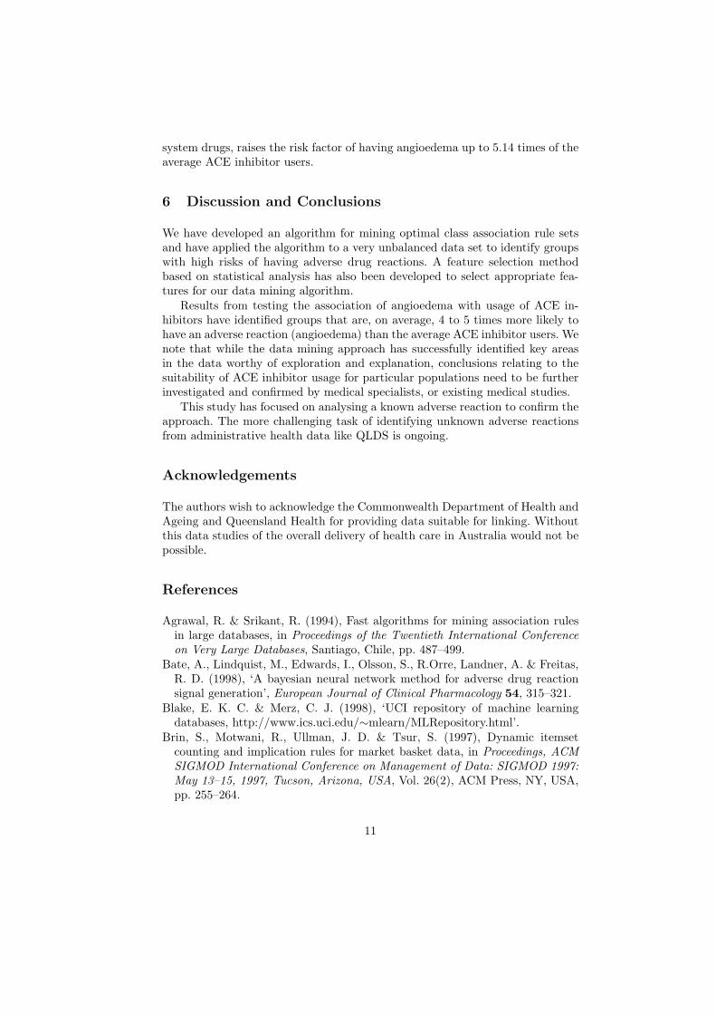
system drugs, raises the risk factor of having angioedema up to 5.14 times of theaverage ACE inhibitor users.

6 Discussion and Conclusions

We have developed an algorithm for mining optimal class association rule setsand have applied the algorithm to a very unbalanced data set to identify groupswith high risks of having adverse drug reactions. A feature selection methodbased on statistical analysis has also been developed to select appropriate fea-tures for our data mining algorithm.

Results from testing the association of angioedema with usage of ACE in-hibitors have identified groups that are, on average, 4 to 5 times more likely tohave an adverse reaction (angioedema) than the average ACE inhibitor users. Wenote that while the data mining approach has successfully identified key areasin the data worthy of exploration and explanation, conclusions relating to thesuitability of ACE inhibitor usage for particular populations need to be furtherinvestigated and confirmed by medical specialists, or existing medical studies.

This study has focused on analysing a known adverse reaction to confirm theapproach. The more challenging task of identifying unknown adverse reactionsfrom administrative health data like QLDS is ongoing.

Acknowledgements

The authors wish to acknowledge the Commonwealth Department of Health andAgeing and Queensland Health for providing data suitable for linking. Withoutthis data studies of the overall delivery of health care in Australia would not bepossible.

References

Agrawal, R. & Srikant, R. (1994), Fast algorithms for mining association rulesin large databases, in Proceedings of the Twentieth International Conferenceon Very Large Databases, Santiago, Chile, pp. 487–499.

Bate, A., Lindquist, M., Edwards, I., Olsson, S., R.Orre, Landner, A. & Freitas,R. D. (1998), ‘A bayesian neural network method for adverse drug reactionsignal generation’, European Journal of Clinical Pharmacology 54, 315–321.

Blake, E. K. C. & Merz, C. J. (1998), ‘UCI repository of machine learningdatabases, http://www.ics.uci.edu/∼mlearn/MLRepository.html’.

Brin, S., Motwani, R., Ullman, J. D. & Tsur, S. (1997), Dynamic itemsetcounting and implication rules for market basket data, in Proceedings, ACMSIGMOD International Conference on Management of Data: SIGMOD 1997:May 13–15, 1997, Tucson, Arizona, USA, Vol. 26(2), ACM Press, NY, USA,pp. 255–264.

11

Dhar, V. & Tuzhilin, A. (1993), ‘Abstract-driven pattern discovery in databases’,IEEE Transactions on Knowledge and Data Engineering 5(6).

DuMouchel, W. (1999), ‘Bayesian data mining in large frequency tables, withan application to the fda spontaneous reporting system’, American StatisticalAssociation 53(3), 177–190.

Fukuda, T., Morimoto, Y., Morishita, S. & Tokuyama, T. (1996), Data miningusing two-dimensional optimized association rules: scheme, algorithms, andvisualization, in Proceedings of the 1996 ACM SIGMOD International Con-ference on Management of Data, Montreal, Quebec, Canada, June 4–6, 1996,ACM Press, New York, pp. 13–23.

Han, J., Pei, J. & Yin, Y. (2000), Mining frequent patterns without candidategeneration, in Proc. 2000 ACM-SIGMOD Int. Conf. on Management of Data(SIGMOD’00), May, pp. 1–12.

Li, J., Shen, H. & Topor, R. (2001), Mining the smallest association rule setfor prediction, in Proceedings of 2001 IEEE International Conference on DataMining (ICDM 2001), IEEE Computer Society Press, pp. 361–368.

Li, J., Shen, H. & Topor, R. (2002), ‘Mining the optimal class assciation ruleset’, Knowledge-based Systems 15(7), 399–405.

Li, J., Shen, H. & Topor, R. (in press), ‘Mining informative rule set for predic-tion’, Journal of intelligent information systems .

Ottervanger, J., Valkenburg, H. A., Grobbee, D. & Stricker, B. C. (1998), ‘Dif-ferences in perceived and presented adverse drug reactions in general practice’,Journal of Clinical Epidemiology 51(9), 795–799.

Piatetsky-Shapiro, G. (1991), Discovery, analysis and presentation of strongrules, in G. Piatetsky-Shapiro, ed., Knowledge Discovery in Databases, AAAIPress / The MIT Press, Menlo Park, California, pp. 229–248.

Reid, M., Euerle, B. & Bollinger, M. (2002), ‘Angioedema’.URL: http://www.emedicine.com/med/topic135.htm

Shenoy, P., Haritsa, J. R., Sudarshan, S., Bhalotia, G., Bawa, M. & Shah, D.(1999), Turbo-charging vertical mining of large databases, in Proceedings of theACM SIGMOD International Conference on Management of Data (SIGMOD-99), ACM SIGMOD Record 29(2), ACM Press, Dallas, Texas, pp. 22–33.

Webb, G. I. (2000), Efficient search for association rules, in Proceedinmgs of the6th ACM SIGKDD International Conference on Knowledge Discovery andData Mining (KDD-00), ACM Press, N. Y., pp. 99–107.

Williams, G., Vickers, D., Baxter, R., Hawkins, S., Kelman, C., Solon, R., He, H.& Gu, L. (2002), Queensland linked data set, Technical Report CMIS 02/21,CSIRO Mathematical and Information Sciences, Canberra. Report on thedevelopment, structure and content of the Queensland Linked Data Set, incollaboration with the Commonwealth Department of Health and Ageing andQueensland Health.

Zaki, M. J., Parthasarathy, S., Ogihara, M. & Li, W. (1997), New algorithmsfor fast discovery of association rules, in Proceedings of the Third Interna-tional Conference on Knowledge Discovery and Data Mining (KDD-97), AAAIPress, p. 283.

12