Resonant states of H3+ and D2H+

Bruno C. Silva, Paolo Barletta, James J. Munro, and Jonathan Tennysona�

Department of Physics and Astronomy, University College London, Gower Street, London WC1E 6BT,United Kingdom

�Received 7 April 2008; accepted 23 May 2008; published online 27 June 2008�

Vibrational resonances for H3+ and D2H+, as well as H3

+ at J=3, are calculated using a complexabsorbing potential �CAP� method with an automated procedure to find stability points in thecomplex plane. Two different CAP functional forms and different CAP extents are used to analyzethe consistency of the results. Calculations are performed using discrete variable representationcontinuum basis elements calculated to high levels of accuracy by diagonalizing large, dense,Hamiltonian matrices. For D2H+, two energy regions are analyzed: the one where D2+H+ is the onlydissociation product and the one where HD+D+ can also be formed. Branching ratios are obtainedin the latter case by using different CAPs. It is shown that H3

+ and D2H+ support some narrowFeshbach-type resonances but that higher angular momentum states must be studied to model thepre-dissociation spectrum recorded by Carrington and co-workers �J. Chem. Phys. 98, 1073�1993��. © 2008 American Institute of Physics. �DOI: 10.1063/1.2945899�

I. INTRODUCTION

The H3+ molecule and its isotopologues are a benchmark

system in chemical physics. It is the simplest bound poly-atomic molecule, having only two electrons and three nuclei.Hence, it is possible to compute its ground electronic surfaceup to dissociation1,2 with high accuracy. Yet, it is hard toobtain a quantitatively and qualitatively satisfactory descrip-tion of its vibrational-rotational spectrum above30 000 cm−1, as the nuclear states in this energy region be-come extremely floppy and the spectrum very dense. H3

+ alsoplays a fundamental role in astronomy, being at the root of aseries of chemical reactions in the interstellar environment.3

It has been detected in both diffuse and dense interstellarmedia, as well as the ionosphere of gas giants.4

More than 20 years ago, Carrington and Kennedy per-formed a remarkable photodissociation experiment on H3

+

that caught the molecular spectroscopy community bysurprise.5,6 An extremely dense spectrum with about 27 000individual lines in a frequency range of only 222 cm−1 wasreported. This was later confirmed in a more refinedexperiment,7 which has attracted considerable theoretical in-terest throughout the years.8–11

So far, the only aspect of the recorded spectrum which isfully understood is its behavior with respect to isotopic sub-stitution, whose explanation rests on semiclassical ratherthan fully quantum mechanical analysis.12–14 Nevertheless, itis accepted that this spectrum involves transitions betweenbound and quasibound states near dissociation and with life-times ranging from 10−9 to 10−6 s. Despite attempts to un-derstand the nature of these states,15 there has been no suc-cessful simulation of the spectrum as yet.16

A good quantitative description of the spectrum thus re-quires accurate calculations of both bound and resonantstates near dissociation. In previous publications,11,17,18 re-

sults for the bound states of H3+ at J=0 and J=3 and D2H+ at

J=0 were presented. Those calculations employed very largebasis sets and were performed at the HPCx supercomputer,reaching an overall accuracy of about 1 cm−1.

There is a broad range of methods available to calculateenergies and lifetimes of metastable states, categorized asbeing L2 or non-L2. The usage of non-L2 methods such as thesearch for poles in the S matrix, or the variational scatteringmethods19 in systems such as H3

+ and D2H+, is computation-ally prohibitive due to the need to calculate the so calledbound-free matrix elements. These difficulties are both dueto the intrinsic need for large basis sets and to the higherdimensionality of the three-particle problem.20,21 L2 methodscan reduce the computational requirements but with somecost in accuracy. The most widely used L2 methods are thestabilization,22 complex scaling,23–25 and complex absorbingpotential26 �CAP� methods.

Although all the L2 methods mentioned can give reliableresults, the CAP method was preferred in this work since itcan be used with basis elements and energy eigenvalues ofthese systems, such as the ones obtained in previous calcu-lations performed by this group.11,17,18 Furthermore, use ofthe automation procedure implemented here makes it pos-sible to use this method to identify the very large number ofresonance states required to model H3

+ predissociationspectrum.

A step taken toward a better understanding of this prob-lem was the work by Mandelshtam and Taylor9 who studiedresonant states of H3

+ for J=0 using a CAP method.27 Thiswork attempted to understand the properties of the meta-stable vibrational states of H3

+ but used a potential energysurface �PES� designed to accurately produce only the lowestbound states and had an incorrect dissociation limit andmissed the R−4 term in the asymptotic region.28

In this paper, we report accurate calculations of energiesand lifetimes of these resonant states, in an energy windowjust above the dissociation limit. The results presented herea�Electronic mail: j.tennyson@ucl.ac.uk.

THE JOURNAL OF CHEMICAL PHYSICS 128, 244312 �2008�

0021-9606/2008/128�24�/244312/13/$23.00 © 2008 American Institute of Physics128, 244312-1

Downloaded 17 Jul 2008 to 144.82.100.66. Redistribution subject to AIP license or copyright; see http://jcp.aip.org/jcp/copyright.jsp

were obtained by applying the CAP method to the basis el-ements obtained from the most accurate dense Hamiltonianmatrix diagonalizations of nuclear motion Hamiltonians forthese systems to date11,17,18 using a PES which is accurate upto the dissociation threshold.2 Results are presented for H3

+ atJ=0 and J=3 and D2H+ at J=0 through a new automaticresonance detection procedure which integrates a consistencycheck and subsequent error estimation.

This paper is structured as follows: Section II outlinesthe theoretical background and computational details of thevibrational-rotational calculations and CAP method; SectionIII describes the preliminary test calculations that determinethe CAP parameters used in the final calculations. In Sec. IV,the final results are presented and discussed. The conclusionsand future work are presented in Sec. V.

II. CAP METHOD

The CAP method involves augmenting the dissociatingsystem’s PES with a complex functional form that absorbsthe continuum part of the wavefunction. Ideally, this non-Hermitian Hamiltonian will produce L2 wavefunctions abovethe dissociation threshold that represent the resonant states inquestion. Riss and Meyer29 have studied this method in somedepth, providing a basic understanding of the way the CAPaffects the spectra of several families of one-dimensionalHamiltonians.

Formally, an imaginary negative potential that acts onthe dissociation coordinate R is added to the system’s Hamil-

tonian H:

H� = H − i�W�R� , �1�

where � is a parameter used to control the CAP’s intensity.

The resulting non-Hermitian Hamiltonian H� defines the en-ergy of the nth resonance En, its width �n, and the corre-sponding L2 wavefunction �n through the relationship

H�����n��� = �En��� − i�n���

2��n��� . �2�

To solve Eq. �2�, H� can be projected on a suitable basis anddiagonalized. In the infinite basis set limit, the eigenvaluescorresponding to the resonant states will be found in the limitwhere �→0. Fortunately, the use of a finite basis set is bothnecessary and beneficial: The error introduced by the CAPand the finite basis set have opposite phases. This impliesthat these errors will cancel each other out at some optimalvalue, �op, thus yielding the complex “observable” associ-ated with the resonant state.

The search for �op is done by studying the behavior ofthe complex eigenvalues of Eq. �2� with values of � rangingfrom zero to a large arbitrary value. This results in N trajec-tories in the complex plane, each associated with an eigen-value En− i�n /2. Through graphical analysis of these trajec-tories, it is possible to identify the point in the complex planethat corresponds to the optimal value �op, and hence estimatethe value for the position En and width �n of the resonantstate. This graphical method consists of locating cusps,

loops, and stability points in the eigenvalue trajectory, whichare known to occur in positions around the true eigenvaluefor the resonances on the complex plane.30

The approach taken in this work is to first diagonalize Hof the system under study and store the basis elements �i andeigenvalues �i lying near the dissociation limit. As one canexpand the functions �n of Eq. �2� onto the basis set ob-tained from the bound state calculation,

��n���� = i

cni �����i� . �3�

The coefficients cni ���, the resonance energies En���, and the

resonance widths �n��� /2 can then be obtained by diagonal-izing the Hamiltonian:

Hji� = � j�H���i� = �i� ji − i�� j�W�R���i� , �4�

where �i is the ith eigenvalue and �i is the ith eigenvector

obtained from the diagonalization of H.Calculations of resonant energies and widths relying

solely on the use of minima and maxima in the eigenvaluetrajectories were performed by Skokov et al.31 and later onby Mussa and Tennyson21 to identify resonant states ofHOCl, which showed good agreement with experiment.32

A. Complex absorbing potentials

The functional form employed in the definition of theCAP is rather arbitrary and depends on a few parameters.Reasonable physical assumptions define a range of choicesfor those parameters, though resonant energies and positionsshould not be affected by the specific choice and shouldshow stability with respect to small variations of the param-eters. One of these assumptions is that CAP’s starting pointr1 should be relatively far inside the dissociation region inorder to absorb only the continuum part of the wavefunction.Nevertheless, the choice of parameters is mostly arbitrary,leading to a degree of uncertainty in the results which so farhas not been properly quantified. As will be shown later,different r1 values may lead to different results for both theresonance energy and width, resulting in an absence of con-sistency between stability points. For this reason, a consis-tency check was implemented in the calculation. This checkinvolves calculating the resonances for a set of CAPs, differ-ing only in their r1 positions, probing the consequences ofabsorbing different regions of the continuum wavefunctionsand verifying the validity of any result obtained.

There are a number of complex absorbing potentialsavailable,33–36 as well as techniques to produce potentialswith optimal properties.27,37 For this reason, we have chosento study two functional forms of CAP, one for its simplicityand the other for its optimal properties.

The simplest and most commonly employed CAP is thenth order monomial potential given by

Wn�R� = � R − r1

r2 − r1�n

, r1 � R � r2. �5�

More formally motivated is the potential due toManolopoulos.35 This potential was more recently refined byGonzalez-Lezana et al.36 �GLM� to

244312-2 Silva et al. J. Chem. Phys. 128, 244312 �2008�

Downloaded 17 Jul 2008 to 144.82.100.66. Redistribution subject to AIP license or copyright; see http://jcp.aip.org/jcp/copyright.jsp

WGLM�R� =2

2� 2�

r2 − r1�2

y�x�, r1 � R � r2, �6�

with y�x� approximately given by

y�x� =4

�c − x�2 +4

�c + x�2 −8

c2 , �7�

where

c = �2K�1/�2� , �8�

and

x = cR − r1

r2 − r1, �9�

where K�1 /�2� is a standard elliptic integral. In both theseCAPs, r2 is placed at the end and r1 at the start of the CAP inthe dissociation coordinate R.

The two most interesting features of the GLM CAP areits minimum reflection properties and the common term inEq. �6� that couples the CAP amplitude to its length, �r=r2−r1, as a single parameter for locating the stability points�op. Unfortunately, due to the method employed in this work,the parameter coupling creates an important difficulty usingthis CAP: To scan all the necessary energies �amplitudes�,one would have to build a new CAP matrix for each ampli-tude. This would significantly increase computational costdue to the number of energy points required for a detailedsearch of such a dense spectrum. For this reason, we chose toremove the common term in Eq. �6�, replacing it instead withthe usual amplitude parameter � while keeping the optimalform of Eq. �7�.

In this work, we have employed both the GLM CAP andthe monomial CAP with n set to 2, henceforth referred as theM2 CAP, to test their effect on both the properties of theresonant states and consistency of the results.

The idea that one must test the consistency of the resultsobtained from the CAP method stems from the assumptionthat changing the complex absorbing potential should nothave a significant effect in the positions and half-widths andfrom the fact that there is no fundamental physical reason forchoosing a particular CAP, apart from setting r1 at somepoint “well” inside the open dissociation channel and r2 atthe end of the wavefunction grid.

B. Automatic resonance detection

As discussed in Sec. II, successive diagonalizations withvarying values of � lead to different trajectories in the com-plex plane. These trajectories must then be inspected one byone. The main difficulty with this approach lies in the factthat to find resonant states one has to inspect thousands ofplots and manually identify all the values of �op for a numberof CAP parameters and functions. To alleviate these difficul-ties, we developed an automated detection procedure thatuses the graphical method criteria described above to detectthe existence of stability points.

The procedure consists of analyzing the individual tra-jectories, obtained for a particular W�R� function along in-creasing values of �. These are scanned in a search for the

nearby occurrence of three conditions. The first conditionarises from the existence of a local maximum or a localminimum in the complex energy, as generally occurs in thepresence of a loop or a cusp. Second, the same trajectory istested for the existence of stability regions where the densityof points along the trajectory has a maximum. This can bestated as

dNE

dl= 0,

d2NE

dl2 � 0, �10�

where NE is the number of complex energy points per unit oftrajectory length and l is the position along the trajectory.Finally, the existence of maxima in the trajectory’s curvatureis tested, with the curvature given by

��� =�E��������� − �����E�����

������2 + E����2�3/2 . �11�

The next step is to identify which � values satisfy all threeconditions within a certain tolerance window. If all threeconditions occur within that window, a successful detectionof a stability point is flagged. Each successful detection isthen recorded. With this information, it is now possible toassess the uncertainty associated with the choice of r1 andidentify which results are truly consistent.

Spurious detections may arise in two situations. First, ifthe CAP range �r is insufficiently long, then the CAP func-tional form will be inadequately sampled, thus leading to theintroduction of an error. Second, if �r is too long, parts ofthe wavefunction that are close to the potential well will beoverabsorbed by the CAP which will significantly affect theposition and width of the detection.

To remove these spurious identifications, an iterativeprocedure removes all stability point detections that producea large deviation from the average of the norm of the com-plex energy. The procedure goes as follows: The average ofthe stability points found over all tested r1 values is calcu-lated; the deviation from the average for each stability pointis computed; the average is recalculated excluding the stabil-ity point with largest deviation and that lies outside the tol-erance window; the process is repeated until no stabilitypoints can be excluded; and finally, the largest deviationfrom the average complex energy that lies inside the toler-ance window is given as the uncertainty, and a percentage ofdetection is then calculated from the fraction of points se-lected over all the tested r1 values.

III. CALCULATIONS

A. PDVR3D energy level calculations

Full diagonalizations of the Hamiltonians for H3+ �Refs.

11 and 17� with angular momentum J=0 and J=3 and D2H+

�Ref. 18� with J=0 were performed using a parallel imple-mentation of the DVR3D �Ref. 38� suite for the calculation ofthe spectra of triatomic molecules, named PDVR3D. Thenuclear Hamiltonian constructed in this program describesthe system in Radau coordinates with the laboratory referen-tial z axis perpendicular to the molecular plane.39,40 An im-proved version41 of this code was implemented on HPCx.42

These calculations use a PES �Ref. 2� that correctly describes

244312-3 Resonant States of H3+ and D2H+ J. Chem. Phys. 128, 244312 �2008�

Downloaded 17 Jul 2008 to 144.82.100.66. Redistribution subject to AIP license or copyright; see http://jcp.aip.org/jcp/copyright.jsp

the dissociation regions of the H3+ system. A correction to this

PES was later on introduced to remove a small unphysicalartifact.11 This surface is henceforth referred to as PPKT2.Although other global PESs for H3

+ have been reported,43,44

these are aimed at both ground and excited states, and it isnot clear that they are as accurate for the ground state. Un-fortunately, lack of computer resources prevented compara-tive tests using these surfaces.

Originally, the H3+ calculations were performed with a

grid defined by 96 angular points and 120 radial points inRadau coordinates with C2v, and not the natural D3h spacialsymmetry. This causes E states in the D3h symmetry group toappear repeated as A1 and B1 states from the C2v group. Notethat, due to the Pauli principle, only the states in the B1

symmetry block are physically allowed for H3+. The radial

basis functions were constructed from spherical oscillators38

with basis parameters �=0, �=0.004 Eh. In the final H3+

calculations, the three-dimensional �3D� Hamiltonian sizewas 79 091, with states converged within 1 cm−1.17 Thesame basis set parameters used for the calculation of H3

+ wereused as the starting point for the D2H+ calculations, leadingto a final 3D Hamiltonian size of 122 000, giving boundstates converged within about 0.1 cm−1. This level of conver-gence is significant since the density of states in D2H+ isapproximately twice that of H3

+.18

To improve upon those results and to provide a measureof convergence for the resonance calculations, two new cal-culations for both D2H+ and H3

+ were performed. The largestcalculation of D2H+ at J=0 was made increasing the radialgrid size to 130 points and setting the final Hamiltonian to asize of 124 818. These calculations achieved an energy con-

vergence to 0.05 cm−1. The largest vibrational H3+ calcula-

tions were performed with the radial grid size extended to140 points and a final 3D Hamiltonian of 94 224, givingenergy states converged to about 0.1 cm−1. These conver-gence values determine lower limits for convergence of theD2H+ and H3

+ resonant states presented in Tables IV and VI,respectively.

An important side effect of changing the number of ra-dial grid points is a change in the overall grid box size. InH3

+, changing the number of grid points from 120 to 140moved the outermost grid point, i.e., the furthest point in theJacobi dissociation coordinate, R3, for any angle, as given inFig. 2, from 19.91 to 21.56 a0. Similarly in D2H+, changingthe number of radial grid points from 120 to 130 moved thefurthest R3 point from 20.70 to 21.58 a0. Thus, the conver-gence tests incorporate the effect of changing the grid boxsize. We note that the grid points are not evenly distributedbut are concentrated at short and intermediate distances andbecome sparser at large distances.

Similar calculations were performed for H3+ at J=3 using

the same basis set parameters and size as the first J=0 cal-culation, but at a very high computational cost: Approxi-mately 45 000 CPU hours.41 This computational cost pre-vented the calculation of other rotational states and the fullconvergence analysis of H3

+ at J=3. However, based upon theresults for J=0, we believe that these states are converged toa similar level of accuracy.

B. CAP method parameters

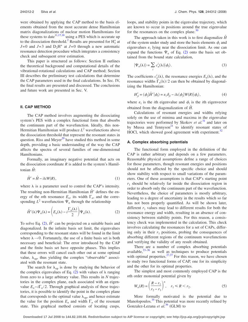
To assess how the CAP forms and parameters influencethe results, tests were performed using D2H+ wavefunctions.This choice comes from the fact that this system allows thestudy of both single and multichannel dissociation throughtwo contiguous energy regions. Figure 1 illustrates the dif-ferent dissociation thresholds for D2H+ and H3

+ plottedagainst the PPKT2 PES. Between 38 659 and 38 992 cm−1,only dissociation of a proton can occur, with the dissociationcoordinate being R3. Above 38 992 cm−1, D2H+ can dissoci-ate into both D++HD through R1 and R2 and H++D2 throughR3. In these tests, we have also restricted ourselves to thecalculation of resonances with A1 symmetry since these arethe hardest to converge.

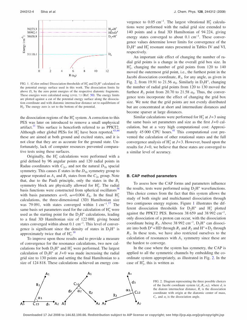
In the case where the system has symmetry, the CAP isapplied to all the symmetric channels by embedding the co-ordinate system appropriately, as illustrated in Fig. 2. In thecase of H3

+, this is written as

FIG. 1. �Color online� Dissociation thresholds of H3+ and D2H+ calculated on

the potential energy surface used in this work. The dissociation limits lieabove De by the zero point energies of the respective diatomic fragments.These energies were calculated using LEVEL 7.5 �Ref. 50�. The energy limitsare plotted against a cut of the potential energy surface along the dissocia-tion coordinate and with diatomic internuclear distance set to equilibrium ofH2. The energy zero is set to the bottom of the potential.

FIG. 2. Diagram representing the three possible choicesof the Jacobi coordinate system �di ,Ri ,�i�, where di isthe diatom internuclear distance, Ri is the dissociationcoordinate with origin at the diatomic center of mass,Ci, and �i is the dissociation angle.

244312-4 Silva et al. J. Chem. Phys. 128, 244312 �2008�

Downloaded 17 Jul 2008 to 144.82.100.66. Redistribution subject to AIP license or copyright; see http://jcp.aip.org/jcp/copyright.jsp

H� = H − i�i=1

3

W�Ri� , �12�

where i runs over the number of symmetric channels, whichis 3 for H3

+. In the D2H+ case,

H� = H − i��W�R1� + W�R2� + V�R3�� , �13�

where the potentials W and V have the same functional formbut with different choices of the parameter r2.

This approach leads to a question in the case where therepresentation of the wavefunction is made in a symmetrylower then that of the potential: For H3

+, which has D3h sym-metry, the dissociation of all three hydrogen atoms would beequally represented by the three possible Jacobi coordinatetransformations. With a C2v representation in Radau coordi-nates, the three transformations to Jacobi coordinates lead toshorter and sparser grids on two of the coordinate systems.For example, R3 as described in Fig. 2, and with the wave-function parameters set for the calculation of highest conver-gence, we obtain a maximum of 21.56 a0 where as for R1 andR2 we obtain 18.64 a0. Because the difference in extent isonly about 10%, we chose to set the total CAP to r2 at 21.56a0 and use the same extent �r for all channels.

When doing the convergence tests, the most significantchange in the number of grid points was done for H3

+. Chang-ing from 120 to 140 radial points in Radau coordinateschanges the position of r2 from 19.91 to 21.56 a0 in theJacobi dissociation coordinate R3, whereas r2 changes from17.24 to 18.67 a0 in R1 and R2. The differences are fairlysmall in both dissociation channels. Since the radial gridchange in the vibrational D2H+ calculations is even smaller,the same set of �r values are used in the consistency analysisof the wavefunction basis convergence tests.

1. � grid

There is a clearly defined window for the lifetime ofresonant states that may participate in the predissociationspectrum that arises from the physical dimensions of theCarrington-Kennedy experimental apparatus. The lower andupper limits for the lifetimes are given by time the ions inthese resonant states take to travel from their origin to thestart and the end of the drift tube, respectively, since the drifttube is where the dissociation must occur to be detected. Thetime that an ion takes to travel from the ion source to thelaser is of the order of 10−6 s.7 This means that the initialstate must have a maximum width of about 10−6 cm−1. De-tection of the dissociation product is sensitive to final stateswith lifetimes between 10−9 and 10−7 s, respectively. Thissets the final state resonance widths approximately between10−5 and 10−3 cm−1. Due to this broad width window, the �grid must obey three constraints: It must cover all the rel-evant CAP intensities that map the positions of the stabilitypoints with � between 10−5 and 10−3 cm−1; it must be suffi-ciently dense to describe the stability points in detail; and thedifferences between the grid points must be small so that theeigenvectors can be matched at each step. This last point isparticularly important since the eigenvalues often changetheir ordering as � increases, reflecting the existence ofcrossings between trajectories. The trajectory tracking isachieved by doing a normalized scalar product between allthe complex eigenvectors in every two successive � steps. Itis desirable for all these constraints to be met with minimumcomputational cost.

To cover the resonance space appropriately at both lowand high energy ranges and to allow for a finer control of thegrid progression, we have chosen to use an exponential func-tion balanced by a fraction for �, as given by

TABLE I. Sample of resonance positions E and half-widths � /2 in cm−1 obtained directly from the automatic stability point detection method for the GLMCAP for a set of 5 �r values, ranging from 4 to 8 a0 with r2 set at 21.58 a0. Powers of 10 are given in parentheses.

�r=4.0 a0 5.0 a0 6.0 a0 7.0 a0 8.0 a0

E � /2 E � /2 E � /2 E � /2 E � /2

38 724.69 3.15�0� 38 724.83 3.16�0�38 729.28 2.95�−1� 38 728.67 5.53�−1� 38 728.70 5.54�−1� 38 728.70 5.73�−1�

38 735.20 1.47�1� 38 735.93 1.63�1�38 739.99 9.33�−1� 38 739.83 1.18�0� 38 739.73 1.20�0� 38 739.71 1.20�0�38 743.70 1.74�−1� 38 743.68 2.12�−1� 38 743.67 2.16�−1� 38 743.67 2.15�−1�

38 753.23 7.31�−6� 38 753.23 7.71�−6� 38 753.23 7.77�−6� 38 753.23 7.94�−6�38 760.54 1.80�−1� 38 760.55 1.76�−1� 38 760.55 1.76�−1� 38 760.55 1.76�−1�,

38 762.27 2.57�−1� 38 762.27 2.22�−1� 38 762.28 2.19�−1� 38 762.28 2.19�−1� 38 762.28 2.19�−1�38 773.53 2.49�−1� 38 773.68 9.28�−2� 38 773.50 2.62�−1� 38 773.50 2.61�−1� 38 773.50 2.59�−1�38 785.13 3.22�−1� 38 785.14 3.69�−1� 38 785.14 3.72�−1� 38 785.14 3.74�−1� 38 785.13 3.74�−1�

38 791.87 2.77�−1� 38 791.88 2.79�−1� 38 791.88 2.80�−1� 38 791.88 2.81�−1�38 797.40 1.30�−1� 38 797.41 1.22�−1� 38 797.41 1.22�−1� 38 797.41 1.22�−1� 38 797.41 1.22�−1�38 805.01 3.44�−1� 38 804.61 1.16�0� 38 804.61 1.16�0� 38 804.61 1.15�0� 38 804.61 1.16�0�

38 811.89 2.82�−2� 38 811.89 2.84�−2� 38 811.89 2.84�−2� 38 811.89 2.90�−2�38 815.92 6.68�−1� 38 815.89 6.88�−1� 38 815.88 6.95�−1� 38 815.88 6.94�−1� 38 815.88 6.99�−1�38 820.23 7.42�−1� 38 820.20 7.64�−1� 38 820.20 7.73�−1� 38 820.19 7.74�−1� 38 820.19 7.87�−1�

38 830.02 4.89�−2� 38 830.02 4.87�−2� 38 830.02 4.88�−2� 38 830.02 4.86�−2�38 837.83 2.20�0�

38 838.30 1.80�0� 38 837.83 2.20�0� 38 837.88 2.18�0� 38 837.92 2.22�0� 38 838.22 2.10�0�38 841.61 3.45�−1� 38 841.76 4.46�−1� 38 842.38 6.60�−1� 38 843.47 1.01�0� 38 845.48 8.97�−1�

244312-5 Resonant States of H3+ and D2H+ J. Chem. Phys. 128, 244312 �2008�

Downloaded 17 Jul 2008 to 144.82.100.66. Redistribution subject to AIP license or copyright; see http://jcp.aip.org/jcp/copyright.jsp

�n = h�n − 1

� − 1, n = 0, . . . ,N , �14�

where h has units of energy and is used to establish the orderof magnitude, � is the progression parameter, and there areN+1 grid points.

For both D2H+ and H3+, we have found that the param-

eters �=1.01 and h=4.39�10−2 cm−1, giving a maximumamplitude of 2.41�105 cm−1 at 1100 points, are sufficient tocover the complex plane for all the eigenvalues tested.

2. Automatic detection

The detection algorithm was calibrated by setting fourparameters. The first two are the tolerance window for theoccurrence of the different detection stability point condi-tions discussed in Sec. II B. Since an accuracy of about0.1 cm−1 is desired, the maximum distance allowed betweenthe existence of points that satisfy those criteria in the realaxis was set to this value. The imaginary energy range cov-ered by the trajectories varies by orders of magnitude fromeigenvalue to eigenvalue. For this reason, tolerance for this

component is given as a percentage of the total imaginaryenergy. We have found that a tolerance of 3% produces con-sistent results.

The second two parameters control the consistency tol-erance between the different stability points detected acrossall the tested r1 values for a particular resonant eigenvalue,as discussed in the end of Sec. II B. We found that definingthese parameters as 0.1 cm−1 for the real part of the energyand 15% was adequate to eliminate spurious detections.

3. CAP consistency

Two sets of consistency tests were performed: The firstto verify that the results are actually consistent for differentr1 positions, i.e., different CAP lengths �r, with a singlefunctional form, and the second to test the GLM against theM2 CAPs. All calculations in this section were performedusing all the available continuum basis elements from themost converged vibrational D2H+ calculation of18 in the in-terval 38 724–38 842 cm−1 as well as a few bound-regionbasis elements for testing purposes. r1 consistency test isshown in Table I. These results indicate that for a particularnumber of states, changing the range covered by the complex

FIG. 3. �Color online� Sample of trajectories in the complex energy plane and their curvatures, generated using the GML CAP for A1 basis elements, for �r

from 4 to 8 a0 in steps of 1 a0, and with � from of 0 to 2�105 cm−1. The plots indicate �a� a resonance at 38 815.90 cm−1 with � /2=0.70 cm−1 and �b� aninconsistent resonance at 38 724.87 cm−1 with � /2=3.16 cm−1. The black squares are the detection results, centered at the averaged real and imaginary partsof the eigenvalue, with sides indicating the maximum deviation in the detected stability points for the total of five CAPs used. �c� and �d� are the respectivenormalized curvatures with respect to the resonant energy. The detection percentage in case �a� was 77.8% and in case �b� was 44.4%.

244312-6 Silva et al. J. Chem. Phys. 128, 244312 �2008�

Downloaded 17 Jul 2008 to 144.82.100.66. Redistribution subject to AIP license or copyright; see http://jcp.aip.org/jcp/copyright.jsp

absorbing potential has an effect on the detection of reso-nances. However, more importantly, there is a high level ofconsistency across most detections.

The differences between consistent and inconsistentstates can be better understood through Fig. 3, which illus-trates the detection of trajectories in the complex energyplane using five GLM CAP with �r values from 2 to 10 a0.By simple visual inspection, it can be seen in case �a� that thetrajectories are consistent in the position of the stabilitypoints and peaks in curvature, whereas in case �b� the posi-tion of the stability points and curvature peaks changes sig-nificantly with �r, suggesting that this result may not bereliable. In fact, the rate of detection given by the automatedprocedure is 77.8% in case �a�, whereas in case �b� it was44.4%, which is in accordance with these observations.

A common feature in these two cases is that the trajec-tory associated with �r=4 a0 appears to have a much lowermaximum curvature then other trajectories. This is also ob-served for all trajectories with �r�4 a0 and for other eigen-values as well. In practice, only 0.0008% of the grid pointsare sampled by CAPs with �r�4 a0 which are clearly notenough for the eigenvalue trajectory calculation to be reli-able. An interesting example is that of the very narrow reso-nance positioned at 38 753.23 cm−1, in Table I, which has avery consistent detection throughout all CAP’s with �r�4a0, but apparently no detection for �r�4 a0. As will beshown later in Sec. IV A, this is caused by the fact that thebasis elements that contribute to this resonant state have am-plitudes close to zero at large distance spatial grid pointswhich introduces an additional numerical error for small �r.

The consistency of results between the GLM and M2CAPs was also tested. The results are shown in Table II andindicate that, with the exception of the state with energy39 460 cm−1 where the detection procedure converged towhat appear to be local minima that were differently empha-sized by each CAP, there is a remarkable consistency in bothpositions and widths of the calculated resonant states with

energies up to 39 187 cm−1. The GLM CAP has a slightlyhigher detection rate in most cases, giving results which aremore consistent as a function of r1. Also, its optimum trans-mission properties allow the use of a smaller � range ofvalues to build the trajectories that lead to detections. Forthese reasons, all final results were calculated using the GLMCAP.

C. D2H+ partial widths

In the case of multidissociation channel systems such asD2H+, the total reaction rate is the sum of the reaction ratesthrough each open reaction channel, i.e., the total probabilityof dissociation is the sum of the probabilities of dissociationthrough all possible channels at a given energy. This wouldimply that the linewidths associated with a particular disso-ciation channel at energies above the threshold should add upto the total linewidth of the system at that same energy. Veri-fication of this property in these resonant calculations is animportant indicator in the reliability of the method. To testthis, a calculation was performed using a GLM CAP appliedseparately to the H++D2 and D++HD dissociation channels.�r was set to 6 a0 and the basis functions have the sameproperties as described in the tests above. The results aftermatching closest resonance energies detected for each disso-ciation channel are presented in Table III.

From these results, it can be seen that, in all except twocases, the sum of the partial widths equals the total widthobtained using a single CAP for all dissociation channels towithin about 30%. The resonance energies obtained vary byabout 0.5 cm−1. These discrepancies are probably becausethe optimal � value for each channel is coupled, as describedby Eq. �13�, leading to a mismatch between the stabilitypoints in the separate channels. Decoupling the � parametercould possibly solve this problem. However, the implemen-tation of this idea is computationally costly. When the CAPis applied solely to the D++HD dissociation channel, some

TABLE II. Comparison of states with half-widths less than 0.15 cm−1, obtained with the GLM and M2 CAPs for a common set of parameters for D2H+ J=0 A1 symmetry calculations. “%” represents the percentage of successful detections over all the nine values of �r from 2 to 10 a0. E and � /2 in cm−1 areaverages after removal of spurious detections. �E and �� /2 are error in cm−1 of energy and half-widths, respectively. Powers of 10 are given in parentheses.

GLM M2

% E � /2 �E �� /2 % E � /2 �E �� /2

66.7 38 685.19 5.34�−6� 0.00 3.93�−6� 77.8 38 685.19 5.16�−6� 0.00 5.57�−6�88.9 38 753.24 6.88�−6� 0.00 3.01�−6� 55.6 38 753.24 6.99�−6� 0.00 3.21�−6�77.8 38 797.41 1.24�−1� 0.01 8.24�−3� 66.7 38 797.41 1.21�−1� 0.01 4.65�−3�55.6 38 811.89 2.71�−2� 0.00 5.83�−3� 77.8 38 811.89 3.04�−2� 0.00 6.89�−3�66.7 38 830.03 4.76�−2� 0.01 3.81�−3� 77.8 38 830.02 4.85�−2� 0.00 2.86�−3�66.7 38 891.22 8.17�−2� 0.02 1.03�−2� 44.4 38 891.23 8.53�−2� 0.01 1.75�−2�77.8 38 918.41 1.22�−1� 0.05 1.69�−2� 88.9 38 918.41 1.28�−1� 0.05 1.86�−2�88.9 39 058.55 1.47�−1� 0.01 4.73�−3� 77.8 39 058.55 1.45�−1� 0.00 3.61�−3�77.8 39 074.43 1.77�−2� 0.00 1.73�−4� 77.8 39 074.43 1.80�−2� 0.00 2.94�−3�88.9 39 119.14 4.08�−2� 0.00 2.06�−3� 88.9 39 119.14 4.03�−2� 0.00 5.15�−3�88.9 −39 129.46 1.96�−2� 0.00 4.67�−4� 77.8 39 129.46 1.92�−2� 0.00 2.44�−3�88.9 39 186.83 8.43�−2� 0.00 3.92�−3� 77.8 39 186.83 8.35�−2� 0.01 1.46�−3�22.2 39 291.15 5.87�−2� 0.06 1.86�−3�55.6 39 460.37 1.20�−1� 0.00 2.19�−4� 88.9 39 460.31 7.14�−2� 0.09 1.19�−2�22.2 39 927.57 1.39�−1� 0.00 1.03�−2�

244312-7 Resonant States of H3+ and D2H+ J. Chem. Phys. 128, 244312 �2008�

Downloaded 17 Jul 2008 to 144.82.100.66. Redistribution subject to AIP license or copyright; see http://jcp.aip.org/jcp/copyright.jsp

widths differ by orders of magnitude on changing the wave-function basis from 120 to 130 radial grid points. This maybebecause Radau coordinates do not permit a complete sam-pling of the D++HD dissociation regions of the potential,leading to difficulties in terms of convergence when adaptingthe CAP to all dissociation channels simultaneously. Never-theless, acceptable results can be obtained by restricting �rin the total CAP to lengths from 4 to 8 a0. This makes �rlarge enough to cover sufficient grid points in the D++HDchannel and short enough not to go too close to the potentialwell.

D. The role of bound vibrational states

Our method involves neglecting nearly all the bound vi-brational states when diagonalizing the CAP Hamiltonian.This assumption needs to be tested, particularly because ofthe presence of asymptotic vibrational states �AVS�,17 whichextend far into the dissociation region where the CAP isplaced. In fact, we have found that the effect of the AVS isnegligible: Only for one H++D2 resonant state the effect issignificant, showing a difference of 0.16 cm−1 in energy and1.75�10−2 cm−1 in width between the calculations with andwithout AVSs, while the remaining states differ by less then0.01 cm−1 in energy and 10% in width. This leads to theconclusion that, from the technical point of view of includingthese states in the CAP calculation, the AVS and all otherbound states show negligible coupling to the resonant statesand therefore are excluded from the final calculations. Nev-ertheless, it must be noted that a link of orthogonality be-tween resonant states and AVS exists. In fact, the basis ele-ments above dissociation depend strongly upon theconvergence of the bound states for their position, and due totheir extension, the AVS are particularly difficult toconverge.

IV. RESULTS AND DISCUSSION

Apart from the technical issues inherent to the CAPmethod as described in Sec. III, there are two more aspects

determining how accurate the results are for a given PES.The first aspect is the number of basis elements used to buildthe CAP matrix, and the second is the size of the basis setused to build these basis elements. The results presented hereshow how these two parameters influence the final resonanceenergies and widths. In terms of the CAP basis convergence,the smallest calculations only use basis elements that liewithin the relevant resonance energy window, as discussed inSec. II, and the intermediate step will be half way in betweenthat number and the maximum available.

A. D2H+ vibrational resonances

The final results for J=0 D2H+ candidate resonances arepresented in Table IV for both the H++D2 and D++HD dis-sociation channels as well as the convergence relative to theCAP basis and the wavefunction basis. The results were ob-tained using 519 A1 states and 485 B1 states lying between38 658 and 41 029 cm−1. Due to the grid constraints imposedby the D++HD dissociation channel, as described in the endof Sec. III B, five CAPs with the GLM functional form wereused with �r ranging from 4 to 8 a0 in steps of 1 a0 with r2

placed at the end of the grid of each respective channel.A total of 384 candidate resonances with width less than

100 cm−1 were detected in the range 38 658–39 658 cm−1, ofwhich 131 have a consistency in �r above 60%. Detectionsin the same energy range with half-widths narrower than0.1 cm−1 are presented in Table IV. Table IV shows thatthere are D2H+ resonant vibrational states narrow enough toplay a role in the predissociation spectrum for this system,which is somewhat surprising since these Feshbach-typeresonances, which arise through energy trapping in the asym-metric stretch and bending degrees of freedom,45 are usuallyassumed to be broader.10,46,47

As expected,21 the resonance widths systematically be-come narrower as either the CAP or wavefunction basis isincreased. Two states, in particular, result in very narrowwidths, namely, states 3 and 11, both with A1 symmetry. Verynarrow widths in these states suggest that �op is very small,

TABLE III. Resonant energies and half-widths in cm−1 for the H++D2, D++HD and total dissociation above theD++HD threshold. This calculation was performed using the GLM CAP with �r=6 a0 for all dissociationchannels and r2 set to the grid limit of both H++D2 and D++HD dissociation channels at 21. 58 and 16. 09 a0,respectively. �� /2 is the difference between the sum of the partial widths and calculated total width. Powers of10 are given in parentheses.

H++D2 D++HD All

��� /2�E � /2 E � /2 E � /2

39 019.59 1.15�0� 39 019.89 3.02�0� 39 018.01 4.00�0� 1.74�−1�39 022.70 1.64�0� 39 022.89 2.68�−2� 39 023.02 1.32�0� 3.44�−1�39 036.86 9.03�−1� 39 035.42 1.46�0� 39 036.53 3.34�0� 9.75�−1�39 074.43 1.78�−2� 39 074.94 3.68�1� 39 075.71 3.70�1� 1.69�−1�39 089.82 3.46�−1� 39 089.08 2.17�−1� 39 089.08 3.69�−1� 1.93�−1�39 097.50 2.30�0� 39 095.36 1.01�0� 39 098.00 3.62�0� 3.09�−1�39 125.95 8.93�−1� 39 125.27 3.42�−1� 39 125.44 1.50�0� 2.63�−1�39 136.19 6.69�−1� 39 136.89 1.58�−1� 39 136.08 9.11�−1� 8.31�−2�39 145.27 1.84�0� 39 144.69 9.58�−3� 39 144.72 1.24�0� 6.08�−1�39 170.62 4.23�−1� 39 171.18 2.06�0� 39 171.73 2.77�0� 2.91�−1�39 175.31 3.50�0� 39 174.21 1.53�0� 39 175.16 5.64�0� 6.08�−1�

244312-8 Silva et al. J. Chem. Phys. 128, 244312 �2008�

Downloaded 17 Jul 2008 to 144.82.100.66. Redistribution subject to AIP license or copyright; see http://jcp.aip.org/jcp/copyright.jsp

leading to wavefunctions that differ very slightly from thestarting eigenvector �. This is confirmed by examining themodulus of the coefficients cn

i ��� in Eq. �3�. Table V showsthe coefficients associated with resonant states, both labeledby the order of the original basis elements. States labeled 3and 11 in Table IV are resonant states �5 and �16 in TableV. It shows that the square modulus of the coefficients cn

5 andcn

16, associated with those particular resonant states, is par-ticularly close to 1, whereas the remaining coefficients are allvery small. To help visualize these resonances, Fig. 4 showsplots of the basis elements �5 and �16, associated with nar-row resonances 3 and 11, respectively, along with basis ele-ment �3 which appears to be associated with resonance 2 inTable IV, and basis element �14 which has a relatively lowassociation with �14, a broad A1 resonance at 38 743.7 cm−1

with half-with of 0.21 cm−1.

The basis elements �5 and �16, associated with 3 and 11,have almost no symmetric stretch excitation, a characteristicakin to the so called horseshoe states10,48 which fundamen-tally are high asymmetric stretch excitations. State 2 has ba-sis element �3 associated with it through a coefficient cn

3

=0.945 41, which is fairly high. It appears though that due tothe presence of a symmetric stretch excitation, the half-widthof this resonant state is significantly larger than either 3 or11. Basis element �14 displays what appears to be a highsymmetric stretch excitation and simultaneously is associ-ated with a broad resonance with width of 0.21 cm−1. Theseobservations suggest that basis elements with low symmetricstretch excitations may provide an indication for the energyof resonant states and a qualitative notion of their width.

A feature of the narrow resonances 3 and 11 is that theydisplay very good wavefunction convergence and very

TABLE IV. Results and convergence for the D2H+ candidate resonant states using a CAP adapted to both the H++D2 and D++HD dissociation channels. Thestates that are within the lifetimes of the observed predissociation spectrum are in boldface. The columns are position of the resonance E, uncertainty in theposition due to consistency �E, resonance half-width � /2, uncertainty in half-width due to consistency �� /2, and detection percentage %. For the conver-gence of results, �E and �� /2 are the difference between the largest calculation and the respective lower convergence calculation for the energy andhalf-widths, respectively: the subscript “a” indicates a CAP eigenvector cutoff at 40 765 cm−1 and the subscript “b” indicates a cutoff at 40 500 cm−1. Wherethere is no subscript. the difference is relative to the lower convergence wavefunction. S is the spatial symmetry of the state. The results are presented in cm−1.Powers of 10 are given in parentheses.

Resonances CAP matrix convergence Basis convergence

E � /2 �E �� /2 % �Ea �Eb ��a /2 ��b /2 �E �� /2 S

1 38 661.82 2.40�−2� 0.14 8.77�−3� 60 0.00 0.01 −1.30�−3� −2.10�−3� A1

2 38 669.66 1.69�−2� 0.10 4.37�−3� 80 0.00 0.01 0.00�0� −9.00�−4� −0.12 −2.78�−2� A1

3 38 685.19 5.24�−6� 0.00 1.43�−6� 60 0.00 0.00 0.00�0� −1.00�−8� −0.01 −2.39�−6� A1

4 38 691.04 6.85�−2� 0.31 1.66�−2� 60 −0.20 −0.02 9.90�−3� 9.00�−3� −0.18 −1.36�−1� A1

5 38 706.55 9.71�−4� 0.00 8.49�−4� 60 0.00 0.00 −5.90�−5� −2.90�−5� −0.01 −1.09�−4� B1

6 38 712.97 7.02�−3� 0.00 0.00(0) 20 −0.07 −0.06 −6.18�−3� −7.18�−3� −0.06 −4.68�−3� B1

7 38 722.37 9.95�−2� 0.32 1.59�−2� 40 0.28 −0.03 2.17�−2� −2.50�−3� 0.37 −3.20�−1� B1

8 38 730.15 1.92�−2� 0.11 4.38�−3� 60 0.00 −0.01 −1.00�−4� −7.00�−4� −0.12 −5.60�−3� B1

9 38 738.25 4.38�−2� 0.00 0.00�0� 20 0.23 −0.32 −4.10�−2� −8.80�−3� 0.04 −9.00�−4� B1

10 38 738.56 5.18�−2� 0.11 4.92�−3� 40 −0.03 −1.00�−3� −0.14 −1.23�−2� B1

11 38 753.24 8.13�−6� 0.00 5.55�−7� 60 0.00 0.00 −1.00�−8� −1.00�−8� 0.00 −9.97�−6� A1

12 38 754.08 7.95�−3� 0.03 3.64�−3� 60 0.00 0.00 1.30�−4� 1.70�−4� −0.01 8.80�−4� B1

13 38 754.50 6.13�−2� 0.50 6.48�−2� 80 0.03 0.04 −5.90�−3� −4.40�−3� −0.11 2.39�−2� B1

14 38 767.79 2.33�−3� 0.00 1.60�−3� 100 0.00 0.00 −3.80�−4� −3.80�−4� −0.01 −3.20�−4� B1

15 38 773.96 2.50�−2� 0.03 1.71�−2� 100 0.00 0.00 −8.00�−4� −7.00�−4� 0.00 −1.20�−3� B1

16 38 778.59 2.65�−2� 0.10 1.56�−2� 80 −0.04 0.01 4.60�−3� 2.50�−3� −0.04 −3.04�−2� B1

17 38 781.48 4.50�−3� 0.01 2.53�−3� 60 0.01 0.00 −8.40�−3� −2.30�−4� −0.02 −4.75�−3� B1

18 38 811.89 2.81�−2� 0.00 1.52�−3� 80 0.00 0.00 0.00�0� 0.00�0� 0.01 −8.00�−4� A1

19 38 830.02 5.01�−2� 0.00 3.39�−3� 80 0.00 0.00 0.00�0� 0.00�0� −0.02 −3.00�−4� A1

20 38 887.53 5.64�−2� 0.00 1.35�−3� 60 0.00 0.00 1.40�−2� 1.00�−4� 0.01 −1.00�−2� B1

21 38 891.23 6.77�−2� 0.02 2.77�−2� 60 0.01 0.00 −1.38�−2� −2.00�−4� 0.02 −1.42�−2� A1

22 38 918.44 8.61�−2� 0.04 4.00�−2� 40 −0.01 0.01 1.40�−3� −2.00�−3� 0.13 −4.19�−2� A1

23 38 952.73 3.63�−2� 0.03 1.60�−2� 100 0.01 0.01 4.00�−3� 3.90�−3� 0.00 −1.20�−3� B1

24 38 978.91 2.58�−3� 0.00 1.58�−3� 60 0.00 0.00 −1.00�−5� −2.00�−5� −0.02 −1.42�−3� B1

TABLE V. Value of the coefficients cni , associated with basis elements �i of the resonant states �n��=�op�.

Four coefficients are chosen to be such that �i��=0�=�i for i=3, 5, 14, and 16. Resonances �3, �5, and �16

correspond to resonances 2, 3, and 11 in Table IV, whereas �14 is a broad resonance with E=38 743.7 cm−1 and� /2=0.21 cm−1. � is given in cm−1. Powers of 10 are given in parentheses.

�3��=65� �5��=69� �14��=57� �16��=67�

�cn3�2 0.945 41�00� 0.859 64�−09� 0.170 66�−05� 0.445 50�−10�

�cn5�2 0.814 63�−01� 1.000 00�00� 0.160 52�−09� 0.389 49�−14�

�cn14�2 0.458 54�−05� 0.214 22�−09� 0.379 14�−00� 0.161 22�−07�

�cn16�2 0.107 13�−01� 0.457 94�−15� 0.198 94�−08� 1.000 00�00�

244312-9 Resonant States of H3+ and D2H+ J. Chem. Phys. 128, 244312 �2008�

Downloaded 17 Jul 2008 to 144.82.100.66. Redistribution subject to AIP license or copyright; see http://jcp.aip.org/jcp/copyright.jsp

FIG. 4. �Color online� Two-dimensional plots of two sections of the A1 D2H+ basis elements �i that correspond to �a� broad resonance 2 in Table IV, �b�narrow resonance 3 in Table IV, �c� broad resonance E=38 743.7 cm−1 and � /2=0.21 cm−1, and �d� narrow resonance 11 in Table IV. These basis elementsare associated with the coefficients cn

3, cn5, cn

14, and cn16 in Table V, respectively. The solid contour shows the classical turning surface. Shades of red show the

negative part of the eigenvector, the darker the deeper, whereas shades of blue the positive part. The amplitude of the eigenvector is normalized to 1 in eachplot, two panels show two different two-dimensional cuts of the wavefunction, and the dotted line indicates where the two sections intersect. Oscillations inlarge R3 regions are fitting artifacts due to the sparsity of the angular grid.

244312-10 Silva et al. J. Chem. Phys. 128, 244312 �2008�

Downloaded 17 Jul 2008 to 144.82.100.66. Redistribution subject to AIP license or copyright; see http://jcp.aip.org/jcp/copyright.jsp

strong consistency in their detection. This can be easily ex-plained by the low coupling that these states have with theremaining basis elements, as indicated by Table V.

We note that there are no resonance widths narrowerthan 0.01 cm−1 above the D++HD dissociation threshold.This may be due to the fact that both H++D2 and D++HDchannels are open, which naturally increases the probabilityof dissociation, reducing resonant lifetimes. However, thebehavior of the resonance widths in this region suggests thatthe widths may be overestimated and may require largerCAP basis sets to fully converge them.

B. H3+ vibrational resonances

The results for the H3+ vibrational resonances with half-

width narrower than 0.1 cm−1 and respective convergence

results are presented in Table VI. They were calculated using592 basis elements for A1 states and 570 basis elements forB1 states, from the energy region 39 273–43 300 cm−1. NineCAPs with �r ranging from 2 to 10 a0 in steps of 1 a0 werecalculated, setting r2 to 21.56 a0. A total of 252 candidateresonances was identified in the energy range39 273–40 273 cm−1, of which 48 have consistency in �rabove 60%. The wavefunctions with 120 radial points hadthe furthermost grid point in the dissociation coordinate R at19.91 a0. Therefore, we maintained the same CAP param-eters as the largest calculation.

Unlike the resonances calculated for D2H+, these reso-nances show larger widths and less consistency in the nar-rowest half-widths. The results appear to have worse wave-function convergence than the ones obtained for D2H+. This

TABLE VI. Results and convergence of H3+ vibrational resonant states. States in boldface are within the lifetime range of the observed predissociation

spectrum. The columns are position of the resonance E, resonance half-width � /2, uncertainty in the position due to consistency �E, uncertainty in half-widthdue to consistency �� /2, detection percentage %, and the C2v symmetry of the state S. The results are presented in cm−1. Powers of 10 are given inparentheses.

Resonances CAP matrix convergence Basis convergence

E � /2 �E �� /2 % �Ea �Eb ��a /2 ��b /2 �E �� /2 S

1 39 288.16 2.90�−2� 0.09 2.20�−2� 55.6 0.00 0.00 −1.00�−7� −2.00�−7� −0.16 −3.16�−5� B1

2 39 288.21 3.50�−2� 0.00 7.74�−3� 22.2 0.00 0.00 0.00�0� 0.00�0� −0.20 −1.30�−3� A1

3 39 303.89 7.71�−2� 0.09 1.93�−2� 22.2 0.00 0.00 0.00�0� 0.00�0� B1

4 39 342.65 9.77�−2� 0.00 1.75�−2� 22.2 −0.01 0.01 3.00�−4� 2.10�−3� A1

5 39 344.07 5.42�−2� 0.02 3.94�−2� 22.2 0.00 0.00 0.00�0� 0.00�0� −0.11 −1.27�−1� B1

6 39 374.52 2.56�−3� 0.00 2.25�−3� 44.4 0.01 0.01 −1.40�−3� −3.00�−3� 1.24 −1.13�−2� A1

7 39 391.20 5.68�−2� 0.00 0.00�0� 11.1 0.00 0.00 −1.00�−5� 3.90�−4� −1.23 −9.26�−1� A1

8 39 396.39 2.83�−2� 0.00 0.00�0� 11.1 0.00 0.22 0.00�0� 5.07�−2� −0.63 5.58�−2� B1

9 39 397.27 812�−2� 0.01 2.88�−2� 44.4 −0.93 −0.07 −1.02�−1� −1.36�−2� B1

10 39 420.42 8.86�−2� 0.00 0.00�0� 11.1 0.00 0.01 −4.00�−4� 1.07�−2� −1.62 −7.33�−1� A1

11 39 431.44 2.91�−2� 0.01 1.29�−2� 22.2 1.06 0.01 −1.21�−0� −7.50�−3� B1

12 39 435.86 6.77�−2� 0.00 3.12�−3� 22.2 0.00 0.01 0.00�0� 8.20�−3� B1

13 39 436.02 6.14�−2� 0.01 4.43�−3� 44.4 −0.14 0.00 6.27�−2� 0.00�0� −0.14 6.76�−2� B1

14 39 469.14 1.02�−2� 0.00 5.66�−3� 33.3 0.00 0.00 0.00�0� 1.30�−3� −0.19 1.09�−2� A1

15 39 478.00 8.19�−2� 0.12 6.67�−2� 55.6 0.00 0.00 −4.00�−4� −1.10�−3� A1

16 39 488.00 9.07�−2� 0.07 6.07�−2� 55.6 0.01 0.01 −3.81�−2� −2.30�−3� −0.05 −1.72�−1� B1

17 39 503.97 6.65�−2� 0.05 2.65�−2� 33.3 0.02 0.00 −1.53�−2� −5.00�−4� −1.46 −5.16�0� B1

18 39 514.85 1.16�−3� 0.00 8.99�−4� 44.4 −0.02 −0.06 2.70�−3� −1.38�−2� A1

19 39 523.38 6.34�−2� 0.02 2.40�−2� 33.3 0.00 0.00 −3.00�−4� −1.40�−4� 1.89 −1.57�0� B1

20 39 552.30 2.01�−2� 0.00 6.78�−4� 22.2 0.00 0.02 −2.00�−4� −9.80�−3� −0.28 −7.84�−1� A1

21 39 552.89 3.83�−3� 0.00 5.04�−4� 33.3 0.00 0.00 0.00�0� 5.50�−3� 0.77 −4.67�−1� B1

22 39 571.29 2.06�−2� 0.01 1.27�−2� 33.3 0.00 0.00 3.00�−5� −3.00�−5� −0.04 −9.62�−2� A1

23 39 604.79 1.15�−3� 0.00 1.52�−4� 33.3 0.00 0.00 −6.30�−3� −1.33�−2� B1

24 39 605.15 8.61�−2� 0.01 2.06�−2� 44.4 −0.80 0.00 −1.58�−1� 1.00�−5� −0.50 −1.53�−1� A1

25 39 667.57 9.75�−2� 0.00 1.28�−3� 33.3 0.00 0.00 0.00�0� 2.00�−4� −2.76 −1.64�0� B1

26 39 720.22 2.10�−2� 0.00 1.43�−2� 77.8 0.00 0.01 0.00�0� 2.29�−2� B1

27 39 725.55 4.29�−2� 0.00 3.02�−2� 66.7 0.00 0.00 −2.10�−3� 0.00�0� −0.20 −3.60�−2� B1

28 39 744.32 2.75�−2� 0.00 1.94�−3� 55.6 0.00 0.00 −6.10�−3� −6.00�−3� 1.19 −2.33�−1� B1

29 39 745.83 3.92�−3� 0.00 2.41�−4� 33.3 0.00 0.00 −2.00�−4� −7.00�−4� A1

30 39 786.87 6.13�−2� 0.01 3.91�−2� 55.6 0.00 0.00 0.00�0� −1.00�−5� −1.64 −1.29�−1� B1

31 39 850.87 3.09�−3� 0.00 2.59�−5� 22.2 0.00 0.00 −1.16�−2� −9.50�−3� −1.99 −2.66�−1� B1

32 39 891.62 6.34�−2� 0.01 1.69�−3� 33.3 0.00 0.00 0.00�0� −7.00�−5� B1

33 39 926.18 7.14�−2� 0.00 1.06�−2� 33.3 0.00 0.01 −8.00�−4� −1.80�−3� A1

34 39 975.55 1.29�−2� 0.02 7.95�−3� 55.6 0.00 0.00 1.00�−4� −5.00�−4� 0.96 4.51�−2� B1

35 40 054.03 4.63�−2� 0.00 1.50�−3� 44.4 0.00 0.00 0.00�0� −5.00�−4� 1.26 −3.73�−1� B1

36 40 184.40 8.22�−2� 0.01 5.38�−3� 44.4 0.00 0.03 1.00�−4� 2.28�−2� −0.15 −1.47�−2� A1

37 40 325.60 3.42�−3� 0.00 3.29�−4� 44.4 0.00 0.00 4.00�−4� 150�−3� 0.99 −4.98�−1� B1

244312-11 Resonant States of H3+ and D2H+ J. Chem. Phys. 128, 244312 �2008�

Downloaded 17 Jul 2008 to 144.82.100.66. Redistribution subject to AIP license or copyright; see http://jcp.aip.org/jcp/copyright.jsp

may be due to the large jump in wavefunction parametersbetween the largest and smallest H3

+ calculation.States pairs �1,2�, �20,21�, and �28,29� in Table VI ap-

pear to be degenerate pairs with E symmetry from the D3h

group which occur in both A1 and B1 symmetries of the C2vgroup, as discussed in Sec. III A. Because of the finite basisset, their energies are not quite identical. This energy split-ting can also be used as a measure of convergence.49

C. H3+ J=3 resonance results

Table VII presents results for J=3 H3+ calculations in-

cluding Coriolis coupling effects and using all the basis ele-ments with corresponding eigenvalues between 39 273 and43 300 cm−1. The calculations were performed over all fourC2v group symmetries, resulting in a total of 893 candidateresonances in the energy range 39 273–40 273 cm−1, 571 ofwhich are consistent to more than 60% in �r, defined by fivevalues ranging from 4 to 8 a0. The resonance widths ob-tained in this case are of the same order of magnitude as theJ=0 H3

+ results, due to their still being substantially Fesh-bach nature. For J=3, the rotational barrier is not sufficientlyhigh to trap shape resonances.10 Nevertheless, the fact thatsome of these Feshbach-type resonances fall within the life-times observed in the predissociation spectrum of H3

+ indi-cates that states with low angular momentum must be studiedto fully characterize this dense spectrum.

V. CONCLUSION

We employ a complex absorbing potential L2 methodwith a new automated procedure to find stability points in thecomplex plane associated with resonant states. This automa-tion enables a consistency and uncertainty analysis of ener-

gies and half-widths to be performed for each candidate reso-nance. We find a number of very well converged, narrow,Feshbach-type resonances for D2H+ with J=0 and for H3

+

with both J=0 and J=3. Thus, in addition to shape reso-nances, Feshbach-type resonances may also play a role in theCarrington-Kennedy predissociation spectrum of H3

+ and itsisotopologues. The present study suggests that all angularmomentum quantum numbers that support bound vibrationalstates should be investigated to gain a full understanding ofthis spectrum.

ACKNOWLEDGMENTS

This project was funded by the EPSRC under the Chem-React Computing Consortium. We thank the HPCx supportteam for their help as well as Hemal Varambhia and IgorKozin for very useful discussions and assistance.

1 R. Prosmiti, O. L. Polyansky, and J. Tennyson, Chem. Phys. Lett. 273,107 �1997�.

2 O. L. Polyansky, R. Prosmiti, W. Klopper, and J. Tennyson, Mol. Phys.98, 261 �2000�.

3 J. Tennyson, Rep. Prog. Phys. 57, 421 �1995�.4 P. Drossart, J. P. Maillard, J. Caldwell, S. J. Kim, J. K. G. Watson, W. A.Majewski, J. Tennyson, S. Miller, S. Atreya, J. Clarke, J. H. Waite, Jr.,and R. Wagener, Nature �London� 340, 539 �1989�.

5 A. Carrington, J. Buttenshaw, and R. A. Kennedy, Mol. Phys. 45, 753�1982�.

6 A. Carrington and R. A. Kennedy, J. Chem. Phys. 81, 91 �1984�.7 A. Carrington, I. R. McNab, and Y. D. West, J. Chem. Phys. 98, 1073�1993�.

8 M. J. Bramley, J. W. Tromp, T. Carrington, Jr., and G. C. Corey, J. Chem.Phys. 100, 6175 �1994�.

9 V. A. Mandelshtam and H. S. Taylor, J. Chem. Soc., Faraday Trans. 93,847 �1997�.

10 E. Pollak and C. Schlier, Acc. Chem. Res. 22, 223 �1989�.11 J. J. Munro, J. Ramanlal, J. Tennyson, and H. Y. Mussa, Mol. Phys. 104,

115 �2006�.

TABLE VII. Results for J=3 H3+ resonant states in cm−1. The columns are position of the resonance E, resonance half-width � /2, uncertainty in the position

due to consistency �E, uncertainty in half-width due to consistency �� /2, detection percentage %, and S is the C2v symmetry symmetry of the state. Powersof 10 are given in parentheses.

E � /2 �E �� /2 % S E � /2 �E �� /2 % S

1 39 280.05 4.82�−2� 0.12 2.52�−2� 60 A2 22 39 501.64 1.65�−2� 0.00 2.50�−3� 60 A2

2 39 288.57 3.48�−2� 0.06 1.52�−2� 100 A2 23 39 504.24 1.50�−2� 0.00 1.41�−3� 60 A2

3 39 293.63 1.23�−2� 0.00 0.00�0� 20 B2 24 39 511.78 1.61�−2� 0.00 1.13�−4� 40 A2

4 39 299.35 1.08�−2� 0.01 5.36�−3� 80 A2 25 39 513.03 2.61�−2� 0.00 3.27�−4� 40 A2

5 39 302.80 7.49�−3� 0.01 1.83�−3� 80 A2 26 39 534.13 9.38�−3� 0.00 9.49�−5� 40 A2

6 39 327.05 1.73�−2� 0.01 1.14�−2� 100 A2 27 39 542.25 4.91�−2� 0.01 1.47�−2� 60 A1

7 39 335.59 1.21�−2� 0.01 6.55�−3� 100 A2 28 39 547.30 5.40�−2� 0.08 1.21�−2� 80 B1

8 39 339.51 3.70�−2� 0.03 1.89�−2� 80 A2 29 39 549.40 1.17�−2� 0.00 0.00�0� 20 A1

9 39 346.79 9.03�−3� 0.00 1.35�−2� 100 A1 30 39 550.06 6.96�−2� 0.02 7.89�−3� 40 B1

10 39 354.59 4.33�−2� 0.03 2.77�−2� 80 A2 31 39 553.74 2.91�−2� 0.00 1.69�−3� 60 A2

11 39 355.57 4.28�−3� 0.00 0.00�0� 20 A2 32 39 558.37 1.91�−2� 0.00 0.00�0� 20 A1

12 39 395.19 3.18�−4� 0.00 7.98�−6� 40 A2 33 39 558.70 8.52�−3� 0.00 1.64�−5� 40 A2

13 39 399.53 2.63�−2� 0.00 7.63�−4� 40 A2 34 39 575.62 2.05�−2� 0.00 4.51�−3� 60 A2

14 39 411.34 9.22�−2� 0.14 4.05�−2� 80 B1 35 39 576.80 2.65�−2� 0.00 3.64�−3� 60 A2

15 39 438.28 6.45�−3� 0.00 2.63�−3� 80 A1 36 39 584.40 1.30�−2� 0.00 4.20�−4� 40 A2

16 39 447.63 4.98�−2� 0.02 1.53�−2� 80 B1 37 39 606.89 2.65�−2� 0.00 3.81�−3� 40 A2

17 39 456.76 4.22�−2� 0.00 7.40�−5� 40 A2 38 39 615.16 1.83�−2� 0.00 1.73�−3� 60 A2

18 39 470.23 2.52�−2� 0.00 4.66�−4� 60 A2 39 39 654.58 7.00�−2� 0.01 1.84�−2� 40 B1

19 39 475.83 3.39�−3� 0.00 0.00�0� 20 B1 40 39 795.06 4.80�−2� 0.20 1.22�−1� 100 A1

20 39 495.56 4.37�−2� 0.01 3.91�−3� 40 A2 41 40 016.57 6.94�−2� 0.01 1.31�−2� 60 B1

21 39 500.71 2.78�−2� 0.01 4.10�−3� 80 B1 42 40 309.21 4.94�−2� 0.01 1.71�−2� 40 A2

244312-12 Silva et al. J. Chem. Phys. 128, 244312 �2008�

Downloaded 17 Jul 2008 to 144.82.100.66. Redistribution subject to AIP license or copyright; see http://jcp.aip.org/jcp/copyright.jsp

12 M. Berblinger, J. M. Gomez-Llorente, E. Pollak, and C. Schlier, Chem.Phys. Lett. 146, 353 �1988�.

13 A. V. Chambers and M. S. Child, Mol. Phys. 65, 1337 �1988�.14 M. Berblinger, C. Schlier, and E. Pollak, J. Phys. Chem. 93, 2319

�1989�.15 J. M. Gomez-Llorente and E. Pollak, J. Chem. Phys. 90, 5406 �1989�.16 J. R. Henderson and J. Tennyson, Mol. Phys. 89, 953 �1996�.17 J. J. Munro, J. Ramanlal, and J. Tennyson, New J. Phys. 7, 196 �2005�.18 P. Barletta, B. C. Silva, J. J. Munro, and J. Tennyson, Mol. Phys. 104,

2801 �2006�.19 H.-D. Meyer, J. Horáek, and L. S. Cederbaum, Phys. Rev. A 43, 3587

�1991�.20 Y. Sajeev and P. Sourav, Current Topics in Atomic, Molecular and Opti-

cal Physics �World Scientific, Singapore, 2006�, pp. 187–198.21 H. Y. Mussa and J. Tennyson, Chem. Phys. Lett. 366, 449 �2002�.22 A. U. Hazi and H. S. Taylor, Phys. Rev. A 1, 1109 �1970�.23 J. Aguilar and J. M. Combes, Commun. Math. Phys. 22, 269 �1971�.24 E. Balslev and J. M. Combes, Commun. Math. Phys. 22, 280 �1971�.25 B. Simon, Ann. Math. 97, 247 �1973�.26 R. Kosloff and D. Kosloff, J. Comput. Phys. 63, 363 �1986�.27 J. Muga, J. Palao, B. Navarro, and I. Egusquiza, Phys. Rep. 395, 357

�2004�.28 W. Meyer, P. Botschwina, and P. G. Burton, J. Chem. Phys. 84, 891

�1986�.29 U. V. Riss and H.-D. Meyer, J. Phys. B 26, 4503 �1993�.30 N. Moiseyev, S. Friedland, and P. R. Certain, J. Chem. Phys. 74, 4739

�1981�.31 S. Skokov, J. M. Bowman, and V. A. Mandelshtam, Phys. Chem. Chem.

Phys. 1, 1279 �1999�.32 A. Callegari and T. R. Rizzo, Chem. Soc. Rev. 30, 214 �2001�.

33 B. Poirier and T. Carrington, Jr., J. Chem. Phys. 118, 17 �2003�.34 B. Poirier and T. Carrington, Jr., J. Chem. Phys. 119, 77 �2003�.35 D. E. Manolopoulos, J. Chem. Phys. 117, 9552 �2002�.36 T. Gonzalez-Lezana, E. J. Rackham, and D. E. Manolopoulos, J. Chem.

Phys. 120, 2247 �2004�.37 O. Shemer, D. Brisker, and N. Moiseyev, Phys. Rev. A 71, 032716

�2005�.38 J. Tennyson, M. A. Kostin, P. Barletta, G. J. Harris, J. Ramanlal, O. L.

Polyansky, and N. F. Zobov, Comput. Phys. Commun. 163, 85 �2004�.39 M. A. Kostin, O. L. Polyansky, and J. Tennyson, J. Chem. Phys. 116,

7564 �2002�.40 M. A. Kostin, O. L. Polyansky, J. Tennyson, and H. Y. Mussa, J. Chem.

Phys. 118, 3538 �2003�.41 J. J. Munro, Ph.D. thesis, University of London, 2006.42 M. Ashworth, I. J. Bush, M. F. Guest, A. G. Sunderland, S. Booth, J.

Hein, L. Smith, K. Stratford, and A. Curioni, Concurrency Comput.:Pract. Exper. 17, 1329 �2005�.

43 A. Aguado, O. Roncero, C. Tablero, C. Sanz, and M. Paniagua, J. Chem.Phys. 112, 1240 �2000�.

44 L. P. Viegas, A. Alijah, and A. J. C. Varandas, J. Chem. Phys. 126,074309 �2007�.

45 N. Moiseyev, Phys. Rep. 302, 212 �1998�.46 G. Drolshagen, F. A. Gianturco, and J. P. Toennies, Isr. J. Chem. 29, 417

�1989�.47 C. Schlier and U. Vix, Chem. Phys. 95, 401 �1985�.48 J. Tennyson and J. R. Henderson, J. Chem. Phys. 91, 3815 �1989�.49 J. R. Henderson, J. Tennyson, and B. T. Sutcliffe, J. Chem. Phys. 98,

7191 �1993�.50 R. J. Le Roy, 2002, University of Waterloo, Chemical Physics Research

Report CP-655, http://scienide.uwaterloo.ca/~leroy/level/.

244312-13 Resonant States of H3+ and D2H+ J. Chem. Phys. 128, 244312 �2008�

Downloaded 17 Jul 2008 to 144.82.100.66. Redistribution subject to AIP license or copyright; see http://jcp.aip.org/jcp/copyright.jsp