Transportation Research Part D 31 (2014) 48–60

Contents lists available at ScienceDirect

Transportation Research Part D

journal homepage: www.elsevier .com/ locate / t rd

Resolving the property right of transportation emissionsthrough public–private partnerships

http://dx.doi.org/10.1016/j.trd.2014.05.0181361-9209/� 2014 Elsevier Ltd. All rights reserved.

⇑ Corresponding author. Tel.: +1 530 204 8576.E-mail addresses: om67@cornell.edu (O.M. Rouhani), dniemeier@ucdavis.edu (D. Niemeier).

Omid M. Rouhani a,⇑, Debbie Niemeier b

a School of Civil and Environmental Engineering, Cornell University, Hollister Hall, Ithaca, NY, USAb Department of Civil and Environmental Engineering, One Shields Avenue, University of California, Davis, CA, USA

a r t i c l e i n f o

Keywords:Public private partnershipsInternalizing emissions costsTransportation networksRoad pricingProperty right

a b s t r a c t

The application of public–private partnerships (P3’s) in the transportation sector hasgrown in popularity worldwide. Despite this important shift in the provision of transpor-tation service, there are clear gaps in knowledge about the impacts of P3 projects, espe-cially on emissions from transportation systems as a whole. Not only should policymakers evaluate the emissions impacts from P3 projects, but they should also think aboutinnovative models that address or charge for emissions into P3 contracts. This addition toP3 contracts could provide a new solution to the long-existing property right paradox: whoowns (is responsible for) emissions from transportation systems? This study attempts tofill the research gap by analyzing these innovative models. Using the road network ofFresno, California, as our case study, we offer a number of interesting insights for policymakers. First, average peak emissions costs range from 1.37 cents per mile (the do-nothingcase) to 1.20 cents per mile (profit-maximizing cases) per vehicle. Although emissionscosts from the P3 projects are lowest for the profit-maximizing cases, the system-wideemissions costs of these cases are highest because of spillover effects. Second, chargingproject owners for the emissions costs of P3 projects is not an effective way to reduce emis-sions or the total costs of travel, especially on a VMT basis. Instead, the public sector shouldimplement emissions-included social cost-based price ceilings. When employing theselimits, project owners could still be charged for the emissions costs. Finally, using total tra-vel time as the only objective function for evaluating P3 projects can be misleading. SeveralP3 projects have shown better outcomes using total travel cost with the inclusion ofemissions and fuel consumption costs, instead of using total travel time as the only objec-tive function.

� 2014 Elsevier Ltd. All rights reserved.

Introduction

The increasing growth of private participation in the operation, maintenance, and financing of transportation infrastruc-ture necessitates the search for more innovative and deliberate Public Private Partnership (P3) models/contracts/legislations.There are many potential P3 projects in the United States that would benefit from well-formulated P3 legislation, and con-sequently P3 contracts (Bel and Foote, 2009; Reinhardt, 2011).

Private sector involvement in the provision of transportation services has important implications for road networks(Rouhani, 2009). It is critical for financing (Engel et al., 2003; Engel et al., 2006; Chung et al., 2010; Bonnafous, 2010), but

O.M. Rouhani, D. Niemeier / Transportation Research Part D 31 (2014) 48–60 49

also has implications for service quality (Bel and Foote, 2009), for environmental impacts (Winkelman et al., 2010), and forsocial issues (Leruth, 2012; Tsamboulas et al., 2013). However, little effort has been made to develop theoretical models toanalyze the emissions-related implications of such projects on actual road networks.

Not only should policy makers evaluate the emissions impacts from P3 projects, but they should also think about inno-vative P3 models that address or charge for the emissions in P3 deals. This addition to P3 contracts could provide a new solu-tion to the long-lasting property right paradox: Who owns (is responsible for) the emissions from transportation systems? Infact, the point of regulation could be changed from the commonly-considered transportation users (drivers) or car manufac-turers to road owners or operators (Rouhani, 2009). Governments could achieve more sustainable and efficient transporta-tion systems by internalizing emissions costs since private operators (owners) will pass these costs on to transportationusers, and this, in turn, will induce more efficient travel behavior from users in relation to their vehicles’ emissions.

Charging road owners could be less complex than charging mobile and hard to trace transportation users, and eventuallythe road owners would transfer the costs to users (internalize the costs). Moreover, the transformation from public to privateownership could facilitate charging for emissions costs since the resulting decentralized system could offer more clearly-defined and exchangeable property rights (Quiggin, 1988). In many cases, the ownership of public roads is vague, involvesmultiple owners/layers, and is poorly regulated. By employing P3 projects along with the implicit ownership transformation,the public sector could charge private owners/operators for the pollution produced from their property.

Much of current theory about P3 projects has been developed using smaller networks and focusing on specific elements ofprivatization other than emissions. For example, theoretical models have been developed to study the effects of time-based(congestion) pricing, the decisions about maintenance and tolling (de Palma and Lindsey, 2002; de Palma et al., 2007), dif-ferent ownership structures (Tan et al., 2010; Winston and Yan, 2011; Rouhani and Niemeier, 2011), various distributions ofvalue of time considering multi-class user features (Yang et al., 2002; Wu et al., 2012), and the dynamics between a small setof public and private roads under various pricing and P3 options (Yang and Meng, 2000; Chen and Subprasom, 2007; Verhoefet al., 1996; de Palma and Lindsey, 2000).

Only a handful of studies have examined more complex networks. Zhang and Levinson (2009) simulated the evolution ofa grid road network and evaluated the short-run and long-run network performances under various ownership structures(private/public and centralized/decentralized). Zhang (2008) developed an evolutionary model that analyzes the combina-tion of pricing, investment, and ownership to study welfare impacts of road privatization on a large-scale network (the TwinCities, Minnesota). Dimitriou et al. (2009) developed a game-theoretic formulation for the joint optimization of capacityinvestments and toll charges within general road networks, examining practical issues such as the regulation of tolls on pri-vately operated highways. Using Fresno’s existing transportation planning model, Rouhani et al. (2013) examined the effectsof privatization on system performance measures and the differences between social cost prices and profit-maximizingprices.

Although many research studies have considered environmental impacts as significant factors in the analysis of P3 pro-jects (Garvin and Bosso, 2008; Rouhani, 2009; Leruth, 2012), the impacts of P3 projects on emissions and fuel consumptionhave not been widely studied in detail and certainly not on a system-wide level. However, numerous detailed models havebeen developed to quantify CO2 emissions, fuel consumption, and standard pollutant emissions produced from transporta-tion networks in the general context (Midenet et al., 2004; Nesamani et al., 2007; Cortés et al., 2008). As one of the few stud-ies, Daniel and Bekka (2000) modeled and estimated changes in vehicle emissions from highway congestion pricing in NewCastle County, Delaware, using its travel demand model. The study found that partial pricing could increase emissions onunpriced substitutes and even aggregate emissions in the case of low price elasticities.

This study attempts to fill the research gap in the following areas: the quantification of emissions from P3 projects; thedifferentiation between profit-maximizing, traditional social cost, emissions-included social cost, and emissions-includedprofit-maximizing prices; and the exploration of the possible approaches to addressing emissions costs (i.e., charging projectowners) into P3 contracts. Building on an earlier paper by Rouhani et al. (2013), we employ a distinctive modeling frame-work to analyze the above-mentioned issues using the transportation network of Fresno, California.

From a wide range of existing P3 models, this study focuses only on concession models that grant a private entity theright to collect tolls from an existing facility and might limit toll rates (Reason Foundation, 2009; Rall et al., 2010;Evenhuis and Vickerman, 2010).

Modeling framework

Benchmark model

The benchmark model is based on an earlier research (Rouhani et al., 2013) estimating the effects of concession projectson the road network of Fresno, CA, using the existing transportation planning model (employing Viper and TP+ as the mainsoftware programs). The benchmark model integrates the following modules: demand analysis, interactive profit maximiza-tion using game theory concepts, and modified traffic assignment.

Road-owners attempt to maximize their profit, which is the sum of the tolls gathered from the segments or the links oftheir road (or tolls on link i–j multiplied by the link’s equilibrium flows for all the roads owned by firm k that comprise the Fk

set, (i, j) e Fk), minus the costs of gathering the tolls (CFk(xij)) for firm k. The core of the benchmark model is the analysis oftravel demand for each private operator. In practice, owners estimate their roads’ demand functions which are based on their

50 O.M. Rouhani, D. Niemeier / Transportation Research Part D 31 (2014) 48–60

own-toll prices and the cross-toll prices (other roads’ tolls). Thus, the User Equilibrium (UE) model can be run for a smallnumber of random price sets to find the resulting travel demand for each road. When the demand functions (x�ijðsÞ) are real-ized, the profit-maximizing pricing (PMP) model can be simplified as follows:

1 The

ðPMPÞ Maxsij

pn ¼ Rði;jÞ�Fk

ðsij:x�ijð�sÞ � CFkðxijÞÞ ð1Þ

s:t: sij � sij ð2Þ

where x� is the modified user equilibrium (UE)1 flow resulting from the toll vector �s, and sij is the maximum toll(s) that can becharged (toll ceiling). For all profit-maximizing cases in this study, sij is assumed to be infinity. Policy makers commonly use �s toforce social optimal prices instead of inefficient for the whole system) profit-maximizing prices. Realizing the demand functions,x�ijð�sÞ, private owners can solve the maximization problem by setting up the first order conditions. However, they can only deter-mine the prices to charge on their own roads, and the prices of other roads are exogenous (if there exists a private road ownedby another firm). In a static framework, we can develop road-owners’ decision-making model using profit maximization andnon-cooperative game theory concepts.

In the Bertrand–Nash equilibrium concept (Magnan de Bornier, 1992), which is assumed for modeling, each player (road-owner) anticipates the equilibrium prices of the other players, and no player has anything to gain by changing his or her ownstrategy unilaterally (Bierman and Fernandez, 1998). To find the equilibrium prices (the best mutual prices), a system ofequations involving all first order conditions will be solved. In fact, each firm solves its own profit maximization problemwhich results in an equation determining the price strategy (the response function) of the firm with respect to other firm’sprices. The system of equations involves all response functions simultaneously and determines the equilibrium prices con-sidering the response of all firms.

Methodology

The benchmark model is used for determining the results of profit-maximizing pricing (PMP) in different conditions/own-ership settings. In addition to investigating the PMP results, a complete analysis of P3 projects requires examining thesocially optimal prices. Common social cost pricing (CSCP) is based on minimizing total travel time on road networksðRðtijðx�ijÞ � x�ijÞ) or the sum of travel times on each link multiplied by its equilibrium flow, by imposing social optimal tollsas follows:

ðCSCPÞ Minsij

Ri�jðtijðx�ijÞ � x�ijÞ ð3Þ

However, the mentioned social cost pricing – CSCP – only accounts for total travel time, and to account for emissions, a morecomplete objective function is needed. Emissions-included social cost pricing (ESCP) can be calculated from the followingoptimization problems:

ðESCPÞ Minsij

Ri�jðtijðx�ijÞ � x�ijÞ þ R

kRi�j

bk � kkLij

tijðx�ijÞ

!� Lij � x�ij

!ð4Þ

where k denotes the emission type (CO2 emissions, CO emissions, etc.), and kk is the emission factor (grams per mile), which

is a non-linear function of speed level Lij

tijðx�ijÞ

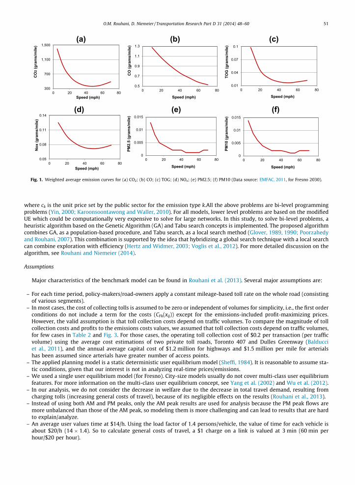
� �, as shown later in Fig. 1. To find the total emissions from each link, kk should be

multiplied by the length of the link (Lij) and its volume (x�ij. The total emissions (in grams or tons) and travel time cannot besummed because of the difference in units. bk has been added to change the emission units from tons to hours. So, bk is acombination of two factors: the cost of each emission type ($/tons) and a general value of time (VOT) measure ($/h). Of noteis that fuel consumption can also be added as a term in the ESCP problem.

Fig. 1 shows the calculated emission factors (kks) for CO2, CO, total organic gases (TOG), NOx, PM2.5, and PM10 emissions.Based on EMFAC (2011), the emission factor figures are the weighted averages of 2030 emission factors (only running emis-sions) for different vehicle classes at different speed levels. The weights are the vehicle miles traveled (VMT) by differentvehicle classes.

In addition to the PMP, CSCP, and ESCP problems, we proposed the emissions-included PMP (EPMP) problem, in whichprivate owners have to pay the public sector for the emissions produced from their roads (Nagurney, 2000). In fact, the EPMPproblem is the same as the general PMP, but the toll collection costs (CFk(xij)) are not zero and are equal to the total costs(value) of emissions generated from the owned roads:

ðEPMPÞ Maxsij

pn ¼ Rði;jÞ�Fksij � x�i;j �sð Þ � Rk ck � kk:

Lij

tijðx�ijÞ

!� Lij � x�ij

!ð5Þ

modified UE assumes that general costs of travel, adding toll costs to travel time, rather than time only drive users’ route choice decision.

300

700

1,100

1,500

0 20 40 60 80

CO

2(g

ram

s/m

ile)

Speed (mph)

(a)

0.5

0.7

0.9

1.1

1.3

0 20 40 60 80

CO

(gra

ms/

mile

)

Speed (mph)

(b)

0.05

0.08

0.11

0.14

0 20 40 60 80

Nox

(gra

ms/

mile

)

Speed (mph)

(d)

0.01

0.04

0.07

0.1

0 20 40 60 80

TOG

(gra

ms/

mile

)

Speed (mph)

(c)

0

0.005

0.01

0.015

0 20 40 60 80

PM2.

5 (g

ram

s/m

ile)

Speed (mph)

(e)

0

0.005

0.01

0.015

0 20 40 60 80

PM10

(gra

ms/

mile

)

Speed (mph)

(f)

Fig. 1. Weighted average emission curves for (a) CO2; (b) CO; (c) TOG; (d) NOx; (e) PM2.5; (f) PM10 (Data source: EMFAC, 2011, for Fresno 2030).

O.M. Rouhani, D. Niemeier / Transportation Research Part D 31 (2014) 48–60 51

where ck is the unit price set by the public sector for the emission type k.All the above problems are bi-level programmingproblems (Yin, 2000; Karoonsoontawong and Waller, 2010). For all models, lower level problems are based on the modifiedUE which could be computationally very expensive to solve for large networks. In this study, to solve bi-level problems, aheuristic algorithm based on the Genetic Algorithm (GA) and Tabu search concepts is implemented. The proposed algorithmcombines GA, as a population-based procedure, and Tabu search, as a local search method (Glover, 1989, 1990; Poorzahedyand Rouhani, 2007). This combination is supported by the idea that hybridizing a global search technique with a local searchcan combine exploration with efficiency (Hertz and Widmer, 2003; Voglis et al., 2012). For more detailed discussion on thealgorithm, see Rouhani and Niemeier (2014).

Assumptions

Major characteristics of the benchmark model can be found in Rouhani et al. (2013). Several major assumptions are:

– For each time period, policy-makers/road-owners apply a constant mileage-based toll rate on the whole road (consistingof various segments).

– In most cases, the cost of collecting tolls is assumed to be zero or independent of volumes for simplicity, i.e., the first orderconditions do not include a term for the costs (CFk(xij)) except for the emissions-included profit-maximizing prices.However, the valid assumption is that toll collection costs depend on traffic volumes. To compare the magnitude of tollcollection costs and profits to the emissions costs values, we assumed that toll collection costs depend on traffic volumes,for few cases in Table 2 and Fig. 3. For those cases, the operating toll collection cost of $0.2 per transaction (per trafficvolume) using the average cost estimations of two private toll roads, Toronto 407 and Dulles Greenway (Balducciet al., 2011), and the annual average capital cost of $1.2 million for highways and $1.5 million per mile for arterialshas been assumed since arterials have greater number of access points.

– The applied planning model is a static deterministic user equilibrium model (Sheffi, 1984). It is reasonable to assume sta-tic conditions, given that our interest is not in analyzing real-time prices/emissions.

– We used a single user equilibrium model (for Fresno). City-size models usually do not cover multi-class user equilibriumfeatures. For more information on the multi-class user equilibrium concept, see Yang et al. (2002) and Wu et al. (2012).

– In our analysis, we do not consider the decrease in welfare due to the decrease in total travel demand, resulting fromcharging tolls (increasing general costs of travel), because of its negligible effects on the results (Rouhani et al., 2013).

– Instead of using both AM and PM peaks, only the AM peak results are used for analysis because the PM peak flows aremore unbalanced than those of the AM peak, so modeling them is more challenging and can lead to results that are hardto explain/analyze.

– An average user values time at $14/h. Using the load factor of 1.4 persons/vehicle, the value of time for each vehicle isabout $20/h (14 � 1.4). So to calculate general costs of travel, a $1 charge on a link is valued at 3 min (60 min perhour/$20 per hour).

Fig. 2. Road network of Fresno, California with the candidate roads (Source: Transportation planning model, city of Fresno).

Table 1Main characteristics of the candidate roads. Source: Transportation planning model, city of Fresno-2030 forecasts.

Name Length-private (Mile) Freeflow speed (MPH) AM Peak VMT (Base-hourly) Offpeak VMT (Base-hourly)

HW1 SR168 4.92 65 70,265 28,009HW2 SR41 7.51 65 133,070 56,900HW3 SR180 5.23 58 68,701 30,138HW4 SR99 8.56 65 136,263 55,509Arterial1 Shaw 8.47 40 44,163 14,710Arterial2 Shields 5.32 40 19,943 7,147Arterial3 Blackstone 4.73 40 21,044 5,420

52 O.M. Rouhani, D. Niemeier / Transportation Research Part D 31 (2014) 48–60

– The assumed base unit emission costs (the first factor determining bk’s) are as follows: $25/ton of CO2, $250/ton of CO,$7,000 ton of NOx, $3,000/ton of TOG, $30,000/ton of PM10, $300,000/ton of PM2.5, and $4/gallon of gasoline (the totalcost calculations only); these figures are inflation-adjusted averages of what various research studies have found, usingthe health costs associated with these emissions in urban areas (Wang et al., 1994; McCubbin and Delucchi, 1999; AEATechnology Environment, 2005; Van Benthem, 2012).

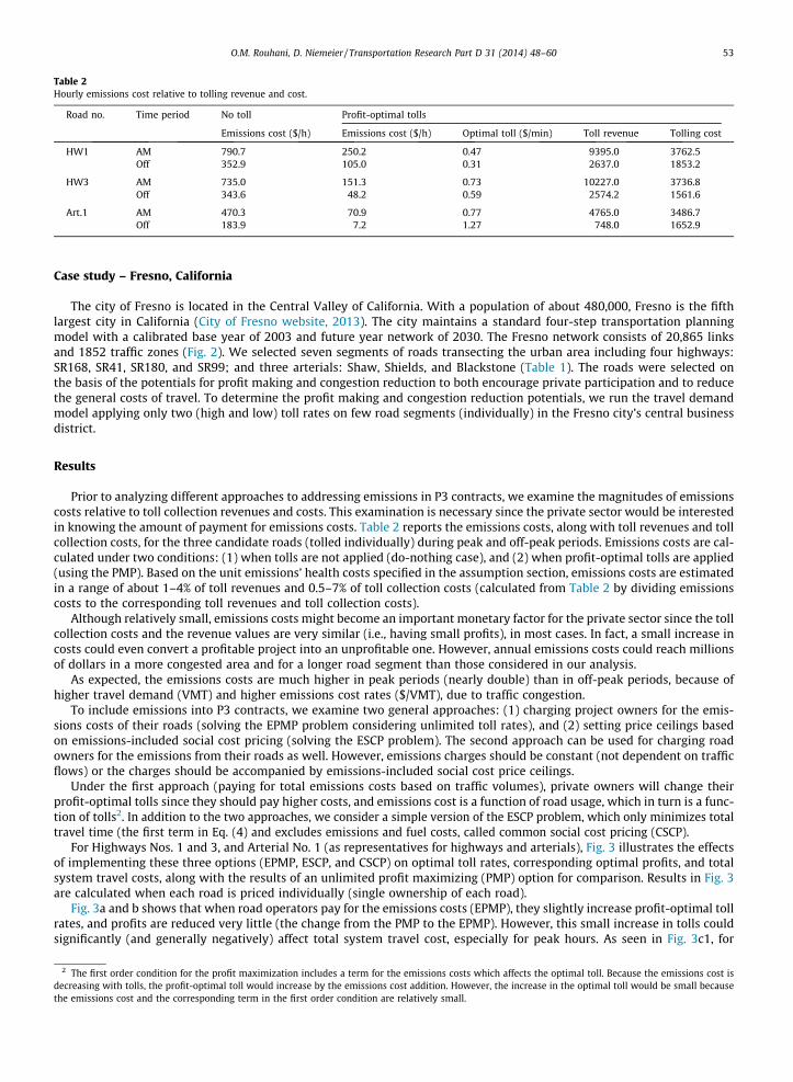
Table 2Hourly emissions cost relative to tolling revenue and cost.

Road no. Time period No toll Profit-optimal tolls

Emissions cost ($/h) Emissions cost ($/h) Optimal toll ($/min) Toll revenue Tolling cost

HW1 AM 790.7 250.2 0.47 9395.0 3762.5Off 352.9 105.0 0.31 2637.0 1853.2

HW3 AM 735.0 151.3 0.73 10227.0 3736.8Off 343.6 48.2 0.59 2574.2 1561.6

Art.1 AM 470.3 70.9 0.77 4765.0 3486.7Off 183.9 7.2 1.27 748.0 1652.9

O.M. Rouhani, D. Niemeier / Transportation Research Part D 31 (2014) 48–60 53

Case study – Fresno, California

The city of Fresno is located in the Central Valley of California. With a population of about 480,000, Fresno is the fifthlargest city in California (City of Fresno website, 2013). The city maintains a standard four-step transportation planningmodel with a calibrated base year of 2003 and future year network of 2030. The Fresno network consists of 20,865 linksand 1852 traffic zones (Fig. 2). We selected seven segments of roads transecting the urban area including four highways:SR168, SR41, SR180, and SR99; and three arterials: Shaw, Shields, and Blackstone (Table 1). The roads were selected onthe basis of the potentials for profit making and congestion reduction to both encourage private participation and to reducethe general costs of travel. To determine the profit making and congestion reduction potentials, we run the travel demandmodel applying only two (high and low) toll rates on few road segments (individually) in the Fresno city’s central businessdistrict.

Results

Prior to analyzing different approaches to addressing emissions in P3 contracts, we examine the magnitudes of emissionscosts relative to toll collection revenues and costs. This examination is necessary since the private sector would be interestedin knowing the amount of payment for emissions costs. Table 2 reports the emissions costs, along with toll revenues and tollcollection costs, for the three candidate roads (tolled individually) during peak and off-peak periods. Emissions costs are cal-culated under two conditions: (1) when tolls are not applied (do-nothing case), and (2) when profit-optimal tolls are applied(using the PMP). Based on the unit emissions’ health costs specified in the assumption section, emissions costs are estimatedin a range of about 1–4% of toll revenues and 0.5–7% of toll collection costs (calculated from Table 2 by dividing emissionscosts to the corresponding toll revenues and toll collection costs).

Although relatively small, emissions costs might become an important monetary factor for the private sector since the tollcollection costs and the revenue values are very similar (i.e., having small profits), in most cases. In fact, a small increase incosts could even convert a profitable project into an unprofitable one. However, annual emissions costs could reach millionsof dollars in a more congested area and for a longer road segment than those considered in our analysis.

As expected, the emissions costs are much higher in peak periods (nearly double) than in off-peak periods, because ofhigher travel demand (VMT) and higher emissions cost rates ($/VMT), due to traffic congestion.

To include emissions into P3 contracts, we examine two general approaches: (1) charging project owners for the emis-sions costs of their roads (solving the EPMP problem considering unlimited toll rates), and (2) setting price ceilings basedon emissions-included social cost pricing (solving the ESCP problem). The second approach can be used for charging roadowners for the emissions from their roads as well. However, emissions charges should be constant (not dependent on trafficflows) or the charges should be accompanied by emissions-included social cost price ceilings.

Under the first approach (paying for total emissions costs based on traffic volumes), private owners will change theirprofit-optimal tolls since they should pay higher costs, and emissions cost is a function of road usage, which in turn is a func-tion of tolls2. In addition to the two approaches, we consider a simple version of the ESCP problem, which only minimizes totaltravel time (the first term in Eq. (4) and excludes emissions and fuel costs, called common social cost pricing (CSCP).

For Highways Nos. 1 and 3, and Arterial No. 1 (as representatives for highways and arterials), Fig. 3 illustrates the effectsof implementing these three options (EPMP, ESCP, and CSCP) on optimal toll rates, corresponding optimal profits, and totalsystem travel costs, along with the results of an unlimited profit maximizing (PMP) option for comparison. Results in Fig. 3are calculated when each road is priced individually (single ownership of each road).

Fig. 3a and b shows that when road operators pay for the emissions costs (EPMP), they slightly increase profit-optimal tollrates, and profits are reduced very little (the change from the PMP to the EPMP). However, this small increase in tolls couldsignificantly (and generally negatively) affect total system travel cost, especially for peak hours. As seen in Fig. 3c1, for

2 The first order condition for the profit maximization includes a term for the emissions costs which affects the optimal toll. Because the emissions cost isdecreasing with tolls, the profit-optimal toll would increase by the emissions cost addition. However, the increase in the optimal toll would be small becausethe emissions cost and the corresponding term in the first order condition are relatively small.

0.00

0.25

0.50

0.75

1.00

1.25

PMP EPMP CSCP ESCP

Tol

l rat

e ($

/mi)

(a-1)Highway 1Highway 3Arterial 1

-7,000

-5,000

-3,000

-1,000

1,000

3,000

5,000

7,000

PMP EPMP CSCP ESCP

Prof

its ($

/hr)

(b-1)Highway 1Highway 3Arterial 1

-2.0%

-1.0%

0.0%

1.0%

2.0%

3.0%

PMP EPMP CSCP ESCP

Cha

nge

in to

tal t

rave

l cos

t (c-1)Highway 1Highway 3Arterial 1

0.00

0.25

0.50

0.75

1.00

1.25

1.50

PMP EPMP CSCP ESCP

Tol

l rat

e ($

/mi)

(a-2)

Highway 1Highway 3Arterial 1

-4,000

-3,000

-2,000

-1,000

0

1,000

PMP EPMP CSCP ESCP

Prof

its ($

/hr)

(b-2)

Highway1Highway 3Arterial 1

-1.5%

-1.0%

-0.5%

0.0%

PMP EPMP CSCP ESCP

Cha

nge

in to

tal t

rave

l cos

t

(c-2)Highway 1Highway 3Arterial 1

Fig. 3. Optimal toll (a), revenue (b), system cost (c) of different approaches to internalize the emissions cost for (1) peak and (2) off-peak periods.

54 O.M. Rouhani, D. Niemeier / Transportation Research Part D 31 (2014) 48–60

Highway No. 1, the change in total travel cost, relative to the do-nothing (no-tolling) case, rises from 1% (PMP) to 1.5%(EPMP).

For the second approach, we need to determine appropriate price ceilings based on social-optimal tolls. One key questionis what types of travel costs should be considered in determining social-optimal toll rates. In most of the cases shown inFig. 3, consideration of fuel and emissions costs in addition to time (ESCP vs. CSCP) has no effect on the system-optimal tollrates and their corresponding profits and system costs. However, for one case, Highway No. 3 in peak period (Fig. 3a1), thesystem-optimal rates for the CSCP and the ESCP solutions are different. Nevertheless, the difference in total system costs istrivial when applying the two different system-optimal rates (with or without considering fuel and emissions costs). How-ever, to ensure the use of toll rates that minimize the total system-wide travel costs, and to determine total travel costs ofvarious options, policy makers should endorse the development of complex models for social cost calculations including allthe travel costs, rather than travel time only.

To compare the two proposed general approaches, we examine the results of solving for the EPMP and ESCP problems. Ingeneral, charging the road operators for the emissions costs without limiting tolls (the EPMP problem) results in higher tollprofits than the profits under limiting tolls (price ceilings) based on the emissions-included system-optimal rates (the ESCPsolution), as expected. On the other hand, the total system travel costs are drastically lower for the ESCP solution than for theEPMP solution.

As discussed before, the trade-offs between raising profits and reducing congestion (travel costs) should drive the deci-sion toward one of these approaches. However, the ESCP solution provides a reasonable level of profit while also improvingtransportation system performance. Moreover, roads, as public goods, should offer an efficient service, not necessarily a prof-itable one. Therefore, the second approach seems superior to the first (EPMP). Therefore, policy makers should limit tolls tosocial-optimal rates rather than charging for emissions costs, which would both reduce travel costs and raise profits.

We also look at the emissions costs generated by each vehicle driving on each individual road. Given the base unit costsassumption in the Assumption section (‘Assumptions’), Fig. 4 shows the AM peak emissions costs per-mile on the P3 candi-date roads under three different conditions: (a) base case (do nothing); (b) CSCP charging all roads (or CSCP1 as shown laterin Table 3); and (c) PMP charging all roads–oligopoly3 (or PMP10 as shown later in Table 3). The emissions unit costs (from theassumption section) are multiplied by the emissions generated from all links of each P3 road, and the resulting figures are sum-marized over all links of the road.

When driving on the P3 candidate roads, the average AM peak emissions costs are 1.37 (base case), 1.23 (CSCP), and 1.20(PMP-oligopoly) cents/mile. In the same order, the corresponding off-peak costs are lower than their AM counterparts. Thesecost rates are low relative to toll rates charged in various cases, as seen later in Table 3. Therefore, the public sector cancharge for these emissions without significantly reducing toll profits.

However, if the public sector considers the emissions generated from P3 roads only, system-wide emissions (and the sys-tem-wide general costs of travel) will be ignored. In fact, the emissions generated from the P3 projects only is the lowest for

3 The oligopoly cases represent markets in which each road is owned by a separate firm/owner, and no firm owns more than one road.

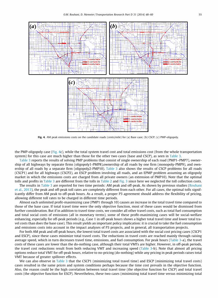
Fig. 4. AM peak emissions costs on the candidate roads (cents/mile) for (a) Base case; (b) CSCP; (c) PMP-oligopoly.

O.M. Rouhani, D. Niemeier / Transportation Research Part D 31 (2014) 48–60 55

the PMP-oligopoly case (Fig. 4c), while the total system travel cost and total emissions cost (from the whole transportationsystem) for this case are much higher than those for the other two cases (base and CSCP), as seen in Table 3.

Table 3 reports the results of solving PMP problems that consist of single ownership of each road (PMP1–PMP7), owner-ship of all highways by separate firms (oligopoly1-PMP8),ownership of all roads by one firm (monopoly-PMP9), and own-ership of all roads by a separate firm (oligopoly2-PMP10). Table 3 also shows the results of CSCP problems for all roads(CSCP1) and for all highways (CSCP2), an ESCP problem involving all roads, and an EPMP problem assuming an oligopolymarket in which the emissions costs are charged from all private owners (an extension of PMP10). Note that the optimaltolls and profits in Table 3 are different from the tolls in Table 2 and Fig. 3 since here we neglected the toll collection costs.

The results in Table 3 are reported for two time periods: AM peak and off-peak. As shown by previous studies (Rouhaniet al., 2013), the peak and off-peak toll rates are completely different from each other. For all cases, the optimal tolls signif-icantly differ from AM peak to off-peak hours. As a result, a proper P3 agreement should address the flexibility of pricing,allowing different toll rates to be charged in different time periods.

Almost each unlimited profit-maximizing case (PMP1 through 10) causes an increase in the total travel time compared tothose of the base case. If total travel time were the only objective function, most of these cases would be dismissed fromfurther consideration. But if in addition to travel time costs, we consider all other travel costs, such as total fuel consumptionand total social costs of emissions (all in monetary terms), some of these profit-maximizing cases will be social-welfareenhancing, especially for off-peak periods (e.g., Case 1 in off-peak hours shows a higher total travel time and lower total tra-vel costs than does the base case). This result yields an important policy implication: it is crucial to take the fuel consumptionand emissions costs into account in the impact analyses of P3 projects, and in general, all transportation projects.

For both AM peak and off-peak hours, the lowest total travel costs are associated with the social cost pricing cases (CSCP1and ESCP), since these cases minimize total travel costs. The reductions in travel costs are reached mainly through raisingaverage speed, which in turn decreases travel time, emissions, and fuel consumption. For peak hours (Table 3-a), the travelcosts of these cases are lower than the do-nothing case, although their total VMTs are higher. However, in off-peak periods,the travel cost reductions result from both reducing VMT and increasing speed (Table 3-b). Note that almost all pricingoptions reduce total VMT for off-peak hours, relative to no-pricing (do-nothing) while any pricing in peak periods raises totalVMT because of greater spillover effects.

We can also observe in Table 3 that the CSCP1 (minimizing total travel time) and ESCP (minimizing total travel costs)cases resulted in the same prices and system conditions perhaps because the time cost prevails in the objective function.Also, the reason could be the high correlation between total travel time (the objective function for CSCP) and total travelcosts (the objective function for ESCP). Nevertheless, these two cases (minimizing total travel time versus minimizing total

Table 3Hourly results of various tolling regimes for (a) AM peak and (b) off-peak.

Problemtype(scenario)

Optimal (Eq.) prices (cents/mile) Total hourlyprofits(1000$)

Total traveltime(Veh-h)

TotalsystemVMT

Ave. speed insystem (mph)

Totalcosts ($)

HW1 HW2 HW3 HW4 Art 1 Art 2 Art 3

(a)Case0 Basecase – – – – – – – – 103,579 3,561,877 34.39 2,854,123Case1 PMP1 33 – – – – – – 10.7 104,566 3,575,961 34.20 2,878,226Case2 PMP2 – 35 – – – – – 23.3 105,066 3,586,574 34.14 2,891,028Case3 PMP3 – – 60 – – – – 10.9 104,687 3,567,505 34.08 2,881,018Case4 PMP4 – – – 26 – – – 23.7 103,301 3,580,953 34.67 2,847,516Case5 PMP5 – – – – 41 – – 6.7 103,960 3,571,988 34.36 2,863,205Case6 PMP6 – – – – – 43 – 2.6 104,129 3,565,636 34.24 2,866,985Case7 PMP7 – – – – – – 28 1.7 103,670 3,565,690 34.39 2,857,456Case8 PMP8 (Oligopoly) 44 46 54 36 – – – 75.4 110,501 3,638,846 32.93 3,016,015Case9 PMP9 (Monopoly) 54 60 57 42 77 87 64 107.7 111,930 3,678,224 32.86 3,048,366Case10 PMP10 (Oligopoly-2) 47 49 54 38 64 64 43 104.6 109,981 3,661,309 33.29 3,002,544Case11 CSCP1 27 22 16 17 31 32 3 72.1 100,042 3,580,068 35.79 2,767,382Case12 CSCP2 27 22 14 18 – – – 56 100,420 3,571,621 35.57 2,777,004Case13 ESCP 27 22 16 17 31 32 3 72.1 100,042 3,580,068 35.79 2,767,382Case14 EPMP 48 50 53 40 66 65 45 97 110,329 3,668,998 33.26 3,010,350

(b)Case0 Basecase – – – – – – – – 36,046 1,477,408 40.99 1,024,036Case1 PMP1 24 – – – – – – 2.7 36,075 1,474,951 40.89 1,023,784Case2 PMP2 – 24 – – – – – 7.4 35,785 1,469,909 41.08 1,016,596Case3 PMP3 – – 30 – – – – 3.3 36,128 1,474,310 40.81 1,025,731Case4 PMP4 – – – 24 – – – 7.5 35,740 1,474,704 41.26 1,015,113Case5 PMP5 – – – – 18 – – 1.3 35,880 1,475,559 41.12 1,019,585Case6 PMP6 – – – – – 16 – 0.5 35,686 1,475,815 41.36 1,014,879Case7 PMP7 – – – – – – 28 0.3 36,085 1,477,666 40.95 1,025,006Case8 PMP8 (Oligopoly) 26 29 43 28 – – – 20.5 36,144 1,464,951 40.53 1,022,079Case9 PMP9 (Monopoly) 25 31 38 28 26 27 20 26.5 36,281 1,467,043 40.44 1,025,067Case10 PMP10 (Oligopoly-2) 26 30 39 28 27 28 26 25.9 36,374 1,466,969 40.33 1,027,447Case11 CSCP1 11 14 11 13 13 14 3 19.1 35,144 1,463,900 41.65 1,000,571Case12 CSCP2 11 14 9 11 – – – 16.2 35,182 1,465,366 41.65 1,001,745Case13 ESCP 11 14 11 13 13 14 3 19.1 35,144 1,463,900 41.65 1,000,571Case14 EPMP 27 31 40 30 29 30 28 21.8 36,415 1,467,255 40.29 1,027,798

56 O.M. Rouhani, D. Niemeier / Transportation Research Part D 31 (2014) 48–60

travel costs) could result in different outcomes. As we observed in Fig. 3a1 for Highway No. 3, the optimal toll rates and theresulting system travel costs for CSCP differ from those of ESCP.

Finally, as discussed before, emissions-included profit-maximizing pricing (EPMP) is not an effective way to reduce emis-sions or to reduce total costs of travel. In fact, the EPMP case yields one of the highest travel costs and results in lower profitsthan the corresponding PMP cases, as expected. Table 3-a shows that for AM peak hours, the EPMP case raises total VMT byabout 3.0% (3,668,998 versus 3,561,877), reduces average speed by about 3.3% (33.26 versus 34.39 mph), and as a resultincreases total travel costs by 5.5% ($3,010,350 versus $2,854,123), relative to the base case. Even though the CSCP1 caseincreases total VMT by about 0.5% (3,580,068 versus 3,561,877), it raises the average speed by about 4.1% (35.79 versus34.39 mph). Consequently, it reduces total travel costs by 3.0% ($2,767,382 versus $2,854,123), relative to the base case.

The failure of the EPMP case provides an important policy insight into the management of emissions using P3 contracts.The public sector should not charge project owners for the emissions directly, especially not based on VMTs or traffic vol-umes. Without price ceilings, charging for emissions costs (EPMP) would encourage private owners to direct the flows fromtheir road(s) to other congested roads even more than with the PMP cases, which in turn would probably increase the totaltravel cost of a system, mainly in peak periods. This result is consistent with what Daniel and Bekka (2000) found-that partialpricing on few highways could increase aggregate emissions from a transportation system. In practice, instead of VMT-basedemission charges, the public sector could enforce price ceiling levels that take into account the emissions costs as well asother social costs.

For some of the cases presented in Table 3, Fig. 5 shows the hourly system-wide travel time costs, fuel consumption costs,and emissions costs. Emissions costs are the sum of the costs of all the emission types, using the base unit emissions costs inthe Assumption section.

As shown in Fig. 5, the total emissions costs comprise small shares of the total travel costs. The highest share (not absolutevalue) among all cases, remarkably, belongs to social cost pricing cases (CSCP and ESCP): about 1.60% for AM peak and 1.72%for off peak out of total travel costs. However, shares are not much different across the cases, with the least shares at 1.55%for AM peak (PMP9) and 1.70% for off-peak (PMP10).

However, the system-wide emissions cost values under profit maximization cases are much higher in magnitude than theemissions costs under the social cost pricing cases; e.g., for AM peak hours, total emissions from the PMP10 and EPMP casescost $47,000 and $47,400 (a 2.79% and a 3.69% increase in emissions costs relative to do-nothing) while total emissions from

0

0.5

1

1.5

2

2.5

3

3.5

Tota

l tra

vel c

ost (

$ m

illio

n/ho

ur)

(a)

0

0.5

1

1.5

2

2.5

3

3.5

Tota

l tra

vel c

ost (

$ m

illio

n/ho

ur)

(b)

Fig. 5. Total travel time, fuel consumption, and emissions costs of various cases for (a) AM peak and (b) off-peak.

0

10

20

30

40

50

Em

issi

ons c

ost (

$ 10

00/ h

our)

(a)

0

10

20

30

40

50

Em

issi

ons c

ost (

$ 10

00/ h

our)

(b)

Fig. 6. Costs of different emission types for (a) AM peak and (b) off-peak.

O.M. Rouhani, D. Niemeier / Transportation Research Part D 31 (2014) 48–60 57

the CSCP1 and CSCP2 cases cost $44,700 and $44,900 (a 2.09% and a 1.8% decrease in costs from do-nothing). From Table 3-a,we can calculate that the higher emissions costs for the PMP10 and EPMP cases result from (1) an approximate 2.8% increaseand a 3.0% increase in total system VMT, and (2) an approximate 3.2% decrease and a 3.3% decrease in the average speed ofthe system, respectively. However, emissions costs of the social cost pricing cases (CSCP1 and CSCP2) are reduced mainlythrough raising average speed (by 4.1% and 3.4%) even though their total VMTs are higher (by 0.5% and 0.3%) than the totalVMT of the do-nothing case.

The total travel time costs and fuel consumption costs shares out of the total costs are much higher than those of theemissions costs, with an average of 72.8% and 25.6% (AM peak) and 70.5% and 27.8% (off-peak), respectively, over all cases.Although the emissions costs are significantly lower than the travel time costs and fuel consumption costs, the values aremisleading. A large proportion of travel time and fuel consumption costs cannot be avoided even with free-flow travel timeconditions, but emissions costs can be reduced by higher proportions and with much broader policy levers.

Fig. 6 provides detailed hourly costs of different emission types for various cases. These costs are also calculated using thebase unit emission costs assumed in the Assumption section.

Examining Fig. 6, one may argue that $45,000 (the average total hourly emissions costs for AM peak cases) is trivial forsocial planning purposes. But the reported total emissions costs are calculated per hour, and the corresponding annual costscan reach $150 million.4 Therefore, even a one or two percent emissions reduction could save millions of dollars even for a mid-size city.

CO2 emissions costs comprise a large share of the total emissions costs (from 88% up to 91%), followed by PM2.5 (4.3–4.5%), NOx (4%), CO (1.5–1.6%), TOG (0.5–0.7%), and PM10 (0.5–0.6%). Shares of various emission types are relatively stableacross different cases although total emissions costs vary substantially relative to the base case: for example in AM peakhours, +3.7% (for PMP9) down to �2.1% (for CSCP1). While the second option (EPMP) and main profit maximization cases(PMP8 to PMP10) result in significantly higher total emissions costs than the base case emissions for AM peak hours, totalemissions costs of these cases are even lower than those of the base case for off-peak hours. A reasonable explanation is thatthe adverse effects of applying high toll rates (resulting from the second option and other unlimited profit-maximizing cases)are much lower for off-peak hours than for peak hours since the traffic spillovers to other uncongested roads do not diminishthe transportation system performance further.

4 To calculate annual values, a combination of off-peak (18 h) and peak (6 h) is considered. The annual costs are then calculated for 250 working days,considering recurrent congestion conditions over these days.

58 O.M. Rouhani, D. Niemeier / Transportation Research Part D 31 (2014) 48–60

Conclusions

This study provides important policy insights into potential approaches to charging emissions when using P3 projects anddesigning their contracts. First, taking the fuel consumption and emissions costs into account is of great importance inimpact analyses of P3 projects. Some of the P3 scenarios would be social welfare-enhancing with a more generalized totaltravel cost objective function, while those same cases would reduce social welfare with a total travel time objective functionas the only criterion. Furthermore, as shown in Fig. 3 1 for Highway No. 3, considering other costs in addition to time couldchange the system-optimal toll rates and their corresponding system travel costs.

Second, for all scenarios, total system emissions costs comprise a small share of total system travel costs (average 1.6%)while CO2 emissions costs comprise a large share of total emissions costs (average 90%). Even though total emissions costsare small relative to total travel time and total fuel consumption costs, emissions costs can be reduced by higher proportionsand with much broader policy levers than can total travel time and fuel consumption costs. On the other hand, emissionscosts are small relative to toll revenues and costs (about 1–4% of toll revenue). Thus, policies to reduce emissions can beemployed without incurring significant revenue losses to road (project) owners.

Finally, we tried to provide insights into the introduction of new approaches to addressing emissions in P3 contracts. Oneimportant precondition for a successful P3 arrangement is that the quality of service be contractible (Fiscal Affairs Office,2004). Therefore, the possible approaches to addressing emissions in P3 contracts are narrowed. We examined two generalapproaches: charging project owners for the emissions costs of their own projects, and setting price ceilings based on emis-sions-included social cost pricing.

The first option generally results in the worst system conditions because private owners are encouraged to directthe flows on their road(s) to other congested roads in order to decrease their emissions costs. The traffic spilloverswould degrade system performance. Nevertheless, using the first option, the emissions costs generated only from P3 roadswould usually be lower than those of other cases. However, measuring (charging for) the emissions levels only on P3roads would provide inappropriate incentives for the P3 owners that could increase emissions costs and total travel costsof the whole transportation system.

The second option, setting price ceilings based on emissions costs or social cost pricing, proved promising for ourcase study. For example, in peak periods, the second option decreases system emissions costs by about 2.09%, mainlythrough raising the system’s average speed by about 4%, even though its total VMT is slightly higher (by 0.5%), relativeto the no-pricing case. On the other hand, the first option increases emissions costs by 3.69%, as a result of (1) anapproximate 3.0% increase in total VMT, and (2) an approximate 3.3% decrease in average speed, relative to the do-nothing case. However, the adverse effects of applying high toll rates (resulting from the second option) are much lowerfor off-peak hours.

The second option can be used for charging emissions from P3 roads as well. However, the emissions charges shouldbe constant (not dependent on traffic flows) or the charges should be accompanied by emissions-included social costprice ceilings so that the profit-oriented road owners could not increase toll rates in response to the internalization ofthe emissions costs. Otherwise, the spillover effects of the resulting higher toll rates could further worsen systemperformance.

However, the applied model is constrained by several limitations and simplifications. City-size transportation planningmodels usually do not include multiple users, and the use of a justified multi-user model requires a separate comprehensivestudy about the distribution of the value of time for users of each origin/destination pair, which was not possible for thisstudy. Another limitation of the study is that the city of Fresno does not have a strong public transportation system, so traveldemands might be less elastic. Therefore, our results may be an underestimation of the potential benefits of pricing/privati-zation for a city with a strong public transportation system. Considering these constraints, one needs to be careful about gen-eralizing the results found by this study to other cases.

Another simplification is that we did not include in our analysis the transaction costs of charging for emissions. The inclu-sion of the transaction costs could have a significant impact on the analysis and could change the results in favor of alter-native policy options to deal with emissions costs, such as higher taxation on fuel or higher fuel efficiency standards (Proostand Van Dender, 2001), and variable speed limits (Bel and Rosell, 2013).

Given the limitations of this study, future studies may consider estimating/calibrating the distribution of the value of timefor users for origin/destination pairs. In addition, although travel demand is assumed to be non-constant in the study, theendogenous travel demand elasticities of the planning model are not calibrated for the significant changes in travel costsas a result of charging. Further research is required to improve the elasticities in this regard. The model can also be developedfurther through the consideration of other innovative pricing/charging options into P3 contracts, such as setting different tollrates for different vehicle types based on their emission rates, and redistributing a portion of toll profits to low emissionvehicles.

Caveat

The transportation planning model used in this study was employed for research purposes only, and not for developingregional transportation plans or transportation improvement programs.

O.M. Rouhani, D. Niemeier / Transportation Research Part D 31 (2014) 48–60 59

Acknowledgements

The authors express their special gratitude to Philine Gaffron from Hamburg University of Technology for her commentsand for providing technical assistance. In addition, the authors would like to thank reviewers for reviewing the paper, sharingthoughts, and offering insightful comments on the paper.

References

AEA Technology Environment, 2005. Damages per tonne emission of PM2.5, NH3, SO2, NOx and VOCs from each EU25 member state and surrounding seas,Clean Air for Europe (CAFE) Programme. European Commission. <http://www.cafe-cba.org/assets/marginal_damage_03-05.pdf> (accessed October2012).

Balducci, P., Shao, G., Amos, A., Rufolo, A., 2011. Costs of alternative revenue-generation systems. National Cooperative Highway Research Program-NCHRPREPORT 689, ISBN 978-0-309-21316-5.

Bel, G., Foote, J., 2009. Tolls, terms, and public interest in road concessions privatization: a comparative analysis of recent transactions in the US and France.Transport. Rev. 29 (3), 397–413.

Bel, G., Rosell, J., 2013. Effects of the 80 KM � H-1 and variable speed limit on air pollution in the metropolitan area of Barcelona. Transport. Res. Part D 23,90–97.

Bierman, H.S., Fernandez, L., 1998. Game Theory: With Economic Application. Addison-Wesley Publishing Company Inc., Reading, MA.Bonnafous, A., 2010. Programming, optimal pricing and partnership contract for infrastructures in PPPs. Res. Transport. Econ. 30 (1), 15–22.Chen, A., Subprasom, K., 2007. Analysis of regulation and policy of private toll roads in a build–operate–transfer scheme under demand uncertainty.

Transport. Res. Part A 41 (6), 537–558.Chung, D., Hensher, D.A., Rose, J.M., 2010. Toward the betterment of risk allocation: investigating risk perceptions of Australian stakeholder groups to

public–private-partnership toll road projects. Res. Transport. Econ. 30 (1), 43–58.City of Fresno website, 2013. <http://www.fresno.gov/DiscoverFresno/default.htm> (accessed November 2013).Cortés, C.E., Vargas, L.S., Corvalán, R.M., 2008. A simulation platform for computing energy consumption and emissions in transportation networks.

Transport. Res. Part D 13 (7), 413–427.Daniel, J.I., Bekka, K., 2000. The environmental impact of highway congestion pricing. J. Urban Econ. 47 (2), 180–215.de Palma, A., Lindsey, R., 2000. Private toll roads: competition under various ownership regimes. Annu. Reg. Sci. 34 (1), 13–35.de Palma, A., Lindsey, R., 2002. Private roads, competition and incentives to adopt time-based congestion tolling. J. Urban Econ. 52 (2), 217–241.de Palma, A., Kilani, M., Lindsey, R., 2007. Maintenance, service quality and congestion pricing with competing roads. Transport. Res. Part B 41 (5), 573–591.Dimitriou, L., Tsekeris, T., Stathopoulos, A., 2009. Joint pricing and design of urban highways with spatial and user group heterogeneity. Netnomics 10 (1),

141–160.EMFAC, 2011. <http://www.arb.ca.gov/jpub/webapp//EMFAC2011WebApp/MainPageServlet?b_action=view> (accessed October 2012).Engel, E., Fischer, R., Galetovic, A., 2003. Privatizing highways in Latin America: fixing what went wrong. Economia 4 (1), 129–158.Engel, E., Fischer, R., Galetovic, A., 2006. Privatizing highways in the United States. Rev. Indust. Org. 29 (1), 27–53.Evenhuis, E., Vickerman, R., 2010. Transport pricing and public–private partnerships in theory: issues and suggestions. Res. Transport. Econ. 30 (1), 6–14.Fiscal Affairs Office, 2004. Public Private Partnerships. International Monetary Fund, Washington DC.Garvin, M.J., Bosso, D., 2008. Assessing the effectiveness of infrastructure public-private partnership programs and projects. Public Works Manage. Policy 13

(2), 162–178.Glover, F., 1989. Tabu search part 1. ORSA J. Comput. 1 (2), 190–206.Glover, F., 1990. Tabu search part 2. ORSA J. Comput. 2 (1), 4–32.Hertz, A., Widmer, M., 2003. Guidelines for the use of meta-heuristics in combinatorial optimization. Euro. J. Oper. Res. 151 (2), 247–252.Karoonsoontawong, A., Waller, S.T., 2010. Integrated network capacity expansion and traffic signal optimization problem: robust bi-level dynamic

formulation. Netw. Spatial Econ. 10 (4), 525–550.Leruth, L.E., 2012. Public–private cooperation in infrastructure development: a principal-agent story of contingent liabilities, fiscal risks, and other

(un)pleasant surprises. Netw. Spatial Econ. 12 (2), 223–237.Magnan de Bornier, J., 1992. The ‘Cournot-Bertrand debate’: a historical perspective. History Polit. Econ. 24 (3), 623–654.McCubbin, D.R., Delucchi, M.A., 1999. The health costs of motor-vehicle related air pollution. J. Transp. Econ. Policy 33 (3), 253–286.Midenet, S., Boillot, F., Pierrelee, J.C., 2004. Signalized intersection with real-time adaptive control: on-field assessment of CO2 and pollutant emission

reduction. Transport. Res. Part D 9 (1), 29–47.Nagurney, A., 2000. Sustainable Transportation Networks. Edward Elgar Publishing Inc., Northampton, MA, USA.Nesamani, K.S., Chu, L., McNally, M.G., Jayakrishnan, R., 2007. Estimation of vehicular emissions by capturing traffic variations. Atmos. Environ. 41 (14),

2996–3008.Poorzahedy, H., Rouhani, O.M., 2007. Hybrid meta-heuristic algorithms for solving transportation network design. Euro. J. Oper. Res. 182 (2), 578–596.Proost, S., Van Dender, K., 2001. The welfare impacts of alternative policies to address atmospheric pollution in urban road transport. Reg. Sci. Urban Econ.

31 (4), 383–411.Quiggin, J., 1988. Private and common property rights in the economics of the environment. J. Econ. Issues 1988, 1071–1087.Rall, J., Reed, J.B., Farber, N.J., 2010. Public-private partnerships for transportation, a toolkit for legislators. In: The National Conference of State Legislatures,

The Forum for America’s Ideas. ISBN 978-1-58024-612-5.Reason Foundation, 2009. Annual Privatization Report, edited by L.C. Gilroy.Reinhardt, W., 2011. The role of private investment in meeting U.S. transportation infrastructure needs, American Road and Transportation Builders

Association (ARTBA) Transportation Development Foundation, May 2011.Rouhani, O.M., 2009. Road privatization and sustainability. MIT J. Plan. 6, 82–105.Rouhani, O.M., Niemeier, D., 2011. Urban network privatization: a small network example. Transport. Res. Record 2221, 46–56.Rouhani, O.M., Niemeier, D., 2014. Flat versus spatially variable tolling: a case study in Fresno, California. J. Transport Geogr. 37, 10–18.Rouhani, O.M., Niemeier, D., Knittel, C., Madani, K., 2013. Integrated modeling framework for leasing urban roads: a case study of Fresno, California.

Transport. Res. Part B 48 (1), 17–30.Sheffi, Y., 1984. Urban Transportation Networks: Equilibrium Analysis with Mathematical Programming Methods. Prentice-Hall, Englewood Cliffs, NJ.Tan, Z., Yang, H., Gu, X., 2010. Properties of pareto-efficient contracts and regulations for road franchising. Transport. Res. Part B 44 (4), 415–433.Tsamboulas, D., Verma, A., Moraiti, P., 2013. Transport infrastructure provision and operations: why should governments choose private–public

partnership? Res. Transport. Econ. 38 (1), 122–127.Van Benthem, A., 2012. Do We Need Speed Limits on Freeways? Working paper, The Wharton School, University of Pennsylvania.Verhoef, E.T., Nijkamp, P., Rietveld, P., 1996. Second-best congestion pricing: the case of an un-tolled alternative. J. Urban Econ. 40, 279–302.Voglis, C., Parsopoulos, K.E., Papageorgiou, D.G., Lagaris, I.E., Vrahatis, M.N., 2012. MEMPSODE: a global optimization software based on hybridization of

population-based algorithms and local searches. Comput. Phys. Commun. 183 (5), 1139–1154.Wang, M.Q., Santini, D.J., Warinner, S.A., 1994. Methods of Valuing Air Pollution and Estimated Monetary Values of Air Pollutants in Various US Regions.

Technical Report, Argonne National Lab.

60 O.M. Rouhani, D. Niemeier / Transportation Research Part D 31 (2014) 48–60

Winkelman, S., Bishins, A., Kooshian, C., 2010. Planning for economic and environmental resilience. Transport. Res. Part A 44 (8), 575–586.Winston, C., Yan, J., 2011. Can privatization of U.S. highways improve motorists’ welfare? J. Public Econ. 95 (7–8), 993–1005.Wu, D., Yin, Y., Lawphongpanich, S., Yang, H., 2012. Design of more equitable congestion pricing and tradable credit schemes for multimodal transportation

networks. Transport. Res. Part B 46 (9), 1273–1287.Yang, H., Meng, Q., 2000. Highway pricing and capacity choice in a road network under a build–operate–transfer scheme. Transport. Res. Part A: Policy

Practice 34 (3), 207–222.Yang, H., Tang, W.H., Cheung, W.M., Meng, Q., 2002. Profitability and welfare gain of private toll roads in a network with heterogeneous users. Transport.

Res. Part A 36 (6), 537–554.Yin, Y., 2000. Genetic algorithm-based approach for bilevel programming models. J. Transport. Eng.: ASCE 26 (2), 115–120.Zhang, L., 2008. Welfare and financial implications of unleashing private-sector investment resources on transportation networks. Transport. Res. Record

2079, 96–108.Zhang, L., Levinson, D., 2009. The economics of road network ownership: an agent-based approach. Int. J. Sust. Transport. 3 (5–6), 339–359.