Reservoir Geomechanical Analyses of Joslyn SAGD Steam ... - ERA

Reservoir Geomechanical Analyses of Joslyn SAGD Steam Release Incident

by

Alireza Khani

A thesis submitted in partial fulfillment of the requirements for the degree of

Doctor of Philosophy in

Geotechnical Engineering

Department of Civil and Environmental Engineering University of Alberta

©Alireza Khani, 2022

ii

Abstract

A noteworthy caprock failure occurred on the Joslyn Steam Assisted Gravity Drainage (SAGD)

property in 2006 that continues to have a significant impact on the approval process for future

SAGD projects. Two reports were released by Alberta government, which are AER Review and

Analysis: Total E&P Canada Ltd. Surface Steam Release of May 18, 2006, Joslyn Creek SAGD

Thermal Operation, and Total E&P Canada Ltd., Summary of investigation into the Joslyn, May

18, 2006 Steam Release. Several potential mechanisms were postulated within those studies but

without definitive resolution. Therefore, the current study's main aim is to reassess the possible

causes of Joslyn caprock failure and to forensically investigate the different mechanisms that may

have contributed to this steam release incident. In addition, the findings of previous studies,

including geomechanical simulations, uncertainties, and risk associated with evaluating caprock

containment of SAGD operations using different approaches will be analyzed and the Joslyn steam

release will be numerically re-analyzed to understand better the possible causes and mechanisms

that led to the only known caprock failure in the 30 years of SAGD operations in Alberta.

In the current study, numerical simulations were divided into three stages; 1) geomechanical

analyses of a fractured medium in the assessment of caprock integrity, 2) hydro-mechanical

analyses of the models to explore the impact of fluid flow on the results 3) coupled reservoir

geomechanical analysis to investigate effects of SAGD operation on geomechanical response of

the models. For the first stage, multiple realizations of the fracture network in caprock were

executed to reflect various geomechanical and geometrical properties of fractures. A distinct

element code, 3DEC, was utilized to evaluate the possible mechanisms of caprock failure in a

fissured and non-fissured caprock. Then, three-dimensional numerical models including caprock

and overburden were simulated under different load conditions and properties to assess the impact

of steam injection pressure on caprock displacement, surface heave, the joint normal and shear

displacements, as well as failure modes. The second stage of the analyses considered fluid flow in

the models to investigate the impact of flow on fractures' geometrical parameters, caprock

displacement, and surface heave. The last numerical modeling stage was 3D sequentially coupled

reservoir geomechanical analyses to simulate the reservoir's behaviors, caprock, and overburden

and examine their complex interactions occurring during SAGD operations from beginning to the

iii

end. This stage consists of two sub-sections: first, post-failure simulation to validate the model

with actual injection and production data as well as surveillance results installed after the steam

release incident and second, using the validated model including all the well pairs and operations

from the beginning to the end of the project to better understand the most likely steam release

scenario of the failure.

Through the analysis of multiple aspects of the Joslyn steam release incident, it is postulated that

a chain of events, each impacting one another, contributed to the surface release. The possible,

interacting multiple events that led to this failure have been identified as:

• excessive bottomhole injection pressure;

• potential low quality cement job performed for the abandonment of vertical observation

wells;

• presence of a gas zone surrounding the abandoned well within the Upper McMurray and

Wabiskaw;

• relatively low quality (less clayey) and thin caprock on the east side of the Joslyn project

area;

• occasionally high water saturation zones within the Upper McMurray Formation; and

• perhaps most critically, the unexpected migration of fluid flow from the west to the east

side of the Joslyn project area leading to elevated pore pressures (and hence lower effective

confining stresses) in the region (gas streak zone) directly overlying the well pair where

the steam release event occurred.

Based on the modeling results in this research which were validated with post-failure SAGD

operations monitoring data, it allowed improved confidence in interpreting these complex events

and re-adjusting the proposed formula to calculate MOP.

iv

PREFACE

This is a “manuscript-style” dissertation, with Chapters 6 and 7 presented and published as detailed

below. Versions of the individual manuscripts as presented in these two chapters may differ

slightly from the published versions.

Chapter 5 was presented at the SPE Canada Heavy Oil Technical Conference, Calgary, Alberta,

Canada and published (March 13 2018) as SPE-189751-MS. This paper entitled “The Influence of

Discontinuities on Geomechanical Analysis of the Joslyn SAGD Steam Release Incident” and was

written by A.Khani; A. Rangriz-Shokri; R. J. Chalaturnyk.

Chapter 6 was presented and published at the geoconvention 2020, Calgary, Alberta, Canada,

September 2020. This paper entitled “The investigation of Fluid Flow in the Fissured Clearwater

Shale Using 3D Numerical Approach – Case Study of Joslyn Creek SAGD Project” and was

written by A.Khani; A. Rangriz-Shokri; R. J. Chalaturnyk.

I was responsible for all data analysis, data interpretation, discussion, and manuscript composition.

Dr. Chalaturnyk was involved in collaboration with TEPCL for data collection, developing the

concept for the dissertation, and as supervisor; he has reviewed all parts of the work. Dr. Rangriz-

Shokri was involved in the numerical modeling with 3DEC and reviewing the results.

v

To MY BEAUTIFUL WIFE, FARNOOSH

MY LITTLE SON, ARTA

And

MY FAMILY

vi

ACKNOWLEDGMENTS

First and foremost, I am deeply grateful to my supervisor, Professor Rick Chalaturnyk, who gave

me the opportunity of starting a PhD position at Reservoir Geomechanics Research Group

(RGRG). His support from the initial to the final level of this work is truly appreciated. I cannot

remember a time that he was mad even once and I always see him with his smile. Thank you, my

smart supervisor, for teaching me the lessons not only in academic way but also in social life.

I would like to thank my friend and colleague, Juan Alejandro Arias Buitrago, whose help,

stimulating suggestions, kind support have been of a great value in this work. I remember

sometimes we have been working together until midnight with a pot of tea.

During this work, I have collaborated with some of my colleagues for whom I have great regard,

and I wish to extend my thanks to all those who have helped me with my work. I offer my regards

to Dr. Alireza Rangriz Shokri, Dr. Nathan Deisman, Dr. Bo Zhang, Abel Junkal, Hope Walls and

the other members of RGRG team.

I express my gratitude to Total E&P Canada for providing me all the invaluable data and this work

would not be completed without their collaborations.

The financial support from the industrial partners for this research work is also gratefully

acknowledged.

I would like to express my heartfelt gratitude to my parents and my brothers who encouraged me

so much remotely from Iran.

Most importantly, none of this would have been possible without the love and patience of my

gorgeous wife, Farnoosh, which has been a constant source of motivation, support and strength all

these years in Canada without having our families around us. And I owe my especial loving thanks

to my cute 1 year old son, Arta, for his patience once I was working on my thesis and he was crying

out of my room and knocking the door to come to me. Love you my cutie.

Alireza Khani

Edmonton, 2022.

vii

Table of Contents

Research Motivation and Problem Statement .......................................................... 1 Research Objectives ................................................................................................. 3

Hypothesis ............................................................................................................... 4 Structure of Dissertation .......................................................................................... 5

Significance of the Work ......................................................................................... 8

Reserves in Alberta .................................................................................................. 9

Oil Sands Recovery Methods .................................................................................. 9 Thermal Recovery Methods ................................................................................... 10

Steam Assisted Gravity Drainage (SAGD) ........................................................... 12 Conventional Stages of SAGD Operation ............................................................. 13

2.5.1. Circulation (Start-up) Phase ............................................................................ 13 2.5.2. Circulation Phase with Pressure Differential .................................................. 14

2.5.3. Semi-SAGD Phase .......................................................................................... 14 2.5.4. SAGD Phase ................................................................................................... 14

Complex Interaction of Geomechanics and Multiphase Flow in SAGD Operation............................................................................................................................... 15

Caprock Integrity ................................................................................................... 17 Maximum Operating Pressure (MOP) ................................................................... 19 To Avoid Failing the Caprock ............................................................................... 19

Location of Joslyn SAGD Scheme ........................................................................ 21 Geology and Stratigraphy ...................................................................................... 21

viii

3.2.1. Quaternary Deposits ........................................................................................ 23 3.2.2. Clearwater Formation ..................................................................................... 23

3.2.1. Wabiskaw Members ........................................................................................ 24 3.2.1.1. Kcw3 .......................................................................................................... 24

3.2.1.2. Kcw2 .......................................................................................................... 24 3.2.1.3. Kcw1 .......................................................................................................... 24

3.2.2. McMurray Formation ...................................................................................... 26 3.2.2.1. Lower McMurray Member ........................................................................ 27

3.2.2.2. Middle McMurray Member ....................................................................... 27 3.2.2.3. Upper McMurray Member ........................................................................ 27

3.2.3. Devonian Bedrock .......................................................................................... 30 Structural Geology and Gas Trapping ................................................................... 31

Criteria for Deep or Shallow Reservoir ................................................................. 31 Stress Regime ........................................................................................................ 34

Wells Platform, Pilot and Phase 2 ......................................................................... 37 Failure Cases Associated with Thermal In-situ Recovery ..................................... 38

Joslyn Steam Release Incident ............................................................................... 41 Geology in the Vicinity of the Steam Release Zone .............................................. 45

Reports on the Steam Release Incident ................................................................ 47 Economic Impacts and Safety Considerations Resulting from Steam Release Incident ................................................................................................................. 48

Data Provided by TEPCL ...................................................................................... 50

4.1.1. Raw Data Files ................................................................................................ 50 4.1.1.1. Field Survey ............................................................................................... 53

4.1.1.2. Wire Line ................................................................................................... 56 4.1.1.3. Core Photo ................................................................................................. 60

4.1.1.4. Lab Documents .......................................................................................... 62 4.1.1.5. Lab Analysis .............................................................................................. 63

4.1.2. Observation Wells (Thermocouples and Piezometers) ................................... 63 4.1.3. Injection and Production Data ........................................................................ 66

4.1.4. Surface Heave Monitoring Data ..................................................................... 67

ix

4.1.5. Petrel Model .................................................................................................... 70 Generating Geo-cellular Model Using Petrel and SKUA-Gocad .......................... 75

4.2.1. Building Simulation Grids Using Real Data ................................................... 75 4.2.1.1. Transferring Generated Surfaces in Petrel to SKUA-Gocad ..................... 75

4.2.1.1. Building Simulation Grids ......................................................................... 77 4.2.2. Constitutive Models, Reservoir and Geomechanical Properties ..................... 83

4.2.2.1. Data Analysis to Define Facies ................................................................. 85 4.2.2.2. Generating a Mechanical Earth Model (MEM) ......................................... 88

4.2.2.3. Required Properties for the Coupling Platform ......................................... 91 Summary .............................................................................................................. 109

Preface ................................................................................................................. 111 Background .......................................................................................................... 113

Model Description and Input Properties .............................................................. 116 Results and Discussion ........................................................................................ 119

5.4.1. Impact of Mechanical Properties of Intact Rock .......................................... 120 5.4.1.1. Young’s Modulus. ................................................................................... 120

5.4.1.2. Poisson’s Ratio ........................................................................................ 122 5.4.1.3. Friction Angle .......................................................................................... 123

5.4.1.4. Cohesion and Tensile Strength ................................................................ 125 5.4.1.5. Dilation Angle ......................................................................................... 126

5.4.2. Impact of Mechanical Properties of Fractures .............................................. 126 5.4.2.1. Normal and Shear Stiffness of the Joints ................................................. 126

5.4.2.2. Joint Friction Angle and Cohesion .......................................................... 128 5.4.2.3. Joint Tensile Strength .............................................................................. 129

5.4.3. Impact of Geometrical Parameters of Fractures ........................................... 129 5.4.3.1. Fracture Size ............................................................................................ 129

5.4.3.2. Fracture Orientation ................................................................................. 131 5.4.3.3. Fracture Intensity ..................................................................................... 133

5.4.4. Impact of Different Load Conditions Applying at the Base of Caprock ...... 134 Conclusions and Remarks .................................................................................... 139

x

Preface ................................................................................................................. 141 Model Description ............................................................................................... 142

Results and Discussion ........................................................................................ 144 6.3.1. Impact of Different Uplift Pressure Conditions Applied at the Base of Caprock

..................................................................................................................... 144 6.3.2. Impact of Fracture Intensity .......................................................................... 147

Geomechanical vs. Hydro-Mechanical Simulation ............................................. 149

Post Failure Simulation for Model Calibration .................................................... 157

Simulation of Steam Release Event using Calibrated Model .............................. 181 7.2.1. Geomechanical and Reservoir Simulation Results ....................................... 184

7.2.1.1. Methodology for Full Field Reservoir Geomechanical Simulations ....... 187 7.2.1.2. Vertical Displacement and Volumetric Strains ....................................... 188

7.2.1.3. Shear and Extensional Failure Zones ...................................................... 196 7.2.1.4. Temperature and Pressure Profiles .......................................................... 199

Summary .............................................................................................................. 203

Introduction .......................................................................................................... 205

Geological Framework ........................................................................................ 205 Extensional Failure Occurred at the Toe of Well pair 1 ...................................... 216

Propagation of the Fractures ................................................................................ 220 Abandoned Well (AB/09-33-095) and Observation Well (100/09-33-095) Near the Heel of Well pair 1 .............................................................................................. 222 More Critical Situation above Well Pair 3 Compared to Well pair 1 .................. 223

Shearing in the Casing of AB/09-33-095 at the Depth of 75 m .......................... 232 Conduit around/in the Abandoned Well AB-09-33-095 ...................................... 235

Connection of AB/09-33-095 to the Surrounding Gas Zone ............................... 236 Unexpected Steam Migration from the Pilot and Other Wells to the Gas Zone Located at the Top of Well pair 1 in Upper McMurray ...................................... 238

xi

Shear Fracture above Pressurized Zone Using Geomechanical 3DEC Code .... 252 Summary ............................................................................................................ 256

Summary .............................................................................................................. 259 Conclusions .......................................................................................................... 262

Recommendations for Future Studies .................................................................. 264

xii

LIST OF TABLES

Table 2-1 Viscous oil production methods (Dusseault 2013) ....................................................... 11

Table 3-1 Operation times for pilot well ....................................................................................... 38

Table 3-2 Failure cases on thermal in-situ recovery methods chronologically (Nikiforuk

2013) .......................................................................................................................... 40

Table 4-1 Summary of available raw data for 512 wells provided by TEPCL ............................. 52

Table 4-2 Summary of available raw data for 72 wells located in interested area provided by

TEPCL ....................................................................................................................... 52

Table 4-3 the location and characteristics of the observation wells ............................................. 65

Table 4-4 Operational data provided for the horizontal wells ..................................................... 67

Table 4-5 Number and thickness of sub layers for each zone ...................................................... 79

Table 4-6 Elevation range for the top and bottom layers of each zone ........................................ 82

Table 4-7 Required properties defined in SKUA-GOCAD for geomechanics simulator ............ 84

Table 4-8 Required properties defined in SKUA-GOCAD for flow simulator ............................ 84

Table 4-9 Percentage of sand and shale for each zone before and after upscaling ....................... 86

Table 4-10 Mechanical group specified for the facies in each zone ............................................. 89

Table 4-11 Required properties for selected constitutive models in the geomechanical

simulator .................................................................................................................... 91

Table 4-12 Biot and thermal expansion coefficients for different materials .............................. 100

Table 4-13 Mechanical properties associated with constitutive models for different

materials ................................................................................................................... 102

Table 4-14 Range of dependent Young’s moduli for different regions ...................................... 103

Table 4-15 Constant horizontal and vertical permeability for the zones except reservoir

(RGRG platform manual, 2019) .............................................................................. 109

Table 4-16 Geomechanical properties for Strain Softening model with respect to stress

induced plastic deformations ................................................................................... 109

Table 5-1 Mechanical properties of intact rock and joints in caprock and overburden

(intact rock properties from TEPCL 2007) .............................................................. 119

Table 7-1 Injector and producer pressure for different phases of SAGD process for the

pilot .......................................................................................................................... 162

xiii

Table 7-2 Injector and producer pressure for different stages of SAGD process for well

pair 4 ........................................................................................................................ 162


pair 3 ........................................................................................................................ 163


pair 5 ........................................................................................................................ 164

Table 7-5 Adjusted mechanical properties in Clearwater and Wabiskaw close to the crater

.................................................................................................................................. 167

Table 7-6 Cumulative oil production for different percentile of original permeability .............. 175

Table 7-7 Injector and producer pressure for different stages of SAGD process for the

pilot .......................................................................................................................... 185


pair 1 ........................................................................................................................ 185


pair 3 ........................................................................................................................ 186


pair 5 ........................................................................................................................ 186


pair 2 ........................................................................................................................ 187


pair 4 ........................................................................................................................ 187

Table 8-1 Well status in January 2007, seven months after steam release [TEPCL, 2007] ....... 226

Table 8-2 Constitutive models and associated mechanical properties for the zones .................. 256

Table 8-3 Mechanical properties for the joints used in the model .............................................. 256

Table 8-4 Summary of chorological events led to steam release incident in Joslyn SAGD

project ...................................................................................................................... 257

Table 9-1 Maximum bottomhole pressure applied in well pairs in pad 204 .............................. 263

xiv

LIST OF FIGURES

Figure 2-1 Oil sands deposits in Alberta (retrieved from Alberta Geologic Survey, 2012) ......... 10

Figure 2-2 Mining and in-situ extraction methods for oil sands (retrieved from Alaska Oil

Sands, 2018) ............................................................................................................... 10

Figure 2-3. The schematic process of Steam Assisted Gravity Drainage (MEG Energy, 2017)

.................................................................................................................................... 12

Figure 2-4 Viscosity Vs. Temperature for bitumen ( after ConocoPhillips, 2009) ...................... 13

Figure 2-5 Short and long tubing during circulation and SAGD phases. (Total report 2007) ..... 15

Figure 2-6 Two major stress paths during SAGD (Chalaturnyk, 1996) ....................................... 17

Figure 2-7 Schematic of caprock failure mechanisms associated with SAGD ............................ 18

Figure 3-1 The location of Joslyn Creek ....................................................................................... 22

Figure 3-2 Stratigraphy of the Joslyn oil sand lease ..................................................................... 23

Figure 3-3 well AC/06-33-095-12W4 core showing Clearwater Formation (TEPCL 2007) ....... 25

Figure 3-4 well 102/11-33-095-12W4 core showing Wabiskaw members (TEPCL 2007) ......... 26

Figure 3-5 well 100/09-33-095-12W4 core showing Middle McMurray ..................................... 28

Figure 3-6 well 100/09-33-095-12W4 core showing pay zone in Middle McMurray ................. 29

Figure 3-7 well 100/09-33-095-12W4 core showing Upper McMurray ...................................... 30

Figure 3-8 well AC/06-33-095-12W4 core showing Devonian bedrock ...................................... 30

Figure 3-9 Structural cross section and gas zones (Retrieved from TEPCL 2007) ...................... 32

Figure 3-10 Gas streak formed along observation well of 104-10-33-095-12W4 (from

TEPCL 2007) ............................................................................................................. 33

Figure 3-11 Shallow reservoirs in Alberta (AER bulletin 201-03) ............................................... 34

Figure 3-12 Stress regime for Joslyn project (TEPCL 2007) ....................................................... 35

Figure 3-13 Direction of maximum horizontal stress in Alberta (Retrieved from Reiter et al.

2014) .......................................................................................................................... 36

Figure 3-14 Wells location in Pilot and Phase 2 ........................................................................... 37

Figure 3-15 Steam release incident from Total’s report ............................................................... 41

Figure 3-16 Rocks from underground on the surface (Khani 2018) ............................................. 42

Figure 3-17 The schematic location of crater in phase 2 .............................................................. 43

Figure 3-18 Aerial photo of the area before and after steam release (TEPCL 2007) ................... 44

Figure 3-19 Location of crater and evaluation well AB/9-33-095-12W4 .................................... 45

xv

Figure 3-20 Geology in the disturbed zone extracted from evaluation well sketch ..................... 46

Figure 4-1 Location of the wells provided by TEPCL (TEPCL 2007) ......................................... 51

Figure 4-2 As-built plan for well 9-33-095-12W4 ....................................................................... 53

Figure 4-3 Universal survey plan for the well 102/09-33-095-12W4 .......................................... 54

Figure 4-4 Schematic pattern for well 104/09-33-095-12W4 ....................................................... 55

Figure 4-5 Site photos for well 100/09-33-095-12W4 ................................................................. 56

Figure 4-6 Header of the LAS file for well 100/09-33-095-12W4 ............................................... 58

Figure 4-7 Ascii log data of the LAS file for well 100/09-33-095-12W4 .................................... 59

Figure 4-8 Wireline image for well 1AC/08-33-095-12W4 ......................................................... 60

Figure 4-9 Core photo for well AD/09-33-095-12W4 belong to depth 47-51 m in Upper

McMurray .................................................................................................................. 61

Figure 4-10 Core description for well 102/09-33-095-12W4 ....................................................... 62

Figure 4-11 Observation wells over interested area, pad 101 and 204 ......................................... 64

Figure 4-12 Max Temperature (C) over time for 103/06-33-095-12W4 located at the heel of

the pilot (TEPCL 2007) ............................................................................................. 65

Figure 4-13 Temperature profile in observation well close to the heel of pilot over time

(TEPCL 2007) ............................................................................................................ 66

Figure 4-14 Location of InSAR, tiltmeters, and GPS installed for surface heave monitoring

after the blow-out ....................................................................................................... 68

Figure 4-15 Surface heave recorded by InSAR, tiltmeters and GPS at the middle of WP4

where maximum displacement recorded at the end of project ................................... 69

Figure 4-16 Surface heave contours recorded by GPS at the end of the project .......................... 69

Figure 4-17 Geo-cellular model provided by TEPCL in Petrel .................................................... 70

Figure 4-18 The main zones from surface to the bed rock in Petrel model .................................. 71

Figure 4-19 Area selected for complete model describing pad 101 and 204 ................................ 72

Figure 4-20 different 17 facies within Upper, Middle and Lower McMurray Formations

based on gamma ray in Petrel model ......................................................................... 73

Figure 4-21 Effective porosity profile within Clearwater, Wabiskaw and McMurray

Formations in Petrel model ........................................................................................ 73

Figure 4-22 Water saturation distribution within Upper, Middle and Lower McMurray

Formations in Petrel model ........................................................................................ 74

xvi

Figure 4-23 vertical permeability profile for the reservoir formation in Petrel model ................. 74

Figure 4-24 Surfaces imported from Petrel to SKUA-GOCAD considering topography ............ 76

Figure 4-25 Thickness of Lower McMurray Formation over the area of interest ........................ 76

Figure 4-26 Generating flat surface for Devonian as a base layer ................................................ 77

Figure 4-27 Imported 304 LAS files to the model to build simulation grids in SKUA-Gocad

.................................................................................................................................... 78

Figure 4-28 Histogram for the thickness of the sub-layers in vertical direction .......................... 79

Figure 4-29 Contour map of elevation level for the Surface and Clearwater layers .................... 80

Figure 4-30 Contour map of elevation level for the Wabiskaw and Upper McMurray layers ..... 81

Figure 4-31 Contour map of elevation level for the Middle McMurray and Devonian layers ..... 81

Figure 4-32 Generated large geo-cellular model in SKUA .......................................................... 83

Figure 4-33 Sand and shale portions in each zone before and after upscaling based on 75 API

as gamma ray cutoff value ......................................................................................... 86

Figure 4-34 Sand and shale fractions from surface to the bedrock ............................................... 87

Figure 4-35 Realization for the facies distribution in the simulation grids .................................. 88

Figure 4-36 Different mechanical groups in Clearwater, Wabiskaw and McMurray zones ........ 90

Figure 4-37 Solid density for each zone in the geological model ................................................. 91

Figure 4-38 Water saturation for Upper and middle McMurray in the geological model ............ 92

Figure 4-39 Water saturation distribution histogram for Upper and Middle McMurray model

.................................................................................................................................... 93

Figure 4-40 Oil saturation for Upper and Middle McMurray in the geological model ................ 93

Figure 4-41 Porosity for the zones in the geological model ......................................................... 94

Figure 4-42 Porosity histograms for Clearwater, Wabiskaw, Upper and Middle McMurray ...... 95

Figure 4-43 Bulk density for the zones in the geological model .................................................. 96

Figure 4-44 Temperature distribution from surface to the bottom of the geological model ........ 97

Figure 4-45 Schematic in-situ pore pressure profile for the interested area [(after TECPL

2007)] ......................................................................................................................... 98

Figure 4-46 In-situ pore pressure profile in the model ................................................................. 98

Figure 4-47 Vertical, minimum, and maximum horizontal stresses from top to bottom ............ 100

Figure 4-48 Bulk modulus property in the model ....................................................................... 102

Figure 4-49 Shear modulus property in the model ..................................................................... 103

xvii

Figure 4-50 In situ stress dependent Young’s modulus .............................................................. 104

Figure 4-51 Histogram of Young’s modulus for Clearwater, Wabiskaw, Upper and middle

McMurray ................................................................................................................ 104

Figure 4-52 Poisson’s ratio profile for different materials in the model .................................... 105

Figure 4-53 Friction angle profile for different materials in the model ...................................... 105

Figure 4-54 Cohesion profile for different materials in the model ............................................. 106

Figure 4-55 Dilation angle profile for different materials in the model ..................................... 106

Figure 4-56 Tension profile for different materials in the model ............................................... 107

Figure 4-57 Horizontal and vertical permeability for simulation grids within the reservoir ...... 108

Figure 5-1 (a) Simplified stratigraphy above Joslyn well pair, and (b) schematic of caprock

failure mechanisms associated with SAGD ............................................................. 116

Figure 5-2 (a) 3DEC model containing caprock with discrete blocks and joints, (b) one of

many realizations of discrete fracture network to represent pre-existing joints in

caprock, (c) central load to imitate SAGD steam chamber, exerted at the base of

the model. ................................................................................................................. 118

Figure 5-3 Impact of Young’s modulus on vertical displacement at the base of caprock and

surface heave ............................................................................................................ 121

Figure 5-4 Impact of Young’s modulus on joint normal and shear displacements .................... 121

Figure 5-5 Impact of Poisson’s ratio on vertical displacement at the base of caprock and

surface heave ............................................................................................................ 122

Figure 5-6 Impact of Poisson’s ratio on joint normal and shear displacements ......................... 123

Figure 5-7 Impact of friction angle on vertical displacement at the base of caprock and

surface heave ............................................................................................................ 124

Figure 5-8 Impact of friction angle on joint normal and shear displacements ........................... 124

Figure 5-9 Impact of cohesion on vertical displacement at the base of caprock and surface

heave ........................................................................................................................ 125

Figure 5-10 Impact of dilation angle on vertical displacement at the base of caprock and

surface heave ............................................................................................................ 126

Figure 5-11 Impact of joint normal stiffness on vertical displacement at the base of caprock

and surface heave ..................................................................................................... 127

Figure 5-12 Impact of joint normal stiffness on joint normal and shear displacements ............. 128

xviii

Figure 5-13 Impact of joint friction angle on joint normal and shear displacements ................. 129

Figure 5-14 Impact of fracture length on vertical displacement at the base of caprock and

surface heave ............................................................................................................ 130

Figure 5-15 Impact of fracture length on joint normal and shear displacements ....................... 131

Figure 5-16 Impact of fracture orientation on vertical displacement at the base of caprock

and surface heave ..................................................................................................... 132

Figure 5-17 Impact of fracture orientation on joint normal and shear displacements ................ 132

Figure 5-18 Impact of fracture intensity on vertical displacement at the base of caprock and

surface heave ............................................................................................................ 133

Figure 5-19 Impact of fracture intensity on joint normal and shear displacements .................... 134

Figure 5-20 Joint Shear Displacement by applying 1800 kPa at the bottom of model .............. 136

Figure 5-21 Impact of applied load on vertical displacement at the base of caprock and

surface heave ............................................................................................................ 137

Figure 5-22 Impact of applied load on joint normal and shear displacements ........................... 137

Figure 5-23 Vertical displacement a) plan view b) bottom view c) vertical cross section at

the center of 3DEC model for 1200 kPa uplift pressure .......................................... 138

Figure 6-1 pore pressure diffusion from a bottom view and cross section A at the middle of

the model .................................................................................................................. 143

Figure 6-2 Impact of applied load on vertical displacement at the base of caprock and surface

heave for HM analysis ............................................................................................. 145

Figure 6-3 Vertical displacement a) plan view b) bottom view c) vertical cross section at the

center of 3DEC model for 1200 kPa uplift pressure ................................................ 146

Figure 6-4 Impact of applied load on joint normal and shear displacements for HM analysis .. 147

Figure 6-5 caprock displacements for regular and high densities in HM analysis ..................... 148

Figure 6-6 Surface heave for regular and high densities in HM analysis ................................... 148

Figure 6-7 Influence of fluid flow in fractures on surface heave ............................................... 149

Figure 6-8 Influence of fluid flow in fractures on caprock displacement ................................... 150

Figure 6-9 Influence of fluid flow in fractures on joint normal displacement ............................ 151

Figure 6-10 Influence of fluid flow in fractures on joint shear displacement ............................ 151

Figure 6-11 Slip modes (a) considering no fluid flow (b) considering fluid flow in

discontinuities .......................................................................................................... 152

xix

Figure 7-1 Sequentially coupled reservoir geomechanical workflow ........................................ 155

Figure 7-2 Shut down well pairs after steam release incident shown in red color ..................... 156

Figure 7-3 Selected area for the post failure simulation model .................................................. 158

Figure 7-4 Dimensions of the post failure geological model ...................................................... 159

Figure 7-5 Operations in the active well pairs after steam release incident over time ............... 159

Figure 7-6 Pilot injector average pressure used in simulation and the blanket BHP obtained

from field ................................................................................................................. 160

Figure 7-7 Pilot producer average pressure used in simulation and the bubble BHP obtained

from field ................................................................................................................. 161

Figure 7-8 Original permeability associated with core data provided by TEPCL ...................... 165

Figure 7-9 The thickness and quality of caprock from the west side to the east side of the

model based on 75 API gamma ray cutoff value ..................................................... 166

Figure 7-10 Variation of absolute permeability with dilation for vertical core specimens

(retrieved from Touhidi-Baghini, 1998) .................................................................. 168

Figure 7-11 Contour of volumetric strain change around pilot after 1600 days ......................... 169

Figure 7-12 Temperature profile and volumetric strain change around the heel of pilot after

1600 days ................................................................................................................. 169

Figure 7-13 Cross section of permeability distribution along crater obtained from original

coefficients of Touhidi-Baghini ............................................................................... 170

Figure 7-14 Influence of Young’s modulus on cumulative oil production (COP) ..................... 171

Figure 7-15 Absolute permeability ratio vs. volumetric strain ................................................... 172

Figure 7-16 COP comparison of uncoupled and coupled models with different coefficients .... 173

Figure 7-17 Changing volumetric strain over time ..................................................................... 174

Figure 7-18 Cumulative oil production for different percentages of original permeability ....... 175

Figure 7-19 Original vertical permeability and 65 percentage of permeability histograms in

the McMurray Formation ......................................................................................... 176

Figure 7-20 the histograms of original horizontal permeability and 0.65 permeability

histograms in the McMurray Formation .................................................................. 176

Figure 7-21 COP for uncoupled and coupled associated with 65% of original permeability

and selected coefficients compared with the real data ............................................. 177

Figure 7-22 Location and number of InSAR, tiltmeters and GPS .............................................. 178

xx

Figure 7-23 Surface heave recorded by InSAR, tiltmeters and GPS at the middle of WP4

where maximum displacement was recorded at the end of project ......................... 179

Figure 7-24 Contours of vertical displacements at the surface and base of caprock at the end

of the project ............................................................................................................ 180

Figure 7-25 Comparison of surface heave obtained from simulation results and GPS .............. 181

Figure 7-26 Selected area for modeling the complete model including all well pairs ............... 182

Figure 7-27 Dimensions of complete geological model in SKUA-GOCAD ............................. 183

Figure 7-28 Chorological operations from the beginning to the end of Joslyn SAGD project .. 184

Figure 7-29 Surface heave contour on March 22nd 2006, 691 days after beginning of the

project ...................................................................................................................... 188

Figure 7-30 Contours of vertical displacements from surface towards the bedrock for cross

sections at the heel (top) and toe (bottom) of the well pairs at day 691 .................. 189

Figure 7-31 Plan view of volumetric strain increment at injector depth at day 691 ................... 190

Figure 7-32 Contours of volumetric strain change from surface to the bedrock for cross


Figure 7-33 Contours of surface heave on May 17th 2006 , 747 days after beginning of the

project ...................................................................................................................... 191

Figure 7-34 Contours of vertical displacements from surface to bedrock for cross sections at

the heel (top) and toe (bottom) of the well pairs at day 747 .................................... 192

Figure 7-35 Plan view of volumetric strain increment at injector depth after 747 days ............. 192

Figure 7-36 Contours of volumetric strain changes from surface to the bedrock for cross


Figure 7-37 Contours of surface heave on March 27th 2009, close to end of the project at day

1792 .......................................................................................................................... 194

Figure 7-38 Contours of vertical displacements from surface to the bedrock for cross sections

at the heel (top) and toe (bottom) of the well pairs at the end of project ................. 194

Figure 7-39 Plan view of volumetric strain increments at the injector depth at the end of the

project ...................................................................................................................... 195

Figure 7-40 Contours of volumetric strain changes from surface to the bedrock for cross

sections at the heel of well pairs, top one, and the toe of well pairs, bottom one,

at the end of the project ............................................................................................ 195

xxi

Figure 7-41 Width of reservoir and geomechanical model at the depth of Wabiskaw member

in a plan view ........................................................................................................... 196

Figure 7-42 State of local failures along well pair 1 and 3 as well as crater plane at day 691 ... 197

Figure 7-43 Extensional and shear failures at the toe of well pair 1 above the injector at day

731, after first fracturing event ................................................................................ 198

Figure 7-44 Plan view of the failures at the depth of injector 1 day before the steam release

incident at day 747 ................................................................................................... 199

Figure 7-45 Temperature profile for the cross section at the toe before (a) and after (b) first

fracturing event on April 12th, 2006. ........................................................................ 200

Figure 7-46 Pressure profile for the cross section at the toe before (a) and after (b) the first

fracturing event on April 12th, 2006 ......................................................................... 201

Figure 7-47 Pressure profile for the cross section at the heel (a) and toe (b) after first

fracturing event on April 12th, 2006 ......................................................................... 202

Figure 7-48 Pressure profile along well pair 1 before (a) and after (b) first fracturing event

on April 12th, 2006 ................................................................................................... 202

Figure 7-49 Temperature profile along all the well pairs at the end of project .......................... 203

Figure 8-1 Gamma ray analysis based on 75 API cutoff value for well 103/11-33-095 ............ 206

Figure 8-2 Core image showing Clearwater, Wabiskaw, Upper and Middle McMurray ........... 207

Figure 8-3 Using 60 API (left) and 75 API (right) as gamma ray cut-off value to categorize

sand and shale .......................................................................................................... 208

Figure 8-4 Selected observation wells to analyze subsurface quality from the west side

towards the east side of the area of interest ............................................................. 209

Figure 8-5 Thickness and quality of caprock from west side (pilot) to east side (crater) of the

project nearby the heel ............................................................................................. 210

Figure 8-6 Thickness and quality of reservoir and pay zone from west side (pilot) to east side

(crater) of the project across the heel of well pairs .................................................. 211

Figure 8-7 Selected observation wells to analyze sub surface along pilot well pair ................. 212

Figure 8-8 Thickness and quality of caprock along pilot well pair from the heel to the toe ...... 213

Figure 8-9 Thickness and quality of reservoir and pay zone along pilot well pair from the

heel to the toe ........................................................................................................... 213

Figure 8-10 Selected observation wells to analyze sub surface along well pair 1 ...................... 214

xxii

Figure 8-11 Thickness and quality of caprock along well pair 1 from the heel to the toe ......... 215

Figure 8-12 Thickness and quality of reservoir and pay zone along well pair 1 from the heel

to the toe ................................................................................................................... 216

Figure 8-13 Short and long tubing status during circulation and SAGD phases ........................ 217

Figure 8-14 Volumetric strain change above the injectors during circulation phase ................. 217

Figure 8-15 Fracturing event on April 12th, 2006 in well pair 1 ................................................. 218

Figure 8-16 Extensional and shear failure at the toe of well pair 1 after first fracturing event

.................................................................................................................................. 219

Figure 8-17 High water saturation at the toe of the injector in well pair 1 ................................. 220

Figure 8-18 Vertical effective stress along the well pair 1 ......................................................... 221

Figure 8-19 Total strain increment along well pair 1 before (top), at (middle) and after

(bottom) first fracturing event on April 12th ............................................................ 222

Figure 8-20 Abandoned and observation wells located in the disturbed zone ........................... 223

Figure 8-21 Temperature profile along well pairs one day before steam release at day 747 ..... 224

Figure 8-22 Pressure front along well pairs one day before steam release at day 747 ............... 225

Figure 8-23 Status of failures at above the well pairs one day before steam release at day 747

obtained from FLAC3D ........................................................................................... 227

Figure 8-24 Stress induced plastic shear strain one day before steam release along well pair

3 (top) and well pair 1 (bottom) ............................................................................... 228

Figure 8-25 Observed anomalies above well pair 1 and 3 from seismic survey obtained from

TEPCL ..................................................................................................................... 229

Figure 8-26 Shear failures in Upper McMurray at the middle of well pair 1 one day before

steam release ............................................................................................................ 230

Figure 8-27 Plastic shear strain profile at different depths along the well pairs one day before

steam release ............................................................................................................ 231

Figure 8-28 Injection pressure and rate during Circulation and Semi-SAGD phases in well

pair 3 prior to steam release, 1, 2, and 3 indicate the events in which the rate of

pressure rises while the injection pressure drops. .................................................... 232

Figure 8-29 Vertical displacement for the grid on abandoned well during SAGD process ....... 233

Figure 8-30 Horizontal displacement for the grid on abandoned well during SAGD process ... 234

Figure 8-31 Stress change for the grid on abandoned well during SAGD process .................... 234

xxiii

Figure 8-32 Vertical displacement for a grid on the abandoned well (right) and another grid

far from abandoned well (left) during SAGD operation .......................................... 235

Figure 8-33 Gas zones in Upper McMurray around abandoned well AB/09-33-095 ................ 237

Figure 8-34 Injection pressure and rate in well pair 1 prior to steam release ............................. 238

Figure 8-35 Cross sections of facies distribution at the heel (top), middle and toe (bottom)

of the well pairs ........................................................................................................ 239

Figure 8-36 Plan view of facies distribution showing the high permeability pathway for

steam migration from the west side to the east side ................................................. 240

Figure 8-37 Horizontal permeability profile along the fluid migration high permeability

pathway .................................................................................................................... 241

Figure 8-38 Selected zones above well pairs at the crater plane to explore the highway ........... 242

Figure 8-39 Pressure change during SAGD operation for the selected zones above the

injectors at the crater plane ...................................................................................... 243

Figure 8-40 Pressure change during SAGD operation for the selected zones at the top of

Middle McMurray at the crater plane ...................................................................... 244

Figure 8-41 Pressure change during SAGD operation for the selected zones in Upper

McMurray at the crater plane ................................................................................... 245

Figure 8-42 Pressure change during SAGD operation for the selected zones in Wabiskaw

members at the crater plane ..................................................................................... 246

Figure 8-43 Heat transfer by convection and conduction in the Formation (Aghabarati 2007)

.................................................................................................................................. 247

Figure 8-44 Temperature profile in observation well 102/06-33-095 over time ........................ 248



Figure 8-47 Selected grids within the reservoir to explore the steam migration high

permeability pathway ............................................................................................... 251

Figure 8-48 Pressure change for the selected grids during SAGD project ................................. 252

Figure 8-49 Central load to imitate SAGD steam chamber, exerted at the base of the model.

.................................................................................................................................. 253

Figure 8-50 Failure status through the continuum caprock under 1400 kPa pressure ................ 254

Figure 8-51 Two sets of joints generated in the fractured caprock ............................................. 254

xxiv

Figure 8-52 Failure status through the fractured caprock under 1400 kPa pressure .................. 255

Figure 8-53 Failure status through the continuum caprock and overburden under 1400 kPa

pressure .................................................................................................................... 255

Figure 8-54 Injection pressure and rate during Circulation and Semi-SAGD phases in well

pair 1 prior to steam release ..................................................................................... 258

Figure 9-1 Generalized and integrated workflow for analysis of Joslyn steam release .............. 261

Figure 9-2 Workflow for analysis of discontinuities within the caprock ................................... 262

xxv

GLOSSARY

Acronyms/Abbreviations Definition AER Alberta Energy Regulator (formerly the ERCB) AI Artificial Intelligence BHP Bottomhole Pressure CBL Cement Bond Logs CDF Core Description File CIM Canadian Institute of Mining, Metallurgy and Petroleum CMG Computer Modelling Group Ltd. CNRL Canadian Natural Resources Limited COP Cumulative Oil Production CSS Cyclic Steam Stimulation DCEL Deer Creek Energy Ltd. DEM Distinct Element Method DFIT Diagnostic Fracture Injection Tests DFN Discrete Fracture Network ERCB Energy Resources Conservation Board FISH A scripting language embedded within FLAC FLAC3D Fast Lagrangian Analysis of Continua in 3 Dimensions FMI Formation Microimager FOAB Father of all Bombs FTS Flow to Surface GPS Global Positioning System GR Gamma Ray HPC High Performance Computer HPCSS High-Pressure Cyclic Steam Stimulation IHS Inclined Heterolithic Strata INJ Injector InSAR Interferometric Synthetic Aperture Radar JKN Normal Joint Stiffness JKS Shear Joint Stiffness Kcw1 The lowermost unit of the Wabiskaw Kcw2 The intermediate unit of the Wabiskaw Kcw3 The top unit of the Wabiskaw KJ kilojoules kPaa kilopascal Absolute kPag kilopascal Gauge LAS Log Ascii Standard MBI Methylene Blue Index

xxvi

MD Measured Depth MEM Mechanical Earth Model MM McMurray MMbbl Million barrels (oil reserves) MOAB Mother of all Bombs MOP Maximum Operating Pressure OBIP Original Bitumen in Place PRD Producer PSD Particle Size Distribution RGRG Reservoir Geomechanics Research Group SAGD Steam Assisted Gravity Drainage SIS Sequential Indicator Simulation SPE Society of Petroleum Engineers TEPCL Total Exploration and Production Canada Ltd TNT Trinitrotoluene TVD True Vertical Depth UTF Underground Test Facility WP Well Pair XRD X-Ray Diffraction 3DEC 3-Dimensional Distinct Element Code

1

INTRODUCTION

“I believe in getting into hot water: it keeps you clean.”

G.K. Chesterton

Research Motivation and Problem Statement

Joslyn Creek SAGD operation has been known as the shallowest thermal in-situ recovery project

in Canada. Due to the caprock's shallow depth, it is more sensitive to volumetric deformation

happening within the reservoir resulting from elevated pressure and temperature steam injection,

so that a careful balance is required between maximum operating pressure (MOP) and the strength

of caprock to avoid caprock failure. Unfortunately, a catastrophic caprock breach happened in the

Joslyn project very early in the start-up phases of a well pair. The caprock was not able to contain

the fluids which escaped to the surface causing substantial land disturbance – a large crater at the

surface was created, trees were knocked down, and caprock rock pieces were found on the surface

(Total 2007). Following the incident and subsequent investigations into the event, approval to

continue the SAGD project under reduced injection pressures was provided but ultimately, the

project was judged to be uneconomic under the reduced MOP and the project was abandoned by

Total Exploration and Production Canada Ltd. (TEPCL). Beyond that, the failure currently

continues to significantly affect the approval process of the other SAGD projects, especially for

the shallow reservoirs. From the above, it is apparent that caprock failure will have significant

negative consequences on a project and be of considerable concern to operators and should be

carefully investigated.

2

Two reports were released by Alberta government, which are the Energy Resources Conservation

Board (ERCB) staff “Review and Analysis: Total E&P Canada Ltd. Surface Steam Release of May

18, 2006, Joslyn Creek SAGD Thermal Operation,” and TEPCL’s. “Summary of investigation into

the Joslyn, May 18, 2006 Steam Release”. Several potential mechanisms were postulated within

those studies but without a definitive resolution of the primary cause of the caprock failure. Some

controversial arguments were presented in the reports that are reanalyzed in this research using

data provided by TEPCL. It should be noted that the Energy Resources Conservation Board

(ERCB) officially became the Alberta Energy Regulator (AER) in 2013. Therefore, to be

consistent in this research, AER will be used instead of ERCB.

Despite the considerable and comprehensive study performed by TEPCL, only basic

geomechanical modeling studies were undertaken to assess the caprock's behavior leading up to

the failure. Regarding the behavior of caprock in the SAGD operation, this investigation was not

sufficient to consider all the aspects around caprock integrity. An appropriate geomechanical

model should include under burden, reservoir and overburden up to the surface to be able to capture

the complex phenomena occurring during SAGD operation.

TEPCL, as the operator, suggested that further work was needed, especially to:

• improve the quality of the geo-mechanical data (stresses and mechanical properties);

• achieve two-way coupling between the reservoir simulator and the geo-mechanical

simulator; and

• investigate the long-term integrity and contribute to monitoring implementation and

interpretation (TEPCL 2007)

In addition, Carlson (2011) noted that "remarkably little has been written about the Joslyn failure.

In fact, there is not one SPE or Petroleum Society of CIM paper on the failure. The web yields no

thesis topics on the matter and, at least at the University of Alberta and the University of Calgary,

there are no research projects on this issue so far. In summary, there is very little published

information on the event and virtually nothing from an engineering perspective on the caprock

failure at Joslyn"

The steam release incident in Joslyn continues to significantly influence the approval process for

current and future thermal recovery projects. To have safe operations and avoid experiencing such

3

failures, AER has been cautious about approving the maximum operating pressure. Lower MOP

may negatively influence project economics, especially when oil prices are relatively low.

Consequently, a field representative geo-cellular model consisting of underburden, reservoir, and

overburden based on Joslyn specific data will be utilized in a sequentially coupled reservoir

geomechanical model to better understand the range of behaviors of all formations from the

reservoir up to the surface. The modeling results will be validated with post-failure SAGD

operations monitoring data which allows improved confidence in interpreting the complex events

that lead to the steam release. Ultimately, recognition of plausible, defensible mechanism(s) that

led to the incident may provide sufficient support for returning to 0.9 as a margin of safety for

MOP in SAGD projects.

Research Objectives

Based on the complete set of project data provided to this research by TEPCL, the overall objective

is to better understand the possible failure mechanisms of the Joslyn steam release incident using

advanced modeling techniques and analysis of the project field data. Reducing uncertainties of the

geological, reservoir, and geomechanical models will help restore confidence for caprock integrity

assessments that ultimately provide a basis for optimized maximum operating pressures in SAGD

projects. Therefore, the main research methods utilized in reaching these objectives are the

following:

I. To review and analyze of two reports prepared by TEPCL as the operator and AER as the

regulator to understand several potential mechanisms postulated within those studies;

however, there was no definitive resolutions in the reports. It will be including the analysis

of controversial subjects in those reports and associated publications with the Joslyn steam

release incident;

II. To better explore the properties of Clearwater shale as the caprock, some simulation-based

sensitivity analyses will be conducted to understand the sensitivity of the properties with

the assumption of a fractured caprock. One of the controversial issues that was not

addressed appropriately in the literature was the probability of pre-existing fractures in the

caprock formation. This will be addressed in this study and both geomechanical and hydro-

4

mechanical simulations will be conducted to investigate the behavior of the fractured

Clearwater shale;

III. To generate a high resolution geo-cellular model which will be utilized in the coupled

reservoir geomechanics platform, available data will be used in SKUA-Gocad. In the

development of the geological model, the facies will be specified for each cell based on the

defined gamma ray cut-off value. Then, constitutive models, reservoir and geomechanical

properties for different facies will be defined for the field scale model which will be

employed for the sequentially coupled simulation;

IV. To utilize an advanced reservoir geomechanical simulation to run the model and better

understand the failure mechanism(s), the first step will be conducting post failure modeling

including the pilot and the well pairs that were under operation after the steam release. This

model will be then calibrated based on a history match to cumulative oil production and

surface deformation during the post-failure operational period. Second step will be

simulation of steam release event using the calibrated model. The larger model, pre-failure

model, will be included all the well pairs involved in the project from the beginning to the

end of the operation. Vertical displacements, volumetric strains, shear and tensile failure

zones, and temperature and pressure profiles for critical times at different locations will be

investigated; and

V. To assemble several lines of evidence that support the proposition for the mechanism(s)

leading to the steam release event, the simulation results plus released reports and papers

associated with the Joslyn blow-out will be utilized. This may result in better explore the

current maximum operating pressure which is applied to the SAGD projects and lead to

define an optimized MOP which has always been a desire and may satisfy both safety and

economy.

Hypothesis

It is hypothesized that through a combination of advanced modeling techniques, including

sequentially coupled reservoir geomechanical simulations, and integration of all project data

including well logs, injection and production data, and post-failure SAGD monitoring data, the

fundamental mechanisms contributing to the caprock failure at the Joslyn SAGD project can be

identified.

5

Structure of Dissertation

Chapter 1- Introduction

This chapter will cover the motivation and problem statement, objective and hypothesis of the

research, and the thesis structure. The importance of this study will also be explained in this

chapter.

Chapter 2- Thermal Recovery Methods and Steam Assisted Gravity Drainage

This chapter discusses about the Alberta's reserves and oil sands recovery methods. The most

common in-situ thermal recovery method in Canada, SAGD, is explained along with different

phases of this specific method of operation. Furthermore, geomechanical impacts on reservoir and

caprock as well as maximum operating injection pressure will be discussed in this chapter.

Chapter 3- Summary of Joslyn Project and the Steam Release Incident

The Joslyn Creek SAGD project's location, geology and stratigraphy including the sub-surface

layers, will be presented in this chapter. The stress regime for the project, well pads and well pairs

layout are also described. Furthermore, the chapter reviews several historical incidents in Alberta's

oil and gas industry followed by a detailed description of the steam release incident occurred in

Joslyn project. A discussion of economic and safety aspects regarding the Joslyn incident is

presented as well.

Chapter 4 - Geological Insights and High Resolution Geo-Cellular Model

Given the generous support provided by TEPCL in providing the full Joslyn project dataset for

this research, it is important to describe and synthesize this valuable dataset. Consequently, the

first part of Chapter 4 describes the data, which includes raw well data files, temperature and

pressure recorded from observation wells, injection and production data, surface heave and

monitoring data, and TEPCL’s geological model developed in the Petrel. The latter part of

Chapter 4 describes the geo-cellular model, using it in the SKUA- Gocad developing the model

for the reservoir geomechanical simulations conducted in this research. A distinct model from

TEPCL’s was required because the field scale reservoir geomechanical simulations required a

model that included the underburden, reservoir, caprock, and overburden up to the ground surface.

This model uses the TEPCL dataset and other resources such as reports and literature. The

6

methodology for building simulation grids, defining constitutive models for sub-surface strata, and

reservoir and geomechanical properties for the grids are also discussed in this chapter.

Chapter 5 - The Influence of Discontinuities on Geomechanical Analysis of the Joslyn SAGD

Steam Release Incident

This chapter explores the consquences of the existence of discontinuities in the caprock. Assuming

the Clearwater shale consists of intact rock and fractures, mechanical properties of both intact and

discontinuities are chosen and their impacts on surface heave, caprock displacement, joint shear

and normal displacements, and failure modes are investigated. In addition, geometry parameters

of the joints such as intensity, persistence and orientation are being analyzed. Finally, the influence

of different load conditions resulted from steam injection in SAGD operation applying at the base

of overburden is investigaed. All the geomechanical simulations in this chapter are under the

assumption of no fluid flow in the model.

Chapter 6 - Investigation of Fluid Flow in the Fissured Clearwater Shale

This chapter aims to explore the effects of fluid flow in the fractured caprock, and the various

loading conditions applying at the base of caprock due to steam injection, on the surface heave,

caprock deformation, and joint normal and shear displacements. In addition, different modes of

failure under various conditions of pore pressure are also inspected for fissured caprock to capture

the collaboration of hydraulic and mechanical phenomena in the fractures. The number of joints

presented in the caprock is also evaluated and its impacts on deformation of intact rock and

discontinuities are investigated.

Chapter 7- Sequentially Coupled Reservoir Geomechanical Simulations of the Joslyn SAGD

Operations

Sequentially coupled reservoir geomechanical simulations have been used to capture the complex

phenomena occurring during the SAGD operations at the Joslyn Project. The large 3D model

obtained from Chapter 4 is used for the simulations to study the behavior of reservoir, caprock and

overburden during different stages of the project under various steam injection pressures. This

chapter divides the numerical studies into two stages. The first stage of modeling will only include

the well pairs which were under operation after the incident. This model is then calibrated using

the available monitoring data from recorded surface heave and production history of the wells.

7

This post-failure simulation provides a critical step to confirm the properties of the model prior to

simulating the steam released incident itself, when all the properties and parameters used in the

calibrated model are kept the same. However, the model extent will be increased to include all the

well pairs in pad 204 as well as the pilot well pair. Simulation will be conducted beginning at day

one of the project and proceeding to the date of the steam release event considering all injection

pressures applied over this period. Employing this complete and validated model will help us better

understand the behavior of different formations over the life of the project.

Chapter 8- Lines of Evidence for the Mechanisms Leading to the Joslyn SAGD Steam

Release Incident

This chapter provides multiple lines of evidence developed from this research for the most likely

steam release scenario. It is divided to 12 sections to explore the mechanisms leading to the Joslyn

SAGD steam release incident step by step.

Chapter 9- Summary and Recommendations for Future Research

The final chapter will present a summary and the main conclusions and findings achieved from

the thesis. It will also have recommendations for future work about this topic.

Appendix A - Joslyn Steam Release Incident

Both major reports released on this incident (AER and TEPCL) are summarized in this appendix.

Appendix B - Theoretical Background for Reservoir Geomechanical Simulation Studies

Governing equations such as fluid flow, heat transfer, and geomechanical formulations used in the

utilized simulators will be presented in this appendix. In addition, coupling parameters, as well as

different coupled reservoir geomechanical methods are summarized.

Appendix C- Commentary of TEPCL and AER Observations based on the Results of this

Research

TEPCL performed a long and comprehensive report to investigate the possible mechanisms that

led to Joslyn’s steam release incident on May 18th, 2006. However, there was no definitive

resolution regarding the mechanisms of the failure; they ultimately presented the most likely and

three alternative steam release scenarios for the failure. As part of the process of assembling lines

of evidence from this research that support a proposition of mechanisms leading to the steam

8

release incident, a critical assessment was undertaken of the views expressed by TEPCL and AER

in their investigative reports. Appendix A presents an analysis of the views put forward by TEPCL

and AER based on the results of this study.

Appendix D- Steam Loss and Released Energy

To better understand how strong could be releasing the amount of energy by Joslyn incident, the

concept of TNT equivalent and an application will be introduced in this appendix.

Significance of the Work

The operating pressure imposed at the base of a caprock must always be kept lower than fracture

pressure to avoid caprock failure. Initiation of a tensile fracture due to overpressure can cause the

fracture's propagation and lead to the caprock failure. Caprock failure will cause negative

consequences for the operator and can lead to increased regulatory oversight.

Therefore, keeping MOP in a safe zone has always been the most critical duty during the SAGD

operation. On the other hand, a relatively low magnitude MOP may lead to the project to be

uneconomic.

The lack of a perfect understanding of Joslyn's failure mechanism has indeed lead to decreased

allowable maximum injection pressure for all the projects after the incident. Consequently, a better

understanding of the mechanism of failure clarifies the Joslyn project's reason and has a benefit

for all the SAGD projects operating in Alberta.

9

THERMAL RECOVERY METHODS AND STEAM ASSISTED

GRAVITY DRAINAGE

Reserves in Alberta

After Venezuela and Saudi Arabia, Canada has the third-largest oil reserve in the world with 97%

of these reserves in the form of immobile viscous oil in sand deposits known as oil sand, a mixture

of bitumen, sand, water, and clay. The most considerable accumulation of oil sands is in Canada,

in which the primary deposits pay zone thickness varies from a wide range of 10 to 90 meters,

viscosities ranging up to 2×106 cP, about 30% porosity. Approximately 97% of the oil sands

reserves are situated in Northern Alberta in the three main regions of Athabasca, Cold Lake, and

Peace River, covering an area of approximately 142,200 km².

Oil Sands Recovery Methods

Only 20% of all oil sands are close enough to the surface to be mined using surface mining methods

with large shovels and trucks. The remainder is deeper than 75 m and can only be economically

produced using in situ recovery methods, to date being primarily thermal recovery methods, which

are used to heat deposits by steam injection to reduce the viscosity of bitumen and mobilize it

enough to bring to the surface with minimal disturbance of land. Figure 2‑2 illustrates surface

mining and in situ recovery methods as the two major approaches to which can be used in the

extraction of viscous bitumen depending on the depth of the reserve (Alaska Oil Sands 2018).

10

Figure 2-1 Oil sands deposits in Alberta (retrieved from Alberta Geologic Survey, 2012)

Thermal Recovery Methods

The bitumen in oil sands reserves is assumed immobile due to its very high viscosity. A variety of

methods have been introduced to produce viscous oil depending on the viscosity, depth, and

reservoir conditions. Table 2-1 summarizes the commercially feasible recovery techniques

implemented in enhancing oil production from heavy and extra heavy oil reserves.

Figure 2-2 Mining and in-situ extraction methods for oil sands (retrieved from Alaska Oil Sands, 2018)

11

Table 2-1 Viscous oil production methods (Dusseault 2013) Technology Description and Applicability Status

IGI Inert Gas Injection

Injected CH4, N2 or flue gas creates a gravity-stabilized downward propagating interface, with displaced oil produced from horizontal wells

Commercial for low μ oils (light or hot)

CP

Cold Production

Horizontal wells, often with lateral branches, use of natural pressures and solution gas drive to produce viscous oil non-thermally

Commercial

for k >2-3 D, μ < 2000 cP

CHOPS

Cold Heavy Oil Production w. Sand

Vertical wells with sand influx encouraged to produce viscous oil from un-cemented sandstones where solution gas is present

Commercial

for k >0.5 D,

μ < 20,000 cP

SAGD

Steam-Assisted

Gravity Drainage

Steam is injected via horizontal wells to produce thermally thinned oil by gravitational segregation, exploiting phase density differences

Commercial

for k >0.5 D,

thick zones

CSS

Cyclic Steam Stimulation

This process has 3 stages: injection, soaking, and production. Steam at high temperature and pressure is injected first into a vertical well for a certain period of time. Then steam is allowed to soak into the formation and heat the bitumen. A mixture of hot oil and condensed steam is then produced from the well.

800-1000 m maximum depth, μ up to 250,000 cP, >20 m thick if μ > 50,000 cP

HWCS

Horizontal Well Cyclic Steam

A basal horizontal well array is used for cycles of steam injection then production, continuing until an economic limit is reached (6-15 cycles)

Emerging for

thick zones, high μ oil

PPT

Pressure Pulse Techniques

Sharp pressure impulses are applied in liquid-saturated strata to increase basic flow rates and reduce the effects of fingering and pore blockage

Emerging, applicable generally

VAPEX

Vapor-Assisted

Petr. Extraction

Diluting vapors are introduced to “melt” the viscous oil, which segregates gravitationally and flows downward to horizontal producing wells

Emerging, probably for μ < 1000 cP

THAI™

Toe-to-Heel Air Injection

Combustion is initiated by air injection and produced fluids are removed through a long horizontal well at the base of the reservoir

Undergoing field testing

12

Among all the mentioned methods in Table 2-1, Steam Assisted Gravity Drainage (SAGD) and

Cyclic Steam Stimulation (CSS) are the two most common in situ recovery methods used in

Northern Alberta. With high pressure and temperature steam injection, both methods reduce

bitumen viscosity and because most oil sands reserves in Alberta are at an appropriate depth for

SAGD, this method is more prevalent than CSS, which is usually used for reservoirs deeper than

300 m. A brief explanation of SAGD operation is provided as follow.

Steam Assisted Gravity Drainage (SAGD)

As illustrated in Figure 2-3, Steam Assisted Gravity Drainage is an enhanced oil recovery method

developed in Alberta for producing high viscosity crude oil. In SAGD, two horizontal, parallel

boreholes are drilled into the oil reservoir. The top well is called the injector which is typically

about 3 to 6 meters above the lower horizontal well known as the producer. A SAGD pad consists

of a cluster of well pairs drilled parallel to each other. High pressure-temperature steam is

continuously injected into the upper injector wells to heat the oil in a zone around the heated area,

the steam chamber, and reduce oil’s viscosity sufficiently to allow it to flow toward the producers

due to gravity. Then, the condensed water and bitumen are recovered to the surface with pumps

(Chalaturnyk 1996, Dusseault 2013).

Figure 2-3. The schematic process of Steam Assisted Gravity Drainage (MEG Energy, 2017)

13

As seen in Figure 2-4 the viscosity of bitumen at in-situ reservoir condition at about 10 ºC is more

than 2×106 cP making it immobile. Bitumen viscosity is considerably reduced to about 10 cP at

around 200 ºC when it comes in to contact with the injected steam.

Figure 2-4 Viscosity Vs. Temperature for bitumen ( after ConocoPhillips, 2009)

Conventional Stages of SAGD Operation

2.5.1. Circulation (Start-up) Phase

At initial reservoir conditions, there generally is no fluid communication between the injector and

producer wells. Communication between injector and producer is, however, necessary to facilitate

the migration of condensed steam and mobilized bitumen emulsion towards the production well.

To achieve this goal, a circulation phase is introduced before formal SAGD production is launched.

The circulation phase is done by simultaneous circulation of steam through both the injector and

producer wells. High-temperature steam is injected in a long tubing string extending to the toe of

the wells. The heat will be transferred to the area between the wells at each well pair. The primary

heating mechanism in the circulation phase is conduction. This phase typically lasts for about 3-4

months.

14

2.5.2. Circulation Phase with Pressure Differential

Differential pressure between the injector and producer will be applied to allow faster heat and

fluid movement between the wells. The typical differential bottomhole pressure (BHP) of the

producer well is around 300 kPa lower than the injector BHP. The circulation phase will continue

until bitumen between the wells is mobile. This phase typically lasts for a few days.

2.5.3. Semi-SAGD Phase

This phase is initiated when communication between the injector and producer wells is achieved.

At this point, there is no steam returned from the injector and the steam is continuously injected

into the reservoir through both long and short tubing at the toe and heel of the injector well,

respectively. This process happens while the producer is kept in circulation and the pressure

differential between two wells is maintained to ensure the wells' connectivity. No oil is produced

from the producer at this phase.

2.5.4. SAGD Phase

At this phase, steam is continuously injected into the reservoir both at the heel and toe of the

injector wells, while the circulation phase is halted in the producer wells and put on oil production

with installed pumps. It should be noted that steam chambers are growing at this stage and

maximum operating pressure in the injectors should be adjusted based on chambers' growth to

keep it less than fracture pressure at the associated depths. Figure 2-5 illustrates long and short

tubing in the injector well, circulation tubing in producer, and their operations during circulation

and SAGD phases.

15

Figure 2-5 Short and long tubing during circulation and SAGD phases. (Total report 2007)

Complex Interaction of Geomechanics and Multiphase Flow in SAGD Operation

High pressure and temperature steam injection in SAGD operation will raise pore pressure and

temperature in the hosting reservoir. Increasing pore pressure affects the reservoir and surrounding

strata in different ways. First, increased pressure will decrease the effective stress/confining

pressure.

Total stress (σ) on the soil at any location is applied to the grains and the pore fluids in a porous

media. The portion of the total stress carried by the grains is called effective stress and is expressed

mathematically as

2-1

where is the effective stress, is total stress, is the Biot’s poro-elastic coefficient and

is pore pressure.

Consequently, according to the above equation, the first significant impact of steam injection

in SAGD is increased pore pressure, which results in a reduction of effective stress. A dramatic

increase in pore pressure causes loss of effective stress to a state lower than the tensile strength of

Pps s a¢ = -

s ¢ s a Pp

16

the formation and initiation of hydraulic fracturing through the reservoir and surrounding

formations. Decreased effective stress may also reactivate dormant pre-existing fractures or faults

(Khan et al. 2011).

The impact of increased pore pressure is the reduction of confining pressure, which may reduce

the shear strength of the rock. Once confining stress is decreased, the individual sand grains will

start to transfer and rotate along the sliding planes, which causes an increase in the bulk volume

of the soil, known as dilation. (Chalaturnyk 1996, Collins 2002, Khan 2011, Rahmati 2016)

Another important aspect regarding steam injection in SAGD operations is a dramatic increase of

temperature in the vicinity of wells in the short term and the reservoir, overburden, side burden,

and under burden in the long term. Initial reservoir temperature usually is around 10 ºC in Alberta

oil sand reservoirs. Typically, thermal recovery techniques increase the temperature to around 200-

300 ºC. This increase in temperature will cause thermal expansion of the rock grains and the pore

fluids. Accordingly, soil grains are willing to expand and deform in all directions. A considerable

lateral total stress is induced as a result of lateral constraints. However, in the vertical direction,

some expansion will occur in the form of surface heave because of a free surface. Surface heave

is observed more in shallow reservoirs compared to deep ones. Due to fewer vertical direction

constraints, the induced vertical total stress changes resulting from thermal expansion are less than

horizontal stresses. This anisotropic total stress change may cause shear stress in the soil and lead

to the initiation of shear failures. Induced thermal stress in SAGD operation can be represented as

follows (Khan 2011)

2-2

where is the induced thermal stress, is Young’s Modulus, is coefficient of thermal

expansion, is temperature change, and is Poisson’s ratio.

Increased temperature also alters the surrounding rocks' mechanical properties, stiffness, and shear

strength, making the rock weaker and susceptible to hit the failure envelope (Khan 2011, Lempp

and Welte 1994, Horsud 1998).

The effects of pressure and temperature changes within and beyond the steam chamber, and

caprock shale are co-occurring and affect each other. That is why, very complex phenomena

1TE TasuD

=-

Ts E a

TD u

17

happen during SAGD operation and alters porosity, absolute and relative permeability, saturation,

compressibility, and capillary pressure in the formations.

The effects of changing pressure and temperature in the SAGD process can be expressed in stress

paths (Chalaturnyk 1996, Li and Chalaturnyk 2005). An increase in pore pressure causes a

reduction of the average of all principal effective stresses, known as mean effective stress. This

stress path depicts a reduction in confining stress applied on the sand grains and reservoir matrix.

The pore pressure increase can generate shear planes in the presence of anisotropic in-situ stresses

in the formation. The second stress path that usually occurs during SAGD operation is increasing

horizontal stresses due to thermal expansion of the solid matrix and pore fluids. In this case, both

mean effective stress and shear stress are increasing as illustrated in Figure 2-6. The combination

of in-situ stress regime, pore pressure, and temperature changes can create a very complex

phenomenon within the reservoir concerning volumetric deformations, permeability changes, and

failure modes (Chalaturnyk 1996).

Figure 2-6 Two major stress paths during SAGD (Chalaturnyk, 1996)

Caprock Integrity

Due to its low density, injected steam would eventually rise and reach the top of the target

formation, as well as the base of caprock. As steam and/or condensed steam hits the base of

caprock, it will spread out laterally resulting in upward hydraulic pressure through the caprock and

18

in combination with the thermal expansion of the reservoir, will result in deformation of the

caprock (Uwiera-Gartner et al. 2011). Based on these effects, the caprock layer may undergo

failure in tension, shear, or a combination of both (Figure 2-7).

Figure 2-7 Schematic of caprock failure mechanisms associated with SAGD

The caprock layer should function as the barrier to contain the steam and prevent any release to

upper formations or the surface. As discussed before, shear failures within the reservoir are

beneficial regarding the production of oil but propagating the shear planes from the reservoir

towards the caprock shale may compromise the caprock containment ability. Furthermore, owing

to the continuous injection of high pressure and temperature steam, the stress state at the base of

caprock may exceed a minimum threshold and cause tensile breaks or shear failures in the

pressurized zones of the overlying caprock. If any substantial caprock failure occurs, steam, steam

condensate, or bitumen may migrate to the ground surface resulting in environmental damage and

potentially substantial financial losses to the operators. Consequently, caprock integrity is an

essential element in the design and operation of all thermal recovery projects.

Several factors are important for caprock integrity analyses. Cohesion and friction angle of the cap

shale layer, as the main shear strength parameters, play a major role in assessing caprock integrity.

Injection pressure at the base of caprock resulting from SAGD operation, size of steam chamber,

shale thickness, caprock depth, the geology of caprock, in-situ stresses state, pre-existing fractures,

19

and pre-existing weakness fissures in the caprock, and ultimately the representative failure

envelope for the caprock should be investigated in caprock integrity. (Collins 2002, Yuan et al.

2013, Chalaturnyk 2011). All these elements must be considered when performing a caprock

integrity analysis.

Maximum Operating Pressure (MOP)

The selection of maximum steam injection operating pressure is one of the critical outputs of

caprock integrity assessments. Aside from all the concerns, a main operational factor that strongly

restricts the assessment of caprock integrity is the maximum operating pressure (MOP), assigned

by regulatory authorities. Before the unfortunate Joslyn steam release incident, MOP was determined based on the depth of the injector and a margin of safety of 0.9 as

MOP bottom-hole (kPa) = caprock fracture closure gradient (kPa/m) × depth of

injector (mTVD) × margin of safety of 0.9 2-3

After the Joslyn incident, AER adopted a revised policy and formulation where the estimation of

MOP is based on the shallowest depth of caprock, instead of the injector depth. Moreover, a margin

of safety of 0.8 (safety factor of 1.25) should also be applied to prevent the potential initiation of

tensile failure in caprock according to the following formulation:

MOP bottom-hole (kPa) = caprock fracture closure gradient (kPa/m) × depth at

shallowest base of caprock (mTVD) × margin of safety of 0.8 2-4

The depth to the shallowest base of the caprock is determined using surface topography. The lowest

valid caprock fracture closure gradient is usually estimated from representative micro fracture

injection tests (Directive 086).

To Avoid Failing the Caprock

Except for maximum operating injection pressure, several other aspects contribute to the

performance of a SAGD operation and the integrity of the caprock. The quality of caprock

concerning the portion of clay, the quality of reservoir with respect to clean sand and IHS, the

thickness of caprock, the existence of pre-existing discontinuities in the formations, the depth of

caprock, the quality of cement job around/in abandoned and observation wells, the existence of

20

gas zones within the reservoir, different facies and material sub-surface, the situation of stress

regime and the temperature of injected steam have substantial influences on the behavior of the

caprock. Therefore, to avoid caprock failure, all these concerns should be carefully addressed in

design of a SAGD project.

21

SUMMARY OF JOSLYN PROJECT AND THE STEAM RELEASE

INCIDENT

Location of Joslyn SAGD Scheme

Joslyn Creek is located about 65 km northwest of Fort McMurray in Alberta, Canada. The location

is legally in Townships 95 and 96, Range 12 and West of the 4th Meridian. Joslyn SAGD operation

previously was owned and operated by TEPCL and was purchased by Canadian Natural Resources

Limited (CNRL) in 2018. Figure 3-1 shows the location of Joslyn Creek. (TEPCL 2007, Hein et

al. 2013).

Geology and Stratigraphy

Figure 3-2 shows the general stratigraphy of the Joslyn Creek oil sand lease. The different regional

geological formations from the ground surface to the bedrock consist of: (TEPCL 2007, Zandi

2012)

1- Unconsolidated Pleistocene tills deposited from the glaciers;

2- Shale, siltstone, sandstone Cretaceous Clearwater Formation including Wabiskaw member

as the caprock;

3- Sandstone and siltstone of Cretaceous McMurray Formation hosting oil sands; and

4- Limestone, shale of Devonian Carbonates Waterways Formation as the bedrock.

These formations are described in more detail in the following sections (TEPCL 2007).

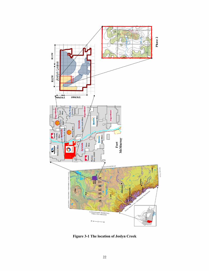
22

Figure 3-1 The location of Joslyn Creek

23

Figure 3-2 Stratigraphy of the Joslyn oil sand lease

3.2.1. Quaternary Deposits

Over the project area, unconsolidated Quaternary tills constitute the uppermost layer and are

composed of Pleistocene sands, clays, silts that were deposited from melted glaciers located in the

north of Canada at the end of the last ice age. This layer of tills and gravel will not act as an

impermeable layer which might possibly impede upward migration of fluids in the event of a

caprock failure.

3.2.2. Clearwater Formation

The Quaternary deposits are underlain by the Clearwater Formation, which consists of shale, silt,

and sandstone units. This formation is dominantly a marine shale with very low hydraulic

conductivity. No bitumen is reported in the formation, and it acts as the barrier to prevent steam

chamber growth beyond McMurray oil sands. Therefore, this shale layer is recognized as the

caprock for the Joslyn SAGD project. This formation thickness is generally about 20-30 meters

24

over the Joslyn Creek area. The geomechanical behaviour of Clearwater shale is intermediate

between a soft rock and hard soil.

3.2.1. Wabiskaw Members

The Wabiskaw Member of the Clearwater Formation directly overlies the McMurray Formation.

This zone is comprised of very fine-grained sands, silts, and shales. The sands in the Wabiskaw

may have a low grade of bitumen and include three units calling Kcw1, Kcw2 and Kcw3 (TEPCL

2007).

3.2.1.1. Kcw3

The top unit of the Wabiskaw consists of fine-grained sands inter-bedded with some muds. The

thickness of the unit is about 2 meters and the permeability is in the range of 0.3 to 2 Darcy. This

layer cannot be considered as a seal against a growing steam chamber.

3.2.1.2. Kcw2

The intermediate part of the Wabiskaw consists of marine shale deposits in which can act as a

barrier against steam migration. Although this sub-layer contains shale and has a constant

thickness, it generally does not meet the AER’s definition as caprock as its thickness is

approximately 5 meters. According to AER, a minimum thickness of 10 m is required for a shale

layer to be considered caprock.

3.2.1.3. Kcw1

The lowermost unit of the Wabiskaw contains medium grey mud interbedded fine-grained sands.

Kcw1 unit is considered a thin layer as its thickness is typically about 1-2 meters, and is unlikely

to serve as a barrier to upward migration of fluids.

A core photo from well 102/11-33-095-12W4 is shown in Figure 3-4, including all Wabiskaw

members.

25

Figure 3-3 Well AC/06-33-095-12W4 core showing Clearwater Formation (TEPCL 2007)

26

Figure 3-4 Well 102/11-33-095-12W4 core showing Wabiskaw members (TEPCL 2007)

3.2.2. McMurray Formation

The bitumen reservoir is found within the Cretaceous-aged McMurray (MM) Formation, which is

composed of a sequence of un-cemented quartz sands in a variety of sizes from very fine to coarse-

grained sands, and channel bank shales and silts. The formation was deposited during a level rise

27

in the Clearwater Sea. This level rise created three members of MM Formation named as lower,

middle, and upper McMurray. The Formation consists of the fluvial deposits at the base in lower

MM, estuarine soils in the middle MM and the marginal marine at the top in Upper MM. The MM

Formation resides from 40 to 60 m below the ground surface and approximately 115 m in depth

(TEPCL 2007, ERCB 2011).

3.2.2.1. Lower McMurray Member

Lower MM sands are covering Devonian carbonates with a thickness of about 20 m. This member

of MM is composed of coarse to medium-grained sand saturated with water and a small amount

of bitumen.

3.2.2.2. Middle McMurray Member

Middle MM is comprised of sands and muds. The channels of sands contain medium to very fine

sands saturated with high amounts of bitumen, making this member an outstanding quality bitumen

reservoir. The thickness of this zone is in the range of 10 to 35 meters.

3.2.2.3. Upper McMurray Member

This straticulate layer consists of fine to very fine-grained soils with marine effects.

Comparatively, this zone has less vertical hydraulic conductivity.

28

Figure 3-5 Well 100/09-33-095-12W4 core showing Middle McMurray

29

Figure 3-6 Well 100/09-33-095-12W4 core showing pay zone in Middle McMurray

30

Figure 3-7 Well 100/09-33-095-12W4 core showing Upper McMurray

3.2.3. Devonian Bedrock

The last layer, Devonian limestone, is known as bedrock/underburden and belongs to Waterways

Formation. However, some fractures were found in this rock, but no bitumen was reported in the

formation. The depth of the Devonian layer is about 110 m below the surface.

Figure 3-8 Well AC/06-33-095-12W4 core showing Devonian bedrock

31

Structural Geology and Gas Trapping

Based on a series of injectivity tests conducted in Wells 102-16-33-95-12W4 and 102-02-33-95-

12W4, several gas zones (Figure 3-9) were found in the upper McMurray and Wabiskaw members

(TEPCL 2007). TEPCL states that these gas zones are most probably continuous over the project

area and act as a barrier to decrease upward propagation of steam chamber pressure. Figure 3-10

shows a closer view of intervals where the gas streak (red zones where neutron and density porosity

logs cross) was detected for observation well 104-10-33-095-12W4.

Criteria for Deep or Shallow Reservoir

As defined in AER Directive 086, which was released after the steam release incident in Joslyn, a

reservoir is considered as a shallow reservoir if it meets the two following conditions:

1- Net bitumen pay zone in Wabiskaw members -McMurray Formations is not zero; and

2- The base of Clearwater shale is less than 150 meters from the ground surface.

Figure 3-11 shows the oil sands region in northeastern Alberta defined as a shallow reservoir

region.

As highlighted in Figure 3-11, the Joslyn project occurs within the shallow region and would be

considered as a shallow reservoir because the base of Clearwater shale is approximately 40-50

meters below the surface. SAGD projects in shallow areas have a potentially higher risk of caprock

integrity issues and losing the containment of the reservoir fluids. This is due to the complex

geological features in shallower depths, geomechanical impacts of injected high pressure and

temperature steam during the SAGD process. Therefore, the regulator has been more diligent in

the approval of the shallow SAGD operations and Directive 086 has been defined to address the

requirements which must be met especially for the shallow SAGD projects in Alberta.

32

Figure 3-9 Structural cross section and gas zones indicated by red colored areas in logs (Retrieved from TEPCL 2007)

33

Figure 3-10 Gas streak formed along observation well of 104-10-33-095-12W4 (from TEPCL 2007)

34

Figure 3-11 Shallow reservoirs in Alberta (AER bulletin 201-03)

Stress Regime

A variety of methods such as mini-frac / DFIT, macro-frac, bore hole breakout profile and density

logs is typically used to estimate the magnitude and direction of principal stresses in the subsurface

within a project area. Engineering analyses were performed on a series of mini-frac tests and

borehole breakout features conducted on Well 08-29-095-12W04 to estimate initial stress states

for the project (TEPCL 2007). The result was compatible with the expected results observed for

the other shallow reservoirs in Northern Alberta. The analysis indicated that the vertical stress, the

Joslyn

Project

35

overburden weight from density log, is the minimum principal stress. The minimum horizontal

stress which is higher than vertical, is the intermediate stress and the maximum horizontal stress

is the maximum principal stress. Consequently, the Joslyn thermal project's stress regime was

distinguished as a reverse faulting regime which was expected according to the other projects in

shallow areas in Alberta.

As Figure 3-12 demonstrates, the vertical stress gradient was estimated to be approximately

21 kPa/m, the minimum horizontal stress gradient is 24 kPa/m and the maximum horizontal stress

gradient is about 31.5 kPa/m. (TEPCL 2007)

Figure 3-12 Stress regime for Joslyn project (TEPCL 2007)

In addition, it was concluded that the direction of the maximum horizontal stress is NE/SW

perpendicular to Rocky Mountains tectonics, as illustrated in Figure 3-13.

Due to increasing overburden weight, the fracture pressure increases with depth, and it should be

considered for the calculation of maximum steam injection pressure. Because of lateral drainage

within the region due to the Athabasca River, pore water pressure does not follow hydrostatic

pressure from caprock shale's base. Therefore, within the Joslyn project area, the reservoir's initial

36

pressure is underpressured compared to the hydrostatic state. Local pore pressure will be discussed

in more detail in Chapter 4.

Figure 3-13 Direction of maximum horizontal stress in Alberta (Retrieved from Reiter et al. 2014)

37

Wells Platform, Pilot and Phase 2

Under AER approval number 9272, Joslyn SAGD project phases 1 and 2 were authorized to

produce 12000 b/d (AER report 2010). Phase 1 includes 1 pilot well pair which is known as 101,

and as shown in Figure 3-14, phase 2 consists of 4 pads and 17 well pairs as follows:

• Pad 201: East-West direction, including 5 well pairs

• Pad 202: East-West direction, including 4 well pairs

• Pad 203: South-North direction, including 3 well pairs

• Pad 204: North-South direction, including 5 well pairs

It should be noted that the focus of this study is on pilot well pair and Pad 204 well pairs because,

as it will be explained later, the Joslyn steam release incident occurred over this area.

Figure 3-14 Wells location in Pilot and Phase 2

38

On May 1st 2004, the Joslyn SAGD project started with steam circulation in the Phase 1 pilot well

pair. The Original Bitumen in Place (OBIP) was estimated as 2 MMbbl for the pilot scheme. Table

3-1 summarizes the start and final dates, and the duration of the operation for each well pair in

pads 101 and 204. Different phases of the operation and the average bottomhole pressure for the

injector and producer will be presented later.

Table 3-1 Operation times for pilot well Well pair From To Duration (day)

Pilot 1-May-04 27-Mar-09 1792

WP1 2-Dec-05 18-May-06 168 WP2 11-Feb-06 18-May-06 97 WP3 4-Dec-05 26-Mar-09 1209 WP4 11-Feb-06 25-Mar-09 1138 WP5 11-Feb-06 28-Mar-09 1141

In September 2005, the Joslyn Creek SAGD project was purchased by TEPCL from Deer Creek

Energy Ltd. (DCEL) and became the operator of the Joslyn project. About 20 months (1 year and

8 months) after operating the pilot well pair, phase 2 of the project started with circulation of well

pair 1 in pad 204 on December 2nd, 2005. OBIP was estimated at about 42 MMbbl for phase 2

(TEPCL 2007). Two days after well pair 1, well pair 3 started to circulate the steam on December

4th, 2005. The other well pairs in pad 204 (WP2, WP4, WP5) started to operate simultaneously and

about 652 days from the beginning of the project in phase 1.

Failure Cases Associated with Thermal In-situ Recovery

Although most of the in-situ thermal oil recovery projects in Alberta are operated safely and meet

very few significant problems during resource exploitation, there have been known occurrences of

oil or steam leaks to the surface because of compromised caprock seals or sheared casing wells.

Operators typically try to inject high-pressure steam to reduce bitumen viscosity and operate

thermal schemes at economically profitable conditions while minimizing caprock failure risks.

Any caprock failure will have undesirable environmental and economic consequences for the

operator, and in some cases, it impacts all the ongoing applications negatively. In this section,

39

some failure cases on thermal in-situ recovery methods are mentioned chronologically in Table

3-2.

Among the above failures, the most remarkable and controversial one, which has remained a

mystery for more than a decade, is the loss of the Joslyn project's steam chamber containment in

2006. One of the primary objectives of this study is to better understand the causes of this failure.

The next section will focus on the Joslyn steam release incident.

40

Table 3-2 Failure cases on thermal in-situ recovery methods chronologically (Nikiforuk 2013) Time Location Operator What happened

1980s

Fort

McMurray

Texaco This blowout made a bitumen geyser due to steam flood within a Fort

McMurray pilot. Very little public information is available on this incident

1988

Cold Lake

Imperial Oil

At this CSS project under Imperial Oil operation, an abandoned evaluation well lost its integrity due to high pressure and temperature steam injection and caused the release of more than 6000 barrels of oil and 1000 barrels of toxic water into the forest. This blowout resulted in chloride pollution of three shallow aquifers in the region

2006

Joslyn Creek

TEPCL

A notable SAGD steam release incident occurred in Joslyn Creek project after a very short period of time (5 months) from the start of steam circulation in well pair 1. It created a 75 m x 125 m large crater on the surface in the forest. This catastrophic caprock failure happened at 5 am and fortunately, no death was reported. This terrible incident is the most known blowout in SAGD operations.

2009

Primrose East

CNRL

At CNRL’s Primrose project, high pressure steam was injected to 80 wells at 4 pads to recover bitumen using CSS. Two well sites were broken and bitumen emulsion was discovered on the surface at Easter zone of the site. In addition, the seepage contaminated the Bonnyville Aquifer and triggered lots of issues for the operator company

2010

Jackfish

Devon

Unusual amount of sand production caused a “Catastrophic Erosional Wear” at the wellhead in Devon’s Jack fish project. This resulted in blowout of the steam in a SAGD well. The failure of the well spilled about 300 m3 of bitumen and about 1000 m3 of water to the surface.

2013

Cold Lake

Imperial Oil

Steam injection in CSS project at Cold Lake caused breaking the casings of several wells led to leak bitumen into the region. A 2002 report stated that 92 out of 585 well (about 16 %) were sheared in only 5 years of operation. Dusseault said “breaking caprock is routine at Imperial’s CSS project in Cold Lake”

2013

Primrose and Wolf

Lake

CNRL

Four bitumen emulsion flow to surface (FTS) blowouts took place in high-pressure cyclic steam stimulation (HPCSS) project belong to Canadian Natural Resources Limited. Three events occurred in the east side of the project and one event happened in the south side. These very catastrophic failures brought much public attention up and cost a lot of money for the operator to investigate the causes and it continues to have negative impacts on the operation.

41

Joslyn Steam Release Incident

While the pilot well pair in phase 1 of the Joslyn project was on SAGD mode and producing

bitumen on the 581st day since the beginning of the project, the operator decided to start phase 2

with steam circulation in the injector and producer of well pair 1 in the pad 204. About five months

later, just two months after circulation and only about one week after conversion of semi-SAGD

phase to SAGD mode in WP1, on May 18, 2006 about 5:15 am, operators at the plant site heard a

very loud “explosion” sound that was estimated to last about 5 minutes. Subsequent investigation

discovered a large crater of 165 m × 65 m was created and about 1400 to 1700 cubic meters of soil

and rocks were deposited across an area of about one kilometer long by about 100 meters wide in

the southwest direction shown in Figure 3-15 (TEPCL 2007). The blow-out occurred in a wooded

region, with many trees knocked down and surprisingly, large pieces of rock from

Wabiskaw/Clearwater caprock were found on the surface. (Figure 3-16). According to TEPCL’s

report (TEPCL 2007), fortunately, there was no deaths or harmful toxic emission into the aquifer

and atmosphere.

Figure 3-15 Steam release incident from Total’s report

42

Figure 3-16 Rocks from underground on the surface (Khani 2018)

The Clearwater shale known as caprock which was supposed to act as a barrier to hold the steam

and hot water beneath the caprock layer had clearly ruptured and steam and associated materials

were released to the surface. As Figure 3-17 shows, the crater was formed on the surface above

the heel of well pair 1 in pad 204. Figure 3-18 shows the area before and after caprock failure and

the steam release incident.

43

Figure 3-17 The schematic location of crater in phase 2

44

Figure 3-18 Aerial photo of the area before and after steam release (TEPCL 2007)

45

Geology in the Vicinity of the Steam Release Zone

Figure 3-19 shows the crater's schematic location due to the steam release and evaluation well

AB/09-33-095-12W4 in pad 204. The Pilot and phase 2 of the operation cover 1,330,551 m2 with

a complex and variety of interval layers with different thicknesses. Detailed stratigraphy of the

geology of the interested area was extracted from the well sketch located in the crater and the

layers are shown in Figure 3-20 from the surface towards the bottom of the pay zone in the

McMurray Formation.

Figure 3-19 Location of crater and evaluation well AB/9-33-095-12W4

46

Figure 3-20 Geology in the disturbed zone extracted from evaluation well sketch

47

Reports on the Steam Release Incident

Two reports were released by the Alberta government, which are:

1. AER staff Review and Analysis: Total E&P Canada Ltd. Surface Steam Release of May

18, 2006 Joslyn Creek SAGD Thermal Operation, and

2. TECPL Summary of investigations into the Joslyn, May 18, 2006 Steam Release.

TEPCL as the operator wrote the latter long report in May 2007 about one year after the steam

release incident and the former report was written by AER’s staff in February 2010 about 4 years

after the failure to respond to the TEPCL’s report.

Immediately after the blow-out, TEPCL began an extensive investigation to identify all the

conditions that may contribute to the failure and understand the causes and the main failure

mechanisms. This long and comprehensive investigation report consists of

• Surface findings

• Geological findings

• Reservoir findings

• Seismic findings

• Geomechanical findings

• Cement bond investigation

The report was distributed to associated experts to explore the failure possibilities and convey

some causes that contributed to the incident. TEPCL reviewed the potential failure processes and

proposed the steam release root cause and ultimately the most likely steam release scenario. In

addition, they stated few alternative scenarios for the failure as well. TEPCL also inspected the

environmental influence of the steam release on groundwater and surface.

AER, as the regulator in Alberta, undertook an exhaustive review of TEPCL’s report regarding

their failure considerations. AER’s staff reviewed the report, prepared their assessment, and

offered their arguments about the steam release. They agree on some points with TEPCL’s

suppositions and disagree on the others. A summary of the proposed scenarios and conclusions

made by TEPCL and AER are provided in appendix A.

48

Economic Impacts and Safety Considerations Resulting from Steam Release Incident

Maximum operating pressures are typically specified for an AER approved project. Higher

maximum operating pressure typically results in a higher production amount, which is favorable

for the operator from an economic point of view, while higher maximum operating pressure will

put the formation at risk of fracturing if the MOP exceeds the fracture pressure at a specified depth.

For SAGD projects, as the steam chamber grows during the life of a thermal project, the pressure

front will approach the caprock and in most cases, the MOP needs to be readjusted to account for

variations in fracture pressure. Consequently, the anticipation of the pressure front is a critical task

and needs to be monitored carefully.

Therefore, an optimized MOP that satisfies both safety considerations and economic benefits is

always controversial in the SAGD operation. MOP is mainly affected by the result of mini-frac

test to define minimum principal stress in the field. There are also uncertainties in the estimation

of minimum principal stress due to heterogeneity and anisotropy as well as unknown geology sub-

surface all over the area of interest. Therefore, a margin of safety is typically applied to the MOP.

Since March 1994 and before the steam release incident at the Joslyn project, the maximum

allowable wellhead injection pressure was defined using Directive 051. In this Directive,

maximum operating pressure was limited to 90 percent of the fracture pressure and was defined as

the following formulation (Directive 051):



In Joslyn Creek, the stress regime was determined to be a reverse faulting regime, and so the

fracture closure pressure was based on the vertical stress gradient.

Assuming a vertical stress gradient of 21 kPa/m as the fracture closure gradient and 90 m as the

depth of injector, the maximum allowable bottomhole pressure before the steam release was

specified as

MOP = 21 × 90 × 0.9 = 1701 kPa

49

After the unfortunate steam release in May 2006, an extra 500 kPa margin of safety was applied

to the injection pressure for the well pairs under operation and the maximum operating pressure at

the bottomhole was limited to 1200 kPa.

As one may distinguish, due to the caprock failure, the maximum allowable bottomhole pressure

was decreased by about 30% which results in reduced production for the operator company.

Ultimately, under this low injection pressure and surveillance monitoring costs, the project was

judged as uneconomic by TEPCL and the operation was abandoned.

AER released the new regulations, Directive 086, for shallow in-situ SAGD operations in

December 16th, 2016. This Directive was defined as a response to the blow-out in Joslyn Creek

SAGD facility and applicable to all the shallow projects in Alberta.

Based on Directive 086, for a project in which the base of the lower Clearwater shale is shallower

than 150 meters, the maximum operating pressure is defined as

MOP bottom-hole (kPa) = caprock fracture closure gradient (kPa/m) × depth at


As one can see, Joslyn caprock failure caused a very significant reduction in allowable injection

pressure for shallow SAGD operations. Here, a comparison of MOP before and after steam release

is performed to better understand the negative influence of the steam release regarding economic

point of view. With the assumption of 36 meters as the base of caprock (Clearwater shale) and 21

kPa/m as the fracture closure gradient, the MOP is calculated as

MOP = 21 × 36 × 0.8 = 605 kPa

Compared to MOP before the incident, the reduction is about 65%. This magnitude of a reduction

in MOP can seriously impact the economic viability of a SAGD project. While a prudent decision

to specify additional safety margins, it is postulated that a lack of verification of the failure

mechanism for this steam release incident led to the imposition of this additional margin of safety

and the definition of a conservative formula to calculate MOP. Consequently, one of the main

motivations for this research is to assemble and assess additional lines of evidence for potential

failure mechanisms that can lead to a re-evaluation of the MOP formula for SAGD projects.

In the next chapter, a high-resolution geo-cellular model is created using the field data, generously

provided by TEPCL, to be utilized in the coupled reservoir geomechanical simulations.

50

GEOLOGICAL INSIGHTS AND HIGH RESOLUTION GEO-CELLULAR

MODEL

Data Provided by TEPCL

With collaboration between the Reservoir Geomechanics Research Group (RGRG) and TEPCL,

the Joslyn creek confidential data was kindly provided by TEPCL for this research. This substantial

amount of invaluable data, more than 210 GB, includes raw well data, observation well recordings,

injection and production data, monitoring and surveillance data, and the geological model

developed by TEPCL in Petrel E&P software platform. Due to confidentiality and the extensive

amount of data, the information will be shown in a summarized form in the following sections and

a typical example will be provided for each data type.

4.1.1. Raw Data Files

As Figure 4-1 demonstrates, the raw data files for 512 wells positioned in the highlighted red area

were provided by TEPCL. Out of all the wells, 395 wells belonged to township 095 and 117 other

wells were located in township 096. As shown in the yellow box in Figure 4-1, range 12, township

095 and section 33 consist of the pilot well pair and the other five well pairs in pad 204, which

cover this study's area of interest. From all provided wells, 72 wells were placed in the interest

area.

51

Figure 4-1 Location of the wells provided by TEPCL (TEPCL 2007)

Raw data files consist of field survey, wireline, core photo, lab documents and lab analysis. Each

file includes a variety of data summarized in Table 4-1 for all the wells and Table 4-2 for the wells

in the area of interest. The following sections will provide a brief explanation of the data combined

with an illustration for this data.

52

Table 4-1 Summary of available raw data for 512 wells provided by TEPCL

WELL 1_FIELDSURVEY

TOTAL WELLS AS-BUILT PLAN UNIVERSAL

SURVEY WELL SCHEMATIC WELLSITE PHOTO

512 93 64 24 64 WELL 2_WIRELINE

TOTAL WELLS LAS FILE WIRELINE

IMAGE WIRELINE MISC

512 473 242 28

WELL 3_COREPHOTO TOTAL WELLS CORE PHOTO

512 445

WELL 4_LABDOCS

TOTAL WELLS

CORE DESCRIPTION

FACIES INTERVAL

GEOLOGICAL FIELD LOG OVERBURDEN LOG

512 435 231 170 140 WELL 5_LABANALYSIS

TOTAL WELLS

DEAN STARK FINAL PSD XRD ROCK PROPERTY

ANALYSIS 512 456 280 8 8

Table 4-2 Summary of available raw data for 72 wells located in interested area provided by TEPCL

WELL 1_FIELDSURVEY

TOTAL WELLS AS-BUILT PLAN UNIVERSAL

SURVEY WELL SCHEMATIC WELLSITE PHOTO

72 37 37 13 37 WELL 2_WIRELINE

TOTAL WELLS LAS FILE WIRELINE

IMAGE WIRELINE MISC

72 57 11 1

WELL 3_COREPHOTO

TOTAL WELLS CORE PHOTO

72 55

WELL 4_LABDOCS

TOTAL WELLS

CORE DESCRIPTION

FACIES INTERVAL

GEOLOGICAL FIELD LOG OVERBURDEN LOG

72 50 28 11 11 WELL 5_LABANALYSIS

TOTAL WELLS

DEAN STARK FINAL PSD XRD ROCK PROPERTY

ANALYSIS 72 57 23 4 4

53

4.1.1.1. Field Survey

Field survey folder includes as-built plan, universal survey, well schematic and well site photo

which are explained as follow:

• As-built Plan

Figure 4-2 shows an as-built plan for the well 9-33-095-12W4. As one can see, it contains the

survey drawing for the wells with all the relevant explanations.

Figure 4-2 As-built plan for well 9-33-095-12W4

54

• Universal Survey

Figure 4-3 shows a universal survey plan with relating information for the well 102/09-33-095-

12W4.

Figure 4-3 Universal survey plan for the well 102/09-33-095-12W4

• Well Schematic

The schematic pattern of some wells is also provided. As an example, the schematic design for

well 104/09-33-095-12W4 is shown in Figure 4-4.

55

Figure 4-4 Schematic pattern for well 104/09-33-095-12W4

56

• Well site photo

Few photos were taken for some wells to realize the situation of the well on the surface. For

instance, Figure 4-5 shows two well site photos for the well 100/09-33-095-12W4.

Figure 4-5 Site photos for well 100/09-33-095-12W4

4.1.1.2. Wire Line

LAS files and wireline image logs are available for some of the wells in the project area.

57

• LAS File

Log ASCII Standard, also known as LAS file, is a standard format to show well log information

in the oil and gas industry. A LAS file is separated into two sections: header and ASCII log data

sections. The header section, shown in Figure 4-6, includes the LAS file version, location of the

well, start and stop depth, service company, license number, logging date, etc. The ASCII log data

section provides the actual data such as gamma ray and porosity in a tabular format shown in

Figure 4-7.

• Wireline Image

For some of the wells, wireline image logs are provided, and they usually include gamma ray,

density porosity, neutron porosity corresponding to the depth, and information about the Formation

tops, as shown in Figure 4-8.

58

Figure 4-6 Header of the LAS file for well 100/09-33-095-12W4

59

Figure 4-7 Ascii log data of the LAS file for well 100/09-33-095-12W4

60

Figure 4-8 Wireline image for well 1AC/08-33-095-12W4

4.1.1.3. Core Photo

Coring provides cylindrical samples using special drill bits from subsurface. The retrieved samples

can be representative of underground formations and are taken to the laboratory for further

analyses. Images of these cores are provided for some wells at specific depths which can be used

61

to identify different subsurface formations. Figure 4-9 shows an example of a core photo for well

AD/09-33-095-12W4.

Figure 4-9 Core photo for well AD/09-33-095-12W4 belong to depth 47-51 m in Upper McMurray

62

4.1.1.4. Lab Documents

The cores extracted from subsurface will be transported to laboratories to define facies, lithology

features, size of particles, core quality. In the end, the corresponding formations will be recognized

for different depths. Lab document files consist of geological field logs, facies intervals,

overburden logs, and core description data. Figure 4-10 demonstrates a Core Description File

(CDF) for well 102/09-33-095-12W4.

Figure 4-10 Core description for well 102/09-33-095-12W4

63

As one can see in the provided CDF, top of formations, facies, grain size, and the mineralogy are

specified in different depth intervals.

4.1.1.5. Lab Analysis

More experiments and analyses will usually be carried out on the cores to measure or estimate

petro-physical properties, particle size distribution (PSD), X-Ray Diffraction (XRD) analysis, and

Methylene Blue Index (MBI) report. The Dean-Stark report also provides saturation of oil, water

and solids for some samples from the cores used in the calibration of petro-physical properties

such as porosity and permeability. PSD tests have been done on the samples to specify the

distribution of soil particles by size. Based on defined standards, one can use PSD data to specify

what percentage of the soil is coarse, medium, or fine grained. XRD identifies the mineralogy of

soil constituents such as quartz, k-feldspar, and calcite. The portion of clay minerals is another

essential analysis that will also be determined in the XRD tests.

4.1.2. Observation Wells (Thermocouples and Piezometers)

Over the area of interest in Joslyn Creek, observation wells were equipped with thermocouples to

measure the temperature along the well at different depths daily. TEPCL has provided observation

wells in pads 101, 201, 202, 203, and 204; however, the observation wells close to pilot and Pad

204 are widely used in this research as they are in the area of interest. As Figure 4-11 demonstrates,

observation wells 103/06-33-095-12W4, 102/06-33-095-12W4, and 100/03-33-095-12W4 are

located at the heel, middle and toe of the pilot well pair, respectively. Observation well 102/10-

33-095-12W4 is at the heel of well pair 3, 102/07-33-095-12W4 is at the middle of well pair 4.

Three additional observation wells 100/10-33-095-12W4, 100/07-33-095-12W4, and 102/02-33-

095-12W4 are located at the heel and middle and toe of well pair 5, respectively.

64

Figure 4-11 Observation wells over interested area, pad 101 and 204

The information provided for each observation well includes start and end dates of monitoring,

passed days since the start of circulation, maximum temperature corresponding to different depths,

distance from the well pair, depth of injector and producers, and the observed temperatures at

different depths. Table 4-3 summarizes some of the observation wells data. As an example, one

can see in Figure 4-12 the maximum temperature recorded over time for the observation well

located at the heel of the pilot.

65

Table 4-3 the location and characteristics of the observation wells Observation Well Location Distance from

the pair(m) Depth of INJ(m)

Depth of PR(m)

Start Date End Date

103/06-33-095-12W4 Heel of Pilot 3.1 86 91 1-Jul-04 1-Jun-09 102/06-33-095-12W4 Middle of Pilot 5.4 85 90 10-Aug-04 1-Jun-09 100/03-33-095-12W4 Toe of Pilot 1 90 95 1-Jul-04 1-Jun-09 102/10-33-095-12W4 Heel of WP3 6 85.9 91.5 15-Apr-06 1-Jun-09 102/07-33-095-12W4 Middle of WP4 7.8 86.4 91.7 15-Apr-06 1-Jun-09 100/10-33-095-12W4 Heel of WP5 18 88 93 12-Mar-08 1-Jun-09 100/07-33-095-12W4 Middle of WP5 13 84.5 86.5 12-Mar-08 1-Jun-09

Figure 4-12 Max Temperature (C) over time for 103/06-33-095-12W4 located at the heel of the pilot (TEPCL 2007)

Moreover, well temperature profiles at different depths associated with different times, and gamma

ray distribution are shown for the same well in Figure 4-13.

020406080100120140160180200

Jan-04 May-05 Oct-06 Feb-08 Jul-09 Nov-10

Temperature (C)

Time (date)

66

Figure 4-13 Temperature profile in observation well close to the heel of pilot over time (TEPCL 2007)

The same information is provided for other observation wells. Unfortunately, there was no pressure

monitoring in the observation wells prior to the steam release incident over the area of interest;

however, observation wells 104/10-33-095-12W4, 102/11-33-095-12W4, and 104/06-33-095-

12W4 were drilled and equipped with piezometers in 2007 more than one year after the steam

release incident.

4.1.3. Injection and Production Data

Injection and production data for the well pairs in pads 101 and 204 are provided in this file. For

all injectors over the area of interest, the rate of steam in the short and long tubing, the rate of water

production from short tubing, head pressure in the long and short tubing, blanket gas pressure as

well temperatures at heel and toe associated with time and stages of SAGD operation are provided.

30

40

50

60

70

80

90

100

110

1200 50 100 150 200

Depth (m)

Temperature (C)

InjectorProducer8/26/20042/22/20079/27/20076/26/20086/18/2009gamma raySeries9

67

Moreover, oil production rate, water production rate, and steam rate in long tubing are delivered

for the producer wells. Casing head pressure, bubble tube pressure, and long tubing head pressure

are also provided in the file. Table 4-4 summarizes the data provided for the well pairs.

Table 4-4 Operational data provided for the horizontal wells Measured Data Unit

Oil Rate m3/d

Steam Rate m3/d

Water Rate m3/d

Fluid Production m3/d

Steam Rate Fraction to Short String v/v

Void Replacement Ratio (VRR) v/v

Instantaneous Steam-Oil Ratio (ISOR) v/v

Water Steam ratio (WSR) v/v

Total Fluid to Steam Ratio (TFSR) v/v

Steam Chamber Pressure kPag

Average Reservoir Sub-Cool Deg C

Cumulative Volume of Oil m3

Cumulative Volume of Steam m3

Cumulative Volume of Water m3

Fluid Production m3

Recovery Factor (RF) %

Cumulative Void Replacement Ratio (CVRR) v/v

Cumulative Steam Oil Ratio (CSOR) v/v

Cumulative Water Steam Ration (CWSR) v/v

Cumulative Total Fluid to Steam Ratio (CTFSR) v/v

4.1.4. Surface Heave Monitoring Data

Following the steam release incident, 4 well pairs adjacent to well pair 1, which was beneath the

crater, were shut-in. The other well pairs in Pad 204, and the pilot well pair were under operation

even after steam release incident, but with considerably lower bottomhole pressure compared to

the pressure prior to the incident. To enhance the operation's safety, TEPCL was required to install

68

monitoring facilities on the top of operating well pairs 3, 4 and 5 as well as the pilot well pair,

shown in Figure 4-14. TEPCL installed 60 InSAR corner reflectors (green diamonds) and 131

tiltmeters (purple circles) for surveillance. TEPCL also used heave monuments (GPS shown as red

squares) to ensure the caprock containment is ensured. TEPCL implemented different monitoring

methods to compare the results from each facility.

Figure 4-14 Location of InSAR, tiltmeters, and GPS installed for surface heave monitoring after the blow-out

As Figure 4-15 demonstrates, GPS recorded a maximum heave of 6 cm at the end of production.

This maximum heave was recorded at the top of well pair 4 as shown in Figure 4-16.

69

Figure 4-15 Surface heave recorded by InSAR, tiltmeters and GPS at the middle of WP4 where maximum displacement recorded at the end of project

Figure 4-16 Surface heave contours recorded by GPS at the end of the project

70

4.1.5. Petrel Model

TEPCL provided a geo-cellular interpretation of Joslyn Creek’s geology in a Petrel model. As

Figure 4-17 shows, the original model was extensive. The model is 3248 m in the East-West

direction, 3751 m in the North-South direction, and 260 m in depth and includes all the pads in

phases 1, 2, and 3.

Figure 4-17 Geo-cellular model provided by TEPCL in Petrel

71

The model was created with 6 main zones including:

1- Surface to Clearwater (Quaternary deposits)

2- Clearwater to Wabiskaw (Clearwater Formation)

3- Wabiskaw to Upper McMurray (Wabiskaw Members)

4- Upper McMurray to Middle McMurray (Upper McMurray)

5- Middle McMurray to Lower McMurray (Middle McMurray)

6- Lower McMurray to Devonian (Lower McMurray)

These zones, as shown in Figure 4-18, were generated based on the markers and cores obtained

from well log analysis. Therefore, the horizons and surfaces built in Petrel were based on field data

and topography was also considered in the model. The area of interest consists of the pilot project

and Pad 204 which are outlined in the yellow box in Figure 4-19.

Figure 4-18 The main zones from surface to the bed rock in Petrel model

72

Figure 4-19 Area selected for complete model describing pad 101 and 204

Based on well log data, TEPCL defined facies and assigned porosity, saturation, and permeability

values to the geo-cellular model. Seventeen facies were specified in the model, defined based on

different gamma ray cut-off values. The petro-physical properties are shown in Figure 4-20 to

Figure 4-23.

73

Figure 4-20 different 17 facies within Upper, Middle and Lower McMurray Formations based on gamma ray in Petrel model

Figure 4-21 Effective porosity profile within Clearwater, Wabiskaw and McMurray Formations in Petrel model

74

Figure 4-22 Water saturation distribution within Upper, Middle and Lower McMurray Formations in Petrel model

Figure 4-23 vertical permeability profile for the reservoir formation in Petrel model

75

Generating Geo-cellular Model Using Petrel and SKUA-Gocad

4.2.1. Building Simulation Grids Using Real Data

TEPCL created the geo-cellular model with the above-mentioned petro-physical properties in

Petrel. Seven surfaces regarding formations tops based on well logs were created in the model.

The surfaces are specified as Ground Surface, Clearwater, Wabiskaw, Upper McMurray, Middle

McMurray, Lower McMurray and Devonian. The petro-physical properties such as porosity, water

saturation, and permeability are defined for the formations based on core measurements. Geo-

statistical approaches were applied to the model to determine the properties of the un-known grids

among the wells. While the TEPCL model served as a valuable reference model, to utilize the

advanced coupled reservoir geomechanical package developed in RGRG, the geological model

and geomechanical properties with respect to the selected constitutive models for different

formations, as well as in situ conditions of stress and pore pressure, needed to be created in SKUA-

Gocad. Consequently, in this research, an independent effort was undertaken to build the geo-

cellular model in SKUA-Gocad and the following section explains the workflow adopted for

model construction and the selection of properties to apply in the coupled simulation for Joslyn

Creek project.

4.2.1.1. Transferring Generated Surfaces in Petrel to SKUA-Gocad

Formations’ tops were defined using well log analysis and formation surfaces were created using

the formations’ top markers provided in Petrel. For the generation of the geological model in

SKUA-Gocad, it was decided to have six major layers in the model named Quaternary, Clearwater,

Wabiskaw, Upper McMurray, Middle McMurray, and Devonian. Seven horizons are needed to

create these formations. Figure 4-24 shows these surfaces once they were imported to SKUA-

Gocad from Petrel. It shows that the topography has been considered in the model and the surfaces

are uneven to represent the subsurface conditions as accurately as possible.

76

Figure 4-24 Surfaces imported from Petrel to SKUA-GOCAD considering topography

As shown in Figure 4-24, Lower McMurray and Devonian surfaces have multiple crossovers over

the area of interest. In this area, the Lower McMurray Formation over Devonian is discontinuous

with a small thickness, as shown in Figure 4-25.

Figure 4-25 Thickness of Lower McMurray Formation over the area of interest

77

The RGRG coupled platform does not accept a discontinuous layer with multiple crossovers.

Therefore, it was decided to assume the top of Lower McMurray and top of Devonian layer at the

same elevation. Care should be taken in the interpretation of Lower McMurray Formation outside

the area of interest as the thickness of Lower McMurray increases. The Devonian surface has been

made flat and pushed down about 65 meters from the previous surface which is Lower McMurray

to create Devonian bedrock layer as shown in Figure 4-26.

The interpretation of Devonian layer provided above is only applicable to the area of interest and

shall not be used outside this area without careful investigation.

Figure 4-26 Generating flat surface for Devonian as a base layer

As Figure 4-27 shows, 304 well logs with associated LAS files are also imported to SKUA-Gocad

to be used for geostatistical approaches in the definition of initial reservoir and geomechanical

properties.

4.2.1.1. Building Simulation Grids

The next step in the work frame to build the geo-cellular model in SKUA is creating the simulation

grids by defining the grid spacing. Through this procedure, the number of sub-layers for each

formation can also be defined by the user. The number of sub-layers will define the thickness of

78

grids in depth, i.e., K direction. For the large geological model shown in above figure, the total

number of layers is 57 in K direction starting from the top layer on the surface and ending with the

bottom of last layer at the base of the model. It means K=1 is the top layer and K=57 is the base

layer. The number and the thickness of the sub-layers for different main zones are shown in

Table 4-5.

Figure 4-27 Imported 304 LAS files to the model to build simulation grids in SKUA-Gocad

79

Table 4-5 Number and thickness of sub layers for each zone Unit Main Zones No of Sub-layers Average Thickness of Sub-layers (m)

1 Quaternary Deposits 2 8.52

2 Clearwater Formations 20 2.2

3 Wabiskaw Members 5 2.3

4 Upper McMurray 1 8.18

5 Middle McMurray 20 3.47

6 Devonian 9 8.03

The thickness of these sub-layers is variable from 1 to 8 meters, with the maximum probability of

1.6 meters depends on the topography of the surfaces which is shown in the histogram curve in

Figure 4-28.

Figure 4-28 Histogram for the thickness of the sub-layers in vertical direction

Tops of formations are not flat except the bottom surface (i.e., the Devonian) as the other

surfaces are built based on the topography and well markers defined as the top of each formation.

The contour map of elevation (Z) for each surface is created, and the range of thickness for each

80

zone can be measured. Figure 4-29 to Figure 4-31 illustrate the elevation contour at the top of each

formation.

Figure 4-29 Contour map of elevation level for the Surface and Clearwater layers

81

Figure 4-30 Contour map of elevation level for the Wabiskaw and Upper McMurray layers

Figure 4-31 Contour map of elevation level for the Middle McMurray and Devonian layers

82

The elevation difference over the surfaces indicates that the assumption of flat surfaces in the

geological models may result in a systematic error in defining facies. Table 4-6 shows the elevation

ranges for each formation's top and the varied thickness for the large geo-cellular model.

Table 4-6 Elevation range for the top and bottom layers of each zone

Zone Top and Bottom of the Zone

Elevation Range

Fluctuation Range of Thickness in Formations

Quaternary Deposits Ground Surface 348 to 328 20

3.5 to 14 Clearwater 335 to 318 17

Clearwater Formations Clearwater 335 to 318 17

18 to 43 Wabiskaw 306 to 287 19

Wabiskaw Members Wabiskaw 306 to 287

7 to 10 Upper McMurray 298 to 279 19 Upper McMurray Formation

Upper McMurray 298 to 279 1.5 to 6

Middle McMurray 294 to 274 20 Middle McMurray Formation

Middle McMurray 294 to 274 43 to 68

Devonian 248 to 212 36

Devonian Bedrock Devonian 248 to 212

Bottom

It illustrates that the elevation of ground surface ranges between -348 and -328 m which means

over the large area of more than 8 million square feet the fluctuation is about 20 meters. Moreover,

the difference between the elevations of well markers for the top of Clearwater layer is about 17

meters from -335 to -318 m. Therefore, the thickness of Quaternary deposits may vary from 3.5 m

to 14 m.

In the large model, 327 cells are created in I direction starting from the south side towards the

north side. The mean length of the cells in I direction is about 11.6 m. Regarding J direction, 384

simulation cells are generated from the west side of the area to the east side with the mean length

of 8.5 meters. Figure 4-32 demonstrates the large geological model for Joslyn Creek project and it

includes the total number of 7157376 cell blocks. It also shows the location of the pilot and pad

204 in the model.

83

Figure 4-32 Generated large geo-cellular model in SKUA

It should also be noted that the aspect ratio for the length of the simulation grids for all the cells

must be kept below 10:1. This aspect ratio is found experimentally and is especially required for

the geomechanical simulator, FLAC3D, to achieve convergence.

4.2.2. Constitutive Models, Reservoir and Geomechanical Properties

At this step, the model size is decreased as the focus is on the area of interest which contains the

pilot and pad 204 and model resolution is increased. The number of grids and the dimensions are

provided in subsequent sections of the chapter. Table 4-7 lists the properties that must be

determined in the SKUA-Gocad for use in the geomechanical simulator.

Table 4-8 lists the properties that are required for the CMG STARS simulator. Note that pore

pressure, temperature, and main zones are common between the reservoir and geomechanics

simulators.

84

Table 4-7 Required properties defined in SKUA-GOCAD for geomechanics simulator Property SKUA Property Name SKUA Property Type SKUA Units Pore Pressure pressure Pressure kPa Total Stress_xx sxx Pressure kPa Total Stress_yy syy Pressure kPa Total Stress_zz szz Pressure kPa Shear Stress_xy sxy Pressure kPa Shear Stress_yz syz Pressure kPa Shear Stress_xz sxz Pressure kPa Mean Effective Stress p_prime Pressure kPa Main Zones reservoir_units Number Integer Mechanical Model ID1 model Number Integer Mechanical Group2 mech_group Number Integer Solid Density densitySolid Density kg/m3 Water Density densityWater Density kg/m3 Oil Density densityOil Density kg/m3 Gas Density densityGas Density kg/m3 Bulk Density densityBulk Density Kg/m3 Thermal Expansion Coefficient_xx thExp_xx Real Number 1/C Thermal Expansion Coefficient_yy thExp_yy Real Number 1/C Thermal Expansion Coefficient_zz thExp_zz Real Number 1/C Itasca Property1 m1 – m10 Real Number N/A Biot Coefficient_xx biot_xx Real Number Ratio Biot Coefficient_yy biot_yy Real Number Ratio Biot Coefficient_zz biot_zz Real Number Ratio Young’s modulus_xx eMod_xx Real Number Pa Young’s modulus_yy eMod_yy Real Number Pa Young’s modulus_zz eMod_zz Real Number Pa Bulk Modulus bulkMod Real Number Pa Shear Modulus shearMod Real Number Pa Poison Ratio pRatio Ratio

Table 4-8 Required properties defined in SKUA-GOCAD for flow simulator

Property SKUA Property Name SKUA Property Type SKUA Units Pore Pressure pressure Pressure kPa Main Zones reservoir_units Number Integer Relative Permeability Rock Type relPermRockType Number Integer Rock Type tHRockType Number Integer Temperature temp Temperature C Porosity por Porosity

85

Permeability_xx k_xx Permeability mD Permeability_yy k_yy Permeability mD Permeability_zz k_zz Permeability mD Water Saturation Sw Water Saturation Ratio Oil Saturation So Oil Saturation Ratio Gas Saturation Sg Gas Saturation Ratio

4.2.2.1. Data Analysis to Define Facies

Gamma ray logs are typically used to determine the facies in a geological model. The gamma ray

log measures natural radioactivity from the surrounding formations of the well. The value of

gamma ray is usually related to the amount of clay in the soil or rock, and it is due to concentration

of radioactive isotopes in clay. Therefore, gamma ray measurement is an appropriate approach to

defining the formation's lithology in and around the borehole (Zhang 2019).

A user-defined value/values for gamma ray cut-off is used to determine the facies in the simulation

grids. Several cut-offs should be defined for higher resolution and recognition of more facies

(Zhang 2019). In this study, 75 API is defined as the cut-off value for the gamma ray log, and two

facies, sand and shale, are recognized in the model.

Due to lack of an agreed-upon resolution for the failure mechanism of the Joslyn steam release

incident, AER released Directive 086 for shallow SAGD operations. In this recent Directive, it is

specified that 75 API should be used as the cut-off value to differentiate sand from shale.

Consequently, the same approach is adopted. The resolution of gamma ray is usually less than one

meter which is less than the simulation grid thickness. Therefore, upscaling is needed to define the

facies for every cell based on the largest proportion specified by the shale cut-off value. The main

formations that the portion of shale and sand are critical in them include Clearwater, Wabiskaw,

Upper McMurray, and Middle McMurray. The histograms of sand and shale before and after

upscaling for these formations are shown in Figure 4-33.

86

Figure 4-33 Sand and shale portions in each zone before and after upscaling based on 75 API as gamma ray cutoff value

As shown in Table 4-9, the Clearwater Formation and Wabiskaw Members are shale dominant

with about 88% and 78% shale in the formations, respectively and the underlying formations,

Upper McMurray, and Middle McMurray, are sand dominant with about 64% and 67% sand,

respectively.

Data from all selected domains including all formations from the surface to Devonian (0 to 110 m

in depth), shows the accumulated vertical proportion of sand and shale. As Figure 4-34 shows, the

Clearwater and Wabiskaw layers are shale dominant and in these regions the permeability is

relatively low. On the other hand, from Wabiskaw towards the reservoir, the yellow color zone is

sand dominant, and the permeability will increase.

Table 4-9 Percentage of sand and shale for each zone before and after upscaling Grid Regions Data Sand (%) Shale (%)

Clearwater Raw 16 84 Blocked 12 88

Wabiskaw Raw 24 76 Blocked 22 78

Upper-MM Raw 64 36 Blocked 64 36

Middle-MM Raw 67 33 Blocked 66 34

87

Figure 4-34 Sand and shale fractions from surface to the bedrock

The variogram models for all formations are created in SKUA based on the available gamma ray

logs. The facies model and several realizations are created for the whole model using Sequential

Indicator Simulation (SIS). Although the effects of the proportion of facies in Quaternary and

Devonian layers are less critical, the heterogeneity could play a significant role in evaluating

reservoir and caprock performance. Figure 4-35 shows the distribution of facies in one of the

realizations.

88

Figure 4-35 Realization for the facies distribution in the simulation grids

4.2.2.2. Generating a Mechanical Earth Model (MEM)

At this point in the development of the geological model, the facies have been specified for each

cell based on the defined gamma ray cut-off value according to AER’s Directive 86, which is

applicable to the case study of this research. The portion of sand and shale is crucial in defining

Clearwater, Wabiskaw, Upper, and Middle McMurray Formations and results in different levels

of heterogeneity in these formations. The heterogeneity has a large influence on the mechanical

performance of the model such as deformability, displacement, and failure modes (Zhang 2019).

It also affects reservoir production performance. To account for these issues, different constitutive

models for shale and sand within the oil sand and related strata must be defined. In this study, it

89

has been assumed that the shale that exists in different formations is not unique regarding clay

contents. Consequently, the grids classified as shale in Clearwater, Wabiskaw, and Upper

McMurray units are considered to have the same constitutive behavior and have been termed

mechanical group 2. Also, the grids in the Upper and Middle McMurray, which are considered the

main reservoir zones, are classified as sand material with the same constitutive model and termed

mechanical group 4. Because of the variation in API units for the sand cells in Clearwater and

Wabiskaw, and the shale grids in Middle McMurray, these zones are treated as silt material and

are defined as mechanical group 3, with its own constitutive model. Quaternary deposits are

specified as till with the mechanical group 1 properties, and ultimately Devonian limestone is

indicated as mechanical group 5. The summary of the materials and corresponding mechanical

group numbers for different formations to achieve heterogeneity within the layers are listed in

Table 4-10. Figure 4-36 also shows the mechanical groups specified for different materials in the

layers.

Table 4-10 Mechanical group specified for the facies in each zone Formation Facies Gamma Ray Material Mechanical Group Number

Quaternary

Till 1

Clearwater Shale >75 Clay 2

Sand <75 Silt 3

Wabiskaw Shale >75 Clay 2

Sand <75 Silt 3

Upper McMurray Shale >75 Clay 2

Sand <75 Sand 4

Middle McMurray Shale >75 Silt 3

Sand <75 Sand 4

Devonian

Limestone 5

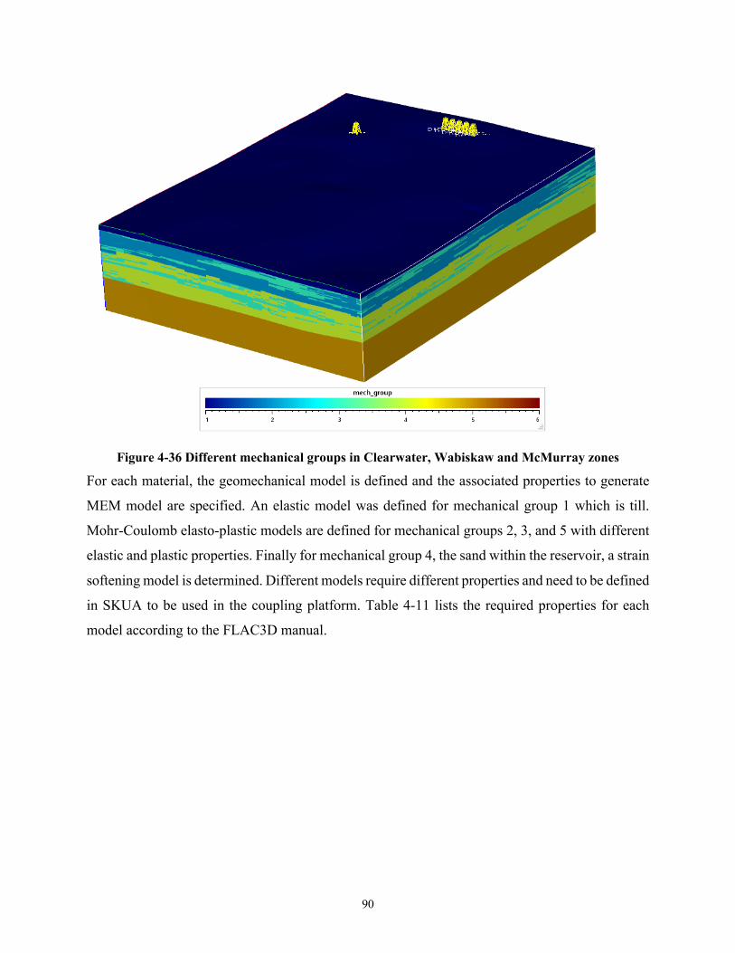
90

Figure 4-36 Different mechanical groups in Clearwater, Wabiskaw and McMurray zones

For each material, the geomechanical model is defined and the associated properties to generate

MEM model are specified. An elastic model was defined for mechanical group 1 which is till.

Mohr-Coulomb elasto-plastic models are defined for mechanical groups 2, 3, and 5 with different

elastic and plastic properties. Finally for mechanical group 4, the sand within the reservoir, a strain

softening model is determined. Different models require different properties and need to be defined

in SKUA to be used in the coupling platform. Table 4-11 lists the required properties for each

model according to the FLAC3D manual.

91

Table 4-11 Required properties for selected constitutive models in the geomechanical simulator Model ID

Mechanical model

No. of required properties

SKUA properties name

Required properties

10 Elastic 2 m1,m2 m1= Bulk Modulus m2= Shear Modulus

15 Mohr-Coulomb 6 m1 to m6

m1= Bulk Modulus m2= Cohesion m3= Dilation m4= Friction m5= Shear Modulus m6= Tension

20 Strain Softening 10 m1 to m10

m1= Bulk Modulus m2= Cohesion m3= Cohesion Table m4= Dilation m5= Dilation Table m6= Friction m7= Friction Table m8= Shear Modulus m9= Tension m10= Tension Table

4.2.2.3. Required Properties for the Coupling Platform

• Solid and Fluid Densities

Solid density is defined for each main zone. Based on the literature, solid densities for Quaternary

deposits, Clearwater Formation, Wabiskaw members, Upper and Middle McMurray, and

Devonian bedrock are assumed as 2700, 2600, 2650, 2600, 2600, and 2700 kg/m3, respectively.

Figure 4-37 shows these values for each Formation in the model.

Figure 4-37 Solid density for each zone in the geological model

92

The density of water, gas, and oil is chosen as 1050, 50 and 900 kg/m3, respectively.

• Water, Oil, and Gas Saturation

TEPCL provided the water saturation for all the grids in the Upper and Middle McMurray in the

Petrel model. They specified the values based on the lab results and well logs. The way that TEPCL

defined the properties is beyond the scope of this research. Most likely, geo-statistical analyses

were done for the model and saturations were estimated for these two layers. It was assumed that

Quaternary, Clearwater, Wabiskaw, and Devonian layers are fully saturated, saturation is set as 1,

as shown in Figure 4-38.

Figure 4-38 Water saturation for Upper and middle McMurray in the geological model

As Figure 4-39 shows the range of water saturation varies between 0 and 1. The distributions of

water saturation within the Upper and Middle McMurray are illustrated in the histograms.

93

Figure 4-39 Water saturation distribution histogram for Upper and Middle McMurray model

Gas saturation is assumed to be 0 in all the layers and the oil saturation is being defined based on

the following formulation.

So=1-Sw 4-1

Therefore, the oil saturation is anticipated based on the water saturation as shown in Figure 4-40.

Figure 4-40 Oil saturation for Upper and Middle McMurray in the geological model

94

• Porosity

Similar to the water saturation model, porosity was provided by TEPCL in the Petrel model. The

model was transferred to SKUA and the values specified for all the cells in Clearwater, Wabiskaw,

Upper and Middle McMurray are not altered. The porosity value was estimated based on the lab

results from the obtained cores in the boreholes. Geo-Statistics was also applied to the known cells

to find the porosity of the other cells among the wells. The porosity distribution for the simulation

grids is shown in Figure 4-41. As one can see, the model exhibits heterogeneity and anisotropy in

the layers.

Figure 4-41 Porosity for the zones in the geological model

The histograms for porosity in Clearwater, Wabiskaw, Upper and Middle McMurray are provided

in Figure 4-42. The mean values of porosity for these layers are 9, 8, 19, and 24 %, respectively.

95

Figure 4-42 Porosity histograms for Clearwater, Wabiskaw, Upper and Middle McMurray

• Bulk Density

The bulk density for each grid is required in the geo-cellular model to apply in the coupled

platform. To calculate the bulk density in each cell, solid and fluid densities, fluid saturations, and

porosity are needed. These properties are specified for the model and the bulk density will be

estimated via the following formulation:

Bulk density = (solid density)(1-porosity) + (porosity)[(Sw)(water density)+

(So)(oil density)+ (Sg)(gas density)] 4-2

where Sw, So, and Sg are the water, oil, and gas saturation, respectively. Figure 4-43 demonstrates

the bulk density profile as a heterogeneous property in the model.

96

Figure 4-43 Bulk density for the zones in the geological model

• Temperature, Pore Pressure, and Stresses

The temperature and pore pressure values are the main coupling parameters transferred between

the reservoir and geomechanical simulators in the coupled platform. The gradient of temperature

is calculated using the ground surface and bottom temperatures to estimate each cell's temperature

associated with depth. The following formulation was employed to estimate the temperature in

different depths with the assumption of 8 degrees Celsius at the surface and 15.3 degrees Celsius

at the bottom of the model.

Temperature = 8 + 0.0429 × depth (Z) 4-3

The temperature profile for the model is shown in Figure 4-44.

97

Figure 4-44 Temperature distribution from surface to the bottom of the geological model

The saturation and density of the oil, water and, gas phases are required to calculate incremental

pore pressures in each cell. The incremental pore pressure for each cell is determined using the

thickness of each grid (dZ) and gravity gradient (g) in the following formula.

𝑑𝑃= (𝑆𝑜𝜌𝑜+𝑆𝑤𝜌𝑤+𝑆𝑔𝜌𝑔) × g × 𝑑𝑍 4-4

Pore pressure is then calculated by summation of the incremental pore pressures of the above grids

for each cell over depth. According to the geology of Northern Alberta which is extensively

discussed in Chalaturnyk (1996), the pore pressure does not follow a hydro-statistic situation once

it gets to top of Wabiskaw members where the pore pressure drops. Figure 4-45 shows this trend

of pore pressure in the region which applies to the Joslyn project (TEPCL 2007). The changing

pore pressure from the top of Wabiskaw is considered in the geo-cellular model, as shown in Figure

4-46.

98

Figure 4-45 Schematic in-situ pore pressure profile for the interested area (after TECPL 2007)

Figure 4-46 In-situ pore pressure profile in the model

99

The same procedure is being taken for the calculation of vertical stress. The incremental stress is

determined by the bulk density for each cell based on the following formulation.

𝑑Szz=𝜌𝑏 × 𝑔 × 𝑑𝑍 4-5

Next, the summation of incremental stresses above each cell gives the vertical stress over depth

for each grid. The in-situ stress situation is anisotropic due to the tectonic regime over the

interested area.Over the Joslyn Creek project, the stress regime is anticipated as reverse based on

TEPCL study with the stress gradient of 21, 24, 31.5 kPa/m for the vertical, minimum horizontal,

and maximum horizontal stresses, respectively. Therefore, Ko (σhmin/ σv) is assumed to be 1.14;

while So (σHmax/σv) is 1.5. Sxx and Syy can be calculated as:

Sxx = (S𝑧z - P) × So + P 4-6

Syy = (Szz - P) × Ko + P 4-7

It should be noted that compressive stresses are negative in Itasca codes. Figure 4-47 shows the

vertical, minimum, and maximum horizontal stresses in the model.

The mean effective stress is also calculated using total stresses and pore pressures as the following.

𝜎′= ((𝜎𝑥+𝜎𝑦+𝜎𝑧)/3) - 𝑃 4-8

• Biot and Thermal Expansion Coefficients

The coefficient of thermal expansion as well as Biot coefficient for different materials are

summarized in Table 4-12.

100

Figure 4-47 Vertical, minimum, and maximum horizontal stresses from top to bottom

Table 4-12 Biot and thermal expansion coefficients for different materials Material Biot Coefficient Coefficient of Thermal Expansion

Till Biot _xx=1, Biot _yy=1, Biot_zz=1 ThExp_xx=0, ThExp_yy=0, ThExp_zz=0

Clay Biot _xx=1, Biot _yy=1, Biot_zz=1 ThExp_xx=1e-6, ThExp_yy=1e-6, ThExp_zz=1e-6

Silt Biot _xx=1, Biot _yy=1, Biot_zz=1 ThExp_xx=3.5e-6, ThExp_yy=3.5e-6, ThExp_zz=3.5e-6

Sand Biot _xx=1, Biot _yy=1, Biot_zz=1 ThExp_xx=2.4e-5, ThExp_yy=2.4e-5, ThExp_zz=2.4e-5

Limestone Biot _xx=1, Biot _yy=1, Biot_zz=1 ThExp_xx=1e-7, ThExp_yy=1e-7, ThExp_zz=1e-7

101

• Elastic and Plastic Properties

Materials' geomechanical properties contribute to both production processes and caprock integrity

and several experimental and numerical investigations have been completed to define formations'

geomechanical properties in Alberta. Chalaturnyk (1996) did a comprehensive study of the

geomechanics role in the thermal recovery process of heavy oil reservoirs for his PhD thesis to

investigate the behavior of oil sands and caprock shale under SAGD operation applied on

Underground Test Facility (UTF). Oldakowski (1994) conducted a series of triaxial compression

tests on oil sand cores, which were obtained from the UTF site, under different stress paths. He

also performed several lab tests on the Clearwater specimens to better understand the

geomechanical behavior of caprock at elevated temperatures regarding elastic and plastic

mechanical properties and permeability variations (Oldakowski 2016). Samieh and Wong (1997)

reported on consolidated drained triaxial compression tests on the oil sand specimens under a

variety of confining stresses. Touhidi-Baghini (1998) conducted triaxial compression tests on the

bitumen-free block samples of the McMurray Formation sand obtained from an outcrop in High

Hill River. Li and Chalaturnyk (2006) conducted simulations based on the available experimental

results and found a comprehensive geomechanical model for oil sands material.

Based on these and numerous other studies which have been completed on the mechanical

properties of different formations in Northern Alberta oil and gas, mining, and thermal recovery

projects, the elastic and plastic properties were chosen for the formations of interest. Elasto-plastic

Mohr-Coulomb models are defined for the formations containing clay, silt, and limestone and a

strain softening M-C model is used for the sand in the Upper and Middle McMurray layers which

are known as the reservoir. (Chalaturnyk, 1996; Oldakowski, 1994; Li and Chalaturnyk 2005)

The Young’s moduli for all formations except till in Quaternary deposits and limestone bedrock

are coupled with the confining stress and the associated formulation to calculate Young’s modulus

presented in Table 4-13. Therefore, the Young’s modulus is heterogeneous in the static model. An

elastic constitutive model is assumed for the till material which requires the definition of bulk and

shear modulus calculated via the following formula and shown in Figure 4-48 and Figure 4-49,

respectively.

K= E / 3(1-2ν) 4-9

G= E / 2(1+𝜈) 4-10

102

Table 4-13 Mechanical properties associated with constitutive models for different materials Material Model Young’s Modulus

(MPa) Poisson’s ratio

Friction angle

Cohesion (kPa)

Tensile (kPa)

Till Elastic 200 0.3 NA NA NA

Clay M-C 0.08𝜎′! + 23.6(Oldakowski) 0.3 30 240 100

Silt M-C 58.4 ×P′ 0.35 35 100 100

Sand Softening 343 × e(0.875P") (Chalaturnyk) 0.25 45 0 0

Limestone M-C 600 0.3 55 500 400

Figure 4-48 Bulk modulus property in the model

103

Figure 4-49 Shear modulus property in the model

• Young’s Modulus

Due to the existence of different facies in the model and various confining stresses on the grids,

Young’s modulus is heterogeneous and it is estimated based on the provided formulations in Table

4-13. Therefore, except for Quaternary deposit and Devonian bedrock, all other formations have a

range of values based on an in situ stress dependent Young’s modulus, as shown in Figure 4-50 ,

instead of only one constant value.

The range and histogram of dependent Young’s moduli for different regions are presented in Table

4-14 and Figure 4-51, respectively.

Table 4-14 Range of dependent Young’s moduli for different regions Grid Regions Material Range of Young’s modulus (MPa)

Quaternary Till 200 Clearwater Clay, Silt 30-90 Wabiskaw Clay, Silt 33-100 Upper McMurray Sand, Clay 80-320 Middle McMurray Sand, Silt 50-400 Devonian Limestone 600

104

Figure 4-50 In situ stress dependent Young’s modulus

Figure 4-51 Histogram of Young’s modulus for Clearwater, Wabiskaw, Upper and middle McMurray

105

With respect to the facies in the formations, the Poison’s ratio, friction angle, cohesion, dilation

angle, and tensile strength as specified in Table 4-13 are illustrated in Figure 4-52 to Figure 4-56.

• Poisson’s ratio

Figure 4-52 Poisson’s ratio profile for different materials in the model

• Friction Angle

Figure 4-53 Friction angle profile for different materials in the model

106

• Cohesion

Figure 4-54 Cohesion profile for different materials in the model

• Dilation Angle

Figure 4-55 Dilation angle profile for different materials in the model

107

• Tensile Strength

Figure 4-56 Tension profile for different materials in the model

• Absolute Permeability

Permeability is a key but uncertain property in the geological model. TEPCL completed a

comprehensive study on absolute permeability using lab results obtained from cores and values

were populated in the model using geostatistical methods. The permeability in x, y and z directions

provided by TEPCL are defined in the SKUA model, as illustrated in Figure 4-57. The importance

of permeability is highlighted when used in a coupling platform to update the stress values and

volumetric deformations. The Middle McMurray is the formation in which permeability plays a

notable role due to the high proportion of high permeable sand within the reservoir. Figure 4-57

shows the anisotropy and heterogeneity in the model for the permeability values within the

reservoir area. A large range of permeability values are considered in the model for the simulation

cells from a very low value of 1 mD to a very high value of about 11000 mD with a mean value

of 1500 mD. The vertical permeability is much lower, about 5 times less than the horizontal

permeability due to Inclined Heterolithic Strata (IHS) existing in the McMurray layer in Alberta.

108

For the remaining layers in the model, permeability was defined based on values found in the

literature. The estimated permeability for the other formations is listed in Table 4-15.

Figure 4-57 Horizontal and vertical permeability for simulation grids within the reservoir

Based on Oldakowski (1994), Chalaturnyk (1996), and Li and Chalaturnyk (2005), a strain-

softening Mohr-Coulomb constitutive model is suitable for the sand grids in the reservoir and the

geomechanical properties with respect to the stress-induced plastic shear strain are listed in Table

4-16.

109

Table 4-15 Constant horizontal and vertical permeability for the zones except reservoir (RGRG platform manual, 2019)

Grid Regions Permeability_xx (mD) Permeability_yy (mD) Permeability_zz (mD) Quaternary 40 40 10 Clearwater 0.004 0.004 0.001 Wabiskaw 0.004 0.004 0.001 Upper-McMurray 50 50 15 Devonian 50 50 10

Table 4-16 Geomechanical properties for Strain Softening model with respect to stress induced plastic deformations

Plastic Shear Strain Cohesion Friction angle (OS0) Dilation angle Tension

0.0000 0 40 20 0

0.0025 0 45 21 0

0.0050 0 46.5 22 0

0.0100 0 47.5 24 0

0.0150 0 48 22 0

0.0200 0 48 22 0

0.0250 0 47.5 20 0

0.0350 0 46.5 18 0

0.0500 0 44 16 0

0.0600 0 43 14 0

0.0700 0 42 12 0

0.0800 0 41 10 0

0.0900 0 40 8 0

Summary

In this chapter, vast data including raw data files, observation wells, injection and production data,

surface heave monitoring, and Petrel model provided by TEPCL was explained. Utilizing this data,

an independent, high-resolution geological model was generated in SKUA-Gocad which was used

for geological assessments within the project area and for coupled reservoir geomechanics

simulations (Chapter 7). In the development of the geological model, the facies have been specified

110

for each cell based on the defined gamma ray cut-off value according to AER’s Directive 86

(75 API), which is applicable to the case study of this research. Because the portion of sand and

shale is crucial in defining Clearwater, Wabiskaw, Upper, and Middle McMurray Formations and

results in different levels of heterogeneity in these formations, different constitutive models for

shale and sand within the oil sand and related strata must be defined. It was assumed that the shale

which exists in different formations is not unique regarding clay contents. Consequently, the grids

classified as shale in Clearwater, Wabiskaw, and Upper McMurray units are considered to have

the same constitutive behavior. Also, the grids in the Upper and Middle McMurray, which are

considered the main reservoir zones, are classified as sand material with the same constitutive

model. Because of the variation in API units for the sand cells in Clearwater and Wabiskaw, and

the shale grids in Middle McMurray, these zones are treated as silt material with its own

constitutive model. Quaternary deposits are specified as till and ultimately Devonian limestone is

indicated as bedrock. The summary of the materials and corresponding mechanical group numbers

for different formations to achieve heterogeneity within the layers were listed in Table 4-10.

Therefore, constitutive models, reservoir and geomechanical properties for different facies were

defined for the model which will be employed for the sequentially coupled reservoir

geomechanical simulation in Chapter 7.

One of the controversial issues that was not addressed appropriately was the probability of pre-

existing fractures in the Caprock Formation. That is why prior to receive the data from TEPCL, in

Chapters 5 and 6 the influence of probable discontinuities in Clearwater caprock on geomechanical

and hydro-mechanical analyses was investigated. 3D numerical models, including caprock and

overburden, were simulated under different load conditions to evaluate the impact of steam

injection pressure applying at the base of fissured caprock.

111

THE INFLUENCE OF DISCONTINUITIES ON GEOMECHANICAL

ANALYSIS OF THE JOSLYN SAGD STEAM

RELEASE INCIDENT1

Preface

As discussed previously, several potential mechanisms were postulated within the two major

reports released by TEPCL as operator and AER as the regulator, but without a definitive

resolution. One of the controversial issues that was not addressed appropriately was the probability

of pre-existing fractures in the Caprock Formation. TEPCL stated that the lack of evidence of

discontinuities in the wells, cores, image logs, and seismic survey does not necessarily mean that

there are certainly no fissures and discontinuities in the Clearwater shale located in Athabasca oil

1 This chapter was extracted from SPE-189751-MS entitled “The Influence of Discontinuities on Geomechanical Analysis of the Joslyn SAGD Steam Release Incident “which has been presented at the SPE Canada Heavy Oil Technical Conference held in

Calgary, Alberta, Canada, 13-14 March 2018.

112

sands Area, Northern Alberta, Canada. It should be noted that cores from these wells might not be

able to meet vertical fractures, especially if the fissures were not presented in a large number.

Furthermore, seismic surveys might also fail to identify fractures due to the limited resolution of

seismic methods. In addition, Clearwater Formation consists of over consolidated clay and with

respect to stress history of this kind of clayey material in Northern Alberta, the caprock may

contain fissures. While not explicitly correct, fractures, joints, planes of weakness will be used

interchangeably within the thesis to refer to discontinuities present in the caprock.

The inclusion of a fractured medium in the assessment of caprock integrity has not been studied

to detect failure modes for SAGD projects located in Alberta. The objective of this chapter is to

explore the effects of the existence of discontinuities (e.g. fractures or fissures) in the Clearwater

caprock, loading conditions applying at the base of caprock resulting from steam injection into the

reservoir in SAGD operations, and steam chamber evolution on surface and caprock deformations,

as well as joint normal and shear displacements. Different modes of failure under various scenarios

are also inspected for fissured and non-fissured caprock.

In this chapter, a distinct element code, 3DEC, was utilized to simulate the possible mechanisms

of caprock failure during SAGD operation with various fracture sets in the Clearwater Formation

caprock. Three-dimensional numerical models, including caprock and overburden, were simulated

under different load conditions to evaluate the impact of steam injection pressure applying at the

base of caprock. Although the mechanisms responsible for the pressure front reaching the base of

caprock in a short amount of time, only one week after converting the well pair to SAGD mode,

for the analyses conducted in this chapter, it is assumed the injected pressure arrives at the base of

Wabiskaw rapidly and provides an upward loading on the base of the caprock and overburden.

The lower bound for maximum operating pressure (MOP) was chosen based on the requirement

presented in Directive 086 and the upper bound was the injection pressure prior to caprock failure.

Multiple realizations of fracture network in caprock were executed to reflect various

geomechanical and geometrical properties of fractures. The results were compared with a previous

study performed by TEPCL with the assumption of a continuum medium for a non-fissured

caprock.

For upper bound MOP conditions, the computed maximum vertical displacements at the base of

caprock for models assuming 1) no fractures, 2) low fracture intensity, and 3) high fracture

113

intensity were 79, 74, and 68 cm, respectively. It was observed that an increase in fracture intensity

results in a reduction in vertical displacement at the base of caprock as well as surface heave. These

variations in behavior are significant and illustrate that the assumption of a non-fractured caprock

(in caprock integrity studies) may lead to conservative estimates of steam containment and

ultimately, underestimating of the risk for caprock failure.

The simulations also showed that at the base of caprock and under lower bound MOP conditions,

relatively few local shear failure zones occurred above the pressurized zone, while for upper bound

MOP conditions, larger zones of both shear and tensile failures were detected. It should be noted

that, in this chapter, it is assumed that caprock is impermeable and there is no pore pressure in the

formation and joints. Lastly, the findings of this study, including geomechanical simulations,

uncertainties, and risk associated with evaluating caprock containment of SAGD operations were

compared with previous studies. The results offer significant insight into our geomechanical

understanding of the process to avoid a potential caprock failure during thermal projects, as

unfortunately was experienced in the Joslyn SAGD steam release incident.

Background

Typically, under a normal operating conditions and sufficient time for steam chambers to grow,

injected steam would eventually rise and reach the top of the oil sands reservoir and contact the

base of the caprock. While the steam chamber spreads out, steam releases its latent heat to the

surrounding formations, reduces the bitumen viscosity, changes pressure and temperature

conditions, and eventually alters the stress state in and around reservoir, including the top of the

target formation and the base of caprock (Chalaturnyk 1996, Collins 2005, Khan et al. 2011, Yuan

et al 2013). Owing to the continuous injection of high pressure and temperature steam, the stress

state at the base of caprock may exceed a minimum threshold and cause tensile or shear failures in

the caprock pressurized zones. If the caprock fails to contain the steam, as unfortunately

experienced in Joslyn SAGD incident, steam would leak to the surface, and can cause catastrophic

environmental issues and huge financial loss to the operators. That is why caprock integrity

assessment is one of the essential components of every thermal recovery project.

The knowledge of strength and deformability behavior of caprock and overburden is vital to assess

the integrity of caprock. The presence of discontinuities such as joints, faults, and bedding planes

114

within a caprock horizon might influence the strength and deformability of caprock and

overburden formations. The existence of fractures also makes the rock behavior heterogeneous

and anisotropic. Along with the presence of discontinuities, the number of fractures and the

orientation of joints would also alter rock mass strength and deformability (Min and Jing (2003),

Kulatilake et al. (2003 and 2004), Baghbanan and Jing (2008), Khani et al. 2013). For instance,

Khani et al. 2013 concluded that with an increase in fracture intensity, the deformation modulus,

Poisson’s ratio, and elastic strength would significantly decrease.

In the literature, the inclusion of fractures in the assessment of caprock integrity for the SAGD

facility operations in Alberta has not been studied to detect failure modes and changes in

deformation. To evaluate the impact of discontinuities on geomechanical behavior of caprock,

mechanical properties of both intact rock and discontinuities should be addressed as well as

geometrical parameters of the fracture systems. However, due to the complex nature of fractures

and the fact that they are largely hidden in subsurface without being directly exposed (Rangriz-

Shokri et al. 2016), it is difficult to obtain joint properties such as normal and shear stiffness,

cohesion, tensile strength, and friction angle, especially for the Clearwater shale Formation,

generally known as a soft rock / hard soil. Because no evaluation has been done on the

discontinuities in the Clearwater shale, a portion of this study is devoted to sensitivity analysis of

mechanical and geometrical properties of discontinuities and their impacts on strength and

deformability of the caprock.

Aside from mechanical properties of caprock, a main operational factor that strongly restricts the

assessment of caprock integrity is the maximum operating pressure (MOP), assigned by regulatory

authorities. As discussed previously, prior to the unfortunate Joslyn steam release incident, MOP

was determined based on the depth of injector and with a margin of safety of 0.9 (factor of safety

of 1.1) as:



After the Joslyn incident, due to the lack of a definitive resolution for the steam release, AER

adopted a revised policy and formulation where MOP is estimated based on the shallowest depth

of caprock base, instead of the injector depth. Moreover, the margin of safety was reduced from

0.9 to 0.8 and this is applied to prevent potential initiation of tensile failure in caprock:

115

MOP bottom-hole (kPa) = caprock fracture closure gradient (kPa/m) × depth at shallowest

base of caprock (mTVD) × margin of safety of 0.8 5-2

The lowest valid caprock fracture closure gradient is usually obtained from representative

diagnostic fracture injection test (DFIT), also known as a minifrac test. To determine the depth of

shallowest base of the caprock, surface topography can be used. Based on the recent AER policy

for caprock integrity, a caprock in the shallow thermal area must be a minimum of 10 m thick,

consist of clay-rich bedrock with gamma-ray values higher than 75 API units, and laterally

continuous across the target reservoir Formation (Directive 086).

In this chapter, a range of possible MOP’s (i.e. the pressure applied at the base of the caprock) are

considered to examine the impact of injection pressure on failure modes and vertical displacement

of caprock and ground surface.

The geomechanical study's main objective is to explore the effects of discontinuities in caprock

and loading conditions resulting from steam chamber evolution on surface heave, caprock

displacement, joint normal and shear displacements. Different modes of failure under various

scenarios of MOPs are also inspected for fissured and non-fissured caprock and the findings of

this study, including geomechanical simulations, uncertainties, and risk associated with evaluating

caprock containment of SAGD operations, were compared with previous studies.

As discussed in Section 3.2, from the ground surface towards the bed rock, the typical geological

formations of Joslyn Creek consists of Quaternary sand and silt deposits (not expected to be a

barrier), Clearwater Formation clay shale (very low permeability and continuous shale acting as

caprock), Wabiskaw Member (three layers of aquifer sands, continuous shale and silts), Upper

McMurray (bitumen filled sand/shale alterations), Upper Middle McMurray (alteration of shale

and low quality sands), and Lower Middle McMurray (good oil sands with permeability of several

Darcy). The simplified stratigraphy above Joslyn SAGD well pair and possible failure mechanisms

due to thermal operation (Uwiera et al. 2011) are shown in Figure 5-1.

116

(a) (b)

Figure 5-1 (a) Simplified stratigraphy above Joslyn well pair, and (b) schematic of caprock failure mechanisms associated with SAGD

Model Description and Input Properties

To establish a better understanding of the impacts of intact rock and joint properties on the failure

mechanisms of fissured caprock, a three-dimensional distinct element code (3DEC) was employed.

As a discontinuum approach, the distinct element method (DEM) considers the behavior of both

intact rock and joints, accounts for finite displacement and rotation of discrete bodies, complete

detachment, and explicitly detects the existence of contacts or interfaces between discrete bodies,

and it is a preferred method to model pre-existing fracture interactions and failure modes (Cundall

and Hart 1992, Nagel et al. 2011, Kresse et al. 2013, Rangriz-Shokri et al. 2017). Discrete fracture

network (DFN) was used to incorporate the pre-existing fractures in 3DEC models because no data

was available to represent any explicit fractures. DFN approach has been long used in the literature

for realistic geometrical representation of complex fractures in fractured rocks (Kulatilake et al.

2003, Min and Jing 2003, Baghbanan 2008, Jing et al. 2009. The 3DEC model of Joslyn project,

used to simulate the possible mechanisms of caprock failure, consists of Quaternary deposits at

the top of caprock, a fissured/non-fissured Clearwater caprock, and thin layer of the Wabiskaw

Member at the base. The intact caprock was assumed impermeable so that no pore pressure

117

developed within the caprock, and consequently, the effective and total stress are considered

identical. The injection pressure from SAGD chamber was modeled as a load at the base of

caprock, and the impacts of heat and fluid flow in the oil sands reservoir were neglected.

The full mechanical model size was 500 m × 500 m × 44 m, as shown in Figure 5-2. The extent of

the inner domain was extended to reduce the boundary effects. Two sets of fractures with different

orientations were applied to the caprock. The load simulating the underlying SAGD steam

chamber was applied to a center region of 90 m × 90 m at the base of Wabiskaw thin layer, as

shown in the following figure. A summary of the base model's input data of intact rock and joint

properties is provided in Table 5-1.

A set of sensitivity analyses were performed on a wide range of reasonable values for intact rock

and joint properties to explore their geomechanical responses on failure modes and surface and

subsurface displacements under the various amount of load imitating steam chamber pressure.

Emphasis was on the vertical displacement at the base of caprock as well as surface heave because

the surface heave is usually monitored using available tools such as tilt-meters, InSAR

(Interferometric Synthetic Aperture Radar) and GPS. However, the results show that monitoring

surface heave cannot be the only measurement to assure that steam is safely contained in target

formation and has not breached the caprock. The lack of knowledge about geology of subsurface,

the possibility of pre-existing fractures, the uncertainty of in-situ stresses, and high uncertainty in

the mechanical properties of caprock and overburden make the judgment of caprock integrity very

susceptible and conditional. This chapter reveals how discontinuities with no fluid flow in the

fractures might affect the failure mechanisms and result in a compromised caprock.

118

a)

b)

c)

Figure 5-2 (a) 3DEC model containing caprock with discrete blocks and joints, (b) one of many realizations of discrete fracture network to represent pre-existing joints in caprock, (c) central load

to imitate SAGD steam chamber, exerted at the base of the model.

119

Table 5-1 Mechanical properties of intact rock and joints in caprock and overburden (intact rock properties from TEPCL 2007)

Intact rock properties Clearwater caprock Quaternary deposits

Young's modulus (kPa) 5.00E+5 2.00E+5

Poisson's ratio 0.4 0.3

Friction angle (°) 30 35

Cohesion (kPa) 100 100

Tensile strength (kPa) 0 50

Dilation angle (°) 20 15

Rock density (kg/m3) 2140 2140

Joint properties

Normal stiffness (kPa/m) 4.50E+05

Shear stiffness (kPa/m) 0.1×joint normal stiffness

Friction angle (°) 20

Cohesion (kPa) 100

Tensile strength (kPa) 100

Results and Discussion

In this section, the results of multiple realizations representing SAGD steam chamber pressure

front underlying a fissured caprock for Joslyn Creek are presented. The emphasis is on the vertical

displacement at the base of caprock, surface heave, joint normal and shear displacements in

addition to caprock failure modes. Impacts of mechanical properties of intact rock and

discontinuities, the role of geometrical parameters of pre-existing fractures, and the policies to

determine maximum operating pressure of SAGD projects are also discussed.

Base Model:

The caprock in the base model, containing 200 fractures with 0.0025 fracture intensity, undergoes

a load of 1200 kPa which imitates the steam chamber pressure resulted from steam injection in

SAGD operation. The mechanical properties for the layers and joints properties are summarized

120

in Table 5-1. The simulation results suggest a maximum of 47.9 cm vertical displacement at the

base of caprock and 39.5 cm heave at the ground surface. Maximum joint displacement was

associated with shear failure as of 0.42 cm while the maximum normal displacement was

calculated as 0.1 cm for the base model. The impact of elastic and plastic properties of the intact

rock on displacements of the formations and discontinuities are investigated and the results are

presented in the next section.

5.4.1. Impact of Mechanical Properties of Intact Rock

5.4.1.1. Young’s Modulus.

The Young’s modulus of intact rock for Clearwater was assumed to equal 500 MPa, as reported

by Total (TECPL, 2007), and its value was varied between 300 to 1000 MPa to understand the

impact of this elastic property on caprock behavior. All other simulation parameters were kept

unchanged to isolate the impact of the stiffness of intact rock. Figure 5-3 demonstrates that an

increase in Young’s modulus results in a significant reduction of the vertical displacements at the

base of caprock and surface heave. However, the difference between vertical displacements at the

base of caprock and surface would decrease for a stiffer rock with a larger Young’s modulus. This

variation is 12 cm for Young’s modulus of 300 MPa and 5.5 cm for Young’s modulus of

1000 MPa. This implies that a decrease in Young’s modulus increases intact rock deformability

so that the more deformable rock, under identical loading conditions, would lead to more vertical

displacement between caprock base and ground surface compared to a more rigid rock. Also, a

more deformable intact rock shows larger joint displacements. Figure 5-4 displays that higher

Young’s modulus results in lower joint normal and shear displacements.

121

Figure 5-3 Impact of Young’s modulus on vertical displacement at the base of caprock and surface heave

Figure 5-4 Impact of Young’s modulus on joint normal and shear displacements

20

30

40

50

60

70

200 300 400 500 600 700 800 900 1000 1100

Vertical Displacement (cm)

Young's Modulus (kPa)

Surface Heave (cm)

Caprock Displacement (cm)

0

0.1

0.2

0.3

0.4

0.5

0.6

0.7

0.8

0.9

200 300 400 500 600 700 800 900 1000 1100

Joint Displacement (cm)

Young's Modulus

Joint Normal Displacement (cm)

Joint Shear Displacement (cm)

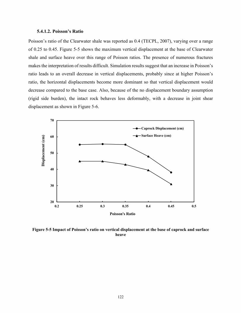
122

5.4.1.2. Poisson’s Ratio

Poisson’s ratio of the Clearwater shale was reported as 0.4 (TECPL, 2007), varying over a range

of 0.25 to 0.45. Figure 5-5 shows the maximum vertical displacement at the base of Clearwater

shale and surface heave over this range of Poisson ratios. The presence of numerous fractures

makes the interpretation of results difficult. Simulation results suggest that an increase in Poisson’s

ratio leads to an overall decrease in vertical displacements, probably since at higher Poisson’s

ratio, the horizontal displacements become more dominant so that vertical displacement would

decrease compared to the base case. Also, because of the no displacement boundary assumption

(rigid side burden), the intact rock behaves less deformably, with a decrease in joint shear

displacement as shown in Figure 5-6.

Figure 5-5 Impact of Poisson’s ratio on vertical displacement at the base of caprock and surface heave

20

30

40

50

60

70

0.2 0.25 0.3 0.35 0.4 0.45 0.5

Displacement (cm)

Poisson's Ratio


Surface Heave (cm)

123

Figure 5-6 Impact of Poisson’s ratio on joint normal and shear displacements

5.4.1.3. Friction Angle

The friction angle of Clearwater shale in the base model was 30°, as reported by Total and has

been varied in a range of 10° to 40° for the sensitivity analysis. Increasing friction angle reduces

the vertical displacements because the rock can withstand higher loads before it undergoes failure

and it results in less vertical displacements at the base of caprock and ground surface. However, it

would not significantly change deformability of rock as elastic parameters of Young’s modulus

and Poisson’s ratio. Note the subtle changes of vertical displacement in

Figure 5-7 compared to Figure 5-3 and Figure 5-5. Figure 5-8 suggests that friction angle of intact

rock does not systematically affect joint displacements because of the different orientation of pre-

existing fractures in the caprock.

0

0.1

0.2

0.3

0.4

0.5

0.6

0.7

0.8

0.9

0.2 0.25 0.3 0.35 0.4 0.45 0.5


Poisson's Ratio



124

Figure 5-7 Impact of friction angle on vertical displacement at the base of caprock and surface

heave

Figure 5-8 Impact of friction angle on joint normal and shear displacements

20

30

40

50

60

70

5 10 15 20 25 30 35 40 45

Displacement (cm)

Friction Angle (º)


Surface Heave (cm)

0

0.1

0.2

0.3

0.4

0.5

0.6

0.7

0.8

0.9

5 10 15 20 25 30 35 40 45 50


Friction Angle



125

5.4.1.4. Cohesion and Tensile Strength

The cohesion of Clearwater shale was varied between 0 and 0.1 MPa. The vertical displacements

were not significantly affected by cohesion, but a smaller amount of slippage was observed for

larger values of cohesion as illustrated in Figure 5-9. Based on the material properties, it seems

that frictional component of strength in the constitutive law has a higher impact on vertical

displacement than cohesion. Also, the tensile strength varied between 0 and 1 MPa with no

significant impact on block and joint displacements since shear (slip) mode was the governing

failure mechanism.

Figure 5-9 Impact of cohesion on vertical displacement at the base of caprock and surface heave

20

30

40

50

60

70

0 1000 2000 3000 4000 5000 6000 7000 8000 9000 10000 11000

Displacement (cm)

Cohesion(Pa)


Surface Heave (cm)

126

5.4.1.5. Dilation Angle

Dilation angle was varied between 0 to 50° with a base value of 20°. As shown in Figure 5-10,

dilation angle does not cause a significant change in surface heave and caprock displacement. A

higher dilation angle makes the rock mass less prone to failure and results in a subtle decrease of

vertical displacements with no substantial impact on joint displacements.

Figure 5-10 Impact of dilation angle on vertical displacement at the base of caprock and surface heave

While this section had discussed the impacts of variation in intact rock properties, the effect of

mechanical properties of fractures on displacements of the formation and discontinuities are

inspected and the results are shown in the next section.

5.4.2. Impact of Mechanical Properties of Fractures

5.4.2.1. Normal and Shear Stiffness of the Joints

No data was reported for joint properties of Clearwater shale in the Joslyn incident report and

available literature. Consequently, for this study, normal joint stiffness (jkn) was assumed to vary

20

30

40

50

60

70

0 10 20 30 40 50 60

Displacement (cm)

Dilation Angle


Surface Heave (cm)

127

between 5 and 1000 kPa/m and the value of shear joint stiffness (jks) was assumed to be 10% of

normal joint stiffness (Singh 1973) . Simulation results indicated that an increase in joint stiffness

did not affect vertical displacements, as shown in Figure 5-11, but it resulted in a decrease in both

normal and shear joint displacement as shown in Figure 5-12.

Figure 5-11 Impact of joint normal stiffness on vertical displacement at the base of caprock and surface heave

20

30

40

50

60

70

0E+00 3E+08 5E+08 8E+08 1E+09 1E+09


Joint Normal Stiffness (Pa/m)

Surface Heave (cm)


128

Figure 5-12 Impact of joint normal stiffness on joint normal and shear displacements

5.4.2.2. Joint Friction Angle and Cohesion

An increase in joint friction angle (0 to 55°) and joint cohesion (0 to 0.1 MPa) had no significant

change on intact rock displacements, resulting in less amount of shear failure and a decrease in

joint displacements as shown in Figure 5-13. An increase in friction angle, compared to cohesion,

results in more stable joints and less shear failure in joints.

0

0.1

0.2

0.3

0.4

0.5

0.6

0.7

0.8

0.9

1

1.1

1.2

0.00E+00 2.50E+08 5.00E+08 7.50E+08 1.00E+09 1.25E+09 1.50E+09


Joint Stiffness (Pa/m)



129

Figure 5-13 Impact of joint friction angle on joint normal and shear displacements

5.4.2.3. Joint Tensile Strength

For selected values of 0 to 1 MPa, joint tensile strength showed no impact on joints and intact rock

displacements, neither significantly altered the modes of failure, probably because most joint

failures were associated with failure in shear mode.

The geometrical parameters of discontinuities are analyzed in the following section.

5.4.3. Impact of Geometrical Parameters of Fractures

Along with mechanical properties of joints and intact rock, geometrical distribution of fractures

such as fracture size, orientation, and intensity can affect the mechanical behavior of a fractured

rock.

5.4.3.1. Fracture Size

Assuming the same intensity and power law distribution for all fracture sets in Clearwater caprock,

three sets of small (5 m to 30 m), medium (10 m to 50 m), and large (20 m to 90 m) fracture sizes

were generated. It was observed that an increase in fracture size resulted in larger vertical

0

0.1

0.2

0.3

0.4

0.5

0.6

0.7

0.8

0.9

1

1.1

1.2

0 5 10 15 20 25 30 35 40 45 50 55 60


Joint Friction Angle



130

displacements, both at the base of caprock and ground surface as demonstrated in Figure 5-14 and

larger shear displacement in joints as presented in Figure 5-15. This observation suggests that

larger fractures in caprock might experience larger displacements along the fracture planes, and

not effectively increase the intact rock displacement. This could be translated into higher steam

containment with less surface heave compared to a non-fissured caprock. Therefore, the size of

fractures should be considered for the interpretation of monitoring surveillance data.

Figure 5-14 Impact of fracture length on vertical displacement at the base of caprock and surface heave

20

30

40

50

60

70

10 20 30 40 50 60


Fracture Persistence (m)

Surface Heave


131

Figure 5-15 Impact of fracture length on joint normal and shear displacements

5.4.3.2. Fracture Orientation

Dip angle of fractures was varied between 0 (almost horizontal) to 90° (almost vertical). An

increase in fracture dip angle resulted in more significant vertical displacement of caprock and

surface heave. Fractures with dip angle close to 30° experienced more instability and were more

prone to shear failure. This is likely the result of the maximum principal stress being horizontal

and the stress components follow a reverse faulting regime (Figure 5-16). Various fractures under

different conditions (fracture distribution, fracture orientation, and stress regime) would cause

failure in diverse planes, so the interpretation of joint displacement trend is not straightforward, as

shown in Figure 5-17.

0

0.1

0.2

0.3

0.4

0.5

0.6

0.7

0.8

0.9

10 20 30 40 50 60


Fracture Persistence (m)



132

Figure 5-16 Impact of fracture orientation on vertical displacement at the base of caprock and surface heave

Figure 5-17 Impact of fracture orientation on joint normal and shear displacements

20

30

40

50

60

70

0 10 20 30 40 50 60 70 80 90 100


Fracture Orientation


Surface Heave (cm)

0

0.1

0.2

0.3

0.4

0.5

0.6

0.7

0.8

0.9

0 10 20 30 40 50 60 70 80 90 100


Fracture Orientation



133

5.4.3.3. Fracture Intensity

In 3DEC, fracture intensity is defined based on P32 (the area of fractures per unit volume).

Simulation results in Figure 5-18 suggest that using higher fracture intensity leads to less vertical

displacement at the base of caprock and surface heave, highlighting that fracture intensity

significantly affected deformability and strength of the rock mass. Also, larger joint displacements

were experienced when fracture intensity was increased, as illustrated in Figure 5-19. It is worth

noting that higher fracture intensity (i.e., a higher number of fractures) resulted in less surface

heave. This observation indicates that ignoring the assumption of non-fissured caprock might

ultimately lead to underestimating the risk for caprock failure and raises the question that the

integrity of caprock may not be properly addressed if monitoring of surface heave is the only

measure to be taken by operators and regulatory bodies.

Figure 5-18 Impact of fracture intensity on vertical displacement at the base of caprock and surface heave

20

30

40

50

60

70

0 100 200 300 400 500


Number of Fractures


Surfece Heave (cm)

134

Figure 5-19 Impact of fracture intensity on joint normal and shear displacements

5.4.4. Impact of Different Load Conditions Applying at the Base of Caprock

Aside from mechanical properties of the caprock, the applied load exerted at the base of caprock

due to steam injection pressure and temperature of SAGD steam chamber strongly influences the

caprock integrity assessment. This restriction, assigned by regulatory authorities, is represented

through the maximum operating pressure (MOP). As formulated previously, MOP was determined

based on the depth of injector and a safety factor of 1.1 prior to the steam release, while after the

Joslyn incident, AER adopted a revised policy and formulated MOP based on the shallowest depth

of caprock base instead of the injector depth and introduced a safety factor of 1.25 to avoid

potential initiation of tensile failure in caprock.

Based on the AER policy for caprock integrity (Directive 086), a caprock in the shallow thermal

area must be a minimum of 10 m thick, composed of clay-rich bedrock with gamma-ray values

higher than 75 API units, and laterally continuous across the target reservoir Formation. The depth

at the shallowest base of Clearwater caprock, where gamma-ray values are higher than 75 API

0

0.1

0.2

0.3

0.4

0.5

0.6

0.7

0.8

0.9

0 100 200 300 400 500


Number of Fractures



135

units, is 44 meters based on well log 100-09-033 which was in the vicinity of disturbed zone. The

mini-frac test results indicated that the minimum principal stress was vertical, and a value of 21

kPa/m was estimated for the fracture closure gradient. Prior to the Joslyn steam release incident,

MOP was calculated 1785 kPa for the injector at a depth of 85m without a margin of safety. Using

the current AER formulation, the lower bound of MOP is estimated 740 kPa with respect to the

depth of 44 meters for the base of caprock if Wabiskaw is also considered as caprock. The history

of injection pressure of the Joslyn SAGD site revealed that one month before caprock failure,

during Semi-SAGD phase, steam was injected at a pressure of 1800 kPag. Consequently, in this

study, 1800 kPa was selected as the upper bound of MOP. After the Joslyn caprock failure, four

neighboring well pairs were shut-in, and other well pairs were operated with a MOP of 1200 kPa.

For the lower bound of MOP, 740 kPa based on the current AER formulation, maximum vertical

displacement would be 28.2 cm at the base of caprock with an associated heave of 23.6 cm at

ground surface. If MOP is increased to 1200 kPa, the vertical displacements at the base of caprock

and surface will increase to 47.9 and 39.5 cm, respectively. For the upper bound of MOP, 1800

kPa, practiced by the operator in Joslyn SAGD well pair before failure, the associated vertical

displacement at the base of caprock and surface heave would increase to 75 and 61cm,

respectively. It should also be noted that the number of joints undergoing slippage due to failure

increases by applying a higher load at the base of caprock, i.e. higher MOPs lead to more failure

along fracture planes.

136

Figure 5-20 Joint Shear Displacement by applying 1800 kPa at the bottom of model

Examining the vertical displacement results indicates that higher load from SAGD steam chamber

increases the difference between subsurface and surface displacement by increasing the vertical

displacement of caprock and surface heave, as presented in Figure 5-21 and Figure 5-22. This is

observed because a portion of the applied load would be spent on changing shear and normal

displacements of the joints within the caprock, leading to less deformation at the ground surface.

137

Figure 5-21 Impact of applied load on vertical displacement at the base of caprock and surface heave

Figure 5-22 Impact of applied load on joint normal and shear displacements

0

10

20

30

40

50

60

70

80

90

600 800 1000 1200 1400 1600 1800 2000


Applied Load (kPa)

Surface HeaveCaprock Displacement

0

0.1

0.2

0.3

0.4

0.5

0.6

0.7

0.8

0.9

1

600 800 1000 1200 1400 1600 1800 2000


Applied Load (kPa)



138

The vertical displacement contours in 3D perspective and vertical-cross section at the center of

3DEC model for 1200 kPa as the uplift load at the base of caprock are shown in Figure 5-23.

Figure 5-23 Vertical displacement a) plan view b) bottom view c) vertical cross section at the center of 3DEC model for 1200 kPa uplift pressure

From the simulation results, it was noticed that even for lower bound of MOP, it appears that

failure in fractures, yet with small displacements, would occur if fracture intensity in the caprock

was sufficiently high. In addition, it is shown earlier that the joint properties play a significant role

139

for the behavior of joints in terms of shear and tensile failures. Consequently, at any certain injected

pressure, fracture density and joint properties may define if the joints are failed or not. Recall that

in this chapter, only geomechanical effects were investigated and no fluid flow was included in

the simulation. The impact of fluid flow coupling with geomechanics on deformation and the

caprock's failure modes are investigated and discussed in Chapter 6.

A previous basic geomechanical analysis performed by TEPCL on deformation of Joslyn SAGD

well pair was reported after the steam release incident (TEPCL 2007). Adopting a continuum

approach, the simplified two-dimensional model had the assumption of no fractures in caprock.

For a MOP of 1800 kPa, both vertical displacements at the base of caprock and the ground surface

were estimated to be 80 cm. It is worth to note that if the subsurface formations are deformable,

the vertical displacement at the base of caprock will be expected to differ from the surface heave.

In our study, using a three-dimensional discontinuum approach with no fractures and for a MOP

of 1800 kPa, the vertical displacements at the base of caprock and ground surface were 79 and 62

cm, respectively. If a pre-existing fracture set with an intensity of 0.006 (i.e. 450 small fractures)

was assumed, the vertical displacements at the base of caprock and the ground surface would

reduce to 68 and 56 cm, respectively. If a strain-softening constitutive model was adopted, the

vertical displacements at the base of caprock, and especially at the ground surface, would decrease

even more to 67 and 52 cm, respectively. Given the fact that pre-existing fractures are usually

present in most rocks and they might strongly affect the mechanical behavior of rock mass, these

variations in calculated vertical displacements indicate that the assumption of a non-fissured

caprock might lead to very conservative estimates of steam containment and ultimately, result in

underestimation of the risk for caprock failure. Moreover, pore pressure in fractured caprock needs

to be investigated because it may cause fracture propagation and increase the occurrence of failures

in caprock.

Conclusions and Remarks

The mechanical properties of both intact rock and discontinuities of Clearwater shale Formation

were inspected to assess discontinuities' role in the geomechanical behavior of the Clearwater

caprock in the Joslyn Scheme. Young’s modulus, Poisson’s ratio, and friction angle were found to

influence vertical displacements of caprock and surface heave. In addition, deformability, strength,

140

and geometrical properties of the fractures could affect the overall geomechanical response of rock

mass. Simulation results indicated that an increase in normal and shear stiffness of fractures did

not show a considerable effect on caprock and ground surface displacements, but it resulted in

reduced numbers of failures as well as lower normal and shear displacements in joints. Also,

strength parameters of joints did not alter surface heave but controlled the shear mode and slippage

of failed joints.

Along with the presence of discontinuities, the impacts of geometrical parameters of fractures and

the degree of fracturing on rock mass strength and deformability were studied. Inclusion of larger

fractures in the model led to higher values of displacements at the base of caprock and ground

surface. Altering fracture orientation from almost horizontal to almost vertical resulted in a subtle

increase of surface heave and fractures with dip angle close to 30° were more prone to shear failure.

Fracture intensity strongly affected deformability and strength of rock mass and less surface heave

was experienced when fracture intensity increased. This observation raises a concern whether

caprock integrity can be properly addressed when monitoring of surface heave is the main measure

to be taken by operators and regulatory bodies.

Aside from mechanical properties of the caprock, the applied load exerted at the base of caprock

due to steam pressure and temperature of SAGD chamber, strongly influenced the caprock

integrity assessment. Higher load from SAGD steam chamber increased the difference between

subsurface and surface displacement by increasing the vertical displacement of caprock and

surface heave. It was also noted that the existence of fractures could cause local shear failure in

the caprock, even below the AER mandated values of MOP.

Some variations in calculated vertical displacements were noted because of the role of pre-existing

fractures. Our discontinuum approach showed that the assumption of a non-fissured caprock might

lead to very conservative estimates of steam containment and ultimately, result in underestimating

the risk for caprock failure.

141

INVESTIGATION OF FLUID FLOW IN THE FISSURED CLEARWATER

SHALE 2

Preface

In the previous chapter, the injection pressure resulting from a growing steam chamber was

assumed to act on a caprock's base and place a vertical load on the caprock and overburden. A base

model was selected based on the stratigraphy of the project and mechanical properties of the

Clearwater Formation provided in TEPCL’s report. Figure 5-2 and Table 5-1 present the geometry

of the base model and mechanical properties which are used for the simulations, respectively. The

impacts of uplift pressure applied beneath the caprock on deformations, failure modes and

discontinuities were evaluated. Since no studies had been found that had considered a range of

mechanical properties of Clearwater shale and its discontinuities as well as the Quaternary

2 This chapter was extracted from a paper entitled “The investigation of Fluid Flow in the Fissured Clearwater Shale Using 3D Numerical Approach – Case Study of Joslyn Creek SAGD Project “which has been presented at the GeoConvention Virtual Event

2020 held in Calgary, Alberta, Canada, 21-23 September 2020.

142

deposits, a comprehensive sensitivity analysis was performed on the fissured caprock with respect

to different mechanical properties of the intact and geometrical parameters of fractures. The

induced displacements at the base of caprock and ground surface as well as stress state in the model

were investigated in Chapter 5. All evaluations were completed with the assumption of no fluid

flow in the model. While this provided valuable insights into how the caprock system would

behave, ultimately, it is necessary to include the role of pore pressure migration (diffusion) into

the fracture system response. Given the very low caprock matrix permeability, hydro-mechanical

analyses discussed in this chapter have assumed that fluid flow does not penetrate the matrix and

fluid flow only occurs within the discontinuities. Consequently, the results of the coupled hydro-

mechanical simulations to assess the performance of the fissured caprock under different

conditions will be presented in the following sections.

Understanding the hydro-mechanical behavior of fractures regarding pore pressure increase and

failure modes is undeniably necessary for caprock integrity assessment if the existence of

discontinuities in the field is likely. This chapter aims to explore the effects of fluid flow in the

fractured caprock, and the various loading conditions applying at the base of caprock due to steam

injection, on the surface heave, caprock deformation, and joint normal and shear displacements.

In addition, different modes of failure under various conditions of pore pressure are also inspected

for fissured caprock to capture the collaboration of hydraulic and mechanical phenomena in the

fractures. The number of joints presented in the caprock is also evaluated and its impacts on

deformation of intact rock and discontinuities are investigated.

Model Description

Similar to the modelling approach used in Chapter 5, 3DEC is also utilized to simulate the possible

mechanisms of caprock failure during SAGD operation with various fracture sets under different

scenarios of fluid flow imposed on the fissured caprock shale. Furthermore, for a variety of

maximum operating pressure conditions, the displacements at the base of caprock and ground

surface for the models with the assumption of flow in the fractures are inspected and compared

with the results of the previous study performed with the assumption of no flow in the fissured

caprock.

143

The base model which was utilized in the previous chapter is selected with the same size,

mechanical properties of intact and fractures as provided in Table 5-1.

The bulk modulus and density of water, as the single fluid in the simulation, are 2.2×107 Pa and

1×103 (kg/m), respectively. The model was initialized first, the displacements were set to zero and

the simulation was run to investigate different conditions in the model. Figure 6-1 demonstrated

the pore pressure diffusion at the base of caprock and section A is a cross section at the middle of

the model. As an example, 1200 kPa for the uplift pressure was applied at the base of the model

and the same procedure was taken for all the other loading conditions.

Figure 6-1 pore pressure diffusion from a bottom view and cross section A at the middle of the model

In this chapter, the emphasis is on the evaluation of vertical displacement at the base of caprock,

surface heave, joint normal and shear displacements as well as failure modes. A range of injection

pressures from 600 kPa to 1800 kPa representing the uplift pressure at the base of caprock was

applied to the model for simulation purposes. As discussed in Section 5.4.4, the amount of pressure

144

at the base of caprock resulting from steam injection during SAGD operation will significantly

influence caprock's performance in regard to deformation and failure modes. Based on the current

policy of AER, MOP for Joslyn is about 740 kPa assuming a 44 m depth for the base of caprock,

while the injection pressure that was experienced during Semi-SAGD was about 1800 kPa. That

is why a range of 600 kPa to 1800 kPa was selected for this study.

In the geomechanical study, it was found that applying higher fracture intensity leads to less

vertical displacement at the base of caprock and surface heave, highlighting the fact that fracture

intensity significantly affected deformability and strength of the rock mass. Therefore, two sets of

fracture intensities are selected for the hydro-mechanical simulation to investigate the influences

on the results. The regular fracture intensity is 0.0025 with about 200 fractures in the base model

and higher fracture intensity is defined as 0.006 with more than 500 fractures.

Then, the results of the realizations of SAGD steam chamber underlying a fissured caprock with

fluid flow inside discontinuities will be presented. The demonstrated results for geomechanical

study in the previous chapter will be compared with hydro-mechanical results to better understand

the impact of fluid flow in the pre-existing fractures for the fissured caprock.

Results and Discussion

6.3.1. Impact of Different Uplift Pressure Conditions Applied at the Base of Caprock

For the lower bound of MOP, 740 kPa, maximum vertical displacement would be 33.5 cm at the

base of caprock with an associated heave of 28 cm at the ground surface. If MOP is increased to

1200 kPa, the vertical displacements at the base of caprock and surface will increase to 61.8 and

50 cm, respectively. For the upper bound of MOP, 1800 kPa, practiced by the operator in the well

pair 1 prior to the failure, the associated vertical displacement at the base of caprock and surface

heave would increase to 98.5 and 84 cm respectively. It should also be noted that the number of

slipped joints due to failure increases by applying a higher load at the base of caprock, i.e., higher

MOPs lead to more failure along fracture planes. Figure 6-2 shows the vertical displacements'

situation under a variety of uplift pressure for the hydro-mechanical study. It illustrates that higher

load from SAGD steam chamber increases the difference between sub-surface and surface

145

displacements by increasing the vertical displacement of caprock and surface heave. This is

experienced because a portion of the applied load would be spent on changing shear and normal

displacements of the joints within the caprock, leading to less deformation at the ground surface.

Figure 6-2 Impact of applied load on vertical displacement at the base of caprock and surface heave for HM analysis

The vertical displacement contours in plan view, bottom view and the vertical-cross section at the

center of 3DEC model for 1200 kPa as the uplift load at the base of caprock are shown in Figure

6-3.

0

20

40

60

80

100

120

600 800 1000 1200 1400 1600 1800 2000


Applied Load (kPa)

HM Surface Heave

HM Caprock Displacement

146

Figure 6-3 Vertical displacement a) plan view b) bottom view c) vertical cross section at the center of 3DEC model for 1200 kPa uplift pressure

Figure 6-4 illustrates that increase of the applied load at the base of caprock results in higher joint

normal and shear displacements when the fluid flow is considered within the fractures located in

the Clearwater Formation.

147

Figure 6-4 Impact of applied load on joint normal and shear displacements for HM analysis

6.3.2. Impact of Fracture Intensity

Two sets of fracture intensities were investigated and as Figure 6-5 and Figure 6-6 show, both

caprock displacement and surface heave are decreased by increasing the number of fractures in the

caprock. This observation indicates that the number of fractures in the caprock should be estimated

as accurately as possible with the lowest amount of uncertainty. Because less fractures lead to

underestimating the risk for caprock failure and raises the question that the integrity of caprock

could not be properly addressed if monitoring of surface heave is the only measurement that will

be taken into consideration by operators.

0

0.2

0.4

0.6

0.8

1

1.2

1.4

1.6

600 800 1000 1200 1400 1600 1800 2000


Applied Load (kPa)

HM Joint Normal Displacement

HM Joint Shear Displacement

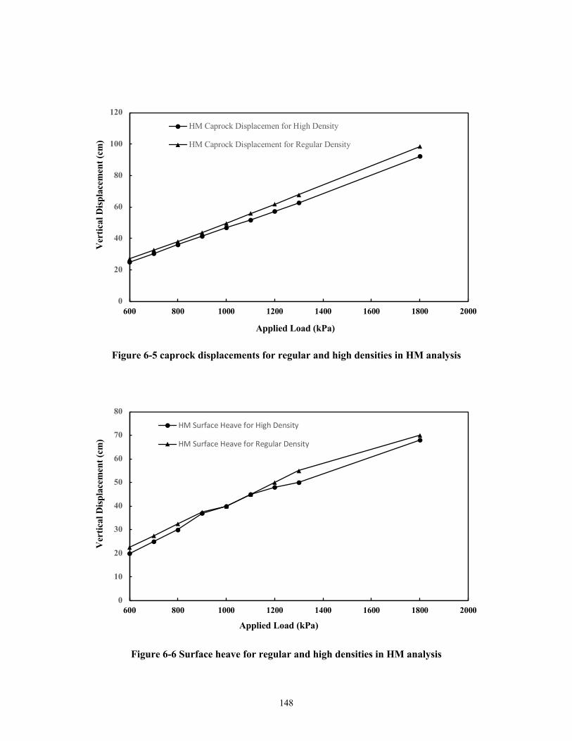
148

Figure 6-5 caprock displacements for regular and high densities in HM analysis

Figure 6-6 Surface heave for regular and high densities in HM analysis

0

20

40

60

80

100

120

600 800 1000 1200 1400 1600 1800 2000


Applied Load (kPa)

HM Caprock Displacemen for High Density

HM Caprock Displacement for Regular Density

0

10

20

30

40

50

60

70

80

600 800 1000 1200 1400 1600 1800 2000


Applied Load (kPa)

HM Surface Heave for High Density

HM Surface Heave for Regular Density

149

Geomechanical vs. Hydro-Mechanical Simulation

The results of both geomechanical and hydro-mechanical investigations were demonstrated in

previous sections. In this section, both scenarios' results are compared to understand the models'

behavior under the explained conditions. Figure 6-7 shows that for the lower bound of MOP, 740

kPa, the surface heave with the existence of fluid flow in the model is about 18% higher than the

same situation when no fluid flow is considered. For 1200 kPa the difference is about 26% and for

the upper bound of the injection pressure at 1800 kPa, the surface heave is about 37% higher when

fluid flow is reflected in the simulation. The results show a non-linear relationship between the

surface heave increments for different amounts of uplift pressure at the base of caprock. This

indicates that the simulation has to be performed for each situation to achieve the best estimation.

Figure 6-7 Influence of fluid flow in fractures on surface heave

The displacement for the base of caprock is also increasing with consideration of fluid flow in the

simulation. Figure 6-8 shows that the increase is about 18%, 29%, and 31% for applied loads of

740, 1200, and 1800 kPa, respectively.

0

10

20

30

40

50

60

70

80

90

600 800 1000 1200 1400 1600 1800 2000


Applied Load (kPa)

HM Surface Heave

Geomech Surface Heave

150

Figure 6-8 Influence of fluid flow in fractures on caprock displacement

The simulation results demonstrate that fluid flow within the fractures in the hydro-mechanical

analysis causes a reduction of effective normal stress on the joints planes. Consequently, joint

normal and shear displacements increase significantly compared to the case considering no fluid

flow in the model as shown in Figure 6-9 and Figure 6-10, respectively.

0

20

40

60

80

100

120

600 800 1000 1200 1400 1600 1800 2000


Applied Load (kPa)

HM Caprock Displacement

Geomech Caprock Displacement

151

Figure 6-9 Influence of fluid flow in fractures on joint normal displacement

Figure 6-10 Influence of fluid flow in fractures on joint shear displacement

0

0.1

0.2

0.3

0.4

0.5

0.6

0.7

600 700 800 900 1000 1100 1200 1300 1400 1500 1600 1700 1800 1900


Applied Load (kPa)

HM Joint Normal Displacement

Geomech Joint Normal Displacement

0

0.2

0.4

0.6

0.8

1

1.2

1.4

1.6

600 700 800 900 1000 1100 1200 1300 1400 1500 1600 1700 1800 1900


Applied Load (kPa)

HM Joint Shear Displacement

Geomech Joint Shear Displacement

152

It was observed that considering fluid flow in the fractures results in the reduction of effective

stress on the joint planes. As Figure 6-11 clearly shows, touching shear failure envelope sooner

and having more sheared planes than the analyses with no flow could be the consequences of the

flow in the fractures. The obtained results illustrate that once fluid flow is considered in

discontinuities under 1800 kPa as uplift pressure at the base of caprock, displacement at the base

of caprock and joint normal displacement is increased by 30%, 58%, respectively. These variations

in behavior are significant and prove that the assumption of no fluid flow in the fractured caprock

may lead to overestimation of steam containment and ultimately, underestimation of the risk for

caprock failure.

Figure 6-11 Slip modes (a) considering no fluid flow (b) considering fluid flow in discontinuities

153

In Chapters 5 and 6, it was assumed that the caprock is fissured and pre-existing fractures are

observed over the area of interest.

Due to lack of discontinuities in the data provided by TEPCL, the sequentially coupled reservoir

geomechanical simulations utilizing high geo-cellular obtained in Chapter 4 will be carried out in

the next chapter assuming a continuum caprock over the interested area in the Joslyn project.

154

SEQUENTIALLY COUPLED RESERVOIR GEOMECHANICAL

SIMULATIONS OF THE JOSLYN SAGD

OPERATIONS

In the comprehensive report released by TEPCL (2007), 2D finite element geomechanical

simulations were presented that did not consider temperature and pressure changes within the

reservoir during SAGD process. In that report, TEPCL stated that a coupled reservoir

geomechanical simulation to capture all the complex phenomena happening during SAGD

operation at different stages is necessary. This coupled simulation, particularly in 3D, for a large

field-scale model is very complicated; however, this model is necessary to better understand the

interaction between reservoir and geomechanics during SAGD process. As discussed in Chapter 2,

by continuous injection of steam to the reservoir, temperature and pressure will change in and

around the chamber zone of the SAGD operation. After a certain time, the altered pressure and

temperature will change the stress and strain situations in the model, resulting in stress-induced

volumetric deformations within the area. Consequently, the permeability will be altered, and this

change should be applied to the reservoir simulator as the updated input data with respect to the

user-defined coupling time. Applying actual injection and production data at different stages of

the SAGD process to a large field-scale model with multi-million cells is a very time-consuming

process; however, it is of interest if more definitive results aid the interpretation of potential failure

mechanisms for the Joslyn steam release incident.

155

Consequently, 3D sequentially coupled reservoir geomechanical simulations were conducted

using the RGRG high performance computer (HPC). At this stage, the sequentially coupled

reservoir geomechanical simulation platform developed internally in RGRG is used. Figure 7-1

illustrates the workflow of the platform. The high-resolution geological model discussed in

Chapter 4 was used for the reservoir geomechanical simulations.

Figure 7-1 Sequentially coupled reservoir geomechanical workflow

Concerning computation time and the result's accuracy, coupled methods are commonly divided

into three major categories as 1) one way/uncoupled, 2) sequentially and 3) fully coupled. A brief

explanation with regards to each approach will be presented in Section B.4.

Appendix B also summarizes the governing equations used in the reservoir and geomechanics

simulators.

Once steam release to the surface above the heel of well pair 1 in Pad 204 was observed on May

18th 2006, TEPCL promptly shut down the associated well pair and the three other adjacent well

156

pairs including well pair 1 and 2 in pad 204, well pair 1 in Pad 203, and well pair 4 in pad 202 as


Figure 7-2 Shut down well pairs after steam release incident shown in red color

Except for these four well pairs, the remaining well pairs remained in operation albeit with a

considerably lower steam injection pressure. During SAGD operations in the other wells, TEPCL

was required to equip the field with surveillance instrumentation to monitor the operation safely

from caprock integrity point of view. The remaining well pairs remained in operation for almost

Schematic Crater

157

two years after the steam release incident and stress induced deformation within the reservoir and

overlying formations was captured by the surveillance monitoring systems. This data offers an

invaluable opportunity to validate the reservoir geomechanical model, which can then be used to

model the pre-steam release formation behavior.

Therefore, the first stage of modeling will only include the pilot and well pairs 3, 4, 5 which were

under operation after the incident. This model is then calibrated using the available monitoring

data from recorded surface heave and production history of the wells. This post-failure simulation

provides a critical step to confirm the properties of the model prior to simulating the steam released

incident itself, when all the properties and parameters used in the calibrated model are kept the

same. However, the model extent will be increased to include all the well pairs in pad 204 as well

as the pilot well pair. Simulation will be conducted beginning at day one of the project and

proceeding to the date of the steam release event considering all injection pressures applied over

this period. Employing this complete and validated model will help us better understand the

behavior of different formations over the life of the project.

Post Failure Simulation for Model Calibration

The initial step in the post-failure modelling involves exporting and initializing the associated

geological model generated in SKUA-Gocad to the RGRG modeling platform, which is built

around CMG-STARS and the geomechanical code ITASCA-FLAC3D. As shown in Figure 7-3,

this model only includes the pilot and the well pairs that were under operation after the steam

release.

158

Figure 7-3 Selected area for the post failure simulation model

Initially, the model is “cut” from the large model and consists of 1.9 million simulation grids with

218 cells in I direction (South to North) with an average length of 5.7 m, 154 cells in J direction

(West to East) with an average length of 4.3 m, and 57 cells in K direction (Top to Bottom) with

a variable length range of 1-8 m according to different formations. The dimensions of the model

are shown in Figure 7-4.

The model is initialized based on the properties described in Chapter 4 and the boundary conditions

are fixed in x and y directions at the base, fixed in x and free in y at the sides and free to move at

the ground surface.

Figure 7-5 depicts the chronological events of different steps of the SAGD operation at Joslyn

creek and shows that after 748 days from the beginning of the project (the start of the pilot well

pair), the steam release process to the surface above well pair 1. It also shows the start of circulation

for well pairs 3, 4, and 5 after the steam release incident in which monitoring facilities were

installed above well pairs 3, 4, 5, and the pilot plant to measure the surface heave.

159

Figure 7-4 Dimensions of the post failure geological model

Figure 7-5 Operations in the active well pairs after steam release incident over time

The operation pressures of injectors and producers associated with time for the well pairs used in

the simulation are extracted from field data provided by TEPCL. Average pressures in the injectors

are obtained from the average of blanket gas bottomhole pressure during different phases of SAGD

in which the pressure variations are not substantial. The average values for the pilot injector are

160

presented in Figure 7-6. Similarly, average pressures in the producers are obtained from the

average of bubble tube bottomhole pressure during different phases of SAGD and the values are

presented in Figure 7-7.

Figure 7-6 Pilot injector average pressure used in simulation and the blanket BHP obtained from field

0

200

400

600

800

1000

1200

1400

1600

1800

0 500 1000 1500 2000

Pressure (kPa)

Time (days)

INJ Avg Pressure (Simulation) Blnkt BHP Field Data

161

Figure 7-7 Pilot producer average pressure used in simulation and the bubble BHP obtained from field

Figure 7-6 and Figure 7-7 are provided as examples of how the average pressures in the injector

and producer for different stages of SAGD in the pilot well pair were calculated. This process was

used for all remaining well pairs. This data for the pilot and the rest of well pairs is summarized in

Table 7-1 to Table 7-4 for the post failure simulation.

Simulations within the coupling platform require defining after how many days the reservoir and

geomechanical models should be coupled using an internal code which connects the reservoir to

geomechanical simulators. Thus, operation of the wells and user-defined coupling dates for the

reservoir simulator were established based on the data presented in Table 7-1 to Table 7-4.

0

200

400

600

800

1000

1200

1400

1600

1800

0 500 1000 1500 2000

Pressure (kPa)

Time (days)

PRD Avg Pressure (Simulation) Bubble BHP (Field Data)

162

Table 7-1 Injector and producer pressure for different phases of SAGD process for the pilot Pilot Well Pair Operations

Injector Producer

Day from start From To Duration

(day) Stage Avg. Pressure (kPa)

Avg. Pressure (kPa)

0 4-May-04 13-Sep-04 136 Circulation 1304 1290

137 14-Sep-04 11-Jan-05 120 SAGD 1198 1005

257 12-Jan-05 1-Feb-05 21 Shut in 0 0

278 2-Feb-05 24-Jan-06 357 SAGD 1161 693

635 25-Jan-06 1-Mar-06 36 Shut in 0 0

671 2-Mar-06 9-Jul-07 495 SAGD 980 612

1166 10-Jul-07 9-Oct-07 92 SAGD 893 493

1258 10-Oct-07 16-Dec-07 68 Shut in 0 0

1326 17-Dec-07 27-Mar-09 467 SAGD 1061 591

1793

1788

Table 7-2 Injector and producer pressure for different stages of SAGD process for well pair 4 Well pair 4

Injector Producer

Day from

start From To

Duration

(day) Stage

Avg. Pressure

(kPa)

Avg. Pressure

(kPa)

755 25-May-06 13-Aug-06 81 Circulation 1346 1397

836 14-Aug-06 11-Sep-06 29 shut in 0 928

865 12-Sep-06 30-Sep-06 19 SAGD 946 668

884 1-Oct-06 13-Oct-06 13 Shut in 0 686

897 14-Oct-06 20-Dec-06 68 SAGD 975 711

965 21-Dec-06 2-Jun-07 164 SAGD 1082 886

163

1129 3-Jun-07 2-Oct-07 122 SAGD 805 686

1251 3-Oct-07 13-Nov-07 42 Shut in 0 795

1293 14-Nov-07 23-Dec-07 40 SAGD 778 547

1333 24-Dec-07 24-Mar-09 457 SAGD 1147 885

1790

1790


Injector Producer

Day from

start

From To Duration

(day)

Stage Avg. Pressure

(kPa)

Avg. Pressure

(kPa)

1011 5-Feb-07 11-Apr-07 66 Circulation 945 1030

1077 12-Apr-07 15-May-07 34 Shut in 0 0

1111 16-May-07 6-Oct-07 144 Circulation 1054 1041

1255 7-Oct-07 19-Dec-07 74 Shut in 0 0

1329 20-Dec-07 16-Feb-08 59 SAGD 1012 890

1388 17-Feb-08 10-Feb-09 360 SAGD 1177 953

1748 11-Feb-09 25-Mar-09 43 SAGD 838 778

1791

164


Injector Producer

Day from

start

From To Duration

(day)

Stage Avg. Pressure

(kPa)

Avg. Pressure

(kPa)

1112 17-May-07 21-Jul-07 66 Circulation 1083 1087

1178 22-Jul-07 5-Sep-07 46 SemiSAGD 1101 939

1224 6-Sep-07 9-Oct-07 34 SAGD 1163 825

1258 10-Oct-07 13-Nov-07 35 Shut in 0 0

1293 14-Nov-07 3-Feb-09 448 SAGD 1173 825

1741 4-Feb-09 27-Mar-09 52 SAGD 850 910

1793

As discussed in the following sections, permeability, and plastic properties of shale and silt in

Clearwater and Wabiskaw layers required adjustment within the model. The original permeability

distribution for the simulation grids provided by TEPCL is illustrated in Figure 7-8 which is

obtained from correlations with the available core data. As an example, the correlation of

horizontal permeability is also shown for the log 1AB/13-33-095-12W4. It is postulated that these

correlations are not representative of the lab data. Consequently, permeability remains an uncertain

parameter that will be investigated and calibrated in the coupling platform based on the cumulative

oil production obtained from the field.

165

Figure 7-8 Original permeability associated with core data provided by TEPCL

By analyzing the available well logs located at different parts of the field, higher gamma ray values

were observed on the west side of the project site near the pilot plant compared to the east side

close to well pair 1, in proximity to where the steam release incident occurred. It also indicates

that the caprock is less clayey on the east side, inferring that the caprock's quality from a caprock

integrity point of view is less favorable than on the west side of the project area. If the cut-off value

to categorize the sand and shale grids is chosen as 75 API, which is identified in the AER Directive

86 for shallow SAGD reservoirs, the results indicate the presence of thicker caprock at the west

side compared to the east side, as illustrated in Figure 7-9. Additional details of the well logs

investigation will be provided in Section 10.2. As an example, Figure 7-9 exhibits the inspection

of well logs 103/11-33-095, 103/10-33-095, and 100/09-33-095 located near the heels of the pilot,

166

well pair 3, and well pair 1, respectively. The figure compares the thickness and quality of the

caprock from the west side towards the east side over the area of interest.

West East

Figure 7-9 The thickness and quality of caprock from the west side to the east side of the model based on 75 API gamma ray cutoff value

Therefore, to have more accurate results and decrease the uncertainties in the coupled platform,

the results of this investigation are considered for the model and the plastic properties in the

Clearwater shale and Wabiskaw over well pair 1 are modified, as noted in Table 7-5, to reflect the

lower quality of caprock within that area.

The most important and critical aspect in the coupling platform is updating permeability

distribution in the grids due to stress induced deformations occurring in the model. Adjusting

permeability associated with deformations in the oil sands has been a significant subject for

researchers and industry since the start of SAGD operation in the 1980s. Several aspects have been

studied to better understand the influence of deformation on the porosity and permeability values.

The most critical aspects that should be investigated to understand better the permeability change

in the oil sands due to induced volumetric deformation are the density of sand, isotropic or

anisotropic stress regime applying on the formation, the existence of relatively low or high

confining stress in the field, stress paths, and contraction or dilation happening in the oil sand.

167

Mori and Tamura (1986), Oldakowski (1994), Scott et al. (1994), Chalaturnyk (1996), Touhidi-

Baghini (1998), Samieh and Wong (1997), Li and Chalaturnyk (2006) have conducted different

tests to directly measure the permeability of oil sands in the laboratories or estimate permeability

values in numerical models to anticipate the behavior of the oil sands. Generally, expansion of

pore spaces in porous media resulted from elastic deformation and creation of a flow channel due

to stress induced plastic deformation resulted from shear failures are two major categories to

anticipate the permeability change. The literature shows that shear failures in the formation

typically change permeability substantially, while isotropic unloading does not cause a significant

effect.

Table 7-5 Adjusted mechanical properties in Clearwater and Wabiskaw close to the crater Grid Regions Material Adjusted Properties

Clearwater

Clay

Cohesion = 1.2e5 Pa

Dilation angle = 0 degree

Friction angle = 15 degree

Tension = 5e4 Pa

Silt

Cohesion = 5e4 Pa



Tension = 5e4 Pa

Wabiskaw

Clay

Cohesion = 1.2e5 Pa



Tension = 5e4 Pa

Silt

Cohesion = 5e4 Pa



Tension = 5e4 Pa

Touhidi-Baghini (1998) investigated the variation of absolute permeability with dilation for

vertical core samples versus the volumetric strain in which dilation is assumed positive and

compared test results with other available results, as shown in Figure 7-10.

168

Figure 7-10 Variation of absolute permeability with dilation for vertical core specimens (retrieved from Touhidi-Baghini, 1998)

Touhidi-Baghini (1998) determined an exponential relationship for the ratio of the permeability

and volumetric strain as follows:

7-1

where a = 1 and b = 17.3 for the vertical permeability multiplier and b = 9.07 for the horizontal

permeability multiplier.

In the post failure simulation, Touhidi-Baghini coefficients (a,b) were initially used for updating

permeability in the model regarding stress-induced volumetric strain changes after a specific time

defined by the user for coupling reservoir and geomechanical simulations.

By assuming Touhidi-Baghini coefficients for updating permeability, one way and sequentially

coupled reservoir geomechanical simulations were conducted on the model with respect to the

original permeability values in the simulation grids. Simulations were conducted based on the

parameters listed in Table 7-1 to Table 7-4 for different stages of the SAGD operation. A time of

1600 days was chosen as the simulation time for the end of the project. Figure 7-11 shows the

contours of volumetric strain increment (maximum value of approximately 0.008) around the pilot

[ ]expnx

volox

k a bk

e= ×

169

well pairs after 1600 days. These results will be ultimately used to investigate the effect of Touhidi-

Baghini permeability model coefficients.

Figure 7-11 Contour of volumetric strain change around pilot after 1600 days

The volumetric strain and temperature obtained from reservoir simulator after 1600 days are also

demonstrated in Figure 7-12.

Figure 7-12 Temperature profile and volumetric strain change around the heel of pilot after 1600 days

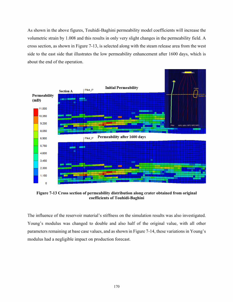
170

As shown in the above figures, Touhidi-Baghini permeability model coefficients will increase the

volumetric strain by 1.008 and this results in only very slight changes in the permeability field. A

cross section, as shown in Figure 7-13, is selected along with the steam release area from the west

side to the east side that illustrates the low permeability enhancement after 1600 days, which is

about the end of the operation.

Figure 7-13 Cross section of permeability distribution along crater obtained from original coefficients of Touhidi-Baghini

The influence of the reservoir material’s stiffness on the simulation results was also investigated.

Young’s modulus was changed to double and also half of the original value, with all other

parameters remaining at base case values, and as shown in Figure 7-14, these variations in Young’s

modulus had a negligible impact on production forecast.

171

Figure 7-14 Influence of Young’s modulus on cumulative oil production (COP)

There is a potential that permeability equation coefficients may differ from those obtained by

Touhidi-Baghini (1998) since these coefficients were determined from lab results conducted on

bitumen-free samples of a McMurray Formation river valley outcrop, which may have experienced

a unique stress history and this stress history was not replicated for the lab testing specimens which

would impact permeability measurements. Furthermore, for large, field scale models similar to the

model used in this study, these coefficients may need to be adjusted. Zhang (2019) investigated

the variations of permeability values associated with induced volumetric strain during SAGD

operation and used a=1, b(x,y)=90.7, and b(z)=174.8 as the coefficients for the field scale models.

Due to similar formations used in this study and that used by Zhang (2019) in his case study, the

same values of coefficients have been chosen for this research study of the Joslyn SAGD project.

These coefficients have been applied to the exponential relationship of the permeability and

volumetric strain suggested by Touhidi-Baghini. As shown in Figure 7-15, the permeability

enhancement for the maximum volumetric strain of 0.008 resulted from simulation becoming 2.07

as opposed to the previous value of 1.008.

0100002000030000400005000060000700008000090000100000110000120000130000140000

0 500 1000 1500 2000 2500

COP (m3)

Time (days)

SEQ Coupled

Double E

Half E

172

Figure 7-15 Absolute permeability ratio vs. volumetric strain

Adjusting the coupling coefficients according to Zhang (2019) will generate a considerable

difference between uncoupled and coupled results due to the interaction of geomechanics with

multiphase fluid flow in the oil sands reservoir. The plot in Figure 7-16 shows cumulative oil

production under the assumption of different values of coefficients in the model. It demonstrates

the influence of the selected coefficients for this study on the results. The simulation COP obtained

from the selected coefficients is about 59 % higher than uncoupled situation in which the

permeability is not updated based on induced volumetric strain and it shows the significant

influence of coupling coefficients for updating permeability with regards to volumetric strain

changes. It also shows the results when the coefficients are doubled compared to the specified ones

for this research.

a=1, b(x,y)=90.7, b(z)=174.8

173

Figure 7-16 COP comparison of uncoupled and coupled models with different coefficients

The volumetric strain changes at the injector depth in a plan view and the cross section along the

pilot well at day 5 (~start of project) and day 1600 (~end of project), are also demonstrated in

Figure 9 17.

0

50000

100000

150000

200000

250000

300000

0 500 1000 1500 2000 2500

COP (m

3 )

Time (days)

Uncoupled

SEQ Coupled with Original Coefficients

SEQ Coupled with Selected Coefficients

SEQ Coupled with Double Selected Coefficients 120 %

59 %

174

Figure 7-17 Changing volumetric strain over time

To explore the influence the shift in permeability resulting from modifying the permeability

equation coefficients has on overall cumulative oil production, the original permeability

distributions within the model were adjusted by 43%, 50%, 65% and 70% of their initial values.

For sequentially coupled simulations, Figure 7-18 clearly illustrates the geomechanical effects on

production performance as a result of these permeability variations and the final COP values for

these simulations are summarized in

Table 7-6. Note that the original permeability distribution results in a COP that is much higher

than actual recorded production in the field. The reason could be the high permeability assigned

to the simulation cells in the model. TEPCL justified initial permeability for the uncoupled

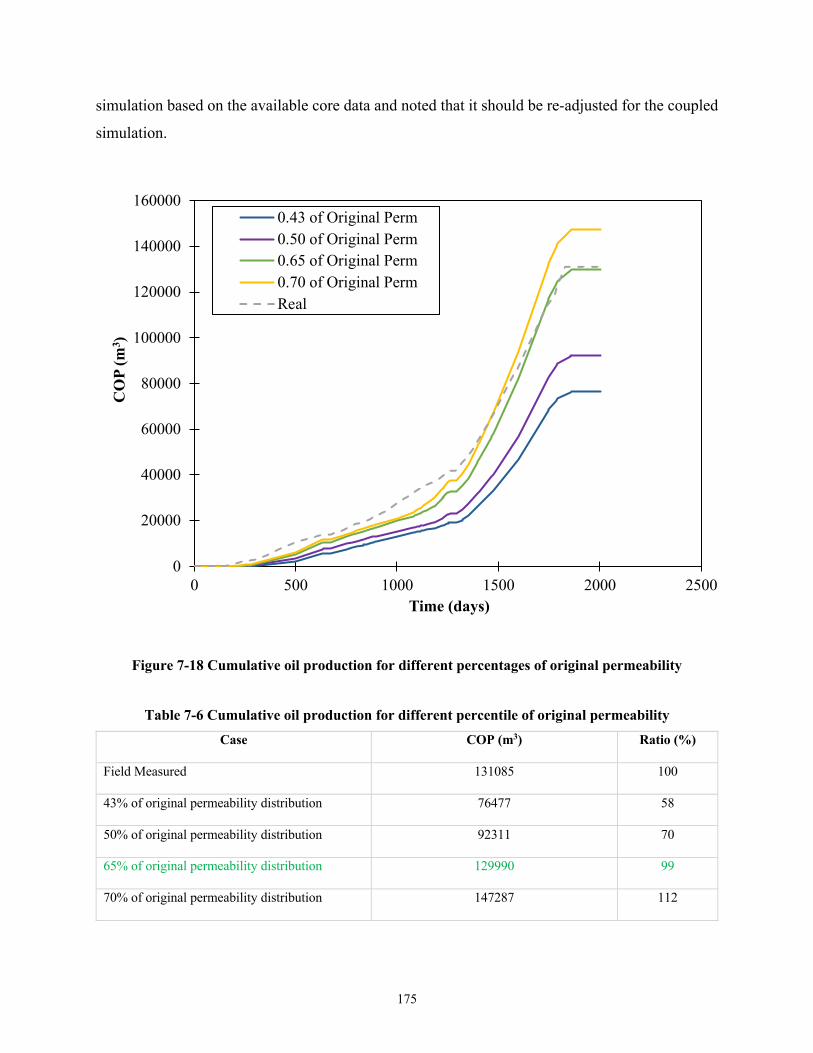
175

simulation based on the available core data and noted that it should be re-adjusted for the coupled

simulation.

Figure 7-18 Cumulative oil production for different percentages of original permeability

Table 7-6 Cumulative oil production for different percentile of original permeability Case COP (m3) Ratio (%)

Field Measured 131085 100

43% of original permeability distribution 76477 58




0

20000

40000

60000

80000

100000

120000

140000

160000

0 500 1000 1500 2000 2500

COP (m

3 )

Time (days)

0.43 of Original Perm0.50 of Original Perm0.65 of Original Perm0.70 of Original PermReal

176

It should be mentioned that to define different percentages of original permeability for the

simulations, the entire distribution of permeabilities were shifted for all the grids in the reservoir.

As an example, the histograms of the original vertical and horizontal permeabilities and 65

percentage of these values in the McMurray Formation are shown in Figure 7-19 and Figure 7-20.

Figure 7-19 Original vertical permeability and 65 percentage of permeability histograms in the McMurray Formation

Figure 7-20 the histograms of original horizontal permeability and 0.65 permeability histograms in the McMurray Formation

177

Based on the results illustrated in Figure 7-18, a downward shift in the original permeability

distribution of 65% provides a very good match using field measured oil production as the

objective metric. It has been assumed that this demonstrates model verification by updating the

permeability coefficients as well as initial permeability in the grids.

An uncoupled analysis was also piloted on the updated permeability and coefficients to investigate

the difference between uncoupled and coupled platforms with respect to oil production. Interaction

of fluid and deformation increases the cumulative oil production by about 45%, as shown in Figure

7-21.

Figure 7-21 COP for uncoupled and coupled associated with 65% of original permeability and selected coefficients compared with the real data

Additional valuable data for calibration of the post failure simulation is monitoring data available

from surveillance instrumentation installed in the field after steam release incident on the surface

above the well pairs under operation. If the model is accurately calibrated, the surface heave

0

20000

40000

60000

80000

100000

120000

140000

0 500 1000 1500 2000 2500

COP (m

3 )

Time (days)

0.65Perm_SEQ

0.65Perm_UN

Real

45%

178

resulting from the interaction of geomechanics events with flow simulation should be compatible

with the values measured on the surface.

TEPCL installed 60 InSAR corner reflectors (Green spheres and crosses) and 131 tiltmeters (red

squares) for the surveillance program. They also used heave monuments (GPS) to ensure the

caprock containment is achieved. The location of monitoring instrumentation is shown in Figure

7-22.

Figure 7-22 Location and number of InSAR, tiltmeters and GPS

TEPCL provided the measurements from all monitoring facilities recorded after the steam release

incident. This vast amount of raw data is confidential and cannot be provided in this document.

This provided data was analyzed, and the maximum heave surface recorded above the middle of

well pair 4, as shown in Figure 7-23, after about 1790 days was estimated to be 6 cm. Figure 7-23

179

provides a subset of the surface monitoring points, highlighting 2 InSAR, 1 tiltmeter and 1 GPS

measurement records at the midpoint along well pair 4 (blue circle in Figure 7-23).

Figure 7-23 Surface heave recorded by InSAR, tiltmeters and GPS at the middle of WP4 where maximum displacement was recorded at the end of project

Sequentially coupled reservoir geomechanical simulation results over the post-failure time period

(model calibration period), which included the operational history of four well pairs, were used to

extract surface heave predictions over the Joslyn project area. Figure 7-24 shows surface heave

contours versus the displacement at the base of caprock at the end of the Joslyn project. The results

show that the displacement value at the base of caprock is more than the surface heave which

agrees with the results of discontinuum analysis of the fissured caprock, as discussed in Chapter

5. This observation is important when considering caprock integrity analysis to prevent generating

of major failures at the base of caprock.

180

Figure 7-24 Contours of vertical displacements at the surface and base of caprock at the end of the project

Surface heave based on GPS monument field data also matches closely the validated sequentially

coupled reservoir geomechanical model results, shown in Figure 7-25.

Based on the reasonable match of the calibrated numerical model predictions with production data

(Figure 7-21), surface heave contours and the location of maximum surface heave over well pair

4 (Figure 7-25), it has been concluded that the “post-failure” model has been sufficiently validated

to reliable deploy the model in examining the processes leading up to the steam release incident.

Consequently, the model can now be extended to include all the well pairs in pads 101 and 204

from the beginning to the end of the project considering all actual data associated with pressure

and temperature changes in the injectors and producers over the life of the project.

181

Figure 7-25 Comparison of surface heave obtained from simulation results and GPS

Simulation of Steam Release Event using Calibrated Model

Chapter 4 provided an extensive description of the methodology of generating simulation grids in

the SKUA-Gocad and defining all reservoir and geomechanical properties for different facies

according to available data for the Joslyn project. To be more accurate, the Young’s moduli for all

formations except till in Quaternary deposits and limestone bedrock are coupled with the confining

stress based on the associated formulations for different formations obtained from literature. In

addition, as explained in Section 9.1, adjusted plastic properties of shale and silt in Clearwater and

Wabiskaw layers were specified for the region near the steam release location. Using defined

properties and original permeability obtained from TEPCL in the coupling simulations results in

much higher COP compared to the field data. Therefore, the coupled model with different values

of permeability were run and results for a 65% reduction in the original permeability distribution

182

in all grids was found to reasonably match with the field COP. Furthermore, the surface heave for

this model was investigated and the results indicated a reasonable comparison of field measured

surface heave and simulation predictions for the same region.

Therefore, calibration of the formation properties based on a history match to cumulative oil

production and surface deformation during the post-failure operational period now provides a

reliable foundation to explore the operational period leading up to the steam release event. These

simulation results are utilized in Chapter 8 to assemble several lines of evidence that support the

proposition for the mechanism(s) leading to the steam release event.

Figure 7-26 shows a plan view of the area of the larger model required for the simulation studies,

including all the well pairs, is extracted from the original extensive geo-cellular model.

Figure 7-26 Selected area for modeling the complete model including all well pairs

This model comprises 2.75 million simulation grid blocks with 230 cells in I direction (South to

North) with an average length of 6.2 m, 210 cells in J direction (West to East) with an average

length of 4.5 m within the reservoir and 8 m in the extended area beyond the reservoir domain for

the geomechanical model, and 57 cells in K direction (Top to Bottom) with a variable range of 1-

183

8 m in length are kept the same as post failure model. The dimensions of the complete model are


Figure 7-28 chronologically summarizes the operations from the beginning of the project in May

2004 by steam circulation in the pilot until the project's termination in March 2009 that was about

three years after the steam release incident in May 2006.

Figure 7-27 Dimensions of complete geological model in SKUA-GOCAD

184

Figure 7-28 Chorological operations from the beginning to the end of Joslyn SAGD project

The injector and producer pressures during the life of the project for different phases of SAGD

process in all the well pairs over the area of interest for the reservoir simulator are extracted from

the raw data provided by TEPCL. Each well's operation is listed in Table 7-7 to Table 7-12 to

analyze the complete model.

7.2.1. Geomechanical and Reservoir Simulation Results

Extensive surveillance data collected by TECPL during the post-failure operational period of the

Joslyn project has provided invaluable field monitoring results for calibrating the model. This

provides confidence in now utilizing the model to perform simulations using the full operational

history (since the beginning of the pilot project in 2004) of all well pairs in the field to gain insight

into possible mechanisms that preceded the steam release incident. The full 3D model developed

for the reservoir geomechanical simulations contains approximately 3 million grid blocks and

consequently, is computationally expensive to run even using the RGRG high performance

computing facility - simply debugging the input file took months to accomplish. For this reason,

only deterministic simulations were conducted. The following section discusses relevant model

outputs related to the behavior of the Joslyn reservoir.

185

Table 7-7 Injector and producer pressure for different stages of SAGD process for the pilot Pilot Well Pair Operations

Injector Producer

Day from start

From To Duration (day)

Stage Avg. Pressure (kPa)

Avg. Pressure (kPa)

0 4-May-04 13-Sep-04 136 Circulation 1304 1290

137 14-Sep-04 11-Jan-05 120 SAGD 1198 1005

257 12-Jan-05 1-Feb-05 21 Shut in 0 0

278 2-Feb-05 24-Jan-06 357 SAGD 1161 693

635 25-Jan-06 1-Mar-06 36 Shut in 0 0

671 2-Mar-06 9-Jul-07 495 SAGD 980 612

1166 10-Jul-07 9-Oct-07 92 SAGD 893 493

1258 10-Oct-07 16-Dec-07 68 Shut in 0 0

1326 17-Dec-07 27-Mar-09 467 SAGD 1061 591

1793

1788


Injector Producer

Day from start



Avg. Pressure (kPa)

581 2-Dec-05 22-Mar-06 111 Circulation 1427 1433

692 23-Mar-06 12-Apr-06 21 SemiSAGD 1800 1550

713 13-Apr-06 1-May-06 19 SemiSAGD 1577 1450

732 2-May-06 9-May-06 8 Shut in 0 0

740 10-May-06 18-May-06 9 SAGD 1400 1400

749

186


Injector Producer

Day from start



Avg. Pressure (kPa)

583 4-Dec-05 23-Mar-06 110 Circulation 1467 1458

693 24-Mar-06 12-Apr-06 20 SemiSAGD 1709 1524

713 13-Apr-06 23-Apr-06 11 SemiSAGD 1780 1750

724 24-Apr-06 18-May-06 25 SemiSAGD 1710 1520

749 19-May-06 4-Feb-07 262 Shut in 0 0


1077 12-Apr-07 15-May-07 34 Shut in 0 0

1111 16-May-07 6-Oct-07 144 Circulation 1054 1041

1255 7-Oct-07 19-Dec-07 74 Shut in 0 0

1329 20-Dec-07 16-Feb-08 59 SAGD 1012 890

1388 17-Feb-08 10-Feb-09 360 SAGD 1177 953

1748 11-Feb-09 25-Mar-09 43 SAGD 838 778

1791


Injector Producer

Day from start



Avg. Pressure (kPa)


729 29-Apr-06 18-May-06 20 SemiSAGD 1702 1535

749 19-May-06 16-May-07 363 shut in 566 114

1112 17-May-07 21-Jul-07 66 Circulation 1083 1087

1178 22-Jul-07 5-Sep-07 46 SemiSAGD 1101 939

1224 6-Sep-07 9-Oct-07 34 SAGD 1163 825

1258 10-Oct-07 13-Nov-07 35 Shut in 0 0

1293 14-Nov-07 3-Feb-09 448 SAGD 1173 825

1741 4-Feb-09 27-Mar-09 52 SAGD 850 910

1793

187


Injector Producer

Day from start



Avg. Pressure (kPa)


728 28-Apr-06 17-May-06 20 SemiSAGD 1750 1497

748 18-May-06

Shut in 0 0


Injector Producer

Day from start



Avg. Pressure (kPa)


729 29-Apr-06 24-May-06 26 SemiSAGD 1622 1489

755 25-May-06 13-Aug-06 81 Circulation 1346 1397

836 14-Aug-06 11-Sep-06 29 Shut in 0 928

865 12-Sep-06 30-Sep-06 19 SAGD 946 668

884 1-Oct-06 13-Oct-06 13 Shut in 0 686

897 14-Oct-06 20-Dec-06 68 SAGD 975 711

965 21-Dec-06 2-Jun-07 164 SAGD 1082 886

1129 3-Jun-07 2-Oct-07 122 SAGD 805 686

1251 3-Oct-07 13-Nov-07 42 Shut in 0 795

1293 14-Nov-07 23-Dec-07 40 SAGD 778 547

1333 24-Dec-07 24-Mar-09 457 SAGD 1147 885

1790

7.2.1.1. Methodology for Full Field Reservoir Geomechanical Simulations

The simulations were conducted over the time period May 2004 until its termination in March

2009. Days 691, 747, and 1792 are selected for this section to investigate vertical displacements

and volumetric strain increments. Day 691 was selected to study the situation of the area of interest

prior to the first fracturing event occurring above well pair1 on April 12th 2006 (day 712). Day 747

188

is selected because it is only one day before the steam release incident. The results have also been

obtained from the geomechanical simulator for day 1792 as the Joslyn SAGD project's last day.

7.2.1.2. Vertical Displacement and Volumetric Strains

Day 691 (March 22nd, 2006)

A plan view of the surface heave magnitudes and distribution predicted from the simulations at

day 691 are illustrated in Figures 9-24. The maximum value is about 5 cm observed above the toe

of well pair 1 and the heels of well pairs 3 and 4.

Figure 7-29 Surface heave contour on March 22nd 2006, 691 days after beginning of the project

The full model is in 3D, but to better understand the subsurface situation, two 2D cross sections

were selected to observe the vertical displacement variations from the surface to the bottom of

Devonian bedrock. In Figure 7-30, the cross section on top is passing through the well pairs' heel

and the bottom one is along the toe of the well pairs. Regarding the vertical displacement

189

magnitude, maximum deformation is experienced near the toe of well pair 1, while the heel of well

pair 3 has the highest value compared to the heels of other well pairs. These results support the

actual data recorded from field observations.

Figure 7-30 Contours of vertical displacements from surface towards the bedrock for cross sections at the heel (top) and toe (bottom) of the well pairs at day 691

A plan view of volumetric strain increments at the depth of injector wells is extracted to compare

the well pairs' situation. As shown in Figure 7-31, the pilot well pair had been under operation for

about two years before phase 2 started with steam circulation in well pair 1. As one expects, the

volumetric strain around the injector should be larger compared to the regions surrounding other

well pairs. And this is clearly evidenced in Figure 7-31 where the contours only 110 days after the

start of the circulation phase at well pair 1.

Volumetric strain increments are also inspected along the cross sections at the heel and toe of the

well pairs. As shown in Figure 7-32, the maximum value is occurring above the heel of the pilot

in the top cross section and above the toe of well pair 1 in the bottom cross section.

190

Figure 7-31 Plan view of volumetric strain increment at injector depth at day 691

Figure 7-32 Contours of volumetric strain change from surface to the bedrock for cross sections at the heel (top) and toe (bottom) of the well pairs at day 691

191

Day 747 (May 17th, 2006)

The contours of vertical displacements are shown in Figure 7-33 and they illustrate that the surface

heave above the heel of well pair 3 is higher than the heel of the other well pairs. If surface heave

measurements are used as a proxy for potential caprock failure, then it might be expected that there

is a higher failure potential above the heel of well pair 3 rather than above the heel of well pair 1,

the approximate location for the steam release event. It is notable that the toe of well pair 1 and 3

are also experiencing high values of displacements at the surface.

Figure 7-33 Contours of surface heave on May 17th 2006 , 747 days after beginning of the project

Figure 7-34 shows the cross sections near the heel and toe of the well pairs. It demonstrates that

more deformation is experienced at the base of caprock and close to the heel of well pair 3

compared to the other well pairs, while the vertical displacement is higher at the toe of well pair 1

at the base of caprock.

192

Figure 7-34 Contours of vertical displacements from surface to bedrock for cross sections at the heel (top) and toe (bottom) of the well pairs at day 747

The volumetric strain changes above injectors are also inspected one day before the blow-out

incident and the results suggest that the strain changes are more significant along well pair 3 than

well pair 1, as shown in Figure 7-35.

The cross sections along the heel and toe of the well pairs also show the highest value at the heel

of well pair 3 at day 747; however, the heel of well pair 1 is experiencing more volumetric change

than day 691, as illustrated in Figure 7-36.

Figure 7-35 Plan view of volumetric strain increment at injector depth after 747 days

193

Figure 7-36 Contours of volumetric strain changes from surface to the bedrock for cross sections at the heel (top) and toe (bottom) of the well pairs at day 747

Day 1792 (March 27th, 2009, end of the project)

As explained before in section 4.1.4, TEPCL installed monitoring facilities after the blow-out

incident, and it was shown that the highest amount of surface heave was recorded between the heel

and the middle of well pair 4 which is in very good agreement with the numerical simulation results

as illustrated in Figure 7-37.

The heel and toe 2D cross sections shown in Figure 7-38 indicate that the largest deformations are

experienced at the top of well pair 4 close to the heel while the maximum displacements along the

toe of well pairs are at the base of caprock above the pilot well pair. It should be noted that after

the blow-out, well pairs 1 and 2 were permanently shut down and that is why the deformation at

the end of the project above these well pairs are the least compared to the other well pairs.

194

Figure 7-37 Contours of surface heave on March 27th 2009, close to end of the project at day 1792

Figure 7-38 Contours of vertical displacements from surface to the bedrock for cross sections at the heel (top) and toe (bottom) of the well pairs at the end of project

Figure 7-39 and Figure 7-40 exhibit the plan and cross-sectional view of scaled volumetric strain

increments above injectors and along with the heels and toes, respectively. The profiles show that

195

the steam chambers are getting mature at the end of the project and more shear-induced volumetric

deformations are experienced at the top of operated well pairs.

Figure 7-39 Plan view of volumetric strain increments at the injector depth at the end of the project

Figure 7-40 Contours of volumetric strain changes from surface to the bedrock for cross sections at the heel of well pairs, top one, and the toe of well pairs, bottom one, at the end of the project

196

7.2.1.3. Shear and Extensional Failure Zones

Figure 7-41 specifies the dimensions of reservoir and geomechanical model in the plan view at the

depth of Wabiskaw member for the complete model.

Figure 7-41 Width of reservoir and geomechanical model at the depth of Wabiskaw member in a plan view

Day 691 (March 22nd, 2006)

Prior to April 12th, when a fracturing event was predicted to occur around well pair 1, the

development of shear stress and any associated shear yield zones can be inspected along well pairs

1 and 3. To examine potential shear yield zones, the state of failure within the simulation model

was extracted from four orthogonal 2D cross sections near the south side and the north side of the

197

crater. As Figure 7-42 shows, except for a few local shear failures happening at the toe of well pair

1, no other failures are detected in the model prior to the fracturing event on April 12th 2006.

Figure 7-42 State of local failures along well pair 1 and 3 as well as crater plane at day 691

198

Day 747 (May 17th, 2006)

The simulation results predicated the development of shear and extensional yield zones at the toe

of well pair 1 at day 731, which is after fracturing event, as shown in Figure 7-43.

Figure 7-43 Extensional and shear failures at the toe of well pair 1 above the injector at day 731, after first fracturing event

For day 747, which is 1 day before steam release, reasonable zones of shear and extensional yield

are predicted to occur at the heel of well pair 3 and the toe of well pair 1, as shown in Figure 7-44.

199

Figure 7-44 Plan view of the failures at the depth of injector 1 day before the steam release incident at day 747

7.2.1.4. Temperature and Pressure Profiles

Temperature and pressure profiles are investigated at the toe of well pairs with a higher potential

to be altered during circulation and semi-SAGD, as the geomechanical results demonstrate. Before

and after April 12th, 2006, are critical to investigate the reservoir's situation when the pressure

dropped severely, and the steam injection rate increased dramatically. That is why the 2D cross

sections were selected at day 691 and 731 before and after the first fracturing event respectively,

to illustrate the temperature and pressure profiles states. Figure 7-45 displays the temperature

profiles at the toe of the wells.

200

Figure 7-45 Temperature profile for the cross section at the toe before (a) and after (b) first fracturing event on April 12th, 2006.

The pressure profile is the other important profile that can be compared before and after the

fracturing event. Figure 7-46 shows the difference between the cross sections at the toe of the well

pairs on days 691 and 731. The profile noticeably shows a dramatic pressure drop around the toe

of well pair 1 where tensile fractures are indicated in geomechanical results.

Pore pressure is also investigated around the heel of the well to assess whether the same

observation is true for this region of the reservoir. Figure 7-47 compares the pressure profile at the

heel and toe of the wells at day 731 after the first fracturing event, and as illustrated, the pressure

drop is predicted to only occur within the toe region of well pair 1.

The pressure distribution is finally explored along well pair 1 and Figure 7-48 shows the pressure

profile at days 691 and 731 before and after the first fracturing event happened on day 712.

201

Figure 7-46 Pressure profile for the cross section at the toe before (a) and after (b) the first fracturing event on April 12th, 2006

Growing steam chambers at the top of the well pairs are investigated via the temperature profile at

the end of Joslyn project on day 1792, considering all actual operation injection pressures and

temperatures applied to the horizontal wells and the results are shown in Figure 7-49. These cross

sections are extracted from the flow simulator along with all the well pairs over the area of interest.

Maximum surface heave is expected to be experienced above the heel of well pair 4 based on

TEPCL findings from the monitoring data facilities installed after the steam release incident. It is

also proven by the temperature profile along well pair 4 showing an excellent development of

steam chamber between the heel and middle of this well pair.

202

Figure 7-47 Pressure profile for the cross section at the heel (a) and toe (b) after first fracturing event on April 12th, 2006

Figure 7-48 Pressure profile along well pair 1 before (a) and after (b) first fracturing event on April 12th, 2006

203

Figure 7-49 Temperature profile along all the well pairs at the end of project

Summary

In this chapter, as the first step, post failure modeling for model calibration was conducted. The

initial step in the post-failure modelling involves exporting and initializing the associated

geological model generated in SKUA-Gocad (generated in Chapter 4) to the RGRG modeling

204

platform, which was built around CMG-STARS and the geomechanical code ITASCA-FLAC3D.

This model only included the pilot and the well pairs that were under operation after the steam

release. The operation pressure associated with time for the well pairs was extracted from actual

raw data provided by TEPCL and applied to the model. All the reservoir and geomechanical

properties were assigned to simulation grids and the plastic properties of shale and silt in

Clearwater and Wabiskaw layers were adjusted for the region near the steam release location.

Using these properties, adjusted coefficients of the exponential relationship for the ratio of the

permeability and volumetric strain and original permeability obtained from TEPCL in the coupling

simulations resulted in much higher COP compared to the field data. Therefore, the coupled model

with different values of permeability was ran and the results showed that 65% of the original

permeability distribution in all grids would reasonably match with the field COP. Furthermore, the

surface heave for this model was investigated and the results disclosed the reasonable comparison

of field measured surface heave and simulation predictions for the same region.

Therefore, calibration of the model based on a history match to cumulative oil production and

surface deformation during the post-failure operational period provided a reliable foundation to

explore the operational period leading up to the steam release event.

Second step was simulation of steam release event using the calibrated model. The larger model,

pre-failure model, included all the well pairs involved in the project from the beginning to the end

of the operation. Vertical displacements, volumetric strains, shear and tensile failure zones, and

temperature and pressure profiles for critical times at different locations were investigated and the

results were provided in this chapter. These simulation results plus released reports and papers

associated with the Joslyn blow-out will be utilized in Chapter 8 to assemble several lines of

evidence that support the proposition for the mechanism(s) leading to the steam release event.

205

LINES OF EVIDENCE FOR MECHANISMS LEADING TO JOSLYN

STEAM RELEASES INCIDENT

Introduction




three alternative steam release scenarios for the failure. As part of the process of assembling lines

of evidence from this research that support a proposition of mechanisms leading to the steam

release incident, a critical assessment was undertaken of the views expressed by TEPCL and AER

in their investigative reports. Appendix C presents an analysis of the views put forward by TEPCL

and AER based on the results of this research study. This chapter provides multiple lines of

evidence developed from this research for the most likely steam release scenario.

Geological Framework

The gamma ray was obtained from the raw data provided by TEPCL. Based on Directive 086

released by AER for shallow SAGD projects, the facies and stratigraphy is identified for the

available wellbores in the area of interest. Using GR logs, core images and CDF files, the thickness

of different formations is determined. The cut-off to recognize shale and sand is 75 API which is

a requirement to categorize caprock shale based on Alberta regulator’s Directive. This procedure

206

was done for all the critical wells across the area of interest however only well 103/11-33-095

located close to heel of the pilot is presented (Figure 8-1) in this section as an example. The

selected value for cut-off to determine sand and shale using the gamma ray log is crucial to

categorize the formations based on the clay portion.

Figure 8-1 Gamma ray analysis based on 75 API cutoff value for well 103/11-33-095

Figure 8-2 also shows the core image for this well consists of Clearwater, Wabiskaw, Upper and

Middle McMurray regions.

207

Figure 8-2 Core image showing Clearwater, Wabiskaw, Upper and Middle McMurray

Before the Joslyn incident, there was not a specified cut-off value in the regulator’s Directives and

the operators made their own decision in this regard; however, after the Joslyn steam release, to

improve the safety of the thermal operations, the cut-off value to determine the facies of shale or

sand was precisely defined.

In Directive 086, the Clearwater caprock should meet the following criteria:

• The thickness must be at least 10 m

• The gamma ray must be higher than 75 API to be recognized as a clay-rich material

• It must be laterally continuous across the area of interest

Based on the provided data, 60 API was chosen by TEPCL as gamma ray cut-off value to

distinguish shale from sand. The higher value for cut-off value makes the caprock stronger with a

higher portion of clay in the shale however, the thickness of the caprock may change with the

selected cut-off value.

An investigation is done on the stratigraphy and the thickness of the formations for two cases

208

a) TEPCL selected 60 API as the gamma ray cut-off value for the Joslyn SAGD project.

b) 75 API was used as the recent requirement for the gamma ray cut-off value by AER for the

shallow reservoirs, including Joslyn Creek scheme.

Figure 8-3 demonstrates the gamma ray logs as well as the formations thicknesses for both cases.

Figure 8-3 Using 60 API (left) and 75 API (right) as gamma ray cut-off value to categorize sand and shale

As one can see, the thickness of caprock decreases substantially when 75 API is applied as the

gamma ray cut-off value instead of 60 API so that the thickness of caprock may not even meet the

requirement for a caprock according to the updated Directive.

209

In this study, three section views are selected to compare the quality and thickness of caprock,

reservoir and pay zones with respect to guidelines of Directive 086.

Wellbore 103/11-33-095 is close to the heel of the pilot wells, wellbore 103/10-33-095 is located

near the heel of well pair 3 in Pad 204 and finally observation well 100/09-33-095 which is in the

crater and close to the heel of well pair 1 was selected to analyze the quality and the thickness of

caprock, reservoir and other formations using gamma ray logs and CDF files. These wells are

respectively located in the west side (close to the pilot), center (close to WP3), and east side (close

to the crater) across the interested area as shown in Figure 8-4.

Figure 8-4 Selected observation wells to analyze subsurface quality from the west side towards the east side of the area of interest

The investigation is conducted and illustrated in Figure 8-5 and Figure 8-6 to show the

stratigraphy and the thickness of the formations from surface to the base of McMurray Formation.

Easting (m)

Northing (m)

210

Considering the requirements in Directive 086 and as it is shown in Figure 8-5, the thickness of

Clearwater shale in the west side close to the heel of the pilot is the maximum with about 26 m

thickness, as one moves toward the east side of the project, the thickness of caprock at the top of

well pair 3’s heel is about 16.5 m. Ultimately at the east end of the project, close to the crater and

the heel of well pair 1, the caprock has the minimum thickness with a value of only 7.5 m. The

variation of the gamma ray with the cut-off value of 75 API, could also be another parameter to

compare the quality of caprock concerning the portion of clay in the caprock. Based on the value

of gamma ray, it shows that the west side of the project has a higher value of gamma ray in the

caprock and could be implied that the quality of the caprock, according to caprock integrity point

of view, is better than the east side of the project. It should be noted that this observation is taken

into consideration for generating the geo-cellular model of the interested area in the coupled

reservoir geomechanical platform.

Figure 8-5 Thickness and quality of caprock from west side (pilot) to east side (crater) of the project nearby the heel

Figure 8-6 demonstrates that the quality of the pay zone within the reservoir with respect to the

clean sand and the lack of IHS on the east side and close to the crater is somehow better than the

west side regarding the gamma ray values and thickness. The thickness of the pay zone close to

211

the heel of well pair 1 is about 29 m in which the quality of sand is very good with no IHS.

However, the pay zone close to well pair 3 consists of few thin layers of shale. The pay zone close

to the heel of the pilot has no consistent pay zone and it is split into two pay zones with some low-

quality sandstone combined with IHS layers in between. The figure also exhibits that the upper

part of Middle McMurray above the pay zone consists of a considerable portion of clay and may

be a barrier to the upward movement of steam. This is more obvious around the pilot and the crater,

while at the top of well pair 3, the formation consists of clean sands with relatively less clayey

layers above the pay zone, which can imply that the steam can move easier through and hit the

Wabiskaw members easier.

Figure 8-6 Thickness and quality of reservoir and pay zone from west side (pilot) to east side (crater) of the project across the heel of well pairs

The second section view, which is essential to analyze, is along the pilot well pair to investigate

the quality of the formations as shown in Figure 8-7.

In this section, three wellbores 103/11-33-095, 1AC/06-33-095, and 1AB/03-33-095 are selected

close to the heel, middle, and toe of the pilot, respectively, to compare the value of gamma ray in

different formations.

212

Figure 8-7 Selected observation wells to analyze sub surface along pilot well pair

As Figure 8-8 shows, the thickness of Clearwater shale has the maximum value close to the heel

of the pilot in well 103/11-33-095; however, it seems that the value of gamma ray and consequently

the quality of caprock is the best near the toe of the well pair. Also, Figure 8-9 demonstrates that

the quality and the thickness of the pay zone with clean sand are very good at the heel and the

middle of the pilot wells while the quality of the reservoir is not good near the toe of wells.

Northing (m)

Easting (m)

213

Figure 8-8 Thickness and quality of caprock along pilot well pair from the heel to the toe

Figure 8-9 Thickness and quality of reservoir and pay zone along pilot well pair from the heel to the toe

214

The last section view, which is critical to understand, is the quality and thickness of the formations

along the well pair 1 in which the steam release occurred above the heel. This section is shown in

Figure 8-10.

Figure 8-10 Selected observation wells to analyze sub surface along well pair 1

As Figure 8-11 shows, the thickness of the Clearwater shale has the minimum value at the heel

compared to the middle and toe of well pair 1.

Easting (m)

Northing (m)

215

Figure 8-11 Thickness and quality of caprock along well pair 1 from the heel to the toe

It can also be implied that the quality of pay zones within the reservoir at the heel, middle and toe

of the well pair are almost the same and consists of excellent quality of clean sands; however, the

thickness of the pay zone at the middle is the maximum (Figure 8-12).

216

Figure 8-12 Thickness and quality of reservoir and pay zone along well pair 1 from the heel to the toe

The evaluation of the caprock and reservoir regarding the thickness and quality of the facies is

necessary to better understand the subsurface geology of SAGD operation. The most likely steam

release scenario will be proposed in the next section using the results obtained from the validated

coupled reservoir geomechanical simulation and the above investigation.

The following sections are a step-by-step breakdown of the most likely steam release scenario

proposed by the author based on the comprehensive investigation and numerical analyses

performed on Joslyn Creek scheme. Supporting pieces of evidence for each section are also

provided.

Extensional Failure Occurred at the Toe of Well pair 1

TEPCL showed in Figure 8-13 that the steam was injected from long tubing at the toe of injector

during circulation phase which lasted about 111 days with an average pressure of about 1450 kPa.

217

Figure 8-13 Short and long tubing status during circulation and SAGD phases

Consequently, if there is a probability of fracture initiation during this phase, the well pair's toe

was affected by injected steam pressure more than the heel of the wells. To verify this argument,

the volumetric strain change at the top of injectors during circulation is shown in Figure 8-14. As

the volumetric strain change in the plan view supports, the toe was experiencing more volumetric

strain than the heel of the injector.

Figure 8-14 Volumetric strain change above the injectors during circulation phase

218

Then the operation was converted to semi-SAGD phase where the steam was injected through both

short and long tubing occasionally at about 1800 kPag which was slightly above approved fracture

pressure at the depth of the injector which was about 85 meter with the assumption of 21 kPa/m

as minimum principal stress gradient. After about 3 weeks from converting to semi-SAGD, a very

significant pressure drop happened on April 12th 2006 with a considerable increase of injection

rate in the well as shown in Figure 8-15.

Figure 8-15 Fracturing event on April 12th, 2006 in well pair 1

This observation may indicate initiation of a tensile fracture, but the tensile failure location is an

important question that was not answered by TEPCL nor AER with no supportive evidence.

Interestingly, the coupling platform, which was validated by post-failure monitoring and

production data, illustrates the initiation of tensile fractures above the toe of the injector in well

pair 1 as demonstrated in Figure 8-16. The geomechanical model also shows that some local

failures are also observed at the heel and toe, but tensile failures only occurred at the toe of the

well.

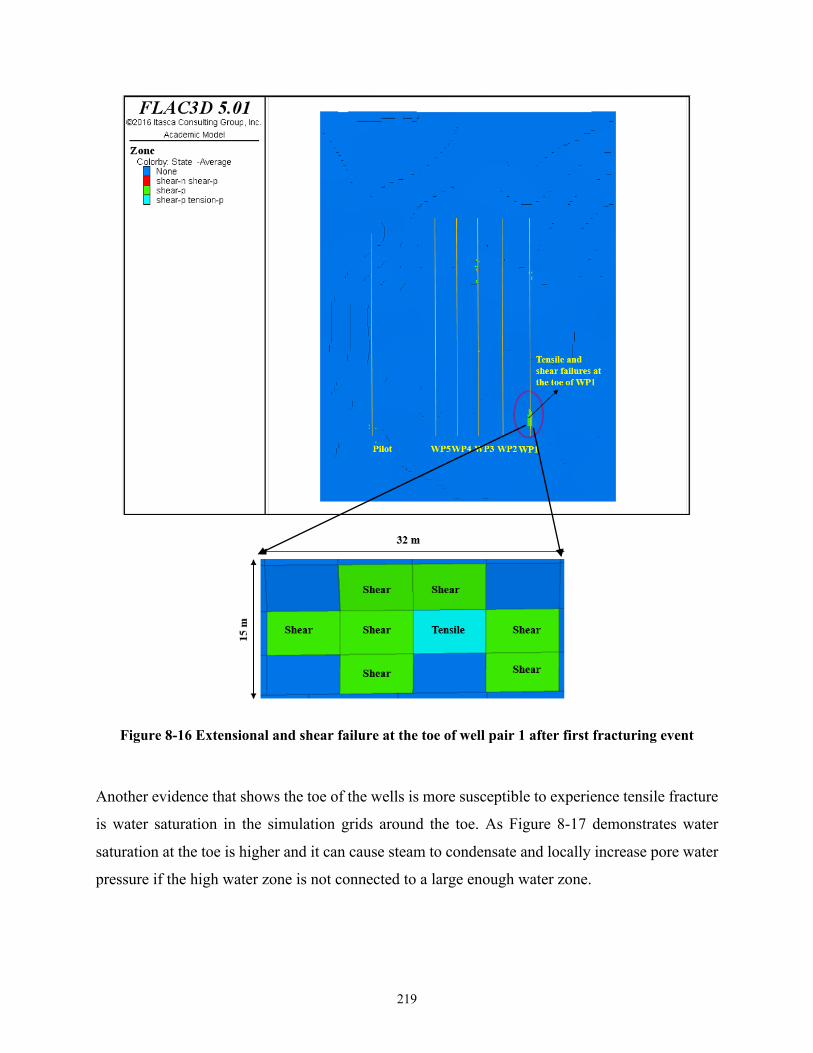
219

Figure 8-16 Extensional and shear failure at the toe of well pair 1 after first fracturing event

Another evidence that shows the toe of the wells is more susceptible to experience tensile fracture

is water saturation in the simulation grids around the toe. As Figure 8-17 demonstrates water

saturation at the toe is higher and it can cause steam to condensate and locally increase pore water

pressure if the high water zone is not connected to a large enough water zone.

220

Figure 8-17 High water saturation at the toe of the injector in well pair 1

Propagation of the Fractures

The tensile and shear fractures are initiated at the toe of well pair 1 within the reservoir Formation.

The steam is also injected at about triple amount of injection rate compared to the situation prior

to the fracturing event on April 12th. As confirmed, bitumen is cold and immobile in the oil sands

within the pay zone and the steam may have a very little leak off into the adjacent reservoir in a

short time. Therefore, the fracture propagates and grows rapidly in a direction in which the

resistivity is the least (TEPCL 2007)

The mini frac test indicates that the stress regime is reverse and the minimum principal stress

should be vertical which is in agreement with other projects in the shallow area in Northern Alberta

oil sands. Then, the fracture will propagate perpendicular to the minimum effective stress which

is vertical. Therefore, the fracture will grow horizontally in the pay zone. Steam is continuously

injected through the injector and causes a reduction in effective vertical stress. Consequently, the

fracture will propagate horizontally towards the heel of the well along the well pair direction in

which the resistance is the least with minimum effective vertical stresses, compared to other

directions. This is demonstrated by the results obtained from coupled reservoir geomechanical

221

simulation. FLAC 3D results show that the minimum effective stress is vertical and along the well

pair 1, as one can see in Figure 8-18.

Figure 8-18 Vertical effective stress along the well pair 1

It should be noted that the compressive stresses in FLAC3D are negative; therefore, the maximum

principal stress is the minimum principal stress in reality.

In addition, to better understand the direction of fracture propagation, the volumetric strain change

has also been investigated along well pair 1 over time. As Figure 8-19 illustrates, volumetric strain

increment is initiated from the toe of the well pair and propagates towards the heel of the well in

which the vertical abandoned well is located, as shown in the following figure.

222

Figure 8-19 Total strain increment along well pair 1 before (top), at (middle) and after (bottom) first fracturing event on April 12th

Abandoned Well (AB/09-33-095) and Observation Well (100/09-33-095) Near the Heel of Well pair 1

An abandoned well, AB/09-33, with a nearby observation well, 100/09-33 are located in the crater

at the surface and both are less than 20 meters away from the injector in well pair 1 subsurface

(TEPCL 2007). These two vertical wells are shown in Figure 8-20.

223

Figure 8-20 Abandoned and observation wells located in the disturbed zone

TEPCL declares that there is no CBL for these wells. Accordingly, the cement job's quality

in/around the casing of the wells cannot be verified. No cement return was also reported for the

abandoned well, making it more suspicious to have some gaps in the cement.

More Critical Situation above Well Pair 3 Compared to Well pair 1

All the observations from the field and the numerical modeling results show that the situation is

much more critical to experience a failure above well pair 3 compared to well pair 1 in which the

224

steam released to the surface. More pieces of evidence to prove this hypothesis is provided as

follows.

Temperature profiles obtained from the calibrated coupled simulation platform in CMG within the

reservoir are shown in Figure 8-21 at day 747, one day before steam release. As one can see, it

shows that at the heel of well pair 3 the temperature front is much stronger than the temperature

profile at the heel of well pair 1 in which the disturbed zone was created due to the blow-out

incident.

Figure 8-21 Temperature profile along well pairs one day before steam release at day 747

225

The pressure front above the injectors shows the same behavior and as it is demonstrated in Figure

8-22, pressure at the heel of well pair 3 is much higher, about double, than the pressure at the heel

of well pair 1 on May 17th, 2006, the day before caprock failure.

Figure 8-22 Pressure front along well pairs one day before steam release at day 747

A seismic survey was done by TEPCL in 2007 after the blow-out across the interested area and

the results are provided in Table 8-1. Although well pair 1 and 3 started simultaneously with

similar injection pressures, the maximum temperature in well pair 3 is 4 times higher than the

226

maximum temperature at the well pair 1 after about 5 months from the beginning of the SAGD

operation in Pad 204.

Table 8-1 Well status in January 2007, seven months after steam release [TEPCL, 2007]

Well pair

ID

Well pair

Status

Wellbore

Downhole

Pressure

Wellbore

Downhole max

Temperature

History

Max Pressure

Regime

Applied

Well pair 1 Shut 200-400 kPag 10 ˚C

3.5 months Circulation,

1.5 months Semi-SAGD,

Steam Release

1800 kPag

Well pair 2 Shut 200-400 kPag 20 ˚C 3 months Circulation 1775 kPag

Well pair 3 Shut 350 kPag 40 ˚C 3.5 months Circulation,

1.5 months Semi-SAGD 1800 kPag

Well pair 4 SAGD mode 1100 kPag 190 ˚C 6 months Circulation,

3 months SAGD 1775 kPag

Shear failures in the geomechanical model are investigated after calibration of the coupled

reservoir geomechanical simulation and the obtained results associated with the failure status

above the well pairs are illustrated in Figure 8-23. Again, after 747 days from the beginning of the

project, one can clearly see that the local failures in the model are noticeably more above well pair

3 compared to well pair 1.

227

Figure 8-23 Status of failures at above the well pairs one day before steam release at day 747 obtained from FLAC3D

Another inspected indicator is the amount of induced plastic shear strain along well pair 1 and 3.

Figure 8-24 verifies higher plastic shear strain at the heel of well pair 3 compared to well pair 1.

228

Figure 8-24 Stress induced plastic shear strain one day before steam release along well pair 3 (top) and well pair 1 (bottom)

Interestingly, the seismic study performed by TEPCL after the steam release observed anomalies

above both well pair 1 and 3. These anomalies that are illustrated in Figure 8-25 could be the gas

zones. Consequently, the situation above both well pairs with respect to the gas zone is the same.

229

Figure 8-25 Observed anomalies above well pair 1 and 3 from seismic survey obtained from TEPCL

All provided evidence confirms that the heel of well pair 3 has more potential to experience failure

than the heel of well pair 1 in which the disturbed zone is located. However, the blow-out occurred

at the top of well pair 1 above the heel. The only difference between the heel of well pair 1 and 3

is the existence of the abandoned well AB/09-33-095 close to well pair 1. This abandoned well

has no CBL file and the lack of cement return to surface was also reported for the well.

Consequently, the hypothesis regarding the contribution of the vertical wellbore to the steam

release becomes very likely, although more investigations are needed to prove the hypothesis. The

following sections will provide more supporting materials to understand the mechanism of the

failure better.

The coupling reservoir geomechanical simulation results show that even in the lack of abandoned

well contribution to the steam release, the shear failure occurs in the Upper McMurray at the

middle of well pair 1. As Figure 8-26 clarifies, the only spot that shows shear failure at the base of

Wabiskaw in the depth of 44 meters on the day before the steam release is at the middle of the well

230

pair 1, not at the heel where caprock failure happened on May 18th 2006. This observation then

fortifies the hypothesis of vertical well’s role in the caprock failure.

Figure 8-26 Shear failures in Upper McMurray at the middle of well pair 1 one day before steam release

The plastic shear strains were also studied in the FLAC3D model for various depths for all the

wells located in the area of interest. The extracted results in Figure 8-27 show that on May 17th

2006, one day before failure, the highest value of plastic shear strain is taking place above injectors.

By decreasing depth, plastic shear strain decreases and the only observed plastic shear strain

231

happening in the Upper McMurray is at the middle of well pair 1, as highlighted in the figure

below. Relatively, the plastic shear strain zone above the pay zone is very hard to see while, it will

grow in the pay zone at the depth of 77 meter.

Figure 8-27 Plastic shear strain profile at different depths along the well pairs one day before steam release

Both TEPCL and AER concluded that the blow-out was related to an excessively high bottomhole

pressure of about 1800 kPag experienced during semi-SAGD phase at well pair 1 while the

injection and production data shows that well pair 3 has also experienced an excessively high

bottomhole pressure, shown in Figure 8-28. As mentioned before, the injector well in well pair 3

experienced 1783 kPag as maximum BHP on April 20, 2006 after 138 days from the start of the

operation during semi-SAGD phase, while in the injector of well pair 1, the maximum BHP was

1769 kPag, even less than well pair 3, on April 9, 2020 only after 129 days from the start of the

well pair operation during semi-SAGD phase.

232

Figure 8-28 Injection pressure and rate during Circulation and Semi-SAGD phases in well pair 3 prior to steam release, 1, 2, and 3 indicate the events in which the rate of pressure

rises while the injection pressure drops.

Besides excessive BHP that was practiced in well pair 3, as the above graph shows, the pressure

drops and steam rate increases suddenly on January 16th, April 20th, and May 5th, which can be the

reason for the local failures.

However it was shown that the geology around well pair 3 has more failure potential in comparison

with well pair 1 and another critical difference between well pair 1 and 3 is the existence of two

vertical wells close to the injector in well pair 1.

Shearing in the Casing of AB/09-33-095 at the Depth of 75 m

As AER indicated, the abandoned well AB/09-33-095 is more likely the one that transferred fluid

from the pay zone to the gas sand zone since the observation well 100/09-33-095 is less damaged.

The tensile fracture occurred at the toe is propagating horizontally along the well pair 1 (Figure

8-18) until it hits the vertical abandoned well.

233

The pressure at that time is about 1550 kPag and with respect to the gradient of fracture pressure

which is 21 kPa/m, it can shear the wellbore at the depth of 75 meters which is compatible with

the scenario.

On April 21st, the pressure dropped for the second time and steam injection rate increased. It shows

another fracturing event that is believed to have occurred around the abandoned well AB/09-33-

095.

Due to the lack of trajectory data of the abandoned well, the actual well is not explicitly modeled

in the simulation but one of the grids which is approximately located at the abandoned well was

selected, as shown as a blue triangle in Figure 8-32) to investigate x and z displacements and the

effective principal stress over time. The results achieved from the coupling platform show that

vertical displacements overtime at that zone is increasing due to the pressure caused by continuous

steam injection. The vertical displacement suddenly drops on April 21st when the abandoned well

is experiencing a failure. Simultaneously, the horizontal displacement increases in the mentioned

zone and implies that a shear failure may happen on the wall of abandoned well AB/09-33-095.

Figure 8-29 and Figure 8-30 show these phenomena, respectively.

Figure 8-29 Vertical displacement for the grid on abandoned well during SAGD process

234

Figure 8-30 Horizontal displacement for the grid on abandoned well during SAGD process

On the other side, total and effective minimum principal stresses, and pore pressure at the grid are

investigated. The graph in Figure 8-31 demonstrates that at day 731, the effective stress suddenly

drops, which may indicate a shear failure is happening as the result of pore pressure increase at

that grid on well AB/09-33-095.

Figure 8-31 Stress change for the grid on abandoned well during SAGD process

235

Another grid, shown as a green triangle between well pair 2 and 3, was selected to verify the

vertical displacement only drops around the abandoned well at day 731 within the pay zone. As

Figure 8-32 compares, the vertical displacement is continuously increasing even at day 731 while

this trend is changed for the grid located on the abandoned well and the z-displacement is dropped

suddenly at day 731.

Figure 8-32 Vertical displacement for a grid on the abandoned well (right) and another grid far from abandoned well (left) during SAGD operation

Conduit around/in the Abandoned Well AB-09-33-095

After cementing the abandoned/observation wells, an acoustic log will typically be run into the

well to evaluate the cement bond's quality and integrity. This Cement Bond Log (CBL) is a

necessary tool to verify the quality of cement job and avoid the destructive consequences of doing

a poor cement job. The lack of a proper cement situation between the casing wall and the Formation

for the observation wells combined with poor cement job in the casing of the abandoned well may

have negative consequences such as occurring shear bond around the casing, moving fluid through

the gaps in the cement and connecting producing zone to water-bearing zone.

236

In the cement job process, the injected cement through the middle of the well will fill up the gap

around the casing and the Formation and then return to the surface when all the space is filled with

cement. At this stage, CBL is operated in the well and the top of cement is recognized and tagged.

On the other hand, if the cement does not return to the surface, one can suspect a thief zone around

the well which does not allow filling up all the gaps around the well. Under these circumstances,

the existence of a conduit and gaps in the cement is possible.

Unfortunately, as TEPCL states, there is no CBL for both the abandoned and observation wells

located less than 20 meters away from the injector in well pair 1. No return of cement has also

been reported for the abandoned well AB/09-33-095. Consequently, there is no certainty about a

good quality cement job in/around the abandoned well AB/09-33-095. Due to the lack of CBL, the

probability of an existing conduit or pathway in the cement around or inside the vertical abandoned

well for upward steam to movement is highly conceivable.

The vertical well's diameter is typically 250 mm, the casing diameter is usually 177.8 mm, and

therefore the annulus which is supposed to be filled up with cement is about 70-100 mm. In the

case of conduit existence in the cement, a considerable amount of fluid could transfer through the

poor cement.

In my opinion, it is doubtful for steam to move from the injector towards Upper

McMurray/Wabiskaw C, which is about 40 meters above the injector, through the reservoir in such

a short time, only 2 months after circulation, concerning the reverse stress regime that causes

horizontal propagation of the fractures.

Consequently, based on the abovementioned reasons, the most likely pathway to transfer steam

from the injector to the gas zone located within the Upper McMurray/Wabiskaw is through the

gaps or conduits in the poor cement job around/in the abandoned well of AB/09-33-095.

Connection of AB/09-33-095 to the Surrounding Gas Zone

The porosity logs are available for abandoned well AB/09-33. The density porosity log, which is

the solid black line, measures the bulk density of the Formation, and the neutron porosity log,

shown in the dashed red line, measures the hydrogen content. The areas in which the dashed red

line is on the right side of the solid back line indicate gas sand. As one can see in Figure 8-33, it

237

shows that this abandoned well goes through a gas zone at the Upper McMurray/Wabiskaw, which

supports this hypothesis that the injected fluid, migrating in gaps or conduits around the well

AB/09-33-095 can be easily connected into the gas zone if the pressure is high enough to overcome

the resisting stresses.

Figure 8-33 Gas zones in Upper McMurray around abandoned well AB/09-33-095

The connection of pore fluid from the pay zone through the vertical well to the gas zone at the

depth of 50 meters can open a new window to the steam release incident's failure mechanism.

As shown in Figure 8-34, bottomhole pressure dropped from 1650 to 1520 kPag, and steam rate

raised on April 24th, 2006, showing a connection between the vertical well and the surrounding

gas zone.

238

Figure 8-34 Injection pressure and rate in well pair 1 prior to steam release

Unexpected Steam Migration from the Pilot and Other Wells to the Gas Zone Located at the Top of Well pair 1 in Upper McMurray

TEPCL did comprehensive work on defining facies for the simulation grids and geological

stratigraphy in the model with respect to a variety of gamma ray values and other available data as

well as geo-statistics analysis. They defined 17 facies for the geological model generated in Petrel

with different portions of clay, silt, mud, and sand.

Besides my analysis on Joslyn steam release, I performed an investigation regarding the facies and

categorized the material around the heel, middle and toe of the well pairs in pads 101 and 204 to

better understand facies distribution from the west side to the east side of the interested area. Three

cross sections were taken from these three parts of the wells, as shown in Figure 8-35. The red

color in the model shows the tidal channel with very high permeability compared to the other

facies. The figure also demonstrates, the facies are homogenous close to the heel of well pairs

while more heterogeneity is observed at the middle and toe of the wells in the geological model.

The first cross section shows the consistent and reasonably homogenous high-permeability

pathway from the pilot towards the heel of well pair 1 in which the steam release occurred. Indeed,

this path is suspicious for the migration of fluid, into which steam was injected about two years,

from the pilot in the west side towards the gas zones located at the Upper McMurray in the east

239

side. It could be an unexpected pathway for the migration of fluid within the reservoir and needs

to be investigated in more detail.

Figure 8-35 Cross sections of facies distribution at the heel (top), middle and toe (bottom) of the well pairs

Figure 8-36 also shows the high-permeability pathway from the pilot to well pair 1 in a plan view.

240

Figure 8-36 Plan view of facies distribution showing the high permeability pathway for steam migration from the west side to the east side

The horizontal permeability was also investigated in the cross section close to the crater in Figure

8-37. It also confirms a pathway with high permeability, about 6000 mD, which is capable to

transfer escaped fluid from pilot towards well pair 1 and the associated gas zone in Upper

McMurray.

241

Figure 8-37 Horizontal permeability profile along the fluid migration high permeability pathway

The calibrated coupled reservoir geomechanical simulation results provide an opportunity to

explore how pore pressures develop within this high-permeability pathway. Six zones above the

well pairs located in the pay zone, as shown in Figure 8-38, were selected to asses how pore

pressures changed over the SAGD operational period.

242

Figure 8-38 Selected zones above well pairs at the crater plane to explore the highway

The value of pressure for each zone was extracted from FLAC3D. The graphs are drawn in Figure

8-39, and as one can see, the results remarkably demonstrate that although the pressure profiles in

the zones are different, a similar trend of changing pressure among these zones is followed. On

day 748, in which steam released to the surface and caprock failed, injectors 1 and 2 were shut-in.

As one can see, the pressure drop does not happen only for these two wells. All the zones above

the wells experience the pressure drop on that day which indicates that they are somehow

connected in the selected zones.

243

Figure 8-39 Pressure change during SAGD operation for the selected zones above the injectors at the crater plane

Another six zones located in different depths were chosen to better understand the behavior at the

top of Middle McMurray Formation. The same procedure was taken, and as shown in Figure 8-40,

the trend of changing pore pressure in the zones follows each other. It indicates the connection

among the zones in this area is maintained.

244

Figure 8-40 Pressure change during SAGD operation for the selected zones at the top of Middle McMurray at the crater plane

Figure 8-41 illustrates that this trend is also observed in Upper McMurray in which gas sand zones

are presented. Therefore, in the Upper McMurray, the pressure change trend in one zone is like the

others and the zones are still connected.

245

Figure 8-41 Pressure change during SAGD operation for the selected zones in Upper McMurray at the crater plane

Finally, the zones were selected in the Wabiskaw layer to realize how the pore pressure reacts over

time. The graphs are available in Figure 8-42 and it interestingly shows that the pressure during

SAGD operation remains unchanged for all the zones. This behavior indicates that the zones are

not connected anymore within the Wabiskaw members.

246

Figure 8-42 Pressure change during SAGD operation for the selected zones in Wabiskaw members at the crater plane

Different graphs for different zones located at different depths from the pay zone to Wabiskaw

imply that steam and hot water can be unpredictably migrated from the west side close to the pilot

well pair to the east side nearby the disturbed zone. It should be noted that the pilot well pair was

under thermal operation for about two years prior to steam release incident above well pair 1.

Three observation wells were available close to the heel, middle, and toe of the pilot during SAGD

operation. Fortunately, all the wells were equipped with thermocouples and temperatures in

different depths were recorded over time. A study was done by Aghabarati (2017) to investigate

the heat transfer by convection and conduction in the formations based on temperature

observations during SAGD process versus the distance from a hot interface. The investigation is

summarized in Figure 8-43, showing how the temperature may change after a certain time in

convection and conduction phenomena based on the thermal diffusivity of the Formation and the

fluid velocity.

247

Figure 8-43 Heat transfer by convection and conduction in the Formation (Aghabarati 2007)

248

The circulation phase of the pilot well pair was launched on May 4th, 2004. The presented graphs

in Figure 8-44 show the temperature profiles for observation well 102/06-33-095 located close to

the middle of the pilot well pair. The injector is at the depth of 85 meters and the producer’s depth

is 90 meters, showing in solid orange and green horizontal lines, respectively. Temperature profiles

were drawn in 2004, 2005, 2007, and 2008 for different depths. The light blue line shows the

temperature change on May 15th, 2007. It indicates that the temperature is 16 centigrade degrees

at the depth of 60 meters, about 25 meters away from the hot interface. The same depth is selected

in the dark blue solid line showing the temperature profile on September 18th, 2007. It illustrates

that the temperature has increased to 38 centigrade degrees after only four months. Referring to

Figure 8-43, this substantial change in temperature during this short amount of time is probably

due to convection within the reservoir and the existence of pore fluid movement around the

observation well.

The purple line showing the temperature profile on January 15th, 2008 indicates that the pressure

was dropped in 2008 and the conduction appeared within the reservoir.

Figure 8-44 Temperature profile in observation well 102/06-33-095 over time

249

Available temperature data in observation well 103/06-33-095 located close to the heel of the well

pair is presented in Figure 8-45 for the depth of 50 meters. The temperature on September 27th,

2007 is about 11 degrees, while on June 26th, 2008 the temperature has increased to 28 degrees.

17 degrees change in temperature during 9 months can not occur due to a conduction only

mechanism. This observation well also implies that a hot fluid is transferring energy close to the

well.


The temperature profiles for the observation well 100/03-33-095 located near the toe of the pilot

wells are also analyzed. The data in Figure 8-46 shows that from August 2004 to January 2008,

the temperature at the depth of 60 meters only changed about 6 centigrade degrees. After about

four years, this small change in temperature indicates that conduction was the main heat transfer

at the toe of the pilot.

250


The results are in very good agreement with the proposed high permeability pathway for migration

of fluid during SAGD operation in Joslyn Creek.

As a result, the existence of a high permeable fluid conduit that causes unanticipated migration of

injected steam during SAGD operation from the pilot and other well pairs towards the gas zone

located in Upper McMurray above well pairs 1 and 3 is recognized. The subsequent evidence to

prove this scenario analyzes the pressure profile in CMG-STARS as the flow simulator in the

coupled reservoir geomechanical simulation. Figure 8-47 shows the pressure change over a cross

section passing across the crater created by the steam release incident. P1 to P6 are the grids chosen

on the proposed high permeability pathway from the gas zone close to abandoned well AB/09-33-

095 towards the top of the pay zone close to the pilot wells. P7 is selected close to the injector

where it is not on the high permeability pathway of steam migration.

251

Figure 8-47 Selected grids within the reservoir to explore the steam migration high permeability pathway

Figure 8-48 presents the pressure change over time for all the grid points in the above figure. As

one can see, the trend of pressure behavior is the same from p1 to p6, which are located on the

steam migration pathway. Interestingly, the dashed brown line shows the different behavior for

p7, which is not on the proposed high permeability pathway.

252

Figure 8-48 Pressure change for the selected grids during SAGD project

Shear Fracture above Pressurized Zone Using Geomechanical 3DEC Code

After the beginning of the Joslyn SAGD project on May 4th 2004 by operating the pilot well pair,

some fluid was unexpectedly migrating from west side close to the pilot well pair towards east

side close to Well pair 1. The fluid was accumulating in the gas zones located in Upper McMurray.

The gas zones and particularly the one above well pair 1 were pressurized during 748 days since

the start of the project. It was proved in the above sections that before the steam release happened,

the injector in well pair 1 was connected to the gas zone and steam was injecting under about 1400

kPag.

The base of Wabiskaw layer is at the depth of 44 meters, in which the fracture pressure is about

880 kPa by the assumption of a 20 kPa/m gradient for the minimum principal stress. Therefore, a

tensile or shear failure was expected to initiate at the pressurized zone at the base of Wabiskaw by

applying 1400 kPa. This fracture will propagate towards the surface and as soon as hitting the

253

ground surface, the pressure will suddenly drop in the gas zone and cause a flashback of the hot

fluid pooled there over time. The flashback of hot water to the steam needs an enormous volume

while there is not enough volume to handle it except by pushing the Formation up to the surface

which causes an explosive nature of the failure.

A geomechanical model was created utilizing 3DEC, retrieved from Chapters 5 and 6, to illustrate

the failure propagation towards the surface and determine caprock's behavior under the injection

pressure just before the steam release incident.

The geomechanical model's size is 500m × 500m × 44m, as shown in Figure 8-49. The load,

simulating the underlying SAGD steam chamber, was applied to a center region of 90 m x 90 m

at the base of the Wabiskaw layer, as shown in the following figure.

Figure 8-49 Central load to imitate SAGD steam chamber, exerted at the base of the model.

Three scenarios were investigated regarding intact/fractured caprock and elastic/M-C elastoplastic

constitutive models for the Quaternary deposits.

• Continuum caprock and Elastic Constitutive Model for the Quaternary Deposits

For the first case, it was assumed that the constitutive model for the Quaternary deposits is elastic

so that the fractures initiating from the base of caprock propagates upward to hit the base of

Quaternary. The Wabiskaw members and Clearwater Formation are intact and M-C elastoplastic

254

constitutive model is assigned for these layers. The mechanical properties applied for this scenario

are summarized in Table 8-2.

Figure 8-50 demonstrates the state of failures through the caprock under 1400 kPa pressure applied

prior to the steam release.

Figure 8-50 Failure status through the continuum caprock under 1400 kPa pressure

• Fractured caprock and Elastic Constitutive Model for the Quaternary Deposits

For the second case, all properties are kept the same except applying a fracture density of 0.005 in

the caprock as a discrete fracture network which includes about 370 joints in the form of two

perpendicular sets with a variety of persistency from 10 to 50 meters as shown in Figure 8-51.

Figure 8-51 Two sets of joints generated in the fractured caprock

255

The assumed mechanical properties of the joints are presented in Table 8-3. Accordingly, Figure

8-52 illustrates the caprock's failure modes when the caprock is fractured under 1400 kPa as the

steam injection pressure.

Figure 8-52 Failure status through the fractured caprock under 1400 kPa pressure

• Continuum caprock and M-C Elasto-plastic Constitutive Model for the Quaternary Deposits

For the last case, a Mohr-Coulomb elastoplastic model was assigned to the Quaternary deposit so

that this layer can be failed under a sufficient pressure. Therefore, the fracture can grow and reach

the surface, as shown in Figure 8-53.

Figure 8-53 Failure status through the continuum caprock and overburden under 1400 kPa pressure

A summary of input data for intact rock and joints for the base model is provided in Table 8-2 and

Table 8-3, respectively.

256

Table 8-2 Constitutive models and associated mechanical properties for the zones

Scenario Formation Constitutive model

Young’s modulus (MPa)

Poisson

ratio Friction Cohesion

(kPa) Tensile (kPa) Dilation

Case 1

Quaternary Elastic 200 0.3 NA NA NA NA

Wabiskaw and Clearwater

M-C elasto plastic 100 0.3 35 240 200 10

Case 3 Quaternary M-C elasto

plastic 200 0.3 35 100 50 15

Wabiskaw and caprock

M-C elasto plastic 100 0.3 35 240 200 10

Table 8-3 Mechanical properties for the joints used in the model Normal stiffness (kPa/m) 4.50E+05

Shear stiffness (kPa/m) 0.1× joint normal stiffness

Friction angle (°) 20

Cohesion (kPa) 100

Tensile strength (kPa) 100

Summary

To summarize the main points in the above sections, Table 8-4 recaps all the events around well

pair 1 during SAGD operation since April 12th 2006. As mentioned before, the pressure suddenly

dropped about 200 kPa from 1760 to 1560 kPa on April 12th combined with increasing steam

injection rate from 75 to 135 m3/day. This was not a regular pressure drop and caused a tensile

failure at the toe of well pair 1, mentioned in Figure 8-54 as event 1.

The fracture propagated horizontally due to the reverse stress regime and developed along well

pair 1 in which the minimum vertical effective stress is experienced. After about 9 days, on April

21st, another pressure drop occurred which, I believe, was a shear failure around evaluation well

AB/09-33-095 located near the heel of well pair 1 where the crater was created on the surface.

This event is known as event 2.

Then, the steam was continuously injected through the gaps and conduit in/around the abandoned

well, and on April 24th, pressure dropped again from 1650 to 1520 kPa combined with an

257

increasing steam injection rate from 170 to 190 m3/day. This event shows a minor fracture to

connect the abandoned well to the surrounding gas zone located in Upper McMurray. This event

is known as event 3.

The pressure increased with a constant injection rate showing steam injection into the gas zone

and is shown in Figure 8-54 as event 4.

Finally, on April 25th, a significant drop in pressure occurred while the injection rate remained

constant. This behavior indicates that a fracture was initiated in the pressurized zone at the base of

Wabiskaw and propagated towards the surface. It was followed by shut in the well for one week

to install the pump. After pump installation, the well pair was under SAGD operation but the

pressure could not exceed 1300 kPa, where the propagation of fracture heading towards the surface

was initiated. This is the 5th event prior to the blow-out event on May 18th 2006.

Table 8-4 Summary of chorological events led to steam release incident in Joslyn SAGD project

Date Pressure change

Range (Pressure) Rate Range

(Rate) Event

12-13 April Drop 1760-1560 increase 75-135 tensile fracture at the toe (1)

21-22 April Drop 1560-1320 increase 160-190 a shear failure around abandoned well(2)

22-24 April Increase 1320-1650 constant injecting steam to the wellbore

24-24.5 April Drop 1650-1520 increase 170-190 a small fracturing event connecting the well to the gas zone(3)

24.5-25.5 April Increase 1520-1680 constant injecting to gas zone(4)

25.5-27 April Drop 1680-1300 constant propagating the fracture from Clearwater to surface(5)

258

Figure 8-54 Injection pressure and rate during Circulation and Semi-SAGD phases in well pair 1 prior to steam release

259

SUMMARY, CONCLUSIONS AND RECOMMENDATIONS FOR FUTURE

RESEARCH

Summary

SAGD is a very complex operation which has been utilized in Alberta to produce bitumen from

sub-surface oil sands. During this process, high pressure and temperature steam is injected into the

reservoir and bitumen/condensed water are produced from horizontal well pairs. Elevated

temperatures are required to reduce the viscosity of the heavy oil and enable it to flow under gravity

toward the producing well. Pressure and temperature inside and around a growing steam chamber

are continuously changing, resulting in the interaction of geomechanics and multiphase flow in oil

sands. Stress-induced deformations within the reservoir, overburden and underburden will result

in changes of porosity, absolute and relative permeability as well as surface heave. Pore pressure

increase causes a reduction in mean effective stress and results in unloading sand grains and

reservoir matrix. In the case of the shallow Joslyn SAGD project, where the initial stress state is a

reverse faulting regime, these effective stress changes may cause shear failure within the reservoir.

Furthermore, temperature increase causes thermal expansion of sand grains, reservoir matrix and

pore fluid results in horizontal stress increase. The combination of pressure and temperature effects

creates a net change in the porosity and permeability of affected zones. Consequently,

geomechanics is interactively coupled with the multiphase thermal flow and cannot be accounted

for as a simple constant/variable compressibility parameter in conventional reservoir simulators.

260

To capture the complex interaction of geomechanics and fluid flow in the McMurray oil sands

(production/injection processes) and overburden formations (caprock integrity) requires reservoir

geomechanical simulations.

In this research, a sequentially coupled reservoir geomechanical platform developed internally in

Reservoir Geomechanics Research Group (RGRG) at the University of Alberta was employed to

achieve this purpose. A 3D, field scale simulation model for the Joslyn SAGD project was

developed that included all the initial project well pairs, their detailed production/injection history

and the geological heterogeneity existing in the field.

The McMurray Formation oil sands are also known for their complex geological features and the

resulting heterogeneity within the reservoir due to these features will cause inconsistent steam

chambers over the area resulting in non-uniform porosity and permeability changes. In this study,

care was taken to realistically model the reservoir's heterogeneity in order to include any potential

influence on the steam release mechanisms. Selection of appropriate constitutive models for each

major facies within the simulation model was completed using existing knowledge from the

literature and internal UAlberta experimental studies. For field scale models, this still remains a

challenge given the challenges of upscaling between laboratory scale tests and field scale grid sizes

in the model.

A unique component of this study was the opportunity to perform model calibration studies on the

field behaviour using significant reservoir surveillance data captured post steam release for the

project area likely unaffected by the release event. The calibration process allowed constitutive

models to be adjusted to match the field monitored data and then (re)apply the model to simulations

from initiation of the project through to the time of the steam release event.

Figure 9-1 demonstrates the workflow used in this research to inspect the behavior of formations

and assess potential reservoir geomechanical processes that may have contributed to the steam

release at the Joslyn SAGD project.

261

Figure 9-1 Generalized and integrated workflow for analysis of Joslyn steam release

An additional complicating factor in the study of reservoir geomechanical mechanisms is the

potential existence of pre-existing fractures (discontinuities) with the caprock and their influence

on the deformation response of the caprock. Separate sensitivity studies were completed using a

discrete element modelling approach to better understand how the presence of discontinuities in

the caprock could possibly contribute to the mechanisms leading to the steam release event. The

results from these studies showed that the existence of fractures in the caprock altered vertical

displacements at the base of caprock, surface heave, normal and shear joint displacements, and

failure modes compared to the caprock with no discontinuities. Furthermore, the influence of fluid

flow in the model was also inspected and the contribution to the results was provided in this study.

Figure 9-2 illustrates the workflow for analyzing the existence of discontinuities in the caprock.

262

Figure 9-2 Workflow for analysis of discontinuities within the caprock

Conclusions

Based on this research, many lines of evidence were provided in Chapter 8 that characterized a

sequence of events within the Joslyn SAGD project that likely contributed to the steam release

event. In their assessment reports, both TEPCL and AER stated that the excessive bottomhole

pressure applied in well pair 1 was the main cause of the failure. Based on the results of this

research, it is not evident that the operating bottomhole pressure of approximately 1800 kPag,

while definitely providing the energy necessary to propagate the steam release process, was in and

of itself, the primary cause of the initiation of the caprock failure.

Firstly, as summarized in Table 9-1, all the well pairs at the time of the release were operating at

pressures similar to well pair 1 and all were above the approval MOP of 1700 kPag. As noted in

Table 9-1, it was actually well pair 3 that was operating at the highest bottomhole pressure at the

time of the steam release. Consequently, if excessive bottom hole pressure was a primary driver

for steam release, well pair 3, based on its pressure history, should have featured more prominently

as a pathway for steam release – it did not.

263

Table 9-1 Maximum bottomhole pressure applied in well pairs in pad 204 Injector Date Max bottomhole pressure (kPag) Phase

Well pair 1 9-Apr-06 1769 Semi-SAGD

Well pair 2 6-May-06 1760 Semi-SAGD

Well pair 3 20-Apr-06 1783 Semi-SAGD



As discussed, and summarized in Chapter 8, this research explored multiple aspects of the Joslyn

SAGD project to elucidate what other possible reasons/mechanisms, beyond excessive bottomhole

pressures, may have contributed to the steam release. Based on the research outcomes, it is

postulated that one of the primary factors leading to the steam release was an undetected migration

of pore pressures within the upper McMurray Formation from the pilot project area to the region

overlying well pair 1. These elevated pore pressures, which lead to lower effective stresses, would

have created a region of lower shear strength and consequently, reduced resistance to the loads

imposed during the SAGD startup phases in well pair 1. Coincident with this was evidence of

lower quality (less clay) caprock along the eastern side of the project area, in the region of well

pair 1, in comparison to the western side (pilot project) of the project area and the presence of a

gas zone within the Upper McMurray/Wabiskaw units above well pair 1 that was likely pressurized

from the pore pressure migration from the pilot project area.

It is also postulated that existence of the abandoned wellbore and its proximity to the well pair 1

location provided a pathway for pressure and fluid communication vertically from the reservoir

towards the gas zone and caprock. While the borehole was not modelled explicitly, the reservoir

geomechanical simulations did provide evidence of anomalous deformation response immediately

prior to the steam release event within the region of the model coincident with the abandoned well

location.

As a result of the steam release event and the common perception that the main cause of failure

was an excessive bottomhole pressure, the AER derived a new directive (Directive 086) for

shallow SAGD reservoirs in Alberta. This directive provided a revised formulation to calculate

264

MOP, which effectively reduced the allowable MOP to decrease the chance of tensile (extensional)

caprock failure. The new formulation essentially replaced the depth of the injector with the depth

of caprock base and decreased the safety factor from 1.25 to 1.10. (increased margin of safety from

0.8 to 0.9). Although the reduction in MOP definitely contributes to a reduced risk of caprock

failure, reduced operation pressures also result in decreased production and potentially unfavorable

project economics. Based on the lines of evidence established in this research to better define the

mechanisms/processes that lead to the Joslyn steam release event, it is suggested that the Directive

086 MOP formulation be revisited with consideration of adjusting the margin of safety back to the

previous value of 0.9. Given the geological uncertainties that will remain for all projects, it is

suggested that the fracture closure gradient still be computed at the base of caprock. Equation 9-1

defines the new MOP equation.



Recommendations for Future Studies

Recognizing the limitations that are inherent in detailed reservoir geomechanical studies at field

scale, multiple additional studies are recommended to explore the failure mechanism at Joslyn in

more detail. The following summarizes recommendations for future research studies:

• The 3D sequentially coupled reservoir geomechanical simulations conducted in this

research adopted a continuum model for the caprock. As shown by sensitivity studies

completed using a discrete element approach, the presence of discontinuities in the caprock

can influence its behaviour during SAGD. Consequently, it is recommended that advanced

reservoir geomechanics simulations be conducted using discrete fractures within the

caprock.

• Calibrating the lab test results with the field data more accurately. The permeability

distribution, absolute and relative permeabilities for different formations are also the areas

that have wide potential to work on.

• Improving the facies distribution within the geocellular model to better capture the

geological heterogeneities within the model. This would also provide improved

265

distribution of constitutive models that would likely capture more detailed responses within

the reservoir geomechanical simulations.

• Additional experimental studies to refine the constitutive behaviour of Clearwater

Formation lithologies, including a focused effort to understand the hydro-mechanical

properties of fractures (discontinuities) within Clearwater shales.

• Utilizing artificial intelligence (AI) techniques and machine learning in this study and

comparing the results with this study’s outcome is highly recommended since there is about

300 GB data available for the Joslyn project and it could be a very good source for these

new techniques to explore and potentially, predict such incidents.

266

REFERENCES

Alberta Energy Regulator. Oil sands facts and statistics

Alberta Geological Survey, Alberta Oil Sands Map, Feb. 5, 2012,

(http://www.ags.gov.ab.ca/graphics/cbm/oil_sands/alberta_oil_sands_map2.jpg.)

Alaska oil sands, Alberta tar sands (https://alaskaoilsands.wordpress.com/).

Alberta Energy Regulator. (2016). Directive 086 - Reservoir Containment Application Requirements for Steam-Assisted Gravity Drainage Projects in the Shallow Athabasca Oil Sands Area.

Alberta Energy Regulator. (2014). Bulletin 2014-03- Regulatory Approach for Shallow Thermal In Situ Oil Sands Applications in the Wabiskaw-McMurray Deposit of the Athabasca Oil Sands Area.

Alberta Energy Regulator. (1994). Directive 051- Injection and Disposal Wells – Well Classifications, Completions, Logging, and Testing Requirements.

Aghabarati, M. (2017). Reanalyzing Thermocouple Temperature Response for Evidence of Convective Flow. MSc thesis, University of Alberta, Edmonton, Canada.

Butler, R.M., and Stephens, D.J. (1981). The Gravity Drainage of Steam-heated Heavy Oil to Parallel Horizontal Wells. Journal of Canadian Petroleum Technology. 20(2): 90-96.

Butler, R. M., McNab, G. S., and Lo, H. Y. (1981). Theoretical Studies on the Gravity Drainage of Oil during In-Situ Steam Heating. The Canadian Journal of Chemical Engineering, 59, 455–460.

Baghbanan, A., and Jing, L. (2008). Stress Effects on Permeability in Fractured Rock Mass with Correlated Fracture Length and Aperture. International Journal of Rock Mechanics and Mining Science, 45 (8): p.1320–1334.

Baghbanan A. (2008). Scale and Stress Effects on Hydro-Mechanical Properties of Fractured Rock Masses. PhD Dissertation, KTH Royal Institute of Technology, Sweden.

Butler, R.M. (1991). Thermal Recovery of Oil and Bitumen. Publisher: Prentice Hall, ISBN-13: 978-0139149535. 528 p.

Cengel, Y. (2007) Heat & Mass Transfer: A Practical Approach, McGraw-Hill Education (India) Pvt Limited, ISBN: 007063453X, 9780070634534. 879 p.

Carlson, M. (2012). An Analysis of the caprock Failure at Joslyn. SPE-156962-PP.

Carlson, M. (2011). Detailed Consideration of the Proposed Joslyn Failure Mechanism. Canadian Energy Technology & Innovation.

267

Collins, P. M. (2007). Geomechanical Effects on the SAGD Process. Society of Petroleum Engineers. doi: 10.2118/97905-PA.

Collins, P.M. (2002). Injection Pressures for Geomechanical Enhancement of Recovery Process in the Athabasca Oil Sands. SPE 79028-MS presented at SPE International Thermal Operations and Heavy Oil Symposium and International Horizontal Well Technology Conference, 4-7 November, Calgary, Alberta, doi: 10.2118/79028-MS.

Cundall, P.A., and Hart, R.D. (1992). Numerical Modelling of Discontinua, Engineering Computations, 9 (2): 101-113, doi: 10.1108/eb023851.

Chalaturnyk, R.J. 1996. Geomechanics of the Steam-Assisted Gravity Drainage Process in Heavy Oil Reservoirs. PhD Dissertation. University of Alberta, Edmonton, Canada.

Chin, L.Y., Thomas, L.K., Sylte, J.E., and Pierson, R.G. (2002). Iterative Coupled Analysis of Geomechanics and Fluid Flow for Rock Compaction in Reservoir Simulation. Oil & Gas Science and Technology - Rev. IFP, Vol. 57, No.5, pp. 485-497.

Dusseault, M.B. (2013). Screening Criteria and Technology Sequencing for In-situ Viscous Oil Production, Heavy-oil and Oil-sand Petroleum Systems in Alberta and Beyond, Frances J. Hein, Dale Leckie, Steve Larter, John R. Suter AAPG Studies in Geology 64, p. 655–668, doi:10.1306/13371598St643565.

Dusseault, M. B. (1977b). The Goetechnical Characteristics of Athabasca Oil Sands. PhD Dissertation, University of Alberta, Edmonton, Canada.

Dean, R.H. Gai, X. Stone, C.M. and Minkoff, S.E. (2003). A Comparison of Techniques for Coupling Porous Flow and Geomechanics. Proceedings of the SPE Reservoir Simulation Symposium, February 3-5, Houston, Texas.

Deisman, N., Chalaturnyk, R. J., and Ivars, D. M. (2009). An Adaptive Continuum / Discontinuum Coupled Reservoir Geomechanics Simulation Approach for Fractured Reservoirs. SPE-119254-MS, In SPE Reservoir Simulation Symposium. Woodlands, TX.

Espinoza, C. E. (1983). A New Formulation for Numerical Simulation of Compaction, Sensitivity Studies for Steam Injection. Society of Petroleum Engineers. doi:10.2118/12246-MS.

Gutierrez, M., Youn D. J., (2015). Effects of Fracture Distribution and Length Scale on the Equivalent Continuum Elastic Compliance of Fractured Rock Masses. Journal of Rock Mechanics and Geotechnical Engineering, 7 (6): 626-637.

Horsrud, P., SØnstebØ, E.F., and BØe, R. (1998). Mechanical and Petrophysical Properties of North Sea Shales. International Journal of Rock Mechanics and Mining Sciences, 35, No. 8, 1009.(https://doi.org/10.1016/S0148-9062(98)00162-4 )

Hein, F. J., Leckie, D, Larter, S. and Suter J. R. (2012). Joslyn Creek Steam-Assisted Gravity Drainage: Geologic Considerations Related to a Surface Steam Release Incident, Athabasca Oil Sands Area, Northeastern Alberta, Canada. In book: Heavy-oil and Oil-sand Petroleum

268

Systems in Alberta and Beyond Edition: AAPG Studies in Geology 64Chapter: 28. Publisher: American Association of Petroleum Geologists.

Itasca Consulting Group Limited. FLAC3D – Fast Lagrangian Analysis of Continua in 3 Dimensions Version 5.01, User’s Manual. Minneapolis.

Itasca Consulting Group Limited. 3DEC – Distinct Element Modeling of Jointed and Blocky Material in 3 Dimensions Version 5.0, User’s Manual. Minneapolis.

Jing, L., Min, K. B., Baghbanan A. (2009). Stress and Scale-Dependency of the Hydro- Mechanical Properties of Fractured Rock. Rock mechanics new research, NOVA Publisher

Kulatilake, P.H.S.W., Park, J., Um, J., (2004). Estimation of Rock Mass Strength and Deformability in 3-D for a 30 m Cube at a Depth of 485 m at Aspo Hard Rock Laboratory, Geotechnical and Geological Engineering, 22 (313).

Kulatilake, P.H.S.W., Um, J., Wang, M., Escandon, R. F., Narvaiz, J., (2003). Stochastic Fracture Geometry Modeling in 3-D Including Validations for a Part of Arrowhead East Tunnel, California, USA. Engineering Geology, 70 (1-2): 131–155.

Khani, A., Baghbanan, A., Hashemolhosseini, H. (2013). Numerical Investigation of the Effect of Fracture Intensity on Deformability and REV of Fractured Rock Masses. International Journal of Rock Mechanics & Mining Sciences, 63: p.104–112.

Khani, A., Baghbanan, A., Norouzi, S., Hashemolhosseini, H. (2013). Effects of Fracture Geometry and Stress on the Strength of a Fractured Rock Mass, International Journal of Rock Mechanics & Mining Sciences, 60: p.345–352.

Kresse, O. et al. (2013). Numerical Modeling of Hydraulic Fractures Interaction in Complex Naturally Fractured Formations. Rock Mechanics Rock Engineering 46, 555–568. https://doi.org/10.1007/s00603-012-0359-2

Khan, S., Han, H., Ansari, S., and Khosravi, N. (2011). caprock Integrity Analysis in Thermal Operations: An Integrated Geomechanics Approach. World Heavy Oil Congress, Edmonton, AB. WHOC11-609.

Lempp, C., Natau, O., Bayer, U., and Welte, D. H. (1994). The Effect of Temperature on Rock Mechanical Properties and Fracture Mechanisms in Source Rocks-Experimental Results. In Rock Mechanics in Petroleum Engineering. Society of Petroleum Engineers.

Li, P. (2006). Numerical Simulation of the SAGD Process Coupled with Geomechanical Behavior. PhD Dissertation, University of Albert, Edmonton, Canada.

Li, P. and Chalaturnyk, R.J. (2005). Geomechanical Model of Oil Sands. Paper presented at the SPE International Thermal Operations and Heavy Oil Symposium, Calgary, Alberta, Canada. doi: https://doi.org/10.2118/97949-MS

269

Li, P. and Chalaturnyk, R.J. (2009). History Match of the UTF Phase A Project with Coupled Reservoir Geomechanical Simulation. The Journal of Canadian Petroleum Technology. 48 (1): 29–35.

Li, P., and Chalaturnyk, R.J. (2006). Permeability Variations Associated With Shearing and Isotropic Unloading During the SAGD Process. Journal of Canadian Petroleum Technology 45: doi: https://doi.org/10.2118/06-01-05

Lewis, R.W. Majorana, C.E. and Schrefler, B.A. (1986). A Coupled Finite Element Model for the Consolidation of Non-isothermal Elastoplastic Porous Media. Transp Porous Media, doi: 10.1007/BF00714690.

Min, K.B., Jing, L. (2003). Numerical Determination of the Equivalent Elastic Compliance Tensor for Fractured Rock Masses Using the Distinct Element Method. International Journal of Rock Mechanics and Mining Science, 40(6):795–816.

Nagel, N. B., Gil, I., Sanchez-nagel, M., and Damjanac, B. (2011). Simulating Hydraulic Fracturing in Real Fractured Rocks over the Limits of Pseudo3D Models. Society of Petroleum Engineers. doi:10.2118/140480-MS.

Nikiforuk, A. (2013). Next Oil Sands Threat: Cracking caprock.

Oldakowski, K. (1994). Stress Induced Permeability Changes of Athabasca Oil Sands. MSc Thesis, University of Alberta, Edmonton, Canada.

Oldakowski, K., Sawatzky, R. P., and Alvarez, J. M. (2016). Geomechanical Properties of Clearwater Shale at Elevated Temperatures. Society of Petroleum Engineers. doi:10.2118/180694-MS

Rahmati, E. (2016). Numerical Assessment of caprock Integrity in SAGD Operations Considering Mechanical Anisotropic Behavior of Shale Layers. PhD Dissertation, University of Alberta, Edmonton, Canada.

Rahmati, E., Nouri, A., and Fattahpour, V. (2014). caprock Integrity Analysis during a SAGD Operation Using an Anisotropic Elasto-Plastic Model. Paper presented at the SPE Heavy Oil Conference-Canada, Calgary, Alberta, Canada. doi: https://doi.org/10.2118/170114-MS

Reiter, K et al. (2014). A Revised Crustal Stress Orientation Database for Canada. Tectonophysics, Volume 636, Pages 111-124.

Rangriz Shokri, A., Babadagli, T., & Jafari, A. (2016). A Critical Analysis of the Relationship Between Statistical- and Fractal-Fracture-Network Characteristics and Effective Fracture-Network Permeability. Society of Petroleum Engineers. doi: 10.2118/181743-PA

Rangriz Shokri, A., Chalaturnyk, R. J., Bearinger, D., Virues, C., & Lehmann, J. (2017). Constraining the Complexity of Stimulated Reservoir Volume during Multi-Stage Hydraulic Fracturing of Horizontal Wells through Inter-Well Pressure Hit Modeling. Society of Petroleum Engineers, doi:10.2118/187188-MS.

270

Samieh A. and Wong R. (1997). Deformation of Athabasca Oil Sand at Low Effective Stresses under Varying Boundary Conditions. Canadian Geotechnical Journal 34: 985-990.

Settari, A., Walters, D., and Behie, G. (1999). Reservoir Geomechanics: New Approach to Reservoir Engineering Analysis. Proceedings of the Technical Meeting/Petroleum Conference of the South Saskatchewan Section, Regina, Canada.

Scott, J.D., Proskin, S.A. and Adhikary, D.P. (1994). Volume and Permeability Changes Associated with Steam Stimulation in an Oil Sands Reservoir. Journal of Canadian Petroleum Technology, 33(7): 44-52.

Singh, B. (1973). Continuum characterization of jointed rock masses: Part II—Significance of low shear modulus. International Journal of Rock Mechanics and Mining Sciences & Geomechanics Abstracts, 10, 337-349.

Total E&P Canada Ltd., (2007). Summary of Investigations into the Joslyn May 18th 2006, Steam Release.

Touhidi-Baghini A., (1998). Absolute Permeability of McMurray Formation Oil Sands at Low Confining Stresses. PhD Dissertation, University of Alberta, Edmonton, Canada.

Ertekin, T., Abou-Kassem, J., and King, G. (2001). Basic Applied Reservoir Simulation. ISBN: 978-1-55563-089-8.

Tran, D., Settari, A. and Nghiem, L. (2004). New Iterative Coupling between a Reservoir Simulator and a Geomechanics Module. SPE Journal, 9: 362-369.

Uwiera, M., Carlson, M., Walters, D., and Palmgren, C., (2011). Geomechanical Simulation of caprock Performance for A Proposed, Low Pressure, Steam-Assisted Gravity Drainage Pilot Project. Canadian Unconventional Resources Conference, Calgary, Canada.

Yuan, Y., Xu, B., and Palmgren, C. (2013). Design of caprock Integrity in Thermal Stimulation of Shallow Oil-Sands Reservoirs. Society of Petroleum Engineers. doi: 10.2118/149371-PA

Zhao, N. (2012). Integration of Reservoir Simulation and Geomechanics. PhD Dissertation, University of Utah, USA.

Zhang B. (2019). Integrated Reservoir-Geomechanics Upscaling Workflow. PhD Dissertation, University of Alberta, Edmonton, Canada.

Zandi S. (2011). Numerical Modeling of Geomechanical Effects of Steam Injection in SAGD Heavy Oil Recovery. PhD Dissertation, MINES Paris Tech, Centre de Géosciences, Paris, France.

271

Appendix A: SUMMARY OF TEPCL AND

AER REPORTS

A.1 Summary of TEPCL’s Scenarios

On April 12th 2006, four months after the beginning of operations in well pair 1 of pad 204, the

bottomhole pressure suddenly dropped and steam injection rate increased. This was an anomaly

and not related to the communication of injector and producer wells during normal SAGD

evolution. It was concluded that a mechanical failure occurred on April 12th as the injection

pressure was about 1800 kPa, close to the fracture pressure at the depth of injector (TEPCL 2007,

AER 2010). Figure A-1 shows the injection pressure and injection rate for the well pair during the

operation.

Figure A-1 Well pair 204-I1P1 pressure and steam injection rate

272

TEPCL identified that the cumulative volume of steam lost due to this mechanical failure until the

steam release to the surface was estimated to be between 1000 to 2600 m3 in cold water equivalent.

Flashing back of this amount of hot water to the steam could release about 109 KJ of energy.

A.1.1 Total’s Most Likely Scenario for the Steam Release Incident After considering multiple scenarios identified in their technical analyses, TEPCL concluded that

the most likely scenario for the steam release was

• “A fast, gravity-driven, local development of a steam chamber, also known as chimney, to

the top of the reservoir, probably involving sand dilation”

• A lateral extension of the pressured area below the first shale seal at the top of the reservoir

• One or more shear failures on the edge of the pressurized area allowed the steam to breach

within the gas zone in the upper McMurray and/or Wabiskaw members

• A significant water/steam storage in the SAGD localized steam chamber, fracture system,

and upper McMurray porous sands

• Ultimately, a catastrophic shear failure of Clearwater shale leading to release of steam at

the surface on May 18th 2006” (Quoted form TEPCL 2007).

A.1.2 Other Potential Failure Scenarios

Several hypotheses identified during TEPCLs’ investigations are discussed below.

Hypothesis Ⅰ: Shear failure at the edge of pressurized zone

This process is the main part of the most likely scenario proposed by TEPCL. According to:

• Continuum-simplified geomechanical analysis performed by TEPCL and

• The technical analysis of the reservoir point of view regarding injection pressures front at

different stages of the operation

Shear failure at the pressurized zones below any potential subsurface seals is accepted and

compatible with the steam release incident's observations. Therefore, TEPCL agrees that it is very

likely that any potential seal could be sheared due to applied injection pressure.

Hypothesis Ⅱ: Moving liquid through poor cement job within and around observation, evaluation,

or abandoned wells

273

TEPCL remained uncertain about the plausibility of this scenario. All available cement bond data

for all the wells located around the crater was reviewed and it was concluded that due to severely

limited data and lack of Cement Bond Logs (CBL) for the nearby wells, it was not possible to draw

a clear conclusion regarding the quality of cement job and the potential conduit through the cement

for the steam to rise along with the wells close to steam release disturbance zone.

According to the 3D high-resolution seismic survey, which was performed after the incident,

TEPCL, concluded that the affected zone by steam release was not linked to the wells in the area.

Hypothesis Ⅲ: Pre-existing fractures

No pre-existing fractures and structural features were observed in cores, logs and seismic data for

the disturbed and surrounding area from the top of McMurray up to the surface. Again, TEPCL

was not certain about the lack of fractures because, first, the vertical fractures will not be shown

in the wells and, second, the resolution of the seismic survey may not able to capture

discontinuities. Based on well 02-33-095-12W4 FMI image, a discontinuity was visible at a depth

of 106 m within underlying limestone Devonian Formation, while no fracture is observed in the

overburden (Figure A-2).

a)

274

b)

Figure A-2 a) Fracture at depth of 106 m in the well 2-33-95-12W4 b) No fracture is observed in Clearwater shale (TEPCL 2007)

Hypothesis Ⅳ: Erosion or other sedimentary feature

Neither logs nor seismic results prove the existence of any erosion or other sedimentary feature.

Again, because they could not find an erosion, it does not mean there is no erosion or fissures in

the overburden deposits.

Hypothesis Ⅴ: Induced hydraulic fracture (Tensile failure)

First, the stress regime in the affected zone is interpreted to be a reverse fault regime. Typically,

the hydraulic fracture direction is perpendicular to the minimum principal stress, which is the

vertical stress in this case, and it means that tensile fractures should propagate horizontally.

Second, if the hydraulic fracture occurred, it would be during the circulation phase of the operation

in which the injection pressure was high enough while the steam release took place more than a

month later. Finally, while the condition of SAGD operation is different from the mini-frac test

dynamic, the mini-frac results show that very high pressure is needed to initiate tensile fractures.

From TEPCL’s point of view, all these observations prove that the hypothesis of hydraulic fracture

as the origin of the incident was unlikely.

Hypothesis Ⅵ: Thermal failure of shale due to high temperature steam injection

275

It is proven that once the temperature front of the steam chamber hits the base of caprock, the

mechanical and petro-physical properties of clays are altered due to mineralogy changes (TEPCL

2007). This degradation of shale seal is not significant enough to be a major cause for the failure

of the caprock. However, it may make the shale rock weaker and assist to fail in either shear or

tensile mode. On the other hand, the high number of uncertainties on the initial properties of shale

makes it difficult to certainly prove that this hypothesis is a major cause for the steam release

incident.

In conclusion, TEPCL indicated that from the above potential failure processes,

• Shear failure at the pressurized zone is likely

• Thermal failure of shale may make the shale weaker

• The other hypotheses, pre-existing fractures, sedimentary features, wellbore pathway, and

hydraulic fracture, are unlikely

A.2 Summary of AER Report

AER reviewed the TEPCL’s investigation report and conducted their evaluation regarding the

failure as well. As noted in their report, the regulator did not support the most likely scenario

proposed by TEPCL. In this section, AER’s arguments in support of and against Total’s most

likely and alternative steam release scenarios will be presented first. Then, AER’s most likely

steam release mechanism, as well as the alternatives, are summarized.

A.2.1 AER Observations on Arguments Supporting Total’s Most Likely Scenario

1) AER agreed that mini-frac test results support that the induced tensile fractures should be

horizontal due to reverse stress regime but cautioned that the mini-frac test results may not

be representative of the stress state near the steam release zone because it was performed on

Well AA/8-29-095-12W4 which is more than 2300 m away from the affected area, however

no evidence of major structural variations in geology was found between where the DFIT

was run and the steam release location Figure A-3 shows the distance between the well in

which mini-frac was performed and the crater.

276

Figure A-3 Distance between mini-frac test and the disturbed zone

2) AER agreed that geomechanical modelling predicted shear failure occurring near the

boundaries of the pressurized zone of caprock ( length of 100 m with 1400 kPa beneath the

caprock to shear the caprock)

3) AER agreed that the 3-D seismic interpretation which was done after the failure did not

support vertical wellbore involvement but cautioned that the seismic study's resolution may

have been inadequate to rule out wellbore related mechanisms because the vertical wells

were within 20 meters of the injector 204-I1. Figure A-4 shows the location of the

observation well 100/09-33 and evaluation well B/09-33.

277

Figure A-4 Location of the observation wells 0/09-33 and evaluation well B/09-33

4) AER agreed that a single vertical fracture growing from the horizontal wellbores to the

surface would likely not occur as multiple fracturing events and the explosive nature of the

steam release incident would require energy storage.

5) AER agreed that 3-D seismic results support the presence of a localized dilation zone

pathway in the reservoir. TEPCL’s history match reservoir modeling required inclusion of

a 50 Darcy vertical permeability channel within the McMurray Formation (described by

TEPCL as a “chimney”) during the 4-month circulation phase.

A.2.2 AER Observations on Arguments against Total’s Most Likely Scenario

1) It is a noteworthy coincidence that the surface release occurred in the vicinity of AB/09-

33-095-12W4, (the evaluation well) and 00/09-33-095-12W4 (a vertical observation well).

278

As Figure A-5 demonstrates, both wells are located within in the disturbed area. As noted

in the TEPCL report, the abandoned evaluation vertical well, AB/09-33-095-12W4, was

not cased and it was not possible to locate it on the surface.

2) It is unlikely that a localized vertical dilation chimney can develop in only 4 months from

the circulation of well pair 1 and insufficient evidence was provided to support a vertical

chimney. Collins (2007) has noted that shearing/dilation processes occurring within the

shallow reservoirs in Alberta usually propagate horizontally with 15–20-degree turbulence.

Figure A-5 Photo of disturbed zone including AB/09-33-095-12W4 evaluation well and 00/09-33-095-12W4 observation vertical well (Total)

3) The development of a “dilation chimney” during the circulation phase of SAGD requires

drainage and should produce some bitumen and condensed steam but there was no bitumen

production reported from the producer at this stage of the SAGD operation.

4) Insufficient evidence was provided to support initiation of a “chimney” close to the heel of

well pair 1. Based on data provided by TEPCL, the AER did not agree that there was a

zone of unique, high quality of the reservoir around the heel of the well.

279

5) Because the steam release occurred after conversion of well pair 204-I1P1 to semi-SAGD

phase, the AER stated that under semi- SAGD with injecting steam at the toe of the injector

through long tubing and at the heel through the short tubing, the steam had to go into the

reservoir.

6) The AER felt not enough evidence was provided to prove the lack of discontinuities in the

caprock and as such, had doubts of the integrity of caprock. The AER has found evidence

that karst processes at the end of Wabiskaw geology time has resulted in fissures and

discontinuities in Clearwater shale, Wabiskaw and McMurray Formations. AER concluded

that it is likely that the weakness in the McMurray and caprock may contribute to the

release incident.

A.2.3 AER Observations on Arguments Regarding TEPCL Alternative Scenarios

A) Wellbore Conduit

AER believed that the existence of two vertical wells in the disturbed zone was a significant

coincidence. They concluded that after converting circulation to semi-SAGD, a horizontal fracture

was initiated close to the heel of the injector in well pair 1 and propagated horizontally and hit a

vertical wellbore. The high-pressure injected steam went through the gaps and channels left in the

cement plug in the abandoned well AB/09-33 or behind cemented casing in the observation well

00/09-33. Mechanical failure observed on April 12th caused the steam's communication in the

vertical wellbore and either Upper McMurray or Wabiskaw gas zones beneath caprock. The

establishment of communication results in the flow of steam to the upper zones, which caused

shear or tensile fractures of the seals, and ultimately the shear failure of the caprock allowed the

steam to seep into overburden and release to the surface.

AER referred to the “cement bond insights” analysis performed by TEPCL and concluded that the

above scenario is likely because:

• The analysis stated that a single-stage plug back, abandonment with no cement returns and no

tagging of cement top were reported regarding evaluation well, AB/09-33. Therefore, some

conduits may have been left in the well for the steam to move upwards. Moreover, a cement

280

bond over clean unconsolidated sand in McMurray Formation is not necessarily a good barrier

to hold high-pressure steam.

• Casing used in the 00/9-33 observation well was 73 mm (2.875 inch) tubing. However, the

cement top was not tagged, cement returned to the surface. A cement bond log was not

performed in the well and, therefore, there is no proof that a good quality cement job was done

around the well.

The seismic interpretation did not support this scenario and the regulator concluded that the

seismic interpretation probably did not have enough resolution and the interpretation is likely to

be inaccurate.

B) Poor caprock Integrity and existence of discontinuities in Clearwater shale and the reservoir to

make a pathway

The literature in Alberta shows that karsting probably would create some fissures and weakness

zones within the reservoir and overburden formations. As mentioned before, a horizontal tensile

fracture could occur within the reservoir and reached one of the pre-existing fractures to find a

pathway for the steam to get to the gas zone. Alternatively, the Caprock's natural fractures may

play the same role to transfer the injected steam from beneath the caprock to the above layers up

to the surface. However, AER believed that because of infilling materials in the fractures, not high

enough injection pressure, and reverse stress regime, it is unlikely that natural fractures can lonely

cause this failure.

C) Vertical tensile failure (hydraulic fracture) in the reservoir and caprock

Two scenarios have been proposed for vertical hydraulic fracturing:

• On April 12th 2006, due to high injection pressure applied during the circulation phase, a

vertical fracture was initiated from the injector and established communication between the

injector and permeable zone with gas streak in the upper McMurray and or Wabiskaw A zone.

Due to higher leak off at the permeable zone, the propagation of fracture slowed down and

steam was pooled beneath the caprock, then a shear failure happened at the pressurized zone

under the caprock and launched a pathway to the surface. This scenario needs several

fracturing events in the upper McMurray, Wabiskaw, and Clearwater shale.

281

• A vertical fracture was initiated and hurried from the injector to the permeable zone in

Wabiskaw C. Then fracture propagation stopped and steam started to accumulate under

Wabiskaw A until the mechanical failure occurred on April 12 under Wabiskaw A and made

communication directly between the injector and beneath caprock. The remaining process is

the same as the above scenario.

AER believed that the most important argument against the vertical fracture is the mini-frac test

result indicating the tensile fractures should propagate horizontally at the beginning. However, the

mini-frac test had been performed about 2.3 km away from the disturbed zone and it could not be

an accurate representative result for the stress regime. Besides, the vertical stress was not

considerably higher than the minimum horizontal stress and it could be affected by karsting and

established a lower minimum horizontal stress, which is less than vertical stress.

A seismic study showing a narrow pathway as a fracture reaching down to the injector would

support the vertical fracture theory.

A.2.4 AER’s Most Likely Steam Release Scenario Staff believed that injection pressure in circulation phase of the operation exceeded the fracture

pressure calculated from mini-frac test in the lower depths and it was the primary reason for the

blow-out incident. The most likely steam release scenario from AER’s point of view is summarized

as follows:

1- On March 23 2006, the operation converted from circulation to semi SAGD phase and

steam was injected from the heel of the injector into the reservoir for the first time. About

three weeks later, on April 12, a vertical fracture was initiated close to the heel of the

injector and caused communication between the injector and permeable zone in Wabiskaw

C gas zone.

2- It accumulated high-pressure steam and water beneath the Wabiskaw A and caused a shear

failure at the pressurized zone under Wabiskaw A on April 21, and established the pathway

for steam from the injector toward the base of Clearwater caprock.

3- Again, high pressure steam and water accumulated under caprock for about one month and

created a high pressure pool beneath Clearwater shale caprock which caused the shear

failure at the pressurized zone. The caprock was broken, the failure reached to the surface

282

and caused a rapid drop in the high-pressure pool. The pool of steam and water flashed

back to vapor and released an enormous amount of energy. This high amount of energy

caused the explosion that happened on May 18, 2006.

A.2.5 AER’s Suggested Alternative Scenarios • Staff believed that a strong alternative for the most likely scenario is the conduit for steam

to escape from the reservoir through the weakness zone around the abandoned evaluation

well, which is near the injector and only 20 meters away from the crater. On April 12, the

mechanical failure caused initiation of a horizontal fracture close to the injector of well

pair 1, which propagated toward the abandoned well and established a pathway for steam

from the injector to the evaluation well. Then Steam moved up through the gap and

channels of the cement around the well and reached the permeable gas zone in Wabiskaw

C. The scenario will be the same as the most likely case from this point.

• AER concluded that none of the scenarios are against assisting pre-existing discontinuities;

if they exist, however, in lack of very high injection pressure, which was applied during

circulation, the fissures could not be the only reason for the explosion.

• AER also stated that TEPCL’s hypothesis regarding the creation of dilation chimney in this

short period is unlikely.

A.2.6 Noncompliance ruling by AER against TEPCL AER concluded that TEPCL was in noncompliance with Joslyn approval and Directive 051

concerning MOP and they applied an injection pressure higher than the approved operating

pressure. In addition, the automated shutdown facility did not work for the operating pressure

of 1800 kPaa, which was also in noncompliance with the approved scheme.

283

Appendix B: THEORETICAL BACKGROUND

FOR RESERVOIR GEOMECHANICAL

SIMULATION STUDIES

B.1. Governing Equations

Dr. Butler, the father of the steam assisted gravity drainage (SAGD) process, invented the SAGD

technique as an in-situ thermal recovery method while working at Imperial Oil in the early 1980’s.

In SAGD, high pressure and high-temperature steam are injected into the reservoir. The heat

conduction and convection from steam into the reservoir cause a significant reduction in bitumen's

viscosity and make it mobile. Then, under gravitational forces, the bitumen flows downwards into

a producer well (Butler and Stephens 1981), as shown in Figure B-1 B-1. Heat transfer equations

are used to determine the behavior of the formation regarding conduction and convection aspects

and solid mechanics governing equations are applied to investigate the formation’s deformations

and mechanical behavior. During this process, the pressure and temperature as well as oil and

water saturation will affect the stress and strain conditions of the formation. Altered stress and

strain regimes and induced volumetric deformation will change the porosity and permeability of

the reservoir. New permeability values will result in changes to pore pressures and so flow, heat,

and geomechanics are affecting each other simultaneously (Chalaturnyk 1996, Collins 2002, Khan

et al. 2011, Yuan et al 2013). Therefore, a coupled reservoir geomechanical analysis is necessary

to capture all the processes happening during a SAGD operation. This chapter presents the

governing equations that are generally applied to describe the SAGD process.

284

Figure B-1 Heat transfer and growing steam chamber in SAGD (after from Rahmati 2016)

B.1.1 Fluid Flow Equations

B.1.1.1 Darcy’s Law

The law was introduced by Henry Darcy, a French engineer, based on the experimental results on

the water flow through sand and is a fundamental law in porous media flow. This empirical law

connects fluid flow rates through a porous medium and the potential gradient of the flow. The

formulation was derived for a single-phase fluid flow. However, it applies to multiphase flow

considering some modifications. Darcy’s law for both single and multiphase flows is presented as

follows (Ertekin et al. 2001)

• Darcy’s Law for a Single phase Flow

With the assumptions of a homogeneous, Newtonian, Laminar fluid flow and no chemical reaction

between the fluid and porous medium, Darcy’s law in differential form is expressed as

B-1. ( )cku p Zb gµ

= - Ñ - Ñ! !!

285

where is unit conversion factor for the transmissibility coefficient, k is absolute rock

permeability in the direction of flow, is fluid viscosity, is pressure, is the unit weight, Z

is elevation head and is fluid flow rate per unit cross-sectional area perpendicular to the flow

direction (Ertekin et al. 2001)

• Darcy’s Law for Multiphase Flow

For a multiphase flow including water, gas and oil, the law is presented as

B-2.

where l is the corresponding phase, i.e. Water, gas or oil, and is the relative permeability of

phase l (Ertekin et al. 2001).

B.1.1.2 Conservation of Mass

In this section conservation of mass is presented for incompressible fluids and slightly

compressible fluids as following (Ertekin et al. 2001)

Mass in – Mass out = Ma B-3.

B-4.

In X direction

B-5.

In Y direction

B-6.

In Z direction

cb

µ p g

u!

( )rlc l l

l

kku p Zb gµ

= - Ñ - Ñ! !!

rlk

m vmv

r r® ==

( )xx x

vv v Maxrr r ¶é ù- + =ê ú¶ë û

( )yy y

vv v Ma

yr

r r¶é ù

- + =ê ú¶ë û

286

B-7.

Resulting in:

B-8.

• For Incompressible Fluids

Density is constant for incompressible fluids, and does not change over time. Therefore,

B-9.

and

B-10.

.

B-11.

Resulting in:

B-12.

Based on Darcy’s law:

B-13.

results in

.

B-14.

( )zz z

vv v Mazrr r ¶é ù- + =ê ú¶ë û

( )( ) ( )yx zvv vx y z t

rr r r¶¶ ¶ ¶- - - =

¶ ¶ ¶ ¶

0tr¶=

¶

( )x xx

v v vx x xr rr¶ ¶ ¶

= +¶ ¶ ¶

0xr¶=

¶

0yx zvv vx y z

¶¶ ¶+ + =

¶ ¶ ¶

xk pvxµ¶

=¶

2 2 2

2 2 2 0k p k p k px y zµ µ µ¶ ¶ ¶

+ + =¶ ¶ ¶

287

• For Slightly Compressible Fluids

B-15.

B-16.

Right side of the equation:

B-17.

B-18.

B-19.

B-20.

B-21.

where v, m, are volume, mass and density, are velocity and viscosity, C is compressibility,

and Q is Applied flux, respectively.

B.1.1.3 Fluid Flow Equations in Multiphase Flow

Darcy’s law was originally derived for a single phase system in which absolute permeability is

introduced to define porous medium capacity to transport the fluid. In the multiphase flow system,

some necessary modifications should be applied to the equations as follows:

• Using relative permeability instead of absolute permeability

• Applying phase potential considering density and capillary pressure of the phases

• Defining phases viscosity

0tr¶¹

¶

yx zvv vx y z t

rr r r¶¶ ¶ ¶

+ + =¶ ¶ ¶ ¶

( ) 1 1 1v

v vv vt t v t v t v t

rr r rr

¶¶ ¶ ¶ ¶= = = +

¶ ¶ ¶ ¶ ¶

1 1v v pv t v p t

r r¶ ¶ ¶=

¶ ¶ ¶

1 v Cv p¶

=¶

yx zvv v pCx y z t

r r r r¶¶ ¶ ¶

+ + =¶ ¶ ¶ ¶

2 2 2

2 2 2p k p k p k pC Qt x y zµ µ µ¶ ¶ ¶ ¶

= + + +¶ ¶ ¶ ¶

r ,v µ

288

Substituting Darcy’s law for multiphase flow into mass conservation equations will provide the

following fluid flow equations (Ertekin et al. 2001).

For the oil component:

B-22.

For the water component:

B-23.

For the gas component:

B-24.

The governing equation for a three-phase fluid of oil, water and gas saturation is

B-25.

Capillary pressure and relative permeability are rock-fluid properties, which are introduced by

saturations of different phases in the multiphase flow analyses.

ro o ro oc x x o c y y o

o o o o

ro o b oc z z o osc

o o c o

k p Z k p Zk A x k A yx B x x y B y y

k p Z V Sk A z qz B z z a t B

b g b gµ µ

fb gµ

é ùé ù æ ö¶ ¶ ¶ ¶ ¶ ¶æ ö- D + - Dê úç ÷ê ú ç ÷¶ ¶ ¶ ¶ ¶ ¶è ø è øë û ë ûé ù æ ö¶ ¶ ¶ ¶æ ö+ - D = -ç ÷ç ÷ê ú¶ ¶ ¶ ¶è øë û è ø

rw w rw wc x x w c y y w

w w w w

rw w b wc z z w wsc

w w c w

k p Z k p Zk A x k A yx B x x y B y y

k p Z V Sk A z qz B z z a t B

b g b gµ µ

fb gµ

é ùé ù æ ö¶ ¶ ¶ ¶ ¶ ¶æ ö- D + - Dê úç ÷ê ú ç ÷¶ ¶ ¶ ¶ ¶ ¶è ø è øë û ë ûé ù æ ö¶ ¶ ¶ ¶æ ö+ - D = -ç ÷ç ÷ê ú¶ ¶ ¶ ¶è øë û è ø

rg g ro s oc x x g c x x o

g g o o

rg g ro s oc y y g c y y o

g g o o

rg gc z z g c z z

g g

k p Z k R p Zk A k A xx B x x B x x

k p Z k R p Zk A k A yy B y y B y y

k p Z kk A k Az B z z

b g b gµ µ

b g b gµ µ

b g bµ

é ù¶æ ö¶ ¶ ¶ ¶æ ö- + - Dê úç ÷ç ÷¶ ¶ ¶ ¶ ¶è øê úè øë ûé ù¶æ ö æ ö¶ ¶ ¶ ¶

+ - + - Dê úç ÷ ç ÷¶ ¶ ¶ ¶ ¶ê úè øè øë û

¶æ ö¶ ¶+ - +ç ÷¶ ¶ ¶è ø

ro s oo

o o

gb s ofgsc s osc

c g o

R p Z zB z z

SV R S q R qa t B B

gµ

f f

é ù¶ ¶æ ö- Dê úç ÷¶ ¶è øê úë ûæ ö¶

= + - -ç ÷ç ÷¶ è ø

1o w gS S S+ + =

289

B-26.

B-27.

In a water wet system, 𝑃𝐶owand 𝑃𝐶𝑔𝑂are capillary pressure between oil and water and capillary

pressure between gas and oil, respectively.

B-28.

B-29.

B-30.

krw , krg, kro are relative permeability to water, gas and oil respectively. kwi, kgi, koi are effective

permeability of water, gas and oil in ⅰ direction respectively. ki is absolute permeability in ⅰ

direction.

The bulk compressibility depends on porosity, saturation, and compressibility of each phase and

solid rock as following

B-31.

where 𝐶b, 𝐶r, 𝐶oand 𝐶w are the compressibility of bulk, solid rock, oil, and water, respectively.

is the initial porosity of the porous medium. (Turgay Ertekin 2001).

B.1.2 Heat Transfer Equations

Heat is a form of energy transferable from one system to another due to temperature differences

between two systems or materials. Heat transfer is a branch of science that deals with investigating

the rates of heat transfer in a system. Conduction, convection, and radiation are three different

modes of heat transfer. (Cengel 2007)

According to Butler, the heat is transferred by conduction and convection in SAGD, and the

radiation mechanism is negligible. (Butler, 1997) Thus, two main heat transfer mechanisms are

explained in the following sections.

( )cow o w wP P P f S= - =

( )cgo g o gP P P f S= - =

( )wirw w

i

kk f Sk

= =

( )girg g

i

kk f S

k= =

( , )oiro w g

i

kk f S Sk

= =

(1 ) ( )b r o o w wC C C S C Sf f= - + +

f

290

Conduction

Conduction is a mode of energy transfer in which the heat from the particles of a substance with

higher temperature transfers to the adjacent particles with lower temperature once those particles

are in contact with each other. Conduction can occur in solids, liquids, and gases. (Cengel 2007)

The rate of heat conduction in a system is related to the affected area, temperature difference and

the thickness of the substance as following

B-32.

The equation is called Fourier’s law of heat conduction and k is the thermal conductivity of the

material which measures the material's capacity to transfer heat and is temperature gradient

which is the rate change of temperature with distance

Convection

Convection is another mechanism of heat transfer between a solid surface and the adjacent in-

motion liquid or gas. This mechanism is the combination of conduction and fluid motion. In the

lack of fluid motion, the heat transfer between the particles is pure conduction. If the fluid moves

relative to the solids, the heat convection will be higher. Newton’s law of cooling presents the

amount of convection rate as

B-33.

where h is the convection heat transfer coefficient, As is the surface area through which convection

energy transfer occurs, Ts is the surface temperature and is the temperature of the fluid

sufficiently far from the surface.

The convection heat transfer coefficient is not a fluid property. It is an experimental parameter

whose value depends on fluid velocity, surface geometry, and the nature of the fluid in motion

(Cengel 2007).

B.1.3 Geomechanical Equations

Conservation of Momentum

conductiondTQ kAdx

= -!

dTdx

( )convection s sQ hA T T¥= -!

T¥

291

Based on Newton’s second law of motion, the linear momentum of the particle is expressed as

B-34.

Total momentum is the integration as following

B-35.

The momentum time rate of change

B-36.

which is the applied force on the body. As Figure B-2 illustrates, the force comprises of the body

force and surface traction as

B-37.

B-38.

B-39.

p mv dp vdm dp v dVr= ® = ® =! ! !

dp v dV p v dVr r= ® =ò ò ò! ! !

p v dVt t

r¶ ¶=

¶ ¶ ò!

V S

v dV bdV tdSt

r r¶= +

¶ ò ò ò! !!

t ns=! !

V S

v dV bdV ndSt

r r s¶® = +

¶ ò ò ò!! !

292

Figure B-2 Body force and surface traction applied on a surface

According to Divergence theory

B-40.

Therefore

B-41.

In Cartesian system, the Cauchy’s equation of momentum for a continuum solid body is expressed

as (Elsworth, 2016)

B-42.

S V

ndS dVs s= Ñ×ò ò!

V V

dv dV bdV dVdtdv gdt

r r s

r s r

= + Ñ×

® =Ñ× +

ò ò ò! !

!

2

2iji

ij

u gt x

sr r

¶¶= +

¶ ¶

293

Hook’s Law

The relationship of stress and strain for isotropic material is expressed in Hook’s law as

B-43.

is called stiffness matrix and in terms of Young’s modulus and Poisson’s ratio, Hook’s law

can be also expressed as (Elsworth, 2016)

B-44.

or

B-45.

The strain in terms of displacement can be expressed as

B-46.

and the effective stress is presented as

B-47.

ij ijkl klDs e=

ijklD

( )( )1ij ij kk ij ijEe s n s d s= - -

( )

( )

( )

1

1

1

ii ii jj kk

jj jj ii kk

kk kk ii jj

ijij

ikik

jkjk

E

E

E

G

G

G

e s n s s

e s n s s

e s n s s

tg

tg

tg

é ù= - +ë û

é ù= - +ë û

é ù= - +ë û

=

=

=

12

jiij

j i

uux x

eæ ö¶¶

= +ç ÷ç ÷¶ ¶è ø

ij ij pps s a¢ = -

294

B.1.4 Coupling Parameters

Injection of high pressure and high temperature steam into the reservoir in SAGD operation will

affect the pressure and temperature of the reservoir formation. The altered pressure and

temperature will alter the effective stress and volumetric deformation of the porous zone within

the reservoir according to the following relationship.

B-48.

where is Biot’s coefficient, is bulk modulus, and is the coefficient of linear thermal

expansion.

On the other hand, the altered stress results in deformation of the rock and the induced volumetric

strain will change the permeability of the formation. The new permeability will introduce new

pressure and temperature in operation. Different relationships between volumetric strain and

permeability have been proposed by researchers for different material based on various

experimental analyses (Deisman et al. 2009)

B.2. Reservoir Simulator

In this research, CMG-STARS was employed as the flow simulator in the sequentially coupled

reservoir geomechanical platform developed in Reservoir Geomechanics Research Group

(RGRG) at the University of Alberta. STARS is widely used as a thermal reservoir simulator that

accurately simulates simple to highly complex thermal recovery processes. To simulate complex

thermal recovery methods such as SAGD used in the Joslyn Scheme, the software must be capable

of modeling steam temperature and pressure distribution, heat transfer, and multiphase fluid flow

(CMG manual). STARS has a strong platform for simulating the applied flow during SAGD

process such that it was utilized as the reservoir simulator in the coupled platform.

B.3. Geomechanics Simulator

FLAC3D (Fast Lagrangian Analysis of Continua in 3 Dimensions) was used as a geomechanical

simulator for continuum caprock in the coupling platform. FLAC3D is widely used in geotechnical

and geomechanical soil and rock analyses in engineering design of civil, mining, and oil and gas

industry. This software is developed by Itasca and employs an explicit finite volume formulation

1 3n n n nij ij mn t mnP k Ts s a d a d+

= - D - D

a kta

295

to capture the complex behaviors of 3D models including large strain and stress, non-linear

constitutive behavior for the material, heterogeneity, and failure modes over an interested area

(ITASCA/FLAC3D manual). While this code is typically utilized to simulate continuum media or

occasionally discontinuum zones with less than 20 discrete faults, joints, bedding planes in the

model, 3DEC (3-Dimensional Distinct Element Code) is typically used for discontinuum analyses

for rock masses. In this research, 3DEC was also utilized for geomechanical analyses of fractured

caprock. 3DEC is also developed by Itasca group and utilizes Distinct Element Method (DEM) to

capture the behavior of discontinuities and blocks consists of large displacement along

discontinuities as well as the rotation of both rigid and deformable blocks (ITASCA/3DEC

manual). Itasca codes are included a powerful built-in scripting language known as FISH which

users can use to write their scripts for a variety of analyses.

B.4. Coupled Reservoir Geomechanical Platform

Conventional reservoir simulators do not typically integrate strain and stress changes in response

to pressure and temperature alterations due to continuous steam injection into the reservoir but

instead assume that the mechanical properties do not change. The properties related to

geomechanics, such as porosity and permeability, are solely computed from constant rock

compressibility, which is a time-invariant rock property. Additionally, the conventional simulators

simplify a reservoir's interaction with its overburden and side-burden and assume equivalence of

reservoir conditions with laboratory conditions under which the rock compressibility was

measured. These calculations have some limitations and are not as accurate as necessary for

geomechanical simulations. Therefore, to avoid inaccuracy in the results, a coupled reservoir

geomechanical model to consider the impact of pressure and temperature changes on the current

deformations is necessary.

Espinoza (1983) started to apply the stress to reservoir state and modified a new formulation for

numerical simulation of compaction in steam injection. Subsequent to Espinoza’s efforts, the book

of "The Finite Element Method in the Deformation and Consolidation of Porous Media" was

released by Lewis and Schrefler (1986). They studied the governing equations for multiphase flow

in a deforming porous medium, presented constitutive relationships for variable permeabilities,

and validated the elastic and elasto-plastic consolidation in a porous medium. Chalaturnyk (1996)

published his Ph.D. thesis on geomechanics of the steam assisted gravity drainage process in heavy

296

oil reservoirs in which he investigated important effects of geomechanics on reservoir recovery.

Settari et al. (1999) stated that reservoir simulators ignore the geomechanical aspects in porous

media which is not accurate. It was an early attempt to consider the effects of pressure and

temperature on the stress state of the reservoir. They developed a new approach to reservoir

engineering analysis by consideration of reservoir geomechanics. Building on this work, Chin et

al. (2002) used an iterative procedure for coupled analysis of multi-phase flow and geomechanics

in a flow simulator. They also applied variable boundary conditions to the large-scale field models.

Dean et al. (2013) compared three main explicit, iterative and fully coupled methods. Tran et al.

(2004) developed a new iterative coupling method to apply in CMG reservoir simulator called

pseudo-coupling with the claim that the method is the same as a fully coupling model with more

efficiency in computational cost. It should be noted that most fully coupled models are

computationally expensive to run. Li and Chalaturnyk (2009) used CMG’s STARS to couple

geomechanical and fluid flow for UTF phase A and did a history match on the model based on

actual data. Therefore, a variety of methodologies have been introduced by researchers to take

geomechanics into account. In recent years, several commercial reservoir simulators have their

geomechanics module; however, the model's accuracy, speed, and adaptability are the critical

factors for the users. An appropriate approach for coupling reservoir and geomechanical simulators

considering all aspects with low uncertainty is on the edge of knowledge. Research and further

development are still ongoing in integrating geomechanical properties in reservoir simulators

updated reservoir properties in geomechanical models (Zhao, 2012).

Eventually, the SAGD operation investigation can be simulated either in conventional reservoir

models by introducing time-invariant rock compressibility or in coupled reservoir geomechanical

models. The geomechanical simulator provides an accurate mechanical framework while

describing the fluids do not accurately meet the requirements. On the other hand, the reservoir

model gives a decent description of the fluid flow within the reservoir; however, the description

of the geomechanical phenomenon is then simplified. Two simulators might be integrated into

each other to satisfy the equations in both reservoir and geomechanical sides. Each simulator

solves its equations independently, and information passes between simulators (Li and

Chalaturnyk 2009).

Generally, geomechanics is coupled with fluid flow with respect to updating the porosity and

permeability of the Formation. However, the coupled simulation that updates only the

297

permeability, can be accurate even once the stress solution is run in a larger interval of time

compared to the fluid flow simulator.

Concerning computation time and the result's accuracy, coupled methods are commonly divided

into three major categories. A brief explanation with regards to each approach will be presented as

follows.

• One-way Coupling or Uncoupled Approach

In this type of coupling, the flow equations are separately solved by the reservoir simulator to find

the pressure and temperature changes. Next, updated pressure and temperature are fed into

geomechanical simulator at each time step and the geomechanics model runs based on the updated

pressure and temperature to analyze induced deformation and stress in the Formation. The outcome

of geomechanics is not passed back to flow model. This coupling approach is typically used to

analyze the mechanical results to investigate failure, heave or subsidence. The computation time

is low compared to the other coupling methods; however, it leads to some errors if the fluid is

incompressible or slightly compressible (Dean et al. 2003).

• Iterative Sequentially Coupling

In the iterative sequentially coupling approach, both flow and geomechanics equations are solved

separately. Updated pressure and temperature distributions are passed out from the flow simulator

at pre-defined time steps to geomechanics simulator and the stress-induced deformation changes

in terms of new permeability and/or porosity is fed back to reservoir simulator (Tran et al. 2004).

The process is called implicit if all the coupling parameters are iterated between each time step

and if not, the approach is called explicit (Deisman et al. 2009). Settari and Walters (1999) stated

that the iterative coupling method results are as accurate as the fully coupled method; however,

the computation time is more efficient. This type of coupling is schematically shown in Figure B-

3 and utilized for the coupling platform using in this study.

298

Figure B-3 Coupled reservoir geomechanical workflow for continuum and discontinuum media (Deisman et al, 2009)

• Fully Coupled Approach

In the fully coupled approach, fluid flow and geomechanical equations are solved simultaneously

and the results are stored in larger matrices, which causes the approach to be costly in terms of

computation time and complexity.

B.5 Summary

Using a combination of advanced modeling techniques, including sequentially coupled reservoir

geomechanical simulations, and integration of all project data including well logs, injection and

production data, and post-failure SAGD monitoring data, the fundamental mechanisms

contributing to the caprock failure at the Joslyn SAGD project will be identified in this study.

Sequentially coupled reservoir geomechanical simulations have been used to capture the complex

phenomena occurring during that SAGD operations at the Joslyn SAGD Project. A field-size 3D

model will be used for the simulations to study the behavior of reservoir, caprock and overburden

during different stages of the project under various steam injection pressures. The post-failure

surveillance monitoring data and field injection and production data provides a unique opportunity

to calibrate the model which will be used for the analyses.

299

Appendix C: COMMENTARY OF TEPCL AND

AER OBSERVATIONS BASED ON THE

RESULTS OF THIS RESEARCH




three alternative steam release scenarios for the failure. In this chapter, first, the view of TEPCL

regarding different scenarios will be analyzed. It includes the arguments supporting and against

TEPCL’s scenarios. After that, the view of AER regarding TEPCL’s most likely and alternative

scenarios about the steam release and AER’s view on the mechanisms of the failure will be

investigated. It should be noted that the statements from TEPCL and AER from the corresponding

reports are directly quoted here with no alterations nor personal interpretations.

C.1 Analysis of TEPCL’s Steam Release Scenarios

C.1.1 Analysis of TEPCL’s Most Likely Steam Release Scenario

To read the extensive report with all the details regarding the steam release incident, one may find

“Summary of investigations into the Joslyn May 18th 2006 Steam Release”, public documentation

written by TEPCL in December 2007. In this section, the main arguments provided in the most

likely steam release scenario are mentioned to be analyzed.

300

TEPCL concluded that all events that led to the steam release were related to the excessive

bottomhole pressure, which was about 1800 kPag experienced in the injector of well pair 1 during

circulation and semi-SAGD phases.

Based on my analysis on Joslyn incident, well pair 1 was not the only well pair in pad 204 that

experienced overpressure in the injector and producer during circulation and semi-SAGD phases.

Specifically, well pair 3 also experienced a high bottomhole pressure during Semi-SAGD phase.

The injector in well pair 3 experienced 1783 kPag as the maximum BHP on April 20, 2006 after

138 days from the start of the operation during semi-SAGD phase, while the maximum BHP of

the injector in well pair 1 was 1769 kPag on April 9, 2006 after 129 days from the start of the well

pair operation during semi-SAGD phase. This pressure was even less than the maximum pressure

applied in well pair 3. Figure C-1 and Figure C-2 illustrate injector bottomhole pressure overtime

for the injectors in well pairs 3 and 1, respectively.

Figure C-1 Injector bottomhole pressure during operation for well pair 3

301

Figure C-2 Injector bottomhole pressure during operation for well pair 1

Therefore, it can be concluded that other reasons may also be contributing to the steam release.

The following is a step-by-step breakdown of TEPCL’s most likely steam release scenario with

supporting information.

A Fast, Gravity-driven Local Development of a Steam Chamber to the Top of the

SAGD Pay Zone, Probably Involving Sand Dilation

TEPCL believed that the most likely mechanism for high-pressure steam/water movement

through the Middle McMurray bitumen pay zone was the quality of Formation and vertical

propagation of a small dilated zone or chimney, about 30 m in diameter, probably soon after the

start of circulation.

Based on my analysis on Joslyn incident and according to the results obtained from coupled

reservoir geomechanical simulation, as Figure C-3 demonstrates, the value of positive volumetric

strain which indicates the dilation in the reservoir is higher at the toe of well pair 1 compared to

its value at the heel of the well pair where the crater was created above. Consequently, if the dilated

zone is supposed to be formed, it should be close to the toe of the injector in well pair 1.

302

Figure C-3 Stress induced plastic strains and dilated zone at the toe and heel of well pair 1

TEPCL provided the following to support why a dilation chimney initiated around the heel of

well pair 1:

• Particularly good reservoir quality in the vicinity of the steam release point relative to the rest

of the well.

My analysis shows that the heel of the well does not necessarily have a better quality of sand

based on the porosity profile along well pair 1 within the reservoir which was originally provided

by TEPCL. As Figure C-4 demonstrates, the middle of the well has cleaner sand compared to the

heel and the quality of sand is relatively good all along the injector in well pair 1.

303

Figure C-4 Effective porosity profile along well pair 1

TEPCL represented the proposed chimney by explicitly introducing a 50 Darcy value for the

permeability around the chimney zone in the reservoir simulator. They did not model the chimney

development with the geomechanical model.

Based on my analysis, and available core data, the original permeability profile provided by

TEPCL in the Petrel model shows that the maximum vertical and horizontal absolute permeability

values over the area of interest are 2 and 11 Darcy, respectively. Therefore, a zone with 50 Darcy

of vertical permeability in the reservoir to improve the described chimney is almost unlikely.

• A channel with very high porosity and oil saturation and no shale extended from a few meters

above the injector in well pair 1 up to a depth of 68 m.

By assuming lack of gas in the porous reservoir, the oil saturation will be calculated using the

water saturation according to the following equation.

So = 1 – Sw 0-1

It indicates that the lower amount of water in porous sand results in a higher amount of oil.

Therefore, Based on my analysis on Joslyn incident and as Figure C-5 shows, oil saturation is

not necessarily the maximum at the injector's heel compared to the other zones at the injector's

vicinity in which TEPCL believes the chimney was formed.

304

Figure C-5 Water saturation profile along well pair 1

• Proximity of the initiation point to the heel of the injector.

TEPCL stated that steam quality in the liner and heat losses to the reservoir were higher at the

heel than at the toe during circulation.

My analysis on Joslyn incident shows no evidence proving that the heat loss was higher at the

heel of the well while the steam was only injected at the toe of the wells during circulation phase,

as illustrated in Figure C-6 .

Figure C-6 Short and long tubing status during circulation and SAGD phases

• Producer-injector distance

305

TEPCL provided a plot of the separation distance of well pair 1, which indicated that there was

a slight, localized minimum distance at the location of the steam release. TEPCL’s argument

appeared to be that this localized minimum may have resulted in localized communication between

the wells, which would aid in drainage of the bitumen and condensed steam, and thus promote

growth of the dilation chimney at that point.

I investigated the distance between the injector and producer along the well pair 1 as illustrated

in Figure C-7 . The highlighted zones indicate that at the middle of the well, the distance between

the injector and producer is also minimum and this zone is even closer to the toe of the well in

which the steam was injected through during circulation phase. Consequently, the zone at the

middle of the well has even more potential for localized communication between the horizontal

wells.

Figure C-7 The distance between injector and producer along well pair 1

A lateral Extension of the Pressurized Area Below the First Major Shale Barrier in

the Upper McMurray

At some point in time, the chimney would have reached the first major shale barrier/baffle in the

more heterogeneous Upper McMurray and vertical movement would have stopped.

My analysis indicates that TEPCL is not specific when the steam gets to the first barrier in the

Upper McMurray. It is essential to know how long it took for the chimney to grow and get to

Upper McMurray, which is about 25-30 meters above the injector.

306

One or More Shear Failures on the Edge of the Pressurized Area

The failures allowed the steam to breach into a gas zone in the Upper McMurray/Wabiskaw C

sand or the Wabiskaw A water sand under the Clearwater caprock.

Initial shear failure of the first major Upper McMurray shale likely established communication

with the porous and permeable Wabiskaw A water sand just beneath the Clearwater caprock

(Kcw3) or with a gas zone in the Upper McMurray or Wabiskaw C sand. TEPCL concluded that

this scenario provided a very good explanation for the sudden increase of injection rate

accompanied by a bottomhole pressure drop from 1800 to 1600 kPag that occurred on April 12-

13.

TEPCL’s report also indicated that there might have been more than one shear failure of Upper

McMurray or Wabiskaw shales before the final shear failure to surface. These events, which

TEPCL believed occurred on April 12-13, April 25, and April 27, were supported by sudden drops

in injection bottomhole pressure while steam rate remained constant or increased.

I argue that TEPCL did not provide any information or shreds of evidence to show when, how,

and at which depth the mentioned failures occurred.

A Significant Water/steam Storage in the Localized SAGD Chamber, Fracture

System, Wabiskaw, and Upper McMurray Porous and Permeable Sands

TEPCL believed that a significant fraction of the 1000 to 2600 m3 (cold water equivalent) of

steam was estimated to be lost from the injector in well pair 1 probably ended up in the Wabiskaw

and gas-bearing McMurray layers by the time the Clearwater caprock and Quaternary overburden

experienced shear failure. Assuming that this volume had condensed within the reservoir and

flashed back to steam during the release to surface, TEPCL estimated that the energy involved in

the release would have been in the order of 1012 Joules.

A Catastrophic Shear Failure of the Clearwater caprock Leading to Release of Steam

at Surface on May 18, 2006.

TEPCL believed that the explosive character of the release was due to both the large volume of

energy stored within the condensed steam and the sudden breaching of the caprock, causing this

stored energy to be released as the water flashed back to steam.

307

Once shear failure conditions were reached below the Clearwater seal, nothing stopped the fast

propagation of shear failure faulting towards the surface even under the reduced bottomhole

pressure applied at the release time.

Based on my analysis on Joslyn incident, the bottomhole pressure of 1400 kPag applied to the

operation just before the steam release was sufficient for generating the fracture at the base of

caprock seal, in which the fracture pressure is only about 800-900 kPa. The numerical results

proving this argument will be presented later.

TEPCL stated that live steam breached the surface quickly, followed by a water/steam mix when

upward-moving water flashed to steam while depressurizing, thus lifting the remaining water at

high velocity. All rock volumes within and adjacent to the steam/water zone experienced fluid

movement at very high velocities. TEPCL stated that rock failure happened along faults/fractures

within the Clearwater, Wabiskaw, and McMurray due to these extreme velocities. Such complete

rock failures were responsible for rock ejection at the surface.

My analysis on Joslyn incident supports this argument and implies that an explosive nature of

the failure is necessary as it was experienced in Joslyn Creek; therefore, it should be a storage of

hot water and steam plus a sudden drop in pressure to cause flashback of the fluid in the storage.

C.1.2 Alternative Steam Release Scenarios

Wellbore Pathway

The explosion occurred within close proximity of two existing wellbores: observation well 100/9-

33-095-12W4 and evaluation well AB/9-33-095-12W4.

TEPCL did not believe that the wellbore pathway was a likely scenario because:

• TEPCL’s high-density 3-D seismic interpretation indicated that both observation well 100/9-

33-095 and evaluation well AB/9-33-095 were not within the chimney of the disturbed zone

that extended down to injector in well pair 1

• TEPCL interpreted both wells to be more than 30 m from the surface crater that resulted from

the steam release

My analysis argues against this arguments because of the following:

308

First, if the hypothesis of a poor cement job around/in vertical wells and steam movement through

the channel around the vertical well is correct, the steam could get to the gas streak zone existing

in the Upper McMurray through the vertical wells. As Figure C-8 shows, the evaluation well

AB/09-33-095 is connected to the disturbed zone at the Upper McMurray Formation and the

connection of the well from the 3D seismic result does not necessarily need to extend from the

surface to below the Upper McMurray.

Figure C-8 Seismic survey interpretation showing evaluation well AB/09-33-095

Second, based on the flashback theory proposed by TEPCL, a very high amount of energy needed

to be released to cause such an explosion. If the explosion started from the pool at the base of

caprock, it is likely to disturb the subsurface downwards as well because that area is weaker than

the neighboring zones due to thermal degrading, offloading caused by the explosion, and maybe

shear planes within the reservoir at the top of horizontal wells.

Third, the resolution of 3D seismic results is always doubtful. In this case, the distance of 10 m

from the evaluation well is relatively very short.

309

Finally, although well pair 3 has a higher potential to break the caprock than well pair 1, the blow-

out disturbed zone was detected near the observation and evaluation vertical wells nearby well pair

1. (refer to section 8.6).

Consequently, the vertical well does not need to be in the middle of the disturbed zone at the

surface because the channel around the well could act as a conduit to transfer the steam from the

reservoir to the pool within the Upper McMurray/Wabiskaw zone, which is about 45 meters below

the surface.

Pre-existing Natural Fracture Pathway and/or Poor Caprock Integrity

TEPCL conducted a visual inspection of the 15 cored wells close to the steam release area and

did not identify any fractures in the overburden interval from the top of SAGD pay to the surface.

Consequently, they concluded that it was unlikely that pre-existing fractures caused the steam

release.

My analysis on Joslyn incident states that although lack of fractures in the cores obtained from

the wells does not necessarily mean that there is no fractures in pad 204, I agree with TEPCL’s

argument that pre-existing fractures cannot be a primary cause for the failure.

TEPCL also concluded that the caprock was of sufficient quality to be a barrier to the vertical

flow of steam based on the geological interpretations.

Based on my analysis of the quality of shale, regarding the clay content, in the vicinity of the

crater is less than the west side of the model close to the pilot. The gamma ray log usually identifies

the portion of clay in the Formation. Higher gamma ray values usually specify higher clay content

in the soil and rock due to concentration of isotopes in clay. The new Directive for shallow

reservoirs in Alberta stated that gamma ray cut-off value should be 75 API or more to be

considered the caprock. Figure C-9 demonstrates that according to 75 API for gamma ray cut-off

value, the high quality part of caprock close to well pair 1 is only 7.5 meters while based on 60

API, as selected cut-off for the gamma ray value by TEPCL, the upper portion of Clearwater

caprock has poor quality and the thickness of caprock would be 20 meters.

310

Figure C-9 Clearwater thickness based on 60 API (left) and 75 API (right) selected cut-off values for gamma ray associated with well 100/09-33-095 located near the heel of well pair 1

Vertical Hydraulic Fracturing of the Reservoir and Caprock

TEPCL believed that fracturing due to high-pressure operations could possibly be oriented in a

direction other than the horizontal. This occurs in deeper formations where the minimum principal

stress is horizontal. However, it could occur in shallow formations if the vertical stress and

minimum horizontal stress were close. If such were the case, then a vertical fracture could move

upwards from the wellbore and provide a pathway for steam.

Based on the mini-frac test results, TEPCL did not believe that it was likely to experience

fracturing in a direction other than horizontal at Joslyn Creek, and therefore the fracture could not

311

have moved upwards to breach the caprock. The mini-frac test report on well AA/08-09-095-12W4

concluded that the vertical stress and minimum horizontal stress were close, but the expected

fracture orientation would be horizontal.

Finally, TEPCL believed that a vertical fracture moving from the wellbore through the caprock on

May 18, 2006, would not have allowed any time to store energy within the reservoir.

My analysis on Joslyn incident expresses that shallow reservoirs located in Northern Alberta

typically follow a reverse regime of initial stresses applicable to the Joslyn Creek project. Based

on mini-frac test interpretation, the minimum principal stress is vertical with a gradient of 20-21

kPa/m. The minimum and maximum horizontal stress gradients are 24 and 31.5 kPa/m,

respectively. Therefore, propagation of any fractures is more likely horizontal.

C.1.3 View of AER

In February 2010, AER released their staff’s review and analysis of the TEPCL’s report after more

than two years from their steam release incident report. This documentation is known as “Total

E&P Canada Ltd. Surface Steam Release of May 18, 2006 Joslyn Creek SAGD Thermal

Operation”. This report is also public and to get further details the reader is encouraged to read the

complete report (AER report, 2010). In this section, first, AER’s arguments supporting and against

TEPCL’s most likely scenario as well as my comments on the arguments are presented. After that,

AER’s view regarding the alternative scenarios proposed by TEPCL is offered. Finally, my

opinions on AER’s most likely and alternative scenarios are summarized along with supporting

materials.

C.1.4 Arguments Supporting Total’s Most Likely Steam Release

Scenario

As summarized below, staff believed that TEPCL’s most likely scenario was plausible for many

of the reasons provided in their detailed analyses.

Mini-frac Test Results Support Horizontal Fractures Only

I totally agree with TEPCL and AER that based on other shallow projects in the area and mini-

frac test results, the propagation of any induced fractures should be horizontal and perpendicular

to the minimum principal stress is the vertical stress over the area of the Joslyn Scheme.

312

TEPCL Was Able to Model Shear Failure of caprock

I believe that a 2D symmetric and homogeneous model without under and overburden, which

TEPCL simulated, is not likely a good representative to catch the complex phenomena occurring

during SAGD operation. Accordingly, applying sequentially coupled reservoir geomechanical

model to investigate the effects of temperature and pressure change on stress and volumetric strain

results in changes of porosity and permeability is necessary.

That is why TEPCL suggested that further work is especially needed to:

• “Improve the quality of the geo-mechanical data (stresses and mechanical properties)

• Achieve two-way coupling between the reservoir simulator and the geo-mechanical simulator.

• Investigate the long term integrity and contribute to monitoring implementation and

interpretation.”

TEPCL’s 3D Seismic Interpretation does not Support Vertical Wellbore

Involvement

Staff agrees that TEPCL’s 3-D seismic interpretation would appear to show that both the 100/9-

33-095 and AB/9-33-095 vertical wells were not within the narrow disturbed zone that extended

down to the injector in well pair 1.

Based on my analysis on Joslyn incident, vertical wells' involvement in the mechanisms leading

to the steam release can not be ruled out as the vertical well does not need to be in the middle of

the disturbed zone at the surface. The channel or gaps left in the cement around the vertical well

could act as a conduit to transfer the steam from the reservoir to the gas pool within the Upper

McMurray/Wabiskaw, which is about 45 meters below the surface. Therefore, the vertical well

does not necessarily need to extend from the surface down to the injector in well pair 1.

Multiple Fracturing Events and Energy Storage do not Support a Vertical Fracture

Event from Wellbore to Surface

The steam release did not occur until after the steam injection bottomhole pressure had been

lowered by 300 to 400 kPa below the estimated fracture pressure at the injection well depth. This

would imply that the steam release was not due to a sudden fracturing from the injection well to

the surface. Staff agrees that this is further supported by the high energy of the blow-out and the

313

series of at least three fracturing events interpreted by drops in the bottomhole pressure at the heel

of injector in well pair 1 over a period of weeks after conversion to semi-SAGD. Staff agrees that

a catastrophic surface release would require storage of steam and steam condensate. TEPCL

assumed that most of the energy storage occurred after the first shear failure event on April 12,

2006. Staff identified another possible two additional shear failures on April 21 and April 25, 2006,

based on bottomhole pressure drops at the injector heel with either stable or slightly increasing

steam rates.

I agree with TEPCL and AER regarding the energy storage needed to have a catastrophic

explosive type of failure in Joslyn. However, neither TEPCL nor AER specified at which depth

and when the mentioned shear failures happened.

3D Seismic Results Support Localized Dilation Zone Pathway

TEPCL’s seismic interpretation identified a narrow chimney of disturbance extending from

injector in well pair 1 to the main disturbed zone above the McMurray layer. In addition, the

geomechanical analysis provided by TEPCL showed that it was theoretically possible for a dilation

zone to move vertically from the horizontal wells to the top of bitumen pay. This was supported

by TEPCL’s reservoir modelling, which showed that a chimney with the vertical permeability of

50 Darcy would allow steam to move up over the 4-month circulation period.

I disagree with this argument because based on the flashback theory of TEPCL, very high amounts

of energy needed to be released to cause such an explosion. If the explosion started from the pool

at the base of caprock, it is likely caused to disturb the subsurface downwards as that zone is

generally weaker than the neighboring zones due to thermal degrading, offloading caused by the

explosion, and maybe shear planes within the reservoir above the horizontal wells.

Furthermore, the original permeability profile from the Petrel model provided by TEPCL based on

the core data shows the maximum vertical permeability in the region for the reservoir is 2 Darcy,

and the maximum horizontal absolute permeability is 11 Darcy. Therefore, a zone with 50 Darcy

of vertical permeability in the reservoir to explain the described chimney is almost unlikely.

C.1.5 Arguments against Total’s Most Likely Scenario

AER believed that there were several outstanding concerns with TEPCL’s most likely scenario,

as expressed in detail below.

314

Steam Release Occurred in Proximity to Vertical Wells

AER considers it to be a significant coincidence that the steam release occurred very close to the

location of two vertical wells: observation well 100/9-33 and evaluation well AB/9-33. Figure C-

10 shows an aerial photograph of the disturbed area, with the two vertical wells' location and well

pair 1 overlaid. Both wells are entirely within the surface disturbed zone caused by the steam

release, and both are less than 20 m from well pair 1. The abandoned evaluation well AB/9-33 was

not cased and could not be located from the surface.

Figure C-10 Aerial photo of disturbed zone showing the location of observation and abandoned wells

Based on my analysis on Joslyn incident, I agree with AER’s argument that the failure did not

happen accidentally close to the abandoned and observation wells in the vicinity of well pair 1

315

while the situation around well pair 3 is even more critical to experience such a failure as will be

explained more in the following sections.

Localized Vertical Dilation Chimney Would Be Unique

While several papers are describing the geomechanical benefits of dilation/shearing, staff

mentioned that they are not aware of any technical literature describing a narrow dilation chimney

that could extend vertically over 20 m of pay, nor has such an unstable, localized growth of a

SAGD steam chamber been reported at other SAGD operations. To the contrary, a paper by Collins

2007 titled “Geomechanical Effects on the SAGD Process” argues that dilation/shearing in shallow

deposits will encourage steam chamber growth horizontally rather than vertically.

TEPCL’s main support for the dilation chimney was the high-density 3-D seismic interpretation

and its belief that vertical fracturing could not occur. Staff noted that a vertical fracture would

likely provide the same seismic response, and staff did not accept that the mini-frac test results

were necessarily representative.

My Analysis on Joslyn Incident Claims that we need to determine a stress regime for pad 204 in

Joslyn project. If the stress regime is identified as reverse and the minimum principal stress is

vertical, the mini-frac test showed it; therefore, neither vertical growing of chimney nor vertical

fracture propagation is acceptable. On the other side, if the stress regime does not follow a reverse

faulting regime, then both cases of vertical chimney growth and vertical fractures are possible with

respect to perpendicularity to the minimum horizontal stress. My analysis on Joslyn Creek incident

indicates that the reason for observing a vertical chimney in the seismic interpretation could be

neither vertical growing of chimney nor vertical propagation of fractures. More explanation is

provided in section 8.4.

Chimney Formation during Circulation Phase Requires Drainage

AER and TEPCL agree that in order to develop a SAGD chimney, in addition to sand dilation,

drainage of the bitumen and condensed steam from the developing chimney would have to occur.

TEPCL believed that the chimney developed during the 4-month circulation phase when both the

injector and producer were circulating at identical high pressures; however, AER believed that

during circulation flow should be away from the well pair due to the large pressure difference

316

between the wells and the reservoir. TEPCL could not model drainage during circulation since its

model’s mechanism for circulation was electric heating.

From AER’s view, the earliest opportunity for drainage was the last week of circulation when a

bottomhole pressure differential of about 200 kPa was imposed between the injector and producer

and during the 18 days under semi-SAGD prior to the first fracturing event on April 12, 2006. If

this were the case, the entire chimney would have to have developed and delivered sufficient steam

to the first shale barrier to cause shear failure within a total time of about three weeks.

My analysis on Joslyn incident shows that the acceptance of this hypothesis requires explanations

on some of the other observations for this incident.

1) Explanation on the preferred location of chimney creation at the heel of the horizontal

injector well

2) Explanation on material balance as no bitumen was produced during the creation of the

chimney

The available injection and production data shows a bottomhole pressure differential of 200 kPa

applied between the injector and producer from March 22 to April 12, about 20 days. In addition,

as Table C-1 shows, well pair 1 was only on SAGD phase for 9 days. It is unlikely to expect any

steam fingering/Chimney, as described in Figure C-11 , in such a short time. Such a chimney needs

to reach the Upper McMurray, which is about 25 meters above the injector.

Table C-1 Different phase of SAGD for Well pair 1 From to Duration Phase

Dec-02-2005 Mar-22-2006 111 Circulation

Mar-23-2006 May-01-2006 40 Semi-SAGD

May-02-2006 May-09-2006 8 Workover

May-10-2006 May-18-2006 9 SAGD

317

Figure C-11 3D exploded view of the model of chimney and the steam finger with vertical permeability of 50 Darcy from TEPCL

Limited Support for Chimney Initiation Point at the Heel of Injector Well

While TEPCL demonstrated that the two vertical wells within the steam release area (wells 00/9-

33 and AB/9-33) encountered good reservoir quality, it was not able to establish that this location

had better quality sand than other locations along well pair 1.

Evaluation well 00/08-33-095-12W4, which is closer towards the toe of well pair 1, encounters

what staff interprets to be comparable reservoir quality with thinner pay. Staff concludes that the

data do not support the evidence of unique reservoir quality improvement at the steam release area.

Similarly, TEPCL did not provide modelling or analysis supporting its contention that the heat

transfer to the reservoir would be maximum at the heel of the well during circulation, when steam

was being injected to the toe of the well.

Based on my analysis on Joslyn incident AER’s argument is reasonable and more supportive

materials from my analysis to prove this argument will be provided in the next section. As an

example, the reservoir and pay zones qualities are compared from two observation wells 100/09-

318

33-095 and AA/08-33-095 located close to the heel and middle of well pair 1, respectively. Figure

C-12 shows that the quality of the reservoir at the heel is not necessarily better than the reservoir’s

quality at the middle of the well.

Figure C-12 Comparison of pay zones near the heel and middle of well pair 1

The Blow-out Occurred after Conversion of Well Pair 1 to Semi-SAGD

TEPCL stated that during circulation, the reservoir was heated mainly by conductive heat transfer.

Steam was not expected to move into the reservoir, because the easiest pathway was back up the

well. However, under semi-SAGD the returns to the injector in well pair 1 were shut in. Steam

319

continued to be injected at the toe through the long tubing, but the short tubing was converted to

inject steam at the heel of the injector. The steam had nowhere to go but into the reservoir.

AER believed that it was likely no coincidence that the first fracturing event occurred 2½ weeks

after well pair 1 went on semi-SAGD. The sudden introduction of steam to the heel of the injector

likely explains why the steam release occurred near the heel.

From my perspective, neither TEPCL nor AER could provide enough evidence to show the

initiation of tensile fractures at the heel of the injector.

Integrity of Caprock is Questionable

TEPCL interpreted the Clearwater shale and underlying Wabiskaw A shale as sealing units for a

SAGD steam chamber. However, in its detailed core review, staff interpreted the Clearwater shale

to be a non-lithified mudstone with sandy mudstone intervals, which may limit its ability to contain

a steam chamber and concluded that the Wabiskaw A shale is too thin to be considered as caprock

for a SAGD steam chamber. In addition, staff believed that there was evidence of karst influence

up to the end of Wabiskaw time (or younger) that could result in natural fractures in the McMurray,

Wabiskaw, and Clearwater. Staff concluded that weaknesses within the reservoir and caprock

might have contributed to the steam release.

My analysis on Joslyn incident agrees with that of AER’s regarding the poor quality of caprock

and indicates that the value of gamma ray is not sufficiently high in the upper portion of Clearwater

close to the heel of well pair1 and it suggests that the shale is not as clayey as the west side of the

project is. Based on Directive 086, the caprock should be laterally continuous across the area of

interest and at least 10 meters thick.

Concerning the existence of natural fractures, they may contribute to transferring fluid in the

formations and speed up the procedure, but there is no certainty that they exist and act as the main

reason for the steam release.

C.1.6 AER’s View on TEPCL’s Alternative Pathways for Steam

Release

AER believed that there were three alternative scenarios for the steam release. These alternatives

may be combined with portions of TEPCL’s most likely scenario.

320

Wellbore Pathway

AER believed that it was a significant coincidence that the breach of caprock occurred in close

proximity to two vertical wells. The following was a scenario for the blow-out involving one of

these wells.

• While on circulation, the pathway of least resistance for steam injected at the toe of injector

in well pair 1 was back up the short tubing at the heel of the well, so it was less likely that

fracturing would have occurred during circulation.

Based on my analysis on Joslyn incident I agree with AER’s argument that fracturing cannot

happen during the circulation phase of SAGD because as Figure C-13 shows the steam can be

returned from the short tubing in the injector.

Figure C-13 Tubing status during Circulation phase of SAGD during Joslyn Creek operation

When well pair 1 was converted from circulation to semi-SAGD on March 26, 2006, the short

tubing was converted over to steam injection, forcing all injected steam (toe and heel) to move into

the reservoir.

• Sometime after the start of semi-SAGD, a horizontal fracture initiated near the heel of the

injector in well pair 1 and moved out into the reservoir until it encountered a vertical wellbore.

Within the pay zone saturated with cold, immobile bitumen, the fracture may have had very

little leak off and could have grown quickly.

I believe that AER did not provide any evidence that shows the fracturing took place at the heel

of the injector. Moreover, they did not also specify the time that the fracture initiated. If a fracture

is initiated after the start of semi-SAGD, one expects to see a sudden drop in bottomhole pressure

along with an increase in steam injection rate. I agree with the rest of the argument.

321

• High-pressure steam moved up channels or gaps left in the cement plug in abandoned

evaluation well AB/9-33 or behind cemented casing in observation well 100/9-33. On April

12, 2006, communication was established up the wellbore with either an Upper

McMurray/Wabiskaw C gas zone or the Wabiskaw A water sand at the base of the Clearwater

caprock. This would account for the sudden drop in bottomhole pressure and the increase in

steam injection rate.

Based on my analysis on Joslyn incident, April 12th was the initiation time of a tensile fracture

after an extensive bottomhole pressure was applied during semi-SAGD phase. Supporting

materials will be provided in the next section.

• Steam continued to flow into the upper zone, and shear failures or vertical fractures of upper

shale barriers occurred until a final shear failure or fracture of the caprock on May 18, 2006.

Staff noted that this scenario did not require the existence of a dilation chimney but could still

match other aspects of TEPCL's release scenario. The main weakness of this scenario is that

TEPCL's 3-D seismic interpretation showed that these wells slightly offset the vertical chimney

interpreted for the steam release pathway.

Based on my analysis on Joslyn incident the conduit or gaps left in the abandoned well can only

transfer the fluid from the reservoir into the gas zone surrounding the vertical well in Upper

McMurray or Wabiskaw C. Under this situation, as explained before, the vertical well does not

need to be entirely in the disturbed zone.

AER was concerned that the seismic interpretation may have been affected by the much larger

disturbed area above the narrow chimney, reducing the accuracy of the response for determining

the exact chimney location relative to the vertical wells. If the seismic interpretation was not

sufficiently accurate, then one of the vertical wells could have provided a pathway for the steam,

most likely well AB/9-33. TEPCL was unable to locate the AB/9-33 wellbore. TEPCL determined

that well 00/9-33 was undamaged by the steam release except for a bent casing, making it a less

likely candidate.

Regarding the potential for the vertical wells to have gaps or channels in the cement, TEPCL listed

the following problems with the two wells at the steam release site:

322

• AB/9-33-095 core hole well abandonment—a single-stage plug back and abandonment with

no cement returns reported and no tagging of the cement top. Staff concluded that the well

abandonment could have left sections of the hole without cement, providing the steam with a

pathway. In addition, a cement bond over a clean unconsolidated oil sands zone is not

necessarily a seal.

• 00/9-33-095 well cement job—a narrow 2 7/8 inch tubing served as casing for this observation

well, the cement top was not tagged (but there were returns to surface), and no cement bond

log was run. Staff agreed with TEPCL that without a cement bond log, it was not possible to

be sure that the cement job was good, despite having cement returns.

My analysis on Joslyn incident totally agrees with AER’s statement regarding the possibility of

gaps or conduits in the abandoned well without having cement return and CBL.

Pre-existing Natural Fracture Pathway

AER believed that the presence of natural fractures alone was not sufficient for this scenario to

have occurred. The natural fractures would have to have been infilled over time with material that

provided some improved permeability to flow. If all that existed were closed fractures, they would

not likely reopen unless the minimum principal stress was horizontal and the fracture closure

pressure was exceeded.

I agree with AER regarding the role of natural fractures in the steam release mechanism.

Vertical Hydraulic Fracturing of the Reservoir and caprock

The key argument against the vertical fracture scenario is that the mini-frac test results indicated

that only horizontal fracturing should occur. However, the mini-frac results also indicated that the

vertical stress was only slightly lower than the minimum horizontal stress, and the test was done

on a well over 1 mile from the release site. If karsting reduced the minimum horizontal stress below

the vertical stress locally, then a vertical fracture could have occurred. A vertical fracture would

also be consistent with TEPCL’s 3-D seismic interpretation. The fracture path reaching down to

the injector could have shown up on the seismic interpretation as a narrow disturbed zone reaching

down to the injector.

Based on my analysis on Joslyn incident there is no evidence regarding karsting or any

geological weaknesses that cause the minimum horizontal stress to be less than the vertical stress.

323

Besides, literature and other provided data show that the stress regime in the shallow reservoirs in

the region is typically reverse, as observed in the Joslyn Creek Scheme.

C.1.7 Analysis of AER’s Most Likely Steam Release Scenario

Compliance Enforcement

AER concluded that TEPCL was in noncompliance with both the scheme's approval and with

Directive 051 by operating at such high pressures prior to the steam release. The scheme was

brought into compliance when TEPCL reduced the operating bottomhole pressure to a maximum

of 1200 kPag subsequent to the steam release.

In addition, staff determined that TEPCL was in noncompliance with the approved operating

procedure that was intended to ensure steam injection could not exceed fracture pressure. Although

the fracture pressure of 1800 kPaa identified in TEPCL’s scheme application was exceeded on

numerous occasions, an automated steam shutdown did not intervene when operators failed to

reduce the steam injection bottomhole pressure. This also was in noncompliance with the approved

procedure identified in TEPCL’s scheme application.

AER’s Most Likely Steam Release Scenario

The underlying cause of the steam release was the injection of steam at excessively high

bottomhole pressures. Well pair 1 was injecting at or close to the fracture pressure interpreted from

mini-frac test results. As the steam moved upwards, the fracture pressure was definitely exceeded

at shallower depths.

My analysis on Joslyn incident indicates that although the excessive bottomhole pressure applied

during semi-SAGD was the start point of the steam release scenario, the provided data shows that

well pair 3 was also injecting steam at pressure levels at or close to the fracture pressure.

Staff had reached the following conclusions regarding the most likely steam release scenario:

I. The conversion of well pair 1 from steam circulation to semi-SAGD forced high-pressure

steam into the bitumen reservoir and, for the first time, steam was injected at the heel of

the well. Eighteen days later, on April 12, 2006, a vertical fracture was initiated near the

heel of the injector and established communication with the Wabiskaw C gas sand.

324

My analysis argues against this scenario and states that first, there is no evidence to prove the

fracture was initiated close to the heel. Second, the main concern is explaining a mechanism by

which the communication was established from the heel to the Wabiskaw C gas zone in detail.

II. High-pressure steam and water pooled under the Wabiskaw A shale causing it to fail under

shear on April 21, 2006, and to establish communication between the injector and the

Wabiskaw A water sand directly underlying the Clearwater caprock.

III. Between April 21 and May 18, 2006, high-pressure steam and water pooled under the

Clearwater caprock caused it to fail under shear and propagated to the surface. Once the

caprock was breached, a rapid pressure drop occurred. This pressure drop caused hot water

accumulating in the Wabiskaw A water sand and the Wabiskaw C gas sand to flash to

vapor. This provided the energy for a catastrophic explosion that disturbed a large surface

area and subsurface volume and threw rocks several hundred meters into the air.

C.1.8 Analysis of AER’s Alternative Steam Release Scenario

Staff concludes that the following most likely steam release scenario involves the nearby

abandoned evaluation well AB/9-33, with a bottomhole location about 20 m from the main surface

crater and a similar distance from the injector in well pair 1.

On April 12, 2006, a horizontal fracture was initiated near the heel of the injector and established

communication with the evaluation well. Steam then moved up through gaps or channels in the

well’s cement abandonment plug until it reached the Wabiskaw C gas sand. From this point, the

scenario would be the same as the AER’s most likely scenario described above, culminating in

shear failure of the caprock.

The regulator believed that neither of the above scenarios precludes a contribution to fracture and

shear failure pathways from pre-existing weaknesses within the reservoir and caprock. However,

in the absence of operation at excessively high bottomhole pressures, staff concludes that it was

unlikely that these weaknesses would have resulted in the blow-out.

Staff did not believe that TEPCL’s dilation chimney pathway was a likely scenario for the initial

vertical rise of the steam.

Based on my analysis on Joslyn incident, I totally agree with AER alternative steam release

scenario except fracturing at the heel of injector as AER provides no evidence.

325

High water saturation at the toe of well pair 1 causes over-pressurized zones resulting in tensile

fractures. If the geology were the same as well pair 3, this failure would not have occurred even

under exceeding bottomhole pressures.

C.2 Steam Loss and Released Energy

According to TEPCL’s report, the bottomhole pressure at the toe of injectors during circulation

phase of SAGD in the well pairs is not measured. This pressure can only be estimated using

pressure loss correction from surface injection pressure and actual injection rate.

TEPCL states that the cumulative volume of steam losses due to the fracturing event on April 12th

prior to the steam release has been estimated between 1,000 and 2,600 m3 in cold water equivalent.

Based on the analyses provided in this study and with respect to the above evidence, this amount

of energy could be more because the steam would have been lost not only from well pair 1 but also

from other well pairs in pad 101 and 204 as discussed before. Considering a conservative point of

view with the assumptions of the estimated volume by TEPCL, condensed steam in the gas zone

and other connected spots, and flashed back to steam during the steam release to the ground

surface, the energy involved in the process would have been in the order of 1e12 J. To better know

how strong could be releasing this amount of energy, the concept of TNT equivalent and an

application will be introduced.

• Concept of TNT Equivalent

The TNT Equivalent is an agreed-upon method for expressing energy, typically used to describe

the energy released in an explosion. The "ton of TNT" is a unit of energy defined by that

convention and is defined as 4.184 gigajoules.

Mother of all bombs (MOAB) and father of all bombs (FOAB) are two large yield bombs designed

for the United States and Russia’s militaries, respectively. In Table 0-2, some explanations about

these two bombs are presented.

Table 0-2 Characteristics of two famous bombs Indicator MOAB1 FOAB2

Mass 10.3 tonnes 7.1 tonnes

TNT equivalent 11 tons of TNT 44 tons of TNT

326

Blast radius 150 meters 300 meters

1 Mother of all Bombs / 2 Father of all Bombs

The explosion of FOAB on the surface is illustrated in Figure C-14 .

Figure C-14 Father of all bombs: a) initial detonation and b) mid explosion

Based on TEPCL estimation, 1e12 joules of energy released in Joslyn is about 250 tons of TNT. In

other words, the released energy resulted from the steam release incident in Joslyn was equivalent

to about 5 times stronger than the Russian Father of All Bombs. Only such an intense explosion

can make a crater of 165 m × 65 m on the surface and eject caprock pieces from 40 meters

subsurface to the surface.

Reservoir Geomechanical Analyses of Joslyn SAGD Steam ... - ERA

Documents

Transcript of Reservoir Geomechanical Analyses of Joslyn SAGD Steam ... - ERA