A GEOMECHANICAL PROPERTY MODEL OF THE ...
125
A GEOMECHANICAL PROPERTY MODEL OF THE TRATTNACH OIL FIELD IN THE UPPER AUSTRIAN MOLASSE BASIN Master’s thesis For the degree of Master of Science at Montanuniversitaet Leoben Autor: Katrin Schmid, BSc. September, 2018 The work of this thesis was supervied by: Univ.-Prof. Mag. rer. nat. Dr. mont. Reinhard F. Sachsenhofer Dr. mont. Wilfried Gruber
-
Upload
khangminh22 -
Category
Documents
-
view
2 -
download
0
Transcript of A GEOMECHANICAL PROPERTY MODEL OF THE ...

A GEOMECHANICAL PROPERTY MODEL OF THE TRATTNACH OIL FIELD IN THE
UPPER AUSTRIAN MOLASSE BASIN
Master’s thesis
For the degree of Master of Science at Montanuniversitaet Leoben
Autor: Katrin Schmid, BSc.
September, 2018
The work of this thesis was supervied by:
Univ.-Prof. Mag. rer. nat. Dr. mont. Reinhard F. Sachsenhofer Dr. mont. Wilfried Gruber

.
Affidavit
I declare in lieu of oath, that I wrote this thesis and performed the associated research myself,
using only literature cited in this volume.
Abstract
The Trattnach field was discovered in 1975 and produces oil from Cenomanian sandstones ever
since. Multiple studies and investigations have been made for this area, concentrating mainly
on the Cretaceous (Cenomanian) reservoir section. In this thesis a geomechanical model is
established. It includes the crystalline basement and the entire basin fill reaching from Jurassic
units to the Miocene sediments of the Innviertel Group. An existing reservoir model provided
by RAG is extended and modified to fulfil the requirements to build a geomechanical grid. The
geomechanical gridding is performed using the “Reservoir Geomechanics” plug-in from
Schlumberger´s Petrel software package. The reservoir section and the additional under- and
overlying horizons up to the earth’s surface are now embedded in a cube of side- and
underburden cells. These allow a smooth simulation using the VISAGE simulator, a finite-
element geomechanics simulator developed by Schlumberger. Running such a simulation
requires a reservoir simulation model and a geomechanic grid which is populated with
geomechanic parameters like Young’s-, bulk and shear modulus, as well as porosity and density
data.
These parameters are calculated using geophysical log data provided by RAG, including
compressional sonic velocities, gamma ray and various resistivity logs. The compressional
sonic velocities are used to calculate missing density, porosity and shear sonic velocity data.
Density logs are created by using Gardner’s empirical relationship. Wyllie’s time average
equation is used for the missing porosity logs and the vp-vs relationship developed by Castagna
is used for the calculation of shear sonic velocities.
With the shear-, compressional velocities and densities of a rock it is possible to calculate
geomechanical parameters like Young’s moduli, Poisson ratios, as well as shear and bulk
moduli. Additionally performed laboratory measurements on core plugs of the reservoir rocks
provide the uniaxial compressive strengths. The Jurassic limestones are the stiffest material
with an averaged Young’s modulus of 48 GPa, the seal rock of the CET1 formation has a
averaged Young’s modulus of 36 GPa and the reservoir rocks formed by the CET2 and CET3
formations have a averaged Young’s modulus of 24 GPa.
The grid has been been populated with all input data combined and represents a new basis for
further geomechanical studies concerning the Trattnach oil reservoir.
Kurzfassung
Das Ölfeld Trattnach wurde 1975 entdeckt und dient seither zur Ölproduktion. Zahlreiche
Studien und Arbeiten zu diesem Ölfeld sind im Laufe der Zeit entstanden, welche sich
allerdings hauptsächlich auf die kretazischen (cenomanen) Speichergesteine konzentrieren. Das
in dieser Arbeit erstellte geomechanische Modell berücksichtigt die gesamte stratigrafische
Entwicklung des oberösterreichischen Molassebeckens, vom Kristallin der Böhmischen Masse
bis hin zu den miozänen Sedimenten der Innviertel-Gruppe. Als Grundlage dient ein von der
RAG bereitgestelltes Reservoir Simulationsmodell. Dieses wurde im Rahmen dieser Arbeit
erweitert und modifiziert um allen Anforderungen eines geomechanischen Modells zu
entsprechen. Die Umwandlung vom Reservoir Modell zum geomechanischen Modell erfolgt in
„Reservoir Geomechanics“ einem Plug-in des Petrel Software Paketes. Der geomechanische
Raster bettet das originale Modell und die hinzugefügten seichteren Horizonte in einen Kubus
von Simulationszellen ein. Diese werden mit geomechanischen Parametern befüllt und
ermöglichen die Verwendung des von Schlumberger entwickelten Finite-Elemente Simulators
VISAGE.
Als Grundlage für die Berechnung der geomechanischen Parameter dient ein von RAG
bereitgestellter Datensatz an geophysikalischen Bohrlochdaten. Die Daten der
Kompressionsgeschwindigkeiten wurden verwendet um die fehlenden Dichten, Porositäten und
Scherwellengeschwindigkeiten zu berechnen. Die Dichtewerte wurden mittels Gardners
empirischer Gleichung berechnet. Zur Ermittlung der Porositäten diente Wyllie’s „time-
average“ Gleichung und die fehlenden Scherwellengeschwindigkeiten wurden mit der von
Castagna entwickelten Kompressions-Scherwellengeschwindigkeitsbeziehung berechnet.
Mittels Dichte und Wellengeschwindigkeiten lassen sich die geomechanischen Parameter
Elastizitäts-, Kompressions- und Schermodul, sowie die Poissonzahl berechnen. Die einaxiale
Druckfestigkeit wurde an Kernproben der Speichergesteine im Labor ermittelt. Die jurassischen
Karbonate haben mit einem gemittelteten Elastizitätsmodul von 48 GPa die größte
Gesteinsfestigkeit. Die Speichergesteine der CET2 und CET3 Einheiten haben einen
gemittelten Elastizitätsmodul von 24 GPa und werden von der Einheit CET1, welche einen
gemittelten Elastizitätsmodul von 36 GPa aufweist, abgedichtet.
Das neu erstellte geomechanische Modell wurde mit all diesen Parametern befüllt und dient
nun als Grundlage für zukünftige gesteinsphysikalische Untersuchungen des Ölfeldes
Trattnach.

Master Thesis Contents
5
CONTENTS
1 Introduction 7
2 Theoretical Background and Geological Setting 9
2.1 Geomechanical Background 9 2.1.1 Stress 9 2.1.2 Strain 11 2.1.3 Stress – Strain Relations 12 2.1.4 Principal Stress & Principal Coordinate System 15 2.1.5 Stress Regimes 16 2.1.6 Rock Strength 18 2.1.7 Interpretation of elastic moduli from uniaxial compression tests 20 2.1.8 Pore Pressure 22
2.2 Geological Setting 24 2.2.1 Basin fill 25 2.2.2 Stratigraphy 26 2.2.3 Petroleum Systems 29
2.3 The Trattnach Field 30 2.3.1 Production History 30 2.3.2 Field Structure and Geology 31 2.3.3 The Trattnach Reservoir 32
3 Dataset 35
3.1 Data Review and Organization 35 3.1.1 Well Data 35 3.1.2 Core Data 36 3.1.3 Model Data 36 3.1.4 Additional Data 37
4 Reservoir Model Setup 38
4.1 Grid 39
4.2 Horizons and Zones 39 4.2.1 Horizon modeling 40 4.2.2 Zonation 41
4.3 Layering 42
5 Geomechanical Model 44
5.1 Creating a Geomechanical Grid 44 5.1.1 Settings 44 5.1.2 Gridding 45
5.2 Property Modeling 50 5.2.1 Density Data 50 5.2.2 Porosity 56 5.2.3 Shear velocity data 62 5.2.4 Elastic properties 65 5.2.5 Uniaxial compressive strength 71

Master Thesis Contents
6
5.3 Grid Population 86 5.3.1 Upscaling 86 5.3.2 Data Analysis 88 5.3.3 Petrophysical Modeling 88
5.4 Geomechanical Material Modeling 90 5.4.1 Creating intact rock materials 90 5.4.2 Creating discontinuity materials 94
5.5 Populate Properties 95
6 Conclusion 100
7 List of Figures 101
8 List of Acronyms and Abbreviations 104
9 References 106
10 Appendix 109
10.1 Density Calculation 109
10.2 Porosity Calculation 110
10.3 Shear Sonic velocity Calculation 111
10.4 Core Plug Data 112
10.5 Well log plot TRAT1 113
10.6 Well log plot TRAT2 114
10.7 Well log plot TRAT3 115
10.8 Well log plot TRAT4 116
10.9 Well log plot TRAT6 117
10.10 Well log plot TRAT7 118
10.11 Well log plot TRAT8 119
10.12 Well log plot TRAT9 120
10.13 Well log plot TRAT10 121
10.14 Well log plot TRAT11 122
10.15 Well log plot TRAT12 123
10.16 Well log plot Weinberg1 124
10.17 Well log plot Gaspoldshofen1 125

Master Thesis Introduction
7
1 INTRODUCTION
The role of geomechanics becomes steadily more important for the exploration and production
of oil and gas (Dusseault, 2011). As the structurally and tectonically simpler fields are already
developed, the industry is exploring at greater depths and targets reservoirs which are more
challenging. A good geomechanical model can enable a better understanding of the
hydrocarbon reservoir and is applicable during the entire exploration and production process.
For example during the exploration stage, with the prediction of pore pressure or by
interpretation of a potential leakage of the seal. The knowledge of pressure conditions helps to
optimize the wellbore stability during the development phase. It is also applicable in the
production phase, by monitoring and interpreting changes in reservoir performance. The
increasing drive and willingness for a better understanding of geomechanical processes related
to a hydrocarbon reservoir, led to the development of several geomechanical software packages.
One of these are the Reservoir Geomechanics and VISAGE plug-in for the Petrel Software
(Schlumberger, 2014). With these software packages it is now possible, in theory, to combine
a geomechanical model with a reservoir model, enabling deeper insights in the behaviour of the
reservoir reacting to geomechanical phenomena.
This study aims to create a first geomechanical model filled with all required properties to
describe and model the geomechanical behaviour of the Trattnach area using this software
package.
The Trattnach field was discovered in 1975 and produces oil ever since. It is the subject of
multiple studies, but most of them concentrate on the Cenomanian reservoir section. Such a
Cenomanian reservoir simulation model forms the foundation for this study. The scope of the
study can be divided into three main tasks.
The first task is the extension of the existing reservoir model up to earth’s surface. The
new model covers the entire basin fill from Jurassic sandstones up to the Miocene
Innviertel Group. This model represents all geologic features including faults,
stratigraphic formations and their zonation.
The next task is to fill this model with all required petrophysical data, which enable the
calculation of the geomechanical properties. The calculated density, porosity and sonic
velocity data is assigned to the model and allows the calculation of all geomechanical
parameters including Young’s modulus, Bulk modulus and Poisson’s ratio. A series of
uniaxial compressive tests are performed to determine the uniaxial compressive strength
of rock samples from the reservoir section.
Master Thesis Introduction
8
The last task involves the conversion of the geological model into a geomechanical
model. The geological model is simplified to fulfil the requirements for a
geomechanical grid, which is populated with all relevant geomechanical properties
describing the different rock materials.
After the completion of all the above mentioned tasks the model can act as a foundation for
further geomechanical simulations. This, however, would require an operational reservoir
simulation model including the history matched production data and pressure changes, which
is not available at moment.
Before going into further detail of the simulation dataset, the next section describes the
important parameters and details of the studied oilfield.

Master Thesis Theoretical Background and Geological Setting
9
2 THEORETICAL BACKGROUND AND GEOLOGICAL SETTING
2.1 GEOMECHANICAL BACKGROUND
This chapter summarizes some geomechanical principles which form the foundation of the
following chapters and calculations. It starts with the basic principles of stress–strain
relationships and how these can be connected to the propagation velocity of seismic waves.
Further the different stress regimes during faulting are explained using Mohr Coulomb’s failure
criteria and rock strength. The last section of chapter 2.1 covers pore pressure.
2.1.1 Stress
Stress (σ) in its simplest form is force (F) acting on an area (A), therefore it can be assumed
that by constant force the stress increases with decreasing area, Eq. 1 (Tipler, 1991).
𝛔 = 𝐅
𝐀 Eq. 1
When considering a sedimentary basin with almost horizontal surfaces and homogenous
sediments the vertical stress represents the sediment thickness times density. However a basin
is not uniformly filled and the simplification that bulk density (ρb) is constant over the sediment
thickness can be improved when integrating the varying density over depth for each basin layer
separately (Eq. 2). A rock at a depth z must have a normal compressive strength that is
sufficient to support the weight of the overburden, the so called overburden stress (σv) (Jaeger
et al., 1979; Zoback, 2014).
𝛔𝐯 = ∫ 𝛒𝐳𝟏 ∗ 𝐠 ∗ 𝐳𝟏 +𝟎
𝐳𝟏
∫ 𝛒𝐳𝟐 ∗ 𝐠 ∗ 𝐳𝟐 +𝐳𝟏
𝐳𝟐
… Eq. 2
A rock body can be separated into rock matrix, formed by the mineral grains and pore space in
between those grains, which can be filled either with water, oil or gas. Therefore the force
acting on a body at depth depends not only on the weight of the overburden, but also on the
weight of fluid in the pore space (Terzaghi, 1925). Eq. 3 shows that the total stress is a
combination of effective stress σ'v and pore pressure (Pp), which is explained in more detail in
chapter 2.1.8.
𝛔𝐯 = 𝛔′𝐯 + 𝐏𝐏 Eq. 3
Effective stress introduced by (Terzaghi, 1925) represents the stress transmitted through the
grain framework and therefore governs the mechanical compaction. Sandstones for example
can show high effective stresses due to the small grain to grain contacts. However forces do
Master Thesis Theoretical Background and Geological Setting
10
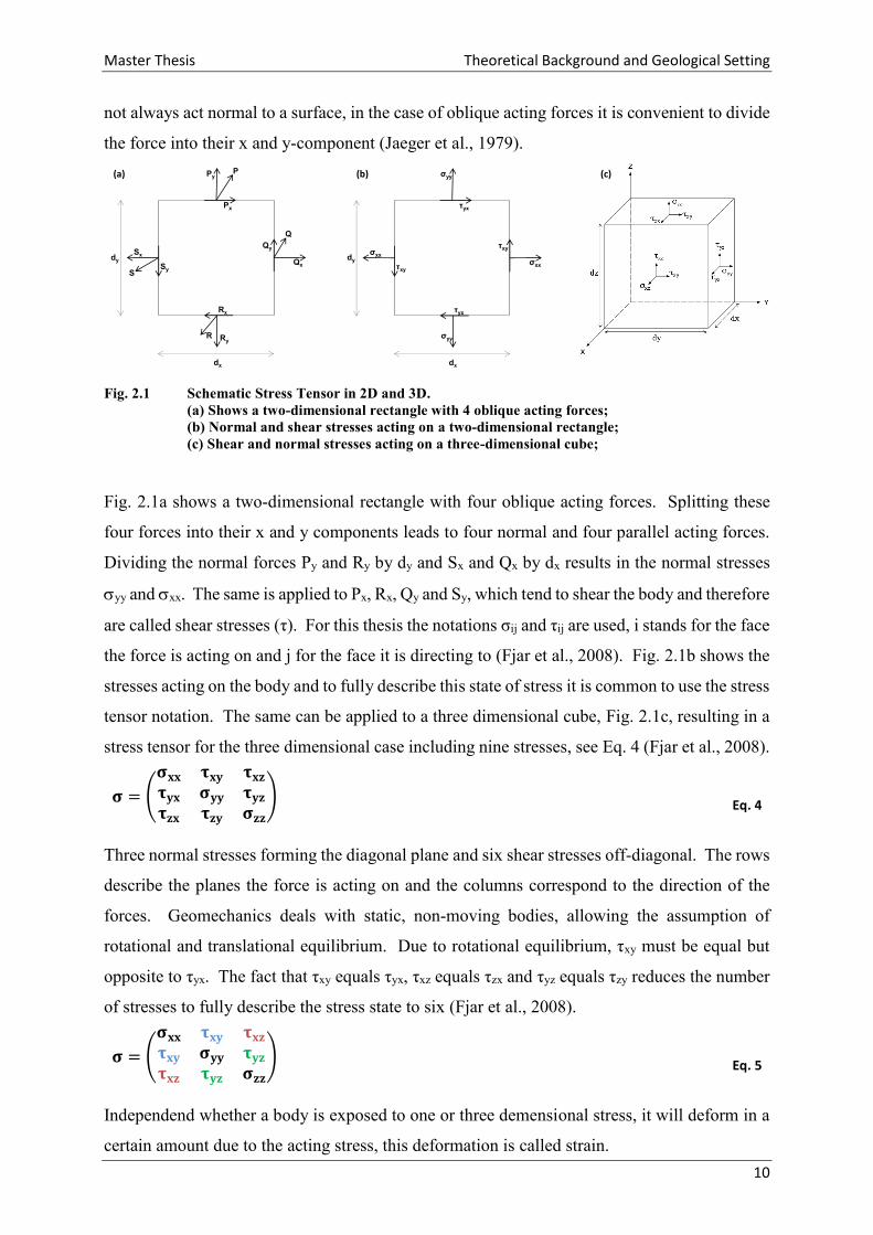
not always act normal to a surface, in the case of oblique acting forces it is convenient to divide
the force into their x and y-component (Jaeger et al., 1979).
Fig. 2.1 Schematic Stress Tensor in 2D and 3D.
(a) Shows a two-dimensional rectangle with 4 oblique acting forces;
(b) Normal and shear stresses acting on a two-dimensional rectangle;
(c) Shear and normal stresses acting on a three-dimensional cube;
Fig. 2.1a shows a two-dimensional rectangle with four oblique acting forces. Splitting these
four forces into their x and y components leads to four normal and four parallel acting forces.
Dividing the normal forces Py and Ry by dy and Sx and Qx by dx results in the normal stresses
yy and xx. The same is applied to Px, Rx, Qy and Sy, which tend to shear the body and therefore
are called shear stresses (τ). For this thesis the notations σij and τij are used, i stands for the face
the force is acting on and j for the face it is directing to (Fjar et al., 2008). Fig. 2.1b shows the
stresses acting on the body and to fully describe this state of stress it is common to use the stress
tensor notation. The same can be applied to a three dimensional cube, Fig. 2.1c, resulting in a
stress tensor for the three dimensional case including nine stresses, see Eq. 4 (Fjar et al., 2008).
𝛔 = (
𝛔𝐱𝐱 𝛕𝐱𝐲 𝛕𝐱𝐳
𝛕𝐲𝐱 𝛔𝐲𝐲 𝛕𝐲𝐳
𝛕𝐳𝐱 𝛕𝐳𝐲 𝛔𝐳𝐳
) Eq. 4
Three normal stresses forming the diagonal plane and six shear stresses off-diagonal. The rows
describe the planes the force is acting on and the columns correspond to the direction of the
forces. Geomechanics deals with static, non-moving bodies, allowing the assumption of
rotational and translational equilibrium. Due to rotational equilibrium, τxy must be equal but
opposite to τyx. The fact that τxy equals τyx, τxz equals τzx and τyz equals τzy reduces the number
of stresses to fully describe the stress state to six (Fjar et al., 2008).
𝛔 = (
𝛔𝐱𝐱 𝛕𝐱𝐲 𝛕𝐱𝐳
𝛕𝐱𝐲 𝛔𝐲𝐲 𝛕𝐲𝐳
𝛕𝐱𝐳 𝛕𝐲𝐳 𝛔𝐳𝐳
) Eq. 5
Independend whether a body is exposed to one or three demensional stress, it will deform in a
certain amount due to the acting stress, this deformation is called strain.
σyy
τyx
σxx
τxy
τxy
τyx
σyy
σxxdy
dx
P
Ry
S
Q
Py
Px
Qx
Qy
Sy
Rx
R
Sxdy
dx
(a) (b) (c)
Master Thesis Theoretical Background and Geological Setting
11
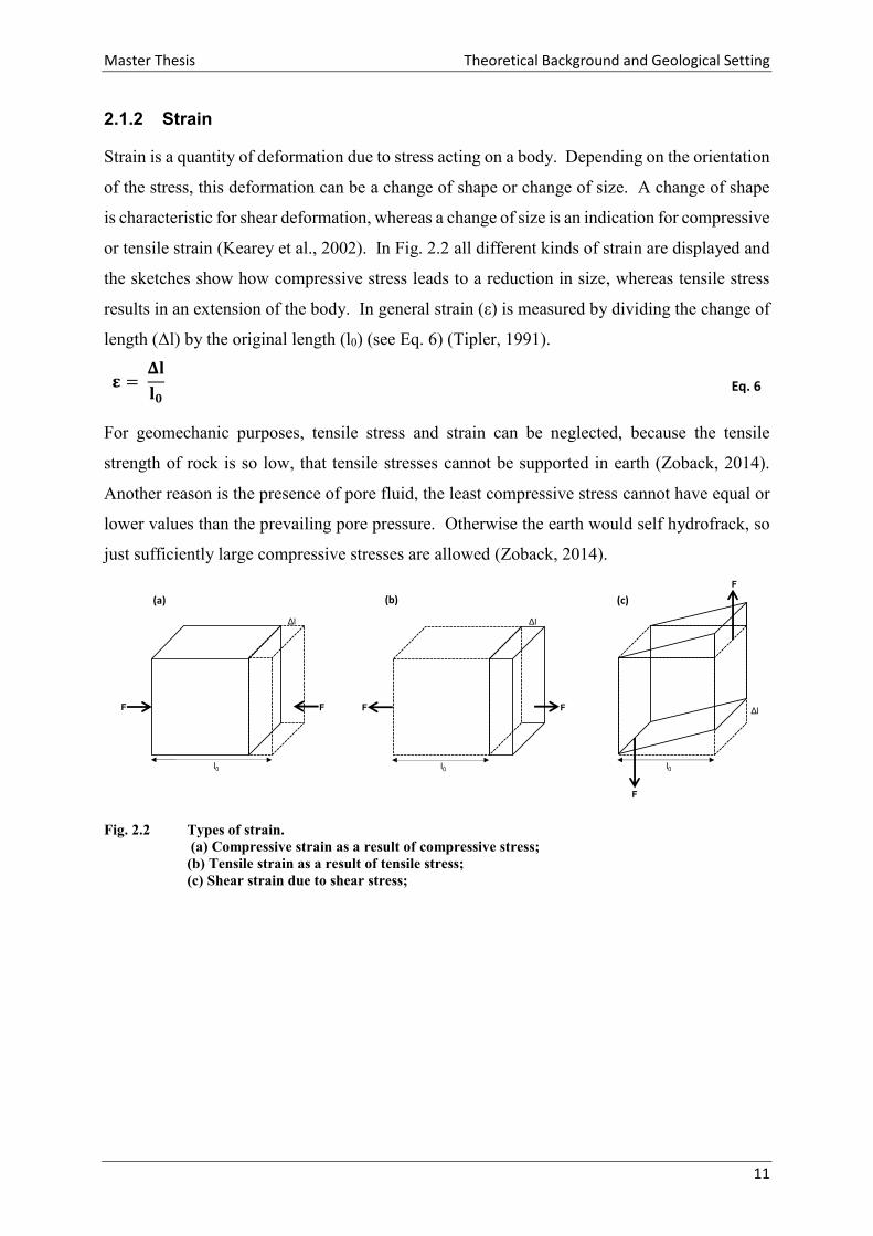
2.1.2 Strain
Strain is a quantity of deformation due to stress acting on a body. Depending on the orientation
of the stress, this deformation can be a change of shape or change of size. A change of shape
is characteristic for shear deformation, whereas a change of size is an indication for compressive
or tensile strain (Kearey et al., 2002). In Fig. 2.2 all different kinds of strain are displayed and
the sketches show how compressive stress leads to a reduction in size, whereas tensile stress
results in an extension of the body. In general strain (ε) is measured by dividing the change of
length (Δl) by the original length (l0) (see Eq. 6) (Tipler, 1991).
𝛆 = 𝚫𝐥
𝐥𝟎 Eq. 6
For geomechanic purposes, tensile stress and strain can be neglected, because the tensile
strength of rock is so low, that tensile stresses cannot be supported in earth (Zoback, 2014).
Another reason is the presence of pore fluid, the least compressive stress cannot have equal or
lower values than the prevailing pore pressure. Otherwise the earth would self hydrofrack, so
just sufficiently large compressive stresses are allowed (Zoback, 2014).
Fig. 2.2 Types of strain.
(a) Compressive strain as a result of compressive stress;
(b) Tensile strain as a result of tensile stress;
(c) Shear strain due to shear stress;
F
Δl
l0
F
l0
Δl
F
F
Δl
l0
FF
(a) (b) (c)
Master Thesis Theoretical Background and Geological Setting
12
2.1.3 Stress – Strain Relations
There are various models to describe the relationship between stress and strain, these
constitutive behaviours describe how stress and strain are connected for a specific material
under load. The existing constitutive models describe the materials responses in either the case
of elasticity, plasticity, viscosity and creep or a combination of these models. Each constitutive
model has a set of equations to describe the relation of stress and strain (Brady et al., 1999).
This thesis, concentrates on elasticity, which is the most common constitutive behaviour and a
very useful tool for describing rock behaviour and especially the behaviour of seismic waves.
A rock subjected to stress strains, which means that the rock changes in shape and / or size, if
this deformation vanishes after the stress is released one speaks of elastic deformation (Kearey
et al., 2002). Elastic deformation can be compared to Hook’s law, which states that up to a
certain limit of stress, the so called yield strength, stress can be assumed to be directly
proportional to strain. Exceeding the yield strength leads to non-linear and partly irreversible
strain, described as ductile or plastic deformation, depending on the rock behaviour. Further
stress increase would lead to failure (Kearey et al., 2002).
The most interesting deformation in the case of geophysics and geomechanics is the elastic
deformation, because seismic waves show an elastic behaviour when propagating in earth. In
more detail, they can be described as bundles of elastic strain energy that propagate in radial
direction from a seismic source. This assumption is not true in the immediate vicinity of the
seismic source, like an explosion (Kearey et al., 2002). The elastic behaviour of waves makes
it very convenient to describe the seismic velocities by the elastic moduli and the density of the
rocks through which they travel (see Eq. 9) (Yilmaz, 2001). An elastic modulus is a material
specific parameter, derived from the constitutive equations for an elastic material. These are
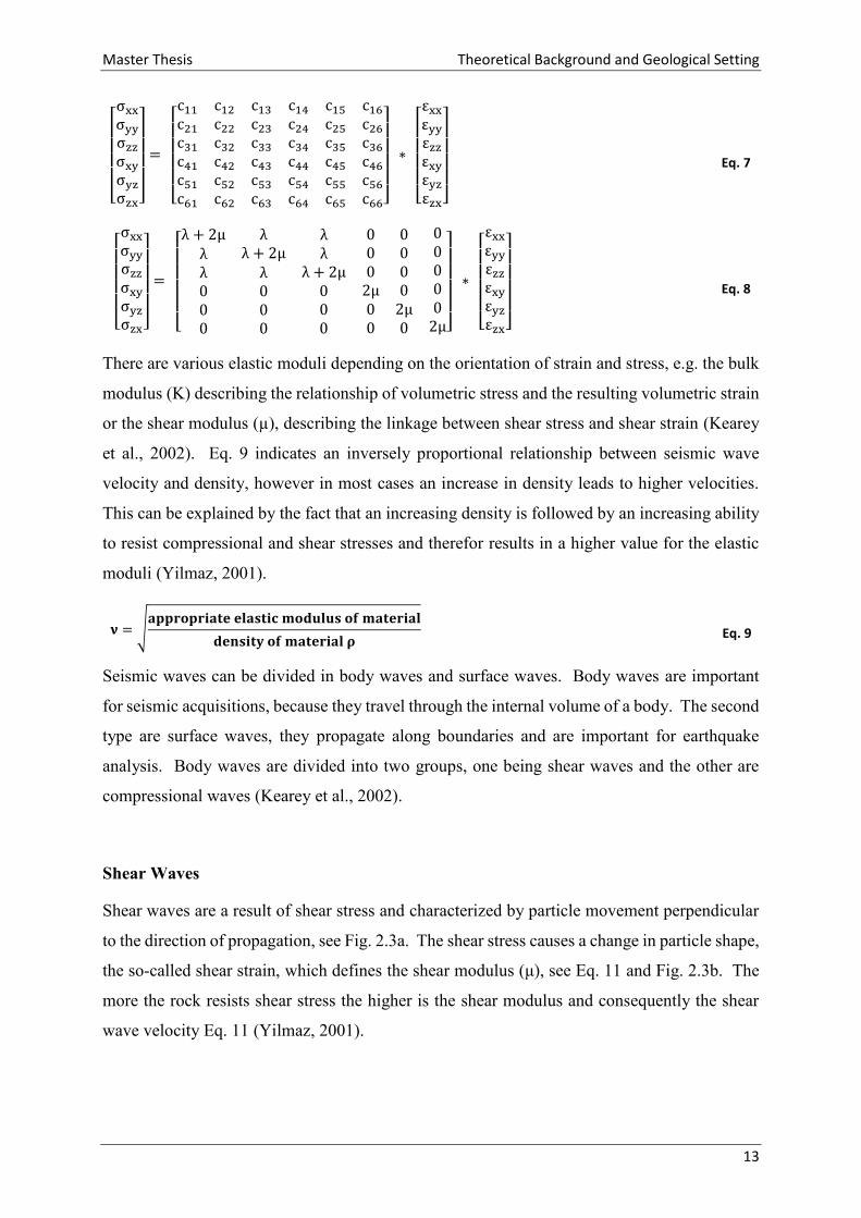
based on a generalized Hook’s law, where the stiffness tensor or elasticity tensor [cij] describes
the stress-strain relation in a more complex three-dimensional way (see Eq. 7). The elasticity
tensor is a fourth order tensor with 21 independent constants, but for an isotropic solid with
infinitesimal small deformations, just two constants remain independent. Simplifying the
elasticity tensor from 21 to 2 independent constants leads to Eq. 8, where µ and λ are elastic
moduli, which describe the linear relationship between stress and strain (Yilmaz, 2001).
Master Thesis Theoretical Background and Geological Setting
13
[ σxx
σyy
σzz
σxy
σyz
σzx]
=
[ c11
c21
c31
c41
c51
c61
c12
c22
c32
c42
c52
c62
c13
c23
c33
c43
c53
c63
c14
c24
c34
c44
c54
c64
c15
c25
c35
c45
c55
c65
c16
c26
c36
c46
c56
c66]
∗
[ εxx
εyy
εzz
εxy
εyz
εzx]
Eq. 7
[ σxx
σyy
σzz
σxy
σyz
σzx]
=
[ λ + 2μ
λλ000
λλ + 2μ
λ000
λλ
λ + 2μ000
0002μ00
00002μ0
000002μ]
∗
[ εxx
εyy
εzz
εxy
εyz
εzx]
Eq. 8
There are various elastic moduli depending on the orientation of strain and stress, e.g. the bulk
modulus (K) describing the relationship of volumetric stress and the resulting volumetric strain
or the shear modulus (µ), describing the linkage between shear stress and shear strain (Kearey
et al., 2002). Eq. 9 indicates an inversely proportional relationship between seismic wave
velocity and density, however in most cases an increase in density leads to higher velocities.
This can be explained by the fact that an increasing density is followed by an increasing ability
to resist compressional and shear stresses and therefor results in a higher value for the elastic
moduli (Yilmaz, 2001).
Seismic waves can be divided in body waves and surface waves. Body waves are important
for seismic acquisitions, because they travel through the internal volume of a body. The second
type are surface waves, they propagate along boundaries and are important for earthquake
analysis. Body waves are divided into two groups, one being shear waves and the other are
compressional waves (Kearey et al., 2002).
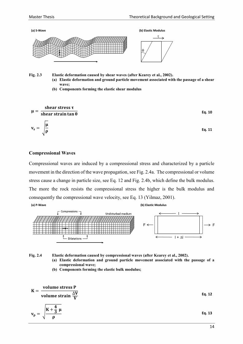
Shear Waves
Shear waves are a result of shear stress and characterized by particle movement perpendicular
to the direction of propagation, see Fig. 2.3a. The shear stress causes a change in particle shape,
the so-called shear strain, which defines the shear modulus (μ), see Eq. 11 and Fig. 2.3b. The
more the rock resists shear stress the higher is the shear modulus and consequently the shear
wave velocity Eq. 11 (Yilmaz, 2001).
𝛎 = √𝐚𝐩𝐩𝐫𝐨𝐩𝐫𝐢𝐚𝐭𝐞 𝐞𝐥𝐚𝐬𝐭𝐢𝐜 𝐦𝐨𝐝𝐮𝐥𝐮𝐬 𝐨𝐟 𝐦𝐚𝐭𝐞𝐫𝐢𝐚𝐥
𝐝𝐞𝐧𝐬𝐢𝐭𝐲 𝐨𝐟 𝐦𝐚𝐭𝐞𝐫𝐢𝐚𝐥 𝛒 Eq. 9
Master Thesis Theoretical Background and Geological Setting
14
(a) S-Wave (b) Elastic Modulus
Fig. 2.3 Elastic deformation caused by shear waves (after Kearey et al., 2002).
(a) Elastic deformation and ground particle movement associated with the passage of a shear
wave;
(b) Components forming the elastic shear modulus
Compressional Waves
Compressional waves are induced by a compressional stress and characterized by a particle
movement in the direction of the wave propagation, see Fig. 2.4a. The compressional or volume
stress cause a change in particle size, see Eq. 12 and Fig. 2.4b, which define the bulk modulus.
The more the rock resists the compressional stress the higher is the bulk modulus and
consequently the compressional wave velocity, see Eq. 13 (Yilmaz, 2001).
(a) P-Wave (b) Elastic Modulus
Fig. 2.4 Elastic deformation caused by compressional waves (after Kearey et al., 2002).
(a) Elastic deformation and ground particle movement associated with the passage of a
compressional wave;
(b) Components forming the elastic bulk modulus;
l
l + Δl
FF
𝛍 = 𝐬𝐡𝐞𝐚𝐫 𝐬𝐭𝐫𝐞𝐬𝐬 𝛕
𝐬𝐡𝐞𝐚𝐫 𝐬𝐭𝐫𝐚𝐢𝐧 𝐭𝐚𝐧𝛉 Eq. 10
𝐯𝐬 = √𝛍
𝛒 Eq. 11
𝐊 = 𝐯𝐨𝐥𝐮𝐦𝐞 𝐬𝐭𝐫𝐞𝐬𝐬 𝐏
𝐯𝐨𝐥𝐮𝐦𝐞 𝐬𝐭𝐫𝐚𝐢𝐧 ∆𝐕𝐕
Eq. 12
𝐯𝐩 = √𝐊 +
𝟒𝟑 𝛍
𝛒 Eq. 13
Master Thesis Theoretical Background and Geological Setting
15
So the knowledge of seismic wave velocities and the densities they travel through is a useful
tool to calculate the compressional and shear moduli. Also most of the modern sonic tool
measurements provide the full digital wave train, including compressional, shear and Stonley
wave arrival times, thus the velocity – elastic moduli can be calculated directly from the well
log measurements (Kearey et al., 2002).
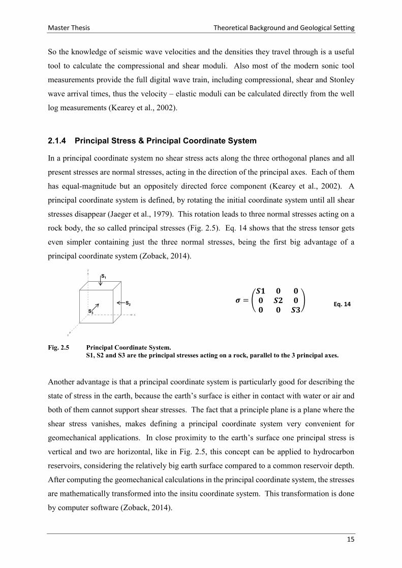
2.1.4 Principal Stress & Principal Coordinate System
In a principal coordinate system no shear stress acts along the three orthogonal planes and all
present stresses are normal stresses, acting in the direction of the principal axes. Each of them
has equal-magnitude but an oppositely directed force component (Kearey et al., 2002). A
principal coordinate system is defined, by rotating the initial coordinate system until all shear
stresses disappear (Jaeger et al., 1979). This rotation leads to three normal stresses acting on a
rock body, the so called principal stresses (Fig. 2.5). Eq. 14 shows that the stress tensor gets
even simpler containing just the three normal stresses, being the first big advantage of a
principal coordinate system (Zoback, 2014).
𝝈 = (𝑺𝟏 𝟎 𝟎𝟎 𝑺𝟐 𝟎𝟎 𝟎 𝑺𝟑
) Eq. 14
Fig. 2.5 Principal Coordinate System.
S1, S2 and S3 are the principal stresses acting on a rock, parallel to the 3 principal axes.
Another advantage is that a principal coordinate system is particularly good for describing the
state of stress in the earth, because the earth’s surface is either in contact with water or air and
both of them cannot support shear stresses. The fact that a principle plane is a plane where the
shear stress vanishes, makes defining a principal coordinate system very convenient for
geomechanical applications. In close proximity to the earth’s surface one principal stress is
vertical and two are horizontal, like in Fig. 2.5, this concept can be applied to hydrocarbon
reservoirs, considering the relatively big earth surface compared to a common reservoir depth.
After computing the geomechanical calculations in the principal coordinate system, the stresses
are mathematically transformed into the insitu coordinate system. This transformation is done
by computer software (Zoback, 2014).
S1
S2
S3
y
x
z
Master Thesis Theoretical Background and Geological Setting
16
2.1.5 Stress Regimes
E.M. Anderson discovered in the 1930s that the stress field is a result of geologic processes
which can be categorized into three major stress regimes (Anderson, 1951). These stress
regimes are based on the fact that the three principal stresses vary in magnitude according to
the prevailing geologic process. As mentioned in chapter 2.1.4 the principal stresses effecting
a rock at depth are divided into one vertical stress (Sv) and two horizontal stresses, the maximum
principal horizontal stress (SHmax) and the minimum principal horizontal stress (Shmin).
Variations of these three stresses Sv, SHmax and Shmin result in different faulting regimes.
They can be described as either a normal faulting regime (NFR), strike-slip faulting regime
(SSFR) or a reverse faulting regime (RFR), depending the biggest of these three stresses
(Anderson, 1951; Zoback, 2014). Some assumptions count for all stress regimes, like the
stresses under the earth’s surface are always compressive, the least principal stress ought to be
greater than the pore pressure, otherwise the earth would self hydrofrac and the strength of pre-
existing faults will always limit the existing stress magnitudes (Zoback, 2014).
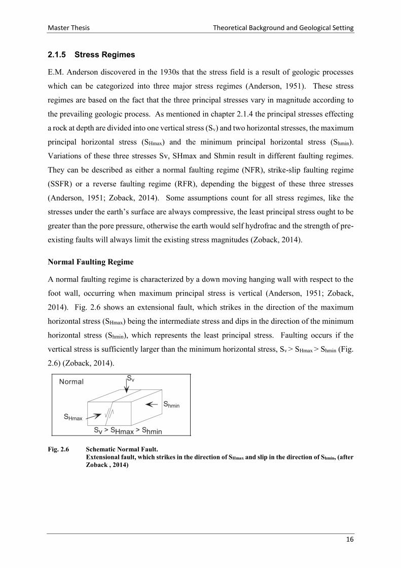
Normal Faulting Regime
A normal faulting regime is characterized by a down moving hanging wall with respect to the
foot wall, occurring when maximum principal stress is vertical (Anderson, 1951; Zoback,
2014). Fig. 2.6 shows an extensional fault, which strikes in the direction of the maximum
horizontal stress (SHmax) being the intermediate stress and dips in the direction of the minimum
horizontal stress (Shmin), which represents the least principal stress. Faulting occurs if the
vertical stress is sufficiently larger than the minimum horizontal stress, Sv > SHmax > Shmin (Fig.
2.6) (Zoback, 2014).
Fig. 2.6 Schematic Normal Fault.
Extensional fault, which strikes in the direction of SHmax and slip in the direction of Shmin, (after
Zoback , 2014)

Master Thesis Theoretical Background and Geological Setting
17
Strike Slip Faulting Regime
In a strike slip faulting regime the faults are nearly vertical and develop with an angle of 30
degree in respect to the maximum horizontal stress, which in this case forms the maximum
principal stress, see Fig. 2.7. As a result, the vertical stress forms the intermediate stress and
the minimum horizontal stress the least principal stress. In this case faulting occurs, if the
maximum horizontal stress is sufficiently larger than the minimum horizontal stress, SHmax > Sv
> Shmin (Fig. 2.7) (Anderson, 1951; Zoback, 2014).
Fig. 2.7 Schematic Strike Slip Fault.
These are nearly vertical faults, which strike in approximately 30 degrees to SHmax
(after Zoback, 2014)
Reverse Faulting Regime
A reverse faulting system is the most compressive stress state in earth, because both
horizontal stresses exceed the vertical stress (Sv), which forms in this case the least principal
stress. In this stress regime, the hanging wall moves up with respect to the foot wall and the
fault dips with 30 degrees in the direction of the maximum horizontal stress, see Fig. 2.8.
Faulting occurs if SHmax > Shmin > Sv (Anderson, 1951; Zoback, 2014).
Fig. 2.8 Schematic Reverse Fault.
Reverse faults strike in the direction of Shmin and dip about 30 degrees in the direction of SHmax
(after Zoback, 2014)
Master Thesis Theoretical Background and Geological Setting
18
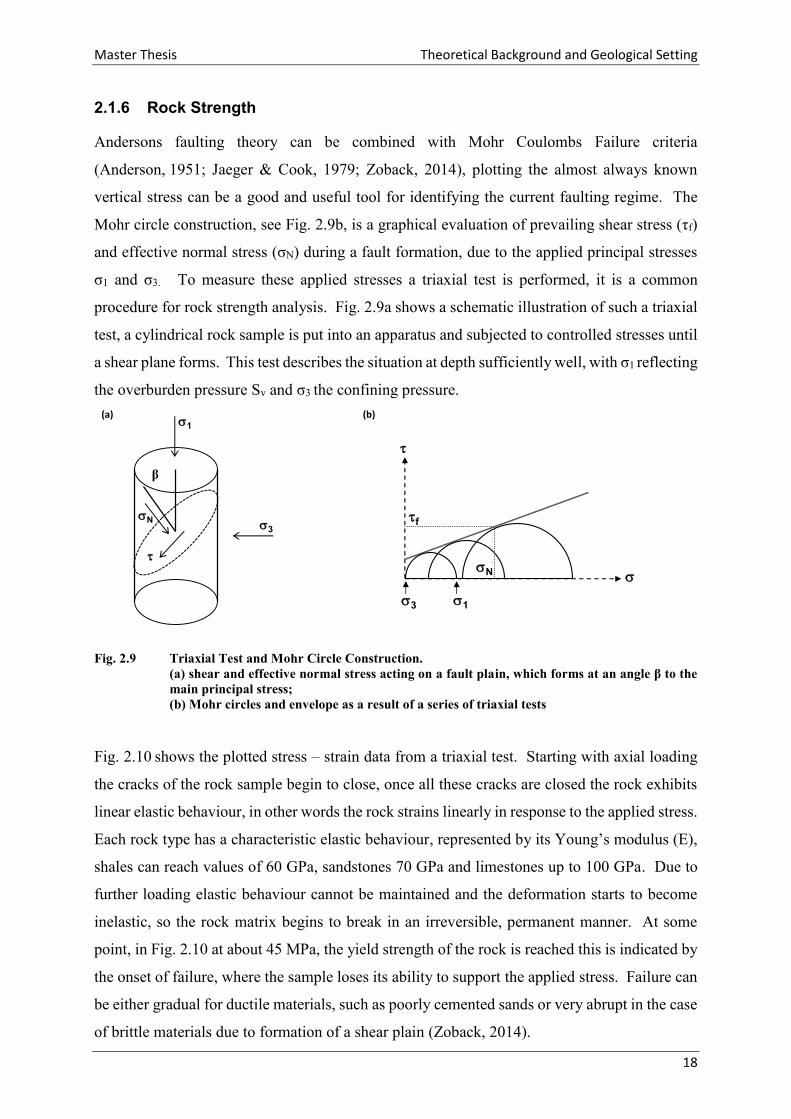
2.1.6 Rock Strength
Andersons faulting theory can be combined with Mohr Coulombs Failure criteria
(Anderson, 1951; Jaeger & Cook, 1979; Zoback, 2014), plotting the almost always known
vertical stress can be a good and useful tool for identifying the current faulting regime. The
Mohr circle construction, see Fig. 2.9b, is a graphical evaluation of prevailing shear stress (τf)
and effective normal stress (σN) during a fault formation, due to the applied principal stresses
σ1 and σ3. To measure these applied stresses a triaxial test is performed, it is a common
procedure for rock strength analysis. Fig. 2.9a shows a schematic illustration of such a triaxial
test, a cylindrical rock sample is put into an apparatus and subjected to controlled stresses until
a shear plane forms. This test describes the situation at depth sufficiently well, with σ1 reflecting
the overburden pressure Sv and σ3 the confining pressure.
(a)
(b)
Fig. 2.9 Triaxial Test and Mohr Circle Construction.
(a) shear and effective normal stress acting on a fault plain, which forms at an angle β to the
main principal stress;
(b) Mohr circles and envelope as a result of a series of triaxial tests
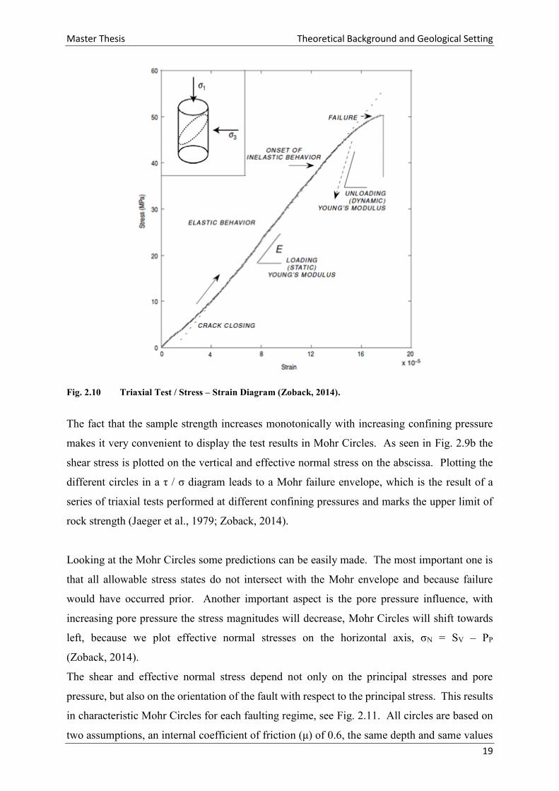
Fig. 2.10 shows the plotted stress – strain data from a triaxial test. Starting with axial loading
the cracks of the rock sample begin to close, once all these cracks are closed the rock exhibits
linear elastic behaviour, in other words the rock strains linearly in response to the applied stress.
Each rock type has a characteristic elastic behaviour, represented by its Young’s modulus (E),
shales can reach values of 60 GPa, sandstones 70 GPa and limestones up to 100 GPa. Due to
further loading elastic behaviour cannot be maintained and the deformation starts to become
inelastic, so the rock matrix begins to break in an irreversible, permanent manner. At some
point, in Fig. 2.10 at about 45 MPa, the yield strength of the rock is reached this is indicated by
the onset of failure, where the sample loses its ability to support the applied stress. Failure can
be either gradual for ductile materials, such as poorly cemented sands or very abrupt in the case
of brittle materials due to formation of a shear plain (Zoback, 2014).
1
3
N
β
1 1 3 31
f
N
3
Master Thesis Theoretical Background and Geological Setting
19
Fig. 2.10 Triaxial Test / Stress – Strain Diagram (Zoback, 2014).
The fact that the sample strength increases monotonically with increasing confining pressure
makes it very convenient to display the test results in Mohr Circles. As seen in Fig. 2.9b the
shear stress is plotted on the vertical and effective normal stress on the abscissa. Plotting the
different circles in a τ / σ diagram leads to a Mohr failure envelope, which is the result of a
series of triaxial tests performed at different confining pressures and marks the upper limit of
rock strength (Jaeger et al., 1979; Zoback, 2014).
Looking at the Mohr Circles some predictions can be easily made. The most important one is
that all allowable stress states do not intersect with the Mohr envelope and because failure
would have occurred prior. Another important aspect is the pore pressure influence, with
increasing pore pressure the stress magnitudes will decrease, Mohr Circles will shift towards
left, because we plot effective normal stresses on the horizontal axis, σN = SV – PP
(Zoback, 2014).
The shear and effective normal stress depend not only on the principal stresses and pore
pressure, but also on the orientation of the fault with respect to the principal stress. This results
in characteristic Mohr Circles for each faulting regime, see Fig. 2.11. All circles are based on
two assumptions, an internal coefficient of friction (μ) of 0.6, the same depth and same values
Master Thesis Theoretical Background and Geological Setting
20
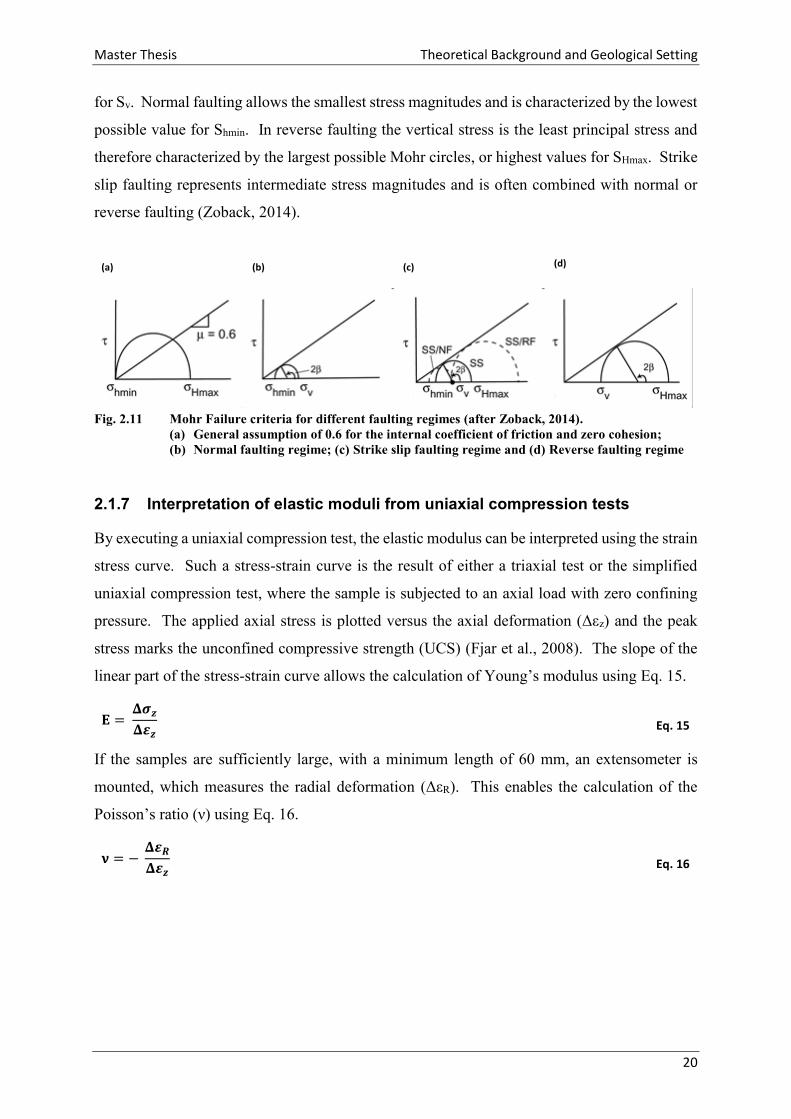
for Sv. Normal faulting allows the smallest stress magnitudes and is characterized by the lowest
possible value for Shmin. In reverse faulting the vertical stress is the least principal stress and
therefore characterized by the largest possible Mohr circles, or highest values for SHmax. Strike
slip faulting represents intermediate stress magnitudes and is often combined with normal or
reverse faulting (Zoback, 2014).
(a) (b) (c) (d)
Fig. 2.11 Mohr Failure criteria for different faulting regimes (after Zoback, 2014).
(a) General assumption of 0.6 for the internal coefficient of friction and zero cohesion;
(b) Normal faulting regime; (c) Strike slip faulting regime and (d) Reverse faulting regime
2.1.7 Interpretation of elastic moduli from uniaxial compression tests
By executing a uniaxial compression test, the elastic modulus can be interpreted using the strain
stress curve. Such a stress-strain curve is the result of either a triaxial test or the simplified
uniaxial compression test, where the sample is subjected to an axial load with zero confining
pressure. The applied axial stress is plotted versus the axial deformation (Δεz) and the peak
stress marks the unconfined compressive strength (UCS) (Fjar et al., 2008). The slope of the
linear part of the stress-strain curve allows the calculation of Young’s modulus using Eq. 15.
𝐄 = 𝚫𝝈𝒛
𝚫𝜺𝒛 Eq. 15
If the samples are sufficiently large, with a minimum length of 60 mm, an extensometer is
mounted, which measures the radial deformation (ΔεR). This enables the calculation of the
Poisson’s ratio (ν) using Eq. 16.
𝛎 = − 𝚫𝜺𝑹
𝚫𝜺𝒛 Eq. 16
Master Thesis Theoretical Background and Geological Setting
21
In case of a nonlinear stress-strain response the Young’s modulus can be interpreted as a secant,
tangent or initial modulus, Fig. 2.12 (Fjar et al., 2008).
The initial modulus (EI) represents the initial slope of the stress-strain curve.
The secant modulus (ES) is a measure from the origin up to a chosen percentage of the
uniaxial compressive strength.
The tangent modulus (ET) is the slope of the stress-strain response at a specific
percentage (commonly at 50% of the uniaxial compressive strength).
The uniaxial compressive strength is strongly influenced by the inheterogeneities of a rock
sample, a careful sample preparation is key for representative uniaxial compression tests,
because flaws and cracks can reduce the rock strength immensely (Witt, 2008).
Fig. 2.12 Three ways to calculate elastic moduli from an axial strain-stress curve (black).
Secant modulus (ES) (green), Initial modulus (EI) (blue), Tangent modulus (ET) (red). Uniaxial
compressive strength (UCS) and the 50% value of UCS are marked (after Fjar et al., 2008)
Initial modulus (EI)
UCS
50% UCS
Secant
modulus (ES)
Tangent modulus (ET)
Master Thesis Theoretical Background and Geological Setting
22
2.1.8 Pore Pressure
During drilling or reservoir analysis it is essential to understand the behavior of fluids present
in the rocks. A good tool is the analysis of pore pressure and pressure gradients, these allow
fluid type prediction and indication of overpressure zones, which can be fatal for wellbore
drilling (Zoback, 2014). Fluid pressure is isotropic, hence the pressure is transmitted through
the whole fluid and has the same value in all directions. Therefore, pore pressure depends just
on the height of the water column and the density of the fluid. The resulting unit kg/cm² is not
very common in oil industry, but can be converted into psi with the conversion factor of 14.2233
psi which corresponds to 1 kg/cm² (Rider et al., 2011). Normal pressure or hydrostatic pore
pressure is calculated as seen in Eq. 17 and increases with 10 MPa/km, corresponding to 0.44
psi/ft for freshwater. This value can vary for other water salinities.
A classic result of pore pressure measurements in a sedimentary basin, see Fig. 2.13, shows the
usefulness of pore pressure gradients. At a first glance, one can divide the underground in three
different pressure zones, characterized by three distinct rates of pressure increase with depth
(Zoback , 2014). The proportionality of the insitu fluid and the gradient allows gas and oil
detection, due to the different pressure gradients (Rider et al., 2011).
Pressure zone one from 0 to 8300 ft represents the hydrostatic zone, this implies an
interconnected pore space and fracture network from bottom to earth surface, since hydrostatic
pressure can exist only as long as there is a connectivity and permeability among the pore space
at depth and the surface. At 8300 ft the pore pressure starts to increase rapidly and a pressure
barrier, for example an impermeable shale, isolates this zones from the shallower above,
otherwise it would equilibrate. Beginning with pressure zone two, the measurements are in the
overpressure zone, which is defined as any pressure above the normal. A water gradient in an
overpressure zone is the same as for the hydrostatic zone, just the absolute (over)pressure is
higher. For example the fast burial of fluid filled sediments, can lead to overpressure if the
fluid cannot escape in time. Furthermore overpressure results in lower effective stresses and
decelerates mechanic compaction (Zoback, 2014).
𝐏𝐏𝐡𝐲𝐝𝐫𝐨
= ∫ 𝛒𝐰(𝐳)𝐠𝐝𝐳 ≈ 𝛒𝐰𝐠𝐳𝐰
𝟎
𝐳
Eq. 17

Master Thesis Theoretical Background and Geological Setting
23
Fig. 2.13 Pore Pressure Measurements (Zoback, 2014).
Red line indicates the pore pressure gradient and the dotted blue line the overburden stress
gradient (Sv) or lithostatic gradient.
Subsequently underpressure is characterized by values lower than normal pressure and is often
a result of uplift (Bjørlykke, 2015). At the transition from pressure zone three to four the pore
pressure reaches a level close to the overburden pressure or lithostatic gradient, indicated by
the blue dotted line. The lithostatic gradient depends on rock density and marks the highest
possible pressures in a well and forms the upper boundary for overpressure. Plotting the
hydrostatic gradient and lithostatic gradient in a diagram with pressure versus depth, generates
a window in which all possible formation pressures must lie (Rider et al., 2011). Another option
is to calculate the ratio of pore pressure and overburden pressure with Eq. 18, in the case of Fig.
2.13 a pore pressure limit of 0.91 is reached (Zoback, 2014).
Looking at fluid saturated rocks a second constitutive law is of importance, because a porous
fluid saturated rock shows poroelastic behavior. In contrast to elasticity this law considers the
fact that the stiffness of saturated rocks depends on the rate the external forces are applied. In
more detail fast loading results in apparently higher stiffness, because the porewater cannot
drain fast enough and carries some of the applied stress. Whereas slow loading leads to a similar
rock stiffness as if no fluids are present (Zoback, 2014).
𝛌 = 𝐏𝐩
𝐒𝐯,
Eq. 18
Master Thesis Theoretical Background and Geological Setting
24
2.2 GEOLOGICAL SETTING
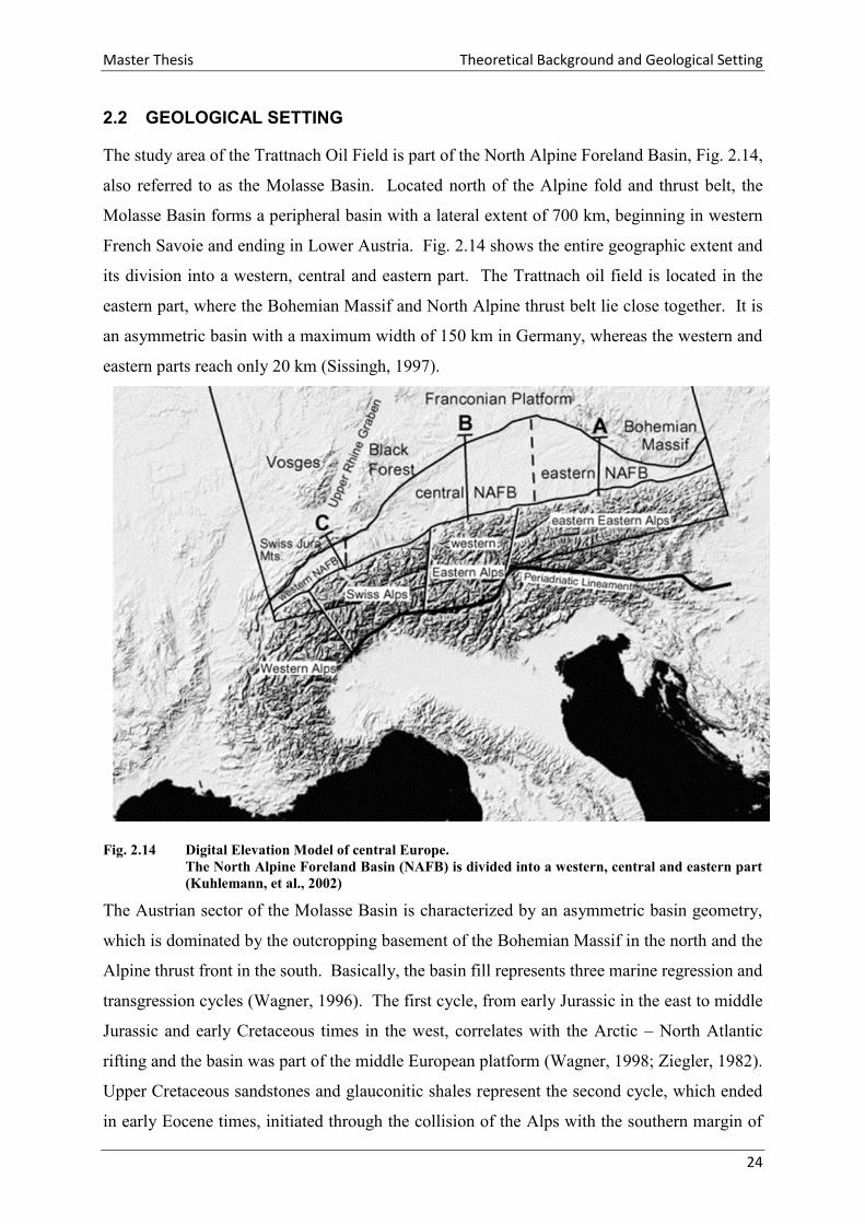
The study area of the Trattnach Oil Field is part of the North Alpine Foreland Basin, Fig. 2.14,
also referred to as the Molasse Basin. Located north of the Alpine fold and thrust belt, the
Molasse Basin forms a peripheral basin with a lateral extent of 700 km, beginning in western
French Savoie and ending in Lower Austria. Fig. 2.14 shows the entire geographic extent and
its division into a western, central and eastern part. The Trattnach oil field is located in the
eastern part, where the Bohemian Massif and North Alpine thrust belt lie close together. It is
an asymmetric basin with a maximum width of 150 km in Germany, whereas the western and
eastern parts reach only 20 km (Sissingh, 1997).
Fig. 2.14 Digital Elevation Model of central Europe.
The North Alpine Foreland Basin (NAFB) is divided into a western, central and eastern part
(Kuhlemann, et al., 2002)
The Austrian sector of the Molasse Basin is characterized by an asymmetric basin geometry,
which is dominated by the outcropping basement of the Bohemian Massif in the north and the
Alpine thrust front in the south. Basically, the basin fill represents three marine regression and
transgression cycles (Wagner, 1996). The first cycle, from early Jurassic in the east to middle
Jurassic and early Cretaceous times in the west, correlates with the Arctic – North Atlantic
rifting and the basin was part of the middle European platform (Wagner, 1998; Ziegler, 1982).
Upper Cretaceous sandstones and glauconitic shales represent the second cycle, which ended
in early Eocene times, initiated through the collision of the Alps with the southern margin of
Master Thesis Theoretical Background and Geological Setting
25
the European platform. Due to the Alpine orogeny the North Alpine Foreland Basin was formed
and the basin infill from late Eocene to present is summarized as the third cycle (Wagner, 1998;
Ziegler, 1982)
2.2.1 Basin fill
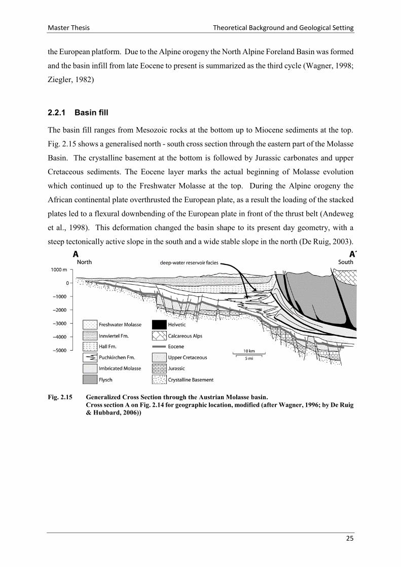
The basin fill ranges from Mesozoic rocks at the bottom up to Miocene sediments at the top.
Fig. 2.15 shows a generalised north - south cross section through the eastern part of the Molasse
Basin. The crystalline basement at the bottom is followed by Jurassic carbonates and upper
Cretaceous sediments. The Eocene layer marks the actual beginning of Molasse evolution
which continued up to the Freshwater Molasse at the top. During the Alpine orogeny the
African continental plate overthrusted the European plate, as a result the loading of the stacked
plates led to a flexural downbending of the European plate in front of the thrust belt (Andeweg
et al., 1998). This deformation changed the basin shape to its present day geometry, with a
steep tectonically active slope in the south and a wide stable slope in the north (De Ruig, 2003).
Fig. 2.15 Generalized Cross Section through the Austrian Molasse basin.
Cross section A on Fig. 2.14 for geographic location, modified (after Wagner, 1996; by De Ruig
& Hubbard, 2006))
Master Thesis Theoretical Background and Geological Setting
26
2.2.2 Stratigraphy
The Bohemian Massif, being part of the European Craton, forms the crystalline basement of
the North Alpine Foreland Basin.
Mesozoic Succession
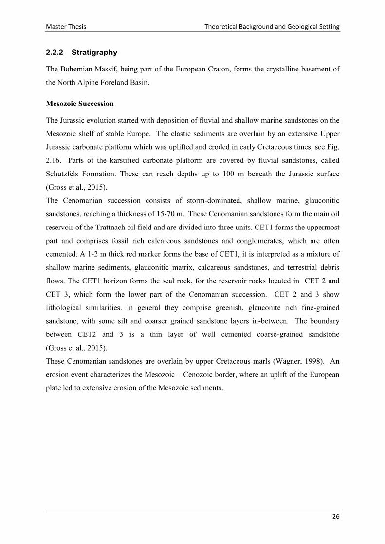
The Jurassic evolution started with deposition of fluvial and shallow marine sandstones on the
Mesozoic shelf of stable Europe. The clastic sediments are overlain by an extensive Upper
Jurassic carbonate platform which was uplifted and eroded in early Cretaceous times, see Fig.
2.16. Parts of the karstified carbonate platform are covered by fluvial sandstones, called
Schutzfels Formation. These can reach depths up to 100 m beneath the Jurassic surface
(Gross et al., 2015).
The Cenomanian succession consists of storm-dominated, shallow marine, glauconitic
sandstones, reaching a thickness of 15-70 m. These Cenomanian sandstones form the main oil
reservoir of the Trattnach oil field and are divided into three units. CET1 forms the uppermost
part and comprises fossil rich calcareous sandstones and conglomerates, which are often
cemented. A 1-2 m thick red marker forms the base of CET1, it is interpreted as a mixture of
shallow marine sediments, glauconitic matrix, calcareous sandstones, and terrestrial debris
flows. The CET1 horizon forms the seal rock, for the reservoir rocks located in CET 2 and
CET 3, which form the lower part of the Cenomanian succession. CET 2 and 3 show
lithological similarities. In general they comprise greenish, glauconite rich fine-grained
sandstone, with some silt and coarser grained sandstone layers in-between. The boundary
between CET2 and 3 is a thin layer of well cemented coarse-grained sandstone
(Gross et al., 2015).
These Cenomanian sandstones are overlain by upper Cretaceous marls (Wagner, 1998). An
erosion event characterizes the Mesozoic – Cenozoic border, where an uplift of the European
plate led to extensive erosion of the Mesozoic sediments.
Master Thesis Theoretical Background and Geological Setting
27
Fig. 2.16 The Mesozoic evolution of the Austrian Molasse Basin (Gross et al., 2015).
Cenozoic Succession
The Cenozoic sediments reach a thickness up to 3000 m in front of the Alps, whereas only a
few meters cover the Bohemian Massif in the north (Nachtmann & Wagner, 1987). According
to Steininger the molasses sediments can be subdivided into three tectonic units
(Steininger et al., 1999). The Autochthonous Molasse includes flat lying sediments in front and
underneath the Alps. In contrast, the Allochthonous Molasse consists molasses sediments,
which have been incorporated into the Alpine nappe stack. Some molasse sediments rest
transgressively on top of various Alpine units and have been transported on their back. They
form the Parautochthonous Molasse.
Master Thesis Theoretical Background and Geological Setting
28
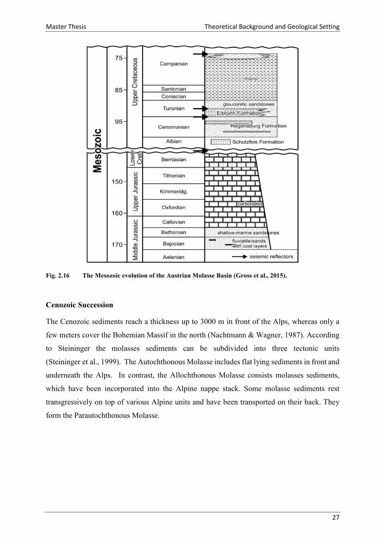
Fig. 2.17 Cenozoic Evolution of the Austrian Molasse Basin (Gross et al., 2015).
The stratigraphic chart in Fig. 2.17 shows the Cenozoic basin fill in more detail, beginning with
fluvial and shallow marine sandstones of the Voitsdorf Formation, Cerithian Beds and Ampfing
sandstones which grade into shallow marine Lithothamnium Limestones. This Lithothamnium
platform drowned in early Oligocene times, due to an abrupt deepening and widening of the
basin (Sissingh, 1997). During these deep water conditions, sometimes organic rich, deep-
water sediments, divided into Schöneck, Dynow, Eggerding and Zupfing Formation,
accumulated in the Molasse Basin (Sachsenhofer et al., 2010). From Mid Oligocene on the
debris from the ascending Alps stopped the starved basin conditions and began to slowly fill up
the Molasse Basin (De Ruig, 2003). From middle Oligocene times on rivers filled the foreland
basin with the Lower Freshwater Molasse and the German and Swiss part of the North Alpine
Foreland Basin east of Munich became dry land (Wagner, 1996). In Austria deep marine
conditions prevailed until early Miocene, a narrow deep marine trough, the so called
Puchkirchen Basin formed the accommodation space for conglomerates, turbidity currents and
debris flows derived from the rising Alps (Nachtmann et al., 1987). New insights, based on the
correlation of 3D seismic data, indicate that the material derived from west and was transported
along the low sinuosity, west-east trending deep water channel (De Ruig et al., 2006).
Master Thesis Theoretical Background and Geological Setting
29
The ongoing northward movement of the Alps formed the Imbricated Molasse sediments,
where parts of the Puchkirchen Formation have been incorporated into the thrust sheets (De
Ruig, 2003). A subaqueous erosional interval separates the deep marine Hall Formation from
the Puchkirchen Group (Gross et al., 2015). Beginning in Badenian times the sedimentation of
the Upper Freshwater Molasse affected the Austrian part of the Molasse Basin. It is composed
of coal bearing clays, sands and fluvial gravels, reaching a thickness of several hundred meters
(Gusterhuber et al., 2013). Most of this thick succession got eroded after Pannonian times,
where up to 800 m sediments have been removed (Gusterhuber et al., 2012).
2.2.3 Petroleum Systems
The Austrian Molasse Basin contains two petroleum systems. One contains thermally
generated oil and gas, reaching from Mesozoic to Oligocene times and the second system is of
Oligocene to Miocene age, containing biogenetic gas (Wagner, 1998; Gross et al., 2018). The
thermogenic petroleum system is charged by Oligocene source rocks, which were deposited
during the first isolation of the Paratethys after the Eocene-Oligocene boundary, where starved
basin conditions led to the deposition of organic matter rich sediments (Schulz et al., 2002;
Sachsenhofer et al., 2010). The Oligocene source rocks comprise, from bottom to top, the
Schöneck, Dynow, Eggerding and Zupfing Formations (Fig. 2.17). The Schöneck Formation,
formerly Fish shale, consists of organic rich marls and shales and forms with total organic
carbon (TOC) contents up to 12 % and hydrogen index values between 500 and 600
mgHC/gTOC the most prominent source rock interval. The overlying organic rich marls and
limestones of the Dynow Formation and dark grey laminated pelites forming the lower
Eggerding Formation, both play a minor role for oil and gas generation (Gratzer et al., 2011).
Important reservoir rocks are the upper Eocene basal sandstones, these contain most of the oil.
Minor reservoirs are Cenomanian sandstones, some Oligocene horizons and the Eocene
Lithothamnium Limestones. The microbial gas is charged from Oligocene to lower Miocene
pelitic rocks and trapped inside the turbiditic and sandy conglomerates of the Puchkirchen
Group and the Hall Formation. Oil accumulation in the Trattnach field commenced during
Miocene times and is produced from lower Cenomanian green sandstones reservoirs, which are
sealed by low permeability Cenomanian rocks and Turonian shales (Gross et al., 2015).
Master Thesis Theoretical Background and Geological Setting
30
2.3 THE TRATTNACH FIELD
The Trattnach field contains two separate oil fields. The main oil field is located inside the
Trattnach mega anticlinale and the second field is located along the Aistersheim fault in the
northern part of the Trattnach area and therefore called North Field. Both produce from
Cenomanian reservoir rocks.
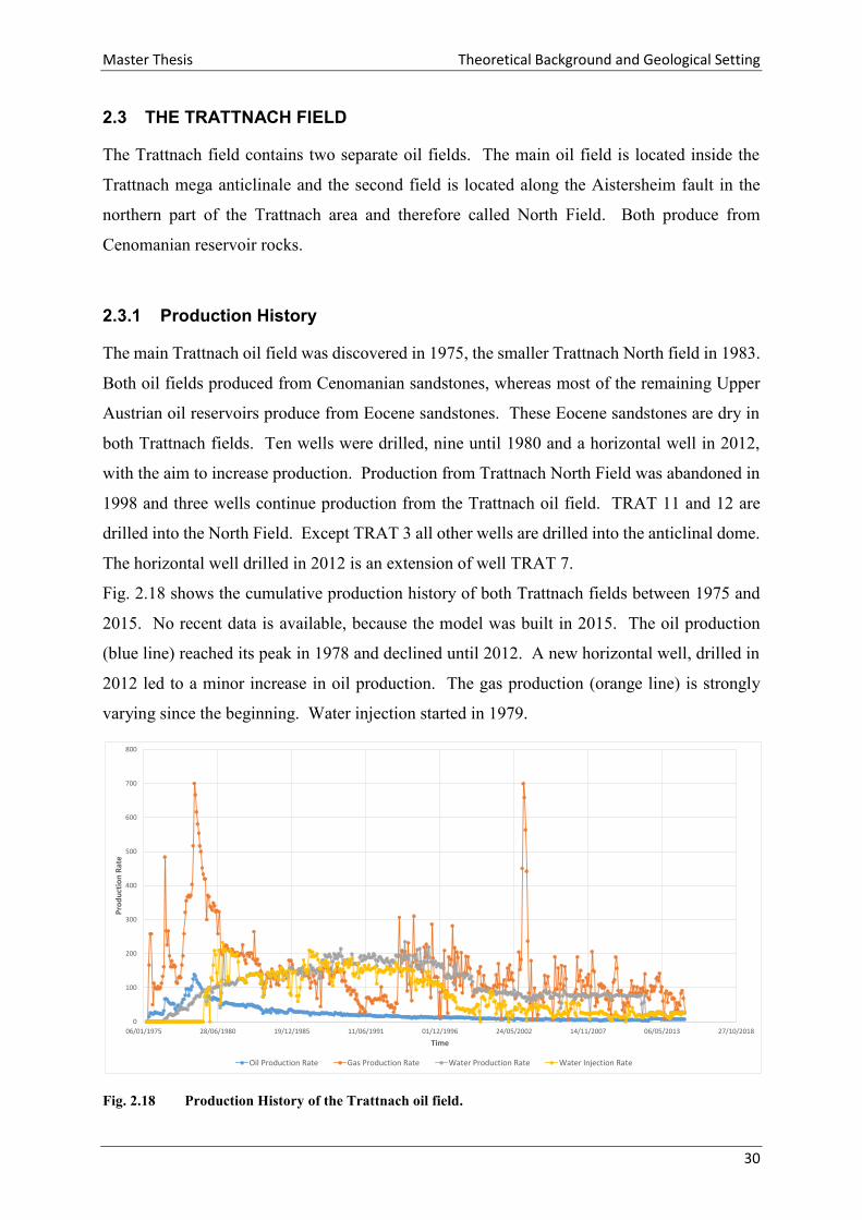
2.3.1 Production History
The main Trattnach oil field was discovered in 1975, the smaller Trattnach North field in 1983.
Both oil fields produced from Cenomanian sandstones, whereas most of the remaining Upper
Austrian oil reservoirs produce from Eocene sandstones. These Eocene sandstones are dry in
both Trattnach fields. Ten wells were drilled, nine until 1980 and a horizontal well in 2012,
with the aim to increase production. Production from Trattnach North Field was abandoned in
1998 and three wells continue production from the Trattnach oil field. TRAT 11 and 12 are
drilled into the North Field. Except TRAT 3 all other wells are drilled into the anticlinal dome.
The horizontal well drilled in 2012 is an extension of well TRAT 7.
Fig. 2.18 shows the cumulative production history of both Trattnach fields between 1975 and
2015. No recent data is available, because the model was built in 2015. The oil production
(blue line) reached its peak in 1978 and declined until 2012. A new horizontal well, drilled in
2012 led to a minor increase in oil production. The gas production (orange line) is strongly
varying since the beginning. Water injection started in 1979.
Fig. 2.18 Production History of the Trattnach oil field.
0
100
200
300
400
500
600
700
800
06/01/1975 28/06/1980 19/12/1985 11/06/1991 01/12/1996 24/05/2002 14/11/2007 06/05/2013 27/10/2018
Pro
du
ctio
n R
ate
Time
Oil Production Rate Gas Production Rate Water Production Rate Water Injection Rate

Master Thesis Theoretical Background and Geological Setting
31
2.3.2 Field Structure and Geology
The faults in the Upper Austrian sector of the Molasse Basin can be separated into a Mesozoic
fault system, with roughly N-S trending faults and a Cenozoic fault system (Fig. 2.19). The
Cenozoic fault system is characterized by a dense network of E-W trending faults, which are a
result of the Alpine nappe loading (Ziegler, 1987).
The Trattnach area is defined by three major faults. Fig. 2.20 shows the Aistersheim fault,
forming the northern border of the study area and the Gaspoldshofen fault in the south, both
show a west – east trend and belong to the Cenozoic fault system. The third is the north-south
trending Schwanenstadt fault, which forms the western border of the reservoir, located in the
so called Trattnach mega-anticlinal. It is a dome structure, containing the sealed oil reservoir
of the Trattnach field. The lower section of Cenomanian green sandstones (CET2, 3) form the
producing reservoir units, whereas the tighter uppermost Cenomanian section (CET1) and
overlying Turonian marls form the seal rock. The North Field is located in an anticlinal structure
which is sealed by the Aistersheim fault in the north. Its producing reservoir rock and seal rock
are from the same lithology as the bigger Trattnach field. Both fields have an initial oil water
contact (OWC) of ~1150m TVDS (true vertical depth subsea).
Fig. 2.19 Fault Systems in Upper Austria.
Green N-S trending faults are of Mesozoic age, blue W-E trending faults have a Cenozoic age
(after Nachtmann, 1995)
Cenozoic Faults
Mesozoic Faults
Oil Fields
Gas Fields
Master Thesis Theoretical Background and Geological Setting
32
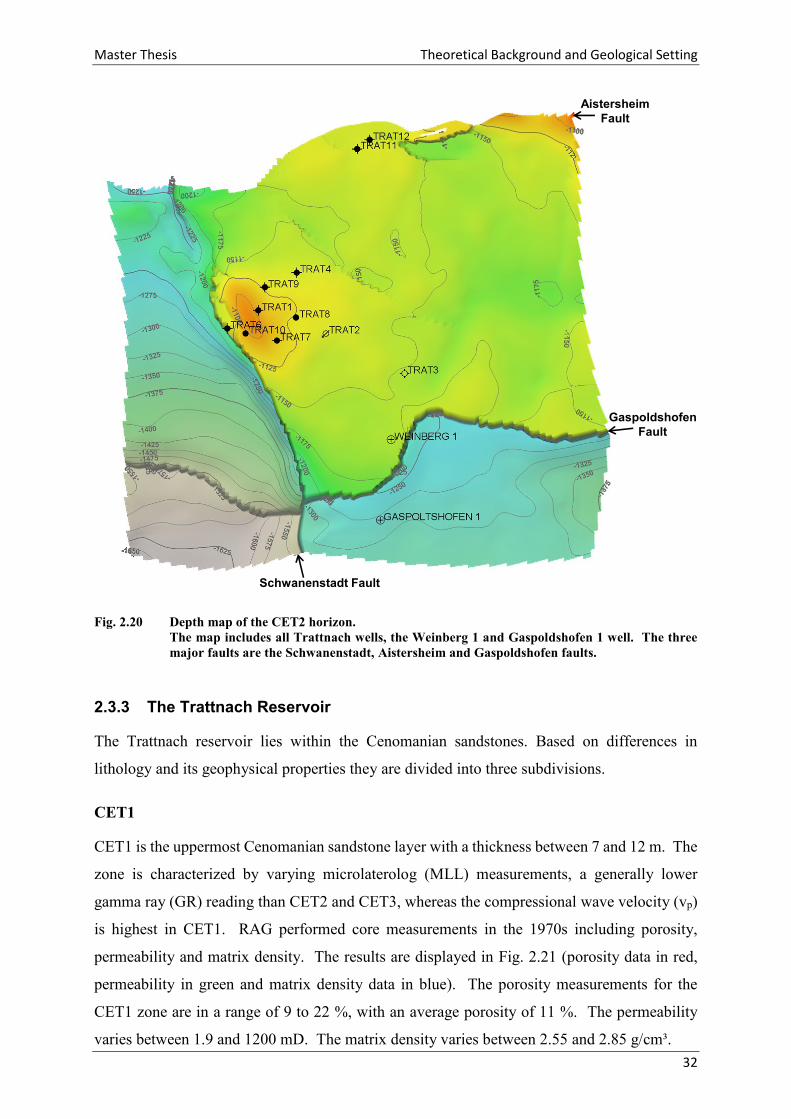
Fig. 2.20 Depth map of the CET2 horizon.
The map includes all Trattnach wells, the Weinberg 1 and Gaspoldshofen 1 well. The three
major faults are the Schwanenstadt, Aistersheim and Gaspoldshofen faults.
2.3.3 The Trattnach Reservoir
The Trattnach reservoir lies within the Cenomanian sandstones. Based on differences in
lithology and its geophysical properties they are divided into three subdivisions.
CET1
CET1 is the uppermost Cenomanian sandstone layer with a thickness between 7 and 12 m. The
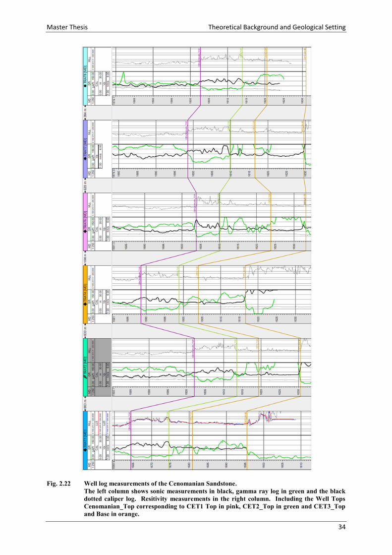
zone is characterized by varying microlaterolog (MLL) measurements, a generally lower
gamma ray (GR) reading than CET2 and CET3, whereas the compressional wave velocity (vp)
is highest in CET1. RAG performed core measurements in the 1970s including porosity,
permeability and matrix density. The results are displayed in Fig. 2.21 (porosity data in red,
permeability in green and matrix density data in blue). The porosity measurements for the
CET1 zone are in a range of 9 to 22 %, with an average porosity of 11 %. The permeability
varies between 1.9 and 1200 mD. The matrix density varies between 2.55 and 2.85 g/cm³.
Schwanenstadt Fault
Aistersheim
Fault
Gaspoldshofen
Fault
Master Thesis Theoretical Background and Geological Setting
33
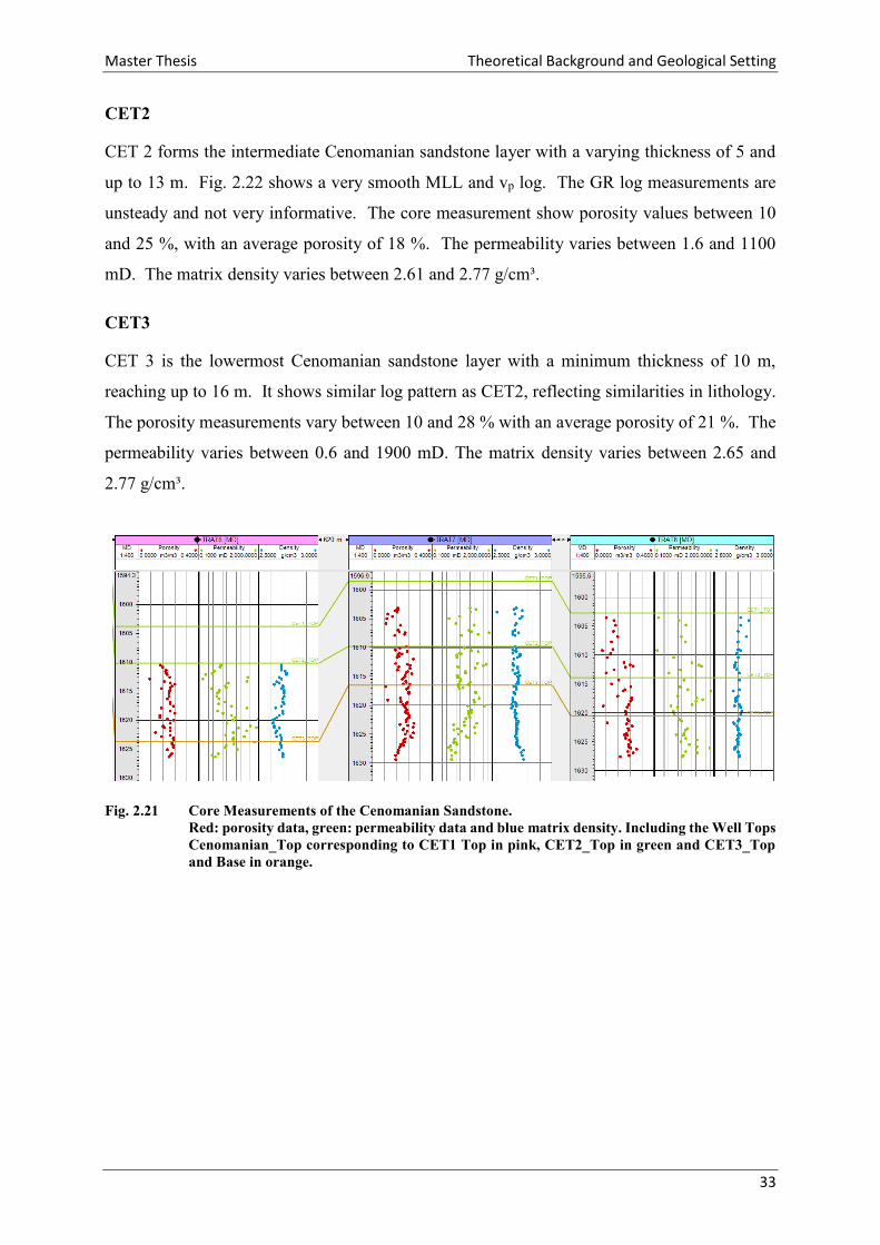
CET2
CET 2 forms the intermediate Cenomanian sandstone layer with a varying thickness of 5 and
up to 13 m. Fig. 2.22 shows a very smooth MLL and vp log. The GR log measurements are
unsteady and not very informative. The core measurement show porosity values between 10
and 25 %, with an average porosity of 18 %. The permeability varies between 1.6 and 1100
mD. The matrix density varies between 2.61 and 2.77 g/cm³.
CET3
CET 3 is the lowermost Cenomanian sandstone layer with a minimum thickness of 10 m,
reaching up to 16 m. It shows similar log pattern as CET2, reflecting similarities in lithology.
The porosity measurements vary between 10 and 28 % with an average porosity of 21 %. The
permeability varies between 0.6 and 1900 mD. The matrix density varies between 2.65 and
2.77 g/cm³.
Fig. 2.21 Core Measurements of the Cenomanian Sandstone.
Red: porosity data, green: permeability data and blue matrix density. Including the Well Tops
Cenomanian_Top corresponding to CET1 Top in pink, CET2_Top in green and CET3_Top
and Base in orange.
Master Thesis Theoretical Background and Geological Setting
34
Fig. 2.22 Well log measurements of the Cenomanian Sandstone.
The left column shows sonic measurements in black, gamma ray log in green and the black
dotted caliper log. Resitivity measurements in the right column. Including the Well Tops
Cenomanian_Top corresponding to CET1 Top in pink, CET2_Top in green and CET3_Top
and Base in orange.
Master Thesis Dataset
35
3 DATASET
Within a university-industry corporation, RAG provided their Trattnach dataset including a
70 km² seismic cube and data of 16 wells including log measurements. To simplify the initial
stages of the reservoir model setup, RAG further provided their static geological model, which
covers the Cenomanian reservoir. The first step was the collection of information, to get an
overview of available data, followed by data organization, with the aim to extract all useful data
for a proper model setup. The focus lies on data usable for the calculation of elastic parameters,
such as density, porosity and compressional and shear wave velocities. The second part are the
faults and interpreted or modelled horizons, those build the basic framework for the
geomechanical model setup.
3.1 DATA REVIEW AND ORGANIZATION
3.1.1 Well Data
The well data includes all available wells and their corresponding well measurements, as well
as calculated well data. Fifteen wells are available, eleven are drilled into the main Trattnach
field, two wells target the Trattnach Nord field and the Weinberg and Gaspoldshofen well cover
the area close to the Gaspoldshofen fault.
Existing well measurements cover the most frequent geophysical logs:
Gamma ray (GR), spontaneous potential (SP) and sonic log (Δt) are available for all
wells. The reservoir section has a good data quality, the logs show big gaps beginning
from Turonian levels up to the surface.
Resistivity logs, include Induction, Conduction, Micrologs and Laterologs.
Occasionally they cover the entire well track, but mostly confine to the Cenomanian and
Eocene part.
Six wells have a neutron porosity log (NPHI), only the two wells drilled into Trattnach
North have a density log (RHOB)
The lack of shear wave logs and the low data density of RHOB logs are compensated by manual
calculation, based on petrophysical principals (see chapter 5.2).
One aim is the setup of a proper well section window, for further interpretation and quality
control of picked well tops. To accomplish this all logging measurements are categorized,

Master Thesis Dataset
36
systematically named and combined. Now the GR track represents all available gamma ray
measurements for all wells. This applies for sonic, density, spontaneous potential, neutron and
all resistivity logs. Additionally, all well tops are renamed and organized according to the
stratigraphic chart seen in Fig. 2.17, all stages and lithostratigraphic formations are located in
subfolders corresponding to their age and are labelled accordingly. Mostly the well tops show
a higher resolution, than the stratigraphic chart, like the zone of the Innviertel Group, which
contains five subgroups.
3.1.2 Core Data
Core measurements were performed by RAG, the data includes porosity, permeability,
saturation and matrix density measurements. All results are linked to their corresponding wells.
Additionally all coring reports were available, containing all performed core measurements and
a detailed core description.
3.1.3 Model Data
The provided reservoir model includes four Petrel models. A geological model built by
Montanuniversitaet Leoben (Chair Petroleum Geology), a geological model built by RAG and
two Reservoir Models built by RAG.
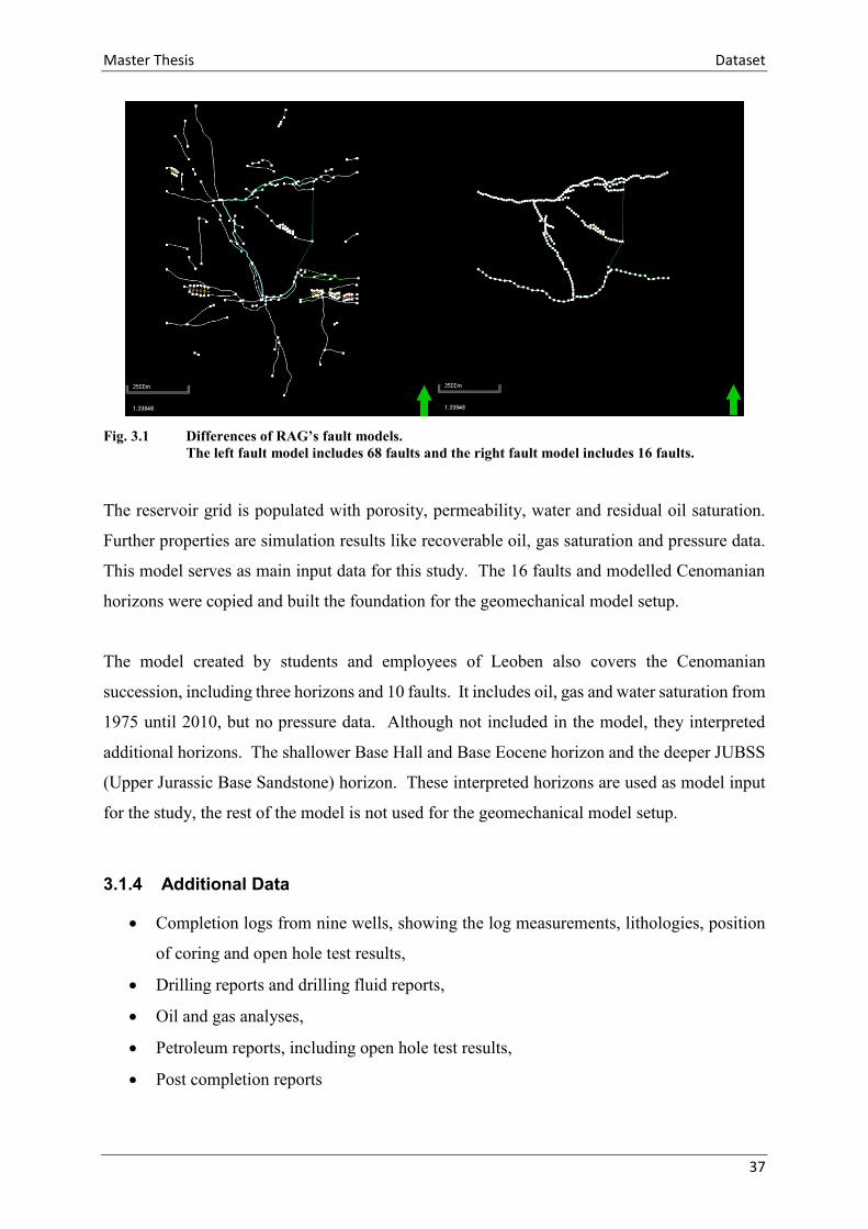
The static model from RAG covers the Cenomanian sandstones, including four horizons: Top
CET1, 2 and 3, as well as Base CET3. The fault model includes 68 faults. The grid contains
bulk volume, porosity and permeability data. This model forms the foundation for RAG’s
reservoir model, but no actual data was used during this study.
RAG’s reservoir model is based on their static model, therefore the geographic extent and
number of horizons are equal. The fault model contains just 16 faults, the difference of the fault
models can be seen in Fig. 3.1, with the bigger fault model on the left-hand side and the
simplified fault model on the right-hand side.
Master Thesis Dataset
37
Fig. 3.1 Differences of RAG’s fault models.
The left fault model includes 68 faults and the right fault model includes 16 faults.
The reservoir grid is populated with porosity, permeability, water and residual oil saturation.
Further properties are simulation results like recoverable oil, gas saturation and pressure data.
This model serves as main input data for this study. The 16 faults and modelled Cenomanian
horizons were copied and built the foundation for the geomechanical model setup.
The model created by students and employees of Leoben also covers the Cenomanian
succession, including three horizons and 10 faults. It includes oil, gas and water saturation from
1975 until 2010, but no pressure data. Although not included in the model, they interpreted
additional horizons. The shallower Base Hall and Base Eocene horizon and the deeper JUBSS
(Upper Jurassic Base Sandstone) horizon. These interpreted horizons are used as model input
for the study, the rest of the model is not used for the geomechanical model setup.
3.1.4 Additional Data
Completion logs from nine wells, showing the log measurements, lithologies, position
of coring and open hole test results,
Drilling reports and drilling fluid reports,
Oil and gas analyses,
Petroleum reports, including open hole test results,
Post completion reports
Master Thesis Reservoir Model Setup
38
4 RESERVOIR MODEL SETUP
RAG’s reservoir model covers the Cenomanian succession, including the produced reservoir
units, formed by the green sandstones (CET3, CET2) and the low permeable seal rock (CET1).
For time saving reasons the picked faults as well as the horizons CET1 Top, CET2 Top, CET3
Top and Base are copied from RAG’s reservoir model, by doing this the history match
performed by the reservoir engineer can be used as well. The main object during the model
extension is to keep all changes in the reservoir area as small as possible, so that the history
match of the reservoir simulation, still fits for the new model.
When performing a geomechanical study the whole section from the earth’s surface down to
the crystalline basement is of interest. Therefore, the model extension up to the earth’s surface
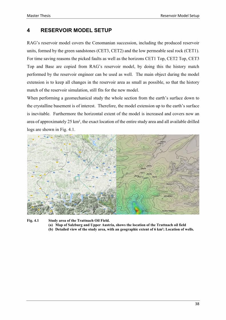
is inevitable. Furthermore the horizontal extent of the model is increased and covers now an
area of approximately 25 km², the exact location of the entire study area and all available drilled
logs are shown in Fig. 4.1.
Fig. 4.1 Study area of the Trattnach Oil Field.
(a) Map of Salzburg and Upper Austria, shows the location of the Trattnach oil field
(b) Detailed view of the study area, with an geographic extent of 6 km²; Location of wells.
Master Thesis Reservoir Model Setup
39
4.1 GRID
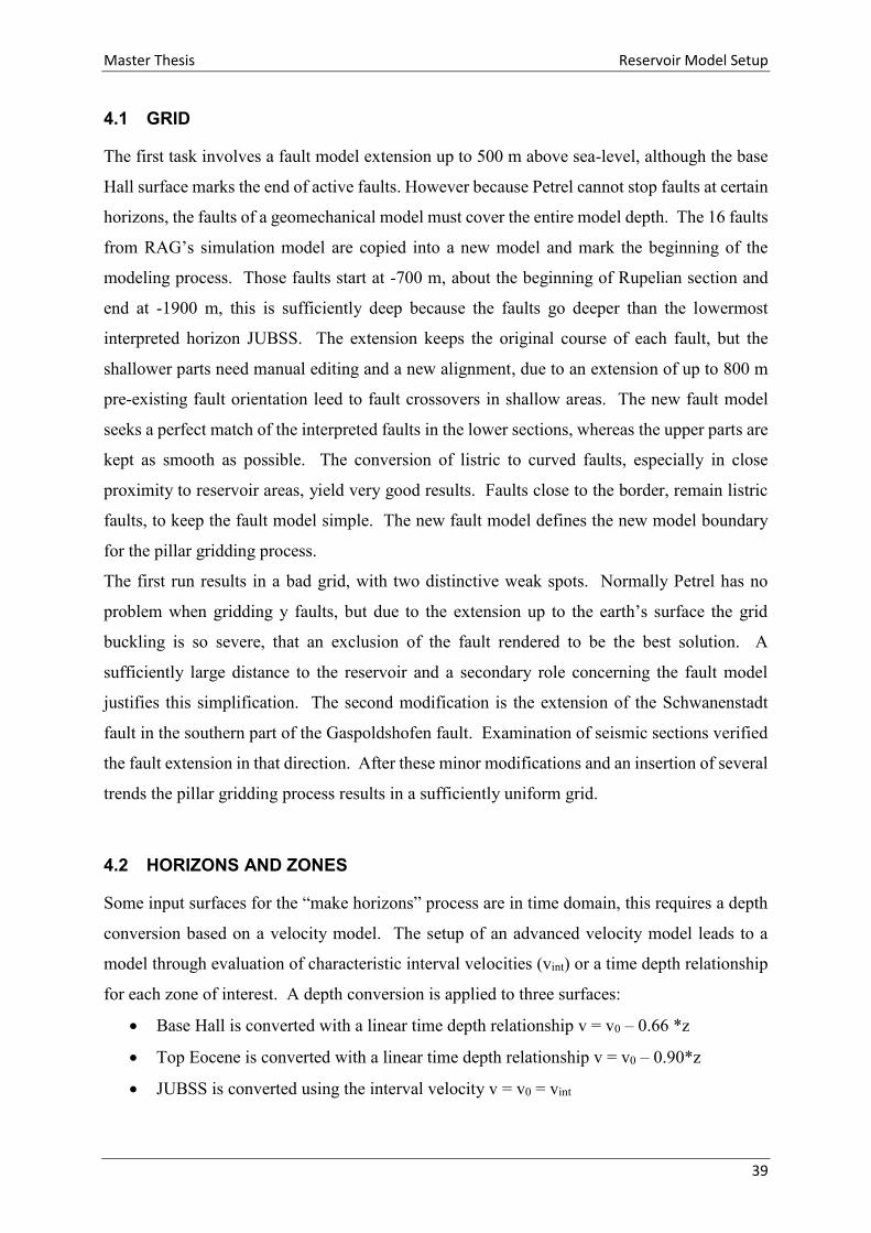
The first task involves a fault model extension up to 500 m above sea-level, although the base
Hall surface marks the end of active faults. However because Petrel cannot stop faults at certain
horizons, the faults of a geomechanical model must cover the entire model depth. The 16 faults
from RAG’s simulation model are copied into a new model and mark the beginning of the
modeling process. Those faults start at -700 m, about the beginning of Rupelian section and
end at -1900 m, this is sufficiently deep because the faults go deeper than the lowermost
interpreted horizon JUBSS. The extension keeps the original course of each fault, but the
shallower parts need manual editing and a new alignment, due to an extension of up to 800 m
pre-existing fault orientation leed to fault crossovers in shallow areas. The new fault model
seeks a perfect match of the interpreted faults in the lower sections, whereas the upper parts are
kept as smooth as possible. The conversion of listric to curved faults, especially in close
proximity to reservoir areas, yield very good results. Faults close to the border, remain listric
faults, to keep the fault model simple. The new fault model defines the new model boundary
for the pillar gridding process.
The first run results in a bad grid, with two distinctive weak spots. Normally Petrel has no
problem when gridding y faults, but due to the extension up to the earth’s surface the grid
buckling is so severe, that an exclusion of the fault rendered to be the best solution. A
sufficiently large distance to the reservoir and a secondary role concerning the fault model
justifies this simplification. The second modification is the extension of the Schwanenstadt
fault in the southern part of the Gaspoldshofen fault. Examination of seismic sections verified
the fault extension in that direction. After these minor modifications and an insertion of several
trends the pillar gridding process results in a sufficiently uniform grid.
4.2 HORIZONS AND ZONES
Some input surfaces for the “make horizons” process are in time domain, this requires a depth
conversion based on a velocity model. The setup of an advanced velocity model leads to a
model through evaluation of characteristic interval velocities (vint) or a time depth relationship
for each zone of interest. A depth conversion is applied to three surfaces:
Base Hall is converted with a linear time depth relationship v = v0 – 0.66 *z
Top Eocene is converted with a linear time depth relationship v = v0 – 0.90*z
JUBSS is converted using the interval velocity v = v0 = vint

Master Thesis Reservoir Model Setup
40
With v0 being the velocity, in m/s, at the top of each zone and z the depth in meters.
Subsequently all input surfaces are available in depth domain. Including the four Cenomanian
surfaces and earth surface, a total of eight surfaces are interpolated along the new grid boundary
defined by the fault model. As a result, all input surfaces have the same area of approximately
25 km².
4.2.1 Horizon modeling
Conversion of these surfaces into horizons, maintains the original structure and location, but
links them to the grid and its comprising faults. Linking faults and horizons allows the
determination of fault cut back, this is a manipulation of offset distances or how much drag is
allowed for a certain fault. The surface to horizon conversion involves multiple horizon
cross-overs in areas of low data density, especially for the Cenomanian horizons which are
separated by very little distances. In a second run a step by step approach resultes in a very
good horizon model. Beginning with the creation of the CET1_Top horizon and stacking of
the CET1 thickness maps beneath, marking the technical start of the CET2 horizon. By doing
this, the horizon fault lines at the base of zone CET1, which fit perfectly to those of CET2_Top,
can be stored and used as an additional input for the second run of CET2_Top horizon creation.
All Cenomanian horizons are created by using this method. Due to the lack of convenient well
tops for the JUBSS horizon, a thickness map creation is not possible and consequently stacking
is no option for the lower model part. The vertical distance between JUBSS and CET3_Base
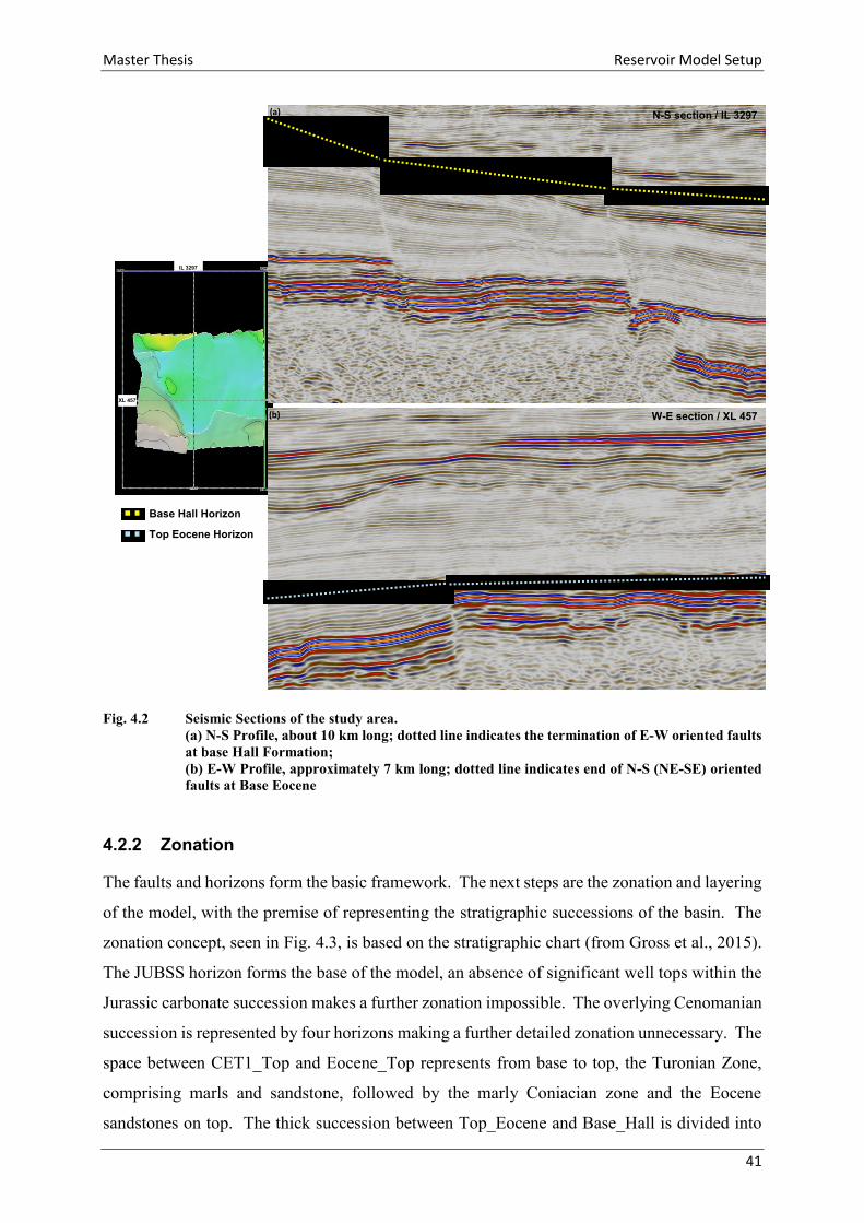
is sufficiently large, so there are no horizon crossovers present. Fig. 4.2 (b) shows that the NW-
SE trending faults stop at the Base Eocene horizon, so stacking Top Eocene succession on top
of the CET1 horizon cannot be performed. Both Cenozoic horizons, Top_Eocene and
Base_Hall are created via the conventional workflow. Summarizing, the Mesozoic horizons
are characterized by two different faulting regimes, one in NW-SE direction and a second in E-
W direction. The Eocene Horizon is displaced by E-W oriented faults, whereas the Base_Hall
and Surface horizons have no active faults (Fig. 4.2).
Master Thesis Reservoir Model Setup
41
Fig. 4.2 Seismic Sections of the study area.
(a) N-S Profile, about 10 km long; dotted line indicates the termination of E-W oriented faults
at base Hall Formation;
(b) E-W Profile, approximately 7 km long; dotted line indicates end of N-S (NE-SE) oriented
faults at Base Eocene
4.2.2 Zonation
The faults and horizons form the basic framework. The next steps are the zonation and layering
of the model, with the premise of representing the stratigraphic successions of the basin. The
zonation concept, seen in Fig. 4.3, is based on the stratigraphic chart (from Gross et al., 2015).
The JUBSS horizon forms the base of the model, an absence of significant well tops within the
Jurassic carbonate succession makes a further zonation impossible. The overlying Cenomanian
succession is represented by four horizons making a further detailed zonation unnecessary. The
space between CET1_Top and Eocene_Top represents from base to top, the Turonian Zone,
comprising marls and sandstone, followed by the marly Coniacian zone and the Eocene
sandstones on top. The thick succession between Top_Eocene and Base_Hall is divided into
2500 m
IL 3297
XL 457
(a)
(b)
N-S section / IL 3297
W-E section / XL 457
Base Hall Horizon
Top Eocene Horizon
Master Thesis Reservoir Model Setup
42
the Fish shale or Schöneck Formation, on top of the Eocene, followed by the Rupelian zone,
including the source rocks of the Dynow and Eggerding. Further on top is the Puchkirchen
Group, which is separated into a Lower and Upper Puchkirchen Formation. The uppermost
interval consists of the Hall Formation at the base and the Innviertel Group on top. The top is
formed by the earth’s surface, an erosional horizon. The combination of horizons and zones
represents the lithostratigraphy of the basin.
4.3 LAYERING
The last step of the setup of the static reservoir model is layering, where a characteristic pattern,
representing the prevailing sequence stratigraphic type, is assigned to each zone, or horizon
interval. There are four different styles of layering available: proportional, follow top or base
and fractions. Due to restrictions for the Cenomanian interval, to keep the changes as minimal
as possible, the layering is an identical adaption of RAG’s reservoir layering. Zone CET_1 has
a fractioning of 1-1-1, resulting in a zone trisection with equally big grid cells, zone CET_2
shows an asymmetric trisection of 1-2-2, with a smaller upper layer and two bigger bottom
layers and CET_3 is divided into two thinner upper layers and one thicker bottom layers 1-1-2.
This layering fits the lithostratigraphy perfectly. CET1 comprises of calcareous sandstones and
conglomerates with an up to 2 m thick red marker bed at the bottom. CET2 and CET3 are
lithologically relatively similar, consisting of glauconite rich fine-grained sandstone, some silt
layers and medium grained sandstone. The boundary between CET2 and CET3 is formed by a
thin well cemented coarse-grained sandstone, showing high resistivity and low DT readings.
According to the seismic section presented in Fig. 4.3 the layering of the Innviertel Zone is
proportional, the layering of the Hall Formation follows the top horizon with onlaps on the base,
the same applies for the Upper Puchkirchen Formation. The lower Puchkirchen Formation has
toplaps, accordingly a follow base layering was chosen. The remaining JUBSS, Turon,
Coniacian, Rupelian and Eocene zones have a proportional layering.

Master Thesis Reservoir Model Setup
43
Fig. 4.3 Grid Slice, final zonation and layering.
The zones show the most prominent stratigraphic sections according to Fig. 2.16 and 2.18. The
layering reflects seismic patterns of each zone.

Master Thesis Geomechanical Model
44
5 GEOMECHANICAL MODEL
5.1 CREATING A GEOMECHANICAL GRID
The main function of geomechanical gridding is the embedding of the reservoir model with
side-, over- and underburden grid cells to enable a smooth geomechanical simulation.
5.1.1 Settings
Depending on the vertical and horizontal extent of the reservoir model several considerations
must be taken into account. Most important is a model aspect ratio of 3:1, which implies 1 km
depth for every 3 km of horizontal extent (Schlumberger, 2015). Adjustment to fulfil this
requirement is done through sideburden and underburden settings. Mostly because the
underburden has no depth limits, all additional unrealistic underburden is considered as stiff
bedrock. In contrast the overburden is limited by the earth’s surface which forms the uppermost
boundary. Depending on the reservoir model extent, two embedding methods are available:
1 Models which already reach earth’s surface need no additional overburden and the
embedding process is reduced to side- and underburden modeling. An advantage of
this embedding process is the possibility to make a more realistic replication of the
present basin geology. A possible disadvantage is that these models can have a
complex grid and need a further simplification in some areas to fulfil the
requirements of a geomechanical grid. The model described in chapter 2.2 is such
a model and the simplification and editing process is described in chapter 5.1.2.
2 Models which cover just the most important parts of the reservoir model, like the
reservoir section and adjacent zones. These models can then be embedded with an
over-, under- and sideburden.
Sideburden
When building a sideburden, the number of grid cells and the way the sideburden cells should
be created must be chosen. Two options are available, either the cells are created by extend by,
for example 1000 m to the left and right hand side of the reservoir model or by multiply by, for
example the sideburden should be 3 times the reservoir grid on both sides (Schlumberger,
2015).
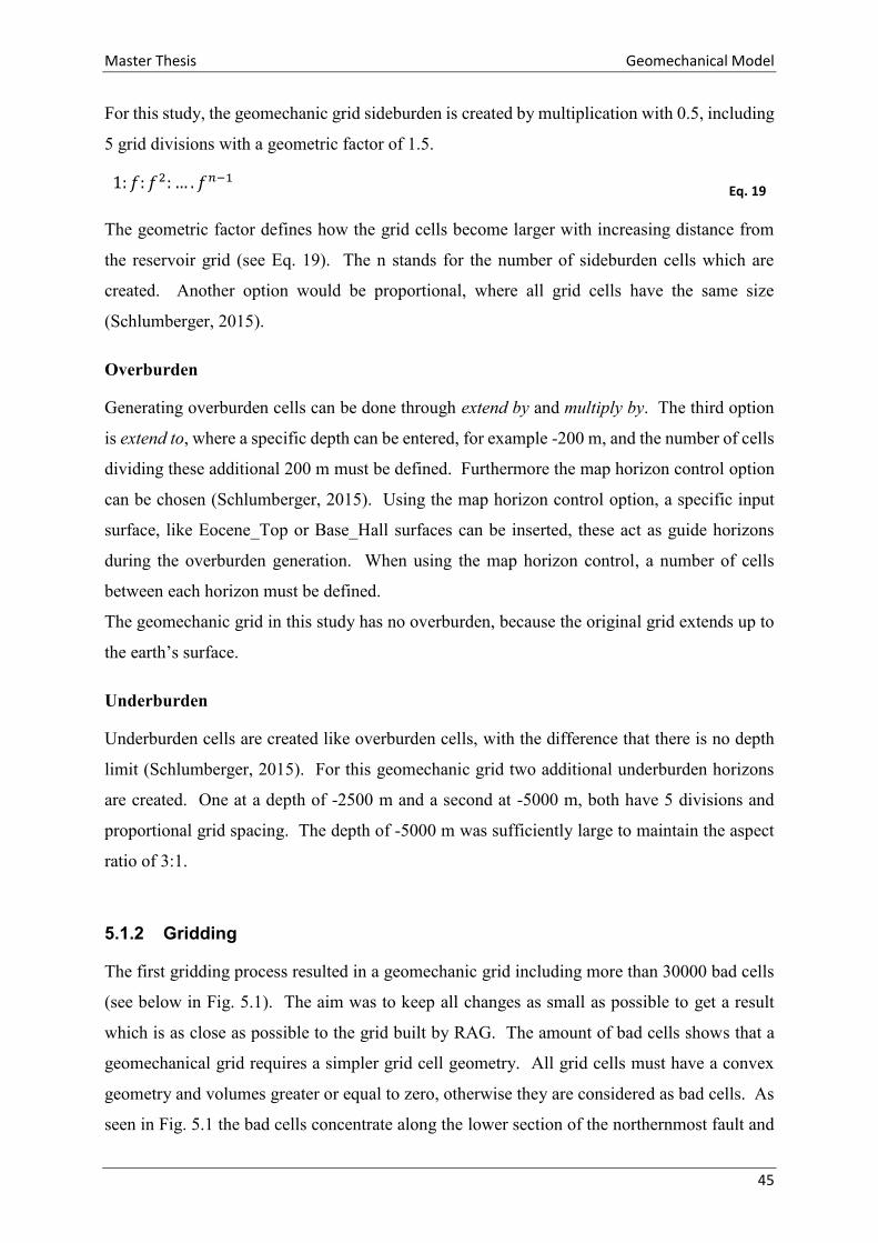
Master Thesis Geomechanical Model
45
For this study, the geomechanic grid sideburden is created by multiplication with 0.5, including
5 grid divisions with a geometric factor of 1.5.
1: 𝑓: 𝑓2: … . 𝑓𝑛−1 Eq. 19
The geometric factor defines how the grid cells become larger with increasing distance from
the reservoir grid (see Eq. 19). The n stands for the number of sideburden cells which are
created. Another option would be proportional, where all grid cells have the same size
(Schlumberger, 2015).
Overburden
Generating overburden cells can be done through extend by and multiply by. The third option
is extend to, where a specific depth can be entered, for example -200 m, and the number of cells
dividing these additional 200 m must be defined. Furthermore the map horizon control option
can be chosen (Schlumberger, 2015). Using the map horizon control option, a specific input
surface, like Eocene_Top or Base_Hall surfaces can be inserted, these act as guide horizons
during the overburden generation. When using the map horizon control, a number of cells
between each horizon must be defined.
The geomechanic grid in this study has no overburden, because the original grid extends up to
the earth’s surface.
Underburden
Underburden cells are created like overburden cells, with the difference that there is no depth
limit (Schlumberger, 2015). For this geomechanic grid two additional underburden horizons
are created. One at a depth of -2500 m and a second at -5000 m, both have 5 divisions and
proportional grid spacing. The depth of -5000 m was sufficiently large to maintain the aspect
ratio of 3:1.
5.1.2 Gridding
The first gridding process resulted in a geomechanic grid including more than 30000 bad cells
(see below in Fig. 5.1). The aim was to keep all changes as small as possible to get a result
which is as close as possible to the grid built by RAG. The amount of bad cells shows that a
geomechanical grid requires a simpler grid cell geometry. All grid cells must have a convex
geometry and volumes greater or equal to zero, otherwise they are considered as bad cells. As
seen in Fig. 5.1 the bad cells concentrate along the lower section of the northernmost fault and
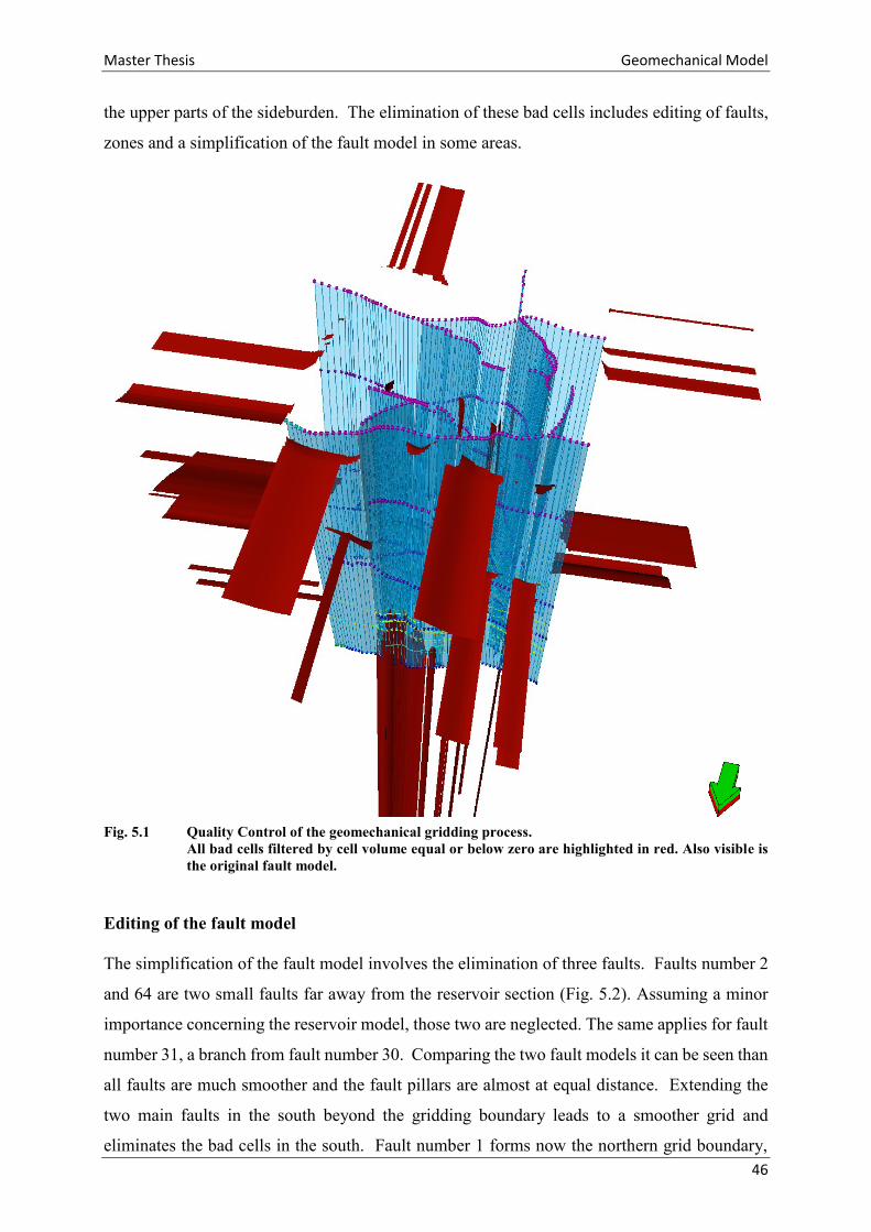
Master Thesis Geomechanical Model
46
the upper parts of the sideburden. The elimination of these bad cells includes editing of faults,
zones and a simplification of the fault model in some areas.
Fig. 5.1 Quality Control of the geomechanical gridding process.
All bad cells filtered by cell volume equal or below zero are highlighted in red. Also visible is
the original fault model.
Editing of the fault model
The simplification of the fault model involves the elimination of three faults. Faults number 2
and 64 are two small faults far away from the reservoir section (Fig. 5.2). Assuming a minor
importance concerning the reservoir model, those two are neglected. The same applies for fault
number 31, a branch from fault number 30. Comparing the two fault models it can be seen than
all faults are much smoother and the fault pillars are almost at equal distance. Extending the
two main faults in the south beyond the gridding boundary leads to a smoother grid and
eliminates the bad cells in the south. Fault number 1 forms now the northern grid boundary,
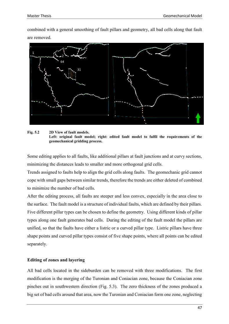
Master Thesis Geomechanical Model
47
combined with a general smoothing of fault pillars and geometry, all bad cells along that fault
are removed.
Fig. 5.2 2D View of fault models.
Left: original fault model; right: edited fault model to fulfil the requirements of the
geomechanical gridding process.
Some editing applies to all faults, like additional pillars at fault junctions and at curvy sections,
minimizing the distances leads to smaller and more orthogonal grid cells.
Trends assigned to faults help to align the grid cells along faults. The geomechanic grid cannot
cope with small gaps between similar trends, therefore the trends are either deleted of combined
to minimize the number of bad cells.
After the editing process, all faults are steeper and less convex, especially in the area close to
the surface. The fault model is a structure of individual faults, which are defined by their pillars.
Five different pillar types can be chosen to define the geometry. Using different kinds of pillar
types along one fault generates bad cells. During the editing of the fault model the pillars are
unified, so that the faults have either a listric or a curved pillar type. Listric pillars have three
shape points and curved pillar types consist of five shape points, where all points can be edited
separately.
Editing of zones and layering
All bad cells located in the sideburden can be removed with three modifications. The first
modification is the merging of the Turonian and Coniacian zone, because the Coniacian zone
pinches out in southwestern direction (Fig. 5.3). The zero thickness of the zones produced a
big set of bad cells around that area, now the Turonian and Coniacian form one zone, neglecting
31
64
21

Master Thesis Geomechanical Model
48
the Turonian sandstone at the border to the Coniacian, for further calculations the whole zone
is considered as marl.
Fig. 5.3 Thickness map Coniacian.
The second modification involves the change of layering, as seen and described in chapter 4.3,
the layering of the Innviertel Group is “follow surface”, Hall Formation and Upper Puchkirchen
Formation have a “follow top” layering and the Lower Puchkirchen Formation “follow base”.
All of these layering options lead to onlaps or offlaps on the border to the adjacent zone.
Reservoir Geomechanics does not support that kind of layering, because the resulting grid cells
do not fulfil the requirements of volume greater than zero and convex geometry. Therefore the
layering of those four zones is changed to a proportion layering. The last modification is the
adjustment of the gridding boundary, resulting in more orthogonal grid cells.
Fig. 5.4 and Fig. 5.5 show the final geomechanic grid including the detailed reservoir grid at
the centre and the embedded area, formed by side- and underburden. The original grid has a
horizontal extent of approximately 6 x 6 km and it is extended by 3 km of sideburden in each
direction. The vertical extent of the model (see yellow section in Fig. 5.5) reaches up to 680 m
above sea level and ends at the JUBSS horizon at a maximum depth of -1800m. The
underburden starts at the JUBSS horizon and ends at a depth of -5000 m. The geomechanic
grid has no overburden, because the original grid extends up to the earth’s surface. It can be
seen that the grid cell size increases with distance to the original grid, this reduces the needed
computer power for further simulations.
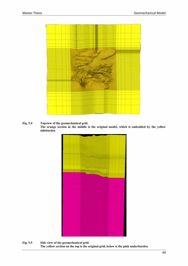
Master Thesis Geomechanical Model
49
Fig. 5.4 Topview of the geomechanical grid.
The orange section in the middle is the original model, which is embedded by the yellow
sideburden
Fig. 5.5 Side view of the geomechanical grid.
The yellow section on the top is the original grid, below is the pink underburden

Master Thesis Geomechanical Model
50
5.2 PROPERTY MODELING
The geomechanical gridding process is followed by material modeling. During this process
one can either choose materials from the material library included in the software or define
characteristic materials based on the basin´s lithology and its different elastic moduli and
strength properties. Calculating the elastic properties requires density, porosity and velocity
information for all available lithologies or zones. The dataset included density logs for two
wells and no shear sonic logs. Porosity data is available for the reservoir sections including
NPHI logs and core measurements. Therefore a property modeling of all missing data is
performed, to allow the calculation of elastic properties and the setup of rock specific materials
for the entire extent of the model.
The property modeling includes calculation of density data based on Gardner’s equation
(Gardner et al., 1974), the computation of porosity logs with Wyllie’s time average equation
(Wyllie et al., 1956) and the calculation of shear sonic logs using Castagna’s and Han’s
empirical vp – vs relationships (Castagna et al., 1985; Castagna, 1993; Han et al., 1986).
5.2.1 Density Data
The fact that the elastic modulus of a rock is calculated by multiplying the velocity and density,
makes density logs inevitable for the calculation of elastic moduli. Unfortunately, only the
TRAT 11 and TRAT 12 wells have density logs and even those do not cover the entire drilled
depth.
The missing density logs were calculated through Gardner´s empirical relationship published
in 1974 (Gardner et al., 1974).
A zone log, which represents the final zonation during the pillar gridding process (Fig. 4.3) is
created and the velocity and density data for each zone extracted. To gain the linear vp-RHOB
function, the extracted vp and RHOB data is plotted for each zone separately. Data for the Hall
and Upper Puchkirchen Formation is taken from well TRAT 11, plotted in Fig. 5.6, all other
available data is taken from well TRAT 12 (see Fig. 5.7). Before plotting the velocities versus
densities, a log conditioning was performed. It included removal of spikes and smoothing of
certain areas with inconsistent data. These smoother density and velocity logs are used to
determine the linear relationship.
The empirical constants a and b are delogarithmized for each zone (see Table 5.1 for results).
Knowing a and b, the density logs for all other wells are calculated using Gardner´s equation.
𝛒 = 𝐚 ∗ 𝐯𝐩𝐛 Eq. 20

Master Thesis Geomechanical Model
51
Due to gaps in the density logs the construction of an empirical relationship was not possible
for the Innviertel Group, Lower Puchkirchen Formation and the Rupelian. Based on similarities
in lithology the following assumptions have been made: Innviertel Group is comparable to Hall
Formation, therefore the empirical relationship of the Hall Formation is applied for the
Innviertel Group. The Upper Puchkirchen Formation is a good fit for the Lower Puchkirchen
Formation and the Eocene function is applied to calculate the density of the Rupelian.
Equation Linear Relationship a b
Hall Formation log(Y) = 0.170032 * log(X) - 0.218061 2.02 0.14
Upper Puchkirchen log(Y) = 0.27461 * log(X) - 0.572581 1.78 0.27
Fish Shale log(Y) = 0.123935 * log(X) + 0.326994 2.12 0.12
Eocene log(Y) = 0.409155 * log(X) + 0.135206 1.37 0.41
Coniacian log(Y) = 0.0919171 * log(X) + 0.356692 2.27 0.09
Turon log(Y) = 0.257638 * log(X) + 0.267475 1.85 0.26
CET1 log(Y) = 0.0997267 * log(X) + 0.347347 2.23 0.10
CET2 log(Y) = 0.440732 * log(X) + 0.134828 1.36 0.44
CET3 log(Y) = 0.198046 * log(X) + 0.272713 1.87 0.20
JUBSS log(Y) = 0.661397 * log(X) - 0.0201822 0.63 0.66
Table 5.1 Gardner’s empirical vp – density Relationship.
Fig. 5.6 Empirical Relationship between vp and RHOB from TRAT11.
Linear relationship and function for the (a) Hall Formation and the (b) Upper Puchkirchen
Formation
(a) (b)
log(Y) = 0.170032 * log(X) - 0.218061 log(Y) = 0.27461 * log(X) - 0.572581

Master Thesis Geomechanical Model
52
Fig. 5.7 Empirical Relationship between vp and RHOB from TRAT12.
Linear relationship and function for the (a) Fish shale, (b) Eocene, (c) Coniacian, (d) Turonian,
(e) CET1, (f) CET2, (g) CET3 and (h) JUBSS
(a) (b)
(c) (d)
(e) (f)
(g) (h)
log(Y) = 0.123935 * log(X) + 0.326994
log(Y) = 0.0997267 * log(X) + 0.347347
log(Y) = 0.198046 * log(X) + 0.272713
log(Y) = 0.0919171 * log(X) + 0.356692
log(Y) = 0.409155 * log(X) + 0.135206
log(Y) = 0.440732 * log(X) + 0.134828
log(Y) = 0.257638 * log(X) + 0.267475
log(Y) = 0.661397 * log(X) - 0.0201822

Master Thesis Geomechanical Model
53
Gardner’s equation, Eq. 20, is applied to each zone for all wells. The calculated density logs
are shown in Fig. 5.8 and the equation for each zone is shown in appendix 10.1 “Density
Calculation”. The gaps in TRAT2, 3 and 4 are a result of missing sonic velocity measurements,
because without velocity information Gardner’s relationship cannot be applied. Nevertheless
all other wells have continuous sonic logs and allow the calculation of density for the Upper
and Lower Puchkirchen Formations, which is later interpolated over the area of TRAT2,
TRAT3 and TRAT4.
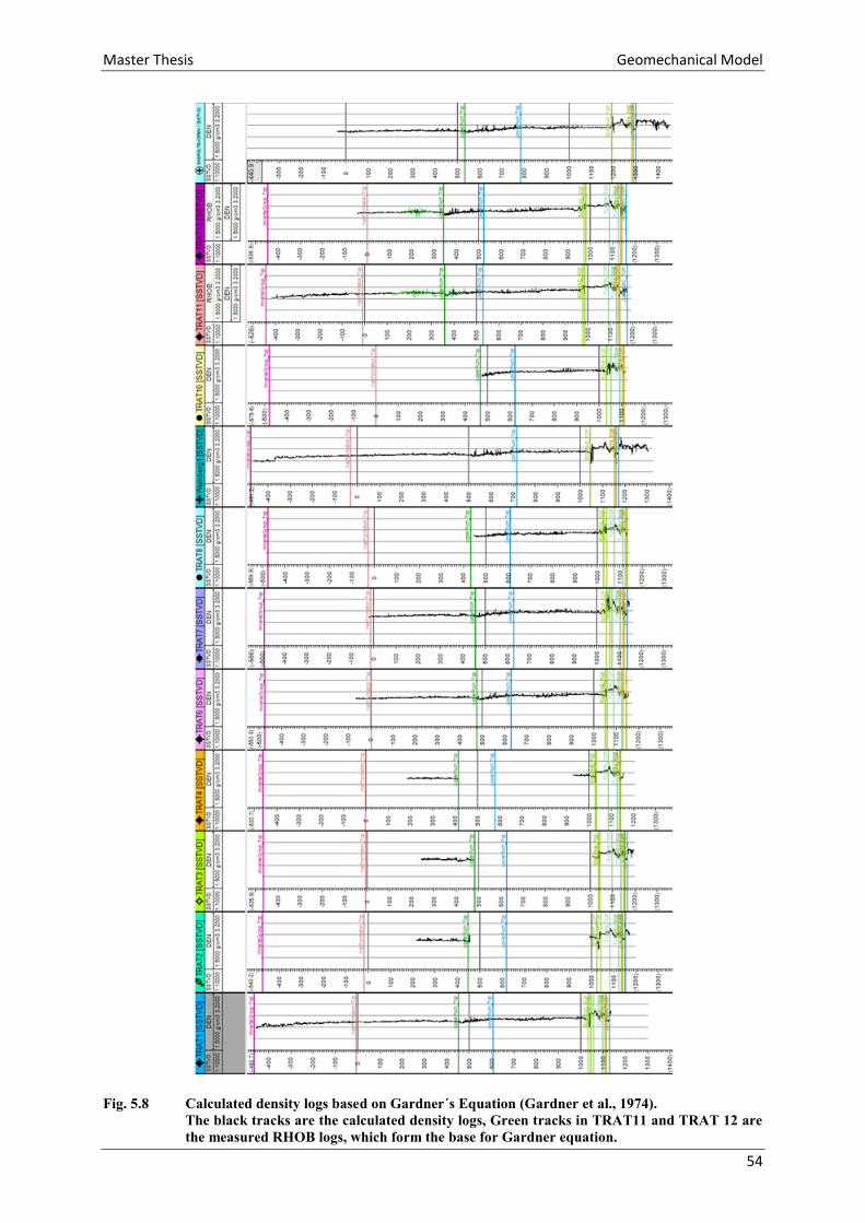
Master Thesis Geomechanical Model
54
Fig. 5.8 Calculated density logs based on Gardner´s Equation (Gardner et al., 1974).
The black tracks are the calculated density logs, Green tracks in TRAT11 and TRAT 12 are
the measured RHOB logs, which form the base for Gardner equation.
Master Thesis Geomechanical Model
55
The density logs are important for the calculation of lithostatic gradients. Multiplying the rock
density (kg/m³) times the acceleration due to gravity (9.8 m/s²) over a depth interval gives the
overburden pressure. The sampling interval of 0.15 m is used as depth interval. The resulting
pressures for each depth interval are summed up to the lithostatic gradient (red curve in Fig.
5.9). The conversion factor from Pascal (Pa) to bar is 10-5. The hydrostatic gradient (blue line)
is calculated by multiplying the water density (kg/m³) times the acceleration due to gravity (9.8
m/s²) and depth. The hydrostatic gradient represents the pore pressure of interconnected pores
up to the earth´s surface. The pressure data plotted for water, oil, gas and mixtures of oil and
water are measurements from open hole tests.
Fig. 5.9 Pressure gradients for the Trattnach field.
The red line is the lithostatic gradient, the blue line the hydrostatic gradient. The green data
point is the pressure from an open hole test (OHT) of the gas bearing Hall Formation. The oil
and water pressure data is also from OHTs in Eocene, Turonian, Cenomanian and Jurassic
units.
0
200
400
600
800
1000
1200
1400
1600
1800
0 50 100 150 200 250 300 350 400
Dep
th [
m]
Pressure [bar]
gas
water
oil
oil&water
Hydrostatic Gradient
Lithostatic Gradient
Master Thesis Geomechanical Model
56
5.2.2 Porosity
Core porosity measurements exist for the reservoir succession. The Cenomanian sandstones
are a relatively thin lithologic unit, resulting in a relatively flat velocity – porosity trend. In Fig.
5.10 the measured core porosities from all wells are plotted against compressional velocities.
The usual trend of decreasing velocity with increasing porosity is not visible, but looking at the
different formation, CET2 and CET3 show a much clearer trend than CET1. An explanation is
the higher clay content in CET1, which causes a scatter around the velocity – porosity trend
(Avseth et al., 2005).
Fig. 5.10 Velocity – porosity trend for Cenomanian reservoir sandstones.
The data includes core porosity measurements from all wells. Nearly horizontal velocity –
porosity trends are observed for all three Cenomanian sandstone units.
Calculating the shear velocities of sandstones requires porosity data. The reservoir sections
have core porosity measurements, whereas the other sections lack in porosity measurements.
Wyllies time – average equation is used to calculate the porosity from sonic measurements
(Wyllie et al., 1956). The apparent porosity (ϕw) is calculated by dividing the compressional
wave slowness of the porous rock (Δtp) and the matrix material (Δtp,ma) by the slowness of the
fluid (Δtfl) present in the pore space and the matrix material. This is a heuristic equation and
the best fit is achieved for water saturated and well compacted sandstones. When applied to
unconsolidated sandstones, Wyllie’s time average porosities are overestimated. To compensate
for these optimistic porosities a lack of compaction correction factor (Cp) is applied (Eq. 22).
This factor ranges between 1.0 and 1.8 for Δt values in µs/ft and is calculated by dividing the
sonic transit time in shales (Δtshale) by 100 (Raymer et al., 1980).
CET 1
CET 2
CET 3

Master Thesis Geomechanical Model
57
𝛟𝒘 = 𝚫𝐭𝐩 − 𝚫𝐭𝐩,𝐦𝐚
𝚫𝐭𝐟𝐥 − 𝚫𝐭𝐩,𝐦𝐚
Eq. 21
𝛟𝐜 = 𝛟𝐰 ∗ 𝟏
𝐂𝐩
Eq. 22
𝐂𝐩 =𝚫𝐭𝐬𝐡𝐚𝐥𝐞
𝟏𝟎𝟎 Eq. 23
The compressional wave slowness of the porous rock (Δtp) is available as a logging
measurement. Literature values (Table 5.2) are used for compressional slowness of the matrix
material (Δtp,ma) and of the pore fluid (Δtfl). For all formations the fluid is treated as saltwater
mud filtrate with Δtfl = 607 µs/m (after Schoen, 2004).
Values from (Rider et al., 2011) Values from (Schoen, 2004)
Lithology Range for Δtp,ma
[µs/m] Lithology
Value for Δtp,ma
[µs/m]
Sandstone (φ 5-20%) 167 - 187 Sandstone φ > 10 % 182
Limestone (φ 5-20%) 155 - 173 Sandstone φ < 10 % 168
Shale 205 - 548
Saltwater 541 - 656
Table 5.2 Sonic matrix compressional slowness (after Rider et al., 2011; Schoen, 2004).
Sandstones with a porosity greater than 10 % have a Δtp,ma of 182 µs/m, those with a porosity
smaller than 10 % have lower matrix slowness 168 µs/m. The Innviertel Group and the Hall
Formation contain a mixture of shale and sand, the porosity is calculated with a matrix slowness
of 200 µs/m. For the two Puchkirchen formations a matrix slowness of 210 µs/m is used, this
reflects the increasing shale content compared to the two uppermost formations.
The Lithothamnium Limestone porosity is calculated with a matrix slowness of 173 µs/m and
the porosity of the Coniacian and Turonian marls fitted the NPHI logs best with a matrix
slowness of 155 µs/m. The applied time-average equations for each unit are shown in appendix
10.2 “Porosity Calculation”.
A quality control of the porosity data is performed by comparing the calculated porosities with
the laboratory measurements. Porosity measurements on core plugs of the reservoir and seal
rock (CET1, 2 and 3) were performed by RAG (see red dots in Fig. 5.11). The calculated
porosity (black line in the first column) and the core porosities (red dots) show a good
Master Thesis Geomechanical Model
58
correlation. Additionally the permeability (green dots in the second column) of the Cenomanian
succession is displayed. These measurements were performed by RAG during the core analysis
in the 1970s.
Fig. 5.11 Quality control of the calculated porosity logs.
Laboratory measurments (red dots) and the calculated porosity log (black line). Permeability
measurements are displayed as green dots.
The resulting porosity logs for all wells are displayed in Fig. 5.12. The gaps in TRAT2, 3 and
4 are a result of missing sonic measurements. Without sonic logs a porosity calculation using
Wyllies’s time-average equation is not possible.
Master Thesis Geomechanical Model
59
Fig. 5.12 Calculated porosity logs based on Wyllie’s time-average equation (Wyllie et al., 1956).
Master Thesis Geomechanical Model
60
Porosities of the Innviertel Group reach values up to 60 %, because of the highly porous
structure of clay components. The porosity in sedimentary basins is strongly controlled by
compaction and show a nonlinear porosity decrease with depth (Avseth et al., 2005). Meaning
that porosity of sands and shales decreases at shallow depths more rapidly than at greater depths.
This is due to packing changes and grain deformation (Avseth et al., 2005). To consider these
porosity variations with depth, the clay- dependent exponential regression model from (Ramm
et al., 1994) has been applied.
𝛟 = 𝐀 ∗ 𝐞−(𝛂+𝛃∗𝐂𝟏)𝐙 Eq. 24
𝐂𝟏 = 𝐕𝐂𝐥
𝐕𝐪𝐳
Eq. 25
Using Eq. 24 allows the calculation of fitted regression curves for sandstones, shales or mixtures
of both lithologies. The porosity is dependent on an initial porosity (A) at zero depth, the clay
index (C1), depth and two regression coefficients and β, which describe the grain frameworks
compressibility. Sandstones have spherical grains this allows for a denser packing and makes
the grain framework, compared to shales relatively stiff. Shales are very soft and easy to
deform, the initially arbitrary aligned clay particles show a high initial porosity and will
rearrange during compaction. This results in a higher porosity loss for shales during burial
(Avseth et al., 2005). Fig. 5.13 shows the derived porosity depth trends for sandstones, shales
and a mixture of sand and shale. All fits have been performed by the method of least squares
with an iterative change of the parameters of and β. A regression curve is calculated for a
mixture of sand and shale to fit the uppermost interval of the Innviertel Group (red curve ). A
second sand-shale regression curve is fitted to the lower Innviertel Group and the Hall
Formation (yellow curve). The blue curve is fitted to sandstones of the Puchkirchen Group,
Rupelian, Eocene and Mesozoic rocks. The shale line (green) is fitted to the same depth interval
as the sand line.
Master Thesis Geomechanical Model
61
Fig. 5.13 Porosity – depth trend for the Trattnach area.
Sand line in blue, shale line in green and the sand-shale line in red. Well data shows porosity
data, calculated during property modeling.
0,0
0,2
0,4
0,6
0,8
1,0
1,2
1,4
1,6
1 16 31 46 61
Dep
th [
km]
Porosity [%]
Well Data Shale Line
Sand Line Sand-Shale Line
Sand-Shale Line
Innviertel
Group
Hall
Formation
Puchkirchen
Group
Rupelian,
Eocene &
Mesozoic
Rocks
Master Thesis Geomechanical Model
62
5.2.3 Shear velocity data
The dataset provided by RAG contained no shear slowness measurements, but a geomechanical
model requires shear velocity input, otherwise, the calculation of elastic parameters is not
possible. As a solution literature data was used to calculate the shear velocities for each zone.
Table 5.3 shows vp – vs relationships, it is a compilation of various empirical equations. They
were derived by Castagna and Han and are based on Castagna’s “mudrock-line” theory,
developed in (Castagna et al., 1985; Castagna, 1993; Han et al., 1986).
Equation Remarks Reference
vs = 0.8042 * vp - 0.8559 Sandstone (Castagna et al., 1985)
vs = 0.7700 * vp - 0.8674 Shale (Castagna, 1993)
vs = 0.7936 * vp - 0.7868 Shaly Sandstone (Han et al., 1986)
vs = 0.8423 * vp - 1.099 Sandstone, Clay content > 0.25 (Han et al., 1986)
vs = 0.7535 * vp - 0.6566 Sandstone, Clay content < 0.25 (Han et al., 1986)
vs = 0.756 * vp - 0.662 Sandstone, porosity > 0.15 (Han et al., 1986)
vs = 0.853 * vp - 1.137 Sandstone, porosity < 0.15 (Han et al., 1986)
vs = -0.055 * vp2 + 1.017 * vp - 1.031 Limestone (watersaturated) (Castagna, 1993)
vs = 0.5832 * vp – 0.07776 Dolomite (watersaturated) (Castagna, 1993)
Table 5.3 Literature data: vp – vs relationships derived by Han and Castagna (after Schoen, 2004)
Depending on the zone lithology the most suitable equation is applied, some zones contain
various lithology types and these are further divided. The Eocene zone is separated into a lower
sandstone and an upper limestone unit. The Rupelian consists of Fish shale, Dynow limestones
and sandstones. The Turonian sequence is separated into a lower marl unit and an upper
sandstone unit. Castagna’s relationship for shales is applied to all marl lithologies. Table 5.4
shows which equation is applied to which zone and the resulting sonic logs are plotted in Fig.
5.14. For the entire input of the shear sonic calculation see appendix 10.3 “Shear sonic velocity
calculation”. When calculating shear sonic velocities for sandstones, clay content and porosity
data is taken into account, as proposed by (Han et al., 1986), see Table 5.3.
Master Thesis Geomechanical Model
63
Equation Lithology vp - vs Relationship
Innviertel Group Sandstone, Gravel, Shale vs = 0.8423 * vp - 1.099 or vs = 0.7535 * vp - 0.6566
Hall Formation Shale, Turbidites vs = 0.7936 * vp - 0.7868
Upper Puchkirchen Sandstone, Gravel, Shale vs = 0.8423 * vp - 1.099 or vs = 0.7535 * vp - 0.6566
Lower Puchkirchen Sandstone, Gravel, Shale vs = 0.8423 * vp - 1.099 or vs = 0.7535 * vp - 0.6566
Rupelian Marls vs = 0.7700 * vp - 0.8674
Dynow Limestone vs = -0.055 * vp2 + 1.017 * vp - 1.031
Fish Shale Shale vs = 0.7700 * vp - 0.8674
Eocene Limestone vs = -0.055 * vp2 + 1.017 * vp - 1.031
Eocene Sandstone vs = 0.756 * vp - 0.662 or vs = 0.853 * vp - 1.137
Coniacian Marl vs = 0.7700 * vp - 0.8674
Turon Glauconitsandstone vs = 0.756 * vp - 0.662 or vs = 0.853 * vp - 1.137
Turon Marl vs = 0.7700 * vp - 0.8674
Cet1 Shale vs = 0.7700 * vp - 0.8674
Cet2 Glauconitsandstone vs = 0.756 * vp - 0.662 or vs = 0.853 * vp - 1.137
Cet3 Glauconitsandstone vs = 0.756 * vp - 0.662 or vs = 0.853 * vp - 1.137
JUBSS Limestone vs = -0.055 * vp2 + 1.017 * vp - 1.031
Table 5.4 Applied vp – vs relationship for each zone (Schoen, 2004)

Master Thesis Geomechanical Model
64
Fig. 5.14 Calculated shear sonic logs.
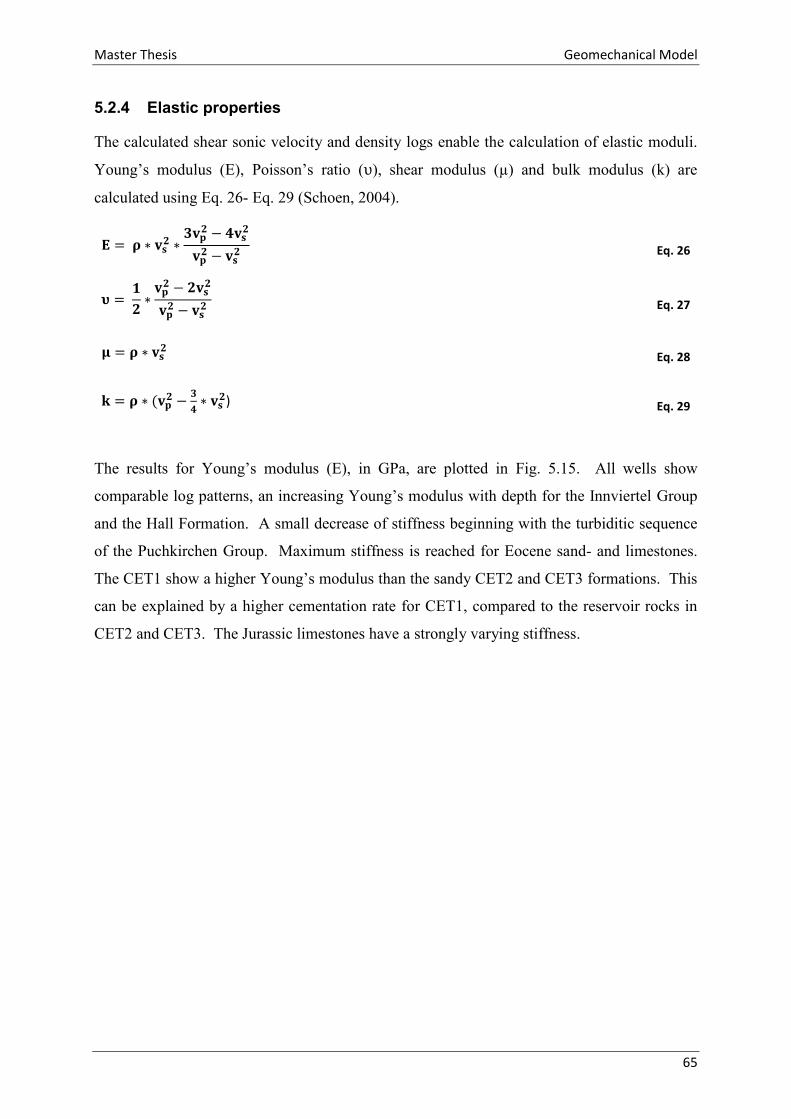
Master Thesis Geomechanical Model
65
5.2.4 Elastic properties
The calculated shear sonic velocity and density logs enable the calculation of elastic moduli.
Young’s modulus (E), Poisson’s ratio (υ), shear modulus (µ) and bulk modulus (k) are
calculated using Eq. 26- Eq. 29 (Schoen, 2004).
The results for Young’s modulus (E), in GPa, are plotted in Fig. 5.15. All wells show
comparable log patterns, an increasing Young’s modulus with depth for the Innviertel Group
and the Hall Formation. A small decrease of stiffness beginning with the turbiditic sequence
of the Puchkirchen Group. Maximum stiffness is reached for Eocene sand- and limestones.
The CET1 show a higher Young’s modulus than the sandy CET2 and CET3 formations. This
can be explained by a higher cementation rate for CET1, compared to the reservoir rocks in
CET2 and CET3. The Jurassic limestones have a strongly varying stiffness.
𝐄 = 𝛒 ∗ 𝐯𝐬𝟐 ∗
𝟑𝐯𝐩𝟐 − 𝟒𝐯𝐬
𝟐
𝐯𝐩𝟐 − 𝐯𝐬
𝟐 Eq. 26
𝛖 = 𝟏
𝟐∗𝐯𝐩
𝟐 − 𝟐𝐯𝐬𝟐
𝐯𝐩𝟐 − 𝐯𝐬
𝟐 Eq. 27
𝛍 = 𝛒 ∗ 𝐯𝐬𝟐 Eq. 28
𝐤 = 𝛒 ∗ (𝐯𝐩𝟐 −
𝟑
𝟒∗ 𝐯𝐬
𝟐) Eq. 29
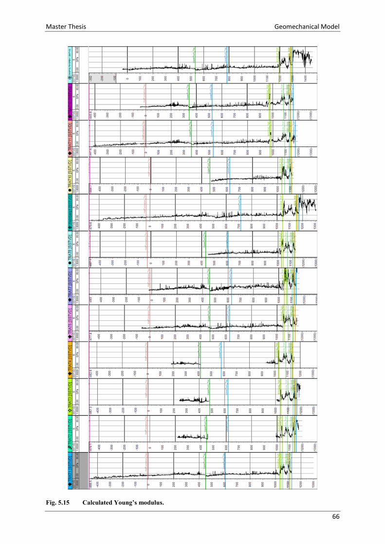
Master Thesis Geomechanical Model
66
Fig. 5.15 Calculated Young’s modulus.
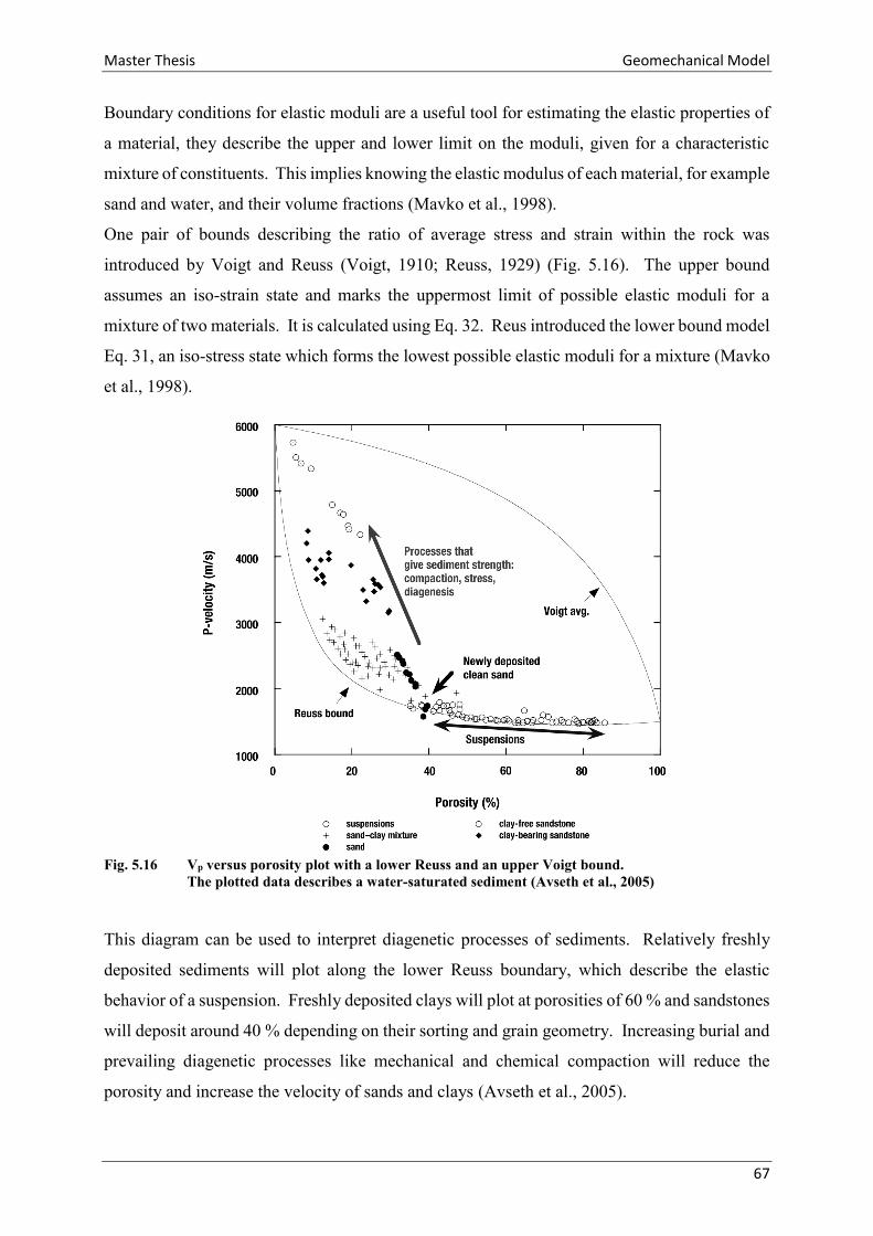
Master Thesis Geomechanical Model
67
Boundary conditions for elastic moduli are a useful tool for estimating the elastic properties of
a material, they describe the upper and lower limit on the moduli, given for a characteristic
mixture of constituents. This implies knowing the elastic modulus of each material, for example
sand and water, and their volume fractions (Mavko et al., 1998).
One pair of bounds describing the ratio of average stress and strain within the rock was
introduced by Voigt and Reuss (Voigt, 1910; Reuss, 1929) (Fig. 5.16). The upper bound
assumes an iso-strain state and marks the uppermost limit of possible elastic moduli for a
mixture of two materials. It is calculated using Eq. 32. Reus introduced the lower bound model
Eq. 31, an iso-stress state which forms the lowest possible elastic moduli for a mixture (Mavko
et al., 1998).
Fig. 5.16 Vp versus porosity plot with a lower Reuss and an upper Voigt bound.
The plotted data describes a water-saturated sediment (Avseth et al., 2005)
This diagram can be used to interpret diagenetic processes of sediments. Relatively freshly
deposited sediments will plot along the lower Reuss boundary, which describe the elastic
behavior of a suspension. Freshly deposited clays will plot at porosities of 60 % and sandstones
will deposit around 40 % depending on their sorting and grain geometry. Increasing burial and
prevailing diagenetic processes like mechanical and chemical compaction will reduce the
porosity and increase the velocity of sands and clays (Avseth et al., 2005).

Master Thesis Geomechanical Model
68
Fig. 5.17 Velocity versus porosity plot for the Cenoman and the Hall Formation.
The upper Voigt bound in blue, lower Reuss bound in orange. The plotted data shows the
Cenomanian sandstones CET1-3 and the relatively uncompacted Hall formation in grey.
The two bounds are calculated for a mixture of clean quartz sandstone and water. Quartz forms
the stiff and water the soft material. Two materials with smaller differences in elastic behavior
would form narrower boundaries (Avseth et al., 2005). A characteristic bulk modulus for quartz
is 36 GPa, whereas that of water is 2.2 GPa (Schoen, 2004).
The Cenoman sandstones plot at porosities between 10 and 25 % with a compressional velocity
of 3100 m/s down to 450 m/s. It can be seen that the strongly cemented sandstones from CET1
plot at higher velocities and lower porosities than CET2 and CET3 sandstones. The plotted
data from the Innviertel Group (grey dots) have not undergone any major diagenetic processes
which increased their strength and plot near the recently deposited sediments.
1000
2000
3000
4000
5000
6000
7000
0,00 0,10 0,20 0,30 0,40 0,50 0,60 0,70 0,80 0,90 1,00
Vel
oci
ty [
m/s
]
Porosity
Voigt
Reuss
HS+
CET1
CET2
CET3
Innviertel Formation
𝐊𝐯 = 𝛟 ∗ 𝐊𝐟𝐥 + (𝟏 − 𝛟) ∗ 𝐊𝐦𝐚 Eq. 30
𝐊𝐑 = 𝛟 ∗ 𝐊𝐟𝐥−𝟏 + (𝟏 − 𝛟) ∗ 𝐊𝐦𝐚
−𝟏 Eq. 31
𝑲𝑽𝑹𝑯 = 𝐊𝐯 + 𝐊𝐑
𝟐 Eq. 32

Master Thesis Geomechanical Model
69
Another set of boundary conditions is introduced by Hashin – Shtrikmann (Hashin et al., 1963),
these are the narrowest possible bounds for estimating an elastic modulus by plotting porosity
versus velocity. Alternatively the calculated bulk moduli can be evaluated by plotting them in
an effective bulk modulus versus porosity diagram.
Hashin and Shtrikman define the bounds by interchanging the moduli of the two materials
(Hashin et al., 1963). The upper bound is defined by a core of soft material surrounded by a
stiff material forming a shell around the core. The lower bound is calculated by switching the
two materials, now the softer material defines the shell and stiffer material the core. Eq. 33 is
used for the upper bound calculation and Eq. 34 for calculating the lower bound (Mavko et al.,
1998).
Fig. 5.18 shows the calculated bulk moduli for the TRAT1 borehole plotted against the porosity.
The upper boundaries Voigt (orange) and Hashin-Shtrikman (yellow) mark the uppermost limit
of elastic moduli for a mixture of materials. The lower boundaries of Reuss and Hashin-
Shtrikman are exactly the same, because the shear modulus of water is zero. When using water
as soft material the modulus of grains in a pore fluid is described by the lower bounds (Avseth
et al., 2005).
The calculated bulk modulus is not correct for the high porosity area between 70 and 90 %, this
data is from the uppermost logging interval where high sonic velocity measurements lead to
unrealistic values for the bulk modulus. The same applies to the overestimated bulk modulus
(>32 GPa) for a porosity lower than 10 %. This data is from the JUBSS and was measured at
the end of the logging period. All other data fits between the boundaries and show a similar
trend to the average bulk modulus introduced by Hill (grey dotted line) (Hill, 1952).
𝐊+𝐇𝐒 = 𝐊𝐦𝐚 +
𝛟
(𝐊𝐟𝐥 − 𝐊𝐦𝐚)−𝟏 + (𝟏 − 𝛟) ∗ (𝐊𝐦𝐚 + ∗
𝟒𝟑𝛍𝐦𝐚)
−𝟏
Eq. 33
𝐊−𝐇𝐒 = 𝐊𝐟𝐥 +
(𝟏 − 𝛟)
(𝐊𝐦𝐚 − 𝐊𝐟𝐥)−𝟏 + 𝛟 ∗ 𝐊𝐟𝐥
−𝟏 Eq. 34
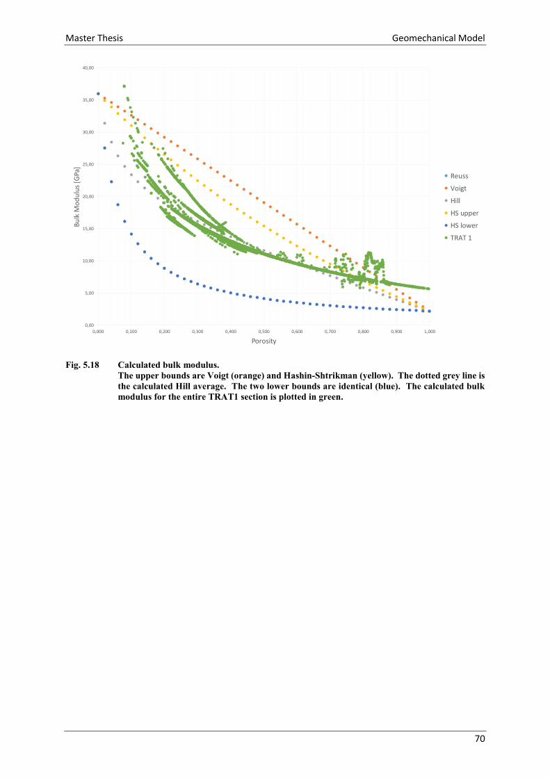
Master Thesis Geomechanical Model
70
Fig. 5.18 Calculated bulk modulus.
The upper bounds are Voigt (orange) and Hashin-Shtrikman (yellow). The dotted grey line is
the calculated Hill average. The two lower bounds are identical (blue). The calculated bulk
modulus for the entire TRAT1 section is plotted in green.
0,00
5,00
10,00
15,00
20,00
25,00
30,00
35,00
40,00
0,000 0,100 0,200 0,300 0,400 0,500 0,600 0,700 0,800 0,900 1,000
Bu
lk M
od
ulu
s [G
Pa]
Porosity
Reuss
Voigt
Hill
HS upper
HS lower
TRAT 1
Master Thesis Geomechanical Model
71
5.2.5 Uniaxial compressive strength
An additional input during geomechanical material modeling is the uniaxial compressive
strength. A series of unconfined compression tests are performed in this section to determine
the uniaxial compression strength (UCS) of core plug samples from the reservoir section of the
wells Trattnach 6 and Trattnach 7. When performing an unconfined compression test an axial
load is applied and gradually increased till failure occurs. This test is a simplification of the
triaxial compression test, where an additional confining pressure allows even higher axial
loading (Fjar et al., 2008). A triaxial compression or shear test could not be performed, because
these tests require a minimum specimen diameter of 50 mm and the core plugs from the
Trattnach wells have a median diameter of 29 mm. Ideally the samples should have a height to
length ratio of 2 up to 2.5 and a reduction factor should be applied to those samples which have
a height to length ratio in the rage between one and two (Witt, 2008). As no sample from the
investigated wells has a height to length ratio larger than two, all measured unconfined
compressive strength values are reduced by the factor calculated with Eq. 35.
Sample Preparation
A uniaxial compression test requires plane parallel surfaces, thus both ends of all seventeen
core plugs were cut using a water cooled stone cutting saw at the Chair of Subsurface
Engineering of the Montanunivesitaet Leoben. All samples have different heights with the goal
to maintain as much height as possible during the preparation of plane parallel surfaces.
Measurement
The uniaxial compressive strength has been determined using the testing facility at the Chair of
Subsurface Engineering. This facility is designed to determine the Young’s modulus via a fully
automated testing procedure which evaluates the Young’s modulus using force controlled
loading and unloading cycles. Due to the small height of the samples the extensometers could
not be mounted. Therefore the fully automated testing procedure could not be performed.
Instead a displacement controlled program is used to determine the uniaxial compressive
strength, using an axial loading of 1.2 mm per minute.
The plane parallel cylindrical samples were embedded between to plane parallel pressure plates,
whereby the upper one is a “kugelkalotte” fixed with springs to ensure a better force
transmission.
𝐫𝐞𝐝𝐮𝐜𝐭𝐢𝐨𝐧 𝐟𝐚𝐜𝐭𝐨𝐫 = 𝟖
𝟕 + 𝟐 ∗𝒉𝒅
Eq. 35

Master Thesis Geomechanical Model
72
The studied core of the Trattnach 6 well contains four core plugs. Only one of these qualified
for the UCS test. The other three samples were smaller than 20 mm with a height to length
ratio of 0.71 and were therefore neglected.
Eleven core plugs are available from the Trattnach 7 well and eight of those were used for the
compression test. The remaining core plugs were too small and a measurement seemed
redundant.
Master Thesis Geomechanical Model
73
Results
TRAT701B
The TRAT701B is a core plug from well Trattnach 7, obtained at a core depth of 1617 m. It is
a glauconitic sandstone sample with a diameter of 29.30 mm and a length of 26.30 mm from
the CET3 horizon, see uppermost picture in Fig. 5.19. The force-time history diagram shows
that failure occurred at an applied force of 11.33 kN. The corresponding uniaxial compressive
strength is 16.80 MPa, a reduction factor of 0.910 is applied, resulting in a uniaxial compressive
strength of 15.28 MPa for the glauconitic sandstone sample. Fig. 5.19 shows the stress-strain
curve, its slope results in a tangential modulus of 2.16 GPa.
Fig. 5.19 Test Results TRAT701B.
0
10
20
0 10 20 30
Forc
e [k
N]
Time [sec]
Force - Time History
0
0,1
0,2
0,3
0,4
0,5
0 10 20 30Dis
pla
cem
ent
[mm
]
Time [sec]
Displacement - Time History
0
5
10
15
20
0 0,005 0,01 0,015 0,02
Stre
ss [
MP
a]
Strain
Stress - Strain

Master Thesis Geomechanical Model
74
TRAT704A
The TRAT704A is a core plug from well Trattnach 7, obtained at a depth of 1614 m. It is a
glauconitic sandstone sample with a diameter of 29.60 mm and a length of 49.40 mm from the
CET2 horizon, see uppermost picture in Fig. 5.20. The force-time history diagram shows that
failure occurred at an applied force of 7.96 kN. The corresponding uniaxial compressive
strength is 8.84 MPa, a reduction factor of 0.774 is applied, resulting in a uniaxial compressive
strength of 7.70 MPa for the glauconitic sandstone sample. Fig. 5.20 shows the stress-strain
curve, its slope results in a tangential modulus of 1.43 GPa.
Fig. 5.20 Test Results TRAT704A.
0
10
20
0 10 20 30 40
Forc
e [k
N]
Time [sec]
Force - Time History
00,10,20,30,40,50,60,7
0 10 20 30 40
Dis
pla
cem
ent
[mm
]
Time [sec]
Displacement - Time History
0
5
10
15
20
0 0,005 0,01 0,015 0,02
Stre
ss [
MP
a]
Strain
Stress - Strain
Master Thesis Geomechanical Model
75
TRAT705
The TRAT705 is a core plug from well Trattnach 7, obtained at a depth of 1613.35 m. It is a
glauconitic sandstone sample with a diameter of 29.60 mm and a length of 33.20 mm from the
CET2 horizon, see uppermost picture in Fig. 5.21 The force-time history diagram shows that
failure occurred at an applied force of 8.07 kN. The corresponding uniaxial compressive
strength is 11.74 MPa, a reduction factor of 0.865 is applied, resulting in a uniaxial compressive
strength of 10.16 MPa for the glauconitic sandstone sample. Fig. 5.21 shows the stress-strain
curve, its slope results in a tangential modulus of 1.36 GPa.
Fig. 5.21 Test Results TRAT705.
0
10
20
0 10 20 30
Forc
e [k
N]
Time [sec]
Force - Time History
0
0,1
0,2
0,3
0,4
0,5
0,6
0 10 20 30
Dis
pla
cem
ent
[mm
]
Time [sec]
Displacement - Time History
0
5
10
15
20
0 0,005 0,01 0,015 0,02
Stre
ss [
MP
a]
Strain
Stress - Strain

Master Thesis Geomechanical Model
76
TRAT709
The TRAT709 is a core plug from well Trattnach 7, obtained at a depth of 1609.10 m. It is a
white-yellow sandstone sample with a diameter of 29.40 mm and a length of 27.60 mm from
the CET1 horizon, see uppermost picture in Fig. 5.22. The force-time history diagram shows
that failure occurred at an applied force of 21.60 kN. The corresponding uniaxial compressive
strength is 31.83 MPa, a reduction factor of 0.901 is applied, resulting in a uniaxial compressive
strength of 28.68 MPa for the sandstone sample. Fig. 5.22 shows the stress-strain curve, its
slope results in a tangential modulus of 3.97 GPa.
Fig. 5.22 Test Results TRAT709.
0
10
20
30
0 10 20 30
Forc
e [k
N]
Time [sec]
Force - Time History
0
0,1
0,2
0,3
0,4
0,5
0 10 20 30
Dis
pla
cem
ent
[mm
]
Time [sec]
Displacement - Time History
05
101520253035
0 0,005 0,01 0,015 0,02
Stre
ss [
MP
a]
Strain
Stress - Strain

Master Thesis Geomechanical Model
77
TRAT712A
The TRAT12A is a core plug from well Trattnach 7, obtained at a depth of 1606.85 m. It is a
strongly weathered glauconitic sandstone sample with a diameter of 28.80 mm and a length of
37.90 mm from the CET1 horizon, see uppermost picture in Fig. 5.23. The force-time history
diagram shows that failure occurred at an applied force of 2.58 kN. The corresponding uniaxial
compressive strength is 3.97 MPa, a reduction factor of 0.831 is applied, resulting in a uniaxial
compressive strength of 3.30 MPa for the glauconitic sandstone sample. Fig. 5.23 shows the
stress-strain curve, its slope results in a tangential modulus of 0.32 GPa.
Fig. 5.23 Test Results TRAT712A.
0
10
20
0 10 20 30 40 50
Forc
e [k
N]
Time [sec]
Force - Time History
00,10,20,30,40,50,60,70,80,9
1
0 10 20 30 40 50
Dis
pla
cem
ent
[mm
]
Time [sec]
Displacement - Time History
0
5
10
15
0 0,005 0,01 0,015 0,02 0,025
Stre
ss [
MP
a]
Strain
Stress - Strain

Master Thesis Geomechanical Model
78
TRAT714A
The TRAT714A is a core plug from well Trattnach 7, obtained at a depth of 1621.90 m. It is a
glauconitic sandstone sample with a diameter of 29.70 mm and a length of 36.50 mm from the
CET3 horizon, see uppermost picture in Fig. 5.24. The force-time history diagram shows that
failure occurred at an applied force of 13.86 kN. The corresponding uniaxial compressive
strength is 19.95 MPa, a reduction factor of 0.846 is applied, resulting in a uniaxial compressive
strength of 16.87 MPa for the glauconitic sandstone sample. Fig. 5.24 shows the stress-strain
curve, its slope results in a tangential modulus of 2.86 GPa.
Fig. 5.24 Test Results TRAT714A.
0
10
20
0 10 20 30
Forc
e [k
N]
Time [sec]
Force - Time History
0
0,1
0,2
0,3
0,4
0,5
0,6
0 10 20 30
Dis
pla
cem
ent
[mm
]
Time [sec]
Displacement - Time History
0
5
10
15
20
0 0,005 0,01 0,015 0,02
Stre
ss [
MP
a]
Strain
Stress - Strain
Master Thesis Geomechanical Model
79
TRAT714B
The TRAT714B is a core plug from well Trattnach 7, obtained at a depth of 1621.90 m. It is a
glauconitic sandstone sample with a diameter of 29.70 mm and a length of 37.30 mm from the
CET3 horizon, see uppermost picture in Fig. 5.25. The force-time history diagram shows that
failure occurred at an applied force of 13.67 kN. The corresponding uniaxial compressive
strength is 19.72 MPa, a reduction factor of 0.841 is applied, resulting in a uniaxial compressive
strength of 16.59 MPa for the glauconitic sandstone sample. Fig. 5.25 shows the stress-strain
curve, its slope results in a tangential modulus of 2.80 GPa.
Fig. 5.25 Test Results TRAT714B.
0
10
20
0 10 20 30
Forc
e [k
N]
Time [sec]
Force - Time History
0
0,1
0,2
0,3
0,4
0,5
0,6
0 10 20 30
Dis
pla
cem
ent
[mm
]
Time [sec]
Displacement - Time History
0
5
10
15
20
0 0,005 0,01 0,015 0,02
Stre
ss [
MP
a]
Strain
Stress - Strain

Master Thesis Geomechanical Model
80
TRAT718
The TRAT718 is a core plug from well Trattnach 7, obtained at a depth of 1619.50 m. It is a
glauconitic sandstone sample with a diameter of 29.60mm and a length of 39.50 mm from the
CET3 horizon, see uppermost picture in Fig. 5.26. The force-time history diagram shows that
failure occurred at an applied force of 11.71 kN. The corresponding uniaxial compressive
strength is 17.03 MPa, a reduction factor of 0.827 is applied, resulting in a uniaxial compressive
strength of 14.09 MPa for the glauconitic sandstone sample. Fig. 5.26 shows the stress-strain
curve, its slope results in a tangential modulus of 1.55 GPa.
Fig. 5.26 Test Results TRAT718.
0
10
20
0 10 20 30 40
Forc
e [k
N]
Time [sec]
Force - Time History
00,10,20,30,40,50,60,70,80,9
0 10 20 30 40
Dis
pla
cem
ent
[mm
]
Time [sec]
Displacement - Time History
0
5
10
15
20
0 0,005 0,01 0,015 0,02 0,025
Stre
ss [
MP
a]
Strain
Stress - Strain

Master Thesis Geomechanical Model
81
TRAT615
The TRAT615 is a core plug from well Trattnach 6, obtained at a depth of 1628 m. It is a
glauconitic sandstone sample with a diameter of 29.70 mm and a length of 31.40 m from the
CET3 horizon, see uppermost picture in Fig. 5.27. The force-time history diagram shows that
failure occurred at an applied force of 17.22 kN. The corresponding uniaxial compressive
strength is 24.87 MPa, a reduction factor of 0.878 is applied, resulting in a uniaxial compressive
strength of 21.83 MPa for the glauconitic sandstone sample. Fig. 5.27 shows the stress-strain
curve, its slope results in a tangential modulus of 2.54 GPa.
Fig. 5.27 Test Results TRAT615.
0
10
20
0 10 20 30
Forc
e [k
N]
Time [sec]
Force - Time History
0
0,1
0,2
0,3
0,4
0,5
0,6
0 10 20 30
Dis
pla
cem
ent
[mm
]
Time [sec]
Displacement - Time History
0
5
10
15
20
25
30
0 0,005 0,01 0,015 0,02
Stre
ss [
MP
a]
Strain
Stress - Strain
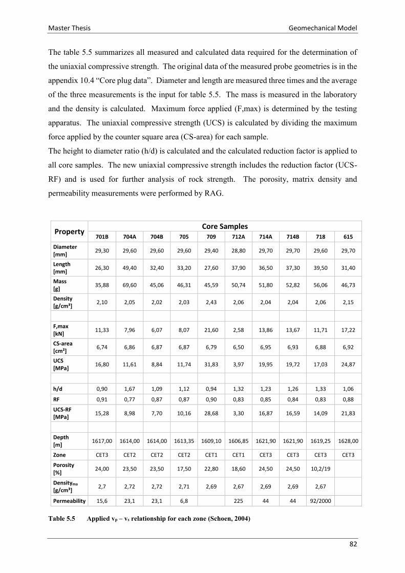
Master Thesis Geomechanical Model
82
The table 5.5 summarizes all measured and calculated data required for the determination of
the uniaxial compressive strength. The original data of the measured probe geometries is in the
appendix 10.4 “Core plug data”. Diameter and length are measured three times and the average
of the three measurements is the input for table 5.5. The mass is measured in the laboratory
and the density is calculated. Maximum force applied (F,max) is determined by the testing
apparatus. The uniaxial compressive strength (UCS) is calculated by dividing the maximum
force applied by the counter square area (CS-area) for each sample.
The height to diameter ratio (h/d) is calculated and the calculated reduction factor is applied to
all core samples. The new uniaxial compressive strength includes the reduction factor (UCS-
RF) and is used for further analysis of rock strength. The porosity, matrix density and
permeability measurements were performed by RAG.
Property Core Samples
701B 704A 704B 705 709 712A 714A 714B 718 615
Diameter [mm]
29,30 29,60 29,60 29,60 29,40 28,80 29,70 29,70 29,60 29,70
Length [mm]
26,30 49,40 32,40 33,20 27,60 37,90 36,50 37,30 39,50 31,40
Mass [g]
35,88 69,60 45,06 46,31 45,59 50,74 51,80 52,82 56,06 46,73
Density [g/cm³]
2,10 2,05 2,02 2,03 2,43 2,06 2,04 2,04 2,06 2,15
F,max [kN]
11,33 7,96 6,07 8,07 21,60 2,58 13,86 13,67 11,71 17,22
CS-area [cm²]
6,74 6,86 6,87 6,87 6,79 6,50 6,95 6,93 6,88 6,92
UCS [MPa]
16,80 11,61 8,84 11,74 31,83 3,97 19,95 19,72 17,03 24,87
h/d 0,90 1,67 1,09 1,12 0,94 1,32 1,23 1,26 1,33 1,06
RF 0,91 0,77 0,87 0,87 0,90 0,83 0,85 0,84 0,83 0,88
UCS-RF [MPa]
15,28 8,98 7,70 10,16 28,68 3,30 16,87 16,59 14,09 21,83
Depth [m]
1617,00 1614,00 1614,00 1613,35 1609,10 1606,85 1621,90 1621,90 1619,25 1628,00
Zone CET3 CET2 CET2 CET2 CET1 CET1 CET3 CET3 CET3 CET3
Porosity [%]
24,00 23,50 23,50 17,50 22,80 18,60 24,50 24,50 10,2/19
Densityma
[g/cm³] 2,7 2,72 2,72 2,71 2,69 2,67 2,69 2,69 2,67
Permeability 15,6 23,1 23,1 6,8 225 44 44 92/2000
Table 5.5 Applied vp – vs relationship for each zone (Schoen, 2004)
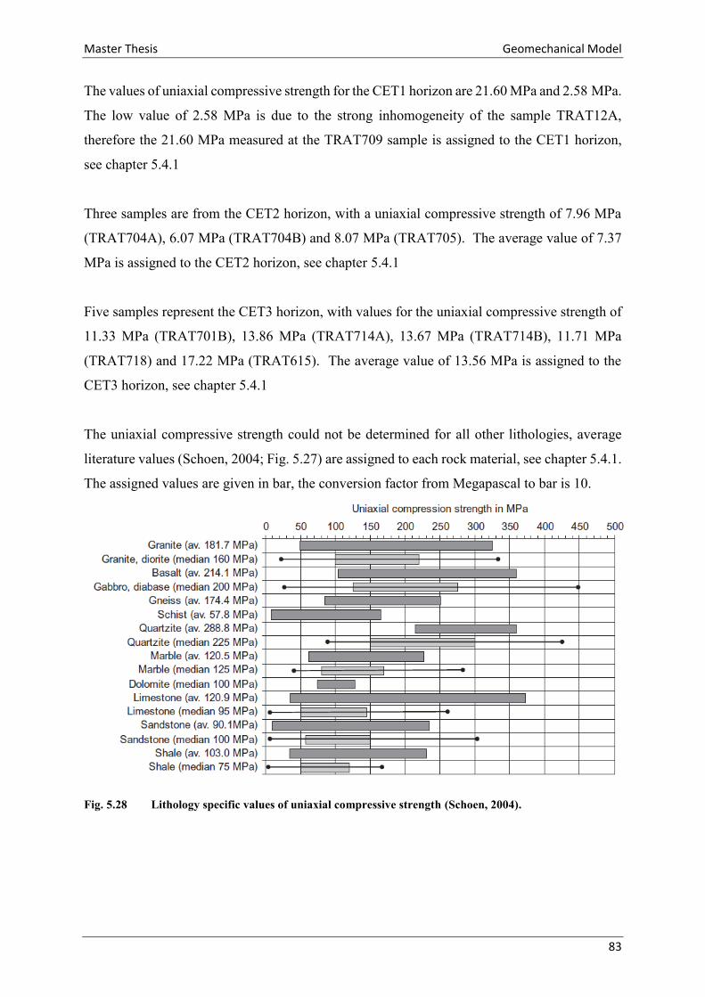
Master Thesis Geomechanical Model
83
The values of uniaxial compressive strength for the CET1 horizon are 21.60 MPa and 2.58 MPa.
The low value of 2.58 MPa is due to the strong inhomogeneity of the sample TRAT12A,
therefore the 21.60 MPa measured at the TRAT709 sample is assigned to the CET1 horizon,
see chapter 5.4.1
Three samples are from the CET2 horizon, with a uniaxial compressive strength of 7.96 MPa
(TRAT704A), 6.07 MPa (TRAT704B) and 8.07 MPa (TRAT705). The average value of 7.37
MPa is assigned to the CET2 horizon, see chapter 5.4.1
Five samples represent the CET3 horizon, with values for the uniaxial compressive strength of
11.33 MPa (TRAT701B), 13.86 MPa (TRAT714A), 13.67 MPa (TRAT714B), 11.71 MPa
(TRAT718) and 17.22 MPa (TRAT615). The average value of 13.56 MPa is assigned to the
CET3 horizon, see chapter 5.4.1
The uniaxial compressive strength could not be determined for all other lithologies, average
literature values (Schoen, 2004; Fig. 5.27) are assigned to each rock material, see chapter 5.4.1.
The assigned values are given in bar, the conversion factor from Megapascal to bar is 10.
Fig. 5.28 Lithology specific values of uniaxial compressive strength (Schoen, 2004).

Master Thesis Geomechanical Model
84
The core sample TRAT615 represents the strength of the CET3 zone. The uniaxial compressive
strength is defined by a vertical stress without the application of a confining pressure. Therefore
σ3=0 and the Mohr Circle representing the σUCS starts at the coordinate origin zero.
Additionally, the Mohr Circles of the seal and reservoir rock zones are plotted. The horizontal
stress is calculated using Eq. 36, were v is the Poisson ratio and σv is the vertical stress,
overburden pressure or lithostatic pressure (Bjørlykke, 2015).
The equation assumes that the compaction process in a sedimentary basin can interpreted as a
uniaxial strain compaction. This can be assumed because the sediment basin is wide compared
to its thickness and the compaction due to additional overburden is interpreted as a one-
dimensional deformation. The second assumption is the linear elastic behavior of the grain
framework and isotropic behavior of the horizontal stress (Bjørlykke, 2015).
The vertical stress and the Poisson ratio are averaged over the three zone intervals (CET1, 2
and CET3) and inserted into Eq.36. A characteristic horizontal stress is calculated for each
zone.
Fig.5.29 shows the Mohr circles of the uniaxial compressive stress and the three Cenomanian
zones for the TRAT6 well. The seal rock (CET1) is characterized by a vertical stress (σ1) of
28.02 MPa and a horizontal stress component(σ3) of 8.44 MPa. The uppermost reservoir rock
(CET2) has a vertical stress (σ1) of 28.62 MPa and a horizontal stress component(σ3) of 10.00
MPa. The lower CET3 horizon has a vertical stress (σ1) of 28.53 MPa and a horizontal stress
component(σ3) of 10.80 MPa
The three zones of the CET1,2 and 3 exhibit a vertical stress which is higher than the measured
uniaxial compressive stress. Plotting the Mohr circles, shows that the present horizontal stress
allows a higher vertical stress.
The measured uniaxial compressive stresses and the calculated vertical and horizontal stresses
of the TRAT7 well are displayed in Fig.5.30. A uniaxial compressive stress of 28.68 MPa is
measured and averaged for the CET3. The CET2 has a uniaxial compressive stress of 8.95 and
the CET3 has 15.7 MPa. The seal rock (CET1) is characterized by a vertical stress (σ1) of 27.20
MPa and a horizontal stress component(σ3) of 9.10 MPa. The uppermost reservoir rock (CET2)
has a vertical stress (σ1) of 27.40 MPa and a horizontal stress component(σ3) of 9.60 MPa. The
lower CET3 horizon has a vertical stress (σ1) of 27.70 MPa and a horizontal stress
component(σ3) of 10.23 MPa
𝝈𝑯 = 𝒗
𝟏 − 𝒗∗ 𝝈𝒗 Eq. 36
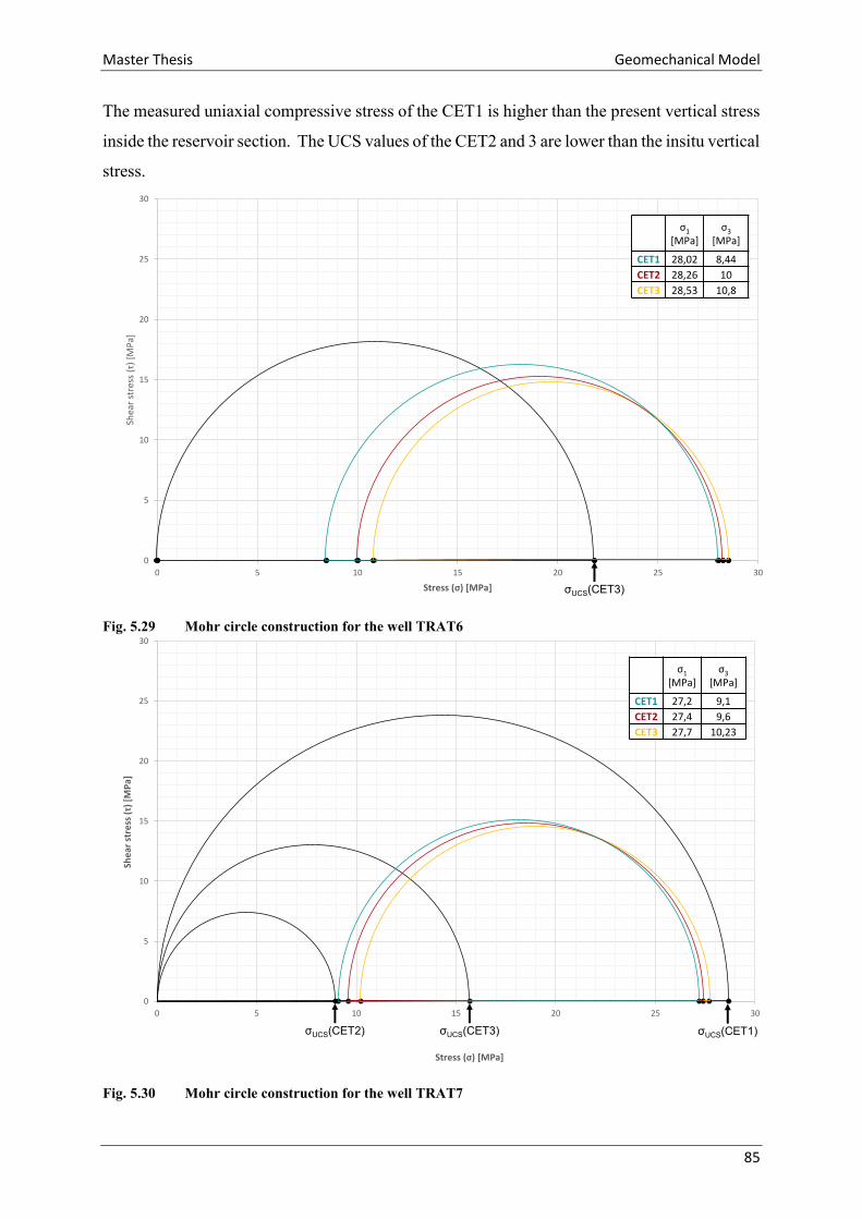
Master Thesis Geomechanical Model
85
The measured uniaxial compressive stress of the CET1 is higher than the present vertical stress
inside the reservoir section. The UCS values of the CET2 and 3 are lower than the insitu vertical
stress.
Fig. 5.29 Mohr circle construction for the well TRAT6
Fig. 5.30 Mohr circle construction for the well TRAT7
0
5
10
15
20
25
30
0 5 10 15 20 25 30
Shea
r st
ress
(τ)
[M
Pa]
Stress (σ) [MPa]
TRAT6
σ3
σ1
σUCS
σUCS(CET3)
σ1
[MPa]σ3
[MPa]
CET1 28,02 8,44
CET2 28,26 10
CET3 28,53 10,8
0
5
10
15
20
25
30
0 5 10 15 20 25 30
Shea
r st
ress
(τ)
[M
Pa]
Stress (σ) [MPa]
TRAT7
σ3
σ1
σUCS
σUCS(CET1)σUCS(CET3)σUCS(CET2)
Stress (σ) [MPa]
She
arst
ress
(τ)
[M
Pa]
σ1
[MPa]σ3
[MPa]
CET1 27,2 9,1
CET2 27,4 9,6
CET3 27,7 10,23

Master Thesis Geomechanical Model
86
5.3 GRID POPULATION
The density, velocity and porosity data are available on a log basis. Upscaling transforms the
well log data into a grid property. The upscaling of the well logs assigns the upscaled property
values to all grid cells penetrated by the well. The rest of the grid remains empty until it is
filled through petrophysical modeling, an interpolation of the upscaled data across the entire
study area.
5.3.1 Upscaling
Usually the grid cells are much coarser than the sampling intervals of well logs and it is
important to choose an adequate setting for the averaging of well data. This depends mostly on
the type of log upscaled. All sonic logs are upscaled using the RMS (Root Mean Squared)
averaging, whereas additive properties like porosity and saturation data is upscaled using
arithmetic mean. All upscaled logs are treated as lines, meaning that log data values are
weighted by the distance between inter-sample mid-points for continuous logs (Schlumberger,
2015).
The following well log measurements are upscaled:
Compressional velocity (vp) using RMS
Shear Velocity (vs) using RMS
Density (DEN) using Arithmetic averaging
The result is displayed in Fig. 5.31. The first three columns show the upscaled properties of vp,
vs and DEN. The coloured data are the upscaled properties, with horizontal lines, marking the
grid cells. The original well logs are also plotted, indicating a good fit between original and
upscaled data.
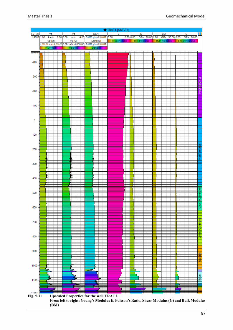
Master Thesis Geomechanical Model
87
Fig. 5.31 Upscaled Properties for the well TRAT1.
From left to right: Young’s Modulus E, Poisson’s Ratio, Shear Modulus (G) and Bulk Modulus
(BM)
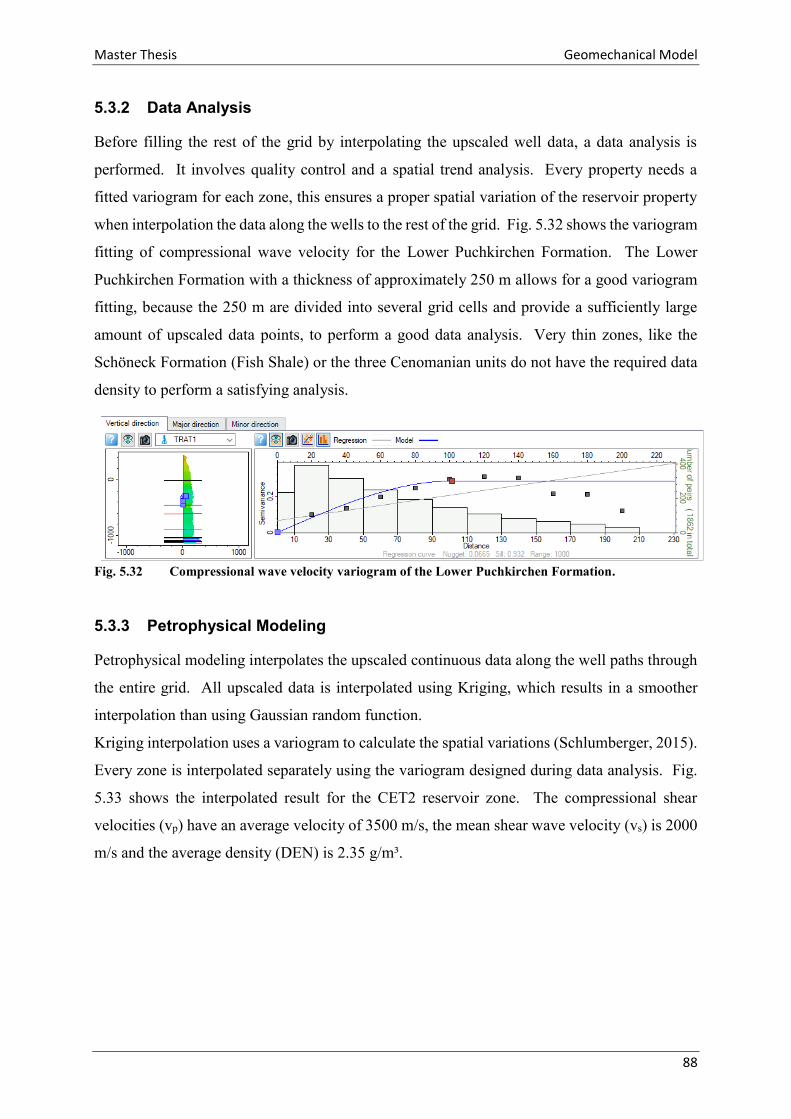
Master Thesis Geomechanical Model
88
5.3.2 Data Analysis
Before filling the rest of the grid by interpolating the upscaled well data, a data analysis is
performed. It involves quality control and a spatial trend analysis. Every property needs a
fitted variogram for each zone, this ensures a proper spatial variation of the reservoir property
when interpolation the data along the wells to the rest of the grid. Fig. 5.32 shows the variogram
fitting of compressional wave velocity for the Lower Puchkirchen Formation. The Lower
Puchkirchen Formation with a thickness of approximately 250 m allows for a good variogram
fitting, because the 250 m are divided into several grid cells and provide a sufficiently large
amount of upscaled data points, to perform a good data analysis. Very thin zones, like the
Schöneck Formation (Fish Shale) or the three Cenomanian units do not have the required data
density to perform a satisfying analysis.
Fig. 5.32 Compressional wave velocity variogram of the Lower Puchkirchen Formation.
5.3.3 Petrophysical Modeling
Petrophysical modeling interpolates the upscaled continuous data along the well paths through
the entire grid. All upscaled data is interpolated using Kriging, which results in a smoother
interpolation than using Gaussian random function.
Kriging interpolation uses a variogram to calculate the spatial variations (Schlumberger, 2015).
Every zone is interpolated separately using the variogram designed during data analysis. Fig.
5.33 shows the interpolated result for the CET2 reservoir zone. The compressional shear
velocities (vp) have an average velocity of 3500 m/s, the mean shear wave velocity (vs) is 2000
m/s and the average density (DEN) is 2.35 g/m³.

Master Thesis Geomechanical Model
89
Fig. 5.33 Interpolated data of the CET 2 Zone.
Compressional wave velocity (vp) with an average velocity of 3500 m/s; Shear wave velocity
(vs) with an average Velocity of 2000 m/s and the modeled density with an average value of
2.35 g/cm³;
After performing the upscaling and petrophysical modeling the grid is filled with the calculated
sonic velocity, permeability and density data. This enables the calculation of elastic moduli on
a grid property basis, so the upscaling and petrophysical modeling must not be performed for
the geomechanical parameters. The Young’s modulus (E), Poisson’s ratio (𝛖), shear modulus
(µ) and bulk modulus (k) are calculated directly in the grid using Eq. 26- Eq. 29 and the
available grid properties of sonic velocities (vp and vs) and the density.
Fig. 5.31 shows the calculated grid properties of the elastic parameters along the well of the
TRAT1, G stands for the shear modulus and BM for bulk modulus. The distribution of the
elastic parameters from the entire geomechanical model is discussed in chapter 5.5.

Master Thesis Geomechanical Model
90
5.4 GEOMECHANICAL MATERIAL MODELING
The Petrel plug-in “Reservoir Geomechanics” (Schlumberger, 2014) distinguishes between
intact rock materials and discontinuity materials, all horizons and zones form intact rock
materials, whereas faults are discontinuity materials. Depending on the type of material
different properties are required for the material modeling process. See Table 5.6 for all required
properties to define an intact rock material and Table 5.7 for discontinuity materials.
5.4.1 Creating intact rock materials
These materials represent the different rock types and consist of a collection of parameters, like
Young’s modulus, Poisson ratio, bulk and shear modulus etc. which represent the various
lithology types. “Reservoir Geomechanics” provides a materials library including sandstone,
limestone shale, chalk, siltstone, salt, as well as dense or loose uniform sands and stiff or soft
clays (Schlumberger, 2015). After adding a material from the library to the current project all
default parameters from Table 5.6, can be adjusted according to the model’s needs. To describe
the different lithology zones of the model, eight materials are created. Their properties are
adjusted according to the calculated parameters during property modeling. The statistic average
of Young’s, shear and bulk modulus is calculated for each zone and assigned. The same applies
for the porosity and density data. The values of the uniaxial compressive strength are either an
average of the measured data or literature values (see chapter 5.2.5). The uniaxial compressive
strength is determined in MPa, but the software requires bar as an input. The literature and
measured data is multiplied with a factor of ten, to convert the unit from MPa to bar.
1. Limestone (LST), representing the Jurassic zone.
It forms the stiffest material with a Young’s modulus of 48 GPa, a shear modulus of 18
GPa and a bulk modulus of 42 GPa. The porosity is quite low with 9 % and the density
is 2.75 g/cm³. According to literature data 1200 bar is a characteristic uniaxial
compressive strength for limestones (see chapter 5.2.5).
2. Marlstone (MARL), representing the Turonian and Coniancian succession.
The material has an average stiffness of 24 GPa, a very low shear modulus of 9.9 GPa
and a moderate bulk modulus of 21 GPa. The porosity is quite high with 20 % and the
density is the same as for the limestones with 2.52 g/cm³. A uniaxial compressive
strength of 1000 bar is assigned, this is a literature value for marlstones (see chapter
5.2.5).
Master Thesis Geomechanical Model
91
3. Glauconitic sandstone (GSST), representing the lower Cenomanian zones
CET 2 and CET 3.
The material is characterized by a Young’s modulus of 24 GPa, the shear modulus is
almost the same as for marlstone with 10 GPa, but the bulk modulus is lower (17 GPa).
The average porosity is 22 % and the density 2.34 g/cm³. The uniaxial compressive
strength of the glauconit sandstone was measured in laboratory and a value of 105 bar
is assigned to this rock material.
4. Cemented glauconitic sandstone (CGSST), representing the upper Cenomanian
zone CET 1.
The high amount of cement makes this material much stiffer compared to the glauconitic
sandstone. A Young’s modulus of 36 GPa, a bulk modulus of 23.3 GPa and the shear
modulus is 14.4 GPa are assigned. Only the limestone will deform less. The cement
reduced the porosity to 12 % and increased the density to 2.56 %. The uniaxial
compressive strength for the cemented glauconitic sandstone is 216 bar, the rock
strength was measured in laboratory.
5. Sandy Limestone (Sandy LST), representing the Eocene zone;
The Eocene sandstone is not present in all wells, zero thickness is no option in
geomechanical gridding, and therefore the Lithothamnium Limestone and Eocene
sandstone are summarized as sandy limestone. The third most stable material with a
Young’s modulus of 30 GPa, bulk modulus of 25 GPa and a shear modulus of 12 GPa.
The porosity and density are varying, but form an average of 35 % and 2.63 g/cm³. A
uniaxial compressive strength of 1000 bar is assigned, according to literature data this
is a suitable value for sandy limestones (see chapter 5.2.5).
6. Shale, representing the Rupelian zone and Hall Formation;
Shale is a very soft material, which deforms easily. It is characterized by a Young’s
modulus of 16 GPa, a bulk modulus of 16.5 and a shear modulus of 6.4 GPa. The
density is 2.35 g/cm³ and the porosity 20 %. According to literature data, shales have
an approximate uniaxial compressive strength of 750 bar (see chapter 5.2.5).
7. Gravity Flow, characteristic for the Puchkirchen series;
Its properties result in a slightly softer material than shale. With a Young’s modulus of
15 GPa, bulk modulus of 15 GPa and a shear modulus of 5.5 GPa. Density is with
2.42 g/cm³ the same as for shale, but the average porosity is higher with 30 %. This
rock material represents a mixture of sandstone and shales, as both of these rock
materials have a uniaxial compressive strength of 750 bar, the same value is assigned to
gravity flows.
Master Thesis Geomechanical Model
92
8. Sandstone (SST), for the Innviertel Group.
The softest material due to small burial depth. An average Young’s modulus of 6 GPa,
bulk modulus of 11 GPa and the lowest shear modulus of 2.2 GPa. Characterized by a
density of 2.28 g/cm³ and a high porosity of 45 %. A uniaxial compressive strength of
750 bar is assigned, this is an averaged literature value (see chapter 5.2.5).
The predefined isotropic elasticity model and a deformation according through Mohr-
Coulombs yield criteria is chosen from the material library for all materials. The definition of
yield criteria is optional, whereas the selection of an elasticity model is mandatory
(Schlumberger, 2015). These materials represent characteristic regions or entire zones, to
which they are assigned during the population process. Later the properties can be overwritten
by the petrophysical modelled properties.
An overview of all relevant material parameters is given in Table 5.6. The data is a combination
of calculated averages for the individual zones, literature values and predefines default values
by the software (Schlumberger, 2014).
The calculated data includes Youngs modulus [GPa], Poisson’s ratio [-], bulk density
[g/cm³], shear modulus [-], bulk modulus k [GPa], porosity [m³/m³] and the unconfined
compressive strength [bar] for the GSST and CGSST;
The literature data includes the unconfined compressive strength [bar] for the LST,
MARL, sandy LST, SHALE, SST and gravity flow materials
The software’s default values include the Biot’s elastic constant [GPa], the linear
thermal coefficient [1/k], the friction angle [deg], the dilatation angle [deg], the tensile
stress cut off [bar] and the hardening/softening coefficient [-].

Master Thesis Geomechanical Model
93
Property
Intact Rock Materials
LST MARL GSST CGSST Sandy
LST SHALE SST
Gravity Flow
Jurassic zone
Turon Coniacian
CET2&3 CET1 Eocene
zone Rupelian
Hall Form. Innviertel
Group Puchkirchen
Series
Youngs Modulus E [GPa] 48.00 25.00 24.00 36.00 30.00 16.00 6.00 15.00
Poisson’s Ratio ν [-] 0.31 0.27 0.26 0.24 0.30 0.33 0.41 0.34
Bulk Density RHOB [g/cm³] 2.75 2.52 2.34 2.56 2.63 2.35 2.28 2.42
Shear Modulus µ [-] 18.00 9.90 10.00 14.40 12.00 6.40 2.00 5.50
Bulk Modulus k [GPa] 42.00 21.00 17.00 23.30 25.00 16.50 11.00 15.00
Biot’s Elastic Const. α [GPa] 1.00 1.00 1.00 1.00 1.00 1.00 1.00 1.00
Porosity [m³/m³] 0.09 0.20 0.22 0.12 0.35 0.20 0.45 0.30
Linear Thermal Coefficient
[1/k] 1.3^-5 1.3^-5 1.3^-5 1.3^-5 1.3^-5 1.3^-5 1.3^-5 1.3^-5
Unconfined Compression Strength
[bar] 1200 1000 105 216 1000 750 750 750
Friction angle [deg] 38.50 38.50 34.90 20.00 38.50 14.40 14.40 14.40
Dilatation angle [deg] 19.25 19.25 17.45 10.00 19.25 7.20 7.20 7.20
Tensile Stress Cut off [bar] 140 140 75 60 140 60 60 60
Hardening / Softening Coefficient
[-] 0.00 0.00 0.00 0.00 0.00 0.00 0.00 0.00
Table 5.6 Properties for creating intact rock materials.
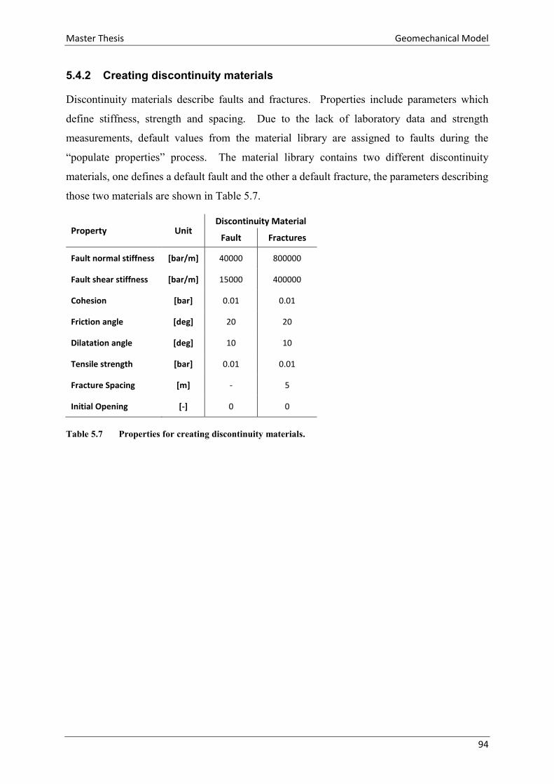
Master Thesis Geomechanical Model
94
5.4.2 Creating discontinuity materials
Discontinuity materials describe faults and fractures. Properties include parameters which
define stiffness, strength and spacing. Due to the lack of laboratory data and strength
measurements, default values from the material library are assigned to faults during the
“populate properties” process. The material library contains two different discontinuity
materials, one defines a default fault and the other a default fracture, the parameters describing
those two materials are shown in Table 5.7.
Property Unit Discontinuity Material
Fault Fractures
Fault normal stiffness [bar/m] 40000 800000
Fault shear stiffness [bar/m] 15000 400000
Cohesion [bar] 0.01 0.01
Friction angle [deg] 20 20
Dilatation angle [deg] 10 10
Tensile strength [bar] 0.01 0.01
Fracture Spacing [m] - 5
Initial Opening [-] 0 0
Table 5.7 Properties for creating discontinuity materials.
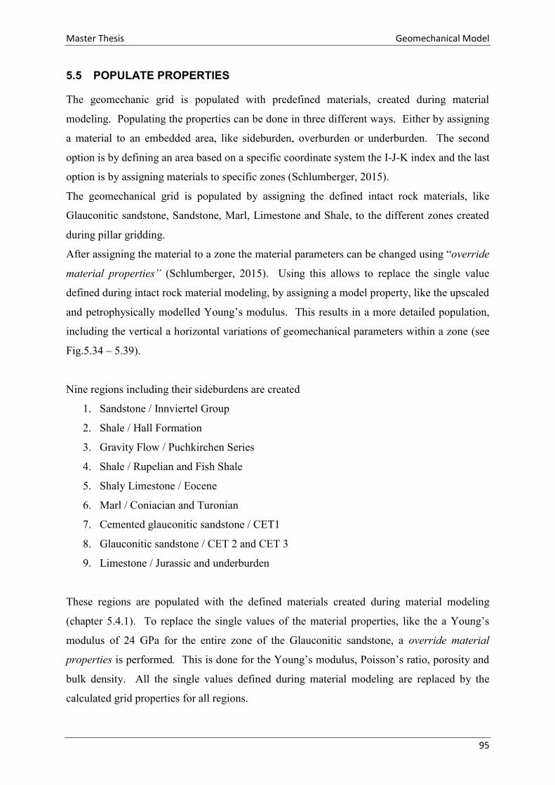
Master Thesis Geomechanical Model
95
5.5 POPULATE PROPERTIES
The geomechanic grid is populated with predefined materials, created during material
modeling. Populating the properties can be done in three different ways. Either by assigning
a material to an embedded area, like sideburden, overburden or underburden. The second
option is by defining an area based on a specific coordinate system the I-J-K index and the last
option is by assigning materials to specific zones (Schlumberger, 2015).
The geomechanical grid is populated by assigning the defined intact rock materials, like
Glauconitic sandstone, Sandstone, Marl, Limestone and Shale, to the different zones created
during pillar gridding.
After assigning the material to a zone the material parameters can be changed using “override
material properties” (Schlumberger, 2015). Using this allows to replace the single value
defined during intact rock material modeling, by assigning a model property, like the upscaled
and petrophysically modelled Young’s modulus. This results in a more detailed population,
including the vertical a horizontal variations of geomechanical parameters within a zone (see
Fig.5.34 – 5.39).
Nine regions including their sideburdens are created
1. Sandstone / Innviertel Group
2. Shale / Hall Formation
3. Gravity Flow / Puchkirchen Series
4. Shale / Rupelian and Fish Shale
5. Shaly Limestone / Eocene
6. Marl / Coniacian and Turonian
7. Cemented glauconitic sandstone / CET1
8. Glauconitic sandstone / CET 2 and CET 3
9. Limestone / Jurassic and underburden
These regions are populated with the defined materials created during material modeling
(chapter 5.4.1). To replace the single values of the material properties, like the a Young’s
modulus of 24 GPa for the entire zone of the Glauconitic sandstone, a override material
properties is performed. This is done for the Young’s modulus, Poisson’s ratio, porosity and
bulk density. All the single values defined during material modeling are replaced by the
calculated grid properties for all regions.
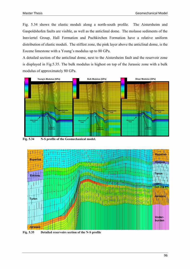
Master Thesis Geomechanical Model
96
Fig. 5.34 shows the elastic moduli along a north-south profile. The Aistersheim and
Gaspoldshofen faults are visible, as well as the anticlinal dome. The molasse sediments of the
Innviertel Group, Hall Formation and Puchkirchen Formation have a relative uniform
distribution of elastic moduli. The stiffest zone, the pink layer above the anticlinal dome, is the
Eocene limestone with a Young’s modulus up to 80 GPa.
A detailed section of the anticlinal dome, next to the Aistersheim fault and the reservoir zone
is displayed in Fig.5.35. The bulk modulus is highest on top of the Jurassic zone with a bulk
modulus of approximately 80 GPa.
Fig. 5.34 N-S profile of the Geomechanical model.
Fig. 5.35 Detailed reservoirs section of the N-S profile
Young‘s Modulus [GPa] Bulk Modulus [GPa] Shear Modulus [GPa]
Aistershaim
Fault
Gaspoldshofen
Fault
Trattnach
Antiklinale
Aistershaim
Fault
Gaspoldshofen
Fault
Trattnach
Antiklinale
Aistershaim
Fault
Gaspoldshofen
Fault
Trattnach
Antiklinale
Turon
Eocene
Jurassic
CET1
CET 2 & 3
Jurassic
Eocene
Turon
Rupelian
Rupelian
Under-
burden

Master Thesis Geomechanical Model
97
Fig. 5.36 shows the distribution of Young’s, bulk and shear modulus along a west – east profile.
The Schwanenstadt fault marks the western boundary of the reservoir zone. Horizontal and
vertical variations within a region are not very prominent.
Fig. 5.36 W-E profile of the Geomechanical model.
The horizontal variation of the bulk modulus along the Top of the Jurassic zone is displayed in
Fig.5.37. The highest values, up to 80 GPa, occur below the anticlinal dome, were the oil
reservoirs are located. A zone of lower values for the bulk modulus is present at the northern
part of the model. The variation of the bulk modulus correlates with variations of bulk densities.
Fig. 5.37 Horizontal variation of Young’s modulus along the Top Jurassic.
Young‘s Modulus [GPa] Bulk Modulus [GPa] Shear Modulus [GPa]
Schwanenstadt Fault Schwanenstadt Fault Schwanenstadt Fault

Master Thesis Geomechanical Model
98
The horizon slice along the top of the reservoir horizon CET2 shows a more uniform bulk
modulus distribution than along the Jurassic horizon. The bulk modulus is in general very low
with an average value of 21 GPa. A slight increase of the bulk modulus is noticeable close to
the major Schwanenstadt and Gaspoldshofen fault.
Fig. 5.38 Horizontal variation of Young’s modulus along the Top CET2 horizon.
The variation of the bulk modulus along the top of the sealing CET1 formation is displayed in
Fig.5.39. The bulk modulus is slightly more varying than on top of the CET2 horizon and the
average bulk modulus is in between the Jurassic an CET2 values, with approximately 36 GPa.
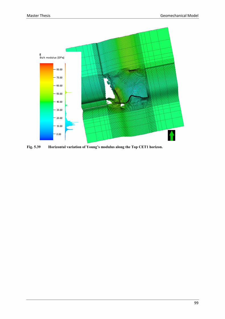
Master Thesis Geomechanical Model
99
Fig. 5.39 Horizontal variation of Young’s modulus along the Top CET1 horizon.

Master Thesis Conclusion
100
6 CONCLUSION
This study aims to model and calculate all properties for the interpretation of the geomechanical
behaviour of the Trattnach area. The thesis can be divided into three main tasks:
The calculation of all relevant petrophysical data. Density, porosity and shear sonic velocity
calculations based on petrophysical relationships have been performed. The density,
porosity and sonic velocities form the foundation for the calculation of all geomechanical
parameters including Young’s modulus, Bulk modulus and Poisson’s ratio. A series of
uniaxial compressive test were performed to determine the uniaxial compressive strength of
rock samples from the reservoir section.
The setup of a geological model in Petrel. An existing reservoir model, covering the area of
the Cenomanian sandstones has been extended up to earth’s surface. The new model now
covers an area of 26 km² and includes the entire basin evolution from Jurassic sandstones up
to the Innviertel Group.
The conversion of the geological model into a geomechanical model has been undergone.
This includes the creation of a geomechanical grid which has been filled with all relevant
elastic properties and intact rock materials.
With these tasks performed the property model is complete. The model shows that the Jurassic
limestone is the most stable formation with a averaged Young's modulus of 48 GPa. These are
followed by the sealing CET1 formation, with 36 GPa. Another stable zone is built by the
Eocene lime- and sandstones with a averaged Young's modulus of 30 GPa. The reservoir rocks
formed by the CET2 and CET3 zone have a Young's modulus of 30 GPa. The Young's modulus
of the zones from the Innviertel Group down to the Rupelian shales increases steadily with
increasing overburden.
This model can now act as the foundation for a geomechanical simulation. When a complete
reservoir simulation is available, a geomechanical simulation, using the in Petrel implemented
VISAGE simulator, can be performed. Unfortunately the provided reservoir simulation
existing, is not sufficient and a geomechanical simulation cannot be performed at this point.
Nevertheless the foundation for starting such a simulation including a working grid and all
properties necessary have been made.

Master Thesis List of Figures
101
7 LIST OF FIGURES
Fig. 2.1 Schematic Stress Tensor in 2D and 3D. 10
Fig. 2.2 Types of strain. 11
Fig. 2.3 Elastic deformation caused by shear waves (after Kearey et al., 2002). 14
Fig. 2.4 Elastic deformation caused by compressional waves (after Kearey et al., 2002). 14
Fig. 2.5 Principal Coordinate System. 15
Fig. 2.6 Schematic Normal Fault. 16
Fig. 2.7 Schematic Strike Slip Fault. 17
Fig. 2.8 Schematic Reverse Fault. 17
Fig. 2.9 Triaxial Test and Mohr Circle Construction. 18
Fig. 2.10 Triaxial Test / Stress – Strain Diagram (Zoback, 2014). 19
Fig. 2.11 Mohr Failure criteria for different faulting regimes (after Zoback, 2014). 20
Fig. 2.12 Three ways to calculate elastic moduli from an axial strain-stress curve (black). 21
Fig. 2.13 Pore Pressure Measurements (Zoback, 2014). 23
Fig. 2.14 Digital Elevation Model of central Europe. 24
Fig. 2.15 Generalized Cross Section through the Austrian Molasse basin. 25
Fig. 2.16 The Mesozoic evolution of the Austrian Molasse Basin (Gross et al., 2015). 27
Fig. 2.17 Cenozoic Evolution of the Austrian Molasse Basin (Gross et al., 2015). 28
Fig. 2.18 Production History of the Trattnach oil field. 30
Fig. 2.19 Fault Systems in Upper Austria. 31
Fig. 2.20 Depth map of the CET2 horizon. 32
Fig. 2.21 Core Measurements of the Cenomanian Sandstone. 33
Fig. 2.22 Well log measurements of the Cenomanian Sandstone. 34
Fig. 3.1 Differences of RAG’s fault models. 37
Fig. 4.1 Study area of the Trattnach Oil Field. 38
Fig. 4.2 Seismic Sections of the study area. 41
Fig. 4.3 Grid Slice, final zonation and layering. 43
Fig. 5.1 Quality Control of the geomechanical gridding process. 46
Fig. 5.2 2D View of fault models. 47

Master Thesis List of Figures
102
Fig. 5.3 Thickness map Coniacian. 48
Fig. 5.4 Topview of the geomechanical grid. 49
Fig. 5.5 Side view of the geomechanical grid. 49
Fig. 5.6 Empirical Relationship between vp and RHOB from TRAT11. 51
Fig. 5.7 Empirical Relationship between vp and RHOB from TRAT12. 52
Fig. 5.8 Calculated density logs based on Gardner´s Equation (Gardner et al., 1974). 54
Fig. 5.9 Pressure gradients for the Trattnach field. 55
Fig. 5.10 Velocity – porosity trend for Cenomanian reservoir sandstones. 56
Fig. 5.11 Quality control of the calculated porosity logs. 58
Fig. 5.12 Calculated porosity logs based on Wyllie’s time-average equation. 59
Fig. 5.13 Porosity – depth trend for the Trattnach area. 61
Fig. 5.14 Calculated shear sonic logs. 64
Fig. 5.15 Calculated Young’s modulus. 66
Fig. 5.16 Vp versus porosity plot with a lower Reuss and an upper Voigt bound. 67
Fig. 5.17 Velocity versus porosity plot for the Cenoman and the Hall Formation. 68
Fig. 5.18 Calculated bulk modulus. 70
Fig. 5.19 Test Results TRAT701B. 73
Fig. 5.20 Test Results TRAT704A. 74
Fig. 5.21 Test Results TRAT705. 75
Fig. 5.22 Test Results TRAT709. 76
Fig. 5.23 Test Results TRAT712A. 77
Fig. 5.24 Test Results TRAT714A. 78
Fig. 5.25 Test Results TRAT714B. 79
Fig. 5.26 Test Results TRAT718. 80
Fig. 5.27 Test Results TRAT615. 81
Fig. 5.28 Lithology specific values of uniaxial compressive strength (Schoen, 2004). 83
Fig. 5.29 Mohr circle construction for the well TRAT6 85
Fig. 5.30 Mohr circle construction for the well TRAT7 85
Fig. 5.31 Upscaled Properties for the well TRAT1. 87
Fig. 5.32 Compressional wave velocity variogram of the Lower Puchkirchen Formation. 88

Master Thesis List of Figures
103
Fig. 5.33 Interpolated data of the CET 2 Zone. 89
Fig. 5.34 N-S profile of the Geomechanical model. 96
Fig. 5.35 Detailed reservoirs section of the N-S profile 96
Fig. 5.36 W-E profile of the Geomechanical model. 97
Fig. 5.37 Horizontal variation of Young’s modulus along the Top Jurassic. 97
Fig. 5.38 Horizontal variation of Young’s modulus along the Top CET2 horizon. 98
Fig. 5.39 Horizontal variation of Young’s modulus along the Top CET1 horizon. 99
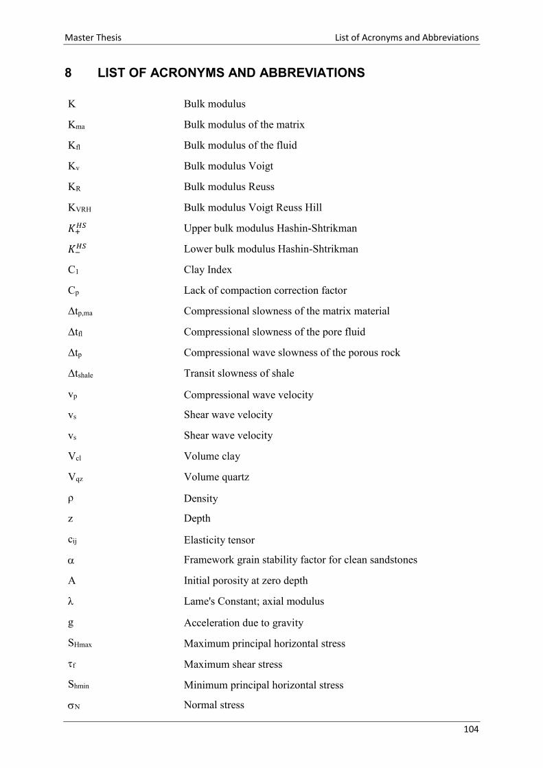
Master Thesis List of Acronyms and Abbreviations
104
8 LIST OF ACRONYMS AND ABBREVIATIONS
K Bulk modulus
Kma Bulk modulus of the matrix
Kfl Bulk modulus of the fluid
Kv Bulk modulus Voigt
KR Bulk modulus Reuss
KVRH Bulk modulus Voigt Reuss Hill
𝐾+𝐻𝑆 Upper bulk modulus Hashin-Shtrikman
𝐾−𝐻𝑆 Lower bulk modulus Hashin-Shtrikman
C1 Clay Index
Cp Lack of compaction correction factor
Δtp,ma Compressional slowness of the matrix material
Δtfl Compressional slowness of the pore fluid
Δtp Compressional wave slowness of the porous rock
Δtshale Transit slowness of shale
vp Compressional wave velocity
vs Shear wave velocity
vs Shear wave velocity
Vcl Volume clay
Vqz Volume quartz
ρ Density
z Depth
cij Elasticity tensor
Framework grain stability factor for clean sandstones
A Initial porosity at zero depth
λ Lame's Constant; axial modulus
g Acceleration due to gravity
SHmax Maximum principal horizontal stress
f Maximum shear stress
Shmin Minimum principal horizontal stress
Normal stress

Master Thesis List of Acronyms and Abbreviations
105
Sv Overburden Stress; vertical Stress
ν Poisson’s Ratio
Pp Pore Pressure
ϕ Porosity
ϕw Time-average porosity
ϕc Corrected porosity
Vertical stress
v Vertical stress
𝜎𝑣′ Effective vertical stress
3 Horizontal stress
β Sensitivity factor towards increasing clay index
µ Shear modulus; Modulus of rigidity
µma Shear modulus of the fluid
Shear Stress
ε Strain
Stress
E Young’s Modulus
ET Tangent modulus
ES Secant modulus
EI Initial modulus
a Empirical constant
b Empirical constant
Δl Change of length
l0 Original length
F Force
h Height
d Diameter
Master Thesis References
106
9 REFERENCES
Anderson, E. M. (1951). The Dynamics of Faulting and Dyke Formation with Applications to Britain.
Edinburgh: Oliver and Boyd.
Andeweg, B., & Cloetingh, S. (1998). Flexure and 'unflexure' of the North Alpine German-Austrian
Molasse Basin: constraints from forward tectonic modelling. In A. Mascle, C. Puigdefabregas,
H. P. Luterbacher, & M. Fernandez, Cenozoic Foreland Basins of Western Europe, pp. 403-
422. Geological Society Special Publications 134.
Avseth, P. T., & Mavko, M. G. (2005). Quantitative Seismic Interpretation, Applying Rock Physics Tools
to Reduce Interpretation Risk. New York: Cambridge University Press.
Bjørlykke, K. (2015). Petroleum Geoscience: From Sedimentary Environments ro Rock Physics.
Heidelberg: Springer-Verlag Berlin.
Brady, B., & Brown, E. T. (1999). Rock Mechanics for Underground Mining. Dordrecht, The
Netherlands: Kluwer Academic Publishers.
Castagna, J. P. (1993). Amplitude-versus-offset analysis; tutorial and review. In J. P. Castagna, & M.
M. Backus, Offset-Dependent Reflectivity—Theory and Practice of AVO Analysis. Tulsa
Oklahoma, USA: Society of Exploration Geophysicists.
Castagna, J. P., Batzle, M. L., & Eastwood, R. L. (1985). Relationships between compressional-wave
and shear-wave velocities in clastic silicate rocks. Geophysics, pp. 571-581.
De Ruig, M. (2003). Deep Marine Sedimentation and Gas Reservoir Distribution in Upper Austria. OIL
GAS European Magazine, 2.
De Ruig, M. J., & Hubbard, S. M. (2006). Seismic facies and reservoir characteristics of a deep-marine
channel belt in the Molasse foreland basin, Puchkirchen Formation, Austria. AAPG Bulletin,
90(5), pp. 735-752.
Dusseault, M B. (2011). Geomechanic Challenges in Petroleum Exploitation. KSCE Journal of Civil
Engineering 15(4), pp. 669-678.
Fjar, E., Holt, R. M., Raaen, A. M., Risnes, R., & Horsrud, P. (2008). Petroleum Related Rock Mechanics
(Vol. Volume 53). Elsevier Science.
Gardner, G. H., Gardner, L. W., & Gregory, A. R. (1974). Formation velocity and density - The
diagnostic basics for stratigraphy traps. Geophysics, 6, pp. 770-780.
Gratzer, R., Bechtel, A., Sachsenhofer, R. F., Linzer, H.-G., Reischenbacher, D., & Schulz, H.-M. (2011).
Oil-oil and oil-source rock correlations in the Alpine Foreland Basin of Austria: Insights from
biomarker and stable carbon isotope studies. Marine and Petroleum Geology, pp. 1171-1186.
Gross, D., Sachsenhofer , R., Rech, A., Sageder, S., Geissler, M., Schnitzer, S., & Troiss, W. (2015). The
Trattnach Oil Field in the North Alpine Foreland Basin (Austria). Austrian Journal of Earth
Sciences(108/2), pp. 151-171.
Gross, D., Sachsenhofer, R. F., Bechtel, A., Gratzer, R., Grundtner, M.-L., Linzer, H.-G., Scheucher, L.
(2018). Petroleum Systems in the austrian sector of the North Alpine Foreland Basin: An
Overview. Journal of Petroleum Geology, pp. 299-318.
Master Thesis References
107
Gusterhuber, J., Dunkl, I., Hinsch, R., Linzer, H., & Sachsenhofer, R. (2012). Neogene uplift and
erosion in the Alpine Foreland Basin (Upper Austria and Salzburg). Geologica Carpatica,
63(4), pp. 298-305.
Gusterhuber, J., Hinsch, R., Linzer, H.-G., & Sachsenhofer, R. F. (2013). Hydrocarbon generation and
migration from sub-thrust source rocks to foreland reservoirs: The Austrian Molasse Basin.
Austrian Journal of Earth Sciences(106/2), pp. 115-136.
Han, D., Nur, A., & Morgan, D. (1986). Effects of porosity and clay content on wave velocities in
sandstones. Geophysics, 11, pp. 2093-2107.
Hashin, Z., & Shtrikman, S. (1963). A variational approach to the theory of the elastic behaviour of
multiphase materials. Journal of the Mechanics and Physics of Solids(Issue 2), pp. 127-140.
Hill, R. (1952). The elastic behaviour of a crystalline aggregate. Proceedings of the Physical Society,
Section A(Issue 5), pp. 349-354.
Jaeger, J. C., & Cook, N. G. (1979). Fundamentals of Rock mechanics (2nd Edition ed.). New York:
Chapman and Hall.
Kearey, P., Brooks, M., & Hill, I. (2002). An Introduction to Geophysical Exploration. Oxford: Blackwell
Science Ltd.
Kuhlemann, J., & Kempf, O. (2002). Post-Eocene evolution of the North Alpine Foreland Basin and its
response to Alpine tectonics. Sedimantary Geology, 152, pp. 45-78.
Mavko, G., Mukerji, T., & Dvorkin, J. (1998). The Rock Physics Handbook. New York: Cambridge
University Press.
Nachtmann, W. (1995). Bruchstrukturen und ihre Bedeutung für die Bildung von Kohlenwasserstoff-
fallen in der oberösterreichischen Molasse. Geologische Paläontologische Mitteilungen, 20,
pp. 221-230.
Nachtmann, W., & Wagner, L. (1987). Mesozoic and Early Tertiary evolution of the Alpine foreland in
Upper Austria and Salzburg, Austria. Tectoniphysics, 137, pp. 61-76.
Ramm, M., & Bjorlykke, K. (1994). Porosity/depth trends in reservoir sandstones: assessing the
quantitative effects of varying pore-pressure, temperature history and mineralogy,
Norwegian Shelf data. Clay Mineralogy, 29, pp. 475-490.
Raymer, L. L., Hunt, E. R., & Gardner, J. S. (1980). An improved sonic transit time-to-porosity
transform. (S. P. (SPWLA), Ed.) Soc. Professional Well Log Analysis (SPWLA) 21st Annual
Logging Symposium.
Reuss, A. (1929). Berechnung der Fließgrenze von Mischkristallen auf Grund der
Plastizitätsbedingung für Einkristalle. Zeitschrift für Angewandte Mathematik und Mechanik,
9.
Rider, M., & Kennedy, M. (2011). The Geological Interpretation of Well Logs. Scotland: Rider-French
Consulting Ltd.
Sachsenhofer, R. F., Leitner, B., Linzer, H., Bechtel, A., Coric, S., Gratzer, R., . . . Soliman, A. (2010).
Deposition, Erosion and Hydrocarbon Source Potential of the Oligocene Eggerding Formation
(Molasse Basin, Austria). Austrian Journal of Earth Science, 103/1, pp. 76-99.
Master Thesis References
108
Schlumberger. (2014). Petrel Reservoir Geomechanics - An integrated environment for 3D and 4D
geomechanics modeling and simulations. software.slb.com/Petrel.
Schlumberger. (2015). Software Manual of the Petrel E&P Software Platform 2015.3. 2015.
Schoen, J. (2004). Physical Properties of Rocks: Fundamentals and Principles of Petrophysics. Elsevier.
Schulz, H., Sachsenhofer, R. F., Bechtel, A., Polesny, H., & Wagner, L. (2002). The origin of
hydrocarbon source rocks in the Austrian Molasse Basin (Eocene–Oligocene transition).
Marine and Petroleum Geology, 19, pp. 683-709.
Sissingh, W. (1997). Tectonostratigraphy of the North Alpine Foreland Basin: correlation of Tertiary
depositional cycles and orogenic phases. Tectonophysics, 282, pp. 223-256.
Steininger, F. F., & Wessely, G. (1999). From the Tethyan Ocean to the Paratethys Sea: Oligocene to
Neogene Stratigraphy, Paleogeography and Paleobiogeography of the circum-Mediterranean
region and the Oligocene to Neogene Basin evolution in Austria . Mitt. Österr. Geol. Ges., pp.
95-116.
Terzaghi, K. (1925). Erdbaumechanik auf Bodenphysikalischer Grundlage. Leipzig-Vienna: Franz
Deuticke.
Tipler, P A. 1991. Physics for Scientists and Engineers. New York : Wortg Publishers Inc., 1991.
Voigt, W. (1910). Lehrbuch der Kristallphysik. Leipzig: Teubner-Verlag.
Wagner, L. R. (1996). Stratigraphy and hydrocarbons in the Upper Austrian Molasse Foredeep (active
margin). In: WESSELY, G. & LIEBL, W., (eds.): Oil and Gas in Alpidic Thrustbelts and Basins of
Central and Eastern Europe. - EAGE Spec. Publ. No. 5, pp. 217-235.
Wagner, L. R. (1998). Tectono-stratigraphy and hydrocarbons in the Molasse Foredeep of Salzburg,
Upper and Lower Austria. In A. Mascle, C. Puigdefabregas, H. P. Luterbacher, & M. Fernandez
, Cenozoic Foreland Basins of Western Europe (pp. 339-369). Geological Society Special
Publications 134.
Witt, K. J. (2008). Grundbau - Taschenbuch Teil1: Geotechnische Grundlagen.
Wyllie, M. R., Gregory, A. R., & Gardner, L. W. (1956). Elastic wave velocities in heterogeneous and
porous media. Geophysics, pp. 41-70.
Yilmaz, Ö. (2001). Seismic Data Analysis: Processing, Inversion, and Interpretation of Seismic Data.
Society of Exploration Geophysicists.
Ziegler, P. A. (1982). Geological Atlas of Western and Central Europe. The Hague: Shell Internationale
Petroleum Maatschappje.
Ziegler, P. A. (1987). Late Cretaceous and Cenozoic intra-plate compressional deformations in the
Alpine foreland-a geodynamic model. Tectonophysics, 137, pp. 389-420.
Zoback , M. D. (2014). Reservoir Geomechanics. New York: Cambridge University Press.
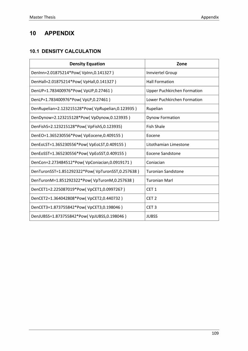
Master Thesis Appendix
109
10 APPENDIX
10.1 DENSITY CALCULATION
Density Equation Zone
DenInn=2.01875214*Pow( VpInn,0.141327 ) Innviertel Group
DenHall=2.01875214*Pow( VpHall,0.141327 ) Hall Formation
DenUP=1.783400976*Pow( VpUP,0.27461 ) Upper Puchkirchen Formation
DenLP=1.783400976*Pow( VpLP,0.27461 ) Lower Puchkirchen Formation
DenRupelian=2.123215128*Pow( VpRupelian,0.123935 ) Rupelian
DenDynow=2.123215128*Pow( VpDynow,0.123935 ) Dynow Formation
DenFishS=2.123215128*Pow( VpFishS,0.123935) Fish Shale
DenEO=1.365230556*Pow( VpEocene,0.409155 ) Eocene
DenEoLST=1.365230556*Pow( VpEoLST,0.409155 ) Litothamian Limestone
DenEoSST=1.365230556*Pow( VpEoSST,0.409155 ) Eocene Sandstone
DenCon=2.273484512*Pow( VpConiacian,0.0919171 ) Coniacian
DenTuronSST=1.851292322*Pow( VpTuronSST,0.257638 ) Turonian Sandstone
DenTuronM=1.851292322*Pow( VpTuronM,0.257638 ) Turonian Marl
DenCET1=2.225087019*Pow( VpCET1,0.0997267 ) CET 1
DenCET2=1.364042808*Pow( VpCET2,0.440732 ) CET 2
DenCET3=1.873755842*Pow( VpCET3,0.198046 ) CET 3
DenJUBSS=1.873755842*Pow( VpJUBSS,0.198046 ) JUBSS

Master Thesis Appendix
110
10.2 POROSITY CALCULATION P
oro
sity
Eq
uat
ion
PH
IEF=
If(
Zon
e_lo
g_lin
ked
_to
_Zo
nat
ion
=0,(
((D
T_n
ew-2
00)/
(60
7-2
00
))),
U)
PH
IEF=
If(
Zon
e_lo
g_lin
ked
_to
_Zo
nat
ion
=2 ,(
((D
T_n
ew-2
00
)/(6
07
-20
0))
), P
HIE
F)
PH
IEF=
If(
Zon
e_lo
g_lin
ked
_to
_Zo
nat
ion
=4,(
((D
T_n
ew-2
10)/
(60
7-2
10
))),
PH
IEF)
PH
IEF=
If(
Zon
e_lo
g_lin
ked
_to
_Zo
nat
ion
=6,(
((D
T_n
ew-1
87)/
(60
7-1
87
))),
PH
IEF)
PH
IEF=
If(
Zon
e_lo
g_lin
ked
_to
_Zo
nat
ion
=8 A
nd
Po
ro_S
on
>=0
.1,(
(DT_
new
-18
7)/
(60
7-1
87
)), P
HIE
F)
PH
IEF=
If(
Zon
e_lo
g_lin
ked
_to
_Zo
nat
ion
=9 A
nd
Po
ro_S
on
<=0
.1,(
(DT_
new
-20
0)/
(60
7-2
00
)), P
HIE
F)
PH
IEF=
If(
Zon
e_lo
g_lin
ked
_to
_Zo
nat
ion
=9 A
nd
Po
ro_S
on
>=0
.1,(
(DT_
new
-20
0)/
(60
7-2
00
)), P
HIE
F)
PH
IEF=
If(
Zon
e_lo
g_lin
ked
_to
_Zo
nat
ion
=10
An
d P
oro
_So
n>=
0.1
,((D
T_n
ew-1
87
)/(6
07
-18
7))
, PH
IEF)
PH
IEF=
If(
Zon
e_lo
g_lin
ked
_to
_Zo
nat
ion
=11
An
d P
oro
_So
n>=
0.1
,((D
T_n
ew-1
87
)/(6
07
-18
7))
, PH
IEF)
PH
IEF=
If(
Zon
e_lo
g_lin
ked
_to
_Zo
nat
ion
=13
,((D
T_n
ew-1
73
)/(6
07
-17
3))
, PH
IEF)
PH
IEF=
If(
Zon
e_lo
g_lin
ked
_to
_Zo
nat
ion
=15
,((D
T_n
ew-1
82
)/(6
07
-18
2))
, PH
IEF)
PH
IEF=
If(
Zon
e_lo
g_lin
ked
_to
_Zo
nat
ion
=21
An
d P
oro
_So
n>=
0.1
,((D
T_n
ew-1
87
)/(6
07
-18
7))
, PH
IEF)
PH
IEF=
If(
Zon
e_lo
g_lin
ked
_to
_Zo
nat
ion
=21
An
d P
oro
_So
n<=
0.1
,((D
T_n
ew-1
87
)/(6
07
-18
7))
, PH
IEF)
PH
IEF=
If(
Zon
e_lo
g_lin
ked
_to
_Zo
nat
ion
=18
An
d P
oro
_So
n>=
0.1
,((D
T_n
ew-1
55
)/(6
07
-15
5))
, PH
IEF)
PH
IEF=
If(
Zon
e_lo
g_lin
ked
_to
_Zo
nat
ion
=23
An
d P
oro
_So
n>=
0.1
,((D
T_n
ew-1
55
)/(6
07
-15
5))
, PH
IEF)
PH
IEF=
If(
Zon
e_lo
g_lin
ked
_to
_Zo
nat
ion
=26
An
d P
oro
_So
n>=
0.1
,(((
DT_
new
-18
2)/
(60
7-1
82
))),
PH
IEF)
PH
IEF=
If(
Zon
e_lo
g_lin
ked
_to
_Zo
nat
ion
=26
An
d P
oro
_So
n<=
0.1
,(((
DT_
new
-16
7)/
(60
7-1
67
))),
PH
IEF)
PH
IEF=
If(
Zon
e_lo
g_lin
ked
_to
_Zo
nat
ion
=28
An
d P
oro
_So
n>=
0.1
,(((
DT_
new
-18
2)/
(60
7-1
82
))*
0.9
), P
HIE
F)
PH
IEF=
If(
Zon
e_lo
g_lin
ked
_to
_Zo
nat
ion
=30
An
d P
oro
_So
n>
=0.1
,(((
DT_
new
-18
7)/
(60
7-1
87
))*
0.9
), P
HIE
F)
PH
IEF=
If(
Zon
e_lo
g_lin
ked
_to
_Zo
nat
ion
=32
,((D
T_n
ew-1
56
)/(6
07
-15
6))
, PH
IEF)
Zon
e
Inn
vier
tel G
rou
p
Hal
l Fo
rmat
ion
Up
per
Pu
chki
rch
en F
orm
atio
n
Low
er P
uch
kirc
hen
Fo
rmat
ion
Ru
pel
ian
Ru
pel
ian
Ru
pel
ian
Dyn
ow
Fo
rmat
ion
Fish
Sh
ale
Lito
tham
ian
Lim
esto
ne
Eoce
ne
San
dst
on
e
Turo
nia
n S
and
sto
ne
Turo
nia
n S
and
sto
ne
Co
nia
cian
Turo
nia
n M
arl
CET
1
CET
1
CET
2
CET
3
JUB
SS
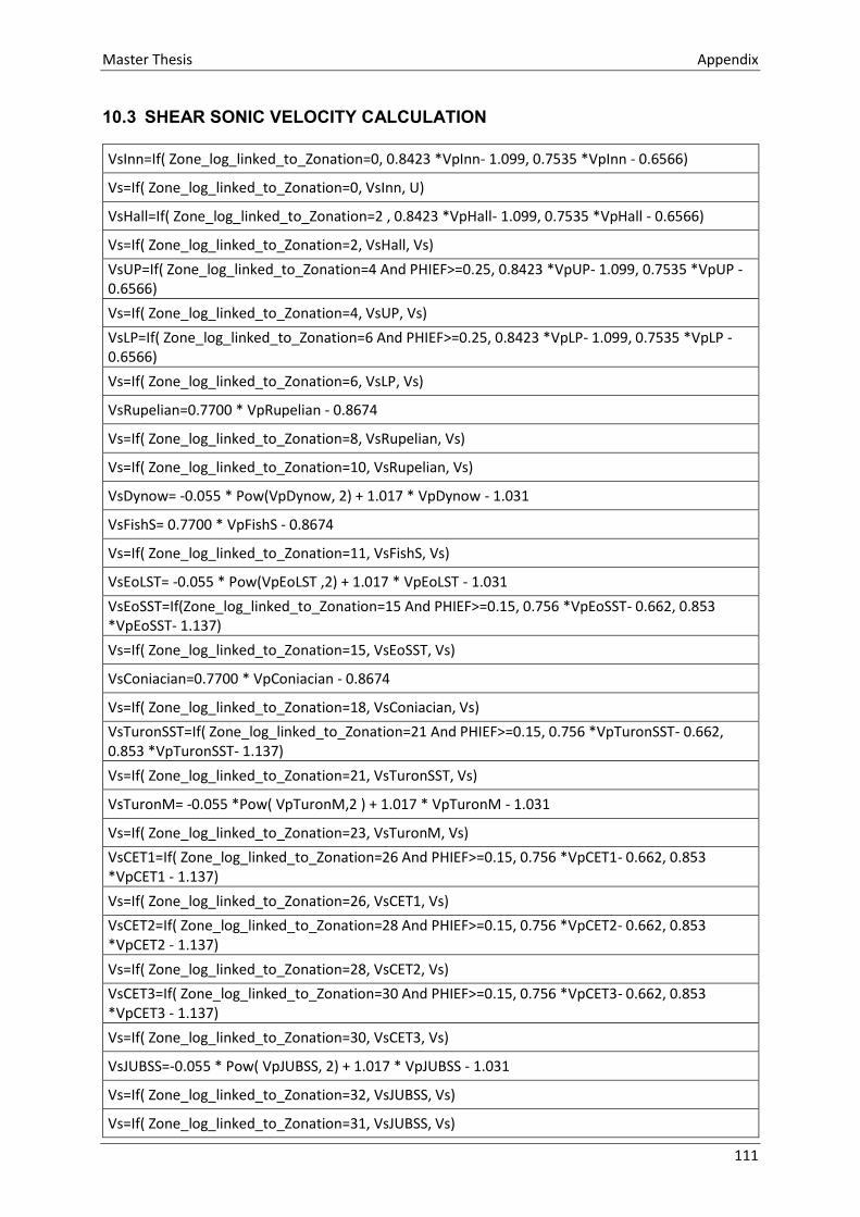
Master Thesis Appendix
111
10.3 SHEAR SONIC VELOCITY CALCULATION
VsInn=If( Zone_log_linked_to_Zonation=0, 0.8423 *VpInn- 1.099, 0.7535 *VpInn - 0.6566)
Vs=If( Zone_log_linked_to_Zonation=0, VsInn, U)
VsHall=If( Zone_log_linked_to_Zonation=2 , 0.8423 *VpHall- 1.099, 0.7535 *VpHall - 0.6566)
Vs=If( Zone_log_linked_to_Zonation=2, VsHall, Vs)
VsUP=If( Zone_log_linked_to_Zonation=4 And PHIEF>=0.25, 0.8423 *VpUP- 1.099, 0.7535 *VpUP - 0.6566)
Vs=If( Zone_log_linked_to_Zonation=4, VsUP, Vs)
VsLP=If( Zone_log_linked_to_Zonation=6 And PHIEF>=0.25, 0.8423 *VpLP- 1.099, 0.7535 *VpLP - 0.6566)
Vs=If( Zone_log_linked_to_Zonation=6, VsLP, Vs)
VsRupelian=0.7700 * VpRupelian - 0.8674
Vs=If( Zone_log_linked_to_Zonation=8, VsRupelian, Vs)
Vs=If( Zone_log_linked_to_Zonation=10, VsRupelian, Vs)
VsDynow= -0.055 * Pow(VpDynow, 2) + 1.017 * VpDynow - 1.031
VsFishS= 0.7700 * VpFishS - 0.8674
Vs=If( Zone_log_linked_to_Zonation=11, VsFishS, Vs)
VsEoLST= -0.055 * Pow(VpEoLST ,2) + 1.017 * VpEoLST - 1.031
VsEoSST=If(Zone_log_linked_to_Zonation=15 And PHIEF>=0.15, 0.756 *VpEoSST- 0.662, 0.853 *VpEoSST- 1.137)
Vs=If( Zone_log_linked_to_Zonation=15, VsEoSST, Vs)
VsConiacian=0.7700 * VpConiacian - 0.8674
Vs=If( Zone_log_linked_to_Zonation=18, VsConiacian, Vs)
VsTuronSST=If( Zone_log_linked_to_Zonation=21 And PHIEF>=0.15, 0.756 *VpTuronSST- 0.662, 0.853 *VpTuronSST- 1.137)
Vs=If( Zone_log_linked_to_Zonation=21, VsTuronSST, Vs)
VsTuronM= -0.055 *Pow( VpTuronM,2 ) + 1.017 * VpTuronM - 1.031
Vs=If( Zone_log_linked_to_Zonation=23, VsTuronM, Vs)
VsCET1=If( Zone_log_linked_to_Zonation=26 And PHIEF>=0.15, 0.756 *VpCET1- 0.662, 0.853 *VpCET1 - 1.137)
Vs=If( Zone_log_linked_to_Zonation=26, VsCET1, Vs)
VsCET2=If( Zone_log_linked_to_Zonation=28 And PHIEF>=0.15, 0.756 *VpCET2- 0.662, 0.853 *VpCET2 - 1.137)
Vs=If( Zone_log_linked_to_Zonation=28, VsCET2, Vs)
VsCET3=If( Zone_log_linked_to_Zonation=30 And PHIEF>=0.15, 0.756 *VpCET3- 0.662, 0.853 *VpCET3 - 1.137)
Vs=If( Zone_log_linked_to_Zonation=30, VsCET3, Vs)
VsJUBSS=-0.055 * Pow( VpJUBSS, 2) + 1.017 * VpJUBSS - 1.031
Vs=If( Zone_log_linked_to_Zonation=32, VsJUBSS, Vs)
Vs=If( Zone_log_linked_to_Zonation=31, VsJUBSS, Vs)
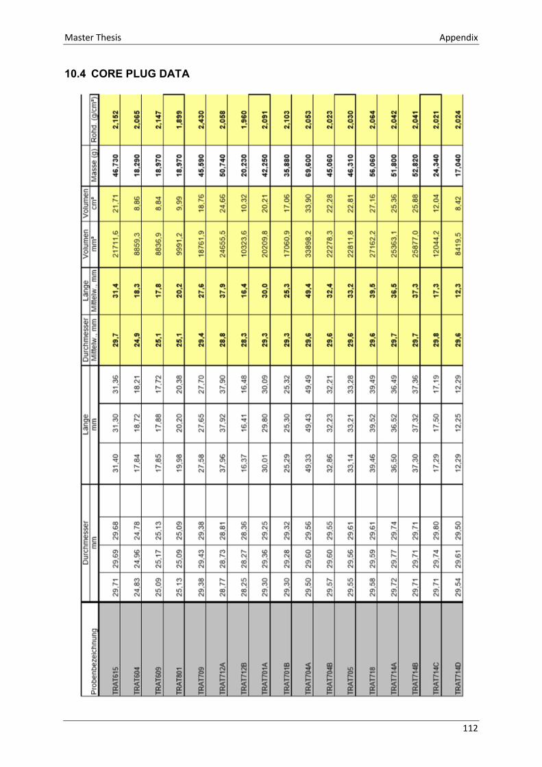
Master Thesis Appendix
112
10.4 CORE PLUG DATA
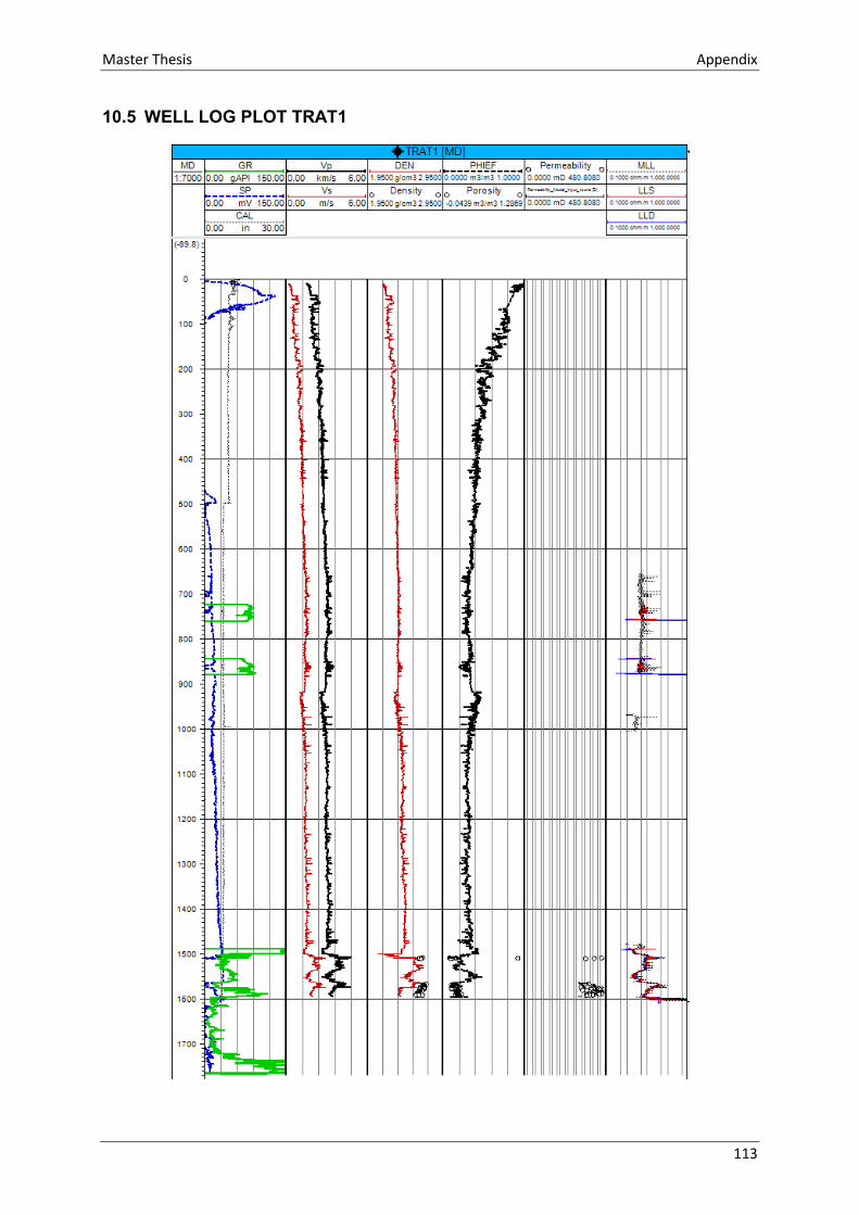
Master Thesis Appendix
113
10.5 WELL LOG PLOT TRAT1

Master Thesis Appendix
114
10.6 WELL LOG PLOT TRAT2

Master Thesis Appendix
115
10.7 WELL LOG PLOT TRAT3

Master Thesis Appendix
116
10.8 WELL LOG PLOT TRAT4
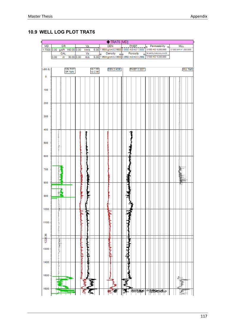
Master Thesis Appendix
117
10.9 WELL LOG PLOT TRAT6

Master Thesis Appendix
118
10.10 WELL LOG PLOT TRAT7

Master Thesis Appendix
119
10.11 WELL LOG PLOT TRAT8

Master Thesis Appendix
120
10.12 WELL LOG PLOT TRAT9
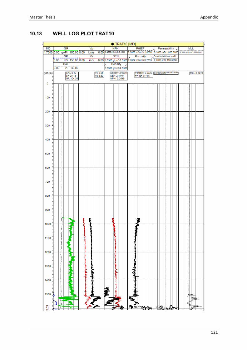
Master Thesis Appendix
121
10.13 WELL LOG PLOT TRAT10
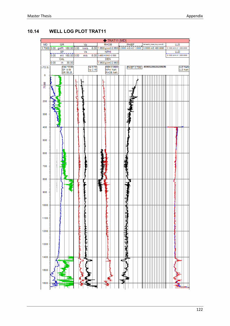
Master Thesis Appendix
122
10.14 WELL LOG PLOT TRAT11
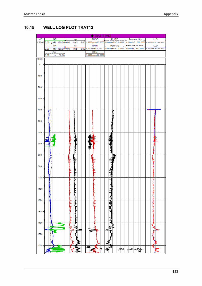
Master Thesis Appendix
123
10.15 WELL LOG PLOT TRAT12
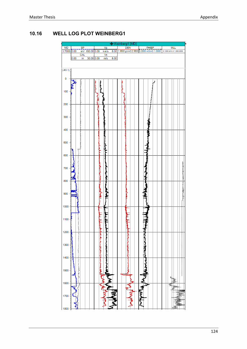
Master Thesis Appendix
124
10.16 WELL LOG PLOT WEINBERG1
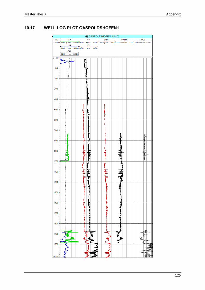
Master Thesis Appendix
125
10.17 WELL LOG PLOT GASPOLDSHOFEN1