Research Collection - ETH Zürich
155
Research Collection Doctoral Thesis Measurement of fracture mechanical properties of snow and application to dry snow slab avalanche release Author(s): Sigrist, Christian Publication Date: 2006 Permanent Link: https://doi.org/10.3929/ethz-a-005282374 Rights / License: In Copyright - Non-Commercial Use Permitted This page was generated automatically upon download from the ETH Zurich Research Collection . For more information please consult the Terms of use . ETH Library
-
Upload
khangminh22 -
Category
Documents
-
view
5 -
download
0
Transcript of Research Collection - ETH Zürich

Research Collection
Doctoral Thesis
Measurement of fracture mechanical properties of snow andapplication to dry snow slab avalanche release
Author(s): Sigrist, Christian
Publication Date: 2006
Permanent Link: https://doi.org/10.3929/ethz-a-005282374
Rights / License: In Copyright - Non-Commercial Use Permitted
This page was generated automatically upon download from the ETH Zurich Research Collection. For moreinformation please consult the Terms of use.
ETH Library

Diss. ETH No. 16736
Measurement of Fracture Mechanical
Properties of Snow and Application
to Dry Snow Slab Avalanche Release
A dissertation submitted to the
SWISS FEDERAL INSTITUTE OF TECHNOLOGY ZÜRICH
for the degree of
DOCTOR OF SCIENCES
presented by
CHRISTIAN SIGRIST
Master of Science in Physics, University of Bern
born 24.03.1976
citizen of Sigriswil, Bern
accepted on the recommendation of
Prof. Dr. Jürg Dual, examiner
Dr. Jürg Schweizer, co-examiner
Dr. Hans-Jakob Schindler, co-examiner
2006

Abstract
A dry snow slab avalanche is released by a sequence of failure processes in the snow cover.
When a weak layer in the snow cover is damaged over a certain area, the weak layer starts
to fail progressively in slope parallel direction. This shear failure disconnects the overlayingslab from the basal layer. Finally, a tensile fracture occurs in slope normal direction across
the layering which releases the slab. For a better understanding of these mechanisms a
well founded understanding of the fracture mechanical properties of homogeneous and
layered snow is essential.
The aim of this work was to investigate the fracture mechanical properties of snow under
tension (mode I) and under shear (mode II) with homogeneous and layered snow samples
on the basis of experiments in the cold laboratory and in the field and to relate the results
to dry slab avalanche release. The experimental work was structured in three groups of
fracture experiments: experiments in mode I with homogeneous snow samples in the cold
laboratory, experiments in mode II with layered snow samples in the cold laboratory and
mode II experiments with in-situ snow beams in the field.
For the mode I experiments, beam-shaped snow specimens cut from homogeneous layersof naturally deposited snow were subjected to three-point bending and cantilever beam
tests. Uncracked specimens were used to determine the tensile strength of snow and
notched specimens to determine the critical stress intensity factor in mode I. The three-
point bending tests provided higher values than the cantilever beam tests. Furthermore
the cantilever beam tests depended on cantilever length. The differences between the test
methods were significant and were attributed to non-negligible size and shape effects.
The fracture process zone was experimentally determined and was estimated to be in
the order of several centimeters, implying that snow has to be considered as a quasi-
brittle material at the scale of our experiments. For a quasi-brittle material linear elastic
fracture mechanics is applicable only with a size correction. As a method to correct the
critical stress intensity factor to the size-independent fracture toughness, K]r, which is
a material property, the equivalent fracture toughness, KfIc, was determined according
to Bazant and Planas (1998) and a size correction function was proposed. The results
for Kcn, ranged from O.SkPay/m for a density of p = 150kg/m3 up to GkPay7 for
a density of p ~ 350kg/W for typical slab layers. It was confirmed that snow has an
extremely low value of KIc. Fracture toughness is expected to be size dependent up to
i

the scale of a slab avalanche.
Layered snow samples including a weak layer were tested in mode II to determine the
energy release rate of a crack propagating along the weak layer A new experimental
setup based on a cantilever beam experiment was designed and proved to be applicablefor layered snow samples In absence of an analytical solution, the finite element method
(FEM) was used to simulate the experiments and determine the energy release rate
numerically A critical energy release rate Gj — 0 04 ± 0 02 J/m2 was found for the
tested weak layers Gf was primarily a material property of the weak layer For similar
snow densities, mode I fracture toughness results were about two times as large as for
the tested weak layers in mode II Two analytical approaches were tested and comparedto the FEM results Both analytical approaches, a homogeneous cantilever beam with
a deep crack, and a bilayer beam with interface crack were highly correlated with the
results obtained from the FE model The analytical results of both approaches were
too large by a factor of about two Due to the higher coefficient of determination, the
cantilever beam approach should be preferred In addition, the dynamic Young's modulus
of the tested snow samples was determined The results for the Young's modulus were
strongly correlated with an index for the Young's modulus derived from a penetrationresistance profile recorded with a snow micro-penetrometer SMP
A field test was developed in which a weak layer in an isolated snow beam was tested in
mode II in-situ on a slope The critical energy release rate Gf was determined numerically
in a FEM simulation The result for the tested weak layers was Gj — 0 07±0 01 J/m2 It
was found that slope normal bending of the slab contributed considerably to the energy
release rate G of our tests and was more important than the component due to shear
loading for angles between 30° and 45° Critical crack sizes of about 25 cm were required
to start fracture propagation along the weak layer of the isolated beams
By applying new test methods to snow and acquiring a considerable data set of fracture
mechanical properties of snow in laboratory and field tests, it was possible to improve
the knowledge and the understanding of the fracture mechanical behaviour of snow It
could be shown that for fracture propagation the material properties of the weak layeras well as of the overlaying slab play an important role Whereas the energy to fracture
a weak layer depends on the material properties of the weak layer, the available energy
for crack propagation depends mainly on the material properties of the overlaying slab
and the slope normal collapse height of a weak layer It is expected that this behaviour
holds also for the scale of a slab avalanche
m

Zusammenfassung
Bevor eine Schneebrettlawine abgleitet, kommt es in der Schneedecke zu einer Reihe
von Bruchprozessen Sobald eine genügend grosse Fläche einer Schwachschicht in der
Schneedecke geschädigt ist, kommt es zu einer selbstständigen Bruchausbreitung ent¬
lang dieser Schwachschicht in hangparalleler Richtung. Durch diesen Scherbruch wird
das Schneebrett von der darunter liegenden Schicht getrennt. Unter der zunehmenden
Last kommt es zu einem Zugbruch senkrecht zur Hangrichtung der zum abgleiten des
Schneebrettes führt. Um diese Mechanismen besser verstehen zu lernen ist es wichtig,vorerst einmal die bruchmechanischen Eigenschaften von homogenem und geschichtetemSchnee zu kennen.
Die Zielsetzung dieser Arbeit war es, in Labor- und in Feldexperimenten die bruchme¬
chanischen Eigenschaften von Schnee unter Zugbelastung (Mode I) und unter Scherbe¬
lastung (Mode II) experimentell zu bestimmen und die Resultate auf die Auslöseprozesse
einer Schneebrettlawine zu übertragen. Die experimentelle Arbeit wurde in drei Gruppen
unterteilt: Mode I Experimente mit homogenen Schneeproben im Kältelabor, Mode II
Experimente mit geschichteten Schneeproben im Kältelabor und Mode II Experimente
mit Schneeblöcken im Gelände
Für die Mode I Tests wurden balkenförmige Schneeproben aus einer homogenen Schicht
der Schneedecke ausgestochen. Diese wurden in Drei-Punkt-Biegeversuchen und in Bal¬
kenversuchen mit einem Ausleger (Cantilever beam tests) getestet. Dabei wurden unge¬
kerbte Proben verwendet um die Zugfestigkeit zu bestimmen und vorgekerbte Proben zur
Bestimmung der kritischen Spannungsintensitätsfaktoren. Die Resultate der Drei-Punkt-
Biegeversuchen fielen höher aus als diejenigen der Balkenversuche. Die Resultate der Bal¬
kenversuche wurden zudem durch die Länge des Auslegers beeinflusst. Die signifikantenUnterschiede zwischen den verschiedenen Testmethoden wurden nicht vernachlässigbarenGrössen- und Formabhängigkeiten zugeordnet. Die Grösse der Bruchprozesszone wurde
aus Experimenten auf einige Zentimeter geschätzt. Dies zeigt, dass für die Grössenord-
nung unserer Experimente Schnee als quasi-brüchiges Material angesehen werden muss.
Handelt es sich um ein quasi-brüchiges Material, ist die linear elastische Bruchmechanik
nur mit einer Grössenkorrektur anwendbar. Um die gemessenen kritischen Spannungsin¬tensitätsfaktoren auf die grössenunabhängige Bruchzähigkeit, KjP, zu korrigieren, wurde
die äquivalente Bruchzähigkeit KJr, nach Bazant und Planas (1998) bestimmt. Für ty-
in

pische Schneeschichten reichten die Resultate für Kjc von O.SkPav'fn für eine Dichte
von p = 150 kg/m3 bis 6kPav/m für eine Dichte von p = 350kg/m3. Damit konnte
bestätige werden, dass Schnee eine extrem niedrige Bruchzähigkeit hat. Es wird erwartet,
dass die Bruchzähigkeit bis hin zur Grösse eines Schneebrettes Grössenabhängig ist.
Aus Experimenten mit geschichteten Schneeproben die eine Schwachschicht enthiel¬
ten wurde die Energiefreisetzungsrate in Mode II bestimmt. Dafür wurde ein neuer
experimenteller Aufbau entwickelt, der auf einem Balkenexperiment beruht. Da kei¬
ne analytische Lösung für die Bestimmung der Energiefreisetzungsrate zur Verfügung
stand, wurde diese numerisch, mittels der finiten Element Methode (FEM) bestimmt.
Für die getesteten Schwachschichten wurde eine kritische Energiefreisetzungsrate von
Gf — 0.04 ± 0.02 J/m2 bestimmt. Gf war in erster Linie eine Materialeigenschaft der
Schwachschicht. Für Schnee vergleichbarer Dichte war die Bruchzähigkeit in Mode I etwa
doppelt so gross wie in Mode II. In der Folge wurden die FEM Resultate mit den Resulta¬
ten zweier adaptierter analytischer Lösungen verglichen. Es handelte sich dabei um eine
analytische Lösung eines homogenen Auslegerbalkens mit einem tiefen Riss und einer
Lösung für einen Balken bestehend aus zwei Schichten mit einem Schichtgrenzenriss.Die Resultate der analytischen Lösungen waren gut korreliert mit den FEM Resultaten,
aber überstiegen diese für beide Lösungen um einen Faktor zwei. Auf Grund des höheren
Bestimmtheitsmasses, sollte die Auslegerbalken-Lösung vorgezogen werden. Zusätzlich
wurde das Elastizitätsmodul der getesteten Schneeproben bestimmt. Die Resultate waren
gut korreliert mit einem Elastizitätsindex der aus einem Eindringwiderstandsprofil eines
Schnee-Mikro-Penetrometers (SMP) bestimmt wurde.
Ein Feldtest wurde entwickelt in dem Schwachschichten in allseitig isolierten Schnee¬
blöcken direkt im Hang in Mode II getestet wurden. Die kritische Energiefreisetzungsratewurde numerisch in einer FEM Simulation bestimmt. Für die getesteten Schwachschich¬
ten lag die kritische Energiefeisetzungsrate bei Gf = 0.07 =t 0.01 J/m2. Ein Durchbie¬
gen des Schneebrettes rechtwinklig zum Hang trägt erheblich zu G bei und kann für
Hangneigungen zwischen 30° und 45° den Beitrag auf Grund der Scherbelastung so¬
gar überwiegen. Kritische Schnittlängen von 25 cm waren nötig, um eine selbstständige
Bruchausbreitung entlang der Schwachschicht auszulösen.
Mit den neuen Testmethoden konnte im Labor und im Feld eine repräsentative Da¬
tenmenge der bruchmechanischen Eigenschaften von Schnee gesammelt werden. Damit
war es möglich das Wissen und Verständnis um die Bruchmechanik von Schnee zu er¬
weitern. Es konnte gezeigt werden, dass für die Bruchausbreitung im Schnee sowohl die
Schwachschicht als auch das darüber liegende Schneebrett eine entscheidende Rolle spie¬
len. Während die Energie die benötigt wird um eine Schwachschicht zu brechen von den
Eigenschaften der Schwachschicht abhängt, hängt die für den Bruchprozess zur Verfü¬
gung stehende Energie vor allem vom Schneebrett ab. Es wird angenommen, dass dies
nicht nur für den experimentellen Fall, sondern auch für den Fall eines Schneebrettes
gilt.
IV

List of Symbols
Symbol Description Unit
A Cross sectional area m2
a Crack length or cut length m
da., Aa, Crack or cut extension m
a,. Critical crack or cut length m
b Ligament width m
D Specimen or structure size m
Do Characteristic structure size m
E Young's modulus Pa
F Applied force N
VfG
Force leading to specimen failure
Energy release rate
N
J/m2Of Critical energy release rate J/m2
Gc Effective critical energy release rate J/m2
9 Gravitational acceleration m/s2JI Slab thickness m
h Specimen height m
K Stress intensity factor Pa^m
k-i, 11,111Stress intensity factor in mode 1, mode II and mode III Pay/m
a; Fracture toughness Pav'ïïï
ax Equivalent fracture toughness Pa^
A'/ Critical stress intensity factor Pa^mL Length of protruding part (CB-test) m
I Specimen length m
M Moment Nm
MF Bending moment due to applied force (per specimen width) N
Ma Bending moment due to body weight i per specimen w dth) N
III: Mass kgP Applied load N
R Size of the fracture process zone m
Rl: Maximum size of the fracture process zone m
r, f Position, position vector m

Symbol Description Unit
5
.s
/
U
u*
a
K
vf
y,w
"'I
Shear modulus
Span (Distance between supporting points, 3PB-test)
Layer thickness
Stored elastic strain energy
Complementary strain energy
DisplacementElastic energy
Fracture energy
Gravitational energy
Specimen or body width
Specific fracture energy
Pa
m
m
J
J
m
J
J
J
m
J/m2
Greek
a
OU)v
i
p
(T, <7(
&roh
acoh
aN
T
T,
Inclination of weak layer to the vertical
Crack tip opening displacement (CTOD)Deformation
Deformation rate
Heaviside step function
Poisson 's ratio
Bimaterial constant
Density
Stress, stress component (/' = 1, 2, 3; j — 1, 2, 3)Tensile strength (Maximum stress a material can
sustain. Equal to 07 if no crack is present)Cohesive stress (cohesive crack model)Maximum cohesive stress (cohesive crack model)Nominal failure stress = nominal strengthNominal stress (Load divided by the original undeformed
and uncracked cross section)Effective stress (Load divided by the remaining cross section)Plastic yield strength (Stress that is necessary to initiate
inelastic behaviour in ductile materials)Shear stress
Shear strengthShear stress due to a gravitational load
Peak (maximum) shear stress
Residual shear stress
Position angle (polar coordinate system)Slope angle, inclination of weak layer to the horizontal
Phase angle of loading
m
1/s
kg/m3Pa
Pa
Pa
Pa
Pa
Pa
Pa
Pa
Pa
Pa
Pa
Pa
Pa
Others
Flexural rigidity Nm
vi

Symbol Description Unit
Subscriptb bottom
c critical (for material properties)f failure
t top
WL weak layer
y yield, yielding
VII

Seite Leer /Blank leaf

Contents
Acknowledgements v
1 Introduction 1
1 1 Living with avalanche danger 1
1 2 Snow as a material 2
1 3 Snow avalanche formation 5
1 4 Dissertation outline 12
2 Fracture mechanics 15
2 1 Definition and history 15
2 2 Strength of materials vs fracture mechanics 16
2 3 Linear elastic fracture mechanics 17
2 3 1 Energy release rate and specific fracture energy 17
2 3 2 Stress intensity factor and fracture toughness 18
2 3 3 Energy release rate versus stress intensity factor 20
2 4 Non linear extensions 20
2 4 1 Brittle, ductile and quasi-brittle fracture behaviour 21
2 4 2 Fracture process zone 22
2 4 3 Consequences of quasi brittle behavior 24
2 5 Failure of interfaces 27
2 5 1 The complex stress intensity factor 27
2 5 2 Energy release rate for an interface crack 28
2 6 Application of fracture mechanical concepts to snow 29
2 6 1 Experimental studies 29
2 6 2 A model for shear fracture propagation 30
2 6 3 A model for a slope normal displacement of the slab 32
3 Methods 35
3 1 Standard measurement techniques for snow characterization 35
3 2 Laboratory tests 37
3 2 1 Sample collection 37
3 2 2 Three-point bending test 38
3 2 3 Cantilever beam test 41
IX

Contents
3 2 4 Shear fracture test 43
3 2 5 FE model of shear fracture test 45
3 3 Field test 47
3 3 1 FE model of field test 49
3 4 Young's modulus 49
3 4 1 Dynamic measurement with cyclic loading device 51
3 4 2 Derived from penetration resistance 51
3 5 High-speed photography 53
4 Results 55
4 1 Fracture in homogeneous snow samples 55
4 11 Behaviour of snow under loading 57
4 12 Tensile strength 58
4 13 Critical stress intensity factor in mode I from 3PB-tests 59
4 14 Critical stress intensity factor in mode I from CB-tests 61
4 15 Quantification of the size effect 63
4 16 Fracture process zone 68
4 17 Application of the failure assessment diagram 69
4 18 Fracture speed in mode I 70
4 2 Fracture in layered snow samples 73
4 2 1 Tested weak layers 73
4 2 2 Young's modulus 75
4 2 3 Energy release rate in mode II 79
4 2 4 Comparison of analytical approaches to FEM results 81
4 2 5 Comparison of mode I and mode II results 83
4 3 Fracture of weak layers on slopes 85
4 3 1 Shear strength of the tested weak layer 85
4 3 2 Energy release rate for the tested weak layer 88
4 3 3 Influence of bending 90
4 3 4 Analytical approach for the field experiments 95
5 Discussion 99
5 1 Fracture in mode I 99
5 11 The load-displacement curve 99
5 12 The bending experiment to determine tensile strength 100
5 13 Comparison of 3PB-tests and CB-tests 101
5 14 Fracture speed 103
5 2 The limitation of LEFM for snow 105
5 2 1 The size correction function 105
5 2 2 The fracture process zone 106
5 2 3 The FAD 107
5 3 Fracture in mode II 108
53 1 Determination of the Young's modulus 108
5 3 2 Energy release rate in a mode II fracture 110
x

Contents
5 3 3 Comparing numerical and analytical solutions 111
5 3 4 Comparing mode I and mode II results 112
5 4 Field experiments 112
5 4 1 Failure behaviour 112
5 4 2 Energy release rate measured in the field 113
5 4 3 FEM results 114
5 4 4 Analytical approach 115
5 4 5 Further use of the field test 116
6 Conclusions 117
6 1 Summary 117
6 2 Conclusions 117
6 3 Outlook 122
Bibliography 125
A Calculation of errors 133
A 1 The error of aN 133
B Stratigraphie snow cover profiles 135
Acknowledgements
Curriculum Vitae
XI

Chapter 1
Introduction
1.1 Living with avalanche danger
The oldest documents reporting on avalanches can be traced back to the time between
the 12th and 14th century. In this period, the Walser and the Alemanni started to
settle even the remotest valleys of the European Alps in search of new living space
(Ammann et al., 1997). From that time on the settlers were increasingly exposed to
the specific dangers of the alpine terrain including mud flows, rock falls, landslides and
snow avalanches, the subject of this thesis. Step by step they learned to live with the
danger and began to search for protection. Already in medieval times people recognizedthat avalanche frequency increased when they cut down too much of the alpine forest.
Letters dating from this time testify that the clearing of forest was prohibited in some
exposed areas. In the 19th century people started to build avalanche defence structures
high up the mountain slopes in areas where avalanches tended to release. First they used
wood or stones to build up fences or walls which were replaced by large steel structures
from the beginning of the 1950ies. Countless damage could be prevented since then,
but up to now it is not possible to control the danger caused by avalanches completely.Avalanches can not be predicted in space and time nor can their extension and runout
path be foreseen in detail.
Nowadays avalanches are not only threatening alpine infrastructure like buildings, roads
or railways but also an increasing number of people following their outdoor activities
in the snow covered mountains. Skiing and snowboarding beyond the controlled runs
has become very popular in recent years and about 90% of an average of 26 fatalities
per year in the Swiss Alps can be attributed to winter sports (Tschirky et al., 2000).The fatal human triggered avalanches are in 90% triggered by the victims or by another
member of their group (Schweizer and Lütschg, 2001), or in other words, the victims
actively expose themselves to danger.
Since the 1940ies the Swiss avalanche warning service has provided information on the
1

Chapter 1 Introduction
actual avalanche situation in Switzerland. Today, a forecast of the avalanche dangerfor the next day, the so called avalanche bulletin1, provides the basis for decisions of
local authorities, persons in charge of road safety, ski patrols and backcountry skiers.
The avalanche forecast has proved to be an indispensable tool to prevent accidents over
the past years. However, the predictability of the avalanche danger is limited. Today,avalanche forecasters use a heuristic approach to estimate the avalanche probability and
characteristics. For a specific situation, the influence of the contributory factors, such
as terrain, meteorological conditions (precipitation, temperature, wind, radiation) and
snowpack including its stability, are empirically weighted. Provided that the relevant
factors are considered, the precision of the forecast depends on how precise every con¬
tributory factor can be determined, if measurable at all. Especially the stability of the
snowpack is still difficult to assess. Another approach to assess avalanche danger would
be to study and model the physical and mechanical processes of avalanche formation
(Schweizer et al., 2003).
With the aim to increase and improve the knowledge of the physical and mechanical
processes involved in avalanche formation, an internal research program was initiated
at the Swiss Federal Institute for Snow and Avalanche Research, SLF, five years ago.
The results of this program should help to increase the predictability of the avalanche
release potential and should further improve the avalanche warning in general. Therefore,
several research projects were launched including projects on spatial variability of the
snow cover, on an improved description of the vertical layering of the snow cover with
special emphasis on so called weak layers, on modelling of the slab release process in
3D, and on fracture nucleation and propagation in the snow cover. The present work is
a contribution to the last topic.
1.2 Snow as a material
Consulting the Encyclopaedia Britannica on "Snow" results in: "Snow is the solid form of
water that crystallizes in the atmosphere and, falling to the Earth, covers, permanentlyor temporarily, about 23 % of the Earth's surface. " It is true that the atmosphere is the
only place where natural snow is formed. If not, the development of man made snow
would probably never have been necessary. However, we will only focus on natural snow
in this work.
The appearance of snow lying on the ground is completely different from the well known
hexagonal shape of a snow flake (Figure 1.1.a). In the following, the most relevant
microstructural and mechanical properties of natural snow will be described. The order
of the properties in the following list was chosen in order to give a logical sequence of
the necessary definitions. The properties were not arranged according to their relevance.
1Between November and April, the avalanche bulletin is provided on a daily basis and available free
of charge on the internet: http://www.slf.ch/avalanche/bulletin-de.html
2

1.2 Snow as a material
(a) (b) (c)
Figure 1.1: (a) Typical hexagonal snow flake, 1mm in diameter (b) Small rounded
grains, 0.25-0.5 mm. (c) Depth hoar, 1-2 mm, (Pictures: archive SLF).
Highly temperature dependent: The temperature of the seasonal snow cover is close
to its melting point Tsnow > 0.95 Tmtll (rfm,u — 273.2 K) resulting in a strong
temperature dependence of all mechanical properties When the temperature in¬
creases in a snow slab, the microstructural stability tends to increase on a long
term, because, due to the metamorphism, bonds grow more quickly (McClung,
1996). However, on a short term the stiffness or hardness of a slab decreases
with increasing temperature favouring fracture processes in a slope (Schweizerand Jamieson, 2003). This shows that it is of great importance to control the
temperature while performing mechanical experiments with snow. The use of a
cold laboratory can guarantee the best possible control over temperature.
Sintering: Sintering is a thermal process in which particles are bonded together via
mass transport events (German, 1996). Sintering is used in industry to form many
objects out of powders. Snow and ice are probably the only natural materials that
experience this effect without external force. This is a result of the existence of
snow close to its melting point. If two snow blocks are brought into contact, even
without pressure, they start to sinter together within seconds, or in other words,
snow has the ability to "heal" after a fracture. The same happens when snow
flakes touch the ground and get in contact with each other, they start to sinter
and change from an almost cohesionless to a bonded, porous or foam like material
with a complex, three-dimensional microstructure.
Complex micro structure: Natural snow is an ice-matrix filled with air and water
vapour (Figure 1.2). When the snow temperature is around 0°C, the ice-matrix
can also contain water. Very soft, newly fallen snow has a density (/;„„„„) of about
60kg/m3. Well settled old snow has a density of about 550kg/m3, above this
density one speaks of firn. Hence, a relative density range {piriow/p><-r) of 0.05
to 0 60 results, where the density of ice is plce = 917kg/m\ This corresponds
to a porosity of 95% to 40%. At first sight snow seems to be comparable to
other cellular solids such as wood, bone or industrial foams. Kirchner et al. (2000)
suggested to describe snow as a foam of ice and to use the theory of cellular
3

Chapter 1 Introduction
Table 1.1: Snow compared to other porous materials. Data from Gibson and Ashby
(1997).
Material Density Relative density Porosity Tensile strength
p (kg/mH) p/pwhd or (kPa)
Snow 50-550 0.05-0.60 40%-95% 0.5-200
Cancellous Bone 95-1330 0.05-0.70 30%-95% 2'000-20'000
Wood 200-750 0.13-0.50 50%-87% 70'000-100'000
materials of Gibson and Ashby (1997) for interpreting mechanical data of snow.
However, there is a difference between most cellular solids and snow: Snow includes
a lot of ice structures protruding into space with no connection to the surrounding
ice-matrix. Such structures contribute to the ice mass but they do not contribute
to the overall strength of the material, because they can not take any load. This
leads to the fragile nature of snow and to a low tensile strength (Table 1.1).
Brittle to ductile transition: The behaviour of snow under loading, depends very
much on how fast it is loaded. For fast loading, i.e. for high strain rates
(è > 10~;is-1), snow behaves brittle and can approximately be considered as
linear elastic material. (Limitations will be discussed in Section 2.4). For low strain
rates (è < 10~r>K~'), snow behaves ductile and has to be considered as viscoelastic
material. A transition from brittle to ductile behaviour can be found at a strain rate
of approximately 10_1s 1depending on temperature and microstructure (Narita,
1980). Snow creep is a common phenomenon in the ductile range and the de¬
termination of snow creep forces on avalanche defence structures was one of the
problems which prompted the study of snow mechanics in the first half of the 20th
century (Bader et al., 1939). Avalanche formation however, involves fast loading
processes and therefore the brittle range will be of relevance in this thesis.
Low specific strength: The very brittle nature of snow is manifested in its low specific
strength, meaning the tensile strength divided by the density {u,/p). Jamieson
and Johnston (1990) found a relation between tensile strength of snow and snow
density of a,, - 79.7 ('pjplcc)2'39 kPa, which might hold up to densities of about
350kg/rn3. As an example this relation leads to a tensile strength of 2.1 kPa
for a snow density of 200kg/m3. The density of ice pwe is 917kg/m3. Thus,
for a very low snow density of GOkg/m3 a specific strength of 2Nm/kg results.
For 350kg/m3 the specific strength equals 23Nm/kg. These are extremely low
values compared to the specific strength of ice, 10'OOONm/kg (<r„f = 9MPa),or aluminium, 30'000Nm/kg. Even commonly used industrial foams have much
larger specific strengths ranging from 1000 to 10'000Nin/kg.
Metamorphism: Snow microstructure changes with time due to its existence close
to the melting point. Ice sublimates in the snow cover and if a vapour pressure
4

1 3 Snow avalanche formation
Figure 1.2. Three-dimensional reconstruction of a snow sample imaged by micro com¬
puter tomography. Fine rounded grains on top of an ice layer. Below the ice layer are
faceted grams (M Schneebeli, SLF)
gradient is present, the vapour is transported upwards along the gradient and finally
recondensates at a colder position in the ice-matrix (Arons and Colbeck, 1995)These processes have a time scale of hours to days The ice-matrix is commonly
divided in grains which are connected by bonds. The metamorphism changes the
shape and the size of the grains Formerly rounded grains (Figure 1.1.b) change to a
more angular shape (Figure lie) and increase in size. The various grain shapes are
classified in gram types (Colbeck et al, 1990). Although the mechanical properties
of snow consisting of different gram types can vary strongly, snow of different grain
types can have the same density Therefore, density is not a sufficient criterion to
characterize mechanical properties Additional to the density, the grain type has
always to be specified
1.3 Snow avalanche formation
Snow avalanches are generally divided in two categories, loose snow avalanches and slab
avalanches (e g McClung and Schaerer, 1993, p 61) Loose snow avalanches start at
a single point at the snow surface and move down the slope as a cohesionless mass
spreading out to a triangular shape, comparable to the slipping of sand Generally, only
a cohesionless surface layer is involved Slab avalanches consist of a cohesive snow slab
that is released over a plane of weakness (Figure 1 3). During the release the slab breaks
apart Slab avalanches are far more dangerous than loose snow avalanches because theyinvolve much larger snow masses and higher speeds. Slab avalanches can further be
5

Chapter 1 Introduction
h i
'
t
Figure 1 3 Dry snow slab avalanche released at Gnaletsch Switzerland in March 2006
divided in dry snow and wet snow avalanches While wet snow avalanches occur mainlyin spring in the European Alps when temperatures are rising dry snow slab avalanches
are endangering people and infrastructure during the whole winter season and can be
attributed for most of the fatalities In this thesis we concentrate on the formation of
dry snow slab avalanches
Snow avalanche formation is an interplay between several factors The five most relevant
formation factors and therefore the most contributing factors to avalanche danger are
terrain (a slope angle of more than 30 is required) precipitation (snow fall occasionally
ram) temperature (including radiation effects) wind and the snow cover (Schweizeret ai 2003)
The natural snow cover is vertically layered comparable to a sandwich Each layer is
the result of a snow fall or a wind transport event Each interface between two layerswas once the surface of the snow cover and was influenced by the atmosphere before it
was buried by a new layer of snow The layers can be characterized and distinguished
according to the gram type the gram size and the hardness A critical situation occurs
when two layers are badly connected either because the bonds at the interface are weak
or because in between is a small layer that is weaker than the adjacent layers below and
above (Figure 1 4) A weak layer or an interface below a thicker cohesive slab within
the snow cover is a prerequisite but not a sufficient condition for slab avalanche release
Ä W%0»
6

1.3 Snow avalanche formation
Figure 1,4: (a) A weak layer consisting of buried surface hoar crystals, collapsed on
the left side and still intact on the right, from Jamieson and Schweizer (2000) (b)Crown fracture of an avalanche. A cohesive slab lays on top of a thin weak layer, from
Schweizer et al (2003)
The properties of the overlaying slab have also to be taken into account (McClung and
Schweizer, 1999)
Up to now, there is practically no hard evidence about how a slab avalanche is released.
This is due to the fact, that all essential processes occur in the snow cover and can not
directly be observed. A closer look at the snow cover while a slab avalanche is released
would simply be too dangerous However, based on observations of slab triggering by
persons or explosives, many of them recorded on videotape, there is indirect evidence
that the release process can be divided in three successive steps (Figure 1.5): First, a
fracture is initiated in a weak layer, then the weak layer fails progressively in a slope
parallel direction and finally a tensile fracture occurs vertical to the slope which releases
the avalanche.
The terms fracture and failure are used as follows in this thesis: The term fracture is
used to describe an explicit fracture mechanical process in tension or shear. The more
general term failure is used, when it is not clear from a macroscopic point of view,
if the process can be treated in a classic fracture mechanical sense. However, from a
microscopic point of few, any failure in snow will involve fracture of ice bonds, thus the
distinction between fracture and failure is also a matter of scale
1. Failure initiation: A failure in a weak layer can be triggered either artificially,
by an abrupt stress increase due to a skier or the detonation of an explosive, or
alternatively, the failure can be triggered naturally, by increasing stress due to a
snow fall event or wind accumulated snow. The majority of dry slab avalanches
7

Chapter 1 Introduction
Figure 1.5: Schematic illustration of the slab release process in three steps: Triggeringof a failure in a weak layer by a skier (1) Propagating failure along the weak layer
(2) Tensile fracture of the slab (3).
release due to loading by new snowfall (McClung and Schaerer, 1993). Once an
initial failure has reached a critical size, it leads to a progressive self-propagatingfailure.
2 Progressive failure of weak layer: After an initial failure has reached a certain
size, a self-propagating failure spreads out in the weak layer in all directions, similar
to the circular waves after a stone has been thrown into water Self-propagatingmeans that no further increase of the load is needed to propagate the failure
This failure was described as a fracture mechanical process where a crack in the
weak layer is loaded in shear due to the inclination of the slope (e.g. McClung,1979: Schweizer and Jamieson, 2003) However, observations show that the fail¬
ure of weak layers include a vertical collapse (Figure 1.4a). Recently, the propaga¬
tion velocity of a collapse in a weak layer was measured in flat terrain (Johnsonet al., 2004) Measurements in inclined terrain showed that failures of the tested
weak layers were accompanied by a slope normal displacement (van Herwijnen and
Jamieson, 2005). The assumption that the failure of a weak layer includes a shear
fracture and a compressive failure seems justified.
3. Tensile fracture: Once the loading due to the weight of the separated slab gets
large enough a tensile or crown fracture crosses the overlaying slab layers (Figure1 4b) The tensile fracture occurs upslope of the fractured weak layer area because
tensile stresses are largest there. This fracture combined with two shear fractures
on both sides of the slab and a compressive failure at the lower end of the slab
8
1.3 Snow avalanche formation
finally releases the slab which slips downslope over the plane of weakness (Figure
1.3).
One crucial question in the research of avalanche formation is how large an initial failure
in a weak layer has to be to become critical, leading to failure propagation without further
loading. This corresponds to the transition between step one and step two in Figure 1.5.
A further question is, once a failure has occurred (step 1) and propagates (step 2), if it
still can be arrested by spatial variations in the weak layer. If failure propagation would
be arrested, then the failure would most possibly not lead to an avalanche release.
In the following, a summary of recent contributions to the research of avalanche formation
is given. The contributions are divided in three groups according to their main focus. The
division is meant to give a clearer picture of the topic by collecting contributions that
base on similar ideas thereby highlighting interconnections between the contributions.
However, the division shall not make the impression that the presented contributions and
theories are contradictory, they simply approach the avalanche formation process from
different directions.
Failure of weak layer: Focus on shear fracture
McClung (1979) started to apply fracture mechanical concepts to model dry snow slab
avalanche release, because snow strength turned out to be not a sufficient criterion to
determine if a snow slab can be released or not (McClung, 1979, 1981, 1987). He focused
on ductile shear failure of the weak layer, followed by shear fracture and propagation. His
two dimensional model is based on the work of Palmer and Rice (1973) which describes
the growth of a slip interface in a clay mass. A slope parallel fracture in mode II and
III is driven by the stress concentrations at the crack tip that form the boundary of the
fractured area (Figure 1.6). The model will be discussed in detail in Section 2.6.2.
The numerical models of Bader and Salm (1990) and Stoffel and Bartelt (2003) base
on a similar idea. They assume a shear crack propagation based on a linear elastic
fracture energy approach. Bader and Salm (1990) assumed an a priori existing zone of
weakness (deficit zone) in a weak layer of length 2o (Figure 1.6). Based on their model,
Schweizer (1999) calculated the length of the deficit zone that is needed for brittle
fracture propagation to be between 5 and 35 m, for typical slab properties. By reviewingthe existing slab release models, Schweizer (1999) stated that in general a critical lengthof between 0.1 and 10 m can be calculated. The results of Stoffel and Bartelt (2003)imply that an existing deficit zone in a weak layer of more than 8 m is required to start
brittle fracture propagation. McClung and Schweizer (1999) stated that for the case of
rapid loading (e.g. induced by a skier) the critical length for fracture propagation would
reduce to 0.1-1 m.
The models summarized above have in common that the existence of a deficit zone of a
considerable size with zero or negligible strength is a prerequisite. However, nobody has
9

Chapter 1 Introduction
£\ü09^
Ȉ#aoo
se»°
fc**1^
Figure 1.6: Snow slab release models with preexisting weakness (deficit zone) A two-
dimensional slope inclined with a slope angle </? and slab height H including a deficit
zone of length 2« Slope parallel shear stress distribution for two models: McClung
(1979) in the middle and Bader and Salm (1990) at bottom, where t(J is the shear
stress due to the slab, tp the peak stress and t, the residual stress. After Schweizer
et al. (2003).
ever observed such a pre-existing crack in a snowpack. And if such a crack or zone would
exist, a most recent contribution by Birkeland et al (2006) indicates that sintering
processes would increase the strength between the fractured layers within minutes to
hours.
Bazant et al. (2003) applied the model of McClung (1979) to formulate a size effect law
for fracture triggering in dry snow slabs Bazant et al (2003) suggested that there is a
strong thickness effect on the fracture toughness in mode II with the fracture toughness
increasing as snow thickness to the power of 1.8 {Kllc ex H18). They stated that by
fitting the proposed size effect law to fracture data for various slab thicknesses would
permit to identify material fracture parameters. This has been done by McClung (2005b).He combined field data with the cohesive crack model to yield estimates for the mode II
shear fracture toughness. The values he found ranged from 0.02kPaA/m to 13kPay/m.
The above mentioned theoretical and numerical models base on the theory of fracture
mechanics. However, it is only recently that experimental studies were carried out to
determine fracture mechanical parameters of snow (Kirchner et al., 2000, 2002a,b; Fail-
lettaz et al., 2002, Schweizer et al., 2004; Sigrist et al., 2005, 2006). Their findings will
10

1.3 Snow avalanche formation
be discussed in detail in Section 2.6 after the necessary background in fracture mechanics
has been introduced.
Based on the findings of Wei et al. (1996) on ice-metal interfaces, Schweizer and Cam¬
ponovo (2001) suggested that fracture propagation would depend on the difference in
stiffness between the weak layer and the slab, more precisely the layer just adjacent to
the weak layer. In fact, observations at fracture lines of slab avalanches showed that
a significant difference in hardness and grain size existed between the layers adjacent
to the fracture interface (Schweizer and Jamieson, 2003). Schweizer and Camponovo
(2001) proposed that interfacial fracture mechanics should be used to describe these
phenomena.
Failure of weak layer: Focus on slope normal collapse
Johnson et al. (2004) studied the fracture propagation of remotely triggered avalanches.
They measured the speed of fracture propagating in flat terrain by capturing the char¬
acteristic "whumpf" sound with geophones, and found a speed of about 20 m/s. Theyobserved a collapse of the weak layer of 1-2 mm and postulated that compressive frac¬
ture of the weak layer, initially triggered by an over-snow traveller on low angle terrain,
would provide the work needed for fracture propagation, and that the velocity of the
resulting flexural wave in the overlying slab that progressively fractures the weak layer,would depend on the stiffness of the slab.
Heierli (2005), motivated by the experiment of Johnson et al. (2004), proposed an
analytical model for a solitary flexural wave, propagating in a layered snowpack includinga collapsible weak layer. The energy for fracture propagation is delivered by the release
of potential energy. This means that a collapsible weak layer with a defined vertical
extension is a prerequisite, in contrast to the model for shear fracture propagation of
McClung (1979) which assumes a weak layer with no slope normal extension. With
this model it is possible to calculate propagation velocity of the wave, its characteristic
length and maximum strain rate at the crack front of the wave. Heierli (2005) calculated
a fracture speed of 20 m/s, for the conditions of the experiment performed by Johnson
et al. (2004).
van Herwijnen and Jamieson (2005) recorded self-triggered fractures in weak snowpack
layers with a high-speed camera. Independent of the slope angle, they observed slopenormal displacement in all fractured weak layers. They measured an average propaga¬
tion speed of 20 m/s. However, they could not determine whether the fracture was
accelerating or not.
Most recently, Heierli and Zaiser (2006) proposed an analytical model on fracture nucle-
ation in a collapsible stratification. The crack energy associated with a localized collapseof the weak layer is calculated. Thereby, size and energy of a critical crack can be evalu¬
ated as function of the material properties of the overlaying slab and the fracture energy
of the weak layer. This model will be discussed in detail in Section 2.6.3.
11

Chapter 1 Introduction
Spatial variability
Schweizer (2002), Kronholm and Schweizer (2003) and Kronholm et al. (2004) proposedthat the spatial irregularity of the snow cover in respect to snow depth, layering, hardness
and grain size - the so-called spatial variability of a snow slope - may also have an
important influence on the fracture propagation potential and on avalanche formation
in general. A high spatial variability on a small scale, that is within one square meter,
may increase the probability of a fracture initiating in this area, whereas a high spatial
variability on a larger scale, that is within a few square meters, may have a stabilizingeffect on the snow slope, because a fracture cannot propagate far enough to release a slab
avalanche. Consequently, scale effects have also a big influence on fracture propagation.
Zaiser (2004) and Fyffe and Zaiser (2004) formulated a theoretical model to investigatethe influence of random variations in strength of the weak layer. They used a cellular
automata model and modelled the weak layer as a displacement softening interface.
No pre-existing crack is necessary in their model. They concluded that the critical flaw
leading to failure is neither an extended shear band nor a point like deficit, but damageclusters of widely varying sizes.
Kronholm and Birkeland (2005) also considered the effect of spatial variation and used a
cellular automata model as well. In contrast to Zaiser (2004) and Fyffe and Zaiser (2004),they did not use random variations of shear strength in the weak layer but used field
data of spatial variability of weak layers (Kronholm, 2004) as input. They concluded that
fractures through snowpack weak layers with large-scale spatial structure are much more
likely to propagate over large areas than fractures through weak layers with smaller-scale
spatial structure.
1.4 Dissertation outline
Before this study, there was only limited data available on fracture mechanical propertiesof snow (see also Section 2.6). Furthermore, the experimental studies that were made
had the following restrictions:
• Tests have only been carried out on homogeneous snow samples.
• Field tests were performed with no adequate temperature control.
• A linear elastic fracture behaviour was assumed, although the specimen size re¬
quirements were not fulfilled.
• The mode I experiments were in fact mixed mode experiments (including mode I
and II).
• A dependence of fracture toughness on the cantilever length could not be explained
plausibly.
12

1.4 Dissertation outline
• The few available data for mode II fractures are based on an experimental setup
which includes also a mode I component.
The aim of this thesis was to measure relevant fracture mechanical parameters of snow,
assess the applicability of different fracture mechanical theories for snow and propose a
conceptual model for the fracture processes involved in slab release. To achieve this aim,
the following objectives were defined:
1. Assess the relevance of fracture toughness for fracture propagation / resistance
in snow and for snow slab release in general. Relate fracture toughness to other
mechanical properties.
2. Design a suitable experimental setup and determine snow fracture toughness in
tension for homogeneous snow samples.
3. Design a suitable experimental setup and determine snow fracture toughness in
shear for layered snow samples.
4. Quantify size and shape effects, so that the results of small scale experiments can
be transferred to the slope scale.
5. Develop a conceptual model which relates measurable fracture mechanical prop¬
erties of snow (objectives 1.-4.) to the fracture processes involved in slab release.
6. Design a field test, based on the experience with the different laboratory tests and
determine in-situ fracture mechanical properties.
The thesis proceeds as follows: Chapter 2 gives the necessary background on fracture
mechanics and points out what has been done so far to adapt fracture mechanical theories
to snow. Chapter 3 explains the required common measurement techniques in snow and
goes into detail on the experimental setups for the different fracture mechanical tests
that were designed and tested in the laboratory and the field. In Chapter 4 the results
of the fracture experiments are presented that were acquired with homogeneous snow
samples for the tensile experiments and with layered samples for the shear experiments.
A discussion of the results including some extrapolations of the laboratory results to the
slope scale are given in Chapter 5. Overall conclusions are drawn in Chapter 6 and an
outlook is given together with recommendations for future work.
13

Seite Leer /
Blank leaf

Chapter 2
Fracture mechanics
The basic problem in fracture
mechanics is to find the amount of
energy available for crack growth and
to compare it to the energy required to
extend the crack. Although
conceptually simple, the problem is far
from trivial.
Bazant and Planas (1998)
2.1 Definition and history
A fracture is a process which partly or fully separates an originally intact body under
external loading. The difficulty to describe fracture processes analytically origins in the
fact that these processes take place in a very local area around the crack tip and are
affected by non-linear effects. Therefore, the strength of materials theory is hardly suited
to describe fractures. The description of such processes is part of a failure theory called
fracture mechanics. The theory of fracture mechanics complements the strength of ma¬
terials theory (e.g. Schindler, 2004).
The roots of fracture mechanics reach back to experiments of Leonardo da Vinci, who
found that the strength of iron wires decreased with increasing length of the wire (An¬derson, 1995). In the last century, Griffith (1921) was the first to formalize the basic
equations for crack propagation based on a global energy balance criterion. However, the
breakthrough of fracture mechanics took only place in the late 1950s, Irwin (1957) was
the first to characterize the situation at the crack tip with the stress intensity factor.
The resulting A'-concept is a cornerstone of linear elastic fracture mechanics. From the
15

Chapter 2 Fracture mechanics
beginning of the 1960s linear elastic fracture mechanics was expanded to elastic-plastic
problems and in the 1980s forms of fracture mechanics appeared that could be appliedto so called quasi-brittle materials such as concrete. Despite the substantial progress
that has been made in the past decades, the theory of fracture mechanics is by far not
completed. Still intensive research takes place in many different fields of fracture me¬
chanics. The author had the opportunity to experience this large effort on occasion of
the 11th International Conference on Fracture in Turin, Italy in spring 2005, where more
than l'OOO contributors were presenting their work.
2.2 Strength of materials vs. fracture mechanics
The problem of general interest in engineering is how a material macroscopically reacts
when stresses or strains are applied. With the continuum mechanics the theoretical basis
has been given to describe the mechanical behaviour of a material. When the questionhas to be answered if a material fails or not, load parameters, like the applied stresses
or strains, are compared to material parameters, e.g. the tensile strength. The tensile
strength indicates the critical stress that, if applied, will bring the material to failure.
However, the situation changes when cracks are present in a material. An example can
be found in everyday life: Considering two sheets of paper, an intact one and one with
a small crack in it. Much less force will be needed to tear the one with the crack in two
pieces. Or in other words, for the same amount of applied stress, a completely different
behaviour results: Material failure in one case, no failure in the other. This is a result of
the stress situation at the crack tip. Stresses and strains can get singular at the crack
tip and therefore these parameters are no longer suited for the description of material
behaviour in presence of a crack.
To complement the strength of materials theory in cases where cracks are present, an
additional theory - the theory of fracture mechanics - was developed. New parameters
were introduced in fracture mechanics such as the stress intensity factor (SIF) K which
is a measure of the "magnitude" of the stress singularity at the crack tip (Section 2.3.2)or the energy release rate G which describes how much energy is set free when a crack
is extended a certain distance (Section 2.3.1).
In the concept of strength, mechanical parameters like stresses or strains are comparedto material parameters like the tensile or compressive strength or the critical strain,
in order to judge if a structure will fail or not. In analogy, in linear elastic fracture
mechanics the fracture mechanical parameters K and G are compared to the critical
stress intensity factor Kr, the so called fracture toughness, or the critical energy release
rate Gc, which is also called the specific fracture energy. Both are material parameters
and thus independent of size and shape of the material.
16

2.3 Linear elastic fracture mechanics
2.3 Linear elastic fracture mechanics
Linear elastic fracture mechanics (LEFM) deals with materials in which non-linear effects
are restricted to small areas. In linear elasticity and under uniaxial loading the strain s is
proportional to the applied stress a and the factor of proportionality is called the elastic
modulus or Young's modulus E = aJe. Linear elasticity is the simplest form of material
behaviour and therefore all mechanical theories were first developed for linear elasticityand later on extended to more complex material behaviour, such as elastic-plastic or
viscoelastic behaviour.
Throughout this thesis a quasistatic fracture process is assumed. The focus is set on the
point where the energy available for crack growth starts to exceed the energy required to
extend the crack, or in other words the point where a crack starts to self-propagate. The
dynamic fracture process that occurs once the required energy for fracture propagationis exceeded is not considered.
2.3.1 Energy release rate and specific fracture energy
Following the terminology of Bazant and Planas (1998), we consider a body of thickness
w in which a crack of length u is present. The energy required to extend the crack
a certain distance da can be written as the newly cracked area times a crack growthresistance, Wf\
dWf = in da Wf. (2-1)
The crack growth resistance Wf can also be associated as the specific fracture energy,
where specific means an energy per unit area of crack growth.
All the energy supply to the body comes from the external work dW = P du, where P
is the applied load and u the displacement of the loading point. The external work is
stored fully or partly as elastic energy dll. When the only energy-consuming process is
fracture, i.e. when no dissipation occurs, the residual energy is the available energy for
a crack advance:
dWrt = dW - dll. (2.2)
Generally, it is more convenient to work with a specific energy G (energy per unit area
of crack growth), than directly with dWp. G is called the energy release rate,
G w da = dWR = dW - dU. (2.3)
Accordingly, the criterion for crack propagation is:
G>Wf. (2.4)
Thus, a crack can propagate when the energy release rate G reaches a critical level,
the critical energy release rate Gc, which if equal to the specific fracture energy of the
material:
Gc = Wf. (2.5)
17

Chapter 2 Fracture mechanics
In cases in which it is not clear if the conditions for an application of linear elastic fracture
mechanics are fulfilled, Gc will be notated as Gf. In such a case, the value of Gf might
depend on the specimen size (see also Section 2.4).
The load P and the elastic strain energy U stored in the material are both functions of
load point displacement u and cut length a. Thus Equation (2.3) can be written as
G w do, = P(u, a) dudU{u,a)
dudu +
0U(u, a)da
da (2.6)
For an equilibrium situation with da = 0 one obtains the second Castigliano's theorem
dU(u,aP(u, a)
du
For an equilibrium situation in which du = 0, Equation (2.6) reduces to
dU(u, a)G I
w da
(2.7)
(2.8)
For a given displacement u, the energy release rate is thus the change in the stored
elastic strain energy due to a change in the crack length a per specimen width w. By
introducing the complementary energy U* as LI* — Pu — U (which is equal to U in case
of a linear elastic behaviour) and substituting U with U* in Equations (2.6) to (2.8) it
can be shown that (Bazant and Planas, 1998, p.26)
G1
w
dU'iP,a)da
(2.9)
For a given load P, the energy release rate is thus the change in the complementary
energy due to a change in the crack length a per specimen width w.
2.3.2 Stress intensity factor and fracture toughness
Depending on how a crack is loaded, three different crack opening modes are defined.
The three modes are presented in Figure 2.1. Mode I is an opening in tension in the x-y
plane. Mode II is an in-plane shear opening, where one crack plane slides on the other
in ,i;-di recti on. Mode III is an out-of-plane shear opening. The two crack planes slide in
opposite >directions.
When a crack in a homogeneous1 and isotropic2 material is loaded in one of the three
modes a stress singularity occurs at the crack tip of the form 1/a/t, where r indicates
the distance to the crack tip. A proportionality constant, k, and a function ftj dependon the mode. It is convenient to replace k with A' = k\/2Ïr, where A is called the
homogeneous denotes a material whose microstructure does not change in any direction,
isotropic denotes a medium whose physical properties are independent of direction.
18

2.3 Linear elastic fracture mechanics
Mode I Mode II Mode III
Figure 2.1: Crack opening modes.
stress intensity factor. Therefore, not the stresses themselves, but the magnitude of the
singularity K is defined as the parameter which controls crack instability. When a crack
is loaded in mode I, the stress field around the crack tip can be written as
<r„(r»Ki
Jlitr//M (2.10)
where r and <p denote a polar coordinate system with the origin in the crack tip. The
stresses close to the crack tip for an arbitrarily loaded structure are the sum of the three
components due to the three different modes (e.g. Bazant and Planas, 1998, p.89):
'2nr[K,f^) f A'„/i7(0) + Knrflf'W] (2.11)
The A'-concept is only useful when it is possible to determine A". If the stresses near the
crack tip are known, K can be determined according to
K( = lim \/'2nr o,t (<f> ~ 0).r->()
(2.12)
For a few simple geometries a closed-form solution exists. For more complex structures
K has to be determined numerically For a crack in an infinite plate under tension the
stress intensity factor is given by
A/ = uNsfïïâ, (2.13)
where un is the nominal stress and a is the crack length. The nominal stress is defined
as the load divided by the original cross section, i.e. the undeformed and uncracked cross
section before loading. In a more general formulation the stress intensity factor in mode
I can be described as
KI = aN^7iY(a/D), (2.14)
where Y(a/D) is a geometry function depending on the relative cut length ajD, where
D is the specimen dimension. Similar expressions can be found for mode II and III.
19

Chapter 2 Fracture mechanics
The fracture toughness in mode I, Kjr., can now be determined according to Equation
(2.14) when a specimen is loaded up to failure and the failure stress is recorded o-j.
The measured failure stress o-j can also be associated as the critical nominal stress. The
value of the stress intensity factor at failure Kij - the critical stress intensity factor -
coincides with the fracture toughness of the material for linear elastic fracture mechanics
(LEFM):
Kic = Kif = (TfVïmY(a/d). (2.15)
The criterion for crack propagation is similar to the criterion for the energy release rate
(Equation 2.4):
K > Kc. (2.16)
2.3.3 Energy release rate versus stress intensity factor
Whereas the energy release rate G is a global parameter providing information about the
released energy of the whole structure due to a crack advance, the stress intensity factor
A' is a local parameter providing information about the stress field around the crack tip.
However, a relation exists between the local parameter K and the global parameter G.
G can be written as
A"2G =
W, (217)
where A2 = K'j -f KjT + KjTT. For plain strain E* = E/{\ - u2), where E is the
Young's modulus of the material and v the Poisson's ratio. For plain stress, E* simplifiesto E* - E.
2.4 Non linear extensions
There are only few materials that have a purely linear elastic behaviour. Commonly, the
materials are categorized according to their behaviour and one speaks of a linear elastic
material or a viscoplastic material for example. But it is important to know that material
behaviour might depend on the material size and the loading rate. For example, the
failure behaviour of an extremely large concrete structure - such as a concrete dam -
can be described by linear elastic fracture mechanics, whereas the failure behaviour of
a small concrete element can not. Or the behaviour of a material such as snow can
be described linear elastically under rapid loading and ductile (i.e. undergoes plastic
deformation) when it is loaded with a low strain rate. The reason for these transitions
will be given in the next section.
20

2.4 Non linear extensions
linear elastic
*\softening
linear elastic
<=f^softening
(a) (b) (c)
Figure 2.2: Types of fracture process zones: (a) brittle, (b) ductile, (c) quasi-brittle
In the ductile case, the nonlinear zone in the linear elastic material can be divided
in a strain softening zone and a plastic deformation zone Adapted from Bazant and
Planas (1998).
2.4.1 Brittle, ductile and quasi-brittle fracture behaviour
The material behaviour in the case of fracture is mainly related to the size of the nonlinear
zone that evolves in front of a crack tip. This nonlinear zone consists of a strain softening
zone, for which the stress decreases at increasing deformation - the fracture process
zone - and is in some cases (ductile materials) surrounded by a zone in which plastic
deformation occurs (Bazant and Planas, 1998, p 104). In the following, three types of
material behaviour are distinguished, which will be of importance in this work.
Brittle: In a material with a brittle behaviour the process zone is negligibly small com¬
pared to the structure size The entire fracture process takes place almost at one
point (Figure 2.2.a). The whole body behaves in good approximation elasticallyand linear elastic fracture mechanics can be applied without restrictions. Material
examples are. glass, brittle ceramics, brittle metals
Ductile: In ductile materials a zone evolves in which plastic deformation takes placeThe nonlinear zone is no longer negligibly small compared to the structure size
The fracture process zone (strain softening) in which the breaking of the material
takes place is still small. As it is shown in Figure 2 2 b, the extension of the
nonlinear zone normal to the crack is similar to the extension in crack direction
This process can be described by elastic-plastic fracture mechanics. An exampleof ductile materials are tough alloys
Quasi-brittle: In quasi-brittle materials the fracture process zone, in which softeningtakes place, is no longer small compared to the structure size. Its extension in
crack direction is much larger than normal to the crack (Figure 2.2.c). Examplesfor quasi-brittle materials are materials with a granular structure such as concrete,
rock, clay or ice (compare Dempsey et al. (1999a,b)). For quasi-brittle materials
LEFM is no longer applicable. However, if the nonlinear zone is not very large
21

Chapter 2 Fracture mechanics
compared to the structure size, there are still possibilities to apply LEFM in an
equivalent sense, see Section 2.4.3.
As it was mentioned already, the applicability of LEFM depends on the structure size
If for example a very small piece of a brittle metal is tested, it will behave quasi-brittle,because the size of the process zone is a material constant and if the size of the structure
gets very small, the process zone is no longer negligible compared to the structure size.
On the other hand, if a concrete dam is considered, LEFM can be applied without
restrictions because the size of the dam is so large that the finite size of the process
zone is negligibly small.
Depending on the strain rate, snow can behave either brittle or ductile. The transition
between brittle and ductile behavior can be found at a strain rate of approximately10~4 s_1 (Narita, 1980). The processes involved in avalanche release occur within seconds
or even a fraction of a second. Therefore, snow can be assumed to behave brittle in
avalanche release. But snow does also show strain softening when loaded (McClung,1987; Schweizer, 1998). This implies that snow should be considered as a quasi-brittlematerial. This assumption will be justified in Chapter 4 and the question will be answered
how large a snow specimen should be to behave brittle.
2.4.2 Fracture process zone
As it was described above, in the presence of a crack, a local non-linear zone evolves
in any material due to the extreme stress concentration at the crack-tip. Although in
linear elastic fracture mechanics this zone is assumed to be of no extension, in reality,this zone will have a finite size /?. For a given load, the size of the process zone dependson the microstructural properties of the material and is therefore a material constant
and independent of the structural size.
For plastic (ductile) materials B was estimated by Irwin (1958) to be
R = -(—)\ (218)7T \cry J
where ay is the plastic yield strength. The maximum length of the fracture process
zone Rc is obtained from Equation (2.18) by setting KL = Klt, i.e. when the load is
increased until the structure fails. For steel this equation results in R*tccl = 0.99 mm
and for aluminium Rfu = 0.92 mm (Bazant and Planas, 1998, p. 108). As long as the
length RL of this non-linear zone remains small compared to the crack length and the
characteristic dimensions of the specimen, LEFM can still be applied (e.g. Anderson,
1995, p 376) In fracture toughness testing of elastic-plastic materials, the applicablestandards require A, at crack instability to be about 8 times smaller than the crack
length a or the ligament width h = h — a, whichever is smaller (ASTM E 399, 1983):
//, a, b > 2.5 (—) = 7.9 R,. (2.19)
22

2.4 Non linear extensions
Figure 2.3: Cohesive crack model (Barenblatt, 1962) with a linear distribution of the
cohesive stresses o-coh(.r) acting on the virtual crack-faces. 6 denotes the crack tip
opening displacement (CTOD) and ocnhmax the maximum cohesive stress, which is
expected to be about the tensile strength a,, of the material.
As snow is a non-ductile material at the strain rates applied in our tests, the non-linear
zone is restricted to the fracture process zone at the crack-tip. In the fracture process zone
the material behavior is characterised by strain softening, i.e. decreasing stresses with
increasing deformation. This behavior can be described by Barenblatt's cohesive force
model (Barenblatt, 1962). The strain-dependent strength of the material is interpreted
as cohesive stresses acoh{x) acting on virtual crack-faces in the range 0 < ,r < Rc, i.e.
the process zone (Figure 2.3). The distribution of cr,,„/,(x) is usually unknown, but for
physical reasons it has to be a decreasing function between the maximum at x = Rc
and zero at x — 0. By replacing the yield strength by the tensile strength of snow crc and
by assuming, for the sake of simplicity, Pt, <£ a and a linear behaviour of the cohesive
stress with x, this model yields (Schindler, 1996):
32(2.20)
This is about three times the value given by Equation 2.18. Moreover, if the condition
Rr <C a is not fulfilled, then Rc becomes dependent on the crack length and specimen
geometry. Beyond LEFM, even Equation 2.20 can considerably underestimate the actual
length of the non-linear zone. Concerning the size requirement which has to be fulfilled
for an application of LEFM, there is only little experience on non-ductile materials in
general and snow in particular. A simplified application of Barenblatt's model to a deeplycracked beam in bending (Schindler, 1996) indicates that the corresponding requirementshould be at least as restrictive as the one given by ASTM E399 for elastic-plastic
23

Chapter 2 Fracture mechanics
4 l0g(CTr)J
\
^L1^ ' ^^
-v- >^
most laboratory ^v LEFM
tests \
/ AtV
most structures \
—-
D, log (D)
Figure 2.4: Fracture mechanical size effect on the strength of a material. Dépendanceof the nominal strength <7/v on the structure size D. According to Bazant and Planas
(1998).
materials. For snow Iic was found to be in the order of several centimeters (Section
4.16).
2.4.3 Consequences of quasi-brittle behavior
If LEFM does not apply, the fracture process is no longer governed by the stress intensityfactors only. This means that the critical stress intensity factor Kj, determined in an
experiment, does not represent the actual fracture toughness A',- of the material, but an
apparent fracture toughness that depends on the geometry and the size of the specimen
used in the experiment The difference between the two parameters is, that Ac is a
material property, while Kf is not If the size criterion for LEFM, Equation (2.19), is not
fulfilled, then
A, /Ac. (2.21)
In this case, Kf is smaller than Kc and thus the measured Kf values have to be corrected,
either to a sample size where LEFM applies to get the real Kjc or to the size of the
problem which has to be solved to get a size corrected Kf value Before a correction of
the measured Kf values is possible, a scaling law has to be found.
Scaling law
It is known that fracture processes governed by nominal stresses or plastic collapseare scalable, whereas those governed by crack instability are not (Bazant and Planas,
1998) The reason is that for a larger structure, more energy is released at the crack
24

2.4 Non linear extensions
front by the same crack extension, Ao. Accordingly, there is no size effect in nominal
strength Of for specimens which are smaller than a certain size. For large sizes a pure
brittle behaviour is dominant and structures fail at a fixed stress intensity factor, which
depends on the absolute crack length. This general behaviour is schematically shown
in Figure 2.4 (Bazant and Planas, 1998), using a general size parameter D. Based on
experimental data of tensile fracture, Bazant and Planas (1998) proposed the following
general scaling law for the nominal strength
of =
,
Q(2.22)'
v/1 + D/A,
where Q is a constant of the dimensions N/m2, and Du a characteristic size. In Figure 2.4,
Do is the point where the line for linear elastic behaviour intersects with the horizontal
line for plastic collapse. However, Equation (2.22) can only serve to predict the size effect
in cases of short cracks or geometrically similar crack systems. For our snow experiments,the specimen sizes D were between 10cm and 30 cm. A) was found to be around 30cm,
thus a ratio D/D0 of about 1 results (Section 4.1.5).
Equivalent fracture toughness
According to Bazant and Planas (1998) it is possible to experimentally obtain an equiv¬alent fracture toughness Kelc, which is an estimate of fracture toughness KIc. By rear¬
ranging Equation (2.22) a linear dependence of the specimen size D is obtained:
1\2— = n -H czD, (2.23)
with r2 = 1/ (D0Q2) and (\ — i/Q2. D as well as <if are determined in experiments.If these data are then plotted as (1/oy) versus D, Ai and Q can be estimated from
slope and intercept of a linear regression by
A) = ~ (2.24)<"2
Q =
-^=. (2.25)
and
By substituting Equations (2.22), (2.24) and (2.25) into Equation (2.14), K,j can be
written as
\/nä ( a
k" =
77^DY\-d)- (226)
For large D, c\ can be neglected in Equation 2.26. According to Figure 2.4 the speci¬men behaviour is linear elastic for large D, i.e. A"// tends to Kjr, and Equation (2.26)simplifies to
lit f°N)y (af'2 Id, \D
*/W- [n)yn
D»D«- (2-27)
25

Chapter 2 Fracture mechanics
K/Kfc
FADunstable region
&
v-v*i&«AN
stable-région
J— aJöc1
Figure 2.5: Theoretical failure assessment diagram (FAD) for brittle material behaviour.
If Equation (2.26) is combined with Equation (2.27), a correction of the measured A'//values to size independent equivalent fracture toughness values, Kfr, is possible, as longas the characteristic size A> is known
L/c• + £*„. (2.28)
The failure assessment diagram
Beyond LEFM, the fracture process is governed by the interaction of the stress intensity
factors Kj and the effective stresses uNa acting in the region of the crack tip. A practicaltool to cope with this complex situation of an interaction of local and global stresses
is the so-called failure assessment diagram (FAD), which represents the interaction as a
failure line in the plane A'/ - aNll, as schematically shown in Figure 5 (British EnergyGeneration Ltd., 2001). FADs are often used to asses the stability of a cracked structural
component in elastic-plastic fracture mechanics. The shape of the FAD depends on the
material of the tested structure. Reversing the idea, the FAD might serve to estimate
fracture toughness KIc from the apparent fracture toughness values Kjj- determined
with specimens that did not fulfil the size requirement (Figure 2.5). In British Energy
Generation Ltd. (2001) a universal FAD was given as
0.3 + 0.7f.i;j;(-0.6L;i)
v/l+0.5L2(2.29)
In the terminology of the present paper, Kr = Kjf/Klc and L, = cta/o/ov
26

2.5 Failure of interfaces
2.5 Failure of interfaces
There is an important difference between fracture behaviour of homogeneous materials
and layered materials, i.e materials that consist of two or more layers with different ma¬
terial properties. Whereas the crack propagation in a homogeneous material is normallynot restricted to a defined direction, in layered materials cracks propagate in general
along the interfaces between two layers. Due to this restriction, considerably different
loading situations can occur. It is known that mode II experiments in homogeneous ma¬
terials are difficult to perform, because cracks tend to change direction, resulting in a
pure mode I situation (Anderson, 1995, p. 91). On the other hand, mode II failures are
particularly a problem in layered materials (Hutchinson and Suo, 1992).
Interfacial fracture mechanics is of importance in many research areas dealing with mod¬
ern layered materials such as laminates, fibers and composites. It has also been appliedto study natural processes, for example, the icing of electrical transmission cables leadingto ice/metal interfaces (Wei et al., 1996). Since snow is also a layered material and the
layering is a precondition for slab avalanche release, an application of interfacial fracture
mechanics seems self-evident and was proposed by Schweizer and Camponovo (2001).
2.5.1 The complex stress intensity factor
The phase angle of loading vp is a measure of the relative shear to tension loading.^ = 0 means pure tension and $ = +tt/2 means pure shear. One important feature of
bimaterial interface cracks is that ty is often non-zero even when the external loading is
normal to the interface plane (Rice, 1988), i.e. even when the external loading is in pure
tension or shear a mode-mixety can exist.
As a result, the crack tip field of an interfacial crack between two dissimilar solids has
not the same shape as in a homogeneous material. It can be described with the complexinterface stress intensity factor K = h\ + ? K2, In this formulation, A| describes not
only tensile stresses but also shear stresses, the same holds for K2, i.e in a bimaterial
crack the two modes are coupled and can not be easily separated. The normal and shear
stresses of the singular field acting on the interface a distance r ahead of the crack tip
are given by Rice (1988):
0-22 + /Via = -r^r*. (2.30)v2tit
The bimaterial constant £ is defined as:
where li(fi, v2l //i, p2) is a function of the shear modulus and the Poisson's ratio of
the two components (e.g. Erdogan and Sih, 1990). If £ - 0 the complex stress intensity
(2.31)
27
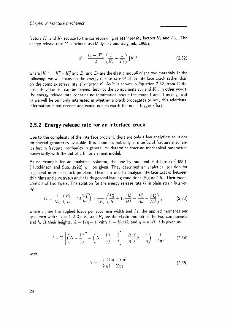
Chapter 2 Fracture mechanics
factors K\ and K2 reduce to the corresponding stress intensity factors Kj and Kn. The
energy release rate G is defined as (Malyshev and Salganik, 1965):
G(l-ß2) 1
+ i1 '*'" (2.32)
where \K\2 = K2 + K2 and A and E2 are the elastic moduli of the two materials. In the
following, we will focus on the energy release rate G of an interface crack rather than
on the complex stress intensity factor K. As it is shown in Equation 2.32, from G the
absolute value |A"| can be derived, but not the components A"! and K2. In other words,
the energy release rate contains no information about the mode I and II mixing. But
as we will be primarily interested in whether a crack propagates or not, this additional
information is not needed and would not be worth the much bigger effort.
2.5.2 Energy release rate for an interface crack
Due to the complexity of the interface problem, there are only a few analytical solutions
for special geometries available. It is common, not only in interfacial fracture mechan¬
ics but in fracture mechanics in general, to determine fracture mechanical parameters
numerically with the aid of a finite element model.
As an example for an analytical solution, the one by Suo and Hutchinson (1990),
(Hutchinson and Suo, 1992) will be given. They described an analytical solution for
a general interface crack problem. Their aim was to analyse interface cracks between
thin films and substrates under fairly general loading conditions (Figure 2.6). Their model
consists of two layers. The solution for the energy release rate G in plain strain is given
by:
G2A
P2
ÎE, \ H
Pt-f + 12
Ml
Ah
M2(2.33)
where Pt are the applied loads per specimen width and M, the applied moments per
specimen width {i = 1,2,3). A and A are the elastic moduli of the two components
and h, H their heights. A — I/77 + S with £ = A/A and ry = h/H. I is given as-
;)-KH n+
3r?3'(2.34)
with
1 + 2Ery + Elf
2ry(l + ^/)(2.35)
28

2.6 Application of fracture mechanical concepts to snow
Solid 1Interface
M3
Solid 2
Neutral Axis I X_
<
Figure 2.6: A bilayer material with a half-plane interface crack. After Hutchinson and
Suo (1992).
2.6 Application of fracture mechanical concepts to
snow
2.6.1 Experimental studies
Fracture mechanical experiments with snow were only performed in the last six years.
Thereby, the focus was set on the determination of the fracture toughness of snow in
mode I and mode II. However, most experiments were done in mode I because the
experimental setup for a mode I test is simpler than for one in mode II, and their exist
anyway only few tests that can be adapted to snow, due to its fragile nature. In the
following, the contributions are listed in chronological order.
Kirchner et al. (2000) were the first to measure a critical stress intensity factor in mode
I for snow. They performed cantilever experiments in the field and evaluated their data
by applying fracture mechanical theories of foams by Gibson and Ashby (1997). Theyfound a relation of
Ku. = A(p„rww/pirt)B, (2.36)
with A — 7.84 kPa sjm and B = 2.3. They suggested that with these extraordinarilylow values of fracture toughness, snow would be one of the most brittle materials known
to man. The data was recorded at temperatures near the melting point and for snow
types that are not known in detail.
Kirchner et al. (2002a,b) used cantilever beam tests to determine fracture toughness in
tension and shear. Notched cantilever beams of snow (50cm x 20cm x 10cm) were
broken under their own weight. This time, all experiments were performed in a cold
laboratory at SLF. A linear elastic approach was used to determine the critical stress
intensity factor A'/y which was directly associated with the fracture toughness Klc.
They concluded that snow fracture toughness in shear is about the same as in tension.
Faillettaz et al. (2002) performed the same field experiments as Kirchner et al. (2000)had done and found fracture toughness values of the same order. They found that the
fracture toughness values depend on the cantilever length and suggested that this could
29

Chapter 2 Fracture mechanics
be a result of a fractal branching pattern of the crack.
Schweizer et al. (2004) measured in the cold laboratory at a temperature of — 10°C and
found for Equation (2.36) values for A between 13.0 kPa ,/m and 21.6kPa1/m, and for
B between 1.9 and 2.1, depending on snow type. They proposed that this snow type
dependence can be taken into account by including a microstructural parameter dmax,
characterizing the grain size,
\J Umar \Picc
where dmaj. is the grain size and C = 0.35 kPa m is a constant. This lead to Kjr =
600 —900Pav^îîï for a typical slab density of p = 180 kg/in3. Based on some experiments
in shear (Kirchner et al., 2002a), they suggested that fracture toughness in shear is
slightly smaller than fracture toughness in tension (Schweizer et al., 2004). Schweizer
et al. (2004) showed that fracture toughness decreases with increasing temperature
until it reaches a minimum between — 10°C and —5UC. This means that fractures can
propagate more easily with increasing snow temperature. However, for temperatures
above this minimum the fracture toughness increases again towards 0°C.
So far, all attempts to determine snow fracture toughness in mode II were performedwith homogeneous snow samples. However, as it was mentioned in Section 2.5, mode
II experiments in homogeneous materials are difficult to perform and the cracks tend to
change direction, resulting in a pure mode I situation. Therefore, it is essential to test
layered samples in mode II.
McClung (2005b) estimated the shear fracture toughness, Kllc from slab avalanche data
to be between 0.02 and 13kPav/m.
Most recently, Gauthier and Jamieson (2006) proposed a drop hammer test for layeredsnow beams on the slope. Thereby, they used a similar geometry to our field test. But
instead of notching the isolated snow beams they applied a drop load at the upper end
of the snow beam and assessed if they could trigger the propagation of a fracture in the
weak layer or not.
2.6.2 A model for shear fracture propagation
McClung (1979, 1981) proposed a model for a shear fracture propagation in a thin, planarweak layer underneath a cohesive, strong slab. The model originates from Palmer and
Rice (1973), who introduced the idea of a shear band in overconsolidated clay. Bazant
et al. (2003) based their formulation of a size effect law for fracture triggering in dry
snow slabs on this model.
The slope model consists of three layers including a rigid basal layer overlaid by an
elastically behaving slab with height H (measured slope normal), and in between a weak
layer (Figure 2.7). The slab is inclined by an angle ip. The weak layer is damaged on a
(2.37)
30

2.6 Application of fracture mechanical concepts to snow
.o*H^
Figure 2.7: Geometry of a two-dimensional snow slab after (Bazant et al, 2003) 2o is
the cohesive crack. Forces acting on an element of slab (top left). Typical shear stress
distribution (bottom)
length 2a. The Young's modulus of the slab E as well as the density of the slab p are
considered as uniform over H. A crack is propagating symmetrically up and downwards
along the weak layer
The equilibrium condition for a unit element dx of the slab leads to (Figure 2.7)
(dxHp)q$m(y){rr + der) =n — — + t, , (2 38)
where rr is the residual shear stress due to friction. As a first approximation no residual
shear stress is assumed, rr = 0 When integrating Equation (2.38)
a = -pyx bin(^) (2.39)
results If 2<7 » H the transition zone of r can be neglected Calculating the comple¬
mentary strain energy of one half of the sliding layer leads to
ir
"l-as H wdx2
-2„-s,F1 a'2 n9
Ha^w rf,a"w
I ^Hud>r=i-pa,u^)}2^^= ^Tr, (2 40)
GE 6EH
where E is the Young's modulus of the snow layer, w the lateral width and rg is the
shear stress that is required to support the weight of the slab if no crack is present (no
31

Chapter 2 Fracture mechanics
tensile forces are acting):
Tg = pgH sin(^). (2.41)
Bazant et al. (2003) state that the one dimensional solution of Equation (2.40) mighteven be acceptable as long as a > H. Furthermore, they point out that situations in
which a <£ H are of no practical interest, because small imperfections always exist in
an alpine snowpack and thus a snow layer would never be stable on a slope.
The energy release rate, G, can be calculated according to Equation (2.9) and (2.40)
1 DU* T2a2G(a)
= -^- = -J—. (2.42)v '
w da 2EIIK '
Since we have set rr = 0, the resulting energy release rate, G, is an upper boundary for
the true energy release rate in case a residual friction would be present.
2.6.3 A model for a slope normal displacement of the slab
Heierli and Zaiser (2006) proposed an analytical model on the gravitational collapse of
horizontal stratifications. In contrast to ordinary fracture dynamics, they assume an ini¬
tially relaxed slab that quits its metastable equilibrium once the weak layer underneath
the slab locally collapses. In this model, the energy functional associated with a localized
collapse of the weak layer is calculated as the sum of the elastic energy Ve, the gravita¬tional energy of the slab Vg and the energy that is required to fracture the weak layerover a given length, Vf
^(u) = K.(u) + V,(u) + V>(u), (2.43)
where u is the displacement in direction normal to the slab Explicitly, the total energy
functional is (Heierli and Zaiser, 2006):
V{u) = I J| {^-^j + pHcju{x) + W/0(-u(x))| dr, (2.44)
where p is the density of the slab and H the slab thickness, g is the gravitationalacceleration, V the flexural rigidity of the slab and 8 the Heaviside step function {0{u) —
1. it > 0 and 0 else). The collapse has to be divided in three phases Bending of the
slab due to a localized collapse without contact to the slab underneath the weak layer,followed by a contact to this layer in one point, followed by a contact over a finite interval.
However, they showed that only the first phase is relevant for fracture propagationbecause the first derivative of the total energy (Equation 2.44) becomes negative before
the slab touches the substratum (Figure 2.8).The half length of a critical crack rr can
be evaluated in terms of the material properties of the overlaying slab and the fracture
energy of the weak layer Wf\
" = (w"') (Z45)
32
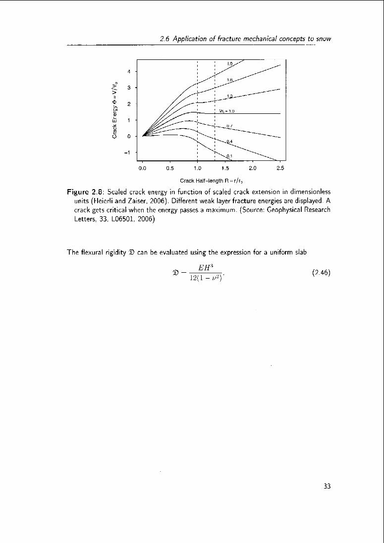
2.6 Application of fracture mechanical concepts to snow
>
ii
e
o
-1 -
M^^^-U^^'^^;::c^\
0.0 0.5 1.0 1.5
Crack Half-length R = r/r0
2.0 2.5
Figure 2.8: Scaled crack energy in function of scaled crack extension in dimensionless
units (Heierli and Zaiser, 2006). Different weak layer fracture energies are displayed. A
crack gets critical when the energy passes a maximum. (Source: Geophysical Research
Letters, 33, L06501, 2006)
The flexural rigidity S can be evaluated using the expression for a uniform slab
EH*S
12(1(2.46)
33

Seite Leer /
Blank leaf

Chapter 3
Methods
3.1 Standard measurement techniques for snow
characterization
In comparison to most other materials, the microstructural and mechanical properties of
snow are highly variable. Therefore, it is essential to characterize the microstructure of
snow whenever experiments are performed. Standard measurement techniques for snow
characterization have been developed in the past, which have now been successfully
applied in snow science for many years. This section gives an overview of the techniques
and procedures that were applied during the experimental work.
Snow classification: Each time when snow samples were collected in the field, the
stratigraphy of the snow cover was characterized in stratigraphie snow cover pro¬
files. Therefore, a snow pit was dug and the snow was analysed regarding its
horizontal layering, the snow type, temperature and density. A snow layer is char¬
acterized by a given snow type. The separation of layers is based on visual and
tactile variations in the snow type. The snow type includes the classification of
three snow properties: the grain shape, the grain size and the snow hardness in¬
dex. They are classified according to the International Classification of Seasonal
Snow on the Ground (ICSSG) (Colbeck et al., 1990). The snow hardness index
is a subjective classification with six classes of penetration resistance: Fist (F),Four-fingers (4F), One-finger (IF), Pencil (P), Knife (K) and Ice (I). In addition
to the identification of the layering a temperature profile was recorded from the
snow surface to the ground, the densities of the different layers were measured
(see next item) and occasionally the ram hardness was measured. See Appendix B
for examples.
Density measurements: The density of a snow layer or a snow specimen is measured
by cutting out small samples with an aluminium cylinder or alternatively with a
35

Chapter 3 Methods
small aluminium box and weighing it on a scale. A standard volume is 100 cm3
but there are also larger cylinders in use. It is common to average two to four
measurements to reduce the effect of measurement errors.
Stability tests: To identify weak layers suited for sampling, stability tests were made.
We used the compression test in which the top of an isolated column of snow
(30 cm x 30 cm) is loaded by tapping on a shovel (Jamieson, 1999). The first ten
taps are done with the fingertips moving the hand from the wrist. The next ten
taps are done by moving the forearm from the elbow. Finally, ten taps are done
moving the arm from the shoulder. Depending on the number of taps the ease of
triggering can be estimated as: 0 — very easy, 1-10 — easy, 11-20 — moderate,
21-30 = hard.
Shear frame test: To measure the shear strength, the shear frame test was used. A
steel frame with an area of 0.025 m2 was placed about half a centimeter above a
weak layer, then the frame was pulled with a force gauge smoothly and quickly,resulting in a planar failure of the weak layer (Jamieson and Johnston, 2001). Due
to the scatter of the test results it is common to average 8 to 12 tests to get a
reliable result.
Snow micro-penetrometer: The SnowMicroPen (SMP) is a high-resolution constant
speed penetrometer. It records the penetration resistance of a small cone (diameter:4 mm, cone angle 60°) which is pushed through the sample perpendicular to the
layering of the snow cover or the snow specimen (Schneebeli and Johnson, 1998;
Schneebeli et al., 1999). Due to the high resolution of the SMP, it is possible to
resolve details in layers that are considered as homogeneous. The SMP resistance
profile is especially qualified to assess the detailed layering of a snow specimenand allows to derive additional parameters, e.g. an index for the Young's modulus
(Johnson and Schneebeli, 1999) as will be discussed in Section 3.4.
Sample characterization: Small snow samples of interesting snow layers, especially of
weak layers were occasionally collected. The samples were cut out of the snow
with small containers of the dimension 5 cm x 5 cm x 5 cm. Then, liquid and dyedblack Diethyl-phthalate was added which filled up the pores in the snow sample.After freezing, the cube was sliced in a microtome and the surface was successively
photographed with a digital camera. Finally, the image was binarized to distinguishbetween ice and pore-space (Good, 1987).
A further standard test in materials science is to measure the tensile and compressive
strength of a material. However, no standard procedures exist to measure the tensile or
the compressive strength of snow, up to now.
36

3 2 Laboratory tests
(a) (b)
Figure 3.1. Homogeneous snow samples were collected by pushing the aluminium cases
with the height parallel to the layering into a thick layer of the snow cover (a) while
for layered samples the cases were used upright (b) in order to include more than one
layer
3.2 Laboratory tests
About 80% of all experiments were performed in the cold laboratory, the rest was per¬
formed in the field For all laboratory tests the snow samples had to be collected in the
field and transported to the laboratory
3.2.1 Sample collection
All snow samples were collected in the field They were either collected close to the
building of the Swiss Federal Institute for Snow and Avalanche Research in Davos
Switzerland at an altitude of 1562m as I or close to the old institute building on
the Weissfluhjoch Davos at 2668 m a s I At both places a cold laboratory is available
with a temperature range of 20 C to 0 C The samples had to be carried to the cold
laboratory one by one in order not to destroy the snow structure Especially for layeredsnow samples the transport was delicate Therefore the collecting area for snow samples
was restricted to a radius of a few hundred meters around the two institute buildingsAfter transport the samples were stored at a temperature of —10JC for a maximum of
two days before testing The experiments were performed at a cold room temperature
of 10 C and occasionally at -15 C
The specimen were cut out of the natural snowpack with beam-shaped aluminium cases
Four different sizes of aluminium cases were used to collect samples The largest was
close to the limit of what could be handled in the field and transported to the laboratory
37

Chapter 3 Methods
Table 3.1: Snow specimen dimensions The standard specimen size is marked in bold
Height // Length / \\ Kit ll </'
(cm) (cm) (cm)
S 20 10
13 .31 10
20 50 10
32 80 10
without destroying the natural snow structure. The other sizes were chosen such that a
size range of 1.4 was achieved. The thickness ir was the same for all specimen sizes -
this is called "2D similarity", according to Bazant and Planas (1998, p 458) - in order to
avoid a possible thickness effect The dimensions are given in Table 3 1 In the standard
size, nineteen cases were available, in all other sizes five. The standard size was alreadyused by Kirchner et al (2002a,b) and Schweizer et al (2004)
For the laboratory tests two kind of samples were used: homogeneous snow samples
consisting of only one layer (.— monolayer) and layered snow samples consisting of two
or more layers ( = multilayer) Snow samples were defined to be homogeneous when no
visible layering was present, i.e. when they consisted of one snow type Homogeneous
snow samples were taken out of the snow cover by selecting a thick enough snow layer
(«• 12 cm) in which the whole aluminium case could be placed without any contact to
adjacent layers Suitable layers were previously defined in a snow profile The aluminium
cases were pushed into the snow cover horizontally with the height of the case parallel to
the layering (Figure 3 la), but later on tested upright This was done, because even within
one layer of the snow cover the density tends to slightly increase with increasing snow
depth. By testing the specimens normal to the layering of the snow cover an influence
of this density increase or a slight undiscovered layering was minimized. Schweizer et al
(2004) showed that tests are influenced by a layering parallel to the test direction. For the
collection of layered snow samples the aluminium cases were pushed into the snow cover
upright with the height of the case vertical to the layering (Figure 3.1b), so that the weak
layer was caught in the middle of the case, resulting in snow specimens consisting of two
homogeneous snow layers separated by a weak layer. Weak layers suited for samplingwere identified previous to collection by applying compression tests
3.2.2 Three-point bending test
The three-point bending test (3PB-test) is a common test configuration in material
science to determine fracture toughness in mode I (eg Tada et al., 2000, p.58) A
beam shaped specimen is notched on one side with a cut of a given depth (normallybetween 0 1 and 0 5 times the beam height), placed on two supporters and loaded in
38

3 2 Laboratory tests
Figure 3 2 (a) Schematic diagram of the three point bending test setup (b) Snow
specimen in place before testing The aluminium plates on top of the cylindrical sup
ports are missing in this image
the middle of the opposite side with an increasing force until the specimen fails
All 3PB-tests were performed with a standard material testing machine (ERICHSEN-Umversalprufmaschine 490) The machine has an upper force limit of 20 kl\l After a first
winter of testing (winter 2003/2004) it turned out that the force range was unnecessarily
high for experiments with snow In the tests forces of a maximum of 200 IM were achieved
On the other hand the force resolution was much too low Therefore the machine was
upgraded during summer 2004 with a new sensor head including a new force sensor
(Figure 3 3) Additionally an improved data processing software was written based on
LabView With the new force sensor the time resolution could be improved from 72 ms to
4 ms with a sampling rate of 2000 Hz where every 8 samples were averaged to decrease
signal noise resulting in an effective sampling rate of 250 Hz The force sensitivity could
be improved from 1 N to less than 15 mN
The standard 3PB test setup needed two slight modifications to be applicable to snow
specimens It was not possible to place soft snow on sharp triangular supporters without
a considerable penetration of the supporters into the fragile snow specimen Instead
aluminium cylinders were used to increase the contact area and to prevent local snow
deformation at the loading points (Figure 3 2) The aluminium cylinders had a diameter
of 6 cm The diameter of the cylinders was expected to have only a minor influence
on the test results The load was applied in displacement control at a constant rate
39

Chapter 3 Methods
Figure 3.3 (a) Design drawing of the new sensor head including the more accurate
force sensor (thin black bolt) (b) Image of the new sensor head (c) Image of the
ERICHSEN Umversalprufmaschine 490 (height ^ 15m including the old sensor head
of 200 mm/mm through another cylinder with a diameter of 5 cm The velocity was
chosen high in order to cause a brittle fracture and to avoid viscous effects As a second
modification small aluminium plates were placed between the cylinders and the specimen
to prevent friction between the supporters and the specimen while testing
The critical force Ff that had to be applied to break the specimens ranged up to 200 N
depending on beam size and snow density Due to this rather low force the weight of the
beam had to be taken into account in calculating the applied stress and stress intensity
factor The weight of a typical sample of a density of 250kg/rn1 is about 25 N
The bending moment in the center of a beam due to an applied force 7 per specimen
width u is
'"' -
tt <3 *>
where s is the span i e the distance between the two supporters The bending moment
in the center of the beam per specimen width due to the body weight can be written as
W, -f'[s' (/ s)JJ (3 2)
where p is the density of the specimen h its height and / its length q is the gravitational
40

3.2 Laboratory tests
acceleration According to Tada et al. (2000) the nominal stress is given as
<y^ = ~{My \ Mu) (33)Ir
The nominal stress is defined as the load divided by the original cross section, i.e. the
undeformed and uncracked cross section before loading The effective stress, a\„, i.e.
the load divided by the remaining cross section, will be defined in Section 4.1.7 The
critical stress intensity factor or the apparent fracture toughness A'// can be calculated
according to Equation (2 15) as a combination of the 3PB-solution and the pure bending
case given by Tada et al. (2000)'
l\,, = y2V^~« [0.95 M,, V, (a/h ) t Mr,Y2(a/l,)\ . (3 4)
Here, A// is the critical bending moment, i e the force at failure, F), has to be inserted
in Equation (3.1) The functions Y\{a/h) and Y^u/h) can be found in Tada et al.
(2000).
1 1.9!) - (a/h)[\ - (u/h)\ [2.15 ,3.n;$(«///) + 2.7(al!,y\,_
_.
t [1| 2(«//;)][l - (a/h)]lL
Y,(a/h) - \.\22- \.\(){a/h) i- 7.lYMa/h)2 - ]:].()H(a/h)' ] \H){a/li) '. (3 6)
V, is valid for a span to height ratio of s/h — \ Since in our experiments the specimens
have a ratio of s/h ~ 2 a correction factor was necessary. According to Schindler
(personal communication) a factor of 0 95 had been found in a numerical computation
to account for the difference in the ratio s/h. For our 3PB-experiments the part due to
the moment M(1 in Equation (3.4), is about 60% of the part due to the force at failure
3.2.3 Cantilever beam test
In addition to the 3PB-tests, cantilever beam tests (CB-tests) were performed Thereby,
the same setup was used that had previously been used by Kirchner et al (2000), Kirchner
et al. (2002a,b) and Schweizer et al. (2004). In the winter 2003/2004 CB-tests were done
simultaneously to the 3PB-tests with specimens from the same snow layer The aim was
to acquire a data set with the CB-tests suited for a direct comparison with the above
mentioned studies and thus to relate the 3PB-tests to previous CB-test results
In the CB-test, one part of the specimen was supported while the other part with length
/, was protruding L was chosen to be either 10 cm or 15 cm of a total specimen lengthof 50 cm. For the CB-tests the standard specimen dimensions of 50cm x 20 cm x 10cm
were used (compare Table 3 1). A cut was made from the top, exactly above the line
where the support ended, until the protruding part broke off under its own weight. This
happened at a critical cut length a — a, (Figure 3.4)
41

Chapter 3 Methods
(a) (b)
Figure 3.4: (a) Schematic diagram of the cantilever beam test setup (b) Image of a
cantilever beam test
In a cantilever beam test the crack front is loaded in mixed mode Therefore, the stress
intensity factor in mode II, A//, had to be taken into account
gI\j t h2,
/<;(3 7)
For /; - a L, the system is equivalent to the asymptotic case of a deep edge crack
under a bending moment and a shear force The corresponding stress intensity factors
are given m Tada et al (2000)
A,Ai A/,
( B
\}Vi(3 8)
A// (3 9)
where \l( /; is the moment per specimen width ( \fcii — kh/x/ (L/2)) b is the ligament
length, b — h a 1\ « is the cantilever weight per specimen width (J'< n — kli/jg) The
constants /M and f,2 have to be determined by finite element modelling and were found
to be
A | -.-S<)7r) A, - I 163 (3 10)
for homogeneous samples (Tada et al, 2000) In a brittle material like snow, the mode
interaction is likely to be governed by the criterion of maximum hoop stress suggested byEvans et al (1963), which leads approximately to the following failure criterion Schindler
(2004)^
' "<
(311)K_n_A,
Im
K,
42

3 2 Laboratory tests
Rearranging Equation (3 11), and replacing A', by the critical stress intensity factor for
the combined mode I and mode II loading, K/ yields'
hj _
'urn_ v»7]^ (312)
Equation (3 12) slightly deviates from the formulation for the critical stress intensity
factor given by Kirchner et al (2002a), Kj — sjKj \ Kj,. Particularly for deep cuts,
Equation (3.12) is the more appropriate approximation. Taking A'// into account in
Equation (3 12) increases Kf for our experiments, compared to a pure mode I htj, byabout 6% for a density of 220 kg/m3 and 37% for a density of 335 kg/m^ The influence
of h'n is thus more important for snow of high densities
3.2.4 Shear fracture test
Mode II testing is primarily of importance in layered materials, see Section 2 5 Although,
much less information is available on mode II than on mode I testing, there exist some
standard test setups for mode II (e.g Hutchinson and Suo, 1992, pp 114). The end-
notched-flexure test (ENF), a kind of 3PB test but with a horizontal cut at one end
instead of a vertical cut in the middle, or the end-loaded-split test (ELS), which was
adapted for snow by Kirchner et al. (2002a) but did not work satisfactory, because rather
a tensile fracture of one part of the split beam was observed than a shear fracture. Due
to the fragile nature of snow, these standard tests are not suited for snow Furthermore,
the handling of layered samples turned out to be even more delicate than the handling of
homogeneous samples. Therefore, a simple cantilever beam experiment was developed
The mode II fracture test consists of a notched cantilever beam that is fixed on one
side. After the layered snow samples had been carried into the cold laboratory, they were
frozen on one side to an aluminium bar. For testing, the bar was rotated 90'
so that the
horizontal snow layering was now vertical, see Figure 3 5 The height / of the specimen
in Figure 3.5 corresponds to the length of the aluminium case with which the specimen
was cut out of the snowpack (see Table 3.1). The aluminium bar with the upright snow
beam was placed on a table, such that one part of thickness tt was protruding and one
part of thickness //, was supported by the table The weak layer was placed exactly above
the edge of the table The protruding layer of thickness /, corresponds to the layer that
was on top of the weak layer in the snow cover (index t — top) and the supported layerof thickness tj, was below (index /; — bottom). On top of the protruding layer a mass of
wUm<i — I A// was placed to increase the shear load at the crack tip and thus to decrease
the cut length With a thin metal saw blade a cut was made along the weak layer from
the top of the specimen towards the bottom until the protruding part of thickness //
broke off.
For the calculation of the energy release rate G for our test geometry, no analyticalsolution could be found However, as a first approximation the cantilever deep crack
solutions of Equations (3 7)-(3.9) could be used. This seemed justified because for our
43

Chapter 3 Methods
Figure 3.5: (a) Schematic diagram of the shear fracture test setup (b) Image of the
shear fracture test while cutting is in progress A weight is placed on top of the
protruding part
tests the ligament length b was in the order of the total tickness h ~ /; As for the CB-test
the loading of the crack tip was expected to be in mixed mode The Young's modulus
h in Equation (3 7) was set equal to E,, the Young's modulus of the protruding part
The Young s modulus of the supported part was assumed to have only a minor influence
due to its fixation on two sides This was confirmed in FE simulations However, in case
of two different materials, A i and k2 may differ from the values given in Equation (3 9)
depending on the material mismatch
To maximize the shear component and minimize the tensile component the whole setup
was tilted by an angle n A minimum tensile load results when the opening moment
equals the normal force at the location of the crack tip Because the cut length varied
from one experiment to the other and because the exact cut length was not known prior
to a test an exact determination of rv was not possible Instead, we looked at the mean
cut length and estimated that for <v = 5 the tensile stress would be close to zero in
most cases
In a specimen fixed coordinate system, where the /y-axis points along the interface (Figure
44

3 2 Laboratory tests
3.5) the torsional moment of Equation (3 8)
0) can be written as
Mru, with center of rotation o. y
Mr I X /;/ g
r,
In
m(j s///(n)
ni()co^((\)0 / ,»i(/(«s((i) - i ,/inq s//;(fv)
(3 13)
where f is the position vector and in is the mass of the protruding snow layer per
specimen width n>- ttlp with /, the length of the protruding layer and / its height g is
the gravitational acceleration l'en, the loading due to the body weight parallel to the
interface, depends on <\ as well and can be written as
l\<n = ingro^{(\) (3.14)
Without any additional loading the center of mass is in the middle of the protruding
layer and r, and /',, can be set to r, - l,/2 and /',,- 1/2 in a more general situation,
i e when an additional weight //?/„,„/ is added on top of the protruding part, the total
mass is increased m = {m,l!(Hl I niitmil) and the center of mass is lifted towards the
additional weight rv transforms to
1 +»I had
"'s/, +" '"/„„</(3 15)
where />>„„„„ -~ tjp is the mass of the protruding snow beam per specimen width.
Accordingly, the additional mass /»/,„„? is also per specimen width Consequently, the
moment Men as a function of the rotation angle a and the additional weight is given
as
Mch ~ {riK,<„,< + l"i,m,i)q rosffv^//
s///(n)- 1 +'»lllllll
(3 16)
3.2.5 FE model of shear fracture test
Since the available analytical solutions for a determination of the energy release rate G
did not match our experimental set up a finite element (FE) model of the experimental
geometry was created. For the modelling the ANSYS workbench was used The geometry
was modelled consisting of two beams of two different materials, shown in Figure 3 6a
The weak layer was considered to have no extension
45

Chapter 3 Methods
IF AN
L
s01 tu
CD CD—\ -i
i. M 0)
ISJ ""*
iiiii
ay
(b)
01 0)
CD n>-i ^
0) 03
NJ _i
"5 ft1! r~^~^
4« «
AN
(0 (d)
Figure 3 6- (a) Geometry of the FE model Black triangles indicate the boundaryconditions Nodes are fixed in i and/or in /y direction (b) Detail of the shear stress
pattern rl(/ acting around the crack tip (ANSYS output) The dashed square in the
center of (a) indicates the magnification of (b) The crack tip is in the center of the
crosshairs The crack is coming down from the top (Material 1 p— 250kg/m3
A-5MPa Material 2 ^-300kg/mJ / -20MPa a- 5 27 |/'|-981N (c)
For comparison a pure shear stress case is simulated (d) The material properties of
material 1 and 2 are the same as for (b) (j f j - 20 N no gravity is applied )
46

3.3 Field test
In two steps the total strain energy lT{u) for a situation with a cut length a, and
11 {a I Aa) for a cut length a t Aa were calculated, where An is a small increase in the
cut length The energy release rate G could then be calculated according to Equation
(2.9) as the difference of these two energies divided by the specimen thickness ir and
the cut length increment Aa-
«M-<'i«±M^W (317)irAa
Aa must be chosen small enough for G{a) to converge but large enough to avoid errors
due to the limited precision of the FE model
To verify the numerical model, the infinitely long thin film of Figure 2 6 was modelled
(/ » /,,. /,) for which Suo and Hutchinson (1990) had derived an exact analytical solution
(Equation 2 33) The difference between numerical results and analytical solution did not
exceed 4% for various loading conditions Subsequently, the model was adapted to our
experimental geometry The geometry, loads and boundary conditions are indicated in
Figure 3 6a Nodes on the left boundary were fixed in x and /y direction, to model
the icing of the snow block to the aluminium bar Nodes on the bottom left boundary
were fixed in </ direction, corresponding to the support of the specimen on the table. The
gravitational acceleration // was implemented, acting with an angle a to the vertical. The
additional weight which was placed on top of the protruding snow layer was modelled
as a point load. Figure 3 6b shows the shear stress r,v acting around the crack tip. The
shear stress can be compared qualitatively to the simulation of a pure shear case (Figure3.6c and d). The stress distributions looks qualitatively the same, although the stress
amplitudes are different, what explains the different colour code The similarity of the
stress patterns should thus justify the assumed 5' for the inclination angle <v
3.3 Field test
As the name implies, weak layers are in general not suited for any kind of transportation.
The shear fracture tests involved a highly delicate transport of some more robust weak
layer specimen to the cold laboratory. However, for many weak layers a transport is not
feasible These weak layers are assumed to be the most relevant for slab avalanche release.
Therefore the development of a field test was a major step towards more "realistic"
experiments even though less accurate More realistic means in this context that larger
samples could be tested in-situ on slopes where avalanches potentially could occur.
The field test was designed to answer the following questions:
• Is it possible to determine the energy release rate of a weak layer directly in the
field?
• Does the cut length depend on the specimen length7
47

Chapter 3 Methods
(a) (b)
Figure 3.7" (a) Schematic diagram of the field test (b) Cutting along the weak layer
of an isolated snow block in a slope
Is a crack propagation possible in slopes less steep than 30 ?
• Can a field test be further developed into a standard field test for operationalavalanche forecasting that would be useful to assess the potential for fracture
propagation7
The field test consisted of snow beams with a width of 30 cm and a variable length of
60cm 120 cm or 180 cm The beams were isolated on all four sides on a slope (Figure3 7) After the weak layer had been identified by compression tests a cut was made
along the weak layer with a snow saw (thickness 2 mm) until the crack length became
critical and self-propagation of the crack started The cut was usually made in downslopedirection and occasionally in upslope direction
In order to make the field experiments comparable to the laboratory tests the width of
the snow beams was kept short in relation to the length For the laboratory tests the
ratio of width to length was «// — 1/5 for the field tests it was u jl —1/2 1/4 l/(>
depending on the beam length The width was kept constant for all beam length as it
was done for the different specimen sizes used in the laboratory for the fracture tests in
mode I The major difference between the field test and the shear fracture test is the
inclination of the weak layer Whereas in the laboratory n was set to 5 corresponding
to an inclination of the weak layer ofr
- 90 n— S5 the field tests were performed
in slopes with an inclination of 25r
55
48

3.4 Young's modulus
Figure 3.8: Geometry of the FE model. Black triangles indicate the boundary conditions.
Nodes are fixed in x and y direction
3.3.1 FE model of field test
As for the shear fracture experiments a FE model was generated for the geometry of the
field experiments. The energy release rate was calculated according to Equation (3.17).A schematic diagram of the FE model can be seen in Figure 3.8. The model consisted of
a basal layer which was fixed in x and y direction at the bottom (black triangles in Figure
3.8) overlayed by a slab consisting of 7? layers. For our experiments the slab was modelled
as to consist of three layers n = 3, because in the SMP penetration resistance signalsthree layers could be clearly distinguished. For a future application the model could be
adjusted to more layers by including additional layers in the input file for ANSYS.
Not only the length of the cut ac, that was made with the snow saw, was modelled but
also the cut thickness. The snow saw had a thickness of 2 mm and therefore this gap
of 2 mm indicated as gap in Figure 3.8. The cut surfaces were modelled as contact and
target areas, in case the two surfaces would get in contact due to bending. However, the
results showed that for the measured critical cut length the slab was stiff enough so that
the two crack surfaces did not get in contact (Section 4.3). The bending of the slab due
to the cut length ac was at maximum half of the gap size of 2 mm.
3.4 Young's modulus
The determination of the Young's modulus E of a given snowpack layer is of prime
importance, since the calculation of fracture mechanical parameters, such as the energy
49

Chapter 3 Methods
release rate or the critical stress intensity factor (in a layered material), requires the
knowledge of the Young's modulus.
A precise measurement of the Young's modulus is still a difficult task and far from being
a standard procedure. One reason for this is again the fragile nature of snow which
makes standard measurement techniques very difficult and sometimes even impossible.
Furthermore, the Young's modulus will depend on the direction of loading. A loading
in lateral direction will result in a different modulus than a loading in vertical direction
due to the vertical layering of the snowpack. Basically, four different approaches can be
distinguished:
• Quasi static: The elasic modulus has traditionally been measured from the linear
elastic region of a uniaxial tensile stress-strain curve, and is defined as the ratio of
stress to strain during elastic loading (Mellor, 1975). Recently, Scapozza (2004)has made uniaxial compression experiments. His findings agreed well with the ones
summarized by Mellor (1975) (see Figure 4.14).
• Dynamic: In dynamic experiments the snow specimen is activated with small
displacements of a given frequency, normally between 10 Hz and 10 kHz. The pulse
propagation, flexural vibration or the force response is measured from which the
Young's modulus is calculated. Mellor (1975, p.257) reports that the results for a
dynamic measurement can be a factor of 2 higher than quasistatic measurements.
Camponovo and Schweizer (2001) performed dynamic torsional shear experiments
at a frequency of 1 Hz with a stress-controlled rheometer and determined the shear
modulus of snow for different snow densities and temperatures.
• Derived from microstructural properties: With the aid of computer micro-
tomography (Schneebeli, 2002) the exact ice-matrix of a given snow sample can
be modelled. By applying the mechanical properties of ice to the matrix, an elastic
modulus for the snow sample can be calculated. This might be the method with
the highest precision, however measurements are time consuming, can only be
made for small samples with a volume of a few cubic centimeters and require an
expensive equipment.
• Derived from penetration resistance: Probably the most promising method
is to calculate an Young's modulus based on the penetration resistance signalof a SnowMicroPen (Johnson and Schneebeli, 1999). A resistance profile can be
acquired directly in the field and within minutes. However, the conversion of the
penetration resistance into an Young's modulus is rather complex and seems to
need a calibration with field measurements first (Kronholm, 2004).
For our experiments we used a dynamic measurement method to evaluate the Young's
modulus and compared the results to the results derived from the SMP penetration
resistance signal.
50

3 4 Young's modulus
3.4.1 Dynamic measurement with cyclic loading device
A prototype of a cyclic loading device, developed at SLF, was used to determine the
Young's modulus (Hempel, 2004) Small cylindrical samples with a diameter of 48 mm
and a height of 30 mm were cut out of the snow specimens after a fracture test Then,
the samples were mounted on a device where they were loaded and unloaded with
a frequency of 100 Hz (Figure 3 9 a) The force response F due to the predefined
displacement Ah = 8//m was recorded A displacement of Ah — 8//m corresponds to a
deformation of e = Ah/h — 2 7 • 10~4 and with the applied frequency of 100 Hz a strain
rate of e = 2 7 10~2s-1 results With the force-displacement information a dynamic
Young's modulus was determined, according to the relation
E =
°
=
* As A Ah'
where h is the height of the sample and A its cross sectional area The calculated Young's
modulus increases rapidly with increasing loading frequency between 0 1 Hz and 50 Hz
and then successively flattens with a further increase in the frequency (Figure 3 9 b) At
frequencies around 200 Hz a resonance was observed which influenced the measurements
considerably This resonance is believed to be either the result of a resonance frequency
of the steel frame or the result of an improper icing of the snow sample to the sample
holder or the pressure plate The icing of the snow sample was a sensitive procedure It
happened that above a certain frequency, the contact between snow and pressure plate
or snow and sample holder deteriorated
From experiments with polycrystallme ice (Smha, 1978) it is known that the Young's
modulus increases with increasing loading frequency (Figure 3 10) For lower frequencies
there is a steep increase which levels off between 100 and 200 Hz
For our measurements a frequency of 100 Hz was chosen, to be as close to a flat region
as possible but still far enough away from the resonance frequency
3.4.2 Derived from penetration resistance
Kronholm (2004) was the first who used the penetration resistance signal of the SnowMi¬
croPen to estimate the Young's modulus of different layers of the snowpack According
to Kronholm (2004), the values of the modulus derived from the SMP signal are too
small by a factor of about 150 compared to the measurements of Mellor (1975)
The theory to calculate the Young's modulus from penetration resistance was developed
by Johnson and Schneebeli (1999) and is based on mechanical theories for cellular solids
(Gibson and Ashby, 1997) The Young's modulus E of a given snow layer can be calcu¬
lated as a function of the average rupture force for the microstructural element within
(3 18)
51

Chapter 3 Methods
Elastic modulus
Phase shift(/n.
j-^roo-o-f^S"SV,V
rv.
100 150 200
Frequency (Hz)
(b)
S-;SSS1
35
30
25
20
250 300
Figure 3.9: (a) Image of the cyclic loading device (F Hempel SLF) (A) solid steel
frame (B) piezo-actuator (C) force sensor, (D) pressure plate, (E) snow sample, (F)sample holder (steel) (b) Young's modulus m dépendance of the applied frequencyMeasurements were performed in winter 2004/2005 by Felix Book for snow consisting
of small rounded grams 0 5-1 mm 1F with a density of about 270 kg/m3
10
^. ^-,*~
.laJ. uJ. J L^iliL
Figure 3.10: Frequency dependence of effective Young s modulus for polycrystallme ice
at 10 C From Smha (1978)
52

3.5 High-speed photography
the layer, fr, and the average microstructural element length in the layer, Ln
E = —à (3.19)
Ln {sin 6 + pros6)
where 9 is half of the angle of the SMP tip (30°) and // the frictional coefficient between
the SMP tip and the snow grains. The frictional coefficient between ice and metal p is
assumed to be 0.25. Ln can be calculated as a function of the number of elements that
fail Ufa,i when the SMP cone with area /I, travels over a distance of Az
i„={^aS\nf0,, J
3.5 High-speed photography
To document in detail the fracture process during the 3PB-tests and the shear fracture
tests, several tests were captured with a high-speed camera. The Vosskühler HCC-1000
camera features a maximum of 462 pps (pictures per second) with an image resolution
of 1024 x 1024 pixels. For lower image resolutions the image rate can even be increased
up to 1825 pps.
The system consists of a camera and a laptop which controls the camera and on which the
data are stored. First data analysis can be done on the laptop right after recording. The
number of images that can be stored is limited to 512 images. Therefore, a higher image
rate results in a shorter recording time. Tests were made with image rates of 115 pps,
230 pps and 462 pps, resulting in recording times of 4.5 s, 2.2 s and 1.1s, respectively.Since the triggering of the camera was made by hand, the image rate could not be
further increased without the risk of missing the fracture. For a further increase of the
image rate an automatic triggering would be necessary. This would be, at least for the
3PB-tests, relatively easy to realize. In the data acquisition program for the 3PB-tests
written in LabView, a trigger signal could be sent to the camera as soon as the recorded
force signal exceeds a given threshold value. As long as the mean peak force is known for
a given specimen size it would be possible to decrease the time between trigger signal
and opening of the camera to approximately 100//s. A further decrease of the time would
not be suitable because the threshold would then be too close to the mean peak force
and, due to the scattering, some tests would fall below the threshold and would not
trigger the camera.
(3.20)
53

Se/te Leer /Blank leaf

Chapter 4
Results
During three winter seasons, 2003/2004, 2004/2005 and 2005/2006 experiments to de¬
termine fracture mechanical properties of snow were performed. In the first two winter
seasons most of the experiments were performed in the cold laboratory. This had the
advantage that precise measuring instruments could be used that would not have been
transportable to the field. Furthermore, the temperature could be controlled and the
experiments were independent of atmospherical conditions like wind, snowfall or radia¬
tion. All snow specimens that were tested in the cold laboratories were collected in the
field and transported to the lab. In the third winter season experiments were performedin the field. Experimenting in the field had the advantage, that test conditions were
representative for the conditions in which fracture processes occur in the snow cover on
a slope. Very fragile weak layers could be tested that could not be transported to the
laboratory without destroying the weak layer.
The chapter is divided in three sections according to the three main experimental focuses:
In Section 4.1 the results of the experiments with homogeneous snow samples performedin the cold laboratory are presented. Section 4.2 summarizes the experiments with layeredsnow samples in the cold laboratory. In Section 4.3 the results of the field experimentswill be given.
4.1 Fracture in homogeneous snow samples
Although a shear fracture in the layered snow cover occurs before the snow slab fails
in tension, as explained in Section 1.3, we started to experiment with homogeneoussnow samples for several reasons: Experiments in homogeneous snow were essential to
improve the understanding of the general fracture mechanical behaviour of snow, to
test and confirm previous results and to gain experience for the more difficult mode II
experiments in layered snow samples. In addition, layered snow samples are in general
55

Table
4.1:Summary
oftype(3PB—
three-pointbending
test,CB=
cantilever
beam
test)andnumber
offractureexperiments
in
mode
I.Snow
type
isgiven
as
grainshape,
grainsizeand
hardnessindexaccording
toICSSG
(Colbecket
al.,1990).
Series
Date
of
Typeand
(number)
Specimen
size
sampling
ofexperiments
{I.h.
iv){cm)
Snow
type
Snow
density
Snow
temp.
Rel.
rut
=sdev(kg/m3)
(T)
deptha/h
to
CKtu
Cl
-c
A6Jan
04
3PB
(7)
B27Jan
04
3PB
(12)
C5Mar
04
3PB
(6)CB
(11)",(4)b
D9/10/11
3PB
(27)Mar
04
CB
(13)°.(26)6
E21Apr
04
3PB
(17)
F27Jan
05
3PB
(53),(17)r
G2Feb
05
3PB
(30)c
2Mar
05
(3densitygroups)
3Mar
05
H10Feb05
3PB
(22),(6)c
I22Feb05
3PB
(23)
(50.20.
10)
(50.20.
10)
(50,20,
10)
(50.20.
10)
(20.8.
10)
(31.13.
10)
(50.20.
10)
(80.32.
10)
(20.8.
10)
(31.13.
10)
(50.20.
10)
(80.32,
10)
(50,20,
10)
same
asF
all4
sizes
same
asF
all4
sizes
Smallrounded,
0.25—
0.5mm.
IF-
Decomposedand
fragmented,
partlyfaceted,
0.5—
1ram.F-4F
Smallroundedand
faceted,
0.25-0.75mm,4F
Smallroundedand
partlymixed
forms.
0.5-1mm.1F-K
Decomposedandfragmented,small
rounded.
0.5—
1ram.F-4F
Smallroundedand
partlydecomposed
andfragmented,0.25—
0.75mm.
IF
Decomposedand
fragmented.
0.5—
lmm.F
Mixed
forms.
0.5—
1.25mm,4F
Smallroundedand
partlymixed
forms.
0.25-0.5mm.1F-K
Smallroundedand
partlydecomposed
and
fragmented.
0.5—
1mm,4F
Smallroundedand
partlydecomposed
andfragmented.
0.5—
1mm,4F-1F
'Cantileyerbeam
testwith
cantileyerlength
L=
10cm
bCantileyerbeam
testwith
cantileyerlength
L=
15cm
cUnnotched3PB
teststodeterminethe
tensilestrength
254^
12
-6.5
0.3..
.
0.55
148±3
-8.8
0.1...0.52
220±7
-10.6
0.1...0.5
0.3...0.63a-b
328±17
-11.0
0.25...0.51
0.74...0.88a-
186±
12
-14.5
0.1
310±
19
-9.3
0.1
107±
22
-9.7
0
221±30
309±
13
239±9
-9.5
0.1
256±
19
-9.1
0.1
to
Ln

4.1 Fracture in homogeneous snow samples
30- î~~"Zt:=1 30-
*n i ^pWff ?fl rP O 9
25-
/ 26
^ 20- J\ ?4 ,-P 9 o
0Ü 1 \ P* « Ia 15-
r\ 22 ^
T3
.5?J \
20
/rP X
10- y \ 0.8 1.0 1.2
Q.
<
5-
0-
j i..
-U H i i I I ' I
1 2 3
Displacement (mm)
Figure 4.1: Load-displacement curve for a three-point bending fracture experiment with
a snow specimen. The test was performed with a displacement rate of 200 mm/min and
a sampling rate of 250 Hz. The inset shows the peak load and the single measurement
points. (Specimen dimensions: 50 cm x 20cm x 10cm, density: 240kg/m3).
even more fragile than homogeneous snow samples.
For the mode I experiments we focused on experiments in three-point bending (3PB-
tests). Additionally, cantilever beam tests (CB-tests) were made in order to directly
compare our results with previously published results obtained with similar cantilever
tests. The 3PB-tests were performed with a standard material testing machine, described
in Section 3.2.2, which recorded a force-displacement signal while testing.
4.1.1 Behaviour of snow under loading
In mechanics and engineering load-displacement or stress-strain diagrams play a crucial
role for the characterization of material behaviour.
For each 3PB-experiment a load-displacement signal was recorded. This information was
57

Chapter 4 Results
used to determine the peak load at failure, Fs. Figure 4.1 shows one representative
example of a force-displacement signal At Omm the sensor head applying the load and
including the force sensor touched the snow specimen. After getting in contact, the
force increased approximately linear until the specimen failed at a displacement of about
1.2 mm and a peak load of Fj = 29.4 N. After failure, the force signal dropped down to
0 N The inset in Figure 4.1 shows the force signal at peak load. The single measurement
points are displayed. The time resolution between successive points was 4/ys. It can be
seen that during the increase of the force several small drops of the force occurred.
These drops became more pronounced and more frequent the closer they occurred to
the specimen failure. Once the peak load was reached, the force signal dropped down to
ON only after a further displacement of about 100pm or a time of 25ms.
4.1.2 Tensile strength
Many field and laboratory experiments have been done in the past to determine the
tensile strength of snow (e.g. Mellor, 1975; Narita, 1980; Jamieson and Johnston, 1990).Although we focus on fracture mechanical properties of snow, tensile strength is still an
important parameter for the calculation of certain fracture mechanical parameters. We
needed the tensile strength for the evaluation of the fracture process zone, Hc, Equation
(2.20), and for the determination of the failure assessment diagram (FAD), Equation
(2.29). First evaluations were made by using literature data for the tensile strength,but the results were not satisfactory, because the nominal stresses of notched specimenexceeded in several cases the tensile strength. This was most probably due to the fact that
previous results were obtained with different test methods and sample sizes. Therefore,
we decided to measure the tensile strength in a 3PB-test, to be able to directly compare
3PB fracture tests with 3PB tensile strength tests.
The tensile strength o> was calculated according to Equation (3.3). In contrast to the
fracture experiments, the specimens were not notched. The specimens were taken from
the same snow layers as for the fracture experiments.
The results are compiled in Figure 4.2 The tested snow consisted mainly of small rounded
grains and mixed forms with densities between 80kg/m3 and 350kg/m3. Details can be
found in Table 4.1. The errors displayed in Figure 4.2 were calculated according to the
elementary laws of error propagation. A detailed description of the error calculation and
a list of the main contributory parameters can be found in Appendix A. The mean error
was 7% and the errors did not exceed 13%. A power law relation a, = ApH was fitted to
the data with {A = 2 x 10"5±5 x 10-r') Nm/kg and an exponent B = 2.44±0.50. The
fit function had a coefficient of determination of R2 = 0.61 (dash-dotted line in Figure
4.2). If one considers the relative density (p/p„>), as it is commonly done in literature,
the resulting tensile strength to relative density function for our 3PB-tests can be written
as (/Vp = 917 kg/rrv*)/ \ '2 44
ctc = 240 ( -?- j kPa. (4.1)
58

4.1 Fracture in homogeneous snow samples
50 100 150 200 250 300 350
Snow density p (kg/m3)
Figure 4.2: Density dependence of the tensile strength measured in 3PB-tests and
comparison to literature data of Jamieson and Johnston (1990) and others (area A)and of Mellor (1975) (area B). The inset is a magnification of the diagram for low snow
densities. The dash-dot line indicates the best power-law fit for our data (Equation
4.1), and the dashed line the power-law fit given by Jamieson and Johnston (1990).
Jamieson and Johnston (1990) found in their field experiments for similar snow types a
relation of: <x(, = 79.7 (p/plce)2'39 kPa (dashed line in Figure 4.2). The data in Figure
4.2 are compared to the results of Jamieson and Johnston (1990) and others and to the
data summarized by Mellor (1975). Our data fall within the range of these two studies.
4.1.3 Critical stress intensity factor in mode I from 3PB-tests
In 3PB-tests with pre-cracked snow beams the critical stress intensity factor, Kjf, was
evaluated according to Equation (3.4). Eight series were made in total, series A to I with
exception of series G, with densities ranging from 150 kg/m3 up to 370 kg/m3. Detailed
information of the series is given in Table 4.1. The results are compiled in Figure 4.3.
59

Chapter 4 Results
n
75o
:= 2-|
0
3PB-tests, standard size
v
o
A (N = 7)B (N = 12)C (N = 6)
(N = 27)
(N = 6)"
(N = 12)
(N = 7)
(N = 6)
V^7
\y
yV^
...
1m
Ci
M"
y
1j.
N = 83
160 200 240 280 320 360
Snow density p (kg/m3)
Figure 4.3: Dependence of the critical stress intensity factor in mode I, Kjf, on snow
density. Only three-point bending tests of the standard size 50 cm x 20 cm x 10 cm of
series A to I are included. The series are colour coded and the number of experimentsof every series is indicated. (Series E to I were performed with the new and better
resolving force sensor). A power-law relation (Equation 4 2) was fitted to the data
(dash-dot line)
Data were colour coded according to the experimental series.
The dependence of mechanical properties on density were analysed in the past and best
fits have been achieved by assuming a power-law relation, y = AxR, where A and B
are constants to be determined (Perla et al., 1982). (The choice of the fit function
will be discussed in section 5.1.3). Our data were best fitted by a power-law with A —
(4.20 x H)-7 ±6.56 x 1()"7) kN m3/'2 kg"' and B = 2.76 ± 0.27 with a coefficient of
correlation of R2 = 0.70:
K,j = 4.20 x 10 -V7(,kPa in. (4.2)
The errors of A'// in Figure 4.3 were calculated analogous to the errors in section 4.1.2
(Appendix A). The mean error was 10% and the errors did not exceed 15%.
60

4 1 Fracture in homogeneous snow samples
Table 4.2: Mean critical stress intensity factor K*If (normalized to the mean density)for the three experiment types (3PB = three-point bending; CB ~ cantilever beam)Series C was normalized to a density of 220 kg/m3 and Series D to 330 kg/m3
Series C
Dt
Scries D
Type of
experiment
Mean K*lf(kPav^m)
•viation
(%)
Mean A?/(kPav/ni)
Deviation
(%)
3PB
CB (L = 10cm)CB (L= 15cm)
0.64 ± 0.23
0.42 ±0.12
0.51 ±0.13
-34
-20
4.27 ±0.66
2.69 ± 0.57
3.18 ±0.53
-37
-25
4.1.4 Critical stress intensity factor in mode I from CB-tests
In series C and D, 3PB-tests were made simultaneously to CB-tests. The aim was to
acquire a data set with the CB-tests suited for a direct comparison with previous studies
and thus to relate the 3PB-tests to previous CB-test results. Cantilever beams with two
different beam length of the protruding part were tested, L = 15 cm and L = 10 cm.
Since we aimed at a comparison of Im/ obtained by different experimental methods and
since the density of the specimens varied slightly, we had to normalize the data to a
defined density
Series C had a mean density of 220±7kg/m3 (Table 4.1). The data were thus normalized
to a density of p() = 220 kg/m'3 in order to eliminate the density dependence. The
density converted value for the critical stress intensity factor A7/ was found by K}f =
Kit + (^A)S " ApB), where A and B are the coefficients found in relation (4.2) The
mean K*f of the CB-tests with L = 10 cm were found to be 34% smaller than the mean
K*If for the 3PB-tests. The CB-tests with L = 15cm were 20% smaller (Table 4.2).The deviations were within the standard errors of the K*j values.
Series D, with a mean density of 328 ± 17kg/m3, was normalized to pn = 330kg/m3.The mean K*[f of the CB-tests with L — 10 cm were found to be 37% smaller than
the mean K*^ for the 3PB-tests The CB-tests with L — 15 cm were 25% smaller. In
contrast to series C the deviations were no longer within the standard errors of the Kjjvalues.
Figure 4.4a shows the calculated K}j values according to Equation (3 12) for series C
and Figure 4.4b for series D. The CB-tests were distinguished according to the length of
the protruding beam and compared to the 3PB-tests of series C and D.
Among the CB-tests, the ones with a cantilever length of L — 10cm failed at smaller
K}f than the ones with L = 15 cm. For the CB-tests, K*lf increased with increasing
cantilever length L (Figure 4.4b). In contrast to the 3PB-tests, the CB-tests showed a
significant dépendance of A^ on the relative cut length a/h (Figure 4.4b).
61

Chapter 4 Results
en
6-
5-
4-
3-
2-
1-
0-
(b)
?R = 0.02
P = 0.48
R = 0.58
P < 0.0001
Series D (p = 330 kg/m )• CB tests, L= 15 cm
a CB tests, /, = 10 cm
O 3PB testsR" = 0.69 /
P = 0.0004 N = 79
—i—
0.50.2 0.3 0.4 0.6
a/h
0.7 0.8 0.9
Figure 4.4: Dependence of the critical stress intensity factor K\s (normalized to the
mean density) on the relative cut depth a/h, (a) for series C and (b) for series D.
Cantilever beam (CB) tests with two different length of the protruding beam are
compared to three-point bending (3PB) tests.
62

4.1 Fracture in homogeneous snow samples
4.1.5 Quantification of the size effect
This section summarizes the results of the experiments to determine the size dépendanceof the critical stress intensity factor, A//. All experiments were performed in three-point
bending. Four different specimen sizes were used for the tests (see Table 3.1), and four
experimental series were performed (Series E, F, H and I, see Table 4.1).
As it was presented in Section 2.4.3 it is possible to experimentally obtain a characteristic
size D0 and an equivalent fracture toughness AT. by plotting the inverse of the square of
the nominal strength aj2 against the specimen height h, and by determining intercept
and slope of a linear regression (Bazant and Planas, 1998). The nominal strength can
be determined according to Equation (3.3) as the nominal stress at failure. Therefore,
the force at failure Ff has to be inserted. Figures 4.5 and 4.6 show the data for series
E, F, H and I. Out of these four diagrams the parameters q and c2 were determined as
intercept and slope of a linear regression line (Equation 2.23).
In the data of series I, Figure 4.6b, two points were excluded in the linear regression
analysis. These two points are marked with an arrow. They were neglected because the
SMP penetration resistance signal was in one case much higher and in one case very low
compared to all other specimen, indicating that these two specimen had different snow
properties.
The coefficients of determination R2 were for all four series low (Table 4.3). However, if
we judge linear regressions with a level of P < 0.05 as statistically significant, the linear
regressions of series E and F were statistically significant and series H was even highly
significant. Only the regression for series I was statistically not significant. The level of
significance P is indicated in Table 3.1.
According to Bazant and Planas (1998), the characteristic size D0 can be calculated out
of the coefficients c\ and c2. The results for series E, F, H and I are listed in Table 3.1.
The mean characteristic size Do was then calculated as mean of the results for the three
statistically significant series E, F and H:
D„ = 0.29 ± 0.08 m. (4.3)
If series I, which was statistically not significant, is also included, D0 = 0.34 ± 0.09 m
results.
In Figure 4.7 the logarithm of the nominal strength as is plotted against the logarithmof the specimen height h for all four series (E, F, H and I). The diagram corresponds to
the schematic diagram in Figure 2.4 showing the fracture mechanical size effect on the
strength of a material (Bazant and Planas, 1998). A linear regression (dash-dotted line
in Figure 4.7) resulted in
log{(Tf) = 0.74 - 0.21lag{h): (4.4)
with a level of significance P = 0.0002 and a coefficient of determination R2 — 0.12. The
slope of the linear regression of —0.21 ±0.05 is significantly lower than the required slope
63

Chapter 4 Results
0.05
0.04-
03
Ol n 03-
0.02-
0.01-
(a)
K^
-'''Û
L-
N = 17
Series E
•1/(of)2 = 0.02 + 0.07/z
95% Confidence Limit
0.05 0.10 0.15 0.20 0.25
Specimen height h (m)
0.30 0.35
0.05
0.04-
03
% 0.03
0.02-
0.01
(b)
K>
Series F
1/(af)2 = 0.01 + 0.03Ä
95% Confidence Limit
t
0.05 0.10 0.15 0.20 0.25
Specimen height/? (m)
0.30 0.35
Figure 4.5: The inverse of the square of the nominal strength af in relation to the
specimen height (a) for Series E, and (b) for Series F.
64

4.1 Fracture in homogeneous snow samples
0.05-(a)
Series H
1/(af)2 = 0.01 +0.04Ä
95% Confidence Limit
0.04-
03
& 0.03- T
N
*~
0.02- l^^r0.01- KM---'"""
— i ' i '
KM N = 22
—, , 1— i | i
0.05 0.10 0.15 0.20 0.25
Specimen height h (m)
0.30 0.35
0.05-
0.04
^ 0.03
0.02-
0.01-
(b)
0.05
X
Series I
1/(af)2 = 0.01 +0.02/1
95% Confidence Limit
0.10 0.15 0.20 0.25
Specimen height h (m)
0.30 0.35
Figure 4.6: The inverse of the square of the nominal strength <7/ in relation to the
specimen height (a) for Series H, and (b) for Series I.
65

Chapter 4 Results
1.4-
1.2-
JC 1 -0
o
0.8
0.6
E
F
o H
a |
i
N = 115
-1 1—
-1.1 -1.0 -0.9 -0.8
log (A)
-1 '-
-0.7
T ' 1—
-0.6 -0.5 -0.4
Figure 4.7: The logarithm of the nominal strength i7f plotted against the logarithmof the specimen height h for series E, F, H and I. The dash-dotted line is a linear
regression to the data.
of -1/2 corresponding to the specimen size range in which LEFM would be applicable
(Figure 2.4).
With the mean value for the characteristic size D{) and Equation (2.28) a correction
function can be found to determine the size independent equivalent fracture toughness
KIc depending on the measured A'//- values:
,
0.29r,
\ + —Kl}. (4.5)
Using this function, the Kjf results of the 3PB-tests of series A to I were corrected to
the according Kfh values. In Figure 4.8 the Kclt as well as the Kjf values are presentedin relation to snow density. For the corrected data a power-law fit resulted in A =
(7.03 x 10"H ± 7.25 x 10"h) kN mH>2 kg' and B = 2.33 ± 0.18 with an R2 = 0.59.
The relation between Kfr and density can thus be written as
Kjc = 7.03 x KrV'33 kPa m. (4.6)
66

4.1 Fracture in homogeneous snow samples
Table 4.3: The characteristic size D0 for the four series E, F, H and I. The coefficients
ci and c2 are intercept and slope of a linear regression in a Of~2 versus h diagram.R2 is the coefficient of determination and P is the level of significance of the linear
regression.
Series Number Snow density f'i c2 DQ R2 P
of tests (kg/nr3) (m4/N2) (m3/N2) (m)
E 17 186 ±12 0.020 ± 0.005 0.066 ± 0.024 0.30 ±0.13 0.34 0.015
F 53 310 ± 19 0.0.11 ± 0.003 0.034 ± 0.015 0.32 ±0.17 0.09 0.0.31
H 22 239 ±9 0.010 ±0.002 0.040 ±0.011 0.25 ± 0.09 0.39 0.002
1 23 256 ±19 0.010 ± 0.002 0.020 ± 0.010 0.50 ± 0.27 0.18 0.059
10
8-
« 6
^ 4Hi
2
3PB-tests, all sizes
K.
N = 170
150 200 250 300 350 400
Snow density, p (kg/m )
Figure 4.8: The critical SIF, Kjf, and the critical SIF corrected to an equivalent fracture
toughness, Kjr, in relation to snow density. Only three-point bending (3PB) test are
presented but the results for all four specimen sizes are included. The dash-dot line is
the best fit for the KJC to density relation (Equation 4.6). The dotted line is the fit
for Kjf (Equation 4.2).
67

Chapter 4 Results
1 1 | f -fi ', i < i
0 100 200 300 400 500
Snow density p (kg/m3)
Figure 4.9: Size of the fracture process zone for snow in relation to snow density. The
black line indicates the mean size for a given density and the dashed area the standard
error.
4.1.6 Fracture process zone
If the tensile strength ar and the fracture toughness Kic are known, the size of the
fracture process zone R,: can be estimated according to Equation (2.20). Since we have
evaluated both, a,, and Kfr. the size of the process zone can be calculated from the
tensile strength to density relation (Equation 4.1) and the relation for the equivalentfracture toughness A'J?t. to density (Equation 4.6). Figure 4.9 shows that the size of the
fracture process zone Rc was between 12 cm and 4cm depending on the snow density.The standard error can be calculated out of the errors for the fit parameters A and
B according to the rules of error propagation. The standard error is indicated by the
dashed area in Figure 4.9. A slight trend can be seen, that the size of Rr decreases with
increasing density.
68

4.1 Fracture in homogeneous snow samples
^
1.6-
1.2-
0.8-
0.4-
0.0
E
F
o H
large
.3
*5>
P>
lP
*Yd***&° small
N = 115
—i 1—
0.0 0.2
—i j 1 ,—
0.4 0.6 0.8
Na c
-] "
1.0 1.2
Figure 4.10: Failure assessment diagram (FAD) for the 3PB-test results for four dif¬
ferent specimen sizes.
4.1.7 Application of the failure assessment diagram
With the measured tensile strength, a,., and the calculated equivalent fracture toughness
values, Itf,., a failure assessment diagram can be calculated (Section 2.4.3). The critical
stress intensity factor, A'//, was divided by Kjc and plotted against the effective stress
a^n divided by the tensile strength ac.
The effective stress <7/va of a 3PB-specimen is similar to the nominal stress a^ (Equation
3.3) of the remaining cross section {h — a). Assuming for the sake of simplicity - as
common in FAD-application - an ideal plastic stress distribution in the ligament, the
elastic stress given by Equation (3.3) is reduced by a factor of 2/3, thus
10~Nn —
(h - a)2— + I hpg [s2 - {Iw 2
(4.7)
Figure 4.10 shows our data in a Kjf/K^ over o-Nl,Ja,. plot. For every 3PB experiment
69

Chapter 4 Results
Table 4.4: Fracture speed, captured with a high-speed camera in 3PB tests.
Test Time resolution Snow density Specimen size Max. fracture speed
(pps) (kg/m3) {I, h, w) (cm) «/,moj (m/s)
115 266 (50, 20, 10) 8.4 ±0.8
230 252 (50, 20, 10) 14.0 ±1.6
400 278 (50, 20, 10) 13.6 ±3.3
230 277 (80, 32, 10) 19.1 ± 1.6
460 255 (80, 32, 10) 22.7 ±3.3
Kjj and <7/vH were determined. Then the corresponding value of Kj, was calculated
according to Equation (4.6) and the ac value according to Equation (4.1). Since the
shape of a FAD curve - indicating the interaction between local and global failure of
the structure - is not known for snow, the simplest version, a straight line between
AV//A7, = I and oNa/a, = 1 was assumed, indicated by the dashed line in Figure 4.10
The data points form four distinct lines. The four lines correspond to the data of the four
different specimen sizes. The results of the largest specimen size form the most upper
line, indicated as "large" in Figure 4.10, whereas the results of the smallest specimen
size form the lowest line ("small"). Each line is the result of the large scattering of the
experimental results. The points where the potential FAD (dashed line) intersects with
the data lines coincide approximately with the mean value of each data line.
The larger the specimen is, the larger is the amount the crack front, i.e. the local
processes acting at the crack tip, contribute to the failure of the whole specimen. The
smaller the specimen, the more the global stresses contribute to specimen failure.
4.1.8 Fracture speed in mode I
Seven 3PB tests of series I were recorded with a high speed camera. Five of these seven
image series could be evaluated. In the remaining two series, the point when fracture
started was not captured. The results of the five experiments are listed in Table 4.4.
Different image rates of 115 pps, 230 pps and 460 pps were used for recording Best
results were achieved with an image rate of 460 pps. However, high resolution resulted
in a short recording time of approximately Is, making it difficult to manually trigger the
camera at the right time.
Figure 4.12 shows a sequence of six images recorded with an image resolution of 460 pps.
Every third image was printed in Figure 4.12, this corresponds to a time difference of
6.5 ms between two images. The specimen size was 80 cm x 32 cm x 10 cm. On the first
image (top left) the notch is visible that was made with a saw previous to testing. In
image two to six a fracture is propagating from the notch upwards in direction of the
loading cylinder which can be seen at the upper image boarder. The fracture speed
70

4.1 Fracture in homogeneous snow samples
20
15
10-
D
Q.
in
(a)
--o- Test 1
•« Test 2
-n- Test 3
m
0.00 0.05 0.10 0.15
Crack tip position (m)
in
30
25
20-
lo¬ts
a>
& 10
10
3u
2 0-LL.
(b)
Test 5
Test 6
-5
0.00 0.05 0.10 0.15 0.20 0.25
Crack tip position (m)
0.30
Figure 4.11: Evolution of the crack speed in relation to the crack depth for (a)to 3 with a specimen size of 50cm x 20cm x 10cm, and for (b) Test 5 and 6
specimen size of 80 cm x 32 cm x 10 cm.
Test 1
with a
for the mode I fracture, vj, was measured by identifying the crack tip on successive
images, calculating the crack advance between the two images and multiplying by the
image resolution Figure 4.11a shows the evolution of the crack speed in relation to
the position of the crack in the specimen for the three tests with a specimen dimen¬
sion of 50 cm x 20 cm x 10 cm and 4.11b for the two specimens with a dimension of
80cm x 32cm x 10cm. The fracture speeds increase until a certain crack depth and
decrease again after that point. The maximum fracture speeds v^mix, are summarized in
Table 4.4.
71

Chapter 4 Results
Figure 4.12: Crack propagation sequence recorded with a high-speed camera during a
3PB-test (Test 6, Table 4.4). The time difference between the images shown is 6.5 ms
The fracture process was recorded with an image rate of 460 pps.
72
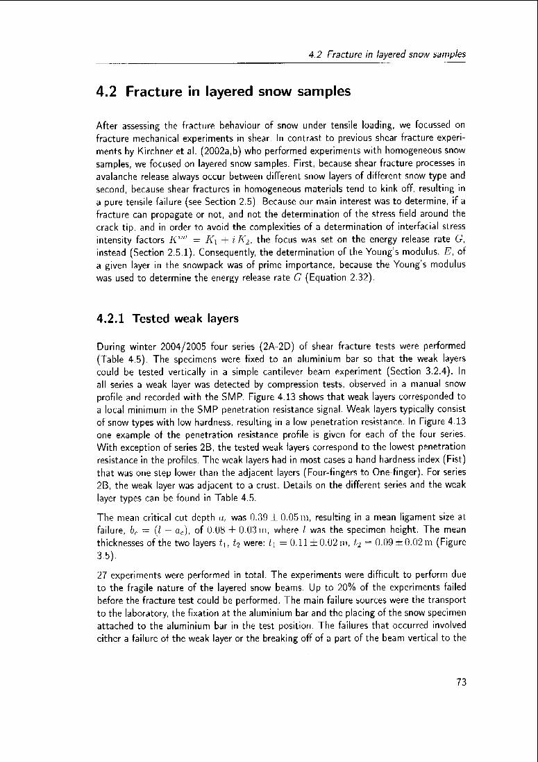
4.2 Fracture in layered snow samples
4.2 Fracture in layered snow samples
After assessing the fracture behaviour of snow under tensile loading, we focussed on
fracture mechanical experiments in shear In contrast to previous shear fracture experi¬
ments by Kirchner et al. (2002a,b) who performed experiments with homogeneous snow
samples, we focused on layered snow samples. First, because shear fracture processes in
avalanche release always occur between different snow layers of different snow type and
second, because shear fractures in homogeneous materials tend to kink off, resulting in
a pure tensile failure (see Section 2.5). Because our main interest was to determine, if a
fracture can propagate or not, and not the determination of the stress field around the
crack tip, and in order to avoid the complexities of a determination of interfacial stress
intensity factors K,nt ~ A7 + iK2, the focus was set on the energy release rate G,
instead (Section 2.5.1). Consequently, the determination of the Young's modulus, E, of
a given layer in the snowpack was of prime importance, because the Young's modulus
was used to determine the energy release rate G (Equation 2,32).
4.2.1 Tested weak layers
During winter 2004/2005 four series (2A-2D) of shear fracture tests were performed
(Table 4.5). The specimens were fixed to an aluminium bar so that the weak layers
could be tested vertically in a simple cantilever beam experiment (Section 3.2.4). In
all series a weak layer was detected by compression tests, observed in a manual snow
profile and recorded with the SMP. Figure 4.13 shows that weak layers corresponded to
a local minimum in the SMP penetration resistance signal. Weak layers typically consist
of snow types with low hardness, resulting in a low penetration resistance. In Figure 4.13
one example of the penetration resistance profile is given for each of the four series.
With exception of series 2B, the tested weak layers correspond to the lowest penetrationresistance in the profiles. The weak layers had in most cases a hand hardness index (Fist)that was one step lower than the adjacent layers (Four-fingers to One-finger). For series
2B, the weak layer was adjacent to a crust. Details on the different series and the weak
layer types can be found in Table 4.5.
The mean critical cut depth a, was 0.39 ± 0.05 m, resulting in a mean ligament size at
failure, br = (/ — ar), of 0.08 ± 0.03 m, where / was the specimen height. The mean
thicknesses of the two layers t,[t l2 were: /, = 0.11 ±0.02m, t2 = 0.09±0.02m (Figure
3.5).
27 experiments were performed in total. The experiments were difficult to perform due
to the fragile nature of the layered snow beams. Up to 20% of the experiments failed
before the fracture test could be performed. The main failure sources were the transport
to the laboratory, the fixation at the aluminium bar and the placing of the snow specimen
attached to the aluminium bar in the test position. The failures that occurred involved
either a failure of the weak layer or the breaking off of a part of the beam vertical to the
73

Table
4.5:Summary
ofshear
fractureexperiments.
Snow
type
isgiven
as
grainshape,
grainsize
and
hardness
indexaccording
to
ICSSG
(Colbecket
al.,1990).
"Upper
layer"denotes
the
layerabove
theweak
layerand
"lower
layer"the
layerunderneath
the
weak
layeraccording
to
theirposition
inthesnow
cover.
Series
Date
of
sampling
Number
of
Snowtemp.
Compression
Grainshape,
grainsize
experiments
(°C)
test
results
-
upper
laver
Number
oftabs
-weak
layer
(rating)-
lower
layer
Hardness
index
Snow
densitv
±sdev
(kg/m3)
2A
24Feb05
2B
24Feb05
2
2C
15Mar
05
10
2D
15Mar05
-9.1
-8.7
-9.1
-9.1
12,12.
12
(moderate)
12.
12.14
(moderate)
13
(moderate)
21
(hard)
Faceted
crystals,0.5—
1mm
4F
IF
267±
5
Faceted
crvstalsandsome
F-4F
surface
hoar.
0.75—
1.5mm
Faceted
crvstals.0.75—
1mm
IF
309±
5
Crust,melt
forms,
0.5mm
IF
275±11
Faceted
crvstals.0.75—
1mm
F-4F
Faceted
crystals.0.5—
1mm
4F-1F
287±2
Smallroundedandsome
4F
234±
10
faceted
crystals.0
5—
1mm
Mixedformsandsome
F
depth
hoar.
0.75—
1.5mm
Mixed
forms,
0.5—
1mm
4F
267±
10
Smallroundedand
IF
330±
6
mixed
forms.
0.5—
75mm
Mixedformsandsome
F
surface
hoar.
1—
2mm
Smallroundedand
1F-K
348±
7
mixed
forms.
0.5—
75mm

4.2 Fracture in layered snow samples
muc
10
m
2>c
o
CDc
CDQ.
z
S(A
'(O
c
o
"53
CD
a.
weak layerseries 2B
0 20 40 60 80 100 120 140 160
Penetration depth (mm)
0 20 40 60 80 100 120 140 160
Penetration depth (mm)
Figure 4.13: Penetration resistance recorded with a SnowMicroPen SMP. For each of
the four tested weak layer types, series 2A to 2D, one example is given. With the
exception of series 2B, the tested weak layers correspond to the lowest penetration
resistances in the profiles.
layering.
4.2.2 Young's modulus
After performing fracture tests, small samples were cut out of the different layers of the
tested specimens. A dynamic Young's modulus of these samples was then measured in a
cyclic loading experiment (see Section 3.4.1). Due to the time consuming measurement
technique, the Young's modulus could not be determined for each specimen that had
been tested in fracture. Each specimen would have required two measurements, one for
the upper layer and one for the lower layer. A selection of 27 measurements was made:
10 in series 2A, 2 in series 2B, 9 in series 2C and 6 in series 2D. The dynamic Young's
modulus, Edyn, of these 27 experiments are shown in Figure 4.14. EdyR is plotted against
75

Chapter 4 Results
200 240 280 320 360
Snow density, p (kg/m3)
Figure 4.14. Dynamic Young's modulus in relation to snow density, measured at a
frequency of 100 Hz (squares) The dash-dot line indicates the best fit of the data
(Equation 4 9) The dashed area (B) indicates the range of the Young s modulus
found by Scapozza (2004) in quasistatic compression experiments (A) are uniaxial
compression and tension experiments compiled by Mellor (1975) and (C) pulse prop
agation or flexural vibration tests at high frequencies, also compiled by Mellor (1975)
Additionally, the results of the dynamic torsional shear experiments of Schweizer and
Camponovo (2002) were converted to Young's modulus values (circles)
snow density A power law relation can be fitted to the data
Edll„ = 1 89 x 10~b p2 "lMPa, (4 8)
with a coefficient of determination of R2 — 0 80 The power law relation is indi
cated as dash-dot line in Figure 4 14 (An exponential relation resulted in Edyn —
2 71 fooos5pMPa ^2 = q 78) For comparison? the range of results summarized byMellor (1975) (area A and C) and by Scapozza (2004) (dashed area B) are added to
Figure 4 14 Furthermore, the results obtained by Schweizer and Camponovo (2002) are
added They determined the shear modulus, S, m dynamic torsional shear experiments
76

4.2 Fracture in layered snow samples
1 \J
£ =(186 + 7)£dyn
x — ' SMP
60- — 95% confidence band
X ^ y
^ 50- ,' / ''03D_
' / ,' o
2 s ^r s
^W's
'
/^ '
1.40- Xbq
°yX--'30-
o
On A/' o°°
^9^' o
20-Q'*S-' o
N = 24
10-^: I ' I ' i -T- ' 1 ' i
0.05 0.10 0.15 0.20 0.25 0.30 0.35
*,(MPa>
Figure 4.15: Correlation of the dynamically measured Young's modulus Edyn with
the index Esmp derived from the penetration resistance signal, recorded with the
SnowMicroPen SMP.
with a rheometer. The shear modulus results of Schweizer and Camponovo (2002) were
converted to Young's modulus values according to the relation for linear elastic material
behaviour: E = 2S{\. 4 v). The Poisson's ratio v was set to 0.17 for the snow densities
of about 230 kg/m3 they used for their experiments.
Alternatively, the SMP penetration resistance signal was used to estimate the Young'smodulus. The big advantage of this method is that an SMP signal is easy and fast to
acquire, the disadvantage is that the conversion from penetration resistance to Young'smodulus is badly calibrated up to now. An IDL (Interactive Data Language) algorithm,
developed by Kronholm (2004) and based on a theory of Johnson and Schneebeli (1999),was used to calculate an index for the Young's modulus as a function of the penetrationresistance (Equations 3.19 and 3.20). However, according to Kronholm (2004), the values
of the index derived from the SMP signal are too small and have to be corrected by a
factor of about 150 to get an appropriate estimate for the Young's modulus.
77

Chapter 4 Results
p
T3
"5.Q.
<
30-
i
t
/
f
t^
25-
*
t
/
r
\
Slope:
s^*~**// (27.4 + 0.3) N/mm
20-Slope: (32.6 + 0.8) N/mm //
/ *
15-f t
/ *
fë
itft
10-
itft
5-
0-
tftftf
"f*/*/
t //
/
/
-5 JLi > i ——T" ' 1 < i*i '
-0.4 0.0 1.6 2.00.4 0.8 1.2
Displacement, AA (mm)
Figure 4.16: Force-displacement diagram of a three-point bending test. (Specimendimensions: 50cm x 20cm x 10cm, density: 240 kg/m3). Indicated are the slopes
{F/Ah) of an initial tangent (black line) and of a tangent over the whole range
where the force increases (black dashed line).
Correlating the index values derived from the SMP data, ESah->, with the results from
the cyclic loading tests, Ed!)„, resulted in a correction factor of Edyn — (186 ± 7) Esmp
with a coefficient of determination of R2 = 0.81 and a level of significance P < 0.0001
(Figure 4.15). Of the 27 measurements with the cyclic loading device only for 24 an
SMP signal was available. Therefore, Figure 4.15 includes only 24 data points.
A further possibility to estimate the Young's modulus would be to use the force-
displacement signals acquired during the three-point bending tests. Out of a force-
displacement diagram the slope of the force increase {F/Ah) can be determined (Figure
4.16). By multiplying this slope with hjA the elastic modulus can be determined ac¬
cording to
(4.9)e A Ah/
where /; is the height of the specimen and A the area of contact of the force sensor.
The height of the specimen in Figure 4.16 was 20 cm and the area of contact is given
by the width of the beam (10 cm) times the width of the contact of the force cylinder.The contact width is assumed to be approximately 1cm. The resulting Young's modulus
for the indicated slopes of F/Ah = 27.4 N/mm and of F/Ah = 32.6N/nun are
78

4.2 Fracture in layered snow samples
E = 5.5 MPa and E = 6.5 MPa, respectively. The specimen in Figure 4.16 had a
density of 240 kg/m3. Compared to the Young's modulus results compiled in Figure
4.14, the values are well within the range of the results of Mellor (1975) and Scapozza
(2004).
However, in a three-point bending test the displacement Ah is a combination of compres¬
sion of the specimen and bending of the specimen. Only the compression is relevant for
the determination of the Young's modulus. Since in the above estimate both components
are included the effective Young's modulus might be underestimated.
4.2.3 Energy release rate in mode II
To evaluate the critical energy release rate Gf for our experiments, no analytical solution
was found. Therefore, Gf was determined numerically in an FE simulation (Section
3.2.5). The critical energy release rate is denoted as Gf in this work and not as G,, as it
is usually done in literature, because index / expresses that the energy release rate will
most probably depend on the test specimen size (compare with K/f vs. Klc in Section
4.1,5)
For every single experiment an FE simulation was run based on the exact geometry
of the experiment. The input parameters were: specimen length, thickness and width
(/, tf.tb, i"), elastic properties of the two layers (Et, Ei,} vu z^), density of the two layers
{pt,pb) cut length at failure (ac), as well as angle of rotation (a) and the additional
mass {niioad) The Poisson's ratio vh v\t were estimated from density according to
v = uo +{p- Po) 5 x 10"' m7kg, (4.10)
with v0 = 0.2 and p0 = 300 kg m-'* according to Mellor (1975). The cut length increment
Aa was set to 0.002 m resulting in Aa/h = 0.004 Changes in Aa did not change the
energy release rate G The Young's modulus of the slab [Et) and the basal layer {Eh)as well as of the weak layer {Ewl) were derived from the SMP penetration resistance
signal This was done by dividing the penetration resistance signal (compare Figure 4.13)in three sections: slab, weak layer and basal layer. In the following the Young's modulus
was derived as average over a whole section, even if the penetration resistance signalshowed variations in one section. The results are compiled in Table 4.6.
Since the crack length a was set equal to the critical crack length a,_ the energy release
rate at the point of failure was assessed. The energy release rate at failure is equal to
the critical energy release rate Gj, the energy that has to be overcome to propagate a
fracture. Gf can thus also be seen as the specific fracture energy of the weak layer, the
energy needed to fracture a weak layer over a unit area.
The results for the critical energy release rate Gf for the different series (2A-2D) are
shown in Figure 4.17. Gj is plotted against various elastic properties of the specimen.
Only for the correlation of Gf with the elastic mismatch between slab and basal layer,
Et/Eb, a slight trend to increase with increasing elastic mismatch could be observed
79

Chapter 4 Results
0.10
0.08
"E 0.06-5
^0.04
0.02-I
(a) A A 2A(N = 8)A 2B(N = 2) o
• 2C(N = 10)Ü 2D(N = 7)
o
#*A
o
* & A,,o
0 o
—!
o
1 r.——-
20
0.10
30 40
£ (MPa)
50 60 12 16
£ (MPa)
(d) A
0.08-o
A
0.06-
A
O
0.04- *• "A
aA
A* A A0
•
0.020
3
E IE,.,
Figure 4.17: Critical energy release rate Gj in relation to the elastic properties of the
specimen: (a) Gf in relation to the Young's modulus of the slab Ef, (b) in relation to
the Young's modulus of the weak layer EWL, (c) in relation to the elastic mismatch
of slab and basal layer Et/Eh, (d) in relation to the elastic mismatch of slab and weak
layer EjEwl- The results are coded according to the four series of winter 2004/2005(Table 4.5).
Table 4.6: Details of the shear fracture experiments.
Series Relative cut
length, a,/I
Thickness
ratio, tt/tb
Young's modulus Gl
Et
(MPa)
Ewl
(MPa)
Eh
(MPa) (mJ/m2)
2A
2B
2C
2D
0.85 ± 0.05
0.80 ± 0.08
0.78 ± 0.07
0.82 ± 0.08
0.96 ±0.15
0.88 ±0.01
1.21 ±0.53
1.26 ±0.63
25.9 ±3.6
20.4 ± 6.0
19.7 ±1.9
54.6 ±2.5
9.1 ±2.5
14.6 ±2.7
11.2 ±2.8
1 4.5 ± 2.8
39.1 ±6.0
30.8 ± 1.7
23.6 ±29
59.3 ±5.4
50 ± 26
55 ± 12
39 ± 6
40 ± 24
80

4.2 Fracture in layered snow samples
(P(4.17a) - 0.49, P(4.17b) = 0.04, P(4.17c) = 0.61, P(4.17d) = 0.49). However, if
the four data points in Figure 4.17c were excluded, for which the Young's modulus of the
slab was bigger than of the basal layer Et/Eb > 1 no statistically significant correlation
could be observed (P = 0.36). The exclusion of these four points from a correlation
is justified because the elastic mismatch starts to increase again for Et/Eb > 1, after
decreasing in positive ./-direction for E,/Eb < 1. Figure 4.17b suggests that the energy
release rate does not depend on the Young's modulus of the weak layer. However, the
range of the Young's modulus for the weak layers tested in our experiments was relatively
narrow, since the properties of the weak layers were similar for all series (Table 4.5). A
multiple regression for Gf and the Young's modulus of Et, Eh and of the weak layer EWl
did not reveal any statistically significant correlation {R2 = 0.15, N — 26, P ~ 0.15).
The mean critical energy release rate for all series was
Gf = 0.044 ±0.020 J/m2. (4.11)
4.2.4 Comparison of analytical approaches to FEM results
To determine the energy release rate G for our experimental geometry no analytical solu¬
tion was available. Therefore, we adapted two general analytical approaches to determine
G. To overcome some of the limitations of the analytical solutions we compared them
to a numerical approach. In the following, the two approaches are described: (1) The
analytical cantilever beam approach is valid for deep cracks but assumes a homogeneous
material, see Section 3.2.4. (2) The analytical bilayer approach assumes two different
materials, but an infinitesimally extended specimen, see Section 2.5.2. An analytical so¬
lution is of importance, even if it is an approximation, because it can render FE modelling
unnecessary for future experiments.
Figure 4.18a compares the cantilever deep crack approach with the FEM results. Energy
release rates were calculated according to Equations (3.7)-(3.9) and Equation (3.16) for
different geometry and material properties. The cantilever results were larger than the
FEM results, but the values were highly correlated {R2 = 0.93, iV = 21, p < 0.0001).The slope was 0.49±0.03. The value of the slope slightly depends on the elastic mismatch
between slab and basal layer, Et/Eb (Figure 4.18c). A linear regression showed a level
of significance of P = 0.003.
The analytical solution of Suo and Hutchinson (1990) for an interface crack between
thin films, Equation (2.33), was adapted to our geometry. For our geometry and loadingsituation /?, = th H — tb and we assume P to be the force due to the body weight
plus the additional weight that was placed on top of the protruding part, therefore,
P\ = P3 = PCh in Equation (3.14). P2 was zero, hî\ was equal to Mob (Equation
3.16). A/3 was zero because the specimen was placed on the table at the point where
A/3 would act. With these assumptions Equation (2.33) simplified to
G-2-Ët[~ir + u^r)+ 2Eh \- au+ u
h> ) (412)
81

Chapter 4 Results
0.5
0.4
-i 0.3
f 0.2-1LULi.
O 0.1-
0.0
(a)
[^-~G(FEM)^.5Ö±äÖ3TG^B"bC)
0.0 0.2 0.4 0.6
G (CB-DC) (J/m2)
0.8 1.0
0.7
5-0.6Q
i
Ü 0-5
g-0.4
LU
£-0.3
0.2
- (c) 0 o
o
o
000.--
''o0
o
o.1
; °. o--0
o
0.5- (b)o'
*»
0.4 -,
M 0.3-—>
o
0'
S 0.2 #LUU.
«'0
Ü 0.1-
o
0.0 - - C(FEM) = (0.49±0.08~j G(BIC) l
0.0 0.2 0.4 0.6 0.8 1
G (BIC) (J/m2)
8- (d)0
„ 6O
cû
ü 4-
5LU n
LL'
o ° o o o
0-o og 0
0.2 0.4 0.6 0.8
£ /£,
1.0 1.2 0.2 0.4 0.6 0.8 1.0 1.2
E IE.
Figure 4.18: Comparison of the energy release rates obtained with the FE model and
(a) the analytical deep crack cantilever approach, and (b) the analytical bilayer with an
interface crack approach. Figures (c) and (d) show the ratio of the energy release rates
in relation to the elastic mismatch EtJEi, for the two analytical solutions. {M = 21).
Overall equilibrium of moments provides a constraint so that the moment A/2 can be
calculated:
M2 = Pctt+ lb - Alt + M( (4.13)
M2 compensates for the fixed side of the beam in our experiments.
In Figure 4.18b the adapted analytical solution for a bilayer material (Suo and Hutchin¬
son, 1990) is compared with the FEM results. The analytical results were larger than
the FEM results. A linear regression resulted in a slope of 0.49 ± 0.08 (P2 = 0.69, N =
21. p < 0.0001). Consequently, for the bilayer approach the slope did not depend on the
elastic mismatch between slab and basal layer, Et/Eb (P = 0.62), because Et as well
as Eb are included in the bilayer approach. (Figure 4.18d).
If the analytical solutions are multiplied with the according correlation factors, they are
valuable solutions to replace the finite element modelling.
82

4.2 Fracture in layered snow samples
0.3-
^E 0.2-
0.0
N = 27
g;^p&
\^.-
CO
0-•**
üv
ü" 0.1 -
0.-*" n
•" "d
'
Doo^oP D
O
e,«*^-
DU
nQD
oc G; (mode II)
160 180 200 220 240 260
Snow density, p (kg/m )
Figure 4.19: Critical energy release rate Gf of the mode II experiments (squares) in
comparison to the critical energy release rate for the mode I experiments (dotted line)and the effective critical energy release rate in Mode I Gc (dashed line) .
4.2.5 Comparison of mode I and mode II results
In order to compare the energy release rate of the mode I experiments and of the mode II
experiments, Equation (2.17): G = K2JE, can be used to transform the critical energy
release rate results in mode I into an energy release rate in mode I. To get the critical
energy release rate in mode I, G/(modeI), in relation to the density, Equation (4.2)was used for the critical stress intensity factor A'// and Equation (4.9) for the Young'smodulus. Figure 4.19 shows the resulting relation (dotted line). To get the specimen size
independent effective critical energy release rate in mode I, G\.(modc I), in relation to the
density, Equation (4.6) was used for the equivalent fracture toughness Kjr (dashed line).For the mode II experiments the density of the weak layer was estimated by converting
the Young's modulus EWL into a density for the weak layer by using Equation (4.9).The mode I critical energy release rate is on average 2.2 times higher than the critical
energy release rate in mode II for the same density of snow. The effective critical energy
release rate Gc is on average 6.5 times higher than the Gf in mode II.
On the other side, Equation (3.7) can be used to get a rough estimate of the magnitude
83

Chapter 4 Results
of the fracture toughness for our weak layer type: \/G Ewl =
v Ef + Imi' The
average weak layer Young's modulus Ewl of our samples was 11.6 MPa (Figure 4.17b).Corresponding to a density of about 200 kg/m3 if Equation (4.9) is used. The mixed
mode interfacial critical stress intensity factor for a shear fracture along a weak layer,
Kfff, resulted in
Kfff = 0.49 ± 0.36 kPaml/2 (4.14)
which is about a factor of 1.9 lower than the critical stress intensity factor in mode I,
Kjf, for samples of similar snow density (see Figure 4.3).
84

4.3 Fracture of weak layers on slopes
4.3 Fracture of weak layers on slopes
Field experiments were performed during three days between 25 January and 3 February
2006. For the test a snow beam including a weak layer was isolated on all for sides and
then a cut was made along the weak layer with a snow saw until the specimen failed
(Section 3.3 and Figure 4.20). An east-facing slope was selected with a slope angle close
to 30° at Strela-Schönenboden, Davos, Switzerland (779 920 / 186 365). In this slope
a weak layer was present in a depth of about 30 cm which consisted of faceted crystalsand partly depth hoar. The weak layer was formed under a 2 mm thick crust during a
period of fine weather in January 2006. Three test series were performed with this weak
layer at intervals of 2 days and 7 days, respectively. Details of the tests can be found in
Table 4.7 and in the stratigraphie snow cover profiles for the three days in Appendix B.
33 experiments were performed in these three days.
The tests can be divided in two groups according to their failure behaviour. The first
group of snow beams failed along the entire weak layer plane after a critical cut length ac
was reached with the saw. Because most of our experiments were performed at a slope
angle of about 30°, the detached part of the beam (the slab) did not slide down over
the failed weak layer plane, but a noticeable displacement of the whole slab could be
observed. A displacement of the upper part of the beam (slab) of approximately 5 mm
can be observed in Figure 4.20c. The weak layer can be identified in the image as darker
area due to higher porosity. In the second group, a fracture propagated along the weak
layer when reaching ac but the weak layer did not fail entirely. The crack was arrested
after a certain distance. In some cases a vertical tensile crack could be observed throughthe overlaying slab. Of the 33 experiments, the weak layer fractured entirely in 22 or
two-thirds of all tested specimen and in 11 tests the crack was arrested.
Tests that were made on slopes steeper than 30° showed that the slab slid down over
the plane of weakness. Tests on slopes with an inclination of about 25° showed that a
similar displacement could be observed as in tests at 30°. Results of the tests with an
other inclination than 30° are not further considered, because only few tests were made
and the weak layers are not comparable to the other data set.
4.3.1 Shear strength of the tested weak layer
The shear strength measurements were performed with the shear frame (Section 3.1).The shear strength is calculated as the measured force divided by the shear frame area
and multiplied with a correction factor (Jamieson and Johnston, 2001). The results of
the shear strength measurements are summarized in Table 4.8.
The mean shear strength was between a factor of 3.4 and 5.4 higher than the effective
shear stress. The effective shear stress is calculated as the slope parallel component of
the load due to the weight {rnsiabgcos{>p)) divided by the base area of the isolated beam
reduced by the area that had been cut with the snow saw («;(/ — ar)).
85

3tu
ceCl.ni
Table
4.7:Summary
ofthe
fieldexperiments.
Dateofthe
fieldday
andnumberoftestare
givenSnow
type
isgiven
as
grainshape,
grainsize
and
hardness
indexaccording
toICSSG
(Colbecket
al.,1990).
Series
Date
of
Number
of
Snow
type
ofweak
laver
Compression
test
Mean
slab
Mean
slab
Snow
/Air
testingexperiments
results
densitythickness
temperature
Number
oftabs
(slopenormal)
(rating)(kg/m3)
(m)
(°C)
3A
25Jan
06
5(4/l)a
Faceted
crystalsand
partlv11,11,12
173
0.27
-6.9/-3.2
depth
hoar.
1—
3mm,F
(moderate)
3B
27Jan
06
21
(13/8)aFaceted
crystalsand
partly13,13;
13.13:
14,12:
187
0.26
-7.4/-9
depth
hoar.
1-
2mm,F
13,13;
15.14:15,13
(moderate)
3C
3Feb06
7(5/2)Q
Faceted
crystalsanddepth
14.15;
15.15;
16.17:
202
0.21
-6.3/-3.5
hoar.
1—2.5mm.F
17.15.15
(moderate)
'(Number
oftest
inwhichthebeam
failedcompletely
/Number
oftests
inwhich
thecrackwasarrested)
lO
Uco

4.3 Fracture of weak layers on slopes
WÈÊÈÊÊ
(b) (c)
Figure 4.20: (a) Image of the study site at Strela-Schönenboden, Davos after testing.It is schematically indicated how a row of field test beams was located. (A) Test
specimen with length of 1.8 m followed by a beam divided in a (B) 0.6 m and a (C)1.2 m beam. (D) Downslope of every test beam a SMP penetration resistance profilewas taken, (b) Field test setup. Cutting along the weak layer of a field test specimenwith length 1.2 m and width 0.3 m. (c) Lower edge of a test specimen. The failure of
the weak layer resulted in a slight downslope displacement of the upper part of the
beam (the slab) of about 5 mm.
87
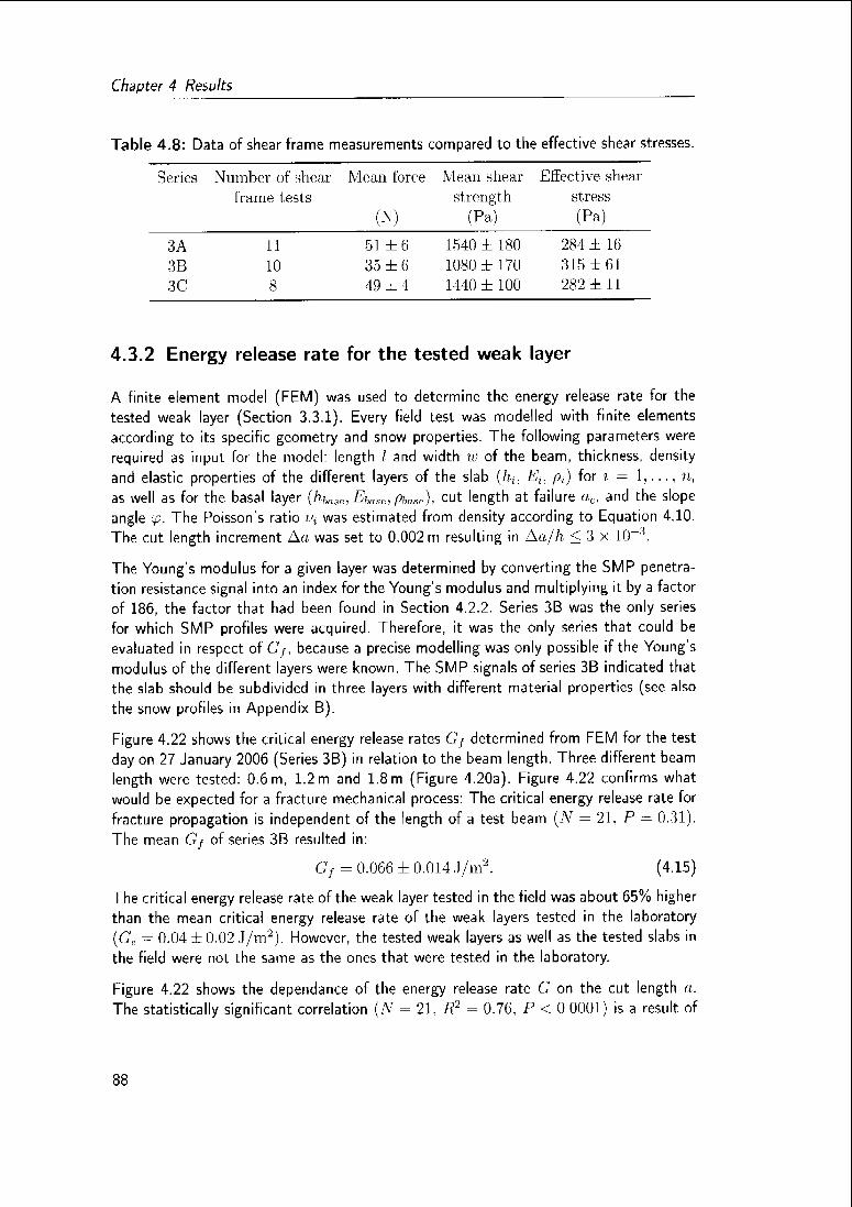
Chapter 4 Results
Table 4.8: Data of shear frame measurements compared to the effective shear stresses.
Series Number of shear Mean force Mean shear Effective shear
frame tests strength stress
(N) (Pa) (Pa)
3A 11 51 ±6 1540 ± 180 284 ± 16
3B 10 35 ± 6 1080 ±170 315 ± 61
3C 8 49 ± 4 1440 ± 100 282 ±11
4.3.2 Energy release rate for the tested weak layer
A finite element model (FEM) was used to determine the energy release rate for the
tested weak layer (Section 3.3.1). Every field test was modelled with finite elements
according to its specific geometry and snow properties. The following parameters were
required as input for the model: length / and width w of the beam, thickness, density
and elastic properties of the different layers of the slab {hi, Etl p/) for i = 1,..., n,
as well as for the basal layer (/ib„„,R, -EW,e, phase), cut length at failure a,c, and the slope
angle <p. The Poisson's ratio v\ was estimated from density according to Equation 4.10.
The cut length increment Aa was set to 0.002 m resulting in Aa/h < 3 x If)-3.
The Young's modulus for a given layer was determined by converting the SMP penetra¬
tion resistance signal into an index for the Young's modulus and multiplying it by a factor
of 186, the factor that had been found in Section 4.2.2. Series 3B was the only series
for which SMP profiles were acquired. Therefore, it was the only series that could be
evaluated in respect of Gf, because a precise modelling was only possible if the Young'smodulus of the different layers were known. The SMP signals of series 3B indicated that
the slab should be subdivided in three layers with different material properties (see also
the snow profiles in Appendix B).
Figure 4.22 shows the critical energy release rates Gf determined from FEM for the test
day on 27 January 2006 (Series 3B) in relation to the beam length. Three different beam
length were tested: 0.6m, 1.2m and 1.8m (Figure 4.20a). Figure 4.22 confirms what
would be expected for a fracture mechanical process: The critical energy release rate for
fracture propagation is independent of the length of a test beam {N = 21, P — 0.31).The mean Gf of series 3B resulted in:
Gf = 0.066 ± 0.014 J/m2. (4.15)
The critical energy release rate of the weak layer tested in the field was about 65% higher
than the mean critical energy release rate of the weak layers tested in the laboratory
{G,. — 0.04 ± 0.02 J/m2). However, the tested weak layers as well as the tested slabs in
the field were not the same as the ones that were tested in the laboratory.
Figure 4.22 shows the dépendance of the energy release rate G on the cut length a.
The statistically significant correlation (N = 21, R2 = 0.76, P < 0.0001) is a result of
88

4.3 Fracture of weak layers on slopes
0.10
-l-J
2a)en
m
£
Ol
c
Q)
15o
> 0.08
m 0.06-
jï 0.04-
o
Beam length / (m)
Figure 4.21: Critical energy release rate Gf determined with FEM in relation to the
beam length for the field tests of 27 January 2006. A linear regression (dotted line)was statistically not significant, i.e. Gf does not depend on the beam length.
the fact that for the different test beams the geometry and the elastic properties were
approximately the same. Thus, if the cut length is increased, the energy release rate
increases too. However, the scattering of the data points represents the fact that the
elastic properties of the various test were not exactly the same.
Figure 4.23 shows a box plot which shows the distribution of the critical crack length
a,, for the three testing days. In statistics, the box plot is a convenient way to display a
summary of five numbers which describe the distribution of a parameter. It consists of the
smallest observation, lower quartile, median, upper quartile and largest observation. The
height of the box, defined by the upper and lower quartile is known as the interquartile
range (IQR) and includes 50% of all values. The position of the median in the box gives
information of the skewness of the distribution. The cross indicates the mean value and
the circles indicate the largest and smallest observation. The so called whiskers indicate
the 5% and 95% level. Figure 4.23 shows that between the three measurement days the
critical cut length tended to increase, although, the mass of the slab did not increase
because there was no snow fall event during this period.
89

Chapter 4 Results
0.10
M 0.08-
g 0.06
0)c
m 0.04-
i—o—I
f—o—I
^fcfer^H^(B?=C>~"i
i—o-^-toe* i
(N = 21, FT = 0.76, P< 0.0001)
0.18 0.20 0.22 0.24
Cut length, a (m)
0.26 0.28
Figure 4.22: Energy release rate G in dépendance of the cut length a. All tests were
made with the same weak layer on 27 January 2006. A linear regression (dotted line)was statistically significant.
4.3.3 Influence of bending
In this section additional results based on the FE model of the field experiment will be
presented.
Although the thickness of the cut that was made in the weak layer was only 2 mm,
corresponding to the 2 mm thick snow saw, the cut surfaces were far from getting in
contact to each other for our cut length ac < 30 cm. Simulations showed that a cut
length of more than 50 cm would have been required to bring the slab in contact with
the basal layer for the elastic properties of the tested slabs. For our cut length, the
vertical displacement of the slab due to bending did never exceed 50% of the gap size
of 2 mm and was in most cases much less than 50% (Figure 4.24).
First simulations were made with a model which included a slab consisting of only one
layer. However, the penetration resistance signals of the slab suggested that the slab
should rather be modelled as to consist of three different layers. In the following the
model was extended to a slab consisting of three layers (see Figure 3.8). Figure 4.25
shows the resulting tensile stresses in slope parallel direction o~y for a model with a one
90

4.3 Fracture of weak layers on slopes
0.32
25 Jan 06 27 Jan 06 3 Feb 06
Figure 4.23: The distribution of the critical cut length ac in a box plot for the three
test days. Mean compression test (CT) results and number of compression tests are
indicated at the bottom.
layer slab and for a model with a slab consisting of three layers with different material
properties. Both beams had a length of 1.2 m and a width of 0.3 m. The basal layer had
a slope normal tickness of h = 13.6 cm, a density of 246 kg/m3 and a Young's modulus
of E = 12.2 MPa. The slab properties are indicated in the caption of Figure 4.25.
Whereas for the one layer slab no stress concentrations can be seen, a different stress
pattern is visible for the three layer slab (Figure 4.25). The stress concentration was not
located where it would have been expected for a bending case, right above the crack tip,
but a certain distance ahead of the crack tip. Obviously this stress concentration was a
result of the combination of different layers with different material properties. However,
results showed that the existence of stress concentrations depended very much on the
properties and thicknesses of the three slab layers.
Finally, the influence of an existing gap on the energy release rate was tested. Therefore,
a beam with rectangular shape was modelled, in contrast to the beam shape in Figure4.25 in which the left and right face are always vertical, independent of the slope angle.The rectangular shape was chosen to be able to model also high slope angles up to
91

Chapter 4 Results
OlSPlATEMElIr
STEP» I
tIME-1.
4v -,
£/ v~'V/
// / !
i7 <
5/
Figure 4.24: Detail of the upslope end of a test beam simulation (ANSYS output).The upper part (slab) bends due to gravity The vertical displacement is indicated as
Au. The horizontal displacement between slab and basal layer has modelling reasons.
80°. The model had the following dimensions: beam length = 1.2 m, beam width —
0.3m, slab thickness — 0.3 m, height of basal layer = 0.1m, cut length — 0.2 m, slab
density = 250 kg/m3, basal layer density - 300 kg/m3, Young's modulus of the slab
E^/ab — 20 MPa, Young's modulus of the basal layer Ehn^ — 30 MPa. (This time the slab
was again modelled as only one layer). The values for the Young's modulus correspond
approximately to what can be found by Equation (4.9). With this model the energy
release rate G was calculated for different slope angles tp for the case when a cut
thickness or gap of 2 mm was included, and for the case when the cut thickness was
set to zero. The cut surfaces were modelled as contact and target area, so that no
penetration of the upper cut surface (the slab) was allowed into the lower cut surface
(the basal layer). Therefore, in case the gap size was set to zero no bending of the
slab was possible. No slope parallel friction between the cut surfaces was assumed. The
results are presented in Figure 4.26a. For a slope angle of 30°, the energy release rate
due to the combined bending and shearing was about 6 times the energy release rate
due to pure shearing.
92

4.3 Fracture of weak layers on slopes
NU I j I HT!H
AN
rriN > of
lUM j HIT l IN
nM( - 4£
AIM
J UN 1 20 Oh
Figure 4.25: Top: Tensile stresses in slope parallel direction av for the modelled
geometry with slab consisting of n—1 layer. (Slab properties: h = 26.6 cm, p =
167kg/m3, E = 6.24MPa). Bottom. ay for a slab with n=3 layers. (Slab properties:
hi = 10.5cm, pi = 120kg/m3, Ex = 3.72MPa; h2 = 15.2cm, p2 = 190kg/m3,E2 = 6.01 MPa; hz = 0.9 cm, p-A - 273 kg/m3, EA = 10.5 MPa).
93

Chapter 4 Results
0.03-
0.02-
O 0.01 -
0.00-
(a) -— bending and shear
-o- -
pure shear
E = 20 MPa
E. = 30 MPa
.^.-o
^0^0-*"
,-o
0---0---0"
0 20 40 60 80
0.14-
0.12-
0.10-
_0.08-
CM
3- 0.06-|
0.04-
0.02-
0.00-
(b) -— bending and shear
-o- -
pure shear
E = 4 MPat
E, = 10 MPa
.5=0-0-^-0"s~
^-o
o--
T"
0
-o-
—1—
_-0
-r-
20 40 60 80
Slope angle, <p (°)
Figure 4.26: Finite element calculation of the energy release rate in dependence of slope
angle for a model including a gap of 2 mm (squares), so that bending is possible, and
for a model with a gap of zero extension (circles). The material properties for the
calculation (a) were: pshlb = 250 kg/m3, pbavf, = 300 kg/m3, Eslnh = 20 MPa, E,ja,w
= 30 MPa; and for (b): ftUj - 250 kg/m3, /W = 300 kg/m3, E,lab = 4 MPa, Ebl= 10 MPa.
Jbaxr
94
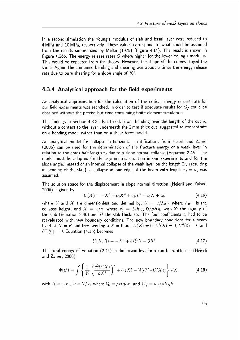
4.3 Fracture of weak layers on slopes
In a second simulation the Young's modulus of slab and basal layer were reduced to
4 MPa and 10 MPa, respectively. These values correspond to what could be assumed
from the results summarized by Mellor (1975) (Figure 4.14) The result is shown in
Figure 4.26b. The energy release rates G where higher for the lower Young's modulus.
This would be expected from the theory. However, the shape of the curves stayed the
same. Again, the combined bending and shearing was about 6 times the energy release
rate due to pure shearing for a slope angle of 30°.
4.3.4 Analytical approach for the field experiments
An analytical approximation for the calculation of the critical energy release rate for
our field experiments was searched, in order to test if adequate results for Gf could be
obtained without the precise but time consuming finite element simulation.
The findings in Section 4.3.3, that the slab was bending over the length of the cut a,
without a contact to the layer underneath the 2 mm thick cut, suggested to concentrate
on a bending model rather than on a shear force model.
An analytical model for collapse in horizontal stratifications from Heierli and Zaiser
(2006) can be used for the determination of the fracture energy of a weak layer in
relation to the crack half length i\, due to a slope normal collapse (Equation 2.45). The
model must be adapted for the asymmetric situation in our experiments and for the
slope angle. Instead of an internal collapse of the weak layer on the length 2r, (resultingin bending of the slab), a collapse at one edge of the beam with length rc = «c was
assumed.
The solution space for the displacement in slope normal direction (Heierli and Zaiser,
2006) is given by
U{X) = -X4 + r3X3 + c2X'2 ± c\X ± c0, (4.16)
where U and X are dimensionless and defined by: U ~ u/hwL where hWL is the
collapse height, and X = x/r{) where r0l = 2\hwL&/pBg, with T> the rigidity of
the slab (Equation 2.46) and H the slab thickness. The four coefficients r, had to be
reevaluated with new boundary conditions. The new boundary conditions for a beam
fixed at X = R and free bending a X = 0 are: U{R) - 0, U'{R) = 0, f/"(0) - 0 and
U'"(0) = 0. Equation (4.16) becomes
U{X, R) = -X4 + 4R3X - 3/?4. (4.17)
The total energy of Equation (2.44) in dimension-less form can be written as (Heierliand Zaiser, 2006)
m) ~ J {è i^^ivW)2 + u{x) + Wf0H;W)} **> (4-18)
with R — r/r0, <i> — V/Vq where Vb — pHghr0 and Wj = uf/pHyh.
95

Chapter 4 Results
By substitution of Equation (4.17) into Equation (4.18), the result for the energy in
dependence of the dimension-less crack extension R is obtained:
<f>(Ii) = -ïiïi + WfR. (4.19)
The energy gets critical when it reaches a maximum, as it was explained in Section 2.6.3.
Thus Equation (4.19) yields
^P = 0 = -3Ä* + Wf. (4.20)dR
By rearranging Equation (4.20) and re-transformation of the dimensionless variables,
a relation between the fracture energy of the weak layer wj which corresponds to the
critical energy release rate Gf (Equation 2.8) and the critical cut length ac can be found:
Equation (4.21) is still for a horizontal situation (slope angle ip = 0). Since our experi¬
ments took place on a slope with a given angle we have to correct for that by ycos{ip).
Furthermore, the cut length ac has to be corrected, because our beam geometry is not
rectangular but a parallelogram with angle <p (see Figure 3.8). The corrected cut length
o,c = ac ± H/'2tan{ip) compensates for the additional weight due to the geometry
difference. Thus, for our experimental situation, Equation (4.21) transforms to
3(pgcos(<p))* <
12 EH
v ;
The resulting critical energy release rate Gf in relation to the cut depth a,, are presented
in Figure 4.27. The data are compared to the numerical FEM results of Figure 4.22. On
average, the analytical results are a factor four lower than the numerical results. If for
comparison Gf is calculated according to the pure shear approach proposed by McClung
(1979), Equation (2.42), the results differ from the numerical results by a factor of 60
up to a factor of 150 (Figure 4.27).
96

4.3 Fracture of weak layers on slopes
Ü
0.10
0.08-
0.06
> 0.04 -
0.02-
0.00
(a) • numerical
o analytical
• •
•• •
• ••
oo o
o oCO
8 c»°
o
o o o
8
CD
O
1 1 1 1 1 1 1 1 1 1
0.18 0.20 0.22 0.24 0.26 0.28
1
0.1-=
E 0.01-i
ü
1E-3-:
1E-4
(b) • numerical
0 bendingA pure shear
.. ..I*..«•• *
o oOCT
CD °o
OO O
O O o
A A^ * A
A
AA A
A A A
CD
zA
O
i | i | i | i | i |
0.18 0.20 0.22 0.24 0.26 0.28
Cut length, a.(m)
Figure 4.27: The critical energy release rate Gf in relation to the cut length a,,, (a)The analytical bending beam results are compared to the numerical FEM results, (b)
Comparison with the pure shear results of Equation (2.42) in logarithmic scale.
97

Seite Leer /
Blank leaf

Chapter 5
Discussion
5.1 Fracture in mode I
5.1.1 The load-displacement curve
In mechanics and engineering load-displacement or stress-strain diagrams play a crucial
role for the characterization of material behaviour. Since a load-displacement curve was
recorded for each three-point bending (3PB) test, a representative example of a load
displacement curve (Figure 4.1) will be discussed here.
The strain rates ê for the 3PB-tests were between 4.2 x 10"1 s"l for the smallest specimen
with a height of 8 cm and 1.3 x 10~2 s_1 for the largest specimen with a height of 32 cm.
Thus the strain rates were clearly in the brittle range according to the brittle to ductile
transition which is between è ~ 1 x l()~3s_1 and ê ~ 1 x 10~5s_1 depending on grain
type and temperature (Narita, 1980). Brittle behaviour is manifested in a linear increase
of the load due to a displacement until failure. However, Figure 4.1 shows that this holds
only to a limited extent for our fracture experiments. The slope decreases slightly towards
the failure point. After the peak load is reached, the force signal does not instantly drop
down to 0 N but remains at a level of about 28 N for a duration of 25 ms.These two
observations indicate that strain softening processes took place during the experiment.
Strain softening processes imply that snow behaves quasi-brittle (see Section 2.4.1).
The small drops in the force signal that became more pronounced and more frequently
towards the point of global specimen failure resemble the so called pop-ins, known
from other materials. Pop-ins are the result of very small brittle crack extensions (e.g.Sumpter, 1991). However, we suggest that these drops in the force signal are rather the
result of local crushing of the ice matrix close to the point of loading. Comparable to
the crushing of honeycombs described by Gibson and Ashby (1997). The load applied by
the sensor head leads to a local compaction of the ice-matrix. This compaction is not
99

Chapter 5 Discussion
continuous but step wise provoking the drops The compaction increases the contact area
and decreases the pressure until the load can be applied to the surrounding ice-matrix
without further local compaction This assumption is supported by the observation of
local deformation of the snow specimen close to the sensor head The deformations
increased with decreasing density but did not exceed a few millimeters
In conclusion, it was found that even for fast loading rates snow undergoes strain soft¬
ening This indicates that the mechanical behaviour of snow involves non-linear effects
that can not be neglected The behaviour can not be assumed as to be purely linear
elastic
5.1.2 The bending experiment to determine tensile strength
The tensile strength of snow was measured in 3PB-tests with unnotched specimens of
different snow densities
Our results for the tensile strength are in good agreement with the results found by
Mellor (1975) and the compilation by Jamieson and Johnston (1990) and others Our
data as well as the fit function fall into the ranges indicated in Figure 4 2 However,
our data are constantly at the upper boundary of the range denoted by Jamieson and
Johnston (1990) and for higher densities even beyond This becomes obvious when our
fit function (dash-dot line) is compared to the fit function of Jamieson and Johnston
(1990) (dashed line) The difference is most probably due to the different type of test
used While Jamieson and Johnston (1990) performed a direct tension experiment, we
performed a bending experiment According to Schindler (private communication), it can
be observed that the results for the tensile strength determined in bending experiment are
generally higher than the ones determined in direct tension experiments Furthermore,
Jamieson and Johnston (1990) report in their study, that their experiments appearedlower for snow densities above 250 kg/m3 than other in-situ studies We confirm this
observation with our data A further explanation might be, that our experiments were
performed in the cold laboratory at a constant snow temperature of —10°C, while the
experiments of Jamieson and Johnston (1990) were performed in the field with no control
on the temperature Typical slab temperatures might be around —5°C Since strengthtends to decrease with increasing temperature (Nanta, 1983) one part of the observed
difference can be attributed to this effect And finally, part of the difference could also
origin in a size effect Our specimen sizes were larger than the ones used by Jamieson
and Johnston (1990) or (Narita, 1983)
In conclusion, the 3PB-test was well suited for the determination of the tensile strength,it was easy to perform and the obtained results were comparable to previously publisheddata The main advantage was that strength and fracture mechanical experiments could
be performed simultaneously, with specimens of the same size and the same snow type
This guaranteed the best possible comparability between fracture and strength data
100

5.1 Fracture in mode I
5.1.3 Comparison of 3PB-tests and CB-tests
Mode I fracture experiments were made with homogeneous snow samples in three-point
bending (3PB-tests). Additionally, cantilever beam tests (CB-tests) were made in order
to directly compare our results with previously published results obtained with similar
cantilever tests.
First, the results of the 3PB-tests will be discussed, especially the relation of the critical
stress intensity factor (SIF), A'//-, to snow density. Then, the 3PB-tests are compared
to the CB-tests, and finally, the CB-tests and 3PB-tests are compared to similar tests
performed in recent years.
For the first time, the 3PB-test was adapted to snow to determine the critical stress
intensity factor KIf. (In the 1960ies Stearns (1964) used a hand-operated press to
apply a three-point load on natural snow-ice samples and measured the flexural strengthand elastic properties of the samples). The results of KIf determined in 3PB-tests are
presented in relation to snow density in Figure 4.3. For this diagram only the data
acquired with the standard specimen size 50 cm x 20 cm x 10 cm were considered. The
data show a large scatter, which is however comparable to other experimental results in
snow. Surprising is, that Kjf for series D is about twice the Ktf for series F, although
both series have about the same mean density of 320 kg/m3 (see Table 4.1 for more
details). The variation can not be attributed to a different snow temperature since the
difference in temperature was small for the two series. It is assumed that the variation
originates in the different snow type of the two series. While the samples for series D were
collected in Davos and consisted of old snow with small rounded grains and partly mixed
forms, the samples of series F were collected about 1000 meter higher at Weissfluhjoch.
The snow was not older than four days and was cut out of a wind slab consisting of
small rounded and partly decomposed and fragmented snow particles. The hand hardness
index was higher for series D (1F-K) than for series F (IF) and a higher penetration
resistance could be identified in the SMP signals (^ 1 N compared to ^0.5N). This
shows that although the series had the same density they differed in other mechanical
properties such as the hardness, the penetration resistance or the Young's modulus.
It is not known, if a power-law best describes the density dépendance of A'//. In fact,
Perla et al. (1982) who used a power-law to describe a strength to density relation,
stated that there is probably little justification for favouring any particular strength to
density correlation, and this might be the same for other mechanical properties such
as Kjf. Our data could also be fitted by a bi-linear model or a more general model
consisting of different functions for different density ranges. In fact, such transitions are
known for other materials but also for snow. According to Golubev and Frolov (1998),there exist several transitions in snow. Two of them can physically be explained and are
well known. The critical densities 550 kg/m3 and 820 kg/m3 are the borderlines between
snow, firn and porous ice. Golubev and Frolov (1998) observed three more borderlines at
about 150, 330 and 700 kg/m3. However, they stated that the structural stages of snow
corresponding to these values remain unclear. In Figure 4.3 a transition could possibly be
101

Chapter 5 Discussion
located at a density of about 280 kg/m3. However, much more data would be required to
assess such a density dépendance. The choice of a particular correlation function would
remain somehow arbitrary. Generally power-law fits are chosen to describe mechanical
properties in relation to density, because the data linearize well in log-log plots.
In Figure 4.4 the CB-tests are compared to the 3PB-tests. According to LEFM, K/f
should be a material constant and independent of the test method, i.e. equivalent to
the fracture toughness Kjc. However, the KIf values for the CB-tests in Figure 4.4a
and Figure 4.4b were considerably smaller than those for the 3PB-tests. Among the
CB-tests, the ones with a cantilever length of L — 10 cm failed at smaller A'// than the
ones with L = lb cm. Hence, a dependence of KIf on the test method can be observed.
The essential difference between the test methods is their different specimen shape,
since the effect due to mixed-mode fracture in the CB-tests was taken into account
(Equation 3,12). Therefore, the geometry of the specimens seems to be responsible for
the difference.
The dependence of Kjf on the cantilever length has previously been described by Faillet-
taz et al. (2002). They proposed that the elastic energy might be stored along a fractal
force pattern instead of being stored homogeneously in the material. Our explanation
is that due to the different cantilever length, the specimen have different shapes. This
shape dependence of A'// is a result of the fact that LEFM can not fully be applied for
the present specimen dimensions, because the size criterion Equation (2.19) is not ful¬
filled. This is also supported by the fact that we estimated the size of the fracture process
zone Rc in the order of 5 cm. Thus for cantilever beam specimen in which a/h > 0.7,
the ligament size gets smaller than the fracture process zone. Therefore, the fracture
process will be mostly governed by plasticity.
In Figure 4.4b linear regressions are applied to the 3PB data and the CB data. The linear
regressions for the CB-tests are statistically significant, while the one for the 3PB-tests
is not. This is due to the fact that for the CB-tests the loading of the crack tip is due
to the weight of the protruding beam. No additional load is applied. Therefore, the load
is approximately the same for different tests with a given L and thus for a longer cut
depth a a higher critical stress intensity factor A'// will result. For the 3PB-tests the
load is constantly increased up to failure for a given cut depth. For differing cut depths,
different loadings will be required to bring the specimen to failure and thus the resulting
Kjf is approximately constant.
The power-law fits suggested by Schweizer et al. (2004) show that their Kjf values
were on average lower than the ones we obtained. Schweizer et al. (2004) reported
values for A between 3.1 x K)-5kNnrV2/kg and 1.3 x 10-r,kNm;V2/kg and for B
between 1.9 and 2.1 depending on snow type. The difference is relatively small up to
a density of about 250 kg/m'3 and further increases with increasing density. The main
reason for the difference can be attributed to the equations used for the determination of
Kjf. Especially for deep cracks, which are expected for higher densities, Equation (3.4)can differ considerably from the one used by Schweizer et al. (2004). Figure 5.1 shows
variations of up to 40% for our data. Since most of our cantilever experiments involved
102

5.1 Fracture in mode I
*£ 3
«50.
1-
O K|f= K./2 i (K,2/4 + 4/3 K^2)"2 (Eq. 3.12)
a K^fK^r°8
fiq a q^qqS
0.3 0.4 0.5 0.6 0.7 0.8 0.9
a/h
Figure 5.1: The critical energy release rate, Kjf, in relation to the relative cut length.The CB-test data evaluated with Equation (3.12) (circles) compared to an evaluation
of the same data with the Equation used by Schweizer et al. (2004) (triangles).
deep cracks it is assumed that Ktf might have been underestimated by Schweizer et al,
(2004).
In conclusion a clear shape dépendance of Kjf was found for the different experimental
methods. This was attributed to a violation of the size criterion of LEFM (Equation 2.19).Our Kjf results were in general higher than previously found values This was attributed
to a more appropriate evaluation method compared to previous studies. For future studies
it should be considered to relate Kjf to other mechanical properties than the density.
A relation to the Young's modulus or the penetration resistance might decrease scatter
considerably.
5.1.4 Fracture speed
3PB-tests were recorded with a high-speed camera. From the recordings the fracture
speed was calculated.
The measurement of the fracture speed was not a primary objective of the high-speed
recording. Primarily, the high speed photography was used to get an impression of the
fracture processes. The measurement of the fracture speed was not very accurate, be¬
cause the crack tip had to be identified on subsequent photos, in order to measure the
crack advance. The identification of the crack tip could be done with a precision not
103

Chapter 5 Discussion
better than Al, = ±5 mm, because of the low contrast in snow. Maybe the contrast could
be increased by illuminating the specimen with ultra-violet light. However, an ultra-violet
light source was not at our disposal.
The fracture velocity in mode I increased until a maximum fracture speed of vpninr
and then decreased again with further crack advance (Figure 4.11). This decrease is
due to the compression forces in the upper part of a bending beam. Figure 4.11 shows
that the maximum fracture speed depends on the specimen size. In the larger specimen
{h = 30 cm) the fracture speed was about 40% higher than in the smaller specimen
{h = 20cm), this suggests that the maximum fracture speed that could be reached in
snow of the tested density was not reached for our specimen sizes.
Observations show that the maximum crack speed in brittle materials reaches hardly
more than half of the Rayleigh wave speed vp (Rafiee et al., 2004). vp is less than 10%
smaller than the shear wave velocity i's (Studer and Koller, 1997), thus
•5$TO (5"1)
where ,9 is the shear modulus, E the Young's modulus, v the Poisson's ratio and p the
snow density.
All recorded 3PB-tests were of series I with a mean snow density of 256 kg/m3 and if we
assume a Young's modulus between 2.5 MPa and 20 MPa, corresponding to what can be
found in literature for this density (e.g. Mellor, 1975; Scapozza, 2004), and a Poisson's
ratio of 0.2 a range of fracture speeds of
24m/b < (0.5 vs) < 67m/s (5.2)
is achieved. If however, the Young's modulus for every test is calculated according to
the relation we found in Equation (4.9), the results for half of the shear wave velocity
are somewhat higher (96 m/s < 0.5 î;^ < 105 m/s). Therefore, the measured fracture
speeds of ~ 20 m/s achieved in our largest specimen is most likely in a region where the
fracture speed accelerated.
Recently, Johnson et al (2004) and van Herwijnen and Jamieson (2005) measured inde¬
pendently propagation speeds of a fracture in a weak snowpack layer of about 20 m/s.However, their experiments were under shear loading and not under tensile loading like in
our tests. Furthermore it is in both cases not clear if the maximum velocity was reached
or if the fracture speed was still accelerating.
Heierli (2005) proposed an analytical model for fracture propagation in a partly collapsible
snow stratification. For the fracture speed he proposed a velocity of v = y/vövs W|th
d2 = gH'2/{12hWi\l ~ t/)), where H is the slab height and hwL the collapse height of
the weak layer. By using the experimental data of Johnson et al (2004), Heierli (2005)was able to reproduce the measured velocity of 20 m/s. Comparing the propagation of
a shear fracture along a weak layer to the shear fracture propagation of earthquakes,
104

5.2 The limitation of LEFM for snow
McClung (2005a) suggested that the shear fracture speed would be in the order of
v = (0.7... 0.9) us- However, if the processes in an earthquake can be compared to the
processes in the snow cover remains unclear.
In conclusion we found fracture speeds of about 20 m/s for tensile fractures in snow.
Indications were found that the measured fracture speeds were still accelerating and
that a terminal velocity could not be measured because of the limited specimen size.
The terminal velocity is assumed to be a factor 1.5 to 5 higher than the measured
fracture speeds.
5.2 The limitation of LEFM for snow
5.2.1 The size correction function
3PB experiments with for different specimen sizes were performed to determine the size
dépendance of Kjf and to find a suitable size correction function. Four experimental
series were performed (Series E, F, H and I).
In Figures 4.5 and 4.6 the coefficients C[ and c2 of the four series E, F, H and I were
determined. With these coefficients it was possible to evaluate the characteristic size D0
being the point where the line for linear elastic behaviour intersects with the horizontal
line for plastic collapse in Figure 2.4. The mean value of the characteristic size for the
three statistically significant series was D0 = 0.29 ± 0.08 m. Thus, Ai is of similar size
as our specimen sizes. This suggests that our specimens were not large enough to be
in a range where LEFM would be applicable (see Figure 2.4). The slope of a linear
regression of —0.21 ± 0.05 in Figure 4.4 was significantly lower than the required slope
of —1/2 corresponding to the specimen size range in which LEFM would be applicable
(Figure 2.4). The reason for this is the large size of the fracture process zone as it will
be discussed in the next section. Snow specimens would need to have a size of several
meters to be in the linear elastic range. However, it is not possible to increase the sample
size substantially, because larger samples cannot be handled any more.
Bazant and Planas (1998, p. Ill) suggested that for concrete Do would be a multiple of
the maximum aggregate size of about 2 to 20, depending on the test conditions. Based on
this assumption and on volume fraction considerations, McClung (2005b) estimated D0
to be about 10 cm for snow. Bazant and Planas (1998) wrote that the ratio b = D/D0should be at least 25 if the deviation from LEFM should be less than 2%. At best we
obtain a ratio of b c^ 1, because Do is similar to our specimen dimensions. This confirms
that the specimen dimensions required for LEFM are not feasible for any experiments.
Even in the case of a snow slab avalanche this criterion is not fulfilled. Mean fracture
depths measured slope perpendicular at the crown (tensile fracture) of slab avalanches
were about 65cm for a data set including natural and human triggers (Perla, 1977) and
about 40cm for only human-triggered avalanches (Schweizer and Liitschg, 2001).
105

Chapter 5 Discussion
With A) the so called equivalent fracture toughness, Kjr (Equation 4.5), was determined.
Kjc is an experimental estimate of the real fracture toughness KIt. As can be seen
in Equation (4.5), the equivalent fracture toughness, KJr, is always larger than the
measured critical stress intensity factors, Kjf. Once the equivalent fracture toughness
is determined it is also possible to determine the critical SIF for any other problem size
D by rearranging Equation (4.5). For example, Equation (4.5) can be used for a first
estimate of a critical stress intensity value representative for a slab avalanche with a
slab thickness D of 50 cm. However, to get a realistic value it would be necessary to
add a shape correction factor accounting for the different shapes between laboratory
experiments and slab geometry. For instance, the ratio {a/h) was kept at 1/10 for the
various sizes of our 3PB specimen. There is no reason, why in a tensile fracture of a slab
on a real slope the ratio between a crack and the slab thickness should also be 1:10.
With our experiments, we confirmed that fracture toughness for snow is very low com¬
pared to other materials, as it was previously stated by others (Kirchner et al., 2000;
Schweizer et al., 2004). For the density range we observed (Figure 4.8) the equiva¬
lent fracture toughness did not exceed lOkPa-y/m. To point out the order of mag¬
nitude a few examples for other materials are given (Gross and Seelig, 2001, p.85):concrete {K,, = 150... 950 MPa y/m"), glass (Klc = 630
...1250 MPa y/rTi), or steel
{Kir = 30'000... 120'00() MPa^E).
In conclusion, we determined the order of magnitude of the characteristic size ü() for
snow. The size of D0 of several centimeters indicated that we are not in the LEFM range
with our specimen dimensions. With D0 an equivalent fracture toughness, KeIc, could be
determined and a size correction function could be proposed. A size correction will be
required for the results of any mechanical experiments in snow. We confirmed that snow
has an extremely low value of Kj, (A'/f < lOkPav/m).
5.2.2 The fracture process zone
With the results for the tensile strength and the equivalent fracture toughness for snow,
the fracture process zone in snow could be determined according to Equation (2.20)
The size of the fracture process zone Rc was estimated to be in the range of five
centimeters (Figure 4.9) with a slight trend to decrease with increasing snow density. At
a density of 100 kg/m3, Rr had a size of 8.9 cm and decreased to 4.1cm for a densityof 400 kg/m3. However, it was observed that this trend depended very much on the
exponents of the fit functions for ac and K% (Equations 4.1 and 4.6). Depending on
how the data are fitted this trend can change, but, and this is important, the influence
on the mean size of R,. stays low.
Nevertheless, it is assumed that R, should decrease with increasing density, because
according to Bazant and Planas (1998) the size of the fracture process zone is linked to
the characteristic structural size of the material. Whereas in a metal, the characteristic
structural size might be in the atomic scale, in snow, the characteristic structural size is
106

5.2 The limitation of LEFM for snow
rather given by the size of the ice grains which build up the ice-matrix, comparable to
the edges which interconnect vertices in a cellular solid (Gibson and Ashby, 1997, p.26).
Typically this size will be in the order of 1/10 millimeter. If the snowpack settles, the
grains get closer packed together which increases the density, resulting in a decrease of
the characteristic size and thus in a decrease of the process zone.
The criterion for LEFM, introduced in Section 2.4.2, that the fracture process zone 7?c
should be smaller than a/8 or {h — «)/8 is clearly not fulfilled for our specimen sizes.
We introduced a pre-crack of length a = /?/10 in our specimens. The crack length a was
between 1cm and 3 cm depending on specimen size. Thus, Rc should be smaller than
a few millimeters to fulfill the criterion. The determined Rt is larger by a factor of 10
Our experiments can therefore not be considered as to be in the linear elastic range. The
fracture behaviour of a non-ductile material due to a relatively large fracture process
zone is often called "quasi-brittle" (Bazant and Planas, 1998).
In conclusion, for the first time, the size of the fracture process zone was experimentallydetermined in snow. The fracture process zone is in the order of centimeters. This proves,
that snow has to be considered as quasi-brittle material for feasible specimen sizes.
5.2.3 The FAD
A failure assessment diagram was established by plotting A'///A'J, over o-Na/cr,, for our
data. Therefore, the fit functions for ac and A7C (Equations 4.1 and 4.6) were used.
The failure assessment diagram (FAD) in Figure 4.10 shows that the method might work
in principle but that the applicability to snow is questionable due to the large scatter of
the data. In the diagram the critical stress intensity factor was divided by the equivalent
fracture toughness and plotted against the effective stress aNa divided by the tensile
strength ac. The results should lie on a curve between 1 on the y-axis and 1 on the
x-axis indicated in Figure 2.5. Because we do not know how the shape of such a curve
looks like for snow, the simplest possibility, a straight line between 1 on the (/-axis and
1 on the ./-axis was assumed in Figure 4.10 (dashed line). A fracture process governed
only by the stress concentration at the crack tip would lie on the y-axis at 1 (pure brittle
behaviour) whereas a failure process governed by overall strength would lie on the x-axis
at point 1 (pure plastic collapse). Thus the closer the points in an FAD are to the y-axis,
the more a fracture process is governed by the stress concentration at the crack tip and
the better the fracture can be described by LEFM.
The four lines of data points originating from calculating the ratio of Kjf/K}c represent
the four different specimen sizes. Figure 4.10 illustrates that the larger the tested snow
specimens were, the closer were the data points found to the ,y-axis Or in other words,
the larger a specimen is, the more important the processes acting at the crack tip
become. Again, the size of the fracture process zone is a key parameter, because for a
large specimen the process zone is negligible while for a small specimen it is not. This
confirms what has been discussed in Section 5.2.1, the larger a specimen is, the closer
107

Chapter 5 Discussion
its behaviour gets to LEFM. This conclusion corresponds to the scaling law of Bazant
and Planas (1998) (Figure 2.4).
The advantage of the FAD method compared to the scaling law of Bazant and Planas
(1998) is that the FAD is independent of the test, whereas the scaling law is limited to
short edge cracks.
Due to the large scatter the data do not concentrate on or around one point. If one
considers the mean value of every specimen size, the mean values lie approximately on
the dashed line.
In conclusion, one can say that due to the limited amount of experimental data and the
large scatter, the shape of an FAD curve for snow could not yet be established. However,
the results are in agreement with the principles of a FAD and the findings correspond to
what had been found based on the scaling law of Bazant and Planas (1998).
5.3 Fracture in mode II
5.3.1 Determination of the Young's modulus
The Young's modulus of our samples was measured with a prototype of a cyclic loadingdevice which was operated at a frequency of 100 Hz. The measured Young's modulus
was compared to a calculated index for the Young's modulus derived from the SMP
penetration resistance signal.
The dynamically measured Young's modulus for our samples was up to a factor of ten
higher than previous quasistatic measurements summarized by Mellor (1975) (area A in
Figure 4.14) and up to a factor of two higher than the results of Scapozza (2004) (area
B). Mellor (1975) mentions that dynamically measured Young's modulus can be up to
a factor of 2 higher than quasistatic ones. Our results are approximately a factor of two
higher than the upper boundary of the Young's modulus reported by Scapozza (2004).The difference between our measurements and the ones compiled by Mellor (1975) (area
A) can not entirely be explained by the different measurement techniques. However, the
variations in the Young's modulus seem to be high even for comparable measurement
techniques, since the results by Scapozza (2004) differ for low densities up to a factor
of ten from the ones compiled by Mellor (1975), although both measurements were
quasistatic.
As it was explained in Section 3.4.1, the frequency and the amplitude of a dynamictest can also have a distinct influence on the resulting Young's modulus (see Figure
3.9b and 3.10). Therefore, we used clear and reproducible criteria for the choice of
these parameters: A frequency which ensures a measurement of the Young's modulus in
the plateau region, a strain rate that ensures measurements in the brittle region and a
deformation that does not cause any inelastic deformation of the snow sample.
108

5.3 Fracture in mode II
The dynamic measurements compiled by Mellor (1975) (area C) are unfortunately only
available for snow densities higher than 300 kg/m3. These values are even higher than
our dynamic values, but again the measurement technique is different.
Since the slope of our data, in Figure 4.14, is flatter than a slope for the Scapozza
(2004) data or the Mellor (1975) data, the deviations decrease between the results for
increasing snow density.
The dynamically measured Young's modulus Edyr, showed good correlation with the
index for the Young's modulus derived from the SMP penetration resistance signal Esmp
{N = 24, R'2 = 0.81, P < 0.0001) (Figure 4.15). The factor of 186±7 is comparable to
the factor of 150 found by Kronholm (2004). However, since Kronholm (2004) correlated
his values to the ones found by Mellor (1975) and our measurements are a factor of ten
higher than the Mellor (1975) results the question arises why our correlation factor is
not a factor often higher than the one by Kronholm (2004). The origin of the difference
remains unclear.
On the theoretical side, it is unclear why the theoretical approach by Johnson and Schnee¬
beli (1999) to convert the penetration resistance into a Young's modulus needs a cor¬
rection factor at all. Obviously, the conversion theory should further be investigated and
calibrated.
It has to be pointed out that the cyclic loading device is only a prototype and that it
was used for the first time on a regular basis for our experiments apart from a few tests
in winter 2003/2004.
A further possibility to estimate the Young's modulus arouse from the load-displacementcurves recorded in our three-point bending tests. The slope of a tangent to the force-
displacement curve can be used to estimate the Young's modulus of the tested specimen.
For our example in Figure 4.16 this resulted in an Young's modulus between 5.5 and
6.5 MPa, depending on how the tangent was chosen. These values are well in the range
of the results found by Scapozza (2004) and at the upper limit of the results summa¬
rized by Mellor (1975). However, the bending of the three-point bending beam was not
considered, what would result in a decrease of the displacement and thus in an increase
of the Young's modulus. Therefore, the estimated values might be lower limit values.
This method might be useful for an independent determination of the Young's modulus in
relation to specimen density, but it would not be useful as an accompanying measurement
to the shear fracture test, because after a shear fracture test the specimen is already
destroyed and can not be used for a further three-point bending test. In this regard, the
advantage of the cyclic loading device is that it needs only very small samples.
In conclusion, the cyclic loading device proved to provide reliable and reproducible results
and seems therefore suited for further laboratory measurements of the Young's modulus.
However, independent verification is recommended. The SMP measurement is by far the
simplest, fastest and most suited for field testing. Therefore for the future, the goal has to
be to further investigate and calibrate the conversion algorithm for the SMP penetration
109
Chapter 5 Discussion
resistance to a Young's modulus. More experiments with different snow types will be
required as well as a sound measurement technique for the Young's modulus which
can serve as basis for the calibration. We believe that the cyclic loading device has the
potential to be used for calibrations.
5.3.2 Energy release rate in a mode II fracture
Mode II fracture experiments were made with layered snow samples. The energy release
rate, G, was calculated by using a finite element model of the experimental geometry.
Based on the findings of Wei et al. (1996), it has been proposed by Schweizer and
Camponovo (2001) that fracture propagation potential in snow would depend on the
material mismatch between the snow layers, or in other words the difference in elastic
properties. The fracture propagation potential is high, when a high critical energy release
rate Gf can be achieved,
i.e. when a high specific fracture energy uf can be overcome
by a crack extension. Gf was correlated to various elastic properties of the test specimen
(Figure 4.17). However, only a slight trend for an increase in Gf with increasing elastic
mismatch Ef/Eb could be observed which was statistically not significant. The findings
on metal-ice interfaces showed that even for large changes in Et/Eb only slight changesin Gf occurred (Wei et al., 1996). Since for our samples, the difference of the Young'smodulus between the two adjacent layers was relatively small, typically not larger than
a factor of two, and the scatter due to the inhomogeneity of the snow and/or due to
the experimental method was large, a possible trend might be hidden. Wei et al. (1996)
suggested decreasing Gf with increasing mismatch. The lack of dependence on the
mismatch suggests Gf to be primarily a material property of the weak layer rather than
to depend on the properties of the adjacent layers. In other words, the energy needed to
destroy the bonds between the weak layer and the adjacent layers seems not to depend
on the elastic mismatch between the two layers. This interpretation should be valid as
long as the mismatch is not large {Ef/Eh 5 10) which might be the case for most
situations in a natural snow cover.
On the other hand, Gf did not depend on the Young's modulus of the weak layer either.
However, the range of the Young's modulus for the weak layers tested in our experiments
was relatively narrow, since the properties of the weak layers were similar for all series. For
different types of weak layers, e.g. surface hoar, distinctly different material properties
are expected. Therefore, we assume that different critical energy release rates would
result and it. should be possible to determine the critical energy release rate for various
weak layer types, as long as the weak layer properties differ significantly so that potential
relations of the energy release rate to material properties are not hidden by the inherently
large scatter.
Compared to energy release rates, for example of ice-aluminium ((7,, ~ 1 J/m2) or of
ice-steel (Gc = 5.J/m2) (Wei et al., 1996), the mean energy release rate for our weak
layers of Gj- ~ 0.04 J/m2 is extremely low. This coincides with other findings in snow,
110

5.3 Fracture in mode II
for example the very low fracture toughness in mode I.
In conclusion, the obtained energy release rate for the tested weak layer were very low
compared to other materials. No statistically significant dépendance of Gf on the elastic
mismatch of the adjacent layers could be observed.
5.3.3 Comparing numerical and analytical solutions
Two analytical approaches to determine G for our shear fracture experiment were com¬
pared to the FEM results. A cantilever beam with deep crack approach and a bilayer
with interface crack approach. Therefore, specimens with different simulated material
properties were modelled with finite elements and compared to the solutions of the two
analytical approaches.
The results showed that for both approaches the resulting energy release rates correlated
well with the modelled ones (Figure 4.18a and b).
The cantilever approach which considers a homogeneous material with a deep crack -
in our experiments the ligament length b was for most cases smaller than the length
of the protruding part b/tt < 1 - showed a dépendance on the elastic mismatch of
the two layers. Obviously, this is a result of the fact that for the deep crack approach
the Young's modulus of the protruding layer EL was used as elastic property for the
whole specimen (homogeneous specimen). Thus, the more the Young's modulus of the
basal layer Eb differs from Et the more the analytical solution differs from the FEM
solution (Figure 4.18c). The factor of about 0.5 between the FEM results and the deep
crack cantilever results seems to be plausible because the analytical calculation is for
a cantilever experiment with free boundary conditions. However, in our experiment one
side is fixed and contributes, if at all, only to a limited extent to the energy release.
The bilayer solution adapted from Hutchinson and Suo (1992) did correlate as well with
the results of the FE simulations. Here, no dépendance of the correlation on the elastic
mismatch was observed (Figure 4.18d). This is what would be expected, since both, the
Young's modulus for the slab Et and for the basal layer Eb, are used in bilayer approach.
As for the deep cantilever approach, a factor of 0.5 between the FEM results and the
bilayer with interface crack approach was observed. The reason might be the same. A
result of the fixation of one side of our experimental specimen.
In conclusion, the results of both analytical approaches showed a good correlation with
the FEM results: Cantilever beam with deep crack approach {R2 = 0.93, N = 21.p <
0.0001), bilayer with interface crack approach (7?2 = 0.69, N = 21,p < 0.0001). For
both a correction factor of about 0.5 was found. However, due to the higher coefficient of
determination {R2), the cantilever beam with deep crack approach should be preferred.
With the cantilever beam with deep crack approach an analytical solution was found to
calculate an approximate energy release rate for our experiments without the need of
finite element simulation.
Ill

Chapter 5 Discussion
5.3.4 Comparing mode I and mode II results
In Figure 4.19 the critical energy release rates for the interfacial fractures in mode II
were compared to fractures in mode I. Thereby, Gf for a mode II fracture was about 2.2
times smaller than Gf for mode I fracture.
In a homogeneous material, the critical energy release rate in mode I is in general lower
than in mode II. This is a further reason why shear fractures in a homogeneous material
kink of resulting in a pure tensile fracture. The reason why this is different in snow is
that results from homogeneous mode I experiments are compared to results of layeredmode II experiments. The stability of a homogeneous snow block is much higher than
the stability of a weak layer in snow, therefore it is not surprising, that the resultingcritical energy release rates are lower in mode II than in mode I.
Additionally, the effective critical energy release rate Gc for the mode I tests, i.e. the size
corrected critical energy release rates, comparable to the effective fracture toughness
K}c, are shown in Figure 4.19. The values are on average 6.5 times bigger than Gf for
the mode II experiments. It is assumed that a size correction function for the mode II
experiments would result in a similar correction factor than for the mode I experiments,
since the specimen size was the same. However, a specific size correction function was
not developed for the mode II experiments. The methodology of Bazant and Planas
(1998) would not have been applicable, because it is only valid for short edge cracks.
5.4 Field experiments
Tests were made in the field with isolated snow beams on an east-facing and 30° steep
slope.
5.4.1 Failure behaviour
As explained in Section 4.3 the failure behaviour of the field tests could be divided into
two categories. In the first category the weak layer failed over the whole beam area and
in the second category the propagating fracture in the weak layer was arrested.
First the question has to be answered if what we observed was a true fracture process or
if it was a global failure of the weak layer because the shear strength was overcome. That
the shear strength was not overcome could be proved by the shear frame measurements,
see Table 4.8. The shear strength was in all tests more than three times the effective
shear stress applied on the remaining area of the weak layer. Two other evidences for
a true fracture propagation were found. First, it was observed that a failure happenedwhich did not fracture the whole weak layer. These failures could be heard by a crackingsound but could rarely be observed by eye because the snow did not offer enough contrast
112

5.4 Field experiments
to detect a fracture. However, occasionally the slab failed in a tensile failure ahead of the
saw position, providing an evidence that a fracture had propagated a certain distance,
generally between 20 cm and 50cm. The position of such a tensile fracture seems to
coincide with the location of the stress concentrations of the ANSYS simulation in
Figure 4.25b. This image shows a stress concentration at a position ahead of the crack
tip where such tensile fractures tended to occur. The second evidence is, that beams of
different beam length / failed at the same critical cut length ac. Since beams of different
length were tested within meters on the same slab and at the same day, the differences
in layer properties for the different beams can be neglected. Thus, a failure due to the
strength exceeding stresses can definitely be excluded, since for the different beam lengththe failure area doubled or even tripled.
To conclude, field tests confirmed that a fracture started to propagate in a weak layer at
a shear stress that was less than 30% of the shear strength of the weak layer, implyingthat a fracture mechanical processes led to the failure of the weak layer.
5.4.2 Energy release rate measured in the field
The geometry of the field experiments was modelled with finite elements. With this
model the energy release rates were calculated.
By using the FE model a mean critical energy release rate of Gf = 0.07 ± 0.01 J/m2was found for the tested weak layer on 27 January 2006. This is about 65% higher than
the value observed in the lab {Gf ~ 0,04 J/m2). To compare these two values means to
compare two characteristic values for two different weak layer types. One would assume
that the weak layer tested in the field is less "weak" than the one tested in the laboratory,
because the energy barrier that has to be overcome to fracture the weak layer is lower for
the lab experiments. However, this did not coincide with our subjective impression of the
weak layers. The weak layers tested in the field seemed to be weaker, from a visual and
tactile point of view, than the ones tested in the laboratory. There are three explanationsfor this disagreement of subjective impression and results: First, the difference between
the results is not large and since the results depended substantially on the numerous
input parameters, the two results might have an error bar which is at least as large
as the difference between the two values. Second, if a size effect is present as it was
observed for fractures in mode I, what will most likely be the case, the Gf results of the
field experiments will be higher, due to the larger specimen sizes in the field. Therefore,
the effective critical energy release rate might be underestimated for the lab experiments
compared to the field. Third, the compression tests showed for both weak layers results
in the moderate stability range. This is a further indication that the stability of the weak
layers was relatively similar.
The critical crack length a,, of our asymmetrical beam can be used to estimate a critical
crack length in an intact slope. This can be done by calculating a^'m the critical cut or
failure length in case of a symmetrical beam, i.e. a beam with an interior crack instead
113

Chapter 5 Discussion
of an edge crack. ascym can be estimated by comparing Equation (2.45), the Equation
for the half length of a critical crack r\. (Heierli and Zaiser, 2006) with Equation (4.21),the analytical calculation of ac for our asymmetrical case. The result is
a>vm = 2 rc = ^3fj(Ji _ 2.45 ac. (5.3)
Thus, for our critical cut length of about 0.25 m, an (fcym of about 0.6 m results. A similar
estimate was made by Kirchner et al. (2002a). From their experiments in homogeneous
snow, Kirchner et al. (2002a) estimated the energy release rate to be of the order of
0.12 J/m2. This would result in critical crack sizes in the order of tenth of centimeters.
Our results confirm this estimate. The critical crack length is much less than the necessary
length of more than 5 m that were proposed by various authors who modelled slab
avalanche release (Bader and Salm, 1990; Stoffel and Bartelt, 2003) (see Section 1.3).The results correspond also to the suggestion of Bazant et al. (2003) that the crack
half length r,, should be larger but in the order of the slab height H. However, asfyrn is
- like all the other mentioned critical crack length - still derived from two dimensional
considerations. In a 3D case, «*<"" is expected to slightly increase.
We can assume that disturbances a*ym of less than one meter in the weak layer can lead
to a fracture propagation in snow. This is a size that can easily be destroyed by an over
snow traveller (Schweizer and Camponovo, 2001).
In conclusion, the energy release rate Gf of a weak layer was for the first time measured
in field experiments. The results for Gf are very low. Our results indicate that critical
crack sizes of less than one meter might be required to start fracture propagation along
a weak layer in a real slope.
5.4.3 FEM results
The FEM results showed, that even a small gap of 2 mm induced by a snow saw can
provoke bending of the slab. The bending contributes a considerable amount of energy
to the available energy for crack propagation.
Figure 4.26a compares the resulting energy release rates G for the case of a pure slope
parallel shear loading of a crack tip (due to the fact that no gap is present between the
cut surfaces) and for the case of a slope parallel shear loading combined with a slope
normal bending component. For slope angles between 30° and 45°, i.e. in the relevant
slope angle range for snow avalanche release, the combined loading provides much more
energy per cracked area. No friction was considered between the cut interfaces for the
pure shear case, therefore the curve (dots) in Figure 4.26 is an upper boundary A critical
energy release rate for the cracking of a weak layer can much easier be overcome by a
combined loading.
In a second simulation with different Young's modulus for the slab and the basal layer
(Figure 4.26b) it could be shown that the shape of the curves did not change, only the
magnitude of the released energy G changed.
114

5.4 Field experiments
The assumption of a combined loading situation is not restricted to our field experiments.
If a weak layer is collapsible, even a small collapse in the order of millimeters or even
less (compare Figure 4.24) is sufficient to cause bending in the slab. However, a gap
will not be present and the bending will be restricted by the collapsed weak layer but it
will contribute to the total energy release rate. The resulting strain energy will thus be
smaller than for the assumption of a gap.
Critical energy release rates or fracture toughness values which base on the shear fracture
propagation model of McClung (1979) may therefore overestimate the actual values.
The small kink in the pure shear curve at a slope angle of 55° in Figure 4.24 originatesfrom an opening moment that decreases the shear loading. For slope angles > 55° the
crack has a mode I component due to bending of the slab in opposite direction of the
bending for lower slope angles. This small kink and the point where the two curves start
to coincide depend on the geometry of the modelled specimen. However, the qualitativebehaviour will stay the same for geometry variations.
In conclusion, it was found that for our test beams a slope normal bending of the slab
contributed considerably to the energy release rate G. Under certain conditions the
bending component was more important than the component due to shear loading. It is
assumed that this holds too for the fracture processes leading to slab release.
5.4.4 Analytical approach
The numerically obtained Gf results for our field experiments were compared to the
results of an analytical solution for collapse in horizontal stratifications. The analyticalsolution was adapted from a model for a localized collapse of the weak layer in flat
terrain proposed by Heierli and Zaiser (2006).
Due to the findings discussed in the last section a model which considers the slopenormal component was adapted to our geometry.
The results obtained with the adapted analytical approach were about a factor of four
lower than the modelled results. Several reasons lead to this underestimation of the
critical energy release rate Gf\ First, the energy contribution due to the shear forces
acting at the crack tip, being a result of the slope angle Lp (see Figure 4.26), are neglected.
Second, the Young's modulus that was used in Equation (4.22), was derived from the
SMP signal as an average over the layering of the slab height IP The determination of
an equivalent Young's modulus for an arbitrary layered slab will be a challenging task.
An equivalent Young's modulus applied to a homogeneous slab would result in the same
deformation for a given load than the real layered slab. Third, the solution proposed byHeierli and Zaiser (2006) was developed for a thin beam, which means that the crack
length is long in relation to the slab thickness {a 3> H), which leads to a minimal value
for Gf, as the bending energy for a thick beam [a ~ H) increases due to the shear
deformation.
115

Chapter 5 Discussion
In conclusion, an analytical solution was found that shows a good correlation with the
results of the FE simulation. The analytical results were lower by about a factor of four,
for our specific geometry. However, further experiments will be necessary to approve
these findings, it is assumed that the factor will change when the geometry or the weak
layer properties change.
5.4.5 Further use of the field test
The field test proved to be reproducible and easy to perform. It is of high importance
that every fracture experiment is accompanied with structural information, e.g. by SMP
measurements. The SMP signal is used to evaluate the layering and to get and index of
the elastic properties. This information is indispensable for a subsequent determination
of the energy release rate. About 30 minutes are required to perform a compression test
to identify the weak layer, one or two fracture tests and to acquire a SMP profile.
The field test is suited to assess the propensity for crack propagation in terms of the
critical crack length or the critical energy release rate. Whereas the crack length gives
information about how long a failure in the weak layer has to be until a fracture starts
to propagate, the critical energy release rate provides information about the energy that
is needed to fracture the weak layer. The energy release rate is a mechanical property of
snow that has not been considered in field tests so far.
The advantage of this field test compared to common stability tests, such as the compres¬
sion test, is that it does not only consider the weak layer but focuses on the interaction
between the properties of the weak layer and the properties of the overlaying slab. This
information is believed to be essential for slab avalanche release. Furthermore, it is as¬
sumed, that because the beams are long compared to a compression test, the fracture
process zone might be fully incorporated in the beam and thus lead to results which are
directly comparable to the processes in the snowpack without a size correction.
However more experiments will be needed. It will be important to test different types of
weak layer to see how they influence the test results. If the field test should become a
standard field test in snow science a calibration of the analytical solution or the analytical
adaptation to thick beams would be necessary to replace the time consuming FEM
simulations.
116

Chapter 6
Conclusions
6.1 Summary
Fracture mechanical experiments with samples of naturally fallen snow were performedin the cold laboratory and in-situ with snow beams in the field. Three different types of
experiments were designed or adapted to snow for fracture tests in mode I and mode
II By determining the critical stress intensity factor in mode I with different specimen
sizes, the limitations of linear elastic fracture mechanics for snow could be quantified.A size correction function could be proposed. The energy release rate for a mode II
fracture in a weak layer was evaluated in the laboratory and in the field. Layered snow
specimen were used. Experimental and FEM results suggest that in case of slab avalanche
release bending of the slab due to a slope normal collapse of the weak layer can supply
a substantial amount of energy to the fracture process.
6.2 Conclusions
By applying new test methods to snow and acquiring a considerable data set of fracture
mechanical properties of snow with laboratory and field tests, it was possible to improve
the knowledge and the understanding of the fracture mechanical behaviour of snow and
to experimentally confirm several hypotheses in snow mechanics.
In the following the Conclusions are structured according to the objectives that were
defined for this thesis and presented in Section 1.4 The order of the objectives was
rearranged to fit the structure of the thesis.
1. Assess the relevance of fracture toughness for fracture propagation resistance in snow
and for snow slab release in general. Relate fracture toughness to other mechanical
properties. (Objective 1)
111

Chapter 6 Conclusions
Field tests confirmed that a fracture started to propagate in a weak layer
at a shear stress that was less than 30% of the shear strength of the weak
layer, implying that a fracture mechanical processes led to the failure of the
weak layer.
Fracture mechanical parameters, such as the fracture toughness or the criti¬
cal energy release rate, are essential to determine if a fracture under a certain
loading condition can start to propagate or not. It might be one of the most
important stability criteria for slab release.
Numerical slab release models base on fracture toughness as an input pa¬
rameter. However, the experimental data on fracture mechanical properties
were found to be scarce and only obtained from samples of homogeneous
snow.
Fracture mechanical parameters were related to other material and mechan¬
ical properties such as the snow density and the Young's modulus, see the
following paragraphs.
2. Design a suitable experimental setup and determine snow fracture toughness in tension
for homogeneous snow samples. (Objective 2)
The classical three-point bending test method was successfully adapted to
experiments with snow. The three-point bending test proved to be applicable
and suitable for fracture mechanical experiments in mode I, as well as for
the determination of the tensile strength.
Simultaneously to the three-point bending tests, cantilever beam tests were
made. The critical stress intensity factors, A'//-, of the cantilever beam tests
were in general slightly higher than previously found values of similar tests.
The discrepancy was attributed to a more appropriate evaluation method
compared to previous studies.
Cantilever beam tests provided approximately 30% lower stress intensity fac¬
tors than the three-point bending tests for specimens of the same snow type.
The results of the cantilever beam tests depended furthermore on the can¬
tilever length. The differences between the test methods were significant and
attributed to non-negligible size and shape effects.
3. Quantify size and shape effects, so that the results of small scale experiments can be
transferred to the slope scale. (Objective 4)
In order to investigate the size and shape-dependence of fracture tough¬
ness measurements on laboratory-sized specimens of snow, tests with three
different specimen geometries and four different sizes were performed.
118

6.2 Conclusions
The three test geometries consisted of a three-point bending test and two
cantilever beam tests with cantilever lengths of 10cm and of 15 cm. A clear
shape dépendance of the critical stress intensity factor, Kjf, was found for
the different test geometries. The influence of an additional size effect was
minimized by using the same specimen size for all three test methods.
In three-point bending tests with four different specimen sizes the size ef¬
fect was experimentally determined and quantified according to Bazant and
Planas (1998). The characteristic size D0, a measure for the "deviation"
from linear elastic behaviour (Section 2.4.3), was determined to be about
30 cm for snow or about the same size as our specimens. The specimen size
D should be about 25 times larger than Do in order to apply linear elastic
fracture mechanics without a size correction.
As a method to correct the critical stress intensity factor to the size-
independent material property K,,. the equivalent fracture toughness, KeIc,
was determined according to Bazant and Planas (1998) and a size cor¬
rection function based on the specimen size D was proposed: KrIc =
\/\ + 0.29/D Kjf. The results for K}c ranged from 0.8kPa^/m for a den¬
sity of p = 150 kg/m-3 up to 6kPav/îïï for a density of p = 350 kg/m3.This corresponds to an effective critical energy release rate G,_ of 0.14 J/m2
(E = 4.7NfPa) and 0.62 J/m2 {E - 57MPa) (Section 4.2.5). We con¬
firmed that snow has an extremely low value of Kjc.
The large Do suggests that fracture toughness is size dependent up to the
scale of a slab avalanche.
The size of the fracture process zone, R,, was estimated from measurements
of the equivalent fracture toughness, A'/,,, and the tensile strength, a,, to
be in the order of several centimeters. R, was in the same order as the cut
length or ligament length of our tests, and thus snow has to be considered
as a quasi-brittle material at the scale of our experiments. For a quasi-brittlematerial linear elastic fracture mechanics (LEFM) is applicable only with a
size correction. The assumption of snow as a quasi-brittle material could be
experimentally confirmed.
If linear elastic fracture mechanics is used to describe snow failure, size
and shape effects have to be taken into account when results of laboratory
or field experiments have to be extrapolated to the slope scale. Therefore,
appropriate scaling laws are essential. This might be of particular importance
for slab release models or for stability assessment by numerical simulations
of snow stratigraphy.
4. Design a suitable experimental setup and determine snow fracture toughness in shear
for layered snow samples. (Objective 3)
Layered snow samples including a weak layer were tested in shear to deter¬
mine the energy release rate of a crack propagating along the weak layer. A
119

Chapter 6 Conclusions
new experimental setup was designed and proved to be applicable for layered
samples.
In absence of an analytical solution, the finite element method (FEM) was
used to simulate the experiments and determine the energy release rate
numerically A critical energy release rate of Gf — 0.04 ± 0.02 J/m2 was
found for the tested weak layers (mainly faceted crystals and mixed forms).No correlation was found between Gf and the elastic properties of the slab,
the weak layer or the basal layer. However, Gf is expected to depend on the
elastic properties of the weak layer for distinctly different weak layer types.
Two analytical approaches were tested and compared to the FEM results.
Both analytical approaches, a homogeneous cantilever beam with a deep
crack, and a bilayer beam with interface crack were highly correlated with
the results obtained from the FE model. The analytical results were too large
by a factor of about 2. Due to the higher coefficient of determination, the
cantilever beam approach should be preferred.
For similar snow densities, critical energy release rates in mode I were on
average a factor of about 2 higher than in mode II.
It is assumed that the size dépendance of the critical energy release rate is
in the same order as for the critical stress intensity factor in mode I, since
the specimen had the same size. However, the size correction function of
Bazant and Planas (1998) can not be adapted to mode II because it is onlyvalid for short edge cracks.
5. Design a field test, based on the experience with the different laboratory tests and
determine in-situ fracture mechanical properties. (Objective 6)
A new type of field test was developed in which isolated snow beams were
tested in-situ on a slope The field test is suited to assess the propensity for
crack propagation in terms of the critical crack length or the critical energy
release rate. Whereas the crack length gives information about how long
a failure in the weak layer has to be until a fracture starts to propagate,
the critical energy release rate provides information about the energy that is
needed to fracture the weak layer.
A critical cut length of about 25 cm was required to start fracture propaga¬
tion in the tested weak layers (mainly faceted crystals). The critical energy
release rate was Gf = 0.07 ± 0.01 J/m2. The critical energy release rate of
a weak layer was for the first time measured in a field experiment.
The measured critical energy release rates Gf are expected to be much closer
to the effective size independent critical energy release rate G,_. Since the
beams are long, the fracture process zone might be fully incorporated in the
beam and thus lead to results which are comparable to the processes in the
snowpack without a size correction.
120

6.2 Conclusions
6. Develop a conceptual model which relates measurable fracture mechanical properties
of snow to the fracture processes involved in slab release. (Objective 5)
In finite element simulations of our field test beams it was found that bending
of the slab in slope normal direction contributes considerably to the energy
release rate G and dominates the component due to shear loading for slope
angles between 30° and 45°. Bending in slope normal direction can be the
result of a gap induced by a snow saw but can also be the result of a collapse
of the weak layer. It is assumed that this will hold for the real slab release
case too,
Critical energy release rates or fracture toughness values calculated based
on the shear fracture propagation model of McClung (1979) may therefore
overestimate the actual values.
Critical crack length found in field tests can be multiplied by a factor of 2.5
to get a rough estimate of the required failure length in a slab. From our
tests results, a failure length of less than one meter would result.
The specific fracture energy that has to be overcome to fracture a weak layer
in the snowpack will depend on the material properties of the weak layer. In
contrast, the available energy for crack propagation will mainly depend on
the material properties of the overlaying slab and the slope normal collapse
height of a weak layer, i.e. for a given weak layer with a given fracture energy
the critical crack length will strongly depend on the slab properties.
7. Additional work
The tensile strength was measured in three-point bending tests. The results
were comparable to previously published data. The main advantage was that
strength and fracture mechanical experiments could be performed simulta¬
neously, with specimens of the same size and snow type.
Mode I fracture speeds were derived from high-speed recordings. The max¬
imum fracture speeds were about 20 m/s. As the samples were small the
fracture speed was still accelerating and a terminal velocity could not be
observed. The terminal velocity is assumed to be a factor of 1.5 to 5 higherthan the measured fracture speeds.
The Young's modulus of our samples was determined in dynamic measure¬
ments with a frequency of 100 Hz using a prototype of a cyclic loading device.
The device provided reliable and reproducible results which were at the upper
limit of previously published data.
The results for the Young's modulus were strongly correlated with an in¬
dex for the Young's modulus derived from a penetration resistance profilerecorded with a snow micro-penetrometer SMP.
121

Chapter 6 Conclusions
6.3 Outlook
We generally recommend for future fracture mechanical studies in snow, to concentrate
on the determination of the energy release rate rather than on the stress intensity factor.
This has several reasons: First, in most cases the additional information about the mode
interaction at the crack tip is not needed. Second, apart from homogeneous materials a
determination of the stress intensity factor is complex. Third, a global energy approach
is more adequate and more intuitive to the avalanche release problem than a local stress
field approach. Once, the sum of the contributory energies exceeds a given threshold a
fracture can propagate.
There are two important points concerning a further development of the field test: First,
different types of weak layers should be tested to see if, and how much their specificfracture energies vary. These results could be very important for stability assessment in
numerical simulations of the snow stratigraphy. Therefore, a calibration of the analytical
solution would be helpful, to replace the time consuming FEM simulations. Second, if
the field test should become a standard field test for snow slope stability assessment, it
should be investigated if it is not sufficient to measure the critical crack length ac to judgethe fracture propagation propensity. ac is supposed to provide the combined information
about how much energy can be released by the slab and how much is required to destroy
the weak layer.
The interaction of slope parallel shear loading at the crack tip and slope normal collapse
has to be further investigated. Therefore more simulations with different geometries and
material properties would be helpful.
To derive the Young's modulus from SMP measurement is by far the simplest and fastest
option, and the most suited one for field testing. Therefore for the future, the goal should
be to further calibrate the conversion algorithm for the SMP penetration resistance to a
Young's modulus. More experiments with different snow types will be required as well as
a sound measurement technique for the Young's modulus which can serve as basis for the
calibration. The cyclic loading device is promising in this respect but further verification
will be needed.
The influence of slab layering on its elastic properties should be assessed in more detail.
After all it will be of interest, if an equivalent Young's modulus of the slab can be
determined or estimated from an SMP penetration resistance signal, this would simplify
calculations or simulations considerably because a homogeneous slab could be assumed
instead of a layered one. This could be done by determining an equivalent Young'smodulus from the bending of a slab in field experiments or simulations. The problem to
be solved would be to find an appropriate algorithm to convert the penetration resistance
signal into an index for an equivalent Young's modulus which could be correlated with
the field data.
For future studies, it should be considered to relate Kjf to other mechanical properties
122

6.3 Outlook
than snow density. A relation to the Young's modulus or the penetration resistance might
decrease scatter considerably.
123

Se/te Leer /DisnK leaf

Bibliography
Ammann, W,Buser, 0
,and Vollenwyder, U. (1997) Lawmen Birkhauser Verlag,
Basel, Switzerland
Anderson, T (1995) Fracture mechanics fundamentals and applications CRC Press,
Boca Raton, USA, 2nd edition
Arons, E M and Colbeck, S C. (1995) Geometry of heat and mass transfer in dry
snow A review of theory and experiment Reviews of Geophysics, 33(4) 463-493
Bader, H and Salm, B (1990) On the mechanics of snow slab release Cold Regions
Science and Techchnology, 17 287-300
Bader, H P, Haefeli, R,Bucher, E
,Thams, C
,Neher, J
,and Eckel, 0 (1939) Der
Schnee und seine Metamorphose Kümmerly &. Frey, Zürich, Switzerland, 3rd edition
Barenblatt, G (1962) The mathematical theory of equilibrium of cracks in brittle
fracture Advances in Applied Mechanics, 7 55-129
Bazant, Z. and Planas, J (1998) Fracture and size effect in concrete and other quasib-rittle materials CRC Press, Boca Raton, USA
Bazant, Z,
Zi, G,and McClung, D (2003) Size effect law and fracture mechan¬
ics of the triggering of dry snow slab avalanches Journal of Geophysical Research,
108(B2) 2119
Birkeland, K W,Kronholm, K
, Logan, S,and Schweizer, J (2006) Field measure¬
ments of sintering after fracture of snowpack weak layers Geophysical Research
Letters, 33 03501
Camponovo, C and Schweizer, J (2001) Rheological measurements of the vicoelastic
properties of snow Annals of Glaciology, 32 44-50
Colbeck, S, Akitaya, E
, Armstrong, R,Gubler, H U
,Lafeuille, J., Lied, K
, McClung,D
,and Morris, E (1990) The international classification for seasonal snow on the
ground International Commission of Snow and Ice of International Association of
Scientific Hydrology / prep by Working group on Snow Classification, Wallingford,
U K
125

Bibliography
Dempsey, J., Adamson, R., and Mulmule, S. (1999a). Scale effects on the in-situ tensile
strength and fracture of ice. Part II: First-year sea ice at Resolute, N.W.T. International
Journal of Fracture, 95:347-366.
Dempsey, J., Defranco, S., Adamson, R., and Mulmule, S. (1999b). Scale effects on
the in-situ tensile strength and fracture of ice. Part I: Large grained freshwater ice at
Spray Lakes Reservoir, Alberta. International Journal of Fracture, 95:325-345.
Erdogan, F. and Sih, G. (1990). On the crack extension in plates under plane loading
and transverse shear. Metallurgical Transactions A, 21A:2419-2429.
Evans, A., Ruhle, M.T Dalgleish, B., and Charalambides, P. (1963). The fracture energy
of bimaterial interfaces. Journal of Basic Engineering, 85:519-527.
Faillettaz, J., Daudon, D., Bonjean, D., and Louchet, F. (2002). Snow toughness mea¬
surements and possible applications to avalanche triggering. In Stevens, J., editor,
Proceedings /SSI/1/ 2002. International Snow Science Workshop, pages 540-543, Pen-
ticton BC, Canada, 29 September-4 October 2002.
Fyffe, B. and Zaiser, M. (2004). The effects of snow variability on slab avalanche release.
Cold Regions Science and Technology, 40:229-242.
Gauthier, D. and Jamieson, J. B. (2006). Towards a field test for fracture propagation
propensity in weak snowpack layers. Journal of Glaciology, 52(176):164-168.
German, R. M. (1996). Sintering theory and practice. John Wiley and Sons Inc., New
York, U.S.A.
Gibson, L. and Ashby, M. (1997). Cellular solids: structure and properties. Cambridge
University Press, Cambridge, U.K., 2nd edition.
Golubev, V. N. and Frolov, A. D. (1998). Modelling the change in structure and me¬
chanical properties in dry-snow densification to ice. Annals Of Glaciology, 26:45-50.
Good, W. (1987). Thin sections, serial cuts and 3-d analysis of snow. In Davos sympo¬
sium on avalanche formation, movement and effects, volume 162, pages 35-47. IAHS
Publication.
Gränicher, H. (1996). Messung beendet - was nun? Teubner, Stuttgart, Germany.
Griffith, A. (1921). The phenomena of rupture and flow in solids. Philosophical Trans¬
actions of the Royal Society of London, Series A, 221:163-197.
Gross, D. and Seelig, T. (2001). Bruchmechanik: mit einer Einführung in die
Mikromechanik. Springer-Verlag, Berlin, Germany, 3nd edition.
Heierli, J. (2005). Solitary fracture waves in metastable snow stratifications. Journal of
Geophysical Research-Earth Surface, 110(F2).
126

Bibliography
Heierli, J and Zaiser, M (2006) An analytical model for fracture nucleation in collapsible
stratifications Geophysical Research Letters, 33 06501
Hempel, F (2004) Evalutation of the macro-elastic-modulus of snow Technical report,
Internal report SLF
Hutchinson, J W and Suo Z (1992) Mixed-mode cracking in layered materials
Advances m Applied Mechanics, 29 63-191
Irwin, G R (1957) Analysis of stresses and strains near the end of a crack traversing
a plate Journal of Applied Mechanics, 24 361-364
Irwin, G R (1958) Fracture, volume 6 Springer-Verlag, Berlin, Germany
Jamieson, J and Johnston, C (1990) In-situ tensile tests of snowpack layers Journal
of Glaciology, 36(122) 102-106
Jamieson, J B (1999) The compression test - after 25 years The Avalanche Review,
18(1) 10-12
Jamieson, J B and Johnston, C (2001) Evaluation of the shear frame test for weak
snowpack layers Annals of Glaciology, 32 59-68
Jamieson, J B and Schweizer, J (2000) Texture and strength changes of buried
surface hoar layers with implications for dry snow-slab avalanche release Journal of
Glaciology, 46(152) 151-160
Johnson, B C,Jamieson, J B
,and Stewart, R R (2004) Seismic measurement
of fracture speed in a weak snowpack layer Cold Regions Science and Technology,
40(1-2) 41-45
Johnson, J and Schneebeli, M (1999) Characterizing the microstructural and microme-
chanical properties of snow Cold Regions Science and Technology, 30(1-3) 91-100
Kirchner, H,Michot, G
,and Schweizer, J (2002a) Fracture toughness of snow in
shear and tension Scripta Matenalia, 46(6) 425-429
Kirchner, H,Michot, G and Schweizer, J (2002b) Fracture toughness of snow in
shear under friction Physical Review E, 66(2) 027103(3)
Kirchner, H,Michot, G
,and Suzuki, T (2000) Fracture toughness of snow in tension
Philosophical Magazine A, 80(5) 1265-1272
Kronholm, K (2004) Spatial variability of snow mechanical properties PhD thesis,
University of Zurich
Kronholm, K and Birkeland, K W (2005) Integrating spatial patterns into a snow
avalanche cellular automata model Geophysical Research Letters, 32 19504
127

Bibliography
Kronholm, K., Schneebell, M,and Schweizer, J. (2004). Spatial variability of micropen-
etration resistance in snow layers on a small slope. Annals Of Glaciology, 38:202-208.
Kronholm, K and Schweizer, J (2003). Snow stability variation on small slopes. Cold
Regions Science And Technology, 37:453-465.
Malyshev, B M. and Salganik, R. L. (1965) Strength of adhesive joints using theory of
cracks. International Journal of Fracture Mechanics, 1(2)114—128
McClung, D M. (1979). Shear fracture precipitated by strain softening as a mechanism
of dry slab avalanche release Journal Of Geophysical Research, 84(NB7):3519-3526
McClung, D. M (1981). Fracture mechanical models of dry slab avalanche release.
Journal of Geophysical Research, 86(NB11):10783-10790.
McClung, D M (1987). Mechanics of snow slab failure from a geotechnical perspective
In Davos Symposium on Avalanche formation, movement and effects, volume 162,
pages 475-508. IAHS Publication.
McClung, D. M (1996). Effects of temperature on fracture in dry slab avalanche release.
Journal of Geophysical Research - Solid Earth, 101 21907-21920.
McClung, D M. (2005a). Approximate estimates of fracture speeds for dry slab
avalanches Geophysical Research Letters, 32(8).
McClung, D. M. (2005b). Dry slab avalanche shear fracture properties from field mea¬
surements Journal of Geophysical Research - Earth Surface, 110(F4) 04005.
McClung, D. M and Schaerer, P (1993). The Avalanche Handbook The Mountaineers,
Seattle, U.S.A
McClung, D. M. and Schweizer, J. (1999). Skier triggering, snow temperatures and the
stability index for dry slab avalanche initiation. Journal of Glaciology, 45(150) 190—
200
Mellor, M. (1975). A review of basic snow mechanics In Symposium at Grindelwald
1974-Snow Mechanics, volume 114, pages 251-291 IAHS Publication.
Narita, H. (1980). Mechanical behaviour and structure of snow under uniaxial tensile
stress Journal of Glaciology, 26(94) 275-282
Narita, H. (1983). An experimental study on tensile fracture of snow Contributions
from the Institute of Low Temperature Science, Hokkaido University, Sapporo, Japan
Series A,No. 32, pages 1-37
Palmer, A. and Rice, J. (1973) The growth of slip surfaces in the progressive failure of
over-consolidated clay Proceedings of the Royal Society of London Series A, 332527-
548
128

Bibliography
Perla, R (1977) Slab avalanche measurements Canadian Geotechnical Journal,
14(2) 206-213
Perla, R,Beck, T M H
,and Cheng, T T (1982) The shear-strength index of alpine
snow Cold Regions Science and Technology, 6 11-20
Rafiee, S,Gross, D
,and Seelig, T (2004) The influence of microcrack nucleation on
dynamic crack growth - a numerical study Engineering Fracture Mechanics, 71 849-
857
Rice, J (1988) Elastic fracture-mechanics concepts for interfacial cracks Journal of
Applied Mechanics-Transactions of the ASME, 55 98-103
Scapozza, C (2004) Entwicklung eines dichte-und temperaturabhängigen Stoffgesetzes
zur Beschreibung des visko-elastischen Verhaltens von Schnee PhD thesis, ETH
Zurich
Schindler, H (1996) Size effects on fracture toughness of brittle materials International
Journal of Fracture, 82 R3-R10
Schindler, H (2004) Grundlagen der Bruchmechanik Lecture Notes ETH, Zürich
Schneebeli, M (2002) The importance of the microstructure of snow in nature and
engineering In Brebbia, C A,Sucharov, L J
,and Pascolo, P
,editors, Design and
nature Comparing design in nature with science and engineering (First International
Conference, Udme, Italy), pages 87-93. WIT Press, Southampton, Boston
Schneebeli, M and Johnson, J B (1998) A constant speed penetrometer for highresolution stratigraphy Annals of Glaciology, 26 107-111
Schneebeli, M., Pielmeier, C,and Johnson, J B (1999) Measuring snow mtcrostruc-
ture and hardness using a high resolution penetrometer Cold Regions Science and
Technology, 30(1-3) 101-114
Schweizer, J (1998) Laboratory experiments on shear failure of snow Annals of
Glaciology, 26 97-102
Schweizer, J (1999) Review of dry snow slab avalanche release Cold Regions Science
and Technology, 30(1-3) 43-57
Schweizer, J (2002) Zufall und Muster Die Variabilität der Schneedecke in neuem
Licht Berg & Steigen, 4/02.53-56
Schweizer, J and Camponovo, C (2001) The skier's zone of influence in triggering slab
avalanches Annals of Glaciology, 32 314-320
Schweizer, J and Camponovo, C (2002) The temperature dependence of the effective
elastic shear modulus of snow Cold Regions Science and Technology, 35 55-64
129

Bibliography
Schweizer J and Jamieson, J (2003) Snowpack properties for snow profile interpreta¬
tion Cold Regions Science and Technology, 37(3) 233-241
Schweizer J Jamieson, J,and Schneebeli, M (2003) Snow slab avalanche formation
Reviews of Geophysics, 41(4) 1016
Schweizer, J and Lutschg, M (2001) Characteristics of human-triggered avalanches
Cold Regions Science and Technology, 33 147-162
Schweizer, J,Michot, G
,and Kirchner H O K (2004) On the fracture toughness of
snow Annals of Glaciology, 38 1-8
Sigrist, C,Schweizer J
,Schindler, H
,and Dual, J (2005) On size and shape effects
in snow fracture toughness measurements Cold Regions Science and Technology,
43(1-2) 24-35
Sigrist, C,Schweizer, J
,Schindler, H
,and Dual, J (2006) The energy release rate of
mode II fractures in layered snow samples International Journal of Fracture 139(3-
4) 461-475
Smha, N (1978) Short-term rheology of polycrystallme ice Journal of Glaciology,
21(85) 457-473
Stearns, S R (1964) Flexural properties of snow and snow-ice Technical Report
(Special Report 59), US Army CRREL, Hanover, New Hampshire, USA
Stoffel, M and Bartelt, P (2003) Modelling snow slab release using a temperature-
dependent viscoelastic finite element model with weak layers Surveys in Geophysics,24 417-430
Studer, J and Koller M (1997) Bodendynamik - Grundlagen, Kennziffern, Probleme
Springer-Verlag, Berlin Germany, 2nd edition
Sumpter, J D G (1991) Pop-in fracture - observations on load drop, displacement
increase, and crack advance International Journal of Fracture, 49 203-218
Suo, Z G and Hutchinson, J W (1990) Interface crack between two elastic layersInternational Journal of Fracture, 43(1) 1-18
Tada, H,Paris, P C
,and Irwin, G R (2000) The stress analysis of cracks handbook
Paris Productions, MO, Saint Louis
Tschirky, F,Brabec, B
,and Kern, M (2000) Avalanche rescue systems in Switzerland
Experience and limitations In Proceedings of the International Snow Science Work¬
shop, Big Sky Montana, USA, 1-6 October 2000, pages 369-376, Montana State
University, Bozeman, USA
van Herwijnen, A and Jamieson, B (2005) High-speed photography of fractures in
weak snowpack layers Cold Regions Science and Technology, 43 71-82
130

Bibliography
Wei, Y., Adamson, R., and Dempsey, J. (1996). Ice/metal interfaces: fracture energy
and fractography. Journal of Materials Science, 31:943-947.
Zaiser, M. (2004). Slab avalanche release viewed as interface fracture in a random
medium. Annals of Glaciology, 38:9-14.
131


Appendix A
Calculation of errors
A.l The error of <rN
In this section the calculation of the error for the nominal stress <t/v of a three-point
bending test, defined in Equation (3.3) ,will be detailed.
By substitution of Equations (3.1) and (3.2) into Equation (3.3), aN is expressed as a
function of the specimen dimensions /, ,s, // and w, the force F and the density p
aN
6
V2
Fb hpq r
iw 8L (I -)2]} (Al)
The dimensions of the specimen could be measured with a precision of 5 mm. Thus,
A/ = A.s = Ah — Am = ±0.005m. Divided by the standard specimen dimensions
(Table 3.1), following relative errors result:
Al
T~ 1%,
As
b
~ 1.2%
Ah
~h~~ 2.5%
Aw
w
5%.
The error of the density measurement was Ap = ±10 kg/m3 and the force was measured
133

Appendix A Calculation of errors
with a precision of AE = ±0.02 N, resulting in relative errors of
^ > 2.5%,P
AF< 0.1%.
In the following, errors smaller or around 1% were neglected. Thus, only h, w and p were
considered in the error calculation. Equation (A.2) can thus be rearranged to
(TN = r-iin ]h 2-f c2ph 1, (A.2)
with Ci = 3/2 Fs and c2 = 3/4(s2 - {I — s)2)g. According to the elementary laws of
error propagation (e.g. Gränicher, 1996) the error of A = w~[h~'2 and B = pfr1 can
be calculated as
AA
AB\2
B )
A.V/A*
w / V h
Ap\'2 {Ah\
P
+ i~)
The error of c/v can then be calculated as
Actn2 = c/2AÄ2^C22AB2,
and by substitution:
Arryv2SFsY 1
2 J >w2hA ¥) W£
3-i „ .,a^V:(«J-(l-«Y)g
Ap
p
+
+
Ah
(A.3)
(A.4)
(A.5)
(A.6)
134

Appendix B
Stratigraphie snow cover profiles
Eidg Institut für Schnee und Lawinenforschung Davos
Figure B.l: Stratigraphie snow cover profile including the weak layers tested in series
2A and 2B
135

Appendix B Stratigraphie snow cover profiles
GR Weissfluhjoch
17.03.2005
S Hang2680 m u M
-Neuschnee
Schwimmschnee
filzig e rundkornig n kantig , kantig abgerundet
Reif Schmelzform —Eislamelle
_
Graupel
-T(°C) 20 18 16
R(N) 1000 900 800
14 12 10 8 6 4 2 0
il -i— - il
700 600 500 400 300 200 100 0
u. u. <00 T- ^ ü_
cma
u
(]>ü_
Kristalle
Form Durchm Rutschblock
.---'.--"
190
180
-
+"
,
.170
160
.150
.140
r-
U
n
5-1 3.
75-1'
ganzer Block
glatt
.CT 13
\ 11
• •
• n
25-5
5-Ï"
75-1 5
5-1
5-75
-
-
• )
-
1130
.120
.110
100
—
•
1-2_
5-75
ganzer Block
glatt
.CT 21yi1^
19°
90
.80
-
.70
60
1150
40
5-1
-
\\X\ 30
1S\SN
20
_
§§^ .
10
i I —. ,—I _ I IiEidg Institut fur Schnee- und Lawinenforschung Davos
Figure B.2: Stratigraphie snow cover profile including the weak layers tested in series
2C and 2D.
136
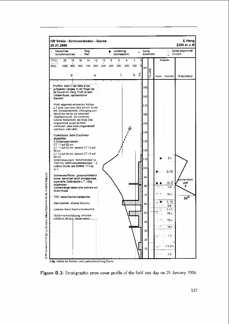
GR Strela - Schonenboden - Davos E Hang
25.01.2006 2305 m u M
i Neuschnee filzig t rundkornig y kantig kantig abgerundetSchwimmschnee Reif Schmelzform - Eislamelle
_Graupel
T(°C) 20 18 16 14 12 10 8 6 4 2 C Kristalle
-+ -f- i — + I
R(N) 1000 900 800 700 600 500 400 300 200 100 Ccm
£
*rLi. u_ <
1c
13
2 m T- Ï u. IÎ Form Durchm Rutschblock
I
[Profilort oben in der Mitte eines
-
grösseren Hanges in der Regel hat190
es Spuren im Hang Profil ist aber
unbeeinflusst repräsentativer 180Standort
Profil allgemein schwacher Aufbau170
z T sinkt man ohne Skis tief ein In der
krit Schwachschicht (Übergang zumAltschnee hat es nur vereinzelt 160
Oberflachenreif) Die einstmals
schone Reifschicht die Ende Dez
eingeschneit wrude ist noch .150vorhanden aber stark umgewandelt 1
und kaum mehr aktiv 71 .140
Rutschblock Beim Drauftreten 1
abgeglitten1
/3 Kompressionstests / 130
CT 11 auf 82 cm '
CT 11 auf 82 cm danach CT 13 auf '
_59 cm j .120
CT 12 auf 82 cm danach CT 15 auf i
59 cm >/
Schermessungen Scherfestigkeit ca ^f 110 • 5-1
1500 Pa Skifahrerstabihtatsindex 1 2 S^mittlere Dichte des Brettes 173 kg f
- m 3 ( .100
• 5-75
Schneeoberflache grossmehrheitlich ^t- locker kammnah leicht windgepresst \ .
90
inanzer Block
exponierte Geländeteile z T völlig \
abgeblasen \.80
J • • 25 5 - f glatt
^^2Sonnenhange haben eine mehrere cm \dicke Kruste \
[ I 1-3
"
TRA keine frischen beobachtet
Alarmzeichen diverse Wumms
Lawinen keine frischen beobachtet
Gefahreneinschatzung erheblich
.70
60
50
n~
75 1
30°
^^ u • 5 75
58
n
fi
1-1 5
75 1w^>?nnn m W N F Hoi ito wonin
4075-1
75 1 :
T 30
j 1 2
20
1 525
10—
I
. .
I i ——
23
Eidg Institut fur Schnee- und Lawinenforschung Davos
Figure B.3: Stratigraphie snow cover profile of the field test day on 25 January 2006
137

Appendix B Stratigraphie snow cover profiles
GR Strela - Schönenboden - Davos E Hang
27.01.2006 2305 m ü M
Neuschnee filzig t rundkornig n kantig
Schwimmschnee Reif Schmelzform —Eislamelle
_, kantig abgerundeti Graupel
-T(°C) 20 18 16 14 12 10 8 6 4 2 0
- - I I I I + h- - -I I + --
R(N) 1000 900 800 700 600 500 400 300 200 100 0
_ü_ n_ <
2 m t- -r u.
cm
x:
LL
Kn
Form
stalle
Durchm Rutschblock
mittlere Dichte des Brettes 228 kgm-3
10 Scherrahmenmessungen
Scherfestigkeit 1080+-170Pa
Eindringtiefe 15 cm1
190
180
.170
-
6x2 Kompressionstests1313 1313 14.12 1313 15,14
(15)13 1714 <
160
weitere Dichtemessungen28 cm mit 167 kg m-332 cm mit 167 kg m-3
\i
i
\
\
\
.150
140
\
\
\
\
.130
120•
- -
5-75
-
110
100
90
•
• •
25-75
25-5
/anzer Block
f rauh
\CJ13
\ 1ïYYT • 25- 5 \
1-7'
^3> [ ]
-
180
.70
60
[J i J 5-1
\ rs: U l ] 5-75.
4-8
1-2
30°
I
T
n
i 5075-1 5
1
140
30
20_, j 1-1 5
—,—i—,—1_
110
— -
1 5-2 5
... i .... i.
\ <
Eidg Institut fur Schnee- und Lawinenforschung Davos
Figure B.4: Stratigraphie snow cover profile of the field test day on 27 January 2006.
138

Eidg Institut für Schnee- und Lawinenforschung Davos
Figure B.5: Stratigraphie snow cover profile of the field test day on 3 February 2006.
139

Seite Leer /
Blank leaf

Acknowledgements
Jürg Schweizer was my adviser at the SLF over the past three years. During this time he
was also a teacher and mentor to me. Under his guidance I was able to enhance my scien¬
tific skills and to benefit from his profound knowledge of snow and of avalanche release.
Despite his workload, his door was always open whenever questions arose. Therefore, I
wish to express my deep gratitude to him.
I would like to thank Prof. Jürg Dual, head of the Center of Mechanics at ETH Zürich,
who offered me the opportunity to write my thesis under his supervision. Our bi-monthly
meetings in Zürich became the "anchor points" throughout these three years.
Hans-Jakob Schindler an expert in fracture mechanics was my co-supervisor. I would like
to thank him especially for his fast and concise replies on all my fracture mechanical
questions, even though most of our communication had to take place by email.
A special thank goes to Joachim Heierli. In countless discussions we used piles of paper
for our drawings and notes, and finally saw clearer into the complexities of fracturing
snow beams and collapsing weak layers. In addition, he was so kind as to review my
thesis.
My thanks go to my group head, Martin Schneebeli. Due to him, the working climate
was ever agreeable and fruitful.
Denes Szabo was the man for any problem concerning the ANSYS workbench. My thanks
go to him.
Felix Book, Ruzica Dadic, Nora Staack and Daniela Schmid helped with the experiments
in the cold lab. In their company the cold temperatures were much easier to bear. Sincere
thanks are given to all of them.
Cordial thanks go to my office mates Kalle Kronholm and Margret Matzl. Kalle famil¬
iarized me with what it meant to be a PhD student. I appreciated the great time and
the many laughs in his company. He became much more than just an ofFice mate to me.
Thanks to Margret, the long days and nights in the office, while we both wrote up our
theses, were much less boring. And thanks to her, the food supply never ran dry!
Mathieu Fauve granted me asylum during my first month in Davos. He also shared my
passion for flying discs. Merci beaucoup, Mat!
My most cordial thanks go to my parents, Hedi and Paul Sigrist and my sister Daniela,
who supported me during all these years.
And finally, thank you Flurina for letting me share life and love with you.

Curriculum Vitae
Personal data
Name
Date of birth
Place of origin
Nationality
Languages
Education
1983-1987
1987-1992
1992-1996
1996
1996-2001
2000-2001
2001
Christian SigristMarch 24, 1976
Sigriswil (BE), Switzerland
Swiss
German (mothertongue), English (spoken, written),French (spoken, written)
Primary school in Heimberg, Switzerland
Secondary school in Heimberg, Switzerland
Gymnasium in Thun, Switzerland
Matura Type C (Natural sciences) at Gymnasium Thun
Studies in Physics, Mathematics and Astronomy at the University
of Bern, Switzerland
Master's thesis in Physics at the Division for Space Research and
Planetary Sciences (Physikalisches Institut) of the University of,
Bern, Switzerland, entitled "Self Optimisation of a Time of FlightMass Spectrometer based on a Simplex Algorithm", Supervisors:
Prof Dr Kathrin Altwegg, Prof Dr Hans BalsigerGraduated as Master of Science in Physics
Academic record
2002 Temporary assistant at the Processor Architecture Laboratory of
the Ecole Polytechnique Fédéral de Lausanne EPFL in Lausanne,
Switzerland
2002-2003 Scientific employee at the Institute for Surgical Technology and
Biomechanics of the Maurice E. Müller Research Center in Bern,
Switzerland
2003-2006 PhD studies at the Swiss Federal Institute for Snow and Avalanche
Research SLF in Davos, Switzerland and the Center of Mechanics
(Department of Mechanical and Process Engineering) at the Swiss
Federal Institute of Technology ETH in Zürich, Switzerland, entit¬
led "Measurement of Fracture Mechanical Properties of Snow and
Application to Dry Snow Slab Avalanche Release" under the super¬
vision of Prof. Dr. Jürg Dual, Dr. Jürg Schweizer and Dr Hans-
Jakob Schindler