Research Article Assessment of WRF Land Surface Model ...

Research ArticleAssessment of WRF Land Surface Model Performance overWest Africa

Ifeanyi C. Achugbu ,1,2,3 Jimy Dudhia ,3 Ayorinde A. Olufayo,2 Ifeoluwa A. Balogun,2

Elijah A. Adefisan,2 and Imoleayo E. Gbode 2,3

1Department ofWater ResourcesManagement and Agrometeorology, Federal University Oye-Ekiti, Oye-Ekiti, Ekiti State, Nigeria2West African Science Service Center on Climate Change and Adapted Land-Use (WASCAL),Federal University of Technology Akure, Akure, Ondo State, Nigeria3Mesoscale and Microscale Meteorology Laboratory, National Center for Atmospheric Research, Boulder, CO, USA

Correspondence should be addressed to Ifeanyi C. Achugbu; [email protected]

Received 19 December 2019; Revised 27 June 2020; Accepted 16 July 2020; Published 7 August 2020

Academic Editor: Eduardo Garcıa-Ortega

Copyright © 2020 Ifeanyi C. Achugbu et al. .is is an open access article distributed under the Creative Commons AttributionLicense, which permits unrestricted use, distribution, and reproduction in any medium, provided the original work isproperly cited.

Simulations with four land surface models (LSMs) (i.e., Noah, Noah-MP, Noah-MP with ground water GW option, and CLM4)using the Weather Research and Forecasting (WRF) model at 12 km horizontal grid resolution were carried out as two sets for 3months (December–February 2011/2012 and July–September 2012) overWest Africa..e objective is to assess the performance ofWRF LSMs in simulating meteorological parameters overWest Africa..emodel precipitation was assessed against TRMMwhilesurface temperature was compared with the ERA-Interim reanalysis dataset. Results show that the LSMs performed differently fordifferent variables in different land-surface conditions. Based on precipitation and temperature, Noah-MP GW is overall the bestfor all the variables and seasons in combination, while Noah came last. Specifically, Noah-MP GW performed best for JAStemperature and precipitation; CLM4 was the best in simulating DJF precipitation, while Noah was the best in simulating DJFtemperature. Noah-MP GW has the wettest Sahel while Noah has the driest one. .e strength of the Tropical Easterly Jet (TEJ) isstrongest in Noah-MP GW and Noah-MP compared with that in CLM4 and Noah. .e core of the African Easterly Jet (AEJ) liesaround 12°N in Noah and 15°N for Noah-MP GW. Noah-MP GW and Noah-MP simulations have stronger influx of moistureadvection from the southwesterly monsoonal wind than the CLM4 and Noah with Noah showing the least influx. Also, analysis ofthe evaporative fraction shows sharp gradient for Noah-MP GW and Noah-MP with wetter Sahel further to the north and furtherto the south for Noah. Noah-MP-GW has the highest amount of soil moisture, while the CLM4 has the least for both the JAS andDJF seasons. .e CLM4 has the highest LH for both DJF and JAS seasons but however has the least SH for both DJF and JASseasons. .e principal difference between the LSMs is in the vegetation representation, description, and parameterization of thesoil water column; hence, improvement is recommended in this regard.

1. Introduction

.e land surface is the principal constituent located in thespace separating the atmosphere and the lithosphere, and itobviously impacts the exchanges of energy and moisturewith the boundary layer. .rough the controlling of thesurface energy balance and water balance, land-surfaceprocesses strongly affect the weather and climate from localto regional and global scales [1]. One of the ways in whichthe land surface affects the climate system is the fact that due

to the direct contact of the land surface with the atmosphere,the land surface reacts as a source and sink of heat andmoisture through the sensible heat flux and evaporation..esurface conditions regulate the important feedback cycles inthe climate system [2]. Also, the partitioning of the surfacenet radiation into sensible and latent heat fluxes determinesthe soil wetness development. .e surface energy fluxes to alarge extent control the surface weather parameters such asthe temperature, humidity, and wind speed and to a lesserextent, low-level cloudiness and precipitation [2]. According

HindawiAdvances in MeteorologyVolume 2020, Article ID 6205308, 30 pageshttps://doi.org/10.1155/2020/6205308

mailto:[email protected]

https://orcid.org/0000-0002-4463-5353

https://orcid.org/0000-0002-2394-6232

https://orcid.org/0000-0001-7519-512X

https://creativecommons.org/licenses/by/4.0/




https://doi.org/10.1155/2020/6205308

to Tiwari et al. [3], it is noteworthy to have a better rep-resentation of the surface boundary conditions in a model asmuch as that of the surface and the atmosphere have aneffect on the prognostic variables.

.e land surface and the atmosphere are inseparable andcannot be isolated as they are firmly coupled systems. .eplanetary boundary layer (layer where intense turbulencetakes place) is the interface that regulates the feedbacks.Despite the significant influence of land-atmosphere ex-change on the daytime planetary boundary layer (PBL),uncertainty remains in the parameterization of surface heatand moisture fluxes in numerical weather models [4]. .eland surface model (LSM) provides heat and moisture fluxesover land to provide a lower boundary condition for verticaltransport in the PBL scheme. .ese fluxes of sensible heatand latent energy are dependent on the surface meteorology,radiative forcing, soil properties, and land use type. .us, anaccurate description of the land surface and vegetationcharacteristics is needed in any numerical weather predic-tion model [5]. .e surface energy exchange is determinedby the terrestrial radiation budget, as shown in the followingequation:

Rnet � SH + LH + G, (1)

where Rnet is the net radiation flux (W/m2), SH is thesensible heat flux (W/m2), LH is the latent heat flux (W/m2),and G is the ground heat flux (W/m2). .e surface availablefluxes (i.e., SH and LH) are net radiation minus ground heatflux. .e net radiation is balanced by outgoing fluxes of LH,SH, and G, whose partitioning strongly depends on theprevailing surface conditions. Some energy is absorbed bythe groundG, this is in fact much lower than average value ofLH and SH for most plant canopies, as most part of availableenergy will be transferred back into the atmosphere assensible and latent heat [6]. LH is the quantity of heatabsorbed or released by water undergoing a change of state.LH is most often the heat released by water as it changesfrom a liquid to gaseous state over a plant canopy throughevapotranspiration.

.e partitioning of the energy available at the surfaceinto latent and sensible heat depends crucially on the soilmoisture [7]. Vegetated surfaces have the ability to drawwater from a depth of order 1m (the root layer), while forbare ground, only the water in the top few centimeters of soilcontributes to evaporation. According to Zheng and Eltahir[8], vegetation cover and soil moisture content play acomparable role in the concept of land-atmosphere inter-actions. .e main difference is that soil moisture anomalypatterns could last for many days to weeks, while vegetationis capable of mobilizing the root zone soil moisture thatwould otherwise not be in contact with the atmosphere. .isconsequently foists a lower boundary condition that couldbe in force for a longer time scale on the atmosphere. So,vegetation responds much slower on a single precipitationoccurrence than the surface soil moisture.

.e land-atmosphere interactions are modulated by theextent of the associated north-south gradient of heat andmoisture in the lower atmosphere [9]. A number of regions

in the world, for example, the Sahel [10, 11], Amazon [12],and Asian monsoon regions [13], have been identified as hotspots of land-atmosphere interactions, where interactionsthrough feedback loops play a critical role in the surfacewater and energy balances as well as regional climate. InWest Africa (WA) where we have strong land-atmospherecoupling, land surface processes, like soil-precipitationfeedback [14], soil moisture initial conditions [14, 15], andvegetation feedbacks [16, 17], have significant impacts on thedynamic downscaling of regional climate models (RCMs).However, explanation of the results, from any one of suchstudies, ought to be tempered by the fact that there areconsiderable discrepancies in African land-atmospherecoupling strength among current state-of-the-art GCMs[18]. Li et al. [19] have demonstrated that land surfaceprocesses play a crucial role in the climate system.

.e land surface has been shown to be an importantfactor in modulating the West African monsoon (WAM)[20]. Nicholson [21] stressed that the land surface charac-teristics and processes have been shown to have a significantimpact on the interannual variability of rainfall in the Sahelregion based on observations. Furthermore, the importanceof surface-atmosphere interactions was one of the mainprinciples of the international African Monsoon Multidis-ciplinary Analysis (AMMA) project [22] which was laterinvestigated in several studies. According to Dirmeyer [23],the WA region typically appears as the one where the soilmoisture feedbacks with the atmosphere are among thestrongest over the globe..e Sahel region has been identifiedas one of strong soil moisture-atmosphere coupling [10].Furthermore, it has been resolved to be the region of theworld with the highest impact of biophysical processes onthe climate [11]. As reviewed by Xue et al. [24], studies bySteiner et al. [25] and Lavender et al. [26] have shown theimportance of the land surface on modulating the WestAfrican Monsoon (WAM). For example, previous studieshave examined the role of changes in the surface albedo, e.g.,[27–29], and the vegetation, e.g., [30–33], on modulating theWAM. All of these studies lead to the general conclusion thatreduced vegetation leads to reduced rainfall.

Parameterization is a method of replacing processes thatare of a very small scale or very complex to be physicallyrepresented in the model through a simplified process.Researchers have focused on the appropriate selection ofWeather Research and Forecasting (WRF) parameteriza-tions schemes for varying conditions and applications[34–47]. Some of these studies concluded that the perfor-mance of the physics schemes varies according to the regionof study including the time of the year. Hence, care should betaken in applying each for a specific study area. However,different climate variables are found to be sensitive to dif-ferent physical parameterizations [37] making the need foran all-inclusive sensitivity analyses more pressing and theprocedure of physics parameterization selection more de-manding [48]. WRF has a number of physics options, whichincludes options for selecting the radiation scheme, surfacelayer scheme, planetary boundary layer (PBL) scheme,microphysics scheme, convective scheme, and land-surfacescheme. .is study assesses the performance of recent WRF

2 Advances in Meteorology

LSMs over West Africa for better simulations over theregion.

Land surface models (LSMs) differ in the number of soiland canopy layers and in the treatment of vegetation-relatedprocesses and hence are able to perform differently. Changesin surface conditions are shown to affect the position andintensity of the African Easterly Jet (AEJ) [49]. .e AMMALand Surface Model Intercomparison (ALMIP) wasdesigned as a step towards a better understanding and ex-planation of surface processes over West Africa [50]. .eidea was to develop a forcing database with the best qualityand highest spatial and temporal resolution data availableand use this database to force state-of-the-art LSMs in orderto better understand key processes at different scales [51].Concerning the LSMs, the AMMA results showed that theyhave a tendency to underestimate surface sensible heat fluxand perhaps baseflow runoff and overestimate evaporationfrom the vegetation canopy. During the monsoon season,evapotranspiration is generally the most significant com-ponent of the water budget, acting to recycle much of therainfall, in particular, over the Sahel [51]. Nevertheless,qualitative estimates of recycling by the LSMs must beinterpreted in view of the fact that the LSMs have a sub-stantial intermodel scatter over the Sahel [51].

Steiner et al. [25] coupled the community land model(CLM3) and the biosphere-atmosphere transfer scheme(BATS) with the ICTP regional climate model (RegCM3)and found out that CLM3 improves the timing of themonsoon advance and retreat across the Guinean Coast andreduces a positive precipitation bias in the Sahel andNorthern Africa. .is results in a higher simulated tem-perature, and by that means, it reduces the negative tem-perature bias found in the Guinean Coast and Sahel in theBATS..ey also emphasized that the improvement in CLM3is triggered by drier soil conditions in the simulation.

In spite of the notable impact of the land-atmosphereexchange on the daytime planetary boundary layer, there arestill some uncertainties in the parameterization of surfaceheat and moisture fluxes in numerical weather models(NWM) [4]. WRF has many LSM options that range fromsimple treatment of subsurface processes like absence ofvegetation or snow cover prediction to advanced physicalmodels with sophisticated vegetation and soil models andsnow cover prediction. Moreover, WRF LSMs use seasonallyadjusted or annually fixed land-use properties read fromlook-up tables in order to allocate surface variables; yet,some land cover parameters like vegetation can change oftenwithin a short time.

Several sensitivity and evaluation studies have beencarried out in different regions [5, 19, 52–56]. .is is nec-essary in order to help firstly the model developers forfurther improvements, secondly, the users in the selection ofLSM options especially in the WRF model, and thirdly,improving the simulations for the area under study..erefore, considering the number of LSMs currently in theWRF model, it remains a difficult task for researchers tochoose a suitable land surface scheme that fits their needs[57] especially over a data sparse region like West Africa.Although, some researchers [58–60] have replaced the land-

use data by incorporating remote sensing data into the LSMsfor more updated and realistic land-use land-cover data inorder to improve the models; this was not done in thisresearch because we wanted to evaluate the performance ofeach WRF LSM in the same standard mode.

Researchers such as Evans et al. [37] examined theperformance of various physics scheme combinations on thesimulation of a series of rainfall events near the southeastcoast of Australia. .ey created a thirty-six member mul-tiphysics ensemble such that each member had a unique setof physics parameterizations. .ey found out that no singleensemble member was found to perform best for all events,variables, and metrics, and this also reflects the fact thatdifferent climate variables are found to be sensitive to dif-ferent physical parameterizations.

Hagos et al. [61] performed different WRF simulationswith NOAH, SSIB, and PLEIM-XIU LSMs and cumulusparameterization schemes over West Africa. .ey found outthat the model simulations consistently differ from theobservations over the Gulf of Guinea, with the modelseemingly overestimating precipitation, and the simulationsdiffer in their northward incursion of precipitation overland. .eir analysis also showed that the African Easterly Jet(AEJ) position for the simulations was too far south for SSIBand too far north for PLEIM-XIU; hence, SSIB was too drywhile PLEIM-XUI was too wet.

Wharton et al. [5] in their study found that the choice ofland-surface model led to a ∼10% improvement in simu-lating hub-height wind speed and that the overall bestperforming models were Noah and Noah-MP. .ey em-phasized that the variability of LSM performance acrossdifferent soil moisture and vegetation canopy conditionssuggests LSM representation of surface energy exchangeprocesses in WRF remains a large source of modeluncertainty.

Jin et al. [53] studied the sensitivity of four land surfaceschemes in the WRF, namely, the simple soil thermal dif-fusion (STD) scheme, Noah scheme, RUC scheme, andcommunity land model version 3 (CLM3). .ey ran foursimulations with four LSMs over the western United States..eir results show that land-surface processes strongly affecttemperature simulations over the area. .ey also found outthat WRF CLM3 with the highest complexity level signifi-cantly improves temperature simulations, except for thewintertime maximum temperature as compared with theobservations. Also, precipitation was substantially over-estimated by WRF with the LSMs over the area and does notshow a close relationship with land-surface processes.

All these researchers and many more have performeddifferent evaluations for different regions, but this research isfocused on examining the role of land-surface processes inthe simulation of some variables in West Africa by carryingout a series of WRF runs using four recent LSM optionswhich includes Noah scheme, Noah-MP, Noah-MP GW,and Community Land Model Version 4 (CLM4), eachhaving different complexity levels. .ere are only few ex-tensive studies on the assessment of regional climate modelssensitivity to multiple land surface models over West Africa..erefore, the impact of different LSMs on West African

Advances in Meteorology 3

Monsoon (WAM) and land surface energy balance is still astudy of importance. Atmospheric simulations over a varietyof land-surface conditions that would be affected by thesurface energy budget, including wet and dry seasons, werecarried out in order to study the impact of LSMs choice onsome WRF simulated parameters. In particular, we evaluatehow the change in LSMs affect the average simulation ofprecipitation and 2m temperature and tried explainingsome reasons behind the differences using the mean wind,soil moisture, and surface energy parameters.

2. Materials and Methods

2.1.WRFModelDescriptionandConfiguration. .eWeatherResearch and Forecasting (WRF) model is a communitynonhydrostatic and fully compressible atmospheric model,maintained by the National Center for Atmospheric Re-search (NCAR). In this study, version 3.9.1.1 the AdvanceResearch dynamical core of WRF model (ARW) was used torun eight different simulations. Each simulation is a 3-month run from December to February (DJF) 2011/2012 dryseason and July to September (JAS) 2012 rainy season overWest Africa with four different LSMs. .is makes it 4 dif-ferent simulations for each season (i.e., 4 separate simula-tions for DJF and JAS season amounting to 8 simulations inall)..e periods were chosen to study the impact of choice ofland surface model over different land surface conditions(i.e., wet and dry) that would affect the surface energybudget.

.e simulations were performed with a 12 km horizontalresolution for a domain that encompasses latitude10°S–30°N and longitude 28°W–28°E as shown inFigure 1(a). Initial and lateral boundary conditions are fromEuropean Center for Medium-Range Weather Forecasts(ECMWF) Interim 6 hourly Re-Analysis (ERA-Interim)data, which has a horizontal resolution of 0.75° [62] andNational Centers for Environmental Protection (NCEP)Final Analysis (FNL) 6 hourly initial soil data (sea surfacetemperature, soil moisture, and temperature) from theNCAR’s Computational and Information System Labora-tory Research Data Archive (CISL RDA) [63] with resolutionof 1°. So, the initial and lateral boundary conditions wereupdated every 6 hours.

.e first 15 days were used as spin-up, hence 16th of Julyto 29th of September 2012 (JAS), for the rainy season and 16thof December 2011 to 28th of February 2012 (DJF), for the dryseason were analysed. .e variables were analysed spatiallywithin the 20°W–20°E and 0°–20°N (the green box area) asshown in Figure 1, while the analysis involving time averageswere within the 10°W–10°E and 5°–15°N boundary as shownin Figure 1(a) so that the domain of interest is moved awayfrom the errors introduced by boundary values. Figure 1(a)also shows the elevation of the study area revealing thehighlands such as the Jos Plateau, Cameroon Mountains,and Fouta Djalon highlands..e geogrid program by defaultwill interpolate land use land cover LULC categories fromthe MODIS IGBP 21-category data in the model. .e LULCdistribution derived from MODIS data is shown inFigure 1(b). It shows barren or sparsely vegetated surfaces

spread across the northern area (from 16°N upwards) andEvergreen Broadleaf Forest around the coastal regions. Mostpart of the Sahel is covered by grasslands with scatteredcroplands and open shrublands between the Sahel-Saharainterface. .e distribution of the dominant soil type in WestAfrica is also shown in Figure 1(c). .e loamy sand, sandyloam, and loam are more dominant in the northern part,while the silty clay loam and clay loam are dominant in thesouthern part.

.e roughness lengths in meters are in some table filesMPTABLE.TBL for Noah-MP for each land use category.VEGPARM.TBL for Noah has minimum and maximumvalues for each category. .e values depend on the range,which has a seasonal change, and depend on the vegetationfraction for each land use in the tables. From the land use inthe models and considering the entire region, the mostdominant land use categories in the study area includeevergreen broadleaf forest, open shrublands, woody sa-vannas, savannas, grasslands, croplands, barren or sparselyvegetated, and water with roughness lengths within therange of 0.5–0.5m, 0.01–0.06m, 0.01–0.05m, 0.15–0.15m,0.10–0.12m, 0.05–0.15m, 0.01–0.01m, and 0.0001–0.0001mfor Noah and CLM4, respectively, and 1.10m, 0.06m,0.60m, 0.50m, 0.12m, 0.15m, 0.00, and 0.00, respectively,for Noah-MP. Hence, Noah-MP has a constant roughnesslength for all seasons.

WRF version 3.9.1.1 has about seven different landsurface physics options from the simple 5-layer soil modelsimply with thermal diffusion in soil layers and no vege-tation or snow cover prediction to Noah LSM, Noah-MP,RUC LSM, PX LSM, CLM4, and SSiB LSMs with sophis-ticated vegetation models and snow cover prediction. .eWRF LSMs are driven by surface energy and water fluxesand predict soil temperature and moisture in different layersdepending on the LSM option in which Noah and Noah-MPhas 4 layers, RUC has 9 layers, PX has 2 layers, and SSiB has 3and 10 layers for CLM4. Noah-MP, RUC, SSiB, and CLM4may predict snow water equivalent on ground. All the WRFland surface models utilize the wind and stability infor-mation from the atmospheric surface layer scheme.

.e Noah LSM (as the most commonly used LSM) wasused to test for four other different physics combinations(results not shown) in which the best combination was usedwith other three LSMs, which includes the Noah-MP, CLM4,and Noah-MP GW. .e Noah-MP GW is a new optionincluding a free drainage soil lower boundary condition,variable water table, and 1-dimensional interaction withhorizontal aquifer transport but no river routing or overlandflow scheme as in hydrological models. All parameterizationschemes apart from the LSMs were the same for all simu-lations. .e new version of rapid radiative transfer model(RRTMG) based on Iacono et al. [64] is selected for de-scribing the long-wave and short-wave radiative transferwithin the atmosphere and to the surface. .e Mel-lor–Yamada Nakanishi and Niino Level 2.5 (MYNN2.5)scheme by Nakanishi and Niino [65] was used for boundary-layer processes with a consistent MYNN surface layerscheme. .e new Tiedtke scheme [66] is applied toparameterise the unresolved deep cumulus clouds. .e


microphysics scheme chosen is the WRF Single-Moment 6-class (WSM6) scheme [67]. .ese were selected based onsome preliminary tests that also agreed with the findings ofGbode et al. [68] who carried out a verification study ofmany atmospheric physics combinations over West Africa.

.e Noah LSM [69] was developed jointly by NationalCenter for Atmospheric Research (NCAR) and NationalCenters for Environmental Prediction (NCEP). It has beenvalidated by many intercomparison studies both in coupled[70, 71] and uncoupled [72–74] modes. Its moderatecomplexity and computational efficiency have made it ef-fective in both operational weather and climate models. Ithas the advantage of being compatible with the time-de-pendent soil fields made available by NCEP in the global

analysis datasets. It has a 4-layer (0.10, 0.30, 0.60, and 1mthick) soil temperature and moisture model in addition tocanopy moisture and snow cover prediction. It has a rootingdepth fixed at 1m including three layers at the top and alsohas one snow layer and one canopy layer. .e mass con-servation law and the diffusive form of Richard’s law con-trols the vertical water mass movement between soil layers,while a conceptual parameterization for the subgrid treat-ment of soil moisture and precipitation controls the infil-tration [75]. Total evapotranspiration in Noah is the sum ofthe canopy intercepted water evaporation, transpirationfrom vegetation canopies, and evaporation from bare soil asweighted by the respective land surface coverage fractions[76]. .e drainage is due to the gravitational percolation

30°N

25°N

20°N

15°N

10°N

5°N

20°W 10°W 10°E 20°E0°

0°

5°S

GMTED2010 30-arc-second topography height (meters MSL)

0 400 800 1200 1600 2000 2400 2800

(a)

20N

15N

10N

5N

020W 10W 10E 20E0

2 3 4 5 6 7 8 9 10 11 12 13 14 15 16 17

(b)

20N

15N

10N

5N

020W 10W 10E 20E0

2 4 6 8 10 12 14

(c)

Figure 1: (a) Map showing the model domain with the elevation map ofWest Africa..e red box (5°N–15°N and 10°E–10°W) is the domainfor area average of the parameters while the green box is the evaluation area for the spatial plots; (b) land use category map of the study area(2. evergreen broadleaf forest; 3. deciduous needleleaf forest; 4. deciduous broadleaf forest; 5. mixed forests; 6. closed shrublands; 7. openshrublands; 8. woody savannas; 9. savannas; 10. grasslands; 11. permanent wetlands; 12. croplands; 13. urban and built-up; 14. cropland/natural vegetationmosaic; 15. snow and ice; 16. barren or sparsely vegetated; 17. water); (c) soil type categorymap of the study area (2. loamysand; 3. sandy loam; 4. silt loam; 5. silt; 6. loam; 7. sandy clay loam; 8. silty clay loam; 9. clay loam; 10. sandy clay; 11. silty clay; 12. clay 13.organic material; 14. Water; 15. bedrock).


below the soil layers. .e surface skin temperature is cal-culated from a surface energy balance equation. .e surfaceenergy fluxes of Noah are calculated over a combined surfacelayer of vegetation and bare soil surface. Such model hindersits further development as a process-based dynamic leafmodel, because it cannot compute photosynthetically activeradiation (PAR), canopy temperature, and related energy,water, and carbon fluxes explicitly [77]. Prediction includes aroot zone, evapotranspiration, soil drainage, and runoff,taking into account vegetation categories, monthly vegeta-tion fraction, and soil texture. It also predicts soil ice, andfractional snow cover effects, has urban treatment options,and takes surface emissivity and albedo properties intoconsideration.

Noah-MP (multiphysics) LSM [77] is an augmentedversion of the Noah LSM. .e vital augmentation is theintroduction of (a) a vegetation canopy layer for individuallycomputing the canopy and the ground surface temperatures,achieved by introducing a semitile subgrid scheme to rep-resent land surface heterogeneity [77], (b) a modified two-stream scheme [78, 79] for transfer of radiation throughvegetation canopy and considering the canopy gaps, (c) aBall-Berry scheme for the canopy stomatal resistance[80–82] which connects stomatal resistance to the photo-synthesis of sunlit and shaded leaves, and (d) a short-termdynamic vegetation model [83] with two options (off andon) in which leaf area index (LAI) and vegetation greennessfraction (GVF) can be predicted from the model whenturned on. Also, a simple TOPMODEL runoff model for thecomputation of surface runoff and groundwater discharge, a3-layer snowmodel, is given in [84], and a frozen soil schemewith exceptional soil permeability is discussed by Niu andYang [85]..e Noah-MP uses multiple options for key land-atmosphere interaction processes. It contains a separatevegetation canopy defined by a canopy top and bottom withleaf physical and radiometric properties used in a two-stream canopy radiation transfer scheme that includesshading effects [77]. Noah-MP contains a multilayer snowpack with liquid water storage and melt/refreeze capabilityand a snow-interception model describing loading/unloading, melt/refreeze, and sublimation of the canopy-intercepted snow. Various options are available for surfacewater infiltration and runoff, and groundwater transfer andstorage including water table depth to an unconfinedaquifer. Horizontal and vertical vegetation density can beprescribed or predicted using prognostic photosynthesis anddynamic vegetation models that allocate carbon to vegeta-tion (leaf, stem, wood, and root) and soil carbon pools (fastand slow) [77].

CLM4 (Community LandModel Version 4 [86] is a stateof the science LSM more often used in climate applications,developed at NCAR in cooperation with many externalcollaborators and includes sophisticated handling of bio-geophysics, hydrology, biogeochemistry, and dynamicvegetation. .e vertical structure comprises of a single-layervegetation canopy, a five-layer snowpack, and a ten-layer soilcolumn [87]. It has 3.8m soil depth divided into 10 layersapproximately at 1.8 cm, 4.5 cm, 9.1 cm, 16.6 cm, 28.9 cm,49.3 cm, 82.9 cm, 138.3 cm, 229.6 cm, and 342.3 cm below

the surface. .e soil water is predicted from the modifiedRichards equation by Zeng and Decker [88]. CLM4 centerson biogeophysics of land surface including vegetation dy-namics modules. .e overland flow is calculated with asimple conceptual TOPMODEL approach to parameterisethe surface runoff. An exchange of water between an un-confined aquifer and the overlying soil column is incor-porated in the soil hydrology scheme [85]. .eparameterization schemes of Niu and Yang [89] and Wangand Zeng [90] is used to calculate the snow cover and snowburial fraction. Some of the major differences between theLSMs are highlighted in Table 1.

2.2. Model Verification and Validation Datasets.Simulated surface air temperature was assessed using theERA-Interim dataset from the ECMWF and simulatedprecipitation using the Tropical Rainfall MeasurementMission (TRMM [92]). .e 0.25o resolution TRMM 3B42product was used as the standard for evaluating the modeloutputs because of its reliability and also that it is a mergeddataset (i.e., a combination of in situ and satellite products)with high-quality precipitation estimates [92]. .e GlobalPrecipitation Climatology Project (GPCP [93, 94]) is an-other genuine source for merged estimates computed frommicrowave, infrared, and sounder data observed by theinternational constellation of precipitation-related satel-lites and precipitation gauge analysis. .is was also ana-lysed to see how good it is in comparison with TRMM overWest Africa. .ese datasets were used for the validationbecause the region (West Africa) is a data sparse regionwith a poorly spread synoptic weather station network,which is insufficient to validate the spatial and temporalspread of the model outputs. Hence, the use of severaldatasets for the model validation was necessary to examinetheir differences in order to clearly understand the modeluncertainties.

2.3. Method of Model Evaluation. .e model evaluation wasalso done using the Taylor diagram that can conciselysummarize the degree of agreement between simulated andobserved variables [95]. .e correspondence amongst dif-ferent patterns is quantified by their correlation, theircentred root-mean-squared difference, and their standarddeviations. Houghton et al. [96] stressed that the diagram isuseful specifically in evaluating multiple aspects of complexmodels or in gauging the relative skills of many dissimilarmodels..e location of eachmodel on the diagram describeshow closely the model’s output pattern corresponds with theobservations. However, each model point in the diagramrepresents the correlation, the standard deviation, and thecentered RMS and is related by the following equations:

E2′ � σ2f + σ2o − 2σfσoR, (2)

where R is the correlation coefficient between the forecastand observation fields; E′ is the centered root-mean-squared(RMS) difference between the fields; and σ2f and σ2o are thevariances of the forecast and the observation fields.


3. Results and Discussion

3.1. Precipitation and Surface Temperature Analysis. Fromthe plot of the average air temperature for JAS (Figure 2),all the simulations were in close resemblance to ERA-interim, which is used as the reference. FNL seems to havehigher temperature than ERA-interim and all the modelsaround 17°N and 20°N. .e areas of high and low values inERA-interim were captured by all the four LSMs. FromFigure 3, the average temperature bias between ERA-Interim and the models for JAS shows that the outputs ofall the model simulations agree with ERA-interim withinthe range of −4 to 3.5°C. .e maximum positive bias wasshown around the EL Djouf basin in Mauritania andNorthern Mali, while the maximum negative bias wasfound around Lake Chad, possibly due to a bias in the laketemperature in the model, for all simulations. But, Noahshows a cold bias relative to ERA-interim in areas above16°N at the northeastern part which other models did notreveal. Areas below 15°N mostly showed bias value closeto zero except for CLM4. Nevertheless, it shows that allthe models could fairly predict rainy season airtemperature.

Figure 4 shows that the spatial distribution of average2m surface temperature for DJF decreases with increasinglatitude just like the reference from areas above 10°N. All themodels and ERA-interim were able to capture reasonablywell the cooling around the highlands of Jos Plateau, Guinea,and Cameroon. However, FNL has higher temperaturearound the coastal areas than ERA-Interim.

From Figure 5, it is seen that the average temperaturebias between ERA-Interim and the models for DJF rangesbetween −4° and 5°C..ere is a maximumwarm bias aroundFouta Djallon highlands in all the simulations. Noah LSMoutput tends to have the coldest bias while CLM4 LSM tendsto have the warmest. Despite having the most sophisticatedsnow, soil, and vegetation physics among the LSMs, CLM4has the strongest positive temperature bias in some majorhighlands and the El Djouf basin. .e deep soil column andwater table in CLM4 might however need a considerablylong time period for temperature and soil moisture to reachequilibrium, mostly in the cold and dry regions [97]. .iscould make it require more spin-up time than other LSMsand might be the reason for having high bias around thesemiarid/arid areas of the region for both temperature andrainfall in JAS season.

From the time series of JAS daily 2m surface temperatureaveraged over 10°W–10°E and 5°–15°N (as shown inFigure 6(a)), the general biases between ERA-Interim and themodels can be clearly seen as ERA is predominantly coolerthan the models. On average, August is the coolest periodwhile September is the warmest, but the model tended to betoo warm in September for all LSMs. From the time series ofaverage daily temperature for DJF (Figure 6(b)), the modelpatterns were very similar to the reference. Noah-MP and theground water option were the closest while Noah was thefurthest being 1-2°C colder than ERA-Interim.

Figure 7 spatially displays the average JAS daily pre-cipitation. .ere seems to be a more intense precipitationcore formed around the Fouta Djallons in Guinea both inTRMM and GPCP and all the models..e orographic effectof the highlands is the reason the models deliver a highprecipitation amount but it appears to be more than that ofthe reference in those areas. When air moves over amountain, it will normally be forced to rise. .e forcedrising air cools and expands as the temperature andpressure drop and consequently condenses and formclouds, if moist. .is will enhance the rainfall activities asseen for the simulations and the reference datasets. Outputsfrom Noah and CLM4 models showed almost no rainfallfrom latitude 17°N northwards, whereas TRMM, GPCP,Noah-MP, and Noah-MP GW displayed some amount ofprecipitation. Also, the models differ in their northwardadvance of precipitation as compared with the reference..e 1-3mm/day precipitation belt stopped around 16°N forNoah, 17°N in CLM4, and 19–20°N for Noah-MP and theground water option, and by implication, it shows thatNoah is relatively dry in comparison with other LSMsunderstudy. Hagos et al. [61] did a similar comparison withNoah, SSIB, and Pleim-Xui LSMs in WRF and also foundout that the simulations differ in their northward incursionof precipitation, where the 2–4mm/day precipitation bandreaches Lake Chad for Noah LSM, while Pleim Xui wasfurther north and SSIB was a little to the south. From thespatial bias of JAS precipitation as presented in Figure 8,the difference between the models and TRMM rangesbetween 5 and 10mm/day. Positive bias >9mm/day wasnoted around the Fouta Djallon highlands. Researchers likeJenkins et al. [98] and Jones et al. [99] have emphasized thatorography plays an important role in West African pre-cipitation patterns. Noah-MP GW showed the largest areaof high precipitation bias among all the LSMs tested.

Table 1: Highlights of some major differences between the LSMs.

Description Noah Noah-MP CLM4Reference [69] [77] [91]No. of model soil layers 4 4 10Depth of total soil column (m) 2 2 3.8Model soil layer thickness 0.1, 0.3, 0.6, 1.0 0.1, 0.3, 0.6, 1.0 0.018, 0.028, 0.045, 0.075, 0.124, 0.204, 0.336, 0.553, 0.913, 1.506Tiling vegetation Not present Present PresentSoil water vertical diffusion Not present Present PresentNo. of snow model layers 1 3 5TOPMODEL for surface runoff Not present Present PresentDynamic vegetation Not present Present PresentExplicit vegetation Not present Present Present


20N

15N

10N

5N

020W 10W 10E 20E0

18 20 22 24 26 28 30 32 34 35

(a)

20N

15N

10N

5N

020W 10W 10E 20E0

18 20 22 24 26 28 30 32 34 35

(b)

20N

15N

10N

5N

020W 10W 10E 20E0

18 20 22 24 26 28 30 32 34 35

(c)

20N

15N

10N

5N

020W 10W 10E 20E0

18 20 22 24 26 28 30 32 34 35

(d)

20N

15N

10N

5N

020W 10W 10E 20E0

18 20 22 24 26 28 30 32 34 35

(e)

20N

15N

10N

5N

020W 10W 10E 20E0

18 20 22 24 26 28 30 32 34 35

(f )

Figure 2: Spatial distribution of average 2 meter surface temperature (°C) for July 16th–Sept 29th, 2012. (a) ERA-interim. (b) FNL. (c) Noah-MP groundwater option. (d) Noah-MP. (e) Noah. (f ) CLM4.

20N

15N

10N

5N

020W 10W 10E 20E0

–4 –3 –2 –1 0 1 2 3

(a)

20N

15N

10N

5N

020W 10W 10E 20E0

–4 –3 –2 –1 0 1 2 3

(b)

Figure 3: Continued.


20N

15N

10N

5N

020W 10W 10E 20E0

–4 –3 –2 –1 0 1 2 3

(c)

20N

15N

10N

5N

020W 10W 10E 20E0

–4 –3 –2 –1 0 1 2 3

(d)

Figure 3: Spatial bias of average 2m surface temperature (°C) for July 16th–Sept 29th, 2012. (a) Noah-MP groundwater option-ERA.(b) Noah-MP-ERA. (c) Noah-ERA. (d) CLM4-ERA.

20N

15N

10N

5N

020W 10W 10E 20E0

18 20 22 24 26 28 30 32 34 35

(a)

20N

15N

10N

5N

020W 10W 10E 20E0

18 20 22 24 26 28 30 32 34 35

(b)

20N

15N

10N

5N

020W 10W 10E 20E0

18 20 22 24 26 28 30 32 34 35

(c)

20N

15N

10N

5N

020W 10W 10E 20E0

18 20 22 24 26 28 30 32 34 35

(d)



From Figure 9, all the models showed a good pattern ofthe West African precipitation as areas above 7°N were dry.All the models were able to capture the coastal precipitationduring this period. However, Noah-MP and the groundwater option (Figures 9(c) and 9(d)) seem to overestimatethe DJF precipitation as the entire coastal region has pre-cipitation, whereas the dry coasts of Ghana, Togo, Benin, andsome parts of Nigeria as seen in TRMM and GPCP were

demonstrated in Noah and a little in CLM4. From the spatialbias of precipitation for DJF in Figure 10, there was a clearoverestimation in Noah-MP and the ground water option,while Noah simulation has the least spatial bias.

All the models showed maximum positive temperaturebias around the EL Djouf basin in Mauritania and NorthernMali which could be as a result of the effect of the WestAfrican heat low prevalent in this area. .is is a low surface

20N

15N

10N

5N

020W 10W 10E 20E0

18 20 22 24 26 28 30 32 34 35

(e)

20N

15N

10N

5N

020W 10W 10E 20E0

18 20 22 24 26 28 30 32 34 35

(f )

Figure 4: Spatial distribution of average 2m surface temperature (°C) for Dec 16th 2011–Feb 28th, 2012. (a) Era-interim. (b) FNL. (c) Noah-MP groundwater option. (d) Noah-MP. (e) Noah. (f ) CLM4.

20N

15N

10N

5N

020W 10W 10E 20E0

–4 –3 –2 –1 0 1 2 3 4 5

(a)

20N

15N

10N

5N

020W 10W 10E 20E0

–4 –3 –2 –1 0 1 2 3 4 5

(b)

20N

15N

10N

5N

020W 10W 10E 20E0

–4 –3 –2 –1 0 1 2 3 4 5

(c)

20N

15N

10N

5N

020W 10W 10E 20E0

–4 –3 –2 –1 0 1 2 3 4 5

(d)

Figure 5: Spatial bias of average temperature (°C) for December 16th, 2011, to February 28th, 2012. (a) Noah-MP groundwater option-ERA.(b) Noah-MP-ERA. (c) Noah-ERA. (d) CLM4-ERA.


28.0

27.0

26.0

25.0

24.0

23.0

Tem

pera

ture

(C)

16Jul 21Jul 26Jul 31Jul 5Aug 10Aug 15Aug 20Aug 25Aug 30Aug 4Sep 9Sep 14Sep 19Sep 24Sep 29SepTime

Noah-mp-gwNoah-mpNoah

Clm4

ERA-IntFnl

(a)

Tem

pera

ture

(C)

30.0

28.0

26.0

24.0

22.0

20.016Dec 21Dec 26Dec 31Dec 5Jan 10Jan 15Jan 20Jan 25Jan 30Jan 4Feb 9Feb 14Feb 19Feb 24Feb

Time


Clm4

ERA-IntFnl

(b)

Figure 6: Time series of daily 2m temperature averaged over 10°W–10°E and 5°–15°N: (a) JAS; (b) DJF.

20N

15N

10N

5N

020W 10W 10E 20E0

1 3 5 7 9 11 13 15 17 19 21 21 25

(a)

20N

15N

10N

5N

020W 10W 10E 20E0

1 3 5 7 9 11 13 15 17 19 21 21 25

(b)



20N

15N

10N

5N

020W 10W 10E 20E0

1 3 5 7 9 11 13 15 17 19 21 21 25

(c)

20N

15N

10N

5N

020W 10W 10E 20E0

1 3 5 7 9 11 13 15 17 19 21 21 25

(d)

20N

15N

10N

5N

020W 10W 10E 20E0

1 3 5 7 9 11 13 15 17 19 21 21 25

(e)

20N

15N

10N

5N

020W 10W 10E 20E0

1 3 5 7 9 11 13 15 17 19 21 21 25

(f )

Figure 7: Spatial distribution of average precipitation for July 16th–Sept 29th, 2012. (a) TRMM. (b) GPCP. (c) Noah-MP groundwateroption. (d) Noah-MP. (e) Noah. (f ) CLM4.

20N

15N

10N

5N

020W 10W 10E 20E0

–5 –4 –3 –2 –1 0 1 2 3 4 5 6 7 8 9 10

(a)

20N

15N

10N

5N

020W 10W 10E 20E0

–5 –4 –3 –2 –1 0 1 2 3 4 5 6 7 8 9 10

(b)

20N

15N

10N

5N

020W 10W 10E 20E0

–5 –4 –3 –2 –1 0 1 2 3 4 5 6 7 8 9 10

(c)

20N

15N

10N

5N

020W 10W 10E 20E0

–5 –4 –3 –2 –1 0 1 2 3 4 5 6 7 8 9 10

(d)

Figure 8: Spatial bias of precipitation for July 16th–Sept 29th, 2012. (a) Noah-MP groundwater option-TRMM. (b) Noah-MP-TRMM.(c) Noah-TRMM. (d) CLM4-TRMM.


1 2 3 4 5 6 7 8 9 10

20N

15N

10N

5N

020W 10W 10E 20E0

(a)

1 2 3 4 5 6 7 8 9 10

20N

15N

10N

5N

020W 10W 10E 20E0

(b)

1 2 3 4 5 6 7 8 9 10

20N

15N

10N

5N

020W 10W 10E 20E0

(c)

1 2 3 4 5 6 7 8 9 10

20N

15N

10N

5N

020W 10W 10E 20E0

(d)

1 2 3 4 5 6 7 8 9 10

20N

15N

10N

5N

020W 10W 10E 20E0

(e)

1 2 3 4 5 6 7 8 9 10

20N

15N

10N

5N

020W 10W 10E 20E0

(f )

Figure 9: Spatial distribution of average precipitation for Dec 16th 2011–Feb 28th, 2012. (a) TRMM. (b) GPCP. (c) Noah-MP groundwateroption-ERA. (d) Noah-MP. (e) Noah. (f ) CLM4.

–6 –5 –4 –3 –2 –1 0 1 2

20N

15N

10N

5N

020W 10W 10E 20E0

(a)

–6 –5 –4 –3 –2 –1 0 1 2

20N

15N

10N

5N

020W 10W 10E 20E0

(b)



pressure region, which develops during the summer, linkedwith high insolation and seasonal surface temperatures.However, the lower bias prevalent for Noah-MP and Noah-MP GW than Noah in areas between latitude 11° and 14°N(which falls to the Savanna region) shows that the inclusionof a dynamic vegetation and groundwater process (as in theNoah-MP GW) can improve the simulation of temperatureover this semiarid region of West Africa to some extentespecially during the monsoon season. But, the area within15°N and 20°N (the Sahel-Sahara interface) showed highpositive bias more than any other region.

Figure 11(a) shows that the model precipitation patternsagree with the reference in some instances and disagree inothers. All the model simulations were completely in dis-agreement with TRMM on July 20th and 21st, August 2nd and24th, and September 1st. All the series have a similar patternwith the reference aside from the listed points. .ere was aclear overestimation from Noah-MP GW option on 21st ofAugust. From Figure 11(b), the simulated precipitationpattern disagrees with the reference on 29th of January and22nd of February but has a similar pattern in other periods..e very little or no precipitation notable for this period ofthe year in the region was well captured in all the models.

From the table showing the average values of the ref-erence and all the model outputs (Table 2), it can be seen thatmost of the simulations have average values close to theobserved value both for rainy and dry season except forprecipitation with a little wide range in some instances. Also,Noah LSM gives a little different average value from otherLSM, which could be related to the fact that it is the leastsophisticated LSM among the ones under the study.However, the change in WRF LSM does not significantlychange the average output of temperature over the area, andthis could mean that the differences in some values might beas a result of atmospheric changes and also the data used forthe initial and boundary conditions. .e Noah MP and theGW option better simulates the minimum temperature thanthe other LSMs. According to Niu et al. [77] and Milovacet al. [100], the reason for this could be attributed to the highvalues of exchange coefficient in the Noah as compared with

Noah MP. .e high exchange coefficient leads to strongerventilation from the surface and results in stronger surfacecooling in the case of Noah [55]. .e high exchange coef-ficient in Noah can overcome the blocking of ventilation bythe moisture and create high temperature during the JASseason. During the DJF season, the temperature simulatedby Noah MP was higher than that from Noah. For the JASseason, the Noah MP and Noah-MP GW simulated wettercondition that corresponds to a lower surface temperaturethan that from Noah. .e mechanism behind this will beexplained better in Section 3.2.

Using the same frequency and data as used in Figures 6and 11 (i.e., daily averaged data series), Taylor diagrams[95] were used to evaluate the models performance incomparison with the ERA-interim (for surface tempera-ture) and TRMM (for precipitation). .e 2m temperatureand precipitation outputs from the eight different WRFruns at 12 km resolution for rainy (JAS) and dry (DJF)seasons with four different land surface schemes and op-tions are compared in the diagrams as shown inFigures 12(a) and 12(b). For precipitation (Figure 12(a)),the correlation coefficient for dry season rainfall rangesfrom 0.69 to 0.74 for the simulations, while the GPCP has acorrelation coefficient of 0.95. Standard deviations rangefrom 0.62 to 1.48 for the simulations. For the rainy seasonprecipitation over the whole region, the correlation coef-ficient ranges from 0.09 to 0.22 for the models and 0.94 forthe GPCP. .e possible reason the correlation coefficientsin surface air temperature are generally higher than those ofprecipitation is because precipitation is more variable intime and harder to simulate precisely [101]. According toChotamonsak et al. [102] and Chawla et al. [103], thedeficiency of rainfall simulation with regional climatemodels is generally a common occurrence. .is resultsfrom the inability of the models to adequately tacklecomplex biogeochemical and biogeophysical processes[104] and the nonlinear interaction of the microphysics,cumulus, and planetary boundary layer schemes. Also,poor correlations with summer rainfall in major parts ofthe Guinea coast subregion in West Africa have also been

–6 –5 –4 –3 –2 –1 0 1 2

20N

15N

10N

5N

020W 10W 10E 20E0

(c)

–6 –5 –4 –3 –2 –1 0 1 2

20N

15N

10N

5N

020W 10W 10E 20E0

(d)

Figure 10: Spatial bias of precipitation for Dec. 16th, 2011–Feb. 28th, 2012. (a) Noah-MP groundwater option-TRMM. (b) Noah-MP-TRMM. (c) Noah-TRMM. (d) CLM4-TRMM.


suggested to be due the region’s complexity associated withorographic and Atlantic Ocean Sea Surface Temperature(SST) influences [105]. Standard deviations range from 1.6to 2.13 for the models and 0.8 for GPCP. .erefore, therewere higher standard deviations for precipitation duringthe rainy season, whereas there were higher values for

surface air temperature during the dry season. Rainy seasonprecipitation is best simulated with the Noah-MP GW,while CLM4 and Noah-MP almost performed equally fordry season precipitation simulations over the study region.

For the 2m temperature (Figure 12(b)), FNL shows ahigh correlation coefficient of 0.98, while the simulations

18

15

12

9

6

3

0

Prec

ipita

tion

amou

nt (m

m/d

ay)

16Jul 21Jul 26Jul 31Jul 5Aug 10Aug 15Aug 20Aug 25Aug 30Aug 4Sep 9Sep 14Sep 19Sep 24Sep 29SepTime


Clm4

TrmmGpcp

(a)

Prec

ipita

tion

amou

nt (m

m/d

ay)

7.0

6.0

5.0

4.0

3.0

2.0

1.0

0.016Dec 21Dec 26Dec 31Dec 5Jan 10Jan 15Jan 20Jan 25Jan 30Jan 4Feb 9Feb 14Feb 19Feb 24Feb

Time


Clm4

TrmmGpcp

(b)

Figure 11: Time series of daily precipitation averaged over 10°W–10°E and 5°–15°N: (a) JAS; (b) DJF.

Table 2: Average reference and simulations for temperature and precipitation.

Variable REF Noah CLM4 Noah-MP Noah-MP GWAir temperature (°C) DJF 25.00 23.98 26.15 25.39 25.45Air temperature (°C) JAS 25.08 25.66 25.71 25.38 25.19Precipitation (mm/day) DJF 1.35 1.02 1.39 1.71 1.71Precipitation (mm/day) JAS 6.11 5.89 6.68 7.10 7.50Min. temperature (°C) DJF 22.14 20.8 23.6 22.56 22.65Max. temperature (°C) DJF 28.52 27.59 29.11 28.31 28.31Min. temperature (°C) JAS 23.97 24.66 24.7 24.43 23.89Max. temperature (°C) JAS 26.49 26.62 27.82 27.2 26.56


correlation coefficient ranges between 0.96 and 0.95 duringthe dry season. .e standard deviation ranges from 0.87 to1.48 for the simulations during the dry season and from 0.45to 1.30 for the rainy season. Noah LSM however performsbest in simulating the dry season surface air temperaturewhile the Noah-MP GW option performs best in simulatingthe rainy season surface air temperature. On average, fromthe four compared schemes based on the analysis of 2mtemperature and precipitation, Noah-MPGWbest simulatesthe rainy season events while CLM4 is good for dry seasonevents over the region.

Although each LSM performed well for some variableand worse for others, but with a view to get the overall bestperforming LSM for all parameters as shown in Tables 3 and4 below, a score table was formulated for each set of variablesas named A, B, C, and D. Four points were assigned to eachmodel that performed best for each variable, three wereassigned for model that came second, two for third, and onefor the worst performing model, i.e., fourth position. Noahgot the highest score for DJF 2m temperature, CLM4 got thehighest for DJF precipitation, and Noah-MP GW got thehighest score for JAS 2m temperature and JAS precipitation.Based on the two most important meteorological parame-ters, Noah-MPGW is the overall best for all the variables andseasons in combination. However, if this is based on the JASseason (the monsoon season), then Noah-MP GW comesfirst, Noah-MP second, CLM4 came third, and Noah camefourth. .is is also the most important season for weatherand climate studies over the region as it is the period for cropgrowing as most farmers depend on the monsoon rainfall foragricultural activities due to poor mechanised farming andirrigation practices.

3.2. Mechanism behind the Response of the LSMs

3.2.1. Atmospheric Circulation. As a means to understandsome of the mechanism behind the differences in thesimulations with the LSMs, it is necessary to examine theatmospheric circulation and the main mechanism ofmoisture transport for the West African Monsoon (WAM)..eWAM circulation is forced by the Sahara heat low (SHL)[17, 49] and the connected midtropospheric high. .e SHLdrives the near surface and moistened southwesterly windsmigrating from the Gulf of Guinea and the high associatedwith the heat low in turn drives the African Easterly Jet(AEJ), which transports moisture westward out of the Sahelregion into the Atlantic Ocean [106, 107]. According toHagos et al. [61], the meridional temperature gradient to-gether with the dry north-easterlies determines how farnorth the moisture is transported through the low-levelsouth-westerlies, the latitudinal location of the AEJ, andfinally the Sahel precipitation. So, the position and strengthof the AEJ could influence the large-scale circulation overWest Africa [49]. Also, at about 200 hPa, there exists theTropical Easterly Jet (TEJ), which is associated with theSouth Asian monsoon outflow and propagates across WestAfrica during boreal summer [105]. Grist and Nicholson[108] have observed a weaker AEJ shifted to the north andstronger TEJ when rainfall is above average over the Sahel.Furthermore, the southwesterly monsoon wind flow atabout 850 hpa is the main source of moisture that migratesfrom the Atlantic Ocean into West Africa. .e strength andposition of these systems are known to affect precipitationover West Africa [109] and also affects other connectedparameters.

0.00

0.25

0.50

0.75

1.00

1.25

1.50

1.75

2.00

2.25

2.50 0.0

0.1

0.2

0.3

0.4

0.5

0.6

0.7

Correlation

0.8

0.9

0.95

0.99

1.0

Stan

dard

ized

dev

iatio

ns (n

orm

aliz

ed)

0.25 0.50 0.75 REF 1.25 1.50 1.75 2.00 2.25 2.50

3

24

5

3

54

1-GPCP2-CLM43-Noah

4-Noah-MP5-Noah-MP-GW

21 1

JAS rainDJF rain

(a)

0.00

0.25

0.50

0.75

1.00

1.25

1.50

0.0

0.1

0.2

0.3

0.4

0.5

0.6

0.7

Correlation

0.8

0.9

0.95

0.99

1.0

Stan

dard

ized

dev

iatio

ns (n

orm

aliz

ed)

0.25 0.50 0.75 REF 1.25 1.50

1-FNL2-CLM43-Noah

4-Noah-MP5-Noah-MP-GW

3

32

4 42

55

11

JAS tempDJF temp

(b)

Figure 12: Taylor diagrams for comparison: (a) precipitation (REF is TRMM); (b) surface air temperature (REF is ERA-Interim) (bluecolours are for the rainy season and red colours are for dry season). .e RMS error and the standard deviation have been normalizedaccording to [95] before plotting the Taylor diagram.


From Figure 13, the core of the TEJ is located ap-proximately at around 200 hPa in all the model runs.However, there are noticeable differences in terms of thestrength of the TEJ, which is strongest in Noah-MP GW andNoah-MP (>16m/s) compared with CLM4 and Noah (about14m/s). .is suggests that the inclusion of the new optionwith interactive groundwater introduced into Noah-MP hasthe tendency to affect the simulation as West Africa andmostly the semiarid area of the region has a strong land-atmosphere interaction (i.e., any change in land propertieshas a strong influence on the atmospheric conditions). Also,this interaction could increase the soil moisture and increasethe latent heat fluxes/evapotranspiration that eventuallyaffects the water vapour and cloud development, leading toprecipitation increase as stronger TEJ enhances deep con-vection, which implies intensified precipitation.

For the AEJ, the strength of the jet (∼8m/s) is almost thesame across the four simulations and the core is locatedaround 600 hPa. .ere are, however, slight differences interms of the latitudinal position of the core as AEJ lies around12°N in Noah, the southernmost, and Noah-MP GW residesaround 15°N, the northernmost. .is explains the reason whythe model simulates low-level monsoon flow in Noah and amore enhanced flow in Noah-MPGW..is could be a reasonfor the dryer Sahel in Noah LSM, as the AEJ is known totransport more moisture out of the Sahel region and reduceprecipitation..is is in line with the findings of Abiodun et al.[110] and Hagos et al. [61]. Figure 14 shows the low-level(850 hpa) wind vector and geopotential height from thesimulations using the four LSMs for JAS period. It shows thatNoah-MP GW and Noah-MP simulations have strongerinflux of moisture advection from the southwesterly mon-soonal wind than the CLM4 and Noah with Noah showingthe least influx..is is evident as the flow fromNoah-MPGWand Noah-MP goes further into the north than that fromCLM4 and Noah..erefore, the weaker influx could also be agood reason why the 1-3mm/day precipitation belt stoppedaround 16°N for Noah and 17°N in CLM4, while that of Noah-MP and Noah-MP GW extended up to 19–20°N as shown inFigure 7. Hence, the characteristics of the two easterly jets(AEJ and TEJ) and monsoon flow (at ∼850 hPa) in Noah-MPGW therefore provide the necessary environment for

convective activities that favours the production of morerainfall events than other models.

3.2.2. Surface Energy and Soil Moisture. In order to explainmore on the reason or mechanism behind the differences aspresented, soil moisture, sensible heat flux, and latent heatflux were also analysed. .e LSM affects the energy balanceat the land surface, which afterward affects the atmosphericconditions through land-atmosphere interactions [19]. InWRF, surface sensible heat (energy for direct heating of theair from the warmer ground) and latent heat (energy forevapotranspiration) fluxes are computed in the LSM andpassed to the planetary boundary layer (PBL) and thusinfluences the simulation of West African Monsoon(WAM). Also, the LSM modulates the energy partitioningbetween the SH and LH fluxes which has a crucial impact onthe atmospheric circulation as demonstrated in a number ofstudies [6, 17, 111, 112]. Latent energy has been stressed tobe the main contributor of differences between LSMs [25].According to [113], higher latent heat fluxes increase themoist entropy flux and the amount of convective availablepotential energy in the boundary layer, likely increasing thefrequency and magnitude of convective rainfall events. .espatial pattern of JAS latent heat fluxes from the foursimulations (Figure 15) matches that of precipitation (Fig-ure 7) and soil moisture (Figure 16). Also, the spatial patternof JAS sensible heat flux from the four simulations (Fig-ure 17) matches that of 2m temperature (Figure 2). Fur-thermore, the spatial pattern of DJF latent heat fluxes fromthe four simulations in Figure 18 is in line with that ofprecipitation in Figure 9. From Figure 19, it is seen that theDJF sensible heat is stronger in Noah-MP and Noah-MPGW than other simulations and also higher as seen in Ta-ble 5. .is could be one of the reasons we have more DJFprecipitation in Noah-MP and Noah-MP GW as increase insensible heat could lead to increased boundary layer heating,increase convective clouds, and could eventually increaseconvective precipitation.

From Figures 20(a) and 20(b), it is clear that there weredifferences in the simulated sensible heat and latent heat fluxamong all the four simulations. .e sensible heat flux on

Table 3: Positions of each model in regards to their performance.

Variable Noah Noah-MP Noah-MP-GW CLM41 DJF 2m temperature 1st 4th 3rd 2nd

2 DJF precipitation 4th 2nd 3rd 1st

3 JAS 2m temperature 4th 2nd 1st 3rd

4 JAS precipitation 4th 2nd 1st 3rd

Table 4: Score table.

(A) (B) (C) (D) Total ScoreNoah 4 1 1 1 7 4th

Noah-MP 1 3 3 3 10 3rd

Noah-MP GW 2 2 4 4 12 1st

CLM4 3 4 2 2 11 2nd

(A) DJF 2m temperature, (B) DJF precipitation, (C) JAS 2m temperature, (D) JAS precipitation.


average increases while the latent heat flux decreases fromsouth to north..is could be due to the effect of the negativegradient in soil moisture from south to north as shown inFigures 16 and 20(d). .is is also in line with the findings ofWolters et al. [114]. Also, the meridional variation of sen-sible heat flux (Figure 20(a)) and temperature (Figure 20(e))are not very identical. .is could be because the temperatureis controlled not only by the sensible heat flux but also byadvective effects [114]. Figure 20(c) shows the meridionalstructure of the zonally averaged evaporative fraction (EF)..e EF is the ratio of latent heat flux to the sum of thesensible and latent heat fluxes. .e southwesterly monsoon

flow and local moisture recycling are the principal sources ofmoisture during the WAM [115]. .e latter process con-tributes about 30% to the precipitation over the West Af-rican subcontinent [116]. From a simple one-dimensionalperspective, increased value of evaporative fraction can belinked to higher values of PBL equivalent potential tem-perature and more favorable conditions for deep convection(e.g., [117, 118]). Also, according to [61], simulations thatshow relatively dry conditions of the Sahel tend to shift thesteep gradient further to the south and those that are rel-atively wet shift the gradient further north. .is is in linewith the sharp gradient from Noah-MP GW and Noah-MP

100

150

200

250

300

400

500

700

8501000

Pres

sure

leve

ls (h

Pa)

0 10N 20N

–16 –12 –8 –4 0 4 8 12 16

–12 –10

–14

–10

–2 –40

–8

–8

–6

–6

–4

–12

–2

(a)

100

150

200

250

300

400

500

700

8501000

Pres

sure

leve

ls (h

Pa)

0 10N 20N

–16 –12 –8 –4 0 4 8 12 16

–8

–10

–10

–14 –12

–8–6

–4

–8

–6 –4–2

–2

(b)

100

150

200

250

300

400

500

700

8501000

Pres

sure

leve

ls (h

Pa)

0 10N 20N

–16 –12 –8 –4 0 4 8 12 16

–12

–14

–10–8

–8

–4

–2

–10

–6

–6

–4 –20

(c)

100

150

200

250

300

400

500

700

8501000

Pres

sure

leve

ls (h

Pa)

0 10N 20N

–16 –12 –8 –4 0 4 8 12 16

–14

–12

–10 –2

–16

–12

–10

–4–6

–8

–8–6

–4–2

(d)

Figure 13:.e vertical cross section of the zonal wind (m/s) overWest Africa from July 16th–Sept 29th, 2012. (a) CLM4. (b) Naoh. (c) Noah-MP. (d) Noah-MP groundwater option.


20N

15N

10N

5N

0

10W20W 10E0 20E

5

1510 1515 1520 1525 1530 1535 1540 1545 1550 1555 1560

CLM4

(a)

20N

15N

10N

5N

0

10W20W 10E0 20E

5

1510 1515 1520 1525 1530 1535 1540 1545 1550 1555 1560

Noah

(b)

20N

15N

10N

5N

0

10W20W 10E0 20E

5

1510 1515 1520 1525 1530 1535 1540 1545 1550 1555 1560

Noah MP

(c)

20N

15N

10N

5N

0

10W20W 10E0 20E

5

1510 1515 1520 1525 1530 1535 1540 1545 1550 1555 1560

Noah MP GW

(d)

Figure 14: Mean JAS wind vectors at the 850 hPa vertical height. Geopotential heights (m) are shown in colours. (a) CLM4. (b) Naoh. (c)Noah-MP. (d) Noah-MP-GW.

20N

15N

10N

5N

020W 10W 10E 20E0

0 20 60 80 100 120 140 16040

(a)

20N

15N

10N

5N

020W 10W 10E 20E0

0 20 60 80 100 120 140 16040

(b)



(Figure 20(c)) with wetter Sahel further to the north and forNoah, which is further to the south. .e situation with theCLM4 is not in line with this as it is further to the north inthe Sahel despite having dryer JAS Sahel than Noah-MP andNoah-MP GW.

Differences in simulated precipitation are probably tocause substantial differences in soil moisture. Also, thevegetation composition is different for all the LSMs, which

affects the surface zone soil moisture. From Table 5, aver-aging the SMOIS for the entire soil column for all thesimulations, Noah-MP GW has the highest amount ofSMOIS while the CLM4 has the least for both the JAS andDJF seasons. .e high soil moisture in Noah-MP GW couldbe attributed to the effect of the interaction with the groundwater. .e CLM4 has the highest LH for both DJF and JASseasons but however has the least SH for both DJF and JAS

20N

15N

10N

5N

020W 10W 10E 20E0

0 20 60 80 100 120 140 16040

(c)

20N

15N

10N

5N

020W 10W 10E 20E0

0 20 60 80 100 120 140 16040

(d)

Figure 15: Spatial distribution of surface latent heat (w/m2) for July 16th–Sept 29th, 2012. (a) Naoh. (b) CLM4. (c) NaohMP. (d) NoahMPGW.

20N

15N

10N

5N

020W 10W 10E 20E0

0.1 0.2 0.3 0.4 0.5 0.6 0.7 0.8 0.9

(a)

20N

15N

10N

5N

020W 10W 10E 20E0

0.1 0.2 0.3 0.4 0.5 0.6 0.7 0.8 0.9

(b)

20N

15N

10N

5N

020W 10W 10E 20E0

0.1 0.2 0.3 0.4 0.5 0.6 0.7 0.8 0.9

(c)

20N

15N

10N

5N

020W 10W 10E 20E0

0.1 0.2 0.3 0.4 0.5 0.6 0.7 0.8 0.9

(d)

Figure 16: Spatial distribution of average soil moisture (m3/m3) for July 16th–Sept 29th, 2012. (a) Naoh. (b) CLM4. (c) NaohMP. (d)NoahMP GW.


20N

15N

10N

5N

020W 10W 10E 20E0

0 20 40 60 80 100 120 140

(a)

20N

15N

10N

5N

020W 10W 10E 20E0

0 20 40 60 80 100 120 140

(b)

20N

15N

10N

5N

020W 10W 10E 20E0

0 20 40 60 80 100 120 140

(c)

20N

15N

10N

5N

0

0 20 40 60 80 100 120 140

20W 10W 10E 20E0

(d)

Figure 17: Spatial distribution of surface sensible heat (w/m2) for July 16th –Sept 29th, 2012. (a) Naoh. (b) CLM4. (c) NaohMP. (d) NoahMPGW.

20N

15N

10N

5N

020W 10W 10E 20E0

0 50 100 150 200 250 300 350

(a)

20N

15N

10N

5N

020W 10W 10E 20E0

0 50 100 150 200 250 300 350

(b)

20N

15N

10N

5N

020W 10W 10E 20E0

0 50 100 150 200 250 300 350

(c)

20N

15N

10N

5N

020W 10W 10E 20E0

0 50 100 150 200 250 300 350

(d)

Figure 18: Spatial distribution of surface latent heat (w/m2) for Dec. 16th, 2011–Feb. 28th, 2012. (a) Naoh. (b) CLM4. (c) NaohMP. (d) NoahMPGW.


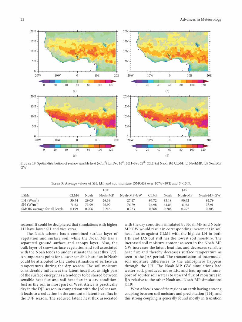
seasons. It could be deciphered that simulations with higherLH have lower SH and vice versa.

.e Noah scheme has a combined surface layer ofvegetation and surface soil, while the Noah MP has aseparated ground surface and canopy layer. Also, thebulk layer of snow/surface vegetation and soil associatedwith the Noah tends to under estimate the heat flux [77].An important point for a lower sensible heat flux in Noahcould be attributed to the underestimation of surface airtemperatures during the dry season. .e soil moistureconsiderably influences the latent heat flux, as high partof the surface energy has a tendency to be shared betweensensible heat flux and soil heat flux in a dry condition.Just as the soil in most part of West Africa is practicallydry in the DJF season in comparison with the JAS season,it leads to a reduction in the amount of latent heat flux inthe DJF season. .e reduced latent heat flux associated

with the dry condition simulated by Noah MP and Noah-MP GW would result in corresponding increment in soilheat flux as against CLM4 with the highest LH in bothDJF and JAS but still has the lowest soil moisture. .eincreased soil moisture content as seen in the Noah-MPGW increases the latent heat flux and decreases sensibleheat flux and thereby decreases surface temperature asseen in the JAS period. .e transmission of intermodelsoil moisture differences to the atmosphere happensthrough the LH. .e Noah-MP GW simulations hadwetter soil, produced more LH, and had upward trans-port of aquifer soil water (to upward flux of moisture) inJJA relative to the other Noah and Noah-MP simulations[119].

West Africa is one of the regions on earth having a strongcoupling between soil moisture and precipitation [114], andthis strong coupling is generally found mostly in transition

20N

15N

10N

5N

020W 10W 10E 20E0

0 20 40 60 80 100 120

(a)

20N

15N

10N

5N

020W 10W 10E 20E0

0 20 40 60 80 100 120

(b)

20N

15N

10N

5N

020W 10W 10E 20E0

0 20 40 60 80 100 120

(c)

20N

15N

10N

5N

020W 10W 10E 20E0

0 20 40 60 80 100 120

(d)

Figure 19: Spatial distribution of surface sensible heat (w/m2) for Dec 16th, 2011–Feb 28th, 2012. (a) Naoh. (b) CLM4. (c) NaohMP. (d) NoahMPGW.

Table 5: Average values of SH, LH, and soil moisture (SMOIS) over 10°W–10°E and 5°–15°N.

DJF JASLSMs CLM4 Noah Noah-MP Noah-MP-GW CLM4 Noah Noah-MP Noah-MP-GWLH (W/m2) 30.54 29.03 26.39 27.47 96.72 83.18 90.62 92.79SH (W/m2) 71.63 73.99 76.90 76.79 36.98 44.84 41.63 38.91SMOIS average for all levels 0.199 0.206 0.216 0.223 0.268 0.288 0.297 0.305


5N 10N 15NLatitude

90

80

70

60

50

40

30

20

Sens

ible

hea

t (W

/m2 )

CLM4Noah

Noah-MPNoah-MP GW

(a)

5N 10N 15NLatitude

Late

nt h

eat (

W/m

2 )

120

100

80

60

40

20

CLM4Noah

Noah-MPNoah-MP GW

(b)

5N 10N 15NLatitude

0.90

0.80

0.70

0.60

0.50

0.40

0.30

0.20

Evap

orat

ion

fract

ion

CLM4Noah

Noah-MPNoah-MP GW

(c)

5N 10N 15NLatitude

0.40

0.35

0.30

0.25

0.20

0.15

Soil

moi

sture

(m3 /m

3 )

CLM4Noah

Noah-MPNoah-MP GW

(d)



zones between wet and dry climates like the Sahel [10]. .esoil moisture controls the albedo and Bowen ratio. Eltahir[118] suggests that a positive feedback mechanism existsbetween soil moisture and rainfall. According to Wang et al.[120], higher soil moisture increases the latent heat flux, andthis is liable to increase the moist entropy flux per unit massof air and the amount of convective available potentialenergy in the boundary layer. .ese processes probablyincrease the frequency and magnitude of convective pre-cipitation events [113]. According to Steiner et al. [25],during the monsoon season, wetter soils and increasedmoisture advection could lead to an increase in the release ofwater vapor to the atmosphere, increasing the amount oflatent energy from the surface. Wolters et al. [114] alsoconcluded that soil moisture modifications could influencethe 850 hPa flow pattern causing deviations in the path of thesquall line overWest Africa..ese results are in line with theconclusions of Hacker [121], who discussed the influence ofsoil moisture initialization in NWP on the predictability ofwinds in the PBL. .is is also in line with our findings, assimulation with higher soil moisture tends to have higherprecipitation as in the case with Noah, Noah-MP, and Noah-MP GW.

Changes in the distribution of roots can dramaticallychange the amount of soil moisture available to plants totranspire as the increase in root depth could increase wateruptake, increase transpiration, increase water vapour, in-crease cloud formation, and increase rainfall [122]. Whileevaporation from bare soil and transpiration from shortvegetation is mostly dependent on soil moisture conditionsin the surface soil layer, tall vegetation can additionallyaccess water in deeper layers [123]. However, despite

having the lowest average amount of SMOIS (Table 5), theCLM4 has high average precipitation corroborated withhigh average LH..is could be explained as CLM4 has totalsoil depth of about 3.8m and thus gives room for deeperpenetration of plant roots to access deeper soil moisture,which could influence the LH..is also has the tendency toincrease the transpiration and hence could explain whyCLM4 has higher LH and EF than other LSMs and higherprecipitation than Noah LSM. .e difficulty in comparingCLM4 with the other tested LSMs here would be as a resultof the differences in mostly the number of soil levels andmight bring about some inconsistencies in averaging forbetter comparison. Also, the high average LH fluxes inCLM4 could lead to a greater evapotranspiration per unitprecipitation which tends to return more water to theatmosphere, thereby leading to the drier soils/reduced soilmoisture as seen for both DJF and JAS season. However,other factors beyond the scope of this study could be inoperation.

Land surface models have become more important innumerical weather prediction models like WRF as morecomplex and sensitive planetary boundary layer schemes areused. .e principal difference between the models is in thevegetation representation, the description, and parameteri-zation of the soil water column in each model. Vegetationsubstantially influences the exchange of momentum, energy,moisture, and trace gases between the surface and the at-mosphere and hence affects all other parameter in one way orthe other..erefore, it is recommended that improvement onthe treatment of surface parameters in the models should beparamount, as this will go long in improving the simulationsespecially in areas of strong land-atmosphere interaction.

5N 10N 15NLatitude

30.0

28.0

26.0

24.0

22.0

20.0

18.0

Tem

pera

ture

(C)

CLM4Noah

Noah-MPNoah-MP GW

(e)

Figure 20: (a) Sensible heat, (b) latent heat, (c) evaporation fraction, (d) soil moisture, and (e) temperature, averaged over the longitudinalextent of the red box in Figure 1 for the JAS period.


4. Conclusion

In all, eight simulations with 4 LSMs (Noah, Noah-MP,CLM4, and Noah-MP GW) using the WRF model werecarried out for two sets of 3months’ (December–February2011/2012 and July–September 2012) period over WestAfrica. .ese were done using the 3.9.1.1 version of WRFmodel to assess the performance of the listed LSMs overWest Africa. .e models’ air temperature was evaluatedusing ERA-Interim, while precipitation was evaluated usingTRMM. In order to provide a succinct statistical summary,the results were plotted in the Taylor diagram.

On average within the red box in Figure 1, CLM4, Noah-MP, and Noah-MP GW all overestimated the precipitationduring both DJF and JAS seasons, while Noah under-estimated it. .e strength of the Tropical Easterly Jet (TEJ) isstrongest in Noah-MP GW and Noah-MP compared withCLM4 and Noah..e core of the African Easterly Jet AEJ liesat the southernmost position in Noah and northernmost forNoah-MP GW. .e Noah-MP GW and Noah-MP simula-tions have stronger influx of wind than the CLM4 and Noahwith Noah showing the least influx. Also, the number of soillayers and the depth was a considerable factor as regards thecause of the differences between the models as CLM4 withhigher soil depth behaved differently by having low soilmoisture with high latent heat.

.e variable of interest is also a factor to be considered inthe selection of LSMs. However, each LSM performed dif-ferently for different variables as a result of the difference inthe model physics, soil layers, and columns, vegetationstructure, and level of model sophistication..erefore, basedon precipitation and 2m temperatures, Noah-MP GW is theoverall best for all the variables and seasons in combination.If this is based on the JAS season (the monsoon season), thenNoah-MP GWwill also come first, Noah-MP second, CLM4third, and Noah will come fourth.

.e West African Monsoon (WAM) controls the rainyseason in West Africa. Researchers like [124] have stressedthat it supplies most of the precipitation because it trans-ports rich moisture into the region through the southwesttrade wind coming from the Atlantics. However, the WAMis a very complex large-scale circulation system, whichentails the interactions of the elements of many scale at-mospheric circulations, thereby making the close to accuratesimulation of precipitation and other variables in the regiona bit more demanding. So long as the improvement of theland surface models can result into a better simulation of theweather parameters, a more in-depth analysis of the impactof the recent WRF land surface models on major features ofthe general circulation of West Africa which includes theintertropical convergent zone (ITCZ), the monsoon depthand strength, the AEJ, TEJ, and AEW, and the deep con-vective systems is recommended as a good area for futureresearch.

Precipitation could be better simulated more extensivelyby testing with several other sets of physics combinationslike the radiation schemes, cumulus schemes, microphysics,and planetary boundary layer schemes in the WRF model.Also, a longer period of simulation to accommodate more

seasons for better comparison between same seasons acrosseach zone in West Africa could lead to a better simulation.From the study, it can be concluded that differences in landsurface have the tendency to alter the weather parameters.Earlier studies have shown that the West African landsurface is an important part in the region’s climate dy-namics. .is has been confirmed in this study, as the studiedparameters are very sensitive to each LSM used. However,differences between the land use in the model and the actualland use could cause discrepancies in the simulations. Also,the accuracy of initial and boundary conditions is crucial tothe successful production of WRF simulations [45] as thedifference could propagate through the atmosphere andhave an effect on the simulation of the dynamical features inWest Africa. Hence, future research would also incorporate areal-time land use data products into the model over WestAfrica with various initial and boundary conditions andprobably compare with an in situ data (if made available) inorder to improve the simulations and have a perfectcomparison.

Finally, despite having constant roughness length valuesfor all season, Noah-MP still performed better than Noahover West Africa. .is could be due to the other im-provements and modifications in the model, but the con-stant roughness length in the model is a factor to look into..is could be a good area for future improvement as toreduce uncertainties in the model for better simulations andforecasts.

Data Availability

.e data used for the research are archived in the NCARHPSS storage. .is could only be made available from thecorresponding author upon reasonable request.

Conflicts of Interest

.e authors declare no conflicts of interest.

Acknowledgments

.e authors would like to thank the Mesoscale and Mi-croscale Meteorology (MMM) Laboratory, NCAR, forsupporting the research and also acknowledge the NCAR’sComputational and Information System Laboratory forproviding the computing facilities for the research. Also,thanks are due to Ming Chen, Micheal Duda, MichealBarlage, Mike Dixon, and other NCAR staff who providedtechnical support. .e research work was primarily fundedby the German Federal Ministry of Education and Research(BMBF) via the WACS-GRP FUTA.

References

[1] W. Zhao and A. Li, “A review on land surface processesmodelling over complex terrain,” Advances in Meteorology,vol. 2015, Article ID 607181, 17 pages, 2015.

[2] P. Viterbo, “.e role of the land surface in the climatesystem,” in Meteorological Training Course Lecture Series,European Centre for Medium Range Weather Forecasting


(ECMWF), Reading, United Kingdom, 2002, https://www.ecmwf.int/node/16961.

[3] P. R. Tiwari, S. C. Kar, S. C. Kar et al., “.e role of landsurface schemes in the regional climate model (RegCM) forseasonal scale simulations over Western Himalaya,”Atmosfera, vol. 28, no. 2, pp. 129–142, 2015.

[4] S. B. Trier, C. A. Davis, and D. A. Ahijevych, “Environmentalcontrols on the simulated diurnal cycle of warm-seasonprecipitation in the Continental United States,” Journal of theAtmospheric Sciences, vol. 67, no. 4, pp. 1066–1090, 2010.

[5] S. Wharton, M. Simpson, J. Osuna, J. Newman, andS. Biraud, Assessment of Land Surface Model Performance inWRF for Simulating Wind at Heights Relevant to the WindEnergy Community, U.S. Department of Energy Office ofScientific and Technical Information, Oak Ridge, TN, USA,S. LLNL-TR-643914, 2013.

[6] A. K. Betts, J. H. Ball, A. C. M. Beljaars, M. J. Miller, andP. A. Viterbo, “.e land surface-atmosphere interaction: areview based on observational and global modeling per-spectives,” Journal of Geophysical Research: Atmospheres,vol. 101, no. D3, pp. 7209–7225, 1996.

[7] C. Klein, J. Bliefernicht, D. Heinzeller, U. Gessner, I. Klein,and H. Kunstmann, “Feedback of observed interannualvegetation change: a regional climate model analysis for theWest African monsoon,” Climate Dynamics, vol. 48, no. 9-10, pp. 2837–2858, 2016.

[8] X. Y. Zheng and E. A. B. Eltahir, “.e role of vegetation in thedynamics of West African monsoons,” Journal of Climate,vol. 12, pp. 1368–1381, 1998.

[9] E. A. B. Eltahir and C. Gong, “Dynamics of wet and dry yearsin West Africa,” Journal of Climate, vol. 9, no. 5, pp. 1030–1042, 1996.

[10] R. D. Koster, P. A. Dirmeyer, Z. Guo et al., “Regions of strongcoupling between soil moisture and precipitation,” Science,vol. 305, no. 5687, pp. 1138–1140, 2004.

[11] Y. Xue, R. W. A. Hutjes, R. J. Harding et al., “.e sahelianclimate (chapter A5),” inVegetation, Water, Humans and theClimate, P. Kabat, Ed., pp. 59–77, Springer-Verlag, Berlin,Germany, 2004.

[12] C. A. Nobre, M. A. Silva Dias, A. D. Culf et al., “.e Amazonclimate,” in Vegetation, Water, Humans and the Climate,P. Kabat, Ed., pp. 79–92, Springer-Verlag, Berlin, Germany,2004.

[13] C. Fu, T. Yasunari, and S. Lutkemeier, “.e Asian monsoonclimate,” in Vegetation, Water, Humans and the Climate,P. Kabat, Ed., pp. 115–127, Springer-Verlag, Berlin, Ger-many, 2004.

[14] A. A. Sorensson, C. G. Menendez, P. Samuelsson, U. Willen,and U. Hansson, “Soil-precipitation feedbacks during theSouth American monsoon as simulated by a regional climatemodel,” Climatic Change, vol. 98, no. 3-4, pp. 429–447, 2010.

[15] T. Sato and Y. Xue, “Validating a regional climate model’sdownscaling ability for East Asian summer monsoonal in-terannual variability,” Climate Dynamics, vol. 41, no. 9-10,pp. 2411–2426, 2013.

[16] Y. Lu and L. M. Kueppers, “Surface energy partitioning overfour dominant vegetation types across the United States in Acoupled regional climate model (weather research andforecasting model 3-community land model 3.5),” Journal ofGeophysical Research: Atmospheres, vol. 117, no. D6, 2012.

[17] Y. Xue, F. De Sales, R. Vasic, C. R. Mechoso, A. Arakawa, andS. Prince, “Global and seasonal assessment of interactionsbetween climate and vegetation biophysical processes: a

GCM study with different land-vegetation representations,”Journal of Climate, vol. 23, no. 6, pp. 1411–1433, 2010.

[18] R. D. Koster, P. A. Dirmeyer, A. N. Hahmann et al.,“Comparing the degree of land-atmosphere interaction infour atmospheric general circulation models,” Journal ofHydrometeorology, vol. 3, no. 3, pp. 363–375, 2002.

[19] W. Li, W. Guo, Y. Xue, C. Fu, and B. Qiu, “Sensitivity of aregional climate model to land surface parameterizationschemes for East Asian summer monsoon simulation,”Climate Dynamics, vol. 47, no. 7-8, pp. 2293–2308, 2015.

[20] A. A. Boone, Y. Xue, F. De Sales et al., “.e regional impact ofland-use land-cover change (LULCC) over West Africa froman ensemble of global climate models under the auspices ofthe WAMME2 project,” Climate Dynamics, vol. 47, no. 11,pp. 3547–3573, 2016.

[21] S. E. Nicholson, “.e West african Sahel: a review of recentstudies on the rainfall regime and its interannual variability,”ISRN Meteorology, vol. 2013, Article ID 453521, 32 pages,2013.

[22] J. L. Redelsperger, C. D. .orncroft, A. Diedhiou, T. Lebel,D. J. Parker, and J. Polcher, “African monsoon multidisci-plinary analysis an international research project and fieldcampaign,” Bulletin of the American Meteorological Society,vol. 87, no. 12, pp. 1739–1746, 2006.

[23] P. A. Dirmeyer, “.e terrestrial segment of soil moisture-climate coupling,” Geophysical Research Letters, vol. 38,no. 16, 2011.

[24] Y. Xue, A. Boone, and C. M. Taylor, “Review of recentdevelopments and the future prospective in West africanatmosphere/land interaction studies,” International Journalof Geophysics, vol. 2012, Article ID 748921, 12 pages, 2012.

[25] A. L. Steiner, J. S. Pal, S. A. Rauscher et al., “Land surfacecoupling in regional climate simulations of the West Africanmonsoon,” Climate Dynamics, vol. 33, no. 6, pp. 869–892,2009.

[26] S. L. Lavender, C. M. Taylor, and A. J. Matthews, “Coupledland-atmosphere intraseasonal variability of theWest africanmonsoon in a GCM,” Journal of Climate, vol. 23, no. 21,pp. 5557–5571, 2010.

[27] J. G. Charney, “Dynamics of deserts and drought in theSahel,” Quarterly Journal of the Royal Meteorological Society,vol. 101, no. 428, pp. 193–202, 1975.

[28] K. Laval and L. Picon, “Effect of a change of the surfacealbedo of the Sahel on climate,” Journal of the AtmosphericSciences, vol. 43, no. 21, pp. 2418–2429, 1986.

[29] Y. C. Sud and M. Fennessy, “A study of the influence ofsurface albedo on July circulation in semi-arid regions usingthe glas GCM,” Journal of Climatology, vol. 2, no. 2,pp. 105–125, 1982.

[30] W. Li, Y. Xue, and I. Poccard, “Numerical investigation ofthe impact of vegetation indices on the variability of WestAfrican summer monsoon,” Journal of the MeteorologicalSociety of Japan, vol. 85A, pp. 363–383, 2007.

[31] Y. Xue, “Biosphere feedback on regional climate in tropicalnorth Africa,” Quarterly Journal of the Royal MeteorologicalSociety, vol. 123, no. 542, pp. 1483–1515, 1997.

[32] Y. Xue, K.-N. Liou, and A. Kasahara, “Investigation ofbiogeophysical feedback on the african climate using a two-dimensional model,” Journal of Climate, vol. 3, no. 3,pp. 337–352, 1990.

[33] X. Zheng and E. A. B. Eltahir, “.e response to deforestationand desertification in a model of West african monsoons,”Geophysical Research Letters, vol. 24, no. 2, pp. 155–158,1997.


https://www.ecmwf.int/node/16961

https://www.ecmwf.int/node/16961

[34] R. Borge, V. Alexandrov, J. Jose del Vas, J. Lumbreras, andE. Rodrıguez, “A comprehensive sensitivity analysis of theWRF model for air quality applications over the IberianPeninsula,” Atmospheric Environment, vol. 42, no. 37,pp. 8560–8574, 2008.

[35] J. Cretat, B. Pohl, Y. Richard, and P. Drobinski, “Uncer-tainties in simulating regional climate of Southern Africa:sensitivity to physical parameterizations using WRF,” Cli-mate Dynamics, vol. 38, no. 3-4, pp. 613–634, 2012.

[36] S. K. Deb, T. P. Srivastava, and C. M. Kishtawal, “.e WRFmodel performance for the simulation of heavy precipitatingevents over Ahmedabad during August 2006,” Journal ofEarth System Science, vol. 117, no. 5, pp. 589–602, 2008.

[37] J. P. Evans, M. Ekstrom, and F. Ji, “Evaluating the perfor-mance of a WRF physics ensemble over South-East Aus-tralia,” Climate Dynamics, vol. 39, no. 6, pp. 1241–1258, 2012.

[38] W. A. Gallus Jr. and J. F. Bresch, “Comparison of impacts ofWRF dynamic core, physics package, and initial conditionson warm season rainfall forecasts,”MonthlyWeather Review,vol. 134, no. 9, pp. 2632–2641, 2006.

[39] M. Garcıa-Dıez, J. Fernandez, L. Fita, and C. Yague, “Sea-sonal dependence of WRF model biases and sensitivity toPBL schemes over Europe,” Quarterly Journal of the RoyalMeteorological Society, vol. 139, no. 671, pp. 501–514, 2013.

[40] S.-Y. Hong, K.-S. Sunny Lim, J.-H. Kim, J.-O. Jade Lim, andJ. Dudhia, “Sensitivity study of cloud-resolving convectivesimulations with WRF using two bulk microphysical pa-rameterizations: ice-phase microphysics versus sedimenta-tion effects,” Journal of AppliedMeteorology and Climatology,vol. 48, no. 1, pp. 61–76, 2009.

[41] I. Jankov, W. A. Gallus Jr., M. Segal, B. Shaw, and S. E. Koch,“.e impact of different WRF model physical parameteri-zations and their interactions on warm season MCS rainfall,”Weather and Forecasting, vol. 20, no. 6, pp. 1048–1060, 2005.

[42] J. S. Kain, S. J. Weiss, J. J. Levit, M. E. Baldwin, andD. R. Bright, “Examination of convection-allowing config-urations of the WRF model for the prediction of severeconvective weather: the SPC/NSSL spring program 2004,”Weather and Forecasting, vol. 21, no. 2, pp. 167–181, 2006.

[43] J. H. Kwun, Y.-K. Seo Kim, J. W. Seo, J. H. Jeong, andS.-H. You, “Sensitivity of MM5 and WRF mesoscale modelpredictions of surface winds in a typhoon to planetaryboundary layer parameterizations,”Natural Hazards, vol. 51,no. 1, pp. 63–77, 2009.

[44] X. Li and Z. Pu, “Sensitivity of numerical simulations of theearly rapid intensification of Hurricane Emily to cumulusparameterization schemes in different model horizontalresolutions,” Journal of the Meteorological Society of Japan,vol. 87, no. 3, pp. 403–421, 2009.

[45] L. Liu, Y. Ma,M.Menenti, X. Zhang, andW.Ma, “Evaluationof WRF modeling in relation to different land surfaceschemes and initial and boundary conditions: a snow eventsimulation over the Tibetan plateau,” Journal of GeophysicalResearch: Atmospheres, vol. 124, no. 1, pp. 209–226, 2019.

[46] S. Lu, W. Guo, Y. Xue, and F. Huang, “Sensitivity of highresolutionWRFmodel to land surface schemes in simulatingboreal summer climate over Central Asia,” EGU, 2020.

[47] D. S. Nolan, J. A. Zhang, and D. P. Stern, “Evaluation ofplanetary boundary layer parameterizations in tropical cy-clones by comparison of in situ observations and high-resolution simulations of Hurricane Isabel (2003). Part I:initialization, maximum winds, and the outer-core boundarylayer,” Monthly Weather Review, vol. 137, no. 11,pp. 3651–3674, 2009.

[48] G. Zittis, P.Hadjinicolaou, and J. Lelieveld, “Comparison ofWRFmodel physics parameterizations over the MENA-CORDEXdomain,” American Journal of Climate Change, vol. 3, no. 5,pp. 490–511, 2014.

[49] K. H. Cook, “Generation of the african easterly jet and its rolein determining West African precipitation,” Journal of Cli-mate, vol. 12, no. 5, pp. 1165–1184, 1999.

[50] A. A. Boone, I. Poccard-Leclercq, Y. Xue, J. Feng, andP. de Rosnay, “Evaluation of the WAMME model surfacefluxes using results from the AMMA land-surface modelintercomparison project,” Climate Dynamics, vol. 35, no. 1,pp. 127–142, 2009.

[51] P. M. Ruti, J. E. Williams, F. Hourdin et al., “.e WestAfrican climate system: a review of the AMMA model inter-comparison initiatives,” Atmospheric Science Letters, vol. 12,no. 1, pp. 116–122, 2011.

[52] J. A. Okalebo, R. J. Oglesby, S. Feng et al., “An evaluation ofthe community land model (version 3.5) and Noah landsurface models for temperature and precipitation overNebraska (central great plains): Implications for agriculturein simulations of future climate change and adaptation,” inClimate Change Adaptation, Resilience and Hazards, ClimateChange Management, W. L. Filho, H. Filho, and G. Cavan,Eds., Springer, Cham, Switzerland, 2016.

[53] J. Jin, N. L. Miller, and N. Schlegel, “Sensitivity study of fourland surface schemes in the WRF model,” Advances inMeteorology, vol. 2010, Article ID 167436, 11 pages, 2010.

[54] J.-F. Miao, D. Chen, and K. Borne, “Evaluation and com-parison of Noah and pleim-xiu land surface models in MM5using GOTE2001 data: spatial and temporal variations innear-surface air temperature,” Journal of Applied Meteo-rology and Climatology, vol. 46, no. 10, pp. 1587–1605, 2007.

[55] J. R. Rajeswari, C. V. Srinivas, T. N. Rao, andB. Venkatraman, “Impact of land surface physics on thesimulation of boundary layer characteristics at a tropicalcoastal station,” Atmospheric Research, vol. 238, Article ID104888, 2020.

[56] A. P. Singh, U. C. Mohanty, P. Sinha, and M. Mandal,“Influence of different land-surface processes on Indiansummer monsoon circulation,” Natural Hazards, vol. 42,no. 2, pp. 423–438, 2007.

[57] X. Chen, T. Yang, X. Wang, C.-Y. Xu, and Z. Yu, “Uncer-tainty intercomparison of different hydrological models insimulating extreme flows,” Water Resources Management,vol. 27, no. 5, pp. 1393–1409, 2012.

[58] J. L. Case, F. J. LaFontaine, S. V. Kumar, and C. D. Peters-Lidard, “Using the NASA-UnifiedWRF to assess the impactsof real-time vegetation on simulations of severe weather,” inProceedings of the 13th Annual WRF User’s Workshop, p. 69,Boulder, CO, USA, 2012.

[59] J. Miller, M. Barlage, X. Zeng, H. Wei, K. Mitchell, andD. Tarpley, “Sensitivity of the NCEP/Noah land surfacemodel to the MODIS green vegetation fraction data set,”Geophysical Research Letters, vol. 33, 2006.

[60] E. Sertel, C. Ormeci, and A. Robock, “Modelling land coverchange impact on the summer climate of the MarmaraRegion, Turkey,” International Journal of Global Warming,vol. 3, no. 1-2, pp. 194–202, 2011.

[61] S. Hagos, L. R. Leung, Y. Xue et al., “Assessment of un-certainties in the response of the African monsoon precip-itation to land use change simulated by a regional model,”Climate Dynamics, vol. 43, no. 9-10, pp. 2765–2775, 2014.

[62] D. P. Dee, S. M. Uppala, A. J. Simmons et al., “.e ERA-Interim reanalysis: configuration and performance of the


data assimilation system,” Quarterly Journal of the RoyalMeteorological Society, vol. 137, no. 656, pp. 553–597, 2011.

[63] U.S. Department of Commerce National Centers for Envi-ronmental Prediction/National Weather Service/NOAA/,“Updated daily NCEP FNL operational model global tro-pospheric analyses, continuing from July 1999,” ResearchData Archive at the National Center for Atmospheric Re-search, Computational and Information Systems Laboratory,2000.

[64] M. J. Iacono, J. S. Delamere, E. J. Mlawer, M. W. Shephard,S. A. Clough, and W. D. Collins, “Radiative forcing by long-lived greenhouse gases: calculations with the AER radiativetransfer models,” Journal of Geophysical Research, vol. 113,no. D13, p. D13103, 2008.

[65] M. Nakanishi and H. Niino, “An improved mellor-yamadalevel-3 model: its numerical stability and application to aregional prediction of advection fog,” Boundary-Layer Me-teorology, vol. 119, no. 2, pp. 397–407, 2006.

[66] C. Zhang, Y. Wang, and K. Hamilton, “Improved repre-sentation of boundary layer clouds over the southeast pacificin ARW-WRF using a modified Tiedtke cumulus parame-terization scheme,” Monthly Weather Review, vol. 139,no. 11, pp. 3489–3513, 2011.

[67] S. Y. Hong and J. O. J. Lim, “.eWRF single-moment 6-classmicrophysics scheme (WSM6),” Journal Korean of Meteo-rological Society, vol. 42, no. 2, pp. 129–151, 2006.

[68] I. E. Gbode, J. Dudhia, K. O. Ogunjobi, and V. O. Ajayi,“Sensitivity of different physics schemes in the wrf modelduring a west african monsoon regime,” <eoretical andApplied Climatology, vol. 136, no. 1-2, pp. 733–751, 2018.

[69] F. Chen and J. Dudhia, “Coupling an advanced land surface-hydrology model with the penn state-NCARMM5modelingsystem. Part I: model implementation and sensitivity,”Monthly Weather Review, vol. 129, no. 4, pp. 569–585, 2001.

[70] A. K. Betts, F. Chen, K. E. Mitchell, and Z. I. Janjic, “As-sessment of the land surface and boundary layer models intwo operational versions of the NCEP Eta Model using FIFEdata,” Monthly Weather Review, vol. 125, no. 11,pp. 2896–2916, 1997.

[71] M. Ek, K. Mitchell, L. Yin et al., “Implementation of Noahland-surface model advances in the NCEP operationalmesoscale Eta model,” Journal of Geophysical Research:Atmospheres, vol. 108, no. D22, p. 8851, 2003.

[72] A. Robock, L. Luo, E. F. Wood et al., “Evaluation of the northAmerican land data assimilation system over the southerngreat plains during the warm season,” Journal of GeophysicalResearch: Atmospheres, vol. 108, no. D22, p. 8846, 2003.

[73] C. A. Schlosser, A. G. Slater, A. Robock et al., “Simulations ofa boreal grassland hydrology at Valdai, Russia: PILPS phase 2(d),” Monthly Weather Review, vol. 128, no. 2, pp. 301–321,2000.

[74] E. F. Wood, D. P. Lettenmaier, X. Liang et al., “.e projectfor intercomparison of land-surface parameterizationschemes (PILPS) phase 2(c) red-Arkansas river basin ex-periment:,” Global and Planetary Change, vol. 19, no. 1–4,pp. 115–135, 1998.

[75] J. C. Schaake, Q. Duan, V. Koren et al., “An intercomparisonof soil moisture fields in the north American land data as-similation system (NLDAS),” Journal of Geophysical Re-search, vol. 109, Article ID D01S90, 2004.

[76] A. McNally, K. Arsenault, S. Kumar et al., “A land dataassimilation system for sub-Saharan Africa food and watersecurity applications,” Scientific Data, vol. 4, no. 1, Article ID170012, 2017.

[77] G.-Y. Niu, Z.-L. Yang, K. E. Mitchell et al., “.e communityNoah land surface model with multiparameterization op-tions (Noah-MP): 1. Model description and evaluation withlocal-scale measurements,” Journal of Geophysical Research,vol. 116, no. D12, 2011.

[78] G.-Y. Niu and Z.-L. Yang, “Effects of vegetation canopyprocesses on snow surface energy and mass balances,”Journal of Geophysical Research: Atmospheres, vol. 109,no. D23, p. D23111, 2004.

[79] R. Yang and M. A. Friedl, “Modeling the effects of three-dimensional vegetation structure on surface radiation andenergy balance in boreal forests,” Journal of GeophysicalResearch, vol. 108, no. D16, p. 8615, 2003.

[80] G. B. Bonan, “A land surface model (LSM version 1.0) forecological,”Hydrological, and Atmospheric Studies: TechnicalDescription and User’s Guide, NCAR Tech. Note NCAR/TN-417+STR, p. 150, National Center for Atmospheric Research,Boulder, CO, USA, 1996.

[81] G. Collatz, M. Ribas-Carbo, and J. Berry, “Coupled photo-synthesis-stomatal conductance model for leaves of C4plants,” Functional Plant Biology, vol. 19, no. 5, pp. 519–538,1992.

[82] P. J. Sellers, D. A. Randall, G. J. Collatz et al., “A revised landsurface parameterization (SiB2) for atmospheric GCMS. PartI: model formulation,” Journal of Climate, vol. 9, no. 4,pp. 676–705, 1996.

[83] R. E. Dickinson, M. Shaikh, R. Bryant, and L. Graumlich,“Interactive canopies for a climate model,” Journal of Cli-mate, vol. 11, no. 11, pp. 2823–2836, 1998.

[84] Z.-L. Yang and G.-Y. Niu, “.e Versatile integrator ofsurface and atmosphere processes,” Global and PlanetaryChange, vol. 38, no. 1-2, pp. 175–189, 2003.

[85] G.-Y. Niu and Z.-L. Yang, “An observation-based formu-lation of snow cover fraction and its evaluation over largeNorth American river basins,” Journal of Geophysical Re-search, vol. 112, no. D21, Article ID D21101, 2007.

[86] K. W. Oleson, D. M. Lawrence, G. B. Bonan et al., “Technicaldescription of version 4.0 of the community land model(CLM),” Tech- Nical Note NCAR/TN-478+STR, p. 257,National Center for Atmos- pheric Research, Boulder, CO,USA, 2010.

[87] W. C. Skamarock, J. B. Klemp, J. Dudhia et al., A Descriptionof the Advanced Research WRF Version 3, NCAR TechnicalNote NCAR/TN-475+STR, Mesoscale and Microscale Mete-orology Division, National Center for Atmospheric Research,Boulder, CO, USA, 2008.

[88] X. Zeng and M. Decker, “Improving the numerical solutionof soil moisture-based Richards equation for land modelswith a deep or shallow water table,” Journal of Hydrome-teorology, vol. 10, no. 1, pp. 308–319, 2009.

[89] G.-Y. Niu and Z.-L. Yang, “Effects of frozen soil on snowmeltrunoff and soil water storage at a continental scale,” Journalof Hydrometeorology, vol. 7, no. 5, pp. 937–952, 2006.

[90] A. Wang and X. Zeng, “Improving the treatment of thevertical snow burial fraction over short vegetation in theNCAR CLM3,” Advances in Atmospheric Sciences, vol. 26,no. 5, pp. 877–886, 2009.

[91] D. M. Lawrence, K. W. Oleson, M. G. Flanner et al., “Pa-rameterization improvements and functional and structuraladvances in version 4 of the community landmodel,” Journalof Advances inModeling Earth Systems, vol. 3, pp. 1942–2466,2011.

[92] G. J. Huffman, D. T. Bolvin, E. J. Nelkin et al., “.e TRMMmultisatellite precipitation analysis (TMPA): quasi-global,


multiyear, combined-sensor precipitation estimates at finescales,” Journal of Hydrometeorology, vol. 8, no. 1, pp. 38–55,2007.

[93] G. J. Huffman, D. T. Bolvin, and R. F. Adler, “GPCP version1.2 one- degree daily precipitation data set,” Research DataArchive at the National Center for Atmospheric Research,Computational and Information Systems Laboratory, 2016.

[94] G. J. Huffman, R. F. Adler, D. T. Bolvin, and G. Gu, “Im-proving the global precipitation record: GPCP version 2.1,”Geophysical Research Letters, vol. 36, no. 17, 2009.

[95] K. E. Taylor, “Summarizing multiple aspects of model per-formance in a single diagram,” Journal of Geophysical Re-search: Atmospheres, vol. 106, no. D7, pp. 7183–7192, 2001.

[96] J. Houghton, Y. Ding, D. J. Griggs, M. Noguer,P. J. van der Linden, and D. Xiaosu, “Climate change 2001:the scientific basis. Contribution of working group i to the3rd assessment report of the intergovernmental panel onclimate change,” Cambridge University Press, Cambridge,UK, 2001.

[97] X. Liang, Z. Xie, andM. Huang, “A new parameterization forsurface and groundwater interactions and its impact onwater budgets with the variable infiltration capacity (VIC)land surface model,” Journal of Geophysical Research,vol. 108, no. D16, p. 8613, 2003.

[98] G. S. Jenkins, A. Kamga, A. Garba, A. Diedhiou, V. Morris,and E. Joseph, “Investigating the West African climatesystem using global/regional climate models,” Bulletin of theAmerican Meteorological Society, vol. 83, no. 4, pp. 583–595,2002.

[99] C. Jones, F. Giorgi, and G. Asrar, “.e coordinated regionaldownscaling experiment: CORDEX, an internationaldownscaling link to CMIP5,” CLIVAR Exchanges, vol. 16,no. 2, pp. 34–40, 2011.

[100] J. Milovac, K. Warrach-Sagi, A. Behrendt, F. Spath,J. Ingwersen, and V. Wulfmeyer, “Investigation of PBLschemes combining the WRF model simulations withscanning water vapor differential absorption lidar mea-surements,” Journal of Geophysical Research: Atmospheres,vol. 121, no. 2, pp. 624–649, 2016.

[101] Y. Jiao and D. Caya, “An investigation of summer precipi-tation simulated by the Canadian regional climate model,”Monthly Weather Review, vol. 134, no. 3, pp. 919–932, 2006.

[102] C. Chotamonsak, E. P. Salathe, J. Kreasuwan, andS. Chantara, “Evaluation of precipitation simulations over.ailand using a WRF regional climate model,” Chiang MaiJournal of Science, vol. 39, no. 4, pp. 623–628, 2012.

[103] I. Chawla, K. K. Osuri, P. P. Mujumdar, and D. Niyogi,“Assessment of the Weather Research and Forecasting(WRF) model for simulation of extreme rainfall events in theupper Ganga Basin,” Hydrology and Earth System Sciences,vol. 22, no. 2, pp. 1095–1117, 2018.

[104] J. Pongratz, C. H. Reick, T. Raddatz, and M. Claussen,“Biogeophysical versus biogeochemical climate response tohistorical anthropogenic land cover change,” GeophysicalResearch Letters, vol. 37, no. 8, 2010.

[105] A. A. Akinsanola and W. Zhou, “Understanding the vari-ability ofWest african summermonsoon rainfall: contrastingtropospheric features and monsoon index,” Atmosphere,vol. 11, no. 3, p. 309, 2020.

[106] S. M. Hagos and K. H. Cook, “Ocean warming and late-twentieth-century sahel drought and recovery,” Journal ofClimate, vol. 21, no. 15, pp. 3797–3814, 2008.

[107] S. Hagos and C. Zhang, “Diabatic heating, divergent cir-culation and moisture transport in the African monsoon

system,” Quarterly Journal of the Royal Meteorological So-ciety, vol. 136, no. S1, pp. 411–425, 2010.

[108] J. P. Grist and S. E. Nicholson, “A study of the dynamicfactors influencing the rainfall variability in theWest AfricanSahel,” Journal of Climate, vol. 14, no. 7, pp. 1337–1359, 2001.

[109] A. A. Akinsanola and K. O. Ogunjobi, “Evaluation ofpresent-day rainfall simulations over West Africa in COR-DEX regional climate models,” Environmental Earth Sci-ences, vol. 76, no. 10, p. 366, 2017.

[110] B. J. Abiodun, J. S. Pal, E. A. Afiesimama, W. J. Gutowski,and A. Adedoyin, “Simulation of West african monsoonusing RegCM3 Part II: impacts of deforestation and de-sertification,” <eoretical and Applied Climatology, vol. 93,no. 3-4, pp. 245–261, 2008.

[111] A. Berg, B. R. Lintner, K. L. Findell, S. Malyshev,P. C. Loikith, and P. Gentine, “Impact of soil moisture-at-mosphere interactions on surface temperature distribution,”Journal of Climate, vol. 27, no. 21, pp. 7976–7993, 2014.

[112] E. M. Fischer, S. I. Seneviratne, L. Vidale P, D. Luthi, andC. Schar, “Soil moisture–atmosphere interactions during the2003 European summer heat wave,” Journal of Climate,vol. 20, no. 20, pp. 5081–5099, 2007.

[113] J. S. Pal and E. A. B. Eltahir, “Pathways relating soil moistureconditions to future summer rainfall within a model of theland-atmosphere system,” Journal of Climate, vol. 14, no. 6,pp. 1227–1242, 2001.

[114] D. Wolters, C. C. van Heerwaarden, J. V.-G. de Arellano,B. Cappelaere, and D. Ramier, “Effects of soil moisturegradients on the path and the intensity of a West Africansquall line,” Quarterly Journal of the Royal MeteorologicalSociety, vol. 136, no. 653, pp. 2162–2175, 2010.

[115] C. D. .orncroft, H. Nguyen, C. Zhang, and P. Peyrille,“Annual cycle of the West African monsoon: regional cir-culations and associated water vapour transport,” QuarterlyJournal of the Royal Meteorological Society, vol. 137, no. 654,pp. 129–147, 2011.

[116] C. Klein, Interactions of regional atmospheric and land surfaceprocesses with the West African monsoon system, Faculty ofApplied Computer Science of the University of Augsburg,Augsburg, Germany, https://www.researchgate.net/publication/316071934_Interactions_of_regional_atmospheric_and_land_surface_processes_with_the_West_African_monsoon_system,Ph.D. thesis, 2016.

[117] A. K. Betts and J. H. Ball, “FIFE surface climate and site-average data set 1987-1989,” Journal of the AtmosphericSciences, vol. 55, no. 7, pp. 1091–1108. in press, 1998.

[118] E. A. B. Eltahir, “A soil moisture-rainfall feedback mecha-nism: 1. .eory and observations,” Water Resources Re-search, vol. 34, no. 4, pp. 765–776, 1998.

[119] M. Barlage, M. Tewari, F. Chen, G. Miguez-Macho,Z.-L. Yang, and G.-Y. Niu, “.e effect of groundwater in-teraction in North American regional climate simulationswith WRF/Noah-MP,” Climatic Change, vol. 129, no. 3-4,pp. 485–498, 2015.

[120] J. Wang, Y. Cui, X. He, J. Zhang, and S. Yan, “Surface albedovariation and its influencing factors over dongkemadi gla-cier, central Tibetan plateau,” Advances in Meteorology,vol. 2015, Article ID 852098, 10 pages, 2015.

[121] J. P. Hacker, “Spatial and temporal scales of boundary layerwind predictability in response to small-amplitude landsurface uncertainty,” Journal of the Atmospheric Sciences,vol. 67, no. 1, pp. 217–233, 2010.


https://www.researchgate.net/publication/316071934_Interactions_of_regional_atmospheric_and_land_surface_processes_with_the_West_African_monsoon_system



[122] A. J. Pitman, “.e evolution of, and revolution in, landsurface schemes designed for climate models,” InternationalJournal of Climatology, vol. 23, no. 5, pp. 479–510, 2003.

[123] C. Schwingshackl, M. Hirschi, and S. I. Seneviratne, “Atheoretical approach to assess soil moisture-climate couplingacross CMIP5 and GLACE-CMIP5 experiments,” EarthSystem Dynamics, vol. 9, no. 4, pp. 1217–1234, 2018.

[124] J.-L. Redelsperger, A. Diongue, A. Diedhiou et al., “Multi-scale description of a Sahelian synoptic weather systemrepresentative of the West African monsoon,” QuarterlyJournal of the Royal Meteorological Society, vol. 128, no. 582,pp. 1229–1257, 2002.


Research Article Assessment of WRF Land Surface Model ...

Documents

Transcript of Research Article Assessment of WRF Land Surface Model ...