Research Article A Class of Two-Person Zero-Sum Matrix ...

Hindawi Publishing CorporationInternational Journal of Mathematics and Mathematical SciencesVolume 2010, Article ID 404792, 22 pagesdoi:10.1155/2010/404792

Research ArticleA Class of Two-Person Zero-Sum Matrix Gameswith Rough Payoffs

Jiuping Xu and Liming Yao

Uncertainty Decision-Making Laboratory, Sichuan University, Chengdu 610064, China

Correspondence should be addressed to Jiuping Xu, [email protected]

Received 10 July 2009; Accepted 17 January 2010

Academic Editor: Attila Gilanyi

Copyright q 2010 J. Xu and L. Yao. This is an open access article distributed under the CreativeCommons Attribution License, which permits unrestricted use, distribution, and reproduction inany medium, provided the original work is properly cited.

We concentrate on discussing a class of two-person zero-sum games with rough payoffs. Based onthe expected value operator and the trust measure of rough variables, the expected equilibriumstrategy and r-trust maximin equilibrium strategy are defined. Five cases whether the game existsr-trust maximin equilibrium strategy are discussed, and the technique of genetic algorithm isapplied to find the equilibrium strategies. Finally, a numerical example is provided to illustratethe practicality and effectiveness of the proposed technique.

1. Introduction

Game theory is widely applied in many fields, such as, economic and management problems,social policy, and international and national politics since it is proposed by von Neumannand Morgenstern [1]. Peski [2] presented the simple necessary and sufficient conditionsfor the comparison of information structures in zero-sum games and solved an problem,which is how to find the value of information in zero-sum games. Owena and McCormick[3] analyzed a “manhunting” game involving a mobile hider and consider a deductivesearch game involving a fugitive, then developed a model based on a base-line model. Thetraditional game theory assumes that all data of a game are known exactly by players.However, there are some games in which players are not able to evaluate exactly somedata in our realistic situations. In these games, the imprecision is due to inaccuracy ofinformation and vague comprehension of situations by players. For these uncertain games,many scholars have made contribution and got some techniques to find the equilibriumstrategies of these games. Some scholars, such as, Berg and Engel [4], Ein-Dor and Kanter[5], Takahashi [6], discussed a two-person zero-sum matrix game with random payoffs. Xu[7] made use of linear programming method to discuss two-person zero-sum game with grey

2 International Journal of Mathematics and Mathematical Sciences

number payoff matrix. Harsanyi [8] made a great contribution in treating the imprecision ofprobabilistic nature in games by developing the theory of Bayesian games. Dhingra et al. [9]combined the cooperative game theory with fuzzy set theory to yield a new optimizationmethod to herein as cooperative fuzzy games and proposed a computational techniqueto solve the multiple objective optimization problems. Then Espin et al. [10] proposed aninnovative fuzzy logic approach to analyze n-person cooperative games and theoreticallyand experimentally examined the results by analyzing three-case studies.

Although many cooperative and noncooperative games with uncertain payoffs areresearched much by many scholars, there is still a kind of games with uncertain payoffs tobe discussed little, that is, games with rough payoffs. Since rough set theory is proposedand studied by Pawlak [11, 12], it is drastic to be applied into many fields, such as, datamining and neural network. Nurmi et al. [13] introduced three uncertainty events in socialchoice such as the impreciseness of a probabilistic, fuzzy, and rough type, further exploreddifficult issues of how diverse types of impreciseness can be combined, and in particularthe combination of roughness with randomness and fuzziness in voting games. Liu [14]proposed a new concept of rough variable which is a measurable function from rough spaceto R. Based on the concept of rough variable, a game with rough payoffs is studied in thispaper.

In game theory, it is an important task to define the concepts of equilibrium strategiesand investigate their properties. However, in these games with uncertain payoffs, there are noconcepts of equilibrium strategies to be accepted widely. Campos [15] has proposed severalmethods to solve fuzzy matrix games based on linear programming but has not definedexplicit concepts of equilibrium strategies. As the extension of the idea of Campos [15],Nishizaki and Sakawa [16] discussed multiobjective matrix game with fuzzy payoffs. Maeda[17] has defined Nash equilibrium strategies based on possibility and necessity measures andinvestigated its properties.

In this paper, based on the concept of rough variable proposed by Liu [14], wediscuss a simplest game, namely, the game in which the number of players is two andrough payoffs which one player receives are equal to rough payoffs which the other playerloses. We defined two kinds of concepts of maximin equilibrium strategies and investigatetheir properties. The rest of this paper is organized as follows. In Section 2, we recalls somedefinitions and properties about two-person zero-sum game and the rough variable. Thentwo concepts of equilibrium strategies of two-person zero-sum game with rough payoffs areintroduced and then their properties are deduced in Section 3. In Section 4, we proposed thetechnique of GA to solve some complicated game problems with rough payoffs which can beconverted into crisp programming problem. Then a numerical example is discussed to showthe effectiveness of the prosed theory and algorithm in Section 5. Finally, the conclusion hasbeen made in Section 6.

2. Basic Concepts of Two-Person Zero-Sum Game and Rough Variable

In this section, let us recall the basic definitions of the two-person zero-sum game in [18]. Theconcept and properties of rough variable proposed by Liu [14] is also reviewed.

2.1. Two-Person Zero-Sum Game

In the game theory, the decision makers realize sufficiently the affection of their actions toothers. The two-person zero-sum game is the simplest case of game theory in which how

International Journal of Mathematics and Mathematical Sciences 3

much one player receives is equal to how much the other loses. When we assume that bothplayers give pure, mixed strategies (see Parthasarathy and Raghavan [19]), such a gamehas been well resolved. But in our realistic world, there are also some noncooperative casesthough more cooperation may exist in games. In reality, the non-cooperation between playersmay be vague. This paper mainly deals with the kind of games with rough payoffs.

In the two-person zero-sum game, what one player receives is equal to how much theother loses which could be illustrated by the following m × n matrix:

P =

⎡⎢⎢⎢⎣

a11 · · · a1n

.... . .

...

an1 · · · ann

⎤⎥⎥⎥⎦, (2.1)

where P denotes the payoff matrix of player I, xij is the payoff of player I when player Iproposes the strategy i, and player II proposes the strategy j. Then, the payoff matrix ofplayer II is −P .

Definition 2.1. A vector x in Rm is said to be a mixed strategy of player I if it satisfies thefollowing condition:

xTem = 1, (2.2)

where the components of x = (x1, x2, . . . , xm)T are greater than or equal to 0; em is an m × 1

vector, whose every component is equal to 1. The mixed strategy of the player II is definedsimilarly. Particularly, a strategy sk = (0, 0, . . . , 1, . . . , 0) is called a pure strategy of player I.Thereinto, the kth component of sk is only equal to 1, the other components are equal to 0.

Definition 2.2. If the mixed strategies x and y are proposed by players I and II, respectively,then the expected payoff of player I is defined by

xTPy =n∑j=1

m∑i=1

aijxiyj . (2.3)

According to Definition 2.2, we have the definition of optimal strategies of players.

Definition 2.3. In one two-person zero-sum game, player I’s mixed strategy x∗ and player II’smixed strategy y∗ are said to be optimal strategies if xTPy∗ ≤ x∗TPy∗ and x∗TPy∗ ≤ x∗TPy forany mixed strategies x and y.

2.2. Rough Variable

Since Pawlak [11] initialized the rough set theory, it has been well developed and applied ina wide variety of uncertainty surrounding real problems.


Definition 2.4 (Slowinski et al. [20]). Let U be a universe and X a set representing a concept.Then its lower approximation is defined by

X ={x ∈ U | R−1(x) ⊂ X

}, (2.4)

and the upper approximation is defined by

X =⋃x∈X

R(x), (2.5)

where R is the similarity relationship on U. Obviously, we have X ⊆ X ⊆ X.

Definition 2.5 (Pawlak [11]). The collection of all sets having the same lower and upperapproximations is called a rough set, denoted by (X,X). Its boundary is defined as follows:

BnR(X) = X −X. (2.6)

Liu [14] also gave a new concept about rough variable. This paper mainly refers to thisbook. The following results will be used extensively.

Definition 2.6. Let Λ be a nonempty set, A a σ-algebra of subsets of Λ, Δ an element in A,and π a nonnegative, real-valued, additive set function. Then (Λ,Δ,A, π) is called a roughspace.

Definition 2.7. A rough variable ξ on the rough space (Λ,Δ,A, π) is a function from Λ to thereal line R such that for every Borel set O of R, we have

{λ ∈ Λ | ξ(λ) ∈ O} ∈ A. (2.7)

The lower and the upper approximations of the rough variable ξ are then defined as follows:

ξ = {ξ(λ) | λ ∈ Δ}, ξ = {ξ(λ) | λ ∈ Λ}. (2.8)

Liu [14] also defined the trust measure of event A by Tr{A} = (1/2)(Tr{A} + Tr{A}), whereTr{A} denotes the upper trust measure of event A, defined by Tr{A} = π{A}/π{Λ}, andTr{A} denotes the lower trust measure of event A, defined by Tr{A}) = π{A ∩Δ}/π{Δ}.

When we do not have information enough to determine the measure π for a real-lifeproblem, we can assumes that all elements in Λ are equally likely to occur. For this case, themeasure π may be viewed as the Lebesgue measure. In this paper, we only consider the roughvariable ξ = ([a, b], [c, d]) such ξ(x) = x for all x ∈ Λ, where c ≤ a < b ≤ d.


Definition 2.8. Let ξ be a rough variable on the rough space (Λ,Δ,A, π). The expected valueof ξ is defined by

E[ξ] =∫+∞

0Tr{ξ ≥ r}dr −

∫0

−∞Tr{ξ ≤ r}dr. (2.9)

Remark 2.9. Let ξ = ([a, b], [c, d]) be a rough variable with c ≤ a ≤ b ≤ d. Then we have

E[ξ] =14(a + b + c + d). (2.10)

Remark 2.10. Assume that ξ and η are both variables with finite expected values. Then for anyreal numbers a and b, we have

E[aξ + bη

]= aE[ξ] + bE

[η]. (2.11)

3. Two Kinds of Equilibrium Strategies of Two-Person Zero-Sum Gamewith Rough Payoffs

Let consider the following example before defining the two-person zero-sum game withrough payoffs. When playing a Chinese poker, there are two teams which are constructedby two persons. Without loss of generality, we assume that Team A is the dealer, then its ruleis as follows.

(1) If the score Team B gets is less than 40, Team A goes on being a dealer and rises ofone grade, denoted as +1.

(2) If the score Team B gets is between 40 and 80, Team B becomes the dealer, denotedas 0.

(3) If the score Team B gets is more than 80, Team B becomes the dealer and rises of onegrade, denoted as −1.

From the description, we know that the rule has determined a kind of classificationwhich is regard as an equivalent relation by Pawlak [12] on the universe [0, 100]. This meansthat obtaining 45 or 75 expresses the same meaning, and they are equivalent or indiscernible.Thus, the rough variable ξ = ([40, 80], [0, 100]) is applied to describe the above process and itstrust measure expresses the probability that Team A obtains +1, or 0, or −1 in every game. Inthe following part, we will only consider the rough variable which is combined by the payoff.

Let the rough variable ξij represent the payoff that the player I receives or player IIloses, then a rough payoff matrix is presented as follows to denote a two-person zero-sumgame:

P =

⎡⎢⎢⎢⎢⎢⎢⎣

ξ11 ξ12 · · · ξ1n

ξ21 ξ22 · · · ξ2n

......

. . ....

ξm1 ξm2 · · · ξmn

⎤⎥⎥⎥⎥⎥⎥⎦. (3.1)


When player I and player II, respectively, choose the mixed strategies x and y, therough payoffs of player I are

xTPy =n∑j=1

m∑i=1

ξijxiyj . (3.2)

3.1. Basic Definition of Two Kinds of Equilibrium Strategies

Because of the vagueness of rough payoffs, it is difficult for players to choose the optimalstrategy. Naturally, we consider how to maximize players’ or minimize the opponent’s roughexpected payoffs. Based on this idea, we propose the following maximin equilibrium strategy.

Definition 3.1. Let rough variable ξij (i = 1, 2, . . . , m, j = 1, 2, . . . , n) represent the payoffs thatthe player receives or player II loses when player I gives the strategy i and player II gives thestrategy j. Then (x∗, y∗) is called a rough expected maximin equilibrium strategy if

E[xTPy∗

]≤ E[x∗TPy∗

]≤ E[x∗TPy

], (3.3)

where P is defined by (3.1).

Remark 3.2. Since the rough variables ξ are independent, then for any mixed strategies x andy, according to Remark 2.10, we have that

E[xTPy

]= E

⎡⎣

n∑j=1

m∑i=1

ξijxiyj

⎤⎦ =

n∑j=1

m∑i=1

E[ξij]xiyj . (3.4)

According to the definition of trust measure of rough variable, we can get anotherway to convert the rough variable into a crisp number. Then we propose another definitionof Nash equilibrium to this game.

Definition 3.3. Let rough variable ξij (i = 1, 2, . . . , m, j = 1, 2, . . . , n) represent the payoffs thatthe player receives or player II loses when player I gives the pure strategy i and player IIgives the pure strategy j. r is the predetermined level of the payoffs, r ∈ R. Then (x∗, y∗) iscalled the r-trust maximin equilibrium strategy if

Tr{xTPy∗ ≥ r

}≤ Tr{x∗TPy∗ ≥ r

}≤ Tr{x∗TPy ≥ r

}, (3.5)


3.2. The Existence of Two Kinds of Equilibrium Strategies

In the following part, we will introduce the equilibrium strategy under the expected operatorand the trust measure, respectively.


3.2.1. The Existence of Expected Maximin Equilibrium Strategies

When the players’ payoffs are crisp numbers, we know that the game surely has a mixedNash equilibrium point. Then we will discuss if there is an expected maximin equilibriumstrategy when the payoffs ξij are characterized as rough variables.

Lemma 3.4. Let ξij (i = 1, 2, . . . , m, j = 1, 2, . . . , n) be rough variables with finite expected values.Then strategy (x∗, y∗) is an expected maximin equilibrium strategy to the game if and only if for everypure strategy sk (k = 1, 2, . . . , m) of player I and st (t = 1, 2, . . . , n) of player II, one has

E[sTkPy

∗]≤ E[x∗TPy∗

]≤ E[x∗TPst

], (3.6)


Proof. The necessity is apparent. Now we only consider the sufficiency. According to (3.6),for every k = 1, 2, . . . , m,

E[sTkPy

∗]≤ E[x∗TPy∗

]. (3.7)

Suppose that x = (x1, x2, . . . , xm) is any one mixed strategy of player I. In (3.7), forevery k, we multiply xk to every inequality. Then

E[sTkPy

∗]xk ≤ E

[x∗TPy∗

]xk

=⇒m∑k=1

E[sTkPy

∗]xk ≤

m∑k=1

E[x∗TPy∗

]xk

=⇒ E[xTPy∗

]≤ E[x∗TPy∗

] m∑k=1

xk

=⇒ E[xTPy∗

]≤ E[x∗TPy∗

].

(3.8)

Similarly, we can prove

E[x∗TPy∗

]≤ E[x∗TPy

]. (3.9)

Thus, the strategy (x∗, y∗) is an expected maximin equilibrium strategy to the game.This completes the proof.

Theorem 3.5. In a two-person zero-sum game, rough variables ξij (i = 1, 2, . . . , m, j = 1, 2, . . . , n)represent the payoffs player I receives or player II loses, and the payoff matrix P is defined by (3.1).Then there at least exists an expected maximin equilibrium strategy to the game.


Proof. Suppose that x = (x1, x2, . . . , xm) is any one mixed strategy of player I. For every purestrategy sk (k = 1, 2, . . . , m) and any strategy y, we define

ρk(x) = max{

0, E[sTkPy

]− E[xTPy

]}. (3.10)

For every xk (k = 1, 2, . . . , m), we define

fk =xk + ρk(x)

1 +∑m

k=1 ρk(x). (3.11)

Obviously, fk ≥ 0 (k = 1, 2, . . . , m),∑m

k=1 fk = 1. Thus, f = (f1, f2, . . . , fm) is a mixed strategyof player I and is a continous function about x. According to Brouwer’s fixed-point theorem,there exists a point x∗ = (x∗1, x

∗2, . . . , x

∗m) satisfying

x∗k =x∗k+ ρk(x∗)

1 +∑m

k=1 ρk(x∗), k = 1, 2, . . . , m. (3.12)

Now, we will prove E[sTkPy] ≤ E[x∗TPy]. For any mixed strategy x = (x1, x2, . . . , xm),let E[sT

hPy] = mink∈J E[sTkPy], (J = {1, 2, . . . , m}). Then

E[sThPy

]= E[sThPy

] m∑k=1

xk ≤m∑k=1

xkE[sTkPy

]= E[xTPy

]. (3.13)

Namely, there exists a pure strategy sh satisfying E[sThPy] ≤ E[xTPy]. Thus, for x∗ =(x∗1, x

∗2, . . . , x

∗m), there exists a pure strategy sh such that E[sT

hPy] ≤ E[x∗TPy]. According

to (3.10), we have ρh(x∗) = 0.For the strategy x∗h (x

∗h > 0) of player I, according to (3.12), we have

x∗h =x∗h+ ρh(x∗)

1 +∑m

k=1 ρk(x∗)=

x∗h

1 +∑m

k=1 ρk(x∗)

=⇒m∑k=1

ρk(x∗) = 0.

(3.14)

By the definition of ρk(x∗), we know that ρk(x∗) is nonegative. Therefore, for every k =1, 2, . . . , m, ρk(x∗) = 0. Then

E[sTkPy

]− E[x∗TPy

]≤ 0,

=⇒ E[sTkPy

]≤ E[x∗TPy

], k = 1, 2, . . . , m.

(3.15)


Similarly, we can prove E[x∗TPy∗] ≤ E[x∗TPst] for every pure strategy st (t =1, 2, . . . , n) of player II. By Lemma 3.4, we know that (x∗, y∗) is an expected maximinequilibrium strategy to the game. This completes the proof.

3.3. The Existence of r-Trust Maximin Equilibrium Strategies

Through the proof of Theorem 3.5, we know that there at least exists an expected maximinequilibrium strategy to any two-person zero-sum game with rough payoffs. Now we willdiscuss the existence of r-trust maximin equilibrium strategy to this kind of game.

Lemma 3.6. Let rough variable ξij (i = 1, 2, . . . , m, j = 1, 2, . . . , n) represent the payoffs that theplayer receives or player II loses when player I gives the strategy i and player II gives the strategy j.Suppose that r is a given number and rough variable ξij = ([aij , bij], [cij , dij]) (cij ≤ bij ≤ aij ≤ dij),then one has

Tr{xTPy ≥ r

}=

⎧⎪⎪⎪⎪⎪⎪⎪⎪⎪⎪⎪⎪⎪⎪⎪⎪⎪⎪⎪⎪⎨⎪⎪⎪⎪⎪⎪⎪⎪⎪⎪⎪⎪⎪⎪⎪⎪⎪⎪⎪⎪⎩

0 if xTDy ≤ r,xTDy − r

2(xTDy − xTCy) if xTBy ≤ r ≤ xTDy,

12

(xTDy − r

xTDy − xTCy +xTBy − r

xTBy − xTAy

)if xTAy ≤ r ≤ xTBy,

12

(xTDy − r

xTDy − xTCy + 1

)if xTCy ≤ r ≤ xTAy,

1 if r ≤ xTCy,

(3.16)

where

A =

⎡⎢⎢⎢⎢⎢⎢⎣

a11 a12 · · · a1n

a21 a22 · · · a2n

......

. . ....

am1 am2 · · · amn

⎤⎥⎥⎥⎥⎥⎥⎦, B =

⎡⎢⎢⎢⎢⎢⎢⎣

b11 b12 · · · b1n

b21 b22 · · · b2n

......

. . ....

bm1 bm2 · · · bmn

⎤⎥⎥⎥⎥⎥⎥⎦,

C =

⎡⎢⎢⎢⎢⎢⎢⎣

c11 c12 · · · c1n

c21 c22 · · · c2n

......

. . ....

cm1 cm2 · · · cmn

⎤⎥⎥⎥⎥⎥⎥⎦, D =

⎡⎢⎢⎢⎢⎢⎢⎣

d11 d12 · · · d1n

d21 d22 · · · d2n

......

. . ....

dm1 dm2 · · · dmn

⎤⎥⎥⎥⎥⎥⎥⎦.

(3.17)


Proof. According to [14], we have

xTPy =m∑i=1

n∑j=1

xiξijyj

=m∑i=1

n∑j=1

([xiyjaij , xiyjbij

],[xiyjcij , xiyjdij

])

=

⎛⎝⎡⎣

m∑i=1

n∑j=1

xiyjaij ,m∑i=1

n∑j=1

xiyjbij

⎤⎦,⎡⎣

m∑i=1

n∑j=1

xiyjcij ,m∑i=1

n∑j=1

xiyjdij

⎤⎦⎞⎠.

(3.18)

Suppose that

A =

⎡⎢⎢⎢⎢⎢⎢⎣

a11 a12 · · · a1n

a21 a22 · · · a2n

......

. . ....

am1 am2 · · · amn

⎤⎥⎥⎥⎥⎥⎥⎦, B =

⎡⎢⎢⎢⎢⎢⎢⎣

b11 b12 · · · b1n

b21 b22 · · · b2n

......

. . ....

bm1 bm2 · · · bmn

⎤⎥⎥⎥⎥⎥⎥⎦,

C =

⎡⎢⎢⎢⎢⎢⎢⎣

c11 c12 · · · c1n

c21 c22 · · · c2n

......

. . ....

cm1 cm2 · · · cmn

⎤⎥⎥⎥⎥⎥⎥⎦, D =

⎡⎢⎢⎢⎢⎢⎢⎣

d11 d12 · · · d1n

d21 d22 · · · d2n

......

. . ....

dm1 dm2 · · · dmn

⎤⎥⎥⎥⎥⎥⎥⎦,

(3.19)

then

xTPy =([xTAy, xTBy

],[xTCy, xTDy

]). (3.20)

thus we have

Tr{xTPy ≥ r

}=

⎧⎪⎪⎪⎪⎪⎪⎪⎪⎪⎪⎪⎪⎪⎪⎪⎪⎨⎪⎪⎪⎪⎪⎪⎪⎪⎪⎪⎪⎪⎪⎪⎪⎪⎩

0 if xTDy ≤ r,xTDy − r

2(xTDy − xTCy) if xTBy ≤ r ≤ xTDy,

12

(xTDy − r


xTBy − xTAy

)if xTAy ≤ r ≤ xTBy,

12

(xTDy − r

xTDy − xTCy + 1

)if xTCy ≤ r ≤ xTAy,

1 if r ≤ xTCy.

(3.21)

This completes the proof.


Because of cij ≤ bij ≤ aij ≤ dij , we can easily have xTCy ≤ xTAy ≤ xTBy ≤ xTDy. Thenlet us discuss the existence of r-trust maximin equilibrium strategy and consider two simplecases firstly.

Theorem 3.7. If r < min{cij} for all i = 1, 2 . . . , m, j = 1, 2, . . . , n, then all strategies (x, y) arer-trust maximin equilibrium strategies.

Proof. Suppose l = min{cij}, then

xTCy =m∑i=1

n∑j=1

cijxiyj ≥m∑i=1

n∑j=1

lxiyj = l. (3.22)

Because r < min{cij} = l, then all strategies (x, y) satisfy xTCy ≥ r, according toLemma 3.6, we have

Tr{xTPy ≥ r

}= 1 ∀(x, y). (3.23)

We choose any strategy (x∗, y∗), for all strategy (x, y),

Tr{xTPy∗ ≥ r

}= Tr{x∗TPy∗ ≥ r

}= Tr{x∗TPy ≥ r

}= 1. (3.24)

Thus, all strategies (x, y) are r-trust maximin equilibrium strategies. This completes the proof.

Theorem 3.8. If r > max{dij} for all i = 1, 2, . . . , m, j = 1, 2, . . . , n, then all strategies (x, y) arer-trust maximin equilibrium strategies.

Proof. The proof is similar with that of Theorem 3.7.

After discussing two particular cases, let us consider the usual case if there exists r-trust maximin equilibrium strategy (x, y).

Theorem 3.9. In a two-person zero-sum game, rough variables ξij (i = 1, 2, . . . , m, j = 1, 2, . . . , n)represent the payoffs player I receives or player II loses, and the payoff matrix P is defined by (3.1).For a predetermined number r, if for all (x, y), they cannot satisfy anyone of the following conditions:(1) xTDy ≤ r, (2) xTBy ≤ r ≤ xTDy, (3) xTAy ≤ r ≤ xTBy, (4) xTCy ≤ r ≤ xTAy, (5) r ≤ xTCy,then there does not exist one r-trust maximin equilibrium strategy.

Proof. Let us only discuss one of five cases, the others are considered similarly. Suppose S ={(x, y) | xTBy ≥ r ≥ xTAy, ∑m

i=1 xi = 1,∑n

j=1 yj = 1, 0 ≤ xi, yj ≤ 1} and Q = {(x, y) | xTAy ≥r ≥ xTCy,

∑mi=1 xi = 1,

∑nj=1 yj = 1, 0 ≤ xi, yj ≤ 1}. If not all (x, y) ∈ S, then without loss

of generality we can suppose other (x, y) ∈ Q. If there exists a r-trust maximin equilibriumstrategy (x∗, y∗) in S, according to Lemma 3.6, we have

Tr{x∗TPy∗ ≥ r

}=

12

(x∗TDy∗ − r

x∗TDy∗ − x∗TCy∗ +x∗TBy∗ − r

x∗TBy∗ − x∗TAy∗). (3.25)


SinceQ/=Φ, then for the strategy y∗, there exists strategy (x, y∗) ∈ Q such that xTCy∗ <r < xTAy∗, then according to Lemma 3.6, we have

Tr{xTPy∗ ≥ r

}=

12

(xTDy∗ − r

xTDy∗ − xTCy∗ + 1

). (3.26)

It is apparent that Tr{x∗TPy∗ ≥ r} ≤ Tr{xTCy∗ > r}. Namely, Tr{x∗TPy∗ ≥r}/>Tr{xTCy∗ > r}. This is in conflict with the definition of r-trust maximin equilibriumstrategy.

Similarly, if (x∗, y∗) ∈ Q, according to Lemma 3.6, we have

Tr{x∗TPy∗ ≥ r

}=

12

(x∗TDy∗ − r

x∗TDy∗ − x∗TCy∗ + 1

). (3.27)

Since S/=Φ, then for the strategy x∗, there exists strategy (x∗, y) such that x∗TBy ≥ r ≥x∗TAy, then

Tr{x∗TPy ≥ r

}=

12

(x∗TDy − r

x∗TDy − x∗TCy +x∗TBy − r

x∗TBy − x∗TAy

). (3.28)

It is apparent that Tr{x∗TPy∗ ≥ r} ≥ Tr{xTCy > r}. Namely, Tr{x∗TPy∗ ≥r}/<Tr{x∗TCy > r}. This is in conflict with the definition of r-trust maximin equilibriumstrategy too. Then there does not exist a r-trust maximin equilibrium strategy in this case.

The other cases can be proved in the same way. This completes the proof.

According to Theorem 3.9, we know that this game exists r-trust maximin equilibriumstrategy (x∗, y∗) only if all strategies (x, y) are in some section, for example, xTBy ≤ r ≤ xTDy.Next let us discuss the following case that all strategies (x, y) are in some section.

Theorem 3.10. For all strategies (x, y) satisfying xTBy ≤ r ≤ xTDy, the game exists a r-trustmaximin equilibrium strategy if and only if linear programming problems (3.29) and (3.30) haveoptimal solutions, where problems (3.29) and (3.30) are separately characterized as follows:

max12

(qTDy − rp

)

s.t.

⎧⎪⎪⎪⎪⎪⎪⎪⎨⎪⎪⎪⎪⎪⎪⎪⎩

qTBy − rp ≤ 0,

qTDy − rp ≥ 0,

q1 + q2 + · · · + qm = p,

qi ≥ 0, i = 1, 2, . . . , m,

(3.29)


where p = 1/(xTDy − xTCy), qT = pxT , y is any fixed vector,

min12

(xTDt − rs

)

s.t.

⎧⎪⎪⎪⎪⎪⎪⎪⎨⎪⎪⎪⎪⎪⎪⎪⎩

xTBt − rs ≤ 0,

xTDt − rs ≥ 0,

t1 + t2 + · · · + tn = s,

ti ≥ 0, i = 1, 2, . . . , n,

(3.30)

where s = 1/(xTDy − xTCy), t = py, x is any fixed vector.

Proof. For all strategies (x, y) satisfying xTBy ≤ r ≤ xTDy, the trust measure function ofpayoffs matrix P is characterized by the following equation:

Tr{xTPy ≥ r

}=

xTDy − r2(xTDy − xTCy) . (3.31)

Suppose M = {(x, y) | xTBy ≤ r ≤ xTDy, ∑mi=1 xi = 1,

∑nj=1 yj = 1, 0 ≤ xi, yj ≤ 1}. According

to the definition of r-trust maximin equilibrium strategy, whether the game equilibrium hasan equilibrium strategy in M is equal to the following two problems.

For any fixed y,

maxxTDy − r

2(xTDy − xTCy)

s.t.

⎧⎪⎪⎪⎪⎪⎪⎪⎨⎪⎪⎪⎪⎪⎪⎪⎩

xTBy ≤ r,xTDy ≥ r,x1 + x2 + · · · + xm = 1,

0 ≤ xi ≤ 1, i = 1, 2, . . . , m.

(3.32)

For any fixed x,

minxTDy − r

2(xTDy − xTCy)

s.t.

⎧⎪⎪⎪⎪⎪⎪⎪⎨⎪⎪⎪⎪⎪⎪⎪⎩

xTBy ≤ r,xTDy ≥ r,y1 + y2 + · · · + yn = 1,

0 ≤ yi ≤ 1, i = 1, 2, . . . , n.

(3.33)


We know that only if the two problems have optimal solution, the game exists anequilibrium strategy. Because problems (3.32) and (3.33) are similar, then let us only discussproblem (3.32). For a fixed y, let p = 1/2(xTDy − xTCy), qT = pxT . Then problem (3.32) isconverted into a linear programming problem

max12

(qTDy − rp

)

s.t.

⎧⎪⎪⎪⎪⎪⎪⎪⎨⎪⎪⎪⎪⎪⎪⎪⎩

qTBy − rp ≤ 0,

qTDy − rp ≥ 0,

q1 + q2 + · · · + qm = p,

qi ≥ 0, i = 1, 2, . . . , m.

(3.34)

Similarly, problem (3.33) can be converted into the following problem, for any fixed x,

min12

(xTDt − rs

)

s.t.

⎧⎪⎪⎪⎪⎪⎪⎪⎨⎪⎪⎪⎪⎪⎪⎪⎩

xTBt − rs ≤ 0,

xTDt − rs ≥ 0,

t1 + t2 + · · · + tn = s,

ti ≥ 0, i = 1, 2, . . . , n,

(3.35)

where s = 1/(xTDy − xTCy), t = py.

For problems (3.29) and (3.30), we can make use of MATLAB to get optimal solutionof the programming problem by turning them a bi-level programming problem. Here, we donot give the detail description. Then we go on to discuss another case that xTCy ≤ r ≤ xTAy.Similarly, we can get the following conclusion.

Theorem 3.11. For all strategies (x, y) satisfying xTCy ≤ r ≤ xTAy, the game exists a r-trustmaximin equilibrium strategy if and only if linear programming problems (3.36) and (3.37) haveoptimal solutions, where problems (3.36) and (3.37) are characterized as follows:

max12

(qTDy − rp + 1

)

s.t.

⎧⎪⎪⎪⎪⎪⎪⎪⎨⎪⎪⎪⎪⎪⎪⎪⎩

qTAy − rp ≥ 0,

qTCy − rp ≤ 0,

q1 + q2 + · · · + qm = p,

qi ≥ 0, i = 1, 2, . . . , m,

(3.36)


where p = 1/(xTDy − xTCy), qT = pxT , y is any fixed vector,

min12

(xTDt − rs + 1

)

s.t.

⎧⎪⎪⎪⎪⎪⎪⎪⎨⎪⎪⎪⎪⎪⎪⎪⎩

xTAt − rs ≥ 0,

xTCt − rs ≤ 0,

t1 + t2 + · · · + tn = s,

ti ≥ 0, i = 1, 2, . . . , n,

(3.37)

where s = 1/(xTDy − xTCy), t = sy, x is any fixed vector.

Proof. It can be proved similarly as Theorem 3.10.

We have discussed many simple cases; there is still a more complicated case thatxTAy ≤ r ≤ xTBy. For this case, according to Lemma 3.6, we have that

Tr{xTPy ≥ r

}=

12

(xTDy − r


xTBy − xTAy

). (3.38)

Right now, the problem to find if the game has the r-trust maximin equilibrium strategy isconverted into the following two problems:

max12

(xTDy − r


xTBy − xTAy

)

s.t.

⎧⎪⎪⎪⎪⎪⎪⎪⎨⎪⎪⎪⎪⎪⎪⎪⎩

xTAy ≤ r,xTBy ≥ r,x1 + x2 + · · · + xm = 1,

xi ≥ 0, i = 1, 2, . . . , m,

(3.39)

where y is any fixed vector, and

min12

(xTDy − r


xTBy − xTAy

)

s.t.

⎧⎪⎪⎪⎪⎪⎪⎪⎨⎪⎪⎪⎪⎪⎪⎪⎩

xTAy ≤ r,xTBy ≥ r,y1 + y2 + · · · + yn = 1,

yi ≥ 0, i = 1, 2, . . . , n,

(3.40)


where x is any fixed vector. The two problems are nonlinear programming problems. Wecan make use of many traditional methods to solve them, for example, methods of feasibledirections (see Polak [21]), Frank-Wolfe methods (see Meyer and Podrazik [22]). However,the solutions we got through these methods are usually local optimal solutions, not theglobal optimal solutions. In the following section, we will introduce an algorithm to solvethe nonlinear programming such as problems (3.39) and (3.40). Then we can get the r-trustminmax equilibrium strategy of the game.

4. Genetic Algorithm

For many complex problems such as problem (3.39) and (3.40), it is difficult to obtain itsoptimal solution by the traditional technique. Therefore, GA is an efficient tool to obtain theefficient solution by its global searching ability. Take problem (3.39) as an example and wewill list the detailed procedure to illustrate how the genetic algorithm introduced by Gen andCheng [23] works. Let H(x, y) = (1/2)((xTDy − r)/(xTDy − xTCy) + (xTBy − r)/(xTBy −xTAy)) express the objective function and X = {(x, y) | xTAy ≤ r, xTBy ≥ r,

∑mi=1 xi =

1,∑m

i=1 yi = 1, yi, xi ≥ 0, i = 1, 2, . . . , m} express the feasible set.(1) Initializing process: the initial population is formed by Npop-size chromo-

somes associated with basic feasible solutions of problem (3.39). Hence any generalprocedure to get them can be applied. Therefore, we can take the solution (x, y) =(x1, . . . , xm;y1, . . . , yn)

T ∈ X as a chromosome. Randomly generate the feasible solution (x, y)in X. Repeat the above process Npop-size times, then we have N initial feasible chromosomes(x1, y1), (x2, y2), . . . , (xNpop-size , yNpopsize).

(2) Evaluation function: in this case, we only attempt to obtain the best solution, whichis absolutely superior to all other alternatives by comparing the objective function. Then wecan construct the evaluation function by the following procedure: (i) compute the objectivevalue H(xi, yi), (ii) the evaluation function is constructed as follows:

eval(xi, yi

)=

H(xi, yi

)∑Npop-size

i=1 H(xi, yi

) (4.1)

which expresses the evaluation value of the ith chromosome in current generation.(3) Selection process: The selection process is based on spinning the roulette wheel

Npop-size times. Each time a single chromosome for a new population is selected in thefollowing way. Calculate the cumulative probability qi for each chromosome (xi, yi):

q0 = 0, qi =i∑j=1

eval(xj , yj

), i = 1, 2, . . . ,pop-size. (4.2)

Generate a random number r in [0, qpop-size] and select the chromosomes (xi, yi) such thatqi−1 < r ≤ qi (1 ≤ 1 ≤ Npop-size). Repeat the above process Npop-size times and obtain Npop-size

copies of chromosomes.(4) Crossover operation: the goal of crossover is to exchange information between two

parent chromosomes in order to produce two new offspring for the next population. Theuniform crossover of Genetic operator proposed by Li et al. [24] in this paper. The detail


is as follows. Generate a random number c ∈ (0, 1) and if c < Pc, then the chromosome(xi, yi) is selected as a parament, where the parameter Pc which is the probability of crossoveroperation. Repeat this process Npop-size times and we get Pc ·Npop-size parent chromosomes toundergo the crossover operation. The crossover operator on (x1, y1) and (x2, y2) will producetwo children as follows:

(X1

Y 1

)= c

(x1

y1

)+ (1 − c)

(x2

y2

),

(X2

Y 2

)= c

(x2

y2

)+ (1 − c)

(x1

y1

).

(4.3)

The children of chromosomes (X1, Y 1) and (X2, Y 2) can be generated as above. They arefeasible if they are both in X and then we replace the parents with them. Or else we keepthe feasible one if it exists. Redo the crossover operator until we obtaine two feasible childrenor a given number of cycles is finished.

(5) Mutation operation: a mutation operator is a random process where one genotypeis replaced by another to generate a new chromosome. Each genotype has the probabilityof mutation, Pm, to change from 0 to 1. Let (xi, yi) be selected as parent. Choose a mutationdirection d ∈ Rm+n randomly. M is an appropriate large positive number. We replace theparent (xi, yi) with the child

(Xi

Y i

)=

(xi

yi

)+M · d. (4.4)

If (Xi, Y i) are infeasible, we set M as a random number between 0 and M until it is feasibleand then replace (xi, yi) with it.

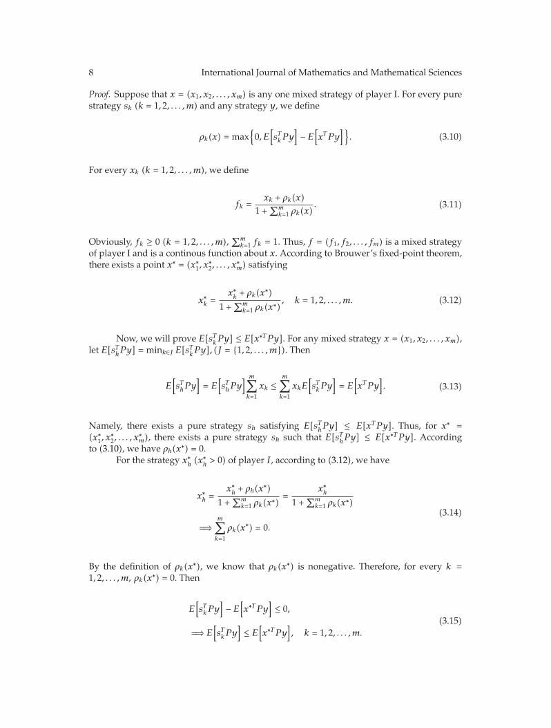
Above all, it can be simply summarized in Procedure 1.

5. Numerical Example

Game theory is widely applied in many fields, such as, economic and management problems,social policy, and international and national politics; sometimes players should consider thestate of uncertainty. A kind of games are usually characterized by rough payoffs. In thissection, we give an example of two-person zero-sum game with rough payoffs to illustratethe effectiveness of the algorithm introduced above. There is a game between player I andplayer II. When player I gives strategy i and player II gives strategy j, player II will givesome money to player I which is at least between cij and aij , or at most between bij and dij .The payoff matrix of player I is as follows

P =

⎡⎢⎢⎣ξ11 ξ12 ξ13

ξ21 ξ22 ξ23

ξ31 ξ32 ξ33

⎤⎥⎥⎦, (5.1)


Input: GA parameters: Npop-size, Pc, Pm and the cycle number GenmaxOutput: optimal sampling level, NPVbeging ← 0;initialization( ) by checking the feasiblity;evaluation(0);while (g ≤ Genmax) do

selection( );crossover( );mutation( );evaluation(g);g ← g + 1;

endOutput: the optimal solution

End

PROCEDURE 1: Procedure of genetic algorithm.

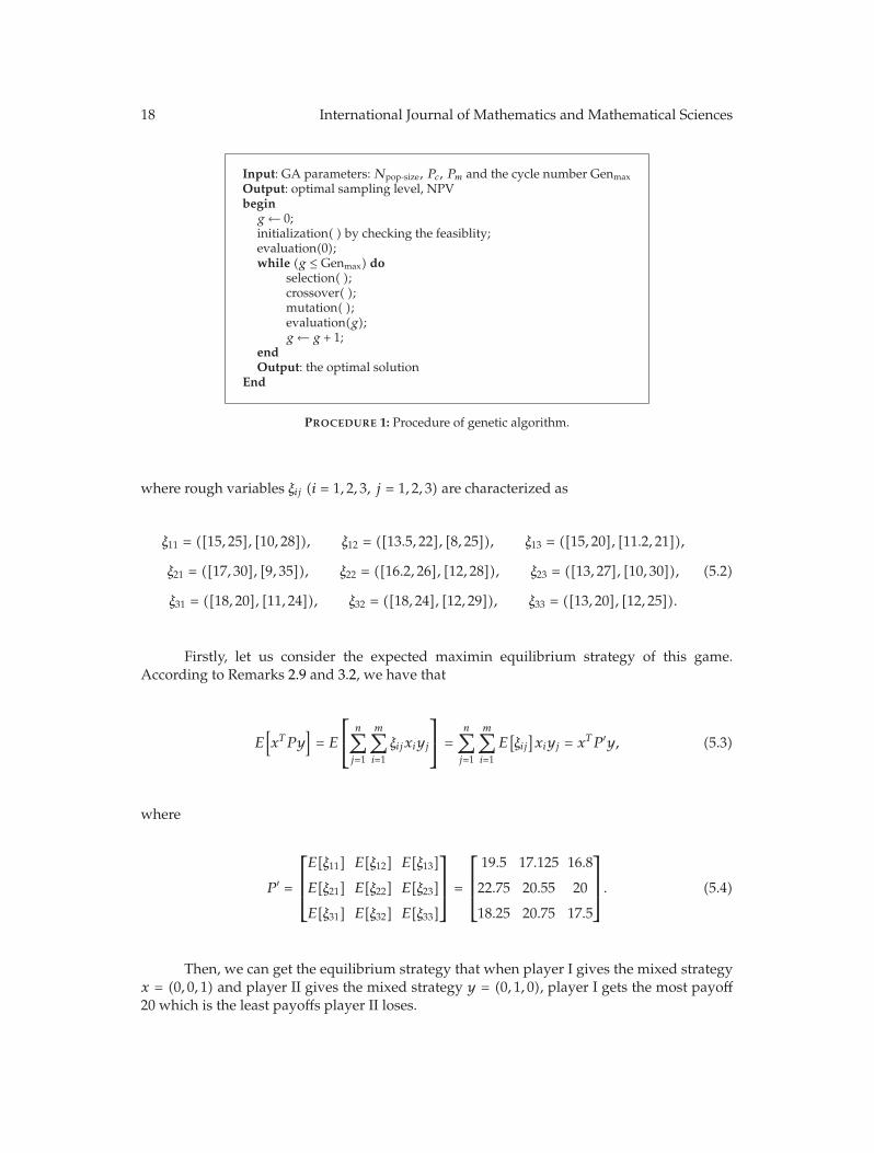
where rough variables ξij (i = 1, 2, 3, j = 1, 2, 3) are characterized as

ξ11 = ([15, 25], [10, 28]), ξ12 = ([13.5, 22], [8, 25]), ξ13 = ([15, 20], [11.2, 21]),

ξ21 = ([17, 30], [9, 35]), ξ22 = ([16.2, 26], [12, 28]), ξ23 = ([13, 27], [10, 30]),

ξ31 = ([18, 20], [11, 24]), ξ32 = ([18, 24], [12, 29]), ξ33 = ([13, 20], [12, 25]).

(5.2)

Firstly, let us consider the expected maximin equilibrium strategy of this game.According to Remarks 2.9 and 3.2, we have that

E[xTPy

]= E

⎡⎣

n∑j=1

m∑i=1

ξijxiyj

⎤⎦ =

n∑j=1

m∑i=1

E[ξij]xiyj = xTP ′y, (5.3)

where

P ′ =

⎡⎢⎢⎣E[ξ11] E[ξ12] E[ξ13]

E[ξ21] E[ξ22] E[ξ23]

E[ξ31] E[ξ32] E[ξ33]

⎤⎥⎥⎦ =

⎡⎢⎢⎣

19.5 17.125 16.8

22.75 20.55 20

18.25 20.75 17.5

⎤⎥⎥⎦. (5.4)

Then, we can get the equilibrium strategy that when player I gives the mixed strategyx = (0, 0, 1) and player II gives the mixed strategy y = (0, 1, 0), player I gets the most payoff20 which is the least payoffs player II loses.


Next, let us consider if this game has the r-trust maximin equilibrium strategy.According to Lemma 3.6, we have

A =

⎡⎢⎢⎣

15 13.5 15

17 16.2 13

18 18 13

⎤⎥⎥⎦, B =

⎡⎢⎢⎣

25 22 20

30 26 27

20 24 20

⎤⎥⎥⎦,

C =

⎡⎢⎢⎣

10 8 11.2

9 12 10

11 12 12

⎤⎥⎥⎦, D =

⎡⎢⎢⎣

28 25 21

35 28 30

24 29 25

⎤⎥⎥⎦.

(5.5)

Then we give five predetermined numbers r and discuss if the game exists a r-trustmaximin equilibrium strategy.

Case 1 (r = 5). Apparently, min cij = 8 and 0 ≤ x, y ≤ 1. Thus, for all (x, y), they satisfyxTCy ≥ 5. Based on Theorem 3.7, we know that all (x, y) are 5-trust maximin equilibriumstrategy of this game.

Case 2 (r = 40). Similarly, maxdij = 35 and 0 ≤ x, y ≤ 1. Thus, for all (x, y), they satisfyxTCy ≤ 40. Based on Theorem 3.8, we know that all (x, y) are 40-trust maximin equilibriumstrategy of this game.

Case 3 (r = 25). Because max bij = 30 and mindij = 21, for 0 ≤ x, y ≤ 1, not all (x, y) satisfyxTBy ≤ 25 ≤ xTDy. According to Theorem 3.9, we know that this game does not exist a25-trust maximin equilibrium strategy.

Case 4 (r = 12.5). Apparently, max cij = 12 and minaij = 13. Thus, for 0 ≤ x, y ≤ 1, all (x, y)satisfy xTCy ≤ 12.5 ≤ xTAy. Based on Theorem 3.11, we can get the following two problems

max12

⎛⎝

3∑i=1

3∑j=1

qiyjdij − 12.5p + 1

⎞⎠

s.t.

⎧⎪⎪⎪⎪⎪⎪⎪⎪⎪⎪⎨⎪⎪⎪⎪⎪⎪⎪⎪⎪⎪⎩

3∑i=1

3∑j=1

qiyjaij − 12.5p ≥ 0,

3∑i=1

3∑j=1

qiyjcij − 12.5p ≤ 0,

q1 + q2 + q3 = p,

q1, q2, q3 ≥ 0,

(5.6)


where y is any fixed strategy, p = 1/(xTDy − xTCy), qT = pxT ,

min12

⎛⎝

3∑i=1

3∑j=1

xitjdij − 12.5s + 1

⎞⎠

s.t.

⎧⎪⎪⎪⎪⎪⎪⎪⎪⎪⎪⎨⎪⎪⎪⎪⎪⎪⎪⎪⎪⎪⎩

3∑i=1

3∑j=1

xitjaij − 12.5s ≥ 0,

3∑i=1

3∑j=1

xitjcij − 12.5s ≤ 0,

t1 + t2 + t3 = s,

t1, t2, t3 ≥ 0,

(5.7)

where x is any fixed strategy, s = 1/(xTDy − xTCy), t = sy.Then we can make use of simplex method to get the optimal solutions of problems

(5.6) and (5.7). The optimal solutions is (x, y)T = (0.378, 0.124, 0.498, 0.397, 0.469, 0.194)T .

Case 5 (r = 19). Apparently, maxaij = 18 and min bij = 20. Thus, for 0 ≤ x, y ≤ 1, all (x, y)satisfy xTAy ≤ 19 ≤ xTBy. Then we can get two nonlinear programming problems.

For any fixed y

max12

⎛⎝∑3

i=1∑3

j=1 xiyjdij − 19∑3

i=1∑3

j=1 xiyj(dij − cij

) +∑3

i=1∑3

j=1 xiyjbij − 19∑3

i=1∑3

j=1 xiyj(bij − aij

)⎞⎠

s.t.

⎧⎪⎪⎪⎪⎪⎪⎪⎪⎪⎪⎨⎪⎪⎪⎪⎪⎪⎪⎪⎪⎪⎩

3∑i=1

3∑j=1

xiyjaij ≤ 19,

3∑i=1

3∑j=1

xiyjbij ≥ 19,

x1 + x2 + x3 = 1,

xi, yj ≥ 0.

(5.8)

For any fixed x,

min12

⎛⎝∑3

i=1∑3

j=1 xiyjdij − 19∑3

i=1∑3

j=1 xiyj(dij − cij

) +∑3

i=1∑3

j=1 xiyjbij − 19∑3

i=1∑3

j=1 xiyj(bij − aij

)⎞⎠

s.t.

⎧⎪⎪⎪⎪⎪⎪⎪⎪⎪⎪⎨⎪⎪⎪⎪⎪⎪⎪⎪⎪⎪⎩

3∑i=1

3∑j=1

xiyjaij ≤ 19,

3∑i=1

3∑j=1

xiyjbij ≥ 19,

y1 + y2 + y3 = 1,

xi, yj ≥ 0.

(5.9)


0.3880.3880.3880.3880.3880.3880.3880.3880.3880.3880.3880.3880.3880.3880.3880.3880.3880.3880.3880.4130.4130.4130.4130.4130.413

Gen

Obj

ecti

veva

lue

0.480.475

0.470.465

0.460.455

0.450.445

0.440.435

0.430.425

0.420.415

0.410.405

0.40.395

0.39

500 1000 1500 2000 2500 3000 3500 4000 4500

Figure 1: The results by GA.

For problems (5.8) and (5.9), we can solve them by using the rough simulation-based genetic algorithm. Let the number of chromosomes in every generation be 20,the probability of crossover 0.85 and of mutation 0.1. Then after a run of a geneticalgorithm computer program (5000 generations), we get the optimal solution (x, y)T =(0.178, 0.251, 0.571, 0.349, 0.479, 0.172)T and the objective value as shown in Figure 1.

6. Conclusion

In this paper, we have considered a class of two-person zero-sum matrix games with roughpayoffs. Firstly, we have given the definition of the game with rough payoffs and thenproposed two kinds of equilibrium strategy. Secondly, we have discussed wether the two-person zero-sum matrix games with rough payoffs exist the equilibrium strategy. Thirdly,we proposed the genetic algorithm to solve the most complicated case. It is an availableand efficient way to search the equilibrium of this kind of games with rough payoffs. Lastly,the numerical example illustrated well our research methods. We have only considered onekind of games with uncertain payoffs. Of course, there are many other games with uncertainpayoffs which need to be researched.

Acknowledgments

This research has been supported by the Key Program of NSFC (Grant no. 70831005) and theNational Science Foundation for Distinguished Young Scholars, China (Grant no. 70425005).

References

[1] J. von Neumann and O. Morgenstern, Theory of Games and Economic Behavior, John Wiley & Sons, NewYork, NY, USA, 1947.

[2] M. Peski, “Comparison of information structures in zero-sum games,” Games and Economic Behavior,vol. 62, no. 2, pp. 732–735, 2008.


[3] G. Owena and G. H. McCormick, “Finding a moving fugitive. A game theoretic representation ofsearch,” Computers & Operations Research, vol. 35, pp. 1994–1962, 2008.

[4] J. Berg and A. Engel, “Matrix games, mixed strategies, and statistical mechanics,” Physical ReviewLetters, vol. 81, pp. 4999–5002, 1998.

[5] L. Ein-Dor and L. Kanter, “Matrix games with nonuniform payoff distributions,” Physica A, vol. 302,no. 1–4, pp. 80–88, 2001.

[6] S. Takahashi, “The number of pure Nash equilibria in a random game with nondecreasing bestresponses,” Games and Economic Behavior, vol. 63, no. 1, pp. 328–340, 2008.

[7] J. Xu, “Zero sum two-person game with grey Number payoff Matrix in Linear Programming,” TheJournal of Grey System, vol. 10, no. 3, pp. 225–233, 1998.

[8] J. C. Harsanyi, “Games with incomplete information played by “BayesianY players. I. The basicmodel,” Management Science, vol. 14, pp. 159–182, 1967.

[9] A. K. Dhingra, S. S. Rao, et al., “A cooperative fuzzy game theoretic approach to multiple objectivedesign optimization,” European Journal of Operational Research, vol. 83, pp. 547–567, 1995.

[10] R. Espin, E. Fernandez, G. Mazcorro, et al., “A fuzzy approach to cooperative n-person games,”European Journal of Operational Research, vol. 176, no. 3, pp. 1735–1751, 2007.

[11] Z. Pawlak, Rough Sets, Kluwer Academic Publishers, Dordrecht, The Netherlands, 1991.[12] Z. Pawlak, “Rough sets,” International Journal of Computer and Information Sciences, vol. 11, no. 5, pp.

341–356, 1982.[13] H. Nurmi, J. Kacprzyk, and M. Fedrizzi, “Probabilistic, fuzzy and rough concepts in social choice,”

European Journal of Operational Research, vol. 95, pp. 264–277, 1996.[14] B. Liu, Theory and Practice of Uncertain Programming, Physica, New York, NY, USA, 2002.[15] L. Campos, “Fuzzy linear programming models to solve fuzzy matrix games,” Fuzzy Sets and Systems,

vol. 32, no. 3, pp. 275–289, 1989.[16] I. Nishizaki and M. Sakawa, Fuzzy and multiobjective games for conflict resolution, vol. 64 of Studies in

Fuzziness and Soft Computing, Physica, Heidelberg, Germany, 2001.[17] T. Maeda, “Characterization of the equilibrium strategy of the bimatrix game with fuzzy payoff,”

Journal of Mathematical Analysis and Applications, vol. 251, no. 2, pp. 885–896, 2000.[18] R. P. Luce and H. Raiffa, Games and Decisions, John Wiley & Sons, New York, NY, USA, 1957.[19] T. Parthasarathy and T. E. S. Raghavan, Some Topics in Two-Person Games, American Elsevier

Publishing, New York, NY, USA, 1971.[20] R. Slowinski, D. Vanderpooten, et al., “A generalized definition of rough approximations based on

similarity,” IEEE Transactions on Knowledge and Data Engineering, vol. 12, no. 2, pp. 331–336, 2000.[21] E. Polak, “A survey of methods of feasible directions for the solution of optimal control problems,”

IEEE Transactions on Automatic Control, vol. 17, no. 5, pp. 591–596, 1972.[22] G. G. L. Meyer and L. J. Podrazik, “A parallel frank-wolfe/gradient projection mthod for optimal

control,” in Proceedings of the 30th Conterence on Decision and Contro, pp. 1705–1710, Brighton, UK,1991.

[23] M. Gen and R. Cheng, Gennetic Algorithms and Engineering Optimization, John Wiley & Sons, NewYork, NY, USA, 2000.

[24] J. Li, J. Xu, and M. Gen, “A class of multiobjective linear programming model with fuzzy randomcoefficients,” Mathematical and Computer Modelling, vol. 44, no. 11-12, pp. 1097–1113, 2006.

Submit your manuscripts athttp://www.hindawi.com

Hindawi Publishing Corporationhttp://www.hindawi.com Volume 2014

MathematicsJournal of


Mathematical Problems in Engineering

Hindawi Publishing Corporationhttp://www.hindawi.com

Differential EquationsInternational Journal of

Volume 2014

Applied MathematicsJournal of


Probability and StatisticsHindawi Publishing Corporationhttp://www.hindawi.com Volume 2014

Journal of


Mathematical PhysicsAdvances in

Complex AnalysisJournal of


OptimizationJournal of


CombinatoricsHindawi Publishing Corporationhttp://www.hindawi.com Volume 2014

International Journal of


Operations ResearchAdvances in

Journal of


Function Spaces

Abstract and Applied AnalysisHindawi Publishing Corporationhttp://www.hindawi.com Volume 2014

International Journal of Mathematics and Mathematical Sciences


The Scientific World JournalHindawi Publishing Corporation http://www.hindawi.com Volume 2014


Algebra

Discrete Dynamics in Nature and Society



Decision SciencesAdvances in

Discrete MathematicsJournal of

Hindawi Publishing Corporationhttp://www.hindawi.com

Volume 2014 Hindawi Publishing Corporationhttp://www.hindawi.com Volume 2014

Stochastic AnalysisInternational Journal of

Research Article A Class of Two-Person Zero-Sum Matrix ...

Documents

Transcript of Research Article A Class of Two-Person Zero-Sum Matrix ...