Report of the European Network of Forensic Science Institutes (ENSFI): formulation and testing of...

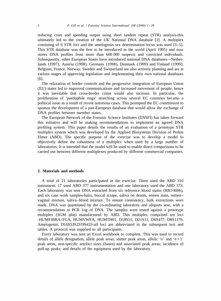
Forensic Science International108 (2000) 1–29

www.elsevier.com/ locate / forsciint

Report of the European Network of Forensic ScienceInstitutes (ENSFI): formulation and testing of

principles to evaluate STR multiplexes

*Peter Gill , Rebecca Sparkes, Lyn Fereday, David J. Werrett

Research and Development, Forensic Science Service, Priory House, Gooch Street North,Birmingham B56 QQ, UK

Received 10 May 1999; received in revised form 29 September 1999; accepted 5 October 1999

Abstract

This paper describes a collaborative exercise organised under the auspices of the EuropeanNetwork of Forensic Science Institutes (ENFSI). The purpose of this EU (European Union)funded group is to carry out research to enable STR loci to be compared between Europeanlaboratories, ultimately leading to the formation of a pan-European database. Accordingly, anexercise was designed to evaluate a prototype STR multiplex system manufactured by AppliedBiosystems (ABD). Each laboratory was sent 12 samples to analyse along with a multiplex kit. Ofspecific interest was the definition of parameters to define the efficiency of the system. Stutter,split allelic peaks (differing by one base), pull-up, heterozygous balance and between locusbalance were all objectively measured. Once the important parameters are defined it is possible todirectly compare performances of different multiplexes and the different laboratories carrying outthe tests. Since the multiplex used was a prototype system, this exercise cannot be regarded as aproficiency test. 2000 Elsevier Science Ireland Ltd. All rights reserved.

Keywords: ENSFI; STR; Multiplex; Validation; Quality

1. Introduction

The proven ability to multiplex short tandem repeats (STRs) [1] was a key step in

*Corresponding author. Tel.: 144-121-607-6871; fax: 144-121-622-2051.E-mail address: [email protected] (P. Gill)

0379-0738/00/$ – see front matter 2000 Elsevier Science Ireland Ltd. All rights reserved.PI I : S0379-0738( 99 )00186-3

2 P. Gill et al. / Forensic Science International 108 (2000) 1 –29

reducing costs and speeding output using short tandem repeat (STR) analysis-thisultimately led to the creation of the UK National DNA database [2]. A multiplexconsisting of 6 STR loci and the amelogenin sex determination locus was used [3–5].This STR database was the first to be introduced in the world (April 1995) and nowstores DNA profiles from more than 600 000 suspects and convicted individuals.Subsequently, other European States have introduced national DNA databases—Nether-lands (1997), Austria (1998), Germany (1998), Denmark (1999) and Finland (1999).Belgium, France, Norway, Sweden and Switzerland are also actively planning and are atvarious stages of approving legislation and implementing their own national databases[6].

The relaxation of border controls and the progressive integration of European Union(EU) states led to improved communications and increased movement of people, henceit was inevitable that cross-border crime would also increase. In particular, theproliferation of ‘paedophile rings’ stretching across several EC countries became apolitical issue as a result of recent notorious cases. This prompted the EC commission tosponsor the development of a pan-European database that would allow the exchange ofDNA profiles between member states.

The European Network of the Forensic Science Institutes (ENSFI) has taken forwardthis initiative and will be making recommendations to implement an agreed DNAprofiling system. This paper details the results of an evaluation of a prototype STRmultiplex system which was developed by the Applied Biosystems Division of PerkinElmer (ABD). The specific purpose of the exercise was to develop a model toobjectively define the robustness of a multiplex when used by a large number oflaboratories. It is intended that the model will be used to enable direct comparisons to becarried out between different multiplexes produced by different commercial companies.

2. Materials and methods

A total of 21 laboratories participated in the exercise. Three used the ABD 310instrument; 17 used ABD 377 instrumentation and one laboratory used the ABD 373.Each laboratory was sent DNA extracted from six reference blood stains (RB1-RB6),and six case work samples-hairs, buccal scrape, saliva on denim, semen stain, semen–vaginal mixture, saliva–blood mixture. To ensure consistency, bulk extractions weremade. DNA was quantitated by the co-ordinating laboratory and aliquots sent, with arecommendation to PCR 1ng of DNA. The samples were tested against a prototypemultiplex (SGM plus) manufactured by ABD. This multiplex comprised ten loci-HUMFIBRA/FGA, HUMVWFA, HUMTH01, D18S51, D21S11, D6S477, D8S1179,Amelogenin, D16S539,D19S433-all loci are abbreviated in the subsequent text andtables. A protocol was supplied to all participants.

Every laboratory was sent an Excel workbook to complete. This was used to recorddetails of allele designation, allele peak areas, stutter peak areas, allelic ‘n’ and ‘n11’peak areas, non-specific artefact sizes (bases) and associated peak areas; incidence ofpull-up peaks; and details of the equipment used by the laboratory.

P. Gill et al. / Forensic Science International 108 (2000) 1 –29 3

2.1. Statistical analysis

Of particular interest was the incidence of artefacts, stutters and ‘n’ bands measuredas a proportion of the total number of loci examined, along with their peak areas relativeto associated allelic peaks. This information was expressed predominantly by use of boxand whiskers plots [7] using MinitabE software.

Box and whiskers plots are useful graphic tools which enable multiple comparisons ofdata to be carried out. The edges of the box are defined the first and third quartiles ie thebox encloses 50% of the data. A line inside the box defines the median. The whiskersare defined by Q1-1.5(Q11Q3) and Q311.5(Q11Q3) where Q1 and Q3 are first andthird quartiles respectively. The points which lie outside the ‘fences’ defined by thewhiskers are ‘outlier’ data. The outlier data may be atypical and merit specialconsideration.

Other standard procedures were used to analyse data included use of scatterplots andhistograms.

2.2. Definitions

The purpose of the analysis was to evaluate characteristics of multiplexes acrossdifferent laboratories using a range of instrumentation. It was of interest to identifylaboratory specific variation as well between laboratory variation.

Performance of loci was defined by assessment of the following [8]:

1. ‘n’ allelic band2. ‘n 1 1’ allelic band3. stutter4. Pull-up5. heterozygous balance6. Inter-locus balance

3. Results

3.1. Discrepancies

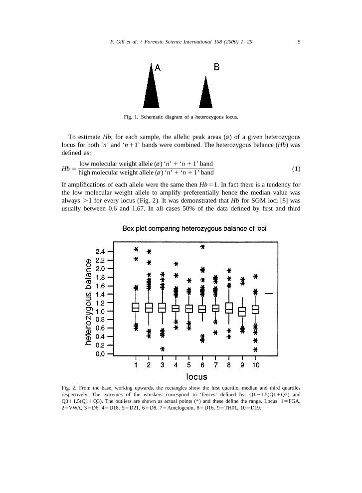
All allele designations of loci were checked. Any discrepancies were noted (Table 1)and the laboratory was contacted for explanations. Two laboratories reported transcrip-tion errors. Another laboratory reported a D18 homozygote 16; the correct genotype was16,19. However, this was not a transcription error-the cause of the discrepancy remainsunknown. In addition, alleles scored as D6 13 and D21 28 by laboratory 16 were nottranscription errors-the profiles were correctly scored but inconsistent with otherlaboratories. The discrepancies recorded by laboratory 10 were attributed to a very poorDNA profile (i.e. alleles were not properly distinguished from the background noise).


Table 1A list of allele designation discrepancies recorded with explanations if known

Laboratory Sample Locus Reported Actual Reasonresult result

Notes of discrepancies1 saliva–blood mixture VWA 22 23 probably stutter3 RB1 D18 16, 16 16, 19 unknown-not transcription error6 semen–vaginal mixture VWA 16, 16 16, 19 transcription error

10 RB3 VWA 16, 17 14, 19 v. poor DNA profile10 RB3 D6 15, 19 17, 18 v. poor DNA profile10 RB3 D18 12, 13 12, 15 v. poor DNA profile10 RB3 D16 11, 13 9, 14 v. poor DNA profile10 RB3 D19 14, 14 14, 14.2 v. poor DNA profile12 RB1 D21S11 28, 28 28, 29 transcription error16 saliva–blood mixture D8 10, 12 10, 13 unknown-not transcription error16 RB5 D6 13 13.2 unknown-not transcription error16 RB5 D21S11 28 28.2 unknown-not transcription error

3.2. Analysis of pull-up

Pull-up is a software artefact that refers to the presence of a band in a region which isnormally occupied by the alleles of a given locus. The band lies directly underneath theallelic band and is always lower in peak area.

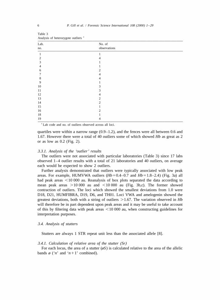
Pull-up was observed in the read regions of all loci. The highest incidence was at D6,D8, D19 and Amelogenin; D18 had the lowest incidence (Table 2).

3.3. Analysis of heterozygote balance

For a given locus (Fig. 1) the heterozygote balance (Hb) can be calculated by twodifferent ways. If A is low molecular weight and B is high molecular weight, then theproportion øA/øB can be calculated, (where ø5peak area).

Table 2The proportion of loci displaying pull-up is recorded

Locus Reference bloods Crime samples Combined

Proportion of pullups Proportion of pullups Proportion of pullupsper locus per locus per locus

FGA 0.028 0.016 0.045VWA 0.008 0.032 0.040D6 0.061 0.121 0.182D18 0.004 0.004 0.008D21 0.020 0.049 0.069D86 0.052 0.100 0.152Amelo 0.033 0.096 0.129D16 0.033 0.017 0.050Th01 0.004 0.012 0.016D19 0.028 0.096 0.124


Fig. 1. Schematic diagram of a heterozygous locus.

To estimate Hb, for each sample, the allelic peak areas (ø) of a given heterozygouslocus for both ‘n’ and ‘n11’ bands were combined. The heterozygous balance (Hb) wasdefined as:

low molecular weight allele (ø) ‘n’ 1 ‘n 1 1’ band]]]]]]]]]]]]]]Hb 5 (1)high molecular weight allele (ø) ‘n’ 1 ‘n 1 1’ band

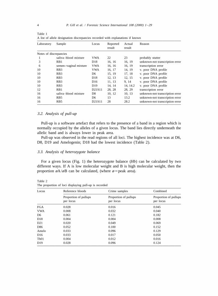
If amplifications of each allele were the same then Hb51. In fact there is a tendency forthe low molecular weight allele to amplify preferentially hence the median value wasalways .1 for every locus (Fig. 2). It was demonstrated that Hb for SGM loci [8] wasusually between 0.6 and 1.67. In all cases 50% of the data defined by first and third

Fig. 2. From the base, working upwards, the rectangles show the first quartile, median and third quartilesrespectively. The extremes of the whiskers correspond to ‘fences’ defined by: Q121.5(Q11Q3) andQ311.5(Q11Q3). The outliers are shown as actual points (*) and these define the range. Locus: 15FGA,25VWA, 35D6, 45D18, 55D21, 65D8, 75Amelogenin, 85D16, 95TH01, 105D19.


Table 3aAnalysis of heterozygote outliers

Lab. No. ofno. observations

1 12 43 14 16 27 48 49 1

10 311 312 413 214 215 116 218 119 4

a Lab code and no. of outliers observed across all loci.

quartiles were within a narrow range (0.9–1.2), and the fences were all between 0.6 and1.67. However there were a total of 40 outliers some of which showed Hb as great as 2or as low as 0.2 (Fig. 2).

3.3.1. Analysis of the ‘outlier’ resultsThe outliers were not associated with particular laboratories (Table 3) since 17 labs

observed 1–4 outlier results with a total of 21 laboratories and 40 outliers, on averageeach would be expected to show 2 outliers.

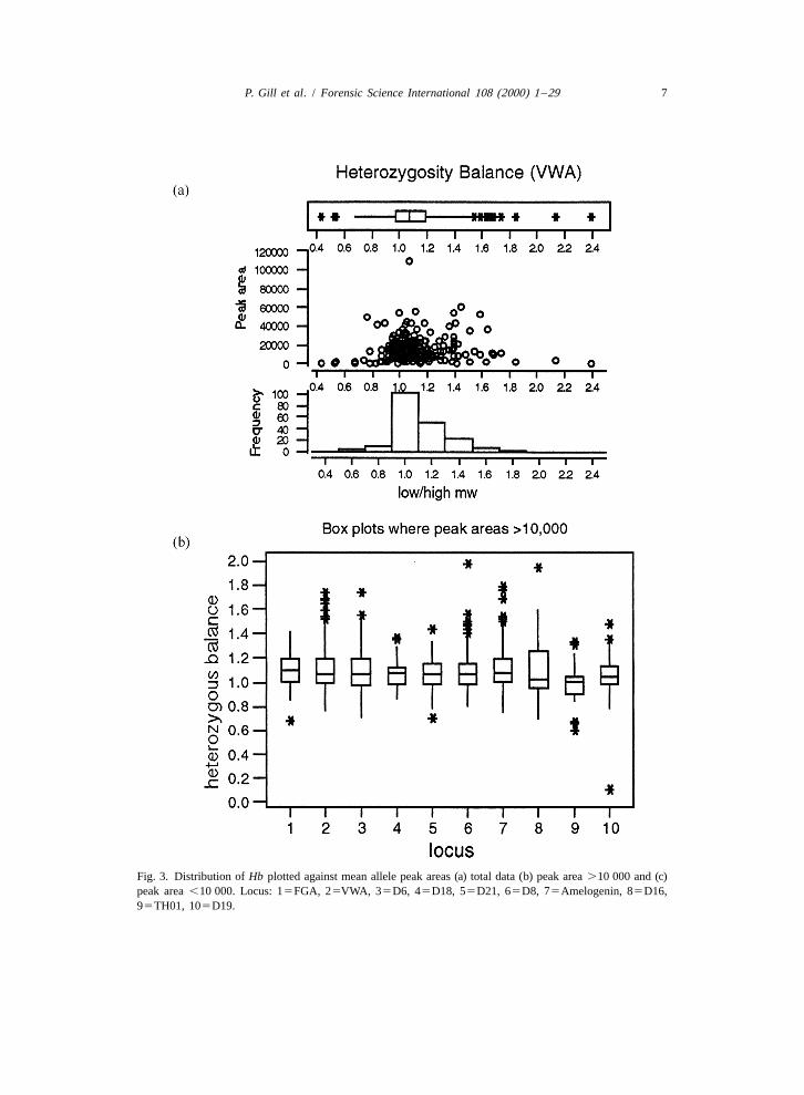
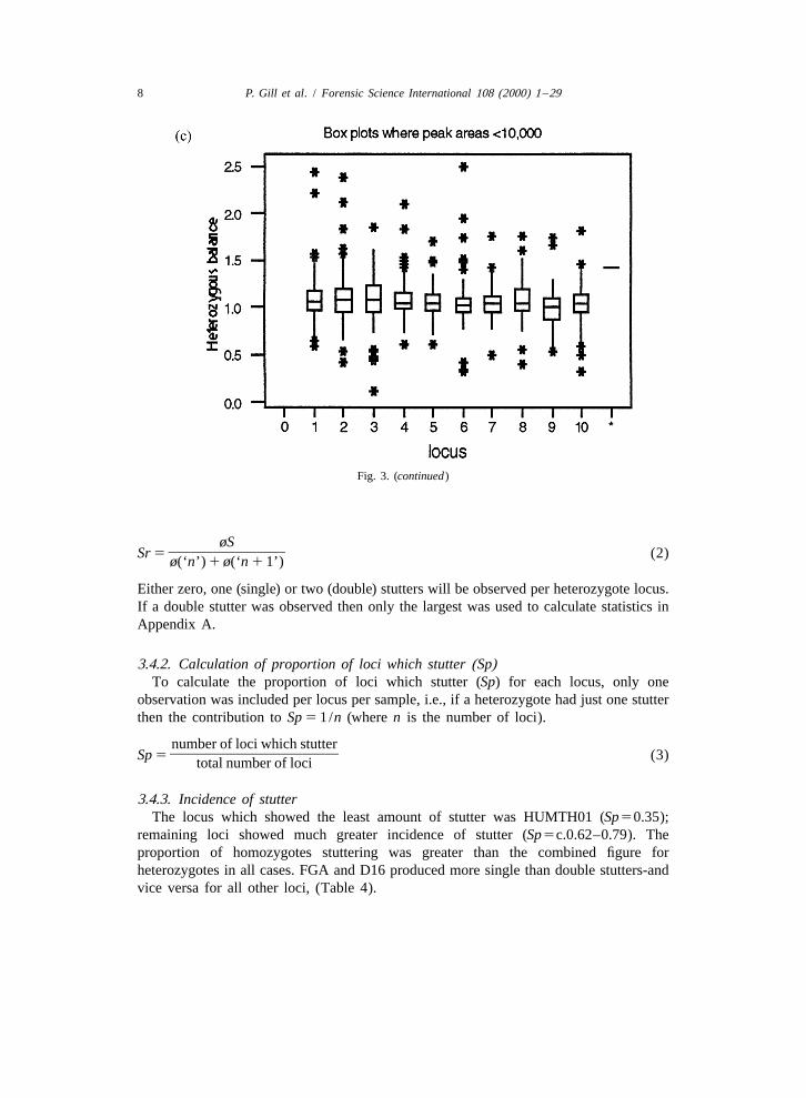
Further analysis demonstrated that outliers were typically associated with low peakareas. For example, HUMVWA outliers (Hb50.4–0.7 and Hb51.8–2.4) (Fig. 3a) allhad peak areas ,10 000 au. Reanalysis of box plots separated the data according tomean peak areas .10 000 au and ,10 000 au (Fig. 3b,c). The former showedcontraction of outliers. The loci which showed the smallest deviations from 1.0 wereD18, D21, HUMFIBRA, D19, D6, and TH01. Loci VWA and amelogenin showed thegreatest deviations, both with a string of outliers .1.67. The variation observed in Hbwill therefore be in part dependent upon peak areas and it may be useful to take accountof this by filtering data with peak areas ,10 000 au, when constructing guidelines forinterpretation purposes.

3.4. Analysis of stutters

Stutters are always 1 STR repeat unit less than the associated allele [8].

3.4.1. Calculation of relative area of the stutter (Sr)For each locus, the area of a stutter (øS) is calculated relative to the area of the allelic

bands ø (‘n’ and ‘n11’ combined).


Fig. 3. Distribution of Hb plotted against mean allele peak areas (a) total data (b) peak area .10 000 and (c)peak area ,10 000. Locus: 15FGA, 25VWA, 35D6, 45D18, 55D21, 65D8, 75Amelogenin, 85D16,95TH01, 105D19.


Fig. 3. (continued)

øS]]]]]]Sr 5 (2)ø(‘n’) 1 ø(‘n 1 1’)

Either zero, one (single) or two (double) stutters will be observed per heterozygote locus.If a double stutter was observed then only the largest was used to calculate statistics inAppendix A.

3.4.2. Calculation of proportion of loci which stutter (Sp)To calculate the proportion of loci which stutter (Sp) for each locus, only one

observation was included per locus per sample, i.e., if a heterozygote had just one stutterthen the contribution to Sp 5 1/n (where n is the number of loci).

number of loci which stutter]]]]]]]]Sp 5 (3)total number of loci

3.4.3. Incidence of stutterThe locus which showed the least amount of stutter was HUMTH01 (Sp50.35);

remaining loci showed much greater incidence of stutter (Sp5c.0.62–0.79). Theproportion of homozygotes stuttering was greater than the combined figure forheterozygotes in all cases. FGA and D16 produced more single than double stutters-andvice versa for all other loci, (Table 4).


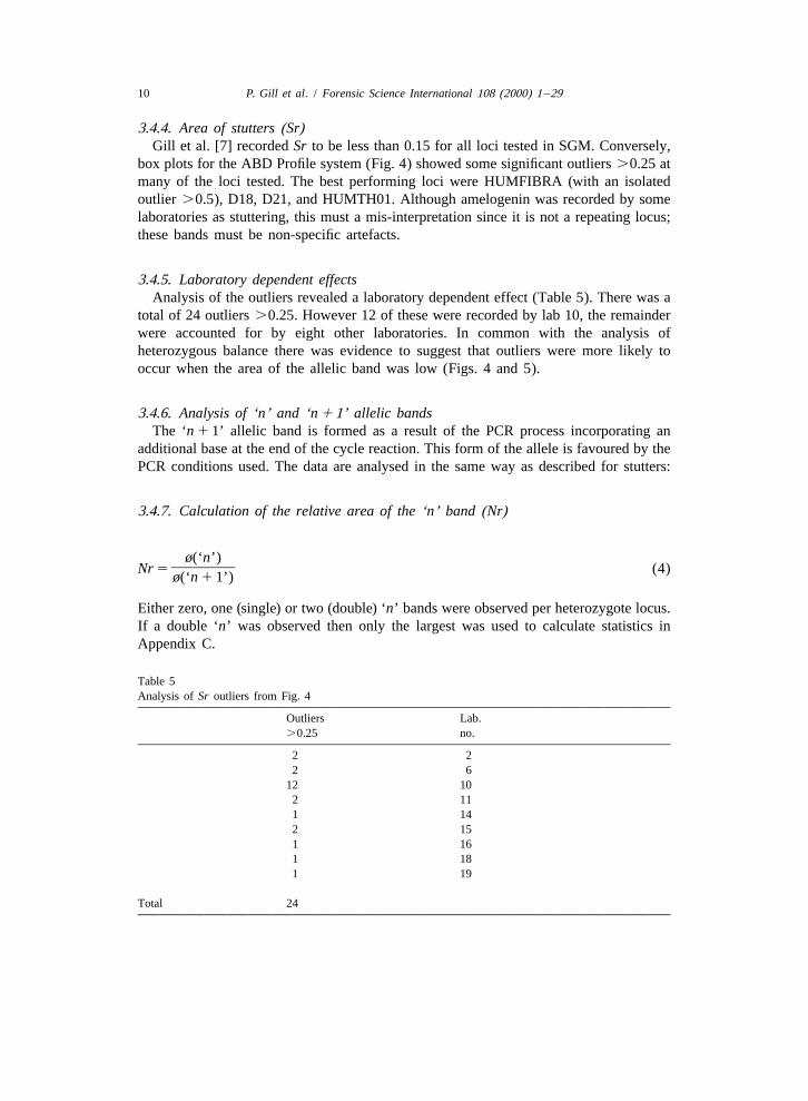
Table 4Analysis of stutter in homozygotes and heterozygotes. The proportion of stutters relative to the total number ofhomozygotes is given in parentheses in column 2; heterozygotes in columns 3 and 4. Total proportion of stutter(Sp) is in column 5

Locus No. of stutters No. of double Totalstutters (hets) no. loci

No. of homs No. of singlestuttering stutters (hets)

FGA 31 (0.76) 65 (0.35) 54 (0.29) 229 (0.66)VWA 16 (0.76) 47 (0.22) 110 (0.52) 231 (0.75)D6 17 (0.77) 34 (0.17) 116 (0.56) 228 (0.73)D18 0 62 (0.27) 79 (0.35) 228 (0.62)D21 16 (0.73) 53 (0.26) 90 (0.44) 228 (0.7)D8 17 (0.77) 36 (0.17) 105 (0.51) 228 (0.69)Amelogenin 0 18 (0.08) 0 231 (0.08)D16 85 (0.67) 35 (0.34) 15 (0.15) 229 (0.59)TH01 23 (0.37) 31 (0.19) 26 (0.16) 227 (0.35)D19 54 (0.64) 46 (0.32) 54 (0.37) 231 (0.67)

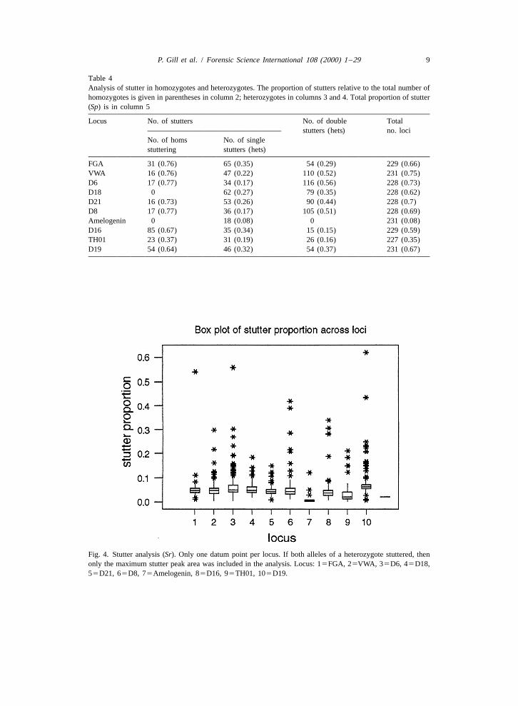
Fig. 4. Stutter analysis (Sr). Only one datum point per locus. If both alleles of a heterozygote stuttered, thenonly the maximum stutter peak area was included in the analysis. Locus: 15FGA, 25VWA, 35D6, 45D18,55D21, 65D8, 75Amelogenin, 85D16, 95TH01, 105D19.


3.4.4. Area of stutters (Sr)Gill et al. [7] recorded Sr to be less than 0.15 for all loci tested in SGM. Conversely,

box plots for the ABD Profile system (Fig. 4) showed some significant outliers .0.25 atmany of the loci tested. The best performing loci were HUMFIBRA (with an isolatedoutlier .0.5), D18, D21, and HUMTH01. Although amelogenin was recorded by somelaboratories as stuttering, this must a mis-interpretation since it is not a repeating locus;these bands must be non-specific artefacts.

3.4.5. Laboratory dependent effectsAnalysis of the outliers revealed a laboratory dependent effect (Table 5). There was a

total of 24 outliers .0.25. However 12 of these were recorded by lab 10, the remainderwere accounted for by eight other laboratories. In common with the analysis ofheterozygous balance there was evidence to suggest that outliers were more likely tooccur when the area of the allelic band was low (Figs. 4 and 5).

3.4.6. Analysis of ‘n’ and ‘n 1 1’ allelic bandsThe ‘n 1 1’ allelic band is formed as a result of the PCR process incorporating an

additional base at the end of the cycle reaction. This form of the allele is favoured by thePCR conditions used. The data are analysed in the same way as described for stutters:

3.4.7. Calculation of the relative area of the ‘n’ band (Nr)

ø(‘n’)]]]Nr 5 (4)ø(‘n 1 1’)

Either zero, one (single) or two (double) ‘n’ bands were observed per heterozygote locus.If a double ‘n’ was observed then only the largest was used to calculate statistics inAppendix C.

Table 5Analysis of Sr outliers from Fig. 4

Outliers Lab..0.25 no.

2 22 6

12 102 111 142 151 161 181 19

Total 24


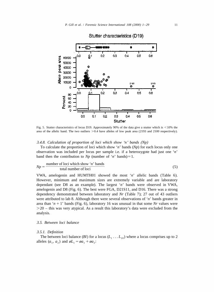
Fig. 5. Stutter characteristics of locus D19. Approximately 90% of the data give a stutter which is ,10% thearea of the allelic band. The two outliers .0.4 have alleles of low peak area (2193 and 2100 respectively).

3.4.8. Calculation of proportion of loci which show ‘n’ bands (Np)To calculate the proportion of loci which show ‘n’ bands (Np) for each locus only one

observation was included per locus per sample i.e. if a heterozygote had just one ‘n’band then the contribution to Np (number of ‘n’ bands)51.

number of loci which show ‘n’ bands]]]]]]]]]]Np 5 (5)total number of loci

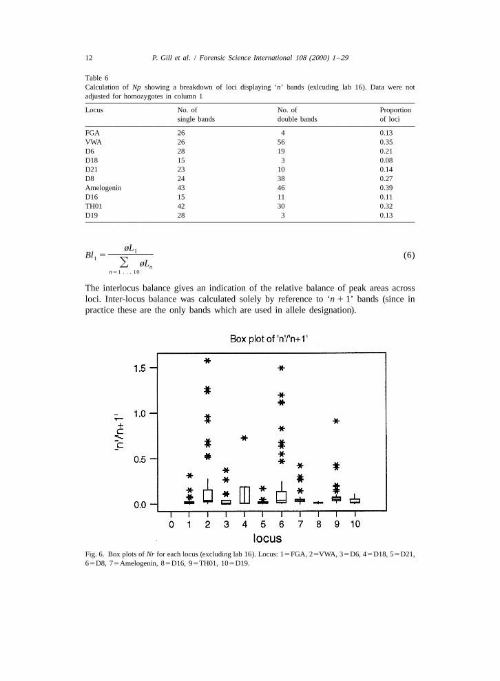
VWA, amelogenin and HUMTH01 showed the most ‘n’ allelic bands (Table 6).However, minimum and maximum sizes are extremely variable and are laboratorydependant (see D8 as an example). The largest ‘n’ bands were observed in VWA,amelogenin and D8 (Fig. 6). The best were FGA, D21S11, and D16. There was a strongdependency demonstrated between laboratory and Nr (Table 7); 27 out of 43 outlierswere attributed to lab 8. Although there were several observations of ‘n’ bands greater inarea than ‘n 1 1’ bands (Fig. 6), laboratory 16 was unusual in that some Nr values were.20 – this was very atypical. As a result this laboratory’s data were excluded from theanalysis.

3.5. Between loci balance

3.5.1. DefinitionThe between loci balance (Bl) for a locus (L . . . L ) where a locus comprises up to 21 10

alleles (a , a ) and øL 5 øa 1 øa :1 2 1 1 2


Table 6Calculation of Np showing a breakdown of loci displaying ‘n’ bands (exlcuding lab 16). Data were notadjusted for homozygotes in column 1

Locus No. of No. of Proportionsingle bands double bands of loci

FGA 26 4 0.13VWA 26 56 0.35D6 28 19 0.21D18 15 3 0.08D21 23 10 0.14D8 24 38 0.27Amelogenin 43 46 0.39D16 15 11 0.11TH01 42 30 0.32D19 28 3 0.13

øL1]]]]Bl 5 (6)1 O øLnn51 . . . 10

The interlocus balance gives an indication of the relative balance of peak areas acrossloci. Inter-locus balance was calculated solely by reference to ‘n 1 1’ bands (since inpractice these are the only bands which are used in allele designation).

Fig. 6. Box plots of Nr for each locus (excluding lab 16). Locus: 15FGA, 25VWA, 35D6, 45D18, 55D21,65D8, 75Amelogenin, 85D16, 95TH01, 105D19.


Table 7Analysis of outliers (Nr) by lab, with details of loci affected and range of ‘n’ / ‘n 1 1’

Lab No. of Loci Rangeinstances affected

1 1 FGA 0.313 1 D6 0.17 1 D21 0.178 27 not Th01 0.15–1.57

10 1 D21 0.1613 9 Th01 0.13–0.6917 2 FGA 0.05–0.0921 1 FGA 0.08

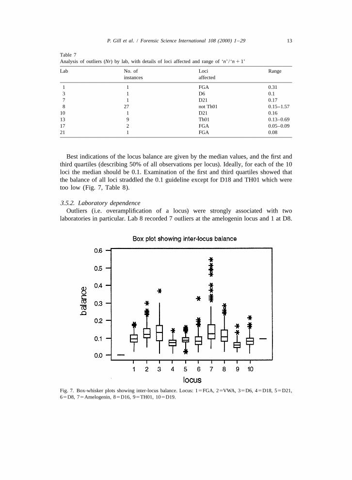
Best indications of the locus balance are given by the median values, and the first andthird quartiles (describing 50% of all observations per locus). Ideally, for each of the 10loci the median should be 0.1. Examination of the first and third quartiles showed thatthe balance of all loci straddled the 0.1 guideline except for D18 and TH01 which weretoo low (Fig. 7, Table 8).

3.5.2. Laboratory dependenceOutliers (i.e. overamplification of a locus) were strongly associated with two

laboratories in particular. Lab 8 recorded 7 outliers at the amelogenin locus and 1 at D8.

Fig. 7. Box-whisker plots showing inter-locus balance. Locus: 15FGA, 25VWA, 35D6, 45D18, 55D21,65D8, 75Amelogenin, 85D16, 95TH01, 105D19.


Table 8Details of outliers observed in Fig. 7. Locus 15FGA, 25VWA, 35D6, 45D18, 55D21, 65D8, 75

Amelogenin, 85D16, 95TH01, 105D19

Lab. No. of outliers Loci

1 3 1, 5, 102 4 2, 6, 74 5 2, 6, 8, 105 1 16 1 57 1 58 8 6, 7

10 10 2, 5, 6, 9, 1011 2 5, 612 2 213 4 5, 6, 715 2 116 3 2, 817 1 118 2 4, 519 2 2, 920 1 321 1 1

Lab 10 recorded outliers at five different loci otherwise 1 or more outliers could beattributed to 17 laboratories (Table 9). Bearing in mind that the exercise incorporatedstains which may be partially degraded it would be expected that some divergencewould be seen.

3.6. Non-specific artefacts

Non-specific artefacts are defined as bands that do not fall under any of the previouscategories described. They may be produced by non-specific priming against DNA(possibly against non-human DNA). Some laboratories reported no artefacts at all, butwhen they were observed, often multiple bands were observed in the same sample. For

Table 9Summary statistics of inter-locus balance

Locus N Mean Median St. Dev. Min Max Q1 Q3

FGA 221 0.10 0.09 0.03 0.02 0.18 0.08 0.11VWA 221 0.13 0.12 0.04 0.05 0.30 0.10 0.15D6 220 0.13 0.13 0.06 0.01 0.37 0.08 0.17D18 221 0.07 0.07 0.03 0.01 0.14 0.05 0.09D21 221 0.09 0.09 0.02 0.02 0.16 0.07 0.10D8 221 0.09 0.08 0.04 0.02 0.33 0.06 0.10Amelogenin 221 0.15 0.12 0.08 0.04 0.55 0.09 0.17D16 221 0.11 0.11 0.05 0.02 0.28 0.08 0.14TH01 221 0.06 0.06 0.02 0.01 0.17 0.04 0.07D19 221 0.08 0.08 0.03 0.01 0.21 0.06 0.1


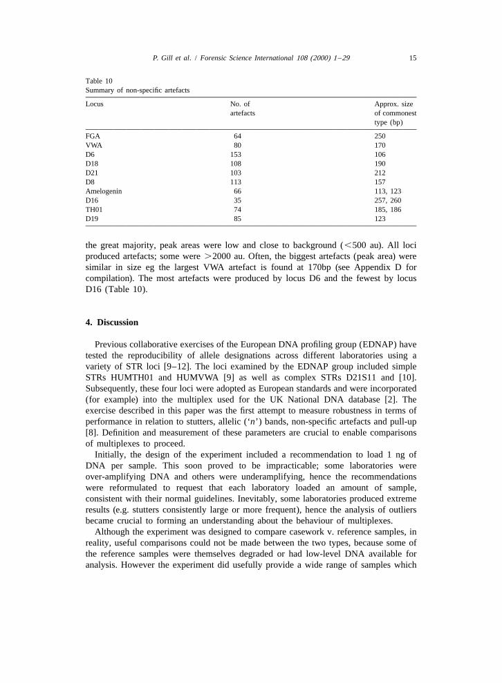
Table 10Summary of non-specific artefacts

Locus No. of Approx. sizeartefacts of commonest

type (bp)

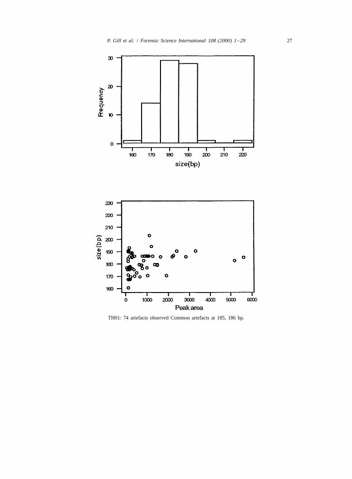
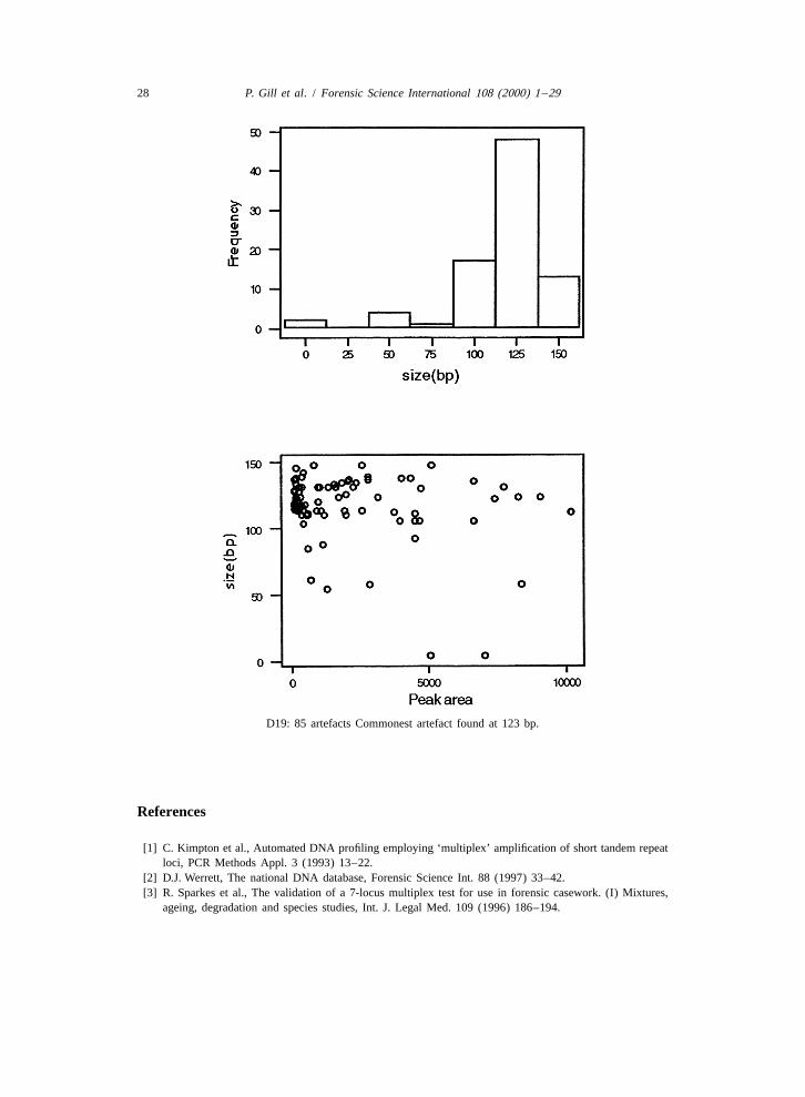
FGA 64 250VWA 80 170D6 153 106D18 108 190D21 103 212D8 113 157Amelogenin 66 113, 123D16 35 257, 260TH01 74 185, 186D19 85 123

the great majority, peak areas were low and close to background (,500 au). All lociproduced artefacts; some were .2000 au. Often, the biggest artefacts (peak area) weresimilar in size eg the largest VWA artefact is found at 170bp (see Appendix D forcompilation). The most artefacts were produced by locus D6 and the fewest by locusD16 (Table 10).

4. Discussion

Previous collaborative exercises of the European DNA profiling group (EDNAP) havetested the reproducibility of allele designations across different laboratories using avariety of STR loci [9–12]. The loci examined by the EDNAP group included simpleSTRs HUMTH01 and HUMVWA [9] as well as complex STRs D21S11 and [10].Subsequently, these four loci were adopted as European standards and were incorporated(for example) into the multiplex used for the UK National DNA database [2]. Theexercise described in this paper was the first attempt to measure robustness in terms ofperformance in relation to stutters, allelic (‘n’) bands, non-specific artefacts and pull-up[8]. Definition and measurement of these parameters are crucial to enable comparisonsof multiplexes to proceed.

Initially, the design of the experiment included a recommendation to load 1 ng ofDNA per sample. This soon proved to be impracticable; some laboratories wereover-amplifying DNA and others were underamplifying, hence the recommendationswere reformulated to request that each laboratory loaded an amount of sample,consistent with their normal guidelines. Inevitably, some laboratories produced extremeresults (e.g. stutters consistently large or more frequent), hence the analysis of outliersbecame crucial to forming an understanding about the behaviour of multiplexes.

Although the experiment was designed to compare casework v. reference samples, inreality, useful comparisons could not be made between the two types, because some ofthe reference samples were themselves degraded or had low-level DNA available foranalysis. However the experiment did usefully provide a wide range of samples which


emulated the full range which may be reasonably expected in casework. No attempt wasmade in this paper to analyse differences between the sample types, however.

The data were collated in a format designed to simplify analysis. The performance ofa multiplex can effectively be defined by calculating 5 or 6 parameters for each of thecharacteristics described, and the results can be visually illustrated by box-whisker plots.The parameters are (a) Median, first quartile, third quartile, the upper fence (and lowerfence for heterozygous balance), the minimum and the maximum (Appendices A–C).Strictly speaking the parameters refer only to the samples employed in this particulartest. Once defined then testing of subsequent multiplexes can follow by comparison (Fig.7) (Tables 8 and 9).

It is suggested that the best performance indicator of a multiplex is given by themedian and quartile observations; the outliers consist of data which are essentiallyatypical and may be laboratory-dependent. However in order to be comparable, andbearing in mind the variation seen between laboratories, subsequent tests using differentmultiplex systems should follow the same format previously described. In particular:

(a) The same sample extracts must be used.(b) Each laboratory must use an equivalent quantity of sample per analysis persample.(c) The same equipment must be used.

Provided that conditions are constant within each laboratory then any variation whichremains in the data should be attributable to the multiplex itself.

Since performance is laboratory-dependent, subsequent testing to compare differentmultiplexes will be needed to assess between laboratory variation in greater detail. i.e.any increase or decrease in performance of a multiplex has to be considered relative tothe within laboratory performance. In principle, this analysis can follow the methodsoutlined above, but it may be necessary to score the key parameters for each laboratoryseparately so that comparisons can be made in a pairwise manner.

In addition the study could easily be extended to compare the performances ofindividual laboratories. This could form the basis of a quality control system wherelaboratories may be assessed against the medians obtained for all of the key parametersoutlined in this paper.

4.1. Current work and future direction

The analysis detailed in this paper was carried out using a prototype multiplex systemthat was manufactured by ABD. The purpose of the exercise was not to act as aproficiency test; rather:

(a) To enable laboratories to gain experience with a new system(b) To be able to make recommendations about the design of new multiplexes(c) To define the parameters to measure the performances of different multiplexes.

For adoption as European standards, the ENSFI group has recommended the followingcore loci:


HUMTH01, HUMVWFA/31A, HUMFIBRA/FGA, D21S11, D8S1179, D18S51, D3S1358.

Manufacturers can provide multiplexes provided that they incorporate the core loci.The ENSFI group will test new multiplexes against the criteria described in this paper.

The ABD prototype multiplex has been reformatted to provide AmpFlSTR SGM PlusE.Performance was improved by altering some primers, and by substituting D3S1358 forD6S477. It was subsequently been adopted for use by the national DNA database ofEngland and Wales.

An exercise is currently under way to generate European statistical populationdatabases for the core loci using the ABD SGM Plus system. Because this system is forcasework use, proficiency testing will be concurrently undertaken to ensure the integrityof the data.

The individuals and their laboratories contributing data to this exercise were asfollows: R. Scheithauer, W. Parsons, Institute of Forensic Medicine, University ofInnsbruck, Austria; D. Leonard, A. Marcotte, DNA Laboratory of NIFS, Brussels,Belgium; N. Morling, B. Eriksen, Department of Forensic Genetics, University ofCopenhagen, Denmark; M. Karjalainen, National Bureau of Investigation CrimeLaboratory, Vantaa, Finland; M.P. Carlotti, C. Ragot, Institut de Recherch Criminelle dela Gendarmerie Nationale, Paris, France; M. Sabatier, Laboratoire de Police Scientifiquede Toulouse, France; U. Schleenbecker, Bundescriminalamt, Weisbaden, Germany; H.J.Kargel, Landescriminalamt, Magdeburg, Germany; L. Garofano, Centro CarabineriInvestigazioni Scientifiche di Parma, Italy; A. Spinella, P. Montagna, Ministero dellInterno, Rome, Italy; A. Kloosterman H. Janssen, Ministerie Van Justitie, NetherlandsForensic Science Laboratory, Rijswijk, Netherlands; B. Mevag, S. Jacobsen, Institute ofForensic Medicine, Rikhospitalet, Oslo, Norway; M. Maria de Santos, Laboratorio dePolicia Cientifica, Policia Judiciara, Portugal; A. Regent, Ministry of the Interior,Forensic Science Laboratory, Slovenia; J.A. Heranz, A.M. Garcia-Rojo Gambin,Ministerio de Interior, Comisaria General Policia Cientifica, Madrid, Spain; A. Jangblad,SKL-National Laboratory of Forensic Science, Linkoping, Sweden; R. Coquoz, Institutde Police Scientific et Criminologie, UNIL-BCH, Lausanne, Switzerland; M. Smyth, TheForensic Science Laboratory, Department of Justice, Republic of Ireland; B. Irwin, J.Peden, Forensic Science Agency of Northern Ireland, Belfast, Northern Ireland; J.Dunlop, Tayside Police FSL, Dundee, Scotland, UK; M. Fairley, Strathclyde Police FSL,Glasgow, Scotland, UK.

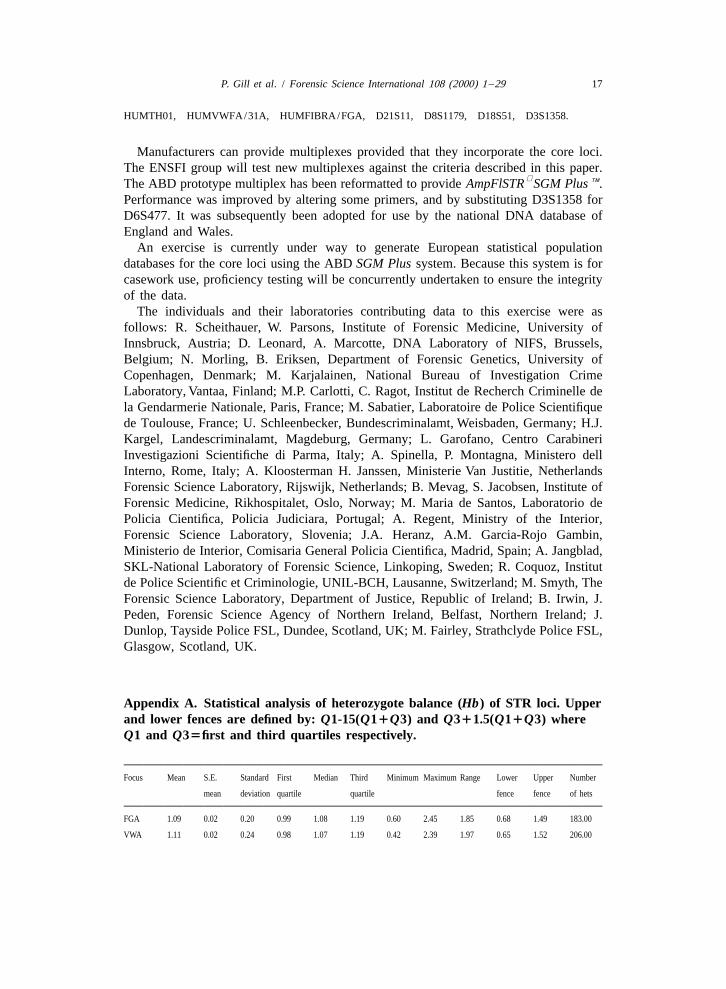
Appendix A. Statistical analysis of heterozygote balance (Hb) of STR loci. Upperand lower fences are defined by: Q1-15(Q11Q3) and Q311.5(Q11Q3) whereQ1 and Q35first and third quartiles respectively.

Focus Mean S.E. Standard First Median Third Minimum Maximum Range Lower Upper Number

mean deviation quartile quartile fence fence of hets

FGA 1.09 0.02 0.20 0.99 1.08 1.19 0.60 2.45 1.85 0.68 1.49 183.00

VWA 1.11 0.02 0.24 0.98 1.07 1.19 0.42 2.39 1.97 0.65 1.52 206.00


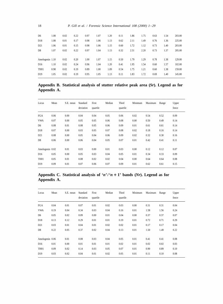
D6 1.08 0.02 0.22 0.97 1.07 1.20 0.11 1.86 1.75 0.63 1.54 203.00

D18 1.08 0.01 0.17 0.98 1.06 1.13 0.62 2.11 1.49 0.76 1.36 225.00

D21 1.06 0.01 0.15 0.98 1.06 1.15 0.60 1.72 1.12 0.73 1.40 203.00

D8 1.07 0.02 0.22 0.97 1.04 1.13 0.32 2.51 2.20 0.73 1.37 205.00

Amelogenin 1.10 0.02 0.20 1.00 1.07 1.15 0.50 1.79 1.29 0.78 1.38 129.00

D16 1.10 0.02 0.24 0.96 1.04 1.20 0.41 1.95 1.54 0.60 1.57 102.00

TH01 0.98 0.02 0.19 0.89 1.00 1.09 0.54 1.75 1.21 0.60 1.38 159.00

D19 1.05 0.02 0.19 0.95 1.05 1.13 0.11 1.83 1.72 0.69 1.40 145.00

Appendix B. Statistical analysis of stutter relative peak area (Sr). Legend as forAppendix A.

Locus Mean S.E. mean Standard First Median Third Minimum Maximum Range Upper

deviation quartile quartile fence

FGA 0.06 0.00 0.04 0.04 0.05 0.06 0.02 0.54 0.52 0.09

VWA 0.07 0.00 0.05 0.05 0.06 0.08 0.00 0.50 0.49 0.14

D6 0.08 0.01 0.08 0.05 0.06 0.09 0.01 0.61 0.61 0.14

D18 0.07 0.00 0.03 0.05 0.07 0.08 0.02 0.18 0.16 0.14

D21 0.08 0.00 0.05 0.04 0.06 0.09 0.02 0.32 0.30 0.16

D8 0.06 0.00 0.06 0.04 0.05 0.07 0.01 0.42 0.41 0.11

Amelogenin 0.02 0.01 0.03 0.00 0.01 0.03 0.00 0.12 0.12 0.07

D16 0.05 0.00 0.05 0.03 0.04 0.05 0.01 0.34 0.33 0.09

TH01 0.05 0.01 0.08 0.02 0.02 0.04 0.00 0.64 0.64 0.08

D19 0.09 0.01 0.07 0.06 0.07 0.09 0.01 0.62 0.61 0.15

Appendix C. Statistical analysis of ‘n’ / ‘n 1 1’ bands (Nr). Legend as forAppendix A.

Locus Mean S.E. mean Standard First Median Third Minimum Maximum Range Upper

deviation quartile quartile fence

FGA 0.04 0.01 0.07 0.01 0.02 0.03 0.00 0.31 0.31 0.04

VWA 0.19 0.04 0.34 0.03 0.04 0.16 0.01 1.58 1.56 0.24

D6 0.05 0.02 0.09 0.00 0.01 0.04 0.00 0.37 0.37 0.07

D18 0.13 0.12 0.29 0.01 0.01 0.19 0.01 0.72 0.71 0.29

D21 0.03 0.01 0.04 0.01 0.02 0.02 0.01 0.17 0.17 0.04

D8 0.22 0.05 0.37 0.02 0.04 0.13 0.01 1.50 1.49 0.22

Amelogenin 0.06 0.01 0.08 0.03 0.04 0.05 0.01 0.41 0.41 0.08

D16 0.01 0.00 0.01 0.01 0.01 0.02 0.01 0.02 0.02 0.03

TH01 0.09 0.02 0.14 0.03 0.05 0.07 0.01 0.90 0.89 0.10

D19 0.03 0.02 0.04 0.01 0.02 0.05 0.01 0.11 0.10 0.08


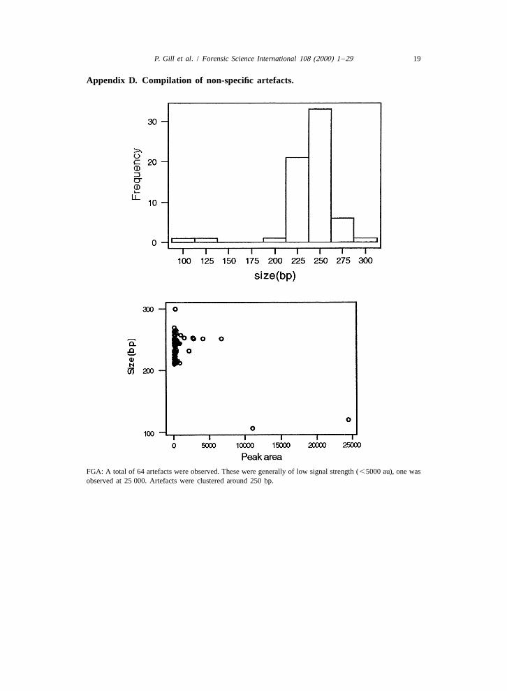
Appendix D. Compilation of non-specific artefacts.

FGA: A total of 64 artefacts were observed. These were generally of low signal strength (,5000 au), one wasobserved at 25 000. Artefacts were clustered around 250 bp.


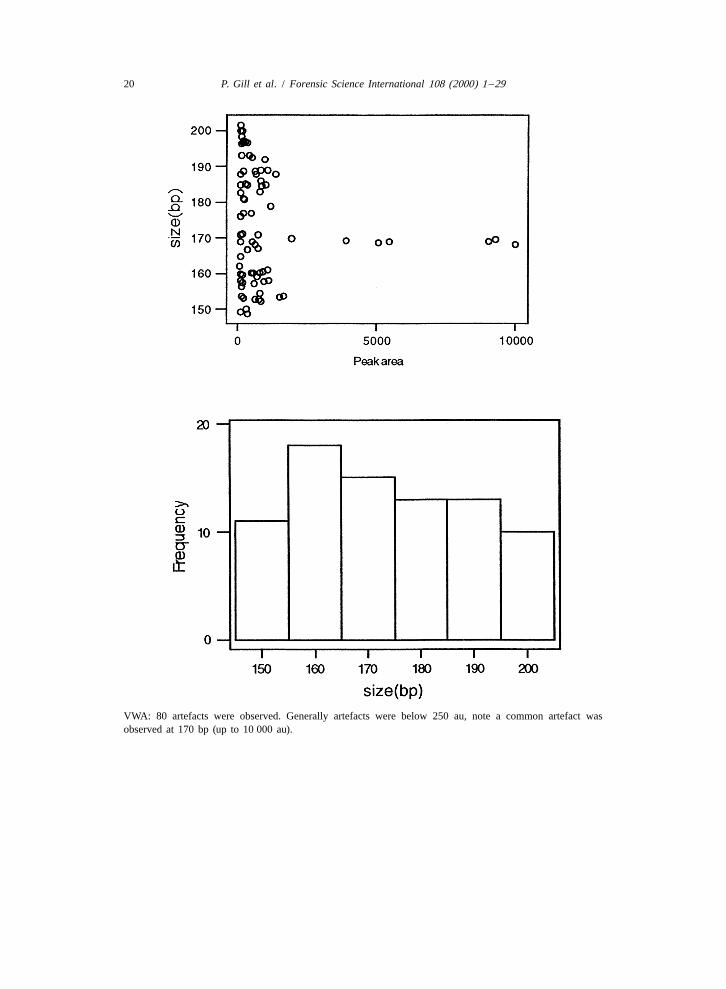
VWA: 80 artefacts were observed. Generally artefacts were below 250 au, note a common artefact wasobserved at 170 bp (up to 10 000 au).


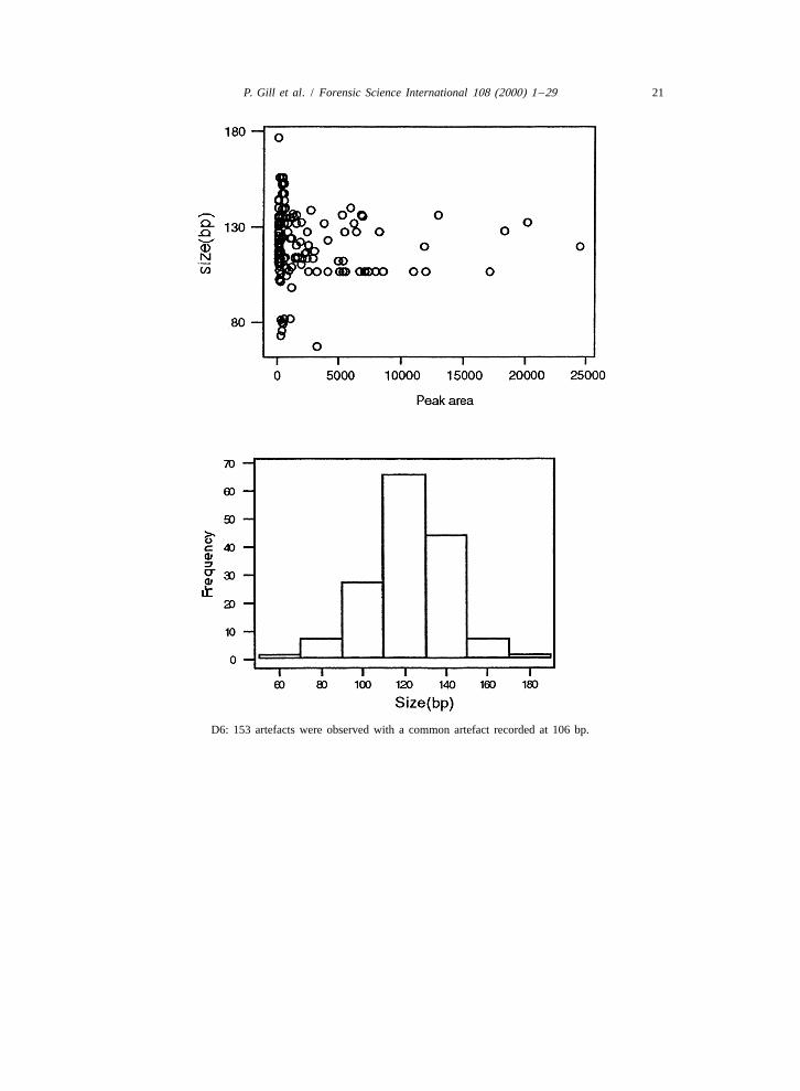
D6: 153 artefacts were observed with a common artefact recorded at 106 bp.


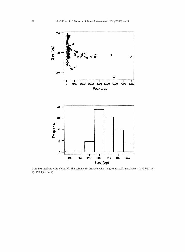
D18: 108 artefacts were observed. The commonest artefacts with the greatest peak areas were at 189 bp, 190bp, 193 bp, 194 bp.


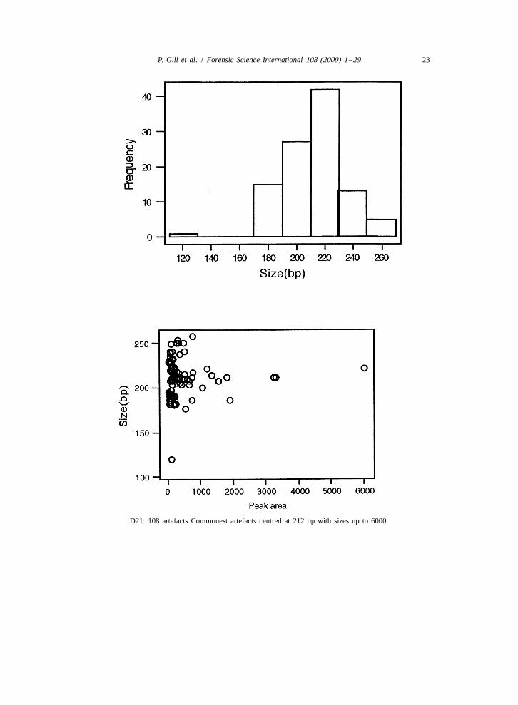
D21: 108 artefacts Commonest artefacts centred at 212 bp with sizes up to 6000.


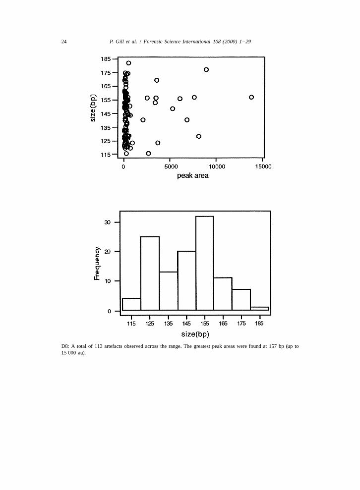
D8: A total of 113 artefacts observed across the range. The greatest peak areas were found at 157 bp (up to15 000 au).


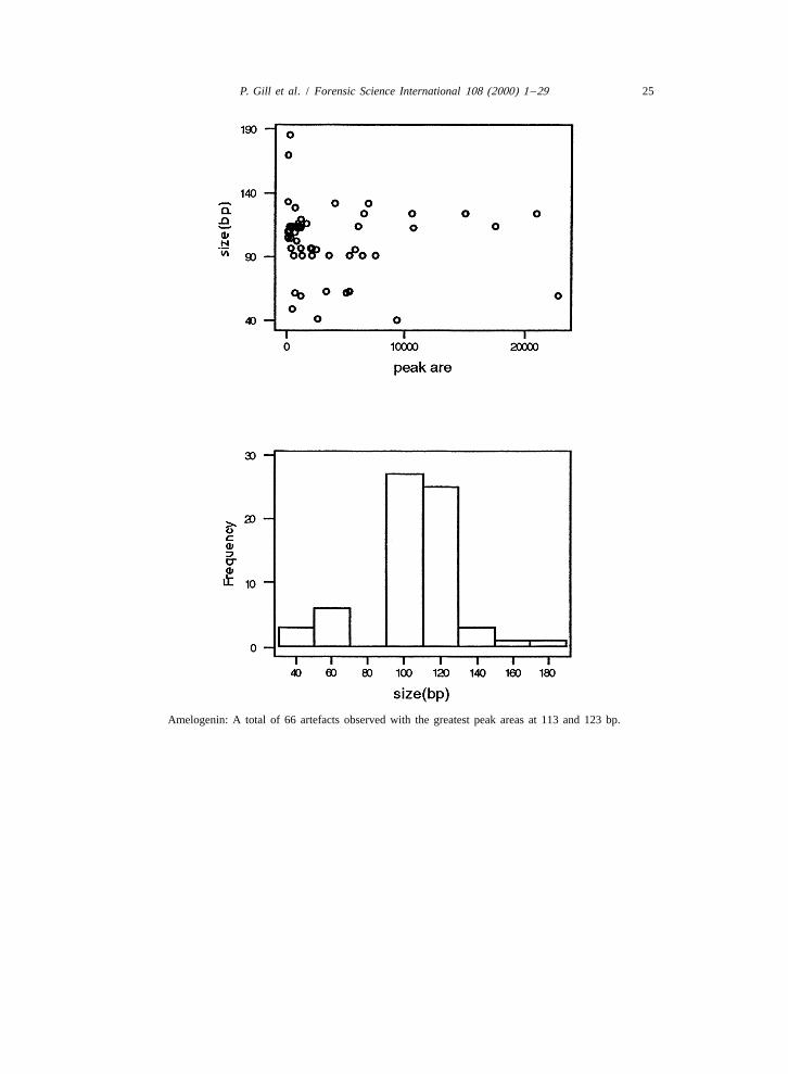
Amelogenin: A total of 66 artefacts observed with the greatest peak areas at 113 and 123 bp.


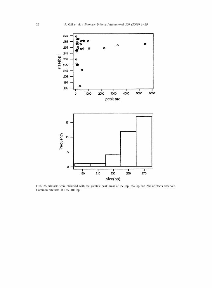
D16: 35 artefacts were observed with the greatest peak areas at 253 bp, 257 bp and 260 artefacts observed.Common artefacts at 185, 186 bp.


TH01: 74 artefacts observed Common artefacts at 185, 186 bp.


D19: 85 artefacts Commonest artefact found at 123 bp.

References

[1] C. Kimpton et al., Automated DNA profiling employing ‘multiplex’ amplification of short tandem repeatloci, PCR Methods Appl. 3 (1993) 13–22.

[2] D.J. Werrett, The national DNA database, Forensic Science Int. 88 (1997) 33–42.[3] R. Sparkes et al., The validation of a 7-locus multiplex test for use in forensic casework. (I) Mixtures,

ageing, degradation and species studies, Int. J. Legal Med. 109 (1996) 186–194.


[4] R. Sparkes et al., The validation of a 7-locus multiplex test for use in forensic casework. (II) Artefacts,casework studies and success rates, Int. J. Legal Med. 109 (1996) 195–204.

[5] K. Sullivan et al., A rapid and quantitative DNA sex test: fluorescence-based PCR analysis of X-Yhomologous gene amelogenin, Biotechniques 15 (1993) 636–641.

[6] P.M. Schneider, DNA databases for offender identification in Europe-The need for technical, legal andpolitical harmonization, in: Proceedings from the second European Symposium on Human Identification,1998, pp. 40–44.

[7] J.W. Tukey, Exploratory Data Analysis, Addison-Wesley Publishing Company, 1977.[8] P. Gill, R. Sparkes, C. Kimpton, Development of guidelines to designate alleles using an STR multiplex

system, Forensic Sci. Int. 89 (1997) 185–197.[9] P. Gill et al., Report of the European DNA profiling group (EDNAP)-towards standardisation of short

tandem repeat (STR) loci, Forensic Sci. Int. 65 (1994) 51–79.[10] P. Gill et al., Report of the European DNA profiling group (EDNAP): An investigation of the complex

STR loci D21S11 and HUMFIBRA (FGA), Forensic Sci. Int. 86 (1997) 25–33.[11] P. Gill, E. d’Aloja, B. Dupuy, B. Eriksen, M. Jangblad, V. Johnson, A.D. Kloosterman, A. Kratzer, M.V.

Lareu, B. Mevag, N. Morling, C. Phillips, H. Pfitzinger, S. Rand, M. Sabatier, R. Scheithauer, H.Schmitter, P. Schneider, I. Skitsa, M.C. Vide, Report of the European DNA Profiling Group (EDNAP) –an investigation of the hypervariable STR loci ACTPB2, APOAI1 and D11S554 and the compound lociD12S391 and D1S1656, Forensic Sci. Int. 98 (1998) 193–200.

[12] C. Kimpton et al., Report on the second EDNAP collaborative STR exercise, Forensic Sci. Int. 71 (1995)137–152.

Report of the European Network of Forensic Science Institutes (ENSFI): formulation and testing of...

Documents

Transcript of Report of the European Network of Forensic Science Institutes (ENSFI): formulation and testing of...