Int. J. Logistics Systems and Management, Vol. 18, No. 1, 2014 3

Copyright © 2014 Inderscience Enterprises Ltd.

Replenishment policy based on information sharing to mitigate the severity of supply chain disruption

Francesco Costantino, Giulio Di Gravio, Ahmed Shaban* and Massimo Tronci Department of Mechanical and Aerospace Engineering, University of Roma ‘La Sapienza’, Via Eudossiana, 18, 00184, Roma, Italy Fax: +39-0644585746 E-mail: francesco.costantino@uniroma1.it E-mail: giulio.digravio@uniroma1.it E-mail: ahmed.shaban@uniroma1.it E-mail: massimo.tronci@uniroma1.it *Corresponding author

Abstract: Modern supply chains are attempting to gain competitive advantages in a fiercely competitive marketplace through adopting new initiatives and practices such as lean and just-in-time. These initiatives are suitable for a stable world but they could make the supply chain more vulnerable to the external disruptions such as natural and man-made disasters. This paper aims at studying the dynamics of a disrupted supply chain under a coordination mechanism that is designed to achieve efficiency and resiliency. The proposed procedure relies on establishing a novel replenishment policy based on an information sharing approach to replace traditional policies. In this policy, replenishment orders will be divided into two streams, transmitting both real demand information and required inventory adjustments to the whole supply chain. A simulation model for a four-echelon supply chain has been considered to evaluate the information sharing policy and to compare it with an order-up-to level policy, determining the dynamics of ordering and inventory before and after the disruption. The results showed how the suggested approach was successful in recovering the disrupted supply chain to a stable performance by reducing effects on inventory and ordering patterns.

Keywords: supply chain disruption; vulnerability; resilience; information sharing; ordering policy; replenishment policy; supply chain dynamics; multi-echelon; risk management; bullwhip effect; simulation.

Reference to this paper should be made as follows: Costantino, F., Di Gravio, G., Shaban, A. and Tronci, M. (2014) ‘Replenishment policy based on information sharing to mitigate the severity of supply chain disruption’, Int. J. Logistics Systems and Management, Vol. 18, No. 1, pp.3–23.

Biographical notes: Francesco Costantino holds an MSc in Mechanical Engineering (2001), a Master in Engineering and Quality Management (2002), and a PhD in Engineering of Industrial Production (2005) at the University of Rome ‘La Sapienza’. Since 2006, he is an Assistant Professor at the Department of Mechanical and Aeronautical Engineering at the same university for the scientific didactic sector ING-IND/17 (Mechanical Industrial Plants). Since 2005, he is the holder of the Chair of Industrial Plants for BS course in Management Engineering of the Faculty of Information, Computer Science and Statistics Engineering, University of Rome ‘La Sapienza’. Since 2002, he is a

4 F. Costantino et al.

Lecturer of Operations Management, Maintenance Management and several masters. His research activity is focused on the analysis and design of industrial, organisational and network systems, with particular attention to risk management, environment and sustainability, supply chain management, methodologies of improvement (lean production and Six Sigma) for organisations. He is the author of more than 60 national and international publications.

Giulio Di Gravio holds an MSc in Mechanical Engineering, a Master in Quality Management and Engineering and a PhD in Engineering of Industrial Production. He is an Assistant Professor of Quality Management at the Faculty of Engineering, University of Rome ‘La Sapienza’. His research activity is focused on the analysis and design of industrial, organisational and network systems, with particular attention to collaboration and coordination problems, information management, performance measurement, risk management and knowledge management. Furthermore, he is specialised in supply chain management, methodologies of improvement (lean production and Six Sigma) for organisations, definition of business and mission strategies, through the application of simulation and expert systems. He is the author of more than 80 national and international publications.

Ahmed Shaban is an Assistant Lecturer in Industrial Engineering Department, Fayoum University, Fayoum, Egypt. He obtained his BSc in Industrial Engineering in 2006 with honour degree from the Fayoum University, and an MSc in Mechanical Design and Production in 2010 from the Cairo University, Cairo, Egypt. Currently, he is conducting his PhD research in supply chain management at the University of Rome ‘La Sapienza’ Rome, Italy. His research interests are in the applications of AI in quality and operations management, logistics and supply chain management, and modelling and optimisation.

Massimo Tronci is a Full Professor of Industrial Mechanical Plants at the Faculty of Engineering of the University of Rome ‘La Sapienza’ since 2001 and a Professor of the courses of industrial plants, operations management, quality management, and maintenance management at the same university. He received his BSc in Mechanical Engineering and his PhD in Energetics – Engineering of Energy Sources – Nuclear, Conventional and Renewable both from the University of Rome ‘La Sapienza’ in 1982 and 1991, respectively. He is the President of the Italian Association of Industrial Mechanical Plants (Associazione Italiana dei Docenti di Impianti Industriali –AIDI). He has over 150 publications in the areas of risk management, supply chain management, quality management, eco-design and green supply chain.

1 Introduction

Supply chain management is a set of approaches to efficiently integrate suppliers, manufacturers, warehouses, and stores to produce and distribute the right quantities of products to the right locations and at the right time, in order to minimise system wide costs while satisfying service level requirements (Simchi-Levi et al., 1998). Modern supply chains are now facing numerous changes that are contributing to increase their complexity, such as the globalisation of businesses and the always more common

Replenishment policy based on information sharing to mitigate the severity 5

adoption of business initiatives such as lean production, efficient consumer response and quick response programmes (Li et al., 2010; Kersten et al., 2011). Tang (2006) indicated that these strategies and initiatives are designed for a stable world but they could make a supply chain more vulnerable to various types of risks caused by uncertain economic cycles, consumer demands and natural and man-made disasters. Risks are quite diverse, arising from sources both internal and external to the supply chain, and can be classified into foreseeable risks and unforeseeable risks (Oke and Gopalakrishnan, 2009). Although the foreseeable risks are more frequent than the unforeseeable risks, the latter, as for disruptions, have more significant effects on supply chain performance. A disruption is defined as an event that interrupts the material flows in the supply chain, resulting in an abrupt stoppage of the movement of goods (Wilson, 2007).

Always more frequently, disruptions affects very dramatically supply chains performances as organisations are generally not prepared to face external events. However, some organisations have succeeded to be resilient to mitigate the negative effects of disruption by adopting appropriate strategies and tools. Norrman and Jansson (2004) provided a good example for a disruption event that disrupted simultaneously both Nokia and Ericsson when lighting caused a fire at a local plant owned by Royal Philips Electronics, N.V., damaging millions of microchips. The two companies confronted the same disruption but the response of each was different. The multiple-supplier strategy allowed Nokia to react effectively and mitigate the crisis. In contrast, Ericsson was relying only on Philips (single sourcing) to get their microchips so their production was disrupted for months and ultimately they lost $400 million in sales (Carvalho et al., 2012a). Ericsson has since implemented new strategies and tools to cope with potential disruptions. In another example, Apple lost many customer orders during a supply shortage of DRAM chips after an earthquake hit Taiwan in 1999 (Tang, 2006). This proves the importance of adopting mitigation strategies that can help supply chains to be resilient when disruptions happen (Min, 2011; Tang, 2006).

As indicated above, organisations and their supply chains must be resilient; they must develop the ability to react to an unforeseeable disturbance so that they can return quickly to their original state or move to a new stable one (Carvalho et al., 2012a; Hanna et al., 2010; Peck, 2005). To help organisations become more resilient, Samvedi and Jain (2012) indicated that there is an urgent need to devise methods to mitigate the effects of the disruptions on the performance of supply chains, arguing that sharing information amongst the partners is a powerful approach. These previous works do not consider the effect of a disruption on the supply chain performances: it is expected that a breakdown at any stage would propagate and disrupt the whole system while, due to its dynamics, the supply chain might bear and should be protected from different problems during the recovery.

This paper presents a coordination mechanism in the form of a novel replenishment policy that would help supply chains to be efficient and resilient to internal and external disruptions. A simulation approach is considered to investigate the effect of a disruptive situation on the supply chain dynamics. The response of the disrupted supply chain under the proposed coordination approach will be compared with the response of the supply chain when a traditional ordering policy is adopted. The simulation results showed how the suggested approach can recover supply chain performance in terms of inventory level and ordering behaviour. Moreover, the results provide insights on how practitioners can behave during and after disruptions in order to control supply chain dynamics.

6 F. Costantino et al.

The rest of the paper is organised as follows: Section 2 reviews the related literature to supply chain disruption, the modelling approach is discussed in Section 3 and the decentralised information sharing policy is presented in Sections 4. The simulation results and comparisons are presented and discussed in Section 5.

2 Literature review

Supply chain risk management, in general, has gained a lot of attention by academics and practitioners in the last years due to the severe impacts of some recent disasters on supply chains performances. Kersten et al. (2011) argue that companies are faced with an increasing risk exposure caused by a greater dependence of supply chain partners on each other, e.g., due to the close integration of their business processes aiming at the reduction of channel inventory. Thun and Hoenig (2011) described risk management as the identification and analysis of risks as well as their control. Supply chain disruption can be considered as one of supply chain risks and the research in this area can be divided into empirical analysis and quantitative analysis, according to the classification of Zegordi and Davarzani (2011). Empirical studies have been carried out in order to investigate the different types of disruptions risks and the different strategies applied to counteract these disruptions. The purpose of the empirical investigation is to give some insights on this topic from a practitioner’s perspective. Thun and Hoenig (2011) conducted an empirical analysis based on a survey with 67 manufacturing plants in the German automotive industry. Their analyses reveal that companies with a high implementation degree of risk management show a better supply chain performance, the companies using reactive supply chain risk management has higher average value in terms of disruptions resilience, whereas the companies pursuing preventive supply chain risk management has better values concerning flexibility or safety stocks. Carvalho et al. (2012b) presented a mapping framework that can allow the identification of current supply chain operations and possible transition states, together with points of vulnerability in order to improve resilience and avoiding possible failure modes. Oke and Gopalakrishnan (2009) empirically investigated the different types of risks and disruptions that a retail supply chain in the USA can face, along with relative mitigation strategies. Craighead et al. (2007) evaluated different kinds of supply chain disruptions based on an empirical study. Besides design characteristics, they investigated two categories of supply chain risk management; the capabilities of recovery and warning. Blackhurst et al. (2005) conducted a study in several industries analysing global sourcing and supply chain disruptions. Kleindorfer and Saad (2005) presented a conceptual framework for the management of disruption risks and, based on empirical data on chemical-industry accidents, provide guidance for the creation of appropriate management systems.

Beside the empirical literature, other researchers have conducted quantitative analysis in order to investigate and quantify the impact of specific disruptions on supply chain performance and to propose the appropriate solutions for such disruptions. While this stream started much earlier, Schmitt and Synder (2012) argued that with the global expansion of supply chains there is a reinforced need for quantitative models addressing supply chain risk management. Meyer et al. (1979) investigated a system consisting of a production facility subject to random failure and repair processes and developed expressions for the average inventory level and for the fraction of time demand is met. Chao (1987) adopted dynamic programming to find optimal policies for electric utility

Replenishment policy based on information sharing to mitigate the severity 7

companies that may face market disruptions. Parlar and Berkin (1991) considered the supply uncertainty problem for a class of EOQ models with a single supplier where the availability and unavailability periods constitute an alternating Poisson process. Parlar and Perry (1996) developed a continuous time model in which the availability of each of n suppliers is uncertain because of equipment breakdowns, labour strikes or other unpredictable circumstances. Tomlin (2006) suggested two different groups of proactive strategies, mitigation and contingency, and discussed the values of these two choices for managing a disruption. He studied a single-product setting in which a firm can source from two suppliers, one that is unreliable and another that is reliable but more expensive. Tang (2006) illustrated robust strategies for mitigating disruption effects and Pochard (2003) discussed an empirical solution based on dual-sourcing to mitigate the likelihood of disruptive events. Qi et al. (2009) formulated an analytical model for a two-echelon supply chain, consisting of a retailer and a supplier, which is exposed to both internal and external disruptions. They assumed that the retailer might experience an internal disruption due to the damage of its inventory and an external disruption from the supplier side when the supplier is broken-down. They modified the classical EOQ to cope with these new situations. Shao (2012) proposed and compared the performance of four demand-side reactive strategies for managing disruptions in a multiple assemble-to-order system with two substitute products where the demand is price-sensitive and disruption-sensitive. Babazadeh and Razmi (2012) considered a stochastic programming approach to handle both operational and disruption risks of the agile supply chain network that is the best competitive strategy for high turbulent business environments.

Simulation modelling as a quantitative analysis tool has also been widely applied to test and investigate performances. Levy (1995) presented a simulation model to examine the impact of demand uncertainty and supplier reliability on the performance of different supply chain network designs. Carvalho et al. (2012a) developed a supply chain simulation for a real case concerned with the Portuguese automotive supply chain. The objective of their study has been to evaluate alternative scenarios of supply chain design for improving resilience to disturbance. Wilson (2007) investigated the effect of a transportation disruption on supply chain performance using system dynamics simulation, comparing a traditional supply chain and a vendor managed inventory (VMI) system when a transportation disruption occurs between two echelons in a five-echelon supply chain. Tuncel and Alpan (2010) showed how a timed Petri nets framework could be used to model and analyse a supply chain network which is subject to various risks. They argued that the developed Petri nets model provides an efficient environment for defining uncertainties in the system and evaluating the value of the risk mitigation actions. Costantino et al. (2013) prove that supply chain disruptions can be considered as a main driver of bullwhip effect and supply chain instability before and after disruptions, through a simulation study. Samvedi and Jain (2012) investigated the effect of sharing the forecasting information on the performance of dynamic supply chain during disruptions as an effort towards resilience. Rong et al. (2008) studied the ordering behaviour of supply chain partners when there is a supply chain disruption through using a new setup of the beer game and discrete-event simulation. They proved that disruptions would cause the reverse bullwhip effect in which orders variability increases as one moves downstream in the supply chain.

The above literature review indicates that most works based on quantitative analysis using either analytical or simulation models has considered only simple structures of supply chains; two or three echelons at most. Schmitt and Singh (2012) argue that

8 F. Costantino et al.

literature on disruption generally focuses on single facilities or pairs of echelons, even though disruptions can have long and lasting effects throughout the supply chain. Therefore, it is important to quantify disruption risk for extended supply chain, as it will be indicated later in this paper. Furthermore, supply chain dynamic behaviour after disruption events has still to be investigated as there are only few researches in the field. It is expected that the rational response of supply chain partners and their ordering behaviour during and after disruption may have significant effect on performances, as it will be indicated later.

3 Modelling methodology

This paper adopts discrete-event simulation to investigate the performance of a supply chain under the disruption and to investigate the impact of different ordering policies before and after stability. A single product four-echelon supply chain (retailer, wholesaler, distributor and factory) is considered (see, Figure 1) in which the information moves in the upstream direction from the retailer to the factory with a certain ordering delay between the echelons and the products moves in the downstream direction with a different delivery delay. It is assumed that the ordering lead-time is 1 period of time and the delivery lead-time is 2 periods of time. Moreover, the inventory capacities of the partners are not limited and the supplier capacity is unlimited where it can fulfil any amount of raw materials needed by the factory. The logic of updating the state variables at any echelon in the supply chain is better clarified in the following flowchart (see, Figure 3), as well as for further simulation settings. The model has been developed with the SIMUL8 package.

Figure 1 A simple serial multi-echelon supply chain (see online version for colours)

Retailer Wholesaler Distributor FactoryCustomer

Information flow

Product flow

The scenario considered in this paper can be represented as follows in Figure 2 where the supply chain had been working normally until a disruption happens.

Figure 2 Supply chain disruption representation (see online version for colours)

Replenishment policy based on information sharing to mitigate the severity 9

The disruption lasts for T2 periods and after that the supply chain starts again to receive the customer demand with a new distribution, not known for any of the echelons. This can happen, for example, when a company is facing an issue of quality so to recall its products or in case of post war, a terrorist attack, a natural disaster or political changes. Although this type of disruption is not frequent, its consequences can have a significant impact on the performances and may last for a very long time, enhancing other inefficiencies as for the bullwhip effect. This event can be modelled by starting the system in an out of balance situation with no incoming shipments or outgoing orders across the whole supply chain. In other words, the partners do not send or receive orders and there is an initial stock that is kept for contingency when the supply chain starts again its operations. However, this initial stock is supposed to be not sufficient to bear the lead-time demand so that the supply chain will soon be in an instable state.

The adoption of specific ordering polices as mitigation and contingency strategies can recover the supply chain performance but it may tend to induce other problems. After disruption, when demand has just started to arrive, the first echelon in the supply chain (retailer) receives the actual customer demand and then transmits it to the upstream suppliers as orders. In the beginning of the recovery, the echelons might underestimate the supply line so that sizable orders will be placed from the downstream echelons to the upstream echelons in order to both recover inventories stability and satisfy the future demand. Those sizable orders will be amplified as they travel up in the supply chain in a rational way, especially in the presence of a disruption situation. For example, the first echelon i will face the actual customer demand and send an order to echelon i + 1 to both recover its inventory position and to satisfy future demand. This order will be always greater than the actual customer demand so that the upstream echelon does not know about the actual customer demand. Accordingly, another sizable order will be placed by echelon i + 1 but based on distorted information from echelon i. Based on the new situation, it is expected that the downstream echelon i will start to place balanced orders to echelon i + 1 corresponds to customer demand. As echelon i + 1 has placed a sizable order, the new incoming orders from the downstream echelon i will not have a quick significant effect on its inventory position so that no orders will be placed from echelon i + 1 to i + 2 and this situation may last for longer period until his inventory position is less than a certain value. These dynamics will be repeated as we move upstream in the supply chain and it is expected that the problem will be severe when the supply chain is not prepared for disruptions or when they are frequent. Therefore, the dynamics of the supply chain during and after disruption has to be controlled adequately in order to balance and recover the supply chain to a stable position.

4 Decentralised information sharing policy

As argued by Samvedi and Jain (2012), sharing information amongst the partners in a supply chain can be considered a powerful approach to mitigate the effect of disruptions. A decentralised system of ordering and replenishment is then proposed to allow the partners to progressively share the actual customer demand. An ordering and replenishment policy is suggested in order to achieve coordination during, after disruption events, and during normal situations as well, improving both efficiency and resiliency.

10 F. Costantino et al.

This tactical approach can be considered as a coordination mechanism to deal with the ordering process of each partner in the supply chain. It relies on dividing orders into two streams; the first stream transmits the real demand x(t), whereas the second stream includes the required inventory adjustments yi(t) (Costantino et al., 2012; Moyaux et al., 2007). This strategy is different from the traditional ordering policies, where an echelon i just orders a quantity Oi(t) without indicating more information about the synthesis of the order. Alternatively, adopting this level of information sharing will allow the echelon i + 1 to know the real market demand and the inventory adjustment of i which helps him to react and place balanced orders during disruption and hence reducing information distortion. This approach also allows each partner to place and receive balanced orders without underestimating or overestimating the supply line while constraining the bullwhip effect.

The amount of tokens yi(t) is used to stabilise the inventory position of any echelon i. Thus, it will be sent to the upstream echelons only when there is a need for inventory recovery. The question is when to order this amount and how much yi(t) to order. Costantino et al. (2012) adopted the change in the observed customer demand level as the main condition for sending tokens. In other words, if the customer demand is stable, the company orders only x(t) where there is no need to order tokens yi(t) from the upstream echelons. However, when customer demand increases, the echelon i expects that the customer demand has changed and its inventory should be adapted and stabilised by ordering a surplus quantity yi(t). Another approach builds on the above (Costantino et al., 2012) is to check first the inventory position and sending a recovery order equals to 1ˆ( ) ( ) ( )i i iy t LD t IP tβ −= − if the supply chain is not stable, where

1ˆ ( )iLD t− is the expected lead time demand and β is a control parameter. However, if the inventory position IPi(t) is within a certain level then the customer demand change is considered to manage the inventory position. In other words, the ordering procedure first senses the presence of a disruption when the inventory position is very low

2 1ˆ( ) ( ),i iIP t LD tη −≤ then it attempts to recover it by adjusting its IPi(t) through ordering a sizable amount of tokens depending on the difference between a target inventory position and current inventory position. This sizable order will be divided into two parts (x(t) and yi(t)) so that the upstream echelon will be able to react only to the customer demand if its inventory position is stable. After stabilising the inventory position, each echelon transmits the actual customer demand plus an amount of tokens depending on the demand variation whenever there is a change in customer demand. Otherwise, if the inventory position is stable and within a certain ranges 2 1 1 1ˆ ˆ( ) ( ) ( )i i iLD t IP t LD tη η− −< ≤ each echelon transmits only the actual customer demand without any change. Generally, tokens and their ordering rules can be summarised and expressed mathematically as in equation (1).

1 1

1 1

1 2 1

1 2 1

0, ( ) ( 1) &

0, ( ) ( 1) &

( ) ( 1) &

( )

ˆ( ) ( )ˆ( ) ( )

ˆ ˆ( ) ( ) ( ), ( ) ( ) ˆ ˆ( ) ( ), ( ) ( )

(

( 1) &

( )

i i

i i

i i i

i

i i

i i i i

IP t LD t

IP t LD ty t LD t IP t IP

if x t x t

if x t x t

if x t x t

if x t x t

t LD t

LD t IP t IP t

x x

LD t

t

η

η

β η

α

β η

−

−

− −

− −

≤ −

> −

≤ −

>

>

>

= − ≤

− ≤−

− 2 1 1 1ˆ ˆ) (( 1) , ( ) ( 1) & ) ( ) ( )i i it i LD t IP t Lf D tx t x t η η− −− > − <

⎧⎪⎪⎪⎨⎪⎪⎪ ≤⎩

(1)

Replenishment policy based on information sharing to mitigate the severity 11

The values of η1 and η2 determine the sensitivity of policy to both normal inventory adjustment required to handle demand variation and other inventory adjustment required to recover disrupted supply chain. When the values of η1 and η2 are high, the response to inventory change will be fast but this could lead to high inventory levels so that they have to be determined carefully.

Figure 3 Replenishment policy (see online version for colours)

The decentralised information sharing policy is represented in details in the following flowchart (see Figure 3). At any time t, each echelon i of the supply chain receives the incoming shipments from the upstream echelon i + 1 and puts them in its inventory. These shipments correspond to the order placed at t – 3: one period for ordering delay and 2 periods for transportations. If there are previous backlogged orders, echelon i will attempt to satisfy them as much as possible. Afterwards, echelon i receives the order of

12 F. Costantino et al.

echelon i – 1, issued at t – 1, and either fulfil it if enough inventory Ii(t) is available or put it in backlog if the available inventory Ii(t) is less than the ordered quantity (partial fulfilment is allowed). Finally, a new order is issued to raise the inventory position to meet the future demand and the current instability.

According to this replenishment policy, the order of each echelon will be in the form [x(t), yi(t)], where x(t) is the real customer demand and yi(t) is the amount of tokens. When echelon i receives the vector of orders from echelon i – 1, it starts to fulfil first the order x(t) then the second part yi(t) respectively (see Figure 3). It means that if there is enough inventory, the two order’s components x(t) and yi(t) will be completely satisfied. However, if there is limited inventory at echelon i, a part of x(t) will be fulfilled and the other part will be considered as backlog to satisfy as soon as the products arrive from the upstream echelon. The amount of tokens will not be considered as a real backlog: if yi–1(t) is the amount of tokens of echelon i – 1 could not be satisfied by echelon i, it is transferred in the current echelon’s tokens order to the upstream echelon if the condition for transferring them is satisfied. Moreover, this amount travels upstream in the supply chain until it finds the required amount of products to be sent downstream until it arrives to echelon i to recover its inventory. Thus, supply chain partners can track the actual customer demand and issue orders to match it while the distortion of information that can arise during disruption is under control. The simulation experiments will prove the robustness of this replenishment policy.

5 Evaluation of the policy

The proposed approach will be compared with a classical ordering policy which has been widely used in the studies of supply chain dynamics (Disney and Lambrecht, 2008). The objective of this work is not to make an extensive comparison with other ordering policies but to emphasise on the need for a coordination mechanism during and after disruptions. The ordering policy for the comparison is the order-up-to level policy in which an order Oi(t) is placed whenever the inventory position IPi(t) of an echelon i is less than a target level Si(t) so that the inventory position would be recovered to its target level. In this policy, each echelon i relies on the information that the echelon receives from his downstream echelon Oi–1(t) to place his order Oi(t). The moving average forecasting technique is adopted to forecast the average lead time demand 1ˆ ( )iLD t− (based on five consecutive orders) of the echelon i – 1 and hence calculating the target level Si(t) where 1ˆ ( )iD t− is the forecasted demand of the echelon i – 1. The target level

Si(t) is calculated as 1 1ˆ ˆ( ) ( ) ( ),i i iS t LD t k tσ− −= + where 1ˆ ( )ik tσ − is a safety stock component to account for demand variation where 1ˆ ( )i tσ − is standard deviation of lead time demand and k is a constant that is used to achieve a certain service level. As the accurate information about customer demand after disruption may not be available, the safety stock will be computed by extending the actual lead time by one (from L = 3 to L = 4). Thus, the order amount that will be sent to the upstream echelon i + 1 will be equal to Oi(t) = Si(t) – IPi(t).

Replenishment policy based on information sharing to mitigate the severity 13

5.1 Demand pattern

Two types of demand patterns have been considered in this study to evaluate the impact of each ordering approach on the supply chain performances. The first customer demand pattern is assumed to be deterministic and stable; it is assumed to be 50 units per period. This deterministic demand is mainly used to validate and verify the simulation models where it is easy to expect the performance under deterministic demands. The second demand pattern is assumed to be stochastic, independent and identically distributed (i.i.d.), and following the normal distribution of N(50, 52). The stochastic demand will be used for the quantitative evaluation and the comparison between the two approaches.

Figure 4 Ordering pattern of each supply chain partner, (a) order-up-to level (b) information sharing (see online version for colours)

0

20

40

60

80

100

120

1 4 7 10 13 16 19 22 25 28 31 34 37 40 43 46 49 52

Units /Time Period

Time Periods

Retailer Orders Vs. Customer Demand

Customer Demand

Retailer Order

0

20

40

60

80

100

120

1 4 7 10 13 16 19 22 25 28 31 34 37 40 43 46 49 52

Units /Time Period

Time Periods

Retailer Orders Vs. Customer Demand

Customer Demand

Retailer Order

0

20

40

60

80

100

120

140

160

180

200

1 4 7 10 13 16 19 22 25 28 31 34 37 40 43 46 49 52

Units /Time Period

Time Periods

Wholesaler Orders Vs. Customer Demand

Customer Demand

Wholesaler Order

0

20

40

60

80

100

120

140

160

180

200

1 4 7 10 13 16 19 22 25 28 31 34 37 40 43 46 49 52

Units /Time Period

Time Periods

Wholesaler Orders Vs. Customer Demand

Customer Demand

Wholesaler Order

0

50

100

150

200

250

300

350

1 4 7 10 13 16 19 22 25 28 31 34 37 40 43 46 49 52

Units /Time Period

Time Periods

Distributor Orders Vs. Customer Demand

Customer Demand

Distributor Order

0

50

100

150

200

250

300

350

1 4 7 10 13 16 19 22 25 28 31 34 37 40 43 46 49 52

Units /Time Period

Time Periods

Distributor Orders Vs. Customer Demand

Customer Demand

Distributor Order

0

100

200

300

400

500

600

1 4 7 10 13 16 19 22 25 28 31 34 37 40 43 46 49 52

Units /Time Period

Time Periods

Factory Orders Vs. Customer Demand

Customer Demand

Factory Order

0

100

200

300

400

500

600

1 4 7 10 13 16 19 22 25 28 31 34 37 40 43 46 49 52

Units /Time Period

Time Periods

Factory Orders Vs. Customer Demand

Customer Demand

Factory Order

(a) (b)

14 F. Costantino et al.

Figure 5 Inventory variation at each supply chain partner, (a) order-up-to level (b) information sharing (see online version for colours)

‐400

‐300

‐200

‐100

0

100

200

300

400

1 3 5 7 9 11 13 15 17 19 21 23 25 27 29 31 33 35 37 39 41 43 45 47 49 51

Inventory Level

Time Periods

Retailer Inventory Wholesaler Inventory

Distributor Inventory Factory Inventory

‐400

‐300

‐200

‐100

0

100

200

300

400

1 3 5 7 9 11 13 15 17 19 21 23 25 27 29 31 33 35 37 39 41 43 45 47 49 51

Inventory Level

Time Periods

Retailer Inventory Wholesaler Inventory

Distributor Inventory Factory Inventory

(a) (b)

The supply chain model has been initialised in an out of balance state in which each echelon has an initial inventory of 100 units that is not enough to cover the total lead time. In addition, there were no incoming or outgoing orders at the start of the simulation run. Each echelon has been ordering an amount equals to the incoming order/demand for the first four periods until there is available data to apply the ordering policy and calculate the expected future demand based on the moving average technique. These initial conditions represent the disruption event along the supply chain. The performances of the supply chain under the information sharing policy and the order-up-to level policy for the deterministic demand are depicted in Figures 4 and 5. The results show that both the approaches succeeded to recover the inventory stability of the different partners of the supply chain. However, there is a significant difference between their performances, especially before stability, in terms of ordering and inventory variations. Furthermore, the instability period concerning the ordering behaviour is higher in case of the order-up-to level. The information sharing policy sends only once an amount that is required to recover the supply chain inventories so that there is only one peak at each echelon’s stream of orders (Figure 4). Afterwards, each echelon issues balanced orders of an amount equal to the actual customer demand to his upstream echelon. Similarly, the order-up-to level starts with sending a sizable order that is overly amplified as it moves upstream in the supply chain and thus, after that, some echelons such as the distributor and the factory stop sending until their inventory position becomes unstable. This situation in reality, and especially when there is disruption instability, could cause many problems for the upstream echelons in the supply chain as explained in Section 4.

5.2 Performance measures

As the scope of this paper is to study the performances of a disrupted supply chain, a set of measures are established to characterise the dynamic behaviour under different ordering policies. In particular, the inventory instability period and the average and variance of inventory level for each echelon will be evaluated and the dynamic behaviour of the supply chain, before and after the inventory stability, will be determined through the bullwhip effect (Lee et al., 1997).

The instability period of an echelon i is an indicator of how an ordering policy is able to recover quickly the inventories stability. In literature, there is not a clear definition for

Replenishment policy based on information sharing to mitigate the severity 15

this measure so it will be defined as the time between the start of inventory unavailability, when the unsatisfied orders of echelon i – 1 has just started to appear (Bi–1(t) > 0), and the time of starting inventory recovery (Ii(t + T) – Bi–1(t) ≥ 0). This measure is very important in order to give an insight on the time required to recover the inventory level and hence the supply chain stability after suffering the disruption. The corresponding inventory is exhibited in Figure 6, given an initial inventory of 100 units at each echelon: the inventory starts unstable as it rapidly goes in the negative side until it recovers back to a stable level in the positive direction. This phenomenon is common for all the partners but it is clear that the downstream echelons stabilise more slowly than the upstream echelons. This can be attributed to the ordering lead time and the unavailability of stock at the downstream echelons. This measure can be minimised through stocking a strategic amount of inventory for emergencies.

Bullwhip effect has been defined as the increase in orders variability as the customer demand information moves upstream in the supply chain (Lee et al., 1997). The bullwhip effect is commonly quantified as the ratio between the variance of orders placed by an echelon i and the variance of customer demand (Bayraktar et al., 2008; Costantino et al., 2013; Zhang and Zhang, 2007). The overall bullwhip effect of a supply chain can be assumed equal to the sum of the bullwhip effect values of all the echelons in the supply chain. These measures can be expressed mathematically as following in equations (2) and (3).

( )( )( ( ))

ii

Var O tBWE

Var x t= (2)

4

1

ii

Overall BWE BWE=

=∑ (3)

where BWEi is the bullwhip effect ratio of an echelon i, Var(Oi(t)) is the variance of the orders issued by the echelon i, Var(x(t)) is the variance of the customer demand, and Overall BWE is the sum of BWEi.

In order to make a fair comparison between the two different ordering policies, the two simulation models must generate the same random data set of customer demand while testing the two policies. This can be accomplished by using the same random seed to run the two simulations models.

6 Discussion of results

The simulation models were adapted in order to get the above performance measures based on 100 simulation runs and with a confidence level of 95%. The replication length of a single simulation run was adopted to be 500 periods in order to capture the long-term performances of the supply chain after stability (see Figure 6). As shown in Figure 6, the supply chain behaviour can be divided into two states; initial state (instable state) and stable state. Accordingly, the performance measures will be calculated and compared in the two different states.

16 F. Costantino et al.

Figure 6 Inventory variation of a single simulation run under a stochastic demand of N(50, 52), (a) order-up-to level (b) information sharing (see online version for colours)

‐800

‐600

‐400

‐200

0

200

400

600

800

1 5 9 13 17 21 25 29 33 37 41 45 49 53 57 61 65 69 73 77 81 85 89 93 97

Inventory Level

Time Periods

Retailer Inventory Wholesaler Inventory

Distributor Inventory Factory Inventory

(a)

‐800

‐600

‐400

‐200

0

200

400

600

800

1 5 9 13 17 21 25 29 33 37 41 45 49 53 57 61 65 69 73 77 81 85 89 93 97

Inventory Level

Time Periods

Retailer Inventory Wholesaler Inventory

Distributor Inventory Factory Inventory

(b)

6.1 Instability period

The comparison between the two ordering policies based on the instability period is depicted in Figure 7. The comparison shows that the order-up-to level policy can recover the supply chain performance (ordering and inventory behaviour) more rapidly than the information sharing policy to some extent. However, this conclusion can be altered by changing the amount of tokens that is sent to recover the inventories whenever there is a severe instability due to a disruption. The amount of tokens is set at

1ˆ( ) ( ) ( )i i iy t LD t IP tβ −= − with β = 0.67 and η1 = 0.67, η2 = 0.5, αi = 3 (corresponding to the total lead time for ordering and delivery). The value of yi(t) is required to recover the supply line of an echelon i to a stable position so that the value of yi(t) can be increased by increasing the value of β. After stabilising the supply line, the information sharing approach sends balanced orders equal to customer demand and an amount of tokens αi(x(t) – x(t – 1)) depending on demand variation (see Figure 3). An investigation on the impact of β on the instability period is depicted in Figure 8. The instability period is decreasing exponentially as the amount of β is increased but this action might increase the bullwhip effect ratio and the average inventory level. At β = 1 the performances of

Replenishment policy based on information sharing to mitigate the severity 17

the two policies are similar (see Figure 8). It can generally be argued that there is a trade-off between the instability period and the other performance measures such as bullwhip effect and inventory behaviour (i.e., average and variance of inventory level). Therefore, if a supply chain is subject to frequent disruptions, the value of β should be selected to be high enough to help the supply chain to get its stability in a timely manner.

Figure 7 Instability period at different supply chain partners for different ordering policies (see online version for colours)

21.30

19.4219.22

16.3716.69

13.4713.36

10.42

0

5

10

15

20

25

Information Sharing Order-up-to Level

Inst

abili

ty p

erio

d

Ordering policyRetailer instability period Wholesaler instability period

Distributor instability period Factory instability period

Figure 8 Instability period at different supply chain partners for different β values (see online version for colours)

0

5

10

15

20

25

30

35

β=0.5 β=0.67 β=0.75 β=1.0

Instab

ility Period

β

Retailer instability period Wholesaler instability period

Distributor instability period Factory instability period

6.2 Inventory level

A comparison based on both average and standard deviation of inventory level is depicted in Figure 9(a) and Figure 9(b), respectively. The results show how the policy of information sharing succeeded to recover the disrupted supply chain to a new acceptable position in terms of inventory level, through the coordination among the different partners. The information sharing of the actual customer demand, although in a

18 F. Costantino et al.

decentralised manner, allowed to effectively react to the disruption and stabilise at the same level of inventory with very low variation in comparison to the order-up-to level policy. The order-up-to level policy stabilises more quickly but at a higher inventory level than the information sharing one, especially at the last echelon (factory). The high standard deviation of the inventory level means that the performance of the supply chain inventories will always be unstable, with periods with excessive inventory and other periods with negative inventory or backlog (see Figure 6). Furthermore, the average inventory level is increasing in the upstream direction. This can be attributed to the distortion that happens in the demand information as it moves in the upstream direction.

Figure 9 Inventory levels under different ordering policies, (a) average of inventory level (b) standard deviation of inventory level (see online version for colours)

‐350

‐300

‐250

‐200

‐150

‐100

‐50

0

50

100

150

Information Sharing Order-up-to Level Information Sharing Order-up-to Level

Before Stability After Stability

Aver

age

Inve

ntor

y

Ordering policy

Retailer inventory average Wholesaler inventory average

Distributor inventory average Factory inventory average (a)

0

50

100

150

200

250

300

350

400

Information Sharing Order-up-to Level Information Sharing Order-up-to Level

Before Stability After Stability

Aver

age

Stan

dard

Dev

iatio

n

Ordering policy

Retailer inventory stdev. Wholesaler inventory stdev.

Distributor inventory stdev. Factory inventory stdev.

(b)

6.3 Ordering behaviour

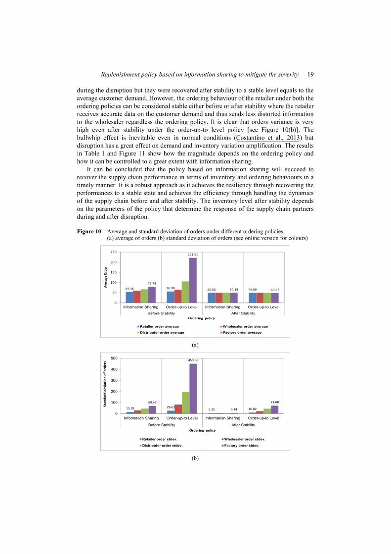
The ordering behaviour of the supply chain before and after stability has been investigated by measuring the average order level, standard deviation of orders, bullwhip effect ratio and overall bullwhip effect. As shown in Figure 10(a) and Figure 10(b), the average and standard deviation of orders issued by different partners had been very high

Replenishment policy based on information sharing to mitigate the severity 19

during the disruption but they were recovered after stability to a stable level equals to the average customer demand. However, the ordering behaviour of the retailer under both the ordering policies can be considered stable either before or after stability where the retailer receives accurate data on the customer demand and thus sends less distorted information to the wholesaler regardless the ordering policy. It is clear that orders variance is very high even after stability under the order-up-to level policy [see Figure 10(b)]. The bullwhip effect is inevitable even in normal conditions (Costantino et al., 2013) but disruption has a great effect on demand and inventory variation amplification. The results in Table 1 and Figure 11 show how the magnitude depends on the ordering policy and how it can be controlled to a great extent with information sharing.

It can be concluded that the policy based on information sharing will succeed to recover the supply chain performance in terms of inventory and ordering behaviours in a timely manner. It is a robust approach as it achieves the resiliency through recovering the performances to a stable state and achieves the efficiency through handling the dynamics of the supply chain before and after stability. The inventory level after stability depends on the parameters of the policy that determine the response of the supply chain partners during and after disruption.

Figure 10 Average and standard deviation of orders under different ordering policies, (a) average of orders (b) standard deviation of orders (see online version for colours)

54.46 56.30 50.03 49.99

79.78

221.51

50.18 48.57

0

50

100

150

200

250

Information Sharing Order-up-to Level Information Sharing Order-up-to Level

Before Stability After Stability

Average Order

Ordering  policy

Retailer order average Wholesaler order average

Distributor order average Factory order average

(a)

15.28 26.635.25 10.02

69.47

450.96

6.14

71.68

0

100

200

300

400

500

Information Sharing Order-up-to Level Information Sharing Order-up-to Level

Before Stability After Stability

Stan

dard deviatio

n of orders

Ordering  policy

Retailer order stdev. Wholesaler order stdev.

Distributor order stdev. Factory order stdev.

(b)

20 F. Costantino et al.

Table 1 Bullwhip effect under different ordering policies

Before stability After stability Echelon i Information

sharing Order-up-to

level Information

sharing Order-up-to

level

Retailer bullwhip effect 9.27 28.17 1.10 3.99 Wholesaler bullwhip effect 32.65 265.65 1.19 19.28 Distributor bullwhip effect 81.59 1514.09 1.34 78.72 Factory bullwhip effect 191.68 8077.23 1.50 204.09

Figure 11 Overall bullwhip effect under different ordering policies (see online version for colours)

315.19

9885.15

5.12 306.08

0

2000

4000

6000

8000

10000

12000

Information Sharing Order-up-to Level Information Sharing Order-up-to Level

Before Stability After Stability

Ove

rall

bullw

hip

effe

ct

Ordering policy

7 Conclusions

Today’s, supply chains have recently faced many disruptions, due to either natural or man-made disasters, that affected very dramatically operational and financial performances as modern market environment is more complex than ever before. A breakdown risk at any stage tends to propagate and disrupt the whole system that might sustain other problems even after the disruption has terminated, due to the dynamics of supply chains.

The contribution of the paper in this research field is exploration of a tactical approach that controls the rational reactions of supply chains’ partners during and after stability while they are struggling to recover back their performances. Through a simulation model of a complex system made of a single product four-echelon supply chain subject to a specific supply chain disruption, a comparison has been conducted between a decentralised information sharing approach and a common classical ordering policy (order-up-to level). In general, the replenishment policy based on information sharing has succeeded to recover the supply chain performance, inventory level and ordering behaviour. However, the recovery period (instability period) and inventory level performances realised after stability are dependent on the specific parameters of the policy that have to be accurately set. This confirmed previous works cited in the literature

Replenishment policy based on information sharing to mitigate the severity 21

review and confirmed that traditional ordering policies should be integrated with new policies that can cope with the complexity of modern supply chains.

The results suggested that facing disruption in a rational manner leads to better performance. Information sharing is a useful tactic that can be integrated with other mitigation and contingency approaches to manage disruption risk. In fact, the model results help practitioners to understand how supply chain disruption propagates along the supply chain to find the appropriate solutions and avoid negative consequences. For example, if there is no incentive to apply a coordination mechanism or information sharing, echelons should be substituted very rapidly in order to control the distortion of information that may be propagated through them. This can also be achieved by holding enough strategic inventories at the downstream echelons to quickly balance and recover a stable behaviour of supply chain partners.

Thus, the most significant managerial implication of this study lies in the need to increase the level of coordination among supply chain members in order achieve both efficiency and resiliency. Furthermore, we have confirmed that this coordination can be achieved through the ordering policy itself with a limited effort of implementation. If the coordination is not possible with all partners, single managers could account for potential disruption events through keeping a strategic stock in order to protect the whole supply chain from its dynamics.

Future research work will consider different patterns of customer demand to model specific events (as for temporal or partial breakdown of echelons, sudden increase of lead times) and test the performances and robustness of the policy under different frequency and length of disruptions. Moreover, the parameters that determine the results of the token approach can be optimised, according to a specific design of experiment for each echelon, to create a complete methodology that could help managers to set the coordination mechanism as its best. Two further streams of research can be developed: first, investigating how the benefits of decentralised information sharing effect can affect different configurations of supply chains (i.e., with more partners per echelons, finite production or inventory capacity, and risk pooling strategies). Then, trying to identify how to manage and evaluate the effect of sharing other information in addition to customer demand such as inventory level and backlog.

Acknowledgements

The authors would like to thank anonymous reviewers for their useful comments and suggestions on an earlier version of this paper.

References Babazadeh, R. and Razmi, J. (2012) ‘A robust stochastic programming approach for agile and

responsive logistics under operational and disruption risks’, International Journal of Logistics Systems and Management, Vol. 13, No. 4, pp.458–482.

Bayraktar, E., Koh, S.C.L., Gunasekaran, A., Sari, K. and Tatoglu, E. (2008) ‘The role of forecasting on bullwhip effect for E-SCM applications’, International Journal of Production Economics, Vol. 113, No. 1, pp.193–204.

22 F. Costantino et al.

Blackhurst, J., Craighead, C.W., Elkins, D. and Handfield, R.B. (2005) ‘An empirically derived agenda of critical research issues for managing supply-chain disruptions’, International Journal of Production Research, Vol. 43, No. 19, pp.4067–4081.

Carvalho, H., Barroso, A.P., Machado, V.H., Azevedo, S. and Cruz-Machado, V. (2012a) ‘Supply chain redesign for resilience using simulation’, Computers and Industrial Engineering, Vol. 62, No. 1, pp.329–341.

Carvalho, H., Cruz-Machado, V. and Tavares, J.G. (2012b) ‘A mapping framework for assessing supply chain resilience’, International Journal of Logistics Systems and Management, Vol. 12, No. 3, pp.354–373.

Chao, H.P. (1987) ‘Inventory policy in the presence of market disruptions’, Operations Research, Vol. 35, No. 2, pp.274–281.

Costantino, F., Di Gravio, G. and Shaban, A. (2012) ‘Ordering policies based on information sharing to mitigate the severity of supply chain disruption’, in Grubbstrom, R.W. and Hinterhuber, H.H. (Eds.): The Seventeenth International Working Seminar on Production Economics, IWSPE, Innsbruck, 20–24 February, pp.91–103.

Costantino, F., Di Gravio, G., Shaban, A. and Tronci, M. (2013) ‘Information sharing policies based on tokens to improve supply chain performances’, International Journal of Logistics Systems and Management, Vol. 14, No. 2, pp.133–160.

Craighead, C.W., Blackhurst, J., Rungtusanatham, M.J. and Handfiels, R.B. (2007) ‘The severity of supply chain disruptions: design characteristics and mitigation capabilities’, Decision Science, Vol. 38, No. 1, pp.131–156.

Disney, S.M. and Lambrecht, M.R. (2008) ‘On replenishment rules, forecasting, and the bullwhip effect in supply chains’, Foundation and Trends R in Technology, Information and Operations Management, Vol. 2, No. 1, pp.1–80.

Hanna, J.B., Skipper, J.B. and Hall, D. (2010) ‘Mitigating supply chain disruption: the importance of top management support to collaboration and flexibility’, International Journal of Logistics Systems and Management, Vol. 6, No. 4, pp.397–414.

Kersten, W., Hohrath, P., Boeger, M. and Singer, C. (2011) ‘A supply chain risk management process’, International Journal of Logistics Systems and Management, Vol. 8, No. 2, pp.152–166.

Kleindorfer, P.R. and Saad, G.H. (2005) ‘Managing disruption risks in supply chains’, Production and Operations Management, Vol. 14, No. 1, pp.53–68.

Lee, H.L., Padmanabhan, V. and Whang, S. (1997) ‘The bullwhip effect in supply chains’, Sloan Management Review, Vol. 38, No. 3, pp.93–102.

Levy, D. (1995) ‘International sourcing and supply chain stability’, Journal of International Business Studies, Vol. 26, No. 1, pp.343–360.

Li, J., Wang, S. and Cheng, T.C.E. (2010) ‘Competition and cooperation in a single-retailer two-supplier supply chain with supply disruption’, International Journal of Production Economics, Vol. 124, No. 1, pp.137–150.

Meyer, R.R., Rothkopf, M.H. and Smith, S.F. (1979) ‘Reliability and inventory in a production storage system’, Management Science, Vol. 25, No. 8, pp.799–807.

Min, H. (2011) ‘Modern maritime piracy in supply chain risk management’, International Journal of Logistics Systems and Management, Vol. 10, No. 1, pp.122–138.

Moyaux, T., Chaib-draa, B. and D’Amours, S. (2007) ‘Information sharing as a coordination mechanism for reducing the bullwhip effect in a supply chain’, IEEE Transactions on Systems, Man and Cybernetics Part C: Applications and Reviews, Vol. 37, No. 3, pp.396–409.

Norrman, A. and Jansson, U. (2004) ‘Ericsson’s proactive supply chain risk management approach after a serious sub-supplier accident’, International Journal of Physical Distribution and Logistics Management, Vol. 34, No. 5, pp.434–456.

Oke, A. and Gopalakrishnan, M. (2009) ‘Managing disruptions in supply chains: a case study of a retail supply chain’, International Journal of Production Economics, Vol. 118, No. 1, pp.168–174.

Replenishment policy based on information sharing to mitigate the severity 23

Parlar, M. and Berkin, D. (1991) ‘Future supply uncertainty in EOQ models’, Naval Research Logistics, Vol. 38, No. 1, pp.295–303.

Parlar, M. and Perry, D. (1996) ‘Inventory models of future supply uncertainty with single and multiple suppliers’, Naval Research Logistics, Vol. 43, No. 2, pp.191–210.

Peck, H. (2005) ‘Drivers of supply chain vulnerability: an integrated framework’, International Journal of Physical Distribution and Logistics Management, Vol. 35, No. 4, pp.210–232.

Pochard, S. (2003) Managing Risks of Supply-Chain Disruptions: Dual Sourcing as a Real Option, Master in Science of Technology and Policy thesis, Engineering Systems Division Massachusetts Institute of Technology.

Qi, L., Shen, Z.J.M. and Snyder, L.V. (2009) ‘A continuous-review inventory model with disruptions’, Production and Operations Management, Vol. 18, No. 5, pp.516–532.

Rong, Y., Shen, Z.J.M. and Snyder, L.V. (2008) ‘The impact of ordering behavior on order-quantity variability: a study of forward and reverse bullwhip effects’, Flexible Services and Manufacturing Journal, Vol. 20, No. 1, pp.95–124.

Samvedi, A. and Jain, V. (2012) ‘Effect of sharing forecast information on the performance of a supply chain experiencing disruptions’, International Journal of Logistics Systems and Management, Vol. 13, No. 4, pp.509–524.

Schmitt, A.J. and Singh, M. (2012) ‘A quantitative analysis of disruption risk in a multi-echelon supply chain’, International Journal of Production Economics, Vol. 139, No. 1, pp.22–32.

Schmitt, A.J. and Snyder, L.V. (2012) ‘Infinite-horizon models for inventory control under yield uncertainty and disruptions’, Computers and Operations Research, Vol. 39, No. 4, pp.850–862.

Shao, X.F. (2012) ‘Demand-side reactive strategies for supply disruptions in a multiple-product system’, International Journal of Production Economics, Vol. 136, No. 1, pp.241–252.

Simchi-Levi, D., Kaminsky, P. and Simchi-Levi, E. (1998) Designing and Managing the Supply Chain, Irwin/McGraw-Hill, New York.

Tang, C. (2006) ‘Robust strategies for mitigating supply chain disruptions’, International Journal of Logistics: Research and Applications, Vol. 9, No. 1, pp.33–45.

Thun, J.H. and Hoenig, D. (2011) ‘An empirical analysis of supply chain risk management in the German automotive industry’, International Journal of Production Economics, Vol. 131, No. 1, pp.242–249.

Tomlin, B. (2006) ‘On the value of mitigation and contingency strategies for managing supply chain disruption risks’, Management Science, Vol. 52, No. 5, pp.639–657.

Tuncel, G. and Alpan, G. (2010) ‘Risk assessment and management for supply chain networks: a case study’, Computers in Industry, Vol. 61, No. 3, pp.250–259.

Wilson, M.C. (2007) ‘The impact of transportation disruptions on supply chain performance’, Transportation Research Part E, Vol. 43, No. 4, pp.295–320.

Zegordi, S.H. and Davarzani, H. (2012) ‘Developing a supply chain disruption analysis model: application of colored Petri-nets’, Expert Systems with Applications, Vol. 39, No. 2, pp.2102–2111.

Zhang, C. and Zhang, C.H. (2007) ‘Design and simulation of demand information sharing in a supply chain’, Simulation Modelling Practice and Theory, Vol. 15, No. 1, pp.32–46.