Relationship between the fractal dimension anisotropy of the spatial faults distribution and the...

$: Relationship between the fractal dimension anisotropy of the spatial faults distribution and the paleostress fields on a Variscan granitic massif (Central Spain): the F-parameter$
Relationship between the fractal dimension anisotropy of the spatial faults

distribution and the paleostress fields on a Variscan granitic massif

(Central Spain): the F-parameter

R. Perez-Lopeza,*, C. Paredesb, A. Munoz-Martınc

aDpto. de Ciencias Ambientales y Recursos Naturales, Facultad de Farmacia, Universidad San Pablo—CEU, Campus Monteprıncipe, Ctra Boadilla del

Monte km 5.3, Boadilla del Monte, Madrid 28688, SpainbDpto. de Matematica Aplicada y Metodos Informaticos, Escuela Tecnica Superior de Ingenieros de Minas, Universidad Politecnica de Madrid, C/Alenza 4,

Madrid 28003, SpaincDpto. de Geodinamica, Facultad de Ciencias Geologicas, Universidad Complutense de Madrid, Avda. Complutense s/n, Madrid 28040, Spain

Received 29 June 2004

Available online 8 March 2005

Abstract

The spatial distribution of faults is usually described as a fractal set characterised by the fractal dimension. In this work, we have filtered

fault patterns interpreted from digital elevation models, aerial photographs and field maps, by using structural geological parameters of the

stress ellipsoid (stress tensor direction and stress ratio R 0) and age of deformation. From these filtered structural maps, we have obtained the

fractal dimension associated with the fracture patterns developed during Permo-Triassic and Alpine tectonic events on a Variscan granitic

massif located in the Spanish Central System. Oriented fractal dimensions were calculated on several transects crossing the fault-filtered

maps. The fractal dimension (D), calculated by 1-D box-counting, describes an ellipse on a polar plot with the short axis as the minimum

value (DHmin) and the long axis as the maximum value (DHmax) of the fractal dimensions measured. From these analyses, we have defined the

F-parameter as a function of the maximum value, minimum value and vertical value of fractal dimension (Dz), FZ(DzKDHmin)/(DHmaxKDHmin). Finally we have established, from a local scale analysis, a perpendicular relationship between the principal axes of the ellipse of the

fractal spatial anisotropy of fractures and the principal axes of the stress tensor (sHmax, sHmin and sz) that generates this dynamic pattern of

fractures. Furthermore, the F-parameter and the stress ratio R 0 are equivalents and, applied in this area, both show a triaxial extension.

q 2005 Elsevier Ltd. All rights reserved.

Keywords: Fractal; Anisotropy; Stress tensor; F-parameter; Spanish Central System

1. Introduction and objectives

The spatial distribution of faults is commonly rep-

resented by structural maps of fracture traces interpreted

from aerial photographs, digital elevation models (DEMs)

and field geological mapping. Structural geologists use

these maps in order to establish the main orientation sets and

the longest faults at this scale. These fracture sets are related

to the stress regime and geological setting and are

0191-8141/$ - see front matter q 2005 Elsevier Ltd. All rights reserved.

doi:10.1016/j.jsg.2005.01.002

* Corresponding author. Tel.: C1-34-913724765; fax: C1-34-

913510496

E-mail addresses: [email protected] (R. Perez-Lopez), cparedes@

dmami.upm.es (C. Paredes), [email protected] (A. Munoz-Martın).

interpreted in terms of kinematics and dynamics. To the

present time, these maps represent a long time interval, with

overlapping fault patterns due to several stress regimes

evolving through geological time. The patterns of reacti-

vated and newly formed fault sets in a particular region can

be identified using several techniques such as cartography,

geochronological dating and stress inversion (Angelier,

1979; Etchecopar et al., 1981; Reches, 1992; De Vicente et

al., 1996). Therefore, it is possible to obtain meso-scale

fracture patterns active during different tectonic events.

At the present time, DEMs are a powerful and useful tool

for the geologist to map morphological lineaments on the

topography at several scales (Mark and Goodchild, 1986).

These lineaments are easily interpreted using shaded relief

digital terrain maps. However, it is highly recommended

that these structural maps be compared with aerial

photographs and satellite orthoimages in the same zone.

Journal of Structural Geology 27 (2005) 663–677

www.elsevier.com/locate/jsg

http://www.elsevier.com/locate/jsg

R. Perez-Lopez et al. / Journal of Structural Geology 27 (2005) 663–677664

Otherwise, errors could be incorporated into the structural

map and subsequent analyses will be spurious or biased

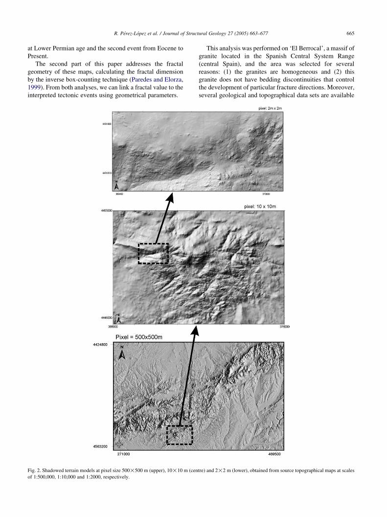
(Perez-Lopez et al., 2000). In this work, three DEMs were

constructed and analysed as a function of pixel size: 2, 10

and 500 m from topographic maps at 1:2000, 1:10,000 and

1:500,000 scale, respectively.

The main goal of this paper is to establish the relationship

between the fractal geometry of the spatial fault distribution

and the stress field. In order to reach this objective, we have

carried out statistical analysis on remote-sensing derived

fault data from Variscan granite of the Spanish Central

System (SCS). In particular: (1) we have mapped the

fracturing in an area from lineament interpretation of

DEMs, aerial photographic interpretation, taking measures

of strike and dip of fractures from field work and applying

fault population analyses to describe the paleostress field;

(2) we have measured the fractal dimension (D) of these

fracture maps by box-counting. From this relationship, it is

possible to define a geometric fractal factor (F) conditioned

by the tectonic regime as shown in the discussion.

Previously, the spatial fault distribution was described as

a fractal set, where the fractal dimension (D) is obtained by

the box-counting technique (Velde et al., 1990; Gillespie et

al., 1993; Walsh and Watterson, 1993; Barton and La

Pointe, 1995; Castaing et al., 1996; Rodrıguez-Pascua et al.,

2003). The so-called box-dimension, D, represents the

fractality or complexity degree of the spatial distribution of

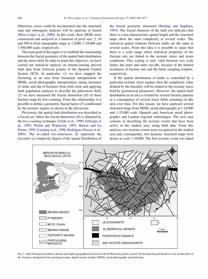
Fig. 1. (left) Geological synthesis sketch and (right) geographical location of the E

the fractures interpreted from geological maps, digital terrain models (DEM), aer

the fractal geometry measured (Hasting and Sugihara,

1993). The fractal character of the fault sets indicates that

there is a non-characteristic spatial length and the structural

maps show the same complexity at several scales. The

statistical spatial relations between faults are the same at

several scales. From this idea it is possible to argue that

there is a scale range where statistical properties of the

fracture sets are linked to the tectonic stress and strain

conditions. This scaling is only valid between two scale

limits: the inner and outer cut-offs, because of the limited

resolution of fracture sets and the finite sampling window,

respectively.

If the spatial distribution of faults is controlled by a

particular tectonic stress regime, then the complexity value

defined by the fractality will be related to the tectonic stress

field by geometrical parameters. However, the spatial fault

distribution in an area is formed by several fracture patterns

as a consequence of several stress fields actuating on this

area over time. For this reason, we have analysed several

structural maps from DEMs, aerial photographs at 1:18,000

and 1:33,000 scale (Spanish and American aerial photo-

graphs) and Landsat regional orthoimages. The next step

consists of describing the tectonic events that have been

active in the studied area, using field data. From this

analysis, two tectonic events were recognized in the studied

area and, consequently, two dynamic structural maps were

drawn at scale 1:10,000. The first tectonic event was dated

l Berrocal granitic massif. On the petrological sketch we can see the plots of

ial photographs and field trips.

R. Perez-Lopez et al. / Journal of Structural Geology 27 (2005) 663–677 665

at Lower Permian age and the second event from Eocene to

Present.

The second part of this paper addresses the fractal

geometry of these maps, calculating the fractal dimension

by the inverse box-counting technique (Paredes and Elorza,

1999). From both analyses, we can link a fractal value to the

interpreted tectonic events using geometrical parameters.

Fig. 2. Shadowed terrain models at pixel size 500!500 m (upper), 10!10 m (cen

of 1:500,000, 1:10,000 and 1:2000, respectively.

This analysis was performed on ‘El Berrocal’, a massif of

granite located in the Spanish Central System Range

(central Spain), and the area was selected for several

reasons: (1) the granites are homogeneous and (2) this

granite does not have bedding discontinuities that control

the development of particular fracture directions. Moreover,

several geological and topographical data sets are available

tre) and 2!2 m (lower), obtained from source topographical maps at scales


in this area: aerial photographs, geological and topographi-

cal maps at several scales, boreholes, petrological and

geochemical data, geochronological ages, etc. (Hidrobap

Project, 1999)

2. Geological and tectonic settings

The granitic massif analysed, ‘El Berrocal’, is located

within the Gredos Mountain Range and has an approximate

surface area of 22 km2. This massif is part of the southern

border of the SCS (Fig. 1). The SCS produces a NE–SW

structural relief that divides two continental basins devel-

oped during the Tertiary from the Duero basin to the north

and the Tajo basin to the south (De Vicente et al., 2004). The

age of the oldest rocks of the SCS ranges from Precambrian

to Upper Palaeozoic and they were affected by several

tectonic and metamorphic events during the Caledonian and

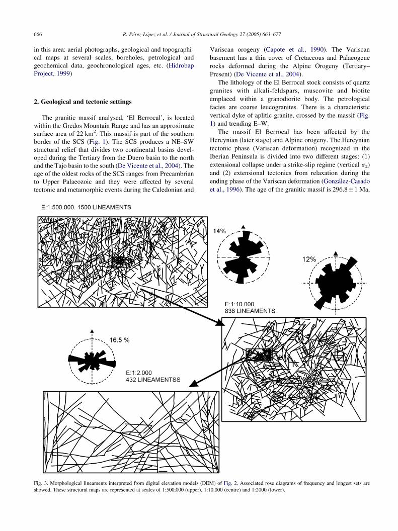
Fig. 3. Morphological lineaments interpreted from digital elevation models (DE

showed. These structural maps are represented at scales of 1:500,000 (upper), 1:1

Variscan orogeny (Capote et al., 1990). The Variscan

basement has a thin cover of Cretaceous and Palaeogene

rocks deformed during the Alpine Orogeny (Tertiary–

Present) (De Vicente et al., 2004).

The lithology of the El Berrocal stock consists of quartz

granites with alkali-feldspars, muscovite and biotite

emplaced within a granodiorite body. The petrological

facies are coarse leucogranites. There is a characteristic

vertical dyke of aplitic granite, crossed by the massif (Fig.

1) and trending E–W.

The massif El Berrocal has been affected by the

Hercynian (later stage) and Alpine orogeny. The Hercynian

tectonic phase (Variscan deformation) recognized in the

Iberian Peninsula is divided into two different stages: (1)

extensional collapse under a strike-slip regime (vertical s2)

and (2) extensional tectonics from relaxation during the

ending phase of the Variscan deformation (Gonzalez-Casado

et al., 1996). The age of the granitic massif is 296.8G1 Ma,

M) of Fig. 2. Associated rose diagrams of frequency and longest sets are

0,000 (centre) and 1:2000 (lower).


dated by Rb/Sr techniques (Campos et al., 1996) and it was

emplaced during the N–S extension of Central Iberia,

developed along the later Hercynian tectonic phase (Lower

Permian) (Casquet et al., 1988).

The Alpine orogeny is affected by the SCS by a strike-

slip stress field (Capote et al., 1990) because of the relative

movement between the Iberian and Eurasian Plates (Vegas

et al., 1990). The geological evolution during this orogeny is

strongly influenced by the stress transmission from the

active borders of the Iberian Peninsula. There are two

tectonic episodes (De Vicente et al., 2004): The Pyrenees

phase, with N–S compression acting from Eocene to

Oligocene and the Betics phase, with NW–SE compression

from Miocene to Present (Munoz-Martın et al., 1998). Both

events activated E–W to ENE–WSW thrust faults as well as

sinistral N–S and dextral NW–SE strike-slip faults under a

strike-slip stress regime in Central Iberia (De Vicente et al.,

2004). The Alpine structures measured in El Berrocal

during the field work correspond to conjugate strike-slip

faults oriented NW–SE and NNE–SSW and normal faults

and dykes oriented NNW–SSE.

3. Structural fault map at scale 1:10,000

From three topographic maps (1:2000, 1:10,000 and

1:500,000; Hidrobap Project, 1999), three DEMs were

constructed (Fig. 2) to generate analytic shaded models

from several illumination orientations. These models were

used to identify morphological discontinuities. The DEMs

were then included in a GIS designed for adding geological

and topographical information.

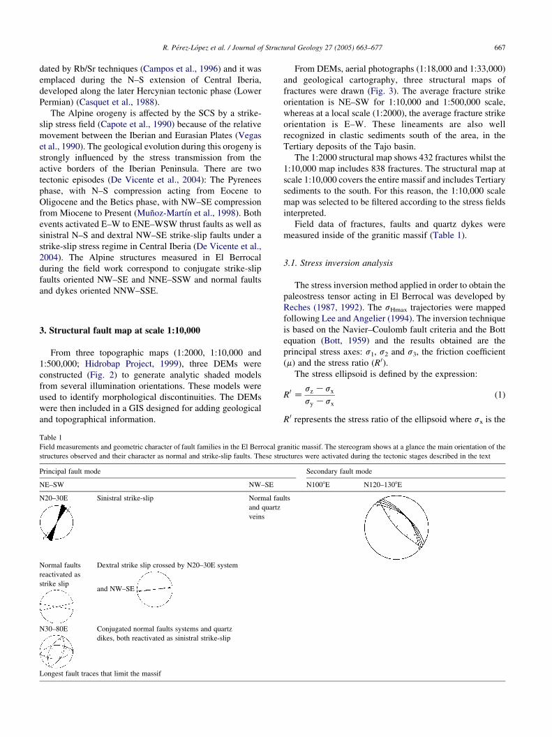
Table 1

Field measurements and geometric character of fault families in the El Berrocal gr

structures observed and their character as normal and strike-slip faults. These str

Principal fault mode

NE–SW NW–SE

N20–30E Sinistral strike-slip Normal fau

and quartz

veins

Normal faults

reactivated as

strike slip

Dextral strike slip crossed by N20–30E system

and NW–SE

N30–80E Conjugated normal faults systems and quartz

dikes, both reactivated as sinistral strike-slip

Longest fault traces that limit the massif

From DEMs, aerial photographs (1:18,000 and 1:33,000)

and geological cartography, three structural maps of

fractures were drawn (Fig. 3). The average fracture strike

orientation is NE–SW for 1:10,000 and 1:500,000 scale,

whereas at a local scale (1:2000), the average fracture strike

orientation is E–W. These lineaments are also well

recognized in clastic sediments south of the area, in the

Tertiary deposits of the Tajo basin.

The 1:2000 structural map shows 432 fractures whilst the

1:10,000 map includes 838 fractures. The structural map at

scale 1:10,000 covers the entire massif and includes Tertiary

sediments to the south. For this reason, the 1:10,000 scale

map was selected to be filtered according to the stress fields

interpreted.

Field data of fractures, faults and quartz dykes were

measured inside of the granitic massif (Table 1).

3.1. Stress inversion analysis

The stress inversion method applied in order to obtain the

paleostress tensor acting in El Berrocal was developed by

Reches (1987, 1992). The sHmax trajectories were mapped

following Lee and Angelier (1994). The inversion technique

is based on the Navier–Coulomb fault criteria and the Bott

equation (Bott, 1959) and the results obtained are the

principal stress axes: s1, s2 and s3, the friction coefficient

(m) and the stress ratio (R 0).

The stress ellipsoid is defined by the expression:

R0 Zsz Ksx

sy Ksx(1)

R 0 represents the stress ratio of the ellipsoid where sx is the

anitic massif. The stereogram shows at a glance the main orientation of the

uctures were activated during the tectonic stages described in the text

Secondary fault mode

N1008E N120–1308E

lts

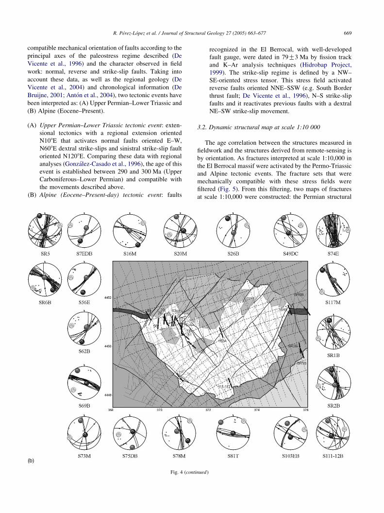
Fig. 4. Paleostress map and trajectory of sHmax obtained for (a) Permian–Lower Triassic extensional tectonic event. Twenty field stations of measurements

describe this event with s1 vertical. (b) Paleostress map and trajectory of sHmax obtained for Alpine–Eocene–present-day extensional and shear tectonic event.

This event is described by 20 field stations of measurements with s1 (8) or s2 (12) vertical. In both figures, each station number is located into the granitic

massif and the fracture activated by this stress field is plotted.


minimum horizontal stress value (sHmin), sy is the

maximum horizontal stress value (sHmax) and sz is the

vertical stress value (sV).

In total, 1994 structural data were collected and 690

measurements of slickenside lineations on fault planes, at

123 locations. From stress inversion results, two main sets

of stress tensors, defined by the orientation of the maximum

horizontal stress (sHmax), were determined (Fig. 4a and b)

showing axial symmetry:

(1)
Family A: sHmax ranged between N708E and N1208E
(2)
Family B: sHmax oriented N1508E and N0108E
The chronological relationship between the sets shows

that the fault families of set A are older than faults of set B,

established from field observations: overlapped slickenside

on fault planes and fault traces crossed by others. The

discrimination of fault families in both events was derived

from three sources: (1) field observation of relative dating

and data collected from absolute dating of episyenite quartz

dykes (Galindo et al., 1994; Gonzalez-Casado et al., 1996);

(2) structures activated during each stress regime; and (3)


compatible mechanical orientation of faults according to the

principal axes of the paleostress regime described (De

Vicente et al., 1996) and the character observed in field

work: normal, reverse and strike-slip faults. Taking into

account these data, as well as the regional geology (De

Vicente et al., 2004) and chronological information (De

Bruijne, 2001; Anton et al., 2004), two tectonic events have

been interpreted as: (A) Upper Permian–Lower Triassic and

(B) Alpine (Eocene–Present).

(A)
Upper Permian–Lower Triassic tectonic event: exten-
sional tectonics with a regional extension oriented

N108E that activates normal faults oriented E–W,

N608E dextral strike-slips and sinistral strike-slip fault

oriented N1208E. Comparing these data with regional

analyses (Gonzalez-Casado et al., 1996), the age of this

event is established between 290 and 300 Ma (Upper

Carboniferous–Lower Permian) and compatible with

the movements described above.

(B)
Alpine (Eocene–Present-day) tectonic event: faults
Fig. 4 (continued)

recognized in the El Berrocal, with well-developed

fault gauge, were dated in 79G3 Ma by fission track

and K–Ar analysis techniques (Hidrobap Project,

1999). The strike-slip regime is defined by a NW–

SE-oriented stress tensor. This stress field activated

reverse faults oriented NNE–SSW (e.g. South Border

thrust fault; De Vicente et al., 1996), N–S strike-slip

faults and it reactivates previous faults with a dextral

NE–SW strike-slip movement.

3.2. Dynamic structural map at scale 1:10 000

The age correlation between the structures measured in

fieldwork and the structures derived from remote-sensing is

by orientation. As fractures interpreted at scale 1:10,000 in

the El Berrocal massif were activated by the Permo-Triassic

and Alpine tectonic events. The fracture sets that were

mechanically compatible with these stress fields were

filtered (Fig. 5). From this filtering, two maps of fractures

at scale 1:10,000 were constructed: the Permian structural


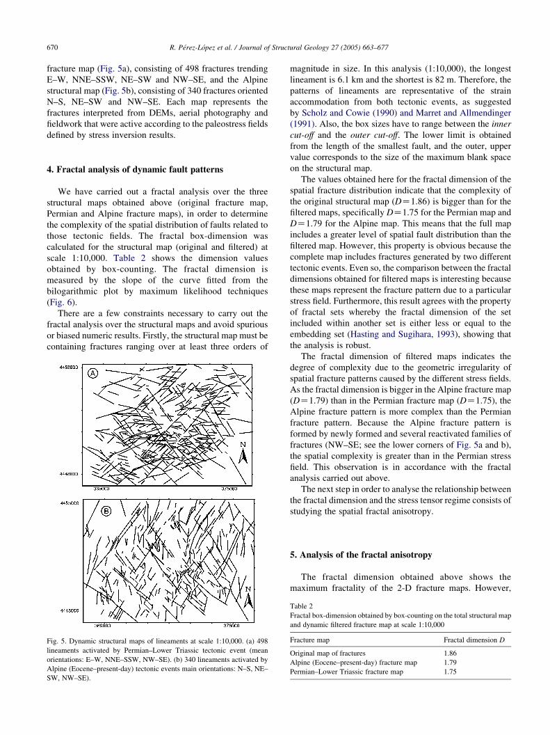
fracture map (Fig. 5a), consisting of 498 fractures trending

E–W, NNE–SSW, NE–SW and NW–SE, and the Alpine

structural map (Fig. 5b), consisting of 340 fractures oriented

N–S, NE–SW and NW–SE. Each map represents the

fractures interpreted from DEMs, aerial photography and

fieldwork that were active according to the paleostress fields

defined by stress inversion results.

4. Fractal analysis of dynamic fault patterns

We have carried out a fractal analysis over the three

structural maps obtained above (original fracture map,

Permian and Alpine fracture maps), in order to determine

the complexity of the spatial distribution of faults related to

those tectonic fields. The fractal box-dimension was

calculated for the structural map (original and filtered) at

scale 1:10,000. Table 2 shows the dimension values

obtained by box-counting. The fractal dimension is

measured by the slope of the curve fitted from the

bilogarithmic plot by maximum likelihood techniques

(Fig. 6).

There are a few constraints necessary to carry out the

fractal analysis over the structural maps and avoid spurious

or biased numeric results. Firstly, the structural map must be

containing fractures ranging over at least three orders of

Fig. 5. Dynamic structural maps of lineaments at scale 1:10,000. (a) 498

lineaments activated by Permian–Lower Triassic tectonic event (mean

orientations: E–W, NNE–SSW, NW–SE). (b) 340 lineaments activated by

Alpine (Eocene–present-day) tectonic events main orientations: N–S, NE–

SW, NW–SE).

magnitude in size. In this analysis (1:10,000), the longest

lineament is 6.1 km and the shortest is 82 m. Therefore, the

patterns of lineaments are representative of the strain

accommodation from both tectonic events, as suggested

by Scholz and Cowie (1990) and Marret and Allmendinger

(1991). Also, the box sizes have to range between the inner

cut-off and the outer cut-off. The lower limit is obtained

from the length of the smallest fault, and the outer, upper

value corresponds to the size of the maximum blank space

on the structural map.

The values obtained here for the fractal dimension of the

spatial fracture distribution indicate that the complexity of

the original structural map (DZ1.86) is bigger than for the

filtered maps, specifically DZ1.75 for the Permian map and

DZ1.79 for the Alpine map. This means that the full map

includes a greater level of spatial fault distribution than the

filtered map. However, this property is obvious because the

complete map includes fractures generated by two different

tectonic events. Even so, the comparison between the fractal

dimensions obtained for filtered maps is interesting because

these maps represent the fracture pattern due to a particular

stress field. Furthermore, this result agrees with the property

of fractal sets whereby the fractal dimension of the set

included within another set is either less or equal to the

embedding set (Hasting and Sugihara, 1993), showing that

the analysis is robust.

The fractal dimension of filtered maps indicates the

degree of complexity due to the geometric irregularity of

spatial fracture patterns caused by the different stress fields.

As the fractal dimension is bigger in the Alpine fracture map

(DZ1.79) than in the Permian fracture map (DZ1.75), the

Alpine fracture pattern is more complex than the Permian

fracture pattern. Because the Alpine fracture pattern is

formed by newly formed and several reactivated families of

fractures (NW–SE; see the lower corners of Fig. 5a and b),

the spatial complexity is greater than in the Permian stress

field. This observation is in accordance with the fractal

analysis carried out above.

The next step in order to analyse the relationship between

the fractal dimension and the stress tensor regime consists of

studying the spatial fractal anisotropy.

5. Analysis of the fractal anisotropy

The fractal dimension obtained above shows the

maximum fractality of the 2-D fracture maps. However,

Table 2

Fractal box-dimension obtained by box-counting on the total structural map

and dynamic filtered fracture map at scale 1:10,000

Fracture map Fractal dimension D

Original map of fractures 1.86

Alpine (Eocene–present-day) fracture map 1.79

Permian–Lower Triassic fracture map 1.75

Fig. 6. Bilogarithmic curve obtained by box counting covering the

structural map of lineaments (Fig. 2-centre) at scale 1:10,000. The fit was

achieved using the maximum likelihood technique and the slope

corresponds to the fractal box-dimension, DZ1.86.


the grid covers the entire fracture map and, therefore, it does

not indicate the direction of maximum complexity or

fractality if they exist. This direction exists because the

fracture density is heterogeneous along the map; the number

of faults in each box is not constant. From this idea, it is

possible to affirm that the fractal dimension of the spatial

distribution of fault is anisotropic. The question is how to

measure this anisotropy.

Perez-Lopez et al. (2000) propose a methodology to

obtain the bidimensional fractal anisotropy. These authors

obtain the fractal box-dimension over transects across the

structure map (normal to the mean fracture sets directions)

and show fracture profiles with a structure similar to a

Cantor’s Dust (Fig. 7). This methodology is based on

Cantor’s Dust analysis of faults applied by Velde et al.

(1990) and revised by Harris et al. (1991). Recently,

Volland and Kruhl (2004) have proposed a similar

methodology to obtain patterns of anisotropies in a

Hercynian fault zone. These authors determine the azi-

Fig. 7. One-dimensional transects cutting the structural fracture map at scale 1:10,0

from the rose diagram. The fracture profiles are obtained by recording the interse

fractal dimension is calculated by a 1-D box-counting. After Perez-Lopez et al. (

muthal anisotropy of the fractal dimension by applying the

Cantor’s Dust method in the analysis of 1-D frequency–size

distribution of fragments. They conclude that two patterns

of fault genesis were recognized.

The fractal dimensions obtained by Perez-Lopez et al.

(2000) range between 0.58 and 0.51. However, when

applying the same transects over the dynamic filtered

maps, these authors found that the fractal dimension ranged

between 0.53 and 0.79. This last result shows a greater

difference between the maximum and minimum values of

fractal dimension of the filtered map than the fractal

dimension obtained from the complete fracture map.

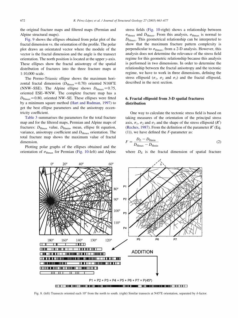
5.1. Methodology to measure the anisotropy

In order to realize a systematic coverage of transects for

the structural fracture maps obtained above, a computer

code, called AFA, was designed Firstly, AFA obtains the

fracture profile on transects taken at 108 increments,

oriented from the north to the south and covering 1808

(Fig. 8-left). However, the intersections between faults and

the profiles obtained depend on the location of the rotation

centre. Perez Lopez (2003) suggests that there is a minimum

value of fault intersection on a fracture profile, the mass

number. To prevent the effect of the lack of mass, the AFA

code draws several transects with the same orientation and

separated by a d-factor (Fig. 8-right). These similar profiles

are added in one unique profile and the maximum

irregularity is incorporated into the analysis. Over this

unique profile we have achieved the 1-D box counting for

00. The strike of these transects is obtained from the main fracture directions

ctions between each transect and fracture. Over these fracture profiles, the

2000).


the original fracture maps and filtered maps (Permian and

Alpine structural maps).

Fig. 9 shows the ellipses obtained from polar plot of the

fractal dimension vs. the orientation of the profile. The polar

plot draws an orientated vector where the module of the

vector is the fractal dimension and the angle is the transect

orientation. The north position is located at the upper y-axis.

These ellipses show the fractal anisotropy of the spatial

distribution of fractures into the three fracture maps at

1:10,000 scale.

The Permo-Triassic ellipse shows the maximum hori-

zontal fractal dimension (DHmaxZ0.70) oriented N1688E

(NNW–SSE). The Alpine ellipse shows DHmaxZ0.75,

oriented ESE–WNW. The complete fracture map has a

DHmaxZ0.80, oriented NW–SE. These ellipses were fitted

by a minimum square method (Hart and Rudman, 1997) to

get the best ellipse parameters and the anisotropy eccen-

tricity coefficient.

Table 3 summarises the parameters for the total fracture

map and for the filtered maps, Permian and Alpine maps of

fractures: DHmax value, DHmin, mean, ellipse fit equation,

variance, anisotropy coefficient and DHmax orientation. The

total fracture map shows the maximum value of fractal

dimension.

Plotting polar graphs of the ellipses obtained and the

orientation of sHmax for Permian (Fig. 10-left) and Alpine

Fig. 8. (left) Transects oriented each 108 from the north to south. (righ

stress fields (Fig. 10-right) shows a relationship between

sHmax and DHmax. From this analysis, sHmax is normal to

DHmax. This geometrical relationship can be interpreted to

show that the maximum fracture pattern complexity is

perpendicular to sHmax, from a 2-D analysis. However, this

analysis does not determine the relevance of the stress field

regime for this geometric relationship because this analysis

is performed in two dimensions. In order to determine the

relationship between the fractal anisotropy and the tectonic

regime, we have to work in three dimensions, defining the

stress ellipsoid (s1, s2 and s3) and the fractal ellipsoid,

described in the next section.

6. Fractal ellipsoid from 3-D spatial fractures

distribution

One way to calculate the tectonic stress field is based on

taking measures of the orientation of the principal stress

axis, s1, s2 and s3 and the shape of the stress ellipsoid (R 0)

(Reches, 1987). From the definition of the parameter R 0 (Eq.

(1)), we have defined the F-parameter as:

F ZDZ KDHmin

DHmax KDHmin

(2)

where DZ is the fractal dimension of spatial fracture

t) Similar transects at N458E orientation, separated by d-factor.

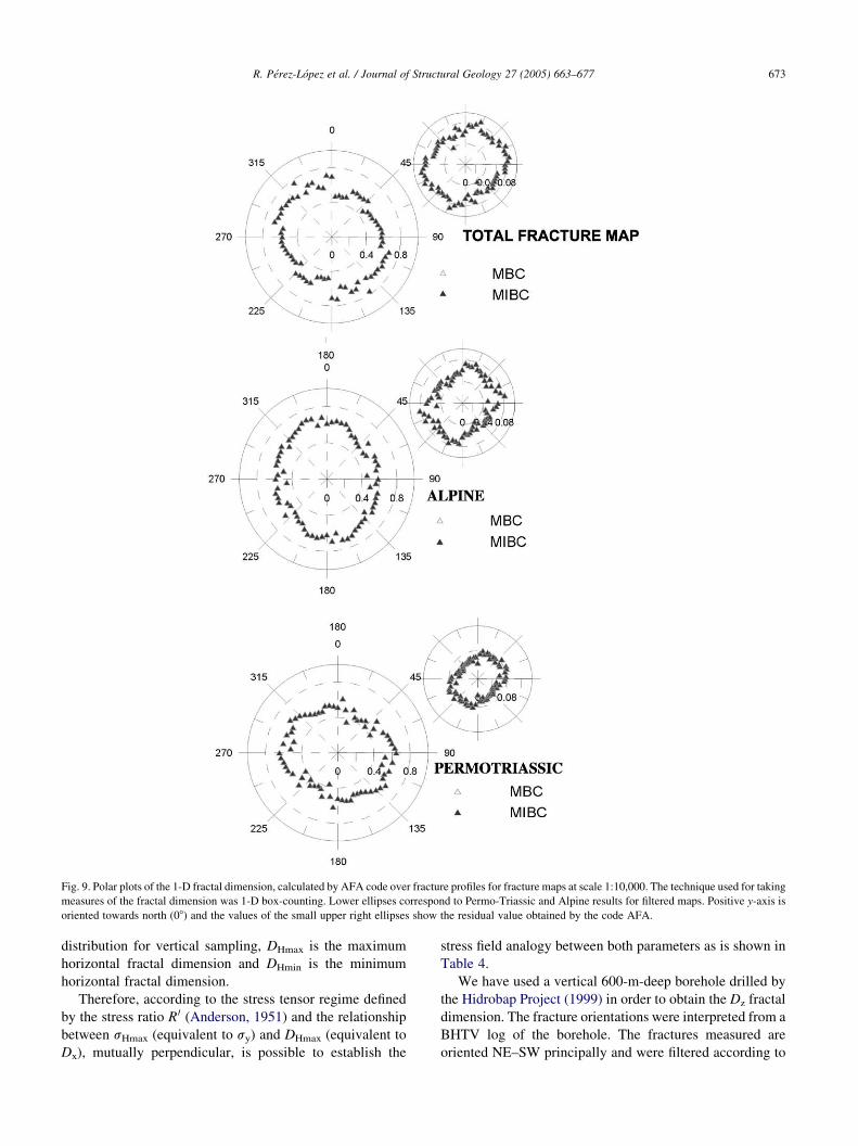
Fig. 9. Polar plots of the 1-D fractal dimension, calculated by AFA code over fracture profiles for fracture maps at scale 1:10,000. The technique used for taking

measures of the fractal dimension was 1-D box-counting. Lower ellipses correspond to Permo-Triassic and Alpine results for filtered maps. Positive y-axis is

oriented towards north (08) and the values of the small upper right ellipses show the residual value obtained by the code AFA.


distribution for vertical sampling, DHmax is the maximum

horizontal fractal dimension and DHmin is the minimum

horizontal fractal dimension.

Therefore, according to the stress tensor regime defined

by the stress ratio R 0 (Anderson, 1951) and the relationship

between sHmax (equivalent to sy) and DHmax (equivalent to

Dx), mutually perpendicular, is possible to establish the

stress field analogy between both parameters as is shown in

Table 4.

We have used a vertical 600-m-deep borehole drilled by

the Hidrobap Project (1999) in order to obtain the Dz fractal

dimension. The fracture orientations were interpreted from a

BHTV log of the borehole. The fractures measured are

oriented NE–SW principally and were filtered according to

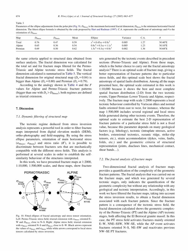
Table 3

Parameters of the ellipse adjustments from the polar plot (Fig. 9). DHmax is the maximum horizontal fractal dimension; DHmin is the minimum horizontal fractal

dimension. The fittest ellipse formula is obtained by the code proposed by Hart and Rudman (1997). C.A. represents the coefficient of anisotropy and q is the

orientation of DHmax

Map DHmax DHmin Mean Ellipse Variance C.A. q

Total 0.76 0.47 0.59 x2C0.45xyC0.9y2 0.005 1.27 N1408E

Alpine 0.65 0.36 0.54 0.8x2C0.3xyC1.1y2 0.005 1.23 N1108E

Permian 0.69 0.50 0.62 1.5x2C0.3xyC0.9y2 0.002 1.36 N1688E


the same criteria applied to structural data obtained from

surface analysis. The fractal dimension was calculated for

the total set and for fracture maps filtered for the Permo-

Triassic and Alpine tectonic stress fields. The fractal

dimension calculated is summarised in Table 5. The vertical

fractal dimension for original structural map (DzZ0.84) is

bigger than Alpine (DzZ0.80) and Permian (DzZ0.79).

According to the analogy shown in Table 4 and the F

values for Alpine and Permo-Triassic fracture patterns

(bigger than one with DzODHmax), both regimes are defined

as triaxial extension.

7. Discussion

7.1. Dynamic filtering of structural map

The tectonic regime deduced from stress inversion

analysis represents a powerful tool in order to filter fracture

maps interpreted from digital elevation models (DEM),

ortho-photography and field-mapping. By using the stress

ellipse parameters, orientation of main horizontal stress

(sHmax, sHmin) and stress ratio (R 0), it is possible to

discriminate between fractures sets that are mechanically

compatible with the different stress fields. This analysis is

performed at several scales in order to establish the self-

similarity behaviour of the structures interpreted.

In this work, we have presented fracture maps at 1:2000,

1:10,000, 1:500,000 scales, and these maps, show fracture

Fig. 10. Fitted ellipses of fractal anisotropy and stress tensor orientation.

Left: Permo-Triassic stress field, triaxial extension with sHmax oriented E–

W and DHmax close to N–S. Right: Alpine stress field, triaxial extension

with sHmax oriented N–S and DHmax close to E–W. Black arrows represent

the values of sHmax and sHmin while white arrows correspond to local stress

tensors calculated by stress inversion.

sets generated by the tectonic events described in precedent

sections (Permo-Triassic and Alpine). From these maps,

which is the better choice to carry out the fractal anisotropy

analysis? There is an optimal scale of fracture map, giving a

better representation of fracture patterns due to particular

stress fields, and this optimal scale best shows the fractal

anisotropy of spatial faults distribution. Among all the maps

presented here, the optimal scale estimated in this work is

1:10,000 because it shows the best and most complete

spatial fracture distribution (2-D) from the two tectonic

events, Upper Permian–Lower Triassic and Alpine, respect-

ively. The fracture map with scale 1:2000 represents a local

tectonic behaviour controlled by Variscan dikes and normal

faults oriented from east to west, for instance, whereas the

map 1:500,000 includes several regional and local stress

fields generated during other tectonic events. Therefore, the

optimal scale to estimate the best 2-D representation of

fracture patterns of a particular stress field is not a fixed

value, because this parameter depends on many geological

factors (e.g. lithology), tectonic (intraplate stresses, active

borders, extensional tectonics, oceanic ridge, strike-slip

tensors, etc.), strain accommodation (dykes, veins, faults,

folds, etc.) and the geometric criteria of structural

representation (joints, diaclases lines, mechanical contact,

shear bands.).

7.2. The fractal analysis of fracture maps

Two-dimensional fractal analysis of fracture maps

provides a quantification of the complexity of the geometric

fracture patterns. The fractal analysis that was carried out on

the fracture maps, and which was generated by several

tectonic stages, only indicates the quantification of the

geometric complexity but without any relationship with any

geological and tectonic interpretation. Accordingly, in this

work we have filtered the fracture maps, taking into account

the stress inversion results, to obtain a fractal dimension

associated with each fracture pattern. Since the fracture

pattern is a consequence of the tectonic stress field, the

fractal dimension calculated shows the geometric complex-

ity of the Permo-Triassic (PT) and the Alpine (AP) tectonic

stages, both affecting the El Berrocal granite massif. In this

case, the PT stress field activates fractures mainly oriented

E–W, NNE–SSW, NW–SE, while the AP event activates

fractures oriented N–S, NE–SW and reactivates previous

NW–SE PT fractures.

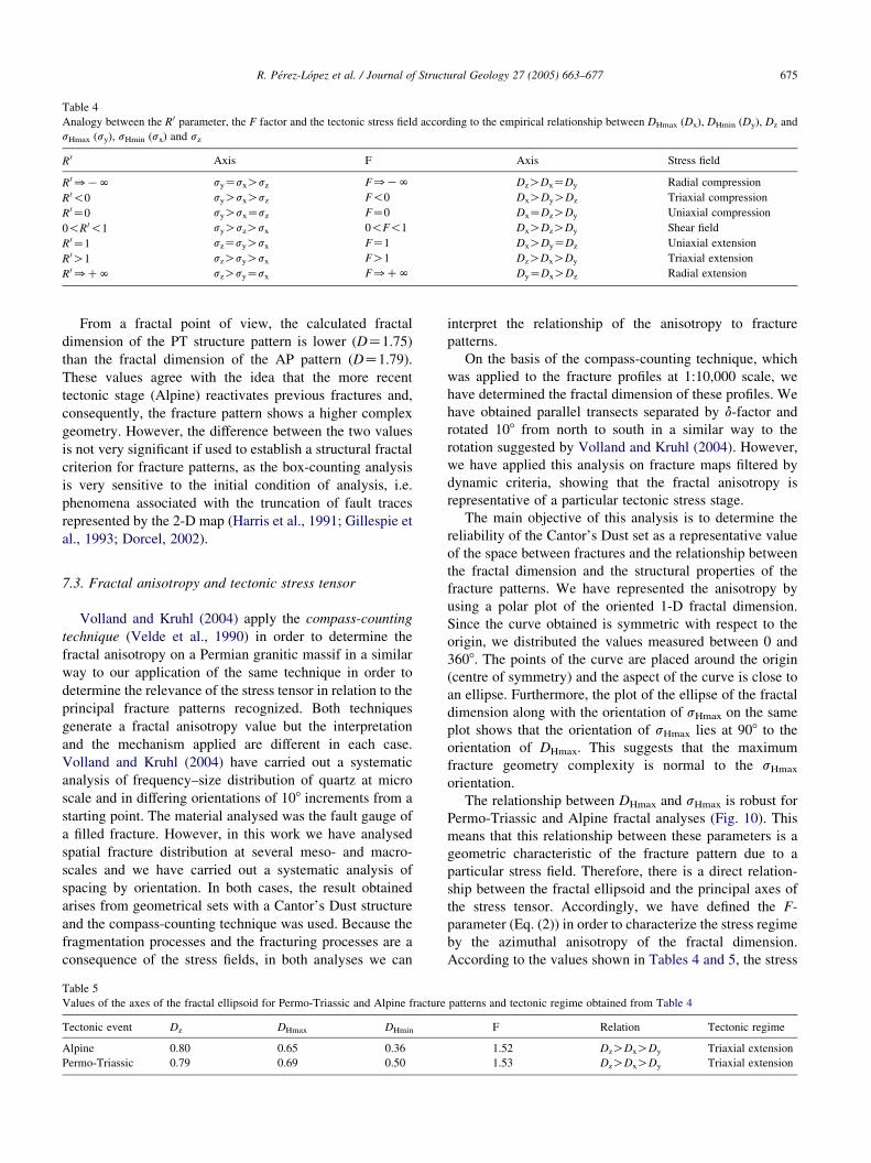
Table 4

Analogy between the R 0 parameter, the F factor and the tectonic stress field according to the empirical relationship between DHmax (Dx), DHmin (Dy), Dz and

sHmax (sy), sHmin (sx) and sz

R 0 Axis F Axis Stress field

R 00KN syZsxOsz F0KN DzODxZDy Radial compression

R 0!0 syOsxOsz F!0 DxODyODz Triaxial compression

R 0Z0 syOsxZsz FZ0 DxZDzODy Uniaxial compression

0!R 0!1 syOszOsx 0!F!1 DxODzODy Shear field

R 0Z1 szZsyOsx FZ1 DxODyZDz Uniaxial extension

R 0O1 szOsyOsx FO1 DzODxODy Triaxial extension

R 00CN szOsyZsx F0CN DyZDxODz Radial extension


From a fractal point of view, the calculated fractal

dimension of the PT structure pattern is lower (DZ1.75)

than the fractal dimension of the AP pattern (DZ1.79).

These values agree with the idea that the more recent

tectonic stage (Alpine) reactivates previous fractures and,

consequently, the fracture pattern shows a higher complex

geometry. However, the difference between the two values

is not very significant if used to establish a structural fractal

criterion for fracture patterns, as the box-counting analysis

is very sensitive to the initial condition of analysis, i.e.

phenomena associated with the truncation of fault traces

represented by the 2-D map (Harris et al., 1991; Gillespie et

al., 1993; Dorcel, 2002).

7.3. Fractal anisotropy and tectonic stress tensor

Volland and Kruhl (2004) apply the compass-counting

technique (Velde et al., 1990) in order to determine the

fractal anisotropy on a Permian granitic massif in a similar

way to our application of the same technique in order to

determine the relevance of the stress tensor in relation to the

principal fracture patterns recognized. Both techniques

generate a fractal anisotropy value but the interpretation

and the mechanism applied are different in each case.

Volland and Kruhl (2004) have carried out a systematic

analysis of frequency–size distribution of quartz at micro

scale and in differing orientations of 108 increments from a

starting point. The material analysed was the fault gauge of

a filled fracture. However, in this work we have analysed

spatial fracture distribution at several meso- and macro-

scales and we have carried out a systematic analysis of

spacing by orientation. In both cases, the result obtained

arises from geometrical sets with a Cantor’s Dust structure

and the compass-counting technique was used. Because the

fragmentation processes and the fracturing processes are a

consequence of the stress fields, in both analyses we can

Table 5

Values of the axes of the fractal ellipsoid for Permo-Triassic and Alpine fracture

Tectonic event Dz DHmax DHmin

Alpine 0.80 0.65 0.36

Permo-Triassic 0.79 0.69 0.50

interpret the relationship of the anisotropy to fracture

patterns.

On the basis of the compass-counting technique, which

was applied to the fracture profiles at 1:10,000 scale, we

have determined the fractal dimension of these profiles. We

have obtained parallel transects separated by d-factor and

rotated 108 from north to south in a similar way to the

rotation suggested by Volland and Kruhl (2004). However,

we have applied this analysis on fracture maps filtered by

dynamic criteria, showing that the fractal anisotropy is

representative of a particular tectonic stress stage.

The main objective of this analysis is to determine the

reliability of the Cantor’s Dust set as a representative value

of the space between fractures and the relationship between

the fractal dimension and the structural properties of the

fracture patterns. We have represented the anisotropy by

using a polar plot of the oriented 1-D fractal dimension.

Since the curve obtained is symmetric with respect to the

origin, we distributed the values measured between 0 and

3608. The points of the curve are placed around the origin

(centre of symmetry) and the aspect of the curve is close to

an ellipse. Furthermore, the plot of the ellipse of the fractal

dimension along with the orientation of sHmax on the same

plot shows that the orientation of sHmax lies at 908 to the

orientation of DHmax. This suggests that the maximum

fracture geometry complexity is normal to the sHmax

orientation.

The relationship between DHmax and sHmax is robust for

Permo-Triassic and Alpine fractal analyses (Fig. 10). This

means that this relationship between these parameters is a

geometric characteristic of the fracture pattern due to a

particular stress field. Therefore, there is a direct relation-

ship between the fractal ellipsoid and the principal axes of

the stress tensor. Accordingly, we have defined the F-

parameter (Eq. (2)) in order to characterize the stress regime

by the azimuthal anisotropy of the fractal dimension.

According to the values shown in Tables 4 and 5, the stress

patterns and tectonic regime obtained from Table 4

F Relation Tectonic regime

1.52 DzODxODy Triaxial extension

1.53 DzODxODy Triaxial extension


field affecting the El Berrocal granite massif is defined as

triaxial extension. Dominant faults measured in field are

normal and normal/strike-slip. The main differences

between Alpine and Permo-Triassic stress fields are the

orientation of sHmax and the parameter that characterizes the

tectonic behaviour: extensional strike-slip in both cases. The

values found in Table 5 show that the shape factor of the

anisotropy fractal ellipse does not show a significant

variation as the stress inversion results suggest and the

Permo-Triassic and Alpine tensors are extensional strike-

slip.

Finally, we have defined the ellipsoid of the azimuthal

anisotropy of the fractal dimension, flattened and constric-

tional, and their correlation with the stress ellipsoid defined

by sx, sy and sz (Fig. 11). The flattened ellipsoid of the

fractal anisotropy is linked with the constrictional stress

ellipsoid and vice versa (Fig. 11) since it is a consequence of

the perpendicular relationship between DHmax and sHmax.

8. Conclusions

The fractal dimension, measured from fracture maps

filtered by stress inversion results, shows the geometric

complexity of the fracture pattern formed by fractures

mechanically compatible with the paleostress field

recognized.

By using 1-D fracture profiles, it is possible to determine

the fractal anisotropy of the spatial fracture distribution,

active during a particular paleostress field. This anisotropy

Fig. 11. Relationship between the stress tensor and the ellipsoid of the fractal aniso

a relationship between the ellipsoid of the fractal anisotropy and the tectonic stre

analysis shows a triaxial extension with R 0 and FO1.

is an ellipse where the long axis is the maximum horizontal

fractal dimension, DHmax, and the short axis is the minimum

horizontal fractal dimension, DHmin.

The obtained results suggest a geometric relationship

between the stress tensor and the fractal anisotropy ellipse,

i.e. that the orientation of sHmax is normal to the orientation

of DHmax.

From the analogy of the orientations between sHmaxZsy,

sHminZsx and sz with DHmaxZDx, DHminZDy and Dz, it is

possible to define the fractal anisotropy ellipsoid by a factor

so-called ‘F’. This F parameter, and subsequently the fractal

anisotropy of fault distribution, defines the tectonic stress

fields in a similar way to the stress ratio R.

Acknowledgements

Thanks are given to the reviewers Dr Tim Needham and

Dr Stefano Mazzoli for their comments and clear reviews in

order to improve the manuscript and the English style. We

thank the Consejo de Seguridad Nuclear of Spain and

ENRESA for supporting partially this work. We also thank

Dr Julio Pardillo for the borehole dataset and Dr Armando

Cisternas, from EOST-Institut de Globe du Strasbourg, for

his kind remarks about the manuscript. This work was

developed in the frame of the HIDROBAP project:

hydrogeology of low permeability media and represents a

part of the thesis defended by the principal author. The

English style was revised by Dr Castineira from Colorado

University at Boulder and USGS of Denver and Dr Liz

tropy. From the stress ratio, R 0 and the F parameter, it is possible to establish

ss regime. In the case of the El Berrocal massif, stress inversion as fractal


Thompson from Midland Valley Exploration (Scotland)—

thanks for your kind help and good directions.

References

Anderson, E.M., 1951. The Dynamics of Faulting. Oliver and Boyd,

Edinburgh. 133pp.

Angelier, J., 1979. Determination of the mean principal direction of stresses

for a given fault population. Tectonophysics 56, 17–26.

Anton, L., Munoz, A., De Vicente, G., 2004. Analisis de la fracturacion y

campos de paleoesfuerzos en el centro-oeste de la Penınsula Iberica.

Geotemas 6 (3), 17–20 (in Spanish).

Barton, C., La Pointe, P.R., 1995. Fractal analysis of scaling and spatial

clustering of fractures. In: Barton, C., La Pointe, P.R. (Eds.), Fractal in

Earth Science. Plenum Press, New York, pp. 141–178.

Bott, M.P.H., 1959. The mechanism of oblique slip faulting. Geological

Magazine 96, 109–117.

Campos, R., Martın-Benavente, C., Perez del Villar, L., Pardillo, J.,

Fernandez-Dıaz, M., Quejido, A., De la Cruz, B., Rivas, P., 1996. El

Berrocal. Aspectos geologicos: litologıa y estructura a escala local y de

emplazamiento. Geogaceta 20 (7), 1618–1621 (in Spanish).

Capote, R., De Vicente, G., Gonzalez-Casado, J.M., 1990. Evolucion de las

deformaciones alpinas en el Sistema Central Espanol. Geogaceta 7, 20–

22 (in Spanish).

Casquet, C., Fuster, J.M., Gonzalez-Casado, J.M., Peinado, M.,

Villaseca, C., 1988. Extensional tectonics and granite emplacement in

the Spanish Central System, a discussion, in: Banda, E., Mendes, V.

(Eds.), Fifth EGT Workshops: The Iberian Peninsula, pp. 65–77.

Castaing, C., Halawani, M.A., Gervais, F., Chiles, J.P., Genter, A.,

Bourgine, B., Ouillon, G., Brosse, J.M., Martin, P., Genna, A.,

Janjou, D., 1996. Scaling relationship in intraplate fracture systems

related to Red Sea rifting. Tectonophysics 262, 291–314.

De Bruijne, C.H., 2001. Denudation, intraplate tectonics and far field

effects; an integrated apatite fission track study in central Spain. Ph.D.,

Vrije Universiteit, Amsterdam, 164pp.

De Vicente, G., Giner, J.L., Munoz-Martın, A., Gonzalez-Casado, J.M.,

Lindo, R., 1996. Determination of present-day stress tensor and

neotectonic interval in the Spanish Central System and Madrid basin,

Central Spain. Tectonophysics 266, 405–424.

De Vicente, G., Vegas, R., Guimera, J., Cloetingh, S., 2004. Estructura

Alpina del Antepaıs Iberico, in: Vera, J.A. (Ed.), Geologıa de Espana

Capıtulo, 7. SGE-IGME, Madrid, pp. 619–625 (in Spanish).

Dorcel, C., 2002. Correlations dans les reseaux de fractures: caracterisation

et consequences avec les propietes hydrauliques. Doctoral These,

University of Rennes (in French).

Etchecopar, A., Vasseur, G., Daigneres, M., 1981. An inverse problem in

micro tectonics for the determination of stress tensor from fault striation

analysis. Journal of Structural Geology 3, 51–65.

Galindo, C., Tornos, F., Darbyshire, D.P.F., Casquet, C., 1994. Rb and K/Ar

chronology of dikes from the Sierra de Guadarrama, Spanish Central

System. Geogaceta 16, 23–26.

Gillespie, P.A., Howard, C.B., Walsh, J.J., Watterson, J., 1993. Measure-

ment and characterisation of spatial distribution of fractures. Tectono-

physics 226, 113–141.

Gonzalez-Casado, J.M., Caballero, J.M., Casquet, C., Galindo, C.,

Tornos, F., 1996. Palaeostress and geotectonic interpretation of the

Alpine Cycle onset in the Sierra del Guadarrama (eastern Iberian

Central System), based on evidence from episyenites. Tectonophysics

262, 213–231.

Harris, C., Franssen, R., Loosveld, R., 1991. Fractal analysis of fractures in

rocks: the Cantor’s Dust method comment. Tectonophysics 198, 107–

115.

Hart, D., Rudman, A.J., 1997. Least-square fit of an ellipse to anisotropic

polar data: application to azimuthally resistivity surveys in karst

regions. Computers & Geoscience 23, 189–194.

Hasting, H.M., Sugihara, H., 1993. Fractals: a User’s Guide for the Natural

Sciences. Oxford Science Publications, Oxford. 235pp.

Hidrobap Project, 1999. Final Open Report, Project no. 0703305. Capıtulo

2: Analisis tectonico y petrologico. ENRESA-CSN (Eds.). Consejo de

Seguridad Nuclear, Madrid, 85pp (in Spanish).

Lee, J.C., Angelier, J., 1994. Paleostress trajectories maps based on the

results of local determinations: the lissage program. Computers and

Geosciences 20, 161–191.

Mark, D.M., Goodchild, M.F., 1986. On the ordering of two-dimensional

space: introduction and relation to tesseral principles, in: Dıaz, B.M.,

Bell, S.B.M. (Eds.), Spatial Data Processing using Tesseral Methods.

NERC, Unit for Thematic Information Systems, Natural Environment

Research Council, Swindon, Great Britain, pp. 179–192.

Marret, R., Allmendinger, R.W., 1991. Estimates of strain due to brittle

faulting: sampling of fault populations. Journal of Structural Geology

13, 47–50.

Munoz-Martın, A., Cloetingh, S., De Vicente, G., Andeweg, B., 1998.

Finite element modelling of Tertiary paleostress fields in the eastern

border of the Tajo basin (central Spain). Tectonophysics 300, 47–62.

Paredes, C., Elorza, F.J., 1999. Fractal and multifractal analysis of fractured

geological media: surface–subsurface correlation. Computers &

Geoscience 25, 1081–1096.

Perez Lopez, R., 2003. On chaos theory applied in seismotectonics: fractal

geometry of faults and earthquakes. European Ph.D. thesis, Universidad

Complutense de Madrid, 380pp. (in Spanish).

Perez-Lopez, R., Munoz-Martın, A., Paredes, C., de Vicente, G.,

Elorza, F.J., 2000. Dimension fractal de la distribucion espacial de

fracturas en el area granıtica de El Berrocal (Sistema Central): relacion

con el tensor de esfuerzos. Revista de la Sociedad Geologica de Espana

13, 487–503 (in Spanish).

Reches, Z., 1987. Determination of the tectonic stress from slip along faults

that obey the Coulomb yield condition. Tectonics 7, 849–861.

Reches, Z., 1992. Constraints of the strength of the upper crust from stress

inversion of fault slip data. Journal of Geophysical Research 97, 12481–

12493.

Rodrıguez-Pascua, M.A., De Vicente, G., Calvo, J.P., Perez-Lopez, R.,

2003. Similarities between recent seismic activity and paleoseismites

during the Late Miocene in the external Betic belt (Spain): relationship

by “b” value and the fractal dimension. Journal of Structural Geology

25, 749–763.

Scholz, C.H., Cowie, P., 1990. Determination of total strain from faulting

using slip measurements. Nature 346, 837–839.

Vegas, R., Vazquez, J.T., Surinacs, E., Marcos-Gonzalez, A., 1990. Model

of distributed deformation, block rotation and crystal thickening for the

formation of the Spanish Central System. Tectonophysics 184, 367–

378.

Velde, B., Dubois, J., Touchard, G., Badri, A., 1990. Fractal analysis of

fractures in rocks: the Cantor’s Dust. Tectonophysics 179, 345–352.

Volland, S., Kruhl, J.H., 2004. Anisotropy quantification: the application of

fractal geometry methods on tectonic fracture patterns of a Hercynian

fault zone in NW-Sardinia. Journal of Structural Geology 26, 1489–

1500.

Walsh, J.J., Watterson, J., 1993. Fractal analysis of fracture patterns using

the standard box-counting technique: valid and invalid methodologies.

Journal of Structural Geology 15, 1509–1512.

Relationship between the fractal dimension anisotropy of the spatial faults distribution and the...

Documents

Transcript of Relationship between the fractal dimension anisotropy of the spatial faults distribution and the...