This document is downloaded from DR-NTU, Nanyang Technological

University Library, Singapore.

Title Relations among stability parameters in the stablesurface layer : golder curves revisited.( Main article )

Author(s) Sharan, Maithili.; Rama Krishna, T. V. B. P. S.; Panda,Jagabandhu.

Citation

Sharan, M., Rama Krishna, T. V. B. P. S., Panda, J.(2005). Relations among stability parameters in the stablesurface layer : golder curves revisited. AtmosphericEnvironment, 39(30), 5619–5623.

Date 2005

URL http://hdl.handle.net/10220/7194

Rights

© 2005 Elsevier. This is the author created version of awork that has been peer reviewed and accepted forpublication by Atmospheric Environment, Elsevier. Itincorporates referee’s comments but changes resultingfrom the publishing process, such as copyediting,structural formatting, may not be reflected in thisdocument. The published version is available at: [DOI:http://dx.doi.org/10.1016/j.atmosenv.2005.05.034 ]

Relations among stability parameters in the stable

surface layer: Golder curves revisited

Maithili Sharanaac

, T.V.B.P.S. Rama Krishnab, Jagabandhu Panda

a

aCentre for Atmospheric Sciences, Indian Institute of Technology, Delhi, Hauz Khas, New

Delhi 110016, India bNEERI Zonal Laboratory, IICT Campus, Uppal Road, Hyderabad 500007, India

cTel.: +91 112659 1312; fax: +91 112658 2037.

E-mail address: mathilis@cas.iitd.ernet.in

Abstract

A nomogram was prepared by [Golder, 1972. Boundary Layer Meteorology 3, 47–58]

to compute the surface layer parameters in stable conditions. This note revisits the

Golder’s curves and examines the methodology underlying their derivation in stable

conditions. The inherent limitation in the methodology used for construction of Golder’s

curves was also noticed by Trombetti et al. (1986). Surface layer fluxes computed using

the parameters derived from modified curves are found to be closer to the turbulence

measurements from CASES-99 experiment for stable conditions than those calculated

from the [Golder, 1972. Boundary Layer Meteorology 3, 47–58] curves.

Keywords: Nomogram; Bulk Richardson number; Surface layer; Golder’s curves

1. Introduction

Golder (1972) proposed a methodology for constructing a nomogram between ln(z/z0)

(z is the height above the ground and z0 is the roughness length) and gradient Richardson

number (Ri) for a fixed value of bulk Richardson number (Rb). This nomogram was

widely used for describing the fluxes in the atmospheric models. However, Golder used

the derivative of potential temperature in the definition of Rb rather than the temperature

difference in the bulk layer. These two methods give rise to different expressions of Rb in

terms of z/L (L is Monin–Obukhov length). Trombetti et al. (1986) also pointed out the

discrepancy in Golder’s curves and indicated the conditions for their validity. Golder

(1972) suggested taking ̅ as the mean geometrical height between the two levels

where temperatures are measured and wind speed u at ̅. Wang (1981) proposed z as the

upper temperature level whereas Sedefian and Bennet (1980) used ̅ and u at the

upper level.

In this note, we revisit Golder’s curves by introducing them first, and then using a

systematic approach to construct the modified curves in stable conditions. The surface

fluxes computed using the parameters drawn from these curves are compared with those

based on turbulence measurements in stable conditions from CASES-99 experiment.

2. Methodology

From similarity theory, under horizontally homogeneous and steady state conditions:

Here is von Karman constant, z is height above the ground, is friction velocity,

is friction temperature, u is mean wind speed, is potential temperature, and

are universal functions of the stability parameter , where L is defined as

is the acceleration due to gravity and is the air temperature.

Integration of Eqs. (1) and (2) gives (Panofsky and Dutton, 1984, p. 134):

where is the temperature at and

in which .

The gradient Richardson number (Ri) is defined as

This can be expressed as a function of using Eqs. (1)–(3) as

In stable conditions, and are expressed as linear functions of

(Businger et al., 1971). Golder’s curves are based on the relation

where is a constant and . From Eqs. (8) and (9),

2.1. Golder’s method

Golder (1972) defined the bulk Richardson number (Rb) as

From Eqs. (7) and (11), Rb is related to Ri (Panofsky and Dutton, 1984, p. 143) as

where

Golder expressed u and

as a function of Ri in Eq. (13). Using Eqs. (1), (4) and (10)

in (13), p can be expressed (Panofsky and Dutton, 1984, p. 138) as

In stable conditions, and in terms of Ri can be given as

Eqs. (15) and (16) are valid only if Kh/Km is assumed to be 1. Here Kh and Km are eddy

diffusivities for heat and momentum respectively. The value of was taken as 7 by

Golder (1972).

Notice that Eq. (12) is a quadratic equation in Ri. This can be solved for the

lowest value of Ri for given values of ln(z/z0) and Rb.

2.2. Alternative procedure

Golder (1972) used the gradient of the potential temperature in the definition of

Rb as shown in Eq. (11). On the other hand, the gradient of the potential temperature

should be approximated as the potential temperature difference divided by the layer

thickness and accordingly Rb is defined as

Using Eqs. (4) and (5) along with Eqs. (3) and (9) in Eq. (17), we get

This gives

For given values of ln(z/z0) and Rb, Eq. (19) is used to compute z/L which in turn is

utilized to calculate Ri from Eqs. (8) and (9) as

Notice that in the expressions of Rb and , we assumed z z0, and thus, z0 compared to

z has been ignored in order to minimize the degrees of freedom for constructing

nomogram for known values of ln(z/z0) and Rb. Since the value of Rb is assumed to be

known from the observations, we have taken z as the upper level at which the

measurements of temperature and wind speed are available, in both Golder’s and

modified methodology. The same approach has also been adopted by Trombetti et al.

(1986).

3. Results and discussion

In Golder’s formulation, for given values of Rb and ln(z/z0), the lowest value of Ri was

computed from the quadratic equation deduced from Eq. (12). These values of Ri were

used to construct a nomogram between ln(z/z0) and Ri for a fixed value of Rb. This

reproduces the nomogram given by Golder (1972) in Fig. 1a.

For constructing a nomogram based on Eq. (14) by expressing p explicitly as a

function of z/L, we express Eq. (12) in terms of z/L by using Eqs. (1), (4), (9) and (20), as

This is a second-degree polynomial in z/L. Trombetti et al. (1986) have also expressed Rb

as a function of z/L, which reduces to a second degree polynomial in z/L for the linear

relation (9) for . The Eq. (21) will have two values of z/L for a given value of Rb and

ln(z/z0). The lowest value of z/L computed from Eq. (21) is utilized for calculating Ri

from Eq. (20). This method leads to the nomogram as given by Golder (1972). However,

Golder’s expression for Rb in terms of z/L, Eq. (21), is different from that derived in our

approach, Eq. (18). The discrepancy, which arises due to the incorrect definition of Rb

used by Golder (1972) in constructing the nomogram, was also noticed by Trombetti et al.

(1986).

Figs. 1a and b shows the variation of ln(z/z0) with Ri for a fixed Rb. Golder’s (1972)

nomogram is shown in Fig. 1a and the nomogram constructed on the basis of the

modified procedure is given in Fig. 1b. The curves are steeper with the modified method

than those obtained from Golder’s method.

In Fig. 1, = 7 is taken following Golder (1972). However, the well-established value

of = 5 as proposed by Dyer (1974) is adopted for computation of results in the rest of

this paper. Turbulence measurements from CASES-99 (Mahrt et al., 2001) in stable

conditions for 0.15 (Sharan et al., 2003) are used for validating the fluxes computed

using the parameters obtained from the nomogram. Wind and temperature measurements

at 10 m level are used. The temperature at is obtained by extrapolating temperatures

measured at 10 and 1.5 m. Friction velocity (Fig. 2a) and heat flux (Fig. 2b) computed

from the modified nomogram are found to be closer to the turbulence observations than

those obtained from Golder’s (1972) nomogram. This is confirmed quantitatively by

computing the Normalised mean square error (NMSE). The NMSE values are 0.096 and

0.05 for computed from Golder and modified nomogram respectively. The

corresponding value of NMSE for heat flux reduces from 0.498 to 0.112 with the

modified curves. In addition, Figs. 3 and 4 reveal that the surface layer parameters

computed from modified curves are found to be closer to the observations than those

obtained from Golder’s curve. The fluxes computed using the procedure outlined in

Trombetti et al. (1986) are found to be almost same to those obtained here based on the

assumption that z is taken as the upper level, z0 as the lower level and .

For comparison with turbulence data, the commonly used value of = 5 is taken.

However, by using the value of = 7 following Golder (1972), the NMSE values are

0.191 and 0.069 for computed from Golder and modified nomograms respectively.

The corresponding values for the surface heat flux are 1.017 and 0.139.

Both nomograms are based on the use of linear functions of z/L for non-dimensional

wind and temperature profiles. However, the applicability of the linear function is limited

to ⁄ (Sharan et al., 2003). Much larger values of are often observed in weak

wind stable conditions.

4. Conclusions

This note revisits the Golder’s (1972) curves relating and ln(z/z0) for fixed values of

and examines the methodology underlying their derivation. New curves derived from

the modified method are shown to differ somewhat from those given by Golder. Both

qualitative and quantitative analysis of the surface layer fluxes derived from the two

methods in relation to the observed turbulent fluxes in stable conditions from CASES-99

experiment show that the modified method performs better.

Acknowledgements

Authors are grateful to Prof. S. Pal Arya and Dr. K. Shankar Rao for their valuable

feedback. Authors wish to thank the reviewers for their valuable comments. This work is

partially supported by the Department of Science and Technology, Government of India.

References

[1] Businger, J.A., Wyngaard, J.C., Izumi, Y., Bradley, E.F., 1971. Flux–profile

relationships in the atmospheric surface layer. Journal of Atmospheric Science 28,

181–189.

[2] Dyer, A.J., 1974. A review of flux profile relationships. Boundary Layer

Meteorology 7, 363–372.

[3] Golder, D., 1972. Relations among stability parameters in the surface layer.

Boundary Layer Meteorology 3, 47–58.

[4] Mahrt, L., Vickers, D., Nakamura, R., Soler, M.R., Sun, J., Burns, S., Lenschow,

D.H., 2001. Shallow drainage flows. Boundary-Layer Meteorology 101, 243–260.

[5] Panofsky, H.A., Dutton, J.A., 1984. Atmospheric Turbulence. Wiley, New York

397pp.

[6] Sedefian, L., Bennet, E., 1980. A comparison of turbulence classification schemes.

Atmospheric Environment 14, 741–750.

[7] Sharan, M., Rama Krishna, T.V.B.P.S., Aditi, 2003. On the bulk Richardson

number and fluxprofile relations in an atmospheric surface layer under weak wind

stable conditions. Atmospheric Environment 37, 3681–3691.

[8] Trombetti, F., Tagliazucca, M., Tampieri, F., Tirabassi, T., 1986. Evaluation of

similarity scales in the stratified surface layer using speed and temperature

gradient. Atmospheric Environment 20, 2465–2471.

[9] Wang, I.T., 1981. The determination of surface-layer stability and eddy fluxes

using wind speed and vertical temperature gradient measurements. Journal of

Applied Meteorology 20, 1241–1248.

List of Figures

Fig. 1. Ri as a function of ln(z/z0) and Rb: (a) reproduced from Golder (1972), Boundary

Layer Meteorology, and (b) with present approach. Isopleths of Rb have been

multiplied by 100.

Fig. 2. Evaluation of (a) friction velocity and (b) heat flux computed from Golder’s

nomogram ( ) and modified nomogram ( ) with CASES-99 data ( ).

Fig. 3. Evaluation of (a) friction velocity, (b) heat flux and (c) stability parameter

computed from Golder’s nomogram (-------) and modified nomogram (——) with

CASES-99 data ( )for the night of October 10 –11, 1999.

Fig. 4. Evaluation of (a) friction velocity (b) heat flux (c) stability parameter

computed from Golder’s nomogram (-------) and modified nomogram (——) with

CASES-99 data ( ) for the night of October 11–12, 1999.

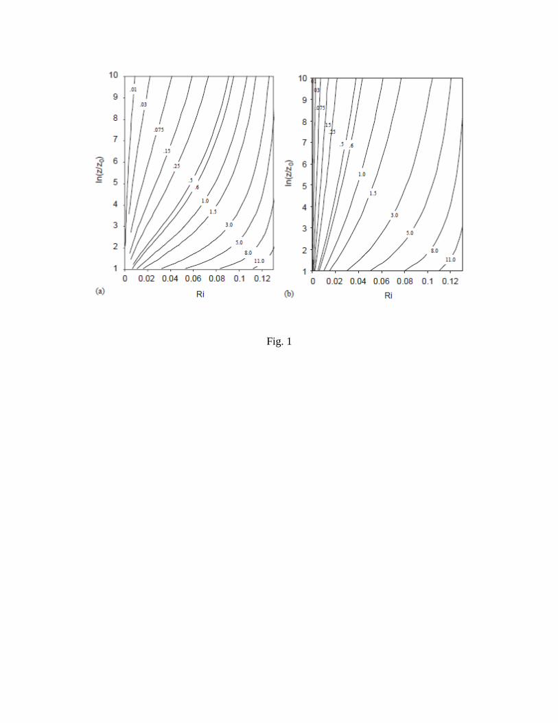
Fig. 1

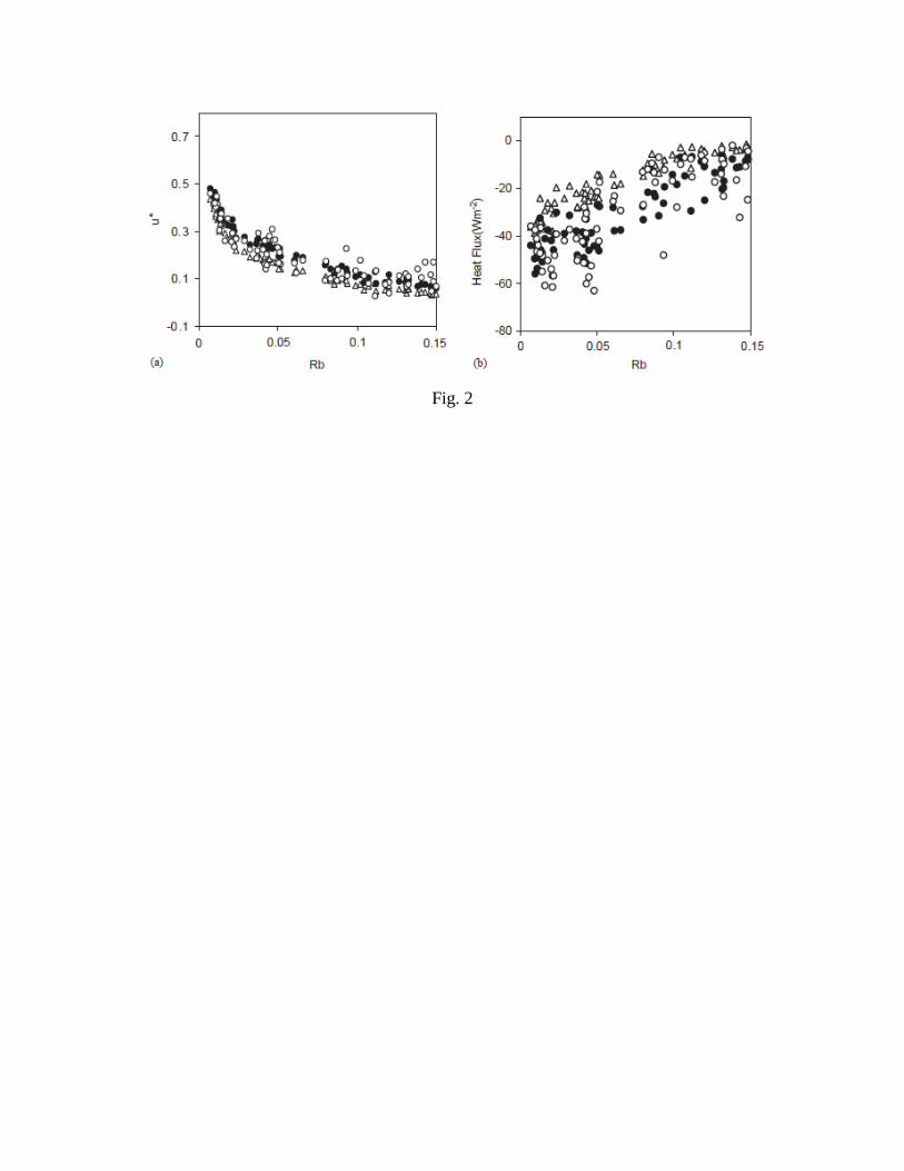
Fig. 2

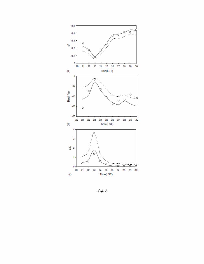
Fig. 3

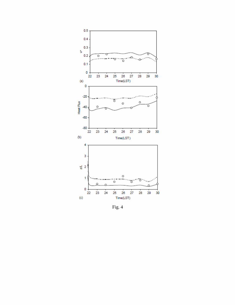
Fig. 4