Geophys. J. Int. (2005) 163, 1039–1048 doi: 10.1111/j.1365-246X.2005.02772.x

GJI

Sei

smol

ogy

Relation between mainshock rupture process and Omori’s lawfor aftershock moment release rate

Yan Y. Kagan and Heidi HoustonDepartment of Earth and Space Sciences, University of California, Los Angeles, California 90095-1567, USA. E-mail: ykagan@ucla.edu

Accepted 2005 August 2. Received 2005 July 21; in original form 2004 October 7

S U M M A R YWe compare the source time functions (i.e., moment release rates) of three large Californiamainshocks with the seismic moment release rates during their aftershock sequences. After-shock moment release rates, computed by summing aftershock moments in time intervals,follow a power-law time dependence similar to Omori’s law from minutes to months after themainshock; furthermore, in contrast to the previously observed saturation in numbers of after-shocks shortly after the mainshock rupture, no such saturation is seen in the aftershock momentrelease rates, which are dominated by the largest aftershocks. We argue that the observed satu-ration in aftershock numbers described by the ‘time offset’ parameter c in Omori’s law is likelyan artefact due to the underreporting of small aftershocks, which is related to the difficulty ofdetecting large numbers of small aftershocks in the mainshock coda. We further propose that itis more natural for c to be negative (i.e. singularity follows the onset of mainshock rupture) thanpositive (singularity precedes onset of rupture). To make a more general comparison of main-shock rupture process and aftershock moment rates, we then scale mainshock time functionsto equalize the effects of the varied seismic moments. For the three California mainshocks, wecompare the scaled time functions with similarly scaled aftershock moment rates. Finally, wecompare global averages of scaled time functions of many shallow events to the average scaledaftershock moment release rate for six California mainshocks. In each of these comparisons,the extrapolation, using Omori’s law, of the aftershock moment rates back in time to the onsetof the mainshock rupture indicates that the temporal intensity of the aftershock moment releaseis about 1.5 orders of magnitude less than the maximum reached by the mainshock rupture.This may be due to the differing amplitudes and relative importance of static and dynamicstresses in aftershock initiation compared to mainshock rupture propagation.

Key words: aftershocks, rupture propagation, seismic coda, seismic-event rates, seismicmoment, statistical methods.

1 I N T RO D U C T I O N

In this work we compare source time functions (seismic momentrelease rates) for California and global shallow large earthquakeswith the seismic moment release rate of aftershock sequences. Byusing moment release rate rather than the number of aftershocks wecircumvent the problem of missing weak aftershocks, since most ofthe total moment in earthquake sequences is contained in the largestevents (Kagan 2002). Because we are interested in the transitionbetween the mainshock rupture process and the beginning of theaftershock sequence, we need to use data from regional and localearthquake catalogues, based on interpretation of high-frequencyseismograms, rather than global catalogues as the former recordaftershocks that are closer in time to the mainshock rupture endthan global catalogues (Kagan 2004).

We use available source-time functions (s.t.f.’s) for several largeCalifornia earthquakes to infer the relation between mainshock rup-

ture process and moment release in their immediate aftershocks.We also analyse s.t.f.’s for global shallow earthquakes. After-shock sequences of large earthquakes in southern California (1952Kern County, 1992 Joshua Tree–Landers–Big Bear sequence, 1994Northridge and 1999 Hector Mine), recorded in the CalTech cata-logue are analysed to demonstrate that from minutes to months afterthe mainshock the moment release follows Omori’s law.

2 T E M P O R A L D I S T R I B U T I O NO F A F T E R S H O C K S

Omori [1894, Eq. (b) p. 117] found that aftershock rate for the 1891Nobi and two other Japanese earthquakes decayed about as

n(t) = K

t + c, (1)

C© 2005 RAS 1039

1040 Y. Y. Kagan and H. Houston

where K and c are coefficients, t is the time since mainshock originand n(t) is the aftershock frequency measured over a certain intervalof time. Presently a more complicated equation is commonly usedto approximate aftershock rate

n(t) = K

(t + c)p. (2)

This expression with the additional exponent parameter p is calledthe modified Omori formula (Utsu 1961; Utsu et al. 1995). Herewe assume that the exponent p is 1.0, its typical value in empiricalstudies (Utsu et al. 1995; Kagan 2004; Gerstenberger et al. 2005—see their Supplement).

The aftershock rate decay still continues now in the focal zone ofthe 1891 Nobi earthquake (Utsu et al. 1995). Statistical analysis ofearthquake catalogues indicates that a power-law dependence char-acterizes the occurrence of both foreshocks and aftershocks. Fromthis point of view a mainshock may be considered as an aftershock,which happens to be stronger than the previous event (Kagan &Knopoff 1981; Agnew 2005; Gerstenberger et al. 2005).

The parameter c in eq. (1) is almost always found to be positiveand typically ranges from 0.5 to 20 hr in empirical studies (Utsu1961; Reasenberg & Jones 1994, 1989; Utsu et al. 1995). It was in-troduced to explain the seeming saturation of aftershock rate closeto the origin time of a mainshock. No reliable empirical regularitiesin the behavior of c have been found. Positive c in eq. (1) meansthat the singularity in eq. (1) occurs before the mainshock, whichis unphysical. Negative c means that the singularity occurs after themainshock. The latter case is a more physically natural assumption.In this case, n(t) is not defined for the period t ≤ −c. This couldcorrespond, for example, to the period of mainshock rupture, dur-ing which individual aftershocks usually cannot be defined, iden-tified, or counted. However, eq. (1) assumes that earthquakes are

−1 0 1 2 3 4 50

0.5

1

1.5

2

2.5

3

3.5

4

4.5

5

Time

Nor

mal

ized

afte

rsho

ck n

umbe

rs

c = 0 c =1

Figure 1. A positive c > 0 in Omori’s law means that the singularity in aftershock rate occurs at negative time (t < 0), that is, before the mainshock. We showOmori laws with c = 1 and c = 0 here in linear scale and below in log-log scale (Fig. 2). In statistical analyses of earthquake catalogues, events before thegreen or black lines may be removed to ensure completeness of aftershock accounting (Kagan 2004). Positive c would fit a relative lack of early aftershocks(either real or apparent), but trends toward a singularity before the mainshock initiation. We propose that the positive empirical value for c is mostly due to theunder-reporting of small aftershocks immediately following a mainshock.

instantaneous, therefore, for times comparable to the rupture timeof mainshocks Omori’s law breaks down, since earthquake countingis not possible for such small time intervals. Moreover, Omori’s lawin its regular form, eqs (1) and (2), predicts that for time t → 0 theaftershock rate stabilizes around K/c. Again, aftershock countingis not usually feasible at the time of mainshock rupture and its coda,hence some time limit (Ogata 1983) needs to be introduced in eqs (1)and (2).

Fig. 1 shows Omori’s law curves in the linear scale, whereas inFig. 2 we display the curves in the more common log–log format.In the log-log case the line with a positive value of c describesa saturation of aftershock rate close to the earthquake origin time.Such a ‘saturation’ has been observed in many aftershock sequences(Reasenberg & Jones 1989, 1994; Utsu et al. 1995). The saturationis usually interpreted as a delay between mainshock rupture endand the start of aftershock activity (Rundle et al. 2003; Kanamori& Brodsky 2004).

Kagan (2004) argues that the real cause of this apparent ratesaturation is not a physical property of aftershock sequences, but isdue to under-reporting of short-term aftershocks, especially smallerones in earthquake catalogues. Peng & Vidale (2004) and Vidaleet al. (2003, 2004) note that the number of aftershocks in the first fewminutes of the sequence observed on high-pass filtered seismogramsis several times higher than aftershock numbers recorded in localcatalogues. Shcherbakov et al. (2004) find that the parameter c inOmori’s law decreases as the magnitude of earthquakes consideredincreases. They attribute this dependence to ‘the undercounting ofsmall aftershocks at short times’. Chen et al. (2004, 2005) findthat in the 1999 Chi-Chi, Taiwan earthquake, aftershocks start afterpassage of the rupture front and they decay according Omori’s laweven when rupture continues at more distant parts of the breakingfault. These results support our interpretation.

C© 2005 RAS, GJI, 163, 1039–1048

Relation between mainshock rupture process and Omori’s law 1041

10−1

100

101

10−2

10−1

100

101

Time

Nor

mal

ized

afte

rsho

ck n

umbe

rs

c = 0

c =1

Figure 2. Same as Fig. 1 but in log-log scale.

3 S E I S M I C M O M E N T R E L E A S E I NE A RT H Q UA K E S A N D A F T E R S H O C K S

3.1 Three California earthquakes and their aftershocks

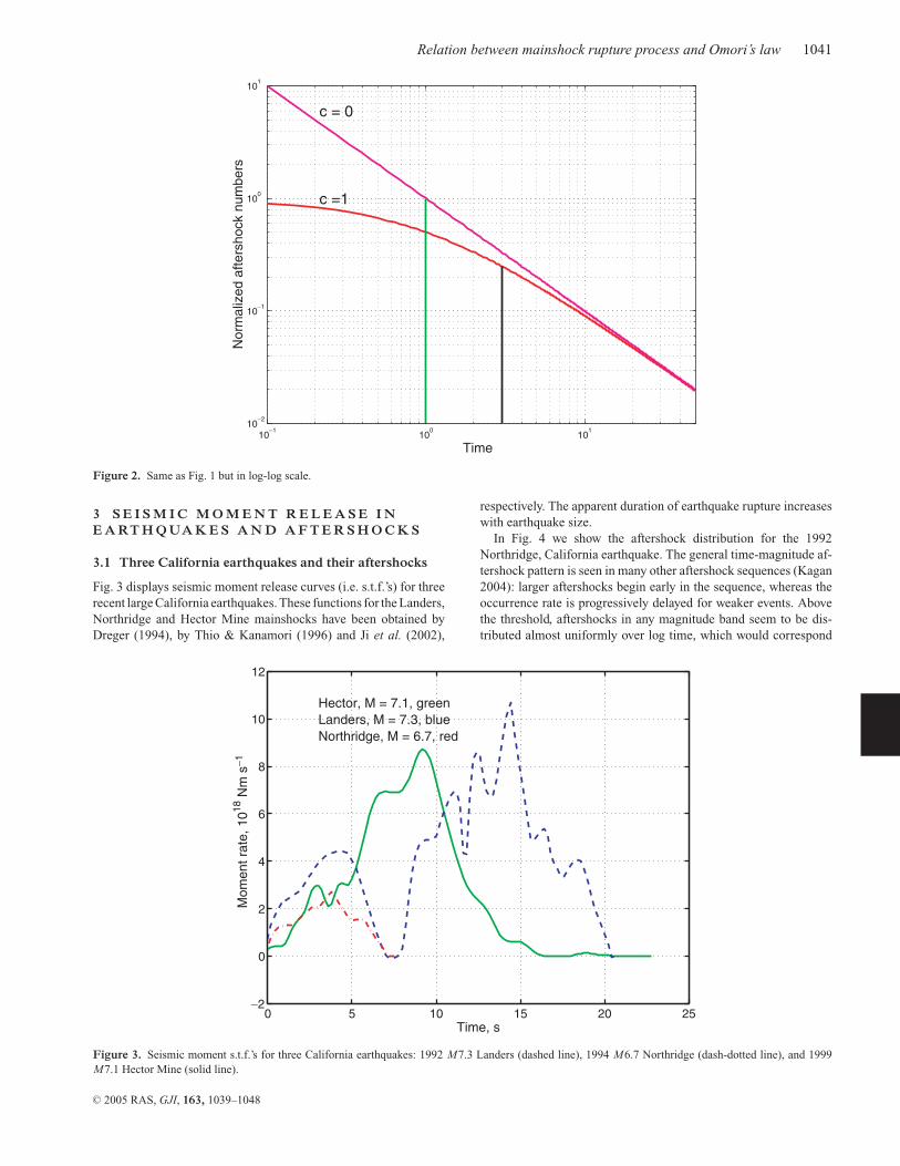
Fig. 3 displays seismic moment release curves (i.e. s.t.f.’s) for threerecent large California earthquakes. These functions for the Landers,Northridge and Hector Mine mainshocks have been obtained byDreger (1994), by Thio & Kanamori (1996) and Ji et al. (2002),

0 5 10 15 20 25−2

0

2

4

6

8

10

12

Time, s

Mom

ent r

ate,

1018

Nm

s−1

Hector, M = 7.1, greenLanders, M = 7.3, blueNorthridge, M = 6.7, red

Figure 3. Seismic moment s.t.f.’s for three California earthquakes: 1992 M7.3 Landers (dashed line), 1994 M6.7 Northridge (dash-dotted line), and 1999M7.1 Hector Mine (solid line).

respectively. The apparent duration of earthquake rupture increaseswith earthquake size.

In Fig. 4 we show the aftershock distribution for the 1992Northridge, California earthquake. The general time-magnitude af-tershock pattern is seen in many other aftershock sequences (Kagan2004): larger aftershocks begin early in the sequence, whereas theoccurrence rate is progressively delayed for weaker events. Abovethe threshold, aftershocks in any magnitude band seem to be dis-tributed almost uniformly over log time, which would correspond

C© 2005 RAS, GJI, 163, 1039–1048

1042 Y. Y. Kagan and H. Houston

10−2

100

102

104

106

108

1.5

2

2.5

3

3.5

4

4.5

5

5.5

6

Time since mainshock (sec)

Afte

rsho

ck m

agni

tude

, ML

sec min hour day 100 d

n = 2934

Figure 4. Time-magnitude distribution of 1994 January 17 M = 6.7 Northridge, California aftershocks. The CalTech earthquake catalogue is used. Events inthe 128 days following the mainshock and between latitude 34.0◦N and 34.5◦N and longitude 118.35◦W and 118.80◦W were selected. The dashed line showsan estimate of the completeness threshold (eq. 6), which can be used to correct aftershock frequency and moment release rate for missing aftershocks.

to their rate decay according to Omori’s law (eq. 1). The magni-tude threshold in early aftershock sequences decreases with time(Wiemer & Katsumata 1999, their Fig. 2; Wiemer et al. 2002, theirFig. 2; Kagan 2004). Therefore, the aftershock magnitude thresholdapproximation by eq. (6) (see below) is also shown.

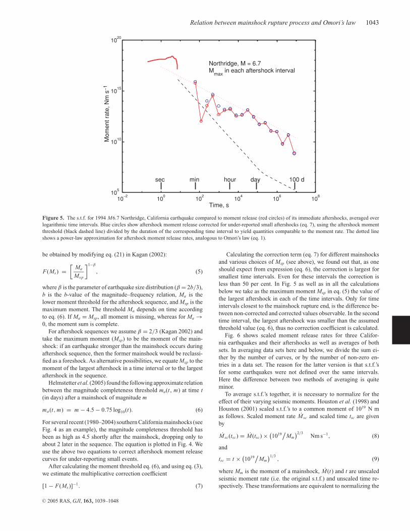
Fig. 5 shows moment release rates during the 1994 Northridge,California earthquake and during its aftershock sequence. We sub-divide time after the mainshock origin into intervals increasing bya factor of 2, and sum the scalar seismic moments of its recordedaftershocks (Kagan 2004). For most of the aftershocks seismic mo-ment was not determined. We assume that their local magnitude isequivalent to the moment magnitude m (Hutton & Jones 1993) andcalculate the moment M (in Nm) as

M = 101.5(m+6), (3)

(Hanks 1992).Fig. 5 suggests that the aftershock moment rate M(t) can be

approximated by a power-law time dependence similar to Omori’slaw

M(t) = k τpk M pk

t + c, (4)

where t is time after mainshock origin, c is a coefficient similarto that in eq. (1), but possibly different in value, M pk is the peakmoment release rate of a mainshock and τ pk is the time the peakoccurs. The coefficient k characterizes the ratio of peak mainshockmoment rate (M pk) and aftershock moment rate extrapolated to τ pk

(with c = 0). We do not yet know how close the end of mainshockmoment release comes to the beginning of the aftershock process;it is possible that there is no actual temporal gap between these twophenomena.

During the occurrence of a mainshock the rupture process isoften punctuated by significant changes in moment-rate ampli-

tude, momentarily stopping or restarting rupture and other rup-ture complexities (Kagan 2004). As a result, large earthquakes in adetailed analysis are often subdivided into several subevents. Af-tershock moment release, on the other hand, is calculated by sum-ming the moments of several separate events. It seems possiblethat in the transition time interval after mainshock rupture endand the beginning of the recorded aftershock sequence, the mo-ment release could exhibit intermediate features—quasi-continuousrupture episodes, which are supplanted by more discrete events.In part our recognition of distinct events is effected by the lim-ited frequency content of seismograms, the presence of noise, etc.With ideal recording, the difference between mainshock and af-tershock moment release rates may not be clear, abrupt, or welldefined.

An advantage of moment summation of aftershocks as opposedto the more usual counting earthquake numbers, is that early inan aftershock sequence many small events may be missing fromthe catalogue as in Fig. 4. This undercount of small earthquakesgives an impression of aftershock rate saturation or rate decaywhen approaching the mainshock rupture end (i.e. going back-wards in time towards the mainshock). In contrast, most of themoment in a sequence is carried by the strongest aftershocks,hence the bias in moment summation is less significant. How-ever, summation of seismic moments carries a significant price—random fluctuations of the sum are very large (Zaliapin et al.2005), hence more summands are needed to yield more reliableresults.

Assuming that the aftershock size distribution follows theGutenberg–Richter relation (Kagan 2004), we can calculate themoment rate of the undetected, or missing weak aftershocks andthus compensate for an incomplete catalogue record. The part ofthe total seismic moment Ms in an aftershock time interval, which ismissing due to incompleteness of the small earthquake record, can

C© 2005 RAS, GJI, 163, 1039–1048

Relation between mainshock rupture process and Omori’s law 1043

10−2

100

102

104

106

108

105

1010

1015

1020

Time, s

Mom

ent r

ate,

Nm

s−1

Northridge, M = 6.7M

max in each aftershock interval

sec min hour day 100 d

Figure 5. The s.t.f. for 1994 M6.7 Northridge, California earthquake compared to moment release (red circles) of its immediate aftershocks, averaged overlogarithmic time intervals. Blue circles show aftershock moment release corrected for under-reported small aftershocks (eq. 7), using the aftershock momentthreshold (black dashed line) divided by the duration of the corresponding time interval to yield quantities comparable to the moment rate. The dotted lineshows a power-law approximation for aftershock moment release rates, analogous to Omori’s law (eq. 1).

be obtained by modifying eq. (21) in Kagan (2002):

F(Ms) =[

Ma

Mxp

]1−β

, (5)

where β is the parameter of earthquake size distribution (β = 2b/3),b is the b-value of the magnitude–frequency relation, Ma is thelower moment threshold for the aftershock sequence, and Mxp is themaximum moment. The threshold Ma depends on time accordingto eq. (6). If Ma = Mxp, all moment is missing, whereas for Ma →0, the moment sum is complete.

For aftershock sequences we assume β = 2/3 (Kagan 2002) andtake the maximum moment (Mxp) to be the moment of the main-shock: if an earthquake stronger than the mainshock occurs duringaftershock sequence, then the former mainshock would be reclassi-fied as a foreshock. As alternative possibilities, we equate Mxp to themoment of the largest aftershock in a time interval or to the largestaftershock in the sequence.

Helmstetter et al. (2005) found the following approximate relationbetween the magnitude completeness threshold ma(t , m) at time t(in days) after a mainshock of magnitude m

ma(t, m) = m − 4.5 − 0.75 log10(t). (6)

For several recent (1980–2004) southern California mainshocks (seeFig. 4 as an example), the magnitude completeness threshold hasbeen as high as 4.5 shortly after the mainshock, dropping only toabout 2 later in the sequence. The equation is plotted in Fig. 4. Weuse the above two equations to correct aftershock moment releasecurves for under-reporting small events.

After calculating the moment threshold eq. (6), and using eq. (3),we estimate the multiplicative correction coefficient

[1 − F(Ms)]−1. (7)

Calculating the correction term (eq. 7) for different mainshocksand various choices of Mxp (see above), we found out that, as oneshould expect from expression (eq. 6), the correction is largest forsmallest time intervals. Even for these intervals the correction isless than 50 per cent. In Fig. 5 as well as in all the calculationsbelow we take as the maximum moment Mxp in eq. (5) the value ofthe largest aftershock in each of the time intervals. Only for timeintervals closest to the mainshock rupture end, is the difference be-tween non-corrected and corrected values observable. In the secondtime interval, the largest aftershock was smaller than the assumedthreshold value (eq. 6), thus no correction coefficient is calculated.

Fig. 6 shows scaled moment release rates for three Califor-nia earthquakes and their aftershocks as well as averages of bothsets. In averaging data sets here and below, we divide the sum ei-ther by the number of curves, or by the number of non-zero en-tries in a data set. The reason for the latter version is that s.t.f.’sfor some earthquakes were not defined over the same intervals.Here the difference between two methods of averaging is quiteminor.

To average s.t.f.’s together, it is necessary to normalize for theeffect of their varying seismic moments. Houston et al. (1998) andHouston (2001) scaled s.t.f.’s to a common moment of 1019 N mas follows. Scaled moment rate Msc and scaled time tsc are givenby

Msc(tsc) = M(tsc) × (1019

/Mm

)2/3Nm s−1, (8)

and

tsc = t × (1019

/Mm

)1/3, (9)

where Mm is the moment of a mainshock, M(t) and t are unscaledseismic moment rate (i.e. the original s.t.f.) and unscaled time re-spectively. These transformations are equivalent to normalizing the

C© 2005 RAS, GJI, 163, 1039–1048

1044 Y. Y. Kagan and H. Houston

10−2

100

102

104

106

108

108

1010

1012

1014

1016

1018

1020

Scaled time, s

Sca

led

mom

ent r

ate,

Nm

s−1

Hector, M = 7.1, green

Landers, M = 7.3, blue

Northridge, M = 6.7, red

Average of source–time functions, magenta

Corrected average aftershock moments, cyan

sec min hour day 100 d

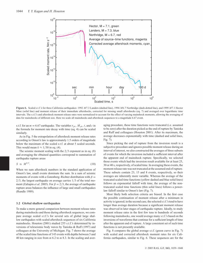
Figure 6. Scaled s.t.f.’s for three California earthquakes: 1992 M7.3 Landers (dashed line), 1994 M6.7 Northridge (dash-dotted line), and 1999 M7.1 HectorMine (solid line) and moment release of their immediate aftershocks, corrected for missing small aftershocks (eq. 7) and averaged over logarithmic timeintervals. The s.t.f.’s and aftershock moment release rates were normalized to account for the effect of varying mainshock moments, allowing the averaging ofdata for mainshocks of different size. Here we scale all mainshocks and aftershock sequences to a magnitude 6.67 event.

s.t.f. for an m = 6.67 earthquake. The variables τpk, M pk, t , and c inthe formula for moment rate decay with time (eq. 4) can be scaledsimilarly.

As in Fig. 5 the extrapolation of aftershock moment release ratesaccording to Omori’s law is approximately 1.5 orders of magnitudebelow the maximum of the scaled s.t.f. at about 5 scaled seconds.This would mean k ≈ 1/30 in eq. (4).

The seismic moment scaling with the 2/3 exponent as in eq. (8)and averaging the obtained quantities correspond to summation ofearthquake rupture areas

S ∝ M2/3. (10)

When we sum aftershock numbers in the standard application ofOmori’s law, small events dominate the sum. In a sum of seismicmoments of events with a Gutenberg–Richter distribution with β =2/3, the largest earthquake on average carries 1/3 of the total mo-ment (Zaliapin et al. 2005). For β = 2/3, the average of earthquakerupture areas balances the influence of large and small earthquakes(Rundle 1989).

3.2 Global shallow earthquakes

To make a more general comparison between moment release ratesduring mainshocks and those during aftershock sequences, we com-pare average scaled s.t.f.’s for several sets of global large shal-low earthquakes with scaled aftershock sequences of six Californiamainshocks. Houston (2001) studied 255 s.t.f.’s determined by in-versions of teleseismic body waves by Tanioka & Ruff (1997) andcolleagues at the University of Michigan. Fig. 7 shows the averageof the scaled time functions of 143 events with depths between 5 and40 km ranging in size from m 6.2 to m 8.3. In the scaling and aver-

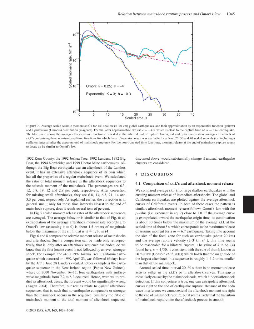
aging procedure, these time functions were truncated (i.e. assumedto be zero) after the duration picked as the end of rupture by Taniokaand Ruff and colleagues (Houston 2001). After its maximum, theaverage decreases exponentially with time (dashed and solid lines,Fig. 7).

Since picking the end of rupture from the inversion result is asubjective procedure and ignores possible moment release during aninterval of interest, we also constructed the averages of three subsetsof events for which the inversion included a sufficient interval afterthe apparent end of mainshock rupture. Specifically, we selectedthose events which had the inversion result available for at least 25,30 or 40 s, respectively, of scaled time. In averaging these events, themoment release rate was not truncated at the assumed end of rupture.These subsets contain 23, 15 and 8 events, respectively, so theiraverages are inherently more variable. Whereas the average of thetruncated scaled time functions (yellow dashed and blue solid lines)follows an exponential falloff with time, the average of the non-truncated scaled time functions (thin solid lines) follows a power-law falloff similar to Omori’s law (Fig. 7).

Most likely both selection criteria are biased. In the first casethe possible continuation of moment release after a minimum inactivity is ignored; in the second case, the selected s.t.f.’s tend to havelonger than average duration because a significant moment releasewas observed in later stages of earthquake rupture. Ideally, to studymoment release rates in the first few tens to hundreds of secondsfollowing mainshocks, one would average many s.t.f.’s based on theinversions of waveforms that continue for a sufficient length of timeafter the apparent end of rupture. A large consistent set of such timefunctions is not presently available.

Fig. 8 compares the global average s.t.f. (green curve in Fig. 7)with scaled and corrected aftershock moment rates for six Cali-fornia earthquakes, similar to Fig. 6. These sequences are for the

C© 2005 RAS, GJI, 163, 1039–1048

Relation between mainshock rupture process and Omori’s law 1045

0 5 10 15 20 25 30 35 4010

15

1016

1017

1018

Scaled time, s

Sca

led

mom

ent r

ate,

Nm

s−1

Omori: K = 0.25; c = −4

Exponential: K = 3; b = −0.3

Figure 7. Average scaled seismic moment s.t.f.’s for 143 shallow (5–40 km) global earthquakes, and their approximation by an exponential function (yellow)and a power-law (Omori’s) distribution (magenta). For the latter approximation we use c = −4 s, which is close to the rupture time of m = 6.67 earthquake.The blue curve shows the average of scaled time functions truncated at the inferred end of rupture. Green, red and cyan curves show averages of subsets ofs.t.f.’s comprising those non-truncated time functions for which the s.t.f inversion result was available for at least 25, 30 and 40 scaled seconds (i.e. including asufficient interval after the apparent end of mainshock rupture). For the non-truncated time functions, moment release at the end of mainshock rupture seemsto decay as 1/t similar to Omori’s law.

1952 Kern County, the 1992 Joshua Tree, 1992 Landers, 1992 BigBear, the 1994 Northridge and 1999 Hector Mine earthquakes. Al-though the Big Bear earthquake was an aftershock of the Landersevent, it has an extensive aftershock sequence of its own whichhas all the properties of a regular mainshock event. We calculatedthe ratio of total moment release in the aftershock sequences tothe seismic moment of the mainshock. The percentages are 6.3,12, 5.8, 19, 12 and 2.8 per cent, respectively. After correctionfor missing small aftershocks, they are 6.8, 13, 6.5, 21, 14 and3.3 per cent, respectively. As explained earlier, the correction is ingeneral small; only for those time intervals closest to the end ofmainshock rupture, does it reach several tens of percent.

In Fig. 9 scaled moment release rates of the aftershock sequencesare averaged. The average behavior is similar to that of Fig. 6: anextrapolation of the average aftershock moment rate according toOmori’s law (assuming c = 0) is about 1.5 orders of magnitudebelow the maximum of the s.t.f., that is, k ≈ 1/30 in (4).

Figs 6 and 8 compare the seismic moment release of mainshocksand aftershocks. Such a comparison can be made only retrospec-tively, that is, only after an aftershock sequence has ended, do weknow that the first (main) event is not followed by an even strongershock. For example, the M6.1 1992 Joshua Tree, California earth-quake which occurred on 1992 April 23, was followed 66 days laterby the M7.3 June 28 Landers event. Another example is the earth-quake sequence in the New Ireland region (Papua New Guinea),where on 2000 November 16–17, four earthquakes with surface-wave magnitude from 7.2 to 8.2 occurred. Hence, were we to pre-dict its aftershock decay, the forecast would be significantly wrong(Kagan 2004). Therefore, our results relate to typical aftershocksequences, that is, such that no earthquake comparable or strongerthan the mainshock occurs in the sequence. Similarly the ratio ofmainshock moment to the total moment of aftershock sequence,

discussed above, would substantially change if unusual earthquakeclusters are considered.

4 D I S C U S S I O N

4.1 Comparison of s.t.f.’s and aftershock moment release

We compared average s.t.f.’s for large shallow earthquakes with theensuing moment release of immediate aftershocks. The global andCalifornia earthquakes are plotted against the average aftershockcurves of California events. In both of these cases the pattern issimilar: aftershock moment release follows Omori’s law with thep-value (i.e. exponent in eq. 2) close to 1.0. If the average curveis extrapolated toward the earthquake origin time, its continuationis about 30 times below the maximum of the average s.t.f. at thescaled time of about 5 s, which corresponds to the maximum releaseof seismic moment for a m = 6.7 earthquake. Taking into accountthe size of the focal zone for such an earthquake (about 20 km)and the average rupture velocity (2–3 km s−1), this time seemsto be reasonable for a bilateral rupture. The value of k in eq. (4)found here, k ≈ 1/30, is consistent with the rule of thumb known asBath’s law (Console et al. 2003) which holds that the magnitude ofthe largest aftershock in a sequence is roughly 1–1.2 units smallerthan that of the mainshock.

Around scaled time interval 20–60 s there is no moment releaseactivity either in the s.t.f.’s or in aftershock curves. This gap ismost likely caused by the mainshock coda, which hinders aftershockdetection. If this conjecture is true, one can extrapolate aftershockcurves right to the end of earthquake rupture. Because of the codawave interference we cannot extend the aftershock moment rate rightto the end of mainshock rupture, but it seems likely that the transitionof mainshock rupture into the aftershock process is smooth.

C© 2005 RAS, GJI, 163, 1039–1048

1046 Y. Y. Kagan and H. Houston

10−2

100

102

104

106

108

106

108

1010

1012

1014

1016

1018

1020

Scaled time, s

Sca

led

mom

ent r

ate,

Nm

s−1

Kern County, M = 7.5, red, R = 6.8 %Joshua Tree, M = 6.1, green, R = 13 %Landers, M = 7.3, blue, R = 6.5 %Big Bear, M = 6.2, magenta, R = 21 %Northridge, M = 6.7, cyan, R = 14 %Hector mine, M = 7.1, black, R = 3.3 %

sec min hour day 100 d

Figure 8. Average scaled s.t.f. for shallow global earthquakes compared to scaled aftershock moment release rates for six California aftershock sequences. Theaverage includes only events with inversion results available for at least 25 s of scaled time. Both types of moment rates were scaled to a magnitude 6.67 event.Two Omori law approximations to the s.t.f.’s are shown with c = −4 s (dashed magenta line), and with c = 0 s (dotted blue line). The California aftershocksequences were corrected for missing small aftershocks (following eq. 7). The coefficient R in the figure is the percent of total seismic moment released byimmediate aftershocks compared to the mainshock scalar moment. The activity level in the aftershock sequences extrapolates to about 30 times less than thepeak rate in the average scaled global time function.

10−2

100

102

104

106

108

106

108

1010

1012

1014

1016

1018

1020

Scaled time, s

Sca

led

linea

rly a

vera

ged

mom

ent r

ate,

Nm

s−1

Global time functions vs. 6 Calif. aftershocksAverage = total moment sum/ (number non–zero entries)

sec min hour day 100 d

Figure 9. Average scaled s.t.f. for global shallow earthquakes with non-truncated time functions (green line taken from Fig. 7) compared to the correctedscaled average for six California aftershock sequences (red line). Approximations of average time function by power-law (Omori) distributions (dashed anddotted lines) are also shown. As before, two Omori law approximations are given with c = −4 s, and with c = 0 s. The average aftershock rates fall about 8orders of magnitude over about 200 days. Extrapolating back in time according to Omori’s law yields a level of aftershock activity about 1.5 orders of magnitudeless than the maximum mainshock moment rate.

C© 2005 RAS, GJI, 163, 1039–1048

Relation between mainshock rupture process and Omori’s law 1047

What might explain the difference between the rate of seismic mo-ment release during mainshock rupture and that extrapolated fromthe aftershock moment release via Omori’s law? The earthquakerupture process is most likely controlled by dynamic stresses: a rup-ture front is concentrated in a pulse (Heaton 1990) with a strongstress wave initiating rupture. In contrast, the aftershock processis essentially static in that dynamic waves generated by an after-shock have almost always left the mainshock focal region beforeoccurrence of a subsequent aftershock. According to various evalu-ations (Antonioli et al. 2002, 2004; Kilb et al. 2002; Gomberg et al.2003) the amplitude of the dynamic stress wave is at least an orderof magnitude stronger than the amplitude of the incremental staticstress. If the number and total moment release of both aftershocksand the rupture events comprising the mainshocks are proportionalto the stress increase, we would expect the s.t.f. to be higher thanthe appropriately scaled aftershock moment release rate. This mayexplain the difference in moment release rates for mainshocks andaftershock sequences.

Moreover, it is likely that the temporal and spatial properties ofearthquake rupture differ significantly from those of an aftershockdistribution. Spatially, aftershock patterns are not different from thegeneral earthquake distribution; they seem to be fractally distributedwith a correlation dimension close to 2 (Robertson et al. 1995; Guo& Ogata 1997). Although it seems likely that the aftershock cloudis slowly expanding with time after a strong earthquake, there is noobvious strong order in the space–time distribution of aftershocks.Earthquake rupture, on the contrary, has a clear pattern of associ-ated with rupture driven by propagating seismic waves (e.g. Heaton1990). Although the propagation of rupture has many complex fea-tures, like temporary stops, change of slip direction, jumping fromone fault segment to another, in general the spatio-temporal evo-lution of rupture exhibits significantly more orderly behavior thanthat of an aftershock sequence. Unfortunately, presently there are in-sufficient numbers of long-duration source inversions for statisticalanalysis of the rupture propagation complexity.

4.2 Reasons for non-zero c-value

Our investigations and analysis of Omori’s law (eq. 1) seem to sug-gest that the parameter c is either close to zero or should be a smallnegative value. What are the reasons for positive values of c, whichhave been reported by many researchers? We can summarize someof the possible causes:

(1) the overlapping of seismic records in the wake of a strongearthquake,

(2) workforce constraint which prevents detailed interpretationof complex seismograms during the beginning of an aftershocksequence,

(3) absence or malfunction of seismic stations close to the sourcezone,

(4) the extended spatio-temporal character of earthquake rupturezone implying failure of the point model of the earthquake source,and

(5) temporary deployment of seismic stations introduces a newfactor in identification and counting of aftershocks, a factor whichis difficult to quantitatively evaluate. Such deployments have littleeffect on the results presented here because

(a) they usually occur at least a few days after the mainshock,therefore cannot influence the aftershock rates in the first hours,a major focus of this work and

(b) the moment release rates (as opposed to numbers ofevents) are dominated by the largest events, which are detectedirrespective of a temporary deployment.

In sum, empirically determined positive values for c arise largelyfrom fitting the functional form of the Omori law to systematicallyunder-counted numbers of aftershocks at early times following amainshock.

What is the time interval between the end of mainshock ruptureand the beginning of the aftershock sequence? Our results shownin Figs 6, 8 and 9 indicate that the interval is small, no longerthan 20–60 s of scaled time, perhaps effectively equal to zero. Theend of mainshock rupture is defined by a relatively low level ofmoment release. If the release is still high, this is considered as acontinuation of the earthquake rupture process. Hence, the low-levelinterval is assumed in the definition of rupture duration during theretrospective interpretation of seismic records. As we suggested, anobjective way to study the late part of the mainshock moment releaseand the beginning aftershock sequence, would be to process all theseismic records to a pre-arranged scaled time interval.

How then can one self-consistently identify an individual earth-quake event? One criterion is to define the end of an individual eventby a rare (low probability) time interval without strong aftershocks.Another is to look at dynamic stress waves at a certain amplitude(or other characteristic property) in the source zone of an earth-quake. An earthquake is considered to end when all such waveshave ceased. Both of these definitions depend on some quantitativecriterion; most likely, the number and properties of such identifiedindividual events would depend strongly on the value adopted.

5 C O N C L U S I O N S

Moment release rates during mainshocks (i.e. s.t.f.’s) are comparedwith moment release rates during aftershock sequences.

From minutes to months following a mainshock, the momentrelease rate of the aftershock sequence follows a power-law decaysimilar to the familiar Omori law for aftershock frequency. We noteinconsistencies in the standard Omori formula, and propose thatthe positive values for c found empirically by many studies aremainly due to the under-reporting of small aftershocks. We useda time-dependent magnitude threshold to approximately estimatecorrections to the aftershock moment rate for this effect.

We made several comparisons of individual California main-shocks and global averages of shallow mainshocks with individualaftershock sequences and with an average California aftershock se-quence. Before averaging, the mainshock time functions and theaftershock moment release rates were scaled to normalize for theeffect of varying mainshock seismic moments.

In all the comparisons, the extrapolation of the aftershock momentrates back in time following Omori’s law yields a rate about 30 timessmaller than the maximum moment rate of the mainshock. Thisdisparity reflects the difference between the process of mainshockrupture, which is highly organized in space and time by dynamicallypropagating stress waves, and the process of aftershock nucleation,which spans a much greater temporal extent.

A C K N O W L E D G M E N T S

We appreciate partial support from the National Science Founda-tion through grants EAR 00-01128, EAR 04-09890, DMS-0306526,from CalTrans grant 59A0363 and from the Southern California

C© 2005 RAS, GJI, 163, 1039–1048

1048 Y. Y. Kagan and H. Houston

Earthquake Center (SCEC). SCEC is funded by NSF Coopera-tive Agreement EAR-0106924 and USGS Cooperative Agreement02HQAG0008. The authors thank J. Vidale and D. D. Jackson ofUCLA for very useful discussions. Publication 922, SCEC.

R E F E R E N C E S

Agnew, D.C., 2005. Earthquakes: Future shock in California, Nature, 435,284–285, doi: 10.1038/435284a.

Antonioli, A., Cocco, M., Das, S. & Henry, C., 2002. Dynamic stress trig-gering during the great 25 March 1998 Antarctic Plate earthquake, Bull.seism. Soc. Am., 92(3), 896–903.

Antonioli, A., Belardinelli, M.E. & Cocco, M., 2004. Modelling dynamicstress changes caused by an extended rupture in an elastic stratified half-space, Geophys. J. Int., 157(1), 229–244.

Chen, Y.-L., Sammis, C.G. & Teng, T.-L., 2004. A high frequency view of1999 Chi-Chi, Taiwan, source rupture and fault mechanics, EOS, Trans.Am. geophys. Un., 85(47), Fall Meet. Suppl., Abstract S33C-07.

Chen, Y.-L., Sammis, C.G. & Teng, T.-L., 2005. A high frequency view of1999 Chi-Chi, Taiwan, source rupture and fault mechanics, Bull. seism.Soc. Am., submitted.

Console, R., Lombardi, A.M., Murru, M. & Rhoades, D., 2003. Bath’s lawand the self-similarity of earthquakes, J. geophys. Res., 108(B2), 2128.

Dreger, D.S., 1994. Investigation of the rupture process of the 28 June1992 Landers earthquake utilizing TERRASCOPE, Bull. seism. Soc. Am.,84(3), 713–724.

Gerstenberger, M.C., Wiemer, S., Jones, L.M. & Reasenberg, P.A., 2005.Real-time forecasts of tomorrow’s earthquakes in California, Nature, 435,328–331, doi: 10.1038/nature03622.

Gomberg, J., Bodin, P. & Reasenberg, P.A., 2003. Observing earthquakestriggered in the near field by dynamic deformations, Bull. seism. Soc.Am., 93, 118–138.

Guo, Z. & Ogata, Y., 1997. Statistical relations between the parameters ofaftershocks in time, space, and magnitude, J. geophys. Res., 102, 2857–2873.

Hanks, T.C., 1992. Small earthquakes, tectonic forces, Science, 256, 1430–1432.

Heaton, T.H., 1990. Evidence for and implications of self-healing pulses ofslip in earthquake rupture, Phys. Earth planet. Inter., 64, 1–20.

Helmstetter, A., Kagan, Y.Y. & Jackson, D.D., 2005. Comparison of short-term and long-term earthquake forecast models for Southern Califor-nia, Bull. seism. Soc. Am., in press, http://scec.ess.ucla.edu/∼ykagan/agnes index.html.

Houston, H., 2001. Influence of depth, focal mechanism, and tectonic settingon the shape and duration of earthquake source time functions, J. geophys.Res., 106, 11 137–11 150.

Houston, H., Benz, H.M. & Vidale, J.E., 1998. Time functions of deepearthquakes from broadband and short-period stacks, J. geophys. Res.,103(B12), 29 895–29 913.

Hutton, L.K. & Jones, L.M., 1993. Local magnitudes and apparent variationsin seismicity rates in Southern California, Bull. seism. Soc. Am., 83, 313–329.

Ji, C., Wald, D.J. & Helmberger, D.V., 2002. Source description of the1999 Hector Mine, California, earthquake, part I: wavelet domain inver-sion theory and resolution analysis, Bull. seism. Soc. Am., 92(4), 1192–1207.

Kagan, Y.Y., 2002. Seismic moment distribution revisited: II. Moment con-servation principle, Geophys. J. Int., 149, 731–754.

Kagan, Y.Y., 2004. Short-term properties of earthquake catalogs and modelsof earthquake source, Bull. seism. Soc. Am., 94(4), 1207–1228.

Kagan, Y.Y. & Knopoff, L., 1981. Stochastic synthesis of earthquake cata-logs, J. geophys. Res., 86, 2853–2862.

Kanamori, H. & Brodsky, E.E., 2004. The physics of earthquakes, Rep. Prog.Phys., 67, 1429–1496, doi:10.1088/0034-4885/67/8/R03.

Kilb, D., Gomberg, J. & Bodin, P., 2002. Aftershock triggering by completeCoulomb stress changes, J. geophys. Res., 107(B4), 2060.

Ogata, Y., 1983. Estimation of the parameters in the modified Omori formulafor aftershock frequencies by the maximum likelihood procedure, J. Phys.Earth, 31, 115–124.

Omori, F., 1894. On the after-shocks of earthquakes, J. College Sci., Imp.Univ. Tokyo, 7, 111–200, (with Plates IV-XIX).

Peng, Z. & Vidale, J.E., 2004. Early aftershock decay rate of the M6 Parkfieldearthquake, EOS, Trans. Am. geophys. Un., 85(47), Fall Meet. Suppl.,Abstract S51C-0170X.

Reasenberg, P.A. & Jones, L.M., 1989. Earthquake hazard after a mainshockin California, Science, 243, 1173–1176.

Reasenberg, P.A. & Jones, L.M., 1994. Earthquake aftershocks: update, Sci-ence, 265, 1251–1252.

Robertson, M.C., Sammis, C.G., Sahimi, M. & Martin, A.J., 1995. Fractalanalysis of three-dimensional spatial distributions of earthquakes with apercolation interpretation, J. geophys. Res., 100, 609–620.

Rundle, J.B., 1989. Derivation of the complete Gutenberg-Richtermagnitude-frequency relation using the principle of scale invariance, J.geophys. Res., 94, 12 337–12 342.

Rundle, J.B., Turcotte, D.L., Shcherbakov, R., Klein, W. & Sammis, C., 2003.Statistical physics approach to understanding the multiscale dynamics ofearthquake fault systems, Rev. Geophys., 41(4), 1019.

Shcherbakov, R., Turcotte, D.L. & Rundle, J.B., 2004. A generalized Omori’slaw for earthquake aftershock decay, Geophys. Res. Lett., 31(11), L11613,doi: 10.1029/2004GL019808.

Tanioka, Y. & Ruff, L., 1997. Source time functions, Seismol. Res. Lett.,68(3), 386–397.

Thio, H.K. & Kanamori, H., 1996. Source complexity of the 1994 Northridgeearthquake and its relation to aftershock mechanisms, Bull. seism. Soc.Am., 86, S84–S92.

Utsu, T., 1961. A statistical study on the occurrence of aftershocks, Geoph.Magazine, 30, 521–605.

Utsu, T., Ogata, Y. & Matsu’ura, R.S., 1995. The centenary of the Omoriformula for a decay law of aftershock activity, J. Phys. Earth, 43, 1–33.

Vidale, J.E., Cochran, E.S., Kanamori, H. & Clayton, R.W., 2003. Afterthe lightning and before the thunder; non-Omori behavior of early after-shocks? EOS, Trans. Am. geophys. Un., 84(46), Fall Meet. Suppl., AbstractS31A-08.

Vidale, J.E., Peng, Z. & Ishii, M., 2004. Anomalous aftershock decay ratesin the first hundred seconds revealed from the Hi-net borehole data, EOS,Trans. Am. geophys. Un., 85(47), Fall Meet. Suppl., Abstract S23C-07.

Wiemer, S. & Katsumata, K., 1999. Spatial variability of seismicity param-eters in aftershock zones, J. geophys. Res., 104, 13 135–13 151.

Wiemer, S., Gerstenberger, M. & Hauksson, E., 2002. Properties of the after-shock sequence of the 1999 M w 7.1 Hector Mine earthquake: implicationsfor aftershock hazard, Bull. seism. Soc. Am., 92, 1227–1240.

Zaliapin, I.V., Kagan, Y.Y. & Schoenberg, F., 2005. Approximating thedistribution of Pareto sums, Pure appl. Geophys., 162(6–7), 1187–1228.

C© 2005 RAS, GJI, 163, 1039–1048