Rehabilitation of the ACL using Synthetic Reinforce-
96
Faculdade de Engenharia da Universidade do Porto Rehabilitation of the ACL using Synthetic Reinforce- ments: A Biomechanical Study João Pedro Lopes Moreira junho de 2020
-
Upload
khangminh22 -
Category
Documents
-
view
2 -
download
0
Transcript of Rehabilitation of the ACL using Synthetic Reinforce-

Faculdade de Engenharia da Universidade do Porto
Rehabilitation of the ACL using Synthetic Reinforce-
ments: A Biomechanical Study
João Pedro Lopes Moreira
junho de 2020

Faculdade de Engenharia da Universidade do Porto
Rehabilitation of the ACL using Synthetic Reinforce-
ments: A Biomechanical Study
João Pedro Lopes Moreira
Dissertação realizada no âmbito do Mestrado em Engenharia Biomédica
Orientador: Prof. Marco Parente – FEUP/INEGI Coorientador: Doutora Nilza Ramião - INEGI
Junho 2020

96
© João Moreira, 2020
i
Abstract
The knee joint is a complex structure with various components, each with their specific
characteristics from their geometry, composition, biomechanics to their interactions with each
other.
This joint, being responsible for providing both stability and motion to the knee, when it is
injured the consequences can be very serious.
Unfortunately, this structure can be easily jeopardized when significant damage is done to its
components. The ACL being one of the more commonly injured structures and, possibly, causing
more devastating effects to the integrity of the joint.
Treatments currently used are mainly surgical, with arthroscopic anatomic grafting being a
popular technique which consists in grafting organic or synthetic tissue to the damaged ACL area.
There are three types of grafts in this technique, but the focus of this work will be on synthetic
ligament grafts.
The objective of this work is to create a model of the Knee joint, introduce a synthetic graft
reinforcement into its Anterior Cruciate Ligament and analyse the behaviour of the joint through
the Finite Element method.
The simulations were performed with a posterior force, of 134N, applied to the Femur and
the Tibia constrained on all degrees of freedom. The tests were performed on rotation angles of
0˚, 15˚ and 30˚.
The results showed that the Reinforcement, with the material properties given here, did not
provide enough stability to the knee causing other components, namely both menisci, the Tibial
and Femoral cartilage, to be under higher stress values than they would normally be in the same
conditions.
The Finite Element method proved to be a great tool, capable of providing accurate simula-
tions at a relative low cost and with time efficiency when compared to the ex-vivo/in-vivo meth-
odologies. But like mentioned previously, the knee joint is a complex structure, making the crea-
tion of a perfectly accurate simulation a big challenge.

iii
Resumo
A articulação do joelho é uma estrutura complexa que possui vários componentes, cada um com
as suas características específicas, desde geometria, composição e biomecânica até às suas inte-
rações entre si.
Esta articulação, sendo responsável por fornecer estabilidade e movimento ao joelho, quando se
encontra lesionada, as consequências podem ser muito graves.
Infelizmente, esta estrutura pode ser facilmente comprometida quando danos significativos são
causados a um dos seus componentes. O Ligamento Cruzado Anterior é uma das estruturas que
se danifica com maior facilidade, possivelmente causando efeitos devastadores à integridade da
articulação.
Os tratamentos atualmente utilizados são principalmente cirúrgicos, sendo o enxerto anatômico
artroscópico a técnica mais popular. Esta consiste em usar um enxerto de tecido orgânico ou
sintético e colocá-lo na área do Ligamento Cruzado Anterior danificada. Existem três tipos de
enxertos, mas o foco deste trabalho será o enxerto de ligamentos sintéticos.
O objetivo deste trabalho é criar um modelo da articulação do joelho, introduzir um reforço de
enxerto sintético no seu Ligamento Cruzado Anterior e analisar o comportamento da articulação
pelo método dos elementos finitos.
As simulações foram realizadas com uma força posterior, de 134N, aplicada no fêmur enquanto
a tíbia se encontre restrita em todos os seus graus de liberdade. Os testes foram realizados em
ângulos de rotação de 0˚, 15˚ e 30˚.
Os resultados obtidos mostraram que o Reforço, com as propriedades de material fornecidas
aqui, não proporcionou estabilidade suficiente ao joelho fazendo com que outros componentes,
como os meniscos, a cartilagem tibial e femoral, estivessem sob valores de stress mais elevados
do que normalmente estariam nas mesmas condições.
O método dos elementos finitos provou ser uma ótima ferramenta, capaz de fornecer simula-
ções precisas a um custo relativamente baixo e com eficiência de tempo quando comparado às
metodologias ex vivo/in vivo. Mas, como mencionado anteriormente, a articulação do joelho é
uma estrutura complexa, tornando a criação de uma simulação completamente precisa um gran-
de desafio.

v
Agradecimentos
Terminando esta dissertação, gostaria de agradecer a todas as pessoas que ajudaram para a
realização da mesma.
Começo por agradecer ao meu orientador, Doutor Marco Parente, pelo continuado acompa-
nhamento e toda a disponibilidade mostrada, toda a ajuda, esforço e paciência dados para for-
necer as melhores condições possíveis para a realização do presente trabalho.
À Doutora Nilza Ramião, que desempenhou o papel de coorientadora, agradeço a disponibili-
dade e apoio no esclarecimento de dúvidas e da ajuda na obtenção do variado material teórico.
Aos vários amigos e colegas que fiz ao longo destes anos, que tornaram todo este percurso
uma experiência consideravelmente mais memorável.
À minha família (meu pai, minha mãe, minha irmã e restantes familiares), que durante todo
o meu percurso académico partilharam todos os meus bons e maus momentos e bons e maus re-
sultados, sem o apoio deles nunca teria sido possível estar onde me encontro neste momento.

vii
Index
1 Introduction 1
1.1 Motivation. . . . . . . . . . . . . . . . . . . . . . . . . . . . . . . . . . . . . . . . . . . . . . . . . . . 1
1.2 Literature Review . . . . . . . . . . . . . . . . . . . . . . . . . . . . . . . . . . . . . . . . . . . . . 2
1.3 Objectives and Structure. . . . . . . . . . . . . . . . . . . . . . . . . . . . . . . . . . . . . . . . . 5
2 Anatomy 7
2.1 The Human Skeletal System . . . . . . . . . . . . . . . . . . . . . . . . . . . . . . . . . . . . . . . 7
2.2 Human Joints . . . . . . . . . . . . . . . . . . . . . . . . . . . . . . . . . . . . . . . . . . . . . . . . 10
2.3 Anatomy Axes/Planes . . . . . . . . . . . . . . . . . . . . . . . . . . . . . . . . . . . . . . . . . . . 12
2.4 Knee Joints . . . . . . . . . . . . . . . . . . . . . . . . . . . . . . . . . . . . . . . . . . . . . . . . . . 13
2.5 Bones . . . . . . . . . . . . . . . . . . . . . . . . . . . . . . . . . . . . . . . . . . . . . . . . . . . . . 14
2.6 Menisci . . . . . . . . . . . . . . . . . . . . . . . . . . . . . . . . . . . . . . . . . . . . . . . . . . . . 15
2.7 Articular Cartilage . . . . . . . . . . . . . . . . . . . . . . . . . . . . . . . . . . . . . . . . . . . . . . 17
2.8 Ligaments . . . . . . . . . . . . . . . . . . . . . . . . . . . . . . . . . . . . . . . . . . . . . . . . . . . 17
3 Common Injuries and Treatments 23
3.1 ACL Tear Treatments techniques. . . . . . . . . . . . . . . . . . . . . . . . . . . . . . . . . . . . 24
4 Knee Biomechanics and Kinematics 27
5 Methodology 29
5.1 Finite Elements Method (FEM). . . . . . . . . . . . . . . . . . . . . . . . . . . . . . . . . . . . . . 29
5.2 Geometrical Model . . . . . . . . . . . . . . . . . . . . . . . . . . . . . . . . . . . . . . . . . . . . 35
6 Results and Discussion 51
6.1 Case 1 (0˚ Rotation). . . . . . . . . . . . . . . . . . . . . . . . . . . . . . . . . . . . . . . . . . . . 52
6.2 Case 2 (15˚ Rotation). . . . . . . . . . . . . . . . . . . . . . . . . . . . . . . . . . . . . . . . . . . . 54
6.3 Case 3 (30˚ Rotation). . . . . . . . . . . . . . . . . . . . . . . . . . . . . . . . . . . . . . . . . . . . 59
7 Conclusions and Future Work 65
7.1 Conclusions . . . . . . . . . . . . . . . . . . . . . . . . . . . . . . . . . . . . . . . . . . . . . . . . . . 65
7.2 Future Work . . . . . . . . . . . . . . . . . . . . . . . . . . . . . . . . . . . . . . . . . . . . . . . . 66
Bibliographic References 68

ix
Figure List
Figure 1.1 - . . . . . . . . . . . . . . . . . . . . . . . . . . . . . . . . . . . . . . . . . . . . . . . . . . . . . . . . 3
Figure 2.1 - . . . . . . . . . . . . . . . . . . . . . . . . . . . . . . . . . . . . . . . . . . . . . . . . . . . . . . . . 7
Figure 2.2 - . . . . . . . . . . . . . . . . . . . . . . . . . . . . . . . . . . . . . . . . . . . . . . . . . . . . . . . . 8
Figure 2.3 - . . . . . . . . . . . . . . . . . . . . . . . . . . . . . . . . . . . . . . . . . . . . . . . . . . . . . . . . 9
Figure 2.4 - . . . . . . . . . . . . . . . . . . . . . . . . . . . . . . . . . . . . . . . . . . . . . . . . . . . . . . . . 9
Figure 2.5 - . . . . . . . . . . . . . . . . . . . . . . . . . . . . . . . . . . . . . . . . . . . . . . . . . . . . . . . 11
Figure 2.6 - . . . . . . . . . . . . . . . . . . . . . . . . . . . . . . . . . . . . . . . . . . . . . . . . . . . . . . . 12
Figure 2.7 - . . . . . . . . . . . . . . . . . . . . . . . . . . . . . . . . . . . . . . . . . . . . . . . . . . . . . . . 12
Figure 2.8 - . . . . . . . . . . . . . . . . . . . . . . . . . . . . . . . . . . . . . . . . . . . . . . . . . . . . . . . 13
Figure 2.9 - . . . . . . . . . . . . . . . . . . . . . . . . . . . . . . . . . . . . . . . . . . . . . . . . . . . . . . . 13
Figure 2.10 - . . . . . . . . . . . . . . . . . . . . . . . . . . . . . . . . . . . . . . . . . . . . . . . . . . . . . . .15
Figure 2.11 - . . . . . . . . . . . . . . . . . . . . . . . . . . . . . . . . . . . . . . . . . . . . . . . . . . . . . . .16
Figure 2.12 - . . . . . . . . . . . . . . . . . . . . . . . . . . . . . . . . . . . . . . . . . . . . . . . . . . . . . . .17
Figure 2.13 - . . . . . . . . . . . . . . . . . . . . . . . . . . . . . . . . . . . . . . . . . . . . . . . . . . . . . . .18
Figure 2.14 - . . . . . . . . . . . . . . . . . . . . . . . . . . . . . . . . . . . . . . . . . . . . . . . . . . . . . . .19
Figure 2.15 - . . . . . . . . . . . . . . . . . . . . . . . . . . . . . . . . . . . . . . . . . . . . . . . . . . . . . . .20
Figure 3.1 - . . . . . . . . . . . . . . . . . . . . . . . . . . . . . . . . . . . . . . . . . . . . . . . . . . . . . . . 25
Figure 4.1 - . . . . . . . . . . . . . . . . . . . . . . . . . . . . . . . . . . . . . . . . . . . . . . . . . . . . . . . 28
Figure 5.1 - . . . . . . . . . . . . . . . . . . . . . . . . . . . . . . . . . . . . . . . . . . . . . . . . . . . . . . . 33
Figure 5.2 - . . . . . . . . . . . . . . . . . . . . . . . . . . . . . . . . . . . . . . . . . . . . . . . . . . . . . . . 37
Figure 5.3 - . . . . . . . . . . . . . . . . . . . . . . . . . . . . . . . . . . . . . . . . . . . . . . . . . . . . . . . 37
Figure 5.4 - . . . . . . . . . . . . . . . . . . . . . . . . . . . . . . . . . . . . . . . . . . . . . . . . . . . . . . . 38
Figure 5.5 - . . . . . . . . . . . . . . . . . . . . . . . . . . . . . . . . . . . . . . . . . . . . . . . . . . . . . . . 38
Figure 5.6 - . . . . . . . . . . . . . . . . . . . . . . . . . . . . . . . . . . . . . . . . . . . . . . . . . . . . . . . 39
Figure 5.7 - . . . . . . . . . . . . . . . . . . . . . . . . . . . . . . . . . . . . . . . . . . . . . . . . . . . . . . . 39
Figure 5.8 - . . . . . . . . . . . . . . . . . . . . . . . . . . . . . . . . . . . . . . . . . . . . . . . . . . . . . . . 40
Figure 5.9 - . . . . . . . . . . . . . . . . . . . . . . . . . . . . . . . . . . . . . . . . . . . . . . . . . . . . . . . 41
Figure 5.10 - . . . . . . . . . . . . . . . . . . . . . . . . . . . . . . . . . . . . . . . . . . . . . . . . . . . . . . .42
Figure 5.11 - . . . . . . . . . . . . . . . . . . . . . . . . . . . . . . . . . . . . . . . . . . . . . . . . . . . . . . .42
Figure 5.12 - . . . . . . . . . . . . . . . . . . . . . . . . . . . . . . . . . . . . . . . . . . . . . . . . . . . . . . .43
Figure 5.13 - . . . . . . . . . . . . . . . . . . . . . . . . . . . . . . . . . . . . . . . . . . . . . . . . . . . . . . .43
Figure 5.14 - . . . . . . . . . . . . . . . . . . . . . . . . . . . . . . . . . . . . . . . . . . . . . . . . . . . . . . .47
Figure 5.15 - . . . . . . . . . . . . . . . . . . . . . . . . . . . . . . . . . . . . . . . . . . . . . . . . . . . . . . .48
Figure 5.16 - . . . . . . . . . . . . . . . . . . . . . . . . . . . . . . . . . . . . . . . . . . . . . . . . . . . . . . .49
Figure 6.1 - . . . . . . . . . . . . . . . . . . . . . . . . . . . . . . . . . . . . . . . . . . . . . . . . . . . . . . . 52
Figure 6.2 - . . . . . . . . . . . . . . . . . . . . . . . . . . . . . . . . . . . . . . . . . . . . . . . . . . . . . . . 52
Figure 6.3 - . . . . . . . . . . . . . . . . . . . . . . . . . . . . . . . . . . . . . . . . . . . . . . . . . . . . . . . 53
Figure 6.4 - . . . . . . . . . . . . . . . . . . . . . . . . . . . . . . . . . . . . . . . . . . . . . . . . . . . . . . . 54
Figure 6.5 - . . . . . . . . . . . . . . . . . . . . . . . . . . . . . . . . . . . . . . . . . . . . . . . . . . . . . . . 54
Figure 6.6 - . . . . . . . . . . . . . . . . . . . . . . . . . . . . . . . . . . . . . . . . . . . . . . . . . . . . . . . 55
Figure 6.7 - . . . . . . . . . . . . . . . . . . . . . . . . . . . . . . . . . . . . . . . . . . . . . . . . . . . . . . . 56
Figure 6.8 - . . . . . . . . . . . . . . . . . . . . . . . . . . . . . . . . . . . . . . . . . . . . . . . . . . . . . . . 56
Figure 6.9 - . . . . . . . . . . . . . . . . . . . . . . . . . . . . . . . . . . . . . . . . . . . . . . . . . . . . . . . 57
Figure 6.10 - . . . . . . . . . . . . . . . . . . . . . . . . . . . . . . . . . . . . . . . . . . . . . . . . . . . . . . .57
Figure 6.11 - . . . . . . . . . . . . . . . . . . . . . . . . . . . . . . . . . . . . . . . . . . . . . . . . . . . . . . .57
Figure 6.12 - . . . . . . . . . . . . . . . . . . . . . . . . . . . . . . . . . . . . . . . . . . . . . . . . . . . . . . .58
Figure 6.13 - . . . . . . . . . . . . . . . . . . . . . . . . . . . . . . . . . . . . . . . . . . . . . . . . . . . . . . .58
Figure 6.14 - . . . . . . . . . . . . . . . . . . . . . . . . . . . . . . . . . . . . . . . . . . . . . . . . . . . . . . .59
Figure 6.15 - . . . . . . . . . . . . . . . . . . . . . . . . . . . . . . . . . . . . . . . . . . . . . . . . . . . . . . .59
Figure 6.16 - . . . . . . . . . . . . . . . . . . . . . . . . . . . . . . . . . . . . . . . . . . . . . . . . . . . . . . .60
Figure 6.17 - . . . . . . . . . . . . . . . . . . . . . . . . . . . . . . . . . . . . . . . . . . . . . . . . . . . . . . .61
Figure 6.18 - . . . . . . . . . . . . . . . . . . . . . . . . . . . . . . . . . . . . . . . . . . . . . . . . . . . . . . .61
Figure 6.19 - . . . . . . . . . . . . . . . . . . . . . . . . . . . . . . . . . . . . . . . . . . . . . . . . . . . . . . .62
Figure 6.20 - . . . . . . . . . . . . . . . . . . . . . . . . . . . . . . . . . . . . . . . . . . . . . . . . . . . . . . .63
Figure 6.21 - . . . . . . . . . . . . . . . . . . . . . . . . . . . . . . . . . . . . . . . . . . . . . . . . . . . . . . .63

xi

Table List
Table 5.1 - . . . . . . . . . . . . . . . . . . . . . . . . . . . . . . . . . . . . . . . . . . . . . . . . . . . . . . . . 36
Table 5.2 - . . . . . . . . . . . . . . . . . . . . . . . . . . . . . . . . . . . . . . . . . . . . . . . . . . . . . . . . 41
Table 5.3 - . . . . . . . . . . . . . . . . . . . . . . . . . . . . . . . . . . . . . . . . . . . . . . . . . . . . . . . . 41
Table 5.4 - . . . . . . . . . . . . . . . . . . . . . . . . . . . . . . . . . . . . . . . . . . . . . . . . . . . . . . . . 42
Table 5.5 - . . . . . . . . . . . . . . . . . . . . . . . . . . . . . . . . . . . . . . . . . . . . . . . . . . . . . . . . 43
Table 5.6 - . . . . . . . . . . . . . . . . . . . . . . . . . . . . . . . . . . . . . . . . . . . . . . . . . . . . . . . . 44

xiii
List of Acronyms and Symbols List of Acronyms ACL Anterior Cruciate Ligament
AMB Anteromedial Bundle
CAE Complete Abaqus Environment
FE Finite Element
FEA Finite Element Analysis
FEM Finite Element Method
LARS Ligament Advanced Reinforcement System
LCL Lateral Collateral Ligament
MCL Medial Collateral Ligament
PCL Posterior Cruciate Ligament
PLB Posterolateral bundle
PET Polyethilene Plyester
List of Symbols
S Coordinate System-Referential
U Offset field
A Nodal dislocation
N Interpolating Function or Shape Function
Normal Stress
p’ Distributed outer action
C Coefficient term of a polynomial
I Exact value of an integral
J Integral value calculated according to Gauss quadrature
P Position of a Gauss Point or Sampling Point (Gauss Quadrature)
W Weight associated with a Gauss point or sampling point
E Young’s Modulus (or Elastic Modulus)
𝜐 Poisson’s Ratio
𝚿 Strain Energy Density Function
xv
𝜅 Dispersion Parameter
𝑭 Deformation Gradient
𝐼1 First Strain Invariant
𝐼2 Second Strain Invariant
𝐼3 Third Strain Invariant
Isochoric Component of the First Strain Invariant
Isochoric Component of the Fourth Invariant
Isochoric Component of the Sixth Invariant
𝒂04,06 Unit vectors that define the preferred direction of one family of fibers in the ref-
erence conFiguretion
Isochoric Right Cauchy-Green Deformation Tensor
𝑪 Right Cauchy-Green Deformation Tensor
𝐶10 Neo-Hookean Parameter
𝑘1, 𝑘2 Parameters of the HGO Model Anisotropic Component
𝜀 Uniaxial Strain
𝜆 Stretch Ratio
𝜌 Statistical distribution function

Chapter 1
Introduction
The knee is one of the most complex and largest articulations on the human body, being
the point in which the femur, tibia and the patella converge. The knee joint has the role of
bearing high loads and allow the necessary mobility for locomotion [1,2].
Besides its bony structure this joint is also constituted by articular cartilage, menisci and
ligaments whose mechanical interactions will be explained further later on this report.
The ligaments provide stability to the joint, with the main ones being the four major lig-
aments supporting the knee. These include the Anterior Cruciate Ligament (ACL), the Posteri-
or Cruciate ligament (PCL), the Medial Collateral ligament (MCL) and the Lateral Collateral
ligament (LCL). The ACL, in conjunction with the PCL, is a crucial component of the knee
which provides stability to the joint in everyday movement and loading activities, by prevent-
ing knee hyperextension and restraining tibial translation [3,4,5,6,7,8].
1.1 - Motivation
Unfortunately, ACL rupture is a very common ligament injury, its location making it prone
to high load stress [7]. ACL rupture, besides inducing pain, severely compromises the joint’s
functionality by altering its kinematics, causing local instability, altering the rotation centre
of the knee and the tibiofemoral contact area depending on its severity. A major problem
resulting from these injuries is the high possibility of it causing secondary lesions on other
parts of the joint like the menisci and articular cartilage [3,4,7,9].
A field in which ACL injury is very common and especially destructive is in sports, mainly
those associated with extreme physical load on the athlete’s legs. For example, sports which
demand activities based on jump-landing tasks and side-step cutting activities such as soccer,
basketball or tennis [3,7,9-12]. For these athletes ACL rupture is a possible career ending in-
jury since it requires an expensive treatment and a long span of time until full recovery, with
the possibility of complete recovery not happening and leaving them with a severe diminished
knee mobility and the chance of developing osteoarthritis. [3,6,7,10]
Current methods to restore a completely torn ACL are mainly surgical, based on the re-
placement of the missing tissue through grafts. These methods use a patellar tendon or ham-
2
strings tendon graft; however, studies have shown that these techniques substantially alter
the biomechanics of the knee compromising the normal interaction between the joint and the
cartilage below, exponentially increasing the risk of Osteoarthritis [4,11-13].
Therefore, research for new techniques and methodologies has been a focus, leading to
the rise in popularity of synthetic reinforcement grafts, which will be mentioned in detail lat-
er.
There have been several studies performed on the biomechanics and kinematics of the
knee joint, mainly focusing on the ACL and its role. These studies had aimed to better under-
stand ACL injuries and their causes, in order to learn how to prevent them and to improve
surgical procedures.
To achieve these aims, several methodologies have been used, such as: ex vivo techniques
[14-17], clinical studies, in vivo evaluations [14,18-20] and computerized simulations.
The first two have many advantages, but also have major disadvantages and limitations
such as the difficulties involved in reproducing natural, pathological and degenerative condi-
tions, the complexity involved in reproducing and measuring strains and forces on the various
joint components and the high cost associated with these methodologies [21-23].
These problems do not manifest as severally on computational simulations, being the bet-
ter alternative to study the knee joints biomechanically with comparably reduced cost and
high efficiency, obviously depending on the robustness of the simulation hardware used
[21,24-26].
The Finite Element analysis method (FEM) specifically is a very important tool, for compu-
tational simulation, capable of providing accurate results with certain reliability [12,14].
However, the knee joint is an extremely complex structure, and its computerized simulation
is still not perfectly applied today, the complexity of this joint stems from its component’s
material properties and interactions with each other [6,14,22,25-26].
However, when a balance between the model’s complexity and computational efficiency
is achieved, the FEM analysis still proves that it is the more suitable tool in providing clinical-
ly useful biomechanical results.
1.2 - Literature Review
Several research works have been performed in the past years with the objective of im-
proving our knowledge and comprehension on the knee joint and its components, many dif-
ferent models have been developed in order to simulate joint biomechanics, kinematics and
the role of its various components. These served has a starting point for this study and will be
presented below.
One of the first models developed with this intent was the four-bar linkage model, in 1917
Lehrbuch der Muskel and Gelenkmechanik [27] were one of the firsts to publish works with
this model, see figure 1 below.
3
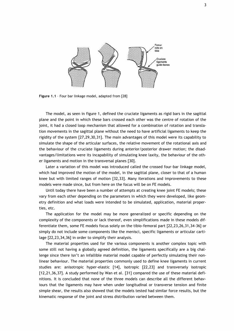
Figure 1.1 – Four bar linkage model, adapted from [28]
The model, as seen in figure 1, defined the cruciate ligaments as rigid bars in the sagittal
plane and the point in which these bars crossed each other was the centre of rotation of the
joint, it had a closed loop mechanism that allowed for a combination of rotation and transla-
tion movements in the sagittal plane without the need to have artificial ligaments to keep the
rigidity of the system [27,29,30,31]. The main advantages of this model were its capability to
simulate the shape of the articular surfaces, the relative movement of the rotational axis and
the behaviour of the cruciate ligaments during anterior/posterior drawer motion; the disad-
vantages/limitations were its incapability of simulating knee laxity, the behaviour of the oth-
er ligaments and motion in the transversal planes [30].
Later a variation of this model was introduced called the crossed four-bar linkage model,
which had improved the motion of the model, in the sagittal plane, closer to that of a human
knee but with limited ranges of motion [32,33]. Many iterations and improvements to these
models were made since, but from here on the focus will be on FE models.
Until today there have been a number of attempts at creating knee joint FE models; these
vary from each other depending on the parameters in which they were developed, like geom-
etry definition and what loads were intended to be simulated, application, material proper-
ties, etc.
The application for the model may be more generalized or specific depending on the
complexity of the components or lack thereof, even simplifications made in these models dif-
ferentiate them, some FE models focus solely on the tibio-femoral part [22,23,26,31,34-36] or
simply do not include some components like the menisci, specific ligaments or articular carti-
lage [22,23,34,36] in order to simplify their analysis.
The material properties used for the various components is another complex topic with
some still not having a globally agreed definition, the ligaments specifically are a big chal-
lenge since there isn’t an infallible material model capable of perfectly simulating their non-
linear behaviour. The material properties commonly used to define knee ligaments in current
studies are: anisotropic hyper-elastic [14], isotropic [22,23] and transversely isotropic
[12,21,36,37]. A study performed by Wan et al. [31] compared the use of these material defi-
nitions. It is concluded that none of the three models can describe all the different behav-
iours that the ligaments may have when under longitudinal or transverse tension and finite
simple shear, the results also showed that the models tested had similar force results, but the
kinematic response of the joint and stress distribution varied between them.
4
As for the type of analysis, knee joint FE analysis can be performed as a static analysis
[12,14], quasi-static analysis [1,14,22,23,26,34,34,35,38] or dynamic analysis [14,34,39-41];
depending on the type motion and what results are intended.
Focusing on FE modelling of the ligament components of the knee joint, simplifying the
ligaments as one-dimensional truss-beams [1,40] or springs elements [26,39,38], is an option
that makes the calculations related to their behaviour easier and help provide faster results
regarding knee kinematics. But this simplification has its disadvantages since this type of
model isn’t capable of showing the stress distribution in the said ligament [22]. Therefore, in
order to obtain more accurate results, it has been concluded that the knee FE model should
have a three-dimensional representation of the ligaments [30].
Some models also apply an initial strain to the model [1,12,21,23,26,37,39,40], this is
done in order to try and replicate the in vivo residual stresses that the ligaments are under in
order to make the model as close to reality as possible.
Even though the creation of a FE knee joint model is a complex subject, as explained
above, its development has been a topic of great interest for many reasons.
Ali Kiapour et al. [14] performed a study that used the FE model of the knee to investi-
gate injury mechanisms. The model used was validated against tibio-femoral kinematics, lig-
aments strain/force and articular cartilage pressure from static, quasi-static and dynamic ex-
periments. The results showed that the model was capable of predicting the kinematics of
the joint and stress/strain fields on the biological tissue with all the model’s predictions be-
ing within 95% confidence intervals average experimental data.
Georges L. et al. [42] used the FE analysis method in order to research the human ACL
when subjected to passive anterior tibial loads. In this article a 3D continuum FE model of the
ACL was developed and used to simulate clinical knee procedures namely the Lachman and
drawer tests. The objective here was to evaluate the existence and severity of an ACL knee
injury by analysing the model joint starting on a flexed position, at 30˚ for the Lachman test
and 90˚ for the drawer test, followed by an anterior tibial displacement of 4mm. The results
obtained showed that both tests have different effects on the ACL’s behaviour, showing that
at 30˚ of flexion stress mainly appears in the mid anterolateral portion of the ACL and as flex-
ion increases the stress that the anteromedial part of the ACL becomes the most stressed.
G. Limbert et al. [12] studied a three-dimensional FE model of the human ACL from ex-
perimental measurements on cadaveric knee specimen which were subjected to kinematic
tests, to perform simulations of passive knee flexion with and without pre-stressing the ACL
and assess the stress distribution on the ligament. They verified that, when the ACL was pre-
stressed, the stress distribution values were within the predicted results and resembled the
values reported in literature; between the pre-stressed and stress-free ACL the results were
similar, but at lower flexion angles, the pre-stressed ACL had higher values of stress distribu-
tion.
Hyung-Soon Park et al. [34] presented a FE analysis of the ACL impingement against the
intercondylar notch during external rotation and abduction of the tibia for noncontact inju-
ries. This research showed that impingement between the lateral wall of the intercondylar
notch and the ACL may occur when the knee rotates externally 29.1˚ and abducted at 10˚
resulting in strong contact pressure and tensile stress on the ACL. With the results obtained,
namely the impact force (at 36.9N) and contact area (at 19.7 mm2), on par with their cadaver
counterparts.
5
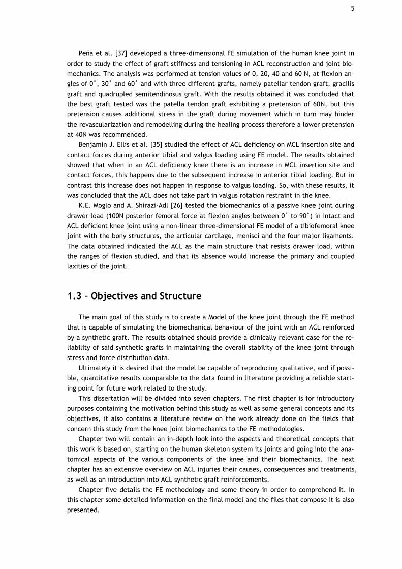
Peña et al. [37] developed a three-dimensional FE simulation of the human knee joint in
order to study the effect of graft stiffness and tensioning in ACL reconstruction and joint bio-
mechanics. The analysis was performed at tension values of 0, 20, 40 and 60 N, at flexion an-
gles of 0˚, 30˚ and 60˚ and with three different grafts, namely patellar tendon graft, gracilis
graft and quadrupled semitendinosus graft. With the results obtained it was concluded that
the best graft tested was the patella tendon graft exhibiting a pretension of 60N, but this
pretension causes additional stress in the graft during movement which in turn may hinder
the revascularization and remodelling during the healing process therefore a lower pretension
at 40N was recommended.
Benjamin J. Ellis et al. [35] studied the effect of ACL deficiency on MCL insertion site and
contact forces during anterior tibial and valgus loading using FE model. The results obtained
showed that when in an ACL deficiency knee there is an increase in MCL insertion site and
contact forces, this happens due to the subsequent increase in anterior tibial loading. But in
contrast this increase does not happen in response to valgus loading. So, with these results, it
was concluded that the ACL does not take part in valgus rotation restraint in the knee.
K.E. Moglo and A. Shirazi-Adl [26] tested the biomechanics of a passive knee joint during
drawer load (100N posterior femoral force at flexion angles between 0˚ to 90˚) in intact and
ACL deficient knee joint using a non-linear three-dimensional FE model of a tibiofemoral knee
joint with the bony structures, the articular cartilage, menisci and the four major ligaments.
The data obtained indicated the ACL as the main structure that resists drawer load, within
the ranges of flexion studied, and that its absence would increase the primary and coupled
laxities of the joint.
1.3 – Objectives and Structure
The main goal of this study is to create a Model of the knee joint through the FE method
that is capable of simulating the biomechanical behaviour of the joint with an ACL reinforced
by a synthetic graft. The results obtained should provide a clinically relevant case for the re-
liability of said synthetic grafts in maintaining the overall stability of the knee joint through
stress and force distribution data.
Ultimately it is desired that the model be capable of reproducing qualitative, and if possi-
ble, quantitative results comparable to the data found in literature providing a reliable start-
ing point for future work related to the study.
This dissertation will be divided into seven chapters. The first chapter is for introductory
purposes containing the motivation behind this study as well as some general concepts and its
objectives, it also contains a literature review on the work already done on the fields that
concern this study from the knee joint biomechanics to the FE methodologies.
Chapter two will contain an in-depth look into the aspects and theoretical concepts that
this work is based on, starting on the human skeleton system its joints and going into the ana-
tomical aspects of the various components of the knee and their biomechanics. The next
chapter has an extensive overview on ACL injuries their causes, consequences and treatments,
as well as an introduction into ACL synthetic graft reinforcements.
Chapter five details the FE methodology and some theory in order to comprehend it. In
this chapter some detailed information on the final model and the files that compose it is also
presented.
6
Chapter six contains the results obtained from the simulation tests performed, these in-
clude the stress and reaction force data for the whole model and the relevant ligaments, and
the discussion of said results.
In chapter seven the conclusions of the study and the future work suggestions for further
development of the model are presented.
At the end the references used throughout the development of this study are given as well
as appendices that contain additional relevant information.
7
Chapter 2
Anatomy
The human body is an incredibly complex biological machine composed by a great number
systems, in this chapter some of these systems will be explored in the context of this work.
2.1 - The Human Skeletal System
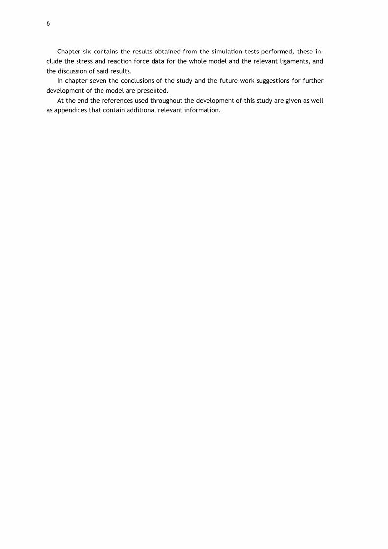
The human skeletal system, figure 2, is composed by the bones of the skeleton, the liga-
ments, cartilage and the connective tissue.
Figure 2.1 – Complete human skeletal system [43]
This system has various roles namely: [8]
- Provide support through its rigid bones, which also provide the body with the frame-
work for its shape and structural support, and the cartilage that also serves to shape
some parts of the human body like the nose and external ears; all of these are kept
together through the ligaments and connective tissue.
- Enables locomotion through the skeletal muscles which are connected to the bones
and, when contracted, make the bones act as levers that transmit the force that they
8
generate. Through the tendons and ligaments, the extent and direction of the force
can be changed affecting the complexity of the movement.
- Storage, the bones possess a storage of essential minerals like calcium, magnesium
and phosphorous. And the concentration of these minerals in the body drops below
normal levels these minerals are released from the bones to the blood stream.
- Protection, bone being a rigid structure, is placed in the human body enveloping cru-
cial body parts like the internal organs. The brain is protected by the skull, the lungs
and heart are protected by the sternum and ribs, the spinal cord is protected by the
vertebrae, the abdominal digestive and reproductive systems are protected by the
pelvis.
- Blood cell production, possible through the red bone marrow located within most
bones.
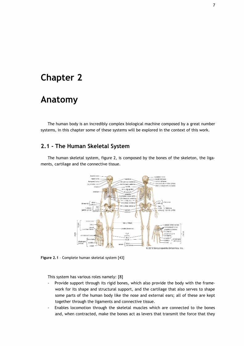
There are 206 bones in total on the human body, all of these are classified according to
their shape: long bones, short bones, flat bones, irregular and sesamoid bones.
Figure 2.2 – Classification of the bones in the Human Body [45]
Long bones are bones whose length exceeds their width, these bones include the humerus,
radios, ulna, femur, tibia, etc. Long bones usually possess a diaphysis composed of compact
bone and a metaphysis composed of cancellous bone. Past the metaphysis, in the extremities
of the bone, are located the epiphysis the line that separates these is called the epiphyseal
line. The diaphysis on long bones is usually thicker towards the middle, this in mainly because
that is where most of the strain is located [8].
Short bones, like the name entails, are short and compact bones. These bones are located
on parts of the body in which a lot of movement is not required, i.e. the wrist and tarsal
bones [8].
Flat bones are thin bones that are usually found in locations in which there is muscle at-
tachment or protection of soft tissue needed, thanks to their surface that allows for it. These
bones are mostly curved composed by cancellous bone and compact tissue. Examples of these
are the ribs and scapula [8].
9
Irregular bones to put it simply, are bones that do not fit the criteria of the previous cat-
egories being peculiar and unique. Some of these bones include the vertebrae, ossicles of the
ear, coccyx, etc.
The patella on the knee is a sesamoid bone, this type of bone is described as small and
round located within tendons with the role of assisting in muscle function [8].
Now going back to the bone composition, the lamellar or mature osseous tissue can be
classified into two types: cancellous or trabecular tissue and cortical or compact tissue. Even
though these tissues have the same constituent elements they differ in their structural organ-
ization and functionality.
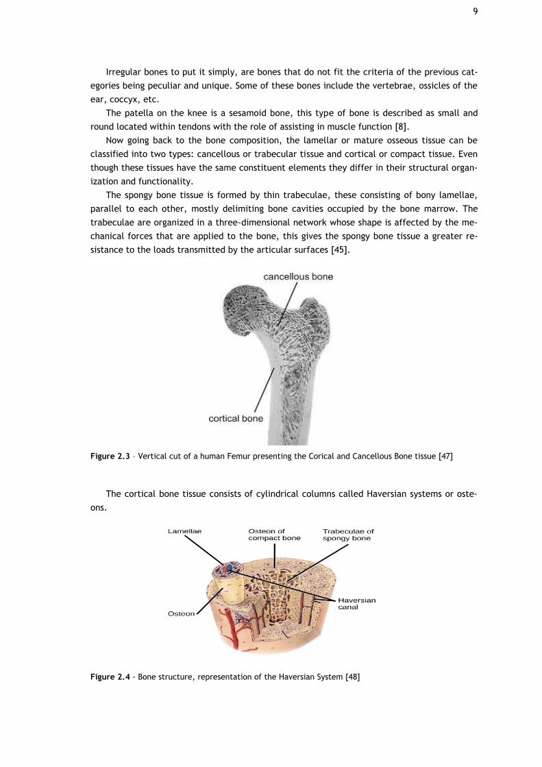
The spongy bone tissue is formed by thin trabeculae, these consisting of bony lamellae,
parallel to each other, mostly delimiting bone cavities occupied by the bone marrow. The
trabeculae are organized in a three-dimensional network whose shape is affected by the me-
chanical forces that are applied to the bone, this gives the spongy bone tissue a greater re-
sistance to the loads transmitted by the articular surfaces [45].
Figure 2.3 – Vertical cut of a human Femur presenting the Corical and Cancellous Bone tissue [47]
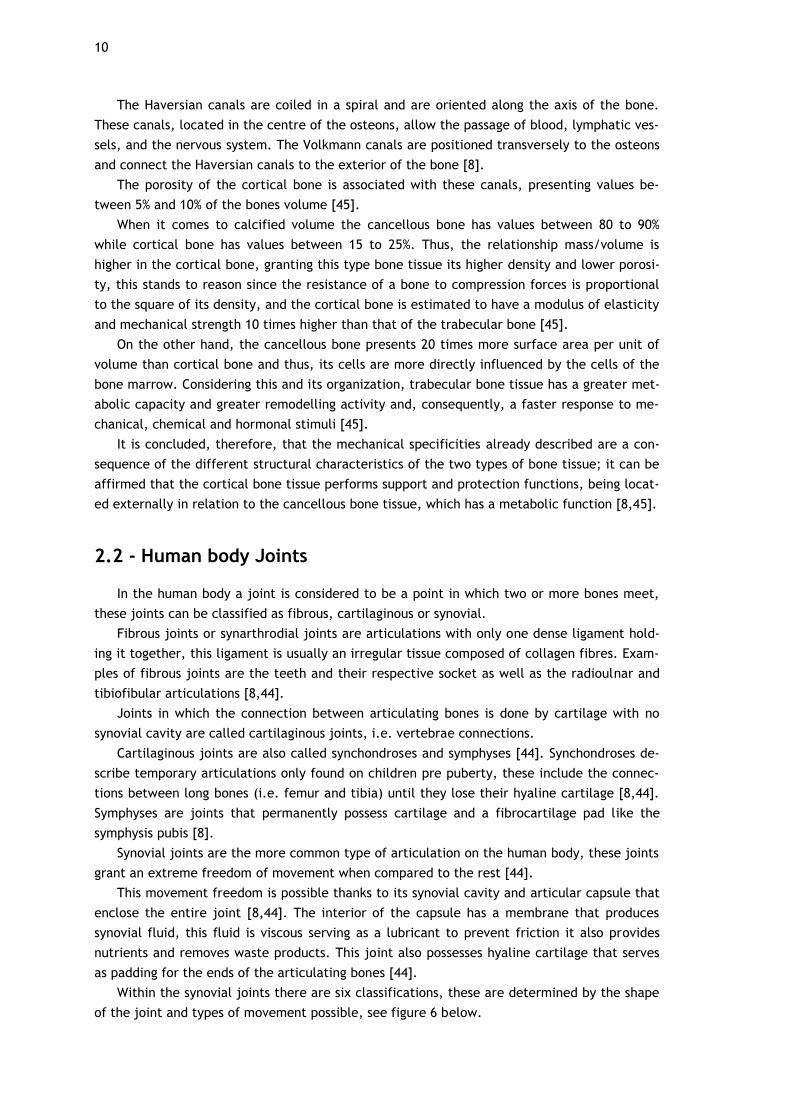
The cortical bone tissue consists of cylindrical columns called Haversian systems or oste-
ons.
Figure 2.4 - Bone structure, representation of the Haversian System [48]
10
The Haversian canals are coiled in a spiral and are oriented along the axis of the bone.
These canals, located in the centre of the osteons, allow the passage of blood, lymphatic ves-
sels, and the nervous system. The Volkmann canals are positioned transversely to the osteons
and connect the Haversian canals to the exterior of the bone [8].
The porosity of the cortical bone is associated with these canals, presenting values be-
tween 5% and 10% of the bones volume [45].
When it comes to calcified volume the cancellous bone has values between 80 to 90%
while cortical bone has values between 15 to 25%. Thus, the relationship mass/volume is
higher in the cortical bone, granting this type bone tissue its higher density and lower porosi-
ty, this stands to reason since the resistance of a bone to compression forces is proportional
to the square of its density, and the cortical bone is estimated to have a modulus of elasticity
and mechanical strength 10 times higher than that of the trabecular bone [45].
On the other hand, the cancellous bone presents 20 times more surface area per unit of
volume than cortical bone and thus, its cells are more directly influenced by the cells of the
bone marrow. Considering this and its organization, trabecular bone tissue has a greater met-
abolic capacity and greater remodelling activity and, consequently, a faster response to me-
chanical, chemical and hormonal stimuli [45].
It is concluded, therefore, that the mechanical specificities already described are a con-
sequence of the different structural characteristics of the two types of bone tissue; it can be
affirmed that the cortical bone tissue performs support and protection functions, being locat-
ed externally in relation to the cancellous bone tissue, which has a metabolic function [8,45].
2.2 - Human body Joints
In the human body a joint is considered to be a point in which two or more bones meet,
these joints can be classified as fibrous, cartilaginous or synovial.
Fibrous joints or synarthrodial joints are articulations with only one dense ligament hold-
ing it together, this ligament is usually an irregular tissue composed of collagen fibres. Exam-
ples of fibrous joints are the teeth and their respective socket as well as the radioulnar and
tibiofibular articulations [8,44].
Joints in which the connection between articulating bones is done by cartilage with no
synovial cavity are called cartilaginous joints, i.e. vertebrae connections.
Cartilaginous joints are also called synchondroses and symphyses [44]. Synchondroses de-
scribe temporary articulations only found on children pre puberty, these include the connec-
tions between long bones (i.e. femur and tibia) until they lose their hyaline cartilage [8,44].
Symphyses are joints that permanently possess cartilage and a fibrocartilage pad like the
symphysis pubis [8].
Synovial joints are the more common type of articulation on the human body, these joints
grant an extreme freedom of movement when compared to the rest [44].
This movement freedom is possible thanks to its synovial cavity and articular capsule that
enclose the entire joint [8,44]. The interior of the capsule has a membrane that produces
synovial fluid, this fluid is viscous serving as a lubricant to prevent friction it also provides
nutrients and removes waste products. This joint also possesses hyaline cartilage that serves
as padding for the ends of the articulating bones [44].
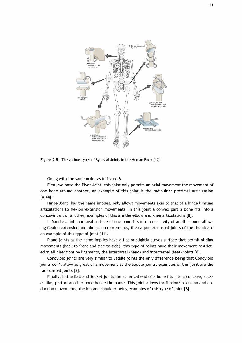
Within the synovial joints there are six classifications, these are determined by the shape
of the joint and types of movement possible, see figure 6 below.
11
Figure 2.5 – The various types of Synovial Joints in the Human Body [49]
Going with the same order as in figure 6.
First, we have the Pivot Joint, this joint only permits uniaxial movement the movement of
one bone around another, an example of this joint is the radioulnar proximal articulation
[8,44].
Hinge Joint, has the name implies, only allows movements akin to that of a hinge limiting
articulations to flexion/extension movements. In this joint a convex part a bone fits into a
concave part of another, examples of this are the elbow and knee articulations [8].
In Saddle Joints and oval surface of one bone fits into a concavity of another bone allow-
ing flexion extension and abduction movements, the carpometacarpal joints of the thumb are
an example of this type of joint [44].
Plane joints as the name implies have a flat or slightly curves surface that permit gliding
movements (back to front and side to side), this type of joints have their movement restrict-
ed in all directions by ligaments, the intertarsal (hand) and intercarpal (feet) joints [8].
Condyloid joints are very similar to Saddle joints the only difference being that Condyloid
joints don’t allow as great of a movement as the Saddle joints, examples of this joint are the
radiocarpal joints [8].
Finally, in the Ball and Socket joints the spherical end of a bone fits into a concave, sock-
et like, part of another bone hence the name. This joint allows for flexion/extension and ab-
duction movements, the hip and shoulder being examples of this type of joint [8].
12
2.3 - Anatomical Axes/Planes
Anatomical axes and planes have been used for a long time by anatomists not only to de-
scribe but also to name many human body parts, therefore it is important to first explain
some of these concepts in order to better describe the relative positions and naming of the
various parts of the knee joint.
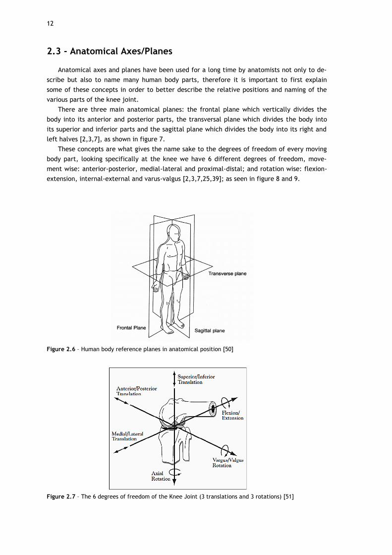
There are three main anatomical planes: the frontal plane which vertically divides the
body into its anterior and posterior parts, the transversal plane which divides the body into
its superior and inferior parts and the sagittal plane which divides the body into its right and
left halves [2,3,7], as shown in figure 7.
These concepts are what gives the name sake to the degrees of freedom of every moving
body part, looking specifically at the knee we have 6 different degrees of freedom, move-
ment wise: anterior-posterior, medial-lateral and proximal-distal; and rotation wise: flexion-
extension, internal-external and varus-valgus [2,3,7,25,39]; as seen in figure 8 and 9.
Figure 2.6 – Human body reference planes in anatomical position [50]
Figure 2.7 – The 6 degrees of freedom of the Knee Joint (3 translations and 3 rotations) [51]
13
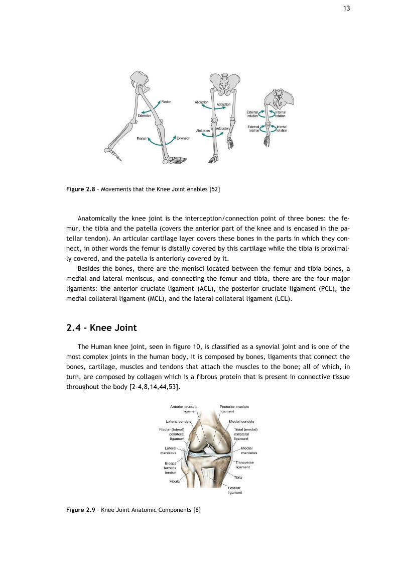
Figure 2.8 – Movements that the Knee Joint enables [52]
Anatomically the knee joint is the interception/connection point of three bones: the fe-
mur, the tibia and the patella (covers the anterior part of the knee and is encased in the pa-
tellar tendon). An articular cartilage layer covers these bones in the parts in which they con-
nect, in other words the femur is distally covered by this cartilage while the tibia is proximal-
ly covered, and the patella is anteriorly covered by it.
Besides the bones, there are the menisci located between the femur and tibia bones, a
medial and lateral meniscus, and connecting the femur and tibia, there are the four major
ligaments: the anterior cruciate ligament (ACL), the posterior cruciate ligament (PCL), the
medial collateral ligament (MCL), and the lateral collateral ligament (LCL).
2.4 - Knee Joint
The Human knee joint, seen in figure 10, is classified as a synovial joint and is one of the
most complex joints in the human body, it is composed by bones, ligaments that connect the
bones, cartilage, muscles and tendons that attach the muscles to the bone; all of which, in
turn, are composed by collagen which is a fibrous protein that is present in connective tissue
throughout the body [2-4,8,14,44,53].
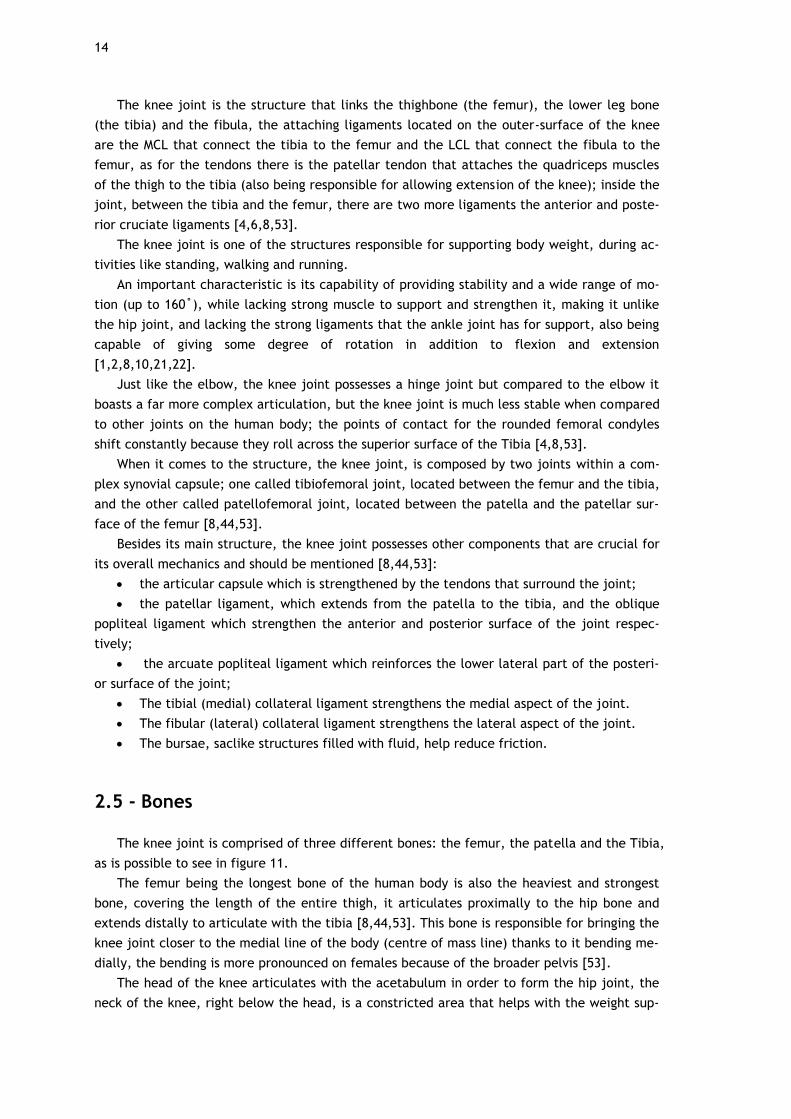
Figure 2.9 – Knee Joint Anatomic Components [8]
14
The knee joint is the structure that links the thighbone (the femur), the lower leg bone
(the tibia) and the fibula, the attaching ligaments located on the outer-surface of the knee
are the MCL that connect the tibia to the femur and the LCL that connect the fibula to the
femur, as for the tendons there is the patellar tendon that attaches the quadriceps muscles
of the thigh to the tibia (also being responsible for allowing extension of the knee); inside the
joint, between the tibia and the femur, there are two more ligaments the anterior and poste-
rior cruciate ligaments [4,6,8,53].
The knee joint is one of the structures responsible for supporting body weight, during ac-
tivities like standing, walking and running.
An important characteristic is its capability of providing stability and a wide range of mo-
tion (up to 160˚), while lacking strong muscle to support and strengthen it, making it unlike
the hip joint, and lacking the strong ligaments that the ankle joint has for support, also being
capable of giving some degree of rotation in addition to flexion and extension
[1,2,8,10,21,22].
Just like the elbow, the knee joint possesses a hinge joint but compared to the elbow it
boasts a far more complex articulation, but the knee joint is much less stable when compared
to other joints on the human body; the points of contact for the rounded femoral condyles
shift constantly because they roll across the superior surface of the Tibia [4,8,53].
When it comes to the structure, the knee joint, is composed by two joints within a com-
plex synovial capsule; one called tibiofemoral joint, located between the femur and the tibia,
and the other called patellofemoral joint, located between the patella and the patellar sur-
face of the femur [8,44,53].
Besides its main structure, the knee joint possesses other components that are crucial for
its overall mechanics and should be mentioned [8,44,53]:
• the articular capsule which is strengthened by the tendons that surround the joint;
• the patellar ligament, which extends from the patella to the tibia, and the oblique
popliteal ligament which strengthen the anterior and posterior surface of the joint respec-
tively;
• the arcuate popliteal ligament which reinforces the lower lateral part of the posteri-
or surface of the joint;
• The tibial (medial) collateral ligament strengthens the medial aspect of the joint.
• The fibular (lateral) collateral ligament strengthens the lateral aspect of the joint.
• The bursae, saclike structures filled with fluid, help reduce friction.
2.5 - Bones
The knee joint is comprised of three different bones: the femur, the patella and the Tibia,
as is possible to see in figure 11.
The femur being the longest bone of the human body is also the heaviest and strongest
bone, covering the length of the entire thigh, it articulates proximally to the hip bone and
extends distally to articulate with the tibia [8,44,53]. This bone is responsible for bringing the
knee joint closer to the medial line of the body (centre of mass line) thanks to it bending me-
dially, the bending is more pronounced on females because of the broader pelvis [53].
The head of the knee articulates with the acetabulum in order to form the hip joint, the
neck of the knee, right below the head, is a constricted area that helps with the weight sup-

15
port [53]. The femur prolongs into the medial and lateral condyles distally, which in turn ar-
ticulate to the tibia [4,53].
The patella or kneecap, as is most commonly called, is a sesamoid bone [44] located be-
tween the tibia and femur. This bone has a round and flat shape and is a lot smaller when
compared to the other two [8], see figure 11. The patella’s functions are to increase the lev-
erage of the tendon and maintain its position when the knee is flexed and protect the knee
joint [53].
During flexion of the knee the patella moves according to the movement; tracking/gliding
up or down, depending on the phase of the movement, in the groove between the two femo-
ral condyles [53].
The tibia, just like the femur, is one of the largest bones in the human body being anoth-
er weight bearing bone in the leg [4,8,44,53]. The tibia articulates proximally to the femur in
the knee joint. In its anterior surface below the condyles there is the tibial tuberosity, which
is the point of attachment for the patellar ligament [8], and distally on its medial surface the
tibia, forms the medial malleolus which articulates with the talus of the ankle forming the
protrusion that we all have on the medial surface of our ankle [8,53].
Figure 2.10 – Bony Components of the Knee Joint [53]
2.6 - Menisci
The meniscus is a component vital for the normal function and longevity of the knee joint,
this knee component is composed by a dense extracellular matrix, which in turn is composed
of water (72%) and collagen (22%) [54]. It is located between the femur and tibia in the “joint
space” [4,8,44,53,54].
The menisci have a number of roles but the most important one is, through congruency,
to transmit load across the tibiofemoral joint in order to significantly decrease the stress that
the articular cartilage is under [21,53]; besides this the menisci is also responsible for provid-
ing joint stability, shock absorption, nutrition, lubrification and proprioception to the knee
joint [21,54,55].
The meniscus is shaped like crescent edges of cartilage located medially and laterally in
the knee, see figure 12, these occupy roughly one-half to two-thirds of the joint space [54];
16
the outer, thicker convex, section of the meniscus is attached to the knee joint capsule while
the inner, thinner concave, part isn’t attached at all [54]. The menisci possess a meniscal
horn that connect them to the subchondral bone of the tibial plateau, these ligaments also
serve as means of transmitting sheer and tensile loads to the bone and also serve as a means
to decrease the contact area [21,54,55].
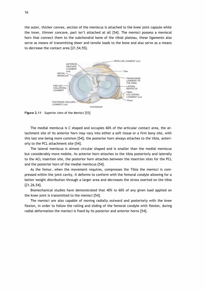
Figure 2.11 – Superior view of the Menisci [53]
The medial meniscus is C shaped and occupies 60% of the articular contact area, the at-
tachment site of its anterior horn may vary into either a soft tissue or a firm bony site, with
this last one being more common [54]; the posterior horn always attaches to the tibia, anteri-
orly to the PCL attachment site [54].
The lateral meniscus is almost circular shaped and is smaller than the medial meniscus
but considerably more mobile, its anterior horn attaches to the tibia posteriorly and laterally
to the ACL insertion site, the posterior horn attaches between the insertion sites for the PCL
and the posterior horn of the medial meniscus [54].
As the femur, when the movement requires, compresses the Tibia the menisci is com-
pressed within the joint cavity, it deforms to conform with the femoral condyle allowing for a
better weight distribution through a larger area and decreases the stress exerted on the tibia
[21,26,54].
Biomechanical studies have demonstrated that 40% to 60% of any given load applied on
the knee joint is transmitted to the menisci [54].
The menisci are also capable of moving radially outward and posteriorly with the knee
flexion, in order to follow the rolling and sliding of the femoral condyle with flexion, during
radial deformation the menisci is fixed by its posterior and anterior horns [54].
17
2.7 - Articular Cartilage
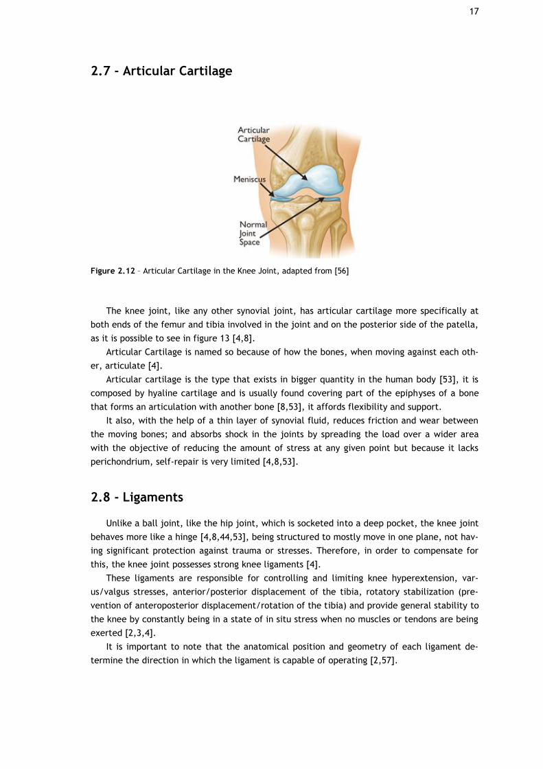
Figure 2.12 – Articular Cartilage in the Knee Joint, adapted from [56]
The knee joint, like any other synovial joint, has articular cartilage more specifically at
both ends of the femur and tibia involved in the joint and on the posterior side of the patella,
as it is possible to see in figure 13 [4,8].
Articular Cartilage is named so because of how the bones, when moving against each oth-
er, articulate [4].
Articular cartilage is the type that exists in bigger quantity in the human body [53], it is
composed by hyaline cartilage and is usually found covering part of the epiphyses of a bone
that forms an articulation with another bone [8,53], it affords flexibility and support.
It also, with the help of a thin layer of synovial fluid, reduces friction and wear between
the moving bones; and absorbs shock in the joints by spreading the load over a wider area
with the objective of reducing the amount of stress at any given point but because it lacks
perichondrium, self-repair is very limited [4,8,53].
2.8 - Ligaments
Unlike a ball joint, like the hip joint, which is socketed into a deep pocket, the knee joint
behaves more like a hinge [4,8,44,53], being structured to mostly move in one plane, not hav-
ing significant protection against trauma or stresses. Therefore, in order to compensate for
this, the knee joint possesses strong knee ligaments [4].
These ligaments are responsible for controlling and limiting knee hyperextension, var-
us/valgus stresses, anterior/posterior displacement of the tibia, rotatory stabilization (pre-
vention of anteroposterior displacement/rotation of the tibia) and provide general stability to
the knee by constantly being in a state of in situ stress when no muscles or tendons are being
exerted [2,3,4].
It is important to note that the anatomical position and geometry of each ligament de-
termine the direction in which the ligament is capable of operating [2,57].
18
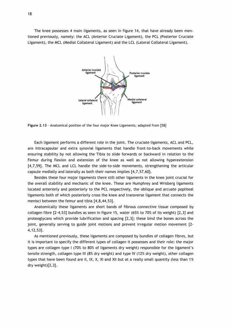
The knee possesses 4 main ligaments, as seen in figure 14, that have already been men-
tioned previously, namely: the ACL (Anterior Cruciate Ligament), the PCL (Posterior Cruciate
Ligament), the MCL (Medial Collateral Ligament) and the LCL (Lateral Collateral Ligament).
Figure 2.13 – Anatomical position of the four major Knee Ligaments, adapted from [58]
Each ligament performs a different role in the joint. The cruciate ligaments, ACL and PCL,
are intracapsular and extra synovial ligaments that handle front-to-back movements while
ensuring stability by not allowing the Tibia to slide forwards or backward in relation to the
Femur during flexion and extension of the knee as well as not allowing hyperextension
[4,7,59]. The MCL and LCL handle the side-to-side movements, strengthening the articular
capsule medially and laterally as both their names implies [4,7,57,60].
Besides these four major ligaments there still other ligaments in the knee joint crucial for
the overall stability and mechanic of the knee. These are Humphrey and Wrisberg ligaments
located anteriorly and posteriorly to the PCL respectively, the oblique and arcuate popliteal
ligaments both of which posteriorly cross the knee and transverse ligament that connects the
menisci between the femur and tibia [4,8,44,53].
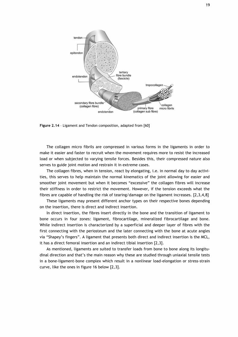
Anatomically these ligaments are short bands of fibrous connective tissue composed by
collagen fibre [2-4,53] bundles as seen in figure 15, water (65% to 70% of its weight) [2,3] and
proteoglycans which provide lubrification and spacing [2,3]; these bind the bones across the
joint, generally serving to guide joint motions and prevent irregular motion movement [2-
4,12,53].
As mentioned previously, these ligaments are composed by bundles of collagen fibres, but
it is important to specify the different types of collagen it possesses and their role: the major
types are collagen type I (70% to 80% of ligaments dry weight) responsible for the ligament’s
tensile strength, collagen type III (8% dry weight) and type IV (12% dry weight), other collagen
types that have been found are II, IX, X, XI and XII but at a really small quantity (less than 1%
dry weight)[2,3].
19
Figure 2.14 – Ligament and Tendon composition, adapted from [60]
The collagen micro fibrils are compressed in various forms in the ligaments in order to
make it easier and faster to recruit when the movement requires more to resist the increased
load or when subjected to varying tensile forces. Besides this, their compressed nature also
serves to guide joint motion and restrain it in extreme cases.
The collagen fibres, when in tension, react by elongating, i.e. in normal day to day activi-
ties, this serves to help maintain the normal kinematics of the joint allowing for easier and
smoother joint movement but when it becomes “excessive” the collagen fibres will increase
their stiffness in order to restrict the movement. However, if the tension exceeds what the
fibres are capable of handling the risk of tearing/damage on the ligament increases. [2,3,4,8]
These ligaments may present different anchor types on their respective bones depending
on the insertion, there is direct and indirect insertion.
In direct insertion, the fibres insert directly in the bone and the transition of ligament to
bone occurs in four zones: ligament, fibrocartilage, mineralized fibrocartilage and bone.
While indirect insertion is characterized by a superficial and deeper layer of fibres with the
first connecting with the periosteum and the later connecting with the bone at acute angles
via “Shapey’s fingers”. A ligament that presents both direct and indirect insertion is the MCL,
it has a direct femoral insertion and an indirect tibial insertion [2,3].
As mentioned, ligaments are suited to transfer loads from bone to bone along its longitu-
dinal direction and that’s the main reason why these are studied through uniaxial tensile tests
in a bone-ligament-bone complex which result in a nonlinear load-elongation or stress-strain
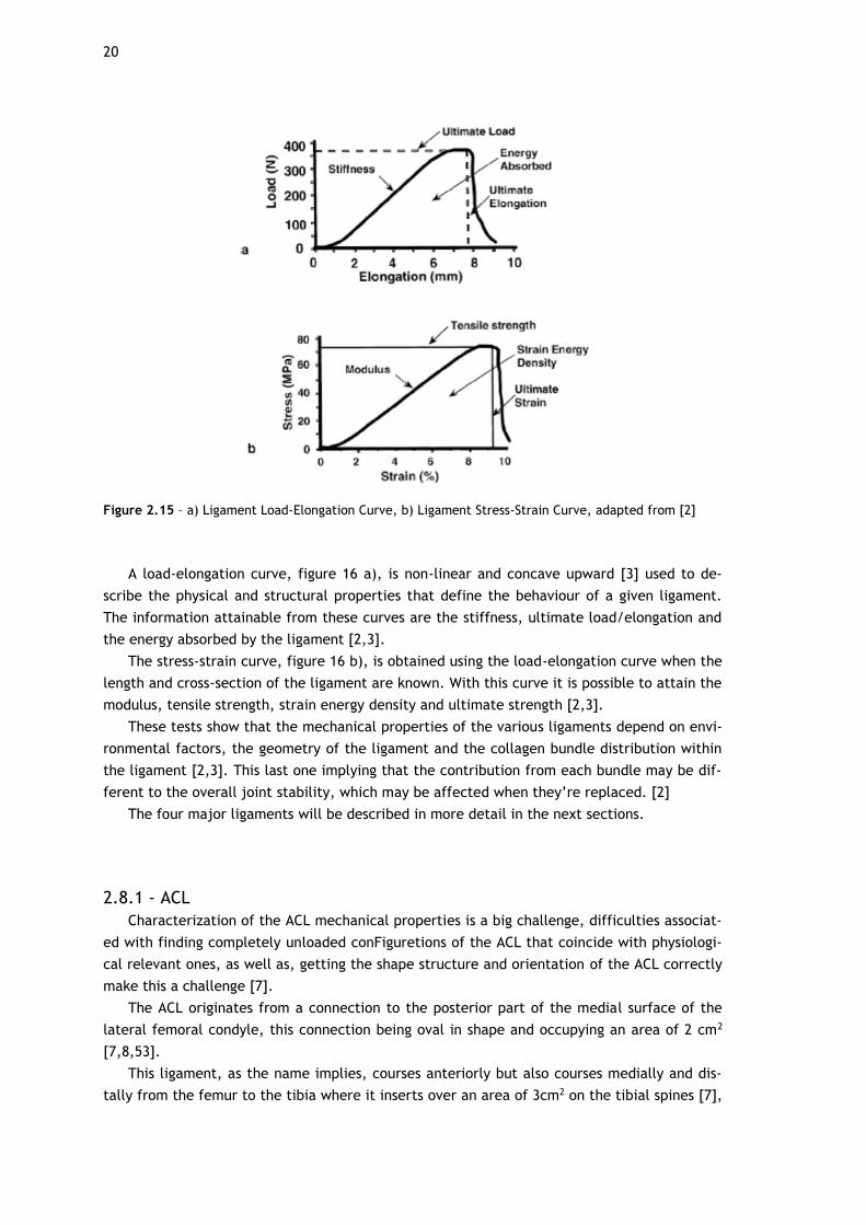
curve, like the ones in figure 16 below [2,3].
20
Figure 2.15 – a) Ligament Load-Elongation Curve, b) Ligament Stress-Strain Curve, adapted from [2]
A load-elongation curve, figure 16 a), is non-linear and concave upward [3] used to de-
scribe the physical and structural properties that define the behaviour of a given ligament.
The information attainable from these curves are the stiffness, ultimate load/elongation and
the energy absorbed by the ligament [2,3].
The stress-strain curve, figure 16 b), is obtained using the load-elongation curve when the
length and cross-section of the ligament are known. With this curve it is possible to attain the
modulus, tensile strength, strain energy density and ultimate strength [2,3].
These tests show that the mechanical properties of the various ligaments depend on envi-
ronmental factors, the geometry of the ligament and the collagen bundle distribution within
the ligament [2,3]. This last one implying that the contribution from each bundle may be dif-
ferent to the overall joint stability, which may be affected when they’re replaced. [2]
The four major ligaments will be described in more detail in the next sections.
2.8.1 - ACL
Characterization of the ACL mechanical properties is a big challenge, difficulties associat-
ed with finding completely unloaded conFiguretions of the ACL that coincide with physiologi-
cal relevant ones, as well as, getting the shape structure and orientation of the ACL correctly
make this a challenge [7].
The ACL originates from a connection to the posterior part of the medial surface of the
lateral femoral condyle, this connection being oval in shape and occupying an area of 2 cm2
[7,8,53].
This ligament, as the name implies, courses anteriorly but also courses medially and dis-
tally from the femur to the tibia where it inserts over an area of 3cm2 on the tibial spines [7],

21
this part of the ligament that is attached to the tibia is substantially wider and stronger when
compared to its other end [7,8,53].
At the tibial insertion, the ligament passes below the transverse meniscal ligament, where
it is believed that some fibres of the ACL blend with the fibres of the anterior attachment of
the lateral meniscus though the relevance of this blending hasn’t been discovered [7].
Interestingly, the cross-section area of the ACL varies along its length, with its smaller
value being located at the mid-substance. The functional reason for this area variation, is to
minimize stress concentrations in the interface between ligament and bone [5,53].
This is also the reason why adult ACL injuries are mainly located in the mid-substance ar-
ea; it also explains why children ACL injuries appear primarily on the bony avulsions, where
modulating and weaker ligament to bone interface exists [7].
Another interesting aspect is that the ACL size also varies depending on sex, with male
ACL being thicker, wider and longer [7,11]; this difference only starting to be noticeable after
the development and growth spurt [7].
Within the ACL there are two discrete bundles: the anteromedial bundle (AMB) and the
posterolateral bundle (PLB) [6,7,22,25]; these two structures possess unalike spatial and me-
chanical properties [7]. Anatomically these two bundles intertwine with each other between
their respective insertion points, in which each occupies 50%, with AMB being longer com-
pared to PLB [7].
Referring now to the insertion sites, the AMB inserts posteriorly and superiorly to the fe-
mur and medially to the tibia, and conversely the PLB inserts anteriorly and inferiorly to the
femur and laterally to the tibia [7]. These bundles have been observed to have reciprocal
tensioning pattern during their function in passive flexion and extension movements of the
knee joint, with AMB (29 mm–35 mm) observed to be tauter in flexion and the PLB (18 mm–26
mm) in extension [7].
2.8.2 - PCL
The Posterior Cruciate Ligament (PCL) is the largest and strongest intra-articular ligament
in the knee joint, it is attached to the tibial spine distally and crosses the knee joint attach-
ing its other end to the lateral aspect of the medial femoral condyle; it is reported that its
femoral attachment can be twice the size of its tibial attachment (112 to 118 mm2) [59].
The PCL, just like the ACL, is comprised of two bundles, the larger one being the anterol-
ateral bundle (ALB) and the smaller one being the posteromedial bundle (PMB); but, to dif-
ferentiate it, the PCL has an inclination angle more horizontal when compared to the ACL,
which has a more vertical angle when in full extension, the same comparison can be made to
their femoral insertions with PCL’s insertion being more horizontal and the ACL’s being more
vertical; the PCL also has a cross section larger than the ACL [59].
Mechanically the PCL has the role to restrain posterior tibial translation at all flexion an-
gles, with both bundles (ALB and PLB) playing significant roles in maintaining knee stability in
case the other bundle fails to respond, suggesting a co-dominant relationship between them
[59].
2.8.3 - MCL
The Medial Collateral Ligament (MCL) is one of the four major ligaments in the knee joint,
it has a length of 8 to 10 cm being the largest structure in the medial aspect of the knee joint.
22
The MCL is comprised by two components: a superficial and a deep component. The su-
perficial MCL component, also named tibial collateral ligament, originates from the posterior
aspect of the medial femoral epicondyle and connect distally to the medial condyle of the
tibia below the joint line near the level of the pes anserinus insertion, this component is acts
as the primary static stabilizer for valgus stress in the knee. The deep MCL component, also
named mid-third capsular ligament, is divided into meniscofemoral and meniscotibial and is
responsible for restraining anterior translation movement of the tibia, with a secondary role
in static stabilization for valgus stress [57].
2.8.3 - LCL
The Lateral Collateral Ligament (LCL) is a ligament considered to be a component of the
posterolateral corner, it runs from the outer surface of the lateral condyle, posteriorly and
obliquely inferiorly, to the fibular head; since the LCL is outside the capsule throughout its
length it is considered an extracapsular ligament [61].
The LCL is majorly responsible for passively stabilizing the lateral aspect of the knee as
well as restraining varus stress at the knee joint (mainly at 0 to 30-degree of knee flexion);
secondarily it also serves as restraint for tibial external rotation, most optimally with the
knee at full extension when the ligament is under greatest force, helping the popliteus ten-
don, popliteofibular ligament, and posterolateral capsule which are the primary static re-
straints.
The LCL is also capable, to a lesser degree, of restraining varus forces at additional flex-
ion ranges and adding stability to tibial internal rotation [61].
23
Chapter 3
Common Injuries and Treatments
Knee injuries are most common on sports [7,10,13,63] accounting with 15% to 50% of all
sports injuries, mainly those in which high stress is focused on the legs; among these the
sports with higher knee injury rate are: soccer, ice-hockey, volleyball, basketball and judo
[10]. By looking at insurance data on licensed competitors, in Finland, showed that in knee
injuries 21% happened in soccer, 20% in judo, 19% in volleyball, 17% in ice-hockey, and 16% in
basketball, with the remaining 7% being distributed between other sports [10].
The cost of knee injuries representing a major part of expenditure for medical care of
sport injuries, the reason being the long and costly rehabilitation and the possibility of im-
pairment (to various degree) [4,14].
As mentioned previously, athletes that practice these sports exert tremendous stresses on
their legs and knees; normally the medial, lateral ligaments and meniscus shift their position,
depending on the movement, while performing high stress activities when the knee is partial-
ly flexed, the meniscus may be trapped between the femur and tibia resulting in a tear of its
cartilage [3].
Most commonly, for the injurie to occur, the lateral surface of the leg is driven medially,
either because the movement was performed incorrectly (on a fall) or because of an external
interaction (a tackle by a different athlete), tearing the medial meniscus; this type of injurie
besides being quite painful, the torn cartilage causes restriction to the movement of the joint
also leading to chronic problems and the possible development of “trick knee”, instability of
the knee. [3,7,10]
Other knee injuries happen involving the tear of the supporting ligaments or damage of
the patella. Rupture of the ACL is a common injury [7,10,13,62], which affect more women
than men [3,7,10,11] (two to seven times more [8]), with a study revealing that during the
activities of ‘‘Youth and Sports’’ (an organized sports and recreation event for Swiss youth)
females were significantly more at risk in six sports: alpinism, downhill skiing, gymnastics,
volleyball, basketball and team handball [4].
This type of injurie tends to happen when, during movement, the weight bearing knee
twists [8].
When an ACL injury is suspected the normal clinical procedure is to, firstly, use the Ante-
rior Drawer and Lachman tests in order to assess the severity of the injury [2,4,22,63]. These
tests consist in the anterior displacement of the tibia by applying a translational load and
24
manually flexing at 90˚ to 30˚, while the femur is fixed; the objective here is to measure the
laxity of the injured joint compare it to a healthy one [2,63].
3.1 - ACL Tear Treatment techniques
As previously mentioned, ACL injury is very common, with 80% of knee-based surgeries be-
ing performed on the ACL [13,63], one of the major problems with complete rupture of the
ACL is that besides leading to incomplete healing it also causes insufficient vascularization.
Reconstruction of the ACL is the more popular method to treat these injurie, it aims to
reinstate stability to the knee and preventing further damage be done to the menisci, it also
reduces the danger of osteoarthritis developing.
Advancement, as led to the creation of the arthroscopic anatomic grafting techniques
which consist in grafting tissue (organic or synthetic) to the damaged ACL area.
A considerable number of different graft types exist, but generally speaking, all grafts can
be organized into three types: autologous grafts, allografts, and synthetic ligaments [13].
An example of autologous grafts is hamstring and bone-patella tendon grafts, these grafts
have the advantage of providing a strong scaffold for in-growth of collagen fibres with mini-
mal risk for body rejection of the grafts. But a major disadvantage is the risk of harvest site
morbidity that it may cause making a long period of rest, and avoiding any kind of straining
activities, necessary for revascularization. This period lasting up to 12 months [13,63,65].
On the opposite spectre, there are the allografts which have the advantage of having low
risk for harvest site morbidity but are prone for graft rejection. These have high potential to
cause a viral infection, have a slower healing process and higher failure rates making them a
very rare choice [13].
As for synthetic ligaments, the option for using synthetic biomaterial to reinforce these
grafts has been in development since the 1980’s, these reinforced grafts were developed to
have increased strength and stability, immediately post operation, to reduce harvest site
morbidity and eliminate potential disease transmission [13,66].
But even though these were the objectives, the first synthetic ligaments were mostly fail-
ures being associated with the development of synovitis.
Nowadays, with the advancement of technology, there has been development of new
kinds of synthetic ligaments with one of them gaining popularity, Ligament Advanced Rein-
forcement System (LARS) [13,67].
LARS is a non-absorbable synthetic graft made out of terephthalic polyethylene polyester
fibres (PET) [67].
PET is a semi crystalline thermoplastic polymer widely used all over the world, being bet-
ter known in the textile industry as “polyester”. This polymer is a naturally transparent,
strong and lightweight plastic used more commonly as fibre for clothing, packaging for various
foods and beverages and as an engineering plastic that, when combined with other materials,
strengthens them [68,69]. It is produced from the synthesis ethylene glycol and terephthalic
acid which are held together by a polymer chain.
The main characteristics that define PET are its chemical resistance not reacting with wa-
ter or organic tissue, its strength to weight ratio, it is a material that is readably available at
a relatively inexpensive cost and it is shatterproof. All these characteristics make this a prom-
ising material for synthetic ligament grafts, but it does have its drawbacks, unfortunately PET
25
is not biodegradable which means that it will stay within the recovered ligament indefinitely
[1].
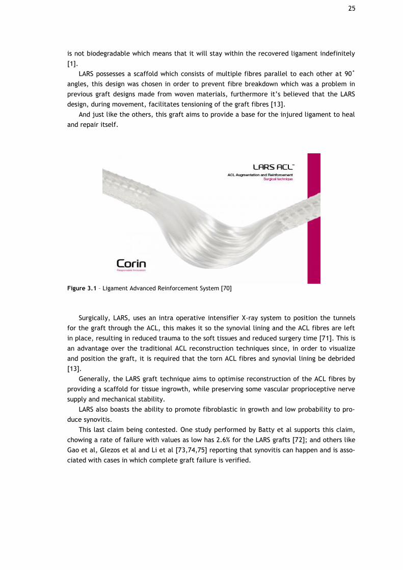
LARS possesses a scaffold which consists of multiple fibres parallel to each other at 90˚
angles, this design was chosen in order to prevent fibre breakdown which was a problem in
previous graft designs made from woven materials, furthermore it’s believed that the LARS
design, during movement, facilitates tensioning of the graft fibres [13].
And just like the others, this graft aims to provide a base for the injured ligament to heal
and repair itself.
Figure 3.1 – Ligament Advanced Reinforcement System [70]
Surgically, LARS, uses an intra operative intensifier X-ray system to position the tunnels
for the graft through the ACL, this makes it so the synovial lining and the ACL fibres are left
in place, resulting in reduced trauma to the soft tissues and reduced surgery time [71]. This is
an advantage over the traditional ACL reconstruction techniques since, in order to visualize
and position the graft, it is required that the torn ACL fibres and synovial lining be debrided
[13].
Generally, the LARS graft technique aims to optimise reconstruction of the ACL fibres by
providing a scaffold for tissue ingrowth, while preserving some vascular proprioceptive nerve
supply and mechanical stability.
LARS also boasts the ability to promote fibroblastic in growth and low probability to pro-
duce synovitis.
This last claim being contested. One study performed by Batty et al supports this claim,
chowing a rate of failure with values as low has 2.6% for the LARS grafts [72]; and others like
Gao et al, Glezos et al and Li et al [73,74,75] reporting that synovitis can happen and is asso-
ciated with cases in which complete graft failure is verified.

26

27
Chapter 4
Knee Biomechanics and Kinematics
Kinematics, when applied to the human body, represent the motion, locomotion and gait
of diarthrodial joints [2]. The information that we can take from analysing the Biomechani-
cal/Kinematic characteristics of the various joints is valuable to obtain a dipper knowledge on
them: knowing how they function during normal movement is important material used for
comparison purposes when diagnosing injury and checking for the success of treatment [2,3].
Specifically, for the knee, examination of the injured joint is performed by analysing the
knee motion and comparing it to that of a non-injured one [2], the Lachman and drawer tests
are an example of this [2,4,22,39]. What the examiner looks for, in these tests, is excess mo-
tion in a direction from the injured knee, the direction in which excessive motion happens is
related to the damaged component within the knee [2].
The function of the knee and its components is to prevent over elongation during normal
movement activities, either rotational, translational or both [1,2,8,10,22,63]. In order to bet-
ter understand knee joint kinematics, it is important to study their behaviour. The knee joint
movements are only possible through its ligaments, other soft tissues and the articular sur-
faces [2,4,7,57,59,62].
The knee has six different degrees of freedom, three rotations and three translations
[2,3,7,14,39]. As for its planes of motion the knee possesses three main axis: the tibial shaft
axis, the epycondral axis and the anteroposterior axis [2]; the translations along these axis
are, respectively: proximal-distal, medial-lateral and anterior-posterior; and the rotations
along these axis are, respectively: internal-external, flexion-extension and varus-valgus, all of
this can be seen in the figure 18 bellow [2].
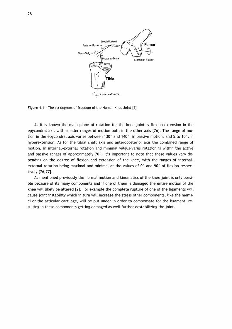
28
Figure 4.1 – The six degrees of freedom of the Human Knee Joint [2]
As it is known the main plane of rotation for the knee joint is flexion-extension in the
epycondral axis with smaller ranges of motion both in the other axis [76]. The range of mo-
tion in the epycondral axis varies between 130° and 140°, in passive motion, and 5 to 10°, in
hyperextension. As for the tibial shaft axis and anteroposterior axis the combined range of
motion, in internal-external rotation and minimal valgus-varus rotation is within the active
and passive ranges of approximately 70°. It’s important to note that these values vary de-
pending on the degree of flexion and extension of the knee, with the ranges of internal-
external rotation being maximal and minimal at the values of 0° and 90° of flexion respec-
tively [76,77].
As mentioned previously the normal motion and kinematics of the knee joint is only possi-
ble because of its many components and if one of them is damaged the entire motion of the
knee will likely be altered [2]. For example the complete rupture of one of the ligaments will
cause joint instability which in turn will increase the stress other components, like the menis-
ci or the articular cartilage, will be put under in order to compensate for the ligament, re-
sulting in these components getting damaged as well further destabilizing the joint.

29
Chapter 5
Methodology
5.1 - Finite Element Method (FEM)
The Finite Element Method, in the engineering field, has the objective of determining the
stress and strain states of an object with arbitrary geometry in which forces are being applied
externally. It is a powerful numerical method, devised for analysis of various engineering
problems, from the more elementary to the more complex, it being capable of handling geo-
metrical complexity, a large array of boundary conditions, nonlinearities and coupled phe-
nomena [78].
There are, nowadays, a large number of licensed computer software that use this method
like Femap, MATLAB, MFEM, Abaqus, etc, that have made it a “regular use” tool in the engi-
neering research field.
The FEM is the numerical technique used for Finite Elements Analysis (FEA), which is used
for this study.
In order to run a FEA, the first step is to divide the structure as a whole into smaller parts,
this is done by creating a mesh. This mesh will contain a large number of elements that will
make up the general shape of the model, the reason for this is to transcribe the complex
shape of the model into a series of, comparably, simpler mathematical points. [78, 79]
The second step is to try and find the solution closest to reality for each finite element,
this solution will be a linear combination of nodal values and approximation functions. Finally,
with the data from each element it is possible to obtain the solution for the whole structure
[78]. Interpolation may occur, since some nodal points might be shared by different elements,
but these approximations are within what is expected [79].
But before implementing a FEA and even meshing the model, first it needs to be catego-
rized by its structure. This is done by classifying it according to its geometry, material type
and applied actions.
Geometry wise the model needs to have a well thought out node and element definition,
this is done through correct node/element number and coordinate assigning, defining individ-
ual nodes/elements or grouping them into sets accordingly.
For the Material, in order to be able to start a FEA a material type needs to be assigned to
the elements of the model. Most, if not all, CAD programs have a material library to choose
from as well as a means to create a custom type of material for analysis.
30
Applied actions pretrains to the constraints and interactions that the model will be under
during analysis.
Another consideration is the inherent simplifications that will have to be done to the
model in order to achieve a balance between results and computing processing power, the
application of the FEM will vary depending on the level of complexity.
The main aspects to have in consideration before applying the FE model in structure anal-
ysis are [78]:
- Whether the Analysis is Dynamic or Static - The consensus is that the actions applied
on the structure are all generally dynamic, and that there is inertia associated to the acceler-
ation to which every single part of the structure is under. But this does not mean that every
situation should be considered as having dynamic behaviour, in some situations the inertia is
negligible, this results from the applied actions having low values; in these cases, the analysis
is considered static.
- Whether the Analysis is Linear or Non-Linear - Generally speaking, in an analysis of a
solid body in which the displacements are small (when compared to the elements of the
structure), it is said that there is no influence on the stress and tension distribution by the
geometry modification, and therefore the entire analysis is performed with the initial un-
modified geometry classifying this as a Linear Analysis. If the opposite happens, i.e. the body
suffers considerable deformation influencing the stress and tension distribution, then it will
be classified as a Non-Linear analysis.
The next parts will show in some detail the formulation of the FE methodology and some
other concepts associated with it, for more detailed information on the subject the reader is
referred to read the original document [78].
5.1.1 - FEM Fundamentals
The formulation of the FEM requires the existence of an integral equation, in other words
the basis of this method is an integral equation. This integral will be converted over a com-
plex domain, of volume V, for a sum of integrals extended to subdomains of simple geometry,
of volume Vi.
This next equation (1) illustrates an example of this, which corresponds to the integral
volume of a function f.
. (1)
On equation (1) it is assumed that
. (2)
By calculating all the extended integrals to the subdomains Vi, there only is the need to
calculate the sum corresponding to the second part of equation (1) to obtain the extended
integral of the entire domain. Another aspect to note is that each subdomain Vi coincides
with an element of the structure with simple geometry.
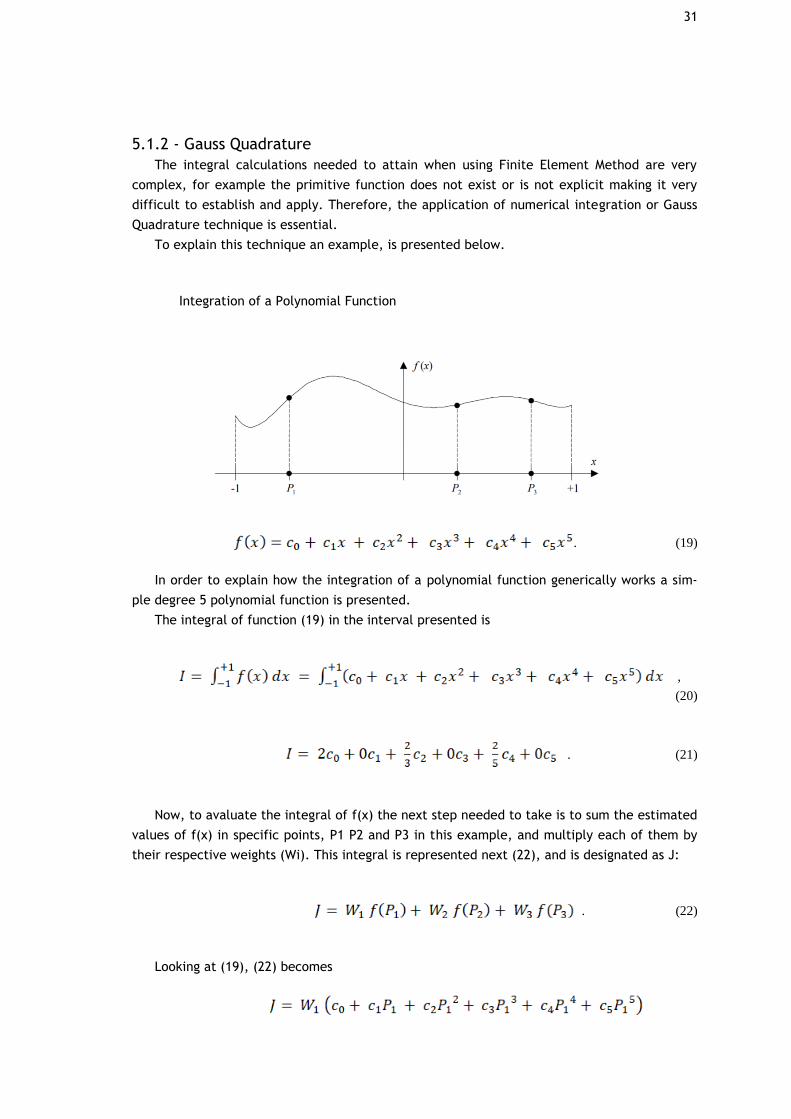
31
5.1.2 - Gauss Quadrature
The integral calculations needed to attain when using Finite Element Method are very
complex, for example the primitive function does not exist or is not explicit making it very
difficult to establish and apply. Therefore, the application of numerical integration or Gauss
Quadrature technique is essential.
To explain this technique an example, is presented below.
Integration of a Polynomial Function
. (19)
In order to explain how the integration of a polynomial function generically works a sim-
ple degree 5 polynomial function is presented.
The integral of function (19) in the interval presented is
,
(20)
. (21)
Now, to avaluate the integral of f(x) the next step needed to take is to sum the estimated
values of f(x) in specific points, P1 P2 and P3 in this example, and multiply each of them by
their respective weights (Wi). This integral is represented next (22), and is designated as J:
. (22)
Looking at (19), (22) becomes
32
(23)
,
or
(24)
.
Since it is intended, in this example, that (24) be equal to (21).
, (25)
and we get:
(26)
,
and considering that values are in both branches of equation (26) for the equality to exist
we can consider that:
. (27)
Then by solving (27) as a system of six equations with the objective of discovering
and , we get:
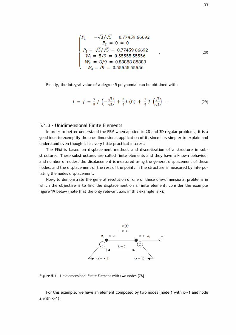
33
. (28)
Finally, the integral value of a degree 5 polynomial can be obtained with:
. (29)
5.1.3 - Unidimensional Finite Elements
In order to better understand the FEM when applied to 2D and 3D regular problems, it is a
good idea to exemplify the one-dimensional application of it, since it is simpler to explain and
understand even though it has very little practical interest.
The FEM is based on displacement methods and discretization of a structure in sub-
structures. These substructures are called finite elements and they have a known behaviour
and number of nodes, the displacement is measured using the general displacement of these
nodes, and the displacement of the rest of the points in the structure is measured by interpo-
lating the nodes displacement.
Now, to demonstrate the general resolution of one of these one-dimensional problems in
which the objective is to find the displacement on a finite element, consider the example
figure 19 below (note that the only relevant axis in this example is x):
Figure 5.1 – Unididmensional Finite Element with two nodes [78]
For this example, we have an element composed by two nodes (node 1 with x=-1 and node
2 with x=1).
34
Equation 12, below, represents the displacement field of the element.
, (12)
with and representing the value for the displacement of nodes 1 and 2, respectively.
Now if we regard the displacement variation between nodes 1 and 2 as linear, we get the
following function:
. (13)
This way, in 13, u(x) is linear in x and respects 12, accurately representing the displace-
ment field of the element.
By placing and separately and writing 13 in a matrix form, as seen in equation 14,
we can represent 13 in a more simplified (equations 15).
, (14)
. (16)
5.1.4 - Virtual Work Principle
The virtual Work Principle or Virtual Displacement Principle is a concept that is associated
with FEM.
It establishes that, the work performed by the external forces in the virtual displacement
of the points in which they are applied, is equal to the work performed by the internal strain
in the virtual deformation of the body. In simplified terms, the external virtual work corre-
sponds to the sum of the internal virtual work.
. (17)
In this context the word “virtual” means that the displacement and the force values may
not correspond to each other, but the force values are static while the displacement values
are cinematic.
Virtual displacement describes any non-verifiable displacement, in other words that does
not exist and that doesn’t originate from the applied load, but that must be cinematically
acknowledge (the frontier cinematic conditions must be met).
Within the Virtual Work principle there are two forms: virtual displacement principle and
virtual force principle; the difference between these two is that in the first one it is consid-
ered the influence of real displacement on virtual forces while in the second the influence of
the virtual forces is considered on the real displacements.

35
. (18)
The equation (18), presented above represents a simplified example of the Virtual Work
Principle when applied to a beam suffering only from axial displacements and forces. Here
represents displacement or virtual deformation, corresponds to the beam’s extension,
vector represents the normal tension on the transversal section of the beam and the dis-
placement field and the distributed outer action ( ) represent the second component
of the beam.
5.2 - Geometrical Model
In this chapter the model used throughout this work is shown in detail, its origin and all
the changes it went through until the finalized form.
5.2.1 - Original Geometrical Model
In order to perform the FE analysis, a geometrical model closely resembling the real knee
joint was necessary. Since the knee joint is an incredibly complex structure with several dif-
ferent components, each with very specific characteristics and morphologies, creating its 3D
model from scratch is an incredibly challenging task in itself, therefore the geometrical mod-
el adopted for this initial study was obtained from the work performed by Diane Carvalho on
her theses “Estudo biomecânico dos meniscos na articulação do joelho humano” [80] whom
originally obtained it from the Open Knee project [81].
The Open Knee is a project aimed to providing a free open source access to a variety of
three-dimensional finite element representations of the knee joint for predictive simulations
of joint load and its effects on the structure; this platform allows anyone interested to use,
test and edit the available models with eleven publications contributing to the development
of this project, besides the studies performed by the Open Knee project development team,
these studies can be accessed here [81].
The Open Knee project is, currently, still a work in progress funded by the National Insti-
tute of General Medical Sciences, National Institute of Biomedical Imaging and Bioengineering,
National States License [81].
The model attained from the Open Knee project, and used originally by Diane, was creat-
ed from a sample of the right knee of a female individual, age 70, weight 77.1 kg and height
1.68 m, cause of death cancer (pneumonia); the figure of the knee were obtained in the
Cleveland Clinic Biomechanics Lab using a Magnetic Resonance (MR) scanner [81].
Throughout her work Diane modified and added several characteristics to the initial mod-
el from The Open Knee project. Therefore, and since Diane’s finished model is the starting
model for this work, it stands to reason to describe the more important aspects and changes
done by her to the model.
Originally, the hole knee was modelled as a single component, hence the first task per-
formed was to identify and divide the various parts of the knee, Diane separated the model
into the following parts: the femur, tibia, femoral cartilage, tibial cartilage which in turn was
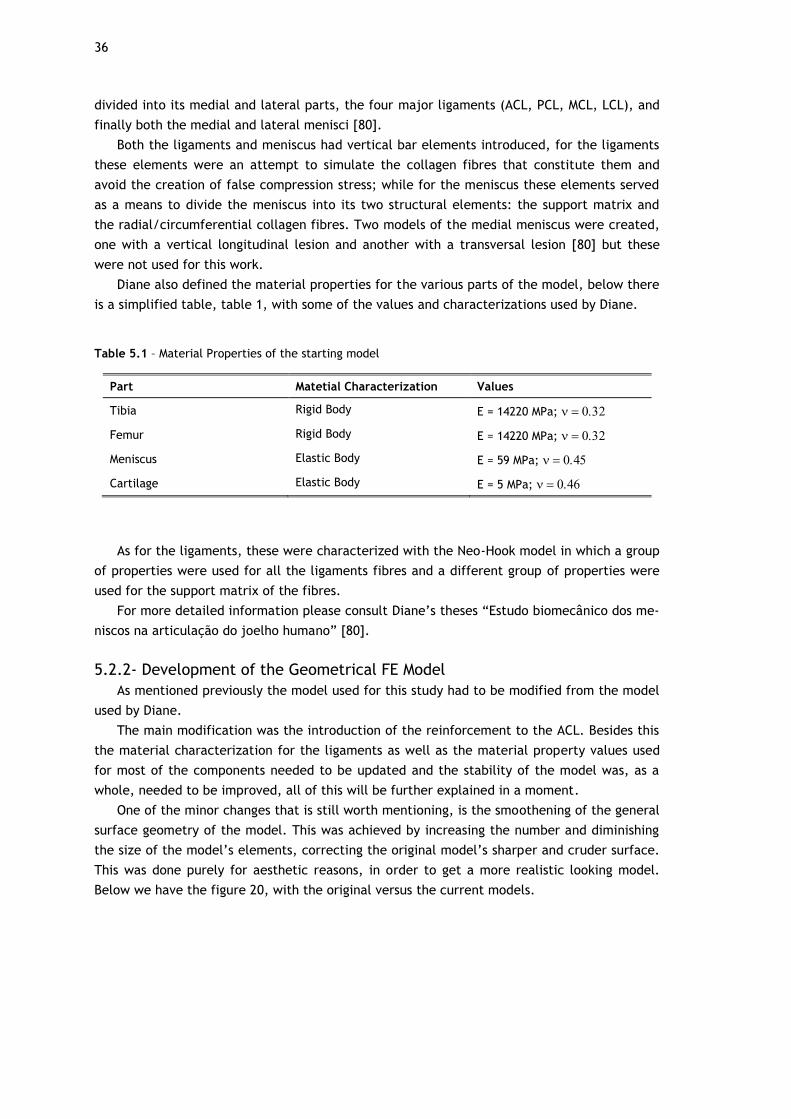
36
divided into its medial and lateral parts, the four major ligaments (ACL, PCL, MCL, LCL), and
finally both the medial and lateral menisci [80].
Both the ligaments and meniscus had vertical bar elements introduced, for the ligaments
these elements were an attempt to simulate the collagen fibres that constitute them and
avoid the creation of false compression stress; while for the meniscus these elements served
as a means to divide the meniscus into its two structural elements: the support matrix and
the radial/circumferential collagen fibres. Two models of the medial meniscus were created,
one with a vertical longitudinal lesion and another with a transversal lesion [80] but these
were not used for this work.
Diane also defined the material properties for the various parts of the model, below there
is a simplified table, table 1, with some of the values and characterizations used by Diane.
Table 5.1 – Material Properties of the starting model
Part Matetial Characterization Values
Tibia Rigid Body E = 14220 MPa; =
Femur Rigid Body E = 14220 MPa; =
Meniscus Elastic Body E = 59 MPa; =
Cartilage Elastic Body E = 5 MPa; =
As for the ligaments, these were characterized with the Neo-Hook model in which a group
of properties were used for all the ligaments fibres and a different group of properties were
used for the support matrix of the fibres.
For more detailed information please consult Diane’s theses “Estudo biomecânico dos me-
niscos na articulação do joelho humano” [80].
5.2.2- Development of the Geometrical FE Model
As mentioned previously the model used for this study had to be modified from the model
used by Diane.
The main modification was the introduction of the reinforcement to the ACL. Besides this
the material characterization for the ligaments as well as the material property values used
for most of the components needed to be updated and the stability of the model was, as a
whole, needed to be improved, all of this will be further explained in a moment.
One of the minor changes that is still worth mentioning, is the smoothening of the general
surface geometry of the model. This was achieved by increasing the number and diminishing
the size of the model’s elements, correcting the original model’s sharper and cruder surface.
This was done purely for aesthetic reasons, in order to get a more realistic looking model.
Below we have the figure 20, with the original versus the current models.

37
Figure 5.2 – [A] Original Model surface geometry; [B] Model surface Geometry post smoothening
5.2.3- Creating the ACL-Reinforcement Component
The ACL from the original model had to be replaced since it was not originally made to
have a reinforcement within it. Therefore, the ACl was removed from the original model and
had to be remade.
The program used for this was SolidWorks, which is a solid modelling computer-aided de-
sign software program.
The process for rebuilding the ligament was as follows, first the whole knee model was
exported from Abaqus and imported to Solidworks as an STL file format, see figure 21 [A],
then the ACL was isolated, see figure 21 [B].
Figure 5.3 – [A] Entire Knee Model in SolidWorks; [B] Isolated ACL in SolidWorks
A B
A B
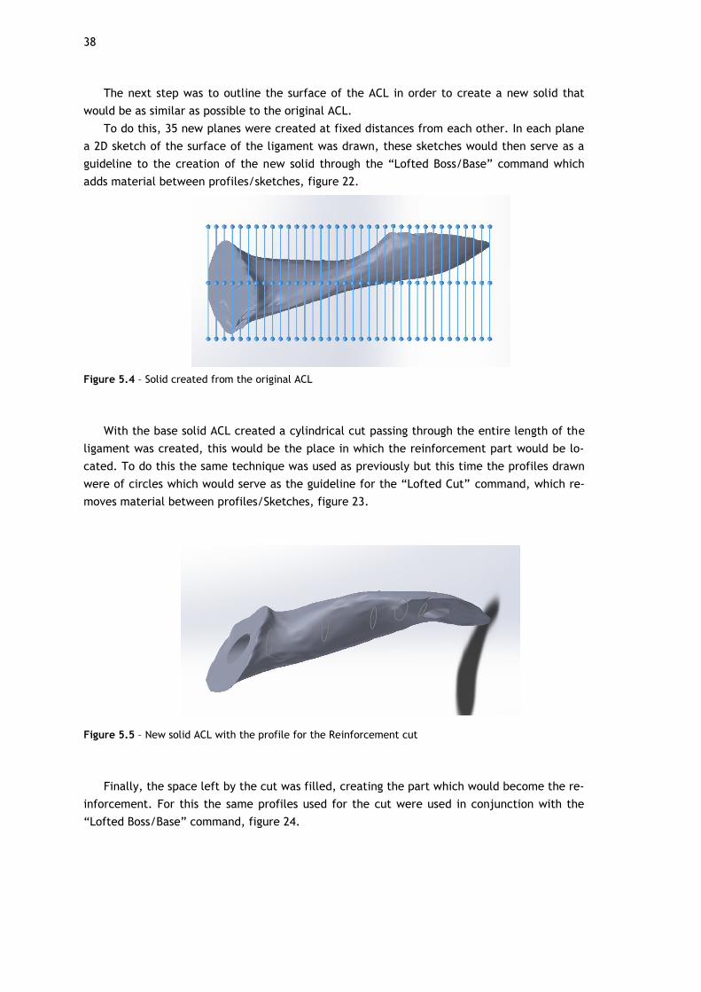
38
The next step was to outline the surface of the ACL in order to create a new solid that
would be as similar as possible to the original ACL.
To do this, 35 new planes were created at fixed distances from each other. In each plane
a 2D sketch of the surface of the ligament was drawn, these sketches would then serve as a
guideline to the creation of the new solid through the “Lofted Boss/Base” command which
adds material between profiles/sketches, figure 22.
Figure 5.4 – Solid created from the original ACL
With the base solid ACL created a cylindrical cut passing through the entire length of the
ligament was created, this would be the place in which the reinforcement part would be lo-
cated. To do this the same technique was used as previously but this time the profiles drawn
were of circles which would serve as the guideline for the “Lofted Cut” command, which re-
moves material between profiles/Sketches, figure 23.
Figure 5.5 – New solid ACL with the profile for the Reinforcement cut
Finally, the space left by the cut was filled, creating the part which would become the re-
inforcement. For this the same profiles used for the cut were used in conjunction with the
“Lofted Boss/Base” command, figure 24.
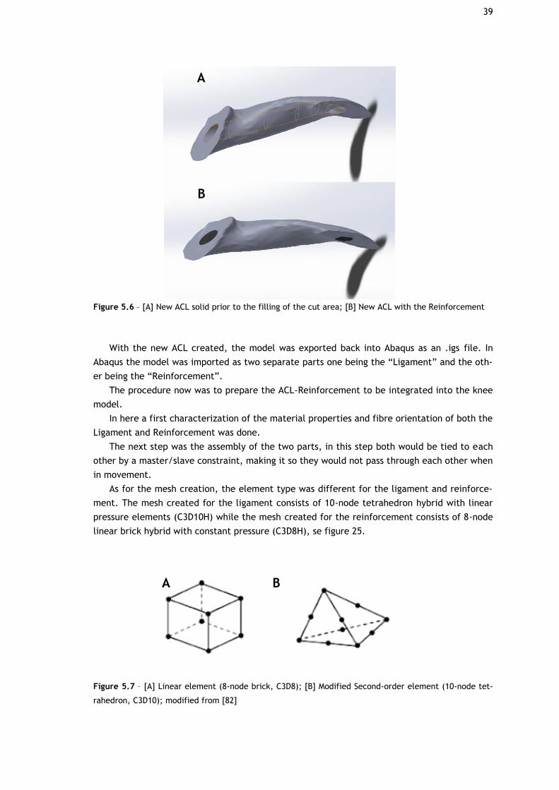
39
Figure 5.6 – [A] New ACL solid prior to the filling of the cut area; [B] New ACL with the Reinforcement
With the new ACL created, the model was exported back into Abaqus as an .igs file. In
Abaqus the model was imported as two separate parts one being the “Ligament” and the oth-
er being the “Reinforcement”.
The procedure now was to prepare the ACL-Reinforcement to be integrated into the knee
model.
In here a first characterization of the material properties and fibre orientation of both the
Ligament and Reinforcement was done.
The next step was the assembly of the two parts, in this step both would be tied to each
other by a master/slave constraint, making it so they would not pass through each other when
in movement.
As for the mesh creation, the element type was different for the ligament and reinforce-
ment. The mesh created for the ligament consists of 10-node tetrahedron hybrid with linear
pressure elements (C3D10H) while the mesh created for the reinforcement consists of 8-node
linear brick hybrid with constant pressure (C3D8H), se figure 25.
Figure 5.7 – [A] Linear element (8-node brick, C3D8); [B] Modified Second-order element (10-node tet-
rahedron, C3D10); modified from [82]
A
B
A B
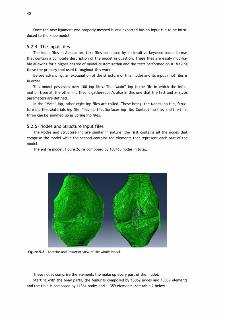
40
Once the new ligament was properly meshed it was exported has an input file to be intro-
duced to the knee model.
5.2.4- The input files
The input files in Abaqus are text files composed by an intuitive keyword-based format
that contain a complete description of the model in question. These files are easily modifia-
ble allowing for a higher degree of model customization and the tests performed on it. Making
these the primary tool used throughout this work.
Before advancing, an explanation of the structure of this model and its input (inp) files is
in order.
This model possesses over 100 inp files. The “Main” inp is the file in which the infor-
mation from all the other inp files is gathered, it’s also in this one that the test and analysis
parameters are defined.
In the “Main” inp, other eight inp files are called. These being: the Nodes inp file, Struc-
ture inp file, Materials inp file, Ties inp file, Surfaces inp file, Contact inp file, and the final
three can be summed up as Spring inp files.
5.2.5- Nodes and Structure input files
The Nodes and Structure inp are similar in nature, the first contains all the nodes that
comprise the model while the second contains the elements that represent each part of the
model.
The entire model, figure 26, is composed by 103465 nodes in total.
Figure 5.8 – Anterior and Posterior view of the whole model
These nodes comprise the elements the make up every part of the model.
Starting with the bony parts, the femur is composed by 13862 nodes and 13859 elements
and the tibia is composed by 11361 nodes and 11359 elements, see table 2 below
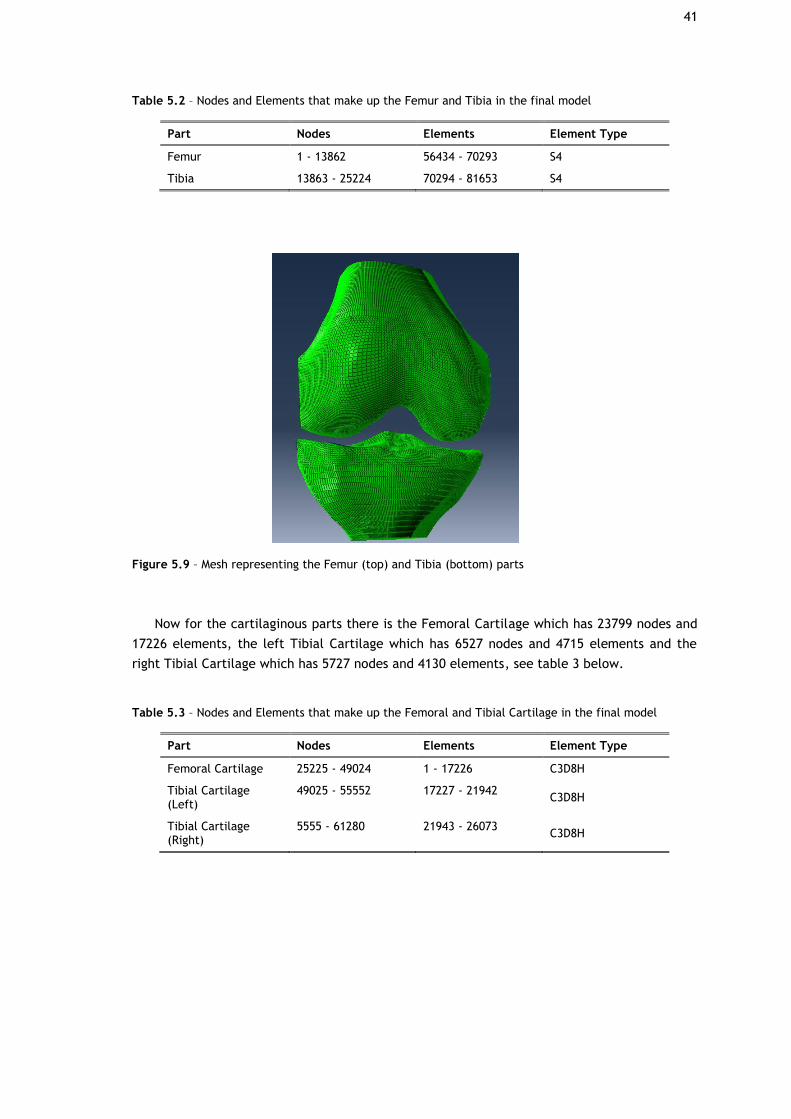
41
Table 5.2 – Nodes and Elements that make up the Femur and Tibia in the final model
Part Nodes Elements Element Type
Femur 1 - 13862 56434 - 70293 S4
Tibia 13863 - 25224 70294 - 81653 S4
Figure 5.9 – Mesh representing the Femur (top) and Tibia (bottom) parts
Now for the cartilaginous parts there is the Femoral Cartilage which has 23799 nodes and
17226 elements, the left Tibial Cartilage which has 6527 nodes and 4715 elements and the
right Tibial Cartilage which has 5727 nodes and 4130 elements, see table 3 below.
Table 5.3 – Nodes and Elements that make up the Femoral and Tibial Cartilage in the final model
Part Nodes Elements Element Type
Femoral Cartilage 25225 - 49024 1 - 17226 C3D8H
Tibial Cartilage (Left)
49025 - 55552 17227 - 21942 C3D8H
Tibial Cartilage (Right)
5555 - 61280 21943 - 26073 C3D8H

42
Figure 5.10 – Mesh representing the Femoral (top) and Tibial (bottom) Cartilage
As for the meniscus, the Medial Meniscus is composed by 5894 nodes and 4549 elements
and the Lateral Meniscus is composed by 5895 nodes and 4549 elements, see table 4 below.
Table 5.4 – Nodes and Elements that make up the Medial and Lateral Menisci in the final model
Part Nodes Elements Element Type
Medial Meniscus 80383 - 86277 42470 - 47019 C3D8H
Lateral Meniscus 74487 - 82382 37850 - 42399 C3D8H
Figure 5.11 – Mesh representing the Medial (right) and Lateral (left) Menisci
Finally, for the four major knee ligaments and reinforcement, the LCL is composed by
7424 nodes and 6655 elements, the MCL is composed by 5780 nodes and 5119 elements, the
PCL is composed by 5921 nodes and 5247 elements, the ACL is composed by 5981 nodes and
3221 and the Reinforcement is composed by 629 nodes and 439 elements. See table 5 below:
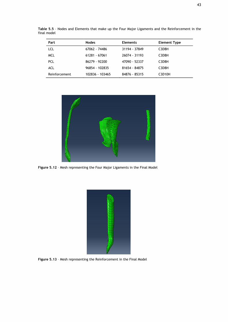
43
Table 5.5 – Nodes and Elements that make up the Four Major Ligaments and the Reinforcement in the final model
Part Nodes Elements Element Type
LCL 67062 - 74486 31194 - 37849 C3D8H
MCL 61281 - 67061 26074 - 31193 C3D8H
PCL 86279 - 92200 47090 - 52337 C3D8H
ACL 96854 - 102835 81654 - 84875 C3D8H
Reinforcement 102836 - 103465 84876 - 85315 C3D10H
Figure 5.12 – Mesh representing the Four Major Ligaments in the Final Model
Figure 5.13 – Mesh representing the Reinforcement in the Final Model
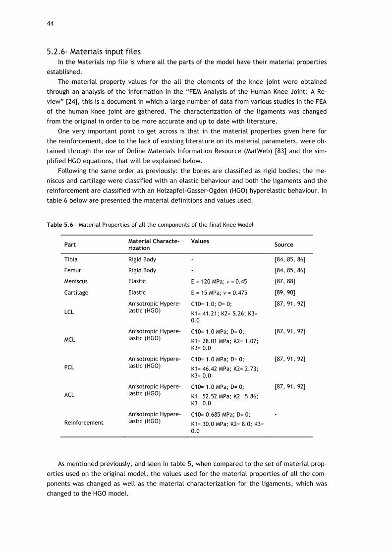
44
5.2.6- Materials input files
In the Materials inp file is where all the parts of the model have their material properties
established.
The material property values for the all the elements of the knee joint were obtained
through an analysis of the information in the “FEM Analysis of the Human Knee Joint: A Re-
view” [24], this is a document in which a large number of data from various studies in the FEA
of the human knee joint are gathered. The characterization of the ligaments was changed
from the original in order to be more accurate and up to date with literature.
One very important point to get across is that in the material properties given here for
the reinforcement, doe to the lack of existing literature on its material parameters, were ob-
tained through the use of Online Materials Information Resource (MatWeb) [83] and the sim-
plified HGO equations, that will be explained below.
Following the same order as previously: the bones are classified as rigid bodies; the me-
niscus and cartilage were classified with an elastic behaviour and both the ligaments and the
reinforcement are classified with an Holzapfel-Gasser-Ogden (HGO) hyperelastic behaviour. In
table 6 below are presented the material definitions and values used.
Table 5.6 – Material Properties of all the components of the final Knee Model
Part Material Characte-rization
Values Source
Tibia Rigid Body - [84, 85, 86]
Femur Rigid Body - [84, 85, 86]
Meniscus Elastic E = 120 MPa; = 0.45 [87, 88]
Cartilage Elastic E = 15 MPa; = 0.475 [89, 90]
LCL
Anisotropic Hypere-lastic (HGO)
C10= 1.0; D= 0;
K1= 41.21; K2= 5.26; K3= 0.0
[87, 91, 92]
MCL
Anisotropic Hypere-lastic (HGO)
C10= 1.0 MPa; D= 0;
K1= 28.01 MPa; K2= 1.07; K3= 0.0
[87, 91, 92]
PCL
Anisotropic Hypere-lastic (HGO)
C10= 1.0 MPa; D= 0;
K1= 46.42 MPa; K2= 2.73; K3= 0.0
[87, 91, 92]
ACL
Anisotropic Hypere-lastic (HGO)
C10= 1.0 MPa; D= 0;
K1= 52.52 MPa; K2= 5.86; K3= 0.0
[87, 91, 92]
Reinforcement
Anisotropic Hypere-lastic (HGO)
C10= 0.685 MPa; D= 0;
K1= 30.0 MPa; K2= 8.0; K3= 0.0
-
As mentioned previously, and seen in table 5, when compared to the set of material prop-
erties used on the original model, the values used for the material properties of all the com-
ponents was changed as well as the material characterization for the ligaments, which was
changed to the HGO model.

45
The HGO constitutive model was first developed by Gasser et al. [93] with the objective
of creating a reliable model that was capable of accurately describing the nonlinear elastic
behaviour of arterial tissue. With their continuous work Gasser et al. achieved a model espe-
cially suited to describe the anisotropic hyperelastic behaviour of collagen fibre reinforced
tissue by adding a scalar parameter that accounts for the dispersion of collagen fibres [94,95].
Even though this model was developed for arterial tissue, it has already been applied to
represent different soft tissue like knee ligaments [14,96] successfully and with better results
than previous methodologies, making it a perfect fit for this work.
In order to better understand the HGO model some concepts will be now presented, for
more detailed and technical information the reader is referred to the original article [93] and
to the Abaqus theory Manual [97].
Before diving into the HGO specific concepts some more general concepts are presented
first. Consider equation 19 below, which represents deformation gradient.
. (19)
The deformation gradient (F), describes the local kinematics of deformation in which X is
the position of a material point in the reference conFiguretion and x represents the material
point in the deformed conFiguretion.
The Jacobian (J) basically refers to the ratio of the reference volume over the deformed
value, only for a homogeneous deformation on a material.
, (20)
where represents the reference density and represents the deformed density.
The Cauchy-Green deformation tensors (C and B) form the basis for constitutive hypere-
lastic model development applied to soft tissues, it provides information on the deformation
measures independent of rigid body rotations.
. (21)
The Strain Energy Density Function is a function that defines the deformation at a given
point as:
Ψ = Ψ (F) . (22)
If the material is isotropic, equation 22 become:
Ψ = Ψ (𝐼1, 𝐼2, 𝐼3) , (23)
in which,
; ; . (24)
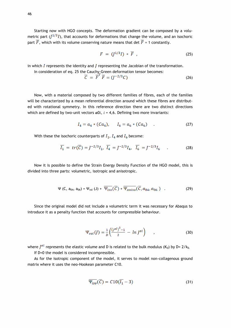
46
Starting now with HGO concepts. The deformation gradient can be composed by a volu-
metric part ( ), that accounts for deformations that change the volume, and an isochoric
part , which with its volume conserving nature means that det = 1 constantly.
, (25)
in which represents the identity and representing the Jacobian of the transformation.
In consideration of eq. 25 the Cauchy-Green deformation tensor becomes:
(26)
Now, with a material composed by two different families of fibres, each of the families
will be characterized by a mean referential direction around which these fibres are distribut-
ed with rotational symmetry. In this reference direction there are two distinct directions
which are defined by two-unit vectors 𝒂0𝑖, 𝑖 = 4,6. Defining two more invariants:
. (27)
With these the isochoric counterparts of , and become:
. (28)
Now it is possible to define the Strain Energy Density Function of the HGO model, this is
divided into three parts: volumetric, isotropic and anisotropic.
Ψ (C, a04, a06) = Ψvol (J) + + . (29)
Since the original model did not include a volumetric term it was necessary for Abaqus to
introduce it as a penalty function that accounts for compressible behaviour.
, (30)
where represents the elastic volume and D is related to the bulk modulus (K0) by D= 2/k0.
If D=0 the model is considered incompressible.
As for the isotropic component of the model, it serves to model non-collagenous ground
matrix where it uses the neo-Hookean parameter C10.
(31)
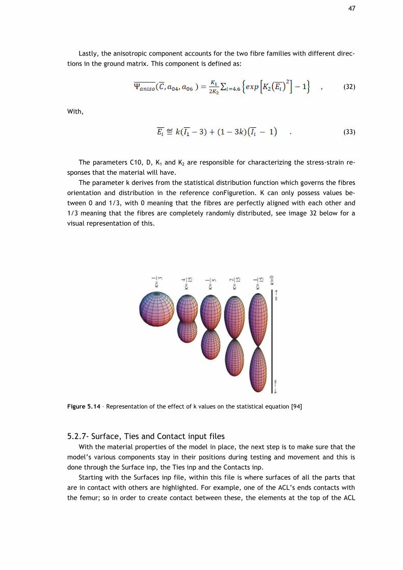
47
Lastly, the anisotropic component accounts for the two fibre families with different direc-
tions in the ground matrix. This component is defined as:
, (32)
With,
. (33)
The parameters C10, D, K1 and K2 are responsible for characterizing the stress-strain re-
sponses that the material will have.
The parameter k derives from the statistical distribution function which governs the fibres
orientation and distribution in the reference conFiguretion. K can only possess values be-
tween 0 and 1/3, with 0 meaning that the fibres are perfectly aligned with each other and
1/3 meaning that the fibres are completely randomly distributed, see image 32 below for a
visual representation of this.
Figure 5.14 – Representation of the effect of k values on the statistical equation [94]
5.2.7- Surface, Ties and Contact input files
With the material properties of the model in place, the next step is to make sure that the
model’s various components stay in their positions during testing and movement and this is
done through the Surface inp, the Ties inp and the Contacts inp.
Starting with the Surfaces inp file, within this file is where surfaces of all the parts that
are in contact with others are highlighted. For example, one of the ACL’s ends contacts with
the femur; so in order to create contact between these, the elements at the top of the ACL
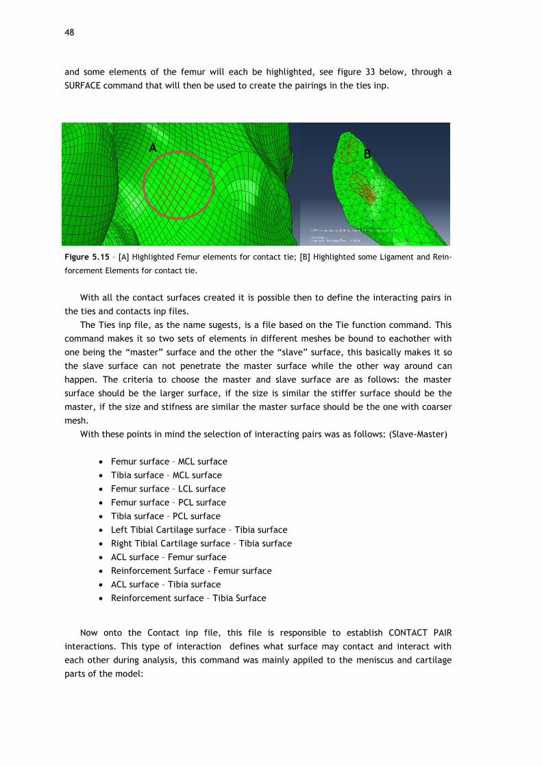
48
and some elements of the femur will each be highlighted, see figure 33 below, through a
SURFACE command that will then be used to create the pairings in the ties inp.
Figure 5.15 – [A] Highlighted Femur elements for contact tie; [B] Highlighted some Ligament and Rein-
forcement Elements for contact tie.
With all the contact surfaces created it is possible then to define the interacting pairs in
the ties and contacts inp files.
The Ties inp file, as the name sugests, is a file based on the Tie function command. This
command makes it so two sets of elements in different meshes be bound to eachother with
one being the “master” surface and the other the “slave” surface, this basically makes it so
the slave surface can not penetrate the master surface while the other way around can
happen. The criteria to choose the master and slave surface are as follows: the master
surface should be the larger surface, if the size is similar the stiffer surface should be the
master, if the size and stifness are similar the master surface should be the one with coarser
mesh.
With these points in mind the selection of interacting pairs was as follows: (Slave-Master)
• Femur surface – MCL surface
• Tibia surface – MCL surface
• Femur surface – LCL surface
• Femur surface – PCL surface
• Tibia surface – PCL surface
• Left Tibial Cartilage surface – Tibia surface
• Right Tibial Cartilage surface – Tibia surface
• ACL surface – Femur surface
• Reinforcement Surface - Femur surface
• ACL surface – Tibia surface
• Reinforcement surface – Tibia Surface
Now onto the Contact inp file, this file is responsible to establish CONTACT PAIR
interactions. This type of interaction defines what surface may contact and interact with
each other during analysis, this command was mainly appiled to the meniscus and cartilage
parts of the model:
A B
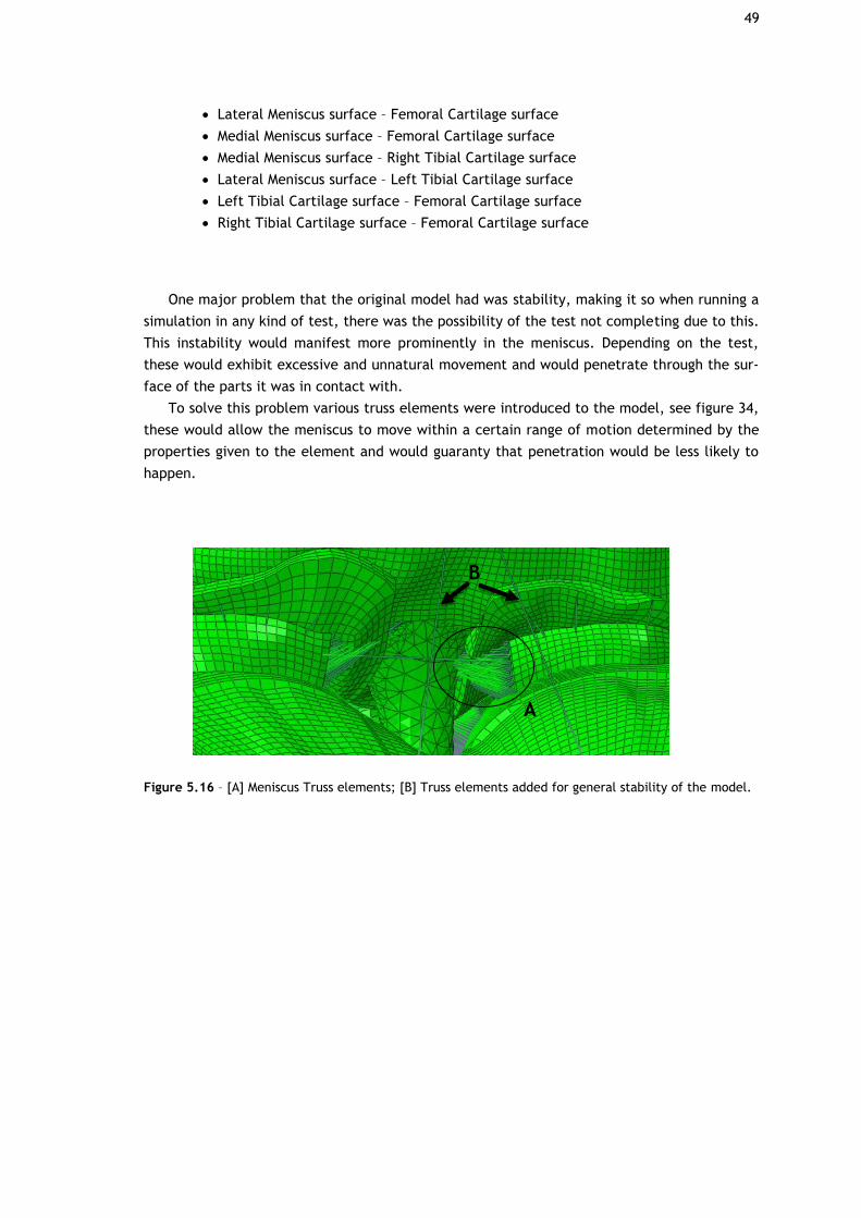
49
• Lateral Meniscus surface – Femoral Cartilage surface
• Medial Meniscus surface – Femoral Cartilage surface
• Medial Meniscus surface – Right Tibial Cartilage surface
• Lateral Meniscus surface – Left Tibial Cartilage surface
• Left Tibial Cartilage surface – Femoral Cartilage surface
• Right Tibial Cartilage surface – Femoral Cartilage surface
One major problem that the original model had was stability, making it so when running a
simulation in any kind of test, there was the possibility of the test not completing due to this.
This instability would manifest more prominently in the meniscus. Depending on the test,
these would exhibit excessive and unnatural movement and would penetrate through the sur-
face of the parts it was in contact with.
To solve this problem various truss elements were introduced to the model, see figure 34,
these would allow the meniscus to move within a certain range of motion determined by the
properties given to the element and would guaranty that penetration would be less likely to
happen.
Figure 5.16 – [A] Meniscus Truss elements; [B] Truss elements added for general stability of the model.
A
B

50

51
Chapter 6
Results and Discussion
To simulate the movement of the knee with the objective of verifying the efficacy of the
reinforcement, the tests were performed based on a case that has been tested experimental-
ly [23] and through FE studies [21,23,37] in literature.
This case entails the application of a force of 134N, anteriorly, on the Tibia at certain
flexion angles. It was designed to simulate the Lachman anterior drawer test, which is used to
diagnose the ACL deficiency.
During this work the force was applied in the Femur and the Tibia was fixed in all degrees
of freedom, see figure 35, while normally this is done the other way around this does not
make a considerable difference since the posterior displacement of the femur with the Tibia
fixed would be equal to that of the anterior displacement of the Tibia with the Femur fixed.
In order to be able to test efficacy of the reinforcement, in a first step the rotation of the
Femur was applied, this rotation was bound to node 2749 at the top of the femur. In a second
step the force of 134N, directed posteriorly, was placed on the same point. This guaranteed
that the force applied would always be on the anterior-posterior axis, simulating the normal
displacement of this structure during movement.
The force was applied at the angles of rotation 0, 15 and 30 degrees of flexion, the data
obtained was about the kinematic behaviour of the model with focus on the ACL-
reinforcement component. The values for maximum principal stress for the hole model and
for the ACL-Reinforcement components are obtained and compared with existing values in the
literature; for the second and third case additional data on the contact pressure values are
obtained for the menisci and cartilaginous components.
The data used for comparison are: the study performed by David Fernandes on his theses
“Finite Element Analysis of the ACL-deficient Knee” in which he used a similar FE approach to
simulate an healthy and deficient knee model [89], the studies performed by Pena et al
[21,37] and Song et al [23].
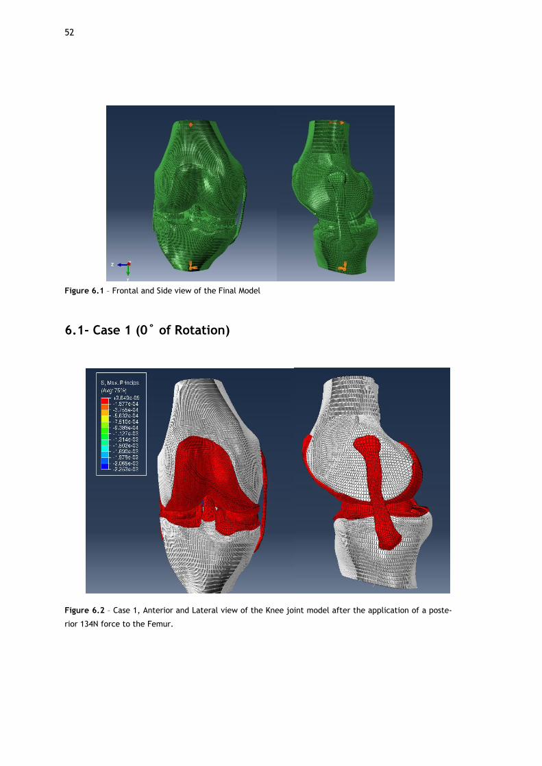
52
Figure 6.1 – Frontal and Side view of the Final Model
6.1- Case 1 (0˚ of Rotation)
Figure 6.2 – Case 1, Anterior and Lateral view of the Knee joint model after the application of a poste-
rior 134N force to the Femur.
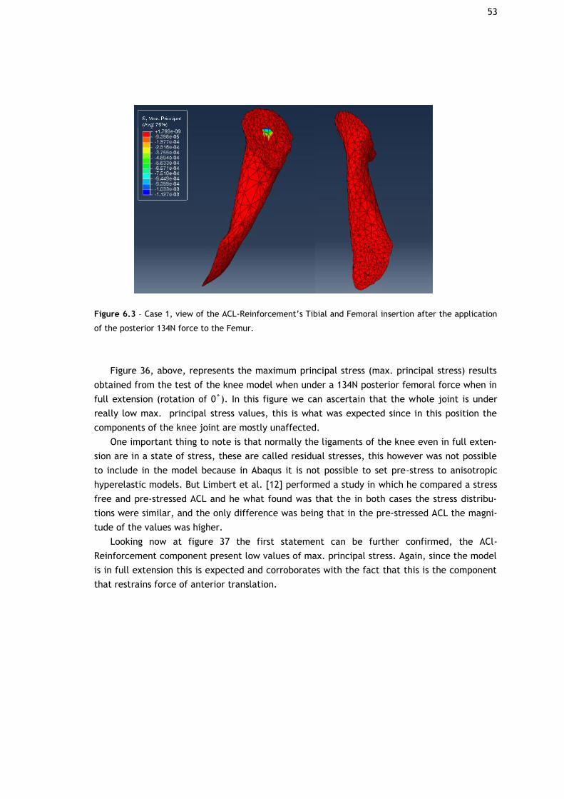
53
Figure 6.3 – Case 1, view of the ACL-Reinforcement’s Tibial and Femoral insertion after the application
of the posterior 134N force to the Femur.
Figure 36, above, represents the maximum principal stress (max. principal stress) results
obtained from the test of the knee model when under a 134N posterior femoral force when in
full extension (rotation of 0˚). In this figure we can ascertain that the whole joint is under
really low max. principal stress values, this is what was expected since in this position the
components of the knee joint are mostly unaffected.
One important thing to note is that normally the ligaments of the knee even in full exten-
sion are in a state of stress, these are called residual stresses, this however was not possible
to include in the model because in Abaqus it is not possible to set pre-stress to anisotropic
hyperelastic models. But Limbert et al. [12] performed a study in which he compared a stress
free and pre-stressed ACL and he what found was that the in both cases the stress distribu-
tions were similar, and the only difference was being that in the pre-stressed ACL the magni-
tude of the values was higher.
Looking now at figure 37 the first statement can be further confirmed, the ACl-
Reinforcement component present low values of max. principal stress. Again, since the model
is in full extension this is expected and corroborates with the fact that this is the component
that restrains force of anterior translation.
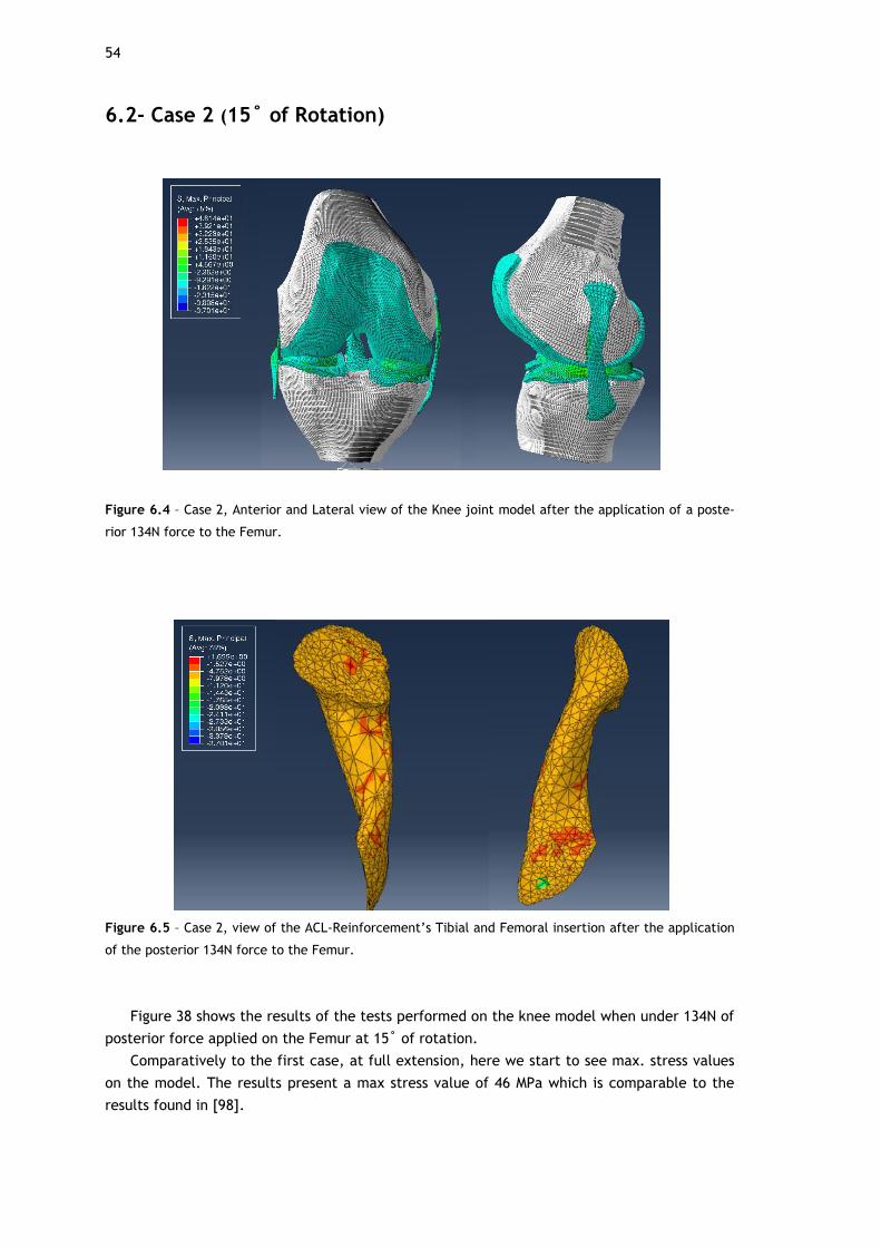
54
6.2- Case 2 (15˚ of Rotation)
Figure 6.4 – Case 2, Anterior and Lateral view of the Knee joint model after the application of a poste-
rior 134N force to the Femur.
Figure 6.5 – Case 2, view of the ACL-Reinforcement’s Tibial and Femoral insertion after the application
of the posterior 134N force to the Femur.
Figure 38 shows the results of the tests performed on the knee model when under 134N of
posterior force applied on the Femur at 15˚ of rotation.
Comparatively to the first case, at full extension, here we start to see max. stress values
on the model. The results present a max stress value of 46 MPa which is comparable to the
results found in [98].
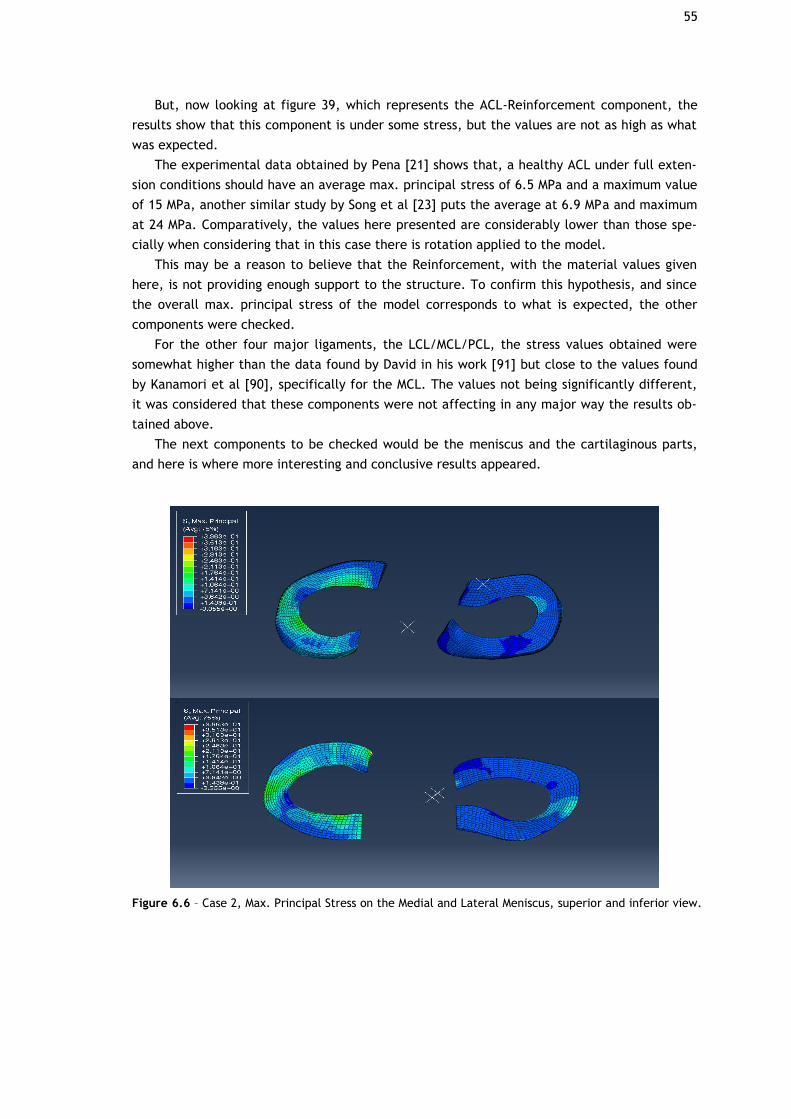
55
But, now looking at figure 39, which represents the ACL-Reinforcement component, the
results show that this component is under some stress, but the values are not as high as what
was expected.
The experimental data obtained by Pena [21] shows that, a healthy ACL under full exten-
sion conditions should have an average max. principal stress of 6.5 MPa and a maximum value
of 15 MPa, another similar study by Song et al [23] puts the average at 6.9 MPa and maximum
at 24 MPa. Comparatively, the values here presented are considerably lower than those spe-
cially when considering that in this case there is rotation applied to the model.
This may be a reason to believe that the Reinforcement, with the material values given
here, is not providing enough support to the structure. To confirm this hypothesis, and since
the overall max. principal stress of the model corresponds to what is expected, the other
components were checked.
For the other four major ligaments, the LCL/MCL/PCL, the stress values obtained were
somewhat higher than the data found by David in his work [91] but close to the values found
by Kanamori et al [90], specifically for the MCL. The values not being significantly different,
it was considered that these components were not affecting in any major way the results ob-
tained above.
The next components to be checked would be the meniscus and the cartilaginous parts,
and here is where more interesting and conclusive results appeared.
Figure 6.6 – Case 2, Max. Principal Stress on the Medial and Lateral Meniscus, superior and inferior view.
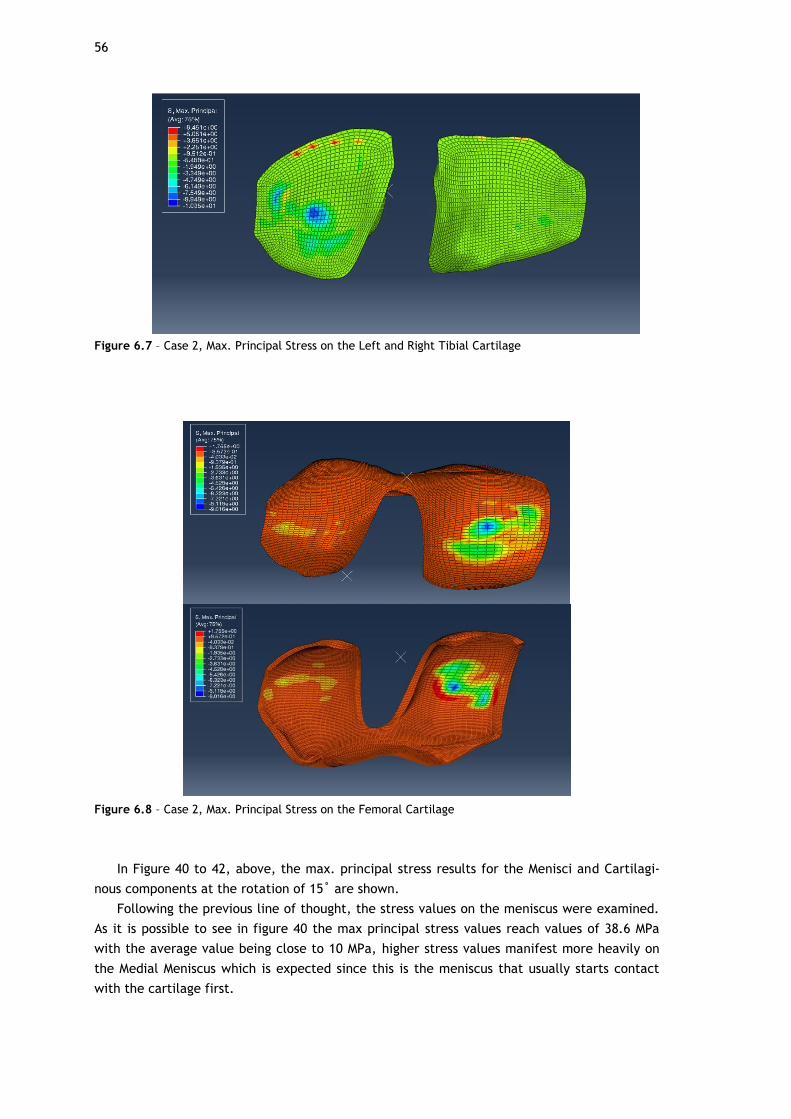
56
Figure 6.7 – Case 2, Max. Principal Stress on the Left and Right Tibial Cartilage
Figure 6.8 – Case 2, Max. Principal Stress on the Femoral Cartilage
In Figure 40 to 42, above, the max. principal stress results for the Menisci and Cartilagi-
nous components at the rotation of 15˚ are shown.
Following the previous line of thought, the stress values on the meniscus were examined.
As it is possible to see in figure 40 the max principal stress values reach values of 38.6 MPa
with the average value being close to 10 MPa, higher stress values manifest more heavily on
the Medial Meniscus which is expected since this is the meniscus that usually starts contact
with the cartilage first.
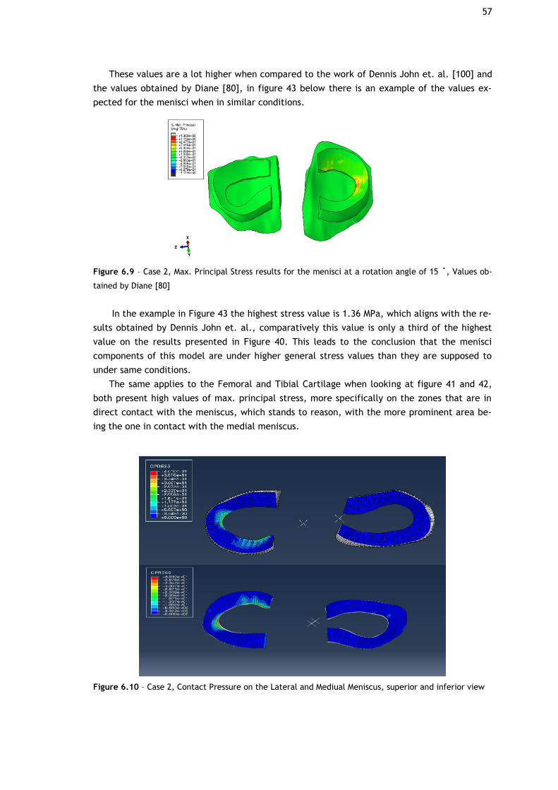
57
These values are a lot higher when compared to the work of Dennis John et. al. [100] and
the values obtained by Diane [80], in figure 43 below there is an example of the values ex-
pected for the menisci when in similar conditions.
Figure 6.9 – Case 2, Max. Principal Stress results for the menisci at a rotation angle of 15 ˚, Values ob-
tained by Diane [80]
In the example in Figure 43 the highest stress value is 1.36 MPa, which aligns with the re-
sults obtained by Dennis John et. al., comparatively this value is only a third of the highest
value on the results presented in Figure 40. This leads to the conclusion that the menisci
components of this model are under higher general stress values than they are supposed to
under same conditions.
The same applies to the Femoral and Tibial Cartilage when looking at figure 41 and 42,
both present high values of max. principal stress, more specifically on the zones that are in
direct contact with the meniscus, which stands to reason, with the more prominent area be-
ing the one in contact with the medial meniscus.
Figure 6.10 – Case 2, Contact Pressure on the Lateral and Mediual Meniscus, superior and inferior view
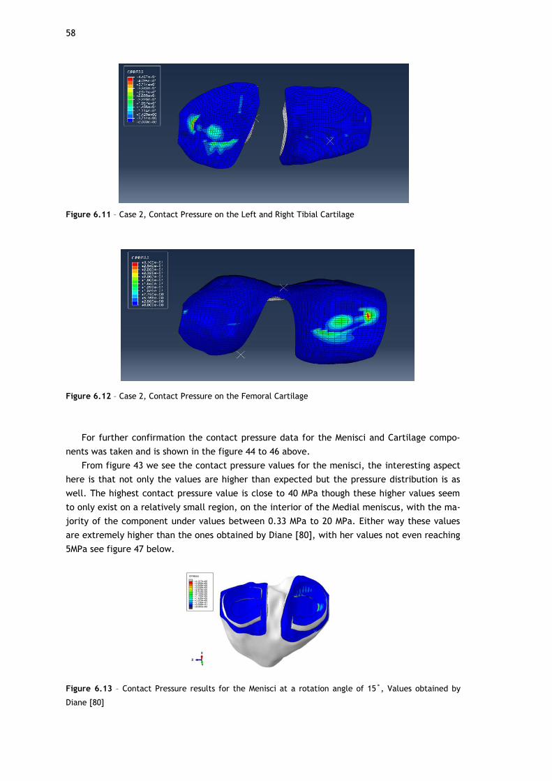
58
Figure 6.11 – Case 2, Contact Pressure on the Left and Right Tibial Cartilage
Figure 6.12 – Case 2, Contact Pressure on the Femoral Cartilage
For further confirmation the contact pressure data for the Menisci and Cartilage compo-
nents was taken and is shown in the figure 44 to 46 above.
From figure 43 we see the contact pressure values for the menisci, the interesting aspect
here is that not only the values are higher than expected but the pressure distribution is as
well. The highest contact pressure value is close to 40 MPa though these higher values seem
to only exist on a relatively small region, on the interior of the Medial meniscus, with the ma-
jority of the component under values between 0.33 MPa to 20 MPa. Either way these values
are extremely higher than the ones obtained by Diane [80], with her values not even reaching
5MPa see figure 47 below.
Figure 6.13 – Contact Pressure results for the Menisci at a rotation angle of 15˚, Values obtained by
Diane [80]
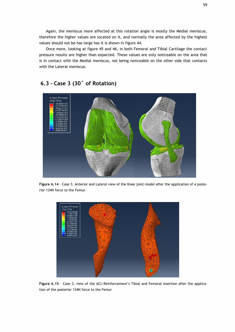
59
Again, the meniscus more affected at this rotation angle is mostly the Medial meniscus,
therefore the higher values are located on it, and normally the area affected by the highest
values should not be has large has it is shown in figure 44.
Once more, looking at figure 45 and 46, in both Femoral and Tibial Cartilage the contact
pressure results are higher than expected. These values are only noticeable on the area that
is in contact with the Medial meniscus, not being noticeable on the other side that contacts
with the Lateral meniscus.
6.3 - Case 3 (30˚ of Rotation)
Figure 6.14 – Case 3, Anterior and Lateral view of the Knee joint model after the application of a poste-
rior 134N force to the Femur.
Figure 6.15 – Case 3, view of the ACL-Reinforcement’s Tibial and Femoral insertion after the applica-
tion of the posterior 134N force to the Femur

60
Figure 48 shows the results of the tests performed on the knee model when under 134N of
posterior force applied on the Femur at 30˚ of rotation.
In this figure it is possible to see higher max. principal stress values than in the previous
case, with 15˚ of rotation, this supports the fact that at higher degrees of flexion the func-
tion of the total structure becomes more demanding and the work load increases in order to
prevent excessive anterior-posterior movement. Once again, the values shown in figure 46 are
within what was expected with a maximum value of around 94 MPa, which is somewhat higher
than the 84MPa obtained by David [98] but the general value distribution is still within reason.
Figure 49 looks more specifically at the ACL-Reinforcements component and here the sit-
uation from the previous case repeats, the values are higher than in 15˚ of rotation but are
still not near the expected values. At this rotation angle with similar conditions the average
max. principal stress value obtained by David is 11.7MPa which is considerably higher than the
highest value of 3.3MPa obtained in Figure 49.
Once again, the other components were checked, and again the values on the other major
ligaments did not suffer any major change from 15˚ to 30˚.
Figure 6.16 – Case 3, Max. Principal Stress on the Medial and Lateral Meniscus, superior and inferior
view.
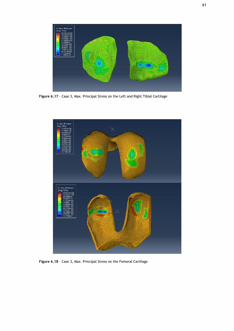
61
Figure 6.17 – Case 3, Max. Principal Stress on the Left and Right Tibial Cartilage
Figure 6.18 – Case 3, Max. Principal Stress on the Femoral Cartilage
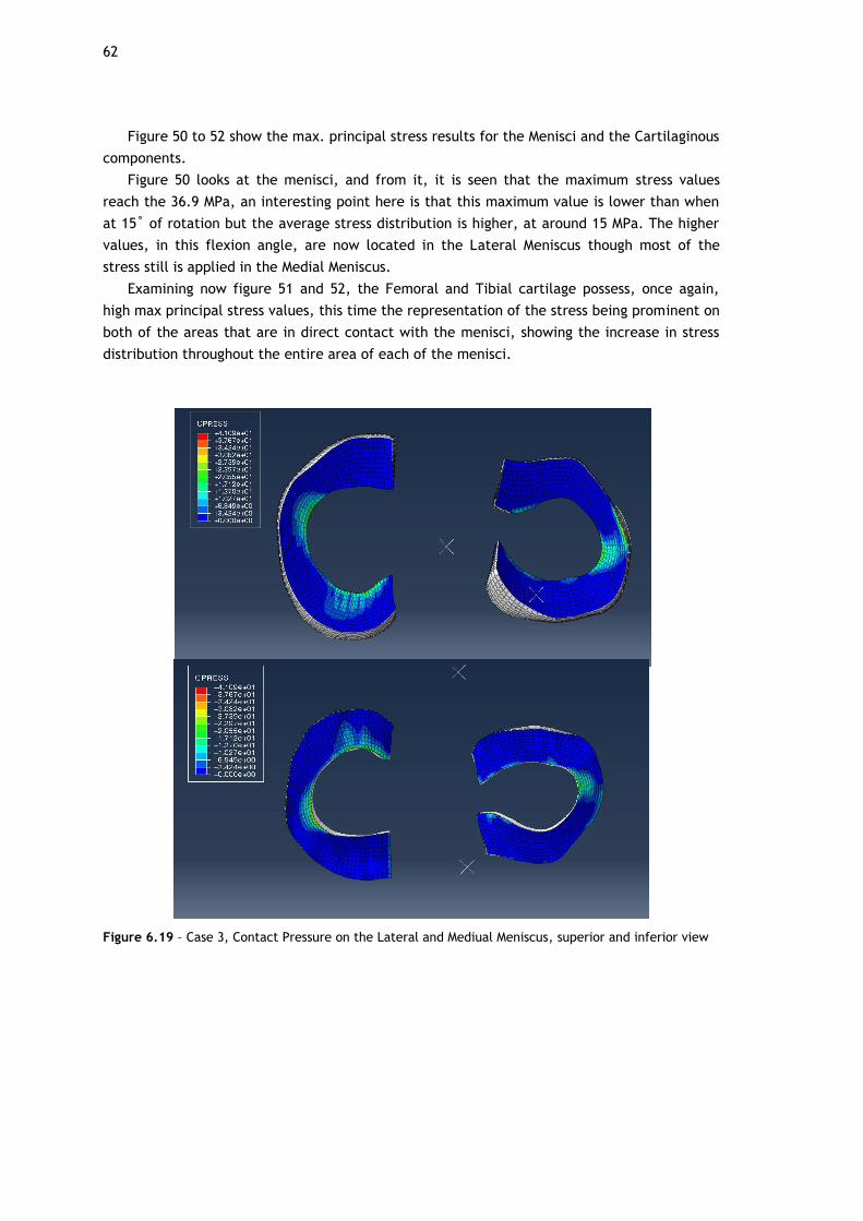
62
Figure 50 to 52 show the max. principal stress results for the Menisci and the Cartilaginous
components.
Figure 50 looks at the menisci, and from it, it is seen that the maximum stress values
reach the 36.9 MPa, an interesting point here is that this maximum value is lower than when
at 15˚ of rotation but the average stress distribution is higher, at around 15 MPa. The higher
values, in this flexion angle, are now located in the Lateral Meniscus though most of the
stress still is applied in the Medial Meniscus.
Examining now figure 51 and 52, the Femoral and Tibial cartilage possess, once again,
high max principal stress values, this time the representation of the stress being prominent on
both of the areas that are in direct contact with the menisci, showing the increase in stress
distribution throughout the entire area of each of the menisci.
Figure 6.19 – Case 3, Contact Pressure on the Lateral and Mediual Meniscus, superior and inferior view

63
Figure 6.20 – Case 3, Contact Pressure on the Left and Right Tibial Cartilage
Figure 6.21 – Case 3, Contact Pressure on the Femoral Cartilage
Figure 53 to 55 show the results for the contact pressure on the menisci and the cartilagi-
nous component of the model.
Generally, the same conclusions can be taken as in the previous case, the values for con-
tact pressure presented are higher than what is normal for these components under the same
conditions. One difference is that, with both meniscus under higher average stress values the
average contact pressure will also increase, this is visually evidenced by the increase in the
areas with higher contact pressure values in both figure 54 and 55. One interesting aspect is
that the values for contact pressure themselves have not significantly changed from 15˚ to
30˚ of rotation the only aspect that has changes is the distribution of these values with the
case of 30˚ of rotation showing more areas with higher values than the case of 15˚ of rotation.

64
As for the Tibial and Femoral Cartilage, in figure 54 and 55, the notable difference from
the previous case is, as mentioned above, that areas that are affected with high contact pres-
sure on both sides are more pronounced almost giving the outline of the menisci shape.
65
Chapter 7
Conclusion and Future work
In this work the efficacy of synthetic reinforcement grafts in keeping the biomechanical
integrity of the knee joint was studied by applying a posterior femoral force on a Finite Ele-
ment model of the knee joint.
7.1 - Conclusion
In order to achieve the main objective of this study, many hurdles had to be overcome.
The main issue encountered was the lack of literature on this theme. Unfortunately, there
aren’t many papers written on the use of Finite Element computerized simulation to study
the biomechanical characteristics and performance of synthetic reinforcement grafts in the
human knee joint. This considerably limited the initial data and information that was possible
to access as well as comparable data.
This issue leaded to another, which was obtaining the material mechanical properties for
the various components of the model.
As mentioned previously the knee joint is an incredibly complex structure and if a model
is to be created that simulates this structure accurate values and methodologies to character-
ize each of its components is needed.
Fortunately, the book “FEM Analysis of the Human Knee Joint: A Review” [24] was incred-
ibly useful in gathering data on most of the model’s components, but even with this, various
tests had to be performed in order to determine which results were the more realistic.
As for the reinforcement, since the type of tests that were executed here have not been
done previously, finding the HGO variables to use on this model proved to be quite the chal-
lenge.
Like mentioned previously, obtaining these values was only possible through the Online
Materials Information Resource (MatWeb) [83], in which there was an overview of the materi-
al properties of PET polyester, and the use of the simplified HGO equations.
Because of what is stated above it is important to note that since these values were taken
from a general PET polyester material data source, the results may have some inherent errors
because the values used here, even though they make a good degree of sense for the situa-
tion they are used in, may not be exactly equal to a real synthetic reinforcement graft.
66
With all the hurdles overcome, the tests were performed, and the results obtained.
Through these it was possible to conclude that the model is in a working state capable, at the
very least, of providing qualitative data.
The simulations performed show that the synthetic reinforcement, with the material
properties given here, does not provide enough biomechanical stability to the knee structure
as evidenced by the low values of max principal stress shown in both rotation cases. These in
turn caused an increase in the general workload of the menisci and cartilaginous components,
showing higher than normal max principal stress and contact pressure values and distribution.
If these values were to happen on a real patient the possibility of further damage being
done to the knee joint, more specifically to the overworked components, would be very high.
Unfortunately, some tests were not possible to perform with the current model mainly
because of time constraints. One test, that was planned to be performed, was the simulation
of a reinforced ACL with missing superficial tissue, this would serve as a simulation of a tear
in the ligament, the results obtained from this test would serve as another comparison basis
for the model’s efficacy.
To conclude, as mentioned throughout this work, the FE model developed here has some
limitations and intricacies associated with it, but based on the overall results produced it can
be affirmed that with more work it can be used to further study the biomechanics of a graft
reinforced knee.
7.2 - Future Work
For future work, the model has several points in which it can be improved upon.
The more pressing one is the material property values for the reinforcement, as men-
tioned previously, for the tests performed here the values used were obtained through re-
search of the PET material itself and its properties used as the variables in the mathematical
equations related to HGO.
Since these values were solely from the recorded properties of PET polyester, an inherent
error may exist since, looking in respect to LARS, these reinforcements are composed by PET
polyester fibres specifically developed for ACL graft reinforcement. Therefore, it would be
beneficial to, if possible, contact one of the companies that deals in the production of these
reinforcement grafts in order to obtain the accurate values for its material properties.
A change that can be made is the use of the HGO method itself to characterize the behav-
iour of the ligaments, this method makes it, so these structures are incompressible which
does not correspond to reality. Nolan et al. [101] released a study in which it he demonstrat-
ed the flaws of the HGO method when used to describe anisotropic hyperelastic structures,
and gives an alternative method that uses a modified anisotropic model that reportedly is ca-
pable of more accurately represent the anisotropic response to hydrostatic tensile loading for
these structures. This new method, if implemented on this model, may improve the results
obtained by bringing more realism to the behaviour of the ligaments.
It would also be beneficial to find a way in which pre-stresses could be applied to the
model’s ligaments and reinforcement, as mentioned previously this would add a layer of real-
ism to the model.
As for the simulations it would be interesting to simulate other types of movements in
which the ACL still plays a role in order obtain even more detailed kinematic results, or simp-

67
ly improve the existing flexion movement until a full motion of walking or running can be per-
formed.
68
Bibliographic References
[1] M. Adouni, A. Shirazi-Adl, R. Shirazi, “Computational biodynamics of human knee joint in
gait: from muscle forces to cartilage stresses”, Journal of Biomechanics, Vol. 45, Issue 12,
2012, pp. 2149-2156
[2] S. L. Woo, et al., “Biomechanics of knee ligaments”, American Journal of Sports Medi-
cine, Vol. 27, Issue 4, 1999, pp. 533-543.
[3] S. L. Woo, et al., “Biomechanics of knee ligaments: injury, healing, and repair”, Journal
of Biomechanics, Vol. 39, Issue 1, 2006, pp. 1-20.
[4] M. Darrow, “The KNEE Sourcebook”, McGraw-Hill, 2001, 1st edition. pp. 288.
[5] S. L. Woo, et al., “Tensile properties of the human femur-anterior cruciate ligament-
tibia complex. The effects of specimen age and orientation”, American Journal of Sports
Medicine, Vol. 19, Issue 3, 1991, pp. 217-225.
[6] A. D. Orsi, et al., “The effects of knee joint kinematics on anterior cruciate ligament
injury and articular cartilage damage”, Computer Methods Biomechanics Biomedical En-
gineering, Vol. 19, Issue 5, 2016, pp. 493-506.
[7] S. G. McLean, K.F. Mallett, and E.M. Arruda, “Deconstructing the anterior cruciate liga-
ment: what we know and do not know about function, material properties, and injury
mechanics”, Journal of Biomechanical Engineering, Vol. 137, Issue 2, 2015, pp. 020906.
[8] F. H. Netter, M. J. Timmons, R. B. Tallitsch, “Human Anatomy”, 7th ed, Pearson, 2011.
[9] E. Alentorn-Geli, et al., “Prevention of anterior cruciate ligament injuries in sports. Part
I: systematic review of risk factors in male athletes”, Knee Surg Sports Traumatol Ar-
throsc, Vol. 22, Issue 1, 2014, pp. 3-15.
[10] M. Loes, L. Dahlstedt, R. Thomee, “A 7-year study on risks and costs of knee injuries in
male and female youth participants in 12 sports”, Scand J Med Sci Sports, Vol 10, Issue 2,
2000, pp. 90-97.
[11] K. Oberhofer, et al., “The influence of muscle-tendon forces on ACL loading during jump
landing: a systematic review”, Muscles, Ligaments and Tendons Journal, Vol. 7, Issue 1,
2017, pp. 125-135.
[12] G. Limbert, M. Taylor, and J. Middleton, “Three-dimensional finite element modelling of
the human ACL: simulation of passive knee flexion with a stressed and stress-free ACL”,
Journal of Biomechanics, Vol. 37, Issue 11, 2004, pp. 1723-1731.
69
[13] Z. Machotka, et al., “Anterior cruciate ligament repair with LARS (ligament advanced
reinforcement system): a systematic review”, Sports Med Arthrosc Rehabil Ther Technol,
Vol. 2, Issue 29, 2010, pp. 29.
[14] A. Kiapour, et al., “Finite element model of the knee for investigation of injury
mechanisms: development and validation”, Journal of Biomechanical Engineering, Vol.
136, Issue 1, 2014, pp. 011002.
[15] G. DeMorat, et al., “Aggressive quadriceps loading can induce noncontact anterior cruci-
ate ligament injury”, American Journal of Sports Medicine, Vol. 32, Issue 2, 2004, pp.
477-483.
[16] E. G. Meyer, R.C. Haut, “Anterior cruciate ligament injury induced by internal tibial
torsion or tibiofemoral compression”, J Biomech, Vol. 41, Issue 16, 2008, pp. 3377-3383.
[17] D. B. Lipps, et al., “Morphologic characteristics help explain the gender difference in
peak anterior cruciate ligament strain during a simulated pivot landing”, American Jour-
nal of Sports Medicine, Vol. 40, Issue 1, 2012, pp. 32-40.
[18] M. Majewski, H. Susanne, S. Klaus, “Epidemiology of athletic knee injuries: A 10-year
study”, The Knee, Vol. 13, Issue 3, 2006, pp. 184-188.
[19] K. R. Ford, G.D. Myer, and T.E. Hewett, “Valgus knee motion during landing in high
school female and male basketball players”, Med Sci Sports Exerc, Vol. 35, Issue 10, 2003,
pp. 1745-1750.
[20] H. Koga, et al., “Mechanisms for noncontact anterior cruciate ligament injuries: knee
joint kinematics in 10 injury situations from female team handball and basketball”,
American Journal of Sports Medicine, Vol. 38, Issue 11, 2010, pp. 2218-2225.
[21] E. Pena, et al., “A three-dimensional finite element analysis of the combined behavior of
ligaments and menisci in the healthy human knee joint”, Journal of Biomechanics, Vol.
39, Issue 9, 2006, pp. 1686-1701.
[22] F. Xie, et al., “A study on construction three-dimensional nonlinear finite element model
and stress distribution analysis of anterior cruciate ligament”, Journal of Biomechanical
Engineering, Vol. 131, Issue 12, 2009, pp. 121007.
[23] Y. Song, et al., “A three-dimensional finite element model of the human anterior
cruciate ligament: a computational analysis with experimental validation”, Journal of
Biomechanics, Vol. 37, Issue3, 2004, pp. 383-390.
[24] Z. Trad, A. Barkaooui, M. Chafra, J. Tavares, “FEM Analysis of the Human Knee Joint: A
Review”, Springer International Publishing, 1st ed, 2018.
[25] S. Hirokawa, R. Tsuruno, “Three-dimensional deformation and stress distribution in an
analytical/computational model of the anterior cruciate ligament”, Journal of Biome-
chanics, 2000. 33(9): p. 1069-77.
[26] K. E. Moglo, A. Shirazi-Adl, “Biomechanics of passive knee joint in drawer: load
transmission in intact and ACL-deficient joints”, The Knee, Vol. 10, Issue 3, 2003, pp.
265-76.
[27] H. Strasser, “Lehrbuch der Muskel und Gelenkmechanik”. Z Anat Entwickl, Vol. 83,
1917, pp. 752–770
[28] S. Burguess, “Critical characteristics and the irreducible knee joint”, Ans Genesis, Vol.
13, 1999, pp. 112-117.
[29] G. Steven, et all., “The influence of four-bar linkage knees on prosthetic swing-phase
floor clearance”, Journal of Prosthetics and Orthotics, Vol. 8, Issue 2, 1996, pp. 34-40.
70
[30] R. Huiskes, L. Blankevoort, “Anatomy and Biomechanics of the Anterior Cruciate
Ligament: A Three-Dimensional Problem”, Springer, Berlin, Heidelberg, 1990.
[31] C. Wan, Z. Hao, S. Wen, “The effect of the variation in ACL constitutive model on joint
kinematics and biomechanics under different loads: a finite element study”, Journal of
Biomechanical Engineering, Vol. 135, Issue 4, 2013, pp. 041002.
[32] A. Menschik, “Mechanics of the knee-joint, part 1”, Z Orthop Ihre Grenzgeb ,Vol. 112,
Issue 3, 1974, pp. 481-495.
[33] F. K. Fuss, “Anatomy of the cruciate ligaments and their function in extension and flex-
ion of the human knee joint”, Am J Anat, Vol. 184, Issue 2, 1989, pp. 165-176.
[34] H. S. Park, et al., “A knee-specific finite element analysis of the human anterior cruciate
ligament impingement against the femoral intercondylar notch”, J Biomech, Vol. 43, Issue
10, 2010, pp. 2039-2042.
[35] B. J. Ellis, et al., “Medial collateral ligament insertion site and contact forces in the ACL-
deficient knee”, J Orthop Res, Vol. 24, Issue 4, 2006, pp. 800-810.
[36] Y. Dhaher, T.H. Kwon, M. Barry, “The effect of connective tissue material uncertainties
on knee joint mechanics under isolated loading conditions”, J Biomech, Vol. 43, Issue 16,
2010, pp. 3118-3125.
[37] E. Pena, et al., “A finite element simulation of the effect of graft stiffness and graft
tensioning in ACL reconstruction”, Clin Biomech (Bristol, Avon), Vol. 20, Issue 6, 2005,
pp. 636-644.
[38] T. L. Donahue, et al., “A finite element model of the human knee joint for the study of
tibio-femoral contact”, J Biomech Eng, Vol. 124, Issue 3, 2002, pp. 273-280.
[39] Yuhua Song, Richard E. Debski, Volker Musahl, Maribeth Thomas, Savio L.-Y. Woo, “A
three-dimensional finite element model of the human anterior cruciate ligament: a com-
putational analysis with experimental validation”, Journal of Biomechanics, Vol. 37, Issue
3, 2004, pp 383-390.
[40] J. M. Penrose, et al., “Development of an accurate three-dimensional finite element
knee model”, Comput Methods Biomech Biomed Engin, Vol. 5, Issue 4, 2002, pp. 291-300.
[41] J. P. Halloran, A.J. Petrella, P.J. Rullkoetter, “Explicit finite element modeling of total
knee replacement mechanics”, J Biomech, Vol. 38, Issue 2, 2005, pp. 323-331.
[42] G. Limbert, J. Middleton, M. Taylor, “Finite element analysis of the human ACL
subjected to passive anterior tibial loads”, Comput Methods Biomech Biomed Engin, Vol.
7, Issue 1, 2004, pp. 1-8.
[43] W. Andrew, February 04, 2020, “Human skeleton ANATOMY”, Enciclopaedia Britannica
[Online], Available: https://www.britannica.com/science/human-skeleton/Axial-and-
visceral-skeleton#info-article-history, Quoted in 21/June/2020.
[44] I. Peat, “Fundamentals of Anatomy and Physiology: For Nursing and Healthcare Stu-
dents”, pp. 656, John Wiley and Sons Ltd, 2016.
[45] J. Fernando, et all., “Estrutura e Dinâmica do Tecido Ósseo”, Clínica Universitária de
Ortopedia, 2012.
[46] Types of Synovial Joints, Lumen Biology for Majors, Available:
https://courses.lumenlearning.com/wm-biology2/chapter/types-of-synovial-joints/,
Quoted in 21/June/2020.
[47] N. M. Willems, et al., “The microstructural and biomechanical development of the
condylar bone: a review”, Eur J Orthod, Vol. 36, Issue 4, 2014, pp. 479-485.
71
[48] Natural Height Growth, February 2014, Available from:
http://www.naturalheightgrowth.com/2014/02/01/update-11-decalcification-bone-layer-
february-1-2014/, Quoted in 21/June/2020
[49] Classification of bones by shape, February 1st, 2014, Available from:
https://slideplayer.com/slide/8238756/, Quoted in 21/June/2020.
[50] T. Khuvasanont, “Age-Related Ankle Strength Degradation and Effects on Slip-Induced
Falls”, Virginia Polytechnic Institute and State University, Thesis for Master of Science in
Industrial and Systems Engineering, 2002.
[51] F. Shereen, M. Elmessiry, “Study of the Effect of Cyclic Stress on the Mechanical Proper-
ties of Braided Anterior Cruciate Ligament (ACL)”, Journal of Textile Science and Engi-
neering, Vol. 6, 2016.
[52] Basic Sciences, Decembre 26, 2016, Available from:
https://musculoskeletalkey.com/basic-sciences/, Quoted in 21/June/2020
[53] G. J. Tortora, “Introduction to the Human Body: The Essentials of Anatomy and Physiol-
ogy”, 8th edition 2009: John Wiley & Sons. 704.
[54] A. J. Fox, et al., “The human meniscus: a review of anatomy, function, injury, and ad-
vances in treatment”, Clin Anat, Vol. 28, Issue 2, 2015, pp. 269-287.
[55] S. Hall, “Basic Biomechanics”, 6 ed, 2012: McGraw-Hill Education.
[56] S. Gupta, V. Ponemone, M. Suthar, “Emerging potential of cell based therapies for
articular cartilage repair and regeneration”, Advances in Tissue Engineering and
Regenerative Medicine, 2017.
[57] K. Andrews, et al., “Review: Medial collateral ligament injuries”, J Orthop, Vol. 14,Issue
4, 2017, po. 550-554.
[58] J. Oliver, TeachMe Anatomy, 11/July/2019, Available from:
https://teachmeanatomy.info/lower-limb/joints/knee-joint/, Quoted at 26/Jan/2020.
[59] S. Pache, et al., “Posterior Cruciate Ligament: Current Concepts Review”, Arch Bone Jt
Surg, Vol. 6, Issue 1, 2018, pp. 8-18.
[60] R. Balius, C. Pedret, Avances Ecográficos en Patología Tendinosa, 2017, Available from:
https://docplayer.es/83460775-Molecula-colageno-tipo-1.html, Quoted at 26/Jan/2020.
[61] M. A. Haddad, J.M. Budich, B.J. Eckenrode, “Conservative Management of an Isolated
Grade Iii Lateral Collateral Ligament Injury in an Adolescent Multi-Sport Athlete: A Case
Report”, Int J Sports Phys Ther, Vol. 11, Issue 4, 2016, pp. 596-606.
[62] U. M. Kujala, et al., “Acute injuries in soccer, ice hockey, volleyball, basketball, judo,
and karate: analysis of national registry data”, Journal of Biomechanics, Vol. 311, Issue
7018, 1995, pp. 1465-1468.
[63] S. M. Gianotti, et al., “Incidence of anterior cruciate ligament injury and other knee lig-
ament injuries: a national population-based study”, J Sci Med Sport, Vol. 12, Issue 6,
2009, pp. 622-627.
[64] S. B. Cohen, et al., “Factors affecting patient selection of graft type in anterior cruciate
ligament reconstruction”, Arthroscopy, Vol. 25, Issue 9, 2009, pp. 1006-1010.
[65] L. M. Tibor, et al., “Clinical outcomes after anterior cruciate ligament reconstruction: a
meta-analysis of autograft versus allograft tissue”, Sports Health, Vol. 2, Issue 1, 2010.
pp. 56-72.
[66] R. Mascarenhas, P.B. MacDonald, “Anterior cruciate ligament reconstruction: a look at
prosthetics--past, present and possible future”, Mcgill J Med, Vol. 11, Issue 1, 2008, pp.
29-37.

72
[67] K. Trieb, et al., “In vivo and in vitro cellular ingrowth into a new generation of artificial
ligaments”, Eur Surg Res, Vol. 36, Issue 3, 2004, pp. 148-151.
[68] Everything you Need to Know About The World's Most Useful Plastic (PET and Polyester),
2016 , Available: https://www.creativemechanisms.com/blog/everything-about-
polyethylene-terephthalate-pet-polyester, Quoted at 21/June/2020
[69] An Introduction to PET (polyethylene terephthalate), PETRA, Available:
http://www.petresin.org/news_introtoPET.asp, Quoted at 21/June/2020
[70] LARS, Corin Australia, Available from: https://www.coringroup.com/au/solutions/lars/,
Quoted at 26/Jan/2020
[71] M. Zuzana, et all., “Ligament Advanced Reinforcement system anterior cruciate ligament
reconstruction”, Sports Medicine Arth Reh Ther and Tech, Vol. 3, 1995, pp. 187-205.
[72] L. M. Batty, et al., “Synthetic devices for reconstructive surgery of the cruciate liga-
ments: a systematic review”, Arthroscopy, Vol. 31, Issue 5, 2015, pp. 957-968.
[73] K. Gao, et al., “Anterior cruciate ligament reconstruction with LARS artificial ligament: a
multicenter study with 3- to 5-year follow-up” Arthroscopy, Vol. 26, Issue 4, 2010, pp.
515-523.
[74] C. M. Glezos, et al., “Disabling synovitis associated with LARS artificial ligament use in
anterior cruciate ligament reconstruction: a case report”, Am J Sports Med, Vol. 40, Issue
5, 2012, pp. 1167-1171.
[75] H. Li, et al., “Biologic failure of a ligament advanced reinforcement system artificial lig-
ament in anterior cruciate ligament reconstruction: a report of serious knee synovitis”,
Arthroscopy, Vol. 28, Issue 4, 2012, pp. 583-586.
[76] M. F. Nordin, et all., “Basic biomechanics of the musculoskeletal system”, pp. 323, Lea
& Febiger, ed. 4, 12/Jan/2012.
[77] A. Hollister, et all., “The Axes of Rotation of the Knee”, Clin Orthop Telat Res, Vol. 290,
1993, pp. 259-268.
[78] A. Azevedo, “MÉTODO DOS ELEMENTOS FINITOS”, Faculdade de Engenharia da Universi-
dade do Porto, 2003.
[79] T. English, “What Is Finite Element Analysis and How Does It Work?”, 2019, Available:
https://interestingengineering.com/what-is-finite-element-analysis-and-how-does-it-work,
Quoted at 21/June/2020
[80] D. Carvalho, “Estudo Biomecânico dos Meniscos na Articulação do Joelho Humano”, Fa-
culdade de Engenharia da Universiade do Porto, Dissertação de Mestrado, 2015.
[81] Scott Sibole, Craig Bennets, Bhusha Borotikar, Steve Maas, Ahmet Erdemir, “Open Knee:
A 3D Finite Element Representation of the Knee Joint”, American Siciety of Biomechanics
Annual Conference, 2008; 1058-1059.
[82] Systemes, D., Abaqus 6.10 Analysis Guide, 2010.
[83] Data, M.-M.P., Overview of materials for Polycarbonate/PET Polyester Blend.
[84] Eihab Muhammed Abdel-Rahman, Mohamed Samir Hefzy., “Threedimensional dynamic
behaviour of the human knee joint under impact loading”, Medical Engineering & Physics,
Vol. 20, Issue 4, 1998, pp 276–290.
[85] B. J. Ellis, et al., “Methodology and sensitivity studies for finite element modeling of the
inferior glenohumeral ligament complex”, Journal of Biomechanics, Vol. 40, Issue 3, 2007,
pp. 603–612
73
[86] S. M. Moore, et al., “The glenohumeral capsule should be evaluated as a sheet of fibrous
tissue: a validated finite element model”, Annals of Biomedical Engineering, Vol. 38, Is-
sue 1, 2010, pp. 66–76
[87] P. Łuczkiewicz, K. Daszkiewicz, J. Chróscielewski, W. Witkowski, P. J. Winklewski, “The
influence of articular cartilage thickness reduction on meniscus biomechanics”, PLoS ONE,
Decembre 9, 2016., 11(12).
[88] P. Beillas, et al., “A new method to investigate in vivo knee behavior using a finite ele-
ment model of the lower limb”, Journal of Biomechanics, Vol. 37, Issue 7, 2004, pp.
1019–1030.
[89] D. Anderson, T. Brown, E. Radin, “The influence of basal cartilage calcification on dy-
namic juxtaarticular stress transmission”, Clinical Orthopaedics and Related Research,
1993, pp 286–307
[90] H. Wei, et al., “The influence of mechanical properties of subchondral plate, femoral
head and neck on dynamic stress distribution of the articular cartilage”, Medical
Engineering & Physics, Vol. 27, Issue 4, 2005, pp. 295–304
[91] J. C. Gardiner, J. A. Weiss, “Subject-specific finite element analysis of the human medi-
al collateral ligament during valgus knee loading”, Journal of Orthopaedic Research, Vol.
21, Issue 6, 2003, pp. 1098– 1106.
[92] E. Peña, B. Calvo, M. A. Martínez, M. Doblaré, “A three-dimensional finite element anal-
ysis of the combined behavior of ligaments and menisci in the healthy human knee joint”,
Journal of Biomechanics, Vol. 39, Issue 9, 2006, pp 1686-1701.
[93] T. C. Gasser, R.W. Ogden, G.A. Holzapfel, “Hyperelastic modelling of arterial layers with
distributed collagen fibre orientations”, J R Soc Interface, Vol. 3, Issue 6, 2006. pp. 15-35.
[94] G. A. Holzapfel, T. C. Gasser, R. Ogden, “A New Constitutive Framework for Arterial Wall
Mechanics and a Comparative Study of Material Models,” Journal of elasticity and the
physical science of solids, Vol. 61, Issue 1, 2000, pp. 1–48.
[95] G. Holzapfel, T. Gasser, “A viscoelastic model for fiber-reinforced composites at finite
strains: Continuum basis, computational aspects and applications”, Computer Methods in
Applied Mechanics and Engineering, Vol. 190, 2001, pp. 4379–4403.
[96] R. W. Westermann, B.R. Wolf, J.M. Elkins, “Effect of ACL reconstruction graft size on
simulated Lachman testing: a finite element analysis”, Iowa Orthop J, Vol. 33, 2013, pp.
70-77.
[97] Systeme, D., Abaqus 6.10 Theory Manual. 2010.
[98] D. Fernandes, “Finite Element Analysis of the ACL-deficient Knee”, Universidade Técnica
de Lisboa, Dissertação de Mestrado, 2014
[99] D. John, D. Pinisetty, N. Gupta, “Image Based Model Development and Analysis of the
Human Knee Joint”, Andreaus U., Iacoviello D. (eds) Biomedical Imaging and Computa-
tional Modeling in Biomechanics, Lecture Notes in Computational Vision and Biomechanics,
Dordrecht, Springer, 2013, vol 4.
[100] D. P. John, N. Gupta, “Image Based Model Development and Analysis of the Human
Knee Joint”, B.I.a.C.M.i. Biomechanics, 2013, pp. 55-79.
[101] D. R. Nolan, et al., “A robust anisotropic hyperelastic formulation for the modelling
of soft tissue”, J Mech Behav Biomed Mater, Vol. 39, 2014, pp. 48-60.

74

Appendix ******************************************************************************************************************* **************************************************************************************************************** ** Knee Model ************************************************************************************************************************************ *include,input=nodes_com_acl_total.inp *include,input=estruturas.inp *include,input=surfaces_total_new_menisco.inp *include,input=materials_hgo_paper_kzero.inp *include,input=ties.inp *include,input=contactos.inp *include,input=ABQsprings8_barra_newmenisco.inp *include,input=menisco_lig.inp *include,input=lig_knee.inp ** ** ** ******************************************************************************************************************* ** Step 1 - Apply rotation flexing X graus ******************************************************************************************************************* ** ** begin step, nonlinear geometry *step,nlgeom,inc=10000 ** **static load step, initial time increment (0.05), step time period (1.0), max time incre-ment(1e-6) *static 0.05, 1.0, 1e-6 ** **reset all values to default *Controls, reset **set analysis as discontinuous *Controls, analysis=discontinuous ** ** *CONTACT CONTROLS, STABILIZE=0.5 ** **set velocity history *boundary, type=velocity ** ** node 20584 (on the Tibia), constrained on all degrees of freedom 20584,1,6,0.0 ** ** node 2749 (on the Femur), constrained so that no rotation happens on the X and Y axis 2749,4,5,0.0
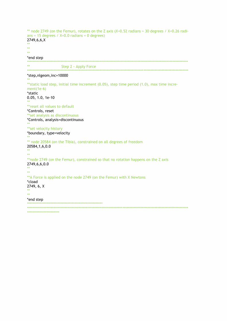
** node 2749 (on the Femur), rotates on the Z axis (X=0.52 radians = 30 degrees / X=0.26 radi-ans = 15 degrees / X=0.0 radians = 0 degrees) 2749,6,6,X ** ** ** *end step ******************************************************************************************************************* ** Step 2 - Apply Force ******************************************************************************************************************* *step,nlgeom,inc=10000 ** **static load step, initial time increment (0.05), step time period (1.0), max time incre-ment(1e-6) *static 0.05, 1.0, 1e-10 ** **reset all values to default *Controls, reset **set analysis as discontinuous *Controls, analysis=discontinuous ** **set velocity history *boundary, type=velocity ** ** node 20584 (on the Tibia), constrained on all degrees of freedom 20584,1,6,0.0 ** ** **node 2749 (on the Femur), constrained so that no rotation happens on the Z axis 2749,6,6,0.0 ** ** **A Force is applied on the node 2749 (on the Femur) with X Newtons *cload 2749, 6, X ** ** *end step ****************************************************** ******************************************************************************************************************************************