American Journal of Computational Linguistics - ACL Anthology
Upload
khangminh22Category
view
0download
0
ACL-IJCNLP 2009
Joint Conference of the47th Annual Meeting of the
Association for Computational Linguisticsand
4th International Joint Conference onNatural Language Processing
of the AFNLP
Proceedings of the Conference
Volume 1
2-7 August 2009Suntec, Singapore

Production and Manufacturing byWorld Scientific Publishing Co Pte Ltd5 Toh Tuck LinkSingapore 596224
c©2009 The Association for Computational Linguisticsand The Asian Federation of Natural Language Processing
Order copies of this and other ACL proceedings from:
Association for Computational Linguistics (ACL)209 N. Eighth StreetStroudsburg, PA 18360USATel: +1-570-476-8006Fax: [email protected]
ISBN 978-1-932432-45-9 / 1-932432-45-0
ii
Preface: General Chair
Welcome to the ACL-IJCNLP 2009, the first joint conference sponsored by the ACL (Associationfor Computational Linguistics) and the AFNLP (Asian Federation of Natural Language Processing).The idea to have a joint conference for ACL and AFNLP was first discussed at ACL-05 (Ann Arbor,Michigan) among Martha Palmer (ACL President), Benjamin T’sou (AFNLP President), Jun’ichi Tsujii(AFNLP Vice President) and Keh-Yih Su (AFNLP Conference Coordinating Committee Chair, also theSecretary General). We are glad that the original idea has come true four years later, and even theaffiliation relationship between these two organizations has been built up now.
In this joint conference, we have tried to mix the spirit from both ACL and AFNLP; and, Singapore,which itself has a mixture of diversified cultures from eastern and western regions, is certainly awonderful place to see how different languages meet each other. We hope you will enjoy this big eventheld in this garden city, which is brought to you via the efforts from each member of the conferenceorganization team.
Among our hard working organizers, I would like to thank the Program Chairs, Jan Wiebe and JianSu, who has carefully selected papers from our record high submissions, and the Local ArrangementsChair, Haizhou Li, who has shown his excellent capability in smoothly organizing various events anddetails. My thanks will also go to other chairs for their competent and hard work: The Webmaster,Minghui Dong; the Demo Chairs, Gary Geunbae Lee and Sabine Schulte im Walde; the Exhibits Chairs,Timothy Baldwin and Philipp Koehn; the Mentoring Service Chairs, Hwee Tou Ng and Florence Reeder;the Publication Chairs, Jing-Shin Chang and Regina Barzilay; the Publicity Chairs, Min-Yen Kan andAndy Way; the Sponsorship Chairs, Hitoshi Isahara and Kim-Teng Lua; the Student Research WorkshopChairs, Davis Dimalen, Jenny Rose Finkel, and Blaise Thomson; also the Faculty Advisors, Grace Ngaiand Brian Roark; the Tutorial Chairs, Diana McCarthy and Chengqing Zong; the Workshop Chairs,Jimmy Lin and Yuji Matsumoto; last, the ACL Business Manager, Priscilla Rasmussen, who not onlyprovides useful advice but also helps to contact more sponsors and get their support.
Besides, I need to express my gratitude to the Conference Coordination Committee for their valuableadvice and support: in which Bonnie Dorr (chair), Steven Bird, Graeme Hirst, Kathleen McCoy, MarthaPalmer, Dragomir Radev, Priscilla Rasmussen, Mark Steedman are from ACL; and Yuji Matsumoto,Keh-Yih Su, Jun’ichi Tsujii, Benjamin T’sou, Kam-Fai Wong are from AFNLP.
Last, I sincerely thank all the authors, reviewers, presenters, invited speakers, sponsors, exhibitors, localsupporting staff, and all the conference attendants. It is you that make this conference possible. Wishyou all enjoy the program that we provide.
Keh-Yih SuACL-IJCNLP 2009 General ChairAugust 2009
iii


Preface: Program Committee Co-Chairs
For the first time, the flagship conferences of the Association for Computational Linguistics (ACL) andthe Asian Federation of Natural Language Processing (AFNLP) – the ACL and IJCNLP – are jointlyorganized as a single event. ACL-IJCNLP 2009 covers a broad spectrum of technical areas relatedto natural language and computation, representing a rich array of the state of the art. The conferenceincludes full papers, short papers, demonstrations, a student research workshop, as well as pre- andpost-conference tutorials and workshops.
This year, we again received a record number of submissions: 925 total valid paper submissions, a 24%increase over ACL-08: HLT. This includes 569 full-paper submissions and 356 short-paper submissionsfrom more than 40 countries – approximately 51% from 20 countries in Asia Pacific, 27% from Canada,Cuba and the United States, 22% from 15 countries in Europe, fewer than 1% from Argentina, andone paper submitted anonymously. We thank all of the authors for submitting papers describing theirrecent work. The significant submission increase is a trend extending over multiple years, and showshow vigorous our field is. We also thank Hwee Tou Ng and Florence Reeder, the Mentoring ServiceCo-Chairs, for organizing a 19-mentor team who provided English scientific paper writing support.
20 Area Chairs worked with 489 Program Committee members and 85 additional reviewers to comeup with 2551 reviews, in total, for the final paper selection. 21% of the full-paper submissions wereaccepted; all will be presented orally. 26% of the short-paper submissions were accepted; some will bepresented orally and some as poster presentations. While short papers are distinguished from full papersin the proceedings, there are no distinctions in the proceedings between short papers presented orally andthose presented as posters. We are absolutely indebted to the Area Chairs, Program Committee members,and additional reviewers for their intensive efforts.
We are delighted to have two keynote speakers: Qiang Yang, who will talk about heterogeneous transferlearning, and Bonnie Webber, who will address discourse and genre. Best (student) paper awards andthe ACL Lifetime Achievement Award will be announced in the last session of the conference as well.
We thank General Conference Chair Keh Yih Su, the Local Arrangements Committee headed byHaizhou Li, and the ACL-AFNLP Conference Coordination Committee chaired by Bonnie Dorr, fortheir help and advice, as well as last years PC Co-Chairs, Johanna Moore and Simone Teufel, for sharingtheir experiences, Jason Eisner for his How to Serve as Program Chair of a Conference website andcorresponding emails, Jing-Shin Chang and Regina Barzilay, the Publication Co-Chairs for putting theproceedings together, and all the other committee chairs for their work. Our thanks go to our assistantChen Bin, who worked tirelessly throughout the entire process, and who made our work with STARTmuch easier. Together, everyone made such a wonderful event possible.
We hope that you enjoy the conference!
Jian Su, Institute for Infocomm ResearchJan Wiebe, University of Pittsburgh
v

Organizing Committee
General Conference Chair:
Su, Keh-Yih (Behavior Design Corp., Taiwan; [email protected])
Program Chairs:
Su, Jian (Institute for Infocomm Research, Singapore; [email protected])Wiebe, Janyce (University of Pittsburgh, USA; [email protected])
Local Organizing Chair:
Li, Haizhou (Institute for Infocomm Research, Singapore; [email protected])
Demo Chairs:
Lee, Gary Geunbae (POSTECH, Korea; [email protected])Schulte im Walde, Sabine (University of Stuttgart, Germany; [email protected])
Exhibits Chairs:
Baldwin, Timothy (University of Melbourne, Australia; [email protected])Koehn, Philipp (University of Edinburgh, UK; [email protected])
Mentoring Service Chairs:
Ng, Hwee Tou (National University of Singapore, Singapore; [email protected])Reeder, Florence (Mitre, USA; [email protected])
Publication Chairs:
Barzilay, Regina (MIT, USA; [email protected])Chang, Jing-Shin (National Chi Nan University, Taiwan; [email protected])
Publicity Chairs:
Kan, Min-Yen (National University of Singapore, Singapore; [email protected])Way, Andy (Dublin City University, Ireland; [email protected])
Sponsorship Chairs:
Americas Sponsorship Co-Chairs:Bangalore, SrinivasDoran, Christine
European Sponsorship Co-Chairs:Koehn, PhilippGenabith, Josef van
Asia Sponsorship Co-Chairs:Isahara, Hitoshi (NICT, Japan; [email protected])Lua, Kim-Teng (COLIPS, Singapore; [email protected])
vii

Student Chairs:
Dimalen, Davis (Academia Sinica, Taiwan; d [email protected])Finkel, Jenny Rose (Stanford University, USA; [email protected])Thomson, Blaise (Cambridge University, UK; [email protected])
Student Workshop Faculty Advisors:
Ngai, Grace (Polytechnic University, Hong Kong; [email protected])Roark, Brian (Oregon Health & Science University, USA; [email protected])
Tutorial Chairs:
McCarthy, Diana (University of Sussex, UK; [email protected])Zong, Chengqing (Chinese Academy of Sciences, China; [email protected])
Workshop Chairs:
Lin, Jimmy (University of Maryland, USA; [email protected])Matsumoto, Yuji (NAIST, Japan; [email protected])
Webmaster:
Dong, Minghui (Institute for Infocomm Research, Singapore; [email protected])
Registration:
Rasmussen, Priscilla(ACL; [email protected])
viii

Program Committee
Program Chairs:
Su, Jian (Institute for Infocomm Research, Singapore; [email protected])Wiebe, Janyce (University of Pittsburgh, USA; [email protected])
Area Chairs:
Agirre, Eneko (University of Basque Country, Spain; [email protected])Ananiadou, Sophia (University of Manchester, UK; [email protected])Belz, Anja (University of Brighton, UK; [email protected])Carenini, Giuseppe (University of British Columbia, Canada; [email protected])Chen, Hsin-Hsi (National Taiwan University, Taiwan, [email protected])Chen, Keh-Jiann (Sinica, Taiwan, [email protected])Curran, James (University of Sydney, Australia; [email protected])Gao, Jian Feng (MSR, USA; [email protected])Harabagiu, Sanda (University of Texas at Dallas, USA, [email protected])Koehn, Philipp (University of Edinburgh, UK; [email protected])Kondrak, Grzegorz (University of Alberta, Canada; [email protected])Meng, Helen Mei-Ling (Chinese University of Hong Kong, HK; [email protected] )Mihalcea, Rada (University of North Texas, USA; [email protected])Poesio, Massimo(University of Trento, Italy; [email protected])Riloff, Ellen (University of Utah, USA; [email protected])Sekine, Satoshi (NewYork University, USA; [email protected])Smith, Noah (CMU, USA; [email protected])Strube, Michael (EML Research, Germany; [email protected])Suzuki, Jun (NTT, Japan; [email protected])Wang, Hai Feng (Toshiba, China; [email protected])
Program Committee Members:
Eugene Agichtein, Gregory Aist, Salah Ait-Mokhtar, Enrique Alfonseca, Yaser Al-Onaizan,Sophia Ananiadou, Alina Andreevskaia, Ion Androutsopoulos, Doug Appelt, Xabier Arregi,Abhishek Arun, Masayuki Asahara, Jordi Atserias, Michaela Atterer
Jason Baldridge, Srinivas Bangalore, Michele Banko, Marco Baroni, Regina Barzilay,Roberto Basili, Sabine Bergler, Shane Bergsma, Steven Bethard, Pushpak Bhattacharyya,Mikhail Bilenko, Philippe Blache, Alan Black, Sasha Blair-Goldensohn, John Blitzer, PhilBlunsom, Philip Blunsom, Bernd Bohnet, Johan Bos, Pierre Boullier, Thorsten Brants, EricBreck, Chris Brew, Ted Briscoe, Chris Brockett, Paul Buitelaar, Razvan Bunescu, Harry Bunt,Stephan Busemann, Donna Byron
Aoife Cahill, Lynne Cahill Cahill, Nicoletta Calzolari, Nick Campbell, Claire Cardie,Giuseppe Carenini, Michael Carl, Xavier Carreras, John Carroll, Francisco Casacuberta, JonChamberlain, Ciprian Chelba, John Chen, Keh-Jiann Chen, Pu-Jen Cheng, Colin Cherry,David Chiang, Key-Sun Choi, Yejin Choi, Monojit Choudhury, Tat-Seng Chua, Jennifer Chu-Carroll, Philip Cimiano, Stephen Clark, James Clarke, Kevin Cohen, Shay Cohen, TrevorCohn, Nigel Collier, John Conroy, Mark Craven, Dan Cristea, Andras Csomai, Silviu-PetrCucerzan, Hang Cui, Aron Culotta, James Curran
Robert Dale, Hal Daume, Eric de la Clergerie, Maarten de Rijke, Vera Demberg, DinaDemner, Dina Demner-Fushman, John DeNero, Li Deng, Yonggang Deng, Pascal Denis, AnnDevitt, Mona Diab, Arantza Diaz, Bill Dolan, John Dowding, Mark Dras, Mark Dredze, JashaDroppo, Amit Dubey, Kevin Duh, Kenneth Dwyer, Chris Dyer
ix
Phil Edmonds, Andreas Eisele, Jacob Eisenstein, Jason Eisner, Michael Elhadad, Mark Ellison,Micha Elsner, Katrin Erk, Andrea Esuli, Marc Ettlinger, Stefan Evert
Ronen Feldman, Christiane Fellbaum, Raquel Fernandez, Elena Filatova, Katja Filippova,Jenny Finkel, Dan Flickinger, Radu Florian, Juliane Fluck, Eric Fosler-Lussier, George Foster,Alex Fraser, Marjorie Freedman, Carol Friedman, Qiang Fu
Evgeniy Gabrilovich, Rob Gaizauskas, Michael Gamon, Albert Gatt, Ulrich Germann, DanielGildea, Jesus Gimenez, Jonathan GInzburg, Roxana Girju, Amir Globerson, AndrewGoldberg, John Goldsmith, Sharon Goldwater, Julio Gonzalo, Ralph Grishman, RodrigoGuido, Tunga Gungor, Iryna Gurevych
Stephanie Haas, Aria Haghighi, Dilek Hakkani-Tur, Keith Hall, John Hansen, SandaHarabagiu, Donna Harman, Saša Hasan, Samer Hassan, Timothy Hazen, Xiaodong He, Jeff Heinz, James Henderson, John Henderson, Andrew Hickl, Erhard Hinrichs, Keikichi Hirose,Julia Hirschberg, Graeme Hirst, Hieu Hoang, Julia Hockenmaier, Beth Ann Hockey, MarkHopkins, Veronique Hoste, Churen Huang, Liang Huang, Sarmad Hussain, Rebecca Hwa,Mei-Yuh Hwang
Nancy Ide, Ryu Iida, Diana Inkpen, Kentaro Inui, Hitoshi Isahara, Abe Ittycheriah, TatsuyaIzuha
Heng Ji, Sittichai Jiampojamarn, Jing Jiang, Mark Johnson, Doug Jones, Gareth Jones
Mijail Kabadjov, Laura Kallmeyer, Nanda Kambhatla, Hiroshi Kanayama, NikiforosKaramanis, Tsuneaki Kato, Hisashi Kawai, Junichi Kazama, Frank Keller, Andre Kempe,Brett Kessler, Mitesh Khapra, Bernd Kiefer, Adam Kilgarriff, Brian Kingsbury, James Kirby,Ewan Klein, Alexandre Klementiev, Kevin Knight, Rob Koeling, Terry Koo, Moshe Koppel,Wessel Kraaij, Emiel Krahmer, Ivana Kruijff-Korbayova, Lun-Wei Ku, Sandra Kuebler,Marco Kuhlmann, Jonas Kuhn, Seth Kulick, Akira Kumano, Shankar Kumar, A. Kumaran,June-Jei Kuo, Sadao Kurohashi, Kui-Lam Kwok
Philippe Langlais, Mirella Lapata, Alberto Lavelli, Gary Lee, Lillian Lee, Yoong Keok Lee,Yue-Shi Lee, Haizhou Li, Hang Li, Xiaolong Li, Percy Liang, Elizabeth Liddy, Dekang Lin,Lucian Lita, Ken Litkowski, Diane Litman, Bing Liu, Qun Liu, Tie-Yan Liu, Yang Liu,Zhanyi Liu, Adam Lopez, Xiaoqiang Luo, Yajuan Lv
Yanjun Ma, Lluís Màrquez, Karin Müller, Bernardo Magnini, Brian Mak, Rob Malouf,Gideon Mann, Daniel Marcu, Katja Markert, David Martínez, Andre Martins, MstislavMaslennikov, Tomoko Matsui, Yuji Matsumoto, Takuya Matsuzaki, Evgeny Matusov, ArneMauser, Diana McCarthy, David McClosky, Mark McConnville, Ryan McDonald, MichaelMcTear, Qiaozhu Mei, Chris Mellish, Arul Menezes, Paola Merlo, Detmar Meurers, DavidMimno, Mandar Mitra, Vibhu Mittal, Yusuke Miyao, Daichi Mochihashi, Saif Mohammad,Rajat Mohanty, Diego Molla-Aliod, Christian Monson, Simonetta Montemagni, Bob Moore,Alex Morgan, Glyn Morrill, Alessandro Moschitti, Dragos Munteanu, Gabriel Murray, SungHyon Myaeng
Vivi Nastase, Tetsuya Nasukawa, Roberto Navigli, Mark-Jan Nederhof, Ani Nenkova, JohnNerbonne, Hwee Tou Ng, Vincent Ng, Patrick Nguyen, Jian-Yun Nie, Zaiqing Nie, TakashiNinomiya, Joakim Nivre, Chikashi Nobata, David Novick, Adrian Novischi
Franz Och, Stephan Oepen, Kemal Oflazer, Alice Oh, Jong-Hoon Oh, Daisuke Okanohara,Naoaki Okazaki, Fredrik Olsson, Constantin Orasan, Miles Osborne, Jahna Otterbacher
x

Tim Paek, Martha Palmer, Bo Pang, Patrick Pantel, Cecile Paris, Rebecca Passonneau,Michael Paul, Matthias Paulik, Anselmo Peñas, Adam Pease, Ted Pedersen, CatherinePelachaud, Slav Petrov, Christopher Pinchak, Maja Popovic, Sameer Pradhan, John Prager,Rashmi Prasad, Detlef Prescher, Stephen Pulman, Sampo Pyysalo
Long Qiu, Silvia Quarteroni, Chris Quirk
Bhuvana Ramabhadran, Ganesh Ramakrishnan, Lance Ramshaw, Giuseppe Riccardi, VerenaRieser, German Rigau, Hae-Chang Rim, Brian Roark, James Rogers, Barbara Rosario,Carolyn Rose, Antti-Veikk Rosti, Patrick Ruch, Marta Ruiz, Andrey Rzhetsky
Kenji Sagae, Horacio Saggion, Benoit Sagot, Tetsuya Sakai, Baskaran Sankaran, MuratSaraclar, Ruhi Sarikaya, Yutaka Sasaki, Giorgio Satta, Anne Schiller, Helmut Schmid, MarcSchroeder, Holger Schwenk, Yohei Seki, Satoshi Sekine, Mike Seltzer, Jungyun Seo, VijayShanker, Hagit Shatkay, Libin Shen, Nobuyuki Shimizu, Luo Si, Advaith Siddharthan, CandySidner, Khalil Simaan, Michel Simard, Gabriel Skantze, David Smith, Noah Smith, RionSnow, Ian Soboroff, Swapna Somasundaran, Radu Soricut, Caroline Sporleder, Rohini Srihari,Mark Steedman, Josef Steinberger, Amanda Stent, Mark Stevenson, Veselin Stoyanov, CarloStrapparava, Michael Strube, Tomek Strzalkowski, Jana Sukkarieh, Maoson Sun, MihaiSurdeanu, Richard Sutcliffe, Stan Szpakowicz, Idan Szpektor
Maite Taboada, John Tait, Hiroya Takamura, David Talbot, Ben Taskar, Joel Tetreault,Simone Teufel, Joerg Tiedemann, Christoph Tillmann, Ivan Titov, Roberto Togneri, KeiichiTokuda, Kristina Toutanova, Roy Tromble, Yuen-Hsien Tseng, Jun’ichi Tsujii, YoshimasaTsuruoka, Dan Tufis, Gokhan Tur
Antal van den Bosch, Josef van Genabith, Keith Vander Linden, Sebastian Varges, TonyVeale, Ashish Venugopal, Paola Verlardi, Yannick Versley, David Vilar, Piek Vossen
Michael Walsh, Stephen Wan, Xiaojun Wan, Qin Wang, Shaojun Wang, Wei Wang, XinglongWang, Taro Watanabe, Andy Way, Bonnie Webber, David Weir, Fuiliang Weng, JanyceWiebe, Theresa Wilson, Shuly Wintner, Yuk Wah Wong, Johan Wouters, Dekai Wu, Hua Wu
Zhuli Xie, Deyi Xiong, Jun Xu, Peng Xu, Jian Xue
Kazuhide Yamamoto, Christopher Yang, Jianwu Yang, Muyun Yang, Kaisheng Yao, UmitYapanel, Scott Wen-tau Yih, Deniz Yuret
Fabio Zanzotto, Dmitry Zelenko, Heiga Zen, Richard Zens, Luke Zettlemoyer, Hao Zhang,Min Zhang, Rong Zhang, Tong Zhang, Yue Zhang, Tiejun Zhao, Bowen Zhou, Denny Zhou,Ming Zhou, Jerry Zhu, Andreas Zollmann, Chengqing Zong, Pierre Zweigenbaum
Additional Reviewers:
Shlomo Argamon, Javier Artiles, Giuseppe Attardi, S.R.K. Branavan, Julian Brooke, DavidBurkett, Yong Cao, Yufeng Chen, Yu Chen, Ying Chen, Bonaventura Coppola, SajibDasgupta, Anirban Dasgupta, Diego De Cao, Oier Lopez de Lacalle, Adi Eyal, Jung-wei Fan,Benoit Favre, Moshe Fresko, Oana Frunza, Bin Gao, Xi-Wu Han, Zhongjun He, CarmenHeger, Zhongjun He, Wenbin Jiang, Richard Johansson, Anna Kazantseva, Alistair Kennedy,Fazel Keshtkar, Gerhard Kremer, Patrik Lambert, Greg Langmead, Oliver Lemon, GregorLeusch, Xiao Li, Shoushan Li, Wei Li, Sujian Li, Xiaojiang Liu, Ting Liu, Yang Liu, Yue Lu,Jia Lu, Weihua Luo, Gang Luo, Yong-Liang Ma, Saab Mansour, Haitao Mi, Peter Nabenda,Peter Nabende, Ramesh Nallapati, Dipasree Pal, Adam Pauls, Emanuele Pianta, DanielePighin, Guilin Qi, Wei Qiao, Tao Qin, Jason Riesa, Felipe Sanchez-Martinez, StevenSchockaert, Dou Shen, Kathrin Spreyer, Jun Sun, Milan Tofiloski, Lav Varshney, Ye-Yi
xi

Wang, Yu-Chieh Wu, Gu Xu, Sibel Yaman, Shiren Ye, Huang Yun, Hui Zhang, Yi Zhang,Bing Zhao, Yu Zhou, Zhemin Zhu, Conghui Zhu
xii

Mentoring Service Committee
Chairs:
Ng, Hwee Tou (National University of Singapore, Singapore; [email protected])Reeder, Florence (Mitre, USA; [email protected])
Members:
Razvan Bunescu, Yee Seng Chan, Chrys Chrystello, Ken Church, Walter Daelemans, DeborahDahl, Robert Daland, Janet Hitzeman, Eduard Hovy, Marilyn Kupetz, Preslav Nakov, Jian-Yun Nie, Kemal Oflazer, Bea Oshika, Dan Roth, Kenneth Samuel, Antal van den Bosch, JohnWhite, Yuk Wah Wong
xiii


Invited Talk:
Heterogeneous Transfer Learning with Real-world Applications
Qiang YangHong Kong University of Science and Technology
Abstract
In many real-world machine learning and data mining applications, we often face the problem wherethe training data are scarce in the feature space of interest, but much data are available in other featurespaces. Many existing learning techniques cannot make use of these auxiliary data, because thesealgorithms are based on the assumption that the training and test data must come from the samedistribution and feature spaces. When this assumption does not hold, we have to seek novel techniquesfor ‘transferring’ the knowledge from one feature space to another. In this talk, I will present our recent works on heterogeneous transfer learning. I will describe how to identify the common parts ofdifferent feature spaces and learn a bridge between them to improve the learning performance in targettask domains. I will also present several interesting applications of heterogeneous transfer learning,such as image clustering and classification, cross-domain classification and collaborative filtering.
Biography
Qiang Yang is a professor in the Department of Computer Science and Engineering, Hong KongUniversity of Science and Technology. His research interests are artificial intelligence, includingautomated planning, machine learning and data mining. He graduated from Peking University in 1982with BSc. in Astrophysics, and obtained his MSc. degrees in Astrophysics and Computer Science fromthe University of Maryland, College Park in 1985 and 1987, respectively. He obtained his PhD inComputer Science from the University of Maryland, College Park in 1989. He was anassistant/associate professor at the University of Waterloo between 1989 and 1995, and a professorand NSERC Industrial Research Chair at Simon Fraser University in Canada from 1995 to 2001.
Qiang Yang has been active in research on artificial intelligence planning, machine learning and datamining. His research teams won the 2004 and 2005 ACM KDDCUP international competitions ondata mining. He has been on several editorial boards of international journals, including IEEEIntelligent Systems, IEEE Transactions on Knowledge and Data Engineering and Web Intelligence.He has been an organizer for several international conferences in AI and data mining, including beingthe conference co-chair for ACM IUI 2010 and ICCBR 2001, program co-chair for PRICAI 2006 andPAKDD 2007, workshop chair for ACM KDD 2007, AAAI tutorial chair for AAAI 2005 and 2006,data mining contest chair for IEEE ICDM 2007 and 2009, and vice chair for ICDM 2006 and CIKM2009. He is a fellow of IEEE and a member of AAAI and ACM. His home page is athttp://www.cse.ust.hk/~qyang
xv

Invited Talk:
Discourse - Early Problems, Current Successes, Future Challenges
Bonnie WebberUniversity of Edinburgh, UK
Abstract
I will look back through nearly forty years of computational research on discourse, noting someproblems (such as context-dependence and inference) that were identified early on as a hindrance tofurther progress, some admirable successes that we have achieved so far in the development ofalgorithms and resources, and some challenges that we may want to (or that we may have to!) take upin the future, with particular attention to problems of data annotation and genre dependence.
Biography
Bonnie Webber was a researcher at Bolt Beranek and Newman while working on the PhD shereceived from Harvard University in 1978. She then taught in the Department of Computer andInformation Science at the University of Pennsylvania for 20 years before joining the School ofInformatics at the University of Edinburgh. Known for research on discourse and on questionanswering, she is a Past President of the Association for Computational Linguistics, co-developer(with Aravind Joshi, Rashmi Prasad, Alan Lee and Eleni Miltsakaki) of the Penn Discourse TreeBank,and co-editor (with Annie Zaenen and Martha Palmer) of the journal, Linguistic Issues in LanguageTechnology.
xvii

Table of Contents
Heterogeneous Transfer Learning for Image Clustering via the SocialWebQiang Yang, Yuqiang Chen, Gui-Rong Xue, Wenyuan Dai and Yong Yu . . . . . . . . . . . . . . . . . . . . . . . 1
Investigations on Word Senses and Word UsagesKatrin Erk, Diana McCarthy and Nicholas Gaylord. . . . . . . . . . . . . . . . . . . . . . . . . . . . . . . . . . . . . . . . .10
A Comparative Study on Generalization of Semantic Roles in FrameNetYuichiroh Matsubayashi, Naoaki Okazaki and Jun’ichi Tsujii . . . . . . . . . . . . . . . . . . . . . . . . . . . . . . . 19
Unsupervised Argument Identification for Semantic Role LabelingOmri Abend, Roi Reichart and Ari Rappoport . . . . . . . . . . . . . . . . . . . . . . . . . . . . . . . . . . . . . . . . . . . . . 28
Brutus: A Semantic Role Labeling System Incorporating CCG, CFG, and Dependency FeaturesStephen Boxwell, Dennis Mehay and Chris Brew . . . . . . . . . . . . . . . . . . . . . . . . . . . . . . . . . . . . . . . . . . 37
Exploiting Heterogeneous Treebanks for ParsingZheng-Yu Niu, Haifeng Wang and Hua Wu . . . . . . . . . . . . . . . . . . . . . . . . . . . . . . . . . . . . . . . . . . . . . . . . 46
Cross Language Dependency Parsing using a Bilingual LexiconHai Zhao, Yan Song, Chunyu Kit and Guodong Zhou. . . . . . . . . . . . . . . . . . . . . . . . . . . . . . . . . . . . . . .55
Topological Field Parsing of GermanJackie Chi Kit Cheung and Gerald Penn . . . . . . . . . . . . . . . . . . . . . . . . . . . . . . . . . . . . . . . . . . . . . . . . . . . 64
Unsupervised Multilingual Grammar InductionBenjamin Snyder, Tahira Naseem and Regina Barzilay . . . . . . . . . . . . . . . . . . . . . . . . . . . . . . . . . . . . . 73
Reinforcement Learning for Mapping Instructions to ActionsS.R.K. Branavan, Harr Chen, Luke Zettlemoyer and Regina Barzilay. . . . . . . . . . . . . . . . . . . . . . . . .82
Learning Semantic Correspondences with Less SupervisionPercy Liang, Michael Jordan and Dan Klein . . . . . . . . . . . . . . . . . . . . . . . . . . . . . . . . . . . . . . . . . . . . . . . 91
Bayesian Unsupervised Word Segmentation with Nested Pitman-Yor Language ModelingDaichi Mochihashi, Takeshi Yamada and Naonori Ueda . . . . . . . . . . . . . . . . . . . . . . . . . . . . . . . . . . . 100
Knowing the Unseen: Estimating Vocabulary Size over Unseen SamplesSuma Bhat and Richard Sproat . . . . . . . . . . . . . . . . . . . . . . . . . . . . . . . . . . . . . . . . . . . . . . . . . . . . . . . . . . 109
A Ranking Approach to Stress Prediction for Letter-to-Phoneme ConversionQing Dou, Shane Bergsma, Sittichai Jiampojamarn and Grzegorz Kondrak . . . . . . . . . . . . . . . . . . 118
Reducing the Annotation Effort for Letter-to-Phoneme ConversionKenneth Dwyer and Grzegorz Kondrak . . . . . . . . . . . . . . . . . . . . . . . . . . . . . . . . . . . . . . . . . . . . . . . . . . 127
Transliteration AlignmentVladimir Pervouchine, Haizhou Li and Bo Lin . . . . . . . . . . . . . . . . . . . . . . . . . . . . . . . . . . . . . . . . . . . .136
Automatic training of lemmatization rules that handle morphological changes in pre-, in- and suffixesalike
Bart Jongejan and Hercules Dalianis . . . . . . . . . . . . . . . . . . . . . . . . . . . . . . . . . . . . . . . . . . . . . . . . . . . . . 145
xix

Revisiting Pivot Language Approach for Machine TranslationHua Wu and Haifeng Wang . . . . . . . . . . . . . . . . . . . . . . . . . . . . . . . . . . . . . . . . . . . . . . . . . . . . . . . . . . . . . 154
Efficient Minimum Error Rate Training and Minimum Bayes-Risk Decoding for Translation Hypergraphsand Lattices
Shankar Kumar, Wolfgang Macherey, Chris Dyer and Franz Och . . . . . . . . . . . . . . . . . . . . . . . . . . . 163
Forest-based Tree Sequence to String Translation ModelHui Zhang, Min Zhang, Haizhou Li, Aiti Aw and Chew Lim Tan . . . . . . . . . . . . . . . . . . . . . . . . . . . 172
Active Learning for Multilingual Statistical Machine TranslationGholamreza Haffari and Anoop Sarkar . . . . . . . . . . . . . . . . . . . . . . . . . . . . . . . . . . . . . . . . . . . . . . . . . . . 181
DEPEVAL(summ): Dependency-based Evaluation for Automatic SummariesKarolina Owczarzak . . . . . . . . . . . . . . . . . . . . . . . . . . . . . . . . . . . . . . . . . . . . . . . . . . . . . . . . . . . . . . . . . . . 190
Summarizing Definition from WikipediaShiren Ye, Tat-Seng Chua and Jie LU . . . . . . . . . . . . . . . . . . . . . . . . . . . . . . . . . . . . . . . . . . . . . . . . . . . . 199
Automatically Generating Wikipedia Articles: A Structure-Aware ApproachChristina Sauper and Regina Barzilay . . . . . . . . . . . . . . . . . . . . . . . . . . . . . . . . . . . . . . . . . . . . . . . . . . . .208
Learning to Tell Tales: A Data-driven Approach to Story GenerationNeil McIntyre and Mirella Lapata . . . . . . . . . . . . . . . . . . . . . . . . . . . . . . . . . . . . . . . . . . . . . . . . . . . . . . . 217
Recognizing Stances in Online DebatesSwapna Somasundaran and Janyce Wiebe . . . . . . . . . . . . . . . . . . . . . . . . . . . . . . . . . . . . . . . . . . . . . . . . 226
Co-Training for Cross-Lingual Sentiment ClassificationXiaojun Wan . . . . . . . . . . . . . . . . . . . . . . . . . . . . . . . . . . . . . . . . . . . . . . . . . . . . . . . . . . . . . . . . . . . . . . . . . . 235
A Non-negative Matrix Tri-factorization Approach to Sentiment Classification with Lexical Prior Knowl-edge
Tao Li, Yi Zhang and Vikas Sindhwani . . . . . . . . . . . . . . . . . . . . . . . . . . . . . . . . . . . . . . . . . . . . . . . . . . 244
Discovering the Discriminative Views: Measuring Term Weights for Sentiment AnalysisJungi Kim, Jin-Ji Li and Jong-Hyeok Lee . . . . . . . . . . . . . . . . . . . . . . . . . . . . . . . . . . . . . . . . . . . . . . . . 253
Compiling a Massive, Multilingual Dictionary via Probabilistic InferenceMausam, Stephen Soderland, Oren Etzioni, Daniel Weld, Michael Skinner and Jeff Bilmes . . . 262
A Metric-based Framework for Automatic Taxonomy InductionHui Yang and Jamie Callan . . . . . . . . . . . . . . . . . . . . . . . . . . . . . . . . . . . . . . . . . . . . . . . . . . . . . . . . . . . . . 271
Learning with Annotation NoiseEyal Beigman and Beata Beigman Klebanov . . . . . . . . . . . . . . . . . . . . . . . . . . . . . . . . . . . . . . . . . . . . . 280
Abstraction and Generalisation in Semantic Role Labels: PropBank, VerbNet or both?Paola Merlo and Lonneke van der Plas . . . . . . . . . . . . . . . . . . . . . . . . . . . . . . . . . . . . . . . . . . . . . . . . . . . 288
Robust Machine Translation Evaluation with Entailment FeaturesSebastian Pado, Michel Galley, Dan Jurafsky and Christopher D. Manning . . . . . . . . . . . . . . . . . . 297
The Contribution of Linguistic Features to Automatic Machine Translation EvaluationEnrique Amigó, Jesús Giménez, Julio Gonzalo and Felisa Verdejo . . . . . . . . . . . . . . . . . . . . . . . . . . 306
xx
A Syntax-Driven Bracketing Model for Phrase-Based TranslationDeyi Xiong, Min Zhang, Aiti Aw and Haizhou Li . . . . . . . . . . . . . . . . . . . . . . . . . . . . . . . . . . . . . . . . . 315
Topological Ordering of Function Words in Hierarchical Phrase-based TranslationHendra Setiawan, Min Yen Kan, Haizhou Li and Philip Resnik . . . . . . . . . . . . . . . . . . . . . . . . . . . . . 324
Phrase-Based Statistical Machine Translation as a Traveling Salesman ProblemMikhail Zaslavskiy, Marc Dymetman and Nicola Cancedda . . . . . . . . . . . . . . . . . . . . . . . . . . . . . . . . 333
Concise Integer Linear Programming Formulations for Dependency ParsingAndre Martins, Noah Smith and Eric Xing . . . . . . . . . . . . . . . . . . . . . . . . . . . . . . . . . . . . . . . . . . . . . . . 342
Non-Projective Dependency Parsing in Expected Linear TimeJoakim Nivre . . . . . . . . . . . . . . . . . . . . . . . . . . . . . . . . . . . . . . . . . . . . . . . . . . . . . . . . . . . . . . . . . . . . . . . . . . 351
Semi-supervised Learning of Dependency Parsers using Generalized Expectation CriteriaGregory Druck, Gideon Mann and Andrew McCallum . . . . . . . . . . . . . . . . . . . . . . . . . . . . . . . . . . . . 360
Dependency Grammar Induction via Bitext Projection ConstraintsKuzman Ganchev, Jennifer Gillenwater and Ben Taskar . . . . . . . . . . . . . . . . . . . . . . . . . . . . . . . . . . . 369
Cross-Domain Dependency Parsing Using a Deep Linguistic GrammarYi Zhang and Rui Wang . . . . . . . . . . . . . . . . . . . . . . . . . . . . . . . . . . . . . . . . . . . . . . . . . . . . . . . . . . . . . . . . 378
A Chinese-English Organization Name Translation System Using Heuristic Web Mining and AsymmetricAlignment
Fan Yang, Jun Zhao and Kang Liu . . . . . . . . . . . . . . . . . . . . . . . . . . . . . . . . . . . . . . . . . . . . . . . . . . . . . . . 387
Reducing Semantic Drift with Bagging and Distributional SimilarityTara McIntosh and James R. Curran . . . . . . . . . . . . . . . . . . . . . . . . . . . . . . . . . . . . . . . . . . . . . . . . . . . . . 396
Jointly Identifying Temporal Relations with Markov LogicKatsumasa Yoshikawa, Sebastian Riedel, Masayuki Asahara and Yuji Matsumoto . . . . . . . . . . . . 405
Profile Based Cross-Document Coreference Using Kernelized Fuzzy Relational ClusteringJian Huang, Sarah M. Taylor, Jonathan L. Smith, Konstantinos A. Fotiadis and C. Lee Giles . . 414
Who, What, When, Where, Why? Comparing Multiple Approaches to the Cross-Lingual 5W TaskKristen Parton, Kathleen R. McKeown, Bob Coyne, Mona T. Diab, Ralph Grishman, Dilek Hakkani-
Tür, Mary Harper, Heng Ji, Wei Yun Ma, Adam Meyers, Sara Stolbach, Ang Sun, Gokhan Tur, Wei Xuand Sibel Yaman . . . . . . . . . . . . . . . . . . . . . . . . . . . . . . . . . . . . . . . . . . . . . . . . . . . . . . . . . . . . . . . . . . . . . . . . . . . 423
Bilingual Co-Training for Monolingual Hyponymy-Relation AcquisitionJong-Hoon Oh, Kiyotaka Uchimoto and Kentaro Torisawa . . . . . . . . . . . . . . . . . . . . . . . . . . . . . . . . . 432
Automatic Set Instance Extraction using the WebRichard C. Wang and William W. Cohen . . . . . . . . . . . . . . . . . . . . . . . . . . . . . . . . . . . . . . . . . . . . . . . . . 441
Extracting Lexical Reference Rules from WikipediaEyal Shnarch, Libby Barak and Ido Dagan . . . . . . . . . . . . . . . . . . . . . . . . . . . . . . . . . . . . . . . . . . . . . . . 450
Employing Topic Models for Pattern-based Semantic Class DiscoveryHuibin Zhang, Mingjie Zhu, Shuming Shi and Ji-Rong Wen . . . . . . . . . . . . . . . . . . . . . . . . . . . . . . . 459
Paraphrase Identification as Probabilistic Quasi-Synchronous RecognitionDipanjan Das and Noah A. Smith . . . . . . . . . . . . . . . . . . . . . . . . . . . . . . . . . . . . . . . . . . . . . . . . . . . . . . . 468
xxi
Stochastic Gradient Descent Training for L1-regularized Log-linear Models with Cumulative PenaltyYoshimasa Tsuruoka, Jun’ichi Tsujii and Sophia Ananiadou . . . . . . . . . . . . . . . . . . . . . . . . . . . . . . . 477
A global model for joint lemmatization and part-of-speech predictionKristina Toutanova and Colin Cherry . . . . . . . . . . . . . . . . . . . . . . . . . . . . . . . . . . . . . . . . . . . . . . . . . . . . 486
Distributional Representations for Handling Sparsity in Supervised Sequence-LabelingFei Huang and Alexander Yates . . . . . . . . . . . . . . . . . . . . . . . . . . . . . . . . . . . . . . . . . . . . . . . . . . . . . . . . . 495
Minimized Models for Unsupervised Part-of-Speech TaggingSujith Ravi and Kevin Knight . . . . . . . . . . . . . . . . . . . . . . . . . . . . . . . . . . . . . . . . . . . . . . . . . . . . . . . . . . . 504
An Error-Driven Word-Character Hybrid Model for Joint Chinese Word Segmentation and POS TaggingCanasai Kruengkrai, Kiyotaka Uchimoto, Jun’ichi Kazama, Yiou Wang, Kentaro Torisawa and
Hitoshi Isahara . . . . . . . . . . . . . . . . . . . . . . . . . . . . . . . . . . . . . . . . . . . . . . . . . . . . . . . . . . . . . . . . . . . . . . . . . . . . . 513
Automatic Adaptation of Annotation Standards: Chinese Word Segmentation and POS Tagging – A CaseStudy
Wenbin Jiang, Liang Huang and Qun Liu . . . . . . . . . . . . . . . . . . . . . . . . . . . . . . . . . . . . . . . . . . . . . . . . 522
Linefeed Insertion into Japanese Spoken Monologue for CaptioningTomohiro Ohno, Masaki Murata and Shigeki Matsubara . . . . . . . . . . . . . . . . . . . . . . . . . . . . . . . . . . . 531
Semi-supervised Learning for Automatic Prosodic Event Detection Using Co-training AlgorithmJe Hun Jeon and Yang Liu . . . . . . . . . . . . . . . . . . . . . . . . . . . . . . . . . . . . . . . . . . . . . . . . . . . . . . . . . . . . . . 540
Summarizing multiple spoken documents: finding evidence from untranscribed audioXiaodan Zhu, Gerald Penn and Frank Rudzicz . . . . . . . . . . . . . . . . . . . . . . . . . . . . . . . . . . . . . . . . . . . . 549
Improving Tree-to-Tree Translation with Packed ForestsYang Liu, Yajuan Lü and Qun Liu . . . . . . . . . . . . . . . . . . . . . . . . . . . . . . . . . . . . . . . . . . . . . . . . . . . . . . . 558
Fast Consensus Decoding over Translation ForestsJohn DeNero, David Chiang and Kevin Knight . . . . . . . . . . . . . . . . . . . . . . . . . . . . . . . . . . . . . . . . . . . 567
Joint Decoding with Multiple Translation ModelsYang Liu, Haitao Mi, Yang Feng and Qun Liu . . . . . . . . . . . . . . . . . . . . . . . . . . . . . . . . . . . . . . . . . . . . 576
Collaborative Decoding: Partial Hypothesis Re-ranking Using Translation Consensus between De-coders
Mu Li, Nan Duan, Dongdong Zhang, Chi-Ho Li and Ming Zhou . . . . . . . . . . . . . . . . . . . . . . . . . . . 585
Variational Decoding for Statistical Machine TranslationZhifei Li, Jason Eisner and Sanjeev Khudanpur . . . . . . . . . . . . . . . . . . . . . . . . . . . . . . . . . . . . . . . . . . . 593
Unsupervised Learning of Narrative Schemas and their ParticipantsNathanael Chambers and Dan Jurafsky . . . . . . . . . . . . . . . . . . . . . . . . . . . . . . . . . . . . . . . . . . . . . . . . . . 602
Learning a Compositional Semantic Parser using an Existing Syntactic ParserRuifang Ge and Raymond Mooney . . . . . . . . . . . . . . . . . . . . . . . . . . . . . . . . . . . . . . . . . . . . . . . . . . . . . . 611
Latent Variable Models of Concept-Attribute AttachmentJoseph Reisinger and Marius Pasca . . . . . . . . . . . . . . . . . . . . . . . . . . . . . . . . . . . . . . . . . . . . . . . . . . . . . . 620
The Chinese Aspect Generation Based on Aspect Selection FunctionsGuowen Yang and John Bateman . . . . . . . . . . . . . . . . . . . . . . . . . . . . . . . . . . . . . . . . . . . . . . . . . . . . . . . . 629
xxii
Quantitative modeling of the neural representation of adjective-noun phrases to account for fMRI acti-vation
Kai-min K. Chang, Vladimir L. Cherkassky, Tom M. Mitchell and Marcel Adam Just . . . . . . . . 638
Capturing Salience with a Trainable Cache Model for Zero-anaphora ResolutionRyu Iida, Kentaro Inui and Yuji Matsumoto . . . . . . . . . . . . . . . . . . . . . . . . . . . . . . . . . . . . . . . . . . . . . . 647
Conundrums in Noun Phrase Coreference Resolution: Making Sense of the State-of-the-ArtVeselin Stoyanov, Nathan Gilbert, Claire Cardie and Ellen Riloff . . . . . . . . . . . . . . . . . . . . . . . . . . . 656
A Novel Discourse Parser Based on Support Vector Machine ClassificationDavid duVerle and Helmut Prendinger . . . . . . . . . . . . . . . . . . . . . . . . . . . . . . . . . . . . . . . . . . . . . . . . . . . 665
Genre distinctions for discourse in the Penn TreeBankBonnie Webber . . . . . . . . . . . . . . . . . . . . . . . . . . . . . . . . . . . . . . . . . . . . . . . . . . . . . . . . . . . . . . . . . . . . . . . . 674
Automatic sense prediction for implicit discourse relations in textEmily Pitler, Annie Louis and Ani Nenkova . . . . . . . . . . . . . . . . . . . . . . . . . . . . . . . . . . . . . . . . . . . . . . 683
A Framework of Feature Selection Methods for Text CategorizationShoushan Li, Rui Xia, Chengqing Zong and Chu-Ren Huang . . . . . . . . . . . . . . . . . . . . . . . . . . . . . . 692
Mine the Easy, Classify the Hard: A Semi-Supervised Approach to Automatic Sentiment ClassificationSajib Dasgupta and Vincent Ng . . . . . . . . . . . . . . . . . . . . . . . . . . . . . . . . . . . . . . . . . . . . . . . . . . . . . . . . . 701
Modeling Latent Biographic Attributes in Conversational GenresNikesh Garera and David Yarowsky . . . . . . . . . . . . . . . . . . . . . . . . . . . . . . . . . . . . . . . . . . . . . . . . . . . . . 710
A Graph-based Semi-Supervised Learning for Question-AnsweringAsli Celikyilmaz, Marcus Thint and Zhiheng Huang . . . . . . . . . . . . . . . . . . . . . . . . . . . . . . . . . . . . . . 719
Combining Lexical Semantic Resources with Question & Answer Archives for Translation-Based AnswerFinding
Delphine Bernhard and Iryna Gurevych . . . . . . . . . . . . . . . . . . . . . . . . . . . . . . . . . . . . . . . . . . . . . . . . . . 728
Answering Opinion Questions with Random Walks on GraphsFangtao Li, Yang Tang, Minlie Huang and Xiaoyan Zhu . . . . . . . . . . . . . . . . . . . . . . . . . . . . . . . . . . . 737
What lies beneath: Semantic and syntactic analysis of manually reconstructed spontaneous speechErin Fitzgerald, Frederick Jelinek and Robert Frank . . . . . . . . . . . . . . . . . . . . . . . . . . . . . . . . . . . . . . . 746
Discriminative Lexicon Adaptation for Improved Character Accuracy - A New Direction in ChineseLanguage Modeling
Yi-cheng Pan, Lin-shan Lee and Sadaoki Furui . . . . . . . . . . . . . . . . . . . . . . . . . . . . . . . . . . . . . . . . . . . 755
Improving Automatic Speech Recognition for Lectures through Transformation-based Rules Learnedfrom Minimal Data
Cosmin Munteanu, Gerald Penn and Xiaodan Zhu . . . . . . . . . . . . . . . . . . . . . . . . . . . . . . . . . . . . . . . . 764
Quadratic-Time Dependency Parsing for Machine TranslationMichel Galley and Christopher D. Manning . . . . . . . . . . . . . . . . . . . . . . . . . . . . . . . . . . . . . . . . . . . . . . 773
A Gibbs Sampler for Phrasal Synchronous Grammar InductionPhil Blunsom, Trevor Cohn, Chris Dyer and Miles Osborne . . . . . . . . . . . . . . . . . . . . . . . . . . . . . . . . 782
xxiii

Source-Language Entailment Modeling for Translating Unknown TermsShachar Mirkin, Lucia Specia, Nicola Cancedda, Ido Dagan, Marc Dymetman and Idan Szpektor
791
Case markers and Morphology: Addressing the crux of the fluency problem in English-Hindi SMTAnanthakrishnan Ramanathan, Hansraj Choudhary, Avishek Ghosh and Pushpak Bhattacharyya800
Dependency Based Chinese Sentence RealizationWei He, Haifeng Wang, Yuqing Guo and Ting Liu . . . . . . . . . . . . . . . . . . . . . . . . . . . . . . . . . . . . . . . . 809
Incorporating Information Status into Generation RankingAoife Cahill and Arndt Riester . . . . . . . . . . . . . . . . . . . . . . . . . . . . . . . . . . . . . . . . . . . . . . . . . . . . . . . . . . 817
A Syntax-Free Approach to Japanese Sentence CompressionTsutomu Hirao, Jun Suzuki and Hideki Isozaki . . . . . . . . . . . . . . . . . . . . . . . . . . . . . . . . . . . . . . . . . . . 826
Application-driven Statistical Paraphrase GenerationShiqi Zhao, Xiang Lan, Ting Liu and Sheng Li . . . . . . . . . . . . . . . . . . . . . . . . . . . . . . . . . . . . . . . . . . . 834
Semi-Supervised Cause Identification from Aviation Safety ReportsIsaac Persing and Vincent Ng . . . . . . . . . . . . . . . . . . . . . . . . . . . . . . . . . . . . . . . . . . . . . . . . . . . . . . . . . . . 843
SMS based Interface for FAQ RetrievalGovind Kothari, Sumit Negi, Tanveer A. Faruquie, Venkatesan T. Chakaravarthy and L. Venkata
Subramaniam . . . . . . . . . . . . . . . . . . . . . . . . . . . . . . . . . . . . . . . . . . . . . . . . . . . . . . . . . . . . . . . . . . . . . . . . . . . . . . 852
Semantic Tagging of Web Search QueriesMehdi Manshadi and Xiao Li . . . . . . . . . . . . . . . . . . . . . . . . . . . . . . . . . . . . . . . . . . . . . . . . . . . . . . . . . . . 861
Mining Bilingual Data from the Web with Adaptively Learnt PatternsLong Jiang, Shiquan Yang, Ming Zhou, Xiaohua Liu and Qingsheng Zhu . . . . . . . . . . . . . . . . . . . 870
Comparing Objective and Subjective Measures of Usability in a Human-Robot Dialogue SystemMary Ellen Foster, Manuel Giuliani and Alois Knoll . . . . . . . . . . . . . . . . . . . . . . . . . . . . . . . . . . . . . . 879
Setting Up User Action Probabilities in User Simulations for Dialog System DevelopmentHua Ai and Diane Litman . . . . . . . . . . . . . . . . . . . . . . . . . . . . . . . . . . . . . . . . . . . . . . . . . . . . . . . . . . . . . . 888
Dialogue Segmentation with Large Numbers of Volunteer Internet AnnotatorsT. Daniel Midgley . . . . . . . . . . . . . . . . . . . . . . . . . . . . . . . . . . . . . . . . . . . . . . . . . . . . . . . . . . . . . . . . . . . . . 897
Robust Approach to Abbreviating Terms: A Discriminative Latent Variable Model with Global Informa-tion
Xu Sun, Naoaki Okazaki and Jun’ichi Tsujii . . . . . . . . . . . . . . . . . . . . . . . . . . . . . . . . . . . . . . . . . . . . . .905
A non-contiguous Tree Sequence Alignment-based Model for Statistical Machine TranslationJun Sun, Min Zhang and Chew Lim Tan . . . . . . . . . . . . . . . . . . . . . . . . . . . . . . . . . . . . . . . . . . . . . . . . . 914
Better Word Alignments with Supervised ITG ModelsAria Haghighi, John Blitzer, John DeNero and Dan Klein . . . . . . . . . . . . . . . . . . . . . . . . . . . . . . . . . . 923
Confidence Measure for Word AlignmentFei Huang . . . . . . . . . . . . . . . . . . . . . . . . . . . . . . . . . . . . . . . . . . . . . . . . . . . . . . . . . . . . . . . . . . . . . . . . . . . . 932
xxiv
A Comparative Study of Hypothesis Alignment and its Improvement for Machine Translation SystemCombination
Boxing Chen, Min Zhang, Haizhou Li and Aiti Aw . . . . . . . . . . . . . . . . . . . . . . . . . . . . . . . . . . . . . . . 941
Incremental HMM Alignment for MT System CombinationChi-Ho Li, Xiaodong He, Yupeng Liu and Ning Xi . . . . . . . . . . . . . . . . . . . . . . . . . . . . . . . . . . . . . . . .949
K-Best A* ParsingAdam Pauls and Dan Klein . . . . . . . . . . . . . . . . . . . . . . . . . . . . . . . . . . . . . . . . . . . . . . . . . . . . . . . . . . . . . 958
Coordinate Structure Analysis with Global Structural Constraints and Alignment-Based Local FeaturesKazuo Hara, Masashi Shimbo, Hideharu Okuma and Yuji Matsumoto . . . . . . . . . . . . . . . . . . . . . . . 967
Learning Context-Dependent Mappings from Sentences to Logical FormLuke Zettlemoyer and Michael Collins . . . . . . . . . . . . . . . . . . . . . . . . . . . . . . . . . . . . . . . . . . . . . . . . . . .976
An Optimal-Time Binarization Algorithm for Linear Context-Free Rewriting Systems with Fan-Out TwoCarlos Gómez-Rodrı́guez and Giorgio Satta . . . . . . . . . . . . . . . . . . . . . . . . . . . . . . . . . . . . . . . . . . . . . . 985
A Polynomial-Time Parsing Algorithm for TT-MCTAGLaura Kallmeyer and Giorgio Satta . . . . . . . . . . . . . . . . . . . . . . . . . . . . . . . . . . . . . . . . . . . . . . . . . . . . . . 994
Distant supervision for relation extraction without labeled dataMike Mintz, Steven Bills, Rion Snow and Daniel Jurafsky . . . . . . . . . . . . . . . . . . . . . . . . . . . . . . . . 1003
Multi-Task Transfer Learning for Weakly-Supervised Relation ExtractionJing Jiang . . . . . . . . . . . . . . . . . . . . . . . . . . . . . . . . . . . . . . . . . . . . . . . . . . . . . . . . . . . . . . . . . . . . . . . . . . . . 1012
Unsupervised Relation Extraction by Mining Wikipedia Texts Using Information from the WebYulan Yan, Naoaki Okazaki, Yutaka Matsuo, Zhenglu Yang and Mitsuru Ishizuka . . . . . . . . . . . 1021
Phrase Clustering for Discriminative LearningDekang Lin and Xiaoyun Wu . . . . . . . . . . . . . . . . . . . . . . . . . . . . . . . . . . . . . . . . . . . . . . . . . . . . . . . . . . 1030
Semi-Supervised Active Learning for Sequence LabelingKatrin Tomanek and Udo Hahn . . . . . . . . . . . . . . . . . . . . . . . . . . . . . . . . . . . . . . . . . . . . . . . . . . . . . . . . 1039
Word or Phrase? Learning Which Unit to Stress for Information RetrievalYoung-In Song, Jung-Tae Lee and Hae-Chang Rim . . . . . . . . . . . . . . . . . . . . . . . . . . . . . . . . . . . . . . 1048
A Generative Blog Post Retrieval Model that Uses Query Expansion based on External CollectionsWouter Weerkamp, Krisztian Balog and Maarten de Rijke . . . . . . . . . . . . . . . . . . . . . . . . . . . . . . . . 1057
Language Identification of Search Engine QueriesHakan Ceylan and Yookyung Kim . . . . . . . . . . . . . . . . . . . . . . . . . . . . . . . . . . . . . . . . . . . . . . . . . . . . . 1066
Exploiting Bilingual Information to Improve Web SearchWei Gao, John Blitzer, Ming Zhou and Kam-Fai Wong . . . . . . . . . . . . . . . . . . . . . . . . . . . . . . . . . . . 1075
xxv


Conference Program
Monday, August 3, 2009
08:30–08:40 Opening Session
08:40–09:40 Invited Talk: Qiang Yang, Heterogeneous Transfer Learning with Real-world Ap-plications
Invited Talk
08:40–09:40 Heterogeneous Transfer Learning for Image Clustering via the SocialWebQiang Yang, Yuqiang Chen, Gui-Rong Xue, Wenyuan Dai and Yong Yu
09:40–10:10 Break
Session 1A: Semantics 1Chaired by Graeme Hirst
10:10–10:35 Investigations on Word Senses and Word UsagesKatrin Erk, Diana McCarthy and Nicholas Gaylord
10:35–11:00 A Comparative Study on Generalization of Semantic Roles in FrameNetYuichiroh Matsubayashi, Naoaki Okazaki and Jun’ichi Tsujii
11:00–11:25 Unsupervised Argument Identification for Semantic Role LabelingOmri Abend, Roi Reichart and Ari Rappoport
11:25–11:50 Brutus: A Semantic Role Labeling System Incorporating CCG, CFG, and Depen-dency FeaturesStephen Boxwell, Dennis Mehay and Chris Brew
xxvii

Monday, August 3, 2009 (continued)
Session 1B: Syntax and Parsing 1Chaired by Christopher Manning
10:10–10:35 Exploiting Heterogeneous Treebanks for ParsingZheng-Yu Niu, Haifeng Wang and Hua Wu
10:35–11:00 Cross Language Dependency Parsing using a Bilingual LexiconHai Zhao, Yan Song, Chunyu Kit and Guodong Zhou
11:00–11:25 Topological Field Parsing of GermanJackie Chi Kit Cheung and Gerald Penn
11:25–11:50 Unsupervised Multilingual Grammar InductionBenjamin Snyder, Tahira Naseem and Regina Barzilay
Session 1C:Statistical and Machine Learning Methods 1Chaired by Jun Suzuki
10:10–10:35 Reinforcement Learning for Mapping Instructions to ActionsS.R.K. Branavan, Harr Chen, Luke Zettlemoyer and Regina Barzilay
10:35–11:00 Learning Semantic Correspondences with Less SupervisionPercy Liang, Michael Jordan and Dan Klein
11:00–11:25 Bayesian Unsupervised Word Segmentation with Nested Pitman-Yor Language ModelingDaichi Mochihashi, Takeshi Yamada and Naonori Ueda
11:25–11:50 Knowing the Unseen: Estimating Vocabulary Size over Unseen SamplesSuma Bhat and Richard Sproat
xxviii

Monday, August 3, 2009 (continued)
Session 1D: Phonology and MorphologyChaired by Jason Eisner
10:10–10:35 A Ranking Approach to Stress Prediction for Letter-to-Phoneme ConversionQing Dou, Shane Bergsma, Sittichai Jiampojamarn and Grzegorz Kondrak
10:35–11:00 Reducing the Annotation Effort for Letter-to-Phoneme ConversionKenneth Dwyer and Grzegorz Kondrak
11:00–11:25 Transliteration AlignmentVladimir Pervouchine, Haizhou Li and Bo Lin
11:25–11:50 Automatic training of lemmatization rules that handle morphological changes in pre-, in-and suffixes alikeBart Jongejan and Hercules Dalianis
11:50–13:20 Lunch
Session 2A: Machine Translation 1Chaired by Qun Liu
13:20–13:45 Revisiting Pivot Language Approach for Machine TranslationHua Wu and Haifeng Wang
13:45–14:10 Efficient Minimum Error Rate Training and Minimum Bayes-Risk Decoding for Transla-tion Hypergraphs and LatticesShankar Kumar, Wolfgang Macherey, Chris Dyer and Franz Och
14:10–14:35 Forest-based Tree Sequence to String Translation ModelHui Zhang, Min Zhang, Haizhou Li, Aiti Aw and Chew Lim Tan
14:35–15:00 Active Learning for Multilingual Statistical Machine TranslationGholamreza Haffari and Anoop Sarkar
xxix

Monday, August 3, 2009 (continued)
Session 2B: Generation and Summariation 1Chaired by Anja Belz
13:20–13:45 DEPEVAL(summ): Dependency-based Evaluation for Automatic SummariesKarolina Owczarzak
13:45–14:10 Summarizing Definition from WikipediaShiren Ye, Tat-Seng Chua and Jie LU
14:10–14:35 Automatically Generating Wikipedia Articles: A Structure-Aware ApproachChristina Sauper and Regina Barzilay
14:35–15:00 Learning to Tell Tales: A Data-driven Approach to Story GenerationNeil McIntyre and Mirella Lapata
Session 2C: Sentiment Analysis and Text Categorization 1Chaired by Katja Markert
13:20–13:45 Recognizing Stances in Online DebatesSwapna Somasundaran and Janyce Wiebe
13:45–14:10 Co-Training for Cross-Lingual Sentiment ClassificationXiaojun Wan
14:10–14:35 A Non-negative Matrix Tri-factorization Approach to Sentiment Classification with LexicalPrior KnowledgeTao Li, Yi Zhang and Vikas Sindhwani
14:35–15:00 Discovering the Discriminative Views: Measuring Term Weights for Sentiment AnalysisJungi Kim, Jin-Ji Li and Jong-Hyeok Lee
xxx

Monday, August 3, 2009 (continued)
Session 2D: Language ResourcesChaired by Nicoletta Calzolari
13:20–13:45 Compiling a Massive, Multilingual Dictionary via Probabilistic InferenceMausam, Stephen Soderland, Oren Etzioni, Daniel Weld, Michael Skinner and Jeff Bilmes
13:45–14:10 A Metric-based Framework for Automatic Taxonomy InductionHui Yang and Jamie Callan
14:10–14:35 Learning with Annotation NoiseEyal Beigman and Beata Beigman Klebanov
14:35–15:00 Abstraction and Generalisation in Semantic Role Labels: PropBank, VerbNet or both?Paola Merlo and Lonneke van der Plas
15:00–15:30 Break
Session 3A: Machine Translation 2Chaired by Haifeng Wang
15:30–15:55 Robust Machine Translation Evaluation with Entailment FeaturesSebastian Pado, Michel Galley, Dan Jurafsky and Christopher D. Manning
15:55–16:20 The Contribution of Linguistic Features to Automatic Machine Translation EvaluationEnrique Amigó, Jesús Giménez, Julio Gonzalo and Felisa Verdejo
16:20–16:45 A Syntax-Driven Bracketing Model for Phrase-Based TranslationDeyi Xiong, Min Zhang, Aiti Aw and Haizhou Li
16:45–17:10 Topological Ordering of Function Words in Hierarchical Phrase-based TranslationHendra Setiawan, Min Yen Kan, Haizhou Li and Philip Resnik
17:10–17:35 Phrase-Based Statistical Machine Translation as a Traveling Salesman ProblemMikhail Zaslavskiy, Marc Dymetman and Nicola Cancedda
xxxi

Monday, August 3, 2009 (continued)
Session 3B: Syntax and Parsing 2Chaired by Dan Klein
15:30–15:55 Concise Integer Linear Programming Formulations for Dependency ParsingAndre Martins, Noah Smith and Eric Xing
15:55–16:20 Non-Projective Dependency Parsing in Expected Linear TimeJoakim Nivre
16:20–16:45 Semi-supervised Learning of Dependency Parsers using Generalized Expectation CriteriaGregory Druck, Gideon Mann and Andrew McCallum
16:45–17:10 Dependency Grammar Induction via Bitext Projection ConstraintsKuzman Ganchev, Jennifer Gillenwater and Ben Taskar
17:10–17:35 Cross-Domain Dependency Parsing Using a Deep Linguistic GrammarYi Zhang and Rui Wang
Session 3C: Information Extraction 1Chaired by Eduard Hovy
15:30–15:55 A Chinese-English Organization Name Translation System Using Heuristic Web Miningand Asymmetric AlignmentFan Yang, Jun Zhao and Kang Liu
15:55–16:20 Reducing Semantic Drift with Bagging and Distributional SimilarityTara McIntosh and James R. Curran
16:20–16:45 Jointly Identifying Temporal Relations with Markov LogicKatsumasa Yoshikawa, Sebastian Riedel, Masayuki Asahara and Yuji Matsumoto
16:45–17:10 Profile Based Cross-Document Coreference Using Kernelized Fuzzy Relational ClusteringJian Huang, Sarah M. Taylor, Jonathan L. Smith, Konstantinos A. Fotiadis and C. LeeGiles
17:10–17:35 Who, What, When, Where, Why? Comparing Multiple Approaches to the Cross-Lingual5W TaskKristen Parton, Kathleen R. McKeown, Bob Coyne, Mona T. Diab, Ralph Grishman, DilekHakkani-Tür, Mary Harper, Heng Ji, Wei Yun Ma, Adam Meyers, Sara Stolbach, Ang Sun,Gokhan Tur, Wei Xu and Sibel Yaman
xxxii

Monday, August 3, 2009 (continued)
Session 3D: Semantics 2Chaired by Patrick Pantel
15:30–15:55 Bilingual Co-Training for Monolingual Hyponymy-Relation AcquisitionJong-Hoon Oh, Kiyotaka Uchimoto and Kentaro Torisawa
15:55–16:20 Automatic Set Instance Extraction using the WebRichard C. Wang and William W. Cohen
16:20–16:45 Extracting Lexical Reference Rules from WikipediaEyal Shnarch, Libby Barak and Ido Dagan
16:45–17:10 Employing Topic Models for Pattern-based Semantic Class DiscoveryHuibin Zhang, Mingjie Zhu, Shuming Shi and Ji-Rong Wen
17:10–17:35 Paraphrase Identification as Probabilistic Quasi-Synchronous RecognitionDipanjan Das and Noah A. Smith
Tuesday, August 4, 2009
Session 4A: Statistical and Machine Learning Methods 2Chaired by Hal Daumé III
08:30–08:55 Stochastic Gradient Descent Training for L1-regularized Log-linear Models with Cumu-lative PenaltyYoshimasa Tsuruoka, Jun’ichi Tsujii and Sophia Ananiadou
08:55–09:20 A global model for joint lemmatization and part-of-speech predictionKristina Toutanova and Colin Cherry
09:20–09:45 Distributional Representations for Handling Sparsity in Supervised Sequence-LabelingFei Huang and Alexander Yates
xxxiii

Tuesday, August 4, 2009 (continued)
Session 4B: Word Segmentation and POS TaggingChaired by Hwee Tou Ng
08:30–08:55 Minimized Models for Unsupervised Part-of-Speech TaggingSujith Ravi and Kevin Knight
08:55–09:20 An Error-Driven Word-Character Hybrid Model for Joint Chinese Word Segmentation andPOS TaggingCanasai Kruengkrai, Kiyotaka Uchimoto, Jun’ichi Kazama, Yiou Wang, Kentaro Torisawaand Hitoshi Isahara
09:20–09:45 Automatic Adaptation of Annotation Standards: Chinese Word Segmentation and POSTagging – A Case StudyWenbin Jiang, Liang Huang and Qun Liu
Session 4C: Spoken Language Processing 1Chaired by Brian Roark
08:30–08:55 Linefeed Insertion into Japanese Spoken Monologue for CaptioningTomohiro Ohno, Masaki Murata and Shigeki Matsubara
08:55–09:20 Semi-supervised Learning for Automatic Prosodic Event Detection Using Co-training Al-gorithmJe Hun Jeon and Yang Liu
09:20–09:45 Summarizing multiple spoken documents: finding evidence from untranscribed audioXiaodan Zhu, Gerald Penn and Frank Rudzicz
Session 4DI: Short Paper 1 (Syntax and Parsing)
Session 4DII: Short Paper 2 (Discourse and Dialogue)
09:45–10:15 Break
xxxiv

Tuesday, August 4, 2009 (continued)
Session 5A: Machine Translation 3Chaired by Dan Gildea
10:15–10:40 Improving Tree-to-Tree Translation with Packed ForestsYang Liu, Yajuan Lü and Qun Liu
10:40–11:05 Fast Consensus Decoding over Translation ForestsJohn DeNero, David Chiang and Kevin Knight
11:05–11:30 Joint Decoding with Multiple Translation ModelsYang Liu, Haitao Mi, Yang Feng and Qun Liu
11:30–11:55 Collaborative Decoding: Partial Hypothesis Re-ranking Using Translation Consensus be-tween DecodersMu Li, Nan Duan, Dongdong Zhang, Chi-Ho Li and Ming Zhou
11:55–12:20 Variational Decoding for Statistical Machine TranslationZhifei Li, Jason Eisner and Sanjeev Khudanpur
Session 5B: Semantics 3Chaired by Diana McCarthy
10:15–10:40 Unsupervised Learning of Narrative Schemas and their ParticipantsNathanael Chambers and Dan Jurafsky
10:40–11:05 Learning a Compositional Semantic Parser using an Existing Syntactic ParserRuifang Ge and Raymond Mooney
11:05–11:30 Latent Variable Models of Concept-Attribute AttachmentJoseph Reisinger and Marius Pasca
11:30–11:55 The Chinese Aspect Generation Based on Aspect Selection FunctionsGuowen Yang and John Bateman
11:55–12:20 Quantitative modeling of the neural representation of adjective-noun phrases to accountfor fMRI activationKai-min K. Chang, Vladimir L. Cherkassky, Tom M. Mitchell and Marcel Adam Just
xxxv

Tuesday, August 4, 2009 (continued)
Session 5C: Discourse and Dialogue 1Chaired by Kathy McKeown
10:15–10:40 Capturing Salience with a Trainable Cache Model for Zero-anaphora ResolutionRyu Iida, Kentaro Inui and Yuji Matsumoto
10:40–11:05 Conundrums in Noun Phrase Coreference Resolution: Making Sense of the State-of-the-ArtVeselin Stoyanov, Nathan Gilbert, Claire Cardie and Ellen Riloff
11:05–11:30 A Novel Discourse Parser Based on Support Vector Machine ClassificationDavid duVerle and Helmut Prendinger
11:30–11:55 Genre distinctions for discourse in the Penn TreeBankBonnie Webber
11:55–12:20 Automatic sense prediction for implicit discourse relations in textEmily Pitler, Annie Louis and Ani Nenkova
Session 5D: Student Research Workshop
12:20–14:20 Short Paper Poster / SRW Poster Session (Lunch)
Session 6A: Short Paper 3 (Machine Translation)
Session 6B: Short Paper 4 (Semantics)
Session 6C: Short Paper 5 (Spoken Language Processing)
xxxvi

Tuesday, August 4, 2009 (continued)
Session 6D: Short Paper 6 (Statistical and Machine Learning Methods 1)
Session 6E: Short Paper 7 (Summarization and Generation)
Session 6F: Short Paper 8 (Sentiment Analysis)
Session 6G: Short Paper 9 (Question Answering)
Session 6H: Short Paper 10 (Statistical and Machine Learning Methods 2)
16:25–16:50 Break
Session 7A: Sentiment Analysis and Text Categorization 2Chaired by Bing Liu
16:50–17:15 A Framework of Feature Selection Methods for Text CategorizationShoushan Li, Rui Xia, Chengqing Zong and Chu-Ren Huang
17:15–17:40 Mine the Easy, Classify the Hard: A Semi-Supervised Approach to Automatic SentimentClassificationSajib Dasgupta and Vincent Ng
17:40–18:05 Modeling Latent Biographic Attributes in Conversational GenresNikesh Garera and David Yarowsky
Session 7B: Question AnsweringChaired by Hae-Chang Rim
16:50–17:15 A Graph-based Semi-Supervised Learning for Question-AnsweringAsli Celikyilmaz, Marcus Thint and Zhiheng Huang
17:15–17:40 Combining Lexical Semantic Resources with Question & Answer Archives for Translation-Based Answer FindingDelphine Bernhard and Iryna Gurevych
17:40–18:05 Answering Opinion Questions with Random Walks on GraphsFangtao Li, Yang Tang, Minlie Huang and Xiaoyan Zhu
xxxvii

Tuesday, August 4, 2009 (continued)
Session 7C: Spoken Language Processing 2Chaired by Yang Liu
16:50–17:15 What lies beneath: Semantic and syntactic analysis of manually reconstructed sponta-neous speechErin Fitzgerald, Frederick Jelinek and Robert Frank
17:15–17:40 Discriminative Lexicon Adaptation for Improved Character Accuracy - A New Directionin Chinese Language ModelingYi-cheng Pan, Lin-shan Lee and Sadaoki Furui
17:40–18:05 Improving Automatic Speech Recognition for Lectures through Transformation-basedRules Learned from Minimal DataCosmin Munteanu, Gerald Penn and Xiaodan Zhu
Session 7D: Short Paper 11 (Information Extraction)
Wednesday, August 5, 2009
08:30–09:30 Invited Talk: Bonnie Webber, Discourse – Early Problems, Current Successes, FutureChallenges
09:30–10:00 Break
Session 8A: Machine Translation 4Chaired by Dekai Wu
09:55–10:20 Quadratic-Time Dependency Parsing for Machine TranslationMichel Galley and Christopher D. Manning
10:20–10:45 A Gibbs Sampler for Phrasal Synchronous Grammar InductionPhil Blunsom, Trevor Cohn, Chris Dyer and Miles Osborne
10:45–11:10 Source-Language Entailment Modeling for Translating Unknown TermsShachar Mirkin, Lucia Specia, Nicola Cancedda, Ido Dagan, Marc Dymetman and IdanSzpektor
11:10–11:35 Case markers and Morphology: Addressing the crux of the fluency problem in English-Hindi SMTAnanthakrishnan Ramanathan, Hansraj Choudhary, Avishek Ghosh and Pushpak Bhat-tacharyya
xxxviii

Wednesday, August 5, 2009 (continued)
Session 8B: Generation and Summarization 2Chaired by Regina Barzilay
09:55–10:20 Dependency Based Chinese Sentence RealizationWei He, Haifeng Wang, Yuqing Guo and Ting Liu
10:20–10:45 Incorporating Information Status into Generation RankingAoife Cahill and Arndt Riester
10:45–11:10 A Syntax-Free Approach to Japanese Sentence CompressionTsutomu Hirao, Jun Suzuki and Hideki Isozaki
11:10–11:35 Application-driven Statistical Paraphrase GenerationShiqi Zhao, Xiang Lan, Ting Liu and Sheng Li
Session 8C: Text Mining and NLP applicationsChaired by Sophia Ananioudou
09:55–10:20 Semi-Supervised Cause Identification from Aviation Safety ReportsIsaac Persing and Vincent Ng
10:20–10:45 SMS based Interface for FAQ RetrievalGovind Kothari, Sumit Negi, Tanveer A. Faruquie, Venkatesan T. Chakaravarthy and L.Venkata Subramaniam
10:45–11:10 Semantic Tagging of Web Search QueriesMehdi Manshadi and Xiao Li
11:10–11:35 Mining Bilingual Data from the Web with Adaptively Learnt PatternsLong Jiang, Shiquan Yang, Ming Zhou, Xiaohua Liu and Qingsheng Zhu
xxxix

Wednesday, August 5, 2009 (continued)
Session 8D: Discourse and Dialogue 2Chaired by Gary Geunbae Lee
09:55–10:20 Comparing Objective and Subjective Measures of Usability in a Human-Robot DialogueSystemMary Ellen Foster, Manuel Giuliani and Alois Knoll
10:20–10:45 Setting Up User Action Probabilities in User Simulations for Dialog System DevelopmentHua Ai and Diane Litman
10:45–11:10 Dialogue Segmentation with Large Numbers of Volunteer Internet AnnotatorsT. Daniel Midgley
11:10–11:35 Robust Approach to Abbreviating Terms: A Discriminative Latent Variable Model withGlobal InformationXu Sun, Naoaki Okazaki and Jun’ichi Tsujii
11:35–12:30 Lunch
12:30–14:00 Business Meeting
14:00–14:25 Break
Session 9A: Machine Translation 5Chaired by Kevin Knight
14:25–14:50 A non-contiguous Tree Sequence Alignment-based Model for Statistical Machine Transla-tionJun Sun, Min Zhang and Chew Lim Tan
14:50–15:15 Better Word Alignments with Supervised ITG ModelsAria Haghighi, John Blitzer, John DeNero and Dan Klein
15:15–15:40 Confidence Measure for Word AlignmentFei Huang
15:40–16:05 A Comparative Study of Hypothesis Alignment and its Improvement for Machine Transla-tion System CombinationBoxing Chen, Min Zhang, Haizhou Li and Aiti Aw
16:05–16:30 Incremental HMM Alignment for MT System CombinationChi-Ho Li, Xiaodong He, Yupeng Liu and Ning Xi
xl

Wednesday, August 5, 2009 (continued)
Session 9B: Syntax and Parsing 3Chaired by James Curran
14:25–14:50 K-Best A* ParsingAdam Pauls and Dan Klein
14:50–15:15 Coordinate Structure Analysis with Global Structural Constraints and Alignment-BasedLocal FeaturesKazuo Hara, Masashi Shimbo, Hideharu Okuma and Yuji Matsumoto
15:15–15:40 Learning Context-Dependent Mappings from Sentences to Logical FormLuke Zettlemoyer and Michael Collins
15:40–16:05 An Optimal-Time Binarization Algorithm for Linear Context-Free Rewriting Systems withFan-Out TwoCarlos Gómez-Rodrı́guez and Giorgio Satta
16:05–16:30 A Polynomial-Time Parsing Algorithm for TT-MCTAGLaura Kallmeyer and Giorgio Satta
Session 9C: Information Extraction 2Chaired by Jian Su
14:25–14:50 Distant supervision for relation extraction without labeled dataMike Mintz, Steven Bills, Rion Snow and Daniel Jurafsky
14:50–15:15 Multi-Task Transfer Learning for Weakly-Supervised Relation ExtractionJing Jiang
15:15–15:40 Unsupervised Relation Extraction by Mining Wikipedia Texts Using Information from theWebYulan Yan, Naoaki Okazaki, Yutaka Matsuo, Zhenglu Yang and Mitsuru Ishizuka
15:40–16:05 Phrase Clustering for Discriminative LearningDekang Lin and Xiaoyun Wu
16:05–16:30 Semi-Supervised Active Learning for Sequence LabelingKatrin Tomanek and Udo Hahn
xli

Wednesday, August 5, 2009 (continued)
Sssion 9D: Information RetrievalChaired by Kam-Fai Wong
14:25–14:50 Word or Phrase? Learning Which Unit to Stress for Information RetrievalYoung-In Song, Jung-Tae Lee and Hae-Chang Rim
14:50–15:15 A Generative Blog Post Retrieval Model that Uses Query Expansion based on ExternalCollectionsWouter Weerkamp, Krisztian Balog and Maarten de Rijke
15:15–15:40 Language Identification of Search Engine QueriesHakan Ceylan and Yookyung Kim
15:40–16:05 Exploiting Bilingual Information to Improve Web SearchWei Gao, John Blitzer, Ming Zhou and Kam-Fai Wong
16:35-18:00 Best Paper Awards, Lifetime Achievement Award and Presentation
18:00–18:30 Closing Session
xlii

Proceedings of the 47th Annual Meeting of the ACL and the 4th IJCNLP of the AFNLP, pages 1–9,Suntec, Singapore, 2-7 August 2009. c©2009 ACL and AFNLP
Heterogeneous Transfer Learning for Image Clustering via the Social Web
Qiang YangHong Kong University of Science and Technology, Clearway Bay,Kowloon, Hong Kong
Yuqiang Chen Gui-Rong Xue Wenyuan Dai Yong YuShanghai Jiao Tong University, 800 Dongchuan Road, Shanghai200240, China
{yuqiangchen,grxue,dwyak,yyu}@apex.sjtu.edu.cn
Abstract
In this paper, we present a new learningscenario, heterogeneous transfer learn-ing, which improves learning performancewhen the data can be in different featurespaces and where no correspondence be-tween data instances in these spaces is pro-vided. In the past, we have classified Chi-nese text documents using English train-ing data under the heterogeneous trans-fer learning framework. In this paper,we present image clustering as an exam-ple to illustrate how unsupervised learningcan be improved by transferring knowl-edge from auxiliary heterogeneous dataobtained from the social Web. Imageclustering is useful for image sense dis-ambiguation in query-based image search,but its quality is often low due to image-data sparsity problem. We extend PLSAto help transfer the knowledge from socialWeb data, which have mixed feature repre-sentations. Experiments on image-objectclustering and scene clustering tasks showthat our approach in heterogeneous trans-fer learning based on the auxiliary data isindeed effective and promising.
1 Introduction
Traditional machine learning relies on the avail-ability of a large amount of data to train a model,which is then applied to test data in the samefeature space. However, labeled data are oftenscarce and expensive to obtain. Various machinelearning strategies have been proposed to addressthis problem, including semi-supervised learning(Zhu, 2007), domain adaptation (Wu and Diet-terich, 2004; Blitzer et al., 2006; Blitzer et al.,2007; Arnold et al., 2007; Chan and Ng, 2007;Daume, 2007; Jiang and Zhai, 2007; Reichart
and Rappoport, 2007; Andreevskaia and Bergler,2008), multi-task learning (Caruana, 1997; Re-ichart et al., 2008; Arnold et al., 2008), self-taughtlearning (Raina et al., 2007), etc. A commonalityamong these methods is that they all require thetraining data and test data to be in the same fea-ture space. In addition, most of them are designedfor supervised learning. However, in practice, weoften face the problem where the labeled data arescarce in their own feature space, whereas theremay be a large amount of labeled heterogeneousdata in another feature space. In such situations, itwould be desirable to transfer the knowledge fromheterogeneous data to domains where we have rel-atively little training data available.
To learn from heterogeneous data, researchershave previously proposed multi-view learning(Blum and Mitchell, 1998; Nigam and Ghani,2000) in which each instance has multiple views indifferent feature spaces. Different from previousworks, we focus on the problem ofheterogeneoustransfer learning, which is designed for situationwhen the training data are in one feature space(such as text), and the test data are in another (suchas images), and there may be no correspondencebetween instances in these spaces. The type ofheterogeneous data can be very different, as in thecase of text and image. To consider how hetero-geneous transfer learning relates to other types oflearning, Figure 1 presents an intuitive illustrationof four learning strategies, including traditionalmachine learning, transfer learning across differ-ent distributions, multi-view learning and hetero-geneous transfer learning. As we can see, animportant distinguishing feature of heterogeneoustransfer learning, as compared to other types oflearning, is that more constraints on the problemare relaxed, such that data instances do not need tocorrespond anymore. This allows, for example, acollection of Chinese text documents to be classi-fied using another collection of English text as the
1

training data (c.f. (Ling et al., 2008) and Section2.1).
In this paper, we will give an illustrative exam-ple of heterogeneous transfer learning to demon-strate how the task of image clustering can ben-efit from learning from the heterogeneous socialWeb data. A major motivation of our work isWeb-based image search, where users submit tex-tual queries and browse through the returned resultpages. One problem is that the user queries are of-ten ambiguous. An ambiguous keyword such as“Apple” might retrieve images of Apple comput-ers and mobile phones, or images of fruits. Im-age clustering is an effective method for improv-ing the accessibility of image search result. Loeffet al. (2006) addressed the image clustering prob-lem with a focus on image sense discrimination.In their approach, images associated with textualfeatures are used for clustering, so that the textand images are clustered at the same time. Specif-ically, spectral clustering is applied to the distancematrix built from a multimodal feature set associ-ated with the images to get a better feature repre-sentation. This new representation contains bothimage and text information, with which the per-formance of image clustering is shown to be im-proved. A problem with this approach is that whenimages contained in the Web search results arevery scarce and when the textual data associatedwith the images are very few, clustering on the im-ages and their associated text may not be very ef-fective.
Different from these previous works, in this pa-per, we address the image clustering problem asa heterogeneous transfer learningproblem. Weaim to leverage heterogeneous auxiliary data, so-cial annotations, etc. to enhance image cluster-ing performance. We observe that the World WideWeb has many annotated images in Web sites suchas Flickr (http://www.flickr.com), whichcan be used as auxiliary information source forour clustering task. In this work, our objectiveis to cluster a small collection of images that weare interested in, where these images are not suf-ficient for traditional clustering algorithms to per-form well due to data sparsity and the low level ofimage features. We investigate how to utilize thereadily available socially annotated image data onthe Web to improve image clustering. Althoughthese auxiliary data may be irrelevant to the im-ages to be clustered and cannot be directly used
to solve the data sparsity problem, we show thatthey can still be used to estimate a goodlatent fea-ture representation, which can be used to improveimage clustering.
2 Related Works
2.1 Heterogeneous Transfer LearningBetween Languages
In this section, we summarize our previous workon cross-language classification as an example ofheterogeneous transfer learning. This exampleis related to our image clustering problem be-cause they both rely on data from different featurespaces.
As the World Wide Web in China grows rapidly,it has become an increasingly important prob-lem to be able to accurately classify Chinese Webpages. However, because the labeled Chinese Webpages are still not sufficient, we often find it diffi-cult to achieve high accuracy by applying tradi-tional machine learning algorithms to the ChineseWeb pages directly. Would it be possible to makethe best use of the relatively abundant labeled En-glish Web pages for classifying the Chinese Webpages?
To answer this question, in (Ling et al., 2008),we developed a novel approach for classifying theWeb pages in Chinese using the training docu-ments in English. In this subsection, we give abrief summary of this work. The problem to besolved is: we are given a collection of labeledEnglish documents and a large number of unla-beled Chinese documents. The English and Chi-nese texts are not aligned. Our objective is to clas-sify the Chinese documents into the same labelspace as the English data.
Our key observation is that even though the datause different text features, they may still sharemany of the same semantic information. What weneed to do is to uncover this latent semantic in-formation by finding out what is common amongthem. We did this in (Ling et al., 2008) by us-ing the information bottleneck theory (Tishby etal., 1999). In our work, we first translated theChinese document into English automatically us-ing some available translation software, such asGoogle translate. Then, we encoded the trainingtext as well as the translated target text together,in terms of the information theory. We allowed allthe information to be put through a ‘bottleneck’and be represented by a limited number ofcode-
2
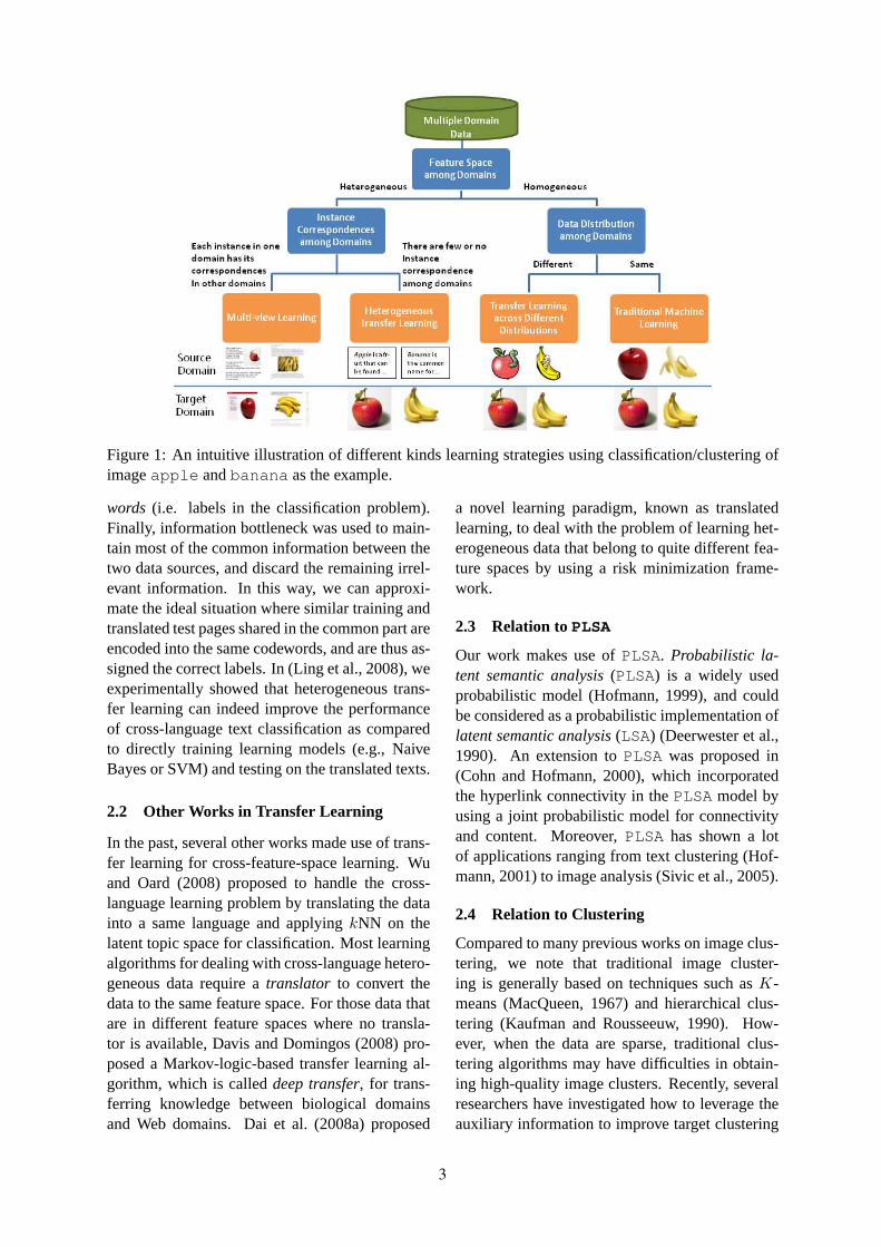
Figure 1: An intuitive illustration of different kinds learning strategies usingclassification/clustering ofimageapple andbanana as the example.
words (i.e. labels in the classification problem).Finally, information bottleneck was used to main-tain most of the common information between thetwo data sources, and discard the remaining irrel-evant information. In this way, we can approxi-mate the ideal situation where similar training andtranslated test pages shared in the common part areencoded into the same codewords, and are thus as-signed the correct labels. In (Ling et al., 2008), weexperimentally showed that heterogeneous trans-fer learning can indeed improve the performanceof cross-language text classification as comparedto directly training learning models (e.g., NaiveBayes or SVM) and testing on the translated texts.
2.2 Other Works in Transfer Learning
In the past, several other works made use of trans-fer learning for cross-feature-space learning. Wuand Oard (2008) proposed to handle the cross-language learning problem by translating the datainto a same language and applyingkNN on thelatent topic space for classification. Most learningalgorithms for dealing with cross-language hetero-geneous data require atranslator to convert thedata to the same feature space. For those data thatare in different feature spaces where no transla-tor is available, Davis and Domingos (2008) pro-posed a Markov-logic-based transfer learning al-gorithm, which is calleddeep transfer, for trans-ferring knowledge between biological domainsand Web domains. Dai et al. (2008a) proposed
a novel learning paradigm, known as translatedlearning, to deal with the problem of learning het-erogeneous data that belong to quite different fea-ture spaces by using a risk minimization frame-work.
2.3 Relation to PLSA
Our work makes use ofPLSA. Probabilistic la-tent semantic analysis(PLSA) is a widely usedprobabilistic model (Hofmann, 1999), and couldbe considered as a probabilistic implementation oflatent semantic analysis(LSA) (Deerwester et al.,1990). An extension toPLSA was proposed in(Cohn and Hofmann, 2000), which incorporatedthe hyperlink connectivity in thePLSA model byusing a joint probabilistic model for connectivityand content. Moreover,PLSA has shown a lotof applications ranging from text clustering (Hof-mann, 2001) to image analysis (Sivic et al., 2005).
2.4 Relation to Clustering
Compared to many previous works on image clus-tering, we note that traditional image cluster-ing is generally based on techniques such asK-means (MacQueen, 1967) and hierarchical clus-tering (Kaufman and Rousseeuw, 1990). How-ever, when the data are sparse, traditional clus-tering algorithms may have difficulties in obtain-ing high-quality image clusters. Recently, severalresearchers have investigated how to leverage theauxiliary information to improve target clustering
3

performance, such as supervised clustering (Fin-ley and Joachims, 2005), semi-supervised cluster-ing (Basu et al., 2004), self-taught clustering (Daiet al., 2008b), etc.
3 Image Clustering with AnnotatedAuxiliary Data
In this section, we present ourannotation-basedprobabilistic latent semantic analysisalgorithm(aPLSA), which extends the traditionalPLSAmodel by incorporating annotated auxiliary im-age data. Intuitively, our algorithmaPLSA per-forms PLSA analysis on the target images, whichare converted to an image instance-to-feature co-occurrence matrix. At the same time, PLSA isalso applied to the annotated image data from so-cial Web, which is converted into a text-to-image-feature co-occurrence matrix. In order to unifythose two separate PLSA models, these two stepsare done simultaneously with common latent vari-ables used as a bridge linking them. Throughthese common latent variables, which are nowconstrained by both target image data and auxil-iary annotation data, a better clustering result isexpected for the target data.
3.1 Probabilistic Latent Semantic Analysis
Let F = {fi}|F|i=1 be an image feature space, and
V = {vi}|V|i=1 be the image data set. Each image
vi ∈ V is represented by abag-of-features{f |f ∈vi ∧ f ∈ F}.
Based on the image data setV, we can esti-mate an image instance-to-feature co-occurrencematrix A|V|×|F| ∈ R
|V|×|F|, where each elementAij (1 ≤ i ≤ |V| and1 ≤ j ≤ |F|) in the matrixA is the frequency of the featurefj appearing inthe instancevi.
LetW = {wi}|W|i=1 be a text feature space. The
annotated image data allow us to obtain the co-occurrence information between imagesv and textfeaturesw ∈ W. An example of annotated im-age data is the Flickr (http://www.flickr.com), which is a social Web site containing a largenumber of annotated images.
By extracting image features from the annotatedimagesv, we can estimate a text-to-image fea-ture co-occurrence matrixB|W|×|F| ∈ R
|W|×|F|,where each elementBij (1 ≤ i ≤ |W| and1 ≤ j ≤ |F|) in the matrixB is the frequencyof the text featurewi and the image featurefj oc-curring together in the annotated image data set.
V Z FP (z|v) P (f |z)
Figure 2: Graphical model representation ofPLSAmodel.
LetZ = {zi}|Z|i=1 be the latent variable set in our
aPLSA model. In clustering, each latent variablezi ∈ Z corresponds to a certain cluster.
Our objective is to estimate a clustering func-tion g : V 7→ Z with the help of the two co-occurrence matricesA andB as defined above.
To formally introduce theaPLSA model, westart from theprobabilistic latent semantic anal-ysis (PLSA) (Hofmann, 1999) model.PLSA isa probabilistic implementation oflatent seman-tic analysis(LSA) (Deerwester et al., 1990). Inour image clustering task,PLSA decomposes theinstance-feature co-occurrence matrixA under theassumption of conditional independence of imageinstancesV and image featuresF , given the latentvariablesZ.
P (f |v) =∑
z∈Z
P (f |z)P (z|v). (1)
The graphical model representation ofPLSA isshown in Figure 2.Based on thePLSA model, the log-likelihood canbe defined as:
L =∑
i
∑
j
Aij∑
j′ Aij′
log P (fj |vi) (2)
whereA|V|×|F| ∈ R|V|×|F| is the image instance-
feature co-occurrence matrix. The termAijP
j′ Aij′
in Equation (2) is a normalization term ensuringeach image is giving the same weight in the log-likelihood.
Using EM algorithm (Dempster et al., 1977),which locally maximizes the log-likelihood ofthePLSA model (Equation (2)), the probabilitiesP (f |z) andP (z|v) can be estimated. Then, theclustering function is derived as
g(v) = argmaxz∈Z
P (z|v). (3)
Due to space limitation, we omit the details for thePLSA model, which can be found in (Hofmann,1999).
3.2 aPLSA: Annotation-based PLSA
In this section, we consider how to incorporatea large number of socially annotated images in a
4

V
W
Z F
P (z|v)
P (z|w)P (f |z)
Figure 3: Graphical model representation ofaPLSA model.
unified PLSA model for the purpose of utilizingthe correlation between text features and imagefeatures. In the auxiliary data, each image has cer-tain textual tags that are attached by users. Thecorrelation between text features and image fea-tures can be formulated as follows.
P (f |w) =∑
z∈Z
P (f |z)P (z|w). (4)
It is clear that Equations (1) and (4) share a sametermP (f |z). So we design a newPLSA model byjoining the probabilistic model in Equation (1) andthe probabilistic model in Equation (4) into a uni-fied model, as shown in Figure 3. In Figure 3, thelatent variablesZ depend not only on the corre-lation between image instancesV and image fea-turesF , but also the correlation between text fea-turesW and image featuresF . Therefore, the aux-iliary socially-annotated image data can be usedto help the target image clustering performance byestimating good set of latent variablesZ.
Based on the graphical model representation inFigure 3, we derive the log-likelihood objectivefunction, in a similar way as in (Cohn and Hof-mann, 2000), as follows
L =∑
j
[
λ∑
i
Aij∑
j′ Aij′
log P (fj |vi)
+(1− λ)∑
l
Blj∑
j′ Blj′
log P (fj |wl)
]
,
(5)
whereA|V|×|F| ∈ R|V|×|F| is the image instance-
feature co-occurrence matrix, andB|W|×|F| ∈R|W|×|F| is the text-to-image feature-level co-
occurrence matrix. Similar to Equation (2),Aij
P
j′ Aij′
and BljP
j′ Blj′
in Equation (5) are the nor-
malization terms to prevent imbalanced cases.Furthermore,λ acts as a trade-off parameter be-
tween the co-occurrence matricesA and B. Inthe extreme case whenλ = 1, the log-likelihoodobjective function ignores all the biases from the
text-to-image occurrence matrixB. In this case,the aPLSA model degenerates to the traditionalPLSA model. Therefore,aPLSA is an extensionto thePLSA model.
Now, the objective is to maximize the log-likelihoodL of theaPLSA model in Equation (5).Then we apply the EM algorithm (Dempster etal., 1977) to estimate the conditional probabilitiesP (f |z), P (z|w) andP (z|v) with respect to eachdependence in Figure 3 as follows.
• E-Step: calculate the posterior probability ofeach latent variablez given the observationof image featuresf , image instancesv andtext featuresw based on the old estimate ofP (f |z), P (z|w) andP (z|v):
P (zk|vi, fj) =P (fj |zk)P (zk|vi)
∑
k′ P (fj |zk′)P (zk′ |vi)
(6)
P (zk|wl, fj) =P (fj |zk)P (zk|wl)
∑
k′ P (fj |zk′)P (zk′ |wl)
(7)
• M-Step: re-estimates conditional probabili-tiesP (zk|vi) andP (zk|wl):
P (zk|vi) =∑
j
Aij∑
j′ Aij′
P (zk|vi, fj) (8)
P (zk|wl) =∑
j
Blj∑
j′ Blj′
P (zk|wl, fj) (9)
and conditional probabilityP (fj |zk), whichis a mixture portion of posterior probabilityof latent variables
P (fj |zk) ∝ λ∑
i
Aij∑
j′ Aij′
P (zk|vi, fj)
+ (1− λ)∑
l
Blj∑
j′ Blj′
P (zk|wl, fj)
(10)
Finally, the clustering function for a certain im-agev is
g(v) = argmaxz∈Z
P (z|v). (11)
From the above equations, we can deriveour annotation-based probabilistic latent semanticanalysis (aPLSA) algorithm. As shown in Algo-rithm 1, aPLSA iteratively performs the E-Stepand the M-Step in order to seek local optimalpoints based on the objective functionL in Equa-tion (5).
5
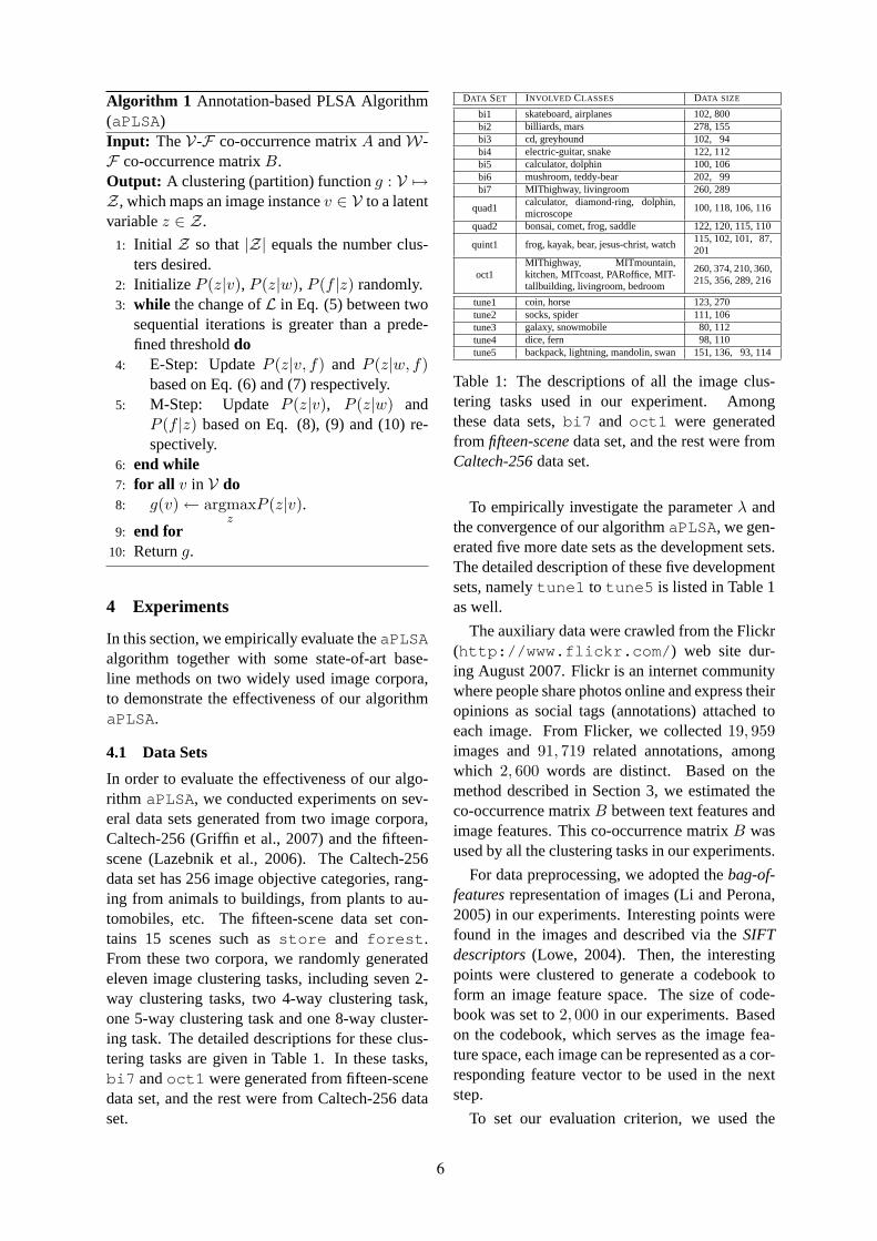
Algorithm 1 Annotation-based PLSA Algorithm(aPLSA)Input: TheV-F co-occurrence matrixA andW-F co-occurrence matrixB.Output: A clustering (partition) functiong : V 7→Z, which maps an image instancev ∈ V to a latentvariablez ∈ Z.
1: Initial Z so that|Z| equals the number clus-ters desired.
2: Initialize P (z|v), P (z|w), P (f |z) randomly.3: while the change ofL in Eq. (5) between two
sequential iterations is greater than a prede-fined thresholddo
4: E-Step: UpdateP (z|v, f) and P (z|w, f)based on Eq. (6) and (7) respectively.
5: M-Step: Update P (z|v), P (z|w) andP (f |z) based on Eq. (8), (9) and (10) re-spectively.
6: end while7: for all v in V do8: g(v)← argmax
zP (z|v).
9: end for10: Returng.
4 Experiments
In this section, we empirically evaluate theaPLSAalgorithm together with some state-of-art base-line methods on two widely used image corpora,to demonstrate the effectiveness of our algorithmaPLSA.
4.1 Data Sets
In order to evaluate the effectiveness of our algo-rithm aPLSA, we conducted experiments on sev-eral data sets generated from two image corpora,Caltech-256 (Griffin et al., 2007) and the fifteen-scene (Lazebnik et al., 2006). The Caltech-256data set has 256 image objective categories, rang-ing from animals to buildings, from plants to au-tomobiles, etc. The fifteen-scene data set con-tains 15 scenes such asstore and forest.From these two corpora, we randomly generatedeleven image clustering tasks, including seven 2-way clustering tasks, two 4-way clustering task,one 5-way clustering task and one 8-way cluster-ing task. The detailed descriptions for these clus-tering tasks are given in Table 1. In these tasks,bi7 andoct1 were generated from fifteen-scenedata set, and the rest were from Caltech-256 dataset.
DATA SET INVOLVED CLASSES DATA SIZE
bi1 skateboard, airplanes 102, 800bi2 billiards, mars 278, 155bi3 cd, greyhound 102, 94bi4 electric-guitar, snake 122, 112bi5 calculator, dolphin 100, 106bi6 mushroom, teddy-bear 202, 99bi7 MIThighway, livingroom 260, 289
quad1calculator, diamond-ring, dolphin,microscope
100, 118, 106, 116
quad2 bonsai, comet, frog, saddle 122, 120, 115, 110
quint1 frog, kayak, bear, jesus-christ, watch115, 102, 101, 87,201
oct1MIThighway, MITmountain,kitchen, MITcoast, PARoffice, MIT-tallbuilding, livingroom, bedroom
260, 374, 210, 360,215, 356, 289, 216
tune1 coin, horse 123, 270tune2 socks, spider 111, 106tune3 galaxy, snowmobile 80, 112tune4 dice, fern 98, 110tune5 backpack, lightning, mandolin, swan 151, 136, 93, 114
Table 1: The descriptions of all the image clus-tering tasks used in our experiment. Amongthese data sets,bi7 and oct1 were generatedfrom fifteen-scenedata set, and the rest were fromCaltech-256data set.
To empirically investigate the parameterλ andthe convergence of our algorithmaPLSA, we gen-erated five more date sets as the development sets.The detailed description of these five developmentsets, namelytune1 to tune5 is listed in Table 1as well.
The auxiliary data were crawled from the Flickr(http://www.flickr.com/) web site dur-ing August 2007. Flickr is an internet communitywhere people share photos online and express theiropinions as social tags (annotations) attached toeach image. From Flicker, we collected19, 959images and91, 719 related annotations, amongwhich 2, 600 words are distinct. Based on themethod described in Section 3, we estimated theco-occurrence matrixB between text features andimage features. This co-occurrence matrixB wasused by all the clustering tasks in our experiments.
For data preprocessing, we adopted thebag-of-featuresrepresentation of images (Li and Perona,2005) in our experiments. Interesting points werefound in the images and described via theSIFTdescriptors(Lowe, 2004). Then, the interestingpoints were clustered to generate a codebook toform an image feature space. The size of code-book was set to2, 000 in our experiments. Basedon the codebook, which serves as the image fea-ture space, each image can be represented as a cor-responding feature vector to be used in the nextstep.
To set our evaluation criterion, we used the
6
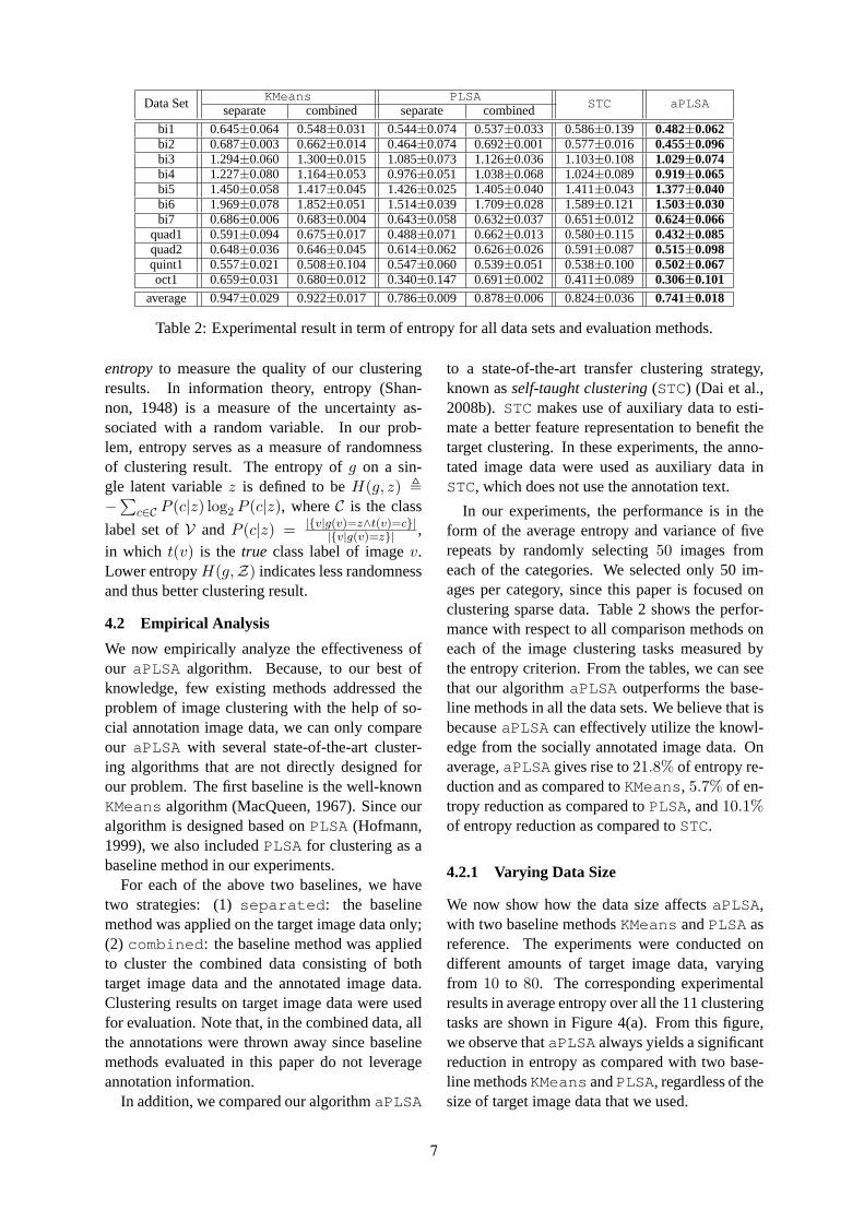
Data Set KMeans PLSASTC aPLSAseparate combined separate combined
bi1 0.645±0.064 0.548±0.031 0.544±0.074 0.537±0.033 0.586±0.139 0.482±0.062bi2 0.687±0.003 0.662±0.014 0.464±0.074 0.692±0.001 0.577±0.016 0.455±0.096bi3 1.294±0.060 1.300±0.015 1.085±0.073 1.126±0.036 1.103±0.108 1.029±0.074bi4 1.227±0.080 1.164±0.053 0.976±0.051 1.038±0.068 1.024±0.089 0.919±0.065bi5 1.450±0.058 1.417±0.045 1.426±0.025 1.405±0.040 1.411±0.043 1.377±0.040bi6 1.969±0.078 1.852±0.051 1.514±0.039 1.709±0.028 1.589±0.121 1.503±0.030bi7 0.686±0.006 0.683±0.004 0.643±0.058 0.632±0.037 0.651±0.012 0.624±0.066
quad1 0.591±0.094 0.675±0.017 0.488±0.071 0.662±0.013 0.580±0.115 0.432±0.085quad2 0.648±0.036 0.646±0.045 0.614±0.062 0.626±0.026 0.591±0.087 0.515±0.098quint1 0.557±0.021 0.508±0.104 0.547±0.060 0.539±0.051 0.538±0.100 0.502±0.067oct1 0.659±0.031 0.680±0.012 0.340±0.147 0.691±0.002 0.411±0.089 0.306±0.101
average 0.947±0.029 0.922±0.017 0.786±0.009 0.878±0.006 0.824±0.036 0.741±0.018
Table 2: Experimental result in term of entropy for all data sets and evaluation methods.
entropy to measure the quality of our clusteringresults. In information theory, entropy (Shan-non, 1948) is a measure of the uncertainty as-sociated with a random variable. In our prob-lem, entropy serves as a measure of randomnessof clustering result. The entropy ofg on a sin-gle latent variablez is defined to beH(g, z) ,
−∑
c∈C P (c|z) log2 P (c|z), whereC is the class
label set ofV and P (c|z) = |{v|g(v)=z∧t(v)=c}||{v|g(v)=z}| ,
in which t(v) is the true class label of imagev.Lower entropyH(g,Z) indicates less randomnessand thus better clustering result.
4.2 Empirical Analysis
We now empirically analyze the effectiveness ofour aPLSA algorithm. Because, to our best ofknowledge, few existing methods addressed theproblem of image clustering with the help of so-cial annotation image data, we can only compareour aPLSA with several state-of-the-art cluster-ing algorithms that are not directly designed forour problem. The first baseline is the well-knownKMeans algorithm (MacQueen, 1967). Since ouralgorithm is designed based onPLSA (Hofmann,1999), we also includedPLSA for clustering as abaseline method in our experiments.
For each of the above two baselines, we havetwo strategies: (1)separated: the baselinemethod was applied on the target image data only;(2) combined: the baseline method was appliedto cluster the combined data consisting of bothtarget image data and the annotated image data.Clustering results on target image data were usedfor evaluation. Note that, in the combined data, allthe annotations were thrown away since baselinemethods evaluated in this paper do not leverageannotation information.
In addition, we compared our algorithmaPLSA
to a state-of-the-art transfer clustering strategy,known asself-taught clustering(STC) (Dai et al.,2008b). STC makes use of auxiliary data to esti-mate a better feature representation to benefit thetarget clustering. In these experiments, the anno-tated image data were used as auxiliary data inSTC, which does not use the annotation text.
In our experiments, the performance is in theform of the average entropy and variance of fiverepeats by randomly selecting50 images fromeach of the categories. We selected only 50 im-ages per category, since this paper is focused onclustering sparse data. Table 2 shows the perfor-mance with respect to all comparison methods oneach of the image clustering tasks measured bythe entropy criterion. From the tables, we can seethat our algorithmaPLSA outperforms the base-line methods in all the data sets. We believe that isbecauseaPLSA can effectively utilize the knowl-edge from the socially annotated image data. Onaverage,aPLSA gives rise to21.8% of entropy re-duction and as compared toKMeans, 5.7% of en-tropy reduction as compared toPLSA, and10.1%of entropy reduction as compared toSTC.
4.2.1 Varying Data Size
We now show how the data size affectsaPLSA,with two baseline methodsKMeans andPLSA asreference. The experiments were conducted ondifferent amounts of target image data, varyingfrom 10 to 80. The corresponding experimentalresults in average entropy over all the 11 clusteringtasks are shown in Figure 4(a). From this figure,we observe thataPLSA always yields a significantreduction in entropy as compared with two base-line methodsKMeans andPLSA, regardless of thesize of target image data that we used.
7
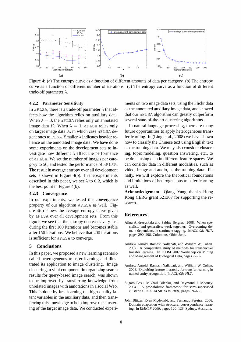
10 20 30 40 50 60 70 800.7
0.75
0.8
0.85
0.9
0.95
1
Data size per category
Ent
ropy
KMeansPLSAaPLSA
(a)
0 0.2 0.4 0.6 0.8 10.4
0.45
0.5
0.55
0.6
0.65
0.7
0.75
λ
Ent
ropy
average over 5 development sets
(b)
0 50 100 150 200 250 3000.5
0.55
0.6
0.65
0.7
0.75
Number of Iteration
Ent
ropy
average over 5 development sets
(c)
Figure 4: (a) The entropy curve as a function of different amounts of data per category. (b) The entropycurve as a function of different number of iterations. (c) The entropy curve as a function of differenttrade-off parameterλ.
4.2.2 Parameter SensitivityIn aPLSA, there is a trade-off parameterλ that af-fects how the algorithm relies on auxiliary data.Whenλ = 0, theaPLSA relies only on annotatedimage dataB. Whenλ = 1, aPLSA relies onlyon target image dataA, in which caseaPLSA de-generates toPLSA. Smallerλ indicates heavier re-liance on the annotated image data. We have donesome experiments on the development sets to in-vestigate how differentλ affect the performanceof aPLSA. We set the number of images per cate-gory to50, and tested the performance ofaPLSA.The result in average entropy over all developmentsets is shown in Figure 4(b). In the experimentsdescribed in this paper, we setλ to 0.2, which isthe best point in Figure 4(b).
4.2.3 ConvergenceIn our experiments, we tested the convergenceproperty of our algorithmaPLSA as well. Fig-ure 4(c) shows the average entropy curve givenby aPLSA over all development sets. From thisfigure, we see that the entropy decreases very fastduring the first100 iterations and becomes stableafter150 iterations. We believe that200 iterationsis sufficient foraPLSA to converge.
5 ConclusionsIn this paper, we proposed a new learning scenariocalled heterogeneous transfer learning and illus-trated its application to image clustering. Imageclustering, a vital component in organizing searchresults for query-based image search, was shownto be improved by transferring knowledge fromunrelated images with annotations in a social Web.This is done by first learning the high-quality la-tent variables in the auxiliary data, and then trans-ferring this knowledge to help improve the cluster-ing of the target image data. We conducted experi-
ments on two image data sets, using the Flickr dataas the annotated auxiliary image data, and showedthat ouraPLSA algorithm can greatly outperformseveral state-of-the-art clustering algorithms.
In natural language processing, there are manyfuture opportunities to apply heterogeneous trans-fer learning. In (Ling et al., 2008) we have shownhow to classify the Chinese text using English textas the training data. We may also consider cluster-ing, topic modeling, question answering, etc., tobe done using data in different feature spaces. Wecan consider data in different modalities, such asvideo, image and audio, as the training data. Fi-nally, we will explore the theoretical foundationsand limitations of heterogeneous transfer learningas well.Acknowledgement Qiang Yang thanks HongKong CERG grant 621307 for supporting the re-search.
References
Alina Andreevskaia and Sabine Bergler. 2008. When spe-cialists and generalists work together: Overcoming do-main dependence in sentiment tagging. InACL-08: HLT,pages 290–298, Columbus, Ohio, June.
Andrew Arnold, Ramesh Nallapati, and William W. Cohen.2007. A comparative study of methods for transductivetransfer learning. In ICDM 2007 Workshop on Miningand Management of Biological Data, pages 77-82.
Andrew Arnold, Ramesh Nallapati, and William W. Cohen.2008. Exploiting feature hierarchy for transfer learning innamed entity recognition. InACL-08: HLT.
Sugato Basu, Mikhail Bilenko, and Raymond J. Mooney.2004. A probabilistic framework for semi-supervisedclustering. InACM SIGKDD 2004, pages 59–68.
John Blitzer, Ryan Mcdonald, and Fernando Pereira. 2006.Domain adaptation with structural correspondence learn-ing. In EMNLP 2006, pages 120–128, Sydney, Australia.
8
John Blitzer, Mark Dredze, and Fernando Pereira. 2007.Biographies, bollywood, boom-boxes and blenders: Do-main adaptation for sentiment classification. InACL 2007,pages 440–447, Prague, Czech Republic.
Avrim Blum and Tom Mitchell. 1998. Combining labeledand unlabeled data with co-training. InCOLT 1998, pages92–100, New York, NY, USA. ACM.
Rich Caruana. 1997. Multitask learning.Machine Learning,28(1):41–75.
Yee Seng Chan and Hwee Tou Ng. 2007. Domain adaptationwith active learning for word sense disambiguation. InACL 2007, Prague, Czech Republic.
David A. Cohn and Thomas Hofmann. 2000. The missinglink - a probabilistic model of document content and hy-pertext connectivity. InNIPS 2000, pages 430–436.
Wenyuan Dai, Yuqiang Chen, Gui-Rong Xue, Qiang Yang,and Yong Yu. 2008a. Translated learning: Transfer learn-ing across different feature spaces. InNIPS 2008, pages353–360.
Wenyuan Dai, Qiang Yang, Gui-Rong Xue, and Yong Yu.2008b. Self-taught clustering. InICML 2008, pages 200–207. Omnipress.
Hal Daume, III. 2007. Frustratingly easy domain adaptation.In ACL 2007, pages 256–263, Prague, Czech Republic.
Jesse Davis and Pedro Domingos. 2008. Deep transfer viasecond-order markov logic. InAAAI 2008 Workshop onTransfer Learning, Chicago, USA.
Scott Deerwester, Susan T. Dumais, George W. Furnas,Thomas K. L, and Richard Harshman. 1990. Indexing bylatent semantic analysis.Journal of the American Societyfor Information Science, pages 391–407.
A. P. Dempster, N. M. Laird, and D. B. Rubin. 1977. Max-imum likelihood from incomplete data via the em algo-rithm. J. of the Royal Statistical Society, 39:1–38.
Thomas Finley and Thorsten Joachims. 2005. Supervisedclustering with support vector machines. InICML 2005,pages 217–224, New York, NY, USA. ACM.
G. Griffin, A. Holub, and P. Perona. 2007. Caltech-256 ob-ject category dataset. Technical Report 7694, CaliforniaInstitute of Technology.
Thomas Hofmann. 1999 Probabilistic latent semantic anal-ysis. In Proc. of Uncertainty in Artificial Intelligence,UAI99. Pages 289–296
Thomas Hofmann. 2001. Unsupervised learning by proba-bilistic latent semantic analysis.Machine Learning. vol-ume 42, number 1-2, pages 177–196. Kluwer AcademicPublishers.
Jing Jiang and Chengxiang Zhai. 2007. Instance weightingfor domain adaptation in NLP. InACL 2007, pages 264–271, Prague, Czech Republic, June.
Leonard Kaufman and Peter J. Rousseeuw. 1990.Findinggroups in data: an introduction to cluster analysis. JohnWiley and Sons, New York.
Svetlana Lazebnik, Cordelia Schmid, and Jean Ponce. 2006.Beyond bags of features: Spatial pyramid matching forrecognizing natural scene categories. InCVPR 2006,pages 2169–2178, Washington, DC, USA.
Fei-Fei Li and Pietro Perona. 2005. A bayesian hierarchi-cal model for learning natural scene categories. InCVPR2005, pages 524–531, Washington, DC, USA.
Xiao Ling, Gui-Rong Xue, Wenyuan Dai, Yun Jiang, QiangYang, and Yong Yu. 2008. Can chinese web pages beclassified with english data source? InWWW 2008, pages969–978, New York, NY, USA. ACM.
Nicolas Loeff, Cecilia Ovesdotter Alm, and David A.Forsyth. 2006. Discriminating image senses by clusteringwith multimodal features. InCOLING/ACL 2006 Mainconference poster sessions, pages 547–554.
David G. Lowe. 2004. Distinctive image features from scale-invariant keypoints. International Journal of ComputerVision (IJCV) 2004, volume 60, number 2, pages 91–110.
J. B. MacQueen. 1967. Some methods for classification andanalysis of multivariate observations. InProceedings ofFifth Berkeley Symposium on Mathematical Statistics andProbability, pages 1:281–297, Berkeley, CA, USA.
Kamal Nigam and Rayid Ghani. 2000. Analyzing the effec-tiveness and applicability of co-training. InProceedingsof the Ninth International Conference on Information andKnowledge Management, pages 86–93, New York, USA.
Rajat Raina, Alexis Battle, Honglak Lee, Benjamin Packer,and Andrew Y. Ng. 2007. Self-taught learning: transferlearning from unlabeled data. InICML 2007, pages 759–766, New York, NY, USA. ACM.
Roi Reichart and Ari Rappoport. 2007. Self-training forenhancement and domain adaptation of statistical parserstrained on small datasets. InACL 2007.
Roi Reichart, Katrin Tomanek, Udo Hahn, and Ari Rap-poport. 2008. Multi-task active learning for linguisticannotations. InACL-08: HLT, pages 861–869.
C. E. Shannon. 1948. A mathematical theory of communi-cation.Bell system technical journal, 27.
J. Sivic, B. C. Russell, A. A. Efros, A. Zisserman, and W. T.Freeman. 2005. Discovering object categories in imagecollections. InICCV 2005.
Naftali Tishby, Fernando C. Pereira, and William Bialek. Theinformation bottleneck method. 1999. InProc. of the 37-th Annual Allerton Conference on Communication, Con-trol and Computing, pages 368–377.
Pengcheng Wu and Thomas G. Dietterich. 2004. Improvingsvm accuracy by training on auxiliary data sources. InICML 2004, pages 110–117, New York, NY, USA.
Yejun Wu and Douglas W. Oard. 2008. Bilingual topic as-pect classification with a few training examples. InACMSIGIR 2008, pages 203–210, New York, NY, USA.
Xiaojin Zhu. 2007. Semi-supervised learning literature sur-vey. Technical Report 1530, Computer Sciences, Univer-sity of Wisconsin-Madison.
9
Proceedings of the 47th Annual Meeting of the ACL and the 4th IJCNLP of the AFNLP, pages 10–18,Suntec, Singapore, 2-7 August 2009. c©2009 ACL and AFNLP
Investigations on Word Senses and Word Usages
Katrin ErkUniversity of Texas at [email protected]
Diana McCarthyUniversity of [email protected]
Nicholas GaylordUniversity of Texas at [email protected]
AbstractThe vast majority of work on word senseshas relied on predefined sense invento-ries and an annotation schema where eachword instance is tagged with the best fit-ting sense. This paper examines the casefor a graded notion of word meaning intwo experiments, one which uses WordNetsenses in a graded fashion, contrasted withthe “winner takes all” annotation, and onewhich asks annotators to judge the similar-ity of two usages. We find that the gradedresponses correlate with annotations fromprevious datasets, but sense assignmentsare used in a way that weakens the case forclear cut sense boundaries. The responsesfrom both experiments correlate with theoverlap of paraphrases from the Englishlexical substitution task which bodes wellfor the use of substitutes as a proxy forword sense. This paper also provides twonovel datasets which can be used for eval-uating computational systems.
1 Introduction
The vast majority of work on word sense tag-ging has assumed that predefined word sensesfrom a dictionary are an adequate proxy for thetask, although of course there are issues withthis enterprise both in terms of cognitive valid-ity (Hanks, 2000; Kilgarriff, 1997; Kilgarriff,2006) and adequacy for computational linguis-tics applications (Kilgarriff, 2006). Furthermore,given a predefined list of senses, annotation effortsand computational approaches to word sense dis-ambiguation (WSD) have usually assumed that onebest fitting sense should be selected for each us-age. While there is usually some allowance made
for multiple senses, this is typically not adopted byannotators or computational systems.
Research on the psychology of concepts (Mur-phy, 2002; Hampton, 2007) shows that categoriesin the human mind are not simply sets with clear-cut boundaries: Some items are perceived asmore typical than others (Rosch, 1975; Rosch andMervis, 1975), and there are borderline cases onwhich people disagree more often, and on whosecategorization they are more likely to change theirminds (Hampton, 1979; McCloskey and Glucks-berg, 1978). Word meanings are certainly relatedto mental concepts (Murphy, 2002). This raisesthe question of whether there is any such thing asthe one appropriate sense for a given occurrence.
In this paper we will explore using graded re-sponses for sense tagging within a novel annota-tion paradigm. Modeling the annotation frame-work after psycholinguistic experiments, we donot train annotators to conform to sense distinc-tions; rather we assess individual differences byasking annotators to produce graded ratings in-stead of making a binary choice. We perform twoannotation studies. In the first one, referred toas WSsim (Word Sense Similarity), annotatorsgive graded ratings on the applicability of Word-Net senses. In the second one, Usim (Usage Sim-ilarity), annotators rate the similarity of pairs ofoccurrences (usages) of a common target word.Both studies explore whether users make use ofa graded scale or persist in making binary deci-sions even when there is the option for a gradedresponse. The first study additionally tests to whatextent the judgments on WordNet senses fall intoclear-cut clusters, while the second study allowsus to explore meaning similarity independently ofany lexicon resource.
10
2 Related Work
Manual word sense assignment is difficult forhuman annotators (Krishnamurthy and Nicholls,2000). Reported inter-annotator agreement (ITA)for fine-grained word sense assignment tasks hasranged between 69% (Kilgarriff and Rosenzweig,2000) for a lexical sample using the HECTOR dic-tionary and 78.6.% using WordNet (Landes et al.,1998) in all-words annotation. The use of morecoarse-grained senses alleviates the problem: InOntoNotes (Hovy et al., 2006), an ITA of 90% isused as the criterion for the construction of coarse-grained sense distinctions. However, intriguingly,for some high-frequency lemmas such as leavethis ITA threshold is not reached even after mul-tiple re-partitionings of the semantic space (Chenand Palmer, 2009). Similarly, the performanceof WSD systems clearly indicates that WSD is noteasy unless one adopts a coarse-grained approach,and then systems tagging all words at best performa few percentage points above the most frequentsense heuristic (Navigli et al., 2007). Good perfor-mance on coarse-grained sense distinctions maybe more useful in applications than poor perfor-mance on fine-grained distinctions (Ide and Wilks,2006) but we do not know this yet and there issome evidence to the contrary (Stokoe, 2005).
Rather than focus on the granularity of clus-ters, the approach we will take in this paperis to examine the phenomenon of word mean-ing both with and without recourse to predefinedsenses by focusing on the similarity of uses of aword. Human subjects show excellent agreementon judging word similarity out of context (Ruben-stein and Goodenough, 1965; Miller and Charles,1991), and human judgments have previously beenused successfully to study synonymy and near-synonymy (Miller and Charles, 1991; Bybee andEddington, 2006). We focus on polysemy ratherthan synonymy. Our aim will be to use WSsimto determine to what extent annotations form co-hesive clusters. In principle, it should be possi-ble to use existing sense-annotated data to explorethis question: almost all sense annotation effortshave allowed annotators to assign multiple sensesto a single occurrence, and the distribution of thesesense labels should indicate whether annotatorsviewed the senses as disjoint or not. However,the percentage of markables that received multi-ple sense labels in existing corpora is small, and itvaries massively between corpora: In the SemCor
corpus (Landes et al., 1998), only 0.3% of allmarkables received multiple sense labels. In theSENSEVAL-3 English lexical task corpus (Mihal-cea et al., 2004) (hereafter referred to as SE-3), theratio is much higher at 8% of all markables1. Thiscould mean annotators feel that there is usually asingle applicable sense, or it could point to a biastowards single-sense assignment in the annotationguidelines and/or the annotation tool. The WSsimexperiment that we report in this paper is designedto eliminate such bias as far as possible and weconduct it on data taken from SemCor and SE-3 sothat we can compare the annotations. Although weuse WordNet for the annotation, our study is not astudy of WordNet per se. We choose WordNet be-cause it is sufficiently fine-grained to examine sub-tle differences in usage, and because traditionallyannotated datasets exist to which we can compareour results.
Predefined dictionaries and lexical resources arenot the only possibilities for annotating lexicalitems with meaning. In cross-lingual settings, theactual translations of a word can be taken as thesense labels (Resnik and Yarowsky, 2000). Re-cently, McCarthy and Navigli (2007) proposedthe English Lexical Substitution task (hereafterreferred to as LEXSUB) under the auspices ofSemEval-2007. It uses paraphrases for words incontext as a way of annotating meaning. The taskwas proposed following a background of discus-sions in the WSD community as to the adequacyof predefined word senses. The LEXSUB datasetcomprises open class words (nouns, verbs, adjec-tives and adverbs) with token instances of eachword appearing in the context of one sentencetaken from the English Internet Corpus (Sharoff,2006). The methodology can only work wherethere are paraphrases, so the dataset only containswords with more than one meaning where at leasttwo different meanings have near synonyms. Formeanings without obvious substitutes the annota-tors were allowed to use multiword paraphrases orwords with slightly more general meanings. Thisdataset has been used to evaluate automatic sys-tems which can find substitutes appropriate for thecontext. To the best of our knowledge there hasbeen no study of how the data collected relates toword sense annotations or judgments of semanticsimilarity. In this paper we examine these relation-
1This is even though both annotation efforts use balancedcorpora, the Brown corpus in the case of SemCor, the BritishNational Corpus for SE-3.
11

ships by re-using data from LEXSUB in both newannotation experiments and testing the results forcorrelation.
3 Annotation
We conducted two experiments through an on-line annotation interface. Three annotators partic-ipated in each experiment; all were native BritishEnglish speakers. The first experiment, WSsim,collected annotator judgments about the applica-bility of dictionary senses using a 5-point ratingscale. The second, Usim, also utilized a 5-pointscale but collected judgments on the similarity inmeaning between two uses of a word. 2 The scalewas 1 – completely different, 2 – mostly different,3 – similar, 4 – very similar and 5 – identical. InUsim, this scale rated the similarity of the two usesof the common target word; in WSsim it rated thesimilarity between the use of the target word andthe sense description. In both experiments, the an-notation interface allowed annotators to revisit andchange previously supplied judgments, and a com-ment box was provided alongside each item.
WSsim. This experiment contained a total of430 sentences spanning 11 lemmas (nouns, verbsand adjectives). For 8 of these lemmas, 50 sen-tences were included, 25 of them randomly sam-pled from SemCor 3 and 25 randomly sampledfrom SE-3.4 The remaining 3 lemmas in the ex-periment each had 10 sentences taken from theLEXSUB data.
WSsim is a word sense annotation task usingWordNet senses.5 Unlike previous word sense an-notation projects, we asked annotators to providejudgments on the applicability of every WordNetsense of the target lemma with the instruction: 6
2Throughout this paper, a target word is assumed to be aword in a given PoS.
3The SemCor dataset was produced alongside WordNet,so it can be expected to support the WordNet sense distinc-tions. The same cannot be said for SE-3.
4Sentence fragments and sentences with 5 or fewer wordswere excluded from the sampling. Annotators were giventhe sentences, but not the original annotation from these re-sources.
5WordNet 1.7.1 was used in the annotation of both SE-3and SemCor; we used the more current WordNet 3.0 afterverifying that the lemmas included in this experiment had thesame senses listed in both versions. Care was taken addition-ally to ensure that senses were not presented in an order thatreflected their frequency of occurrence.
6The guidelines for both experiments are avail-able at http://comp.ling.utexas.edu/people/katrin erk/graded sense and usageannotation
Your task is to rate, for each of these descriptions,how well they reflect the meaning of the boldfacedword in the sentence.Applicability judgments were not binary, but wereinstead collected using the five-point scale givenabove which allowed annotators to indicate notonly whether a given sense applied, but to whatdegree. Each annotator annotated each of the 430items. By having multiple annotators per item anda graded, non-binary annotation scheme we al-low for and measure differences between annota-tors, rather than training annotators to conform toa common sense distinction guideline. By askingannotators to provide ratings for each individualsense, we strive to eliminate all bias towards eithersingle-sense or multiple-sense assignment. In tra-ditional word sense annotation, such bias could beintroduced directly through annotation guidelinesor indirectly, through tools that make it easier toassign fewer senses. We focus not on finding thebest fitting sense but collect judgments on the ap-plicability of all senses.
Usim. This experiment used data from LEXSUB.For more information on LEXSUB, see McCarthyand Navigli (2007). 34 lemmas (nouns, verbs, ad-jectives and adverbs) were manually selected, in-cluding the 3 lemmas also used in WSsim. We se-lected lemmas which exhibited a range of mean-ings and substitutes in the LEXSUB data, withas few multiword substitutes as possible. Eachlemma is the target in 10 LEXSUB sentences. Forour experiment, we took every possible pairwisecomparison of these 10 sentences for a lemma. Werefer to each such pair of sentences as an SPAIR.The resulting dataset comprised 45 SPAIRs perlemma, adding up to 1530 comparisons per anno-tator overall.
In this annotation experiment, annotators sawSPAIRs with a common target word and rated thesimilarity in meaning between the two uses of thetarget word with the instruction:Your task is to rate, for each pair of sentences, howsimilar in meaning the two boldfaced words are ona five-point scale.In addition annotators had the ability to respondwith “Cannot Decide”, indicating that they wereunable to make an effective comparison betweenthe two contexts, for example because the mean-ing of one usage was unclear. This occurred in9 paired occurrences during the course of anno-tation, and these items (paired occurrences) were
12
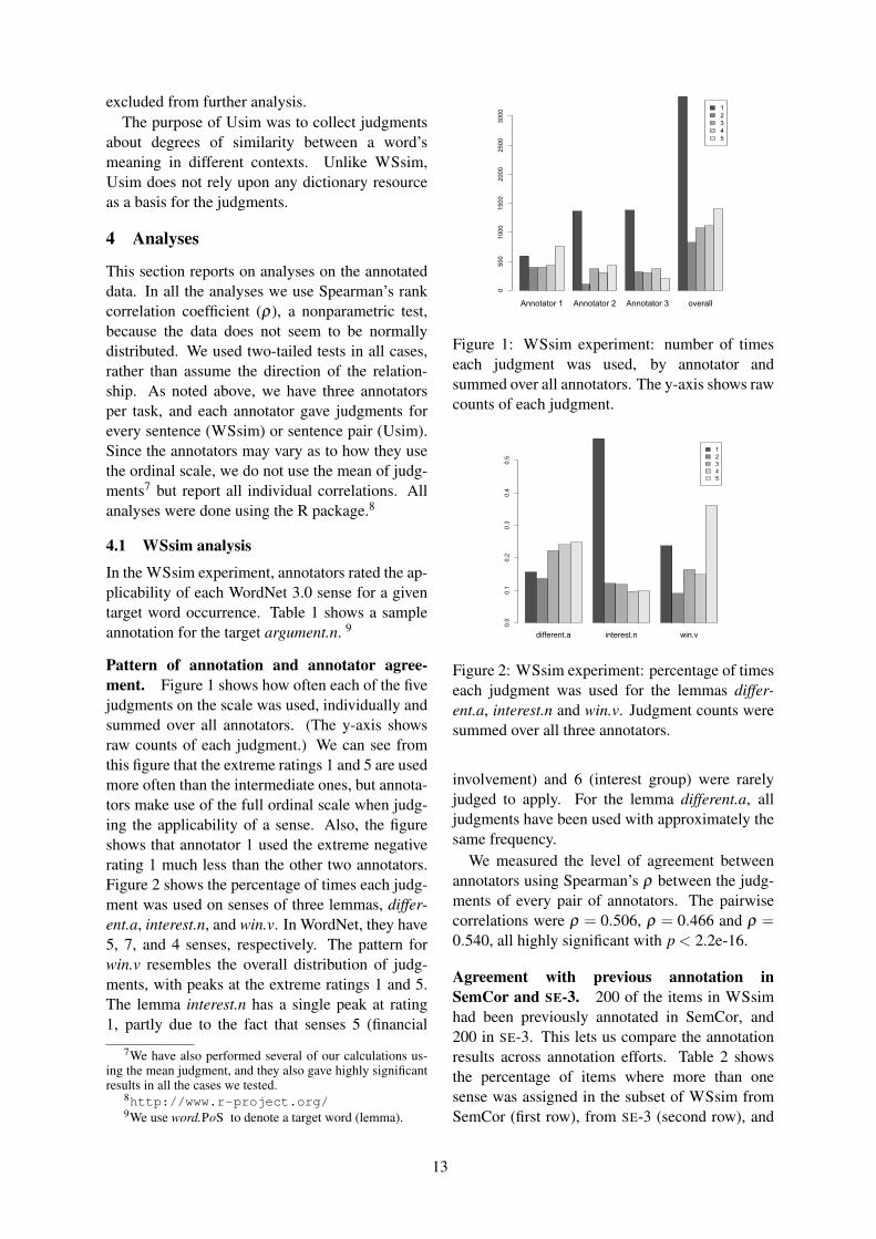
excluded from further analysis.The purpose of Usim was to collect judgments
about degrees of similarity between a word’smeaning in different contexts. Unlike WSsim,Usim does not rely upon any dictionary resourceas a basis for the judgments.
4 Analyses
This section reports on analyses on the annotateddata. In all the analyses we use Spearman’s rankcorrelation coefficient (ρ), a nonparametric test,because the data does not seem to be normallydistributed. We used two-tailed tests in all cases,rather than assume the direction of the relation-ship. As noted above, we have three annotatorsper task, and each annotator gave judgments forevery sentence (WSsim) or sentence pair (Usim).Since the annotators may vary as to how they usethe ordinal scale, we do not use the mean of judg-ments7 but report all individual correlations. Allanalyses were done using the R package.8
4.1 WSsim analysis
In the WSsim experiment, annotators rated the ap-plicability of each WordNet 3.0 sense for a giventarget word occurrence. Table 1 shows a sampleannotation for the target argument.n. 9
Pattern of annotation and annotator agree-ment. Figure 1 shows how often each of the fivejudgments on the scale was used, individually andsummed over all annotators. (The y-axis showsraw counts of each judgment.) We can see fromthis figure that the extreme ratings 1 and 5 are usedmore often than the intermediate ones, but annota-tors make use of the full ordinal scale when judg-ing the applicability of a sense. Also, the figureshows that annotator 1 used the extreme negativerating 1 much less than the other two annotators.Figure 2 shows the percentage of times each judg-ment was used on senses of three lemmas, differ-ent.a, interest.n, and win.v. In WordNet, they have5, 7, and 4 senses, respectively. The pattern forwin.v resembles the overall distribution of judg-ments, with peaks at the extreme ratings 1 and 5.The lemma interest.n has a single peak at rating1, partly due to the fact that senses 5 (financial
7We have also performed several of our calculations us-ing the mean judgment, and they also gave highly significantresults in all the cases we tested.
8http://www.r-project.org/9We use word.PoS to denote a target word (lemma).
Annotator 1 Annotator 2 Annotator 3 overall
1
2
3
4
5
0500
1000
1500
2000
2500
3000
Figure 1: WSsim experiment: number of timeseach judgment was used, by annotator andsummed over all annotators. The y-axis shows rawcounts of each judgment.
different.a interest.n win.v
1
2
3
4
5
0.0
0.1
0.2
0.3
0.4
0.5
Figure 2: WSsim experiment: percentage of timeseach judgment was used for the lemmas differ-ent.a, interest.n and win.v. Judgment counts weresummed over all three annotators.
involvement) and 6 (interest group) were rarelyjudged to apply. For the lemma different.a, alljudgments have been used with approximately thesame frequency.
We measured the level of agreement betweenannotators using Spearman’s ρ between the judg-ments of every pair of annotators. The pairwisecorrelations were ρ = 0.506, ρ = 0.466 and ρ =0.540, all highly significant with p < 2.2e-16.
Agreement with previous annotation inSemCor and SE-3. 200 of the items in WSsimhad been previously annotated in SemCor, and200 in SE-3. This lets us compare the annotationresults across annotation efforts. Table 2 showsthe percentage of items where more than onesense was assigned in the subset of WSsim fromSemCor (first row), from SE-3 (second row), and
13

SensesSentence 1 2 3 4 5 6 7 AnnotatorThis question provoked arguments in America about theNorton Anthology of Literature by Women, some of thecontents of which were said to have had little value asliterature.
1 4 4 2 1 1 3 Ann. 14 5 4 2 1 1 4 Ann. 21 4 5 1 1 1 1 Ann. 3
Table 1: A sample annotation in the WSsim experiment. The senses are: 1:statement, 2:controversy,3:debate, 4:literary argument, 5:parameter, 6:variable, 7:line of reasoning
WSsim judgmentData Orig. ≥ 3 ≥ 4 5WSsim/SemCor 0.0 80.2 57.5 28.3WSsim/SE-3 24.0 78.0 58.3 27.1All WSsim 78.8 57.4 27.7
Table 2: Percentage of items with multiple sensesassigned. Orig: in the original SemCor/SE-3 data.WSsim judgment: items with judgments at orabove the specified threshold. The percentages forWSsim are averaged over the three annotators.
all of WSsim (third row). The Orig. columnindicates how many items had multiple labels inthe original annotation (SemCor or SE-3) 10. Notethat no item had more than one sense label inSemCor. The columns under WSsim judgmentshow the percentage of items (averaged overthe three annotators) that had judgments at orabove the specified threshold, starting from rating3 – similar. Within WSsim, the percentage ofmultiple assignments in the three rows is fairlyconstant. WSsim avoids the bias to one senseby deliberately asking for judgments on theapplicability of each sense rather than askingannotators to find the best one.
To compute the Spearman’s correlation betweenthe original sense labels and those given in theWSsim annotation, we converted SemCor andSE-3 labels to the format used within WSsim: As-signed senses were converted to a judgment of 5,and unassigned senses to a judgment of 1. For theWSsim/SemCor dataset, the correlation betweenoriginal and WSsim annotation was ρ = 0.234,ρ = 0.448, and ρ = 0.390 for the three anno-tators, each highly significant with p < 2.2e-16.For the WSsim/SE-3 dataset, the correlations wereρ = 0.346, ρ = 0.449 and ρ = 0.338, each of themagain highly significant at p < 2.2e-16.
Degree of sense grouping. Next we test to whatextent the sense applicability judgments in the
10Overall, 0.3% of tokens in SemCor have multiple labels,and 8% of tokens in SE-3, so the multiple label assignment inour sample is not an underestimate.
p < 0.05 p < 0.01pos neg pos neg
Ann. 1 30.8 11.4 23.2 5.9Ann. 2 22.2 24.1 19.6 19.6Ann. 3 12.7 12.0 10.0 6.0
Table 3: Percentage of sense pairs that were sig-nificantly positively (pos) or negatively (neg) cor-related at p < 0.05 and p < 0.01, shown by anno-tator.
j ≥ 3 j ≥ 4 j = 5Ann. 1 71.9 49.1 8.1Ann. 2 55.3 24.7 8.1Ann. 3 42.8 24.0 4.9
Table 4: Percentage of sentences in which at leasttwo uncorrelated (p > 0.05) or negatively corre-lated senses have been annotated with judgmentsat the specified threshold.
WSsim task could be explained by more coarse-grained, categorial sense assignments. We firsttest how many pairs of senses for a given lemmashow similar patterns in the ratings that they re-ceive. Table 3 shows the percentage of sense pairsthat were significantly correlated for each anno-tator.11 Significantly positively correlated sensescan possibly be reduced to more coarse-grainedsenses. Would annotators have been able to des-ignate a single appropriate sense given these morecoarse-grained senses? Call two senses groupableif they are significantly positively correlated; in or-der not to overlook correlations that are relativelyweak but existent, we use a cutoff of p = 0.05 forsignificant correlation. We tested how often anno-tators gave ratings of at least similar, i.e. ratings≥ 3, to senses that were not groupable. Table 4shows the percentages of items where at least twonon-groupable senses received ratings at or abovethe specified threshold. The table shows that re-gardless of which annotator we look at, over 40%of all items had two or more non-groupable sensesreceive judgments of at least 3 (similar). There
11We exclude senses that received a uniform rating of 1 onall items. This concerned 4 senses for annotator 2 and 6 forannotator 3.
14

1) We study the methods and concepts that each writer uses todefend the cogency of legal, deliberative, or more generallypolitical prudence against explicit or implicit charges thatpractical thinking is merely a knack or form of cleverness.
2) Eleven CIRA members have been convicted of criminal
charges and others are awaiting trial.
Figure 3: An SPAIR for charge.n. Annotator judg-ments: 2,3,4
were even several items where two or more non-groupable senses each got a judgment of 5. Thesentence in table 1 is a case where several non-groupable senses got ratings ≥ 3. This is mostpronounced for Annotator 2, who along with sense2 (controversy) assigned senses 1 (statement), 7(line of reasoning), and 3 (debate), none of whichare groupable with sense 2.
4.2 Usim analysis
In this experiment, ratings between 1 and 5 weregiven for every pairwise combination of sentencesfor each target lemma. An example of an SPAIR
for charge.n is shown in figure 3. In this case theverdicts from the annotators were 2, 3 and 4.
Pattern of Annotations and Annotator Agree-ment Figure 4 gives a bar chart of the judgmentsfor each annotator and summed over annotators.We can see from this figure that the annotatorsuse the full ordinal scale when judging the simi-larity of a word’s usages, rather than sticking tothe extremes. There is variation across words, de-pending on the relatedness of each word’s usages.Figure 5 shows the judgments for the words bar.n,work.v and raw.a. We see that bar.n has predom-inantly different usages with a peak for category1, work.v has more similar judgments (category 5)compared to any other category and raw.a has apeak in the middle category (3). 12 There are otherwords, like for example fresh.a, where the spreadis more uniform.
To gauge the level of agreement between anno-tators, we calculated Spearman’s ρ between thejudgments of every pair of annotators as in sec-tion 4.1. The pairwise correlations are all highlysignificant (p < 2.2e-16) with Spearman’s ρ =0.502, 0.641 and 0.501 giving an average corre-lation of 0.548. We also perform leave-one-out re-sampling following Lapata (2006) which gave usa Spearman’s correlation of 0.630.
12For figure 5 we sum the judgments over annotators.
Annotator 4 Annotator 5 Annotator 6 overall
12345
050
010
0015
00
Figure 4: Usim experiment: number of times eachjudgment was used, by annotator and summedover all annotators
bar.n raw.a work.v
12345
010
2030
4050
60
Figure 5: Usim experiment: number of times eachjudgment was used for bar.n, work.v and raw.a
Comparison with LEXSUB substitutions Nextwe look at whether the Usim judgments on sen-tence pairs (SPAIRs) correlate with LEXSUB sub-stitutes. To do this we use the overlap of substi-tutes provided by the five LEXSUB annotators be-tween two sentences in an SPAIR. In LEXSUB theannotators had to replace each item (a target wordwithin the context of a sentence) with a substitutethat fitted the context. Each annotator was permit-ted to supply up to three substitutes provided thatthey all fitted the context equally. There were 10sentences per lemma. For our analyses we takeevery SPAIR for a given lemma and calculate theoverlap (inter) of the substitutes provided by theannotators for the two usages under scrutiny. Lets1 and s2 be a pair of sentences in an SPAIR and
15

x1 and x2 be the multisets of substitutes for therespective sentences. Let f req(w,x) be the fre-quency of a substitute w in a multiset x of sub-stitutes for a given sentence. 13 INTER(s1,s2) =
∑w∈x1∩x2 min( f req(w,x1), f req(w,x2))max(|x1|, |x2|)
Using this calculation for each SPAIR we cannow compute the correlation between the Usimjudgments for each annotator and the INTER val-ues, again using Spearman’s. The figures areshown in the leftmost block of table 5. The av-erage correlation for the 3 annotators was 0.488and the p-values were all < 2.2e-16. This showsa highly significant correlation of the Usim judg-ments and the overlap of substitutes.
We also compare the WSsim judgments againstthe LEXSUB substitutes, again using the INTER
measure of substitute overlap. For this analysis,we only use those WSsim sentences that are origi-nally from LEXSUB. In WSsim, the judgments fora sentence comprise judgments for each WordNetsense of that sentence. In order to compare againstINTER, we need to transform these sentence-wiseratings in WSsim to a WSsim-based judgment ofsentence similarity. To this end, we compute theEuclidean Distance14 (ED) between two vectors J1and J2 of judgments for two sentences s1,s2 for thesame lemma `. Each of the n indexes of the vectorrepresent one of the n different WordNet sensesfor `. The value at entry i of the vector J1 is thejudgment that the annotator in question (we do notaverage over annotators here) provided for sense iof ` for sentence s1.
ED(J1,J2) =√
(n
∑i=1
(J1[i]− J2[i])2) (1)
We correlate the Euclidean distances withINTER. We can only test correlation for the subsetof WSsim that overlaps with the LEXSUB data: the30 sentences for investigator.n, function.n and or-der.v, which together give 135 unique SPAIRs. Werefer to this subset as W∩U. The results are givenin the third block of table 5. Note that since we aremeasuring distance between SPAIRs for WSsim
13The frequency of a substitute in a multiset depends onthe number of LEXSUB annotators that picked the substitutefor this item.
14We use Euclidean Distance rather than a normalizingmeasure like Cosine because a sentence where all ratings are5 should be very different from a sentence where all sensesreceived a rating of 1.
Usim All Usim W∩U WSsim W∩Uann. ρ ρ ann. ρ
4 0.383 0.330 1 -0.5205 0.498 0.635 2 -0.5036 0.584 0.631 3 -0.463
Table 5: Annotator correlation with LEXSUB sub-stitute overlap (inter)
whereas INTER is a measure of similarity, the cor-relation is negative. The results are highly signif-icant with individual p-values from < 1.067e-10to < 1.551e-08 and a mean correlation of -0.495.The results in the first and third block of table 5 arenot directly comparable, as the results in the firstblock are for all Usim data and not the subset ofLEXSUB with WSsim annotations. We thereforerepeated the analysis for Usim on the subset ofdata in WSsim and provide the correlation in themiddle section of table 5. The mean correlationfor Usim on this subset of the data is 0.532, whichis a stronger relationship compared to WSsim, al-though there is more discrepancy between individ-ual annotators, with the result for annotator 4 giv-ing a p-value = 9.139e-05 while the other two an-notators had p-values < 2.2e-16.
The LEXSUB substitute overlaps between dif-ferent usages correlate well with both Usim andWSsim judgments, with a slightly stronger rela-tionship to Usim, perhaps due to the more compli-cated representation of word meaning in WSsimwhich uses the full set of WordNet senses.
4.3 Correlation between WSsim and Usim
As we showed in section 4.1, WSsim correlateswith previous word sense annotations in SemCorand SE-3 while allowing the user a more gradedresponse to sense tagging. As we saw in sec-tion 4.2, Usim and WSsim judgments both have ahighly significant correlation with similarity of us-ages as measured using the overlap of substitutesfrom LEXSUB. Here, we look at the correlationof WSsim and Usim, considering again the sub-set of data that is common to both experiments.We again transform WSsim sense judgments forindividual sentences to distances between SPAIRsusing Euclidean Distance (ED). The Spearman’sρ range between −0.307 and −0.671, and all re-sults are highly significant with p-values between0.0003 and < 2.2e-16. As above, the correla-tion is negative because ED is a distance measurebetween sentences in an SPAIR, whereas the judg-
16
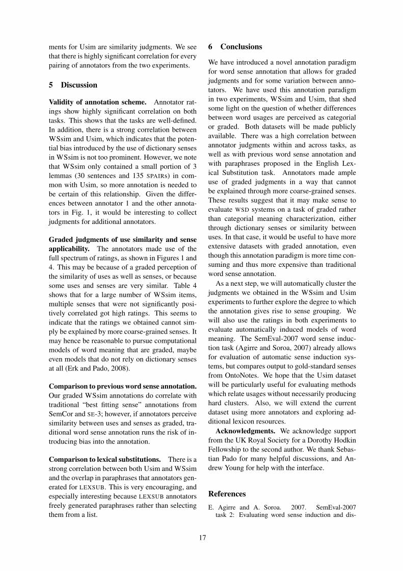
ments for Usim are similarity judgments. We seethat there is highly significant correlation for everypairing of annotators from the two experiments.
5 Discussion
Validity of annotation scheme. Annotator rat-ings show highly significant correlation on bothtasks. This shows that the tasks are well-defined.In addition, there is a strong correlation betweenWSsim and Usim, which indicates that the poten-tial bias introduced by the use of dictionary sensesin WSsim is not too prominent. However, we notethat WSsim only contained a small portion of 3lemmas (30 sentences and 135 SPAIRs) in com-mon with Usim, so more annotation is needed tobe certain of this relationship. Given the differ-ences between annotator 1 and the other annota-tors in Fig. 1, it would be interesting to collectjudgments for additional annotators.
Graded judgments of use similarity and senseapplicability. The annotators made use of thefull spectrum of ratings, as shown in Figures 1 and4. This may be because of a graded perception ofthe similarity of uses as well as senses, or becausesome uses and senses are very similar. Table 4shows that for a large number of WSsim items,multiple senses that were not significantly posi-tively correlated got high ratings. This seems toindicate that the ratings we obtained cannot sim-ply be explained by more coarse-grained senses. Itmay hence be reasonable to pursue computationalmodels of word meaning that are graded, maybeeven models that do not rely on dictionary sensesat all (Erk and Pado, 2008).
Comparison to previous word sense annotation.Our graded WSsim annotations do correlate withtraditional “best fitting sense” annotations fromSemCor and SE-3; however, if annotators perceivesimilarity between uses and senses as graded, tra-ditional word sense annotation runs the risk of in-troducing bias into the annotation.
Comparison to lexical substitutions. There is astrong correlation between both Usim and WSsimand the overlap in paraphrases that annotators gen-erated for LEXSUB. This is very encouraging, andespecially interesting because LEXSUB annotatorsfreely generated paraphrases rather than selectingthem from a list.
6 Conclusions
We have introduced a novel annotation paradigmfor word sense annotation that allows for gradedjudgments and for some variation between anno-tators. We have used this annotation paradigmin two experiments, WSsim and Usim, that shedsome light on the question of whether differencesbetween word usages are perceived as categorialor graded. Both datasets will be made publiclyavailable. There was a high correlation betweenannotator judgments within and across tasks, aswell as with previous word sense annotation andwith paraphrases proposed in the English Lex-ical Substitution task. Annotators made ampleuse of graded judgments in a way that cannotbe explained through more coarse-grained senses.These results suggest that it may make sense toevaluate WSD systems on a task of graded ratherthan categorial meaning characterization, eitherthrough dictionary senses or similarity betweenuses. In that case, it would be useful to have moreextensive datasets with graded annotation, eventhough this annotation paradigm is more time con-suming and thus more expensive than traditionalword sense annotation.
As a next step, we will automatically cluster thejudgments we obtained in the WSsim and Usimexperiments to further explore the degree to whichthe annotation gives rise to sense grouping. Wewill also use the ratings in both experiments toevaluate automatically induced models of wordmeaning. The SemEval-2007 word sense induc-tion task (Agirre and Soroa, 2007) already allowsfor evaluation of automatic sense induction sys-tems, but compares output to gold-standard sensesfrom OntoNotes. We hope that the Usim datasetwill be particularly useful for evaluating methodswhich relate usages without necessarily producinghard clusters. Also, we will extend the currentdataset using more annotators and exploring ad-ditional lexicon resources.
Acknowledgments. We acknowledge supportfrom the UK Royal Society for a Dorothy HodkinFellowship to the second author. We thank Sebas-tian Pado for many helpful discussions, and An-drew Young for help with the interface.
ReferencesE. Agirre and A. Soroa. 2007. SemEval-2007
task 2: Evaluating word sense induction and dis-
17

crimination systems. In Proceedings of the 4thInternational Workshop on Semantic Evaluations(SemEval-2007), pages 7–12, Prague, Czech Repub-lic.
J. Bybee and D. Eddington. 2006. A usage-based ap-proach to Spanish verbs of ’becoming’. Language,82(2):323–355.
J. Chen and M. Palmer. 2009. Improving Englishverb sense disambiguation performance with lin-guistically motivated features and clear sense dis-tinction boundaries. Journal of Language Resourcesand Evaluation, Special Issue on SemEval-2007. inpress.
K. Erk and S. Pado. 2008. A structured vector spacemodel for word meaning in context. In Proceedingsof EMNLP-08, Waikiki, Hawaii.
J. A. Hampton. 1979. Polymorphous concepts in se-mantic memory. Journal of Verbal Learning andVerbal Behavior, 18:441–461.
J. A. Hampton. 2007. Typicality, graded membership,and vagueness. Cognitive Science, 31:355–384.
P. Hanks. 2000. Do word meanings exist? Computersand the Humanities, 34(1-2):205–215(11).
E. H. Hovy, M. Marcus, M. Palmer, S. Pradhan,L. Ramshaw, and R. Weischedel. 2006. OntoNotes:The 90% solution. In Proceedings of the Hu-man Language Technology Conference of the NorthAmerican Chapter of the ACL (NAACL-2006), pages57–60, New York.
N. Ide and Y. Wilks. 2006. Making sense aboutsense. In E. Agirre and P. Edmonds, editors,Word Sense Disambiguation, Algorithms and Appli-cations, pages 47–73. Springer.
A. Kilgarriff and J. Rosenzweig. 2000. Frameworkand results for English Senseval. Computers and theHumanities, 34(1-2):15–48.
A. Kilgarriff. 1997. I don’t believe in word senses.Computers and the Humanities, 31(2):91–113.
A. Kilgarriff. 2006. Word senses. In E. Agirreand P. Edmonds, editors, Word Sense Disambigua-tion, Algorithms and Applications, pages 29–46.Springer.
R. Krishnamurthy and D. Nicholls. 2000. Peelingan onion: the lexicographers’ experience of man-ual sense-tagging. Computers and the Humanities,34(1-2).
S. Landes, C. Leacock, and R. Tengi. 1998. Build-ing semantic concordances. In C. Fellbaum, editor,WordNet: An Electronic Lexical Database. The MITPress, Cambridge, MA.
M. Lapata. 2006. Automatic evaluation of informationordering. Computational Linguistics, 32(4):471–484.
D. McCarthy and R. Navigli. 2007. SemEval-2007task 10: English lexical substitution task. In Pro-ceedings of the 4th International Workshop on Se-mantic Evaluations (SemEval-2007), pages 48–53,Prague, Czech Republic.
M. McCloskey and S. Glucksberg. 1978. Natural cat-egories: Well defined or fuzzy sets? Memory &Cognition, 6:462–472.
R. Mihalcea, T. Chklovski, and A. Kilgarriff. 2004.The Senseval-3 English lexical sample task. In3rd International Workshop on Semantic Evalua-tions (SensEval-3) at ACL-2004, Barcelona, Spain.
G. Miller and W. Charles. 1991. Contextual correlatesof semantic similarity. Language and cognitive pro-cesses, 6(1):1–28.
G. L. Murphy. 2002. The Big Book of Concepts. MITPress.
R. Navigli, K. C. Litkowski, and O. Hargraves.2007. SemEval-2007 task 7: Coarse-grained En-glish all-words task. In Proceedings of the 4thInternational Workshop on Semantic Evaluations(SemEval-2007), pages 30–35, Prague, Czech Re-public.
P. Resnik and D. Yarowsky. 2000. Distinguishingsystems and distinguishing senses: New evaluationmethods for word sense disambiguation. NaturalLanguage Engineering, 5(3):113–133.
E. Rosch and C. B. Mervis. 1975. Family resem-blance: Studies in the internal structure of cate-gories. Cognitive Psychology, 7:573–605.
E. Rosch. 1975. Cognitive representations of seman-tic categories. Journal of Experimental Psychology:General, 104:192–233.
H. Rubenstein and J. Goodenough. 1965. Contextualcorrelates of synonymy. Computational Linguistics,8:627–633.
S. Sharoff. 2006. Open-source corpora: Using the netto fish for linguistic data. International Journal ofCorpus Linguistics, 11(4):435–462.
C. Stokoe. 2005. Differentiating homonymy and pol-ysemy in information retrieval. In Proceedings ofHLT/EMNLP-05, pages 403–410, Vancouver, B.C.,Canada.
18
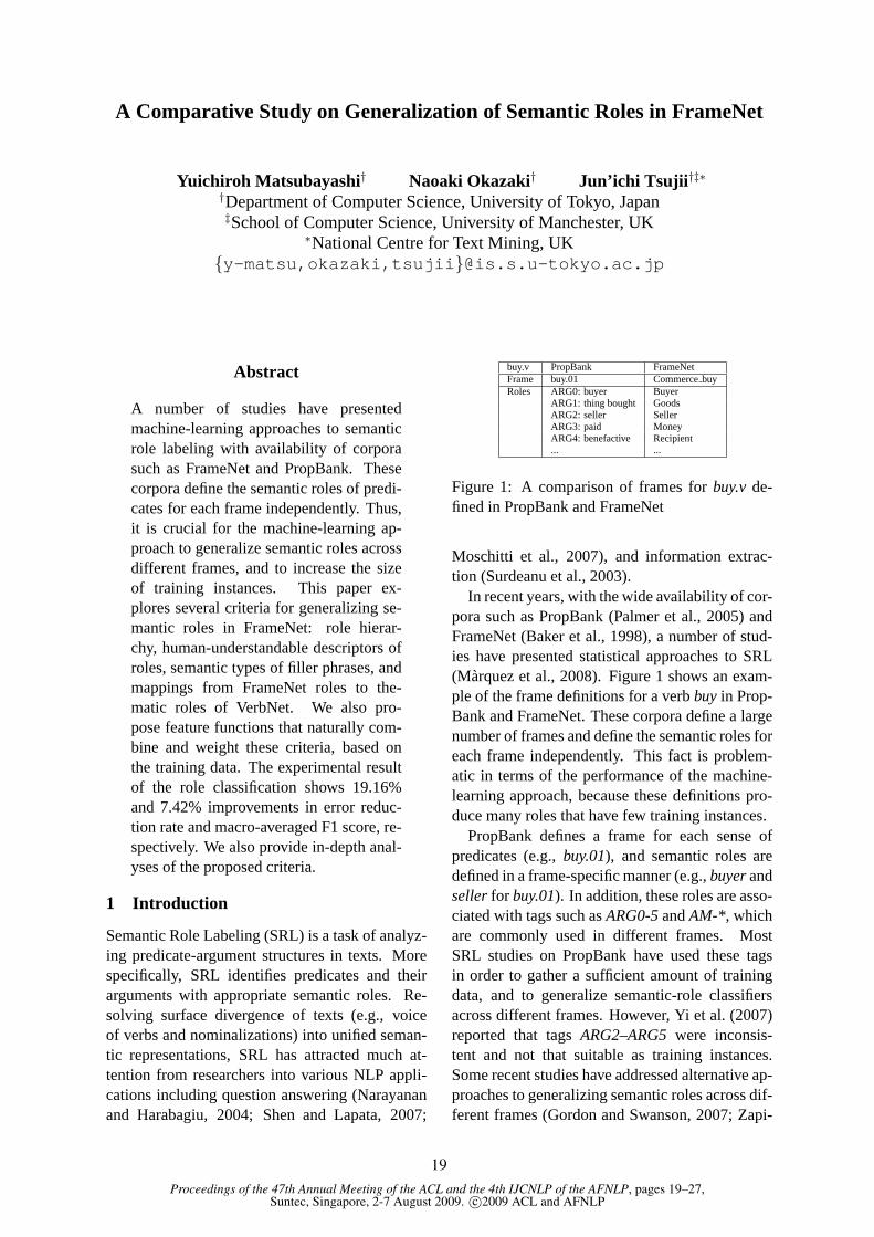
Proceedings of the 47th Annual Meeting of the ACL and the 4th IJCNLP of the AFNLP, pages 19–27,Suntec, Singapore, 2-7 August 2009. c©2009 ACL and AFNLP
A Comparative Study on Generalization of Semantic Roles in FrameNet
Yuichiroh Matsubayashi† Naoaki Okazaki† Jun’ichi Tsujii †‡∗
†Department of Computer Science, University of Tokyo, Japan‡School of Computer Science, University of Manchester, UK
∗National Centre for Text Mining, UK{y-matsu,okazaki,tsujii }@is.s.u-tokyo.ac.jp
Abstract
A number of studies have presentedmachine-learning approaches to semanticrole labeling with availability of corporasuch as FrameNet and PropBank. Thesecorpora define the semantic roles of predi-cates for each frame independently. Thus,it is crucial for the machine-learning ap-proach to generalize semantic roles acrossdifferent frames, and to increase the sizeof training instances. This paper ex-plores several criteria for generalizing se-mantic roles in FrameNet: role hierar-chy, human-understandable descriptors ofroles, semantic types of filler phrases, andmappings from FrameNet roles to the-matic roles of VerbNet. We also pro-pose feature functions that naturally com-bine and weight these criteria, based onthe training data. The experimental resultof the role classification shows 19.16%and 7.42% improvements in error reduc-tion rate and macro-averaged F1 score, re-spectively. We also provide in-depth anal-yses of the proposed criteria.
1 Introduction
Semantic Role Labeling (SRL) is a task of analyz-ing predicate-argument structures in texts. Morespecifically, SRL identifies predicates and theirarguments with appropriate semantic roles. Re-solving surface divergence of texts (e.g., voiceof verbs and nominalizations) into unified seman-tic representations, SRL has attracted much at-tention from researchers into various NLP appli-cations including question answering (Narayananand Harabagiu, 2004; Shen and Lapata, 2007;
buy.v PropBank FrameNetFrame buy.01 CommercebuyRoles ARG0: buyer Buyer
ARG1: thing bought GoodsARG2: seller SellerARG3: paid MoneyARG4: benefactive Recipient... ...
Figure 1: A comparison of frames forbuy.vde-fined in PropBank and FrameNet
Moschitti et al., 2007), and information extrac-tion (Surdeanu et al., 2003).
In recent years, with the wide availability of cor-pora such as PropBank (Palmer et al., 2005) andFrameNet (Baker et al., 1998), a number of stud-ies have presented statistical approaches to SRL(Màrquez et al., 2008). Figure 1 shows an exam-ple of the frame definitions for a verbbuy in Prop-Bank and FrameNet. These corpora define a largenumber of frames and define the semantic roles foreach frame independently. This fact is problem-atic in terms of the performance of the machine-learning approach, because these definitions pro-duce many roles that have few training instances.
PropBank defines a frame for each sense ofpredicates (e.g.,buy.01), and semantic roles aredefined in a frame-specific manner (e.g.,buyerandsellerfor buy.01). In addition, these roles are asso-ciated with tags such asARG0-5andAM-*, whichare commonly used in different frames. MostSRL studies on PropBank have used these tagsin order to gather a sufficient amount of trainingdata, and to generalize semantic-role classifiersacross different frames. However, Yi et al. (2007)reported that tagsARG2–ARG5 were inconsis-tent and not that suitable as training instances.Some recent studies have addressed alternative ap-proaches to generalizing semantic roles across dif-ferent frames (Gordon and Swanson, 2007; Zapi-
19

Transfer::Recipient
Giving::Recipient
Commerce_buy::BuyerCommerce_sell::Buyer Commerce_buy::SellerCommerce_sell::Seller
Giving::Donor
Transfer::Donor
Buyer Seller
Agent role-to-role relationhierarchical classthematic rolerole descriptor
Recipient Donor
Figure 2: An example of role groupings using different criteria.
rain et al., 2008).FrameNet designs semantic roles as frame spe-
cific, but also defines hierarchical relations of se-mantic roles among frames. Figure 2 illustratesan excerpt of the role hierarchy in FrameNet; thisfigure indicates that theBuyer role for theCom-mercebuy frame (Commerce buy::Buyer here-after) and theCommerce sell::Buyer role are in-herited from theTransfer::Recipient role. Al-though the role hierarchy was expected to gener-alize semantic roles, no positive results for roleclassification have been reported (Baldewein et al.,2004). Therefore, the generalization of semanticroles across different frames has been brought upas a critical issue for FrameNet (Gildea and Juraf-sky, 2002; Shi and Mihalcea, 2005; Giuglea andMoschitti, 2006)
In this paper, we explore several criteria for gen-eralizing semantic roles in FrameNet. In addi-tion to the FrameNet hierarchy, we use variouspieces of information: human-understandable de-scriptors of roles, semantic types of filler phrases,and mappings from FrameNet roles to the thematicroles of VerbNet. We also propose feature func-tions that naturally combines these criteria in amachine-learning framework. Using the proposedmethod, the experimental result of the role classi-fication shows 19.16% and 7.42% improvementsin error reduction rate and macro-averaged F1, re-spectively. We provide in-depth analyses with re-spect to these criteria, and state our conclusions.
2 Related Work
Moschitti et al. (2005) first classified roles by us-ing four coarse-grained classes (Core Roles, Ad-juncts, Continuation Arguments and Co-referringArguments), and built a classifier for each coarse-grained class to tag PropBankARG tags. Eventhough the initial classifiers could perform roughestimations of semantic roles, this step was notable to solve the ambiguity problem in PropBankARG2-5. When training a classifier for a seman-
tic role, Baldewein et al. (2004) re-used the train-ing instances of other roles that were similar to thetarget role. As similarity measures, they used theFrameNet hierarchy, peripheral roles of FrameNet,and clusters constructed by a EM-based method.Gordon and Swanson (2007) proposed a general-ization method for the PropBank roles based onsyntactic similarity in frames.
Many previous studies assumed that thematicroles bridged semantic roles in different frames.Gildea and Jurafsky (2002) showed that classifica-tion accuracy was improved by manually replac-ing FrameNet roles into 18 thematic roles. Shiand Mihalcea (2005) and Giuglea and Moschitti(2006) employed VerbNet thematic roles as thetarget of mappings from the roles defined by thedifferent semantic corpora. Using the thematicroles as alternatives ofARG tags, Loper et al.(2007) and Yi et al. (2007) demonstrated that theclassification accuracy of PropBank roles was im-proved forARG2roles, but that it was diminishedfor ARG1. Yi et al. (2007) also described thatARG2–5were mapped to a variety of thematicroles. Zapirain et al. (2008) evaluated PropBankARG tags and VerbNet thematic roles in a state-of-the-art SRL system, and concluded that PropBankARGtags achieved a more robust generalization ofthe roles than did VerbNet thematic roles.
3 Role Classification
SRL is a complex task wherein several problemsare intertwined: frame-evoking word identifica-tion, frame disambiguation(selecting a correctframe from candidates for the evoking word),role-phrase identification(identifying phrases that fillsemantic roles), androle classification(assigningcorrect roles to the phrases). In this paper, we fo-cus on role classification, in which the role gen-eralization is particularly critical to the machinelearning approach.
In the role classification task, we are given asentence, a frame evoking word, a frame, and
20

member roles Commerce_pay::Buyer
Intentionall_act::AgentGiving::Donor Getting::RecipientGiving::RecipientSending::Recipient Giving::TimePlacing::TimeEvent::TimeCommerce_pay::BuyerCommerce_buy::BuyerCommerce_sell::BuyerBuyer
Recipient TimeC_pay::BuyerGIVING::DonorIntentionally_ACT::Agent
Avoiding::AgentEvading::EvaderEvading::EvaderAvoiding::AgentGetting::RecipientEvading::EvaderSt::Sentient St::Physical_ObjGiving::ThemePlacing::Theme
St::State_of_affairsGiving::Reason Evading::ReasonGiving::Means Evading::PurposeTheme::AgentTheme::ThemeCommerce_buy::GoodsGetting::ThemeEvading:: Pursuer
Commerce_buy::BuyerCommerce_sell::SellerEvading::EvaderRole-descriptor groupsHierarchical-relation groups
Semantic-type groupsThematic-role groups Group namelegend
Figure 4: Examples for each type of role group.
INPUT:frame = Commerce_sellcandidate roles ={Seller, Buyer, Goods, Reason, Time, ... , Place}sentence = Can't [you] [sell Commerce_sell] [the factory] [to some other
company]? OUTPUT: sentence = Can't [you Seller] [sell Commerce_sell] [the factory Goods]
[to some other company Buyer] ?
Figure 3: An example of input and output of roleclassification.
phrases that take semantic roles. We are inter-ested in choosing the correct role from the can-didate roles for each phrase in the frame. Figure 3shows a concrete example of input and output; thesemantic roles for the phrases are chosen from thecandidate roles:Seller, Buyer, Goods, Reason,... , andPlace.
4 Design of Role Groups
We formalize the generalization of semantic rolesas the act of grouping several roles into aclass. We define arole group as a set ofrole labels grouped by a criterion. Figure 4shows examples of role groups; a groupGiv-ing::Donor (in the hierarchical-relation groups)contains the rolesGiving::Donor and Com-merce pay::Buyer. The remainder of this sectiondescribes the grouping criteria in detail.
4.1 Hierarchical relations among roles
FrameNet defines hierarchical relations amongframes (frame-to-frame relations). Each relationis assigned one of the seven types of directionalrelationships (Inheritance, Using, Perspectiveon,Causativeof, Inchoativeof, Subframe, and Pre-cedes). Some roles in two related frames are alsoconnected with role-to-role relations. We assumethat this hierarchy is a promising resource for gen-eralizing the semantic roles; the idea is that the
role at a node in the hierarchy inherits the char-acteristics of the roles of its ancestor nodes. Forexample,Commerce sell::Seller in Figure 2 in-herits the property ofGiving::Donor.
For Inheritance, Using, Perspectiveon, andSubframerelations, we assume that descendantroles in these relations have the same or special-ized properties of their ancestors. Hence, for eachroleyi, we define the following two role groups,
Hchildyi
= {y|y = yi ∨ y is a child ofyi},Hdesc
yi= {y|y = yi ∨ y is a descendant ofyi}.
The hierarchical-relation groups in Figure 4 arethe illustrations ofHdesc
yi.
For the relation types Inchoativeof andCausativeof, we define role groups in the oppo-site direction of the hierarchy,
Hparentyi
= {y|y = yi ∨ y is a parent ofyi},Hance
yi= {y|y = yi ∨ y is an ancestor ofyi}.
This is because lower roles ofInchoativeofand Causativeof relations represent more neu-tral stances or consequential states; for example,Killing::Victim is a parent ofDeath::Protagonistin theCausativeof relation.
Finally, thePrecedesrelation describes the se-quence of states and events, but does not spec-ify the direction of semantic inclusion relations.Therefore, we simply tryHchild
yi, Hdesc
yi, Hparent
yi ,andHance
yifor this relation type.
4.2 Human-understandable role descriptor
FrameNet defines each role as frame-specific; inother words, the same identifier does not appearin different frames. However, in FrameNet,human experts assign a human-understandablename to each role in a rather systematic man-ner. Some names are shared by the roles indifferent frames, whose identifiers are dif-ferent. Therefore, we examine the semantic
21
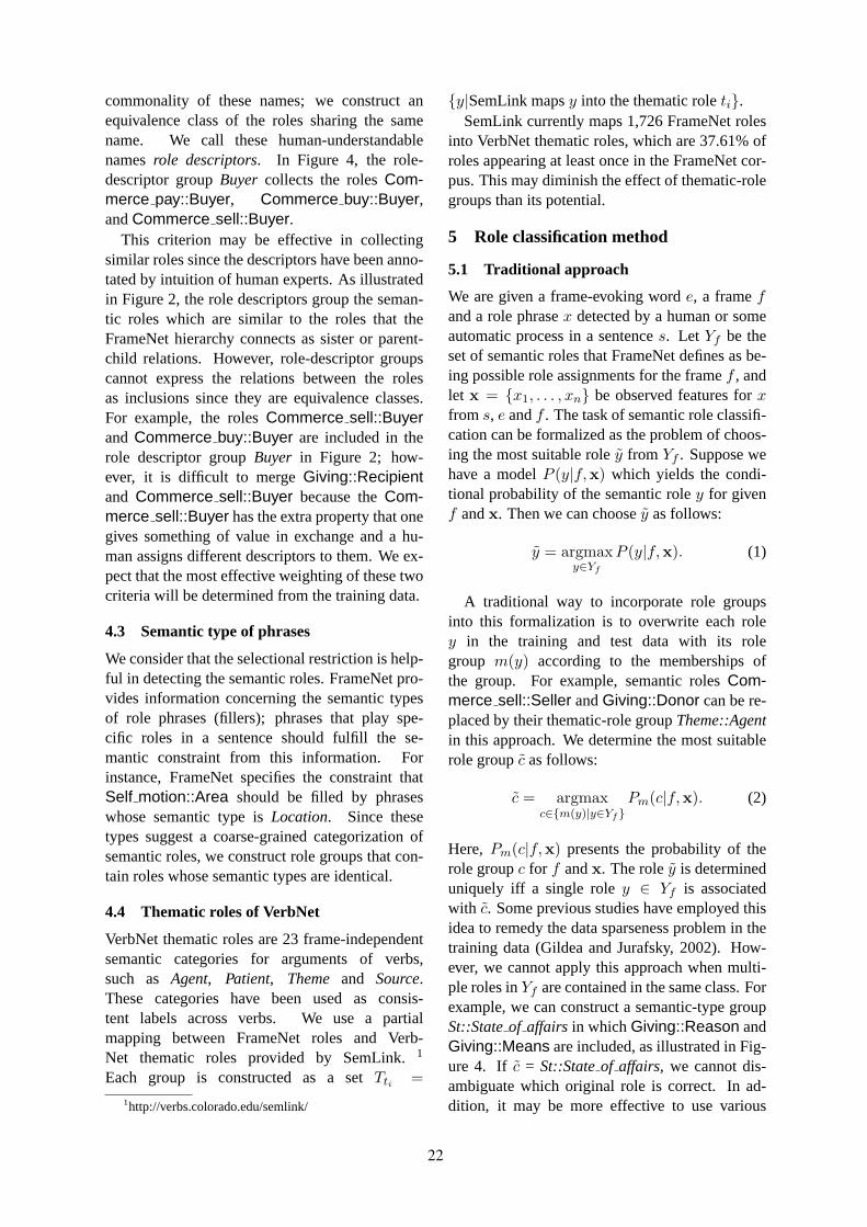
commonality of these names; we construct anequivalence class of the roles sharing the samename. We call these human-understandablenamesrole descriptors. In Figure 4, the role-descriptor groupBuyer collects the rolesCom-merce pay::Buyer, Commerce buy::Buyer,andCommerce sell::Buyer.
This criterion may be effective in collectingsimilar roles since the descriptors have been anno-tated by intuition of human experts. As illustratedin Figure 2, the role descriptors group the seman-tic roles which are similar to the roles that theFrameNet hierarchy connects as sister or parent-child relations. However, role-descriptor groupscannot express the relations between the rolesas inclusions since they are equivalence classes.For example, the rolesCommerce sell::Buyerand Commerce buy::Buyer are included in therole descriptor groupBuyer in Figure 2; how-ever, it is difficult to mergeGiving::Recipientand Commerce sell::Buyer because theCom-merce sell::Buyer has the extra property that onegives something of value in exchange and a hu-man assigns different descriptors to them. We ex-pect that the most effective weighting of these twocriteria will be determined from the training data.
4.3 Semantic type of phrases
We consider that the selectional restriction is help-ful in detecting the semantic roles. FrameNet pro-vides information concerning the semantic typesof role phrases (fillers); phrases that play spe-cific roles in a sentence should fulfill the se-mantic constraint from this information. Forinstance, FrameNet specifies the constraint thatSelf motion::Area should be filled by phraseswhose semantic type isLocation. Since thesetypes suggest a coarse-grained categorization ofsemantic roles, we construct role groups that con-tain roles whose semantic types are identical.
4.4 Thematic roles of VerbNet
VerbNet thematic roles are 23 frame-independentsemantic categories for arguments of verbs,such as Agent, Patient, Theme and Source.These categories have been used as consis-tent labels across verbs. We use a partialmapping between FrameNet roles and Verb-Net thematic roles provided by SemLink.1
Each group is constructed as a setTti =1http://verbs.colorado.edu/semlink/
{y|SemLink mapsy into the thematic roleti}.SemLink currently maps 1,726 FrameNet roles
into VerbNet thematic roles, which are 37.61% ofroles appearing at least once in the FrameNet cor-pus. This may diminish the effect of thematic-rolegroups than its potential.
5 Role classification method
5.1 Traditional approach
We are given a frame-evoking worde, a framefand a role phrasex detected by a human or someautomatic process in a sentences. Let Yf be theset of semantic roles that FrameNet defines as be-ing possible role assignments for the framef , andlet x = {x1, . . . , xn} be observed features forxfrom s, e andf . The task of semantic role classifi-cation can be formalized as the problem of choos-ing the most suitable rolẽy from Yf . Suppose wehave a modelP (y|f,x) which yields the condi-tional probability of the semantic roley for givenf andx. Then we can choosẽy as follows:
ỹ = argmaxy∈Yf
P (y|f,x). (1)
A traditional way to incorporate role groupsinto this formalization is to overwrite each roley in the training and test data with its rolegroup m(y) according to the memberships ofthe group. For example, semantic rolesCom-merce sell::Seller andGiving::Donor can be re-placed by their thematic-role groupTheme::Agentin this approach. We determine the most suitablerole groupc̃ as follows:
c̃ = argmaxc∈{m(y)|y∈Yf}
Pm(c|f,x). (2)
Here, Pm(c|f,x) presents the probability of therole groupc for f andx. The roleỹ is determineduniquely iff a single roley ∈ Yf is associatedwith c̃. Some previous studies have employed thisidea to remedy the data sparseness problem in thetraining data (Gildea and Jurafsky, 2002). How-ever, we cannot apply this approach when multi-ple roles inYf are contained in the same class. Forexample, we can construct a semantic-type groupSt::Stateof affairs in whichGiving::Reason andGiving::Means are included, as illustrated in Fig-ure 4. If c̃ = St::Stateof affairs, we cannot dis-ambiguate which original role is correct. In ad-dition, it may be more effective to use various
22

groupings of roles together in the model. For in-stance, the model could predict the correct roleCommerce sell::Seller for the phrase “you” inFigure 3 more confidently, if it could infer itsthematic-role group asTheme::Agentand its par-ent groupGiving::Donor correctly. Although theensemble of various groupings seems promising,we need an additional procedure to prioritize thegroupings for the case where the models for mul-tiple role groupings disagree; for example, it is un-satisfactory if two models assign the groupsGiv-ing::ThemeandTheme::Agentto the same phrase.
5.2 Role groups as feature functions
We thus propose another approach that incorpo-rates group information as feature functions. Wemodel the conditional probabilityP (y|f,x) by us-ing the maximum entropy framework,
p(y|f,x) =exp(
∑i λigi(x, y))∑
y∈Yfexp(
∑i λigi(x, y))
. (3)
Here,G = {gi} denotes a set ofn feature func-tions, andΛ = {λi} denotes a weight vector forthe feature functions.
In general, feature functions for the maximumentropy model are designed as indicator functionsfor possible pairs ofxj andy. For example, theevent where the head word ofx is “you” (x1 = 1)andx plays the roleCommerce sell::Seller in asentence is expressed by the indicator function,
grole1 (x, y) =
1 (x1 = 1 ∧
y = Commerce sell::Seller)0 (otherwise)
.
(4)We call this kind of feature function anx-role.
In order to incorporate role groups into themodel, we also include all feature functions forpossible pairs ofxj and role groups. Equation 5is an example of a feature function for instanceswhere the head word ofx is “you” andy is in therole groupTheme::Agent,
gtheme2 (x, y) =
1 (x1 = 1 ∧
y ∈ Theme::Agent)0 (otherwise)
. (5)
Thus, this feature function fires for the roles wher-ever the head word “you” playsAgent(e.g.,Com-merce sell::Seller, Commerce buy::Buyer andGiving::Donor). We call this kind of feature func-tion anx-groupfunction.
In this way, we obtainx-group functions for
all grouping methods, e.g.,gthemek , g
hierarchyk .
The role-group features will receive more traininginstances by collecting instances for fine-grainedroles. Thus, semantic roles with few training in-stances are expected to receive additional cluesfrom other training instances via role-group fea-tures. Another advantage of this approach is thatthe usefulness of the different role groups is de-termined by the training processes in terms ofweights of feature functions. Thus, we do not needto assume that we have found the best criterion forgrouping roles; we can allow a training process tochoose the criterion. We will discuss the contribu-tions of different groupings in the experiments.
5.3 Comparison with related work
Baldewein et al. (2004) suggested an approachthat uses role descriptors and hierarchical rela-tions as criteria for generalizing semantic rolesin FrameNet. They created a classifier for eachframe, additionally using training instances for therole A to train the classifier for the roleB, if therolesA andB were judged as similar by a crite-rion. This approach performs similarly to the over-writing approach, and it may obscure the differ-ences among roles. Therefore, they only re-usedthe descriptors as a similarity measure for the roleswhosecorenesswasperipheral. 2
In contrast, we use all kinds of role descriptorsto construct groups. Since we use the feature func-tions for both the original roles and their groups,appropriate units for classification are determinedautomatically in the training process.
6 Experiment and Discussion
We used the training set of the Semeval-2007Shared task (Baker et al., 2007) in order to ascer-tain the contributions of role groups. This datasetconsists of the corpus of FrameNet release 1.3(containing roughly 150,000 annotations), and anadditional full-text annotation dataset. We ran-domly extracted 10% of the dataset for testing, andused the remainder (90%) for training.
Performance was measured by micro- andmacro-averaged F1 (Chang and Zheng, 2008) withrespect to a variety of roles. The micro average bi-ases each F1 score by the frequencies of the roles,
2In FrameNet, each role is assigned one of four differenttypes ofcoreness(core, core-unexpressed, peripheral, extra-thematic) It represents the conceptual necessity of the rolesin the frame to which it belongs.
23
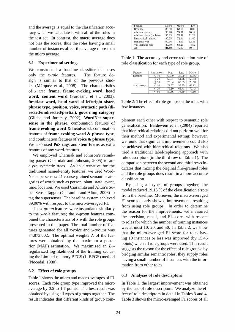
and the average is equal to the classification accu-racy when we calculate it with all of the roles inthe test set. In contrast, the macro average doesnot bias the scores, thus the roles having a smallnumber of instances affect the average more thanthe micro average.
6.1 Experimental settings
We constructed a baseline classifier that usesonly the x-role features. The feature de-sign is similar to that of the previous stud-ies (Màrquez et al., 2008). The characteristicsof x are: frame, frame evoking word, headword, content word (Surdeanu et al., 2003),first/last word, head word of left/right sister,phrase type, position, voice, syntactic path (di-rected/undirected/partial), governing category(Gildea and Jurafsky, 2002),WordNet super-sense in the phrase, combination features offrame evoking word & headword, combinationfeatures offrame evoking word & phrase type,and combination features ofvoice & phrase type.We also usedPoS tagsandstem forms as extrafeatures of any word-features.
We employed Charniak and Johnson’s rerank-ing parser (Charniak and Johnson, 2005) to an-alyze syntactic trees. As an alternative for thetraditional named-entity features, we used Word-Net supersenses: 41 coarse-grained semantic cate-gories of words such as person, plant, state, event,time, location. We used Ciaramita and Altun’s Su-per Sense Tagger (Ciaramita and Altun, 2006) totag the supersenses. The baseline system achieved89.00% with respect to the micro-averaged F1.
Thex-groupfeatures were instantiated similarlyto the x-role features; thex-group features com-bined the characteristics ofx with the role groupspresented in this paper. The total number of fea-tures generated for allx-roles and x-groupswas74,873,602. The optimal weightsΛ of the fea-tures were obtained by the maximum a poste-rior (MAP) estimation. We maximized anL2-regularized log-likelihood of the training set us-ing the Limited-memory BFGS (L-BFGS) method(Nocedal, 1980).
6.2 Effect of role groups
Table 1 shows the micro and macro averages of F1scores. Each role group type improved the microaverage by 0.5 to 1.7 points. The best result wasobtained by using all types of groups together. Theresult indicates that different kinds of group com-
Feature Micro Macro −Err.Baseline 89.00 68.50 0.00role descriptor 90.78 76.58 16.17role descriptor (replace) 90.23 76.19 11.23hierarchical relation 90.25 72.41 11.40semantic type 90.36 74.51 12.38VN thematic role 89.50 69.21 4.52All 91.10 75.92 19.16
Table 1: The accuracy and error reduction rate ofrole classification for each type of role group.
Feature #instances Pre. Rec. Microbaseline ≤ 10 63.89 38.00 47.66
≤ 20 69.01 51.26 58.83≤ 50 75.84 65.85 70.50
+ all groups ≤ 10 72.57 55.85 63.12≤ 20 76.30 65.41 70.43≤ 50 80.86 74.59 77.60
Table 2: The effect of role groups on the roles withfew instances.
plement each other with respect to semantic rolegeneralization. Baldewein et al. (2004) reportedthat hierarchical relations did not perform well fortheir method and experimental setting; however,we found that significant improvements could alsobe achieved with hierarchical relations. We alsotried a traditional label-replacing approach withrole descriptors (in the third row of Table 1). Thecomparison between the second and third rows in-dicates that mixing the original fine-grained rolesand the role groups does result in a more accurateclassification.
By using all types of groups together, themodel reduced 19.16 % of the classification errorsfrom the baseline. Moreover, the macro-averagedF1 scores clearly showed improvements resultingfrom using role groups. In order to determinethe reason for the improvements, we measuredthe precision, recall, and F1-scores with respectto roles for which the number of training instanceswas at most 10, 20, and 50. In Table 2, we showthat the micro-averaged F1 score for roles hav-ing 10 instances or less was improved (by 15.46points) when all role groups were used. This resultsuggests the reason for the effect of role groups; bybridging similar semantic roles, they supply roleshaving a small number of instances with the infor-mation from other roles.
6.3 Analyses of role descriptors
In Table 1, the largest improvement was obtainedby the use of role descriptors. We analyze the ef-fect of role descriptors in detail in Tables 3 and 4.Table 3 shows the micro-averaged F1 scores of all
24
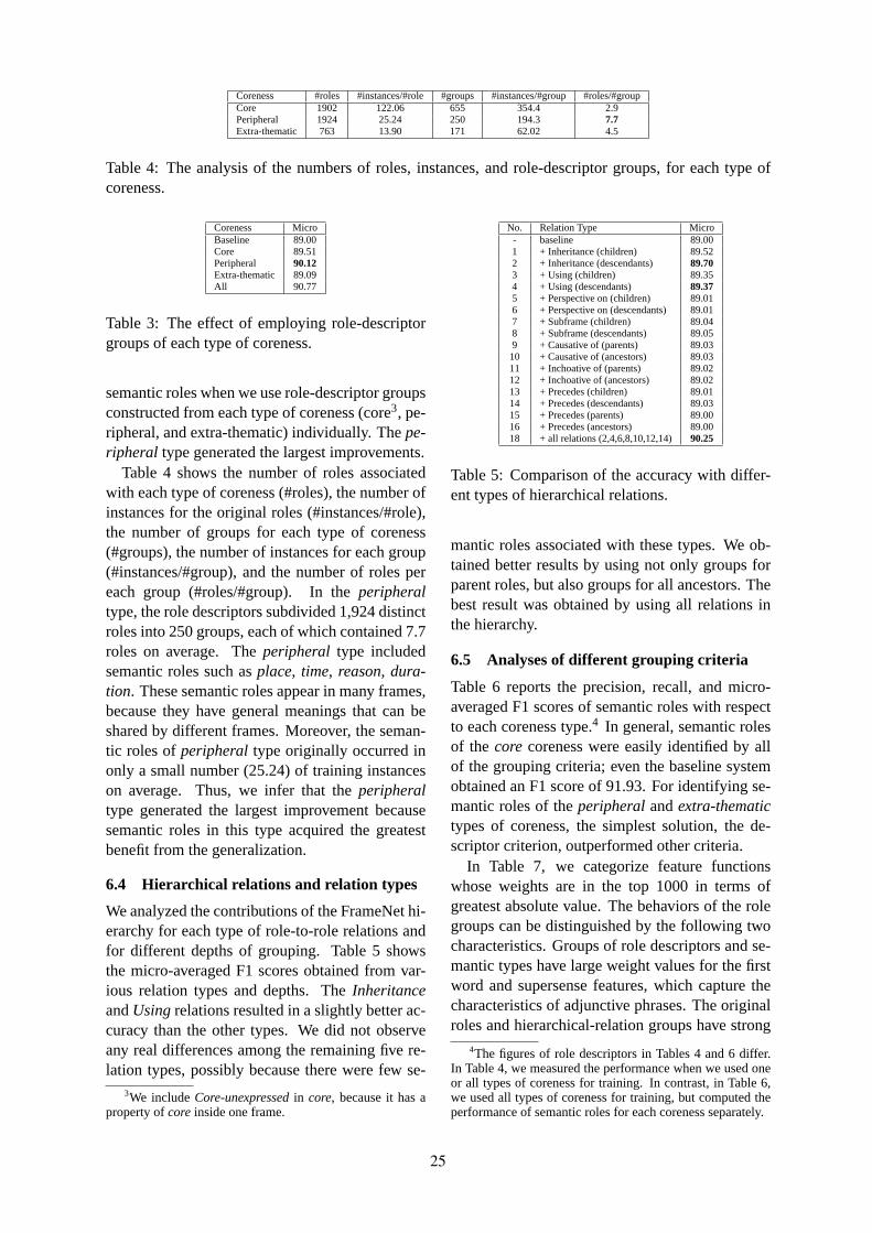
Coreness #roles #instances/#role #groups #instances/#group #roles/#groupCore 1902 122.06 655 354.4 2.9Peripheral 1924 25.24 250 194.3 7.7Extra-thematic 763 13.90 171 62.02 4.5
Table 4: The analysis of the numbers of roles, instances, and role-descriptor groups, for each type ofcoreness.
Coreness MicroBaseline 89.00Core 89.51Peripheral 90.12Extra-thematic 89.09All 90.77
Table 3: The effect of employing role-descriptorgroups of each type of coreness.
semantic roles when we use role-descriptor groupsconstructed from each type of coreness (core3, pe-ripheral, and extra-thematic) individually. Thepe-ripheral type generated the largest improvements.
Table 4 shows the number of roles associatedwith each type of coreness (#roles), the number ofinstances for the original roles (#instances/#role),the number of groups for each type of coreness(#groups), the number of instances for each group(#instances/#group), and the number of roles pereach group (#roles/#group). In theperipheraltype, the role descriptors subdivided 1,924 distinctroles into 250 groups, each of which contained 7.7roles on average. Theperipheral type includedsemantic roles such asplace, time, reason, dura-tion. These semantic roles appear in many frames,because they have general meanings that can beshared by different frames. Moreover, the seman-tic roles ofperipheraltype originally occurred inonly a small number (25.24) of training instanceson average. Thus, we infer that theperipheraltype generated the largest improvement becausesemantic roles in this type acquired the greatestbenefit from the generalization.
6.4 Hierarchical relations and relation types
We analyzed the contributions of the FrameNet hi-erarchy for each type of role-to-role relations andfor different depths of grouping. Table 5 showsthe micro-averaged F1 scores obtained from var-ious relation types and depths. TheInheritanceandUsingrelations resulted in a slightly better ac-curacy than the other types. We did not observeany real differences among the remaining five re-lation types, possibly because there were few se-
3We includeCore-unexpressedin core, because it has aproperty ofcore inside one frame.
No. Relation Type Micro- baseline 89.001 + Inheritance (children) 89.522 + Inheritance (descendants) 89.703 + Using (children) 89.354 + Using (descendants) 89.375 + Perspective on (children) 89.016 + Perspective on (descendants) 89.017 + Subframe (children) 89.048 + Subframe (descendants) 89.059 + Causative of (parents) 89.0310 + Causative of (ancestors) 89.0311 + Inchoative of (parents) 89.0212 + Inchoative of (ancestors) 89.0213 + Precedes (children) 89.0114 + Precedes (descendants) 89.0315 + Precedes (parents) 89.0016 + Precedes (ancestors) 89.0018 + all relations (2,4,6,8,10,12,14) 90.25
Table 5: Comparison of the accuracy with differ-ent types of hierarchical relations.
mantic roles associated with these types. We ob-tained better results by using not only groups forparent roles, but also groups for all ancestors. Thebest result was obtained by using all relations inthe hierarchy.
6.5 Analyses of different grouping criteria
Table 6 reports the precision, recall, and micro-averaged F1 scores of semantic roles with respectto each coreness type.4 In general, semantic rolesof the core coreness were easily identified by allof the grouping criteria; even the baseline systemobtained an F1 score of 91.93. For identifying se-mantic roles of theperipheralandextra-thematictypes of coreness, the simplest solution, the de-scriptor criterion, outperformed other criteria.
In Table 7, we categorize feature functionswhose weights are in the top 1000 in terms ofgreatest absolute value. The behaviors of the rolegroups can be distinguished by the following twocharacteristics. Groups of role descriptors and se-mantic types have large weight values for the firstword and supersense features, which capture thecharacteristics of adjunctive phrases. The originalroles and hierarchical-relation groups have strong
4The figures of role descriptors in Tables 4 and 6 differ.In Table 4, we measured the performance when we used oneor all types of coreness for training. In contrast, in Table 6,we used all types of coreness for training, but computed theperformance of semantic roles for each coreness separately.
25
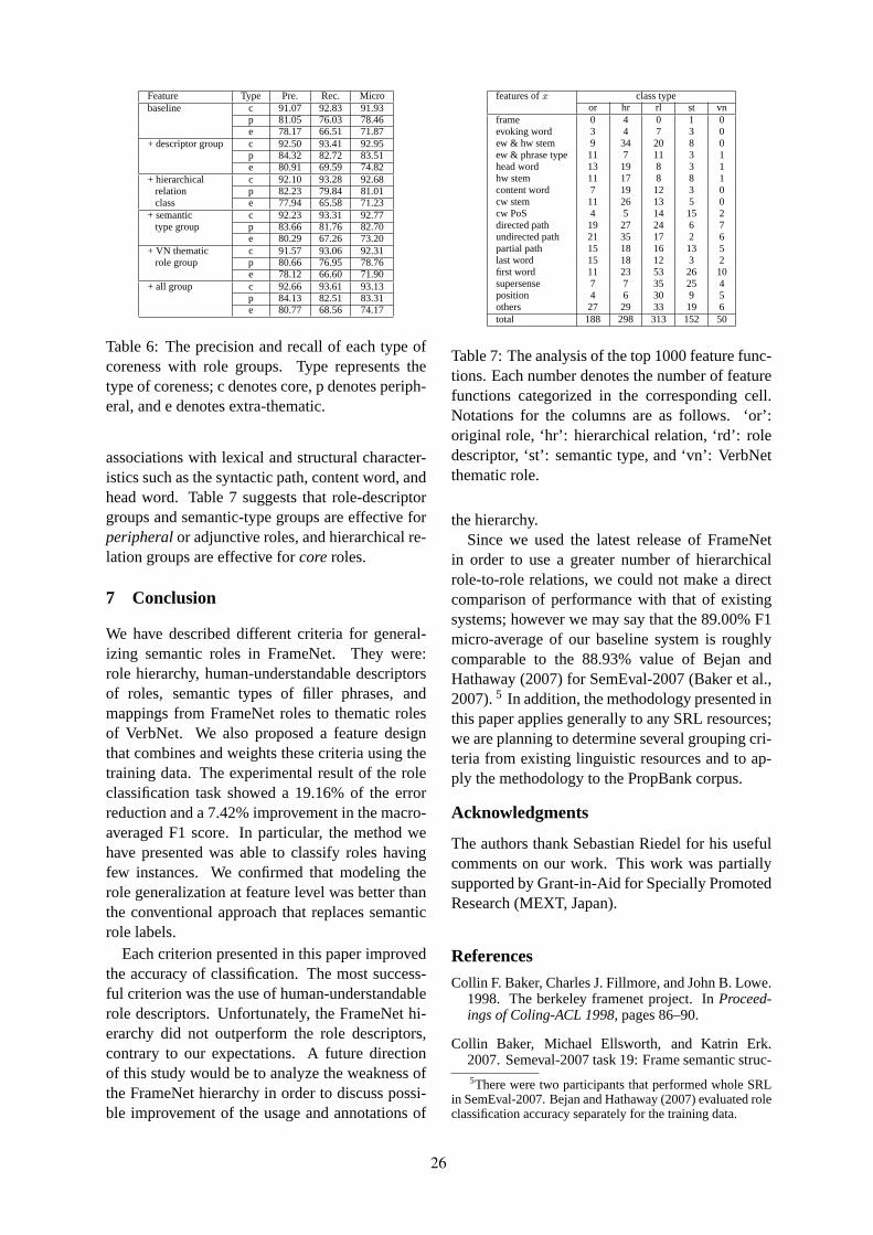
Feature Type Pre. Rec. Microbaseline c 91.07 92.83 91.93
p 81.05 76.03 78.46e 78.17 66.51 71.87
+ descriptor group c 92.50 93.41 92.95p 84.32 82.72 83.51e 80.91 69.59 74.82
+ hierarchical c 92.10 93.28 92.68relation p 82.23 79.84 81.01class e 77.94 65.58 71.23
+ semantic c 92.23 93.31 92.77type group p 83.66 81.76 82.70
e 80.29 67.26 73.20+ VN thematic c 91.57 93.06 92.31
role group p 80.66 76.95 78.76e 78.12 66.60 71.90
+ all group c 92.66 93.61 93.13p 84.13 82.51 83.31e 80.77 68.56 74.17
Table 6: The precision and recall of each type ofcoreness with role groups. Type represents thetype of coreness; c denotes core, p denotes periph-eral, and e denotes extra-thematic.
associations with lexical and structural character-istics such as the syntactic path, content word, andhead word. Table 7 suggests that role-descriptorgroups and semantic-type groups are effective forperipheralor adjunctive roles, and hierarchical re-lation groups are effective forcoreroles.
7 Conclusion
We have described different criteria for general-izing semantic roles in FrameNet. They were:role hierarchy, human-understandable descriptorsof roles, semantic types of filler phrases, andmappings from FrameNet roles to thematic rolesof VerbNet. We also proposed a feature designthat combines and weights these criteria using thetraining data. The experimental result of the roleclassification task showed a 19.16% of the errorreduction and a 7.42% improvement in the macro-averaged F1 score. In particular, the method wehave presented was able to classify roles havingfew instances. We confirmed that modeling therole generalization at feature level was better thanthe conventional approach that replaces semanticrole labels.
Each criterion presented in this paper improvedthe accuracy of classification. The most success-ful criterion was the use of human-understandablerole descriptors. Unfortunately, the FrameNet hi-erarchy did not outperform the role descriptors,contrary to our expectations. A future directionof this study would be to analyze the weakness ofthe FrameNet hierarchy in order to discuss possi-ble improvement of the usage and annotations of
features ofx class typeor hr rl st vn
frame 0 4 0 1 0evoking word 3 4 7 3 0ew & hw stem 9 34 20 8 0ew & phrase type 11 7 11 3 1head word 13 19 8 3 1hw stem 11 17 8 8 1content word 7 19 12 3 0cw stem 11 26 13 5 0cw PoS 4 5 14 15 2directed path 19 27 24 6 7undirected path 21 35 17 2 6partial path 15 18 16 13 5last word 15 18 12 3 2first word 11 23 53 26 10supersense 7 7 35 25 4position 4 6 30 9 5others 27 29 33 19 6total 188 298 313 152 50
Table 7: The analysis of the top 1000 feature func-tions. Each number denotes the number of featurefunctions categorized in the corresponding cell.Notations for the columns are as follows. ‘or’:original role, ‘hr’: hierarchical relation, ‘rd’: roledescriptor, ‘st’: semantic type, and ‘vn’: VerbNetthematic role.
the hierarchy.Since we used the latest release of FrameNet
in order to use a greater number of hierarchicalrole-to-role relations, we could not make a directcomparison of performance with that of existingsystems; however we may say that the 89.00% F1micro-average of our baseline system is roughlycomparable to the 88.93% value of Bejan andHathaway (2007) for SemEval-2007 (Baker et al.,2007).5 In addition, the methodology presented inthis paper applies generally to any SRL resources;we are planning to determine several grouping cri-teria from existing linguistic resources and to ap-ply the methodology to the PropBank corpus.
Acknowledgments
The authors thank Sebastian Riedel for his usefulcomments on our work. This work was partiallysupported by Grant-in-Aid for Specially PromotedResearch (MEXT, Japan).
References
Collin F. Baker, Charles J. Fillmore, and John B. Lowe.1998. The berkeley framenet project. InProceed-ings of Coling-ACL 1998, pages 86–90.
Collin Baker, Michael Ellsworth, and Katrin Erk.2007. Semeval-2007 task 19: Frame semantic struc-5There were two participants that performed whole SRL
in SemEval-2007. Bejan and Hathaway (2007) evaluated roleclassification accuracy separately for the training data.
26
ture extraction. InProceedings of SemEval-2007,pages 99–104.
Ulrike Baldewein, Katrin Erk, Sebastian Padó, andDetlef Prescher. 2004. Semantic role labelingwith similarity based generalization using EM-basedclustering. InProceedings of Senseval-3, pages 64–68.
Cosmin Adrian Bejan and Chris Hathaway. 2007.UTD-SRL: A Pipeline Architecture for Extract-ing Frame Semantic Structures. InProceedingsof SemEval-2007, pages 460–463. Association forComputational Linguistics.
X. Chang and Q. Zheng. 2008. Knowledge Ele-ment Extraction for Knowledge-Based Learning Re-sources Organization.Lecture Notes in ComputerScience, 4823:102–113.
Eugene Charniak and Mark Johnson. 2005. Coarse-to-fine n-best parsing and MaxEnt discriminativereranking. InProceedings of the 43rd Annual Meet-ing on Association for Computational Linguistics,pages 173–180.
Massimiliano Ciaramita and Yasemin Altun. 2006.Broad-coverage sense disambiguation and informa-tion extraction with a supersense sequence tagger. InProceedings of EMNLP-2006, pages 594–602.
Daniel Gildea and Daniel Jurafsky. 2002. Automaticlabeling of semantic roles.Computational Linguis-tics, 28(3):245–288.
Ana-Maria Giuglea and Alessandro Moschitti. 2006.Semantic role labeling via FrameNet, VerbNet andPropBank. InProceedings of the 21st InternationalConference on Computational Linguistics and the44th Annual Meeting of the ACL, pages 929–936.
Andrew Gordon and Reid Swanson. 2007. General-izing semantic role annotations across syntacticallysimilar verbs. InProceedings of ACL-2007, pages192–199.
Edward Loper, Szu-ting Yi, and Martha Palmer. 2007.Combining lexical resources: Mapping betweenpropbank and verbnet. InProceedings of the 7th In-ternational Workshop on Computational Semantics,pages 118–128.
Lluı́s Màrquez, Xavier Carreras, Kenneth C.Litkowski, and Suzanne Stevenson. 2008. Se-mantic role labeling: an introduction to the specialissue.Computational linguistics, 34(2):145–159.
Alessandro Moschitti, Ana-Maria Giuglea, Bonaven-tura Coppola, and Roberto Basili. 2005. Hierar-chical semantic role labeling. InProceedings ofCoNLL-2005, pages 201–204.
Alessandro Moschitti, Silvia Quarteroni, RobertoBasili, and Suresh Manandhar. 2007. Exploitingsyntactic and shallow semantic kernels for questionanswer classification. InProceedings of ACL-07,pages 776–783.
Srini Narayanan and Sanda Harabagiu. 2004. Ques-tion answering based on semantic structures. InPro-ceedings of Coling-2004, pages 693–701.
Jorge Nocedal. 1980. Updating quasi-newton matriceswith limited storage.Mathematics of Computation,35(151):773–782.
Martha Palmer, Daniel Gildea, and Paul Kingsbury.2005. The proposition bank: An annotated cor-pus of semantic roles.Computational Linguistics,31(1):71–106.
Dan Shen and Mirella Lapata. 2007. Using semanticroles to improve question answering. InProceed-ings of EMNLP-CoNLL 2007, pages 12–21.
Lei Shi and Rada Mihalcea. 2005. Putting Pieces To-gether: Combining FrameNet, VerbNet and Word-Net for Robust Semantic Parsing. InProceedings ofCICLing-2005, pages 100–111.
Mihai Surdeanu, Sanda Harabagiu, John Williams, andPaul Aarseth. 2003. Using predicate-argumentstructures for information extraction. InProceed-ings of ACL-2003, pages 8–15.
Szu-ting Yi, Edward Loper, and Martha Palmer. 2007.Can semantic roles generalize across genres? InProceedings of HLT-NAACL 2007, pages 548–555.
Beñat Zapirain, Eneko Agirre, and Lluı́s Màrquez.2008. Robustness and generalization of role sets:PropBank vs. VerbNet. InProceedings of ACL-08:HLT, pages 550–558.
27
Proceedings of the 47th Annual Meeting of the ACL and the 4th IJCNLP of the AFNLP, pages 28–36,Suntec, Singapore, 2-7 August 2009. c©2009 ACL and AFNLP
Unsupervised Argument Identification for Semantic Role Labeling
Omri Abend 1 Roi Reichart2 Ari Rappoport 1
1Institute of Computer Science ,2ICNCHebrew University of Jerusalem
{omria01|roiri|arir}@cs.huji.ac.il
Abstract
The task of Semantic Role Labeling(SRL) is often divided into two sub-tasks:verb argument identification, and argu-ment classification. Current SRL algo-rithms show lower results on the identifi-cation sub-task. Moreover, most SRL al-gorithms are supervised, relying on largeamounts of manually created data. Inthis paper we present an unsupervised al-gorithm for identifying verb arguments,where the only type of annotation requiredis POS tagging. The algorithm makes useof a fully unsupervised syntactic parser,using its output in order to detect clausesand gather candidate argument colloca-tion statistics. We evaluate our algorithmon PropBank10, achieving a precision of56%, as opposed to 47% of a strong base-line. We also obtain an 8% increase inprecision for a Spanish corpus. This isthe first paper that tackles unsupervisedverb argument identification without usingmanually encoded rules or extensive lexi-cal or syntactic resources.
1 Introduction
Semantic Role Labeling (SRL) is a major NLPtask, providing a shallow sentence-level semanticanalysis. SRL aims at identifying the relations be-tween the predicates (usually, verbs) in the sen-tence and their associated arguments.
The SRL task is often viewed as consisting oftwo parts: argument identification (ARGID) and ar-gument classification. The former aims at identi-fying the arguments of a given predicate presentin the sentence, while the latter determines the
type of relation that holds between the identi-fied arguments and their corresponding predicates.The division into two sub-tasks is justified bythe fact that they are best addressed using differ-ent feature sets (Pradhan et al., 2005). Perfor-mance in theARGID stage is a serious bottleneckfor general SRL performance, since only about81% of the arguments are identified, while about95% of the identified arguments are labeled cor-rectly (Màrquez et al., 2008).
SRL is a complex task, which is reflected by thealgorithms used to address it. A standard SRL al-gorithm requires thousands to dozens of thousandssentences annotated with POS tags, syntactic an-notation and SRL annotation. Current algorithmsshow impressive results but only for languages anddomains where plenty of annotated data is avail-able, e.g., English newspaper texts (see Section 2).Results are markedly lower when testing is on adomain wider than the training one, even in En-glish (see the WSJ-Brown results in (Pradhan etal., 2008)).
Only a small number of works that do not re-quire manually labeled SRL training data havebeen done (Swier and Stevenson, 2004; Swier andStevenson, 2005; Grenager and Manning, 2006).These papers have replaced this data with theVerbNet (Kipper et al., 2000) lexical resource ora set of manually written rules and supervisedparsers.
A potential answer to the SRL training data bot-tleneck are unsupervised SRL models that requirelittle to no manual effort for their training. Theiroutput can be used either by itself, or as trainingmaterial for modern supervised SRL algorithms.
In this paper we present an algorithm for unsu-pervised argument identification. The only type ofannotation required by our algorithm is POS tag-
28
ging, which needs relatively little manual effort.The algorithm consists of two stages. As pre-
processing, we use a fully unsupervised parser toparse each sentence. Initially, the set of possi-ble arguments for a given verb consists of all theconstituents in the parse tree that do not containthat predicate. The first stage of the algorithmattempts to detect the minimal clause in the sen-tence that contains the predicate in question. Us-ing this information, it further reduces the possiblearguments only to those contained in the minimalclause, and further prunes them according to theirposition in the parse tree. In the second stage weuse pointwise mutual information to estimate thecollocation strength between the arguments andthe predicate, and use it to filter out instances ofweakly collocating predicate argument pairs.
We use two measures to evaluate the perfor-mance of our algorithm, precision and F-score.Precision reflects the algorithm’s applicability forcreating training data to be used by supervisedSRL models, while the standard SRL F-score mea-sures the model’s performance when used by it-self. The first stage of our algorithm is shown tooutperform a strong baseline both in terms of F-score and of precision. The second stage is shownto increase precision while maintaining a reason-able recall.
We evaluated our model on sections 2-21 ofPropbank. As is customary in unsupervised pars-ing work (e.g. (Seginer, 2007)), we bounded sen-tence length by 10 (excluding punctuation). Ourfirst stage obtained a precision of 52.8%, which ismore than 6% improvement over the baseline. Oursecond stage improved precision to nearly 56%, a9.3% improvement over the baseline. In addition,we carried out experiments on Spanish (on sen-tences of length bounded by 15, excluding punctu-ation), achieving an increase of over 7.5% in pre-cision over the baseline. Our algorithm increasesF–score as well, showing an 1.8% improvementover the baseline in English and a 2.2% improve-ment in Spanish.
Section 2 reviews related work. In Section 3 wedetail our algorithm. Sections 4 and 5 describe theexperimental setup and results.
2 Related Work
The advance of machine learning based ap-proaches in this field owes to the usage of largescale annotated corpora. English is the most stud-
ied language, using the FrameNet (FN) (Baker etal., 1998) and PropBank (PB) (Palmer et al., 2005)resources. PB is a corpus well suited for evalu-ation, since it annotates every non-auxiliary verbin a real corpus (the WSJ sections of the PennTreebank). PB is a standard corpus for SRL eval-uation and was used in the CoNLL SRL sharedtasks of 2004 (Carreras and Màrquez, 2004) and2005 (Carreras and M̀arquez, 2005).
Most work on SRL has been supervised, requir-ing dozens of thousands of SRL annotated train-ing sentences. In addition, most models assumethat a syntactic representation of the sentence isgiven, commonly in the form of a parse tree, a de-pendency structure or a shallow parse. Obtainingthese is quite costly in terms of required humanannotation.
The first work to tackle SRL as an indepen-dent task is (Gildea and Jurafsky, 2002), whichpresented a supervised model trained and evalu-ated on FrameNet. The CoNLL shared tasks of2004 and 2005 were devoted to SRL, and stud-ied the influence of different syntactic annotationsand domain changes on SRL results.Computa-tional Linguisticshas recently published a specialissue on the task (M̀arquez et al., 2008), whichpresents state-of-the-art results and surveys the lat-est achievements and challenges in the field.
Most approaches to the task use a multi-levelapproach, separating the task to anARGID and anargument classification sub-tasks. They then usethe unlabeled argument structure (without the se-mantic roles) as training data for theARGID stageand the entire data (perhaps with other features)for the classification stage. Better performanceis achieved on the classification, where state-of-the-art supervised approaches achieve about81% F-score on the in-domain identification task,of which about 95% are later labeled correctly(Màrquez et al., 2008).
There have been several exceptions to the stan-dard architecture described in the last paragraph.One suggestion poses the problem of SRL as a se-quential tagging of words, training an SVM clas-sifier to determine for each word whether it is in-side, outside or in the beginning of an argument(Hacioglu and Ward, 2003). Other works have in-tegrated argument classification and identificationinto one step (Collobert and Weston, 2007), whileothers went further and combined the former twoalong with parsing into a single model (Musillo
29
and Merlo, 2006).
Work on less supervised methods has beenscarce. Swier and Stevenson (2004) and Swierand Stevenson (2005) presented the first modelthat does not use an SRL annotated corpus. How-ever, they utilize the extensive verb lexicon Verb-Net, which lists the possible argument structuresallowable for each verb, and supervised syntac-tic tools. Using VerbNet along with the output ofa rule-based chunker (in 2004) and a supervisedsyntactic parser (in 2005), they spot instances inthe corpus that are very similar to the syntacticpatterns listed in VerbNet. They then use these asseed for a bootstrapping algorithm, which conse-quently identifies the verb arguments in the corpusand assigns their semantic roles.
Another less supervised work is thatof (Grenager and Manning, 2006), which presentsa Bayesian network model for the argumentstructure of a sentence. They use EM to learnthe model’s parameters from unannotated data,and use this model to tag a test corpus. However,ARGID was not the task of that work, which dealtsolely with argument classification.ARGID wasperformed by manually-created rules, requiring asupervised or manual syntactic annotation of thecorpus to be annotated.
The three works above are relevant but incom-parable to our work, due to the extensive amountof supervision (namely, VerbNet and a rule-basedor supervised syntactic system) they used, both indetecting the syntactic structure and in detectingthe arguments.
Work has been carried out in a few other lan-guages besides English. Chinese has been studiedin (Xue, 2008). Experiments on Catalan and Span-ish were done in SemEval 2007 (Màrquez et al.,2007) with two participating systems. Attemptsto compile corpora for German (Burdchardt et al.,2006) and Arabic (Diab et al., 2008) are also un-derway. The small number of languages for whichextensive SRL annotated data exists reflects theconsiderable human effort required for such en-deavors.
Some SRL works have tried to use unannotateddata to improve the performance of a base su-pervised model. Methods used include bootstrap-ping approaches (Gildea and Jurafsky, 2002; Kateand Mooney, 2007), where large unannotated cor-pora were tagged with SRL annotation, later tobe used to retrain the SRL model. Another ap-
proach used similarity measures either betweenverbs (Gordon and Swanson, 2007) or betweennouns (Gildea and Jurafsky, 2002) to overcomelexical sparsity. These measures were estimatedusing statistics gathered from corpora augmentingthe model’s training data, and were then utilizedto generalize across similar verbs or similar argu-ments.
Attempts to substitute full constituency pars-ing by other sources of syntactic information havebeen carried out in the SRL community. Sugges-tions include posing SRL as a sequence labelingproblem (M̀arquez et al., 2005) or as an edge tag-ging problem in a dependency representation (Ha-cioglu, 2004). Punyakanok et al. (2008) providea detailed comparison between the impact of us-ing shallow vs. full constituency syntactic infor-mation in an English SRL system. Their resultsclearly demonstrate the advantage of using full an-notation.
The identification of arguments has also beencarried out in the context of automatic subcatego-rization frame acquisition. Notable examples in-clude (Manning, 1993; Briscoe and Carroll, 1997;Korhonen, 2002) who all used statistical hypothe-sis testing to filter a parser’s output for arguments,with the goal of compiling verb subcategorizationlexicons. However, these works differ from oursas they attempt to characterize the behavior of averb type, by collecting statistics from various in-stances of that verb, and not to determine whichare the arguments of specific verb instances.
The algorithm presented in this paper performsunsupervised clause detection as an intermedi-ate step towards argument identification. Super-vised clause detection was also tackled as a sepa-rate task, notably in the CoNLL 2001 shared task(Tjong Kim Sang and D̀ejean, 2001). Clause in-formation has been applied to accelerating a syn-tactic parser (Glaysher and Moldovan, 2006).
3 Algorithm
In this section we describe our algorithm. It con-sists of two stages, each of which reduces the setof argument candidates, which a-priori contains allconsecutive sequences of words that do not con-tain the predicate in question.
3.1 Algorithm overview
As pre-processing, we use an unsupervised parserthat generates an unlabeled parse tree for each sen-
30

tence (Seginer, 2007). This parser is unique in thatit is able to induce a bracketing (unlabeled pars-ing) from raw text (without even using POS tags)achieving state-of-the-art results. Since our algo-rithm uses millions to tens of millions sentences,we must use very fast tools. The parser’s highspeed (thousands of words per second) enables usto process these large amounts of data.
The only type of supervised annotation weuse is POS tagging. We use the taggers MX-POST (Ratnaparkhi, 1996) for English and Tree-Tagger (Schmid, 1994) for Spanish, to obtain POStags for our model.
The first stage of our algorithm uses linguisti-cally motivated considerations to reduce the set ofpossible arguments. It does so by confining the setof argument candidates only to those constituentswhich obey the following two restrictions. First,they should be contained in the minimal clausecontaining the predicate. Second, they should bek-th degree cousins of the predicate in the parsetree. We propose a novel algorithm for clause de-tection and use its output to determine which ofthe constituents obey these two restrictions.
The second stage of the algorithm uses point-wise mutual information to rule out constituentsthat appear to be weakly collocating with the pred-icate in question. Since a predicate greatly re-stricts the type of arguments with which it mayappear (this is often referred to as “selectional re-strictions”), we expect it to have certain character-istic arguments with which it is likely to collocate.
3.2 Clause detection stage
The main idea behind this stage is the observationthat most of the arguments of a predicate are con-tained within the minimal clause that contains thepredicate. We tested this on our development data– section 24 of the WSJ PTB, where we saw that86% of the arguments that are also constituents(in the gold standard parse) were indeed containedin that minimal clause (as defined by the tree la-bel types in the gold standard parse that denotea clause, e.g.,S, SBAR). Since we are not pro-vided with clause annotation (or any label), we at-tempted to detect them in an unsupervised manner.Our algorithm attempts to find sub-trees within theparse tree, whose structure resembles the structureof a full sentence. This approximates the notion ofa clause.
L
L
DT
The
NNS
materials
L
L
IN
in
L
DT
each
NN
set
L
VBP
reach
L
L
IN
about
CD
90
NNS
students
L
L L
L L
VBP L
L
VBP L
Figure 1: An example of an unlabeled POS taggedparse tree. The middle tree is theST of ‘reach’with the root as the encoded ancestor. The bot-tom one is theST with its parent as the encodedancestor.
Statistics gathering. In order to detect whichof the verb’s ancestors is the minimal clause, wescore each of the ancestors and select the one thatmaximizes the score. We represent each ancestorusing itsSpinal Tree(ST ). The ST of a givenverb’s ancestor is obtained by replacing all theconstituents that do not contain the verb by a leafhaving a label. This effectively encodes all thek-th degree cousins of the verb (for everyk). Theleaf labels are either the word’s POS in case theconstituent is a leaf, or the generic label “L” de-noting a non-leaf. See Figure 1 for an example.
In this stage we collect statistics of the occur-rences ofSTs in a large corpus. For everyST inthe corpus, we count the number of times it oc-curs in a form we consider to be a clause (positiveexamples), and the number of times it appears inother forms (negative examples).
Positive examples are divided into two maintypes. First, when theST encodes the root an-cestor (as in the middle tree of Figure 1); second,when the ancestor complies to a clause lexico-syntactic pattern. In many languages there is asmall set of lexico-syntactic patterns that mark aclause, e.g. the English ‘that’, the German ‘dass’and the Spanish ‘que’. The patterns which wereused in our experiments are shown in Figure 2.
For each verb instance, we traverse over its an-
31

English
TO + VB. The constituent starts with “to” followed bya verb in infinitive form.
WP. The constituent is preceded by a Wh-pronoun.
That. The constituent is preceded by a “that” markedby an “IN” POS tag indicating that it is a subordinatingconjunction.
Spanish
CQUE. The constituent is preceded by a word with thePOS “CQUE” which denotes the word “que” as a con-junction.
INT. The constituent is preceded by a word with thePOS “INT” which denotes an interrogative pronoun.
CSUB.The constituent is preceded by a word with oneof the POSs “CSUBF”, “CSUBI” or “CSUBX”, whichdenote a subordinating conjunction.
Figure 2: The set of lexico-syntactic patterns thatmark clauses which were used by our model.
cestors from top to bottom. For each of them weupdate the following counters:sentence(ST ) forthe root ancestor’sST , patterni(ST ) for the onescomplying to thei-th lexico-syntactic pattern andnegative(ST ) for the other ancestors1.
Clause detection. At test time, when detectingthe minimal clause of a verb instance, we usethe statistics collected in the previous stage. De-note the ancestors of the verb withA1 . . . Am.For each of them, we calculateclause(STAj
)and total(STAj
). clause(STAj) is the sum
of sentence(STAj) and patterni(STAj
) if thisancestor complies to thei-th pattern (if thereis no such pattern,clause(STAj
) is equal tosentence(STAj
)). total(STAj) is the sum of
clause(STAj) andnegative(STAj
).The selected ancestor is given by:
(1) Amax = argmaxAj
clause(STAj)
total(STAj)
An ST whosetotal(ST ) is less than a smallthreshold2 is not considered a candidate to be theminimal clause, since its statistics may be un-reliable. In case of a tie, we choose the low-est constituent that obtained the maximal score.
1If while traversing the tree, we encounter an ancestorwhose first word is preceded by a coordinating conjunction(marked by the POS tag “CC”), we refrain from performingany additional counter updates. Structures containing coor-dinating conjunctions tend not to obey our lexico-syntacticrules.
2We used 4 per million sentences, derived from develop-ment data.
If there is only one verb in the sentence3 or ifclause(STAj
) = 0 for every 1 ≤ j ≤ m, wechoose the top level constituent by default to bethe minimal clause containing the verb. Other-wise, the minimal clause is defined to be the yieldof the selected ancestor.
Argument identification. For each predicate inthe corpus, its argument candidates are now de-fined to be the constituents contained in the min-imal clause containing the predicate. However,these constituents may be (and are) nested withineach other, violating a major restriction on SRLarguments. Hence we now prune our set, by keep-ing only the siblings of all of the verb’s ancestors,as is common in supervised SRL (Xue and Palmer,2004).
3.3 Using collocations
We use the following observation to filter out somesuperfluous argument candidates: since the argu-ments of a predicate many times bear a semanticconnection with that predicate, they consequentlytend to collocate with it.
We collect collocation statistics from a largecorpus, which we annotate with parse trees andPOS tags. We mark arguments using the argu-ment detection algorithm described in the previoustwo sections, and extract all (predicate, argument)pairs appearing in the corpus. Recall that for eachsentence, the arguments are a subset of the con-stituents in the parse tree.
We use two representations of an argument: oneis the POS tag sequence of the terminals containedin the argument, the other is its head word4. Thepredicate is represented as the conjunction of itslemma with its POS tag.
Denote the number of times a predicatexappeared with an argumenty by nxy. Denotethe total number of (predicate, argument) pairsby N . Using these notations, we define thefollowing quantities:nx = Σynxy, ny = Σxnxy,p(x) = nx
N , p(y) =ny
N andp(x, y) =nxy
N . Thepointwise mutual information ofx andy is thengiven by:
3In this case, every argument in the sentence must be re-lated to that verb.
4Since we do not have syntactic labels, we use an approx-imate notion. For English we use the Bikel parser defaulthead word rules (Bikel, 2004). For Spanish, we use the left-most word.
32
(2) PMI(x, y) = logp(x,y)
p(x)·p(y) = lognxy
(nx·ny)/N
PMI effectively measures the ratio betweenthe number of timesx andy appeared together andthe number of times they were expected to appear,had they been independent.
At test time, when an(x, y) pair is observed, wecheck if PMI(x, y), computed on the large cor-pus, is lower than a thresholdα for either ofx’srepresentations. If this holds, for at least one rep-resentation, we prune all instances of that(x, y)pair. The parameterα may be selected differentlyfor each of the argument representations.
In order to avoid using unreliable statistics,we apply this for a given pair only ifnx·ny
N >
r, for some parameterr. That is, we considerPMI(x, y) to be reliable, only if the denomina-tor in equation (2) is sufficiently large.
4 Experimental Setup
Corpora. We used the PropBank corpus for de-velopment and for evaluation on English. Section24 was used for the development of our model,and sections 2 to 21 were used as our test data.The free parameters of the collocation extractionphase were tuned on the development data. Fol-lowing the unsupervised parsing literature, multi-ple brackets and brackets covering a single wordare omitted. We exclude punctuation accordingto the scheme of (Klein, 2005). As is customaryin unsupervised parsing (e.g. (Seginer, 2007)), webounded the lengths of the sentences in the cor-pus to be at most 10 (excluding punctuation). Thisresults in 207 sentences in the development data,containing a total of 132 different verbs and 173verb instances (of the non-auxiliary verbs in theSRL task, see ‘evaluation’ below) having 403 ar-guments. The test data has 6007 sentences con-taining 1008 different verbs and 5130 verb in-stances (as above) having 12436 arguments.
Our algorithm requires large amounts of datato gather argument structure and collocation pat-terns. For the statistics gathering phase of theclause detection algorithm, we used 4.5M sen-tences of the NANC (Graff, 1995) corpus, bound-ing their length in the same manner. In orderto extract collocations, we used 2M sentencesfrom the British National Corpus (Burnard, 2000)and about 29M sentences from the Dmoz cor-pus (Gabrilovich and Markovitch, 2005). Dmozis a web corpus obtained by crawling and clean-
ing the URLs in the Open Directory Project(dmoz.org). All of the above corpora were parsedusing Seginer’s parser and POS-tagged by MX-POST (Ratnaparkhi, 1996).
For our experiments on Spanish, we used 3.3Msentences of length at most 15 (excluding punctua-tion) extracted from the Spanish Wikipedia. Herewe chose to bound the length by 15 due to thesmaller size of the available test corpus. Thesame data was used both for the first and the sec-ond stages. Our development and test data weretaken from the training data released for the Se-mEval 2007 task on semantic annotation of Span-ish (Màrquez et al., 2007). This data consistedof 1048 sentences of length up to 15, from which200 were randomly selected as our developmentdata and 848 as our test data. The developmentdata included 313 verb instances while the testdata included 1279. All corpora were parsed us-ing the Seginer parser and tagged by the “Tree-Tagger” (Schmid, 1994).
Baselines. Since this is the first paper, to ourknowledge, which addresses the problem of unsu-pervised argument identification, we do not haveany previous results to compare to. We insteadcompare to a baseline which marks allk-th degreecousins of the predicate (for everyk) as arguments(this is the second pruning we use in the clausedetection stage). We name this baseline the ALL
COUSINS baseline. We note that a random base-line would score very poorly since any sequence ofterminals which does not contain the predicate isa possible candidate. Therefore, beating this ran-dom baseline is trivial.
Evaluation. Evaluation is carried out usingstandard SRL evaluation software5. The algorithmis provided with a list of predicates, whose argu-ments it needs to annotate. For the task addressedin this paper, non-consecutive parts of argumentsare treated as full arguments. A match is consid-ered each time an argument in the gold standarddata matches a marked argument in our model’soutput. An unmatched argument is an argumentwhich appears in the gold standard data, and failsto appear in our model’s output, and an exces-sive argument is an argument which appears inour model’s output but does not appear in the goldstandard. Precision and recall are defined accord-ingly. We report an F-score as well (the harmonicmean of precision and recall). We do not attempt
5http://www.lsi.upc.edu/∼srlconll/soft.html#software.
33

to identify multi-word verbs, and therefore do notreport the model’s performance in identifying verbboundaries.
Since our model detects clauses as an interme-diate product, we provide a separate evaluationof this task for the English corpus. We show re-sults on our development data. We use the stan-dard parsing F-score evaluation measure. As agold standard in this evaluation, we mark for eachof the verbs in our development data the minimalclause containing it. A minimal clause is the low-est ancestor of the verb in the parse tree that hasa syntactic label of a clause according to the goldstandard parse of the PTB. A verb is any terminalmarked by one of the POS tags of type verb ac-cording to the gold standard POS tags of the PTB.
5 Results
Our results are shown in Table 1. The left sectionpresents results on English and the right sectionpresents results on Spanish. The top line lists re-sults of the clause detection stage alone. The nexttwo lines list results of the full algorithm (clausedetection + collocations) in two different settingsof the collocation stage. The bottom line presentsthe performance of the ALL COUSINSbaseline.
In the “Collocation Maximum Precision” set-ting the parameters of the collocation stage (α andr) were generally tuned such that maximal preci-sion is achieved while preserving a minimal recalllevel (40% for English, 20% for Spanish on the de-velopment data). In the “Collocation Maximum F-score” the collocation parameters were generallytuned such that the maximum possible F-score forthe collocation algorithm is achieved.
The best or close to best F-score is achievedwhen using the clause detection algorithm alone(59.14% for English, 23.34% for Spanish). Notethat for both English and Spanish F-score im-provements are achieved via a precision improve-ment that is more significant than the recall degra-dation. F-score maximization would be the aim ofa system that uses the output of our unsupervisedARGID by itself.
The “Collocation Maximum Precision”achieves the best precision level (55.97% forEnglish, 21.8% for Spanish) but at the expenseof the largest recall loss. Still, it maintains areasonable level of recall. The “CollocationMaximum F-score” is an example of a model thatprovides a precision improvement (over both the
baseline and the clause detection stage) with arelatively small recall degradation. In the Spanishexperiments its F-score (23.87%) is even a bithigher than that of the clause detection stage(23.34%).
The full two–stage algorithm (clause detection+ collocations) should thus be used when we in-tend to use the model’s output as training data forsupervised SRL engines or supervisedARGID al-gorithms.
In our algorithm, the initial set of potential ar-guments consists of constituents in the Seginerparser’s parse tree. Consequently the fractionof arguments that are also constituents (81.87%for English and 51.83% for Spanish) poses anupper bound on our algorithm’s recall. Notethat the recall of the ALL COUSINS baseline is74.27% (45.75%) for English (Spanish). Thisscore emphasizes the baseline’s strength, and jus-tifies the restriction that the arguments should bek-th cousins of the predicate. The difference be-tween these bounds for the two languages providesa partial explanation for the corresponding gap inthe algorithm’s performance.
Figure 3 shows the precision of the collocationmodel (on development data) as a function of theamount of data it was given. We can see thatthe algorithm reaches saturation at about 5M sen-tences. It achieves this precision while maintain-ing a reasonable recall (an average recall of 43.1%after saturation). The parameters of the colloca-tion model were separately tuned for each corpussize, and the graph displays the maximum whichwas obtained for each of the corpus sizes.
To better understand our model’s performance,we performed experiments on the English cor-pus to test how well its first stage detects clauses.Clause detection is used by our algorithm as a steptowards argument identification, but it can be ofpotential benefit for other purposes as well (seeSection 2). The results are 23.88% recall and 40%precision. As in theARGID task, a random se-lection of arguments would have yielded an ex-tremely poor result.
6 Conclusion
In this work we presented the first algorithm for ar-gument identification that uses neither supervisedsyntactic annotation nor SRL tagged data. Wehave experimented on two languages: English andSpanish. The straightforward adaptability of un-
34

English (Test Data) Spanish (Test Data)Precision Recall F1 Precision Recall F1
Clause Detection 52.84 67.14 59.14 18.00 33.19 23.34Collocation Maximum F–score 54.11 63.53 58.44 20.22 29.13 23.87Collocation Maximum Precision 55.97 40.02 46.67 21.80 18.47 20.00
ALL COUSINSbaseline 46.71 74.27 57.35 14.16 45.75 21.62
Table 1:Precision, Recall and F1 score for the different stages of our algorithm. Results are given for English (PTB, sentenceslength bounded by 10, left part of the table) and Spanish (SemEval 2007 Spanish SRL task, right part of the table). The resultsof the collocation (second) stage are given in two configurations, Collocation Maximum F-score and Collocation MaximumPrecision (see text). The upper bounds on Recall, obtained by taking all arguments output by our unsupervised parser, are81.87% for English and 51.83% for Spanish.
0 2 4 6 8 10
42
44
46
48
50
52
Number of Sentences (Millions)
Prec
ision
Second StageFirst StageBaseline
Figure 3:The performance of the second stage on English(squares) vs. corpus size. The precision of the baseline (trian-gles) and of the first stage (circles) is displayed for reference.The graph indicates the maximum precision obtained for eachcorpus size. The graph reaches saturation at about 5M sen-tences. The average recall of the sampled points from thereon is 43.1%. Experiments were performed on the Englishdevelopment data.
supervised models to different languages is oneof their most appealing characteristics. The re-cent availability of unsupervised syntactic parsershas offered an opportunity to conduct research onSRL, without reliance on supervised syntactic an-notation. This work is the first to address the ap-plication of unsupervised parses to an SRL relatedtask.
Our model displayed an increase in precision of9% in English and 8% in Spanish over a strongbaseline. Precision is of particular interest in thiscontext, as instances tagged by high quality an-notation could be later used as training data forsupervised SRL algorithms. In terms of F–score,our model showed an increase of 1.8% in Englishand of 2.2% in Spanish over the baseline.
Although the quality of unsupervised parses iscurrently low (compared to that of supervised ap-proaches), using great amounts of data in identi-fying recurring structures may reduce noise andin addition address sparsity. The techniques pre-sented in this paper are based on this observation,using around 35M sentences in total for English
and 3.3M sentences for Spanish.As this is the first work which addressed un-
supervisedARGID, many questions remain to beexplored. Interesting issues to address include as-sessing the utility of the proposed methods whensupervised parses are given, comparing our modelto systems with no access to unsupervised parsesand conducting evaluation using more relaxedmeasures.
Unsupervised methods for syntactic tasks havematured substantially in the last few years. No-table examples are (Clark, 2003) for unsupervisedPOS tagging and (Smith and Eisner, 2006) for un-supervised dependency parsing. Adapting our al-gorithm to use the output of these models, either toreduce the little supervision our algorithm requires(POS tagging) or to provide complementary syn-tactic information, is an interesting challenge forfuture work.
References
Collin F. Baker, Charles J. Fillmore and John B. Lowe,1998. The Berkeley FrameNet Project.ACL-COLING ’98.
Daniel M. Bikel, 2004.Intricacies of Collins’ ParsingModel. Computational Linguistics, 30(4):479–511.
Ted Briscoe, John Carroll, 1997.Automatic Extractionof Subcategorization from Corpora.Applied NLP1997.
Aljoscha Burchardt, Katrin Erk, Anette Frank, AndreaKowalski, Sebastian Pad and Manfred Pinkal, 2006The SALSA Corpus: a German Corpus Resource forLexical Semantics.LREC ’06.
Lou Burnard, 2000. User Reference Guide for theBritish National Corpus.Technical report, OxfordUniversity.
Xavier Carreras and Lluı̀s Màrquez, 2004. Intro-duction to the CoNLL–2004 Shared Task: SemanticRole Labeling.CoNLL ’04.
35

Xavier Carreras and Lluı̀s Màrquez, 2005. Intro-duction to the CoNLL–2005 Shared Task: SemanticRole Labeling.CoNLL ’05.
Alexander Clark, 2003.Combining Distributional andMorphological Information for Part of Speech In-duction.EACL ’03.
Ronan Collobert and Jason Weston, 2007.Fast Se-mantic Extraction Using a Novel Neural NetworkArchitecture.ACL ’07.
Mona Diab, Aous Mansouri, Martha Palmer, OlgaBabko-Malaya, Wajdi Zaghouani, Ann Bies andMohammed Maamouri, 2008.A pilot Arabic Prop-Bank.LREC ’08.
Evgeniy Gabrilovich and Shaul Markovitch, 2005.Feature Generation for Text Categorization usingWorld Knowledge.IJCAI ’05.
Daniel Gildea and Daniel Jurafsky, 2002.AutomaticLabeling of Semantic Roles.Computational Lin-guistics, 28(3):245–288.
Elliot Glaysher and Dan Moldovan, 2006.Speed-ing Up Full Syntactic Parsing by Leveraging PartialParsing Decisions.COLING/ACL ’06 poster ses-sion.
Andrew Gordon and Reid Swanson, 2007.Generaliz-ing Semantic Role Annotations across SyntacticallySimilar Verbs.ACL ’07.
David Graff, 1995. North American News Text Cor-pus.Linguistic Data Consortium. LDC95T21.
Trond Grenager and Christopher D. Manning, 2006.Unsupervised Discovery of a Statistical Verb Lexi-con. EMNLP ’06.
Kadri Hacioglu, 2004.Semantic Role Labeling usingDependency Trees.COLING ’04.
Kadri Hacioglu and Wayne Ward, 2003.Target WordDetection and Semantic Role Chunking using Sup-port Vector Machines.HLT-NAACL ’03.
Rohit J. Kate and Raymond J. Mooney, 2007.Semi-Supervised Learning for Semantic Parsing usingSupport Vector Machines.HLT–NAACL ’07.
Karin Kipper, Hoa Trang Dang and Martha Palmer,2000. Class-Based Construction of a Verb Lexicon.AAAI ’00.
Dan Klein, 2005.The Unsupervised Learning of Natu-ral Language Structure.Ph.D. thesis, Stanford Uni-versity.
Anna Korhonen, 2002.Subcategorization Acquisition.Ph.D. thesis, University of Cambridge.
Christopher D. Manning, 1993.Automatic Acquisitionof a Large Subcategorization Dictionary.ACL ’93.
Lluı̀s Màrquez, Xavier Carreras, Kenneth C. Lit-tkowski and Suzanne Stevenson, 2008.SemanticRole Labeling: An introdution to the Special Issue.Computational Linguistics, 34(2):145–159
Lluı̀s Màrquez, Jesus Gim̀enez Pere Comas and NeusCatal̀a, 2005.Semantic Role Labeling as SequentialTagging.CoNLL ’05.
Lluı̀s Màrquez, Lluis Villarejo, M. A. Mart̀ı and Mar-iona Taul̀e, 2007. SemEval–2007 Task 09: Multi-level Semantic Annotation of Catalan and Spanish.The 4th international workshop on Semantic Evalu-ations (SemEval ’07).
Gabriele Musillo and Paula Merlo, 2006.AccurateParsing of the proposition bank.HLT-NAACL ’06.
Martha Palmer, Daniel Gildea and Paul Kingsbury,2005. The Proposition Bank: A Corpus Annotatedwith Semantic Roles.Computational Linguistics,31(1):71–106.
Sameer Pradhan, Kadri Hacioglu, Valerie Krugler,Wayne Ward, James H. Martin and Daniel Jurafsky,2005. Support Vector Learning for Semantic Argu-ment Classification.Machine Learning, 60(1):11–39.
Sameer Pradhan, Wayne Ward, James H. Martin, 2008.Towards Robust Semantic Role Labeling.Computa-tional Linguistics, 34(2):289–310.
Adwait Ratnaparkhi, 1996.Maximum Entropy Part-Of-Speech Tagger.EMNLP ’96.
Helmut Schmid, 1994.Probabilistic Part-of-SpeechTagging Using Decision TreesInternational Confer-ence on New Methods in Language Processing.
Yoav Seginer, 2007.Fast Unsupervised IncrementalParsing.ACL ’07.
Noah A. Smith and Jason Eisner, 2006.AnnealingStructural Bias in Multilingual Weighted GrammarInduction.ACL ’06.
Robert S. Swier and Suzanne Stevenson, 2004.Unsu-pervised Semantic Role Labeling.EMNLP ’04.
Robert S. Swier and Suzanne Stevenson, 2005.Ex-ploiting a Verb Lexicon in Automatic Semantic RoleLabelling. EMNLP ’05.
Erik F. Tjong Kim Sang and Herv́e Déjean, 2001.In-troduction to the CoNLL-2001 Shared Task: ClauseIdentification.CoNLL ’01.
Nianwen Xue and Martha Palmer, 2004.CalibratingFeatures for Semantic Role Labeling.EMNLP ’04.
Nianwen Xue, 2008. Labeling Chinese Predicateswith Semantic Roles.Computational Linguistics,34(2):225–255.
36

Proceedings of the 47th Annual Meeting of the ACL and the 4th IJCNLP of the AFNLP, pages 37–45,Suntec, Singapore, 2-7 August 2009. c©2009 ACL and AFNLP
Brutus: A Semantic Role Labeling System Incorporating CCG, CFG, andDependency Features
Stephen A. Boxwell, Dennis Mehay, and Chris BrewDepartment of LinguisticsThe Ohio State University
{boxwe11,mehay,cbrew}@1ing.ohio-state.edu
Abstract
We describe a semantic role labeling systemthat makes primary use of CCG-based fea-tures. Most previously developed systemsare CFG-based and make extensive use of atreepath feature, which suffers from data spar-sity due to its use of explicit tree configura-tions. CCG affords ways to augment treepath-based features to overcome these data sparsityissues. By adding features over CCG word-word dependencies and lexicalized verbal sub-categorization frames (“supertags”), we canobtain an F-score that is substantially betterthan a previous CCG-based SRL system andcompetitive with the current state of the art. Amanual error analysis reveals that parser errorsaccount for many of the errors of our system.This analysis also suggests that simultaneousincremental parsing and semantic role labelingmay lead to performance gains in both tasks.
1 Introduction
Semantic Role Labeling (SRL) is the process of assign-ing semantic roles to strings of words in a sentence ac-cording to their relationship to the semantic predicatesexpressed in the sentence. The task is difficult becausethe relationship between syntactic relations like “sub-ject” and “object” do not always correspond to seman-tic relations like “agent” and “patient”. An effectivesemantic role labeling system must recognize the dif-ferences between different configurations:
(a) [The man]Arg0 opened [the door]Arg1 [forhim]Arg3 [today]ArgM−TMP .
(b) [The door]Arg1 opened.
(c) [The door]Arg1 was opened by [a man]Arg0.
We use Propbank (Palmer et al., 2005), a corpus ofnewswire text annotated with verb predicate semanticrole information that is widely used in the SRL litera-ture (Màrquez et al., 2008). Rather than describe se-mantic roles in terms of “agent” or “patient”, Propbankdefines semantic roles on a verb-by-verb basis. For ex-ample, the verbopenencodes the OPENERas Arg0, theOPENEEas Arg1, and the beneficiary of the OPENING
action as Arg3. Propbank also defines a set of adjunct
roles, denoted by the letter M instead of a number. Forexample, ArgM-TMP denotes a temporal role, like “to-day”. By using verb-specific roles, Propbank avoidsspecific claims about parallels between the roles of dif-ferent verbs.
We follow the approach in (Punyakanok et al., 2008)in framing the SRL problem as a two-stage pipeline:identification followed by labeling. During identifica-tion, every word in the sentence is labeled either asbearing some (as yet undetermined) semantic role ornot . This is done for each verb. Next, during label-ing, the precise verb-specific roles for each word aredetermined. In contrast to the approach in (Punyakanoket al., 2008), which tags constituents directly, we tagheadwords and then associate them with a constituent,as in a previous CCG-based approach (Gildea andHockenmaier, 2003). Another difference is our choiceof parsers. Brutus uses the CCG parser of (Clark andCurran, 2007, henceforth the C&C parser), Charniak’sparser (Charniak, 2001) for additional CFG-based fea-tures, and MALT parser (Nivre et al., 2007) for de-pendency features, while (Punyakanok et al., 2008)use results from an ensemble of parses from Char-niak’s Parser and a Collins parser (Collins, 2003; Bikel,2004). Finally, the system described in (Punyakanok etal., 2008) uses a joint inference model to resolve dis-crepancies between multiple automatic parses. We donot employ a similar strategy due to the differing no-tions of constituency represented in our parsers (CCGhaving a much more fluid notion of constituency andthe MALT parser using a different approach entirely).
For the identification and labeling steps, we traina maximum entropy classifier (Berger et al., 1996)over sections 02-21 of a version of the CCGbank cor-pus (Hockenmaier and Steedman, 2007) that has beenaugmented by projecting the Propbank semantic anno-tations (Boxwell and White, 2008). We evaluate ourSRL system’s argument predictions at the word stringlevel, making our results directly comparable for eachargument labeling.1
In the following, we briefly introduce the CCGgrammatical formalism and motivate its use in SRL(Sections 2–3). Our main contribution is to demon-strate that CCG — arguably a more expressive and lin-
1This is guaranteed by our string-to-string mapping fromthe original Propbank to the CCGbank.
37

guistically appealing syntactic framework than vanillaCFGs — is a viable basis for the SRL task. This is sup-ported by our experimental results, the setup and detailsof which we give in Sections 4–10. In particular, usingCCG enables us to map semantic roles directly ontoverbal categories, an innovation of our approach thatleads to performance gains (Section 7). We concludewith an error analysis (Section 11), which motivatesour discussion of future research for computational se-mantics with CCG (Section 12).
2 Combinatory Categorial Grammar
Combinatory Categorial Grammar (Steedman, 2000)is a grammatical framework that describes syntacticstructure in terms of the combinatory potential of thelexical (word-level) items. Rather than using standardpart-of-speech tags and grammatical rules, CCG en-codes much of the combinatory potential of each wordby assigning a syntactically informative category. Forexample, the verbloves has the category (s\np)/np,which could be read “the kind of word that would bea sentence if it could combine with a noun phrase onthe right and a noun phrase on the left”. Further, CCGhas the advantage of a transparent interface between theway the words combine and their dependencies withother words. Word-word dependencies in the CCG-bank are encoded using predicate-argument (PARG)relations. PARG relations are defined by the functorword, the argument word, the category of the functorword and which argument slot of the functor categoryis being filled. For example, in the sentenceJohn lovesMary (figure 1), there are two slots on the verbal cat-egory to be filled by NP arguments. The first argu-ment (the subject) fills slot 1. This can be encodedas <loves,john,(s\np)/np,1>, indicating the head ofthe functor, the head of the argument, the functor cat-egory and the argument slot. The second argument(the direct object) fills slot 2. This can be encoded as<loves,mary,(s\np)/np,2>. One of the potential ad-vantages to using CCGbank-style PARG relations isthat they uniformly encode both local and long-rangedependencies — e.g., the noun phrasethe Mary thatJohn lovesexpresses the same set of two dependencies.We will show this to be a valuable tool for semanticrole prediction.
3 Potential Advantages to using CCG
There are many potential advantages to using the CCGformalism in SRL. One is the uniformity with whichCCG can express equivalence classes of local and long-range (including unbounded) dependencies. CFG-based approaches often rely on examining potentiallylong sequences of categories (ortreepaths) between theverb and the target word. Because there are a number ofdifferent treepaths that correspond to a single relation(figure 2), this approach can suffer from data sparsity.CCG, however, can encode all treepath-distinct expres-sions of a single grammatical relation into a single
predicate-argument relationship (figure 3). This fea-ture has been shown (Gildea and Hockenmaier, 2003)to be an effective substitute for treepath-based features.But while predicate-argument-based features are veryeffective, they are still vulnerable both to parser er-rors and to cases where the semantics of a sentencedo not correspond directly to syntactic dependencies.To counteract this, we use both kinds of features withthe expectation that the treepath feature will providelow-level detail to compensate for missed, incorrect orsyntactically impossible dependencies.
Another advantage of a CCG-based approach (andlexicalist approaches in general) is the ability to en-code verb-specific argument mappings. An argumentmapping is a link between the CCG category and thesemantic roles that are likely to go with each of its ar-guments. The projection of argument mappings ontoCCG verbal categories is explored in (Boxwell andWhite, 2008). We describe this feature in more detailin section 7.
4 Identification and Labeling Models
As in previous approaches to SRL, Brutus uses a two-stage pipeline of maximum entropy classifiers. In ad-dition, we train an argument mapping classifier (de-scribed in more detail below) whose predictions areused as features for the labeling model. The samefeatures are extracted for both treebank and automaticparses. Automatic parses were generated using theC&C CCG parser (Clark and Curran, 2007) with itsderivation output format converted to resemble that ofthe CCGbank. This involved following the derivationalbracketings of the C&C parser’s output and recon-structing the backpointers to the lexical heads using anin-house implementation of the basic CCG combina-tory operations. All classifiers were trained to 500 iter-ations of L-BFGS training — a quasi-Newton methodfrom the numerical optimization literature (Liu and No-cedal, 1989) — using Zhang Le’s maxent toolkit.2 Toprevent overfitting we used Gaussian priors with globalvariances of 1 and 5 for the identifier and labeler, re-spectively.3 The Gaussian priors were determined em-pirically by testing on the development set.
Both the identifier and the labeler use the followingfeatures:
(1) Words. Words drawn from a 3 word windowaround the target word,4 with each word asso-ciated with a binary indicator feature.
(2) Part of Speech. Part of Speech tags drawnfrom a 3 word window around the target word,
2Available for download athttp://homepages.inf.ed.ac.uk/s0450736/maxent_toolkit.html.
3Gaussian priors achieve a smoothing effect (to preventoverfitting) by penalizing very large feature weights.
4The size of the window was determined experimentallyon the development set – we use the same window sizesthroughout.
38
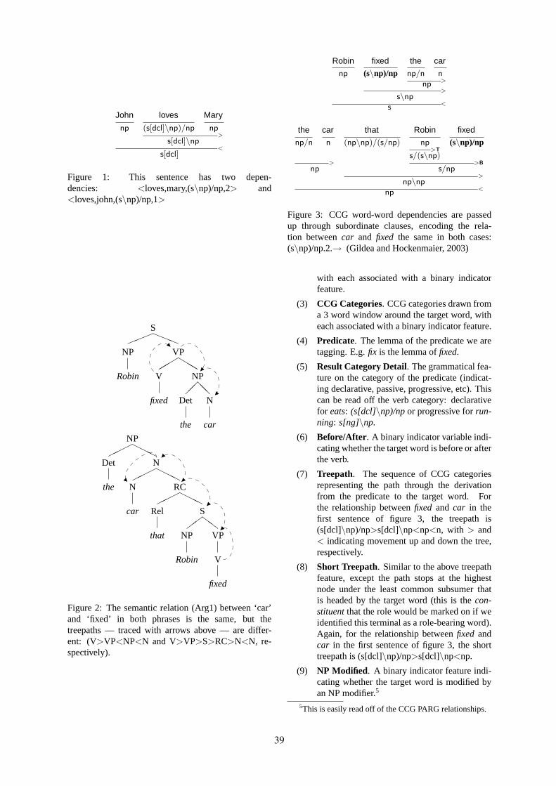
John loves Mary
np (s[dcl]\np)/np np>
s[dcl]\np<
s[dcl]
Figure 1: This sentence has two depen-dencies: <loves,mary,(s\np)/np,2> and<loves,john,(s\np)/np,1>
Saaa
!!!NP
Robin
VPb
bb"
""V
fixed
NP@@��
Det
the
N
car
NPHHH
���Det
the
NHHH
���N
car
RCHHH
���Rel
that
SZZ��
NP
Robin
VP
V
fixed
Figure 2: The semantic relation (Arg1) between ‘car’and ‘fixed’ in both phrases is the same, but thetreepaths — traced with arrows above — are differ-ent: (V>VP<NP<N and V>VP>S>RC>N<N, re-spectively).
Robin fixed the car
np (s\np)/np np/n n>
np>
s\np<
s
the car that Robin fixed
np/n n (np\np)/(s/np) np (s\np)/np>T
s/(s\np)> >B
np s/np>
np\np<
np
Figure 3: CCG word-word dependencies are passedup through subordinate clauses, encoding the rela-tion betweencar and fixed the same in both cases:(s\np)/np.2.→ (Gildea and Hockenmaier, 2003)
with each associated with a binary indicatorfeature.
(3) CCG Categories. CCG categories drawn froma 3 word window around the target word, witheach associated with a binary indicator feature.
(4) Predicate. The lemma of the predicate we aretagging. E.g.fix is the lemma offixed.
(5) Result Category Detail. The grammatical fea-ture on the category of the predicate (indicat-ing declarative, passive, progressive, etc). Thiscan be read off the verb category: declarativefor eats: (s[dcl]\np)/npor progressive forrun-ning: s[ng]\np.
(6) Before/After. A binary indicator variable indi-cating whether the target word is before or afterthe verb.
(7) Treepath. The sequence of CCG categoriesrepresenting the path through the derivationfrom the predicate to the target word. Forthe relationship betweenfixed and car in thefirst sentence of figure 3, the treepath is(s[dcl]\np)/np>s[dcl]\np<np<n, with > and< indicating movement up and down the tree,respectively.
(8) Short Treepath. Similar to the above treepathfeature, except the path stops at the highestnode under the least common subsumer thatis headed by the target word (this is thecon-stituentthat the role would be marked on if weidentified this terminal as a role-bearing word).Again, for the relationship betweenfixed andcar in the first sentence of figure 3, the shorttreepath is (s[dcl]\np)/np>s[dcl]\np<np.
(9) NP Modified. A binary indicator feature indi-cating whether the target word is modified byan NP modifier.5
5This is easily read off of the CCG PARG relationships.
39
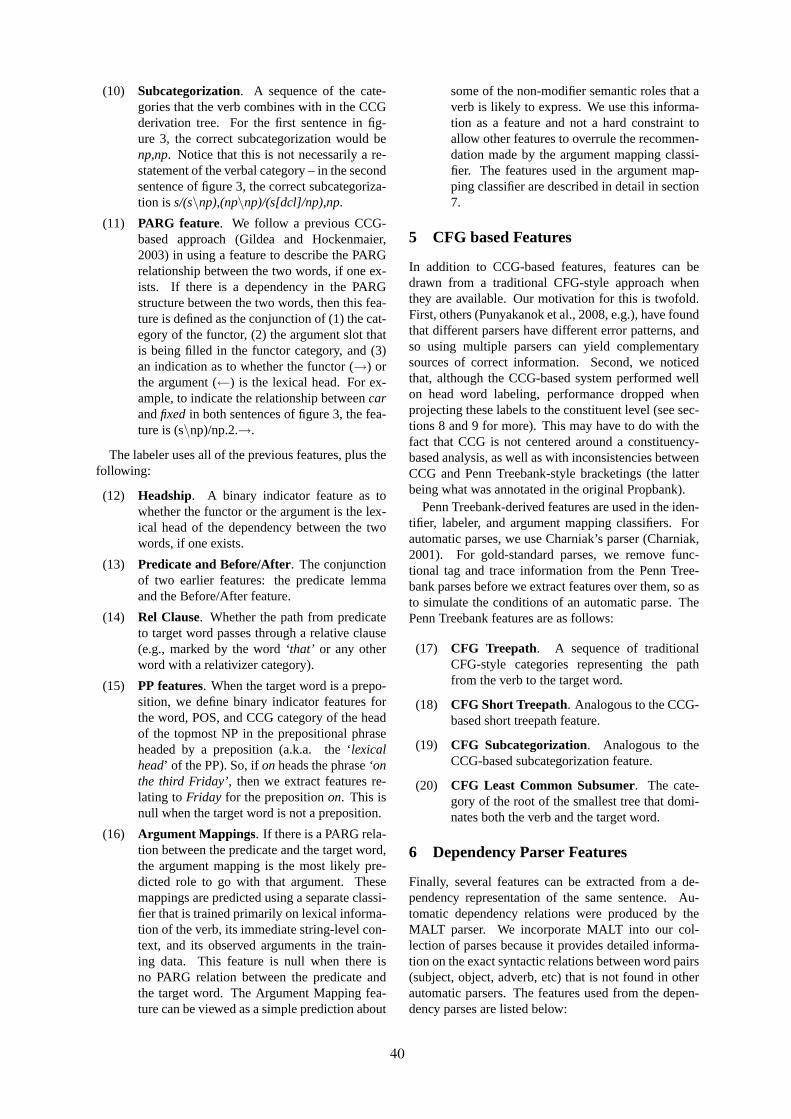
(10) Subcategorization. A sequence of the cate-gories that the verb combines with in the CCGderivation tree. For the first sentence in fig-ure 3, the correct subcategorization would benp,np. Notice that this is not necessarily a re-statement of the verbal category – in the secondsentence of figure 3, the correct subcategoriza-tion iss/(s\np),(np\np)/(s[dcl]/np),np.
(11) PARG feature. We follow a previous CCG-based approach (Gildea and Hockenmaier,2003) in using a feature to describe the PARGrelationship between the two words, if one ex-ists. If there is a dependency in the PARGstructure between the two words, then this fea-ture is defined as the conjunction of (1) the cat-egory of the functor, (2) the argument slot thatis being filled in the functor category, and (3)an indication as to whether the functor (→) orthe argument (←) is the lexical head. For ex-ample, to indicate the relationship betweencarandfixedin both sentences of figure 3, the fea-ture is (s\np)/np.2.→.
The labeler uses all of the previous features, plus thefollowing:
(12) Headship. A binary indicator feature as towhether the functor or the argument is the lex-ical head of the dependency between the twowords, if one exists.
(13) Predicate and Before/After. The conjunctionof two earlier features: the predicate lemmaand the Before/After feature.
(14) Rel Clause. Whether the path from predicateto target word passes through a relative clause(e.g., marked by the word‘that’ or any otherword with a relativizer category).
(15) PP features. When the target word is a prepo-sition, we define binary indicator features forthe word, POS, and CCG category of the headof the topmost NP in the prepositional phraseheaded by a preposition (a.k.a. the ‘lexicalhead’ of the PP). So, ifonheads the phrase‘onthe third Friday’, then we extract features re-lating toFriday for the prepositionon. This isnull when the target word is not a preposition.
(16) Argument Mappings. If there is a PARG rela-tion between the predicate and the target word,the argument mapping is the most likely pre-dicted role to go with that argument. Thesemappings are predicted using a separate classi-fier that is trained primarily on lexical informa-tion of the verb, its immediate string-level con-text, and its observed arguments in the train-ing data. This feature is null when there isno PARG relation between the predicate andthe target word. The Argument Mapping fea-ture can be viewed as a simple prediction about
some of the non-modifier semantic roles that averb is likely to express. We use this informa-tion as a feature and not a hard constraint toallow other features to overrule the recommen-dation made by the argument mapping classi-fier. The features used in the argument map-ping classifier are described in detail in section7.
5 CFG based Features
In addition to CCG-based features, features can bedrawn from a traditional CFG-style approach whenthey are available. Our motivation for this is twofold.First, others (Punyakanok et al., 2008, e.g.), have foundthat different parsers have different error patterns, andso using multiple parsers can yield complementarysources of correct information. Second, we noticedthat, although the CCG-based system performed wellon head word labeling, performance dropped whenprojecting these labels to the constituent level (see sec-tions 8 and 9 for more). This may have to do with thefact that CCG is not centered around a constituency-based analysis, as well as with inconsistencies betweenCCG and Penn Treebank-style bracketings (the latterbeing what was annotated in the original Propbank).
Penn Treebank-derived features are used in the iden-tifier, labeler, and argument mapping classifiers. Forautomatic parses, we use Charniak’s parser (Charniak,2001). For gold-standard parses, we remove func-tional tag and trace information from the Penn Tree-bank parses before we extract features over them, so asto simulate the conditions of an automatic parse. ThePenn Treebank features are as follows:
(17) CFG Treepath. A sequence of traditionalCFG-style categories representing the pathfrom the verb to the target word.
(18) CFG Short Treepath. Analogous to the CCG-based short treepath feature.
(19) CFG Subcategorization. Analogous to theCCG-based subcategorization feature.
(20) CFG Least Common Subsumer. The cate-gory of the root of the smallest tree that domi-nates both the verb and the target word.
6 Dependency Parser Features
Finally, several features can be extracted from a de-pendency representation of the same sentence. Au-tomatic dependency relations were produced by theMALT parser. We incorporate MALT into our col-lection of parses because it provides detailed informa-tion on the exact syntactic relations between word pairs(subject, object, adverb, etc) that is not found in otherautomatic parsers. The features used from the depen-dency parses are listed below:
40
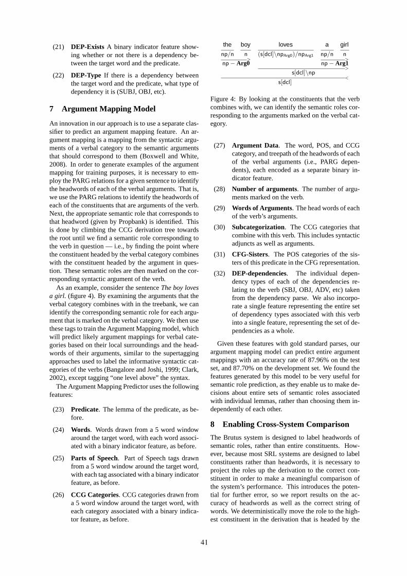
(21) DEP-Exists A binary indicator feature show-ing whether or not there is a dependency be-tween the target word and the predicate.
(22) DEP-Type If there is a dependency betweenthe target word and the predicate, what type ofdependency it is (SUBJ, OBJ, etc).
7 Argument Mapping Model
An innovation in our approach is to use a separate clas-sifier to predict an argument mapping feature. An ar-gument mapping is a mapping from the syntactic argu-ments of a verbal category to the semantic argumentsthat should correspond to them (Boxwell and White,2008). In order to generate examples of the argumentmapping for training purposes, it is necessary to em-ploy the PARG relations for a given sentence to identifythe headwords of each of the verbal arguments. That is,we use the PARG relations to identify the headwords ofeach of the constituents that are arguments of the verb.Next, the appropriate semantic role that corresponds tothat headword (given by Propbank) is identified. Thisis done by climbing the CCG derivation tree towardsthe root until we find a semantic role corresponding tothe verb in question — i.e., by finding the point wherethe constituent headed by the verbal category combineswith the constituent headed by the argument in ques-tion. These semantic roles are then marked on the cor-responding syntactic argument of the verb.
As an example, consider the sentenceThe boy lovesa girl. (figure 4). By examining the arguments that theverbal category combines with in the treebank, we canidentify the corresponding semantic role for each argu-ment that is marked on the verbal category. We then usethese tags to train the Argument Mapping model, whichwill predict likely argument mappings for verbal cate-gories based on their local surroundings and the head-words of their arguments, similar to the supertaggingapproaches used to label the informative syntactic cat-egories of the verbs (Bangalore and Joshi, 1999; Clark,2002), except tagging “one level above” the syntax.
The Argument Mapping Predictor uses the followingfeatures:
(23) Predicate. The lemma of the predicate, as be-fore.
(24) Words. Words drawn from a 5 word windowaround the target word, with each word associ-ated with a binary indicator feature, as before.
(25) Parts of Speech. Part of Speech tags drawnfrom a 5 word window around the target word,with each tag associated with a binary indicatorfeature, as before.
(26) CCG Categories. CCG categories drawn froma 5 word window around the target word, witheach category associated with a binary indica-tor feature, as before.
the boy loves a girl
np/n n (s[dcl]\npArg0)/npArg1 np/n n> >
np− Arg0 np− Arg1>
s[dcl]\np<
s[dcl]
Figure 4: By looking at the constituents that the verbcombines with, we can identify the semantic roles cor-responding to the arguments marked on the verbal cat-egory.
(27) Argument Data. The word, POS, and CCGcategory, and treepath of the headwords of eachof the verbal arguments (i.e., PARG depen-dents), each encoded as a separate binary in-dicator feature.
(28) Number of arguments. The number of argu-ments marked on the verb.
(29) Words of Arguments. The head words of eachof the verb’s arguments.
(30) Subcategorization. The CCG categories thatcombine with this verb. This includes syntacticadjuncts as well as arguments.
(31) CFG-Sisters. The POS categories of the sis-ters of this predicate in the CFG representation.
(32) DEP-dependencies. The individual depen-dency types of each of the dependencies re-lating to the verb (SBJ, OBJ, ADV, etc) takenfrom the dependency parse. We also incorpo-rate a single feature representing the entire setof dependency types associated with this verbinto a single feature, representing the set of de-pendencies as a whole.
Given these features with gold standard parses, ourargument mapping model can predict entire argumentmappings with an accuracy rate of 87.96% on the testset, and 87.70% on the development set. We found thefeatures generated by this model to be very useful forsemantic role prediction, as they enable us to make de-cisions about entire sets of semantic roles associatedwith individual lemmas, rather than choosing them in-dependently of each other.
8 Enabling Cross-System Comparison
The Brutus system is designed to label headwords ofsemantic roles, rather than entire constituents. How-ever, because most SRL systems are designed to labelconstituents rather than headwords, it is necessary toproject the roles up the derivation to the correct con-stituent in order to make a meaningful comparison ofthe system’s performance. This introduces the poten-tial for further error, so we report results on the ac-curacy of headwords as well as the correct string ofwords. We deterministically move the role to the high-est constituent in the derivation that is headed by the
41

a man with glasses spoke
np/n n (np\np)/np np s\np> >
np np\np<
np− speak.Arg0<
s
Figure 5: The role is moved towards the root until theoriginal node is no longer the head of the marked con-stituent.
P R F
G&H (treebank) 67.5% 60.0% 63.5%Brutus (treebank) 88.18% 85.00% 86.56%
G&H (automatic) 55.7% 49.5% 52.4%Brutus (automatic) 76.06% 70.15% 72.99%
Table 1: Accuracy of semantic role prediction usingonly CCG based features.
originally tagged terminal. In most cases, this corre-sponds to the node immediately dominated by the low-est common subsuming node of the the target word andthe verb (figure 5). In some cases, the highest con-stituent that is headed by the target word is not imme-diately dominated by the lowest common subsumingnode (figure 6).
9 Results
Using a version of Brutus incorporating only the CCG-based features described above, we achieve better re-sults than a previous CCG based system (Gildea andHockenmaier, 2003, henceforth G&H). This could bedue to a number of factors, including the fact that oursystem employs a different CCG parser, uses a morecomplete mapping of the Propbank onto the CCGbank,uses a different machine learning approach,6 and has aricher feature set. The results for constituent taggingaccuracy are shown in table 1.
As expected, by incorporating Penn Treebank-basedfeatures and dependency features, we obtain better re-sults than with the CCG-only system. The results forgold standard parses are comparable to the winningsystem of the CoNLL 2005 shared task on semanticrole labeling (Punyakanok et al., 2008). Other systems(Toutanova et al., 2008; Surdeanu et al., 2007; Johans-son and Nugues, 2008) have also achieved comparableresults – we compare our system to (Punyakanok etal., 2008) due to the similarities in our approaches. Theperformance of the full system is shown in table 2.
Table 3 shows the ability of the system to predictthe correct headwords of semantic roles. This is a nec-essary condition for correctness of the full constituent,but not a sufficient one. In parser evaluation, Carroll,Minnen, and Briscoe (Carroll et al., 2003) have argued
6G&H use a generative model with a back-off lattice,whereas we use a maximum entropy classifier.
P R F
P. et al (treebank) 86.22% 87.40% 86.81%Brutus (treebank) 88.29% 86.39% 87.33%
P. et al (automatic) 77.09% 75.51% 76.29%Brutus (automatic) 76.73% 70.45% 73.45%
Table 2: Accuracy of semantic role prediction usingCCG, CFG, and MALT based features.
P R F
Headword (treebank) 88.94% 86.98% 87.95%Boundary (treebank) 88.29% 86.39% 87.33%
Headword (automatic) 82.36% 75.97% 79.04%Boundary (automatic) 76.33% 70.59% 73.35%
Table 3: Accuracy of the system for labeling semanticroles on both constituent boundaries and headwords.Headwords are easier to predict than boundaries, re-flecting CCG’s focus on word-word relations ratherthan constituency.
for dependencies as a more appropriate means of eval-uation, reflecting the focus on headwords from con-stituent boundaries. We argue that, especially in theheavily lexicalized CCG framework, headword evalu-ation is more appropriate, reflecting the emphasis onheadword combinatorics in the CCG formalism.
10 The Contribution of the New Features
Two features which are less frequently used in SRLresearch play a major role in the Brutus system: ThePARG feature (Gildea and Hockenmaier, 2003) andthe argument mapping feature. Removing them hasa strong effect on accuracy when labeling treebankparses, as shown in our feature ablation results in ta-ble 4. We do not report results including the Argu-ment Mapping feature but not the PARG feature, be-cause some predicate-argument relation information isassumed in generating the Argument Mapping feature.
P R F
+PARG +AM 88.77% 86.15% 87.44%+PARG -AM 88.42% 85.78% 87.08%-PARG -AM 87.92% 84.65% 86.26%
Table 4: The effects of removing key features from thesystem on gold standard parses.
The same is true for automatic parses, as shown in ta-ble 5.
11 Error Analysis
Many of the errors made by the Brutus system can betraced directly to erroneous parses, either in the auto-matic or treebank parse. In some cases, PP attachment
42
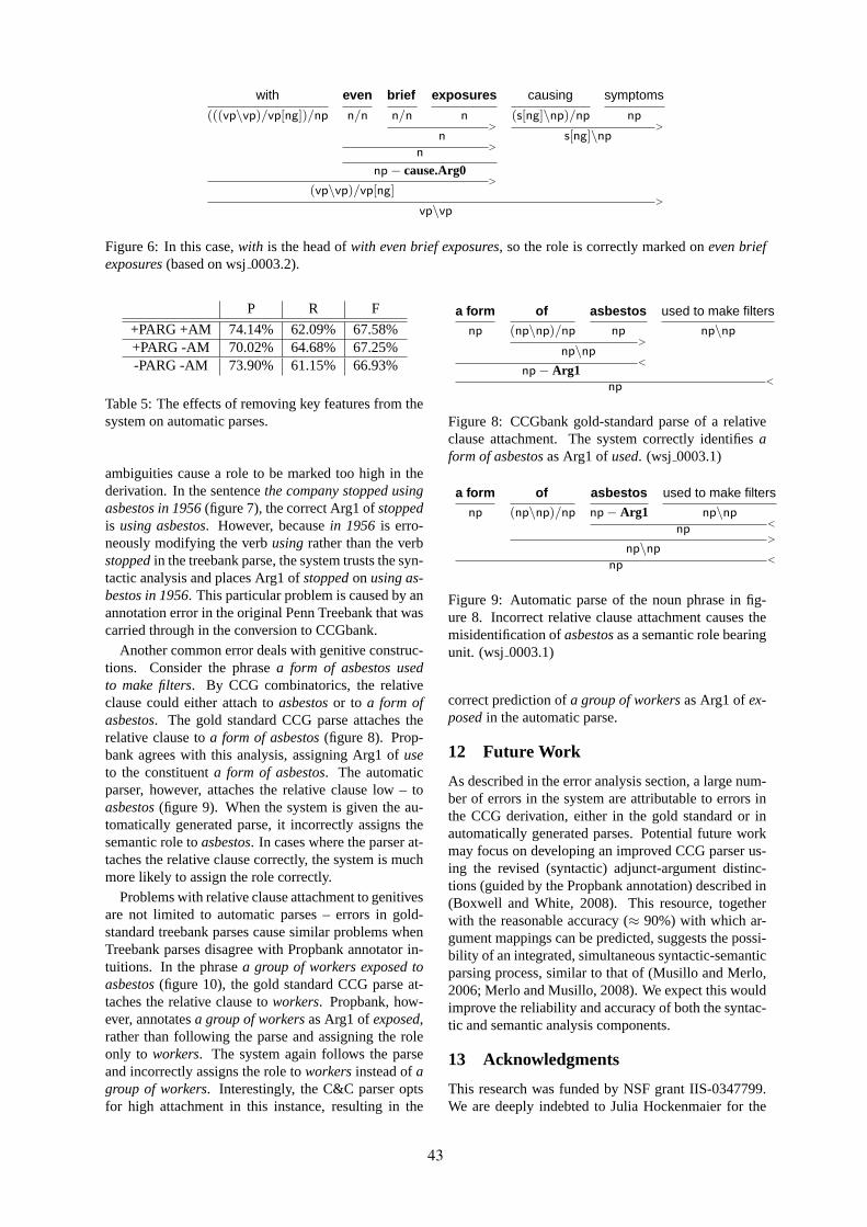
with even brief exposures causing symptoms
(((vp\vp)/vp[ng])/np n/n n/n n (s[ng]\np)/np np> >
n s[ng]\np>
n
np− cause.Arg0>
(vp\vp)/vp[ng]>
vp\vp
Figure 6: In this case,with is the head ofwith even brief exposures, so the role is correctly marked oneven briefexposures(based on wsj0003.2).
P R F
+PARG +AM 74.14% 62.09% 67.58%+PARG -AM 70.02% 64.68% 67.25%-PARG -AM 73.90% 61.15% 66.93%
Table 5: The effects of removing key features from thesystem on automatic parses.
ambiguities cause a role to be marked too high in thederivation. In the sentencethe company stopped usingasbestos in 1956(figure 7), the correct Arg1 ofstoppedis using asbestos. However, becausein 1956 is erro-neously modifying the verbusingrather than the verbstoppedin the treebank parse, the system trusts the syn-tactic analysis and places Arg1 ofstoppedonusing as-bestos in 1956. This particular problem is caused by anannotation error in the original Penn Treebank that wascarried through in the conversion to CCGbank.
Another common error deals with genitive construc-tions. Consider the phrasea form of asbestos usedto make filters. By CCG combinatorics, the relativeclause could either attach toasbestosor to a form ofasbestos. The gold standard CCG parse attaches therelative clause toa form of asbestos(figure 8). Prop-bank agrees with this analysis, assigning Arg1 ofuseto the constituenta form of asbestos. The automaticparser, however, attaches the relative clause low – toasbestos(figure 9). When the system is given the au-tomatically generated parse, it incorrectly assigns thesemantic role toasbestos. In cases where the parser at-taches the relative clause correctly, the system is muchmore likely to assign the role correctly.
Problems with relative clause attachment to genitivesare not limited to automatic parses – errors in gold-standard treebank parses cause similar problems whenTreebank parses disagree with Propbank annotator in-tuitions. In the phrasea group of workers exposed toasbestos(figure 10), the gold standard CCG parse at-taches the relative clause toworkers. Propbank, how-ever, annotatesa group of workersas Arg1 ofexposed,rather than following the parse and assigning the roleonly to workers. The system again follows the parseand incorrectly assigns the role toworkersinstead ofagroup of workers. Interestingly, the C&C parser optsfor high attachment in this instance, resulting in the
a form of asbestos used to make filters
np (np\np)/np np np\np>
np\np<
np− Arg1<
np
Figure 8: CCGbank gold-standard parse of a relativeclause attachment. The system correctly identifiesaform of asbestosas Arg1 ofused. (wsj 0003.1)
a form of asbestos used to make filters
np (np\np)/np np− Arg1 np\np<
np>
np\np<
np
Figure 9: Automatic parse of the noun phrase in fig-ure 8. Incorrect relative clause attachment causes themisidentification ofasbestosas a semantic role bearingunit. (wsj 0003.1)
correct prediction ofa group of workersas Arg1 ofex-posedin the automatic parse.
12 Future Work
As described in the error analysis section, a large num-ber of errors in the system are attributable to errors inthe CCG derivation, either in the gold standard or inautomatically generated parses. Potential future workmay focus on developing an improved CCG parser us-ing the revised (syntactic) adjunct-argument distinc-tions (guided by the Propbank annotation) described in(Boxwell and White, 2008). This resource, togetherwith the reasonable accuracy (≈ 90%) with which ar-gument mappings can be predicted, suggests the possi-bility of an integrated, simultaneous syntactic-semanticparsing process, similar to that of (Musillo and Merlo,2006; Merlo and Musillo, 2008). We expect this wouldimprove the reliability and accuracy of both the syntac-tic and semantic analysis components.
13 Acknowledgments
This research was funded by NSF grant IIS-0347799.We are deeply indebted to Julia Hockenmaier for the
43

the company stopped using asbestos in 1956
np ((s[dcl]\np)/(s[ng]\np)) (s[ng]\np)/np np (s\np)\(s\np)>
s[ng]\np<
s[ng]\np− stop.Arg1>
s[dcl]\np<
s[dcl]
Figure 7: An example of how incorrect PP attachment can causean incorrect labeling. Stop.Arg1 should coverus-ing asbestosrather thanusing asbestos in 1956. This sentence is based on wsj0003.3, with the structure simplifiedfor clarity.
a group of workers exposed to asbestos
np (np\np)/np np− exposed.Arg1 np\np<
np>
np\np<
np
Figure 10: Propbank annotatesa group of workersas Arg1 ofexposed, while CCGbank attaches the relative clauselow. The system incorrectly labelsworkersas a role bearing unit. (Gold standard – wsj0003.1)
use of her PARG generation tool.
References
Srinivas Bangalore and Aravind Joshi. 1999. Su-pertagging: An approach to almost parsing.Com-putational Linguistics, 25(2):237–265.
Adam L. Berger, S. Della Pietra, and V. Della Pietra.1996. A maximum entropy approach to naturallanguage processing.Computational Linguistics,22(1):39–71.
D.M. Bikel. 2004. Intricacies of Collins’ parsingmodel.Computational Linguistics, 30(4):479–511.
Stephen A. Boxwell and Michael White. 2008.Projecting propbank roles onto the ccgbank. InProceedings of the Sixth International LanguageResources and Evaluation Conference (LREC-08),Marrakech, Morocco.
J. Carroll, G. Minnen, and T. Briscoe. 2003. Parserevaluation. Treebanks: Building and Using ParsedCorpora, pages 299–316.
E. Charniak. 2001. Immediate-head parsing for lan-guage models. InProc. ACL-01, volume 39, pages116–123.
Stephen Clark and James R. Curran. 2007. Wide-coverage Efficient Statistical Parsing with CCG andLog-linear Models. Computational Linguistics,33(4):493–552.
Stephen Clark. 2002. Supertagging for combinatorycategorial grammar. InProceedings of the 6th In-ternational Workshop on Tree Adjoining Grammarsand Related Frameworks (TAG+6), pages 19–24,Venice, Italy.
M. Collins. 2003. Head-driven statistical models fornatural language parsing.Computational Linguis-tics, 29(4):589–637.
Daniel Gildea and Julia Hockenmaier. 2003. Identi-fying semantic roles using Combinatory CategorialGrammar. InProc. EMNLP-03.
Julia Hockenmaier and Mark Steedman. 2007. CCG-bank: A Corpus of CCG Derivations and Depen-dency Structures Extracted from the Penn Treebank.Computational Linguistics, 33(3):355–396.
R. Johansson and P. Nugues. 2008. Dependency-based syntactic–semantic analysis with PropBankand NomBank.Proceedings of CoNLL–2008.
D C Liu and Jorge Nocedal. 1989. On the limitedmemory method for large scale optimization.Math-ematical Programming B, 45(3).
Lluı́s Màrquez, Xavier Carreras, Kenneth C. Litowski,and Suzanne Stevenson. 2008. Semantic Role La-beling: An Introduction to the Special Issue.Com-putational Linguistics, 34(2):145–159.
Paola Merlo and Gabrile Musillo. 2008. Semanticparsing for high-precision semantic role labelling. InProceedings of CONLL-08, Manchester, UK.
Gabriele Musillo and Paola Merlo. 2006. Robust pars-ing of the proposition bank. InProceedings of theEACL 2006 Workshop ROMAND, Trento.
J. Nivre, J. Hall, J. Nilsson, A. Chanev, G. Eryigit,S. Kübler, S. Marinov, and E. Marsi. 2007. Malt-Parser: A language-independent system for data-driven dependency parsing.Natural Language En-gineering, 13(02):95–135.
Martha Palmer, Daniel Gildea, and Paul Kingsbury.2005. The Proposition Bank: An Annotated Cor-pus of Semantic Roles.Computational Linguistics,31(1):71–106.
44

Vasin Punyakanok, Dan Roth, and Wen tau Yih. 2008.The Importance of Syntactic Parsing and Inferencein Semantic Role Labeling.Computational Linguis-tics, 34(2):257–287.
Mark Steedman. 2000.The Syntactic Process. MITPress.
M. Surdeanu, L. M̀arquez, X. Carreras, and P. Comas.2007. Combination strategies for semantic role la-beling. Journal of Artificial Intelligence Research,29:105–151.
K. Toutanova, A. Haghighi, and C.D. Manning. 2008.A global joint model for semantic role labeling.Computational Linguistics, 34(2):161–191.
45
Proceedings of the 47th Annual Meeting of the ACL and the 4th IJCNLP of the AFNLP, pages 46–54,Suntec, Singapore, 2-7 August 2009. c©2009 ACL and AFNLP
Exploiting Heterogeneous Treebanks for Parsing
Zheng-Yu Niu, Haifeng Wang, Hua WuToshiba (China) Research and Development Center
5/F., Tower W2, Oriental Plaza, Beijing, 100738, China{niuzhengyu,wanghaifeng,wuhua}@rdc.toshiba.com.cn
Abstract
We address the issue of using heteroge-neous treebanks for parsing by breakingit down into two sub-problems, convert-ing grammar formalisms of the treebanksto the same one, and parsing on thesehomogeneous treebanks. First we pro-pose to employ an iteratively trained tar-get grammar parser to perform grammarformalism conversion, eliminating prede-fined heuristic rules as required in previ-ous methods. Then we provide two strate-gies to refine conversion results, and adopta corpus weighting technique for parsingon homogeneous treebanks. Results on thePenn Treebank show that our conversionmethod achieves 42% error reduction overthe previous best result. Evaluation onthe Penn Chinese Treebank indicates that aconverted dependency treebank helps con-stituency parsing and the use of unlabeleddata by self-training further increases pars-ing f-score to 85.2%, resulting in 6% errorreduction over the previous best result.
1 Introduction
The last few decades have seen the emergence ofmultiple treebanks annotated with different gram-mar formalisms, motivated by the diversity of lan-guages and linguistic theories, which is crucial tothe success of statistical parsing (Abeille et al.,2000; Brants et al., 1999; Bohmova et al., 2003;Han et al., 2002; Kurohashi and Nagao, 1998;Marcus et al., 1993; Moreno et al., 2003; Xue etal., 2005). Availability of multiple treebanks cre-ates a scenario where we have a treebank anno-tated with one grammar formalism, and anothertreebank annotated with another grammar formal-ism that we are interested in. We call the first
a source treebank, and the second a target tree-bank. We thus encounter a problem of how touse these heterogeneous treebanks for target gram-mar parsing. Here heterogeneous treebanks referto two or more treebanks with different grammarformalisms, e.g., one treebank annotated with de-pendency structure (DS) and the other annotatedwith phrase structure (PS).
It is important to acquire additional labeled datafor the target grammar parsing through exploita-tion of existing source treebanks since there is of-ten a shortage of labeled data. However, to ourknowledge, there is no previous study on this is-sue.
Recently there have been some works on us-ing multiple treebanks for domain adaptation ofparsers, where these treebanks have the samegrammar formalism (McClosky et al., 2006b;Roark and Bacchiani, 2003). Other related worksfocus on converting one grammar formalism of atreebank to another and then conducting studies onthe converted treebank (Collins et al., 1999; Forst,2003; Wang et al., 1994; Watkinson and Manand-har, 2001). These works were done either on mul-tiple treebanks with the same grammar formalismor on only one converted treebank. We see thattheir scenarios are different from ours as we workwith multiple heterogeneous treebanks.
For the use of heterogeneous treebanks1, wepropose a two-step solution: (1) converting thegrammar formalism of the source treebank to thetarget one, (2) refining converted trees and usingthem as additional training data to build a targetgrammar parser.
For grammar formalism conversion, we choosethe DS to PS direction for the convenience of thecomparison with existing works (Xia and Palmer,2001; Xia et al., 2008). Specifically, we assumethat the source grammar formalism is dependency
1Here we assume the existence of two treebanks.
46
grammar, and the target grammar formalism isphrase structure grammar.
Previous methods for DS to PS conversion(Collins et al., 1999; Covington, 1994; Xia andPalmer, 2001; Xia et al., 2008) often rely on pre-defined heuristic rules to eliminate converison am-biguity, e.g., minimal projection for dependents,lowest attachment position for dependents, and theselection of conversion rules that add fewer num-ber of nodes to the converted tree. In addition, thevalidity of these heuristic rules often depends ontheir target grammars. To eliminate the heuristicrules as required in previous methods, we proposeto use an existing target grammar parser (trainedon the target treebank) to generate N-best parsesfor each sentence in the source treebank as conver-sion candidates, and then select the parse consis-tent with the structure of the source tree as the con-verted tree. Furthermore, we attempt to use con-verted trees as additional training data to retrainthe parser for better conversion candidates. Theprocedure of tree conversion and parser retrainingwill be run iteratively until a stopping condition issatisfied.
Since some converted trees might be imper-fect from the perspective of the target grammar,we provide two strategies to refine conversion re-sults: (1) pruning low-quality trees from the con-verted treebank, (2) interpolating the scores fromthe source grammar and the target grammar to se-lect better converted trees. Finally we adopt a cor-pus weighting technique to get an optimal combi-nation of the converted treebank and the existingtarget treebank for parser training.
We have evaluated our conversion algorithm ona dependency structure treebank (produced fromthe Penn Treebank) for comparison with previouswork (Xia et al., 2008). We also have investi-gated our two-step solution on two existing tree-banks, the Penn Chinese Treebank (CTB) (Xue etal., 2005) and the Chinese Dependency Treebank(CDT)2 (Liu et al., 2006). Evaluation on WSJ datademonstrates that it is feasible to use a parser forgrammar formalism conversion and the conversionbenefits from converted trees used for parser re-training. Our conversion method achieves 93.8%f-score on dependency trees produced from WSJsection 22, resulting in 42% error reduction overthe previous best result for DS to PS conversion.Results on CTB show that score interpolation is
2Available at http://ir.hit.edu.cn/.
more effective than instance pruning for the useof converted treebanks for parsing and convertedCDT helps parsing on CTB. When coupled withself-training technique, a reranking parser withCTB and converted CDT as labeled data achieves85.2% f-score on CTB test set, an absolute 1.0%improvement (6% error reduction) over the previ-ous best result for Chinese parsing.
The rest of this paper is organized as follows. InSection 2, we first describe a parser based methodfor DS to PS conversion, and then we discuss pos-sible strategies to refine conversion results, andfinally we adopt the corpus weighting techniquefor parsing on homogeneous treebanks. Section3 provides experimental results of grammar for-malism conversion on a dependency treebank pro-duced from the Penn Treebank. In Section 4, weevaluate our two-step solution on two existing het-erogeneous Chinese treebanks. Section 5 reviewsrelated work and Section 6 concludes this work.
2 Our Two-Step Solution
2.1 Grammar Formalism Conversion
Previous DS to PS conversion methods built aconverted tree by iteratively attaching nodes andedges to the tree with the help of conversionrules and heuristic rules, based on current head-dependent pair from a source dependency tree andthe structure of the built tree (Collins et al., 1999;Covington, 1994; Xia and Palmer, 2001; Xia etal., 2008). Some observations can be made onthese methods: (1) for each head-dependent pair,only one locally optimal conversion was kept dur-ing tree-building process, at the risk of pruningglobally optimal conversions, (2) heuristic rulesare required to deal with the problem that onehead-dependent pair might have multiple conver-sion candidates, and these heuristic rules are usu-ally hand-crafted to reflect the structural prefer-ence in their target grammars. To overcome theselimitations, we propose to employ a parser to gen-erate N-best parses as conversion candidates andthen use the structural information of source treesto select the best parse as a converted tree.
We formulate our conversion method as fol-lows.
Let CDS be a source treebank annotated withDS and CPS be a target treebank annotated withPS. Our goal is to convert the grammar formalismof CDS to that of CPS .
We first train a constituency parser on CPS
47

Input: CPS , CDS , Q, and a constituency parser Output: Converted trees CDSPS
1. Initialize:— Set CDS,0
PS as null, DevScore=0, q=0;— Split CPS into training set CPS,train and development set CPS,dev;— Train the parser on CPS,train and denote it by Pq−1;
2. Repeat:— Use Pq−1 to generate N-best PS parses for each sentence in CDS , and convert PS to DS for each parse;— For each sentence in CDS Do
¦ t̂=argmaxtScore(xi,t), and select the t̂-th parse as a converted tree for this sentence;— Let CDS,q
PS represent these converted trees, and let Ctrain=CPS,train⋃
CDS,qPS ;
— Train the parser on Ctrain, and denote the updated parser by Pq;— Let DevScoreq be the f-score of Pq on CPS,dev;— If DevScoreq > DevScore Then DevScore=DevScoreq, and CDS
PS =CDS,qPS ;
— Else break;— q++;Until q > Q
Table 1: Our algorithm for DS to PS conversion.
(90% trees in CPS as training set CPS,train, andother trees as development set CPS,dev) and thenlet the parser generate N-best parses for each sen-tence in CDS .
Let n be the number of sentences (or trees) inCDS and ni be the number of N-best parses gen-erated by the parser for the i-th (1 ≤ i ≤ n) sen-tence in CDS . Let xi,t be the t-th (1 ≤ t ≤ ni)parse for the i-th sentence. Let yi be the tree of thei-th (1 ≤ i ≤ n) sentence in CDS .
To evaluate the quality of xi,t as a conversioncandidate for yi, we convert xi,t to a dependencytree (denoted as xDS
i,t ) and then use unlabeled de-pendency f-score to measure the similarity be-tween xDS
i,t and yi. Let Score(xi,t) denote theunlabeled dependency f-score of xDS
i,t against yi.Then we determine the converted tree for yi bymaximizing Score(xi,t) over the N-best parses.
The conversion from PS to DS works as fol-lows:
Step 1. Use a head percolation table to find thehead of each constituent in xi,t.
Step 2. Make the head of each non-head childdepend on the head of the head child for each con-stituent.
Unlabeled dependency f-score is a harmonicmean of unlabeled dependency precision and unla-beled dependency recall. Precision measures howmany head-dependent word pairs found in xDS
i,t
are correct and recall is the percentage of head-dependent word pairs defined in the gold-standard
tree that are found in xDSi,t . Here we do not take
dependency tags into consideration for evaluationsince they cannot be obtained without more so-phisticated rules.
To improve the quality of N-best parses, we at-tempt to use the converted trees as additional train-ing data to retrain the parser. The procedure oftree conversion and parser retraining can be run it-eratively until a termination condition is satisfied.Here we use the parser’s f-score on CPS,dev as atermination criterion. If the update of training datahurts the performance on CPS,dev, then we stopthe iteration.
Table 1 shows this DS to PS conversion algo-rithm. Q is an upper limit of the number of loops,and Q ≥ 0.
2.2 Target Grammar Parsing
Through grammar formalism conversion, we havesuccessfully turned the problem of using hetero-geneous treebanks for parsing into the problem ofparsing on homogeneous treebanks. Before usingconverted source treebank for parsing, we presenttwo strategies to refine conversion results.
Instance Pruning For some sentences inCDS , the parser might fail to generate high qual-ity N-best parses, resulting in inferior convertedtrees. To clean the converted treebank, we can re-move the converted trees with low unlabeled de-pendency f-scores (defined in Section 2.1) beforeusing the converted treebank for parser training
48
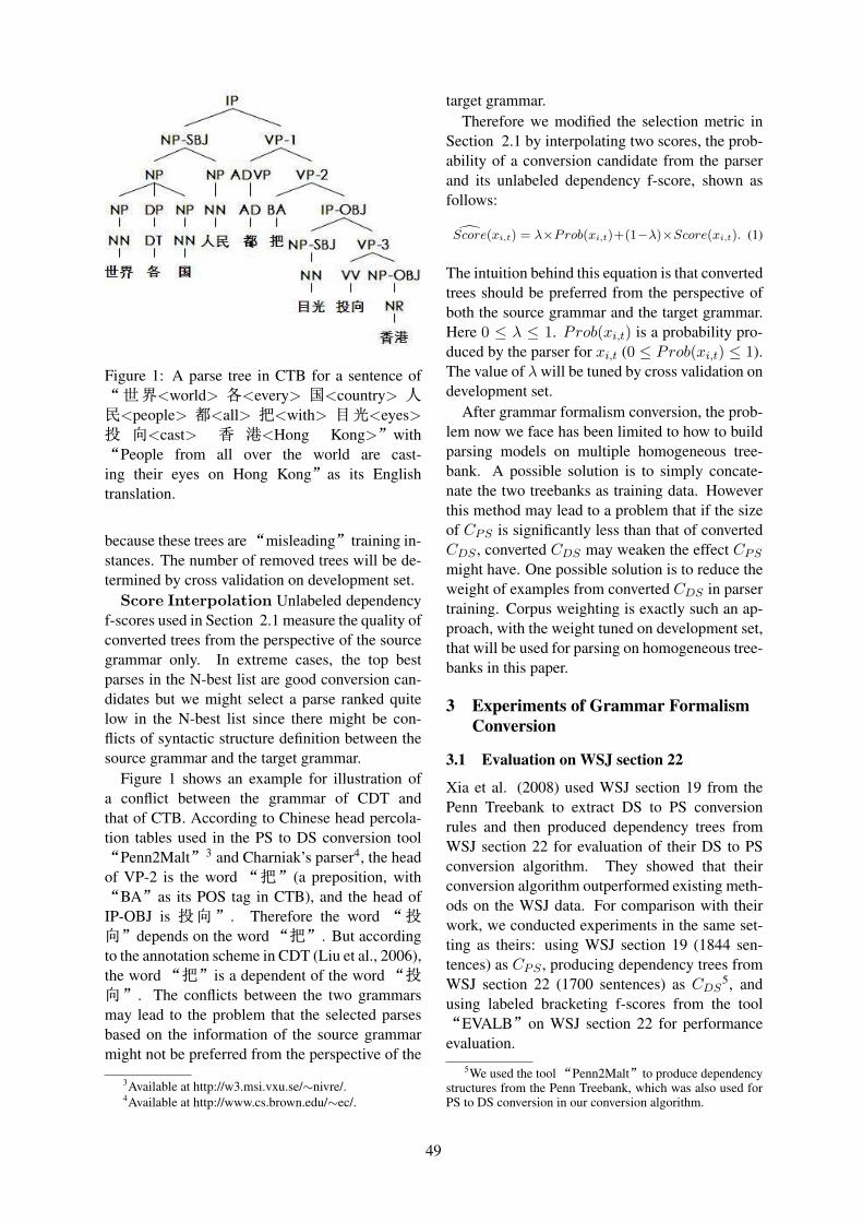
Figure 1: A parse tree in CTB for a sentence of/.<world> �<every> I<country> <¬<people> Ñ<all> r<with> 81<eyes>Ý �<cast> � l<Hong Kong>0with/People from all over the world are cast-ing their eyes on Hong Kong0as its Englishtranslation.
because these trees are/misleading0training in-stances. The number of removed trees will be de-termined by cross validation on development set.
Score Interpolation Unlabeled dependencyf-scores used in Section 2.1 measure the quality ofconverted trees from the perspective of the sourcegrammar only. In extreme cases, the top bestparses in the N-best list are good conversion can-didates but we might select a parse ranked quitelow in the N-best list since there might be con-flicts of syntactic structure definition between thesource grammar and the target grammar.
Figure 1 shows an example for illustration ofa conflict between the grammar of CDT andthat of CTB. According to Chinese head percola-tion tables used in the PS to DS conversion tool/Penn2Malt03 and Charniak’s parser4, the headof VP-2 is the word /r0(a preposition, with/BA0as its POS tag in CTB), and the head ofIP-OBJ is Ý�0. Therefore the word /Ý�0depends on the word/r0. But accordingto the annotation scheme in CDT (Liu et al., 2006),the word/r0is a dependent of the word/Ý�0. The conflicts between the two grammarsmay lead to the problem that the selected parsesbased on the information of the source grammarmight not be preferred from the perspective of the
3Available at http://w3.msi.vxu.se/∼nivre/.4Available at http://www.cs.brown.edu/∼ec/.
target grammar.Therefore we modified the selection metric in
Section 2.1 by interpolating two scores, the prob-ability of a conversion candidate from the parserand its unlabeled dependency f-score, shown asfollows:
̂Score(xi,t) = λ×Prob(xi,t)+(1−λ)×Score(xi,t). (1)
The intuition behind this equation is that convertedtrees should be preferred from the perspective ofboth the source grammar and the target grammar.Here 0 ≤ λ ≤ 1. Prob(xi,t) is a probability pro-duced by the parser for xi,t (0 ≤ Prob(xi,t) ≤ 1).The value of λ will be tuned by cross validation ondevelopment set.
After grammar formalism conversion, the prob-lem now we face has been limited to how to buildparsing models on multiple homogeneous tree-bank. A possible solution is to simply concate-nate the two treebanks as training data. Howeverthis method may lead to a problem that if the sizeof CPS is significantly less than that of convertedCDS , converted CDS may weaken the effect CPS
might have. One possible solution is to reduce theweight of examples from converted CDS in parsertraining. Corpus weighting is exactly such an ap-proach, with the weight tuned on development set,that will be used for parsing on homogeneous tree-banks in this paper.
3 Experiments of Grammar FormalismConversion
3.1 Evaluation on WSJ section 22
Xia et al. (2008) used WSJ section 19 from thePenn Treebank to extract DS to PS conversionrules and then produced dependency trees fromWSJ section 22 for evaluation of their DS to PSconversion algorithm. They showed that theirconversion algorithm outperformed existing meth-ods on the WSJ data. For comparison with theirwork, we conducted experiments in the same set-ting as theirs: using WSJ section 19 (1844 sen-tences) as CPS , producing dependency trees fromWSJ section 22 (1700 sentences) as CDS
5, andusing labeled bracketing f-scores from the tool/EVALB0on WSJ section 22 for performanceevaluation.
5We used the tool/Penn2Malt0to produce dependencystructures from the Penn Treebank, which was also used forPS to DS conversion in our conversion algorithm.
49

All the sentencesDevScore LR LP F
Models (%) (%) (%) (%)The best result ofXia et al. (2008) - 90.7 88.1 89.4
Q-0-method 86.8 92.2 92.8 92.5Q-10-method 88.0 93.4 94.1 93.8
Table 2: Comparison with the work of Xia et al.(2008) on WSJ section 22.
All the sentencesDevScore LR LP F
Models (%) (%) (%) (%)Q-0-method 91.0 91.6 92.5 92.1
Q-10-method 91.6 93.1 94.1 93.6
Table 3: Results of our algorithm on WSJ section2∼18 and 20∼22.
We employed Charniak’s maximum entropy in-spired parser (Charniak, 2000) to generate N-best(N=200) parses. Xia et al. (2008) used POStag information, dependency structures and depen-dency tags in test set for conversion. Similarly, weused POS tag information in the test set to restrictsearch space of the parser for generation of betterN-best parses.
We evaluated two variants of our DS to PS con-version algorithm:
Q-0-method: We set the value of Q as 0 for abaseline method.
Q-10-method: We set the value of Q as 10 tosee whether it is helpful for conversion to retrainthe parser on converted trees.
Table 2 shows the results of our conversion al-gorithm on WSJ section 22. In the experimentof Q-10-method, DevScore reached the highestvalue of 88.0% when q was 1. Then we usedCDS,1
PS as the conversion result. Finally Q-10-method achieved an f-score of 93.8% on WSJ sec-tion 22, an absolute 4.4% improvement (42% er-ror reduction) over the best result of Xia et al.(2008). Moreover, Q-10-method outperformed Q-0-method on the same test set. These results indi-cate that it is feasible to use a parser for DS to PSconversion and the conversion benefits from theuse of converted trees for parser retraining.
3.2 Evaluation on WSJ section 2∼18 and20∼22
In this experiment we evaluated our conversion al-gorithm on a larger test set, WSJ section 2∼18 and20∼22 (totally 39688 sentences). Here we alsoused WSJ section 19 as CPS . Other settings for
All the sentencesLR LP F
Training data (%) (%) (%)1× CTB + CDT PS 84.7 85.1 84.92× CTB + CDT PS 85.1 85.6 85.35× CTB + CDT PS 85.0 85.5 85.310× CTB + CDT PS 85.3 85.8 85.620× CTB + CDT PS 85.1 85.3 85.250× CTB + CDT PS 84.9 85.3 85.1
Table 4: Results of the generative parser on the de-velopment set, when trained with various weight-ing of CTB training set and CDTPS .
this experiment are as same as that in Section 3.1,except that here we used a larger test set.
Table 3 provides the f-scores of our method withQ equal to 0 or 10 on WSJ section 2∼18 and20∼22.
With Q-10-method, DevScore reached the high-est value of 91.6% when q was 1. Finally Q-10-method achieved an f-score of 93.6% on WSJsection 2∼18 and 20∼22, better than that of Q-0-method and comparable with that of Q-10-methodin Section 3.1. It confirms our previous findingthat the conversion benefits from the use of con-verted trees for parser retraining.
4 Experiments of Parsing
We investigated our two-step solution on two ex-isting treebanks, CDT and CTB, and we used CDTas the source treebank and CTB as the target tree-bank.
CDT consists of 60k Chinese sentences, anno-tated with POS tag information and dependencystructure information (including 28 POS tags, and24 dependency tags) (Liu et al., 2006). We did notuse POS tag information as inputs to the parser inour conversion method due to the difficulty of con-version from CDT POS tags to CTB POS tags.
We used a standard split of CTB for perfor-mance evaluation, articles 1-270 and 400-1151 astraining set, articles 301-325 as development set,and articles 271-300 as test set.
We used Charniak’s maximum entropy inspiredparser and their reranker (Charniak and Johnson,2005) for target grammar parsing, called a gener-ative parser (GP) and a reranking parser (RP) re-spectively. We reported ParseVal measures fromthe EVALB tool.
50
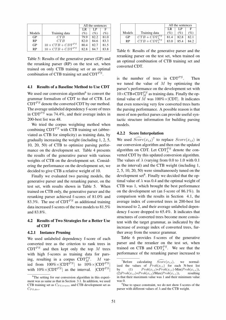
All the sentencesLR LP F
Models Training data (%) (%) (%)GP CTB 79.9 82.2 81.0RP CTB 82.0 84.6 83.3GP 10× CTB + CDT PS 80.4 82.7 81.5RP 10× CTB + CDT PS 82.8 84.7 83.8
Table 5: Results of the generative parser (GP) andthe reranking parser (RP) on the test set, whentrained on only CTB training set or an optimalcombination of CTB training set and CDTPS .
4.1 Results of a Baseline Method to Use CDTWe used our conversion algorithm6 to convert thegrammar formalism of CDT to that of CTB. LetCDTPS denote the converted CDT by our method.The average unlabeled dependency f-score of treesin CDTPS was 74.4%, and their average index in200-best list was 48.
We tried the corpus weighting method whencombining CDTPS with CTB training set (abbre-viated as CTB for simplicity) as training data, bygradually increasing the weight (including 1, 2, 5,10, 20, 50) of CTB to optimize parsing perfor-mance on the development set. Table 4 presentsthe results of the generative parser with variousweights of CTB on the development set. Consid-ering the performance on the development set, wedecided to give CTB a relative weight of 10.
Finally we evaluated two parsing models, thegenerative parser and the reranking parser, on thetest set, with results shown in Table 5. Whentrained on CTB only, the generative parser and thereranking parser achieved f-scores of 81.0% and83.3%. The use of CDTPS as additional trainingdata increased f-scores of the two models to 81.5%and 83.8%.
4.2 Results of Two Strategies for a Better Useof CDT
4.2.1 Instance PruningWe used unlabeled dependency f-score of eachconverted tree as the criterion to rank trees inCDTPS and then kept only the top M treeswith high f-scores as training data for pars-ing, resulting in a corpus CDTPS
M . M var-ied from 100%×|CDTPS | to 10%×|CDTPS |with 10%×|CDTPS | as the interval. |CDTPS |
6The setting for our conversion algorithm in this experi-ment was as same as that in Section 3.1. In addition, we usedCTB training set as CPS,train, and CTB development set asCPS,dev .
All the sentencesLR LP F
Models Training data (%) (%) (%)GP CTB + CDT PS
λ 81.4 82.8 82.1RP CTB + CDT PS
λ 83.0 85.4 84.2
Table 6: Results of the generative parser and thereranking parser on the test set, when trained onan optimal combination of CTB training set andconverted CDT.
is the number of trees in CDTPS . Thenwe tuned the value of M by optimizing theparser’s performance on the development set with10×CTB+CDTPS
M as training data. Finally the op-timal value of M was 100%×|CDT|. It indicatesthat even removing very few converted trees hurtsthe parsing performance. A possible reason is thatmost of non-perfect parses can provide useful syn-tactic structure information for building parsingmodels.
4.2.2 Score InterpolationWe used ̂Score(xi,t)
7 to replace Score(xi,t) inour conversion algorithm and then ran the updatedalgorithm on CDT. Let CDTPS
λ denote the con-verted CDT by this updated conversion algorithm.The values of λ (varying from 0.0 to 1.0 with 0.1as the interval) and the CTB weight (including 1,2, 5, 10, 20, 50) were simultaneously tuned on thedevelopment set8. Finally we decided that the op-timal value of λ was 0.4 and the optimal weight ofCTB was 1, which brought the best performanceon the development set (an f-score of 86.1%). Incomparison with the results in Section 4.1, theaverage index of converted trees in 200-best listincreased to 2, and their average unlabeled depen-dency f-score dropped to 65.4%. It indicates thatstructures of converted trees become more consis-tent with the target grammar, as indicated by theincrease of average index of converted trees, fur-ther away from the source grammar.
Table 6 provides f-scores of the generativeparser and the reranker on the test set, whentrained on CTB and CDTPS
λ . We see that theperformance of the reranking parser increased to
7Before calculating ̂Score(xi,t), we normal-ized the values of Prob(xi,t) for each N-best listby (1) Prob(xi,t)=Prob(xi,t)-Min(Prob(xi,∗)),(2)Prob(xi,t)=Prob(xi,t)/Max(Prob(xi,∗)), resultingin that their maximum value was 1 and their minimum valuewas 0.
8Due to space constraint, we do not show f-scores of theparser with different values of λ and the CTB weight.
51

All the sentencesLR LP F
Models Training data (%) (%) (%)Self-trained GP 10×T+10×D+P 83.0 84.5 83.7
Updated RP CTB+CDT PSλ 84.3 86.1 85.2
Table 7: Results of the self-trained gen-erative parser and updated reranking parseron the test set. 10×T+10×D+P stands for10×CTB+10×CDTPS
λ +PDC.
84.2% f-score, better than the result of the rerank-ing parser with CTB and CDTPS as training data(shown in Table 5). It indicates that the use ofprobability information from the parser for treeconversion helps target grammar parsing.
4.3 Using Unlabeled Data for Parsing
Recent studies on parsing indicate that the use ofunlabeled data by self-training can help parsingon the WSJ data, even when labeled data is rel-atively large (McClosky et al., 2006a; Reichartand Rappoport, 2007). It motivates us to em-ploy self-training technique for Chinese parsing.We used the POS tagged People Daily corpus9
(Jan. 1998∼Jun. 1998, and Jan. 2000∼Dec.2000) (PDC) as unlabeled data for parsing. Firstwe removed the sentences with less than 3 wordsor more than 40 words from PDC to ease pars-ing, resulting in 820k sentences. Then we ran thereranking parser in Section 4.2.2 on PDC and usedthe parses on PDC as additional training data forthe generative parser. Here we tried the corpusweighting technique for an optimal combinationof CTB, CDTPS
λ and parsed PDC, and chose therelative weight of both CTB and CDTPS
λ as 10by cross validation on the development set. Fi-nally we retrained the generative parser on CTB,CDTPS
λ and parsed PDC. Furthermore, we usedthis self-trained generative parser as a base parserto retrain the reranker on CTB and CDTPS
λ .Table 7 shows the performance of self-trained
generative parser and updated reranker on the testset, with CTB and CDTPS
λ as labeled data. We seethat the use of unlabeled data by self-training fur-ther increased the reranking parser’s performancefrom 84.2% to 85.2%. Our results on Chinese dataconfirm previous findings on English data shownin (McClosky et al., 2006a; Reichart and Rap-poport, 2007).
9Available at http://icl.pku.edu.cn/.
4.4 Comparison with Previous Studies forChinese Parsing
Table 8 and 9 present the results of previous stud-ies on CTB. All the works in Table 8 used CTBarticles 1-270 as labeled data. In Table 9, Petrovand Klein (2007) trained their model on CTB ar-ticles 1-270 and 400-1151, and Burkett and Klein(2008) used the same CTB articles and parse treesof their English translation (from the English Chi-nese Translation Treebank) as training data. Com-paring our result in Table 6 with that of Petrovand Klein (2007), we see that CDTPS
λ helps pars-ing on CTB, which brought 0.9% f-score improve-ment. Moreover, the use of unlabeled data furtherboosted the parsing performance to 85.2%, an ab-solute 1.0% improvement over the previous bestresult presented in Burkett and Klein (2008).
5 Related Work
Recently there have been some studies address-ing how to use treebanks with same grammar for-malism for domain adaptation of parsers. Roarkand Bachiani (2003) presented count merging andmodel interpolation techniques for domain adap-tation of parsers. They showed that their sys-tem with count merging achieved a higher perfor-mance when in-domain data was weighted moreheavily than out-of-domain data. McClosky et al.(2006b) used self-training and corpus weighting toadapt their parser trained on WSJ corpus to Browncorpus. Their results indicated that both unla-beled in-domain data and labeled out-of-domaindata can help domain adaptation. In comparisonwith these works, we conduct our study in a dif-ferent setting where we work with multiple het-erogeneous treebanks.
Grammar formalism conversion makes it possi-ble to reuse existing source treebanks for the studyof target grammar parsing. Wang et al. (1994)employed a parser to help conversion of a tree-bank from a simple phrase structure to a more in-formative phrase structure and then used this con-verted treebank to train their parser. Collins et al.(1999) performed statistical constituency parsingof Czech on a treebank that was converted fromthe Prague Dependency Treebank under the guid-ance of conversion rules and heuristic rules, e.g.,one level of projection for any category, minimalprojection for any dependents, and fixed positionof attachment. Xia and Palmer (2001) adopted bet-ter heuristic rules to build converted trees, which
52
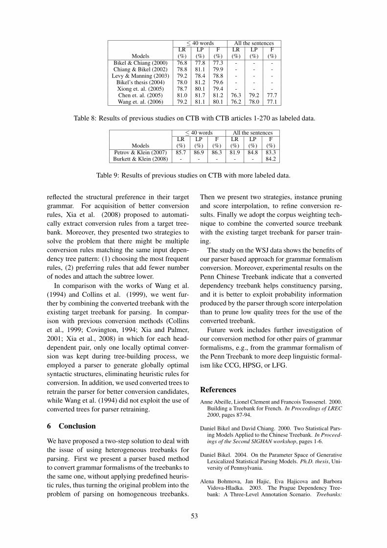
≤ 40 words All the sentencesLR LP F LR LP F
Models (%) (%) (%) (%) (%) (%)Bikel & Chiang (2000) 76.8 77.8 77.3 - - -Chiang & Bikel (2002) 78.8 81.1 79.9 - - -
Levy & Manning (2003) 79.2 78.4 78.8 - - -Bikel’s thesis (2004) 78.0 81.2 79.6 - - -Xiong et. al. (2005) 78.7 80.1 79.4 - - -Chen et. al. (2005) 81.0 81.7 81.2 76.3 79.2 77.7Wang et. al. (2006) 79.2 81.1 80.1 76.2 78.0 77.1
Table 8: Results of previous studies on CTB with CTB articles 1-270 as labeled data.
≤ 40 words All the sentencesLR LP F LR LP F
Models (%) (%) (%) (%) (%) (%)Petrov & Klein (2007) 85.7 86.9 86.3 81.9 84.8 83.3Burkett & Klein (2008) - - - - - 84.2
Table 9: Results of previous studies on CTB with more labeled data.
reflected the structural preference in their targetgrammar. For acquisition of better conversionrules, Xia et al. (2008) proposed to automati-cally extract conversion rules from a target tree-bank. Moreover, they presented two strategies tosolve the problem that there might be multipleconversion rules matching the same input depen-dency tree pattern: (1) choosing the most frequentrules, (2) preferring rules that add fewer numberof nodes and attach the subtree lower.
In comparison with the works of Wang et al.(1994) and Collins et al. (1999), we went fur-ther by combining the converted treebank with theexisting target treebank for parsing. In compar-ison with previous conversion methods (Collinset al., 1999; Covington, 1994; Xia and Palmer,2001; Xia et al., 2008) in which for each head-dependent pair, only one locally optimal conver-sion was kept during tree-building process, weemployed a parser to generate globally optimalsyntactic structures, eliminating heuristic rules forconversion. In addition, we used converted trees toretrain the parser for better conversion candidates,while Wang et al. (1994) did not exploit the use ofconverted trees for parser retraining.
6 Conclusion
We have proposed a two-step solution to deal withthe issue of using heterogeneous treebanks forparsing. First we present a parser based methodto convert grammar formalisms of the treebanks tothe same one, without applying predefined heuris-tic rules, thus turning the original problem into theproblem of parsing on homogeneous treebanks.
Then we present two strategies, instance pruningand score interpolation, to refine conversion re-sults. Finally we adopt the corpus weighting tech-nique to combine the converted source treebankwith the existing target treebank for parser train-ing.
The study on the WSJ data shows the benefits ofour parser based approach for grammar formalismconversion. Moreover, experimental results on thePenn Chinese Treebank indicate that a converteddependency treebank helps constituency parsing,and it is better to exploit probability informationproduced by the parser through score interpolationthan to prune low quality trees for the use of theconverted treebank.
Future work includes further investigation ofour conversion method for other pairs of grammarformalisms, e.g., from the grammar formalism ofthe Penn Treebank to more deep linguistic formal-ism like CCG, HPSG, or LFG.
ReferencesAnne Abeille, Lionel Clement and Francois Toussenel. 2000.
Building a Treebank for French. In Proceedings of LREC2000, pages 87-94.
Daniel Bikel and David Chiang. 2000. Two Statistical Pars-ing Models Applied to the Chinese Treebank. In Proceed-ings of the Second SIGHAN workshop, pages 1-6.
Daniel Bikel. 2004. On the Parameter Space of GenerativeLexicalized Statistical Parsing Models. Ph.D. thesis, Uni-versity of Pennsylvania.
Alena Bohmova, Jan Hajic, Eva Hajicova and BarboraVidova-Hladka. 2003. The Prague Dependency Tree-bank: A Three-Level Annotation Scenario. Treebanks:
53

Building and Using Annotated Corpora. Kluwer Aca-demic Publishers, pages 103-127.
Thorsten Brants, Wojciech Skut and Hans Uszkoreit. 1999.Syntactic Annotation of a German Newspaper Corpus. InProceedings of the ATALA Treebank Workshop, pages 69-76.
David Burkett and Dan Klein. 2008. Two Languages areBetter than One (for Syntactic Parsing). In Proceedings ofEMNLP 2008, pages 877-886.
Eugene Charniak. 2000. A Maximum Entropy InspiredParser. In Proceedings of NAACL 2000, pages 132-139.
Eugene Charniak and Mark Johnson. 2005. Coarse-to-FineN-Best Parsing and MaxEnt Discriminative Reranking. InProceedings of ACL 2005, pages 173-180.
Ying Chen, Hongling Sun and Dan Jurafsky. 2005. A Cor-rigendum to Sun and Jurafsky (2004) Shallow SemanticParsing of Chinese. University of Colorado at BoulderCSLR Tech Report TR-CSLR-2005-01.
David Chiang and Daniel M. Bikel. 2002. Recovering La-tent Information in Treebanks. In Proceedings of COL-ING 2002, pages 1-7.
Micheal Collins, Lance Ramshaw, Jan Hajic and ChristophTillmann. 1999. A Statistical Parser for Czech. In Pro-ceedings of ACL 1999, pages 505-512.
Micheal Covington. 1994. GB Theory as DependencyGrammar. Research Report AI-1992-03.
Martin Forst. 2003. Treebank Conversion - Establishinga Testsuite for a Broad-Coverage LFG from the TIGERTreebank. In Proceedings of LINC at EACL 2003, pages25-32.
Chunghye Han, Narae Han, Eonsuk Ko and Martha Palmer.2002. Development and Evaluation of a Korean Treebankand its Application to NLP. In Proceedings of LREC 2002,pages 1635-1642.
Sadao Kurohashi and Makato Nagao. 1998. Building aJapanese Parsed Corpus While Improving the Parsing Sys-tem. In Proceedings of LREC 1998, pages 719-724.
Roger Levy and Christopher Manning. 2003. Is It Harder toParse Chinese, or the Chinese Treebank? In Proceedingsof ACL 2003, pages 439-446.
Ting Liu, Jinshan Ma and Sheng Li. 2006. Building a Depen-dency Treebank for Improving Chinese Parser. Journal ofChinese Language and Computing, 16(4):207-224.
Mitchell P. Marcus, Beatrice Santorini and Mary AnnMarcinkiewicz. 1993. Building a Large Annotated Cor-pus of English: The Penn Treebank. Computational Lin-guistics, 19(2):313-330.
David McClosky, Eugene Charniak and Mark Johnson.2006a. Effective Self-Training for Parsing. In Proceed-ings of NAACL 2006, pages 152-159.
David McClosky, Eugene Charniak and Mark Johnson.2006b. Reranking and Self-Training for Parser Adapta-tion. In Proceedings of COLING/ACL 2006, pages 337-344.
Antonio Moreno, Susana Lopez, Fernando Sanchez andRalph Grishman. 2003. Developing a Syntactic Anno-tation Scheme and Tools for a Spanish Treebank. Tree-banks: Building and Using Annotated Corpora. KluwerAcademic Publishers, pages 149-163.
Slav Petrov and Dan Klein. 2007. Improved Inference forUnlexicalized Parsing. In Proceedings of HLT/NAACL2007, pages 404-411.
Roi Reichart and Ari Rappoport. 2007. Self-Training for En-hancement and Domain Adaptation of Statistical ParsersTrained on Small Datasets. In Proceedings of ACL 2007,pages 616-623.
Brian Roark and Michiel Bacchiani. 2003. Supervised andUnsupervised PCFG Adaptation to Novel Domains. InProceedings of HLT/NAACL 2003, pages 126-133.
Jong-Nae Wang, Jing-Shin Chang and Keh-Yih Su. 1994.An Automatic Treebank Conversion Algorithm for CorpusSharing. In Proceedings of ACL 1994, pages 248-254.
Mengqiu Wang, Kenji Sagae and Teruko Mitamura. 2006. AFast, Accurate Deterministic Parser for Chinese. In Pro-ceedings of COLING/ACL 2006, pages 425-432.
Stephen Watkinson and Suresh Manandhar. 2001. Translat-ing Treebank Annotation for Evaluation. In Proceedingsof ACL Workshop on Evaluation Methodologies for Lan-guage and Dialogue Systems, pages 1-8.
Fei Xia and Martha Palmer. 2001. Converting DependencyStructures to Phrase Structures. In Proceedings of HLT2001, pages 1-5.
Fei Xia, Rajesh Bhatt, Owen Rambow, Martha Palmerand Dipti Misra. Sharma. 2008. Towards a Multi-Representational Treebank. In Proceedings of the 7th In-ternational Workshop on Treebanks and Linguistic Theo-ries, pages 159-170.
Deyi Xiong, Shuanglong Li, Qun Liu, Shouxun Lin andYueliang Qian. 2005. Parsing the Penn Chinese Tree-bank with Semantic Knowledge. In Proceedings of IJC-NLP 2005, pages 70-81.
Nianwen Xue, Fei Xia, Fu-Dong Chiou and Martha Palmer.2005. The Penn Chinese TreeBank: Phrase Structure An-notation of a Large Corpus. Natural Language Engineer-ing, 11(2):207-238.
54
Proceedings of the 47th Annual Meeting of the ACL and the 4th IJCNLP of the AFNLP, pages 55–63,Suntec, Singapore, 2-7 August 2009. c©2009 ACL and AFNLP
Cross Language Dependency Parsing using a Bilingual Lexicon∗
Hai Zhao(赵赵赵海海海)†‡, Yan Song(宋宋宋彦彦彦)†, Chunyu Kit†, Guodong Zhou‡†Department of Chinese, Translation and Linguistics
City University of Hong Kong83 Tat Chee Avenue, Kowloon, Hong Kong, China‡School of Computer Science and TechnologySoochow University, Suzhou, China 215006
{haizhao,yansong,ctckit}@cityu.edu.hk, [email protected]
AbstractThis paper proposes an approach to en-hance dependency parsing in a languageby using a translated treebank from an-other language. A simple statistical ma-chine translation method, word-by-worddecoding, where not a parallel corpus buta bilingual lexicon is necessary, is adoptedfor the treebank translation. Using an en-semble method, the key information ex-tracted from word pairs with dependencyrelations in the translated text is effectivelyintegrated into the parser for the target lan-guage. The proposed method is evaluatedin English and Chinese treebanks. It isshown that a translated English treebankhelps a Chinese parser obtain a state-of-the-art result.
1 Introduction
Although supervised learning methods bring state-of-the-art outcome for dependency parser infer-ring (McDonald et al., 2005; Hall et al., 2007), alarge enough data set is often required for specificparsing accuracy according to this type of meth-ods. However, to annotate syntactic structure, ei-ther phrase- or dependency-based, is a costly job.Until now, the largest treebanks1 in various lan-guages for syntax learning are with around onemillion words (or some other similar units). Lim-ited data stand in the way of further performanceenhancement. This is the case for each individuallanguage at least. But, this is not the case as weobserve all treebanks in different languages as awhole. For example, of ten treebanks for CoNLL-2007 shared task, none includes more than 500K
∗The study is partially supported by City University ofHong Kong through the Strategic Research Grant 7002037and 7002388. The first author is sponsored by a research fel-lowship from CTL, City University of Hong Kong.
1It is a tradition to call an annotated syntactic corpus astreebank in parsing community.
tokens, while the sum of tokens from all treebanksis about two million (Nivre et al., 2007).
As different human languages or treebanksshould share something common, this makes itpossible to let dependency parsing in multiple lan-guages be beneficial with each other. In this pa-per, we study how to improve dependency parsingby using (automatically) translated texts attachedwith transformed dependency information. As acase study, we consider how to enhance a Chinesedependency parser by using a translated Englishtreebank. What our method relies on is not theclose relation of the chosen language pair but thesimilarity of two treebanks, this is the most differ-ent from the previous work.
Two main obstacles are supposed to confront ina cross-language dependency parsing task. Thefirst is the cost of translation. Machine translationhas been shown one of the most expensive lan-guage processing tasks, as a great deal of time andspace is required to perform this task. In addition,a standard statistical machine translation methodbased on a parallel corpus will not work effec-tively if it is not able to find a parallel corpus thatright covers source and target treebanks. How-ever, dependency parsing focuses on the relationsof word pairs, this allows us to use a dictionary-based translation without assuming a parallel cor-pus available, and the training stage of translationmay be ignored and the decoding will be quite fastin this case. The second difficulty is that the out-puts of translation are hardly qualified for the pars-ing purpose. The most challenge in this aspect ismorphological preprocessing. We regard that themorphological issue should be handled aiming atthe specific language, our solution here is to usecharacter-level features for a target language likeChinese.
The rest of the paper is organized as follows.The next section presents some related existingwork. Section 3 describes the procedure on tree-
55
bank translation and dependency transformation.Section 4 describes a dependency parser for Chi-nese as a baseline. Section 5 describes how aparser can be strengthened from the translatedtreebank. The experimental results are reported inSection 6. Section 7 looks into a few issues con-cerning the conditions that the proposed approachis suitable for. Section 8 concludes the paper.
2 The Related Work
As this work is about exploiting extra resources toenhance an existing parser, it is related to domainadaption for parsing that has been draw some in-terests in recent years. Typical domain adaptationtasks often assume annotated data in new domainabsent or insufficient and a large scale unlabeleddata available. As unlabeled data are concerned,semi-supervised or unsupervised methods will benaturally adopted. In previous works, two basictypes of methods can be identified to enhance anexisting parser from additional resources. The firstis usually focus on exploiting automatic generatedlabeled data from the unlabeled data (Steedmanet al., 2003; McClosky et al., 2006; Reichart andRappoport, 2007; Sagae and Tsujii, 2007; Chenet al., 2008), the second is on combining super-vised and unsupervised methods, and only unla-beled data are considered (Smith and Eisner, 2006;Wang and Schuurmans, 2008; Koo et al., 2008).
Our purpose in this study is to obtain a furtherperformance enhancement by exploiting treebanksin other languages. This is similar to the abovefirst type of methods, some assistant data shouldbe automatically generated for the subsequent pro-cessing. The differences are what type of data areconcerned with and how they are produced. In ourmethod, a machine translation method is appliedto tackle golden-standard treebank, while all theprevious works focus on the unlabeled data.
Although cross-language technique has beenused in other natural language processing tasks,it is basically new for syntactic parsing as fewworks were concerned with this issue. The rea-son is straightforward, syntactic structure is toocomplicated to be properly translated and the costof translation cannot be afforded in many cases.However, we empirically find this difficulty maybe dramatically alleviated as dependencies ratherthan phrases are used for syntactic structure repre-sentation. Even the translation outputs are not sogood as the expected, a dependency parser for the
target language can effectively make use of themby only considering the most related informationextracted from the translated text.
The basic idea to support this work is to makeuse of the semantic connection between differentlanguages. In this sense, it is related to the work of(Merlo et al., 2002) and (Burkett and Klein, 2008).The former showed that complementary informa-tion about English verbs can be extracted fromtheir translations in a second language (Chinese)and the use of multilingual features improves clas-sification performance of the English verbs. Thelatter iteratively trained a model to maximize themarginal likelihood of tree pairs, with alignmentstreated as latent variables, and then jointly parsingbilingual sentences in a translation pair. The pro-posed parser using features from monolingual andmutual constraints helped its log-linear model toachieve better performance for both monolingualparsers and machine translation system. In thiswork, cross-language features will be also adoptedas the latter work. However, although it is not es-sentially different, we only focus on dependencyparsing itself, while the parsing scheme in (Bur-kett and Klein, 2008) based on a constituent rep-resentation.
Among of existing works that we are aware of,we regard that the most similar one to ours is (Ze-man and Resnik, 2008), who adapted a parser to anew language that is much poorer in linguistic re-sources than the source language. However, thereare two main differences between their work andours. The first is that they considered a pair of suf-ficiently related languages, Danish and Swedish,and made full use of the similar characteristics oftwo languages. Here we consider two quite dif-ferent languages, English and Chinese. As fewerlanguage properties are concerned, our approachholds the more possibility to be extended to otherlanguage pairs than theirs. The second is that aparallel corpus is required for their work and astrict statistical machine translation procedure wasperformed, while our approach holds a merit ofsimplicity as only a bilingual lexicon is required.
3 Treebank Translation and DependencyTransformation
3.1 Data
As a case study, this work will be conducted be-tween the source language, English, and the tar-get language, Chinese, namely, we will investigate
56

how a translated English treebank enhances a Chi-nese dependency parser.
For English data, the Penn Treebank (PTB) 3is used. The constituency structures is convertedto dependency trees by using the same rules as(Yamada and Matsumoto, 2003) and the standardtraining/development/test split is used. However,only training corpus (sections 2-21) is used forthis study. For Chinese data, the Chinese Treebank(CTB) version 4.0 is used in our experiments. Thesame rules for conversion and the same data splitis adopted as (Wang et al., 2007): files 1-270 and400-931 as training, 271-300 as testing and files301-325 as development. We use the gold stan-dard segmentation and part-of-speech (POS) tagsin both treebanks.
As a bilingual lexicon is required for our taskand none of existing lexicons are suitable for trans-lating PTB, two lexicons, LDC Chinese-EnglishTranslation Lexicon Version 2.0 (LDC2002L27),and an English to Chinese lexicon in StarDict2,are conflated, with some necessary manual exten-sions, to cover 99% words appearing in the PTB(the most part of the untranslated words are namedentities.). This lexicon includes 123K entries.
3.2 TranslationA word-by-word statistical machine translationstrategy is adopted to translate words attachedwith the respective dependency information fromthe source language to the target one. In detail, aword-based decoding is used, which adopts a log-linear framework as in (Och and Ney, 2002) withonly two features, translation model and languagemodel,
P (c|e) =exp[
∑2i=1 λihi(c, e)]
∑
c exp[∑2
i=1 λihi(c, e)]
Where
h1(c, e) = log(pγ(c|e))
is the translation model, which is converted fromthe bilingual lexicon, and
h2(c, e) = log(pθ(c))
is the language model, a word trigram modeltrained from the CTB. In our experiment, we settwo weights λ1 = λ2 = 1.
2StarDict is an open source dictionary software, availableat http://stardict.sourceforge.net/.
The conversion process of the source treebankis completed by three steps as the following:1. Bind POS tag and dependency relation of aword with itself;2. Translate the PTB text into Chinese word byword. Since we use a lexicon rather than a parallelcorpus to estimate the translation probabilities, wesimply assign uniform probabilities to all transla-tion options. Thus the decoding process is actu-ally only determined by the language model. Sim-ilar to the “bag translation” experiment in (Brownet al., 1990), the candidate target sentences madeup by a sequence of the optional target words areranked by the trigram language model. The outputsentence will be generated only if it is with maxi-mum probability as follows,
c = argmax{pθ(c)pγ(c|e)}= argmax pθ(c)
= argmax∏
pθ(wc)
A beam search algorithm is used for this processto find the best path from all the translation op-tions; As the training stage, especially, the mosttime-consuming alignment sub-stage, is skipped,the translation only includes a decoding procedurethat takes about 4.5 hours for about one millionwords of the PTB in a 2.8GHz PC.3. After the target sentence is generated, the at-tached POS tags and dependency information ofeach English word will also be transferred to eachcorresponding Chinese word. As word order is of-ten changed after translation, the pointer of eachdependency relationship, represented by a serialnumber, should be re-calculated.
Although we try to perform an exact word-by-word translation, this aim cannot be fully reachedin fact, as the following case is frequently encoun-tered, multiple English words have to be translatedinto one Chinese word. To solve this problem,we use a policy that lets the output Chinese wordonly inherits the attached information of the high-est syntactic head in the original multiple Englishwords.
4 Dependency Parsing: Baseline
4.1 Learning Model and FeaturesAccording to (McDonald and Nivre, 2007), alldata-driven models for dependency parsing thathave been proposed in recent years can be de-scribed as either graph-based or transition-based.
57

Table 1: Feature Notations
Notation Meanings The word in the top of stacks′ The first word below the top of stack.s−1,s1... The first word before(after) the word
in the top of stack.i, i+1,... The first (second) word in the
unprocessed sequence, etc.dir Dependent directionh Headlm Leftmost childrm Rightmost childrn Right nearest childform word formpos POS tag of wordcpos1 coarse POS: the first letter of POS tag of wordcpos2 coarse POS: the first two POS tags of wordlnverb the left nearest verbchar1 The first character of a wordchar2 The first two characters of a wordchar−1 The last character of a wordchar−2 The last two characters of a word. ’s, i.e., ‘s.dprel’ means dependent label
of character in the top of stack+ Feature combination, i.e., ‘s.char+i.char’
means both s.char and i.char work as afeature function.
Although the former will be also used as compari-son, the latter is chosen as the main parsing frame-work by this study for the sake of efficiency. In de-tail, a shift-reduce method is adopted as in (Nivre,2003), where a classifier is used to make a parsingdecision step by step. In each step, the classifierchecks a word pair, namely, s, the top of a stackthat consists of the processed words, and, i, thefirst word in the (input) unprocessed sequence, todetermine if a dependent relation should be estab-lished between them. Besides two dependency arcbuilding actions, a shift action and a reduce ac-tion are also defined to maintain the stack and theunprocessed sequence. In this work, we adopt aleft-to-right arc-eager parsing model, that meansthat the parser scans the input sequence from leftto right and right dependents are attached to theirheads as soon as possible (Hall et al., 2007).
While memory-based and margin-based learn-ing approaches such as support vector machinesare popularly applied to shift-reduce parsing, weapply maximum entropy model as the learningmodel for efficient training and adopting over-lapped features as our work in (Zhao and Kit,2008), especially, those character-level ones forChinese parsing. Our implementation of maxi-mum entropy adopts L-BFGS algorithm for pa-rameter optimization as usual.
With notations defined in Table 1, a feature setas shown in Table 2 is adopted. Here, we explainsome terms in Tables 1 and 2. We used a largescale feature selection approach as in (Zhao et al.,2009) to obtain the feature set in Table 2. Somefeature notations in this paper are also borrowedfrom that work.
The feature curroot returns the root of a par-tial parsing tree that includes a specified node.The feature charseq returns a character sequencewhose members are collected from all identifiedchildren for a specified word.
In Table 2, as for concatenating multiple sub-strings into a feature string, there are two ways,seq and bag. The former is to concatenate all sub-strings without do something special. The latterwill remove all duplicated substrings, sort the restand concatenate all at last.
Note that we systemically use a group ofcharacter-level features. Surprisingly, as to ourbest knowledge, this is the first report on using thistype of features in Chinese dependency parsing.Although (McDonald et al., 2005) used the pre-fix of each word form instead of word form itselfas features, character-level features here for Chi-nese is essentially different from that. As Chineseis basically a character-based written language.Character plays an important role in many means,most characters can be formed as single-characterwords, and Chinese itself is character-order freerather than word-order free to some extent. In ad-dition, there is often a close connection betweenthe meaning of a Chinese word and its first or lastcharacter.
4.2 Parsing using a Beam Search Algorithm
In Table 2, the feature preactn returns the previousparsing action type, and the subscript n stands forthe action order before the current action. Theseare a group of Markovian features. Without thistype of features, a shift-reduce parser may directlyscan through an input sequence in linear time.Otherwise, following the work of (Duan et al.,2007) and (Zhao, 2009), the parsing algorithm isto search a parsing action sequence with the max-imal probability.
Sdi= argmax
∏
i
p(di|di−1di−2...),
where Sdiis the object parsing action sequence,
p(di|di−1...) is the conditional probability, and di
58
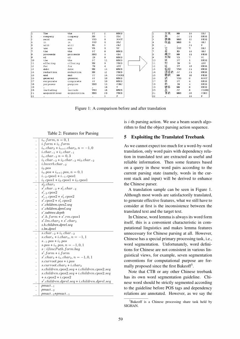
Figure 1: A comparison before and after translation
Table 2: Features for Parsingin.form, n = 0, 1i.form + i1.formin.char2 + in+1.char2, n = −1, 0i.char−1 + i1.char−1
in.char−2 n = 0, 3i1.char−2 + i2.char−2 +i3.char−2
i.lnverb.char−2
i3.posin.pos + in+1.pos, n = 0, 1i−2.cpos1 + i−1.cpos1i1.cpos1 + i2.cpos1 + i3.cpos1s′2.char1
s′.char−2 + s′1.char−2
s′−2.cpos2s′−1.cpos2 + s′1.cpos2s′.cpos2 + s′1.cpos2s’.children.cpos2.seqs’.children.dprel.seqs’.subtree.depths′.h.form + s′.rm.cpos1s′.lm.char2 + s′.char2
s.h.children.dprel.seqs.lm.dprels.char−2 + i1.char−2
s.charn + i.charn, n = −1, 1s−1.pos + i1.poss.pos + in.pos, n = −1, 0, 1s : i|linePath.form.bags′.form + i.forms′.char2 + in.char2, n = −1, 0, 1s.curroot.pos + i.poss.curroot.char2 + i.char2
s.children.cpos2.seq + i.children.cpos2.seqs.children.cpos2.seq + i.children.cpos2.seq+ s.cpos2 + i.cpos2s′.children.dprel.seq + i.children.dprel.seqpreact−1
preact−2
preact−2+preact−1
is i-th parsing action. We use a beam search algo-rithm to find the object parsing action sequence.
5 Exploiting the Translated Treebank
As we cannot expect too much for a word-by-wordtranslation, only word pairs with dependency rela-tion in translated text are extracted as useful andreliable information. Then some features basedon a query in these word pairs according to thecurrent parsing state (namely, words in the cur-rent stack and input) will be derived to enhancethe Chinese parser.
A translation sample can be seen in Figure 1.Although most words are satisfactorily translated,to generate effective features, what we still have toconsider at first is the inconsistence between thetranslated text and the target text.
In Chinese, word lemma is always its word formitself, this is a convenient characteristic in com-putational linguistics and makes lemma featuresunnecessary for Chinese parsing at all. However,Chinese has a special primary processing task, i.e.,word segmentation. Unfortunately, word defini-tions for Chinese are not consistent in various lin-guistical views, for example, seven segmentationconventions for computational purpose are for-mally proposed since the first Bakeoff3.
Note that CTB or any other Chinese treebankhas its own word segmentation guideline. Chi-nese word should be strictly segmented accordingto the guideline before POS tags and dependencyrelations are annotated. However, as we say the
3Bakeoff is a Chinese processing share task held bySIGHAN.
59
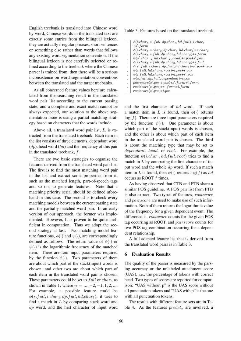
English treebank is translated into Chinese wordby word, Chinese words in the translated text areexactly some entries from the bilingual lexicon,they are actually irregular phrases, short sentencesor something else rather than words that followsany existing word segmentation convention. If thebilingual lexicon is not carefully selected or re-fined according to the treebank where the Chineseparser is trained from, then there will be a seriousinconsistence on word segmentation conventionsbetween the translated and the target treebanks.
As all concerned feature values here are calcu-lated from the searching result in the translatedword pair list according to the current parsingstate, and a complete and exact match cannot bealways expected, our solution to the above seg-mentation issue is using a partial matching strat-egy based on characters that the words include.
Above all, a translated word pair list, L, is ex-tracted from the translated treebank. Each item inthe list consists of three elements, dependant word(dp), head word (hd) and the frequency of this pairin the translated treebank, f .
There are two basic strategies to organize thefeatures derived from the translated word pair list.The first is to find the most matching word pairin the list and extract some properties from it,such as the matched length, part-of-speech tagsand so on, to generate features. Note that amatching priority serial should be defined afore-hand in this case. The second is to check everymatching models between the current parsing stateand the partially matched word pair. In an earlyversion of our approach, the former was imple-mented. However, It is proven to be quite inef-ficient in computation. Thus we adopt the sec-ond strategy at last. Two matching model fea-ture functions, φ(·) and ψ(·), are correspondinglydefined as follows. The return value of φ(·) orψ(·) is the logarithmic frequency of the matcheditem. There are four input parameters requiredby the function φ(·). Two parameters of themare about which part of the stack(input) words ischosen, and other two are about which part ofeach item in the translated word pair is chosen.These parameters could be set to full or charn asshown in Table 1, where n = ...,−2,−1, 1, 2, ....For example, a possible feature could beφ(s.full, i.char1, dp.full, hd.char1), it tries tofind a match in L by comparing stack word anddp word, and the first character of input word
Table 3: Features based on the translated treebank
φ(i.char3, s′.full, dp.char3, hd.full)+i.char3
+s′.formφ(i.char3, s.char2, dp.char3, hd.char2)+s.char2
φ(i.char3, s.full, dp.char3, hd.char2)+s.formψ(s′.char−2, hd.char−2, head)+i.pos+s′.posφ(i.char3, s.full, dp.char3, hd.char2)+s.fullφ(s′.full, i.char4, dp.full, hd.char4)+s′.pos+i.posψ(i.full, hd.char2, root)+i.pos+s.posψ(i.full, hd.char2, root)+i.pos+s′.posψ(s.full, dp.full, dependant)+i.pospairscore(s′.pos, i.pos)+s′.form+i.formrootscore(s′.pos)+s′.form+i.formrootscore(s′.pos)+i.pos
and the first character of hd word. If sucha match item in L is found, then φ(·) returnslog(f). There are three input parameters requiredby the function ψ(·). One parameter is aboutwhich part of the stack(input) words is chosen,and the other is about which part of each itemin the translated word pair is chosen. The thirdis about the matching type that may be set todependant, head, or root. For example, thefunction ψ(i.char1, hd.full, root) tries to find amatch in L by comparing the first character of in-put word and the whole dp word. If such a matchitem in L is found, then ψ(·) returns log(f) as hdoccurs as ROOT f times.
As having observed that CTB and PTB share asimilar POS guideline. A POS pair list from PTBis also extract. Two types of features, rootscoreand pairscore are used to make use of such infor-mation. Both of them returns the logarithmic valueof the frequency for a given dependent event. Thedifference is, rootscore counts for the given POStag occurring as ROOT, and pairscore counts fortwo POS tag combination occurring for a depen-dent relationship.
A full adapted feature list that is derived fromthe translated word pairs is in Table 3.
6 Evaluation Results
The quality of the parser is measured by the pars-ing accuracy or the unlabeled attachment score(UAS), i.e., the percentage of tokens with correcthead. Two types of scores are reported for compar-ison: “UAS without p” is the UAS score withoutall punctuation tokens and “UAS with p” is the onewith all punctuation tokens.
The results with different feature sets are in Ta-ble 4. As the features preactn are involved, a
60
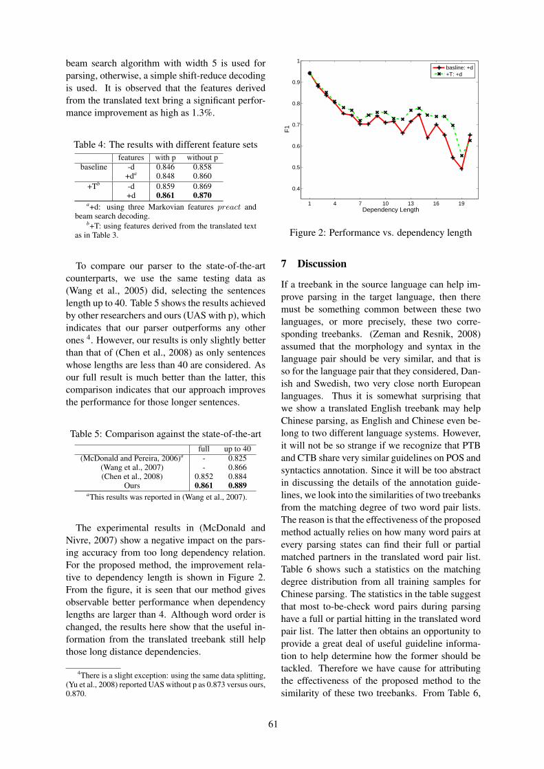
beam search algorithm with width 5 is used forparsing, otherwise, a simple shift-reduce decodingis used. It is observed that the features derivedfrom the translated text bring a significant perfor-mance improvement as high as 1.3%.
Table 4: The results with different feature setsfeatures with p without p
baseline -d 0.846 0.858+da 0.848 0.860
+Tb -d 0.859 0.869+d 0.861 0.870
a+d: using three Markovian features preact andbeam search decoding.
b+T: using features derived from the translated textas in Table 3.
To compare our parser to the state-of-the-artcounterparts, we use the same testing data as(Wang et al., 2005) did, selecting the sentenceslength up to 40. Table 5 shows the results achievedby other researchers and ours (UAS with p), whichindicates that our parser outperforms any otherones 4. However, our results is only slightly betterthan that of (Chen et al., 2008) as only sentenceswhose lengths are less than 40 are considered. Asour full result is much better than the latter, thiscomparison indicates that our approach improvesthe performance for those longer sentences.
Table 5: Comparison against the state-of-the-artfull up to 40
(McDonald and Pereira, 2006)a - 0.825(Wang et al., 2007) - 0.866(Chen et al., 2008) 0.852 0.884
Ours 0.861 0.889aThis results was reported in (Wang et al., 2007).
The experimental results in (McDonald andNivre, 2007) show a negative impact on the pars-ing accuracy from too long dependency relation.For the proposed method, the improvement rela-tive to dependency length is shown in Figure 2.From the figure, it is seen that our method givesobservable better performance when dependencylengths are larger than 4. Although word order ischanged, the results here show that the useful in-formation from the translated treebank still helpthose long distance dependencies.
4There is a slight exception: using the same data splitting,(Yu et al., 2008) reported UAS without p as 0.873 versus ours,0.870.
1 4 7 10 13 16 19
0.4
0.5
0.6
0.7
0.8
0.9
1
Dependency Length
F1
basline: +d+T: +d
Figure 2: Performance vs. dependency length
7 Discussion
If a treebank in the source language can help im-prove parsing in the target language, then theremust be something common between these twolanguages, or more precisely, these two corre-sponding treebanks. (Zeman and Resnik, 2008)assumed that the morphology and syntax in thelanguage pair should be very similar, and that isso for the language pair that they considered, Dan-ish and Swedish, two very close north Europeanlanguages. Thus it is somewhat surprising thatwe show a translated English treebank may helpChinese parsing, as English and Chinese even be-long to two different language systems. However,it will not be so strange if we recognize that PTBand CTB share very similar guidelines on POS andsyntactics annotation. Since it will be too abstractin discussing the details of the annotation guide-lines, we look into the similarities of two treebanksfrom the matching degree of two word pair lists.The reason is that the effectiveness of the proposedmethod actually relies on how many word pairs atevery parsing states can find their full or partialmatched partners in the translated word pair list.Table 6 shows such a statistics on the matchingdegree distribution from all training samples forChinese parsing. The statistics in the table suggestthat most to-be-check word pairs during parsinghave a full or partial hitting in the translated wordpair list. The latter then obtains an opportunity toprovide a great deal of useful guideline informa-tion to help determine how the former should betackled. Therefore we have cause for attributingthe effectiveness of the proposed method to thesimilarity of these two treebanks. From Table 6,
61

we also find that the partial matching strategy de-fined in Section 5 plays a very important role inimproving the whole matching degree. Note thatour approach is not too related to the characteris-tics of two languages. Our discussion here bringsan interesting issue, which difference is more im-portant in cross language processing, between twolanguages themselves or the corresponding anno-tated corpora? This may be extensively discussedin the future work.
Table 6: Matching degree distributiondependant-match head-match Percent (%)
None None 9.6None Partial 16.2None Full 9.9Partial None 12.4Partial Partial 42.6Partial Full 7.3Full None 3.7Full Partial 7.0Full Full 0.2
Note that only a bilingual lexicon is adopted inour approach. We regard it one of the most mer-its for our approach. A lexicon is much easier tobe obtained than an annotated corpus. One of theremained question about this work is if the bilin-gual lexicon should be very specific for this kindof tasks. According to our experiences, actually, itis not so sensitive to choose a highly refined lexi-con or not. We once found many words, mostlynamed entities, were outside the lexicon. Thuswe managed to collect a named entity translationdictionary to enhance the original one. However,this extra effort did not receive an observable per-formance improvement in return. Finally we re-alize that a lexicon that can guarantee two wordpair lists highly matched is sufficient for this work,and this requirement may be conveniently satis-fied only if the lexicon consists of adequate high-frequent words from the source treebank.
8 Conclusion and Future Work
We propose a method to enhance dependencyparsing in one language by using a translated tree-bank from another language. A simple statisti-cal machine translation technique, word-by-worddecoding, where only a bilingual lexicon is nec-essary, is used to translate the source treebank.As dependency parsing is concerned with the re-lations of word pairs, only those word pairs withdependency relations in the translated treebank are
chosen to generate some additional features to en-hance the parser for the target language. The ex-perimental results in English and Chinese tree-banks show the proposed method is effective andhelps the Chinese parser in this work achieve astate-of-the-art result.
Note that our method is evaluated in two tree-banks with a similar annotation style and it avoidsusing too many linguistic properties. Thus themethod is in the hope of being used in other simi-larly annotated treebanks 5. For an immediate ex-ample, we may adopt a translated Chinese tree-bank to improve English parsing. Although thereare still something to do, the remained key workhas been as simple as considering how to deter-mine the matching strategy for searching the trans-lated word pair list in English according to theframework of our method. .
Acknowledgements
We’d like to give our thanks to three anonymousreviewers for their insightful comments, Dr. ChenWenliang for for helpful discussions and Mr. LiuJun for helping us fix a bug in our scoring pro-gram.
ReferencesPeter F. Brown, John Cocke, Stephen A. Della Pietra,
Vincent J. Della Pietra, Fredrick Jelinek, John D.Lafferty, Robert L. Mercer, and Paul S. Roossin.1990. A statistical approach to machine translation.Computational Linguistics, 16(2):79–85.
David Burkett and Dan Klein. 2008. Two lan-guages are better than one (for syntactic parsing). InEMNLP-2008, pages 877–886, Honolulu, Hawaii,USA.
Wenliang Chen, Daisuke Kawahara, Kiyotaka Uchi-moto, Yujie Zhang, and Hitoshi Isahara. 2008. De-pendency parsing with short dependency relationsin unlabeled data. In Proceedings of IJCNLP-2008,Hyderabad, India, January 8-10.
Xiangyu Duan, Jun Zhao, and Bo Xu. 2007. Proba-bilistic parsing action models for multi-lingual de-pendency parsing. In Proceedings of the CoNLLShared Task Session of EMNLP-CoNLL 2007, pages940–946, Prague, Czech, June 28-30.
Johan Hall, Jens Nilsson, Joakim Nivre,Gülsen Eryiǧit, Beáta Megyesi, Mattias Nils-son, and Markus Saers. 2007. Single malt or5For example, Catalan and Spanish treebanks from the
AnCora(-Es/Ca) Multilevel Annotated Corpus that are an-notated by the Universitat de Barcelona (CLiC-UB) and theUniversitat Politècnica de Catalunya (UPC).
62
blended? a study in multilingual parser optimiza-tion. In Proceedings of the CoNLL Shared TaskSession of EMNLP-CoNLL 2007, pages 933–939,Prague, Czech, June.
Terry Koo, Xavier Carreras, and Michael Collins.2008. Simple semi-supervised dependency parsing.In Proceedings of ACL-08: HLT, pages 595–603,Columbus, Ohio, USA, June.
David McClosky, Eugene Charniak, and Mark John-son. 2006. Reranking and self-training for parseradaptation. In Proceedings of ACL-COLING 2006,pages 337–344, Sydney, Australia, July.
Ryan McDonald and Joakim Nivre. 2007. Charac-terizing the errors of data-driven dependency pars-ing models. In Proceedings of the 2007 Joint Con-ference on Empirical Methods in Natural LanguageProcessing and Computational Natural LanguageLearning (EMNLP-CoNLL 2007), pages 122–131,Prague, Czech, June 28-30.
Ryan McDonald and Fernando Pereira. 2006. Onlinelearning of approximate dependency parsing algo-rithms. In Proceedings of EACL-2006, pages 81–88,Trento, Italy, April.
Ryan McDonald, Koby Crammer, and FernandoPereira. 2005. Online large-margin training of de-pendency parsers. In Proceedings of ACL-2005,pages 91–98, Ann Arbor, Michigan, USA, June 25-30.
Paola Merlo, Suzanne Stevenson, Vivian Tsang, andGianluca Allaria. 2002. A multilingual paradigmfor automatic verb classification. In ACL-2002,pages 207–214, Philadelphia, Pennsylvania, USA.
Joakim Nivre, Johan Hall, Sandra Kübler, Ryan Mc-Donald, Jens Nilsson, Sebastian Riedel, and DenizYuret. 2007. The conll 2007 shared task on de-pendency parsing. In Proceedings of the CoNLLShared Task Session of EMNLP-CoNLL 2007, page915–932, Prague, Czech, June.
Joakim Nivre. 2003. An efficient algorithm for projec-tive dependency parsing. In Proceedings of IWPT-2003), pages 149–160, Nancy, France, April 23-25.
Franz Josef Och and Hermann Ney. 2002. Discrimina-tive training and maximum entropy models for sta-tistical machine translation. In Proceedings of ACL-2002, pages 295–302, Philadelphia, USA, July.
Roi Reichart and Ari Rappoport. 2007. Self-trainingfor enhancement and domain adaptation of statisticalparsers trained on small datasets. In Proceedings ofACL-2007, pages 616–623, Prague, Czech Republic,June.
Kenji Sagae and Jun’ichi Tsujii. 2007. Dependencyparsing and domain adaptation with lr models andparser ensembles. In Proceedings of the CoNLLShared Task Session of EMNLP-CoNLL 2007, page1044–1050, Prague, Czech, June 28-30.
Noah A. Smith and Jason Eisner. 2006. Annealingstructural bias in multilingual weighted grammar in-duction. In Proceedings of ACL-COLING 2006,page 569–576, Sydney, Australia, July.
Mark Steedman, Miles Osborne, Anoop Sarkar,Stephen Clark, Rebecca Hwa, Julia Hockenmaier,Paul Ruhlen, Steven Baker, and Jeremiah Crim.2003. Bootstrapping statistical parsers from smalldatasets. In Proceedings of EACL-2003, page331–338, Budapest, Hungary, April.
Qin Iris Wang and Dale Schuurmans. 2008. Semi-supervised convex training for dependency parsing.In Proceedings of ACL-08: HLT, pages 532–540,Columbus, Ohio, USA, June.
Qin Iris Wang, Dale Schuurmans, and Dekang Lin.2005. Strictly lexical dependency parsing. In Pro-ceedings of IWPT-2005, pages 152–159, Vancouver,BC, Canada, October.
Qin Iris Wang, Dekang Lin, and Dale Schuurmans.2007. Simple training of dependency parsers viastructured boosting. In Proceedings of IJCAI 2007,pages 1756–1762, Hyderabad, India, January.
Hiroyasu Yamada and Yuji Matsumoto. 2003. Sta-tistical dependency analysis with support vectormachines. In Proceedings of IWPT-2003), page195–206, Nancy, France, April.
Kun Yu, Daisuke Kawahara, and Sadao Kurohashi.2008. Chinese dependency parsing with largescale automatically constructed case structures. InProceedings of COLING-2008, pages 1049–1056,Manchester, UK, August.
Daniel Zeman and Philip Resnik. 2008. Cross-language parser adaptation between related lan-guages. In Proceedings of IJCNLP 2008 Workshopon NLP for Less Privileged Languages, pages 35–42, Hyderabad, India, January.
Hai Zhao and Chunyu Kit. 2008. Parsing syntactic andsemantic dependencies with two single-stage max-imum entropy models. In Proceeding of CoNLL-2008, pages 203–207, Manchester, UK.
Hai Zhao, Wenliang Chen, Chunyu Kit, and GuodongZhou. 2009. Multilingual dependency learning:A huge feature engineering method to semantic de-pendency parsing. In Proceedings of CoNLL-2009,Boulder, Colorado, USA.
Hai Zhao. 2009. Character-level dependencies inchinese: Usefulness and learning. In EACL-2009,pages 879–887, Athens, Greece.
63
Proceedings of the 47th Annual Meeting of the ACL and the 4th IJCNLP of the AFNLP, pages 64–72,Suntec, Singapore, 2-7 August 2009. c©2009 ACL and AFNLP
Topological Field Parsing of German
Jackie Chi Kit CheungDepartment of Computer Science
University of TorontoToronto, ON, M5S 3G4, [email protected]
Gerald PennDepartment of Computer Science
University of TorontoToronto, ON, M5S 3G4, [email protected]
Abstract
Freer-word-order languages such as Ger-man exhibit linguistic phenomena thatpresent unique challenges to traditionalCFG parsing. Such phenomena producediscontinuous constituents, which are notnaturally modelled by projective phrasestructure trees. In this paper, we exam-ine topological field parsing, a shallowform of parsing which identifies the ma-jor sections of a sentence in relation tothe clausal main verb and the subordinat-ing heads. We report the results of topo-logical field parsing of German using theunlexicalized, latent variable-based Berke-ley parser (Petrov et al., 2006) Withoutany language- or model-dependent adapta-tion, we achieve state-of-the-art results onthe TüBa-D/Z corpus, and a modified NE-GRA corpus that has been automaticallyannotated with topological fields (Beckerand Frank, 2002). We also perform a qual-itative error analysis of the parser output,and discuss strategies to further improvethe parsing results.
1 Introduction
Freer-word-order languages such as German ex-hibit linguistic phenomena that present uniquechallenges to traditional CFG parsing. Topic focusordering and word order constraints that are sen-sitive to phenomena other than grammatical func-tion produce discontinuous constituents, which arenot naturally modelled by projective (i.e., with-out crossing branches) phrase structure trees. Inthis paper, we examine topological field parsing, ashallow form of parsing which identifies the ma-jor sections of a sentence in relation to the clausalmain verb and subordinating heads, when present.We report the results of parsing German using
the unlexicalized, latent variable-based Berkeleyparser (Petrov et al., 2006). Without any language-or model-dependent adaptation, we achieve state-of-the-art results on the TüBa-D/Z corpus (Telljo-hann et al., 2004), with a F1-measure of 95.15%using gold POS tags. A further reranking ofthe parser output based on a constraint involv-ing paired punctuation produces a slight additionalperformance gain. To facilitate comparison withprevious work, we also conducted experiments ona modified NEGRA corpus that has been automat-ically annotated with topological fields (Beckerand Frank, 2002), and found that the Berkeleyparser outperforms the method described in thatwork. Finally, we perform a qualitative error anal-ysis of the parser output on the TüBa-D/Z corpus,and discuss strategies to further improve the pars-ing results.
German syntax and parsing have been studiedusing a variety of grammar formalisms. Hocken-maier (2006) has translated the German TIGERcorpus (Brants et al., 2002) into a CCG-basedtreebank to model word order variations in Ger-man. Foth et al. (2004) consider a version of de-pendency grammars known as weighted constraintdependency grammars for parsing German sen-tences. On the NEGRA corpus (Skut et al., 1998),they achieve an accuracy of 89.0% on parsing de-pendency edges. In Callmeier (2000), a platformfor efficient HPSG parsing is developed. Thisparser is later extended by Frank et al. (2003)with a topological field parser for more efficientparsing of German. The system by Rohrer andForst (2006) produces LFG parses using a manu-ally designed grammar and a stochastic parse dis-ambiguation process. They test on the TIGER cor-pus and achieve an F1-measure of 84.20%. InDubey and Keller (2003), PCFG parsing of NE-GRA is improved by using sister-head dependen-cies, which outperforms standard head lexicaliza-tion as well as an unlexicalized model. The best
64
performing model with gold tags achieve an F1
of 75.60%. Sister-head dependencies are useful inthis case because of the flat structure of NEGRA’strees.
In contrast to the deeper approaches to parsingdescribed above, topological field parsing identi-fies the major sections of a sentence in relationto the clausal main verb and subordinating heads,when present. Like other forms of shallow pars-ing, topological field parsing is useful as the firststage to further processing and eventual seman-tic analysis. As mentioned above, the output ofa topological field parser is used as a guide tothe search space of a HPSG parsing algorithm inFrank et al. (2003). In Neumann et al. (2000),topological field parsing is part of a divide-and-conquer strategy for shallow analysis of Germantext with the goal of improving an information ex-traction system.
Existing work in identifying topological fieldscan be divided into chunkers, which identify thelowest-level non-recursive topological fields, andparsers, which also identify sentence and clausalstructure.
Veenstra et al. (2002) compare three approachesto topological field chunking based on finite statetransducers, memory-based learning, and PCFGsrespectively. It is found that the three techniquesperform about equally well, with F1 of 94.1% us-ing POS tags from the TnT tagger, and 98.4% withgold tags. In Liepert (2003), a topological fieldchunker is implemented using a multi-class ex-tension to the canonically two-class support vec-tor machine (SVM) machine learning framework.Parameters to the machine learning algorithm arefine-tuned by a genetic search algorithm, with aresulting F1-measure of 92.25%. Training the pa-rameters to SVM does not have a large effect onperformance, increasing the F1-measure in the testset by only 0.11%.
The corpus-based, stochastic topological fieldparser of Becker and Frank (2002) is based ona standard treebank PCFG model, in which ruleprobabilities are estimated by frequency counts.This model includes several enhancements, whichare also found in the Berkeley parser. First,they use parameterized categories, splitting non-terminals according to linguistically based intu-itions, such as splitting different clause types (theydo not distinguish different clause types as basiccategories, unlike TüBa-D/Z). Second, they take
into account punctuation, which may help iden-tify clause boundaries. They also binarize the veryflat topological tree structures, and prune rulesthat only occur once. They test their parser on aversion of the NEGRA corpus, which has beenannotated with topological fields using a semi-automatic method.
Ule (2003) proposes a process termed DirectedTreebank Refinement (DTR). The goal of DTR isto refine a corpus to improve parsing performance.DTR is comparable to the idea of latent variablegrammars on which the Berkeley parser is based,in that both consider the observed treebank to beless than ideal and both attempt to refine it by split-ting and merging nonterminals. In this work, split-ting and merging nonterminals are done by consid-ering the nonterminals’ contexts (i.e., their parentnodes) and the distribution of their productions.Unlike in the Berkeley parser, splitting and merg-ing are distinct stages, rather than parts of a sin-gle iteration. Multiple splits are found first, thenmultiple rounds of merging are performed. Nosmoothing is done. As an evaluation, DTR is ap-plied to topological field parsing of the TüBa-D/Zcorpus. We discuss the performance of these topo-logical field parsers in more detail below.
All of the topological parsing proposals pre-date the advent of the Berkeley parser. The exper-iments of this paper demonstrate that the Berke-ley parser outperforms previous methods, many ofwhich are specialized for the task of topologicalfield chunking or parsing.
2 Topological Field Model of German
Topological fields are high-level linear fields inan enclosing syntactic region, such as a clause(Höhle, 1983). These fields may have constraintson the number of words or phrases they contain,and do not necessarily form a semantically co-herent constituent. Although it has been arguedthat a few languages have no word-order con-straints whatsoever, most “free word-order” lan-guages (even Warlpiri) have at the very least somesort of sentence- or clause-initial topic field fol-lowed by a second position that is occupied byclitics, a finite verb or certain complementizersand subordinating conjunctions. In a few Ger-manic languages, including German, the topologyis far richer than that, serving to identify all ofthe components of the verbal head of a clause,except for some cases of long-distance dependen-
65

cies. Topological fields are useful, because whileGermanic word order is relatively free with respectto grammatical functions, the order of the topolog-ical fields is strict and unvarying.
Type FieldsVL (KOORD) (C) (MF) VC (NF)V1 (KOORD) (LV) LK (MF) (VC) (NF)V2 (KOORD) (LV) VF LK (MF) (VC) (NF)
Table 1: Topological field model of German.Simplified from TüBa-D/Z corpus’s annotationschema (Telljohann et al., 2006).
In the German topological field model, clausesbelong to one of three types: verb-last (VL), verb-second (V2), and verb-first (V1), each with a spe-cific sequence of topological fields (Table 1). VLclauses include finite and non-finite subordinateclauses, V2 sentences are typically declarativesentences and WH-questions in matrix clauses,and V1 sentences include yes-no questions, andcertain conditional subordinate clauses. Below,we give brief descriptions of the most commontopological fields.
• VF (Vorfeld or ‘pre-field’) is the first con-stituent in sentences of the V2 type. This isoften the topic of the sentence, though as ananonymous reviewer pointed out, this posi-tion does not correspond to a single functionwith respect to information structure. (e.g.,the reviewer suggested this case, where VFcontains the focus: –Wer kommt zur Party?–Peter kommt zur Party. –Who is coming tothe Party? –Peter is coming to the party.)
• LK (Linke Klammer or ‘left bracket’) is theposition for finite verbs in V1 and V2 sen-tences. It is replaced by a complementizerwith the field label C in VL sentences.
• MF (Mittelfeld or ‘middle field’) is an op-tional field bounded on the left by LK andon the right by the verbal complex VC orby NF. Most verb arguments, adverbs, andprepositional phrases are found here, unlessthey have been fronted and put in the VF, orare prosodically heavy and postposed to theNF field.
• VC is the verbal complex field. It includesinfinite verbs, as well as finite verbs in VLsentences.
• NF (Nachfeld or ‘post-field’) containsprosodically heavy elements such as post-posed prepositional phrases or relativeclauses.
• KOORD1 (Koordinationsfeld or ‘coordina-tion field’) is a field for clause-level conjunc-tions.
• LV (Linksversetzung or ‘left dislocation’) isused for resumptive constructions involvingleft dislocation. For a detailed linguistictreatment, see (Frey, 2004).
Exceptions to the topological field model as de-scribed above do exist. For instance, parentheticalconstructions exist as a mostly syntactically inde-pendent clause inside another sentence. In our cor-pus, they are attached directly underneath a clausalnode without any intervening topological field, asin the following example. In this example, the par-enthetical construction is highlighted in bold print.Some clause and topological field labels under theNF field are omitted for clarity.
(1) (a) (SIMPX “(VF Man) (LK muß) (VC verstehen) ”, (SIMPX sagte er), “ (NF daß dieseMinderheiten seit langer Zeit massiv von denNazis bedroht werden)). ”
(b) Translation: “One must understand,” he said,“that these minorities have been massivelythreatened by the Nazis for a long time.”
3 A Latent Variable Parser
For our experiments, we used the latent variable-based Berkeley parser (Petrov et al., 2006). La-tent variable parsing assumes that an observedtreebank represents a coarse approximation ofan underlying, optimally refined grammar whichmakes more fine-grained distinctions in the syn-tactic categories. For example, the noun phrasecategory NP in a treebank could be viewed as acoarse approximation of two noun phrase cate-gories corresponding to subjects and object, NPˆS,and NPˆVP.
The Berkeley parser automates the process offinding such distinctions. It starts with a simple bi-narized X-bar grammar style backbone, and goesthrough iterations of splitting and merging non-terminals, in order to maximize the likelihood ofthe training set treebank. In the splitting stage,
1The TüBa-D/Z corpus distinguishes coordinating andnon-coordinating particles, as well as clausal and field co-ordination. These distinctions need not concern us for thisexplanation.
66

Figure 1: “I could never have done that just for aesthetic reasons.” Sample TüBa-D/Z tree, with topolog-ical field annotations and edge labels. Topological field layer in bold.
an Expectation-Maximization algorithm is used tofind a good split for each nonterminal. In themerging stage, categories that have been over-split are merged together to keep the grammar sizetractable and reduce sparsity. Finally, a smoothingstage occurs, where the probabilities of rules foreach nonterminal are smoothed toward the prob-abilities of the other nonterminals split from thesame syntactic category.
The Berkeley parser has been applied to theTüBaD/Z corpus in the constituent parsing sharedtask of the ACL-2008 Workshop on Parsing Ger-man (Petrov and Klein, 2008), achieving an F1-measure of 85.10% and 83.18% with and withoutgold standard POS tags respectively2. We chosethe Berkeley parser for topological field parsingbecause it is known to be robust across languages,and because it is an unlexicalized parser. Lexi-calization has been shown to be useful in moregeneral parsing applications due to lexical depen-dencies in constituent parsing (e.g. (Kübler et al.,2006; Dubey and Keller, 2003) in the case of Ger-man). However, topological fields explain a higherlevel of structure pertaining to clause-level wordorder, and we hypothesize that lexicalization is un-likely to be helpful.
4 Experiments
4.1 DataFor our experiments, we primarily used the TüBa-D/Z (Tübinger Baumbank des Deutschen / Schrift-sprache) corpus, consisting of 26116 sentences(20894 training, 2611 development, 2089 test,with a further 522 sentences held out for future ex-
2This evaluation considered grammatical functions aswell as the syntactic category.
periments)3 taken from the German newspaper dietageszeitung. The corpus consists of four levelsof annotation: clausal, topological, phrasal (otherthan clausal), and lexical. We define the task oftopological field parsing to be recovering the firsttwo levels of annotation, following Ule (2003).
We also tested the parser on a version of the NE-GRA corpus derived by Becker and Frank (2002),in which syntax trees have been made projec-tive and topological fields have been automaticallyadded through a series of linguistically informedtree modifications. All internal phrasal structurenodes have also been removed. The corpus con-sists of 20596 sentences, which we split into sub-sets of the same size as described by Becker andFrank (2002)4. The set of topological fields inthis corpus differs slightly from the one used inTüBa-D/Z, making no distinction between clausetypes, nor consistently marking field or clauseconjunctions. Because of the automatic anno-tation of topological fields, this corpus containsnumerous annotation errors. Becker and Frank(2002) manually corrected their test set and eval-uated the automatic annotation process, reportinglabelled precision and recall of 93.0% and 93.6%compared to their manual annotations. There arealso punctuation-related errors, including miss-ing punctuation, sentences ending in commas, andsentences composed of single punctuation marks.We test on this data in order to provide a bet-ter comparison with previous work. Although wecould have trained the model in Becker and Frank(2002) on the TüBa-D/Z corpus, it would not have
3These are the same splits into training, development, andtest sets as in the ACL-08 Parsing German workshop. Thiscorpus does not include sentences of length greater than 40.
416476 training sentences, 1000 development, 1058 test-ing, and 2062 as held-out data. We were unable to obtainthe exact subsets used by Becker and Frank (2002). We willdiscuss the ramifications of this on our evaluation procedure.
67
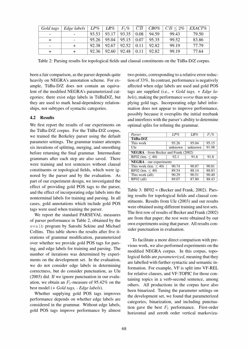
Gold tags Edge labels LP% LR% F1% CB CB0% CB ≤ 2% EXACT%- - 93.53 93.17 93.35 0.08 94.59 99.43 79.50+ - 95.26 95.04 95.15 0.07 95.35 99.52 83.86- + 92.38 92.67 92.52 0.11 92.82 99.19 77.79+ + 92.36 92.60 92.48 0.11 92.82 99.19 77.64
Table 2: Parsing results for topological fields and clausal constituents on the TüBa-D/Z corpus.
been a fair comparison, as the parser depends quiteheavily on NEGRA’s annotation scheme. For ex-ample, TüBa-D/Z does not contain an equiva-lent of the modified NEGRA’s parameterized cat-egories; there exist edge labels in TüBaD/Z, butthey are used to mark head-dependency relation-ships, not subtypes of syntactic categories.
4.2 ResultsWe first report the results of our experiments onthe TüBa-D/Z corpus. For the TüBa-D/Z corpus,we trained the Berkeley parser using the defaultparameter settings. The grammar trainer attemptssix iterations of splitting, merging, and smoothingbefore returning the final grammar. Intermediategrammars after each step are also saved. Therewere training and test sentences without clausalconstituents or topological fields, which were ig-nored by the parser and by the evaluation. Aspart of our experiment design, we investigated theeffect of providing gold POS tags to the parser,and the effect of incorporating edge labels into thenonterminal labels for training and parsing. In allcases, gold annotations which include gold POStags were used when training the parser.
We report the standard PARSEVAL measuresof parser performance in Table 2, obtained by theevalb program by Satoshi Sekine and MichaelCollins. This table shows the results after five it-erations of grammar modification, parameterizedover whether we provide gold POS tags for pars-ing, and edge labels for training and parsing. Thenumber of iterations was determined by experi-ments on the development set. In the evaluation,we do not consider edge labels in determiningcorrectness, but do consider punctuation, as Ule(2003) did. If we ignore punctuation in our evalu-ation, we obtain an F1-measure of 95.42% on thebest model (+ Gold tags, - Edge labels).
Whether supplying gold POS tags improvesperformance depends on whether edge labels areconsidered in the grammar. Without edge labels,gold POS tags improve performance by almost
two points, corresponding to a relative error reduc-tion of 33%. In contrast, performance is negativelyaffected when edge labels are used and gold POStags are supplied (i.e., + Gold tags, + Edge la-bels), making the performance worse than not sup-plying gold tags. Incorporating edge label infor-mation does not appear to improve performance,possibly because it oversplits the initial treebankand interferes with the parser’s ability to determineoptimal splits for refining the grammar.
Parser LP% LR% F1%TüBa-D/ZThis work 95.26 95.04 95.15Ule unknown unknown 91.98NEGRA - from Becker and Frank (2002)BF02 (len. ≤ 40) 92.1 91.6 91.8NEGRA - our experimentsThis work (len. ≤ 40) 90.74 90.87 90.81BF02 (len. ≤ 40) 89.54 88.14 88.83This work (all) 90.29 90.51 90.40BF02 (all) 89.07 87.80 88.43
Table 3: BF02 = (Becker and Frank, 2002). Pars-ing results for topological fields and clausal con-stituents. Results from Ule (2003) and our resultswere obtained using different training and test sets.The first row of results of Becker and Frank (2002)are from that paper; the rest were obtained by ourown experiments using that parser. All results con-sider punctuation in evaluation.
To facilitate a more direct comparison with pre-vious work, we also performed experiments on themodified NEGRA corpus. In this corpus, topo-logical fields are parameterized, meaning that theyare labelled with further syntactic and semantic in-formation. For example, VF is split into VF-RELfor relative clauses, and VF-TOPIC for those con-taining topics in a verb-second sentence, amongothers. All productions in the corpus have alsobeen binarized. Tuning the parameter settings onthe development set, we found that parameterizedcategories, binarization, and including punctua-tion gave the best F1 performance. First-orderhorizontal and zeroth order vertical markoviza-
68

tion after six iterations of splitting, merging, andsmoothing gave the best F1 result of 91.78%. Weparsed the corpus with both the Berkeley parserand the best performing model of Becker andFrank (2002).
The results of these experiments on the test setfor sentences of length 40 or less and for all sen-tences are shown in Table 3. We also show otherresults from previous work for reference. Wefind that we achieve results that are better thanthe model in Becker and Frank (2002) on the testset. The difference is statistically significant (p =0.0029, Wilcoxon signed-rank).
The results we obtain using the parser of Beckerand Frank (2002) are worse than the results de-scribed in that paper. We suggest the followingreasons for this discrepancy. While the test setused in the paper was manually corrected for eval-uation, we did not correct our test set, because itwould be difficult to ensure that we adhered to thesame correction guidelines. No details of the cor-rection process were provided in the paper, and de-scriptive grammars of German provide insufficientguidance on many of the examples in NEGRA onissues such as ellipses, short infinitival clauses,and expanded participial constructions modifyingnouns. Also, because we could not obtain the ex-act sets used for training, development, and test-ing, we had to recreate the sets by randomly split-ting the corpus.
4.3 Category Specific ResultsWe now return to the TüBa-D/Z corpus for amore detailed analysis, and examine the category-specific results for our best performing model (+Gold tags, - Edge labels). Overall, Table 4 showsthat the best performing topological field cate-gories are those that have constraints on the typeof word that is allowed to fill it (finite verbs inLK, verbs in VC, complementizers and subordi-nating conjunctions in C). VF, in which only oneconstituent may appear, also performs relativelywell. Topological fields that can contain a vari-able number of heterogeneous constituents, on theother hand, have poorer F1-measure results. MF,which is basically defined relative to the positionsof fields on either side of it, is parsed several pointsbelow LK, C, and VC in accuracy. NF, whichcontains different kinds of extraposed elements, isparsed at a substantially worse level.
Poorly parsed categories tend to occur infre-
quently, including LV, which marks a rare re-sumptive construction; FKOORD, which markstopological field coordination; and the discoursemarker DM. The other clause-level constituents(PSIMPX for clauses in paratactic constructions,RSIMPX for relative clauses, and SIMPX forother clauses) also perform below average.
Topological FieldsCategory # LP% LR% F1%PARORD 20 100.00 100.00 100.00VCE 3 100.00 100.00 100.00LK 2186 99.68 99.82 99.75C 642 99.53 98.44 98.98VC 1777 98.98 98.14 98.56VF 2044 96.84 97.55 97.20KOORD 99 96.91 94.95 95.92MF 2931 94.80 95.19 94.99NF 643 83.52 81.96 82.73FKOORD 156 75.16 73.72 74.43LV 17 10.00 5.88 7.41Clausal ConstituentsCategory # LP% LR% F1%SIMPX 2839 92.46 91.97 92.21RSIMPX 225 91.23 92.44 91.83PSIMPX 6 100.00 66.67 80.00DM 28 59.26 57.14 58.18
Table 4: Category-specific results using grammarwith no edge labels and passing in gold POS tags.
4.4 Reranking for Paired PunctuationWhile experimenting with the development setof TüBa-D/Z, we noticed that the parser some-times returns parses, in which paired punctuation(e.g. quotation marks, parentheses, brackets) isnot placed in the same clause–a linguistically im-plausible situation. In these cases, the high-levelinformation provided by the paired punctuation isoverridden by the overall likelihood of the parsetree. To rectify this problem, we performed a sim-ple post-hoc reranking of the 50-best parses pro-duced by the best parameter settings (+ Gold tags,- Edge labels), selecting the first parse that placespaired punctuation in the same clause, or return-ing the best parse if none of the 50 parses satisfythe constraint. This procedure improved the F1-measure to 95.24% (LP = 95.39%, LR = 95.09%).
Overall, 38 sentences were parsed with pairedpunctuation in different clauses, of which 16 werereranked. Of the 38 sentences, reranking improvedperformance in 12 sentences, did not affect perfor-mance in 23 sentences (of which 10 already had aperfect parse), and hurt performance in three sen-tences. A two-tailed sign test suggests that rerank-
69

ing improves performance (p = 0.0352). We dis-cuss below why sentences with paired punctuationin different clauses can have perfect parse results.
To investigate the upper-bound in performancethat this form of reranking is able to achieve, wecalculated some statistics on our (+ Gold tags, -Edge labels) 50-best list. We found that the aver-age rank of the best scoring parse by F1-measureis 2.61, and the perfect parse is present for 1649of the 2088 sentences at an average rank of 1.90.The oracle F1-measure is 98.12%, indicating thata more comprehensive reranking procedure mightallow further performance gains.
4.5 Qualitative Error AnalysisAs a further analysis, we extracted the worst scor-ing fifty sentences by F1-measure from the parsedtest set (+ Gold tags, - Edge labels), and comparedthem against the gold standard trees, noting thecause of the error. We analyze the parses beforereranking, to see how frequently the paired punc-tuation problem described above severely affects aparse. The major mistakes made by the parser aresummarized in Table 5.
Problem Freq.Misidentification of Parentheticals 19Coordination problems 13Too few SIMPX 10Paired punctuation problem 9Other clause boundary errors 7Other 6Too many SIMPX 3Clause type misidentification 2MF/NF boundary 2LV 2VF/MF boundary 2
Table 5: Types and frequency of parser errors inthe fifty worst scoring parses by F1-measure, us-ing parameters (+ Gold tags, - Edge labels).
Misidentification of Parentheticals Parentheti-cal constructions do not have any dependencies onthe rest of the sentence, and exist as a mostly syn-tactically independent clause inside another sen-tence. They can occur at the beginning, end, orin the middle of sentences, and are often set offorthographically by punctuation. The parser hasproblems identifying parenthetical constructions,often positing a parenthetical construction whenthat constituent is actually attached to a topolog-ical field in a neighbouring clause. The follow-ing example shows one such misidentification in
bracket notation. Clause internal topological fieldsare omitted for clarity.
(2) (a) TüBa-D/Z: (SIMPX Weder das Ausmaß derSchönheit noch der frühere oder spätereZeitpunkt der Geburt macht einen der Zwillingefür eine Mutter mehr oder weniger echt /authentisch / überlegen).
(b) Parser: (SIMPX Weder das Ausmaß derSchönheit noch der frühere oder spätereZeitpunkt der Geburt macht einen der Zwillingefür eine Mutter mehr oder weniger echt)(PARENTHETICAL / authentisch /überlegen.)
(c) Translation: “Neither the degree of beauty northe earlier or later time of birth makes one of thetwins any more or less real/authentic/superior toa mother.”
We hypothesized earlier that lexicalization isunlikely to give us much improvement in perfor-mance, because topological fields work on a do-main that is higher than that of lexical dependen-cies such as subcategorization frames. However,given the locally independent nature of legitimateparentheticals, a limited form of lexicalization orsome other form of stronger contextual informa-tion might be needed to improve identification per-formance.
Coordination Problems The second most com-mon type of error involves field and clause coordi-nations. This category includes missing or incor-rect FKOORD fields, and conjunctions of clausesthat are misidentified. In the following example,the conjoined MFs and following NF in the cor-rect parse tree are identified as a single long MF.
(3) (a) TüBa-D/Z: Auf dem europäischen Kontinentaber hat (FKOORD (MF kein Land und keineMacht ein derartiges Interesse an gutenBeziehungen zu Rußland) und (MF auch keinLand solche Erfahrungen im Umgang mitRußland)) (NF wie Deutschland).
(b) Parser: Auf dem europäischen Kontinent aberhat (MF kein Land und keine Macht einderartiges Interesse an guten Beziehungen zuRußland und auch kein Land solcheErfahrungen im Umgang mit Rußland wieDeutschland).
(c) Translation: “On the European continent,however, no land and no power has such aninterest in good relations with Russia (asGermany), and also no land (has) suchexperience in dealing with Russia as Germany.”
Other Clause Errors Other clause-level errorsinclude the parser predicting too few or too manyclauses, or misidentifying the clause type. Clausesare sometimes confused with NFs, and there is onecase of a relative clause being misidentified as a
70
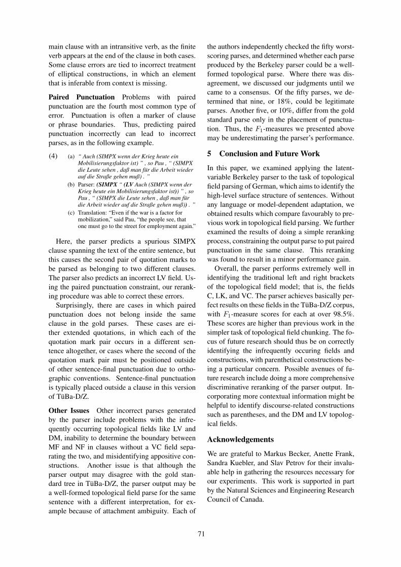
main clause with an intransitive verb, as the finiteverb appears at the end of the clause in both cases.Some clause errors are tied to incorrect treatmentof elliptical constructions, in which an elementthat is inferable from context is missing.
Paired Punctuation Problems with pairedpunctuation are the fourth most common type oferror. Punctuation is often a marker of clauseor phrase boundaries. Thus, predicting pairedpunctuation incorrectly can lead to incorrectparses, as in the following example.
(4) (a) “ Auch (SIMPX wenn der Krieg heute einMobilisierungsfaktor ist) ” , so Pau , “ (SIMPXdie Leute sehen , daß man für die Arbeit wiederauf die Straße gehen muß) . ”
(b) Parser: (SIMPX “ (LV Auch (SIMPX wenn derKrieg heute ein Mobilisierungsfaktor ist)) ” , soPau , “ (SIMPX die Leute sehen , daß man fürdie Arbeit wieder auf die Straße gehen muß)) . ”
(c) Translation: “Even if the war is a factor formobilization,” said Pau, “the people see, thatone must go to the street for employment again.”
Here, the parser predicts a spurious SIMPXclause spanning the text of the entire sentence, butthis causes the second pair of quotation marks tobe parsed as belonging to two different clauses.The parser also predicts an incorrect LV field. Us-ing the paired punctuation constraint, our rerank-ing procedure was able to correct these errors.
Surprisingly, there are cases in which pairedpunctuation does not belong inside the sameclause in the gold parses. These cases are ei-ther extended quotations, in which each of thequotation mark pair occurs in a different sen-tence altogether, or cases where the second of thequotation mark pair must be positioned outsideof other sentence-final punctuation due to ortho-graphic conventions. Sentence-final punctuationis typically placed outside a clause in this versionof TüBa-D/Z.
Other Issues Other incorrect parses generatedby the parser include problems with the infre-quently occurring topological fields like LV andDM, inability to determine the boundary betweenMF and NF in clauses without a VC field sepa-rating the two, and misidentifying appositive con-structions. Another issue is that although theparser output may disagree with the gold stan-dard tree in TüBa-D/Z, the parser output may bea well-formed topological field parse for the samesentence with a different interpretation, for ex-ample because of attachment ambiguity. Each of
the authors independently checked the fifty worst-scoring parses, and determined whether each parseproduced by the Berkeley parser could be a well-formed topological parse. Where there was dis-agreement, we discussed our judgments until wecame to a consensus. Of the fifty parses, we de-termined that nine, or 18%, could be legitimateparses. Another five, or 10%, differ from the goldstandard parse only in the placement of punctua-tion. Thus, the F1-measures we presented abovemay be underestimating the parser’s performance.
5 Conclusion and Future Work
In this paper, we examined applying the latent-variable Berkeley parser to the task of topologicalfield parsing of German, which aims to identify thehigh-level surface structure of sentences. Withoutany language or model-dependent adaptation, weobtained results which compare favourably to pre-vious work in topological field parsing. We furtherexamined the results of doing a simple rerankingprocess, constraining the output parse to put pairedpunctuation in the same clause. This rerankingwas found to result in a minor performance gain.
Overall, the parser performs extremely well inidentifying the traditional left and right bracketsof the topological field model; that is, the fieldsC, LK, and VC. The parser achieves basically per-fect results on these fields in the TüBa-D/Z corpus,with F1-measure scores for each at over 98.5%.These scores are higher than previous work in thesimpler task of topological field chunking. The fo-cus of future research should thus be on correctlyidentifying the infrequently occuring fields andconstructions, with parenthetical constructions be-ing a particular concern. Possible avenues of fu-ture research include doing a more comprehensivediscriminative reranking of the parser output. In-corporating more contextual information might behelpful to identify discourse-related constructionssuch as parentheses, and the DM and LV topolog-ical fields.
Acknowledgements
We are grateful to Markus Becker, Anette Frank,Sandra Kuebler, and Slav Petrov for their invalu-able help in gathering the resources necessary forour experiments. This work is supported in partby the Natural Sciences and Engineering ResearchCouncil of Canada.
71
ReferencesM. Becker and A. Frank. 2002. A stochastic topo-
logical parser for German. In Proceedings of the19th International Conference on ComputationalLinguistics, pages 71–77.
S. Brants, S. Dipper, S. Hansen, W. Lezius, andG. Smith. 2002. The TIGER Treebank. In Proceed-ings of the Workshop on Treebanks and LinguisticTheories, pages 24–41.
U. Callmeier. 2000. PET–a platform for experimen-tation with efficient HPSG processing techniques.Natural Language Engineering, 6(01):99–107.
A. Dubey and F. Keller. 2003. Probabilistic parsingfor German using sister-head dependencies. In Pro-ceedings of the 41st Annual Meeting of the Associa-tion for Computational Linguistics, pages 96–103.
K.A. Foth, M. Daum, and W. Menzel. 2004. Abroad-coverage parser for German based on defea-sible constraints. Constraint Solving and LanguageProcessing.
A. Frank, M. Becker, B. Crysmann, B. Kiefer, andU. Schaefer. 2003. Integrated shallow and deepparsing: TopP meets HPSG. In Proceedings of the41st Annual Meeting of the Association for Compu-tational Linguistics, pages 104–111.
W. Frey. 2004. Notes on the syntax and the pragmaticsof German Left Dislocation. In H. Lohnstein andS. Trissler, editors, The Syntax and Semantics of theLeft Periphery, pages 203–233. Mouton de Gruyter,Berlin.
J. Hockenmaier. 2006. Creating a CCGbank and aWide-Coverage CCG Lexicon for German. In Pro-ceedings of the 21st International Conference onComputational Linguistics and 44th Annual Meet-ing of the Association for Computational Linguis-tics, pages 505–512.
T.N. Höhle. 1983. Topologische Felder. Ph.D. thesis,Köln.
S. Kübler, E.W. Hinrichs, and W. Maier. 2006. Is it re-ally that difficult to parse German? In Proceedingsof EMNLP.
M. Liepert. 2003. Topological Fields Chunking forGerman with SVM’s: Optimizing SVM-parameterswith GA’s. In Proceedings of the International Con-ference on Recent Advances in Natural LanguageProcessing (RANLP), Bulgaria.
G. Neumann, C. Braun, and J. Piskorski. 2000. ADivide-and-Conquer Strategy for Shallow Parsingof German Free Texts. In Proceedings of the sixthconference on Applied natural language processing,pages 239–246. Morgan Kaufmann Publishers Inc.San Francisco, CA, USA.
S. Petrov and D. Klein. 2008. Parsing German withLatent Variable Grammars. In Proceedings of theACL-08: HLT Workshop on Parsing German (PaGe-08), pages 33–39.
S. Petrov, L. Barrett, R. Thibaux, and D. Klein. 2006.Learning accurate, compact, and interpretable treeannotation. In Proceedings of the 21st Interna-tional Conference on Computational Linguistics and44th Annual Meeting of the Association for Compu-tational Linguistics, pages 433–440, Sydney, Aus-tralia, July. Association for Computational Linguis-tics.
C. Rohrer and M. Forst. 2006. Improving coverageand parsing quality of a large-scale LFG for Ger-man. In Proceedings of the Language Resourcesand Evaluation Conference (LREC-2006), Genoa,Italy.
W. Skut, T. Brants, B. Krenn, and H. Uszkoreit.1998. A Linguistically Interpreted Corpus of Ger-man Newspaper Text. Proceedings of the ESSLLIWorkshop on Recent Advances in Corpus Annota-tion.
H. Telljohann, E. Hinrichs, and S. Kubler. 2004.The TüBa-D/Z treebank: Annotating German with acontext-free backbone. In Proceedings of the FourthInternational Conference on Language Resourcesand Evaluation (LREC 2004), pages 2229–2235.
H. Telljohann, E.W. Hinrichs, S. Kubler, and H. Zins-meister. 2006. Stylebook for the Tubingen Tree-bank of Written German (TüBa-D/Z). Seminar furSprachwissenschaft, Universitat Tubingen, Tubin-gen, Germany.
T. Ule. 2003. Directed Treebank Refinement for PCFGParsing. In Proceedings of Workshop on Treebanksand Linguistic Theories (TLT) 2003, pages 177–188.
J. Veenstra, F.H. Müller, and T. Ule. 2002. Topolog-ical field chunking for German. In Proceedings ofthe Sixth Conference on Natural Language Learn-ing, pages 56–62.
72
Proceedings of the 47th Annual Meeting of the ACL and the 4th IJCNLP of the AFNLP, pages 73–81,Suntec, Singapore, 2-7 August 2009. c©2009 ACL and AFNLP
Unsupervised Multilingual Grammar Induction
Benjamin Snyder, Tahira Naseem, and Regina BarzilayComputer Science and Artificial Intelligence Laboratory
Massachusetts Institute of Technology{bsnyder, tahira, regina}@csail.mit.edu
Abstract
We investigate the task of unsupervisedconstituency parsing from bilingual par-allel corpora. Our goal is to use bilin-gual cues to learn improved parsing mod-els for each language and to evaluate thesemodels on held-out monolingual test data.We formulate a generative Bayesian modelwhich seeks to explain the observed par-allel data through a combination of bilin-gual and monolingual parameters. To thisend, we adapt a formalism known as un-ordered tree alignment to our probabilisticsetting. Using this formalism, our modelloosely binds parallel trees while allow-ing language-specific syntactic structure.We perform inference under this model us-ing Markov Chain Monte Carlo and dy-namic programming. Applying this modelto three parallel corpora (Korean-English,Urdu-English, and Chinese-English) wefind substantial performance gains overthe CCM model, a strong monolingualbaseline. On average, across a variety oftesting scenarios, our model achieves an8.8 absolute gain in F-measure. 1
1 Introduction
In this paper we investigate the task of unsuper-vised constituency parsing when bilingual paral-lel text is available. Our goal is to improve pars-ing performance on monolingual test data for eachlanguage by using unsupervised bilingual cues attraining time. Multilingual learning has been suc-cessful for other linguistic induction tasks such aslexicon acquisition, morphological segmentation,and part-of-speech tagging (Genzel, 2005; Snyderand Barzilay, 2008; Snyder et al., 2008; Snyder
1Code and the outputs of our experiments are available athttp://groups.csail.mit.edu/rbg/code/multiling induction.
et al., 2009). We focus here on the unsupervisedinduction of unlabeled constituency brackets. Thistask has been extensively studied in a monolingualsetting and has proven to be difficult (Charniakand Carroll, 1992; Klein and Manning, 2002).
The key premise of our approach is that am-biguous syntactic structures in one language maycorrespond to less uncertain structures in the otherlanguage. For instance, the English sentence Isaw [the student [from MIT]] exhibits the classicproblem of PP-attachment ambiguity. However,its Urdu translation, literally glossed as I [[MIT of ]student] saw, uses a genitive phrase that may onlybe attached to the adjacent noun phrase. Know-ing the correspondence between these sentencesshould help us resolve the English ambiguity.
One of the main challenges of unsupervisedmultilingual learning is to exploit cross-lingualpatterns discovered in data, while still allowinga wide range of language-specific idiosyncrasies.To this end, we adapt a formalism known as un-ordered tree alignment (Jiang et al., 1995) toa probabilistic setting. Under this formalism,any two trees can be embedded in an alignmenttree. This alignment tree allows arbitrary partsof the two trees to diverge in structure, permittinglanguage-specific grammatical structure to be pre-served. Additionally, a computational advantageof this formalism is that the marginalized probabil-ity over all possible alignments for any two treescan be efficiently computed with a dynamic pro-gram in linear time.
We formulate a generative Bayesian modelwhich seeks to explain the observed parallel datathrough a combination of bilingual and mono-lingual parameters. Our model views each pairof sentences as having been generated as fol-lows: First an alignment tree is drawn. Eachnode in this alignment tree contains either a soli-tary monolingual constituent or a pair of coupledbilingual constituents. For each solitary mono-
73
lingual constituent, a sequence of part-of-speechtags is drawn from a language-specific distribu-tion. For each pair of coupled bilingual con-stituents, a pair of part-of-speech sequences aredrawn jointly from a cross-lingual distribution.Word-level alignments are then drawn based onthe tree alignment. Finally, parallel sentences areassembled from these generated part-of-speech se-quences and word-level alignments.
To perform inference under this model, we usea Metropolis-Hastings within-Gibbs sampler. Wesample pairs of trees and then compute marginal-ized probabilities over all possible alignments us-ing dynamic programming.
We test the effectiveness of our bilingual gram-mar induction model on three corpora of paralleltext: English-Korean, English-Urdu and English-Chinese. The model is trained using bilingualdata with automatically induced word-level align-ments, but is tested on purely monolingual datafor each language. In all cases, our model out-performs a state-of-the-art baseline: the Con-stituent Context Model (CCM) (Klein and Man-ning, 2002), sometimes by substantial margins.On average, over all the testing scenarios that westudied, our model achieves an absolute increasein F-measure of 8.8 points, and a 19% reductionin error relative to a theoretical upper bound.
2 Related Work
The unsupervised grammar induction task hasbeen studied extensively, mostly in a monolin-gual setting (Charniak and Carroll, 1992; Stolckeand Omohundro, 1994; Klein and Manning, 2002;Seginer, 2007). While PCFGs perform poorly onthis task, the CCM model (Klein and Manning,2002) has achieved large gains in performance andis among the state-of-the-art probabilistic modelsfor unsupervised constituency parsing. We there-fore use CCM as our basic model of monolingualsyntax.
While there has been some previous work onbilingual CFG parsing, it has mainly focused onimproving MT systems rather than monolingualparsing accuracy. Research in this direction waspioneered by (Wu, 1997), who developed Inver-sion Transduction Grammars to capture cross-lingual grammar variations such as phrase re-orderings. More general formalisms for the samepurpose were later developed (Wu and Wong,1998; Chiang, 2005; Melamed, 2003; Eisner,
2003; Zhang and Gildea, 2005; Blunsom et al.,2008). We know of only one study which eval-uates these bilingual grammar formalisms on thetask of grammar induction itself (Smith and Smith,2004). Both our model and even the monolingualCCM baseline yield far higher performance on thesame Korean-English corpus.
Our approach is closer to the unsupervisedbilingual parsing model developed by Kuhn(2004), which aims to improve monolingual per-formance. Assuming that trees induced over paral-lel sentences have to exhibit certain structural reg-ularities, Kuhn manually specifies a set of rulesfor determining when parsing decisions in the twolanguages are inconsistent with GIZA++ word-level alignments. By incorporating these con-straints into the EM algorithm he was able to im-prove performance over a monolingual unsuper-vised PCFG. Still, the performance falls short ofstate-of-the-art monolingual models such as theCCM.
More recently, there has been a body of workattempting to improve parsing performance by ex-ploiting syntactically annotated parallel data. Inone strand of this work, annotations are assumedonly in a resource-rich language and are projectedonto a resource-poor language using the paralleldata (Hwa et al., 2005; Xi and Hwa, 2005). Inanother strand of work, syntactic annotations areassumed on both sides of the parallel data, and amodel is trained to exploit the parallel data at testtime as well (Smith and Smith, 2004; Burkett andKlein, 2008). In contrast to this work, our goalis to explore the benefits of multilingual grammarinduction in a fully unsupervised setting.
We finally note a recent paper which uses pa-rameter tying to improve unsupervised depen-dency parse induction (Cohen and Smith, 2009).While the primary performance gains occur whentying related parameters within a language, someadditional benefit is observed through bilingual ty-ing, even in the absence of a parallel corpus.
3 Model
We propose an unsupervised Bayesian model forlearning bilingual syntactic structure using paral-lel corpora. Our key premise is that difficult-to-learn syntactic structures of one language may cor-respond to simpler or less uncertain structures inthe other language. We treat the part-of-speechtag sequences of parallel sentences, as well as their
74
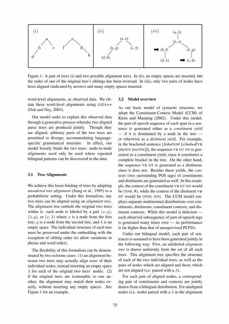
(i) (ii) (iii)
Figure 1: A pair of trees (i) and two possible alignment trees. In (ii), no empty spaces are inserted, butthe order of one of the original tree’s siblings has been reversed. In (iii), only two pairs of nodes havebeen aligned (indicated by arrows) and many empty spaces inserted.
word-level alignments, as observed data. We ob-tain these word-level alignments using GIZA++(Och and Ney, 2003).
Our model seeks to explain this observed datathrough a generative process whereby two alignedparse trees are produced jointly. Though theyare aligned, arbitrary parts of the two trees arepermitted to diverge, accommodating language-specific grammatical structure. In effect, ourmodel loosely binds the two trees: node-to-nodealignments need only be used where repeatedbilingual patterns can be discovered in the data.
3.1 Tree Alignments
We achieve this loose binding of trees by adaptingunordered tree alignment (Jiang et al., 1995) to aprobabilistic setting. Under this formalism, anytwo trees can be aligned using an alignment tree.The alignment tree embeds the original two treeswithin it: each node is labeled by a pair (x, y),(λ, y), or (x, λ) where x is a node from the firsttree, y is a node from the second tree, and λ is anempty space. The individual structure of each treemust be preserved under the embedding with theexception of sibling order (to allow variations inphrase and word order).
The flexibility of this formalism can be demon-strated by two extreme cases: (1) an alignment be-tween two trees may actually align none of theirindividual nodes, instead inserting an empty spaceλ for each of the original two trees’ nodes. (2)if the original trees are isomorphic to one an-other, the alignment may match their nodes ex-actly, without inserting any empty spaces. SeeFigure 1 for an example.
3.2 Model overview
As our basic model of syntactic structure, weadopt the Constituent-Context Model (CCM) ofKlein and Manning (2002). Under this model,the part-of-speech sequence of each span in a sen-tence is generated either as a constituent yield— if it is dominated by a node in the tree —or otherwise as a distituent yield. For example,in the bracketed sentence [John/NNP [climbed/VB
[the/DT tree/NN]]], the sequence VB DT NN is gen-erated as a constituent yield, since it constitutes acomplete bracket in the tree. On the other hand,the sequence VB DT is generated as a distituent,since it does not. Besides these yields, the con-texts (two surrounding POS tags) of constituentsand distituents are generated as well. In this exam-ple, the context of the constituent VB DT NN wouldbe (NNP, #), while the context of the distituent VB
DT would be (NNP, NN). The CCM model em-ploys separate multinomial distributions over con-stituents, distituents, constituent contexts, and dis-tituent contexts. While this model is deficient —each observed subsequence of part-of-speech tagsis generated many times over — its performanceis far higher than that of unsupervised PCFGs.
Under our bilingual model, each pair of sen-tences is assumed to have been generated jointly inthe following way: First, an unlabeled alignmenttree is drawn uniformly from the set of all suchtrees. This alignment tree specifies the structureof each of the two individual trees, as well as thepairs of nodes which are aligned and those whichare not aligned (i.e. paired with a λ).
For each pair of aligned nodes, a correspond-ing pair of constituents and contexts are jointlydrawn from a bilingual distribution. For unalignednodes (i.e. nodes paired with a λ in the alignment
75

tree), a single constituent and context are drawn,from language-specific distributions. Distituentsand their contexts are also drawn from language-specific distributions. Finally, word-level align-ments are drawn based on the structure of thealignment tree.
In the next two sections, we describe our modelin more formal detail by specifying the parame-ters and generative process by which sentences areformed.
3.3 ParametersOur model employs a number of multinomial dis-tributions:
• πCi : over constituent yields of language i,
• πDi : over distituent yields of language i,
• φCi : over constituent contexts of language i,
• φDi : over distituent contexts of language i,
• ω : over pairs of constituent yields, one fromthe first language and the other from the sec-ond language,
• Gzpair : over a finite set of integer val-ues {−m, . . . ,−2,−1, 0, 1, 2, . . . ,m}, mea-suring the Giza-score of aligned tree nodepairs (see below),
• Gznode : over a finite set of integer values{−m, . . . ,−2,−1, 0}, measuring the Giza-score of unaligned tree nodes (see below).
The first four distributions correspond exactly tothe parameters of the CCM model. Parameter ω isa “coupling parameter” which measures the com-patibility of tree-aligned constituent yield pairs.The final two parameters measure the compatibil-ity of syntactic alignments with the observed lexi-cal GIZA++ alignments. Intuitively, aligned nodesshould have a high density of word-level align-ments between them, and unaligned nodes shouldhave few lexical alignments.
More formally, consider a tree-aligned nodepair (n1, n2) with corresponding yields (y1, y2).We call a word-level alignment good if it alignsa word in y1 with a word in y2. We call a word-level alignment bad if it aligns a word in y1 witha word outside y2, or vice versa. The Giza-score for (n1, n2) is the number of good wordalignments minus the number of bad word align-ments. For example, suppose the constituent my
long name is node-aligned to its Urdu translationmera lamba naam. If only the word-pairs my/meraand name/naam are aligned, then the Giza-scorefor this node-alignment would be 2. If however,the English word long were (incorrectly) alignedunder GIZA++ to some Urdu word outside the cor-responding constituent, then the score would dropto 1. This score could even be negative if the num-ber of bad alignments exceeds those that are good.Distribution Gzpair provides a probability for thesescores (up to some fixed absolute value).
For an unaligned node n with correspondingyield y, only bad GIZA++ alignments are possible,thus the Giza-score for these nodes will always bezero or negative. Distribution Gznode provides aprobability for these scores (down to some fixedvalue). We want our model to find tree alignmentssuch that both aligned node pairs and unalignednodes have high Giza-score.
3.4 Generative ProcessNow we describe the stochastic process wherebythe observed parallel sentences and their word-level alignments are generated, according to ourmodel.
As the first step in the Bayesian generative pro-cess, all the multinomial parameters listed in theprevious section are drawn from their conjugatepriors — Dirichlet distributions of appropriate di-mension. Then, each pair of word-aligned parallelsentences is generated through the following pro-cess:
1. A pair of binary trees T1 and T2 along withan alignment tree A are drawn according toP (T1, T2, A). A is an alignment tree for T1
and T2 if it can be obtained by the follow-ing steps: First insert blank nodes (labeled byλ) into T1 and T2. Then permute the orderof sibling nodes such that the two resultingtrees T ′
1 and T ′2 are identical in structure. Fi-
nally, overlay T ′1 and T ′
2 to obtain A. We ad-ditionally require that A contain no extrane-ous nodes – that is no nodes with two blanklabels (λ, λ). See Figure 1 for an example.
We define the distribution P (T1, T2, A) to beuniform over all pairs of binary trees and theiralignments.
2. For each node in A of the form (n1, λ) (i.e.nodes in T1 left unaligned by A), draw
(i) a constituent yield according to πC1 ,
76
(ii) a constituent context according to φC1 ,
(iii) a Giza-score according to Gznode.
3. For each node in A of the form (λ, n2) (i.e.nodes in T2 left unaligned by A), draw
(i) a constituent yield according to πC2 ,
(ii) a constituent context according to φC2 ,
(iii) a Giza-score according to Gznode.
4. For each node in A of the form (n1, n2) (i.e.tree-aligned node pairs), draw
(i) a pair of constituent yields (y1, y2) ac-cording to:
φC1 (y1) · φC
2 (y2) · ω(y1, y2)Z
(1)
which is a product of experts combiningthe language specific context-yield dis-tributions as well as the coupling distri-bution ω with normalization constant Z,
(ii) a pair of contexts according to the ap-propriate language-specific parameters,
(iii) a Giza-score according to Gzpair.
5. For each span in Ti not dominated by a node(for each language i ∈ {1, 2}), draw a dis-tituent yield according to πD
i and a distituentcontext according to φD
i .
6. Draw actual word-level alignments consis-tent with the Giza-scores, according to a uni-form distribution.
In the next section we turn to the problem ofinference under this model when only the part-of-speech tag sequences of parallel sentences andtheir word-level alignments are observed.
3.5 InferenceGiven a corpus of paired part-of-speech tag se-quences (s1, s2) and their GIZA++ alignmentsg, we would ideally like to predict the set oftree pairs (T1,T2) which have highest proba-bility when conditioned on the observed data:P
(T1,T2
∣∣s1, s2,g). We could rewrite this by
explicitly integrating over the yield, context, cou-pling, Giza-score parameters as well as the align-ment trees. However, since maximizing this in-tegral directly would be intractable, we resort tostandard Markov chain sampling techniques. Weuse Gibbs sampling (Hastings, 1970) to draw treesfor each sentence conditioned on those drawn for
all other sentences. The samples form a Markovchain which is guaranteed to converge to the truejoint distribution over all sentences.
In the monolingual setting, there is a well-known tree sampling algorithm (Johnson et al.,2007). This algorithm proceeds in top-down fash-ion by sampling individual split points using themarginal probabilities of all possible subtrees.These marginals can be efficiently pre-computedand form the “inside” table of the famous Inside-Outside algorithm. However, in our setting, treescome in pairs, and their joint probability cruciallydepends on their alignment.
For the ith parallel sentence, we wish to jointlysample the pair of trees (T1, T2)i together withtheir alignment Ai. To do so directly would in-volve simultaneously marginalizing over all pos-sible subtrees as well as all possible alignmentsbetween such subtrees when sampling upper-levelsplit points. We know of no obvious algorithmfor computing this marginal. We instead first sam-ple the pair of trees (T1, T2)i from a simpler pro-posal distribution Q. Our proposal distribution as-sumes that no nodes of the two trees are alignedand therefore allows us to use the recursive top-down sampling algorithm mentioned above. Aftera new tree pair T ∗ = (T ∗
1 , T ∗2 )i is drawn from Q,
we accept the pair with the following probability:
min{
1,P (T ∗|T−i,A−i) Q(T |T−i,A−i)P (T |T−i,A−i) Q(T ∗|T−i,A−i)
}where T is the previously sampled tree-pair forsentence i, P is the true model probability, andQ is the probability under the proposal distribu-tion. This use of a tractable proposal distributionand acceptance ratio is known as the Metropolis-Hastings algorithm and it preserves the conver-gence guarantee of the Gibbs sampler (Hastings,1970). To compute the terms P (T ∗|T−i,A−i)and P (T |T−i,A−i) in the acceptance ratio above,we need to marginalize over all possible align-ments between tree pairs.
Fortunately, for any given pair of trees T1 andT2 this marginalization can be computed usinga dynamic program in time O(|T1||T2|). Herewe provide a very brief sketch. For every pairof nodes n1 ∈ T1, n2 ∈ T2, a table stores themarginal probability of the subtrees rooted at n1
and n2, respectively. A dynamic program buildsthis table from the bottom up: For each node pairn1, n2, we sum the probabilities of all local align-ment configurations, each multiplied by the appro-
77
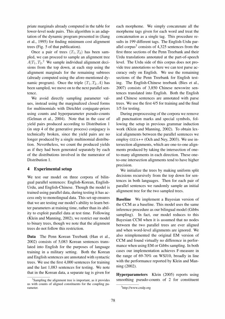
priate marginals already computed in the table forlower-level node pairs. This algorithm is an adap-tation of the dynamic program presented in (Jianget al., 1995) for finding minimum cost alignmenttrees (Fig. 5 of that publication).
Once a pair of trees (T1, T2) has been sam-pled, we can proceed to sample an alignment treeA|T1, T2.2 We sample individual alignment deci-sions from the top down, at each step using thealignment marginals for the remaining subtrees(already computed using the afore-mentioned dy-namic program). Once the triple (T1, T2, A) hasbeen sampled, we move on to the next parallel sen-tence.
We avoid directly sampling parameter val-ues, instead using the marginalized closed formsfor multinomials with Dirichlet conjugate-priorsusing counts and hyperparameter pseudo-counts(Gelman et al., 2004). Note that in the case ofyield pairs produced according to Distribution 1(in step 4 of the generative process) conjugacy istechnically broken, since the yield pairs are nolonger produced by a single multinomial distribu-tion. Nevertheless, we count the produced yieldsas if they had been generated separately by eachof the distributions involved in the numerator ofDistribution 1.
4 Experimental setup
We test our model on three corpora of bilin-gual parallel sentences: English-Korean, English-Urdu, and English-Chinese. Though the model istrained using parallel data, during testing it has ac-cess only to monolingual data. This set-up ensuresthat we are testing our model’s ability to learn bet-ter parameters at training time, rather than its abil-ity to exploit parallel data at test time. Following(Klein and Manning, 2002), we restrict our modelto binary trees, though we note that the alignmenttrees do not follow this restriction.
Data The Penn Korean Treebank (Han et al.,2002) consists of 5,083 Korean sentences trans-lated into English for the purposes of languagetraining in a military setting. Both the Koreanand English sentences are annotated with syntactictrees. We use the first 4,000 sentences for trainingand the last 1,083 sentences for testing. We notethat in the Korean data, a separate tag is given for
2Sampling the alignment tree is important, as it providesus with counts of aligned constituents for the coupling pa-rameter.
each morpheme. We simply concatenate all themorpheme tags given for each word and treat theconcatenation as a single tag. This procedure re-sults in 199 different tags. The English-Urdu par-allel corpus3 consists of 4,325 sentences from thefirst three sections of the Penn Treebank and theirUrdu translations annotated at the part-of-speechlevel. The Urdu side of this corpus does not pro-vide tree annotations so here we can test parse ac-curacy only on English. We use the remainingsections of the Penn Treebank for English test-ing. The English-Chinese treebank (Bies et al.,2007) consists of 3,850 Chinese newswire sen-tences translated into English. Both the Englishand Chinese sentences are annotated with parsetrees. We use the first 4/5 for training and the final1/5 for testing.
During preprocessing of the corpora we removeall punctuation marks and special symbols, fol-lowing the setup in previous grammar inductionwork (Klein and Manning, 2002). To obtain lex-ical alignments between the parallel sentences weemploy GIZA++ (Och and Ney, 2003). We use in-tersection alignments, which are one-to-one align-ments produced by taking the intersection of one-to-many alignments in each direction. These one-to-one intersection alignments tend to have higherprecision.
We initialize the trees by making uniform splitdecisions recursively from the top down for sen-tences in both languages. Then for each pair ofparallel sentences we randomly sample an initialalignment tree for the two sampled trees.
Baseline We implement a Bayesian version ofthe CCM as a baseline. This model uses the sameinference procedure as our bilingual model (Gibbssampling). In fact, our model reduces to thisBayesian CCM when it is assumed that no nodesbetween the two parallel trees are ever alignedand when word-level alignments are ignored. Wealso reimplemented the original EM version ofCCM and found virtually no difference in perfor-mance when using EM or Gibbs sampling. In bothcases our implementation achieves F-measure inthe range of 69-70% on WSJ10, broadly in linewith the performance reported by Klein and Man-ning (2002).
Hyperparameters Klein (2005) reports usingsmoothing pseudo-counts of 2 for constituent
3http://www.crulp.org
78
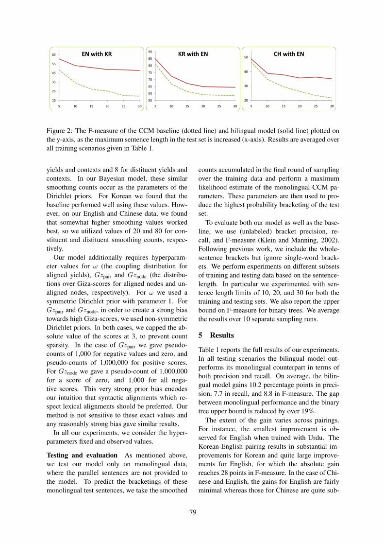
Figure 2: The F-measure of the CCM baseline (dotted line) and bilingual model (solid line) plotted onthe y-axis, as the maximum sentence length in the test set is increased (x-axis). Results are averaged overall training scenarios given in Table 1.
yields and contexts and 8 for distituent yields andcontexts. In our Bayesian model, these similarsmoothing counts occur as the parameters of theDirichlet priors. For Korean we found that thebaseline performed well using these values. How-ever, on our English and Chinese data, we foundthat somewhat higher smoothing values workedbest, so we utilized values of 20 and 80 for con-stituent and distituent smoothing counts, respec-tively.
Our model additionally requires hyperparam-eter values for ω (the coupling distribution foraligned yields), Gzpair and Gznode (the distribu-tions over Giza-scores for aligned nodes and un-aligned nodes, respectively). For ω we used asymmetric Dirichlet prior with parameter 1. ForGzpair and Gznode, in order to create a strong biastowards high Giza-scores, we used non-symmetricDirichlet priors. In both cases, we capped the ab-solute value of the scores at 3, to prevent countsparsity. In the case of Gzpair we gave pseudo-counts of 1,000 for negative values and zero, andpseudo-counts of 1,000,000 for positive scores.For Gznode we gave a pseudo-count of 1,000,000for a score of zero, and 1,000 for all nega-tive scores. This very strong prior bias encodesour intuition that syntactic alignments which re-spect lexical alignments should be preferred. Ourmethod is not sensitive to these exact values andany reasonably strong bias gave similar results.
In all our experiments, we consider the hyper-parameters fixed and observed values.
Testing and evaluation As mentioned above,we test our model only on monolingual data,where the parallel sentences are not provided tothe model. To predict the bracketings of thesemonolingual test sentences, we take the smoothed
counts accumulated in the final round of samplingover the training data and perform a maximumlikelihood estimate of the monolingual CCM pa-rameters. These parameters are then used to pro-duce the highest probability bracketing of the testset.
To evaluate both our model as well as the base-line, we use (unlabeled) bracket precision, re-call, and F-measure (Klein and Manning, 2002).Following previous work, we include the whole-sentence brackets but ignore single-word brack-ets. We perform experiments on different subsetsof training and testing data based on the sentence-length. In particular we experimented with sen-tence length limits of 10, 20, and 30 for both thetraining and testing sets. We also report the upperbound on F-measure for binary trees. We averagethe results over 10 separate sampling runs.
5 Results
Table 1 reports the full results of our experiments.In all testing scenarios the bilingual model out-performs its monolingual counterpart in terms ofboth precision and recall. On average, the bilin-gual model gains 10.2 percentage points in preci-sion, 7.7 in recall, and 8.8 in F-measure. The gapbetween monolingual performance and the binarytree upper bound is reduced by over 19%.
The extent of the gain varies across pairings.For instance, the smallest improvement is ob-served for English when trained with Urdu. TheKorean-English pairing results in substantial im-provements for Korean and quite large improve-ments for English, for which the absolute gainreaches 28 points in F-measure. In the case of Chi-nese and English, the gains for English are fairlyminimal whereas those for Chinese are quite sub-
79

Max Sent. Length Monolingual Bilingual Upper BoundTest Train Precision Recall F1 Precision Recall F1 F1
EN
with
KR 10
10 52.74 39.53 45.19 57.76 43.30 49.50 85.620 41.87 31.38 35.87 61.66 46.22 52.83 85.630 33.43 25.06 28.65 64.41 48.28 55.19 85.6
2020 35.12 25.12 29.29 56.96 40.74 47.50 83.330 26.26 18.78 21.90 60.07 42.96 50.09 83.3
30 30 23.95 16.81 19.76 58.01 40.73 47.86 82.4
KR
with
EN 10
10 71.07 62.55 66.54 75.63 66.56 70.81 93.620 71.35 62.79 66.80 77.61 68.30 72.66 93.630 71.37 62.81 66.82 77.87 68.53 72.91 93.6
2020 64.28 54.73 59.12 70.44 59.98 64.79 91.930 64.29 54.75 59.14 70.81 60.30 65.13 91.9
30 30 63.63 54.17 58.52 70.11 59.70 64.49 91.9
EN
with
CH 10
10 50.09 34.18 40.63 37.46 25.56 30.39 81.020 58.86 40.17 47.75 50.24 34.29 40.76 81.030 64.81 44.22 52.57 68.24 46.57 55.36 81.0
2020 41.90 30.52 35.31 38.64 28.15 32.57 84.330 52.83 38.49 44.53 58.50 42.62 49.31 84.3
30 30 46.35 33.67 39.00 51.40 37.33 43.25 84.1
CH
with
EN 10
10 39.87 27.71 32.69 40.62 28.23 33.31 81.920 43.44 30.19 35.62 47.54 33.03 38.98 81.930 43.63 30.32 35.77 54.09 37.59 44.36 81.9
2020 29.80 23.46 26.25 36.93 29.07 32.53 88.030 30.05 23.65 26.47 43.99 34.63 38.75 88.0
30 30 24.46 19.41 21.64 39.61 31.43 35.05 88.4
EN
with
UR 10
10 57.98 45.68 51.10 73.43 57.85 64.71 88.120 70.57 55.60 62.20 80.24 63.22 70.72 88.130 75.39 59.40 66.45 79.04 62.28 69.67 88.1
2020 57.78 43.86 49.87 67.26 51.06 58.05 86.330 63.12 47.91 54.47 64.45 48.92 55.62 86.3
30 30 57.36 43.02 49.17 57.97 43.48 49.69 85.7
Table 1: Unlabeled precision, recall and F-measure for the monolingual baseline and the bilingual modelon several test sets. We report results for different combinations of maximum sentence length in both thetraining and test sets. The right most column, in all cases, contains the maximum F-measure achievableusing binary trees. The best performance for each test-length is highlighted in bold.
stantial. This asymmetry should not be surprising,as Chinese on its own seems to be quite a bit moredifficult to parse than English.
We also investigated the impact of sentencelength for both the training and testing sets. Forour model, adding sentences of greater length tothe training set leads to increases in parse accu-racy for short sentences. For the baseline, how-ever, adding this additional training data degradesperformance in the case of English paired with Ko-rean. Figure 2 summarizes the performance ofour model for different sentence lengths on sev-eral of the test-sets. As shown in the figure, thelargest improvements tend to occur at longer sen-tence lengths.
6 Conclusion
We have presented a probabilistic model for bilin-gual grammar induction which uses raw paralleltext to learn tree pairs and their alignments. Ourformalism loosely binds the two trees, using bilin-gual patterns when possible, but allowing substan-tial language-specific variation. We tested ourmodel on three test sets and showed substantialimprovement over a state-of-the-art monolingualbaseline.4
4The authors acknowledge the support of the NSF (CA-REER grant IIS-0448168, grant IIS-0835445, and grant IIS-0835652). Thanks to Amir Globerson and members of theMIT NLP group for their helpful suggestions. Any opinions,findings, or conclusions are those of the authors, and do notnecessarily reflect the views of the funding organizations
80

ReferencesAnn Bies, Martha Palmer, Justin Mott, and Colin
Warner. 2007. English Chinese translation treebankv 1.0. LDC2007T02.
Phil Blunsom, Trevor Cohn, and Miles Osborne. 2008.Bayesian synchronous grammar induction. In Pro-ceedings of NIPS.
David Burkett and Dan Klein. 2008. Two languagesare better than one (for syntactic parsing). In Pro-ceedings of EMNLP, pages 877–886.
Eugene Charniak and Glen Carroll. 1992. Two exper-iments on learning probabilistic dependency gram-mars from corpora. In Proceedings of the AAAIWorkshop on Statistically-Based NLP Techniques,pages 1–13.
David Chiang. 2005. A hierarchical phrase-basedmodel for statistical machine translation. In Pro-ceedings of the ACL, pages 263–270.
Shay B. Cohen and Noah A. Smith. 2009. Shared lo-gistic normal distributions for soft parameter tyingin unsupervised grammar induction. In Proceedingsof the NAACL/HLT.
Jason Eisner. 2003. Learning non-isomorphic treemappings for machine translation. In The Compan-ion Volume to the Proceedings of the ACL, pages205–208.
Andrew Gelman, John B. Carlin, Hal S. Stern, andDonald B. Rubin. 2004. Bayesian data analysis.Chapman and Hall/CRC.
Dmitriy Genzel. 2005. Inducing a multilingual dictio-nary from a parallel multitext in related languages.In Proceedings of EMNLP/HLT, pages 875–882.
C. Han, N.R. Han, E.S. Ko, H. Yi, and M. Palmer.2002. Penn Korean Treebank: Development andevaluation. In Proc. Pacific Asian Conf. Languageand Comp.
W. K. Hastings. 1970. Monte carlo sampling meth-ods using Markov chains and their applications.Biometrika, 57:97–109.
R. Hwa, P. Resnik, A. Weinberg, C. Cabezas, andO. Kolak. 2005. Bootstrapping parsers via syntacticprojection across parallel texts. Journal of NaturalLanguage Engineering, 11(3):311–325.
T. Jiang, L. Wang, and K. Zhang. 1995. Alignment oftrees – an alternative to tree edit. Theoretical Com-puter Science, 143(1):137–148.
M. Johnson, T. Griffiths, and S. Goldwater. 2007.Bayesian inference for PCFGs via Markov chainMonte Carlo. In Proceedings of the NAACL/HLT,pages 139–146.
Dan Klein and Christopher D. Manning. 2002. Agenerative constituent-context model for improvedgrammar induction. In Proceedings of the ACL,pages 128–135.
D. Klein. 2005. The Unsupervised Learning of Natu-ral Language Structure. Ph.D. thesis, Stanford Uni-versity.
Jonas Kuhn. 2004. Experiments in parallel-text basedgrammar induction. In Proceedings of the ACL,pages 470–477.
I. Dan Melamed. 2003. Multitext grammarsand synchronous parsers. In Proceedings of theNAACL/HLT, pages 79–86.
Franz Josef Och and Hermann Ney. 2003. A sys-tematic comparison of various statistical alignmentmodels. Computational Linguistics, 29(1):19–51.
Yoav Seginer. 2007. Fast unsupervised incrementalparsing. In Proceedings of the ACL, pages 384–391.
David A. Smith and Noah A. Smith. 2004. Bilingualparsing with factored estimation: Using English toparse Korean. In Proceeding of EMNLP, pages 49–56.
Benjamin Snyder and Regina Barzilay. 2008. Un-supervised multilingual learning for morphologicalsegmentation. In Proceedings of the ACL/HLT,pages 737–745.
Benjamin Snyder, Tahira Naseem, Jacob Eisenstein,and Regina Barzilay. 2008. Unsupervised multi-lingual learning for POS tagging. In Proceedings ofEMNLP, pages 1041–1050.
Benjamin Snyder, Tahira Naseem, Jacob Eisenstein,and Regina Barzilay. 2009. Adding more languagesimproves unsupervised multilingual part-of-speechtagging: A Bayesian non-parametric approach. InProceedings of the NAACL/HLT.
Andreas Stolcke and Stephen M. Omohundro. 1994.Inducing probabilistic grammars by Bayesian modelmerging. In Proceedings of ICGI, pages 106–118.
Dekai Wu and Hongsing Wong. 1998. Machinetranslation with a stochastic grammatical channel.In Proceedings of the ACL/COLING, pages 1408–1415.
Dekai Wu. 1997. Stochastic inversion transductiongrammars and bilingual parsing of parallel corpora.Computational Linguistics, 23(3):377–403.
Chenhai Xi and Rebecca Hwa. 2005. A backoffmodel for bootstrapping resources for non-englishlanguages. In Proceedings of EMNLP, pages 851 –858.
Hao Zhang and Daniel Gildea. 2005. Stochastic lex-icalized inversion transduction grammar for align-ment. In Proceedings of the ACL, pages 475–482.
81
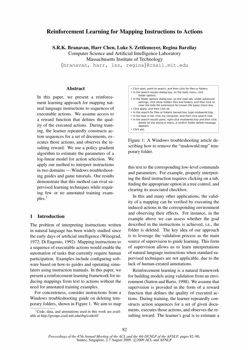
Proceedings of the 47th Annual Meeting of the ACL and the 4th IJCNLP of the AFNLP, pages 82–90,Suntec, Singapore, 2-7 August 2009. c©2009 ACL and AFNLP
Reinforcement Learning for Mapping Instructions to Actions
S.R.K. Branavan, Harr Chen, Luke S. Zettlemoyer, Regina BarzilayComputer Science and Artificial Intelligence Laboratory
Massachusetts Institute of Technology{branavan, harr, lsz, regina}@csail.mit.edu
Abstract
In this paper, we present a reinforce-ment learning approach for mapping nat-ural language instructions to sequences ofexecutable actions. We assume access toa reward function that defines the qual-ity of the executed actions. During train-ing, the learner repeatedly constructs ac-tion sequences for a set of documents, ex-ecutes those actions, and observes the re-sulting reward. We use a policy gradientalgorithm to estimate the parameters of alog-linear model for action selection. Weapply our method to interpret instructionsin two domains — Windows troubleshoot-ing guides and game tutorials. Our resultsdemonstrate that this method can rival su-pervised learning techniques while requir-ing few or no annotated training exam-ples.1
1 Introduction
The problem of interpreting instructions writtenin natural language has been widely studied sincethe early days of artificial intelligence (Winograd,1972; Di Eugenio, 1992). Mapping instructions toa sequence of executable actions would enable theautomation of tasks that currently require humanparticipation. Examples include configuring soft-ware based on how-to guides and operating simu-lators using instruction manuals. In this paper, wepresent a reinforcement learning framework for in-ducing mappings from text to actions without theneed for annotated training examples.
For concreteness, consider instructions from aWindows troubleshooting guide on deleting tem-porary folders, shown in Figure 1. We aim to map
1Code, data, and annotations used in this work are avail-able at http://groups.csail.mit.edu/rbg/code/rl/
Figure 1: A Windows troubleshooting article de-scribing how to remove the “msdownld.tmp” tem-porary folder.
this text to the corresponding low-level commandsand parameters. For example, properly interpret-ing the third instruction requires clicking on a tab,finding the appropriate option in a tree control, andclearing its associated checkbox.
In this and many other applications, the valid-ity of a mapping can be verified by executing theinduced actions in the corresponding environmentand observing their effects. For instance, in theexample above we can assess whether the goaldescribed in the instructions is achieved, i.e., thefolder is deleted. The key idea of our approachis to leverage the validation process as the mainsource of supervision to guide learning. This formof supervision allows us to learn interpretationsof natural language instructions when standard su-pervised techniques are not applicable, due to thelack of human-created annotations.
Reinforcement learning is a natural frameworkfor building models using validation from an envi-ronment (Sutton and Barto, 1998). We assume thatsupervision is provided in the form of a rewardfunction that defines the quality of executed ac-tions. During training, the learner repeatedly con-structs action sequences for a set of given docu-ments, executes those actions, and observes the re-sulting reward. The learner’s goal is to estimate a
82
policy — a distribution over actions given instruc-tion text and environment state — that maximizesfuture expected reward. Our policy is modeled in alog-linear fashion, allowing us to incorporate fea-tures of both the instruction text and the environ-ment. We employ a policy gradient algorithm toestimate the parameters of this model.
We evaluate our method on two distinct applica-tions: Windows troubleshooting guides and puz-zle game tutorials. The key findings of our ex-periments are twofold. First, models trained onlywith simple reward signals achieve surprisinglyhigh results, coming within 11% of a fully su-pervised method in the Windows domain. Sec-ond, augmenting unlabeled documents with evena small fraction of annotated examples greatly re-duces this performance gap, to within 4% in thatdomain. These results indicate the power of learn-ing from this new form of automated supervision.
2 Related Work
Grounded Language Acquisition Our workfits into a broader class of approaches that aim tolearn language from a situated context (Mooney,2008a; Mooney, 2008b; Fleischman and Roy,2005; Yu and Ballard, 2004; Siskind, 2001; Oates,2001). Instances of such approaches includework on inferring the meaning of words fromvideo data (Roy and Pentland, 2002; Barnard andForsyth, 2001), and interpreting the commentaryof a simulated soccer game (Chen and Mooney,2008). Most of these approaches assume someform of parallel data, and learn perceptual co-occurrence patterns. In contrast, our emphasisis on learning language by proactively interactingwith an external environment.
Reinforcement Learning for Language Pro-cessing Reinforcement learning has been previ-ously applied to the problem of dialogue manage-ment (Scheffler and Young, 2002; Roy et al., 2000;Litman et al., 2000; Singh et al., 1999). Thesesystems converse with a human user by taking ac-tions that emit natural language utterances. Thereinforcement learning state space encodes infor-mation about the goals of the user and what theysay at each time step. The learning problem is tofind an optimal policy that maps states to actions,through a trial-and-error process of repeated inter-action with the user.
Reinforcement learning is applied very differ-ently in dialogue systems compared to our setup.
In some respects, our task is more easily amenableto reinforcement learning. For instance, we are notinteracting with a human user, so the cost of inter-action is lower. However, while the state space canbe designed to be relatively small in the dialoguemanagement task, our state space is determined bythe underlying environment and is typically quitelarge. We address this complexity by developinga policy gradient algorithm that learns efficientlywhile exploring a small subset of the states.
3 Problem Formulation
Our task is to learn a mapping between documentsand the sequence of actions they express. Figure 2shows how one example sentence is mapped tothree actions.
Mapping Text to Actions As input, we aregiven a document d, comprising a sequence of sen-tences (u1, . . . , u`), where each ui is a sequenceof words. Our goal is to map d to a sequence ofactions ~a = (a0, . . . , an−1). Actions are predictedand executed sequentially.2
An action a = (c,R,W ′) encompasses a com-mand c, the command’s parameters R, and thewords W ′ specifying c and R. Elements of R re-fer to objects available in the environment state, asdescribed below. Some parameters can also referto words in document d. Additionally, to accountfor words that do not describe any actions, c canbe a null command.
The Environment The environment state Especifies the set of objects available for interac-tion, and their properties. In Figure 2, E is shownon the right. The environment state E changesin response to the execution of command c withparameters R according to a transition distribu-tion p(E ′|E , c, R). This distribution is a priori un-known to the learner. As we will see in Section 5,our approach avoids having to directly estimatethis distribution.
State To predict actions sequentially, we need totrack the state of the document-to-actions map-ping over time. A mapping state s is a tuple(E , d, j,W ), where E refers to the current environ-ment state; j is the index of the sentence currentlybeing interpreted in document d; and W containswords that were mapped by previous actions for
2That is, action ai is executed before ai+1 is predicted.
83

Figure 2: A three-step mapping from an instruction sentence to a sequence of actions in Windows 2000.For each step, the figure shows the words selected by the action, along with the corresponding systemcommand and its parameters. The words of W ′ are underlined, and the words of W are highlighted ingrey.
the same sentence. The mapping state s is ob-served after each action.
The initial mapping state s0 for document d is(Ed, d, 0, ∅); Ed is the unique starting environmentstate for d. Performing action a in state s =(E , d, j,W ) leads to a new state s′ according todistribution p(s′|s, a), defined as follows: E tran-sitions according to p(E ′|E , c, R), W is updatedwith a’s selected words, and j is incremented ifall words of the sentence have been mapped. Forthe applications we consider in this work, environ-ment state transitions, and consequently mappingstate transitions, are deterministic.
Training During training, we are provided witha set D of documents, the ability to sample fromthe transition distribution, and a reward functionr(h). Here, h = (s0, a0, . . . , sn−1, an−1, sn) isa history of states and actions visited while in-terpreting one document. r(h) outputs a real-valued score that correlates with correct actionselection.3 We consider both immediate reward,which is available after each action, and delayedreward, which does not provide feedback until thelast action. For example, task completion is a de-layed reward that produces a positive value afterthe final action only if the task was completed suc-cessfully. We will also demonstrate how manu-ally annotated action sequences can be incorpo-rated into the reward.
3In most reinforcement learning problems, the rewardfunction is defined over state-action pairs, as r(s, a) — in thiscase, r(h) =
Pt r(st, at), and our formulation becomes a
standard finite-horizon Markov decision process. Policy gra-dient approaches allow us to learn using the more generalcase of history-based reward.
The goal of training is to estimate parameters θof the action selection distribution p(a|s, θ), calledthe policy. Since the reward correlates with ac-tion sequence correctness, the θ that maximizesexpected reward will yield the best actions.
4 A Log-Linear Model for Actions
Our goal is to predict a sequence of actions. Weconstruct this sequence by repeatedly choosing anaction given the current mapping state, and apply-ing that action to advance to a new state.
Given a state s = (E , d, j,W ), the space of pos-sible next actions is defined by enumerating sub-spans of unused words in the current sentence (i.e.,subspans of the jth sentence of d not in W ), andthe possible commands and parameters in envi-ronment state E .4 We model the policy distribu-tion p(a|s; θ) over this action space in a log-linearfashion (Della Pietra et al., 1997; Lafferty et al.,2001), giving us the flexibility to incorporate a di-verse range of features. Under this representation,the policy distribution is:
p(a|s; θ) =eθ·φ(s,a)
∑
a′
eθ·φ(s,a′), (1)
where φ(s, a) ∈ Rn is an n-dimensional feature
representation. During test, actions are selectedaccording to the mode of this distribution.
4For parameters that refer to words, the space of possiblevalues is defined by the unused words in the current sentence.
84
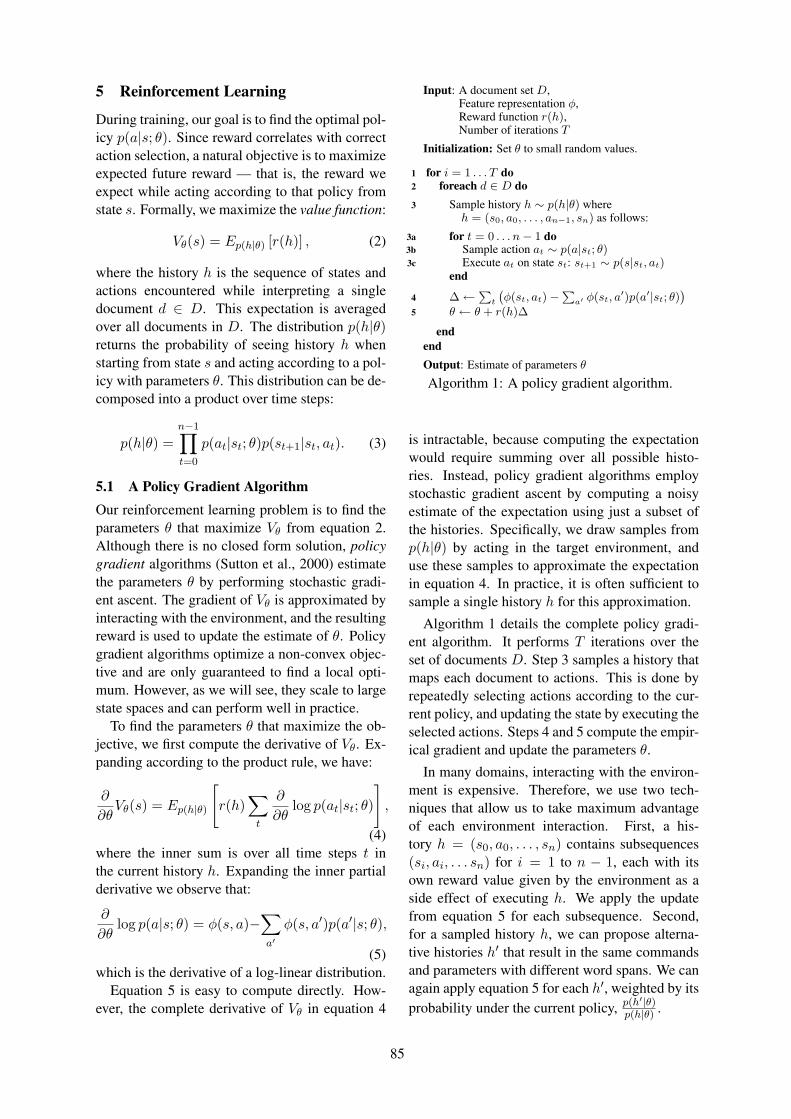
5 Reinforcement Learning
During training, our goal is to find the optimal pol-icy p(a|s; θ). Since reward correlates with correctaction selection, a natural objective is to maximizeexpected future reward — that is, the reward weexpect while acting according to that policy fromstate s. Formally, we maximize the value function:
Vθ(s) = Ep(h|θ) [r(h)] , (2)
where the history h is the sequence of states andactions encountered while interpreting a singledocument d ∈ D. This expectation is averagedover all documents in D. The distribution p(h|θ)returns the probability of seeing history h whenstarting from state s and acting according to a pol-icy with parameters θ. This distribution can be de-composed into a product over time steps:
p(h|θ) =
n−1∏
t=0
p(at|st; θ)p(st+1|st, at). (3)
5.1 A Policy Gradient AlgorithmOur reinforcement learning problem is to find theparameters θ that maximize Vθ from equation 2.Although there is no closed form solution, policygradient algorithms (Sutton et al., 2000) estimatethe parameters θ by performing stochastic gradi-ent ascent. The gradient of Vθ is approximated byinteracting with the environment, and the resultingreward is used to update the estimate of θ. Policygradient algorithms optimize a non-convex objec-tive and are only guaranteed to find a local opti-mum. However, as we will see, they scale to largestate spaces and can perform well in practice.
To find the parameters θ that maximize the ob-jective, we first compute the derivative of Vθ. Ex-panding according to the product rule, we have:
∂
∂θVθ(s) = Ep(h|θ)
[
r(h)∑
t
∂
∂θlog p(at|st; θ)
]
,
(4)where the inner sum is over all time steps t inthe current history h. Expanding the inner partialderivative we observe that:
∂
∂θlog p(a|s; θ) = φ(s, a)−
∑
a′
φ(s, a′)p(a′|s; θ),
(5)which is the derivative of a log-linear distribution.
Equation 5 is easy to compute directly. How-ever, the complete derivative of Vθ in equation 4
Input: A document set D,Feature representation φ,Reward function r(h),Number of iterations T
Initialization: Set θ to small random values.
for i = 1 . . . T do1foreach d ∈ D do2
Sample history h ∼ p(h|θ) where3h = (s0, a0, . . . , an−1, sn) as follows:
3a for t = 0 . . . n− 1 do3b Sample action at ∼ p(a|st; θ)3c Execute at on state st: st+1 ∼ p(s|st, at)
end
∆←P
t
`φ(st, at)−
Pa′ φ(st, a
′)p(a′|st; θ)´
4θ ← θ + r(h)∆5
endendOutput: Estimate of parameters θ
Algorithm 1: A policy gradient algorithm.
is intractable, because computing the expectationwould require summing over all possible histo-ries. Instead, policy gradient algorithms employstochastic gradient ascent by computing a noisyestimate of the expectation using just a subset ofthe histories. Specifically, we draw samples fromp(h|θ) by acting in the target environment, anduse these samples to approximate the expectationin equation 4. In practice, it is often sufficient tosample a single history h for this approximation.
Algorithm 1 details the complete policy gradi-ent algorithm. It performs T iterations over theset of documents D. Step 3 samples a history thatmaps each document to actions. This is done byrepeatedly selecting actions according to the cur-rent policy, and updating the state by executing theselected actions. Steps 4 and 5 compute the empir-ical gradient and update the parameters θ.
In many domains, interacting with the environ-ment is expensive. Therefore, we use two tech-niques that allow us to take maximum advantageof each environment interaction. First, a his-tory h = (s0, a0, . . . , sn) contains subsequences(si, ai, . . . sn) for i = 1 to n − 1, each with itsown reward value given by the environment as aside effect of executing h. We apply the updatefrom equation 5 for each subsequence. Second,for a sampled history h, we can propose alterna-tive histories h′ that result in the same commandsand parameters with different word spans. We canagain apply equation 5 for each h′, weighted by itsprobability under the current policy, p(h
′|θ)p(h|θ) .
85
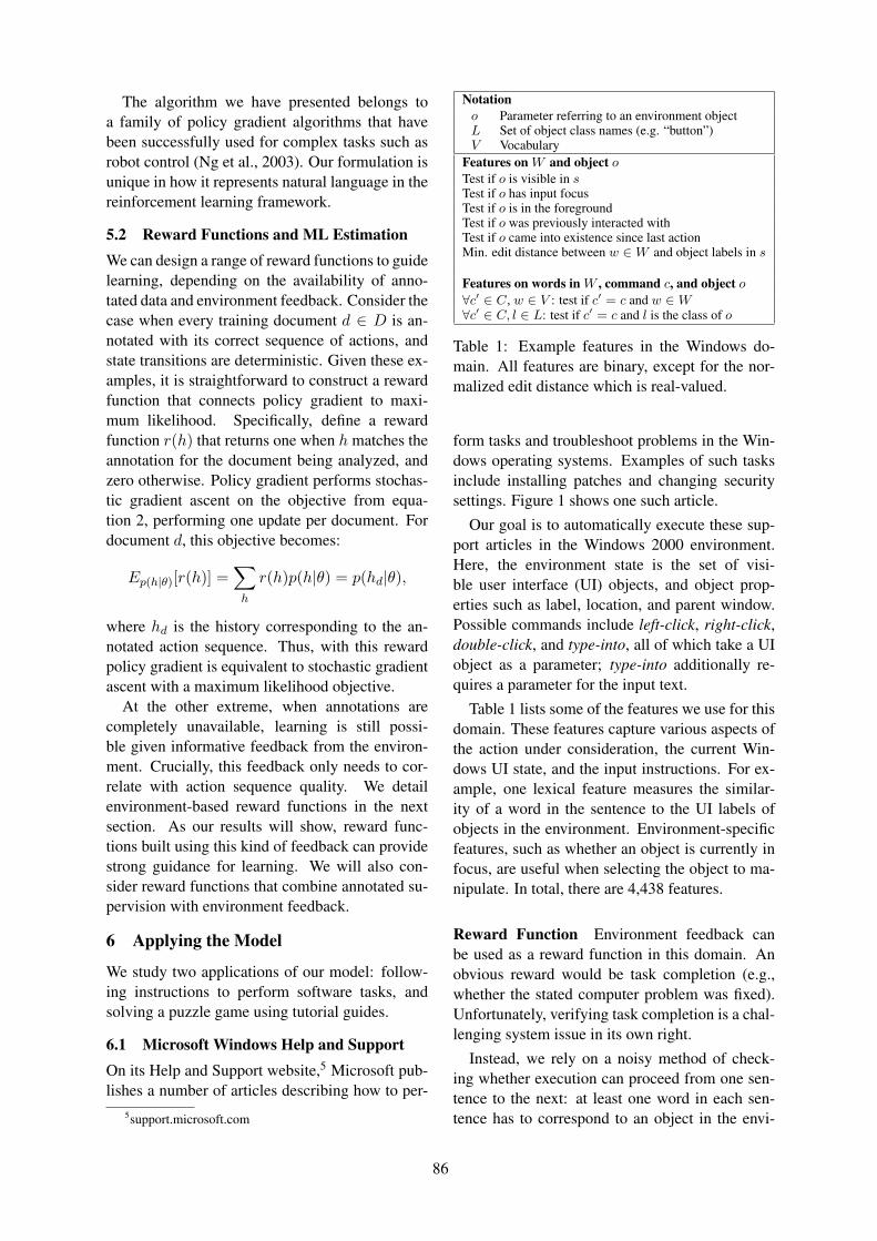
The algorithm we have presented belongs toa family of policy gradient algorithms that havebeen successfully used for complex tasks such asrobot control (Ng et al., 2003). Our formulation isunique in how it represents natural language in thereinforcement learning framework.
5.2 Reward Functions and ML EstimationWe can design a range of reward functions to guidelearning, depending on the availability of anno-tated data and environment feedback. Consider thecase when every training document d ∈ D is an-notated with its correct sequence of actions, andstate transitions are deterministic. Given these ex-amples, it is straightforward to construct a rewardfunction that connects policy gradient to maxi-mum likelihood. Specifically, define a rewardfunction r(h) that returns one when h matches theannotation for the document being analyzed, andzero otherwise. Policy gradient performs stochas-tic gradient ascent on the objective from equa-tion 2, performing one update per document. Fordocument d, this objective becomes:
Ep(h|θ)[r(h)] =∑
h
r(h)p(h|θ) = p(hd|θ),
where hd is the history corresponding to the an-notated action sequence. Thus, with this rewardpolicy gradient is equivalent to stochastic gradientascent with a maximum likelihood objective.
At the other extreme, when annotations arecompletely unavailable, learning is still possi-ble given informative feedback from the environ-ment. Crucially, this feedback only needs to cor-relate with action sequence quality. We detailenvironment-based reward functions in the nextsection. As our results will show, reward func-tions built using this kind of feedback can providestrong guidance for learning. We will also con-sider reward functions that combine annotated su-pervision with environment feedback.
6 Applying the Model
We study two applications of our model: follow-ing instructions to perform software tasks, andsolving a puzzle game using tutorial guides.
6.1 Microsoft Windows Help and SupportOn its Help and Support website,5 Microsoft pub-lishes a number of articles describing how to per-
5support.microsoft.com
Notationo Parameter referring to an environment objectL Set of object class names (e.g. “button”)V Vocabulary
Features on W and object oTest if o is visible in sTest if o has input focusTest if o is in the foregroundTest if o was previously interacted withTest if o came into existence since last actionMin. edit distance between w ∈W and object labels in s
Features on words in W , command c, and object o∀c′ ∈ C, w ∈ V : test if c′ = c and w ∈W∀c′ ∈ C, l ∈ L: test if c′ = c and l is the class of o
Table 1: Example features in the Windows do-main. All features are binary, except for the nor-malized edit distance which is real-valued.
form tasks and troubleshoot problems in the Win-dows operating systems. Examples of such tasksinclude installing patches and changing securitysettings. Figure 1 shows one such article.
Our goal is to automatically execute these sup-port articles in the Windows 2000 environment.Here, the environment state is the set of visi-ble user interface (UI) objects, and object prop-erties such as label, location, and parent window.Possible commands include left-click, right-click,double-click, and type-into, all of which take a UIobject as a parameter; type-into additionally re-quires a parameter for the input text.
Table 1 lists some of the features we use for thisdomain. These features capture various aspects ofthe action under consideration, the current Win-dows UI state, and the input instructions. For ex-ample, one lexical feature measures the similar-ity of a word in the sentence to the UI labels ofobjects in the environment. Environment-specificfeatures, such as whether an object is currently infocus, are useful when selecting the object to ma-nipulate. In total, there are 4,438 features.
Reward Function Environment feedback canbe used as a reward function in this domain. Anobvious reward would be task completion (e.g.,whether the stated computer problem was fixed).Unfortunately, verifying task completion is a chal-lenging system issue in its own right.
Instead, we rely on a noisy method of check-ing whether execution can proceed from one sen-tence to the next: at least one word in each sen-tence has to correspond to an object in the envi-
86
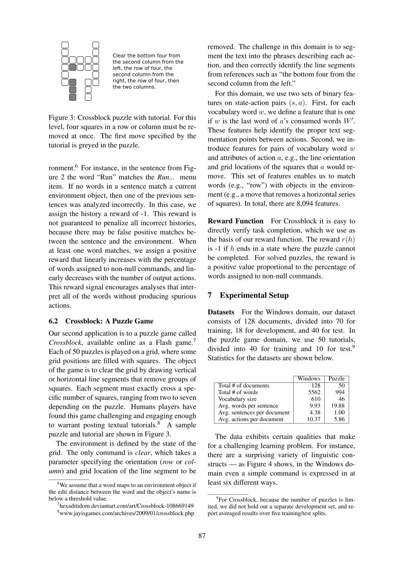
Figure 3: Crossblock puzzle with tutorial. For thislevel, four squares in a row or column must be re-moved at once. The first move specified by thetutorial is greyed in the puzzle.
ronment.6 For instance, in the sentence from Fig-ure 2 the word “Run” matches the Run... menuitem. If no words in a sentence match a currentenvironment object, then one of the previous sen-tences was analyzed incorrectly. In this case, weassign the history a reward of -1. This reward isnot guaranteed to penalize all incorrect histories,because there may be false positive matches be-tween the sentence and the environment. Whenat least one word matches, we assign a positivereward that linearly increases with the percentageof words assigned to non-null commands, and lin-early decreases with the number of output actions.This reward signal encourages analyses that inter-pret all of the words without producing spuriousactions.
6.2 Crossblock: A Puzzle Game
Our second application is to a puzzle game calledCrossblock, available online as a Flash game.7
Each of 50 puzzles is played on a grid, where somegrid positions are filled with squares. The objectof the game is to clear the grid by drawing verticalor horizontal line segments that remove groups ofsquares. Each segment must exactly cross a spe-cific number of squares, ranging from two to sevendepending on the puzzle. Humans players havefound this game challenging and engaging enoughto warrant posting textual tutorials.8 A samplepuzzle and tutorial are shown in Figure 3.
The environment is defined by the state of thegrid. The only command is clear, which takes aparameter specifying the orientation (row or col-umn) and grid location of the line segment to be
6We assume that a word maps to an environment object ifthe edit distance between the word and the object’s name isbelow a threshold value.
7hexaditidom.deviantart.com/art/Crossblock-1086691498www.jayisgames.com/archives/2009/01/crossblock.php
removed. The challenge in this domain is to seg-ment the text into the phrases describing each ac-tion, and then correctly identify the line segmentsfrom references such as “the bottom four from thesecond column from the left.”
For this domain, we use two sets of binary fea-tures on state-action pairs (s, a). First, for eachvocabulary word w, we define a feature that is oneif w is the last word of a’s consumed words W ′.These features help identify the proper text seg-mentation points between actions. Second, we in-troduce features for pairs of vocabulary word wand attributes of action a, e.g., the line orientationand grid locations of the squares that a would re-move. This set of features enables us to matchwords (e.g., “row”) with objects in the environ-ment (e.g., a move that removes a horizontal seriesof squares). In total, there are 8,094 features.
Reward Function For Crossblock it is easy todirectly verify task completion, which we use asthe basis of our reward function. The reward r(h)is -1 if h ends in a state where the puzzle cannotbe completed. For solved puzzles, the reward isa positive value proportional to the percentage ofwords assigned to non-null commands.
7 Experimental Setup
Datasets For the Windows domain, our datasetconsists of 128 documents, divided into 70 fortraining, 18 for development, and 40 for test. Inthe puzzle game domain, we use 50 tutorials,divided into 40 for training and 10 for test.9
Statistics for the datasets are shown below.
Windows PuzzleTotal # of documents 128 50Total # of words 5562 994Vocabulary size 610 46Avg. words per sentence 9.93 19.88Avg. sentences per document 4.38 1.00Avg. actions per document 10.37 5.86
The data exhibits certain qualities that makefor a challenging learning problem. For instance,there are a surprising variety of linguistic con-structs — as Figure 4 shows, in the Windows do-main even a simple command is expressed in atleast six different ways.
9For Crossblock, because the number of puzzles is lim-ited, we did not hold out a separate development set, and re-port averaged results over five training/test splits.
87
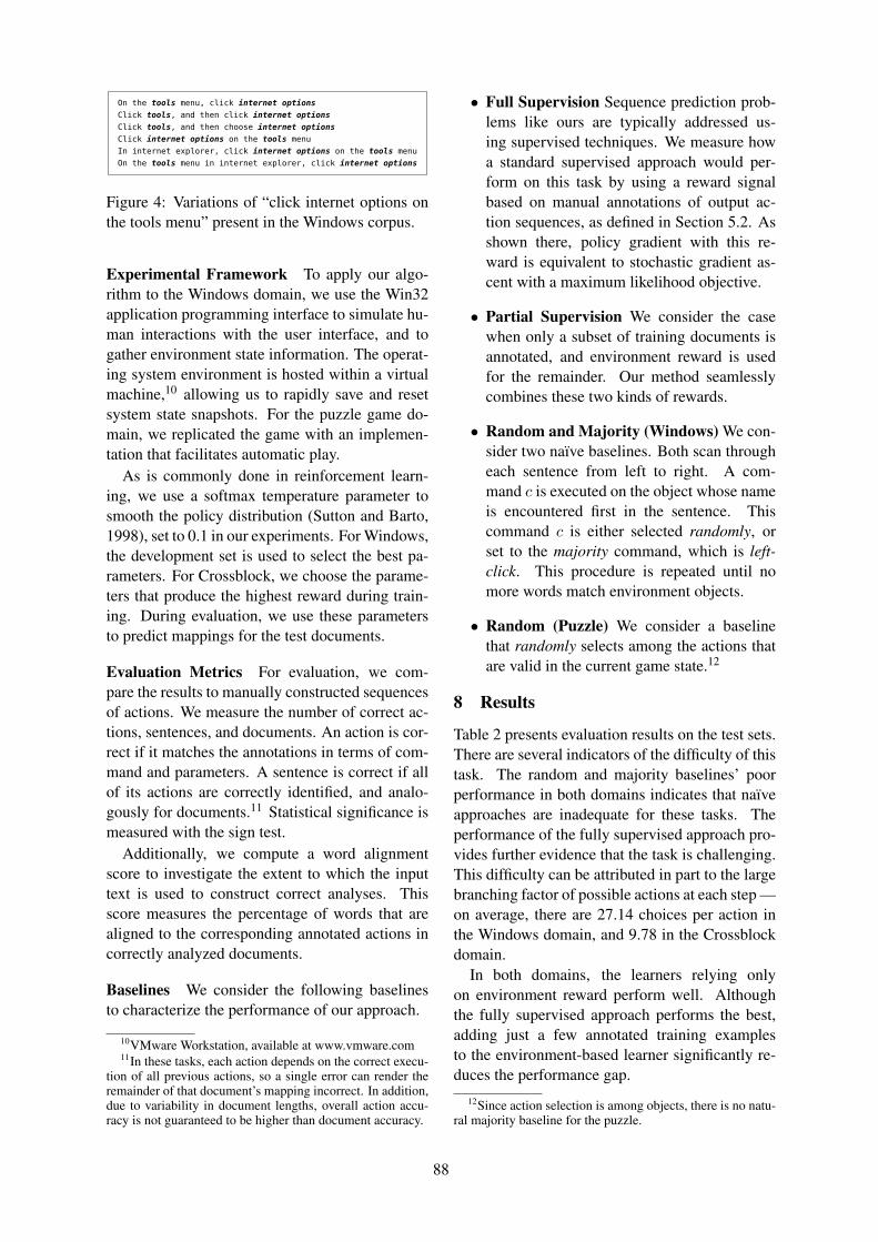
Figure 4: Variations of “click internet options onthe tools menu” present in the Windows corpus.
Experimental Framework To apply our algo-rithm to the Windows domain, we use the Win32application programming interface to simulate hu-man interactions with the user interface, and togather environment state information. The operat-ing system environment is hosted within a virtualmachine,10 allowing us to rapidly save and resetsystem state snapshots. For the puzzle game do-main, we replicated the game with an implemen-tation that facilitates automatic play.
As is commonly done in reinforcement learn-ing, we use a softmax temperature parameter tosmooth the policy distribution (Sutton and Barto,1998), set to 0.1 in our experiments. For Windows,the development set is used to select the best pa-rameters. For Crossblock, we choose the parame-ters that produce the highest reward during train-ing. During evaluation, we use these parametersto predict mappings for the test documents.
Evaluation Metrics For evaluation, we com-pare the results to manually constructed sequencesof actions. We measure the number of correct ac-tions, sentences, and documents. An action is cor-rect if it matches the annotations in terms of com-mand and parameters. A sentence is correct if allof its actions are correctly identified, and analo-gously for documents.11 Statistical significance ismeasured with the sign test.
Additionally, we compute a word alignmentscore to investigate the extent to which the inputtext is used to construct correct analyses. Thisscore measures the percentage of words that arealigned to the corresponding annotated actions incorrectly analyzed documents.
Baselines We consider the following baselinesto characterize the performance of our approach.
10VMware Workstation, available at www.vmware.com11In these tasks, each action depends on the correct execu-
tion of all previous actions, so a single error can render theremainder of that document’s mapping incorrect. In addition,due to variability in document lengths, overall action accu-racy is not guaranteed to be higher than document accuracy.
• Full Supervision Sequence prediction prob-lems like ours are typically addressed us-ing supervised techniques. We measure howa standard supervised approach would per-form on this task by using a reward signalbased on manual annotations of output ac-tion sequences, as defined in Section 5.2. Asshown there, policy gradient with this re-ward is equivalent to stochastic gradient as-cent with a maximum likelihood objective.
• Partial Supervision We consider the casewhen only a subset of training documents isannotated, and environment reward is usedfor the remainder. Our method seamlesslycombines these two kinds of rewards.
• Random and Majority (Windows) We con-sider two naı̈ve baselines. Both scan througheach sentence from left to right. A com-mand c is executed on the object whose nameis encountered first in the sentence. Thiscommand c is either selected randomly, orset to the majority command, which is left-click. This procedure is repeated until nomore words match environment objects.
• Random (Puzzle) We consider a baselinethat randomly selects among the actions thatare valid in the current game state.12
8 Results
Table 2 presents evaluation results on the test sets.There are several indicators of the difficulty of thistask. The random and majority baselines’ poorperformance in both domains indicates that naı̈veapproaches are inadequate for these tasks. Theperformance of the fully supervised approach pro-vides further evidence that the task is challenging.This difficulty can be attributed in part to the largebranching factor of possible actions at each step —on average, there are 27.14 choices per action inthe Windows domain, and 9.78 in the Crossblockdomain.
In both domains, the learners relying onlyon environment reward perform well. Althoughthe fully supervised approach performs the best,adding just a few annotated training examplesto the environment-based learner significantly re-duces the performance gap.
12Since action selection is among objects, there is no natu-ral majority baseline for the puzzle.
88

Windows PuzzleAction Sent. Doc. Word Action Doc. Word
Random baseline 0.128 0.101 0.000 —– 0.081 0.111 —–Majority baseline 0.287 0.197 0.100 —– —– —– —–Environment reward ∗ 0.647 ∗ 0.590 ∗ 0.375 0.819 ∗ 0.428 ∗ 0.453 0.686Partial supervision � 0.723 ∗ 0.702 0.475 0.989 0.575 ∗ 0.523 0.850Full supervision � 0.756 0.714 0.525 0.991 0.632 0.630 0.869
Table 2: Performance on the test set with different reward signals and baselines. Our evaluation measuresthe proportion of correct actions, sentences, and documents. We also report the percentage of correctword alignments for the successfully completed documents. Note the puzzle domain has only single-sentence documents, so its sentence and document scores are identical. The partial supervision linerefers to 20 out of 70 annotated training documents for Windows, and 10 out of 40 for the puzzle. Eachresult marked with ∗ or � is a statistically significant improvement over the result immediately above it;∗ indicates p < 0.01 and � indicates p < 0.05.
Figure 5: Comparison of two training scenarios where training is done using a subset of annotateddocuments, with and without environment reward for the remaining unannotated documents.
Figure 5 shows the overall tradeoff between an-notation effort and system performance for the twodomains. The ability to make this tradeoff is oneof the advantages of our approach. The figure alsoshows that augmenting annotated documents withadditional environment-reward documents invari-ably improves performance.
The word alignment results from Table 2 in-dicate that the learners are mapping the correctwords to actions for documents that are success-fully completed. For example, the models that per-form best in the Windows domain achieve nearlyperfect word alignment scores.
To further assess the contribution of the instruc-tion text, we train a variant of our model withoutaccess to text features. This is possible in the gamedomain, where all of the puzzles share a singlegoal state that is independent of the instructions.This variant solves 34% of the puzzles, suggest-ing that access to the instructions significantly im-proves performance.
9 Conclusions
In this paper, we presented a reinforcement learn-ing approach for inducing a mapping between in-structions and actions. This approach is able to useenvironment-based rewards, such as task comple-tion, to learn to analyze text. We showed that hav-ing access to a suitable reward function can signif-icantly reduce the need for annotations.
Acknowledgments
The authors acknowledge the support of the NSF(CAREER grant IIS-0448168, grant IIS-0835445,grant IIS-0835652, and a Graduate Research Fel-lowship) and the ONR. Thanks to Michael Collins,Amir Globerson, Tommi Jaakkola, Leslie PackKaelbling, Dina Katabi, Martin Rinard, and mem-bers of the MIT NLP group for their suggestionsand comments. Any opinions, findings, conclu-sions, or recommendations expressed in this paperare those of the authors, and do not necessarily re-flect the views of the funding organizations.
89

ReferencesKobus Barnard and David A. Forsyth. 2001. Learning
the semantics of words and pictures. In Proceedingsof ICCV.
David L. Chen and Raymond J. Mooney. 2008. Learn-ing to sportscast: a test of grounded language acqui-sition. In Proceedings of ICML.
Stephen Della Pietra, Vincent J. Della Pietra, andJohn D. Lafferty. 1997. Inducing features of ran-dom fields. IEEE Trans. Pattern Anal. Mach. Intell.,19(4):380–393.
Barbara Di Eugenio. 1992. Understanding natural lan-guage instructions: the case of purpose clauses. InProceedings of ACL.
Michael Fleischman and Deb Roy. 2005. Intentionalcontext in situated language learning. In Proceed-ings of CoNLL.
John Lafferty, Andrew McCallum, and FernandoPereira. 2001. Conditional random fields: Prob-abilistic models for segmenting and labeling se-quence data. In Proceedings of ICML.
Diane J. Litman, Michael S. Kearns, Satinder Singh,and Marilyn A. Walker. 2000. Automatic optimiza-tion of dialogue management. In Proceedings ofCOLING.
Raymond J. Mooney. 2008a. Learning languagefrom its perceptual context. In Proceedings ofECML/PKDD.
Raymond J. Mooney. 2008b. Learning to connect lan-guage and perception. In Proceedings of AAAI.
Andrew Y. Ng, H. Jin Kim, Michael I. Jordan, andShankar Sastry. 2003. Autonomous helicopter flightvia reinforcement learning. In Advances in NIPS.
James Timothy Oates. 2001. Grounding knowledgein sensors: Unsupervised learning for language andplanning. Ph.D. thesis, University of MassachusettsAmherst.
Deb K. Roy and Alex P. Pentland. 2002. Learn-ing words from sights and sounds: a computationalmodel. Cognitive Science 26, pages 113–146.
Nicholas Roy, Joelle Pineau, and Sebastian Thrun.2000. Spoken dialogue management using proba-bilistic reasoning. In Proceedings of ACL.
Konrad Scheffler and Steve Young. 2002. Automaticlearning of dialogue strategy using dialogue simula-tion and reinforcement learning. In Proceedings ofHLT.
Satinder P. Singh, Michael J. Kearns, Diane J. Litman,and Marilyn A. Walker. 1999. Reinforcement learn-ing for spoken dialogue systems. In Advances inNIPS.
Jeffrey Mark Siskind. 2001. Grounding the lexical se-mantics of verbs in visual perception using force dy-namics and event logic. J. Artif. Intell. Res. (JAIR),15:31–90.
Richard S. Sutton and Andrew G. Barto. 1998. Re-inforcement Learning: An Introduction. The MITPress.
Richard S. Sutton, David McAllester, Satinder Singh,and Yishay Mansour. 2000. Policy gradient meth-ods for reinforcement learning with function approx-imation. In Advances in NIPS.
Terry Winograd. 1972. Understanding Natural Lan-guage. Academic Press.
Chen Yu and Dana H. Ballard. 2004. On the integra-tion of grounding language and learning objects. InProceedings of AAAI.
90

Proceedings of the 47th Annual Meeting of the ACL and the 4th IJCNLP of the AFNLP, pages 91–99,Suntec, Singapore, 2-7 August 2009. c©2009 ACL and AFNLP
Learning Semantic Correspondences with Less Supervision
Percy LiangUC Berkeley
Michael I. JordanUC Berkeley
Dan KleinUC Berkeley
Abstract
A central problem in grounded language acqui-sition is learning the correspondences between arich world state and a stream of text which refer-ences that world state. To deal with the high de-gree of ambiguity present in this setting, we presenta generative model that simultaneously segmentsthe text into utterances and maps each utteranceto a meaning representation grounded in the worldstate. We show that our model generalizes acrossthree domains of increasing difficulty—Robocupsportscasting, weather forecasts (a new domain),and NFL recaps.
1 Introduction
Recent work in learning semantics has focusedon mapping sentences to meaning representa-tions (e.g., some logical form) given aligned sen-tence/meaning pairs as training data (Ge andMooney, 2005; Zettlemoyer and Collins, 2005;Zettlemoyer and Collins, 2007; Lu et al., 2008).However, this degree of supervision is unrealisticfor modeling human language acquisition and canbe costly to obtain for building large-scale, broad-coverage language understanding systems.
A more flexible direction is grounded languageacquisition: learning the meaning of sentencesin the context of an observed world state. Thegrounded approach has gained interest in variousdisciplines (Siskind, 1996; Yu and Ballard, 2004;Feldman and Narayanan, 2004; Gorniak and Roy,2007). Some recent work in the NLP commu-nity has also moved in this direction by relaxingthe amount of supervision to the setting whereeach sentence is paired with a small set of can-didate meanings (Kate and Mooney, 2007; Chenand Mooney, 2008).
The goal of this paper is to reduce the amountof supervision even further. We assume that we aregiven a world state represented by a set of recordsalong with a text, an unsegmented sequence ofwords. For example, in the weather forecast do-main (Section 2.2), the text is the weather report,
and the records provide a structured representationof the temperature, sky conditions, etc.
In this less restricted data setting, we must re-solve multiple ambiguities: (1) the segmentationof the text into utterances; (2) the identification ofrelevant facts, i.e., the choice of records and as-pects of those records; and (3) the alignment of ut-terances to facts (facts are the meaning represen-tations of the utterances). Furthermore, in someof our examples, much of the world state is notreferenced at all in the text, and, conversely, thetext references things which are not represented inour world state. This increased amount of ambigu-ity and noise presents serious challenges for learn-ing. To cope with these challenges, we propose aprobabilistic generative model that treats text seg-mentation, fact identification, and alignment in asingle unified framework. The parameters of thishierarchical hidden semi-Markov model can be es-timated efficiently using EM.
We tested our model on the task of aligningtext to records in three different domains. Thefirst domain is Robocup sportscasting (Chen andMooney, 2008). Their best approach (KRISPER)obtains 67% F1; our method achieves 76.5%. Thisdomain is simplified in that the segmentation isknown. The second domain is weather forecasts,for which we created a new dataset. Here, thefull complexity of joint segmentation and align-ment arises. Nonetheless, we were able to obtainreasonable results on this task. The third domainwe considered is NFL recaps (Barzilay and Lap-ata, 2005; Snyder and Barzilay, 2007). The lan-guage used in this domain is richer by orders ofmagnitude, and much of it does not reference theworld state. Nonetheless, taking the first unsuper-vised approach to this problem, we were able tomake substantial progress: We achieve an F1 of53.2%, which closes over half of the gap betweena heuristic baseline (26%) and supervised systems(68%–80%).
91
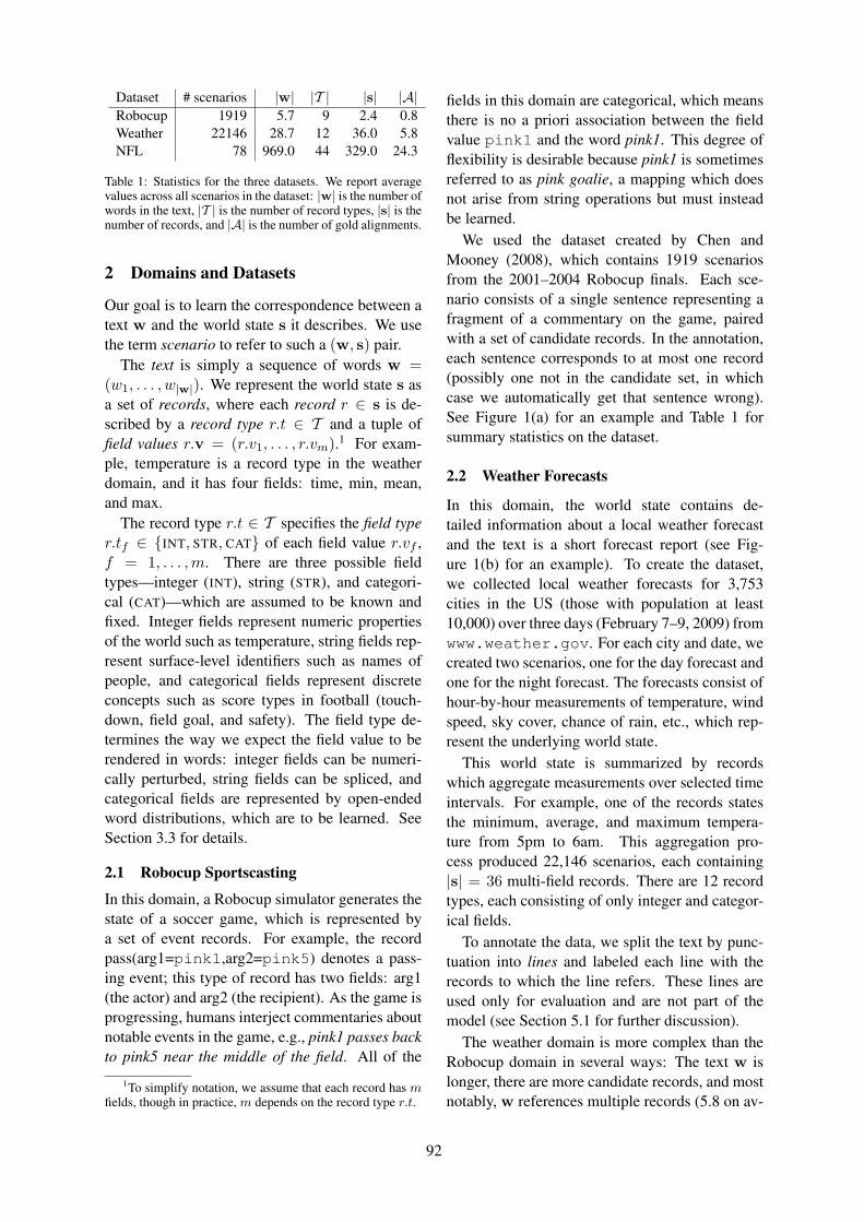
Dataset # scenarios |w| |T | |s| |A|Robocup 1919 5.7 9 2.4 0.8Weather 22146 28.7 12 36.0 5.8NFL 78 969.0 44 329.0 24.3
Table 1: Statistics for the three datasets. We report averagevalues across all scenarios in the dataset: |w| is the number ofwords in the text, |T | is the number of record types, |s| is thenumber of records, and |A| is the number of gold alignments.
2 Domains and Datasets
Our goal is to learn the correspondence between atext w and the world state s it describes. We usethe term scenario to refer to such a (w, s) pair.
The text is simply a sequence of words w =(w1, . . . , w|w|). We represent the world state s asa set of records, where each record r ∈ s is de-scribed by a record type r.t ∈ T and a tuple offield values r.v = (r.v1, . . . , r.vm).1 For exam-ple, temperature is a record type in the weatherdomain, and it has four fields: time, min, mean,and max.
The record type r.t ∈ T specifies the field typer.tf ∈ {INT, STR, CAT} of each field value r.vf ,f = 1, . . . ,m. There are three possible fieldtypes—integer (INT), string (STR), and categori-cal (CAT)—which are assumed to be known andfixed. Integer fields represent numeric propertiesof the world such as temperature, string fields rep-resent surface-level identifiers such as names ofpeople, and categorical fields represent discreteconcepts such as score types in football (touch-down, field goal, and safety). The field type de-termines the way we expect the field value to berendered in words: integer fields can be numeri-cally perturbed, string fields can be spliced, andcategorical fields are represented by open-endedword distributions, which are to be learned. SeeSection 3.3 for details.
2.1 Robocup Sportscasting
In this domain, a Robocup simulator generates thestate of a soccer game, which is represented bya set of event records. For example, the recordpass(arg1=pink1,arg2=pink5) denotes a pass-ing event; this type of record has two fields: arg1(the actor) and arg2 (the recipient). As the game isprogressing, humans interject commentaries aboutnotable events in the game, e.g., pink1 passes backto pink5 near the middle of the field. All of the
1To simplify notation, we assume that each record has mfields, though in practice, m depends on the record type r.t.
fields in this domain are categorical, which meansthere is no a priori association between the fieldvalue pink1 and the word pink1. This degree offlexibility is desirable because pink1 is sometimesreferred to as pink goalie, a mapping which doesnot arise from string operations but must insteadbe learned.
We used the dataset created by Chen andMooney (2008), which contains 1919 scenariosfrom the 2001–2004 Robocup finals. Each sce-nario consists of a single sentence representing afragment of a commentary on the game, pairedwith a set of candidate records. In the annotation,each sentence corresponds to at most one record(possibly one not in the candidate set, in whichcase we automatically get that sentence wrong).See Figure 1(a) for an example and Table 1 forsummary statistics on the dataset.
2.2 Weather Forecasts
In this domain, the world state contains de-tailed information about a local weather forecastand the text is a short forecast report (see Fig-ure 1(b) for an example). To create the dataset,we collected local weather forecasts for 3,753cities in the US (those with population at least10,000) over three days (February 7–9, 2009) fromwww.weather.gov. For each city and date, wecreated two scenarios, one for the day forecast andone for the night forecast. The forecasts consist ofhour-by-hour measurements of temperature, windspeed, sky cover, chance of rain, etc., which rep-resent the underlying world state.
This world state is summarized by recordswhich aggregate measurements over selected timeintervals. For example, one of the records statesthe minimum, average, and maximum tempera-ture from 5pm to 6am. This aggregation pro-cess produced 22,146 scenarios, each containing|s| = 36 multi-field records. There are 12 recordtypes, each consisting of only integer and categor-ical fields.
To annotate the data, we split the text by punc-tuation into lines and labeled each line with therecords to which the line refers. These lines areused only for evaluation and are not part of themodel (see Section 5.1 for further discussion).
The weather domain is more complex than theRobocup domain in several ways: The text w islonger, there are more candidate records, and mostnotably, w references multiple records (5.8 on av-
92
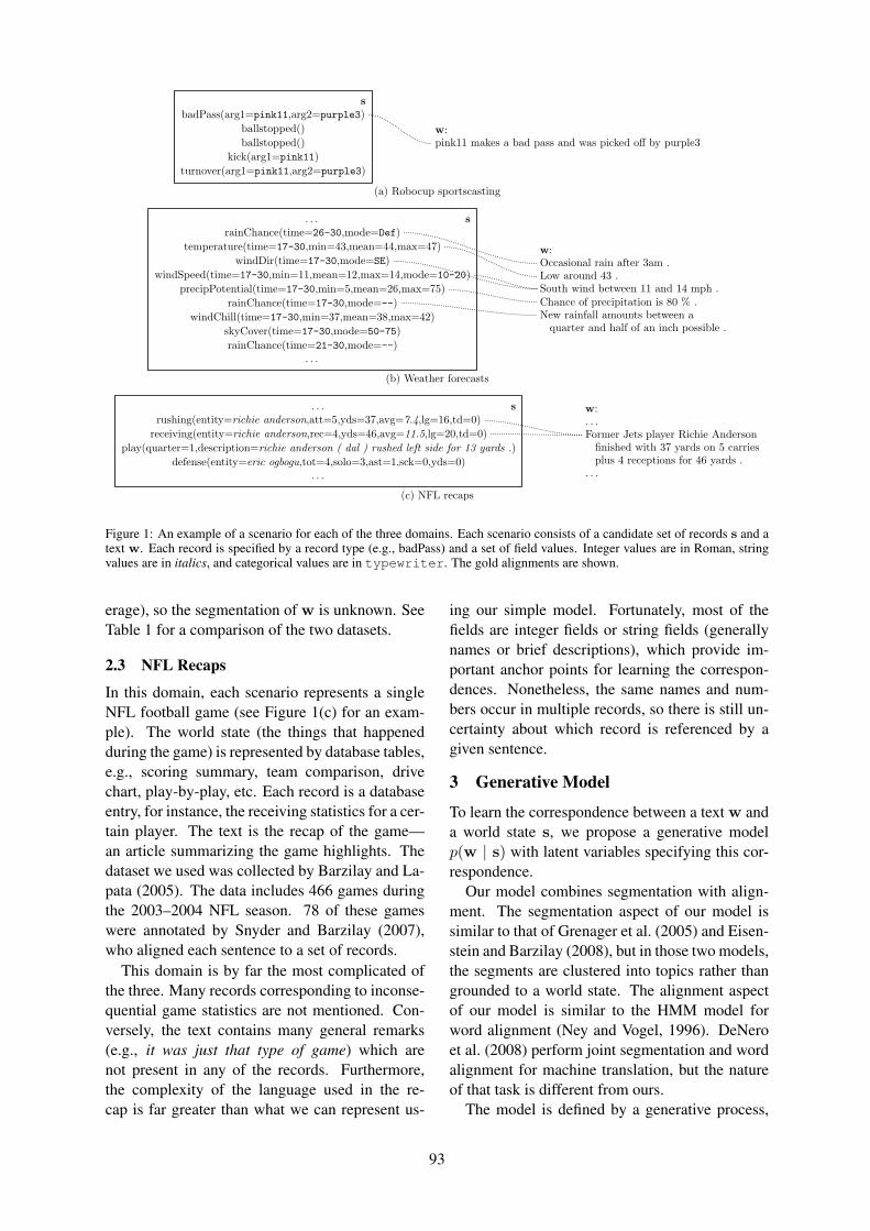
xbadPass(arg1=pink11,arg2=purple3)
ballstopped()ballstopped()
kick(arg1=pink11)turnover(arg1=pink11,arg2=purple3)
s
w:pink11 makes a bad pass and was picked off by purple3
(a) Robocup sportscasting
. . .rainChance(time=26-30,mode=Def)
temperature(time=17-30,min=43,mean=44,max=47)windDir(time=17-30,mode=SE)
windSpeed(time=17-30,min=11,mean=12,max=14,mode=10-20)precipPotential(time=17-30,min=5,mean=26,max=75)
rainChance(time=17-30,mode=--)windChill(time=17-30,min=37,mean=38,max=42)
skyCover(time=17-30,mode=50-75)rainChance(time=21-30,mode=--)
. . .
s
w:Occasional rain after 3am .Low around 43 .South wind between 11 and 14 mph .Chance of precipitation is 80 % .New rainfall amounts between a
quarter and half of an inch possible .
(b) Weather forecasts
. . .rushing(entity=richie anderson,att=5,yds=37,avg=7.4,lg=16,td=0)
receiving(entity=richie anderson,rec=4,yds=46,avg=11.5,lg=20,td=0)play(quarter=1,description=richie anderson ( dal ) rushed left side for 13 yards .)
defense(entity=eric ogbogu,tot=4,solo=3,ast=1,sck=0,yds=0). . .
s w:. . .Former Jets player Richie Anderson
finished with 37 yards on 5 carriesplus 4 receptions for 46 yards .
. . .
(c) NFL recaps
Figure 1: An example of a scenario for each of the three domains. Each scenario consists of a candidate set of records s and atext w. Each record is specified by a record type (e.g., badPass) and a set of field values. Integer values are in Roman, stringvalues are in italics, and categorical values are in typewriter. The gold alignments are shown.
erage), so the segmentation of w is unknown. SeeTable 1 for a comparison of the two datasets.
2.3 NFL Recaps
In this domain, each scenario represents a singleNFL football game (see Figure 1(c) for an exam-ple). The world state (the things that happenedduring the game) is represented by database tables,e.g., scoring summary, team comparison, drivechart, play-by-play, etc. Each record is a databaseentry, for instance, the receiving statistics for a cer-tain player. The text is the recap of the game—an article summarizing the game highlights. Thedataset we used was collected by Barzilay and La-pata (2005). The data includes 466 games duringthe 2003–2004 NFL season. 78 of these gameswere annotated by Snyder and Barzilay (2007),who aligned each sentence to a set of records.
This domain is by far the most complicated ofthe three. Many records corresponding to inconse-quential game statistics are not mentioned. Con-versely, the text contains many general remarks(e.g., it was just that type of game) which arenot present in any of the records. Furthermore,the complexity of the language used in the re-cap is far greater than what we can represent us-
ing our simple model. Fortunately, most of thefields are integer fields or string fields (generallynames or brief descriptions), which provide im-portant anchor points for learning the correspon-dences. Nonetheless, the same names and num-bers occur in multiple records, so there is still un-certainty about which record is referenced by agiven sentence.
3 Generative Model
To learn the correspondence between a text w anda world state s, we propose a generative modelp(w | s) with latent variables specifying this cor-respondence.
Our model combines segmentation with align-ment. The segmentation aspect of our model issimilar to that of Grenager et al. (2005) and Eisen-stein and Barzilay (2008), but in those two models,the segments are clustered into topics rather thangrounded to a world state. The alignment aspectof our model is similar to the HMM model forword alignment (Ney and Vogel, 1996). DeNeroet al. (2008) perform joint segmentation and wordalignment for machine translation, but the natureof that task is different from ours.
The model is defined by a generative process,
93
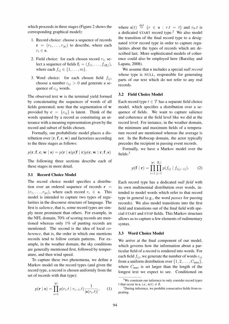
which proceeds in three stages (Figure 2 shows thecorresponding graphical model):
1. Record choice: choose a sequence of recordsr = (r1, . . . , r|r|) to describe, where eachri ∈ s.
2. Field choice: for each chosen record ri, se-lect a sequence of fields fi = (fi1, . . . , fi|fi|),where each fij ∈ {1, . . . ,m}.
3. Word choice: for each chosen field fij ,choose a number cij > 0 and generate a se-quence of cij words.
The observed text w is the terminal yield formedby concatenating the sequences of words of allfields generated; note that the segmentation of wprovided by c = {cij} is latent. Think of thewords spanned by a record as constituting an ut-terance with a meaning representation given by therecord and subset of fields chosen.
Formally, our probabilistic model places a dis-tribution over (r, f , c,w) and factorizes accordingto the three stages as follows:
p(r, f , c,w | s) = p(r | s)p(f | r)p(c,w | r, f , s)
The following three sections describe each ofthese stages in more detail.
3.1 Record Choice ModelThe record choice model specifies a distribu-tion over an ordered sequence of records r =(r1, . . . , r|r|), where each record ri ∈ s. Thismodel is intended to capture two types of regu-larities in the discourse structure of language. Thefirst is salience, that is, some record types are sim-ply more prominent than others. For example, inthe NFL domain, 70% of scoring records are men-tioned whereas only 1% of punting records arementioned. The second is the idea of local co-herence, that is, the order in which one mentionsrecords tend to follow certain patterns. For ex-ample, in the weather domain, the sky conditionsare generally mentioned first, followed by temper-ature, and then wind speed.
To capture these two phenomena, we define aMarkov model on the record types (and given therecord type, a record is chosen uniformly from theset of records with that type):
p(r | s) =
|r|∏
i=1
p(ri.t | ri−1.t)1
|s(ri.t)|, (1)
where s(t) def= {r ∈ s : r.t = t} and r0.t is
a dedicated START record type.2 We also modelthe transition of the final record type to a desig-nated STOP record type in order to capture regu-larities about the types of records which are de-scribed last. More sophisticated models of coher-ence could also be employed here (Barzilay andLapata, 2008).
We assume that s includes a special null recordwhose type is NULL, responsible for generatingparts of our text which do not refer to any realrecords.
3.2 Field Choice Model
Each record type t ∈ T has a separate field choicemodel, which specifies a distribution over a se-quence of fields. We want to capture salienceand coherence at the field level like we did at therecord level. For instance, in the weather domain,the minimum and maximum fields of a tempera-ture record are mentioned whereas the average isnot. In the Robocup domain, the actor typicallyprecedes the recipient in passing event records.
Formally, we have a Markov model over thefields:3
p(f | r) =
|r|∏
i=1
|fj |∏
j=1
p(fij | fi(j−1)). (2)
Each record type has a dedicated null field withits own multinomial distribution over words, in-tended to model words which refer to that recordtype in general (e.g., the word passes for passingrecords). We also model transitions into the firstfield and transitions out of the final field with spe-cial START and STOP fields. This Markov structureallows us to capture a few elements of rudimentarysyntax.
3.3 Word Choice Model
We arrive at the final component of our model,which governs how the information about a par-ticular field of a record is rendered into words. Foreach field fij , we generate the number of words cijfrom a uniform distribution over {1, 2, . . . , Cmax},where Cmax is set larger than the length of thelongest text we expect to see. Conditioned on
2We constrain our inference to only consider record typest that occur in s, i.e., s(t) 6= ∅.
3During inference, we prohibit consecutive fields from re-peating.
94
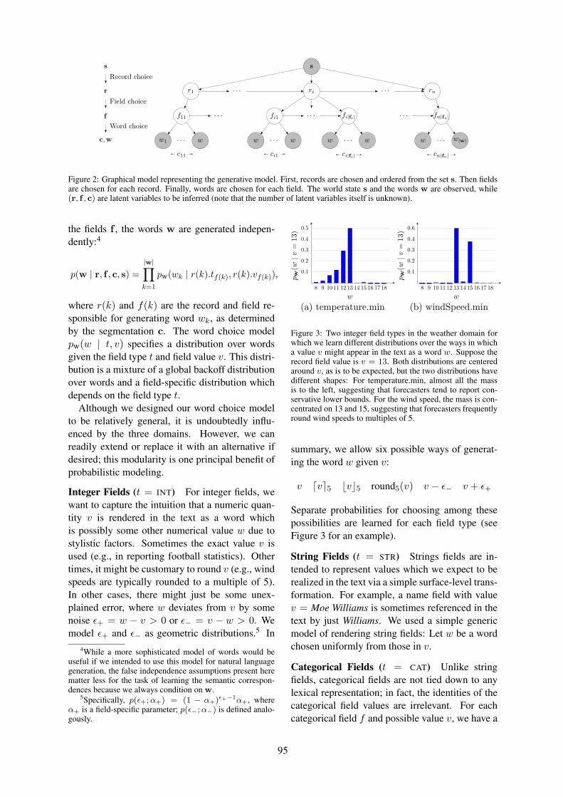
s
r
f
c,w
s
r1
f11
w1 · · · w
c11
· · ·
· · · ri
fi1
w · · · w
ci1
· · · fi|fi|
w · · · w
ci|fi|
· · · rn
· · · fn|fn|
w · · · w|w|
cn|fn|
Record choice
Field choice
Word choice
Figure 2: Graphical model representing the generative model. First, records are chosen and ordered from the set s. Then fieldsare chosen for each record. Finally, words are chosen for each field. The world state s and the words w are observed, while(r, f , c) are latent variables to be inferred (note that the number of latent variables itself is unknown).
the fields f , the words w are generated indepen-dently:4
p(w | r, f , c, s) =
|w|∏
k=1
pw(wk | r(k).tf(k), r(k).vf(k)),
where r(k) and f(k) are the record and field re-sponsible for generating word wk, as determinedby the segmentation c. The word choice modelpw(w | t, v) specifies a distribution over wordsgiven the field type t and field value v. This distri-bution is a mixture of a global backoff distributionover words and a field-specific distribution whichdepends on the field type t.
Although we designed our word choice modelto be relatively general, it is undoubtedly influ-enced by the three domains. However, we canreadily extend or replace it with an alternative ifdesired; this modularity is one principal benefit ofprobabilistic modeling.
Integer Fields (t = INT) For integer fields, wewant to capture the intuition that a numeric quan-tity v is rendered in the text as a word whichis possibly some other numerical value w due tostylistic factors. Sometimes the exact value v isused (e.g., in reporting football statistics). Othertimes, it might be customary to round v (e.g., windspeeds are typically rounded to a multiple of 5).In other cases, there might just be some unex-plained error, where w deviates from v by somenoise ε+ = w − v > 0 or ε− = v − w > 0. Wemodel ε+ and ε− as geometric distributions.5 In
4While a more sophisticated model of words would beuseful if we intended to use this model for natural languagegeneration, the false independence assumptions present herematter less for the task of learning the semantic correspon-dences because we always condition on w.
5Specifically, p(ε+;α+) = (1 − α+)ε+−1α+, whereα+ is a field-specific parameter; p(ε−;α−) is defined analo-gously.
8 9 10 11 12 13 14 15 16 17 18
w
0.1
0.2
0.3
0.4
0.5
pw
(w|v
=13
)8 9 10 11 12 13 14 15 16 17 18
w
0.1
0.2
0.3
0.4
0.6
pw
(w|v
=13
)
(a) temperature.min (b) windSpeed.min
Figure 3: Two integer field types in the weather domain forwhich we learn different distributions over the ways in whicha value v might appear in the text as a word w. Suppose therecord field value is v = 13. Both distributions are centeredaround v, as is to be expected, but the two distributions havedifferent shapes: For temperature.min, almost all the massis to the left, suggesting that forecasters tend to report con-servative lower bounds. For the wind speed, the mass is con-centrated on 13 and 15, suggesting that forecasters frequentlyround wind speeds to multiples of 5.
summary, we allow six possible ways of generat-ing the word w given v:
v dve5 bvc5 round5(v) v − ε− v + ε+
Separate probabilities for choosing among thesepossibilities are learned for each field type (seeFigure 3 for an example).
String Fields (t = STR) Strings fields are in-tended to represent values which we expect to berealized in the text via a simple surface-level trans-formation. For example, a name field with valuev = Moe Williams is sometimes referenced in thetext by just Williams. We used a simple genericmodel of rendering string fields: Let w be a wordchosen uniformly from those in v.
Categorical Fields (t = CAT) Unlike stringfields, categorical fields are not tied down to anylexical representation; in fact, the identities of thecategorical field values are irrelevant. For eachcategorical field f and possible value v, we have a
95
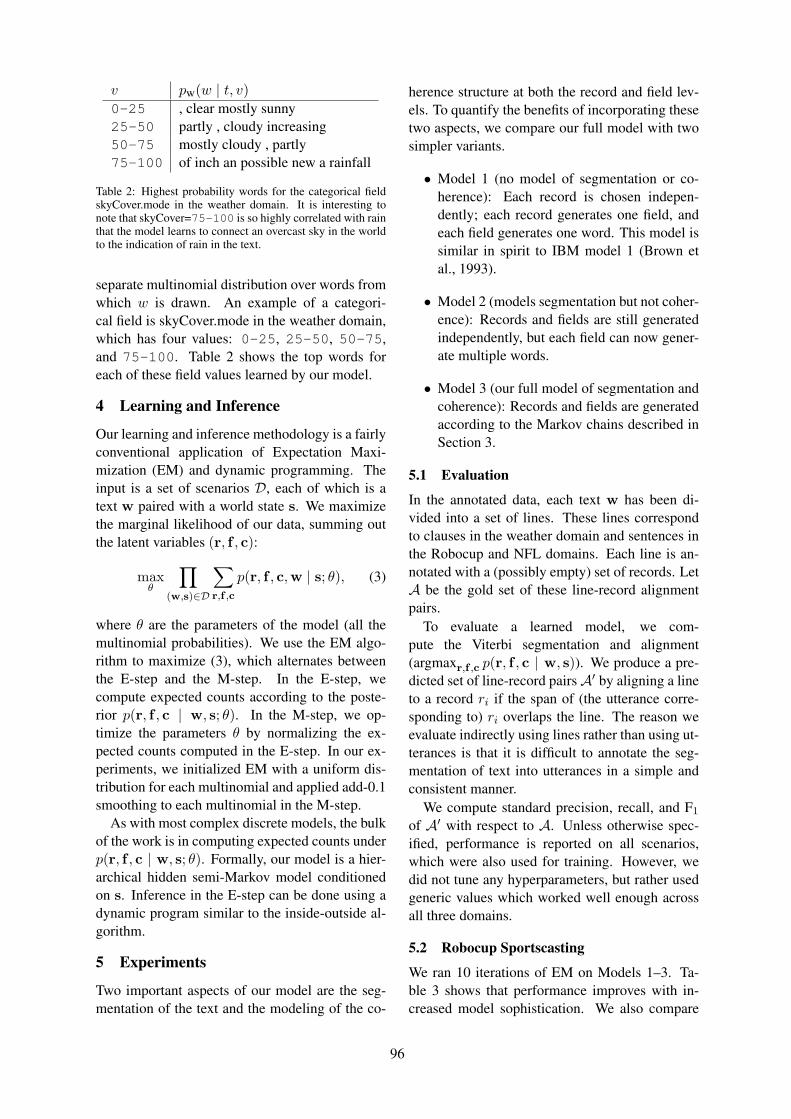
v pw(w | t, v)0-25 , clear mostly sunny25-50 partly , cloudy increasing50-75 mostly cloudy , partly75-100 of inch an possible new a rainfall
Table 2: Highest probability words for the categorical fieldskyCover.mode in the weather domain. It is interesting tonote that skyCover=75-100 is so highly correlated with rainthat the model learns to connect an overcast sky in the worldto the indication of rain in the text.
separate multinomial distribution over words fromwhich w is drawn. An example of a categori-cal field is skyCover.mode in the weather domain,which has four values: 0-25, 25-50, 50-75,and 75-100. Table 2 shows the top words foreach of these field values learned by our model.
4 Learning and Inference
Our learning and inference methodology is a fairlyconventional application of Expectation Maxi-mization (EM) and dynamic programming. Theinput is a set of scenarios D, each of which is atext w paired with a world state s. We maximizethe marginal likelihood of our data, summing outthe latent variables (r, f , c):
maxθ
∏
(w,s)∈D
∑
r,f ,c
p(r, f , c,w | s; θ), (3)
where θ are the parameters of the model (all themultinomial probabilities). We use the EM algo-rithm to maximize (3), which alternates betweenthe E-step and the M-step. In the E-step, wecompute expected counts according to the poste-rior p(r, f , c | w, s; θ). In the M-step, we op-timize the parameters θ by normalizing the ex-pected counts computed in the E-step. In our ex-periments, we initialized EM with a uniform dis-tribution for each multinomial and applied add-0.1smoothing to each multinomial in the M-step.
As with most complex discrete models, the bulkof the work is in computing expected counts underp(r, f , c | w, s; θ). Formally, our model is a hier-archical hidden semi-Markov model conditionedon s. Inference in the E-step can be done using adynamic program similar to the inside-outside al-gorithm.
5 Experiments
Two important aspects of our model are the seg-mentation of the text and the modeling of the co-
herence structure at both the record and field lev-els. To quantify the benefits of incorporating thesetwo aspects, we compare our full model with twosimpler variants.
• Model 1 (no model of segmentation or co-herence): Each record is chosen indepen-dently; each record generates one field, andeach field generates one word. This model issimilar in spirit to IBM model 1 (Brown etal., 1993).
• Model 2 (models segmentation but not coher-ence): Records and fields are still generatedindependently, but each field can now gener-ate multiple words.
• Model 3 (our full model of segmentation andcoherence): Records and fields are generatedaccording to the Markov chains described inSection 3.
5.1 Evaluation
In the annotated data, each text w has been di-vided into a set of lines. These lines correspondto clauses in the weather domain and sentences inthe Robocup and NFL domains. Each line is an-notated with a (possibly empty) set of records. LetA be the gold set of these line-record alignmentpairs.
To evaluate a learned model, we com-pute the Viterbi segmentation and alignment(argmaxr,f ,c p(r, f , c | w, s)). We produce a pre-dicted set of line-record pairsA′ by aligning a lineto a record ri if the span of (the utterance corre-sponding to) ri overlaps the line. The reason weevaluate indirectly using lines rather than using ut-terances is that it is difficult to annotate the seg-mentation of text into utterances in a simple andconsistent manner.
We compute standard precision, recall, and F1
of A′ with respect to A. Unless otherwise spec-ified, performance is reported on all scenarios,which were also used for training. However, wedid not tune any hyperparameters, but rather usedgeneric values which worked well enough acrossall three domains.
5.2 Robocup Sportscasting
We ran 10 iterations of EM on Models 1–3. Ta-ble 3 shows that performance improves with in-creased model sophistication. We also compare
96

Method Precision Recall F1
Model 1 78.6 61.9 69.3Model 2 74.1 84.1 78.8Model 3 77.3 84.0 80.5
Table 3: Alignment results on the Robocup sportscastingdataset.
Method F1
Random baseline 48.0Chen and Mooney (2008) 67.0Model 3 75.7
Table 4: F1 scores based on the 4-fold cross-validationscheme in Chen and Mooney (2008).
our model to the results of Chen and Mooney(2008) in Table 4.
Figure 4 provides a closer look at the predic-tions made by each of our three models for a par-ticular example. Model 1 easily mistakes pink10for the recipient of a pass record because decisionsare made independently for each word. Model 2chooses the correct record, but having no modelof the field structure inside a record, it proposesan incorrect field segmentation (although our eval-uation is insensitive to this). Equipped with theability to prefer a coherent field sequence, Model3 fixes these errors.
Many of the remaining errors are due to thegarbage collection phenomenon familiar fromword alignment models (Moore, 2004; Liang etal., 2006). For example, the ballstopped recordoccurs frequently but is never mentioned in thetext. At the same time, there is a correlation be-tween ballstopped and utterances such as pink2holds onto the ball, which are not aligned to anyrecord in the annotation. As a result, our modelincorrectly chooses to align the two.
5.3 Weather Forecasts
For the weather domain, staged training was nec-essary to get good results. For Model 1, we ran15 iterations of EM. For Model 2, we ran 5 it-erations of EM on Model 1, followed by 10 it-erations on Model 2. For Model 3, we ran 5 it-erations of Model 1, 5 iterations of a simplifiedvariant of Model 3 where records were chosen in-dependently, and finally, 5 iterations of Model 3.When going from one model to another, we usedthe final posterior distributions of the former to ini-
Method Precision Recall F1
Model 1 49.9 75.1 60.0Model 2 67.3 70.4 68.8Model 3 76.3 73.8 75.0
Table 5: Alignment results on the weather forecast dataset.
[Model 1]r:f :w:
passarg2=pink10
pink10 turns the ball over to purple5
[Model 2]r:f :w:
turnoverx
pink10 turns the ball overarg2=purple5
to purple5
[Model 3]r:f :w:
turnoverarg1=pink10
pink10x
turns the ball over toarg2=purple5
purple5
Figure 4: An example of predictions made by each of thethree models on the Robocup dataset.
tialize the parameters of the latter.6 We also pro-hibited utterances in Models 2 and 3 from crossingpunctuation during inference.
Table 5 shows that performance improves sub-stantially in the more sophisticated models, thegains being greater than in the Robocup domain.Figure 5 shows the predictions of the three modelson an example. Model 1 is only able to form iso-lated (but not completely inaccurate) associations.By modeling segmentation, Model 2 accounts forthe intermediate words, but errors are still madedue to the lack of Markov structure. Model 3remedies this. However, unexpected structuresare sometimes learned. For example, the temper-ature.time=6-21 field indicates daytime, whichhappens to be perfectly correlated with the wordhigh, although high intuitively should be associ-ated with the temperature.max field. In these casesof high correlation (Table 2 provides another ex-ample), it is very difficult to recover the properalignment without additional supervision.
5.4 NFL Recaps
In order to scale up our models to the NFL do-main, we first pruned for each sentence the recordswhich have either no numerical values (e.g., 23,23-10, 2/4) nor name-like words (e.g., those thatappear only capitalized in the text) in common.This eliminated all but 1.5% of the record can-didates per sentence, while maintaining an ora-
6It is interesting to note that this type of staged trainingis evocative of language acquisition in children: lexical asso-ciations are formed (Model 1) before higher-level discoursestructure is learned (Model 3).
97

[Model 1]r:f :w: cloudy , with a
windDirtime=6-21high near
temperaturemax=63
63 .
windDirmode=SE
east southeast wind between
windSpeedmin=5
5 and
windSpeedmean=9
11 mph .
[Model 2]r:f :w:
rainChancemode=–cloudy ,
temperaturex
with atime=6-21high near
max=6363 .
windDirmode=SE
east southeast windx
between 5 and
windSpeedmean=911 mph .
[Model 3]r:f :w:
skyCoverx
cloudy ,
temperaturex
with atime=6-21high near
max=6363
mean=56.
windDirmode=SE
east southeastx
wind between
windSpeedmin=5
5max=13and 11
xmph .
Figure 5: An example of predictions made by each of the three models on the weather dataset.
cle alignment F1 score of 88.7. Guessing a singlerandom record for each sentence yields an F1 of12.0. A reasonable heuristic which uses weightednumber- and string-matching achieves 26.7.
Due to the much greater complexity of this do-main, Model 2 was easily misled as it tried with-out success to find a coherent segmentation of thefields. We therefore created a variant, Model 2’,where we constrained each field to generate ex-actly one word. To train Model 2’, we ran 5 it-erations of EM where each sentence is assumedto have exactly one record, followed by 5 itera-tions where the constraint was relaxed to also al-low record boundaries at punctuation and the wordand. We did not experiment with Model 3 sincethe discourse structure on records in this domain isnot at all governed by a simple Markov model onrecord types—indeed, most regions do not refer toany records at all. We also fixed the backoff prob-ability to 0.1 instead of learning it and enforcedzero numerical deviation on integer field values.
Model 2’ achieved an F1 of 39.9, an improve-ment over Model 1, which attained 32.8. Inspec-tion of the errors revealed the following problem:The alignment task requires us to sometimes aligna sentence to multiple redundant records (e.g.,play and score) referenced by the same part of thetext. However, our model generates each part oftext from only one record, and thus it can only al-low an alignment to one record.7 To cope with thisincompatibility between the data and our notion ofsemantics, we used the following solution: We di-vided the records into three groups by type: play,score, and other. Each group has a copy of themodel, but we enforce that they share the samesegmentation. We also introduce a potential thatcouples the presence or absence of records across
7The model can align a sentence to multiple records pro-vided that the records are referenced by non-overlappingparts of the text.
Method Precision Recall F1
Random (with pruning) 13.1 11.0 12.0Baseline 29.2 24.6 26.7Model 1 25.2 46.9 32.8Model 2’ 43.4 37.0 39.9Model 2’ (with groups) 46.5 62.1 53.2Graph matching (sup.) 73.4 64.5 68.6Multilabel global (sup.) 87.3 74.5 80.3
Table 6: Alignment results on the NFL dataset. Graph match-ing and multilabel are supervised results reported in Snyderand Barzilay (2007).9
groups on the same segment to capture regular co-occurrences between redundant records.
Table 6 shows our results. With groups, weachieve an F1 of 53.2. Though we still trail su-pervised techniques, which attain numbers in the68–80 range, we have made substantial progressover our baseline using an unsupervised method.Furthermore, our model provides a more detailedanalysis of the correspondence between the worldstate and text, rather than just producing a singlealignment decision. Most of the remaining errorsmade by our model are due to a lack of calibra-tion. Sometimes, our false positives are close callswhere a sentence indirectly references a record,and our model predicts the alignment whereas theannotation standard does not. We believe that fur-ther progress is possible with a richer model.
6 Conclusion
We have presented a generative model of corre-spondences between a world state and an unseg-mented stream of text. By having a joint modelof salience, coherence, and segmentation, as wellas a detailed rendering of the values in the worldstate into words in the text, we are able to copewith the increased ambiguity that arises in this newdata setting, successfully pushing the limits of un-supervision.
98

ReferencesR. Barzilay and M. Lapata. 2005. Collective content selec-
tion for concept-to-text generation. In Human LanguageTechnology and Empirical Methods in Natural LanguageProcessing (HLT/EMNLP), pages 331–338, Vancouver,B.C.
R. Barzilay and M. Lapata. 2008. Modeling local coher-ence: An entity-based approach. Computational Linguis-tics, 34:1–34.
P. F. Brown, S. A. D. Pietra, V. J. D. Pietra, and R. L. Mer-cer. 1993. The mathematics of statistical machine trans-lation: Parameter estimation. Computational Linguistics,19:263–311.
D. L. Chen and R. J. Mooney. 2008. Learning to sportscast:A test of grounded language acquisition. In InternationalConference on Machine Learning (ICML), pages 128–135. Omnipress.
J. DeNero, A. Bouchard-Côté, and D. Klein. 2008. Samplingalignment structure under a Bayesian translation model.In Empirical Methods in Natural Language Processing(EMNLP), pages 314–323, Honolulu, HI.
J. Eisenstein and R. Barzilay. 2008. Bayesian unsupervisedtopic segmentation. In Empirical Methods in Natural Lan-guage Processing (EMNLP), pages 334–343.
J. Feldman and S. Narayanan. 2004. Embodied meaning in aneural theory of language. Brain and Language, 89:385–392.
R. Ge and R. J. Mooney. 2005. A statistical semantic parserthat integrates syntax and semantics. In ComputationalNatural Language Learning (CoNLL), pages 9–16, AnnArbor, Michigan.
P. Gorniak and D. Roy. 2007. Situated language understand-ing as filtering perceived affordances. Cognitive Science,31:197–231.
T. Grenager, D. Klein, and C. D. Manning. 2005. Unsu-pervised learning of field segmentation models for infor-mation extraction. In Association for Computational Lin-guistics (ACL), pages 371–378, Ann Arbor, Michigan. As-sociation for Computational Linguistics.
R. J. Kate and R. J. Mooney. 2007. Learning language se-mantics from ambiguous supervision. In Association forthe Advancement of Artificial Intelligence (AAAI), pages895–900, Cambridge, MA. MIT Press.
P. Liang, B. Taskar, and D. Klein. 2006. Alignment by agree-ment. In North American Association for ComputationalLinguistics (NAACL), pages 104–111, New York City. As-sociation for Computational Linguistics.
W. Lu, H. T. Ng, W. S. Lee, and L. S. Zettlemoyer. 2008. Agenerative model for parsing natural language to meaningrepresentations. In Empirical Methods in Natural Lan-guage Processing (EMNLP), pages 783–792.
R. C. Moore. 2004. Improving IBM word alignment model1. In Association for Computational Linguistics (ACL),pages 518–525, Barcelona, Spain. Association for Com-putational Linguistics.
H. Ney and S. Vogel. 1996. HMM-based word align-ment in statistical translation. In International Conferenceon Computational Linguistics (COLING), pages 836–841.Association for Computational Linguistics.
J. M. Siskind. 1996. A computational study of cross-situational techniques for learning word-to-meaning map-pings. Cognition, 61:1–38.
B. Snyder and R. Barzilay. 2007. Database-text alignmentvia structured multilabel classification. In InternationalJoint Conference on Artificial Intelligence (IJCAI), pages1713–1718, Hyderabad, India.
C. Yu and D. H. Ballard. 2004. On the integration of ground-ing language and learning objects. In Association for theAdvancement of Artificial Intelligence (AAAI), pages 488–493, Cambridge, MA. MIT Press.
L. S. Zettlemoyer and M. Collins. 2005. Learning to mapsentences to logical form: Structured classification withprobabilistic categorial grammars. In Uncertainty in Arti-ficial Intelligence (UAI), pages 658–666.
L. S. Zettlemoyer and M. Collins. 2007. Online learn-ing of relaxed CCG grammars for parsing to logicalform. In Empirical Methods in Natural Language Pro-cessing and Computational Natural Language Learning(EMNLP/CoNLL), pages 678–687.
99
Proceedings of the 47th Annual Meeting of the ACL and the 4th IJCNLP of the AFNLP, pages 100–108,Suntec, Singapore, 2-7 August 2009. c©2009 ACL and AFNLP
Bayesian Unsupervised Word Segmentation withNested Pitman-Yor Language Modeling
Daichi Mochihashi Takeshi Yamada Naonori UedaNTT Communication Science Laboratories
Hikaridai 2-4, Keihanna Science City, Kyoto, Japan{daichi,yamada,ueda}@cslab.kecl.ntt.co.jp
Abstract
In this paper, we propose a new Bayesianmodel for fully unsupervised word seg-mentation and an efficient blocked Gibbssampler combined with dynamic program-ming for inference. Our model is a nestedhierarchical Pitman-Yor language model,where Pitman-Yor spelling model is em-bedded in the word model. We confirmedthat it significantly outperforms previousreported results in both phonetic tran-scripts and standard datasets for Chineseand Japanese word segmentation. Ourmodel is also considered as a way to con-struct an accurate word n-gram languagemodel directly from characters of arbitrarylanguage, without any “word” indications.
1 Introduction
“Word” is no trivial concept in many languages.Asian languages such as Chinese and Japanesehave no explicit word boundaries, thus word seg-mentation is a crucial first step when processingthem. Even in western languages, valid “words”are often not identical to space-separated tokens.For example, proper nouns such as “United King-dom” or idiomatic phrases such as “with respectto” actually function as a single word, and we of-ten condense them into the virtual words “UK”and “w.r.t.”.
In order to extract “words” from text streams,unsupervised word segmentation is an importantresearch area because the criteria for creating su-pervised training data could be arbitrary, and willbe suboptimal for applications that rely on seg-mentations. It is particularly difficult to create“correct” training data for speech transcripts, col-loquial texts, and classics where segmentations areoften ambiguous, let alone is impossible for un-known languages whose properties computationallinguists might seek to uncover.
From a scientific point of view, it is also inter-esting because it can shed light on how childrenlearn “words” without the explicitly given bound-aries for every word, which is assumed by super-vised learning approaches.
Lately, model-based methods have been intro-duced for unsupervised segmentation, in particu-lar those based on Dirichlet processes on words(Goldwater et al., 2006; Xu et al., 2008). Thismaximizes the probability of word segmentationw given a string s :
ŵ = argmaxw
p(w|s) . (1)
This approach often implicitly includes heuristiccriteria proposed so far1, while having a clear sta-tistical semantics to find the most probable wordsegmentation that will maximize the probability ofthe data, here the strings.
However, they are still naı̈ve with respect toword spellings, and the inference is very slow ow-ing to inefficient Gibbs sampling. Crucially, sincethey rely on sampling a word boundary betweentwo neighboring words, they can leverage only upto bigram word dependencies.
In this paper, we extend this work to pro-pose a more efficient and accurate unsupervisedword segmentation that will optimize the per-formance of the word n-gram Pitman-Yor (i.e.Bayesian Kneser-Ney) language model, with anaccurate character ∞-gram Pitman-Yor spellingmodel embedded in word models. Further-more, it can be viewed as a method for buildinga high-performance n-gram language model di-rectly from character strings of arbitrary language.It is carefully smoothed and has no “unknownwords” problem, resulting from its model struc-ture.
This paper is organized as follows. In Section 2,1For instance, TANGO algorithm (Ando and Lee, 2003)
essentially finds segments such that character n-gram proba-bilities are maximized blockwise, averaged over n.
100
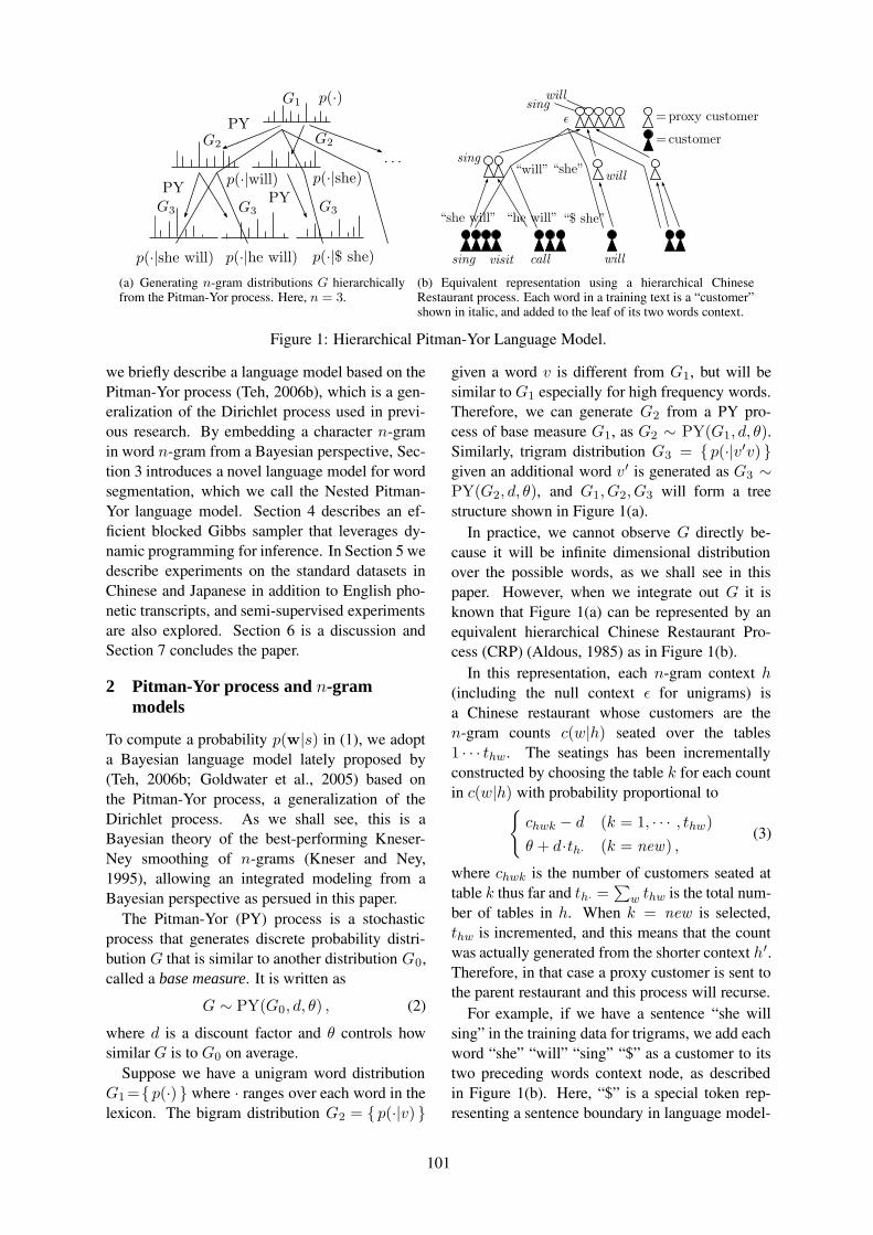
(a) Generating n-gram distributions G hierarchicallyfrom the Pitman-Yor process. Here, n = 3.
(b) Equivalent representation using a hierarchical ChineseRestaurant process. Each word in a training text is a “customer”shown in italic, and added to the leaf of its two words context.
Figure 1: Hierarchical Pitman-Yor Language Model.
we briefly describe a language model based on thePitman-Yor process (Teh, 2006b), which is a gen-eralization of the Dirichlet process used in previ-ous research. By embedding a character n-gramin word n-gram from a Bayesian perspective, Sec-tion 3 introduces a novel language model for wordsegmentation, which we call the Nested Pitman-Yor language model. Section 4 describes an ef-ficient blocked Gibbs sampler that leverages dy-namic programming for inference. In Section 5 wedescribe experiments on the standard datasets inChinese and Japanese in addition to English pho-netic transcripts, and semi-supervised experimentsare also explored. Section 6 is a discussion andSection 7 concludes the paper.
2 Pitman-Yor process and n-grammodels
To compute a probability p(w|s) in (1), we adopta Bayesian language model lately proposed by(Teh, 2006b; Goldwater et al., 2005) based onthe Pitman-Yor process, a generalization of theDirichlet process. As we shall see, this is aBayesian theory of the best-performing Kneser-Ney smoothing of n-grams (Kneser and Ney,1995), allowing an integrated modeling from aBayesian perspective as persued in this paper.
The Pitman-Yor (PY) process is a stochasticprocess that generates discrete probability distri-bution G that is similar to another distribution G0,called a base measure. It is written as
G ∼ PY(G0, d, θ) , (2)where d is a discount factor and θ controls howsimilar G is to G0 on average.
Suppose we have a unigram word distributionG1 ={ p(·) } where · ranges over each word in thelexicon. The bigram distribution G2 = { p(·|v) }
given a word v is different from G1, but will besimilar to G1 especially for high frequency words.Therefore, we can generate G2 from a PY pro-cess of base measure G1, as G2 ∼ PY(G1, d, θ).Similarly, trigram distribution G3 = { p(·|v′v) }given an additional word v′ is generated as G3 ∼PY(G2, d, θ), and G1, G2, G3 will form a treestructure shown in Figure 1(a).
In practice, we cannot observe G directly be-cause it will be infinite dimensional distributionover the possible words, as we shall see in thispaper. However, when we integrate out G it isknown that Figure 1(a) can be represented by anequivalent hierarchical Chinese Restaurant Pro-cess (CRP) (Aldous, 1985) as in Figure 1(b).
In this representation, each n-gram context h
(including the null context ε for unigrams) isa Chinese restaurant whose customers are then-gram counts c(w|h) seated over the tables1 · · · thw. The seatings has been incrementallyconstructed by choosing the table k for each countin c(w|h) with probability proportional to
{
chwk − d (k = 1, · · · , thw)
θ + d·th· (k = new) ,(3)
where chwk is the number of customers seated attable k thus far and th· =
∑
w thw is the total num-ber of tables in h. When k = new is selected,thw is incremented, and this means that the countwas actually generated from the shorter context h′.Therefore, in that case a proxy customer is sent tothe parent restaurant and this process will recurse.
For example, if we have a sentence “she willsing” in the training data for trigrams, we add eachword “she” “will” “sing” “$” as a customer to itstwo preceding words context node, as describedin Figure 1(b). Here, “$” is a special token rep-resenting a sentence boundary in language model-
101

ing (Brown et al., 1992).As a result, the n-gram probability of this hier-
archical Pitman-Yor language model (HPYLM) isrecursively computed as
p(w|h) =c(w|h)−d·thw
θ+c(h)+
θ+d·th·θ+c(h)
p(w|h′),
(4)where p(w|h′) is the same probability using a(n−1)-gram context h′. When we set thw ≡ 1, (4)recovers a Kneser-Ney smoothing: thus a HPYLMis a Bayesian Kneser-Ney language model as wellas an extension of the hierarchical Dirichlet Pro-cess (HDP) used in Goldwater et al. (2006). θ, d
are hyperparameters that can be learned as Gammaand Beta posteriors, respectively, given the data.For details, see Teh (2006a).
The inference of this model interleaves addingand removing a customer to optimize thw, d, andθ using MCMC. However, in our case “words”are not known a priori: the next section describeshow to accomplish this by constructing a nestedHPYLM of words and characters, with the associ-ated inference algorithm.
3 Nested Pitman-Yor Language Model
Thus far we have assumed that the unigram G1
is already given, but of course it should also begenerated as G1 ∼ PY(G0, d, θ).
Here, a problem occurs: What should we use forG0, namely the prior probabilities over words2?If a lexicon is finite, we can use a uniform priorG0(w) = 1/|V | for every word w in lexicon V .However, with word segmentation every substringcould be a word, thus the lexicon is not limited butwill be countably infinite.
Building an accurate G0 is crucial for wordsegmentation, since it determines how the possi-ble words will look like. Previous work using aDirichlet process used a relatively simple prior forG0, namely an uniform distribution over charac-ters (Goldwater et al., 2006), or a prior solely de-pendent on word length with a Poisson distributionwhose parameter is fixed by hand (Xu et al., 2008).
In contrast, in this paper we use a simple butmore elaborate model, that is, a character n-gramlanguage model that also employs HPYLM. Thisis important because in English, for example,words are likely to end in ‘–tion’ and begin with
2Note that this is different from unigrams, which are pos-terior distribution given data.
Figure 2: Chinese restaurant representation of ourNested Pitman-Yor Language Model (NPYLM).‘re–’, but almost never end in ‘–tio’ nor begin with‘sre–’ 3.
Therefore, we useG0(w) = p(c1 · · · ck) (5)
=
k∏
i=1
p(ci|c1 · · · ci−1) (6)
where string c1 · · · ck is a spelling of w, andp(ci|c1 · · · ci−1) is given by the character HPYLMaccording to (4).
This language model, which we call NestedPitman-Yor Language Model (NPYLM) hereafter,is the hierarchical language model shown in Fig-ure 2, where the character HPYLM is embeddedas a base measure of the word HPYLM.4 As thefinal base measure for the character HPYLM, weused a uniform prior over the possible charactersof a given language. To avoid dependency on n-gram order n, we actually used the ∞-gram lan-guage model (Mochihashi and Sumita, 2007), avariable order HPYLM, for characters. However,for generality we hereafter state that we used theHPYLM. The theory remains the same for ∞-grams, except sampling or marginalizing over n
as needed.Furthermore, we corrected (5) so that word
length will have a Poisson distribution whose pa-rameter can now be estimated for a given languageand word type. We describe this in detail in Sec-tion 4.3.Chinese Restaurant RepresentationIn our NPYLM, the word model and the charac-ter model are not separate but connected througha nested CRP. When a word w is generated fromits parent at the unigram node, it means that w
3Imagine we try to segment an English character string“itisrecognizedasthe· · · .”
4Strictly speaking, this is not “nested” in the sense of aNested Dirichlet process (Rodriguez et al., 2008) and couldbe called “hierarchical HPYLM”, which denotes anothermodel for domain adaptation (Wood and Teh, 2008).
102
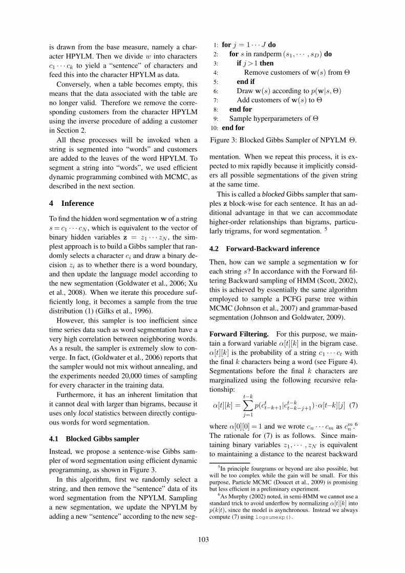
is drawn from the base measure, namely a char-acter HPYLM. Then we divide w into charactersc1 · · · ck to yield a “sentence” of characters andfeed this into the character HPYLM as data.
Conversely, when a table becomes empty, thismeans that the data associated with the table areno longer valid. Therefore we remove the corre-sponding customers from the character HPYLMusing the inverse procedure of adding a customerin Section 2.
All these processes will be invoked when astring is segmented into “words” and customersare added to the leaves of the word HPYLM. Tosegment a string into “words”, we used efficientdynamic programming combined with MCMC, asdescribed in the next section.
4 Inference
To find the hidden word segmentation w of a strings = c1 · · · cN , which is equivalent to the vector ofbinary hidden variables z = z1 · · · zN , the sim-plest approach is to build a Gibbs sampler that ran-domly selects a character ci and draw a binary de-cision zi as to whether there is a word boundary,and then update the language model according tothe new segmentation (Goldwater et al., 2006; Xuet al., 2008). When we iterate this procedure suf-ficiently long, it becomes a sample from the truedistribution (1) (Gilks et al., 1996).
However, this sampler is too inefficient sincetime series data such as word segmentation have avery high correlation between neighboring words.As a result, the sampler is extremely slow to con-verge. In fact, (Goldwater et al., 2006) reports thatthe sampler would not mix without annealing, andthe experiments needed 20,000 times of samplingfor every character in the training data.
Furthermore, it has an inherent limitation thatit cannot deal with larger than bigrams, because ituses only local statistics between directly contigu-ous words for word segmentation.
4.1 Blocked Gibbs sampler
Instead, we propose a sentence-wise Gibbs sam-pler of word segmentation using efficient dynamicprogramming, as shown in Figure 3.
In this algorithm, first we randomly select astring, and then remove the “sentence” data of itsword segmentation from the NPYLM. Samplinga new segmentation, we update the NPYLM byadding a new “sentence” according to the new seg-
1: for j = 1 · · · J do2: for s in randperm (s1, · · · , sD) do3: if j >1 then4: Remove customers of w(s) from Θ5: end if6: Draw w(s) according to p(w|s,Θ)7: Add customers of w(s) to Θ8: end for9: Sample hyperparameters of Θ
10: end for
Figure 3: Blocked Gibbs Sampler of NPYLM Θ.
mentation. When we repeat this process, it is ex-pected to mix rapidly because it implicitly consid-ers all possible segmentations of the given stringat the same time.
This is called a blocked Gibbs sampler that sam-ples z block-wise for each sentence. It has an ad-ditional advantage in that we can accommodatehigher-order relationships than bigrams, particu-larly trigrams, for word segmentation. 5
4.2 Forward-Backward inference
Then, how can we sample a segmentation w foreach string s? In accordance with the Forward fil-tering Backward sampling of HMM (Scott, 2002),this is achieved by essentially the same algorithmemployed to sample a PCFG parse tree withinMCMC (Johnson et al., 2007) and grammar-basedsegmentation (Johnson and Goldwater, 2009).
Forward Filtering. For this purpose, we main-tain a forward variable α[t][k] in the bigram case.α[t][k] is the probability of a string c1 · · · ct withthe final k characters being a word (see Figure 4).Segmentations before the final k characters aremarginalized using the following recursive rela-tionship:
α[t][k] =t−k∑
j=1
p(ctt−k+1|c
t−kt−k−j+1)·α[t−k][j] (7)
where α[0][0] = 1 and we wrote cn · · · cm as cmn .6
The rationale for (7) is as follows. Since main-taining binary variables z1, · · · , zN is equivalentto maintaining a distance to the nearest backward
5In principle fourgrams or beyond are also possible, butwill be too complex while the gain will be small. For thispurpose, Particle MCMC (Doucet et al., 2009) is promisingbut less efficient in a preliminary experiment.
6As Murphy (2002) noted, in semi-HMM we cannot use astandard trick to avoid underflow by normalizing α[t][k] intop(k|t), since the model is asynchronous. Instead we alwayscompute (7) using logsumexp().
103
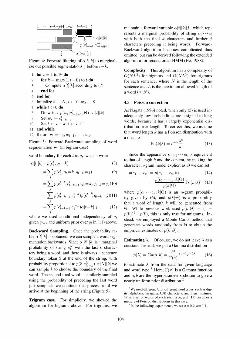
Figure 4: Forward filtering of α[t][k] to marginal-ize out possible segmentations j before t−k.
1: for t = 1 to N do2: for k = max(1, t−L) to t do3: Compute α[t][k] according to (7).4: end for5: end for6: Initialize t← N , i← 0, w0 ← $7: while t > 0 do8: Draw k ∝ p(wi|c
tt−k+1,Θ) · α[t][k]
9: Set wi ← ctt−k+1
10: Set t← t− k, i← i + 111: end while12: Return w = wi, wi−1, · · · , w1.Figure 5: Forward-Backward sampling of wordsegmentation w. (in bigram case)
word boundary for each t as qt, we can writeα[t][k]=p(ct
1, qt =k) (8)
=∑
j
p(ct1, qt =k, qt−k =j) (9)
=∑
j
p(ct−k1 , ct
t−k+1, qt =k, qt−k =j)(10)
=∑
j
p(ctt−k+1|c
t−k1 )p(ct−k
1 , qt−k =j)(11)
=∑
j
p(ctt−k+1|c
t−k1 )α[t−k][j] , (12)
where we used conditional independency of qt
given qt−k and uniform prior over qt in (11) above.
Backward Sampling. Once the probability ta-ble α[t][k] is obtained, we can sample a word seg-mentation backwards. Since α[N ][k] is a marginalprobability of string cN
1 with the last k charac-ters being a word, and there is always a sentenceboundary token $ at the end of the string, withprobability proportional to p($|cN
N−k)·α[N ][k] wecan sample k to choose the boundary of the finalword. The second final word is similarly sampledusing the probability of preceding the last wordjust sampled: we continue this process until wearrive at the beginning of the string (Figure 5).
Trigram case. For simplicity, we showed thealgorithm for bigrams above. For trigrams, we
maintain a forward variable α[t][k][j], which rep-resents a marginal probability of string c1 · · · ct
with both the final k characters and further j
characters preceding it being words. Forward-Backward algorithm becomes complicated thusomitted, but can be derived following the extendedalgorithm for second order HMM (He, 1988).
Complexity This algorithm has a complexity ofO(NL2) for bigrams and O(NL3) for trigramsfor each sentence, where N is the length of thesentence and L is the maximum allowed length ofa word (≤ N ).
4.3 Poisson correction
As Nagata (1996) noted, when only (5) is used in-adequately low probabilities are assigned to longwords, because it has a largely exponential dis-tribution over length. To correct this, we assumethat word length k has a Poisson distribution witha mean λ:
Po(k|λ) = e−λ λk
k!. (13)
Since the appearance of c1 · · · ck is equivalentto that of length k and the content, by making thecharacter n-gram model explicit as Θ we can set
p(c1 · · · ck) = p(c1 · · · ck, k) (14)
=p(c1 · · · ck, k|Θ)
p(k|Θ)Po(k|λ) (15)
where p(c1 · · · ck, k|Θ) is an n-gram probabil-ity given by (6), and p(k|Θ) is a probabilitythat a word of length k will be generated fromΘ. While previous work used p(k|Θ) = (1 −p($))k−1p($), this is only true for unigrams. In-stead, we employed a Monte Carlo method thatgenerates words randomly from Θ to obtain theempirical estimates of p(k|Θ).
Estimating λ. Of course, we do not leave λ as aconstant. Instead, we put a Gamma distribution
p(λ) = Ga(a, b) =ba
Γ(a)λa−1e−bλ (16)
to estimate λ from the data for given languageand word type.7 Here, Γ(x) is a Gamma functionand a, b are the hyperparameters chosen to give anearly uniform prior distribution.8
7We used different λ for different word types, such as dig-its, alphabets, hiragana, CJK characters, and their mixtures.W is a set of words of each such type, and (13) becomes amixture of Poisson distributions in this case.
8In the following experiments, we set a=0.2, b=0.1.
104
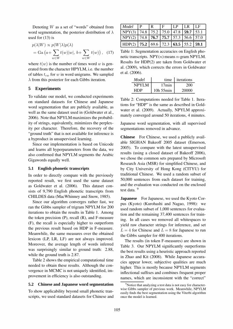
Denoting W as a set of “words” obtained fromword segmentation, the posterior distribution of λ
used for (13) isp(λ|W ) ∝ p(W |λ)p(λ)
= Ga(
a+∑
w∈W
t(w)|w|, b+∑
w∈W
t(w))
, (17)
where t(w) is the number of times word w is gen-erated from the character HPYLM, i.e. the numberof tables tεw for w in word unigrams. We sampledλ from this posterior for each Gibbs iteration.
5 Experiments
To validate our model, we conducted experimentson standard datasets for Chinese and Japaneseword segmentation that are publicly available, aswell as the same dataset used in (Goldwater et al.,2006). Note that NPYLM maximizes the probabil-ity of strings, equivalently, minimizes the perplex-ity per character. Therefore, the recovery of the“ground truth” that is not available for inference isa byproduct in unsupervised learning.
Since our implementation is based on Unicodeand learns all hyperparameters from the data, wealso confirmed that NPYLM segments the ArabicGigawords equally well.
5.1 English phonetic transcripts
In order to directly compare with the previouslyreported result, we first used the same datasetas Goldwater et al. (2006). This dataset con-sists of 9,790 English phonetic transcripts fromCHILDES data (MacWhinney and Snow, 1985).
Since our algorithm converges rather fast, weran the Gibbs sampler of trigram NPYLM for 200iterations to obtain the results in Table 1. Amongthe token precision (P), recall (R), and F-measure(F), the recall is especially higher to outperformthe previous result based on HDP in F-measure.Meanwhile, the same measures over the obtainedlexicon (LP, LR, LF) are not always improved.Moreover, the average length of words inferredwas surprisingly similar to ground truth: 2.88,while the ground truth is 2.87.
Table 2 shows the empirical computational timeneeded to obtain these results. Although the con-vergence in MCMC is not uniquely identified, im-provement in efficiency is also outstanding.
5.2 Chinese and Japanese word segmentation
To show applicability beyond small phonetic tran-scripts, we used standard datasets for Chinese and
Model P R F LP LR LFNPY(3) 74.8 75.2 75.0 47.8 59.7 53.1NPY(2) 74.8 76.7 75.7 57.3 56.6 57.0HDP(2) 75.2 69.6 72.3 63.5 55.2 59.1
Table 1: Segmentation accuracies on English pho-netic transcripts. NPY(n) means n-gram NPYLM.Results for HDP(2) are taken from Goldwater etal. (2009), which corrects the errors in Goldwateret al. (2006).
Model time iterationsNPYLM 17min 200HDP 10h 55min 20000
Table 2: Computations needed for Table 1. Itera-tions for “HDP” is the same as described in Gold-water et al. (2009). Actually, NPYLM approxi-mately converged around 50 iterations, 4 minutes.
Japanese word segmentation, with all supervisedsegmentations removed in advance.
Chinese For Chinese, we used a publicly avail-able SIGHAN Bakeoff 2005 dataset (Emerson,2005). To compare with the latest unsupervisedresults (using a closed dataset of Bakeoff 2006),we chose the common sets prepared by MicrosoftResearch Asia (MSR) for simplified Chinese, andby City University of Hong Kong (CITYU) fortraditional Chinese. We used a random subset of50,000 sentences from each dataset for training,and the evaluation was conducted on the enclosedtest data. 9
Japanese For Japanese, we used the Kyoto Cor-pus (Kyoto) (Kurohashi and Nagao, 1998): weused random subset of 1,000 sentences for evalua-tion and the remaining 37,400 sentences for train-ing. In all cases we removed all whitespaces toyield raw character strings for inference, and setL = 4 for Chinese and L = 8 for Japanese to runthe Gibbs sampler for 400 iterations.
The results (in token F-measures) are shown inTable 3. Our NPYLM significantly ourperformsthe best results using a heuristic approach reportedin Zhao and Kit (2008). While Japanese accura-cies appear lower, subjective qualities are muchhigher. This is mostly because NPYLM segmentsinflectional suffixes and combines frequent propernames, which are inconsistent with the “correct”
9Notice that analyzing a test data is not easy for character-wise Gibbs sampler of previous work. Meanwhile, NPYLMeasily finds the best segmentation using the Viterbi algorithmonce the model is learned.
105
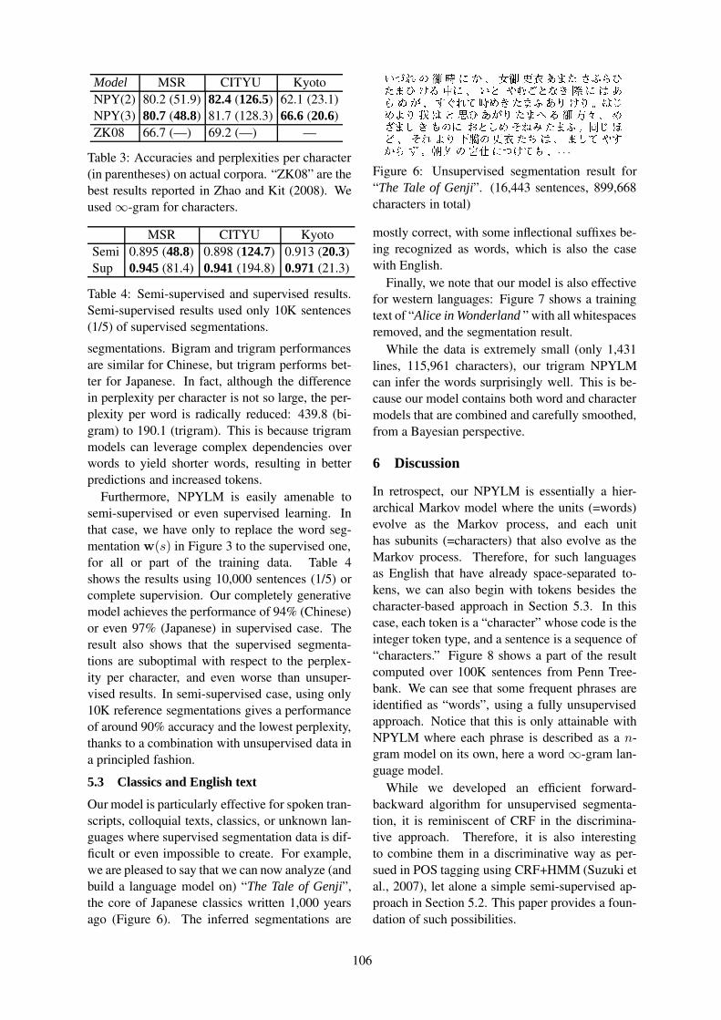
Model MSR CITYU KyotoNPY(2) 80.2 (51.9) 82.4 (126.5) 62.1 (23.1)NPY(3) 80.7 (48.8) 81.7 (128.3) 66.6 (20.6)ZK08 66.7 (—) 69.2 (—) —
Table 3: Accuracies and perplexities per character(in parentheses) on actual corpora. “ZK08” are thebest results reported in Zhao and Kit (2008). Weused∞-gram for characters.
MSR CITYU KyotoSemi 0.895 (48.8) 0.898 (124.7) 0.913 (20.3)Sup 0.945 (81.4) 0.941 (194.8) 0.971 (21.3)
Table 4: Semi-supervised and supervised results.Semi-supervised results used only 10K sentences(1/5) of supervised segmentations.segmentations. Bigram and trigram performancesare similar for Chinese, but trigram performs bet-ter for Japanese. In fact, although the differencein perplexity per character is not so large, the per-plexity per word is radically reduced: 439.8 (bi-gram) to 190.1 (trigram). This is because trigrammodels can leverage complex dependencies overwords to yield shorter words, resulting in betterpredictions and increased tokens.
Furthermore, NPYLM is easily amenable tosemi-supervised or even supervised learning. Inthat case, we have only to replace the word seg-mentation w(s) in Figure 3 to the supervised one,for all or part of the training data. Table 4shows the results using 10,000 sentences (1/5) orcomplete supervision. Our completely generativemodel achieves the performance of 94% (Chinese)or even 97% (Japanese) in supervised case. Theresult also shows that the supervised segmenta-tions are suboptimal with respect to the perplex-ity per character, and even worse than unsuper-vised results. In semi-supervised case, using only10K reference segmentations gives a performanceof around 90% accuracy and the lowest perplexity,thanks to a combination with unsupervised data ina principled fashion.5.3 Classics and English text
Our model is particularly effective for spoken tran-scripts, colloquial texts, classics, or unknown lan-guages where supervised segmentation data is dif-ficult or even impossible to create. For example,we are pleased to say that we can now analyze (andbuild a language model on) “The Tale of Genji”,the core of Japanese classics written 1,000 yearsago (Figure 6). The inferred segmentations are
����������� �����������������������! ���� �"�#%$�&���('*),+.-/'!021�3�54%��(6879�&:9;<�>=8�?@19�>�BAC�(DE"ED,F�4.G?2HID�JK4L'2M. %��7NDO����P�#Q�%RES(�T?U �/V�1%WX��ZY('�V!?C[B\>]��>�BA8F�^IGQ_` �L[a��HIDEbac.�9�>�L��d%4&�e�.Vf=%)>:���(g�Fih.j5� kBlK�m@"a=EWO�
· · ·
Figure 6: Unsupervised segmentation result for“The Tale of Genji”. (16,443 sentences, 899,668characters in total)
mostly correct, with some inflectional suffixes be-ing recognized as words, which is also the casewith English.
Finally, we note that our model is also effectivefor western languages: Figure 7 shows a trainingtext of “Alice in Wonderland ” with all whitespacesremoved, and the segmentation result.
While the data is extremely small (only 1,431lines, 115,961 characters), our trigram NPYLMcan infer the words surprisingly well. This is be-cause our model contains both word and charactermodels that are combined and carefully smoothed,from a Bayesian perspective.
6 Discussion
In retrospect, our NPYLM is essentially a hier-archical Markov model where the units (=words)evolve as the Markov process, and each unithas subunits (=characters) that also evolve as theMarkov process. Therefore, for such languagesas English that have already space-separated to-kens, we can also begin with tokens besides thecharacter-based approach in Section 5.3. In thiscase, each token is a “character” whose code is theinteger token type, and a sentence is a sequence of“characters.” Figure 8 shows a part of the resultcomputed over 100K sentences from Penn Tree-bank. We can see that some frequent phrases areidentified as “words”, using a fully unsupervisedapproach. Notice that this is only attainable withNPYLM where each phrase is described as a n-gram model on its own, here a word∞-gram lan-guage model.
While we developed an efficient forward-backward algorithm for unsupervised segmenta-tion, it is reminiscent of CRF in the discrimina-tive approach. Therefore, it is also interestingto combine them in a discriminative way as per-sued in POS tagging using CRF+HMM (Suzuki etal., 2007), let alone a simple semi-supervised ap-proach in Section 5.2. This paper provides a foun-dation of such possibilities.
106

lastly,shepicturedtoherselfhowthissamelittlesisterofherswould,intheafter-time,beherselfagrownwoman;andhowshewouldkeep,throughallherriperyears,thesimpleandlovingheartofherchildhood:andhowshewouldgatheraboutherotherlittlechildren,andmaketheireyesbrightandeagerwithmanyastrangetale,perhapsevenwiththedreamofwonderlandoflongago:andhowshewouldfeelwithalltheirsimplesorrows,andfindapleasureinalltheirsimplejoys,rememberingherownchild-life,andthehappysummerdays.
(a) Training data (in part).last ly , she pictured to herself how this same little sis-ter of her s would , inthe after - time , be herself agrownwoman ; and how she would keep , through allher riperyears , the simple and loving heart of her child hood : andhow she would gather about her other little children ,andmake theireyes bright and eager with many a strange tale, perhaps even with the dream of wonderland of longago: and how she would feel with all their simple sorrow s ,and find a pleasure in all their simple joys , remember ingher own child - life , and thehappy summerday s .
(b) Segmentation result. Note we used no dictionary.
Figure 7: Word segmentation of “Alice in Wonder-land ”.
7 Conclusion
In this paper, we proposed a much more efficientand accurate model for fully unsupervised wordsegmentation. With a combination of dynamicprogramming and an accurate spelling model froma Bayesian perspective, our model significantlyoutperforms the previous reported results, and theinference is very efficient.
This model is also considered as a way to builda Bayesian Kneser-Ney smoothed word n-gramlanguage model directly from characters with no“word” indications. In fact, it achieves lower per-plexity per character than that based on supervisedsegmentations. We believe this will be particu-larly beneficial to build a language model on suchtexts as speech transcripts, colloquial texts or un-known languages, where word boundaries are hardor even impossible to identify a priori.
Acknowledgments
We thank Vikash Mansinghka (MIT) for a mo-tivating discussion leading to this research, andSatoru Takabayashi (Google) for valuable techni-cal advice.
References
David Aldous, 1985. Exchangeability and RelatedTopics, pages 1–198. Springer Lecture Notes inMath. 1117.
Rie Kubota Ando and Lillian Lee. 2003. Mostly-Unsupervised Statistical Segmentation of Japanese
nevertheless ,he was admiredby many of his immediate subordinatesfor his long work hoursand dedication to building northwestinto what he called a “ mega carrier. ”
althoughpreliminary findingswere reportedmore than a year ago ,the latest resultsappearin today ’snew england journal of medicine ,a forumlikely to bring new attention to the problem.
south korearegistered a trade deficit of $ 101 millionin october, reflecting the country ’s economic sluggishness, according to government figures released wednesday.
Figure 8: Generative phrase segmentation of PennTreebank text computed by NPYLM. Each line isa “word” consisting of actual words.
Kanji Sequences. Natural Language Engineering,9(2):127–149.
Peter F. Brown, Vincent J. Della Pietra, Robert L. Mer-cer, Stephen A. Della Pietra, and Jennifer C. Lai.1992. An Estimate of an Upper Bound for the En-tropy of English. Computational Linguistics, 18:31–40.
Arnaud Doucet, Christophe Andrieu, and RomanHolenstein. 2009. Particle Markov Chain MonteCarlo. in submission.
Tom Emerson. 2005. SIGHAN Bakeoff 2005.http://www.sighan.org/bakeoff2005/.
W. R. Gilks, S. Richardson, and D. J. Spiegelhalter.1996. Markov Chain Monte Carlo in Practice.Chapman & Hall / CRC.
Sharon Goldwater, Thomas L. Griffiths, and MarkJohnson. 2005. Interpolating Between Types andTokens by Estimating Power-Law Generators. InNIPS 2005.
Sharon Goldwater, Thomas L. Griffiths, and MarkJohnson. 2006. Contextual Dependencies in Un-supervised Word Segmentation. In Proceedings ofACL/COLING 2006, pages 673–680.
Sharon Goldwater, Thomas L. Griffiths, and MarkJohnson. 2009. A Bayesian framework for wordsegmentation: Exploring the effects of context.Cognition, in press.
Yang He. 1988. Extended Viterbi algorithm for sec-ond order hidden Markov process. In Proceedingsof ICPR 1988, pages 718–720.
107
Mark Johnson and Sharon Goldwater. 2009. Im-proving nonparameteric Bayesian inference: exper-iments on unsupervised word segmentation withadaptor grammars. In NAACL 2009.
Mark Johnson, Thomas L. Griffiths, and Sharon Gold-water. 2007. Bayesian Inference for PCFGs viaMarkov Chain Monte Carlo. In Proceedings ofHLT/NAACL 2007, pages 139–146.
Reinhard Kneser and Hermann Ney. 1995. Improvedbacking-off for m-gram language modeling. In Pro-ceedings of ICASSP, volume 1, pages 181–184.
Sadao Kurohashi and Makoto Nagao. 1998. Buildinga Japanese Parsed Corpus while Improving the Pars-ing System. In Proceedings of LREC 1998, pages719–724. http://nlp.kuee.kyoto-u.ac.jp/nl-resource/corpus.html.
Brian MacWhinney and Catherine Snow. 1985. TheChild Language Data Exchange System. Journal ofChild Language, 12:271–296.
Daichi Mochihashi and Eiichiro Sumita. 2007. TheInfinite Markov Model. In NIPS 2007.
Kevin Murphy. 2002. Hidden semi-Markov models(segment models). http://www.cs.ubc.ca/˜murphyk/Papers/segment.pdf.
Masaaki Nagata. 1996. Automatic Extraction ofNew Words from Japanese Texts using General-ized Forward-Backward Search. In Proceedings ofEMNLP 1996, pages 48–59.
Abel Rodriguez, David Dunson, and Alan Gelfand.2008. The Nested Dirichlet Process. Journal of theAmerican Statistical Association, 103:1131–1154.
Steven L. Scott. 2002. Bayesian Methods for HiddenMarkov Models. Journal of the American StatisticalAssociation, 97:337–351.
Jun Suzuki, Akinori Fujino, and Hideki Isozaki. 2007.Semi-Supervised Structured Output Learning Basedon a Hybrid Generative and Discriminative Ap-proach. In Proceedings of EMNLP-CoNLL 2007,pages 791–800.
Yee Whye Teh. 2006a. A Bayesian Interpreta-tion of Interpolated Kneser-Ney. Technical ReportTRA2/06, School of Computing, NUS.
Yee Whye Teh. 2006b. A Hierarchical Bayesian Lan-guage Model based on Pitman-Yor Processes. InProceedings of ACL/COLING 2006, pages 985–992.
Frank Wood and Yee Whye Teh. 2008. A Hierarchical,Hierarchical Pitman-Yor Process Language Model.In ICML 2008 Workshop on Nonparametric Bayes.
Jia Xu, Jianfeng Gao, Kristina Toutanova, and Her-mann Ney. 2008. Bayesian Semi-Supervised Chi-nese Word Segmentation for Statistical MachineTranslation. In Proceedings of COLING 2008,pages 1017–1024.
Hai Zhao and Chunyu Kit. 2008. An Empirical Com-parison of Goodness Measures for UnsupervisedChinese Word Segmentation with a Unified Frame-work. In Proceedings of IJCNLP 2008.
108

Proceedings of the 47th Annual Meeting of the ACL and the 4th IJCNLP of the AFNLP, pages 109–117,Suntec, Singapore, 2-7 August 2009. c©2009 ACL and AFNLP
Knowing the Unseen: Estimating Vocabulary Size over UnseenSamples
Suma BhatDepartment of ECEUniversity of Illinois
Richard SproatCenter for Spoken Language Understanding
Oregon Health & Science [email protected]
Abstract
Empirical studies on corpora involve mak-ing measurements of several quantities forthe purpose of comparing corpora, creat-ing language models or to make general-izations about specific linguistic phenom-ena in a language. Quantities such as av-erage word length are stable across sam-ple sizes and hence can be reliably esti-mated from large enough samples. How-ever, quantities such asvocabulary sizechange with sample size. Thus measure-ments based on a given sample will needto beextrapolatedto obtain their estimatesover larger unseen samples. In this work,we propose a novelnonparametricestima-tor of vocabulary size. Our main result isto show thestatistical consistencyof theestimator – the first of its kind in the lit-erature. Finally, we compare our proposalwith the state of the art estimators (bothparametric and nonparametric) on largestandard corpora; apart from showing thefavorable performance of our estimator,we also see that the classical Good-Turingestimator consistently underestimates thevocabulary size.
1 Introduction
Empirical studies on corpora involve making mea-surements of several quantities for the purpose ofcomparing corpora, creating language models orto make generalizations about specific linguisticphenomena in a language. Quantities such as av-erage word length or average sentence length arestable across sample sizes. Hence empirical mea-surements from large enough samples tend to bereliable for even larger sample sizes. On the otherhand, quantities associated with word frequencies,such as the number ofhapax legomenaor the num-
ber of distinct word types changes are strictly sam-ple size dependent. Given a sample we can ob-tain the seen vocabulary and the seen number ofhapax legomena. However, for the purpose ofcomparison of corpora of different sizes or lin-guistic phenomena based on samples of differentsizes it is imperative that these quantities be com-pared based on similar sample sizes. We thus needmethods to extrapolate empirical measurements ofthese quantities to arbitrary sample sizes.
Our focus in this study will be estimators ofvocabulary size for samples larger than the sam-ple available. There is an abundance of estima-tors of population size (in our case, vocabularysize) in existing literature. Excellent survey arti-cles that summarize the state-of-the-art are avail-able in (Bunge and Fitzpatrick, 1993) and (Gan-dolfi and Sastri, 2004). Of particular interest tous is the set of estimators that have been shownto model word frequency distributions well. Thisstudy proposes a nonparametric estimator of vo-cabulary size and evaluates its theoretical and em-pirical performance. For comparison we considersome state-of-the-art parametric and nonparamet-ric estimators of vocabulary size.
The proposed non-parametric estimator for thenumber of unseen elements assumes a regimecharacterizing word frequency distributions. Thiswork is motivated by a scaling formulation to ad-dress the problem of unlikely events proposed in(Baayen, 2001; Khmaladze, 1987; Khmaladze andChitashvili, 1989; Wagner et al., 2006). We alsodemonstrate that the estimator is strongly consis-tent under the natural scaling formulation. Whilecompared with other vocabulary size estimates,we see that our estimator performs at least as wellas some of the state of the art estimators.
2 Previous Work
Many estimators of vocabulary size are availablein the literature and a comparison of several non
109

parametric estimators of population size occurs in(Gandolfi and Sastri, 2004). While a definite com-parison including parametric estimators is lacking,there is also no known work comparing methodsof extrapolation of vocabulary size. Baroni andEvert, in (Baroni and Evert, 2005), evaluate theperformance of some estimators in extrapolatingvocabulary size for arbitrary sample sizes but limitthe study to parametric estimators. Since we con-sider both parametric and nonparametric estima-tors here, we consider this to be the first studycomparing a set of estimators for extrapolating vo-cabulary size.
Estimators of vocabulary size that we comparecan be broadly classified into two types:
1. Nonparametric estimators- here word fre-quency information from the given samplealone is used to estimate the vocabulary size.A good survey of the state of the art is avail-able in (Gandolfi and Sastri, 2004). In thispaper, we compare our proposed estimatorwith the canonical estimators available in(Gandolfi and Sastri, 2004).
2. Parametric estimators- here a probabilisticmodel capturing the relation between ex-pected vocabulary size and sample size is theestimator. Given a sample of sizen, thesample serves to calculate the parameters ofthe model. The expected vocabulary for agiven sample size is then determined usingthe explicit relation. The parametric esti-mators considered in this study are (Baayen,2001; Baroni and Evert, 2005),
(a) Zipf-Mandelbrot estimator (ZM);
(b) finite Zipf-Mandelbrot estimator (fZM).
In addition to the above estimators we considera novel non parametric estimator. It is the nonpara-metric estimator that we propose, taking into ac-count the characteristic feature of word frequencydistributions, to which we will turn next.
3 Novel Estimator of Vocabulary size
We observe(X1, . . . ,Xn), an i.i.d. sequencedrawn according to a probability distributionPfrom a large, but finite, vocabularyΩ. Our goalis in estimating the “essential” size of the vocabu-lary Ω using only the observations. In other words,having seen a sample of sizen we wish to know,given another sample from the same population,
how many unseen elements we would expect tosee. Our nonparametric estimator for the numberof unseen elements is motivated by the character-istic property of word frequency distributions, theLarge Number of Rare Events(LNRE) (Baayen,2001). We also demonstrate that the estimator isstrongly consistent under a natural scaling formu-lation described in (Khmaladze, 1987).
3.1 A Scaling Formulation
Our main interest is in probability distributionsPwith the property that a large number of words inthe vocabularyΩ are unlikely, i.e., the chance anyword appears eventually in an arbitrarily long ob-servation is strictly between 0 and 1. The authorsin (Baayen, 2001; Khmaladze and Chitashvili,1989; Wagner et al., 2006) propose a natural scal-ing formulation to study this problem; specifically,(Baayen, 2001) has a tutorial-like summary of thetheoretical work in (Khmaladze, 1987; Khmaladzeand Chitashvili, 1989). In particular, the authorsconsider asequenceof vocabulary sets and prob-ability distributions, indexed by the observationsizen. Specifically, the observation(X1, . . . ,Xn)is drawn i.i.d. from a vocabularyΩn according toprobability Pn. If the probability of a word, sayω ∈ Ωn is p, then the probability that this specificwordω does not occur in an observation of sizen
is(1− p)n .
Forω to be an unlikely word, we would like thisprobability for largen to remain strictly between0 and 1. This implies that
č
n≤ p ≤
ĉ
n, (1)
for some strictly positive constants0 < č < ĉ <
∞. We will assume throughout this paper thatč
and ĉ are the same for every wordω ∈ Ωn. Thisimplies that the vocabulary size is growinglin-early with the observation size:
n
ĉ≤ |Ωn| ≤
n
č.
This model is called theLNRE zoneand its appli-cability in natural language corpora is studied indetail in (Baayen, 2001).
3.2 Shadows
Consider the observation string(X1, . . . ,Xn) andlet us denote the quantity of interest – the number
110
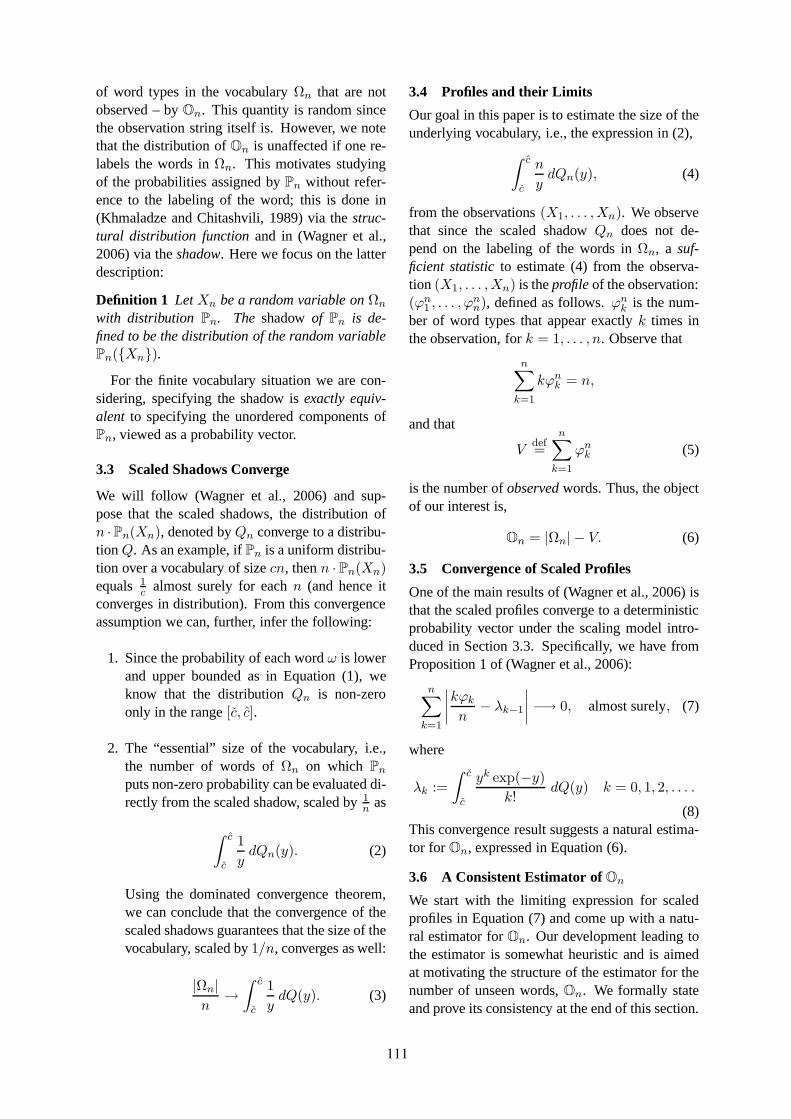
of word types in the vocabularyΩn that are notobserved – byOn. This quantity is random sincethe observation string itself is. However, we notethat the distribution ofOn is unaffected if one re-labels the words inΩn. This motivates studyingof the probabilities assigned byPn without refer-ence to the labeling of the word; this is done in(Khmaladze and Chitashvili, 1989) via thestruc-tural distribution functionand in (Wagner et al.,2006) via theshadow. Here we focus on the latterdescription:
Definition 1 LetXn be a random variable onΩn
with distribution Pn. The shadowof Pn is de-fined to be the distribution of the random variablePn({Xn}).
For the finite vocabulary situation we are con-sidering, specifying the shadow isexactly equiv-alent to specifying the unordered components ofPn, viewed as a probability vector.
3.3 Scaled Shadows Converge
We will follow (Wagner et al., 2006) and sup-pose that the scaled shadows, the distribution ofn ·Pn(Xn), denoted byQn converge to a distribu-tion Q. As an example, ifPn is a uniform distribu-tion over a vocabulary of sizecn, thenn · Pn(Xn)equals 1
calmost surely for eachn (and hence it
converges in distribution). From this convergenceassumption we can, further, infer the following:
1. Since the probability of each wordω is lowerand upper bounded as in Equation (1), weknow that the distributionQn is non-zeroonly in the range[č, ĉ].
2. The “essential” size of the vocabulary, i.e.,the number of words ofΩn on which Pn
puts non-zero probability can be evaluated di-rectly from the scaled shadow, scaled by1
nas
∫ ĉ
č
1
ydQn(y). (2)
Using the dominated convergence theorem,we can conclude that the convergence of thescaled shadows guarantees that the size of thevocabulary, scaled by1/n, converges as well:
|Ωn|
n→
∫ ĉ
č
1
ydQ(y). (3)
3.4 Profiles and their Limits
Our goal in this paper is to estimate the size of theunderlying vocabulary, i.e., the expression in (2),
∫ ĉ
č
n
ydQn(y), (4)
from the observations(X1, . . . ,Xn). We observethat since the scaled shadowQn does not de-pend on the labeling of the words inΩn, a suf-ficient statisticto estimate (4) from the observa-tion (X1, . . . ,Xn) is theprofileof the observation:(ϕn
1 , . . . , ϕnn), defined as follows.ϕn
k is the num-ber of word types that appear exactlyk times inthe observation, fork = 1, . . . , n. Observe that
n∑
k=1
kϕnk = n,
and that
Vdef=
n∑
k=1
ϕnk (5)
is the number ofobservedwords. Thus, the objectof our interest is,
On = |Ωn| − V. (6)
3.5 Convergence of Scaled Profiles
One of the main results of (Wagner et al., 2006) isthat the scaled profiles converge to a deterministicprobability vector under the scaling model intro-duced in Section 3.3. Specifically, we have fromProposition 1 of (Wagner et al., 2006):
n∑
k=1
∣
∣
∣
∣
kϕk
n− λk−1
∣
∣
∣
∣
−→ 0, almost surely, (7)
where
λk :=
∫ č
č
yk exp(−y)
k!dQ(y) k = 0, 1, 2, . . . .
(8)This convergence result suggests a natural estima-tor for On, expressed in Equation (6).
3.6 A Consistent Estimator ofOn
We start with the limiting expression for scaledprofiles in Equation (7) and come up with a natu-ral estimator forOn. Our development leading tothe estimator is somewhat heuristic and is aimedat motivating the structure of the estimator for thenumber of unseen words,On. We formally stateand prove its consistency at the end of this section.
111

3.6.1 A Heuristic Derivation
Starting from (7), let us first make the approxima-tion that
kϕk
n≈ λk−1, k = 1, . . . , n. (9)
We now have the formal calculation
n∑
k=1
ϕnk
n≈
n∑
k=1
λk−1
k(10)
=
n∑
k=1
∫ ĉ
č
e−yyk−1
k!dQ(y)
≈
∫ ĉ
č
e−y
y
(
n∑
k=1
yk
k!
)
dQ(y) (11)
≈
∫ ĉ
č
e−y
y(ey − 1) dQ(y) (12)
≈|Ωn|
n−
∫ ĉ
č
e−y
ydQ(y). (13)
Here the approximation in Equation (10) followsfrom the approximation in Equation (9), the ap-proximation in Equation (11) involves swappingthe outer discrete summation with integration andis justified formally later in the section, the ap-proximation in Equation (12) follows because
n∑
k=1
yk
k!→ ey − 1,
as n → ∞, and the approximation in Equa-tion (13) is justified from the convergence in Equa-tion (3). Now, comparing Equation (13) withEquation (6), we arrive at an approximation forour quantity of interest:
On
n≈
∫ ĉ
č
e−y
ydQ(y). (14)
The geometric series allows us to write
1
y=
1
ĉ
∞∑
ℓ=0
(
1−y
ĉ
)ℓ
, ∀y ∈ (0, ĉ) . (15)
Approximating this infinite series by a finite sum-mation, we have for ally ∈ (č, ĉ),
1
y−
1
ĉ
M∑
ℓ=0
(
1−y
ĉ
)ℓ
=
(
1− yĉ
)M
y
≤
(
1− čĉ
)M
č. (16)
It helps to write the truncated geometric series asa power series iny:
1
ĉ
M∑
ℓ=0
(
1−y
ĉ
)ℓ
=1
ĉ
M∑
ℓ=0
ℓ∑
k=0
(
ℓ
k
)
(−1)k(y
ĉ
)k
=1
ĉ
M∑
k=0
(
M∑
ℓ=k
(
ℓ
k
)
)
(−1)k(y
ĉ
)k
=
M∑
k=0
(−1)k aMk yk, (17)
where we have written
aMk :=
1
ĉk+1
(
M∑
ℓ=k
(
ℓ
k
)
)
.
Substituting the finite summation approximationin Equation 16 and its power series expression inEquation (17) into Equation (14) and swapping thediscrete summation with the integral, we can con-tinue
On
n≈
M∑
k=0
(−1)kaM
k
∫ ĉ
č
e−yyk dQ(y)
=
M∑
k=0
(−1)kaM
k k!λk. (18)
Here, in Equation (18), we used the definition ofλk from Equation (8). From the convergence inEquation (7), we finally arrive at our estimate:
On ≈
M∑
k=0
(−1)k aMk (k + 1)! ϕk+1. (19)
3.6.2 Consistency
Our main result is the demonstration of the consis-tency of the estimator in Equation (19).
Theorem 1 For anyǫ > 0,
limn→∞
∣
∣
∣On −
∑Mk=0 (−1)k aM
k (k + 1)! ϕk+1
∣
∣
∣
n≤ ǫ
almost surely, as long as
M ≥č log2 e + log2 (ǫč)
log2 (ĉ− č)− 1− log2 (ĉ). (20)
112

Proof: From Equation (6), we have
On
n=
|Ωn|
n−
n∑
k=1
ϕk
n
=|Ωn|
n−
n∑
k=1
λk−1
k−
n∑
k=1
1
k
(
kϕk
n− λk−1
)
. (21)
The first term in the right hand side (RHS) ofEquation (21) converges as seen in Equation (3).The third term in the RHS of Equation (21) con-verges to zero, almost surely, as seen from Equa-tion (7). The second term in the RHS of Equa-tion (21), on the other hand,
n∑
k=1
λk−1
k=
∫ ĉ
č
e−y
y
(
n∑
k=1
yk
k!
)
dQ(y)
→
∫ ĉ
č
e−y
y(ey − 1) dQ(y), n →∞,
=
∫ ĉ
č
1
ydQ(y)−
∫ ĉ
č
e−y
ydQ(y).
The monotone convergence theorem justifies theconvergence in the second step above. Thus weconclude that
limn→∞
On
n=
∫ ĉ
č
e−y
ydQ(y) (22)
almost surely. Coming to the estimator, we canwrite it as the sum of two terms:
M∑
k=0
(−1)k aMk k!λk (23)
+M∑
k=0
(−1)k aMk k!
(
(k + 1) ϕk+1
n− λk
)
.
The second term in Equation (23) above is seen toconverge to zero almost surely asn → ∞, usingEquation (7) and noting thatM is a constant notdepending onn. The first term in Equation (23)can be written as, using the definition ofλk fromEquation (8),
∫ ĉ
č
e−y
(
M∑
k=0
(−1)k aMk yk
)
dQ(y). (24)
Combining Equations (22) and (24), we have that,almost surely,
limn→∞
On −∑M
k=0 (−1)k aMk (k + 1)! ϕk+1
n=
∫ ĉ
č
e−y
(
1
y−
M∑
k=0
(−1)k aMk yk
)
dQ(y). (25)
Combining Equation (16) with Equation (17), wehave
0 <1
y−
M∑
k=0
(−1)k aMk yk ≤
(
1− čĉ
)M
č. (26)
The quantity in Equation (25) can now be upperbounded by, using Equation (26),
e−č(
1− čĉ
)M
č.
For M that satisfy Equation (20) this term is lessthanǫ. The proof concludes.
3.7 Uniform Consistent Estimation
One of the main issues with actually employingthe estimator for the number of unseen elements(cf. Equation (19)) is that it involves knowing theparameter̂c. In practice, there is no natural way toobtain any estimate on this parameterĉ. It wouldbe most useful if there were a way to modify theestimator in a way that it does not depend on theunobservable quantitŷc. In this section we see thatsuch a modification is possible, while still retain-ing the main theoretical performance result of con-sistency (cf. Theorem 1).
The first step to see the modification is in ob-serving where the need forĉ arises: it is in writingthe geometric series for the function1
y(cf. Equa-
tions (15) and (16)). If we could let̂c along withthe number of elementsM itself depend on thesample sizen, then we could still have the geo-metric series formula. More precisely, we have
1
y−
1
ĉn
Mn∑
ℓ=0
(
1−y
ĉn
)ℓ
=1
y
(
1−y
ĉn
)Mn
→ 0, n →∞,
as long as
ĉn
Mn→ 0, n →∞. (27)
This simple calculation suggests that we can re-placeĉ andM in the formula for the estimator (cf.Equation (19)) by terms that depend onn and sat-isfy the condition expressed by Equation (27).
113

4 Experiments
4.1 Corpora
In our experiments we used the following corpora:
1. TheBritish National Corpus(BNC): A cor-pus of about 100 million words of written andspoken British English from the years 1975-1994.
2. TheNew York Times Corpus(NYT): A cor-pus of about 5 million words.
3. TheMalayalam Corpus(MAL): A collectionof about 2.5 million words from varied ar-ticles in the Malayalam language from theCentral Institute of Indian Languages.
4. The Hindi Corpus (HIN): A collection ofabout 3 million words from varied articles inthe Hindi language also from the Central In-stitute of Indian Languages.
4.2 Methodology
We would like to see how well our estimator per-forms in terms of estimating the number of unseenelements. A natural way to study this is to ex-pose only half of an existing corpus to be observedand estimate the number of unseen elements (as-suming the the actual corpus is twice the observedsize). We can then check numerically how wellour estimator performs with respect to the “true”value. We use a subset (the first 10%, 20%, 30%,40% and 50%) of the corpus as theobserved sam-ple to estimate the vocabulary over twice the sam-ple size. The following estimators have been com-pared.
Nonparametric: Along with our proposed esti-mator (in Section 3), the following canonical es-timators available in (Gandolfi and Sastri, 2004)and (Baayen, 2001) are studied.
1. Our proposed estimatorOn (cf. Section 3):since the estimator is rather involved we con-sider only small values ofM (we see empir-ically that the estimator converges for verysmall values ofM itself) and choosêc = M.
This allows our estimator for the number ofunseen elements to be of the following form,for different values ofM :
M On
1 2 (ϕ1 − ϕ2)
2 32 (ϕ1 − ϕ2) + 3
4ϕ3
3 43 (ϕ1 − ϕ2) + 8
9
(
ϕ3 −ϕ4
3
)
Using this, the estimator of the true vocabu-lary size is simply,
On + V. (28)
Here (cf. Equation (5))
V =
n∑
k=1
ϕnk . (29)
In the simulations below, we have consideredM large enough until we see numerical con-vergence of the estimators: in all the cases,no more than a value of 4 is needed forM .For the English corpora, very small values ofM suffice – in particular, we have consideredthe average of the first three different estima-tors (corresponding to the first three valuesof M ). For the non-English corpora, we haveneeded to considerM = 4.
2. Gandolfi-Sastri estimator,
VGSdef=
n
n− ϕ1
(
V + ϕ1γ2)
, (30)
where
γ2 =ϕ1 − n− V
2n+
√
5n2 + 2n(V − 3ϕ1) + (V − ϕ1)2
2n;
3. Chao estimator,
VChaodef= V +
ϕ21
2ϕ2; (31)
4. Good-Turing estimator,
VGTdef=
V(
1− ϕ1
n
) ; (32)
5. “Simplistic” estimator,
VSmpldef= V
(nnew
n
)
; (33)
here the supposition is that the vocabularysize scales linearly with the sample size (herennew is the new sample size);
6. Baayen estimator,
VByndef= V +
(ϕ1
n
)
nnew; (34)
here the supposition is that the vocabularygrowth rate at the observed sample size isgiven by the ratio of the number ofhapaxlegomenato the sample size (cf. (Baayen,2001) pp. 50).
114
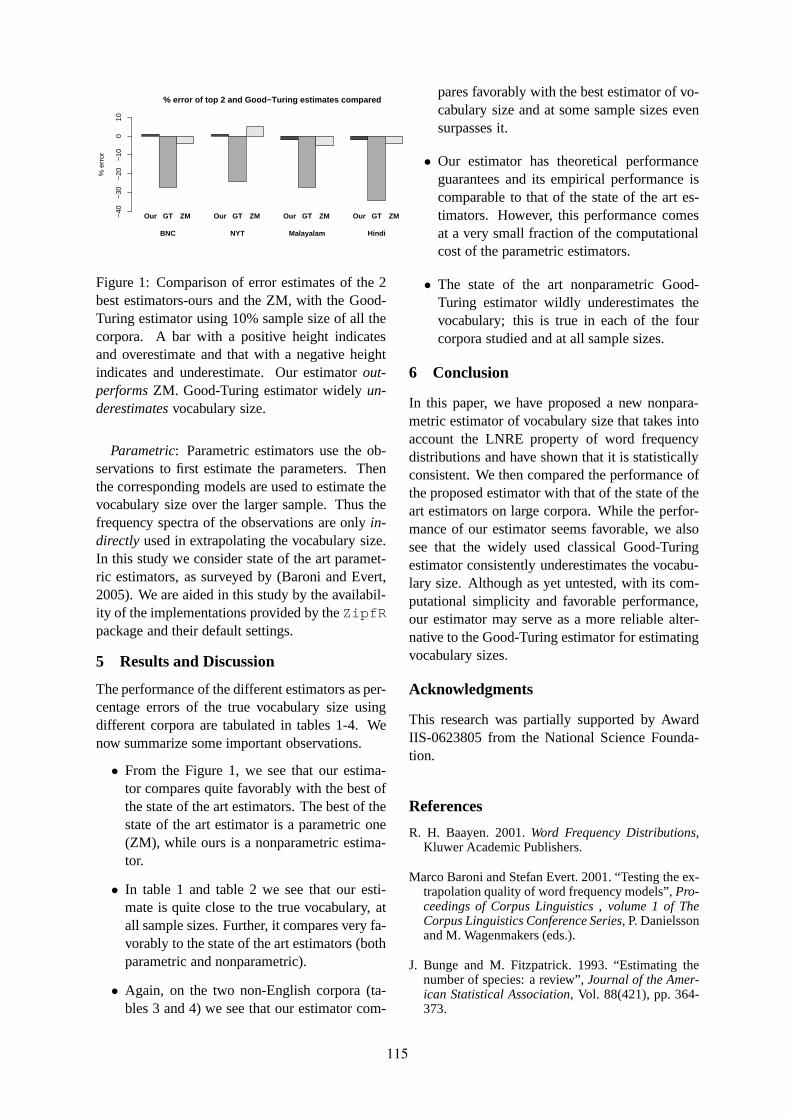
% error of top 2 and Good−Turing estimates compared%
err
or
−40
−30
−20
−10
010
Our GT ZM Our GT ZM Our GT ZM Our GT ZM
BNC NYT Malayalam Hindi
Figure 1: Comparison of error estimates of the 2best estimators-ours and the ZM, with the Good-Turing estimator using 10% sample size of all thecorpora. A bar with a positive height indicatesand overestimate and that with a negative heightindicates and underestimate. Our estimatorout-performsZM. Good-Turing estimator widelyun-derestimatesvocabulary size.
Parametric: Parametric estimators use the ob-servations to first estimate the parameters. Thenthe corresponding models are used to estimate thevocabulary size over the larger sample. Thus thefrequency spectra of the observations are onlyin-directly used in extrapolating the vocabulary size.In this study we consider state of the art paramet-ric estimators, as surveyed by (Baroni and Evert,2005). We are aided in this study by the availabil-ity of the implementations provided by theZipfRpackage and their default settings.
5 Results and Discussion
The performance of the different estimators as per-centage errors of the true vocabulary size usingdifferent corpora are tabulated in tables 1-4. Wenow summarize some important observations.
• From the Figure 1, we see that our estima-tor compares quite favorably with the best ofthe state of the art estimators. The best of thestate of the art estimator is a parametric one(ZM), while ours is a nonparametric estima-tor.
• In table 1 and table 2 we see that our esti-mate is quite close to the true vocabulary, atall sample sizes. Further, it compares very fa-vorably to the state of the art estimators (bothparametric and nonparametric).
• Again, on the two non-English corpora (ta-bles 3 and 4) we see that our estimator com-
pares favorably with the best estimator of vo-cabulary size and at some sample sizes evensurpasses it.
• Our estimator has theoretical performanceguarantees and its empirical performance iscomparable to that of the state of the art es-timators. However, this performance comesat a very small fraction of the computationalcost of the parametric estimators.
• The state of the art nonparametric Good-Turing estimator wildly underestimates thevocabulary; this is true in each of the fourcorpora studied and at all sample sizes.
6 Conclusion
In this paper, we have proposed a new nonpara-metric estimator of vocabulary size that takes intoaccount the LNRE property of word frequencydistributions and have shown that it is statisticallyconsistent. We then compared the performance ofthe proposed estimator with that of the state of theart estimators on large corpora. While the perfor-mance of our estimator seems favorable, we alsosee that the widely used classical Good-Turingestimator consistently underestimates the vocabu-lary size. Although as yet untested, with its com-putational simplicity and favorable performance,our estimator may serve as a more reliable alter-native to the Good-Turing estimator for estimatingvocabulary sizes.
Acknowledgments
This research was partially supported by AwardIIS-0623805 from the National Science Founda-tion.
References
R. H. Baayen. 2001.Word Frequency Distributions,Kluwer Academic Publishers.
Marco Baroni and Stefan Evert. 2001. “Testing the ex-trapolation quality of word frequency models”,Pro-ceedings of Corpus Linguistics , volume 1 of TheCorpus Linguistics Conference Series, P. Danielssonand M. Wagenmakers (eds.).
J. Bunge and M. Fitzpatrick. 1993. “Estimating thenumber of species: a review”,Journal of the Amer-ican Statistical Association, Vol. 88(421), pp. 364-373.
115
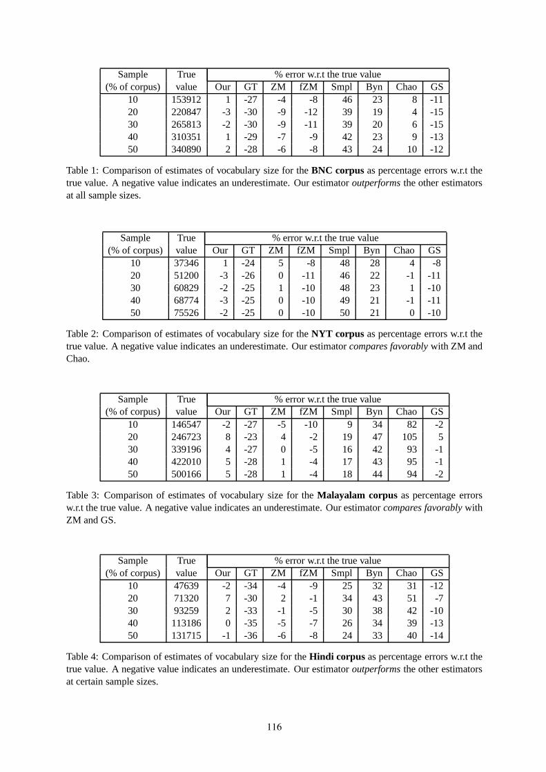
Sample True % error w.r.t the true value(% of corpus) value Our GT ZM fZM Smpl Byn Chao GS
10 153912 1 -27 -4 -8 46 23 8 -1120 220847 -3 -30 -9 -12 39 19 4 -1530 265813 -2 -30 -9 -11 39 20 6 -1540 310351 1 -29 -7 -9 42 23 9 -1350 340890 2 -28 -6 -8 43 24 10 -12
Table 1: Comparison of estimates of vocabulary size for theBNC corpus as percentage errors w.r.t thetrue value. A negative value indicates an underestimate. Our estimatoroutperformsthe other estimatorsat all sample sizes.
Sample True % error w.r.t the true value(% of corpus) value Our GT ZM fZM Smpl Byn Chao GS
10 37346 1 -24 5 -8 48 28 4 -820 51200 -3 -26 0 -11 46 22 -1 -1130 60829 -2 -25 1 -10 48 23 1 -1040 68774 -3 -25 0 -10 49 21 -1 -1150 75526 -2 -25 0 -10 50 21 0 -10
Table 2: Comparison of estimates of vocabulary size for theNYT corpus as percentage errors w.r.t thetrue value. A negative value indicates an underestimate. Our estimatorcompares favorablywith ZM andChao.
Sample True % error w.r.t the true value(% of corpus) value Our GT ZM fZM Smpl Byn Chao GS
10 146547 -2 -27 -5 -10 9 34 82 -220 246723 8 -23 4 -2 19 47 105 530 339196 4 -27 0 -5 16 42 93 -140 422010 5 -28 1 -4 17 43 95 -150 500166 5 -28 1 -4 18 44 94 -2
Table 3: Comparison of estimates of vocabulary size for theMalayalam corpus as percentage errorsw.r.t the true value. A negative value indicates an underestimate. Our estimatorcompares favorablywithZM and GS.
Sample True % error w.r.t the true value(% of corpus) value Our GT ZM fZM Smpl Byn Chao GS
10 47639 -2 -34 -4 -9 25 32 31 -1220 71320 7 -30 2 -1 34 43 51 -730 93259 2 -33 -1 -5 30 38 42 -1040 113186 0 -35 -5 -7 26 34 39 -1350 131715 -1 -36 -6 -8 24 33 40 -14
Table 4: Comparison of estimates of vocabulary size for theHindi corpus as percentage errors w.r.t thetrue value. A negative value indicates an underestimate. Our estimatoroutperformsthe other estimatorsat certain sample sizes.
116

A. Gandolfi and C. C. A. Sastri. 2004. “Nonparamet-ric Estimations about Species not Observed in aRandom Sample”,Milan Journal of Mathematics,Vol. 72, pp. 81-105.
E. V. Khmaladze. 1987. “The statistical analysis oflarge number of rare events”,Technical Report, De-partment of Mathematics and Statistics., CWI, Am-sterdam, MS-R8804.
E. V. Khmaladze and R. J. Chitashvili. 1989. “Statis-tical analysis of large number of rate events and re-lated problems”,Probability theory and mathemati-cal statistics(Russian), Vol. 92, pp. 196-245.
. P. Santhanam, A. Orlitsky, and K. Viswanathan, “Newtricks for old dogs: Large alphabet probability es-timation”, in Proc. 2007IEEE Information TheoryWorkshop, Sept. 2007, pp. 638–643.
A. B. Wagner, P. Viswanath and S. R. Kulkarni. 2006.“Strong Consistency of the Good-Turing estimator”,IEEE Symposium on Information Theory, 2006.
117
Proceedings of the 47th Annual Meeting of the ACL and the 4th IJCNLP of the AFNLP, pages 118–126,Suntec, Singapore, 2-7 August 2009. c©2009 ACL and AFNLP
A Ranking Approach to Stress Predictionfor Letter-to-Phoneme Conversion
Qing Dou, Shane Bergsma, Sittichai Jiampojamarn and Grzegorz KondrakDepartment of Computing Science
University of AlbertaEdmonton, AB, T6G 2E8, Canada
{qdou,bergsma,sj,kondrak}@cs.ualberta.ca
Abstract
Correct stress placement is important intext-to-speech systems, in terms of boththe overall accuracy and the naturalness ofpronunciation. In this paper, we formu-late stress assignment as a sequence pre-diction problem. We represent words assequences of substrings, and use the sub-strings as features in a Support Vector Ma-chine (SVM) ranker, which is trained torank possible stress patterns. The rank-ing approach facilitates inclusion of arbi-trary features over both the input sequenceand output stress pattern. Our system ad-vances the current state-of-the-art, predict-ing primary stress in English, German, andDutch with up to 98% word accuracy onphonemes, and 96% on letters. The sys-tem is also highly accurate in predictingsecondary stress. Finally, when applied intandem with an L2P system, it substan-tially reduces the word error rate whenpredicting both phonemes and stress.
1 Introduction
In many languages, certain syllables in words arephonetically more prominent in terms of duration,pitch, and loudness. This phenomenon is referredto aslexical stress. In some languages, the loca-tion of stress is entirely predictable. For example,lexical stress regularly falls on the initial syllablein Hungarian, and on the penultimate syllable inPolish. In other languages, such as English andRussian, any syllable in the word can be stressed.
Correct stress placement is important in text-to-speech systems because it affects the accuracyof human word recognition (Tagliapietra and Ta-bossi, 2005; Arciuli and Cupples, 2006). How-ever, the issue has often been ignored in previ-ous letter-to-phoneme (L2P) systems. The sys-tems that do generate stress markers often do not
report separate figures on stress prediction accu-racy, or they only provide results on a single lan-guage. Some only predict primary stress mark-ers (Black et al., 1998; Webster, 2004; Demberget al., 2007), while those that predict both primaryand secondary stress generally achieve lower ac-curacy (Bagshaw, 1998; Coleman, 2000; Pearsonet al., 2000).
In this paper, we formulate stress assignment asa sequence prediction problem. We divide eachword into a sequence of substrings, and use thesesubstrings as features for a Support Vector Ma-chine (SVM) ranker. For a given sequence length,there is typically only a small number of stresspatterns in use. The task of the SVM is to rankthe true stress pattern above the small number ofacceptable alternatives. This is the first systemto predict stress within a powerful discriminativelearning framework. By using a ranking approach,we enable the use of arbitrary features over the en-tire (input) sequence and (output) stress pattern.We show that the addition of a feature for the en-tire output sequence improves prediction accuracy.
Our experiments on English, German, andDutch demonstrate that our ranking approach sub-stantially outperforms previous systems. TheSVM ranker achieves exceptional 96.2% word ac-curacy on the challenging task of predicting thefull stress pattern in English. Moreover, whencombining our stress predictions with a state-of-the-art L2P system (Jiampojamarn et al., 2008),we set a new standard for the combined predictionof phonemes and stress.
The paper is organized as follows. Section 2provides background on lexical stress and a taskdefinition. Section 3 presents our automatic stressprediction algorithm. In Section 4, we confirm thepower of the discriminative approach with experi-ments on three languages. Section 5 describes howstress is integrated into L2P conversion.
118

2 Background and Task Definition
There is a long history of research into the prin-ciples governing lexical stress placement. Zipf(1929) showed that stressed syllables are of-ten those with low frequency in speech, whileunstressed syllables are usually very common.Chomsky and Halle (1968) proposed a set ofcontext-sensitive rules for producing Englishstress from underlying word forms. Due to itsimportance in text-to-speech, there is also a longhistory of computational stress prediction sys-tems (Fudge, 1984; Church, 1985; Williams,1987). While these early approaches dependon human definitions of vowel tensity, syllableweight, word etymology, etc., our work followsa recent trend of purely data-driven approaches tostress prediction (Black et al., 1998; Pearson et al.,2000; Webster, 2004; Demberg et al., 2007).
In many languages, only two levels of stressare distinguished: stressed and unstressed. How-ever, some languages exhibit more than two levelsof stress. For example, in the English wordeco-nomic, the first and the third syllable are stressed,with the former receiving weaker emphasis thanthe latter. In this case, the initial syllable is saidto carry a secondary stress. Although each wordhas only one primary stress, it may have any num-ber of secondary stresses. Predicting the full stresspattern is therefore inherently more difficult thanpredicting the location of primary stress only.
Our objective is to automatically assign primaryand, where possible, secondary stress to out-of-vocabulary words. Stress is an attribute of sylla-bles, but syllabification is a non-trivial task in it-self (Bartlett et al., 2008). Rather than assumingcorrect syllabification of the input word, we in-stead follow Webster (2004) in placing the stresson the vowel which constitutes the nucleus of thestressed syllable. If the syllable boundaries areknown, the mapping from the vowel to the cor-responding syllable is straightforward.
We investigate the assignment of stress to tworelated but different entities: the spoken word(represented by its phonetic transcription), andthe written word (represented by its orthographicform). Although stress is a prosodic feature, as-signing stress to written words (“stressed orthog-raphy”) has been utilized as a preprocessing stagefor the L2P task (Webster, 2004). This prepro-cessing is motivated by two factors. First, stressgreatly influences the pronunciation of vowels in
English (c.f., allow vs. alloy). Second, sincephoneme predictors typically utilize only localcontext around a letter, they do not incorporate theglobal, long-range information that is especiallypredictive of stress, such as penultimate syllableemphasis associated with the suffix-ation. By tak-ing stressed orthography as input, the L2P systemis able to implicitly leverage morphological infor-mation beyond the local context.
Indicating stress on letters can also be help-ful to humans, especially second-language learn-ers. In some languages, such as Spanish, ortho-graphic markers are obligatory in words with ir-regular stress. The location of stress is often ex-plicitly marked in textbooks for students of Rus-sian. In both languages, the standard method ofindicating stress is to place an acute accent abovethe vowel bearing primary stress, e.g.,adiós. Thesecondary stress in English can be indicated witha grave accent (Coleman, 2000), e.g.,prèćede.
In summary, our task is to assign primary andsecondary stress markers to stress-bearing vowelsin an input word. The input word may be eitherphonemes or letters. If a stressed vowel is repre-sented by more than one letter, we adopt the con-vention of marking the first vowel of the vowel se-quence, e.g.,méeting. In this way, we are able tofocus on the task of stress prediction, without hav-ing to determine at the same time the exact sylla-ble boundaries, or whether a vowel letter sequencerepresents one or more spoken vowels (e.g.,beat-ing vs. be-at-i-fy).
3 Automatic Stress Prediction
Our stress assignment system maps a word,w, to astressed-form of the word,̄w. We formulate stressassignment as a sequence prediction problem. Theassignment is made in three stages:
(1) First, we map words to substrings (s), the ba-sic units in our sequence (Section 3.1).
(2) Then, a particular stress pattern (t) is chosenfor each substring sequence. We use a sup-port vector machine (SVM) to rank the possi-ble patterns for each sequence (Section 3.2).
(3) Finally, the stress pattern is used to producethe stressed-form of the word (Section 3.3).
Table 1 gives examples of words at each stage ofthe algorithm. We discuss each step in more detail.
119

Word Substrings Pattern Word’w → s → t → w̄
worker → wor-ker → 1-0 → wórkeroverdo → ov-ver-do→ 2-0-1 → òverd́oreact → re-ac → 0-1 → reáct
æbstrækt→ æb-ræk → 0-1 → æbstrǽktprisid → ri-sid → 2-1 → prı̀sı́d
Table 1: The steps in our stress prediction sys-tem (with orthographic and phonetic predictionexamples): (1) word splitting, (2) support vectorranking of stress patterns, and (3) pattern-to-vowelmapping.
3.1 Word Splitting
The first step in our approach is to represent theword as a sequence ofN individual units: w →s = {s1-s2-...-sN}. These units are used to definethe features and outputs used by the SVM ranker.Although we are ultimately interested in assigningstress to individual vowels in the phoneme and let-ter sequence, it is beneficial to represent the task inunits larger than individual letters.
Our substrings are similar to syllables; theyhave a vowel as their nucleus and include con-sonant context. By approximating syllables, oursubstring patterns will allow us to learn recur-rent stress regularities, as well as dependenciesbetween neighboring substrings. Since determin-ing syllable breaks is a non-trivial task, we in-stead adopt the following simple splitting tech-nique. Each vowel in the word forms the nucleusof a substring. Any single preceding or follow-ing consonant is added to the substring unit. Thus,each substring consists of at most three symbols(Table 1).
Using shorter substrings reduces the sparsity ofour training data; words likecryer, dryer andfryerare all mapped to the same form:ry-er. TheSVM can thus generalize from observed words tosimilarly-spelled, unseen examples.
Since the number of vowels equals the num-ber of syllables in the phonetic form of the word,applying this approach to phonemes will alwaysgenerate the correct number of syllables. For let-ters, splitting may result in a different number ofunits than the true syllabification, e.g.,pronounce→ ron-no-un-ce. This does not prevent the systemfrom producing the correct stress assignment afterthe pattern-to-vowel mapping stage (Section 3.3)is complete.
3.2 Stress Prediction with SVM Ranking
After creating a sequence of substring units,s ={s1-s2-...-sN}, the next step is to choose an out-put sequence,t = {t1-t2-...-tN}, that encodeswhether each unit is stressed or unstressed. Weuse the number ‘1’ to indicate that a substring re-ceives primary stress, ‘2’ for secondary stress, and‘0’ to indicate no stress. We call this output se-quence thestress patternfor a word. Table 1 givesexamples of words, substrings, and stress patterns.
We use supervised learning to train a system topredict the stress pattern. We generate training(s, t) pairs in the obvious way from our stress-marked training words,̄w. That is, we first ex-tract the letter/phoneme portion,w, and use itto create the substrings,s. We then create thestress pattern,t, usingw̄’s stress markers. Giventhe training pairs, any sequence predictor can beused, for example a Conditional Random Field(CRF) (Lafferty et al., 2001) or a structured per-ceptron (Collins, 2002). However, we can takeadvantage of a unique property of our problem touse a more expressive framework than is typicallyused in sequence prediction.
The key observation is that the output space ofpossible stress patterns is actually fairly limited.Clopper (2002) shows that people have strongpreferences for particular sequences of stress, andthis is confirmed by our training data (Section 4.1).In English, for example, we find that for each setof spoken words with the same number of sylla-bles, there are no more than fifteen different stresspatterns. In total, among 55K English training ex-amples, there are only 70 different stress patterns.In both German and Dutch there are only about50 patterns in 250K examples.1 Therefore, for aparticular input sequence, we can safely limit ourconsideration to only the small set of output pat-terns of the same length.
Thus, unlike typical sequence predictors, we donot have to search for the highest-scoring outputaccording to our model. We can enumerate thefull set of outputs and simply choose the highest-scoring one. This enables a more expressive rep-resentation. We can define arbitrary features overthe entire output sequence. In a typical CRF orstructured perceptron approach, only output fea-tures that can be computed incrementally duringsearch are used (e.g. Markov transition featuresthat permit Viterbi search). Since search is not
1See (Dou, 2009) for more details.
120
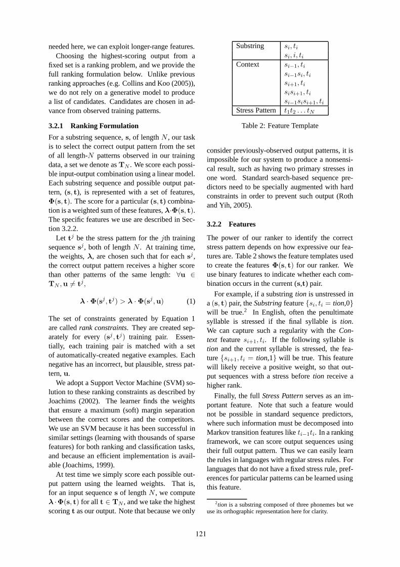
needed here, we can exploit longer-range features.Choosing the highest-scoring output from a
fixed set is a ranking problem, and we provide thefull ranking formulation below. Unlike previousranking approaches (e.g. Collins and Koo (2005)),we do not rely on a generative model to producea list of candidates. Candidates are chosen in ad-vance from observed training patterns.
3.2.1 Ranking Formulation
For a substring sequence,s, of lengthN , our taskis to select the correct output pattern from the setof all length-N patterns observed in our trainingdata, a set we denote asTN . We score each possi-ble input-output combination using a linear model.Each substring sequence and possible output pat-tern, (s, t), is represented with a set of features,Φ(s, t). The score for a particular (s, t) combina-tion is a weighted sum of these features,λ·Φ(s, t).The specific features we use are described in Sec-tion 3.2.2.
Let tj be the stress pattern for thejth trainingsequencesj, both of lengthN . At training time,the weights,λ, are chosen such that for eachsj ,the correct output pattern receives a higher scorethan other patterns of the same length:∀u ∈TN ,u 6= tj,
λ ·Φ(sj, tj) > λ ·Φ(sj ,u) (1)
The set of constraints generated by Equation 1are calledrank constraints. They are created sep-arately for every(sj , tj) training pair. Essen-tially, each training pair is matched with a setof automatically-created negative examples. Eachnegative has an incorrect, but plausible, stress pat-tern,u.
We adopt a Support Vector Machine (SVM) so-lution to these ranking constraints as described byJoachims (2002). The learner finds the weightsthat ensure a maximum (soft) margin separationbetween the correct scores and the competitors.We use an SVM because it has been successful insimilar settings (learning with thousands of sparsefeatures) for both ranking and classification tasks,and because an efficient implementation is avail-able (Joachims, 1999).
At test time we simply score each possible out-put pattern using the learned weights. That is,for an input sequences of lengthN , we computeλ ·Φ(s, t) for all t ∈ TN , and we take the highestscoringt as our output. Note that because we only
Substring si, tisi, i, ti
Context si−1, tisi−1si, tisi+1, tisisi+1, tisi−1sisi+1, ti
Stress Pattern t1t2 . . . tN
Table 2: Feature Template
consider previously-observed output patterns, it isimpossible for our system to produce a nonsensi-cal result, such as having two primary stresses inone word. Standard search-based sequence pre-dictors need to be specially augmented with hardconstraints in order to prevent such output (Rothand Yih, 2005).
3.2.2 Features
The power of our ranker to identify the correctstress pattern depends on how expressive our fea-tures are. Table 2 shows the feature templates usedto create the featuresΦ(s, t) for our ranker. Weuse binary features to indicate whether each com-bination occurs in the current (s,t) pair.
For example, if a substringtion is unstressed ina(s, t) pair, theSubstringfeature{si, ti = tion,0}will be true.2 In English, often the penultimatesyllable is stressed if the final syllable istion.We can capture such a regularity with theCon-text featuresi+1, ti. If the following syllable istion and the current syllable is stressed, the fea-ture{si+1, ti = tion,1} will be true. This featurewill likely receive a positive weight, so that out-put sequences with a stress beforetion receive ahigher rank.
Finally, the full Stress Patternserves as an im-portant feature. Note that such a feature wouldnot be possible in standard sequence predictors,where such information must be decomposed intoMarkov transition features liketi−1ti. In a rankingframework, we can score output sequences usingtheir full output pattern. Thus we can easily learnthe rules in languages with regular stress rules. Forlanguages that do not have a fixed stress rule, pref-erences for particular patterns can be learned usingthis feature.
2tion is a substring composed of three phonemes but weuse its orthographic representation here for clarity.
121
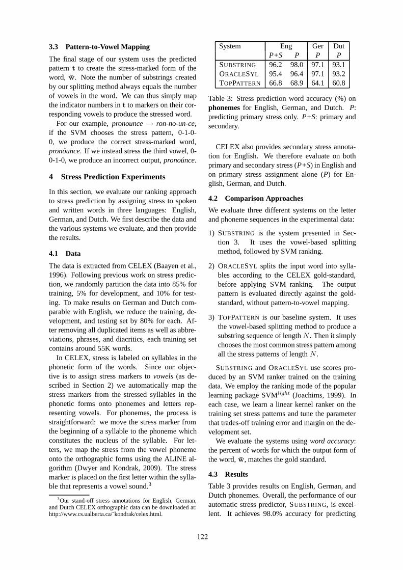
3.3 Pattern-to-Vowel Mapping
The final stage of our system uses the predictedpatternt to create the stress-marked form of theword, w̄. Note the number of substrings createdby our splitting method always equals the numberof vowels in the word. We can thus simply mapthe indicator numbers int to markers on their cor-responding vowels to produce the stressed word.
For our example,pronounce→ ron-no-un-ce,if the SVM chooses the stress pattern, 0-1-0-0, we produce the correct stress-marked word,pronóunce. If we instead stress the third vowel, 0-0-1-0, we produce an incorrect output,pronóunce.
4 Stress Prediction Experiments
In this section, we evaluate our ranking approachto stress prediction by assigning stress to spokenand written words in three languages: English,German, and Dutch. We first describe the data andthe various systems we evaluate, and then providethe results.
4.1 Data
The data is extracted from CELEX (Baayen et al.,1996). Following previous work on stress predic-tion, we randomly partition the data into 85% fortraining, 5% for development, and 10% for test-ing. To make results on German and Dutch com-parable with English, we reduce the training, de-velopment, and testing set by 80% for each. Af-ter removing all duplicated items as well as abbre-viations, phrases, and diacritics, each training setcontains around 55K words.
In CELEX, stress is labeled on syllables in thephonetic form of the words. Since our objec-tive is to assign stress markers tovowels(as de-scribed in Section 2) we automatically map thestress markers from the stressed syllables in thephonetic forms onto phonemes and letters rep-resenting vowels. For phonemes, the process isstraightforward: we move the stress marker fromthe beginning of a syllable to the phoneme whichconstitutes the nucleus of the syllable. For let-ters, we map the stress from the vowel phonemeonto the orthographic forms using the ALINE al-gorithm (Dwyer and Kondrak, 2009). The stressmarker is placed on the first letter within the sylla-ble that represents a vowel sound.3
3Our stand-off stress annotations for English, German,and Dutch CELEX orthographic data can be downloaded at:http://www.cs.ualberta.ca/˜kondrak/celex.html.
System Eng Ger DutP+S P P P
SUBSTRING 96.2 98.0 97.1 93.1ORACLESYL 95.4 96.4 97.1 93.2TOPPATTERN 66.8 68.9 64.1 60.8
Table 3: Stress prediction word accuracy (%) onphonemesfor English, German, and Dutch.P:predicting primary stress only.P+S: primary andsecondary.
CELEX also provides secondary stress annota-tion for English. We therefore evaluate on bothprimary and secondary stress (P+S) in English andon primary stress assignment alone (P) for En-glish, German, and Dutch.
4.2 Comparison Approaches
We evaluate three different systems on the letterand phoneme sequences in the experimental data:
1) SUBSTRING is the system presented in Sec-tion 3. It uses the vowel-based splittingmethod, followed by SVM ranking.
2) ORACLESYL splits the input word into sylla-bles according to the CELEX gold-standard,before applying SVM ranking. The outputpattern is evaluated directly against the gold-standard, without pattern-to-vowel mapping.
3) TOPPATTERN is our baseline system. It usesthe vowel-based splitting method to produce asubstring sequence of lengthN . Then it simplychooses the most common stress pattern amongall the stress patterns of lengthN .
SUBSTRING and ORACLESYL use scores pro-duced by an SVM ranker trained on the trainingdata. We employ the ranking mode of the popularlearning package SVMlight (Joachims, 1999). Ineach case, we learn a linear kernel ranker on thetraining set stress patterns and tune the parameterthat trades-off training error and margin on the de-velopment set.
We evaluate the systems usingword accuracy:the percent of words for which the output form ofthe word,w̄, matches the gold standard.
4.3 Results
Table 3 provides results on English, German, andDutch phonemes. Overall, the performance of ourautomatic stress predictor, SUBSTRING, is excel-lent. It achieves 98.0% accuracy for predicting
122
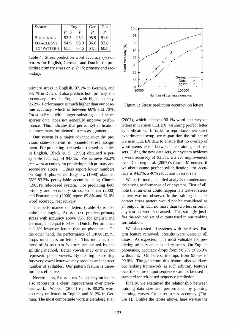
System Eng Ger DutP+S P P P
SUBSTRING 93.5 95.1 95.9 91.0ORACLESYL 94.6 96.0 96.6 92.8TOPPATTERN 65.5 67.6 64.1 60.8
Table 4: Stress prediction word accuracy (%) onletters for English, German, and Dutch.P: pre-dicting primary stress only.P+S: primary and sec-ondary.
primary stress in English, 97.1% in German, and93.1% in Dutch. It also predicts both primary andsecondary stress in English with high accuracy,96.2%. Performance is much higher than our base-line accuracy, which is between 60% and 70%.ORACLESYL , with longer substrings and hencesparser data, does not generally improve perfor-mance. This indicates that perfect syllabificationis unnecessary for phonetic stress assignment.
Our system is a major advance over the pre-vious state-of-the-art in phonetic stress assign-ment. For predicting stressed/unstressed syllablesin English, Black et al. (1998) obtained a per-syllable accuracy of 94.6%. We achieve 96.2%per-wordaccuracy for predicting both primary andsecondary stress. Others report lower numberson English phonemes. Bagshaw (1998) obtained65%-83.3% per-syllable accuracy using Church(1985)’s rule-based system. For predicting bothprimary and secondary stress, Coleman (2000)and Pearson et al. (2000) report 69.8% and 81.0%word accuracy, respectively.
The performance on letters (Table 4) is alsoquite encouraging. SUBSTRING predicts primarystress with accuracy above 95% for English andGerman, and equal to 91% in Dutch. Performanceis 1-3% lower on letters than on phonemes. Onthe other hand, the performance of ORACLESYL
drops much less on letters. This indicates thatmost of SUBSTRING’s errors are caused by thesplitting method. Letter vowels may or may notrepresent spoken vowels. By creating a substringfor every vowel letter we may produce an incorrectnumber of syllables. Our pattern feature is there-fore less effective.
Nevertheless, SUBSTRING’s accuracy on lettersalso represents a clear improvement over previ-ous work. Webster (2004) reports 80.3% wordaccuracy on letters in English and 81.2% in Ger-man. The most comparable work is Demberg et al.
84
86
88
90
92
94
96
98
100
10000 100000
Wor
d A
ccur
acy
(%)
Number of training examples
GermanDutch
English
Figure 1: Stress prediction accuracy on letters.
(2007), which achieves 90.1% word accuracy onletters in German CELEX, assuming perfect lettersyllabification. In order to reproduce their strictexperimental setup, we re-partition the full set ofGerman CELEX data to ensure that no overlap ofword stems exists between the training and testsets. Using the new data sets, our system achievesa word accuracy of 92.3%, a 2.2% improvementover Demberg et al. (2007)’s result. Moreover, ifwe also assume perfect syllabification, the accu-racy is 94.3%, a 40% reduction in error rate.
We performed a detailed analysis to understandthe strong performance of our system. First of all,note that an error could happen if a test-set stresspattern was not observed in the training data; itscorrect stress pattern would not be considered asan output. In fact, no more than two test errors inany test set were so caused. This strongly justi-fies the reduced set of outputs used in our rankingformulation.
We also tested all systems with the Stress Pat-tern feature removed. Results were worse in allcases. As expected, it is most valuable for pre-dicting primary and secondary stress. On Englishphonemes, accuracy drops from 96.2% to 95.3%without it. On letters, it drops from 93.5% to90.0%. The gain from this feature also validatesour ranking framework, as such arbitrary featuresover the entire output sequence can not be used instandard search-based sequence prediction.
Finally, we examined the relationship betweentraining data size and performance by plottinglearning curves for letter stress accuracy (Fig-ure 1). Unlike the tables above, here we use the
123

full set of data in Dutch and German CELEX tocreate the largest-possible training sets (255K ex-amples). None of the curves are levelling off; per-formance grows log-linearly across the full range.
5 Lexical stress and L2P conversion
In this section, we evaluate various methods ofcombining stress prediction with phoneme gener-ation. We first describe the specific system that weuse for letter-to-phoneme (L2P) conversion. Wethen discuss the different ways stress predictioncan be integrated with L2P, and define the systemsused in our experiments. Finally, we provide theresults.
5.1 The L2P system
We combine stress prediction with a state-of-the-art L2P system (Jiampojamarn et al., 2008). Likeour stress ranker, their system is a data-driven se-quence predictor that is trained with supervisedlearning. The score for each output sequence isa weighted combination of features. The featureweights are trained using the Margin Infused Re-laxed Algorithm (MIRA) (Crammer and Singer,2003), a powerful online discriminative trainingframework. Like other recent L2P systems (Bisaniand Ney, 2002; Marchand and Damper, 2007; Ji-ampojamarn et al., 2007), this approach does notgenerate stress, nor does it consider stress when itgenerates phonemes.
For L2P experiments, we use the same training,testing, and development data as was used in Sec-tion 4. For all experiments, we use the develop-ment set to determine at which iteration to stoptraining in the online algorithm.
5.2 Combining stress and phonemegeneration
Various methods have been used for combiningstress and phoneme generation. Phonemes can begenerated without regard to stress, with stress as-signed as a post-process (Bagshaw, 1998; Cole-man, 2000). Both van den Bosch (1997) andBlack et al. (1998) argue that stress should be pre-dicted at the same time as phonemes. They ex-pand the output set to distinguish between stressedand unstressed phonemes. Similarly, Demberg etal. (2007) produce phonemes, stress, and syllable-boundaries within a single joint n-gram model.Pearson et al. (2000) generate phonemes and stresstogether by jointly optimizing a decision-tree
phoneme-generator and a stress predictor based onstress pattern counts. In contrast, Webster (2004)first assigns stress to letters, creating an expandedinput set, and then predicts both phonemes andstress jointly. The system marks stress on let-ter vowels by determining the correspondence be-tween affixes and stress in written words.
Following the above approaches, we can expandthe input or output symbols of our L2P system toinclude stress. However, since both decision treesystems and our L2P predictor utilize only localcontext, they may produce invalid global output.One option, used by Demberg et al. (2007), is toadd a constraint to the output generation, requiringeach output sequence to have exactly one primarystress.
We enhance this constraint, based on the obser-vation that the number of valid output sequencesis fairly limited (Section 3.2). The modified sys-tem produces the highest-scoring sequence suchthat the output’s corresponding stress pattern hasbeen observed in our training data. We call thisthe stress pattern constraint. This is a tighterconstraint than having only one primary stress.4
Another advantage is that it provides some guid-ance for the assignment of secondary stress.
Inspired by the aforementioned strategies, weevaluate the following approaches:
1) JOINT: The L2P system’s input sequence is let-ters, the output sequence is phonemes+stress.
2) JOINT+CONSTR: Same as JOINT, except it se-lects the highest scoring output that obeys thestress pattern constraint.
3) POSTPROCESS: The L2P system’s input is let-ters, the output is phonemes. It then applies theSVM stress ranker (Section 3) to the phonemesto produce the full phoneme+stress output.
4) LETTERSTRESS: The L2P system’s input isletters+stress, the output is phonemes+stress.It creates the stress-marked letters by applyingthe SVM ranker to the input letters as a pre-process.
5) ORACLESTRESS: The same input/output asLETTERSTRESS, except it uses the gold-standard stress on letters (Section 4.1).4In practice, the L2P system generates a top-N list, and
we take the highest-scoring output on the list that satisfiesthe constraint. If none satisfy the constraint, we take the topoutput that has only one primary stress.
124

System Eng Ger DutP+S P P P
JOINT 78.9 80.0 86.0 81.1JOINT+CONSTR 84.6 86.0 90.8 88.7POSTPROCESS 86.2 87.6 90.9 88.8LETTERSTRESS 86.5 87.2 90.1 86.6ORACLESTRESS 91.4 91.4 92.6 94.5Festival 61.2 62.5 71.8 65.1
Table 5: Combined phonemeand stress predic-tion word accuracy (%) for English, German, andDutch. P: predicting primary stress only.P+S:primary and secondary.
Note that while the first approach uses onlylocal information to make predictions (featureswithin a context window around the current let-ter), systems 2 to 5 leverage global information insome manner: systems 3 and 4 use the predictionsof our stress ranker, while 2 uses a global stresspattern constraint.5
We also generated stress and phonemes usingthe popular Festival Speech Synthesis System6
(version 1.96, 2004) and report its accuracy.
5.3 Results
Word accuracy results for predicting bothphonemes and stress are provided in Table 5.First of all, note that the JOINT approach,which simply expands the output set, is 4%-8% worse than all other comparison systemsacross the three languages. These results clearlyindicate the drawbacks of predicting stress us-ing only local information. In English, bothLETTERSTRESS and POSTPROCESS performbest, while POSTPROCESS and the constrainedsystem are highest on German and Dutch. Resultsusing the oracle letter stress show that givenperfect stress assignment on letters, phonemesand stress can be predicted very accurately, in allcases above 91%.
We also found that the phoneme prediction ac-curacy alone (i.e., without stress) is quite simi-lar for all the systems. The gains over JOINT
on combined stress and phoneme accuracy arealmost entirely due to more accurate stress as-signment. Utilizing the oracle stress on lettersmarkedly improves phoneme prediction in English
5This constraint could also help the other systems. How-ever, since they already use global information, it yields onlymarginal improvements.
6http://www.cstr.ed.ac.uk/projects/festival/
(from 88.8% to 91.4%). This can be explained bythe fact that English vowels are often reduced toschwa when unstressed (Section 2).
Predicting both phonemes and stress is a chal-lenging task, and each of our globally-informedsystems represents a major improvement over pre-vious work. The accuracy of Festival is muchlower even than our JOINT approach, but the rel-ative performance on the different languages isquite similar.
A few papers report accuracy on the combinedstress and phoneme prediction task. The most di-rectly comparable work is van den Bosch (1997),which also predicts primary and secondary stressusing English CELEX data. However, the re-ported word accuracy is only 62.1%. Three otherpapers report word accuracy on phonemes andstress, using different data sets. Pearson et al.(2000) report 58.5% word accuracy for predictingphonemes and primary/secondary stress. Black etal. (1998) report 74.6% word accuracy in English,while Webster (2004) reports 68.2% on Englishand 82.9% in German (all primary stress only).Finally, Demberg et al. (2007) report word accu-racy on predicting phonemes, stress,and syllab-ification on German CELEX data. They achieve86.3% word accuracy.
6 Conclusion
We have presented a discriminative ranking ap-proach to lexical stress prediction, which clearlyoutperforms previously developed systems. Theapproach is largely language-independent, appli-cable to both orthographic and phonetic repre-sentations, and flexible enough to handle multi-ple stress levels. When combined with an exist-ing L2P system, it achieves impressive accuracyin generating pronunciations together with theirstress patterns. In the future, we will investigateadditional features to leverage syllabic and mor-phological information, when available. Kernelfunctions could also be used to automatically cre-ate a richer feature space; preliminary experimentshave shown gains in performance using polyno-mial and RBF kernels with our stress ranker.
Acknowledgements
This research was supported by the NaturalSciences and Engineering Research Council ofCanada, the Alberta Ingenuity Fund, and the Al-berta Informatics Circle of Research Excellence.
125
References
Joanne Arciuli and Linda Cupples. 2006. The pro-cessing of lexical stress during visual word recog-nition: Typicality effects and orthographic corre-lates. Quarterly Journal of Experimental Psychol-ogy, 59(5):920–948.
Harald Baayen, Richard Piepenbrock, and Leon Gu-likers. 1996. The CELEX2 lexical database.LDC96L14.
Paul C. Bagshaw. 1998. Phonemic transcription byanalogy in text-to-speech synthesis: Novel wordpronunciation and lexicon compression.ComputerSpeech and Language, 12(2):119–142.
Susan Bartlett, Grzegorz Kondrak, and Colin Cherry.2008. Automatic syllabification with structuredSVMs for letter-to-phoneme conversion. InACL-08: HLT, pages 568–576.
Maximilian Bisani and Hermann Ney. 2002. Investi-gations on joint-multigram models for grapheme-to-phoneme conversion. InICSLP, pages 105–108.
Alan W Black, Kevin Lenzo, and Vincent Pagel. 1998.Issues in building general letter to sound rules. InThe 3rd ESCA Workshop on Speech Synthesis, pages77–80.
Noam Chomsky and Morris Halle. 1968. The soundpattern of English.New York: Harper and Row.
Kenneth Church. 1985. Stress assignment in letterto sound rules for speech synthesis. InACL, pages246–253.
Cynthia G. Clopper. 2002. Frequency of stress pat-terns in English: A computational analysis.IULCWorking Papers Online.
John Coleman. 2000. Improved prediction of stress inout-of-vocabulary words. InIEEE Seminar on theState of the Art in Speech Synthesis.
Michael Collins and Terry Koo. 2005. Discriminativereranking for natural language parsing.Computa-tional Linguistics, 31(1):25–70.
Michael Collins. 2002. Discriminative training meth-ods for Hidden Markov Models: Theory and ex-periments with perceptron algorithms. InEMNLP,pages 1–8.
Koby Crammer and Yoram Singer. 2003. Ultracon-servative online algorithms for multiclass problems.Journal of Machine Learning Research, 3:951–991.
Vera Demberg, Helmut Schmid, and Gregor Möhler.2007. Phonological constraints and morphologi-cal preprocessing for grapheme-to-phoneme conver-sion. InACL, pages 96–103.
Qing Dou. 2009. An SVM ranking approach to stressassignment. Master’s thesis, University of Alberta.
Kenneth Dwyer and Grzegorz Kondrak. 2009. Reduc-ing the annotation effort for letter-to-phoneme con-version. InACL-IJCNLP.
Erik C. Fudge. 1984. English word-stress.London:Allen and Unwin.
Sittichai Jiampojamarn, Grzegorz Kondrak, and TarekSherif. 2007. Applying many-to-many alignmentsand Hidden Markov Models to letter-to-phonemeconversion. InNAACL-HLT 2007, pages 372–379.
Sittichai Jiampojamarn, Colin Cherry, and GrzegorzKondrak. 2008. Joint processing and discriminativetraining for letter-to-phoneme conversion. InACL-08: HLT, pages 905–913.
Thorsten Joachims. 1999. Making large-scale SupportVector Machine learning practical. In B. Schölkopfand C. Burges, editors,Advances in Kernel Meth-ods: Support Vector Machines, pages 169–184.MIT-Press.
Thorsten Joachims. 2002. Optimizing search enginesusing clickthrough data. InKDD, pages 133–142.
John D. Lafferty, Andrew McCallum, and FernandoC. N. Pereira. 2001. Conditional Random Fields:Probabilistic models for segmenting and labeling se-quence data. InICML, pages 282–289.
Yannick Marchand and Robert I. Damper. 2007. Cansyllabification improve pronunciation by analogy ofEnglish? Natural Language Engineering, 13(1):1–24.
Steve Pearson, Roland Kuhn, Steven Fincke, and NickKibre. 2000. Automatic methods for lexical stressassignment and syllabification. InICSLP, pages423–426.
Dan Roth and Wen-tau Yih. 2005. Integer linear pro-gramming inference for conditional random fields.In ICML, pages 736–743.
Lara Tagliapietra and Patrizia Tabossi. 2005. Lexicalstress effects in Italian spoken word recognition. InThe XXVII Annual Conference of the Cognitive Sci-ence Society, pages 2140–2144.
Antal van den Bosch. 1997.Learning to pronouncewritten words: A study in inductive language learn-ing. Ph.D. thesis, Universiteit Maastricht.
Gabriel Webster. 2004. Improving letter-to-pronunciation accuracy with automaticmorphologically-based stress prediction. InICSLP, pages 2573–2576.
Briony Williams. 1987. Word stress assignment in atext-to-speech synthesis system for British English.Computer Speech and Language, 2:235–272.
George Kingsley Zipf. 1929. Relative frequency as adeterminant of phonetic change.Harvard Studies inClassical Philology, 15:1–95.
126

Proceedings of the 47th Annual Meeting of the ACL and the 4th IJCNLP of the AFNLP, pages 127–135,Suntec, Singapore, 2-7 August 2009. c©2009 ACL and AFNLP
Reducing the Annotation Effort for Letter-to-Phoneme Conversion
Kenneth Dwyer and Grzegorz KondrakDepartment of Computing Science
University of AlbertaEdmonton, AB, Canada, T6G 2E8
{dwyer,kondrak}@cs.ualberta.ca
Abstract
Letter-to-phoneme (L2P) conversion is theprocess of producing a correct phonemesequence for a word, given its letters. Itis often desirable to reduce the quantity oftraining data — and hence human anno-tation — that is needed to train an L2Pclassifier for a new language. In this pa-per, we confront the challenge of buildingan accurate L2P classifier with a minimalamount of training data by combining sev-eral diverse techniques: context ordering,letter clustering, active learning, and pho-netic L2P alignment. Experiments on sixlanguages show up to 75% reduction in an-notation effort.
1 Introduction
The task of letter-to-phoneme (L2P) conversionis to produce a correct sequence of phonemes,given the letters that comprise a word. An ac-curate L2P converter is an important componentof a text-to-speech system. In general, a lookuptable does not suffice for L2P conversion, sinceout-of-vocabulary words (e.g., proper names) areinevitably encountered. This motivates the needfor classification techniques that can predict thephonemes for an unseen word.
Numerous studies have contributed to the de-velopment of increasingly accurate L2P sys-tems (Black et al., 1998; Kienappel and Kneser,2001; Bisani and Ney, 2002; Demberg et al., 2007;Jiampojamarn et al., 2008). A common assump-tion made in these works is that ample amounts oflabelled data are available for training a classifier.Yet, in practice, this is the case for only a smallnumber of languages. In order to train an L2P clas-sifier for a new language, we must first annotatewords in that language with their correct phonemesequences. As annotation is expensive, we would
like to minimize the amount of effort that is re-quired to build an adequate training set. The ob-jective of this work is not necessarily to achievestate-of-the-art performance when presented withlarge amounts of training data, but to outperformother approaches when training data is limited.
This paper proposes a system for training an ac-curate L2P classifier while requiring as few an-notated words as possible. We employ decisiontrees as our supervised learning method because oftheir transparency and flexibility. We incorporatecontext ordering into a decision tree learner thatguides its tree-growing procedure towards gener-ating more intuitive rules. A clustering over lettersserves as a back-off model in cases where individ-ual letter counts are unreliable. An active learningtechnique is employed to request the phonemes(labels) for the words that are expected to be themost informative. Finally, we apply a novel L2Palignment technique based on phonetic similarity,which results in impressive gains in accuracy with-out relying on any training data.
Our empirical evaluation on several L2Pdatasets demonstrates that significant reductionsin annotation effort are indeed possible in this do-main. Individually, all four enhancements improvethe accuracy of our decision tree learner. The com-bined system yields savings of up to 75% in thenumber of words that have to be labelled, and re-ductions of at least 52% are observed on all thedatasets. This is achieved without any additionaltuning for the various languages.
The paper is organized as follows. Section 2 ex-plains how supervised learning for L2P conversionis carried out with decision trees, our classifier ofchoice. Sections 3 through 6 describe our fourmain contributions towards reducing the annota-tion effort for L2P: context ordering (Section 3),clustering letters (Section 4), active learning (Sec-tion 5), and phonetic alignment (Section 6). Ourexperimental setup and results are discussed in
127
Sections 7 and 8, respectively. Finally, Section 9offers some concluding remarks.
2 Decision tree learning of L2P classifiers
In this work, we employ a decision tree modelto learn the mapping from words to phoneme se-quences. Decision tree learners are attractive be-cause they are relatively fast to train, require littleor no parameter tuning, and the resulting classifiercan be interpreted by the user. A number of priorstudies have applied decision trees to L2P data andhave reported good generalization accuracy (An-dersen et al., 1996; Black et al., 1998; Kienappeland Kneser, 2001). Also, the widely-used Festi-val Speech Synthesis System (Taylor et al., 1998)relies on decision trees for L2P conversion.
We adopt the standard approach of using theletter context as features. The decision tree pre-dicts the phoneme for the focus letter based onthe m letters that appear before and after it inthe word (including the focus letter itself, and be-ginning/end of word markers, where applicable).The model predicts a phoneme independently foreach letter in a given word. In order to keep ourmodel simple and transparent, we do not explorethe possibility of conditioning on adjacent (pre-dicted) phonemes. Any improvement in accuracyresulting from the inclusion of phoneme featureswould also be realized by the baseline that wecompare against, and thus would not materially in-fluence our findings.
We employ binary decision trees because theysubstantially outperformed n-ary trees in our pre-liminary experiments. In L2P, there are manyunique values for each attribute, namely, the let-ters of a given alphabet. In a n-ary tree each de-cision node partitions the data into n subsets, oneper letter, that are potentially sparse. By contrast,a binary tree creates one branch for the nominatedletter, and one branch grouping the remaining let-ters into a single subset. In the forthcoming exper-iments, we use binary decision trees exclusively.
3 Context ordering
In the L2P task, context letters that are adjacentto the focus letter tend to be more important thancontext letters that are further away. For exam-ple, the English letter c is usually pronounced as[s] if the following letter is e or i. The generaltree-growing algorithm has no notion of the letterdistance, but instead chooses the letters on the ba-
sis of their estimated information gain (Manningand Schütze, 1999). As a result, it will sometimesquery a letter at position +3 (denoted l3), for ex-ample, before examining the letters that are closerto the center of the context window.
We propose to modify the tree-growing proce-dure to encourage the selection of letters near thefocus letter before those at greater offsets are ex-amined. In its strictest form, which resemblesthe “dynamically expanding context” search strat-egy of Davel and Barnard (2004), li can only bequeried after l0, . . . , li−1 have been queried. How-ever, this approach seems overly rigid for L2P. InEnglish, for example, l2 can directly influence thepronunciation of a vowel regardless of the value ofl1 (c.f., the difference between rid and ride).
Instead, we adopt a less intrusive strategy,which we refer to as “context ordering,” that biasesthe decision tree toward letters that are closer tothe focus, but permits gaps when the informationgain for a distant letter is relatively high. Specif-ically, the ordering constraint described above isstill applied, but only to letters that have above-average information gain (where the average iscalculated across all letters/attributes). This meansthat a letter with above-average gain that is eligi-ble with respect to the ordering will take prece-dence over an ineligible letter that has an evenhigher gain. However, if all the eligible lettershave below-average gain, the ineligible letter withthe highest gain is selected irrespective of its posi-tion. Our only strict requirement is that the focusletter must always be queried first, unless its infor-mation gain is zero.
Kienappel and Kneser (2001) also worked onimproving decision tree performance for L2P, anddevised tie-breaking rules in the event that the tree-growing procedure ranked two or more questionsas being equally informative. In our experiencewith L2P datasets, exact ties are rare; our contextordering mechanism will have more opportunitiesto guide the tree-growing process. We expect thischange to improve accuracy, especially when theamount of training data is very limited. By biasingthe decision tree learner toward questions that areintuitively of greater utility, we make it less proneto overfitting on small data samples.
4 Clustering letters
A decision tree trained on L2P data bases its pho-netic predictions on the surrounding letter context.
128

Yet, when making predictions for unseen words,contexts will inevitably be encountered that didnot appear in the training data. Instead of rely-ing solely on the particular letters that surroundthe focus letter, we postulate that the learner couldachieve better generalization if it had access toinformation about the types of letters that appearbefore and after. That is, instead of treating let-ters as abstract symbols, we would like to encodeknowledge of the similarity between certain lettersas features. One way of achieving this goal is togroup the letters into classes or clusters based ontheir contextual similarity. Then, when a predic-tion has to be made for an unseen (or low probabil-ity) letter sequence, the letter classes can provideadditional information.
Kienappel and Kneser (2001) report accuracygains when applying letter clustering to the L2Ptask. However, their decision tree learner incorpo-rates neighboring phoneme predictions, and em-ploys a variety of different pruning strategies; theportion of the gains attributable to letter clusteringare not evident. In addition to exploring the effectof letter clustering on a wider range of languages,we are particularly concerned with the impact thatclustering has on decision tree performance whenthe training set is small. The addition of letter classfeatures to the data may enable the active learnerto better evaluate candidate words in the pool, andtherefore make more informed selections.
To group the letters into classes, we employa hierarchical clustering algorithm (Brown et al.,1992). One advantage of inducing a hierarchy isthat we need not commit to a particular level ofgranularity; in other words, we are not required tospecify the number of classes beforehand, as is thecase with some other clustering algorithms.1
The clustering algorithm is initialized by plac-ing each letter in its own class, and then pro-ceeds in a bottom-up manner. At each step, thepair of classes is merged that leads to the small-est loss in the average mutual information (Man-ning and Schütze, 1999) between adjacent classes.The merging process repeats until a single classremains that contains all the letters in the alpha-bet. Recall that in our problem setting we haveaccess to a (presumably) large pool of unanno-tated words. The unigram and bigram frequen-cies required by the clustering algorithm are cal-
1This approach is inspired by the work of Miller et al.(2004), who clustered words for a named-entity tagging task.
Letter Bit String Letter Bit Stringa 01000 n 1111b 10000000 o 01001c 10100 p 10001d 11000 q 1000001e 0101 r 111010f 100001 s 11010g 11001 t 101010h 10110 u 0111i 0110 v 100110j 10000001 w 100111k 10111 x 111011l 11100 y 11011
m 10010 z 101011# 00
Table 1: Hierarchical clustering of English letters
culated from these words; hence, the letters canbe grouped into classes prior to annotation. Theletter classes only need to be computed once fora given language. We implemented a brute-forceversion of the algorithm that examines all the pos-sible merges at each step, and generates a hierar-chy within a few hours. However, when dealingwith a larger number of unique tokens (e.g., whenclustering words instead of letters), additional op-timizations are needed in order to make the proce-dure tractable.
The resulting hierarchy takes the form of a bi-nary tree, where the root node/cluster contains allthe letters, and each leaf contains a single let-ter. Hence, each letter can be represented by a bitstring that describes the path from the root to itsleaf. As an illustration, the clustering in Table 1was automatically generated from the words in theEnglish CMU Pronouncing Dictionary (CarnegieMellon University, 1998). It is interesting to notethat the first bit distinguishes vowels from con-sonants, meaning that these were the last twogroups that were merged by the clustering algo-rithm. Note also that the beginning/end of wordmarker (#) is included in the hierarchy, and is thelast character to be absorbed into a larger clus-ter. This indicates that # carries more informa-tion than most letters, as is to be expected, in lightof its distinct status. We also experimented witha manually-constructed letter hierarchy, but ob-served no significant differences in accuracy vis-à-vis the automatic clustering.
129
5 Active learning
Whereas a passive supervised learning algorithmis provided with a collection of training exam-ples that are typically drawn at random, an activelearner has control over the labelled data that it ob-tains (Cohn et al., 1992). The latter attempts to se-lect its training set intelligently by requesting thelabels of only those examples that are judged to bethe most useful or informative. Numerous studieshave demonstrated that active learners can makemore efficient use of unlabelled data than do pas-sive learners (Abe and Mamitsuka, 1998; Milleret al., 2004; Culotta and McCallum, 2005). How-ever, relatively few researchers have applied activelearning techniques to the L2P domain. This isdespite the fact that annotated data for training anL2P classifier is not available in most languages.We briefly review two relevant studies before pro-ceeding to describe our active learning strategy.
Maskey et al. (2004) propose a bootstrappingtechnique that iteratively requests the labels of then most frequent words in a corpus. A classifier istrained on the words that have been annotated thusfar, and then predicts the phonemes for each of then words being considered. Words for which theprediction confidence is above a certain thresholdare immediately added to the lexicon, while the re-maining words must be verified (and corrected, ifnecessary) by a human annotator. The main draw-back of such an approach lies in the risk of addingerroneous entries to the lexicon when the classifieris overly confident in a prediction.
Kominek and Black (2006) devise a word se-lection strategy based on letter n-gram coverageand word length. Their method slightly outper-forms random selection, thereby establishing pas-sive learning as a strong baseline. However, only asingle Italian dataset was used, and the results donot necessarily generalize to other languages.
In this paper, we propose to apply an ac-tive learning technique known as Query-by-Bagging (Abe and Mamitsuka, 1998). We con-sider a pool-based active learning setting, wherebythe learner has access to a pool of unlabelled ex-amples (words), and may obtain labels (phonemesequences) at a cost. This is an iterative proce-dure in which the learner trains a classifier on thecurrent set of labelled training data, then selectsone or more new examples to label, according tothe classifier’s predictions on the pool data. Oncelabelled, these examples are added to the training
set, the classifier is re-trained, and the process re-peats until some stopping criterion is met (e.g., an-notation resources are exhausted).
Query-by-Bagging (QBB) is an instance of theQuery-by-Committee algorithm (Freund et al.,1997), which selects examples that have high clas-sification variance. At each iteration, QBB em-ploys the bagging procedure (Breiman, 1996) tocreate a committee of classifiers C. Given a train-ing set T containing k examples (in our setting,k is the total number of letters that have been la-belled), bagging creates each committee memberby sampling k times from T (with replacement),and then training a classifier Ci on the resultingdata. The example in the pool that maximizes thedisagreement among the predictions of the com-mittee members is selected.
A crucial question is how to calculate thedisagreement among the predicted phoneme se-quences for a word in the pool. In the L2P domain,we assume that a human annotator specifies thephonemes for an entire word, and that the activelearner cannot query individual letters. We requirea measure of confidence at the word level; yet, ourclassifiers make predictions at the letter level. Thisis analogous to the task of estimating record confi-dence using field confidence scores in informationextraction (Culotta and McCallum, 2004).
Our solution is as follows. Let w be a word inthe pool. Each classifier Ci predicts the phonemefor each letter l ∈ w. These “votes” are aggre-gated to produce a vector vl for letter l that indi-cates the distribution of the |C| predictions over itspossible phonemes. We then compute the marginfor each letter: If {p, p′} ∈ vl are the two highestvote totals, then the margin is M(vl) = |p − p′|.A small margin indicates disagreement among theconstituent classifiers. We define the disagreementscore for the entire word as the minimum margin:
score(w) = minl∈w
{M(vl)} (1)
We also experimented with maximum vote en-tropy and average margin/entropy, where the av-erage is taken over all the letters in a word. Theminimum margin exhibited the best performanceon our development data; hence, we do not pro-vide a detailed evaluation of the other measures.
6 L2P alignment
Before supervised learning can take place, theletters in each word need to be aligned with
130
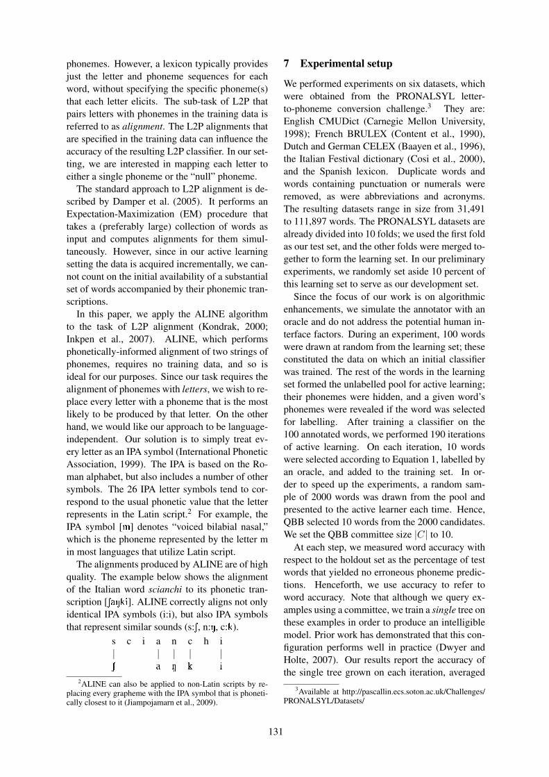
phonemes. However, a lexicon typically providesjust the letter and phoneme sequences for eachword, without specifying the specific phoneme(s)that each letter elicits. The sub-task of L2P thatpairs letters with phonemes in the training data isreferred to as alignment. The L2P alignments thatare specified in the training data can influence theaccuracy of the resulting L2P classifier. In our set-ting, we are interested in mapping each letter toeither a single phoneme or the “null” phoneme.
The standard approach to L2P alignment is de-scribed by Damper et al. (2005). It performs anExpectation-Maximization (EM) procedure thattakes a (preferably large) collection of words asinput and computes alignments for them simul-taneously. However, since in our active learningsetting the data is acquired incrementally, we can-not count on the initial availability of a substantialset of words accompanied by their phonemic tran-scriptions.
In this paper, we apply the ALINE algorithmto the task of L2P alignment (Kondrak, 2000;Inkpen et al., 2007). ALINE, which performsphonetically-informed alignment of two strings ofphonemes, requires no training data, and so isideal for our purposes. Since our task requires thealignment of phonemes with letters, we wish to re-place every letter with a phoneme that is the mostlikely to be produced by that letter. On the otherhand, we would like our approach to be language-independent. Our solution is to simply treat ev-ery letter as an IPA symbol (International PhoneticAssociation, 1999). The IPA is based on the Ro-man alphabet, but also includes a number of othersymbols. The 26 IPA letter symbols tend to cor-respond to the usual phonetic value that the letterrepresents in the Latin script.2 For example, theIPA symbol [m] denotes “voiced bilabial nasal,”which is the phoneme represented by the letter min most languages that utilize Latin script.
The alignments produced by ALINE are of highquality. The example below shows the alignmentof the Italian word scianchi to its phonetic tran-scription [SaNki]. ALINE correctly aligns not onlyidentical IPA symbols (i:i), but also IPA symbolsthat represent similar sounds (s:S, n:N, c:k).
s c i a n c h i| | | | |S a N k i
2ALINE can also be applied to non-Latin scripts by re-placing every grapheme with the IPA symbol that is phoneti-cally closest to it (Jiampojamarn et al., 2009).
7 Experimental setup
We performed experiments on six datasets, whichwere obtained from the PRONALSYL letter-to-phoneme conversion challenge.3 They are:English CMUDict (Carnegie Mellon University,1998); French BRULEX (Content et al., 1990),Dutch and German CELEX (Baayen et al., 1996),the Italian Festival dictionary (Cosi et al., 2000),and the Spanish lexicon. Duplicate words andwords containing punctuation or numerals wereremoved, as were abbreviations and acronyms.The resulting datasets range in size from 31,491to 111,897 words. The PRONALSYL datasets arealready divided into 10 folds; we used the first foldas our test set, and the other folds were merged to-gether to form the learning set. In our preliminaryexperiments, we randomly set aside 10 percent ofthis learning set to serve as our development set.
Since the focus of our work is on algorithmicenhancements, we simulate the annotator with anoracle and do not address the potential human in-terface factors. During an experiment, 100 wordswere drawn at random from the learning set; theseconstituted the data on which an initial classifierwas trained. The rest of the words in the learningset formed the unlabelled pool for active learning;their phonemes were hidden, and a given word’sphonemes were revealed if the word was selectedfor labelling. After training a classifier on the100 annotated words, we performed 190 iterationsof active learning. On each iteration, 10 wordswere selected according to Equation 1, labelled byan oracle, and added to the training set. In or-der to speed up the experiments, a random sam-ple of 2000 words was drawn from the pool andpresented to the active learner each time. Hence,QBB selected 10 words from the 2000 candidates.We set the QBB committee size |C| to 10.
At each step, we measured word accuracy withrespect to the holdout set as the percentage of testwords that yielded no erroneous phoneme predic-tions. Henceforth, we use accuracy to refer toword accuracy. Note that although we query ex-amples using a committee, we train a single tree onthese examples in order to produce an intelligiblemodel. Prior work has demonstrated that this con-figuration performs well in practice (Dwyer andHolte, 2007). Our results report the accuracy ofthe single tree grown on each iteration, averaged
3Available at http://pascallin.ecs.soton.ac.uk/Challenges/PRONALSYL/Datasets/
131
over 10 random draws of the initial training set.For our decision tree learner, we utilized the J48
algorithm provided by Weka (Witten and Frank,2005). We also experimented with Wagon (Tayloret al., 1998), an implementation of CART, but J48performed better during preliminary trials. We ranJ48 with default parameter settings, except that bi-nary trees were grown (see Section 2), and subtreeraising was disabled.4
Our feature template was established during de-velopment set experiments with the English CMUdata; the data from the other five languages did notinfluence these choices. The letter context con-sisted of the focus letter and the 3 letters appear-ing before and after the focus (or beginning/end ofword markers, where applicable). For letter classfeatures, bit strings of length 1 through 6 wereused for the focus letter and its immediate neigh-bors. Bit strings of length at most 3 were usedat positions +2 and −2, and no such features wereadded at ±3.5 We experimented with other config-urations, including using bit strings of up to length6 at all positions, but they did not produce consis-tent improvements over the selected scheme.
8 Results
We first examine the contributions of the indi-vidual system components, and then compare ourcomplete system to the baseline. The dashedcurves in Figure 1 represent the baseline perfor-mance with no clustering, no context ordering,random sampling, and ALINE, unless otherwisenoted. In all plots, the error bars show the 99%confidence interval for the mean. Because the av-erage word length differs across languages, we re-port the number of words along the x-axis. Wehave verified that our system does not substantiallyalter the average number of letters per word in thetraining set for any of these languages. Hence, thenumber of words reported here is representative ofthe true annotation effort.
4Subtree raising is an expensive pruning operation thathad a negligible impact on accuracy during preliminary ex-periments. Our pruning performs subtree replacement only.
5The idea of lowering the specificity of letter class ques-tions as the context length increases is due to Kienappel andKneser (2001), and is intended to avoid overfitting. However,their configuration differs from ours in that they use longercontext lengths (4 for German and 5 for English) and ask let-ter class questions at every position. Essentially, the authorstuned the feature set in order to optimize performance on eachproblem, whereas we seek a more general representation thatwill perform well on a variety of languages.
8.1 Context ordering
Our context ordering strategy improved the ac-curacy of the decision tree learner on every lan-guage (see Figure 1a). Statistically significant im-provements were realized on Dutch, French, andGerman. Our expectation was that context order-ing would be particularly helpful during the earlyrounds of active learning, when there is a greaterrisk of overfitting on the small training sets. Forsome languages (notably, German and Spanish)this was indeed the case; yet, for Dutch, contextordering became more effective as the training setincreased in size.
It should be noted that our context orderingstrategy is sufficiently general that it can be im-plemented in other decision tree learners that growbinary trees, such as Wagon/CART (Taylor et al.,1998). An n-ary implementation is also feasible,although we have not tried this variation.
8.2 Clustering letters
As can be seen in Figure 1b, clustering letters intoclasses tended to produce a steady increase in ac-curacy. The only case where it had no statisticallysignificant effect was on English. Another benefitof clustering is that it reduces variance. The confi-dence intervals are generally wider when cluster-ing is disabled, meaning that the system’s perfor-mance was less sensitive to changes in the initialtraining set when letter classes were used.
8.3 Active learning
On five of the six datasets, Query-by-Bagging re-quired significantly fewer labelled examples toreach the maximum level of performance achievedby the passive learner (see Figure 1c). For in-stance, on the Spanish dataset, random samplingreached 97% word accuracy after 1420 words hadbeen annotated, whereas QBB did so with only510 words — a 64% reduction in labelling ef-fort. Similarly, savings ranging from 30% to 63%were observed for the other languages, with theexception of English, where a statistically insignif-icant 4% reduction was recorded. Since English ishighly irregular in comparison with the other fivelanguages, the active learner tends to query exam-ples that are difficult to classify, but which are un-helpful in terms of generalization.
It is important to note that empirical compar-isons of different active learning techniques haveshown that random sampling establishes a very
132
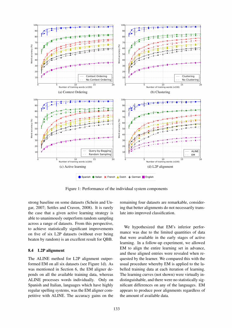
0 5 10 15 20Number of training words (x100)
10
20
30
40
50
60
70
80
90
100
Word
acc
ura
cy (
%)
Context OrderingNo Context Ordering
(a) Context Ordering
0 5 10 15 20Number of training words (x100)
10
20
30
40
50
60
70
80
90
100
Word
acc
ura
cy (
%)
ClusteringNo Clustering
(b) Clustering
0 5 10 15 20Number of training words (x100)
10
20
30
40
50
60
70
80
90
100
Word
acc
ura
cy (
%)
Query-by-BaggingRandom Sampling
(c) Active learning
0 5 10 15 20Number of training words (x100)
10
20
30
40
50
60
70
80
90
100
Word
acc
ura
cy (
%)
ALINEEM
(d) L2P alignment
Spanish Italian +French Dutch + German English
Figure 1: Performance of the individual system components
strong baseline on some datasets (Schein and Un-gar, 2007; Settles and Craven, 2008). It is rarelythe case that a given active learning strategy isable to unanimously outperform random samplingacross a range of datasets. From this perspective,to achieve statistically significant improvementson five of six L2P datasets (without ever beingbeaten by random) is an excellent result for QBB.
8.4 L2P alignment
The ALINE method for L2P alignment outper-formed EM on all six datasets (see Figure 1d). Aswas mentioned in Section 6, the EM aligner de-pends on all the available training data, whereasALINE processes words individually. Only onSpanish and Italian, languages which have highlyregular spelling systems, was the EM aligner com-petitive with ALINE. The accuracy gains on the
remaining four datasets are remarkable, consider-ing that better alignments do not necessarily trans-late into improved classification.
We hypothesized that EM’s inferior perfor-mance was due to the limited quantities of datathat were available in the early stages of activelearning. In a follow-up experiment, we allowedEM to align the entire learning set in advance,and these aligned entries were revealed when re-quested by the learner. We compared this with theusual procedure whereby EM is applied to the la-belled training data at each iteration of learning.The learning curves (not shown) were virtually in-distinguishable, and there were no statistically sig-nificant differences on any of the languages. EMappears to produce poor alignments regardless ofthe amount of available data.
133

0 5 10 15 20Number of training words (x100)
10
20
30
40
50
60
70
80
90
100
Word
acc
ura
cy (
%)
Complete SystemBaseline
Spanish Italian +French Dutch + German English
Figure 2: Performance of the complete system
8.5 Complete system
The complete system consists of context order-ing, clustering, Query-by-Bagging, and ALINE;the baseline represents random sampling with EMalignment and no additional enhancements. Fig-ure 2 plots the word accuracies for all six datasets.
Although the absolute word accuracies variedconsiderably across the different languages, oursystem significantly outperformed the baseline inevery instance. On the French dataset, for ex-ample, the baseline labelled 1850 words beforereaching its maximum accuracy of 64%, whereasthe complete system required only 480 queries toreach 64% accuracy. This represents a reductionof 74% in the labelling effort. The savings for theother languages are: Spanish, 75%; Dutch, 68%;English, 59%; German, 59%; and Italian, 52%.6
Interestingly, the savings are the highest on Span-ish, even though the corresponding accuracy gainsare the smallest. This demonstrates that our ap-proach is also effective on languages with rela-tively transparent orthography.
At first glance, the performance of both sys-tems appears to be rather poor on the Englishdataset. To put our results into perspective, Blacket al. (1998) report 57.8% accuracy on this datasetwith a similar alignment method and decision treelearner. Our baseline system achieves 57.3% ac-curacy when 90,000 words have been labelled.Hence, the low values in Figure 2 simply reflectthe fact that many more examples are required to
6The average savings in the number of labelled wordswith respect to the entire learning curve are similar, rangingfrom 50% on Italian to 73% on Spanish.
learn an accurate classifier for the English data.
9 Conclusions
We have presented a system for learning a letter-to-phoneme classifier that combines four distinctenhancements in order to minimize the amountof data that must be annotated. Our experimentsinvolving datasets from several languages clearlydemonstrate that unlabelled data can be used moreefficiently, resulting in greater accuracy for a giventraining set size, without any additional tuningfor the different languages. The experiments alsoshow that a phonetically-based aligner may bepreferable to the widely-used EM alignment tech-nique, a discovery that could lead to the improve-ment of L2P accuracy in general.
While this work represents an important stepin reducing the cost of constructing an L2P train-ing set, we intend to explore other active learnersand classification algorithms, including sequencelabelling strategies (Settles and Craven, 2008).We also plan to incorporate user-centric enhance-ments (Davel and Barnard, 2004; Culotta and Mc-Callum, 2005) with the aim of reducing both theeffort and expertise that is required to annotatewords with their phoneme sequences.
Acknowledgments
We would like to thank Sittichai Jiampojamarn forhelpful discussions and for providing an imple-mentation of the Expectation-Maximization align-ment algorithm. This research was supported bythe Natural Sciences and Engineering ResearchCouncil of Canada (NSERC) and the InformaticsCircle of Research Excellence (iCORE).
ReferencesNaoki Abe and Hiroshi Mamitsuka. 1998. Query
learning strategies using boosting and bagging. InProc. International Conference on Machine Learn-ing, pages 1–9.
Ove Andersen, Ronald Kuhn, Ariane Lazaridès, PaulDalsgaard, Jürgen Haas, and Elmar Nöth. 1996.Comparison of two tree-structured approaches forgrapheme-to-phoneme conversion. In Proc. Inter-national Conference on Spoken Language Process-ing, volume 3, pages 1700–1703.
R. Harald Baayen, Richard Piepenbrock, and Leon Gu-likers, 1996. The CELEX2 lexical database. Lin-guistic Data Consortium, Univ. of Pennsylvania.
134
Maximilian Bisani and Hermann Ney. 2002. Investi-gations on joint-multigram models for grapheme-to-phoneme conversion. In Proc. International Confer-ence on Spoken Language Processing, pages 105–108.
Alan W. Black, Kevin Lenzo, and Vincent Pagel. 1998.Issues in building general letter to sound rules. InESCA Workshop on Speech Synthesis, pages 77–80.
Leo Breiman. 1996. Bagging predictors. MachineLearning, 24(2):123–140.
Peter F. Brown, Vincent J. Della Pietra, Peter V. deS-ouza, Jennifer C. Lai, and Robert L. Mercer. 1992.Class-based n-gram models of natural language.Computational Linguistics, 18(4):467–479.
Carnegie Mellon University. 1998. The Carnegie Mel-lon pronouncing dictionary.
David A. Cohn, Les E. Atlas, and Richard E. Ladner.1992. Improving generalization with active learn-ing. Machine Learning, 15(2):201–221.
Alain Content, Phillppe Mousty, and Monique Radeau.1990. Brulex: Une base de données lexicales in-formatisée pour le français écrit et parlé. L’annéePsychologique, 90:551–566.
Piero Cosi, Roberto Gretter, and Fabio Tesser. 2000.Festival parla Italiano. In Proc. Giornate delGruppo di Fonetica Sperimentale.
Aron Culotta and Andrew McCallum. 2004. Con-fidence estimation for information extraction. InProc. HLT-NAACL, pages 109–114.
Aron Culotta and Andrew McCallum. 2005. Reduc-ing labeling effort for structured prediction tasks. InProc. National Conference on Artificial Intelligence,pages 746–751.
Robert I. Damper, Yannick Marchand, John-David S.Marsters, and Alexander I. Bazin. 2005. Align-ing text and phonemes for speech technology appli-cations using an EM-like algorithm. InternationalJournal of Speech Technology, 8(2):147–160.
Marelie Davel and Etienne Barnard. 2004. The effi-cient generation of pronunciation dictionaries: Hu-man factors during bootstrapping. In Proc. Interna-tional Conference on Spoken Language Processing,pages 2797–2800.
Vera Demberg, Helmut Schmid, and Gregor Möhler.2007. Phonological constraints and morphologi-cal preprocessing for grapheme-to-phoneme conver-sion. In Proc. ACL, pages 96–103.
Kenneth Dwyer and Robert Holte. 2007. Decision treeinstability and active learning. In Proc. EuropeanConference on Machine Learning, pages 128–139.
Yoav Freund, H. Sebastian Seung, Eli Shamir, and Naf-tali Tishby. 1997. Selective sampling using thequery by committee algorithm. Machine Learning,28(2-3):133–168.
Diana Inkpen, Raphaëlle Martin, and AlainDesrochers. 2007. Graphon: un outil pourla transcription phonétique des mots français.Unpublished manuscript.
International Phonetic Association. 1999. Handbookof the International Phonetic Association: A Guideto the Use of the International Phonetic Alphabet.Cambridge University Press.
Sittichai Jiampojamarn, Colin Cherry, and GrzegorzKondrak. 2008. Joint processing and discriminativetraining for letter-to-phoneme conversion. In Proc.ACL, pages 905–913.
Sittichai Jiampojamarn, Aditya Bhargava, Qing Dou,Kenneth Dwyer, and Grzegorz Kondrak. 2009. Di-recTL: a language-independent approach to translit-eration. In Named Entities Workshop (NEWS):Shared Task on Transliteration. Submitted.
Anne K. Kienappel and Reinhard Kneser. 2001. De-signing very compact decision trees for grapheme-to-phoneme transcription. In Proc. European Con-ference on Speech Communication and Technology,pages 1911–1914.
John Kominek and Alan W. Black. 2006. Learn-ing pronunciation dictionaries: Language complex-ity and word selection strategies. In Proc. HLT-NAACL, pages 232–239.
Grzegorz Kondrak. 2000. A new algorithm for thealignment of phonetic sequences. In Proc. NAACL,pages 288–295.
Christopher D. Manning and Hinrich Schütze. 1999.Foundations of Statistical Natural Language Pro-cessing. MIT Press.
Sameer R. Maskey, Alan W. Black, and Laura M.Tomokiya. 2004. Boostrapping phonetic lexiconsfor new languages. In Proc. International Confer-ence on Spoken Language Processing, pages 69–72.
Scott Miller, Jethran Guinness, and Alex Zamanian.2004. Name tagging with word clusters and dis-criminative training. In Proc. HLT-NAACL, pages337–342.
Andrew I. Schein and Lyle H. Ungar. 2007. Activelearning for logistic regression: an evaluation. Ma-chine Learning, 68(3):235–265.
Burr Settles and Mark Craven. 2008. An analysisof active learning strategies for sequence labelingtasks. In Proc. Conference on Empirical Methodsin Natural Language Processing, pages 1069–1078.
Paul A. Taylor, Alan Black, and Richard Caley. 1998.The architecture of the Festival Speech SynthesisSystem. In ESCA Workshop on Speech Synthesis,pages 147–151.
Ian H. Witten and Eibe Frank. 2005. Data Mining:Practical Machine Learning Tools and Techniques.Morgan Kaufmann, 2nd edition.
135
Proceedings of the 47th Annual Meeting of the ACL and the 4th IJCNLP of the AFNLP, pages 136–144,Suntec, Singapore, 2-7 August 2009. c©2009 ACL and AFNLP
Transliteration Alignment
Vladimir Pervouchine, Haizhou LiInstitute for Infocomm Research
A*STAR, Singapore 138632{vpervouchine,hli}@i2r.a-star.edu.sg
Bo LinSchool of Computer Engineering
NTU, Singapore [email protected]
AbstractThis paper studies transliteration align-ment, its evaluation metrics and applica-tions. We propose a new evaluation met-ric, alignment entropy, grounded on theinformation theory, to evaluate the align-ment quality without the need for the goldstandard reference and compare the metricwith F -score. We study the use of phono-logical features and affinity statistics fortransliteration alignment at phoneme andgrapheme levels. The experiments showthat better alignment consistently leads tomore accurate transliteration. In transliter-ation modeling application, we achieve amean reciprocal rate (MRR) of 0.773 onXinhua personal name corpus, a signifi-cant improvement over other reported re-sults on the same corpus. In transliterationvalidation application, we achieve 4.48%equal error rate on a large LDC corpus.
1 Introduction
Transliteration is a process of rewriting a wordfrom a source language to a target language in adifferent writing system using the word’s phono-logical equivalent. The word and its translitera-tion form a transliteration pair. Many efforts havebeen devoted to two areas of studies where thereis a need to establish the correspondence betweengraphemes or phonemes between a transliterationpair, also known as transliteration alignment.
One area is the generative transliteration model-ing (Knight and Graehl, 1998), which studies howto convert a word from one language to another us-ing statistical models. Since the models are trainedon an aligned parallel corpus, the resulting statisti-cal models can only be as good as the alignment ofthe corpus. Another area is the transliteration vali-dation, which studies the ways to validate translit-eration pairs. For example Knight and Graehl
(1998) use the lexicon frequency, Qu and Grefen-stette (2004) use the statistics in a monolingualcorpus and the Web, Kuo et al. (2007) use proba-bilities estimated from the transliteration model tovalidate transliteration candidates. In this paper,we propose using the alignment distance betweenthe a bilingual pair of words to establish the evi-dence of transliteration candidacy. An example oftransliteration pair alignment is shown in Figure 1.
e5e1 e2 e3 e4
c1 c2 c3
A L I C E
艾 丽 斯
source graphemes
target graphemes
e1 e2 e3grapheme tokens
Figure 1: An example of grapheme alignment (Al-ice, 艾丽斯), where a Chinese grapheme, a char-acter, is aligned to an English grapheme token.
Like the word alignment in statistical ma-chine translation (MT), transliteration alignmentbecomes one of the important topics in machinetransliteration, which has several unique chal-lenges. Firstly, the grapheme sequence in a wordis not delimited into grapheme tokens, resultingin an additional level of complexity. Secondly, tomaintain the phonological equivalence, the align-ment has to make sense at both grapheme andphoneme levels of the source and target languages.This paper reports progress in our ongoing spokenlanguage translation project, where we are inter-ested in the alignment problem of personal nametransliteration from English to Chinese.
This paper is organized as follows. In Section 2,we discuss the prior work. In Section 3, we in-troduce both statistically and phonologically mo-tivated alignment techniques and in Section 4 weadvocate an evaluation metric, alignment entropythat measures the alignment quality. We report theexperiments in Section 5. Finally, we conclude inSection 6.
136
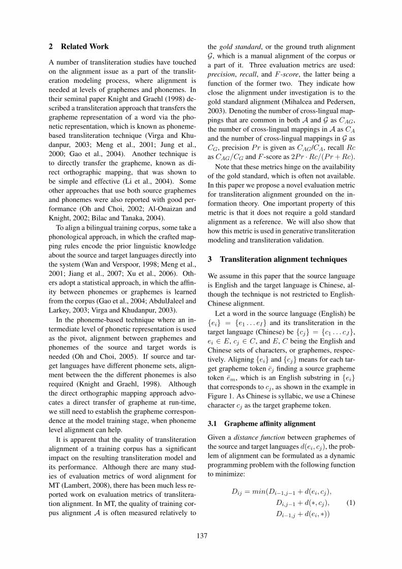
2 Related Work
A number of transliteration studies have touchedon the alignment issue as a part of the translit-eration modeling process, where alignment isneeded at levels of graphemes and phonemes. Intheir seminal paper Knight and Graehl (1998) de-scribed a transliteration approach that transfers thegrapheme representation of a word via the pho-netic representation, which is known as phoneme-based transliteration technique (Virga and Khu-danpur, 2003; Meng et al., 2001; Jung et al.,2000; Gao et al., 2004). Another technique isto directly transfer the grapheme, known as di-rect orthographic mapping, that was shown tobe simple and effective (Li et al., 2004). Someother approaches that use both source graphemesand phonemes were also reported with good per-formance (Oh and Choi, 2002; Al-Onaizan andKnight, 2002; Bilac and Tanaka, 2004).
To align a bilingual training corpus, some take aphonological approach, in which the crafted map-ping rules encode the prior linguistic knowledgeabout the source and target languages directly intothe system (Wan and Verspoor, 1998; Meng et al.,2001; Jiang et al., 2007; Xu et al., 2006). Oth-ers adopt a statistical approach, in which the affin-ity between phonemes or graphemes is learnedfrom the corpus (Gao et al., 2004; AbdulJaleel andLarkey, 2003; Virga and Khudanpur, 2003).
In the phoneme-based technique where an in-termediate level of phonetic representation is usedas the pivot, alignment between graphemes andphonemes of the source and target words isneeded (Oh and Choi, 2005). If source and tar-get languages have different phoneme sets, align-ment between the the different phonemes is alsorequired (Knight and Graehl, 1998). Althoughthe direct orthographic mapping approach advo-cates a direct transfer of grapheme at run-time,we still need to establish the grapheme correspon-dence at the model training stage, when phonemelevel alignment can help.
It is apparent that the quality of transliterationalignment of a training corpus has a significantimpact on the resulting transliteration model andits performance. Although there are many stud-ies of evaluation metrics of word alignment forMT (Lambert, 2008), there has been much less re-ported work on evaluation metrics of translitera-tion alignment. In MT, the quality of training cor-pus alignment A is often measured relatively to
the gold standard, or the ground truth alignmentG, which is a manual alignment of the corpus ora part of it. Three evaluation metrics are used:precision, recall, and F -score, the latter being afunction of the former two. They indicate howclose the alignment under investigation is to thegold standard alignment (Mihalcea and Pedersen,2003). Denoting the number of cross-lingual map-pings that are common in both A and G as CAG,the number of cross-lingual mappings in A as CAand the number of cross-lingual mappings in G asCG, precision Pr is given as CAG/CA, recall Rcas CAG/CG and F -score as 2Pr ·Rc/(Pr+Rc).
Note that these metrics hinge on the availabilityof the gold standard, which is often not available.In this paper we propose a novel evaluation metricfor transliteration alignment grounded on the in-formation theory. One important property of thismetric is that it does not require a gold standardalignment as a reference. We will also show thathow this metric is used in generative transliterationmodeling and transliteration validation.
3 Transliteration alignment techniques
We assume in this paper that the source languageis English and the target language is Chinese, al-though the technique is not restricted to English-Chinese alignment.
Let a word in the source language (English) be{ei} = {e1 . . . eI} and its transliteration in thetarget language (Chinese) be {cj} = {c1 . . . cJ},ei ∈ E, cj ∈ C, and E, C being the English andChinese sets of characters, or graphemes, respec-tively. Aligning {ei} and {cj} means for each tar-get grapheme token c̄j finding a source graphemetoken ēm, which is an English substring in {ei}that corresponds to cj , as shown in the example inFigure 1. As Chinese is syllabic, we use a Chinesecharacter cj as the target grapheme token.
3.1 Grapheme affinity alignment
Given a distance function between graphemes ofthe source and target languages d(ei, cj), the prob-lem of alignment can be formulated as a dynamicprogramming problem with the following functionto minimize:
Dij = min(Di−1,j−1 + d(ei, cj),
Di,j−1 + d(∗, cj),Di−1,j + d(ei, ∗))
(1)
137
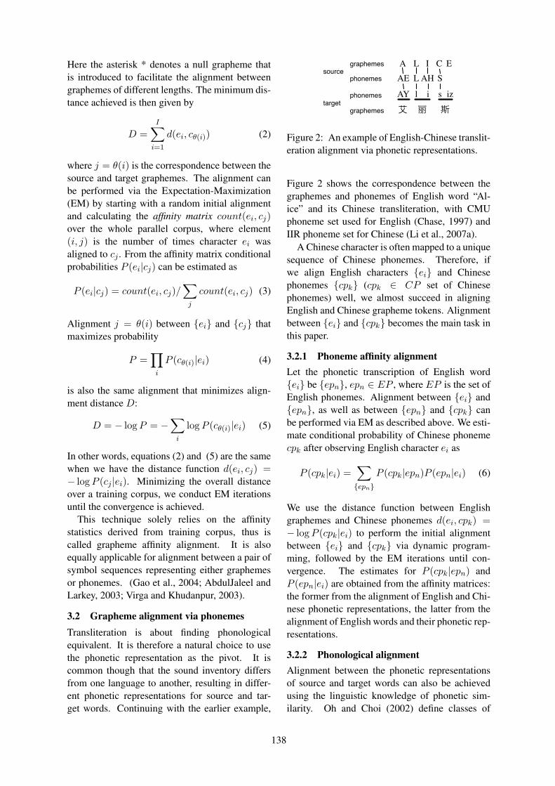
Here the asterisk * denotes a null grapheme thatis introduced to facilitate the alignment betweengraphemes of different lengths. The minimum dis-tance achieved is then given by
D =I
∑
i=1
d(ei, cθ(i)) (2)
where j = θ(i) is the correspondence between thesource and target graphemes. The alignment canbe performed via the Expectation-Maximization(EM) by starting with a random initial alignmentand calculating the affinity matrix count(ei, cj)over the whole parallel corpus, where element(i, j) is the number of times character ei wasaligned to cj . From the affinity matrix conditionalprobabilities P (ei|cj) can be estimated as
P (ei|cj) = count(ei, cj)/∑
j
count(ei, cj) (3)
Alignment j = θ(i) between {ei} and {cj} thatmaximizes probability
P =∏
i
P (cθ(i)|ei) (4)
is also the same alignment that minimizes align-ment distance D:
D = − logP = −∑
i
logP (cθ(i)|ei) (5)
In other words, equations (2) and (5) are the samewhen we have the distance function d(ei, cj) =− logP (cj |ei). Minimizing the overall distanceover a training corpus, we conduct EM iterationsuntil the convergence is achieved.
This technique solely relies on the affinitystatistics derived from training corpus, thus iscalled grapheme affinity alignment. It is alsoequally applicable for alignment between a pair ofsymbol sequences representing either graphemesor phonemes. (Gao et al., 2004; AbdulJaleel andLarkey, 2003; Virga and Khudanpur, 2003).
3.2 Grapheme alignment via phonemesTransliteration is about finding phonologicalequivalent. It is therefore a natural choice to usethe phonetic representation as the pivot. It iscommon though that the sound inventory differsfrom one language to another, resulting in differ-ent phonetic representations for source and tar-get words. Continuing with the earlier example,
艾
AE L AH SA L I C E
AY l i s iz
丽 斯
graphemes
phonemes
phonemes
graphemes
source
target
Figure 2: An example of English-Chinese translit-eration alignment via phonetic representations.
Figure 2 shows the correspondence between thegraphemes and phonemes of English word “Al-ice” and its Chinese transliteration, with CMUphoneme set used for English (Chase, 1997) andIIR phoneme set for Chinese (Li et al., 2007a).
A Chinese character is often mapped to a uniquesequence of Chinese phonemes. Therefore, ifwe align English characters {ei} and Chinesephonemes {cpk} (cpk ∈ CP set of Chinesephonemes) well, we almost succeed in aligningEnglish and Chinese grapheme tokens. Alignmentbetween {ei} and {cpk} becomes the main task inthis paper.
3.2.1 Phoneme affinity alignmentLet the phonetic transcription of English word{ei} be {epn}, epn ∈ EP , where EP is the set ofEnglish phonemes. Alignment between {ei} and{epn}, as well as between {epn} and {cpk} canbe performed via EM as described above. We esti-mate conditional probability of Chinese phonemecpk after observing English character ei as
P (cpk|ei) =∑
{epn}
P (cpk|epn)P (epn|ei) (6)
We use the distance function between Englishgraphemes and Chinese phonemes d(ei, cpk) =− logP (cpk|ei) to perform the initial alignmentbetween {ei} and {cpk} via dynamic program-ming, followed by the EM iterations until con-vergence. The estimates for P (cpk|epn) andP (epn|ei) are obtained from the affinity matrices:the former from the alignment of English and Chi-nese phonetic representations, the latter from thealignment of English words and their phonetic rep-resentations.
3.2.2 Phonological alignmentAlignment between the phonetic representationsof source and target words can also be achievedusing the linguistic knowledge of phonetic sim-ilarity. Oh and Choi (2002) define classes of
138
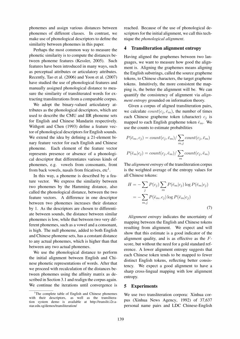
phonemes and assign various distances betweenphonemes of different classes. In contrast, wemake use of phonological descriptors to define thesimilarity between phonemes in this paper.
Perhaps the most common way to measure thephonetic similarity is to compute the distances be-tween phoneme features (Kessler, 2005). Suchfeatures have been introduced in many ways, suchas perceptual attributes or articulatory attributes.Recently, Tao et al. (2006) and Yoon et al. (2007)have studied the use of phonological features andmanually assigned phonological distance to mea-sure the similarity of transliterated words for ex-tracting transliterations from a comparable corpus.
We adopt the binary-valued articulatory at-tributes as the phonological descriptors, which areused to describe the CMU and IIR phoneme setsfor English and Chinese Mandarin respectively.Withgott and Chen (1993) define a feature vec-tor of phonological descriptors for English sounds.We extend the idea by defining a 21-element bi-nary feature vector for each English and Chinesephoneme. Each element of the feature vectorrepresents presence or absence of a phonologi-cal descriptor that differentiates various kinds ofphonemes, e.g. vowels from consonants, frontfrom back vowels, nasals from fricatives, etc1.
In this way, a phoneme is described by a fea-ture vector. We express the similarity betweentwo phonemes by the Hamming distance, alsocalled the phonological distance, between the twofeature vectors. A difference in one descriptorbetween two phonemes increases their distanceby 1. As the descriptors are chosen to differenti-ate between sounds, the distance between similarphonemes is low, while that between two very dif-ferent phonemes, such as a vowel and a consonant,is high. The null phoneme, added to both Englishand Chinese phoneme sets, has a constant distanceto any actual phonemes, which is higher than thatbetween any two actual phonemes.
We use the phonological distance to performthe initial alignment between English and Chi-nese phonetic representations of words. After thatwe proceed with recalculation of the distances be-tween phonemes using the affinity matrix as de-scribed in Section 3.1 and realign the corpus again.We continue the iterations until convergence is
1The complete table of English and Chinese phonemeswith their descriptors, as well as the translitera-tion system demo is available at http://translit.i2r.a-star.edu.sg/demos/transliteration/
reached. Because of the use of phonological de-scriptors for the initial alignment, we call this tech-nique the phonological alignment.
4 Transliteration alignment entropy
Having aligned the graphemes between two lan-guages, we want to measure how good the align-ment is. Aligning the graphemes means aligningthe English substrings, called the source graphemetokens, to Chinese characters, the target graphemetokens. Intuitively, the more consistent the map-ping is, the better the alignment will be. We canquantify the consistency of alignment via align-ment entropy grounded on information theory.
Given a corpus of aligned transliteration pairs,we calculate count(cj , ēm), the number of timeseach Chinese grapheme token (character) cj ismapped to each English grapheme token ēm. Weuse the counts to estimate probabilities
P (ēm, cj) = count(cj , ēm)/∑
m,j
count(cj , ēm)
P (ēm|cj) = count(cj , ēm)/∑
m
count(cj , ēm)
The alignment entropy of the transliteration corpusis the weighted average of the entropy values forall Chinese tokens:
H = −∑
j
P (cj)∑
m
P (ēm|cj) logP (ēm|cj)
= −∑
m,j
P (ēm, cj) logP (ēm|cj)
(7)
Alignment entropy indicates the uncertainty ofmapping between the English and Chinese tokensresulting from alignment. We expect and willshow that this estimate is a good indicator of thealignment quality, and is as effective as the F -score, but without the need for a gold standard ref-erence. A lower alignment entropy suggests thateach Chinese token tends to be mapped to fewerdistinct English tokens, reflecting better consis-tency. We expect a good alignment to have asharp cross-lingual mapping with low alignmententropy.
5 Experiments
We use two transliteration corpora: Xinhua cor-pus (Xinhua News Agency, 1992) of 37,637personal name pairs and LDC Chinese-English
139
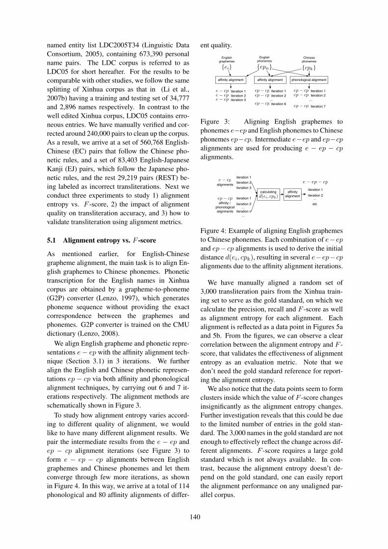
named entity list LDC2005T34 (Linguistic DataConsortium, 2005), containing 673,390 personalname pairs. The LDC corpus is referred to asLDC05 for short hereafter. For the results to becomparable with other studies, we follow the samesplitting of Xinhua corpus as that in (Li et al.,2007b) having a training and testing set of 34,777and 2,896 names respectively. In contrast to thewell edited Xinhua corpus, LDC05 contains erro-neous entries. We have manually verified and cor-rected around 240,000 pairs to clean up the corpus.As a result, we arrive at a set of 560,768 English-Chinese (EC) pairs that follow the Chinese pho-netic rules, and a set of 83,403 English-JapaneseKanji (EJ) pairs, which follow the Japanese pho-netic rules, and the rest 29,219 pairs (REST) be-ing labeled as incorrect transliterations. Next weconduct three experiments to study 1) alignmententropy vs. F -score, 2) the impact of alignmentquality on transliteration accuracy, and 3) how tovalidate transliteration using alignment metrics.
5.1 Alignment entropy vs. F -score
As mentioned earlier, for English-Chinesegrapheme alignment, the main task is to align En-glish graphemes to Chinese phonemes. Phonetictranscription for the English names in Xinhuacorpus are obtained by a grapheme-to-phoneme(G2P) converter (Lenzo, 1997), which generatesphoneme sequence without providing the exactcorrespondence between the graphemes andphonemes. G2P converter is trained on the CMUdictionary (Lenzo, 2008).
We align English grapheme and phonetic repre-sentations e− ep with the affinity alignment tech-nique (Section 3.1) in 3 iterations. We furtheralign the English and Chinese phonetic represen-tations ep − cp via both affinity and phonologicalalignment techniques, by carrying out 6 and 7 it-erations respectively. The alignment methods areschematically shown in Figure 3.
To study how alignment entropy varies accord-ing to different quality of alignment, we wouldlike to have many different alignment results. Wepair the intermediate results from the e − ep andep − cp alignment iterations (see Figure 3) toform e − ep − cp alignments between Englishgraphemes and Chinese phonemes and let themconverge through few more iterations, as shownin Figure 4. In this way, we arrive at a total of 114phonological and 80 affinity alignments of differ-
ent quality.
{cpk}{ei}
Englishgraphemes
{epn}English
phonemesChinese
phonemes
affinity alignment affinity alignment
e! ep iteration 1e! ep iteration 2e! ep iteration 3
ep! cp iteration 1ep! cp iteration 2
...ep! cp iteration 6
phonological alignment
ep! cp iteration 1ep! cp iteration 2
...ep! cp iteration 7
Figure 3: Aligning English graphemes tophonemes e−ep and English phonemes to Chinesephonemes ep−cp. Intermediate e−ep and ep−cpalignments are used for producing e − ep − cpalignments.
e! epalignments
ep! cpaffinity /
phonologicalalignments
iteration 1iteration 2iteration 3
iteration 1iteration 2
iteration n...
...
calculatingd(ei, cpk)
affinityalignment
iteration 1iteration 2
...
e! ep! cp
etc
Figure 4: Example of aligning English graphemesto Chinese phonemes. Each combination of e−epand ep− cp alignments is used to derive the initialdistance d(ei, cpk), resulting in several e−ep−cpalignments due to the affinity alignment iterations.
We have manually aligned a random set of3,000 transliteration pairs from the Xinhua train-ing set to serve as the gold standard, on which wecalculate the precision, recall and F -score as wellas alignment entropy for each alignment. Eachalignment is reflected as a data point in Figures 5aand 5b. From the figures, we can observe a clearcorrelation between the alignment entropy and F -score, that validates the effectiveness of alignmententropy as an evaluation metric. Note that wedon’t need the gold standard reference for report-ing the alignment entropy.
We also notice that the data points seem to formclusters inside which the value of F -score changesinsignificantly as the alignment entropy changes.Further investigation reveals that this could be dueto the limited number of entries in the gold stan-dard. The 3,000 names in the gold standard are notenough to effectively reflect the change across dif-ferent alignments. F -score requires a large goldstandard which is not always available. In con-trast, because the alignment entropy doesn’t de-pend on the gold standard, one can easily reportthe alignment performance on any unaligned par-allel corpus.
140
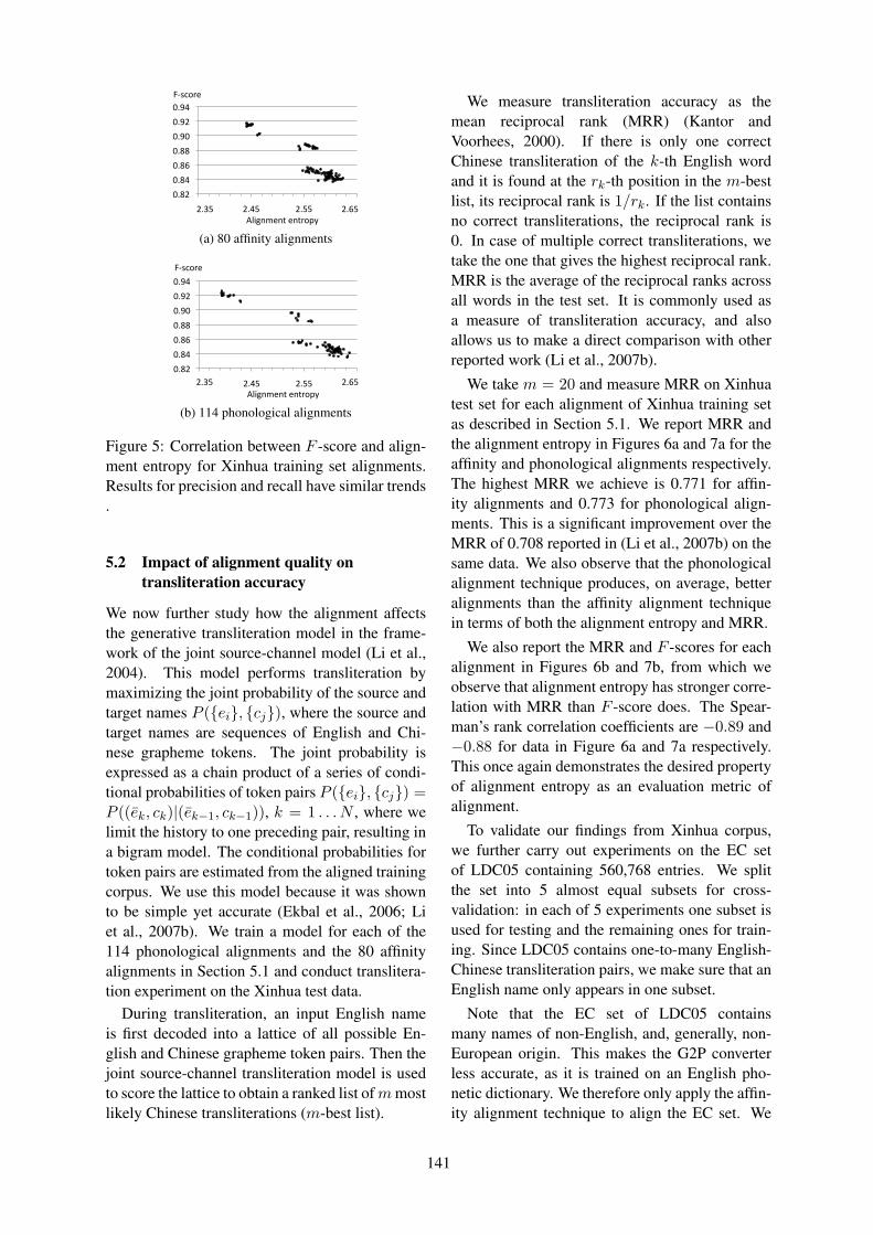
!"#$%
!"#&%
!"#'%
!"##%
!"(!%
!"($%
!"(&%
$")*% $"&*% $"**% $"'*%
!"#$%&'
()*+,-',./',.&%01
2345 2365
(a) 80 affinity alignments
!"#$%
!"#&%
!"#'%
!"##%
!"(!%
!"($%
!"(&%
$")*% $"&*% $"**% $"'*%
!"#$%&'%()'%(*+,-
./01 ./21
3456+*'
(b) 114 phonological alignments
Figure 5: Correlation between F -score and align-ment entropy for Xinhua training set alignments.Results for precision and recall have similar trends.
5.2 Impact of alignment quality ontransliteration accuracy
We now further study how the alignment affectsthe generative transliteration model in the frame-work of the joint source-channel model (Li et al.,2004). This model performs transliteration bymaximizing the joint probability of the source andtarget names P ({ei}, {cj}), where the source andtarget names are sequences of English and Chi-nese grapheme tokens. The joint probability isexpressed as a chain product of a series of condi-tional probabilities of token pairs P ({ei}, {cj}) =P ((ēk, ck)|(ēk−1, ck−1)), k = 1 . . . N , where welimit the history to one preceding pair, resulting ina bigram model. The conditional probabilities fortoken pairs are estimated from the aligned trainingcorpus. We use this model because it was shownto be simple yet accurate (Ekbal et al., 2006; Liet al., 2007b). We train a model for each of the114 phonological alignments and the 80 affinityalignments in Section 5.1 and conduct translitera-tion experiment on the Xinhua test data.
During transliteration, an input English nameis first decoded into a lattice of all possible En-glish and Chinese grapheme token pairs. Then thejoint source-channel transliteration model is usedto score the lattice to obtain a ranked list ofmmostlikely Chinese transliterations (m-best list).
We measure transliteration accuracy as themean reciprocal rank (MRR) (Kantor andVoorhees, 2000). If there is only one correctChinese transliteration of the k-th English wordand it is found at the rk-th position in the m-bestlist, its reciprocal rank is 1/rk. If the list containsno correct transliterations, the reciprocal rank is0. In case of multiple correct transliterations, wetake the one that gives the highest reciprocal rank.MRR is the average of the reciprocal ranks acrossall words in the test set. It is commonly used asa measure of transliteration accuracy, and alsoallows us to make a direct comparison with otherreported work (Li et al., 2007b).
We take m = 20 and measure MRR on Xinhuatest set for each alignment of Xinhua training setas described in Section 5.1. We report MRR andthe alignment entropy in Figures 6a and 7a for theaffinity and phonological alignments respectively.The highest MRR we achieve is 0.771 for affin-ity alignments and 0.773 for phonological align-ments. This is a significant improvement over theMRR of 0.708 reported in (Li et al., 2007b) on thesame data. We also observe that the phonologicalalignment technique produces, on average, betteralignments than the affinity alignment techniquein terms of both the alignment entropy and MRR.
We also report the MRR and F -scores for eachalignment in Figures 6b and 7b, from which weobserve that alignment entropy has stronger corre-lation with MRR than F -score does. The Spear-man’s rank correlation coefficients are −0.89 and−0.88 for data in Figure 6a and 7a respectively.This once again demonstrates the desired propertyof alignment entropy as an evaluation metric ofalignment.
To validate our findings from Xinhua corpus,we further carry out experiments on the EC setof LDC05 containing 560,768 entries. We splitthe set into 5 almost equal subsets for cross-validation: in each of 5 experiments one subset isused for testing and the remaining ones for train-ing. Since LDC05 contains one-to-many English-Chinese transliteration pairs, we make sure that anEnglish name only appears in one subset.
Note that the EC set of LDC05 containsmany names of non-English, and, generally, non-European origin. This makes the G2P converterless accurate, as it is trained on an English pho-netic dictionary. We therefore only apply the affin-ity alignment technique to align the EC set. We
141

!"#$!%
!"#$$%
!"#&!%
!"#&$%
!"##!%
!"##$%
'"($% '")$% '"$$% '"&$%
MRR
Alignmententropy
(a) 80 affinity alignments
!"#$!%
!"#$$%
!"#&!%
!"#&$%
!"##!%
!"##$%
!"'(% !"')% !"'&% !"''% !"*!% !"*(% !"*)%
MRR
F‐score
(b) 80 affinity alignments
Figure 6: Mean reciprocal ratio on Xinhua testset vs. alignment entropy and F -score for mod-els trained with different affinity alignments.
use each iteration of the alignment in the translit-eration modeling and present the resulting MRRalong with alignment entropy in Figure 8. TheMRR results are the averages of five values pro-duced in the five-fold cross-validations.
We observe a clear correlation between thealignment entropy and transliteration accuracy ex-pressed by MRR on LDC05 corpus, similar to thaton Xinhua corpus, with the Spearman’s rank cor-relation coefficient of −0.77. We obtain the high-est average MRR of 0.720 on the EC set.
5.3 Validating transliteration usingalignment measure
Transliteration validation is a hypothesis test thatdecides whether a given transliteration pair is gen-uine or not. Instead of using the lexicon fre-quency (Knight and Graehl, 1998) or Web statis-tics (Qu and Grefenstette, 2004), we propose vali-dating transliteration pairs according to the align-ment distance D between the aligned Englishgraphemes and Chinese phonemes (see equations(2) and (5)). A distance function d(ei, cpk) isestablished from each alignment on the Xinhuatraining set as discussed in Section 5.2.
An audit of LDC05 corpus groups the corpusinto three sets: an English-Chinese (EC) set of560,768 samples, an English-Japanese (EJ) setof 83,403 samples and the REST set of 29,219
!"#$!%
!"#$$%
!"#&!%
!"#&$%
!"##!%
!"##$%
'"($% '")$% '"$$% '"&$%
MRR
Alignmententropy
(a) 114 phonological alignments
!"#$!%
!"#$$%
!"#&!%
!"#&$%
!"##!%
!"##$%
!"'(% !"')% !"'&% !"''% !"*!% !"*(% !"*)%
MRR
F‐score
(b) 114 phonological alignments
Figure 7: Mean reciprocal ratio on Xinhua testset vs. alignment entropy and F -score for modelstrained with different phonological alignments.
!"#!$%
!"#!&%
!"#!'%
!"#(!%
!"#()%
!"#($%
!"#(&%
!"#('%
!"#)!%
("*!% )"!!% )"(!% )")!%
!""
#$%&'()'*+)'*,-./
Figure 8: Mean reciprocal ratio vs. alignment en-tropy for alignments of EC set.
samples that are not transliteration pairs. Wemark the EC name pairs as genuine and the rest112,622 name pairs that do not follow the Chi-nese phonetic rules as false transliterations, thuscreating the ground truth labels for an English-Chinese transliteration validation experiment. Inother words, LDC05 has 560,768 genuine translit-eration pairs and 112,622 false ones.
We run one iteration of alignment over LDC05(both genuine and false) with the distance func-tion d(ei, cpk) derived from the affinity matrix ofone aligned Xinhua training set. In this way, eachtransliteration pair in LDC05 provides an align-ment distance. One can expect that a genuinetransliteration pair typically aligns well, leadingto a low distance, while a false transliteration pairwill do otherwise. To remove the effect of wordlength, we normalize the distance by the Englishname length, the Chinese phonetic transcription
142
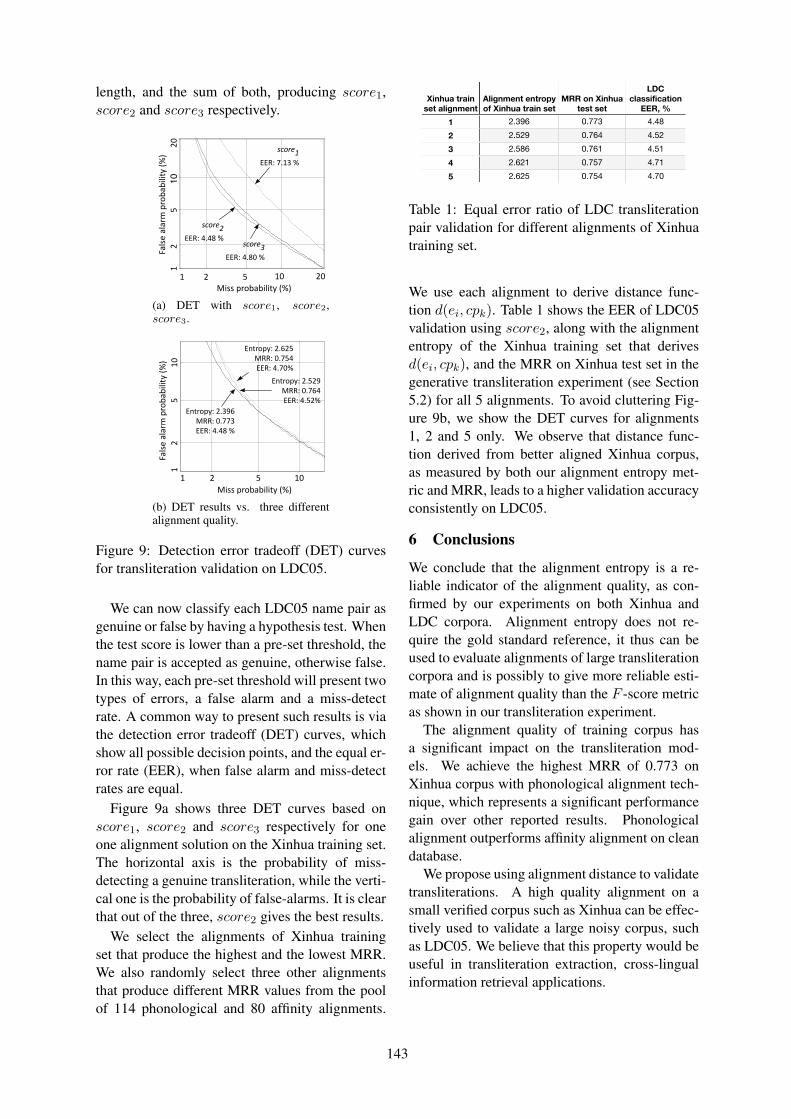
length, and the sum of both, producing score1,score2 and score3 respectively.
Missprobability(%)
Falsealarmprobability(%
)
2 5 10
12
510
1 20
20
score2EER:4.48%
score1EER:7.13%
score3EER:4.80%
(a) DET with score1, score2,score3.
1 2 5 10
12
510
Missprobability(%)
Falsealarmprobability(%
)
Entropy:2.396MRR:0.773EER:4.48%
Entropy:2.529MRR:0.764EER:4.52%
Entropy:2.625MRR:0.754EER:4.70%
(b) DET results vs. three differentalignment quality.
Figure 9: Detection error tradeoff (DET) curvesfor transliteration validation on LDC05.
We can now classify each LDC05 name pair asgenuine or false by having a hypothesis test. Whenthe test score is lower than a pre-set threshold, thename pair is accepted as genuine, otherwise false.In this way, each pre-set threshold will present twotypes of errors, a false alarm and a miss-detectrate. A common way to present such results is viathe detection error tradeoff (DET) curves, whichshow all possible decision points, and the equal er-ror rate (EER), when false alarm and miss-detectrates are equal.
Figure 9a shows three DET curves based onscore1, score2 and score3 respectively for oneone alignment solution on the Xinhua training set.The horizontal axis is the probability of miss-detecting a genuine transliteration, while the verti-cal one is the probability of false-alarms. It is clearthat out of the three, score2 gives the best results.
We select the alignments of Xinhua trainingset that produce the highest and the lowest MRR.We also randomly select three other alignmentsthat produce different MRR values from the poolof 114 phonological and 80 affinity alignments.
Xinhua train
set alignment
Alignment entropy
of Xinhua train set
MRR on Xinhua
test set
LDC
classification
EER, %
1
2
3
4
5
2.396 0.773 4.48
2.529 0.764 4.52
2.586 0.761 4.51
2.621 0.757 4.71
2.625 0.754 4.70
Table 1: Equal error ratio of LDC transliterationpair validation for different alignments of Xinhuatraining set.
We use each alignment to derive distance func-tion d(ei, cpk). Table 1 shows the EER of LDC05validation using score2, along with the alignmententropy of the Xinhua training set that derivesd(ei, cpk), and the MRR on Xinhua test set in thegenerative transliteration experiment (see Section5.2) for all 5 alignments. To avoid cluttering Fig-ure 9b, we show the DET curves for alignments1, 2 and 5 only. We observe that distance func-tion derived from better aligned Xinhua corpus,as measured by both our alignment entropy met-ric and MRR, leads to a higher validation accuracyconsistently on LDC05.
6 Conclusions
We conclude that the alignment entropy is a re-liable indicator of the alignment quality, as con-firmed by our experiments on both Xinhua andLDC corpora. Alignment entropy does not re-quire the gold standard reference, it thus can beused to evaluate alignments of large transliterationcorpora and is possibly to give more reliable esti-mate of alignment quality than the F -score metricas shown in our transliteration experiment.
The alignment quality of training corpus hasa significant impact on the transliteration mod-els. We achieve the highest MRR of 0.773 onXinhua corpus with phonological alignment tech-nique, which represents a significant performancegain over other reported results. Phonologicalalignment outperforms affinity alignment on cleandatabase.
We propose using alignment distance to validatetransliterations. A high quality alignment on asmall verified corpus such as Xinhua can be effec-tively used to validate a large noisy corpus, suchas LDC05. We believe that this property would beuseful in transliteration extraction, cross-lingualinformation retrieval applications.
143
ReferencesNasreen AbdulJaleel and Leah S. Larkey. 2003. Sta-
tistical transliteration for English-Arabic cross lan-guage information retrieval. In Proc. ACM CIKM.
Yaser Al-Onaizan and Kevin Knight. 2002. Machinetransliteration of names in arabic text. In Proc. ACLWorkshop: Computational Apporaches to SemiticLanguages.
Slaven Bilac and Hozumi Tanaka. 2004. A hybridback-transliteration system for Japanese. In Proc.COLING, pages 597–603.
Lin L. Chase. 1997. Error-responsive feedback mech-anisms for speech recognizers. Ph.D. thesis, CMU.
Asif Ekbal, Sudip Kumar Naskar, and Sivaji Bandy-opadhyay. 2006. A modified joint source-channelmodel for transliteration. In Proc. COLING/ACL,pages 191–198
Wei Gao, Kam-Fai Wong, and Wai Lam. 2004.Phoneme-based transliteration of foreign names forOOV problem. In Proc. IJCNLP, pages 374–381.
Long Jiang, Ming Zhou, Lee-Feng Chien, and ChengNiu. 2007. Named entity translation with web min-ing and transliteration. In IJCAI, pages 1629–1634.
Sung Young Jung, SungLim Hong, and Eunok Paek.2000. An English to Korean transliteration model ofextended Markov window. In Proc. COLING, vol-ume 1.
Paul. B. Kantor and Ellen. M. Voorhees. 2000. TheTREC-5 confusion track: comparing retrieval meth-ods for scanned text. Information Retrieval, 2:165–176.
Brett Kessler. 2005. Phonetic comparison algo-rithms. Transactions of the Philological Society,103(2):243–260.
Kevin Knight and Jonathan Graehl. 1998. Machinetransliteration. Computational Linguistics, 24(4).
Jin-Shea Kuo, Haizhou Li, and Ying-Kuei Yang. 2007.A phonetic similarity model for automatic extractionof transliteration pairs. ACM Trans. Asian LanguageInformation Processing, 6(2).
Patrik Lambert. 2008. Exploiting lexical informa-tion and discriminative alignment training in statis-tical machine translation. Ph.D. thesis, UniversitatPolitècnica de Catalunya, Barcelona, Spain.
Kevin Lenzo. 1997. t2p: text-to-phoneme converterbuilder. http://www.cs.cmu.edu/˜lenzo/t2p/.
Kevin Lenzo. 2008. The CMU pronounc-ing dictionary. http://www.speech.cs.cmu.edu/cgi-bin/cmudict.
Haizhou Li, Min Zhang, and Jian Su. 2004. A jointsource-channel model for machine transliteration.In Proc. ACL, pages 159–166.
Haizhou Li, Bin Ma, and Chin-Hui Lee. 2007a. Avector space modeling approach to spoken languageidentification. IEEE Trans. Acoust., Speech, SignalProcess., 15(1):271–284.
Haizhou Li, Khe Chai Sim, Jin-Shea Kuo, and MinghuiDong. 2007b. Semantic transliteration of personalnames. In Proc. ACL, pages 120–127.
Linguistic Data Consortium. 2005. LDC Chinese-English name entity lists LDC2005T34.
Helen M. Meng, Wai-Kit Lo, Berlin Chen, and KarenTang. 2001. Generate phonetic cognates to han-dle name entities in English-Chinese cross-languagespoken document retrieval. In Proc. ASRU.
Rada Mihalcea and Ted Pedersen. 2003. An evaluationexercise for word alignment. In Proc. HLT-NAACL,pages 1–10.
Jong-Hoon Oh and Key-Sun Choi. 2002. An English-Korean transliteration model using pronunciationand contextual rules. In Proc. COLING 2002.
Jong-Hoon Oh and Key-Sun Choi. 2005. Machinelearning based english-to-korean transliteration us-ing grapheme and phoneme information. IEICETrans. Information and Systems, E88-D(7):1737–1748.
Yan Qu and Gregory Grefenstette. 2004. Finding ideo-graphic representations of Japanese names written inLatin script via language identification and corpusvalidation. In Proc. ACL, pages 183–190.
Tao Tao, Su-Youn Yoon, Andrew Fisterd, RichardSproat, and ChengXiang Zhai. 2006. Unsupervisednamed entity transliteration using temporal and pho-netic correlation. In Proc. EMNLP, pages 250–257.
Paola Virga and Sanjeev Khudanpur. 2003. Translit-eration of proper names in cross-lingual informationretrieval. In Proc. ACL MLNER.
Stephen Wan and Cornelia Maria Verspoor. 1998. Au-tomatic English-Chinese name transliteration for de-velopment of multilingual resources. In Proc. COL-ING, pages 1352–1356.
M. M. Withgott and F. R. Chen. 1993. Computationalmodels of American speech. Centre for the study oflanguage and information.
Xinhua News Agency. 1992. Chinese transliterationof foreign personal names. The Commercial Press.
LiLi Xu, Atsushi Fujii, and Tetsuya Ishikawa. 2006.Modeling impression in probabilistic transliterationinto Chinese. In Proc. EMNLP, pages 242–249.
Su-Youn Yoon, Kyoung-Young Kim, and RichardSproat. 2007. Multilingual transliteration using fea-ture based phonetic method. In Proc. ACL, pages112–119.
144
Proceedings of the 47th Annual Meeting of the ACL and the 4th IJCNLP of the AFNLP, pages 145–153,Suntec, Singapore, 2-7 August 2009. c©2009 ACL and AFNLP
Automatic training of lemmatization rules that handle morphological changes in pre-, in- and suffixes alike
Bart Jongejan CST-University of Copenhagen
Njalsgade 140-142 2300 København S Denmark
Hercules Dalianis† ‡ †DSV, KTH - Stockholm University Forum 100, 164 40 Kista, Sweden
‡Euroling AB, SiteSeeker Igeldammsgatan 22c
112 49 Stockholm, Sweden [email protected]
Abstract
We propose a method to automatically train lemmatization rules that handle prefix, infix and suffix changes to generate the lemma from the full form of a word. We explain how the lemmatization rules are created and how the lemmatizer works. We trained this lemmatizer on Danish, Dutch, English, German, Greek, Icelandic, Norwegian, Polish, Slovene and Swedish full form-lemma pairs respectively. We obtained significant improvements of 24 percent for Polish, 2.3 percent for Dutch, 1.5 percent for English, 1.2 percent for German and 1.0 percent for Swedish compared to plain suffix lemmatization using a suffix-only lem-matizer. Icelandic deteriorated with 1.9 per-cent. We also made an observation regarding the number of produced lemmatization rules as a function of the number of training pairs.
1 Introduction
Lemmatizers and stemmers are valuable human language technology tools to improve precision and recall in an information retrieval setting. For example, stemming and lemmatization make it possible to match a query in one morphological form with a word in a document in another mor-phological form. Lemmatizers can also be used in lexicography to find new words in text mate-rial, including the words’ frequency of use. Other applications are creation of index lists for book indexes as well as key word lists
Lemmatization is the process of reducing a word to its base form, normally the dictionary look-up form (lemma) of the word. A trivial way to do this is by dictionary look-up. More ad-vanced systems use hand crafted or automatically
generated transformation rules that look at the surface form of the word and attempt to produce the correct base form by replacing all or parts of the word.
Stemming conflates a word to its stem. A stem does not have to be the lemma of the word, but can be any trait that is shared between a group of words, so that even the group membership itself can be regarded as the group’s stem.
The most famous stemmer is the Porter Stem-mer for English (Porter 1980). This stemmer re-moves around 60 different suffixes, using rewrit-ing rules in two steps.
The paper is structured as follows: section 2 discusses related work, section 3 explains what the new algorithm is supposed to do, section 4 describes some details of the new algorithm, sec-tion 5 evaluates the results, conclusions are drawn in section 6, and finally in section 7 we mention plans for further tests and improve-ments.
2 Related work
There have been some attempts in creating stemmers or lemmatizers automatically. Ek-mekçioglu et al. (1996) have used N-gram matching for Turkish that gave slightly better results than regular rule based stemming. Theron and Cloete (1997) learned two-level rules for English, Xhosa and Afrikaans, but only single character insertions, replacements and additions were allowed. Oard et al. (2001) used a language independent stemming technique in a dictionary based cross language information retrieval ex-periment for German, French and Italian where English was the search language. A four stage backoff strategy for improving recall was intro-
145
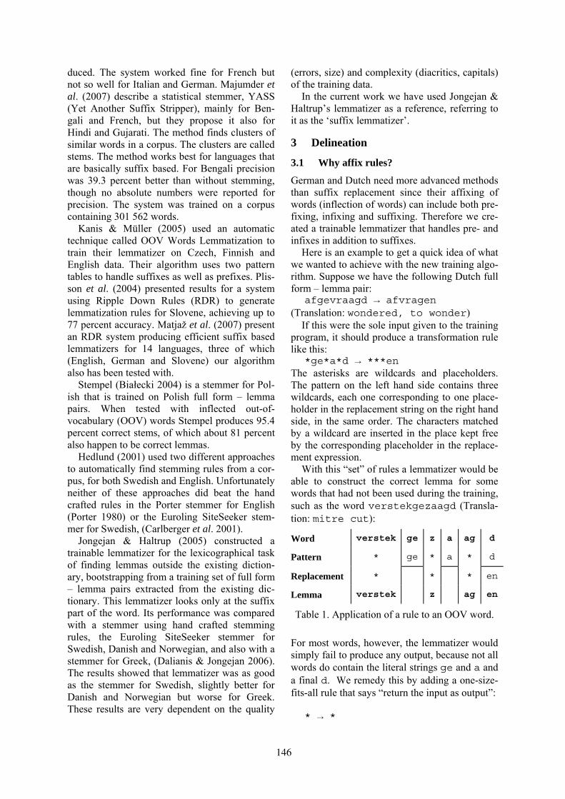
duced. The system worked fine for French but not so well for Italian and German. Majumder et al. (2007) describe a statistical stemmer, YASS (Yet Another Suffix Stripper), mainly for Ben-gali and French, but they propose it also for Hindi and Gujarati. The method finds clusters of similar words in a corpus. The clusters are called stems. The method works best for languages that are basically suffix based. For Bengali precision was 39.3 percent better than without stemming, though no absolute numbers were reported for precision. The system was trained on a corpus containing 301 562 words.
Kanis & Müller (2005) used an automatic technique called OOV Words Lemmatization to train their lemmatizer on Czech, Finnish and English data. Their algorithm uses two pattern tables to handle suffixes as well as prefixes. Plis-son et al. (2004) presented results for a system using Ripple Down Rules (RDR) to generate lemmatization rules for Slovene, achieving up to 77 percent accuracy. Matjaž et al. (2007) present an RDR system producing efficient suffix based lemmatizers for 14 languages, three of which (English, German and Slovene) our algorithm also has been tested with.
Stempel (Białecki 2004) is a stemmer for Pol-ish that is trained on Polish full form – lemma pairs. When tested with inflected out-of-vocabulary (OOV) words Stempel produces 95.4 percent correct stems, of which about 81 percent also happen to be correct lemmas.
Hedlund (2001) used two different approaches to automatically find stemming rules from a cor-pus, for both Swedish and English. Unfortunately neither of these approaches did beat the hand crafted rules in the Porter stemmer for English (Porter 1980) or the Euroling SiteSeeker stem-mer for Swedish, (Carlberger et al. 2001).
Jongejan & Haltrup (2005) constructed a trainable lemmatizer for the lexicographical task of finding lemmas outside the existing diction-ary, bootstrapping from a training set of full form – lemma pairs extracted from the existing dic-tionary. This lemmatizer looks only at the suffix part of the word. Its performance was compared with a stemmer using hand crafted stemming rules, the Euroling SiteSeeker stemmer for Swedish, Danish and Norwegian, and also with a stemmer for Greek, (Dalianis & Jongejan 2006). The results showed that lemmatizer was as good as the stemmer for Swedish, slightly better for Danish and Norwegian but worse for Greek. These results are very dependent on the quality
(errors, size) and complexity (diacritics, capitals) of the training data.
In the current work we have used Jongejan & Haltrup’s lemmatizer as a reference, referring to it as the ‘suffix lemmatizer’.
3 Delineation
3.1 Why affix rules?
German and Dutch need more advanced methods than suffix replacement since their affixing of words (inflection of words) can include both pre-fixing, infixing and suffixing. Therefore we cre-ated a trainable lemmatizer that handles pre- and infixes in addition to suffixes.
Here is an example to get a quick idea of what we wanted to achieve with the new training algo-rithm. Suppose we have the following Dutch full form – lemma pair:
afgevraagd → afvragen (Translation: wondered, to wonder)
If this were the sole input given to the training program, it should produce a transformation rule like this:
*ge*a*d → ***en The asterisks are wildcards and placeholders. The pattern on the left hand side contains three wildcards, each one corresponding to one place-holder in the replacement string on the right hand side, in the same order. The characters matched by a wildcard are inserted in the place kept free by the corresponding placeholder in the replace-ment expression.
With this “set” of rules a lemmatizer would be able to construct the correct lemma for some words that had not been used during the training, such as the word verstekgezaagd (Transla-tion: mitre cut):
Word verstek ge z a ag d
Pattern * ge * a * d
Replacement * * * en
Lemma verstek z ag en
Table 1. Application of a rule to an OOV word.
For most words, however, the lemmatizer would simply fail to produce any output, because not all words do contain the literal strings ge and a and a final d. We remedy this by adding a one-size-fits-all rule that says “return the input as output”:
* → *
146
So now our rule set consists of two rules: *ge*a*d → ***en * → *
The lemmatizer then finds the rule with the most specific pattern (see 4.2) that matches and ap-plies only this rule. The last rule’s pattern matches any word and so the lemmatizer cannot fail to produce output. Thus, in our toy rule set consisting of two rules, the first rule handles words like gevraagd, afgezaagd, geklaagd, (all three correctly) and getalmd (incorrectly) while the second rule handles words like directeur (correctly) and zei (incor-rectly).
3.2 Inflected vs. agglutinated languages
A lemmatizer that only applies one rule per word is useful for inflected languages, a class of lan-guages that includes all Indo-European lan-guages. For these languages morphological change is not a productive process, which means that no word can be morphologically changed in an unlimited number of ways. Ideally, there are only a finite number of inflection schemes and thus a finite number of lemmatization rules should suffice to lemmatize indefinitely many words.
In agglutinated languages, on the other hand, there are classes of words that in principle have innumerous word forms. One way to lemmatize such words is to peel off all agglutinated mor-phemes one by one. This is an iterative process and therefore the lemmatizer discussed in this paper, which applies only one rule per word, is not an obvious choice for agglutinated lan-guages.
3.3 Supervised training
An automatic process to create lemmatization rules is described in the following sections. By reserving a small part of the available training data for testing it is possible to quite accurately estimate the probability that the lemmatizer would produce the right lemma given any un-known word belonging to the language, even without requiring that the user masters the lan-guage (Kohavi 1995).
On the downside, letting a program construct lemmatization rules requires an extended list of full form – lemma pairs that the program can exercise on – at least tens of thousands and pos-sibly over a million entries (Dalianis and Jonge-jan 2006).
3.4 Criteria for success
The main challenge for the training algorithm is that it must produce rules that accurately lemma-tize OOV words. This requirement translates to two opposing tendencies during training. On the one hand we must trust rules with a wide basis of training examples more than rules with a small basis, which favours rules with patterns that fit many words. On the other hand we have the in-compatible preference for cautious rules with rather specific patterns, because these must be better at avoiding erroneous rule applications than rules with generous patterns. The envisaged expressiveness of the lemmatization rules – al-lowing all kinds of affixes and an unlimited number of wildcards – turns the challenge into a difficult balancing act.
In the current work we wanted to get an idea of the advantages of an affix-based algorithm compared to a suffix-only based algorithm. Therefore we have made the task as hard as pos-sible by not allowing language specific adapta-tions to the algorithms and by not subdividing the training words in word classes.
4 Generation of rules and look-up data structure
4.1 Building a rule set from training pairs
The training algorithm generates a data structure consisting of rules that a lemmatizer must trav-erse to arrive at a rule that is elected to fire.
Conceptually the training process is as fol-lows. As the data structure is being built, the full form in each training pair is tentatively lemma-tized using the data structure that has been cre-ated up to that stage. If the elected rule produces the right lemma from the full form, nothing needs to be done. Otherwise, the data structure must be expanded with a rule such that the new rule a) is elected instead of the erroneous rule and b) produces the right lemma from the full form. The training process terminates when the full forms in all pairs in the training set are trans-formed to their corresponding lemmas.
After training, the data structure of rules is made permanent and can be consulted by a lem-matizer. The lemmatizer must elect and fire rules in the same way as the training algorithm, so that all words from the training set are lemmatized correctly. It may however fail to produce the cor-rect lemmas for words that were not in the train-ing set – the OOV words.
147

4.2 Internal structure of rules: prime and derived rules
During training the Ratcliff/Obershelp algorithm (Ratcliff & Metzener 1988) is used to find the longest non-overlapping similar parts in a given full form – lemma pair. For example, in the pair
afgevraagd → afvragen the longest common substring is vra, followed by af and g. These similar parts are replaced with wildcards and placeholders:
*ge*a*d → ***en Now we have the prime rule for the training pair, the least specific rule necessary to lemmatize the word correctly. Rules with more specific patterns – derived rules – can be created by adding char-acters and by removing or adding wildcards. A rule that is derived from another rule (derived or prime) is more specific than the original rule: Any word that is successfully matched by the pattern of a derived rule is also successfully matched by the pattern of the original rule, but the converse is not the case. This establishes a partial ordering of all rules. See Figures 1 and 2, where the rules marked ‘p’ are prime rules and those marked ‘d’ are derived.
Innumerous rules can be derived from a rule with at least one wildcard in its pattern, but only a limited number can be tested in a finite time. To keep the number of candidate rules within practical limits, we used the strategy that the pat-tern of a candidate is minimally different from its parent’s pattern: it can have one extra literal character or one wildcard less or replace one wildcard with one literal character. Alternatively, a candidate rule (such as the bottom rule in Fig-ure 4) can arise by merging two rules. Within these constraints, the algorithm creates all possi-ble candidate rules that transform one or more training words to their corresponding lemmas.
4.3 External structure of rules: partial or-dering in a DAG and in a tree
We tried two different data structures to store new lemmatizer rules, a directed acyclic graph (DAG) and a plain tree structure with depth first, left to right traversal.
The DAG (Figure 1) expresses the complete partial ordering of the rules. There is no prefer-ential order between the children of a rule and all paths away from the root must be regarded as equally valid. Therefore the DAG may lead to several lemmas for the same input word. For ex-ample, without the rule in the bottom part of Fig-ure 1, the word gelopen would have been lem-
matized to both lopen (correct) and gelopen (incorrect):
gelopen: *ge* → ** lopen *pen → *pen gelopen
By adding a derived rule as a descendent of both these two rules, we make sure that lemmatization of the word gelopen is only handled by one rule and only results in the correct lemma:
gelopen: *ge*pen → **pen lopen
Figure 1. Five training pairs as supporters for five rules in a DAG.
The tree in Figure 2 is a simpler data structure and introduces a left to right preferential order between the children of a rule. Only one rule fires and only one lemma per word is produced. For example, because the rule *ge* → ** pre-cedes its sibling rule *en → *, whenever the former rule is applicable, the latter rule and its descendents are not even visited, irrespective of their applicability. In our example, the former rule – and only the former rule – handles the lemmatization of gelopen, and since it pro-duces the correct lemma an additional rule is not necessary.
In contrast to the DAG, the tree implements negation: if the Nth sibling of a row of children fires, it not only means that the pattern of the Nth rule matches the word, it also means that the pat-terns of the N-1 preceding siblings do not match the word. Such implicit negation is not possible in the DAG, and this is probably the main reason why the experiments with the DAG-structure lead to huge numbers of rules, very little gener-
* → * ui → ui
*ge* → ** overgegaan → overgaan
*en → * uien→ ui
*pen →*pen lopen → lopen
*ge*pen → **pen gelopen → lopen
p
p p
d
d
148

alization, uncontrollable training times (months, not minutes!) and very low lemmatization qual-ity. On the other hand, the experiments with the tree structure were very successful. The building time of the rules is acceptable, taking small re-cursive steps during the training part. The mem-ory use is tractable and the quality of the results is good provided good training material.
Figure 2. The same five training pairs as sup-porters for only four rules in a tree.
4.4 Rule selection criteria
This section pertains to the training algorithm employing a tree.
The typical situation during training is that a rule that already has been added to the tree makes lemmatization errors on some of the train-ing words. In that case one or more corrective children have to be added to the rule1.
If the pattern of a new child rule only matches some, but not all training words that are lemma-tized incorrectly by the parent, a right sibling rule must be added. This is repeated until all training words that the parent does not lemmatize correctly are matched by the leftmost child rule or one of its siblings.
A candidate child rule is faced with training words that the parent did not lemmatize correctly and, surprisingly, also supporters of the parent, because the pattern of the candidate cannot dis-criminate between these two groups.
On the output side of the candidate appear the training pairs that are lemmatized correctly by the candidate, those that are lemmatized incor-
1 If the case of a DAG, care must be taken that the complete representation of the partial ordering of rules is maintained. Any new rule not only becomes a child of the rule that it was aimed at as a corrective child, but often also of several other rules.
rectly and those that do not match the pattern of the candidate.
For each candidate rule the training algorithm creates a 2×3 table (see Table 2) that counts the number of training pairs that the candidate lem-matizes correctly or incorrectly or that the candi-date does not match. The two columns count the training pairs that, respectively, were lemmatized incorrectly and correctly by the parent. These six parameters Nxy can be used to select the best can-didate. Only four parameters are independent, because the numbers of training words that the parent lemmatized incorrectly (Nw) and correctly (Nr) are the same for all candidates. Thus, after the application of the first and most significant selection criterion, up to three more selection criteria of decreasing significance can be applied if the preceding selection ends in a tie.
Parent Child
Incorrect Correct (supporters)
Correct Nwr Nrr
Incorrect Nww Nrw
Not matched Nwn Nrn
Sum Nw Nr
Table 2. The six parameters for rule selection among candidate rules.
A large Nwr and a small Nrw are desirable. Nwr is a measure for the rate at which the updated data structure has learned to correctly lemmatize those words that previously were lemmatized incorrectly. A small Nrw indicates that only few words that previously were lemmatized correctly are spoiled by the addition of the new rule. It is less obvious how the other numbers weigh in.
We have obtained the most success with crite-ria that first select for highest Nwr + Nrr - Nrw . If the competition ends in a tie, we select for lowest Nrr among the remaining candidates. If the com-petition again ends in a tie, we select for highest Nrn – Nww . Due to the marginal effect of a fourth criterion we let the algorithm randomly select one of the remaining candidates instead.
The training pairs that are matched by the pat-tern of the winning rule become the supporters and non-supporters of that new rule and are no longer supporters or non-supporters of the par-ent. If the parent still has at least one non-supporter, the remaining supporters and non-supporters – the training pairs that the winning
* → * ui → ui
*ge* → ** overgegaan → overgaan
gelopen → lopen
*en → * uien→ ui
*pen →*pen lopen → lopen
p
p p
d
149
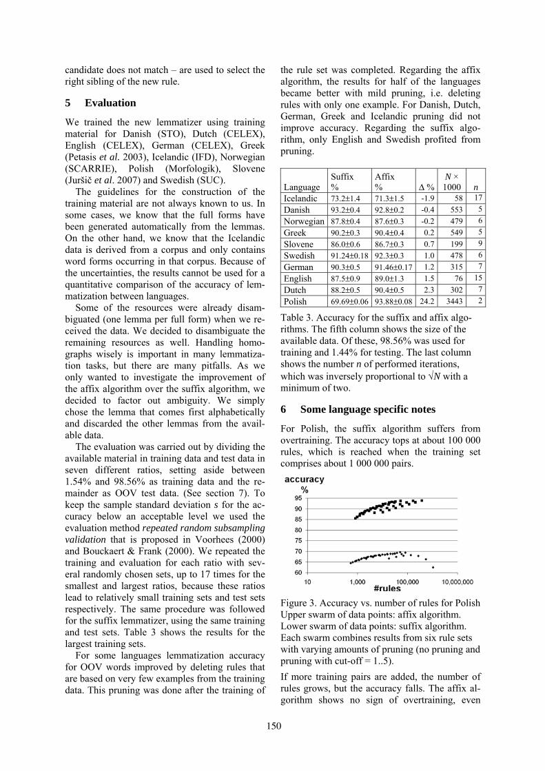
candidate does not match – are used to select the right sibling of the new rule.
5 Evaluation
We trained the new lemmatizer using training material for Danish (STO), Dutch (CELEX), English (CELEX), German (CELEX), Greek (Petasis et al. 2003), Icelandic (IFD), Norwegian (SCARRIE), Polish (Morfologik), Slovene (Juršič et al. 2007) and Swedish (SUC).
The guidelines for the construction of the training material are not always known to us. In some cases, we know that the full forms have been generated automatically from the lemmas. On the other hand, we know that the Icelandic data is derived from a corpus and only contains word forms occurring in that corpus. Because of the uncertainties, the results cannot be used for a quantitative comparison of the accuracy of lem-matization between languages.
Some of the resources were already disam-biguated (one lemma per full form) when we re-ceived the data. We decided to disambiguate the remaining resources as well. Handling homo-graphs wisely is important in many lemmatiza-tion tasks, but there are many pitfalls. As we only wanted to investigate the improvement of the affix algorithm over the suffix algorithm, we decided to factor out ambiguity. We simply chose the lemma that comes first alphabetically and discarded the other lemmas from the avail-able data.
The evaluation was carried out by dividing the available material in training data and test data in seven different ratios, setting aside between 1.54% and 98.56% as training data and the re-mainder as OOV test data. (See section 7). To keep the sample standard deviation s for the ac-curacy below an acceptable level we used the evaluation method repeated random subsampling validation that is proposed in Voorhees (2000) and Bouckaert & Frank (2000). We repeated the training and evaluation for each ratio with sev-eral randomly chosen sets, up to 17 times for the smallest and largest ratios, because these ratios lead to relatively small training sets and test sets respectively. The same procedure was followed for the suffix lemmatizer, using the same training and test sets. Table 3 shows the results for the largest training sets.
For some languages lemmatization accuracy for OOV words improved by deleting rules that are based on very few examples from the training data. This pruning was done after the training of
the rule set was completed. Regarding the affix algorithm, the results for half of the languages became better with mild pruning, i.e. deleting rules with only one example. For Danish, Dutch, German, Greek and Icelandic pruning did not improve accuracy. Regarding the suffix algo-rithm, only English and Swedish profited from pruning.
Language Suffix %
Affix % Δ %
N × 1000 n
Icelandic 73.2±1.4 71.3±1.5 -1.9 58 17Danish 93.2±0.4 92.8±0.2 -0.4 553 5Norwegian 87.8±0.4 87.6±0.3 -0.2 479 6Greek 90.2±0.3 90.4±0.4 0.2 549 5Slovene 86.0±0.6 86.7±0.3 0.7 199 9Swedish 91.24±0.18 92.3±0.3 1.0 478 6German 90.3±0.5 91.46±0.17 1.2 315 7English 87.5±0.9 89.0±1.3 1.5 76 15Dutch 88.2±0.5 90.4±0.5 2.3 302 7Polish 69.69±0.06 93.88±0.08 24.2 3443 2
Table 3. Accuracy for the suffix and affix algo-rithms. The fifth column shows the size of the available data. Of these, 98.56% was used for training and 1.44% for testing. The last column shows the number n of performed iterations, which was inversely proportional to √N with a minimum of two.
6 Some language specific notes
For Polish, the suffix algorithm suffers from overtraining. The accuracy tops at about 100 000 rules, which is reached when the training set comprises about 1 000 000 pairs.
Figure 3. Accuracy vs. number of rules for Polish Upper swarm of data points: affix algorithm. Lower swarm of data points: suffix algorithm. Each swarm combines results from six rule sets with varying amounts of pruning (no pruning and pruning with cut-off = 1..5).
If more training pairs are added, the number of rules grows, but the accuracy falls. The affix al-gorithm shows no sign of overtraining, even
150
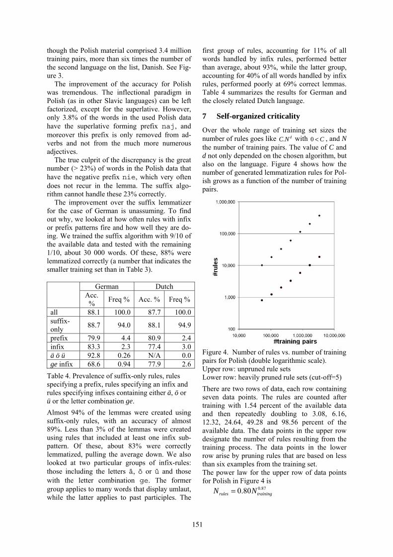
though the Polish material comprised 3.4 million training pairs, more than six times the number of the second language on the list, Danish. See Fig-ure 3.
The improvement of the accuracy for Polish was tremendous. The inflectional paradigm in Polish (as in other Slavic languages) can be left factorized, except for the superlative. However, only 3.8% of the words in the used Polish data have the superlative forming prefix naj, and moreover this prefix is only removed from ad-verbs and not from the much more numerous adjectives.
The true culprit of the discrepancy is the great number (> 23%) of words in the Polish data that have the negative prefix nie, which very often does not recur in the lemma. The suffix algo-rithm cannot handle these 23% correctly.
The improvement over the suffix lemmatizer for the case of German is unassuming. To find out why, we looked at how often rules with infix or prefix patterns fire and how well they are do-ing. We trained the suffix algorithm with 9/10 of the available data and tested with the remaining 1/10, about 30 000 words. Of these, 88% were lemmatized correctly (a number that indicates the smaller training set than in Table 3).
German Dutch
Acc. % Freq % Acc. % Freq %
all 88.1 100.0 87.7 100.0suffix-only 88.7 94.0 88.1 94.9
prefix 79.9 4.4 80.9 2.4infix 83.3 2.3 77.4 3.0ä ö ü 92.8 0.26 N/A 0.0ge infix 68.6 0.94 77.9 2.6
Table 4. Prevalence of suffix-only rules, rules specifying a prefix, rules specifying an infix and rules specifying infixes containing either ä, ö or ü or the letter combination ge.
Almost 94% of the lemmas were created using suffix-only rules, with an accuracy of almost 89%. Less than 3% of the lemmas were created using rules that included at least one infix sub-pattern. Of these, about 83% were correctly lemmatized, pulling the average down. We also looked at two particular groups of infix-rules: those including the letters ä, ö or ü and those with the letter combination ge. The former group applies to many words that display umlaut, while the latter applies to past participles. The
first group of rules, accounting for 11% of all words handled by infix rules, performed better than average, about 93%, while the latter group, accounting for 40% of all words handled by infix rules, performed poorly at 69% correct lemmas. Table 4 summarizes the results for German and the closely related Dutch language.
7 Self-organized criticality
Over the whole range of training set sizes the number of rules goes like dNC. with C<0 , and N the number of training pairs. The value of C and d not only depended on the chosen algorithm, but also on the language. Figure 4 shows how the number of generated lemmatization rules for Pol-ish grows as a function of the number of training pairs.
Figure 4. Number of rules vs. number of training pairs for Polish (double logarithmic scale). Upper row: unpruned rule sets Lower row: heavily pruned rule sets (cut-off=5)
There are two rows of data, each row containing seven data points. The rules are counted after training with 1.54 percent of the available data and then repeatedly doubling to 3.08, 6.16, 12.32, 24.64, 49.28 and 98.56 percent of the available data. The data points in the upper row designate the number of rules resulting from the training process. The data points in the lower row arise by pruning rules that are based on less than six examples from the training set. The power law for the upper row of data points for Polish in Figure 4 is
87.080.0 trainingrules NN =
151
As a comparison, for Icelandic the power law for the unpruned set of rules is
90.032.1 trainingrules NN =
These power law expressions are derived for the affix algorithm. For the suffix algorithm the ex-ponent in the Polish power law expression is very close to 1 (0.98), which indicates that the suffix lemmatizer is not good at all at generaliz-ing over the Polish training data: the number of rules grows almost proportionally with the num-ber of training words. (And, as Figure 3 shows, to no avail.) On the other hand, the suffix lem-matizer fares better than the affix algorithm for Icelandic data, because in that case the exponent in the power law expression is lower: 0.88 versus 0.90.
The power law is explained by self-organized criticality (Bak et al. 1987, 1988). Rule sets that originate from training sets that only differ in a single training example can be dissimilar to any degree depending on whether and where the dif-ference is tipping the balance between competing rule candidates. Whether one or the other rule candidate wins has a very significant effect on the parts of the tree that emanate as children or as siblings from the winning node. If the difference has an effect close to the root of the tree, a large expanse of the tree is affected. If the difference plays a role closer to a leaf node, only a small patch of the tree is affected. The effect of adding a single training example can be compared with dropping a single rice corn on top of a pile of rice, which can create an avalanche of unpredict-able size.
8 Conclusions
Affix rules perform better than suffix rules if the language has a heavy pre- and infix morphology and the size of the training data is big. The new algorithm worked very well with the Polish Mor-fologik dataset and compares well with the Stempel algorithm (Białecki 2008).
Regarding Dutch and German we have ob-served that the affix algorithm most often applies suffix-only rules to OOV words. We have also observed that words lemmatized this way are lemmatized better than average. The remaining words often need morphological changes in more than one position, for example both in an infix and a suffix. Although these changes are corre-lated by the inflectional rules of the language, the number of combinations is still large, while at the same time the number of training examples exhibiting such combinations is relatively small.
Therefore the more complex rules involving infix or prefix subpatterns or combinations thereof are less well-founded than the simple suffix-only rules. The lemmatization accuracy of the com-plex rules will therefore in general be lower than that of the suffix-only rules. The reason why the affix algorithm is still better than the algorithm that only considers suffix rules is that the affix algorithm only generates suffix-only rules from words with suffix-only morphology. The suffix-only algorithm is not able to generalize over training examples that do not fulfil this condition and generates many rules based on very few ex-amples. Consequently, everything else being equal, the set of suffix-only rules generated by the affix algorithm must be of higher quality than the set of rules generated by the suffix algorithm.
The new affix algorithm has fewer rules sup-ported by only one example from the training data than the suffix algorithm. This means that the new algorithm is good at generalizing over small groups of words with exceptional mor-phology. On the other hand, the bulk of ‘normal’ training words must be bigger for the new affix based lemmatizer than for the suffix lemmatizer. This is because the new algorithm generates im-mense numbers of candidate rules with only marginal differences in accuracy, requiring many examples to find the best candidate.
When we began experimenting with lemmati-zation rules with unrestricted numbers of affixes, we could not know whether the limited amount of available training data would be sufficient to fix the enormous amount of free variables with enough certainty to obtain higher quality results than obtainable with automatically trained lem-matizers allowing only suffix transformations.
However, the results that we have obtained with the new affix algorithm are on a par with or better than those of the suffix lemmatizer. There is still room for improvements as only part of the parameter space of the new algorithm has been searched. The case of Polish shows the superior-ity of the new algorithm, whereas the poor re-sults for Icelandic, a suffix inflecting language with many inflection types, were foreseeable, because we only had a small training set.
9 Future work Work with the new affix lemmatizer has until now focused on the algorithm. To really know if the carried out theoretical work is valuable we would like to try it out in a real search setting in a search engine and see if the users appreciate the new algorithm’s results.
152

References Per Bak, Chao Tang and Kurt Wiesenfeld. 1987. Self-
Organized Criticality: An Explanation of 1/f Noise, Phys. Rev. Lett., vol. 59,. pp. 381-384, 1987
Per Bak, Chao Tang and Kurt Wiesenfeld . 1988. Phys. Rev. A38, (1988), pp. 364-374
Andrzej Białecki, 2004, Stempel - Algorithmic Stemmer for Polish Language http://www.getopt.org/stempel/
Remco R. Bouckaert and Eibe Frank. 2000. Evaluat-ing the Replicability of Significance Tests for Comparing Learning Algorithms. In H. Dai, R. Srikant, & C. Zhang (Eds.), Proc. 8th Pacific-Asia Conference, PAKDD 2004, Sydney, Australia, May 26-28, 2004 (pp. 3-12). Berlin: Springer.
Johan Carlberger, Hercules Dalianis, Martin Hassel, and Ola Knutsson. 2001. Improving Precision in Information Retrieval for Swedish using Stem-ming. In the Proceedings of NoDaLiDa-01 - 13th Nordic Conference on Computational Linguistics, May 21-22, Uppsala, Sweden.
Celex: http://celex.mpi.nl/
Hercules Dalianis and Bart Jongejan 2006. Hand-crafted versus Machine-learned Inflectional Rules: the Euroling-SiteSeeker Stemmer and CST's Lem-matiser, in Proceedings of the International Con-ference on Language Resources and Evaluation, LREC 2006.
F. Çuna Ekmekçioglu, Mikael F. Lynch, and Peter Willett. 1996. Stemming and N-gram matching for term conflation in Turkish texts. Information Re-search, 7(1) pp 2-6.
Niklas Hedlund 2001. Automatic construction of stemming rules, Master Thesis, NADA-KTH, Stockholm, TRITA-NA-E0194.
IFD: Icelandic Centre for Language Technology, http://tungutaekni.is/researchsystems/rannsoknir_12en.html
Bart Jongejan and Dorte Haltrup. 2005. The CST Lemmatiser. Center for Sprogteknologi, University of Copenhagen version 2.7 (August, 23 2005) http://cst.dk/online/lemmatiser/cstlemma.pdf
Jakub Kanis and Ludek Müller. 2005. Automatic Lemmatizer Construction with Focus on OOV Words Lemmatization in Text, Speech and Dia-logue, Lecture Notes in Computer Science, Berlin / Heidelberg, pp 132-139
Ron Kohavi. 1995. A study of cross-validation and bootstrap for accuracy estimation and model selec-tion. Proceedings of the Fourteenth International Joint Conference on Artificial Intelligence 2 (12): 1137–1143, Morgan Kaufmann, San Mateo.
Prasenjit Majumder, Mandar Mitra, Swapan K. Parui, Gobinda Kole, Pabitra Mitra, and Kalyankumar Datta. 2007. YASS: Yet another suffix stripper. ACM Transactions on Information Systems , Vol-ume 25 , Issue 4, October 2007.
Juršič Matjaž, Igor Mozetič, and Nada Lavrač. 2007. Learning ripple down rules for efficient lemmatiza-tion In proceeding of the Conference on Data Min-ing and Data Warehouses (SiKDD 2007), October 12, 2007, Ljubljana, Slovenia
Morfologik: Polish morphological analyzer http://mac.softpedia.com/get/Word-Processing/Morfologik.shtml
Douglas W. Oard, Gina-Anne Levow, and Clara I. Cabezas. 2001. CLEF experiments at Maryland: Statistical stemming and backoff translation. In Cross-language information retrieval and evalua-tion: Proceeding of the Clef 2000 workshops Carol Peters Ed. Springer Verlag pp. 176-187. 2001.
Georgios Petasis, Vangelis Karkaletsis , Dimitra Far-makiotou , Ion Androutsopoulos and Constantine D. Spyropoulo. 2003. A Greek Morphological Lexicon and its Exploitation by Natural Language Processing Applications. In Lecture Notes on Computer Science (LNCS), vol.2563, "Advances in Informatics - Post-proceedings of the 8th Pan-hellenic Conference in Informatics", Springer Ver-lag.
Joël Plisson, Nada Lavrač, and Dunja Mladenic. 2004, A rule based approach to word lemmatization, Proceedings of the 7th International Multi-conference Information Society, IS-2004, Institut Jozef Stefan, Ljubljana, pp.83-6.
Martin F. Porter 1980. An algorithm for suffix strip-ping. Program, vol 14, no 3, pp 130-130.
John W. Ratcliff and David Metzener, 1988. Pattern Matching: The Gestalt Approach, Dr. Dobb's Journal, page 46, July 1988.
SCARRIE 2009. Scandinavian Proofreading Tools http://ling.uib.no/~desmedt/scarrie/
STO: http://cst.ku.dk/sto_ordbase/
SUC 2009. Stockholm Umeå corpus, http://www.ling.su.se/staff/sofia/suc/suc.html
Pieter Theron and Ian Cloete 1997 Automatic acquisi-tion of two-level morphological rules, Proceedings of the fifth conference on Applied natural language processing, p.103-110, March 31-April 03, 1997, Washington, DC.
Ellen M. Voorhees. 2000. Variations in relevance judgments and the measurement of retrieval effec-tiveness, J. of Information Processing and Man-agement 36 (2000) pp 697-716
153

Proceedings of the 47th Annual Meeting of the ACL and the 4th IJCNLP of the AFNLP, pages 154–162,Suntec, Singapore, 2-7 August 2009. c©2009 ACL and AFNLP
Revisiting Pivot Language Approach for Machine Translation
Hua Wu and Haifeng WangToshiba (China) Research and Development Center
5/F., Tower W2, Oriental Plaza, Beijing, 100738, China{wuhua, wanghaifeng}@rdc.toshiba.com.cn
AbstractThis paper revisits the pivot language ap-proach for machine translation. First,we investigate three different methodsfor pivot translation. Then we employa hybrid method combining RBMT andSMT systems to fill up the data gapfor pivot translation, where the source-pivot and pivot-target corpora are inde-pendent. Experimental results on spo-ken language translation show that thishybrid method significantly improves thetranslation quality, which outperforms themethod using a source-target corpus ofthe same size. In addition, we pro-pose a system combination approach toselect better translations from those pro-duced by various pivot translation meth-ods. This method regards system com-bination as a translation evaluation prob-lem and formalizes it with a regressionlearning model. Experimental results in-dicate that our method achieves consistentand significant improvement over individ-ual translation outputs.
1 Introduction
Current statistical machine translation (SMT) sys-tems rely on large parallel and monolingual train-ing corpora to produce translations of relativelyhigher quality. Unfortunately, large quantities ofparallel data are not readily available for some lan-guages pairs, therefore limiting the potential useof current SMT systems. In particular, for speechtranslation, the translation task often focuses on aspecific domain such as the travel domain. It is es-pecially difficult to obtain such a domain-specificcorpus for some language pairs such as Chinese toSpanish translation.
To circumvent the data bottleneck, some re-searchers have investigated to use a pivot language
approach (Cohn and Lapata, 2007; Utiyama andIsahara, 2007; Wu and Wang 2007; Bertoldi et al.,2008). This approach introduces a third language,named the pivot language, for which there existlarge source-pivot and pivot-target bilingual cor-pora. A pivot task was also designed for spokenlanguage translation in the evaluation campaign ofIWSLT 2008 (Paul, 2008), where English is usedas a pivot language for Chinese to Spanish trans-lation.
Three different pivot strategies have been in-vestigated in the literature. The first is basedon phrase table multiplication (Cohn and Lap-ata 2007; Wu and Wang, 2007). It multiplescorresponding translation probabilities and lexicalweights in source-pivot and pivot-target transla-tion models to induce a new source-target phrasetable. We name it the triangulation method. Thesecond is the sentence translation strategy, whichfirst translates the source sentence to the pivot sen-tence, and then to the target sentence (Utiyama andIsahara, 2007; Khalilov et al., 2008). We name itthe transfer method. The third is to use existingmodels to build a synthetic source-target corpus,from which a source-target model can be trained(Bertoldi et al., 2008). For example, we can ob-tain a source-pivot corpus by translating the pivotsentence in the source-pivot corpus into the targetlanguage with pivot-target translation models. Wename it the synthetic method.
The working condition with the pivot languageapproach is that the source-pivot and pivot-targetparallel corpora are independent, in the sense thatthey are not derived from the same set of sen-tences, namely independently sourced corpora.Thus, some linguistic phenomena in the source-pivot corpus will lost if they do not exist in thepivot-target corpus, and vice versa. In order to fillup this data gap, we make use of rule-based ma-chine translation (RBMT) systems to translate thepivot sentences in the source-pivot or pivot-target
154
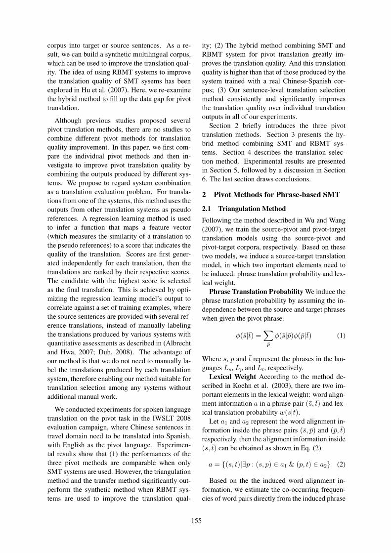
corpus into target or source sentences. As a re-sult, we can build a synthetic multilingual corpus,which can be used to improve the translation qual-ity. The idea of using RBMT systems to improvethe translation quality of SMT sysems has beenexplored in Hu et al. (2007). Here, we re-examinethe hybrid method to fill up the data gap for pivottranslation.
Although previous studies proposed severalpivot translation methods, there are no studies tocombine different pivot methods for translationquality improvement. In this paper, we first com-pare the individual pivot methods and then in-vestigate to improve pivot translation quality bycombining the outputs produced by different sys-tems. We propose to regard system combinationas a translation evaluation problem. For transla-tions from one of the systems, this method uses theoutputs from other translation systems as pseudoreferences. A regression learning method is usedto infer a function that maps a feature vector(which measures the similarity of a translation tothe pseudo references) to a score that indicates thequality of the translation. Scores are first gener-ated independently for each translation, then thetranslations are ranked by their respective scores.The candidate with the highest score is selectedas the final translation. This is achieved by opti-mizing the regression learning model’s output tocorrelate against a set of training examples, wherethe source sentences are provided with several ref-erence translations, instead of manually labelingthe translations produced by various systems withquantitative assessments as described in (Albrechtand Hwa, 2007; Duh, 2008). The advantage ofour method is that we do not need to manually la-bel the translations produced by each translationsystem, therefore enabling our method suitable fortranslation selection among any systems withoutadditional manual work.
We conducted experiments for spoken languagetranslation on the pivot task in the IWSLT 2008evaluation campaign, where Chinese sentences intravel domain need to be translated into Spanish,with English as the pivot language. Experimen-tal results show that (1) the performances of thethree pivot methods are comparable when onlySMT systems are used. However, the triangulationmethod and the transfer method significantly out-perform the synthetic method when RBMT sys-tems are used to improve the translation qual-
ity; (2) The hybrid method combining SMT andRBMT system for pivot translation greatly im-proves the translation quality. And this translationquality is higher than that of those produced by thesystem trained with a real Chinese-Spanish cor-pus; (3) Our sentence-level translation selectionmethod consistently and significantly improvesthe translation quality over individual translationoutputs in all of our experiments.
Section 2 briefly introduces the three pivottranslation methods. Section 3 presents the hy-brid method combining SMT and RBMT sys-tems. Section 4 describes the translation selec-tion method. Experimental results are presentedin Section 5, followed by a discussion in Section6. The last section draws conclusions.
2 Pivot Methods for Phrase-based SMT
2.1 Triangulation MethodFollowing the method described in Wu and Wang(2007), we train the source-pivot and pivot-targettranslation models using the source-pivot andpivot-target corpora, respectively. Based on thesetwo models, we induce a source-target translationmodel, in which two important elements need tobe induced: phrase translation probability and lex-ical weight.
Phrase Translation Probability We induce thephrase translation probability by assuming the in-dependence between the source and target phraseswhen given the pivot phrase.
φ(s̄|t̄) =∑
p̄
φ(s̄|p̄)φ(p̄|t̄) (1)
Where s̄, p̄ and t̄ represent the phrases in the lan-guages Ls, Lp and Lt, respectively.
Lexical Weight According to the method de-scribed in Koehn et al. (2003), there are two im-portant elements in the lexical weight: word align-ment information a in a phrase pair (s̄, t̄) and lex-ical translation probability w(s|t).
Let a1 and a2 represent the word alignment in-formation inside the phrase pairs (s̄, p̄) and (p̄, t̄)respectively, then the alignment information inside(s̄, t̄) can be obtained as shown in Eq. (2).
a = {(s, t)|∃p : (s, p) ∈ a1 & (p, t) ∈ a2} (2)
Based on the the induced word alignment in-formation, we estimate the co-occurring frequen-cies of word pairs directly from the induced phrase
155
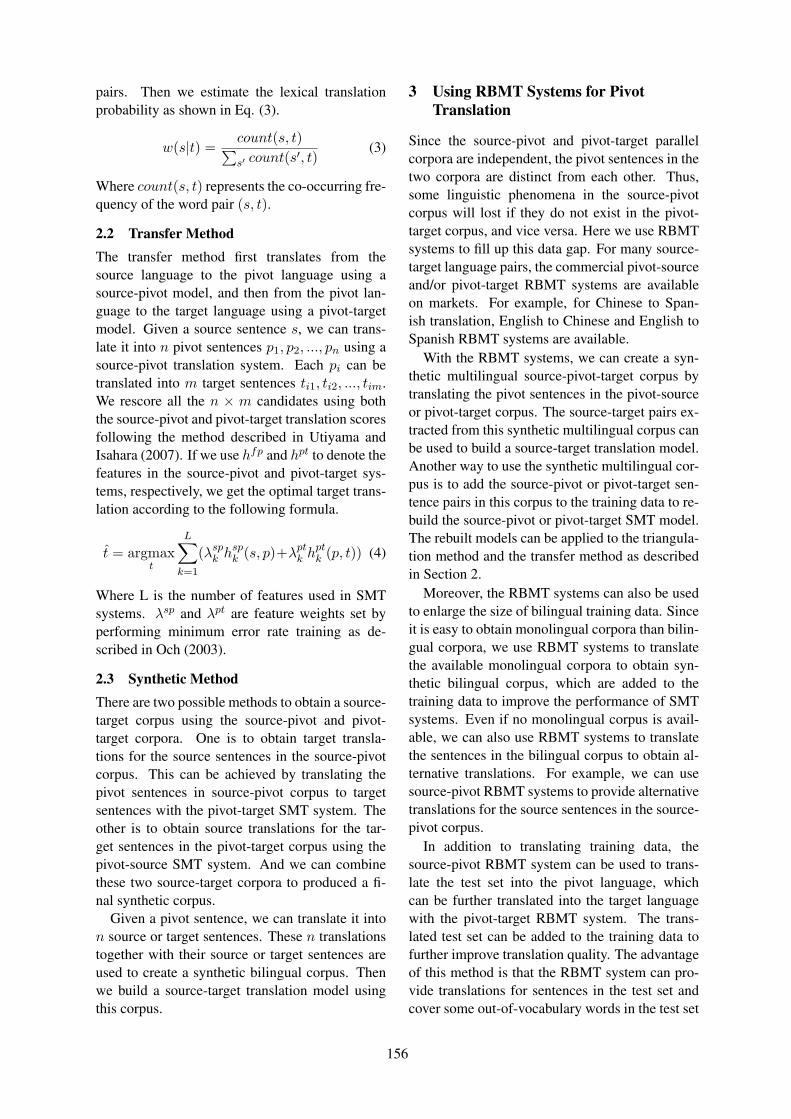
pairs. Then we estimate the lexical translationprobability as shown in Eq. (3).
w(s|t) =count(s, t)
∑
s′ count(s′, t)(3)
Where count(s, t) represents the co-occurring fre-quency of the word pair (s, t).
2.2 Transfer MethodThe transfer method first translates from thesource language to the pivot language using asource-pivot model, and then from the pivot lan-guage to the target language using a pivot-targetmodel. Given a source sentence s, we can trans-late it into n pivot sentences p1, p2, ..., pn using asource-pivot translation system. Each pi can betranslated into m target sentences ti1, ti2, ..., tim.We rescore all the n × m candidates using boththe source-pivot and pivot-target translation scoresfollowing the method described in Utiyama andIsahara (2007). If we use hfp and hpt to denote thefeatures in the source-pivot and pivot-target sys-tems, respectively, we get the optimal target trans-lation according to the following formula.
t̂ = argmaxt
L∑
k=1
(λspk hsp
k (s, p)+λptk hpt
k (p, t)) (4)
Where L is the number of features used in SMTsystems. λsp and λpt are feature weights set byperforming minimum error rate training as de-scribed in Och (2003).
2.3 Synthetic MethodThere are two possible methods to obtain a source-target corpus using the source-pivot and pivot-target corpora. One is to obtain target transla-tions for the source sentences in the source-pivotcorpus. This can be achieved by translating thepivot sentences in source-pivot corpus to targetsentences with the pivot-target SMT system. Theother is to obtain source translations for the tar-get sentences in the pivot-target corpus using thepivot-source SMT system. And we can combinethese two source-target corpora to produced a fi-nal synthetic corpus.
Given a pivot sentence, we can translate it inton source or target sentences. These n translationstogether with their source or target sentences areused to create a synthetic bilingual corpus. Thenwe build a source-target translation model usingthis corpus.
3 Using RBMT Systems for PivotTranslation
Since the source-pivot and pivot-target parallelcorpora are independent, the pivot sentences in thetwo corpora are distinct from each other. Thus,some linguistic phenomena in the source-pivotcorpus will lost if they do not exist in the pivot-target corpus, and vice versa. Here we use RBMTsystems to fill up this data gap. For many source-target language pairs, the commercial pivot-sourceand/or pivot-target RBMT systems are availableon markets. For example, for Chinese to Span-ish translation, English to Chinese and English toSpanish RBMT systems are available.
With the RBMT systems, we can create a syn-thetic multilingual source-pivot-target corpus bytranslating the pivot sentences in the pivot-sourceor pivot-target corpus. The source-target pairs ex-tracted from this synthetic multilingual corpus canbe used to build a source-target translation model.Another way to use the synthetic multilingual cor-pus is to add the source-pivot or pivot-target sen-tence pairs in this corpus to the training data to re-build the source-pivot or pivot-target SMT model.The rebuilt models can be applied to the triangula-tion method and the transfer method as describedin Section 2.
Moreover, the RBMT systems can also be usedto enlarge the size of bilingual training data. Sinceit is easy to obtain monolingual corpora than bilin-gual corpora, we use RBMT systems to translatethe available monolingual corpora to obtain syn-thetic bilingual corpus, which are added to thetraining data to improve the performance of SMTsystems. Even if no monolingual corpus is avail-able, we can also use RBMT systems to translatethe sentences in the bilingual corpus to obtain al-ternative translations. For example, we can usesource-pivot RBMT systems to provide alternativetranslations for the source sentences in the source-pivot corpus.
In addition to translating training data, thesource-pivot RBMT system can be used to trans-late the test set into the pivot language, whichcan be further translated into the target languagewith the pivot-target RBMT system. The trans-lated test set can be added to the training data tofurther improve translation quality. The advantageof this method is that the RBMT system can pro-vide translations for sentences in the test set andcover some out-of-vocabulary words in the test set
156

that are uncovered by the training data. It can alsochange the distribution of some phrase pairs andreinforce some phrase pairs relative to the test set.
4 Translation Selection
We propose a method to select the optimal trans-lation from those produced by various translationsystems. We regard sentence-level translation se-lection as a machine translation (MT) evaluationproblem and formalize this problem with a regres-sion learning model. For each translation, thismethod uses the outputs from other translationsystems as pseudo references. The regression ob-jective is to infer a function that maps a featurevector (which measures the similarity of a trans-lation from one system to the pseudo references)to a score that indicates the quality of the transla-tion. Scores are first generated independently foreach translation, then the translations are rankedby their respective scores. The candidate with thehighest score is selected.
The similar ideas have been explored in previ-ous studies. Albrecht and Hwa (2007) proposeda method to evaluate MT outputs with pseudoreferences using support vector regression as thelearner to evaluate translations. Duh (2008) pro-posed a ranking method to compare the transla-tions proposed by several systems. These twomethods require quantitative quality assessmentsby human judges for the translations produced byvarious systems in the training set. When we applysuch methods to translation selection, the relativevalues of the scores assigned by the subject sys-tems are important. In different data conditions,the relative values of the scores assigned by thesubject systems may change. In order to train a re-liable learner, we need to prepare a balanced train-ing set, where the translations produced by differ-ent systems under different conditions are requiredto be manually evaluated. In extreme cases, weneed to relabel the training data to obtain betterperformance. In this paper, we modify the methodin Albrecht and Hwa (2007) to only prepare hu-man reference translations for the training exam-ples, and then evaluate the translations producedby the subject systems against the references us-ing BLEU score (Papineni et al., 2002). We usesmoothed sentence-level BLEU score to replacethe human assessments, where we use additivesmoothing to avoid zero BLEU scores when wecalculate the n-gram precisions. In this case, we
ID Description1-4 n-gram precisions against pseudo refer-
ences (1 ≤ n ≤ 4)5-6 PER and WER7-8 precision, recall, fragmentation from
METEOR (Lavie and Agarwal, 2007)9-12 precisions and recalls of non-
consecutive bigrams with a gapsize of m (1 ≤ m ≤ 2)
13-14 longest common subsequences15-19 n-gram precision against a target cor-
pus (1 ≤ n ≤ 5)
Table 1: Feature sets for regression learning
can easily retrain the learner under different con-ditions, therefore enabling our method to be ap-plied to sentence-level translation selection fromany sets of translation systems without any addi-tional human work.
In regression learning, we infer a functionf that maps a multi-dimensional input vec-tor x to a continuous real value y, such thatthe error over a set of m training examples,(x1, y1), (x2, y2), ..., (xm, ym), is minimized ac-cording to a loss function. In the context of trans-lation selection, y is assigned as the smoothedBLEU score. The function f represents a math-ematic model of the automatic evaluation metrics.The input sentence is represented as a feature vec-tor x, which are extracted from the input sen-tence and the comparisons against the pseudo ref-erences. We use the features as shown in Table 1.
5 Experiments
5.1 Data
We performed experiments on spoken languagetranslation for the pivot task of IWSLT 2008. Thistask translates Chinese to Spanish using Englishas the pivot language. Table 2 describes the dataused for model training in this paper, including theBTEC (Basic Travel Expression Corpus) Chinese-English (CE) corpus and the BTEC English-Spanish (ES) corpus provided by IWSLT 2008 or-ganizers, the HIT olympic CE corpus (2004-863-008)1 and the Europarl ES corpus2. There aretwo kinds of BTEC CE corpus: BTEC CE1 and
1http://www.chineseldc.org/EN/purchasing.htm2http://www.statmt.org/europarl/
157

Corpus Size SW TWBTEC CE1 20,000 164K 182KBTEC CE2 18,972 177K 182K
HIT CE 51,791 490K 502KBTEC ES 19,972 182K 185K
Europarl ES 400,000 8,485K 8,219K
Table 2: Training data. SW and TW representsource words and target words, respectively.
BTEC CE2. BTEC CE1 was distributed for thepivot task in IWSLT 2008 while BTEC CE2 wasfor the BTEC CE task, which is parallel to theBTEC ES corpus. For Chinese-English transla-tion, we mainly used BTEC CE1 corpus. We usedthe BTEC CE2 corpus and the HIT Olympic cor-pus for comparison experiments only. We used theEnglish parts of the BTEC CE1 corpus, the BTECES corpus, and the HIT Olympic corpus (if in-volved) to train a 5-gram English language model(LM) with interpolated Kneser-Ney smoothing.For English-Spanish translation, we selected 400ksentence pairs from the Europarl corpus that areclose to the English parts of both the BTEC CEcorpus and the BTEC ES corpus. Then we builta Spanish LM by interpolating an out-of-domainLM trained on the Spanish part of this selectedcorpus with the in-domain LM trained with theBTEC corpus.
For Chinese-English-Spanish translation, weused the development set (devset3) released forthe pivot task as the test set, which contains 506source sentences, with 7 reference translations inEnglish and Spanish. To be capable of tuning pa-rameters on our systems, we created a develop-ment set of 1,000 sentences taken from the trainingsets, with 3 reference translations in both Englishand Spanish. This development set is also used totrain the regression learning model.
5.2 Systems and Evaluation Method
We used two commercial RBMT systems in ourexperiments: System A for Chinese-English bidi-rectional translation and System B for English-Chinese and English-Spanish translation. Forphrase-based SMT translation, we used the Mosesdecoder (Koehn et al., 2007) and its support train-ing scripts. We ran the decoder with its defaultsettings and then used Moses’ implementation ofminimum error rate training (Och, 2003) to tunethe feature weights on the development set.
To select translation among outputs producedby different pivot translation systems, we usedSVM-light (Joachins, 1999) to perform supportvector regression with the linear kernel.
Translation quality was evaluated using both theBLEU score proposed by Papineni et al. (2002)and also the modified BLEU (BLEU-Fix) score3
used in the IWSLT 2008 evaluation campaign,where the brevity calculation is modified to useclosest reference length instead of shortest refer-ence length.
5.3 Results by Using SMT Systems
We conducted the pivot translation experimentsusing the BTEC CE1 and BTEC ES describedin Section 5.1. We used the three methods de-scribed in Section 2 for pivot translation. For thetransfer method, we selected the optimal transla-tions among 10× 10 candidates. For the syntheticmethod, we used the ES translation model to trans-late the English part of the CE corpus to Spanish toconstruct a synthetic corpus. And we also used theBTEC CE1 corpus to build a EC translation modelto translate the English part of ES corpus into Chi-nese. Then we combined these two synthetic cor-pora to build a Chinese-Spanish translation model.In our experiments, only 1-best Chinese or Span-ish translation was used since using n-best resultsdid not greatly improve the translation quality. Weused the method described in Section 4 to selecttranslations from the translations produced by thethree systems. For each system, we used threedifferent alignment heuristics (grow, grow-diag,grow-diag-final4) to obtain the final alignment re-sults, and then constructed three different phrasetables. Thus, for each system, we can get threedifferent translations for each input. These differ-ent translations can serve as pseudo references forthe outputs of other systems. In our case, for eachsentence, we have 6 pseudo reference translations.In addition, we found out that the grow heuristicperformed the best for all the systems. Thus, foran individual system, we used the translation re-sults produced using the grow alignment heuristic.
The translation results are shown in Table 3.ASR and CRR represent different input condi-tions, namely the result of automatic speech recog-
3https://www.slc.atr.jp/Corpus/IWSLT08/eval/IWSLT08auto eval.tgz
4A description of the alignment heuristics can be found athttp://www.statmt.org/jhuws/?n=FactoredTraining.TrainingParameters
158

Method BLEU BLEU-FixTriangulation 33.70/27.46 31.59/25.02
Transfer 33.52/28.34 31.36/26.20Synthetic 34.35/27.21 32.00/26.07
Combination 38.14/29.32 34.76/27.39
Table 3: CRR/ASR translation results by usingSMT systems
nition and correct recognition result, respectively.Here, we used the 1-best ASR result. From thetranslation results, it can be seen that three meth-ods achieved comparable translation quality onboth ASR and CRR inputs, with the translation re-sults on CRR inputs are much better than those onASR inputs because of the errors in the ASR in-puts. The results also show that our translation se-lection method is very effective, which achievedabsolute improvements of about 4 and 1 BLEUscores on CRR and ASR inputs, respectively.
5.4 Results by Using both RBMT and SMTSystems
In order to fill up the data gap as discussed in Sec-tion 3, we used the RBMT System A to translatethe English sentences in the ES corpus into Chi-nese. As described in Section 3, this corpus canbe used by the three pivot translation methods.First, the synthetic Chinese-Spanish corpus can becombined with those produced by the EC and ESSMT systems, which were used in the syntheticmethod. Second, the synthetic Chinese-Englishcorpus can be added into the BTEC CE1 corpus tobuild the CE translation model. In this way, the in-tersected English phrases in the CE corpus and EScorpus becomes more, which enables the Chinese-Spanish translation model induced using the trian-gulation method to cover more phrase pairs. Forthe transfer method, the CE translation quality canbe also improved, which would result in the im-provement of the Spanish translation quality.
The translation results are shown in the columnsunder ”EC RBMT” in Table 4. As compared withthose in Table 3, the translation quality was greatlyimproved, with absolute improvements of at least5.1 and 3.9 BLEU scores on CRR and ASR inputsfor system combination results. The above resultsindicate that RBMT systems indeed can be used tofill up the data gap for pivot translation.
In our experiments, we also used a CE RBMTsystem to enlarge the size of training data by pro-
0
0.1
0.2
0.3
0.4
0.5
0.6
0.7
0.8
0.9
1 2 3 4 5 6 7
Phrase length
Cove
rage
SMT (Triangulation)
+EC RBMT
+EC RBMT+CE RBMT
+EC RBMT+CE RBMT+Test Set
Figure 1: Coverage on test source phrases
viding alternative English translations for the Chi-nese part of the CE corpus. The translation resultsare shown in the columns under “+CE RBMT” inTable 4. From the translation results, it can beseen that, enlarging the size of training data withRBMT systems can further improve the translationquality.
In addition to translating the training data, theCE RBMT system can be also used to translate thetest set into English, which can be further trans-lated into Spanish with the ES RBMT system B.56
The translated test set can be further added to thetraining data to improve translation quality. Thecolumns under “+Test Set” in Table 4 describesthe translation results. The results show that trans-lating the test set using RBMT systems greatly im-proved the translation result, with further improve-ments of about 2 and 1.5 BLEU scores on CRRand ASR inputs, respectively.
The results also indicate that both the triangula-tion method and the transfer method greatly out-performed the synthetic method when we com-bined both RBMT and SMT systems in our exper-iments. Further analysis shows that the syntheticmethod contributed little to system combination.The selection results are almost the same as thoseselected from the translations produced by the tri-angulation and transfer methods.
In order to further analyze the translation re-sults, we evaluated the above systems by examin-ing the coverage of the phrase tables over the testphrases. We took the triangulation method as acase study, the results of which are shown in Fig-
5Although using the ES RBMT system B to translate thetraining data did not improve the translation quality, it im-proved the translation quality by translating the test set.
6The RBMT systems achieved a BLEU score of 24.36 onthe test set.
159
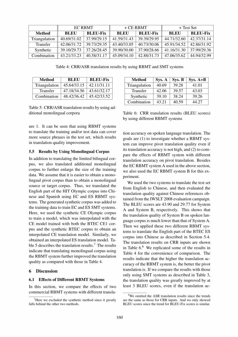
EC RBMT + CE RBMT + Test SetMethod BLEU BLEU-Fix BLEU BLEU-Fix BLEU BLEU-Fix
Triangulation 40.69/31.02 37.99/29.15 41.59/31.43 39.39/29.95 44.71/32.60 42.37/31.14Transfer 42.06/31.72 39.73/29.35 43.40/33.05 40.73/30.06 45.91/34.52 42.86/31.92Synthetic 39.10/29.73 37.26/28.45 39.90/30.00 37.90/28.66 41.16/31.30 37.99/29.36
Combination 43.21/33.23 40.58/31.17 45.09/34.10 42.88/31.73 47.06/35.62 44.94/32.99
Table 4: CRR/ASR translation results by using RBMT and SMT systems
Method BLEU BLEU-FixTriangulation 45.64/33.15 42.11/31.11
Transfer 47.18/34.56 43.61/32.17Combination 48.42/36.42 45.42/33.52
Table 5: CRR/ASR translation results by using ad-ditional monolingual corpora
ure 1. It can be seen that using RBMT systemsto translate the training and/or test data can covermore source phrases in the test set, which resultsin translation quality improvement.
5.5 Results by Using Monolingual CorpusIn addition to translating the limited bilingual cor-pus, we also translated additional monolingualcorpus to further enlarge the size of the trainingdata. We assume that it is easier to obtain a mono-lingual pivot corpus than to obtain a monolingualsource or target corpus. Thus, we translated theEnglish part of the HIT Olympic corpus into Chi-nese and Spanish using EC and ES RBMT sys-tems. The generated synthetic corpus was added tothe training data to train EC and ES SMT systems.Here, we used the synthetic CE Olympic corpusto train a model, which was interpolated with theCE model trained with both the BTEC CE1 cor-pus and the synthetic BTEC corpus to obtain aninterpolated CE translation model. Similarly, weobtained an interpolated ES translation model. Ta-ble 5 describes the translation results.7 The resultsindicate that translating monolingual corpus usingthe RBMT system further improved the translationquality as compared with those in Table 4.
6 Discussion
6.1 Effects of Different RBMT SystemsIn this section, we compare the effects of twocommercial RBMT systems with different transla-
7Here we excluded the synthetic method since it greatlyfalls behind the other two methods.
Method Sys. A Sys. B Sys. A+BTriangulation 40.69 39.28 41.01
Transfer 42.06 39.57 43.03Synthetic 39.10 38.24 39.26
Combination 43.21 40.59 44.27
Table 6: CRR translation results (BLEU scores)by using different RBMT systems
tion accuracy on spoken language translation. Thegoals are (1) to investigate whether a RBMT sys-tem can improve pivot translation quality even ifits translation accuracy is not high, and (2) to com-pare the effects of RBMT system with differenttranslation accuracy on pivot translation. Besidesthe EC RBMT system A used in the above section,we also used the EC RBMT system B for this ex-periment.
We used the two systems to translate the test setfrom English to Chinese, and then evaluated thetranslation quality against Chinese references ob-tained from the IWSLT 2008 evaluation campaign.The BLEU scores are 43.90 and 29.77 for SystemA and System B, respectively. This shows thatthe translation quality of System B on spoken lan-guage corpus is much lower than that of System A.Then we applied these two different RBMT sys-tems to translate the English part of the BTEC EScorpus into Chinese as described in Section 5.4.The translation results on CRR inputs are shownin Table 6.8 We replicated some of the results inTable 4 for the convenience of comparison. Theresults indicate that the higher the translation ac-curacy of the RBMT system is, the better the pivottranslation is. If we compare the results with thoseonly using SMT systems as described in Table 3,the translation quality was greatly improved by atleast 3 BLEU scores, even if the translation ac-
8We omitted the ASR translation results since the trendsare the same as those for CRR inputs. And we only showedBLEU scores since the trend for BLEU-Fix scores is similar.
160
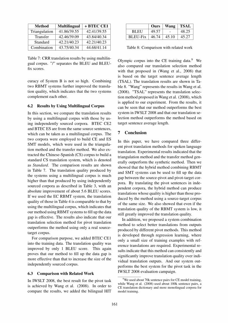
Method Multilingual + BTEC CE1Triangulation 41.86/39.55 42.41/39.55
Transfer 42.46/39.09 43.84/40.34Standard 42.21/40.23 42.21/40.23
Combination 43.75/40.34 44.68/41.14
Table 7: CRR translation results by using multilin-gual corpus. ”/” separates the BLEU and BLEU-fix scores.
curacy of System B is not so high. Combiningtwo RBMT systems further improved the transla-tion quality, which indicates that the two systemscomplement each other.
6.2 Results by Using Multilingual Corpus
In this section, we compare the translation resultsby using a multilingual corpus with those by us-ing independently sourced corpora. BTEC CE2and BTEC ES are from the same source sentences,which can be taken as a multilingual corpus. Thetwo corpora were employed to build CE and ESSMT models, which were used in the triangula-tion method and the transfer method. We also ex-tracted the Chinese-Spanish (CS) corpus to build astandard CS translation system, which is denotedas Standard. The comparison results are shownin Table 7. The translation quality produced bythe systems using a multilingual corpus is muchhigher than that produced by using independentlysourced corpora as described in Table 3, with anabsolute improvement of about 5.6 BLEU scores.If we used the EC RBMT system, the translationquality of those in Table 4 is comparable to that byusing the multilingual corpus, which indicates thatour method using RBMT systems to fill up the datagap is effective. The results also indicate that ourtranslation selection method for pivot translationoutperforms the method using only a real source-target corpus.
For comparison purpose, we added BTEC CE1into the training data. The translation quality wasimproved by only 1 BLEU score. This againproves that our method to fill up the data gap ismore effective than that to increase the size of theindependently sourced corpus.
6.3 Comparison with Related Work
In IWSLT 2008, the best result for the pivot taskis achieved by Wang et al. (2008). In order tocompare the results, we added the bilingual HIT
Ours Wang TSALBLEU 49.57 - 48.25
BLEU-Fix 46.74 45.10 45.27
Table 8: Comparison with related work
Olympic corpus into the CE training data.9 Wealso compared our translation selection methodwith that proposed in (Wang et al., 2008) thatis based on the target sentence average length(TSAL). The translation results are shown in Ta-ble 8. ”Wang” represents the results in Wang et al.(2008). ”TSAL” represents the translation selec-tion method proposed in Wang et al. (2008), whichis applied to our experiment. From the results, itcan be seen that our method outperforms the bestsystem in IWSLT 2008 and that our translation se-lection method outperforms the method based ontarget sentence average length.
7 Conclusion
In this paper, we have compared three differ-ent pivot translation methods for spoken languagetranslation. Experimental results indicated that thetriangulation method and the transfer method gen-erally outperform the synthetic method. Then weshowed that the hybrid method combining RBMTand SMT systems can be used to fill up the datagap between the source-pivot and pivot-target cor-pora. By translating the pivot sentences in inde-pendent corpora, the hybrid method can producetranslations whose quality is higher than those pro-duced by the method using a source-target corpusof the same size. We also showed that even if thetranslation quality of the RBMT system is low, itstill greatly improved the translation quality.
In addition, we proposed a system combinationmethod to select better translations from outputsproduced by different pivot methods. This methodis developed through regression learning, whereonly a small size of training examples with ref-erence translations are required. Experimental re-sults indicate that this method can consistently andsignificantly improve translation quality over indi-vidual translation outputs. And our system out-performs the best system for the pivot task in theIWSLT 2008 evaluation campaign.
9We used about 70k sentence pairs for CE model training,while Wang et al. (2008) used about 100k sentence pairs, aCE translation dictionary and more monolingual corpora formodel training.
161
ReferencesJoshua S. Albrecht and Rebecca Hwa. 2007. Regres-
sion for Sentence-Level MT Evaluation with PseudoReferences. In Proceedings of the 45th AnnualMeeting of the Accosiation of Computational Lin-guistics, pages 296–303.
Nicola Bertoldi, Madalina Barbaiani, Marcello Fed-erico, and Roldano Cattoni. 2008. Phrase-BasedStatistical Machine Translation with Pivot Lan-guages. In Proceedings of the International Work-shop on Spoken Language Translation, pages 143-149.
Tevor Cohn and Mirella Lapata. 2007. Machine Trans-lation by Triangulation: Making Effective Use ofMulti-Parallel Corpora. In Proceedings of the 45thAnnual Meeting of the Association for Computa-tional Linguistics, pages 348–355.
Kevin Duh. 2008. Ranking vs. Regression in MachineTranslation Evaluation. In Proceedings of the ThirdWorkshop on Statistical Machine Translation, pages191–194.
Xiaoguang Hu, Haifeng Wang, and Hua Wu. 2007.Using RBMT Systems to Produce Bilingual Corpusfor SMT. In Proceedings of the 2007 Joint Con-ference on Empirical Methods in Natural LanguageProcessing and Computational Natural LanguageLearning, pages 287–295.
Thorsten Joachims. 1999. Making Large-ScaleSVM Learning Practical. In Bernhard Schöelkopf,Christopher Burges, and Alexander Smola, edi-tors, Advances in Kernel Methods - Support VectorLearning. MIT Press.
Maxim Khalilov, Marta R. Costa-Jussà, Carlos A.Henrı́quez, José A.R. Fonollosa, Adolfo Hernández,José B. Mariño, Rafael E. Banchs, Chen Boxing,Min Zhang, Aiti Aw, and Haizhou Li. 2008. TheTALP & I2R SMT Systems for IWSLT 2008. InProceedings of the International Workshop on Spo-ken Language Translation, pages 116–123.
Philipp Koehn, Franz J. Och, and Daniel Marcu.2003. Statistical phrase-based translation. In HLT-NAACL: Human Language Technology Conferenceof the North American Chapter of the Associationfor Computational Linguistics, pages 127–133.
Philipp Koehn, Hieu Hoang, Alexanda Birch, ChrisCallison-Burch, Marcello Federico, Nicola Bertoldi,Brooke Cowan, Wade Shen, Christine Moran,Richard Zens, Chris Dyer, Ondrej Bojar, AlexandraConstantin, and Evan Herbst. 2007. Moses: OpenSource Toolkit for Statistical Machine Translation.In Proceedings of the 45th Annual Meeting of theAssocia-tion for Computational Linguistics, demon-stration session, pages 177–180.
Alon Lavie and Abhaya Agarwal. 2007. METEOR:An Automatic Metric for MT Evaluation with HighLevels of Correlation with Human Judgments. In
Proceedings of Workshop on Statistical MachineTranslation at the 45th Annual Meeting of the As-sociation of Computational Linguistics, pages 228–231.
Franz J. Och. 2003. Minimum Error Rate Trainingin Statistical Machine Translation. In Proceedingsof the 41st Annual Meeting of the Association forComputational Linguistics, pages 160–167.
Kishore Papineni, Salim Roukos, Todd Ward, and Wei-Jing Zhu. 2002. BLEU: a Method for AutomaticEvaluation of Machine Translation. In Proceedingsof the 40th annual meeting of the Association forComputational Linguistics, pages 311–318.
Michael Paul. 2008. Overview of the IWSLT 2008Evaluation Campaign. In Proceedings of the In-ternational Workshop on Spoken Language Trans-lation, pages 1–17.
Masao Utiyama and Hitoshi Isahara. 2007. A Com-parison of Pivot Methods for Phrase-Based Statisti-cal Machine Translation. In Proceedings of humanlanguage technology: the Conference of the NorthAmerican Chapter of the Association for Computa-tional Linguistics, pages 484–491.
Haifeng Wang, Hua Wu, Xiaoguang Hu, Zhanyi Liu,Jianfeng Li, Dengjun Ren, and Zhengyu Niu. 2008.The TCH Machine Translation System for IWSLT2008. In Proceedings of the International Workshopon Spoken Language Translation, pages 124–131.
Hua Wu and Haifeng Wang. 2007. Pivot Lan-guage Approach for Phrase-Based Statistical Ma-chine Translation. In Proceedings of 45th AnnualMeeting of the Association for Computational Lin-guistics, pages 856–863.
162

Proceedings of the 47th Annual Meeting of the ACL and the 4th IJCNLP of the AFNLP, pages 163–171,Suntec, Singapore, 2-7 August 2009. c©2009 ACL and AFNLP
Efficient Minimum Error Rate Training andMinimum Bayes-Risk Decoding for
Translation Hypergraphs and LatticesShankar Kumar1 and Wolfgang Macherey1 and Chris Dyer2 and Franz Och1
1Google Inc.1600 Amphitheatre Pkwy.
Mountain View, CA 94043, USA{shankarkumar,wmach,och}@google.com
2Department of LinguisticsUniversity of Maryland
College Park, MD 20742, [email protected]
Abstract
Minimum Error Rate Training (MERT)and Minimum Bayes-Risk (MBR) decod-ing are used in most current state-of-the-art Statistical Machine Translation (SMT)systems. The algorithms were originallydeveloped to work with N -best lists oftranslations, and recently extended to lat-tices that encode many more hypothesesthan typical N -best lists. We here extendlattice-based MERT and MBR algorithmsto work with hypergraphs that encode avast number of translations produced byMT systems based on Synchronous Con-text Free Grammars. These algorithmsare more efficient than the lattice-basedversions presented earlier. We show howMERT can be employed to optimize pa-rameters for MBR decoding. Our exper-iments show speedups from MERT andMBR as well as performance improve-ments from MBR decoding on several lan-guage pairs.
1 Introduction
Statistical Machine Translation (SMT) systemshave improved considerably by directly using theerror criterion in both training and decoding. Bydoing so, the system can be optimized for thetranslation task instead of a criterion such as like-lihood that is unrelated to the evaluation met-ric. Two popular techniques that incorporate theerror criterion are Minimum Error Rate Train-ing (MERT) (Och, 2003) and Minimum Bayes-Risk (MBR) decoding (Kumar and Byrne, 2004).These two techniques were originally developedfor N -best lists of translation hypotheses and re-cently extended to translation lattices (Machereyet al., 2008; Tromble et al., 2008) generated by aphrase-based SMT system (Och and Ney, 2004).Translation lattices contain a significantly higher
number of translation alternatives relative to N -best lists. The extension to lattices reduces theruntimes for both MERT and MBR, and gives per-formance improvements from MBR decoding.
SMT systems based on synchronous contextfree grammars (SCFG) (Chiang, 2007; Zollmannand Venugopal, 2006; Galley et al., 2006) haverecently been shown to give competitive perfor-mance relative to phrase-based SMT. For thesesystems, a hypergraph or packed forest provides acompact representation for encoding a huge num-ber of translation hypotheses (Huang, 2008).
In this paper, we extend MERT and MBRdecoding to work on hypergraphs produced bySCFG-based MT systems. We present algorithmsthat are more efficient relative to the lattice al-gorithms presented in Macherey et al. (2008;Tromble et al. (2008). Lattice MBR decoding usesa linear approximation to the BLEU score (Pap-ineni et al., 2001); the weights in this linear lossare set heuristically by assuming that n-gram pre-cisions decay exponentially with n. However, thismay not be optimal in practice. We employ MERTto select these weights by optimizing BLEU scoreon a development set.
A related MBR-inspired approach for hyper-graphs was developed by Zhang and Gildea(2008). In this work, hypergraphs were rescored tomaximize the expected count of synchronous con-stituents in the translation. In contrast, our MBRalgorithm directly selects the hypothesis in thehypergraph with the maximum expected approx-imate corpus BLEU score (Tromble et al., 2008).
will soon announce
X1 X2
X1 X2
X1 X2
X1 X2
X1 X2
X1 its future in the
X1 its future in the
Suzuki
soon
its future in
X1 announces
Rally World Championship
Figure 1: An example hypergraph.
163

2 Translation Hypergraphs
A translation lattice compactly encodes a largenumber of hypotheses produced by a phrase-basedSMT system. The corresponding representationfor an SMT system based on SCFGs (e.g. Chi-ang (2007), Zollmann and Venugopal (2006), Miet al. (2008)) is a directed hypergraph or a packedforest (Huang, 2008).
Formally, a hypergraph is a pair H = 〈V, E〉consisting of a vertex set V and a set of hyperedgesE ⊆ V∗ × V . Each hyperedge e ∈ E connects ahead vertex h(e) with a sequence of tail verticesT (e) = {v1, ..., vn}. The number of tail verticesis called the arity (|e|) of the hyperedge. If the ar-ity of a hyperedge is zero, h(e) is called a sourcevertex. The arity of a hypergraph is the maximumarity of its hyperedges. A hyperedge of arity 1 is aregular edge, and a hypergraph of arity 1 is a regu-lar graph (lattice). Each hyperedge is labeled witha rule re from the SCFG. The number of nontermi-nals on the right-hand side of re corresponds withthe arity of e. An example without scores is shownin Figure 1. A path in a translation hypergraph in-duces a translation hypothesis E along with its se-quence of SCFG rules D = r1, r2, ..., rK which,if applied to the start symbol, derives E. The se-quence of SCFG rules induced by a path is alsocalled a derivation tree for E.
3 Minimum Error Rate Training
Given a set of source sentences FS1 with corre-
sponding reference translations RS1 , the objective
of MERT is to find a parameter set λ̂M1 which min-
imizes an automated evaluation criterion under alinear model:
λ̂M1 = arg min
λM1
SXs=1
Err`Rs, Ê(Fs; λM
1 )´ff
Ê(Fs; λM1 ) = arg max
E
SXs=1
λmhm(E, Fs)
ff.
In the context of statistical machine translation,the optimization procedure was first described inOch (2003) for N -best lists and later extended tophrase-lattices in Macherey et al. (2008). The al-gorithm is based on the insight that, under a log-linear model, the cost function of any candidatetranslation can be represented as a line in the planeif the initial parameter set λM
1 is shifted along adirection dM
1 . Let C = {E1, ..., EK} denote a setof candidate translations, then computing the bestscoring translation hypothesis Ê out of C results inthe following optimization problem:
Ê(F ; γ) = arg maxE∈C
n(λM
1 + γ · dM1 )> · hM
1 (E, F )o
= arg maxE∈C
Xm
λmhm(E, F )| {z }=a(E,F )
+ γ ·Xm
dmhm(E, F )| {z }=b(E,F )
ff
= arg maxE∈C
˘a(E, F ) + γ · b(E, F )| {z }
(∗)
¯Hence, the total score (∗) for each candidate trans-lation E ∈ C can be described as a line withγ as the independent variable. For any particu-lar choice of γ, the decoder seeks that translationwhich yields the largest score and therefore corre-sponds to the topmost line segment. If γ is shiftedfrom −∞ to +∞, other translation hypothesesmay at some point constitute the topmost line seg-ments and thus change the decision made by thedecoder. The entire sequence of topmost line seg-ments is called upper envelope and provides an ex-haustive representation of all possible outcomesthat the decoder may yield if γ is shifted alongthe chosen direction. Both the translations andtheir corresponding line segments can efficientlybe computed without incorporating any error crite-rion. Once the envelope has been determined, thetranslation candidates of its constituent line seg-ments are projected onto their corresponding errorcounts, thus yielding the exact and unsmoothed er-ror surface for all candidate translations encodedin C. The error surface can now easily be traversedin order to find that γ̂ under which the new param-eter set λM
1 + γ̂ · dM1 minimizes the global error.
In this section, we present an extension of thealgorithm described in Macherey et al. (2008)that allows us to efficiently compute and repre-sent upper envelopes over all candidate transla-tions encoded in hypergraphs. Conceptually, thealgorithm works by propagating (initially empty)envelopes from the hypergraph’s source nodesbottom-up to its unique root node, thereby ex-panding the envelopes by applying SCFG rules tothe partial candidate translations that are associ-ated with the envelope’s constituent line segments.To recombine envelopes, we need two operators:the sum and the maximum over convex polygons.To illustrate which operator is applied when, wetransform H = 〈V, E〉 into a regular graph withtyped nodes by (1) marking all vertices v ∈ V withthe symbol ∨ and (2) replacing each hyperedgee ∈ E , |e| > 1, with a small subgraph consistingof a new vertex v∧(e) whose incoming and out-going edges connect the same head and tail nodes
164

Algorithm 1 ∧-operation (Sum)input: associative map a: V → Env(V), hyperarc eoutput: Minkowski sum of envelopes over T (e)
for (i = 0; i < |T (e)|; ++i) {v = Ti(e);pq.enqueue(〈 v, i, 0〉);
}
L = ∅;D = 〈 e, ε1 · · · ε|e|〉while (!pq.empty()) {
〈 v, i, j〉 = pq.dequeue();` = A[v][j];D[i+1] = `.D;if (L.empty() ∨ L.back().x < `.x) {
if (0 < j) {`.y += L.back().y - A[v][j-1].y;`.m += L.back().m - A[v][j-1].m;
}L.push_back(`);L.back().D = D;
} else {L.back().y += `.y;L.back().m += `.m;L.back().D[i+1] = `.D;if (0 < j) {
L.back().y -= A[v][j-1].y;L.back().m -= A[v][j-1].m;
}}if (++j < A[v].size())
pq.enqueue(〈 v, i, j〉);}return L;
in the transformed graph as were connected by ein the original graph. The unique outgoing edgeof v∧(e) is associated with the rule re; incomingedges are not linked to any rule. Figure 2 illus-trates the transformation for a hyperedge with ar-ity 3. The graph transformation is isomorphic.
The rules associated with every hyperedge spec-ify how line segments in the envelopes of a hyper-edge’s tail nodes can be combined. Suppose wehave a hyperedge e with rule re : X → aX1bX2cand T (e) = {v1, v2}. Then we substitute X1 andX2 in the rule with candidate translations associ-ated with line segments in envelopes Env(v1) andEnv(v2) respectively.
To derive the algorithm, we consider the gen-eral case of a hyperedge e with rule re : X →w1X1w2...wnXnwn+1. Because the right-handside of re has n nonterminals, the arity of e is|e| = n. Let T (e) = {v1, ..., vn} denote thetail nodes of e. We now assume that each tailnode vi ∈ T (e) is associated with the upper en-velope over all candidate translations that are in-duced by derivations of the corresponding nonter-minal symbol Xi. These envelopes shall be de-
Algorithm 2 ∨-operation (Max)input: array L[0..K-1] containing line objectsoutput: upper envelope of L
Sort(L:m);j = 0; K = size(L);for (i = 0; i < K; ++i) {
` = L[i];`.x = -∞;if (0 < j) {
if (L[j-1].m == `.m) {if (`.y <= L[j-1].y) continue;--j;
}while (0 < j) {
`.x = (`.y - L[j-1].y)/(L[j-1].m - `.m);
if (L[j-1].x < `.x) break;--j;
}if (0 == j) `.x = -∞;L[j++] = `;
} else L[j++] = `;}L.resize(j);return L;
noted by Env(vi). To decompose the problem ofcomputing and propagating the tail envelopes overthe hyperedge e to its head node, we now definetwo operations, one for either node type, to spec-ify how envelopes associated with the tail verticesare propagated to the head vertex.
Nodes of Type “∧”: For a type ∧ node, theresulting envelope is the Minkowski sum overthe envelopes of the incoming edges (Berg etal., 2008). Since the envelopes of the incomingedges are convex hulls, the Minkowski sum pro-vides an upper bound to the number of line seg-ments that constitute the resulting envelope: thebound is the sum over the number of line seg-ments in the envelopes of the incoming edges, i.e.:∣∣Env(v∧(e))
∣∣ ≤ ∑v∨∈T (e)
∣∣Env(v∨)∣∣.
Algorithm 1 shows the pseudo code for comput-ing the Minkowski sum over multiple envelopes.The line objects ` used in this algorithm areencoded as 4-tuples, each consisting of the x-intercept with `’s left-adjacent line stored as `.x,the slope `.m, the y-intercept `.y, and the (partial)derivation tree `.D. At the beginning, the leftmostline segment of each envelope is inserted into apriority queue pq. The priority is defined in termsof a line’s x-intercept such that lower values implyhigher priority. Hence, the priority queue enumer-ates all line segments from left to right in ascend-ing order of their x-intercepts, which is the orderneeded to compute the Minkowski sum.
Nodes of Type “∨”: The operation performed
165
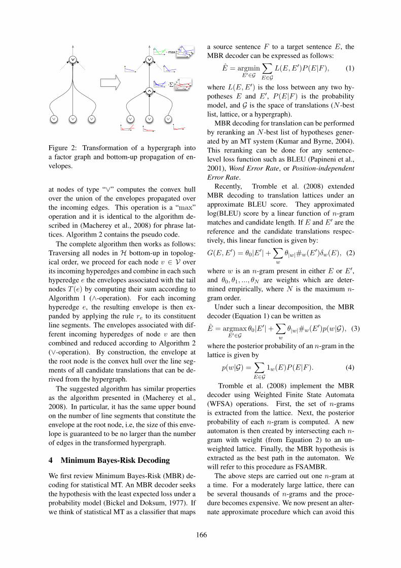
=!
= max
Figure 2: Transformation of a hypergraph intoa factor graph and bottom-up propagation of en-velopes.
at nodes of type “∨” computes the convex hullover the union of the envelopes propagated overthe incoming edges. This operation is a “max”operation and it is identical to the algorithm de-scribed in (Macherey et al., 2008) for phrase lat-tices. Algorithm 2 contains the pseudo code.
The complete algorithm then works as follows:Traversing all nodes in H bottom-up in topolog-ical order, we proceed for each node v ∈ V overits incoming hyperedges and combine in each suchhyperedge e the envelopes associated with the tailnodes T (e) by computing their sum according toAlgorithm 1 (∧-operation). For each incominghyperedge e, the resulting envelope is then ex-panded by applying the rule re to its constituentline segments. The envelopes associated with dif-ferent incoming hyperedges of node v are thencombined and reduced according to Algorithm 2(∨-operation). By construction, the envelope atthe root node is the convex hull over the line seg-ments of all candidate translations that can be de-rived from the hypergraph.
The suggested algorithm has similar propertiesas the algorithm presented in (Macherey et al.,2008). In particular, it has the same upper boundon the number of line segments that constitute theenvelope at the root node, i.e, the size of this enve-lope is guaranteed to be no larger than the numberof edges in the transformed hypergraph.
4 Minimum Bayes-Risk Decoding
We first review Minimum Bayes-Risk (MBR) de-coding for statistical MT. An MBR decoder seeksthe hypothesis with the least expected loss under aprobability model (Bickel and Doksum, 1977). Ifwe think of statistical MT as a classifier that maps
a source sentence F to a target sentence E, theMBR decoder can be expressed as follows:
Ê = argminE′∈G
∑E∈G
L(E,E′)P (E|F ), (1)
where L(E,E′) is the loss between any two hy-potheses E and E′, P (E|F ) is the probabilitymodel, and G is the space of translations (N -bestlist, lattice, or a hypergraph).
MBR decoding for translation can be performedby reranking an N -best list of hypotheses gener-ated by an MT system (Kumar and Byrne, 2004).This reranking can be done for any sentence-level loss function such as BLEU (Papineni et al.,2001), Word Error Rate, or Position-independentError Rate.
Recently, Tromble et al. (2008) extendedMBR decoding to translation lattices under anapproximate BLEU score. They approximatedlog(BLEU) score by a linear function of n-grammatches and candidate length. If E and E′ are thereference and the candidate translations respec-tively, this linear function is given by:
G(E,E′) = θ0|E′|+∑w
θ|w|#w(E′)δw(E), (2)
where w is an n-gram present in either E or E′,and θ0, θ1, ..., θN are weights which are deter-mined empirically, where N is the maximum n-gram order.
Under such a linear decomposition, the MBRdecoder (Equation 1) can be written as
Ê = argmaxE′∈G
θ0|E′|+∑w
θ|w|#w(E′)p(w|G), (3)
where the posterior probability of an n-gram in thelattice is given by
p(w|G) =∑E∈G
1w(E)P (E|F ). (4)
Tromble et al. (2008) implement the MBRdecoder using Weighted Finite State Automata(WFSA) operations. First, the set of n-gramsis extracted from the lattice. Next, the posteriorprobability of each n-gram is computed. A newautomaton is then created by intersecting each n-gram with weight (from Equation 2) to an un-weighted lattice. Finally, the MBR hypothesis isextracted as the best path in the automaton. Wewill refer to this procedure as FSAMBR.
The above steps are carried out one n-gram ata time. For a moderately large lattice, there canbe several thousands of n-grams and the proce-dure becomes expensive. We now present an alter-nate approximate procedure which can avoid this
166

enumeration making the resulting algorithm muchfaster than FSAMBR.
4.1 Efficient MBR for latticesThe key idea behind this new algorithm is torewrite the n-gram posterior probability (Equa-tion 4) as follows:
p(w|G) =∑E∈G
∑e∈E
f(e, w,E)P (E|F ) (5)
where f(e, w,E) is a score assigned to edge e onpath E containing n-gram w:
f(e, w,E) =
1 w ∈ e, p(e|G) > p(e′|G),
e′ precedes e on E0 otherwise
(6)
In other words, for each path E, we count the edgethat contributes n-gram w and has the highest edgeposterior probability relative to its predecessors onthe path E; there is exactly one such edge on eachlattice path E.
We note that f(e, w,E) relies on the full pathE which means that it cannot be computed basedon local statistics. We therefore approximate thequantity f(e, w,E) with f∗(e, w,G) that countsthe edge e with n-gram w that has the highest arcposterior probability relative to predecessors in theentire lattice G. f∗(e, w,G) can be computed lo-cally, and the n-gram posterior probability basedon f∗ can be determined as follows:
p(w|G) =XE∈G
Xe∈E
f∗(e, w,G)P (E|F ) (7)
=Xe∈E
1w∈ef∗(e, w,G)
XE∈G
1E(e)P (E|F )
=Xe∈E
1w∈ef∗(e, w,G)P (e|G),
where P (e|G) is the posterior probability of a lat-tice edge. The algorithm to perform Lattice MBRis given in Algorithm 3. For each node t in the lat-tice, we maintain a quantity Score(w, t) for eachn-gram w that lies on a path from the source nodeto t. Score(w, t) is the highest posterior probabil-ity among all edges on the paths that terminate on tand contain n-gram w. The forward pass requirescomputing the n-grams introduced by each edge;to do this, we propagate n-grams (up to maximumorder −1) terminating on each node.
4.2 Extension to HypergraphsWe next extend the Lattice MBR decoding algo-rithm (Algorithm 3) to rescore hypergraphs pro-duced by a SCFG based MT system. Algorithm 4is an extension to the MBR decoder on lattices
Algorithm 3 MBR Decoding on Lattices1: Sort the lattice nodes topologically.2: Compute backward probabilities of each node.3: Compute posterior prob. of each n-gram:4: for each edge e do5: Compute edge posterior probability P (e|G).6: Compute n-gram posterior probs. P (w|G):7: for each n-gram w introduced by e do8: Propagate n− 1 gram suffix to he.9: if p(e|G) > Score(w, T (e)) then
10: Update posterior probs. and scores:p(w|G) += p(e|G) − Score(w, T (e)).Score(w, he) = p(e|G).
11: else12: Score(w, he) = Score(w, T (e)).13: end if14: end for15: end for16: Assign scores to edges (given by Equation 3).17: Find best path in the lattice (Equation 3).
(Algorithm 3). However, there are important dif-ferences when computing the n-gram posteriorprobabilities (Step 3). In this inside pass, we nowmaintain both n-gram prefixes and suffixes (up tothe maximum order−1) on each hypergraph node.This is necessary because unlike a lattice, new n-grams may be created at subsequent nodes by con-catenating words both to the left and the right sideof the n-gram. When the arity of the edge is 2,a rule has the general form aX1bX2c, where X1
and X2 are sequences from tail nodes. As a result,we need to consider all new sequences which canbe created by the cross-product of the n-grams onthe two tail nodes. E.g. if X1 = {c, cd, d} andX2 = {f, g}, then a total of six sequences willresult. In practice, such a cross-product is not pro-
Algorithm 4 MBR Decoding on Hypergraphs1: Sort the hypergraph nodes topologically.2: Compute inside probabilities of each node.3: Compute posterior prob. of each hyperedge P (e|G).4: Compute posterior prob. of each n-gram:5: for each hyperedge e do6: Merge the n-grams on the tail nodes T (e). If the
same n-gram is present on multiple tail nodes, keepthe highest score.
7: Apply the rule on e to the n-grams on T (e).8: Propagate n− 1 gram prefixes/suffixes to he.9: for each n-gram w introduced by this hyperedge do
10: if p(e|G) > Score(w, T (e)) then11: p(w|G) += p(e|G) − Score(w, T (e))
Score(w, he) = p(e|G)12: else13: Score(w, he) = Score(w, T (e))14: end if15: end for16: end for17: Assign scores to hyperedges (Equation 3).18: Find best path in the hypergraph (Equation 3).
167
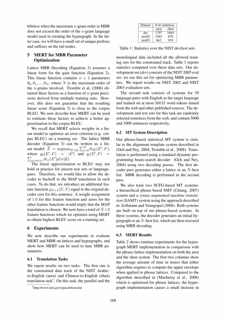
hibitive when the maximum n-gram order in MBRdoes not exceed the order of the n-gram languagemodel used in creating the hypergraph. In the lat-ter case, we will have a small set of unique prefixesand suffixes on the tail nodes.
5 MERT for MBR ParameterOptimization
Lattice MBR Decoding (Equation 3) assumes alinear form for the gain function (Equation 2).This linear function contains n + 1 parametersθ0, θ1, ..., θN , where N is the maximum order ofthe n-grams involved. Tromble et al. (2008) ob-tained these factors as a function of n-gram preci-sions derived from multiple training runs. How-ever, this does not guarantee that the resultinglinear score (Equation 2) is close to the corpusBLEU. We now describe how MERT can be usedto estimate these factors to achieve a better ap-proximation to the corpus BLEU.
We recall that MERT selects weights in a lin-ear model to optimize an error criterion (e.g. cor-pus BLEU) on a training set. The lattice MBRdecoder (Equation 3) can be written as a lin-ear model: Ê = argmaxE′∈G
∑Ni=0 θigi(E′, F ),
where g0(E′, F ) = |E′| and gi(E′, F ) =∑w:|w|=i #w(E′)p(w|G).The linear approximation to BLEU may not
hold in practice for unseen test sets or language-pairs. Therefore, we would like to allow the de-coder to backoff to the MAP translation in suchcases. To do that, we introduce an additional fea-ture function gN+1(E,F ) equal to the original de-coder cost for this sentence. A weight assignmentof 1.0 for this feature function and zeros for theother feature functions would imply that the MAPtranslation is chosen. We now have a total of N+2feature functions which we optimize using MERTto obtain highest BLEU score on a training set.
6 Experiments
We now describe our experiments to evaluateMERT and MBR on lattices and hypergraphs, andshow how MERT can be used to tune MBR pa-rameters.
6.1 Translation TasksWe report results on two tasks. The first one isthe constrained data track of the NIST Arabic-to-English (aren) and Chinese-to-English (zhen)translation task1. On this task, the parallel and the
1http://www.nist.gov/speech/tests/mt
Dataset # of sentencesaren zhen
dev 1797 1664nist02 1043 878nist03 663 919
Table 1: Statistics over the NIST dev/test sets.
monolingual data included all the allowed train-ing sets for the constrained track. Table 1 reportsstatistics computed over these data sets. Our de-velopment set (dev) consists of the NIST 2005 evalset; we use this set for optimizing MBR parame-ters. We report results on NIST 2002 and NIST2003 evaluation sets.
The second task consists of systems for 39language-pairs with English as the target languageand trained on at most 300M word tokens minedfrom the web and other published sources. The de-velopment and test sets for this task are randomlyselected sentences from the web, and contain 5000and 1000 sentences respectively.
6.2 MT System Description
Our phrase-based statistical MT system is simi-lar to the alignment template system described in(Och and Ney, 2004; Tromble et al., 2008). Trans-lation is performed using a standard dynamic pro-gramming beam-search decoder (Och and Ney,2004) using two decoding passes. The first de-coder pass generates either a lattice or an N -bestlist. MBR decoding is performed in the secondpass.
We also train two SCFG-based MT systems:a hierarchical phrase-based SMT (Chiang, 2007)system and a syntax augmented machine transla-tion (SAMT) system using the approach describedin Zollmann and Venugopal (2006). Both systemsare built on top of our phrase-based systems. Inthese systems, the decoder generates an initial hy-pergraph or an N -best list, which are then rescoredusing MBR decoding.
6.3 MERT Results
Table 2 shows runtime experiments for the hyper-graph MERT implementation in comparison withthe phrase-lattice implementation on both the arenand the zhen system. The first two columns showthe average amount of time in msecs that eitheralgorithm requires to compute the upper envelopewhen applied to phrase lattices. Compared to thealgorithm described in (Macherey et al., 2008)which is optimized for phrase lattices, the hyper-graph implementation causes a small increase in
168
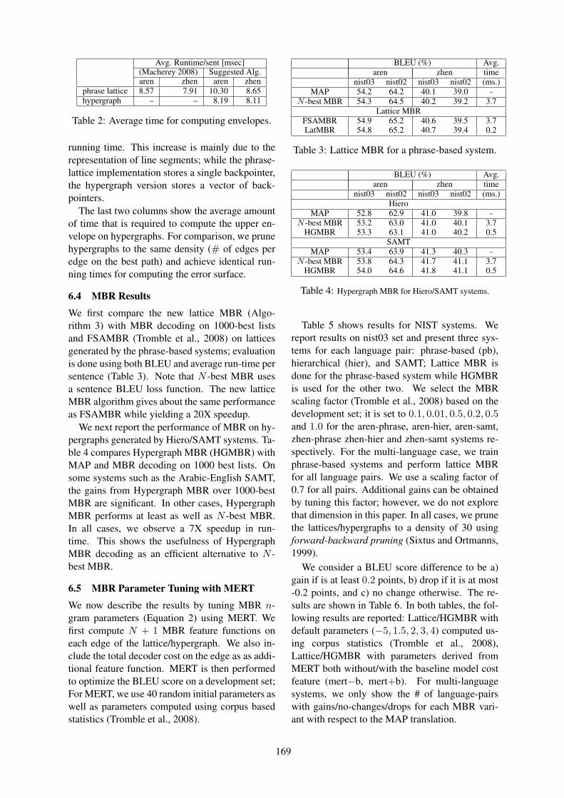
Avg. Runtime/sent [msec](Macherey 2008) Suggested Alg.aren zhen aren zhen
phrase lattice 8.57 7.91 10.30 8.65hypergraph – – 8.19 8.11
Table 2: Average time for computing envelopes.
running time. This increase is mainly due to therepresentation of line segments; while the phrase-lattice implementation stores a single backpointer,the hypergraph version stores a vector of back-pointers.
The last two columns show the average amountof time that is required to compute the upper en-velope on hypergraphs. For comparison, we prunehypergraphs to the same density (# of edges peredge on the best path) and achieve identical run-ning times for computing the error surface.
6.4 MBR Results
We first compare the new lattice MBR (Algo-rithm 3) with MBR decoding on 1000-best listsand FSAMBR (Tromble et al., 2008) on latticesgenerated by the phrase-based systems; evaluationis done using both BLEU and average run-time persentence (Table 3). Note that N -best MBR usesa sentence BLEU loss function. The new latticeMBR algorithm gives about the same performanceas FSAMBR while yielding a 20X speedup.
We next report the performance of MBR on hy-pergraphs generated by Hiero/SAMT systems. Ta-ble 4 compares Hypergraph MBR (HGMBR) withMAP and MBR decoding on 1000 best lists. Onsome systems such as the Arabic-English SAMT,the gains from Hypergraph MBR over 1000-bestMBR are significant. In other cases, HypergraphMBR performs at least as well as N -best MBR.In all cases, we observe a 7X speedup in run-time. This shows the usefulness of HypergraphMBR decoding as an efficient alternative to N -best MBR.
6.5 MBR Parameter Tuning with MERT
We now describe the results by tuning MBR n-gram parameters (Equation 2) using MERT. Wefirst compute N + 1 MBR feature functions oneach edge of the lattice/hypergraph. We also in-clude the total decoder cost on the edge as as addi-tional feature function. MERT is then performedto optimize the BLEU score on a development set;For MERT, we use 40 random initial parameters aswell as parameters computed using corpus basedstatistics (Tromble et al., 2008).
BLEU (%) Avg.aren zhen time
nist03 nist02 nist03 nist02 (ms.)MAP 54.2 64.2 40.1 39.0 -
N -best MBR 54.3 64.5 40.2 39.2 3.7Lattice MBR
FSAMBR 54.9 65.2 40.6 39.5 3.7LatMBR 54.8 65.2 40.7 39.4 0.2
Table 3: Lattice MBR for a phrase-based system.
BLEU (%) Avg.aren zhen time
nist03 nist02 nist03 nist02 (ms.)Hiero
MAP 52.8 62.9 41.0 39.8 -N -best MBR 53.2 63.0 41.0 40.1 3.7
HGMBR 53.3 63.1 41.0 40.2 0.5SAMT
MAP 53.4 63.9 41.3 40.3 -N -best MBR 53.8 64.3 41.7 41.1 3.7
HGMBR 54.0 64.6 41.8 41.1 0.5
Table 4: Hypergraph MBR for Hiero/SAMT systems.
Table 5 shows results for NIST systems. Wereport results on nist03 set and present three sys-tems for each language pair: phrase-based (pb),hierarchical (hier), and SAMT; Lattice MBR isdone for the phrase-based system while HGMBRis used for the other two. We select the MBRscaling factor (Tromble et al., 2008) based on thedevelopment set; it is set to 0.1, 0.01, 0.5, 0.2, 0.5and 1.0 for the aren-phrase, aren-hier, aren-samt,zhen-phrase zhen-hier and zhen-samt systems re-spectively. For the multi-language case, we trainphrase-based systems and perform lattice MBRfor all language pairs. We use a scaling factor of0.7 for all pairs. Additional gains can be obtainedby tuning this factor; however, we do not explorethat dimension in this paper. In all cases, we prunethe lattices/hypergraphs to a density of 30 usingforward-backward pruning (Sixtus and Ortmanns,1999).
We consider a BLEU score difference to be a)gain if is at least 0.2 points, b) drop if it is at most-0.2 points, and c) no change otherwise. The re-sults are shown in Table 6. In both tables, the fol-lowing results are reported: Lattice/HGMBR withdefault parameters (−5, 1.5, 2, 3, 4) computed us-ing corpus statistics (Tromble et al., 2008),Lattice/HGMBR with parameters derived fromMERT both without/with the baseline model costfeature (mert−b, mert+b). For multi-languagesystems, we only show the # of language-pairswith gains/no-changes/drops for each MBR vari-ant with respect to the MAP translation.
169

We observed in the NIST systems that MERTresulted in short translations relative to MAP onthe unseen test set. To prevent this behavior,we modify the MERT error criterion to includea sentence-level brevity scorer with parameter α:BLEU+brevity(α). This brevity scorer penalizeseach candidate translation that is shorter than theaverage length over its reference translations, us-ing a penalty term which is linear in the differencebetween either length. We tune α on the develop-ment set so that the brevity score of MBR transla-tion is close to that of the MAP translation.
In the NIST systems, MERT yields small im-provements on top of MBR with default param-eters. This is the case for Arabic-English Hi-ero/SAMT. In all other cases, we see no changeor even a slight degradation due to MERT.We hypothesize that the default MBR parame-ters (Tromble et al., 2008) are well tuned. There-fore there is little gain by additional tuning usingMERT.
In the multi-language systems, the results showa different trend. We observe that MBR with de-fault parameters results in gains on 18 pairs, nodifferences on 9 pairs, and losses on 12 pairs.When we optimize MBR features with MERT, thenumber of language pairs with gains/no changes/-drops is 22/5/12. Thus, MERT has a bigger impacthere than in the NIST systems. We hypothesizethat the default MBR parameters are sub-optimalfor some language pairs and that MERT helps tofind better parameter settings. In particular, MERTavoids the need for manually tuning these param-eters by language pair.
Finally, when baseline model costs are addedas an extra feature (mert+b), the number of pairswith gains/no changes/drops is 26/8/5. This showsthat this feature can allow MBR decoding to back-off to the MAP translation. When MBR does notproduce a higher BLEU score relative to MAPon the development set, MERT assigns a higherweight to this feature function. We see such aneffect for 4 systems.
7 Discussion
We have presented efficient algorithmswhich extend previous work on lattice-basedMERT (Macherey et al., 2008) and MBR de-coding (Tromble et al., 2008) to work withhypergraphs. Our new MERT algorithm can workwith both lattices and hypergraphs. On lattices, itachieves similar run-times as the implementation
System BLEU (%)MAP MBR
default mert-b mert+baren.pb 54.2 54.8 54.8 54.9aren.hier 52.8 53.3 53.5 53.7aren.samt 53.4 54.0 54.4 54.0zhen.pb 40.1 40.7 40.7 40.9zhen.hier 41.0 41.0 41.0 41.0zhen.samt 41.3 41.8 41.6 41.7
Table 5: MBR Parameter Tuning on NIST systems
MBR wrt. MAP default mert-b mert+b# of gains 18 22 26# of no-changes 9 5 8# of drops 12 12 5
Table 6: MBR on Multi-language systems.
described in Macherey et al. (2008). The newLattice MBR decoder achieves a 20X speeduprelative to either FSAMBR implementationdescribed in Tromble et al. (2008) or MBR on1000-best lists. The algorithm gives comparableresults relative to FSAMBR. On hypergraphsproduced by Hierarchical and Syntax AugmentedMT systems, our MBR algorithm gives a 7Xspeedup relative to 1000-best MBR while givingcomparable or even better performance.
Lattice MBR decoding is obtained under a lin-ear approximation to BLEU, where the weightsare obtained using n-gram precisions derived fromdevelopment data. This may not be optimal inpractice for unseen test sets and language pairs,and the resulting linear loss may be quite differ-ent from the corpus level BLEU. In this paper, wehave described how MERT can be employed toestimate the weights for the linear loss functionto maximize BLEU on a development set. On anexperiment with 40 language pairs, we obtain im-provements on 26 pairs, no difference on 8 pairsand drops on 5 pairs. This was achieved with-out any need for manual tuning for each languagepair. The baseline model cost feature helps the al-gorithm effectively back off to the MAP transla-tion in language pairs where MBR features alonewould not have helped.
MERT and MBR decoding are popular tech-niques for incorporating the final evaluation met-ric into the development of SMT systems. We be-lieve that our efficient algorithms will make themmore widely applicable in both SCFG-based andphrase-based MT systems.
170
ReferencesM. Berg, O. Cheong, M. Krefeld, and M. Overmars,
2008. Computational Geometry: Algorithms andApplications, chapter 13, pages 290–296. Springer-Verlag, 3rd edition.
P. J. Bickel and K. A. Doksum. 1977. MathematicalStatistics: Basic Ideas and Selected topics. Holden-Day Inc., Oakland, CA, USA.
D. Chiang. 2007. Hierarchical phrase based transla-tion . Computational Linguistics, 33(2):201 – 228.
M. Galley, J. Graehl, K. Knight, D. Marcu, S. DeNeefe,W. Wang, and I. Thayer. 2006. Scalable Inferenceand Training of Context-Rich Syntactic TranslationModels. . In COLING/ACL, Sydney, Australia.
L. Huang. 2008. Advanced Dynamic Programmingin Semiring and Hypergraph Frameworks. In COL-ING, Manchester, UK.
S. Kumar and W. Byrne. 2004. Minimum Bayes-Risk Decoding for Statistical Machine Translation.In HLT-NAACL, Boston, MA, USA.
W. Macherey, F. Och, I. Thayer, and J. Uszkoreit.2008. Lattice-based Minimum Error Rate Train-ing for Statistical Machine Translation. In EMNLP,Honolulu, Hawaii, USA.
H. Mi, L. Huang, and Q. Liu. 2008. Forest-BasedTranslation. In ACL, Columbus, OH, USA.
F. Och and H. Ney. 2004. The Alignment TemplateApproach to Statistical Machine Translation. Com-putational Linguistics, 30(4):417 – 449.
F. Och. 2003. Minimum Error Rate Training in Statis-tical Machine Translation. In ACL, Sapporo, Japan.
K. Papineni, S. Roukos, T. Ward, and W. Zhu. 2001.Bleu: a Method for Automatic Evaluation of Ma-chine Translation. Technical Report RC22176(W0109-022), IBM Research Division.
A. Sixtus and S. Ortmanns. 1999. High QualityWord Graphs Using Forward-Backward Pruning. InICASSP, Phoenix, AZ, USA.
R. Tromble, S. Kumar, F. Och, and W. Macherey. 2008.Lattice Minimum Bayes-Risk Decoding for Statis-tical Machine Translation. In EMNLP, Honolulu,Hawaii.
H. Zhang and D. Gildea. 2008. Efficient Multi-passDecoding for Synchronous Context Free Grammars.In ACL, Columbus, OH, USA.
A. Zollmann and A. Venugopal. 2006. Syntax Aug-mented Machine Translation via Chart Parsing. InHLT-NAACL, New York, NY, USA.
171

Proceedings of the 47th Annual Meeting of the ACL and the 4th IJCNLP of the AFNLP, pages 172–180,Suntec, Singapore, 2-7 August 2009. c©2009 ACL and AFNLP
Forest-based Tree Sequence to String Translation Model
Hui Zhang1, 2 Min Zhang1 Haizhou Li1 Aiti Aw1 Chew Lim Tan2 1Institute for Infocomm Research 2National University of Singapore
[email protected] {mzhang, hli, aaiti}@i2r.a-star.edu.sg [email protected]
Abstract
This paper proposes a forest-based tree se-quence to string translation model for syntax- based statistical machine translation, which automatically learns tree sequence to string translation rules from word-aligned source-side-parsed bilingual texts. The proposed model leverages on the strengths of both tree sequence-based and forest-based translation models. Therefore, it can not only utilize forest structure that compactly encodes exponential number of parse trees but also capture non-syntactic translation equivalences with linguis-tically structured information through tree se-quence. This makes our model potentially more robust to parse errors and structure di-vergence. Experimental results on the NIST MT-2003 Chinese-English translation task show that our method statistically significantly outperforms the four baseline systems.
1 Introduction
Recently syntax-based statistical machine trans-lation (SMT) methods have achieved very prom-ising results and attracted more and more inter-ests in the SMT research community. Fundamen-tally, syntax-based SMT views translation as a structural transformation process. Therefore, structure divergence and parse errors are two of the major issues that may largely compromise the performance of syntax-based SMT (Zhang et al., 2008a; Mi et al., 2008).
Many solutions have been proposed to address the above two issues. Among these advances, forest-based modeling (Mi et al., 2008; Mi and Huang, 2008) and tree sequence-based modeling (Liu et al., 2007; Zhang et al., 2008a) are two interesting modeling methods with promising results reported. Forest-based modeling aims to improve translation accuracy through digging the potential better parses from n-bests (i.e. forest) while tree sequence-based modeling aims to
model non-syntactic translations with structured syntactic knowledge. In nature, the two methods would be complementary to each other since they manage to solve the negative impacts of monolingual parse errors and cross-lingual struc-ture divergence on translation results from dif-ferent viewpoints. Therefore, one natural way is to combine the strengths of the two modeling methods for better performance of syntax-based SMT. However, there are many challenges in combining the two methods into a single model from both theoretical and implementation engi-neering viewpoints. In theory, one may worry about whether the advantage of tree sequence has already been covered by forest because forest encodes implicitly a huge number of parse trees and these parse trees may generate many differ-ent phrases and structure segmentations given a source sentence. In system implementation, the exponential combinations of tree sequences with forest structures make the rule extraction and decoding tasks much more complicated than that of the two individual methods.
In this paper, we propose a forest-based tree sequence to string model, which is designed to integrate the strengths of the forest-based and the tree sequence-based modeling methods. We pre-sent our solutions that are able to extract transla-tion rules and decode translation results for our model very efficiently. A general, configurable platform was designed for our model. With this platform, we can easily implement our method and many previous syntax-based methods by simple parameter setting. We evaluate our method on the NIST MT-2003 Chinese-English translation tasks. Experimental results show that our method significantly outperforms the two individual methods and other baseline methods. Our study shows that the proposed method is able to effectively combine the strengths of the forest-based and tree sequence-based methods, and thus having great potential to address the issues of parse errors and non-syntactic transla-
172

tions resulting from structure divergence. It also indicates that tree sequence and forest play dif-ferent roles and make contributions to our model in different ways.
The remainder of the paper is organized as fol-lows. Section 2 describes related work while sec-tion 3 defines our translation model. In section 4 and section 5, the key rule extraction and decod-ing algorithms are elaborated. Experimental re-sults are reported in section 6 and the paper is concluded in section 7.
2 Related work
As discussed in section 1, two of the major chal-lenges to syntax-based SMT are structure diver-gence and parse errors. Many techniques have been proposed to address the structure diver-gence issue while only fewer studies are reported in addressing the parse errors in the SMT re-search community.
To address structure divergence issue, many researchers (Eisner, 2003; Zhang et al., 2007) propose using the Synchronous Tree Substitution Grammar (STSG) grammar in syntax-based SMT since the STSG uses larger tree fragment as translation unit. Although promising results have been reported, STSG only uses one single sub-tree as translation unit which is still committed to the syntax strictly. Motivated by the fact that non-syntactic phrases make non-trivial contribu-tion to phrase-based SMT, the tree sequence-based translation model is proposed (Liu et al., 2007; Zhang et al., 2008a) that uses tree se-quence as the basic translation unit, rather than using single sub-tree as in the STSG. Here, a tree sequence refers to a sequence of consecutive sub-trees that are embedded in a full parse tree. For any given phrase in a sentence, there is at least one tree sequence covering it. Thus the tree sequence-based model has great potential to ad-dress the structure divergence issue by using tree sequence-based non-syntactic translation rules. Liu et al. (2007) propose the tree sequence con-cept and design a tree sequence to string transla-tion model. Zhang et al. (2008a) propose a tree sequence-based tree to tree translation model and Zhang et al. (2008b) demonstrate that the tree sequence-based modelling method can well ad-dress the structure divergence issue for syntax-based SMT.
To overcome the parse errors for SMT, Mi et al. (2008) propose a forest-based translation method that uses forest instead of one best tree as translation input, where a forest is a compact rep-resentation of exponentially number of n-best
parse trees. Mi and Huang (2008) propose a for-est-based rule extraction algorithm, which learn tree to string rules from source forest and target string. By using forest in rule extraction and de-coding, their methods are able to well address the parse error issue.
From the above discussion, we can see that traditional tree sequence-based method uses sin-gle tree as translation input while the forest-based model uses single sub-tree as the basic translation unit that can only learn tree-to-string (Galley et al. 2004; Liu et al., 2006) rules. There-fore, the two methods display different strengths, and which would be complementary to each other. To integrate their strengths, in this paper, we propose a forest-based tree sequence to string translation model.
3 Forest-based tree sequence to string model
In this section, we first explain what a packed forest is and then define the concept of the tree sequence in the context of forest followed by the discussion on our proposed model.
3.1 Packed Forest
A packed forest (forest in short) is a special kind of hyper-graph (Klein and Manning, 2001; Huang and Chiang, 2005), which is used to rep-resent all derivations (i.e. parse trees) for a given sentence under a context free grammar (CFG). A forest F is defined as a triple , , , where
is non-terminal node set, is hyper-edge set and is leaf node set (i.e. all sentence words). A forest F satisfies the following two conditions:
1) Each node in should cover a phrase, which is a continuous word sub-sequence in .
2) Each hyper-edge in is defined as … … , , , where … … covers a sequence of conti-nuous and non-overlap phrases, is the father node of the children sequence … … . The phrase covered by is just the sum of all the phrases covered by each child node .
We here introduce another concept that is used in our subsequent discussions. A complete forest CF is a general forest with one additional condi-tion that there is only one root node N in CF, i.e., all nodes except the root N in a CF must have at least one father node.
Fig. 1 is a complete forest while Fig. 7 is a non-complete forest due to the virtual node “VV+VV” introduced in Fig. 7. Fig. 2 is a hyper-edge (IP => NP VP) of Fig. 1, where NP covers
173
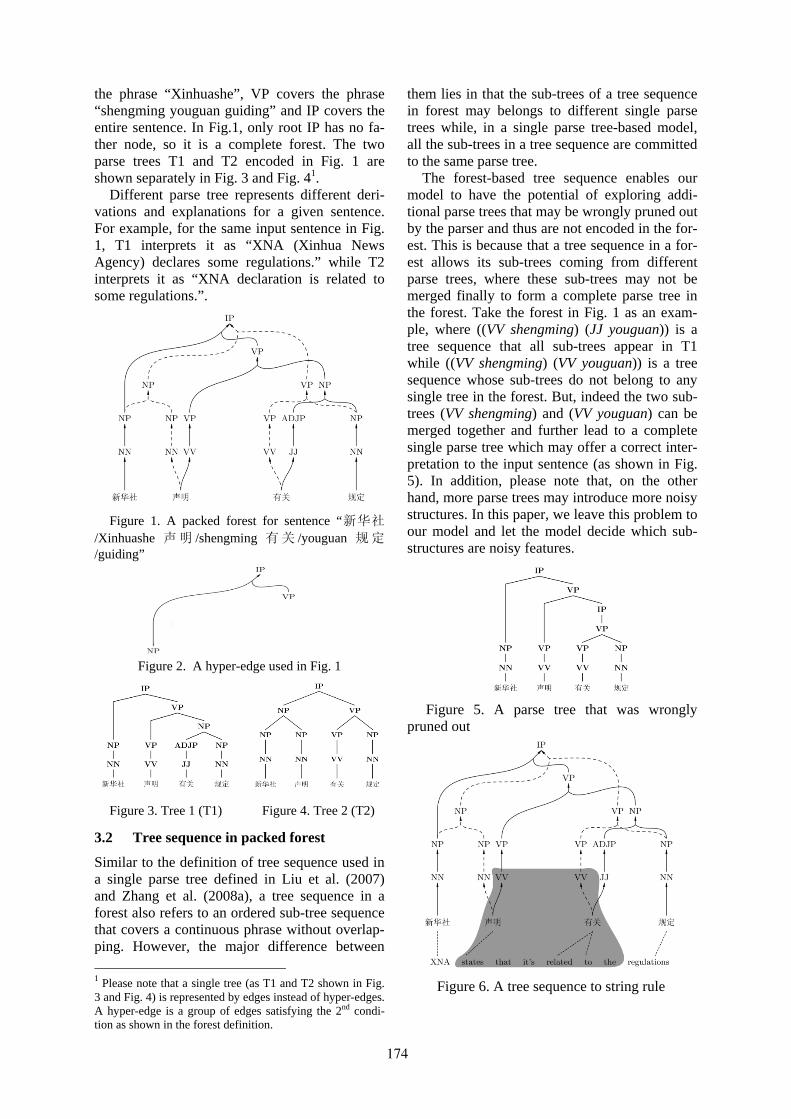
the phrase “Xinhuashe”, VP covers the phrase “shengming youguan guiding” and IP covers the entire sentence. In Fig.1, only root IP has no fa-ther node, so it is a complete forest. The two parse trees T1 and T2 encoded in Fig. 1 are shown separately in Fig. 3 and Fig. 41.
Different parse tree represents different deri-vations and explanations for a given sentence. For example, for the same input sentence in Fig. 1, T1 interprets it as “XNA (Xinhua News Agency) declares some regulations.” while T2 interprets it as “XNA declaration is related to some regulations.”.
Figure 1. A packed forest for sentence “新华社
/Xinhuashe 声明 /shengming 有关 /youguan 规定/guiding”
Figure 2. A hyper-edge used in Fig. 1
Figure 3. Tree 1 (T1) Figure 4. Tree 2 (T2)
3.2 Tree sequence in packed forest
Similar to the definition of tree sequence used in a single parse tree defined in Liu et al. (2007) and Zhang et al. (2008a), a tree sequence in a forest also refers to an ordered sub-tree sequence that covers a continuous phrase without overlap-ping. However, the major difference between 1 Please note that a single tree (as T1 and T2 shown in Fig. 3 and Fig. 4) is represented by edges instead of hyper-edges. A hyper-edge is a group of edges satisfying the 2nd condi-tion as shown in the forest definition.
them lies in that the sub-trees of a tree sequence in forest may belongs to different single parse trees while, in a single parse tree-based model, all the sub-trees in a tree sequence are committed to the same parse tree.
The forest-based tree sequence enables our model to have the potential of exploring addi-tional parse trees that may be wrongly pruned out by the parser and thus are not encoded in the for-est. This is because that a tree sequence in a for-est allows its sub-trees coming from different parse trees, where these sub-trees may not be merged finally to form a complete parse tree in the forest. Take the forest in Fig. 1 as an exam-ple, where ((VV shengming) (JJ youguan)) is a tree sequence that all sub-trees appear in T1 while ((VV shengming) (VV youguan)) is a tree sequence whose sub-trees do not belong to any single tree in the forest. But, indeed the two sub-trees (VV shengming) and (VV youguan) can be merged together and further lead to a complete single parse tree which may offer a correct inter-pretation to the input sentence (as shown in Fig. 5). In addition, please note that, on the other hand, more parse trees may introduce more noisy structures. In this paper, we leave this problem to our model and let the model decide which sub-structures are noisy features.
Figure 5. A parse tree that was wrongly pruned out
Figure 6. A tree sequence to string rule
174

A tree-sequence to string translation rule in a forest is a triple <L, R, A>, where L is the tree sequence in source language, R is the string con-taining words and variables in target language, and A is the alignment between the leaf nodes of L and R. This definition is similar to that of (Liu et al. 2007, Zhang et al. 2008a) except our tree-sequence is defined in forest. The shaded area of Fig. 6 exemplifies a tree sequence to string trans-lation rule in the forest.
3.3 Forest-based tree-sequence to string translation model
Given a source forest F and target translation TS as well as word alignment A, our translation model is formulated as:
Pr , , ∑ ∏ , , ,
By the above Eq., translation becomes a tree
sequence structure to string mapping issue. Giv-en the F, TS and A, there are multiple derivations that could map F to TS under the constraint A. The mapping probability Pr , , in our study is obtained by summing over the probabili-ties of all derivations Θ. The probability of each derivation is given as the product of the prob-abilities of all the rules ( )ip r used in the deriva-tion (here we assume that each rule is applied independently in a derivation).
Our model is implemented under log-linear framework (Och and Ney, 2002). We use seven basic features that are analogous to the common-ly used features in phrase-based systems (Koehn, 2003): 1) bidirectional rule mapping probabilities, 2) bidirectional lexical rule translation probabili-ties, 3) target language model, 4) number of rules used and 5) number of target words. In addition, we define two new features: 1) number of leaf nodes in auxiliary rules (the auxiliary rule will be explained later in this paper) and 2) product of the probabilities of all hyper-edges of the tree sequences in forest.
4 Training
This section discusses how to extract our transla-tion rules given a triple , , . As we know, the traditional tree-to-string rules can be easily extracted from , , using the algo-rithm of Mi and Huang (2008)2. We would like
2 Mi and Huang (2008) extend the tree-based rule extraction algorithm (Galley et al., 2004) to forest-based by introduc-ing non-deterministic mechanism. Their algorithm consists of two steps, minimal rule extraction and composed rule generation.
to leverage on their algorithm in our study. Un-fortunately, their algorithm is not directly appli-cable to our problem because tree rules have only one root while tree sequence rules have multiple roots. This makes the tree sequence rule extrac-tion very complex due to its interaction with for-est structure. To address this issue, we introduce the concepts of virtual node and virtual hyper-edge to convert a complete parse forest to a non-complete forest which is designed to en-code all the tree sequences that we want. There-fore, by doing so, the tree sequence rules can be extracted from a forest in the following two steps:
1) Convert the complete parse forest into a non-complete forest in order to cover those tree sequences that cannot be covered by a single tree node.
2) Employ the forest-based tree rule extraction algorithm (Mi and Huang, 2008) to extract our rules from the non-complete forest.
To facilitate our discussion, here we introduce two notations:
• Alignable: A consecutive source phrase is an alignable phrase if and only if it can be aligned with at least one consecutive target phrase under the word-alignment con-straint. The covered source span is called alignable span.
• Node sequence: a sequence of nodes (ei-ther leaf or internal nodes) in a forest cov-ering a consecutive span.
Algorithm 1 illustrates the first step of our rule extraction algorithm, which is a CKY-style Dy-namic Programming (DP) algorithm to add vir-tual nodes into forest. It includes the following steps:
1) We traverse the forest to visit each span in bottom-up fashion (line 1-2), 1.1) for each span [u,v] that is covered by
single tree nodes3, we put these tree nodes into the set NSS(u,v) and go back to step 1 (line 4-6).
1.2) otherwise we concatenate the tree se-quences of sub-spans to generate the set of tree sequences covering the cur-rent larger span (line 8-13). Then, we prune the set of node sequences (line 14). If this span is alignable, we create virtual father nodes and corres-ponding virtual hyper-edges to link the node sequences with the virtual father nodes (line 15-20).
3 Note that in a forest, there would be multiple single tree nodes covering the same span as shown Fig.1.
175

2) Finally we obtain a forest with each align-able span covered by either original tree nodes or the newly-created tree sequence virtual nodes.
Theoretically, there is exponential number of node sequences in a forest. Take Fig. 7 as an ex-ample. The NSS of span [1,2] only contains “NP” since it is alignable and covered by the single tree node NP. However, span [2,3] cannot be covered by any single tree node, so we have to create the NSS of span[2,3] by concatenating the NSSs of span [2,2] and span [3,3]. Since NSS of span [2,2] contains 4 element {“NN”, “NP”, “VV”, “VP”} and NSS of span [3, 3] also con-tains 4 element {“VV”, “VP”, “JJ”, “ADJP”}, NSS of span [2,3] contains 16=4*4 elements. To make the NSS manageable, we prune it with the following thresholds:
• each node sequence should contain less than n nodes
• each node sequence set should contain less than m node sequences
• sort node sequences according to their lengths and only keep the k shortest ones
Each virtual node is simply labeled by the concatenation of all its children’s labels as shown in Fig. 7. Algorithm 1. add virtual nodes into forest Input: packed forest F, alignment A Notation:
L: length of source sentence NSS(u,v): the set of node sequences covering span [u,v] VN(ns): virtual father node for node sequence ns.
Output: modified forest F with virtual nodes 1. for length := 0 to L - 1 do 2. for start := 1 to L - length do 3. stop := start + length 4. if span[start, stop] covered by tree nodes then 5. for each node n of span [start, stop] do 6. add n into NSS(start, stop) 7. else 8. for pivot := start to stop - 1 9. for each ns1 in NSS(start, pivot) do 10. for each ns2 in NSS(pivot+1, stop) do 11. create 1 2 12. if ns is not in NSS(start, stop) then 13. add ns into NSS(start, stop) 14. do pruning on NSS(start, stop) 15. if the span[start, stop] is alignable then 16. for each ns of NSS(start, stop) do 17. if node VN(ns) is not in F then 18. add node VN(ns) into F 19. add a hyper-edge h into F, 20. let lhs(h) := VN(ns), rhs(h) := ns
Algorithm 1 outputs a non-complete forest CF with each alignable span covered by either tree nodes or virtual nodes. Then we can easily ex-
tract our rules from the CF using the tree rule extraction algorithm (Mi and Huang, 2008).
Finally, to calculate rule feature probabilities for our model, we need to calculate the fractional counts (it is a kind of probability defined in Mi and Huang, 2008) of each translation rule in a parse forest. In the tree case, we can use the in-side-outside-based methods (Mi and Huang 2008) to do it. In the tree sequence case, since the previous method cannot be used directly, we provide another solution by making an indepen-dent assumption that each tree in a tree sequence is independent to each other. With this assump-tion, the fractional counts of both tree and tree sequence can be calculated as follows:
where is the fractional counts to be calcu-lated for rule r, a frag is either lhs(r) (excluding virtual nodes and virtual hyper-edges) or any tree node in a forest, TOP is the root of the forest, . and .) are the outside and inside probabil-ities of nodes, . returns the root nodes of a tree sequence fragment, . returns the leaf nodes of a tree sequence fragment, is the hyper-edge probability.
Figure 7. A virtual node in forest
5 Decoding
We benefit from the same strategy as used in our rule extraction algorithm in designing our decod-ing algorithm, recasting the forest-based tree se-quence-to-string decoding problem as a forest-based tree-to-string decoding problem. Our de-coding algorithm consists of four steps:
1) Convert the complete parse forest to a non-complete one by introducing virtual nodes.
176
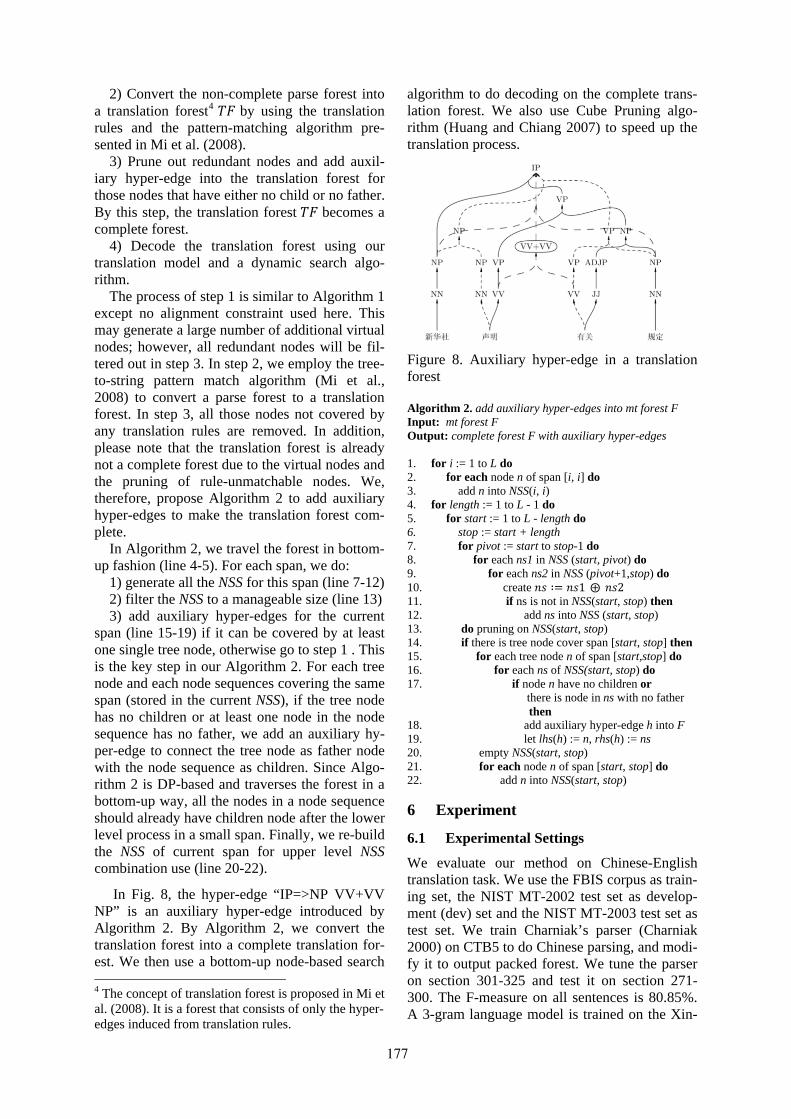
2) Convert the non-complete parse forest into a translation forest4 by using the translation rules and the pattern-matching algorithm pre-sented in Mi et al. (2008).
3) Prune out redundant nodes and add auxil-iary hyper-edge into the translation forest for those nodes that have either no child or no father. By this step, the translation forest becomes a complete forest.
4) Decode the translation forest using our translation model and a dynamic search algo-rithm.
The process of step 1 is similar to Algorithm 1 except no alignment constraint used here. This may generate a large number of additional virtual nodes; however, all redundant nodes will be fil-tered out in step 3. In step 2, we employ the tree-to-string pattern match algorithm (Mi et al., 2008) to convert a parse forest to a translation forest. In step 3, all those nodes not covered by any translation rules are removed. In addition, please note that the translation forest is already not a complete forest due to the virtual nodes and the pruning of rule-unmatchable nodes. We, therefore, propose Algorithm 2 to add auxiliary hyper-edges to make the translation forest com-plete.
In Algorithm 2, we travel the forest in bottom-up fashion (line 4-5). For each span, we do:
1) generate all the NSS for this span (line 7-12) 2) filter the NSS to a manageable size (line 13) 3) add auxiliary hyper-edges for the current
span (line 15-19) if it can be covered by at least one single tree node, otherwise go to step 1 . This is the key step in our Algorithm 2. For each tree node and each node sequences covering the same span (stored in the current NSS), if the tree node has no children or at least one node in the node sequence has no father, we add an auxiliary hy-per-edge to connect the tree node as father node with the node sequence as children. Since Algo-rithm 2 is DP-based and traverses the forest in a bottom-up way, all the nodes in a node sequence should already have children node after the lower level process in a small span. Finally, we re-build the NSS of current span for upper level NSS combination use (line 20-22).
In Fig. 8, the hyper-edge “IP=>NP VV+VV NP” is an auxiliary hyper-edge introduced by Algorithm 2. By Algorithm 2, we convert the translation forest into a complete translation for-est. We then use a bottom-up node-based search 4 The concept of translation forest is proposed in Mi et al. (2008). It is a forest that consists of only the hyper-edges induced from translation rules.
algorithm to do decoding on the complete trans-lation forest. We also use Cube Pruning algo-rithm (Huang and Chiang 2007) to speed up the translation process.
Figure 8. Auxiliary hyper-edge in a translation forest Algorithm 2. add auxiliary hyper-edges into mt forest F Input: mt forest F Output: complete forest F with auxiliary hyper-edges 1. for i := 1 to L do 2. for each node n of span [i, i] do 3. add n into NSS(i, i) 4. for length := 1 to L - 1 do 5. for start := 1 to L - length do 6. stop := start + length 7. for pivot := start to stop-1 do 8. for each ns1 in NSS (start, pivot) do 9. for each ns2 in NSS (pivot+1,stop) do 10. create 1 2 11. if ns is not in NSS(start, stop) then 12. add ns into NSS (start, stop) 13. do pruning on NSS(start, stop) 14. if there is tree node cover span [start, stop] then 15. for each tree node n of span [start,stop] do 16. for each ns of NSS(start, stop) do 17. if node n have no children or
there is node in ns with no father then
18. add auxiliary hyper-edge h into F 19. let lhs(h) := n, rhs(h) := ns 20. empty NSS(start, stop) 21. for each node n of span [start, stop] do 22. add n into NSS(start, stop)
6 Experiment
6.1 Experimental Settings
We evaluate our method on Chinese-English translation task. We use the FBIS corpus as train-ing set, the NIST MT-2002 test set as develop-ment (dev) set and the NIST MT-2003 test set as test set. We train Charniak’s parser (Charniak 2000) on CTB5 to do Chinese parsing, and modi-fy it to output packed forest. We tune the parser on section 301-325 and test it on section 271-300. The F-measure on all sentences is 80.85%. A 3-gram language model is trained on the Xin-
177
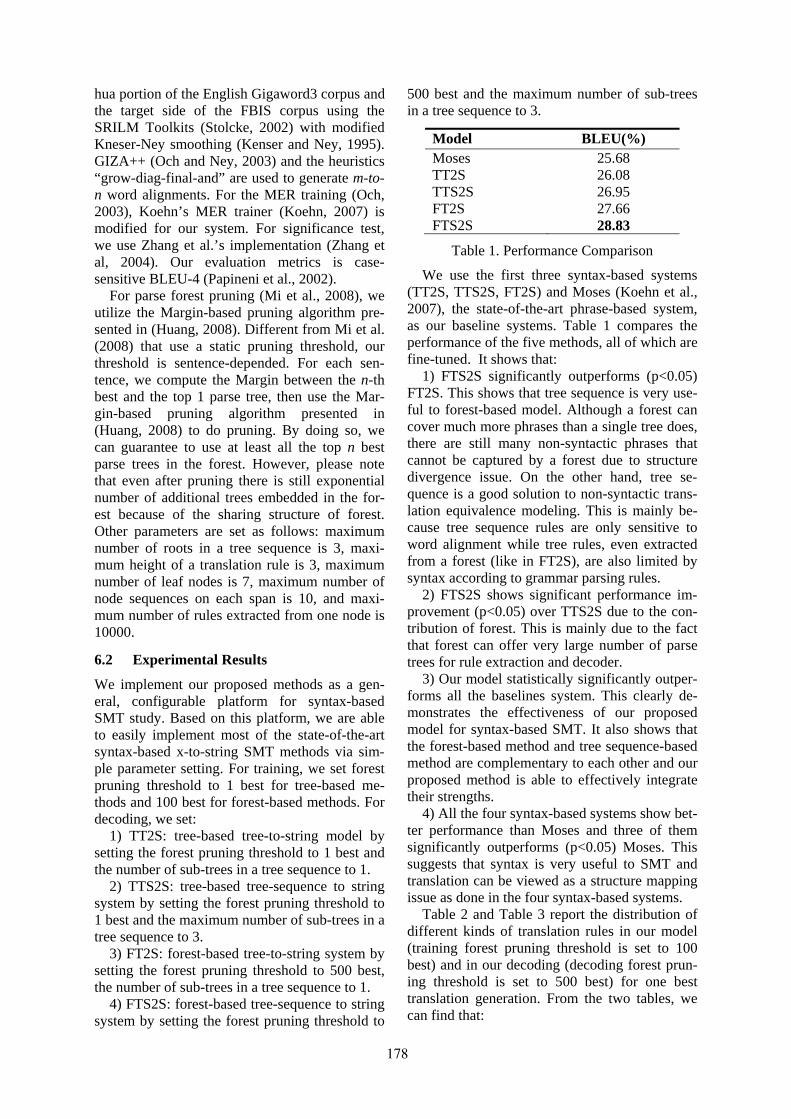
hua portion of the English Gigaword3 corpus and the target side of the FBIS corpus using the SRILM Toolkits (Stolcke, 2002) with modified Kneser-Ney smoothing (Kenser and Ney, 1995). GIZA++ (Och and Ney, 2003) and the heuristics “grow-diag-final-and” are used to generate m-to-n word alignments. For the MER training (Och, 2003), Koehn’s MER trainer (Koehn, 2007) is modified for our system. For significance test, we use Zhang et al.’s implementation (Zhang et al, 2004). Our evaluation metrics is case-sensitive BLEU-4 (Papineni et al., 2002).
For parse forest pruning (Mi et al., 2008), we utilize the Margin-based pruning algorithm pre-sented in (Huang, 2008). Different from Mi et al. (2008) that use a static pruning threshold, our threshold is sentence-depended. For each sen-tence, we compute the Margin between the n-th best and the top 1 parse tree, then use the Mar-gin-based pruning algorithm presented in (Huang, 2008) to do pruning. By doing so, we can guarantee to use at least all the top n best parse trees in the forest. However, please note that even after pruning there is still exponential number of additional trees embedded in the for-est because of the sharing structure of forest. Other parameters are set as follows: maximum number of roots in a tree sequence is 3, maxi-mum height of a translation rule is 3, maximum number of leaf nodes is 7, maximum number of node sequences on each span is 10, and maxi-mum number of rules extracted from one node is 10000.
6.2 Experimental Results
We implement our proposed methods as a gen-eral, configurable platform for syntax-based SMT study. Based on this platform, we are able to easily implement most of the state-of-the-art syntax-based x-to-string SMT methods via sim-ple parameter setting. For training, we set forest pruning threshold to 1 best for tree-based me-thods and 100 best for forest-based methods. For decoding, we set:
1) TT2S: tree-based tree-to-string model by setting the forest pruning threshold to 1 best and the number of sub-trees in a tree sequence to 1.
2) TTS2S: tree-based tree-sequence to string system by setting the forest pruning threshold to 1 best and the maximum number of sub-trees in a tree sequence to 3.
3) FT2S: forest-based tree-to-string system by setting the forest pruning threshold to 500 best, the number of sub-trees in a tree sequence to 1.
4) FTS2S: forest-based tree-sequence to string system by setting the forest pruning threshold to
500 best and the maximum number of sub-trees in a tree sequence to 3.
Model BLEU(%) Moses 25.68 TT2S 26.08 TTS2S 26.95 FT2S 27.66 FTS2S 28.83
Table 1. Performance Comparison
We use the first three syntax-based systems (TT2S, TTS2S, FT2S) and Moses (Koehn et al., 2007), the state-of-the-art phrase-based system, as our baseline systems. Table 1 compares the performance of the five methods, all of which are fine-tuned. It shows that:
1) FTS2S significantly outperforms (p<0.05) FT2S. This shows that tree sequence is very use-ful to forest-based model. Although a forest can cover much more phrases than a single tree does, there are still many non-syntactic phrases that cannot be captured by a forest due to structure divergence issue. On the other hand, tree se-quence is a good solution to non-syntactic trans-lation equivalence modeling. This is mainly be-cause tree sequence rules are only sensitive to word alignment while tree rules, even extracted from a forest (like in FT2S), are also limited by syntax according to grammar parsing rules.
2) FTS2S shows significant performance im-provement (p<0.05) over TTS2S due to the con-tribution of forest. This is mainly due to the fact that forest can offer very large number of parse trees for rule extraction and decoder.
3) Our model statistically significantly outper-forms all the baselines system. This clearly de-monstrates the effectiveness of our proposed model for syntax-based SMT. It also shows that the forest-based method and tree sequence-based method are complementary to each other and our proposed method is able to effectively integrate their strengths.
4) All the four syntax-based systems show bet-ter performance than Moses and three of them significantly outperforms (p<0.05) Moses. This suggests that syntax is very useful to SMT and translation can be viewed as a structure mapping issue as done in the four syntax-based systems.
Table 2 and Table 3 report the distribution of different kinds of translation rules in our model (training forest pruning threshold is set to 100 best) and in our decoding (decoding forest prun-ing threshold is set to 500 best) for one best translation generation. From the two tables, we can find that:
178

Rule Type Tree to String
Tree Sequence to String
L 4,854,406 20,526,674 P 37,360,684 58,826,261 U 3,297,302 3,775,734
All 45,512,392 83,128,669
Table 2. # of rules extracted from training cor-pus. L means fully lexicalized, P means partially lexicalized, U means unlexicalized.
Rule Type Tree
to String Tree Sequence
to String L 10,592 1,161 P 7,132 742 U 4,874 278
All 22,598 2,181
Table 3. # of rules used to generate one-best translation result in testing
1) In Table 2, the number of tree sequence
rules is much larger than that of tree rules al-though our rule extraction algorithm only ex-tracts those tree sequence rules over the spans that tree rules cannot cover. This suggests that the non-syntactic structure mapping is still a big challenge to syntax-based SMT.
2) Table 3 shows that the tree sequence rules is around 9% of the tree rules when generating the one-best translation. This suggests that around 9% of translation equivalences in the test set can be better modeled by tree sequence to string rules than by tree to string rules. The 9% tree sequence rules contribute 1.17 BLEU score improvement (28.83-27.66 in Table 1) to FTS2S over FT2S.
3) In Table 3, the fully-lexicalized rules are the major part (around 60%), followed by the partially-lexicalized (around 35%) and un-lexicalized (around 15%). However, in Table 2, partially-lexicalized rules extracted from training corpus are the major part (more than 70%). This suggests that most partially-lexicalized rules are less effective in our model. This clearly directs our future work in model optimization.
BLEU (%)
N-best \ model FT2S FTS2S 100 Best 27.40 28.61 500 Best 27.66 28.83 2500 Best 27.66 28.96 5000 Best 27.79 28.89
Table 4. Impact of the forest pruning
Forest pruning is a key step for forest-based method. Table 4 reports the performance of the two forest-based models using different values of the forest pruning threshold for decoding. It shows that:
1) FTS2S significantly outperforms (p<0.05) FT2S consistently in all test cases. This again demonstrates the effectiveness of our proposed model. Even if in the 5000 Best case, tree se-quence is still able to contribute 1.1 BLEU score improvement (28.89-27.79). It indicates the ad-vantage of tree sequence cannot be covered by forest even if we utilize a very large forest.
2) The BLEU scores are very similar to each other when we increase the forest pruning thre-shold. Moreover, in one case the performance even drops. This suggests that although more parse trees in a forest can offer more structure information, they may also introduce more noise that may confuse the decoder.
7 Conclusion
In this paper, we propose a forest-based tree-sequence to string translation model to combine the strengths of forest-based methods and tree-sequence based methods. This enables our model to have the great potential to address the issues of structure divergence and parse errors for syn-tax-based SMT. We convert our forest-based tree sequence rule extraction and decoding issues to tree-based by introducing virtual nodes, virtual hyper-edges and auxiliary rules (hyper-edges). In our system implementation, we design a general and configurable platform for our method, based on which we can easily realize many previous syntax-based methods. Finally, we examine our methods on the FBIS corpus and the NIST MT-2003 Chinese-English translation task. Experi-mental results show that our model greatly out-performs the four baseline systems. Our study demonstrates that forest-based method and tree sequence-based method are complementary to each other and our proposed method is able to effectively combine the strengths of the two in-dividual methods for syntax-based SMT.
Acknowledgement
We would like to thank Huang Yun for preparing the pictures in this paper; Run Yan for providing the java version modified MERT program and discussion on the details of MOSES; Mi Haitao for his help and discussion on re-implementing the FT2S model; Sun Jun and Xiong Deyi for their valuable suggestions.
179

References Eugene Charniak. 2000. A maximum-entropy inspired
parser. NAACL-00. Jason Eisner. 2003. Learning non-isomorphic tree
mappings for MT. ACL-03 (companion volume). Michel Galley, Mark Hopkins, Kevin Knight and Da-
niel Marcu. 2004. What’s in a translation rule? HLT-NAACL-04. 273-280.
Liang Huang. 2008. Forest Reranking: Discriminative Parsing with Non-Local Features. ACL-HLT-08. 586-594
Liang Huang and David Chiang. 2005. Better k-best Parsing. IWPT-05.
Liang Huang and David Chiang. 2007. Forest rescor-ing: Faster decoding with integrated language models. ACL-07. 144–151
Liang Huang, Kevin Knight and Aravind Joshi. 2006. Statistical Syntax-Directed Translation with Ex-tended Domain of Locality. AMTA-06. (poster)
Reinhard Kenser and Hermann Ney. 1995. Improved backing-off for M-gram language modeling. ICASSP-95. 181-184
Dan Klein and Christopher D. Manning. 2001. Pars-ing and Hypergraphs. IWPT-2001.
Philipp Koehn, F. J. Och and D. Marcu. 2003. Statis-tical phrase-based translation. HLT-NAACL-03. 127-133.
Philipp Koehn, Hieu Hoang, Alexandra Birch, Chris Callison-Burch, Marcello Federico, Nicola Bertol-di, Brooke Cowan, Wade Shen, Christine Moran, Richard Zens, Chris Dyer, Ondrej Bojar, Alexandra Constantin and Evan Herbst. 2007. Moses: Open Source Toolkit for Statistical Machine Translation. ACL-07. 177-180. (poster)
Yang Liu, Qun Liu and Shouxun Lin. 2006. Tree-to-String Alignment Template for Statistical Machine Translation. COLING-ACL-06. 609-616.
Yang Liu, Yun Huang, Qun Liu and Shouxun Lin. 2007. Forest-to-String Statistical Translation Rules. ACL-07. 704-711.
Haitao Mi, Liang Huang, and Qun Liu. 2008. Forest-based translation. ACL-HLT-08. 192-199.
Haitao Mi and Liang Huang. 2008. Forest-based Translation Rule Extraction. EMNLP-08. 206-214.
Franz J. Och and Hermann Ney. 2002. Discriminative training and maximum entropy models for statis-tical machine translation. ACL-02. 295-302.
Franz J. Och. 2003. Minimum error rate training in statistical machine translation. ACL-03. 160-167.
Franz Josef Och and Hermann Ney. 2003. A Syste-matic Comparison of Various Statistical Alignment Models. Computational Linguistics. 29(1) 19-51.
Kishore Papineni, Salim Roukos, ToddWard and Wei-Jing Zhu. 2002. BLEU: a method for automat-ic evaluation of machine translation. ACL-02. 311-318.
Andreas Stolcke. 2002. SRILM - an extensible lan-guage modeling toolkit. ICSLP-02. 901-904.
Min Zhang, Hongfei Jiang, Ai Ti Aw, Jun Sun, Sheng Li and Chew Lim Tan. 2007. A Tree-to-Tree Alignment-based Model for Statistical Machine Translation. MT-Summit-07. 535-542.
Min Zhang, Hongfei Jiang, Aiti Aw, Haizhou Li, Chew Lim Tan, Sheng Li. 2008a. A Tree Sequence Alignment-based Tree-to-Tree Translation Model. ACL-HLT-08. 559-567.
Min Zhang, Hongfei Jiang, Haizhou Li, Aiti Aw, Sheng Li. 2008b. Grammar Comparison Study for Translational Equivalence Modeling and Statistic-al Machine Translation. COLING-08. 1097-1104.
Ying Zhang, Stephan Vogel, Alex Waibel. 2004. In-terpreting BLEU/NIST scores: How much im-provement do we need to have a better system? LREC-04. 2051-2054.
180

Proceedings of the 47th Annual Meeting of the ACL and the 4th IJCNLP of the AFNLP, pages 181–189,Suntec, Singapore, 2-7 August 2009. c©2009 ACL and AFNLP
Active Learning for Multilingual Statistical Machine Translation∗
Gholamreza Haffari and Anoop SarkarSchool of Computing Science, Simon Fraser University
British Columbia, Canada{ghaffar1,anoop}@cs.sfu.ca
Abstract
Statistical machine translation (SMT)models require bilingual corpora for train-ing, and these corpora are often multi-lingual with parallel text in multiple lan-guages simultaneously. We introduce anactive learning task of adding a new lan-guage to an existing multilingual set ofparallel text and constructing high qualityMT systems, from each language in thecollection into this new target language.We show that adding a new language usingactive learning to the EuroParl corpus pro-vides a significant improvement comparedto a random sentence selection baseline.We also provide new highly effective sen-tence selection methods that improve ALfor phrase-based SMT in the multilingualand single language pair setting.
1 IntroductionThe main source of training data for statisticalmachine translation (SMT) models is a parallelcorpus. In many cases, the same information isavailable in multiple languages simultaneously asa multilingual parallel corpus, e.g., European Par-liament (EuroParl) and U.N. proceedings. In thispaper, we consider how to use active learning (AL)in order to add a new language to such a multilin-gual parallel corpus and at the same time we con-struct an MT system from each language in theoriginal corpus into this new target language. Weintroduce a novel combined measure of translationquality for multiple target language outputs (thesame content from multiple source languages).
The multilingual setting provides new opportu-nities for AL over and above a single languagepair. This setting is similar to the multi-task ALscenario (Reichart et al., 2008). In our case, themultiple tasks are individual machine translationtasks for several language pairs. The nature of thetranslation processes vary from any of the source
∗Thanks to James Peltier for systems support for our ex-periments. This research was partially supported by NSERC,Canada (RGPIN: 264905) and an IBM Faculty Award.
languages to the new language depending on thecharacteristics of each source-target language pair,hence these tasks are competing for annotating thesame resource. However it may be that in a singlelanguage pair, AL would pick a particular sentencefor annotation, but in a multilingual setting, a dif-ferent source language might be able to provide agood translation, thus saving annotation effort. Inthis paper, we explore how multiple MT systemscan be used to effectively pick instances that aremore likely to improve training quality.
Active learning is framed as an iterative learn-ing process. In each iteration new human labeledinstances (manual translations) are added to thetraining data based on their expected training qual-ity. However, if we start with only a small amountof initial parallel data for the new target language,then translation quality is very poor and requiresa very large injection of human labeled data tobe effective. To deal with this, we use a novelframework for active learning: we assume we aregiven a small amount of parallel text and a largeamount of monolingual source language text; us-ing these resources, we create a large noisy par-allel text which we then iteratively improve usingsmall injections of human translations. When webuild multiple MT systems from multiple sourcelanguages to the new target language, each MTsystem can be seen as a different ‘view’ on the de-sired output translation. Thus, we can train ourmultiple MT systems using either self-training orco-training (Blum and Mitchell, 1998). In self-training each MT system is re-trained using humanlabeled data plus its own noisy translation outputon the unlabeled data. In co-training each MT sys-tem is re-trained using human labeled data plusnoisy translation output from the other MT sys-tems in the ensemble. We use consensus transla-tions (He et al., 2008; Rosti et al., 2007; Matusovet al., 2006) as an effective method for co-trainingbetween multiple MT systems.
This paper makes the following contributions:• We provide a new framework for multilingual
MT, in which we build multiple MT systemsand add a new language to an existing multi-lingual parallel corpus. The multilingual set-
181
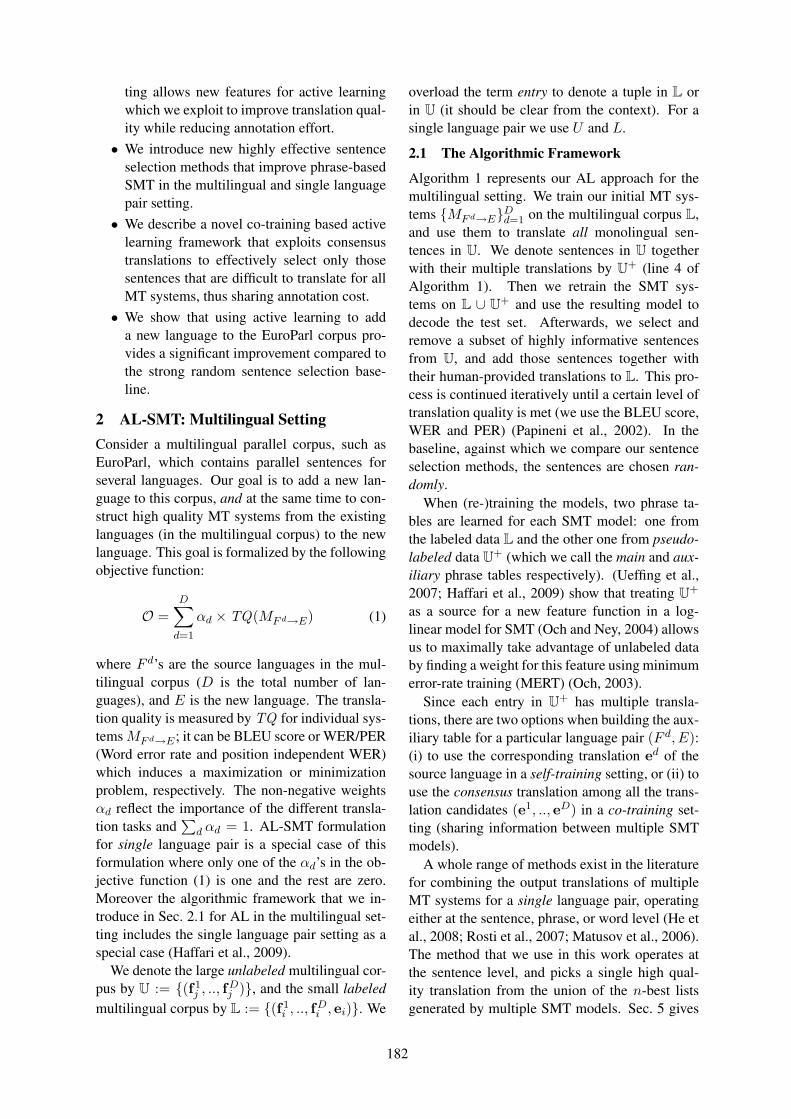
ting allows new features for active learningwhich we exploit to improve translation qual-ity while reducing annotation effort.• We introduce new highly effective sentence
selection methods that improve phrase-basedSMT in the multilingual and single languagepair setting.• We describe a novel co-training based active
learning framework that exploits consensustranslations to effectively select only thosesentences that are difficult to translate for allMT systems, thus sharing annotation cost.• We show that using active learning to add
a new language to the EuroParl corpus pro-vides a significant improvement compared tothe strong random sentence selection base-line.
2 AL-SMT: Multilingual SettingConsider a multilingual parallel corpus, such asEuroParl, which contains parallel sentences forseveral languages. Our goal is to add a new lan-guage to this corpus, and at the same time to con-struct high quality MT systems from the existinglanguages (in the multilingual corpus) to the newlanguage. This goal is formalized by the followingobjective function:
O =D∑
d=1
αd × TQ(MF d→E) (1)
where F d’s are the source languages in the mul-tilingual corpus (D is the total number of lan-guages), and E is the new language. The transla-tion quality is measured by TQ for individual sys-temsMF d→E ; it can be BLEU score or WER/PER(Word error rate and position independent WER)which induces a maximization or minimizationproblem, respectively. The non-negative weightsαd reflect the importance of the different transla-tion tasks and
∑
d αd = 1. AL-SMT formulationfor single language pair is a special case of thisformulation where only one of the αd’s in the ob-jective function (1) is one and the rest are zero.Moreover the algorithmic framework that we in-troduce in Sec. 2.1 for AL in the multilingual set-ting includes the single language pair setting as aspecial case (Haffari et al., 2009).
We denote the large unlabeled multilingual cor-pus by U := {(f1
j , .., fDj )}, and the small labeled
multilingual corpus by L := {(f1i , .., f
Di , ei)}. We
overload the term entry to denote a tuple in L orin U (it should be clear from the context). For asingle language pair we use U and L.
2.1 The Algorithmic Framework
Algorithm 1 represents our AL approach for themultilingual setting. We train our initial MT sys-tems {MF d→E}Dd=1 on the multilingual corpus L,and use them to translate all monolingual sen-tences in U. We denote sentences in U togetherwith their multiple translations by U
+ (line 4 ofAlgorithm 1). Then we retrain the SMT sys-tems on L ∪ U
+ and use the resulting model todecode the test set. Afterwards, we select andremove a subset of highly informative sentencesfrom U, and add those sentences together withtheir human-provided translations to L. This pro-cess is continued iteratively until a certain level oftranslation quality is met (we use the BLEU score,WER and PER) (Papineni et al., 2002). In thebaseline, against which we compare our sentenceselection methods, the sentences are chosen ran-domly.
When (re-)training the models, two phrase ta-bles are learned for each SMT model: one fromthe labeled data L and the other one from pseudo-labeled data U
+ (which we call the main and aux-iliary phrase tables respectively). (Ueffing et al.,2007; Haffari et al., 2009) show that treating U
+
as a source for a new feature function in a log-linear model for SMT (Och and Ney, 2004) allowsus to maximally take advantage of unlabeled databy finding a weight for this feature using minimumerror-rate training (MERT) (Och, 2003).
Since each entry in U+ has multiple transla-
tions, there are two options when building the aux-iliary table for a particular language pair (F d, E):(i) to use the corresponding translation ed of thesource language in a self-training setting, or (ii) touse the consensus translation among all the trans-lation candidates (e1, .., eD) in a co-training set-ting (sharing information between multiple SMTmodels).
A whole range of methods exist in the literaturefor combining the output translations of multipleMT systems for a single language pair, operatingeither at the sentence, phrase, or word level (He etal., 2008; Rosti et al., 2007; Matusov et al., 2006).The method that we use in this work operates atthe sentence level, and picks a single high qual-ity translation from the union of the n-best listsgenerated by multiple SMT models. Sec. 5 gives
182
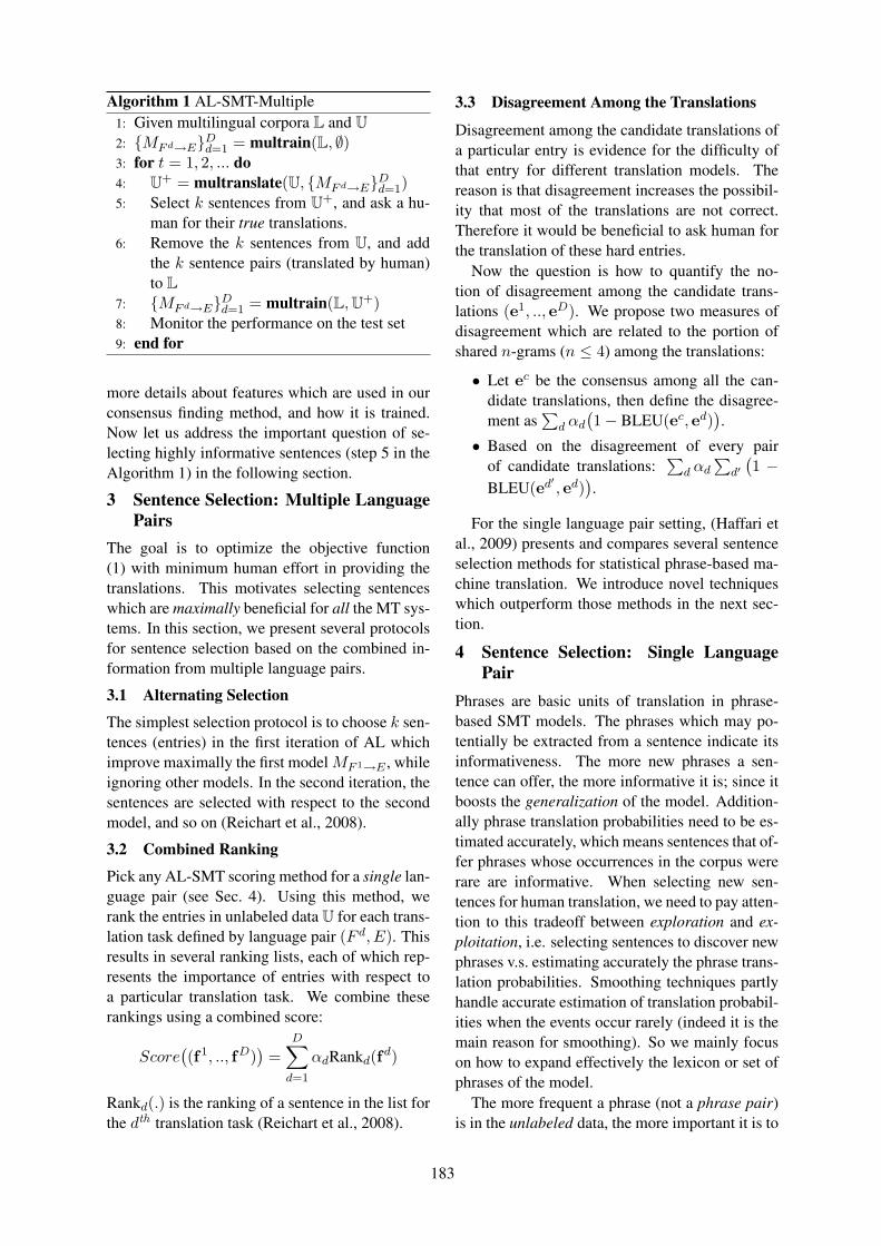
Algorithm 1 AL-SMT-Multiple1: Given multilingual corpora L and U
2: {MF d→E}Dd=1 = multrain(L, ∅)3: for t = 1, 2, ... do4: U
+ = multranslate(U, {MF d→E}Dd=1)5: Select k sentences from U
+, and ask a hu-man for their true translations.
6: Remove the k sentences from U, and addthe k sentence pairs (translated by human)to L
7: {MF d→E}Dd=1 = multrain(L,U+)8: Monitor the performance on the test set9: end for
more details about features which are used in ourconsensus finding method, and how it is trained.Now let us address the important question of se-lecting highly informative sentences (step 5 in theAlgorithm 1) in the following section.
3 Sentence Selection: Multiple LanguagePairs
The goal is to optimize the objective function(1) with minimum human effort in providing thetranslations. This motivates selecting sentenceswhich are maximally beneficial for all the MT sys-tems. In this section, we present several protocolsfor sentence selection based on the combined in-formation from multiple language pairs.
3.1 Alternating Selection
The simplest selection protocol is to choose k sen-tences (entries) in the first iteration of AL whichimprove maximally the first modelMF 1→E , whileignoring other models. In the second iteration, thesentences are selected with respect to the secondmodel, and so on (Reichart et al., 2008).
3.2 Combined Ranking
Pick any AL-SMT scoring method for a single lan-guage pair (see Sec. 4). Using this method, werank the entries in unlabeled data U for each trans-lation task defined by language pair (F d, E). Thisresults in several ranking lists, each of which rep-resents the importance of entries with respect toa particular translation task. We combine theserankings using a combined score:
Score(
(f1, .., fD))
=D∑
d=1
αdRankd(fd)
Rankd(.) is the ranking of a sentence in the list forthe dth translation task (Reichart et al., 2008).
3.3 Disagreement Among the Translations
Disagreement among the candidate translations ofa particular entry is evidence for the difficulty ofthat entry for different translation models. Thereason is that disagreement increases the possibil-ity that most of the translations are not correct.Therefore it would be beneficial to ask human forthe translation of these hard entries.
Now the question is how to quantify the no-tion of disagreement among the candidate trans-lations (e1, .., eD). We propose two measures ofdisagreement which are related to the portion ofshared n-grams (n ≤ 4) among the translations:
• Let ec be the consensus among all the can-didate translations, then define the disagree-ment as
∑
d αd
(
1− BLEU(ec, ed))
.
• Based on the disagreement of every pairof candidate translations:
∑
d αd∑
d′(
1 −BLEU(ed′ , ed)
)
.
For the single language pair setting, (Haffari etal., 2009) presents and compares several sentenceselection methods for statistical phrase-based ma-chine translation. We introduce novel techniqueswhich outperform those methods in the next sec-tion.
4 Sentence Selection: Single LanguagePair
Phrases are basic units of translation in phrase-based SMT models. The phrases which may po-tentially be extracted from a sentence indicate itsinformativeness. The more new phrases a sen-tence can offer, the more informative it is; since itboosts the generalization of the model. Addition-ally phrase translation probabilities need to be es-timated accurately, which means sentences that of-fer phrases whose occurrences in the corpus wererare are informative. When selecting new sen-tences for human translation, we need to pay atten-tion to this tradeoff between exploration and ex-ploitation, i.e. selecting sentences to discover newphrases v.s. estimating accurately the phrase trans-lation probabilities. Smoothing techniques partlyhandle accurate estimation of translation probabil-ities when the events occur rarely (indeed it is themain reason for smoothing). So we mainly focuson how to expand effectively the lexicon or set ofphrases of the model.
The more frequent a phrase (not a phrase pair)is in the unlabeled data, the more important it is to
183

know its translation; since it is more likely to seeit in test data (specially when the test data is in-domain with respect to unlabeled data). The morefrequent a phrase is in the labeled data, the moreunimportant it is; since probably we have observedmost of its translations.
In the labeled dataL, phrases are the ones whichare extracted by the SMT models; but what arethe candidate phrases in the unlabeled data U?We use the currently trained SMT models to an-swer this question. Each translation in the n-bestlist of translations (generated by the SMT mod-els) corresponds to a particular segmentation ofa sentence, which breaks that sentence into sev-eral fragments (see Fig. 1). Some of these frag-ments are the source language part of a phrase pairavailable in the phrase table, which we call regularphrases and denote their set byXreg
s for a sentences. However, there are some fragments in the sen-tence which are not covered by the phrase table –possibly because of the OOVs (out-of-vocabularywords) or the constraints imposed by the phraseextraction algorithm – called Xoov
s for a sentences. Each member of Xoov
s offers a set of potentialphrases (also referred to as OOV phrases) whichare not observed due to the latent segmentation ofthis fragment. We present two generative modelsfor the phrases and show how to estimate and usethem for sentence selection.
4.1 Model 1
In the first model, the generative story is to gen-erate phrases for each sentence based on indepen-dent draws from a multinomial. The sample spaceof the multinomial consists of both regular andOOV phrases.
We build two models, i.e. two multinomials,one for labeled data and the other one for unla-beled data. Each model is trained by maximizingthe log-likelihood of its corresponding data:
LD :=∑
s∈DP̃ (s)
∑
x∈Xs
logP (x|θD) (2)
where D is either L or U , P̃ (s) is the empiri-cal distribution of the sentences1, and θD is theparameter vector of the corresponding probability
1P̃ (s) is the number of times that the sentence s is seenin D divided by the number of all sentences in D.
distribution. When x ∈ Xoovs , we will have
P (x|θU ) =∑
h∈Hx
P (x, h|θU )
=∑
h∈Hx
P (h)P (x|h,θU )
=1
|Hx|∑
h∈Hx
∏
y∈Y hx
θU (y) (3)
where Hx is the space of all possible segmenta-tions for the OOV fragment x, Y h
x is the result-ing phrases from x based on the segmentation h,and θU (y) is the probability of the OOV phrasey in the multinomial associated with U . We letHx to be all possible segmentations of the frag-ment x for which the resulting phrase lengths arenot greater than the maximum length constraint forphrase extraction in the underlying SMT model.Since we do not know anything about the segmen-tations a priori, we have put a uniform distributionover such segmentations.
Maximizing (2) to find the maximum likelihoodparameters for this model is an extremely diffi-cult problem2. Therefore, we maximize the fol-lowing lower-bound on the log-likelihood whichis derived using Jensen’s inequality:
LD ≥∑
s∈DP̃ (s)
[
∑
x∈Xregs
log θD(x)
+∑
x∈Xoovs
∑
h∈Hx
1
|Hx|∑
y∈Y hx
log θD(y)]
(4)
Maximizing (4) amounts to set the probability ofeach regular / potential phrase proportional to itscount / expected count in the data D.
Let ρk(xi:j) be the number of possible segmen-tations from position i to position j of an OOVfragment x, and k is the maximum phrase length;
ρk(x1:|x|) =
0, if |x| = 0
1, if |x| = 1∑k
i=1 ρk(xi+1:|x|), otherwise
which gives us a dynamic programming algorithmto compute the number of segmentation |Hx| =ρk(x1:|x|) of the OOV fragment x. The expectedcount of a potential phrase y based on an OOVsegment x is (see Fig. 1.c):
E[y|x] =
∑
i≤j δ[y=xi:j ]ρk(x1:i−1)ρk(xj+1:|x|)
ρk(x)
2Setting partial derivatives of the Lagrangian to zeroamounts to finding the roots of a system of multivariate poly-nomials (a major topic in Algebraic Geometry).
184
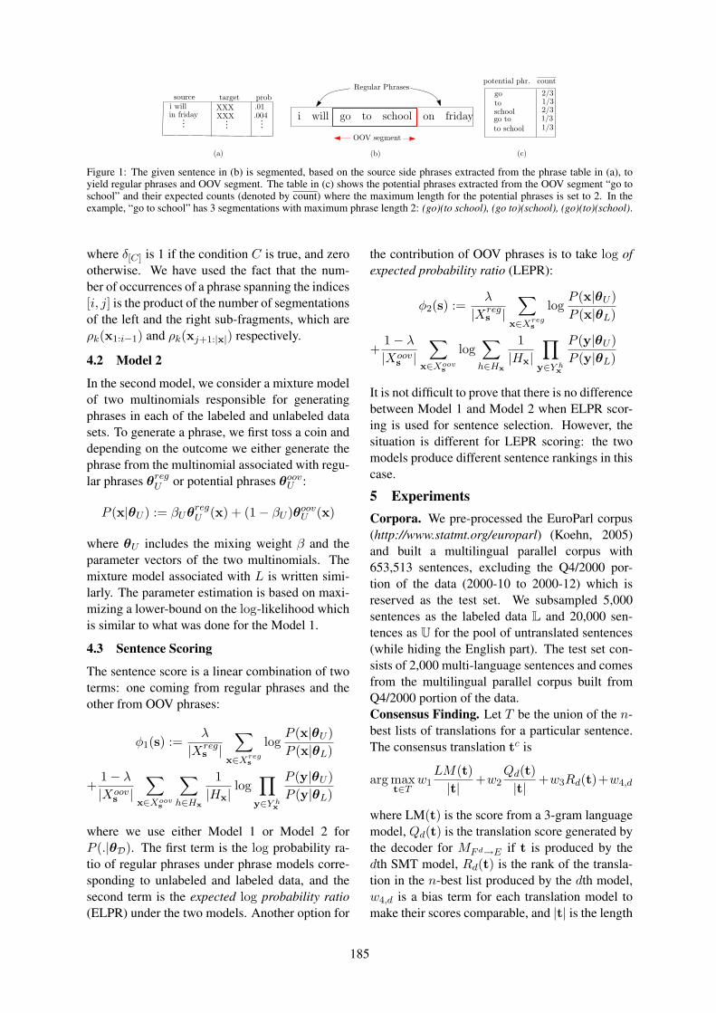
i will go to school on friday
Regular Phrases
OOV segment
gotoschoolgo toto school
2/3
2/31/3
1/31/3
i willin friday
XXXXXX
.01.004...
......
(a)
potential phr.
source target prob
count
(b) (c)
Figure 1: The given sentence in (b) is segmented, based on the source side phrases extracted from the phrase table in (a), toyield regular phrases and OOV segment. The table in (c) shows the potential phrases extracted from the OOV segment “go toschool” and their expected counts (denoted by count) where the maximum length for the potential phrases is set to 2. In theexample, “go to school” has 3 segmentations with maximum phrase length 2: (go)(to school), (go to)(school), (go)(to)(school).
where δ[C] is 1 if the condition C is true, and zerootherwise. We have used the fact that the num-ber of occurrences of a phrase spanning the indices[i, j] is the product of the number of segmentationsof the left and the right sub-fragments, which areρk(x1:i−1) and ρk(xj+1:|x|) respectively.
4.2 Model 2
In the second model, we consider a mixture modelof two multinomials responsible for generatingphrases in each of the labeled and unlabeled datasets. To generate a phrase, we first toss a coin anddepending on the outcome we either generate thephrase from the multinomial associated with regu-lar phrases θreg
U or potential phrases θoovU :
P (x|θU ) := βUθregU (x) + (1− βU )θoov
U (x)
where θU includes the mixing weight β and theparameter vectors of the two multinomials. Themixture model associated with L is written simi-larly. The parameter estimation is based on maxi-mizing a lower-bound on the log-likelihood whichis similar to what was done for the Model 1.
4.3 Sentence Scoring
The sentence score is a linear combination of twoterms: one coming from regular phrases and theother from OOV phrases:
φ1(s) :=λ
|Xregs |
∑
x∈Xregs
logP (x|θU )
P (x|θL)
+1− λ|Xoov
s |∑
x∈Xoovs
∑
h∈Hx
1
|Hx|log
∏
y∈Y hx
P (y|θU )
P (y|θL)
where we use either Model 1 or Model 2 forP (.|θD). The first term is the log probability ra-tio of regular phrases under phrase models corre-sponding to unlabeled and labeled data, and thesecond term is the expected log probability ratio(ELPR) under the two models. Another option for
the contribution of OOV phrases is to take log ofexpected probability ratio (LEPR):
φ2(s) :=λ
|Xregs |
∑
x∈Xregs
logP (x|θU )
P (x|θL)
+1− λ|Xoov
s |∑
x∈Xoovs
log∑
h∈Hx
1
|Hx|∏
y∈Y hx
P (y|θU )
P (y|θL)
It is not difficult to prove that there is no differencebetween Model 1 and Model 2 when ELPR scor-ing is used for sentence selection. However, thesituation is different for LEPR scoring: the twomodels produce different sentence rankings in thiscase.
5 ExperimentsCorpora. We pre-processed the EuroParl corpus(http://www.statmt.org/europarl) (Koehn, 2005)and built a multilingual parallel corpus with653,513 sentences, excluding the Q4/2000 por-tion of the data (2000-10 to 2000-12) which isreserved as the test set. We subsampled 5,000sentences as the labeled data L and 20,000 sen-tences as U for the pool of untranslated sentences(while hiding the English part). The test set con-sists of 2,000 multi-language sentences and comesfrom the multilingual parallel corpus built fromQ4/2000 portion of the data.Consensus Finding. Let T be the union of the n-best lists of translations for a particular sentence.The consensus translation tc is
arg maxt∈T
w1LM(t)|t|
+w2Qd(t)|t|
+w3Rd(t)+w4,d
where LM(t) is the score from a 3-gram languagemodel, Qd(t) is the translation score generated bythe decoder for MF d→E if t is produced by thedth SMT model, Rd(t) is the rank of the transla-tion in the n-best list produced by the dth model,w4,d is a bias term for each translation model tomake their scores comparable, and |t| is the length
185
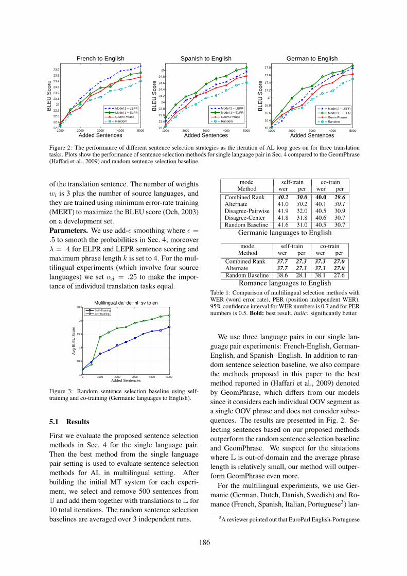
1000 2000 3000 4000 500022.6
22.7
22.8
22.9
23
23.1
23.2
23.3
23.4
23.5
23.6
Added Sentences
BLE
U S
core
French to English
Model 2 − LEPRModel 1 − ELPRGeom PhraseRandom
1000 2000 3000 4000 500023.2
23.4
23.6
23.8
24
24.2
24.4
24.6
24.8
25
Added Sentences
BLE
U S
core
Spanish to English
Model 2 − LEPRModel 1 − ELPRGeom PhraseRandom
1000 2000 3000 4000 500016.2
16.4
16.6
16.8
17
17.2
17.4
17.6
17.8
Added Sentences
BLE
U S
core
German to English
Model 2 − LEPRModel 1 − ELPRGeom PhraseRandom
Figure 2: The performance of different sentence selection strategies as the iteration of AL loop goes on for three translationtasks. Plots show the performance of sentence selection methods for single language pair in Sec. 4 compared to the GeomPhrase(Haffari et al., 2009) and random sentence selection baseline.
of the translation sentence. The number of weightswi is 3 plus the number of source languages, andthey are trained using minimum error-rate training(MERT) to maximize the BLEU score (Och, 2003)on a development set.Parameters. We use add-ε smoothing where ε =.5 to smooth the probabilities in Sec. 4; moreoverλ = .4 for ELPR and LEPR sentence scoring andmaximum phrase length k is set to 4. For the mul-tilingual experiments (which involve four sourcelanguages) we set αd = .25 to make the impor-tance of individual translation tasks equal.
0 1000 2000 3000 4000 500018
18.5
19
19.5
20
20.5
Added Sentences
Avg
BLE
U S
core
Mulilingual da−de−nl−sv to en
Self−TrainingCo−Training
Figure 3: Random sentence selection baseline using self-training and co-training (Germanic languages to English).
5.1 Results
First we evaluate the proposed sentence selectionmethods in Sec. 4 for the single language pair.Then the best method from the single languagepair setting is used to evaluate sentence selectionmethods for AL in multilingual setting. Afterbuilding the initial MT system for each experi-ment, we select and remove 500 sentences fromU and add them together with translations to L for10 total iterations. The random sentence selectionbaselines are averaged over 3 independent runs.
mode self-train co-trainMethod wer per wer per
Combined Rank 40.2 30.0 40.0 29.6Alternate 41.0 30.2 40.1 30.1Disagree-Pairwise 41.9 32.0 40.5 30.9Disagree-Center 41.8 31.8 40.6 30.7Random Baseline 41.6 31.0 40.5 30.7
Germanic languages to English
mode self-train co-trainMethod wer per wer per
Combined Rank 37.7 27.3 37.3 27.0Alternate 37.7 27.3 37.3 27.0Random Baseline 38.6 28.1 38.1 27.6
Romance languages to EnglishTable 1: Comparison of multilingual selection methods withWER (word error rate), PER (position independent WER).95% confidence interval for WER numbers is 0.7 and for PERnumbers is 0.5. Bold: best result, italic: significantly better.
We use three language pairs in our single lan-guage pair experiments: French-English, German-English, and Spanish- English. In addition to ran-dom sentence selection baseline, we also comparethe methods proposed in this paper to the bestmethod reported in (Haffari et al., 2009) denotedby GeomPhrase, which differs from our modelssince it considers each individual OOV segment asa single OOV phrase and does not consider subse-quences. The results are presented in Fig. 2. Se-lecting sentences based on our proposed methodsoutperform the random sentence selection baselineand GeomPhrase. We suspect for the situationswhere L is out-of-domain and the average phraselength is relatively small, our method will outper-form GeomPhrase even more.
For the multilingual experiments, we use Ger-manic (German, Dutch, Danish, Swedish) and Ro-mance (French, Spanish, Italian, Portuguese3) lan-
3A reviewer pointed out that EuroParl English-Portuguese
186

0 1000 2000 3000 4000 5000
18.2
18.4
18.6
18.8
19
19.2
19.4
19.6
19.8
20
Added Sentences
Avg
BLE
U S
core
Self−Train Mulilingual da−de−nl−sv to en
AlternateCombineRankDisagree−PairwiseDisagree−CenterRandom
1000 1500 2000 2500 3000 3500 4000 4500 500019.3
19.4
19.5
19.6
19.7
19.8
19.9
20
20.1
20.2
20.3
Added Sentences
Avg
BLE
U S
core
Co−Train Mulilingual da−de−nl−sv to en
AlternateCombineRankDisagree−PairwiseDisagree−CenterRandom
0 1000 2000 3000 4000 500021.6
21.8
22
22.2
22.4
22.6
22.8
23
23.2
23.4
23.6
Added Sentences
Avg
BLE
U S
core
Self−Train Mulilingual fr−es−it−pt to en
AlternateCombineRankRandom
1000 1500 2000 2500 3000 3500 4000 4500 500022.6
22.8
23
23.2
23.4
23.6
23.8
Added SentencesA
vg B
LEU
Sco
re
Co−Train Mulilingual fr−es−it−pt to en
AlternateCombineRankRandom
Figure 4: The left/right plot show the performance of our AL methods for multilingual setting combined with self-training/co-training. The sentence selection methods from Sec. 3 are compared with random sentence selection baseline. The top plots cor-respond to Danish-German-Dutch-Swedish to English, and the bottom plots correspond to French-Spanish-Italian-Portugueseto English.
guages as the source and English as the target lan-guage as two sets of experiments.4 Fig. 3 showsthe performance of random sentence selection forAL combined with self-training/co-training for themulti-source translation from the four Germaniclanguages to English. It shows that the co-trainingmode outperforms the self-training mode by al-most 1 BLEU point. The results of selectionstrategies in the multilingual setting are presentedin Fig. 4 and Tbl. 1. Having noticed that Model1 with ELPR performs well in the single languagepair setting, we use it to rank entries for individualtranslation tasks. Then these rankings are used by‘Alternate’ and ‘Combined Rank’ selection strate-gies in the multilingual case. The ‘CombinedRank’ method outperforms all the other methodsincluding the strong random selection baseline inboth self-training and co-training modes. Thedisagreement-based selection methods underper-form the baseline for translation of Germanic lan-guages to English, so we omitted them for the Ro-mance language experiments.
5.2 Analysis
The basis for our proposed methods has been thepopularity of regular/OOV phrases in U and their
data is very noisy and future work should omit this pair.4Choice of Germanic and Romance for our experimental
setting is inspired by results in (Cohn and Lapata, 2007)
unpopularity in L, which is measured by P (x|θU )P (x|θL) .
We need P (x|θU ), the estimated distribution ofphrases in U , to be as similar as possible to P ∗(x),the true distribution of phrases in U . We investi-gate this issue for regular/OOV phrases as follows:• Using the output of the initially trained MT sys-tem on L, we extract the regular/OOV phrases asdescribed in §4. The smoothed relative frequen-cies give us the regular/OOV phrasal distributions.• Using the true English translation of the sen-tences in U , we extract the true phrases. Separat-ing the phrases into two sets of regular and OOVphrases defined by the previous step, we use thesmoothed relative frequencies and form the trueOOV/regular phrasal distributions.
We use the KL-divergence to see how dissim-ilar are a pair of given probability distributions.As Tbl. 2 shows, the KL-divergence between thetrue and estimated distributions are less than that
De2En Fr2En Es2EnKL(P ∗reg ‖ Preg) 4.37 4.17 4.38KL(P ∗reg ‖ unif ) 5.37 5.21 5.80KL(P ∗oov ‖ Poov) 3.04 4.58 4.73KL(P ∗oov ‖ unif ) 3.41 4.75 4.99
Table 2: For regular/OOV phrases, the KL-divergence be-tween the true distribution (P ∗) and the estimated (P ) or uni-form (unif ) distributions are shown, where:KL(P ∗ ‖ P ) :=
Px P ∗(x) log P∗(x)
P (x).
187

100
101
102
103
104
105
10−6
10−5
10−4
10−3
10−2
10−1
100
Rank
Pro
babi
lity
Regular Phrases in U
Estimated DistributionTrue Distribution
100
101
102
103
104
105
10−6
10−5
10−4
10−3
10−2
10−1
100
Rank
Pro
babi
lity
OOV Phrases in U
Estimated DistributionTrue Distribution
Figure 5: The log-log Zipf plots representing the true andestimated probabilities of a (source) phrase vs the rank ofthat phrase in the German to English translation task. Theplots for the Spanish to English and French to English tasksare also similar to the above plots, and confirm a power lawbehavior in the true phrasal distributions.
between the true and uniform distributions, in allthree language pairs. Since uniform distributionconveys no information, this is evidence that thereis some information encoded in the estimated dis-tribution about the true distribution. Howeverwe noticed that the true distributions of regu-lar/OOV phrases exhibit Zipfian (power law) be-havior5 which is not well captured by the esti-mated distributions (see Fig. 5). Enhancing the es-timated distributions to capture this power law be-havior would improve the quality of the proposedsentence selection methods.
6 Related Work(Haffari et al., 2009) provides results for activelearning for MT using a single language pair. Ourwork generalizes to the use of multilingual corporausing new methods that are not possible with a sin-gle language pair. In this paper, we also introducenew selection methods that outperform the meth-ods in (Haffari et al., 2009) even for MT with asingle language pair. In addition in this paper byconsidering multilingual parallel corpora we wereable to introduce co-training for AL, while (Haf-fari et al., 2009) only use self-training since theyare using a single language pair.
5This observation is at the phrase level and not at the word(Zipf, 1932) or even n-gram level (Ha et al., 2002).
(Reichart et al., 2008) introduces multi-task ac-tive learning where unlabeled data require annota-tions for multiple tasks, e.g. they consider named-entities and parse trees, and showed that multi-ple tasks helps selection compared to individualtasks. Our setting is different in that the target lan-guage is the same across multiple MT tasks, whichwe exploit to use consensus translations and co-training to improve active learning performance.
(Callison-Burch and Osborne, 2003b; Callison-Burch and Osborne, 2003a) provide a co-trainingapproach to MT, where one language pair createsdata for another language pair. In contrast, ourco-training approach uses consensus translationsand our setting for active learning is very differ-ent from their semi-supervised setting. A Ph.D.proposal by Chris Callison-Burch (Callison-burch,2003) lays out the promise of AL for SMT andproposes some algorithms. However, the lack ofexperimental results means that performance andfeasibility of those methods cannot be comparedto ours.
While we use consensus translations (He et al.,2008; Rosti et al., 2007; Matusov et al., 2006)as an effective method for co-training in this pa-per, unlike consensus for system combination, thesource languages for each of our MT systems aredifferent, which rules out a set of popular methodsfor obtaining consensus translations which assumetranslation for a single language pair. Finally, webriefly note that triangulation (see (Cohn and Lap-ata, 2007)) is orthogonal to the use of co-trainingin our work, since it only enhances each MT sys-tem in our ensemble by exploiting the multilingualdata. In future work, we plan to incorporate trian-gulation into our active learning approach.
7 ConclusionThis paper introduced the novel active learningtask of adding a new language to an existing multi-lingual set of parallel text. We construct SMT sys-tems from each language in the collection into thenew target language. We show that we can take ad-vantage of multilingual corpora to decrease anno-tation effort thanks to the highly effective sentenceselection methods we devised for active learningin the single language-pair setting which we thenapplied to the multilingual sentence selection pro-tocols. In the multilingual setting, a novel co-training method for active learning in SMT is pro-posed using consensus translations which outper-forms AL-SMT with self-training.
188

ReferencesAvrim Blum and Tom Mitchell. 1998. Combin-
ing Labeled and Unlabeled Data with Co-Training.In Proceedings of the Eleventh Annual Conferenceon Computational Learning Theory (COLT 1998),Madison, Wisconsin, USA, July 24-26. ACM.
Chris Callison-Burch and Miles Osborne. 2003a.Bootstrapping parallel corpora. In NAACL work-shop: Building and Using Parallel Texts: DataDriven Machine Translation and Beyond.
Chris Callison-Burch and Miles Osborne. 2003b. Co-training for statistical machine translation. In Pro-ceedings of the 6th Annual CLUK Research Collo-quium.
Chris Callison-burch. 2003. Active learning for statis-tical machine translation. In PhD Proposal, Edin-burgh University.
Trevor Cohn and Mirella Lapata. 2007. Machinetranslation by triangulation: Making effective use ofmulti-parallel corpora. In ACL.
Le Quan Ha, E. I. Sicilia-Garcia, Ji Ming, and F.J.Smith. 2002. Extension of zipf’s law to words andphrases. In Proceedings of the 19th internationalconference on Computational linguistics.
Gholamreza Haffari, Maxim Roy, and Anoop Sarkar.2009. Active learning for statistical phrase-basedmachine translation. In NAACL.
Xiaodong He, Mei Yang, Jianfeng Gao, PatrickNguyen, and Robert Moore. 2008. Indirect-hmm-based hypothesis alignment for combining outputsfrom machine translation systems. In EMNLP.
Philipp Koehn. 2005. Europarl: A parallel corpus forstatistical machine translation. In MT Summit.
Evgeny Matusov, Nicola Ueffing, and Hermann Ney.2006. Computing consensus translation from multi-ple machine translation systems using enhanced hy-potheses alignment. In EACL.
Franz Josef Och and Hermann Ney. 2004. The align-ment template approach to statistical machine trans-lation. Computational Linguistics, 30(4):417–449.
Franz Josef Och. 2003. Minimum error rate trainingin statistical machine translation. In ACL ’03: Pro-ceedings of the 41st Annual Meeting on Associationfor Computational Linguistics.
Kishore Papineni, Salim Roukos, Todd Ward, and Weijing Zhu. 2002. Bleu: A method for automatic eval-uation of machine translation. In ACL ’02: Proceed-ings of the 41st Annual Meeting on Association forComputational Linguistics.
Roi Reichart, Katrin Tomanek, Udo Hahn, and AriRappoport. 2008. Multi-task active learning for lin-guistic annotations. In ACL.
Antti-Veikko Rosti, Necip Fazil Ayan, Bing Xiang,Spyros Matsoukas, Richard M. Schwartz, and Bon-nie Jean Dorr. 2007. Combining outputs from mul-tiple machine translation systems. In NAACL.
Nicola Ueffing, Gholamreza Haffari, and AnoopSarkar. 2007. Transductive learning for statisticalmachine translation. In ACL.
George Zipf. 1932. Selective Studies and the Principleof Relative Frequency in Language. Harvard Uni-versity Press.
189
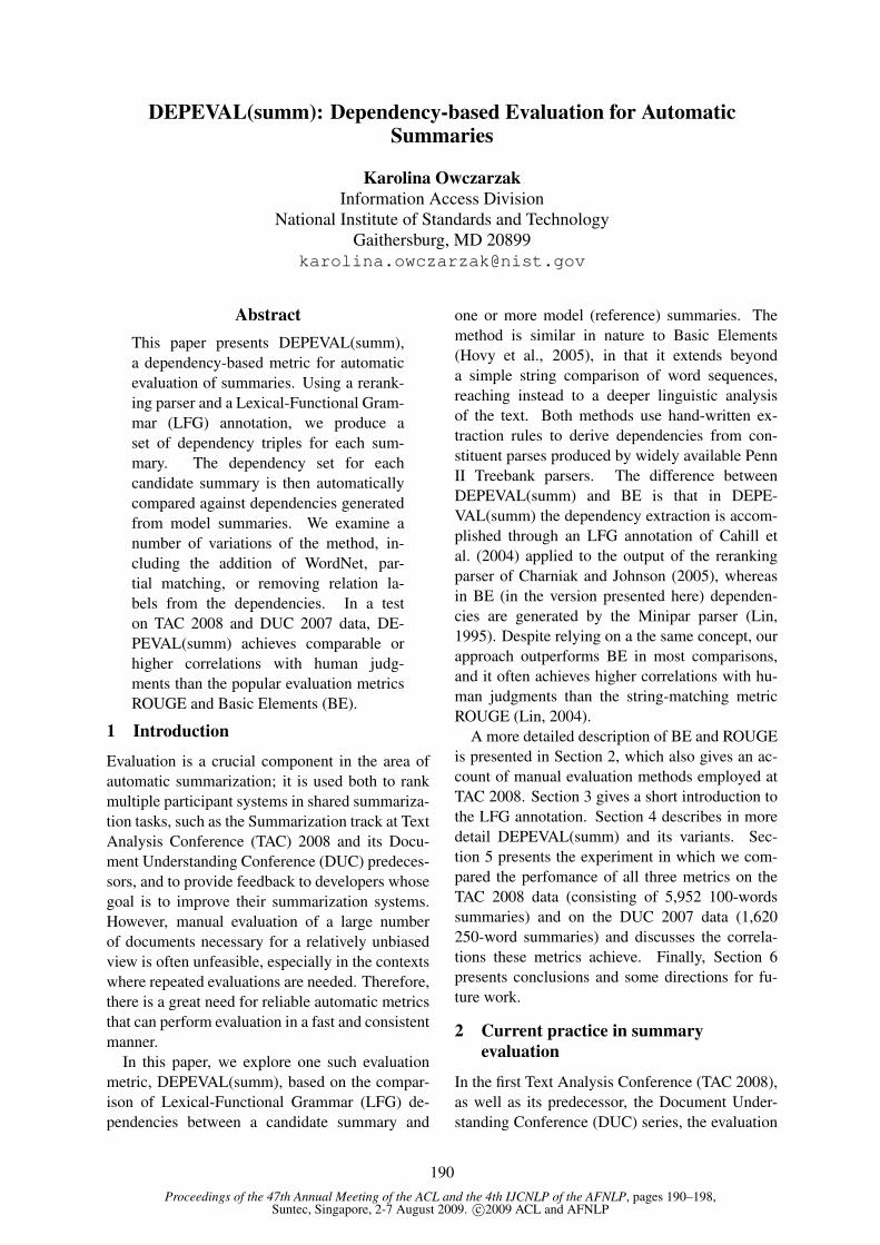
Proceedings of the 47th Annual Meeting of the ACL and the 4th IJCNLP of the AFNLP, pages 190–198,Suntec, Singapore, 2-7 August 2009. c©2009 ACL and AFNLP
DEPEVAL(summ): Dependency-based Evaluation for AutomaticSummaries
Karolina OwczarzakInformation Access Division
National Institute of Standards and TechnologyGaithersburg, MD 20899
AbstractThis paper presents DEPEVAL(summ),a dependency-based metric for automaticevaluation of summaries. Using a rerank-ing parser and a Lexical-Functional Gram-mar (LFG) annotation, we produce aset of dependency triples for each sum-mary. The dependency set for eachcandidate summary is then automaticallycompared against dependencies generatedfrom model summaries. We examine anumber of variations of the method, in-cluding the addition of WordNet, par-tial matching, or removing relation la-bels from the dependencies. In a teston TAC 2008 and DUC 2007 data, DE-PEVAL(summ) achieves comparable orhigher correlations with human judg-ments than the popular evaluation metricsROUGE and Basic Elements (BE).
1 Introduction
Evaluation is a crucial component in the area ofautomatic summarization; it is used both to rankmultiple participant systems in shared summariza-tion tasks, such as the Summarization track at TextAnalysis Conference (TAC) 2008 and its Docu-ment Understanding Conference (DUC) predeces-sors, and to provide feedback to developers whosegoal is to improve their summarization systems.However, manual evaluation of a large numberof documents necessary for a relatively unbiasedview is often unfeasible, especially in the contextswhere repeated evaluations are needed. Therefore,there is a great need for reliable automatic metricsthat can perform evaluation in a fast and consistentmanner.
In this paper, we explore one such evaluationmetric, DEPEVAL(summ), based on the compar-ison of Lexical-Functional Grammar (LFG) de-pendencies between a candidate summary and
one or more model (reference) summaries. Themethod is similar in nature to Basic Elements(Hovy et al., 2005), in that it extends beyonda simple string comparison of word sequences,reaching instead to a deeper linguistic analysisof the text. Both methods use hand-written ex-traction rules to derive dependencies from con-stituent parses produced by widely available PennII Treebank parsers. The difference betweenDEPEVAL(summ) and BE is that in DEPE-VAL(summ) the dependency extraction is accom-plished through an LFG annotation of Cahill etal. (2004) applied to the output of the rerankingparser of Charniak and Johnson (2005), whereasin BE (in the version presented here) dependen-cies are generated by the Minipar parser (Lin,1995). Despite relying on a the same concept, ourapproach outperforms BE in most comparisons,and it often achieves higher correlations with hu-man judgments than the string-matching metricROUGE (Lin, 2004).
A more detailed description of BE and ROUGEis presented in Section 2, which also gives an ac-count of manual evaluation methods employed atTAC 2008. Section 3 gives a short introduction tothe LFG annotation. Section 4 describes in moredetail DEPEVAL(summ) and its variants. Sec-tion 5 presents the experiment in which we com-pared the perfomance of all three metrics on theTAC 2008 data (consisting of 5,952 100-wordssummaries) and on the DUC 2007 data (1,620250-word summaries) and discusses the correla-tions these metrics achieve. Finally, Section 6presents conclusions and some directions for fu-ture work.
2 Current practice in summaryevaluation
In the first Text Analysis Conference (TAC 2008),as well as its predecessor, the Document Under-standing Conference (DUC) series, the evaluation
190

of summarization tasks was conducted using bothmanual and automatic methods. Since manualevaluation is still the undisputed gold standard,both at TAC and DUC there was much effort toevaluate manually as much data as possible.
2.1 Manual evaluationManual assessment, performed by human judges,usually centers around two main aspects of sum-mary quality: content and form. Similarly to Ma-chine Translation, where these two aspects are rep-resented by the categories of Accuracy and Flu-ency, in automatic summarization evaluation per-formed at TAC and DUC they surface as (Content)Responsiveness and Readability. In TAC 2008(Dang and Owczarzak, 2008), however, ContentResponsiveness was replaced by Overall Respon-siveness, conflating these two dimensions and re-flecting the overall quality of the summary: thedegree to which a summary was responding tothe information need contained in the topic state-ment, as well as its linguistic quality. A sepa-rate Readability score was still provided, assess-ing the fluency and structure independently of con-tent, based on such aspects as grammaticality, non-redundancy, referential clarity, focus, structure,and coherence. Both Overall Responsiveness andReadability were evaluated according to a five-point scale, ranging from “Very Poor” to “VeryGood”.
Content was evaluated manually by NIST asses-sors using the Pyramid framework (Passonneau etal., 2005). In the Pyramid evaluation, assessorsfirst extract all possible “information nuggets”, orSummary Content Units (SCUs) from the fourhuman-crafted model summaries on a given topic.Each SCU is assigned a weight in proportion to thenumber of model summaries in which it appears,on the assumption that information which appearsin most or all human-produced model summariesis more essential to the topic. Once all SCUs areharvested from the model summaries, assessorsdetermine how many of these SCUs are presentin each of the automatic peer summaries. Thefinal score for an automatic summary is its totalSCU weight divided by the maximum SCU weightavailable to a summary of average length (wherethe average length is determined by the mean SCUcount of the model summaries for this topic).
All types of manual assessment are expensiveand time-consuming, which is why it can be rarely
provided for all submitted runs in shared taskssuch as the TAC Summarization track. It is alsonot a viable tool for system developers who ide-ally would like a fast, reliable, and above all au-tomatic evaluation method that can be used to im-prove their systems. The creation and testing ofautomatic evaluation methods is, therefore, an im-portant research venue, and the goal is to produceautomatic metrics that will correlate with manualassessment as closely as possible.
2.2 Automatic evaluationAutomatic metrics, because of their relative speed,can be applied more widely than manual evalua-tion. In TAC 2008 Summarization track, all sub-mitted runs were scored with the ROUGE (Lin,2004) and Basic Elements (BE) metrics (Hovy etal., 2005).
ROUGE is a collection of string-comparisontechniques, based on matching n-grams betweena candidate string and a reference string. Thestring in question might be a single sentence (asin the case of translation), or a set of sentences(as in the case of summaries). The variations ofROUGE range from matching unigrams (i.e. sin-gle words) to matching four-grams, with or with-out lemmatization and stopwords, with the optionsof using different weights or skip-n-grams (i.e.matching n-grams despite intervening words). Thetwo versions used in TAC 2008 evaluations wereROUGE-2 and ROUGE-SU4, where ROUGE-2calculates the proportion of matching bigrams be-tween the candidate summary and the referencesummaries, and ROUGE-SU4 is a combination ofunigram match and skip-bigram match with skipdistance of 4 words.
BE, on the other hand, employs a certain de-gree of linguistic analysis in the assessment pro-cess, as it rests on comparing the “Basic Elements”between the candidate and the reference. Basic El-ements are syntactic in nature, and comprise theheads of major syntactic constituents in the text(noun, verb, adjective, etc.) and their modifiersin a dependency relation, expressed as a triple(head, modifier, relation type). First, the input textis parsed with a syntactic parser, then Basic Ele-ments are extracted from the resulting parse, andthe candidate BEs are matched against the refer-ence BEs. In TAC 2008 and DUC 2008 evalua-tions the BEs were extracted with Minipar (Lin,1995). Since BE, contrary to ROUGE, does not
191

rely solely on the surface sequence of words to de-termine similarity between summaries, but delvesinto what could be called a shallow semantic struc-ture, comprising thematic roles such as subject andobject, it is likely to notice identity of meaningwhere such identity is obscured by variations inword order. In fact, when it comes to evaluationof automatic summaries, BE shows higher corre-lations with human judgments than ROUGE, al-though the difference is not large enough to bestatistically significant. In the TAC 2008 evalua-tions, BE-HM (a version of BE where the wordsare stemmed and the relation type is ignored) ob-tained a correlation of 0.911 with human assess-ment of overall responsiveness and 0.949 with thePyramid score, whereas ROUGE-2 showed corre-lations of 0.894 and 0.946, respectively.
While using dependency information is an im-portant step towards integrating linguistic knowl-edge into the evaluation process, there are manyways in which this could be approached. Sincethis type of evaluation processes information instages (constituent parser, dependency extraction,and the method of dependency matching betweena candidate and a reference), there is potentialfor variance in performance among dependency-based evaluation metrics that use different com-ponents. Therefore, it is interesting to compareour method, which relies on the Charniak-Johnsonparser and the LFG annotation, with BE, whichuses Minipar to parse the input and produce de-pendencies.
3 Lexical-Functional Grammar and theLFG parser
The method discussed in this paper rests on theassumptions of Lexical-Functional Grammar (Ka-plan and Bresnan, 1982; Bresnan, 2001) (LFG). InLFG sentence structure is represented in terms ofc(onstituent)-structure and f(unctional)-structure.C-structure represents the word order of the sur-face string and the hierarchical organisation ofphrases in terms of trees. F-structures are re-cursive feature structures, representing abstractgrammatical relations such as subject, object,oblique, adjunct, etc., approximating to predicate-argument structure or simple logical forms. C-structure and f-structure are related by means offunctional annotations in c-structure trees, whichdescribe f-structures.
While c-structure is sensitive to surface rear-
rangement of constituents, f-structure abstractsaway from (some of) the particulars of surface re-alization. The sentences John resigned yesterdayand Yesterday, John resigned will receive differ-ent tree representations, but identical f-structures.The f-structure can also be described in terms of aflat set of triples, or dependencies. In triples for-mat, the f-structure for these two sentences is rep-resented in 1.
(1)
subject(resign,john)person(john,3)number(john,sg)tense(resign,past)adjunct(resign,yesterday)person(yesterday,3)number(yesterday,sg)
Cahill et al. (2004), in their presentation ofLFG parsing resources, distinguish 32 types ofdependencies, divided into two major groups: agroup of predicate-only dependencies and non-predicate dependencies. Predicate-only dependen-cies are those whose path ends in a predicate-value pair, describing grammatical relations. Forinstance, in the sentence John resigned yester-day, predicate-only dependencies would include:subject(resign, john) and adjunct(resign, yester-day), while non-predicate dependencies are per-son(john,3), number(john,sg), tense(resign,past),person(yesterday,3), num(yesterday,sg). Otherpredicate-only dependencies include: apposition,complement, open complement, coordination, de-terminer, object, second object, oblique, secondoblique, oblique agent, possessive, quantifier, rel-ative clause, topic, and relative clause pronoun.The remaining non-predicate dependencies are:adjectival degree, coordination surface form, fo-cus, complementizer forms: if, whether, and that,modal, verbal particle, participle, passive, pro-noun surface form, and infinitival clause.
These 32 dependencies, produced by LFG an-notation, and the overlap between the set of de-pendencies derived from the candidate summaryand the reference summaries, form the basis of ourevaluation method, which we present in Section 4.
First, a summary is parsed with the Charniak-Johnson reranking parser (Charniak and Johnson,2005) to obtain the phrase-structure tree. Then,a sequence of scripts annotates the output, trans-lating the relative phrase position into f-structuraldependencies. The treebank-based LFG annota-tion used in this paper and developed by Cahill etal. (2004) obtains high precision and recall rates.As reported in Cahill et al. (2008), the version of
192

the LFG parser which applies the LFG annotationalgorithm to the earlier Charniak’s parser (Char-niak, 2000) obtains an f-score of 86.97 on the WallStreet Journal Section 23 test set. The LFG parseris robust as well, with coverage levels exceeding99.9%, measured in terms of complete spanningparse.
4 Dependency-based evaluation
Our dependency-based evaluation method, simi-larly to BE, compares two unordered sets of de-pendencies: one bag contains dependencies har-vested from the candidate summary and the othercontains dependencies from one or more referencesummaries. Overlap between the candidate bagand the reference bag is calculated in the formof precision, recall, and the f-measure (with pre-cision and recall equally weighted). Since forROUGE and BE the only reported score is recall,we present recall results here as well, calculated asin 2:
(2) DEPEVAL(summ) Recall = |Dcand|∩|Dref ||Dref |
where Dcand are the candidate dependenciesand Dref are the reference dependencies.
The dependency-based method using LFG an-notation has been successfully employed in theevaluation of Machine Translation (MT). InOwczarzak (2008), the method achieves equal orhigher correlations with human judgments thanMETEOR (Banerjee and Lavie, 2005), one of thebest-performing automatic MT evaluation metrics.However, it is not clear that the method can be ap-plied without change to the task of assessing au-tomatic summaries; after all, the two tasks - ofsummarization and translation - produce outputsthat are different in nature. In MT, the unit oftext is a sentence; text is translated, and the trans-lation evaluated, sentence by sentence. In auto-matic summarization, the output unit is a sum-mary with length varying depending on task, butwhich most often consists of at least several sen-tences. This has bearing on the matching pro-cess: with several sentences on the candidate andreference side each, there is increased possibilityof trivial matches, such as dependencies contain-ing function words, which might inflate the sum-mary score even in the absence of important con-tent. This is particularly likely if we were to em-ploy partial matching for dependencies. Partialmatching (indicated in the result tables with the
tag pm) “splits” each predicate dependency intotwo, replacing one or the other element with avariable, e.g. for the dependency subject(resign,John) we would obtain two partial dependenciessubject(resign, x) and subject(x, John). This pro-cess helps circumvent some of the syntactic andlexical variation between a candidate and a refer-ence, and it proved very useful in MT evaluation(Owczarzak, 2008). In summary evaluation, aswill be shown in Section 5, it leads to higher cor-relations with human judgments only in the caseof human-produced model summaries, because al-most any variation between two model summariesis “legal”, i.e. either a paraphrase or another, butequally relevant, piece of information. For au-tomatic summaries, which are of relatively poorquality, partial matching lowers our method’s abil-ity to reflect human judgment, because it results inoverly generous matching in situations where theexamined information is neither a paraphrase norrelevant.
Similarly, evaluating a summary against theunion of all references, as we do in the base-line version of our method, increases the poolof possible matches, but may also produce scoreinflation through matching repetitive informationacross models. To deal with this, we produce aversion of the score (marked in the result tableswith the tag one) that counts only one “hit” for ev-ery dependency match, independent of how manyinstances of a given dependency are present in thecomparison.
The use of WordNet1 module (Rennie, 2000)did not provide a great advantage (see resultstagged with wn), and sometimes even lowered ourcorrelations, especially in evaluation of automaticsystems. This makes sense if we take into consid-eration that WordNet lists all possible synonymsfor all possible senses of a word, and so, givena great number of cross-sentence comparisons inmulti-sentence summaries, there is an increasedrisk of spurious matches between words which,despite being potentially synonymous in certaincontexts, are not equivalent in the text.
Another area of concern was the potential noiseintroduced by the parser and the annotation pro-cess. Due to parsing errors, two otherwise equiv-alent expressions might be encoded as differ-ing sets of dependencies. In MT evaluation,the dependency-based method can alleviate parser
1http://wordnet.princeton.edu/
193

noise by comparing n-best parses for the candidateand the reference (Owczarzak et al., 2007), but thisis not an efficient solution for comparing multi-sentence summaries. We have therefore attemptedto at least partially counteract this issue by remov-ing relation labels from the dependencies (i.e. pro-ducing dependencies of the form (resign, John) in-stead of subject(resign, John)), which did providesome improvement (see results tagged with norel).
Finally, we experimented with a predicate-onlyversion of the evaluation, where only the predi-cate dependencies participate in the comparison,excluding dependencies that provide purely gram-matical information such as person, tense, or num-ber (tagged in the results table as pred). Thismove proved beneficial only in the case of systemsummaries, perhaps by decreasing the number oftrivial matches, but decreased the method’s corre-lation for model summaries, where such detailedinformation might be necessary to assess the de-gree of similarity between two human summaries.
5 Experimental results
The first question we have to ask is: which ofthe manual evaluation categories do we want ourmetric to imitate? It is unlikely that a single au-tomatic measure will be able to correctly reflectboth Readability and Content Responsiveness, asform and content are separate qualities and needdifferent measures. Content seems to be the moreimportant aspect, especially given that Readabil-ity can be partially derived from Responsiveness(a summary high in content cannot be very lowin readability, although some very readable sum-maries can have little relevant content). ContentResponsiveness was provided in DUC 2007 data,but not in TAC 2008, where the extrinsic Pyra-mid measure was used to evaluate content. It is,in fact, preferable to compare our metric againstthe Pyramid score rather than Content Responsive-ness, because both the Pyramid and our methodaim to measure the degree of similarity betweena candidate and a model, whereas Content Re-sponsiveness is a direct assessment of whether thesummary’s content is adequate given a topic anda source text. The Pyramid is, at the same time,a costly manual evaluation method, so an auto-matic metric that successfully emulates it wouldbe a useful replacement.
Another question is whether we focus onsystem-level or summary-level evaluation. The
correlation values at the summary-level are gener-ally much lower than on the system-level, whichmeans the metrics are better at evaluating sys-tem performance than the quality of individualsummaries. System-level evaluations are essen-tial to shared summarization tasks; summary-levelassessment might be useful to developers whowant to test the effect of particular improvementsin their system. Of course, the ideal evaluationmetric would show high correlations with humanjudgment on both levels.
We used the data from the TAC 2008 andDUC 2007 Summarization tracks. The first setcomprised 58 system submissions and 4 human-produced model summaries for each of the 96 sub-topics (there were 48 topics, each of which re-quired two summaries: a main and an update sum-mary), as well as human-produced Overall Re-sponsiveness and Pyramid scores for each sum-mary. The second set included 32 system submis-sions and 4 human models for each of the 45 top-ics. For fair comparison of models and systems,we used jackknifing: while each model was evalu-ated against the remaining three models, each sys-tem summary was evaluated four times, each timeagainst a different set of three models, and the fourscores were averaged.
5.1 System-level correlationsTable 1 presents system-level Pearson’s cor-relations between the scores provided by ourdependency-based metric DEPEVAL(summ),as well as the automatic metrics ROUGE-2,ROUGE-SU4, and BE-HM used in the TACevaluation, and the manual Pyramid scores, whichmeasured the content quality of the systems.It also includes correlations with the manualOverall Responsiveness score, which reflectedboth content and linguistic quality. Table 3 showsthe correlations with Content Responsivenessfor DUC 2007 data for ROUGE, BE, and thosefew select versions of DEPEVAL(summ) whichachieve optimal results on TAC 2008 data (fora more detailed discussion of the selection seeSection 6).
The correlations are listed for the following ver-sions of our method: pm - partial matching fordependencies; wn - WordNet; pred - matchingpredicate-only dependencies; norel - ignoring de-pendency relation label; one - counting a matchonly once irrespective of how many instances of
194
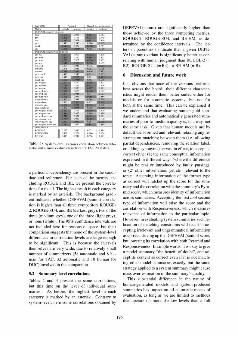
TAC 2008 Pyramid Overall ResponsivenessMetric models systems models systemsDEPEVAL(summ): Variationsbase 0.653 0.931 0.883 0.862pm 0.690 0.811 0.943 0.740wn 0.687 0.929 0.888 0.860pred 0.415 0.946 0.706 0.909norel 0.676 0.929 0.880 0.861one 0.585 0.958* 0.858 0.900DEPEVAL(summ): Combinationspm wn 0.694 0.903 0.952* 0.839pm pred 0.534 0.880 0.898 0.831pm norel 0.722 0.907 0.936 0.835pm one 0.611 0.950 0.876 0.895wn pred 0.374 0.946 0.716 0.912wn norel 0.405 0.941 0.752 0.905wn one 0.611 0.952 0.856 0.897pred norel 0.415 0.945 0.735 0.905pred one 0.415 0.953 0.721 0.921*norel one 0.600 0.958* 0.863 0.900pm wn pred 0.527 0.870 0.905 0.821pm wn norel 0.738 0.897 0.931 0.826pm wn one 0.634 0.936 0.887 0.881pm pred norel 0.642 0.876 0.946 0.815pm pred one 0.504 0.948 0.817 0.907pm norel one 0.725 0.941 0.905 0.880wn pred norel 0.433 0.944 0.764 0.906wn pred one 0.385 0.950 0.722 0.919wn norel one 0.632 0.954 0.872 0.896pred norel one 0.452 0.955 0.756 0.919pm wn pred norel 0.643 0.861 0.940 0.800pm wn pred one 0.486 0.932 0.809 0.890pm pred norel one 0.711 0.939 0.881 0.891pm wn norel one 0.743* 0.930 0.902 0.870wn pred norel one 0.467 0.950 0.767 0.918pm wn pred norel one 0.712 0.927 0.887 0.880Other metricsROUGE-2 0.277 0.946 0.725 0.894ROUGE-SU4 0.457 0.928 0.866 0.874BE-HM 0.423 0.949 0.656 0.911
Table 1: System-level Pearson’s correlation between auto-matic and manual evaluation metrics for TAC 2008 data.
a particular dependency are present in the candi-date and reference. For each of the metrics, in-cluding ROUGE and BE, we present the correla-tions for recall. The highest result in each categoryis marked by an asterisk. The background gradi-ent indicates whether DEPEVAL(summ) correla-tion is higher than all three competitors ROUGE-2, ROUGE-SU4, and BE (darkest grey), two of thethree (medium grey), one of the three (light grey),or none (white). The 95% confidence intervals arenot included here for reasons of space, but theircomparison suggests that none of the system-leveldifferences in correlation levels are large enoughto be significant. This is because the intervalsthemselves are very wide, due to relatively smallnumber of summarizers (58 automatic and 8 hu-man for TAC; 32 automatic and 10 human forDUC) involved in the comparison.
5.2 Summary-level correlationsTables 2 and 4 present the same correlations,but this time on the level of individual sum-maries. As before, the highest level in eachcategory is marked by an asterisk. Contrary tosystem-level, here some correlations obtained by
DEPEVAL(summ) are significantly higher thanthose achieved by the three competing metrics,ROUGE-2, ROUGE-SU4, and BE-HM, as de-termined by the confidence intervals. The let-ters in parenthesis indicate that a given DEPE-VAL(summ) variant is significantly better at cor-relating with human judgment than ROUGE-2 (=R2), ROUGE-SU4 (= R4), or BE-HM (= B).
6 Discussion and future work
It is obvious that none of the versions performsbest across the board; their different character-istics might render them better suited either formodels or for automatic systems, but not forboth at the same time. This can be explained ifwe understand that evaluating human gold stan-dard summaries and automatically generated sum-maries of poor-to-medium quality is, in a way, notthe same task. Given that human models are bydefault well-formed and relevant, relaxing any re-straints on matching between them (i.e. allowingpartial dependencies, removing the relation label,or adding synonyms) serves, in effect, to accept ascorrect either (1) the same conceptual informationexpressed in different ways (where the differencemight be real or introduced by faulty parsing),or (2) other information, yet still relevant to thetopic. Accepting information of the former typeas correct will ratchet up the score for the sum-mary and the correlation with the summary’s Pyra-mid score, which measures identity of informationacross summaries. Accepting the first and secondtype of information will raise the score and thecorrelation with Responsiveness, which measuresrelevance of information to the particular topic.However, in evaluating system summaries such re-laxation of matching constraints will result in ac-cepting irrelevant and ungrammatical informationas correct, driving up the DEPEVAL(summ) score,but lowering its correlation with both Pyramid andResponsiveness. In simple words, it is okay to givea model summary “the benefit of doubt”, and ac-cept its content as correct even if it is not match-ing other model summaries exactly, but the samestrategy applied to a system summary might causemass over-estimation of the summary’s quality.
This substantial difference in the nature ofhuman-generated models and system-producedsummaries has impact on all automatic means ofevaluation, as long as we are limited to methodsthat operate on more shallow levels than a full
195
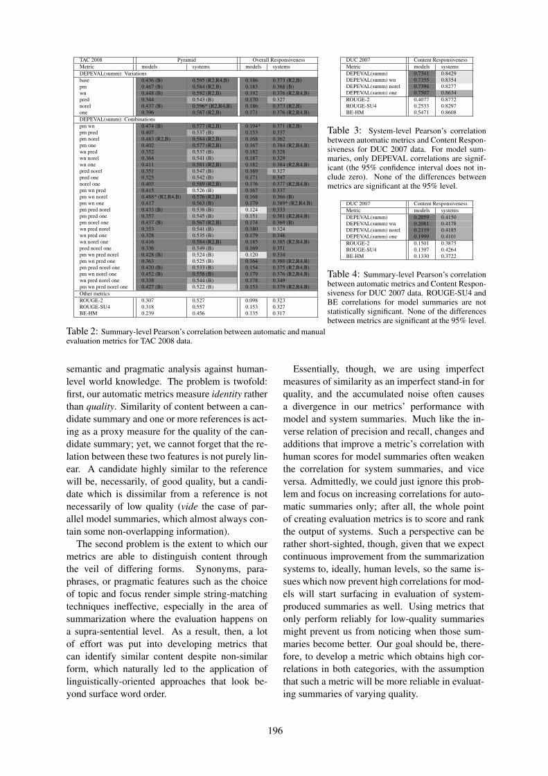
TAC 2008 Pyramid Overall ResponsivenessMetric models systems models systemsDEPEVAL(summ): Variationsbase 0.436 (B) 0.595 (R2,R4,B) 0.186 0.373 (R2,B)pm 0.467 (B) 0.584 (R2,B) 0.183 0.368 (B)wn 0.448 (B) 0.592 (R2,B) 0.192 0.376 (R2,R4,B)pred 0.344 0.543 (B) 0.170 0.327norel 0.437 (B) 0.596* (R2,R4,B) 0.186 0.373 (R2,B)one 0.396 0.587 (R2,B) 0.171 0.376 (R2,R4,B)DEPEVAL(summ): Combinationspm wn 0.474 (B) 0.577 (R2,B) 0.194* 0.371 (R2,B)pm pred 0.407 0.537 (B) 0.153 0.337pm norel 0.483 (R2,B) 0.584 (R2,B) 0.168 0.362pm one 0.402 0.577 (R2,B) 0.167 0.384 (R2,R4,B)wn pred 0.352 0.537 (B) 0.182 0.328wn norel 0.364 0.541 (B) 0.187 0.329wn one 0.411 0.581 (R2,B) 0.182 0.384 (R2,R4,B)pred norel 0.351 0.547 (B) 0.169 0.327pred one 0.325 0.542 (B) 0.171 0.347norel one 0.403 0.589 (R2,B) 0.176 0.377 (R2,R4,B)pm wn pred 0.415 0.526 (B) 0.167 0.337pm wn norel 0.488* (R2,R4,B) 0.576 (R2,B) 0.168 0.366 (B)pm wn one 0.417 0.563 (B) 0.179 0.389* (R2,R4.B)pm pred norel 0.433 (B) 0.538 (B) 0.124 0.333pm pred one 0.357 0.545 (B) 0.151 0.381 (R2,R4,B)pm norel one 0.437 (B) 0.567 (R2,B) 0.174 0.369 (B)wn pred norel 0.353 0.541 (B) 0.180 0.324wn pred one 0.328 0.535 (B) 0.179 0.346wn norel one 0.416 0.584 (R2,B) 0.185 0.385 (R2,R4,B)pred norel one 0.336 0.549 (B) 0.169 0.351pm wn pred norel 0.428 (B) 0.524 (B) 0.120 0.334pm wn pred one 0.363 0.525 (B) 0.164 0.380 (R2,R4,B)pm pred norel one 0.420 (B) 0.533 (B) 0.154 0.375 (R2,R4,B)pm wn norel one 0.452 (B) 0.558 (B) 0.179 0.376 (R2,R4,B)wn pred norel one 0.338 0.544 (B) 0.178 0.349pm wn pred norel one 0.427 (B) 0.522 (B) 0.153 0.379 (R2,R4,B)Other metricsROUGE-2 0.307 0.527 0.098 0.323ROUGE-SU4 0.318 0.557 0.153 0.327BE-HM 0.239 0.456 0.135 0.317
Table 2: Summary-level Pearson’s correlation between automatic and manualevaluation metrics for TAC 2008 data.
DUC 2007 Content ResponsivenessMetric models systemsDEPEVAL(summ) 0.7341 0.8429DEPEVAL(summ) wn 0.7355 0.8354DEPEVAL(summ) norel 0.7394 0.8277DEPEVAL(summ) one 0.7507 0.8634ROUGE-2 0.4077 0.8772ROUGE-SU4 0.2533 0.8297BE-HM 0.5471 0.8608
Table 3: System-level Pearson’s correlationbetween automatic metrics and Content Respon-siveness for DUC 2007 data. For model sum-maries, only DEPEVAL correlations are signif-icant (the 95% confidence interval does not in-clude zero). None of the differences betweenmetrics are significant at the 95% level.
DUC 2007 Content ResponsivenessMetric models systemsDEPEVAL(summ) 0.2059 0.4150DEPEVAL(summ) wn 0.2081 0.4178DEPEVAL(summ) norel 0.2119 0.4185DEPEVAL(summ) one 0.1999 0.4101ROUGE-2 0.1501 0.3875ROUGE-SU4 0.1397 0.4264BE-HM 0.1330 0.3722
Table 4: Summary-level Pearson’s correlationbetween automatic metrics and Content Respon-siveness for DUC 2007 data. ROUGE-SU4 andBE correlations for model summaries are notstatistically significant. None of the differencesbetween metrics are significant at the 95% level.
semantic and pragmatic analysis against human-level world knowledge. The problem is twofold:first, our automatic metrics measure identity ratherthan quality. Similarity of content between a can-didate summary and one or more references is act-ing as a proxy measure for the quality of the can-didate summary; yet, we cannot forget that the re-lation between these two features is not purely lin-ear. A candidate highly similar to the referencewill be, necessarily, of good quality, but a candi-date which is dissimilar from a reference is notnecessarily of low quality (vide the case of par-allel model summaries, which almost always con-tain some non-overlapping information).
The second problem is the extent to which ourmetrics are able to distinguish content throughthe veil of differing forms. Synonyms, para-phrases, or pragmatic features such as the choiceof topic and focus render simple string-matchingtechniques ineffective, especially in the area ofsummarization where the evaluation happens ona supra-sentential level. As a result, then, a lotof effort was put into developing metrics thatcan identify similar content despite non-similarform, which naturally led to the application oflinguistically-oriented approaches that look be-yond surface word order.
Essentially, though, we are using imperfectmeasures of similarity as an imperfect stand-in forquality, and the accumulated noise often causesa divergence in our metrics’ performance withmodel and system summaries. Much like the in-verse relation of precision and recall, changes andadditions that improve a metric’s correlation withhuman scores for model summaries often weakenthe correlation for system summaries, and viceversa. Admittedly, we could just ignore this prob-lem and focus on increasing correlations for auto-matic summaries only; after all, the whole pointof creating evaluation metrics is to score and rankthe output of systems. Such a perspective can berather short-sighted, though, given that we expectcontinuous improvement from the summarizationsystems to, ideally, human levels, so the same is-sues which now prevent high correlations for mod-els will start surfacing in evaluation of system-produced summaries as well. Using metrics thatonly perform reliably for low-quality summariesmight prevent us from noticing when those sum-maries become better. Our goal should be, there-fore, to develop a metric which obtains high cor-relations in both categories, with the assumptionthat such a metric will be more reliable in evaluat-ing summaries of varying quality.
196
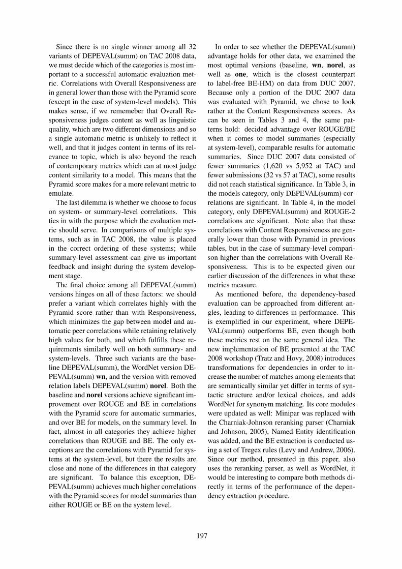
Since there is no single winner among all 32variants of DEPEVAL(summ) on TAC 2008 data,we must decide which of the categories is most im-portant to a successful automatic evaluation met-ric. Correlations with Overall Responsiveness arein general lower than those with the Pyramid score(except in the case of system-level models). Thismakes sense, if we rememeber that Overall Re-sponsiveness judges content as well as linguisticquality, which are two different dimensions and soa single automatic metric is unlikely to reflect itwell, and that it judges content in terms of its rel-evance to topic, which is also beyond the reachof contemporary metrics which can at most judgecontent similarity to a model. This means that thePyramid score makes for a more relevant metric toemulate.
The last dilemma is whether we choose to focuson system- or summary-level correlations. Thisties in with the purpose which the evaluation met-ric should serve. In comparisons of multiple sys-tems, such as in TAC 2008, the value is placedin the correct ordering of these systems; whilesummary-level assessment can give us importantfeedback and insight during the system develop-ment stage.
The final choice among all DEPEVAL(summ)versions hinges on all of these factors: we shouldprefer a variant which correlates highly with thePyramid score rather than with Responsiveness,which minimizes the gap between model and au-tomatic peer correlations while retaining relativelyhigh values for both, and which fulfills these re-quirements similarly well on both summary- andsystem-levels. Three such variants are the base-line DEPEVAL(summ), the WordNet version DE-PEVAL(summ) wn, and the version with removedrelation labels DEPEVAL(summ) norel. Both thebaseline and norel versions achieve significant im-provement over ROUGE and BE in correlationswith the Pyramid score for automatic summaries,and over BE for models, on the summary level. Infact, almost in all categories they achieve highercorrelations than ROUGE and BE. The only ex-ceptions are the correlations with Pyramid for sys-tems at the system-level, but there the results areclose and none of the differences in that categoryare significant. To balance this exception, DE-PEVAL(summ) achieves much higher correlationswith the Pyramid scores for model summaries thaneither ROUGE or BE on the system level.
In order to see whether the DEPEVAL(summ)advantage holds for other data, we examined themost optimal versions (baseline, wn, norel, aswell as one, which is the closest counterpartto label-free BE-HM) on data from DUC 2007.Because only a portion of the DUC 2007 datawas evaluated with Pyramid, we chose to lookrather at the Content Responsiveness scores. Ascan be seen in Tables 3 and 4, the same pat-terns hold: decided advantage over ROUGE/BEwhen it comes to model summaries (especiallyat system-level), comparable results for automaticsummaries. Since DUC 2007 data consisted offewer summaries (1,620 vs 5,952 at TAC) andfewer submissions (32 vs 57 at TAC), some resultsdid not reach statistical significance. In Table 3, inthe models category, only DEPEVAL(summ) cor-relations are significant. In Table 4, in the modelcategory, only DEPEVAL(summ) and ROUGE-2correlations are significant. Note also that thesecorrelations with Content Responsiveness are gen-erally lower than those with Pyramid in previoustables, but in the case of summary-level compari-son higher than the correlations with Overall Re-sponsiveness. This is to be expected given ourearlier discussion of the differences in what thesemetrics measure.
As mentioned before, the dependency-basedevaluation can be approached from different an-gles, leading to differences in performance. Thisis exemplified in our experiment, where DEPE-VAL(summ) outperforms BE, even though boththese metrics rest on the same general idea. Thenew implementation of BE presented at the TAC2008 workshop (Tratz and Hovy, 2008) introducestransformations for dependencies in order to in-crease the number of matches among elements thatare semantically similar yet differ in terms of syn-tactic structure and/or lexical choices, and addsWordNet for synonym matching. Its core moduleswere updated as well: Minipar was replaced withthe Charniak-Johnson reranking parser (Charniakand Johnson, 2005), Named Entity identificationwas added, and the BE extraction is conducted us-ing a set of Tregex rules (Levy and Andrew, 2006).Since our method, presented in this paper, alsouses the reranking parser, as well as WordNet, itwould be interesting to compare both methods di-rectly in terms of the performance of the depen-dency extraction procedure.
197

ReferencesSatanjeev Banerjee and Alon Lavie. 2005. METEOR:
An automatic metric for MT evaluation with im-proved correlation with human judgments. In Pro-ceedings of the ACL 2005 Workshop on Intrinsic andExtrinsic Evaluation Measures for MT and/or Sum-marization, pages 65–73, Ann Arbor, MI, USA.
Joan Bresnan. 2001. Lexical-Functional Syntax.Blackwell, Oxford.
Aoife Cahill, Michael Burke, Ruth O’Donovan, Josefvan Genabith, and Andy Way. 2004. Long-distance dependency resolution in automatically ac-quired wide-coverage PCFG-based LFG approxima-tions. In Proceedings of the 42th Annual Meetingof the Association for Computational Linguistics,pages 320–327, Barcelona, Spain.
Aoife Cahill, Michael Burke, Ruth O’Donovan, StefanRiezler, Josef van Genabith, and Andy Way. 2008.Wide-coverage deep statistical parsing using auto-matic dependency structure annotation. Comput.Linguist., 34(1):81–124.
Eugene Charniak and Mark Johnson. 2005. Coarse-to-fine n-best parsing and MaxEnt discriminativereranking. In ACL 2005: Proceedings of the 43rdAnnual Meeting of the Association for Computa-tional Linguistics, pages 173–180, Morristown, NJ,USA. Association for Computational Linguistics.
Eugene Charniak. 2000. A maximum entropy inspiredparser. In Proceedings of the 1st Annual Meeting ofthe North American Chapter of the Association forComputational Linguistics, pages 132–139, Seattle,WA, USA.
Hoa Trang Dang and Karolina Owczarzak. 2008.Overview of the tac 2008 summarization track: Up-date task. In to appear in: Proceedings of the 1stText Analysis Conference (TAC).
Eduard Hovy, Chin-Yew Lin, and Liang Zhou. 2005.Evaluating DUC 2005 using Basic Elements. InProceedings of the 5th Document UnderstandingConference (DUC).
Ronald M. Kaplan and Joan Bresnan, 1982. The Men-tal Representation of Grammatical Relations, chap-ter Lexical-functional Grammar: A Formal Systemfor Grammatical Representation. MIT Press, Cam-bridge, MA, USA.
Roger Levy and Galen Andrew. 2006. Tregex and tsur-geon: Tools for querying and manipulating tree datastructures. In Proceedings of the 5th InternationalConference on Language Resources and Evaluation.
Dekang Lin. 1995. A dependency-based method forevaluating broad-coverage parsers. In Proceedingsof the 14th International Joint Conference on Artifi-cial Intelligence, pages 1420–1427.
Chin-Yew Lin. 2004. ROUGE: A package for au-tomatic evaluation of summaries. In Proceedingsof the ACL 2004 Workshop: Text SummarizationBranches Out, pages 74–81.
Karolina Owczarzak, Josef van Genabith, and AndyWay. 2007. Evaluating Machine Translation withLFG dependencies. Machine Translation, 21(2):95–119.
Karolina Owczarzak. 2008. A novel dependency-based evaluation metric for Machine Translation.Ph.D. thesis, Dublin City University.
Rebecca J. Passonneau, Ani Nenkova, Kathleen McK-eown, and Sergey Sigelman. 2005. Applyingthe Pyramid method in DUC 2005. In Proceed-ings of the 5th Document Understanding Conference(DUC).
Jason Rennie. 2000. Wordnet::querydata: aPerl module for accessing the WordNet database.http://people.csail.mit.edu/ jrennie/WordNet.
Stephen Tratz and Eduard Hovy. 2008. Summariza-tion evaluation using transformed Basic Elements.In Proceedings of the 1st Text Analysis Conference(TAC).
198

Proceedings of the 47th Annual Meeting of the ACL and the 4th IJCNLP of the AFNLP, pages 199–207,Suntec, Singapore, 2-7 August 2009. c©2009 ACL and AFNLP
Summarizing Definition from Wikipedia
Shiren Ye and Tat-Seng Chua and Jie LuLab of Media Search
National University of Singapore{yesr|chuats|luj}@comp.nus.edu.sg
Abstract
Wikipedia provides a wealth of knowl-edge, where the first sentence, infobox(and relevant sentences), and even the en-tire document of a wiki article could beconsidered as diverse versions of sum-maries (definitions) of the target topic.We explore how to generate a series ofsummaries with various lengths based onthem. To obtain more reliable associationsbetween sentences, we introduce wiki con-cepts according to the internal links inWikipedia. In addition, we develop anextended document concept lattice modelto combine wiki concepts and non-textualfeatures such as the outline and infobox.The model can concatenate representativesentences from non-overlapping salient lo-cal topics for summary generation. We testour model based on our annotated wiki ar-ticles which topics come from TREC-QA2004-2006 evaluations. The results showthat the model is effective in summariza-tion and definition QA.
1 IntroductionNowadays, ‘ask Wikipedia’ has become as pop-ular as ‘Google it’ during Internet surfing, asWikipedia is able to provide reliable informationabout the concept (entity) that the users want. Asthe largest online encyclopedia, Wikipedia assem-bles immense human knowledge from thousands ofvolunteer editors, and exhibits significant contribu-tions to NLP problems such as semantic related-ness, word sense disambiguation and question an-swering (QA).
For a given definition query, many search en-gines (e.g., specified by ‘define:’ in Google) oftenplace the first sentence of the corresponding wiki1article at the top of the returned list. The use of
1 For readability, we follow the upper/lower case ruleon web (say, ‘web pages’ and ‘on the Web’), and utilize
one-sentence snippets provides a brief and concisedescription of the query. However, users often needmore information beyond such a one-sentence de-finition, while feeling that the corresponding wikiarticle is too long. Thus, there is a strong demandto summarize wiki articles as definitions with vari-ous lengths to suite different user needs.
The initial motivation of this investigation is tofind better definition answer for TREC-QA taskusing Wikipedia (Kor and Chua, 2007). Accord-ing to past results on TREC-QA (Voorhees, 2004;Voorhees and Dang, 2005), definition queries areusually recognized as being more difficult than fac-toid and list queries. Wikipedia could help toimprove the quality of answer finding and evenprovide the answers directly. Its results are bet-ter than other external resources such as WordNet,Gazetteers and Google’s define operator, especiallyfor definition QA (Lita et al., 2004).
Different from the free text used in QA and sum-marization, a wiki article usually contains valuableinformation like infobox and wiki link. Infoboxtabulates the key properties about the target, suchas birth place/date and spouse for a person as wellas type, founder and products for a company. In-fobox, as a form of thumbnail biography, can beconsidered as a mini version of a wiki article’s sum-mary. In addition, the relevant concepts existing ina wiki article usually refer to other wiki pages bywiki internal links, which will form a close set ofreference relations. The current Wikipedia recur-sively defines over 2 million concepts (in English)via wiki links. Most of these concepts are multi-word terms, whereas WordNet has only 50,000 plusmulti-word terms. Any term could appear in thedefinition of a concept if necessary, while the totalvocabulary existing in WordNet’s glossary defini-tion is less than 2000. Wikipedia addresses explicitsemantics for numerous concepts. These specialknowledge representations will provide additionalinformation for analysis and summarization. Wethus need to extend existing summarization tech-nologies to take advantage of the knowledge repre-sentations in Wikipedia.
‘wiki(pedia) articles’ and ‘on (the) Wikipedia’, the latter re-ferring to the entire Wikipedia.
199
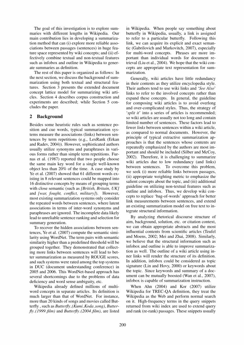
The goal of this investigation is to explore sum-maries with different lengths in Wikipedia. Ourmain contribution lies in developing a summariza-tion method that can (i) explore more reliable asso-ciations between passages (sentences) in huge fea-ture space represented by wiki concepts; and (ii) ef-fectively combine textual and non-textual featuressuch as infobox and outline in Wikipedia to gener-ate summaries as definition.
The rest of this paper is organized as follows: Inthe next section, we discuss the background of sum-marization using both textual and structural fea-tures. Section 3 presents the extended documentconcept lattice model for summarizing wiki arti-cles. Section 4 describes corpus construction andexperiments are described; while Section 5 con-cludes the paper.
2 BackgroundBesides some heuristic rules such as sentence po-sition and cue words, typical summarization sys-tems measure the associations (links) between sen-tences by term repetitions (e.g., LexRank (Erkanand Radev, 2004)). However, sophisticated authorsusually utilize synonyms and paraphrases in vari-ous forms rather than simple term repetitions. Fur-nas et al. (1987) reported that two people choosethe same main key word for a single well-knownobject less than 20% of the time. A case study byYe et al. (2007) showed that 61 different words ex-isting in 8 relevant sentences could be mapped into16 distinctive concepts by means of grouping termswith close semantic (such as [British, Britain, UK]and [war, fought, conflict, military]). However,most existing summarization systems only considerthe repeated words between sentences, where latentassociations in terms of inter-word synonyms andparaphrases are ignored. The incomplete data likelylead to unreliable sentence ranking and selection forsummary generation.
To recover the hidden associations between sen-tences, Ye et al. (2007) compute the semantic simi-larity using WordNet. The term pairs with semanticsimilarity higher than a predefined threshold will begrouped together. They demonstrated that collect-ing more links between sentences will lead to bet-ter summarization as measured by ROUGE scores,and such systems were rated among the top systemsin DUC (document understanding conference) in2005 and 2006. This WordNet-based approach hasseveral shortcomings due to the problems of datadeficiency and word sense ambiguity, etc.
Wikipedia already defined millions of multi-word concepts in separate articles. Its definition ismuch larger than that of WordNet. For instance,more than 20 kinds of songs and movies called But-terfly , such as Butterfly (Kumi Koda song), Butter-fly (1999 film) and Butterfly (2004 film), are listed
in Wikipedia. When people say something aboutbutterfly in Wikipedia, usually, a link is assignedto refer to a particular butterfly. Following thislink, we can acquire its explicit and exact seman-tic (Gabrilovich and Markovitch, 2007), especiallyfor multi-word concepts. Phrases are more im-portant than individual words for document re-trieval (Liu et al., 2004). We hope that the wiki con-cepts are appropriate text representation for sum-marization.
Generally, wiki articles have little redundancyin their contents as they utilize encyclopedia style.Their authors tend to use wiki links and ‘See Also’links to refer to the involved concepts rather thanexpand these concepts. In general, the guidelinefor composing wiki articles is to avoid overlongand over-complicated styles. Thus, the strategy of‘split it’ into a series of articles is recommended;so wiki articles are usually not too long and containlimited number of sentences. These factors lead tofewer links between sentences within a wiki article,as compared to normal documents. However, theprinciple of typical extractive summarization ap-proaches is that the sentences whose contents arerepeatedly emphasized by the authors are most im-portant and should be included (Silber and McCoy,2002). Therefore, it is challenging to summarizewiki articles due to low redundancy (and links)between sentences. To overcome this problem,we seek (i) more reliable links between passages,(ii) appropriate weighting metric to emphasize thesalient concepts about the topic, and (iii) additionalguideline on utilizing non-textual features such asoutline and infobox. Thus, we develop wiki con-cepts to replace ‘bag-of-words’ approach for betterlink measurements between sentences, and extendan existing summarization model on free text to in-tegrate structural information.
By analyzing rhetorical discourse structure ofaim, background, solution, etc. or citation context,we can obtain appropriate abstracts and the mostinfluential contents from scientific articles (Teufeland Moens, 2002; Mei and Zhai, 2008). Similarly,we believe that the structural information such asinfobox and outline is able to improve summariza-tion as well. The outline of a wiki article using in-ner links will render the structure of its definition.In addition, infobox could be considered as topicsignature (Lin and Hovy, 2000) or keywords aboutthe topic. Since keywords and summary of a doc-ument can be mutually boosted (Wan et al., 2007),infobox is capable of summarization instruction.
When Ahn (2004) and Kor (2007) utilizeWikipedia for TREC-QA definition, they treat theWikipedia as the Web and perform normal searchon it. High-frequency terms in the query snippetsreturned from wiki index are used to extend queryand rank (re-rank) passages. These snippets usually
200

come from multiple wiki articles. Here the use-ful information may be beyond these snippets butexisting terms are possibly irrelevant to the topic.On the contrary, our approach concentrates on thewiki article having the exact topic only. We as-sume that every sentence in the article is used to de-fine the query topic, no matter whether it containsthe term(s) of the topic or not. In order to extractsome salient sentences from the article as definitionsummaries, we will build a summarization modelthat describes the relations between the sentences,where both textual and structural features are con-sidered.
3 Our Approach
3.1 Wiki ConceptsIn this subsection, we address how to find rea-sonable and reliable links between sentences usingwiki concepts.
Consider a sentence: ‘After graduating fromBoston University in 1988, she went to work at aCalvin Klein store in Boston.’ from a wiki article‘Carolyn Bessette Kennedy’2, we can find 11 dis-tinctive terms, such as after, graduate, Boston, Uni-versity,1988, go, work, Calvin, Klein, store, Boston,if stop words are ignored.
However, multi-word terms such as BostonUniversity and Calvin Klein are linked to thecorresponding wiki articles, where their definitionsare given. Clearly, considering the anchor texts astwo wiki concepts rather than four words is morereasonable. Their granularity are closer to semanticcontent units in a summarization evaluation methodPyramid (Nenkova et al., 2007) and nuggets inTREC-QA . When the text is represented bywiki concepts, whose granularity is similar to theevaluation units, it is possibly easy to detect thematching output using a model. Here,• Two separate words, Calvin and Klein, are
meaningless and should be discarded; oth-erwise, spurious links between sentences arelikely to occur.
• Boston University and Boston are processedseparately, as they are different named entities.No link between them is appropriate3.
• Terms such as ‘John F. Kennedy, Jr.’ and‘John F. Kennedy’ will be considered as twodiverse wiki concepts, but we do not accounton how many repeated words there are.
• Different anchor texts, such as U.S.A. andUnited States of America, are recognized as
2All sample sentences in this paper come from this articleif not specified.
3Consider new pseudo sentence: ‘After graduating fromStanford in 1988, she went to work ... in Boston.’ We do notneed assign link between Stanford and Boston as well.
an identical concept since they refer to thesame wiki article.
• Two concepts, such as money and cash, willbe merged into an identical concept when theirsemantics are similar.
In wiki articles, the first occurrence of a wikiconcept is tagged by a wiki link, but there is nosuch a link to its subsequent occurrences in the re-maining parts of the text in most cases. To allevi-ate this problem, a set of heuristic rules is proposedto unify the subsequent occurrences of concepts innormal text with previous wiki concepts in the an-chor text. These heuristic rules include: (i) edit dis-tance between linked wiki concept and candidatesin normal text is larger than a predefined threshold;and (ii) partially overlapping words beginning withcapital letter, etc.
After filtering out wiki concepts, the words re-maining in wiki articles could be grouped into twosets: close-class terms like pronouns and preposi-tions as well as open-class terms like nouns andverbs. For example, in the sentence ‘She died at age33, along with her husband and sister’, the open-class terms include die, age, 33, husband and sister.Even though most open-class terms are defined inWikipedia as well, the authors of the article do notconsider it necessary to present their references us-ing wiki links. Hence, we need to extend wiki con-cepts by concatenating them with these open-classterms to form an extended vector. In addition, weignore all close-class terms, since we cannot findefficient method to infer reliable links across them.As a result, texts are represented as a vector of wikiconcepts.
Once we introduce wiki concepts to replace typ-ical ‘bag-of-words’ approach, the dimensions ofconcept space will reach six order of magnitudes.We cannot ignore the data spareness issue and com-putation cost when the concept space is so huge.Actually, for a wiki article and a set of relevant arti-cles, the involved concepts are limited, and we needto explore them in a small sub-space. For instance,59 articles about Kennedy family in Wikipedia have10,399 distinctive wiki concepts only, where 5,157wiki concepts exist twice and more. Computing theoverlapping among them is feasible.
Furthermore, we need to merge the wiki conceptswith identical or close semantic (namely, buildinglinks between these synonyms and paraphrases).We measure the semantic similarity between twoconcepts by using cosine distance between theirwiki articles, which are represented as the vectorsof wiki concepts as well. For computation effi-ciency, we calculate semantic similarities betweenall promising concept pairs beforehand, and thenretrieve the value in a Hash table directly. We spentCPU time of about 12.5 days preprocessing the se-
201

mantic calculation. Details are available at our tech-nical report (Lu et al., 2008).
Following the principle of TFIDF, we definethe weighing metric for the vector representedby wiki concepts using the entire Wikipedia asthe observation collection. We define the CFIDFweight of wiki concept i in article j as:
wi,j = cfi,j· idfi =ni,j
∑
k nk,j
· log|D|
|dj : ti ∈ dj| ,(1)
where cfi,j is the frequency of concept i in arti-cle j; idfi is the inverse frequency of concept iin Wikipedia; and D is the number of articles inWikipedia. Here, sparse wiki concepts will havemore contribution.
In brief, we represent articles in terms of wikiconcepts using the steps below.
1. Extract the wiki concepts marked by wikilinks in context.
2. Detect the remaining open-class terms as wikiconcepts as well.
3. Merge concepts whose semantic similarity islarger than predefined threshold (0.35 in ourexperiments) into the one with largest idf .
4. Weight all concepts according to Eqn (1).
3.2 Document Concept Lattice ModelNext, we build the document concept lattice (DCL)for articles represented by wiki concepts. For il-lustration on how DCL is built, we consider 8 sen-tences from DUC 2005 Cluster d324e (Ye et al.,2007) as case study. 8 sentences, represented by 16distinctive concepts A-P, are considered as the basenodes 1-8 as shown in Figure 1. Once we groupnodes by means of the maximal common conceptsamong base nodes hierarchically, we can obtain thederived nodes 11-41, which form a DCL. A derivednode will annotate a local topic through a set ofshared concepts, and define a sub concept space thatcontains the covered base nodes under proper pro-jection. The derived node, accompanied with itsbase nodes, is apt to interpret a particular argument(or statement) about the involved concepts. Further-more, one base node among them, coupled with thecorresponding sentence, is capable of this interpre-tation and could represent the other base nodes tosome degree.
In order to Extract a set of sentences to coverkey distinctive local topics (arguments) as much aspossible, we need to select a set of important non-overlapping derived nodes. We measure the impor-tance of node N in DCL of article j in term of rep-resentative power (RP) as:
RP (N) =∑
ci∈N
(|ci|·wi,j)/ log(|N |), (2)
� � � � � � � � � � � � � � � � � � � � � � � � � � � � � � � � � � � � � � � � � � � � � � � � � � � � � � � � � � � � � � � � � � � � � � � � � � � � � � � � � � � � � � � � � � � � � � � � � � � � � � � � � � � � � � � � � � � � � � � � � � � � � � � � � �
� � � � � � � � � � � � � � � � � � � � � �
� � � � � � � � � � � � � � � � � � � � � � � � � � �
� � � � � � � � � � � � � � � � � � � � � � � � � � � � � � � � � � � � Figure 1: A sample of concept lattice
where concept ci in node N is weighted by wi,j
according to Eqn (1), and |N | denotes the conceptnumber in N (if N is a base node) or the numberof distinct concepts in |N | (if N is a derived node),respectively. Here, |ci| represents the c’s frequencyin N , and log(|N |) reflects N ’s cost if N is selected(namely, how many concepts are used in N ). Forexample, 7 concepts in sentence 1 lead to the total|c| of 34 if their weights are set to 1 equally. ItsRP is RP (1) = 34/log(7) = 40.23. Similarly,RP (31) = 6 ∗ 3/log(3) = 37.73.
By selecting a set of non-overlapping derivednodes with maximal RP, we are able to obtain a setof local topics with highest representativeness anddiversity. Next, a representative sentence with max-imal RP in each of such derived nodes is chosen torepresent the local topics in observation. When thelength of the required summary changes, the num-ber of the local topics needed will also be modi-fied. Consequently, we are able to select the sets ofappropriate derived nodes in diverse generalizationlevels, and obtain various versions of summariescontaining the local topics with appropriate gran-ularities.
In the DCL example shown in Figure 1, if we ex-pect to have a summary with two sentences, we willselect the derived nodes 31 and 32 with highest RP.Nodes 31 and 32 will infer sentences 4 and 2, andthey will be concatenated to form a summary. If thesummary is increased to three sentences, then threederived nodes 31, 23 and 33 with maximal RP willrender representative sentences 4, 5 and 6. Hence,the different number of actual sentences (4+5+6 vs.4+2) will be selected depending on the length ofthe required summary. The uniqueness of DCL isthat the sentences used in a shorter summary maynot appear in a longer summary for the same sourcetext. According to the distinctive derived nodes indiverse levels, the sentences with different general-ization abilities are chosen to generate various sum-maries.
202
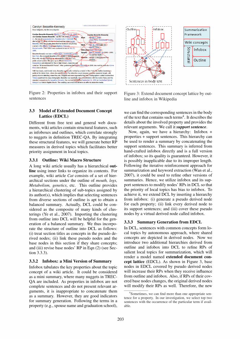
Figure 2: Properties in infobox and their supportsentences
3.3 Model of Extended Document ConceptLattice (EDCL)
Different from free text and general web docu-ments, wiki articles contain structural features, suchas infoboxes and outlines, which correlate stronglyto nuggets in definition TREC-QA. By integratingthese structural features, we will generate better RPmeasures in derived topics which facilitates betterpriority assignment in local topics.
3.3.1 Outline: Wiki Macro StructureA long wiki article usually has a hierarchical out-line using inner links to organize its contents. Forexample, wiki article Cat consists of a set of hier-archical sections under the outline of mouth, legs,Metabolism, genetics, etc. This outline providesa hierarchical clustering of sub-topics assigned byits author(s), which implies that selecting sentencesfrom diverse sections of outline is apt to obtain abalanced summary. Actually, DCL could be con-sidered as the composite of many kinds of clus-terings (Ye et al., 2007). Importing the clusteringfrom outline into DCL will be helpful for the gen-eration of a balanced summary. We thus incorpo-rate the structure of outline into DCL as follows:(i) treat section titles as concepts in the pseudo de-rived nodes; (ii) link these pseudo nodes and thebase nodes in this section if they share concepts;and (iii) revise base nodes’ RP in Eqn (2) (see Sec-tion 3.3.3).
3.3.2 Infobox: a Mini Version of SummaryInfobox tabulates the key properties about the topicconcept of a wiki article. It could be consideredas a mini summary, where many nuggets in TREC-QA are included. As properties in infobox are notcomplete sentences and do not present relevant ar-guments, it is inappropriate to concatenate themas a summary. However, they are good indicatorsfor summary generation. Following the terms in aproperty (e.g., spouse name and graduation school),
� � � � � � � � � � � � � � � �� � � � � � � � � � � � � � � � � � � �� � � � ! � � "# $ % $ & ' ( & ) * + ,- . + / $ ( )0 ( 1 ' 2 ' 3456785769:; < = > ? > @
Figure 3: Extend document concept lattice by out-line and infobox in Wikipedia
we can find the corresponding sentences in the bodyof the text that contains such terms4. It describes thedetails about the involved property and provides therelevant arguments. We call it support sentence.
Now, again, we have a hierarchy: Infobox +properties + support sentences. This hierarchy canbe used to render a summary by concatenating thesupport sentences. This summary is inferred fromhand-crafted infobox directly and is a full versionof infobox; so its quality is guaranteed. However, itis possibly inapplicable due to its improper length.Following the iterative reinforcement approach forsummarization and keyword extraction (Wan et al.,2007), it could be used to refine other versions ofsummaries. Hence, we utilize infobox and its sup-port sentences to modify nodes’ RPs in DCL so thatthe priority of local topics has bias to infobox. Toachieve it, we extend DCL by inserting a hierarchyfrom infobox: (i) generate a pseudo derived nodefor each property; (ii) link every derived node toits support sentences; and (iii) cover these pseudonodes by a virtual derived node called infobox.
3.3.3 Summary Generation from EDCLIn DCL, sentences with common concepts form lo-cal topics by autonomous approach, where sharedconcepts are depicted in derived nodes. Now weintroduce two additional hierarchies derived fromoutline and infobox into DCL to refine RPs ofsalient local topics for summarization, which willrender a model named extended document con-cept lattice (EDCL). As shown in Figure 3, basenodes in EDCL covered by pseudo derived nodeswill increase their RPs when they receive influencefrom outline and infobox. Also, if RPs of their cov-ered base nodes changes, the original derived nodeswill modify their RPs as well. Therefore, the new
4Sometimes, we can find more than one appropriate sen-tence for a property. In our investigation, we select top twosentences with the occurrence of the particular term if avail-able.
203
RPs in derived nodes and based nodes will lead tobetter priority of ranking derived nodes, which islikely to result in a better summary. One importantdirect consequence of introducing the extra hierar-chies is to increase the RP of nodes relevant to out-line and infobox so that the summaries from EDCLare likely to follow human-crafted ones.
The influence of human effects are transmittedin a ‘V’ curve approach. We utilize the followingsteps to generate a summary with a given length(say m sentences) from EDCL.
1. Build a normal DCL, and compute RP foreach node according to Eqn 2.
2. Generate pseudo derived nodes (denoted byP ) based on outline and infobox, and link thepseudo derived nodes to their relevant basenodes (denoted by B0).
3. Update RP in B0 by magnifying the contri-bution of shared concepts between P and N0
5.
4. Update RP in derived nodes that cover B0 onaccount of the new RP in B0.
5. Select m non-overlapping derived nodes withmaximal RP as the current observation.
6. Concatenate representative sentences withtop RP from each derived node in the currentobservation as output.
7. If one representative sentence is covered bymore than one derived node in step 5, theoutput will be less than m sentences. In thiscase, we need to increase m and repeat step5-6 until m sentences are selected.
4 ExperimentsThe purposes of our experiment are two-fold: (i)evaluate the effects of wiki definition to the TREC-QA task; and (ii) examine the characteristics andsummarization performance of EDCL.
4.1 Corpus ConstructionWe adopt the tasks of TREC-QA in 2004-2006(TREC 12-14) as test scope. We retrieve arti-cles with identical topic names from Wikipedia6.Non-letter transformations are permitted (e.g., from‘Carolyn Bessette-Kennedy’ to ‘Carolyn Bessette-Kennedy’). Because our focus is summariza-tion evaluation, we ignore the cases in TREC-QA where the exact topics do not exist inWikipedia, even though relevant topics are avail-able (e.g., ‘France wins World Cup in soccer’in TREC-QA vs. ‘France national football team’
5We magnify it by adding |c0| ∗ wc ∗ η. Here, c0 is theshared concepts between P and N0, and η is the influencefactor and set to 2-5 in our experiments.
6The dump is available athttp://download.wikimedia.org/. Our dumpwas downloaded in Sept 2007.
and ‘2006 FIFA World Cup’ in Wikipedia). Fi-nally, among the 215 topics in TREC 12-14, we ob-tain 180 wiki articles with the same topics.
We ask 15 undergraduate and graduate studentsfrom the Department of English Literature in Na-tional University of Singapore to choose 7-14 sen-tences in the above wiki articles as extractive sum-maries. Each wiki article is annotated by 3 per-sons separately. In order for the volunteers to avoidthe bias from TREC-QA corpus, we do not providequeries and nuggets used in TREC-QA. Similar toTREC nuggets, we call the selected sentences wikinuggets. Wiki nuggets provides the ground truthof the performance evaluation, since some TRECnuggets are possibly unavailable in Wikipedia.
Here, we did not ask the volunteers to createsnippets (like TREC-QA) or compose an abstrac-tive summary (like DUC). This is because of thespecial style of wiki articles: the entire documentis a long summary without trivial stuff. Usually, wedo not need to concatenate key phrases from diversesentences to form a recapitulative sentence. Mean-while, selecting a set of salient sentences to form aconcise version is a relatively less time-consumingbut applicable approach. Snippets, by and large,lead to bad readability, and therefore we do not em-ploy this approach.
In addition, the volunteers also annotate 7-10pairs of question/answer for each article for fur-ther research on QA using Wikipedia. The cor-pus, called TREC-Wiki collection, is available atour site (http://nuscu.ddns.comp.nus.edu.sg). Thesystem of Wikipedia summarization using EDCL islaunched on the Web as well.
4.2 Corpus Exploration
4.2.1 Answer availability
The availability of answers in Wikipedia for TREC-QA could be measured in two aspects: (i) howmany TREC-QA topics have been covered byWikipedia? and (ii) how many nuggets could befound in the corresponding wiki article? We findthat (i) over 80% of topics (180/215) in the TREC12-14 are available in Wikipedia, and (ii) about47% TREC nuggets could be detected directly fromWikipedia (examining applet modified from Pour-pre (Lin and Demner-Fushman, 2006)). In contrast,6,463 nuggets existing in TREC-QA 12-14 are dis-tributed in 4,175 articles from AQUAINT corpus.We can say that Wikipedia is the answer goldminefor TREC-QA questions.
When we look into these TREC nuggets in wikiarticles closely, we find that most of them are em-bedded in wiki links or relevant to infobox. It sug-gests that they are indicators for sentences havingnuggets.
204
4.2.2 Correlation between TREC nuggetsand non-text features
Analyzing the features used could let us understandsummarization better (Nenkova and Louis, 2008).Here, we focus on the statistical analysis betweenTREC/wiki nuggets and non-textual features suchas wiki links, infobox and outline. The featuresused are introduced in Table 1. The correlation co-efficients are listed in Table 2.
Observation: (1) On the whole, wiki nuggetsexhibit higher correlation to non-textual featuresthan TREC nuggets do. The possible reason is thatTREC nuggets are extracted from AQUAINT ratherthan Wikipedia. (2) As compared to other features,infobox and wiki links strongly relate to nuggets.They are thus reliable features beyond text for sum-marization. (3) Sentence positions exhibit weakcorrelation to nuggets, even though the first sen-tence of an article is a good one-sentence definition.
Feature DescriptionLink Does the sentence have link?Topic rel. Does the sentence contain any
word in topic concept?Outline rel. Does the sentence hold word in
its section title(s) (outline)?Infobox rel. Is it a support sentence?Position First sentence of the article, first
sentence and last sentence of aparagraph, or others?
Table 1: Features for correlation measurement
Feature TREC nuggets Wiki nuggetsLink 0.087 0.120Topic rel. 0.038 0.058Outline rel. 0.078 0.076Infobox rel. 0.089 0.170Position -0.047 0.021
Table 2: Correlation Coefficients between non-textual features in Wiki and TREC/wiki nuggets
4.3 Statistical Characteristics of EDCLWe design four runs with various configurations asshown in Table 3. We implement a sentence re-ranking program using MMR (maximal marginalrelevance) (Carbonell and Goldstein, 1998) in Run1, which is considered as the test baseline. We ap-ply standard DCL in Run 2, where concepts aredetermined according to their definitions in Word-Net (Ye et al., 2007). We introduce wiki conceptsfor standard DCL in Run 3. Run 4 is the full ver-
sion of EDCL, which considers both outline and in-fobox.
Observations: (1) In Run 1, the average num-ber of distinctive words per article is near to 1200after stop words are filtered out. When we mergediverse words having similar semantic according toWordNet concepts , we obtain 873 concepts per ar-ticle on average in Run 2. The word number de-creases by about 28% as a result of the omissionof close-class terms and the merging of synonymsand paraphrases. (2) When wiki concepts are intro-duced in Run 3, the number of concepts continuesto decrease. Here, some adjacent single-word termsare merged into wiki concepts if they are annotatedby wiki links. Even though the reduction of totalconcepts is limited, these new wiki concepts willgroup the terms that cannot be detected by Word-Net. (3) DCL based on WordNet concepts has lessderived nodes (Run 3) than DCL based on wiki con-cepts does, although the former has more concepts.It implies that wiki concepts lead to higher link den-sity in DCL as more links between concepts can bedetected. (4) Outline and infobox will bring addi-tional 54 derived nodes (from 1695 to 1741). Ad-ditional computation cost is limited when they areintroduced into EDCL.
Run 1 Word co-occurrence + MMRRun 2 Basic DCL model (WordNet concepts)Run 3 DCL + wiki conceptsRun 4 EDCL (DCL + wiki concepts + outline
+ infobox)
Table 3: Test configurations
Concepts Base nodes Derived nodesRun 1 1173 (number of words)Run 2 873 259 1517Run 3 826 259 1695Run 4 831 259 1741
Table 4: Average node/concept numbers in DCLand EDCL
4.4 Summarization Performance of EDCLWe evaluate the performance of EDCL from two as-pects such as contribution to TREC-QA definitiontask and accuracy of summarization in our TREC-Wiki collection.
Since factoid/list questions are about the most es-sential information of the target as well, like Cui’sapproach (2005), we treat factoid/list answers asessential nuggets and add them to the gold stan-dard list of definition nuggets. We set the sentencenumber of summaries generated by the system to
205

12. We examine the definition quality by nugget re-call (NR) and an approximation to nugget precision(NP) on answer length. These scores are combinedusing the F1 and F3 measures. The recall in F3
is weighted three times as important as precision.The evaluation is automatically conducted by Pour-pre v1.1 (Lin and Demner-Fushman, 2006).
Based on the performance of EDCL for TREC-QA definition task listed in Table 5, we observethat: (i) When EDCL considers wiki concepts andstructural features such as outline and infobox, itsF-scores increase significantly (Run 3 and Run 4).(ii) Table 5 also lists the results of Cui’s system(marked by asterisk) using bigram soft patterns(Cui et al., 2005), which is trained by TREC-12and tested on TREC 13. Our EDCL can achievecomparable or better F-scores on the 180 topics inTREC 12-14. It suggests that Wikipedia could pro-vide high-quality definition directly even though wedo not use AQUAINT. (iii) The precision of EDCLin Run 4 outperforms that of soft-pattern approachremarkably (from 0.34 to 0.497). One possible rea-son is that all sentences in a wiki article are orientedto its topic, and the sentence irrelevant to its topichardly occurs.
NR NP F1 F3
Run 1 0.247 0.304 0.273 0.252Run 2 0.262 0.325 0.290 0.267Run 3 0.443 0.431 0.431 0.442Run 4 0.538 0.497 0.517 0.534Bigram SP* 0.552 0.340 0.421 0.510
Table 5: EDCL evaluated by TREC-QA nuggets
�� � �� � �� � �� � �� � �� � �� � � � � � � � � � � � �� � � � � � � � � �� �
Figure 4: Performance of summarizing Wikipediausing EDCL with different configurations
We also test the performance of EDCL using ex-tractive summaries in TREC-Wiki collection. Bymeans of comparing to each set of sentences se-lected by a volunteer, we examine how many ex-act annotated sentences are selected by the system
using different configurations. The average recallsand precisions as well as their F-scores are shownin Figure 4.
Observations: (i) The structural information ofWikipeida has significant contribution to EDCL forsummarization. We manually examine some sum-maries and find that the sentences containing morewiki links are apt to be chosen when wiki conceptsare introduced in EDCL. Most sentences in outputsummaries in Run 4 usually have 1-3 links and rel-evant to infobox or outline. (ii) When using wikiconcepts, infobox and outline to enrich DCL, wefind that the precision of sentence selection has im-proved more than the recall. It reaffirms the con-clusion in the previous TREC-QA test in this sub-section. (iii) In addition, we manually examine thesummaries on some wiki articles with common top-ics, such as car, house, money, etc. We find that thesummaries generated by EDCL could effectivelygrasp the key information about the topics when thesentence number of summaries exceeds 10.
5 Conclusion and Future WorkWikipedia recursively defines enormous conceptsin huge vector space of wiki concepts. The explicitsemantic representation via wiki concepts allowsus to obtain more reliable links between passages.Wikipedia’s special structural features, such as wikilinks, infobox and outline, reflect the hidden humanknowledge. The first sentence of a wiki article, in-fobox (and its support sentences), outline (and itsrelevant sentences), as well as the entire documentcould be considered as diverse summaries with var-ious lengths. In our proposed model, local topicsare autonomously organized in a lattice structureaccording to their overlapping relations. The hier-archies derived from infobox and outline are im-ported to refine the representative powers of localtopics by emphasizing the concepts relevant to in-fobox and outline. Experiments indicate that ourproposed model exhibits promising performance insummarization and QA definition tasks.
Of course, there are rooms to further improve themodel. Possible improvements includes: (a) usingadvanced semantic and parsing technologies to de-tect the support and relevant sentences for infoboxand outline; (b) summarizing multiple articles in awiki category; and (c) exploring the mapping fromclose-class terms to open-class terms for more linksbetween passages is likely to forward some interest-ing results.
More generally, the knowledge hidden in non-textual features of Wikipedia allow the model toharvest better definition summaries. It is challeng-ing but possibly fruitful to recast the normal docu-ments with wiki styles so as to adopt EDCL for freetext and enrich the research efforts on other NLPtasks.
206
References[Ahn et al.2004] David Ahn, Valentin Jijkoun, et al.
2004. Using Wikipedia at the TREC QA Track. InText REtrieval Conference.
[Carbonell and Goldstein1998] J. Carbonell andJ. Goldstein. 1998. The use of mmr, diversity-basedre-ranking for reordering documents and producingsummaries. In SIGIR, pages 335–336.
[Cui et al.2005] Hang Cui, Min-Yen Kan, and Tat-SengChua. 2005. Generic soft pattern models for de-finitional question answering. In Proceedings ofthe 28th annual international ACM SIGIR confer-ence on research and development in information re-trieval, pages 384–391, New York, NY, USA. ACM.
[Erkan and Radev2004] Güneş Erkan and Dragomir R.Radev. 2004. LexRank: Graph-based Lexical Cen-trality as Salience in Text Summarization. ArtificialIntelligence Research, 22:457–479.
[Furnas et al.1987] George W. Furnas, Thomas K. Lan-dauer, Louis M. Gomez, and Susan T. Dumais.1987. The vocabulary problem in human-systemcommunication. Communications of the ACM,30(11):964–971.
[Gabrilovich and Markovitch2007] EvgeniyGabrilovich and Shaul Markovitch. 2007. Com-puting semantic relatedness using wikipedia-basedexplicit semantic analysis. In Proceedings of TheTwentieth International Joint Conference for Arti-ficial Intelligence, pages 1606–1611, Hyderabad,India.
[Kor and Chua2007] Kian-Wei Kor and Tat-Seng Chua.2007. Interesting nuggets and their impact on defin-itional question answering. In Proceedings of the30th annual international ACM SIGIR conferenceon Research and development in information re-trieval, pages 335–342, New York, NY, USA. ACM.
[Lin and Demner-Fushman2006] Jimmy J. Lin andDina Demner-Fushman. 2006. Methods for auto-matically evaluating answers to complex questions.Information Retrieval, 9(5):565–587.
[Lin and Hovy2000] Chin-Yew Lin and Eduard Hovy.2000. The automated acquisition of topic signa-tures for text summarization. In Proceedings of the18th conference on Computational linguistics, pages495–501, Morristown, NJ, USA. ACL.
[Lita et al.2004] Lucian Vlad Lita, Warren A. Hunt, andEric Nyberg. 2004. Resource analysis for ques-tion answering. In Proceedings of the ACL 2004on Interactive poster and demonstration sessions,page 18, Morristown, NJ, USA. ACL.
[Liu et al.2004] Shuang Liu, Fang Liu, Clement Yu, andWeiyi Meng. 2004. An effective approach to docu-ment retrieval via utilizing wordnet and recognizing
phrases. In Proceedings of the 27th annual interna-tional ACM SIGIR conference on Research and de-velopment in information retrieval, pages 266–272,New York, NY, USA. ACM.
[Lu et al.2008] Jie Lu, Shiren Ye, and Tat-SengChua. 2008. Explore semantic similarityand semantic relatedness via wikipedia. Tech-nical report, National Univeristy of Singapore,http://nuscu.ddns.comp.nus.edu.sg.
[Mei and Zhai2008] Qiaozhu Mei and ChengXiangZhai. 2008. Generating impact-based summariesfor scientific literature. In Proceedings of ACL-08:HLT, pages 816–824, Columbus, Ohio, June. ACL.
[Nenkova and Louis2008] Ani Nenkova and AnnieLouis. 2008. Can you summarize this? identify-ing correlates of input difficulty for multi-documentsummarization. In Proceedings of ACL-08: HLT,pages 825–833, Columbus, Ohio, June. ACL.
[Nenkova et al.2007] Ani Nenkova, Rebecca Passon-neau, and Kathleen McKeown. 2007. The pyra-mid method: Incorporating human content selectionvariation in summarization evaluation. ACM Trans-actions on Speech and Language Processing, 4(2):4.
[Silber and McCoy2002] H. Grogory Silber and Kath-leen F. McCoy. 2002. Efficiently computed lexicalchains as an intermediate representation for auto-matic text summarization. Computational Linguis-tics, 28(4):487–496.
[Teufel and Moens2002] Simone Teufel and MarcMoens. 2002. Summarizing scientific articles:experiments with relevance and rhetorical sta-tus. Computational Linguistics, 28(4):409–445,December.
[Voorhees and Dang2005] Ellen M. Voorhees andHoa Trang Dang. 2005. Overview of the trec2005 question answering track. In Text REtrievalConference.
[Voorhees2004] Ellen M. Voorhees. 2004. Overviewof the trec 2004 question answering track. In TextREtrieval Conference.
[Wan et al.2007] Xiaojun Wan, Jianwu Yang, and Jian-guo Xiao. 2007. Towards an iterative reinforcementapproach for simultaneous document summarizationand keyword extraction. In Proceedings of the 45thAnnual Meeting of the Association of ComputationalLinguistics, pages 552–559, Prague, Czech Repub-lic, June. ACL.
[Ye et al.2007] Shiren Ye, Tat-Seng Chua, Min-YenKan, and Long Qiu. 2007. Document con-cept lattice for text understanding and summariza-tion. Information Processing and Management,43(6):1643–1662.
207
Proceedings of the 47th Annual Meeting of the ACL and the 4th IJCNLP of the AFNLP, pages 208–216,Suntec, Singapore, 2-7 August 2009. c©2009 ACL and AFNLP
Automatically Generating Wikipedia Articles:A Structure-Aware Approach
Christina Sauper and Regina BarzilayComputer Science and Artificial Intelligence Laboratory
Massachusetts Institute of Technology{csauper,regina}@csail.mit.edu
Abstract
In this paper, we investigate an ap-proach for creating a comprehensive tex-tual overview of a subject composed of in-formation drawn from the Internet. We usethe high-level structure of human-authoredtexts to automatically induce a domain-specific template for the topic structure ofa new overview. The algorithmic innova-tion of our work is a method to learn topic-specific extractors for content selectionjointly for the entire template. We aug-ment the standard perceptron algorithmwith a global integer linear programmingformulation to optimize both local fit ofinformation into each topic and global co-herence across the entire overview. Theresults of our evaluation confirm the bene-fits of incorporating structural informationinto the content selection process.
1 Introduction
In this paper, we consider the task of automaticallycreating a multi-paragraph overview article thatprovides a comprehensive summary of a subject ofinterest. Examples of such overviews include ac-tor biographies from IMDB and disease synopsesfrom Wikipedia. Producing these texts by hand isa labor-intensive task, especially when relevant in-formation is scattered throughout a wide range ofInternet sources. Our goal is to automate this pro-cess. We aim to create an overview of a subject –e.g., 3-M Syndrome – by intelligently combiningrelevant excerpts from across the Internet.
As a starting point, we can employ meth-ods developed for multi-document summarization.However, our task poses additional technical chal-lenges with respect to content planning. Gen-erating a well-rounded overview article requiresproactive strategies to gather relevant material,
such as searching the Internet. Moreover, the chal-lenge of maintaining output readability is mag-nified when creating a longer document that dis-cusses multiple topics.
In our approach, we explore how the high-level structure of human-authored documents canbe used to produce well-formed comprehensiveoverview articles. We select relevant material foran article using a domain-specific automaticallygenerated content template. For example, a tem-plate for articles about diseases might contain di-agnosis, causes, symptoms, and treatment. Oursystem induces these templates by analyzing pat-terns in the structure of human-authored docu-ments in the domain of interest. Then, it producesa new article by selecting content from the Internetfor each part of this template. An example of oursystem’s output1 is shown in Figure 1.
The algorithmic innovation of our work is amethod for learning topic-specific extractors forcontent selection jointly across the entire template.Learning a single topic-specific extractor can beeasily achieved in a standard classification frame-work. However, the choices for different topicsin a template are mutually dependent; for exam-ple, in a multi-topic article, there is potential forredundancy across topics. Simultaneously learn-ing content selection for all topics enables us toexplicitly model these inter-topic connections.
We formulate this task as a structured classifica-tion problem. We estimate the parameters of ourmodel using the perceptron algorithm augmentedwith an integer linear programming (ILP) formu-lation, run over a training set of example articlesin the given domain.
The key features of this structure-aware ap-proach are twofold:
1This system output was added to Wikipedia at http://en.wikipedia.org/wiki/3-M syndrome on June26, 2008. The page’s history provides examples of changesperformed by human editors to articles created by our system.
208

Diagnosis . . . No laboratories offering molecular genetic testing for prenatal diagnosis of 3-M syndrome are listed in theGeneTests Laboratory Directory. However, prenatal testing may be available for families in which the disease-causing mutationshave been identified in an affected family member in a research or clinical laboratory.
Causes Three M syndrome is thought to be inherited as an autosomal recessive genetic trait. Human traits, including the classicgenetic diseases, are the product of the interaction of two genes, one received from the father and one from the mother. In recessivedisorders, the condition does not occur unless an individual inherits the same defective gene for the same trait from each parent. . . .
Symptoms . . . Many of the symptoms and physical features associated with the disorder are apparent at birth (congenital). Insome cases, individuals who carry a single copy of the disease gene (heterozygotes) may exhibit mild symptoms associated withThree M syndrome.
Treatment . . . Genetic counseling will be of benefit for affected individuals and their families. Family members of affected indi-viduals should also receive regular clinical evaluations to detect any symptoms and physical characteristics that may be potentiallyassociated with Three M syndrome or heterozygosity for the disorder. Other treatment for Three M syndrome is symptomatic andsupportive.
Figure 1: A fragment from the automatically created article for 3-M Syndrome.
• Automatic template creation: Templatesare automatically induced from human-authored documents. This ensures that theoverview article will have the breadth ex-pected in a comprehensive summary, withcontent drawn from a wide variety of Inter-net sources.
• Joint parameter estimation for content se-lection: Parameters are learned jointly forall topics in the template. This procedure op-timizes both local relevance of informationfor each topic and global coherence acrossthe entire article.
We evaluate our approach by creating articles intwo domains: Actors and Diseases. For a data set,we use Wikipedia, which contains articles simi-lar to those we wish to produce in terms of lengthand breadth. An advantage of this data set is thatWikipedia articles explicitly delineate topical sec-tions, facilitating structural analysis. The resultsof our evaluation confirm the benefits of structure-aware content selection over approaches that donot explicitly model topical structure.
2 Related Work
Concept-to-text generation and text-to-text gener-ation take very different approaches to content se-lection. In traditional concept-to-text generation,a content planner provides a detailed template forwhat information should be included in the outputand how this information should be organized (Re-iter and Dale, 2000). In text-to-text generation,such templates for information organization arenot available; sentences are selected based on theirsalience properties (Mani and Maybury, 1999).While this strategy is robust and portable across
domains, output summaries often suffer from co-herence and coverage problems.
In between these two approaches is work ondomain-specific text-to-text generation. Instancesof these tasks are biography generation in sum-marization and answering definition requests inquestion-answering. In contrast to a generic sum-marizer, these applications aim to characterizethe types of information that are essential in agiven domain. This characterization varies greatlyin granularity. For instance, some approachescoarsely discriminate between biographical andnon-biographical information (Zhou et al., 2004;Biadsy et al., 2008), while others go beyond binarydistinction by identifying atomic events – e.g., oc-cupation and marital status – that are typically in-cluded in a biography (Weischedel et al., 2004;Filatova and Prager, 2005; Filatova et al., 2006).Commonly, such templates are specified manuallyand are hard-coded for a particular domain (Fujiiand Ishikawa, 2004; Weischedel et al., 2004).
Our work is related to these approaches; how-ever, content selection in our work is driven bydomain-specific automatically induced templates.As our experiments demonstrate, patterns ob-served in domain-specific training data providesufficient constraints for topic organization, whichis crucial for a comprehensive text.
Our work also relates to a large body of recentwork that uses Wikipedia material. Instances ofthis work include information extraction, ontologyinduction and resource acquisition (Wu and Weld,2007; Biadsy et al., 2008; Nastase, 2008; Nastaseand Strube, 2008). Our focus is on a different task— generation of new overview articles that followthe structure of Wikipedia articles.
209

3 Method
The goal of our system is to produce a compre-hensive overview article given a title – e.g., Can-cer. We assume that relevant information on thesubject is available on the Internet but scatteredamong several pages interspersed with noise.
We are provided with a training corpus consist-ing of n documents d1 . . . dn in the same domain– e.g., Diseases. Each document di has a title anda set of delineated sections2 si1 . . . sim. The num-ber of sections m varies between documents. Eachsection sij also has a corresponding heading hij –e.g., Treatment.
Our overview article creation process consistsof three parts. First, a preprocessing step createsa template and searches for a number of candidateexcerpts from the Internet. Next, parameters mustbe trained for the content selection algorithm us-ing our training data set. Finally, a complete ar-ticle may be created by combining a selection ofcandidate excerpts.
1. Preprocessing (Section 3.1) Our prepro-cessing step leverages previous work in topicsegmentation and query reformulation to pre-pare a template and a set of candidate ex-cerpts for content selection. Template gen-eration must occur once per domain, whereassearch occurs every time an article is gener-ated in both learning and application.
(a) Template Induction To create a con-tent template, we cluster all sectionheadings hi1 . . . him for all documentsdi. Each cluster is labeled with the mostcommon heading hij within the clus-ter. The largest k clusters are selected tobecome topics t1 . . . tk, which form thedomain-specific content template.
(b) Search For each document that wewish to create, we retrieve from the In-ternet a set of r excerpts ej1 . . . ejr foreach topic tj from the template. We de-fine appropriate search queries using therequested document title and topics tj .
2. Learning Content Selection (Section 3.2)For each topic tj , we learn the correspondingtopic-specific parameters wj to determine the
2In data sets where such mark-up is not available, one canemploy topical segmentation algorithms as an additional pre-processing step.
quality of a given excerpt. Using the percep-tron framework augmented with an ILP for-mulation for global optimization, the systemis trained to select the best excerpt for eachdocument di and each topic tj . For train-ing, we assume the best excerpt is the originalhuman-authored text sij .
3. Application (Section 3.2) Given the title ofa requested document, we select several ex-cerpts from the candidate vectors returned bythe search procedure (1b) to create a com-prehensive overview article. We perform thedecoding procedure jointly using learned pa-rameters w1 . . .wk and the same ILP formu-lation for global optimization as in training.The result is a new document with k excerpts,one for each topic.
3.1 Preprocessing
Template Induction A content template speci-fies the topical structure of documents in one do-main. For instance, the template for articles aboutactors consists of four topics t1 . . . t4: biography,early life, career, and personal life. Using thistemplate to create the biography of a new actorwill ensure that its information coverage is con-sistent with existing human-authored documents.
We aim to derive these templates by discoveringcommon patterns in the organization of documentsin a domain of interest. There has been a sizableamount of research on structure induction rangingfrom linear segmentation (Hearst, 1994) to contentmodeling (Barzilay and Lee, 2004). At the coreof these methods is the assumption that fragmentsof text conveying similar information have simi-lar word distribution patterns. Therefore, often asimple segment clustering across domain texts canidentify strong patterns in content structure (Barzi-lay and Elhadad, 2003). Clusters containing frag-ments from many documents are indicative of top-ics that are essential for a comprehensive sum-mary. Given the simplicity and robustness of thisapproach, we utilize it for template induction.
We cluster all section headings hi1 . . . him fromall documents di using a repeated bisectioningalgorithm (Zhao et al., 2005). As a similarityfunction, we use cosine similarity weighted withTF*IDF. We eliminate any clusters with low in-ternal similarity (i.e., smaller than 0.5), as we as-sume these are “miscellaneous” clusters that willnot yield unified topics.
210
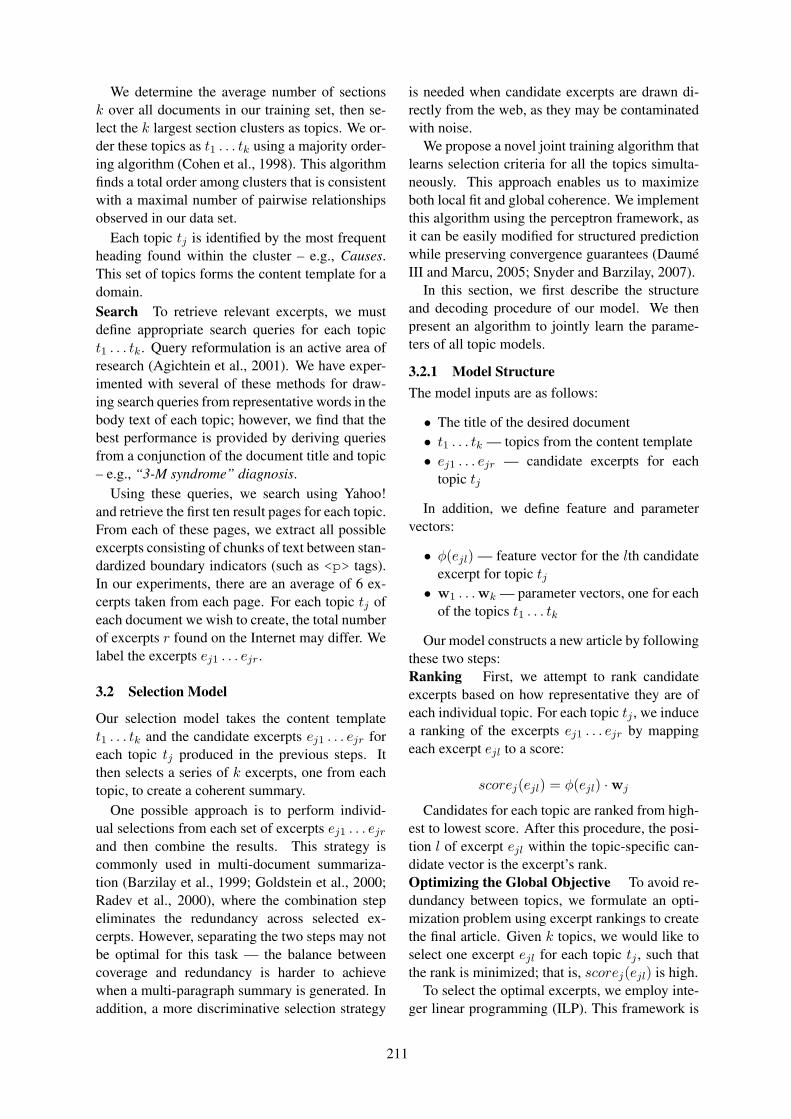
We determine the average number of sectionsk over all documents in our training set, then se-lect the k largest section clusters as topics. We or-der these topics as t1 . . . tk using a majority order-ing algorithm (Cohen et al., 1998). This algorithmfinds a total order among clusters that is consistentwith a maximal number of pairwise relationshipsobserved in our data set.
Each topic tj is identified by the most frequentheading found within the cluster – e.g., Causes.This set of topics forms the content template for adomain.Search To retrieve relevant excerpts, we mustdefine appropriate search queries for each topict1 . . . tk. Query reformulation is an active area ofresearch (Agichtein et al., 2001). We have exper-imented with several of these methods for draw-ing search queries from representative words in thebody text of each topic; however, we find that thebest performance is provided by deriving queriesfrom a conjunction of the document title and topic– e.g., “3-M syndrome” diagnosis.
Using these queries, we search using Yahoo!and retrieve the first ten result pages for each topic.From each of these pages, we extract all possibleexcerpts consisting of chunks of text between stan-dardized boundary indicators (such as <p> tags).In our experiments, there are an average of 6 ex-cerpts taken from each page. For each topic tj ofeach document we wish to create, the total numberof excerpts r found on the Internet may differ. Welabel the excerpts ej1 . . . ejr.
3.2 Selection Model
Our selection model takes the content templatet1 . . . tk and the candidate excerpts ej1 . . . ejr foreach topic tj produced in the previous steps. Itthen selects a series of k excerpts, one from eachtopic, to create a coherent summary.
One possible approach is to perform individ-ual selections from each set of excerpts ej1 . . . ejr
and then combine the results. This strategy iscommonly used in multi-document summariza-tion (Barzilay et al., 1999; Goldstein et al., 2000;Radev et al., 2000), where the combination stepeliminates the redundancy across selected ex-cerpts. However, separating the two steps may notbe optimal for this task — the balance betweencoverage and redundancy is harder to achievewhen a multi-paragraph summary is generated. Inaddition, a more discriminative selection strategy
is needed when candidate excerpts are drawn di-rectly from the web, as they may be contaminatedwith noise.
We propose a novel joint training algorithm thatlearns selection criteria for all the topics simulta-neously. This approach enables us to maximizeboth local fit and global coherence. We implementthis algorithm using the perceptron framework, asit can be easily modified for structured predictionwhile preserving convergence guarantees (DauméIII and Marcu, 2005; Snyder and Barzilay, 2007).
In this section, we first describe the structureand decoding procedure of our model. We thenpresent an algorithm to jointly learn the parame-ters of all topic models.
3.2.1 Model StructureThe model inputs are as follows:
• The title of the desired document• t1 . . . tk — topics from the content template• ej1 . . . ejr — candidate excerpts for each
topic tj
In addition, we define feature and parametervectors:
• φ(ejl) — feature vector for the lth candidateexcerpt for topic tj
• w1 . . .wk — parameter vectors, one for eachof the topics t1 . . . tk
Our model constructs a new article by followingthese two steps:Ranking First, we attempt to rank candidateexcerpts based on how representative they are ofeach individual topic. For each topic tj , we inducea ranking of the excerpts ej1 . . . ejr by mappingeach excerpt ejl to a score:
scorej(ejl) = φ(ejl) ·wj
Candidates for each topic are ranked from high-est to lowest score. After this procedure, the posi-tion l of excerpt ejl within the topic-specific can-didate vector is the excerpt’s rank.Optimizing the Global Objective To avoid re-dundancy between topics, we formulate an opti-mization problem using excerpt rankings to createthe final article. Given k topics, we would like toselect one excerpt ejl for each topic tj , such thatthe rank is minimized; that is, scorej(ejl) is high.
To select the optimal excerpts, we employ inte-ger linear programming (ILP). This framework is
211
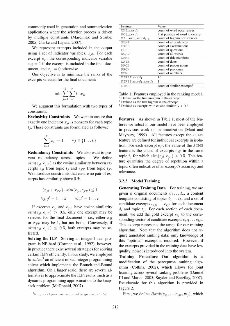
commonly used in generation and summarizationapplications where the selection process is drivenby multiple constraints (Marciniak and Strube,2005; Clarke and Lapata, 2007).
We represent excerpts included in the outputusing a set of indicator variables, xjl. For eachexcerpt ejl, the corresponding indicator variablexjl = 1 if the excerpt is included in the final doc-ument, and xjl = 0 otherwise.
Our objective is to minimize the ranks of theexcerpts selected for the final document:
mink∑
j=1
r∑l=1
l · xjl
We augment this formulation with two types ofconstraints.Exclusivity Constraints We want to ensure thatexactly one indicator xjl is nonzero for each topictj . These constraints are formulated as follows:
r∑l=1
xjl = 1 ∀j ∈ {1 . . . k}
Redundancy Constraints We also want to pre-vent redundancy across topics. We definesim(ejl, ej′l′) as the cosine similarity between ex-cerpts ejl from topic tj and ej′l′ from topic tj′ .We introduce constraints that ensure no pair of ex-cerpts has similarity above 0.5:
(xjl + xj′l′) · sim(ejl, ej′l′) ≤ 1
∀j, j′ = 1 . . . k ∀l, l′ = 1 . . . r
If excerpts ejl and ej′l′ have cosine similaritysim(ejl, ej′l′) > 0.5, only one excerpt may beselected for the final document – i.e., either xjl
or xj′l′ may be 1, but not both. Conversely, ifsim(ejl, ej′l′) ≤ 0.5, both excerpts may be se-lected.Solving the ILP Solving an integer linear pro-gram is NP-hard (Cormen et al., 1992); however,in practice there exist several strategies for solvingcertain ILPs efficiently. In our study, we employedlp solve,3 an efficient mixed integer programmingsolver which implements the Branch-and-Boundalgorithm. On a larger scale, there are several al-ternatives to approximate the ILP results, such as adynamic programming approximation to the knap-sack problem (McDonald, 2007).
3http://lpsolve.sourceforge.net/5.5/
Feature ValueUNI wordi count of word occurrencesPOS wordi first position of word in excerptBI wordi wordi+1 count of bigram occurrencesSENT count of all sentencesEXCL count of exclamationsQUES count of questionsWORD count of all wordsNAME count of title mentionsDATE count of datesPROP count of proper nounsPRON count of pronounsNUM count of numbersFIRST word1 1∗
FIRST word1 word2 1†
SIMS count of similar excerpts‡
Table 1: Features employed in the ranking model.∗ Defined as the first unigram in the excerpt.† Defined as the first bigram in the excerpt.‡ Defined as excerpts with cosine similarity > 0.5
Features As shown in Table 1, most of the fea-tures we select in our model have been employedin previous work on summarization (Mani andMaybury, 1999). All features except the SIMSfeature are defined for individual excerpts in isola-tion. For each excerpt ejl, the value of the SIMSfeature is the count of excerpts ejl′ in the sametopic tj for which sim(ejl, ejl′) > 0.5. This fea-ture quantifies the degree of repetition within atopic, often indicative of an excerpt’s accuracy andrelevance.
3.2.2 Model Training
Generating Training Data For training, we aregiven n original documents d1 . . . dn, a contenttemplate consisting of topics t1 . . . tk, and a set ofcandidate excerpts eij1 . . . eijr for each documentdi and topic tj . For each section of each docu-ment, we add the gold excerpt sij to the corre-sponding vector of candidate excerpts eij1 . . . eijr.This excerpt represents the target for our trainingalgorithm. Note that the algorithm does not re-quire annotated ranking data; only knowledge ofthis “optimal” excerpt is required. However, ifthe excerpts provided in the training data have lowquality, noise is introduced into the system.Training Procedure Our algorithm is amodification of the perceptron ranking algo-rithm (Collins, 2002), which allows for jointlearning across several ranking problems (DauméIII and Marcu, 2005; Snyder and Barzilay, 2007).Pseudocode for this algorithm is provided inFigure 2.
First, we define Rank(eij1 . . . eijr,wj), which
212

ranks all excerpts from the candidate excerptvector eij1 . . . eijr for document di and topictj . Excerpts are ordered by scorej(ejl) usingthe current parameter values. We also defineOptimize(eij1 . . . eijr), which finds the optimalselection of excerpts (one per topic) given rankedlists of excerpts eij1 . . . eijr for each document di
and topic tj . These functions follow the rankingand optimization procedures described in Section3.2.1. The algorithm maintains k parameter vec-tors w1 . . .wk, one associated with each topic tjdesired in the final article. During initialization,all parameter vectors are set to zeros (line 2).
To learn the optimal parameters, this algorithmiterates over the training set until the parametersconverge or a maximum number of iterations isreached (line 3). For each document in the train-ing set (line 4), the following steps occur: First,candidate excerpts for each topic are ranked (lines5-6). Next, decoding through ILP optimization isperformed over all ranked lists of candidate ex-cerpts, selecting one excerpt for each topic (line7). Finally, the parameters are updated in a jointfashion. For each topic (line 8), if the selectedexcerpt is not similar enough to the gold excerpt(line 9), the parameters for that topic are updatedusing a standard perceptron update rule (line 10).When convergence is reached or the maximum it-eration count is exceeded, the learned parametervalues are returned (line 12).
The use of ILP during each step of trainingsets this algorithm apart from previous work. Inprior research, ILP was used as a postprocess-ing step to remove redundancy and make otherglobal decisions about parameters (McDonald,2007; Marciniak and Strube, 2005; Clarke and La-pata, 2007). However, in our training, we inter-twine the complete decoding procedure with theparameter updates. Our joint learning approachfinds per-topic parameter values that are maxi-mally suited for the global decoding procedure forcontent selection.
4 Experimental Setup
We evaluate our method by observing the qualityof automatically created articles in different do-mains. We compute the similarity of a large num-ber of articles produced by our system and sev-eral baselines to the original human-authored arti-cles using ROUGE, a standard metric for summaryquality. In addition, we perform an analysis of edi-
Input:d1 . . . dn: A set of n documents, each containing
k sections si1 . . . sik
eij1 . . . eijr: Sets of candidate excerpts for each topictj and document di
Define:Rank(eij1 . . . eijr,wj):
As described in Section 3.2.1:Calculates scorej(eijl) for all excerpts for
document di and topic tj , using parameters wj .Orders the list of excerpts by scorej(eijl)
from highest to lowest.Optimize(ei11 . . . eikr):
As described in Section 3.2.1:Finds the optimal selection of excerpts to form a
final article, given ranked lists of excerptsfor each topic t1 . . . tk.
Returns a list of k excerpts, one for each topic.φ(eijl):
Returns the feature vector representing excerpt eijl
Initialization:1 For j = 1 . . . k2 Set parameters wj = 0Training:3 Repeat until convergence or while iter < itermax:4 For i = 1 . . . n5 For j = 1 . . . k6 Rank(eij1 . . . eijr,wj)7 x1 . . . xk = Optimize(ei11 . . . eikr)8 For j = 1 . . . k9 If sim(xj , sij) < 0.810 wj = wj + φ(sij)− φ(xi)11 iter = iter + 112 Return parameters w1 . . .wk
Figure 2: An algorithm for learning several rank-ing problems with a joint decoding mechanism.
tor reaction to system-produced articles submittedto Wikipedia.
Data For evaluation, we consider two domains:American Film Actors and Diseases. These do-mains have been commonly used in prior workon summarization (Weischedel et al., 2004; Zhouet al., 2004; Filatova and Prager, 2005; Demner-Fushman and Lin, 2007; Biadsy et al., 2008). Ourtext corpus consists of articles drawn from the cor-responding categories in Wikipedia. There are2,150 articles in American Film Actors and 523articles in Diseases. For each domain, we ran-domly select 90% of articles for training and teston the remaining 10%. Human-authored articlesin both domains contain an average of four top-ics, and each topic contains an average of 193words. In order to model the real-world scenariowhere Wikipedia articles are not always available(as for new or specialized topics), we specificallyexclude Wikipedia sources during our search pro-
213
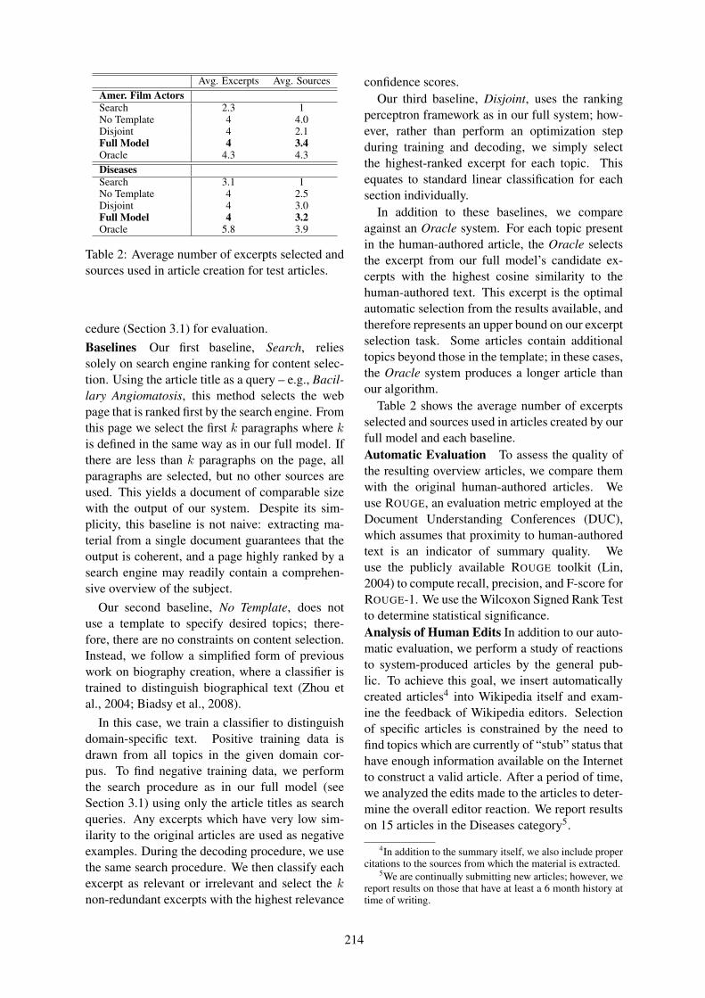
Avg. Excerpts Avg. SourcesAmer. Film ActorsSearch 2.3 1No Template 4 4.0Disjoint 4 2.1Full Model 4 3.4Oracle 4.3 4.3DiseasesSearch 3.1 1No Template 4 2.5Disjoint 4 3.0Full Model 4 3.2Oracle 5.8 3.9
Table 2: Average number of excerpts selected andsources used in article creation for test articles.
cedure (Section 3.1) for evaluation.Baselines Our first baseline, Search, reliessolely on search engine ranking for content selec-tion. Using the article title as a query – e.g., Bacil-lary Angiomatosis, this method selects the webpage that is ranked first by the search engine. Fromthis page we select the first k paragraphs where kis defined in the same way as in our full model. Ifthere are less than k paragraphs on the page, allparagraphs are selected, but no other sources areused. This yields a document of comparable sizewith the output of our system. Despite its sim-plicity, this baseline is not naive: extracting ma-terial from a single document guarantees that theoutput is coherent, and a page highly ranked by asearch engine may readily contain a comprehen-sive overview of the subject.
Our second baseline, No Template, does notuse a template to specify desired topics; there-fore, there are no constraints on content selection.Instead, we follow a simplified form of previouswork on biography creation, where a classifier istrained to distinguish biographical text (Zhou etal., 2004; Biadsy et al., 2008).
In this case, we train a classifier to distinguishdomain-specific text. Positive training data isdrawn from all topics in the given domain cor-pus. To find negative training data, we performthe search procedure as in our full model (seeSection 3.1) using only the article titles as searchqueries. Any excerpts which have very low sim-ilarity to the original articles are used as negativeexamples. During the decoding procedure, we usethe same search procedure. We then classify eachexcerpt as relevant or irrelevant and select the knon-redundant excerpts with the highest relevance
confidence scores.Our third baseline, Disjoint, uses the ranking
perceptron framework as in our full system; how-ever, rather than perform an optimization stepduring training and decoding, we simply selectthe highest-ranked excerpt for each topic. Thisequates to standard linear classification for eachsection individually.
In addition to these baselines, we compareagainst an Oracle system. For each topic presentin the human-authored article, the Oracle selectsthe excerpt from our full model’s candidate ex-cerpts with the highest cosine similarity to thehuman-authored text. This excerpt is the optimalautomatic selection from the results available, andtherefore represents an upper bound on our excerptselection task. Some articles contain additionaltopics beyond those in the template; in these cases,the Oracle system produces a longer article thanour algorithm.
Table 2 shows the average number of excerptsselected and sources used in articles created by ourfull model and each baseline.Automatic Evaluation To assess the quality ofthe resulting overview articles, we compare themwith the original human-authored articles. Weuse ROUGE, an evaluation metric employed at theDocument Understanding Conferences (DUC),which assumes that proximity to human-authoredtext is an indicator of summary quality. Weuse the publicly available ROUGE toolkit (Lin,2004) to compute recall, precision, and F-score forROUGE-1. We use the Wilcoxon Signed Rank Testto determine statistical significance.Analysis of Human Edits In addition to our auto-matic evaluation, we perform a study of reactionsto system-produced articles by the general pub-lic. To achieve this goal, we insert automaticallycreated articles4 into Wikipedia itself and exam-ine the feedback of Wikipedia editors. Selectionof specific articles is constrained by the need tofind topics which are currently of “stub” status thathave enough information available on the Internetto construct a valid article. After a period of time,we analyzed the edits made to the articles to deter-mine the overall editor reaction. We report resultson 15 articles in the Diseases category5.
4In addition to the summary itself, we also include propercitations to the sources from which the material is extracted.
5We are continually submitting new articles; however, wereport results on those that have at least a 6 month history attime of writing.
214

Recall Precision F-scoreAmer. Film ActorsSearch 0.09 0.37 0.13 ∗
No Template 0.33 0.50 0.39 ∗
Disjoint 0.45 0.32 0.36 ∗
Full Model 0.46 0.40 0.41Oracle 0.48 0.64 0.54 ∗
DiseasesSearch 0.31 0.37 0.32 †
No Template 0.32 0.27 0.28 ∗
Disjoint 0.33 0.40 0.35 ∗
Full Model 0.36 0.39 0.37Oracle 0.59 0.37 0.44 ∗
Table 3: Results of ROUGE-1 evaluation.∗ Significant with respect to our full model for p ≤ 0.05.† Significant with respect to our full model for p ≤ 0.10.
Since Wikipedia is a live resource, we do notrepeat this procedure for our baseline systems.Adding articles from systems which have previ-ously demonstrated poor quality would be im-proper, especially in Diseases. Therefore, wepresent this analysis as an additional observationrather than a rigorous technical study.
5 Results
Automatic Evaluation The results of this evalu-ation are shown in Table 3. Our full model outper-forms all of the baselines. By surpassing the Dis-joint baseline, we demonstrate the benefits of jointclassification. Furthermore, the high performanceof both our full model and the Disjoint baselinerelative to the other baselines shows the impor-tance of structure-aware content selection. TheOracle system, which represents an upper boundon our system’s capabilities, performs well.
The remaining baselines have different flaws:Articles produced by the No Template baselinetend to focus on a single topic extensively at theexpense of breadth, because there are no con-straints to ensure diverse topic selection. On theother hand, performance of the Search baselinevaries dramatically. This is expected; this base-line relies heavily on both the search engine andindividual web pages. The search engine must cor-rectly rank relevant pages, and the web pages mustprovide the important material first.Analysis of Human Edits The results of our ob-servation of editing patterns are shown in Table4. These articles have resided on Wikipedia fora period of time ranging from 5-11 months. Allof them have been edited, and no articles were re-moved due to lack of quality. Moreover, ten au-tomatically created articles have been promoted
Type CountTotal articles 15
Promoted articles 10Edit types
Intra-wiki links 36Formatting 25Grammar 20Minor topic edits 2Major topic changes 1
Total edits 85
Table 4: Distribution of edits on Wikipedia.
by human editors from stubs to regular Wikipediaentries based on the quality and coverage of thematerial. Information was removed in three casesfor being irrelevant, one entire section and twosmaller pieces. The most common changes weresmall edits to formatting and introduction of linksto other Wikipedia articles in the body text.
6 Conclusion
In this paper, we investigated an approach for cre-ating a multi-paragraph overview article by select-ing relevant material from the web and organiz-ing it into a single coherent text. Our algorithmyields significant gains over a structure-agnosticapproach. Moreover, our results demonstrate thebenefits of structured classification, which out-performs independently trained topical classifiers.Overall, the results of our evaluation combinedwith our analysis of human edits confirm that theproposed method can effectively produce compre-hensive overview articles.
This work opens several directions for future re-search. Diseases and American Film Actors ex-hibit fairly consistent article structures, which aresuccessfully captured by a simple template cre-ation process. However, with categories that ex-hibit structural variability, more sophisticated sta-tistical approaches may be required to produce ac-curate templates. Moreover, a promising directionis to consider hierarchical discourse formalismssuch as RST (Mann and Thompson, 1988) to sup-plement our template-based approach.
AcknowledgmentsThe authors acknowledge the support of the NSF (CA-REER grant IIS-0448168, grant IIS-0835445, and grant IIS-0835652) and NIH (grant V54LM008748). Thanks to MikeCollins, Julia Hirschberg, and members of the MIT NLPgroup for their helpful suggestions and comments. Any opin-ions, findings, conclusions, or recommendations expressed inthis paper are those of the authors, and do not necessarily re-flect the views of the funding organizations.
215
ReferencesEugene Agichtein, Steve Lawrence, and Luis Gravano. 2001.
Learning search engine specific query transformations forquestion answering. In Proceedings of WWW, pages 169–178.
Regina Barzilay and Noemie Elhadad. 2003. Sentence align-ment for monolingual comparable corpora. In Proceed-ings of EMNLP, pages 25–32.
Regina Barzilay and Lillian Lee. 2004. Catching the drift:Probabilistic content models, with applications to genera-tion and summarization. In Proceedings of HLT-NAACL,pages 113–120.
Regina Barzilay, Kathleen R. McKeown, and Michael El-hadad. 1999. Information fusion in the context of multi-document summarization. In Proceedings of ACL, pages550–557.
Fadi Biadsy, Julia Hirschberg, and Elena Filatova. 2008.An unsupervised approach to biography production usingwikipedia. In Proceedings of ACL/HLT, pages 807–815.
James Clarke and Mirella Lapata. 2007. Modelling com-pression with discourse constraints. In Proceedings ofEMNLP-CoNLL, pages 1–11.
William W. Cohen, Robert E. Schapire, and Yoram Singer.1998. Learning to order things. In Proceedings of NIPS,pages 451–457.
Michael Collins. 2002. Ranking algorithms for named-entityextraction: Boosting and the voted perceptron. In Pro-ceedings of ACL, pages 489–496.
Thomas H. Cormen, Charles E. Leiserson, and Ronald L.Rivest. 1992. Intoduction to Algorithms. The MIT Press.
Hal Daumé III and Daniel Marcu. 2005. A large-scale explo-ration of effective global features for a joint entity detec-tion and tracking model. In Proceedings of HLT/EMNLP,pages 97–104.
Dina Demner-Fushman and Jimmy Lin. 2007. Answer-ing clinical questions with knowledge-based and statisti-cal techniques. Computational Linguistics, 33(1):63–103.
Elena Filatova and John M. Prager. 2005. Tell me what youdo and I’ll tell you what you are: Learning occupation-related activities for biographies. In Proceedings ofHLT/EMNLP, pages 113–120.
Elena Filatova, Vasileios Hatzivassiloglou, and KathleenMcKeown. 2006. Automatic creation of domain tem-plates. In Proceedings of ACL, pages 207–214.
Atsushi Fujii and Tetsuya Ishikawa. 2004. Summarizing en-cyclopedic term descriptions on the web. In Proceedingsof COLING, page 645.
Jade Goldstein, Vibhu Mittal, Jaime Carbonell, and MarkKantrowitz. 2000. Multi-document summarization bysentence extraction. In Proceedings of NAACL-ANLP,pages 40–48.
Marti A. Hearst. 1994. Multi-paragraph segmentation of ex-pository text. In Proceedings of ACL, pages 9–16.
Chin-Yew Lin. 2004. ROUGE: A package for automaticevaluation of summaries. In Proceedings of ACL, pages74–81.
Inderjeet Mani and Mark T. Maybury. 1999. Advances inAutomatic Text Summarization. The MIT Press.
William C. Mann and Sandra A. Thompson. 1988. Rhetor-ical structure theory: Toward a functional theory of textorganization. Text, 8(3):243–281.
Tomasz Marciniak and Michael Strube. 2005. Beyond thepipeline: Discrete optimization in NLP. In Proceedingsof CoNLL, pages 136–143.
Ryan McDonald. 2007. A study of global inference algo-rithms in multi-document summarization. In Proceedingsof EICR, pages 557–564.
Vivi Nastase and Michael Strube. 2008. Decoding wikipediacategories for knowledge acquisition. In Proceedings ofAAAI, pages 1219–1224.
Vivi Nastase. 2008. Topic-driven multi-document summa-rization with encyclopedic knowledge and spreading acti-vation. In Proceedings of EMNLP, pages 763–772.
Dragomir R. Radev, Hongyan Jing, and MalgorzataBudzikowska. 2000. Centroid-based summarizationof multiple documents: sentence extraction, utility-based evaluation, and user studies. In Proceedings ofANLP/NAACL, pages 21–29.
Ehud Reiter and Robert Dale. 2000. Building Natural Lan-guage Generation Systems. Cambridge University Press,Cambridge.
Benjamin Snyder and Regina Barzilay. 2007. Multiple as-pect ranking using the good grief algorithm. In Proceed-ings of HLT-NAACL, pages 300–307.
Ralph M. Weischedel, Jinxi Xu, and Ana Licuanan. 2004. Ahybrid approach to answering biographical questions. InNew Directions in Question Answering, pages 59–70.
Fei Wu and Daniel S. Weld. 2007. Autonomously semanti-fying wikipedia. In Proceedings of CIKM, pages 41–50.
Ying Zhao, George Karypis, and Usama Fayyad. 2005.Hierarchical clustering algorithms for document datasets.Data Mining and Knowledge Discovery, 10(2):141–168.
L. Zhou, M. Ticrea, and Eduard Hovy. 2004. Multi-document biography summarization. In Proceedings ofEMNLP, pages 434–441.
216

Proceedings of the 47th Annual Meeting of the ACL and the 4th IJCNLP of the AFNLP, pages 217–225,Suntec, Singapore, 2-7 August 2009. c©2009 ACL and AFNLP
Learning to Tell Tales: A Data-driven Approach to Story Generation
Neil McIntyre and Mirella LapataSchool of Informatics, University of Edinburgh10 Crichton Street, Edinburgh, EH8 9AB, UK
[email protected], [email protected]
Abstract
Computational story telling has sparkedgreat interest in artificial intelligence,partly because of its relevance to educa-tional and gaming applications. Tradition-ally, story generators rely on a large repos-itory of background knowledge contain-ing information about the story plot andits characters. This information is detailedand usually hand crafted. In this paper wepropose a data-driven approach for gen-erating short children’s stories that doesnot require extensive manual involvement.We create an end-to-end system that real-izes the various components of the gen-eration pipeline stochastically. Our systemfollows a generate-and-and-rank approachwhere the space of multiple candidate sto-ries is pruned by considering whether theyare plausible, interesting, and coherent.
1 Introduction
Recent years have witnessed increased interest inthe use of interactive language technology in ed-ucational and entertainment applications. Compu-tational story telling could play a key role in theseapplications by effectively engaging learners andassisting them in creating a story. It could also al-low teachers to generate stories on demand thatsuit their classes’ needs. And enhance the enter-tainment value of role-playing games1. The major-ity of these games come with a set of pre-specifiedplots that the players must act out. Ideally, the plotshould adapt dynamically in response to the play-ers’ actions.
Computational story telling has a longstandingtradition in the field of artificial intelligence. Earlywork has been largely inspired by Propp’s (1968)
1A role-playing game (RPG) is a game in which the par-ticipants assume the roles of fictional characters and act outan adventure.
typology of narrative structure. Propp identified inRussian fairy tales a small number of recurringunits (e.g., the hero is defeated, the villain causesharm) and rules that could be used to describe theirrelation (e.g., the hero is pursued and the rescued).Story grammars (Thorndyke, 1977) were initiallyused to capture Propp’s high-level plot elementsand character interactions. A large body of morerecent work views story generation as a form ofagent-based planning (Theune et al., 2003; Fass,2002; Oinonen et al., 2006). The agents act ascharacters with a list of goals. They form plansof action and try to fulfill them. Interesting storiesemerge as agents’ plans interact and cause failuresand possible replanning.
Perhaps the biggest challenge faced by compu-tational story generators is the amount of worldknowledge required to create compelling stories.A hypothetical system must have informationabout the characters involved, how they inter-act, what their goals are, and how they influencetheir environment. Furthermore, all this informa-tion must be complete and error-free if it is to beused as input to a planning algorithm. Tradition-ally, this knowledge is created by hand, and mustbe recreated for different domains. Even the sim-ple task of adding a new character requires a wholenew set of action descriptions and goals.
A second challenge concerns the generationtask itself and the creation of stories character-ized by high-quality prose. Most story genera-tion systems focus on generating plot outlines,without considering the actual linguistic structuresfound in the stories they are trying to mimic (butsee Callaway and Lester 2002 for a notable ex-ception). In fact, there seems to be little com-mon ground between story generation and naturallanguage generation (NLG), despite extensive re-search in both fields. The NLG process (Reiter andDale, 2000) is often viewed as a pipeline consist-ing of content planning (selecting and structuringthe story’s content), microplanning (sentence ag-
217
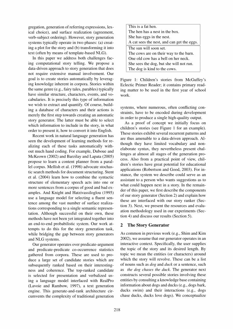
gregation, generation of referring expressions, lex-ical choice), and surface realization (agreement,verb-subject ordering). However, story generationsystems typically operate in two phases: (a) creat-ing a plot for the story and (b) transforming it intotext (often by means of template-based NLG).
In this paper we address both challenges fac-ing computational story telling. We propose adata-driven approach to story generation that doesnot require extensive manual involvement. Ourgoal is to create stories automatically by leverag-ing knowledge inherent in corpora. Stories withinthe same genre (e.g., fairy tales, parables) typicallyhave similar structure, characters, events, and vo-cabularies. It is precisely this type of informationwe wish to extract and quantify. Of course, build-ing a database of characters and their actions ismerely the first step towards creating an automaticstory generator. The latter must be able to selectwhich information to include in the story, in whatorder to present it, how to convert it into English.
Recent work in natural language generation hasseen the development of learning methods for re-alizing each of these tasks automatically with-out much hand coding. For example, Duboue andMcKeown (2002) and Barzilay and Lapata (2005)propose to learn a content planner from a paral-lel corpus. Mellish et al. (1998) advocate stochas-tic search methods for document structuring. Stentet al. (2004) learn how to combine the syntacticstructure of elementary speech acts into one ormore sentences from a corpus of good and bad ex-amples. And Knight and Hatzivassiloglou (1995)use a language model for selecting a fluent sen-tence among the vast number of surface realiza-tions corresponding to a single semantic represen-tation. Although successful on their own, thesemethods have not been yet integrated together intoan end-to-end probabilistic system. Our work at-tempts to do this for the story generation task,while bridging the gap between story generatorsand NLG systems.
Our generator operates over predicate-argumentand predicate-predicate co-occurrence statisticsgathered from corpora. These are used to pro-duce a large set of candidate stories which aresubsequently ranked based on their interesting-ness and coherence. The top-ranked candidateis selected for presentation and verbalized us-ing a language model interfaced with RealPro(Lavoie and Rambow, 1997), a text generationengine. This generate-and-rank architecture cir-cumvents the complexity of traditional generation
This is a fat hen.The hen has a nest in the box.She has eggs in the nest.A cat sees the nest, and can get the eggs.The sun will soon set.The cows are on their way to the barn.One old cow has a bell on her neck.She sees the dog, but she will not run.The dog is kind to the cows.
Figure 1: Children’s stories from McGuffey’sEclectic Primer Reader; it contains primary read-ing matter to be used in the first year of schoolwork.
systems, where numerous, often conflicting con-straints, have to be encoded during developmentin order to produce a single high-quality output.
As a proof of concept we initially focus onchildren’s stories (see Figure 1 for an example).These stories exhibit several recurrent patterns andare thus amenable to a data-driven approach. Al-though they have limited vocabulary and non-elaborate syntax, they nevertheless present chal-lenges at almost all stages of the generation pro-cess. Also from a practical point of view, chil-dren’s stories have great potential for educationalapplications (Robertson and Good, 2003). For in-stance, the system we describe could serve as anassistant to a person who wants suggestions as towhat could happen next in a story. In the remain-der of this paper, we first describe the componentsof our story generator (Section 2) and explain howthese are interfaced with our story ranker (Sec-tion 3). Next, we present the resources and evalu-ation methodology used in our experiments (Sec-tion 4) and discuss our results (Section 5).
2 The Story Generator
As common in previous work (e.g., Shim and Kim2002), we assume that our generator operates in aninteractive context. Specifically, the user suppliesthe topic of the story and its desired length. Bytopic we mean the entities (or characters) aroundwhich the story will revolve. These can be a listof nouns such as dog and duck or a sentence, suchas the dog chases the duck. The generator nextconstructs several possible stories involving theseentities by consulting a knowledge base containinginformation about dogs and ducks (e.g., dogs bark,ducks swim) and their interactions (e.g., dogschase ducks, ducks love dogs). We conceptualize
218
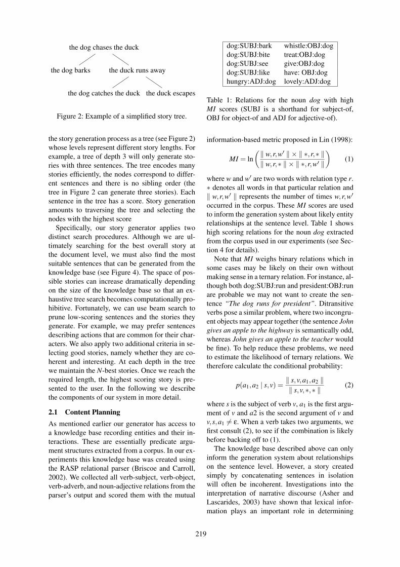
the dog chases the duck
the dog barks the duck runs away
the dog catches the duck the duck escapes
Figure 2: Example of a simplified story tree.
the story generation process as a tree (see Figure 2)whose levels represent different story lengths. Forexample, a tree of depth 3 will only generate sto-ries with three sentences. The tree encodes manystories efficiently, the nodes correspond to differ-ent sentences and there is no sibling order (thetree in Figure 2 can generate three stories). Eachsentence in the tree has a score. Story generationamounts to traversing the tree and selecting thenodes with the highest score
Specifically, our story generator applies twodistinct search procedures. Although we are ul-timately searching for the best overall story atthe document level, we must also find the mostsuitable sentences that can be generated from theknowledge base (see Figure 4). The space of pos-sible stories can increase dramatically dependingon the size of the knowledge base so that an ex-haustive tree search becomes computationally pro-hibitive. Fortunately, we can use beam search toprune low-scoring sentences and the stories theygenerate. For example, we may prefer sentencesdescribing actions that are common for their char-acters. We also apply two additional criteria in se-lecting good stories, namely whether they are co-herent and interesting. At each depth in the treewe maintain the N-best stories. Once we reach therequired length, the highest scoring story is pre-sented to the user. In the following we describethe components of our system in more detail.
2.1 Content PlanningAs mentioned earlier our generator has access toa knowledge base recording entities and their in-teractions. These are essentially predicate argu-ment structures extracted from a corpus. In our ex-periments this knowledge base was created usingthe RASP relational parser (Briscoe and Carroll,2002). We collected all verb-subject, verb-object,verb-adverb, and noun-adjective relations from theparser’s output and scored them with the mutual
dog:SUBJ:bark whistle:OBJ:dogdog:SUBJ:bite treat:OBJ:dogdog:SUBJ:see give:OBJ:dogdog:SUBJ:like have: OBJ:doghungry:ADJ:dog lovely:ADJ:dog
Table 1: Relations for the noun dog with highMI scores (SUBJ is a shorthand for subject-of,OBJ for object-of and ADJ for adjective-of).
information-based metric proposed in Lin (1998):
MI = ln(‖ w,r,w′ ‖ × ‖ ∗,r,∗ ‖‖ w,r,∗ ‖ × ‖ ∗,r,w′ ‖
)(1)
where w and w′ are two words with relation type r.∗ denotes all words in that particular relation and‖ w,r,w′ ‖ represents the number of times w,r,w′
occurred in the corpus. These MI scores are usedto inform the generation system about likely entityrelationships at the sentence level. Table 1 showshigh scoring relations for the noun dog extractedfrom the corpus used in our experiments (see Sec-tion 4 for details).
Note that MI weighs binary relations which insome cases may be likely on their own withoutmaking sense in a ternary relation. For instance, al-though both dog:SUBJ:run and president:OBJ:runare probable we may not want to create the sen-tence “The dog runs for president”. Ditransitiveverbs pose a similar problem, where two incongru-ent objects may appear together (the sentence Johngives an apple to the highway is semantically odd,whereas John gives an apple to the teacher wouldbe fine). To help reduce these problems, we needto estimate the likelihood of ternary relations. Wetherefore calculate the conditional probability:
p(a1,a2 | s,v) =‖ s,v,a1,a2 ‖‖ s,v,∗,∗ ‖
(2)
where s is the subject of verb v, a1 is the first argu-ment of v and a2 is the second argument of v andv,s,a1 6= ε. When a verb takes two arguments, wefirst consult (2), to see if the combination is likelybefore backing off to (1).
The knowledge base described above can onlyinform the generation system about relationshipson the sentence level. However, a story createdsimply by concatenating sentences in isolationwill often be incoherent. Investigations into theinterpretation of narrative discourse (Asher andLascarides, 2003) have shown that lexical infor-mation plays an important role in determining
219

SUBJ:chase
OBJ:chase
SUBJ:run
SUBJ:escape
SUBJ:fall
OBJ:catch SUBJ:frighten
SUBJ:jump
1 2
2
6
5
8
15
Figure 3: Graph encoding (partially ordered)chains of events
the discourse relations between propositions. Al-though we don’t have an explicit model of rhetor-ical relations and their effects on sentence order-ing, we capture the lexical inter-dependencies be-tween sentences by focusing on events (verbs)and their precedence relationships in the corpus.For every entity in our training corpus we extractevent chains similar to those proposed by Cham-bers and Jurafsky (2008). Specifically, we identifythe events every entity relates to and record their(partial) order. We assume that verbs sharing thesame arguments are more likely to be semanticallyrelated than verbs with no arguments in common.For example, if we know that someone steals andthen runs, we may expect the next action to be thatthey hide or that they are caught.
In order to track entities and their associatedevents throughout a text, we first resolve entitymentions using OpenNLP2. The list of events per-formed by co-referring entities and their gram-matical relation (i.e., subject or object) are sub-sequently stored in a graph. The edges betweenevent nodes are scored using the MI equationgiven in (1). A fragment of the action graphis shown in Figure 3 (for simplicity, the edgesin the example are weighted with co-occurrencefrequencies). Contrary to Chambers and Juraf-sky (2008) we do not learn global narrativechains over an entire corpus. Currently, we con-sider local chains of length two and three (i.e.,chains of two or three events sharing gram-matical arguments). The generator consults thegraph when selecting a verb for an entity. Itwill favor verbs that are part of an event chain(e.g., SUBJ:chase → SUBJ:run → SUBJ:fall inFigure 3). This way, the search space is effectivelypruned as finding a suitable verb in the current sen-tence is influenced by the choice of verb in the nextsentence.
2See http://opennlp.sourceforge.net/.
2.2 Sentence PlanningSo far we have described how we gather knowl-edge about entities and their interactions, whichmust be subsequently combined into a sentence.The backbone of our sentence planner is a gram-mar with subcategorization information which wecollected from the lexicon created by Korhonenand Briscoe (2006) and the COMLEX dictionary(Grishman et al., 1994). The grammar rules actas templates. They each take a verb as their headand propose ways of filling its argument slots. Thismeans that when generating a story, the choice ofverb will affect the structure of the sentence. Thesubcategorization templates are weighted by theirprobability of occurrence in the reference dictio-naries. This allows the system to prefer less elab-orate grammatical structures. The grammar ruleswere converted to a format compatible with oursurface realizer (see Section 2.3) and include in-formation pertaining to mood, agreement, argu-ment role, etc.
Our sentence planner aggregates together infor-mation from the knowledge base, without how-ever generating referring expressions. Althoughthis would be a natural extension, we initiallywanted to assess whether the stochastic approachadvocated here is feasible at all, before venturingtowards more ambitious components.
2.3 Surface RealizationThe surface realization process is performed byRealPro (Lavoie and Rambow (1997)). The sys-tem takes an abstract sentence representation andtransforms it into English. There are several gram-matical issues that will affect the final realizationof the sentence. For nouns we must decide whetherthey are singular or plural, whether they are pre-ceded by a definite or indefinite article or with noarticle at all. Adverbs can either be pre-verbal orpost-verbal. There is also the issue of selectingan appropriate tense for our generated sentences,however, we simply assume all sentences are inthe present tense. Since we do not know a prioriwhich of these parameters will result in a gram-matical sentence, we generate all possible combi-nations and select the most likely one according toa language model. We used the SRI toolkit to traina trigram language model on the British NationalCorpus, with interpolated Kneser-Ney smoothingand perplexity as the scoring metric for the gener-ated sentences.
220

root
dog
. . . bark
bark(dog) bark at(dog,OBJ)
bark at(dog,duck) bark at(dog,cat)
bark(dog,ADV)
bark(dog,loudly)
hide run
duck
quack
. . .
run
. . .
fly
. . .
Figure 4: Simplified generation example for the in-put sentence the dog chases the duck.
2.4 Sentence Generation ExampleIt is best to illustrate the generation procedure witha simple example (see Figure 4). Given the sen-tence the dog chases the duck as input, our gen-erator assumes that either dog or duck will be thesubject of the following sentence. This is a some-what simplistic attempt at generating coherent sto-ries. Centering (Grosz et al., 1995) and other dis-course theories argue that topical entities are likelyto appear in prominent syntactic positions such assubject or object. Next, we select verbs from theknowledge base that take the words duck and dogas their subject (e.g., bark, run, fly). Our beamsearch procedure will reduce the list of verbs toa small subset by giving preference to those thatare likely to follow chase and have duck and dogas their subjects or objects.
The sentence planner gives a set of possibleframes for these verbs which may introduce ad-ditional entities (see Figure 4). For example, barkcan be intransitive or take an object or adver-bial complement. We select an object for bark,by retrieving from the knowledge base the setof objects it co-occurs with. Our surface real-izer will take structures like “bark(dog,loudly)”,“bark at(dog,cat)”, “bark at(dog,duck)” and gen-erate the sentences the dog barks loudly, the dogbarks at the cat and the dog barks at the duck. Thisprocedure is repeated to create a list of possiblecandidates for the third sentence, and so on.
As Figure 4 illustrates, there are many candidatesentences for each entity. In default of generatingall of these exhaustively, our system utilizes theMI scores from the knowledge base to guide the
search. So, at each choice point in the generationprocess, e.g., when selecting a verb for an entity ora frame for a verb, we consider the N best alterna-tives assuming that these are most likely to appearin a good story.
3 Story Ranking
We have so far described most modules of ourstory generator, save one important component,namely the story ranker. As explained earlier, ourgenerator produces stories stochastically, by rely-ing on co-occurrence frequencies collected fromthe training corpus. However, there is no guaran-tee that these stories will be interesting or coher-ent. Engaging stories have some element of sur-prise and originality in them (Turner, 1994). Ourstories may simply contain a list of actions typi-cally performed by the story characters. Or in theworst case, actions that make no sense when col-lated together.
Ideally, we would like to be able to discern in-teresting stories from tedious ones. Another im-portant consideration is their coherence. We haveto ensure that the discourse smoothly transitionsfrom one topic to the next. To remedy this, wedeveloped two ranking functions that assess thecandidate stories based on their interest and coher-ence. Following previous work (Stent et al., 2004;Barzilay and Lapata, 2007) we learn these rankingfunctions from training data (i.e., stories labeledwith numeric values for interestingness and coher-ence).
Interest Model A stumbling block to assessinghow interesting a story may be, is that the very no-tion of interestingness is subjective and not verywell understood. Although people can judge fairlyreliably whether they like or dislike a story, theyhave more difficulty isolating what exactly makesit interesting. Furthermore, there are virtually noempirical studies investigating the linguistic (sur-face level) correlates of interestingness. We there-fore conducted an experiment where we asked par-ticipants to rate a set of human authored stories interms of interest. Our stories were Aesop’s fablessince they resemble the stories we wish to gener-ate. They are fairly short (average length was 3.7sentences) and with a few characters. We askedparticipants to judge 40 fables on a set of crite-ria: plot, events, characters, coherence and interest(using a 5-point rating scale). The fables were splitinto 5 sets of 8; each participant was randomly as-signed one of the 5 sets to judge. We obtained rat-
221
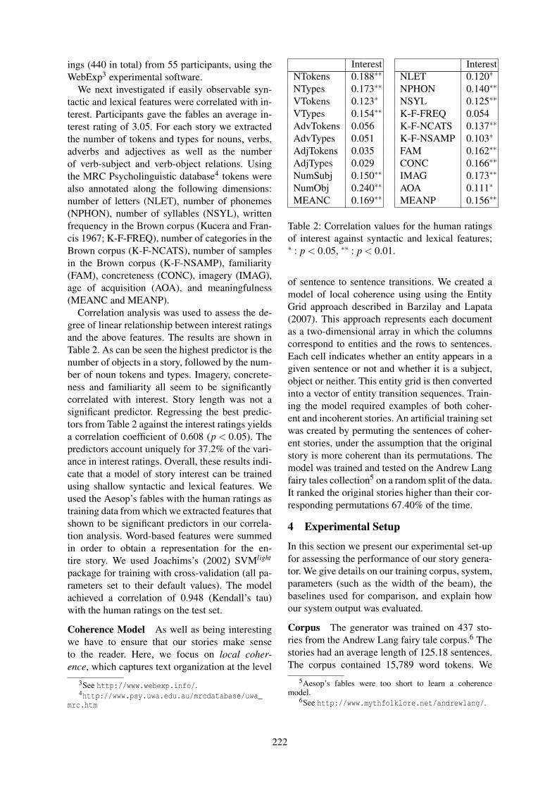
ings (440 in total) from 55 participants, using theWebExp3 experimental software.
We next investigated if easily observable syn-tactic and lexical features were correlated with in-terest. Participants gave the fables an average in-terest rating of 3.05. For each story we extractedthe number of tokens and types for nouns, verbs,adverbs and adjectives as well as the numberof verb-subject and verb-object relations. Usingthe MRC Psycholinguistic database4 tokens werealso annotated along the following dimensions:number of letters (NLET), number of phonemes(NPHON), number of syllables (NSYL), writtenfrequency in the Brown corpus (Kucera and Fran-cis 1967; K-F-FREQ), number of categories in theBrown corpus (K-F-NCATS), number of samplesin the Brown corpus (K-F-NSAMP), familiarity(FAM), concreteness (CONC), imagery (IMAG),age of acquisition (AOA), and meaningfulness(MEANC and MEANP).
Correlation analysis was used to assess the de-gree of linear relationship between interest ratingsand the above features. The results are shown inTable 2. As can be seen the highest predictor is thenumber of objects in a story, followed by the num-ber of noun tokens and types. Imagery, concrete-ness and familiarity all seem to be significantlycorrelated with interest. Story length was not asignificant predictor. Regressing the best predic-tors from Table 2 against the interest ratings yieldsa correlation coefficient of 0.608 (p < 0.05). Thepredictors account uniquely for 37.2% of the vari-ance in interest ratings. Overall, these results indi-cate that a model of story interest can be trainedusing shallow syntactic and lexical features. Weused the Aesop’s fables with the human ratings astraining data from which we extracted features thatshown to be significant predictors in our correla-tion analysis. Word-based features were summedin order to obtain a representation for the en-tire story. We used Joachims’s (2002) SVMlight
package for training with cross-validation (all pa-rameters set to their default values). The modelachieved a correlation of 0.948 (Kendall’s tau)with the human ratings on the test set.
Coherence Model As well as being interestingwe have to ensure that our stories make senseto the reader. Here, we focus on local coher-ence, which captures text organization at the level
3See http://www.webexp.info/.4http://www.psy.uwa.edu.au/mrcdatabase/uwa_
mrc.htm
Interest InterestNTokens 0.188∗∗ NLET 0.120∗
NTypes 0.173∗∗ NPHON 0.140∗∗
VTokens 0.123∗ NSYL 0.125∗∗
VTypes 0.154∗∗ K-F-FREQ 0.054AdvTokens 0.056 K-F-NCATS 0.137∗∗
AdvTypes 0.051 K-F-NSAMP 0.103∗
AdjTokens 0.035 FAM 0.162∗∗
AdjTypes 0.029 CONC 0.166∗∗
NumSubj 0.150∗∗ IMAG 0.173∗∗
NumObj 0.240∗∗ AOA 0.111∗
MEANC 0.169∗∗ MEANP 0.156∗∗
Table 2: Correlation values for the human ratingsof interest against syntactic and lexical features;∗ : p < 0.05, ∗∗ : p < 0.01.
of sentence to sentence transitions. We created amodel of local coherence using using the EntityGrid approach described in Barzilay and Lapata(2007). This approach represents each documentas a two-dimensional array in which the columnscorrespond to entities and the rows to sentences.Each cell indicates whether an entity appears in agiven sentence or not and whether it is a subject,object or neither. This entity grid is then convertedinto a vector of entity transition sequences. Train-ing the model required examples of both coher-ent and incoherent stories. An artificial training setwas created by permuting the sentences of coher-ent stories, under the assumption that the originalstory is more coherent than its permutations. Themodel was trained and tested on the Andrew Langfairy tales collection5 on a random split of the data.It ranked the original stories higher than their cor-responding permutations 67.40% of the time.
4 Experimental Setup
In this section we present our experimental set-upfor assessing the performance of our story genera-tor. We give details on our training corpus, system,parameters (such as the width of the beam), thebaselines used for comparison, and explain howour system output was evaluated.
Corpus The generator was trained on 437 sto-ries from the Andrew Lang fairy tale corpus.6 Thestories had an average length of 125.18 sentences.The corpus contained 15,789 word tokens. We
5Aesop’s fables were too short to learn a coherencemodel.
6See http://www.mythfolklore.net/andrewlang/.
222
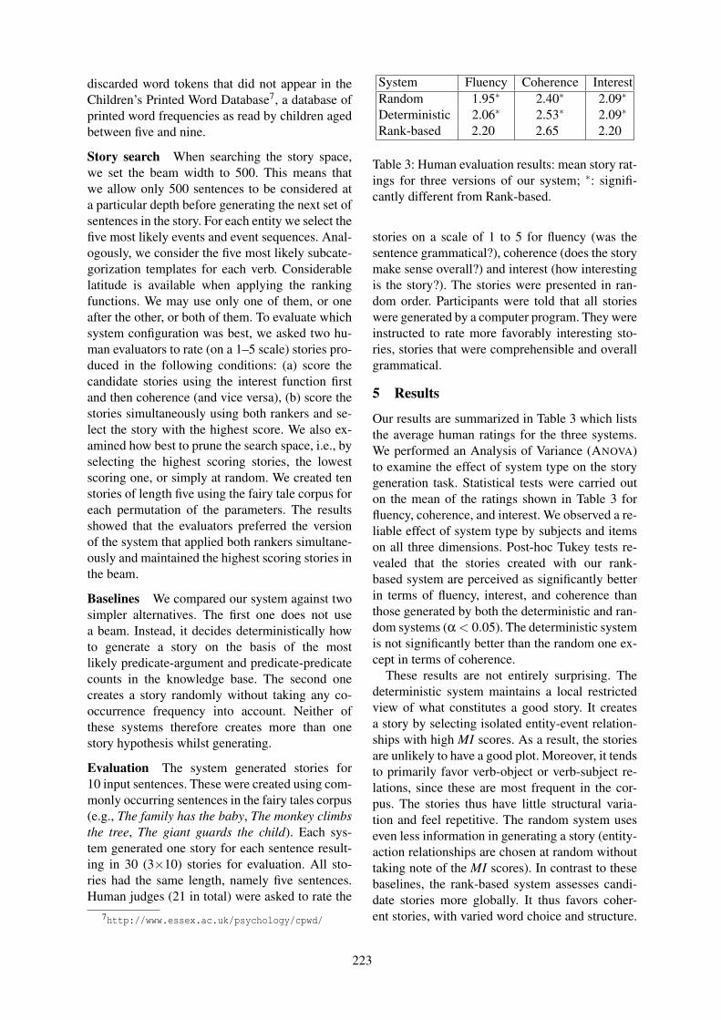
discarded word tokens that did not appear in theChildren’s Printed Word Database7, a database ofprinted word frequencies as read by children agedbetween five and nine.
Story search When searching the story space,we set the beam width to 500. This means thatwe allow only 500 sentences to be considered ata particular depth before generating the next set ofsentences in the story. For each entity we select thefive most likely events and event sequences. Anal-ogously, we consider the five most likely subcate-gorization templates for each verb. Considerablelatitude is available when applying the rankingfunctions. We may use only one of them, or oneafter the other, or both of them. To evaluate whichsystem configuration was best, we asked two hu-man evaluators to rate (on a 1–5 scale) stories pro-duced in the following conditions: (a) score thecandidate stories using the interest function firstand then coherence (and vice versa), (b) score thestories simultaneously using both rankers and se-lect the story with the highest score. We also ex-amined how best to prune the search space, i.e., byselecting the highest scoring stories, the lowestscoring one, or simply at random. We created tenstories of length five using the fairy tale corpus foreach permutation of the parameters. The resultsshowed that the evaluators preferred the versionof the system that applied both rankers simultane-ously and maintained the highest scoring stories inthe beam.
Baselines We compared our system against twosimpler alternatives. The first one does not usea beam. Instead, it decides deterministically howto generate a story on the basis of the mostlikely predicate-argument and predicate-predicatecounts in the knowledge base. The second onecreates a story randomly without taking any co-occurrence frequency into account. Neither ofthese systems therefore creates more than onestory hypothesis whilst generating.
Evaluation The system generated stories for10 input sentences. These were created using com-monly occurring sentences in the fairy tales corpus(e.g., The family has the baby, The monkey climbsthe tree, The giant guards the child). Each sys-tem generated one story for each sentence result-ing in 30 (3×10) stories for evaluation. All sto-ries had the same length, namely five sentences.Human judges (21 in total) were asked to rate the
7http://www.essex.ac.uk/psychology/cpwd/
System Fluency Coherence InterestRandom 1.95∗ 2.40∗ 2.09∗
Deterministic 2.06∗ 2.53∗ 2.09∗
Rank-based 2.20 2.65 2.20
Table 3: Human evaluation results: mean story rat-ings for three versions of our system; ∗: signifi-cantly different from Rank-based.
stories on a scale of 1 to 5 for fluency (was thesentence grammatical?), coherence (does the storymake sense overall?) and interest (how interestingis the story?). The stories were presented in ran-dom order. Participants were told that all storieswere generated by a computer program. They wereinstructed to rate more favorably interesting sto-ries, stories that were comprehensible and overallgrammatical.
5 Results
Our results are summarized in Table 3 which liststhe average human ratings for the three systems.We performed an Analysis of Variance (ANOVA)to examine the effect of system type on the storygeneration task. Statistical tests were carried outon the mean of the ratings shown in Table 3 forfluency, coherence, and interest. We observed a re-liable effect of system type by subjects and itemson all three dimensions. Post-hoc Tukey tests re-vealed that the stories created with our rank-based system are perceived as significantly betterin terms of fluency, interest, and coherence thanthose generated by both the deterministic and ran-dom systems (α < 0.05). The deterministic systemis not significantly better than the random one ex-cept in terms of coherence.
These results are not entirely surprising. Thedeterministic system maintains a local restrictedview of what constitutes a good story. It createsa story by selecting isolated entity-event relation-ships with high MI scores. As a result, the storiesare unlikely to have a good plot. Moreover, it tendsto primarily favor verb-object or verb-subject re-lations, since these are most frequent in the cor-pus. The stories thus have little structural varia-tion and feel repetitive. The random system useseven less information in generating a story (entity-action relationships are chosen at random withouttaking note of the MI scores). In contrast to thesebaselines, the rank-based system assesses candi-date stories more globally. It thus favors coher-ent stories, with varied word choice and structure.
223
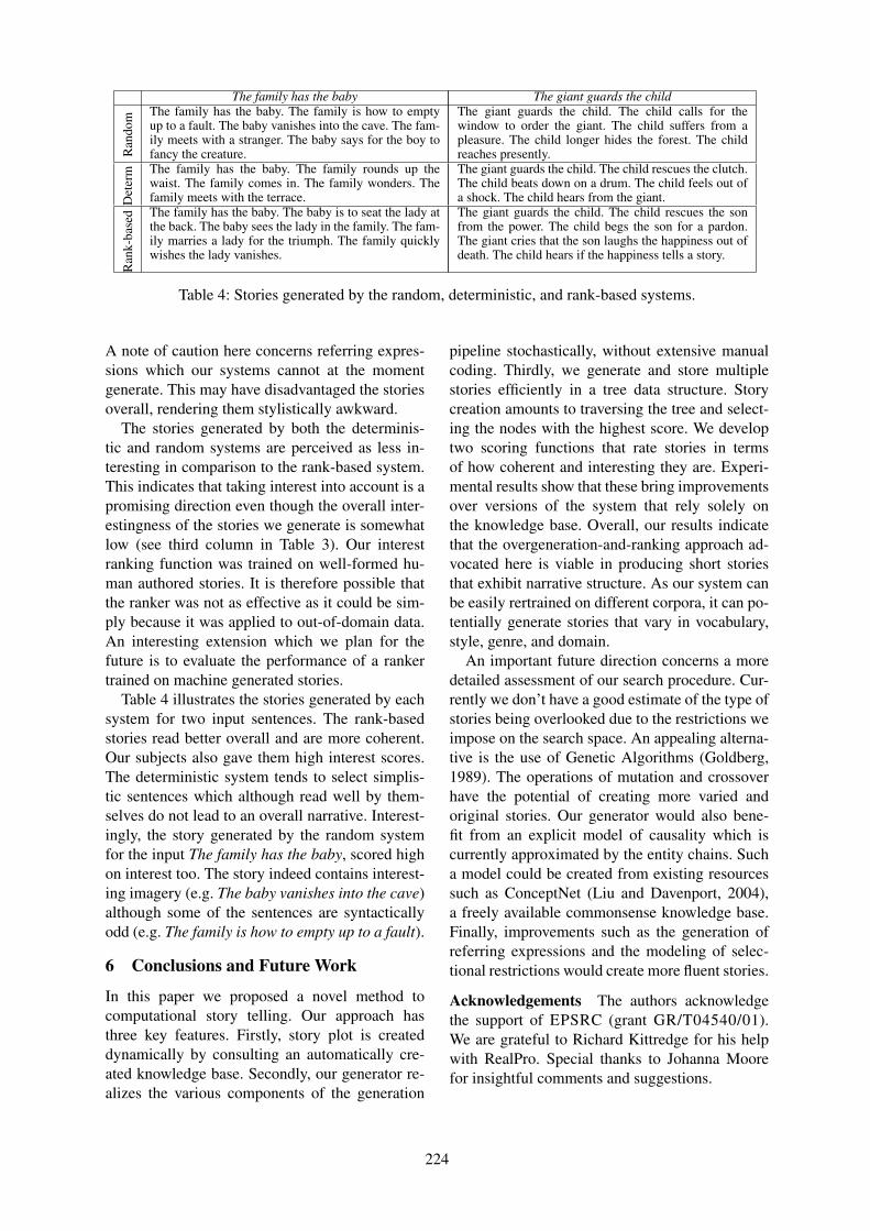
The family has the baby The giant guards the child
Ran
dom The family has the baby. The family is how to empty
up to a fault. The baby vanishes into the cave. The fam-ily meets with a stranger. The baby says for the boy tofancy the creature.
The giant guards the child. The child calls for thewindow to order the giant. The child suffers from apleasure. The child longer hides the forest. The childreaches presently.
Det
erm The family has the baby. The family rounds up the
waist. The family comes in. The family wonders. Thefamily meets with the terrace.
The giant guards the child. The child rescues the clutch.The child beats down on a drum. The child feels out ofa shock. The child hears from the giant.
Ran
k-ba
sed The family has the baby. The baby is to seat the lady at
the back. The baby sees the lady in the family. The fam-ily marries a lady for the triumph. The family quicklywishes the lady vanishes.
The giant guards the child. The child rescues the sonfrom the power. The child begs the son for a pardon.The giant cries that the son laughs the happiness out ofdeath. The child hears if the happiness tells a story.
Table 4: Stories generated by the random, deterministic, and rank-based systems.
A note of caution here concerns referring expres-sions which our systems cannot at the momentgenerate. This may have disadvantaged the storiesoverall, rendering them stylistically awkward.
The stories generated by both the determinis-tic and random systems are perceived as less in-teresting in comparison to the rank-based system.This indicates that taking interest into account is apromising direction even though the overall inter-estingness of the stories we generate is somewhatlow (see third column in Table 3). Our interestranking function was trained on well-formed hu-man authored stories. It is therefore possible thatthe ranker was not as effective as it could be sim-ply because it was applied to out-of-domain data.An interesting extension which we plan for thefuture is to evaluate the performance of a rankertrained on machine generated stories.
Table 4 illustrates the stories generated by eachsystem for two input sentences. The rank-basedstories read better overall and are more coherent.Our subjects also gave them high interest scores.The deterministic system tends to select simplis-tic sentences which although read well by them-selves do not lead to an overall narrative. Interest-ingly, the story generated by the random systemfor the input The family has the baby, scored highon interest too. The story indeed contains interest-ing imagery (e.g. The baby vanishes into the cave)although some of the sentences are syntacticallyodd (e.g. The family is how to empty up to a fault).
6 Conclusions and Future Work
In this paper we proposed a novel method tocomputational story telling. Our approach hasthree key features. Firstly, story plot is createddynamically by consulting an automatically cre-ated knowledge base. Secondly, our generator re-alizes the various components of the generation
pipeline stochastically, without extensive manualcoding. Thirdly, we generate and store multiplestories efficiently in a tree data structure. Storycreation amounts to traversing the tree and select-ing the nodes with the highest score. We developtwo scoring functions that rate stories in termsof how coherent and interesting they are. Experi-mental results show that these bring improvementsover versions of the system that rely solely onthe knowledge base. Overall, our results indicatethat the overgeneration-and-ranking approach ad-vocated here is viable in producing short storiesthat exhibit narrative structure. As our system canbe easily rertrained on different corpora, it can po-tentially generate stories that vary in vocabulary,style, genre, and domain.
An important future direction concerns a moredetailed assessment of our search procedure. Cur-rently we don’t have a good estimate of the type ofstories being overlooked due to the restrictions weimpose on the search space. An appealing alterna-tive is the use of Genetic Algorithms (Goldberg,1989). The operations of mutation and crossoverhave the potential of creating more varied andoriginal stories. Our generator would also bene-fit from an explicit model of causality which iscurrently approximated by the entity chains. Sucha model could be created from existing resourcessuch as ConceptNet (Liu and Davenport, 2004),a freely available commonsense knowledge base.Finally, improvements such as the generation ofreferring expressions and the modeling of selec-tional restrictions would create more fluent stories.
Acknowledgements The authors acknowledgethe support of EPSRC (grant GR/T04540/01).We are grateful to Richard Kittredge for his helpwith RealPro. Special thanks to Johanna Moorefor insightful comments and suggestions.
224

ReferencesAsher, Nicholas and Alex Lascarides. 2003. Logics of Con-
versation. Cambridge University Press.Barzilay, Regina and Mirella Lapata. 2005. Collective con-
tent selection for concept-to-text generation. In Proceed-ings of the HLT/EMNLP. Vancouver, pages 331–338.
Barzilay, Regina and Mirella Lapata. 2007. Modeling localcoherence: An entity-based approach. Computational Lin-guistics 34(1):1–34.
Briscoe, E. and J. Carroll. 2002. Robust accurate statisti-cal annotation of general text. In Proceedings of the 3rdLREC. Las Palmas, Gran Canaria, pages 1499–1504.
Callaway, Charles B. and James C. Lester. 2002. Narrativeprose generation. Artificial Intelligence 2(139):213–252.
Chambers, Nathanael and Dan Jurafsky. 2008. Unsupervisedlearning of narrative event chains. In Proceedings of ACL-08: HLT . Columbus, OH, pages 789–797.
Duboue, Pablo A. and Kathleen R. McKeown. 2002. Con-tent planner construction via evolutionary algorithms anda corpus-based fitness function. In Proceedings of the 2ndINLG. Ramapo Mountains, NY.
Fass, S. 2002. Virtual Storyteller: An Approach to Compu-tational Storytelling. Master’s thesis, Dept. of ComputerScience, University of Twente.
Goldberg, David E. 1989. Genetic Algorithms in Search, Op-timization and Machine Learning. Addison-Wesley Long-man Publishing Co., Inc., Boston, MA.
Grishman, Ralph, Catherine Macleod, and Adam Meyers.1994. COMLEX syntax: Building a computational lexi-con. In Proceedings of the 15th COLING. Kyoto, Japan,pages 268–272.
Grosz, Barbara J., Aravind K. Joshi, and Scott Weinstein.1995. Centering: A framework for modeling the lo-cal coherence of discourse. Computational Linguistics21(2):203–225.
Joachims, Thorsten. 2002. Optimizing search engines us-ing clickthrough data. In Proceedings of the 8th ACMSIGKDD. Edmonton, AL, pages 133–142.
Knight, Kevin and Vasileios Hatzivassiloglou. 1995. Two-level, many-paths generation. In Proceedings of the 33rdACL. Cambridge, MA, pages 252–260.
Korhonen, Y. Krymolowski, A. and E.J. Briscoe. 2006. Alarge subcategorization lexicon for natural language pro-cessing applications. In Proceedings of the 5th LREC.Genova, Italy.
Kucera, Henry and Nelson Francis. 1967. ComputationalAnalysis of Present-day American English. Brown Uni-versity Press, Providence, RI.
Lavoie, Benoit and Owen Rambow. 1997. A fast and portablerealizer for text generation systems. In Proceedings of the5th ANCL. Washington, D.C., pages 265–268.
Lin, Dekang. 1998. Automatic retrieval and clustering of sim-ilar words. In Proceedings of the 17th COLING. Montréal,QC, pages 768–774.
Liu, Hugo and Glorianna Davenport. 2004. ConceptNet: apractical commonsense reasoning toolkit. BT TechnologyJournal 22(4):211–226.
Mellish, Chris, Alisdair Knott, Jon Oberlander, and MickO’Donnell. 1998. Experiments using stochastic search fortext planning. In Eduard Hovy, editor, Proceedings of the9th INLG. New Brunswick, NJ, pages 98–107.
Oinonen, K.M., M. Theune, A. Nijholt, and J.R.R. Uijlings.2006. Designing a story database for use in automaticstory generation. In R. Harper, M. Rauterberg, andM. Combetto, editors, Entertainment Computing – ICEC2006. Springer Verlag, Berlin, volume 4161 of LectureNotes in Computer Science, pages 298–301.
Propp, Vladimir. 1968. The Morphology of Folk Tale. Uni-versity of Texas Press, Austin, TX.
Reiter, E and R Dale. 2000. Building Natural-Language Gen-eration Systems. Cambridge University Press.
Robertson, Judy and Judith Good. 2003. Ghostwriter: A nar-rative virtual environment for children. In Proceedings ofIDC2003. Preston, England, pages 85–91.
Shim, Yunju and Minkoo Kim. 2002. Automatic short storygenerator based on autonomous agents. In Proceedings ofPRIMA. London, UK, pages 151–162.
Stent, Amanda, Rashmi Prasad, and Marilyn Walker. 2004.Trainable sentence planning for complex information pre-sentation in spoken dialog systems. In Proceedings of the42nd ACL. Barcelona, Spain, pages 79–86.
Theune, M., S. Faas, D.K.J. Heylen, and A. Nijholt. 2003.The virtual storyteller: Story creation by intelligent agents.In S. Gbel, N. Braun, U. Spierling, J. Dechau, and H. Di-ener, editors, TIDSE-2003. Fraunhofer IRB Verlag, Darm-stadt, pages 204–215.
Thorndyke, Perry W. 1977. Cognitive structures in compre-hension and memory of narrative discourse. CognitivePsychology 9(1):77–110.
Turner, Scott T. 1994. The creative process: A computermodel of storytelling and creativity. Erlbaum, Hillsdale,NJ.
225
Proceedings of the 47th Annual Meeting of the ACL and the 4th IJCNLP of the AFNLP, pages 226–234,Suntec, Singapore, 2-7 August 2009. c©2009 ACL and AFNLP
Recognizing Stances in Online Debates
Swapna SomasundaranDept. of Computer Science
University of PittsburghPittsburgh, PA 15260
Janyce WiebeDept. of Computer Science
University of PittsburghPittsburgh, PA 15260
Abstract
This paper presents an unsupervised opin-ion analysis method fordebate-side clas-sification, i.e., recognizing which stance aperson is taking in an online debate. Inorder to handle the complexities of thisgenre, we mine the web to learn associa-tions that are indicative of opinion stancesin debates. We combine this knowledgewith discourse information, and formu-late the debate side classification task asan Integer Linear Programming problem.Our results show that our method is sub-stantially better than challenging baselinemethods.
1 Introduction
This paper presents a method fordebate-side clas-sification, i.e., recognizing which stance a per-son is taking in an online debate posting. In on-line debate forums, people debate issues, expresstheir preferences, and argue why their viewpoint isright. In addition to expressing positive sentimentsabout one’s preference, a key strategy is also toexpress negative sentiments about the other side.For example, in the debate“which mobile phone isbetter: iPhone or Blackberry,”a participant on theiPhone side may explicitly assert and rationalizewhy the iPhone is better, and, alternatively, also ar-gue why the Blackberry is worse. Thus, to recog-nize stances, we need to consider not only whichopinions are positive and negative, but also whatthe opinions are about (theirtargets).
Participants directly express their opinions,such as“The iPhone is cool,”but, more often, theymention associated aspects. Some aspects are par-ticular to one topic (e.g., Active-X is part of IEbut not Firefox), and so distinguish between them.But even an aspect the topics share may distin-guish between them, because people who are pos-itive toward one topic may value that aspect more.
For example, both the iPhone and Blackberry havekeyboards, but we observed in our corpus that pos-itive opinions about the keyboard are associatedwith the pro Blackberry stance. Thus, we need tofind distinguishing aspects, which the topics mayor may not share.
Complicating the picture further, participantsmay concede positive aspects of the opposing is-sue or topic, without coming out in favor of it,and they may concede negative aspects of the is-sue or topic they support. For example, in the fol-lowing sentence, the speaker says positive thingsabout the iPhone, even though he does not pre-fer it: “Yes, the iPhone may be cool to take it outand play with and show off, but past that, it offersnothing.” Thus, we need to consider discourse re-lations to sort out which sentiments in fact revealthe writer’s stance, and which are merely conces-sions.
Many opinion mining approaches find negativeand positive words in a document, and aggregatetheir counts to determine the final document po-larity, ignoring the targets of the opinions. Somework in product review mining finds aspects of acentral topic, and summarizes opinions with re-spect to these aspects. However, they do not finddistinguishing factors associated with a preferencefor a stance. Finally, while other opinion anal-ysis systems have considered discourse informa-tion, they have not distinguished between conces-sionary and non-concessionary opinions when de-termining the overall stance of a document.
This work proposes an unsupervised opinionanalysis method to address the challenges de-scribed above. First, for each debate side, we minethe web for opinion-target pairs that are associatedwith a preference for that side. This informationis employed, in conjunction with discourse infor-mation, in an Integer Linear Programming (ILP)framework. This framework combines the individ-ual pieces of information to arrive at debate-side
226
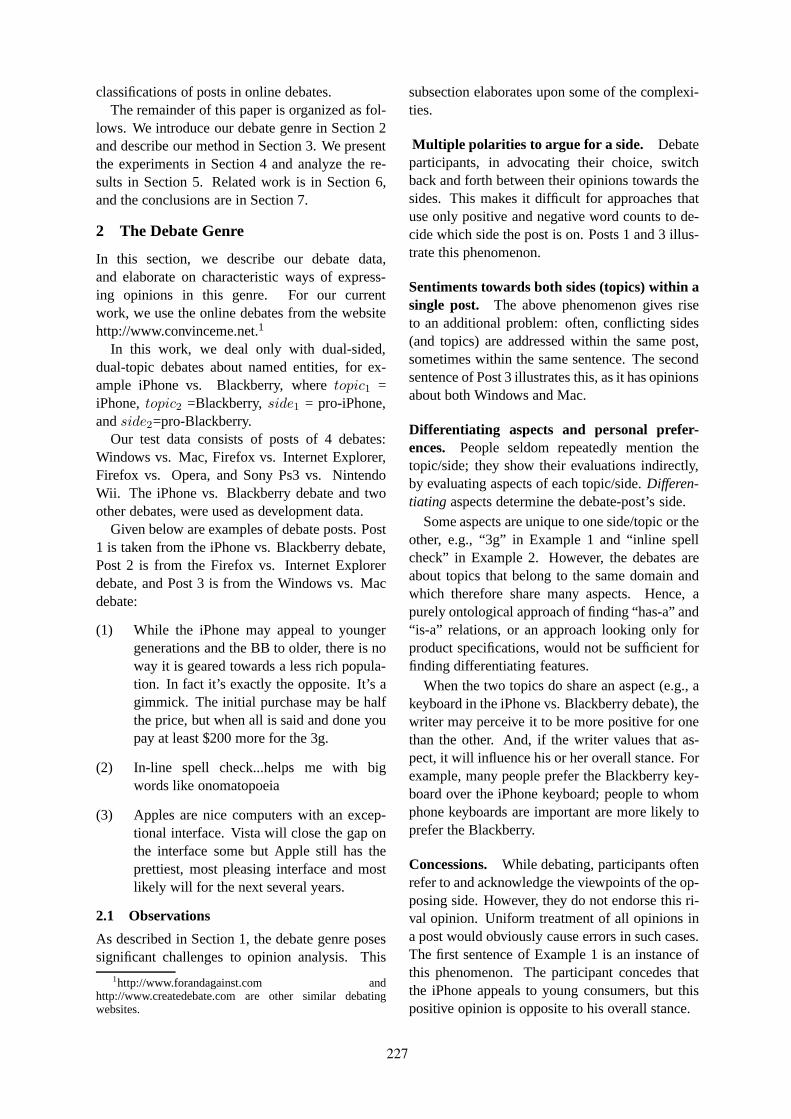
classifications of posts in online debates.The remainder of this paper is organized as fol-
lows. We introduce our debate genre in Section 2and describe our method in Section 3. We presentthe experiments in Section 4 and analyze the re-sults in Section 5. Related work is in Section 6,and the conclusions are in Section 7.
2 The Debate Genre
In this section, we describe our debate data,and elaborate on characteristic ways of express-ing opinions in this genre. For our currentwork, we use the online debates from the websitehttp://www.convinceme.net.1
In this work, we deal only with dual-sided,dual-topic debates about named entities, for ex-ample iPhone vs. Blackberry, wheretopic1 =iPhone,topic2 =Blackberry,side1 = pro-iPhone,andside2=pro-Blackberry.
Our test data consists of posts of 4 debates:Windows vs. Mac, Firefox vs. Internet Explorer,Firefox vs. Opera, and Sony Ps3 vs. NintendoWii. The iPhone vs. Blackberry debate and twoother debates, were used as development data.
Given below are examples of debate posts. Post1 is taken from the iPhone vs. Blackberry debate,Post 2 is from the Firefox vs. Internet Explorerdebate, and Post 3 is from the Windows vs. Macdebate:
(1) While the iPhone may appeal to youngergenerations and the BB to older, there is noway it is geared towards a less rich popula-tion. In fact it’s exactly the opposite. It’s agimmick. The initial purchase may be halfthe price, but when all is said and done youpay at least $200 more for the 3g.
(2) In-line spell check...helps me with bigwords like onomatopoeia
(3) Apples are nice computers with an excep-tional interface. Vista will close the gap onthe interface some but Apple still has theprettiest, most pleasing interface and mostlikely will for the next several years.
2.1 Observations
As described in Section 1, the debate genre posessignificant challenges to opinion analysis. This
1http://www.forandagainst.com andhttp://www.createdebate.com are other similar debatingwebsites.
subsection elaborates upon some of the complexi-ties.
Multiple polarities to argue for a side. Debateparticipants, in advocating their choice, switchback and forth between their opinions towards thesides. This makes it difficult for approaches thatuse only positive and negative word counts to de-cide which side the post is on. Posts 1 and 3 illus-trate this phenomenon.
Sentiments towards both sides (topics) within asingle post. The above phenomenon gives riseto an additional problem: often, conflicting sides(and topics) are addressed within the same post,sometimes within the same sentence. The secondsentence of Post 3 illustrates this, as it has opinionsabout both Windows and Mac.
Differentiating aspects and personal prefer-ences. People seldom repeatedly mention thetopic/side; they show their evaluations indirectly,by evaluating aspects of each topic/side.Differen-tiating aspects determine the debate-post’s side.
Some aspects are unique to one side/topic or theother, e.g., “3g” in Example 1 and “inline spellcheck” in Example 2. However, the debates areabout topics that belong to the same domain andwhich therefore share many aspects. Hence, apurely ontological approach of finding “has-a” and“is-a” relations, or an approach looking only forproduct specifications, would not be sufficient forfinding differentiating features.
When the two topics do share an aspect (e.g., akeyboard in the iPhone vs. Blackberry debate), thewriter may perceive it to be more positive for onethan the other. And, if the writer values that as-pect, it will influence his or her overall stance. Forexample, many people prefer the Blackberry key-board over the iPhone keyboard; people to whomphone keyboards are important are more likely toprefer the Blackberry.
Concessions. While debating, participants oftenrefer to and acknowledge the viewpoints of the op-posing side. However, they do not endorse this ri-val opinion. Uniform treatment of all opinions ina post would obviously cause errors in such cases.The first sentence of Example 1 is an instance ofthis phenomenon. The participant concedes thatthe iPhone appeals to young consumers, but thispositive opinion is opposite to his overall stance.
227
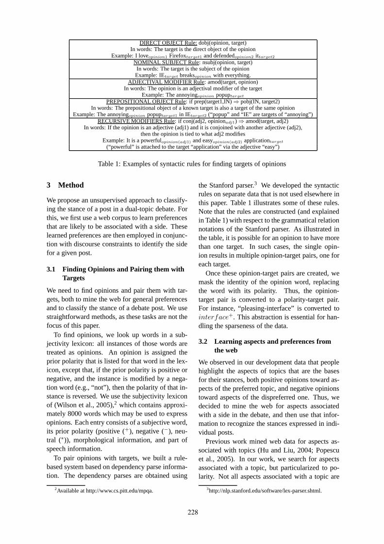
DIRECT OBJECT Rule:dobj(opinion, target)In words: The target is the direct object of the opinion
Example: I loveopinion1 Firefoxtarget1 and defendedopinion2 ittarget2
NOMINAL SUBJECT Rule: nsubj(opinion, target)In words: The target is the subject of the opinionExample: IEtarget breaksopinion with everything.
ADJECTIVAL MODIFIER Rule: amod(target, opinion)In words: The opinion is an adjectival modifier of the target
Example: The annoyingopinion popuptarget
PREPOSITIONAL OBJECT Rule: if prep(target1,IN)⇒ pobj(IN, target2)In words: The prepositional object of a known target is also atarget of the same opinion
Example: The annoyingopinion popuptarget1 in IEtarget2 (“popup” and “IE” are targets of “annoying”)RECURSIVE MODIFIERS Rule: if conj(adj2, opinionadj1) ⇒ amod(target, adj2)
In words: If the opinion is an adjective (adj1) and it is conjoined with another adjective (adj2),then the opinion is tied to what adj2 modifies
Example: It is a powerfulopinion(adj1) and easyopinion(adj2) applicationtarget
(“powerful” is attached to the target “application” via theadjective “easy”)
Table 1: Examples of syntactic rules for finding targets of opinions
3 Method
We propose an unsupervised approach to classify-ing the stance of a post in a dual-topic debate. Forthis, we first use a web corpus to learn preferencesthat are likely to be associated with a side. Theselearned preferences are then employed in conjunc-tion with discourse constraints to identify the sidefor a given post.
3.1 Finding Opinions and Pairing them withTargets
We need to find opinions and pair them with tar-gets, both to mine the web for general preferencesand to classify the stance of a debate post. We usestraightforward methods, as these tasks are not thefocus of this paper.
To find opinions, we look up words in a sub-jectivity lexicon: all instances of those words aretreated as opinions. An opinion is assigned theprior polarity that is listed for that word in the lex-icon, except that, if the prior polarity is positive ornegative, and the instance is modified by a nega-tion word (e.g., “not”), then the polarity of that in-stance is reversed. We use the subjectivity lexiconof (Wilson et al., 2005),2 which contains approxi-mately 8000 words which may be used to expressopinions. Each entry consists of a subjective word,its prior polarity (positive (+), negative (−), neu-tral (∗)), morphological information, and part ofspeech information.
To pair opinions with targets, we built a rule-based system based on dependency parse informa-tion. The dependency parses are obtained using
2Available at http://www.cs.pitt.edu/mpqa.
the Stanford parser.3 We developed the syntacticrules on separate data that is not used elsewhere inthis paper. Table 1 illustrates some of these rules.Note that the rules are constructed (and explainedin Table 1) with respect to the grammatical relationnotations of the Stanford parser. As illustrated inthe table, it is possible for an opinion to have morethan one target. In such cases, the single opin-ion results in multiple opinion-target pairs, one foreach target.
Once these opinion-target pairs are created, wemask the identity of the opinion word, replacingthe word with its polarity. Thus, the opinion-target pair is converted to a polarity-target pair.For instance, “pleasing-interface” is converted tointerface+. This abstraction is essential for han-dling the sparseness of the data.
3.2 Learning aspects and preferences fromthe web
We observed in our development data that peoplehighlight the aspects of topics that are the basesfor their stances, both positive opinions toward as-pects of the preferred topic, and negative opinionstoward aspects of the dispreferred one. Thus, wedecided to mine the web for aspects associatedwith a side in the debate, and then use that infor-mation to recognize the stances expressed in indi-vidual posts.
Previous work mined web data for aspects as-sociated with topics (Hu and Liu, 2004; Popescuet al., 2005). In our work, we search for aspectsassociated with a topic, but particularized to po-larity. Not all aspects associated with a topic are
3http://nlp.stanford.edu/software/lex-parser.shtml.
228
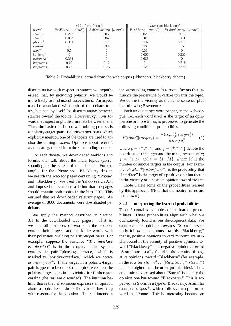
side1 (pro-iPhone) side2 (pro-blackberry)termp P (iPhone+|termp) P (blackberry−|termp) P (iPhone−|termp) P (blackberry+|termp)storm+ 0.227 0.068 0.022 0.613storm− 0.062 0.843 0.06 0.03phone+ 0.333 0.176 0.137 0.313e-mail+ 0 0.333 0.166 0.5ipod+ 0.5 0 0.33 0battery− 0 0 0.666 0.333network− 0.333 0 0.666 0keyboard+ 0.09 0.12 0 0.718keyboard− 0.25 0.25 0.125 0.375
Table 2: Probabilities learned from the web corpus (iPhone vs. blackberry debate)
discriminative with respect to stance; we hypoth-esized that, by including polarity, we would bemore likely to find useful associations. An aspectmay be associated with both of the debate top-ics, but not, by itself, be discriminative betweenstances toward the topics. However,opinionsto-ward that aspect might discriminate between them.Thus, the basic unit in our web mining process isa polarity-target pair. Polarity-target pairs whichexplicitly mention one of the topics are used to an-chor the mining process. Opinions about relevantaspects are gathered from the surrounding context.
For each debate, we downloaded weblogs andforums that talk about the main topics (corre-sponding to the sides) of that debate. For ex-ample, for the iPhone vs. Blackberry debate,we search the web for pages containing “iPhone”and “Blackberry.” We used the Yahoo search APIand imposed the search restriction that the pagesshould contain both topics in the http URL. Thisensured that we downloaded relevant pages. Anaverage of 3000 documents were downloaded perdebate.
We apply the method described in Section3.1 to the downloaded web pages. That is,we find all instances of words in the lexicon,extract their targets, and mask the words withtheir polarities, yielding polarity-target pairs. Forexample, suppose the sentence“The interfaceis pleasing” is in the corpus. The systemextracts the pair “pleasing-interface,” which ismasked to “positive-interface,” which we notateas interface+. If the target in a polarity-targetpair happens to be one of the topics, we select thepolarity-target pairs in its vicinity for further pro-cessing (the rest are discarded). The intuition be-hind this is that, if someone expresses an opinionabout a topic, he or she is likely to follow it upwith reasons for that opinion. The sentiments in
the surrounding context thus reveal factors that in-fluence the preference or dislike towards the topic.We define the vicinity as the same sentence plusthe following 5 sentences.
Each unique target wordtargeti in the web cor-pus, i.e., each word used as the target of an opin-ion one or more times, is processed to generate thefollowing conditional probabilities.
P (topicqj |target
pi ) =
#(topicqj , target
pi )
#targetpi
(1)
wherep = {+,− ,∗ } andq = {+,− ,∗ } denote thepolarities of the target and the topic, respectively;j = {1, 2}; and i = {1...M}, whereM is thenumber of unique targets in the corpus. For exam-ple,P (Mac+|interface+) is the probability that“interface” is the target of a positive opinion that isin the vicinity of a positive opinion toward “Mac.”
Table 2 lists some of the probabilities learnedby this approach. (Note that the neutral cases arenot shown.)
3.2.1 Interpreting the learned probabilities
Table 2 contains examples of the learned proba-bilities. These probabilities align with what wequalitatively found in our development data. Forexample, the opinions towards “Storm” essen-tially follow the opinions towards “Blackberry;”that is, positive opinions toward “Storm” are usu-ally found in the vicinity of positive opinions to-ward “Blackberry,” and negative opinions toward“Storm” are usually found in the vicinity of neg-ative opinions toward “Blackberry” (for example,in the row forstorm+, P (blackberry+|storm+)is much higher than the other probabilities). Thus,an opinion expressed about “Storm” is usually theopinion one has toward “Blackberry.” This is ex-pected, as Storm is a type of Blackberry. A similarexample isipod+, which follows the opinion to-ward the iPhone. This is interesting because an
229

iPod is not a phone; the association is due to pref-erence for the brand. In contrast, the probabilitydistribution for “phone” does not show a prefer-ence for any one side, even though both iPhoneand Blackberry are phones. This indicates thatopinions towards phones in general will not beable to distinguish between the debate sides.
Another interesting case is illustrated by theprobabilities for “e-mail.” People who like e-mailcapability are more likely to praise the Blackberry,or even criticize the iPhone — they would thus be-long to the pro-Blackberry camp.
While we noted earlier that positive evaluationsof keyboards are associated with positive evalua-tions of the Blackberry (by far the highest prob-ability in that row), negative evaluations of key-boards, are, however,not a strong discriminatingfactor.
For the other entries in the table, we see thatcriticisms of batteries and the phone network aremore associated with negative sentiments towardsthe iPhones.
The possibility of these various cases motivatesour approach, in which opinions and their polar-ities are considered when searching for associa-tions between debate topics and their aspects.
3.3 Debate-side classification
Once we have the probabilities collected from theweb, we can build our classifier to classify the de-bate posts.
Here again, we use the process described in Sec-tion 3.1 to extract polarity-target pairs for eachopinion expressed in the post. LetN be the num-ber of instances of polarity-target pairs in the post.For each instanceIj (j = {1...N}), we look upthe learned probabilities of Section 3.2 to createtwo scores,wj anduj :
wj = P (topic+1 |target
pi ) + P (topic−2 |target
pi ) (2)
uj = P (topic−1 |targetpi ) + P (topic+
2 |targetpi ) (3)
wheretargetpi is the polarity-target type of which
Ij is an instance.Scorewj corresponds toside1 and uj corre-
sponds toside2. A point to note is that, if a tar-get word is repeated, and it occurs in differentpolarity-target instances, it is counted as a sepa-rate instance each time — that is, here we accountfor tokens, not types. Via Equations 2 and 3, weinterpret the observed polarity-target instanceIj interms of debate sides.
We formulate the problem of finding the over-all side of the post as an Integer Linear Program-ming (ILP) problem. The side that maximizes theoverall side-score for the post, given all theN in-stancesIj, is chosen by maximizing the objectivefunction
N∑
j=1
(wjxj + ujyj) (4)
subject to the following constraints
xj ∈ {0, 1}, ∀j (5)
yj ∈ {0, 1}, ∀j (6)
xj + yj = 1, ∀j (7)
xj − xj−1 = 0, j ∈ {2..N} (8)
yj − yj−1 = 0, j ∈ {2..N} (9)
Equations 5 and 6 implement binary constraints.Equation 7 enforces the constraint that eachIj canbelong to exactly one side. Finally, Equations 8and 9 ensure that a single side is chosen for theentire post.
3.4 Accounting for concession
As described in Section 2, debate participants of-ten acknowledge the opinions held by the oppos-ing side. We recognize such discourse constructsusing the Penn Discourse Treebank (Prasad et al.,2007) list of discourse connectives. In particu-lar, we use the list of connectives from the Con-cession and Contra-expectation category. Exam-ples of connectives in these categories are “while,”“nonetheless,” “however,” and “even if.” We useapproximations to finding the arguments to thediscourse connectives (ARG1andARG2in PennDiscourse Treebank terms). If the connective ismid-sentence, the part of the sentence prior tothe connective is considered conceded, and thepart that follows the connective is considered non-conceded. An example is the second sentence ofExample 3. If, on the other hand, the connectiveis sentence-initial, the sentence is split at the firstcomma that occurs mid sentence. The first part isconsidered conceded, and the second part is con-sidered non-conceded. An example is the first sen-tence of Example 1.
The opinions occurring in the conceded part areinterpreted in reverse. That is, the weights corre-sponding to the sideswj anduj are interchangedin equation 4. Thus, conceded opinions are effec-tively made to count towards the opposing side.
230

4 Experiments
On http://www.convinceme.net, the html page foreach debate contains side information for eachpost (side1 is blue in color andside2 is green).This gives us automatically labeled data for ourevaluations. For each of the 4 debates in our testset, we use posts with at least 5 sentences for eval-uation.
4.1 Baselines
We implemented two baselines: the OpTopic sys-tem that uses topic information only, and theOpPMI system that uses topic as well as relatedword (noun) information. All systems use thesame lexicon, as well as exactly the same pro-cesses for opinion finding and opinion-target pair-ing.
The OpTopic system This system considersonly explicit mentions of the topic for the opin-ion analysis. Thus, for this system, the stepof opinion-target pairing only finds alltopic+
1 ,topic−1 , topic+
2 , topic−2 instances in the post(where, for example, an instance oftopic+
1 is apositive opinion whose target is explicitlytopic1).The polarity-topic pairs are counted for each de-bate side according to the following equations.
score(side1) = #topic+1 + #topic−2 (10)
score(side2) = #topic−1 + #topic+2 (11)
The post is assigned the side with the higher score.
The OpPMI system This system finds opinion-target pairs for not only the topics, but also for thewords in the debate that are significantly related toeither of the topics.
We find semantic relatedness of each noun inthe post with the two main topics of the debateby calculating the Pointwise Mutual Information(PMI) between the term and each topic over theentire web corpus. We use the API provided by theMeasures of Semantic Relatedness (MSR)4 enginefor this purpose. The MSR engine issues Googlequeries to retrieve documents and finds the PMIbetween any two given words. Table 3 lists PMIsbetween the topics and the words from Table 2.
Each nounk is assigned to the topic with thehigher PMI score. That is, ifPMI(topic1,k) > PMI(topic2,k) ⇒k= topic1
and if4http://cwl-projects.cogsci.rpi.edu/msr/
PMI(topic2,k) > PMI(topic1,k) ⇒k= topic2
Next, the polarity-target pairs are found for thepost, as before, and Equations 10 and 11 are usedto assign a side to the post as in the OpTopicsystem, except that here, related nouns are alsocounted as instances of their associated topics.
word iPhone blackberrystorm 0.923 0.941phone 0.908 0.885e-mail 0.522 0.623ipod 0.909 0.976battery 0.974 0.927network 0.658 0.961keyboard 0.961 0.983
Table 3: PMI of words with the topics
4.2 Results
Performance is measured using the follow-ing metrics: Accuracy (#Correct
#Total posts), Precision
(#Correct#guessed
), Recall (#Correct#relevant
) and F-measure
( 2∗Precision∗Recall(Precision+Recall)).
In our task, it is desirable to make a pre-diction for all the posts; hence#relevant =#Total posts. This results in Recall and Accu-racy being the same. However, all of the systemsdo not classify a post if the post does not con-tain the information it needs. Thus,#guessed ≤#Total posts, and Precision is not the same asAccuracy.
Table 4 reports the performance of four systemson the test data: the two baselines, our methodusing the preferences learned from the web cor-pus (OpPr) and the method additionally using dis-course information to reverse conceded opinions.
The OpTopic has low recall. This is expected,because it relies only on opinions explicitly towardthe topics.
The OpPMI has better recall than OpTopic;however, the precision drops for some debates. Webelieve this is due to the addition of noise. This re-sult suggests that not all terms that are relevant toa topic are useful for determining the debate side.
Finally, both of the OpPr systems are better thanboth baselines in Accuracy as well as F-measurefor all four debates.
The accuracy of the full OpPr system improves,on average, by 35 percentage points over the Op-Topic system, and by 20 percentage points over the
231
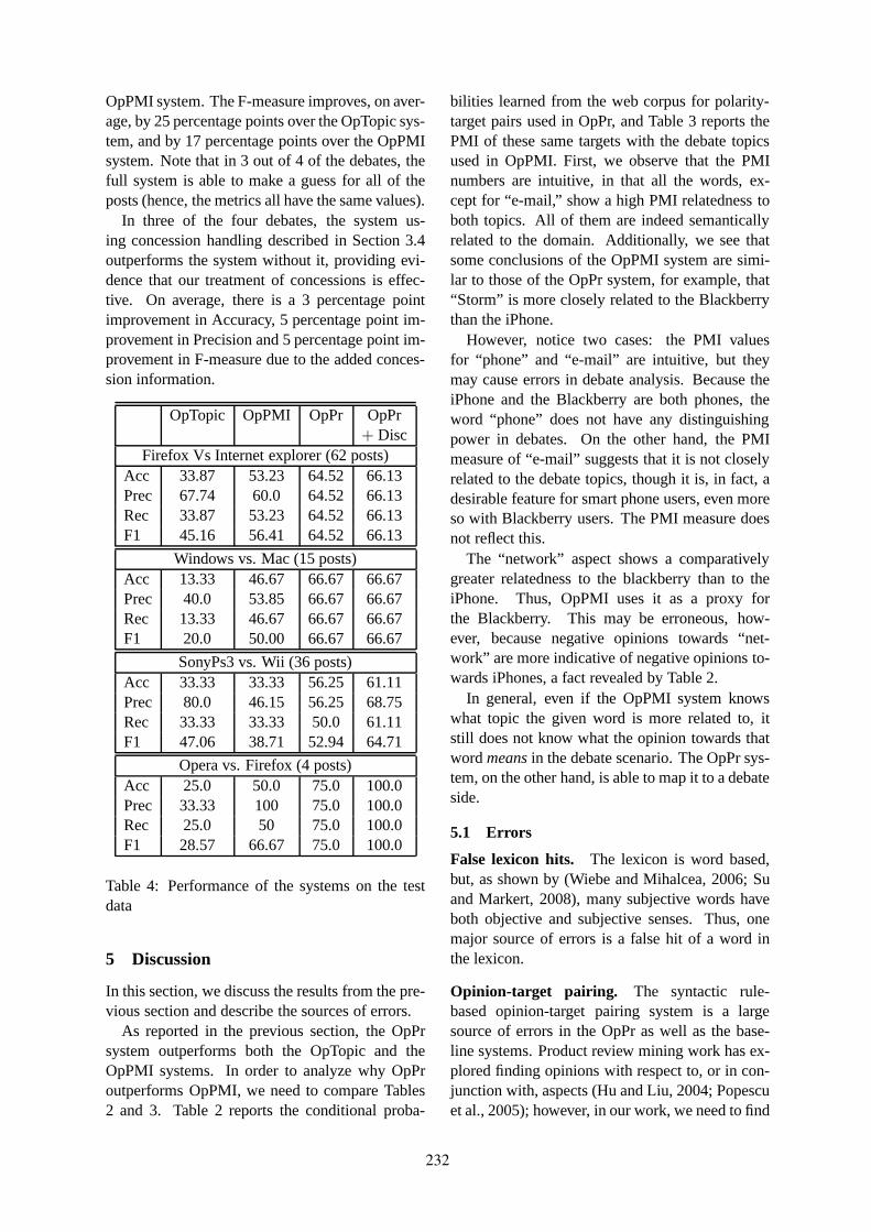
OpPMI system. The F-measure improves, on aver-age, by 25 percentage points over the OpTopic sys-tem, and by 17 percentage points over the OpPMIsystem. Note that in 3 out of 4 of the debates, thefull system is able to make a guess for all of theposts (hence, the metrics all have the same values).
In three of the four debates, the system us-ing concession handling described in Section 3.4outperforms the system without it, providing evi-dence that our treatment of concessions is effec-tive. On average, there is a 3 percentage pointimprovement in Accuracy, 5 percentage point im-provement in Precision and 5 percentage point im-provement in F-measure due to the added conces-sion information.
OpTopic OpPMI OpPr OpPr+ Disc
Firefox Vs Internet explorer (62 posts)Acc 33.87 53.23 64.52 66.13Prec 67.74 60.0 64.52 66.13Rec 33.87 53.23 64.52 66.13F1 45.16 56.41 64.52 66.13
Windows vs. Mac (15 posts)Acc 13.33 46.67 66.67 66.67Prec 40.0 53.85 66.67 66.67Rec 13.33 46.67 66.67 66.67F1 20.0 50.00 66.67 66.67
SonyPs3 vs. Wii (36 posts)Acc 33.33 33.33 56.25 61.11Prec 80.0 46.15 56.25 68.75Rec 33.33 33.33 50.0 61.11F1 47.06 38.71 52.94 64.71
Opera vs. Firefox (4 posts)Acc 25.0 50.0 75.0 100.0Prec 33.33 100 75.0 100.0Rec 25.0 50 75.0 100.0F1 28.57 66.67 75.0 100.0
Table 4: Performance of the systems on the testdata
5 Discussion
In this section, we discuss the results from the pre-vious section and describe the sources of errors.
As reported in the previous section, the OpPrsystem outperforms both the OpTopic and theOpPMI systems. In order to analyze why OpProutperforms OpPMI, we need to compare Tables2 and 3. Table 2 reports the conditional proba-
bilities learned from the web corpus for polarity-target pairs used in OpPr, and Table 3 reports thePMI of these same targets with the debate topicsused in OpPMI. First, we observe that the PMInumbers are intuitive, in that all the words, ex-cept for “e-mail,” show a high PMI relatedness toboth topics. All of them are indeed semanticallyrelated to the domain. Additionally, we see thatsome conclusions of the OpPMI system are simi-lar to those of the OpPr system, for example, that“Storm” is more closely related to the Blackberrythan the iPhone.
However, notice two cases: the PMI valuesfor “phone” and “e-mail” are intuitive, but theymay cause errors in debate analysis. Because theiPhone and the Blackberry are both phones, theword “phone” does not have any distinguishingpower in debates. On the other hand, the PMImeasure of “e-mail” suggests that it is not closelyrelated to the debate topics, though it is, in fact, adesirable feature for smart phone users, even moreso with Blackberry users. The PMI measure doesnot reflect this.
The “network” aspect shows a comparativelygreater relatedness to the blackberry than to theiPhone. Thus, OpPMI uses it as a proxy forthe Blackberry. This may be erroneous, how-ever, because negative opinions towards “net-work” are more indicative of negative opinions to-wards iPhones, a fact revealed by Table 2.
In general, even if the OpPMI system knowswhat topic the given word is more related to, itstill does not know what the opinion towards thatwordmeansin the debate scenario. The OpPr sys-tem, on the other hand, is able to map it to a debateside.
5.1 Errors
False lexicon hits. The lexicon is word based,but, as shown by (Wiebe and Mihalcea, 2006; Suand Markert, 2008), many subjective words haveboth objective and subjective senses. Thus, onemajor source of errors is a false hit of a word inthe lexicon.
Opinion-target pairing. The syntactic rule-based opinion-target pairing system is a largesource of errors in the OpPr as well as the base-line systems. Product review mining work has ex-plored finding opinions with respect to, or in con-junction with, aspects (Hu and Liu, 2004; Popescuet al., 2005); however, in our work, we need to find
232
information in the other direction – that is, giventhe opinion, what is the opinion about. Stoyanovand Cardie (2008) work on opinion co-reference;however, we need to identify the specific target.
Pragmatic opinions. Some of the errors are dueto the fact that the opinions expressed in the postare pragmatic. This becomes a problem especiallywhen the debate post is small, and we have fewother lexical clues in the post. The following postis an example:
(4) The blackberry is something like $150 andthe iPhone is $500. I don’t think it’s worthit. You could buy a iPod separate and havea boatload of extra money left over.
In this example, the participant mentions thedifference in the prices in the first sentence. Thissentence implies a negative opinion towards theiPhone. However, recognizing this would requirea system to have extensive world knowledge. Inthe second sentence, the lexicon does hit the word“worth,” and, using syntactic rules, we can deter-mine it is negated. However, the opinion-targetpairing system only tells us that the opinion is tiedto the “it.” A co-reference system would be neededto tie the “it” to “iPhone” in the first sentence.
6 Related Work
Several researchers have worked on similar tasks.Kim and Hovy (2007) predict the results of anelection by analyzing forums discussing the elec-tions. Theirs is a supervised bag-of-words sys-tem using unigrams, bigrams, and trigrams as fea-tures. In contrast, our approach is unsupervised,and exploits different types of information. Bansalet al. (2008) predict the vote from congressionalfloor debates using agreement/disagreement fea-tures. We do not model inter-personal exchanges;instead, we model factors that influence stancetaking. Lin at al (2006) identify opposing perspec-tives. Though apparently related at the task level,perspectives as they define them are not the sameas opinions. Their approach does not involve anyopinion analysis. Fujii and Ishikawa (2006) alsowork with arguments. However, their focus is onargument visualization rather than on recognizingstances.
Other researchers have also mined data to learnassociations among products and features. Intheir work on mining opinions in comparative sen-tences, Ganapathibhotla and Liu (2008) look for
user preferences for one product’s features overanother’s. We do not exploit comparative con-structs, but rather probabilistic associations. Thus,our approach and theirs are complementary. Anumber of works in product review mining (Huand Liu, 2004; Popescu et al., 2005; Kobayashi etal., 2005; Bloom et al., 2007) automatically findfeatures of the reviewed products. However, ourapproach is novel in that it learns and exploits as-sociations among opinion/polarity, topics, and as-pects.
Several researchers have recognized the im-portant role discourse plays in opinion analysis(Polanyi and Zaenen, 2005; Snyder and Barzilay,2007; Somasundaran et al., 2008; Asher et al.,2008; Sadamitsu et al., 2008). However, previouswork did not account for concessions in determin-ing whether an opinion supports one side or theother.
More sophisticated approaches to identifyingopinions and recognizing their contextual polar-ity have been published (e.g., (Wilson et al., 2005;Ikeda et al., 2008; Sadamitsu et al., 2008)). Thosecomponents are not the focus of our work.
7 Conclusions
This paper addresses challenges faced by opinionanalysis in the debate genre. In our method, fac-tors that influence the choice of a debate side arelearned by mining a web corpus for opinions. Thisknowledge is exploited in an unsupervised methodfor classifying the side taken by a post, which alsoaccounts for concessionary opinions.
Our results corroborate our hypothesis that find-ing relations between aspects associated with atopic, but particularized to polarity, is more effec-tive than finding relations between topics and as-pects alone. The system that implements this in-formation, mined from the web, outperforms theweb PMI-based baseline. Our hypothesis that ad-dressing concessionary opinions is useful is alsocorroborated by improved performance.
Acknowledgments
This research was supported in part by theDepartment of Homeland Security under grantN000140710152. We would also like to thankVladislav D. Veksler for help with the MSR en-gine, and the anonymous reviewers for their help-ful comments.
233

References
Nicholas Asher, Farah Benamara, and Yvette YannickMathieu. 2008. Distilling opinion in discourse:A preliminary study. InColing 2008: Companionvolume: Posters and Demonstrations, pages 5–8,Manchester, UK, August.
Mohit Bansal, Claire Cardie, and Lillian Lee. 2008.The power of negative thinking: Exploiting labeldisagreement in the min-cut classification frame-work. In Proceedings of COLING: Companion vol-ume: Posters.
Kenneth Bloom, Navendu Garg, and Shlomo Argamon.2007. Extracting appraisal expressions. InHLT-NAACL 2007, pages 308–315, Rochester, NY.
Atsushi Fujii and Tetsuya Ishikawa. 2006. A sys-tem for summarizing and visualizing arguments insubjective documents: Toward supporting decisionmaking. InProceedings of the Workshop on Senti-ment and Subjectivity in Text, pages 15–22, Sydney,Australia, July. Association for Computational Lin-guistics.
Murthy Ganapathibhotla and Bing Liu. 2008. Miningopinions in comparative sentences. InProceedingsof the 22nd International Conference on Compu-tational Linguistics (Coling 2008), pages 241–248,Manchester, UK, August.
Minqing Hu and Bing Liu. 2004. Mining opinion fea-tures in customer reviews. InAAAI-2004.
Daisuke Ikeda, Hiroya Takamura, Lev-Arie Ratinov,and Manabu Okumura. 2008. Learning to shiftthe polarity of words for sentiment classification. InProceedings of the Third International Joint Confer-ence on Natural Language Processing (IJCNLP).
Soo-Min Kim and Eduard Hovy. 2007. Crystal: An-alyzing predictive opinions on the web. InPro-ceedings of the 2007 Joint Conference on EmpiricalMethods in Natural Language Processing and Com-putational Natural Language Learning (EMNLP-CoNLL), pages 1056–1064.
Nozomi Kobayashi, Ryu Iida, Kentaro Inui, and YujiMatsumoto. 2005. Opinion extraction using alearning-based anaphora resolution technique. InProceedings of the 2nd International Joint Confer-ence on Natural Language Processing (IJCNLP-05),poster, pages 175–180.
Wei-Hao Lin, Theresa Wilson, Janyce Wiebe, andAlexander Hauptmann. 2006. Which side are youon? Identifying perspectives at the document andsentence levels. InProceedings of the 10th Con-ference on Computational Natural Language Learn-ing (CoNLL-2006), pages 109–116, New York, NewYork.
Livia Polanyi and Annie Zaenen. 2005. Contextualvalence shifters. InComputing Attitude and Affectin Text. Springer.
Ana-Maria Popescu, Bao Nguyen, and Oren Et-zioni. 2005. OPINE: Extracting product fea-tures and opinions from reviews. InProceedingsof HLT/EMNLP 2005 Interactive Demonstrations,pages 32–33, Vancouver, British Columbia, Canada,October. Association for Computational Linguistics.
R. Prasad, E. Miltsakaki, N. Dinesh, A. Lee, A. Joshi,L. Robaldo, and B. Webber, 2007.PDTB 2.0 Anno-tation Manual.
Kugatsu Sadamitsu, Satoshi Sekine, and Mikio Ya-mamoto. 2008. Sentiment analysis based onprobabilistic models using inter-sentence informa-tion. In European Language Resources Associa-tion (ELRA), editor, Proceedings of the Sixth In-ternational Language Resources and Evaluation(LREC’08), Marrakech, Morocco, May.
Benjamin Snyder and Regina Barzilay. 2007. Multipleaspect ranking using the good grief algorithm. InProceedings of NAACL-2007.
Swapna Somasundaran, Janyce Wiebe, and Josef Rup-penhofer. 2008. Discourse level opinion interpre-tation. In Proceedings of the 22nd InternationalConference on Computational Linguistics (Coling2008), pages 801–808, Manchester, UK, August.
Veselin Stoyanov and Claire Cardie. 2008. Topicidentification for fine-grained opinion analysis. InProceedings of the 22nd International Conferenceon Computational Linguistics (Coling 2008), pages817–824, Manchester, UK, August. Coling 2008 Or-ganizing Committee.
Fangzhong Su and Katja Markert. 2008. Fromword to sense: a case study of subjectivity recogni-tion. In Proceedings of the 22nd International Con-ference on Computational Linguistics (COLING-2008), Manchester, UK, August.
Janyce Wiebe and Rada Mihalcea. 2006. Word senseand subjectivity. InProceedings of COLING-ACL2006.
Theresa Wilson, Janyce Wiebe, and Paul Hoffmann.2005. Recognizing contextual polarity in phrase-level sentiment analysis. InHLT-EMNLP, pages347–354, Vancouver, Canada.
234
Proceedings of the 47th Annual Meeting of the ACL and the 4th IJCNLP of the AFNLP, pages 235–243,Suntec, Singapore, 2-7 August 2009. c©2009 ACL and AFNLP
Co-Training for Cross-Lingual Sentiment Classification
Xiaojun Wan
Institute of Compute Science and Technology & Key Laboratory of Computational Lin-guistics, MOE
Peking University, Beijing 100871, China [email protected]
Abstract
The lack of Chinese sentiment corpora limits the research progress on Chinese sentiment classification. However, there are many freely available English sentiment corpora on the Web. This paper focuses on the problem of cross-lingual sentiment classification, which leverages an available English corpus for Chi-nese sentiment classification by using the Eng-lish corpus as training data. Machine transla-tion services are used for eliminating the lan-guage gap between the training set and test set, and English features and Chinese features are considered as two independent views of the classification problem. We propose a co-training approach to making use of unlabeled Chinese data. Experimental results show the effectiveness of the proposed approach, which can outperform the standard inductive classifi-ers and the transductive classifiers.
1 Introduction
Sentiment classification is the task of identifying the sentiment polarity of a given text. The senti-ment polarity is usually positive or negative and the text genre is usually product review. In recent years, sentiment classification has drawn much attention in the NLP field and it has many useful applications, such as opinion mining and summa-rization (Liu et al., 2005; Ku et al., 2006; Titov and McDonald, 2008).
To date, a variety of corpus-based methods have been developed for sentiment classification. The methods usually rely heavily on an anno-tated corpus for training the sentiment classifier. The sentiment corpora are considered as the most valuable resources for the sentiment classifica-tion task. However, such resources in different languages are very imbalanced. Because most previous work focuses on English sentiment classification, many annotated corpora for Eng-lish sentiment classification are freely available on the Web. However, the annotated corpora for
Chinese sentiment classification are scarce and it is not a trivial task to manually label reliable Chinese sentiment corpora. The challenge before us is how to leverage rich English corpora for Chinese sentiment classification. In this study, we focus on the problem of cross-lingual senti-ment classification, which leverages only English training data for supervised sentiment classifica-tion of Chinese product reviews, without using any Chinese resources. Note that the above prob-lem is not only defined for Chinese sentiment classification, but also for various sentiment analysis tasks in other different languages.
Though pilot studies have been performed to make use of English corpora for subjectivity classification in other languages (Mihalcea et al., 2007; Banea et al., 2008), the methods are very straightforward by directly employing an induc-tive classifier (e.g. SVM, NB), and the classifica-tion performance is far from satisfactory because of the language gap between the original lan-guage and the translated language.
In this study, we propose a co-training ap-proach to improving the classification accuracy of polarity identification of Chinese product re-views. Unlabeled Chinese reviews can be fully leveraged in the proposed approach. First, ma-chine translation services are used to translate English training reviews into Chinese reviews and also translate Chinese test reviews and addi-tional unlabeled reviews into English reviews. Then, we can view the classification problem in two independent views: Chinese view with only Chinese features and English view with only English features. We then use the co-training approach to making full use of the two redundant views of features. The SVM classifier is adopted as the basic classifier in the proposed approach. Experimental results show that the proposed ap-proach can outperform the baseline inductive classifiers and the more advanced transductive classifiers.
The rest of this paper is organized as follows: Section 2 introduces related work. The proposed
235
co-training approach is described in detail in Section 3. Section 4 shows the experimental re-sults. Lastly we conclude this paper in Section 5.
2 Related Work 2.1 Sentiment Classification
Sentiment classification can be performed on words, sentences or documents. In this paper we focus on document sentiment classification. The methods for document sentiment classification can be generally categorized into lexicon-based and corpus-based.
Lexicon-based methods usually involve deriv-ing a sentiment measure for text based on senti-ment lexicons. Turney (2002) predicates the sen-timent orientation of a review by the average se-mantic orientation of the phrases in the review that contain adjectives or adverbs, which is de-noted as the semantic oriented method. Kim and Hovy (2004) build three models to assign a sen-timent category to a given sentence by combin-ing the individual sentiments of sentiment-bearing words. Hiroshi et al. (2004) use the tech-nique of deep language analysis for machine translation to extract sentiment units in text documents. Kennedy and Inkpen (2006) deter-mine the sentiment of a customer review by counting positive and negative terms and taking into account contextual valence shifters, such as negations and intensifiers. Devitt and Ahmad (2007) explore a computable metric of positive or negative polarity in financial news text.
Corpus-based methods usually consider the sentiment analysis task as a classification task and they use a labeled corpus to train a sentiment classifier. Since the work of Pang et al. (2002), various classification models and linguistic fea-tures have been proposed to improve the classifi-cation performance (Pang and Lee, 2004; Mullen and Collier, 2004; Wilson et al., 2005; Read, 2005). Most recently, McDonald et al. (2007) investigate a structured model for jointly classi-fying the sentiment of text at varying levels of granularity. Blitzer et al. (2007) investigate do-main adaptation for sentiment classifiers, focus-ing on online reviews for different types of prod-ucts. Andreevskaia and Bergler (2008) present a new system consisting of the ensemble of a cor-pus-based classifier and a lexicon-based classi-fier with precision-based vote weighting.
Chinese sentiment analysis has also been stud-ied (Tsou et al., 2005; Ye et al., 2006; Li and Sun, 2007) and most such work uses similar lexicon-
based or corpus-based methods for Chinese sen-timent classification.
To date, several pilot studies have been per-formed to leverage rich English resources for sentiment analysis in other languages. Standard Naïve Bayes and SVM classifiers have been ap-plied for subjectivity classification in Romanian (Mihalcea et al., 2007; Banea et al., 2008), and the results show that automatic translation is a viable alternative for the construction of re-sources and tools for subjectivity analysis in a new target language. Wan (2008) focuses on lev-eraging both Chinese and English lexicons to improve Chinese sentiment analysis by using lexicon-based methods. In this study, we focus on improving the corpus-based method for cross-lingual sentiment classification of Chinese prod-uct reviews by developing novel approaches.
2.2 Cross-Domain Text Classification
Cross-domain text classification can be consid-ered as a more general task than cross-lingual sentiment classification. In the problem of cross-domain text classification, the labeled and unla-beled data come from different domains, and their underlying distributions are often different from each other, which violates the basic as-sumption of traditional classification learning.
To date, many semi-supervised learning algo-rithms have been developed for addressing the cross-domain text classification problem by transferring knowledge across domains, includ-ing Transductive SVM (Joachims, 1999), EM(Nigam et al., 2000), EM-based Naïve Bayes classifier (Dai et al., 2007a), Topic-bridged PLSA (Xue et al., 2008), Co-Clustering based classification (Dai et al., 2007b), two-stage ap-proach (Jiang and Zhai, 2007). DauméIII and Marcu (2006) introduce a statistical formulation of this problem in terms of a simple mixture model.
In particular, several previous studies focus on the problem of cross-lingual text classification, which can be considered as a special case of general cross-domain text classification. Bel et al. (2003) present practical and cost-effective solu-tions. A few novel models have been proposed to address the problem, e.g. the EM-based algo-rithm (Rigutini et al., 2005), the information bot-tleneck approach (Ling et al., 2008), the multi-lingual domain models (Gliozzo and Strapparava, 2005), etc. To the best of our knowledge, co-training has not yet been investigated for cross-domain or cross-lingual text classification.
236
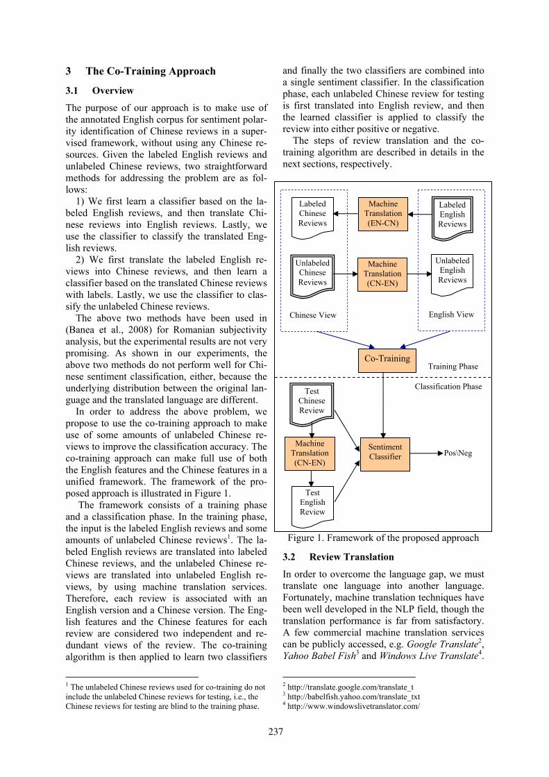
3 The Co-Training Approach
3.1 Overview
The purpose of our approach is to make use of the annotated English corpus for sentiment polar-ity identification of Chinese reviews in a super-vised framework, without using any Chinese re-sources. Given the labeled English reviews and unlabeled Chinese reviews, two straightforward methods for addressing the problem are as fol-lows:
1) We first learn a classifier based on the la-beled English reviews, and then translate Chi-nese reviews into English reviews. Lastly, we use the classifier to classify the translated Eng-lish reviews.
2) We first translate the labeled English re-views into Chinese reviews, and then learn a classifier based on the translated Chinese reviews with labels. Lastly, we use the classifier to clas-sify the unlabeled Chinese reviews.
The above two methods have been used in (Banea et al., 2008) for Romanian subjectivity analysis, but the experimental results are not very promising. As shown in our experiments, the above two methods do not perform well for Chi-nese sentiment classification, either, because the underlying distribution between the original lan-guage and the translated language are different.
In order to address the above problem, we propose to use the co-training approach to make use of some amounts of unlabeled Chinese re-views to improve the classification accuracy. The co-training approach can make full use of both the English features and the Chinese features in a unified framework. The framework of the pro-posed approach is illustrated in Figure 1.
The framework consists of a training phase and a classification phase. In the training phase, the input is the labeled English reviews and some amounts of unlabeled Chinese reviews1. The la-beled English reviews are translated into labeled Chinese reviews, and the unlabeled Chinese re-views are translated into unlabeled English re-views, by using machine translation services. Therefore, each review is associated with an English version and a Chinese version. The Eng-lish features and the Chinese features for each review are considered two independent and re-dundant views of the review. The co-training algorithm is then applied to learn two classifiers
1 The unlabeled Chinese reviews used for co-training do not include the unlabeled Chinese reviews for testing, i.e., the Chinese reviews for testing are blind to the training phase.
and finally the two classifiers are combined into a single sentiment classifier. In the classification phase, each unlabeled Chinese review for testing is first translated into English review, and then the learned classifier is applied to classify the review into either positive or negative.
The steps of review translation and the co-training algorithm are described in details in the next sections, respectively.
Figure 1. Framework of the proposed approach
3.2 Review Translation
In order to overcome the language gap, we must translate one language into another language. Fortunately, machine translation techniques have been well developed in the NLP field, though the translation performance is far from satisfactory. A few commercial machine translation services can be publicly accessed, e.g. Google Translate2, Yahoo Babel Fish3 and Windows Live Translate4.
2 http://translate.google.com/translate_t 3 http://babelfish.yahoo.com/translate_txt 4 http://www.windowslivetranslator.com/
Unlabeled Chinese Reviews
Labeled English Reviews
Machine Translation (CN-EN)
Co-Training
Machine Translation (EN-CN)
Labeled Chinese Reviews
Unlabeled English Reviews
Pos\Neg
Chinese View English View
Test Chinese Review
Sentiment Classifier
Machine Translation (CN-EN)
Test English Review
Training Phase
Classification Phase
237
In this study, we adopt Google Translate for both English-to-Chinese Translation and Chinese-to-English Translation, because it is one of the state-of-the-art commercial machine translation systems used today. Google Translate applies statistical learning techniques to build a transla-tion model based on both monolingual text in the target language and aligned text consisting of examples of human translations between the lan-guages.
3.3 The Co-Training Algorithm
The co-training algorithm (Blum and Mitchell, 1998) is a typical bootstrapping method, which starts with a set of labeled data, and increase the amount of annotated data using some amounts of unlabeled data in an incremental way. One im-portant aspect of co-training is that two condi-tional independent views are required for co-training to work, but the independence assump-tion can be relaxed. Till now, co-training has been successfully applied to statistical parsing (Sarkar, 2001), reference resolution (Ng and Cardie, 2003), part of speech tagging (Clark et al., 2003), word sense disambiguation (Mihalcea, 2004) and email classification (Kiritchenko and Matwin, 2001).
In the context of cross-lingual sentiment clas-sification, each labeled English review or unla-beled Chinese review has two views of features: English features and Chinese features. Here, a review is used to indicate both its Chinese ver-sion and its English version, until stated other-wise. The co-training algorithm is illustrated in Figure 2. In the algorithm, the class distribution in the labeled data is maintained by balancing the parameter values of p and n at each iteration.
The intuition of the co-training algorithm is that if one classifier can confidently predict the class of an example, which is very similar to some of labeled ones, it can provide one more training example for the other classifier. But, of course, if this example happens to be easy to be classified by the first classifier, it does not mean that this example will be easy to be classified by the second classifier, so the second classifier will get useful information to improve itself and vice versa (Kiritchenko and Matwin, 2001).
In the co-training algorithm, a basic classifica-tion algorithm is required to construct Cen and Ccn. Typical text classifiers include Support Vec-tor Machine (SVM), Naïve Bayes (NB), Maxi-mum Entropy (ME), K-Nearest Neighbor (KNN), etc. In this study, we adopt the widely-used SVM classifier (Joachims, 2002). Viewing input data
as two sets of vectors in a feature space, SVM constructs a separating hyperplane in the space by maximizing the margin between the two data sets. The English or Chinese features used in this study include both unigrams and bigrams5 and the feature weight is simply set to term fre-quency6. Feature selection methods (e.g. Docu-ment Frequency (DF), Information Gain (IG), and Mutual Information (MI)) can be used for dimension reduction. But we use all the features in the experiments for comparative analysis, be-cause there is no significant performance im-provement after applying the feature selection techniques in our empirical study. The output value of the SVM classifier for a review indi-cates the confidence level of the review’s classi-fication. Usually, the sentiment polarity of a re-view is indicated by the sign of the prediction value.
Given: - Fen and Fcn are redundantly sufficient
sets of features, where Fen represents the English features, Fcn represents the Chinese features;
- L is a set of labeled training reviews; - U is a set of unlabeled reviews;
Loop for I iterations: 1. Learn the first classifier Cen from L
based on Fen; 2. Use Cen to label reviews from U
based on Fen; 3. Choose p positive and n negative the
most confidently predicted reviews Een from U;
4. Learn the second classifier Ccn from L based on Fcn;
5. Use Ccn to label reviews from U based on Fcn;
6. Choose p positive and n negative the most confidently predicted reviews Ecn from U;
7. Removes reviews Een∪Ecn from U7; 8. Add reviews Een∪Ecn with the corre-
sponding labels to L; Figure 2. The co-training algorithm
In the training phase, the co-training algorithm learns two separate classifiers: Cen and Ccn. 5 For Chinese text, a unigram refers to a Chinese word and a bigram refers to two adjacent Chinese words. 6 Term frequency performs better than TFIDF by our em-pirical analysis. 7 Note that the examples with conflicting labels are not in-cluded in Een∪Ecn In other words, if an example is in both Een and Ecn, but the labels for the example is conflicting, the example will be excluded from Een∪Ecn.
238
Therefore, in the classification phase, we can obtain two prediction values for a test review. We normalize the prediction values into [-1, 1] by dividing the maximum absolute value. Finally, the average of the normalized values is used as the overall prediction value of the review.
4 Empirical Evaluation 4.1 Evaluation Setup
4.1.1 Data set
The following three datasets were collected and used in the experiments:
Test Set (Labeled Chinese Reviews): In or-der to assess the performance of the proposed approach, we collected and labeled 886 product reviews (451 positive reviews + 435 negative reviews) from a popular Chinese IT product web site-IT1688. The reviews focused on such prod-ucts as mp3 players, mobile phones, digital cam-era and laptop computers.
Training Set (Labeled English Reviews): There are many labeled English corpora avail-able on the Web and we used the corpus con-structed for multi-domain sentiment classifica-tion (Blitzer et al., 2007)9, because the corpus was large-scale and it was within similar do-mains as the test set. The dataset consisted of 8000 Amazon product reviews (4000 positive reviews + 4000 negative reviews) for four differ-ent product types: books, DVDs, electronics and kitchen appliances.
Unlabeled Set (Unlabeled Chinese Reviews): We downloaded additional 1000 Chinese product reviews from IT168 and used the reviews as the unlabeled set. Therefore, the unlabeled set and the test set were in the same domain and had similar underlying feature distributions.
Each Chinese review was translated into Eng-lish review, and each English review was trans-lated into Chinese review. Therefore, each re-view has two independent views: English view and Chinese view. A review is represented by both its English view and its Chinese view.
Note that the training set and the unlabeled set are used in the training phase, while the test set is blind to the training phase.
4.1.2 Evaluation Metric
We used the standard precision, recall and F-measure to measure the performance of positive and negative class, respectively, and used the 8 http://www.it168.com 9 http://www.cis.upenn.edu/~mdredze/datasets/sentiment/
accuracy metric to measure the overall perform-ance of the system. The metrics are defined the same as in general text categorization.
4.1.3 Baseline Methods
In the experiments, the proposed co-training ap-proach (CoTrain) is compared with the following baseline methods:
SVM(CN): This method applies the inductive SVM with only Chinese features for sentiment classification in the Chinese view. Only English-to-Chinese translation is needed. And the unla-beled set is not used.
SVM(EN): This method applies the inductive SVM with only English features for sentiment classification in the English view. Only Chinese-to-English translation is needed. And the unla-beled set is not used.
SVM(ENCN1): This method applies the in-ductive SVM with both English and Chinese fea-tures for sentiment classification in the two views. Both English-to-Chinese and Chinese-to-English translations are required. And the unla-beled set is not used.
SVM(ENCN2): This method combines the re-sults of SVM(EN) and SVM(CN) by averaging the prediction values in the same way with the co-training approach.
TSVM(CN): This method applies the trans-ductive SVM with only Chinese features for sen-timent classification in the Chinese view. Only English-to-Chinese translation is needed. And the unlabeled set is used.
TSVM(EN): This method applies the trans-ductive SVM with only English features for sen-timent classification in the English view. Only Chinese-to-English translation is needed. And the unlabeled set is used.
TSVM(ENCN1): This method applies the transductive SVM with both English and Chinese features for sentiment classification in the two views. Both English-to-Chinese and Chinese-to-English translations are required. And the unla-beled set is used.
TSVM(ENCN2): This method combines the results of TSVM(EN) and TSVM(CN) by aver-aging the prediction values.
Note that the first four methods are straight-forward methods used in previous work, while the latter four methods are strong baselines be-cause the transductive SVM has been widely used for improving the classification accuracy by leveraging additional unlabeled examples.
239

4.2 Evaluation Results
4.2.1 Method Comparison
In the experiments, we first compare the pro-posed co-training approach (I=40 and p=n=5) with the eight baseline methods. The three pa-rameters in the co-training approach are empiri-cally set by considering the total number (i.e. 1000) of the unlabeled Chinese reviews. In our empirical study, the proposed approach can per-form well with a wide range of parameter values, which will be shown later. Table 1 shows the comparison results.
Seen from the table, the proposed co-training approach outperforms all eight baseline methods over all metrics. Among the eight baselines, the best one is TSVM(ENCN2), which combines the results of two transductive SVM classifiers. Ac-tually, TSVM(ENCN2) is similar to CoTrain because CoTrain also combines the results of two classifiers in the same way. However, the co-training approach can train two more effective classifiers, and the accuracy values of the com-ponent English and Chinese classifiers are 0.775 and 0.790, respectively, which are higher than the corresponding TSVM classifiers. Overall, the use of transductive learning and the combination of English and Chinese views are beneficial to the final classification accuracy, and the co-training approach is more suitable for making use of the unlabeled Chinese reviews than the transductive SVM.
4.2.2 Influences of Iteration Number (I)
Figure 3 shows the accuracy curve of the co-training approach (Combined Classifier) with different numbers of iterations. The iteration number I is varied from 1 to 80. When I is set to 1, the co-training approach is degenerated into SVM(ENCN2). The accuracy curves of the com-ponent English and Chinese classifiers learned in the co-training approach are also shown in the
figure. We can see that the proposed co-training approach can outperform the best baseline-TSVM(ENCN2) after 20 iterations. After a large number of iterations, the performance of the co-training approach decreases because noisy train-ing examples may be selected from the remain-ing unlabeled set. Finally, the performance of the approach does not change any more, because the algorithm runs out of all possible examples in the unlabeled set. Fortunately, the proposed ap-proach performs well with a wide range of itera-tion numbers. We can also see that the two com-ponent classifier has similar trends with the co-training approach. It is encouraging that the com-ponent Chinese classifier alone can perform bet-ter than the best baseline when the iteration number is set between 40 and 70.
4.2.3 Influences of Growth Size (p, n)
Figure 4 shows how the growth size at each it-eration (p positive and n negative confident ex-amples) influences the accuracy of the proposed co-training approach. In the above experiments, we set p=n, which is considered as a balanced growth. When p differs very much from n, the growth is considered as an imbalanced growth. Balanced growth of (2, 2), (5, 5), (10, 10) and (15, 15) examples and imbalanced growth of (1, 5), (5, 1) examples are compared in the figure. We can see that the performance of the co-training approach with the balanced growth can be improved after a few iterations. And the per-formance of the co-training approach with large p and n will more quickly become unchanged, because the approach runs out of the limited ex-amples in the unlabeled set more quickly. How-ever, the performance of the co-training ap-proaches with the two imbalanced growths is always going down quite rapidly, because the labeled unbalanced examples hurt the perform-ance badly at each iteration.
Positive Negative Total Method Precision Recall F-measure Precision Recall F-measure Accuracy
SVM(CN) 0.733 0.865 0.793 0.828 0.674 0.743 0.771 SVM(EN) 0.717 0.803 0.757 0.766 0.671 0.716 0.738
SVM(ENCN1) 0.744 0.820 0.781 0.792 0.708 0.748 0.765 SVM(ENCN2) 0.746 0.847 0.793 0.816 0.701 0.754 0.775
TSVM(CN) 0.724 0.878 0.794 0.838 0.653 0.734 0.767 TSVM(EN) 0.732 0.860 0.791 0.823 0.674 0.741 0.769
TSVM(ENCN1) 0.743 0.878 0.805 0.844 0.685 0.756 0.783 TSVM(ENCN2) 0.744 0.896 0.813 0.863 0.680 0.761 0.790
CoTrain (I=40; p=n=5) 0.768 0.905 0.831 0.879 0.717 0.790 0.813
Table 1. Comparison results
240
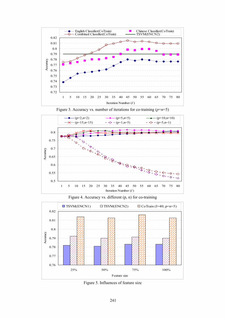
0.72
0.73
0.740.75
0.76
0.77
0.78
0.790.8
0.81
0.82
1 5 10 15 20 25 30 35 40 45 50 55 60 65 70 75 80
Iteration Number (I )
Acc
urac
y
English Classifier(CoTrain) Chinese Classifier(CoTrain)Combined Classifier(CoTrain) TSVM(ENCN2)
Figure 3. Accuracy vs. number of iterations for co-training (p=n=5)
0.5
0.55
0.6
0.65
0.7
0.75
0.8
1 5 10 15 20 25 30 35 40 45 50 55 60 65 70 75 80Iteration Number (I )
Acc
urac
y
(p=2,n=2) (p=5,n=5) (p=10,n=10)(p=15,n=15) (p=1,n=5) (p=5,n=1)
Figure 4. Accuracy vs. different (p, n) for co-training
0.76
0.77
0.78
0.79
0.8
0.81
0.82
25% 50% 75% 100%
Feature size
Acc
urac
y
TSVM(ENCN1) TSVM(ENCN2) CoTrain (I=40; p=n=5)
Figure 5. Influences of feature size
241

4.2.4 Influences of Feature Selection
In the above experiments, all features (unigram + bigram) are used. As mentioned earlier, feature selection techniques are widely used for dimen-sion reduction. In this section, we further con-duct experiments to investigate the influences of feature selection techniques on the classification results. We use the simple but effective docu-ment frequency (DF) for feature selection. Fig-ures 6 show the comparison results of different feature sizes for the co-training approach and two strong baselines. The feature size is meas-ured as the proportion of the selected features against the total features (i.e. 100%).
We can see from the figure that the feature se-lection technique has very slight influences on the classification accuracy of the methods. It can be seen that the co-training approach can always outperform the two baselines with different fea-ture sizes. The results further demonstrate the effectiveness and robustness of the proposed co-training approach.
5 Conclusion and Future Work
In this paper, we propose to use the co-training approach to address the problem of cross-lingual sentiment classification. The experimental results show the effectiveness of the proposed approach.
In future work, we will improve the sentiment classification accuracy in the following two ways:
1) The smoothed co-training approach used in (Mihalcea, 2004) will be adopted for sentiment classification. The approach has the effect of “smoothing” the learning curves. During the bootstrapping process of smoothed co-training, the classifier at each iteration is replaced with a majority voting scheme applied to all classifiers constructed at previous iterations.
2) The feature distributions of the translated text and the natural text in the same language are still different due to the inaccuracy of the ma-chine translation service. We will employ the structural correspondence learning (SCL) domain adaption algorithm used in (Blitzer et al., 2007) for linking the translated text and the natural text.
Acknowledgments This work was supported by NSFC (60873155), RFDP (20070001059), Beijing Nova Program (2008B03), National High-tech R&D Program (2008AA01Z421) and NCET (NCET-08-0006). We also thank the anonymous reviewers for their useful comments.
References A. Andreevskaia and S. Bergler. 2008. When special-
ists and generalists work together: overcoming domain dependence in sentiment tagging. In Pro-ceedings of ACL-08: HLT.
C. Banea, R. Mihalcea, J. Wiebe and S. Hassan. 2008. Multilingual subjectivity analysis using machine translation. In Proceedings of EMNLP-2008.
N. Bel, C. H. A. Koster, and M. Villegas. 2003. Cross-lingual text categorization. In Proceedings of ECDL-03.
J. Blitzer, M. Dredze and F. Pereira. 2007. Biogra-phies, bollywood, boom-boxes and blenders: do-main adaptation for sentiment classification. In Proceedings of ACL-07.
A. Blum and T. Mitchell. 1998. Combining labeled and unlabeled data with cotraining. In Proceedings of COLT-98.
S. Brody, R. Navigli and M. Lapata. 2006. Ensemble methods for unsupervised WSD. In Proceedings of COLING-ACL-2006.
S. Clark, J. R. Curran, and M. Osborne. 2003. Boot-strapping POS taggers using unlabelled data. In Proceedings of CoNLL-2003.
W. Dai, G.-R. Xue, Q. Yang, Y. Yu. 2007a. Transfer-ring Naïve Bayes Classifiers for text classification. In Proceedings of AAAI-07.
W. Dai, G.-R. Xue, Q. Yang, Y. Yu. 2007b. Co-clustering based classification for out-of-domain documents. In Proceedings of KDD-07.
H. DauméIII and D. Marcu. 2006. Domain adaptation for statistical classifiers. Journal of Artificial Intel-ligence Research, 26:101–126.
A. Devitt and K. Ahmad. 2007. Sentiment polarity identification in financial news: a cohesion-based approach. In Proceedings of ACL2007.
T. G. Dietterich. 1997. Machine learning research: four current directions. AI Magazine, 18(4), 1997.
A. Gliozzo and C. Strapparava. 2005. Cross language text categorization by acquiring multilingual do-main models from comparable corpora. In Pro-ceedings of the ACL Workshop on Building and Using Parallel Texts.
K. Hiroshi, N. Tetsuya and W. Hideo. 2004. Deeper sentiment analysis using machine translation tech-nology. In Proceedings of COLING-04.
J. Jiang and C. Zhai. 2007. A two-stage approach to domain adaptation for statistical classifiers. In Pro-ceedings of CIKM-07.
T. Joachims. 1999. Transductive inference for text classification using support vector machines. In Proceedings of ICML-99.
242

T. Joachims. 2002. Learning to classify text using support vector machines. Dissertation, Kluwer, 2002.
A. Kennedy and D. Inkpen. 2006. Sentiment classifi-cation of movie reviews using contextual valence shifters. Computational Intelligence, 22(2):110-125.
S.-M. Kim and E. Hovy. 2004. Determining the sen-timent of opinions. In Proceedings of COLING-04.
S. Kiritchenko and S. Matwin. 2001. Email classifica-tion with co-training. In Proceedings of the 2001 Conference of the Centre for Advanced Studies on Collaborative Research.
L.-W. Ku, Y.-T. Liang and H.-H. Chen. 2006. Opin-ion extraction, summarization and tracking in news and blog corpora. In Proceedings of AAAI-2006.
J. Li and M. Sun. 2007. Experimental study on senti-ment classification of Chinese review using ma-chine learning techniques. In Proceeding of IEEE-NLPKE-07.
X. Ling, W. Dai, Y. Jiang, G.-R. Xue, Q. Yang, and Y. Yu. 2008. Can Chinese Web pages be classified with English data source? In Proceedings of WWW-08.
B. Liu, M. Hu and J. Cheng. 2005. Opinion observer: Analyzing and comparing opinions on the web. In Proceedings of WWW-2005.
R. McDonald, K. Hannan, T. Neylon, M. Wells and J. Reynar. 2007. Structured models for fine-to-coarse sentiment analysis. In Proceedings of ACL-07.
R. Mihalcea. 2004. Co-training and self-training for word sense disambiguation. In Proceedings of CONLL-04.
R. Mihalcea, C. Banea and J. Wiebe. 2007. Learning multilingual subjective language via cross-lingual projections. In Proceedings of ACL-2007.
T. Mullen and N. Collier. 2004. Sentiment analysis using support vector machines with diverse infor-mation sources. In Proceedings of EMNLP-04.
V. Ng and C. Cardie. 2003. Weakly supervised natu-ral language learning without redundant views. In Proceedings of HLT-NAACL-03.
K. Nigam, A. K. McCallum, S. Thrun, and T. Mitchell. 2000. Text Classification from Labeled and Unlabeled Documents using EM. Machine Learning, 39(2-3):103–134.
B. Pang, L. Lee and S. Vaithyanathan. 2002. Thumbs up? sentiment classification using machine learn-ing techniques. In Proceedings of EMNLP-02.
B. Pang and L. Lee. 2004. A sentimental education: sentiment analysis using subjectivity summariza-tion based on minimum cuts. In Proceedings of ACL-04.
J. Read. 2005. Using emoticons to reduce dependency in machine learning techniques for sentiment clas-sification. In Proceedings of ACL-05.
L. Rigutini, M. Maggini and B. Liu. 2005. An EM based training algorithm for cross-language text categorization. In Proceedings of WI-05.
A. Sarkar. 2001. Applying cotraining methods to sta-tistical parsing. In Proceedings of NAACL-2001.
I. Titov and R. McDonald. 2008. A joint model of text and aspect ratings for sentiment summarization. In Proceedings of ACL-08:HLT.
B. K. Y. Tsou, R. W. M. Yuen, O. Y. Kwong, T. B. Y. La and W. L. Wong. 2005. Polarity classification of celebrity coverage in the Chinese press. In Pro-ceedings of International Conference on Intelli-gence Analysis.
P. Turney. 2002. Thumbs up or thumbs down? seman-tic orientation applied to unsupervised classifica-tion of reviews. In Proceedings of ACL-2002.
X. Wan. 2008. Using bilingual knowledge and en-semble techniques for unsupervised Chinese sen-timent analysis. In Proceedings of EMNLP-2008.
T. Wilson, J. Wiebe and P. Hoffmann. 2005. Recog-nizing Contextual Polarity in Phrase-Level Senti-ment Analysis. In Proceedings of HLT/EMNLP-05.
G.-R. Xue, W. Dai, Q. Yang, Y. Yu. 2008. Topic-bridged PLSA for cross-domain text classification. In Proceedings of SIGIR-08.
Q. Ye, W. Shi and Y. Li. 2006. Sentiment classifica-tion for movie reviews in Chinese by improved semantic oriented approach. In Proceedings of 39th Hawaii International Conference on System Sci-ences, 2006.
243

Proceedings of the 47th Annual Meeting of the ACL and the 4th IJCNLP of the AFNLP, pages 244–252,Suntec, Singapore, 2-7 August 2009. c©2009 ACL and AFNLP
A Non-negative Matrix Tri-factorization Approach toSentiment Classification with Lexical Prior Knowledge
Tao Li Yi ZhangSchool of Computer Science
Florida International University{taoli,yzhan004}@cs.fiu.edu
Vikas SindhwaniMathematical Sciences
IBM T.J. Watson Research [email protected]
Abstract
Sentiment classification refers to the taskof automatically identifying whether agiven piece of text expresses positive ornegative opinion towards a subject at hand.The proliferation of user-generated webcontent such as blogs, discussion forumsand online review sites has made it possi-ble to perform large-scale mining of pub-lic opinion. Sentiment modeling is thusbecoming a critical component of marketintelligence and social media technologiesthat aim to tap into the collective wis-dom of crowds. In this paper, we considerthe problem of learning high-quality senti-ment models with minimal manual super-vision. We propose a novel approach tolearn from lexical prior knowledge in theform of domain-independent sentiment-laden terms, in conjunction with domain-dependent unlabeled data and a few la-beled documents. Our model is based on aconstrained non-negative tri-factorizationof the term-document matrix which canbe implemented using simple update rules.Extensive experimental studies demon-strate the effectiveness of our approach ona variety of real-world sentiment predic-tion tasks.
1 Introduction
Web 2.0 platforms such as blogs, discussion fo-rums and other such social media have now givena public voice to every consumer. Recent sur-veys have estimated that a massive number of in-ternet users turn to such forums to collect rec-ommendations for products and services, guid-ing their own choices and decisions by the opin-ions that other consumers have publically ex-pressed. Gleaning insights by monitoring and an-alyzing large amounts of such user-generated data
is thus becoming a key competitive differentia-tor for many companies. While tracking brandperceptions in traditional media is hardly a newchallenge, handling the unprecedented scale ofunstructured user-generated web content requiresnew methodologies. These methodologies arelikely to be rooted in natural language processingand machine learning techniques.
Automatically classifying the sentiment ex-pressed in a blog around selected topics of interestis a canonical machine learning task in this dis-cussion. A standard approach would be to manu-ally label documents with their sentiment orienta-tion and then apply off-the-shelf text classificationtechniques. However, sentiment is often conveyedwith subtle linguistic mechanisms such as the useof sarcasm and highly domain-specific contextualcues. This makes manual annotation of sentimenttime consuming and error-prone, presenting a bot-tleneck in learning high quality models. Moreover,products and services of current focus, and asso-ciated community of bloggers with their idiosyn-cratic expressions, may rapidly evolve over timecausing models to potentially lose performanceand become stale. This motivates the problem oflearning robust sentiment models from minimalsupervision.
In their seminal work, (Pang et al., 2002)demonstrated that supervised learning signifi-cantly outperformed a competing body of workwhere hand-crafted dictionaries are used to assignsentiment labels based on relative frequencies ofpositive and negative terms. As observed by (Ng etal., 2006), most semi-automated dictionary-basedapproaches yield unsatisfactory lexicons, with ei-ther high coverage and low precision or vice versa.However, the treatment of such dictionaries asforms of prior knowledge that can be incorporatedin machine learning models is a relatively less ex-plored topic; even lesser so in conjunction withsemi-supervised models that attempt to utilize un-
244

labeled data. This is the focus of the current paper.Our models are based on a constrained non-
negative tri-factorization of the term-documentmatrix, which can be implemented using simpleupdate rules. Treated as a set of labeled features,the sentiment lexicon is incorporated as one set ofconstraints that enforce domain-independent priorknowledge. A second set of constraints introducedomain-specific supervision via a few documentlabels. Together these constraints enable learningfrom partial supervision along both dimensions ofthe term-document matrix, in what may be viewedmore broadly as a framework for incorporatingdual-supervision in matrix factorization models.We provide empirical comparisons with severalcompeting methodologies on four, very differentdomains – blogs discussing enterprise softwareproducts, political blogs discussing US presiden-tial candidates, amazon.com product reviews andIMDB movie reviews. Results demonstrate the ef-fectiveness and generality of our approach.
The rest of the paper is organized as follows.We begin by discussing related work in Section 2.Section 3 gives a quick background on Non-negative Matrix Tri-factorization models. In Sec-tion 4, we present a constrained model and compu-tational algorithm for incorporating lexical knowl-edge in sentiment analysis. In Section 5, we en-hance this model by introducing document labelsas additional constraints. Section 6 presents anempirical study on four datasets. Finally, Section 7concludes this paper.
2 Related Work
We point the reader to a recent book (Pang andLee, 2008) for an in-depth survey of literature onsentiment analysis. In this section, we brisklycover related work to position our contributionsappropriately in the sentiment analysis and ma-chine learning literature.
Methods focussing on the use and generation ofdictionaries capturing the sentiment of words haveranged from manual approaches of developingdomain-dependent lexicons (Das and Chen, 2001)to semi-automated approaches (Hu and Liu, 2004;Zhuang et al., 2006; Kim and Hovy, 2004), andeven an almost fully automated approach (Turney,2002). Most semi-automated approaches have metwith limited success (Ng et al., 2006) and super-vised learning models have tended to outperformdictionary-based classification schemes (Pang et
al., 2002). A two-tier scheme (Pang and Lee,2004) where sentences are first classified as sub-jective versus objective, and then applying the sen-timent classifier on only the subjective sentencesfurther improves performance. Results in thesepapers also suggest that using more sophisticatedlinguistic models, incorporating parts-of-speechand n-gram language models, do not improve overthe simple unigram bag-of-words representation.In keeping with these findings, we also adopt aunigram text model. A subjectivity classificationphase before our models are applied may furtherimprove the results reported in this paper, but ourfocus is on driving the polarity prediction stagewith minimal manual effort.
In this regard, our model brings two inter-related but distinct themes from machine learningto bear on this problem: semi-supervised learn-ing and learning from labeled features. The goalof the former theme is to learn from few labeledexamples by making use of unlabeled data, whilethe goal of the latter theme is to utilize weakprior knowledge about term-class affinities (e.g.,the term “awful” indicates negative sentiment andtherefore may be considered as a negatively la-beled feature). Empirical results in this paperdemonstrate that simultaneously attempting boththese goals in a single model leads to improve-ments over models that focus on a single goal.(Goldberg and Zhu, 2006) adapt semi-supervisedgraph-based methods for sentiment analysis butdo not incorporate lexical prior knowledge in theform of labeled features. Most work in machinelearning literature on utilizing labeled features hasfocused on using them to generate weakly labeledexamples that are then used for standard super-vised learning: (Schapire et al., 2002) propose onesuch framework for boosting logistic regression;(Wu and Srihari, 2004) build a modified SVMand (Liu et al., 2004) use a combination of clus-tering and EM based methods to instantiate simi-lar frameworks. By contrast, we incorporate lex-ical knowledge directly as constraints on our ma-trix factorization model. In recent work, Druck etal. (Druck et al., 2008) constrain the predictions ofa multinomial logistic regression model on unla-beled instances in a Generalized Expectation for-mulation for learning from labeled features. Un-like their approach which uses only unlabeled in-stances, our method uses both labeled and unla-beled documents in conjunction with labeled and
245

unlabeled words.The matrix tri-factorization models explored in
this paper are closely related to the models pro-posed recently in (Li et al., 2008; Sindhwani et al.,2008). Though, their techniques for proving algo-rithm convergence and correctness can be readilyadapted for our models, (Li et al., 2008) do notincorporate dual supervision as we do. On theother hand, while (Sindhwani et al., 2008) do in-corporate dual supervision in a non-linear kernel-based setting, they do not enforce non-negativityor orthogonality – aspects of matrix factorizationmodels that have shown benefits in prior empiricalstudies, see e.g., (Ding et al., 2006).
We also note the very recent work of (Sind-hwani and Melville, 2008) which proposes a dual-supervision model for semi-supervised sentimentanalysis. In this model, bipartite graph regulariza-tion is used to diffuse label information along bothsides of the term-document matrix. Conceptually,their model implements a co-clustering assump-tion closely related to Singular Value Decomposi-tion (see also (Dhillon, 2001; Zha et al., 2001) formore on this perspective) while our model is basedon Non-negative Matrix Factorization. In anotherrecent paper (Sandler et al., 2008), standard regu-larization models are constrained using graphs ofword co-occurences. These are very recently pro-posed competing methodologies, and we have notbeen able to address empirical comparisons withthem in this paper.
Finally, recent efforts have also looked at trans-fer learning mechanisms for sentiment analysis,e.g., see (Blitzer et al., 2007). While our focusis on single-domain learning in this paper, we notethat cross-domain variants of our model can alsobe orthogonally developed.
3 Background
3.1 Basic Matrix Factorization Model
Our proposed models are based on non-negativematrix Tri-factorization (Ding et al., 2006). Inthese models, an m× n term-document matrix Xis approximated by three factors that specify softmembership of terms and documents in one of k-classes:
X ≈ FSGT . (1)where F is an m× k non-negative matrix repre-senting knowledge in the word space, i.e., i-th rowof F represents the posterior probability of word
i belonging to the k classes, G is an n× k non-negative matrix representing knowledge in docu-ment space, i.e., the i-th row of G represents theposterior probability of document i belonging tothe k classes, and S is an k× k nonnegative matrixproviding a condensed view of X .
The matrix factorization model is similar tothe probabilistic latent semantic indexing (PLSI)model (Hofmann, 1999). In PLSI, X is treatedas the joint distribution between words and doc-uments by the scaling X → X̄ = X/∑i j Xi j thus∑i j X̄i j = 1). X̄ is factorized as
X̄ ≈WSDT ,∑k
Wik = 1,∑k
D jk = 1,∑k
Skk = 1.
(2)where X is the m × n word-document seman-tic matrix, X = WSD, W is the word class-conditional probability, and D is the documentclass-conditional probability and S is the classprobability distribution.
PLSI provides a simultaneous solution for theword and document class conditional distribu-tion. Our model provides simultaneous solutionfor clustering the rows and the columns of X . Toavoid ambiguity, the orthogonality conditions
FT F = I, GT G = I. (3)
can be imposed to enforce each row of F and Gto possess only one nonzero entry. Approximatingthe term-document matrix with a tri-factorizationwhile imposing non-negativity and orthogonal-ity constraints gives a principled framework forsimultaneously clustering the rows (words) andcolumns (documents) of X . In the context of co-clustering, these models return excellent empiri-cal performance, see e.g., (Ding et al., 2006). Ourgoal now is to bias these models with constraintsincorporating (a) labels of features (coming froma domain-independent sentiment lexicon), and (b)labels of documents for the purposes of domain-specific adaptation. These enhancements are ad-dressed in Sections 4 and 5 respectively.
4 Incorporating Lexical Knowledge
We used a sentiment lexicon generated by theIBM India Research Labs that was developed forother text mining applications (Ramakrishnan etal., 2003). It contains 2,968 words that have beenhuman-labeled as expressing positive or negativesentiment. In total, there are 1,267 positive (e.g.“great”) and 1,701 negative (e.g., “bad”) unique
246

terms after stemming. We eliminated terms thatwere ambiguous and dependent on context, suchas “dear” and “fine”. It should be noted, that thislist was constructed without a specific domain inmind; which is further motivation for using train-ing examples and unlabeled data to learn domainspecific connotations.
Lexical knowledge in the form of the polarityof terms in this lexicon can be introduced in thematrix factorization model. By partially specify-ing term polarities via F , the lexicon influencesthe sentiment predictions G over documents.
4.1 Representing Knowledge in Word Space
Let F0 represent prior knowledge about sentiment-laden words in the lexicon, i.e., if word i is apositive word (F0)i1 = 1 while if it is negative(F0)i2 = 1. Note that one may also use soft sen-timent polarities though our experiments are con-ducted with hard assignments. This informationis incorporated in the tri-factorization model via asquared loss term,
minF,G,S‖X −FSGT‖2 +αTr
[
(F−F0)TC1(F−F0)
]
(4)where the notation Tr(A) means trace of the matrixA. Here, α > 0 is a parameter which determinesthe extent to which we enforce F ≈ F0, C1 is a m×m diagonal matrix whose entry (C1)ii = 1 if thecategory of the i-th word is known (i.e., specifiedby the i-th row of F0) and (C1)ii = 0 otherwise.The squared loss terms ensure that the solution forF in the otherwise unsupervised learning problembe close to the prior knowledge F0. Note that ifC1 = I, then we know the class orientation of allthe words and thus have a full specification of F0,Eq.(4) is then reduced to
minF,G,S‖X−FSGT‖2 +α‖F−F0‖
2 (5)
The above model is generic and it allows certainflexibility. For example, in some cases, our priorknowledge on F0 is not very accurate and we usesmaller α so that the final results are not depen-dent on F0 very much, i.e., the results are mostlyunsupervised learning results. In addition, the in-troduction of C1 allows us to incorporate partialknowledge on word polarity information.
4.2 Computational Algorithm
The optimization problem in Eq.( 4) can be solvedusing the following update rules
G jk← G jk(XT FS) jk
(GGT XT FS) jk, (6)
Sik ← Sik(FT XG)ik
(FT FSGT G)ik. (7)
Fik← Fik(XGST +αC1F0)ik
(FFT XGST +αC1F)ik. (8)
The algorithm consists of an iterative procedureusing the above three rules until convergence. Wecall this approach Matrix Factorization with Lex-ical Knowledge (MFLK) and outline the precisesteps in the table below.
Algorithm 1 Matrix Factorization with LexicalKnowledge (MFLK)begin1. Initialization:
Initialize F = F0G to K-means clustering results,S = (FT F)−1FT XG(GT G)−1.
2. Iteration:Update G: fixing F,S, updating GUpdate F: fixing S,G, updating FUpdate S: fixing F,G, updating S
end
4.3 Algorithm Correctness and Convergence
Updating F,G,S using the rules above leads to anasymptotic convergence to a local minima. Thiscan be proved using arguments similar to (Dinget al., 2006). We outline the proof of correctnessfor updating F since the squared loss term that in-volves F is a new component in our models.
Theorem 1 The above iterative algorithm con-verges.
Theorem 2 At convergence, the solution satisfiesthe Karuch, Kuhn, Tucker optimality condition,i.e., the algorithm converges correctly to a localoptima.
Theorem 1 can be proved using the standardauxiliary function approach used in (Lee and Se-ung, 2001).Proof of Theorem 2. Following the theory of con-strained optimization (Nocedal and Wright, 1999),
247

we minimize the following function
L(F)= ||X−FSGT ||2 +αTr[
(F−F0)TC1(F−F0)
]
Note that the gradient of L is,
∂L∂F
=−2XGST +2FSGT GST +2αC1(F−F0).
(9)The KKT complementarity condition for the non-negativity of Fik gives
[−2XGST +FSGT GST +2αC1(F−F0)]ikFik = 0.
(10)This is the fixed point relation that local minimafor F must satisfy. Given an initial guess of F , thesuccessive update of F using Eq.(8) will convergeto a local minima. At convergence, we have
Fik = Fik(XGST +αC1F0)ik
(FFT XGST +αC1F)ik.
which is equivalent to the KKT condition ofEq.(10). The correctness of updating rules for G inEq.(6) and S in Eq.(7) have been proved in (Dinget al., 2006). u–
Note that we do not enforce exact orthogonalityin our updating rules since this often implies softerclass assignments.
5 Semi-Supervised Learning WithLexical Knowledge
So far our models have made no demands on hu-man effort, other than unsupervised collection ofthe term-document matrix and a one-time effort incompiling a domain-independent sentiment lexi-con. We now assume that a few documents aremanually labeled for the purposes of capturingsome domain-specific connotations leading to amore domain-adapted model. The partial labelson documents can be described using G0 where(G0)i1 = 1 if the document expresses positive sen-timent, and (G0)i2 = 1 for negative sentiment. Aswith F0, one can also use soft sentiment labelingfor documents, though our experiments are con-ducted with hard assignments.
Therefore, the semi-supervised learning withlexical knowledge can be described as
minF,G,S‖X−FSGT‖2 +αTr
[
(F−F0)TC1(F−F0)
]
+
βTr[
(G−G0)TC2(G−G0)
]
Where α > 0,β > 0 are parameters which deter-mine the extent to which we enforce F ≈ F0 and
G ≈ G0 respectively, C1 and C2 are diagonal ma-trices indicating the entries of F0 and G0 that cor-respond to labeled entities. The squared loss termsensure that the solution for F,G, in the otherwiseunsupervised learning problem, be close to theprior knowledge F0 and G0.
5.1 Computational Algorithm
The optimization problem in Eq.( 4) can be solvedusing the following update rules
G jk← G jk(XT FS+βC2G0) jk
(GGT XT FS+βGGTC2G0) jk(11)
Sik ← Sik(FT XG)ik
(FT FSGT G)ik. (12)
Fik← Fik(XGST +αC1F0)ik
(FFT XGST +αC1F)ik. (13)
Thus the algorithm for semi-supervised learningwith lexical knowledge based on our matrix fac-torization framework, referred as SSMFLK, con-sists of an iterative procedure using the above threerules until convergence. The correctness and con-vergence of the algorithm can also be proved usingsimilar arguments as what we outlined earlier forMFLK in Section 4.3.
A quick word about computational complexity.The term-document matrix is typically very sparsewith z� nm non-zero entries while k is typicallyalso much smaller than n,m. By using sparse ma-trix multiplications and avoiding dense intermedi-ate matrices, the updates can be very efficientlyand easily implemented. In particular, updatingF,S,G each takes O(k2(m + n) + kz) time per it-eration which scales linearly with the dimensionsand density of the data matrix. Empirically, thenumber of iterations before practical convergenceis usually very small (less than 100). Thus, com-putationally our approach scales to large datasetseven though our experiments are run on relativelysmall-sized datasets.
6 Experiments
6.1 Datasets Description
Four different datasets are used in our experi-ments.
Movies Reviews: This is a popular dataset insentiment analysis literature (Pang et al., 2002).It consists of 1000 positive and 1000 negativemovie reviews drawn from the IMDB archive ofthe rec.arts.movies.reviews newsgroups.
248
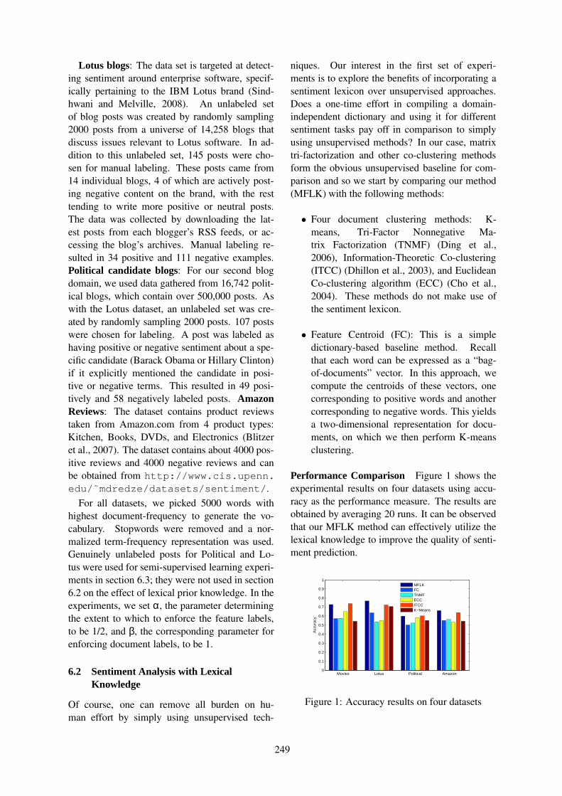
Lotus blogs: The data set is targeted at detect-ing sentiment around enterprise software, specif-ically pertaining to the IBM Lotus brand (Sind-hwani and Melville, 2008). An unlabeled setof blog posts was created by randomly sampling2000 posts from a universe of 14,258 blogs thatdiscuss issues relevant to Lotus software. In ad-dition to this unlabeled set, 145 posts were cho-sen for manual labeling. These posts came from14 individual blogs, 4 of which are actively post-ing negative content on the brand, with the resttending to write more positive or neutral posts.The data was collected by downloading the lat-est posts from each blogger’s RSS feeds, or ac-cessing the blog’s archives. Manual labeling re-sulted in 34 positive and 111 negative examples.Political candidate blogs: For our second blogdomain, we used data gathered from 16,742 polit-ical blogs, which contain over 500,000 posts. Aswith the Lotus dataset, an unlabeled set was cre-ated by randomly sampling 2000 posts. 107 postswere chosen for labeling. A post was labeled ashaving positive or negative sentiment about a spe-cific candidate (Barack Obama or Hillary Clinton)if it explicitly mentioned the candidate in posi-tive or negative terms. This resulted in 49 posi-tively and 58 negatively labeled posts. AmazonReviews: The dataset contains product reviewstaken from Amazon.com from 4 product types:Kitchen, Books, DVDs, and Electronics (Blitzeret al., 2007). The dataset contains about 4000 pos-itive reviews and 4000 negative reviews and canbe obtained from http://www.cis.upenn.edu/˜mdredze/datasets/sentiment/.
For all datasets, we picked 5000 words withhighest document-frequency to generate the vo-cabulary. Stopwords were removed and a nor-malized term-frequency representation was used.Genuinely unlabeled posts for Political and Lo-tus were used for semi-supervised learning experi-ments in section 6.3; they were not used in section6.2 on the effect of lexical prior knowledge. In theexperiments, we set α, the parameter determiningthe extent to which to enforce the feature labels,to be 1/2, and β, the corresponding parameter forenforcing document labels, to be 1.
6.2 Sentiment Analysis with LexicalKnowledge
Of course, one can remove all burden on hu-man effort by simply using unsupervised tech-
niques. Our interest in the first set of experi-ments is to explore the benefits of incorporating asentiment lexicon over unsupervised approaches.Does a one-time effort in compiling a domain-independent dictionary and using it for differentsentiment tasks pay off in comparison to simplyusing unsupervised methods? In our case, matrixtri-factorization and other co-clustering methodsform the obvious unsupervised baseline for com-parison and so we start by comparing our method(MFLK) with the following methods:
• Four document clustering methods: K-means, Tri-Factor Nonnegative Ma-trix Factorization (TNMF) (Ding et al.,2006), Information-Theoretic Co-clustering(ITCC) (Dhillon et al., 2003), and EuclideanCo-clustering algorithm (ECC) (Cho et al.,2004). These methods do not make use ofthe sentiment lexicon.
• Feature Centroid (FC): This is a simpledictionary-based baseline method. Recallthat each word can be expressed as a “bag-of-documents” vector. In this approach, wecompute the centroids of these vectors, onecorresponding to positive words and anothercorresponding to negative words. This yieldsa two-dimensional representation for docu-ments, on which we then perform K-meansclustering.
Performance Comparison Figure 1 shows theexperimental results on four datasets using accu-racy as the performance measure. The results areobtained by averaging 20 runs. It can be observedthat our MFLK method can effectively utilize thelexical knowledge to improve the quality of senti-ment prediction.
Movies Lotus Political Amazon0
0.1
0.2
0.3
0.4
0.5
0.6
0.7
0.8
0.9
1
Acc
urac
y
MFLKFCTNMFECCITCCK−Means
Figure 1: Accuracy results on four datasets
249
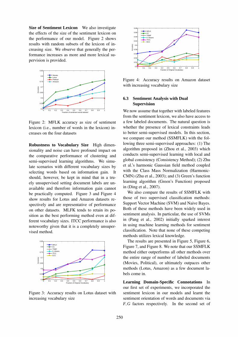
Size of Sentiment Lexicon We also investigatethe effects of the size of the sentiment lexicon onthe performance of our model. Figure 2 showsresults with random subsets of the lexicon of in-creasing size. We observe that generally the per-formance increases as more and more lexical su-pervision is provided.
0 0.1 0.2 0.3 0.4 0.5 0.6 0.7 0.8 0.9 10.5
0.55
0.6
0.65
0.7
0.75
0.8
0.85
Fraction of sentiment words labeled
Acc
urac
y
MoviesLotusPoliticalAmazon
Figure 2: MFLK accuracy as size of sentimentlexicon (i.e., number of words in the lexicon) in-creases on the four datasets
Robustness to Vocabulary Size High dimen-sionality and noise can have profound impact onthe comparative performance of clustering andsemi-supervised learning algorithms. We simu-late scenarios with different vocabulary sizes byselecting words based on information gain. Itshould, however, be kept in mind that in a tru-ely unsupervised setting document labels are un-available and therefore information gain cannotbe practically computed. Figure 3 and Figure 4show results for Lotus and Amazon datasets re-spectively and are representative of performanceon other datasets. MLFK tends to retain its po-sition as the best performing method even at dif-ferent vocabulary sizes. ITCC performance is alsonoteworthy given that it is a completely unsuper-vised method.
0 0.1 0.2 0.3 0.4 0.5 0.6 0.7 0.8 0.9 10.5
0.55
0.6
0.65
0.7
0.75
0.8
0.85
Fraction of Original Vocabulary
Acc
urac
y
MFLKFCTNMFK−MeansITCCECC
Figure 3: Accuracy results on Lotus dataset withincreasing vocabulary size
0 0.1 0.2 0.3 0.4 0.5 0.6 0.7 0.8 0.9 10.5
0.52
0.54
0.56
0.58
0.6
0.62
0.64
0.66
0.68
Fraction of Original Vocabulary
Acc
urac
y
MFLKFCTNMFK−MeansITCCECC
Figure 4: Accuracy results on Amazon datasetwith increasing vocabulary size
6.3 Sentiment Analysis with DualSupervision
We now assume that together with labeled featuresfrom the sentiment lexicon, we also have access toa few labeled documents. The natural question iswhether the presence of lexical constraints leadsto better semi-supervised models. In this section,we compare our method (SSMFLK) with the fol-lowing three semi-supervised approaches: (1) Thealgorithm proposed in (Zhou et al., 2003) whichconducts semi-supervised learning with local andglobal consistency (Consistency Method); (2) Zhuet al.’s harmonic Gaussian field method coupledwith the Class Mass Normalization (Harmonic-CMN) (Zhu et al., 2003); and (3) Green’s functionlearning algorithm (Green’s Function) proposedin (Ding et al., 2007).
We also compare the results of SSMFLK withthose of two supervised classification methods:Support Vector Machine (SVM) and Naive Bayes.Both of these methods have been widely used insentiment analysis. In particular, the use of SVMsin (Pang et al., 2002) initially sparked interestin using machine learning methods for sentimentclassification. Note that none of these competingmethods utilizes lexical knowledge.
The results are presented in Figure 5, Figure 6,Figure 7, and Figure 8. We note that our SSMFLKmethod either outperforms all other methods overthe entire range of number of labeled documents(Movies, Political), or ultimately outpaces othermethods (Lotus, Amazon) as a few document la-bels come in.
Learning Domain-Specific Connotations Inour first set of experiments, we incorporated thesentiment lexicon in our models and learnt thesentiment orientation of words and documents viaF,G factors respectively. In the second set of
250

0.1 0.15 0.2 0.25 0.3 0.35 0.4 0.45 0.50.4
0.45
0.5
0.55
0.6
0.65
0.7
0.75
0.8
Number of documents labeled as a fraction of the original set of labeled documents
Acc
urac
y
SSMFLKConsistency MethodHomonic−CMNGreen FunctionSVMNaive Bays
Figure 5: Accuracy results with increasing numberof labeled documents on Movies dataset
0.1 0.15 0.2 0.25 0.3 0.35 0.4 0.45 0.50.3
0.4
0.5
0.6
0.7
0.8
0.9
Number of documents labeled as a fraction of the original set of labeled documents
Acc
urac
y
SSMFLKConsistency MethodHomonic−CMNGreen Function SVMNaive Bayes
Figure 6: Accuracy results with increasing numberof labeled documents on Lotus dataset
experiments, we additionally introduced labeleddocuments for domain-specific adjustments. Be-tween these experiments, we can now look forwords that switch sentiment polarity. These wordsare interesting because their domain-specific con-notation differs from their lexical orientation. Foramazon reviews, the following words switchedpolarity from positive to negative: fan, impor-tant, learning, cons, fast, feature, happy, memory,portable, simple, small, work while the followingwords switched polarity from negative to positive:address, finish, lack, mean, budget, rent, throw.Note that words like fan, memory probably referto product or product components (i.e., computerfan and memory) in the amazon review contextbut have a very different connotation say in thecontext of movie reviews where they probably re-fer to movie fanfare and memorable performances.We were surprised to see happy switch polarity!Two examples of its negative-sentiment usage are:I ended up buying a Samsung and I couldn’t bemore happy and BORING, not one single excitingthing about this book. I was happy when my lunchbreak ended so I could go back to work and stopreading.
0.1 0.15 0.2 0.25 0.3 0.35 0.4 0.45 0.50.3
0.35
0.4
0.45
0.5
0.55
0.6
0.65
0.7
0.75
0.8
Number of documents labeled as a fraction of the original set of labeled documents
Acc
urac
y
SSMFLKConsistency MethodHomonic−CMNGreen FunctionSVMNaive Bays
Figure 7: Accuracy results with increasing numberof labeled documents on Political dataset
0.1 0.15 0.2 0.25 0.3 0.35 0.4 0.45 0.50.4
0.45
0.5
0.55
0.6
0.65
0.7
0.75
0.8
Number of documents labeled as a fraction of the original set of labeled documents
Acc
urac
y
SSMFLKConsistency MethodHomonic−CMNGreen FunctionSVMNaive Bays
Figure 8: Accuracy results with increasing numberof labeled documents on Amazon dataset
7 Conclusion
The primary contribution of this paper is to pro-pose and benchmark new methodologies for sen-timent analysis. Non-negative Matrix Factoriza-tions constitute a rich body of algorithms that havefound applicability in a variety of machine learn-ing applications: from recommender systems todocument clustering. We have shown how to buildeffective sentiment models by appropriately con-straining the factors using lexical prior knowledgeand document annotations. To more effectivelyutilize unlabeled data and induce domain-specificadaptation of our models, several extensions arepossible: facilitating learning from related do-mains, incorporating hyperlinks between docu-ments, incorporating synonyms or co-occurencesbetween words etc. As a topic of vigorous currentactivity, there are several very recently proposedcompeting methodologies for sentiment analysisthat we would like to benchmark against. Theseare topics for future work.
Acknowledgement: The work of T. Li is par-tially supported by NSF grants DMS-0844513 andCCF-0830659. We would also like to thank PremMelville and Richard Lawrence for their support.
251
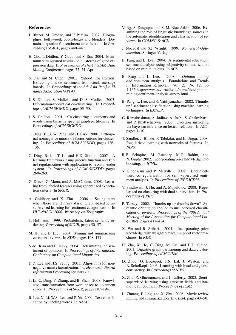
References
J. Blitzer, M. Dredze, and F. Pereira. 2007. Biogra-phies, bollywood, boom-boxes and blenders: Do-main adaptation for sentiment classification. In Pro-ceedings of ACL, pages 440–447.
H. Cho, I. Dhillon, Y. Guan, and S. Sra. 2004. Mini-mum sum squared residue co-clustering of gene ex-pression data. In Proceedings of The 4th SIAM DataMining Conference, pages 22–24, April.
S. Das and M. Chen. 2001. Yahoo! for amazon:Extracting market sentiment from stock messageboards. In Proceedings of the 8th Asia Pacific Fi-nance Association (APFA).
I. S. Dhillon, S. Mallela, and D. S. Modha. 2003.Information-theoretical co-clustering. In Proceed-ings of ACM SIGKDD, pages 89–98.
I. S. Dhillon. 2001. Co-clustering documents andwords using bipartite spectral graph partitioning. InProceedings of ACM SIGKDD.
C. Ding, T. Li, W. Peng, and H. Park. 2006. Orthogo-nal nonnegative matrix tri-factorizations for cluster-ing. In Proceedings of ACM SIGKDD, pages 126–135.
C. Ding, R. Jin, T. Li, and H.D. Simon. 2007. Alearning framework using green’s function and ker-nel regularization with application to recommendersystem. In Proceedings of ACM SIGKDD, pages260–269.
G. Druck, G. Mann, and A. McCallum. 2008. Learn-ing from labeled features using generalized expecta-tion criteria. In SIGIR.
A. Goldberg and X. Zhu. 2006. Seeing starswhen there aren’t many stars: Graph-based semi-supervised learning for sentiment categorization. InHLT-NAACL 2006: Workshop on Textgraphs.
T. Hofmann. 1999. Probabilistic latent semantic in-dexing. Proceeding of SIGIR, pages 50–57.
M. Hu and B. Liu. 2004. Mining and summarizingcustomer reviews. In KDD, pages 168–177.
S.-M. Kim and E. Hovy. 2004. Determining the sen-timent of opinions. In Proceedings of InternationalConference on Computational Linguistics.
D.D. Lee and H.S. Seung. 2001. Algorithms for non-negative matrix factorization. In Advances in NeuralInformation Processing Systems 13.
T. Li, C. Ding, Y. Zhang, and B. Shao. 2008. Knowl-edge transformation from word space to documentspace. In Proceedings of SIGIR, pages 187–194.
B. Liu, X. Li, W.S. Lee, and P. Yu. 2004. Text classifi-cation by labeling words. In AAAI.
V. Ng, S. Dasgupta, and S. M. Niaz Arifin. 2006. Ex-amining the role of linguistic knowledge sources inthe automatic identification and classification of re-views. In COLING & ACL.
J. Nocedal and S.J. Wright. 1999. Numerical Opti-mization. Springer-Verlag.
B. Pang and L. Lee. 2004. A sentimental education:sentiment analysis using subjectivity summarizationbased on minimum cuts. In ACL.
B. Pang and L. Lee. 2008. Opinion miningand sentiment analysis. Foundations and Trendsin Information Retrieval: Vol. 2: No 12, pp1-135 http://www.cs.cornell.edu/home/llee/opinion-mining-sentiment-analysis-survey.html.
B. Pang, L. Lee, and S. Vaithyanathan. 2002. Thumbsup? sentiment classification using machine learningtechniques. In EMNLP.
G. Ramakrishnan, A. Jadhav, A. Joshi, S. Chakrabarti,and P. Bhattacharyya. 2003. Question answeringvia bayesian inference on lexical relations. In ACL,pages 1–10.
T. Sandler, J. Blitzer, P. Talukdar, and L. Ungar. 2008.Regularized learning with networks of features. InNIPS.
R.E. Schapire, M. Rochery, M.G. Rahim, andN. Gupta. 2002. Incorporating prior knowledge intoboosting. In ICML.
V. Sindhwani and P. Melville. 2008. Document-word co-regularization for semi-supervised senti-ment analysis. In Proceedings of IEEE ICDM.
V. Sindhwani, J. Hu, and A. Mojsilovic. 2008. Regu-larized co-clustering with dual supervision. In Pro-ceedings of NIPS.
P. Turney. 2002. Thumbs up or thumbs down? Se-mantic orientation applied to unsupervised classifi-cation of reviews. Proceedings of the 40th AnnualMeeting of the Association for Computational Lin-guistics, pages 417–424.
X. Wu and R. Srihari. 2004. Incorporating priorknowledge with weighted margin support vector ma-chines. In KDD.
H. Zha, X. He, C. Ding, M. Gu, and H.D. Simon.2001. Bipartite graph partitioning and data cluster-ing. Proceedings of ACM CIKM.
D. Zhou, O. Bousquet, T.N. Lal, J. Weston, andB. Scholkopf. 2003. Learning with local and globalconsistency. In Proceedings of NIPS.
X. Zhu, Z. Ghahramani, and J. Lafferty. 2003. Semi-supervised learning using gaussian fields and har-monic functions. In Proceedings of ICML.
L. Zhuang, F. Jing, and X. Zhu. 2006. Movie reviewmining and summarization. In CIKM, pages 43–50.
252
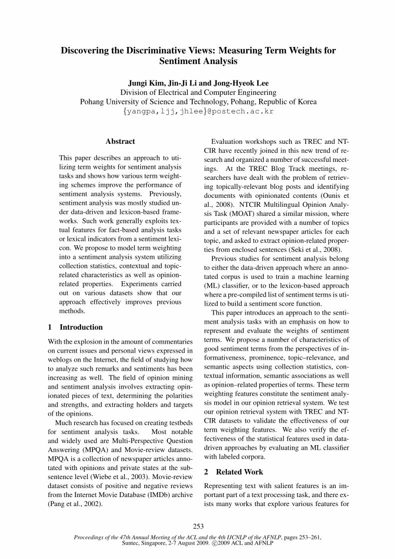
Proceedings of the 47th Annual Meeting of the ACL and the 4th IJCNLP of the AFNLP, pages 253–261,Suntec, Singapore, 2-7 August 2009. c©2009 ACL and AFNLP
Discovering the Discriminative Views: Measuring Term Weights forSentiment Analysis
Jungi Kim, Jin-Ji Li and Jong-Hyeok LeeDivision of Electrical and Computer Engineering
Pohang University of Science and Technology, Pohang, Republic of Korea{yangpa,ljj,jhlee}@postech.ac.kr
Abstract
This paper describes an approach to uti-lizing term weights for sentiment analysistasks and shows how various term weight-ing schemes improve the performance ofsentiment analysis systems. Previously,sentiment analysis was mostly studied un-der data-driven and lexicon-based frame-works. Such work generally exploits tex-tual features for fact-based analysis tasksor lexical indicators from a sentiment lexi-con. We propose to model term weightinginto a sentiment analysis system utilizingcollection statistics, contextual and topic-related characteristics as well as opinion-related properties. Experiments carriedout on various datasets show that ourapproach effectively improves previousmethods.
1 Introduction
With the explosion in the amount of commentarieson current issues and personal views expressed inweblogs on the Internet, the field of studying howto analyze such remarks and sentiments has beenincreasing as well. The field of opinion miningand sentiment analysis involves extracting opin-ionated pieces of text, determining the polaritiesand strengths, and extracting holders and targetsof the opinions.
Much research has focused on creating testbedsfor sentiment analysis tasks. Most notableand widely used are Multi-Perspective QuestionAnswering (MPQA) and Movie-review datasets.MPQA is a collection of newspaper articles anno-tated with opinions and private states at the sub-sentence level (Wiebe et al., 2003). Movie-reviewdataset consists of positive and negative reviewsfrom the Internet Movie Database (IMDb) archive(Pang et al., 2002).
Evaluation workshops such as TREC and NT-CIR have recently joined in this new trend of re-search and organized a number of successful meet-ings. At the TREC Blog Track meetings, re-searchers have dealt with the problem of retriev-ing topically-relevant blog posts and identifyingdocuments with opinionated contents (Ounis etal., 2008). NTCIR Multilingual Opinion Analy-sis Task (MOAT) shared a similar mission, whereparticipants are provided with a number of topicsand a set of relevant newspaper articles for eachtopic, and asked to extract opinion-related proper-ties from enclosed sentences (Seki et al., 2008).
Previous studies for sentiment analysis belongto either the data-driven approach where an anno-tated corpus is used to train a machine learning(ML) classifier, or to the lexicon-based approachwhere a pre-compiled list of sentiment terms is uti-lized to build a sentiment score function.
This paper introduces an approach to the senti-ment analysis tasks with an emphasis on how torepresent and evaluate the weights of sentimentterms. We propose a number of characteristics ofgood sentiment terms from the perspectives of in-formativeness, prominence, topic–relevance, andsemantic aspects using collection statistics, con-textual information, semantic associations as wellas opinion–related properties of terms. These termweighting features constitute the sentiment analy-sis model in our opinion retrieval system. We testour opinion retrieval system with TREC and NT-CIR datasets to validate the effectiveness of ourterm weighting features. We also verify the ef-fectiveness of the statistical features used in data-driven approaches by evaluating an ML classifierwith labeled corpora.
2 Related Work
Representing text with salient features is an im-portant part of a text processing task, and there ex-ists many works that explore various features for
253
text analysis systems (Sebastiani, 2002; Forman,2003). Sentiment analysis task have also been us-ing various lexical, syntactic, and statistical fea-tures (Pang and Lee, 2008). Pang et al. (2002)employed n-gram and POS features for ML meth-ods to classify movie-review data. Also, syntac-tic features such as the dependency relationship ofwords and subtrees have been shown to effectivelyimprove the performances of sentiment analysis(Kudo and Matsumoto, 2004; Gamon, 2004; Mat-sumoto et al., 2005; Ng et al., 2006).
While these features are usually employed bydata-driven approaches, there are unsupervised ap-proaches for sentiment analysis that make use of aset of terms that are semantically oriented towardexpressing subjective statements (Yu and Hatzi-vassiloglou, 2003). Accordingly, much researchhas focused on recognizing terms’ semantic ori-entations and strength, and compiling sentimentlexicons (Hatzivassiloglou and Mckeown, 1997;Turney and Littman, 2003; Kamps et al., 2004;Whitelaw et al., 2005; Esuli and Sebastiani, 2006).
Interestingly, there are conflicting conclusionsabout the usefulness of the statistical features insentiment analysis tasks (Pang and Lee, 2008).Pang et al. (2002) presents empirical results in-dicating that using term presence over term fre-quency is more effective in a data-driven sentimentclassification task. Such a finding suggests thatsentiment analysis may exploit different types ofcharacteristics from the topical tasks, that, unlikefact-based text analysis tasks, repetition of termsdoes not imply a significance on the overall senti-ment. On the other hand, Wiebe et al. (2004) havenoted that hapax legomena (terms that only appearonce in a collection of texts) are good signs fordetecting subjectivity. Other works have also ex-ploited rarely occurring terms for sentiment anal-ysis tasks (Dave et al., 2003; Yang et al., 2006).
The opinion retrieval task is a relatively recentissue that draws both the attention of IR and NLPcommunities. Its task is to find relevant documentsthat also contain sentiments about a given topic.Generally, the opinion retrieval task has been ap-proached as a two–stage task: first, retrieving top-ically relevant documents, then reranking the doc-uments by the opinion scores (Ounis et al., 2006).This approach is also appropriate for evaluationsystems such as NTCIR MOAT that assumes thatthe set of topically relevant documents are alreadyknown in advance. On the other hand, there are
also some interesting works on modeling the topicand sentiment of documents in a unified way (Meiet al., 2007; Zhang and Ye, 2008).
3 Term Weighting and SentimentAnalysis
In this section, we describe the characteristics ofterms that are useful in sentiment analysis, andpresent our sentiment analysis model as part ofan opinion retrieval system and an ML sentimentclassifier.
3.1 Characteristics of Good Sentiment Terms
This section examines the qualities of useful termsfor sentiment analysis tasks and correspondingfeatures. For the sake of organization, we cate-gorize the sources of features into either global orlocal knowledge, and either topic-independent ortopic-dependent knowledge.
Topic-independently speaking, a good senti-ment term is discriminative and prominent, suchthat the appearance of the term imposes greaterinfluence on the judgment of the analysis system.The rare occurrence of terms in document collec-tions has been regarded as a very important featurein IR methods, and effective IR models of today,either explicitly or implicitly, accommodate thisfeature as an Inverse Document Frequency (IDF)heuristic (Fang et al., 2004). Similarly, promi-nence of a term is recognized by the frequency ofthe term in its local context, formulated as TermFrequency (TF) in IR.
If a topic of the text is known, terms that are rel-evant and descriptive of the subject should be re-garded to be more useful than topically-irrelevantand extraneous terms. One way of measuring thisis using associations between the query and terms.Statistical measures of associations between termsinclude estimations by the co-occurrence in thewhole collection, such as Point-wise Mutual In-formation (PMI) and Latent Semantic Analysis(LSA). Another method is to use proximal infor-mation of the query and the word, using syntacticstructure such as dependency relations of wordsthat provide the graphical representation of thetext (Mullen and Collier, 2004). The minimumspans of words in such graph may represent theirassociations in the text. Also, the distance betweenwords in the local context or in the thesaurus-like dictionaries such as WordNet may be approx-imated as such measure.
254

3.2 Opinion Retrieval ModelThe goal of an opinion retrieval system is to find aset of opinionated documents that are relevant to agiven topic. We decompose the opinion retrievalsystem into two tasks: the topical retrieval taskand the sentiment analysis task. This two-stageapproach for opinion retrieval has been taken bymany systems and has been shown to perform well(Ounis et al., 2006). The topic and the sentimentaspects of the opinion retrieval task are modeledseparately, and linearly combined together to pro-duce a list of topically-relevant and opinionateddocuments as below.
ScoreOpRet(D,Q) = λ·Scorerel(D,Q)+(1−λ)·Scoreop(D,Q)
The topic-relevance model Scorerel may be sub-stituted by any IR system that retrieves relevantdocuments for the query Q. For tasks such asNTCIR MOAT, relevant documents are alreadyknown in advance and it becomes unnecessary toestimate the relevance degree of the documents.We focus on modeling the sentiment aspect ofthe opinion retrieval task, assuming that the topic-relevance of documents is provided in some way.
To assign documents with sentiment degrees,we estimate the probability of a document D togenerate a query Q and to possess opinions as in-dicated by a random variable Op.1 Assuming uni-form prior probabilities of documentsD, queryQ,and Op, and conditional independence between Qand Op, the opinion score function reduces to es-timating the generative probability of Q and Opgiven D.
Scoreop(D,Q) ≡ p(D | Op,Q) ∝ p(Op,Q | D)
If we regard that the document D is representedas a bag of words and that the words are uniformlydistributed, then
p(Op,Q | D) =X
w∈D
p(Op,Q | w) · p(w | D)
=X
w∈D
p(Op | w) · p(Q | w) · p(w | D) (1)
Equation 1 consists of three factors: the proba-bility of a word to be opinionated (P (Op|w)), thelikelihood of a query given a word (P (Q|w)), andthe probability of a document generating a word(P (w|D)). Intuitively speaking, the probability ofa document embodying topically related opinion isestimated by accumulating the probabilities of all
1Throughout this paper, Op indicates Op = 1.
words from the document to have sentiment mean-ings and associations with the given query.
In the following sections, we assess the threefactors of the sentiment models from the perspec-tives of term weighting.
3.2.1 Word Sentiment ModelModeling the sentiment of a word has been a pop-ular approach in sentiment analysis. There aremany publicly available lexicon resources. Thesize, format, specificity, and reliability differ in allthese lexicons. For example, lexicon sizes rangefrom a few hundred to several hundred thousand.Some lexicons assign real number scores to in-dicate sentiment orientations and strengths (i.e.probabilities of having positive and negative sen-timents) (Esuli and Sebastiani, 2006) while otherlexicons assign discrete classes (weak/strong, pos-itive/negative) (Wilson et al., 2005). There aremanually compiled lexicons (Stone et al., 1966)while some are created semi-automatically by ex-panding a set of seed terms (Esuli and Sebastiani,2006).
The goal of this paper is not to create or choosean appropriate sentiment lexicon, but rather it isto discover useful term features other than thesentiment properties. For this reason, one sen-timent lexicon, namely SentiWordNet, is utilizedthroughout the whole experiment.
SentiWordNet is an automatically generatedsentiment lexicon using a semi-supervised method(Esuli and Sebastiani, 2006). It consists of Word-Net synsets, where each synset is assigned threeprobability scores that add up to 1: positive, nega-tive, and objective.
These scores are assigned at sense level (synsetsin WordNet), and we use the following equationsto assess the sentiment scores at the word level.
p(Pos | w) = maxs∈synset(w)
SWNP os(s)
p(Neg | w) = maxs∈synset(w)
SWNNeg(s)
p(Op | w) = max (p(Pos | w), p(Neg | w))
where synset(w) is the set of synsets of w andSWNPos(s), SWNNeg(s) are positive and neg-ative scores of a synset in SentiWordNet. We as-sess the subjective score of a word as the maxi-mum value of the positive and the negative scores,because a word has either a positive or a negativesentiment in a given context.
The word sentiment model can also make useof other types of sentiment lexicons. The sub-
255
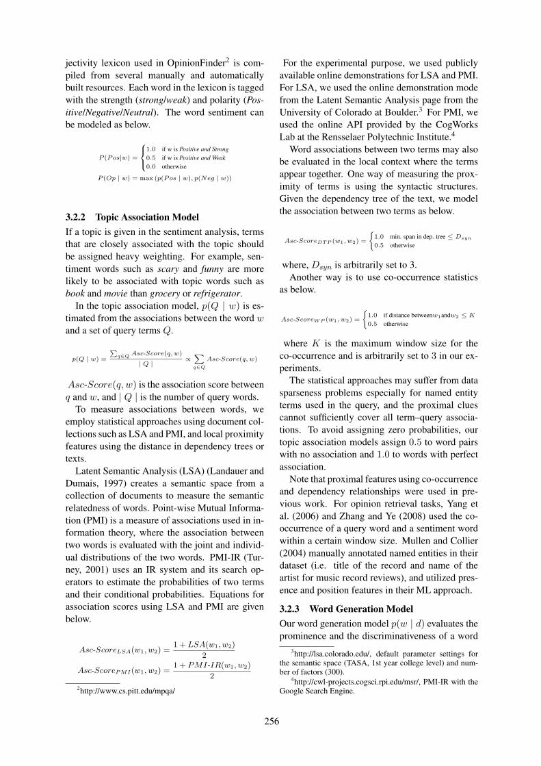
jectivity lexicon used in OpinionFinder2 is com-piled from several manually and automaticallybuilt resources. Each word in the lexicon is taggedwith the strength (strong/weak) and polarity (Pos-itive/Negative/Neutral). The word sentiment canbe modeled as below.
P (Pos|w) =
8><>:1.0 if w is Positive and Strong0.5 if w is Positive and Weak0.0 otherwise
P (Op | w) = max (p(Pos | w), p(Neg | w))
3.2.2 Topic Association ModelIf a topic is given in the sentiment analysis, termsthat are closely associated with the topic shouldbe assigned heavy weighting. For example, sen-timent words such as scary and funny are morelikely to be associated with topic words such asbook and movie than grocery or refrigerator.
In the topic association model, p(Q | w) is es-timated from the associations between the word wand a set of query terms Q.
p(Q | w) =
Pq∈Q Asc-Score(q, w)
| Q |∝Xq∈Q
Asc-Score(q, w)
Asc-Score(q, w) is the association score betweenq and w, and | Q | is the number of query words.
To measure associations between words, weemploy statistical approaches using document col-lections such as LSA and PMI, and local proximityfeatures using the distance in dependency trees ortexts.
Latent Semantic Analysis (LSA) (Landauer andDumais, 1997) creates a semantic space from acollection of documents to measure the semanticrelatedness of words. Point-wise Mutual Informa-tion (PMI) is a measure of associations used in in-formation theory, where the association betweentwo words is evaluated with the joint and individ-ual distributions of the two words. PMI-IR (Tur-ney, 2001) uses an IR system and its search op-erators to estimate the probabilities of two termsand their conditional probabilities. Equations forassociation scores using LSA and PMI are givenbelow.
Asc-ScoreLSA(w1, w2) =1 + LSA(w1, w2)
2
Asc-ScorePMI(w1, w2) =1 + PMI-IR(w1, w2)
2
2http://www.cs.pitt.edu/mpqa/
For the experimental purpose, we used publiclyavailable online demonstrations for LSA and PMI.For LSA, we used the online demonstration modefrom the Latent Semantic Analysis page from theUniversity of Colorado at Boulder.3 For PMI, weused the online API provided by the CogWorksLab at the Rensselaer Polytechnic Institute.4
Word associations between two terms may alsobe evaluated in the local context where the termsappear together. One way of measuring the prox-imity of terms is using the syntactic structures.Given the dependency tree of the text, we modelthe association between two terms as below.
Asc-ScoreDT P (w1, w2) =
(1.0 min. span in dep. tree ≤ Dsyn
0.5 otherwise
where, Dsyn is arbitrarily set to 3.Another way is to use co-occurrence statistics
as below.
Asc-ScoreW P (w1, w2) =
(1.0 if distance betweenw1andw2 ≤ K0.5 otherwise
where K is the maximum window size for theco-occurrence and is arbitrarily set to 3 in our ex-periments.
The statistical approaches may suffer from datasparseness problems especially for named entityterms used in the query, and the proximal cluescannot sufficiently cover all term–query associa-tions. To avoid assigning zero probabilities, ourtopic association models assign 0.5 to word pairswith no association and 1.0 to words with perfectassociation.
Note that proximal features using co-occurrenceand dependency relationships were used in pre-vious work. For opinion retrieval tasks, Yang etal. (2006) and Zhang and Ye (2008) used the co-occurrence of a query word and a sentiment wordwithin a certain window size. Mullen and Collier(2004) manually annotated named entities in theirdataset (i.e. title of the record and name of theartist for music record reviews), and utilized pres-ence and position features in their ML approach.
3.2.3 Word Generation ModelOur word generation model p(w | d) evaluates theprominence and the discriminativeness of a word
3http://lsa.colorado.edu/, default parameter settings forthe semantic space (TASA, 1st year college level) and num-ber of factors (300).
4http://cwl-projects.cogsci.rpi.edu/msr/, PMI-IR with theGoogle Search Engine.
256

w in a document d. These issues correspond to thecore issues of traditional IR tasks. IR models, suchas Vector Space (VS), probabilistic models suchas BM25, and Language Modeling (LM), albeit indifferent forms of approach and measure, employheuristics and formal modeling approaches to ef-fectively evaluate the relevance of a term to a doc-ument (Fang et al., 2004). Therefore, we estimatethe word generation model with popular IR mod-els’ the relevance scores of a document d given was a query.5
p(w | d) ≡ IR-SCORE(w, d)
In our experiments, we use the Vector Spacemodel with Pivoted Normalization (VS), Proba-bilistic model (BM25), and Language modelingwith Dirichlet Smoothing (LM).
V SPN(w, d) =1 + ln(1 + ln(c(w, d)))
(1− s) + s ·| d |avgdl
· lnN + 1
df(w)
BM25(w, d) = lnN − df(w) + 0.5
df(w) + 0.5·
(k1 + 1) · c(w, d)
k1
“(1− b) + b
|d|avgdl
”+ c(w, d)
LMDI(w, d) = ln
1 +
c(w, d)
µ · c(w,C)
!+ ln
µ
| d | +µ
c(w, d) is the frequency of w in d, | d | is thenumber of unique terms in d, avgdl is the average| d | of all documents, N is the number of doc-uments in the collection, df(w) is the number ofdocuments with w, C is the entire collection, andk1 and b are constants 2.0 and 0.75.
3.3 Data-driven ApproachTo verify the effectiveness of our term weight-ing schemes in experimental settings of the data-driven approach, we carry out a set of simple ex-periments with ML classifiers. Specifically, weexplore the statistical term weighting features ofthe word generation model with Support Vectormachine (SVM), faithfully reproducing previouswork as closely as possible (Pang et al., 2002).
Each instance of train and test data is repre-sented as a vector of features. We test variouscombinations of the term weighting schemes listedbelow.
• PRESENCE: binary indicator for the pres-ence of a term• TF: term frequency5With proper assumptions and derivations, p(w | d) can
be derived to language modeling approaches. Refer to (Zhaiand Lafferty, 2004).
• VS.TF: normalized tf as in VS• BM25.TF: normalized tf as in BM25• IDF: inverse document frequency• VS.IDF: normalized idf as in VS• BM25.IDF: normalized idf as in BM25
4 Experiment
Our experiments consist of an opinion retrievaltask and a sentiment classification task. We useMPQA and movie-review corpora in our experi-ments with an ML classifier. For the opinion re-trieval task, we use the two datasets used by TRECblog track and NTCIR MOAT evaluation work-shops.
The opinion retrieval task at TREC Blog Trackconsists of three subtasks: topic retrieval, opinionretrieval, and polarity retrieval. Opinion and polar-ity retrieval subtasks use the relevant documentsretrieved at the topic retrieval stage. On the otherhand, the NTCIR MOAT task aims to find opin-ionated sentences given a set of documents that arealready hand-assessed to be relevant to the topic.
4.1 Opinion Retieval Task – TREC BlogTrack
4.1.1 Experimental SettingTREC Blog Track uses the TREC Blog06 corpus(Macdonald and Ounis, 2006). It is a collectionof RSS feeds (38.6 GB), permalink documents(88.8GB), and homepages (28.8GB) crawled onthe Internet over an eleven week period from De-cember 2005 to February 2006.
Non-relevant content of blog posts such asHTML tags, advertisement, site description, andmenu are removed with an effective internal spamremoval algorithm (Nam et al., 2009). While oursentiment analysis model uses the entire relevantportion of the blog posts, further stopword re-moval and stemming is done for the blog retrievalsystem.
For the relevance retrieval model, we faithfullyreproduce the passage-based language model withpseudo-relevance feedback (Lee et al., 2008).
We use in total 100 topics from TREC 2007 and2008 blog opinion retrieval tasks (07:901-950 and08:1001-1050). We use the topics from Blog 07to optimize the parameter for linearly combiningthe retrieval and opinion models, and use Blog 08topics as our test data. Topics are extracted onlyfrom the Title field, using the Porter stemmer anda stopword list.
257

Table 1: Performance of opinion retrieval modelsusing Blog 08 topics. The linear combination pa-rameter λ is optimized on Blog 07 topics. † indi-cates statistical significance at the 1% level overthe baseline.
Model MAP R-prec P@10TOPIC REL. 0.4052 0.4366 0.6440BASELINE 0.4141 0.4534 0.6440
VS 0.4196 0.4542 0.6600BM25 0.4235† 0.4579 0.6600
LM 0.4158 0.4520 0.6560PMI 0.4177 0.4538 0.6620LSA 0.4155 0.4526 0.6480WP 0.4165 0.4533 0.6640
BM25·PMI 0.4238† 0.4575 0.6600BM25·LSA 0.4237† 0.4578 0.6600BM25·WP 0.4237† 0.4579 0.6600
BM25·PMI·WP 0.4242† 0.4574 0.6620BM25·LSA·WP 0.4238† 0.4576 0.6580
4.1.2 Experimental Result
Retrieval performances using different combina-tions of term weighting features are presented inTable 1. Using only the word sentiment model isset as our baseline.
First, each feature of the word generation andtopic association models are tested; all features ofthe models improve over the baseline. We observethat the features of our word generation model ismore effective than those of the topic associationmodel. Among the features of the word generationmodel, the most improvement was achieved withBM25, improving the MAP by 2.27%.
Features of the topic association model showonly moderate improvements over the baseline.We observe that these features generally improveP@10 performance, indicating that they increasethe accuracy of the sentiment analysis system.PMI out-performed LSA for all evaluation mea-sures. Among the topic association models, PMIperforms the best in MAP and R-prec, while WPachieved the biggest improvement in P@10.
Since BM25 performs the best among the wordgeneration models, its combination with other fea-tures was investigated. Combinations of BM25with the topic association models all improve theperformance of the baseline and BM25. Thisdemonstrates that the word generation model andthe topic association model are complementary toeach other.
The best MAP was achieved with BM25, PMI,and WP (+2.44% over the baseline). We observethat PMI and WP also complement each other.
4.2 Sentiment Analysis Task – NTCIRMOAT
4.2.1 Experimental Setting
Another set of experiments for our opinion analy-sis model was carried out on the NTCIR-7 MOATEnglish corpus. The English opinion corpusfor NTCIR MOAT consists of newspaper articlesfrom the Mainichi Daily News, Korea Times, Xin-hua News, Hong Kong Standard, and the StraitsTimes. It is a collection of documents manu-ally assessed for relevance to a set of queriesfrom NTCIR-7 Advanced Cross-lingual Informa-tion Access (ACLIA) task. The corpus consists of167 documents, or 4,711 sentences for 14 test top-ics. Each sentence is manually tagged with opin-ionatedness, polarity, and relevance to the topic bythree annotators from a pool of six annotators.
For preprocessing, no removal or stemming isperformed on the data. Each sentence was pro-cessed with the Stanford English parser6 to pro-duce a dependency parse tree. Only the Title fieldsof the topics were used.
For performance evaluations of opinion and po-larity detection, we use precision, recall, and F-measure, the same measure used to report the offi-cial results at the NTCIR MOAT workshop. Thereare lenient and strict evaluations depending on theagreement of the annotators; if two out of three an-notators agreed upon an opinion or polarity anno-tation then it is used during the lenient evaluation,similarly three out of three agreements are usedduring the strict evaluation. We present the perfor-mances using the lenient evaluation only, for thetwo evaluations generally do not show much dif-ference in relative performance changes.
Since MOAT is a classification task, we use athreshold parameter to draw a boundary betweenopinionated and non-opinionated sentences. Wereport the performance of our system using theNTCIR-7 dataset, where the threshold parameteris optimized using the NTCIR-6 dataset.
4.2.2 Experimental Result
We present the performance of our sentiment anal-ysis system in Table 2. As in the experiments with
6http://nlp.stanford.edu/software/lex-parser.shtml
258
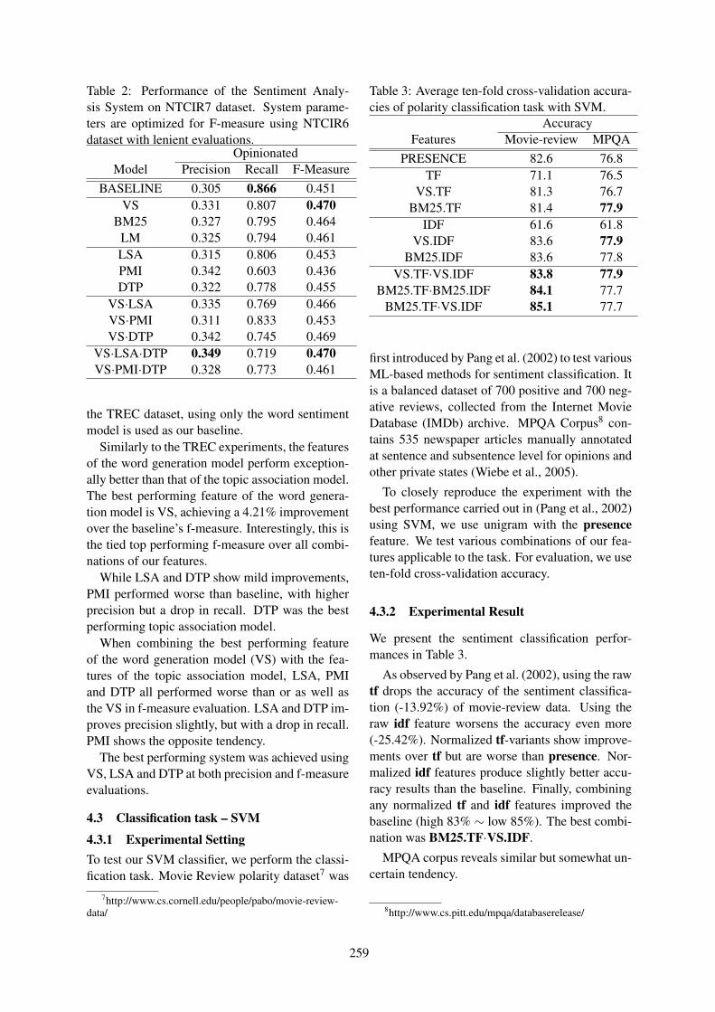
Table 2: Performance of the Sentiment Analy-sis System on NTCIR7 dataset. System parame-ters are optimized for F-measure using NTCIR6dataset with lenient evaluations.
OpinionatedModel Precision Recall F-Measure
BASELINE 0.305 0.866 0.451VS 0.331 0.807 0.470
BM25 0.327 0.795 0.464LM 0.325 0.794 0.461LSA 0.315 0.806 0.453PMI 0.342 0.603 0.436DTP 0.322 0.778 0.455
VS·LSA 0.335 0.769 0.466VS·PMI 0.311 0.833 0.453VS·DTP 0.342 0.745 0.469
VS·LSA·DTP 0.349 0.719 0.470VS·PMI·DTP 0.328 0.773 0.461
the TREC dataset, using only the word sentimentmodel is used as our baseline.
Similarly to the TREC experiments, the featuresof the word generation model perform exception-ally better than that of the topic association model.The best performing feature of the word genera-tion model is VS, achieving a 4.21% improvementover the baseline’s f-measure. Interestingly, this isthe tied top performing f-measure over all combi-nations of our features.
While LSA and DTP show mild improvements,PMI performed worse than baseline, with higherprecision but a drop in recall. DTP was the bestperforming topic association model.
When combining the best performing featureof the word generation model (VS) with the fea-tures of the topic association model, LSA, PMIand DTP all performed worse than or as well asthe VS in f-measure evaluation. LSA and DTP im-proves precision slightly, but with a drop in recall.PMI shows the opposite tendency.
The best performing system was achieved usingVS, LSA and DTP at both precision and f-measureevaluations.
4.3 Classification task – SVM
4.3.1 Experimental SettingTo test our SVM classifier, we perform the classi-fication task. Movie Review polarity dataset7 was
7http://www.cs.cornell.edu/people/pabo/movie-review-data/
Table 3: Average ten-fold cross-validation accura-cies of polarity classification task with SVM.
AccuracyFeatures Movie-review MPQA
PRESENCE 82.6 76.8TF 71.1 76.5
VS.TF 81.3 76.7BM25.TF 81.4 77.9
IDF 61.6 61.8VS.IDF 83.6 77.9
BM25.IDF 83.6 77.8VS.TF·VS.IDF 83.8 77.9
BM25.TF·BM25.IDF 84.1 77.7BM25.TF·VS.IDF 85.1 77.7
first introduced by Pang et al. (2002) to test variousML-based methods for sentiment classification. Itis a balanced dataset of 700 positive and 700 neg-ative reviews, collected from the Internet MovieDatabase (IMDb) archive. MPQA Corpus8 con-tains 535 newspaper articles manually annotatedat sentence and subsentence level for opinions andother private states (Wiebe et al., 2005).
To closely reproduce the experiment with thebest performance carried out in (Pang et al., 2002)using SVM, we use unigram with the presencefeature. We test various combinations of our fea-tures applicable to the task. For evaluation, we useten-fold cross-validation accuracy.
4.3.2 Experimental Result
We present the sentiment classification perfor-mances in Table 3.
As observed by Pang et al. (2002), using the rawtf drops the accuracy of the sentiment classifica-tion (-13.92%) of movie-review data. Using theraw idf feature worsens the accuracy even more(-25.42%). Normalized tf-variants show improve-ments over tf but are worse than presence. Nor-malized idf features produce slightly better accu-racy results than the baseline. Finally, combiningany normalized tf and idf features improved thebaseline (high 83% ∼ low 85%). The best combi-nation was BM25.TF·VS.IDF.
MPQA corpus reveals similar but somewhat un-certain tendency.
8http://www.cs.pitt.edu/mpqa/databaserelease/
259

4.4 Discussion
Overall, the opinion retrieval and the sentimentanalysis models achieve improvements using ourproposed features. Especially, the features of theword generation model improve the overall per-formances drastically. Its effectiveness is also ver-ified with a data-driven approach; the accuracy ofa sentiment classifier trained on a polarity datasetwas improved by various combinations of normal-ized tf and idf statistics.
Differences in effectiveness of VS, BM25, andLM come from parameter tuning and corpus dif-ferences. For the TREC dataset, BM25 performedbetter than the other models, and for the NTCIRdataset, VS performed better.
Our features of the topic association modelshow mild improvement over the baseline perfor-mance in general. PMI and LSA, both modelingthe semantic associations between words, showdifferent behaviors on the datasets. For the NT-CIR dataset, LSA performed better, while PMIis more effective for the TREC dataset. We be-lieve that the explanation lies in the differencesbetween the topics for each dataset. In general,the NTCIR topics are general descriptive wordssuch as “regenerative medicine”, “American econ-omy after the 911 terrorist attacks”, and “law-suit brought against Microsoft for monopolisticpractices.” The TREC topics are more named-entity-like terms such as “Carmax”, “Wikipediaprimary source”, “Jiffy Lube”, “Starbucks”, and“Windows Vista.” We have experimentally shownthat LSA is more suited to finding associationsbetween general terms because its training docu-ments are from a general domain.9 Our PMI mea-sure utilizes a web search engine, which covers avariety of named entity terms.
Though the features of our topic associationmodel, WP and DTP, were evaluated on differentdatasets, we try our best to conjecture the differ-ences. WP on TREC dataset shows a small im-provement of MAP compared to other topic asso-ciation features, while the precision is improvedthe most when this feature is used alone. The DTPfeature displays similar behavior with precision. Italso achieves the best f-measure over other topicassociation features. DTP achieves higher rela-tive improvement (3.99% F-measure verse 2.32%MAP), and is more effective for improving the per-formance in combination with LSA and PMI.
9TASA Corpus, http://lsa.colorado.edu/spaces.html
5 Conclusion
In this paper, we proposed various term weightingschemes and how such features are modeled in thesentiment analysis task. Our proposed features in-clude corpus statistics, association measures usingsemantic and local-context proximities. We haveempirically shown the effectiveness of the featureswith our proposed opinion retrieval and sentimentanalysis models.
There exists much room for improvement withfurther experiments with various term weightingmethods and datasets. Such methods include,but by no means limited to, semantic similaritiesbetween word pairs using lexical resources suchas WordNet (Miller, 1995) and data-driven meth-ods with various topic-dependent term weightingschemes on labeled corpus with topics such asMPQA.
Acknowledgments
This work was supported in part by MKE & IITAthrough IT Leading R&D Support Project and inpart by the BK 21 Project in 2009.
ReferencesKushal Dave, Steve Lawrence, and David M. Pennock. 2003.
Mining the peanut gallery: Opinion extraction and seman-tic classification of product reviews. In Proceedings ofWWW, pages 519–528.
Andrea Esuli and Fabrizio Sebastiani. 2006. Sentiword-net: A publicly available lexical resource for opinion min-ing. In Proceedings of the 5th Conference on LanguageResources and Evaluation (LREC’06), pages 417–422,Geneva, IT.
Hui Fang, Tao Tao, and ChengXiang Zhai. 2004. A formalstudy of information retrieval heuristics. In SIGIR ’04:Proceedings of the 27th annual international ACM SIGIRconference on Research and development in informationretrieval, pages 49–56, New York, NY, USA. ACM.
George Forman. 2003. An extensive empirical study of fea-ture selection metrics for text classification. Journal ofMachine Learning Research, 3:1289–1305.
Michael Gamon. 2004. Sentiment classification on customerfeedback data: noisy data, large feature vectors, and therole of linguistic analysis. In Proceedings of the Inter-national Conference on Computational Linguistics (COL-ING).
Vasileios Hatzivassiloglou and Kathleen R. Mckeown. 1997.Predicting the semantic orientation of adjectives. In Pro-ceedings of the 35th Annual Meeting of the Associationfor Computational Linguistics (ACL’97), pages 174–181,madrid, ES.
Jaap Kamps, Maarten Marx, Robert J. Mokken, andMaarten De Rijke. 2004. Using wordnet to measure se-mantic orientation of adjectives. In Proceedings of the4th International Conference on Language Resources andEvaluation (LREC’04), pages 1115–1118, Lisbon, PT.
260
Taku Kudo and Yuji Matsumoto. 2004. A boosting algorithmfor classification of semi-structured text. In Proceedingsof the Conference on Empirical Methods in Natural Lan-guage Processing (EMNLP).
Thomas K. Landauer and Susan T. Dumais. 1997. A solutionto plato’s problem: The latent semantic analysis theory ofacquisition, induction, and representation of knowledge.Psychological Review, 104(2):211–240, April.
Yeha Lee, Seung-Hoon Na, Jungi Kim, Sang-Hyob Nam,Hun young Jung, and Jong-Hyeok Lee. 2008. Kle at trec2008 blog track: Blog post and feed retrieval. In Proceed-ings of TREC-08.
Craig Macdonald and Iadh Ounis. 2006. The TREC Blogs06collection: creating and analysing a blog test collection.Technical Report TR-2006-224, Department of ComputerScience, University of Glasgow.
Shotaro Matsumoto, Hiroya Takamura, and Manabu Oku-mura. 2005. Sentiment classification using word sub-sequences and dependency sub-trees. In Proceedings ofPAKDD’05, the 9th Pacific-Asia Conference on Advancesin Knowledge Discovery and Data Mining.
Qiaozhu Mei, Xu Ling, Matthew Wondra, Hang Su, andChengXiang Zhai. 2007. Topic sentiment mixture: Mod-eling facets and opinions in weblogs. In Proceedings ofWWW, pages 171–180, New York, NY, USA. ACM Press.
George A. Miller. 1995. Wordnet: a lexical database forenglish. Commun. ACM, 38(11):39–41.
Tony Mullen and Nigel Collier. 2004. Sentiment analysisusing support vector machines with diverse informationsources. In Proceedings of the Conference on Empiri-cal Methods in Natural Language Processing (EMNLP),pages 412–418, July. Poster paper.
Sang-Hyob Nam, Seung-Hoon Na, Yeha Lee, and Jong-Hyeok Lee. 2009. Diffpost: Filtering non-relevant con-tent based on content difference between two consecutiveblog posts. In ECIR.
Vincent Ng, Sajib Dasgupta, and S. M. Niaz Arifin. 2006.Examining the role of linguistic knowledge sources in theautomatic identification and classification of reviews. InProceedings of the COLING/ACL Main Conference PosterSessions, pages 611–618, Sydney, Australia, July. Associ-ation for Computational Linguistics.
I. Ounis, M. de Rijke, C. Macdonald, G. A. Mishne, andI. Soboroff. 2006. Overview of the trec-2006 blog track.In Proceedings of TREC-06, pages 15–27, November.
I. Ounis, C. Macdonald, and I. Soboroff. 2008. Overviewof the trec-2008 blog track. In Proceedings of TREC-08,pages 15–27, November.
Bo Pang and Lillian Lee. 2008. Opinion mining and sen-timent analysis. Foundations and Trends in InformationRetrieval, 2(1-2):1–135.
Bo Pang, Lillian Lee, and Shivakumar Vaithyanathan. 2002.Thumbs up? Sentiment classification using machinelearning techniques. In Proceedings of the Conferenceon Empirical Methods in Natural Language Processing(EMNLP), pages 79–86.
Fabrizio Sebastiani. 2002. Machine learning in automatedtext categorization. ACM Computing Surveys, 34(1):1–47.
Yohei Seki, David Kirk Evans, Lun-Wei Ku, Le Sun, Hsin-Hsi Chen, and Noriko Kando. 2008. Overview of mul-tilingual opinion analysis task at ntcir-7. In Proceedingsof The 7th NTCIR Workshop (2007/2008) - Evaluation ofInformation Access Technologies: Information Retrieval,Question Answering and Cross-Lingual Information Ac-
cess.
Philip J. Stone, Dexter C. Dunphy, Marshall S. Smith, andDaniel M. Ogilvie. 1966. The General Inquirer: A Com-puter Approach to Content Analysis. MIT Press, Cam-bridge, USA.
Peter D. Turney and Michael L. Littman. 2003. Measur-ing praise and criticism: Inference of semantic orientationfrom association. ACM Transactions on Information Sys-tems, 21(4):315–346.
Peter D. Turney. 2001. Mining the web for synonyms: Pmi-ir versus lsa on toefl. In EMCL ’01: Proceedings of the12th European Conference on Machine Learning, pages491–502, London, UK. Springer-Verlag.
Casey Whitelaw, Navendu Garg, and Shlomo Argamon.2005. Using appraisal groups for sentiment analysis. InProceedings of the 14th ACM international conferenceon Information and knowledge management (CIKM’05),pages 625–631, Bremen, DE.
Janyce Wiebe, E. Breck, Christopher Buckley, Claire Cardie,P. Davis, B. Fraser, Diane Litman, D. Pierce, Ellen Riloff,Theresa Wilson, D. Day, and Mark Maybury. 2003. Rec-ognizing and organizing opinions expressed in the worldpress. In Proceedings of the 2003 AAAI Spring Sympo-sium on New Directions in Question Answering.
Janyce M. Wiebe, Theresa Wilson, Rebecca Bruce, MatthewBell, and Melanie Martin. 2004. Learning subjec-tive language. Computational Linguistics, 30(3):277–308,September.
Janyce Wiebe, Theresa Wilson, and Claire Cardie. 2005.Annotating expressions of opinions and emotions inlanguage. Language Resources and Evaluation,39(2/3):164–210.
Theresa Wilson, Janyce Wiebe, and Paul Hoffmann. 2005.Recognizing contextual polarity in phrase-level sentimentanalysis. In Proceedings of the Conference on HumanLanguage Technology and Empirical Methods in NaturalLanguage Processing (HLT-EMNLP’05), pages 347–354,Vancouver, CA.
Kiduk Yang, Ning Yu, Alejandro Valerio, and Hui Zhang.2006. WIDIT in TREC-2006 Blog track. In Proceedingsof TREC.
Hong Yu and Vasileios Hatzivassiloglou. 2003. Towards an-swering opinion questions: Separating facts from opinionsand identifying the polarity of opinion sentences. In Pro-ceedings of 2003 Conference on the Empirical Methods inNatural Language Processing (EMNLP’03), pages 129–136, Sapporo, JP.
Chengxiang Zhai and John Lafferty. 2004. A study ofsmoothing methods for language models applied to infor-mation retrieval. ACM Trans. Inf. Syst., 22(2):179–214.
Min Zhang and Xingyao Ye. 2008. A generation modelto unify topic relevance and lexicon-based sentiment foropinion retrieval. In SIGIR ’08: Proceedings of the 31stannual international ACM SIGIR conference on Researchand development in information retrieval, pages 411–418,New York, NY, USA. ACM.
261
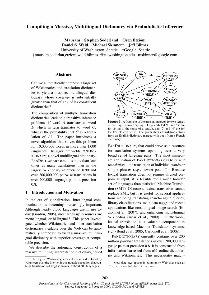
Proceedings of the 47th Annual Meeting of the ACL and the 4th IJCNLP of the AFNLP, pages 262–270,Suntec, Singapore, 2-7 August 2009. c©2009 ACL and AFNLP
Compiling a Massive, Multilingual Dictionary via Probabilistic Inference
Mausam Stephen Soderland Oren EtzioniDaniel S. Weld Michael Skinner* Jeff BilmesUniversity of Washington, Seattle *Google, Seattle
{mausam,soderlan,etzioni,weld,bilmes}@cs.washington.edu [email protected]
Abstract
Can we automatically compose a large setof Wiktionaries and translation dictionar-ies to yield a massive, multilingual dic-tionary whose coverage is substantiallygreater than that of any of its constituentdictionaries?
The composition of multiple translationdictionaries leads to a transitive inferenceproblem: if word A translates to wordB which in turn translates to word C,what is the probability that C is a trans-lation of A? The paper introduces anovel algorithm that solves this problemfor 10,000,000 words in more than 1,000languages. The algorithm yields PANDIC-TIONARY, a novel multilingual dictionary.PANDICTIONARY contains more than fourtimes as many translations than in thelargest Wiktionary at precision 0.90 andover 200,000,000 pairwise translations inover 200,000 language pairs at precision0.8.
1 Introduction and Motivation
In the era of globalization, inter-lingual com-munication is becoming increasingly important.Although nearly 7,000 languages are in use to-day (Gordon, 2005), most language resources aremono-lingual, or bi-lingual.1 This paper investi-gates whether Wiktionaries and other translationdictionaries available over the Web can be auto-matically composed to yield a massive, multilin-gual dictionary with superior coverage at compa-rable precision.
We describe the automatic construction of amassive multilingual translation dictionary, called
1The English Wiktionary, a lexical resource developed byvolunteers over the Internet is one notable exception that con-tains translations of English words in about 500 languages.
Figure 1: A fragment of the translation graph for two sensesof the English word ‘spring’. Edges labeled ‘1’ and ‘3’ arefor spring in the sense of a season, and ‘2’ and ‘4’ are forthe flexible coil sense. The graph shows translation entriesfrom an English dictionary merged with ones from a Frenchdictionary.
PANDICTIONARY, that could serve as a resourcefor translation systems operating over a verybroad set of language pairs. The most immedi-ate application of PANDICTIONARY is to lexicaltranslation—the translation of individual words orsimple phrases (e.g., “sweet potato”). Becauselexical translation does not require aligned cor-pora as input, it is feasible for a much broaderset of languages than statistical Machine Transla-tion (SMT). Of course, lexical translation cannotreplace SMT, but it is useful for several applica-tions including translating search-engine queries,library classifications, meta-data tags,2 and recentapplications like cross-lingual image search (Et-zioni et al., 2007), and enhancing multi-lingualWikipedias (Adar et al., 2009). Furthermore,lexical translation is a valuable component inknowledge-based Machine Translation systems,e.g., (Bond et al., 2005; Carbonell et al., 2006).
PANDICTIONARY currently contains over 200million pairwise translations in over 200,000 lan-guage pairs at precision 0.8. It is constructed frominformation harvested from 631 online dictionar-ies and Wiktionaries. This necessitates match-
2Meta-data tags appear in community Web sites such asflickr.com and del.icio.us.
262
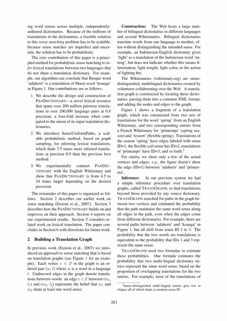
ing word senses across multiple, independently-authored dictionaries. Because of the millions oftranslations in the dictionaries, a feasible solutionto this sense matching problem has to be scalable;because sense matches are imperfect and uncer-tain, the solution has to be probabilistic.
The core contribution of this paper is a princi-pled method for probabilistic sense matching to in-fer lexical translations between two languages thatdo not share a translation dictionary. For exam-ple, our algorithm can conclude that Basque word‘udaherri’ is a translation of Maori word ‘koanga’in Figure 1. Our contributions are as follows:
1. We describe the design and construction ofPANDICTIONARY—a novel lexical resourcethat spans over 200 million pairwise transla-tions in over 200,000 language pairs at 0.8precision, a four-fold increase when com-pared to the union of its input translation dic-tionaries.
2. We introduce SenseUniformPaths, a scal-able probabilistic method, based on graphsampling, for inferring lexical translations,which finds 3.5 times more inferred transla-tions at precison 0.9 than the previous bestmethod.
3. We experimentally contrast PANDIC-TIONARY with the English Wiktionary andshow that PANDICTIONARY is from 4.5 to24 times larger depending on the desiredprecision.
The remainder of this paper is organized as fol-lows. Section 2 describes our earlier work onsense matching (Etzioni et al., 2007). Section 3describes how the PANDICTIONARY builds on andimproves on their approach. Section 4 reports onour experimental results. Section 5 considers re-lated work on lexical translation. The paper con-cludes in Section 6 with directions for future work.
2 Building a Translation Graph
In previous work (Etzioni et al., 2007) we intro-duced an approach to sense matching that is basedon translation graphs (see Figure 1 for an exam-ple). Each vertex v ∈ V in the graph is an or-dered pair (w, l) where w is a word in a languagel. Undirected edges in the graph denote transla-tions between words: an edge e ∈ E between (w1,l1) and (w2, l2) represents the belief that w1 andw2 share at least one word sense.
Construction: The Web hosts a large num-ber of bilingual dictionaries in different languagesand several Wiktionaries. Bilingual dictionariestranslate words from one language to another, of-ten without distinguishing the intended sense. Forexample, an Indonesian-English dictionary gives‘light’ as a translation of the Indonesian word ‘en-teng’, but does not indicate whether this means il-lumination, light weight, light color, or the actionof lighting fire.
The Wiktionaries (wiktionary.org) are sense-distinguished, multilingual dictionaries created byvolunteers collaborating over the Web. A transla-tion graph is constructed by locating these dictio-naries, parsing them into a common XML format,and adding the nodes and edges to the graph.
Figure 1 shows a fragment of a translationgraph, which was constructed from two sets oftranslations for the word ‘spring’ from an EnglishWiktionary, and two corresponding entries froma French Wiktionary for ‘printemps’ (spring sea-son) and ‘ressort’ (flexible spring). Translations ofthe season ‘spring’ have edges labeled with senseID=1, the flexible coil sense has ID=2, translationsof ‘printemps’ have ID=3, and so forth.3
For clarity, we show only a few of the actualvertices and edges; e.g., the figure doesn’t showthe edge (ID=1) between ‘udaherri’ and ‘primav-era’.
Inference: In our previous system we hada simple inference procedure over translationgraphs, called TRANSGRAPH, to find translationsbeyond those provided by any source dictionary.TRANSGRAPH searched for paths in the graph be-tween two vertices and estimated the probabilitythat the path maintains the same word sense alongall edges in the path, even when the edges comefrom different dictionaries. For example, there areseveral paths between ‘udaherri’ and ‘koanga’ inFigure 1, but all shift from sense ID 1 to 3. Theprobability that the two words are translations isequivalent to the probability that IDs 1 and 3 rep-resent the same sense.
TRANSGRAPH used two formulae to estimatethese probabilities. One formula estimates theprobability that two multi-lingual dictionary en-tries represent the same word sense, based on theproportion of overlapping translations for the twoentries. For example, most of the translations of
3Sense-distinguished multi-lingual entries give rise tocliques all of which share a common sense ID.
263

French ‘printemps’ are also translations of the sea-son sense of ‘spring’. A second formula is basedon triangles in the graph (useful for bilingual dic-tionaries): a clique of 3 nodes with an edge be-tween each pair of nodes. In such cases, there isa high probability that all 3 nodes share a wordsense.
Critique: While TRANSGRAPH was the firstto present a scalable inference method for lexicaltranslation, it suffers from several drawbacks. Itsformulae operate only on local information: pairsof senses that are adjacent in the graph or triangles.It does not incorporate evidence from longer pathswhen an explicit triangle is not present. Moreover,the probabilities from different paths are com-bined conservatively (either taking the max overall paths, or using “noisy or” on paths that arecompletely disjoint, except end points), thus lead-ing to suboptimal precision/recall.
In response to this critique, the next sectionpresents an inference algorithm, called SenseUni-formPaths (SP), with substantially improved recallat equivalent precision.
3 Translation Inference Algorithms
In essence, inference over a translation graphamounts to transitive sense matching: if word Atranslates to word B, which translates in turn toword C, what is the probability that C is a trans-lation of A? If B is polysemous then C may notshare a sense with A. For example, in Figure 2(a)if A is the French word ‘ressort’ (the flexible-coil sense of spring) and B is the English word‘spring’, then Slovenian word ‘vzmet’ may or maynot be a correct translation of ‘ressort’ dependingon whether the edge (B,C) denotes the flexible-coil sense of spring, the season sense, or anothersense. Indeed, given only the knowledge of thepath A − B − C we cannot claim anything withcertainty regarding A to C.
However, if A, B, and C are on a circuit thatstarts at A, passes through B and C and re-turns to A, there is a high probability that allnodes on that circuit share a common word sense,given certain restrictions that we enumerate later.Where TRANSGRAPH used evidence from circuitsof length 3, we extend this to paths of arbitrarylengths.
To see how this works, let us begin with the sim-plest circuit, a triangle of three nodes as shown inFigure 2(b). We can be quite certain that ‘vzmet’
shares the sense of coil with both ‘spring’ and‘ressort’. Our reasoning is as follows: eventhough both ‘ressort’ and ‘spring’ are polysemousthey share only one sense. For a triangle to formwe have two choices – (1) either ‘vzmet’ meansspring coil, or (2) ‘vzmet’ means both the springseason and jurisdiction, but not spring coil. Thelatter is possible but such a coincidence is very un-likely, which is why a triangle is strong evidencefor the three words to share a sense.
As an example of longer paths, our inferencealgorithms can conclude that in Figure 2(c), both‘molla’ and ‘vzmet’ have the sense coil, eventhough no explicit triangle is present. To showthis, let us define a translation circuit as follows:
Definition 1 A translation circuit from v∗1 withsense s∗ is a cycle that starts and ends at v∗1 withno repeated vertices (other than v∗1 at end points).Moreover, the path includes an edge between v∗1and another vertex v∗2 that also has sense s∗.
All vertices on a translation circuit are mutualtranslations with high probability, as in Figure2(c). The edge from ‘spring’ indicates that ‘vzmet’means either coil or season, while the edge from‘ressort’ indicates that ‘molla’ means either coilor jurisdiction. The edge from ‘vzmet’ to ‘molla’indicates that they share a sense, which will hap-pen if all nodes share the sense season or if either‘vzmet’ has the unlikely combination of coil andjurisdiction (or ‘molla’ has coil and season).
We also develop a mathematical model ofsense-assignment to words that lets us formallyprove these insights. For more details on the the-ory please refer to our extended version. This pa-per reports on our novel algorithm and experimen-tal results.
These insights suggest a basic version of our al-gorithm: “given two vertices, v∗1 and v∗2 , that sharea sense (say s∗) compute all translation circuitsfrom v∗1 in the sense s∗; mark all vertices in thecircuits as translations of the sense s∗”.
To implement this algorithm we need to decidewhether a vertex lies on a translation circuit, whichis trickier than it seems. Notice that knowingthat v is connected independently to v∗1 and v∗2doesn’t imply that there exists a translation circuitthrough v, because both paths may go through acommon node, thus violating of the definition oftranslation circuit. For example, in Figure 2(d) theCatalan word ‘ploma’ has paths to both spring andressort, but there is no translation circuit through
264
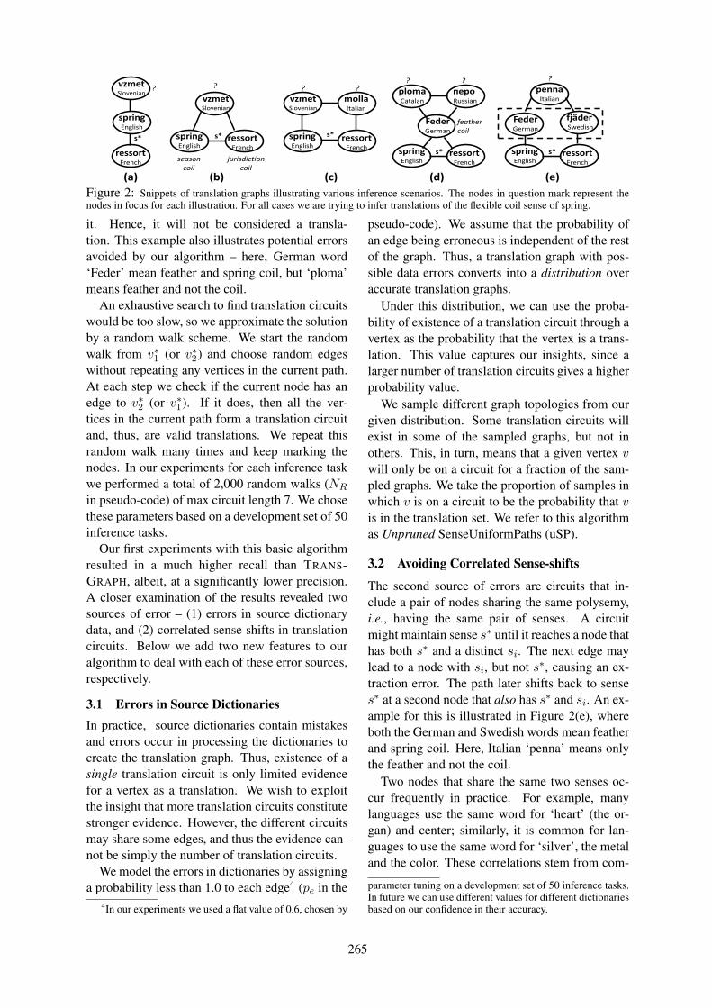
springEnglish
ressortFrench
vzmetSlovenian
springEnglish
ressortFrench
vzmetSlovenian
springEnglish
vzmetSlovenian
ressortFrench
mollaItalian
springEnglish
ressortFrench
plomaCatalan
FederGerman
перо Russian
springEnglish
ressortFrench
fjäderSwedish
pennaItalian
FederGerman
(a) (b) (c) (d) (e)
seasoncoil
jurisdictioncoil
s* s*
s* s*
s*
? ? ?? ?
feathercoil
?
?
Figure 2: Snippets of translation graphs illustrating various inference scenarios. The nodes in question mark represent thenodes in focus for each illustration. For all cases we are trying to infer translations of the flexible coil sense of spring.
it. Hence, it will not be considered a transla-tion. This example also illustrates potential errorsavoided by our algorithm – here, German word‘Feder’ mean feather and spring coil, but ‘ploma’means feather and not the coil.
An exhaustive search to find translation circuitswould be too slow, so we approximate the solutionby a random walk scheme. We start the randomwalk from v∗1 (or v∗2) and choose random edgeswithout repeating any vertices in the current path.At each step we check if the current node has anedge to v∗2 (or v∗1). If it does, then all the ver-tices in the current path form a translation circuitand, thus, are valid translations. We repeat thisrandom walk many times and keep marking thenodes. In our experiments for each inference taskwe performed a total of 2,000 random walks (NR
in pseudo-code) of max circuit length 7. We chosethese parameters based on a development set of 50inference tasks.
Our first experiments with this basic algorithmresulted in a much higher recall than TRANS-GRAPH, albeit, at a significantly lower precision.A closer examination of the results revealed twosources of error – (1) errors in source dictionarydata, and (2) correlated sense shifts in translationcircuits. Below we add two new features to ouralgorithm to deal with each of these error sources,respectively.
3.1 Errors in Source DictionariesIn practice, source dictionaries contain mistakesand errors occur in processing the dictionaries tocreate the translation graph. Thus, existence of asingle translation circuit is only limited evidencefor a vertex as a translation. We wish to exploitthe insight that more translation circuits constitutestronger evidence. However, the different circuitsmay share some edges, and thus the evidence can-not be simply the number of translation circuits.
We model the errors in dictionaries by assigninga probability less than 1.0 to each edge4 (pe in the
4In our experiments we used a flat value of 0.6, chosen by
pseudo-code). We assume that the probability ofan edge being erroneous is independent of the restof the graph. Thus, a translation graph with pos-sible data errors converts into a distribution overaccurate translation graphs.
Under this distribution, we can use the proba-bility of existence of a translation circuit through avertex as the probability that the vertex is a trans-lation. This value captures our insights, since alarger number of translation circuits gives a higherprobability value.
We sample different graph topologies from ourgiven distribution. Some translation circuits willexist in some of the sampled graphs, but not inothers. This, in turn, means that a given vertex vwill only be on a circuit for a fraction of the sam-pled graphs. We take the proportion of samples inwhich v is on a circuit to be the probability that vis in the translation set. We refer to this algorithmas Unpruned SenseUniformPaths (uSP).
3.2 Avoiding Correlated Sense-shifts
The second source of errors are circuits that in-clude a pair of nodes sharing the same polysemy,i.e., having the same pair of senses. A circuitmight maintain sense s∗ until it reaches a node thathas both s∗ and a distinct si. The next edge maylead to a node with si, but not s∗, causing an ex-traction error. The path later shifts back to senses∗ at a second node that also has s∗ and si. An ex-ample for this is illustrated in Figure 2(e), whereboth the German and Swedish words mean featherand spring coil. Here, Italian ‘penna’ means onlythe feather and not the coil.
Two nodes that share the same two senses oc-cur frequently in practice. For example, manylanguages use the same word for ‘heart’ (the or-gan) and center; similarly, it is common for lan-guages to use the same word for ‘silver’, the metaland the color. These correlations stem from com-
parameter tuning on a development set of 50 inference tasks.In future we can use different values for different dictionariesbased on our confidence in their accuracy.
265

Figure 3: The set {B, C} has a shared ambiguity - eachnode has both sense 1 (from the lower clique) and sense 2(from the upper clique). A circuit that contains two nodesfrom the same ambiguity set with an intervening node not inthat set is likely to create translation errors.
mon metaphor and the shared evolutionary rootsof some languages.
We are able to avoid circuits with this type ofcorrelated sense-shift by automatically identifyingambiguity sets, sets of nodes known to share mul-tiple senses. For instance, in Figure 2(e) ‘Feder’and ‘fjäder’ form an ambiguity set (shown withindashed lines), as they both mean feather and coil.
Definition 2 An ambiguity set A is a set of ver-tices that all share the same two senses. I.e.,∃s1, s2, with s1 6= s2 s.t. ∀v ∈ A, sense(v, s1)∧sense(v, s2), where sense(v, s) denotes that v hassense s.
To increase the precision of our algorithm weprune the circuits that contain two nodes in thesame ambiguity set and also have one or more in-tervening nodes that are not in the ambiguity set.There is a strong likelihood that the interveningnodes will represent a translation error.
Ambiguity sets can be detected from the graphtopology as follows. Each clique in the graph rep-resents a set of vertices that share a common wordsense. When two cliques intersect in two or morevertices, the intersecting vertices share the wordsense of both cliques. This may either mean thatboth cliques represent the same word sense, or thatthe intersecting vertices form an ambiguity set. Alarge overlap between two cliques makes the for-mer case more likely; a small overlap makes itmore likely that we have found an ambiguity set.
Figure 3 illustrates one such computation.All nodes of the clique V1, V2, A, B,C,D sharea word sense, and all nodes of the cliqueB,C,E, F, G, H also share a word sense. The set{B,C} has nodes that have both senses, formingan ambiguity set. We denote the set of ambiguitysets by A in the pseudo-code.
Having identified these ambiguity sets, we mod-ify our random walk scheme by keeping track of
whether we are entering or leaving an ambiguityset. We prune away all paths that enter the sameambiguity set twice. We name the resulting algo-rithm SenseUniformPaths (SP), summarized at ahigh level in Algorithm 1.Comparing Inference Algorithms Our evalua-tion demonstrated that SP outperforms uSP. Boththese algorithms have significantly higher recallthan TRANSGRAPH algorithm. The detailed re-sults are presented in Section 4.2. We choose SPas our inference algorithm for all further research,in particular to create PANDICTIONARY.
3.3 Compiling PanDictionary
Our goal is to automatically compile PANDIC-TIONARY, a sense-distinguished lexical transla-tion resource, where each entry is a distinct wordsense. Associated with each word sense is a list oftranslations in multiple languages.
We use Wiktionary senses as the base sensesfor PANDICTIONARY. Recall that SP requires twonodes (v∗1 and v∗2) for inference. We use the Wik-tionary source word as v∗1 and automatically pickthe second word from the set of Wiktionary trans-lations of that sense by choosing a word that iswell connected, and, which does not appear inother senses of v∗1 (i.e., is expected to share onlyone sense with v∗1).
We first run SenseUniformPaths to expand theapproximately 50,000 senses in the English Wik-tionary. We further expand any senses from theother Wiktionaries that are not yet covered byPANDICTIONARY, and add these to PANDIC-TIONARY. This results in the creation of theworld’s largest multilingual, sense-distinguishedtranslation resource, PANDICTIONARY. It con-tains a little over 80,000 senses. Its constructiontakes about three weeks on a 3.4 GHz processorwith a 2 GB memory.
Algorithm 1 S.P.(G, v∗1, v∗2,A)
1: parameters NG: no. of graph samples, NR: no. of ran-dom walks, pe: prob. of sampling an edge
2: create NG versions of G by sampling each edge indepen-dently with probability pe
3: for all i = 1..NG do4: for all vertices v : rp[v][i] = 05: perform NR random walks starting at v∗1 (or v∗2 ) and
pruning any walk that enters (or exits) an ambiguityset in A twice. All walks that connect to v∗2 (or v∗1 )form a translation circuit.
6: for all vertices v do7: if(v is on a translation circuit) rp[v][i] = 1
8: return∑
irp[v][i]
NGas the prob. that v is a translation
266

4 Empirical Evaluation
In our experiments we investigate three key ques-tions: (1) which of the three algorithms (TG, uSPand SP) is superior for translation inference (Sec-tion 4.2)? (2) how does the coverage of PANDIC-TIONARY compare with the largest existing mul-tilingual dictionary, the English Wiktionary (Sec-tion 4.3)? (3) what is the benefit of inference overthe mere aggregation of 631 dictionaries (Section4.4)? Additionally, we evaluate the inference algo-rithm on two other dimensions – variation with thedegree of polysemy of source word, and variationwith original size of the seed translation set.
4.1 Experimental Methodology
Ideally, we would like to evaluate a random sam-ple of the more than 1,000 languages representedin PANDICTIONARY.5 However, a high-qualityevaluation of translation between two languagesrequires a person who is fluent in both languages.Such people are hard to find and may not evenexist for many language pairs (e.g., Basque andMaori). Thus, our evaluation was guided by ourability to recruit volunteer evaluators. Since weare based in an English speaking country we wereable to recruit local volunteers who are fluent ina range of languages and language families, andwho are also bilingual in English.6
The experiments in Sections 4.2 and 4.3 testwhether translations in a PANDICTIONARY haveaccurate word senses. We provided our evalua-tors with a random sample of translations into theirnative language. For each translation we showedthe English source word and gloss of the intendedsense. For example, a Dutch evaluator was shownthe sense ‘free (not imprisoned)’ together with theDutch word ‘loslopende’. The instructions wereto mark a word as correct if it could be used to ex-press the intended sense in a sentence in their na-tive language. For experiments in Section 4.4 wetested precision of pairwise translations, by havinginformants in several pairs of languages discusswhether the words in their respective languagescan be used for the same sense.
We use the tags of correct or incorrect to com-pute the precision: the percentage of correct trans-
5The distribution of words in PANDICTIONARY is highlynon-uniform ranging from 182,988 words in English to 6,154words in Luxembourgish and 189 words in Tuvalu.
6The languages used was based on the availability of na-tive speakers. This varied between the different experiments,which were conducted at different times.
Figure 4: The SenseUniformPaths algorithm (SP) morethan doubles the number of correct translations at precision0.95, compared to a baseline of translations that can be foundwithout inference.
lations divided by correct plus incorrect transla-tions. We then order the translations by probabil-ity and compute the precision at various probabil-ity thresholds.
4.2 Comparing Inference Algorithms
Our first evaluation compares our SenseUniform-Paths (SP) algorithm (before and after pruning)with TRANSGRAPH on both precision and num-ber of translations.
To carry out this comparison, we randomly sam-pled 1,000 senses from English Wiktionary andran the three algorithms over them. We evalu-ated the results on 7 languages – Chinese, Danish,German, Hindi, Japanese, Russian, and Turkish.Each informant tagged 60 random translations in-ferred by each algorithm, which resulted in 360-400 tags per algorithm7. The precision over thesewas taken as a surrogate for the precision acrossall the senses.
We compare the number of translations for eachalgorithm at comparable precisions. The baselineis the set of translations (for these 1000 senses)found in the source dictionaries without inference,which has a precision 0.95 (as evaluated by ourinformants).8
Our results are shown in Figure 4. At this highprecision, SP more than doubles the number ofbaseline translations, finding 5 times as many in-ferred translations (in black) as TG.
Indeed, both uSP and SP massively outperformTG. SP is consistently better than uSP, since itperforms better for polysemous words, due to itspruning based on ambiguity sets. We conclude
7Some translations were marked as “Don’t know”.8Our informants tended to underestimate precision, often
marking correct translations in minor senses of a word as in-correct.
267
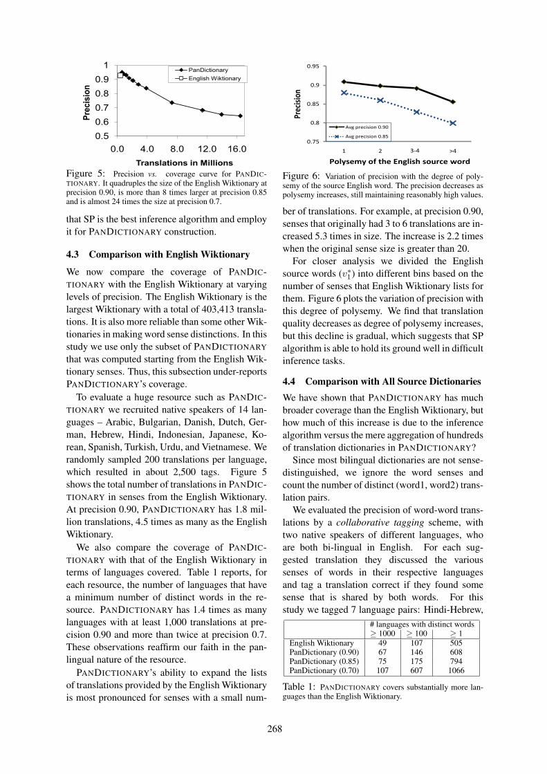
0.5
0.6
0.7
0.8
0.9
1
0.0 4.0 8.0 12.0 16.0
Pre
cis
ion
Translations in Millions
PanDictionary
English Wiktionary
Figure 5: Precision vs. coverage curve for PANDIC-TIONARY. It quadruples the size of the English Wiktionary atprecision 0.90, is more than 8 times larger at precision 0.85and is almost 24 times the size at precision 0.7.
that SP is the best inference algorithm and employit for PANDICTIONARY construction.
4.3 Comparison with English Wiktionary
We now compare the coverage of PANDIC-TIONARY with the English Wiktionary at varyinglevels of precision. The English Wiktionary is thelargest Wiktionary with a total of 403,413 transla-tions. It is also more reliable than some other Wik-tionaries in making word sense distinctions. In thisstudy we use only the subset of PANDICTIONARY
that was computed starting from the English Wik-tionary senses. Thus, this subsection under-reportsPANDICTIONARY’s coverage.
To evaluate a huge resource such as PANDIC-TIONARY we recruited native speakers of 14 lan-guages – Arabic, Bulgarian, Danish, Dutch, Ger-man, Hebrew, Hindi, Indonesian, Japanese, Ko-rean, Spanish, Turkish, Urdu, and Vietnamese. Werandomly sampled 200 translations per language,which resulted in about 2,500 tags. Figure 5shows the total number of translations in PANDIC-TIONARY in senses from the English Wiktionary.At precision 0.90, PANDICTIONARY has 1.8 mil-lion translations, 4.5 times as many as the EnglishWiktionary.
We also compare the coverage of PANDIC-TIONARY with that of the English Wiktionary interms of languages covered. Table 1 reports, foreach resource, the number of languages that havea minimum number of distinct words in the re-source. PANDICTIONARY has 1.4 times as manylanguages with at least 1,000 translations at pre-cision 0.90 and more than twice at precision 0.7.These observations reaffirm our faith in the pan-lingual nature of the resource.
PANDICTIONARY’s ability to expand the listsof translations provided by the English Wiktionaryis most pronounced for senses with a small num-
0.75
0.8
0.85
0.9
0.95
1 2 3,4 >4
Prec
isio
n
Avg precision 0.90
Avg precision 0.85
Polysemy of the English source word
3-4
Figure 6: Variation of precision with the degree of poly-semy of the source English word. The precision decreases aspolysemy increases, still maintaining reasonably high values.
ber of translations. For example, at precision 0.90,senses that originally had 3 to 6 translations are in-creased 5.3 times in size. The increase is 2.2 timeswhen the original sense size is greater than 20.
For closer analysis we divided the Englishsource words (v∗1) into different bins based on thenumber of senses that English Wiktionary lists forthem. Figure 6 plots the variation of precision withthis degree of polysemy. We find that translationquality decreases as degree of polysemy increases,but this decline is gradual, which suggests that SPalgorithm is able to hold its ground well in difficultinference tasks.
4.4 Comparison with All Source DictionariesWe have shown that PANDICTIONARY has muchbroader coverage than the English Wiktionary, buthow much of this increase is due to the inferencealgorithm versus the mere aggregation of hundredsof translation dictionaries in PANDICTIONARY?
Since most bilingual dictionaries are not sense-distinguished, we ignore the word senses andcount the number of distinct (word1, word2) trans-lation pairs.
We evaluated the precision of word-word trans-lations by a collaborative tagging scheme, withtwo native speakers of different languages, whoare both bi-lingual in English. For each sug-gested translation they discussed the varioussenses of words in their respective languagesand tag a translation correct if they found somesense that is shared by both words. For thisstudy we tagged 7 language pairs: Hindi-Hebrew,
# languages with distinct words≥ 1000 ≥ 100 ≥ 1
English Wiktionary 49 107 505PanDictionary (0.90) 67 146 608PanDictionary (0.85) 75 175 794PanDictionary (0.70) 107 607 1066
Table 1: PANDICTIONARY covers substantially more lan-guages than the English Wiktionary.
268

0
50
100
150
200
250
EW 631D PD(0.9) PD(0.85) PD(0.8)
Inferred transl. Direct transl.
Tran
slat
ions
(in m
illio
ns)
Figure 7: The number of distinct word-word translationpairs from PANDICTIONARY is several times higher than thenumber of translation pairs in the English Wiktionary (EW)or in all 631 source dictionaries combined (631 D). A major-ity of PANDICTIONARY translations are inferred by combin-ing entries from multiple dictionaries.
Japanese-Russian, Chinese-Turkish, Japanese-German, Chinese-Russian, Bengali-German, andHindi-Turkish.
Figure 7 compares the number of word-wordtranslation pairs in the English Wiktionary (EW),in all 631 source dictionaries (631 D), and in PAN-DICTIONARY at precisions 0.90, 0.85, and 0.80.PANDICTIONARY increases the number of word-word translations by 73% over the source dictio-nary translations at precision 0.90 and increases itby 2.7 times at precision 0.85. PANDICTIONARY
also adds value by identifying the word sense ofthe translation, which is not given in most of thesource dictionaries.
5 Related Work
Because we are considering a relatively new prob-lem (automatically building a panlingual transla-tion resource) there is little work that is directly re-lated to our own. The closest research is our previ-ous work on TRANSGRAPH algorithm (Etzioni etal., 2007). Our current algorithm outperforms theprevious state of the art by 3.5 times at precision0.9 (see Figure 4). Moreover, we compile this in adictionary format, thus considerably reducing theresponse time compared to TRANSGRAPH, whichperformed inference at query time.
There has been considerable research on meth-ods to acquire translation lexicons from eitherMRDs (Neff and McCord, 1990; Helmreich etal., 1993; Copestake et al., 1994) or from par-allel text (Gale and Church, 1991; Fung, 1995;Melamed, 1997; Franz et al., 2001), but this hasgenerally been limited to a small number of lan-guages. Manually engineered dictionaries such asEuroWordNet (Vossen, 1998) are also limited toa relatively small set of languages. There is somerecent work on compiling dictionaries from mono-
lingual corpora, which may scale to several lan-guage pairs in future (Haghighi et al., 2008).
Little work has been done in combining mul-tiple dictionaries in a way that maintains wordsenses across dictionaries. Gollins and Sanderson(2001) explored using triangulation between alter-nate pivot languages in cross-lingual informationretrieval. Their triangulation essentially mixestogether circuits for all word senses, hence, is un-able to achieve high precision.
Dyvik’s “semantic mirrors” uses translationpaths to tease apart distinct word senses frominputs that are not sense-distinguished (Dyvik,2004). However, its expensive processing andreliance on parallel corpora would not scale tolarge numbers of languages. Earlier (Knight andLuk, 1994) discovered senses of Spanish words bymatching several English translations to a Word-Net synset. This approach applies only to specifickinds of bilingual dictionaries, and also requires ataxonomy of synsets in the target language.
Random walks, graph sampling and MonteCarlo simulations are popular in literature, though,to our knowledge, none have applied these to ourspecific problems (Henzinger et al., 1999; Andrieuet al., 2003; Karger, 1999).
6 ConclusionsWe have described the automatic construction ofa unique multilingual translation resource, calledPANDICTIONARY, by performing probabilistic in-ference over the translation graph. Overall, theconstruction process consists of large scale in-formation extraction over the Web (parsing dic-tionaries), combining it into a single resource (atranslation graph), and then performing automatedreasoning over the graph (SenseUniformPaths) toyield a much more extensive and useful knowl-edge base.
We have shown that PANDICTIONARY hasmore coverage than any other existing bilingualor multilingual dictionary. Even at the high preci-sion of 0.90, PANDICTIONARY more than quadru-ples the size of the English Wiktionary, the largestavailable multilingual resource today.
We plan to make PANDICTIONARY availableto the research community, and also to the Wik-tionary community in an effort to bolster their ef-forts. PANDICTIONARY entries can suggest newtranslations for volunteers to add to Wiktionaryentries, particularly if combined with an intelli-gent editing tool (e.g., (Hoffmann et al., 2009)).
269

Acknowledgments
This research was supported by a gift from theUtilika Foundation to the Turing Center at Uni-versity of Washington. We acknowledge PaulBeame, Nilesh Dalvi, Pedro Domingos, RohitKhandekar, Daniel Lowd, Parag, Jonathan Pool,Hoifung Poon, Vibhor Rastogi, Gyanit Singh forfruitful discussions and insightful comments onthe research. We thank the language experts whodonated their time and language expertise to eval-uate our systems. We also thank the anynomousreviewers of the previous drafts of this paper fortheir valuable suggestions in improving the evalu-ation and presentation.
ReferencesE. Adar, M. Skinner, and D. Weld. 2009. Information
arbitrage in multi-lingual Wikipedia. In Procs. ofWeb Search and Data Mining(WSDM 2009).
C. Andrieu, N. De Freitas, A. Doucet, and M. Jor-dan. 2003. An Introduction to MCMC for MachineLearning. Machine Learning, 50:5–43.
F. Bond, S. Oepen, M. Siegel, A. Copestake, andD D. Flickinger. 2005. Open source machine trans-lation with DELPH-IN. In Open-Source MachineTranslation Workshop at MT Summit X.
J. Carbonell, S. Klein, D. Miller, M. Steinbaum,T. Grassiany, and J. Frey. 2006. Context-based ma-chine translation. In AMTA.
A. Copestake, T. Briscoe, P. Vossen, A. Ageno,I. Castellon, F. Ribas, G. Rigau, H. Rodriquez, andA. Samiotou. 1994. Acquisition of lexical trans-lation relations from MRDs. Machine Translation,3(3–4):183–219.
H. Dyvik. 2004. Translation as semantic mirrors: fromparallel corpus to WordNet. Language and Comput-ers, 49(1):311–326.
O. Etzioni, K. Reiter, S. Soderland, and M. Sammer.2007. Lexical translation with application to imagesearch on the Web. In Machine Translation SummitXI.
M. Franz, S. McCarly, and W. Zhu. 2001. English-Chinese information retrieval at IBM. In Proceed-ings of TREC 2001.
P. Fung. 1995. A pattern matching method for findingnoun and proper noun translations from noisy paral-lel corpora. In Proceedings of ACL-1995.
W. Gale and K.W. Church. 1991. A Program forAligning Sentences in Bilingual Corpora. In Pro-ceedings of ACL-1991.
T. Gollins and M. Sanderson. 2001. Improving crosslanguage retrieval with triangulated translation. InSIGIR.
Raymond G. Gordon, Jr., editor. 2005. Ethnologue:Languages of the World (Fifteenth Edition). SIL In-ternational.
A. Haghighi, P. Liang, T. Berg-Kirkpatrick, andD. Klein. 2008. Learning bilingual lexicons frommonolingual corpora. In ACL.
S. Helmreich, L. Guthrie, and Y. Wilks. 1993. Theuse of machine readable dictionaries in the Panglossproject. In AAAI Spring Symposium on BuildingLexicons for Machine Translation.
Monika R. Henzinger, Allan Heydon, Michael Mitzen-macher, and Marc Najork. 1999. Measuring indexquality using random walks on the web. In WWW.
R. Hoffmann, S. Amershi, K. Patel, F. Wu, J. Foga-rty, and D. S. Weld. 2009. Amplifying commu-nity content creation with mixed-initiative informa-tion extraction. In ACM SIGCHI (CHI2009).
D. R. Karger. 1999. A randomized fully polynomialapproximation scheme for the all-terminal networkreliability problem. SIAM Journal of Computation,29(2):492–514.
K. Knight and S. Luk. 1994. Building a large-scaleknowledge base for machine translation. In AAAI.
I.D. Melamed. 1997. A Word-to-Word Model ofTranslational Equivalence. In Proceedings of ACL-1997 and EACL-1997, pages 490–497.
M. Neff and M. McCord. 1990. Acquiring lexical datafrom machine-readable dictionary resources for ma-chine translation. In 3rd Intl Conference on Theoret-ical and Methodological Issues in Machine Transla-tion of Natural Language.
P. Vossen, editor. 1998. EuroWordNet: A multilingualdatabase with lexical semantic networds. KluwerAcademic Publishers.
270
Proceedings of the 47th Annual Meeting of the ACL and the 4th IJCNLP of the AFNLP, pages 271–279,Suntec, Singapore, 2-7 August 2009. c©2009 ACL and AFNLP
A Metric-based Framework for Automatic Taxonomy Induction
Hui Yang
Language Technologies Institute
School of Computer Science
Carnegie Mellon University
Jamie Callan
Language Technologies Institute
School of Computer Science
Carnegie Mellon University
Abstract
This paper presents a novel metric-based
framework for the task of automatic taxonomy
induction. The framework incrementally clus-
ters terms based on ontology metric, a score
indicating semantic distance; and transforms
the task into a multi-criteria optimization
based on minimization of taxonomy structures
and modeling of term abstractness. It com-
bines the strengths of both lexico-syntactic
patterns and clustering through incorporating
heterogeneous features. The flexible design of
the framework allows a further study on which
features are the best for the task under various
conditions. The experiments not only show
that our system achieves higher F1-measure
than other state-of-the-art systems, but also re-
veal the interaction between features and vari-
ous types of relations, as well as the interac-
tion between features and term abstractness.
1 Introduction
Automatic taxonomy induction is an important
task in the fields of Natural Language
Processing, Knowledge Management, and Se-
mantic Web. It has been receiving increasing
attention because semantic taxonomies, such as
WordNet (Fellbaum, 1998), play an important
role in solving knowledge-rich problems, includ-
ing question answering (Harabagiu et al., 2003)
and textual entailment (Geffet and Dagan, 2005).
Nevertheless, most existing taxonomies are ma-
nually created at great cost. These taxonomies
are rarely complete; it is difficult to include new
terms in them from emerging or rapidly changing
domains. Moreover, manual taxonomy construc-
tion is time-consuming, which may make it un-
feasible for specialized domains and personalized
tasks. Automatic taxonomy induction is a solu-
tion to augment existing resources and to pro-
duce new taxonomies for such domains and
tasks.
Automatic taxonomy induction can be decom-
posed into two subtasks: term extraction and re-
lation formation. Since term extraction is rela-
tively easy, relation formation becomes the focus
of most research on automatic taxonomy induc-
tion. In this paper, we also assume that terms in a
taxonomy are given and concentrate on the sub-
task of relation formation.
Existing work on automatic taxonomy induc-
tion has been conducted under a variety of
names, such as ontology learning, semantic class
learning, semantic relation classification, and
relation extraction. The approaches fall into two
main categories: pattern-based and clustering-
based. Pattern-based approaches define lexical-
syntactic patterns for relations, and use these pat-
terns to discover instances of relations. Cluster-
ing-based approaches hierarchically cluster terms
based on similarities of their meanings usually
represented by a vector of quantifiable features.
Pattern-based approaches are known for their
high accuracy in recognizing instances of rela-
tions if the patterns are carefully chosen, either
manually (Berland and Charniak, 1999; Kozare-
va et al., 2008) or via automatic bootstrapping
(Hearst, 1992; Widdows and Dorow, 2002; Girju
et al., 2003). The approaches, however, suffer
from sparse coverage of patterns in a given cor-
pus. Recent studies (Etzioni et al., 2005; Kozare-
va et al., 2008) show that if the size of a corpus,
such as the Web, is nearly unlimited, a pattern
has a higher chance to explicitly appear in the
corpus. However, corpus size is often not that
large; hence the problem still exists. Moreover,
since patterns usually extract instances in pairs,
the approaches suffer from the problem of incon-
sistent concept chains after connecting pairs of
instances to form taxonomy hierarchies.
Clustering-based approaches have a main ad-
vantage that they are able to discover relations
271
which do not explicitly appear in text. They also
avoid the problem of inconsistent chains by ad-
dressing the structure of a taxonomy globally
from the outset. Nevertheless, it is generally be-
lieved that clustering-based approaches cannot
generate relations as accurate as pattern-based
approaches. Moreover, their performance is
largely influenced by the types of features used.
The common types of features include contextual
(Lin, 1998), co-occurrence (Yang and Callan,
2008), and syntactic dependency (Pantel and Lin,
2002; Pantel and Ravichandran, 2004). So far
there is no systematic study on which features
are the best for automatic taxonomy induction
under various conditions.
This paper presents a metric-based taxonomy
induction framework. It combines the strengths
of both pattern-based and clustering-based ap-
proaches by incorporating lexico-syntactic pat-
terns as one type of features in a clustering
framework. The framework integrates contex-
tual, co-occurrence, syntactic dependency, lexi-
cal-syntactic patterns, and other features to learn
an ontology metric, a score indicating semantic
distance, for each pair of terms in a taxonomy; it
then incrementally clusters terms based on their
ontology metric scores. The incremental cluster-
ing is transformed into an optimization problem
based on two assumptions: minimum evolution
and abstractness. The flexible design of the
framework allows a further study of the interac-
tion between features and relations, as well as
that between features and term abstractness.
2 Related Work
There has been a substantial amount of research
on automatic taxonomy induction. As we men-
tioned earlier, two main approaches are pattern-
based and clustering-based.
Pattern-based approaches are the main trend
for automatic taxonomy induction. Though suf-
fering from the problems of sparse coverage and
inconsistent chains, they are still popular due to
their simplicity and high accuracy. They have
been applied to extract various types of lexical
and semantic relations, including is-a, part-of,
sibling, synonym, causal, and many others.
Pattern-based approaches started from and still
pay a great deal of attention to the most common
is-a relations. Hearst (1992) pioneered using a
hand crafted list of hyponym patterns as seeds
and employing bootstrapping to discover is-a
relations. Since then, many approaches (Mann,
2002; Etzioni et al., 2005; Snow et al., 2005)
have used Hearst-style patterns in their work on
is-a relations. For instance, Mann (2002) ex-
tracted is-a relations for proper nouns by Hearst-
style patterns. Pantel et al. (2004) extended is-a
relation acquisition towards terascale, and auto-
matically identified hypernym patterns by mi-
nimal edit distance.
Another common relation is sibling, which de-
scribes the relation of sharing similar meanings
and being members of the same class. Terms in
sibling relations are also known as class mem-
bers or similar terms. Inspired by the conjunction
and appositive structures, Riloff and Shepherd
(1997), Roark and Charniak (1998) used co-
occurrence statistics in local context to discover
sibling relations. The KnowItAll system (Etzioni
et al., 2005) extended the work in (Hearst, 1992)
and bootstrapped patterns on the Web to discover
siblings; it also ranked and selected the patterns
by statistical measures. Widdows and Dorow
(2002) combined symmetric patterns and graph
link analysis to discover sibling relations. Davi-
dov and Rappoport (2006) also used symmetric
patterns for this task. Recently, Kozareva et al.
(2008) combined a double-anchored hyponym
pattern with graph structure to extract siblings.
The third common relation is part-of. Berland
and Charniak (1999) used two meronym patterns
to discover part-of relations, and also used statis-
tical measures to rank and select the matching
instances. Girju et al. (2003) took a similar ap-
proach to Hearst (1992) for part-of relations.
Other types of relations that have been studied
by pattern-based approaches include question-
answer relations (such as birthdates and inven-
tor) (Ravichandran and Hovy, 2002), synonyms
and antonyms (Lin et al., 2003), general purpose
analogy (Turney et al., 2003), verb relations (in-
cluding similarity, strength, antonym, enable-
ment and temporal) (Chklovski and Pantel,
2004), entailment (Szpektor et al., 2004), and
more specific relations, such as purpose, creation
(Cimiano and Wenderoth, 2007), LivesIn, and
EmployedBy (Bunescu and Mooney , 2007).
The most commonly used technique in pat-
tern-based approaches is bootstrapping (Hearst,
1992; Etzioni et al., 2005; Girju et al., 2003; Ra-
vichandran and Hovy, 2002; Pantel and Pennac-
chiotti, 2006). It utilizes a few man-crafted seed
patterns to extract instances from corpora, then
extracts new patterns using these instances, and
continues the cycle to find new instances and
new patterns. It is effective and scalable to large
datasets; however, uncontrolled bootstrapping
272
soon generates undesired instances once a noisy
pattern brought into the cycle.
To aid bootstrapping, methods of pattern
quality control are widely applied. Statistical
measures, such as point-wise mutual information
(Etzioni et al., 2005; Pantel and Pennacchiotti,
2006) and conditional probability (Cimiano and
Wenderoth, 2007), have been shown to be ef-
fective to rank and select patterns and instances.
Pattern quality control is also investigated by
using WordNet (Girju et al., 2006), graph struc-
tures built among terms (Widdows and Dorow,
2002; Kozareva et al., 2008), and pattern clusters
(Davidov and Rappoport, 2008).
Clustering-based approaches usually represent
word contexts as vectors and cluster words based
on similarities of the vectors (Brown et al., 1992;
Lin, 1998). Besides contextual features, the vec-
tors can also be represented by verb-noun rela-
tions (Pereira et al., 1993), syntactic dependency
(Pantel and Ravichandran, 2004; Snow et al.,
2005), co-occurrence (Yang and Callan, 2008),
conjunction and appositive features (Caraballo,
1999). More work is described in (Buitelaar et
al., 2005; Cimiano and Volker, 2005). Cluster-
ing-based approaches allow discovery of rela-
tions which do not explicitly appear in text. Pan-
tel and Pennacchiotti (2006), however, pointed
out that clustering-based approaches generally
fail to produce coherent cluster for small corpora.
In addition, clustering-based approaches had on-
ly applied to solve is-a and sibling relations.
Many clustering-based approaches face the
challenge of appropriately labeling non-leaf clus-
ters. The labeling amplifies the difficulty in crea-
tion and evaluation of taxonomies. Agglomera-
tive clustering (Brown et al., 1992; Caraballo,
1999; Rosenfeld and Feldman, 2007; Yang and
Callan, 2008) iteratively merges the most similar
clusters into bigger clusters, which need to be
labeled. Divisive clustering, such as CBC (Clus-
tering By Committee) which constructs cluster
centroids by averaging the feature vectors of a
subset of carefully chosen cluster members (Pan-
tel and Lin, 2002; Pantel and Ravichandran,
2004), also need to label the parents of split clus-
ters. In this paper, we take an incremental clus-
tering approach, in which terms and relations are
added into a taxonomy one at a time, and their
parents are from the existing taxonomy. The ad-
vantage of the incremental approach is that it
eliminates the trouble of inventing cluster labels
and concentrates on placing terms in the correct
positions in a taxonomy hierarchy.
The work by Snow et al. (2006) is the most
similar to ours because they also took an incre-
mental approach to construct taxonomies. In their
work, a taxonomy grows based on maximization
of conditional probability of relations given evi-
dence; while in our work based on optimization
of taxonomy structures and modeling of term
abstractness. Moreover, our approach employs
heterogeneous features from a wide range; while
their approach only used syntactic dependency.
We compare system performance between (Snow
et al., 2006) and our framework in Section 5.
3 The Features
The features used in this work are indicators of semantic relations between terms. Given two in-put terms yx cc , , a feature is defined as a func-tion generating a single numeric score
∈),( yx cch ℝ or a vector of numeric scores ∈),( yx cch ℝ
n. The features include contextual,
co-occurrence, syntactic dependency, lexical-syntactic patterns, and miscellaneous.
The first set of features captures contextual in-
formation of terms. According to Distributional
Hypothesis (Harris, 1954), words appearing in
similar contexts tend to be similar. Therefore,
word meanings can be inferred from and
represented by contexts. Based on the hypothe-
sis, we develop the following features: (1) Glob-
al Context KL-Divergence: The global context of
each input term is the search results collected
through querying search engines against several
corpora (Details in Section 5.1). It is built into a
unigram language model without smoothing for
each term. This feature function measures the
Kullback-Leibler divergence (KL divergence)
between the language models associated with the
two inputs. (2) Local Context KL-Divergence:
The local context is the collection of all the left
two and the right two words surrounding an input
term. Similarly, the local context is built into a
unigram language model without smoothing for
each term; the feature function outputs KL diver-
gence between the models.
The second set of features is co-occurrence. In
our work, co-occurrence is measured by point-
wise mutual information between two terms:
)()(
),(log),(
yx
yxyx
cCountcCount
ccCountccpmi =
where Count(.) is defined as the number of doc-
uments or sentences containing the term(s); or n
as in “Results 1-10 of about n for term” appear-
ing on the first page of Google search results for
a term or the concatenation of a term pair. Based
273
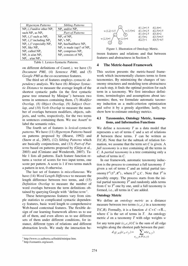
on different definitions of Count(.), we have (3)
Document PMI, (4) Sentence PMI, and (5)
Google PMI as the co-occurrence features.
The third set of features employs syntactic de-
pendency analysis. We have (6) Minipar Syntac-
tic Distance to measure the average length of the
shortest syntactic paths (in the first syntactic
parse tree returned by Minipar1) between two
terms in sentences containing them, (7) Modifier
Overlap, (8) Object Overlap, (9) Subject Over-
lap, and (10) Verb Overlap to measure the num-
ber of overlaps between modifiers, objects, sub-
jects, and verbs, respectively, for the two terms
in sentences containing them. We use Assert2 to
label the semantic roles.
The fourth set of features is lexical-syntactic
patterns. We have (11) Hypernym Patterns based
on patterns proposed by (Hearst, 1992) and
(Snow et al., 2005), (12) Sibling Patterns which
are basically conjunctions, and (13) Part-of Pat-
terns based on patterns proposed by (Girju et al.,
2003) and (Cimiano and Wenderoth, 2007). Ta-
ble 1 lists all patterns. Each feature function re-
turns a vector of scores for two input terms, one
score per pattern. A score is 1 if two terms match
a pattern in text, 0 otherwise.
The last set of features is miscellaneous. We
have (14) Word Length Difference to measure the
length difference between two terms, and (15)
Definition Overlap to measure the number of
word overlaps between the term definitions ob-
tained by querying Google with “define:term”.
These heterogeneous features vary from sim-
ple statistics to complicated syntactic dependen-
cy features, basic word length to comprehensive
Web-based contextual features. The flexible de-
sign of our learning framework allows us to use
all of them, and even allows us to use different
sets of them under different conditions, for in-
stance, different types of relations and different
abstraction levels. We study the interaction be-
1 http://www.cs.ualberta.ca/lindek/minipar.htm. 2 http://cemantix.org/assert.
tween features and relations and that between
features and abstractness in Section 5.
4 The Metric-based Framework
This section presents the metric-based frame-
work which incrementally clusters terms to form
taxonomies. By minimizing the changes of tax-
onomy structures and modeling term abstractness
at each step, it finds the optimal position for each
term in a taxonomy. We first introduce defini-
tions, terminologies and assumptions about tax-
onomies; then, we formulate automatic taxono-
my induction as a multi-criterion optimization
and solve it by a greedy algorithm; lastly, we
show how to estimate ontology metrics.
4.1 Taxonomies, Ontology Metric, Assump-
tions, and Information Functions
We define a taxonomy T as a data model that
represents a set of terms C and a set of relations
R between these terms. T can be written as
T(C,R). Note that for the subtask of relation for-
mation, we assume that the term set C is given. A
full taxonomy is a tree containing all the terms in
C. A partial taxonomy is a tree containing only a
subset of terms in C.
In our framework, automatic taxonomy induc-
tion is the process to construct a full taxonomy T̂
given a set of terms C and an initial partial tax-
onomy ),( 000RST , where CS ⊆
0 . Note that T0
is
possibly empty. The process starts from the ini-
tial partial taxonomy T0 and randomly adds terms
from C to T0 one by one, until a full taxonomy is
formed, i.e., all terms in C are added.
Ontology Metric
We define an ontology metric as a distance
measure between two terms (cx,cy) in a taxonomy
T(C,R). Formally, it is a function →× CCd : ℝ+,
where C is the set of terms in T. An ontology
metric d on a taxonomy T with edge weights w
for any term pair (cx,cy)∈C is the sum of all edge
weights along the shortest path between the pair:
∑∈
=
),(
,),(
,
)(),(
yxPe
yxyxwT
yx
ewccd
Hypernym Patterns Sibling Patterns
NPx (,)?and/or other NPy NPx and/or NPy
such NPy as NPx Part-of Patterns
NPy (,)? such as NPx NPx of NPy
NPy (,)? including NPx NPy’s NPx
NPy (,)? especially NPx NPy has/had/have NPx
NPy like NPx NPy is made (up)? of NPx
NPy called NPx NPy comprises NPx
NPx is a/an NPy NPy consists of NPx
NPx , a/an NPy
Table 1. Lexico-Syntactic Patterns.
Figure 1. Illustration of Ontology Metric.
274
where ),( yxP is the set of edges defining the
shortest path from term cx to cy . Figure 1 illu-
strates ontology metrics for a 5-node taxonomy.
Section 4.3 presents the details of learning ontol-
ogy metrics.
Information Functions
The amount of information in a taxonomy T is
measured and represented by an information
function Info(T). An information function is de-
fined as the sum of the ontology metrics among a
set of term pairs. The function can be defined
over a taxonomy, or on a single level of a tax-
onomy. For a taxonomy T(C,R), we define its
information function as:
∑∈<
=
Cycxcyx
yx ccdTInfo
,,
),()( (1)
Similarly, we define the information function
for an abstraction level Li as:
∑∈<
=
iLycxcyx
yxii ccdLInfo
,,
),()( (2)
where Li is the subset of terms lying at the ith lev-
el of a taxonomy T. For example, in Figure 1,
node 1 is at level L1, node 2 and node 5 level L2.
Assumptions
Given the above definitions about taxonomies,
we make the following assumptions:
Minimum Evolution Assumption. Inspired by
the minimum evolution tree selection criterion
widely used in phylogeny (Hendy and Penny,
1985), we assume that a good taxonomy not only
minimizes the overall semantic distance among
the terms but also avoid dramatic changes. Con-
struction of a full taxonomy is proceeded by add-
ing terms one at a time, which yields a series of
partial taxonomies. After adding each term, the
current taxonomy Tn+1
from the previous tax-
onomy Tn is one that introduces the least changes
between the information in the two taxonomies:
),(minarg '
'
1TTInfoT
n
T
n∆=
+
where the information change function is
|)()(| ),( babaTInfoTInfoTTInfo −=∆ .
Abstractness Assumption. In a taxonomy, con-crete concepts usually lay at the bottom of the hierarchy while abstract concepts often occupy the intermediate and top levels. Concrete con-cepts often represent physical entities, such as “basketball” and “mercury pollution”. While ab-stract concepts, such as “science” and “econo-my”, do not have a physical form thus we must imagine their existence. This obvious difference suggests that there is a need to treat them diffe-rently in taxonomy induction. Hence we assume that terms at the same abstraction level have
common characteristics and share the same Info(.) function. We also assume that terms at different abstraction levels have different characteristics; hence they do not necessarily share the same Info(.) function. That is to say, ,concept Tc ∈∀
, leveln abstractio TLi ⊂ (.). uses ii InfocLc ⇒∈
4.2 Problem Formulation
The Minimum Evolution Objective
Based on the minimum evolution assumption, we
define the goal of taxonomy induction is to find
the optimal full taxonomy T̂ such that the infor-
mation changes are the least since the initial par-
tial taxonomy T0, i.e., to find:
),(minargˆ '0
'
TTInfoT
T
∆= (3)
where 'T is a full taxonomy, i.e., the set of terms
in 'T equals C.
To find the optimal solution for Equation (3),
T̂ , we need to find the optimal term set Ĉ and
the optimal relation set R̂ . Since the optimal term
set for a full taxonomy is always C, the only un-
known part left is R̂ . Thus, Equation (3) can be
transformed equivalently into: )),(),,((minargˆ 000''
'
RSTRCTInfoR
R
∆=
Note that in the framework, terms are added
incrementally into a taxonomy. Each term inser-
tion yields a new partial taxonomy T. By the
minimum evolution assumption, the optimal next
partial taxonomy is one gives the least informa-
tion change. Therefore, the updating function for
the set of relations 1+nR after a new term z is in-
serted can be calculated as:
)),(),},{((minargˆ '
'
nnn
R
RSTRzSTInfoR ∪∆=
By plugging in the definition of the information
change function (.,.)Info∆ in Section 4.1 and Equ-
ation (1), the updating function becomes:
|),(),(|minargˆ
,}{,'
∑∑∈∪∈
−=
nSycxc
yx
znSycxc
yx
R
ccdccdR
The above updating function can be transformed
into a minimization problem:
yx
ccdccdu
ccdccdu
u
znSycxc
yx
nSycxc
yx
nSycxc
yx
znSycxc
yx
<
−≤
−≤
∑∑
∑∑
∪∈∈
∈∪∈
}{,,
,}{,
),(),(
),(),( subject to
min
The minimization follows the minimum evolu-
tion assumption; hence we call it the minimum
evolution objective.
275
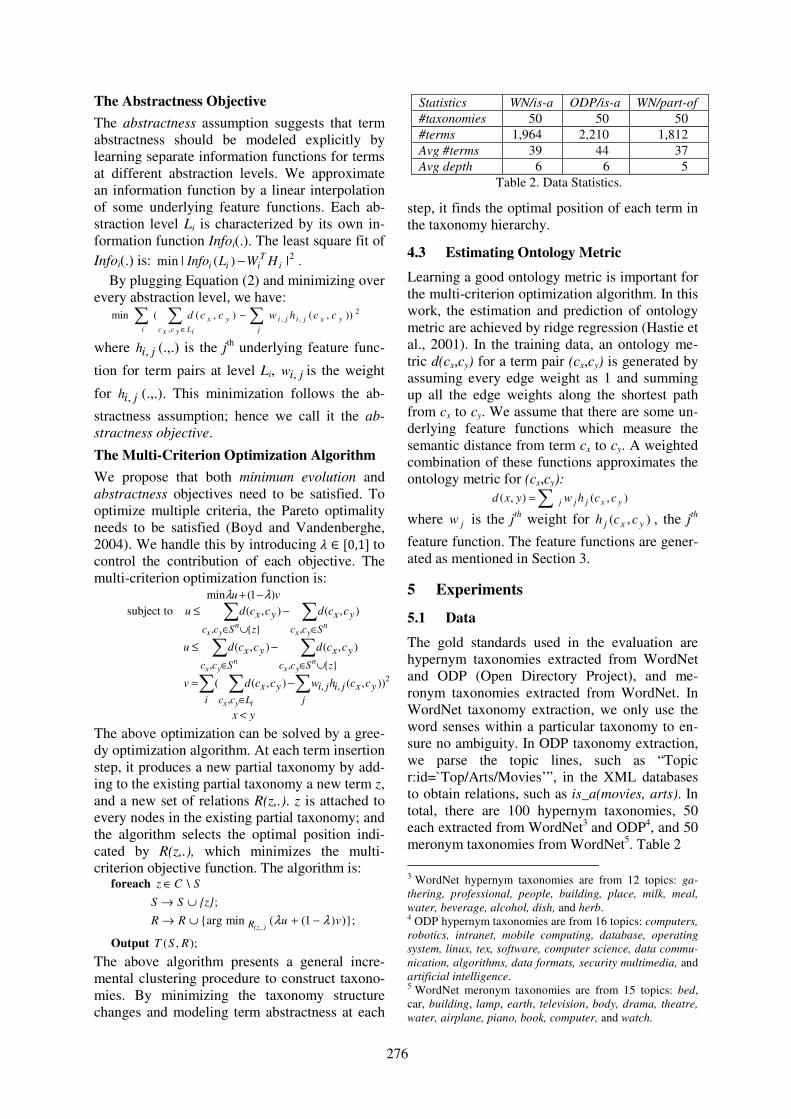
The Abstractness Objective
The abstractness assumption suggests that term
abstractness should be modeled explicitly by
learning separate information functions for terms
at different abstraction levels. We approximate
an information function by a linear interpolation
of some underlying feature functions. Each ab-
straction level Li is characterized by its own in-
formation function Infoi(.). The least square fit of
Infoi(.) is: .|)(|min 2i
Tiii HWLInfo −
By plugging Equation (2) and minimizing over
every abstraction level, we have: 2
,,
,
)),(),((min yxji
j
ji
i iLycxc
yx cchwccd ∑∑ ∑ −
∈
where jih , (.,.) is the jth underlying feature func-
tion for term pairs at level Li, jiw , is the weight
for jih , (.,.). This minimization follows the ab-
stractness assumption; hence we call it the ab-
stractness objective.
The Multi-Criterion Optimization Algorithm
We propose that both minimum evolution and
abstractness objectives need to be satisfied. To
optimize multiple criteria, the Pareto optimality
needs to be satisfied (Boyd and Vandenberghe,
2004). We handle this by introducing � � �0,1� to
control the contribution of each objective. The
multi-criterion optimization function is:
yx
cchwccdv
ccdccdu
ccdccdu
vu
yxji
j
ji
i Lcc
yx
zScc
yx
Scc
yx
Scc
yx
zScc
yx
iyx
nyx
nyx
nyx
nyx
<
−=
−≤
−≤
−+
∑∑ ∑
∑∑
∑∑
∈
∪∈∈
∈∪∈
2)),(),((
),(),(
),(),( subject to
)1(min
,,
,
}{,,
,}{,
λλ
The above optimization can be solved by a gree-
dy optimization algorithm. At each term insertion
step, it produces a new partial taxonomy by add-
ing to the existing partial taxonomy a new term z,
and a new set of relations R(z,.). z is attached to
every nodes in the existing partial taxonomy; and
the algorithm selects the optimal position indi-
cated by R(z,.), which minimizes the multi-
criterion objective function. The algorithm is:
);,(
)};)1((min{arg
;
\
RST
vuRR
{z}SS
SCz
(z,.)R
Output
foreach
λλ −+∪→
∪→
∈
The above algorithm presents a general incre-
mental clustering procedure to construct taxono-
mies. By minimizing the taxonomy structure
changes and modeling term abstractness at each
step, it finds the optimal position of each term in
the taxonomy hierarchy.
4.3 Estimating Ontology Metric
Learning a good ontology metric is important for
the multi-criterion optimization algorithm. In this
work, the estimation and prediction of ontology
metric are achieved by ridge regression (Hastie et
al., 2001). In the training data, an ontology me-
tric d(cx,cy) for a term pair (cx,cy) is generated by
assuming every edge weight as 1 and summing
up all the edge weights along the shortest path
from cx to cy. We assume that there are some un-
derlying feature functions which measure the
semantic distance from term cx to cy. A weighted
combination of these functions approximates the
ontology metric for (cx,cy):
∑= ),(),( yxjjj cchwyxd
where jw is the jth weight for ),( yxj cch , the j
th
feature function. The feature functions are gener-
ated as mentioned in Section 3.
5 Experiments
5.1 Data
The gold standards used in the evaluation are
hypernym taxonomies extracted from WordNet
and ODP (Open Directory Project), and me-
ronym taxonomies extracted from WordNet. In
WordNet taxonomy extraction, we only use the
word senses within a particular taxonomy to en-
sure no ambiguity. In ODP taxonomy extraction,
we parse the topic lines, such as “Topic
r:id=`Top/Arts/Movies’”, in the XML databases
to obtain relations, such as is_a(movies, arts). In
total, there are 100 hypernym taxonomies, 50
each extracted from WordNet3 and ODP
4, and 50
meronym taxonomies from WordNet5. Table 2
3 WordNet hypernym taxonomies are from 12 topics: ga-
thering, professional, people, building, place, milk, meal,
water, beverage, alcohol, dish, and herb. 4 ODP hypernym taxonomies are from 16 topics: computers,
robotics, intranet, mobile computing, database, operating
system, linux, tex, software, computer science, data commu-
nication, algorithms, data formats, security multimedia, and
artificial intelligence. 5 WordNet meronym taxonomies are from 15 topics: bed,
car, building, lamp, earth, television, body, drama, theatre,
water, airplane, piano, book, computer, and watch.
Statistics WN/is-a ODP/is-a WN/part-of
#taxonomies 50 50 50
#terms 1,964 2,210 1,812
Avg #terms 39 44 37
Avg depth 6 6 5
Table 2. Data Statistics.
276

summarizes the data statistics.
We also use two Web-based auxiliary datasets
to generate features mentioned in Section 3:
• Wikipedia corpus. The entire Wikipedia corpus
is downloaded and indexed by Indri6. The top
100 documents returned by Indri are the global
context of a term when querying with the term.
• Google corpus. A collection of the top 1000
documents by querying Google using each
term, and each term pair. Each top 1000 docu-
ments are the global context of a query term.
Both corpora are split into sentences and are used
to generate contextual, co-occurrence, syntactic
dependency and lexico-syntactic pattern features.
5.2 Methodology
We evaluate the quality of automatic generated
taxonomies by comparing them with the gold
standards in terms of precision, recall and F1-
measure. F1-measure is calculated as 2*P*R/
(P+R), where P is precision, the percentage of
correctly returned relations out of the total re-
turned relations, R is recall, the percentage of
correctly returned relations out of the total rela-
tions in the gold standard.
Leave-one-out cross validation is used to aver-
age the system performance across different
training and test datasets. For each 50 datasets
from WordNet hypernyms, WordNet meronyms
or ODP hypernyms, we randomly pick 49 of
them to generate training data, and test on the
remaining dataset. We repeat the process for 50
times, with different training and test sets at each
6 http://www.lemurproject.org/indri/.
time, and report the averaged precision, recall
and F1-measure across all 50 runs.
We also group the fifteen features in Section 3
into six sets: contextual, co-concurrence, pat-
terns, syntactic dependency, word length differ-
ence and definition. Each set is turned on one by
one for experiments in Section 5.4 and 5.5.
5.3 Performance of Taxonomy Induction
In this section, we compare the following auto-
matic taxonomy induction systems: HE, the sys-
tem by Hearst (1992) with 6 hypernym patterns;
GI, the system by Girju et al. (2003) with 3 me-
ronym patterns; PR, the probabilistic framework
by Snow et al. (2006); and ME, the metric-based
framework proposed in this paper. To have a fair
comparison, for PR, we estimate the conditional
probability of a relation given the evidence
P(Rij|Eij), as in (Snow et al. 2006), by using the
same set of features as in ME.
Table 3 shows precision, recall, and F1-
measure of each system for WordNet hypernyms
(is-a), WordNet meronyms (part-of) and ODP
hypernyms (is-a). Bold font indicates the best
performance in a column. Note that HE is not
applicable to part-of, so is GI to is-a.
Table 3 shows that systems using heterogene-
ous features (PR and ME) achieve higher F1-
measure than systems only using patterns (HE
and GI) with a significant absolute gain of >30%.
Generally speaking, pattern-based systems show
higher precision and lower recall, while systems
using heterogeneous features show lower preci-
sion and higher recall. However, when consider-
ing both precision and recall, using heterogene-
ous features is more effective than just using pat-
terns. The proposed system ME consistently pro-
duces the best F1-measure for all three tasks. The performance of the systems for ODP/is-a
is worse than that for WordNet/is-a. This may be because there is more noise in ODP than in
WordNet/is-a
System Precision Recall F1-measure
HE 0.85 0.32 0.46
GI n/a n/a n/a
PR 0.75 0.73 0.74
ME 0.82 0.79 0.82
ODP/is-a
System Precision Recall F1-measure
HE 0.31 0.29 0.30
GI n/a n/a n/a
PR 0.60 0.72 0.65
ME 0.64 0.70 0.67
WordNet/part-of
System Precision Recall F1-measure
HE n/a n/a n/a
GI 0.75 0.25 0.38
PR 0.68 0.52 0.59
ME 0.69 0.55 0.61
Table 3. System Performance.
Feature is-a sibling part-
of
Benefited
Relations
Contextual 0.21 0.42 0.12 sibling
Co-occur. 0.48 0.41 0.28 All
Patterns 0.46 0.41 0.30 All
Syntactic 0.22 0.36 0.12 sibling
Word Leng. 0.16 0.16 0.15 All but
limited
Definition 0.12 0.18 0.10 Sibling but
limited
Best Features Co-
occur.,
patterns
Contextual,
co-occur.,
patterns
Co-
occur.,
patterns
Table 4. F1-measure for Features vs. Relations: WordNet.
277
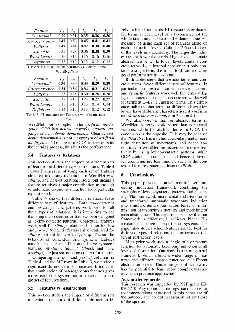
WordNet. For example, under artificial intelli-gence, ODP has neural networks, natural lan-guage and academic departments. Clearly, aca-demic departments is not a hyponym of artificial intelligence. The noise in ODP interferes with the learning process, thus hurts the performance.
5.4 Features vs. Relations
This section studies the impact of different sets of features on different types of relations. Table 4 shows F1-measure of using each set of features alone on taxonomy induction for WordNet is-a, sibling, and part-of relations. Bold font means a feature set gives a major contribution to the task of automatic taxonomy induction for a particular type of relation.
Table 4 shows that different relations favor different sets of features. Both co-occurrence and lexico-syntactic patterns work well for all three types of relations. It is interesting to see that simple co-occurrence statistics work as good as lexico-syntactic patterns. Contextual features work well for sibling relations, but not for is-a and part-of. Syntactic features also work well for sibling, but not for is-a and part-of. The similar behavior of contextual and syntactic features may be because that four out of five syntactic features (Modifier, Subject, Object, and Verb overlaps) are just surrounding context for a term.
Comparing the is-a and part-of columns in Table 4 and the ME rows in Table 3, we notice a significant difference in F1-measure. It indicates that combination of heterogeneous features gives more rise to the system performance than a sin-gle set of features does.
5.5 Features vs. Abstractness
This section studies the impact of different sets of features on terms at different abstraction le-
vels. In the experiments, F1-measure is evaluated for terms at each level of a taxonomy, not the whole taxonomy. Table 5 and 6 demonstrate F1-measure of using each set of features alone on each abstraction levels. Columns 2-6 are indices of the levels in a taxonomy. The larger the indic-es are, the lower the levels. Higher levels contain abstract terms, while lower levels contain con-crete terms. L1 is ignored here since it only con-tains a single term, the root. Bold font indicates good performance in a column.
Both tables show that abstract terms and con-crete terms favor different sets of features. In particular, contextual, co-occurrence, pattern, and syntactic features work well for terms at L4-L6, i.e., concrete terms; co-occurrence works well for terms at L2-L3, i.e., abstract terms. This differ-ence indicates that terms at different abstraction levels have different characteristics; it confirms our abstractness assumption in Section 4.1.
We also observe that for abstract terms in WordNet, patterns work better than contextual features; while for abstract terms in ODP, the conclusion is the opposite. This may be because that WordNet has a richer vocabulary and a more rigid definition of hypernyms, and hence is-a relations in WordNet are recognized more effec-tively by using lexico-syntactic patterns; while ODP contains more noise, and hence it favors features requiring less rigidity, such as the con-textual features generated from the Web.
6 Conclusions
This paper presents a novel metric-based tax-onomy induction framework combining the strengths of lexico-syntactic patterns and cluster-ing. The framework incrementally clusters terms and transforms automatic taxonomy induction into a multi-criteria optimization based on mini-mization of taxonomy structures and modeling of term abstractness. The experiments show that our framework is effective; it achieves higher F1-measure than three state-of-the-art systems. The paper also studies which features are the best for different types of relations and for terms at dif-ferent abstraction levels.
Most prior work uses a single rule or feature function for automatic taxonomy induction at all levels of abstraction. Our work is a more general framework which allows a wider range of fea-tures and different metric functions at different abstraction levels. This more general framework has the potential to learn more complex taxono-mies than previous approaches.
Acknowledgements This research was supported by NSF grant IIS-0704210. Any opinions, findings, conclusions, or recommendations expressed in this paper are of the authors, and do not necessarily reflect those of the sponsor.
Feature L2 L3 L4 L5 L6
Contextual 0.29 0.31 0.35 0.36 0.36
Co-occurrence 0.47 0.56 0.45 0.41 0.41
Patterns 0.47 0.44 0.42 0.39 0.40
Syntactic 0.31 0.28 0.36 0.38 0.39
Word Length 0.16 0.16 0.16 0.16 0.16
Definition 0.12 0.12 0.12 0.12 0.12
Table 5. F1-measure for Features vs. Abstractness:
WordNet/is-a.
Feature L2 L3 L4 L5 L6
Contextual 0.30 0.30 0.33 0.29 0.29
Co-occurrence 0.34 0.36 0.34 0.31 0.31
Patterns 0.23 0.25 0.30 0.28 0.28
Syntactic 0.18 0.18 0.23 0.27 0.27
Word Length 0.15 0.15 0.15 0.14 0.14
Definition 0.13 0.13 0.13 0.12 0.12
Table 6. F1-measure for Features vs. Abstractness:
ODP/is-a.
278
References
M. Berland and E. Charniak. 1999. Finding parts in very
large corpora. ACL’99.
S. Boyd and L. Vandenberghe. 2004. Convex optimization.
In Cambridge University Press, 2004.
P. Brown, V. D. Pietra, P. deSouza, J. Lai, and R. Mercer.
1992. Class-based ngram models for natural language.
Computational Linguistics, 18(4):468–479.
P. Buitelaar, P. Cimiano, and B. Magnini. 2005. Ontology
Learning from Text: Methods, Evaluation and Applica-
tions. Volume 123 Frontiers in Artificial Intelligence and
Applications.
R. Bunescu and R. Mooney. 2007. Learning to Extract
Relations from the Web using Minimal Supervision.
ACL’07.
S. Caraballo. 1999. Automatic construction of a hypernym-
labeled noun hierarchy from text. ACL’99.
T. Chklovski and P. Pantel. 2004. VerbOcean: mining the
web for fine-grained semantic verb relations. EMNLP
’04.
P. Cimiano and J. Volker. 2005. Towards large-scale, open-
domain and ontology-based named entity classification.
RANLP’07.
P. Cimiano and J. Wenderoth. 2007. Automatic Acquisition
of Ranked Qualia Structures from the Web. ACL’07.
D. Davidov and A. Rappoport. 2006. Efficient Unsuper-
vised Discovery of Word Categories Using Symmetric
Patterns and High Frequency Words. ACL’06.
D. Davidov and A. Rappoport. 2008. Classification of Se-
mantic Relationships between Nominals Using Pattern
Clusters. ACL’08.
D. Downey, O. Etzioni, and S. Soderland. 2005. A Probabil-
istic model of redundancy in information extraction. IJ-
CAI’05.
O. Etzioni, M. Cafarella, D. Downey, A. Popescu, T.
Shaked, S. Soderland, D. Weld, and A. Yates. 2005. Un-
supervised named-entity extraction from the web: an ex-
perimental study. Artificial Intelligence, 165(1):91–134.
C. Fellbuam. 1998. WordNet: An Electronic Lexical Data-
base. MIT Press. 1998.
M. Geffet and I. Dagan. 2005. The Distributional Inclusion
Hypotheses and Lexical Entailment. ACL’05.
R. Girju, A. Badulescu, and D. Moldovan. 2003. Learning
Semantic Constraints for the Automatic Discovery of
Part-Whole Relations. HLT’03.
R. Girju, A. Badulescu, and D. Moldovan. 2006. Automatic
Discovery of Part-Whole Relations. Computational Lin-
guistics, 32(1): 83-135.
Z. Harris. 1985. Distributional structure. In Word, 10(23):
146-162s, 1954.
T. Hastie, R. Tibshirani and J. Friedman. 2001. The Ele-
ments of Statistical Learning: Data Mining, Inference,
and Prediction. Springer-Verlag, 2001.
M. Hearst. 1992. Automatic acquisition of hyponyms from
large text corpora. COLING’92.
M. D. Hendy and D. Penny. 1982. Branch and bound algo-
rithms to determine minimal evolutionary trees. Mathe-
matical Biosciences 59: 277-290.
Z. Kozareva, E. Riloff, and E. Hovy. 2008. Semantic Class
Learning from the Web with Hyponym Pattern Linkage
Graphs. ACL’08.
D. Lin, 1998. Automatic retrieval and clustering of similar
words. COLING’98.
D. Lin, S. Zhao, L. Qin, and M. Zhou. 2003. Identifying
Synonyms among Distributionally Similar Words. IJ-
CAI’03.
G. S. Mann. 2002. Fine-Grained Proper Noun Ontologies
for Question Answering. In Proceedings of SemaNet’ 02:
Building and Using Semantic Networks, Taipei.
P. Pantel and D Lin. 2002. Discovering word senses from
text. SIGKDD’02.
P. Pantel and D. Ravichandran. 2004. Automatically labe-
ling semantic classes. HLT/NAACL’04.
P. Pantel, D. Ravichandran, and E. Hovy. 2004. Towards
terascale knowledge acquisition. COLING’04.
P. Pantel and M. Pennacchiotti. 2006. Espresso: Leveraging
Generic Patterns for Automatically Harvesting Semantic
Relations. ACL’06.
F. Pereira, N. Tishby, and L. Lee. 1993. Distributional clus-
tering of English words. ACL’93.
D. Ravichandran and E. Hovy. 2002. Learning surface text
patterns for a question answering system. ACL’02.
E. Riloff and J. Shepherd. 1997. A corpus-based approach
for building semantic lexicons. EMNLP’97.
B. Roark and E. Charniak. 1998. Noun-phrase co-
occurrence statistics for semi-automatic semantic lexicon
construction. ACL/COLING’98.
R. Snow, D. Jurafsky, and A. Y. Ng. 2005. Learning syntac-
tic patterns for automatic hypernym discovery. NIPS’05.
R. Snow, D. Jurafsky, and A. Y. Ng. 2006. Semantic Tax-
onomy Induction from Heterogeneous Evidence.
ACL’06.
B. Rosenfeld and R. Feldman. 2007. Clustering for unsu-
pervised relation identification. CIKM’07.
P. Turney, M. Littman, J. Bigham, and V. Shnayder. 2003.
Combining independent modules to solve multiple-
choice synonym and analogy problems. RANLP’03.
S. M. Harabagiu, S. J. Maiorano and M. A. Pasca. 2003.
Open-Domain Textual Question Answering Techniques.
Natural Language Engineering 9 (3): 1-38, 2003.
I. Szpektor, H. Tanev, I. Dagan, and B. Coppola. 2004.
Scaling web-based acquisition of entailment relations.
EMNLP’04.
D. Widdows and B. Dorow. 2002. A graph model for unsu-
pervised Lexical acquisition. COLING ’02.
H. Yang and J. Callan. 2008. Learning the Distance Metric
in a Personal Ontology. Workshop on Ontologies and In-
formation Systems for the Semantic Web of CIKM’08.
279
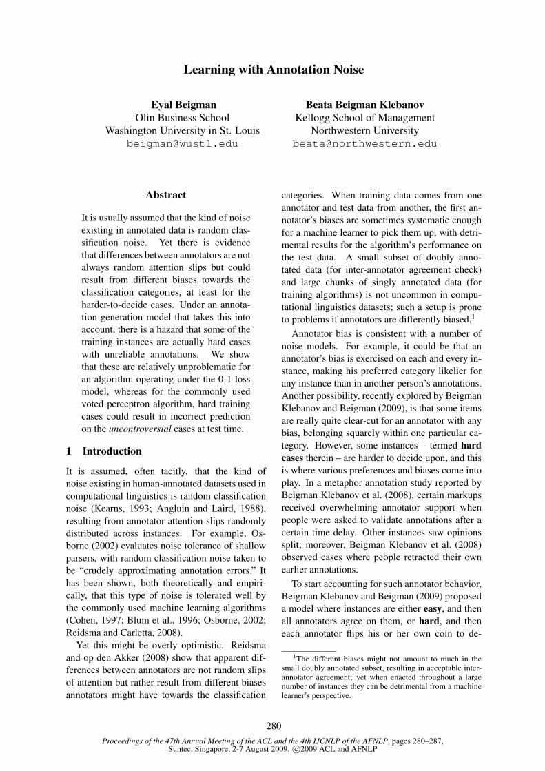
Proceedings of the 47th Annual Meeting of the ACL and the 4th IJCNLP of the AFNLP, pages 280–287,Suntec, Singapore, 2-7 August 2009. c©2009 ACL and AFNLP
Learning with Annotation Noise
Eyal BeigmanOlin Business School
Washington University in St. [email protected]
Beata Beigman KlebanovKellogg School of Management
Northwestern [email protected]
Abstract
It is usually assumed that the kind of noiseexisting in annotated data is random clas-sification noise. Yet there is evidencethat differences between annotators are notalways random attention slips but couldresult from different biases towards theclassification categories, at least for theharder-to-decide cases. Under an annota-tion generation model that takes this intoaccount, there is a hazard that some of thetraining instances are actually hard caseswith unreliable annotations. We showthat these are relatively unproblematic foran algorithm operating under the 0-1 lossmodel, whereas for the commonly usedvoted perceptron algorithm, hard trainingcases could result in incorrect predictionon the uncontroversial cases at test time.
1 Introduction
It is assumed, often tacitly, that the kind ofnoise existing in human-annotated datasets used incomputational linguistics is random classificationnoise (Kearns, 1993; Angluin and Laird, 1988),resulting from annotator attention slips randomlydistributed across instances. For example, Os-borne (2002) evaluates noise tolerance of shallowparsers, with random classification noise taken tobe “crudely approximating annotation errors.” Ithas been shown, both theoretically and empiri-cally, that this type of noise is tolerated well bythe commonly used machine learning algorithms(Cohen, 1997; Blum et al., 1996; Osborne, 2002;Reidsma and Carletta, 2008).
Yet this might be overly optimistic. Reidsmaand op den Akker (2008) show that apparent dif-ferences between annotators are not random slipsof attention but rather result from different biasesannotators might have towards the classification
categories. When training data comes from oneannotator and test data from another, the first an-notator’s biases are sometimes systematic enoughfor a machine learner to pick them up, with detri-mental results for the algorithm’s performance onthe test data. A small subset of doubly anno-tated data (for inter-annotator agreement check)and large chunks of singly annotated data (fortraining algorithms) is not uncommon in compu-tational linguistics datasets; such a setup is proneto problems if annotators are differently biased.1
Annotator bias is consistent with a number ofnoise models. For example, it could be that anannotator’s bias is exercised on each and every in-stance, making his preferred category likelier forany instance than in another person’s annotations.Another possibility, recently explored by BeigmanKlebanov and Beigman (2009), is that some itemsare really quite clear-cut for an annotator with anybias, belonging squarely within one particular ca-tegory. However, some instances – termed hardcases therein – are harder to decide upon, and thisis where various preferences and biases come intoplay. In a metaphor annotation study reported byBeigman Klebanov et al. (2008), certain markupsreceived overwhelming annotator support whenpeople were asked to validate annotations after acertain time delay. Other instances saw opinionssplit; moreover, Beigman Klebanov et al. (2008)observed cases where people retracted their ownearlier annotations.
To start accounting for such annotator behavior,Beigman Klebanov and Beigman (2009) proposeda model where instances are either easy, and thenall annotators agree on them, or hard, and theneach annotator flips his or her own coin to de-
1The different biases might not amount to much in thesmall doubly annotated subset, resulting in acceptable inter-annotator agreement; yet when enacted throughout a largenumber of instances they can be detrimental from a machinelearner’s perspective.
280

cide on a label (each annotator can have a different“coin” reflecting his or her biases). For annota-tions generated under such a model, there is a dan-ger of hard instances posing as easy – an observedagreement between annotators being a result of allcoins coming up heads by chance. They thereforedefine the expected proportion of hard instances inagreed items as annotation noise. They providean example from the literature where an annota-tion noise rate of about 15% is likely.
The question addressed in this article is: Howproblematic is learning from training data with an-notation noise? Specifically, we are interested inestimating the degree to which performance oneasy instances at test time can be hurt by the pre-sence of hard instances in training data.
Definition 1 The hard case bias, τ , is the portionof easy instances in the test data that are misclas-sified as a result of hard instances in the trainingdata.
This article proceeds as follows. First, we showthat a machine learner operating under a 0-1 lossminimization principle could sustain a hard casebias of θ( 1√
N) in the worst case. Thus, while an-
notation noise is hazardous for small datasets, it isbetter tolerated in larger ones. However, 0-1 lossminimization is computationally intractable forlarge datasets (Feldman et al., 2006; Guruswamiand Raghavendra, 2006); substitute loss functionsare often used in practice. While their tolerance torandom classification noise is as good as for 0-1loss, their tolerance to annotation noise is worse.For example, the perceptron family of algorithmshandle random classification noise well (Cohen,1997). We show in section 3.4 that the widelyused Freund and Schapire (1999) voted percep-tron algorithm could face a constant hard case biaswhen confronted with annotation noise in trainingdata, irrespective of the size of the dataset. Finally,we discuss the implications of our findings for thepractice of annotation studies and for data utiliza-tion in machine learning.
2 0-1 Loss
Let a sample be a sequence x1, . . . , xN drawn uni-formly from the d-dimensional discrete cube Id ={−1, 1}d with corresponding labels y1, . . . , yN ∈{−1, 1}. Suppose further that the learning al-gorithm operates by finding a hyperplane (w,ψ),w ∈ Rd, ψ ∈ R, that minimizes the empirical er-rorL(w,ψ) =
∑j=1...N [yj−sgn(
∑i=1...d x
ijw
i−
ψ)]2. Let there be H hard cases, such that the an-notation noise is γ = H
N .2
Theorem 1 In the worst case configuration of in-stances a hard case bias of τ = θ( 1√
N) cannot be
ruled out with constant confidence.
Idea of the proof : We prove by explicit con-struction of an adversarial case. Suppose there isa plane that perfectly separates the easy instances.The θ(N) hard instances will be concentrated ina band parallel to the separating plane, that isnear enough to the plane so as to trap only aboutθ(√N) easy instances between the plane and the
band (see figure 1 for an illustration). For a ran-dom labeling of the hard instances, the centrallimit theorem shows there is positive probabilitythat there would be an imbalance between +1 and−1 labels in favor of −1s on the scale of
√N ,
which, with appropriate constants, would lead tothe movement of the empirically minimal separa-tion plane to the right of the hard case band, mis-classifying the trapped easy cases.
Proof : Let v = v(x) =∑
i=1...d xi denote the
sum of the coordinates of an instance in Id andtake λe =
√d · F−1(
√γ · 2−
d2 + 1
2) and λh =√d · F−1(γ +
√γ · 2−
d2 + 1
2), where F (t) is thecumulative distribution function of the normal dis-tribution. Suppose further that instances xj suchthat λe < vj < λh are all and only hard instances;their labels are coinflips. All other instances areeasy, and labeled y = y(x) = sgn(v). In this case,the hyperplane 1√
d(1 . . . 1) is the true separation
plane for the easy instances, with ψ = 0. Figure 1shows this configuration.
According to the central limit theorem, for d,Nlarge, the distribution of v is well approximated byN (0,
√d). If N = c1 · 2d, for some 0 < c1 < 4,
the second application of the central limit the-orem ensures that, with high probability, aboutγN = c1γ2d items would fall between λe and λh(all hard), and
√γ · 2−
d2N = c1
√γ2d would fall
between 0 and λe (all easy, all labeled +1).Let Z be the sum of labels of the hard cases,
Z =∑
i=1...H yi. Applying the central limit the-orem a third time, for large N , Z will, with ahigh probability, be distributed approximately as
2In Beigman Klebanov and Beigman (2009), annotationnoise is defined as percentage of hard instances in the agreedannotations; this implies noise measurement on multiply an-notated material. When there is just one annotator, no dis-tinction between easy vs hard instances can be made; in thissense, all hard instances are posing as easy.
281

0 λe λh
Figure 1: The adversarial case for 0-1 loss.Squares correspond to easy instances, circles – tohard ones. Filled squares and circles are labeled−1, empty ones are labeled +1.
N (0,√γN). This implies that a value as low as
−2σ cannot be ruled out with high (say 95%) con-fidence. Thus, an imbalance of up to 2
√γN , or of
2√c1γ2d, in favor of −1s is possible.
There are between 0 and λh about 2√c1
√γ2d
more−1 hard instances than +1 hard instances, asopposed to c1
√γ2d easy instances that are all +1.
As long as c1 < 2√c1, i.e. c1 < 4, the empirically
minimal threshold would move to λh, resulting in
a hard case bias of τ =√γ√c12d
(1−γ)·c12d = θ( 1√N
).To see that this is the worst case scenario, we
note that 0-1 loss sustained on θ(N) hard casesis the order of magnitude of the possible imba-lance between −1 and +1 random labels, whichis θ(
√N). For hard case loss to outweigh the loss
on the misclassified easy instances, there cannotbe more than θ(
√N) of the latter 2
Note that the proof requires that N = θ(2d)namely, that asymptotically the sample includesa fixed portion of the instances. If the sample isasymptotically smaller, then λe will have to be ad-justed such that λe =
√d · F−1(θ( 1√
N) + 1
2).According to theorem 1, for a 10K dataset with
15% hard case rate, a hard case bias of about 1%cannot be ruled out with 95% confidence.
Theorem 1 suggests that annotation noise asdefined here is qualitatively different from moremalicious types of noise analyzed in the agnosticlearning framework (Kearns and Li, 1988; Haus-sler, 1992; Kearns et al., 1994), where an adver-
sary can not only choose the placement of the hardcases, but also their labels. In worst case, the 0-1loss model would sustain a constant rate of errordue to malicious noise, whereas annotation noiseis tolerated quite well in large datasets.
3 Voted Perceptron
Freund and Schapire (1999) describe the votedperceptron. This algorithm and its many vari-ants are widely used in the computational lin-guistics community (Collins, 2002a; Collins andDuffy, 2002; Collins, 2002b; Collins and Roark,2004; Henderson and Titov, 2005; Viola andNarasimhan, 2005; Cohen et al., 2004; Carreraset al., 2005; Shen and Joshi, 2005; Ciaramita andJohnson, 2003). In this section, we show that thevoted perceptron can be vulnerable to annotationnoise. The algorithm is shown below.
Algorithm 1 Voted PerceptronTrainingInput: a labeled training set (x1, y1), . . . , (xN , yN )Output: a list of perceptrons w1, . . . , wN
Initialize: t← 0; w1 ← 0; ψ1 ← 0for t = 1 . . . N doŷt ← sign(〈wt, xt〉+ ψt)
wt+1 ← wt + yt−ŷt2· xt
ψt+1 ← ψt + yt−ŷt2· 〈wt, xt〉
end for
ForecastingInput: a list of perceptrons w1, . . . , wN
an unlabeled instance xOutput: A forecasted label y
ŷ ←PN
t=1 sign(〈wt, xt〉+ ψt)
y ← sign(ŷ)
The voted perceptron algorithm is a refinementof the perceptron algorithm (Rosenblatt, 1962;Minsky and Papert, 1969). Perceptron is a dy-namic algorithm; starting with an initial hyper-plane w0, it passes repeatedly through the labeledsample. Whenever an instance is misclassifiedby wt, the hyperplane is modified to adapt to theinstance. The algorithm terminates once it haspassed through the sample without making anyclassification mistakes. The algorithm terminatesiff the sample can be separated by a hyperplane,and in this case the algorithm finds a separatinghyperplane. Novikoff (1962) gives a bound on thenumber of iterations the algorithm goes throughbefore termination, when the sample is separableby a margin.
282

The perceptron algorithm is vulnerable to noise,as even a little noise could make the sample in-separable. In this case the algorithm would cycleindefinitely never meeting termination conditions,wt would obtain values within a certain dynamicrange but would not converge. In such setting,imposing a stopping time would be equivalent todrawing a random vector from the dynamic range.
Freund and Schapire (1999) extend the percep-tron to inseparable samples with their voted per-ceptron algorithm and give theoretical generaliza-tion bounds for its performance. The basic ideaunderlying the algorithm is that if the dynamicrange of the perceptron is not too large then wtwould classify most instances correctly most ofthe time (for most values of t). Thus, for a samplex1, . . . , xN the new algorithm would keep trackof w0, . . . , wN , and for an unlabeled instance x itwould forecast the classification most prominentamongst these hyperplanes.
The bounds given by Freund and Schapire(1999) depend on the hinge loss of the dataset. Insection 3.2 we construct a difficult setting for thisalgorithm. To prove that voted perceptron wouldsuffer from a constant hard case bias in this set-ting using the exact dynamics of the perceptron isbeyond the scope of this article. Instead, in sec-tion 3.3 we provide a lower bound on the hingeloss for a simplified model of the perceptron algo-rithm dynamics, which we argue would be a goodapproximation to the true dynamics in the settingwe constructed. For this simplified model, weshow that the hinge loss is large, and the boundsin Freund and Schapire (1999) cannot rule out aconstant level of error regardless of the size of thedataset. In section 3.4 we study the dynamics ofthe model and prove that τ = θ(1) for the adver-sarial setting.
3.1 Hinge Loss
Definition 2 The hinge loss of a labeled instance(x, y) with respect to hyperplane (w,ψ) and mar-gin δ > 0 is given by ζ = ζ(ψ, δ) = max(0, δ −y · (〈w, x〉 − ψ)).
ζ measures the distance of an instance frombeing classified correctly with a δ margin. Figure 2shows examples of hinge loss for various datapoints.
Theorem 2 (Freund and Schapire (1999))After one pass on the sample, the probabilitythat the voted perceptron algorithm does not
δζ
ζζ
ζ
ζ ζ
Figure 2: Hinge loss ζ for various data points in-curred by the separator with margin δ.
predict correctly the label of a test instancexN+1 is bounded by 2
N+1EN+1
[d+Dδ
]2where
D = D(w,ψ, δ) =√∑N
i=1 ζ2i .
This result is used to explain the convergence ofweighted or voted perceptron algorithms (Collins,2002a). It is useful as long as the expected value ofD is not too large. We show that in an adversarialsetting of the annotation noise D is large, hencethese bounds are trivial.
3.2 Adversarial Annotation Noise
Let a sample be a sequence x1, . . . , xN drawn uni-formly from Id with y1, . . . , yN ∈ {−1, 1}. Easycases are labeled y = y(x) = sgn(v) as before,with v = v(x) =
∑i=1...d x
i. The true separationplane for the easy instances is w∗ = 1√
d(1 . . . 1),
ψ∗ = 0. Suppose hard cases are those wherev(x) > c1
√d, where c1 is chosen so that the
hard instances account for γN of all instances.3
Figure 3 shows this setting.
3.3 Lower Bound on Hinge Loss
In the simplified case, we assume that the algo-rithm starts training with the hyperplane w0 =w∗ = 1√
d(1 . . . 1), and keeps it throughout the
training, only updating ψ. In reality, each hard in-stance can be decomposed into a component that isparallel to w∗, and a component that is orthogonalto it. The expected contribution of the orthogonal
3See the proof of 0-1 case for a similar construction usingthe central limit theorem.
283
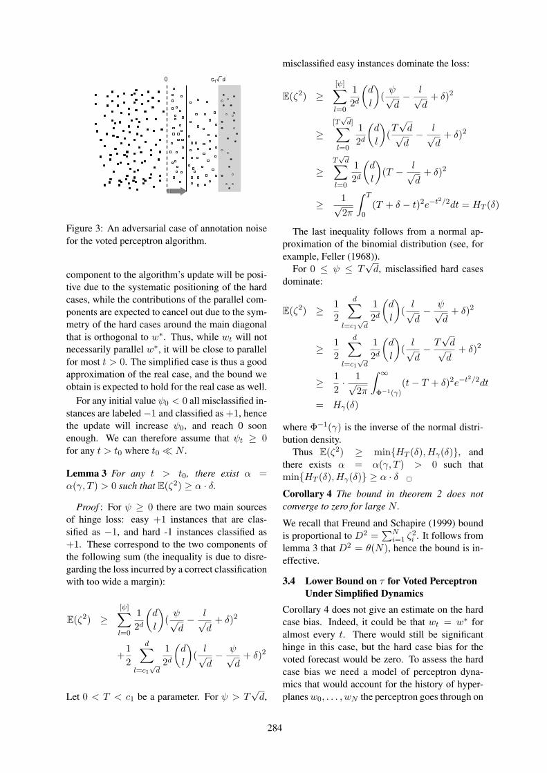
0 c1√d
Figure 3: An adversarial case of annotation noisefor the voted perceptron algorithm.
component to the algorithm’s update will be posi-tive due to the systematic positioning of the hardcases, while the contributions of the parallel com-ponents are expected to cancel out due to the sym-metry of the hard cases around the main diagonalthat is orthogonal to w∗. Thus, while wt will notnecessarily parallel w∗, it will be close to parallelfor most t > 0. The simplified case is thus a goodapproximation of the real case, and the bound weobtain is expected to hold for the real case as well.
For any initial value ψ0 < 0 all misclassified in-stances are labeled −1 and classified as +1, hencethe update will increase ψ0, and reach 0 soonenough. We can therefore assume that ψt ≥ 0for any t > t0 where t0 � N .
Lemma 3 For any t > t0, there exist α =α(γ, T ) > 0 such that E(ζ2) ≥ α · δ.
Proof : For ψ ≥ 0 there are two main sourcesof hinge loss: easy +1 instances that are clas-sified as −1, and hard -1 instances classified as+1. These correspond to the two components ofthe following sum (the inequality is due to disre-garding the loss incurred by a correct classificationwith too wide a margin):
E(ζ2) ≥[ψ]∑l=0
12d
(d
l
)(ψ√d− l√
d+ δ)2
+12
d∑l=c1
√d
12d
(d
l
)(l√d− ψ√
d+ δ)2
Let 0 < T < c1 be a parameter. For ψ > T√d,
misclassified easy instances dominate the loss:
E(ζ2) ≥[ψ]∑l=0
12d
(d
l
)(ψ√d− l√
d+ δ)2
≥[T√d]∑
l=0
12d
(d
l
)(T√d√d− l√
d+ δ)2
≥T√d∑
l=0
12d
(d
l
)(T − l√
d+ δ)2
≥ 1√2π
∫ T
0(T + δ − t)2e−t
2/2dt = HT (δ)
The last inequality follows from a normal ap-proximation of the binomial distribution (see, forexample, Feller (1968)).
For 0 ≤ ψ ≤ T√d, misclassified hard cases
dominate:
E(ζ2) ≥ 12
d∑l=c1
√d
12d
(d
l
)(l√d− ψ√
d+ δ)2
≥ 12
d∑l=c1
√d
12d
(d
l
)(l√d− T
√d√d
+ δ)2
≥ 12· 1√
2π
∫ ∞
Φ−1(γ)(t− T + δ)2e−t
2/2dt
= Hγ(δ)
where Φ−1(γ) is the inverse of the normal distri-bution density.
Thus E(ζ2) ≥ min{HT (δ),Hγ(δ)}, andthere exists α = α(γ, T ) > 0 such thatmin{HT (δ),Hγ(δ)} ≥ α · δ 2
Corollary 4 The bound in theorem 2 does notconverge to zero for large N .
We recall that Freund and Schapire (1999) boundis proportional to D2 =
∑Ni=1 ζ
2i . It follows from
lemma 3 that D2 = θ(N), hence the bound is in-effective.
3.4 Lower Bound on τ for Voted PerceptronUnder Simplified Dynamics
Corollary 4 does not give an estimate on the hardcase bias. Indeed, it could be that wt = w∗ foralmost every t. There would still be significanthinge in this case, but the hard case bias for thevoted forecast would be zero. To assess the hardcase bias we need a model of perceptron dyna-mics that would account for the history of hyper-planesw0, . . . , wN the perceptron goes through on
284

a sample x1, . . . , xN . The key simplification inour model is assuming that wt parallels w∗ for allt, hence the next hyperplane depends only on theoffset ψt. This is a one dimensional Markov ran-dom walk governed by the distribution
P(ψt+1−ψt = r|ψt) = P(x|yt − ŷt2
·〈w∗, x〉 = r)
In general −d ≤ ψt ≤ d but as mentioned beforelemma 3, we may assume ψt > 0.
Lemma 5 There exists c > 0 such that with a highprobability ψt > c ·
√d for most 0 ≤ t ≤ N .
Proof : Let c0 = F−1(γ2 + 12); c1 = F−1(1−γ).
We designate the intervals I0 = [0, c0 ·√d]; I1 =
[c0 ·√d, c1 ·
√d] and I2 = [c1 ·
√d, d] and define
Ai = {x : v(x) ∈ Ii} for i = 0, 1, 2. Note that theconstants c0 and c1 are chosen so that P(A0) = γ
2and P(A2) = γ. It follows from the constructionin section 3.2 that A0 and A1 are easy instancesand A2 are hard. Given a sample x1, . . . , xN , amisclassification of xt ∈ A0 by ψt could only hap-pen when an easy +1 instance is classified as −1.Thus the algorithm would shift ψt to the left byno more than |vt − ψt| since vt = 〈w∗, xt〉. Thisshows that ψt ∈ I0 implies ψt+1 ∈ I0. In thesame manner, it is easy to verify that if ψt ∈ Ijand xt ∈ Ak then ψt+1 ∈ Ik, unless j = 0 andk = 1, in which case ψt+1 ∈ I0 because xt ∈ A1
would be classified correctly by ψt ∈ I0.We construct a Markov chain with three states
a0 = 0, a1 = c0 ·√d and a2 = c1 ·
√d governed
by the following transition distribution:1− γ
2 0 γ2
γ2 1− γ γ
2
γ2
12 −
3γ2
12 + γ
Let Xt be the state at time t. The principal eigen-vector of the transition matrix (1
3 ,13 ,
13) gives the
stationary probability distribution of Xt. ThusXt ∈ {a1, a2} with probability 2
3 . Since the tran-sition distribution of Xt mirrors that of ψt, andsince aj are at the leftmost borders of Ij , respec-tively, it follows that Xt ≤ ψt for all t, thusXt ∈ {a1, a2} implies ψt ∈ I1∪I2. It follows thatψt > c0 ·
√d with probability 2
3 , and the lemmafollows from the law of large numbers 2
Corollary 6 With high probability τ = θ(1).
Proof : Lemma 5 shows that for a samplex1, . . . , xN with high probability ψt is most of
the time to the right of c ·√d. Consequently
for any x in the band 0 ≤ v ≤ c ·√d we get
sign(〈w∗, x〉+ψt) = −1 for most t hence by defi-nition, the voted perceptron would classify suchan instance as −1, although it is in fact a +1 easyinstance. Since there are θ(N) misclassified easyinstances, τ = θ(1) 2
4 Discussion
In this article we show that training with annota-tion noise can be detrimental for test-time resultson easy, uncontroversial instances; we termed thisphenomenon hard case bias. Although underthe 0-1 loss model annotation noise can be tole-rated for larger datasets (theorem 1), minimizingsuch loss becomes intractable for larger datasets.Freund and Schapire (1999) voted perceptron al-gorithm and its variants are widely used in compu-tational linguistics practice; our results show thatit could suffer a constant rate of hard case bias ir-respective of the size of the dataset (section 3.4).
How can hard case bias be reduced? One pos-sibility is removing as many hard cases as onecan not only from the test data, as suggested inBeigman Klebanov and Beigman (2009), but fromthe training data as well. Adding the second an-notator is expected to detect about half the hardcases, as they would surface as disagreements be-tween the annotators. Subsequently, a machinelearner can be told to ignore those cases duringtraining, reducing the risk of hard case bias. Whilethis is certainly a daunting task, it is possible thatfor annotation studies that do not require expertannotators and extensive annotator training, thenewly available access to a large pool of inexpen-sive annotators, such as the Amazon MechanicalTurk scheme (Snow et al., 2008),4 or embeddingthe task in an online game played by volunteers(Poesio et al., 2008; von Ahn, 2006) could providesome solutions.
Reidsma and op den Akker (2008) suggest adifferent option. When non-overlapping parts ofthe dataset are annotated by different annotators,each classifier can be trained to reflect the opinion(albeit biased) of a specific annotator, using dif-ferent parts of the datasets. Such “subjective ma-chines” can be applied to a new set of data; anitem that causes disagreement between classifiersis then extrapolated to be a case of potential dis-agreement between the humans they replicate, i.e.
4http://aws.amazon.com/mturk/
285
a hard case. Our results suggest that, regardlessof the success of such an extrapolation scheme indetecting hard cases, it could erroneously invali-date easy cases: Each classifier would presumablysuffer from a certain hard case bias, i.e. classifyincorrectly things that are in fact uncontroversialfor any human annotator. If each such classifierhas a different hard case bias, some inter-classifierdisagreements would occur on easy cases. De-pending on the distribution of those easy cases inthe feature space, this could invalidate valuablecases. If the situation depicted in figure 1 corre-sponds to the pattern learned by one of the clas-sifiers, it would lead to marking the easy casesclosest to the real separation boundary (those be-tween 0 and λe) as hard, and hence unsuitable forlearning, eliminating the most informative mate-rial from the training data.
Reidsma and Carletta (2008) recently showedby simulation that different types of annotatorbehavior have different impact on the outcomes ofmachine learning from the annotated data. Our re-sults provide a theoretical analysis that points inthe same direction: While random classificationnoise is tolerable, other types of noise – such asannotation noise handled here – are more proble-matic. It is therefore important to develop modelsof annotator behavior and of the resulting imper-fections of the annotated datasets, in order to di-agnose the potential learning problem and suggestmitigation strategies.
ReferencesDana Angluin and Philip Laird. 1988. Learning from
Noisy Examples. Machine Learning, 2(4):343–370.
Beata Beigman Klebanov and Eyal Beigman. 2009.From Annotator Agreement to Noise Models. Com-putational Linguistics, accepted for publication.
Beata Beigman Klebanov, Eyal Beigman, and DanielDiermeier. 2008. Analyzing Disagreements. InCOLING 2008 Workshop on Human Judgments inComputational Linguistics, pages 2–7, Manchester,UK.
Avrim Blum, Alan Frieze, Ravi Kannan, and SantoshVempala. 1996. A Polynomial-Time Algorithm forLearning Noisy Linear Threshold Functions. In Pro-ceedings of the 37th Annual IEEE Symposium onFoundations of Computer Science, pages 330–338,Burlington, Vermont, USA.
Xavier Carreras, Llúis Màrquez, and Jorge Castro.2005. Filtering-Ranking Perceptron Learning forPartial Parsing. Machine Learning, 60(1):41–71.
Massimiliano Ciaramita and Mark Johnson. 2003. Su-persense Tagging of Unknown Nouns in WordNet.In Proceedings of the Empirical Methods in NaturalLanguage Processing Conference, pages 168–175,Sapporo, Japan.
William Cohen, Vitor Carvalho, and Tom Mitchell.2004. Learning to Classify Email into “SpeechActs”. In Proceedings of the Empirical Methodsin Natural Language Processing Conference, pages309–316, Barcelona, Spain.
Edith Cohen. 1997. Learning Noisy Perceptrons bya Perceptron in Polynomial Time. In Proceedingsof the 38th Annual Symposium on Foundations ofComputer Science, pages 514–523, Miami Beach,Florida, USA.
Michael Collins and Nigel Duffy. 2002. New RankingAlgorithms for Parsing and Tagging: Kernels overDiscrete Structures, and the Voted Perceptron. InProceedings of the 40th Annual Meeting on Associa-tion for Computational Linguistics, pages 263–370,Philadelphia, USA.
Michael Collins and Brian Roark. 2004. Incremen-tal Parsing with the Perceptron Algorithm. In Pro-ceedings of the 42nd Annual Meeting on Associa-tion for Computational Linguistics, pages 111–118,Barcelona, Spain.
Michael Collins. 2002a. Discriminative TrainingMethods for Hidden Markov Hodels: Theory andExperiments with Perceptron Algorithms. In Pro-ceedings of the Empirical Methods in Natural Lan-guage Processing Conference, pages 1–8, Philadel-phia, USA.
Michael Collins. 2002b. Ranking Algorithms forNamed Entity Extraction: Boosting and the VotedPerceptron. In Proceedings of the 40th AnnualMeeting on Association for Computational Linguis-tics, pages 489–496, Philadelphia, USA.
Vitaly Feldman, Parikshit Gopalan, Subhash Khot, andAshok Ponnuswami. 2006. New Results for Learn-ing Noisy Parities and Halfspaces. In Proceedingsof the 47th Annual IEEE Symposium on Foundationsof Computer Science, pages 563–574, Los Alamitos,CA, USA.
William Feller. 1968. An Introduction to ProbabilityTheory and Its Application, volume 1. Wiley, NewYork, 3rd edition.
Yoav Freund and Robert Schapire. 1999. Large Mar-gin Classification Using the Perceptron Algorithm.Machine Learning, 37(3):277–296.
Venkatesan Guruswami and Prasad Raghavendra.2006. Hardness of Learning Halfspaces with Noise.In Proceedings of the 47th Annual IEEE Symposiumon Foundations of Computer Science, pages 543–552, Los Alamitos, CA, USA.
286
David Haussler. 1992. Decision Theoretic General-izations of the PAC Model for Neural Net and otherLearning Applications. Information and Computa-tion, 100(1):78–150.
James Henderson and Ivan Titov. 2005. Data-DefinedKernels for Parse Reranking Derived from Proba-bilistic Models. In Proceedings of the 43rd AnnualMeeting on Association for Computational Linguis-tics, pages 181–188, Ann Arbor, Michigan, USA.
Michael Kearns and Ming Li. 1988. Learning in thePresence of Malicious Errors. In Proceedings of the20th Annual ACM symposium on Theory of Comput-ing, pages 267–280, Chicago, USA.
Michael Kearns, Robert Schapire, and Linda Sellie.1994. Toward Efficient Agnostic Learning. Ma-chine Learning, 17(2):115–141.
Michael Kearns. 1993. Efficient Noise-TolerantLearning from Statistical Queries. In Proceedingsof the 25th Annual ACM Symposium on Theory ofComputing, pages 392–401, San Diego, CA, USA.
Marvin Minsky and Seymour Papert. 1969. Percep-trons: An Introduction to Computational Geometry.MIT Press, Cambridge, Mass.
A. B. Novikoff. 1962. On convergence proofs on per-ceptrons. Symposium on the Mathematical Theoryof Automata, 12:615–622.
Miles Osborne. 2002. Shallow Parsing Using Noisyand Non-Stationary Training Material. Journal ofMachine Learning Research, 2:695–719.
Massimo Poesio, Udo Kruschwitz, and ChamberlainJon. 2008. ANAWIKI: Creating Anaphorically An-notated Resources through Web Cooperation. InProceedings of the 6th International Language Re-sources and Evaluation Conference, Marrakech,Morocco.
Dennis Reidsma and Jean Carletta. 2008. Reliabilitymeasurement without limit. Computational Linguis-tics, 34(3):319–326.
Dennis Reidsma and Rieks op den Akker. 2008. Ex-ploiting Subjective Annotations. In COLING 2008Workshop on Human Judgments in ComputationalLinguistics, pages 8–16, Manchester, UK.
Frank Rosenblatt. 1962. Principles of Neurodynamics:Perceptrons and the Theory of Brain Mechanisms.Spartan Books, Washington, D.C.
Libin Shen and Aravind Joshi. 2005. Incremen-tal LTAG Parsing. In Proceedings of the HumanLanguage Technology Conference and EmpiricalMethods in Natural Language Processing Confer-ence, pages 811–818, Vancouver, British Columbia,Canada.
Rion Snow, Brendan O’Connor, Daniel Jurafsky, andAndrew Ng. 2008. Cheap and Fast – But is itGood? Evaluating Non-Expert Annotations for Nat-ural Language Tasks. In Proceedings of the Empir-ical Methods in Natural Language Processing Con-ference, pages 254–263, Honolulu, Hawaii.
Paul Viola and Mukund Narasimhan. 2005. Learningto Extract Information from Semi-Structured TextUsing a Discriminative Context Free Grammar. InProceedings of the 28th Annual International ACMSIGIR Conference on Research and Developmentin Information Retrieval, pages 330–337, Salvador,Brazil.
Luis von Ahn. 2006. Games with a purpose. Com-puter, 39(6):92–94.
287
Proceedings of the 47th Annual Meeting of the ACL and the 4th IJCNLP of the AFNLP, pages 288–296,Suntec, Singapore, 2-7 August 2009. c©2009 ACL and AFNLP
Abstraction and Generalisation in Semantic Role Labels:PropBank, VerbNet or both?
Paola MerloLinguistics DepartmentUniversity of Geneva
5 Rue de Candolle, 1204 GenevaSwitzerland
Lonneke Van Der PlasLinguistics DepartmentUniversity of Geneva
5 Rue de Candolle, 1204 GenevaSwitzerland
Abstract
Semantic role labels are the representa-tion of the grammatically relevant aspectsof a sentence meaning. Capturing thenature and the number of semantic rolesin a sentence is therefore fundamental tocorrectly describing the interface betweengrammar and meaning. In this paper, wecompare two annotation schemes, Prop-Bank and VerbNet, in a task-independent,general way, analysing how well they farein capturing the linguistic generalisationsthat are known to hold for semantic rolelabels, and consequently how well theygrammaticalise aspects of meaning. Weshow that VerbNet is more verb-specificand better able to generalise to new seman-tic role instances, while PropBank bettercaptures some of the structural constraintsamong roles. We conclude that these tworesources should be used together, as theyare complementary.
1 Introduction
Most current approaches to language analysis as-sume that the structure of a sentence depends onthe lexical semantics of the verb and of other pred-icates in the sentence. It is also assumed that onlycertain aspects of a sentence meaning are gram-maticalised. Semantic role labels are the represen-tation of the grammatically relevant aspects of asentence meaning.
Capturing the nature and the number of seman-tic roles in a sentence is therefore fundamentalto correctly describe the interface between gram-mar and meaning, and it is of paramount impor-tance for all natural language processing (NLP)applications that attempt to extract meaning rep-resentations from analysed text, such as question-answering systems or even machine translation.
The role of theories of semantic role lists is toobtain a set of semantic roles that can apply toany argument of any verb, to provide an unam-biguous identifier of the grammatical roles of theparticipants in the event described by the sentence(Dowty, 1991). Starting from the first proposals(Gruber, 1965; Fillmore, 1968; Jackendoff, 1972),several approaches have been put forth, rangingfrom a combination of very few roles to lists ofvery fine-grained specificity. (See Levin and Rap-paport Hovav (2005) for an exhaustive review).
In NLP, several proposals have been put forth inrecent years and adopted in the annotation of largesamples of text (Baker et al., 1998; Palmer et al.,2005; Kipper, 2005; Loper et al., 2007). The an-notated PropBank corpus, and therefore implicitlyits role labels inventory, has been largely adoptedin NLP because of its exhaustiveness and becauseit is coupled with syntactic annotation, propertiesthat make it very attractive for the automatic learn-ing of these roles and their further applications toNLP tasks. However, the labelling choices madeby PropBank have recently come under scrutiny(Zapirain et al., 2008; Loper et al., 2007; Yi et al.,2007).
The annotation of PropBank labels has beenconceived in a two-tiered fashion. A first tierassigns abstract labels such as ARG0 or ARG1,while a separate annotation records the second-tier, verb-sense specific meaning of these labels.Labels ARG0 or ARG1 are assigned to the mostprominent argument in the sentence (ARG1 forunaccusative verbs and ARG0 for all other verbs).The other labels are assigned in the order of promi-nence. So, while the same high-level labels areused across verbs, they could have different mean-ings for different verb senses. Researchers haveusually concentrated on the high-level annotation,but as indicated in Yi et al. (2007), there is rea-son to think that these labels do not generaliseacross verbs, nor to unseen verbs or to novel verb
288
senses. Because the meaning of the role annota-tion is verb-specific, there is also reason to thinkthat it fragments the data and creates data sparse-ness, making automatic learning from examplesmore difficult. These short-comings are more ap-parent in the annotation of less prominent and lessfrequent roles, marked by the ARG2 to ARG5 la-bels.
Zapirain et al. (2008), Loper et al. (2007) andYi et al. (2007) investigated the ability of the Prop-Bank role inventory to generalise compared to theannotation in another semantic role list, proposedin the electronic dictionary VerbNet. VerbNet la-bels are assigned in a verb-class specific way andhave been devised to be more similar to the inven-tories of thematic role lists usually proposed bylinguists. The results in these papers are conflict-ing.
While Loper et al. (2007) and Yi et al. (2007)show that augmenting PropBank labels with Verb-Net labels increases generalisation of the less fre-quent labels, such as ARG2, to new verbs and newdomains, they also show that PropBank labels per-form better overall, in a semantic role labellingtask. Confirming this latter result, Zapirain et al.(2008) find that PropBank role labels are more ro-bust than VerbNet labels in predicting new verbusages, unseen verbs, and they port better to newdomains.
The apparent contradiction of these results canbe due to several confounding factors in the exper-iments. First, the argument labels for which theVerbNet improvement was found are infrequent,and might therefore not have influenced the over-all results enough to counterbalance new errors in-troduced by the finer-grained annotation scheme;second, the learning methods in both these exper-imental settings are largely based on syntactic in-formation, thereby confounding learning and gen-eralisation due to syntax — which would favourthe more syntactically-driven PropBank annota-tion — with learning due to greater generality ofthe semantic role annotation; finally, task-specificlearning-based experiments do not guarantee thatthe learners be sufficiently powerful to make useof the full generality of the semantic role labels.
In this paper, we compare the two annotationschemes, analysing how well they fare in captur-ing the linguistic generalisations that are knownto hold for semantic role labels, and consequentlyhow well they grammaticalise aspects of mean-
ing. Because the well-attested strong correlationbetween syntactic structure and semantic role la-bels (Levin and Rappaport Hovav, 2005; Merloand Stevenson, 2001) could intervene as a con-founding factor in this analysis, we expressly limitour investigation to data analyses and statisticalmeasures that do not exploit syntactic properties orparsing techniques. The conclusions reached thisway are not task-specific and are therefore widelyapplicable.
To preview, based on results in section 3, weconclude that PropBank is easier to learn, butVerbNet is more informative in general, it gener-alises better to new role instances and its labels aremore strongly correlated to specific verbs. In sec-tion 4, we show that VerbNet labels provide finer-grained specificity. PropBank labels are more con-centrated on a few VerbNet labels at higher fre-quency. This is not true at low frequency, whereVerbNet provides disambiguations to overloadedPropBank variables. Practically, these two setsof results indicate that both annotation schemescould be useful in different circumstances, and atdifferent frequency bands. In section 5, we reportresults indicating that PropBank role sets are high-level abstractions of VerbNet role sets and thatVerbNet role sets are more verb and class-specific.In section 6, we show that PropBank more closelycaptures the thematic hierarchy and is more corre-lated to grammatical functions, hence potentiallymore useful for semantic role labelling, for learn-ers whose features are based on the syntactic tree.Finally, in section 7, we summarise some previ-ous results, and we provide new statistical evi-dence to argue that VerbNet labels are more gen-eral across verbs. These conclusions are reachedby task-independent statistical analyses. The dataand the measures used to reach these conclusionsare discussed in the next section.
2 Materials and Method
In data analysis and inferential statistics, carefulpreparation of the data and choice of the appropri-ate statistical measures are key. We illustrate thedata and the measures used here.
2.1 Data and Semantic Role Annotation
Proposition Bank (Palmer et al., 2005) addsLevin’s style predicate-argument annotation andindication of verbs’ alternations to the syntacticstructures of the Penn Treebank (Marcus et al.,
289

1993).
It defines a limited role typology. Roles arespecified for each verb individually. Verbal pred-icates in the Penn Treebank (PTB) receive a labelREL and their arguments are annotated with ab-stract semantic role labels A0-A5 or AA for thosecomplements of the predicative verb that are con-sidered arguments, while those complements ofthe verb labelled with a semantic functional labelin the original PTB receive the composite seman-tic role label AM-X , where X stands for labelssuch as LOC, TMP or ADV, for locative, tem-poral and adverbial modifiers respectively. Prop-Bank uses two levels of granularity in its annota-tion, at least conceptually. Arguments receivinglabels A0-A5 or AA do not express consistent se-mantic roles and are specific to a verb, while argu-ments receiving an AM-X label are supposed tobe adjuncts and the respective roles they expressare consistent across all verbs. However, amongargument labels, A0 and A1 are assigned attempt-ing to capture Proto-Agent and Proto-Patient prop-erties (Dowty, 1991). They are, therefore, morevalid across verbs and verb instances than the A2-A5 labels. Numerical results in Yi et al. (2007)show that 85% of A0 occurrences translate intoAgent roles and more than 45% instances of A1map into Patient and Patient-like roles, using aVerbNet labelling scheme. This is also confirmedby our counts, as illustrated in Tables 3 and 4 anddiscussed in Section 4 below.
VerbNet is a lexical resource for English verbs,yielding argumental and thematic information(Kipper, 2005). VerbNet resembles WordNet inspirit, it provides a verbal lexicon tying verbal se-mantics (theta-roles and selectional restrictions) toverbal distributional syntax. VerbNet defines 23thematic roles that are valid across verbs. The listof thematic roles can be seen in the first column ofTable 4.
For some of our comparisons below to be valid,we will need to reduce the inventory of labels ofVerbNet to the same number of labels in Prop-Bank. Following previous work (Loper et al.,2007), we define equivalence classes of VerbNetlabels. We will refer to these classes as VerbNetgroups. The groups we define are illustrated inFigure 1. Notice also that all our comparisons,like previous work, will be limited to the obliga-tory arguments in PropBank, the A0 to A5, AAarguments, to be comparable to VerbNet. VerbNet
is a lexicon and by definition it does not list op-tional modifiers (the arguments labelled AM-X inPropBank).
In order to support the joint use of both these re-sources and their comparison, SemLink has beendeveloped (Loper et al., 2007). SemLink1 pro-vides mappings from PropBank to VerbNet for theWSJ portion of the Penn Treebank. The mappinghave been annotated automatically by a two-stageprocess: a lexical mapping and an instance classi-fier (Loper et al., 2007). The results were hand-corrected. In addition to semantic roles for bothPropBank and VerbNet, SemLink contains infor-mation about verbs, their senses and their VerbNetclasses which are extensions of Levin’s classes.
The annotations in SemLink 1.1. are not com-plete. In the analyses presented here, we haveonly considered occurrences of semantic roles forwhich both a PropBank and a VerbNet label isavailable in the data (roughly 45% of the Prop-Bank semantic roles have a VerbNet semanticrole).2 Furthermore, we perform our analyses ontraining and development data only. This meansthat we left section 23 of the Wall Street Journalout. The analyses are done on the basis of 106,459semantic role pairs.
For the analysis concerning the correlation be-tween semantic roles and syntactic dependenciesin Section 6, we merged the SemLink data with thenon-projectivised gold data of the CoNNL 2008shared task on syntactic and semantic dependencyparsing (Surdeanu et al., 2008). Only those depen-dencies that bear both a syntactic and a semanticlabel have been counted for test and developmentset. We have discarded discontinous arguments.Analyses are based on 68,268 dependencies in to-tal.
2.2 Measures
In the following sections, we will use simple pro-portions, entropy, joint entropy, conditional en-tropy, mutual information, and a normalised formof mutual information which measures correlationbetween nominal attributes called symmetric un-certainty (Witten and Frank, 2005, 291). These areall widely used measures (Manning and Schuetze,1999), excepted perhaps the last one. We brieflydescribe it here.
1(http://verbs.colorado.edu/semlink/)2In some cases SemLink allows for multiple annotations.
In those cases we selected the first annotation.
290
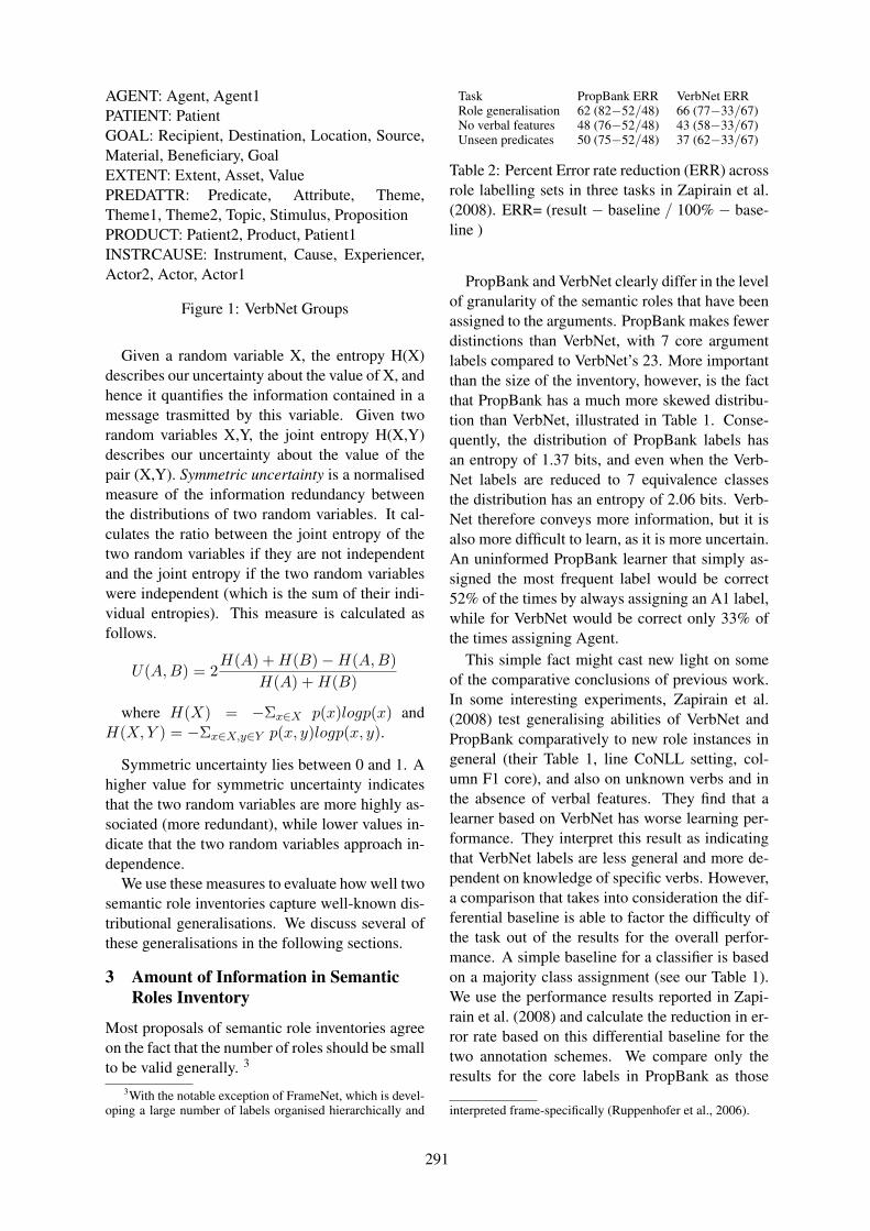
AGENT: Agent, Agent1PATIENT: PatientGOAL: Recipient, Destination, Location, Source,Material, Beneficiary, GoalEXTENT: Extent, Asset, ValuePREDATTR: Predicate, Attribute, Theme,Theme1, Theme2, Topic, Stimulus, PropositionPRODUCT: Patient2, Product, Patient1INSTRCAUSE: Instrument, Cause, Experiencer,Actor2, Actor, Actor1
Figure 1: VerbNet Groups
Given a random variable X, the entropy H(X)describes our uncertainty about the value of X, andhence it quantifies the information contained in amessage trasmitted by this variable. Given tworandom variables X,Y, the joint entropy H(X,Y)describes our uncertainty about the value of thepair (X,Y). Symmetric uncertainty is a normalisedmeasure of the information redundancy betweenthe distributions of two random variables. It cal-culates the ratio between the joint entropy of thetwo random variables if they are not independentand the joint entropy if the two random variableswere independent (which is the sum of their indi-vidual entropies). This measure is calculated asfollows.
U(A, B) = 2H(A) + H(B)−H(A, B)
H(A) + H(B)
where H(X) = −Σx∈X p(x)logp(x) andH(X, Y ) = −Σx∈X,y∈Y p(x, y)logp(x, y).
Symmetric uncertainty lies between 0 and 1. Ahigher value for symmetric uncertainty indicatesthat the two random variables are more highly as-sociated (more redundant), while lower values in-dicate that the two random variables approach in-dependence.
We use these measures to evaluate how well twosemantic role inventories capture well-known dis-tributional generalisations. We discuss several ofthese generalisations in the following sections.
3 Amount of Information in SemanticRoles Inventory
Most proposals of semantic role inventories agreeon the fact that the number of roles should be smallto be valid generally. 3
3With the notable exception of FrameNet, which is devel-oping a large number of labels organised hierarchically and
Task PropBank ERR VerbNet ERRRole generalisation 62 (82−52/48) 66 (77−33/67)No verbal features 48 (76−52/48) 43 (58−33/67)Unseen predicates 50 (75−52/48) 37 (62−33/67)
Table 2: Percent Error rate reduction (ERR) acrossrole labelling sets in three tasks in Zapirain et al.(2008). ERR= (result − baseline / 100% − base-line )
PropBank and VerbNet clearly differ in the levelof granularity of the semantic roles that have beenassigned to the arguments. PropBank makes fewerdistinctions than VerbNet, with 7 core argumentlabels compared to VerbNet’s 23. More importantthan the size of the inventory, however, is the factthat PropBank has a much more skewed distribu-tion than VerbNet, illustrated in Table 1. Conse-quently, the distribution of PropBank labels hasan entropy of 1.37 bits, and even when the Verb-Net labels are reduced to 7 equivalence classesthe distribution has an entropy of 2.06 bits. Verb-Net therefore conveys more information, but it isalso more difficult to learn, as it is more uncertain.An uninformed PropBank learner that simply as-signed the most frequent label would be correct52% of the times by always assigning an A1 label,while for VerbNet would be correct only 33% ofthe times assigning Agent.
This simple fact might cast new light on someof the comparative conclusions of previous work.In some interesting experiments, Zapirain et al.(2008) test generalising abilities of VerbNet andPropBank comparatively to new role instances ingeneral (their Table 1, line CoNLL setting, col-umn F1 core), and also on unknown verbs and inthe absence of verbal features. They find that alearner based on VerbNet has worse learning per-formance. They interpret this result as indicatingthat VerbNet labels are less general and more de-pendent on knowledge of specific verbs. However,a comparison that takes into consideration the dif-ferential baseline is able to factor the difficulty ofthe task out of the results for the overall perfor-mance. A simple baseline for a classifier is basedon a majority class assignment (see our Table 1).We use the performance results reported in Zapi-rain et al. (2008) and calculate the reduction in er-ror rate based on this differential baseline for thetwo annotation schemes. We compare only theresults for the core labels in PropBank as those
interpreted frame-specifically (Ruppenhofer et al., 2006).
291
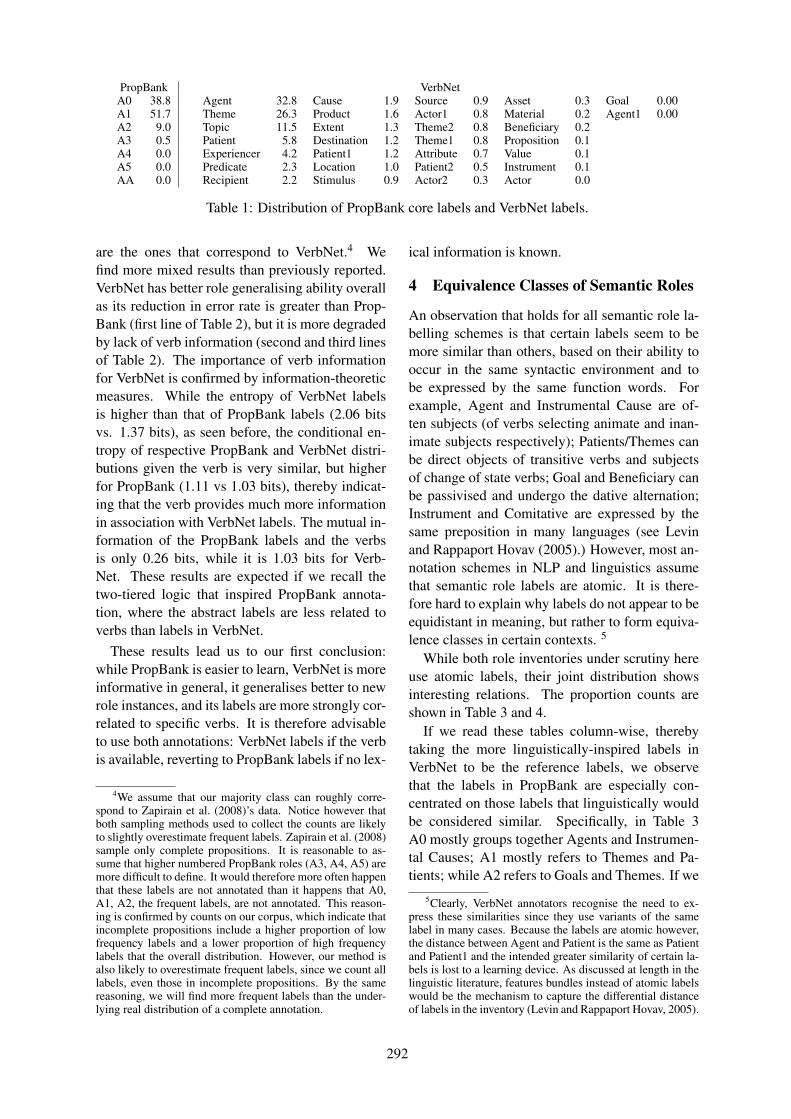
PropBank VerbNetA0 38.8 Agent 32.8 Cause 1.9 Source 0.9 Asset 0.3 Goal 0.00A1 51.7 Theme 26.3 Product 1.6 Actor1 0.8 Material 0.2 Agent1 0.00A2 9.0 Topic 11.5 Extent 1.3 Theme2 0.8 Beneficiary 0.2A3 0.5 Patient 5.8 Destination 1.2 Theme1 0.8 Proposition 0.1A4 0.0 Experiencer 4.2 Patient1 1.2 Attribute 0.7 Value 0.1A5 0.0 Predicate 2.3 Location 1.0 Patient2 0.5 Instrument 0.1AA 0.0 Recipient 2.2 Stimulus 0.9 Actor2 0.3 Actor 0.0
Table 1: Distribution of PropBank core labels and VerbNet labels.
are the ones that correspond to VerbNet.4 Wefind more mixed results than previously reported.VerbNet has better role generalising ability overallas its reduction in error rate is greater than Prop-Bank (first line of Table 2), but it is more degradedby lack of verb information (second and third linesof Table 2). The importance of verb informationfor VerbNet is confirmed by information-theoreticmeasures. While the entropy of VerbNet labelsis higher than that of PropBank labels (2.06 bitsvs. 1.37 bits), as seen before, the conditional en-tropy of respective PropBank and VerbNet distri-butions given the verb is very similar, but higherfor PropBank (1.11 vs 1.03 bits), thereby indicat-ing that the verb provides much more informationin association with VerbNet labels. The mutual in-formation of the PropBank labels and the verbsis only 0.26 bits, while it is 1.03 bits for Verb-Net. These results are expected if we recall thetwo-tiered logic that inspired PropBank annota-tion, where the abstract labels are less related toverbs than labels in VerbNet.
These results lead us to our first conclusion:while PropBank is easier to learn, VerbNet is moreinformative in general, it generalises better to newrole instances, and its labels are more strongly cor-related to specific verbs. It is therefore advisableto use both annotations: VerbNet labels if the verbis available, reverting to PropBank labels if no lex-
4We assume that our majority class can roughly corre-spond to Zapirain et al. (2008)’s data. Notice however thatboth sampling methods used to collect the counts are likelyto slightly overestimate frequent labels. Zapirain et al. (2008)sample only complete propositions. It is reasonable to as-sume that higher numbered PropBank roles (A3, A4, A5) aremore difficult to define. It would therefore more often happenthat these labels are not annotated than it happens that A0,A1, A2, the frequent labels, are not annotated. This reason-ing is confirmed by counts on our corpus, which indicate thatincomplete propositions include a higher proportion of lowfrequency labels and a lower proportion of high frequencylabels that the overall distribution. However, our method isalso likely to overestimate frequent labels, since we count alllabels, even those in incomplete propositions. By the samereasoning, we will find more frequent labels than the under-lying real distribution of a complete annotation.
ical information is known.
4 Equivalence Classes of Semantic Roles
An observation that holds for all semantic role la-belling schemes is that certain labels seem to bemore similar than others, based on their ability tooccur in the same syntactic environment and tobe expressed by the same function words. Forexample, Agent and Instrumental Cause are of-ten subjects (of verbs selecting animate and inan-imate subjects respectively); Patients/Themes canbe direct objects of transitive verbs and subjectsof change of state verbs; Goal and Beneficiary canbe passivised and undergo the dative alternation;Instrument and Comitative are expressed by thesame preposition in many languages (see Levinand Rappaport Hovav (2005).) However, most an-notation schemes in NLP and linguistics assumethat semantic role labels are atomic. It is there-fore hard to explain why labels do not appear to beequidistant in meaning, but rather to form equiva-lence classes in certain contexts. 5
While both role inventories under scrutiny hereuse atomic labels, their joint distribution showsinteresting relations. The proportion counts areshown in Table 3 and 4.
If we read these tables column-wise, therebytaking the more linguistically-inspired labels inVerbNet to be the reference labels, we observethat the labels in PropBank are especially con-centrated on those labels that linguistically wouldbe considered similar. Specifically, in Table 3A0 mostly groups together Agents and Instrumen-tal Causes; A1 mostly refers to Themes and Pa-tients; while A2 refers to Goals and Themes. If we
5Clearly, VerbNet annotators recognise the need to ex-press these similarities since they use variants of the samelabel in many cases. Because the labels are atomic however,the distance between Agent and Patient is the same as Patientand Patient1 and the intended greater similarity of certain la-bels is lost to a learning device. As discussed at length in thelinguistic literature, features bundles instead of atomic labelswould be the mechanism to capture the differential distanceof labels in the inventory (Levin and Rappaport Hovav, 2005).
292

A0 A1 A2 A3 A4 A5 AAAgent 32.6 0.2 - - - - -Patient 0.0 5.8 - - - - -Goal 0.0 1.5 4.0 0.2 0.0 0.0 -Extent - 0.2 1.3 0.2 - - -PredAttr 1.2 39.3 2.9 0.0 - - 0.0Product 0.1 2.7 0.6 - 0.0 - -InstrCause 4.8 2.2 0.3 0.1 - - -
Table 3: Distribution of PropBank by VerbNetgroup labels according to SemLink. Counts indi-cated as 0.0 approximate zero by rounding, whilea - sign indicates that no occurrences were found.
read these tables row-wise, thereby concentratingon the grouping of PropBank labels provided byVerbNet labels, we see that low frequency Prop-Bank labels are more evenly spread across Verb-Net labels than the frequent labels, and it is moredifficult to identify a dominant label than for high-frequency labels. Because PropBank groups to-gether VerbNet labels at high frequency, whileVerbNet labels make different distinctions at lowerfrequencies, the distribution of PropBank is muchmore skewed than VerbNet, yielding the differ-ences in distributions and entropy discussed in theprevious section.
We can draw, then, a second conclusion: whileVerbNet is finer-grained than PropBank, the twoclassifications are not in contradiction with eachother. VerbNet greater specificity can be used indifferent ways depending on the frequency of thelabel. Practically, PropBank labels could providea strong generalisation to a VerbNet annotation athigh-frequency. VerbNet labels, on the other hand,can act as disambiguators of overloaded variablesin PropBank. This conclusion was also reachedby Loper et al. (2007). Thus, both annotationschemes could be useful in different circumstancesand at different frequency bands.
5 The Combinatorics of Semantic Roles
Semantic roles exhibit paradigmatic generalisa-tions — generalisations across similar semanticroles in the inventory — (which we saw in section4.) They also show syntagmatic generalisations,generalisations that concern the context. One kindof context is provided by what other roles they canoccur with. It has often been observed that cer-tain semantic roles sets are possible, while oth-ers are not; among the possible sets, certain aremuch more frequent than others (Levin and Rap-paport Hovav, 2005). Some linguistically-inspired
A0 A1 A2 A3 A4 A5 AAActor 0.0 - - - - - -Actor1 0.8 - - - - - -Actor2 - 0.3 0.1 - - - -Agent1 0.0 - - - - - -Agent 32.6 0.2 - - - - -Asset - 0.1 0.0 0.2 - - -Attribute - 0.1 0.7 - - - -Beneficiary - 0.0 0.1 0.1 0.0 - -Cause 0.7 1.1 0.1 0.1 - - -Destination - 0.4 0.8 0.0 - - -Experiencer 3.3 0.9 0.1 - - - -Extent - - 1.3 - - - -Goal - - - - 0.0 - -Instrument - - 0.1 0.0 - - -Location 0.0 0.4 0.6 0.0 - 0.0 -Material - 0.1 0.1 0.0 - - -Patient 0.0 5.8 - - - - -Patient1 0.1 1.1 - - - - -Patient2 - 0.1 0.5 - - - -Predicate - 1.2 1.1 0.0 - - -Product 0.0 1.5 0.1 - 0.0 - -Proposition - 0.0 0.1 - - - -Recipient - 0.3 2.0 - 0.0 - -Source - 0.3 0.5 0.1 - - -Stimulus - 1.0 - - - - -Theme 0.8 25.1 0.5 0.0 - - 0.0Theme1 0.4 0.4 0.0 0.0 - - -Theme2 0.1 0.4 0.3 - - - -Topic - 11.2 0.3 - - - -Value - 0.1 - - - - -
Table 4: Distribution of PropBank by originalVerbNet labels according to SemLink. Countsindicated as 0.0 approximate zero by rounding,while a - sign indicates that no occurrences werefound.
semantic role labelling techniques do attempt tomodel these dependencies directly (Toutanova etal., 2008; Merlo and Musillo, 2008).
Both annotation schemes impose tight con-straints on co-occurrence of roles, independentlyof any verb information, with 62 role sets forPropBank and 116 role combinations for VerbNet,fewer than possible. Among the observed rolesets, some are more frequent than expected un-der an assumption of independence between roles.For example, in PropBank, propositions compris-ing A0, A1 roles are observed 85% of the time,while they would be expected to occur only in 20%of the cases. In VerbNet the difference is also greatbetween the 62% observed Agent, PredAttr propo-sitions and the 14% expected.
Constraints on possible role sets are the expres-sion of structural constraints among roles inheritedfrom syntax, which we discuss in the next section,but also of the underlying event structure of theverb. Because of this relation, we expect a strongcorrelation between role sets and their associated
293
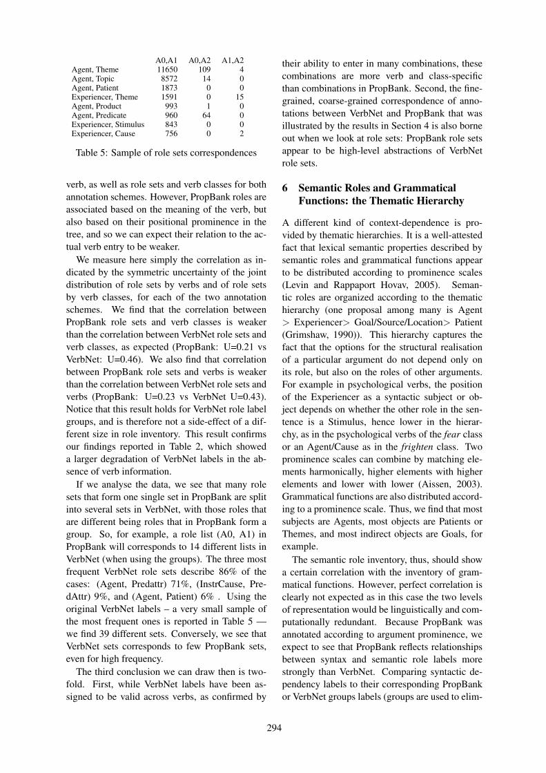
A0,A1 A0,A2 A1,A2Agent, Theme 11650 109 4Agent, Topic 8572 14 0Agent, Patient 1873 0 0Experiencer, Theme 1591 0 15Agent, Product 993 1 0Agent, Predicate 960 64 0Experiencer, Stimulus 843 0 0Experiencer, Cause 756 0 2
Table 5: Sample of role sets correspondences
verb, as well as role sets and verb classes for bothannotation schemes. However, PropBank roles areassociated based on the meaning of the verb, butalso based on their positional prominence in thetree, and so we can expect their relation to the ac-tual verb entry to be weaker.
We measure here simply the correlation as in-dicated by the symmetric uncertainty of the jointdistribution of role sets by verbs and of role setsby verb classes, for each of the two annotationschemes. We find that the correlation betweenPropBank role sets and verb classes is weakerthan the correlation between VerbNet role sets andverb classes, as expected (PropBank: U=0.21 vsVerbNet: U=0.46). We also find that correlationbetween PropBank role sets and verbs is weakerthan the correlation between VerbNet role sets andverbs (PropBank: U=0.23 vs VerbNet U=0.43).Notice that this result holds for VerbNet role labelgroups, and is therefore not a side-effect of a dif-ferent size in role inventory. This result confirmsour findings reported in Table 2, which showeda larger degradation of VerbNet labels in the ab-sence of verb information.
If we analyse the data, we see that many rolesets that form one single set in PropBank are splitinto several sets in VerbNet, with those roles thatare different being roles that in PropBank form agroup. So, for example, a role list (A0, A1) inPropBank will corresponds to 14 different lists inVerbNet (when using the groups). The three mostfrequent VerbNet role sets describe 86% of thecases: (Agent, Predattr) 71%, (InstrCause, Pre-dAttr) 9%, and (Agent, Patient) 6% . Using theoriginal VerbNet labels – a very small sample ofthe most frequent ones is reported in Table 5 —we find 39 different sets. Conversely, we see thatVerbNet sets corresponds to few PropBank sets,even for high frequency.
The third conclusion we can draw then is two-fold. First, while VerbNet labels have been as-signed to be valid across verbs, as confirmed by
their ability to enter in many combinations, thesecombinations are more verb and class-specificthan combinations in PropBank. Second, the fine-grained, coarse-grained correspondence of anno-tations between VerbNet and PropBank that wasillustrated by the results in Section 4 is also borneout when we look at role sets: PropBank role setsappear to be high-level abstractions of VerbNetrole sets.
6 Semantic Roles and GrammaticalFunctions: the Thematic Hierarchy
A different kind of context-dependence is pro-vided by thematic hierarchies. It is a well-attestedfact that lexical semantic properties described bysemantic roles and grammatical functions appearto be distributed according to prominence scales(Levin and Rappaport Hovav, 2005). Seman-tic roles are organized according to the thematichierarchy (one proposal among many is Agent> Experiencer> Goal/Source/Location> Patient(Grimshaw, 1990)). This hierarchy captures thefact that the options for the structural realisationof a particular argument do not depend only onits role, but also on the roles of other arguments.For example in psychological verbs, the positionof the Experiencer as a syntactic subject or ob-ject depends on whether the other role in the sen-tence is a Stimulus, hence lower in the hierar-chy, as in the psychological verbs of the fear classor an Agent/Cause as in the frighten class. Twoprominence scales can combine by matching ele-ments harmonically, higher elements with higherelements and lower with lower (Aissen, 2003).Grammatical functions are also distributed accord-ing to a prominence scale. Thus, we find that mostsubjects are Agents, most objects are Patients orThemes, and most indirect objects are Goals, forexample.
The semantic role inventory, thus, should showa certain correlation with the inventory of gram-matical functions. However, perfect correlation isclearly not expected as in this case the two levelsof representation would be linguistically and com-putationally redundant. Because PropBank wasannotated according to argument prominence, weexpect to see that PropBank reflects relationshipsbetween syntax and semantic role labels morestrongly than VerbNet. Comparing syntactic de-pendency labels to their corresponding PropBankor VerbNet groups labels (groups are used to elim-
294

inate the confound of different inventory sizes), wefind that the joint entropy of PropBank and depen-dency labels is 2.61 bits while the joint entropy ofVerbNet and dependency labels is 3.32 bits. Thesymmetric uncertainty of PropBank and depen-dency labels is 0.49, while the symmetric uncer-tainty of VerbNet and dependency labels is 0.39.
On the basis of these correlations, we can con-firm previous findings: PropBank more closelycaptures the thematic hierarchy and is more corre-lated to grammatical functions, hence potentiallymore useful for semantic role labelling, for learn-ers whose features are based on the syntactic tree.VerbNet, however, provides a level of annotationthat is more independent of syntactic information,a property that might be useful in several applica-tions, such as machine translation, where syntacticinformation might be too language-specific.
7 Generality of Semantic Roles
Semantic roles are not meant to be domain-specific, but rather to encode aspects of our con-ceptualisation of the world. A semantic role in-ventory that wants to be linguistically perspicuousand also practically useful in several tasks needs toreflect our grammatical representation of events.VerbNet is believed to be superior in this respectto PropBank, as it attempts to be less verb-specificand to be portable across classes. Previous results(Loper et al., 2007; Zapirain et al., 2008) appear toindicate that this is not the case because a labellerhas better performance with PropBank labels thanwith VerbNet labels. But these results are task-specific, and they were obtained in the context ofparsing. Since we know that PropBank is moreclosely related to grammatical function and syn-tactic annotation than VerbNet, as indicated abovein Section 6, then these results could simply indi-cate that parsing predicts PropBank labels betterbecause they are more closely related to syntacticlabels, and not because the semantic roles inven-tory is more general.
Several of the findings in the previous sectionsshed light on the generality of the semantic roles inthe two inventories. Results in Section 3 show thatprevious results can be reinterpreted as indicatingthat VerbNet labels generalise better to new roles.
We attempt here to determine the generality ofthe “meaning” of a role label without recourseto a task-specific experiment. It is often claimedin the literature that semantic roles are better de-
scribed by feature bundles. In particular, the fea-tures sentience and volition have been shown to beuseful in distinguishing Proto-Agents from Proto-Patients (Dowty, 1991). These features can be as-sumed to be correlated to animacy. Animacy hasindeed been shown to be a reliable indicator ofsemantic role differences (Merlo and Stevenson,2001). Personal pronouns in English grammati-calise animacy. We extract all the occurrences ofthe unambiguously animate pronouns (I, you, he,she, us, we, me, us, him) and the unambiguouslyinanimate pronoun it, for each semantic role label,in PropBank and VerbNet. We find occurrencesfor three semantic role labels in PropBank and sixin VerbNet. We reduce the VerbNet groups to fiveby merging Patient roles with PredAttr roles toavoid artificial variation among very similar roles.An analysis of variance of the distributions of thepronous yields a significant effect of animacy forVerbNet (F(4)=5.62, p< 0.05), but no significanteffect for PropBank (F(2)=4.94, p=0.11). This re-sult is a preliminary indication that VerbNet labelsmight capture basic components of meaning moreclearly than PropBank labels, and that they mighttherefore be more general.
8 Conclusions
In this paper, we have proposed a task-independent, general method to analyse anno-tation schemes. The method is based oninformation-theoretic measures and comparisonwith attested linguistic generalisations, to evalu-ate how well semantic role inventories and anno-tations capture grammaticalised aspects of mean-ing. We show that VerbNet is more verb-specificand better able to generalise to new semantic roles,while PropBank, because of its relation to syntax,better captures some of the structural constraintsamong roles. Future work will investigate anotherbasic property of semantic role labelling schemes:cross-linguistic validity.
Acknowledgements
We thank James Henderson and Ivan Titov foruseful comments. The research leading to theseresults has received partial funding from the EUFP7 programme (FP7/2007-2013) under grantagreement number 216594 (CLASSIC project:www.classic-project.org).
295

ReferencesJudith Aissen. 2003. Differential object marking:
Iconicity vs. economy. Natural Language and Lin-guistic Theory, 21:435–483.
Collin F. Baker, Charles J. Fillmore, and John B. Lowe.1998. The Berkeley FrameNet project. In Proceed-ings of the Thirty-Sixth Annual Meeting of the As-sociation for Computational Linguistics and Seven-teenth International Conference on ComputationalLinguistics (ACL-COLING’98), pages 86–90, Mon-treal, Canada.
David Dowty. 1991. Thematic proto-roles and argu-ment selection. Language, 67(3):547–619.
Charles Fillmore. 1968. The case for case. In EmmonBach and Harms, editors, Universals in LinguisticTheory, pages 1–88. Holt, Rinehart, and Winston.
Jane Grimshaw. 1990. Argument Structure. MITPress.
Jeffrey Gruber. 1965. Studies in Lexical Relation.MIT Press, Cambridge, MA.
Ray Jackendoff. 1972. Semantic Interpretation inGenerative Grammar. MIT Press, Cambridge, MA.
Karin Kipper. 2005. VerbNet: A broad-coverage, com-prehensive verb lexicon. Ph.D. thesis, University ofPennsylvania.
Beth Levin and Malka Rappaport Hovav. 2005. Ar-gument Realization. Cambridge University Press,Cambridge, UK.
Edward Loper, Szu ting Yi, and Martha Palmer. 2007.Combining lexical resources: Mapping betweenPropBank and VerbNet. In Proceedings of theIWCS.
Christopher Manning and Hinrich Schuetze. 1999.Foundations of Statistical Natural Language Pro-cessing. MIT Press.
Mitch Marcus, Beatrice Santorini, and M.A.Marcinkiewicz. 1993. Building a large anno-tated corpus of English: the Penn Treebank.Computational Linguistics, 19:313–330.
Paola Merlo and Gabriele Musillo. 2008. Semanticparsing for high-precision semantic role labelling.In Proceedings of the Twelfth Conference on Com-putational Natural Language Learning (CONLL-08), pages 1–8, Manchester, UK.
Paola Merlo and Suzanne Stevenson. 2001. Automaticverb classification based on statistical distributionsof argument structure. Computational Linguistics,27(3):373–408.
Martha Palmer, Daniel Gildea, and Paul Kingsbury.2005. The Proposition Bank: An annotated cor-pus of semantic roles. Computational Linguistics,31:71–105.
Josef Ruppenhofer, Michael Ellsworth, MiriamPetruck, Christopher Johnson, and Jan Scheffczyk.2006. Framenet ii: Theory and practice. Technicalreport, Berkeley,CA.
Mihai Surdeanu, Richard Johansson, Adam Meyers,Lluı́s Màrquez, and Joakim Nivre. 2008. TheCoNLL-2008 shared task on joint parsing of syn-tactic and semantic dependencies. In Proceedingsof the 12th Conference on Computational NaturalLanguage Learning (CoNLL-2008), pages 159–177.
Kristina Toutanova, Aria Haghighi, and Christopher D.Manning. 2008. A global joint model for semanticrole labeling. Computational Linguistics, 34(2).
Ian Witten and Eibe Frank. 2005. Data Mining. Else-vier.
Szu-ting Yi, Edward Loper, and Martha Palmer. 2007.Can semantic roles generalize across genres? InProceedings of the Human Language Technologies2007 (NAACL-HLT’07), pages 548–555, Rochester,New York, April.
Beñat Zapirain, Eneko Agirre, and Lluı́s Màrquez.2008. Robustness and generalization of role sets:PropBank vs. VerbNet. In Proceedings of ACL-08:HLT, pages 550–558, Columbus, Ohio, June.
296
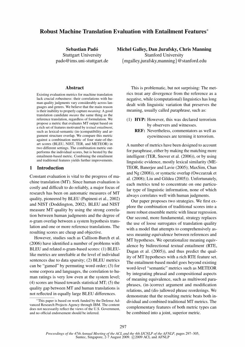
Proceedings of the 47th Annual Meeting of the ACL and the 4th IJCNLP of the AFNLP, pages 297–305,Suntec, Singapore, 2-7 August 2009. c©2009 ACL and AFNLP
Robust Machine Translation Evaluation with Entailment Features∗
Sebastian PadóStuttgart University
Michel Galley, Dan Jurafsky, Chris ManningStanford University
{mgalley,jurafsky,manning}@stanford.edu
AbstractExisting evaluation metrics for machine translationlack crucial robustness: their correlations with hu-man quality judgments vary considerably across lan-guages and genres. We believe that the main reasonis their inability to properly capture meaning: A goodtranslation candidate means the same thing as thereference translation, regardless of formulation. Wepropose a metric that evaluates MT output based ona rich set of features motivated by textual entailment,such as lexical-semantic (in-)compatibility and ar-gument structure overlap. We compare this metricagainst a combination metric of four state-of-the-art scores (BLEU, NIST, TER, and METEOR) intwo different settings. The combination metric out-performs the individual scores, but is bested by theentailment-based metric. Combining the entailmentand traditional features yields further improvements.
1 Introduction
Constant evaluation is vital to the progress of ma-chine translation (MT). Since human evaluation iscostly and difficult to do reliably, a major focus ofresearch has been on automatic measures of MTquality, pioneered by BLEU (Papineni et al., 2002)and NIST (Doddington, 2002). BLEU and NISTmeasure MT quality by using the strong correla-tion between human judgments and the degree ofn-gram overlap between a system hypothesis trans-lation and one or more reference translations. Theresulting scores are cheap and objective.
However, studies such as Callison-Burch et al.(2006) have identified a number of problems withBLEU and related n-gram-based scores: (1) BLEU-like metrics are unreliable at the level of individualsentences due to data sparsity; (2) BLEU metricscan be “gamed” by permuting word order; (3) forsome corpora and languages, the correlation to hu-man ratings is very low even at the system level;(4) scores are biased towards statistical MT; (5) thequality gap between MT and human translations isnot reflected in equally large BLEU differences.
∗This paper is based on work funded by the Defense Ad-vanced Research Projects Agency through IBM. The contentdoes not necessarily reflect the views of the U.S. Government,and no official endorsement should be inferred.
This is problematic, but not surprising: The met-rics treat any divergence from the reference as anegative, while (computational) linguistics has longdealt with linguistic variation that preserves themeaning, usually called paraphrase, such as:
(1) HYP: However, this was declared terrorismby observers and witnesses.
REF: Nevertheless, commentators as well aseyewitnesses are terming it terrorism.
A number of metrics have been designed to accountfor paraphrase, either by making the matching moreintelligent (TER, Snover et al. (2006)), or by usinglinguistic evidence, mostly lexical similarity (ME-TEOR, Banerjee and Lavie (2005); MaxSim, Chanand Ng (2008)), or syntactic overlap (Owczarzak etal. (2008); Liu and Gildea (2005)). Unfortunately,each metrics tend to concentrate on one particu-lar type of linguistic information, none of whichalways correlates well with human judgments.
Our paper proposes two strategies. We first ex-plore the combination of traditional scores into amore robust ensemble metric with linear regression.Our second, more fundamental, strategy replacesthe use of loose surrogates of translation qualitywith a model that attempts to comprehensively as-sess meaning equivalence between references andMT hypotheses. We operationalize meaning equiv-alence by bidirectional textual entailment (RTE,Dagan et al. (2005)), and thus predict the qual-ity of MT hypotheses with a rich RTE feature set.The entailment-based model goes beyond existingword-level “semantic” metrics such as METEORby integrating phrasal and compositional aspectsof meaning equivalence, such as multiword para-phrases, (in-)correct argument and modificationrelations, and (dis-)allowed phrase reorderings. Wedemonstrate that the resulting metric beats both in-dividual and combined traditional MT metrics. Thecomplementary features of both metric types canbe combined into a joint, superior metric.
297
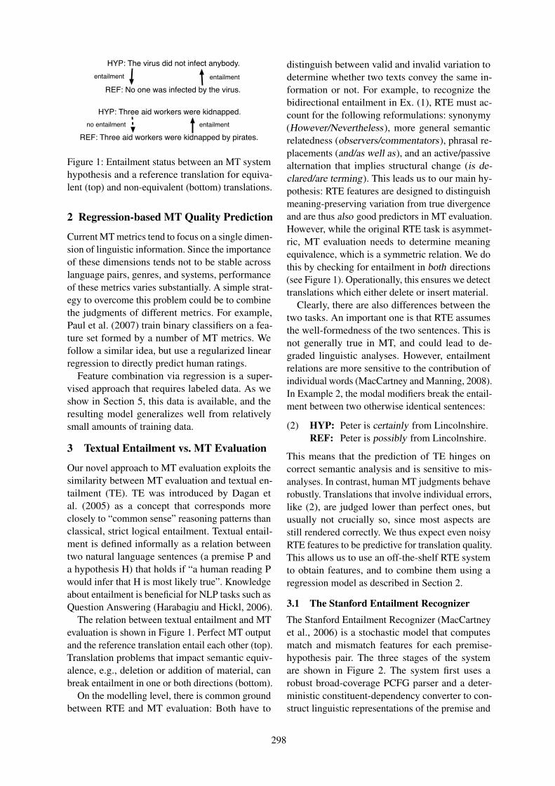
HYP: Three aid workers were kidnapped.
REF: Three aid workers were kidnapped by pirates.no entailment entailment
HYP: The virus did not infect anybody.
REF: No one was infected by the virus.entailment entailment
Figure 1: Entailment status between an MT systemhypothesis and a reference translation for equiva-lent (top) and non-equivalent (bottom) translations.
2 Regression-based MT Quality Prediction
Current MT metrics tend to focus on a single dimen-sion of linguistic information. Since the importanceof these dimensions tends not to be stable acrosslanguage pairs, genres, and systems, performanceof these metrics varies substantially. A simple strat-egy to overcome this problem could be to combinethe judgments of different metrics. For example,Paul et al. (2007) train binary classifiers on a fea-ture set formed by a number of MT metrics. Wefollow a similar idea, but use a regularized linearregression to directly predict human ratings.
Feature combination via regression is a super-vised approach that requires labeled data. As weshow in Section 5, this data is available, and theresulting model generalizes well from relativelysmall amounts of training data.
3 Textual Entailment vs. MT Evaluation
Our novel approach to MT evaluation exploits thesimilarity between MT evaluation and textual en-tailment (TE). TE was introduced by Dagan etal. (2005) as a concept that corresponds moreclosely to “common sense” reasoning patterns thanclassical, strict logical entailment. Textual entail-ment is defined informally as a relation betweentwo natural language sentences (a premise P anda hypothesis H) that holds if “a human reading Pwould infer that H is most likely true”. Knowledgeabout entailment is beneficial for NLP tasks such asQuestion Answering (Harabagiu and Hickl, 2006).
The relation between textual entailment and MTevaluation is shown in Figure 1. Perfect MT outputand the reference translation entail each other (top).Translation problems that impact semantic equiv-alence, e.g., deletion or addition of material, canbreak entailment in one or both directions (bottom).
On the modelling level, there is common groundbetween RTE and MT evaluation: Both have to
distinguish between valid and invalid variation todetermine whether two texts convey the same in-formation or not. For example, to recognize thebidirectional entailment in Ex. (1), RTE must ac-count for the following reformulations: synonymy(However/Nevertheless), more general semanticrelatedness (observers/commentators), phrasal re-placements (and/as well as), and an active/passivealternation that implies structural change (is de-clared/are terming). This leads us to our main hy-pothesis: RTE features are designed to distinguishmeaning-preserving variation from true divergenceand are thus also good predictors in MT evaluation.However, while the original RTE task is asymmet-ric, MT evaluation needs to determine meaningequivalence, which is a symmetric relation. We dothis by checking for entailment in both directions(see Figure 1). Operationally, this ensures we detecttranslations which either delete or insert material.
Clearly, there are also differences between thetwo tasks. An important one is that RTE assumesthe well-formedness of the two sentences. This isnot generally true in MT, and could lead to de-graded linguistic analyses. However, entailmentrelations are more sensitive to the contribution ofindividual words (MacCartney and Manning, 2008).In Example 2, the modal modifiers break the entail-ment between two otherwise identical sentences:
(2) HYP: Peter is certainly from Lincolnshire.REF: Peter is possibly from Lincolnshire.
This means that the prediction of TE hinges oncorrect semantic analysis and is sensitive to mis-analyses. In contrast, human MT judgments behaverobustly. Translations that involve individual errors,like (2), are judged lower than perfect ones, butusually not crucially so, since most aspects arestill rendered correctly. We thus expect even noisyRTE features to be predictive for translation quality.This allows us to use an off-the-shelf RTE systemto obtain features, and to combine them using aregression model as described in Section 2.
3.1 The Stanford Entailment RecognizerThe Stanford Entailment Recognizer (MacCartneyet al., 2006) is a stochastic model that computesmatch and mismatch features for each premise-hypothesis pair. The three stages of the systemare shown in Figure 2. The system first uses arobust broad-coverage PCFG parser and a deter-ministic constituent-dependency converter to con-struct linguistic representations of the premise and
298

Stage 3: Feature computation (w/ numbers of features)
Premise: India buys 1,000 tanks.Hypothesis: India acquires arms.
Stage 1: Linguistic analysis
India
buys
1,000 tankssubj dobj
India
acquires
armssubj dobj
Stage 2: Alignment
India
buys
1,000 tankssubj dobj
India
acquires
armssubj dobj
0.9
1.0 0.7
Alignment (8):Semantic compatibility (34): Insertions anddeletions (20):Preservation of reference (16):Structural alignment (28):
Overall alignment qualityModality, Factivity, Polarity, Quantification, Lexical-semantic relatedness, TenseFelicity of appositions and adjuncts, Types of unaligned material Locations, Dates, Entities
Alignment of main verbs and syntactically prominent words, Argument structure (mis-)matches
Figure 2: The Stanford Entailment Recognizer
the hypothesis. The results are typed dependencygraphs that contain a node for each word and la-beled edges representing the grammatical relationsbetween words. Named entities are identified, andcontiguous collocations grouped. Next, it identifiesthe highest-scoring alignment from each node inthe hypothesis graph to a single node in the premisegraph, or to null. It uses a locally decomposablescoring function: The score of an alignment is thesum of the local word and edge alignment scores.The computation of these scores make extensiveuse of about ten lexical similarity resources, in-cluding WordNet, InfoMap, and Dekang Lin’s the-saurus. Since the search space is exponential inthe hypothesis length, the system uses stochastic(rather than exhaustive) search based on Gibbs sam-pling (see de Marneffe et al. (2007)).
Entailment features. In the third stage, the sys-tem produces roughly 100 features for each alignedpremise-hypothesis pair. A small number of themare real-valued (mostly quality scores), but mostare binary implementations of small linguistic the-ories whose activation indicates syntactic and se-
mantic (mis-)matches of different types. Figure 2groups the features into five classes. Alignmentfeatures measure the overall quality of the align-ment as given by the lexical resources. Semanticcompatibility features check to what extent thealigned material has the same meaning and pre-serves semantic dimensions such as modality andfactivity, taking a limited amount of context intoaccount. Insertion/deletion features explicitly ad-dress material that remains unaligned and assess itsfelicity. Reference features ascertain that the twosentences actually refer to the same events and par-ticipants. Finally, structural features add structuralconsiderations by ensuring that argument structureis preserved in the translation. See MacCartney etal. (2006) for details on the features, and Sections5 and 6 for examples of feature firings.
Efficiency considerations. The use of deep lin-guistic analysis makes our entailment-based met-ric considerably more heavyweight than traditionalMT metrics. The average total runtime per sentencepair is 5 seconds on an AMD 2.6GHz Opteron core– efficient enough to perform regular evaluations ondevelopment and test sets. We are currently investi-gating caching and optimizations that will enablethe use of our metric for MT parameter tuning in aMinimum Error Rate Training setup (Och, 2003).
4 Experimental Evaluation
4.1 Experiments
Traditionally, human ratings for MT quality havebeen collected in the form of absolute scores on afive- or seven-point Likert scale, but low reliabil-ity numbers for this type of annotation have raisedconcerns (Callison-Burch et al., 2008). An alter-native that has been adopted by the yearly WMTevaluation shared tasks since 2008 is the collectionof pairwise preference judgments between pairs ofMT hypotheses which can be elicited (somewhat)more reliably. We demonstrate that our approachworks well for both types of annotation and differ-ent corpora. Experiment 1 models absolute scoreson Asian newswire, and Experiment 2 pairwisepreferences on European speech and news data.
4.2 Evaluation
We evaluate the output of our models both on thesentence and on the system level. At the sentencelevel, we can correlate predictions in Experiment 1directly with human judgments with Spearman’s ρ ,
299

a non-parametric rank correlation coefficient appro-priate for non-normally distributed data. In Experi-ment 2, the predictions cannot be pooled betweensentences. Instead of correlation, we compute “con-sistency” (i.e., accuracy) with human preferences.
System-level predictions are computed in bothexperiments from sentence-level predictions, as theratio of sentences for which each system providedthe best translation (Callison-Burch et al., 2008).We extend this procedure slightly because real-valued predictions cannot predict ties, while humanraters decide for a significant portion of sentences(as much as 80% in absolute score annotation) to“tie” two systems for first place. To simulate thisbehavior, we compute “tie-aware” predictions asthe percentage of sentences where the system’s hy-pothesis was assigned a score better or at most ε
worse than the best system. ε is set to match thefrequency of ties in the training data.
Finally, the predictions are again correlated withhuman judgments using Spearman’s ρ . “Tie aware-ness” makes a considerable practical difference,improving correlation figures by 5–10 points.1
4.3 Baseline MetricsWe consider four baselines. They are small regres-sion models as described in Section 2 over com-ponent scores of four widely used MT metrics. Toalleviate possible nonlinearity, we add all featuresin linear and log space. Each baselines carries thename of the underlying metric plus the suffix -R.2
BLEUR includes the following 18 sentence-levelscores: BLEU-n and n-gram precision scores(1 ≤ n ≤ 4); BLEU brevity penalty (BP); BLEUscore divided by BP. To counteract BLEU’s brittle-ness at the sentence level, we also smooth BLEU-nand n-gram precision as in Lin and Och (2004).
NISTR consists of 16 features. NIST-n scores(1 ≤ n ≤ 10) and information-weighted n-gramprecision scores (1 ≤ n ≤ 4); NIST brevity penalty(BP); and NIST score divided by BP.
1Due to space constraints, we only show results for “tie-aware” predictions. See Padó et al. (2009) for a discussion.
2The regression models can simulate the behaviour of eachcomponent by setting the weights appropriately, but are strictlymore powerful. A possible danger is that the parameters over-fit on the training set. We therefore verified that the threenon-trivial “baseline” regression models indeed confer a bene-fit over the default component combination scores: BLEU-1(which outperformed BLEU-4 in the MetricsMATR 2008 eval-uation), NIST-4, and TER (with all costs set to 1). We foundhigher robustness and improved correlations for the regressionmodels. An exception is BLEU-1 and NIST-4 on Expt. 1 (Ar,Ch), which perform 0.5–1 point better at the sentence level.
TERR includes 50 features. We start with thestandard TER score and the number of each of thefour edit operations. Since the default uniform costdoes not always correlate well with human judg-ment, we duplicate these features for 9 non-uniformedit costs. We find it effective to set insertion costclose to 0, as a way of enabling surface variation,and indeed the new TERp metric uses a similarlylow default insertion cost (Snover et al., 2009).
METEORR consists of METEOR v0.7.
4.4 Combination Metrics
The following three regression models implementthe methods discussed in Sections 2 and 3.
MTR combines the 85 features of the four base-line models. It uses no entailment features.
RTER uses the 70 entailment features describedin Section 3.1, but no MTR features.
MT+RTER uses all MTR and RTER features,combining matching and entailment evidence.3
5 Expt. 1: Predicting Absolute Scores
Data. Our first experiment evaluates the modelswe have proposed on a corpus with traditional an-notation on a seven-point scale, namely the NISTOpenMT 2008 corpus.4 The corpus contains trans-lations of newswire text into English from threesource languages (Arabic (Ar), Chinese (Ch), Urdu(Ur)). Each language consists of 1500–2800 sen-tence pairs produced by 7–15 MT systems.
We use a “round robin” scheme. We optimizethe weights of our regression models on two lan-guages and then predict the human scores on thethird language. This gauges performance of ourmodels when training and test data come from thesame genre, but from different languages, whichwe believe to be a setup of practical interest. Foreach test set, we set the system-level tie parameterε so that the relative frequency of ties was equalto the training set (65–80%). Hypotheses generallyhad to receive scores within 0.3−0.5 points to tie.
Results. Table 1 shows the results. We first con-centrate on the upper half (sentence-level results).The predictions of all models correlate highly sig-nificantly with human judgments, but we still seerobustness issues for the individual MT metrics.
3Software for RTER and MT+RTER is available fromhttp://nlp.stanford.edu/software/mteval.shtml.
4Available from http://www.nist.gov.
300

Evaluation Data Metricstrain test BLEUR METEORR NISTR TERR MTR RTER MT+RTER
Sentence-levelAr+Ch Ur 49.9 49.1 49.5 50.1 50.1 54.5 55.6Ar+Ur Ch 53.9 61.1 53.1 50.3 57.3 58.0 62.7Ch+Ur Ar 52.5 60.1 50.4 54.5 55.2 59.9 61.1
System-levelAr+Ch Ur 73.9 68.4 50.0 90.0∗ 92.7∗ 77.4∗ 81.0∗Ar+Ur Ch 38.5 44.3 40.0 59.0∗ 51.8∗ 47.7 57.3∗Ch+Ur Ar 59.7∗ 86.3∗ 61.9∗ 42.1 48.1 59.7∗ 61.7∗
Table 1: Expt. 1: Spearman’s ρ for correlation between human absolute scores and model predictions onNIST OpenMT 2008. Sentence level: All correlations are highly significant. System level: ∗: p<0.05.
METEORR achieves the best correlation for Chi-nese and Arabic, but fails for Urdu, apparently themost difficult language. TERR shows the best resultfor Urdu, but does worse than METEORR for Ara-bic and even worse than BLEUR for Chinese. TheMTR combination metric alleviates this problem tosome extent by improving the “worst-case” perfor-mance on Urdu to the level of the best individualmetric. The entailment-based RTER system outper-forms MTR on each language. It particularly im-proves on MTR’s correlation on Urdu. Even thoughMETEORR still does somewhat better than MTRand RTER, we consider this an important confirma-tion for the usefulness of entailment features in MTevaluation, and for their robustness.5
In addition, the combined model MT+RTER isbest for all three languages, outperforming METE-ORR for each language pair. It performs consid-erably better than either MTR or RTER. This is asecond result: the types of evidence provided byMTR and RTER appear to be complementary andcan be combined into a superior model.
On the system level (bottom half of Table 1),there is high variance due to the small number ofpredictions per language, and many predictions arenot significantly correlated with human judgments.BLEUR, METEORR, and NISTR significantly pre-dict one language each (all Arabic); TERR, MTR,and RTER predict two languages. MT+RTER isthe only model that shows significance for all threelanguages. This result supports the conclusions wehave drawn from the sentence-level analysis.
Further analysis. We decided to conduct a thor-ough analysis of the Urdu dataset, the most difficultsource language for all metrics. We start with a fea-
5These results are substantially better than the performanceour metric showed in the MetricsMATR 2008 challenge. Be-yond general enhancement of our model, we attribute the lessgood MetricsMATR 2008 results to an infelicitous choiceof training data for the submission, coupled with the largeamount of ASR output in the test data, whose disfluenciesrepresent an additional layer of problems for deep approaches.
20 40 60 80 100
0.42
0.46
0.50
0.54
% Training data MT08 Ar+Ch
Spe
arm
an's
rho
on
MT
08
Ur
●
●
●
●
● ● ●● ●
●● ●
●●
● ● ● ●
●
●
MetricsMt−RteRRteRMtRMetR
Figure 3: Experiment 1: Learning curve (Urdu).
ture ablation study. Removing any feature groupfrom RTER results in drops in correlation of at leastthree points. The largest drops occur for the struc-tural (δ = −11) and insertion/deletion (δ = −8)features. Thus, all feature groups appear to con-tribute to the good correlation of RTER. However,there are big differences in the generality of thefeature groups: in isolation, the insertion/deletionfeatures achieve almost no correlation, and need tobe complemented by more robust features.
Next, we analyze the role of training data. Fig-ure 3 shows Urdu average correlations for modelstrained on increasing subsets of the training data(10% increments, 10 random draws per step; Arand Ch show similar patterns.) METEORR does notimprove, which is to be expected given the modeldefinition. RTER has a rather flat learning curvethat climbs to within 2 points of the final correla-tion value for 20% of the training set (about 400sentence pairs). Apparently, entailment features donot require a large training set, presumably becausemost features of RTER are binary. The remainingtwo models, MTR and MT+RTER, show clearerbenefit from more data. With 20% of the total data,they climb to within 5 points of their final perfor-mance, but keep slowly improving further.
301
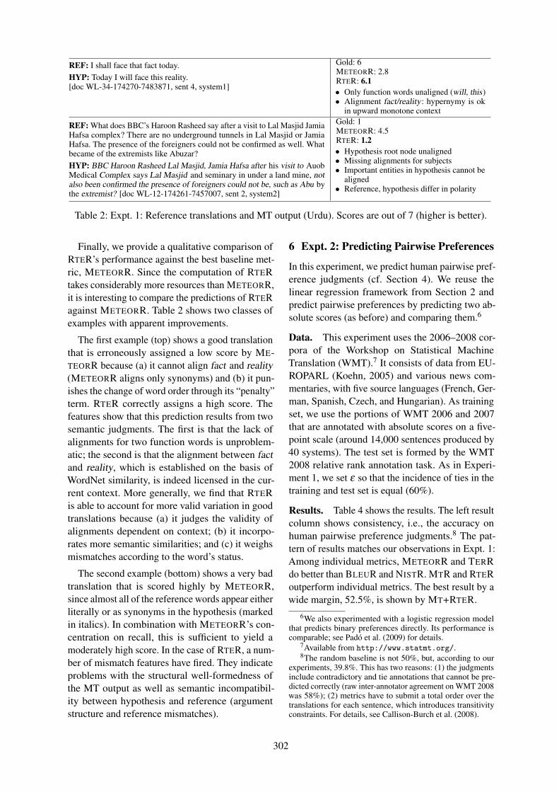
REF: I shall face that fact today.HYP: Today I will face this reality.[doc WL-34-174270-7483871, sent 4, system1]
Gold: 6METEORR: 2.8RTER: 6.1• Only function words unaligned (will, this)• Alignment fact/reality: hypernymy is ok
in upward monotone context
REF: What does BBC’s Haroon Rasheed say after a visit to Lal Masjid JamiaHafsa complex? There are no underground tunnels in Lal Masjid or JamiaHafsa. The presence of the foreigners could not be confirmed as well. Whatbecame of the extremists like Abuzar?HYP: BBC Haroon Rasheed Lal Masjid, Jamia Hafsa after his visit to AuobMedical Complex says Lal Masjid and seminary in under a land mine, notalso been confirmed the presence of foreigners could not be, such as Abu bythe extremist? [doc WL-12-174261-7457007, sent 2, system2]
Gold: 1METEORR: 4.5RTER: 1.2• Hypothesis root node unaligned• Missing alignments for subjects• Important entities in hypothesis cannot be
aligned• Reference, hypothesis differ in polarity
Table 2: Expt. 1: Reference translations and MT output (Urdu). Scores are out of 7 (higher is better).
Finally, we provide a qualitative comparison ofRTER’s performance against the best baseline met-ric, METEORR. Since the computation of RTERtakes considerably more resources than METEORR,it is interesting to compare the predictions of RTERagainst METEORR. Table 2 shows two classes ofexamples with apparent improvements.
The first example (top) shows a good translationthat is erroneously assigned a low score by ME-TEORR because (a) it cannot align fact and reality(METEORR aligns only synonyms) and (b) it pun-ishes the change of word order through its “penalty”term. RTER correctly assigns a high score. Thefeatures show that this prediction results from twosemantic judgments. The first is that the lack ofalignments for two function words is unproblem-atic; the second is that the alignment between factand reality, which is established on the basis ofWordNet similarity, is indeed licensed in the cur-rent context. More generally, we find that RTERis able to account for more valid variation in goodtranslations because (a) it judges the validity ofalignments dependent on context; (b) it incorpo-rates more semantic similarities; and (c) it weighsmismatches according to the word’s status.
The second example (bottom) shows a very badtranslation that is scored highly by METEORR,since almost all of the reference words appear eitherliterally or as synonyms in the hypothesis (markedin italics). In combination with METEORR’s con-centration on recall, this is sufficient to yield amoderately high score. In the case of RTER, a num-ber of mismatch features have fired. They indicateproblems with the structural well-formedness ofthe MT output as well as semantic incompatibil-ity between hypothesis and reference (argumentstructure and reference mismatches).
6 Expt. 2: Predicting Pairwise Preferences
In this experiment, we predict human pairwise pref-erence judgments (cf. Section 4). We reuse thelinear regression framework from Section 2 andpredict pairwise preferences by predicting two ab-solute scores (as before) and comparing them.6
Data. This experiment uses the 2006–2008 cor-pora of the Workshop on Statistical MachineTranslation (WMT).7 It consists of data from EU-ROPARL (Koehn, 2005) and various news com-mentaries, with five source languages (French, Ger-man, Spanish, Czech, and Hungarian). As trainingset, we use the portions of WMT 2006 and 2007that are annotated with absolute scores on a five-point scale (around 14,000 sentences produced by40 systems). The test set is formed by the WMT2008 relative rank annotation task. As in Experi-ment 1, we set ε so that the incidence of ties in thetraining and test set is equal (60%).
Results. Table 4 shows the results. The left resultcolumn shows consistency, i.e., the accuracy onhuman pairwise preference judgments.8 The pat-tern of results matches our observations in Expt. 1:Among individual metrics, METEORR and TERRdo better than BLEUR and NISTR. MTR and RTERoutperform individual metrics. The best result by awide margin, 52.5%, is shown by MT+RTER.
6We also experimented with a logistic regression modelthat predicts binary preferences directly. Its performance iscomparable; see Padó et al. (2009) for details.
7Available from http://www.statmt.org/.8The random baseline is not 50%, but, according to our
experiments, 39.8%. This has two reasons: (1) the judgmentsinclude contradictory and tie annotations that cannot be pre-dicted correctly (raw inter-annotator agreement on WMT 2008was 58%); (2) metrics have to submit a total order over thetranslations for each sentence, which introduces transitivityconstraints. For details, see Callison-Burch et al. (2008).
302
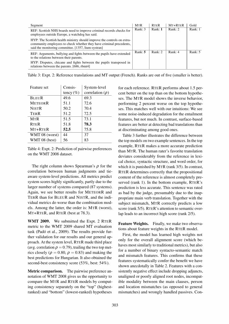
Segment MTR RTER MT+RTER Gold
REF: Scottish NHS boards need to improve criminal records checks foremployees outside Europe, a watchdog has said.
HYP: The Scottish health ministry should improve the controls on extra-community employees to check whether they have criminal precedents,said the monitoring committee. [1357, lium-systran]
Rank: 3 Rank: 1 Rank: 2 Rank: 1
REF: Arguments, bullying and fights between the pupils have extendedto the relations between their parents.HYP: Disputes, chicane and fights between the pupils transposed inrelations between the parents. [686, rbmt4]
Rank: 5 Rank: 2 Rank: 4 Rank: 5
Table 3: Expt. 2: Reference translations and MT output (French). Ranks are out of five (smaller is better).
Feature set Consis-tency (%)
System-levelcorrelation (ρ)
BLEUR 49.6 69.3METEORR 51.1 72.6NISTR 50.2 70.4TERR 51.2 72.5MTR 51.5 73.1RTER 51.8 78.3MT+RTER 52.5 75.8WMT 08 (worst) 44 37WMT 08 (best) 56 83
Table 4: Expt. 2: Prediction of pairwise preferenceson the WMT 2008 dataset.
The right column shows Spearman’s ρ for thecorrelation between human judgments and tie-aware system-level predictions. All metrics predictsystem scores highly significantly, partly due to thelarger number of systems compared (87 systems).Again, we see better results for METEORR andTERR than for BLEUR and NISTR, and the indi-vidual metrics do worse than the combination mod-els. Among the latter, the order is: MTR (worst),MT+RTER, and RTER (best at 78.3).
WMT 2009. We submitted the Expt. 2 RTERmetric to the WMT 2009 shared MT evaluationtask (Padó et al., 2009). The results provide fur-ther validation for our results and our general ap-proach. At the system level, RTER made third place(avg. correlation ρ = 0.79), trailing the two top met-rics closely (ρ = 0.80, ρ = 0.83) and making thebest predictions for Hungarian. It also obtained thesecond-best consistency score (53%, best: 54%).
Metric comparison. The pairwise preference an-notation of WMT 2008 gives us the opportunity tocompare the MTR and RTER models by comput-ing consistency separately on the “top” (highest-ranked) and “bottom” (lowest-ranked) hypotheses
for each reference. RTER performs about 1.5 per-cent better on the top than on the bottom hypothe-ses. The MTR model shows the inverse behavior,performing 2 percent worse on the top hypothe-ses. This matches well with our intuitions: We seesome noise-induced degradation for the entailmentfeatures, but not much. In contrast, surface-basedfeatures are better at detecting bad translations thanat discriminating among good ones.
Table 3 further illustrates the difference betweenthe top models on two example sentences. In the topexample, RTER makes a more accurate predictionthan MTR. The human rater’s favorite translationdeviates considerably from the reference in lexi-cal choice, syntactic structure, and word order, forwhich it is punished by MTR (rank 3/5). In contrast,RTER determines correctly that the propositionalcontent of the reference is almost completely pre-served (rank 1). In the bottom example, RTER’sprediction is less accurate. This sentence was ratedas bad by the judge, presumably due to the inap-propriate main verb translation. Together with thesubject mismatch, MTR correctly predicts a lowscore (rank 5/5). RTER’s attention to semantic over-lap leads to an incorrect high score (rank 2/5).
Feature Weights. Finally, we make two observa-tions about feature weights in the RTER model.
First, the model has learned high weights notonly for the overall alignment score (which be-haves most similarly to traditional metrics), but alsofor a number of binary syntacto-semantic matchand mismatch features. This confirms that thesefeatures systematically confer the benefit we haveshown anecdotally in Table 2. Features with a con-sistently negative effect include dropping adjuncts,unaligned or poorly aligned root nodes, incompat-ible modality between the main clauses, personand location mismatches (as opposed to generalmismatches) and wrongly handled passives. Con-
303
versely, higher scores result from factors such ashigh alignment score, matching embeddings underfactive verbs, and matches between appositions.
Second, good MT evaluation feature weights arenot good weights for RTE. Some differences, par-ticularly for structural features, are caused by thelow grammaticality of MT data. For example, thefeature that fires for mismatches between depen-dents of predicates is unreliable on the WMT data.Other differences do reflect more fundamental dif-ferences between the two tasks (cf. Section 3). Forexample, RTE puts high weights onto quantifierand polarity features, both of which have the poten-tial of influencing entailment decisions, but are (atleast currently) unimportant for MT evaluation.
7 Related Work
Researchers have exploited various resources to en-able the matching between words or n-grams thatare semantically close but not identical. Banerjeeand Lavie (2005) and Chan and Ng (2008) useWordNet, and Zhou et al. (2006) and Kauchakand Barzilay (2006) exploit large collections ofautomatically-extracted paraphrases. These ap-proaches reduce the risk that a good translationis rated poorly due to lexical deviation, but do notaddress the problem that a translation may containmany long matches while lacking coherence andgrammaticality (cf. the bottom example in Table 2).
Thus, incorporation of syntactic knowledge hasbeen the focus of another line of research. Amigóet al. (2006) use the degree of overlap between thedependency trees of reference and hypothesis as apredictor of translation quality. Similar ideas havebeen applied by Owczarzak et al. (2008) to LFGparses, and by Liu and Gildea (2005) to featuresderived from phrase-structure tress. This approachhas also been successful for the related task ofsummarization evaluation (Hovy et al., 2006).
The most comparable work to ours is Giménezand Márquez (2008). Our results agree on the cru-cial point that the use of a wide range of linguisticknowledge in MT evaluation is desirable and im-portant. However, Giménez and Márquez advocatethe use of a bottom-up development process thatbuilds on a set of “heterogeneous”, independentmetrics each of which measures overlap with re-spect to one linguistic level. In contrast, our aimis to provide a “top-down”, integrated motivationfor the features we integrate through the textualentailment recognition paradigm.
8 Conclusion and Outlook
In this paper, we have explored a strategy for theevaluation of MT output that aims at comprehen-sively assessing the meaning equivalence betweenreference and hypothesis. To do so, we exploit thecommon ground between MT evaluation and theRecognition of Textual Entailment (RTE), both ofwhich have to distinguish valid from invalid lin-guistic variation. Conceputalizing MT evaluationas an entailment problem motivates the use of arich feature set that covers, unlike almost all earliermetrics, a wide range of linguistic levels, includinglexical, syntactic, and compositional phenomena.
We have used an off-the-shelf RTE system tocompute these features, and demonstrated that aregression model over these features can outper-form an ensemble of traditional MT metrics in twoexperiments on different datasets. Even though thefeatures build on deep linguistic analysis, they arerobust enough to be used in a real-world setting, atleast on written text. A limited amount of trainingdata is sufficient, and the weights generalize well.
Our data analysis has confirmed that each of thefeature groups contributes to the overall success ofthe RTE metric, and that its gains come from itsbetter success at abstracting away from valid vari-ation (such as word order or lexical substitution),while still detecting major semantic divergences.We have also clarified the relationship between MTevaluation and textual entailment: The majority ofphenomena (but not all) that are relevant for RTEare also informative for MT evaluation.
The focus of this study was on the use of an ex-isting RTE infrastructure for MT evaluation. Futurework will have to assess the effectiveness of individ-ual features and investigate ways to customize RTEsystems for the MT evaluation task. An interestingaspect that we could not follow up on in this paperis that entailment features are linguistically inter-pretable (cf. Fig. 2) and may find use in uncoveringsystematic shortcomings of MT systems.
A limitation of our current metric is that it islanguage-dependent and relies on NLP tools inthe target language that are still unavailable formany languages, such as reliable parsers. To someextent, of course, this problem holds as well forstate-of-the-art MT systems. Nevertheless, it mustbe an important focus of future research to developrobust meaning-based metrics for other languagesthat can cash in the promise that we have shownfor evaluating translation into English.
304

ReferencesEnrique Amigó, Jesús Giménez, Julio Gonzalo, and
Lluı́s Màrquez. 2006. MT Evaluation: Human-like vs. human acceptable. In Proceedings of COL-ING/ACL 2006, pages 17–24, Sydney, Australia.
Satanjeev Banerjee and Alon Lavie. 2005. METEOR:An automatic metric for MT evaluation with im-proved correlation with human judgments. In Pro-ceedings of the ACL Workshop on Intrinsic and Ex-trinsic Evaluation Measures, pages 65–72, Ann Ar-bor, MI.
Chris Callison-Burch, Miles Osborne, and PhilippKoehn. 2006. Re-evaluating the role of BLEUin machine translation research. In Proceedings ofEACL, pages 249–256, Trento, Italy.
Chris Callison-Burch, Cameron Fordyce, PhilippKoehn, Christof Monz, and Josh Schroeder. 2008.Further meta-evaluation of machine translation. InProceedings of the ACL Workshop on Statistical Ma-chine Translation, pages 70–106, Columbus, OH.
Yee Seng Chan and Hwee Tou Ng. 2008. MAXSIM: Amaximum similarity metric for machine translationevaluation. In Proceedings of ACL-08: HLT, pages55–62, Columbus, Ohio, June.
Ido Dagan, Oren Glickman, and Bernardo Magnini.2005. The PASCAL recognising textual entailmentchallenge. In Proceedings of the PASCAL Chal-lenges Workshop on Recognising Textual Entailment,Southampton, UK.
Marie-Catherine de Marneffe, Trond Grenager, BillMacCartney, Daniel Cer, Daniel Ramage, ChloéKiddon, and Christopher D. Manning. 2007. Align-ing semantic graphs for textual inference and ma-chine reading. In Proceedings of the AAAI SpringSymposium, Stanford, CA.
George Doddington. 2002. Automatic evaluation ofmachine translation quality using n-gram cooccur-rence statistics. In Proceedings of HLT, pages 128–132, San Diego, CA.
Jesús Giménez and Lluı́s Márquez. 2008. Het-erogeneous automatic MT evaluation through non-parametric metric combinations. In Proceedings ofIJCNLP, pages 319–326, Hyderabad, India.
Sanda Harabagiu and Andrew Hickl. 2006. Methodsfor using textual entailment in open-domain ques-tion answering. In Proceedings of ACL, pages 905–912, Sydney, Australia.
Eduard Hovy, Chin-Yew Lin, Liang Zhou, and JunichiFukumoto. 2006. Automated summarization evalu-ation with basic elements. In Proceedings of LREC,Genoa, Italy.
David Kauchak and Regina Barzilay. 2006. Paraphras-ing for automatic evaluation. In Proceedings of HLT-NAACL, pages 455–462.
Phillip Koehn. 2005. Europarl: A parallel corpus forstatistical machine translation. In Proceedings of theMT Summit X, Phuket, Thailand.
Chin-Yew Lin and Franz Josef Och. 2004. ORANGE:a method for evaluating automatic evaluation met-rics for machine translation. In Proceedings of COL-ING, pages 501–507, Geneva, Switzerland.
Ding Liu and Daniel Gildea. 2005. Syntactic featuresfor evaluation of machine translation. In Proceed-ings of the ACL Workshop on Intrinsic and ExtrinsicEvaluation Measures, pages 25–32, Ann Arbor, MI.
Bill MacCartney and Christopher D. Manning. 2008.Modeling semantic containment and exclusion innatural language inference. In Proceedings of COL-ING, pages 521–528, Manchester, UK.
Bill MacCartney, Trond Grenager, Marie-Catherinede Marneffe, Daniel Cer, and Christopher D. Man-ning. 2006. Learning to recognize features ofvalid textual entailments. In Proceedings of NAACL,pages 41–48, New York City, NY.
Franz Josef Och. 2003. Minimum error rate trainingin statistical machine translation. In Proceedings ofACL, pages 160–167, Sapporo, Japan.
Karolina Owczarzak, Josef van Genabith, and AndyWay. 2008. Evaluating machine translation withLFG dependencies. Machine Translation, 21(2):95–119.
Sebastian Padó, Michel Galley, Dan Jurafsky, andChristopher D. Manning. 2009. Textual entailmentfeatures for machine translation evaluation. In Pro-ceedings of the EACL Workshop on Statistical Ma-chine Translation, pages 37–41, Athens, Greece.
Kishore Papineni, Salim Roukos, Todd Ward, and Wei-Jing Zhu. 2002. BLEU: a method for automaticevaluation of machine translation. In Proceedingsof ACL, pages 311–318, Philadelphia, PA.
Michael Paul, Andrew Finch, and Eiichiro Sumita.2007. Reducing human assessment of machinetranslation quality to binary classifiers. In Proceed-ings of TMI, pages 154–162, Skövde, Sweden.
Matthew Snover, Bonnie Dorr, Richard Schwartz, Lin-nea Micciulla, and John Makhoul. 2006. A studyof translation edit rate with targeted human annota-tion. In Proceedings of AMTA, pages 223–231, Cam-bridge, MA.
Matthew Snover, Nitin Madnani, Bonnie J. Dorr, andRichard Schwartz. 2009. Fluency, adequacy, orHTER? Exploring different human judgments witha tunable MT metric. In Proceedings of the EACLWorkshop on Statistical Machine Translation, pages259–268, Athens, Greece.
Liang Zhou, Chin-Yew Lin, and Eduard Hovy. 2006.Re-evaluating machine translation results with para-phrase support. In Proceedings of EMNLP, pages77–84, Sydney, Australia.
305
Proceedings of the 47th Annual Meeting of the ACL and the 4th IJCNLP of the AFNLP, pages 306–314,Suntec, Singapore, 2-7 August 2009. c©2009 ACL and AFNLP
The Contribution of Linguistic Features to Automatic MachineTranslation Evaluation
Enrique Amigó1 Jesús Giménez2 Julio Gonzalo 1 Felisa Verdejo1
1UNED, Madrid{enrique,julio,felisa}@lsi.uned.es
2UPC, [email protected]
Abstract
A number of approaches to AutomaticMT Evaluation based on deep linguisticknowledge have been suggested. How-ever, n-gram based metrics are still to-day the dominant approach. The mainreason is that the advantages of employ-ing deeper linguistic information have notbeen clarified yet. In this work, we pro-pose a novel approach for meta-evaluationof MT evaluation metrics, since correla-tion cofficient against human judges donot reveal details about the advantages anddisadvantages of particular metrics. Wethen use this approach to investigate thebenefits of introducing linguistic featuresinto evaluation metrics. Overall, our ex-periments show that (i) both lexical andlinguistic metrics present complementaryadvantages and (ii) combining both kindsof metrics yields the most robust meta-evaluation performance.
1 Introduction
Automatic evaluation methods based on similarityto human references have substantially acceleratedthe development cycle of many NLP tasks, suchas Machine Translation, Automatic Summariza-tion, Sentence Compression and Language Gen-eration. These automatic evaluation metrics allowdevelopers to optimize their systems without theneed for expensive human assessments for eachof their possible system configurations. However,estimating the system output quality according toits similarity to human references is not a trivialtask. The main problem is that many NLP tasksare open/subjective; therefore, different humansmay generate different outputs, all of them equallyvalid. Thus, language variability is an issue.
In order to tackle language variability in the
context of Machine Translation, a considerable ef-fort has also been made to include deeper linguis-tic information in automatic evaluation metrics,both syntactic and semantic (see Section 2 for de-tails). However, the most commonly used metricsare still based on n-gram matching. The reason isthat the advantages of employing higher linguisticprocessing levels have not been clarified yet.
The main goal of our work is to analyze to whatextent deep linguistic features can contribute to theautomatic evaluation of translation quality. Forthat purpose, we compare – using four differenttest beds – the performance of 16 n-gram basedmetrics, 48 linguistic metrics and one combinedmetric from the state of the art.
Analyzing the reliability of evaluation met-rics requires meta-evaluation criteria. In this re-spect, we identify important drawbacks of thestandard meta-evaluation methods based on cor-relation with human judgements. In order toovercome these drawbacks, we then introduce sixnovel meta-evaluation criteria which represent dif-ferent metric reliability dimensions. Our analysisindicates that: (i) both lexical and linguistic met-rics have complementary advantages and differentdrawbacks; (ii) combining both kinds of metricsis a more effective and robust evaluation methodacross all meta-evaluation criteria.
In addition, we also perform a qualitative analy-sis of one hundred sentences that were incorrectlyevaluated by state-of-the-art metrics. The analysisconfirms that deep linguistic techniques are neces-sary to avoid the most common types of error.
Section 2 examines the state of the art Section 3describes the test beds and metrics considered inour experiments. In Section 4 the correlation be-tween human assessors and metrics is computed,with a discussion of its drawbacks. In Section 5different quality aspects of metrics are analysed.Conclusions are drawn in the last section.
306

2 Previous Work on MachineTranslation Meta-Evaluation
Insofar as automatic evaluation metrics for ma-chine translation have been proposed, differentmeta-evaluation frameworks have been graduallyintroduced. For instance, Papineni et al. (2001)introduced the BLEU metric and evaluated its re-liability in terms of Pearson correlation with hu-man assessments for adequacy and fluency judge-ments. With the aim of overcoming some of thedeficiencies of BLEU, Doddington (2002) intro-duced the NIST metric. Metric reliability wasalso estimated in terms of correlation with humanassessments, but over different document sourcesand for a varying number of references and seg-ment sizes. Melamed et al. (2003) argued, at thetime of introducing the GTM metric, that Pearsoncorrelation coefficients can be affected by scaleproperties, and suggested, in order to avoid thiseffect, to use the non-parametric Spearman corre-lation coefficients instead.
Lin and Och (2004) experimented, unlike pre-vious works, with a wide set of metrics, includingNIST, WER (Nießen et al., 2000), PER (Tillmannet al., 1997), and variants of ROUGE, BLEU andGTM. They computed both Pearson and Spearmancorrelation, obtaining similar results in both cases.In a different work, Banerjee and Lavie (2005) ar-gued that the measured reliability of metrics canbe due to averaging effects but might not be robustacross translations. In order to address this issue,they computed the translation-by-translation cor-relation with human judgements (i.e., correlationat the segment level).
All that metrics were based on n-gram over-lap. But there is also extensive research fo-cused on including linguistic knowledge in met-rics (Owczarzak et al., 2006; Reeder et al., 2001;Liu and Gildea, 2005; Amigó et al., 2006; Mehayand Brew, 2007; Giménez and Màrquez, 2007;Owczarzak et al., 2007; Popovic and Ney, 2007;Giménez and Màrquez, 2008b) among others. Inall these cases, metrics were also evaluated bymeans of correlation with human judgements.
In a different research line, several authorshave suggested approaching automatic evalua-tion through the combination of individual metricscores. Among the most relevant let us cite re-search by Kulesza and Shieber (2004), Albrechtand Hwa (2007). But finding optimal metriccombinations requires a meta-evaluation criterion.
Most approaches again rely on correlation withhuman judgements. However, some of them mea-sured the reliability of metric combinations interms of their ability to discriminate between hu-man translations and automatic ones (human like-ness) (Amigó et al., 2005). .
In this work, we present a novel approach tometa-evaluation which is distinguished by the useof additional easily interpretable meta-evaluationcriteria oriented to measure different aspects ofmetric reliability. We then apply this approach tofind out about the advantages and challenges of in-cluding linguistic features in meta-evaluation cri-teria.
3 Metrics and Test Beds
3.1 Metric Set
For our study, we have compiled a rich set of met-ric variants at three linguistic levels: lexical, syn-tactic, and semantic. In all cases, translation qual-ity is measured by comparing automatic transla-tions against a set of human references.
At the lexical level, we have included severalstandard metrics, based on different similarity as-sumptions: edit distance (WER, PER and TER),lexical precision (BLEU and NIST), lexical recall(ROUGE), and F-measure (GTM and METEOR). Atthe syntactic level, we have used several familiesof metrics based on dependency parsing (DP) andconstituency trees (CP). At the semantic level, wehave included three different families which op-erate using named entities (NE), semantic roles(SR), and discourse representations (DR). A de-tailed description of these metrics can be found in(Giménez and Màrquez, 2007).
Finally, we have also considered ULC, whichis a very simple approach to metric combina-tion based on the unnormalized arithmetic meanof metric scores, as described by Giménez andMàrquez (2008a). ULC considers a subset of met-rics which operate at several linguistic levels. Thisapproach has proven very effective in recent eval-uation campaigns. Metric computation has beencarried out using the IQMT Framework for Auto-matic MT Evaluation (Giménez, 2007)1. The sim-plicity of this approach (with no training of themetric weighting scheme) ensures that the poten-tial advantages detected in our experiments are notdue to overfitting effects.
1http://www.lsi.upc.edu/˜nlp/IQMT
307

2004 2005AE CE AE CE
#references 5 5 5 4#systemsassessed 5 10 5+1 5#casesassessed 347 447 266 272
Table 1: NIST 2004/2005 MT Evaluation Cam-paigns. Test bed description
3.2 Test Beds
We use the test beds from the 2004 and 2005NIST MT Evaluation Campaigns (Le and Przy-bocki, 2005)2. Both campaigns include two dif-ferent translations exercises: Arabic-to-English(‘AE’) and Chinese-to-English (‘CE’). Human as-sessments of adequacy and fluency, on a 1-5 scale,are available for a subset of sentences, each eval-uated by two different human judges. A brief nu-merical description of these test beds is availablein Table 1. The corpus AE05 includes, apart fromfive automatic systems, one human-aided systemthat is only used in our last experiment.
4 Correlation with Human Judgements
4.1 Correlation at the Segment vs. SystemLevels
Let us first analyze the correlation with humanjudgements for linguistic vs. n-gram based met-rics. Figure 1 shows the correlation obtained byeach automatic evaluation metric at system level(horizontal axis) versus segment level (verticalaxis) in our test beds. Linguistic metrics are rep-resented by grey plots, and black plots representmetrics based on n-gram overlap.
The most remarkable aspect is that there existsa certain trade-off between correlation at segmentversus system level. In fact, this graph producesa negative Pearson correlation coefficient betweensystem and segment levels of 0.44. In other words,depending on how the correlation is computed,the relative predictive power of metrics can swap.Therefore, we need additional meta-evaluation cri-teria in order to clarify the behavior of linguisticmetrics as compared to n-gram based metrics.
However, there are some exceptions. Somemetrics achieve high correlation at both levels.The first one is ULC (the circle in the plot), whichcombines both kind of metrics in a heuristic way(see Section 3.1). The metric nearest to ULC is
2http://www.nist.gov/speech/tests/mt
Figure 1: Averaged Pearson correlation at systemvs. segment level over all test beds.
DP-Or-?, which computes lexical overlapping buton dependency relationships. These results are afirst evidence of the advantages of combining met-rics at several linguistic processing levels.
4.2 Drawbacks of Correlation-basedMeta-evaluation
Although correlation with human judgements isconsidered the standard meta-evaluation criterion,it presents serious drawbacks. With respect tocorrelation at system level, the main problem isthat the relative performance of different metricschanges almost randomly between testbeds. Oneof the reasons is that the number of assessed sys-tems per testbed is usually low, and then correla-tion has a small number of samples to be estimatedwith. Usually, the correlation at system level iscomputed over no more than a few systems.
For instance, Table 2 shows the best 10 met-rics in CE05 according to their correlation withhuman judges at the system level, and then theranking they obtain in the AE05 testbed. Thereare substantial swaps between both rankings. In-deed, the Pearson correlation of both ranks is only0.26. This result supports the intuition in (Baner-jee and Lavie, 2005) that correlation at segmentlevel is necessary to ensure the reliability of met-rics in different situations.
However, the correlation values of metrics atsegment level have also drawbacks related to theirinterpretability. Most metrics achieve a Pearsoncoefficient lower than 0.5. Figure 2 shows twopossible relationships between human and metric
308
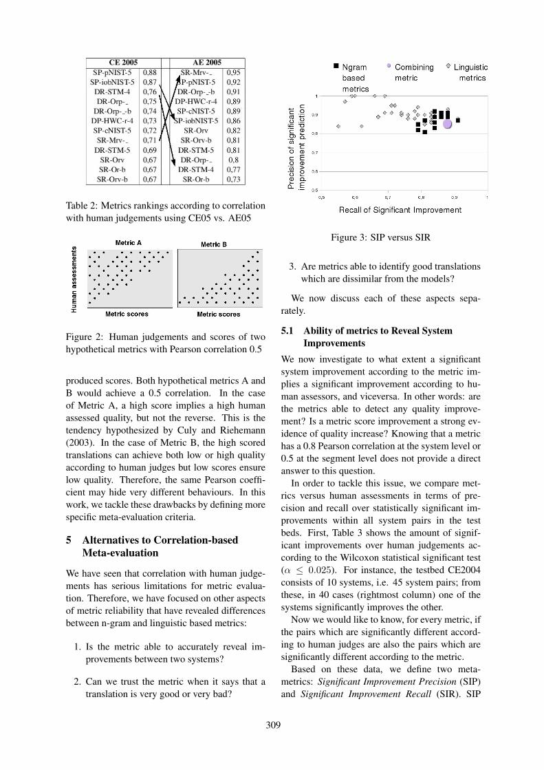
Table 2: Metrics rankings according to correlationwith human judgements using CE05 vs. AE05
Figure 2: Human judgements and scores of twohypothetical metrics with Pearson correlation 0.5
produced scores. Both hypothetical metrics A andB would achieve a 0.5 correlation. In the caseof Metric A, a high score implies a high humanassessed quality, but not the reverse. This is thetendency hypothesized by Culy and Riehemann(2003). In the case of Metric B, the high scoredtranslations can achieve both low or high qualityaccording to human judges but low scores ensurelow quality. Therefore, the same Pearson coeffi-cient may hide very different behaviours. In thiswork, we tackle these drawbacks by defining morespecific meta-evaluation criteria.
5 Alternatives to Correlation-basedMeta-evaluation
We have seen that correlation with human judge-ments has serious limitations for metric evalua-tion. Therefore, we have focused on other aspectsof metric reliability that have revealed differencesbetween n-gram and linguistic based metrics:
1. Is the metric able to accurately reveal im-provements between two systems?
2. Can we trust the metric when it says that atranslation is very good or very bad?
Figure 3: SIP versus SIR
3. Are metrics able to identify good translationswhich are dissimilar from the models?
We now discuss each of these aspects sepa-rately.
5.1 Ability of metrics to Reveal SystemImprovements
We now investigate to what extent a significantsystem improvement according to the metric im-plies a significant improvement according to hu-man assessors, and viceversa. In other words: arethe metrics able to detect any quality improve-ment? Is a metric score improvement a strong ev-idence of quality increase? Knowing that a metrichas a 0.8 Pearson correlation at the system level or0.5 at the segment level does not provide a directanswer to this question.
In order to tackle this issue, we compare met-rics versus human assessments in terms of pre-cision and recall over statistically significant im-provements within all system pairs in the testbeds. First, Table 3 shows the amount of signif-icant improvements over human judgements ac-cording to the Wilcoxon statistical significant test(α ≤ 0.025). For instance, the testbed CE2004consists of 10 systems, i.e. 45 system pairs; fromthese, in 40 cases (rightmost column) one of thesystems significantly improves the other.
Now we would like to know, for every metric, ifthe pairs which are significantly different accord-ing to human judges are also the pairs which aresignificantly different according to the metric.
Based on these data, we define two meta-metrics: Significant Improvement Precision (SIP)and Significant Improvement Recall (SIR). SIP
309
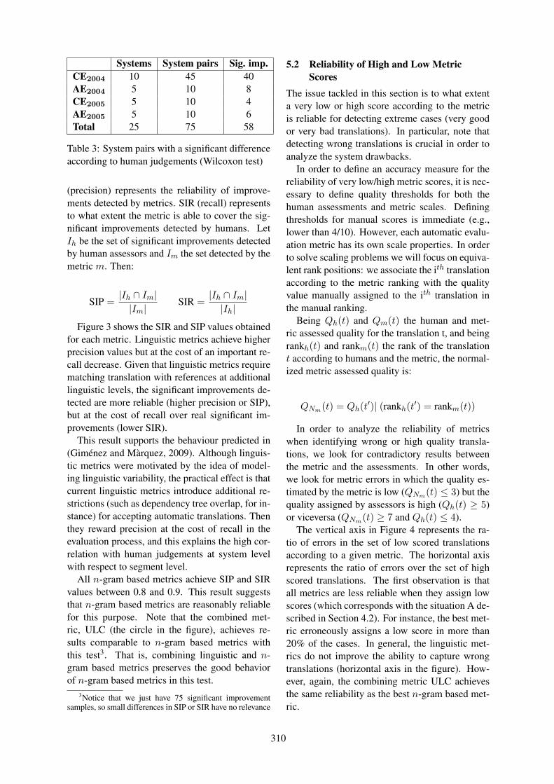
Systems System pairs Sig. imp.CE2004 10 45 40AE2004 5 10 8CE2005 5 10 4AE2005 5 10 6Total 25 75 58
Table 3: System pairs with a significant differenceaccording to human judgements (Wilcoxon test)
(precision) represents the reliability of improve-ments detected by metrics. SIR (recall) representsto what extent the metric is able to cover the sig-nificant improvements detected by humans. LetIh be the set of significant improvements detectedby human assessors and Im the set detected by themetric m. Then:
SIP =|Ih ∩ Im||Im|
SIR =|Ih ∩ Im||Ih|
Figure 3 shows the SIR and SIP values obtainedfor each metric. Linguistic metrics achieve higherprecision values but at the cost of an important re-call decrease. Given that linguistic metrics requirematching translation with references at additionallinguistic levels, the significant improvements de-tected are more reliable (higher precision or SIP),but at the cost of recall over real significant im-provements (lower SIR).
This result supports the behaviour predicted in(Giménez and Màrquez, 2009). Although linguis-tic metrics were motivated by the idea of model-ing linguistic variability, the practical effect is thatcurrent linguistic metrics introduce additional re-strictions (such as dependency tree overlap, for in-stance) for accepting automatic translations. Thenthey reward precision at the cost of recall in theevaluation process, and this explains the high cor-relation with human judgements at system levelwith respect to segment level.
All n-gram based metrics achieve SIP and SIRvalues between 0.8 and 0.9. This result suggeststhat n-gram based metrics are reasonably reliablefor this purpose. Note that the combined met-ric, ULC (the circle in the figure), achieves re-sults comparable to n-gram based metrics withthis test3. That is, combining linguistic and n-gram based metrics preserves the good behaviorof n-gram based metrics in this test.
3Notice that we just have 75 significant improvementsamples, so small differences in SIP or SIR have no relevance
5.2 Reliability of High and Low MetricScores
The issue tackled in this section is to what extenta very low or high score according to the metricis reliable for detecting extreme cases (very goodor very bad translations). In particular, note thatdetecting wrong translations is crucial in order toanalyze the system drawbacks.
In order to define an accuracy measure for thereliability of very low/high metric scores, it is nec-essary to define quality thresholds for both thehuman assessments and metric scales. Definingthresholds for manual scores is immediate (e.g.,lower than 4/10). However, each automatic evalu-ation metric has its own scale properties. In orderto solve scaling problems we will focus on equiva-lent rank positions: we associate the ith translationaccording to the metric ranking with the qualityvalue manually assigned to the ith translation inthe manual ranking.
Being Qh(t) and Qm(t) the human and met-ric assessed quality for the translation t, and beingrankh(t) and rankm(t) the rank of the translationt according to humans and the metric, the normal-ized metric assessed quality is:
QNm(t) = Qh(t′)| (rankh(t′) = rankm(t))
In order to analyze the reliability of metricswhen identifying wrong or high quality transla-tions, we look for contradictory results betweenthe metric and the assessments. In other words,we look for metric errors in which the quality es-timated by the metric is low (QNm(t) ≤ 3) but thequality assigned by assessors is high (Qh(t) ≥ 5)or viceversa (QNm(t) ≥ 7 and Qh(t) ≤ 4).
The vertical axis in Figure 4 represents the ra-tio of errors in the set of low scored translationsaccording to a given metric. The horizontal axisrepresents the ratio of errors over the set of highscored translations. The first observation is thatall metrics are less reliable when they assign lowscores (which corresponds with the situation A de-scribed in Section 4.2). For instance, the best met-ric erroneously assigns a low score in more than20% of the cases. In general, the linguistic met-rics do not improve the ability to capture wrongtranslations (horizontal axis in the figure). How-ever, again, the combining metric ULC achievesthe same reliability as the best n-gram based met-ric.
310

In order to check the robustness of these results,we computed the correlation of individual metricfailures between test beds, obtaining 0.67 Pearsonfor the lowest correlated test bed pair (AE2004 andCE2005) and 0.88 for the highest correlated pair(AE2004 and CE2004).
Figure 4: Counter sample ratio for high vs lowmetric scored translations
5.2.1 Analysis of Evaluation SamplesIn order to shed some light on the reasons for theautomatic evaluation failures when assigning lowscores, we have manually analyzed cases in whicha metric score is low but the quality according tohumans is high (QNm ≤ 3 and Qh ≥ 7). Wehave studied 100 sentence evaluation cases fromrepresentatives of each metric family including: 1-PER, BLEU, DP-Or-?, GTM (e = 2), METEORand ROUGEL. The evaluation cases have been ex-tracted from the four test beds. We have identifiedfour main (non exclusive) failure causes:Format issues, e.g. “US ” vs “United States”).Elements such as abbreviations, acronyms or num-bers which do not match the manual translation.Pseudo-synonym terms, e.g. “US Scheduled theRelease” vs. “US set to Release”). ) In most ofthese cases, synonymy can only be identified fromthe discourse context. Therefore, terminologicalresources (e.g., WordNet) are not enough to tacklethis problem.Non relevant information omissions, e.g.“Thank you” vs. “Thank you very much” or“dollar” vs. “US dollar”)). The translationsystem obviates some information which, incontext, is not considered crucial by the humanassessors. This effect is specially important in
short sentences.Incorrect structures that change the meaningwhile maintaining the same idea (e.g., “BushPraises NASA ’s Mars Mission” vs “ Bush praisesnasa of Mars mission” ).
Note that all of these kinds of failure - exceptformatting issues - require deep linguistic process-ing while n-gram overlap or even synonyms ex-tracted from a standard ontology are not enough todeal with them. This conclusion motivates the in-corporation of linguistic processing into automaticevaluation metrics.
5.3 Ability to Deal with Translations that areDissimilar to References.
The results presented in Section 5.2 indicate that ahigh score in metrics tends to be highly related totruly good translations. This is due to the fact thata high word overlapping with human references isa reliable evidence of quality. However, in somecases the translations to be evaluated are not sosimilar to human references.
An example of this appears in the test bedNIST05AE which includes a human-aided sys-tem, LinearB (Callison-Burch, 2005). This systemproduces correct translations whose words do notnecessarily overlap with references. On the otherhand, a statistics based system tends to produceincorrect translations with a high level of lexicaloverlapping with the set of human references. Thiscase was reported by Callison-Burch et al. (2006)and later studied by Giménez and Màrquez (2007).They found out that lexical metrics fail to pro-duce reliable evaluation scores. They favor sys-tems which share the expected reference sublan-guage (e.g., statistical) and penalize those whichdo not (e.g., LinearB).
We can find in our test bed many instances inwhich the statistical systems obtain a metric scoresimilar to the assisted system while achieving alower mark according to human assessors. For in-stance, for the following translations, ROUGEL
assigns a slightly higher score to the output of astatistical system which contains a lot of grammat-ical and syntactical failures.
Human assisted system: The Chinese President made un-precedented criticism of the leaders of Hong Kong afterpolitical failings in the former British colony on Mon-day . Human assessment=8.5.
Statistical system: Chinese President Hu Jintao today un-precedented criticism to the leaders of Hong Kongwake political and financial failure in the formerBritish colony. Human assessment=3.
311
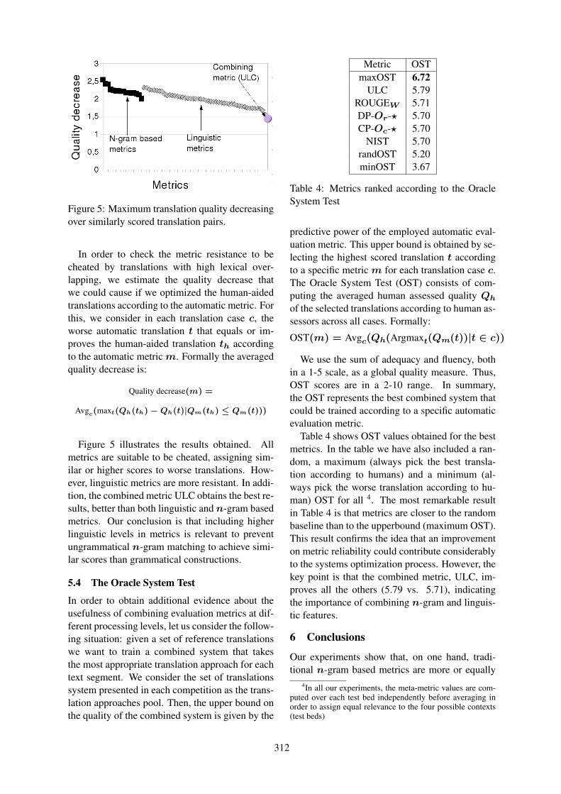
Figure 5: Maximum translation quality decreasingover similarly scored translation pairs.
In order to check the metric resistance to becheated by translations with high lexical over-lapping, we estimate the quality decrease thatwe could cause if we optimized the human-aidedtranslations according to the automatic metric. Forthis, we consider in each translation case c, theworse automatic translation t that equals or im-proves the human-aided translation th accordingto the automatic metric m. Formally the averagedquality decrease is:
Quality decrease(m) =
Avgc(maxt(Qh(th)−Qh(t)|Qm(th) ≤ Qm(t)))
Figure 5 illustrates the results obtained. Allmetrics are suitable to be cheated, assigning sim-ilar or higher scores to worse translations. How-ever, linguistic metrics are more resistant. In addi-tion, the combined metric ULC obtains the best re-sults, better than both linguistic and n-gram basedmetrics. Our conclusion is that including higherlinguistic levels in metrics is relevant to preventungrammatical n-gram matching to achieve simi-lar scores than grammatical constructions.
5.4 The Oracle System Test
In order to obtain additional evidence about theusefulness of combining evaluation metrics at dif-ferent processing levels, let us consider the follow-ing situation: given a set of reference translationswe want to train a combined system that takesthe most appropriate translation approach for eachtext segment. We consider the set of translationssystem presented in each competition as the trans-lation approaches pool. Then, the upper bound onthe quality of the combined system is given by the
Metric OSTmaxOST 6.72
ULC 5.79ROUGEW 5.71DP-Or-? 5.70CP-Oc-? 5.70
NIST 5.70randOST 5.20minOST 3.67
Table 4: Metrics ranked according to the OracleSystem Test
predictive power of the employed automatic eval-uation metric. This upper bound is obtained by se-lecting the highest scored translation t accordingto a specific metric m for each translation case c.The Oracle System Test (OST) consists of com-puting the averaged human assessed quality Qh
of the selected translations according to human as-sessors across all cases. Formally:
OST(m) = Avgc(Qh(Argmaxt(Qm(t))|t ∈ c))
We use the sum of adequacy and fluency, bothin a 1-5 scale, as a global quality measure. Thus,OST scores are in a 2-10 range. In summary,the OST represents the best combined system thatcould be trained according to a specific automaticevaluation metric.
Table 4 shows OST values obtained for the bestmetrics. In the table we have also included a ran-dom, a maximum (always pick the best transla-tion according to humans) and a minimum (al-ways pick the worse translation according to hu-man) OST for all 4. The most remarkable resultin Table 4 is that metrics are closer to the randombaseline than to the upperbound (maximum OST).This result confirms the idea that an improvementon metric reliability could contribute considerablyto the systems optimization process. However, thekey point is that the combined metric, ULC, im-proves all the others (5.79 vs. 5.71), indicatingthe importance of combining n-gram and linguis-tic features.
6 Conclusions
Our experiments show that, on one hand, tradi-tional n-gram based metrics are more or equally
4In all our experiments, the meta-metric values are com-puted over each test bed independently before averaging inorder to assign equal relevance to the four possible contexts(test beds)
312

reliable for estimating the translation quality at thesegment level, for predicting significant improve-ment between systems and for detecting poor andexcellent translations.
On the other hand, linguistically motivated met-rics improve n-gram metrics in two ways: (i) theyachieve higher correlation with human judgementsat system level and (ii) they are more resistant toreward poor translations with high word overlap-ping with references.
The underlying phenomenon is that, ratherthan managing the linguistics variability, linguis-tic based metrics introduce additional restrictionsfor assigning high scores. This effect decreasesthe recall over significant system improvementsachieved by n-gram based metrics and does notsolve the problem of detecting wrong translations.Linguistic metrics, however, are more difficult tocheat.
In general, the greatest pitfall of metrics is thelow reliability of low metric values. Our qualita-tive analysis of evaluated sentences has shown thatdeeper linguistic techniques are necessary to over-come the important surface differences betweenacceptable automatic translations and human ref-erences.
But our key finding is that combining both kindsof metrics gives top performance according to ev-ery meta-evaluation criteria. In addition, our Com-bined System Test shows that, when training acombined translation system, using metrics at sev-eral linguistic processing levels improves substan-tially the use of individual metrics.
In summary, our results motivate: (i) work-ing on new linguistic metrics for overcoming thebarrier of linguistic variability and (ii) perform-ing new metric combining schemes based on lin-ear regression over human judgements (Kuleszaand Shieber, 2004), training models over hu-man/machine discrimination (Albrecht and Hwa,2007) or non parametric methods based on refer-ence to reference distances (Amigó et al., 2005).
Acknowledgments
This work has been partially supported by theSpanish Government, project INES/Text-Mess.We are indebted to the three ACL anonymous re-viewers which provided detailed suggestions toimprove our work.
ReferencesJoshua Albrecht and Rebecca Hwa. 2007. Regression
for Sentence-Level MT Evaluation with Pseudo Ref-erences. In Proceedings of the 45th Annual Meet-ing of the Association for Computational Linguistics(ACL), pages 296–303.
Enrique Amigó, Julio Gonzalo, Anselmo Pe nas, andFelisa Verdejo. 2005. QARLA: a Framework forthe Evaluation of Automatic Summarization. InProceedings of the 43rd Annual Meeting of the Asso-ciation for Computational Linguistics (ACL), pages280–289.
Enrique Amigó, Jesús Giménez, Julio Gonzalo, andLluı́s Màrquez. 2006. MT Evaluation: Human-Like vs. Human Acceptable. In Proceedings ofthe Joint 21st International Conference on Com-putational Linguistics and the 44th Annual Meet-ing of the Association for Computational Linguistics(COLING-ACL), pages 17–24.
Satanjeev Banerjee and Alon Lavie. 2005. METEOR:An Automatic Metric for MT Evaluation with Im-proved Correlation with Human Judgments. In Pro-ceedings of ACL Workshop on Intrinsic and Extrin-sic Evaluation Measures for MT and/or Summariza-tion.
Chris Callison-Burch, Miles Osborne, and PhilippKoehn. 2006. Re-evaluating the Role of BLEU inMachine Translation Research. In Proceedings of11th Conference of the European Chapter of the As-sociation for Computational Linguistics (EACL).
Chris Callison-Burch. 2005. Linear B system descrip-tion for the 2005 NIST MT evaluation exercise. InProceedings of the NIST 2005 Machine TranslationEvaluation Workshop.
Christopher Culy and Susanne Z. Riehemann. 2003.The Limits of N-gram Translation Evaluation Met-rics. In Proceedings of MT-SUMMIT IX, pages 1–8.
George Doddington. 2002. Automatic Evaluationof Machine Translation Quality Using N-gram Co-Occurrence Statistics. In Proceedings of the 2nd In-ternational Conference on Human Language Tech-nology, pages 138–145.
Jesús Giménez and Lluı́s Màrquez. 2007. Linguis-tic Features for Automatic Evaluation of Heteroge-neous MT Systems. In Proceedings of the ACLWorkshop on Statistical Machine Translation, pages256–264.
Jesús Giménez and Lluı́s Màrquez. 2008a. Hetero-geneous Automatic MT Evaluation Through Non-Parametric Metric Combinations. In Proceedings ofthe Third International Joint Conference on NaturalLanguage Processing (IJCNLP), pages 319–326.
Jesús Giménez and Lluı́s Màrquez. 2008b. On the Ro-bustness of Linguistic Features for Automatic MTEvaluation. (Under submission).
313
Jesús Giménez and Lluı́s Màrquez. 2009. On the Ro-bustness of Syntactic and Semantic Features for Au-tomatic MT Evaluation. In Proceedings of the 4thWorkshop on Statistical Machine Translation (EACL2009).
Jesús Giménez. 2007. IQMT v 2.0. Technical Manual(LSI-07-29-R). Technical report, TALP ResearchCenter. LSI Department. http://www.lsi.upc.edu/˜nlp/IQMT/IQMT.v2.1.pdf.
Alex Kulesza and Stuart M. Shieber. 2004. A learn-ing approach to improving sentence-level MT evalu-ation. In Proceedings of the 10th International Con-ference on Theoretical and Methodological Issues inMachine Translation (TMI), pages 75–84.
Audrey Le and Mark Przybocki. 2005. NIST 2005 ma-chine translation evaluation official results. In Offi-cial release of automatic evaluation scores for allsubmissions, August.
Chin-Yew Lin and Franz Josef Och. 2004. AutomaticEvaluation of Machine Translation Quality UsingLongest Common Subsequence and Skip-BigramStatics. In Proceedings of the 42nd Annual Meet-ing of the Association for Computational Linguistics(ACL).
Ding Liu and Daniel Gildea. 2005. Syntactic Featuresfor Evaluation of Machine Translation. In Proceed-ings of ACL Workshop on Intrinsic and ExtrinsicEvaluation Measures for MT and/or Summarization,pages 25–32.
Dennis Mehay and Chris Brew. 2007. BLEUATRE:Flattening Syntactic Dependencies for MT Evalu-ation. In Proceedings of the 11th Conference onTheoretical and Methodological Issues in MachineTranslation (TMI).
I. Dan Melamed, Ryan Green, and Joseph P. Turian.2003. Precision and Recall of Machine Transla-tion. In Proceedings of the Joint Conference on Hu-man Language Technology and the North AmericanChapter of the Association for Computational Lin-guistics (HLT-NAACL).
Sonja Nießen, Franz Josef Och, Gregor Leusch, andHermann Ney. 2000. An Evaluation Tool for Ma-chine Translation: Fast Evaluation for MT Research.In Proceedings of the 2nd International Conferenceon Language Resources and Evaluation (LREC).
Karolina Owczarzak, Declan Groves, Josef Van Gen-abith, and Andy Way. 2006. Contextual Bitext-Derived Paraphrases in Automatic MT Evaluation.In Proceedings of the 7th Conference of the As-sociation for Machine Translation in the Americas(AMTA), pages 148–155.
Karolina Owczarzak, Josef van Genabith, and AndyWay. 2007. Labelled Dependencies in MachineTranslation Evaluation. In Proceedings of the ACLWorkshop on Statistical Machine Translation, pages104–111.
Kishore Papineni, Salim Roukos, Todd Ward, and Wei-Jing Zhu. 2001. Bleu: a method for automatic eval-uation of machine translation, RC22176. Technicalreport, IBM T.J. Watson Research Center.
Maja Popovic and Hermann Ney. 2007. Word ErrorRates: Decomposition over POS classes and Appli-cations for Error Analysis. In Proceedings of theSecond Workshop on Statistical Machine Transla-tion, pages 48–55, Prague, Czech Republic, June.Association for Computational Linguistics.
Florence Reeder, Keith Miller, Jennifer Doyon, andJohn White. 2001. The Naming of Things andthe Confusion of Tongues: an MT Metric. In Pro-ceedings of the Workshop on MT Evaluation ”Whodid what to whom?” at Machine Translation SummitVIII, pages 55–59.
Christoph Tillmann, Stefan Vogel, Hermann Ney,A. Zubiaga, and H. Sawaf. 1997. Accelerated DPbased Search for Statistical Translation. In Proceed-ings of European Conference on Speech Communi-cation and Technology.
314
Proceedings of the 47th Annual Meeting of the ACL and the 4th IJCNLP of the AFNLP, pages 315–323,Suntec, Singapore, 2-7 August 2009. c©2009 ACL and AFNLP
A Syntax-Driven Bracketing Model for Phrase-Based Translation
Deyi Xiong, Min Zhang, Aiti Aw and Haizhou LiHuman Language Technology
Institute for Infocomm Research1 Fusionopolis Way, #21-01South Connexis, Singapore 138632
{dyxiong, mzhang, aaiti, hli }@i2r.a-star.edu.sg
Abstract
Syntactic analysis influences the way inwhich the source sentence is translated.Previous efforts add syntactic constraintsto phrase-based translation by directlyrewarding/punishing a hypothesis when-ever it matches/violates source-side con-stituents. We present a new model thatautomatically learns syntactic constraints,including but not limited to constituentmatching/violation, from training corpus.The model brackets a source phrase asto whether it satisfies the learnt syntac-tic constraints. The bracketed phrases arethen translated as a whole unit by the de-coder. Experimental results and analy-sis show that the new model outperformsother previous methods and achieves asubstantial improvement over the baselinewhich is not syntactically informed.
1 Introduction
The phrase-based approach is widely adopted instatistical machine translation (SMT). It segmentsa source sentence into a sequence of phrases, thentranslates and reorder these phrases in the target.In such a process, original phrase-based decod-ing (Koehn et al., 2003) does not take advan-tage of any linguistic analysis, which, however,is broadly used in rule-based approaches. Sinceit is not linguistically motivated, original phrase-based decoding might produce ungrammatical oreven wrong translations. Consider the followingChinese fragment with its parse tree:
Src: [把 [[7月 11日]NP [设立 [为 [航海 节]NP]PP]VP ]IP ]VP
Ref: established July 11 as Sailing Festival day
Output: [to/把 [〈[set up/设立 [for/为 naviga-tion/航海]] on July 11/7月11日〉 knots/节]]
The output is generated from a phrase-based sys-tem which does not involve any syntactic analy-sis. Here we use “[]” (straight orientation) and“〈〉” (inverted orientation) to denote the commonstructure of the source fragment and its transla-tion found by the decoder. We can observe thatthe decoder inadequately breaks up the second NPphrase and translates the two words “航海” and“节” separately. However, the parse tree of thesource fragment constrains the phrase “航海 节”to be translated as a unit.
Without considering syntactic constraints fromthe parse tree, the decoder makes wrong decisionsnot only on phrase movement but also on the lex-ical selection for the multi-meaning word “节”1.To avert such errors, the decoder can fully respectlinguistic structures by only allowing syntacticconstituent translations and reorderings. This, un-fortunately, significantly jeopardizes performance(Koehn et al., 2003; Xiong et al., 2008) because byintegrating syntactic constraint into decoding as ahard constraint, it simply prohibits any other use-ful non-syntactic translations which violate con-stituent boundaries.
To better leverage syntactic constraint yet stillallow non-syntactic translations, Chiang (2005)introduces a count for each hypothesis and ac-cumulates it whenever the hypothesis exactlymatches syntactic boundaries on the source side.On the contrary, Marton and Resnik (2008) andCherry (2008) accumulate a count whenever hy-potheses violate constituent boundaries. Theseconstituent matching/violation counts are used asa feature in the decoder’s log-linear model andtheir weights are tuned via minimal error ratetraining (MERT) (Och, 2003). In this way, syn-tactic constraint is integrated into decoding as asoft constraint to enable the decoder to reward hy-potheses that respect syntactic analyses or to pe-
1This word can be translated into “section”, “festival”,and “knot” in different contexts.
315
nalize hypotheses that violate syntactic structures.Although experiments show that this con-
stituent matching/violation counting featureachieves significant improvements on variouslanguage-pairs, one issue is that matching syn-tactic analysis can not always guarantee a goodtranslation, and violating syntactic structure doesnot always induce a bad translation. Marton andResnik (2008) find that some constituency typesfavor matching the source parse while othersencourage violations. Therefore it is necessary tointegrate more syntactic constraints into phrasetranslation, not just the constraint of constituentmatching/violation.
The other issue is that during decoding we aremore concerned with the question of phrase co-hesion, i.e. whether the current phrase can betranslated as a unit or not within particular syntac-tic contexts (Fox, 2002)2, than that of constituentmatching/violation. Phrase cohesion is one ofthe main reasons that we introduce syntactic con-straints (Cherry, 2008). If a source phrase remainscontiguous after translation, we refer this type ofphrasebracketable, otherwiseunbracketable. Itis more desirable to translate a bracketable phrasethan an unbracketable one.
In this paper, we propose a syntax-driven brack-eting (SDB) model to predict whether a phrase(a sequence of contiguous words) is bracketableor not using rich syntactic constraints. We parsethe source language sentences in the word-alignedtraining corpus. According to the word align-ments, we define bracketable and unbracketableinstances. For each of these instances, we auto-matically extract relevant syntactic features fromthe source parse tree as bracketing evidences.Then we tune the weights of these features us-ing a maximum entropy (ME) trainer. In this way,we build two bracketing models: 1) a unary SDBmodel (UniSDB) which predicts whether an inde-pendent phrase is bracketable or not; and 2) a bi-nary SDB model(BiSDB) which predicts whethertwo neighboring phrases are bracketable. Similarto previous methods, our SDB model is integratedinto the decoder’s log-linear model as a feature sothat we can inherit the idea of soft constraints.
In contrast to the constituent matching/violationcounting (CMVC) (Chiang, 2005; Marton andResnik, 2008; Cherry, 2008), our SDB model has
2Here we expand the definition of phrase to include bothsyntactic and non-syntactic phrases.
the following advantages
• The SDB model automatically learns syntac-tic constraints from training data while theCMVC uses manually defined syntactic con-straints: constituency matching/violation. Inour SDB model, each learned syntactic fea-ture from bracketing instances can be consid-ered as a syntactic constraint. Therefore wecan use thousands of syntactic constraints toguide phrase translation.
• The SDB model maintains and protects thestrength of the phrase-based approach in abetter way than the CMVC does. It is able toreward non-syntactic translations by assign-ing an adequate probability to them if thesetranslations are appropriate to particular syn-tactic contexts on the source side, rather thanalways punish them.
We test our SDB model against the baselinewhich doest not use any syntactic constraints onChinese-to-English translation. To compare withthe CMVC, we also conduct experiments using(Marton and Resnik, 2008)’s XP+. The XP+ ac-cumulates a count for each hypothesis wheneverit violates the boundaries of a constituent with alabel from{NP, VP, CP, IP, PP, ADVP, QP, LCP,DNP}. The XP+ is the best feature among all fea-tures that Marton and Resnik use for Chinese-to-English translation. Our experimental results dis-play that our SDB model achieves a substantialimprovement over the baseline and significantlyoutperforms XP+ according to the BLEU metric(Papineni et al., 2002). In addition, our analysisshows further evidences of the performance gainfrom a different perspective than that of BLEU.
The paper proceeds as follows. In section 2 wedescribe how to learn bracketing instances froma training corpus. In section 3 we elaborate thesyntax-driven bracketing model, including featuregeneration and the integration of the SDB modelinto phrase-based SMT. In section 4 and 5, wepresent our experiments and analysis. And we fi-nally conclude in section 6.
2 The Acquisition of BracketingInstances
In this section, we formally define the bracket-ing instance, comprising two types namely binarybracketing instance and unary bracketing instance.
316

We present an algorithm to automatically ex-tract these bracketing instances from word-alignedbilingual corpus where the source language sen-tences are parsed.
Let c and e be the source sentence and thetarget sentence,W be the word alignment be-tween them,T be the parse tree ofc. Wedefine a binary bracketing instance as a tu-ple 〈b, τ(ci..j), τ(cj+1..k), τ(ci..k)〉 where b ∈{bracketable, unbracketable}, ci..j and cj+1..k
are two neighboring source phrases andτ(T, s)(τ(s) for short) is a subtree function which returnsthe minimal subtree covering the source sequences from the source parse treeT . Note thatτ(ci..k)includes bothτ(ci..j) andτ(cj+1..k). For the twoneighboring source phrases, the following condi-tions are satisfied:
∃eu..v, ep..q ∈ e s.t.
∀(m,n) ∈ W, i ≤ m ≤ j ↔ u ≤ n ≤ v (1)
∀(m,n) ∈ W, j + 1 ≤ m ≤ k ↔ p ≤ n ≤ q (2)
The above (1) means that there exists a targetphraseeu..v aligned toci..j and (2) denotes a tar-get phraseep..q aligned tocj+1..k. If eu..v andep..q are neighboring to each other or all words be-tween the two phrases are aligned to null, we setb = bracketable, otherwiseb = unbracketable.From a binary bracketing instance, we derive aunary bracketing instance〈b, τ(ci..k)〉, ignoringthe subtreesτ(ci..j) andτ(cj+1..k).
Let n be the number of words ofc. If we ex-tract all potential bracketing instances, there willbe o(n2) unary instances ando(n3) binary in-stances. To keep the number of bracketing in-stances tractable, we only record 4 representa-tive bracketing instances for each indexj: 1) thebracketable instance with the minimalτ(ci..k), 2)the bracketable instance with the maximalτ(ci..k),3) the unbracketable instance with the minimalτ(ci..k), and 4) the unbracketable instance with themaximalτ(ci..k).
Figure 1 shows the algorithm to extract brack-eting instances. Line 3-11 find all potential brack-eting instances for each(i, j, k) ∈ c but only keep4 bracketing instances for each indexj: two min-imal and two maximal instances. This algorithmlearns binary bracketing instances, from which wecan derive unary bracketing instances.
1: Input : sentence pair(c, e), the parse treeT of c and theword alignmentW betweenc ande
2: < := ∅3: for each(i, j, k) ∈ c do4: if There exist a target phraseeu..v aligned toci..j and
ep..q aligned tocj+1..k then5: Getτ(ci..j), τ(cj+1..k), andτ(ci..k)6: Determineb according to the relationship between
eu..v andep..q
7: if τ(ci..k) is currently maximal or minimalthen8: Update bracketing instances for indexj9: end if
10: end if11: end for12: for eachj ∈ c do13: < := < ∪ {bracketing instances fromj}14: end for15: Output : bracketing instances<
Figure 1: Bracketing Instances Extraction Algo-rithm.
3 The Syntax-Driven Bracketing Model
3.1 The Model
Our interest is to automatically detect phrasebracketing using rich contextual information. Weconsider this task as a binary-class classificationproblem: whether the current source phrases isbracketable (b) within particular syntactic contexts(τ(s)). If two neighboring sub-phrasess1 ands2
are given, we can use more inner syntactic con-texts to complete this binary classification task.
We construct the syntax-driven bracketingmodel within the maximum entropy framework. Aunary SDB model is defined as:
PUniSDB(b|τ(s), T ) =
exp(∑
i θihi(b, τ(s), T )∑
b exp(∑
i θihi(b, τ(s), T )(3)
wherehi ∈ {0, 1} is a binary feature functionwhich we will describe in the next subsection, andθi is the weight ofhi. Similarly, a binary SDBmodel is defined as:
PBiSDB(b|τ(s1), τ(s2), τ(s), T ) =
exp(∑
i θihi(b, τ(s1), τ(s2), τ(s), T )∑
b exp(∑
i θihi(b, τ(s1), τ(s2), τ(s), T )(4)
The most important advantage of ME-basedSDB model is its capacity of incorporating morefine-grained contextual features besides the binaryfeature that detects constituent boundary violationor matching. By employing these features, wecan investigate the value of various syntactic con-straints in phrase translation.
317

j i n g f a n g p o l i c e
y i f e n g s u o b l o c k
l e b a o z h a b o m b
x i a n c h a n g s c e n e
N N N N
N P
V P
A S V V A D N N
A D V P
V P
N P
I P
s
s 1 s 2
Figure 2: Illustration of syntax-driven featuresused in SDB. Here we only show the features forthe source phrases. The triangle, rounded rect-angle and rectangle denote the rule feature, pathfeature and constituent boundary matching featurerespectively.
3.2 Syntax-Driven Features
Let s be the source phrase in question,s1 ands2
be the two neighboring sub-phrases.σ(.) is theroot node ofτ(.). The SDB model exploits varioussyntactic features as follows.
• Rule Features (RF)We use the CFG rules ofσ(s), σ(s1) andσ(s2) as features. These features capturesyntactic “horizontal context” which demon-strates the expansion trend of the sourcephrases, s1 ands2 on the parse tree.
In figure 2, the CFG rule “ADVP→AD”,“VP→VV AS NP”, and “VP→ADVPVP” are used as features fors1, s2 and srespectively.
• Path Features (PF)The tree pathσ(s1)..σ(s) connectingσ(s1)and σ(s), σ(s2)..σ(s) connecting σ(s2)and σ(s), andσ(s)..ρ connectingσ(s) andthe root nodeρ of the whole parse tree areused as features. These features providesyntactic “vertical context” which shows thegeneration history of the source phrases onthe parse tree.
( a ) ( b ) ( c )
Figure 3: Three scenarios of the relationship be-tween phrase boundaries and constituent bound-aries. The gray circles are constituent boundarieswhile the black circles are phrase boundaries.
In figure 2, the path features are “ADVPVP”, “VP VP” and “VP IP” for s1, s2 andsrespectively.
• Constituent Boundary Matching Features(CBMF)These features are to capture the relationshipbetween a source phrases and τ(s) orτ(s)’s subtrees. There are three differentscenarios3: 1) exact match, wheres exactlymatches the boundaries ofτ(s) (figure 3(a)),2) inside match, where s exactly spans asequence ofτ(s)’s subtrees (figure 3(b)), and3) crossing, wheres crosses the boundariesof one or two subtrees ofτ(s) (figure 3(c)).In the case of 1) or 2), we set the value ofthis feature toσ(s)-M or σ(s)-I respectively.When s crosses the boundaries of the sub-constituentεl on s’s left, we set the value toσ(εl)-LC; If s crosses the boundaries of thesub-constituentεr on s’s right, we set thevalue toσ(εr)-RC; If both, we set the valueto σ(εl)-LC-σ(εr)-RC.
Let’s revisit the Figure 2. The sourcephrases1 exactly matches the constituentADVP, therefore CBMF is “ADVP-M”. Thesource phrases2 exactly spans two sub-treesVV and AS of VP, therefore CBMF is“VP-I”. Finally, the source phrases crossboundaries of the lower VP on the right,therefore CBMF is “VP-RC”.
3.3 The Integration of the SDB Model intoPhrase-Based SMT
We integrate the SDB model into phrase-basedSMT to help decoder perform syntax-drivenphrase translation. In particular, we add a
3The three scenarios that we define here are similar tothose in (L̈u et al., 2002).
318

new feature into the log-linear translation model:PSDB(b|T, τ(.)). This feature is computed by theSDB model described in equation (3) or equation(4), which estimates a probability that a sourcespan is to be translated as a unit within partic-ular syntactic contexts. If a source span can betranslated as a unit, the feature will give a higherprobability even though this span violates bound-aries of a constituent. Otherwise, a lower proba-bility is given. Through this additional feature, wewant the decoder to prefer hypotheses that trans-late source spans which can be translated as a unit,and avoids translating those which are discontinu-ous after translation. The weight of this new fea-ture is tuned via MERT, which measures the extentto which this feature should be trusted.
In this paper, we implement the SDB model in astate-of-the-art phrase-based system which adaptsa binary bracketing transduction grammar (BTG)(Wu, 1997) to phrase translation and reordering,described in (Xiong et al., 2006). Whenever aBTG merging rule (s → [s1 s2] or s → 〈s1 s2〉)is used, the SDB model gives a probability to thespans covered by the rule, which estimates theextent to which the span is bracketable. For theunary SDB model, we only consider the featuresfrom τ(s). For the binary SDB model, we use allfeatures fromτ(s1), τ(s2) andτ(s) since the bi-nary SDB model is naturally suitable to the binaryBTG rules.
The SDB model, however, is not only limitedto phrase-based SMT using BTG rules. Since itis applied on a source span each time, any otherhierarchical phrase-based or syntax-based systemthat translates source spans recursively or linearly,can adopt the SDB model.
4 Experiments
We carried out the MT experiments on Chinese-to-English translation, using (Xiong et al., 2006)’ssystem as our baseline system. We modified thebaseline decoder to incorporate our SDB mod-els as descried in section 3.3. In order to com-pare with Marton and Resnik’s approach, we alsoadapted the baseline decoder to their XP+ feature.
4.1 Experimental Setup
In order to obtain syntactic trees for SDB modelsand XP+, we parsed source sentences using a lex-icalized PCFG parser (Xiong et al., 2005). Theparser was trained on the Penn Chinese Treebank
with an F1 score of 79.4%.All translation models were trained on the FBIS
corpus. We removed 15,250 sentences, for whichthe Chinese parser failed to produce syntacticparse trees. To obtain word-level alignments, weran GIZA++ (Och and Ney, 2000) on the remain-ing corpus in both directions, and applied the“grow-diag-final” refinement rule (Koehn et al.,2005) to produce the final many-to-many wordalignments. We built our four-gram languagemodel using Xinhua section of the English Gi-gaword corpus (181.1M words) with the SRILMtoolkit (Stolcke, 2002).
For the efficiency of MERT, we built our de-velopment set (580 sentences) using sentences notexceeding 50 characters from the NIST MT-02 set.We evaluated all models on the NIST MT-05 setusing case-sensitive BLEU-4. Statistical signif-icance in BLEU score differences was tested bypaired bootstrap re-sampling (Koehn, 2004).
4.2 SDB Training
We extracted 6.55M bracketing instances from ourtraining corpus using the algorithm shown in fig-ure 1, which contains 4.67M bracketable instancesand 1.89M unbracketable instances. From ex-tracted bracketing instances we generated syntax-driven features, which include 73,480 rule fea-tures, 153,614 path features and 336 constituentboundary matching features. To tune weights offeatures, we ran the MaxEnt toolkit (Zhang, 2004)with iteration number being set to 100 and Gaus-sian prior to 1 to avoid overfitting.
4.3 Results
We ran the MERT module with our decoders totune the feature weights. The values are shownin Table 1. ThePSDB receives the largest featureweight, 0.29 for UniSDB and 0.38 for BiSDB, in-dicating that the SDB models exert a nontrivial im-pact on decoder.
In Table 2, we present our results. Like (Mar-ton and Resnik, 2008), we find that the XP+ fea-ture obtains a significant improvement of 1.08BLEU over the baseline. However, using allsyntax-driven features described in section 3.2,our SDB models achieve larger improvementsof up to 1.67 BLEU. The binary SDB (BiSDB)model statistically significantly outperforms Mar-ton and Resnik’s XP+ by an absolute improvementof 0.59 (relatively 2%). It is also marginally betterthan the unary SDB model.
319
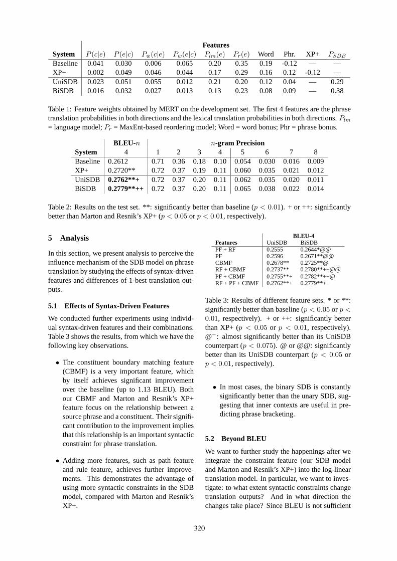
FeaturesSystem P (c|e) P (e|c) Pw(c|e) Pw(e|c) Plm(e) Pr(e) Word Phr. XP+ PSDB
Baseline 0.041 0.030 0.006 0.065 0.20 0.35 0.19 -0.12 — —XP+ 0.002 0.049 0.046 0.044 0.17 0.29 0.16 0.12 -0.12 —UniSDB 0.023 0.051 0.055 0.012 0.21 0.20 0.12 0.04 — 0.29BiSDB 0.016 0.032 0.027 0.013 0.13 0.23 0.08 0.09 — 0.38
Table 1: Feature weights obtained by MERT on the development set. The first 4 features are the phrasetranslation probabilities in both directions and the lexical translation probabilities in both directions.Plm
= language model;Pr = MaxEnt-based reordering model; Word = word bonus; Phr = phrase bonus.
BLEU-n n-gram PrecisionSystem 4 1 2 3 4 5 6 7 8Baseline 0.2612 0.71 0.36 0.18 0.10 0.054 0.030 0.016 0.009XP+ 0.2720** 0.72 0.37 0.19 0.11 0.060 0.035 0.021 0.012UniSDB 0.2762**+ 0.72 0.37 0.20 0.11 0.062 0.035 0.020 0.011BiSDB 0.2779**++ 0.72 0.37 0.20 0.11 0.065 0.038 0.022 0.014
Table 2: Results on the test set. **: significantly better than baseline (p < 0.01). + or ++: significantlybetter than Marton and Resnik’s XP+ (p < 0.05 or p < 0.01, respectively).
5 Analysis
In this section, we present analysis to perceive theinfluence mechanism of the SDB model on phrasetranslation by studying the effects of syntax-drivenfeatures and differences of 1-best translation out-puts.
5.1 Effects of Syntax-Driven Features
We conducted further experiments using individ-ual syntax-driven features and their combinations.Table 3 shows the results, from which we have thefollowing key observations.
• The constituent boundary matching feature(CBMF) is a very important feature, whichby itself achieves significant improvementover the baseline (up to 1.13 BLEU). Bothour CBMF and Marton and Resnik’s XP+feature focus on the relationship between asource phrase and a constituent. Their signifi-cant contribution to the improvement impliesthat this relationship is an important syntacticconstraint for phrase translation.
• Adding more features, such as path featureand rule feature, achieves further improve-ments. This demonstrates the advantage ofusing more syntactic constraints in the SDBmodel, compared with Marton and Resnik’sXP+.
BLEU-4Features UniSDB BiSDBPF + RF 0.2555 0.2644*@@PF 0.2596 0.2671**@@CBMF 0.2678** 0.2725**@RF + CBMF 0.2737** 0.2780**++@@PF + CBMF 0.2755**+ 0.2782**++@−
RF + PF + CBMF 0.2762**+ 0.2779**++
Table 3: Results of different feature sets. * or **:significantly better than baseline (p < 0.05 or p <0.01, respectively). + or ++: significantly betterthan XP+ (p < 0.05 or p < 0.01, respectively).@−: almost significantly better than its UniSDBcounterpart (p < 0.075). @ or @@: significantlybetter than its UniSDB counterpart (p < 0.05 orp < 0.01, respectively).
• In most cases, the binary SDB is constantlysignificantly better than the unary SDB, sug-gesting that inner contexts are useful in pre-dicting phrase bracketing.
5.2 Beyond BLEU
We want to further study the happenings after weintegrate the constraint feature (our SDB modeland Marton and Resnik’s XP+) into the log-lineartranslation model. In particular, we want to inves-tigate: to what extent syntactic constraints changetranslation outputs? And in what direction thechanges take place? Since BLEU is not sufficient
320

System CCM Rate (%)Baseline 43.5XP+ 74.5BiSDB 72.4
Table 4: Consistent constituent matching rates re-ported on 1-best translation outputs.
to provide such insights, we introduce a new sta-tistical metric which measures the proportion ofsyntactic constituents4 whose boundaries are con-sistently matched by decoder during translation.This proportion, which we callconsistent con-stituent matching (CCM) rate , reflects the ex-tent to which the translation output respects thesource parse tree.
In order to calculate this rate, we output transla-tion results as well as phrase alignments found bydecoders. Then for each multi-branch constituentcji spanning fromi to j on the source side, we
check the following conditions.
• If its boundariesi andj are aligned to phrasesegmentation boundaries found by decoder.
• If all target phrases insidecji ’s target span5
are aligned to the source phrases withincji
and not to the phrases outsidecji .
If both conditions are satisfied, the constituentcji
is consistently matched by decoder.Table 4 shows the consistent constituent match-
ing rates. Without using any source-side syntac-tic information, the baseline obtains a low CCMrate of 43.53%, indicating that the baseline de-coder violates the source parse tree more than itrespects the source structure. The translation out-put described in section 1 is actually generated bythe baseline decoder, where the second NP phraseboundaries are violated.
By integrating syntactic constraints into decod-ing, we can see that both Marton and Resnik’sXP+ and our SDB model achieve a significantlyhigher constituent matching rate, suggesting thatthey are more likely to respect the source struc-ture. The examples in Table 5 show that the de-coder is able to generate better translations if it is
4We only consider multi-branch constituents.5Given a phrase alignmentP = {cg
f ↔ eqp}, if the seg-
mentation withincji defined byP is cj
i = cj1i1
...cjkik
, and
cjrir↔ evr
ur∈ P, 1 ≤ r ≤ k, we define thetarget spanof cj
i
as a pair where the first element ismin(eu1 ...euk ) and thesecond element ismax(ev1 ...evk ), similar to (Fox, 2002).
CCM Rates (%)System <6 6-10 11-15 16-20 >20XP+ 75.2 70.9 71.0 76.2 82.2BiSDB 69.3 74.7 74.2 80.0 85.6
Table 6: Consistent constituent matching rates forstructures with different spans.
faithful to the source parse tree by using syntacticconstraints.
We further conducted a deep comparison oftranslation outputs of BiSDB vs. XP+ with re-gard to constituent matching and violation. Wefound two significant differences that may explainwhy our BiSDB outperforms XP+. First, althoughthe overall CCM rate of XP+ is higher than thatof BiSDB, BiSDB obtains higher CCM rates forlong-span structures than XP+ does, which areshown in Table 6. Generally speaking, viola-tions of long-span constituents have a more neg-ative impact on performance than short-span vio-lations if these violations are toxic. This explainswhy BiSDB achieves relatively higher precisionimprovements for highern-grams over XP+, asshown in Table 3.
Second, compared with XP+ that only punishesconstituent boundary violations, our SDB modelis able to encourage violations if these violationsare done on bracketable phrases. We observed inmany cases that by violating constituent bound-aries BiSDB produces better translations than XP+does, which on the contrary matches these bound-aries. Still consider the example shown in section1. The following translations are found by XP+and BiSDB respectively.
XP+: [to/把 〈[set up/设立 [for the/为 [naviga-tion/航海 section/节]]] on July 11/7月11日〉]
BiSDB: [to/把 〈[[set up/设立 a/为] [marine/航海festival/节]] on July 11/7月11日〉]
XP+ here matches all constituent boundaries whileBiSDB violates the PP constituent to translate thenon-syntactic phrase “设立 为”. Table 7 showsmore examples. From these examples, we clearlysee that appropriate violations are helpful and evennecessary for generating better translations. Byallowing appropriate violations to translate non-syntactic phrases according to particular syntac-tic contexts, our SDB model better inherits thestrength of phrase-based approach than XP+.
321
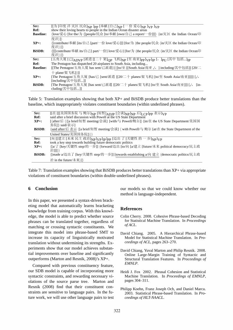
Src: [[为 [印度洋灾区民众]NP ]PP[奉献 [自己]NP [一份爱心]NP ]VP ]VPRef: show their loving hearts to people in the Indian Ocean disaster areasBaseline: 〈love/爱心 [for the/为 〈[people/民众 [to/奉献 [own/自己 a report/一份]]] 〉 〈in/灾区 the Indian Ocean/印
度洋〉]〉XP+: 〈[contribute/奉献 [its/自己 [part/一份 love/爱心]]] [for/为 〈the people/民众 〈in/灾区 the Indian Ocean/印
度洋〉〉]〉BiSDB: 〈[[[contribute/奉献 its/自己] part/一份] love/爱心] [for/为 〈the people/民众 〈in/灾区 the Indian Ocean印
度洋〉〉]〉Src: [五角大厦 [已]ADVP [派遣 [[二十架]QP飞机]NP [至南亚]PP]VP]IP [,]PU [其中包括...]IPRef: The Pentagon has dispatched 20 airplanes to South Asia, including...Baseline: [[The Pentagon/五角大厦 has sent/已派遣] [〈[to/至 [[South Asia/南亚 ,/,] including/其中包括]] [20/二
十 plane/架飞机]〉]]XP+: [The Pentagon/五角大厦 [has/已 [sent/派遣 [[20/二十 planes/架飞机] [to/至 South Asia/南亚]]]]] [,/ ,
[including/其中包括...]]BiSDB: [The Pentagon/五角大厦 [has sent/已派遣 [[20/二十 planes/架飞机] [to/至 South Asia/南亚]]] [,/, [in-
cluding/其中包括...]]
Table 5: Translation examples showing that both XP+ and BiSDB produce better translations than thebaseline, which inappropriately violates constituent boundaries (within underlined phrases).
Src: [[在 [[[美国国务院与鲍尔]NP [短暂]ADJP [会谈]NP]NP后]LCP]PP表示]VPRef: said after a brief discussion with Powell at the US State DepartmentXP+: [〈after/后 〈〈[a brief/短暂 meeting/会谈] [with/与 Powell/鲍尔]〉 [in/在 the US State Department/美国国
务院]〉 said/表示]BiSDB: 〈said after/后表示 〈[a brief/短暂 meeting/会谈] 〈 with Powell/与鲍尔 [at/在 the State Department of the
United States/美国国务院]〉〉〉Src: [向 [[建立 [未来民主政治]NP]VP]IP]PP[迈出了 [关键性的一步]NP]VPRef: took a key step towards building future democratic politicsXP+: 〈[a/了 [key/关键性 step/的一步]] 〈forward/迈出 [to/向 [a/建立 [future/未来 political democracy/民主政
治]]] 〉〉BiSDB: 〈[made a/迈出了 [key/关键性 step/的一步]] [towards establishing a/向建立 〈democratic politics/民主政
治 in the future/未来〉]〉
Table 7: Translation examples showing that BiSDB produces better translations than XP+ via appropriateviolations of constituent boundaries (within double-underlined phrases).
6 Conclusion
In this paper, we presented a syntax-driven brack-eting model that automatically learns bracketingknowledge from training corpus. With this knowl-edge, the model is able to predict whether sourcephrases can be translated together, regardless ofmatching or crossing syntactic constituents. Weintegrate this model into phrase-based SMT toincrease its capacity of linguistically motivatedtranslation without undermining its strengths. Ex-periments show that our model achieves substan-tial improvements over baseline and significantlyoutperforms (Marton and Resnik, 2008)’s XP+.
Compared with previous constituency feature,our SDB model is capable of incorporating moresyntactic constraints, and rewarding necessary vi-olations of the source parse tree. Marton andResnik (2008) find that their constituent con-straints are sensitive to language pairs. In the fu-ture work, we will use other language pairs to test
our models so that we could know whether ourmethod is language-independent.
References
Colin Cherry. 2008. Cohesive Phrase-based Decodingfor Statistical Machine Translation. InProceedingsof ACL.
David Chiang. 2005. A Hierarchical Phrase-basedModel for Statistical Machine Translation. InPro-ceedings of ACL, pages 263–270.
David Chiang, Yuval Marton and Philip Resnik. 2008.Online Large-Margin Training of Syntactic andStructural Translation Features. InProceedings ofEMNLP.
Heidi J. Fox 2002. Phrasal Cohesion and StatisticalMachine Translation. InProceedings of EMNLP,pages 304–311.
Philipp Koehn, Franz Joseph Och, and Daniel Marcu.2003. Statistical Phrase-based Translation. InPro-ceedings of HLT-NAACL.
322

Philipp Koehn. 2004. Statistical Significance Tests forMachine Translation Evaluation. InProceedings ofEMNLP.
Philipp Koehn, Amittai Axelrod, Alexandra BirchMayne, Chris Callison-Burch, Miles Osborne andDavid Talbot. 2005. Edinburgh System Descrip-tion for the 2005 IWSLT Speech Translation Eval-uation. InInternational Workshop on Spoken Lan-guage Translation.
Yajuan L̈u, Sheng Li, Tiezhun Zhao and Muyun Yang.2002. Learning Chinese Bracketing KnowledgeBased on a Bilingual Language Model. InProceed-ings of COLING.
Yuval Marton and Philip Resnik. 2008. Soft SyntacticConstraints for Hierarchical Phrase-Based Transla-tion. In Proceedings of ACL.
Franz Josef Och and Hermann Ney. 2000. ImprovedStatistical Alignment Models. InProceedings ofACL 2000.
Franz Josef Och. 2003. Minimum Error Rate Trainingin Statistical Machine Translation. InProceedingsof ACL 2003.
Kishore Papineni, Salim Roukos, Todd Ward, and Wei-Jing Zhu. 2002. Bleu: a Method for AutomaticallyEvaluation of Machine Translation. InProceedingsof ACL.
Andreas Stolcke. 2002. SRILM - an Extensible Lan-guage Modeling Toolkit. InProceedings of Interna-tional Conference on Spoken Language Processing,volume 2, pages 901-904.
Dekai Wu. 1997. Stochastic Inversion TransductionGrammars and Bilingual Parsing of Parallel Cor-pora.Computational Linguistics, 23(3):377-403.
Deyi Xiong, Shuanglong Li, Qun Liu, Shouxun Lin,Yueliang Qian. 2005. Parsing the Penn ChineseTreebank with Semantic Knowledge. InProceed-ings of IJCNLP, Jeju Island, Korea.
Deyi Xiong, Qun Liu and Shouxun Lin. 2006. Max-imum Entropy Based Phrase Reordering Model forStatistical Machine Translation. InProceedings ofACL-COLING 2006.
Deyi Xiong, Min Zhang, Aiti Aw, and Haizhou Li.2008. Linguistically Annotated BTG for StatisticalMachine Translation. InProceedings of COLING2008.
Le Zhang. 2004. Maximum Entropy Model-ing Tooklkit for Python and C++. Available athttp://homepages.inf.ed.ac.uk/s0450736/maxenttoolkit.html.
323
Proceedings of the 47th Annual Meeting of the ACL and the 4th IJCNLP of the AFNLP, pages 324–332,Suntec, Singapore, 2-7 August 2009. c©2009 ACL and AFNLP
Topological Ordering of Function Wordsin Hierarchical Phrase-based Translation
Hendra Setiawan1 and Min-Yen Kan2 and Haizhou Li3 and Philip Resnik1
1University of Maryland Institute for Advanced Computer Studies2School of Computing, National University of Singapore
3Human Language Technology, Institute for Infocomm Research, Singapore{hendra,resnik}@umiacs.umd.edu,
[email protected], [email protected]
Abstract
Hierarchical phrase-based models are at-tractive because they provide a consis-tent framework within which to character-ize both local and long-distance reorder-ings, but they also make it dif�cult todistinguish many implausible reorderingsfrom those that are linguistically plausi-ble. Rather than appealing to annotation-driven syntactic modeling, we address thisproblem by observing the in�uential roleof function words in determining syntac-tic structure, and introducing soft con-straints on function word relationships aspart of a standard log-linear hierarchi-cal phrase-based model. Experimentationon Chinese-English and Arabic-Englishtranslation demonstrates that the approachyields signi�cant gains in performance.
1 IntroductionHierarchical phrase-based models (Chiang, 2005;Chiang, 2007) offer a number of attractive bene-�ts in statistical machine translation (SMT), whilemaintaining the strengths of phrase-based systems(Koehn et al., 2003). The most important of theseis the ability to model long-distance reordering ef-�ciently. To model such a reordering, a hierar-chical phrase-based system demands no additionalparameters, since long and short distance reorder-ings are modeled identically using synchronouscontext free grammar (SCFG) rules. The samerule, depending on its topological ordering � i.e.its position in the hierarchical structure � can af-fect both short and long spans of text. Interest-ingly, hierarchical phrase-based models providethis bene�t without making any linguistic commit-ments beyond the structure of the model.
However, the system's lack of linguistic com-mitment is also responsible for one of its great-
est drawbacks. In the absence of linguistic knowl-edge, the system models linguistic structure usingan SCFG that contains only one type of nontermi-nal symbol1. As a result, the system is susceptibleto the overgeneration problem: the grammar maysuggest more reordering choices than appropriate,and many of those choices lead to ungrammaticaltranslations.
Chiang (2005) hypothesized that incorrect re-ordering choices would often correspond to hier-archical phrases that violate syntactic boundariesin the source language, and he explored the useof a �constituent feature� intended to reward theapplication of hierarchical phrases which respectsource language syntactic categories. Althoughthis did not yield signi�cant improvements, Mar-ton and Resnik (2008) and Chiang et al. (2008)extended this approach by introducing soft syn-tactic constraints similar to the constituent feature,but more �ne-grained and sensitive to distinctionsamong syntactic categories; these led to substan-tial improvements in performance. Zollman et al.(2006) took a complementary approach, constrain-ing the application of hierarchical rules to respectsyntactic boundaries in the target language syn-tax. Whether the focus is on constraints from thesource language or the target language, the mainingredient in both previous approaches is the ideaof constraining the spans of hierarchical phrases torespect syntactic boundaries.
In this paper, we pursue a different approachto improving reordering choices in a hierarchicalphrase-based model. Instead of biasing the modeltoward hierarchical phrases whose spans respectsyntactic boundaries, we focus on the topologi-cal ordering of phrases in the hierarchical struc-ture. We conjecture that since incorrect reorder-ing choices correspond to incorrect topological or-derings, boosting the probability of correct topo-
1In practice, one additional nonterminal symbol is used in�glue rules�. This is not relevant in the present discussion.
324
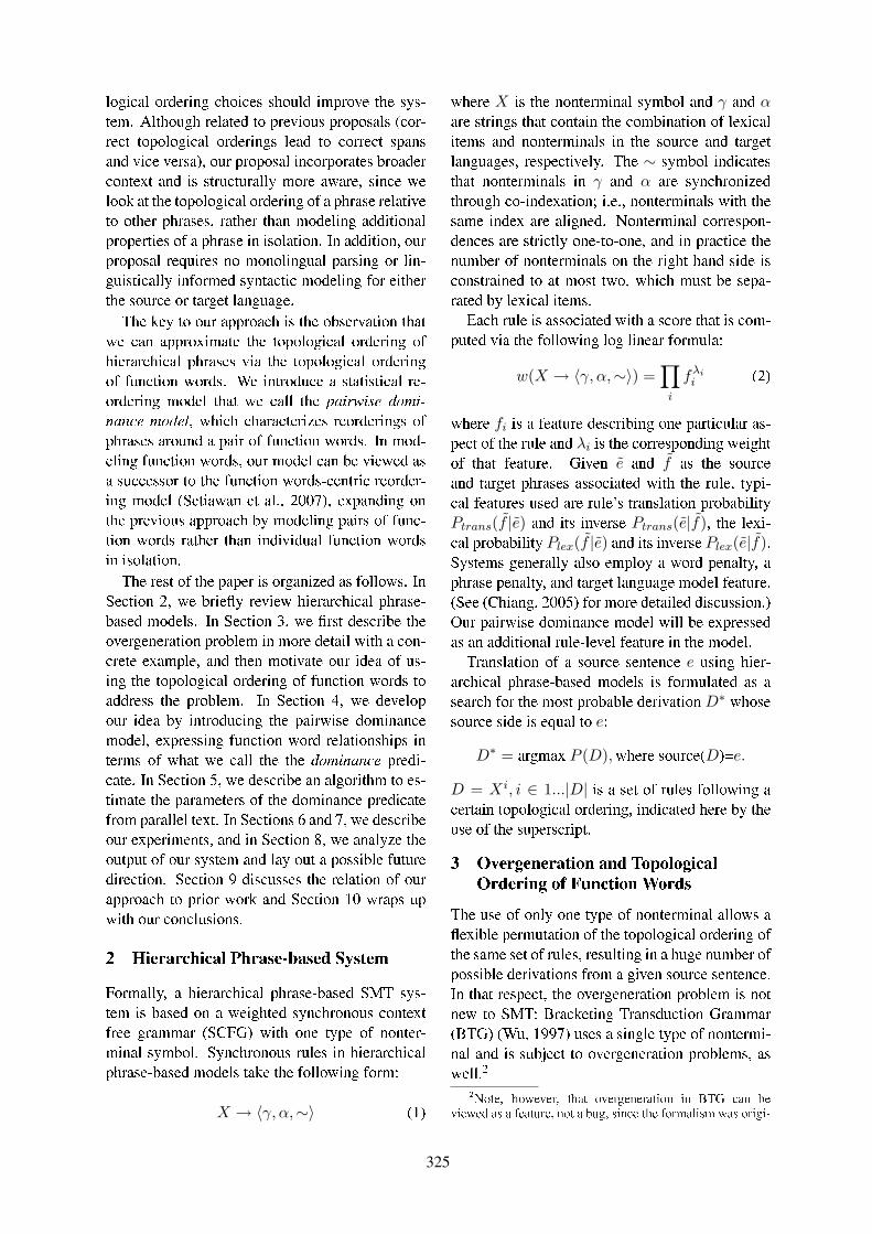
logical ordering choices should improve the sys-tem. Although related to previous proposals (cor-rect topological orderings lead to correct spansand vice versa), our proposal incorporates broadercontext and is structurally more aware, since welook at the topological ordering of a phrase relativeto other phrases, rather than modeling additionalproperties of a phrase in isolation. In addition, ourproposal requires no monolingual parsing or lin-guistically informed syntactic modeling for eitherthe source or target language.
The key to our approach is the observation thatwe can approximate the topological ordering ofhierarchical phrases via the topological orderingof function words. We introduce a statistical re-ordering model that we call the pairwise domi-nance model, which characterizes reorderings ofphrases around a pair of function words. In mod-eling function words, our model can be viewed asa successor to the function words-centric reorder-ing model (Setiawan et al., 2007), expanding onthe previous approach by modeling pairs of func-tion words rather than individual function wordsin isolation.
The rest of the paper is organized as follows. InSection 2, we brie�y review hierarchical phrase-based models. In Section 3, we �rst describe theovergeneration problem in more detail with a con-crete example, and then motivate our idea of us-ing the topological ordering of function words toaddress the problem. In Section 4, we developour idea by introducing the pairwise dominancemodel, expressing function word relationships interms of what we call the the dominance predi-cate. In Section 5, we describe an algorithm to es-timate the parameters of the dominance predicatefrom parallel text. In Sections 6 and 7, we describeour experiments, and in Section 8, we analyze theoutput of our system and lay out a possible futuredirection. Section 9 discusses the relation of ourapproach to prior work and Section 10 wraps upwith our conclusions.
2 Hierarchical Phrase-based System
Formally, a hierarchical phrase-based SMT sys-tem is based on a weighted synchronous contextfree grammar (SCFG) with one type of nonter-minal symbol. Synchronous rules in hierarchicalphrase-based models take the following form:
X → 〈γ, α,∼〉 (1)
where X is the nonterminal symbol and γ and αare strings that contain the combination of lexicalitems and nonterminals in the source and targetlanguages, respectively. The ∼ symbol indicatesthat nonterminals in γ and α are synchronizedthrough co-indexation; i.e., nonterminals with thesame index are aligned. Nonterminal correspon-dences are strictly one-to-one, and in practice thenumber of nonterminals on the right hand side isconstrained to at most two, which must be sepa-rated by lexical items.
Each rule is associated with a score that is com-puted via the following log linear formula:
w(X → 〈γ, α,∼〉) =∏
i
fλii (2)
where fi is a feature describing one particular as-pect of the rule and λi is the corresponding weightof that feature. Given ẽ and f̃ as the sourceand target phrases associated with the rule, typi-cal features used are rule's translation probabilityPtrans(f̃ |ẽ) and its inverse Ptrans(ẽ|f̃), the lexi-cal probability Plex(f̃ |ẽ) and its inverse Plex(ẽ|f̃).Systems generally also employ a word penalty, aphrase penalty, and target language model feature.(See (Chiang, 2005) for more detailed discussion.)Our pairwise dominance model will be expressedas an additional rule-level feature in the model.
Translation of a source sentence e using hier-archical phrase-based models is formulated as asearch for the most probable derivation D∗ whosesource side is equal to e:
D∗ = argmax P (D), where source(D)=e.
D = Xi, i ∈ 1...|D| is a set of rules following acertain topological ordering, indicated here by theuse of the superscript.
3 Overgeneration and TopologicalOrdering of Function Words
The use of only one type of nonterminal allows a�exible permutation of the topological ordering ofthe same set of rules, resulting in a huge number ofpossible derivations from a given source sentence.In that respect, the overgeneration problem is notnew to SMT: Bracketing Transduction Grammar(BTG) (Wu, 1997) uses a single type of nontermi-nal and is subject to overgeneration problems, aswell.2
2Note, however, that overgeneration in BTG can beviewed as a feature, not a bug, since the formalism was origi-
325

The problem may be less severe in hierarchi-cal phrase-based MT than in BTG, since lexicalitems on the rules' right hand sides often limit thespan of nonterminals. Nonetheless overgenerationof reorderings is still problematic, as we illustrateusing the hypothetical Chinese-to-English exam-ple in Fig. 1.
Suppose we want to translate the Chinese sen-tence in Fig. 1 into English using the following setof rules:
1. Xa → 〈� Z X1, computers and X1〉2. Xb → 〈X14 X2, X1 are X2〉3. Xc → 〈Cå , cell phones 〉4. Xd → 〈X1{�Ò , inventions of X1〉5. Xe → 〈ÞÇ-� , the last century 〉Co-indexation of nonterminals on the right hand
side is indicated by subscripts, and for our ex-amples the label of the nonterminal on the lefthand side is used as the rule's unique identi�er.To correctly translate the sentence, a hierarchicalphrase-based system needs to model the subjectnoun phrase, object noun phrase and copula con-structions; these are captured by rules Xa, Xd andXb respectively, so this set of rules represents ahierarchical phrase-based system that can be usedto correctly translate the Chinese sentence. Notethat the Chinese word order is correctly preservedin the subject (Xa) as well as copula constructions(Xb), and correctly inverted in the object construc-tion (Xd).
However, although it can generate the correcttranslation in Fig. 2, the grammar has no mech-anism to prevent the generation of an incorrecttranslation like the one illustrated in Fig. 3. Ifwe contrast the topological ordering of the rulesin Fig. 2 and Fig. 3, we observe that the differenceis small but quite signi�cant. Using precede sym-bol (≺) to indicate the �rst operand immediatelydominates the second operand in the hierarchicalstructure, the topological orderings in Fig. 2 andFig. 3 are Xa ≺ Xb ≺ Xc ≺ Xd ≺ Xe andXd ≺ Xa ≺ Xb ≺ Xc ≺ Xe, respectively. Theonly difference is the topological ordering of Xd:in Fig. 2, it appears below most of the other hier-archical phrases, while in Fig. 3, it appears aboveall the other hierarchical phrases.nally introduced for bilingual analysis rather than generationof translations.
Modeling the topological ordering of hierarchi-cal phrases is computationally prohibitive, sincethere are literally millions of hierarchical rules inthe system's automatically-learned grammar andmillions of possible ways to order their applica-tion. To avoid this computational problem andstill model the topological ordering, we proposeto use the topological ordering of function wordsas a practical approximation. This is motivated bythe fact that function words tend to carry crucialsyntactic information in sentences, serving as the�glue� for content-bearing phrases. Moreover, thepositional relationships between function wordsand content phrases tends to be �xed (e.g., in En-glish, prepositions invariably precede their objectnoun phrase), at least for the languages we haveworked with thus far.
In the Chinese sentence above, there are threefunction words involved: the conjunctionZ (and),the copula 4 (are), and the noun phrase marker{ (of).3 Using the function words as approximaterepresentations of the rules in which they appear,the topological ordering of hierarchical phrases inFig. 2 is Z(and) ≺ 4(are) ≺ {(of), while thatin Fig. 3 is {(of) ≺ Z(and) ≺ 4(are).4 Wecan distinguish the correct and incorrect reorder-ing choices by looking at this simple information.In the correct reordering choice,{(of) appears atthe lower level of the hierarchy while in the incor-rect one,{(of) appears at the highest level of thehierarchy.
4 Pairwise Dominance ModelOur example suggests that we may be able to im-prove the translation model's sensitivity to correctversus incorrect reordering choices by modelingthe topological ordering of function words. We doso by introducing a predicate capturing the domi-nance relationship in a derivation between pairs ofneighboring function words.5
Let us de�ne a predicate d(Y ′, Y ′′) that takestwo function words as input and outputs one of
3We use the term �noun phrase marker� here in a generalsense, meaning that in this example it helps tell us that thephrase is part of an NP, not as a technical linguistic term. Itserves in other grammatical roles, as well. Disambiguatingthe syntactic roles of function words might be a particularlyuseful thing to do in the model we are proposing; this is aquestion for future research.
4Note that for expository purposes, we designed our sim-ple grammar to ensure that these function words appear inseparate rules.
5Two function words are considered neighbors iff no otherfunction word appears between them in the source sentence.
326

� Z Cå 4 �Ò{ÞÇ-�
?XXXXXz
»»»»»9?? ? ?arecomputers and cell phones inventions of the last century
Figure 1: A running example of Chinese-to-English translation.
Xa⇒〈� Z Xb, computers and Xb〉⇒〈� Z Xc4 Xd, computers and Xc are Xd〉⇒〈� ZCå4 Xd, computers and cell phones are Xd〉⇒〈� ZCå4 Xe{�Ò , computers and cell phones are inventions of Xe〉⇒〈� ZCå4ÞÇ-�{�Ò , computers and cell phones are inventions of the last century〉
Figure 2: The derivation that leads to the correct translation
Xd⇒〈Xa{�Ò , inventions of Xa〉⇒〈� Z Xb{�Ò , inventions of computers and Xb〉⇒〈� Z Xc4 Xe{�Ò , inventions of computers and Xc are Xe〉⇒〈� ZCå4 Xe{�Ò , inventions of computers and cell phones are Xe〉⇒〈� ZCå4ÞÇ-�{�Ò , inventions of computers and cell phones are the last century〉
Figure 3: The derivation that leads to the incorrect translation
four values: {leftFirst, rightFirst, dontCare, nei-ther}, where Y ′ appears to the left of Y ′′ in thesource sentence. The value leftFirst indicates thatin the derivation's topological ordering, Y ′ pre-cedes Y ′′ (i.e. Y ′ dominates Y ′′ in the hierarchi-cal structure), while rightFirst indicates that Y ′′
dominates Y ′. In Fig. 2, d(Y ′, Y ′′) = leftFirstfor Y ′ = the copula 4 (are) and Y ′′ = the nounphrase marker{ (of).
The dontCare and neither values capture twoadditional relationships: dontCare indicates thatthe topological ordering of the function words is�exible, and neither indicates that the topologi-cal ordering of the function words is disjoint. Theformer is useful in cases where the hierarchicalphrases suggest the same kind of reordering, andtherefore restricting their topological ordering isnot necessary. This is illustrated in Fig. 2 by thepairZ(and) and the copula 4(are), where puttingeither one above the other does not change the �-nal word order. The latter is useful in cases wherethe two function words do not share a same parent.
Formally, this model requires several changes inthe design of the hierarchical phrase-based system.
1. To facilitate topological ordering of functionwords, the hierarchical phrases must be sub-categorized with function words. Taking Xb
in Fig. 2 as a case in point, subcategorization
using function words would yield:6
Xb(4 ≺{) → Xc4 Xd({) (3)
The subcategorization (indicated by theinformation in parentheses following thenonterminal) propagates the function word4(are) of Xb to the higher level structure to-gether with the function word {(of) of Xd.This propagation process generalizes to otherrules by maintaining the ordering of the func-tion words according to their appearance inthe source sentence. Note that the subcate-gorized nonterminals often resemble genuinesyntactic categories, for instance X({) canfrequently be interpreted as a noun phrase.
2. To facilitate the computation of the domi-nance relationship, the coindexing in syn-chronized rules (indicated by the ∼ symbolin Eq. 1) must be expanded to include infor-mation not only about the nonterminal corre-spondences but also about the alignment ofthe lexical items. For example, adding lexi-cal alignment information to rule Xd wouldyield:
Xd → 〈X1{2�Ò3, inventions3 of2 X1〉(4)
6The target language side is concealed for clarity.
327
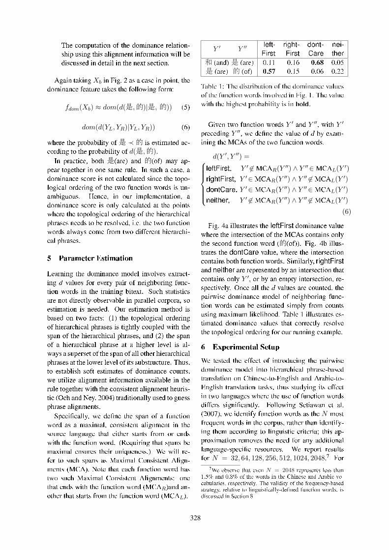
The computation of the dominance relation-ship using this alignment information will bediscussed in detail in the next section.
Again taking Xb in Fig. 2 as a case in point, thedominance feature takes the following form:
fdom(Xb) ≈ dom(d(4,{)|4, {)) (5)
dom(d(YL, YR)|YL, YR)) (6)
where the probability of4 ≺{ is estimated ac-cording to the probability of d(4,{).
In practice, both 4(are) and {(of) may ap-pear together in one same rule. In such a case, adominance score is not calculated since the topo-logical ordering of the two function words is un-ambiguous. Hence, in our implementation, adominance score is only calculated at the pointswhere the topological ordering of the hierarchicalphrases needs to be resolved, i.e. the two functionwords always come from two different hierarchi-cal phrases.
5 Parameter Estimation
Learning the dominance model involves extract-ing d values for every pair of neighboring func-tion words in the training bitext. Such statisticsare not directly observable in parallel corpora, soestimation is needed. Our estimation method isbased on two facts: (1) the topological orderingof hierarchical phrases is tightly coupled with thespan of the hierarchical phrases, and (2) the spanof a hierarchical phrase at a higher level is al-ways a superset of the span of all other hierarchicalphrases at the lower level of its substructure. Thus,to establish soft estimates of dominance counts,we utilize alignment information available in therule together with the consistent alignment heuris-tic (Och and Ney, 2004) traditionally used to guessphrase alignments.
Speci�cally, we de�ne the span of a functionword as a maximal, consistent alignment in thesource language that either starts from or endswith the function word. (Requiring that spans bemaximal ensures their uniqueness.) We will re-fer to such spans as Maximal Consistent Align-ments (MCA). Note that each function word hastwo such Maximal Consistent Alignments: onethat ends with the function word (MCAR)and an-other that starts from the function word (MCAL).
Y ′ Y ′′ left- right- dont- nei-First First Care ther
Z (and) 4 (are) 0.11 0.16 0.68 0.054 (are) { (of) 0.57 0.15 0.06 0.22
Table 1: The distribution of the dominance valuesof the function words involved in Fig. 1. The valuewith the highest probability is in bold.
Given two function words Y ′ and Y ′′, with Y ′
preceding Y ′′, we de�ne the value of d by exam-ining the MCAs of the two function words.
d(Y ′, Y ′′) =
leftFirst, Y ′ 6∈ MCAR(Y ′′) ∧ Y ′′∈ MCAL(Y ′)rightFirst, Y ′∈ MCAR(Y ′′) ∧ Y ′′ 6∈ MCAL(Y ′)dontCare, Y ′∈ MCAR(Y ′′) ∧ Y ′′∈ MCAL(Y ′)neither, Y ′ 6∈ MCAR(Y ′′) ∧ Y ′′ 6∈ MCAL(Y ′)
(6)
Fig. 4a illustrates the leftFirst dominance valuewhere the intersection of the MCAs contains onlythe second function word ({(of)). Fig. 4b illus-trates the dontCare value, where the intersectioncontains both function words. Similarly, rightFirstand neither are represented by an intersection thatcontains only Y ′, or by an empty intersection, re-spectively. Once all the d values are counted, thepairwise dominance model of neighboring func-tion words can be estimated simply from countsusing maximum likelihood. Table 1 illustrates es-timated dominance values that correctly resolvethe topological ordering for our running example.
6 Experimental SetupWe tested the effect of introducing the pairwisedominance model into hierarchical phrase-basedtranslation on Chinese-to-English and Arabic-to-English translation tasks, thus studying its effectin two languages where the use of function wordsdiffers signi�cantly. Following Setiawan et al.(2007), we identify function words as the N mostfrequent words in the corpus, rather than identify-ing them according to linguistic criteria; this ap-proximation removes the need for any additionallanguage-speci�c resources. We report resultsfor N = 32, 64, 128, 256, 512, 1024, 2048.7 For
7We observe that even N = 2048 represents less than1.5% and 0.8% of the words in the Chinese and Arabic vo-cabularies, respectively. The validity of the frequency-basedstrategy, relative to linguistically-de�ned function words, isdiscussed in Section 8
328

na
nb
jj
jz
jz
jthe last centuryof
innovationsare
cell phonesand
computers
� Z
Cå 4
Þ
-�{�Ò
jz
jz
jj
jthe last centuryof
innovationsare
cell phonesand
computers
� Z
Cå 4
Þ
-
�{�Ò
Figure 4: Illustrations for: a) the leftFirst value,and b) the dontCare value. Thickly borderedboxes are MCAs of the function words while solidcircles are the alignment points of the functionwords. The gray boxes are the intersections of thetwo MCAs.
all experiments, we report performance using theBLEU score (Papineni et al., 2002), and we assessstatistical signi�cance using the standard boot-strapping approach introduced by (Koehn, 2004).
Chinese-to-English experiments. We trainedthe system on the NIST MT06 Eval corpus ex-cluding the UN data (approximately 900K sen-tence pairs). For the language model, we used a 5-gram model with modi�ed Kneser-Ney smoothing(Kneser and Ney, 1995) trained on the English sideof our training data as well as portions of the Giga-word v2 English corpus. We used the NIST MT03test set as the development set for optimizing inter-polation weights using minimum error rate train-ing (MERT; (Och and Ney, 2002)). We carried outevaluation of the systems on the NIST 2006 eval-uation test (MT06) and the NIST 2008 evaluationtest (MT08). We segmented Chinese as a prepro-cessing step using the Harbin segmenter (Zhao etal., 2001).
Arabic-to-English experiments. We trainedthe system on a subset of 950K sentence pairsfrom the NIST MT08 training data, selected by
�subsampling� from the full training data using amethod proposed by Kishore Papineni (personalcommunication). The subsampling algorithm se-lects sentence pairs from the training data in away that seeks reasonable representation for all n-grams appearing in the test set. For the languagemodel, we used a 5-gram model trained on the En-glish portion of the whole training data plus por-tions of the Gigaword v2 corpus. We used theNIST MT03 test set as the development set foroptimizing the interpolation weights using MERT.We carried out the evaluation of the systems on theNIST 2006 evaluation set (MT06) and the NIST2008 evaluation set (MT08). Arabic source textwas preprocessed by separating clitics, the de�-niteness marker, and the future tense marker fromtheir stems.
7 Experimental Results
Chinese-to-English experiments. Table 2 sum-marizes the results of our Chinese-to-English ex-periments. These results con�rm that the pairwisedominance model can signi�cantly increase per-formance as measured by the BLEU score, with aconsistent pattern of results across the MT06 andMT08 test sets. Modeling N = 32 drops the per-formance marginally below baseline, suggestingthat perhaps there are not enough words for thepairwise dominance model to work with. Dou-bling the number of words (N = 64) producesa small gain, and de�ning the pairwise dominancemodel using N = 128 most frequent words pro-duces a statistically signi�cant 1-point gain overthe baseline (p < 0.01). Larger values of Nyield statistically signi�cant performance abovethe baseline, but without further improvementsover N = 128.Arabic-to-English experiments. Table 3 sum-marizes the results of our Arabic-to-English ex-periments. This set of experiments shows a pat-tern consistent with what we observed in Chinese-to-English translation, again generally consistentacross MT06 and MT08 test sets although mod-eling a small number of lexical items (N = 32)brings a marginal improvement over the baseline.In addition, we again �nd that the pairwise dom-inance model with N = 128 produces the mostsigni�cant gain over the baseline in the MT06,although, interestingly, modeling a much largernumber of lexical items (N = 2048) yields thestrongest improvement for the MT08 test set.
329
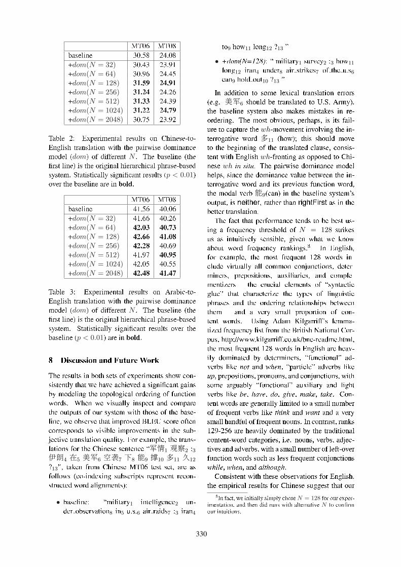
MT06 MT08baseline 30.58 24.08+dom(N = 32) 30.43 23.91+dom(N = 64) 30.96 24.45+dom(N = 128) 31.59 24.91+dom(N = 256) 31.24 24.26+dom(N = 512) 31.33 24.39+dom(N = 1024) 31.22 24.79+dom(N = 2048) 30.75 23.92
Table 2: Experimental results on Chinese-to-English translation with the pairwise dominancemodel (dom) of different N . The baseline (the�rst line) is the original hierarchical phrase-basedsystem. Statistically signi�cant results (p < 0.01)over the baseline are in bold.
MT06 MT08baseline 41.56 40.06+dom(N = 32) 41.66 40.26+dom(N = 64) 42.03 40.73+dom(N = 128) 42.66 41.08+dom(N = 256) 42.28 40.69+dom(N = 512) 41.97 40.95+dom(N = 1024) 42.05 40.55+dom(N = 2048) 42.48 41.47
Table 3: Experimental results on Arabic-to-English translation with the pairwise dominancemodel (dom) of different N . The baseline (the�rst line) is the original hierarchical phrase-basedsystem. Statistically signi�cant results over thebaseline (p < 0.01) are in bold.
8 Discussion and Future Work
The results in both sets of experiments show con-sistently that we have achieved a signi�cant gainsby modeling the topological ordering of functionwords. When we visually inspect and comparethe outputs of our system with those of the base-line, we observe that improved BLEU score oftencorresponds to visible improvements in the sub-jective translation quality. For example, the trans-lations for the Chinese sentence ��<1 �2 :3��4 ó5 ��6 8ñ7 �8 �9 À10 õ11 È12
?13�, taken from Chinese MT06 test set, are asfollows (co-indexing subscripts represent recon-structed word alignments):
• baseline: �military1 intelligence2 un-der observation8 in5 u.s.6 air raids7 :3 iran4
to9 how11 long12 ?13 �
• +dom(N=128): � military1 survey2 :3 how11
long12 iran4 under8 air strikes7 of the u.s6
can9 hold out10 ?13 �
In addition to some lexical translation errors(e.g. ��6 should be translated to U.S. Army),the baseline system also makes mistakes in re-ordering. The most obvious, perhaps, is its fail-ure to capture the wh-movement involving the in-terrogative word õ11 (how); this should moveto the beginning of the translated clause, consis-tent with English wh-fronting as opposed to Chi-nese wh in situ. The pairwise dominance modelhelps, since the dominance value between the in-terrogative word and its previous function word,the modal verb �9(can) in the baseline system'soutput, is neither, rather than rightFirst as in thebetter translation.
The fact that performance tends to be best us-ing a frequency threshold of N = 128 strikesus as intuitively sensible, given what we knowabout word frequency rankings.8 In English,for example, the most frequent 128 words in-clude virtually all common conjunctions, deter-miners, prepositions, auxiliaries, and comple-mentizers � the crucial elements of �syntacticglue� that characterize the types of linguisticphrases and the ordering relationships betweenthem � and a very small proportion of con-tent words. Using Adam Kilgarriff's lemma-tized frequency list from the British National Cor-pus, http://www.kilgarriff.co.uk/bnc-readme.html,the most frequent 128 words in English are heav-ily dominated by determiners, �functional� ad-verbs like not and when, �particle� adverbs likeup, prepositions, pronouns, and conjunctions, withsome arguably �functional� auxiliary and lightverbs like be, have, do, give, make, take. Con-tent words are generally limited to a small numberof frequent verbs like think and want and a verysmall handful of frequent nouns. In contrast, ranks129-256 are heavily dominated by the traditionalcontent-word categories, i.e. nouns, verbs, adjec-tives and adverbs, with a small number of left-overfunction words such as less frequent conjunctionswhile, when, and although.
Consistent with these observations for English,the empirical results for Chinese suggest that our
8In fact, we initially simply chose N = 128 for our exper-imentation, and then did runs with alternative N to con�rmour intuitions.
330

approximation of function words using word fre-quency is reasonable. Using a list of approxi-mately 900 linguistically identi�ed function wordsin Chinese extracted from (Howard, 2002), we ob-serve that that the performance drops when in-creasing N above 128 corresponds to a large in-crease in the number of non-function words usedin the model. For example, with N = 2048, theproportion of non-function words is 88%, com-pared to 60% when N = 128.9
One natural extension of this work, therefore,would be to tighten up our characterization offunction words, whether statistically, distribution-ally, or simply using manually created resourcesthat exist for many languages. As a �rst step, wedid a version of the Chinese-English experimentusing the list of approximately 900 genuine func-tion words, testing on the Chinese MT06 set. Per-haps surprisingly, translation performance, 30.90BLEU, was around the level we obtained whenusing frequency to approximate function words atN = 64. However, we observe that many ofthe words in the linguistically motivated functionword list are quite infrequent; this suggests thatdata sparseness may be an additional factor worthinvestigating.
Finally, although we believe there are strongmotivations for focusing on the role of functionwords in reordering, there may well be value inextending the dominance model to include contentcategories. Verbs and many nouns have subcat-egorization properties that may in�uence phraseordering, for example, and this may turn out to ex-plain the increase in Arabic-English performancefor N = 2048 using the MT08 test set. More gen-erally, the approach we are taking can be viewedas a way of selectively lexicalizing the automati-cally extracted grammar, and there is a large rangeof potentially interesting choices in how such lex-icalization could be done.
9 Related Work
In the introduction, we discussed Chiang's (2005)constituency feature, related ideas explored byMarton and Resnik (2008) and Chiang et al.(2008), and the target-side variation investigatedby Zollman et al. (2006). These methods differfrom each other mainly in terms of the speci�c lin-
9We plan to do corresponding experimentation and anal-ysis for Arabic once we identify a suitable list of manuallyidenti�ed function words.
guistic knowledge being used and on which sidethe constraints are applied.
Shen et al. (2008) proposed to use lin-guistic knowledge expressed in terms of a de-pendency grammar, instead of a syntactic con-stituency grammar. Villar et al. (2008) attemptedto use syntactic constituency on both the sourceand target languages in the same spirit as the con-stituency feature, along with some simple pattern-based heuristics � an approach also investigated byIglesias et al. (2009). Aiming at improving the se-lection of derivations, Zhou et al. (2008) proposedprior derivation models utilizing syntactic annota-tion of the source language, which can be seen assmoothing the probabilities of hierarchical phrasefeatures.
A key point is that the model we have intro-duced in this paper does not require the linguisticsupervision needed in most of this prior work. Weestimate the parameters of our model from paralleltext without any linguistic annotation. That said,we would emphasize that our approach is, in fact,motivated in linguistic terms by the role of func-tion words in natural language syntax.
10 ConclusionWe have presented a pairwise dominance modelto address reordering issues that are not handledparticularly well by standard hierarchical phrase-based modeling. In particular, the minimal lin-guistic commitment in hierarchical phrase-basedmodels renders them susceptible to overgenera-tion of reordering choices. Our proposal han-dles the overgeneration problem by identifyinghierarchical phrases with function words and byusing function word relationships to incorporatesoft constraints on topological orderings. Ourexperimental results demonstrate that introducingthe pairwise dominance model into hierarchicalphrase-based modeling improves performance sig-ni�cantly in large-scale Chinese-to-English andArabic-to-English translation tasks.
AcknowledgmentsThis research was supported in part by theGALE program of the Defense Advanced Re-search Projects Agency, Contract No. HR0011-06-2-001. Any opinions, �ndings, conclusions orrecommendations expressed in this paper are thoseof the authors and do not necessarily re�ect theview of the sponsors.
331
ReferencesDavid Chiang, Yuval Marton, and Philip Resnik. 2008.
Online large-margin training of syntactic and struc-tural translation features. In Proceedings of the2008 Conference on Empirical Methods in Natu-ral Language Processing, pages 224�233, Honolulu,Hawaii, October.
David Chiang. 2005. A hierarchical phrase-basedmodel for statistical machine translation. In Pro-ceedings of the 43rd Annual Meeting of the Associa-tion for Computational Linguistics (ACL'05), pages263�270, Ann Arbor, Michigan, June. Associationfor Computational Linguistics.
David Chiang. 2007. Hierarchical phrase-based trans-lation. Computational Linguistics, 33(2):201�228.
Jiaying Howard. 2002. A Student Handbook for Chi-nese Function Words. The Chinese University Press.
Gonzalo Iglesias, Adria de Gispert, Eduardo R. Banga,and William Byrne. 2009. Rule �ltering by patternfor ef�cient hierarchical translation. In Proceedingsof the 12th Conference of the European Chapter ofthe Association of Computational Linguistics (to ap-pear).
R. Kneser and H. Ney. 1995. Improved backing-off for m-gram language modeling. In Proceed-ings of IEEE International Conference on Acoustics,Speech, and Signal Processing95, pages 181�184,Detroit, MI, May.
Philipp Koehn, Franz J. Och, and Daniel Marcu. 2003.Statistical phrase-based translation. In Proceedingsof the 2003 Human Language Technology Confer-ence of the North American Chapter of the Associa-tion for Computational Linguistics, pages 127�133,Edmonton, Alberta, Canada, May. Association forComputational Linguistics.
Philipp Koehn. 2004. Statistical signi�cance tests formachine translation evaluation. In Proceedings ofEMNLP 2004, pages 388�395, Barcelona, Spain,July.
Yuval Marton and Philip Resnik. 2008. Soft syntac-tic constraints for hierarchical phrased-based trans-lation. In Proceedings of The 46th Annual Meet-ing of the Association for Computational Linguis-tics: Human Language Technologies, pages 1003�1011, Columbus, Ohio, June.
Franz Josef Och and Hermann Ney. 2002. Discrim-inative training and maximum entropy models forstatistical machine translation. In Proceedings of40th Annual Meeting of the Association for Com-putational Linguistics, pages 295�302, Philadelphia,Pennsylvania, USA, July.
Franz Josef Och and Hermann Ney. 2004. The align-ment template approach to statistical machine trans-lation. Computational Linguistics, 30(4):417�449.
Kishore Papineni, Salim Roukos, Todd Ward, and Wei-Jing Zhu. 2002. Bleu: a method for automaticevaluation of machine translation. In Proceedingsof 40th Annual Meeting of the Association for Com-putational Linguistics, pages 311�318, Philadelphia,Pennsylvania, USA, July.
Hendra Setiawan, Min-Yen Kan, and Haizhou Li.2007. Ordering phrases with function words. InProceedings of the 45th Annual Meeting of the As-sociation of Computational Linguistics, pages 712�719, Prague, Czech Republic, June.
Libin Shen, Jinxi Xu, and Ralph Weischedel. 2008.A new string-to-dependency machine translation al-gorithm with a target dependency language model.In Proceedings of The 46th Annual Meeting of theAssociation for Computational Linguistics: HumanLanguage Technologies, pages 577�585, Columbus,Ohio, June.
David Vilar, Daniel Stein, and Hermann Ney. 2008.Analysing soft syntax features and heuristics for hi-erarchical phrase based machine translation. Inter-national Workshop on Spoken Language Translation2008, pages 190�197, October.
Dekai Wu. 1997. Stochastic inversion transductiongrammars and bilingual parsing of parallel corpora.Computational Linguistics, 23(3):377�404, Sep.
Tiejun Zhao, Yajuan Lv, Jianmin Yao, Hao Yu, MuyunYang, and Fang Liu. 2001. Increasing accuracyof chinese segmentation with strategy of multi-stepprocessing. Journal of Chinese Information Pro-cessing (Chinese Version), 1:13�18.
Bowen Zhou, Bing Xiang, Xiaodan Zhu, and YuqingGao. 2008. Prior derivation models for formallysyntax-based translation using linguistically syntac-tic parsing and tree kernels. In Proceedings ofthe ACL-08: HLT Second Workshop on Syntax andStructure in Statistical Translation (SSST-2), pages19�27, Columbus, Ohio, June.
Andreas Zollmann and Ashish Venugopal. 2006. Syn-tax augmented machine translation via chart parsing.In Proceedings on the Workshop on Statistical Ma-chine Translation, pages 138�141, New York City,June.
332

Proceedings of the 47th Annual Meeting of the ACL and the 4th IJCNLP of the AFNLP, pages 333–341,Suntec, Singapore, 2-7 August 2009. c©2009 ACL and AFNLP
Phrase-Based Statistical Machine Translation as a Traveling SalesmanProblem
Mikhail Zaslavskiy∗ Marc Dymetman Nicola CanceddaMines ParisTech, Institut Curie Xerox Research Centre Europe77305 Fontainebleau, France 38240 Meylan, France
[email protected] {marc.dymetman,nicola.cancedda}@xrce.xerox.com
Abstract
An efficient decoding algorithm is a cru-cial element of any statistical machinetranslation system. Some researchers havenoted certain similarities between SMTdecoding and the famous Traveling Sales-man Problem; in particular (Knight, 1999)has shown that any TSP instance can bemapped to a sub-case of a word-basedSMT model, demonstrating NP-hardnessof the decoding task. In this paper, we fo-cus on the reverse mapping, showing thatany phrase-based SMT decoding problemcan be directly reformulated as a TSP. Thetransformation is very natural, deepens ourunderstanding of the decoding problem,and allows direct use of any of the pow-erful existing TSP solvers for SMT de-coding. We test our approach on threedatasets, and compare a TSP-based de-coder to the popular beam-search algo-rithm. In all cases, our method providescompetitive or better performance.
1 Introduction
Phrase-based systems (Koehn et al., 2003) areprobably the most widespread class of StatisticalMachine Translation systems, and arguably one ofthe most successful. They use aligned sequencesof words, called biphrases, as building blocks fortranslations, and score alternative candidate trans-lations for the same source sentence based on alog-linear model of the conditional probability oftarget sentences given the source sentence:
p(T, a|S) =1
ZS
exp∑
k
λkhk(S, a, T ) (1)
where thehk are features, that is, functions of thesource stringS, of the target stringT , and of the
∗ This work was conducted during an internship atXRCE.
alignmenta, where the alignment is a representa-tion of the sequence of biphrases that where usedin order to buildT from S; Theλk’s are weightsandZS is a normalization factor that guaranteesthat p is a proper conditional probability distri-bution over the pairs(T, A). Some features arelocal, i.e. decompose over biphrases and can beprecomputed and stored in advance. These typ-ically include forward and reverse phrase condi-tional probability featureslog p(t̃|s̃) as well aslog p(s̃|t̃), where s̃ is the source side of thebiphrase and̃t the target side, and the so-called“phrase penalty” and “word penalty” features,which count the number of phrases and words inthe alignment. Other features arenon-local, i.e.depend on the order in which biphrases appear inthe alignment. Typical non-local features includeone or more n-gram language models as well asa distortion feature, measuring by how much theorder of biphrases in the candidate translation de-viates from their order in the source sentence.
Given such a model, where theλi’s have beentuned on a development set in order to minimizesome error rate (see e.g. (Lopez, 2008)), togetherwith a library of biphrases extracted from somelarge training corpus, adecoderimplements theactual search among alternative translations:
(a∗, T ∗) = arg max(a,T )
P (T, a|S). (2)
The decoding problem (2) is a discrete optimiza-tion problem. Usually, it is very hard to find theexact optimum and, therefore, an approximate so-lution is used. Currently, most decoders are basedon some variant of a heuristic left-to-right search,that is, they attempt to build a candidate translation(a, T ) incrementally, from left to right, extendingthe current partial translation at each step with anew biphrase, and computing a score composed oftwo contributions: one for the known elements ofthe partial translation so far, and one a heuristic
333

estimate of the remaining cost for completing thetranslation. The variant which is mostly used isa form ofbeam-search, where several partial can-didates are maintained in parallel, and candidatesfor which the current score is too low are prunedin favor of candidates that are more promising.
We will see in the next section that some char-acteristics of beam-search make it a suboptimalchoice for phrase-based decoding, and we willpropose an alternative. This alternative is based onthe observation that phrase-based decoding can bevery naturally cast as a Traveling Salesman Prob-lem (TSP), one of the best studied problems incombinatorial optimization. We will show that thisformulation is not only a powerful conceptual de-vice for reasoning on decoding, but is also prac-tically convenient: in the same amount of time,off-the-shelf TSP solvers can find higher scoringsolutions than the state-of-the art beam-search de-coder implemented inMoses(Hoang and Koehn,2008).
2 Related work
Beam-search decodingIn beam-search decoding, candidate translationprefixes are iteratively extended with new phrases.In its most widespread variant,stack decoding,prefixes obtained by consuming the same numberof source words, no matter which, are grouped to-gether in the samestack1 and compete against oneanother.Thresholdandhistogrampruning are ap-plied: the former consists in dropping all prefixeshaving a score lesser than the best score by morethan some fixed amount (a parameter of the algo-rithm), the latter consists in dropping all prefixesbelow a certain rank.
While quite successful in practice, stack decod-ing presents some shortcomings. A first one is thatprefixes obtained by translating different subsetsof source words compete against one another. Inone early formulation of stack decoding for SMT(Germann et al., 2001), the authors indeed pro-posed to lazily create one stack for each subsetof source words, but acknowledged issues withthe potential combinatorial explosion in the num-ber of stacks. This problem is reduced by the useof heuristics for estimating the cost of translatingthe remaining part of the source sentence. How-
1While commonly adopted in the speech and SMT com-munities, this is a bit of a misnomer, since the used data struc-tures are priority queues, not stacks.
ever, this solution is only partially satisfactory. Onthe one hand, heuristics should be computationallylight, much lighter than computing the actual bestscore itself, while, on the other hand, the heuris-tics should be tight, as otherwise pruning errorswill ensue. There is no clear criterion to guidein this trade-off. Even when good heuristics areavailable, the decoder will show a bias towardsputting at the beginning the translation of a certainportion of the source, either because this portionis less ambiguous (i.e. its translation has largerconditional probability) or because the associatedheuristics is less tight, hence more optimistic. Fi-nally, since the translation is built left-to-right thedecoder cannot optimize the search by taking ad-vantage of highly unambiguous and informativeportions that should be best translated far from thebeginning. All these reasons motivate consideringalternative decoding strategies.
Word-based SMT and the TSPAs already mentioned, the similarity betweenSMT decoding and TSP was recognized in(Knight, 1999), who focussed on showing thatany TSP can be reformulated as a sub-class of theSMT decoding problem, proving that SMT decod-ing is NP-hard. Following this work, the exis-tence of many efficient TSP algorithms then in-spired certain adaptations of the underlying tech-niques to SMT decoding for word-based models.Thus, (Germann et al., 2001) adapt a TSP sub-tour elimination strategy to an IBM-4 model, us-ing generic Integer Programming techniques. Thepaper comes close to a TSP formulation of de-coding with IBM-4 models, but does not pursuethis route to the end, stating that“It is difficultto convert decoding into straight TSP, but a widerange of combinatorial optimization problems (in-cluding TSP) can be expressed in the more gen-eral framework of linear integer programming”.By employing generic IP techniques, it is how-ever impossible to rely on the variety of moreefficient both exact and approximate approacheswhich have been designed specifically for the TSP.In (Tillmann and Ney, 2003) and (Tillmann, 2006),the authors modify a certain Dynamic Program-ming technique used for TSP for use with an IBM-4 word-based model and a phrase-based model re-spectively. However, to our knowledge, none ofthese works has proposed a direct reformulationof these SMT models as TSP instances. We be-lieve we are the first to do so, working in our case
334
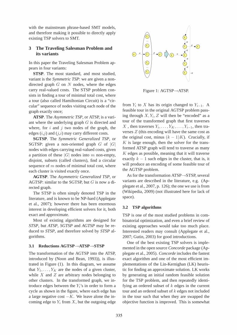
with the mainstream phrase-based SMT models,and therefore making it possible to directly applyexisting TSP solvers to SMT.
3 The Traveling Salesman Problem andits variants
In this paper the Traveling Salesman Problem ap-pears in four variants:
STSP. The most standard, and most studied,variant is theSymmetric TSP: we are given a non-directed graphG on N nodes, where the edgescarry real-valued costs. The STSP problem con-sists in finding a tour of minimal total cost, wherea tour (also called Hamiltonian Circuit) is a “cir-cular” sequence of nodes visiting each node of thegraph exactly once;
ATSP. TheAsymmetric TSP, or ATSP, is a vari-ant where the underlying graphG is directed andwhere, for i and j two nodes of the graph, theedges (i,j) and (j,i) may carry different costs.
SGTSP. The Symmetric Generalized TSP, orSGTSP: given a non-oriented graphG of |G|nodes with edges carrying real-valued costs, givena partition of these|G| nodes intom non-empty,disjoint, subsets (called clusters), find a circularsequence ofm nodes of minimal total cost, whereeach cluster is visited exactly once.
AGTSP. TheAsymmetric Generalized TSP, orAGTSP: similar to the SGTSP, butG is now a di-rected graph.
The STSP is often simply denoted TSP in theliterature, and is known to be NP-hard (Applegateet al., 2007); however there has been enormousinterest in developing efficient solvers for it, bothexact and approximate.
Most of existing algorithms are designed forSTSP, but ATSP, SGTSPandAGTSPmay be re-duced toSTSP, and therefore solved bySTSPal-gorithms.
3.1 Reductions AGTSP→ATSP→STSP
The transformation of the AGTSP into the ATSP,introduced by (Noon and Bean, 1993)), is illus-trated in Figure (1). In this diagram, we assumethat Y1, . . . , YK are the nodes of a given cluster,while X andZ are arbitrary nodes belonging toother clusters. In the transformed graph, we in-troduce edges between theYi’s in order to form acycle as shown in the figure, where each edge hasa large negative cost−K. We leave alone the in-coming edge toYi from X, but the outgoing edge
Figure 1: AGTSP→ATSP.
from Yi to X has its origin changed toYi−1. Afeasible tour in the original AGTSP problem pass-ing throughX, Yi, Z will then be “encoded” as atour of the transformed graph that first traversesX , then traversesYi, . . . , YK , . . . , Yi−1, then tra-versesZ (this encoding will have the same cost asthe original cost, minus(k − 1)K). Crucially, ifK is large enough, then the solver for the trans-formed ATSP graph will tend to traverse as manyK edges as possible, meaning that it will traverseexactlyk − 1 such edges in the cluster, that is, itwill produce an encoding of some feasible tour ofthe AGTSP problem.
As for the transformation ATSP→STSP, severalvariants are described in the literature, e.g. (Ap-plegate et al., 2007, p. 126); the one we use is from(Wikipedia, 2009) (not illustrated here for lack ofspace).
3.2 TSP algorithms
TSP is one of the most studied problems in com-binatorial optimization, and even a brief review ofexisting approaches would take too much place.Interested readers may consult (Applegate et al.,2007; Gutin, 2003) for good introductions.
One of the best existing TSP solvers is imple-mented in the open sourceConcordepackage (Ap-plegate et al., 2005).Concordeincludes the fastestexact algorithm and one of the most efficient im-plementations of the Lin-Kernighan (LK) heuris-tic for finding an approximate solution. LK worksby generating an initial random feasible solutionfor the TSP problem, and then repeatedly identi-fying an ordered subset ofk edges in the currenttour and an ordered subset ofk edges not includedin the tour such that when they are swapped theobjective function is improved. This is somewhat
335
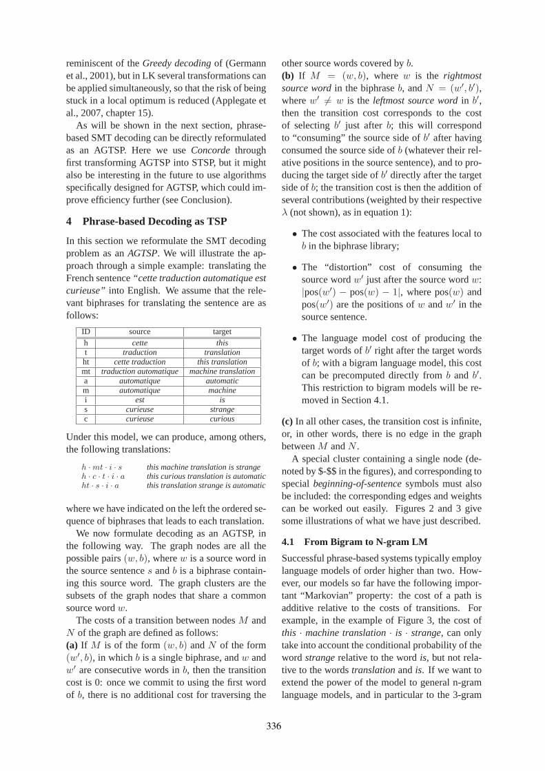
reminiscent of theGreedy decodingof (Germannet al., 2001), but in LK several transformations canbe applied simultaneously, so that the risk of beingstuck in a local optimum is reduced (Applegate etal., 2007, chapter 15).
As will be shown in the next section, phrase-based SMT decoding can be directly reformulatedas an AGTSP. Here we useConcorde throughfirst transforming AGTSP into STSP, but it mightalso be interesting in the future to use algorithmsspecifically designed for AGTSP, which could im-prove efficiency further (see Conclusion).
4 Phrase-based Decoding as TSP
In this section we reformulate the SMT decodingproblem as anAGTSP. We will illustrate the ap-proach through a simple example: translating theFrench sentence“cette traduction automatique estcurieuse” into English. We assume that the rele-vant biphrases for translating the sentence are asfollows:
ID source targeth cette thist traduction translationht cette traduction this translationmt traduction automatique machine translationa automatique automaticm automatique machinei est iss curieuse strangec curieuse curious
Under this model, we can produce, among others,the following translations:
h · mt · i · s this machine translation is strangeh · c · t · i · a this curious translation is automaticht · s · i · a this translation strange is automatic
where we have indicated on the left the ordered se-quence of biphrases that leads to each translation.
We now formulate decoding as an AGTSP, inthe following way. The graph nodes are all thepossible pairs(w, b), wherew is a source word inthe source sentences andb is a biphrase contain-ing this source word. The graph clusters are thesubsets of the graph nodes that share a commonsource wordw.
The costs of a transition between nodesM andN of the graph are defined as follows:(a) If M is of the form(w, b) andN of the form(w′, b), in whichb is a single biphrase, andw andw′ are consecutive words inb, then the transitioncost is 0: once we commit to using the first wordof b, there is no additional cost for traversing the
other source words covered byb.(b) If M = (w, b), where w is the rightmostsource wordin the biphraseb, andN = (w′, b′),wherew′ 6= w is the leftmost source wordin b′,then the transition cost corresponds to the costof selectingb′ just after b; this will correspondto “consuming” the source side ofb′ after havingconsumed the source side ofb (whatever their rel-ative positions in the source sentence), and to pro-ducing the target side ofb′ directly after the targetside ofb; the transition cost is then the addition ofseveral contributions (weighted by their respectiveλ (not shown), as in equation 1):
• The cost associated with the features local tob in the biphrase library;
• The “distortion” cost of consuming thesource wordw′ just after the source wordw:|pos(w′) − pos(w) − 1|, where pos(w) andpos(w′) are the positions ofw andw′ in thesource sentence.
• The language model cost of producing thetarget words ofb′ right after the target wordsof b; with a bigram language model, this costcan be precomputed directly fromb and b′.This restriction to bigram models will be re-moved in Section 4.1.
(c) In all other cases, the transition cost is infinite,or, in other words, there is no edge in the graphbetweenM andN .
A special cluster containing a single node (de-noted by $-$$ in the figures), and corresponding tospecialbeginning-of-sentencesymbols must alsobe included: the corresponding edges and weightscan be worked out easily. Figures 2 and 3 givesome illustrations of what we have just described.
4.1 From Bigram to N-gram LM
Successful phrase-based systems typically employlanguage models of order higher than two. How-ever, our models so far have the following impor-tant “Markovian” property: the cost of a path isadditive relative to the costs of transitions. Forexample, in the example of Figure 3, the cost ofthis · machine translation· is · strange, can onlytake into account the conditional probability of theword strangerelative to the wordis, but not rela-tive to the wordstranslationandis. If we want toextend the power of the model to general n-gramlanguage models, and in particular to the 3-gram
336

Figure 2: Transition graph for the source sentencecette traduction automatique est curieuse. Onlyedges entering or exiting the node traduction−mtare shown. The only successor to[traduction−mt] is [automatique− mt], and[cette− ht] is not apredecessor of[traduction− mt].
Figure 3: A GTSP tours is illustrated, correspond-ing to the displayed output.
case (on which we concentrate here, but the tech-niques can be easily extended to the general case),the following approach can be applied.
Compiling Out for Trigram modelsThis approach consists in “compiling out” allbiphrases with a target side of only one word.We replace each biphraseb with single-word tar-get side by “extended” biphrasesb1, . . . , br, whichare “concatenations” ofb and some other biphraseb′ in the library.2 To give an example, considerthat we: (1) remove from the biphrase library thebiphrasei, which has a single word target, and (2)add to the library the extended biphrasesmti, ti,si, . . ., that is, all the extended biphrases consist-ing of the concatenation of a biphrase in the librarywith i, then it is clear that these extended biphraseswill provide enough context to compute a trigramprobability for the target word produced immedi-ately next (in the examples, for the wordsstrange,
2In the figures, such “concatenations” are denoted by[b′ · b] ; they are interpreted as encapsulations of first con-suming the source side ofb′, whether or not this source sideprecedes the source side ofb in the source sentence, produc-ing the target side ofb′, consuming the source side ofb, andproducing the target side ofb immediately after that ofb′.
Figure 4: Compiling-out of biphrasei: (est,is).
automaticandautomaticrespectively). If we dothat exhaustively for all biphrases (relevant for thesource sentence at hand) that, likei, have a single-word target, we will obtain a representation thatallows a trigram language model to be computedat each point.
The situation becomes clearer by looking at Fig-ure 4, where we have only eliminated the biphrasei, and only shown some of the extended biphrasesthat now encapsulatei, and where we show onevalid circuit. Note that we are now able to as-sociate with the edge connecting the two nodes(est, mti) and(curieuse, s) a trigram cost becausemti provides a large enough target context.
While this exhaustive “compiling out” methodworks in principle, it has a serious defect: if forthe sentence to be translated, there arem relevantbiphrases, among whichk have single-word tar-gets, then we will create on the order ofkm ex-tended biphrases, which may represent a signif-icant overhead for the TSP solver, as soon ask
is large relative tom, which is typically the case.The problem becomes even worse if we extend thecompiling-out method to n-gram language modelswith n > 3. In the Future Work section below,we describe a powerful approach for circumvent-ing this problem, but with which we have not ex-perimented yet.
5 Experiments
5.1 Monolingual word re-ordering
In the first series of experiments we consider theartificial task of reconstructing the original wordorder of a given English sentence. First, we ran-domly permute words in the sentence, and thenwe try to reconstruct the original order by max-
337
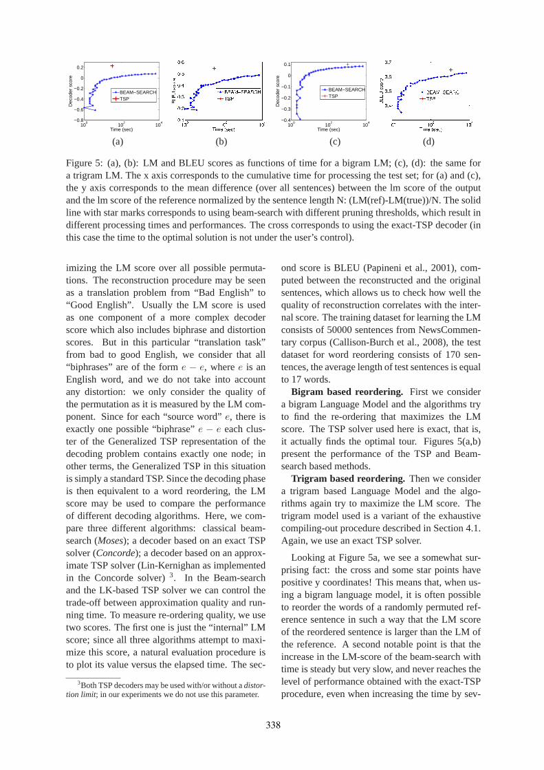
100
102
104−0.8
−0.6
−0.4
−0.2
0
0.2
Time (sec)
Dec
oder
sco
re
BEAM−SEARCHTSP
100
102
104−0.4
−0.3
−0.2
−0.1
0
0.1
Time (sec)
Dec
oder
sco
re
BEAM−SEARCHTSP
(a) (b) (c) (d)
Figure 5: (a), (b): LM and BLEU scores as functions of time for a bigramLM; (c), (d): the same fora trigram LM. The x axis corresponds to the cumulative time for processing the test set; for (a) and (c),the y axis corresponds to the mean difference (over all sentences) between the lm score of the outputand the lm score of the reference normalized by the sentence length N: (LM(ref)-LM(true))/N. The solidline with star marks corresponds to using beam-search with different pruning thresholds, which result indifferent processing times and performances. The cross corresponds to using the exact-TSP decoder (inthis case the time to the optimal solution is not under the user’s control).
imizing the LM score over all possible permuta-tions. The reconstruction procedure may be seenas a translation problem from “Bad English” to“Good English”. Usually the LM score is usedas one component of a more complex decoderscore which also includes biphrase and distortionscores. But in this particular “translation task”from bad to good English, we consider that all“biphrases” are of the forme − e, wheree is anEnglish word, and we do not take into accountany distortion: we only consider the quality ofthe permutation as it is measured by the LM com-ponent. Since for each “source word”e, there isexactly one possible “biphrase”e − e each clus-ter of the Generalized TSP representation of thedecoding problem contains exactly one node; inother terms, the Generalized TSP in this situationis simply a standard TSP. Since the decoding phaseis then equivalent to a word reordering, the LMscore may be used to compare the performanceof different decoding algorithms. Here, we com-pare three different algorithms: classical beam-search (Moses); a decoder based on an exact TSPsolver (Concorde); a decoder based on an approx-imate TSP solver (Lin-Kernighan as implementedin the Concorde solver)3. In the Beam-searchand the LK-based TSP solver we can control thetrade-off between approximation quality and run-ning time. To measure re-ordering quality, we usetwo scores. The first one is just the “internal” LMscore; since all three algorithms attempt to maxi-mize this score, a natural evaluation procedure isto plot its value versus the elapsed time. The sec-
3Both TSP decoders may be used with/or without adistor-tion limit; in our experiments we do not use this parameter.
ond score is BLEU (Papineni et al., 2001), com-puted between the reconstructed and the originalsentences, which allows us to check how well thequality of reconstruction correlates with the inter-nal score. The training dataset for learning the LMconsists of 50000 sentences from NewsCommen-tary corpus (Callison-Burch et al., 2008), the testdataset for word reordering consists of 170 sen-tences, the average length of test sentences is equalto 17 words.
Bigram based reordering. First we considera bigram Language Model and the algorithms tryto find the re-ordering that maximizes the LMscore. The TSP solver used here is exact, that is,it actually finds the optimal tour. Figures 5(a,b)present the performance of the TSP and Beam-search based methods.
Trigram based reordering. Then we considera trigram based Language Model and the algo-rithms again try to maximize the LM score. Thetrigram model used is a variant of the exhaustivecompiling-out procedure described in Section 4.1.Again, we use an exact TSP solver.
Looking at Figure 5a, we see a somewhat sur-prising fact: the cross and some star points havepositive y coordinates! This means that, when us-ing a bigram language model, it is often possibleto reorder the words of a randomly permuted ref-erence sentence in such a way that the LM scoreof the reordered sentence is larger than the LM ofthe reference. A second notable point is that theincrease in the LM-score of the beam-search withtime is steady but very slow, and never reaches thelevel of performance obtained with the exact-TSPprocedure, even when increasing the time by sev-
338

eral orders of magnitude. Also to be noted is thatthe solution obtained by the exact-TSP is provablythe optimum, which is almost never the case ofthe beam-search procedure. In Figure 5b, we re-port the BLEU score of the reordered sentencesin the test set relative to the original referencesentences. Here we see that the exact-TSP out-puts are closer to the references in terms of BLEUthan the beam-search solutions. Although the TSPoutput does not recover the reference sentences(it produces sentences with a slightly higher LMscore than the references), it does reconstruct thereferences better than the beam-search. The ex-periments with trigram language models (Figures5(c,d)) show similar trends to those with bigrams.
5.2 Translation experiments with a bigramlanguage model
In this section we consider two real translationtasks, namely, translation from English to French,trained on Europarl (Koehn et al., 2003) and trans-lation from German to Spanish training on theNewsCommentary corpus. For Europarl, the train-ing set includes 2.81 million sentences, and thetest set 500. For NewsCommentary the trainingset is smaller: around 63k sentences, with a testset of 500 sentences. Figure 6 presents Decoderand Bleu scores as functions of time for the twocorpuses.
Since in the real translation task, the size of theTSP graph is much larger than in the artificial re-ordering task (in our experiments the median sizeof the TSP graph was around 400 nodes, some-times growing up to 2000 nodes), directly apply-ing the exact TSP solver would take too long; in-stead we use the approximate LK algorithm andcompare it to Beam-Search. The efficiency of theLK algorithm can be significantly increased by us-ing a good initialization. To compare the quality ofthe LK and Beam-Search methods we take a roughinitial solution produced by the Beam-Search al-gorithm using a small value for the stack size andthen use it as initial point, both for the LK algo-rithm and for further Beam-Search optimization(where as before we vary the Beam-Search thresh-olds in order to trade quality for time).
In the case of the Europarl corpus, we observethat LK outperforms Beam-Search in terms of theDecoder score as well as in terms of the BLEUscore. Note that the difference between the two al-gorithms increases steeply at the beginning, which
means that we can significantly increase the qual-ity of the Beam-Search solution by using the LKalgorithm at a very small price. In addition, it isimportant to note that the BLEU scores obtained inthese experiments correspond to feature weights,in the log-linear model (1), that have been opti-mized for the Moses decoder, but not for the TSPdecoder: optimizing these parameters relatively tothe TSP decoder could improve its BLEU scoresstill further.
On the News corpus, again, LK outperformsBeam-Search in terms of the Decoder score. Thesituation with the BLEU score is more confuse.Both algorithms do not show any clear score im-provement with increasing running time whichsuggests that the decoder’s objective function isnot very well correlated with the BLEU score onthis corpus.
6 Future Work
In section 4.1, we described a general “compilingout” method for extending our TSP representationto handling trigram and N-gram language models,but we noted that the method may lead to combi-natorial explosion of the TSP graph. While thisproblem was manageable for the artificial mono-lingual word re-ordering (which had only one pos-sible translation for each source word), it be-comes unwieldy for the real translation experi-ments, which is why in this paper we only consid-ered bigram LMs for these experiments. However,we know how to handle this problem in principle,and we now describe a method that we plan to ex-periment with in the future.
To avoid the large number of artificial biphrasesas in 4.1, we perform anadaptive selection. Let ussuppose that(w, b) is a SMT decoding graph node,whereb is a biphrase containing only one word onthe target side. On the first step, when we evaluatethe traveling cost from(w, b) to (w′, b′), we takethe language model component equal to
minb′′ 6=b′,b
− log p(b′.v|b.e, b′′.e),
whereb′.v represents the first word of theb′ tar-get side, b.e is the only word of theb targetside, andb′′.e is the last word of theb′′ tar-get size. This procedure underestimates the totalcost of tour passing through biphrases that have asingle-word target. Therefore if the optimal tourpasses only through biphrases with more than one
339
103
104
105−273
−272.5
−272
−271.5
−271
Time (sec)
Dec
oder
sco
re
BEAM−SEARCHTSP (LK)
103
104
1050.18
0.185
0.19
Time (sec)
BLE
U s
core
BEAM−SEARCHTSP (LK)
103
104−414
−413.8
−413.6
−413.4
−413.2
−413
Time (sec)
Dec
oder
sco
re
TSP (LK)BEAM−SEARCH
103
1040.242
0.243
0.244
0.245
Time (sec)
BLE
U s
core
TSP (LK)BEAM−SEARCH
(a) (b) (c) (d)
Figure 6: (a), (b): Europarl corpus, translation from English to French; (c),(d): NewsCommentary cor-pus, translation from German to Spanish. Average value of the decoder and the BLEU scores (over 500test sentences) as a function of time. The trade-off quality/time in the case of LK is controlled by thenumber of iterations, and each point corresponds to a particular number of iterations, in our experimentsLK was run with a number of iterations varying between 2k and 170k. The same trade-off in the case ofBeam-Search is controlled by varying the beam thresholds.
word on their target side, then we are sure thatthis tour is also optimal in terms of the tri-gramlanguage model. Otherwise, if the optimal tourpasses through(w, b), whereb is a biphrase hav-ing a single-word target, we add only the extendedbiphrases related tob as we described in section4.1, and then we recompute the optimal tour. Iter-ating this procedure provably converges to an op-timal solution.
This powerful method, which was proposed in(Kam and Kopec, 1996; Popat et al., 2001) in thecontext of a finite-state model (but not of TSP),can be easily extended to N-gram situations, andtypically converges in a small number of itera-tions.
7 Conclusion
The main contribution of this paper has been topropose a transformation for an arbitrary phrase-based SMT decoding instance into a TSP instance.While certain similarities of SMT decoding andTSP were already pointed out in (Knight, 1999),where it was shown that any Traveling SalesmanProblem may be reformulated as an instance ofa (simplistic) SMT decoding task, and while cer-tain techniques used for TSP were then adapted toword-based SMT decoding (Germann et al., 2001;Tillmann and Ney, 2003; Tillmann, 2006), we arenot aware of any previous work that shows thatSMT decoding can be directly reformulated as aTSP. Beside the general interest of this transfor-mation for understanding decoding, it also opensthe door to direct application of the variety of ex-isting TSP algorithms to SMT. Our experimentson synthetic and real data show that fast TSP al-gorithms can handle selection and reordering in
SMT comparably or better than the state-of-the-art beam-search strategy, converging on solutionswith higher objective function in a shorter time.
The proposed method proceeds by first con-structing an AGTSP instance from the decodingproblem, and then converting this instance firstinto ATSP and finally into STSP. At this point, adirect application of the well known STSP solverConcorde(with Lin-Kernighan heuristic) alreadygives good results. We believe however that theremight exist even more efficient alternatives. In-stead of converting the AGTSP instance into aSTSP instance, it might prove better to use di-rectly algorithms expressly designed for ATSPor AGTSP. For instance, some of the algorithmstested in the context of theDIMACS implemen-tation challenge for ATSP (Johnson et al., 2002)might well prove superior. There is also active re-search around AGTSP algorithms. Recently neweffective methods based on a “memetic” strategy(Buriol et al., 2004; Gutin et al., 2008) have beenput forward. These methods combined with ourproposed formulation provide ready-to-use SMTdecoders, which it will be interesting to compare.
Acknowledgments
Thanks to Vassilina Nikoulina for her advice aboutrunning Moses on the test datasets.
340
References
David L. Applegate, Robert E. Bixby, Vasek Chvatal,and William J. Cook. 2005. Concordetsp solver. http://www.tsp.gatech.edu/concorde.html.
David L. Applegate, Robert E. Bixby, Vasek Chvatal,and William J. Cook. 2007.The Traveling Sales-man Problem: A Computational Study (PrincetonSeries in Applied Mathematics). Princeton Univer-sity Press, January.
Luciana Buriol, Paulo M. França, and Pablo Moscato.2004. A new memetic algorithm for the asymmetrictraveling salesman problem.Journal of Heuristics,10(5):483–506.
Chris Callison-Burch, Philipp Koehn, Christof Monz,Josh Schroeder, and Cameron Shaw Fordyce, edi-tors. 2008.Proceedings of the Third Workshop onSMT. ACL, Columbus, Ohio, June.
Ulrich Germann, Michael Jahr, Kevin Knight, andDaniel Marcu. 2001. Fast decoding and optimaldecoding for machine translation. InIn Proceedingsof ACL 39, pages 228–235.
Gregory Gutin, Daniel Karapetyan, and Krasnogor Na-talio. 2008. Memetic algorithm for the generalizedasymmetric traveling salesman problem. InNICSO2007, pages 199–210. Springer Berlin.
G. Gutin. 2003. Travelling salesman and related prob-lems. InHandbook of Graph Theory.
Hieu Hoang and Philipp Koehn. 2008. Design of theMoses decoder for statistical machine translation. InACL 2008 Software workshop, pages 58–65, Colum-bus, Ohio, June. ACL.
D.S. Johnson, G. Gutin, L.A. McGeoch, A. Yeo,W. Zhang, and A. Zverovich. 2002. Experimen-tal analysis of heuristics for the atsp. InThe Trav-elling Salesman Problem and Its Variations, pages445–487.
Anthony C. Kam and Gary E. Kopec. 1996. Documentimage decoding by heuristic search.IEEE Transac-tions on Pattern Analysis and Machine Intelligence,18:945–950.
Kevin Knight. 1999. Decoding complexity in word-replacement translation models.ComputationalLinguistics, 25:607–615.
Philipp Koehn, Franz Josef Och, and Daniel Marcu.2003. Statistical phrase-based translation. InNAACL 2003, pages 48–54, Morristown, NJ, USA.Association for Computational Linguistics.
Adam Lopez. 2008. Statistical machine translation.ACM Comput. Surv., 40(3):1–49.
C. Noon and J.C. Bean. 1993. An efficient transforma-tion of the generalized traveling salesman problem.INFOR, pages 39–44.
Kishore Papineni, Salim Roukos, Todd Ward, andWei J. Zhu. 2001. BLEU: a Method for AutomaticEvaluation of Machine Translation.IBM ResearchReport, RC22176.
Kris Popat, Daniel H. Greene, Justin K. Romberg, andDan S. Bloomberg. 2001. Adding linguistic con-straints to document image decoding: Comparingthe iterated complete path and stack algorithms.
Christoph Tillmann and Hermann Ney. 2003. Word re-ordering and a dynamic programming beam searchalgorithm for statistical machine translation.Com-put. Linguist., 29(1):97–133.
Christoph Tillmann. 2006. Efficient Dynamic Pro-gramming Search Algorithms For Phrase-BasedSMT. InWorkshop On Computationally Hard Prob-lems And Joint Inference In Speech And LanguageProcessing.
Wikipedia. 2009. Travelling Salesman Problem —Wikipedia, The Free Encyclopedia. [Online; ac-cessed 5-May-2009].
341
Proceedings of the 47th Annual Meeting of the ACL and the 4th IJCNLP of the AFNLP, pages 342–350,Suntec, Singapore, 2-7 August 2009. c©2009 ACL and AFNLP
Concise Integer Linear Programming Formulationsfor Dependency Parsing
André F. T. Martins∗† Noah A. Smith∗ Eric P. Xing∗∗School of Computer Science, Carnegie Mellon University, Pittsburgh, PA 15213, USA
†Instituto de Telecomunicações, Instituto Superior Técnico, Lisboa, Portugal{afm,nasmith,epxing}@cs.cmu.edu
Abstract
We formulate the problem of non-projective dependency parsing as apolynomial-sized integer linear pro-gram. Our formulation is able to handlenon-local output features in an efficientmanner; not only is it compatible withprior knowledge encoded as hard con-straints, it can also learn soft constraintsfrom data. In particular, our model is ableto learn correlations among neighboringarcs (siblings and grandparents), wordvalency, and tendencies toward nearly-projective parses. The model parametersare learned in a max-margin frameworkby employing a linear programmingrelaxation. We evaluate the performanceof our parser on data in several naturallanguages, achieving improvements overexisting state-of-the-art methods.
1 Introduction
Much attention has recently been devoted to in-teger linear programming (ILP) formulations ofNLP problems, with interesting results in appli-cations like semantic role labeling (Roth and Yih,2005; Punyakanok et al., 2004), dependency pars-ing (Riedel and Clarke, 2006), word alignmentfor machine translation (Lacoste-Julien et al.,2006), summarization (Clarke and Lapata, 2008),and coreference resolution (Denis and Baldridge,2007), among others. In general, the rationale forthe development of ILP formulations is to incorpo-rate non-local features or global constraints, whichare often difficult to handle with traditional algo-rithms. ILP formulations focus more on the mod-eling of problems, rather than algorithm design.While solving an ILP is NP-hard in general, fastsolvers are available today that make it a practicalsolution for many NLP problems.
This paper presents new, concise ILP formu-lations for projective and non-projective depen-
dency parsing. We believe that our formula-tions can pave the way for efficient exploitation ofglobal features and constraints in parsing applica-tions, leading to more powerful models. Riedeland Clarke (2006) cast dependency parsing asan ILP, but efficient formulations remain an openproblem. Our formulations offer the followingcomparative advantages:
• The numbers of variables and constraints arepolynomial in the sentence length, as opposed torequiring exponentially many constraints, elim-inating the need for incremental procedures likethe cutting-plane algorithm;
• LP relaxations permit fast online discriminativetraining of the constrained model;
• Soft constraints may be automatically learnedfrom data. In particular, our formulations han-dle higher-order arc interactions (like siblingsand grandparents), model word valency, and canlearn to favor nearly-projective parses.
We evaluate the performance of the new parserson standard parsing tasks in seven languages. Thetechniques that we present are also compatiblewith scenarios where expert knowledge is avail-able, for example in the form of hard or soft first-order logic constraints (Richardson and Domin-gos, 2006; Chang et al., 2008).
2 Dependency Parsing
2.1 Preliminaries
A dependency tree is a lightweight syntactic repre-sentation that attempts to capture functional rela-tionships between words. Lately, this formalismhas been used as an alternative to phrase-basedparsing for a variety of tasks, ranging from ma-chine translation (Ding and Palmer, 2005) to rela-tion extraction (Culotta and Sorensen, 2004) andquestion answering (Wang et al., 2007).
Let us first describe formally the set of legal de-pendency parse trees. Consider a sentence x =
342
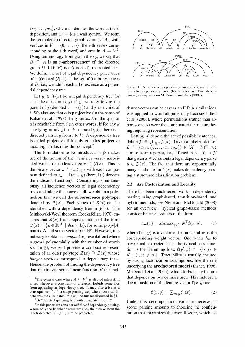
〈w0, . . . , wn〉, where wi denotes the word at the i-th position, and w0 = $ is a wall symbol. We formthe (complete1) directed graph D = 〈V,A〉, withvertices in V = {0, . . . , n} (the i-th vertex corre-sponding to the i-th word) and arcs in A = V 2.Using terminology from graph theory, we say thatB ⊆ A is an r-arborescence2 of the directedgraph D if 〈V,B〉 is a (directed) tree rooted at r.We define the set of legal dependency parse treesof x (denoted Y(x)) as the set of 0-arborescencesof D, i.e., we admit each arborescence as a poten-tial dependency tree.
Let y ∈ Y(x) be a legal dependency tree forx; if the arc a = 〈i, j〉 ∈ y, we refer to i as theparent of j (denoted i = π(j)) and j as a child ofi. We also say that a is projective (in the sense ofKahane et al., 1998) if any vertex k in the span ofa is reachable from i (in other words, if for any ksatisfying min(i, j) < k < max(i, j), there is adirected path in y from i to k). A dependency treeis called projective if it only contains projectivearcs. Fig. 1 illustrates this concept.3
The formulation to be introduced in §3 makesuse of the notion of the incidence vector associ-ated with a dependency tree y ∈ Y(x). This isthe binary vector z , 〈za〉a∈A with each compo-nent defined as za = I(a ∈ y) (here, I(.) denotesthe indicator function). Considering simultane-ously all incidence vectors of legal dependencytrees and taking the convex hull, we obtain a poly-hedron that we call the arborescence polytope,denoted by Z(x). Each vertex of Z(x) can beidentified with a dependency tree in Y(x). TheMinkowski-Weyl theorem (Rockafellar, 1970) en-sures that Z(x) has a representation of the formZ(x) = {z ∈ R|A| | Az ≤ b}, for some p-by-|A|matrix A and some vector b in Rp. However, it isnot easy to obtain a compact representation (wherep grows polynomially with the number of wordsn). In §3, we will provide a compact represen-tation of an outer polytope Z̄(x) ⊇ Z(x) whoseinteger vertices correspond to dependency trees.Hence, the problem of finding the dependency treethat maximizes some linear function of the inci-
1The general case where A ⊆ V 2 is also of interest; itarises whenever a constraint or a lexicon forbids some arcsfrom appearing in dependency tree. It may also arise as aconsequence of a first-stage pruning step where some candi-date arcs are eliminated; this will be further discussed in §4.
2Or “directed spanning tree with designated root r.”3In this paper, we consider unlabeled dependency parsing,
where only the backbone structure (i.e., the arcs without thelabels depicted in Fig. 1) is to be predicted.
Figure 1: A projective dependency graph.
Figure 2: Non-projective dependency graph.
those that assume each dependency decision is in-dependent modulo the global structural constraintthat dependency graphs must be trees. Such mod-els are commonly referred to as edge-factored sincetheir parameters factor relative to individual edgesof the graph (Paskin, 2001; McDonald et al.,2005a). Edge-factored models have many computa-tional benefits, most notably that inference for non-projective dependency graphs can be achieved inpolynomial time (McDonald et al., 2005b). The pri-mary problem in treating each dependency as in-dependent is that it is not a realistic assumption.Non-local information, such as arity (or valency)and neighbouring dependencies, can be crucial toobtaining high parsing accuracies (Klein and Man-ning, 2002; McDonald and Pereira, 2006). How-ever, in the data-driven parsing setting this can bepartially adverted by incorporating rich feature rep-resentations over the input (McDonald et al., 2005a).
The goal of this work is to further our currentunderstanding of the computational nature of non-projective parsing algorithms for both learning andinference within the data-driven setting. We start byinvestigating and extending the edge-factored modelof McDonald et al. (2005b). In particular, we ap-peal to the Matrix Tree Theorem for multi-digraphsto design polynomial-time algorithms for calculat-ing both the partition function and edge expecta-tions over all possible dependency graphs for a givensentence. To motivate these algorithms, we showthat they can be used in many important learningand inference problems including min-risk decod-ing, training globally normalized log-linear mod-els, syntactic language modeling, and unsupervised
learning via the EM algorithm – none of which havepreviously been known to have exact non-projectiveimplementations.
We then switch focus to models that account fornon-local information, in particular arity and neigh-bouring parse decisions. For systems that model ar-ity constraints we give a reduction from the Hamilto-nian graph problem suggesting that the parsing prob-lem is intractable in this case. For neighbouringparse decisions, we extend the work of McDonaldand Pereira (2006) and show that modeling verticalneighbourhoods makes parsing intractable in addi-tion to modeling horizontal neighbourhoods. A con-sequence of these results is that it is unlikely thatexact non-projective dependency parsing is tractablefor any model assumptions weaker than those madeby the edge-factored models.
1.1 Related WorkThere has been extensive work on data-driven de-pendency parsing for both projective parsing (Eis-ner, 1996; Paskin, 2001; Yamada and Matsumoto,2003; Nivre and Scholz, 2004; McDonald et al.,2005a) and non-projective parsing systems (Nivreand Nilsson, 2005; Hall and Nóvák, 2005; McDon-ald et al., 2005b). These approaches can often beclassified into two broad categories. In the first cat-egory are those methods that employ approximateinference, typically through the use of linear timeshift-reduce parsing algorithms (Yamada and Mat-sumoto, 2003; Nivre and Scholz, 2004; Nivre andNilsson, 2005). In the second category are thosethat employ exhaustive inference algorithms, usu-ally by making strong independence assumptions, asis the case for edge-factored models (Paskin, 2001;McDonald et al., 2005a; McDonald et al., 2005b).Recently there have also been proposals for exhaus-tive methods that weaken the edge-factored assump-tion, including both approximate methods (McDon-ald and Pereira, 2006) and exact methods through in-teger linear programming (Riedel and Clarke, 2006)or branch-and-bound algorithms (Hirakawa, 2006).
For grammar based models there has been limitedwork on empirical systems for non-projective pars-ing systems, notable exceptions include the workof Wang and Harper (2004). Theoretical studies ofnote include the work of Neuhaus and Böker (1997)showing that the recognition problem for a mini-
$ Figure 1: A projective dependency graph.
Figure 2: Non-projective dependency graph.
those that assume each dependency decision is in-dependent modulo the global structural constraintthat dependency graphs must be trees. Such mod-els are commonly referred to as edge-factored sincetheir parameters factor relative to individual edgesof the graph (Paskin, 2001; McDonald et al.,2005a). Edge-factored models have many computa-tional benefits, most notably that inference for non-projective dependency graphs can be achieved inpolynomial time (McDonald et al., 2005b). The pri-mary problem in treating each dependency as in-dependent is that it is not a realistic assumption.Non-local information, such as arity (or valency)and neighbouring dependencies, can be crucial toobtaining high parsing accuracies (Klein and Man-ning, 2002; McDonald and Pereira, 2006). How-ever, in the data-driven parsing setting this can bepartially adverted by incorporating rich feature rep-resentations over the input (McDonald et al., 2005a).
The goal of this work is to further our currentunderstanding of the computational nature of non-projective parsing algorithms for both learning andinference within the data-driven setting. We start byinvestigating and extending the edge-factored modelof McDonald et al. (2005b). In particular, we ap-peal to the Matrix Tree Theorem for multi-digraphsto design polynomial-time algorithms for calculat-ing both the partition function and edge expecta-tions over all possible dependency graphs for a givensentence. To motivate these algorithms, we showthat they can be used in many important learningand inference problems including min-risk decod-ing, training globally normalized log-linear mod-els, syntactic language modeling, and unsupervised
learning via the EM algorithm – none of which havepreviously been known to have exact non-projectiveimplementations.
We then switch focus to models that account fornon-local information, in particular arity and neigh-bouring parse decisions. For systems that model ar-ity constraints we give a reduction from the Hamilto-nian graph problem suggesting that the parsing prob-lem is intractable in this case. For neighbouringparse decisions, we extend the work of McDonaldand Pereira (2006) and show that modeling verticalneighbourhoods makes parsing intractable in addi-tion to modeling horizontal neighbourhoods. A con-sequence of these results is that it is unlikely thatexact non-projective dependency parsing is tractablefor any model assumptions weaker than those madeby the edge-factored models.
1.1 Related WorkThere has been extensive work on data-driven de-pendency parsing for both projective parsing (Eis-ner, 1996; Paskin, 2001; Yamada and Matsumoto,2003; Nivre and Scholz, 2004; McDonald et al.,2005a) and non-projective parsing systems (Nivreand Nilsson, 2005; Hall and Nóvák, 2005; McDon-ald et al., 2005b). These approaches can often beclassified into two broad categories. In the first cat-egory are those methods that employ approximateinference, typically through the use of linear timeshift-reduce parsing algorithms (Yamada and Mat-sumoto, 2003; Nivre and Scholz, 2004; Nivre andNilsson, 2005). In the second category are thosethat employ exhaustive inference algorithms, usu-ally by making strong independence assumptions, asis the case for edge-factored models (Paskin, 2001;McDonald et al., 2005a; McDonald et al., 2005b).Recently there have also been proposals for exhaus-tive methods that weaken the edge-factored assump-tion, including both approximate methods (McDon-ald and Pereira, 2006) and exact methods through in-teger linear programming (Riedel and Clarke, 2006)or branch-and-bound algorithms (Hirakawa, 2006).
For grammar based models there has been limitedwork on empirical systems for non-projective pars-ing systems, notable exceptions include the workof Wang and Harper (2004). Theoretical studies ofnote include the work of Neuhaus and Böker (1997)showing that the recognition problem for a mini-
$
Figure 1: A projective dependency parse (top), and a non-projective dependency parse (bottom) for two English sen-tences; examples from McDonald and Satta (2007).
dence vectors can be cast as an ILP. A similar ideawas applied to word alignment by Lacoste-Julienet al. (2006), where permutations (rather than ar-borescences) were the combinatorial structure be-ing requiring representation.
Letting X denote the set of possible sentences,define Y ,
⋃x∈X Y(x). Given a labeled dataset
L , 〈〈x1, y1〉, . . . , 〈xm, ym〉〉 ∈ (X × Y)m, weaim to learn a parser, i.e., a function h : X → Ythat given x ∈ X outputs a legal dependency parsey ∈ Y(x). The fact that there are exponentiallymany candidates in Y(x) makes dependency pars-ing a structured classification problem.
2.2 Arc Factorization and LocalityThere has been much recent work on dependencyparsing using graph-based, transition-based, andhybrid methods; see Nivre and McDonald (2008)for an overview. Typical graph-based methodsconsider linear classifiers of the form
hw(x) = argmaxy∈Y w>f(x, y), (1)
where f(x, y) is a vector of features and w is thecorresponding weight vector. One wants hw tohave small expected loss; the typical loss func-tion is the Hamming loss, `(y′; y) , |{〈i, j〉 ∈y′ : 〈i, j〉 /∈ y}|. Tractability is usually ensuredby strong factorization assumptions, like the oneunderlying the arc-factored model (Eisner, 1996;McDonald et al., 2005), which forbids any featurethat depends on two or more arcs. This induces adecomposition of the feature vector f(x, y) as:
f(x, y) =∑
a∈y fa(x). (2)
Under this decomposition, each arc receives ascore; parsing amounts to choosing the configu-ration that maximizes the overall score, which, as
343
shown by McDonald et al. (2005), is an instanceof the maximal arborescence problem. Combi-natorial algorithms (Chu and Liu, 1965; Edmonds,1967) can solve this problem in cubic time.4 Ifthe dependency parse trees are restricted to beprojective, cubic-time algorithms are available viadynamic programming (Eisner, 1996). While inthe projective case, the arc-factored assumptioncan be weakened in certain ways while maintain-ing polynomial parser runtime (Eisner and Satta,1999), the same does not happen in the nonprojec-tive case, where finding the highest-scoring treebecomes NP-hard (McDonald and Satta, 2007).Approximate algorithms have been employed tohandle models that are not arc-factored (althoughfeatures are still fairly local): McDonald andPereira (2006) adopted an approximation basedon O(n3) projective parsing followed by a hill-climbing algorithm to rearrange arcs, and Smithand Eisner (2008) proposed an algorithm based onloopy belief propagation.
3 Dependency Parsing as an ILP
Our approach will build a graph-based parserwithout the drawback of a restriction to local fea-tures. By formulating inference as an ILP, non-local features can be easily accommodated in ourmodel; furthermore, by using a relaxation tech-nique we can still make learning tractable. The im-pact of LP-relaxed inference in the learning prob-lem was studied elsewhere (Martins et al., 2009).
A linear program (LP) is an optimization prob-lem of the form
minx∈Rd c>xs.t. Ax ≤ b.
(3)
If the problem is feasible, the optimum is attainedat a vertex of the polyhedron that defines the con-straint space. If we add the constraint x ∈ Zd, thenthe above is called an integer linear program(ILP). For some special parameter settings—e.g.,when b is an integer vector and A is totally uni-modular5—all vertices of the constraining polyhe-dron are integer points; in these cases, the integerconstraint may be suppressed and (3) is guaran-teed to have integer solutions (Schrijver, 2003).Of course, this need not happen: solving a gen-eral ILP is an NP-complete problem. Despite this
4There is also a quadratic algorithm due to Tarjan (1977).5A matrix is called totally unimodular if the determinants
of each square submatrix belong to {0, 1,−1}.
fact, fast solvers are available today that make thisa practical solution for many problems. Their per-formance depends on the dimensions and degreeof sparsity of the constraint matrix A.
Riedel and Clarke (2006) proposed an ILP for-mulation for dependency parsing which refinesthe arc-factored model by imposing linguisticallymotivated “hard” constraints that forbid some arcconfigurations. Their formulation includes an ex-ponential number of constraints—one for eachpossible cycle. Since it is intractable to throwin all constraints at once, they propose a cutting-plane algorithm, where the cycle constraints areonly invoked when violated by the current solu-tion. The resulting algorithm is still slow, and anarc-factored model is used as a surrogate duringtraining (i.e., the hard constraints are only used attest time), which implies a discrepancy betweenthe model that is optimized and the one that is ac-tually going to be used.
Here, we propose ILP formulations that elim-inate the need for cycle constraints; in fact, theyrequire only a polynomial number of constraints.Not only does our model allow expert knowledgeto be injected in the form of constraints, it is alsocapable of learning soft versions of those con-straints from data; indeed, it can handle featuresthat are not arc-factored (correlating, for exam-ple, siblings and grandparents, modeling valency,or preferring nearly projective parses). While, aspointed out by McDonald and Satta (2007), theinclusion of these features makes inference NP-hard, by relaxing the integer constraints we obtainapproximate algorithms that are very efficient andcompetitive with state-of-the-art methods. In thispaper, we focus on unlabeled dependency parsing,for clarity of exposition. If it is extended to labeledparsing (a straightforward extension), our formu-lation fully subsumes that of Riedel and Clarke(2006), since it allows using the same hard con-straints and features while keeping the ILP poly-nomial in size.
3.1 The Arborescence Polytope
We start by describing our constraint space. Ourformulations rely on a concise polyhedral repre-sentation of the set of candidate dependency parsetrees, as sketched in §2.1. This will be accom-plished by drawing an analogy with a networkflow problem.
Let D = 〈V,A〉 be the complete directed graph
344
associated with a sentence x ∈ X , as stated in§2. A subgraph y = 〈V,B〉 is a legal dependencytree (i.e., y ∈ Y(x)) if and only if the followingconditions are met:
1. Each vertex in V \ {0} must have exactly oneincoming arc in B,
2. 0 has no incoming arcs in B,
3. B does not contain cycles.
For each vertex v ∈ V , let δ−(v) , {〈i, j〉 ∈A | j = v} denote its set of incoming arcs, andδ+(v) , {〈i, j〉 ∈ A | i = v} denote its set ofoutgoing arcs. The two first conditions can be eas-ily expressed by linear constraints on the incidencevector z:∑
a∈δ−(j) za = 1, j ∈ V \ {0} (4)∑a∈δ−(0) za = 0 (5)
Condition 3 is somewhat harder to express. Ratherthan adding exponentially many constraints, onefor each potential cycle (like Riedel and Clarke,2006), we equivalently replace condition 3 by
3′. B is connected.
Note that conditions 1-2-3 are equivalent to 1-2-3′, in the sense that both define the same set Y(x).However, as we will see, the latter set of condi-tions is more convenient. Connectedness of graphscan be imposed via flow constraints (by requir-ing that, for any v ∈ V \ {0}, there is a directedpath in B connecting 0 to v). We adapt the singlecommodity flow formulation for the (undirected)minimum spanning tree problem, due to Magnantiand Wolsey (1994), that requires O(n2) variablesand constraints. Under this model, the root nodemust send one unit of flow to every other node.By making use of extra variables, φ , 〈φa〉a∈A,to denote the flow of commodities through eacharc, we are led to the following constraints in ad-dition to Eqs. 4–5 (we denote U , [0, 1], andB , {0, 1} = U ∩ Z):
• Root sends flow n:∑a∈δ+(0) φa = n (6)
• Each node consumes one unit of flow:∑a∈δ−(j)
φa −∑
a∈δ+(j)
φa = 1, j ∈ V \ {0} (7)
• Flow is zero on disabled arcs:
φa ≤ nza, a ∈ A (8)
• Each arc indicator lies in the unit interval:
za ∈ U, a ∈ A. (9)
These constraints project an outer bound of the ar-borescence polytope, i.e.,
Z̄(x) , {z ∈ R|A| | (z,φ) satisfy (4–9)}⊇ Z(x). (10)
Furthermore, the integer points of Z̄(x) are pre-cisely the incidence vectors of dependency treesin Y(x); these are obtained by replacing Eq. 9 by
za ∈ B, a ∈ A. (11)
3.2 Arc-Factored ModelGiven our polyhedral representation of (an outerbound of) the arborescence polytope, we cannow formulate dependency parsing with an arc-factored model as an ILP. By storing the arc-local feature vectors into the columns of a matrixF(x) , [fa(x)]a∈A, and defining the score vec-tor s , F(x)>w (each entry is an arc score) theinference problem can be written as
maxy∈Y(x)
w>f(x, y) = maxz∈Z(x)
w>F(x)z
= maxz,φ
s>z
s.t. A
[zφ
]≤ b
z ∈ B(12)
where A is a sparse constraint matrix (withO(|A|)non-zero elements), and b is the constraint vec-tor; A and b encode the constraints (4–9). Thisis an ILP with O(|A|) variables and constraints(hence, quadratic in n); if we drop the integerconstraint the problem becomes the LP relaxation.As is, this formulation is no more attractive thansolving the problem with the existing combinato-rial algorithms discussed in §2.2; however, we cannow start adding non-local features to build a morepowerful model.
3.3 Sibling and Grandparent FeaturesTo cope with higher-order features of the formfa1,...,aK (x) (i.e., features whose values depend onthe simultaneous inclusion of arcs a1, . . . , aK on
345

a candidate dependency tree), we employ a lin-earization trick (Boros and Hammer, 2002), defin-ing extra variables za1...aK , za1 ∧ . . .∧zaK . Thislogical relation can be expressed by the followingO(K) agreement constraints:6
za1...aK ≤ zai , i = 1, . . . ,Kza1...aK ≥
∑Ki=1 zai −K + 1. (13)
As shown by McDonald and Pereira (2006) andCarreras (2007), the inclusion of features thatcorrelate sibling and grandparent arcs may behighly beneficial, even if doing so requires resort-ing to approximate algorithms.7 Define Rsibl ,{〈i, j, k〉 | 〈i, j〉 ∈ A, 〈i, k〉 ∈ A} and Rgrand ,{〈i, j, k〉 | 〈i, j〉 ∈ A, 〈j, k〉 ∈ A}. To includesuch features in our formulation, we need to addextra variables zsibl , 〈zr〉r∈Rsibl and zgrand ,〈zr〉r∈Rgrand that indicate the presence of siblingand grandparent arcs. Observe that these indica-tor variables are conjunctions of arc indicator vari-ables, i.e., zsibl
ijk = zij ∧ zik and zgrandijk = zij ∧ zjk.
Hence, these features can be handled in our formu-lation by adding the following O(|A| · |V |) vari-ables and constraints:
zsiblijk ≤ zij , zsibl
ijk ≤ zik, zsiblijk ≥ zij + zik − 1
(14)for all triples 〈i, j, k〉 ∈ Rsibl, and
zgrandijk ≤ zij , z
grandijk ≤ zjk, z
grandijk ≥ zij+zjk−1
(15)for all triples 〈i, j, k〉 ∈ Rgrand. Let R , A ∪Rsibl ∪ Rgrand; by redefining z , 〈zr〉r∈R andF(x) , [fr(x)]r∈R, we may express our inferenceproblem as in Eq. 12, with O(|A| · |V |) variablesand constraints.
Notice that the strategy just described to han-dle sibling features is not fully compatible withthe features proposed by Eisner (1996) for pro-jective parsing, as the latter correlate only con-secutive siblings and are also able to place spe-cial features on the first child of a given word.The ability to handle such “ordered” features isintimately associated with Eisner’s dynamic pro-gramming parsing algorithm and with the Marko-vian assumptions made explicitly by his genera-tive model. We next show how similar features
6Actually, any logical condition can be encoded with lin-ear constraints involving binary variables; see e.g. Clarke andLapata (2008) for an overview.
7By sibling features we mean features that depend onpairs of sibling arcs (i.e., of the form 〈i, j〉 and 〈i, k〉); bygrandparent features we mean features that depend on pairsof grandparent arcs (of the form 〈i, j〉 and 〈j, k〉).
can be incorporated in our model by adding “dy-namic” constraints to our ILP. Define:
znext siblijk ,
1 if 〈i, j〉 and 〈i, k〉 are
consecutive siblings,0 otherwise,
zfirst childij ,
{1 if j is the first child of i,0 otherwise.
Suppose (without loss of generality) that i < j <k ≤ n. We could naively compose the constraints(14) with additional linear constraints that encodethe logical relation
znext siblijk = zsibl
ijk ∧∧
j<l<k ¬zil,
but this would yield a constraint matrix withO(n4) non-zero elements. Instead, we define aux-iliary variables βjk and γij :
βjk =
{1, if ∃l s.t. π(l) = π(j) < j < l < k0, otherwise,
γij =
{1, if ∃k s.t. i < k < j and 〈i, k〉 ∈ y0, otherwise.
(16)
Then, we have that znext siblijk = zsibl
ijk ∧ (¬βjk) andzfirst childij = zij∧(¬γij), which can be encoded via
znext siblijk ≤ zsibl
ijk zfirst childij ≤ zij
znext siblijk ≤ 1− βjk zfirst child
ij ≤ 1− γij
znext siblijk ≥ zsibl
ijk − βjk zfirst childij ≥ zij − γij
The following “dynamic” constraints encode thelogical relations for the auxiliary variables (16):
βj(j+1) = 0 γi(i+1) = 0βj(k+1) ≥ βjk γi(j+1) ≥ γij
βj(k+1) ≥∑i<j
zsiblijk γi(j+1) ≥ zij
βj(k+1) ≤ βjk +∑i<j
zsiblijk γi(j+1) ≤ γij + zij
Auxiliary variables and constraints are definedanalogously for the case n ≥ i > j > k. Thisresults in a sparser constraint matrix, with onlyO(n3) non-zero elements.
3.4 Valency FeaturesA crucial fact about dependency grammars is thatwords have preferences about the number and ar-rangement of arguments and modifiers they ac-cept. Therefore, it is desirable to include features
346

that indicate, for a candidate arborescence, howmany outgoing arcs depart from each vertex; de-note these quantities by vi ,
∑a∈δ+(i) za, for
each i ∈ V . We call vi the valency of the ith ver-tex. We add valency indicators zval
ik , I(vi = k)for i ∈ V and k = 0, . . . , n− 1. This way, we areable to penalize candidate dependency trees thatassign unusual valencies to some of their vertices,by specifying a individual cost for each possiblevalue of valency. The following O(|V |2) con-straints encode the agreement between valency in-dicators and the other variables:∑n−1
k=0 kzvalik =
∑a∈δ+(i) za, i ∈ V (17)∑n−1
k=0 zvalik = 1, i ∈ Vzvalik ≥ 0, i ∈ V, k ∈ {0, . . . , n− 1}
3.5 Projectivity FeaturesFor most languages, dependency parse trees tendto be nearly projective (cf. Buchholz and Marsi,2006). We wish to make our model capable oflearning to prefer “nearly” projective parses when-ever that behavior is observed in the data.
The multicommodity directed flow model ofMagnanti and Wolsey (1994) is a refinement of themodel described in §3.1 which offers a compactand elegant way to indicate nonprojective arcs, re-quiring O(n3) variables and constraints. In thismodel, every node k 6= 0 defines a commodity:one unit of commodity k originates at the rootnode and must be delivered to node k; the vari-able φk
ij denotes the flow of commodity k in arc〈i, j〉. We first replace (4–9) by (18–22):
• The root sends one unit of commodity to eachnode:∑
a∈δ−(0)
φka −
∑a∈δ+(0)
φka = −1, k ∈ V \ {0} (18)
• Any node consumes its own commodity and noother:∑
a∈δ−(j)
φka −
∑a∈δ+(j)
φka = δk
j , j, k ∈ V \ {0} (19)
where δkj , I(j = k) is the Kronecker delta.
• Disabled arcs do not carry any flow:
φka ≤ za, a ∈ A, k ∈ V (20)
• There are exactly n enabled arcs:∑a∈A za = n (21)
• All variables lie in the unit interval:
za ∈ U, φka ∈ U, a ∈ A, k ∈ V (22)
We next define auxiliary variables ψjk that indi-cate if there is a path from j to k. Since each ver-tex except the root has only one incoming arc, thefollowing linear equalities are enough to describethese new variables:
ψjk =∑
a∈δ−(j) φka, j, k ∈ V \ {0}
ψ0k = 1, k ∈ V \ {0}. (23)
Now, define indicators znp , 〈znpa 〉a∈A, where
znpa , I(a ∈ y and a is nonprojective).
From the definition of projective arcs in §2.1, wehave that znp
a = 1 if and only if the arc is active(za = 1) and there is some vertex k in the span ofa = 〈i, j〉 such that ψik = 0. We are led to thefollowing O(|A| · |V |) constraints for 〈i, j〉 ∈ A:
znpij ≤ zij
znpij ≥ zij − ψik, min(i, j) ≤ k ≤ max(i, j)
znpij ≤ −
∑max(i,j)−1k=min(i,j)+1 ψik + |j − i| − 1
There are other ways to introduce nonprojectiv-ity indicators and alternative definitions of “non-projective arc.” For example, by using dynamicconstraints of the same kind as those in §3.3,we can indicate arcs that “cross” other arcs withO(n3) variables and constraints, and a cubic num-ber of non-zero elements in the constraint matrix(omitted for space).
3.6 Projective ParsingIt would be straightforward to adapt the con-straints in §3.5 to allow only projective parse trees:simply force znp
a = 0 for any a ∈ A. But there aremore efficient ways of accomplish this. While it isdifficult to impose projectivity constraints or cycleconstraints individually, there is a simpler way ofimposing both. Consider 3 (or 3′) from §3.1.
Proposition 1 Replace condition 3 (or 3′) with
3′′. If 〈i, j〉 ∈ B, then, for any k = 1, . . . , nsuch that k 6= j, the parent of k must satisfy(defining i′ , min(i, j) and j′ , max(i, j)):i′ ≤ π(k) ≤ j′, if i′ < k < j′,π(k) < i′ ∨ π(k) > j′, if k < i′ or k > j′
or k = i.
347

Then, Y(x) will be redefined as the set of projec-tive dependency parse trees.
We omit the proof for space. Conditions 1, 2, and3′′ can be encoded with O(n2) constraints.
4 Experiments
We report experiments on seven languages, six(Danish, Dutch, Portuguese, Slovene, Swedishand Turkish) from the CoNLL-X shared task(Buchholz and Marsi, 2006), and one (English)from the CoNLL-2008 shared task (Surdeanu etal., 2008).8 All experiments are evaluated usingthe unlabeled attachment score (UAS), using thedefault settings.9 We used the same arc-factoredfeatures as McDonald et al. (2005) (included in theMSTParser toolkit10); for the higher-order modelsdescribed in §3.3–3.5, we employed simple higherorder features that look at the word, part-of-speechtag, and (if available) morphological informationof the words being correlated through the indica-tor variables. For scalability (and noting that someof the models require O(|V | · |A|) constraints andvariables, which, when A = V 2, grows cubicallywith the number of words), we first prune the basegraph by running a simple algorithm that ranks thek-best candidate parents for each word in the sen-tence (we set k = 10); this reduces the number ofcandidate arcs to |A| = kn.11 This strategy is sim-ilar to the one employed by Carreras et al. (2008)to prune the search space of the actual parser. Theranker is a local model trained using a max-margincriterion; it is arc-factored and not subject to anystructural constraints, so it is very fast.
The actual parser was trained via the onlinestructured passive-aggressive algorithm of Cram-mer et al. (2006); it differs from the 1-best MIRAalgorithm of McDonald et al. (2005) by solv-ing a sequence of loss-augmented inference prob-lems.12 The number of iterations was set to 10.
The results are summarized in Table 1; for thesake of comparison, we reproduced three strong
8We used the provided train/test splits except for English,for which we tested on the development partition. For train-ing, sentences longer than 80 words were discarded. For test-ing, all sentences were kept (the longest one has length 118).
9http://nextens.uvt.nl/∼conll/software.html
10http://sourceforge.net/projects/mstparser
11Note that, unlike reranking approaches, there are still ex-ponentially many candidate parse trees after pruning. Theoracle constrained to pick parents from these lists achieves> 98% in every case.
12The loss-augmented inference problem can also be ex-pressed as an LP for Hamming loss functions that factor overarcs; we refer to Martins et al. (2009) for further details.
baselines, all of them state-of-the-art parsers basedon non-arc-factored models: the second ordermodel of McDonald and Pereira (2006), the hy-brid model of Nivre and McDonald (2008), whichcombines a (labeled) transition-based and a graph-based parser, and a refinement of the latter, dueto Martins et al. (2008), which attempts to ap-proximate non-local features.13 We did not repro-duce the model of Riedel and Clarke (2006) sincethe latter is tailored for labeled dependency pars-ing; however, experiments reported in that paperfor Dutch (and extended to other languages in theCoNLL-X task) suggest that their model performsworse than our three baselines.
By looking at the middle four columns, we cansee that adding non-arc-factored features makesthe models more accurate, for all languages. Withthe exception of Portuguese, the best results areachieved with the full set of features. We canalso observe that, for some languages, the valencyfeatures do not seem to help. Merely modelingthe number of dependents of a word may not beas valuable as knowing what kinds of dependentsthey are (for example, distinguishing among argu-ments and adjuncts).
Comparing with the baselines, we observe thatour full model outperforms that of McDonald andPereira (2006), and is in line with the most ac-curate dependency parsers (Nivre and McDonald,2008; Martins et al., 2008), obtained by com-bining transition-based and graph-based parsers.14
Notice that our model, compared with these hy-brid parsers, has the advantage of not requiring anensemble configuration (eliminating, for example,the need to tune two parsers). Unlike the ensem-bles, it directly handles non-local output featuresby optimizing a single global objective. Perhapsmore importantly, it makes it possible to exploitexpert knowledge through the form of hard globalconstraints. Although not pursued here, the samekind of constraints employed by Riedel and Clarke(2006) can straightforwardly fit into our model,after extending it to perform labeled dependencyparsing. We believe that a careful design of fea-
13Unlike our model, the hybrid models used here as base-lines make use of the dependency labels at training time; in-deed, the transition-based parser is trained to predict a la-beled dependency parse tree, and the graph-based parser usethese predicted labels as input features. Our model ignoresthis information at training time; therefore, this comparisonis slightly unfair to us.
14See also Zhang and Clark (2008) for a different approachthat combines transition-based and graph-based methods.
348
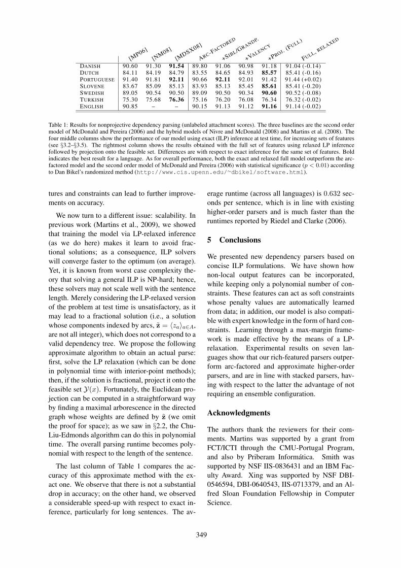
[MP06]
[NM08]
[MDSX08]
ARC-FACTORED
+SIBL/GRANDP.
+VALENCY
+PROJ. (FULL)
FULL, RELAXED
DANISH 90.60 91.30 91.54 89.80 91.06 90.98 91.18 91.04 (-0.14)DUTCH 84.11 84.19 84.79 83.55 84.65 84.93 85.57 85.41 (-0.16)PORTUGUESE 91.40 91.81 92.11 90.66 92.11 92.01 91.42 91.44 (+0.02)SLOVENE 83.67 85.09 85.13 83.93 85.13 85.45 85.61 85.41 (-0.20)SWEDISH 89.05 90.54 90.50 89.09 90.50 90.34 90.60 90.52 (-0.08)TURKISH 75.30 75.68 76.36 75.16 76.20 76.08 76.34 76.32 (-0.02)ENGLISH 90.85 – – 90.15 91.13 91.12 91.16 91.14 (-0.02)
Table 1: Results for nonprojective dependency parsing (unlabeled attachment scores). The three baselines are the second ordermodel of McDonald and Pereira (2006) and the hybrid models of Nivre and McDonald (2008) and Martins et al. (2008). Thefour middle columns show the performance of our model using exact (ILP) inference at test time, for increasing sets of features(see §3.2–§3.5). The rightmost column shows the results obtained with the full set of features using relaxed LP inferencefollowed by projection onto the feasible set. Differences are with respect to exact inference for the same set of features. Boldindicates the best result for a language. As for overall performance, both the exact and relaxed full model outperform the arc-factored model and the second order model of McDonald and Pereira (2006) with statistical significance (p < 0.01) accordingto Dan Bikel’s randomized method (http://www.cis.upenn.edu/∼dbikel/software.html).
tures and constraints can lead to further improve-ments on accuracy.
We now turn to a different issue: scalability. Inprevious work (Martins et al., 2009), we showedthat training the model via LP-relaxed inference(as we do here) makes it learn to avoid frac-tional solutions; as a consequence, ILP solverswill converge faster to the optimum (on average).Yet, it is known from worst case complexity the-ory that solving a general ILP is NP-hard; hence,these solvers may not scale well with the sentencelength. Merely considering the LP-relaxed versionof the problem at test time is unsatisfactory, as itmay lead to a fractional solution (i.e., a solutionwhose components indexed by arcs, z̃ = 〈za〉a∈A,are not all integer), which does not correspond to avalid dependency tree. We propose the followingapproximate algorithm to obtain an actual parse:first, solve the LP relaxation (which can be donein polynomial time with interior-point methods);then, if the solution is fractional, project it onto thefeasible set Y(x). Fortunately, the Euclidean pro-jection can be computed in a straightforward wayby finding a maximal arborescence in the directedgraph whose weights are defined by z̃ (we omitthe proof for space); as we saw in §2.2, the Chu-Liu-Edmonds algorithm can do this in polynomialtime. The overall parsing runtime becomes poly-nomial with respect to the length of the sentence.
The last column of Table 1 compares the ac-curacy of this approximate method with the ex-act one. We observe that there is not a substantialdrop in accuracy; on the other hand, we observeda considerable speed-up with respect to exact in-ference, particularly for long sentences. The av-
erage runtime (across all languages) is 0.632 sec-onds per sentence, which is in line with existinghigher-order parsers and is much faster than theruntimes reported by Riedel and Clarke (2006).
5 Conclusions
We presented new dependency parsers based onconcise ILP formulations. We have shown hownon-local output features can be incorporated,while keeping only a polynomial number of con-straints. These features can act as soft constraintswhose penalty values are automatically learnedfrom data; in addition, our model is also compati-ble with expert knowledge in the form of hard con-straints. Learning through a max-margin frame-work is made effective by the means of a LP-relaxation. Experimental results on seven lan-guages show that our rich-featured parsers outper-form arc-factored and approximate higher-orderparsers, and are in line with stacked parsers, hav-ing with respect to the latter the advantage of notrequiring an ensemble configuration.
Acknowledgments
The authors thank the reviewers for their com-ments. Martins was supported by a grant fromFCT/ICTI through the CMU-Portugal Program,and also by Priberam Informática. Smith wassupported by NSF IIS-0836431 and an IBM Fac-ulty Award. Xing was supported by NSF DBI-0546594, DBI-0640543, IIS-0713379, and an Al-fred Sloan Foundation Fellowship in ComputerScience.
349
ReferencesE. Boros and P.L. Hammer. 2002. Pseudo-Boolean op-
timization. Discrete Applied Mathematics, 123(1–3):155–225.
S. Buchholz and E. Marsi. 2006. CoNLL-X sharedtask on multilingual dependency parsing. In Proc.of CoNLL.
X. Carreras, M. Collins, and T. Koo. 2008. TAG,dynamic programming, and the perceptron for effi-cient, feature-rich parsing. In Proc. of CoNLL.
X. Carreras. 2007. Experiments with a higher-orderprojective dependency parser. In Proc. of CoNLL.
M. Chang, L. Ratinov, and D. Roth. 2008. Constraintsas prior knowledge. In ICML Workshop on PriorKnowledge for Text and Language Processing.
Y. J. Chu and T. H. Liu. 1965. On the shortest arbores-cence of a directed graph. Science Sinica, 14:1396–1400.
J. Clarke and M. Lapata. 2008. Global inferencefor sentence compression an integer linear program-ming approach. JAIR, 31:399–429.
K. Crammer, O. Dekel, J. Keshet, S. Shalev-Shwartz,and Y. Singer. 2006. Online passive-aggressive al-gorithms. JMLR, 7:551–585.
A. Culotta and J. Sorensen. 2004. Dependency treekernels for relation extraction. In Proc. of ACL.
P. Denis and J. Baldridge. 2007. Joint determinationof anaphoricity and coreference resolution using in-teger programming. In Proc. of HLT-NAACL.
Y. Ding and M. Palmer. 2005. Machine translation us-ing probabilistic synchronous dependency insertiongrammar. In Proc. of ACL.
J. Edmonds. 1967. Optimum branchings. Journalof Research of the National Bureau of Standards,71B:233–240.
J. Eisner and G. Satta. 1999. Efficient parsing forbilexical context-free grammars and head automatongrammars. In Proc. of ACL.
J. Eisner. 1996. Three new probabilistic models for de-pendency parsing: An exploration. In Proc. of COL-ING.
S. Kahane, A. Nasr, and O. Rambow. 1998. Pseudo-projectivity: a polynomially parsable non-projectivedependency grammar. In Proc. of COLING-ACL.
S. Lacoste-Julien, B. Taskar, D. Klein, and M. I. Jor-dan. 2006. Word alignment via quadratic assign-ment. In Proc. of HLT-NAACL.
T. L. Magnanti and L. A. Wolsey. 1994. OptimalTrees. Technical Report 290-94, Massachusetts In-stitute of Technology, Operations Research Center.
A. F. T. Martins, D. Das, N. A. Smith, and E. P. Xing.2008. Stacking dependency parsers. In Proc. ofEMNLP.
A. F. T. Martins, N. A. Smith, and E. P. Xing. 2009.Polyhedral outer approximations with application tonatural language parsing. In Proc. of ICML.
R. T. McDonald and F. C. N. Pereira. 2006. Onlinelearning of approximate dependency parsing algo-rithms. In Proc. of EACL.
R. McDonald and G. Satta. 2007. On the complex-ity of non-projective data-driven dependency pars-ing. In Proc. of IWPT.
R. T. McDonald, F. Pereira, K. Ribarov, and J. Hajič.2005. Non-projective dependency parsing usingspanning tree algorithms. In Proc. of HLT-EMNLP.
J. Nivre and R. McDonald. 2008. Integrating graph-based and transition-based dependency parsers. InProc. of ACL-HLT.
V. Punyakanok, D. Roth, W. Yih, and D. Zimak. 2004.Semantic role labeling via integer linear program-ming inference. In Proc. of COLING.
M. Richardson and P. Domingos. 2006. Markov logicnetworks. Machine Learning, 62(1):107–136.
S. Riedel and J. Clarke. 2006. Incremental integerlinear programming for non-projective dependencyparsing. In Proc. of EMNLP.
R. T. Rockafellar. 1970. Convex Analysis. PrincetonUniversity Press.
D. Roth and W. T. Yih. 2005. Integer linear program-ming inference for conditional random fields. InICML.
A. Schrijver. 2003. Combinatorial Optimization:Polyhedra and Efficiency, volume 24 of Algorithmsand Combinatorics. Springer.
D. A. Smith and J. Eisner. 2008. Dependency parsingby belief propagation. In Proc. of EMNLP.
M. Surdeanu, R. Johansson, A. Meyers, L. Màrquez,and J. Nivre. 2008. The conll-2008 shared taskon joint parsing of syntactic and semantic dependen-cies. Proc. of CoNLL.
R. E. Tarjan. 1977. Finding optimum branchings. Net-works, 7(1):25–36.
M. Wang, N. A. Smith, and T. Mitamura. 2007. Whatis the Jeopardy model? A quasi-synchronous gram-mar for QA. In Proceedings of EMNLP-CoNLL.
Y. Zhang and S. Clark. 2008. A tale oftwo parsers: investigating and combining graph-based and transition-based dependency parsing us-ing beam-search. In Proc. of EMNLP.
350

Proceedings of the 47th Annual Meeting of the ACL and the 4th IJCNLP of the AFNLP, pages 351–359,Suntec, Singapore, 2-7 August 2009. c©2009 ACL and AFNLP
Non-Projective Dependency Parsing in Expected Linear Time
Joakim NivreUppsala University, Department of Linguistics and Philology, SE-75126 Uppsala
Växjö University, School of Mathematics and Systems Engineering, SE-35195 VäxjöE-mail: [email protected]
Abstract
We present a novel transition system fordependency parsing, which constructs arcsonly between adjacent words but can parsearbitrary non-projective trees by swappingthe order of words in the input. Addingthe swapping operation changes the timecomplexity for deterministic parsing fromlinear to quadratic in the worst case, butempirical estimates based on treebank datashow that the expected running time is infact linear for the range of data attested inthe corpora. Evaluation on data from fivelanguages shows state-of-the-art accuracy,with especially good results for the labeledexact match score.
1 Introduction
Syntactic parsing using dependency structures hasbecome a standard technique in natural languageprocessing with many different parsing models, inparticular data-driven models that can be trainedon syntactically annotated corpora (Yamada andMatsumoto, 2003; Nivre et al., 2004; McDonaldet al., 2005a; Attardi, 2006; Titov and Henderson,2007). A hallmark of many of these models is thatthey can be implemented very efficiently. Thus,transition-based parsers normally run in linear orquadratic time, using greedy deterministic searchor fixed-width beam search (Nivre et al., 2004; At-tardi, 2006; Johansson and Nugues, 2007; Titovand Henderson, 2007), and graph-based modelssupport exact inference in at most cubic time,which is efficient enough to make global discrim-inative training practically feasible (McDonald etal., 2005a; McDonald et al., 2005b).
However, one problem that still has not founda satisfactory solution in data-driven dependencyparsing is the treatment of discontinuous syntacticconstructions, usually modeled by non-projective
dependency trees, as illustrated in Figure 1. In aprojective dependency tree, the yield of every sub-tree is a contiguous substring of the sentence. Thisis not the case for the tree in Figure 1, where thesubtrees rooted at node 2 (hearing) and node 4(scheduled) both have discontinuous yields.
Allowing non-projective trees generally makesparsing computationally harder. Exact inferencefor parsing models that allow non-projective treesis NP hard, except under very restricted indepen-dence assumptions (Neuhaus and Bröker, 1997;McDonald and Pereira, 2006; McDonald andSatta, 2007). There is recent work on algorithmsthat can cope with important subsets of all non-projective trees in polynomial time (Kuhlmannand Satta, 2009; Gómez-Rodrı́guez et al., 2009),but the time complexity is at best O(n6), whichcan be problematic in practical applications. Eventhe best algorithms for deterministic parsing run inquadratic time, rather than linear (Nivre, 2008a),unless restricted to a subset of non-projectivestructures as in Attardi (2006) and Nivre (2007).
But allowing non-projective dependency treesalso makes parsing empirically harder, becauseit requires that we model relations between non-adjacent structures over potentially unboundeddistances, which often has a negative impact onparsing accuracy. On the other hand, it is hardlypossible to ignore non-projective structures com-pletely, given that 25% or more of the sentencesin some languages cannot be given a linguisticallyadequate analysis without invoking non-projectivestructures (Nivre, 2006; Kuhlmann and Nivre,2006; Havelka, 2007).
Current approaches to data-driven dependencyparsing typically use one of two strategies to dealwith non-projective trees (unless they ignore themcompletely). Either they employ a non-standardparsing algorithm that can combine non-adjacentsubstructures (McDonald et al., 2005b; Attardi,2006; Nivre, 2007), or they try to recover non-
351
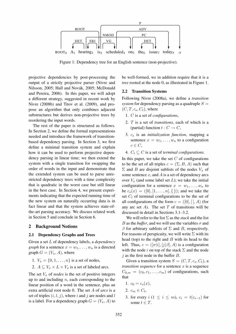
ROOT0 A1
� �?
DET
hearing2
� �?
SBJ
is3
� �?
ROOT
scheduled4
� �?
VG
on5
� �?
NMOD
the6
� �?
DET
issue7
� �?
PC
today8
� �?
ADV
.9?
� �P
Figure 1: Dependency tree for an English sentence (non-projective).
projective dependencies by post-processing theoutput of a strictly projective parser (Nivre andNilsson, 2005; Hall and Novák, 2005; McDonaldand Pereira, 2006). In this paper, we will adopta different strategy, suggested in recent work byNivre (2008b) and Titov et al. (2009), and pro-pose an algorithm that only combines adjacentsubstructures but derives non-projective trees byreordering the input words.
The rest of the paper is structured as follows.In Section 2, we define the formal representationsneeded and introduce the framework of transition-based dependency parsing. In Section 3, we firstdefine a minimal transition system and explainhow it can be used to perform projective depen-dency parsing in linear time; we then extend thesystem with a single transition for swapping theorder of words in the input and demonstrate thatthe extended system can be used to parse unre-stricted dependency trees with a time complexitythat is quadratic in the worst case but still linearin the best case. In Section 4, we present experi-ments indicating that the expected running time ofthe new system on naturally occurring data is infact linear and that the system achieves state-of-the-art parsing accuracy. We discuss related workin Section 5 and conclude in Section 6.
2 Background Notions
2.1 Dependency Graphs and TreesGiven a set L of dependency labels, a dependencygraph for a sentence x = w1, . . . , wn is a directedgraph G = (Vx, A), where
1. Vx = {0, 1, . . . , n} is a set of nodes,
2. A ⊆ Vx × L× Vx is a set of labeled arcs.
The set Vx of nodes is the set of positive integersup to and including n, each corresponding to thelinear position of a word in the sentence, plus anextra artificial root node 0. The set A of arcs is aset of triples (i, l, j), where i and j are nodes and lis a label. For a dependency graph G = (Vx, A) to
be well-formed, we in addition require that it is atree rooted at the node 0, as illustrated in Figure 1.
2.2 Transition SystemsFollowing Nivre (2008a), we define a transitionsystem for dependency parsing as a quadruple S =(C, T, cs, Ct), where
1. C is a set of configurations,
2. T is a set of transitions, each of which is a(partial) function t : C → C,
3. cs is an initialization function, mapping asentence x = w1, . . . , wn to a configurationc ∈ C,
4. Ct ⊆ C is a set of terminal configurations.In this paper, we take the set C of configurationsto be the set of all triples c = (Σ, B,A) such thatΣ and B are disjoint sublists of the nodes Vx ofsome sentence x, andA is a set of dependency arcsover Vx (and some label set L); we take the initialconfiguration for a sentence x = w1, . . . , wn tobe cs(x) = ([0], [1, . . . , n], { }); and we take theset Ct of terminal configurations to be the set ofall configurations of the form c = ([0], [ ], A) (forany arc set A). The set T of transitions will bediscussed in detail in Sections 3.1–3.2.
We will refer to the list Σ as the stack and the listB as the buffer, and we will use the variables σ andβ for arbitrary sublists of Σ and B, respectively.For reasons of perspicuity, we will write Σ with itshead (top) to the right and B with its head to theleft. Thus, c = ([σ|i], [j|β], A) is a configurationwith the node i on top of the stack Σ and the nodej as the first node in the buffer B.
Given a transition system S = (C, T, cs, Ct), atransition sequence for a sentence x is a sequenceC0,m = (c0, c1, . . . , cm) of configurations, suchthat
1. c0 = cs(x),
2. cm ∈ Ct,3. for every i (1 ≤ i ≤ m), ci = t(ci−1) for
some t ∈ T .
352

Transition Condition
LEFT-ARCl ([σ|i, j], B,A)⇒ ([σ|j], B,A∪{(j, l, i)}) i 6= 0
RIGHT-ARCl ([σ|i, j], B,A)⇒ ([σ|i], B,A∪{(i, l, j)})
SHIFT (σ, [i|β], A)⇒ ([σ|i], β, A)
SWAP ([σ|i, j], β, A)⇒ ([σ|j], [i|β], A) 0 < i < j
Figure 2: Transitions for dependency parsing; Tp = {LEFT-ARCl, RIGHT-ARCl, SHIFT}; Tu = Tp ∪ {SWAP}.
The parse assigned to S by C0,m is the depen-dency graph Gcm = (Vx, Acm), where Acm is theset of arcs in cm.
A transition system S is sound for a class G ofdependency graphs iff, for every sentence x andtransition sequence C0,m for x in S, Gcm ∈ G. Sis complete for G iff, for every sentence x and de-pendency graph G for x in G, there is a transitionsequence C0,m for x in S such that Gcm = G.
2.3 Deterministic Transition-Based Parsing
An oracle for a transition system S is a functiono : C → T . Ideally, o should always return theoptimal transition t for a given configuration c, butall we require formally is that it respects the pre-conditions of transitions in T . That is, if o(c) = tthen t is permissible in c. Given an oracle o, deter-ministic transition-based parsing can be achievedby the following simple algorithm:
PARSE(o, x)1 c← cs(x)2 while c 6∈ Ct3 do t← o(c); c← t(c)4 return Gc
Starting in the initial configuration cs(x), theparser repeatedly calls the oracle function o for thecurrent configuration c and updates c according tothe oracle transition t. The iteration stops when aterminal configuration is reached. It is easy to seethat, provided that there is at least one transitionsequence in S for every sentence, the parser con-structs exactly one transition sequence C0,m for asentence x and returns the parse defined by the ter-minal configuration cm, i.e., Gcm = (Vx, Acm).Assuming that the calls o(c) and t(c) can both beperformed in constant time, the worst-case timecomplexity of a deterministic parser based on atransition system S is given by an upper bound onthe length of transition sequences in S.
When building practical parsing systems, theoracle can be approximated by a classifier trainedon treebank data, a technique that has been usedsuccessfully in a number of systems (Yamada andMatsumoto, 2003; Nivre et al., 2004; Attardi,2006). This is also the approach we will take inthe experimental evaluation in Section 4.
3 Transitions for Dependency Parsing
Having defined the set of configurations, includinginitial and terminal configurations, we will nowfocus on the transition set T required for depen-dency parsing. The total set of transitions that willbe considered is given in Figure 2, but we will startin Section 3.1 with the subset Tp (p for projective)consisting of the first three. In Section 3.2, wewill add the fourth transition (SWAP) to get the fulltransition set Tu (u for unrestricted).
3.1 Projective Dependency Parsing
The minimal transition set Tp for projective depen-dency parsing contains three transitions:
1. LEFT-ARCl updates a configuration with i, jon top of the stack by adding (j, l, i) toA andreplacing i, j on the stack by j alone. It ispermissible as long as i is distinct from 0.
2. RIGHT-ARCl updates a configuration withi, j on top of the stack by adding (i, l, j) toA and replacing i, j on the stack by i alone.
3. SHIFT updates a configuration with i as thefirst node of the buffer by removing i fromthe buffer and pushing it onto the stack.
The system Sp = (C, Tp, cs, Ct) is sound andcomplete for the set of projective dependencytrees (over some label set L) and has been used,in slightly different variants, by a number oftransition-based dependency parsers (Yamada andMatsumoto, 2003; Nivre, 2004; Attardi, 2006;
353
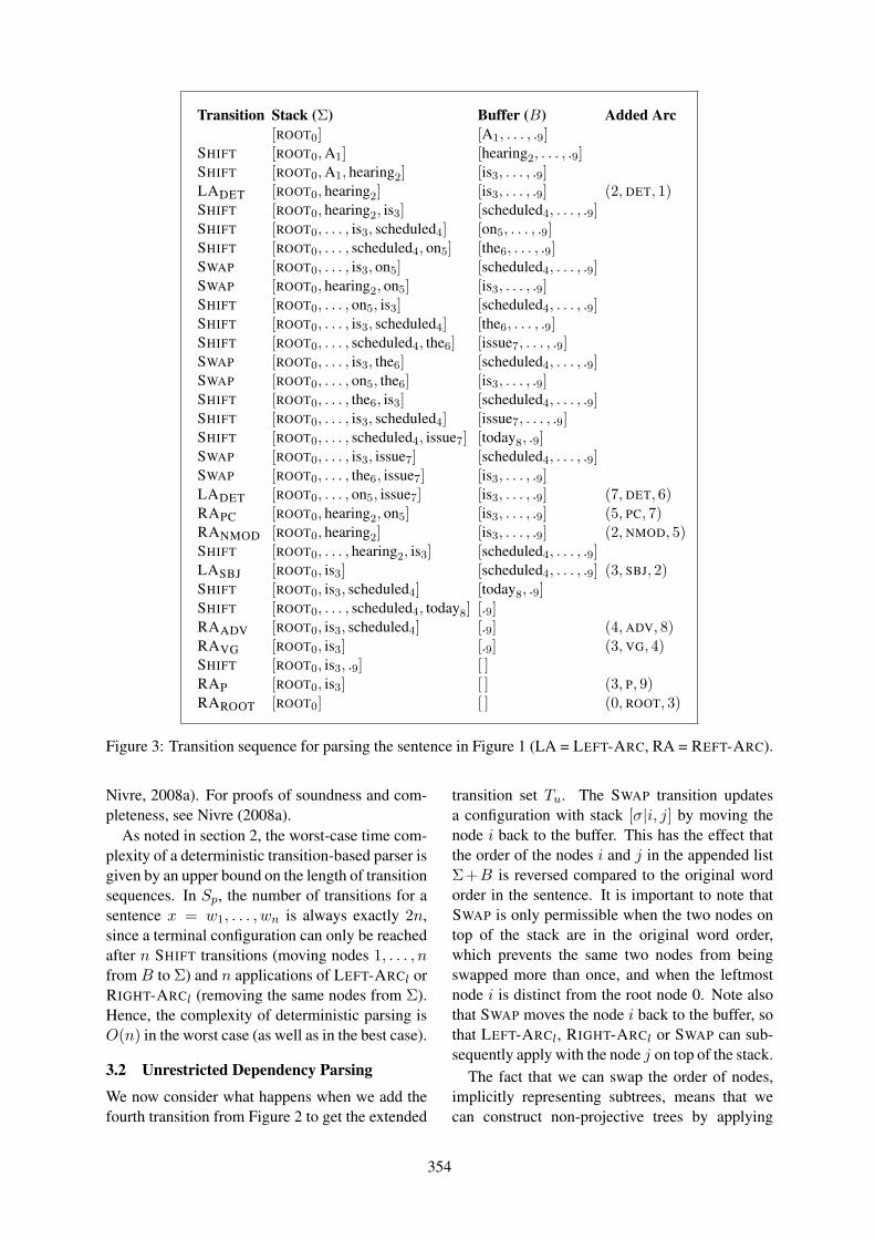
Transition Stack (Σ) Buffer (B) Added Arc[ROOT0] [A1, . . . , .9]
SHIFT [ROOT0,A1] [hearing2, . . . , .9]SHIFT [ROOT0,A1, hearing2] [is3, . . . , .9]LADET [ROOT0, hearing2] [is3, . . . , .9] (2, DET, 1)SHIFT [ROOT0, hearing2, is3] [scheduled4, . . . , .9]SHIFT [ROOT0, . . . , is3, scheduled4] [on5, . . . , .9]SHIFT [ROOT0, . . . , scheduled4, on5] [the6, . . . , .9]SWAP [ROOT0, . . . , is3, on5] [scheduled4, . . . , .9]SWAP [ROOT0, hearing2, on5] [is3, . . . , .9]SHIFT [ROOT0, . . . , on5, is3] [scheduled4, . . . , .9]SHIFT [ROOT0, . . . , is3, scheduled4] [the6, . . . , .9]SHIFT [ROOT0, . . . , scheduled4, the6] [issue7, . . . , .9]SWAP [ROOT0, . . . , is3, the6] [scheduled4, . . . , .9]SWAP [ROOT0, . . . , on5, the6] [is3, . . . , .9]SHIFT [ROOT0, . . . , the6, is3] [scheduled4, . . . , .9]SHIFT [ROOT0, . . . , is3, scheduled4] [issue7, . . . , .9]SHIFT [ROOT0, . . . , scheduled4, issue7] [today8, .9]SWAP [ROOT0, . . . , is3, issue7] [scheduled4, . . . , .9]SWAP [ROOT0, . . . , the6, issue7] [is3, . . . , .9]LADET [ROOT0, . . . , on5, issue7] [is3, . . . , .9] (7, DET, 6)RAPC [ROOT0, hearing2, on5] [is3, . . . , .9] (5, PC, 7)RANMOD [ROOT0, hearing2] [is3, . . . , .9] (2, NMOD, 5)SHIFT [ROOT0, . . . , hearing2, is3] [scheduled4, . . . , .9]LASBJ [ROOT0, is3] [scheduled4, . . . , .9] (3, SBJ, 2)SHIFT [ROOT0, is3, scheduled4] [today8, .9]SHIFT [ROOT0, . . . , scheduled4, today8] [.9]RAADV [ROOT0, is3, scheduled4] [.9] (4, ADV, 8)RAVG [ROOT0, is3] [.9] (3, VG, 4)SHIFT [ROOT0, is3, .9] [ ]RAP [ROOT0, is3] [ ] (3, P, 9)RAROOT [ROOT0] [ ] (0, ROOT, 3)
Figure 3: Transition sequence for parsing the sentence in Figure 1 (LA = LEFT-ARC, RA = REFT-ARC).
Nivre, 2008a). For proofs of soundness and com-pleteness, see Nivre (2008a).
As noted in section 2, the worst-case time com-plexity of a deterministic transition-based parser isgiven by an upper bound on the length of transitionsequences. In Sp, the number of transitions for asentence x = w1, . . . , wn is always exactly 2n,since a terminal configuration can only be reachedafter n SHIFT transitions (moving nodes 1, . . . , nfrom B to Σ) and n applications of LEFT-ARCl orRIGHT-ARCl (removing the same nodes from Σ).Hence, the complexity of deterministic parsing isO(n) in the worst case (as well as in the best case).
3.2 Unrestricted Dependency Parsing
We now consider what happens when we add thefourth transition from Figure 2 to get the extended
transition set Tu. The SWAP transition updatesa configuration with stack [σ|i, j] by moving thenode i back to the buffer. This has the effect thatthe order of the nodes i and j in the appended listΣ+B is reversed compared to the original wordorder in the sentence. It is important to note thatSWAP is only permissible when the two nodes ontop of the stack are in the original word order,which prevents the same two nodes from beingswapped more than once, and when the leftmostnode i is distinct from the root node 0. Note alsothat SWAP moves the node i back to the buffer, sothat LEFT-ARCl, RIGHT-ARCl or SWAP can sub-sequently apply with the node j on top of the stack.
The fact that we can swap the order of nodes,implicitly representing subtrees, means that wecan construct non-projective trees by applying
354
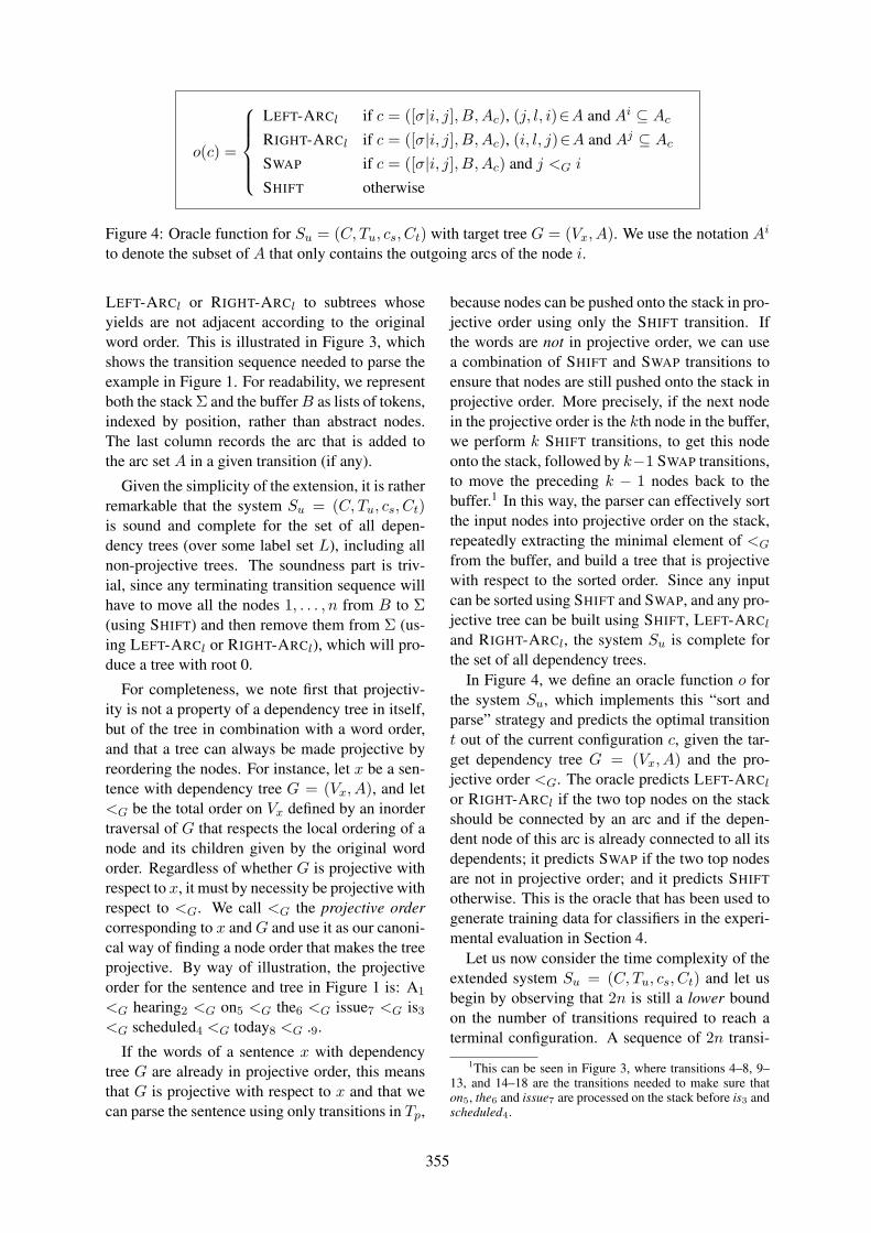
o(c) =
LEFT-ARCl if c = ([σ|i, j], B,Ac), (j, l, i)∈A and Ai ⊆ AcRIGHT-ARCl if c = ([σ|i, j], B,Ac), (i, l, j)∈A and Aj ⊆ AcSWAP if c = ([σ|i, j], B,Ac) and j <G iSHIFT otherwise
Figure 4: Oracle function for Su = (C, Tu, cs, Ct) with target tree G = (Vx, A). We use the notation Ai
to denote the subset of A that only contains the outgoing arcs of the node i.
LEFT-ARCl or RIGHT-ARCl to subtrees whoseyields are not adjacent according to the originalword order. This is illustrated in Figure 3, whichshows the transition sequence needed to parse theexample in Figure 1. For readability, we representboth the stack Σ and the bufferB as lists of tokens,indexed by position, rather than abstract nodes.The last column records the arc that is added tothe arc set A in a given transition (if any).
Given the simplicity of the extension, it is ratherremarkable that the system Su = (C, Tu, cs, Ct)is sound and complete for the set of all depen-dency trees (over some label set L), including allnon-projective trees. The soundness part is triv-ial, since any terminating transition sequence willhave to move all the nodes 1, . . . , n from B to Σ(using SHIFT) and then remove them from Σ (us-ing LEFT-ARCl or RIGHT-ARCl), which will pro-duce a tree with root 0.
For completeness, we note first that projectiv-ity is not a property of a dependency tree in itself,but of the tree in combination with a word order,and that a tree can always be made projective byreordering the nodes. For instance, let x be a sen-tence with dependency tree G = (Vx, A), and let<G be the total order on Vx defined by an inordertraversal of G that respects the local ordering of anode and its children given by the original wordorder. Regardless of whether G is projective withrespect to x, it must by necessity be projective withrespect to <G. We call <G the projective ordercorresponding to x andG and use it as our canoni-cal way of finding a node order that makes the treeprojective. By way of illustration, the projectiveorder for the sentence and tree in Figure 1 is: A1
<G hearing2 <G on5 <G the6 <G issue7 <G is3
<G scheduled4 <G today8 <G .9.
If the words of a sentence x with dependencytree G are already in projective order, this meansthat G is projective with respect to x and that wecan parse the sentence using only transitions in Tp,
because nodes can be pushed onto the stack in pro-jective order using only the SHIFT transition. Ifthe words are not in projective order, we can usea combination of SHIFT and SWAP transitions toensure that nodes are still pushed onto the stack inprojective order. More precisely, if the next nodein the projective order is the kth node in the buffer,we perform k SHIFT transitions, to get this nodeonto the stack, followed by k−1 SWAP transitions,to move the preceding k − 1 nodes back to thebuffer.1 In this way, the parser can effectively sortthe input nodes into projective order on the stack,repeatedly extracting the minimal element of <Gfrom the buffer, and build a tree that is projectivewith respect to the sorted order. Since any inputcan be sorted using SHIFT and SWAP, and any pro-jective tree can be built using SHIFT, LEFT-ARCland RIGHT-ARCl, the system Su is complete forthe set of all dependency trees.
In Figure 4, we define an oracle function o forthe system Su, which implements this “sort andparse” strategy and predicts the optimal transitiont out of the current configuration c, given the tar-get dependency tree G = (Vx, A) and the pro-jective order <G. The oracle predicts LEFT-ARClor RIGHT-ARCl if the two top nodes on the stackshould be connected by an arc and if the depen-dent node of this arc is already connected to all itsdependents; it predicts SWAP if the two top nodesare not in projective order; and it predicts SHIFT
otherwise. This is the oracle that has been used togenerate training data for classifiers in the experi-mental evaluation in Section 4.
Let us now consider the time complexity of theextended system Su = (C, Tu, cs, Ct) and let usbegin by observing that 2n is still a lower boundon the number of transitions required to reach aterminal configuration. A sequence of 2n transi-
1This can be seen in Figure 3, where transitions 4–8, 9–13, and 14–18 are the transitions needed to make sure thaton5, the6 and issue7 are processed on the stack before is3 andscheduled4.
355

Figure 5: Abstract running time during training (black) and parsing (white) for Arabic (1460/146 sen-tences) and Danish (5190/322 sentences).
tions occurs when no SWAP transitions are per-formed, in which case the behavior of the systemis identical to the simpler system Sp. This is im-portant, because it means that the best-case com-plexity of the deterministic parser is stillO(n) andthat the we can expect to observe the best case forall sentences with projective dependency trees.
The exact number of additional transitionsneeded to reach a terminal configuration is deter-mined by the number of SWAP transitions. SinceSWAP moves one node from Σ to B, there willbe one additional SHIFT for every SWAP, whichmeans that the total number of transitions is 2n +2k, where k is the number of SWAP transitions.Given the condition that SWAP can only apply in aconfiguration c = ([σ|i, j], B,A) if 0 < i < j, thenumber of SWAP transitions is bounded by n(n−1)
2 ,which means that 2n + n(n − 1) = n + n2 is anupper bound on the number of transitions in a ter-minating sequence. Hence, the worst-case com-plexity of the deterministic parser is O(n2).
The running time of a deterministic transition-based parser using the system Su is O(n) in thebest case and O(n2) in the worst case. But whatabout the average case? Empirical studies, basedon data from a wide range of languages, haveshown that dependency trees tend to be projectiveand that most non-projective trees only containa small number of discontinuities (Nivre, 2006;Kuhlmann and Nivre, 2006; Havelka, 2007). Thisshould mean that the expected number of swapsper sentence is small, and that the running time islinear on average for the range of inputs that occurin natural languages. This is a hypothesis that will
be tested experimentally in the next section.
4 Experiments
Our experiments are based on five data sets fromthe CoNLL-X shared task: Arabic, Czech, Danish,Slovene, and Turkish (Buchholz and Marsi, 2006).These languages have been selected because thedata come from genuine dependency treebanks,whereas all the other data sets are based on somekind of conversion from another type of represen-tation, which could potentially distort the distribu-tion of different types of structures in the data.
4.1 Running Time
In section 3.2, we hypothesized that the expectedrunning time of a deterministic parser using thetransition system Su would be linear, rather thanquadratic. To test this hypothesis, we examinehow the number of transitions varies as a func-tion of sentence length. We call this the abstractrunning time, since it abstracts over the actualtime needed to compute each oracle prediction andtransition, which is normally constant but depen-dent on the type of classifier used.
We first measured the abstract running time onthe training sets, using the oracle to derive thetransition sequence for every sentence, to see howmany transitions are required in the ideal case. Wethen performed the same measurement on the testsets, using classifiers trained on the oracle transi-tion sequences from the training sets (as describedbelow in Section 4.2), to see whether the trainedparsers deviate from the ideal case.
The result for Arabic and Danish can be seen
356

Arabic Czech Danish Slovene TurkishSystem AS EM AS EM AS EM AS EM AS EMSu 67.1 (9.1) 11.6 82.4 (73.8) 35.3 84.2 (22.5) 26.7 75.2 (23.0) 29.9 64.9 (11.8) 21.5Sp 67.3 (18.2) 11.6 80.9 (3.7) 31.2 84.6 (0.0) 27.0 74.2 (3.4) 29.9 65.3 (6.6) 21.0Spp 67.2 (18.2) 11.6 82.1 (60.7) 34.0 84.7 (22.5) 28.9 74.8 (20.7) 26.9 65.5 (11.8) 20.7Malt-06 66.7 (18.2) 11.0 78.4 (57.9) 27.4 84.8 (27.5) 26.7 70.3 (20.7) 19.7 65.7 (9.2) 19.3MST-06 66.9 (0.0) 10.3 80.2 (61.7) 29.9 84.8 (62.5) 25.5 73.4 (26.4) 20.9 63.2 (11.8) 20.2MSTMalt 68.6 (9.4) 11.0 82.3 (69.2) 31.2 86.7 (60.0) 29.8 75.9 (27.6) 26.6 66.3 (9.2) 18.6
Table 1: Labeled accuracy; AS = attachment score (non-projective arcs in brackets); EM = exact match.
in Figure 5, where black dots represent trainingsentences (parsed with the oracle) and white dotsrepresent test sentences (parsed with a classifier).For Arabic there is a very clear linear relationshipin both cases with very few outliers. Fitting thedata with a linear function using the least squaresmethod gives us m = 2.06n (R2 = 0.97) for thetraining data and m = 2.02n (R2 = 0.98) for thetest data, where m is the number of transitions inparsing a sentence of length n. For Danish, thereis clearly more variation, especially for the train-ing data, but the least-squares approximation stillexplains most of the variance, with m = 2.22n(R2 = 0.85) for the training data and m = 2.07n(R2 = 0.96) for the test data. For both languages,we thus see that the classifier-based parsers havea lower mean number of transitions and less vari-ance than the oracle parsers. And in both cases, theexpected number of transitions is only marginallygreater than the 2n of the strictly projective transi-tion system Sp.
We have chosen to display results for Arabicand Danish because they are the two extremes inour sample. Arabic has the smallest variance andthe smallest linear coefficients, and Danish has thelargest variance and the largest coefficients. Theremaining three languages all lie somewhere inthe middle, with Czech being closer to Arabic andSlovene closer to Danish. Together, the evidencefrom all five languages strongly corroborates thehypothesis that the expected running time for thesystem Su is linear in sentence length for naturallyoccurring data.
4.2 Parsing Accuracy
In order to assess the parsing accuracy that canbe achieved with the new transition system, wetrained a deterministic parser using the new tran-sition system Su for each of the five languages.For comparison, we also trained two parsers using
Sp, one that is strictly projective and one that usesthe pseudo-projective parsing technique to recovernon-projective dependencies in a post-processingstep (Nivre and Nilsson, 2005). We will refer tothe latter system as Spp. All systems use SVMclassifiers with a polynomial kernel to approxi-mate the oracle function, with features and para-meters taken from Nivre et al. (2006), which wasthe best performing transition-based system in theCoNLL-X shared task.2
Table 1 shows the labeled parsing accuracy ofthe parsers measured in two ways: attachmentscore (AS) is the percentage of tokens with thecorrect head and dependency label; exact match(EM) is the percentage of sentences with a com-pletely correct labeled dependency tree. The scorein brackets is the attachment score for the (small)subset of tokens that are connected to their headby a non-projective arc in the gold standard parse.For comparison, the table also includes resultsfor the two best performing systems in the origi-nal CoNLL-X shared task, Malt-06 (Nivre et al.,2006) and MST-06 (McDonald et al., 2006), aswell as the integrated system MSTMalt, which isa graph-based parser guided by the predictions ofa transition-based parser and currently has the bestreported results on the CoNLL-X data sets (Nivreand McDonald, 2008).
Looking first at the overall attachment score, wesee that Su gives a substantial improvement overSp (and outperforms Spp) for Czech and Slovene,where the scores achieved are rivaled only by thecombo system MSTMalt. For these languages,there is no statistical difference between Su andMSTMalt, which are both significantly better thanall the other parsers, except Spp for Czech (Mc-Nemar’s test, α = .05). This is accompaniedby an improvement on non-projective arcs, where
2Complete information about experimental settings canbe found at http://stp.lingfil.uu.se/∼nivre/exp/.
357
Su outperforms all other systems for Czech andis second only to the two MST parsers (MST-06and MSTMalt) for Slovene. It is worth noting thatthe percentage of non-projective arcs is higher forCzech (1.9%) and Slovene (1.9%) than for any ofthe other languages.
For the other three languages, Su has a dropin overall attachment score compared to Sp, butnone of these differences is statistically signifi-cant. In fact, the only significant differences inattachment score here are the positive differencesbetween MSTMalt and all other systems for Arabicand Danish, and the negative difference betweenMST-06 and all other systems for Turkish. Theattachment scores for non-projective arcs are gen-erally very low for these languages, except for thetwo MST parsers on Danish, but Su performs atleast as well as Spp on Danish and Turkish. (Theresults for Arabic are not very meaningful, giventhat there are only eleven non-projective arcs inthe entire test set, of which the (pseudo-)projectiveparsers found two and Su one, while MSTMalt andMST-06 found none at all.)
Considering the exact match scores, finally, it isvery interesting to see that Su almost consistentlyoutperforms all other parsers, including the combosystem MSTMalt, and sometimes by a fairly widemargin (Czech, Slovene). The difference is statis-tically significant with respect to all other systemsexcept MSTMalt for Slovene, all except MSTMalt
and Spp for Czech, and with respect to MSTMalt
for Turkish. For Arabic and Danish, there are nosignificant differences in the exact match scores.We conclude that Su may increase the probabil-ity of finding a completely correct analysis, whichis sometimes reflected also in the overall attach-ment score, and we conjecture that the strength ofthe positive effect is dependent on the frequencyof non-projective arcs in the language.
5 Related Work
Processing non-projective trees by swapping theorder of words has recently been proposed by bothNivre (2008b) and Titov et al. (2009), but thesesystems cannot handle unrestricted non-projectivetrees. It is worth pointing out that, although thesystem described in Nivre (2008b) uses four tran-sitions bearing the same names as the transitionsof Su, the two systems are not equivalent. In par-ticular, the system of Nivre (2008b) is sound butnot complete for the class of all dependency trees.
There are also affinities to the system of Attardi(2006), which combines non-adjacent nodes onthe stack instead of swapping nodes and is equiva-lent to a restricted version of our system, where nomore than two consecutive SWAP transitions arepermitted. This restriction preserves linear worst-case complexity at the expense of completeness.Finally, the algorithm first described by Covington(2001) and used for data-driven parsing by Nivre(2007), is complete but has quadratic complexityeven in the best case.
6 Conclusion
We have presented a novel transition system fordependency parsing that can handle unrestrictednon-projective trees. The system reuses standardtechniques for building projective trees by com-bining adjacent nodes (representing subtrees withadjacent yields), but adds a simple mechanism forswapping the order of nodes on the stack, whichgives a system that is sound and complete for theset of all dependency trees over a given label setbut behaves exactly like the standard system forthe subset of projective trees. As a result, the timecomplexity of deterministic parsing is O(n2) inthe worst case, which is rare, but O(n) in the bestcase, which is common, and experimental resultson data from five languages support the conclusionthat expected running time is linear in the lengthof the sentence. Experimental results also showthat parsing accuracy is competitive, especiallyfor languages like Czech and Slovene where non-projective dependency structures are common, andespecially with respect to the exact match score,where it has the best reported results for four outof five languages. Finally, the simplicity of thesystem makes it very easy to implement.
Future research will include an in-depth erroranalysis to find out why the system works betterfor some languages than others and why the exactmatch score improves even when the attachmentscore goes down. In addition, we want to explorealternative oracle functions, which try to minimizethe number of swaps by allowing the stack to betemporarily “unsorted”.
Acknowledgments
Thanks to Johan Hall and Jens Nilsson for helpwith implementation and evaluation, and to MarcoKuhlmann and three anonymous reviewers foruseful comments.
358
ReferencesGiuseppe Attardi. 2006. Experiments with a multi-
language non-projective dependency parser. In Pro-ceedings of CoNLL, pages 166–170.
Sabine Buchholz and Erwin Marsi. 2006. CoNLL-Xshared task on multilingual dependency parsing. InProceedings of CoNLL, pages 149–164.
Michael A. Covington. 2001. A fundamental algo-rithm for dependency parsing. In Proceedings of the39th Annual ACM Southeast Conference, pages 95–102.
Carlos Gómez-Rodrı́guez, David Weir, and John Car-roll. 2009. Parsing mildly non-projective depen-dency structures. In Proceedings of EACL, pages291–299.
Keith Hall and Vaclav Novák. 2005. Corrective mod-eling for non-projective dependency parsing. InProceedings of IWPT, pages 42–52.
Jiri Havelka. 2007. Beyond projectivity: Multilin-gual evaluation of constraints and measures on non-projective structures. In Proceedings of the 45th An-nual Meeting of the Association of ComputationalLinguistics, pages 608–615.
Richard Johansson and Pierre Nugues. 2007. Incre-mental dependency parsing using online learning. InProceedings of the Shared Task of EMNLP-CoNLL,pages 1134–1138.
Marco Kuhlmann and Joakim Nivre. 2006. Mildlynon-projective dependency structures. In Proceed-ings of the COLING/ACL Main Conference PosterSessions, pages 507–514.
Marco Kuhlmann and Giorgio Satta. 2009. Treebankgrammar techniques for non-projective dependencyparsing. In Proceedings of EACL, pages 478–486.
Ryan McDonald and Fernando Pereira. 2006. Onlinelearning of approximate dependency parsing algo-rithms. In Proceedings of EACL, pages 81–88.
Ryan McDonald and Giorgio Satta. 2007. On the com-plexity of non-projective data-driven dependencyparsing. In Proceedings of IWPT, pages 122–131.
Ryan McDonald, Koby Crammer, and FernandoPereira. 2005a. Online large-margin training of de-pendency parsers. In Proceedings of ACL, pages 91–98.
Ryan McDonald, Fernando Pereira, Kiril Ribarov, andJan Hajič. 2005b. Non-projective dependency pars-ing using spanning tree algorithms. In Proceedingsof HLT/EMNLP, pages 523–530.
Ryan McDonald, Kevin Lerman, and Fernando Pereira.2006. Multilingual dependency analysis with atwo-stage discriminative parser. In Proceedings ofCoNLL, pages 216–220.
Peter Neuhaus and Norbert Bröker. 1997. The com-plexity of recognition of linguistically adequate de-pendency grammars. In Proceedings of ACL/EACL,pages 337–343.
Joakim Nivre and Ryan McDonald. 2008. Integrat-ing graph-based and transition-based dependencyparsers. In Proceedings of ACL, pages 950–958.
Joakim Nivre and Jens Nilsson. 2005. Pseudo-projective dependency parsing. In Proceedings ofACL, pages 99–106.
Joakim Nivre, Johan Hall, and Jens Nilsson. 2004.Memory-based dependency parsing. In Proceedingsof CoNLL, pages 49–56.
Joakim Nivre, Johan Hall, Jens Nilsson, GülsenEryiğit, and Svetoslav Marinov. 2006. Labeledpseudo-projective dependency parsing with supportvector machines. In Proceedings of CoNLL, pages221–225.
Joakim Nivre. 2004. Incrementality in deterministicdependency parsing. In Proceedings of the Work-shop on Incremental Parsing: Bringing Engineeringand Cognition Together (ACL), pages 50–57.
Joakim Nivre. 2006. Constraints on non-projective de-pendency graphs. In Proceedings of EACL, pages73–80.
Joakim Nivre. 2007. Incremental non-projective de-pendency parsing. In Proceedings of NAACL HLT,pages 396–403.
Joakim Nivre. 2008a. Algorithms for deterministic in-cremental dependency parsing. Computational Lin-guistics, 34:513–553.
Joakim Nivre. 2008b. Sorting out dependency pars-ing. In Proceedings of the 6th International Con-ference on Natural Language Processing (GoTAL),pages 16–27.
Ivan Titov and James Henderson. 2007. A latent vari-able model for generative dependency parsing. InProceedings of IWPT, pages 144–155.
Ivan Titov, James Henderson, Paola Merlo, andGabriele Musillo. 2009. Online graph planarizationfor synchronous parsing of semantic and syntacticdependencies. In Proceedings of IJCAI.
Hiroyasu Yamada and Yuji Matsumoto. 2003. Statis-tical dependency analysis with support vector ma-chines. In Proceedings of IWPT, pages 195–206.
359

Proceedings of the 47th Annual Meeting of the ACL and the 4th IJCNLP of the AFNLP, pages 360–368,Suntec, Singapore, 2-7 August 2009. c©2009 ACL and AFNLP
Semi-supervised Learning of Dependency Parsersusing Generalized Expectation Criteria
Gregory DruckDept. of Computer ScienceUniversity of Massachusetts
Amherst, MA [email protected]
Gideon MannGoogle, Inc.76 9th Ave.
New York, NY [email protected]
Andrew McCallumDept. of Computer ScienceUniversity of Massachusetts
Amherst, MA [email protected]
Abstract
In this paper, we propose a novel methodfor semi-supervised learning of non-projective log-linear dependency parsersusing directly expressed linguistic priorknowledge (e.g. a noun’s parent is often averb). Model parameters are estimated us-ing a generalized expectation (GE) objec-tive function that penalizes the mismatchbetween model predictions and linguisticexpectation constraints. In a comparisonwith two prominent “unsupervised” learn-ing methods that require indirect biasingtoward the correct syntactic structure, weshow that GE can attain better accuracywith as few as 20 intuitive constraints. Wealso present positive experimental resultson longer sentences in multiple languages.
1 Introduction
Early approaches to parsing assumed a grammarprovided by human experts (Quirk et al., 1985).Later approaches avoided grammar writing bylearning the grammar from sentences explicitlyannotated with their syntactic structure (Black etal., 1992). While such supervised approaches haveyielded accurate parsers (Charniak, 2001), thesyntactic annotation of corpora such as the PennTreebank is extremely costly, and consequentlythere are few treebanks of comparable size.
As a result, there has been recent interest inunsupervised parsing. However, in order to at-tain reasonable accuracy, these methods have tobe carefully biased towards the desired syntac-tic structure. This weak supervision has beenencoded using priors and initializations (Kleinand Manning, 2004; Smith, 2006), specializedmodels (Klein and Manning, 2004; Seginer,2007; Bod, 2006), and implicit negative evi-dence (Smith, 2006). These indirect methods for
leveraging prior knowledge can be cumbersomeand unintuitive for a non-machine-learning expert.
This paper proposes a method for directly guid-ing the learning of dependency parsers with nat-urally encoded linguistic insights. Generalizedexpectation (GE) (Mann and McCallum, 2008;Druck et al., 2008) is a recently proposed frame-work for incorporating prior knowledge into thelearning of conditional random fields (CRFs) (Laf-ferty et al., 2001). GE criteria express a preferenceon the value of a model expectation. For example,we know that “in English, when a determiner is di-rectly to the left of a noun, the noun is usually theparent of the determiner”. With GE we may adda term to the objective function that encourages afeature-rich CRF to match this expectation on un-labeled data, and in the process learn about relatedfeatures. In this paper we use a non-projective de-pendency tree CRF (Smith and Smith, 2007).
While a complete exploration of linguistic priorknowledge for dependency parsing is beyond thescope of this paper, we provide several promis-ing demonstrations of the proposed method. Onthe English WSJ10 data set, GE training outper-forms two prominent unsupervised methods usingonly 20 constraints either elicited from a humanor provided by an “oracle” simulating a human.We also present experiments on longer sentencesin Dutch, Spanish, and Turkish in which we obtainaccuracy comparable to supervised learning withtens to hundreds of complete parsed sentences.
2 Related Work
This work is closely related to the prototype-driven grammar induction method of Haghighiand Klein (2006), which uses prototype phrasesto guide the EM algorithm in learning a PCFG.Direct comparison with this method is not possi-ble because we are interested in dependency syn-tax rather than phrase structure syntax. However,the approach we advocate has several significant
360
advantages. GE is more general than prototype-driven learning because GE constraints can be un-certain. Additionally prototype-driven grammarinduction needs to be used in conjunction withother unsupervised methods (distributional simi-larity and CCM (Klein and Manning, 2004)) toattain reasonable accuracy, and is only evaluatedon length 10 or less sentences with no lexical in-formation. In contrast, GE uses only the providedconstraints and unparsed sentences, and is used totrain a feature-rich discriminative model.
Conventional semi-supervised learning requiresparsed sentences. Kate and Mooney (2007) andMcClosky et al. (2006) both use modified formsof self-training to bootstrap parsers from limitedlabeled data. Wang et al. (2008) combine a struc-tured loss on parsed sentences with a least squaresloss on unlabeled sentences. Koo et al. (2008) usea large unlabeled corpus to estimate cluster fea-tures which help the parser generalize with fewerexamples. Smith and Eisner (2007) apply entropyregularization to dependency parsing. The abovemethods can be applied to small seed corpora, butMcDonald1 has criticized such methods as work-ing from an unrealistic premise, as a significantamount of the effort required to build a treebankcomes in the first 100 sentences (both because ofthe time it takes to create an appropriate rubric andto train annotators).
There are also a number of methods for unsu-pervised learning of dependency parsers. Kleinand Manning (2004) use a carefully initialized andstructured generative model (DMV) in conjunc-tion with the EM algorithm to get the first positiveresults on unsupervised dependency parsing. Asempirical evidence of the sensitivity of DMV toinitialization, Smith (2006) (pg. 37) uses three dif-ferent initializations, and only one, the method ofKlein and Manning (2004), gives accuracy higherthan 31% on the WSJ10 corpus (see Section 5).This initialization encodes the prior knowledgethat long distance attachments are unlikely.
Smith and Eisner (2005) develop contrastiveestimation (CE), in which the model is encour-aged to move probability mass away from im-plicit negative examples defined using a care-fully chosen neighborhood function. For instance,Smith (2006) (pg. 82) uses eight different neigh-borhood functions to estimate parameters for theDMV model. The best performing neighborhood
1R. McDonald, personal communication, 2007
function DEL1ORTRANS1 provides accuracy of57.6% on WSJ10 (see Section 5). Another neigh-borhood, DEL1ORTRANS2, provides accuracy of51.2%. The remaining six neighborhood func-tions provide accuracy below 50%. This demon-strates that constructing an appropriate neighbor-hood function can be delicate and challenging.
Smith and Eisner (2006) propose structural an-nealing (SA), in which a strong bias for local de-pendency attachments is enforced early in learn-ing, and then gradually relaxed. This method issensitive to the annealing schedule. Smith (2006)(pg. 136) use 10 annealing schedules in conjunc-tion with three initializers. The best performingcombination attains accuracy of 66.7% on WSJ10,but the worst attains accuracy of 32.5%.
Finally, Seginer (2007) and Bod (2006) ap-proach unsupervised parsing by constructingnovel syntactic models. The development and tun-ing of the above methods constitute the encodingof prior domain knowledge about the desired syn-tactic structure. In contrast, our framework pro-vides a straightforward and explicit method for in-corporating prior knowledge.
Ganchev et al. (2009) propose a related methodthat uses posterior constrained EM to learn a pro-jective target language parser using only a sourcelanguage parser and word alignments.
3 Generalized Expectation Criteria
Generalized expectation criteria (Mann and Mc-Callum, 2008; Druck et al., 2008) are terms ina parameter estimation objective function that ex-press a preference on the value of a model expec-tation. Let x represent input variables (i.e. a sen-tence) and y represent output variables (i.e. a parsetree). A generalized expectation term G(λ) is de-fined by a constraint function G(y,x) that returnsa non-negative real value given input and outputvariables, an empirical distribution p̃(x) over in-put variables (i.e. unlabeled data), a model distri-bution pλ(y|x), and a score function S:
G(λ) = S(Ep̃(x)[Epλ(y|x)[G(y,x)]]).
In this paper, we use a score function that is thesquared difference of the model expectation of Gand some target expectation G̃:
Ssq = −(G̃− Ep̃(x)[Epλ(y|x)[G(y,x)]])2 (1)
We can incorporate prior knowledge into the train-ing of pλ(y|x) by specifying the from of the con-straint function G and the target expectation G̃.
361

Importantly, G does not need to match a particularfeature in the underlying model.
The complete objective function2 includes mul-tiple GE terms and a prior on parameters3, p(λ)
O(λ;D) = p(λ) +∑
GG(λ)
GE has been applied to logistic regression mod-els (Mann and McCallum, 2007; Druck et al.,2008) and linear chain CRFs (Mann and McCal-lum, 2008). In the following sections we applyGE to non-projective CRF dependency parsing.
3.1 GE in General CRFs
We first consider an arbitrarily structured condi-tional random field (Lafferty et al., 2001) pλ(y|x).We describe the CRF for non-projective depen-dency parsing in Section 3.2. The probability ofan output y conditioned on an input x is
pλ(y|x) =1
Zxexp
(
∑
j
λjFj(y,x))
,
where Fj are feature functions over the cliquesof the graphical model and Z(x) is a normaliz-ing constant that ensures pλ(y|x) sums to 1. Weare interested in the expectation of constraint func-tion G(x,y) under this model. We abbreviate thismodel expectation as:
Gλ = Ep̃(x)[Epλ(y|x)[G(y,x)]]
It can be shown that partial derivative of G(λ) us-ing Ssq4 with respect to model parameter λj is
∂
∂λjG(λ) = 2(G̃−Gλ) (2)
(
Ep̃(x)
[
Epλ(y|x) [G(y,x)Fj(y,x)]
−Epλ(y|x) [G(y,x)]Epλ(y|x) [Fj(y,x)]])
.
Equation 2 has an intuitive interpretation. The firstterm (on the first line) is the difference between themodel and target expectations. The second term
2In general, the objective function could also include thelikelihood of available labeled data, but throughout this paperwe assume we have no parsed sentences.
3Throughout this paper we use a Gaussian prior on pa-rameters with σ2 = 10.
4In previous work, S was the KL-divergence from the tar-get expectation. The partial derivative of the KL divergencescore function includes the same covariance term as abovebut substitutes a different multiplicative term: G̃/Gλ.
(the rest of the equation) is the predicted covari-ance between the constraint function G and themodel feature function Fj . Therefore, if the con-straint is not satisfied, GE updates parameters forfeatures that the model predicts are related to theconstraint function.
If there are constraint functions G for all modelfeature functions Fj , and the target expectationsG̃ are estimated from labeled data, then the glob-ally optimal parameter setting under the GE objec-tive function is equivalent to the maximum likeli-hood solution. However, GE does not require sucha one-to-one correspondence between constraintfunctions and model feature functions. This al-lows bootstrapping of feature-rich models with asmall number of prior expectation constraints.
3.2 Non-Projective Dependency Tree CRFs
We now define a CRF pλ(y|x) for unlabeled, non-projective5 dependency parsing. The tree y is rep-resented as a vector of the same length as the sen-tence, where yi is the index of the parent of wordi. The probability of a tree y given sentence x is
pλ(y|x) =1
Zxexp
(
n∑
i=1
∑
j
λjfj(xi, xyi ,x))
,
where fj are edge-factored feature functions thatconsider the child input (word, tag, or other fea-ture), the parent input, and the rest of the sen-tence. This factorization implies that dependencydecisions are independent conditioned on the in-put sentence x if y is a tree. ComputingZx and theedge expectations needed for partial derivatives re-quires summing over all possible trees for x.
By relating the sum of the scores of all possibletrees to counting the number of spanning trees in agraph, it can be shown that Zx is the determinantof the Kirchoff matrix K, which is constructed us-ing the scores of possible edges. (McDonald andSatta, 2007; Smith and Smith, 2007). Computingthe determinant takes O(n3) time, where n is thelength of the sentence. To compute the marginalprobability of a particular edge k → i (i.e. yi=k),the score of any edge k′ → i such that k′ 6= k isset to 0. The determinant of the resulting modi-fied Kirchoff matrix Kk→i is then the sum of thescores of all trees that include the edge k → i. The
5Note that we could instead define a CRF for projectivedependency parse trees and use a variant of the inside outsidealgorithm for inference. We choose non-projective because itis the more general case.
362

marginal p(yi=k|x; θ) can be computed by divid-ing this score by Zx (McDonald and Satta, 2007).Computing all edge expectations with this algo-rithm takes O(n5) time. Smith and Smith (2007)describe a more efficient algorithm that can com-pute all edge expectations in O(n3) time using theinverse of the Kirchoff matrix K−1.
3.3 GE for Non-Projective Dependency TreeCRFs
While in general constraint functions G mayconsider multiple edges, in this paper we useedge-factored constraint functions. In this caseEpλ(y|x)[G(y,x)]Epλ(y|x)[Fj(y,x)], the secondterm of the covariance in Equation 2, can becomputed using the edge marginal distributionspλ(yi|x). The first term of the covarianceEpλ(y|x)[G(y,x)Fj(y,x)] is more difficult tocompute because it requires the marginal proba-bility of two edges pλ(yi, yi′ |x). It is important tonote that the model pλ is still edge-factored.
The sum of the scores of all trees that containedges k → i and k′ → i′ can be computed by set-ting the scores of edges j → i such that j 6= k andj′ → i′ such that j′ 6= k′ to 0, and computing thedeterminant of the resulting modified Kirchoff ma-trixKk→i,k′→i′ . There areO(n4) pairs of possibleedges, and the determinant computation takes timeO(n3), so this naive algorithm takes O(n7) time.
An improved algorithm computes, for each pos-sible edge k → i, a modified Kirchoff matrixKk→i that requires the presence of that edge.Then, the method of Smith and Smith (2007) canbe used to compute the probability of every pos-sible edge conditioned on the presence of k → i,pλ(yi′ =k′|yi = k,x), using K−1
k→i. Multiplyingthis probability by pλ(yi=k|x) yields the desiredtwo edge marginal. Because this algorithm pullsthe O(n3) matrix operation out of the inner loopover edges, the run time is reduced to O(n5).
If it were possible to perform only one O(n3)matrix operation per sentence, then the gradientcomputation would take onlyO(n4) time, the timerequired to consider all pairs of edges. Unfortu-nately, there is no straightforward generalizationof the method of Smith and Smith (2007) to thetwo edge marginal problem. Specifically, Laplaceexpansion generalizes to second-order matrix mi-nors, but it is not clear how to compute second-order cofactors from the inverse Kirchoff matrixalone (c.f. (Smith and Smith, 2007)).
Consequently, we also propose an approxima-tion that can be used to speed up GE training atthe expense of a less accurate covariance compu-tation. We consider different cases of the edgesk → i, and k′ → i′.
• pλ(yi=k, yi′=k′|x)=0 when i=i′ and k 6=k′(different parent for the same word), or wheni=k′ and k=i′ (cycle), because these pairs ofedges break the tree constraint.
• pλ(yi=k, yi′ =k′|x)=pλ(yi=k|x) when i=i′, k=k′.
• pλ(yi=k, yi′ =k′|x)≈pλ(yi=k|x)pλ(yi′ =k′|x) when i 6= i′ and i 6= k′ or i′ 6= k(different words, do not create a cycle). Thisapproximation assumes that pairs of edgesthat do not fall into one of the above casesare conditionally independent given x. Thisis not true because there are partial trees inwhich k → i and k′ → i′ can appear sepa-rately, but not together (for example if i = k′
and the partial tree contains i′ → k).
Using this approximation, the covariance for onesentence is approximately equal to
n∑
i
Epλ(yi|x)[fj(xi, xyi ,x)g(xi, xyi ,x)]
−n∑
i
Epλ(yi|x)[fj(xi, xyi ,x)]Epλ(yi|x)[g(xi, xyi ,x)]
−n∑
i,k
pλ(yi=k|x)pλ(yk=i|x)fj(xi, xk,x)g(xk, xi,x).
Intuitively, the first and second terms compute acovariance over possible parents for a single word,and the third term accounts for cycles. Computingthe above takes O(n3) time, the time required tocompute single edge marginals. In this paper, weuse the O(n5) exact method, though we find thatthe accuracy attained by approximate training isusually within 5% of the exact method.
If G is not edge-factored, then we need to com-pute a marginal over three or more edges, makingexact training intractable. An appealing alterna-tive to a similar approximation to the above woulduse loopy belief propagation to efficiently approx-imate the marginals (Smith and Eisner, 2008).
In this paper g is binary and normalized by itstotal count in the corpus. The expectation of g isthen the probability that it indicates a true edge.
363

4 Linguistic Prior Knowledge
Training parsers using GE with the aid of linguistsis an exciting direction for future work. In this pa-per, we use constraints derived from several basictypes of linguistic knowledge.
One simple form of linguistic knowledge is theset of possible parent tags for a given child tag.This type of constraint was used in the devel-opment of a rule-based dependency parser (De-busmann et al., 2004). Additional informationcan be obtained from small grammar fragments.Haghighi and Klein (2006) provide a list of proto-type phrase structure rules that can be augmentedwith dependencies and used to define constraintsinvolving parent and child tags, surrounding orinterposing tags, direction, and distance. Finallythere are well known hypotheses about the direc-tion and distance of attachments that can be usedto define constraints. Eisner and Smith (2005) usethe fact that short attachments are more commonto improve unsupervised parsing accuracy.
4.1 “Oracle” constraints
For some experiments that follow we use “ora-cle” constraints that are estimated from labeleddata. This involves choosing feature templates(motivated by the linguistic knowledge describedabove) and estimating target expectations. Oraclemethods used in this paper consider three simplestatistics of candidate constraint functions: countc̃(g), edge count c̃edge(g), and edge probabilityp̃(edge|g). Let D be the labeled corpus.
c̃(g) =∑
x∈D
∑
i
∑
j
g(xi, xj ,x)
c̃edge(g) =∑
(x,y)∈D
∑
i
g(xi, xyi ,x)
p̃(edge|g) =c̃edge(g)
c̃(g)
Constraint functions are selected according tosome combination of the above statistics. Insome cases we additionally prune the candidateset by considering only certain templates. Tocompute the target expectation, we simply usebin(p̃(edge|g)), where bin returns the closestvalue in the set {0, 0.1, 0.25, 0.5, 0.75, 1}. Thiscan be viewed as specifying that g is very indica-tive of edge, somewhat indicative of edge, etc.
5 Experimental Comparison withUnsupervised Learning
In this section we compare GE training with meth-ods for unsupervised parsing. We use the WSJ10corpus (as processed by Smith (2006)), which iscomprised of English sentences of ten words orfewer (after stripping punctuation) from the WSJportion of the Penn Treebank. As in previous worksentences contain only part-of-speech tags.
We compare GE and supervised training of anedge-factored CRF with unsupervised learning ofa DMV model (Klein and Manning, 2004) usingEM and contrastive estimation (CE) (Smith andEisner, 2005). We also report the accuracy of anattach-right baseline6. Finally, we report the ac-curacy of a constraint baseline that assigns a scoreto each possible edge that is the sum of the targetexpectations for all constraints on that edge. Pos-sible edges without constraints receive a score of0. These scores are used as input to the maximumspanning tree algorithm, which returns the besttree. Note that this is a strong baseline because itcan handle uncertain constraints, and the tree con-straint imposed by the MST algorithm helps infor-mation propagate across edges.
We note that there are considerable differencesbetween the DMV and CRF models. The DMVmodel is more expressive than the CRF becauseit can model the arity of a head as well as sib-ling relationships. Because these features considermultiple edges, including them in the CRF modelwould make exact inference intractable (McDon-ald and Satta, 2007). However, the CRF may con-sider the distance between head and child, whereasDMV does not model distance. The CRF alsomodels non-projective trees, which when evaluat-ing on English is likely a disadvantage.
Consequently, we experiment with two sets offeatures for the CRF model. The first, restrictedset includes features that consider the head andchild tags of the dependency conjoined with thedirection of the attachment, (parent-POS,child-POS,direction). With this feature set, the CRFmodel is less expressive than DMV. The sec-ond full set includes standard features for edge-factored dependency parsers (McDonald et al.,2005), though still unlexicalized. The CRF can-not consider valency even with the full feature set,but this is balanced by the ability to use distance.
6The reported accuracies with the DMV model and theattach-right baseline are taken from (Smith, 2006).
364
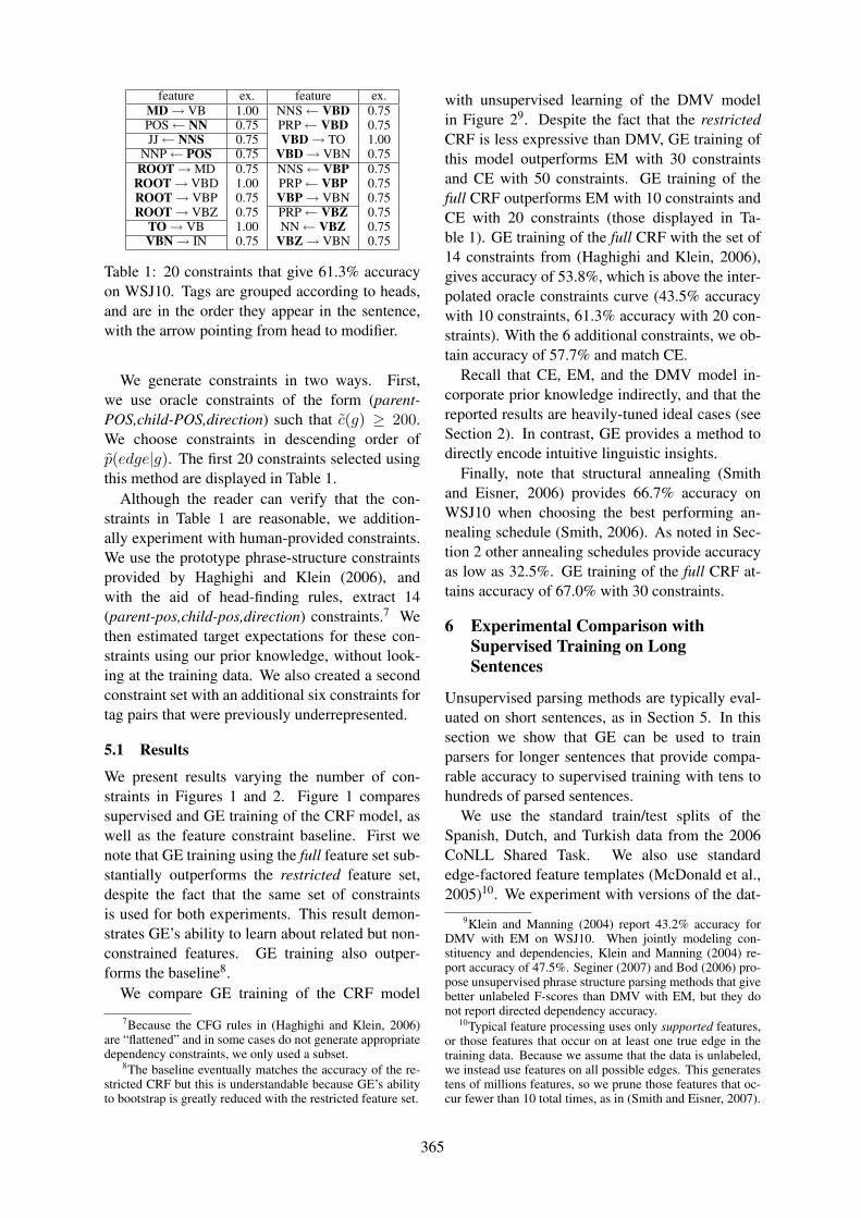
feature ex. feature ex.MD→ VB 1.00 NNS← VBD 0.75POS← NN 0.75 PRP← VBD 0.75JJ← NNS 0.75 VBD→ TO 1.00
NNP← POS 0.75 VBD→ VBN 0.75ROOT→MD 0.75 NNS← VBP 0.75
ROOT→ VBD 1.00 PRP← VBP 0.75ROOT→ VBP 0.75 VBP→ VBN 0.75ROOT→ VBZ 0.75 PRP← VBZ 0.75
TO→ VB 1.00 NN← VBZ 0.75VBN→ IN 0.75 VBZ→ VBN 0.75
Table 1: 20 constraints that give 61.3% accuracyon WSJ10. Tags are grouped according to heads,and are in the order they appear in the sentence,with the arrow pointing from head to modifier.
We generate constraints in two ways. First,we use oracle constraints of the form (parent-POS,child-POS,direction) such that c̃(g) ≥ 200.We choose constraints in descending order ofp̃(edge|g). The first 20 constraints selected usingthis method are displayed in Table 1.
Although the reader can verify that the con-straints in Table 1 are reasonable, we addition-ally experiment with human-provided constraints.We use the prototype phrase-structure constraintsprovided by Haghighi and Klein (2006), andwith the aid of head-finding rules, extract 14(parent-pos,child-pos,direction) constraints.7 Wethen estimated target expectations for these con-straints using our prior knowledge, without look-ing at the training data. We also created a secondconstraint set with an additional six constraints fortag pairs that were previously underrepresented.
5.1 Results
We present results varying the number of con-straints in Figures 1 and 2. Figure 1 comparessupervised and GE training of the CRF model, aswell as the feature constraint baseline. First wenote that GE training using the full feature set sub-stantially outperforms the restricted feature set,despite the fact that the same set of constraintsis used for both experiments. This result demon-strates GE’s ability to learn about related but non-constrained features. GE training also outper-forms the baseline8.
We compare GE training of the CRF model
7Because the CFG rules in (Haghighi and Klein, 2006)are “flattened” and in some cases do not generate appropriatedependency constraints, we only used a subset.
8The baseline eventually matches the accuracy of the re-stricted CRF but this is understandable because GE’s abilityto bootstrap is greatly reduced with the restricted feature set.
with unsupervised learning of the DMV modelin Figure 29. Despite the fact that the restrictedCRF is less expressive than DMV, GE training ofthis model outperforms EM with 30 constraintsand CE with 50 constraints. GE training of thefull CRF outperforms EM with 10 constraints andCE with 20 constraints (those displayed in Ta-ble 1). GE training of the full CRF with the set of14 constraints from (Haghighi and Klein, 2006),gives accuracy of 53.8%, which is above the inter-polated oracle constraints curve (43.5% accuracywith 10 constraints, 61.3% accuracy with 20 con-straints). With the 6 additional constraints, we ob-tain accuracy of 57.7% and match CE.
Recall that CE, EM, and the DMV model in-corporate prior knowledge indirectly, and that thereported results are heavily-tuned ideal cases (seeSection 2). In contrast, GE provides a method todirectly encode intuitive linguistic insights.
Finally, note that structural annealing (Smithand Eisner, 2006) provides 66.7% accuracy onWSJ10 when choosing the best performing an-nealing schedule (Smith, 2006). As noted in Sec-tion 2 other annealing schedules provide accuracyas low as 32.5%. GE training of the full CRF at-tains accuracy of 67.0% with 30 constraints.
6 Experimental Comparison withSupervised Training on LongSentences
Unsupervised parsing methods are typically eval-uated on short sentences, as in Section 5. In thissection we show that GE can be used to trainparsers for longer sentences that provide compa-rable accuracy to supervised training with tens tohundreds of parsed sentences.
We use the standard train/test splits of theSpanish, Dutch, and Turkish data from the 2006CoNLL Shared Task. We also use standardedge-factored feature templates (McDonald et al.,2005)10. We experiment with versions of the dat-
9Klein and Manning (2004) report 43.2% accuracy forDMV with EM on WSJ10. When jointly modeling con-stituency and dependencies, Klein and Manning (2004) re-port accuracy of 47.5%. Seginer (2007) and Bod (2006) pro-pose unsupervised phrase structure parsing methods that givebetter unlabeled F-scores than DMV with EM, but they donot report directed dependency accuracy.
10Typical feature processing uses only supported features,or those features that occur on at least one true edge in thetraining data. Because we assume that the data is unlabeled,we instead use features on all possible edges. This generatestens of millions features, so we prune those features that oc-cur fewer than 10 total times, as in (Smith and Eisner, 2007).
365
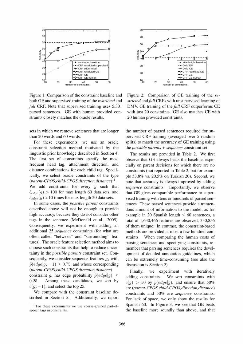
10 20 30 40 50 6010
20
30
40
50
60
70
80
90
number of constraints
accu
racy
constraint baselineCRF restricted supervisedCRF supervisedCRF restricted GECRF GECRF GE human
Figure 1: Comparison of the constraint baseline andboth GE and supervised training of the restricted andfull CRF. Note that supervised training uses 5,301parsed sentences. GE with human provided con-straints closely matches the oracle results.
10 20 30 40 50 6010
20
30
40
50
60
70
80
number of constraints
accu
racy
attach right baselineDMV EMDMV CECRF restricted GECRF GECRF GE human
Figure 2: Comparison of GE training of the re-stricted and full CRFs with unsupervised learning ofDMV. GE training of the full CRF outperforms CEwith just 20 constraints. GE also matches CE with20 human provided constraints.
sets in which we remove sentences that are longerthan 20 words and 60 words.
For these experiments, we use an oracleconstraint selection method motivated by thelinguistic prior knowledge described in Section 4.The first set of constraints specify the mostfrequent head tag, attachment direction, anddistance combinations for each child tag. Specif-ically, we select oracle constraints of the type(parent-CPOS,child-CPOS,direction,distance)11.We add constraints for every g such thatc̃edge(g) > 100 for max length 60 data sets, andc̃edge(g)>10 times for max length 20 data sets.
In some cases, the possible parent constraintsdescribed above will not be enough to providehigh accuracy, because they do not consider othertags in the sentence (McDonald et al., 2005).Consequently, we experiment with adding anadditional 25 sequence constraints (for what areoften called “between” and “surrounding” fea-tures). The oracle feature selection method aims tochoose such constraints that help to reduce uncer-tainty in the possible parents constraint set. Con-sequently, we consider sequence features gs withp̃(edge|gs=1) ≥ 0.75, and whose corresponding(parent-CPOS,child-CPOS,direction,distance)constraint g, has edge probability p̃(edge|g) ≤0.25. Among these candidates, we sort byc̃(gs=1), and select the top 25.
We compare with the constraint baseline de-scribed in Section 5. Additionally, we report
11For these experiments we use coarse-grained part-of-speech tags in constraints.
the number of parsed sentences required for su-pervised CRF training (averaged over 5 randomsplits) to match the accuracy of GE training usingthe possible parents + sequence constraint set.
The results are provided in Table 2. We firstobserve that GE always beats the baseline, espe-cially on parent decisions for which there are noconstraints (not reported in Table 2, but for exam-ple 53.8% vs. 20.5% on Turkish 20). Second, wenote that accuracy is always improved by addingsequence constraints. Importantly, we observethat GE gives comparable performance to super-vised training with tens or hundreds of parsed sen-tences. These parsed sentences provide a tremen-dous amount of information to the model, as forexample in 20 Spanish length ≤ 60 sentences, atotal of 1,630,466 features are observed, 330,856of them unique. In contrast, the constraint-basedmethods are provided at most a few hundred con-straints. When comparing the human costs ofparsing sentences and specifying constraints, re-member that parsing sentences requires the devel-opment of detailed annotation guidelines, whichcan be extremely time-consuming (see also thediscussion is Section 2).
Finally, we experiment with iterativelyadding constraints. We sort constraints withc̃(g) > 50 by p̃(edge|g), and ensure that 50%are (parent-CPOS,child-CPOS,direction,distance)constraints and 50% are sequence constraints.For lack of space, we only show the results forSpanish 60. In Figure 3, we see that GE beatsthe baseline more soundly than above, and that
366
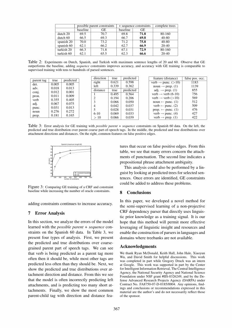
possible parent constraints + sequence constraints complete treesbaseline GE baseline GE
dutch 20 69.5 70.7 69.8 71.8 80-160dutch 60 66.5 69.3 66.7 69.8 40-80spanish 20 70.0 73.2 71.2 75.8 40-80spanish 60 62.1 66.2 62.7 66.9 20-40turkish 20 66.3 71.8 67.1 72.9 80-160turkish 60 62.1 65.5 62.3 66.6 20-40
Table 2: Experiments on Dutch, Spanish, and Turkish with maximum sentence lengths of 20 and 60. Observe that GEoutperforms the baseline, adding sequence constraints improves accuracy, and accuracy with GE training is comparable tosupervised training with tens to hundreds of parsed sentences.
parent tag true predicteddet. 0.005 0.005adv. 0.018 0.013conj. 0.012 0.001pron. 0.011 0.009verb 0.355 0.405adj. 0.067 0.075punc. 0.031 0.013noun 0.276 0.272prep. 0.181 0.165
direction true predictedright 0.621 0.598left 0.339 0.362distance true predicted1 0.495 0.5642 0.194 0.2063 0.066 0.0504 0.042 0.0375 0.028 0.0316-10 0.069 0.033> 10 0.066 0.039
feature (distance) false pos. occ.verb→ punc. (>10) 1183
noun→ prep. (1) 1139adj. → prep. (1) 855
verb→ verb (6-10) 756verb→ verb (>10) 569noun← punc. (1) 512verb← punc. (2) 509prep. ← punc. (1) 476verb→ punc. (4) 427verb→ prep. (1) 422
Table 3: Error analysis for GE training with possible parent + sequence constraints on Spanish 60 data. On the left, thepredicted and true distribution over parent coarse part-of-speech tags. In the middle, the predicted and true distributions overattachment directions and distances. On the right, common features on false positive edges.
100 200 300 400 500 600 700 80025
30
35
40
45
50
55
60
65
70
75
number of constraints
accu
racy
Spanish (maximum length 60)
constraint baselineGE
Figure 3: Comparing GE training of a CRF and constraintbaseline while increasing the number of oracle constraints.
adding constraints continues to increase accuracy.
7 Error Analysis
In this section, we analyze the errors of the modellearned with the possible parent + sequence con-straints on the Spanish 60 data. In Table 3, wepresent four types of analysis. First, we presentthe predicted and true distributions over coarse-grained parent part of speech tags. We can seethat verb is being predicted as a parent tag moreoften then it should be, while most other tags arepredicted less often than they should be. Next, weshow the predicted and true distributions over at-tachment direction and distance. From this we seethat the model is often incorrectly predicting leftattachments, and is predicting too many short at-tachments. Finally, we show the most commonparent-child tag with direction and distance fea-
tures that occur on false positive edges. From thistable, we see that many errors concern the attach-ments of punctuation. The second line indicates aprepositional phrase attachment ambiguity.
This analysis could also be performed by a lin-guist by looking at predicted trees for selected sen-tences. Once errors are identified, GE constraintscould be added to address these problems.
8 Conclusions
In this paper, we developed a novel method forthe semi-supervised learning of a non-projectiveCRF dependency parser that directly uses linguis-tic prior knowledge as a training signal. It is ourhope that this method will permit more effectiveleveraging of linguistic insight and resources andenable the construction of parsers in languages anddomains where treebanks are not available.
AcknowledgmentsWe thank Ryan McDonald, Keith Hall, John Hale, XiaoyunWu, and David Smith for helpful discussions. This workwas completed in part while Gregory Druck was an internat Google. This work was supported in part by the Centerfor Intelligent Information Retrieval, The Central IntelligenceAgency, the National Security Agency and National ScienceFoundation under NSF grant #IIS-0326249, and by the De-fense Advanced Research Projects Agency (DARPA) underContract No. FA8750-07-D-0185/0004. Any opinions, find-ings and conclusions or recommendations expressed in thismaterial are the author’s and do not necessarily reflect thoseof the sponsor.
367
ReferencesE. Black, J. Lafferty, and S. Roukos. 1992. Development and
evaluation of a broad-coverage probabilistic grammar ofenglish language computer manuals. In ACL, pages 185–192.
Rens Bod. 2006. An all-subtrees approach to unsupervisedparsing. In ACL, pages 865–872.
E. Charniak. 2001. Immediate-head parsing for languagemodels. In ACL.
R. Debusmann, D. Duchier, A. Koller, M. Kuhlmann,G. Smolka, and S. Thater. 2004. A relational syntax-semantics interface based on dependency grammar. InCOLING.
G. Druck, G. S. Mann, and A. McCallum. 2008. Learningfrom labeled features using generalized expectation crite-ria. In SIGIR.
J. Eisner and N.A. Smith. 2005. Parsing with soft and hardconstraints on dependency length. In IWPT.
Kuzman Ganchev, Jennifer Gillenwater, and Ben Taskar.2009. Dependency grammar induction via bitext projec-tion constraints. In ACL.
A. Haghighi and D. Klein. 2006. Prototype-driven grammarinduction. In COLING.
R. J. Kate and R. J. Mooney. 2007. Semi-supervised learningfor semantic parsing using support vector machines. InHLT-NAACL (Short Papers).
D. Klein and C. Manning. 2004. Corpus-based inductionof syntactic structure: Models of dependency and con-stituency. In ACL.
T. Koo, X. Carreras, and M. Collins. 2008. Simple semi-supervised dependency parsing. In ACL.
J. Lafferty, A. McCallum, and F. Pereira. 2001. Conditionalrandom fields: Probabilistic models for segmenting andlabeling sequence data. In ICML.
G. Mann and A. McCallum. 2007. Simple, robust, scal-able semi-supervised learning via expectation regulariza-tion. In ICML.
G. Mann and A. McCallum. 2008. Generalized expectationcriteria for semi-supervised learning of conditional ran-dom fields. In ACL.
D. McClosky, E. Charniak, and M. Johnson. 2006. Effectiveself-training for parsing. In HLT-NAACL.
Ryan McDonald and Giorgio Satta. 2007. On the complex-ity of non-projective data-driven dependency parsing. InProc. of IWPT, pages 121–132.
Ryan McDonald, Koby Crammer, and Fernando Pereira.2005. Online large-margin training of dependencyparsers. In ACL, pages 91–98.
R. Quirk, S. Greenbaum, G. Leech, and J. Svartvik. 1985.A Comprehensive Grammar of the English Language.Longman.
Yoav Seginer. 2007. Fast unsupervised incremental parsing.In ACL, pages 384–391, Prague, Czech Republic.
Noah A. Smith and Jason Eisner. 2005. Contrastive esti-mation: training log-linear models on unlabeled data. InACL, pages 354–362.
Noah A. Smith and Jason Eisner. 2006. Annealing struc-tural bias in multilingual weighted grammar induction. InCOLING-ACL, pages 569–576.
David A. Smith and Jason Eisner. 2007. Bootstrappingfeature-rich dependency parsers with entropic priors. InEMNLP-CoNLL, pages 667–677.
David A. Smith and Jason Eisner. 2008. Dependency parsingby belief propagation. In EMNLP.
David A. Smith and Noah A. Smith. 2007. Probabilisticmodels of nonprojective dependency trees. In EMNLP-CoNLL, pages 132–140.
Noah A. Smith. 2006. Novel Estimation Methods for Un-supervised Discovery of Latent Structure in Natural Lan-guage Text. Ph.D. thesis, Johns Hopkins University.
Qin Iris Wang, Dale Schuurmans, and Dekang Lin. 2008.Semi-supervised convex training for dependency parsing.In ACL, pages 532–540.
368

Proceedings of the 47th Annual Meeting of the ACL and the 4th IJCNLP of the AFNLP, pages 369–377,Suntec, Singapore, 2-7 August 2009. c©2009 ACL and AFNLP
Dependency Grammar Induction via Bitext Projection Constraints
Kuzman Ganchev and Jennifer Gillenwater and Ben TaskarDepartment of Computer and Information ScienceUniversity of Pennsylvania, Philadelphia PA, USA
{kuzman,jengi,taskar}@seas.upenn.edu
Abstract
Broad-coverage annotated treebanks nec-essary to train parsers do not exist formany resource-poor languages. The wideavailability of parallel text and accurateparsers in English has opened up the pos-sibility of grammar induction through par-tial transfer across bitext. We considergenerative and discriminative models fordependency grammar induction that useword-level alignments and a source lan-guage parser (English) to constrain thespace of possible target trees. Unlikeprevious approaches, our framework doesnot require full projected parses, allowingpartial, approximate transfer through lin-ear expectation constraints on the spaceof distributions over trees. We considerseveral types of constraints that rangefrom generic dependency conservation tolanguage-specific annotation rules for aux-iliary verb analysis. We evaluate our ap-proach on Bulgarian and Spanish CoNLLshared task data and show that we con-sistently outperform unsupervised meth-ods and can outperform supervised learn-ing for limited training data.
1 Introduction
For English and a handful of other languages,there are large, well-annotated corpora with a vari-ety of linguistic information ranging from namedentity to discourse structure. Unfortunately, forthe vast majority of languages very few linguis-tic resources are available. This situation islikely to persist because of the expense of creat-ing annotated corpora that require linguistic exper-tise (Abeillé, 2003). On the other hand, parallelcorpora between many resource-poor languagesand resource-rich languages are ample, motivat-
ing recent interest in transferring linguistic re-sources from one language to another via paralleltext. For example, several early works (Yarowskyand Ngai, 2001; Yarowsky et al., 2001; Merloet al., 2002) demonstrate transfer of shallow pro-cessing tools such as part-of-speech taggers andnoun-phrase chunkers by using word-level align-ment models (Brown et al., 1994; Och and Ney,2000).
Alshawi et al. (2000) and Hwa et al. (2005)explore transfer of deeper syntactic structure:dependency grammars. Dependency and con-stituency grammar formalisms have long coex-isted and competed in linguistics, especially be-yond English (Mel’čuk, 1988). Recently, depen-dency parsing has gained popularity as a simpler,computationally more efficient alternative to con-stituency parsing and has spurred several super-vised learning approaches (Eisner, 1996; Yamadaand Matsumoto, 2003a; Nivre and Nilsson, 2005;McDonald et al., 2005) as well as unsupervised in-duction (Klein and Manning, 2004; Smith and Eis-ner, 2006). Dependency representation has beenused for language modeling, textual entailmentand machine translation (Haghighi et al., 2005;Chelba et al., 1997; Quirk et al., 2005; Shen et al.,2008), to name a few tasks.
Dependency grammars are arguably more ro-bust to transfer since syntactic relations betweenaligned words of parallel sentences are better con-served in translation than phrase structure (Fox,2002; Hwa et al., 2005). Nevertheless, sev-eral challenges to accurate training and evalua-tion from aligned bitext remain: (1) partial wordalignment due to non-literal or distant transla-tion; (2) errors in word alignments and source lan-guage parses, (3) grammatical annotation choicesthat differ across languages and linguistic theo-ries (e.g., how to analyze auxiliary verbs, conjunc-tions).
In this paper, we present a flexible learning
369
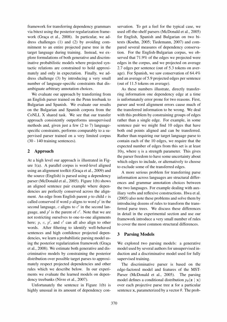
framework for transferring dependency grammarsvia bitext using the posterior regularization frame-work (Graça et al., 2008). In particular, we ad-dress challenges (1) and (2) by avoiding com-mitment to an entire projected parse tree in thetarget language during training. Instead, we ex-plore formulations of both generative and discrim-inative probabilistic models where projected syn-tactic relations are constrained to hold approxi-mately and only in expectation. Finally, we ad-dress challenge (3) by introducing a very smallnumber of language-specific constraints that dis-ambiguate arbitrary annotation choices.
We evaluate our approach by transferring froman English parser trained on the Penn treebank toBulgarian and Spanish. We evaluate our resultson the Bulgarian and Spanish corpora from theCoNLL X shared task. We see that our transferapproach consistently outperforms unsupervisedmethods and, given just a few (2 to 7) language-specific constraints, performs comparably to a su-pervised parser trained on a very limited corpus(30 - 140 training sentences).
2 Approach
At a high level our approach is illustrated in Fig-ure 1(a). A parallel corpus is word-level alignedusing an alignment toolkit (Graça et al., 2009) andthe source (English) is parsed using a dependencyparser (McDonald et al., 2005). Figure 1(b) showsan aligned sentence pair example where depen-dencies are perfectly conserved across the align-ment. An edge from English parent p to child c iscalled conserved if word p aligns to word p′ in thesecond language, c aligns to c′ in the second lan-guage, and p′ is the parent of c′. Note that we arenot restricting ourselves to one-to-one alignmentshere; p, c, p′, and c′ can all also align to otherwords. After filtering to identify well-behavedsentences and high confidence projected depen-dencies, we learn a probabilistic parsing model us-ing the posterior regularization framework (Graçaet al., 2008). We estimate both generative and dis-criminative models by constraining the posteriordistribution over possible target parses to approxi-mately respect projected dependencies and otherrules which we describe below. In our experi-ments we evaluate the learned models on depen-dency treebanks (Nivre et al., 2007).
Unfortunately the sentence in Figure 1(b) ishighly unusual in its amount of dependency con-
servation. To get a feel for the typical case, weused off-the-shelf parsers (McDonald et al., 2005)for English, Spanish and Bulgarian on two bi-texts (Koehn, 2005; Tiedemann, 2007) and com-pared several measures of dependency conserva-tion. For the English-Bulgarian corpus, we ob-served that 71.9% of the edges we projected wereedges in the corpus, and we projected on average2.7 edges per sentence (out of 5.3 tokens on aver-age). For Spanish, we saw conservation of 64.4%and an average of 5.9 projected edges per sentence(out of 11.5 tokens on average).
As these numbers illustrate, directly transfer-ring information one dependency edge at a timeis unfortunately error prone for two reasons. First,parser and word alignment errors cause much ofthe transferred information to be wrong. We dealwith this problem by constraining groups of edgesrather than a single edge. For example, in somesentence pair we might find 10 edges that haveboth end points aligned and can be transferred.Rather than requiring our target language parse tocontain each of the 10 edges, we require that theexpected number of edges from this set is at least10η, where η is a strength parameter. This givesthe parser freedom to have some uncertainty aboutwhich edges to include, or alternatively to chooseto exclude some of the transferred edges.
A more serious problem for transferring parseinformation across languages are structural differ-ences and grammar annotation choices betweenthe two languages. For example dealing with aux-iliary verbs and reflexive constructions. Hwa et al.(2005) also note these problems and solve them byintroducing dozens of rules to transform the trans-ferred parse trees. We discuss these differencesin detail in the experimental section and use ourframework introduce a very small number of rulesto cover the most common structural differences.
3 Parsing Models
We explored two parsing models: a generativemodel used by several authors for unsupervised in-duction and a discriminative model used for fullysupervised training.
The discriminative parser is based on theedge-factored model and features of the MST-Parser (McDonald et al., 2005). The parsingmodel defines a conditional distribution pθ(z | x)over each projective parse tree z for a particularsentence x, parameterized by a vector θ. The prob-
370
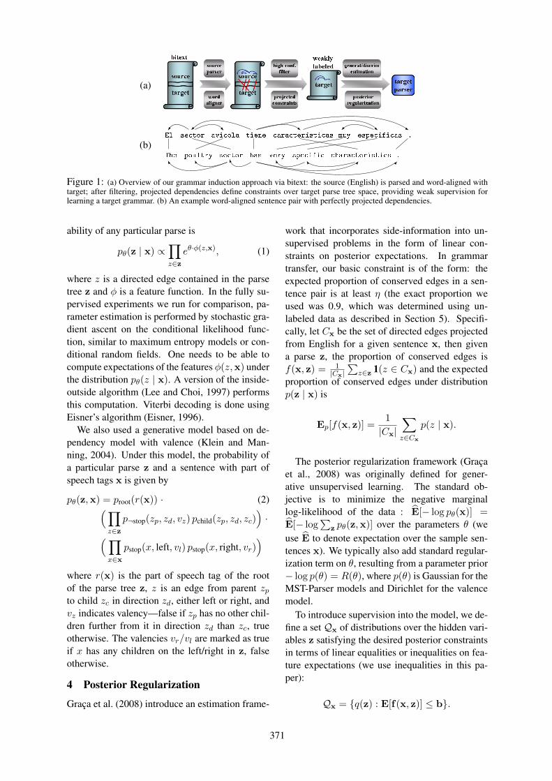
(a)
(b)
Figure 1: (a) Overview of our grammar induction approach via bitext: the source (English) is parsed and word-aligned withtarget; after filtering, projected dependencies define constraints over target parse tree space, providing weak supervision forlearning a target grammar. (b) An example word-aligned sentence pair with perfectly projected dependencies.
ability of any particular parse is
pθ(z | x) ∝∏
z∈zeθ·φ(z,x), (1)
where z is a directed edge contained in the parsetree z and φ is a feature function. In the fully su-pervised experiments we run for comparison, pa-rameter estimation is performed by stochastic gra-dient ascent on the conditional likelihood func-tion, similar to maximum entropy models or con-ditional random fields. One needs to be able tocompute expectations of the features φ(z,x) underthe distribution pθ(z | x). A version of the inside-outside algorithm (Lee and Choi, 1997) performsthis computation. Viterbi decoding is done usingEisner’s algorithm (Eisner, 1996).
We also used a generative model based on de-pendency model with valence (Klein and Man-ning, 2004). Under this model, the probability ofa particular parse z and a sentence with part ofspeech tags x is given by
pθ(z,x) = proot(r(x)) · (2)(
∏
z∈zp¬stop(zp, zd, vz) pchild(zp, zd, zc)
)
·(
∏
x∈xpstop(x, left, vl) pstop(x, right, vr)
)
where r(x) is the part of speech tag of the rootof the parse tree z, z is an edge from parent zpto child zc in direction zd, either left or right, andvz indicates valency—false if zp has no other chil-dren further from it in direction zd than zc, trueotherwise. The valencies vr/vl are marked as trueif x has any children on the left/right in z, falseotherwise.
4 Posterior Regularization
Graça et al. (2008) introduce an estimation frame-
work that incorporates side-information into un-supervised problems in the form of linear con-straints on posterior expectations. In grammartransfer, our basic constraint is of the form: theexpected proportion of conserved edges in a sen-tence pair is at least η (the exact proportion weused was 0.9, which was determined using un-labeled data as described in Section 5). Specifi-cally, let Cx be the set of directed edges projectedfrom English for a given sentence x, then givena parse z, the proportion of conserved edges isf(x, z) = 1
|Cx|∑
z∈z 1(z ∈ Cx) and the expectedproportion of conserved edges under distributionp(z | x) is
Ep[f(x, z)] =1
|Cx|∑
z∈Cx
p(z | x).
The posterior regularization framework (Graçaet al., 2008) was originally defined for gener-ative unsupervised learning. The standard ob-jective is to minimize the negative marginallog-likelihood of the data : ̂E[− log pθ(x)] =̂E[− log
∑
z pθ(z,x)] over the parameters θ (weuse ̂E to denote expectation over the sample sen-tences x). We typically also add standard regular-ization term on θ, resulting from a parameter prior− log p(θ) = R(θ), where p(θ) is Gaussian for theMST-Parser models and Dirichlet for the valencemodel.
To introduce supervision into the model, we de-fine a set Qx of distributions over the hidden vari-ables z satisfying the desired posterior constraintsin terms of linear equalities or inequalities on fea-ture expectations (we use inequalities in this pa-per):
Qx = {q(z) : E[f(x, z)] ≤ b}.
371
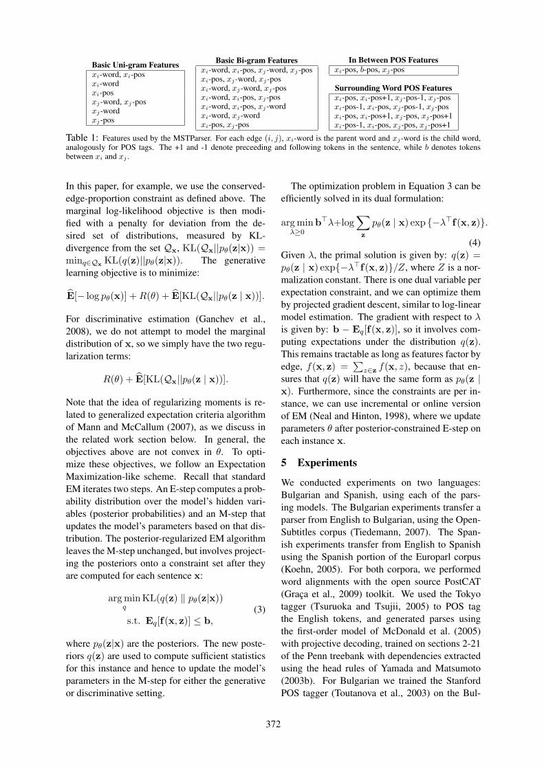
Basic Uni-gram Featuresxi-word, xi-posxi-wordxi-posxj-word, xj-posxj-wordxj-pos
Basic Bi-gram Featuresxi-word, xi-pos, xj-word, xj-posxi-pos, xj-word, xj-posxi-word, xj-word, xj-posxi-word, xi-pos, xj-posxi-word, xi-pos, xj-wordxi-word, xj-wordxi-pos, xj-pos
In Between POS Featuresxi-pos, b-pos, xj-pos
Surrounding Word POS Featuresxi-pos, xi-pos+1, xj-pos-1, xj-posxi-pos-1, xi-pos, xj-pos-1, xj-posxi-pos, xi-pos+1, xj-pos, xj-pos+1xi-pos-1, xi-pos, xj-pos, xj-pos+1
Table 1: Features used by the MSTParser. For each edge (i, j), xi-word is the parent word and xj-word is the child word,analogously for POS tags. The +1 and -1 denote preceeding and following tokens in the sentence, while b denotes tokensbetween xi and xj .
In this paper, for example, we use the conserved-edge-proportion constraint as defined above. Themarginal log-likelihood objective is then modi-fied with a penalty for deviation from the de-sired set of distributions, measured by KL-divergence from the set Qx, KL(Qx||pθ(z|x)) =minq∈Qx KL(q(z)||pθ(z|x)). The generativelearning objective is to minimize:
̂E[− log pθ(x)] +R(θ) + ̂E[KL(Qx||pθ(z | x))].
For discriminative estimation (Ganchev et al.,2008), we do not attempt to model the marginaldistribution of x, so we simply have the two regu-larization terms:
R(θ) + ̂E[KL(Qx||pθ(z | x))].
Note that the idea of regularizing moments is re-lated to generalized expectation criteria algorithmof Mann and McCallum (2007), as we discuss inthe related work section below. In general, theobjectives above are not convex in θ. To opti-mize these objectives, we follow an ExpectationMaximization-like scheme. Recall that standardEM iterates two steps. An E-step computes a prob-ability distribution over the model’s hidden vari-ables (posterior probabilities) and an M-step thatupdates the model’s parameters based on that dis-tribution. The posterior-regularized EM algorithmleaves the M-step unchanged, but involves project-ing the posteriors onto a constraint set after theyare computed for each sentence x:
arg minq
KL(q(z) ‖ pθ(z|x))
s.t. Eq[f(x, z)] ≤ b,(3)
where pθ(z|x) are the posteriors. The new poste-riors q(z) are used to compute sufficient statisticsfor this instance and hence to update the model’sparameters in the M-step for either the generativeor discriminative setting.
The optimization problem in Equation 3 can beefficiently solved in its dual formulation:
arg minλ≥0
b>λ+log∑
z
pθ(z | x) exp {−λ>f(x, z)}.
(4)Given λ, the primal solution is given by: q(z) =pθ(z | x) exp{−λ>f(x, z)}/Z, where Z is a nor-malization constant. There is one dual variable perexpectation constraint, and we can optimize themby projected gradient descent, similar to log-linearmodel estimation. The gradient with respect to λis given by: b − Eq[f(x, z)], so it involves com-puting expectations under the distribution q(z).This remains tractable as long as features factor byedge, f(x, z) =
∑
z∈z f(x, z), because that en-sures that q(z) will have the same form as pθ(z |x). Furthermore, since the constraints are per in-stance, we can use incremental or online versionof EM (Neal and Hinton, 1998), where we updateparameters θ after posterior-constrained E-step oneach instance x.
5 Experiments
We conducted experiments on two languages:Bulgarian and Spanish, using each of the pars-ing models. The Bulgarian experiments transfer aparser from English to Bulgarian, using the Open-Subtitles corpus (Tiedemann, 2007). The Span-ish experiments transfer from English to Spanishusing the Spanish portion of the Europarl corpus(Koehn, 2005). For both corpora, we performedword alignments with the open source PostCAT(Graça et al., 2009) toolkit. We used the Tokyotagger (Tsuruoka and Tsujii, 2005) to POS tagthe English tokens, and generated parses usingthe first-order model of McDonald et al. (2005)with projective decoding, trained on sections 2-21of the Penn treebank with dependencies extractedusing the head rules of Yamada and Matsumoto(2003b). For Bulgarian we trained the StanfordPOS tagger (Toutanova et al., 2003) on the Bul-
372
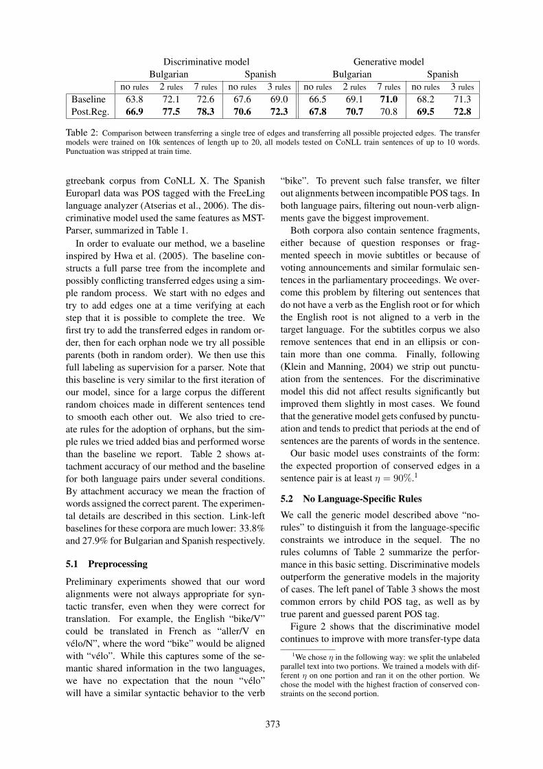
Discriminative model Generative modelBulgarian Spanish Bulgarian Spanish
no rules 2 rules 7 rules no rules 3 rules no rules 2 rules 7 rules no rules 3 rules
Baseline 63.8 72.1 72.6 67.6 69.0 66.5 69.1 71.0 68.2 71.3Post.Reg. 66.9 77.5 78.3 70.6 72.3 67.8 70.7 70.8 69.5 72.8
Table 2: Comparison between transferring a single tree of edges and transferring all possible projected edges. The transfermodels were trained on 10k sentences of length up to 20, all models tested on CoNLL train sentences of up to 10 words.Punctuation was stripped at train time.
gtreebank corpus from CoNLL X. The SpanishEuroparl data was POS tagged with the FreeLinglanguage analyzer (Atserias et al., 2006). The dis-criminative model used the same features as MST-Parser, summarized in Table 1.
In order to evaluate our method, we a baselineinspired by Hwa et al. (2005). The baseline con-structs a full parse tree from the incomplete andpossibly conflicting transferred edges using a sim-ple random process. We start with no edges andtry to add edges one at a time verifying at eachstep that it is possible to complete the tree. Wefirst try to add the transferred edges in random or-der, then for each orphan node we try all possibleparents (both in random order). We then use thisfull labeling as supervision for a parser. Note thatthis baseline is very similar to the first iteration ofour model, since for a large corpus the differentrandom choices made in different sentences tendto smooth each other out. We also tried to cre-ate rules for the adoption of orphans, but the sim-ple rules we tried added bias and performed worsethan the baseline we report. Table 2 shows at-tachment accuracy of our method and the baselinefor both language pairs under several conditions.By attachment accuracy we mean the fraction ofwords assigned the correct parent. The experimen-tal details are described in this section. Link-leftbaselines for these corpora are much lower: 33.8%and 27.9% for Bulgarian and Spanish respectively.
5.1 Preprocessing
Preliminary experiments showed that our wordalignments were not always appropriate for syn-tactic transfer, even when they were correct fortranslation. For example, the English “bike/V”could be translated in French as “aller/V envélo/N”, where the word “bike” would be alignedwith “vélo”. While this captures some of the se-mantic shared information in the two languages,we have no expectation that the noun “vélo”will have a similar syntactic behavior to the verb
“bike”. To prevent such false transfer, we filterout alignments between incompatible POS tags. Inboth language pairs, filtering out noun-verb align-ments gave the biggest improvement.
Both corpora also contain sentence fragments,either because of question responses or frag-mented speech in movie subtitles or because ofvoting announcements and similar formulaic sen-tences in the parliamentary proceedings. We over-come this problem by filtering out sentences thatdo not have a verb as the English root or for whichthe English root is not aligned to a verb in thetarget language. For the subtitles corpus we alsoremove sentences that end in an ellipsis or con-tain more than one comma. Finally, following(Klein and Manning, 2004) we strip out punctu-ation from the sentences. For the discriminativemodel this did not affect results significantly butimproved them slightly in most cases. We foundthat the generative model gets confused by punctu-ation and tends to predict that periods at the end ofsentences are the parents of words in the sentence.
Our basic model uses constraints of the form:the expected proportion of conserved edges in asentence pair is at least η = 90%.1
5.2 No Language-Specific RulesWe call the generic model described above “no-rules” to distinguish it from the language-specificconstraints we introduce in the sequel. The norules columns of Table 2 summarize the perfor-mance in this basic setting. Discriminative modelsoutperform the generative models in the majorityof cases. The left panel of Table 3 shows the mostcommon errors by child POS tag, as well as bytrue parent and guessed parent POS tag.
Figure 2 shows that the discriminative modelcontinues to improve with more transfer-type data
1We chose η in the following way: we split the unlabeledparallel text into two portions. We trained a models with dif-ferent η on one portion and ran it on the other portion. Wechose the model with the highest fraction of conserved con-straints on the second portion.
373
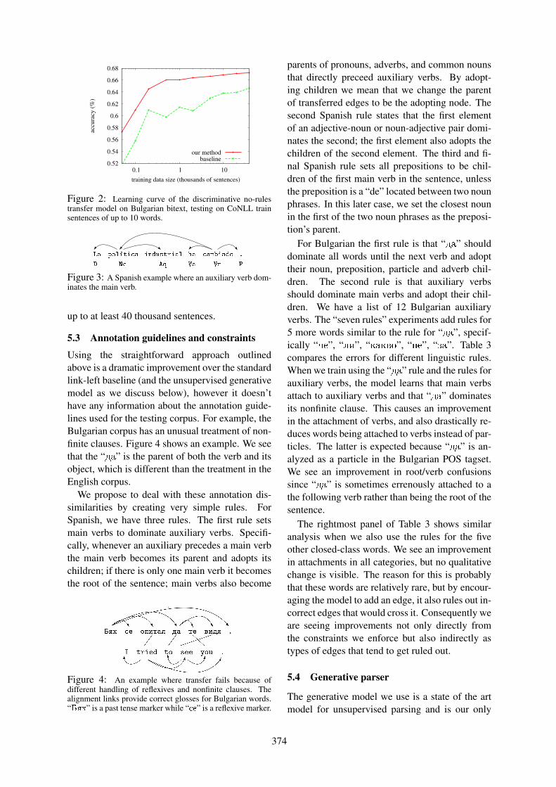
0.52
0.54
0.56
0.58
0.6
0.62
0.64
0.66
0.68
0.1 1 10
accu
racy
(%
)
training data size (thousands of sentences)
our methodbaseline
Figure 2: Learning curve of the discriminative no-rulestransfer model on Bulgarian bitext, testing on CoNLL trainsentences of up to 10 words.
Figure 3: A Spanish example where an auxiliary verb dom-inates the main verb.
up to at least 40 thousand sentences.
5.3 Annotation guidelines and constraints
Using the straightforward approach outlinedabove is a dramatic improvement over the standardlink-left baseline (and the unsupervised generativemodel as we discuss below), however it doesn’thave any information about the annotation guide-lines used for the testing corpus. For example, theBulgarian corpus has an unusual treatment of non-finite clauses. Figure 4 shows an example. We seethat the “da” is the parent of both the verb and itsobject, which is different than the treatment in theEnglish corpus.
We propose to deal with these annotation dis-similarities by creating very simple rules. ForSpanish, we have three rules. The first rule setsmain verbs to dominate auxiliary verbs. Specifi-cally, whenever an auxiliary precedes a main verbthe main verb becomes its parent and adopts itschildren; if there is only one main verb it becomesthe root of the sentence; main verbs also become
Figure 4: An example where transfer fails because ofdifferent handling of reflexives and nonfinite clauses. Thealignment links provide correct glosses for Bulgarian words.“B�h” is a past tense marker while “se” is a reflexive marker.
parents of pronouns, adverbs, and common nounsthat directly preceed auxiliary verbs. By adopt-ing children we mean that we change the parentof transferred edges to be the adopting node. Thesecond Spanish rule states that the first elementof an adjective-noun or noun-adjective pair domi-nates the second; the first element also adopts thechildren of the second element. The third and fi-nal Spanish rule sets all prepositions to be chil-dren of the first main verb in the sentence, unlessthe preposition is a “de” located between two nounphrases. In this later case, we set the closest nounin the first of the two noun phrases as the preposi-tion’s parent.
For Bulgarian the first rule is that “da” shoulddominate all words until the next verb and adopttheir noun, preposition, particle and adverb chil-dren. The second rule is that auxiliary verbsshould dominate main verbs and adopt their chil-dren. We have a list of 12 Bulgarian auxiliaryverbs. The “seven rules” experiments add rules for5 more words similar to the rule for “da”, specif-ically “qe”, “li”, “kakvo”, “ne”, “za”. Table 3compares the errors for different linguistic rules.When we train using the “da” rule and the rules forauxiliary verbs, the model learns that main verbsattach to auxiliary verbs and that “da” dominatesits nonfinite clause. This causes an improvementin the attachment of verbs, and also drastically re-duces words being attached to verbs instead of par-ticles. The latter is expected because “da” is an-alyzed as a particle in the Bulgarian POS tagset.We see an improvement in root/verb confusionssince “da” is sometimes errenously attached to athe following verb rather than being the root of thesentence.
The rightmost panel of Table 3 shows similaranalysis when we also use the rules for the fiveother closed-class words. We see an improvementin attachments in all categories, but no qualitativechange is visible. The reason for this is probablythat these words are relatively rare, but by encour-aging the model to add an edge, it also rules out in-correct edges that would cross it. Consequently weare seeing improvements not only directly fromthe constraints we enforce but also indirectly astypes of edges that tend to get ruled out.
5.4 Generative parser
The generative model we use is a state of the artmodel for unsupervised parsing and is our only
374
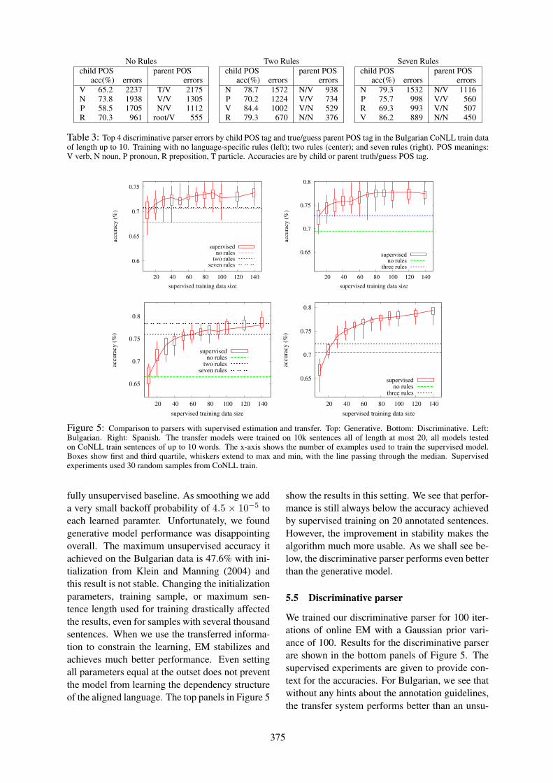
No Rules Two Rules Seven Ruleschild POS parent POS
acc(%) errors errorsV 65.2 2237 T/V 2175N 73.8 1938 V/V 1305P 58.5 1705 N/V 1112R 70.3 961 root/V 555
child POS parent POSacc(%) errors errors
N 78.7 1572 N/V 938P 70.2 1224 V/V 734V 84.4 1002 V/N 529R 79.3 670 N/N 376
child POS parent POSacc(%) errors errors
N 79.3 1532 N/V 1116P 75.7 998 V/V 560R 69.3 993 V/N 507V 86.2 889 N/N 450
Table 3: Top 4 discriminative parser errors by child POS tag and true/guess parent POS tag in the Bulgarian CoNLL train dataof length up to 10. Training with no language-specific rules (left); two rules (center); and seven rules (right). POS meanings:V verb, N noun, P pronoun, R preposition, T particle. Accuracies are by child or parent truth/guess POS tag.
0.6
0.65
0.7
0.75
20 40 60 80 100 120 140
accu
racy
(%
)
supervised training data size
supervisedno rules
two rulesseven rules
0.65
0.7
0.75
0.8
20 40 60 80 100 120 140
accu
racy
(%
)supervised training data size
supervisedno rules
three rules
0.65
0.7
0.75
0.8
20 40 60 80 100 120 140
accu
racy
(%
)
supervised training data size
supervisedno rules
two rulesseven rules
0.65
0.7
0.75
0.8
20 40 60 80 100 120 140
accu
racy
(%
)
supervised training data size
supervisedno rules
three rules
Figure 5: Comparison to parsers with supervised estimation and transfer. Top: Generative. Bottom: Discriminative. Left:Bulgarian. Right: Spanish. The transfer models were trained on 10k sentences all of length at most 20, all models testedon CoNLL train sentences of up to 10 words. The x-axis shows the number of examples used to train the supervised model.Boxes show first and third quartile, whiskers extend to max and min, with the line passing through the median. Supervisedexperiments used 30 random samples from CoNLL train.
fully unsupervised baseline. As smoothing we adda very small backoff probability of 4.5 × 10⁻⁵ toeach learned paramter. Unfortunately, we foundgenerative model performance was disappointingoverall. The maximum unsupervised accuracy itachieved on the Bulgarian data is 47.6% with ini-tialization from Klein and Manning (2004) andthis result is not stable. Changing the initializationparameters, training sample, or maximum sen-tence length used for training drastically affectedthe results, even for samples with several thousandsentences. When we use the transferred informa-tion to constrain the learning, EM stabilizes andachieves much better performance. Even settingall parameters equal at the outset does not preventthe model from learning the dependency structureof the aligned language. The top panels in Figure 5
show the results in this setting. We see that perfor-mance is still always below the accuracy achievedby supervised training on 20 annotated sentences.However, the improvement in stability makes thealgorithm much more usable. As we shall see be-low, the discriminative parser performs even betterthan the generative model.
5.5 Discriminative parser
We trained our discriminative parser for 100 iter-ations of online EM with a Gaussian prior vari-ance of 100. Results for the discriminative parserare shown in the bottom panels of Figure 5. Thesupervised experiments are given to provide con-text for the accuracies. For Bulgarian, we see thatwithout any hints about the annotation guidelines,the transfer system performs better than an unsu-
375

pervised parser, comparable to a supervised parsertrained on 10 sentences. However, if we spec-ify just the two rules for “da” and verb conjuga-tions performance jumps to that of training on 60-70 fully labeled sentences. If we have just a lit-tle more prior knowledge about how closed-classwords are handled, performance jumps above 140fully labeled sentence equivalent.
We observed another desirable property of thediscriminative model. While the generative modelcan get confused and perform poorly when thetraining data contains very long sentences, the dis-criminative parser does not appear to have thisdrawback. In fact we observed that as the maxi-mum training sentence length increased, the pars-ing performance also improved.
6 Related Work
Our work most closely relates to Hwa et al. (2005),who proposed to learn generative dependencygrammars using Collins’ parser (Collins, 1999) byconstructing full target parses via projected de-pendencies and completion/transformation rules.Hwa et al. (2005) found that transferring depen-dencies directly was not sufficient to get a parserwith reasonable performance, even when boththe source language parses and the word align-ments are performed by hand. They adjusted forthis by introducing on the order of one or twodozen language-specific transformation rules tocomplete target parses for unaligned words andto account for diverging annotation rules. Trans-ferring from English to Spanish in this way, theyachieve 72.1% and transferring to Chinese theyachieve 53.9%.
Our learning method is very closely related tothe work of (Mann and McCallum, 2007; Mannand McCallum, 2008) who concurrently devel-oped the idea of using penalties based on pos-terior expectations of features not necessarily inthe model in order to guide learning. They calltheir method generalized expectation constraintsor alternatively expectation regularization. In thisvolume (Druck et al., 2009) use this frameworkto train a dependency parser based on constraintsstated as corpus-wide expected values of linguis-tic rules. The rules select a class of edges (e.g.auxiliary verb to main verb) and require that theexpectation of these be close to some value. Themain difference between this work and theirs isthe source of the information (a linguistic infor-
mant vs. cross-lingual projection). Also, we de-fine our regularization with respect to inequalityconstraints (the model is not penalized for exceed-ing the required model expectations), while theyrequire moments to be close to an estimated value.We suspect that the two learning methods couldperform comparably when they exploit similar in-formation.
7 Conclusion
In this paper, we proposed a novel and effec-tive learning scheme for transferring dependencyparses across bitext. By enforcing projected de-pendency constraints approximately and in expec-tation, our framework allows robust learning fromnoisy partially supervised target sentences, insteadof committing to entire parses. We show that dis-criminative training generally outperforms gener-ative approaches even in this very weakly super-vised setting. By adding easily specified language-specific constraints, our models begin to rivalstrong supervised baselines for small amounts ofdata. Our framework can handle a wide range ofconstraints and we are currently exploring richersyntactic constraints that involve conservation ofmultiple edge constructions as well as constraintson conservation of surface length of dependen-cies.
Acknowledgments
This work was partially supported by an Integra-tive Graduate Education and Research Trainee-ship grant from National Science Foundation(NSFIGERT 0504487), by ARO MURI SUB-TLE W911NF-07-1-0216 and by the EuropeanProjects AsIsKnown (FP6-028044) and LTfLL(FP7-212578).
References
A. Abeillé. 2003. Treebanks: Building and UsingParsed Corpora. Springer.
H. Alshawi, S. Bangalore, and S. Douglas. 2000.Learning dependency translation models as collec-tions of finite state head transducers. ComputationalLinguistics, 26(1).
J. Atserias, B. Casas, E. Comelles, M. González,L. Padró, and M. Padró. 2006. Freeling 1.3: Syn-tactic and semantic services in an open-source nlplibrary. In Proc. LREC, Genoa, Italy.
376
P. F. Brown, S. Della Pietra, V. J. Della Pietra, and R. L.Mercer. 1994. The mathematics of statistical ma-chine translation: Parameter estimation. Computa-tional Linguistics, 19(2):263–311.
C. Chelba, D. Engle, F. Jelinek, V. Jimenez, S. Khudan-pur, L. Mangu, H. Printz, E. Ristad, R. Rosenfeld,A. Stolcke, and D. Wu. 1997. Structure and perfor-mance of a dependency language model. In Proc.Eurospeech.
M. Collins. 1999. Head-Driven Statistical Models forNatural Language Parsing. Ph.D. thesis, Universityof Pennsylvania.
G. Druck, G. Mann, and A. McCallum. 2009. Semi-supervised learning of dependency parsers usinggeneralized expectation criteria. In Proc. ACL.
J. Eisner. 1996. Three new probabilistic models for de-pendency parsing: an exploration. In Proc. CoLing.
H. Fox. 2002. Phrasal cohesion and statistical machinetranslation. In Proc. EMNLP, pages 304–311.
K. Ganchev, J. Graca, J. Blitzer, and B. Taskar.2008. Multi-view learning over structured and non-identical outputs. In Proc. UAI.
J. Graça, K. Ganchev, and B. Taskar. 2008. Expec-tation maximization and posterior constraints. InProc. NIPS.
J. Graça, K. Ganchev, and B. Taskar. 2009. Post-cat - posterior constrained alignment toolkit. In TheThird Machine Translation Marathon.
A. Haghighi, A. Ng, and C. Manning. 2005. Ro-bust textual inference via graph matching. In Proc.EMNLP.
R. Hwa, P. Resnik, A. Weinberg, C. Cabezas, andO. Kolak. 2005. Bootstrapping parsers via syntacticprojection across parallel texts. Natural LanguageEngineering, 11:11–311.
D. Klein and C. Manning. 2004. Corpus-based induc-tion of syntactic structure: Models of dependencyand constituency. In Proc. of ACL.
P. Koehn. 2005. Europarl: A parallel corpus for statis-tical machine translation. In MT Summit.
S. Lee and K. Choi. 1997. Reestimation and best-first parsing algorithm for probabilistic dependencygrammar. In In WVLC-5, pages 41–55.
G. Mann and A. McCallum. 2007. Simple, robust,scalable semi-supervised learning via expectationregularization. In Proc. ICML.
G. Mann and A. McCallum. 2008. Generalized expec-tation criteria for semi-supervised learning of con-ditional random fields. In Proc. ACL, pages 870 –878.
R. McDonald, K. Crammer, and F. Pereira. 2005. On-line large-margin training of dependency parsers. InProc. ACL, pages 91–98.
I. Mel’čuk. 1988. Dependency syntax: theory andpractice. SUNY. inci.
P. Merlo, S. Stevenson, V. Tsang, and G. Allaria. 2002.A multilingual paradigm for automatic verb classifi-cation. In Proc. ACL.
R. M. Neal and G. E. Hinton. 1998. A new view of theEM algorithm that justifies incremental, sparse andother variants. In M. I. Jordan, editor, Learning inGraphical Models, pages 355–368. Kluwer.
J. Nivre and J. Nilsson. 2005. Pseudo-projective de-pendency parsing. In Proc. ACL.
J. Nivre, J. Hall, S. Kübler, R. McDonald, J. Nils-son, S. Riedel, and D. Yuret. 2007. The CoNLL2007 shared task on dependency parsing. In Proc.EMNLP-CoNLL.
F. J. Och and H. Ney. 2000. Improved statistical align-ment models. In Proc. ACL.
C. Quirk, A. Menezes, and C. Cherry. 2005. De-pendency treelet translation: syntactically informedphrasal smt. In Proc. ACL.
L. Shen, J. Xu, and R. Weischedel. 2008. A newstring-to-dependency machine translation algorithmwith a target dependency language model. In Proc.of ACL.
N. Smith and J. Eisner. 2006. Annealing structuralbias in multilingual weighted grammar induction. InProc. ACL.
J. Tiedemann. 2007. Building a multilingual parallelsubtitle corpus. In Proc. CLIN.
K. Toutanova, D. Klein, C. Manning, and Y. Singer.2003. Feature-rich part-of-speech tagging with acyclic dependency network. In Proc. HLT-NAACL.
Y. Tsuruoka and J. Tsujii. 2005. Bidirectional infer-ence with the easiest-first strategy for tagging se-quence data. In Proc. HLT/EMNLP.
H. Yamada and Y. Matsumoto. 2003a. Statistical de-pendency analysis with support vector machines. InProc. IWPT, pages 195–206.
H. Yamada and Y. Matsumoto. 2003b. Statistical de-pendency analysis with support vector machines. InProc. IWPT.
D. Yarowsky and G. Ngai. 2001. Inducing multilin-gual pos taggers and np bracketers via robust pro-jection across aligned corpora. In Proc. NAACL.
D. Yarowsky, G. Ngai, and R. Wicentowski. 2001.Inducing multilingual text analysis tools via robustprojection across aligned corpora. In Proc. HLT.
377
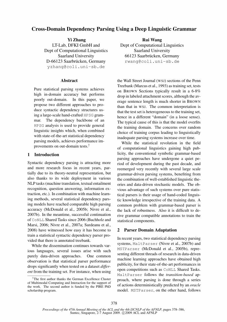
Proceedings of the 47th Annual Meeting of the ACL and the 4th IJCNLP of the AFNLP, pages 378–386,Suntec, Singapore, 2-7 August 2009. c©2009 ACL and AFNLP
Cross-Domain Dependency Parsing Using a Deep Linguistic Grammar
Yi ZhangLT-Lab, DFKI GmbH and
Dept of Computational LinguisticsSaarland University
D-66123 Saarbrücken, [email protected]
Rui WangDept of Computational Linguistics
Saarland University66123 Saarbrücken, [email protected]
Abstract
Pure statistical parsing systems achieveshigh in-domain accuracy but performspoorly out-domain. In this paper, wepropose two different approaches to pro-duce syntactic dependency structures us-ing a large-scale hand-crafted HPSG gram-mar. The dependency backbone of anHPSG analysis is used to provide generallinguistic insights which, when combinedwith state-of-the-art statistical dependencyparsing models, achieves performance im-provements on out-domain tests.†
1 Introduction
Syntactic dependency parsing is attracting moreand more research focus in recent years, par-tially due to its theory-neutral representation, butalso thanks to its wide deployment in variousNLP tasks (machine translation, textual entailmentrecognition, question answering, information ex-traction, etc.). In combination with machine learn-ing methods, several statistical dependency pars-ing models have reached comparable high parsingaccuracy (McDonald et al., 2005b; Nivre et al.,2007b). In the meantime, successful continuationof CoNLL Shared Tasks since 2006 (Buchholz andMarsi, 2006; Nivre et al., 2007a; Surdeanu et al.,2008) have witnessed how easy it has become totrain a statistical syntactic dependency parser pro-vided that there is annotated treebank.
While the dissemination continues towards var-ious languages, several issues arise with suchpurely data-driven approaches. One commonobservation is that statistical parser performancedrops significantly when tested on a dataset differ-ent from the training set. For instance, when using
†The first author thanks the German Excellence Clusterof Multimodal Computing and Interaction for the support ofthe work. The second author is funded by the PIRE PhDscholarship program.
the Wall Street Journal (WSJ) sections of the PennTreebank (Marcus et al., 1993) as training set, testson BROWN Sections typically result in a 6-8%drop in labeled attachment scores, although the av-erage sentence length is much shorter in BROWN
than that in WSJ. The common interpretation isthat the test set is heterogeneous to the training set,hence in a different “domain” (in a loose sense).The typical cause of this is that the model overfitsthe training domain. The concerns over randomchoice of training corpus leading to linguisticallyinadequate parsing systems increase over time.
While the statistical revolution in the fieldof computational linguistics gaining high pub-licity, the conventional symbolic grammar-basedparsing approaches have undergone a quiet pe-riod of development during the past decade, andreemerged very recently with several large scalegrammar-driven parsing systems, benefiting fromthe combination of well-established linguistic the-ories and data-driven stochastic models. The ob-vious advantage of such systems over pure statis-tical parsers is their usage of hand-coded linguis-tic knowledge irrespective of the training data. Acommon problem with grammar-based parser isthe lack of robustness. Also it is difficult to de-rive grammar compatible annotations to train thestatistical components.
2 Parser Domain Adaptation
In recent years, two statistical dependency parsingsystems, MaltParser (Nivre et al., 2007b) andMSTParser (McDonald et al., 2005b), repre-senting different threads of research in data-drivenmachine learning approaches have obtained highpublicity, for their state-of-the-art performances inopen competitions such as CoNLL Shared Tasks.MaltParser follows the transition-based ap-proach, where parsing is done through a seriesof actions deterministically predicted by an oraclemodel. MSTParser, on the other hand, follows
378
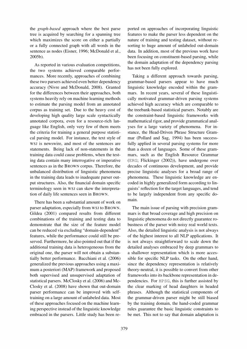
the graph-based approach where the best parsetree is acquired by searching for a spanning treewhich maximizes the score on either a partiallyor a fully connected graph with all words in thesentence as nodes (Eisner, 1996; McDonald et al.,2005b).
As reported in various evaluation competitions,the two systems achieved comparable perfor-mances. More recently, approaches of combiningthese two parsers achieved even better dependencyaccuracy (Nivre and McDonald, 2008). Grantedfor the differences between their approaches, bothsystems heavily rely on machine learning methodsto estimate the parsing model from an annotatedcorpus as training set. Due to the heavy cost ofdeveloping high quality large scale syntacticallyannotated corpora, even for a resource-rich lan-guage like English, only very few of them meetsthe criteria for training a general purpose statisti-cal parsing model. For instance, the text style ofWSJ is newswire, and most of the sentences arestatements. Being lack of non-statements in thetraining data could cause problems, when the test-ing data contain many interrogative or imperativesentences as in the BROWN corpus. Therefore, theunbalanced distribution of linguistic phenomenain the training data leads to inadequate parser out-put structures. Also, the financial domain specificterminology seen in WSJ can skew the interpreta-tion of daily life sentences seen in BROWN.
There has been a substantial amount of work onparser adaptation, especially from WSJ to BROWN.Gildea (2001) compared results from differentcombinations of the training and testing data todemonstrate that the size of the feature modelcan be reduced via excluding “domain-dependent”features, while the performance could still be pre-served. Furthermore, he also pointed out that if theadditional training data is heterogeneous from theoriginal one, the parser will not obtain a substan-tially better performance. Bacchiani et al. (2006)generalized the previous approaches using a maxi-mum a posteriori (MAP) framework and proposedboth supervised and unsupervised adaptation ofstatistical parsers. McClosky et al. (2006) and Mc-Closky et al. (2008) have shown that out-domainparser performance can be improved with self-training on a large amount of unlabeled data. Mostof these approaches focused on the machine learn-ing perspective instead of the linguistic knowledgeembraced in the parsers. Little study has been re-
ported on approaches of incorporating linguisticfeatures to make the parser less dependent on thenature of training and testing dataset, without re-sorting to huge amount of unlabeled out-domaindata. In addition, most of the previous work havebeen focusing on constituent-based parsing, whilethe domain adaptation of the dependency parsinghas not been fully explored.
Taking a different approach towards parsing,grammar-based parsers appear to have muchlinguistic knowledge encoded within the gram-mars. In recent years, several of these linguisti-cally motivated grammar-driven parsing systemsachieved high accuracy which are comparable tothe treebank-based statistical parsers. Notably arethe constraint-based linguistic frameworks withmathematical rigor, and provide grammatical anal-yses for a large variety of phenomena. For in-stance, the Head-Driven Phrase Structure Gram-mar (Pollard and Sag, 1994) has been success-fully applied in several parsing systems for morethan a dozen of languages. Some of these gram-mars, such as the English Resource Grammar(ERG; Flickinger (2002)), have undergone overdecades of continuous development, and provideprecise linguistic analyses for a broad range ofphenomena. These linguistic knowledge are en-coded in highly generalized form according to lin-guists’ reflection for the target languages, and tendto be largely independent from any specific do-main.
The main issue of parsing with precision gram-mars is that broad coverage and high precision onlinguistic phenomena do not directly guarantee ro-bustness of the parser with noisy real world texts.Also, the detailed linguistic analysis is not alwaysof the highest interest to all NLP applications. Itis not always straightforward to scale down thedetailed analyses embraced by deep grammars toa shallower representation which is more acces-sible for specific NLP tasks. On the other hand,since the dependency representation is relativelytheory-neutral, it is possible to convert from otherframeworks into its backbone representation in de-pendencies. For HPSG, this is further assisted bythe clear marking of head daughters in headedphrases. Although the statistical components ofthe grammar-driven parser might be still biasedby the training domain, the hand-coded grammarrules guarantee the basic linguistic constraints tobe met. This not to say that domain adaptation is
379
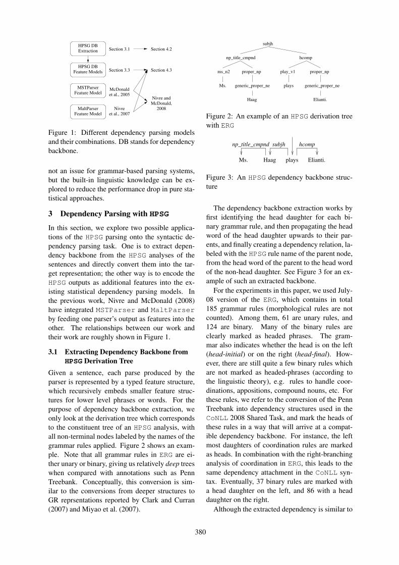
HPSG DB
Extraction
HPSG DB
Feature Models
MSTParser
Feature Model
MaltParser
Feature Model
Section 3.1
Section 3.3
McDonald
et al., 2005
Nivre
et al., 2007
Nivre and
McDonald,
2008
Section 4.2
Section 4.3
Figure 1: Different dependency parsing modelsand their combinations. DB stands for dependencybackbone.
not an issue for grammar-based parsing systems,but the built-in linguistic knowledge can be ex-plored to reduce the performance drop in pure sta-tistical approaches.
3 Dependency Parsing with HPSG
In this section, we explore two possible applica-tions of the HPSG parsing onto the syntactic de-pendency parsing task. One is to extract depen-dency backbone from the HPSG analyses of thesentences and directly convert them into the tar-get representation; the other way is to encode theHPSG outputs as additional features into the ex-isting statistical dependency parsing models. Inthe previous work, Nivre and McDonald (2008)have integrated MSTParser and MaltParserby feeding one parser’s output as features into theother. The relationships between our work andtheir work are roughly shown in Figure 1.
3.1 Extracting Dependency Backbone fromHPSG Derivation Tree
Given a sentence, each parse produced by theparser is represented by a typed feature structure,which recursively embeds smaller feature struc-tures for lower level phrases or words. For thepurpose of dependency backbone extraction, weonly look at the derivation tree which correspondsto the constituent tree of an HPSG analysis, withall non-terminal nodes labeled by the names of thegrammar rules applied. Figure 2 shows an exam-ple. Note that all grammar rules in ERG are ei-ther unary or binary, giving us relatively deep treeswhen compared with annotations such as PennTreebank. Conceptually, this conversion is sim-ilar to the conversions from deeper structures toGR reprsentations reported by Clark and Curran(2007) and Miyao et al. (2007).
np_title_cmpnd
ms_n2 proper_np
subjh
generic_proper_ne
Haag
play_v1
hcomp
proper_np
generic_proper_ne
Elianti.
playsMs.
Figure 2: An example of an HPSG derivation treewith ERG
Ms. Haag plays Elianti.
hcompnp_title_cmpnd subjh
Figure 3: An HPSG dependency backbone struc-ture
The dependency backbone extraction works byfirst identifying the head daughter for each bi-nary grammar rule, and then propagating the headword of the head daughter upwards to their par-ents, and finally creating a dependency relation, la-beled with the HPSG rule name of the parent node,from the head word of the parent to the head wordof the non-head daughter. See Figure 3 for an ex-ample of such an extracted backbone.
For the experiments in this paper, we used July-08 version of the ERG, which contains in total185 grammar rules (morphological rules are notcounted). Among them, 61 are unary rules, and124 are binary. Many of the binary rules areclearly marked as headed phrases. The gram-mar also indicates whether the head is on the left(head-initial) or on the right (head-final). How-ever, there are still quite a few binary rules whichare not marked as headed-phrases (according tothe linguistic theory), e.g. rules to handle coor-dinations, appositions, compound nouns, etc. Forthese rules, we refer to the conversion of the PennTreebank into dependency structures used in theCoNLL 2008 Shared Task, and mark the heads ofthese rules in a way that will arrive at a compat-ible dependency backbone. For instance, the leftmost daughters of coordination rules are markedas heads. In combination with the right-branchinganalysis of coordination in ERG, this leads to thesame dependency attachment in the CoNLL syn-tax. Eventually, 37 binary rules are marked witha head daughter on the left, and 86 with a headdaughter on the right.
Although the extracted dependency is similar to
380
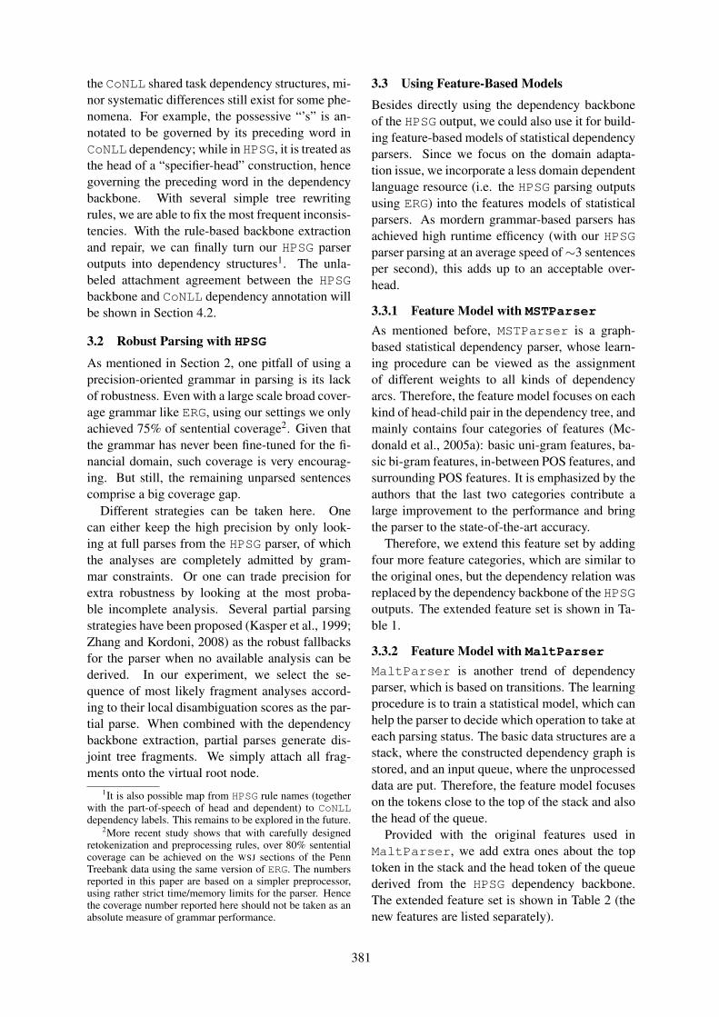
the CoNLL shared task dependency structures, mi-nor systematic differences still exist for some phe-nomena. For example, the possessive “’s” is an-notated to be governed by its preceding word inCoNLL dependency; while in HPSG, it is treated asthe head of a “specifier-head” construction, hencegoverning the preceding word in the dependencybackbone. With several simple tree rewritingrules, we are able to fix the most frequent inconsis-tencies. With the rule-based backbone extractionand repair, we can finally turn our HPSG parseroutputs into dependency structures1. The unla-beled attachment agreement between the HPSGbackbone and CoNLL dependency annotation willbe shown in Section 4.2.
3.2 Robust Parsing with HPSG
As mentioned in Section 2, one pitfall of using aprecision-oriented grammar in parsing is its lackof robustness. Even with a large scale broad cover-age grammar like ERG, using our settings we onlyachieved 75% of sentential coverage2. Given thatthe grammar has never been fine-tuned for the fi-nancial domain, such coverage is very encourag-ing. But still, the remaining unparsed sentencescomprise a big coverage gap.
Different strategies can be taken here. Onecan either keep the high precision by only look-ing at full parses from the HPSG parser, of whichthe analyses are completely admitted by gram-mar constraints. Or one can trade precision forextra robustness by looking at the most proba-ble incomplete analysis. Several partial parsingstrategies have been proposed (Kasper et al., 1999;Zhang and Kordoni, 2008) as the robust fallbacksfor the parser when no available analysis can bederived. In our experiment, we select the se-quence of most likely fragment analyses accord-ing to their local disambiguation scores as the par-tial parse. When combined with the dependencybackbone extraction, partial parses generate dis-joint tree fragments. We simply attach all frag-ments onto the virtual root node.
1It is also possible map from HPSG rule names (togetherwith the part-of-speech of head and dependent) to CoNLLdependency labels. This remains to be explored in the future.
2More recent study shows that with carefully designedretokenization and preprocessing rules, over 80% sententialcoverage can be achieved on the WSJ sections of the PennTreebank data using the same version of ERG. The numbersreported in this paper are based on a simpler preprocessor,using rather strict time/memory limits for the parser. Hencethe coverage number reported here should not be taken as anabsolute measure of grammar performance.
3.3 Using Feature-Based ModelsBesides directly using the dependency backboneof the HPSG output, we could also use it for build-ing feature-based models of statistical dependencyparsers. Since we focus on the domain adapta-tion issue, we incorporate a less domain dependentlanguage resource (i.e. the HPSG parsing outputsusing ERG) into the features models of statisticalparsers. As mordern grammar-based parsers hasachieved high runtime efficency (with our HPSGparser parsing at an average speed of∼3 sentencesper second), this adds up to an acceptable over-head.
3.3.1 Feature Model with MSTParserAs mentioned before, MSTParser is a graph-based statistical dependency parser, whose learn-ing procedure can be viewed as the assignmentof different weights to all kinds of dependencyarcs. Therefore, the feature model focuses on eachkind of head-child pair in the dependency tree, andmainly contains four categories of features (Mc-donald et al., 2005a): basic uni-gram features, ba-sic bi-gram features, in-between POS features, andsurrounding POS features. It is emphasized by theauthors that the last two categories contribute alarge improvement to the performance and bringthe parser to the state-of-the-art accuracy.
Therefore, we extend this feature set by addingfour more feature categories, which are similar tothe original ones, but the dependency relation wasreplaced by the dependency backbone of the HPSGoutputs. The extended feature set is shown in Ta-ble 1.
3.3.2 Feature Model with MaltParserMaltParser is another trend of dependencyparser, which is based on transitions. The learningprocedure is to train a statistical model, which canhelp the parser to decide which operation to take ateach parsing status. The basic data structures are astack, where the constructed dependency graph isstored, and an input queue, where the unprocesseddata are put. Therefore, the feature model focuseson the tokens close to the top of the stack and alsothe head of the queue.
Provided with the original features used inMaltParser, we add extra ones about the toptoken in the stack and the head token of the queuederived from the HPSG dependency backbone.The extended feature set is shown in Table 2 (thenew features are listed separately).
381
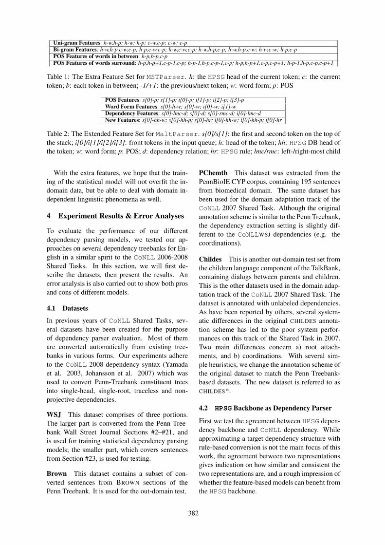
Uni-gram Features: h-w,h-p; h-w; h-p; c-w,c-p; c-w; c-pBi-gram Features: h-w,h-p,c-w,c-p; h-p,c-w,c-p; h-w,c-w,c-p; h-w,h-p,c-p; h-w,h-p,c-w; h-w,c-w; h-p,c-pPOS Features of words in between: h-p,b-p,c-pPOS Features of words surround: h-p,h-p+1,c-p-1,c-p; h-p-1,h-p,c-p-1,c-p; h-p,h-p+1,c-p,c-p+1; h-p-1,h-p,c-p,c-p+1
Table 1: The Extra Feature Set for MSTParser. h: the HPSG head of the current token; c: the currenttoken; b: each token in between; -1/+1: the previous/next token; w: word form; p: POS
POS Features: s[0]-p; s[1]-p; i[0]-p; i[1]-p; i[2]-p; i[3]-pWord Form Features: s[0]-h-w; s[0]-w; i[0]-w; i[1]-wDependency Features: s[0]-lmc-d; s[0]-d; s[0]-rmc-d; i[0]-lmc-dNew Features: s[0]-hh-w; s[0]-hh-p; s[0]-hr; i[0]-hh-w; i[0]-hh-p; i[0]-hr
Table 2: The Extended Feature Set for MaltParser. s[0]/s[1]: the first and second token on the top ofthe stack; i[0]/i[1]/i[2]/i[3]: front tokens in the input queue; h: head of the token; hh: HPSG DB head ofthe token; w: word form; p: POS; d: dependency relation; hr: HPSG rule; lmc/rmc: left-/right-most child
With the extra features, we hope that the train-ing of the statistical model will not overfit the in-domain data, but be able to deal with domain in-dependent linguistic phenomena as well.
4 Experiment Results & Error Analyses
To evaluate the performance of our differentdependency parsing models, we tested our ap-proaches on several dependency treebanks for En-glish in a similar spirit to the CoNLL 2006-2008Shared Tasks. In this section, we will first de-scribe the datasets, then present the results. Anerror analysis is also carried out to show both prosand cons of different models.
4.1 Datasets
In previous years of CoNLL Shared Tasks, sev-eral datasets have been created for the purposeof dependency parser evaluation. Most of themare converted automatically from existing tree-banks in various forms. Our experiments adhereto the CoNLL 2008 dependency syntax (Yamadaet al. 2003, Johansson et al. 2007) which wasused to convert Penn-Treebank constituent treesinto single-head, single-root, traceless and non-projective dependencies.
WSJ This dataset comprises of three portions.The larger part is converted from the Penn Tree-bank Wall Street Journal Sections #2–#21, andis used for training statistical dependency parsingmodels; the smaller part, which covers sentencesfrom Section #23, is used for testing.
Brown This dataset contains a subset of con-verted sentences from BROWN sections of thePenn Treebank. It is used for the out-domain test.
PChemtb This dataset was extracted from thePennBioIE CYP corpus, containing 195 sentencesfrom biomedical domain. The same dataset hasbeen used for the domain adaptation track of theCoNLL 2007 Shared Task. Although the originalannotation scheme is similar to the Penn Treebank,the dependency extraction setting is slightly dif-ferent to the CoNLLWSJ dependencies (e.g. thecoordinations).
Childes This is another out-domain test set fromthe children language component of the TalkBank,containing dialogs between parents and children.This is the other datasets used in the domain adap-tation track of the CoNLL 2007 Shared Task. Thedataset is annotated with unlabeled dependencies.As have been reported by others, several system-atic differences in the original CHILDES annota-tion scheme has led to the poor system perfor-mances on this track of the Shared Task in 2007.Two main differences concern a) root attach-ments, and b) coordinations. With several sim-ple heuristics, we change the annotation scheme ofthe original dataset to match the Penn Treebank-based datasets. The new dataset is referred to asCHILDES*.
4.2 HPSG Backbone as Dependency Parser
First we test the agreement between HPSG depen-dency backbone and CoNLL dependency. Whileapproximating a target dependency structure withrule-based conversion is not the main focus of thiswork, the agreement between two representationsgives indication on how similar and consistent thetwo representations are, and a rough impression ofwhether the feature-based models can benefit fromthe HPSG backbone.
382
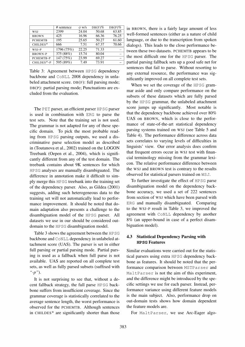
# sentence φ w/s DB(F)% DB(P)%WSJ 2399 24.04 50.68 63.85BROWN 425 16.96 66.36 76.25PCHEMTB 195 25.65 50.27 61.60CHILDES* 666 7.51 67.37 70.66WSJ-P 1796 (75%) 22.25 71.33 –BROWN-P 375 (88%) 15.74 80.04 –PCHEMTB-P 147 (75%) 23.99 69.27 –CHILDES*-P 595 (89%) 7.49 73.91 –
Table 3: Agreement between HPSG dependencybackbone and CoNLL 2008 dependency in unla-beled attachment score. DB(F): full parsing mode;DB(P): partial parsing mode; Punctuations are ex-cluded from the evaluation.
The PET parser, an efficient parser HPSG parseris used in combination with ERG to parse thetest sets. Note that the training set is not used.The grammar is not adapted for any of these spe-cific domain. To pick the most probable read-ing from HPSG parsing outputs, we used a dis-criminative parse selection model as describedin (Toutanova et al., 2002) trained on the LOGONTreebank (Oepen et al., 2004), which is signifi-cantly different from any of the test domain. Thetreebank contains about 9K sentences for whichHPSG analyses are manually disambiguated. Thedifference in annotation make it difficult to sim-ply merge this HPSG treebank into the training setof the dependency parser. Also, as Gildea (2001)suggests, adding such heterogeneous data to thetraining set will not automatically lead to perfor-mance improvement. It should be noted that do-main adaptation also presents a challenge to thedisambiguation model of the HPSG parser. Alldatasets we use in our should be considered out-domain to the HPSG disambiguation model.
Table 3 shows the agreement between the HPSGbackbone and CoNLL dependency in unlabeled at-tachment score (UAS). The parser is set in eitherfull parsing or partial parsing mode. Partial pars-ing is used as a fallback when full parse is notavailable. UAS are reported on all complete testsets, as well as fully parsed subsets (suffixed with“-p”).
It is not surprising to see that, without a de-cent fallback strategy, the full parse HPSG back-bone suffers from insufficient coverage. Since thegrammar coverage is statistically correlated to theaverage sentence length, the worst performance isobserved for the PCHEMTB. Although sentencesin CHILDES* are significantly shorter than those
in BROWN, there is a fairly large amount of lesswell-formed sentences (either as a nature of childlanguage, or due to the transcription from spokendialogs). This leads to the close performance be-tween these two datasets. PCHEMTB appears to bethe most difficult one for the HPSG parser. Thepartial parsing fallback sets up a good safe net forsentences that fail to parse. Without resorting toany external resource, the performance was sig-nificantly improved on all complete test sets.
When we set the coverage of the HPSG gram-mar aside and only compare performance on thesubsets of these datasets which are fully parsedby the HPSG grammar, the unlabeled attachmentscore jumps up significantly. Most notable isthat the dependency backbone achieved over 80%UAS on BROWN, which is close to the perfor-mance of state-of-the-art statistical dependencyparsing systems trained on WSJ (see Table 5 andTable 4). The performance difference across datasets correlates to varying levels of difficulties inlinguists’ view. Our error analysis does confirmthat frequent errors occur in WSJ test with finan-cial terminology missing from the grammar lexi-con. The relative performance difference betweenthe WSJ and BROWN test is contrary to the resultsobserved for statistical parsers trained on WSJ.
To further investigate the effect of HPSG parsedisambiguation model on the dependency back-bone accuracy, we used a set of 222 sentencesfrom section of WSJ which have been parsed withERG and manually disambiguated. Comparingto the WSJ-P result in Table 3, we improved theagreement with CoNLL dependency by another8% (an upper-bound in case of a perfect disam-biguation model).
4.3 Statistical Dependency Parsing withHPSG Features
Similar evaluations were carried out for the statis-tical parsers using extra HPSG dependency back-bone as features. It should be noted that the per-formance comparison between MSTParser andMaltParser is not the aim of this experiment,and the difference might be introduced by the spe-cific settings we use for each parser. Instead, per-formance variance using different feature modelsis the main subject. Also, performance drop onout-domain tests shows how domain dependentthe feature models are.
For MaltParser, we use Arc-Eager algo-
383
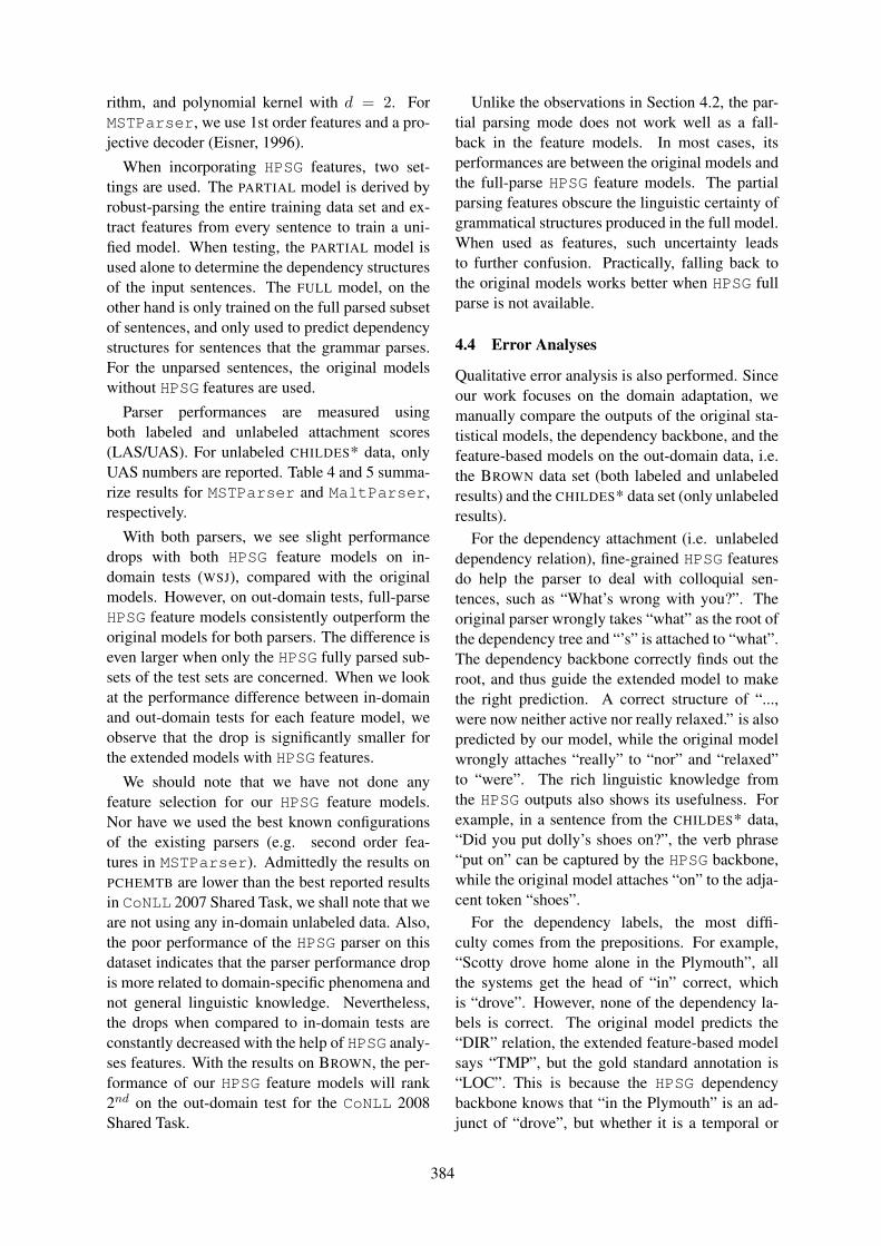
rithm, and polynomial kernel with d = 2. ForMSTParser, we use 1st order features and a pro-jective decoder (Eisner, 1996).
When incorporating HPSG features, two set-tings are used. The PARTIAL model is derived byrobust-parsing the entire training data set and ex-tract features from every sentence to train a uni-fied model. When testing, the PARTIAL model isused alone to determine the dependency structuresof the input sentences. The FULL model, on theother hand is only trained on the full parsed subsetof sentences, and only used to predict dependencystructures for sentences that the grammar parses.For the unparsed sentences, the original modelswithout HPSG features are used.
Parser performances are measured usingboth labeled and unlabeled attachment scores(LAS/UAS). For unlabeled CHILDES* data, onlyUAS numbers are reported. Table 4 and 5 summa-rize results for MSTParser and MaltParser,respectively.
With both parsers, we see slight performancedrops with both HPSG feature models on in-domain tests (WSJ), compared with the originalmodels. However, on out-domain tests, full-parseHPSG feature models consistently outperform theoriginal models for both parsers. The difference iseven larger when only the HPSG fully parsed sub-sets of the test sets are concerned. When we lookat the performance difference between in-domainand out-domain tests for each feature model, weobserve that the drop is significantly smaller forthe extended models with HPSG features.
We should note that we have not done anyfeature selection for our HPSG feature models.Nor have we used the best known configurationsof the existing parsers (e.g. second order fea-tures in MSTParser). Admittedly the results onPCHEMTB are lower than the best reported resultsin CoNLL 2007 Shared Task, we shall note that weare not using any in-domain unlabeled data. Also,the poor performance of the HPSG parser on thisdataset indicates that the parser performance dropis more related to domain-specific phenomena andnot general linguistic knowledge. Nevertheless,the drops when compared to in-domain tests areconstantly decreased with the help of HPSG analy-ses features. With the results on BROWN, the per-formance of our HPSG feature models will rank2nd on the out-domain test for the CoNLL 2008Shared Task.
Unlike the observations in Section 4.2, the par-tial parsing mode does not work well as a fall-back in the feature models. In most cases, itsperformances are between the original models andthe full-parse HPSG feature models. The partialparsing features obscure the linguistic certainty ofgrammatical structures produced in the full model.When used as features, such uncertainty leadsto further confusion. Practically, falling back tothe original models works better when HPSG fullparse is not available.
4.4 Error Analyses
Qualitative error analysis is also performed. Sinceour work focuses on the domain adaptation, wemanually compare the outputs of the original sta-tistical models, the dependency backbone, and thefeature-based models on the out-domain data, i.e.the BROWN data set (both labeled and unlabeledresults) and the CHILDES* data set (only unlabeledresults).
For the dependency attachment (i.e. unlabeleddependency relation), fine-grained HPSG featuresdo help the parser to deal with colloquial sen-tences, such as “What’s wrong with you?”. Theoriginal parser wrongly takes “what” as the root ofthe dependency tree and “’s” is attached to “what”.The dependency backbone correctly finds out theroot, and thus guide the extended model to makethe right prediction. A correct structure of “...,were now neither active nor really relaxed.” is alsopredicted by our model, while the original modelwrongly attaches “really” to “nor” and “relaxed”to “were”. The rich linguistic knowledge fromthe HPSG outputs also shows its usefulness. Forexample, in a sentence from the CHILDES* data,“Did you put dolly’s shoes on?”, the verb phrase“put on” can be captured by the HPSG backbone,while the original model attaches “on” to the adja-cent token “shoes”.
For the dependency labels, the most diffi-culty comes from the prepositions. For example,“Scotty drove home alone in the Plymouth”, allthe systems get the head of “in” correct, whichis “drove”. However, none of the dependency la-bels is correct. The original model predicts the“DIR” relation, the extended feature-based modelsays “TMP”, but the gold standard annotation is“LOC”. This is because the HPSG dependencybackbone knows that “in the Plymouth” is an ad-junct of “drove”, but whether it is a temporal or
384
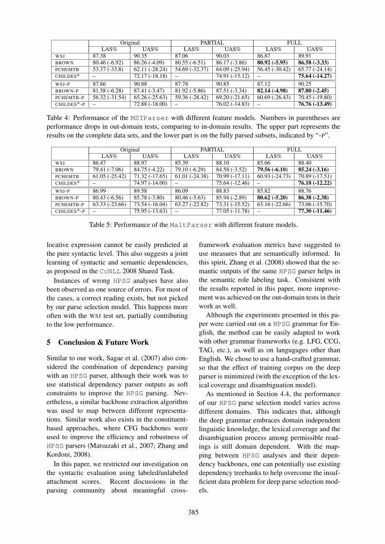
Original PARTIAL FULLLAS% UAS% LAS% UAS% LAS% UAS%
WSJ 87.38 90.35 87.06 90.03 86.87 89.91BROWN 80.46 (-6.92) 86.26 (-4.09) 80.55 (-6.51) 86.17 (-3.86) 80.92 (-5.95) 86.58 (-3.33)PCHEMTB 53.37 (-33.8) 62.11 (-28.24) 54.69 (-32.37) 64.09 (-25.94) 56.45 (-30.42) 65.77 (-24.14)CHILDES* – 72.17 (-18.18) – 74.91 (-15.12) – 75.64 (-14.27)WSJ-P 87.86 90.88 87.78 90.85 87.12 90.25BROWN-P 81.58 (-6.28) 87.41 (-3.47) 81.92 (-5.86) 87.51 (-3.34) 82.14 (-4.98) 87.80 (-2.45)PCHEMTB-P 56.32 (-31.54) 65.26 (-25.63) 59.36 (-28.42) 69.20 (-21.65) 60.69 (-26.43) 70.45 (-19.80)CHILDES*-P – 72.88 (-18.00) – 76.02 (-14.83) – 76.76 (-13.49)
Table 4: Performance of the MSTParser with different feature models. Numbers in parentheses areperformance drops in out-domain tests, comparing to in-domain results. The upper part represents theresults on the complete data sets, and the lower part is on the fully parsed subsets, indicated by “-P”.
Original PARTIAL FULLLAS% UAS% LAS% UAS% LAS% UAS%
WSJ 86.47 88.97 85.39 88.10 85.66 88.40BROWN 79.41 (-7.06) 84.75 (-4.22) 79.10 (-6.29) 84.58 (-3.52) 79.56 (-6.10) 85.24 (-3.16)PCHEMTB 61.05 (-25.42) 71.32 (-17.65) 61.01 (-24.38) 70.99 (-17.11) 60.93 (-24.73) 70.89 (-17.51)CHILDES* – 74.97 (-14.00) – 75.64 (-12.46) – 76.18 (-12.22)WSJ-P 86.99 89.58 86.09 88.83 85.82 88.76BROWN-P 80.43 (-6.56) 85.78 (-3.80) 80.46 (-5.63) 85.94 (-2.89) 80.62 (-5.20) 86.38 (-2.38)PCHEMTB-P 63.33 (-23.66) 73.54 (-16.04) 63.27 (-22.82) 73.31 (-15.52) 63.16 (-22.66) 73.06 (-15.70)CHILDES*-P – 75.95 (-13.63) – 77.05 (-11.78) – 77.30 (-11.46)
Table 5: Performance of the MaltParser with different feature models.
locative expression cannot be easily predicted atthe pure syntactic level. This also suggests a jointlearning of syntactic and semantic dependencies,as proposed in the CoNLL 2008 Shared Task.
Instances of wrong HPSG analyses have alsobeen observed as one source of errors. For most ofthe cases, a correct reading exists, but not pickedby our parse selection model. This happens moreoften with the WSJ test set, partially contributingto the low performance.
5 Conclusion & Future Work
Similar to our work, Sagae et al. (2007) also con-sidered the combination of dependency parsingwith an HPSG parser, although their work was touse statistical dependency parser outputs as softconstraints to improve the HPSG parsing. Nev-ertheless, a similar backbone extraction algorithmwas used to map between different representa-tions. Similar work also exists in the constituent-based approaches, where CFG backbones wereused to improve the efficiency and robustness ofHPSG parsers (Matsuzaki et al., 2007; Zhang andKordoni, 2008).
In this paper, we restricted our investigation onthe syntactic evaluation using labeled/unlabeledattachment scores. Recent discussions in theparsing community about meaningful cross-
framework evaluation metrics have suggested touse measures that are semantically informed. Inthis spirit, Zhang et al. (2008) showed that the se-mantic outputs of the same HPSG parser helps inthe semantic role labeling task. Consistent withthe results reported in this paper, more improve-ment was achieved on the out-domain tests in theirwork as well.
Although the experiments presented in this pa-per were carried out on a HPSG grammar for En-glish, the method can be easily adapted to workwith other grammar frameworks (e.g. LFG, CCG,TAG, etc.), as well as on langugages other thanEnglish. We chose to use a hand-crafted grammar,so that the effect of training corpus on the deepparser is minimized (with the exception of the lex-ical coverage and disambiguation model).
As mentioned in Section 4.4, the performanceof our HPSG parse selection model varies acrossdifferent domains. This indicates that, althoughthe deep grammar embraces domain independentlinguistic knowledge, the lexical coverage and thedisambiguation process among permissible read-ings is still domain dependent. With the map-ping between HPSG analyses and their depen-dency backbones, one can potentially use existingdependency treebanks to help overcome the insuf-ficient data problem for deep parse selection mod-els.
385
ReferencesMichiel Bacchiani, Michael Riley, Brian Roark, and Richard
Sproat. 2006. Map adaptation of stochastic grammars.Computer speech and language, 20(1):41–68.
Sabine Buchholz and Erwin Marsi. 2006. CoNLL-X sharedtask on multilingual dependency parsing. In Proceedingsof the 10th Conference on Computational Natural Lan-guage Learning (CoNLL-X), New York City, USA.
Stephen Clark and James Curran. 2007. Formalism-independent parser evaluation with ccg and depbank. InProceedings of the 45th Annual Meeting of the Associationof Computational Linguistics, pages 248–255, Prague,Czech Republic.
Jason Eisner. 1996. Three new probabilistic models for de-pendency parsing: An exploration. In Proceedings of the16th International Conference on Computational Linguis-tics (COLING-96), pages 340–345, Copenhagen, Den-mark.
Dan Flickinger. 2002. On building a more efficient grammarby exploiting types. In Stephan Oepen, Dan Flickinger,Jun’ichi Tsujii, and Hans Uszkoreit, editors, CollaborativeLanguage Engineering, pages 1–17. CSLI Publications.
Daniel Gildea. 2001. Corpus variation and parser perfor-mance. In Proceedings of the 2001 Conference on Em-pirical Methods in Natural Language Processing, pages167–202, Pittsburgh, USA.
Walter Kasper, Bernd Kiefer, Hans-Ulrich Krieger, C.J.Rupp, and Karsten Worm. 1999. Charting the depths ofrobust speech processing. In Proceedings of the 37th An-nual Meeting of the Association for Computational Lin-guistics (ACL 1999), pages 405–412, Maryland, USA.
Mitchell P. Marcus, Beatrice Santorini, and Mary AnnMarcinkiewicz. 1993. Building a large annotated corpusof english: The penn treebank. Computational Linguis-tics, 19(2):313–330.
Takuya Matsuzaki, Yusuke Miyao, and Jun’ichi Tsujii. 2007.Efficient HPSG parsing with supertagging and CFG-filtering. In Proceedings of the 20th International JointConference on Artificial Intelligence (IJCAI 2007), pages1671–1676, Hyderabad, India.
David McClosky, Eugene Charniak, and Mark Johnson.2006. Reranking and self-training for parser adaptation.In Proceedings of the 21st International Conference onComputational Linguistics and the 44th Annual Meetingof the Association for Computational Linguistics, pages337–344, Sydney, Australia.
David McClosky, Eugene Charniak, and Mark Johnson.2008. When is self-training effective for parsing? InProceedings of the 22nd International Conference onComputational Linguistics (Coling 2008), pages 561–568,Manchester, UK.
Ryan Mcdonald, Koby Crammer, and Fernando Pereira.2005a. Online large-margin training of dependencyparsers. In Proceedings of the 43rd Annual Meeting ofthe Association for Computational Linguistics (ACL’05),pages 91–98, Ann Arbor, Michigan.
Ryan McDonald, Fernando Pereira, Kiril Ribarov, and JanHajic. 2005b. Non-Projective Dependency Parsing us-ing Spanning Tree Algorithms. In Proceedings of HLT-EMNLP 2005, pages 523–530, Vancouver, Canada.
Yusuke Miyao, Kenji Sagae, and Jun’ichi Tsujii. 2007. To-wards framework-independent evaluation of deep linguis-tic parsers. In Proceedings of the GEAF07 Workshop,pages 238–258, Stanford, CA.
Joakim Nivre and Ryan McDonald. 2008. Integrating graph-based and transition-based dependency parsers. In Pro-ceedings of ACL-08: HLT, pages 950–958, Columbus,Ohio, June.
Joakim Nivre, Johan Hall, Sandra Kübler, Ryan McDonald,Jens Nilsson, Sebastian Riedel, and Deniz Yuret. 2007a.The CoNLL 2007 shared task on dependency parsing.In Proceedings of EMNLP-CoNLL 2007, pages 915–932,Prague, Czech Republic.
Joakim Nivre, Jens Nilsson, Johan Hall, Atanas Chanev,Gülsen Eryigit, Sandra Kübler, Svetoslav Marinov, andErwin Marsi. 2007b. Maltparser: A language-independent system for data-driven dependency parsing.Natural Language Engineering, 13(1):1–41.
Stephan Oepen, Helge Dyvik, Jan Tore Lønning, Erik Vell-dal, Dorothee Beermann, John Carroll, Dan Flickinger,Lars Hellan, Janne Bondi Johannessen, Paul Meurer,Torbjørn Nordgård, and Victoria Rosén. 2004. Som åkapp-ete med trollet? Towards MRS-Based Norwegian–English Machine Translation. In Proceedings of the 10thInternational Conference on Theoretical and Methodolog-ical Issues in Machine Translation, Baltimore, USA.
Carl J. Pollard and Ivan A. Sag. 1994. Head-DrivenPhrase Structure Grammar. University of Chicago Press,Chicago, USA.
Kenji Sagae, Yusuke Miyao, and Jun’ichi Tsujii. 2007. Hpsgparsing with shallow dependency constraints. In Pro-ceedings of the 45th Annual Meeting of the Associationof Computational Linguistics, pages 624–631, Prague,Czech Republic.
Mihai Surdeanu, Richard Johansson, Adam Meyers, Lluı́sMàrquez, and Joakim Nivre. 2008. The CoNLL-2008shared task on joint parsing of syntactic and semanticdependencies. In Proceedings of the 12th Conferenceon Computational Natural Language Learning (CoNLL-2008), Manchester, UK.
Kristina Toutanova, Christoper D. Manning, Stuart M.Shieber, Dan Flickinger, and Stephan Oepen. 2002. Parseranking for a rich HPSG grammar. In Proceedings of the1st Workshop on Treebanks and Linguistic Theories (TLT2002), pages 253–263, Sozopol, Bulgaria.
Yi Zhang and Valia Kordoni. 2008. Robust Parsing with aLarge HPSG Grammar. In Proceedings of the Sixth Inter-national Language Resources and Evaluation (LREC’08),Marrakech, Morocco.
Yi Zhang, Rui Wang, and Hans Uszkoreit. 2008. Hy-brid Learning of Dependency Structures from Heteroge-neous Linguistic Resources. In Proceedings of the TwelfthConference on Computational Natural Language Learn-ing (CoNLL 2008), pages 198–202, Manchester, UK.
386
Proceedings of the 47th Annual Meeting of the ACL and the 4th IJCNLP of the AFNLP, pages 387–395,Suntec, Singapore, 2-7 August 2009. c©2009 ACL and AFNLP
A Chinese-English Organization Name Translation System Using
Heuristic Web Mining and Asymmetric Alignment
Fan Yang, Jun Zhao, Kang Liu
National Laboratory of Pattern Recognition
Institute of Automation, Chinese Academy of Sciences, Beijing 100190, China {fyang,jzhao,kliu}@nlpr.ia.ac.cn
Abstract
In this paper, we propose a novel system for
translating organization names from Chinese
to English with the assistance of web
resources. Firstly, we adopt a chunking-
based segmentation method to improve the
segmentation of Chinese organization names
which is plagued by the OOV problem.
Then a heuristic query construction method
is employed to construct an efficient query
which can be used to search the bilingual
Web pages containing translation
equivalents. Finally, we align the Chinese
organization name with English sentences
using the asymmetric alignment method to
find the best English fragment as the
translation equivalent. The experimental
results show that the proposed method
outperforms the baseline statistical machine
translation system by 30.42%.
1 Introduction
The task of Named Entity (NE) translation is to
translate a named entity from the source language
to the target language, which plays an important
role in machine translation and cross-language
information retrieval (CLIR). The organization
name (ON) translation is the most difficult
subtask in NE translation. The structure of ON is
complex and usually nested, including person
name, location name and sub-ON etc. For
example, the organization name “北京诺基亚通信有限公司 (Beijing Nokia Communication
Ltd.)” contains a company name (诺基亚/Nokia)
and a location name (北京/Beijing). Therefore,
the translation of organization names should
combine transliteration and translation together.
Many previous researchers have tried to solve
ON translation problem by building a statistical
model or with the assistance of web resources.
The performance of ON translation using web
knowledge is determined by the solution of the
following two problems:
� The efficiency of web page searching: how
can we find the web pages which contain the
translation equivalent when the amount of the
returned web pages is limited?
� The reliability of the extraction method: how
reliably can we extract the translation equivalent
from the web pages that we obtained in the
searching phase?
For solving these two problems, we propose a
Chinese-English organization name translation
system using heuristic web mining and
asymmetric alignment, which has three
innovations.
1) Chunking-based segmentation: A Chinese
ON is a character sequences, we need to segment
it before translation. But the OOV words always
make the ON segmentation much more difficult.
We adopt a new two-phase method here. First,
the Chinese ON is chunked and each chunk is
classified into four types. Then, different types of
chunks are segmented separately using different
strategies. Through chunking the Chinese ON
first, the OOVs can be partitioned into one chunk
which will not be segmented in the next phase. In
this way, the performance of segmentation is
improved.
2) Heuristic Query construction: We need to
obtain the bilingual web pages that contain both
the input Chinese ON and its translation
equivalent. But in most cases, if we just send the
Chinese ON to the search engine, we will always
get the Chinese monolingual web pages which
don’t contain any English word sequences, let
alone the English translation equivalent. So we
propose a heuristic query construction method to
generate an efficient bilingual query. Some
words in the Chinese ON are selected and their
translations are added into the query. These
English words will act as clues for searching
387
bilingual web pages. The selection of the Chinese
words to be translated will take into
consideration both the translation confidence of
the words and the information contents that they
contain for the whole ON.
3) Asymmetric alignment: When we extract the
translation equivalent from the web pages, the
traditional method should recognize the named
entities in the target language sentence first, and
then the extracted NEs will be aligned with the
source ON. However, the named entity
recognition (NER) will always introduce some
mistakes. In order to avoid NER mistakes, we
propose an asymmetric alignment method which
align the Chinese ON with an English sentence
directly and then extract the English fragment
with the largest alignment score as the equivalent.
The asymmetric alignment method can avoid the
influence of improper results of NER and
generate an explicit matching between the source
and the target phrases which can guarantee the
precision of alignment.
In order to illustrate the above ideas clearly,
we give an example of translating the Chinese
ON “中国华融资产管理公司 (China Huarong
Asset Management Corporation)”.
Step1: We first chunk the ON, where “LC”,
“NC”, “MC” and “KC” are the four types of
chunks defined in Section 4.2. 中国(China)/LC 华融(Huarong)/NC 资产管理(asset management)/MC 公司(corporation)/KC
Step2: We segment the ON based on the
chunking results. 中国(china) 华融(Huarong) 资产(asset) 管理(management) 公司(corporation)
If we do not chunk the ON first, the OOV
word “华融(Huarong)” may be segmented as “华 融”. This result will certainly lead to translation
errors.
Step 3: Query construction:
We select the words “资产” and “管理” to
translate and a bilingual query is constructed as:
“ 中 国 华 融 资 产 管 理 公 司 ” + asset +
management
If we don’t add some English words into the
query, we may not obtain the web pages which
contain the English phrase “China Huarong Asset
Management Corporation”. In that case, we can
not extract the translation equivalent.
Step 4: Asymmetric Alignment: We extract a
sentence “…President of China Huarong Asset
Management Corporation…” from the returned
snippets. Then the best fragment of the sentence
“China Huarong Asset Management
Corporation” will be extracted as the translation
equivalent. We don’t need to implement English
NER process which may make mistakes.
The remainder of the paper is structured as
follows. Section 2 reviews the related works. In
Section 3, we present the framework of our
system. We discuss the details of the ON
chunking in Section 4. In Section 5, we introduce
the approach of heuristic query construction. In
section 6, we will analyze the asymmetric
alignment method. The experiments are reported
in Section 7. The last section gives the
conclusion and future work.
2 Related Work
In the past few years, researchers have proposed
many approaches for organization translation.
There are three main types of methods. The first
type of methods translates ONs by building a
statistical translation model. The model can be
built on the granularity of word [Stalls et al.,
1998], phrase [Min Zhang et al., 2005] or
structure [Yufeng Chen et al., 2007]. The second
type of methods finds the translation equivalent
based on the results of alignment from the source
ON to the target ON [Huang et al., 2003; Feng et
al., 2004; Lee et al., 2006]. The ONs are
extracted from two corpora. The corpora can be
parallel corpora [Moore et al., 2003] or content-
aligned corpora [Kumano et al., 2004]. The third
type of methods introduces the web resources
into ON translation. [Al-Onaizan et al., 2002]
uses the web knowledge to assist NE translation
and [Huang et al., 2004; Zhang et al., 2005; Chen
et al., 2006] extracts the translation equivalents
from web pages directly.
The above three types of methods have their
advantages and shortcomings. The statistical
translation model can give an output for any
input. But the performance is not good enough on
complex ONs. The method of extracting
translation equivalents from bilingual corpora
can obtain high-quality translation equivalents.
But the quantity of the results depends heavily on
the amount and coverage of the corpora. So this
kind of method is fit for building a reliable ON
dictionary. In the third type of method, with the
assistance of web pages, the task of ON
translation can be viewed as a two-stage process.
Firstly, the web pages that may contain the target
translation are found through a search engine.
Then the translation equivalent will be extracted
from the web pages based on the alignment score
with the original ON. This method will not
388

depend on the quantity and quality of the corpora
and can be used for translating complex ONs.
3 The Framework of Our System
The Framework of our ON translation system
shown in Figure 1 has four modules.
Figure 1. System framework
1) Chunking-based ON Segmentation Module:
The input of this module is a Chinese ON. The
Chunking model will partition the ON into
chunks, and label each chunk using one of four
classes. Then, different segmentation strategies
will be executed for different types of chunks.
2) Statistical Organization Translation Module:
The input of the module is a word set in which
the words are selected from the Chinese ON. The
module will output the translation of these words.
3) Web Retrieval Module: When input a
Chinese ON, this module generates a query
which contains both the ON and some words’
translation output from the translation module.
Then we can obtain the snippets that may contain
the translation of the ON from the search engine.
The English sentences will be extracted from
these snippets.
4) NE Alignment Module: In this module, the
asymmetric alignment method is employed to
align the Chinese ON with these English
sentences obtained in Web retrieval module. The
best part of the English sentences will be
extracted as the translation equivalent.
4 The Chunking-based Segmentation
for Chinese ONs
In this section, we will illustrate a chunking-
based Chinese ON segmentation method, which
can efficiently deal with the ONs containing
OOVs.
4.1 The Problems in ON Segmentation
The performance of the statistical ON translation
model is dependent on the precision of the
Chinese ON segmentation to some extent. When
Chinese words are aligned with English words,
the mistakes made in Chinese segmentation may
result in wrong alignment results. We also need
correct segmentation results when decoding. But
Chinese ONs usually contain some OOVs that
are hard to segment, especially the ONs
containing names of people or brand names. To
solve this problem, we try to chunk Chinese ONs
firstly and the OOVs will be partitioned into one
chunk. Then the segmentation will be executed
for every chunk except the chunks containing
OOVs.
4.2 Four Types of Chunks
We define the following four types of chunks for
Chinese ONs:
� Location Chunk (LC): LC contains the
location information of an ON.
� Name Chunk (NC): NC contains the name
or brand information of an ON. In most
cases, Name chunks should be
transliterated.
� Modification Chunk (MC): MC contains
the modification information of an ON.
� Key word Chunk (KC): KC contains the
type information of an ON.
The following is an example of an ON
containing these four types of chunks. 北京(Beijing)/LC 百 富 勤 (Peregrine)/NC投资咨询(investment consulting)/MC 有限公司(co.)/KC
In the above example, the OOV “百富勤(Peregrine)” is partitioned into name chunk. Then
the name chunk will not be segmented.
4.3 The CRFs Model for Chunking
Considered as a discriminative probabilistic
model for sequence joint labeling and with the
advantage of flexible feature fusion ability,
Conditional Random Fields (CRFs) [J.Lafferty et
al., 2001] is believed to be one of the best
probabilistic models for sequence labeling tasks.
So the CRFs model is employed for chunking.
We select 6 types of features which are proved
to be efficient for chunking through experiments.
The templates of features are shown in Table 1,
389
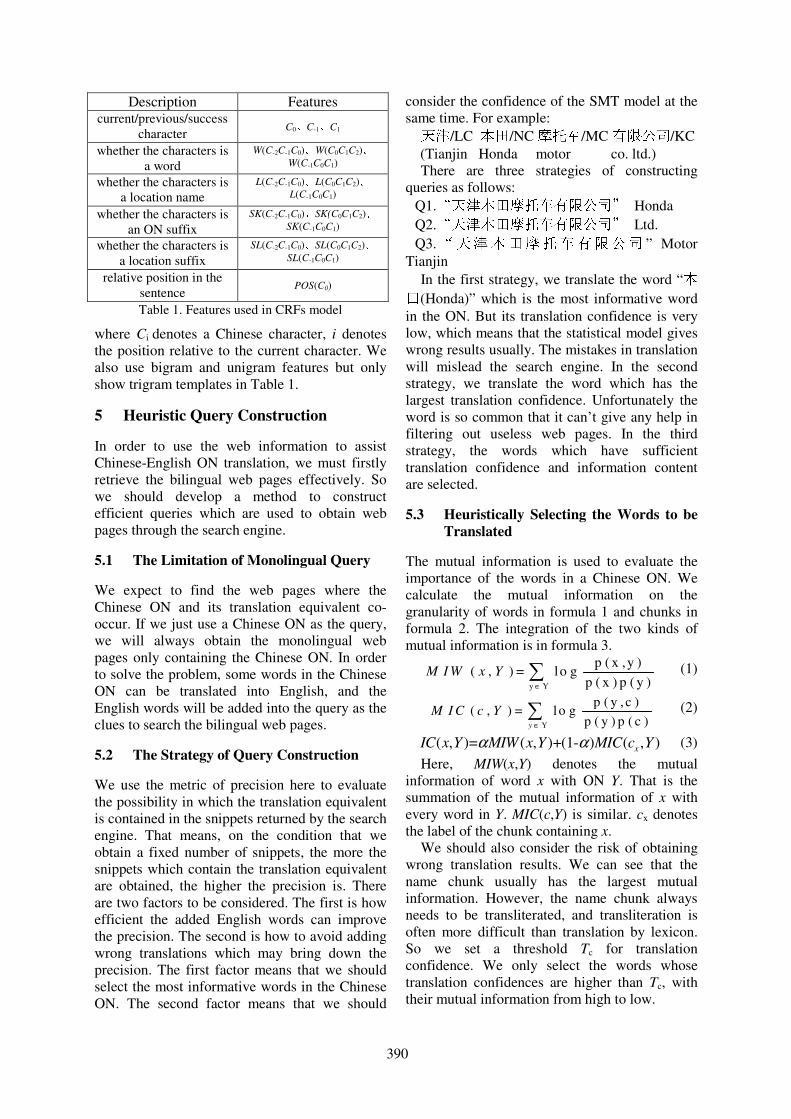
Description Features current/previous/success
character C0、C-1、C1
whether the characters is
a word
W(C-2C-1C0)、W(C0C1C2)、W(C-1C0C1)
whether the characters is
a location name L(C-2C-1C0)、L(C0C1C2)、
L(C-1C0C1)
whether the characters is
an ON suffix SK(C-2C-1C0)、SK(C0C1C2)、
SK(C-1C0C1)
whether the characters is
a location suffix SL(C-2C-1C0)、SL(C0C1C2)、
SL(C-1C0C1)
relative position in the
sentence POS(C0)
Table 1. Features used in CRFs model
where Ci denotes a Chinese character, i denotes
the position relative to the current character. We
also use bigram and unigram features but only
show trigram templates in Table 1.
5 Heuristic Query Construction
In order to use the web information to assist
Chinese-English ON translation, we must firstly
retrieve the bilingual web pages effectively. So
we should develop a method to construct
efficient queries which are used to obtain web
pages through the search engine.
5.1 The Limitation of Monolingual Query
We expect to find the web pages where the
Chinese ON and its translation equivalent co-
occur. If we just use a Chinese ON as the query,
we will always obtain the monolingual web
pages only containing the Chinese ON. In order
to solve the problem, some words in the Chinese
ON can be translated into English, and the
English words will be added into the query as the
clues to search the bilingual web pages.
5.2 The Strategy of Query Construction
We use the metric of precision here to evaluate
the possibility in which the translation equivalent
is contained in the snippets returned by the search
engine. That means, on the condition that we
obtain a fixed number of snippets, the more the
snippets which contain the translation equivalent
are obtained, the higher the precision is. There
are two factors to be considered. The first is how
efficient the added English words can improve
the precision. The second is how to avoid adding
wrong translations which may bring down the
precision. The first factor means that we should
select the most informative words in the Chinese
ON. The second factor means that we should
consider the confidence of the SMT model at the
same time. For example: 天津/LC 本田/NC 车摩托 /MC 有限公司/KC
(Tianjin Honda motor co. ltd.)
There are three strategies of constructing
queries as follows:
Q1.“天津本田摩托车有限公司” Honda
Q2.“天津本田摩托车有限公司” Ltd.
Q3.“天津本田摩托车有限公司 ” Motor
Tianjin
In the first strategy, we translate the word “本田(Honda)” which is the most informative word
in the ON. But its translation confidence is very
low, which means that the statistical model gives
wrong results usually. The mistakes in translation
will mislead the search engine. In the second
strategy, we translate the word which has the
largest translation confidence. Unfortunately the
word is so common that it can’t give any help in
filtering out useless web pages. In the third
strategy, the words which have sufficient
translation confidence and information content
are selected.
5.3 Heuristically Selecting the Words to be
Translated
The mutual information is used to evaluate the
importance of the words in a Chinese ON. We
calculate the mutual information on the
granularity of words in formula 1 and chunks in
formula 2. The integration of the two kinds of
mutual information is in formula 3.
y Y
p ( x ,y )( , ) = lo g
p ( x ) p ( y )M I W x Y
∈
∑ (1)
Y
p ( y , c )( , ) = lo g
p ( y ) p ( c )y
M I C c Y∈
∑ (2)
( , )= ( , )+(1- ) ( , )x
IC x Y MIW x Y MIC c Yα α (3)
Here, MIW(x,Y) denotes the mutual
information of word x with ON Y. That is the
summation of the mutual information of x with
every word in Y. MIC(c,Y) is similar. cx denotes
the label of the chunk containing x.
We should also consider the risk of obtaining
wrong translation results. We can see that the
name chunk usually has the largest mutual
information. However, the name chunk always
needs to be transliterated, and transliteration is
often more difficult than translation by lexicon.
So we set a threshold Tc for translation
confidence. We only select the words whose
translation confidences are higher than Tc, with
their mutual information from high to low.
390
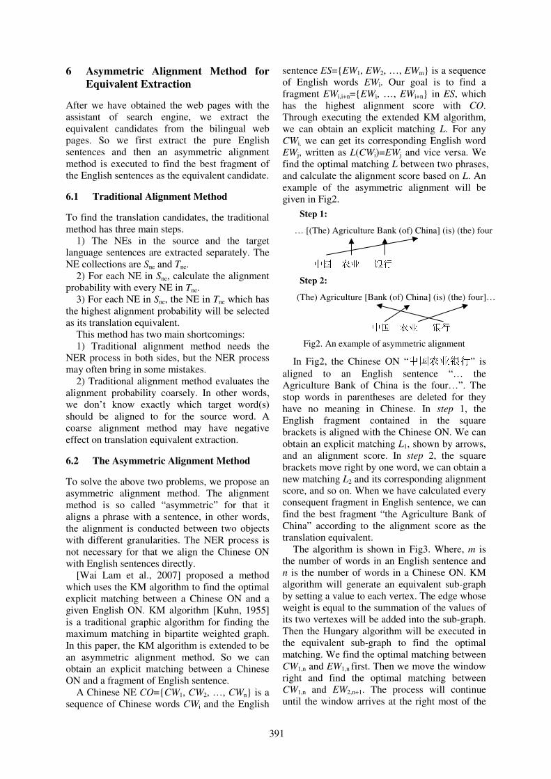
6 Asymmetric Alignment Method for
Equivalent Extraction
After we have obtained the web pages with the
assistant of search engine, we extract the
equivalent candidates from the bilingual web
pages. So we first extract the pure English
sentences and then an asymmetric alignment
method is executed to find the best fragment of
the English sentences as the equivalent candidate.
6.1 Traditional Alignment Method
To find the translation candidates, the traditional
method has three main steps.
1) The NEs in the source and the target
language sentences are extracted separately. The
NE collections are Sne and Tne.
2) For each NE in Sne, calculate the alignment
probability with every NE in Tne.
3) For each NE in Sne, the NE in Tne which has
the highest alignment probability will be selected
as its translation equivalent.
This method has two main shortcomings:
1) Traditional alignment method needs the
NER process in both sides, but the NER process
may often bring in some mistakes.
2) Traditional alignment method evaluates the
alignment probability coarsely. In other words,
we don’t know exactly which target word(s)
should be aligned to for the source word. A
coarse alignment method may have negative
effect on translation equivalent extraction.
6.2 The Asymmetric Alignment Method
To solve the above two problems, we propose an
asymmetric alignment method. The alignment
method is so called “asymmetric” for that it
aligns a phrase with a sentence, in other words,
the alignment is conducted between two objects
with different granularities. The NER process is
not necessary for that we align the Chinese ON
with English sentences directly.
[Wai Lam et al., 2007] proposed a method
which uses the KM algorithm to find the optimal
explicit matching between a Chinese ON and a
given English ON. KM algorithm [Kuhn, 1955]
is a traditional graphic algorithm for finding the
maximum matching in bipartite weighted graph.
In this paper, the KM algorithm is extended to be
an asymmetric alignment method. So we can
obtain an explicit matching between a Chinese
ON and a fragment of English sentence.
A Chinese NE CO={CW1, CW2, …, CWn} is a
sequence of Chinese words CWi and the English
sentence ES={EW1, EW2, …, EWm} is a sequence
of English words EWi. Our goal is to find a
fragment EWi,i+n={EWi, …, EWi+n} in ES, which
has the highest alignment score with CO.
Through executing the extended KM algorithm,
we can obtain an explicit matching L. For any
CWi, we can get its corresponding English word
EWj, written as L(CWi)=EWj and vice versa. We
find the optimal matching L between two phrases,
and calculate the alignment score based on L. An
example of the asymmetric alignment will be
given in Fig2.
Fig2. An example of asymmetric alignment
In Fig2, the Chinese ON “中国农业银行” is
aligned to an English sentence “… the
Agriculture Bank of China is the four…”. The
stop words in parentheses are deleted for they
have no meaning in Chinese. In step 1, the
English fragment contained in the square
brackets is aligned with the Chinese ON. We can
obtain an explicit matching L1, shown by arrows,
and an alignment score. In step 2, the square
brackets move right by one word, we can obtain a
new matching L2 and its corresponding alignment
score, and so on. When we have calculated every
consequent fragment in English sentence, we can
find the best fragment “the Agriculture Bank of
China” according to the alignment score as the
translation equivalent.
The algorithm is shown in Fig3. Where, m is
the number of words in an English sentence and
n is the number of words in a Chinese ON. KM
algorithm will generate an equivalent sub-graph
by setting a value to each vertex. The edge whose
weight is equal to the summation of the values of
its two vertexes will be added into the sub-graph.
Then the Hungary algorithm will be executed in
the equivalent sub-graph to find the optimal
matching. We find the optimal matching between
CW1,n and EW1,n first. Then we move the window
right and find the optimal matching between
CW1,n and EW2,n+1. The process will continue
until the window arrives at the right most of the
… [(The) Agriculture Bank (of) China] (is) (the) four 中国 农业 银行
(The) Agriculture [Bank (of) China] (is) (the) four]… 中国 农业 银行
Step 1:
Step 2:
391

English sentence. When the window moves right,
we only need to find a new matching for the new
added English vertex EWend and the Chinese
vertex Cdrop which has been matched with EWstart
in the last step. In the Hungary algorithm, the
matching is added through finding an augmenting
path. So we only need to find one augmenting
path each time. The time complexity of finding
an augmenting path is O(n3). So the whole
complexity of asymmetric alignment is O(m*n3).
Algorithm: Asymmetric Alignment Algorithm
Input: A segmented Chinese ON CO and an
English sentence ES.
Output: an English fragment EWk,k+n
1. Let start=1, end=n, L0=null
2. Using KM algorithm to find the optimal
matching between two phrases CW1,n and
EWstart,end based on the previous matching Lstart-
1. We obtain a matching Lstart and calculate the
alignment score Sstart based on Lstart.
3. CWdrop = L(EWstart) L(CWdrop)=null.
4. If (end==m) go to 7, else start=start+1,
end=end+1.
5. Calculate the feasible vertex labeling for the
vertexes CWdrop and EWend
6. Go to 2.
7. The fragment EWk,k+n-1 which has the highest
alignment score will be returned.
Fig3. The asymmetric alignment algorithm
6.3 Obtain the Translation Equivalent
For each English sentence, we can obtain a
fragment ESi,i+n which has the highest alignment
score. We will also take into consideration the
frequency information of the fragment and its
distance away from the Chinese ON. We use
formula (4) to obtain a final score for each
translation candidate ETi and select the largest
one as translation result.
( )= + log( +1)+ log(1 / +1)i i i i
S ET SA C Dα β γ (4)
Where Ci denotes the frequency of ETi, and Di
denotes the nearest distance between ETi and the
Chinese ON.
7 Experiments
We carried out experiments to investigate the
performance improvement of ON translation
under the assistance of web knowledge.
7.1 Experimental Data
Our experiment data are extracted from
LDC2005T34. There are two corpora,
ldc_propernames_org_ce_v1.beta (Indus_corpus
for short) and ldc_propernames_indu
stry_ce_v1.beta (Org_corpus for short). Some
pre-process will be executed to filter out some
noisy translation pairs. For example, the
translation pairs involving other languages such
as Japanese and Korean will be filtered out.
There are 65,835 translation pairs that we used as
the training corpus and the chunk labels are
added manually.
We randomly select 250 translation pairs from
the Org_corpus and 253 translation pairs from
the Indus_corpus. Altogether, there are 503
translation pairs as the testing set.
7.2 The Effect of Chunking-based
Segmentation upon ON Translation
In order to evaluate the influence of segmentation
results upon the statistical ON translation system,
we compare the results of two translation models.
One model uses chunking-based segmentation
results as input, while the other uses traditional
segmentation results.
To train the CRFs-chunking model, we
randomly selected 59,200 pairs of equivalent
translations from Indus_corpus and org_corpus.
We tested the performance on the set which
contains 6,635 Chinese ONs and the results are
shown as Table-2.
For constructing a statistical ON translation
model, we use GIZA++1 to align the Chinese NEs
and the English NEs in the training set. Then the
phrase-based machine translation system
MOSES2 is adopted to translate the 503 Chinese
NEs in testing set into English.
Precision Recall F-measure
LC 0.8083 0.7973 0.8028
NC 0.8962 0.8747 0.8853
MC 0.9104 0.9073 0.9088
KC 0.9844 0.9821 0.9833
All 0.9437 0.9372 0.9404 Table 2. The test results of CRFs-chunking model
We have two metrics to evaluate the
translation results. The first metric L1 is used to
evaluate whether the translation result is exactly
the same as the answer. The second metric L2 is
used to evaluate whether the translation result
contains almost the same words as the answer,
1 http://www.fjoch.com/GIZA++.html 2 http://www.statmt.org/moses/
392

without considering the order of words. The
results are shown in Table-3:
chunking-based
segmentation
traditional
segmentation
L1 21.47% 18.29%
L2 40.76% 36.78% Table 3. Comparison of segmentation influence
From the above experimental data, we can see
that the chunking-based segmentation improves
L1 precision from 18.29% to 21.47% and L2
precision from 36.78% to 40.76% in comparison
with the traditional segmentation method.
Because the segmentation results will be used in
alignment, the errors will affect the computation
of alignment probability. The chunking based
segmentation can generate better segmentation
results; therefore better alignment probabilities
can be obtained.
7.3 The Efficiency of Query Construction
The heuristic query construction method aims to
improve the efficiency of Web searching. The
performance of searching for translation
equivalents mostly depends on how to construct
the query. To test its validity, we design four
kinds of queries and evaluate their ability using
the metric of average precision in formula 5 and
macro average precision (MAP) in formula 6,
1
1P r
Ni
i i
HA vera g e ec is io n
N S=
= ∑ (5)
where Hi is the count of snippets that contain at
least one equivalent for the ith query. And Si is
the total number of snippets we got for the ith
query,
1= 1
1
( )
1 j
i
HN
j j
iM A P
R iN H =
= ∑∑ (6)
where R(i) is the order of snippet where the ith
equivalent occurs. We construct four kinds of
queries for the 503 Chinese ONs in testing set as
follows:
Q1: only the Chinese ON.
Q2: the Chinese ON and the results of the
statistical translation model.
Q3: the Chinese ON and some parts’
translation selected by the heuristic query
construction method.
Q4: the Chinese ON and its correct English
translation equivalent.
We obtain at most 100 snippets from Google
for every query. Sometimes there are not enough
snippets as we expect. We set α in formula 4 at
0.7,and the threshold of translation confidence
at 0.05. The results are shown as Table 4.
Average
precision
MAP
Q1 0.031 0.0527
Q2 0.187 0.2061
Q3 0.265 0.3129
Q4 1.000 1.0000 Table 4. Comparison of four types query
Here we can see that, the result of Q4 is the
upper bound of the performance, and the Q1 is
the lower bound of the performance. We
concentrate on the comparison between Q2 and
Q3. Q2 contains the translations of every word in
a Chinese ON, while Q3 just contains the
translations of the words we select using the
heuristic method. Q2 may give more information
to search engine about which web pages we
expect to obtain, but it also brings in translation
mistakes that may mislead the search engine. The
results show that Q3 is better than Q2, which
proves that a careful clue selection is needed.
7.4 The Effect of Asymmetric Alignment
Algorithm
The asymmetric alignment method can avoid the
mistakes made in the NER process and give an
explicit alignment matching. We will compare
the asymmetric alignment algorithm with the
traditional alignment method on performance.
We adopt two methods to align the Chinese NE
with the English sentences. The first method has
two phases, the English ONs are extracted from
English sentences firstly, and then the English
ONs are aligned with the Chinese ON. Lastly, the
English ON with the highest alignment score will
be selected as the translation equivalent. We use
the software Lingpipe3 to recognize NEs in the
English sentences. The alignment probability can
be calculated as formula 7:
( , ) ( | )i j
i j
Score C E p e c= ∑∑ (7)
The second method is our asymmetric
alignment algorithm. Our method is different
from the one in [Wai Lam et al., 2007] which
segmented a Chinese ON using an English ON as
suggestion. We segment the Chinese ON using
the chunking-based segmentation method. The
English sentences extracted from snippets will be
preprocessed. Some stop words will be deleted,
such as “the”, “of”, “on” etc. To execute the
extended KM algorithm for finding the best
alignment matching, we must assure that the
vertex number in each side of the bipartite is the
3 http://www.alias-i.com/lingpipe/
393

same. So we will execute a phrase combination
process before alignment, which combines some
frequently occurring consequent English words
into single vertex, such as “limited company” etc.
The combination is based on the phrase pair table
which is generated from phrase-based SMT
system. The results are shown in Table 5:
Asymmetric
Alignment
Traditional
method
Statistical
model
Top1 48.71% 36.18% 18.29%
Top5 53.68% 46.12% -- Table 5. Comparison the precision of alignment
method
From the results (column 1 and column 2) we
can see that, the Asymmetric alignment method
outperforms the traditional alignment method.
Our method can overcome the mistakes
introduced in the NER process. On the other
hand, in our asymmetric alignment method, there
are two main reasons which may result in
mistakes, one is that the correct equivalent
doesn’t occur in the snippet; the other is that
some English ONs can’t be aligned to the
Chinese ON word by word.
7.5 Comparison between Statistical ON
Translation Model and Our Method
Compared with the statistical ON translation
model, we can see that the performance is
improved from 18.29% to 48.71% (the bold data
shown in column 1 and column 3 of Table 5) by
using our Chinese-English ON translation system.
Transforming the translation problem into the
problem of searching for the correct translation
equivalent in web pages has three advantages.
First, word order determination is difficult in
statistical machine translation (SMT), while
search engines are insensitive to this problem.
Second, SMT often loses some function word
such as “the”, “a”, “of”, etc, while our method
can avoid this problem because such words are
stop words in search engines. Third, SMT often
makes mistakes in the selection of synonyms.
This problem can be solved by the fuzzy
matching of search engines. In summary, web
assistant method makes Chinese ON translation
easier than traditional SMT method.
8 Conclusion
In this paper, we present a new approach which
translates the Chinese ON into English with the
assistance of web resources. We first adopt the
chunking-based segmentation method to improve
the ON segmentation. Then a heuristic query
construction method is employed to construct a
query which can search translation equivalent
more efficiently. At last, the asymmetric
alignment method aligns the Chinese ON with
English sentences directly. The performance of
ON translation is improved from 18.29% to
48.71%. It proves that our system can work well
on the Chinese-English ON translation task. In
the future, we will try to apply this method in
mining the NE translation equivalents from
monolingual web pages. In addition, the
asymmetric alignment algorithm also has some
space to be improved.
Acknowledgement
The work is supported by the National High
Technology Development 863 Program of China
under Grants no. 2006AA01Z144, and the
National Natural Science Foundation of China
under Grants no. 60673042 and 60875041.
References
Yaser Al-Onaizan and Kevin Knight. 2002.
Translating named entities using monolingual and
bilingual resources. In Proc of ACL-2002.
Yufeng Chen, Chenqing Zong. 2007. A Structure-
Based Model for Chinese Organization Name
Translation. In Proc. of ACM Transactions on
Asian Language Information Processing (TALIP)
Donghui Feng, Yajuan Lv, Ming Zhou. 2004. A new
approach for English-Chinese named entity
alignment. In Proc. of EMNLP 2004.
Fei Huang, Stephan Vogal. 2002. Improved named
entity translation and bilingual named entity
extraction. In Proc. of the 4th IEEE International
Conference on Multimodal Interface.
Fei Huang, Stephan Vogal, Alex Waibel. 2003.
Automatic extraction of named entity translingual
equivalence based on multi-feature cost
minimization. In Proc. of the 2003 Annual
Conference of the ACL, Workshop on Multilingual
and Mixed-language Named Entity Recognition
Masaaki Nagata, Teruka Saito, and Kenji Suzuki.
2001. Using the Web as a Bilingual Dictionary. In
Proc. of ACL 2001 Workshop on Data-driven
Methods in Machine Translation.
David Chiang. 2005. A hierarchical phrase-based
model for statistical machine translation. In Proc. of
ACL 2005.
Conrad Chen, Hsin-His Chen. 2006. A High-Accurate
Chinese-English NE Backward Translation System
Combining Both Lexical Information and Web
Statistics. In Proc. of ACL 2006.
394
Wai Lam, Shing-Kit Chan. 2007. Named Entity
Translation Matching and Learning: With
Application for Mining Unseen Translations. In
Proc. of ACM Transactions on Information
Systems.
Chun-Jen Lee, Jason S. Chang, Jyh-Shing R. Jang.
2006. Alignment of bilingual named entities in
parallel corpora using statistical models and
multiple knowledge sources. In Proc. of ACM
Transactions on Asian Language Information
Processing (TALIP).
Kuhn, H. 1955. The Hungarian method for the
assignment problem. Naval Rese. Logist. Quart
2,83-97.
Min Zhang., Haizhou Li, Su Jian, Hendra Setiawan.
2005. A phrase-based context-dependent joint
probability model for named entity translation. In
Proc. of the 2nd International Joint Conference on
Natural Language Processing(IJCNLP)
Ying Zhang, Fei Huang, Stephan Vogel. 2005. Mining
translations of OOV terms from the web through
cross-lingual query expansion. In Proc. of the 28th
ACM SIGIR.
Bonnie Glover Stalls and Kevin Knight. 1998.
Translating names and technical terms in Arabic
text. In Proc. of the COLING/ACL Workshop on
Computational Approaches to Semitic Language.
J. Lafferty, A. McCallum, and F. Pereira. 2001.
Conditional random fields: Probabilistic models for
segmenting and labeling sequence data. In Proc.
ICML-2001.
Tadashi Kumano, Hideki Kashioka, Hideki Tanaka
and Takahiro Fukusima. 2004. Acquiring bilingual
named entity translations from content-aligned
corpora. In Proc. IJCNLP-04.
Robert C. Moore. 2003. Learning translation of
named-entity phrases from parallel corpora. In Proc.
of 10th
conference of the European chapter of ACL.
395
Proceedings of the 47th Annual Meeting of the ACL and the 4th IJCNLP of the AFNLP, pages 396–404,Suntec, Singapore, 2-7 August 2009. c©2009 ACL and AFNLP
Reducing semantic drift with bagging and distributional similarity
Tara McIntosh and James R. CurranSchool of Information Technologies
University of SydneyNSW 2006, Australia
{tara,james}@it.usyd.edu.au
Abstract
Iterative bootstrapping algorithms are typ-ically compared using a single set of hand-picked seeds. However, we demonstratethat performance varies greatly depend-ing on these seeds, and favourable seedsfor one algorithm can perform very poorlywith others, making comparisons unreli-able. We exploit this wide variation withbagging, sampling from automatically ex-tracted seeds to reduce semantic drift.
However, semantic drift still occurs inlater iterations. We propose an integrateddistributional similarity filter to identifyand censor potential semantic drifts, en-suring over 10% higher precision when ex-tracting large semantic lexicons.
1 Introduction
Iterative bootstrapping algorithms have been pro-posed to extract semantic lexicons forNLP taskswith limited linguistic resources. Bootstrappingwas initially proposed by Riloff and Jones (1999),and has since been successfully applied to extract-ing general semantic lexicons (Riloff and Jones,1999; Thelen and Riloff, 2002), biomedical enti-ties (Yu and Agichtein, 2003), facts (Paşca et al.,2006), and coreference data (Yang and Su, 2007).
Bootstrapping approaches are attractive becausethey are domain and language independent, re-quire minimal linguistic pre-processing and can beapplied to raw text, and are efficient enough fortera-scale extraction (Paşca et al., 2006).
Bootstrapping is minimally supervised, as it isinitialised with a small number of seed instancesof the information to extract. For semantic lexi-cons, these seeds are terms from the category of in-terest. The seeds identify contextual patterns thatexpress a particular semantic category, which inturn recognise new terms (Riloff and Jones, 1999).
Unfortunately,semantic driftoften occurs whenambiguous or erroneous terms and/or patterns areintroduced into and then dominate the iterativeprocess (Curran et al., 2007).
Bootstrapping algorithms are typically com-pared using only a single set of hand-picked seeds.We first show that different seeds cause these al-gorithms to generate diverse lexicons which varygreatly in precision. This makes evaluation un-reliable – seeds which perform well on one algo-rithm can perform surprisingly poorly on another.In fact, random gold-standard seeds often outper-form seeds carefully chosen by domain experts.
Our second contribution exploits this diversitywe have identified. We present an unsupervisedbagging algorithm which samples from the ex-tracted lexicon rather than relying on existinggazetteers or hand-selected seeds. Each sample isthen fed back as seeds to the bootstrapper and theresults combined using voting. This both improvesthe precision of the lexicon and the robustness ofthe algorithms to the choice of initial seeds.
Unfortunately, semantic drift still dominates inlater iterations, since erroneous extracted termsand/or patterns eventually shift the category’s di-rection. Our third contribution focuses on detect-ing and censoring the terms introduced by seman-tic drift. We integrate a distributional similarityfilter directly into WMEB (McIntosh and Curran,2008). This filter judges whether a new term ismore similar to the earlier or most recently ex-tracted terms, a sign of potential semantic drift.
We demonstrate these methods for extractingbiomedical semantic lexicons using two bootstrap-ping algorithms. Our unsupervised bagging ap-proach outperforms carefully hand-picked seedsby ∼ 10% in later iterations. Our distributionalsimilarity filter gives a similar performance im-provement. This allows us to produce large lexi-cons accurately and efficiently for domain-specificlanguage processing.
396
2 Background
Hearst (1992) exploited patterns for informationextraction, to acquireis-arelations using manuallydevised patterns likesuch Z as X and/or YwhereXandY are hyponyms ofZ. Riloff and Jones (1999)extended this with an automated bootstrapping al-gorithm,Multi-level Bootstrapping(MLB ), whichiteratively extracts semantic lexicons from text.
In MLB , bootstrapping alternates between twostages: pattern extraction and selection, and termextraction and selection.MB is seeded with a smallset of user selectedseedterms. These seeds areused to identify contextual patterns they appear in,which in turn identify new lexicon entries. Thisprocess is repeated with the new lexicon termsidentifying new patterns. In each iteration, the top-n candidates are selected, based on a metric scor-ing their membership in the category and suitabil-ity for extracting additional terms and patterns.
Bootstrapping eventually extracts polysemousterms and patterns which weakly constrain thesemantic class, causing the lexicon’s meaning toshift, calledsemantic driftby Curran et al. (2007).For example, female firstnames may drift intoflowers whenIris andRoseare extracted. Manyvariations on bootstrapping have been developedto reduce semantic drift.1
One approach is to extract multiple semanticcategories simultaneously, where the individualbootstrapping instances compete with one anotherin an attempt to actively direct the categories awayfrom each other. Multi-category algorithms out-perform MLB (Thelen and Riloff, 2002), and wefocus on these algorithms in our experiments.
In BASILISK, MEB, and WMEB, each compet-ing category iterates simultaneously between theterm and pattern extraction and selection stages.These algorithms differ in how terms and patternsselected by multiple categories are handled, andtheir scoring metrics. InBASILISK (Thelen andRiloff, 2002), candidate terms are ranked highly ifthey have strong evidence for a category and littleor no evidence for other categories. This typicallyfavours less frequent terms, as they will match farfewer patterns and are thus more likely to belongto one category. Patterns are selected similarly,however patterns may also be selected by differ-ent categories in later iterations.
Curran et al. (2007) introducedMutual Exclu-
1Komachi et al. (2008) used graph-based algorithms toreduce semantic drift for Word Sense Disambiguation.
sion Bootstrapping(MEB) which forces stricterboundaries between the competing categories thanBASILISK. In MEB, the key assumptions are thatterms only belong to a category and that patternsonly extract terms of a single category. Semanticdrift is reduced by eliminating patterns that collidewith multiple categories in an iteration and by ig-noring colliding candidate terms (for the currentiteration). This excludes generic patterns that canoccur frequently with multiple categories, and re-duces the chance of assigning ambiguous terms totheir less dominant sense.
2.1 Weighted MEB
The scoring of candidate terms and patterns inMEB is näıve. Candidates which 1) match the mostinput instances; and 2) have the potential to gen-erate the most new candidates, are preferred (Cur-ran et al., 2007). This second criterion aims to in-crease recall. However, the selected instances arehighly likely to introduce drift.
Our WeightedMEB algorithm (McIntosh andCurran, 2008), extendsMEB by incorporating termand pattern weighting, and a cumulative patternpool. WMEB uses theχ2 statistic to identify pat-terns and terms that are strongly associated withthe growing lexicon terms and their patterns re-spectively. The terms and patterns are then rankedfirst by the number of input instances they match(as inMEB), but then by their weighted score.
In MEB and BASILISK2, the top-k patterns foreach iteration are used to extract new candidateterms. As the lexicons grow, general patterns candrift into the top-k and as a result the earlier pre-cise patterns lose their extracting influence. InWMEB, the pattern pool accumulates all top-k pat-terns from previous iterations, to ensure previouspatterns can contribute.
2.2 Distributional Similarity
Distributional similarity has been used to ex-tract semantic lexicons (Grefenstette, 1994), basedon thedistributional hypothesisthat semanticallysimilar words appear in similar contexts (Harris,1954). Words are represented by context vectors,and words are considered similar if their contextvectors are similar.
Patterns and distributional methods have beencombined previously. Pantel and Ravichandran
2In BASILISK, k is increased by one in each iteration, toensure at least one new pattern is introduced.
397
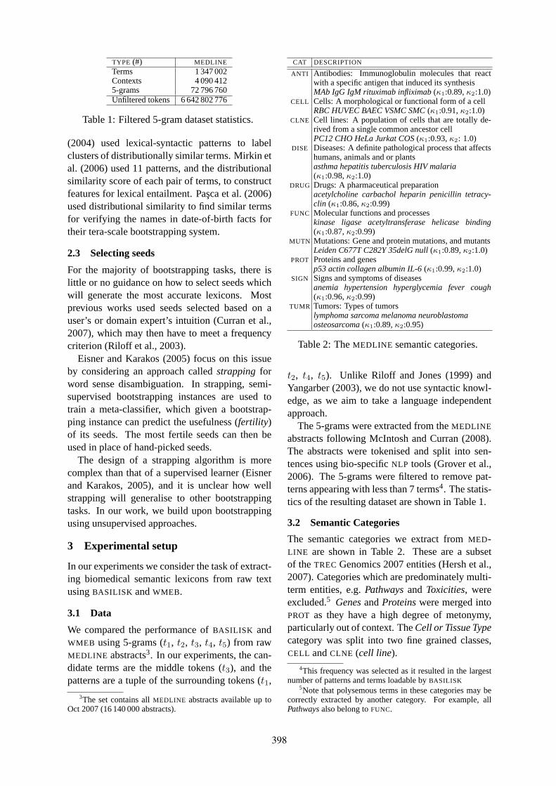
TYPE (#) MEDLINE
Terms 1 347 002Contexts 4 090 4125-grams 72 796 760Unfiltered tokens 6 642 802 776
Table 1: Filtered 5-gram dataset statistics.
(2004) used lexical-syntactic patterns to labelclusters of distributionally similar terms. Mirkin etal. (2006) used 11 patterns, and the distributionalsimilarity score of each pair of terms, to constructfeatures for lexical entailment. Paşca et al. (2006)used distributional similarity to find similar termsfor verifying the names in date-of-birth facts fortheir tera-scale bootstrapping system.
2.3 Selecting seeds
For the majority of bootstrapping tasks, there islittle or no guidance on how to select seeds whichwill generate the most accurate lexicons. Mostprevious works used seeds selected based on auser’s or domain expert’s intuition (Curran et al.,2007), which may then have to meet a frequencycriterion (Riloff et al., 2003).
Eisner and Karakos (2005) focus on this issueby considering an approach calledstrapping forword sense disambiguation. In strapping, semi-supervised bootstrapping instances are used totrain a meta-classifier, which given a bootstrap-ping instance can predict the usefulness (fertility)of its seeds. The most fertile seeds can then beused in place of hand-picked seeds.
The design of a strapping algorithm is morecomplex than that of a supervised learner (Eisnerand Karakos, 2005), and it is unclear how wellstrapping will generalise to other bootstrappingtasks. In our work, we build upon bootstrappingusing unsupervised approaches.
3 Experimental setup
In our experiments we consider the task of extract-ing biomedical semantic lexicons from raw textusingBASILISK andWMEB.
3.1 Data
We compared the performance ofBASILISK andWMEB using 5-grams (t1, t2, t3, t4, t5) from rawMEDLINE abstracts3. In our experiments, the can-didate terms are the middle tokens (t3), and thepatterns are a tuple of the surrounding tokens (t1,
3The set contains allMEDLINE abstracts available up toOct 2007 (16 140 000 abstracts).
CAT DESCRIPTION
ANTI Antibodies: Immunoglobulin molecules that reactwith a specific antigen that induced its synthesisMAb IgG IgM rituximab infliximab(κ1:0.89,κ2:1.0)
CELL Cells: A morphological or functional form of a cellRBC HUVEC BAEC VSMC SMC(κ1:0.91,κ2:1.0)
CLNE Cell lines: A population of cells that are totally de-rived from a single common ancestor cellPC12 CHO HeLa Jurkat COS(κ1:0.93,κ2: 1.0)
DISE Diseases: A definite pathological process that affectshumans, animals and or plantsasthma hepatitis tuberculosis HIV malaria(κ1:0.98,κ2:1.0)
DRUG Drugs: A pharmaceutical preparationacetylcholine carbachol heparin penicillin tetracy-clin (κ1:0.86,κ2:0.99)
FUNC Molecular functions and processeskinase ligase acetyltransferase helicase binding(κ1:0.87,κ2:0.99)
MUTN Mutations: Gene and protein mutations, and mutantsLeiden C677T C282Y 35delG null(κ1:0.89,κ2:1.0)
PROT Proteins and genesp53 actin collagen albumin IL-6(κ1:0.99,κ2:1.0)
SIGN Signs and symptoms of diseasesanemia hypertension hyperglycemia fever cough(κ1:0.96,κ2:0.99)
TUMR Tumors: Types of tumorslymphoma sarcoma melanoma neuroblastomaosteosarcoma(κ1:0.89,κ2:0.95)
Table 2: TheMEDLINE semantic categories.
t2, t4, t5). Unlike Riloff and Jones (1999) andYangarber (2003), we do not use syntactic knowl-edge, as we aim to take a language independentapproach.
The 5-grams were extracted from theMEDLINE
abstracts following McIntosh and Curran (2008).The abstracts were tokenised and split into sen-tences using bio-specificNLP tools (Grover et al.,2006). The 5-grams were filtered to remove pat-terns appearing with less than 7 terms4. The statis-tics of the resulting dataset are shown in Table 1.
3.2 Semantic Categories
The semantic categories we extract fromMED-LINE are shown in Table 2. These are a subsetof theTREC Genomics 2007 entities (Hersh et al.,2007). Categories which are predominately multi-term entities, e.g.Pathwaysand Toxicities, wereexcluded.5 GenesandProteinswere merged intoPROT as they have a high degree of metonymy,particularly out of context. TheCell or Tissue Typecategory was split into two fine grained classes,CELL andCLNE (cell line).
4This frequency was selected as it resulted in the largestnumber of patterns and terms loadable byBASILISK
5Note that polysemous terms in these categories may becorrectly extracted by another category. For example, allPathwaysalso belong toFUNC.
398

The five hand-picked seeds used for each cat-egory are shown in italics in Table 2. These werecarefully chosen based on the evaluators’ intuition,and are as unambiguous as possible with respect tothe other categories.
We also utilised terms instop categorieswhichare known to cause semantic drift in specificclasses. These extra categories bound the lexi-cal space and reduce ambiguity (Yangarber, 2003;Curran et al., 2007). We used four stop cate-gories introduced in McIntosh and Curran (2008):AMINO ACID , ANIMAL , BODY andORGANISM.
3.3 Lexicon evaluation
The evaluation involves manually inspecting eachextracted term and judging whether it was a mem-ber of the semantic class. This manual evaluationis extremely time consuming and is necessary dueto the limited coverage of biomedical resources.To make later evaluations more efficient, all eval-uators’ decisions for each category are cached.
Unfamiliar terms were checked using onlineresources includingMEDLINE, Medical SubjectHeadings (MeSH), Wikipedia. Each ambiguousterm was counted as correct if it was classified intoone of its correct categories, such aslymphomawhich is a TUMR and DISE. If a term was un-ambiguously part of a multi-word term we consid-ered it correct. Abbreviations, acronyms and typo-graphical variations were included. We also con-sidered obvious spelling mistakes to be correct,such asnuetrophilsinstead ofneutrophils(a typeof CELL). Non-specific modifiers are marked asincorrect, for example,gastrointestinalmay be in-correctly extracted forTUMR, as part of the entitygastrointestinal carcinoma. However, the modi-fier may also be used forDISE (gastrointestinalinfection) andCELL.
The terms were evaluated by two domain ex-perts. Inter-annotator agreement was measuredon the top-100 terms extracted byBASILISK andWMEB with the hand-picked seeds for each cat-egory. All disagreements were discussed, and thekappa scores, before (κ1) and after (κ2) the discus-sions, are shown in Table 2. Each score is above0.8 which reflects an agreement strength of “al-most perfect” (Landis and Koch, 1977).
For comparing the accuracy of the systems weevaluated the precision of samples of the lexiconsextracted for each category. We report averageprecision over the 10 semantic categories on the
1-200, 401-600 and 801-1000 term samples, andover the first 1000 terms. In each algorithm, eachcategory is initialised with 5 seed terms, and thenumber of patterns,k, is set to 5. In each itera-tion, 5 lexicon terms are extracted by each cate-gory. Each algorithm is run for 200 iterations.
4 Seed diversity
The first step in bootstrapping is to select a set ofseeds by hand. Thesehand-pickedseeds are typi-cally chosen by a domain expert who selects a rea-sonably unambiguous representative sample of thecategory with high coverage by introspection.
To improve the seeds, the frequency of the po-tential seeds in the corpora is often considered, onthe assumption that highly frequent seeds are bet-ter (Thelen and Riloff, 2002). Unfortunately, theseseeds may be too general and extract many non-specific patterns. Another approach is to identifyseeds using hyponym patterns like,* is a [NAMED
ENTITY] (Meij and Katrenko, 2007).This leads us to our first investigation of seed
variability and the methodology used to comparebootstrapping algorithms. Typically algorithmsare compared using one set of hand-picked seedsfor each category (Pennacchiotti and Pantel, 2006;McIntosh and Curran, 2008). This approach doesnot provide a fair comparison or any detailed anal-ysis of the algorithms under investigation. Aswe shall see, it is possible that the seeds achievethe maximum precision for one algorithm and theminimum for another, and thus the single compar-ison is inappropriate. Even evaluating on multiplecategories does not ensure the robustness of theevaluation. Secondly, it provides no insight intothe sensitivity of an algorithm to different seeds.
4.1 Analysis with random gold seeds
Our initial analysis investigated the sensitivity andvariability of the lexicons generated using differ-ent seeds. We instantiated each algorithm 10 timeswith different random gold seeds (Sgold) for eachcategory. We randomly sample Sgold from twosets of correct terms extracted from the evalua-tion cache.UNION: the correct terms extracted byBASILISK and WMEB; and UNIQUE: the correctterms uniquely identified by only one algorithm.The degree of ambiguity of each seed is unknownand term frequency is not considered during therandom selection.
Firstly, we investigated the variability of the
399
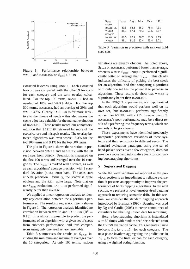
50
60
70
80
90
50 60 70 80 90 100
BA
SIL
ISK
(pr
ecis
ion)
WMEB (precision)
Hand-pickedAverage
Figure 1: Performance relationship betweenWMEB andBASILISK on Sgold UNION
extracted lexicons usingUNION. Each extractedlexicon was compared with the other 9 lexiconsfor each category and the term overlap calcu-lated. For the top 100 terms,BASILISK had anoverlap of 18% andWMEB 44%. For the top500 terms,BASILISK had an overlap of 39% andWMEB 47%. ClearlyBASILISK is far more sensi-tive to the choice of seeds – this also makes thecache a lot less valuable for the manual evaluationof BASILISK. These results match our annotators’intuition that BASILISK retrieved far more of theesoteric, rare and misspelt results. The overlap be-tween algorithms was even worse: 6.3% for thetop 100 terms and 9.1% for the top 500 terms.
The plot in Figure 1 shows the variation in pre-cision betweenWMEB andBASILISK with the 10seed sets fromUNION. Precision is measured onthe first 100 terms and averaged over the 10 cate-gories. The Shand is marked with a square, as wellas each algorithms’ average precision with 1 stan-dard deviation (S.D.) error bars. The axes startat 50% precision. Visually, the scatter is quiteobvious and theS.D. quite large. Note that onour Shand evaluation,BASILISK performed signif-icantly better than average.
We applied a linear regression analysis to iden-tify any correlation between the algorithm’s per-formances. The resulting regression line is shownin Figure 1. The regression analysis identified nocorrelation betweenWMEB andBASILISK (R2 =0.13). It is almost impossible to predict the per-formance of an algorithm with a given set of seedsfrom another’s performance, and thus compar-isons using only one seed set are unreliable.
Table 3 summarises the results on Sgold, in-cluding the minimum and maximum averages overthe 10 categories. At only 100 terms, lexicon
Sgold Shand Avg. Min. Max. S.D.UNION
BASILISK 80.5 68.3 58.3 78.8 7.31WMEB 88.1 87.1 79.3 93.5 5.97UNIQUE
BASILISK 80.5 67.1 56.7 83.5 9.75WMEB 88.1 91.6 82.4 95.4 3.71
Table 3: Variation in precision with random goldseed sets
variations are already obvious. As noted above,Shand onBASILISK performed better than average,whereasWMEB Sgold UNIQUE performed signifi-cantly better on average than Shand. This clearlyindicates the difficulty of picking the best seedsfor an algorithm, and that comparing algorithmswith only one set has the potential to penalise analgorithm. These results do show thatWMEB issignificantly better thanBASILISK.
In the UNIQUE experiments, we hypothesizedthat each algorithm would perform well on itsown set, but BASILISK performs significantlyworse thanWMEB, with a S.D. greater than 9.7.BASILISK ’s poor performance may be a direct re-sult of it preferring low frequency terms, which areunlikely to be good seeds.
These experiments have identified previouslyunreported performance variations of these sys-tems and their sensitivity to different seeds. Thestandard evaluation paradigm, using one set ofhand-picked seeds over a few categories, does notprovide a robust and informative basis for compar-ing bootstrapping algorithms.
5 Supervised Bagging
While the wide variation we reported in the pre-vious section is an impediment to reliable evalua-tion, it presents an opportunity to improve the per-formance of bootstrapping algorithms. In the nextsection, we present a novel unsupervised baggingapproach to reducing semantic drift. In this sec-tion, we consider the standard bagging approachintroduced by Breiman (1996). Bagging was usedby Ng and Cardie (2003) to create committees ofclassifiers for labelling unseen data for retraining.
Here, a bootstrapping algorithm is instantiatedn = 50 times with random seed sets selected fromtheUNION evaluation cache. This generatesn newlexiconsL1, L2, . . . , Ln for each category. Thenext phase involves aggregating the predictions inL1−n to form the final lexicon for each category,using a weighted voting function.
400
1-200 401-600 801-1000 1-1000Shand
BASILISK 76.3 67.8 58.3 66.7WMEB 90.3 82.3 62.0 78.6Sgold BAGBASILISK 84.2 80.2 58.2 78.2WMEB 95.1 79.7 65.0 78.6
Table 4: Bagging with 50 gold seed sets
Our weighting function is based on two relatedhypotheses of terms in highly accurate lexicons: 1)the more category lexicons inL1−n a term appearsin, the more likely the term is a member of thecategory; 2) terms ranked higher in lexicons aremore reliable category members. Firstly, we rankthe aggregated terms by the number of lexiconsthey appear in, and to break ties, we take the termthat was extracted in the earliest iteration acrossthe lexicons.
5.1 Supervised results
Table 4 compares the average precisions of thelexicons forBASILISK and WMEB using just thehand-picked seeds (Shand) and 50 sample super-vised bagging (Sgold BAG).
Bagging with samples from Sgold successfullyincreased the performance of bothBASILISK andWMEB in the top 200 terms. While the improve-ment continued forBASILISK in later sections, ithad a more variable effect forWMEB. Overall,BASILISK gets the greater improvement in perfor-mance (a 12% gain), almost reaching the perfor-mance ofWMEB across the top 1000 terms, whileWMEB’s performance is the same for both Shand
and Sgold BAG. We believe the greater variabilityin BASILISK meant it benefited from bagging withgold seeds.
6 Unsupervised bagging
A significant problem for supervised bagging ap-proaches is that they require a larger set of gold-standard seed terms to sample from – either anexisting gazetteer or a large hand-picked set. Inour case, we used the evaluation cache which tookconsiderable time to accumulate. This saddlesthe major application of bootstrapping, the quickconstruction of accurate semantic lexicons, with achicken-and-egg problem.
However, we propose a novel solution – sam-pling from the terms extracted with the hand-picked seeds (Lhand). WMEB already has veryhigh precision for the top extracted terms (88.1%
BAGGING 1-200 401-600 801-1000 1-1000Top-100BASILISK 72.3 63.5 58.8 65.1WMEB 90.2 78.5 66.3 78.5Top-200BASILISK 70.7 60.7 45.5 59.8WMEB 91.0 78.4 62.2 77.0Top-500BASILISK 63.5 60.5 45.4 56.3WMEB 92.5 80.9 59.1 77.2PDF-500BASILISK 69.6 68.3 49.6 62.3WMEB 92.9 80.7 72.1 81.0
Table 5: Bagging with 50 unsupervised seed sets
for the top 100 terms) and may provide an accept-able source of seed terms. This approach nowonly requires the original 50 hand-picked seedterms across the 10 categories, rather than the2100 terms used above. The process now uses tworounds of bootstrapping: first to create Lhand tosample from and then another round with the 50sets of randomly unsupervised seeds, Srand.
The next decision is how to sample Srand fromLhand. One approach is to use uniform randomsampling from restricted sections of Lhand. Weperformed random sampling from the top 100,200 and 500 terms of Lhand. The seeds from thesmaller samples will have higher precision, butless diversity.
In a truly unsupervised approach, it is impossi-ble to know if and when semantic drift occurs andthus using arbitrary cut-offs can reduce the diver-sity of the selected seeds. To increase diversity wealso sampled from the topn=500 using a proba-bility density function (PDF) using rejection sam-pling, wherer is the rank of the term in Lhand:
PDF(r) =
∑ni=r i−1
∑ni=1
∑nj=i j
−1(1)
6.1 Unsupervised results
Table 5 shows the average precision of the lex-icons after bagging on the unsupervised seeds,sampled from the top 100 – 500 terms from Lhand.Using the top 100 seed sample is much less effec-tive than Sgold BAG for BASILISK but nearly as ef-fective for WMEB. As the sample size increases,WMEB steadily improves with the increasing vari-ability, howeverBASILISK is more effective whenthe more precise seeds are sampled from higherranking terms in the lexicons.
Sampling withPDF-500 results in more accuratelexicons over the first 1000 terms than the other
401

0
0.5
1
1.5
2
2.5
3
0 100 200 300 400 500 600 700 800 900 1000
Drif
t
Number of terms
CorrectIncorrect
Figure 2: Semantic drift inCELL (n=20, m=20)
sampling methods forWMEB. In particular,WMEB
is more accurate with the unsupervised seeds thanthe Sgold and Shand (81.0% vs 78.6% and 78.6%).WMEB benefits from the larger variability intro-duced by the more diverse sets of seeds, and thegreater variability available out-weighs the poten-tial noise from incorrect seeds. ThePDF-500 dis-tribution allows some variability whilst still prefer-ring the most reliable unsupervised seeds. In thecritical later iterations,WMEB PDF-500 improvesover supervised bagging (Sgold BAG) by 7% andthe original hand-picked seeds (Shand) by 10%.
7 Detecting semantic drift
As shown above, semantic drift still dominates thelater iterations of bootstrapping even after bag-ging. In this section, we propose distributionalsimilarity measurements over the extracted lexi-con to detect semantic drift during the bootstrap-ping process. Our hypothesis is that semantic drifthas occurred when a candidate term is more sim-ilar to recently added terms than to the seed andhigh precision terms added in the earlier iterations.We experiment with a range of values of both.
Given a growing lexicon of sizeN , LN , letL1...n correspond to the firstn terms extracted intoL, andL(N−m)...N correspond to the lastm termsadded toLN . In an iteration, lett be the next can-didate term to be added to the lexicon.
We calculate the average distributional similar-ity (sim) of t with all terms inL1...n and those inL(N−m)...N and call the ratio thedrift for termt:
drift(t, n, m) =sim(L1...n, t)
sim(L(N−m)...N , t)(2)
Smaller values ofdrift(t, n, m) correspond tothe current term moving further away from the
first terms. Adrift(t, n, m) of 0.2 correspondsto a 20% difference in average similarity betweenL1...n andL(N−m)...N for termt.
Drift can be used as a post-processing step to fil-ter terms that are a possible consequence of drift.However, our main proposal is to incorporate thedrift measure directly within theWMEB bootstrap-ping algorithm, to detect and then prevent drift oc-curing. In each iteration, the set of candidate termsto be added to the lexicon are scored and rankedfor their suitability. We now additionally deter-mine the drift of each candidate term before it isadded to the lexicon. If the term’s drift is below aspecified threshold, it is discarded from the extrac-tion process. If the term has zero similarity withthe lastm terms, but is similar to at least one ofthe firstn terms, the term is selected. Preventingthe drifted term from entering the lexicon duringthe bootstrapping process, has a flow on effect asit will not be able to extract additional divergentpatterns which would lead to accelerated drift.
For calculating drift we use the distributionalsimilarity approach described in Curran (2004).We extracted window-based features from thefiltered 5-grams to form context vectors foreach term. We used the standard t-test weightand weighted Jaccard measure functions (Curran,2004). This system produces a distributional scorefor each pair of terms presented by the bootstrap-ping system.
7.1 Drift detection results
To evaluate our semantic drift detection we incor-porate our process inWMEB. Candidate terms arestill weighted inWMEB using theχ2 statistic as de-scribed in (McIntosh and Curran, 2008). Many oftheMEDLINE categories suffer from semantic driftin WMEB in the later stages. Figure 2 shows thedistribution of correct and incorrect terms appear-ing in theCELL lexicon extracted using Shand withthe term’s ranks plotted against their drift scores.Firstly, it is evident that incorrect terms begin todominate in later iterations. Encouragingly, thereis a trend where low values of drift correspond toincorrect terms being added. Drift also occurs inANTI andMUTN, with an average precision at 801-1000 terms of 41.5% and 33.0% respectively.
We utilise drift in two ways with WMEB;as a post-processing filter (WMEB+POST) andinternally during the term selection phase(WMEB+DIST). Table 6 shows the performance
402
1-200 401-600 801-1000 1000WMEB 90.3 82.3 62.0 78.6WMEB+POSTn:20 m:5 90.3 82.3 62.1 78.6n:20 m:20 90.3 81.5 62.0 76.9n:100 m:5 90.2 82.3 62.1 78.6n:100 m:20 90.3 82.1 62.1 78.1WMEB+DISTn:20 m:5 90.8 79.7 72.1 80.2n:20 m:20 90.6 80.1 76.3 81.4n:100 m:5 90.5 82.0 79.3 82.8n:100 m:20 90.5 81.5 77.5 81.9
Table 6: Semantic drift detection results
of drift detection withWMEB, using Shand. Weuse a drift threshold of 0.2 which was selectedempirically. A higher value substantially reducedthe lexicons’ size, while a lower value resultedin little improvements. We experimented withvarious sizes of initial termsL1...n (n=20,n=100)andL(N−m)...N (m=5,m=20).
There is little performance variation observedin the variousWMEB+POST experiments. Over-all, WMEB+POST was outperformed slightly byWMEB. The post-filtering removed many incor-rect terms, but did not address the underlying driftproblem. This only allowed additional incorrectterms to enter the top 1000, resulting in no appre-ciable difference.
Slight variations in precision are obtained usingWMEB+DIST in the first 600 terms, but noticeablegains are achieved in the 801-1000 range. This isnot surprising as drift in many categories does notstart until later (cf. Figure 2).
With respect to the drift parametersn andm, wefound values ofn below 20 to be inadequate. Weexperimented initially withn=5 terms, but this isequivalent to comparing the new candidate termsto the initial seeds. Settingm to 5 was also lessuseful than a larger sample, unlessn was alsolarge. The best performance gain of 4.2% over-all for 1000 terms and 17.3% at 801-1000 termswas obtained usingn=100 andm=5. In differentphases ofWMEB+DIST we reduce semantic driftsignificantly. In particular, at 801-1000,ANTI in-crease by 46% to 87.5% andMUTN by 59% to92.0%.
For our final experiments, we report the perfor-mance of our best performingWMEB+DIST sys-tem (n=100m=5) using the 10 randomGOLD seedsets from section 4.1, in Table 7. On averageWMEB+DIST performs aboveWMEB, especially inthe later iterations where the difference is 6.3%.
Shand Avg. Min. Max. S.D.1-200WMEB 90.3 82.2 73.3 91.5 6.43WMEB+DIST 90.7 84.8 78.0 91.0 4.61401-600WMEB 82.3 66.8 61.4 74.5 4.67WMEB+DIST 82.0 73.1 65.2 79.3 4.52
Table 7: Final accuracy with drift detection
8 Conclusion
In this paper, we have proposed unsupervisedbagging and integrated distributional similarity tominimise the problem of semantic drift in itera-tive bootstrapping algorithms, particularly whenextracting large semantic lexicons.
There are a number of avenues that require fur-ther examination. Firstly, we would like to takeour two-round unsupervised bagging further byperforming another iteration of sampling and thenbootstrapping, to see if we can get a further im-provement. Secondly, we also intend to experi-ment with machine learning methods for identify-ing the correct cutoff for the drift score. Finally,we intend to combine the bagging and distribu-tional approaches to further improve the lexicons.
Our initial analysis demonstrated that the outputand accuracy of bootstrapping systems can be verysensitive to the choice of seed terms and thereforerobust evaluation requires results averaged acrossrandomised seed sets. We exploited this variabilityto create both supervised and unsupervised bag-ging algorithms. The latter requires no more seedsthan the original algorithm but performs signifi-cantly better and more reliably in later iterations.Finally, we incorporated distributional similaritymeasurements directly intoWMEB which detectand censor terms which could lead to semanticdrift. This approach significantly outperformedstandardWMEB, with a 17.3% improvement overthe last 200 terms extracted (801-1000). The resultis an efficient, reliable and accurate system for ex-tracting large-scale semantic lexicons.
Acknowledgments
We would like to thank Dr Cassie Thornley, oursecond evaluator who also helped with the eval-uation guidelines; and the anonymous reviewersfor their helpful feedback. This work was sup-ported by the CSIRO ICT Centre and the Aus-tralian Research Council under Discovery projectDP0665973.
403

ReferencesLeo Breiman. 1996. Bagging predictors.Machine Learning,
26(2):123–140.
James R. Curran, Tara Murphy, and Bernhard Scholz. 2007.Minimising semantic drift with mutual exclusion boot-strapping. InProceedings of the 10th Conference of thePacific Association for Computational Linguistics, pages172–180, Melbourne, Australia.
James R. Curran. 2004.From Distributional to SemanticSimilarity. Ph.D. thesis, University of Edinburgh.
Jason Eisner and Damianos Karakos. 2005. Bootstrappingwithout the boot. InProceedings of the Conference onHuman Language Technology and Conference on Empiri-cal Methods in Natural Language Processing, pages 395–402, Vancouver, British Columbia, Canada.
Gregory Grefenstette. 1994.Explorations in Automatic The-saurus Discovery. Kluwer Academic Publishers, USA.
Claire Grover, Michael Matthews, and Richard Tobin. 2006.Tools to address the interdependence between tokeni-sation and standoff annotation. InProceedings of theMulti-dimensional Markup in Natural Language Process-ing Workshop, Trento, Italy.
Zellig Harris. 1954. Distributional structure. Word,10(2/3):146–162.
Marti A. Hearst. 1992. Automatic acquisition of hyponymsfrom large text corpora. InProceedings of the 14th Inter-national Conference on Computational Linguistics, pages539–545, Nantes, France.
William Hersh, Aaron M. Cohen, Lynn Ruslen, andPhoebe M. Roberts. 2007. TREC 2007 Genomics TrackOverview. InProceedings of the 16th Text REtrieval Con-ference, Gaithersburg, MD, USA.
Mamoru Komachi, Taku Kudo, Masashi Shimbo, and YujiMatsumoto. 2008. Graph-based analysis of semantic driftin Espresso-like bootstrapping algorithms. InProceedingsof the Conference on Empirical Methods in Natural Lan-guage Processing, pages 1011–1020, Honolulu, USA.
J. Richard Landis and Gary G. Koch. 1977. The measure-ment of observer agreement in categorical data.Biomet-rics, 33(1):159–174.
Tara McIntosh and James R. Curran. 2008. Weighted mu-tual exclusion bootstrapping for domain independent lex-icon and template acquisition. InProceedings of the Aus-tralasian Language Technology Association Workshop,pages 97–105, Hobart, Australia.
Edgar Meij and Sophia Katrenko. 2007. Bootstrapping lan-guage associated with biomedical entities. The AID groupat TREC Genomics 2007. InProceedings of The 16th TextREtrieval Conference, Gaithersburg, MD, USA.
Shachar Mirkin, Ido Dagan, and Maayan Geffet. 2006. In-tegrating pattern-based and distributional similarity meth-ods for lexical entailment acquistion. InProceedings ofthe 21st International Conference on Computational Lin-guisitics and the 44th Annual Meeting of the Associationfor Computational Linguistics, pages 579–586, Sydney,Australia.
Vincent Ng and Claire Cardie. 2003. Weakly supervisednatural language learning without redundant views. InProceedings of the Human Language Technology Confer-ence of the North American Chapter of the Associationfor Computational Linguistics, pages 94–101, Edmonton,USA.
Marius Paşca, Dekang Lin, Jeffrey Bigham, Andrei Lifchits,and Alpa Jain. 2006. Names and similarities on the web:Fact extraction in the fast lane. InProceedings of the 21stInternational Conference on Computational Linguisiticsand the 44th Annual Meeting of the Association for Com-putational Linguistics, pages 809–816, Sydney, Australia.
Patrick Pantel and Deepak Ravichandran. 2004. Automati-cally labelling semantic classes. InProceedings of the Hu-man Language Technology Conference of the North Amer-ican Chapter of the Association for Computational Lin-guistics, pages 321–328, Boston, MA, USA.
Marco Pennacchiotti and Patrick Pantel. 2006. A bootstrap-ping algorithm for automatically harvesting semantic re-lations. InProceedings of Inference in Computational Se-mantics (ICoS-06), pages 87–96, Buxton, England.
Ellen Riloff and Rosie Jones. 1999. Learning dictionariesfor information extraction by multi-level bootstrapping. InProceedings of the 16th National Conference on ArtificialIntelligence and the 11th Innovative Applications of Ar-tificial Intelligence Conference, pages 474–479, Orlando,FL, USA.
Ellen Riloff, Janyce Wiebe, and Theresa Wilson. 2003.Learning subjective nouns using extraction pattern boot-strapping. InProceedings of the Seventh Conference onNatural Language Learning (CoNLL-2003), pages 25–32.
Michael Thelen and Ellen Riloff. 2002. A bootstrappingmethod for learning semantic lexicons using extractionpattern contexts. InProceedings of the Conference on Em-pirical Methods in Natural Language Processing, pages214–221, Philadelphia, USA.
Xiaofeng Yang and Jian Su. 2007. Coreference resolu-tion using semantic relatedness information from automat-ically discovered patterns. InProceedings of the 45th An-nual Meeting of the Association for Computational Lin-guistics, pages 528–535, Prague, Czech Republic.
Roman Yangarber. 2003. Counter-training in discovery ofsemantic patterns. InProceedings of the 41st AnnualMeeting of the Association for Computational Linguistics,pages 343–350, Sapporo, Japan.
Hong Yu and Eugene Agichtein. 2003. Extracting synony-mous gene and protein terms from biological literature.Bioinformatics, 19(1):i340–i349.
404
Proceedings of the 47th Annual Meeting of the ACL and the 4th IJCNLP of the AFNLP, pages 405–413,Suntec, Singapore, 2-7 August 2009. c©2009 ACL and AFNLP
Jointly Identifying Temporal Relations with Markov Logic
Katsumasa YoshikawaNAIST, Japan
Sebastian RiedelUniversity of Tokyo, [email protected]
Masayuki AsaharaNAIST, Japan
Yuji MatsumotoNAIST, Japan
AbstractRecent work on temporal relation iden-tification has focused on three types ofrelations between events: temporal rela-tions between an event and a time expres-sion, between a pair of events and betweenan event and the document creation time.These types of relations have mostly beenidentified in isolation by event pairwisecomparison. However, this approach ne-glects logical constraints between tempo-ral relations of different types that we be-lieve to be helpful. We therefore propose aMarkov Logic model that jointly identifiesrelations of all three relation types simul-taneously. By evaluating our model on theTempEval data we show that this approachleads to about 2% higher accuracy for allthree types of relations —and to the bestresults for the task when compared to thoseof other machine learning based systems.
1 Introduction
Temporal relation identification (or temporal or-dering) involves the prediction of temporal orderbetween events and/or time expressions mentionedin text, as well as the relation between events in adocument and the time at which the document wascreated.
With the introduction of the TimeBank corpus(Pustejovsky et al., 2003), a set of documents an-notated with temporal information, it became pos-sible to apply machine learning to temporal order-ing (Boguraev and Ando, 2005; Mani et al., 2006).These tasks have been regarded as essential forcomplete document understanding and are usefulfor a wide range of NLP applications such as ques-tion answering and machine translation.
Most of these approaches follow a simpleschema: they learn classifiers that predict the tem-poral order of a given event pair based on a set of
the pair’s of features. This approach is local in thesense that only a single temporal relation is consid-ered at a time.
Learning to predict temporal relations in this iso-lated manner has at least two advantages over anyapproach that considers several temporal relationsjointly. First, it allows us to use off-the-shelf ma-chine learning software that, up until now, has beenmostly focused on the case of local classifiers. Sec-ond, it is computationally very efficient both interms of training and testing.
However, the local approach has a inherentdrawback: it can lead to solutions that violate logi-cal constraints we know to hold for any sets of tem-poral relations. For example, by classifying tempo-ral relations in isolation we may predict that eventA happened before, and event B after, the timeof document creation, but also that event A hap-pened after event B—a clear contradiction in termsof temporal logic.
In order to repair the contradictions that the localclassifier predicts, Chambers and Jurafsky (2008)proposed a global framework based on Integer Lin-ear Programming (ILP). They showed that largeimprovements can be achieved by explicitly incor-porating temporal constraints.
The approach we propose in this paper is similarin spirit to that of Chambers and Jurafsky: we seekto improve the accuracy of temporal relation iden-tification by predicting relations in a more globalmanner. However, while they focused only on thetemporal relations between events mentioned in adocument, we also jointly predict the temporal or-der between events and time expressions, and be-tween events and the document creation time.
Our work also differs in another important as-pect from the approach of Chambers and Jurafsky.Instead of combining the output of a set of localclassifiers using ILP, we approach the problem ofjoint temporal relation identification using MarkovLogic (Richardson and Domingos, 2006). In this
405
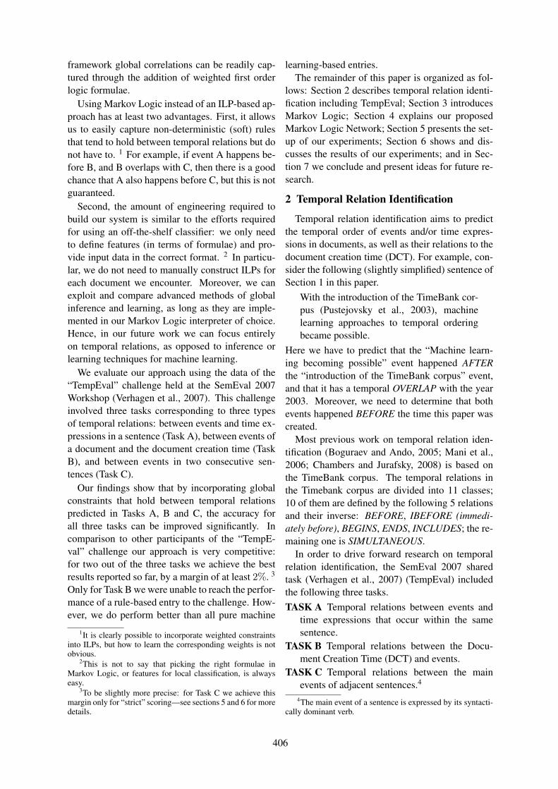
framework global correlations can be readily cap-tured through the addition of weighted first orderlogic formulae.
Using Markov Logic instead of an ILP-based ap-proach has at least two advantages. First, it allowsus to easily capture non-deterministic (soft) rulesthat tend to hold between temporal relations but donot have to. 1 For example, if event A happens be-fore B, and B overlaps with C, then there is a goodchance that A also happens before C, but this is notguaranteed.
Second, the amount of engineering required tobuild our system is similar to the efforts requiredfor using an off-the-shelf classifier: we only needto define features (in terms of formulae) and pro-vide input data in the correct format. 2 In particu-lar, we do not need to manually construct ILPs foreach document we encounter. Moreover, we canexploit and compare advanced methods of globalinference and learning, as long as they are imple-mented in our Markov Logic interpreter of choice.Hence, in our future work we can focus entirelyon temporal relations, as opposed to inference orlearning techniques for machine learning.
We evaluate our approach using the data of the“TempEval” challenge held at the SemEval 2007Workshop (Verhagen et al., 2007). This challengeinvolved three tasks corresponding to three typesof temporal relations: between events and time ex-pressions in a sentence (Task A), between events ofa document and the document creation time (TaskB), and between events in two consecutive sen-tences (Task C).
Our findings show that by incorporating globalconstraints that hold between temporal relationspredicted in Tasks A, B and C, the accuracy forall three tasks can be improved significantly. Incomparison to other participants of the “TempE-val” challenge our approach is very competitive:for two out of the three tasks we achieve the bestresults reported so far, by a margin of at least 2%. 3
Only for Task B we were unable to reach the perfor-mance of a rule-based entry to the challenge. How-ever, we do perform better than all pure machine
1It is clearly possible to incorporate weighted constraintsinto ILPs, but how to learn the corresponding weights is notobvious.
2This is not to say that picking the right formulae inMarkov Logic, or features for local classification, is alwayseasy.
3To be slightly more precise: for Task C we achieve thismargin only for “strict” scoring—see sections 5 and 6 for moredetails.
learning-based entries.The remainder of this paper is organized as fol-
lows: Section 2 describes temporal relation identi-fication including TempEval; Section 3 introducesMarkov Logic; Section 4 explains our proposedMarkov Logic Network; Section 5 presents the set-up of our experiments; Section 6 shows and dis-cusses the results of our experiments; and in Sec-tion 7 we conclude and present ideas for future re-search.
2 Temporal Relation Identification
Temporal relation identification aims to predictthe temporal order of events and/or time expres-sions in documents, as well as their relations to thedocument creation time (DCT). For example, con-sider the following (slightly simplified) sentence ofSection 1 in this paper.
With the introduction of the TimeBank cor-pus (Pustejovsky et al., 2003), machinelearning approaches to temporal orderingbecame possible.
Here we have to predict that the “Machine learn-ing becoming possible” event happened AFTERthe “introduction of the TimeBank corpus” event,and that it has a temporal OVERLAP with the year2003. Moreover, we need to determine that bothevents happened BEFORE the time this paper wascreated.
Most previous work on temporal relation iden-tification (Boguraev and Ando, 2005; Mani et al.,2006; Chambers and Jurafsky, 2008) is based onthe TimeBank corpus. The temporal relations inthe Timebank corpus are divided into 11 classes;10 of them are defined by the following 5 relationsand their inverse: BEFORE, IBEFORE (immedi-ately before), BEGINS, ENDS, INCLUDES; the re-maining one is SIMULTANEOUS.
In order to drive forward research on temporalrelation identification, the SemEval 2007 sharedtask (Verhagen et al., 2007) (TempEval) includedthe following three tasks.TASK A Temporal relations between events and
time expressions that occur within the samesentence.
TASK B Temporal relations between the Docu-ment Creation Time (DCT) and events.
TASK C Temporal relations between the mainevents of adjacent sentences.4
4The main event of a sentence is expressed by its syntacti-cally dominant verb.
406
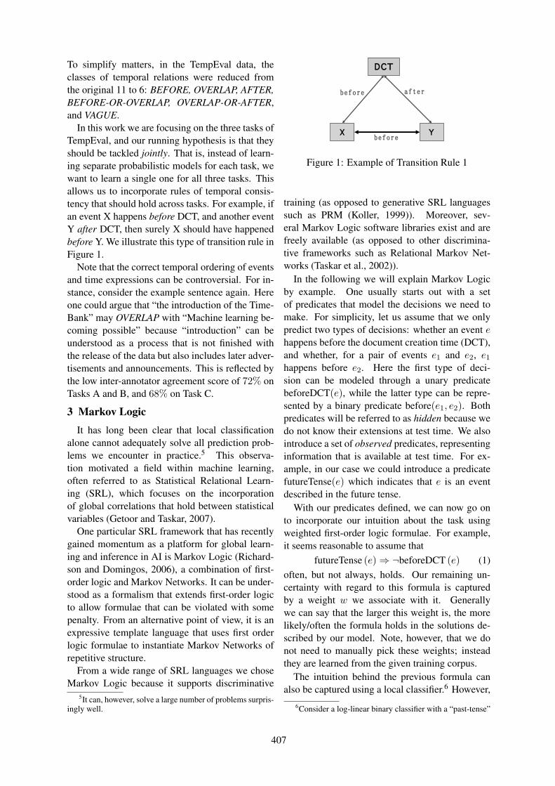
To simplify matters, in the TempEval data, theclasses of temporal relations were reduced fromthe original 11 to 6: BEFORE, OVERLAP, AFTER,BEFORE-OR-OVERLAP, OVERLAP-OR-AFTER,and VAGUE.
In this work we are focusing on the three tasks ofTempEval, and our running hypothesis is that theyshould be tackled jointly. That is, instead of learn-ing separate probabilistic models for each task, wewant to learn a single one for all three tasks. Thisallows us to incorporate rules of temporal consis-tency that should hold across tasks. For example, ifan event X happens before DCT, and another eventY after DCT, then surely X should have happenedbefore Y. We illustrate this type of transition rule inFigure 1.
Note that the correct temporal ordering of eventsand time expressions can be controversial. For in-stance, consider the example sentence again. Hereone could argue that “the introduction of the Time-Bank” may OVERLAP with “Machine learning be-coming possible” because “introduction” can beunderstood as a process that is not finished withthe release of the data but also includes later adver-tisements and announcements. This is reflected bythe low inter-annotator agreement score of 72% onTasks A and B, and 68% on Task C.
3 Markov LogicIt has long been clear that local classification
alone cannot adequately solve all prediction prob-lems we encounter in practice.5 This observa-tion motivated a field within machine learning,often referred to as Statistical Relational Learn-ing (SRL), which focuses on the incorporationof global correlations that hold between statisticalvariables (Getoor and Taskar, 2007).
One particular SRL framework that has recentlygained momentum as a platform for global learn-ing and inference in AI is Markov Logic (Richard-son and Domingos, 2006), a combination of first-order logic and Markov Networks. It can be under-stood as a formalism that extends first-order logicto allow formulae that can be violated with somepenalty. From an alternative point of view, it is anexpressive template language that uses first orderlogic formulae to instantiate Markov Networks ofrepetitive structure.
From a wide range of SRL languages we choseMarkov Logic because it supports discriminative
5It can, however, solve a large number of problems surpris-ingly well.
Figure 1: Example of Transition Rule 1
training (as opposed to generative SRL languagessuch as PRM (Koller, 1999)). Moreover, sev-eral Markov Logic software libraries exist and arefreely available (as opposed to other discrimina-tive frameworks such as Relational Markov Net-works (Taskar et al., 2002)).
In the following we will explain Markov Logicby example. One usually starts out with a setof predicates that model the decisions we need tomake. For simplicity, let us assume that we onlypredict two types of decisions: whether an event ehappens before the document creation time (DCT),and whether, for a pair of events e1 and e2, e1
happens before e2. Here the first type of deci-sion can be modeled through a unary predicatebeforeDCT(e), while the latter type can be repre-sented by a binary predicate before(e1, e2). Bothpredicates will be referred to as hidden because wedo not know their extensions at test time. We alsointroduce a set of observed predicates, representinginformation that is available at test time. For ex-ample, in our case we could introduce a predicatefutureTense(e) which indicates that e is an eventdescribed in the future tense.
With our predicates defined, we can now go onto incorporate our intuition about the task usingweighted first-order logic formulae. For example,it seems reasonable to assume that
futureTense (e)⇒ ¬beforeDCT (e) (1)often, but not always, holds. Our remaining un-certainty with regard to this formula is capturedby a weight w we associate with it. Generallywe can say that the larger this weight is, the morelikely/often the formula holds in the solutions de-scribed by our model. Note, however, that we donot need to manually pick these weights; insteadthey are learned from the given training corpus.
The intuition behind the previous formula canalso be captured using a local classifier.6 However,
6Consider a log-linear binary classifier with a “past-tense”
407

Markov Logic also allows us to say more:beforeDCT (e1) ∧ ¬beforeDCT (e2)
⇒ before (e1, e2) (2)In this case, we made a statement about moreglobal properties of a temporal ordering that can-not be captured with local classifiers. This formulais also an example of the transition rules as seen inFigure 2. This type of rule forms the core idea ofour joint approach.
A Markov Logic Network (MLN) M is a set ofpairs (φ,w) where φ is a first order formula and wis a real number (the formula’s weight). It defines aprobability distribution over sets of ground atoms,or so-called possible worlds, as follows:
p (y) =1Z
exp
∑(φ,w)∈M
w∑c∈Cφ
fφc (y)
(3)
Here each c is a binding of free variables in φ toconstants in our domain. Each fφ
c is a binary fea-ture function that returns 1 if in the possible worldy the ground formula we get by replacing the freevariables in φ with the constants in c is true, and0 otherwise. Cφ is the set of all bindings for thefree variables in φ. Z is a normalisation constant.Note that this distribution corresponds to a MarkovNetwork (the so-called Ground Markov Network)where nodes represent ground atoms and factorsrepresent ground formulae.
Designing formulae is only one part of the game.In practice, we also need to choose a trainingregime (in order to learn the weights of the formu-lae we added to the MLN) and a search/inferencemethod that picks the most likely set of groundatoms (temporal relations in our case) given ourtrained MLN and a set of observations. How-ever, implementations of these methods are oftenalready provided in existing Markov Logic inter-preters such as Alchemy 7 and Markov thebeast. 8
4 Proposed Markov Logic Network
As stated before, our aim is to jointly tackleTasks A, B and C of the TempEval challenge. Inthis section we introduce the Markov Logic Net-work we designed for this goal.
We have three hidden predicates, correspondingto Tasks A, B, and C: relE2T(e, t, r) represents thetemporal relation of class r between an event e
feature: here for every event e the decision “e happens be-fore DCT” becomes more likely with a higher weight for thisfeature.
7http://alchemy.cs.washington.edu/8http://code.google.com/p/thebeast/
Figure 2: Example of Transition Rule 2
and a time expression t; relDCT(e, r) denotes thetemporal relation r between an event e and DCT;relE2E(e1, e2, r) represents the relation r betweentwo events of the adjacent sentences, e1 and e2.
Our observed predicates reflect information wewere given (such as the words of a sentence), andadditional information we extracted from the cor-pus (such as POS tags and parse trees). Note thatthe TempEval data also contained temporal rela-tions that were not supposed to be predicted. Theserelations are represented using two observed pred-icates: relT2T(t1, t2, r) for the relation r betweentwo time expressions t1 and t2; dctOrder(t, r) forthe relation r between a time expression t and afixed DCT.
An illustration of all “temporal” predicates, bothhidden and observed, can be seen in Figure 3.
4.1 Local Formula
Our MLN is composed of several weighted for-mulae that we divide into two classes. The firstclass contains local formulae for the Tasks A, Band C. We say that a formula is local if it onlyconsiders the hidden temporal relation of a singleevent-event, event-time or event-DCT pair. Theformulae in the second class are global: they in-volve two or more temporal relations at the sametime, and consider Tasks A, B and C simultane-ously.
The local formulae are based on features em-ployed in previous work (Cheng et al., 2007;Bethard and Martin, 2007) and are listed in Table 1.What follows is a simple example in order to illus-trate how we implement each feature as a formula(or set of formulae).
Consider the tense-feature for Task C. For thisfeature we first introduce a predicate tense(e, t)that denotes the tense t for an event e. Then we
408
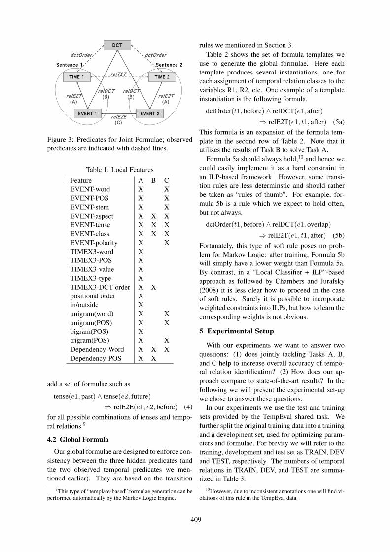
Figure 3: Predicates for Joint Formulae; observedpredicates are indicated with dashed lines.
Table 1: Local FeaturesFeature A B CEVENT-word X XEVENT-POS X XEVENT-stem X XEVENT-aspect X X XEVENT-tense X X XEVENT-class X X XEVENT-polarity X XTIMEX3-word XTIMEX3-POS XTIMEX3-value XTIMEX3-type XTIMEX3-DCT order X Xpositional order Xin/outside Xunigram(word) X Xunigram(POS) X Xbigram(POS) Xtrigram(POS) X XDependency-Word X X XDependency-POS X X
add a set of formulae such as
tense(e1, past) ∧ tense(e2, future)⇒ relE2E(e1, e2, before) (4)
for all possible combinations of tenses and tempo-ral relations.9
4.2 Global Formula
Our global formulae are designed to enforce con-sistency between the three hidden predicates (andthe two observed temporal predicates we men-tioned earlier). They are based on the transition
9This type of “template-based” formulae generation can beperformed automatically by the Markov Logic Engine.
rules we mentioned in Section 3.Table 2 shows the set of formula templates we
use to generate the global formulae. Here eachtemplate produces several instantiations, one foreach assignment of temporal relation classes to thevariables R1, R2, etc. One example of a templateinstantiation is the following formula.
dctOrder(t1, before) ∧ relDCT(e1, after)⇒ relE2T(e1, t1, after) (5a)
This formula is an expansion of the formula tem-plate in the second row of Table 2. Note that itutilizes the results of Task B to solve Task A.
Formula 5a should always hold,10 and hence wecould easily implement it as a hard constraint inan ILP-based framework. However, some transi-tion rules are less determinstic and should ratherbe taken as “rules of thumb”. For example, for-mula 5b is a rule which we expect to hold often,but not always.
dctOrder(t1, before) ∧ relDCT(e1, overlap)⇒ relE2T(e1, t1, after) (5b)
Fortunately, this type of soft rule poses no prob-lem for Markov Logic: after training, Formula 5bwill simply have a lower weight than Formula 5a.By contrast, in a “Local Classifier + ILP”-basedapproach as followed by Chambers and Jurafsky(2008) it is less clear how to proceed in the caseof soft rules. Surely it is possible to incorporateweighted constraints into ILPs, but how to learn thecorresponding weights is not obvious.
5 Experimental Setup
With our experiments we want to answer twoquestions: (1) does jointly tackling Tasks A, B,and C help to increase overall accuracy of tempo-ral relation identification? (2) How does our ap-proach compare to state-of-the-art results? In thefollowing we will present the experimental set-upwe chose to answer these questions.
In our experiments we use the test and trainingsets provided by the TempEval shared task. Wefurther split the original training data into a trainingand a development set, used for optimizing param-eters and formulae. For brevity we will refer to thetraining, development and test set as TRAIN, DEVand TEST, respectively. The numbers of temporalrelations in TRAIN, DEV, and TEST are summa-rized in Table 3.
10However, due to inconsistent annotations one will find vi-olations of this rule in the TempEval data.
409

Table 2: Joint Formulae for Global ModelTask FormulaA→ B dctOrder(t, R1) ∧ relE2T(e, t, R2)⇒ relDCT(e, R3)B → A dctOrder(t, R1) ∧ relDCT(e, R2)⇒ relE2T(e, t, R3)B → C relDCT(e1, R1) ∧ relDCT(e2, R2)⇒ relE2E(e1, e2, R3)C → B relDCT(e1, R1) ∧ relE2E(e1, e2, R2)⇒ relDCT(e2, R3)A→ C relE2T(e1, t1, R1) ∧ relT2T(t1, t2, R2) ∧ relE2T(e2, t2, R3)⇒ relE2E(e1, e2, R4)C → A relE2T(e2, t2, R1) ∧ relT2T(t1, t2, R2) ∧ relE2E(e1, e2, R3)⇒ relE2T(e1, t1, R4)
Table 3: Numbers of Labeled Relations for AllTasks
TRAIN DEV TEST TOTALTask A 1359 131 169 1659Task B 2330 227 331 2888Task C 1597 147 258 2002
For feature generation we use the followingtools. 11 POS tagging is performed with TnTver2.2;12 for our dependency-based features we useMaltParser 1.0.0.13 For inference in our modelswe use Cutting Plane Inference (Riedel, 2008) withILP as a base solver. This type of inference is ex-act and often very fast because it avoids instantia-tion of the complete Markov Network. For learningwe apply one-best MIRA (Crammer and Singer,2003) with Cutting Plane Inference to find the cur-rent model guess. Both training and inference algo-rithms are provided by Markov thebeast, a MarkovLogic interpreter tailored for NLP applications.
Note that there are several ways to manually op-timize the set of formulae to use. One way is topick a task and then choose formulae that increasethe accuracy for this task on DEV. However, ourprimary goal is to improve the performance of allthe tasks together. Hence we choose formulae withrespect to the total score over all three tasks. Wewill refer to this type of optimization as “averagedoptimization”. The total scores of the all three tasksare defined as follows:
Ca + Cb + Cc
Ga + Gb + Gc
where Ca, Cb, and Cc are the number of the cor-rectly identified labels in each task, and Ga, Gb,and Gc are the numbers of gold labels of each task.Our system necessarily outputs one label to one re-lational link to identify. Therefore, for all our re-
11Since the TempEval trial has no restriction on pre-processing such as syntactic parsing, most participants usedsome sort of parsers.
12http://www.coli.uni-saarland.de/˜thorsten/tnt/
13http://w3.msi.vxu.se/˜nivre/research/MaltParser.html
sults, precision, recall, and F-measure are the exactsame value.
For evaluation, TempEval proposed the two scor-ing schemes: “strict” and “relaxed”. For strict scor-ing we give full credit if the relations match, and nocredit if they do not match. On the other hand, re-laxed scoring gives credit for a relation accordingto Table 4. For example, if a system picks the re-lation “AFTER” that should have been “BEFORE”according to the gold label, it gets neither “strict”nor “relaxed” credit. But if the system assigns“B-O (BEFORE-OR-OVERLAP)” to the relation,it gets a 0.5 “relaxed” score (and still no “strict”score).
6 Results
In the following we will first present our com-parison of the local and global model. We will thengo on to put our results into context and comparethem to the state-of-the-art.
6.1 Impact of Global Formulae
First, let us show the results on TEST in Ta-ble 5. You will find two columns, “Global” and“Local”, showing scores achieved with and with-out joint formulae, respectively. Clearly, the globalmodels scores are higher than the local scores forall three tasks. This is also reflected by the last rowof Table 5. Here we see that we have improvedthe averaged performance across the three tasks byapproximately 2.5% (ρ < 0.01, McNemar’s test 2-tailed). Note that with 3.5% the improvements areparticularly large for Task C.
The TempEval test set is relatively small (see Ta-ble 3). Hence it is not clear how well our resultswould generalize in practice. To overcome this is-sue, we also evaluated the local and global modelusing 10-fold cross validation on the training data(TRAIN + DEV). The corresponding results can beseen in Table 6. Note that the general picture re-mains: performance for all tasks is improved, andthe averaged score is improved only slightly lessthan for the TEST results. However, this time thescore increase for Task B is lower than before. We
410
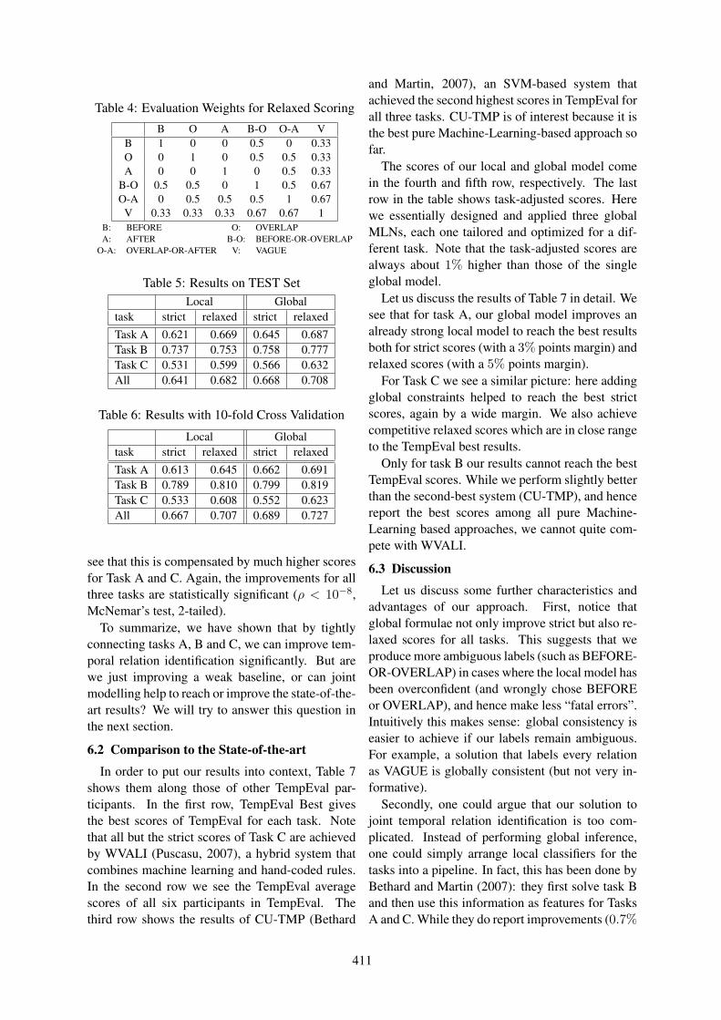
Table 4: Evaluation Weights for Relaxed Scoring
B O A B-O O-A VB 1 0 0 0.5 0 0.33O 0 1 0 0.5 0.5 0.33A 0 0 1 0 0.5 0.33
B-O 0.5 0.5 0 1 0.5 0.67O-A 0 0.5 0.5 0.5 1 0.67
V 0.33 0.33 0.33 0.67 0.67 1B: BEFORE O: OVERLAPA: AFTER B-O: BEFORE-OR-OVERLAP
O-A: OVERLAP-OR-AFTER V: VAGUE
Table 5: Results on TEST SetLocal Global
task strict relaxed strict relaxedTask A 0.621 0.669 0.645 0.687Task B 0.737 0.753 0.758 0.777Task C 0.531 0.599 0.566 0.632All 0.641 0.682 0.668 0.708
Table 6: Results with 10-fold Cross Validation
Local Globaltask strict relaxed strict relaxedTask A 0.613 0.645 0.662 0.691Task B 0.789 0.810 0.799 0.819Task C 0.533 0.608 0.552 0.623All 0.667 0.707 0.689 0.727
see that this is compensated by much higher scoresfor Task A and C. Again, the improvements for allthree tasks are statistically significant (ρ < 10−8,McNemar’s test, 2-tailed).
To summarize, we have shown that by tightlyconnecting tasks A, B and C, we can improve tem-poral relation identification significantly. But arewe just improving a weak baseline, or can jointmodelling help to reach or improve the state-of-the-art results? We will try to answer this question inthe next section.
6.2 Comparison to the State-of-the-art
In order to put our results into context, Table 7shows them along those of other TempEval par-ticipants. In the first row, TempEval Best givesthe best scores of TempEval for each task. Notethat all but the strict scores of Task C are achievedby WVALI (Puscasu, 2007), a hybrid system thatcombines machine learning and hand-coded rules.In the second row we see the TempEval averagescores of all six participants in TempEval. Thethird row shows the results of CU-TMP (Bethard
and Martin, 2007), an SVM-based system thatachieved the second highest scores in TempEval forall three tasks. CU-TMP is of interest because it isthe best pure Machine-Learning-based approach sofar.
The scores of our local and global model comein the fourth and fifth row, respectively. The lastrow in the table shows task-adjusted scores. Herewe essentially designed and applied three globalMLNs, each one tailored and optimized for a dif-ferent task. Note that the task-adjusted scores arealways about 1% higher than those of the singleglobal model.
Let us discuss the results of Table 7 in detail. Wesee that for task A, our global model improves analready strong local model to reach the best resultsboth for strict scores (with a 3% points margin) andrelaxed scores (with a 5% points margin).
For Task C we see a similar picture: here addingglobal constraints helped to reach the best strictscores, again by a wide margin. We also achievecompetitive relaxed scores which are in close rangeto the TempEval best results.
Only for task B our results cannot reach the bestTempEval scores. While we perform slightly betterthan the second-best system (CU-TMP), and hencereport the best scores among all pure Machine-Learning based approaches, we cannot quite com-pete with WVALI.
6.3 Discussion
Let us discuss some further characteristics andadvantages of our approach. First, notice thatglobal formulae not only improve strict but also re-laxed scores for all tasks. This suggests that weproduce more ambiguous labels (such as BEFORE-OR-OVERLAP) in cases where the local model hasbeen overconfident (and wrongly chose BEFOREor OVERLAP), and hence make less “fatal errors”.Intuitively this makes sense: global consistency iseasier to achieve if our labels remain ambiguous.For example, a solution that labels every relationas VAGUE is globally consistent (but not very in-formative).
Secondly, one could argue that our solution tojoint temporal relation identification is too com-plicated. Instead of performing global inference,one could simply arrange local classifiers for thetasks into a pipeline. In fact, this has been done byBethard and Martin (2007): they first solve task Band then use this information as features for TasksA and C. While they do report improvements (0.7%
411

Table 7: Comparison with Other Systems
Task A Task B Task Cstrict relaxed strict relaxed strict relaxed
TempEval Best 0.62 0.64 0.80 0.81 0.55 0.64TempEval Average 0.56 0.59 0.74 0.75 0.51 0.58CU-TMP 0.61 0.63 0.75 0.76 0.54 0.58Local Model 0.62 0.67 0.74 0.75 0.53 0.60Global Model 0.65 0.69 0.76 0.78 0.57 0.63Global Model (Task-Adjusted) (0.66) (0.70) (0.76) (0.79) (0.58) (0.64)
on Task A, and about 0.5% on Task C), generallythese improvements do not seem as significant asours. What is more, by design their approach cannot improve the first stage (Task B) of the pipeline.
On the same note, we also argue that our ap-proach does not require more implementation ef-forts than a pipeline. Essentially we only have toprovide features (in the form of formulae) to theMarkov Logic Engine, just as we have to providefor a SVM or MaxEnt classifier.
Finally, it became more clear to us that there areproblems inherent to this task and dataset that wecannot (or only partially) solve using global meth-ods. First, there are inconsistencies in the trainingdata (as reflected by the low inter-annotator agree-ment) that often mislead the learner—this prob-lem applies to learning of local and global formu-lae/features alike. Second, the training data is rela-tively small. Obviously, this makes learning of re-liable parameters more difficult, particularly whendata is as noisy as in our case. Third, the tempo-ral relations in the TempEval dataset only directlyconnect a small subset of events. This makes globalformulae less effective.14
7 Conclusion
In this paper we presented a novel approach totemporal relation identification. Instead of usinglocal classifiers to predict temporal order in a pair-wise fashion, our approach uses Markov Logic toincorporate both local features and global transi-tion rules between temporal relations.
We have focused on transition rules betweentemporal relations of the three TempEval subtasks:temporal ordering of events, of events and time ex-pressions, and of events and the document creationtime. Our results have shown that global transitionrules lead to significantly higher accuracy for allthree tasks. Moreover, our global Markov Logic
14See (Chambers and Jurafsky, 2008) for a detailed discus-sion of this problem, and a possible solution for it.
model achieves the highest scores reported so farfor two of three tasks, and very competitive resultsfor the remaining one.
While temporal transition rules can also be cap-tured with an Integer Linear Programming ap-proach (Chambers and Jurafsky, 2008), MarkovLogic has at least two advantages. First, handlingof “rules of thumb” between less specific tempo-ral relations (such as OVERLAP or VAGUE) isstraightforward—we simply let the Markov LogicEngine learn weights for these rules. Second, thereis less engineering overhead for us to perform, be-cause we do not need to generate ILPs for each doc-ument.
However, potential for further improvementsthrough global approaches seems to be limited bythe sparseness and inconsistency of the data. Toovercome this problem, we are planning to use ex-ternal or untagged data along with methods for un-supervised learning in Markov Logic (Poon andDomingos, 2008).
Furthermore, TempEval-2 15 is planned for 2010and it has challenging temporal ordering tasks infive languages. So, we would like to investigate theutility of global formulae for multilingual tempo-ral ordering. Here we expect that while lexical andsyntax-based features may be quite language de-pendent, global transition rules should hold acrosslanguages.
Acknowledgements
This work is partly supported by the IntegratedDatabase Project, Ministry of Education, Culture,Sports, Science and Technology of Japan.
ReferencesSteven Bethard and James H. Martin. 2007. Cu-tmp:
Temporal relation classification using syntactic andsemantic features. In Proceedings of the 4th Interna-tional Workshop on SemEval-2007., pages 129–132.15http://www.timeml.org/tempeval2/
412

Branimir Boguraev and Rie Kubota Ando. 2005.Timeml-compliant text analysis for temporal reason-ing. In Proceedings of the 19th International JointConference on Artificial Intelligence, pages 997–1003.
Nathanael Chambers and Daniel Jurafsky. 2008.Jointly combining implicit constraints improves tem-poral ordering. In Proceedings of the 2008 Con-ference on Empirical Methods in Natural LanguageProcessing, pages 698–706, Honolulu, Hawaii, Oc-tober. Association for Computational Linguistics.
Yuchang Cheng, Masayuki Asahara, and Yuji Mat-sumoto. 2007. Naist.japan: Temporal relation iden-tification using dependency parsed tree. In Proceed-ings of the 4th International Workshop on SemEval-2007., pages 245–248.
Koby Crammer and Yoram Singer. 2003. Ultracon-servative online algorithms for multiclass problems.Journal of Machine Learning Research, 3:951–991.
Lise Getoor and Ben Taskar. 2007. Introduction to Sta-tistical Relational Learning (Adaptive Computationand Machine Learning). The MIT Press.
Daphne Koller, 1999. Probabilistic Relational Models,pages 3–13. Springer, Berlin/Heidelberg, Germany.
Inderjeet Mani, Marc Verhagen, Ben Wellner,Chong Min Lee, and James Pustejovsky. 2006.Machine learning of temporal relations. In ACL-44:Proceedings of the 21st International Conferenceon Computational Linguistics and the 44th annualmeeting of the Association for Computational Lin-guistics, pages 753–760, Morristown, NJ, USA.Association for Computational Linguistics.
Hoifung Poon and Pedro Domingos. 2008. Joint unsu-pervised coreference resolution with Markov Logic.In Proceedings of the 2008 Conference on Empiri-cal Methods in Natural Language Processing, pages650–659, Honolulu, Hawaii, October. Association forComputational Linguistics.
Georgiana Puscasu. 2007. Wvali: Temporal relationidentification by syntactico-semantic analysis. InProceedings of the 4th International Workshop onSemEval-2007., pages 484–487.
James Pustejovsky, Jose Castano, Robert Ingria, ReserSauri, Robert Gaizauskas, Andrea Setzer, and Gra-ham Katz. 2003. The timebank corpus. In Proceed-ings of Corpus Linguistics 2003, pages 647–656.
Matthew Richardson and Pedro Domingos. 2006.Markov logic networks. In Machine Learning.
Sebastian Riedel. 2008. Improving the accuracy andefficiency of map inference for markov logic. In Pro-ceedings of UAI 2008.
Ben Taskar, Abbeel Pieter, and Daphne Koller. 2002.Discriminative probabilistic models for relationaldata. In Proceedings of the 18th Annual Conferenceon Uncertainty in Artificial Intelligence (UAI-02),pages 485–492, San Francisco, CA. Morgan Kauf-mann.
Marc Verhagen, Robert Gaizaukas, Frank Schilder,Mark Hepple, Graham Katz, and James Pustejovsky.2007. Semeval-2007 task 15: Tempeval temporal re-lation identification. In Proceedings of the 4th Inter-national Workshop on SemEval-2007., pages 75–80.
413
Proceedings of the 47th Annual Meeting of the ACL and the 4th IJCNLP of the AFNLP, pages 414–422,Suntec, Singapore, 2-7 August 2009. c©2009 ACL and AFNLP
Profile Based Cross-Document CoreferenceUsing Kernelized Fuzzy Relational Clustering
Jian Huang† Sarah M. Taylor‡ Jonathan L. Smith‡ Konstantinos A. Fotiadis‡ C. Lee Giles††College of Information Sciences and Technology
Pennsylvania State University, University Park, PA 16802, USA{jhuang, giles}@ist.psu.edu
‡Advanced Technology Office, Lockheed Martin IS&GS, Arlington, VA 22203, USA{sarah.m.taylor, jonathan.l.smith, konstantinos.a.fotiadis}@lmco.com
Abstract
Coreferencing entities across documentsin a large corpus enables advanceddocument understanding tasks such asquestion answering. This paper presentsa novel cross document coreferenceapproach that leverages the profilesof entities which are constructed byusing information extraction tools andreconciled by using a within-documentcoreference module. We propose tomatch the profiles by using a learnedensemble distance function comprisedof a suite of similarity specialists. Wedevelop a kernelized soft relationalclustering algorithm that makes use ofthe learned distance function to partitionthe entities into fuzzy sets of identities.We compare the kernelized clusteringmethod with a popular fuzzy relationclustering algorithm (FRC) and show 5%improvement in coreference performance.Evaluation of our proposed methodson a large benchmark disambiguationcollection shows that they comparefavorably with the top runs in theSemEval evaluation.
1 Introduction
A named entity that represents a person, an or-ganization or a geo-location may appear withinand across documents in different forms. Crossdocument coreference (CDC) is the task of con-solidating named entities that appear in multipledocuments according to their real referents. CDCis a stepping stone for achieving intelligent in-formation access to vast and heterogeneous textcorpora, which includes advanced NLP techniquessuch as document summarization and question an-swering. A related and well studied task is within
document coreference (WDC), which limits thescope of disambiguation to within the boundary ofa document. When namesakes appear in an article,the author can explicitly help to disambiguate, us-ing titles and suffixes (as in the example, “GeorgeBush Sr. ... the younger Bush”) besides othermeans. Cross document coreference, on the otherhand, is a more challenging task because theselinguistics cues and sentence structures no longerapply, given the wide variety of context and stylesin different documents.
Cross document coreference research has re-cently become more popular due to the increasinginterests in the web person search task (Artileset al., 2007). Here, a search query for a personname is entered into a search engine and thedesired outputs are documents clustered accordingto the identities of the entities in question. Inour work, we propose to drill down to the sub-document mention level and construct an entityprofile with the support of information extractiontools and reconciled with WDC methods. Henceour IE based approach has access to accurateinformation such as a person’s mentions and geo-locations for disambiguation. Simple IR basedCDC approaches (e.g. (Gooi and Allan, 2004)), onthe other hand, may simply use all the terms andthis can be detrimental to accuracy. For example, abiography of John F. Kennedy is likely to mentionmembers of his family with related positions,besides references to other political figures. Evenwith careful word selection, these textual featurescan still confuse the disambiguation system aboutthe true identity of the person.
We propose to handle the CDC task using anovel kernelized fuzzy relational clustering algo-rithm, which allows probabilistic cluster mem-bership assignment. This not only addresses theintrinsic uncertainty nature of the CDC problem,but also yields additional performance improve-ment. We propose to use a specialist ensemble
414
learning approach to aggregate the diverse set ofsimilarities in comparing attributes and relation-ships in entity profiles. Our approach is first fullydescribed in Section 2. The effectiveness of theproposed method is demonstrated using real worldbenchmark test sets in Section 3. We reviewrelated work in cross document coreference andconclude in Section 5.
2 Methods
2.1 Document Level and Profile Based CDC
We make distinctions between document level andprofile based cross document coreference. Docu-ment level CDC makes a simplifying assumptionthat a named entity (and its variants) in a documenthas one underlying real identity. The assump-tion is generally acceptable but may be violatedwhen a document refers to namesakes at the sametime (e.g. George W. Bush and George H. W.Bush referred to as George or President Bush).Furthermore, the context surrounding the personNE President Clinton can be counterproductivefor disambiguating the NE Senator Clinton, withboth entities likely to appear in a document at thesame time. The simplified document level CDChas nevertheless been used in the WePS evaluation(Artiles et al., 2007), called the web people task.
In this work, we advocate profile based disam-biguation that aims to leverage the advances inNLP techniques. Rather than treating a documentas simply a bag of words, an information extrac-tion tool first extracts NE’s and their relationships.For the NE’s of interest (i.e. persons in this work),a within-document coreference (WDC) modulethen links the entities deemed as referring tothe same underlying identity into a WDC chain.This process includes both anaphora resolution(resolving ‘He’ and its antecedent ‘President Clin-ton’) and entity tracking (resolving ‘Bill’ and‘President Clinton’). Let E = {e1, ..., eN} denotethe set of N chained entities (each correspondingto a WDC chain), provided as input to the CDCsystem. We intentionally do not distinguish whichdocument each ej belongs to, as profile basedCDC can potentially rectify WDC errors by lever-aging information across document boundaries.Each ei is represented as a profile which containsthe NE, its attributes and associated relationships,i.e. ej =< ej,1, ..., ej,L > (ej,l can be a textualattribute or a pointer to another entity). The profilebased CDC method generates a partition of E ,
represented by a partition matrix U (where uij
denotes the membership of an entity ej to the i-th identity cluster). Therefore, the chained entitiesplaced in a name cluster are deemed as coreferent.
Profile based CDC addresses a finer grainedcoreference problem in the mention level, enabledby the recent advances in IE and WDC techniques.In addition, profile based CDC facilitates userinformation consumption with structured informa-tion and short summary passages. Next, we focuson the relational clustering algorithm that lies atthe core of the profile based CDC system. We thenturn our attention to the specialist learning algo-rithm for the distance function used in clustering,capable of leveraging the available training data.
2.2 CDC Using Fuzzy Relational Clustering2.2.1 PreliminariesTraditionally, hard clustering algorithms (whereuij ∈ {0, 1}) such as complete linkage hierarchi-cal agglomerative clustering (Mann and Yarowsky,2003) have been applied to the disambiguationproblem. In this work, we propose to use fuzzyclustering methods (relaxing the membership con-dition to uij ∈ [0, 1]) as a better way of handlinguncertainty in cross document coreference. First,consider the following motivating example,Example. The named entity President Bush isextracted from the sentence “President Bush ad-dressed the nation from the Oval Office Monday.”
• Without additional cues, a hard clusteringalgorithm has to arbitrarily assign themention “President Bush” to either the NE“George W. Bush” or “George H. W. Bush”.
• A soft clustering algorithm, on the otherhand, can assign equal probability to the twoidentities, indicating low entropy or highuncertainty in the solution. Additionally, thesoft clustering algorithm can assign lowerprobability to the identity “Governor JebBush”, reflecting a less likely (though notimpossible) coreference decision.
We first formalize the cross document corefer-ence problem as a soft clustering problem, whichminimizes the following objective function:
JC(E) =C∑
i=1
N∑
j=1um
ij d2(ej ,vi) (1)
s.t.C∑
i=1uij = 1 and
N∑
j=1uij > 0, uij ∈ [0, 1]
415
where vi is a virtual (implicit) prototype of the i-thcluster (ej ,vi ∈ D) and m controls the fuzzinessof the solution (m > 1; the solution approacheshard clustering as m approaches 1). We willfurther explain the generic distance function d :D × D → R in the next subsection. The goalof the optimization is to minimize the sum ofdeviations of patterns to the cluster prototypes.The clustering solution is a fuzzy partition Pθ ={Ci}, where ej ∈ Ci if and only if uij > θ.
We note from the outset that the optimizationfunctional has the same form as the classicalFuzzy C-Means (FCM) algorithm (Bezdek, 1981),but major differences exist. FCM, as most ob-ject clustering algorithms, deals with object datarepresented in a vectorial form. In our case, thedata is purely relational and only the mutual rela-tionships between entities can be determined. Tobe exact, we can define the similarity/dissimilaritybetween a pair of attributes or relationships ofthe same type l between entities ej and ek ass(l)(ej , ek). For instance, the similarity betweenthe occupations ‘President’ and ‘Commander inChief’ can be computed using the JC semanticdistance (Jiang and Conrath, 1997) with WordNet;the similarity of co-occurrence with other peoplecan be measured by the Jaccard coefficient. In thenext section, we propose to compute the relationstrength r(·, ·) from the component similaritiesusing aggregation weights learned from trainingdata. Hence the N chained entities to be clusteredcan be represented as relational data using an n×nmatrix R, where rj,k = r(ej , ek). The Any Rela-tion Clustering Algorithm (ARCA) (Corsini et al.,2005; Cimino et al., 2006) represents relationaldata as object data using their mutual relationstrength and uses FCM for clustering. We adoptthis approach to transform (objectify) a relationalpattern ej into an N dimensional vector rj (i.e.the j-th row in the matrix R) using a mappingΘ : D → RN . In other words, each chained entityis represented as a vector of its relation strengthswith all the entities. Fuzzy clusters can thenbe obtained by grouping closely related patternsusing object clustering algorithm.
Furthermore, it is well known that FCMis a spherical clustering algorithm and thusis not generally applicable to relational datawhich may yield relational clusters of arbitraryand complicated shapes. Also, the distance inthe transformed space may be non-Euclidean,
rendering many clustering algorithms ineffective(many FCM extensions theoretically requirethe underlying distance to satisfy certain metricproperties). In this work, we propose kernelizedARCA (called KARC) which uses a kernel-induced metric to handle the objectified relationaldata, as we introduce next.
2.2.2 Kernelized Fuzzy ClusteringKernelization (Schölkopf and Smola, 2002) is amachine learning technique to transform patternsin the data space to a high-dimensional featurespace so that the structure of the data can be moreeasily and adequately discovered. Specifically, anonlinear transformation Φ maps data in RN toH of possibly infinite dimensions (Hilbert space).The key idea is the kernel trick – without explicitlyspecifying Φ and H, the inner product in H canbe computed by evaluating a kernel function K inthe data space, i.e. < Φ(ri), Φ(rj) >= K(ri, rj)(one of the most frequently used kernel func-tions is the Gaussian RBF kernel: K(rj , rk) =exp(−λ‖rj − rk‖2)). This technique has beensuccessfully applied to SVMs to classify non-linearly separable data (Vapnik, 1995). Kerneliza-tion preserves the simplicity in the formalism ofthe underlying clustering algorithm, meanwhile ityields highly nonlinear boundaries so that spheri-cal clustering algorithms can apply (e.g. (Zhangand Chen, 2003) developed a kernelized objectclustering algorithm based on FCM).
Let wi denote the objectified virtual cluster vi,i.e. wi = Θ(vi). Using the kernel trick, thesquared distance between Φ(rj) and Φ(wi) in thefeature space H can be computed as:
‖Φ(rj)− Φ(wi)‖2H (2)
= < Φ(rj)− Φ(wi), Φ(rj)− Φ(wi) >
= < Φ(rj), Φ(rj) > −2 < Φ(rj), Φ(wi) >
+ < Φ(wi),Φ(wi) >
= 2− 2K(rj ,wi) (3)
assuming K(r, r) = 1. The KARC algorithm
defines the generic distance d as d2(ej ,vi)def=
‖Φ(rj)−Φ(wi)‖2H = ‖Φ(Θ(ej))−Φ(Θ(vi))‖2
H
(we also use d2ji as a notational shorthand).
Using Lagrange Multiplier as in FCM, the opti-mal solution for Equation (1) is:
uij =
[
C∑
h=1
(
d2ji
d2jh
)1/(m−1)]−1
, (d2ji 6= 0)
1 , (d2ji = 0)
(4)
416
Φ(wi) =
N∑
k=1um
ikΦ(rk)
N∑
k=1um
ik
(5)
Since Φ is an implicit mapping, Eq. (5) cannot be explicitly evaluated. On the other hand,plugging Eq. (5) into Eq. (3), d2
ji can be explicitlyrepresented by using the kernel matrix,
d2ji = 2− 2 ·
N∑
k=1um
ikK(rj , rk)
N∑
k=1um
ik
(6)
With the derivation, the kernelized fuzzy clus-tering algorithm KARC works as follows. Thechained entities E are first objectified into therelation strength matrix R using SEG, the detailsof which are described in the following section.The Gram matrix K is then computed based onthe relation strength vectors using the kernel func-tion. For a given number of clusters C, theinitialization step is done by randomly picking Cpatterns as cluster centers, equivalently, C indices{n1, .., nC} are randomly picked from {1, .., N}.D0 is initialized by setting d2
ji = 2− 2K(rj , rni).KARC alternately updates the membership matrixU and the kernel distance matrix D until conver-gence or running more than maxIter iterations(Algorithm 1). Finally, the soft partition is gen-erated based on the membership matrix U , whichis the desired cross document coreference result.
Algorithm 1 KARC Alternating OptimizationInput: Gram matrix K; #Clusters C; threshold θ
initialize D0
t ← 0repeat
t ← t + 1// 1– Update membership matrix U t:
uij =(d2
ji)− 1
m−1
∑C
h=1(d2
jh)− 1
m−1
// 2– Update kernel distance matrix Dt:
d2ji = 2− 2 ·
N∑
k=1
umikKjk
N∑
k=1
umik
until (t > maxIter) or(t > 1 and |U t − U t−1| < ε)
Pθ ← Generate soft partition(U t, θ)Output: Fuzzy partition Pθ
2.2.3 Cluster ValidationIn the CDC setting, the number of true underlyingidentities may vary depending on the entities’ levelof ambiguity (e.g. name frequency). Selecting theoptimal number of clusters is in general a hardresearch question in clustering1. We adopt theXie-Beni Index (XBI) (Xie and Beni, 1991) as inARCA, which is one of the most popular clustervalidities for fuzzy clustering algorithms. Xie-Beni Index (XBI) measures the goodness of clus-tering using the ratio of the intra-cluster variationand the inter-cluster separation. We measure thekernelized XBI (KXBI) in the feature space as,
KXBI =
C∑
i=1
N∑
j=1um
ij ‖Φ(rj)− Φ(wi)‖2H
N · min1≤i<j≤C
‖Φ(wi)− Φ(wj)‖2H
where the nominator is readily computed using Dand the inter-cluster separation in the denominatorcan be evaluated using the similar kernel trickabove (details omitted). Note that KXBI is onlydefined for C > 1. Thus we pick the C thatcorresponds to the first minimum of KXBI, andthen compare its objective function value JC withthe cluster variance (J1 for C = 1). The optimalC is chosen from the minimum of the two2.
2.3 Specialist Ensemble Learning of RelationStrengths between Entities
One remaining element in the overall CDC ap-proach is how the relation strength rj,k betweentwo entities is computed. In (Cohen et al., 2003),a binary SVM model is trained and its confidencein predicting the non-coreferent class is used asthe distance metric. In our case of using in-formation extraction results for disambiguation,however, only some of the similarity features arepresent based on the available relationships in twoprofiles. In this work, we propose to treat eachsimilarity function as a specialist that specializesin computing the similarity of a particular typeof relationship. Indeed, the similarity functionbetween a pair of attributes or relationships may initself be a sophisticated component algorithm. Weutilize the specialist ensemble learning framework(Freund et al., 1997) to combine these component
1In particular, clustering algorithms that regularize theoptimization with cluster size are not applicable in our case.
2In practice, the entities to be disambiguated tend to bedominated by several major identities. Hence performancegenerally does not vary much in the range of large C values.
417
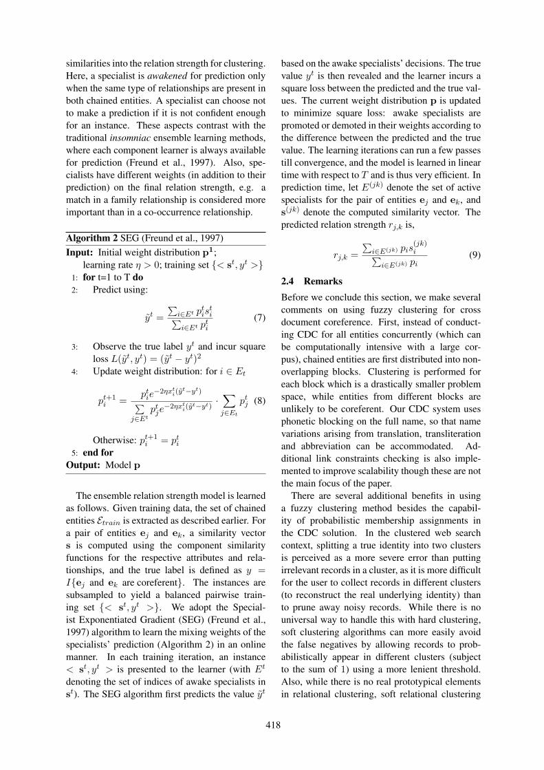
similarities into the relation strength for clustering.Here, a specialist is awakened for prediction onlywhen the same type of relationships are present inboth chained entities. A specialist can choose notto make a prediction if it is not confident enoughfor an instance. These aspects contrast with thetraditional insomniac ensemble learning methods,where each component learner is always availablefor prediction (Freund et al., 1997). Also, spe-cialists have different weights (in addition to theirprediction) on the final relation strength, e.g. amatch in a family relationship is considered moreimportant than in a co-occurrence relationship.
Algorithm 2 SEG (Freund et al., 1997)Input: Initial weight distribution p1;
learning rate η > 0; training set {< st, yt >}1: for t=1 to T do2: Predict using:
ỹt =
∑
i∈Et ptis
ti
∑
i∈Et pti
(7)
3: Observe the true label yt and incur squareloss L(ỹt, yt) = (ỹt − yt)2
4: Update weight distribution: for i ∈ Et
pt+1i =
ptie−2ηxt
i(ỹt−yt)
∑
j∈Et
ptje−2ηxt
i(ỹt−yt)
·∑
j∈Et
ptj (8)
Otherwise: pt+1i = pt
i
5: end forOutput: Model p
The ensemble relation strength model is learnedas follows. Given training data, the set of chainedentities Etrain is extracted as described earlier. Fora pair of entities ej and ek, a similarity vectors is computed using the component similarityfunctions for the respective attributes and rela-tionships, and the true label is defined as y =I{ej and ek are coreferent}. The instances aresubsampled to yield a balanced pairwise train-ing set {< st, yt >}. We adopt the Special-ist Exponentiated Gradient (SEG) (Freund et al.,1997) algorithm to learn the mixing weights of thespecialists’ prediction (Algorithm 2) in an onlinemanner. In each training iteration, an instance< st, yt > is presented to the learner (with Et
denoting the set of indices of awake specialists inst). The SEG algorithm first predicts the value ỹt
based on the awake specialists’ decisions. The truevalue yt is then revealed and the learner incurs asquare loss between the predicted and the true val-ues. The current weight distribution p is updatedto minimize square loss: awake specialists arepromoted or demoted in their weights according tothe difference between the predicted and the truevalue. The learning iterations can run a few passestill convergence, and the model is learned in lineartime with respect to T and is thus very efficient. Inprediction time, let E(jk) denote the set of activespecialists for the pair of entities ej and ek, ands(jk) denote the computed similarity vector. Thepredicted relation strength rj,k is,
rj,k =
∑
i∈E(jk) pis(jk)i
∑
i∈E(jk) pi(9)
2.4 RemarksBefore we conclude this section, we make severalcomments on using fuzzy clustering for crossdocument coreference. First, instead of conduct-ing CDC for all entities concurrently (which canbe computationally intensive with a large cor-pus), chained entities are first distributed into non-overlapping blocks. Clustering is performed foreach block which is a drastically smaller problemspace, while entities from different blocks areunlikely to be coreferent. Our CDC system usesphonetic blocking on the full name, so that namevariations arising from translation, transliterationand abbreviation can be accommodated. Ad-ditional link constraints checking is also imple-mented to improve scalability though these are notthe main focus of the paper.
There are several additional benefits in usinga fuzzy clustering method besides the capabil-ity of probabilistic membership assignments inthe CDC solution. In the clustered web searchcontext, splitting a true identity into two clustersis perceived as a more severe error than puttingirrelevant records in a cluster, as it is more difficultfor the user to collect records in different clusters(to reconstruct the real underlying identity) thanto prune away noisy records. While there is nouniversal way to handle this with hard clustering,soft clustering algorithms can more easily avoidthe false negatives by allowing records to prob-abilistically appear in different clusters (subjectto the sum of 1) using a more lenient threshold.Also, while there is no real prototypical elementsin relational clustering, soft relational clustering
418
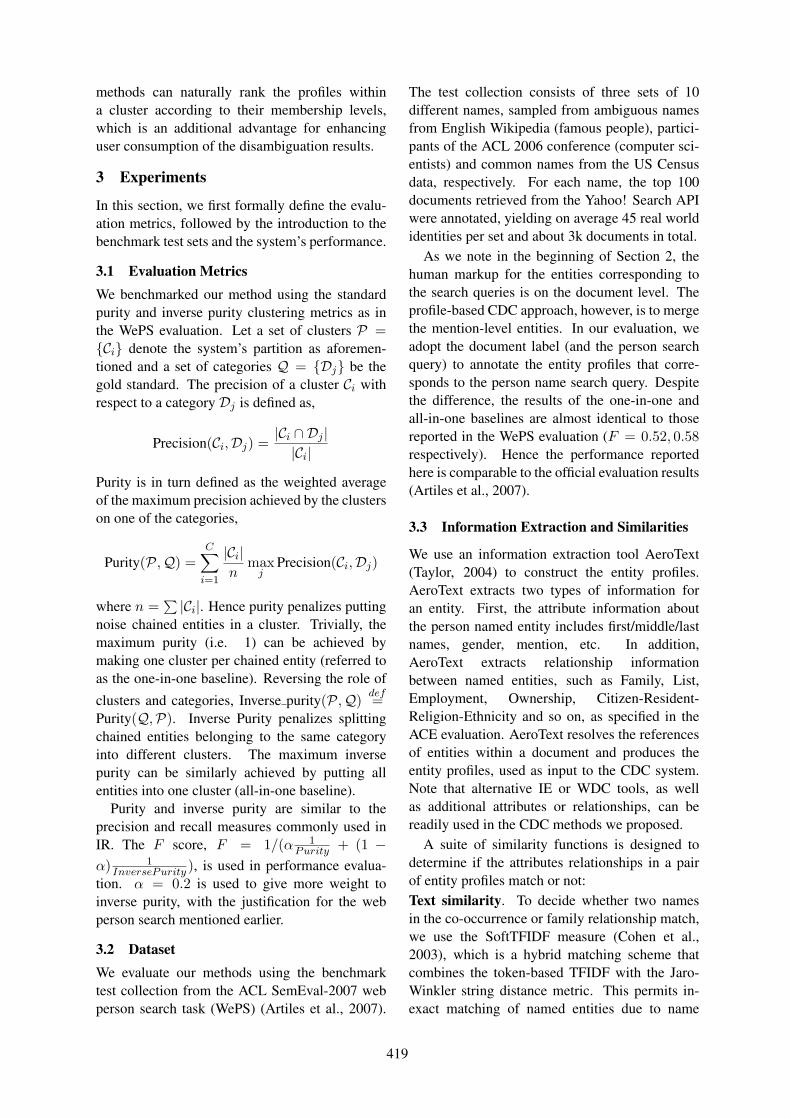
methods can naturally rank the profiles withina cluster according to their membership levels,which is an additional advantage for enhancinguser consumption of the disambiguation results.
3 Experiments
In this section, we first formally define the evalu-ation metrics, followed by the introduction to thebenchmark test sets and the system’s performance.
3.1 Evaluation MetricsWe benchmarked our method using the standardpurity and inverse purity clustering metrics as inthe WePS evaluation. Let a set of clusters P ={Ci} denote the system’s partition as aforemen-tioned and a set of categories Q = {Dj} be thegold standard. The precision of a cluster Ci withrespect to a category Dj is defined as,
Precision(Ci,Dj) =|Ci ∩ Dj ||Ci|
Purity is in turn defined as the weighted averageof the maximum precision achieved by the clusterson one of the categories,
Purity(P,Q) =C
∑
i=1
|Ci|n
maxj
Precision(Ci,Dj)
where n =∑ |Ci|. Hence purity penalizes putting
noise chained entities in a cluster. Trivially, themaximum purity (i.e. 1) can be achieved bymaking one cluster per chained entity (referred toas the one-in-one baseline). Reversing the role of
clusters and categories, Inverse purity(P,Q)def=
Purity(Q,P). Inverse Purity penalizes splittingchained entities belonging to the same categoryinto different clusters. The maximum inversepurity can be similarly achieved by putting allentities into one cluster (all-in-one baseline).
Purity and inverse purity are similar to theprecision and recall measures commonly used inIR. The F score, F = 1/(α 1
Purity + (1 −α) 1
InversePurity ), is used in performance evalua-tion. α = 0.2 is used to give more weight toinverse purity, with the justification for the webperson search mentioned earlier.
3.2 DatasetWe evaluate our methods using the benchmarktest collection from the ACL SemEval-2007 webperson search task (WePS) (Artiles et al., 2007).
The test collection consists of three sets of 10different names, sampled from ambiguous namesfrom English Wikipedia (famous people), partici-pants of the ACL 2006 conference (computer sci-entists) and common names from the US Censusdata, respectively. For each name, the top 100documents retrieved from the Yahoo! Search APIwere annotated, yielding on average 45 real worldidentities per set and about 3k documents in total.
As we note in the beginning of Section 2, thehuman markup for the entities corresponding tothe search queries is on the document level. Theprofile-based CDC approach, however, is to mergethe mention-level entities. In our evaluation, weadopt the document label (and the person searchquery) to annotate the entity profiles that corre-sponds to the person name search query. Despitethe difference, the results of the one-in-one andall-in-one baselines are almost identical to thosereported in the WePS evaluation (F = 0.52, 0.58respectively). Hence the performance reportedhere is comparable to the official evaluation results(Artiles et al., 2007).
3.3 Information Extraction and Similarities
We use an information extraction tool AeroText(Taylor, 2004) to construct the entity profiles.AeroText extracts two types of information foran entity. First, the attribute information aboutthe person named entity includes first/middle/lastnames, gender, mention, etc. In addition,AeroText extracts relationship informationbetween named entities, such as Family, List,Employment, Ownership, Citizen-Resident-Religion-Ethnicity and so on, as specified in theACE evaluation. AeroText resolves the referencesof entities within a document and produces theentity profiles, used as input to the CDC system.Note that alternative IE or WDC tools, as wellas additional attributes or relationships, can bereadily used in the CDC methods we proposed.
A suite of similarity functions is designed todetermine if the attributes relationships in a pairof entity profiles match or not:Text similarity. To decide whether two namesin the co-occurrence or family relationship match,we use the SoftTFIDF measure (Cohen et al.,2003), which is a hybrid matching scheme thatcombines the token-based TFIDF with the Jaro-Winkler string distance metric. This permits in-exact matching of named entities due to name
419
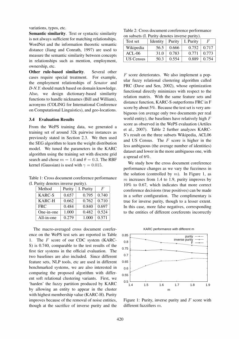
variations, typos, etc.Semantic similarity. Text or syntactic similarityis not always sufficient for matching relationships.WordNet and the information theoretic semanticdistance (Jiang and Conrath, 1997) are used tomeasure the semantic similarity between conceptsin relationships such as mention, employment,ownership, etc.Other rule-based similarity. Several othercases require special treatment. For example,the employment relationships of Senator andD-N.Y. should match based on domain knowledge.Also, we design dictionary-based similarityfunctions to handle nicknames (Bill and William),acronyms (COLING for International Conferenceon Computational Linguistics), and geo-locations.
3.4 Evaluation Results
From the WePS training data, we generated atraining set of around 32k pairwise instances aspreviously stated in Section 2.3. We then usedthe SEG algorithm to learn the weight distributionmodel. We tuned the parameters in the KARCalgorithm using the training set with discrete gridsearch and chose m = 1.6 and θ = 0.3. The RBFkernel (Gaussian) is used with γ = 0.015.
Table 1: Cross document coreference performance(I. Purity denotes inverse purity).
Method Purity I. Purity F
KARC-S 0.657 0.795 0.740KARC-H 0.662 0.762 0.710FRC 0.484 0.840 0.697One-in-one 1.000 0.482 0.524All-in-one 0.279 1.000 0.571
The macro-averaged cross document corefer-ence on the WePS test sets are reported in Table1. The F score of our CDC system (KARC-S) is 0.740, comparable to the test results of thefirst tier systems in the official evaluation. Thetwo baselines are also included. Since differentfeature sets, NLP tools, etc are used in differentbenchmarked systems, we are also interested incomparing the proposed algorithm with differ-ent soft relational clustering variants. First, we‘harden’ the fuzzy partition produced by KARCby allowing an entity to appear in the clusterwith highest membership value (KARC-H). Purityimproves because of the removal of noise entities,though at the sacrifice of inverse purity and the
Table 2: Cross document coreference performanceon subsets (I. Purity denotes inverse purity).
Test set Identity Purity I. Purity F
Wikipedia 56.5 0.666 0.752 0.717ACL-06 31.0 0.783 0.771 0.773US Census 50.3 0.554 0.889 0.754
F score deteriorates. We also implement a pop-ular fuzzy relational clustering algorithm calledFRC (Dave and Sen, 2002), whose optimizationfunctional directly minimizes with respect to therelation matrix. With the same feature sets anddistance function, KARC-S outperforms FRC in Fscore by about 5%. Because the test set is very am-biguous (on average only two documents per realworld entity), the baselines have relatively high Fscore as observed in the WePS evaluation (Artileset al., 2007). Table 2 further analyzes KARC-S’s result on the three subsets Wikipedia, ACL06and US Census. The F score is higher in theless ambiguous (the average number of identities)dataset and lower in the more ambiguous one, witha spread of 6%.
We study how the cross document coreferenceperformance changes as we vary the fuzziness inthe solution (controlled by m). In Figure 1, asm increases from 1.4 to 1.9, purity improves by10% to 0.67, which indicates that more correctcoreference decisions (true positives) can be madein a softer configuration. The complimentary istrue for inverse purity, though to a lesser extent.In this case, more false negatives, correspondingto the entities of different coreferents incorrectly
0.5
0.55
0.6
0.65
0.7
0.75
0.8
0.85
1.4 1.5 1.6 1.7 1.8 1.9
m
KARC performance with different m
purityinverse purity
F
Figure 1: Purity, inverse purity and F score withdifferent fuzzifiers m.
420
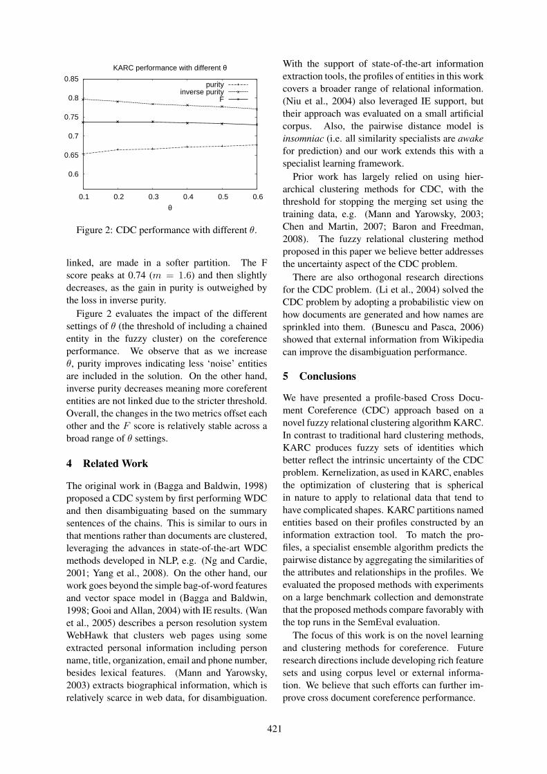
0.6
0.65
0.7
0.75
0.8
0.85
0.1 0.2 0.3 0.4 0.5 0.6
θ
KARC performance with different θ
purityinverse purity
F
Figure 2: CDC performance with different θ.
linked, are made in a softer partition. The Fscore peaks at 0.74 (m = 1.6) and then slightlydecreases, as the gain in purity is outweighed bythe loss in inverse purity.
Figure 2 evaluates the impact of the differentsettings of θ (the threshold of including a chainedentity in the fuzzy cluster) on the coreferenceperformance. We observe that as we increaseθ, purity improves indicating less ‘noise’ entitiesare included in the solution. On the other hand,inverse purity decreases meaning more coreferententities are not linked due to the stricter threshold.Overall, the changes in the two metrics offset eachother and the F score is relatively stable across abroad range of θ settings.
4 Related Work
The original work in (Bagga and Baldwin, 1998)proposed a CDC system by first performing WDCand then disambiguating based on the summarysentences of the chains. This is similar to ours inthat mentions rather than documents are clustered,leveraging the advances in state-of-the-art WDCmethods developed in NLP, e.g. (Ng and Cardie,2001; Yang et al., 2008). On the other hand, ourwork goes beyond the simple bag-of-word featuresand vector space model in (Bagga and Baldwin,1998; Gooi and Allan, 2004) with IE results. (Wanet al., 2005) describes a person resolution systemWebHawk that clusters web pages using someextracted personal information including personname, title, organization, email and phone number,besides lexical features. (Mann and Yarowsky,2003) extracts biographical information, which isrelatively scarce in web data, for disambiguation.
With the support of state-of-the-art informationextraction tools, the profiles of entities in this workcovers a broader range of relational information.(Niu et al., 2004) also leveraged IE support, buttheir approach was evaluated on a small artificialcorpus. Also, the pairwise distance model isinsomniac (i.e. all similarity specialists are awakefor prediction) and our work extends this with aspecialist learning framework.
Prior work has largely relied on using hier-archical clustering methods for CDC, with thethreshold for stopping the merging set using thetraining data, e.g. (Mann and Yarowsky, 2003;Chen and Martin, 2007; Baron and Freedman,2008). The fuzzy relational clustering methodproposed in this paper we believe better addressesthe uncertainty aspect of the CDC problem.
There are also orthogonal research directionsfor the CDC problem. (Li et al., 2004) solved theCDC problem by adopting a probabilistic view onhow documents are generated and how names aresprinkled into them. (Bunescu and Pasca, 2006)showed that external information from Wikipediacan improve the disambiguation performance.
5 Conclusions
We have presented a profile-based Cross Docu-ment Coreference (CDC) approach based on anovel fuzzy relational clustering algorithm KARC.In contrast to traditional hard clustering methods,KARC produces fuzzy sets of identities whichbetter reflect the intrinsic uncertainty of the CDCproblem. Kernelization, as used in KARC, enablesthe optimization of clustering that is sphericalin nature to apply to relational data that tend tohave complicated shapes. KARC partitions namedentities based on their profiles constructed by aninformation extraction tool. To match the pro-files, a specialist ensemble algorithm predicts thepairwise distance by aggregating the similarities ofthe attributes and relationships in the profiles. Weevaluated the proposed methods with experimentson a large benchmark collection and demonstratethat the proposed methods compare favorably withthe top runs in the SemEval evaluation.
The focus of this work is on the novel learningand clustering methods for coreference. Futureresearch directions include developing rich featuresets and using corpus level or external informa-tion. We believe that such efforts can further im-prove cross document coreference performance.
421
ReferencesJavier Artiles, Julio Gonzalo, and Satoshi Sekine.
2007. The SemEval-2007 WePS evaluation:Establishing a benchmark for the web people searchtask. In Proceedings of the 4th InternationalWorkshop on Semantic Evaluations (SemEval-2007), pages 64–69.
Amit Bagga and Breck Baldwin. 1998. Entity-basedcross-document coreferencing using the vectorspace model. In Proceedings of 36th InternationalConference On Computational Linguistics (ACL)and 17th international conference on Computationallinguistics (COLING), pages 79–85.
Alex Baron and Marjorie Freedman. 2008. Whois who and what is what: Experiments in cross-document co-reference. In Proceedings of the2008 Conference on Empirical Methods in NaturalLanguage Processing (EMNLP), pages 274–283.
J. C. Bezdek. 1981. Pattern Recognition with FuzzyObjective Function Algoritms. Plenum Press, NY.
Razvan Bunescu and Marius Pasca. 2006. Usingencyclopedic knowledge for named entity disam-biguation. In Proceedings of the 11th Conferenceof the European Chapter of the Association forComputational Linguistics (EACL), pages 9–16.
Ying Chen and James Martin. 2007. Towardsrobust unsupervised personal name disambiguation.In Proc. of 2007 Joint Conference on EmpiricalMethods in Natural Language Processing andComputational Natural Language Learning.
Mario G. C. A. Cimino, Beatrice Lazzerini, andFrancesco Marcelloni. 2006. A novel approachto fuzzy clustering based on a dissimilarity relationextracted from data using a TS system. PatternRecognition, 39(11):2077–2091.
William W. Cohen, Pradeep Ravikumar, andStephen E. Fienberg. 2003. A comparison ofstring distance metrics for name-matching tasks.In Proceedings of IJCAI Workshop on InformationIntegration on the Web.
Paolo Corsini, Beatrice Lazzerini, and FrancescoMarcelloni. 2005. A new fuzzy relational clusteringalgorithm based on the fuzzy c-means algorithm.Soft Computing, 9(6):439 – 447.
Rajesh N. Dave and Sumit Sen. 2002. Robust fuzzyclustering of relational data. IEEE Transactions onFuzzy Systems, 10(6):713–727.
Yoav Freund, Robert E. Schapire, Yoram Singer, andManfred K. Warmuth. 1997. Using and combiningpredictors that specialize. In Proceedings of thetwenty-ninth annual ACM symposium on Theory ofcomputing (STOC), pages 334–343.
Chung H. Gooi and James Allan. 2004. Cross-document coreference on a large scale corpus. InProceedings of the Human Language Technology
Conference of the North American Chapter ofthe Association for Computational Linguistics(NAACL), pages 9–16.
Jay J. Jiang and David W. Conrath. 1997.Semantic similarity based on corpus statistics andlexical taxonomy. In Proceedings of InternationalConference Research on Computational Linguistics.
Xin Li, Paul Morie, and Dan Roth. 2004. Robustreading: Identification and tracing of ambiguousnames. In Proceedings of the Human LanguageTechnology Conference and the North AmericanChapter of the Association for ComputationalLinguistics (HLT-NAACL), pages 17–24.
Gideon S. Mann and David Yarowsky. 2003.Unsupervised personal name disambiguation. InConference on Computational Natural LanguageLearning (CoNLL), pages 33–40.
Vincent Ng and Claire Cardie. 2001. Improving ma-chine learning approaches to coreference resolution.In Proceedings of the 40th Annual Meeting of theAssociation for Computational Linguistics (ACL),pages 104–111.
Cheng Niu, Wei Li, and Rohini K. Srihari. 2004.Weakly supervised learning for cross-documentperson name disambiguation supported by infor-mation extraction. In Proceedings of the 42ndAnnual Meeting on Association for ComputationalLinguistics (ACL), pages 597–604.
Bernhard Schölkopf and Alex Smola. 2002. Learningwith Kernels. MIT Press, Cambridge, MA.
Sarah M. Taylor. 2004. Information extraction tools:Deciphering human language. IT Professional,6(6):28 – 34.
Vladimir Vapnik. 1995. The Nature of StatisticalLearning Theory. Springer-Verlag New York.
Xiaojun Wan, Jianfeng Gao, Mu Li, and BinggongDing. 2005. Person resolution in person searchresults: WebHawk. In Proceedings of the 14thACM international conference on Information andknowledge management (CIKM), pages 163–170.
Xuanli Lisa Xie and Gerardo Beni. 1991. A validitymeasure for fuzzy clustering. IEEE Transactionson Pattern Analysis and Machine Intelligence,13(8):841 – 847.
Xiaofeng Yang, Jian Su, Jun Lang, Chew L. Tan,Ting Liu, and Sheng Li. 2008. An entity-mention model for coreference resolution withinductive logic programming. In Proceedings ofthe 46th Annual Meeting of the Association forComputational Linguistics (ACL), pages 843–851.
Dao-Qiang Zhang and Song-Can Chen. 2003.Clustering incomplete data using kernel-based fuzzyc-means algorithm. Neural Processing Letters,18(3):155 – 162.
422
Proceedings of the 47th Annual Meeting of the ACL and the 4th IJCNLP of the AFNLP, pages 423–431,Suntec, Singapore, 2-7 August 2009. c©2009 ACL and AFNLP
Who, What, When, Where, Why? Comparing Multiple Approaches to the Cross-Lingual 5W Task
Kristen Parton*, Kathleen R. McKeown*, Bob Coyne*, Mona T. Diab*, Ralph Grishman†, Dilek Hakkani-Tür‡, Mary Harper§, Heng Ji•, Wei Yun Ma*,
Adam Meyers†, Sara Stolbach*, Ang Sun†, Gokhan Tur˚, Wei Xu† and Sibel Yaman‡
*Columbia University New York, NY, USA {kristen, kathy, coyne, mdiab, ma,
sara}@cs.columbia.edu
†New York University New York, NY, USA
{grishman, meyers, asun, xuwei} @cs.nyu.edu
‡International Computer Science Institute
Berkeley, CA, USA {dilek, sibel}
@icsi.berkeley.edu
§Human Lang. Tech. Ctr. of Excellence, Johns Hopkins
and U. of Maryland, College Park
•City University of New York
New York, NY, USA [email protected]
˚SRI International Palo Alto, CA, USA
Abstract
Cross-lingual tasks are especially difficult due to the compounding effect of errors in language processing and errors in machine translation (MT). In this paper, we present an error analysis of a new cross-lingual task: the 5W task, a sentence-level understanding task which seeks to return the English 5W's (Who, What, When, Where and Why) corresponding to a Chinese sentence. We analyze systems that we developed, identifying specific prob-lems in language processing and MT that cause errors. The best cross-lingual 5W sys-tem was still 19% worse than the best mono-lingual 5W system, which shows that MT significantly degrades sentence-level under-standing. Neither source-language nor target-language analysis was able to circumvent problems in MT, although each approach had advantages relative to the other. A detailed error analysis across multiple systems sug-gests directions for future research on the problem.
1 Introduction
In our increasingly global world, it is ever more likely for a mono-lingual speaker to require in-formation that is only available in a foreign lan-guage document. Cross-lingual applications ad-dress this need by presenting information in the speaker’s language even when it originally ap-peared in some other language, using machine
translation (MT) in the process. In this paper, we present an evaluation and error analysis of a cross-lingual application that we developed for a government-sponsored evaluation, the 5W task.
The 5W task seeks to summarize the informa-tion in a natural language sentence by distilling it into the answers to the 5W questions: Who, What, When, Where and Why. To solve this problem, a number of different problems in NLP must be addressed: predicate identification, ar-gument extraction, attachment disambiguation, location and time expression recognition, and (partial) semantic role labeling. In this paper, we address the cross-lingual 5W task: given a source-language sentence, return the 5W’s trans-lated (comprehensibly) into the target language. Success in this task requires a synergy of suc-cessful MT and answer selection.
The questions we address in this paper are:
• How much does machine translation (MT) degrade the performance of cross-lingual 5W systems, as compared to monolingual performance?
• Is it better to do source-language analysis and then translate, or do target-language analysis on MT?
• Which specific problems in language processing and/or MT cause errors in 5W answers?
In this evaluation, we compare several differ-ent approaches to the cross-lingual 5W task, two that work on the target language (English) and one that works in the source language (Chinese).
423

A central question for many cross-lingual appli-cations is whether to process in the source lan-guage and then translate the result, or translate documents first and then process the translation. Depending on how errorful the translation is, results may be more accurate if models are de-veloped for the source language. However, if there are more resources in the target language, then the translate-then-process approach may be more appropriate. We present a detailed analysis, both quantitative and qualitative, of how the ap-proaches differ in performance.
We also compare system performance on hu-man translation (which we term reference trans-lations) and MT of the same data in order to de-termine how much MT degrades system per-formance. Finally, we do an in-depth analysis of the errors in our 5W approaches, both on the NLP side and the MT side. Our results provide explanations for why different approaches suc-ceed, along with indications of where future ef-fort should be spent.
2 Prior Work
The cross-lingual 5W task is closely related to cross-lingual information retrieval and cross-lingual question answering (Wang and Oard 2006; Mitamura et al. 2008). In these tasks, a system is presented a query or question in the target language and asked to return documents or answers from a corpus in the source language. Although MT may be used in solving this task, it is only used by the algorithms – the final evalua-tion is done in the source language. However, in many real-life situations, such as global business, international tourism, or intelligence work, users may not be able to read the source language. In these cases, users must rely on MT to understand the system response. (Parton et al. 2008) exam-ine the case of “translingual” information re-trieval, where evaluation is done on translated results in the target language. In cross-lingual information extraction (Sudo et al. 2004) the evaluation is also done on MT, but the goal is to learn knowledge from a large corpus, rather than analyzing individual sentences.
The 5W task is also closely related to Seman-tic Role Labeling (SRL), which aims to effi-ciently and effectively derive semantic informa-tion from text. SRL identifies predicates and their arguments in a sentence, and assigns roles to each argument. For example, in the sentence “I baked a cake yesterday.”, the predicate “baked” has three arguments. “I” is the subject of
the predicate, “a cake” is the object and “yester-day” is a temporal argument.
Since the release of large data resources anno-tated with relevant levels of semantic informa-tion, such as the FrameNet (Baker et al., 1998) and PropBank corpora (Kingsbury and Palmer, 2003), efficient approaches to SRL have been developed (Carreras and Marquez, 2005). Most approaches to the problem of SRL follow the Gildea and Jurafsky (2002) model. First, for a given predicate, the SRL system identifies its arguments' boundaries. Second, the Argument types are classified depending on an adopted lexical resource such as PropBank or FrameNet. Both steps are based on supervised learning over labeled gold standard data. A final step uses heu-ristics to resolve inconsistencies when applying both steps simultaneously to the test data.
Since many of the SRL resources are English, most of the SRL systems to date have been for English. There has been work in other languages such as German and Chinese (Erk 2006; Sun 2004; Xue and Palmer 2005). The systems for the other languages follow the successful models devised for English, e.g. (Gildea and Palmer, 2002; Chen and Rambow, 2003; Moschitti, 2004; Xue and Palmer, 2004; Haghighi et al., 2005).
3 The Chinese-English 5W Task
3.1 5W Task Description
We participated in the 5W task as part of the DARPA GALE (Global Autonomous Language Exploitation) project. The goal is to identify the 5W’s (Who, What, When, Where and Why) for a complete sentence. The motivation for the 5W task is that, as their origin in journalism suggests, the 5W’s cover the key information nuggets in a sentence. If a system can isolate these pieces of information successfully, then it can produce a précis of the basic meaning of the sentence. Note that this task differs from QA tasks, where “Who” and “What” usually refer to definition type questions. In this task, the 5W’s refer to se-mantic roles within a sentence, as defined in Ta-ble 1.
In order to get all 5W’s for a sentence correct, a system must identify a top-level predicate, ex-tract the correct arguments, and resolve attach-ment ambiguity. In the case of multiple top-level predicates, any of the top-level predicates may be chosen. In the case of passive verbs, the Who is the agent (often expressed as a “by clause”, or not stated), and the What should include the syn-tactic subject.
424
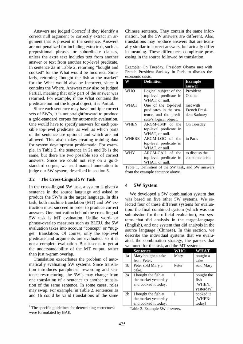
Answers are judged Correct1 if they identify a correct null argument or correctly extract an ar-gument that is present in the sentence. Answers are not penalized for including extra text, such as prepositional phrases or subordinate clauses, unless the extra text includes text from another answer or text from another top-level predicate. In sentence 2a in Table 2, returning “bought and cooked” for the What would be Incorrect. Simi-larly, returning “bought the fish at the market” for the What would also be Incorrect, since it contains the Where. Answers may also be judged Partial, meaning that only part of the answer was returned. For example, if the What contains the predicate but not the logical object, it is Partial.
Since each sentence may have multiple correct sets of 5W’s, it is not straightforward to produce a gold-standard corpus for automatic evaluation. One would have to specify answers for each pos-sible top-level predicate, as well as which parts of the sentence are optional and which are not allowed. This also makes creating training data for system development problematic. For exam-ple, in Table 2, the sentence in 2a and 2b is the same, but there are two possible sets of correct answers. Since we could not rely on a gold-standard corpus, we used manual annotation to judge our 5W system, described in section 5.
3.2 The Cross-Lingual 5W Task
In the cross-lingual 5W task, a system is given a sentence in the source language and asked to produce the 5W’s in the target language. In this task, both machine translation (MT) and 5W ex-traction must succeed in order to produce correct answers. One motivation behind the cross-lingual 5W task is MT evaluation. Unlike word- or phrase-overlap measures such as BLEU, the 5W evaluation takes into account “concept” or “nug-get” translation. Of course, only the top-level predicate and arguments are evaluated, so it is not a complete evaluation. But it seeks to get at the understandability of the MT output, rather than just n-gram overlap.
Translation exacerbates the problem of auto-matically evaluating 5W systems. Since transla-tion introduces paraphrase, rewording and sen-tence restructuring, the 5W’s may change from one translation of a sentence to another transla-tion of the same sentence. In some cases, roles may swap. For example, in Table 2, sentences 1a and 1b could be valid translations of the same
1 The specific guidelines for determining correctness were formulated by BAE.
Chinese sentence. They contain the same infor-mation, but the 5W answers are different. Also, translations may produce answers that are textu-ally similar to correct answers, but actually differ in meaning. These differences complicate proc-essing in the source followed by translation.
Example: On Tuesday, President Obama met with French President Sarkozy in Paris to discuss the economic crisis. W Definition Example
answer WHO Logical subject of the
top-level predicate in WHAT, or null.
President Obama
WHAT One of the top-level predicates in the sen-tence, and the predi-cate’s logical object.
met with French Presi-dent Sarkozy
WHEN ARGM-TMP of the top-level predicate in WHAT, or null.
On Tuesday
WHERE ARGM-LOC of the top-level predicate in WHAT, or null.
in Paris
WHY ARGM-CAU of the top-level predicate in WHAT, or null.
to discuss the economic crisis
Table 1. Definition of the 5W task, and 5W answers from the example sentence above.
4 5W System
We developed a 5W combination system that was based on five other 5W systems. We se-lected four of these different systems for evalua-tion: the final combined system (which was our submission for the official evaluation), two sys-tems that did analysis in the target-language (English), and one system that did analysis in the source language (Chinese). In this section, we describe the individual systems that we evalu-ated, the combination strategy, the parsers that we tuned for the task, and the MT systems. Sentence WHO WHAT 1a Mary bought a cake
from Peter. Mary bought a
cake 1b Peter sold Mary a
cake. Peter sold Mary
2a I bought the fish at the market yesterday and cooked it today.
I bought the fish [WHEN: yesterday]
2b I bought the fish at the market yesterday and cooked it today.
I cooked it [WHEN: today]
Table 2. Example 5W answers.
425

4.1 Latent Annotation Parser
For this work, we have re-implemented and en-hanced the Berkeley parser (Petrov and Klein 2007) in several ways: (1) developed a new method to handle rare words in English and Chi-nese; (2) developed a new model of unknown Chinese words based on characters in the word; (3) increased robustness by adding adaptive modification of pruning thresholds and smooth-ing of word emission probabilities. While the enhancements to the parser are important for ro-bustness and accuracy, it is even more important to train grammars matched to the conditions of use. For example, parsing a Chinese sentence containing full-width punctuation with a parser trained on half-width punctuation reduces accu-racy by over 9% absolute F. In English, parsing accuracy is seriously compromised by training a grammar with punctuation and case to process sentences without them.
We developed grammars for English and Chi-nese trained specifically for each genre by sub-sampling from available treebanks (for English, WSJ, BN, Brown, Fisher, and Switchboard; for Chinese, CTB5) and transforming them for a particular genre (e.g., for informal speech, we replaced symbolic expressions with verbal forms and remove punctuation and case) and by utiliz-ing a large amount of genre-matched self-labeled training parses. Given these genre-specific parses, we extracted chunks and POS tags by script. We also trained grammars with a subset of function tags annotated in the treebank that indi-cate case role information (e.g., SBJ, OBJ, LOC, MNR) in order to produce function tags.
4.2 Individual 5W Systems
The English systems were developed for the monolingual 5W task and not modified to handle MT. They used hand-crafted rules on the output of the latent annotation parser to extract the 5Ws.
English-function used the function tags from the parser to map parser constituents to the 5Ws. First the Who, When, Where and Why were ex-tracted, and then the remaining pieces of the sen-tence were returned as the What. The goal was to make sure to return a complete What answer and avoid missing the object.
English-LF, on the other hand, used a system developed over a period of eight years (Meyers et al. 2001) to map from the parser’s syntactic constituents into logical grammatical relations (GLARF), and then extracted the 5Ws from the logical form. As a back-up, it also extracted
GLARF relations from another English-treebank trained parser, the Charniak parser (Charniak 2001). After the parses were both converted to the 5Ws, they were then merged, favoring the system that: recognized the passive, filled more 5W slots or produced shorter 5W slots (provid-ing that the WHAT slot consisted of more than just the verb). A third back-up method extracted 5Ws from part-of-speech tag patterns. Unlike English-function, English-LF explicitly tried to extract the shortest What possible, provided there was a verb and a possible object, in order to avoid multiple predicates or other 5W answers.
Chinese-align uses the latent annotation parser (trained for Chinese) to parse the Chinese sentences. A dependency tree converter (Johans-son and Nuges 2007) was applied to the constitu-ent-based parse trees to obtain the dependency relations and determine top-level predicates. A set of hand-crafted dependency rules based on observation of Chinese OntoNotes were used to map from the Chinese function tags into Chinese 5Ws. Finally, Chinese-align used the alignments of three separate MT systems to translate the 5Ws: a phrase-based system, a hierarchical phrase-based system, and a syntax augmented hierarchical phrase-based system. Chinese-align faced a number of problems in using the align-ments, including the fact that the best MT did not always have the best alignment. Since the predi-cate is essential, it tried to detect when verbs were deleted in MT, and back-off to a different MT system. It also used strategies for finding and correcting noisy alignments, and for filtering When/Where answers from Who and What.
4.3 Hybrid System
A merging algorithm was learned based on a de-velopment test set. The algorithm selected all 5W’s from a single system, rather than trying to merge W’s from different systems, since the predicates may vary across systems. For each document genre (described in section 5.4), we ranked the systems by performance on the devel-opment data. We also experimented with a vari-ety of features (for instance, does “What” include a verb). The best-performing features were used in combination with the ranked list of priority systems to create a rule-based merger.
4.4 MT Systems
The MT Combination system used by both of the English 5W systems combined up to nine sepa-rate MT systems. System weights for combina-tion were optimized together with the language
426
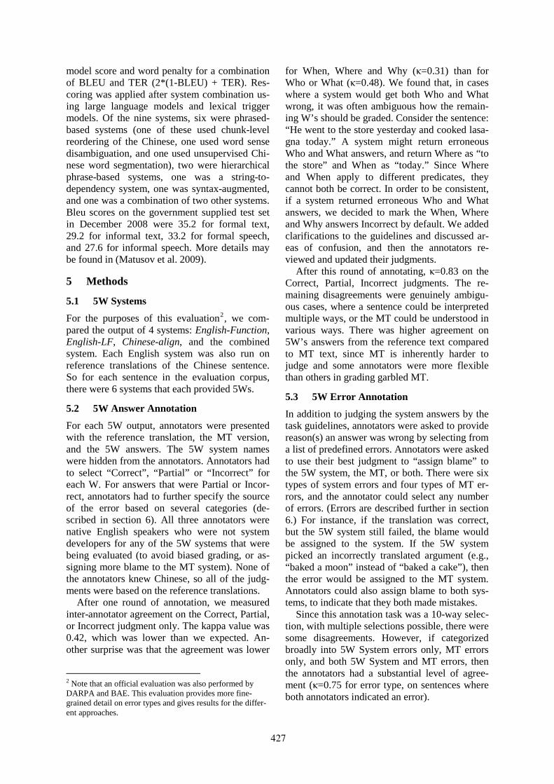
model score and word penalty for a combination of BLEU and TER (2*(1-BLEU) + TER). Res-coring was applied after system combination us-ing large language models and lexical trigger models. Of the nine systems, six were phrased-based systems (one of these used chunk-level reordering of the Chinese, one used word sense disambiguation, and one used unsupervised Chi-nese word segmentation), two were hierarchical phrase-based systems, one was a string-to-dependency system, one was syntax-augmented, and one was a combination of two other systems. Bleu scores on the government supplied test set in December 2008 were 35.2 for formal text, 29.2 for informal text, 33.2 for formal speech, and 27.6 for informal speech. More details may be found in (Matusov et al. 2009).
5 Methods
5.1 5W Systems
For the purposes of this evaluation2, we com-pared the output of 4 systems: English-Function, English-LF, Chinese-align, and the combined system. Each English system was also run on reference translations of the Chinese sentence. So for each sentence in the evaluation corpus, there were 6 systems that each provided 5Ws.
5.2 5W Answer Annotation
For each 5W output, annotators were presented with the reference translation, the MT version, and the 5W answers. The 5W system names were hidden from the annotators. Annotators had to select “Correct”, “Partial” or “Incorrect” for each W. For answers that were Partial or Incor-rect, annotators had to further specify the source of the error based on several categories (de-scribed in section 6). All three annotators were native English speakers who were not system developers for any of the 5W systems that were being evaluated (to avoid biased grading, or as-signing more blame to the MT system). None of the annotators knew Chinese, so all of the judg-ments were based on the reference translations.
After one round of annotation, we measured inter-annotator agreement on the Correct, Partial, or Incorrect judgment only. The kappa value was 0.42, which was lower than we expected. An-other surprise was that the agreement was lower
2 Note that an official evaluation was also performed by DARPA and BAE. This evaluation provides more fine-grained detail on error types and gives results for the differ-ent approaches.
for When, Where and Why (κ=0.31) than for Who or What (κ=0.48). We found that, in cases where a system would get both Who and What wrong, it was often ambiguous how the remain-ing W’s should be graded. Consider the sentence: “He went to the store yesterday and cooked lasa-gna today.” A system might return erroneous Who and What answers, and return Where as “to the store” and When as “today.” Since Where and When apply to different predicates, they cannot both be correct. In order to be consistent, if a system returned erroneous Who and What answers, we decided to mark the When, Where and Why answers Incorrect by default. We added clarifications to the guidelines and discussed ar-eas of confusion, and then the annotators re-viewed and updated their judgments.
After this round of annotating, κ=0.83 on the Correct, Partial, Incorrect judgments. The re-maining disagreements were genuinely ambigu-ous cases, where a sentence could be interpreted multiple ways, or the MT could be understood in various ways. There was higher agreement on 5W’s answers from the reference text compared to MT text, since MT is inherently harder to judge and some annotators were more flexible than others in grading garbled MT.
5.3 5W Error Annotation
In addition to judging the system answers by the task guidelines, annotators were asked to provide reason(s) an answer was wrong by selecting from a list of predefined errors. Annotators were asked to use their best judgment to “assign blame” to the 5W system, the MT, or both. There were six types of system errors and four types of MT er-rors, and the annotator could select any number of errors. (Errors are described further in section 6.) For instance, if the translation was correct, but the 5W system still failed, the blame would be assigned to the system. If the 5W system picked an incorrectly translated argument (e.g., “baked a moon” instead of “baked a cake”), then the error would be assigned to the MT system. Annotators could also assign blame to both sys-tems, to indicate that they both made mistakes.
Since this annotation task was a 10-way selec-tion, with multiple selections possible, there were some disagreements. However, if categorized broadly into 5W System errors only, MT errors only, and both 5W System and MT errors, then the annotators had a substantial level of agree-ment (κ=0.75 for error type, on sentences where both annotators indicated an error).
427
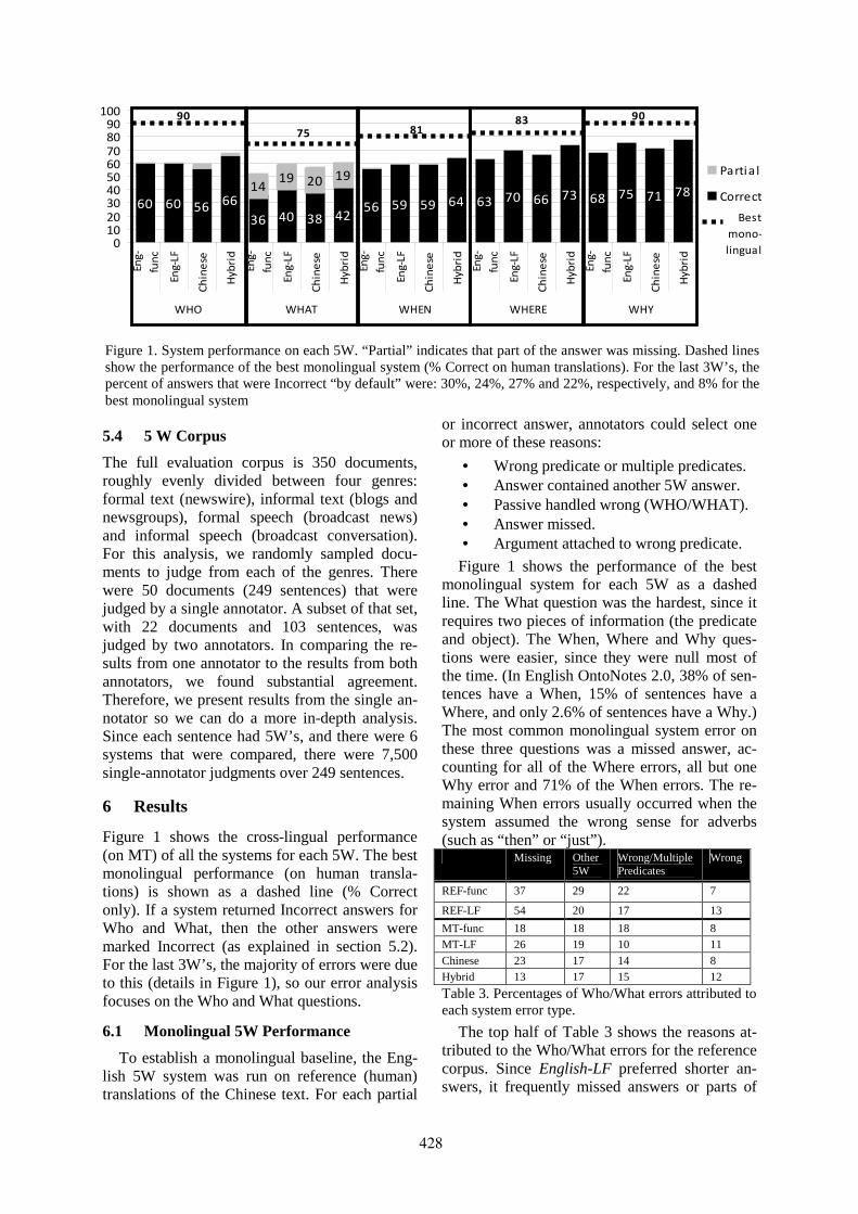
5.4 5 W Corpus
The full evaluation corpus is 350 documents, roughly evenly divided between four genres: formal text (newswire), informal text (blogs and newsgroups), formal speech (broadcast news) and informal speech (broadcast conversation). For this analysis, we randomly sampled docu-ments to judge from each of the genres. There were 50 documents (249 sentences) that were judged by a single annotator. A subset of that set, with 22 documents and 103 sentences, was judged by two annotators. In comparing the re-sults from one annotator to the results from both annotators, we found substantial agreement. Therefore, we present results from the single an-notator so we can do a more in-depth analysis. Since each sentence had 5W’s, and there were 6 systems that were compared, there were 7,500 single-annotator judgments over 249 sentences.
6 Results
Figure 1 shows the cross-lingual performance (on MT) of all the systems for each 5W. The best monolingual performance (on human transla-tions) is shown as a dashed line (% Correct only). If a system returned Incorrect answers for Who and What, then the other answers were marked Incorrect (as explained in section 5.2). For the last 3W’s, the majority of errors were due to this (details in Figure 1), so our error analysis focuses on the Who and What questions.
6.1 Monolingual 5W Performance
To establish a monolingual baseline, the Eng-lish 5W system was run on reference (human) translations of the Chinese text. For each partial
or incorrect answer, annotators could select one or more of these reasons:
• Wrong predicate or multiple predicates. • Answer contained another 5W answer. • Passive handled wrong (WHO/WHAT). • Answer missed. • Argument attached to wrong predicate.
Figure 1 shows the performance of the best monolingual system for each 5W as a dashed line. The What question was the hardest, since it requires two pieces of information (the predicate and object). The When, Where and Why ques-tions were easier, since they were null most of the time. (In English OntoNotes 2.0, 38% of sen-tences have a When, 15% of sentences have a Where, and only 2.6% of sentences have a Why.) The most common monolingual system error on these three questions was a missed answer, ac-counting for all of the Where errors, all but one Why error and 71% of the When errors. The re-maining When errors usually occurred when the system assumed the wrong sense for adverbs (such as “then” or “just”). Missing Other
5W Wrong/Multiple Predicates
Wrong
REF-func 37 29 22 7
REF-LF 54 20 17 13
MT-func 18 18 18 8 MT-LF 26 19 10 11
Chinese 23 17 14 8 Hybrid 13 17 15 12
Table 3. Percentages of Who/What errors attributed to each system error type.
The top half of Table 3 shows the reasons at-tributed to the Who/What errors for the reference corpus. Since English-LF preferred shorter an-swers, it frequently missed answers or parts of
Figure 1. System performance on each 5W. “Partial” indicates that part of the answer was missing. Dashed lines show the performance of the best monolingual system (% Correct on human translations). For the last 3W’s, the percent of answers that were Incorrect “by default” were: 30%, 24%, 27% and 22%, respectively, and 8% for the best monolingual system
60 60 5666
36 40 38 4256 59 59 64 63 70 66 73 68 75 71 78
19201914
01020
3040506070
8090
100
En
g-
fun
c
En
g-L
F
Ch
ine
se
Hyb
rid
En
g-
fun
c
En
g-L
F
Ch
ine
se
Hyb
rid
En
g-
fun
c
En
g-L
F
Ch
ine
se
Hyb
rid
En
g-
fun
c
En
g-L
F
Ch
ine
se
Hyb
rid
En
g-
fun
c
En
g-L
F
Ch
ine
se
Hyb
rid
WHO WHAT WHEN WHERE WHY
Partia l
Correct
90
75 8183
90
Best
mono-
lingual
428
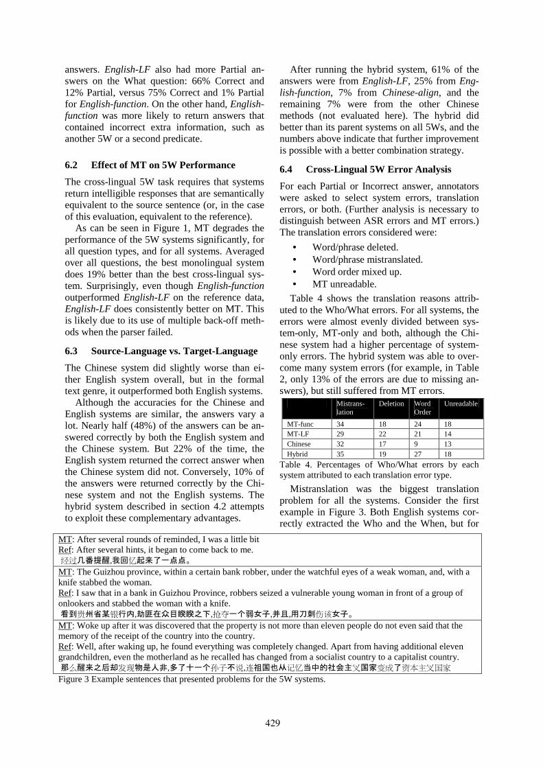
answers. English-LF also had more Partial an-swers on the What question: 66% Correct and 12% Partial, versus 75% Correct and 1% Partial for English-function. On the other hand, English-function was more likely to return answers that contained incorrect extra information, such as another 5W or a second predicate.
6.2 Effect of MT on 5W Performance
The cross-lingual 5W task requires that systems return intelligible responses that are semantically equivalent to the source sentence (or, in the case of this evaluation, equivalent to the reference).
As can be seen in Figure 1, MT degrades the performance of the 5W systems significantly, for all question types, and for all systems. Averaged over all questions, the best monolingual system does 19% better than the best cross-lingual sys-tem. Surprisingly, even though English-function outperformed English-LF on the reference data, English-LF does consistently better on MT. This is likely due to its use of multiple back-off meth-ods when the parser failed.
6.3 Source-Language vs. Target-Language
The Chinese system did slightly worse than ei-ther English system overall, but in the formal text genre, it outperformed both English systems.
Although the accuracies for the Chinese and English systems are similar, the answers vary a lot. Nearly half (48%) of the answers can be an-swered correctly by both the English system and the Chinese system. But 22% of the time, the English system returned the correct answer when the Chinese system did not. Conversely, 10% of the answers were returned correctly by the Chi-nese system and not the English systems. The hybrid system described in section 4.2 attempts to exploit these complementary advantages.
After running the hybrid system, 61% of the answers were from English-LF, 25% from Eng-lish-function, 7% from Chinese-align, and the remaining 7% were from the other Chinese methods (not evaluated here). The hybrid did better than its parent systems on all 5Ws, and the numbers above indicate that further improvement is possible with a better combination strategy.
6.4 Cross-Lingual 5W Error Analysis
For each Partial or Incorrect answer, annotators were asked to select system errors, translation errors, or both. (Further analysis is necessary to distinguish between ASR errors and MT errors.) The translation errors considered were:
• Word/phrase deleted. • Word/phrase mistranslated. • Word order mixed up. • MT unreadable.
Table 4 shows the translation reasons attrib-uted to the Who/What errors. For all systems, the errors were almost evenly divided between sys-tem-only, MT-only and both, although the Chi-nese system had a higher percentage of system-only errors. The hybrid system was able to over-come many system errors (for example, in Table 2, only 13% of the errors are due to missing an-swers), but still suffered from MT errors.
Table 4. Percentages of Who/What errors by each system attributed to each translation error type.
Mistranslation was the biggest translation problem for all the systems. Consider the first example in Figure 3. Both English systems cor-rectly extracted the Who and the When, but for
Mistrans-lation
Deletion Word Order
Unreadable
MT-func 34 18 24 18 MT-LF 29 22 21 14 Chinese 32 17 9 13 Hybrid 35 19 27 18
MT: After several rounds of reminded, I was a little bit Ref: After several hints, it began to come back to me. 经过几番提醒,我回忆起来了一点点。 MT: The Guizhou province, within a certain bank robber, under the watchful eyes of a weak woman, and, with a knife stabbed the woman. Ref: I saw that in a bank in Guizhou Province, robbers seized a vulnerable young woman in front of a group of onlookers and stabbed the woman with a knife. 看到贵州省某银行内,劫匪在众目睽睽之下,抢夺一个弱女子,并且,用刀刺伤该女子。 MT: Woke up after it was discovered that the property is not more than eleven people do not even said that the memory of the receipt of the country into the country. Ref: Well, after waking up, he found everything was completely changed. Apart from having additional eleven grandchildren, even the motherland as he recalled has changed from a socialist country to a capitalist country. 那么醒来之后却发现物是人非,多了十一个孙子不说,连祖国也从记忆当中的社会主义国家变成了资本主义国家 Figure 3 Example sentences that presented problems for the 5W systems.
429
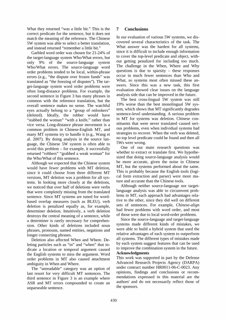
What they returned “was a little bit.” This is the correct predicate for the sentence, but it does not match the meaning of the reference. The Chinese 5W system was able to select a better translation, and instead returned “remember a little bit.”
Garbled word order was chosen for 21-24% of the target-language system Who/What errors, but only 9% of the source-language system Who/What errors. The source-language word order problems tended to be local, within-phrase errors (e.g., “the dispute over frozen funds” was translated as “the freezing of disputes”). The tar-get-language system word order problems were often long-distance problems. For example, the second sentence in Figure 3 has many phrases in common with the reference translation, but the overall sentence makes no sense. The watchful eyes actually belong to a “group of onlookers” (deleted). Ideally, the robber would have “stabbed the woman” “with a knife,” rather than vice versa. Long-distance phrase movement is a common problem in Chinese-English MT, and many MT systems try to handle it (e.g., Wang et al. 2007). By doing analysis in the source lan-guage, the Chinese 5W system is often able to avoid this problem – for example, it successfully returned “robbers” “grabbed a weak woman” for the Who/What of this sentence.
Although we expected that the Chinese system would have fewer problems with MT deletion, since it could choose from three different MT versions, MT deletion was a problem for all sys-tems. In looking more closely at the deletions, we noticed that over half of deletions were verbs that were completely missing from the translated sentence. Since MT systems are tuned for word-based overlap measures (such as BLEU), verb deletion is penalized equally as, for example, determiner deletion. Intuitively, a verb deletion destroys the central meaning of a sentence, while a determiner is rarely necessary for comprehen-sion. Other kinds of deletions included noun phrases, pronouns, named entities, negations and longer connecting phrases.
Deletion also affected When and Where. De-leting particles such as “in” and “when” that in-dicate a location or temporal argument caused the English systems to miss the argument. Word order problems in MT also caused attachment ambiguity in When and Where.
The “unreadable” category was an option of last resort for very difficult MT sentences. The third sentence in Figure 3 is an example where ASR and MT errors compounded to create an unparseable sentence.
7 Conclusions
In our evaluation of various 5W systems, we dis-covered several characteristics of the task. The What answer was the hardest for all systems, since it is difficult to include enough information to cover the top-level predicate and object, with-out getting penalized for including too much. The challenge in the When, Where and Why questions is due to sparsity – these responses occur in much fewer sentences than Who and What, so systems most often missed these an-swers. Since this was a new task, this first evaluation showed clear issues on the language analysis side that can be improved in the future.
The best cross-lingual 5W system was still 19% worse than the best monolingual 5W sys-tem, which shows that MT significantly degrades sentence-level understanding. A serious problem in MT for systems was deletion. Chinese con-stituents that were never translated caused seri-ous problems, even when individual systems had strategies to recover. When the verb was deleted, no top level predicate could be found and then all 5Ws were wrong.
One of our main research questions was whether to extract or translate first. We hypothe-sized that doing source-language analysis would be more accurate, given the noise in Chinese MT, but the systems performed about the same. This is probably because the English tools (logi-cal form extraction and parser) were more ma-ture and accurate than the Chinese tools.
Although neither source-language nor target-language analysis was able to circumvent prob-lems in MT, each approach had advantages rela-tive to the other, since they did well on different sets of sentences. For example, Chinese-align had fewer problems with word order, and most of those were due to local word-order problems.
Since the source-language and target-language systems made different kinds of mistakes, we were able to build a hybrid system that used the relative advantages of each system to outperform all systems. The different types of mistakes made by each system suggest features that can be used to improve the combination system in the future. Acknowledgments This work was supported in part by the Defense Advanced Research Projects Agency (DARPA) under contract number HR0011-06-C-0023. Any opinions, findings and conclusions or recom-mendations expressed in this material are the authors' and do not necessarily reflect those of the sponsors.
430
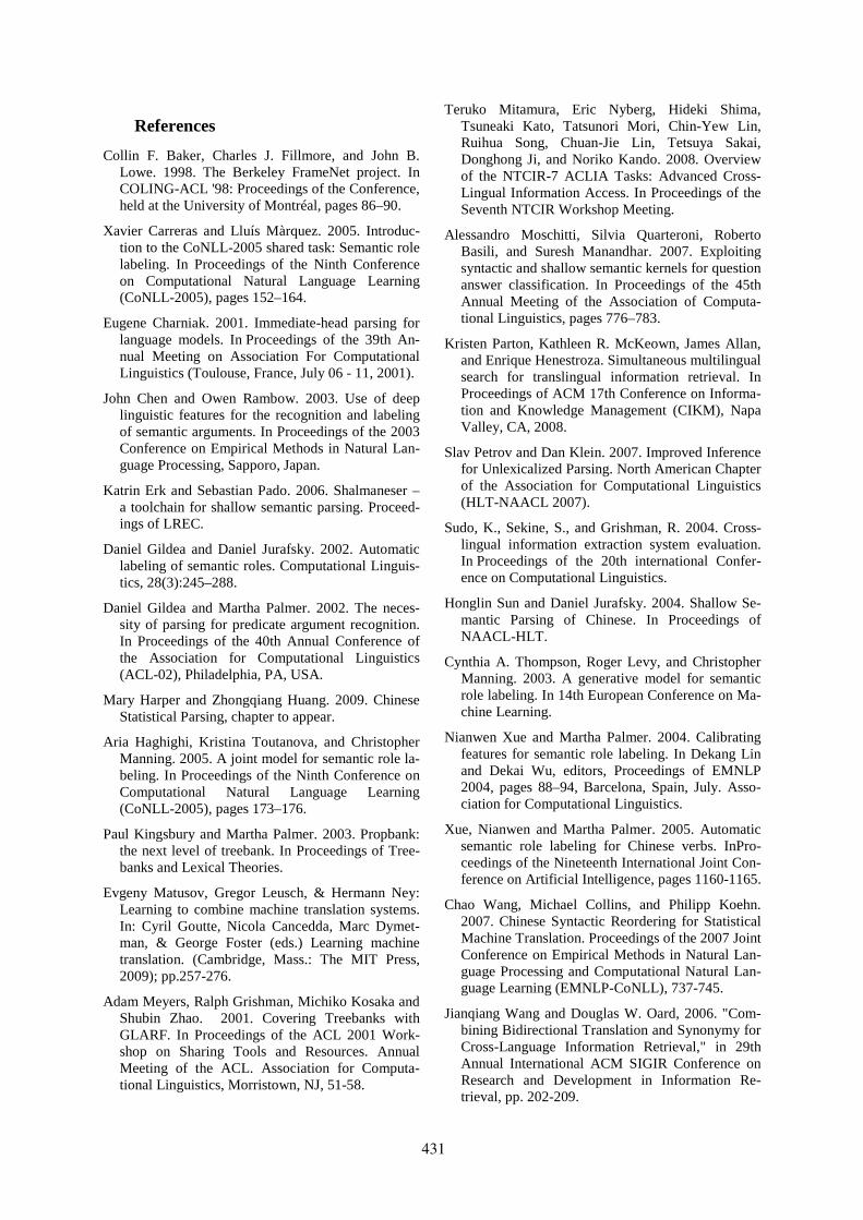
References
Collin F. Baker, Charles J. Fillmore, and John B. Lowe. 1998. The Berkeley FrameNet project. In COLING-ACL '98: Proceedings of the Conference, held at the University of Montréal, pages 86–90.
Xavier Carreras and Lluís Màrquez. 2005. Introduc-tion to the CoNLL-2005 shared task: Semantic role labeling. In Proceedings of the Ninth Conference on Computational Natural Language Learning (CoNLL-2005), pages 152–164.
Eugene Charniak. 2001. Immediate-head parsing for language models. In Proceedings of the 39th An-nual Meeting on Association For Computational Linguistics (Toulouse, France, July 06 - 11, 2001).
John Chen and Owen Rambow. 2003. Use of deep linguistic features for the recognition and labeling of semantic arguments. In Proceedings of the 2003 Conference on Empirical Methods in Natural Lan-guage Processing, Sapporo, Japan.
Katrin Erk and Sebastian Pado. 2006. Shalmaneser – a toolchain for shallow semantic parsing. Proceed-ings of LREC.
Daniel Gildea and Daniel Jurafsky. 2002. Automatic labeling of semantic roles. Computational Linguis-tics, 28(3):245–288.
Daniel Gildea and Martha Palmer. 2002. The neces-sity of parsing for predicate argument recognition. In Proceedings of the 40th Annual Conference of the Association for Computational Linguistics (ACL-02), Philadelphia, PA, USA.
Mary Harper and Zhongqiang Huang. 2009. Chinese Statistical Parsing, chapter to appear.
Aria Haghighi, Kristina Toutanova, and Christopher Manning. 2005. A joint model for semantic role la-beling. In Proceedings of the Ninth Conference on Computational Natural Language Learning (CoNLL-2005), pages 173–176.
Paul Kingsbury and Martha Palmer. 2003. Propbank: the next level of treebank. In Proceedings of Tree-banks and Lexical Theories.
Evgeny Matusov, Gregor Leusch, & Hermann Ney: Learning to combine machine translation systems. In: Cyril Goutte, Nicola Cancedda, Marc Dymet-man, & George Foster (eds.) Learning machine translation. (Cambridge, Mass.: The MIT Press, 2009); pp.257-276.
Adam Meyers, Ralph Grishman, Michiko Kosaka and Shubin Zhao. 2001. Covering Treebanks with GLARF. In Proceedings of the ACL 2001 Work-shop on Sharing Tools and Resources. Annual Meeting of the ACL. Association for Computa-tional Linguistics, Morristown, NJ, 51-58.
Teruko Mitamura, Eric Nyberg, Hideki Shima, Tsuneaki Kato, Tatsunori Mori, Chin-Yew Lin, Ruihua Song, Chuan-Jie Lin, Tetsuya Sakai, Donghong Ji, and Noriko Kando. 2008. Overview of the NTCIR-7 ACLIA Tasks: Advanced Cross-Lingual Information Access. In Proceedings of the Seventh NTCIR Workshop Meeting.
Alessandro Moschitti, Silvia Quarteroni, Roberto Basili, and Suresh Manandhar. 2007. Exploiting syntactic and shallow semantic kernels for question answer classification. In Proceedings of the 45th Annual Meeting of the Association of Computa-tional Linguistics, pages 776–783.
Kristen Parton, Kathleen R. McKeown, James Allan, and Enrique Henestroza. Simultaneous multilingual search for translingual information retrieval. In Proceedings of ACM 17th Conference on Informa-tion and Knowledge Management (CIKM), Napa Valley, CA, 2008.
Slav Petrov and Dan Klein. 2007. Improved Inference for Unlexicalized Parsing. North American Chapter of the Association for Computational Linguistics (HLT-NAACL 2007).
Sudo, K., Sekine, S., and Grishman, R. 2004. Cross-lingual information extraction system evaluation. In Proceedings of the 20th international Confer-ence on Computational Linguistics.
Honglin Sun and Daniel Jurafsky. 2004. Shallow Se-mantic Parsing of Chinese. In Proceedings of NAACL-HLT.
Cynthia A. Thompson, Roger Levy, and Christopher Manning. 2003. A generative model for semantic role labeling. In 14th European Conference on Ma-chine Learning.
Nianwen Xue and Martha Palmer. 2004. Calibrating features for semantic role labeling. In Dekang Lin and Dekai Wu, editors, Proceedings of EMNLP 2004, pages 88–94, Barcelona, Spain, July. Asso-ciation for Computational Linguistics.
Xue, Nianwen and Martha Palmer. 2005. Automatic semantic role labeling for Chinese verbs. InPro-ceedings of the Nineteenth International Joint Con-ference on Artificial Intelligence, pages 1160-1165.
Chao Wang, Michael Collins, and Philipp Koehn. 2007. Chinese Syntactic Reordering for Statistical Machine Translation. Proceedings of the 2007 Joint Conference on Empirical Methods in Natural Lan-guage Processing and Computational Natural Lan-guage Learning (EMNLP-CoNLL), 737-745.
Jianqiang Wang and Douglas W. Oard, 2006. "Com-bining Bidirectional Translation and Synonymy for Cross-Language Information Retrieval," in 29th Annual International ACM SIGIR Conference on Research and Development in Information Re-trieval, pp. 202-209.
431
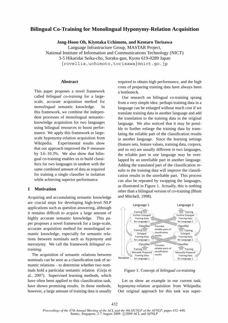
Proceedings of the 47th Annual Meeting of the ACL and the 4th IJCNLP of the AFNLP, pages 432–440,Suntec, Singapore, 2-7 August 2009. c©2009 ACL and AFNLP
Bilingual Co-Training for Monolingual Hyponymy-Relation Acquisition
Jong-Hoon Oh, Kiyotaka Uchimoto, and Kentaro TorisawaLanguage Infrastructure Group, MASTAR Project,
National Institute of Information and Communications Technology (NICT)3-5 Hikaridai Seika-cho, Soraku-gun, Kyoto 619-0289 Japan{rovellia,uchimoto,torisawa}@nict.go.jp
Abstract
This paper proposes a novel frameworkcalled bilingual co-training for a large-scale, accurate acquisition method formonolingual semantic knowledge. Inthis framework, we combine the indepen-dent processes of monolingual semantic-knowledge acquisition for two languagesusing bilingual resources to boost perfor-mance. We apply this framework to large-scale hyponymy-relation acquisition fromWikipedia. Experimental results showthat our approach improved the F-measureby 3.6–10.3%. We also show that bilin-gual co-training enables us to build classi-fiers for two languages in tandem with thesame combined amount of data as requiredfor training a single classifier in isolationwhile achieving superior performance.
1 Motivation
Acquiring and accumulating semantic knowledgeare crucial steps for developing high-level NLPapplications such as question answering, althoughit remains difficult to acquire a large amount ofhighly accurate semantic knowledge. This pa-per proposes a novel framework for a large-scale,accurate acquisition method for monolingual se-mantic knowledge, especially for semantic rela-tions between nominals such as hyponymy andmeronymy. We call the framework bilingual co-training.
The acquisition of semantic relations betweennominals can be seen as a classification task of se-mantic relations – to determine whether two nom-inals hold a particular semantic relation (Girju etal., 2007). Supervised learning methods, whichhave often been applied to this classification task,have shown promising results. In those methods,however, a large amount of training data is usually
required to obtain high performance, and the highcosts of preparing training data have always beena bottleneck.
Our research on bilingual co-training sprangfrom a very simple idea: perhaps training data in alanguage can be enlarged without much cost if wetranslate training data in another language and addthe translation to the training data in the originallanguage. We also noticed that it may be possi-ble to further enlarge the training data by trans-lating the reliable part of the classification resultsin another language. Since the learning settings(feature sets, feature values, training data, corpora,and so on) are usually different in two languages,the reliable part in one language may be over-lapped by an unreliable part in another language.Adding the translated part of the classification re-sults to the training data will improve the classifi-cation results in the unreliable part. This processcan also be repeated by swapping the languages,as illustrated in Figure 1. Actually, this is nothingother than a bilingual version of co-training (Blumand Mitchell, 1998).
Language 1 Language 2
Iteration
Manually Prepared
Training Data
for Language 1
Classifier Classifier
Training Training
Enlarged
Training Data
for Language 1
Enlarged
Training Data
for Language 2
Manually Prepared
Training Data
for Language 2
ClassifierClassifier
Further Enlarged
Training Data
for Language 1
Further Enlarged
Training Data
for Language 2
Translate
reliable parts of
classification
results
Training
Training Training
Training
….. …..
Translate
reliable parts of
classification
results
Figure 1: Concept of bilingual co-training
Let us show an example in our current task:hyponymy-relation acquisition from Wikipedia.Our original approach for this task was super-
432
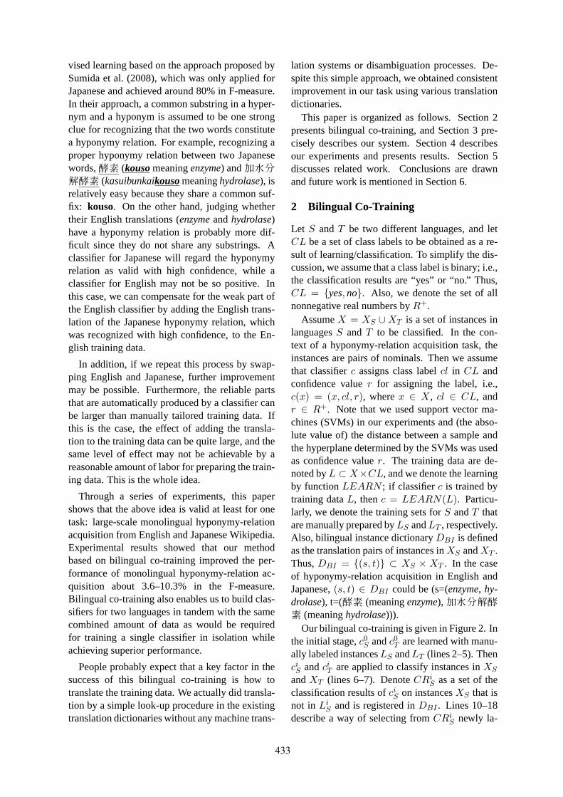
vised learning based on the approach proposed bySumida et al. (2008), which was only applied forJapanese and achieved around 80% in F-measure.In their approach, a common substring in a hyper-nym and a hyponym is assumed to be one strongclue for recognizing that the two words constitutea hyponymy relation. For example, recognizing aproper hyponymy relation between two Japanesewords,�� (kouso meaning enzyme) and������ (kasuibunkaikouso meaning hydrolase), isrelatively easy because they share a common suf-fix: kouso. On the other hand, judging whethertheir English translations (enzyme and hydrolase)have a hyponymy relation is probably more dif-ficult since they do not share any substrings. Aclassifier for Japanese will regard the hyponymyrelation as valid with high confidence, while aclassifier for English may not be so positive. Inthis case, we can compensate for the weak part ofthe English classifier by adding the English trans-lation of the Japanese hyponymy relation, whichwas recognized with high confidence, to the En-glish training data.
In addition, if we repeat this process by swap-ping English and Japanese, further improvementmay be possible. Furthermore, the reliable partsthat are automatically produced by a classifier canbe larger than manually tailored training data. Ifthis is the case, the effect of adding the transla-tion to the training data can be quite large, and thesame level of effect may not be achievable by areasonable amount of labor for preparing the train-ing data. This is the whole idea.
Through a series of experiments, this papershows that the above idea is valid at least for onetask: large-scale monolingual hyponymy-relationacquisition from English and Japanese Wikipedia.Experimental results showed that our methodbased on bilingual co-training improved the per-formance of monolingual hyponymy-relation ac-quisition about 3.6–10.3% in the F-measure.Bilingual co-training also enables us to build clas-sifiers for two languages in tandem with the samecombined amount of data as would be requiredfor training a single classifier in isolation whileachieving superior performance.
People probably expect that a key factor in thesuccess of this bilingual co-training is how totranslate the training data. We actually did transla-tion by a simple look-up procedure in the existingtranslation dictionaries without any machine trans-
lation systems or disambiguation processes. De-spite this simple approach, we obtained consistentimprovement in our task using various translationdictionaries.
This paper is organized as follows. Section 2presents bilingual co-training, and Section 3 pre-cisely describes our system. Section 4 describesour experiments and presents results. Section 5discusses related work. Conclusions are drawnand future work is mentioned in Section 6.
2 Bilingual Co-Training
Let S and T be two different languages, and letCL be a set of class labels to be obtained as a re-sult of learning/classification. To simplify the dis-cussion, we assume that a class label is binary; i.e.,the classification results are “yes” or “no.” Thus,CL = {yes, no}. Also, we denote the set of allnonnegative real numbers by R+.
Assume X = XS ∪ XT is a set of instances inlanguages S and T to be classified. In the con-text of a hyponymy-relation acquisition task, theinstances are pairs of nominals. Then we assumethat classifier c assigns class label cl in CL andconfidence value r for assigning the label, i.e.,c(x) = (x, cl, r), where x ∈ X , cl ∈ CL, andr ∈ R+. Note that we used support vector ma-chines (SVMs) in our experiments and (the abso-lute value of) the distance between a sample andthe hyperplane determined by the SVMs was usedas confidence value r. The training data are de-noted by L ⊂ X×CL, and we denote the learningby function LEARN ; if classifier c is trained bytraining data L, then c = LEARN(L). Particu-larly, we denote the training sets for S and T thatare manually prepared by LS and LT , respectively.Also, bilingual instance dictionary DBI is definedas the translation pairs of instances in XS and XT .Thus, DBI = {(s, t)} ⊂ XS × XT . In the caseof hyponymy-relation acquisition in English andJapanese, (s, t) ∈ DBI could be (s=(enzyme, hy-drolase), t=(�� (meaning enzyme),������ (meaning hydrolase))).
Our bilingual co-training is given in Figure 2. Inthe initial stage, c0
S and c0T are learned with manu-
ally labeled instances LS and LT (lines 2–5). ThenciS and ci
T are applied to classify instances in XS
and XT (lines 6–7). Denote CRiS as a set of the
classification results of ciS on instances XS that is
not in LiS and is registered in DBI . Lines 10–18
describe a way of selecting from CRiS newly la-
433
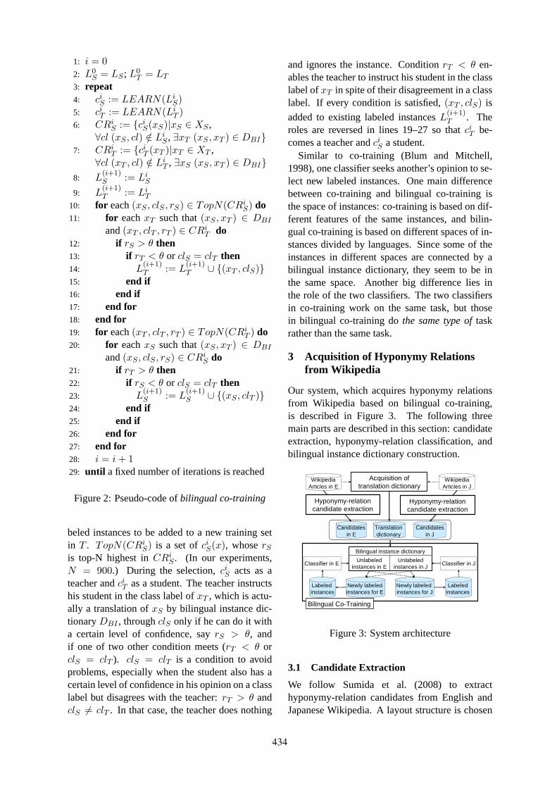
1: i = 02: L0
S = LS ; L0T = LT
3: repeat4: ci
S := LEARN(LiS)
5: ciT := LEARN(Li
T )6: CRi
S := {ciS(xS)|xS ∈ XS ,
∀cl (xS , cl) /∈ LiS , ∃xT (xS , xT ) ∈ DBI}
7: CRiT := {ci
T (xT )|xT ∈ XT ,∀cl (xT , cl) /∈ Li
T , ∃xS (xS , xT ) ∈ DBI}8: L
(i+1)S := Li
S
9: L(i+1)T := Li
T
10: for each (xS , clS , rS) ∈ TopN(CRiS) do
11: for each xT such that (xS , xT ) ∈ DBI
and (xT , clT , rT ) ∈ CRiT do
12: if rS > θ then13: if rT < θ or clS = clT then14: L
(i+1)T := L
(i+1)T ∪ {(xT , clS)}
15: end if16: end if17: end for18: end for19: for each (xT , clT , rT ) ∈ TopN(CRi
T ) do20: for each xS such that (xS , xT ) ∈ DBI
and (xS , clS , rS) ∈ CRiS do
21: if rT > θ then22: if rS < θ or clS = clT then23: L
(i+1)S := L
(i+1)S ∪ {(xS , clT )}
24: end if25: end if26: end for27: end for28: i = i + 129: until a fixed number of iterations is reached
Figure 2: Pseudo-code of bilingual co-training
beled instances to be added to a new training setin T . TopN(CRi
S) is a set of ciS(x), whose rS
is top-N highest in CRiS . (In our experiments,
N = 900.) During the selection, ciS acts as a
teacher and ciT as a student. The teacher instructs
his student in the class label of xT , which is actu-ally a translation of xS by bilingual instance dic-tionary DBI , through clS only if he can do it witha certain level of confidence, say rS > θ, andif one of two other condition meets (rT < θ orclS = clT ). clS = clT is a condition to avoidproblems, especially when the student also has acertain level of confidence in his opinion on a classlabel but disagrees with the teacher: rT > θ andclS �= clT . In that case, the teacher does nothing
and ignores the instance. Condition rT < θ en-ables the teacher to instruct his student in the classlabel of xT in spite of their disagreement in a classlabel. If every condition is satisfied, (xT , clS) is
added to existing labeled instances L(i+1)T . The
roles are reversed in lines 19–27 so that ciT be-
comes a teacher and ciS a student.
Similar to co-training (Blum and Mitchell,1998), one classifier seeks another’s opinion to se-lect new labeled instances. One main differencebetween co-training and bilingual co-training isthe space of instances: co-training is based on dif-ferent features of the same instances, and bilin-gual co-training is based on different spaces of in-stances divided by languages. Since some of theinstances in different spaces are connected by abilingual instance dictionary, they seem to be inthe same space. Another big difference lies inthe role of the two classifiers. The two classifiersin co-training work on the same task, but thosein bilingual co-training do the same type of taskrather than the same task.
3 Acquisition of Hyponymy Relationsfrom Wikipedia
Our system, which acquires hyponymy relationsfrom Wikipedia based on bilingual co-training,is described in Figure 3. The following threemain parts are described in this section: candidateextraction, hyponymy-relation classification, andbilingual instance dictionary construction.
Classifier in E Classifier in J
Labeled instances
Labeled instances
WikipediaArticles in E
WikipediaArticles in J
Candidatesin J
Candidatesin E
Acquisition of translation dictionary
Bilingual Co-Training
Unlabeled instances in J
Unlabeled instances in E
Bilingual instance dictionary
Newly labeled instances for E
Newly labeled instances for J
Translation dictionary
Hyponymy-relation candidate extraction
Hyponymy-relation candidate extraction
Figure 3: System architecture
3.1 Candidate Extraction
We follow Sumida et al. (2008) to extracthyponymy-relation candidates from English andJapanese Wikipedia. A layout structure is chosen
434
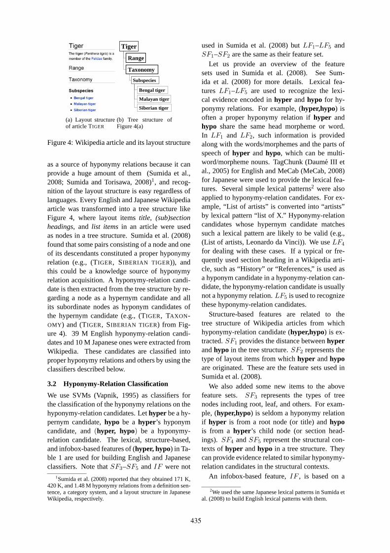
(a) Layout structureof article TIGER
Range
Siberian tiger
Bengal tiger
Subspecies
Taxonomy
Tiger
Malayan tiger
(b) Tree structure ofFigure 4(a)
Figure 4: Wikipedia article and its layout structure
as a source of hyponymy relations because it canprovide a huge amount of them (Sumida et al.,2008; Sumida and Torisawa, 2008)1, and recog-nition of the layout structure is easy regardless oflanguages. Every English and Japanese Wikipediaarticle was transformed into a tree structure likeFigure 4, where layout items title, (sub)sectionheadings, and list items in an article were usedas nodes in a tree structure. Sumida et al. (2008)found that some pairs consisting of a node and oneof its descendants constituted a proper hyponymyrelation (e.g., (TIGER, SIBERIAN TIGER)), andthis could be a knowledge source of hyponymyrelation acquisition. A hyponymy-relation candi-date is then extracted from the tree structure by re-garding a node as a hypernym candidate and allits subordinate nodes as hyponym candidates ofthe hypernym candidate (e.g., (TIGER, TAXON-OMY) and (TIGER, SIBERIAN TIGER) from Fig-ure 4). 39 M English hyponymy-relation candi-dates and 10 M Japanese ones were extracted fromWikipedia. These candidates are classified intoproper hyponymy relations and others by using theclassifiers described below.
3.2 Hyponymy-Relation Classification
We use SVMs (Vapnik, 1995) as classifiers forthe classification of the hyponymy relations on thehyponymy-relation candidates. Let hyper be a hy-pernym candidate, hypo be a hyper’s hyponymcandidate, and (hyper, hypo) be a hyponymy-relation candidate. The lexical, structure-based,and infobox-based features of (hyper, hypo) in Ta-ble 1 are used for building English and Japaneseclassifiers. Note that SF3–SF5 and IF were not
1Sumida et al. (2008) reported that they obtained 171 K,420 K, and 1.48 M hyponymy relations from a definition sen-tence, a category system, and a layout structure in JapaneseWikipedia, respectively.
used in Sumida et al. (2008) but LF1–LF5 andSF1–SF2 are the same as their feature set.
Let us provide an overview of the featuresets used in Sumida et al. (2008). See Sum-ida et al. (2008) for more details. Lexical fea-tures LF1–LF5 are used to recognize the lexi-cal evidence encoded in hyper and hypo for hy-ponymy relations. For example, (hyper,hypo) isoften a proper hyponymy relation if hyper andhypo share the same head morpheme or word.In LF1 and LF2, such information is providedalong with the words/morphemes and the parts ofspeech of hyper and hypo, which can be multi-word/morpheme nouns. TagChunk (Daumé III etal., 2005) for English and MeCab (MeCab, 2008)for Japanese were used to provide the lexical fea-tures. Several simple lexical patterns2 were alsoapplied to hyponymy-relation candidates. For ex-ample, “List of artists” is converted into “artists”by lexical pattern “list of X.” Hyponymy-relationcandidates whose hypernym candidate matchessuch a lexical pattern are likely to be valid (e.g.,(List of artists, Leonardo da Vinci)). We use LF4
for dealing with these cases. If a typical or fre-quently used section heading in a Wikipedia arti-cle, such as “History” or “References,” is used asa hyponym candidate in a hyponymy-relation can-didate, the hyponymy-relation candidate is usuallynot a hyponymy relation. LF5 is used to recognizethese hyponymy-relation candidates.
Structure-based features are related to thetree structure of Wikipedia articles from whichhyponymy-relation candidate (hyper,hypo) is ex-tracted. SF1 provides the distance between hyperand hypo in the tree structure. SF2 represents thetype of layout items from which hyper and hypoare originated. These are the feature sets used inSumida et al. (2008).
We also added some new items to the abovefeature sets. SF3 represents the types of treenodes including root, leaf, and others. For exam-ple, (hyper,hypo) is seldom a hyponymy relationif hyper is from a root node (or title) and hypois from a hyper’s child node (or section head-ings). SF4 and SF5 represent the structural con-texts of hyper and hypo in a tree structure. Theycan provide evidence related to similar hyponymy-relation candidates in the structural contexts.
An infobox-based feature, IF , is based on a
2We used the same Japanese lexical patterns in Sumida etal. (2008) to build English lexical patterns with them.
435

Type Description Example
LF1 Morphemes/words hyper: tiger∗, hypo: Siberian, hypo: tiger∗
LF2 POS of morphemes/words hyper: NN∗, hypo: NP, hypo: NN∗
LF3 hyper and hypo, themselves hyper: Tiger, hypo: Siberian tigerLF4 Used lexical patterns hyper: “List of X”, hypo: “Notable X”LF5 Typical section headings hyper: History, hypo: ReferenceSF1 Distance between hyper and hypo 3SF2 Type of layout items hyper: title, hypo: bulleted listSF3 Type of tree nodes hyper: root node, hypo: leaf nodeSF4 LF1 and LF3 of hypo’s parent node LF3:SubspeciesSF5 LF1 and LF3 of hyper’s child node LF3: TaxonomyIF Semantic properties of hyper and hypo hyper: (taxobox,species), hypo: (taxobox,name)
Table 1: Feature type and its value. ∗ in LF1 and LF2 represent the head morpheme/word and its POS.Except those in LF4 and LF5, examples are derived from (TIGER, SIBERIAN TIGER) in Figure 4.
Wikipedia infobox, a special kind of template, thatdescribes a tabular summary of an article subjectexpressed by attribute-value pairs. An attributetype coupled with the infobox name to which itbelongs provides the semantic properties of itsvalue that enable us to easily understand whatthe attribute value means (Auer and Lehmann,2007; Wu and Weld, 2007). For example, in-fobox template City Japan in Wikipedia articleKyoto contains several attribute-value pairs suchas “Mayor=Daisaku Kadokawa” as attribute=itsvalue. What Daisaku Kadokawa, the attributevalue of mayor in the example, represents is hardto understand alone if we lack knowledge, butits attribute type, mayor, gives a clue–DaisakuKadokawa is a mayor related to Kyoto. Thesesemantic properties enable us to discover seman-tic evidence for hyponymy relations. We ex-tract triples (infobox name, attribute type, attributevalue) from the Wikipedia infoboxes and encodesuch information related to hyper and hypo in ourfeature set IF .3
3.3 Bilingual Instance DictionaryConstruction
Multilingual versions of Wikipedia articles areconnected by cross-language links and usuallyhave titles that are bilinguals of each other (Erd-mann et al., 2008). English and Japanese articlesconnected by a cross-language link are extractedfrom Wikipedia, and their titles are regarded astranslation pairs4. The translation pairs between
3We obtained 1.6 M object-attribute-value triples inJapanese and 5.9 M in English.
4197 K translation pairs were extracted.
English and Japanese terms are used for buildingbilingual instance dictionary DBI for hyponymy-relation acquisition, where DBI is composed oftranslation pairs between English and Japanesehyponymy-relation candidates5.
4 Experiments
We used the MAY 2008 version of EnglishWikipedia and the JUNE 2008 version ofJapanese Wikipedia for our experiments. 24,000hyponymy-relation candidates, randomly selectedin both languages, were manually checked to buildtraining, development, and test sets6. Around8,000 hyponymy relations were found in the man-ually checked data for both languages7. 20,000 ofthe manually checked data were used as a train-ing set for training the initial classifier. The restwere equally divided into development and testsets. The development set was used to select theoptimal parameters in bilingual co-training and thetest set was used to evaluate our system.
We used TinySVM (TinySVM, 2002) with apolynomial kernel of degree 2 as a classifier. Themaximum iteration number in the bilingual co-training was set as 100. Two parameters, θ andTopN , were selected through experiments on thedevelopment set. θ = 1 and TopN=900 showed
5We also used redirection links in English and JapaneseWikipedia for recognizing the variations of terms when webuilt a bilingual instance dictionary with Wikipedia cross-language links.
6It took about two or three months to check them in eachlanguage.
7Regarding a hyponymy relation as a positive sample andthe others as a negative sample for training SVMs, “positivesample:negative sample” was about 8,000:16,000=1:2
436

the best performance and were used as the optimalparameter in the following experiments.
We conducted three experiments to show ef-fects of bilingual co-training, training data size,and bilingual instance dictionaries. In the first twoexperiments, we experimented with a bilingual in-stance dictionary derived from Wikipedia cross-language links. Comparison among systems basedon three different bilingual instance dictionaries isshown in the third experiment.
Precision (P ), recall (R), and F1-measure (F1),as in Eq (1), were used as the evaluation measures,where Rel represents a set of manually checkedhyponymy relations and HRbyS represents a setof hyponymy-relation candidates classified as hy-ponymy relations by the system:
P = |Rel ∩HRbyS|/|HRbyS| (1)
R = |Rel ∩HRbyS|/|Rel|F1 = 2× (P ×R)/(P + R)
4.1 Effect of Bilingual Co-Training
ENGLISH JAPANESE
P R F1 P R F1
SYT 78.5 63.8 70.4 75.0 77.4 76.1INIT 77.9 67.4 72.2 74.5 78.5 76.6TRAN 76.8 70.3 73.4 76.7 79.3 78.0BICO 78.0 83.7 80.7 78.3 85.2 81.6
Table 2: Performance of different systems (%)
Table 2 shows the comparison results of the foursystems. SYT represents the Sumida et al. (2008)system that we implemented and tested with thesame data as ours. INIT is a system based on ini-tial classifier c0 in bilingual co-training. We trans-lated training data in one language by using ourbilingual instance dictionary and added the trans-lation to the existing training data in the otherlanguage like bilingual co-training did. The sizeof the English and Japanese training data reached20,729 and 20,486. We trained initial classifier c0
with the new training data. TRAN is a systembased on the classifier. BICO is a system basedon bilingual co-training.
For Japanese, SYT showed worse performancethan that reported in Sumida et al. (2008), proba-bly due to the difference in training data size (oursis 20,000 and Sumida et al. (2008) was 29,900).The size of the test data was also different – oursis 2,000 and Sumida et al. (2008) was 1,000.
Comparison between INIT and SYT shows theeffect of SF3–SF5 and IF , newly introducedfeature types, in hyponymy-relation classification.INIT consistently outperformed SYT, although thedifference was merely around 0.5–1.8% in F1.
BICO showed significant performance im-provement (around 3.6–10.3% in F1) over SYT,INIT, and TRAN regardless of the language. Com-parison between TRAN and BICO showed thatbilingual co-training is useful for enlarging thetraining data and that the performance gain bybilingual co-training cannot be achieved by sim-ply translating the existing training data.
81
79
77
75
73
60 55 50 45 40 35 30 25 20
F1
Training Data (103)
EnglishJapanese
Figure 5: F1 curves based on the increase of train-ing data size during bilingual co-training
Figure 5 shows F1 curves based on the sizeof the training data including those manually tai-lored and automatically obtained through bilin-gual co-training. The curve starts from 20,000 andends around 55,000 in Japanese and 62,000 in En-glish. As the training data size increases, the F1
curves tend to go upward in both languages. Thisindicates that the two classifiers cooperate wellto boost their performance through bilingual co-training.
We recognized 5.4 M English and 2.41 MJapanese hyponymy relations from the classifi-cation results of BICO on all hyponymy-relationcandidates in both languages.
4.2 Effect of Training Data Size
We performed two tests to investigate the effect ofthe training data size on bilingual co-training. Thefirst test posed the following question: “If we build2n training samples by hand and the building costis the same in both languages, which is better fromthe monolingual aspects: 2n monolingual trainingsamples or n bilingual training samples?” Table 3and Figure 6 show the results.
437
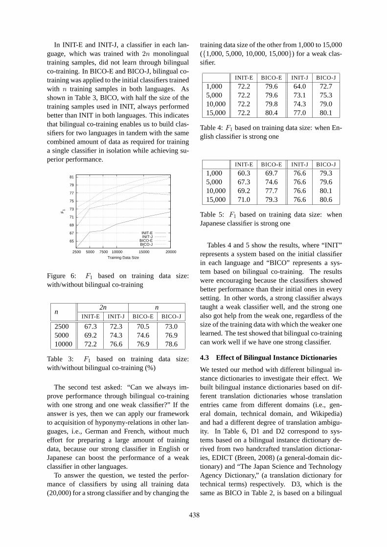
In INIT-E and INIT-J, a classifier in each lan-guage, which was trained with 2n monolingualtraining samples, did not learn through bilingualco-training. In BICO-E and BICO-J, bilingual co-training was applied to the initial classifiers trainedwith n training samples in both languages. Asshown in Table 3, BICO, with half the size of thetraining samples used in INIT, always performedbetter than INIT in both languages. This indicatesthat bilingual co-training enables us to build clas-sifiers for two languages in tandem with the samecombined amount of data as required for traininga single classifier in isolation while achieving su-perior performance.
81
79
77
75
73
71
69
67
65
20000 15000 10000 7500 5000 2500
F1
Training Data Size
INIT-EINIT-J
BICO-EBICO-J
Figure 6: F1 based on training data size:with/without bilingual co-training
n2n n
INIT-E INIT-J BICO-E BICO-J
2500 67.3 72.3 70.5 73.05000 69.2 74.3 74.6 76.910000 72.2 76.6 76.9 78.6
Table 3: F1 based on training data size:with/without bilingual co-training (%)
The second test asked: “Can we always im-prove performance through bilingual co-trainingwith one strong and one weak classifier?” If theanswer is yes, then we can apply our frameworkto acquisition of hyponymy-relations in other lan-guages, i.e., German and French, without mucheffort for preparing a large amount of trainingdata, because our strong classifier in English orJapanese can boost the performance of a weakclassifier in other languages.
To answer the question, we tested the perfor-mance of classifiers by using all training data(20,000) for a strong classifier and by changing the
training data size of the other from 1,000 to 15,000({1,000, 5,000, 10,000, 15,000}) for a weak clas-sifier.
INIT-E BICO-E INIT-J BICO-J
1,000 72.2 79.6 64.0 72.75,000 72.2 79.6 73.1 75.310,000 72.2 79.8 74.3 79.015,000 72.2 80.4 77.0 80.1
Table 4: F1 based on training data size: when En-glish classifier is strong one
INIT-E BICO-E INIT-J BICO-J
1,000 60.3 69.7 76.6 79.35,000 67.3 74.6 76.6 79.610,000 69.2 77.7 76.6 80.115,000 71.0 79.3 76.6 80.6
Table 5: F1 based on training data size: whenJapanese classifier is strong one
Tables 4 and 5 show the results, where “INIT”represents a system based on the initial classifierin each language and “BICO” represents a sys-tem based on bilingual co-training. The resultswere encouraging because the classifiers showedbetter performance than their initial ones in everysetting. In other words, a strong classifier alwaystaught a weak classifier well, and the strong onealso got help from the weak one, regardless of thesize of the training data with which the weaker onelearned. The test showed that bilingual co-trainingcan work well if we have one strong classifier.
4.3 Effect of Bilingual Instance Dictionaries
We tested our method with different bilingual in-stance dictionaries to investigate their effect. Webuilt bilingual instance dictionaries based on dif-ferent translation dictionaries whose translationentries came from different domains (i.e., gen-eral domain, technical domain, and Wikipedia)and had a different degree of translation ambigu-ity. In Table 6, D1 and D2 correspond to sys-tems based on a bilingual instance dictionary de-rived from two handcrafted translation dictionar-ies, EDICT (Breen, 2008) (a general-domain dic-tionary) and “The Japan Science and TechnologyAgency Dictionary,” (a translation dictionary fortechnical terms) respectively. D3, which is thesame as BICO in Table 2, is based on a bilingual
438
instance dictionary derived from Wikipedia. EN-TRY represents the number of translation dictio-nary entries used for building a bilingual instancedictionary. E2J (or J2E) represents the averagetranslation ambiguities of English (or Japanese)terms in the entries. To show the effect of thesetranslation ambiguities, we used each dictionaryunder two different conditions, α=5 and ALL. α=5represents the condition where only translation en-tries with less than five translation ambiguities areused; ALL represents no restriction on translationambiguities.
DIC F1 DIC STATISTICS
TYPE E J ENTRY E2J J2E
D1 α=5 76.5 78.4 588K 1.80 1.77D1 ALL 75.0 77.2 990K 7.17 2.52D2 α=5 76.9 78.5 667K 1.89 1.55D2 ALL 77.0 77.9 750K 3.05 1.71D3 α=5 80.7 81.6 197K 1.03 1.02D3 ALL 80.7 81.6 197K 1.03 1.02
Table 6: Effect of different bilingual instance dic-tionaries
The results showed that D3 was the best andthat the performances of the others were sim-ilar to each other. The differences in the F1
scores between α=5 and ALL were relatively smallwithin the same system triggered by translationambiguities. The performance gap between D3and the other systems might explain the fact thatboth hyponymy-relation candidates and the trans-lation dictionary used in D3 were extracted fromthe same dataset (i.e., Wikipedia), and thus thebilingual instance dictionary built with the trans-lation dictionary in D3 had better coverage ofthe Wikipedia entries consisting of hyponymy-relation candidates than the other bilingual in-stance dictionaries. Although D1 and D2 showedlower performance than D3, the experimental re-sults showed that bilingual co-training was alwayseffective no matter which dictionary was used(Note that F1 of INIT in Table 2 was 72.2 in En-glish and 76.6 in Japanese.)
5 Related Work
Li and Li (2002) proposed bilingual bootstrappingfor word translation disambiguation. Similar tobilingual co-training, classifiers for two languagescooperated in learning with bilingual resources in
bilingual bootstrapping. However, the two clas-sifiers in bilingual bootstrapping were for a bilin-gual task but did different tasks from the monolin-gual viewpoint. A classifier in each language is forword sense disambiguation, where a class label (orword sense) is different based on the languages.On the contrary, classifiers in bilingual co-trainingcooperate in doing the same type of tasks.
Bilingual resources have been used for mono-lingual tasks including verb classification andnoun phrase semantic interpolation (Merlo et al.,2002; Girju, 2006). However, unlike ours, their fo-cus was limited to bilingual features for one mono-lingual classifier based on supervised learning.
Recently, there has been increased interest in se-mantic relation acquisition from corpora. Someregarded Wikipedia as the corpora and appliedhand-crafted or machine-learned rules to acquiresemantic relations (Herbelot and Copestake, 2006;Kazama and Torisawa, 2007; Ruiz-casado et al.,2005; Nastase and Strube, 2008; Sumida et al.,2008; Suchanek et al., 2007). Several researcherswho participated in SemEval-07 (Girju et al.,2007) proposed methods for the classification ofsemantic relations between simple nominals inEnglish sentences. However, the previous workseldom considered the bilingual aspect of seman-tic relations in the acquisition of monolingual se-mantic relations.
6 Conclusion
We proposed a bilingual co-training approach andapplied it to hyponymy-relation acquisition fromWikipedia. Experiments showed that bilingualco-training is effective for improving the perfor-mance of classifiers in both languages. We fur-ther showed that bilingual co-training enables usto build classifiers for two languages in tandem,outperforming classifiers trained individually foreach language while requiring no more trainingdata in total than a single classifier trained in iso-lation.
We showed that bilingual co-training is alsohelpful for boosting the performance of a weakclassifier in one language with the help of a strongclassifier in the other language without loweringthe performance of either classifier. This indicatesthat the framework can reduce the cost of prepar-ing training data in new languages with the help ofour English and Japanese strong classifiers. Ourfuture work focuses on this issue.
439

References
Sören Auer and Jens Lehmann. 2007. What haveInnsbruck and Leipzig in common? Extracting se-mantics from wiki content. In Proc. of the 4thEuropean Semantic Web Conference (ESWC 2007),pages 503–517. Springer.
Avrim Blum and Tom Mitchell. 1998. Combining la-beled and unlabeled data with co-training. In COLT’98: Proceedings of the eleventh annual conferenceon Computational learning theory, pages 92–100.
Jim Breen. 2008. EDICT Japanese/English dictionaryfile, The Electronic Dictionary Research and Devel-opment Group, Monash University.
Hal Daumé III, John Langford, and Daniel Marcu.2005. Search-based structured prediction as classi-fication. In Proc. of NIPS Workshop on Advances inStructured Learning for Text and Speech Processing,Whistler, Canada.
Maike Erdmann, Kotaro Nakayama, Takahiro Hara,and Shojiro Nishio. 2008. A bilingual dictionaryextracted from the Wikipedia link structure. In Proc.of DASFAA, pages 686–689.
Roxana Girju, Preslav Nakov, Vivi Nastase, Stan Sz-pakowicz, Peter Turney, and Deniz Yuret. 2007.Semeval-2007 task 04: Classification of semantic re-lations between nominals. In Proc. of the FourthInternational Workshop on Semantic Evaluations(SemEval-2007), pages 13–18.
Roxana Girju. 2006. Out-of-context noun phrase se-mantic interpretation with cross-linguistic evidence.In CIKM ’06: Proceedings of the 15th ACM inter-national conference on Information and knowledgemanagement, pages 268–276.
Aurelie Herbelot and Ann Copestake. 2006. Acquir-ing ontological relationships from Wikipedia usingRMRS. In Proc. of the ISWC 2006 Workshop onWeb Content Mining with Human Language Tech-nologies.
Jun’ichi Kazama and Kentaro Torisawa. 2007. Ex-ploiting Wikipedia as external knowledge for namedentity recognition. In Proc. of Joint Conference onEmpirical Methods in Natural Language Process-ing and Computational Natural Language Learning,pages 698–707.
Cong Li and Hang Li. 2002. Word translation disam-biguation using bilingual bootstrapping. In Proc. ofthe 40th Annual Meeting of the Association for Com-putational Linguistics, pages 343–351.
MeCab. 2008. MeCab: Yet another part-of-speechand morphological analyzer. http://mecab.sourceforge.net/.
Paola Merlo, Suzanne Stevenson, Vivian Tsang, andGianluca Allaria. 2002. A multilingual paradigmfor automatic verb classification. In Proc. of the
40th Annual Meeting of the Association for Compu-tational Linguistics, pages 207–214.
Vivi Nastase and Michael Strube. 2008. DecodingWikipedia categories for knowledge acquisition. InProc. of AAAI 08, pages 1219–1224.
Maria Ruiz-casado, Enrique Alfonseca, and PabloCastells. 2005. Automatic extraction of semanticrelationships for Wordnet by means of pattern learn-ing from Wikipedia. In Proc. of NLDB, pages 67–79. Springer Verlag.
Fabian M. Suchanek, Gjergji Kasneci, and GerhardWeikum. 2007. Yago: A Core of Semantic Knowl-edge. In Proc. of the 16th international conferenceon World Wide Web, pages 697–706.
Asuka Sumida and Kentaro Torisawa. 2008. Hack-ing Wikipedia for hyponymy relation acquisition. InProc. of the Third International Joint Conferenceon Natural Language Processing (IJCNLP), pages883–888, January.
Asuka Sumida, Naoki Yoshinaga, and Kentaro Tori-sawa. 2008. Boosting precision and recall of hy-ponymy relation acquisition from hierarchical lay-outs in Wikipedia. In Proceedings of the 6th In-ternational Conference on Language Resources andEvaluation.
TinySVM. 2002. http://chasen.org/˜taku/software/TinySVM.
Vladimir N. Vapnik. 1995. The nature of statisticallearning theory. Springer-Verlag New York, Inc.,New York, NY, USA.
Fei Wu and Daniel S. Weld. 2007. Autonomously se-mantifying Wikipedia. In CIKM ’07: Proceedingsof the sixteenth ACM conference on Conference oninformation and knowledge management, pages 41–50.
440
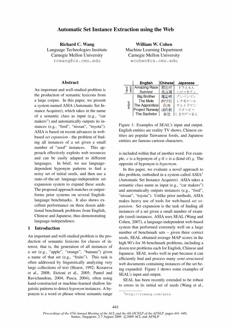
Proceedings of the 47th Annual Meeting of the ACL and the 4th IJCNLP of the AFNLP, pages 441–449,Suntec, Singapore, 2-7 August 2009. c©2009 ACL and AFNLP
Automatic Set Instance Extraction using the Web
Richard C. WangLanguage Technologies Institute
Carnegie Mellon [email protected]
William W. CohenMachine Learning Department
Carnegie Mellon [email protected]
AbstractAn important and well-studied problem isthe production of semantic lexicons froma large corpus. In this paper, we presenta system named ASIA (Automatic Set In-stance Acquirer), which takes in the nameof a semantic class as input (e.g., “carmakers”) and automatically outputs its in-stances (e.g., “ford”, “nissan”, “toyota”).ASIA is based on recent advances in web-based set expansion - the problem of find-ing all instances of a set given a smallnumber of “seed” instances. This ap-proach effectively exploits web resourcesand can be easily adapted to differentlanguages. In brief, we use language-dependent hyponym patterns to find anoisy set of initial seeds, and then use astate-of-the-art language-independent setexpansion system to expand these seeds.The proposed approach matches or outper-forms prior systems on several English-language benchmarks. It also shows ex-cellent performance on three dozen addi-tional benchmark problems from English,Chinese and Japanese, thus demonstratinglanguage-independence.
1 Introduction
An important and well-studied problem is the pro-duction of semantic lexicons for classes of in-terest; that is, the generation of all instances ofa set (e.g., “apple”, “orange”, “banana”) givena name of that set (e.g., “fruits”). This task isoften addressed by linguistically analyzing verylarge collections of text (Hearst, 1992; Kozarevaet al., 2008; Etzioni et al., 2005; Pantel andRavichandran, 2004; Pasca, 2004), often usinghand-constructed or machine-learned shallow lin-guistic patterns to detect hyponym instances. A hy-ponym is a word or phrase whose semantic range
Figure 1: Examples of SEAL’s input and output.English entities are reality TV shows, Chinese en-tities are popular Taiwanese foods, and Japaneseentities are famous cartoon characters.
is included within that of another word. For exam-ple, x is a hyponym of y if x is a (kind of) y. Theopposite of hyponym is hypernym.
In this paper, we evaluate a novel approach tothis problem, embodied in a system called ASIA1
(Automatic Set Instance Acquirer). ASIA takes asemantic class name as input (e.g., “car makers”)and automatically outputs instances (e.g., “ford”,“nissan”, “toyota”). Unlike prior methods, ASIAmakes heavy use of tools for web-based set ex-pansion. Set expansion is the task of finding allinstances of a set given a small number of exam-ple (seed) instances. ASIA uses SEAL (Wang andCohen, 2007), a language-independent web-basedsystem that performed extremely well on a largenumber of benchmark sets – given three correctseeds, SEAL obtained average MAP scores in thehigh 90’s for 36 benchmark problems, including adozen test problems each for English, Chinese andJapanese. SEAL works well in part because it canefficiently find and process many semi-structuredweb documents containing instances of the set be-ing expanded. Figure 1 shows some examples ofSEAL’s input and output.
SEAL has been recently extended to be robustto errors in its initial set of seeds (Wang et al.,
1http://rcwang.com/asia
441

2008), and to use bootstrapping to iteratively im-prove its performance (Wang and Cohen, 2008).These extensions allow ASIA to extract instancesof sets from the Web, as follows. First, given asemantic class name (e.g., “fruits”), ASIA uses asmall set of language-dependent hyponym patterns(e.g., “fruits such as ”) to find a large but noisyset of seed instances. Second, ASIA uses the ex-tended version of SEAL to expand the noisy set ofseeds.
ASIA’s approach is motivated by the conjecturethat for many natural classes, the amount of infor-mation available in semi-structured documents onthe Web is much larger than the amount of infor-mation available in free-text documents; hence, itis natural to attempt to augment search for set in-stances in free-text with semi-structured documentanalysis. We show that ASIA performs extremelywell experimentally. On the 36 benchmarks usedin (Wang and Cohen, 2007), which are relativelysmall closed sets (e.g., countries, constellations,NBA teams), ASIA has excellent performancefor both recall and precision. On four additionalEnglish-language benchmark problems (US states,countries, singers, and common fish), we com-pare to recent work by Kozareva, Riloff, and Hovy(Kozareva et al., 2008), and show comparable orbetter performance on each of these benchmarks;this is notable because ASIA requires less infor-mation than the work of Kozareva et al (their sys-tem requires a concept name and a seed). We alsocompare ASIA on twelve additional benchmarksto the extended Wordnet 2.1 produced by Snowet al (Snow et al., 2006), and show that for thesetwelve sets, ASIA produces more than five timesas many set instances with much higher precision(98% versus 70%).
Another advantage of ASIA’s approach is that itis nearly language-independent: since the underly-ing set-expansion tools are language-independent,all that is needed to support a new target languageis a new set of hyponym patterns for that lan-guage. In this paper, we present experimental re-sults for Chinese and Japanese, as well as English,to demonstrate this language-independence.
We present related work in Section 2, and ex-plain our proposed approach for ASIA in Sec-tion 3. Section 4 presents the details of our ex-periments, as well as the experimental results. Acomparison of results are illustrated in Section 5,and the paper concludes in Section 6.
2 Related Work
There has been a significant amount of researchdone in the area of semantic class learning (akalexical acquisition, lexicon induction, hyponymextraction, or open-domain information extrac-tion). However, to the best of our knowledge, thereis not a system that can perform set instance ex-traction in multiple languages given only the nameof the set.
Hearst (Hearst, 1992) presented an approachthat utilizes hyponym patterns for extracting can-didate instances given the name of a semantic set.The approach presented in Section 3.1 is based onthis work, except that we extended it to two otherlanguages: Chinese and Japanese.
Pantel et al (Pantel and Ravichandran, 2004)presented an algorithm for automatically inducingnames for semantic classes and for finding theirinstances by using “concept signatures” (statisticson co-occuring instances). Pasca (Pasca, 2004)presented a method for acquiring named entities inarbitrary categories using lexico-syntactic extrac-tion patterns. Etzioni et al (Etzioni et al., 2005)presented the KnowItAll system that also utilizeshyponym patterns to extract class instances fromthe Web. All the systems mentioned rely on eithera English part-of-speech tagger, a parser, or both,and hence are language-dependent.
Kozareva et al (Kozareva et al., 2008) illustratedan approach that uses a single hyponym patterncombined with graph structures to learn semanticclass from the Web. Section 5.1 shows that ourapproach is competitive experimentally; however,their system requires more information, as it usesthe name of the semantic set and a seed instance.
Pasca (Paşca, 2007b; Paşca, 2007a) illustrateda set expansion approach that extracts instancesfrom Web search queries given a set of input seedinstances. This approach is similar in flavor toSEAL but, addresses a different task from that ad-dressed here: for ASIA the user provides no seeds,but instead provides the name of the set being ex-panded. We compare to Pasca’s system in Sec-tion 5.2.
Snow et al (Snow et al., 2006) use known hyper-nym/hyponym pairs to generate training data for amachine-learning system, which then learns manylexico-syntactic patterns. The patterns learned arebased on English-language dependency parsing.We compare to Snow et al’s results in Section 5.3.
442
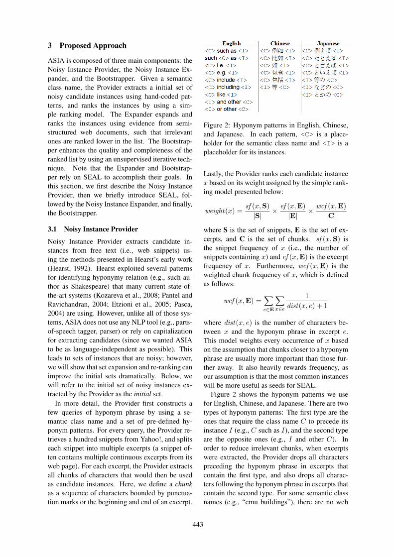
3 Proposed Approach
ASIA is composed of three main components: theNoisy Instance Provider, the Noisy Instance Ex-pander, and the Bootstrapper. Given a semanticclass name, the Provider extracts a initial set ofnoisy candidate instances using hand-coded pat-terns, and ranks the instances by using a sim-ple ranking model. The Expander expands andranks the instances using evidence from semi-structured web documents, such that irrelevantones are ranked lower in the list. The Bootstrap-per enhances the quality and completeness of theranked list by using an unsupervised iterative tech-nique. Note that the Expander and Bootstrap-per rely on SEAL to accomplish their goals. Inthis section, we first describe the Noisy InstanceProvider, then we briefly introduce SEAL, fol-lowed by the Noisy Instance Expander, and finally,the Bootstrapper.
3.1 Noisy Instance Provider
Noisy Instance Provider extracts candidate in-stances from free text (i.e., web snippets) us-ing the methods presented in Hearst’s early work(Hearst, 1992). Hearst exploited several patternsfor identifying hyponymy relation (e.g., such au-thor as Shakespeare) that many current state-of-the-art systems (Kozareva et al., 2008; Pantel andRavichandran, 2004; Etzioni et al., 2005; Pasca,2004) are using. However, unlike all of those sys-tems, ASIA does not use any NLP tool (e.g., parts-of-speech tagger, parser) or rely on capitalizationfor extracting candidates (since we wanted ASIAto be as language-independent as possible). Thisleads to sets of instances that are noisy; however,we will show that set expansion and re-ranking canimprove the initial sets dramatically. Below, wewill refer to the initial set of noisy instances ex-tracted by the Provider as the initial set.
In more detail, the Provider first constructs afew queries of hyponym phrase by using a se-mantic class name and a set of pre-defined hy-ponym patterns. For every query, the Provider re-trieves a hundred snippets from Yahoo!, and splitseach snippet into multiple excerpts (a snippet of-ten contains multiple continuous excerpts from itsweb page). For each excerpt, the Provider extractsall chunks of characters that would then be usedas candidate instances. Here, we define a chunkas a sequence of characters bounded by punctua-tion marks or the beginning and end of an excerpt.
Figure 2: Hyponym patterns in English, Chinese,and Japanese. In each pattern, <C> is a place-holder for the semantic class name and <I> is aplaceholder for its instances.
Lastly, the Provider ranks each candidate instancex based on its weight assigned by the simple rank-ing model presented below:
weight(x) =sf (x,S)
|S|× ef (x,E)
|E|× wcf (x,E)
|C|
where S is the set of snippets, E is the set of ex-cerpts, and C is the set of chunks. sf (x,S) isthe snippet frequency of x (i.e., the number ofsnippets containing x) and ef (x,E) is the excerptfrequency of x. Furthermore, wcf (x,E) is theweighted chunk frequency of x, which is definedas follows:
wcf (x,E) =∑
e∈E
∑
x∈e
1
dist(x, e) + 1
where dist(x, e) is the number of characters be-tween x and the hyponym phrase in excerpt e.This model weights every occurrence of x basedon the assumption that chunks closer to a hyponymphrase are usually more important than those fur-ther away. It also heavily rewards frequency, asour assumption is that the most common instanceswill be more useful as seeds for SEAL.
Figure 2 shows the hyponym patterns we usefor English, Chinese, and Japanese. There are twotypes of hyponym patterns: The first type are theones that require the class name C to precede itsinstance I (e.g., C such as I), and the second typeare the opposite ones (e.g., I and other C). Inorder to reduce irrelevant chunks, when excerptswere extracted, the Provider drops all characterspreceding the hyponym phrase in excerpts thatcontain the first type, and also drops all charac-ters following the hyponym phrase in excerpts thatcontain the second type. For some semantic classnames (e.g., “cmu buildings”), there are no web
443
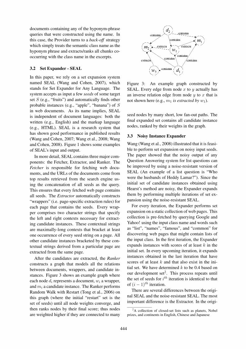
documents containing any of the hyponym-phrasequeries that were constructed using the name. Inthis case, the Provider turns to a back-off strategywhich simply treats the semantic class name as thehyponym phrase and extracts/ranks all chunks co-occurring with the class name in the excerpts.
3.2 Set Expander - SEAL
In this paper, we rely on a set expansion systemnamed SEAL (Wang and Cohen, 2007), whichstands for Set Expander for Any Language. Thesystem accepts as input a few seeds of some targetset S (e.g., “fruits”) and automatically finds otherprobable instances (e.g., “apple”, “banana”) of Sin web documents. As its name implies, SEALis independent of document languages: both thewritten (e.g., English) and the markup language(e.g., HTML). SEAL is a research system thathas shown good performance in published results(Wang and Cohen, 2007; Wang et al., 2008; Wangand Cohen, 2008). Figure 1 shows some examplesof SEAL’s input and output.
In more detail, SEAL contains three major com-ponents: the Fetcher, Extractor, and Ranker. TheFetcher is responsible for fetching web docu-ments, and the URLs of the documents come fromtop results retrieved from the search engine us-ing the concatenation of all seeds as the query.This ensures that every fetched web page containsall seeds. The Extractor automatically constructs“wrappers” (i.e. page-specific extraction rules) foreach page that contains the seeds. Every wrap-per comprises two character strings that specifythe left and right contexts necessary for extract-ing candidate instances. These contextual stringsare maximally-long contexts that bracket at leastone occurrence of every seed string on a page. Allother candidate instances bracketed by these con-textual strings derived from a particular page areextracted from the same page.
After the candidates are extracted, the Rankerconstructs a graph that models all the relationsbetween documents, wrappers, and candidate in-stances. Figure 3 shows an example graph whereeach node di represents a document, wi a wrapper,and mi a candidate instance. The Ranker performsRandom Walk with Restart (Tong et al., 2006) onthis graph (where the initial “restart” set is theset of seeds) until all node weights converge, andthen ranks nodes by their final score; thus nodesare weighted higher if they are connected to many
Figure 3: An example graph constructed bySEAL. Every edge from node x to y actually hasan inverse relation edge from node y to x that isnot shown here (e.g., m1 is extracted by w1).
seed nodes by many short, low fan-out paths. Thefinal expanded set contains all candidate instancenodes, ranked by their weights in the graph.
3.3 Noisy Instance Expander
Wang (Wang et al., 2008) illustrated that it is feasi-ble to perform set expansion on noisy input seeds.The paper showed that the noisy output of anyQuestion Answering system for list questions canbe improved by using a noise-resistant version ofSEAL (An example of a list question is “Whowere the husbands of Heddy Lamar?”). Since theinitial set of candidate instances obtained usingHearst’s method are noisy, the Expander expandsthem by performing multiple iterations of set ex-pansion using the noise-resistant SEAL.
For every iteration, the Expander performs setexpansion on a static collection of web pages. Thiscollection is pre-fetched by querying Google andYahoo! using the input class name and words suchas “list”, “names”, “famous”, and “common” fordiscovering web pages that might contain lists ofthe input class. In the first iteration, the Expanderexpands instances with scores of at least k in theinitial set. In every upcoming iteration, it expandsinstances obtained in the last iteration that havescores of at least k and that also exist in the ini-tial set. We have determined k to be 0.4 based onour development set2. This process repeats untilthe set of seeds for ith iteration is identical to thatof (i− 1)th iteration.
There are several differences between the origi-nal SEAL and the noise-resistant SEAL. The mostimportant difference is the Extractor. In the origi-
2A collection of closed-set lists such as planets, Nobelprizes, and continents in English, Chinese and Japanese
444
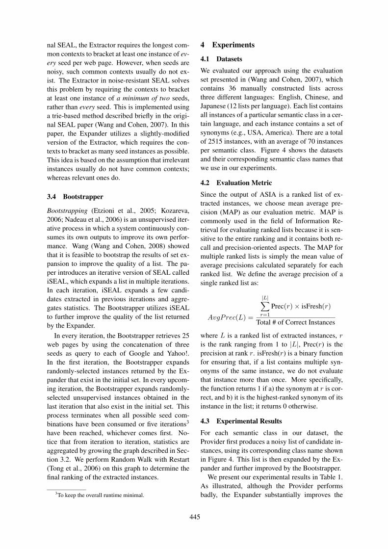
nal SEAL, the Extractor requires the longest com-mon contexts to bracket at least one instance of ev-ery seed per web page. However, when seeds arenoisy, such common contexts usually do not ex-ist. The Extractor in noise-resistant SEAL solvesthis problem by requiring the contexts to bracketat least one instance of a minimum of two seeds,rather than every seed. This is implemented usinga trie-based method described briefly in the origi-nal SEAL paper (Wang and Cohen, 2007). In thispaper, the Expander utilizes a slightly-modifiedversion of the Extractor, which requires the con-texts to bracket as many seed instances as possible.This idea is based on the assumption that irrelevantinstances usually do not have common contexts;whereas relevant ones do.
3.4 Bootstrapper
Bootstrapping (Etzioni et al., 2005; Kozareva,2006; Nadeau et al., 2006) is an unsupervised iter-ative process in which a system continuously con-sumes its own outputs to improve its own perfor-mance. Wang (Wang and Cohen, 2008) showedthat it is feasible to bootstrap the results of set ex-pansion to improve the quality of a list. The pa-per introduces an iterative version of SEAL callediSEAL, which expands a list in multiple iterations.In each iteration, iSEAL expands a few candi-dates extracted in previous iterations and aggre-gates statistics. The Bootstrapper utilizes iSEALto further improve the quality of the list returnedby the Expander.
In every iteration, the Bootstrapper retrieves 25web pages by using the concatenation of threeseeds as query to each of Google and Yahoo!.In the first iteration, the Bootstrapper expandsrandomly-selected instances returned by the Ex-pander that exist in the initial set. In every upcom-ing iteration, the Bootstrapper expands randomly-selected unsupervised instances obtained in thelast iteration that also exist in the initial set. Thisprocess terminates when all possible seed com-binations have been consumed or five iterations3
have been reached, whichever comes first. No-tice that from iteration to iteration, statistics areaggregated by growing the graph described in Sec-tion 3.2. We perform Random Walk with Restart(Tong et al., 2006) on this graph to determine thefinal ranking of the extracted instances.
3To keep the overall runtime minimal.
4 Experiments
4.1 Datasets
We evaluated our approach using the evaluationset presented in (Wang and Cohen, 2007), whichcontains 36 manually constructed lists acrossthree different languages: English, Chinese, andJapanese (12 lists per language). Each list containsall instances of a particular semantic class in a cer-tain language, and each instance contains a set ofsynonyms (e.g., USA, America). There are a totalof 2515 instances, with an average of 70 instancesper semantic class. Figure 4 shows the datasetsand their corresponding semantic class names thatwe use in our experiments.
4.2 Evaluation Metric
Since the output of ASIA is a ranked list of ex-tracted instances, we choose mean average pre-cision (MAP) as our evaluation metric. MAP iscommonly used in the field of Information Re-trieval for evaluating ranked lists because it is sen-sitive to the entire ranking and it contains both re-call and precision-oriented aspects. The MAP formultiple ranked lists is simply the mean value ofaverage precisions calculated separately for eachranked list. We define the average precision of asingle ranked list as:
AvgPrec(L) =
|L|∑
r=1
Prec(r)× isFresh(r)
Total # of Correct Instances
where L is a ranked list of extracted instances, ris the rank ranging from 1 to |L|, Prec(r) is theprecision at rank r. isFresh(r) is a binary functionfor ensuring that, if a list contains multiple syn-onyms of the same instance, we do not evaluatethat instance more than once. More specifically,the function returns 1 if a) the synonym at r is cor-rect, and b) it is the highest-ranked synonym of itsinstance in the list; it returns 0 otherwise.
4.3 Experimental Results
For each semantic class in our dataset, theProvider first produces a noisy list of candidate in-stances, using its corresponding class name shownin Figure 4. This list is then expanded by the Ex-pander and further improved by the Bootstrapper.
We present our experimental results in Table 1.As illustrated, although the Provider performsbadly, the Expander substantially improves the
445
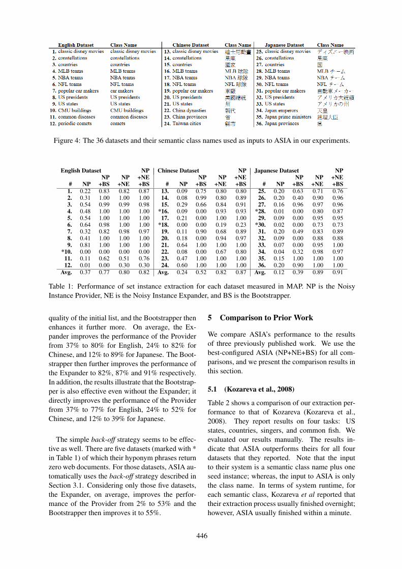
Figure 4: The 36 datasets and their semantic class names used as inputs to ASIA in our experiments.
English Dataset NP Chinese Dataset NP Japanese Dataset NPNP NP +NE NP NP +NE NP NP +NE
# NP +BS +NE +BS # NP +BS +NE +BS # NP +BS +NE +BS1. 0.22 0.83 0.82 0.87 13. 0.09 0.75 0.80 0.80 25. 0.20 0.63 0.71 0.762. 0.31 1.00 1.00 1.00 14. 0.08 0.99 0.80 0.89 26. 0.20 0.40 0.90 0.963. 0.54 0.99 0.99 0.98 15. 0.29 0.66 0.84 0.91 27. 0.16 0.96 0.97 0.964. 0.48 1.00 1.00 1.00 *16. 0.09 0.00 0.93 0.93 *28. 0.01 0.00 0.80 0.875. 0.54 1.00 1.00 1.00 17. 0.21 0.00 1.00 1.00 29. 0.09 0.00 0.95 0.956. 0.64 0.98 1.00 1.00 *18. 0.00 0.00 0.19 0.23 *30. 0.02 0.00 0.73 0.737. 0.32 0.82 0.98 0.97 19. 0.11 0.90 0.68 0.89 31. 0.20 0.49 0.83 0.898. 0.41 1.00 1.00 1.00 20. 0.18 0.00 0.94 0.97 32. 0.09 0.00 0.88 0.889. 0.81 1.00 1.00 1.00 21. 0.64 1.00 1.00 1.00 33. 0.07 0.00 0.95 1.00
*10. 0.00 0.00 0.00 0.00 22. 0.08 0.00 0.67 0.80 34. 0.04 0.32 0.98 0.9711. 0.11 0.62 0.51 0.76 23. 0.47 1.00 1.00 1.00 35. 0.15 1.00 1.00 1.0012. 0.01 0.00 0.30 0.30 24. 0.60 1.00 1.00 1.00 36. 0.20 0.90 1.00 1.00
Avg. 0.37 0.77 0.80 0.82 Avg. 0.24 0.52 0.82 0.87 Avg. 0.12 0.39 0.89 0.91
Table 1: Performance of set instance extraction for each dataset measured in MAP. NP is the NoisyInstance Provider, NE is the Noisy Instance Expander, and BS is the Bootstrapper.
quality of the initial list, and the Bootstrapper thenenhances it further more. On average, the Ex-pander improves the performance of the Providerfrom 37% to 80% for English, 24% to 82% forChinese, and 12% to 89% for Japanese. The Boot-strapper then further improves the performance ofthe Expander to 82%, 87% and 91% respectively.In addition, the results illustrate that the Bootstrap-per is also effective even without the Expander; itdirectly improves the performance of the Providerfrom 37% to 77% for English, 24% to 52% forChinese, and 12% to 39% for Japanese.
The simple back-off strategy seems to be effec-tive as well. There are five datasets (marked with *in Table 1) of which their hyponym phrases returnzero web documents. For those datasets, ASIA au-tomatically uses the back-off strategy described inSection 3.1. Considering only those five datasets,the Expander, on average, improves the perfor-mance of the Provider from 2% to 53% and theBootstrapper then improves it to 55%.
5 Comparison to Prior Work
We compare ASIA’s performance to the resultsof three previously published work. We use thebest-configured ASIA (NP+NE+BS) for all com-parisons, and we present the comparison results inthis section.
5.1 (Kozareva et al., 2008)
Table 2 shows a comparison of our extraction per-formance to that of Kozareva (Kozareva et al.,2008). They report results on four tasks: USstates, countries, singers, and common fish. Weevaluated our results manually. The results in-dicate that ASIA outperforms theirs for all fourdatasets that they reported. Note that the inputto their system is a semantic class name plus oneseed instance; whereas, the input to ASIA is onlythe class name. In terms of system runtime, foreach semantic class, Kozareva et al reported thattheir extraction process usually finished overnight;however, ASIA usually finished within a minute.
446

N Kozareva ASIA N Kozareva ASIAUS States Countries
25 1.00 1.00 50 1.00 1.0050 1.00 1.00 100 1.00 1.0064 0.78 0.78 150 1.00 1.00
200 0.90 0.93300 0.61 0.67323 0.57 0.62
Singers Common Fish10 1.00 1.00 10 1.00 1.0025 1.00 1.00 25 1.00 1.0050 0.97 1.00 50 1.00 1.0075 0.96 1.00 75 0.93 1.00100 0.96 1.00 100 0.84 1.00150 0.95 0.97 116 0.80 1.00180 0.91 0.96
Table 2: Set instance extraction performance com-pared to Kozareva et al. We report our precisionfor all semantic classes and at the same ranks re-ported in their work.
5.2 (Paşca, 2007b)
We compare ASIA to Pasca (Paşca, 2007b) andpresent comparison results in Table 3. There areten semantic classes in his evaluation dataset, andthe input to his system for each class is a set ofseed entities rather than a class name. We evaluateevery instance manually for each class. The resultsshow that, on average, ASIA performs better.
However, we should emphasize that for thethree classes: movie, person, and video game,ASIA did not initially converge to the correct in-stance list given the most natural concept name.Given “movies”, ASIA returns as instances stringslike “comedy”, “action”, “drama”, and other kindsof movies. Given “video games”, it returns “PSP”,“Xbox”, “Wii”, etc. Given “people”, it returns“musicians”, “artists”, “politicians”, etc. We ad-dressed this problem by simply re-running ASIAwith a more specific class name (i.e., the first onereturned); however, the result suggests that futurework is needed to support automatic constructionof hypernym hierarchy using semi-structured webdocuments.
5.3 (Snow et al., 2006)
Snow (Snow et al., 2006) has extended the Word-Net 2.1 by adding thousands of entries (synsets)at a relatively high precision. They have madeseveral versions of extended WordNet available4.For comparison purposes, we selected the version(+30K) that achieved the best F-score in their ex-periments.
4http://ai.stanford.edu/˜rion/swn/
Precision @Target Class System 25 50 100 150 250
Cities Pasca 1.00 0.96 0.88 0.84 0.75ASIA 1.00 1.00 0.97 0.98 0.96
Countries Pasca 1.00 0.98 0.95 0.82 0.60ASIA 1.00 1.00 1.00 1.00 0.79
Drugs Pasca 1.00 1.00 0.96 0.92 0.75ASIA 1.00 1.00 1.00 1.00 0.98
Food Pasca 0.88 0.86 0.82 0.78 0.62ASIA 1.00 1.00 0.93 0.95 0.90
Locations Pasca 1.00 1.00 1.00 1.00 1.00ASIA 1.00 1.00 1.00 1.00 1.00
Newspapers Pasca 0.96 0.98 0.93 0.86 0.54ASIA 1.00 1.00 0.98 0.99 0.85
Universities Pasca 1.00 1.00 1.00 1.00 0.99ASIA 1.00 1.00 1.00 1.00 1.00
Movies Pasca 0.92 0.90 0.88 0.84 0.79Comedy Movies ASIA 1.00 1.00 1.00 1.00 1.00
People Pasca 1.00 1.00 1.00 1.00 1.00Jazz Musicians ASIA 1.00 1.00 1.00 0.94 0.88
Video Games Pasca 1.00 1.00 0.99 0.98 0.98PSP Games ASIA 1.00 1.00 1.00 0.99 0.97
Pasca 0.98 0.97 0.94 0.90 0.80Average ASIA 1.00 1.00 0.99 0.98 0.93
Table 3: Set instance extraction performance com-pared to Pasca. We report our precision for all se-mantic classes and at the same ranks reported inhis work.
For the experimental comparison, we focusedon leaf semantic classes from the extended Word-Net that have many hypernyms, so that a mean-ingful comparison could be made: specifically, weselected nouns that have at least three hypernyms,such that the hypernyms are the leaf nodes in thehypernym hierarchy of WordNet. Of these, 210were extended by Snow. Preliminary experimentsshowed that (as in the experiments with Pasca’sclasses above) ASIA did not always converge tothe intended meaning; to avoid this problem, weinstituted a second filter, and discarded ASIA’s re-sults if the intersection of hypernyms from ASIAand WordNet constituted less than 50% of thosein WordNet. About 50 of the 210 nouns passedthis filter. Finally, we manually evaluated preci-sion and recall of a randomly selected set of twelveof these 50 nouns.
We present the results in Table 4. We used afixed cut-off score5 of 0.3 to truncate the rankedlist produced by ASIA, so that we can computeprecision. Since only a few of these twelve nounsare closed sets, we cannot generally compute re-call; instead, we define relative recall to be theratio of correct instances to the union of correctinstances from both systems. As shown in the re-sults, ASIA has much higher precision, and muchhigher relative recall. When we evaluated Snow’sextended WordNet, we assumed all instances that
5Determined from our development set.
447
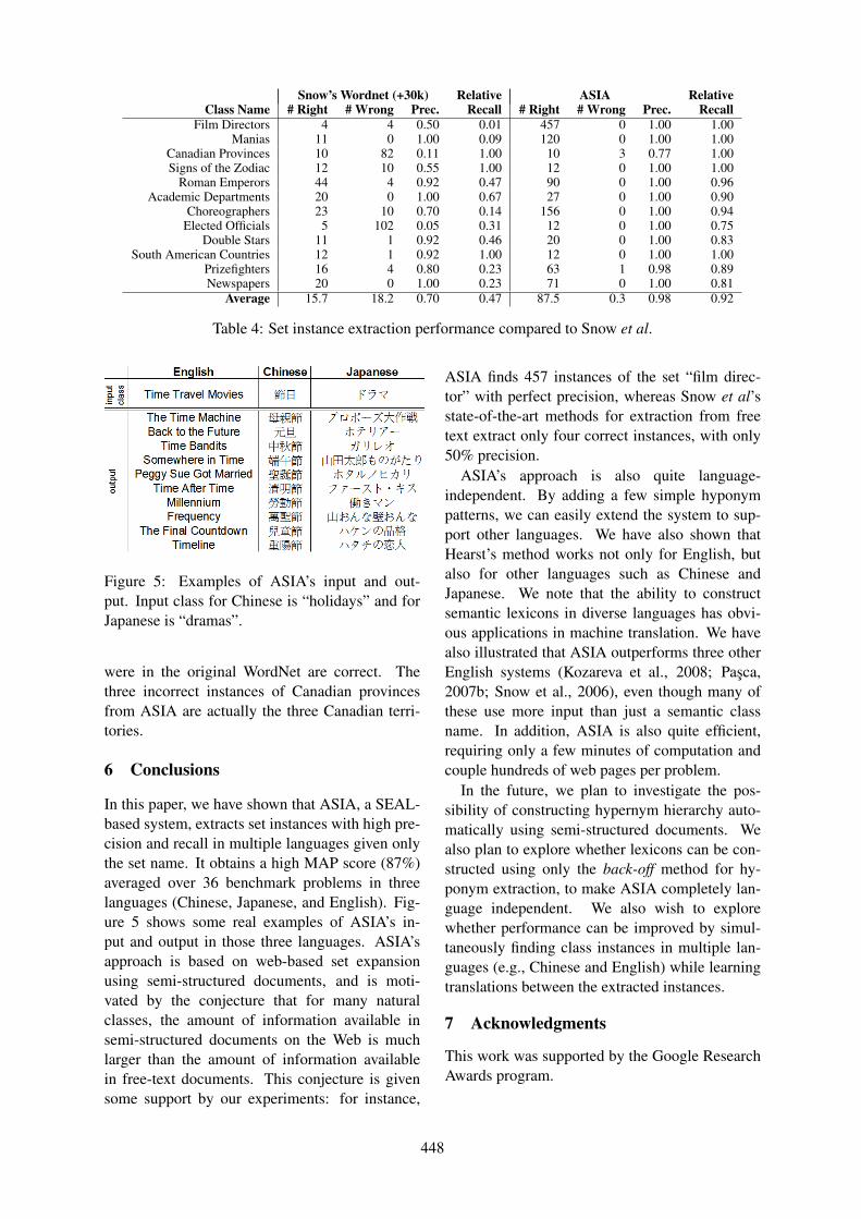
Snow’s Wordnet (+30k) Relative ASIA RelativeClass Name # Right # Wrong Prec. Recall # Right # Wrong Prec. Recall
Film Directors 4 4 0.50 0.01 457 0 1.00 1.00Manias 11 0 1.00 0.09 120 0 1.00 1.00
Canadian Provinces 10 82 0.11 1.00 10 3 0.77 1.00Signs of the Zodiac 12 10 0.55 1.00 12 0 1.00 1.00
Roman Emperors 44 4 0.92 0.47 90 0 1.00 0.96Academic Departments 20 0 1.00 0.67 27 0 1.00 0.90
Choreographers 23 10 0.70 0.14 156 0 1.00 0.94Elected Officials 5 102 0.05 0.31 12 0 1.00 0.75
Double Stars 11 1 0.92 0.46 20 0 1.00 0.83South American Countries 12 1 0.92 1.00 12 0 1.00 1.00
Prizefighters 16 4 0.80 0.23 63 1 0.98 0.89Newspapers 20 0 1.00 0.23 71 0 1.00 0.81
Average 15.7 18.2 0.70 0.47 87.5 0.3 0.98 0.92
Table 4: Set instance extraction performance compared to Snow et al.
Figure 5: Examples of ASIA’s input and out-put. Input class for Chinese is “holidays” and forJapanese is “dramas”.
were in the original WordNet are correct. Thethree incorrect instances of Canadian provincesfrom ASIA are actually the three Canadian terri-tories.
6 Conclusions
In this paper, we have shown that ASIA, a SEAL-based system, extracts set instances with high pre-cision and recall in multiple languages given onlythe set name. It obtains a high MAP score (87%)averaged over 36 benchmark problems in threelanguages (Chinese, Japanese, and English). Fig-ure 5 shows some real examples of ASIA’s in-put and output in those three languages. ASIA’sapproach is based on web-based set expansionusing semi-structured documents, and is moti-vated by the conjecture that for many naturalclasses, the amount of information available insemi-structured documents on the Web is muchlarger than the amount of information availablein free-text documents. This conjecture is givensome support by our experiments: for instance,
ASIA finds 457 instances of the set “film direc-tor” with perfect precision, whereas Snow et al’sstate-of-the-art methods for extraction from freetext extract only four correct instances, with only50% precision.
ASIA’s approach is also quite language-independent. By adding a few simple hyponympatterns, we can easily extend the system to sup-port other languages. We have also shown thatHearst’s method works not only for English, butalso for other languages such as Chinese andJapanese. We note that the ability to constructsemantic lexicons in diverse languages has obvi-ous applications in machine translation. We havealso illustrated that ASIA outperforms three otherEnglish systems (Kozareva et al., 2008; Paşca,2007b; Snow et al., 2006), even though many ofthese use more input than just a semantic classname. In addition, ASIA is also quite efficient,requiring only a few minutes of computation andcouple hundreds of web pages per problem.
In the future, we plan to investigate the pos-sibility of constructing hypernym hierarchy auto-matically using semi-structured documents. Wealso plan to explore whether lexicons can be con-structed using only the back-off method for hy-ponym extraction, to make ASIA completely lan-guage independent. We also wish to explorewhether performance can be improved by simul-taneously finding class instances in multiple lan-guages (e.g., Chinese and English) while learningtranslations between the extracted instances.
7 Acknowledgments
This work was supported by the Google ResearchAwards program.
448
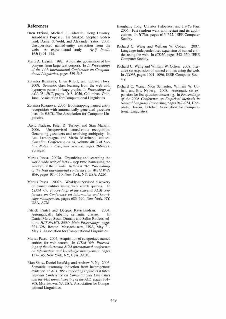
ReferencesOren Etzioni, Michael J. Cafarella, Doug Downey,
Ana-Maria Popescu, Tal Shaked, Stephen Soder-land, Daniel S. Weld, and Alexander Yates. 2005.Unsupervised named-entity extraction from theweb: An experimental study. Artif. Intell.,165(1):91–134.
Marti A. Hearst. 1992. Automatic acquisition of hy-ponyms from large text corpora. In In Proceedingsof the 14th International Conference on Computa-tional Linguistics, pages 539–545.
Zornitsa Kozareva, Ellen Riloff, and Eduard Hovy.2008. Semantic class learning from the web withhyponym pattern linkage graphs. In Proceedings ofACL-08: HLT, pages 1048–1056, Columbus, Ohio,June. Association for Computational Linguistics.
Zornitsa Kozareva. 2006. Bootstrapping named entityrecognition with automatically generated gazetteerlists. In EACL. The Association for Computer Lin-guistics.
David Nadeau, Peter D. Turney, and Stan Matwin.2006. Unsupervised named-entity recognition:Generating gazetteers and resolving ambiguity. InLuc Lamontagne and Mario Marchand, editors,Canadian Conference on AI, volume 4013 of Lec-ture Notes in Computer Science, pages 266–277.Springer.
Marius Paşca. 2007a. Organizing and searching theworld wide web of facts – step two: harnessing thewisdom of the crowds. In WWW ’07: Proceedingsof the 16th international conference on World WideWeb, pages 101–110, New York, NY, USA. ACM.
Marius Paşca. 2007b. Weakly-supervised discoveryof named entities using web search queries. InCIKM ’07: Proceedings of the sixteenth ACM con-ference on Conference on information and knowl-edge management, pages 683–690, New York, NY,USA. ACM.
Patrick Pantel and Deepak Ravichandran. 2004.Automatically labeling semantic classes. InDaniel Marcu Susan Dumais and Salim Roukos, ed-itors, HLT-NAACL 2004: Main Proceedings, pages321–328, Boston, Massachusetts, USA, May 2 -May 7. Association for Computational Linguistics.
Marius Pasca. 2004. Acquisition of categorized namedentities for web search. In CIKM ’04: Proceed-ings of the thirteenth ACM international conferenceon Information and knowledge management, pages137–145, New York, NY, USA. ACM.
Rion Snow, Daniel Jurafsky, and Andrew Y. Ng. 2006.Semantic taxonomy induction from heterogenousevidence. In ACL ’06: Proceedings of the 21st Inter-national Conference on Computational Linguisticsand the 44th annual meeting of the ACL, pages 801–808, Morristown, NJ, USA. Association for Compu-tational Linguistics.
Hanghang Tong, Christos Faloutsos, and Jia-Yu Pan.2006. Fast random walk with restart and its appli-cations. In ICDM, pages 613–622. IEEE ComputerSociety.
Richard C. Wang and William W. Cohen. 2007.Language-independent set expansion of named enti-ties using the web. In ICDM, pages 342–350. IEEEComputer Society.
Richard C. Wang and William W. Cohen. 2008. Iter-ative set expansion of named entities using the web.In ICDM, pages 1091–1096. IEEE Computer Soci-ety.
Richard C. Wang, Nico Schlaefer, William W. Co-hen, and Eric Nyberg. 2008. Automatic set ex-pansion for list question answering. In Proceedingsof the 2008 Conference on Empirical Methods inNatural Language Processing, pages 947–954, Hon-olulu, Hawaii, October. Association for Computa-tional Linguistics.
449

Proceedings of the 47th Annual Meeting of the ACL and the 4th IJCNLP of the AFNLP, pages 450–458,Suntec, Singapore, 2-7 August 2009. c©2009 ACL and AFNLP
Extracting Lexical Reference Rules from Wikipedia
Eyal ShnarchComputer Science Department
Bar-Ilan UniversityRamat-Gan 52900, [email protected]
Libby BarakDept. of Computer Science
University of TorontoToronto, Canada M5S 1A4
Ido DaganComputer Science Department
Bar-Ilan UniversityRamat-Gan 52900, Israel
Abstract
This paper describes the extraction fromWikipedia of lexical referencerules, iden-tifying references to term meanings trig-gered by other terms. We present extrac-tion methods geared to cover the broadrange of the lexical reference relation andanalyze them extensively. Most extrac-tion methods yield high precision levels,and our rule-base is shown to perform bet-ter than other automatically constructedbaselines in a couple of lexical expan-sion and matching tasks. Our rule-baseyields comparable performance to Word-Net while providing largely complemen-tary information.
1 Introduction
A most common need in applied semantic infer-ence is to infer the meaning of a target term fromother terms in a text. For example, a Question An-swering system may infer the answer to a ques-tion regardingluxury carsfrom a text mentioningBentley, which provides a concrete reference to thesought meaning.
Aiming to capture such lexical inferences wefollowed (Glickman et al., 2006), which coinedthe term lexical reference(LR) to denote refer-ences in text to the specific meaning of a targetterm. They further analyzed the dataset of the FirstRecognizing Textual Entailment Challenge (Da-gan et al., 2006), which includes examples drawnfrom seven different application scenarios. It wasfound that an entailing text indeed includes a con-crete reference to practically every term in the en-tailed (inferred) sentence.
The lexical reference relation between twoterms may be viewed as a lexical inference rule,denotedLHS⇒ RHS. Such rule indicates that theleft-hand-side term would generate a reference, in
some texts, to a possible meaning of the right handside term, as theBentley⇒ luxury carexample.
In the above example the LHS is a hyponym ofthe RHS. Indeed, the commonly used hyponymy,synonymy and some cases of the meronymy rela-tions are special cases of lexical reference. How-ever, lexical reference is a broader relation. Forinstance, the LR rulephysician⇒ medicinemaybe useful to infer the topicmedicinein a text cate-gorization setting, while an information extractionsystem may utilize the ruleMargaret Thatcher⇒ United Kingdomto infer a UK announcementfrom the text “Margaret Thatcher announced”.
To perform such inferences, systems need largescale knowledge bases of LR rules. A prominentavailable resource is WordNet (Fellbaum, 1998),from which classical relations such as synonyms,hyponyms and some cases of meronyms may beused as LR rules. An extension to WordNet waspresented by (Snow et al., 2006). Yet, availableresources do not cover the full scope of lexical ref-erence.
This paper presents the extraction of a large-scale rule base from Wikipedia designed to covera wide scope of the lexical reference relation. Asa starting point we examine the potential of defi-nition sentences as a source for LR rules (Ide andJean, 1993; Chodorow et al., 1985; Moldovan andRus, 2001). When writing a concept definition,one aims to formulate a concise text that includesthe most characteristic aspects of the defined con-cept. Therefore, a definition is a promising sourcefor LR relations between the defined concept andthe definition terms.
In addition, we extract LR rules from Wikipediaredirect and hyperlink relations. As a guide-line, we focused on developing simple extrac-tion methods that may be applicable for otherWeb knowledge resources, rather than focusingon Wikipedia-specific attributes. Overall, our rulebase contains about 8 million candidate lexical ref-
450

erence rules.1
Extensive analysis estimated that 66% of ourrules are correct, while different portions of therule base provide varying recall-precision trade-offs. Following further error analysis we intro-duce rule filtering which improves inference per-formance. The rule base utility was evaluatedwithin two lexical expansion applications, yield-ing better results than other automatically con-structed baselines and comparable results to Word-Net. A combination with WordNet achieved thebest performance, indicating the significant mar-ginal contribution of our rule base.
2 Background
Many works on machine readable dictionaries uti-lized definitions to identify semantic relations be-tween words (Ide and Jean, 1993). Chodorow etal. (1985) observed that the head of the definingphrase is a genus term that describes the definedconcept and suggested simple heuristics to find it.Other methods use a specialized parser or a set ofregular expressions tuned to a particular dictionary(Wilks et al., 1996).
Some works utilized Wikipedia to build an on-tology. Ponzetto and Strube (2007) identifiedthe subsumption (IS-A) relation from Wikipedia’scategory tags, while in Yago (Suchanek et al.,2007) these tags, redirect links and WordNet wereused to identify instances of 14 predefined spe-cific semantic relations. These methods dependon Wikipedia’s category system. The lexical refer-ence relation we address subsumes most relationsfound in these works, while our extractions are notlimited to a fixed set of predefined relations.
Several works examined Wikipedia texts, ratherthan just its structured features. Kazama and Tori-sawa (2007) explores the first sentence of an ar-ticle and identifies the first noun phrase followingthe verbbeas a label for the article title. We repro-duce this part of their work as one of our baselines.Toral and Mũnoz (2007) uses all nouns in the firstsentence. Gabrilovich and Markovitch (2007) uti-lized Wikipedia-based concepts as the basis for ahigh-dimensional meaning representation space.
Hearst (1992) utilized a list of patterns indica-tive for the hyponym relation in general texts.Snow et al. (2006) use syntactic path patterns asfeatures for supervised hyponymy and synonymy
1For download seeTextual Entailment Resource Poolatthe ACL-wiki (http://aclweb.org/aclwiki)
classifiers, whose training examples are derivedautomatically from WordNet. They use these clas-sifiers to suggest extensions to the WordNet hierar-chy, the largest one consisting of 400K new links.Their automatically created resource is regarded inour paper as a primary baseline for comparison.
Many works addressed the more general notionof lexical associations, or association rules (e.g.(Ruge, 1992; Rapp, 2002)). For example,TheBeatles, Abbey Roadand Sgt. Pepperwould allbe considered lexically associated. However thisis a rather loose notion, which only indicates thatterms are semantically “related” and are likely toco-occur with each other. On the other hand, lex-ical reference is a special case of lexical associa-tion, which specifies concretely that a reference tothe meaning of one term may be inferred from theother. For example,Abbey Roadprovides a con-crete reference toThe Beatles, enabling to infer asentence like “I listened to The Beatles” from “ Ilistened to Abbey Road”, while it does not referspecifically toSgt. Pepper.
3 Extracting Rules from Wikipedia
Our goal is to utilize the broad knowledge ofWikipedia to extract a knowledge base of lexicalreference rules. Each Wikipedia article providesa definition for the concept denoted by thetitleof the article. As the most concise definition wetake the first sentence of each article, following(Kazama and Torisawa, 2007). Our preliminaryevaluations showed that taking the entire first para-graph as the definition rarely introduces new validrules while harming extraction precision signifi-cantly.
Since a concept definition usually employsmore general terms than the defined concept (Ideand Jean, 1993), the concept title is more likelyto refer to terms in its definition rather than viceversa. Therefore the title is taken as the LHS ofthe constructed rule while the extracted definitionterm is taken as its RHS. As Wikipedia’s titles aremostly noun phrases, the terms we extract as RHSsare the nouns and noun phrases in the definition.The remainder of this section describes our meth-ods for extracting rules from the definition sen-tence and from additional Wikipedia information.
Be-Comp Following the general idea in(Kazama and Torisawa, 2007), we identify theIS-A pattern in the definition sentence by extract-ing nominal complements of the verb ‘be’, taking
451
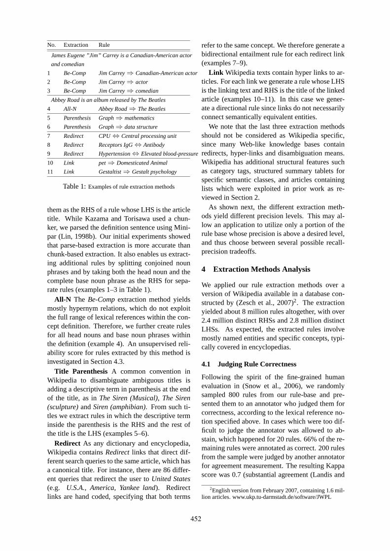
No. Extraction Rule
James Eugene ”Jim” Carrey is a Canadian-American actor
and comedian
1 Be-Comp Jim Carrey⇒ Canadian-American actor
2 Be-Comp Jim Carrey⇒ actor
3 Be-Comp Jim Carrey⇒ comedian
Abbey Road is an album released by The Beatles
4 All-N Abbey Road⇒ The Beatles
5 Parenthesis Graph⇒ mathematics
6 Parenthesis Graph⇒ data structure
7 Redirect CPU⇔ Central processing unit
8 Redirect Receptors IgG⇔ Antibody
9 Redirect Hypertension⇔ Elevated blood-pressure
10 Link pet⇒ Domesticated Animal
11 Link Gestaltist⇒ Gestalt psychology
Table 1:Examples of rule extraction methods
them as the RHS of a rule whose LHS is the articletitle. While Kazama and Torisawa used a chun-ker, we parsed the definition sentence using Mini-par (Lin, 1998b). Our initial experiments showedthat parse-based extraction is more accurate thanchunk-based extraction. It also enables us extract-ing additional rules by splitting conjoined nounphrases and by taking both the head noun and thecomplete base noun phrase as the RHS for sepa-rate rules (examples 1–3 in Table 1).
All-N The Be-Compextraction method yieldsmostly hypernym relations, which do not exploitthe full range of lexical references within the con-cept definition. Therefore, we further create rulesfor all head nouns and base noun phrases withinthe definition (example 4). An unsupervised reli-ability score for rules extracted by this method isinvestigated in Section 4.3.
Title Parenthesis A common convention inWikipedia to disambiguate ambiguous titles isadding a descriptive term in parenthesis at the endof the title, as inThe Siren (Musical), The Siren(sculpture)andSiren (amphibian). From such ti-tles we extract rules in which the descriptive terminside the parenthesis is the RHS and the rest ofthe title is the LHS (examples 5–6).
Redirect As any dictionary and encyclopedia,Wikipedia containsRedirectlinks that direct dif-ferent search queries to the same article, which hasa canonical title. For instance, there are 86 differ-ent queries that redirect the user toUnited States(e.g. U.S.A., America, Yankee land). Redirectlinks are hand coded, specifying that both terms
refer to the same concept. We therefore generate abidirectional entailment rule for each redirect link(examples 7–9).
Link Wikipedia texts contain hyper links to ar-ticles. For each link we generate a rule whose LHSis the linking text and RHS is the title of the linkedarticle (examples 10–11). In this case we gener-ate a directional rule since links do not necessarilyconnect semantically equivalent entities.
We note that the last three extraction methodsshould not be considered as Wikipedia specific,since many Web-like knowledge bases containredirects, hyper-links and disambiguation means.Wikipedia has additional structural features suchas category tags, structured summary tablets forspecific semantic classes, and articles containinglists which were exploited in prior work as re-viewed in Section 2.
As shown next, the different extraction meth-ods yield different precision levels. This may al-low an application to utilize only a portion of therule base whose precision is above a desired level,and thus choose between several possible recall-precision tradeoffs.
4 Extraction Methods Analysis
We applied our rule extraction methods over aversion of Wikipedia available in a database con-structed by (Zesch et al., 2007)2. The extractionyielded about 8 million rules altogether, with over2.4 million distinct RHSs and 2.8 million distinctLHSs. As expected, the extracted rules involvemostly named entities and specific concepts, typi-cally covered in encyclopedias.
4.1 Judging Rule Correctness
Following the spirit of the fine-grained humanevaluation in (Snow et al., 2006), we randomlysampled 800 rules from our rule-base and pre-sented them to an annotator who judged them forcorrectness, according to the lexical reference no-tion specified above. In cases which were too dif-ficult to judge the annotator was allowed to ab-stain, which happened for 20 rules. 66% of the re-maining rules were annotated as correct. 200 rulesfrom the sample were judged by another annotatorfor agreement measurement. The resulting Kappascore was 0.7 (substantial agreement (Landis and
2English version from February 2007, containing 1.6 mil-lion articles. www.ukp.tu-darmstadt.de/software/JWPL
452

Extraction Per Method Accumulated
Method P Est. #Rules P %obtained
Redirect 0.87 1,851,384 0.87 31
Be-Comp 0.78 1,618,913 0.82 60
Parenthesis 0.71 94,155 0.82 60
Link 0.7 485,528 0.80 68
All-N 0.49 1,580,574 0.66 100
Table 2:Manual analysis: precision and estimated numberof correct rules per extraction method, and precision and %of correct rules obtained of rule-sets accumulated by method.
Koch, 1997)), either when considering all the ab-stained rules as correct or as incorrect.
The middle columns of Table 2 present, for eachextraction method, the obtained percentage of cor-rect rules (precision) and their estimated absolutenumber. This number is estimated by multiplyingthe number of annotated correct rules for the ex-traction method by the sampling proportion. In to-tal, we estimate that our resource contains 5.6 mil-lion correct rules. For comparison, Snow’s pub-lished extension to WordNet3, which covers simi-lar types of terms but is restricted to synonyms andhyponyms, includes 400,000 relations.
The right part of Table 2 shows the perfor-mance figures for accumulated rule bases, createdby adding the extraction methods one at a time inorder of their precision.% obtainedis the per-centage of correct rules in each rule base out ofthe total number of correct rules extracted jointlyby all methods (the union set).
We can see that excluding theAll-N methodall extraction methods reach quite high precisionlevels of 0.7-0.87, with accumulated precision of0.84. By selecting only a subset of the extrac-tion methods, according to their precision, one canchoose different recall-precision tradeoff pointsthat suit application preferences.
The less accurateAll-N method may be usedwhen high recall is important, accounting for 32%of the correct rules. An examination of the pathsin All-N reveals, beyond standard hyponymy andsynonymy, various semantic relations that satisfylexical reference, such asLocation, OccupationandCreation, as illustrated in Table 3. Typical re-lations covered byRedirectandLink rules include
3http://ai.stanford.edu/∼rion/swn/4As a non-comparable reference, Snow’s fine-grained
evaluation showed a precision of 0.84 on 10K rules and 0.68on 20K rules; however, they were interested only in the hy-ponym relation while we evaluate our rules according to thebroader LR relation.
synonyms (NY State Trooper⇒ New York StatePolice), morphological derivations (irritate ⇒ ir-ritation), different spellings or naming (Pytagoras⇒ Pythagoras) and acronyms (AIS⇒ Alarm Indi-cation Signal).
4.2 Error Analysis
We sampled 100 rules which were annotated as in-correct and examined the causes of errors. Figure1 shows the distribution of error types.
Wrong NP part - The most common error(35% of the errors) is taking an inappropriate partof a noun phrase (NP) as the rule right hand side(RHS). As described in Section 3, we create tworules from each extracted NP, by taking both thehead noun and the complete base NP as RHSs.While both rules are usually correct, there arecases in which the left hand side (LHS) refers tothe NP as a whole but not to part of it. For ex-ample,Margaret Thatcherrefers toUnited King-dombut not toKingdom. In Section 5 we suggesta filtering method which addresses some of theseerrors. Future research may exploit methods fordetecting multi-words expressions.
All-N pattern errors
13%
Transparent head
11%
Wrong NP part
35%
Technical errors
10%Dates and Places
5%
Link errors
5%
Redirect errors
5%
Related but not
Referring
16%
Figure 1:Error analysis: type of incorrect rules
Related but not Referring - Although all termsin a definition are highly related to the defined con-cept, not all are referred by it. For example theorigin of a person (*The Beatles⇒ Liverpool5) orfamily ties such as ‘daughter of’ or ‘sire of’.
All-N errors - Some of the articles start with along sentence which may include information thatis not directly referred by the title of the article.For instance, consider*Interstate 80⇒ Califor-nia from “Interstate 80 runs from California toNew Jersey”. In Section 4.3 we further analyzethis type of error and point at a possible directionfor addressing it.
Transparent head- This is the phenomenon inwhich the syntactic head of a noun phrase does
5The asterisk denotes an incorrect rule
453
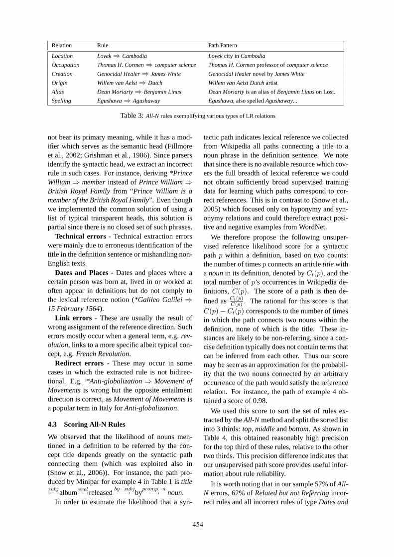
Relation Rule Path Pattern
Location Lovek⇒ Cambodia Lovekcity in Cambodia
Occupation Thomas H. Cormen⇒ computer science Thomas H. Cormenprofessor ofcomputer science
Creation Genocidal Healer⇒ James White Genocidal Healernovel byJames White
Origin Willem van Aelst⇒ Dutch Willem van Aelst Dutchartist
Alias Dean Moriarty⇒ Benjamin Linus Dean Moriartyis an alias ofBenjamin Linuson Lost.
Spelling Egushawa⇒ Agushaway Egushawa, also spelledAgushaway...
Table 3:All-N rules exemplifying various types of LR relations
not bear its primary meaning, while it has a mod-ifier which serves as the semantic head (Fillmoreet al., 2002; Grishman et al., 1986). Since parsersidentify the syntactic head, we extract an incorrectrule in such cases. For instance, deriving*PrinceWilliam⇒ memberinstead ofPrince William⇒British Royal Familyfrom “Prince William is amember of the British Royal Family”. Even thoughwe implemented the common solution of using alist of typical transparent heads, this solution ispartial since there is no closed set of such phrases.
Technical errors - Technical extraction errorswere mainly due to erroneous identification of thetitle in the definition sentence or mishandling non-English texts.
Dates and Places- Dates and places where acertain person was born at, lived in or worked atoften appear in definitions but do not comply tothe lexical reference notion (*Galileo Galilei ⇒15 February 1564).
Link errors - These are usually the result ofwrong assignment of the reference direction. Sucherrors mostly occur when a general term, e.g.rev-olution, links to a more specific albeit typical con-cept, e.g.French Revolution.
Redirect errors - These may occur in somecases in which the extracted rule is not bidirec-tional. E.g. *Anti-globalization⇒ Movement ofMovementsis wrong but the opposite entailmentdirection is correct, asMovement of Movementsisa popular term in Italy forAnti-globalization.
4.3 Scoring All-N Rules
We observed that the likelihood of nouns men-tioned in a definition to be referred by the con-cept title depends greatly on the syntactic pathconnecting them (which was exploited also in(Snow et al., 2006)). For instance, the path pro-duced by Minipar for example 4 in Table 1 istitlesubj←−albumvrel−→released
by−subj−→ bypcomp−n−→ noun.
In order to estimate the likelihood that a syn-
tactic path indicates lexical reference we collectedfrom Wikipedia all paths connecting a title to anoun phrase in the definition sentence. We notethat since there is no available resource which cov-ers the full breadth of lexical reference we couldnot obtain sufficiently broad supervised trainingdata for learning which paths correspond to cor-rect references. This is in contrast to (Snow et al.,2005) which focused only on hyponymy and syn-onymy relations and could therefore extract posi-tive and negative examples from WordNet.
We therefore propose the following unsuper-vised reference likelihood score for a syntacticpath p within a definition, based on two counts:the number of timesp connects an articletitle witha nounin its definition, denoted byCt(p), and thetotal number ofp’s occurrences in Wikipedia de-finitions, C(p). The score of a path is then de-fined asCt(p)
C(p) . The rational for this score is thatC(p)− Ct(p) corresponds to the number of timesin which the path connects two nouns within thedefinition, none of which is the title. These in-stances are likely to be non-referring, since a con-cise definition typically does not contain terms thatcan be inferred from each other. Thus our scoremay be seen as an approximation for the probabil-ity that the two nouns connected by an arbitraryoccurrence of the path would satisfy the referencerelation. For instance, the path of example 4 ob-tained a score of 0.98.
We used this score to sort the set of rules ex-tracted by theAll-N method and split the sorted listinto 3 thirds:top, middleandbottom. As shown inTable 4, this obtained reasonably high precisionfor the top third of these rules, relative to the othertwo thirds. This precision difference indicates thatour unsupervised path score provides useful infor-mation about rule reliability.
It is worth noting that in our sample 57% ofAll-N errors, 62% ofRelated but not Referringincor-rect rules and all incorrect rules of typeDates and
454
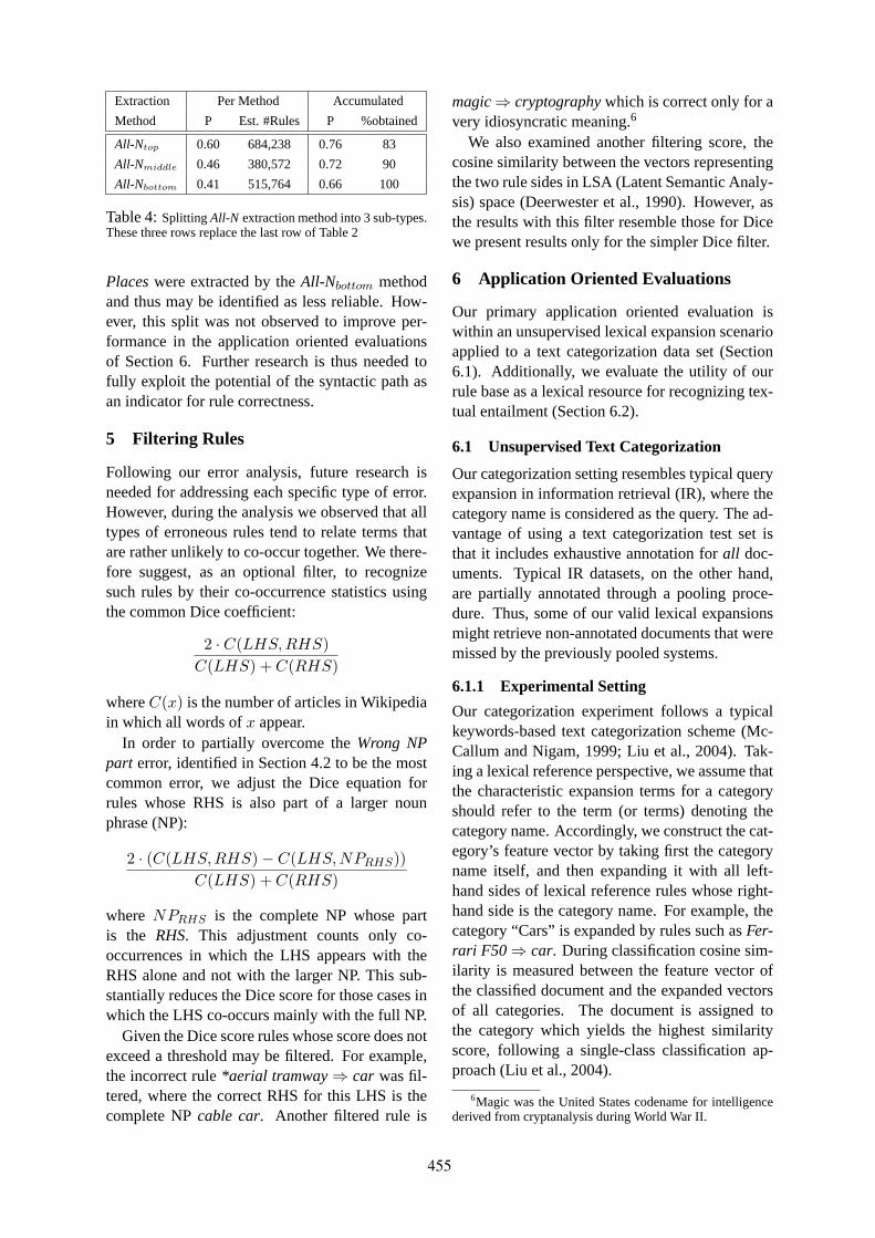
Extraction Per Method Accumulated
Method P Est. #Rules P %obtained
All-Ntop 0.60 684,238 0.76 83
All-Nmiddle 0.46 380,572 0.72 90
All-Nbottom 0.41 515,764 0.66 100
Table 4:SplittingAll-N extraction method into 3 sub-types.These three rows replace the last row of Table 2
Placeswere extracted by theAll-Nbottom methodand thus may be identified as less reliable. How-ever, this split was not observed to improve per-formance in the application oriented evaluationsof Section 6. Further research is thus needed tofully exploit the potential of the syntactic path asan indicator for rule correctness.
5 Filtering Rules
Following our error analysis, future research isneeded for addressing each specific type of error.However, during the analysis we observed that alltypes of erroneous rules tend to relate terms thatare rather unlikely to co-occur together. We there-fore suggest, as an optional filter, to recognizesuch rules by their co-occurrence statistics usingthe common Dice coefficient:
2 · C(LHS, RHS)C(LHS) + C(RHS)
whereC(x) is the number of articles in Wikipediain which all words ofx appear.
In order to partially overcome theWrong NPpart error, identified in Section 4.2 to be the mostcommon error, we adjust the Dice equation forrules whose RHS is also part of a larger nounphrase (NP):
2 · (C(LHS, RHS)− C(LHS, NPRHS))C(LHS) + C(RHS)
where NPRHS is the complete NP whose partis the RHS. This adjustment counts only co-occurrences in which the LHS appears with theRHS alone and not with the larger NP. This sub-stantially reduces the Dice score for those cases inwhich the LHS co-occurs mainly with the full NP.
Given the Dice score rules whose score does notexceed a threshold may be filtered. For example,the incorrect rule*aerial tramway⇒ car was fil-tered, where the correct RHS for this LHS is thecomplete NPcable car. Another filtered rule is
magic⇒ cryptographywhich is correct only for avery idiosyncratic meaning.6
We also examined another filtering score, thecosine similarity between the vectors representingthe two rule sides in LSA (Latent Semantic Analy-sis) space (Deerwester et al., 1990). However, asthe results with this filter resemble those for Dicewe present results only for the simpler Dice filter.
6 Application Oriented Evaluations
Our primary application oriented evaluation iswithin an unsupervised lexical expansion scenarioapplied to a text categorization data set (Section6.1). Additionally, we evaluate the utility of ourrule base as a lexical resource for recognizing tex-tual entailment (Section 6.2).
6.1 Unsupervised Text Categorization
Our categorization setting resembles typical queryexpansion in information retrieval (IR), where thecategory name is considered as the query. The ad-vantage of using a text categorization test set isthat it includes exhaustive annotation forall doc-uments. Typical IR datasets, on the other hand,are partially annotated through a pooling proce-dure. Thus, some of our valid lexical expansionsmight retrieve non-annotated documents that weremissed by the previously pooled systems.
6.1.1 Experimental Setting
Our categorization experiment follows a typicalkeywords-based text categorization scheme (Mc-Callum and Nigam, 1999; Liu et al., 2004). Tak-ing a lexical reference perspective, we assume thatthe characteristic expansion terms for a categoryshould refer to the term (or terms) denoting thecategory name. Accordingly, we construct the cat-egory’s feature vector by taking first the categoryname itself, and then expanding it with all left-hand sides of lexical reference rules whose right-hand side is the category name. For example, thecategory “Cars” is expanded by rules such asFer-rari F50⇒ car. During classification cosine sim-ilarity is measured between the feature vector ofthe classified document and the expanded vectorsof all categories. The document is assigned tothe category which yields the highest similarityscore, following a single-class classification ap-proach (Liu et al., 2004).
6Magic was the United States codename for intelligencederived from cryptanalysis during World War II.
455

Rule Base R P F1
Baselines:
No Expansion 0.19 0.54 0.28
WikiBL 0.19 0.53 0.28
Snow400K 0.19 0.54 0.28
Lin 0.25 0.39 0.30
WordNet 0.30 0.47 0.37
Extraction Methods from Wikipedia:
Redirect + Be-Comp 0.22 0.55 0.31
All rules 0.31 0.38 0.34
All rules + Dice filter 0.31 0.49 0.38
Union:
WordNet + WikiAll rules+Dice 0.35 0.47 0.40
Table 5:Results of different rule bases for 20 newsgroupscategory name expansion
It should be noted that keyword-based textcategorization systems employ various additionalsteps, such as bootstrapping, which generalize tomulti-class settings and further improve perfor-mance. Our basic implementation suffices to eval-uate comparatively the direct impact of differentexpansion resources on the initial classification.
For evaluation we used the test set of the“bydate” version of the 20-News Groups collec-tion,7 which contains 18,846 documents parti-tioned (nearly) evenly over the 20 categories8.
6.1.2 Baselines Results
We compare the quality of our rule base expan-sions to 5 baselines (Table 5). The first avoids anyexpansion, classifying documents based on cosinesimilarity with category names only. As expected,it yields relatively high precision but low recall,indicating the need for lexical expansion.
The second baseline is our implementation ofthe relevant part of the Wikipedia extraction in(Kazama and Torisawa, 2007), taking the firstnoun after abeverb in the definition sentence, de-noted asWikiBL. This baseline does not improveperformance at all over no expansion.
The next two baselines employ state-of-the-artlexical resources. One uses Snow’s extension toWordNet which was mentioned earlier. This re-source did not yield a noticeable improvement, ei-
7www.ai.mit.edu/people/jrennie/20Newsgroups.8The keywords used as category names are: athe-
ism; graphic; microsoft windows; ibm,pc,hardware;mac,hardware; x11,x-windows; sale; car; motorcycle;baseball; hockey; cryptography; electronics; medicine; outerspace; christian(noun & adj); gun; mideast,middle east;politics; religion
ther over theNo Expansionbaseline or overWord-Net when joined with its expansions. The sec-ond usesLin dependency similarity, a syntactic-dependency based distributional word similarityresource described in (Lin, 1998a)9. We used var-ious thresholds on the length of the expansion listderived from this resource. The best result, re-ported here, provides only a minor F1 improve-ment overNo Expansion, with modest recall in-crease and significant precision drop, as can be ex-pected from such distributional method.
The last baseline usesWordNetfor expansion.First we expand all the senses of each categoryname by their derivations and synonyms. Each ob-tained term is then expanded by its hyponyms, orby its meronyms if it has no hyponyms. Finally,the results are further expanded by their deriva-tions and synonyms.10 WordNetexpansions im-prove substantially both Recall and F1 relative toNo Expansion, while decreasing precision.
6.1.3 Wikipedia Results
We then used for expansion different subsetsof our rule base, producing alternative recall-precision tradeoffs. Table 5 presents the most in-teresting results. Using any subset of the rulesyields better performance than any of the otherautomatically constructed baselines (Lin, Snowand WikiBL). Utilizing the most precise extrac-tion methods ofRedirectandBe-Compyields thehighest precision, comparable toNo Expansion,but just a small recall increase. Using the entirerule base yields the highest recall, while filteringrules by the Dice coefficient (with 0.1 threshold)substantially increases precision without harmingrecall. With this configuration our automatically-constructed resource achieves comparable perfor-mance to the manually builtWordNet.
Finally, since a dictionary and an encyclopediaare complementary in nature, we applied the unionof WordNetand the filteredWikipediaexpansions.This configuration yields the best results: it main-tainsWordNet’s precision and adds nearly 50% tothe recall increase ofWordNetoverNo Expansion,indicating the substantial marginal contribution ofWikipedia. Furthermore, with the fast growth ofWikipedia the recall of our resource is expected toincrease while maintaining its precision.
9Downloaded from www.cs.ualberta.ca/lindek/demos.htm10We also tried expanding by the entire hyponym hierarchy
and considering only the first sense of each synset, but themethod described above achieved the best performance.
456

Category Name Expanding Terms
Politics opposition, coalition, whip(a)
Cryptography adversary, cryptosystem, key
Mac PowerBook, Radius(b), Grab(c)
Religion heaven, creation, belief, missionary
Medicine doctor, physician, treatment, clinical
Computer Graphics radiosity(d), rendering, siggraph(e)
Table 6:SomeWikipediarules not inWordNet, which con-tributed to text categorization. (a) a legislator who enforceleadership desire (b) a hardware firm specializing in Macin-tosh equipment (c) a Macintosh screen capture software (d)an illumination algorithm (e) a computer graphics conference
Configuration Accuracy Accuracy Drop
WordNet + Wikipedia 60.0 % -
Without WordNet 57.7 % 2.3 %
Without Wikipedia 58.9 % 1.1 %
Table 7:RTE accuracy results for ablation tests.
Table 6 illustrates few examples of useful rulesthat were found inWikipediabut not inWordNet.We conjecture that in other application settingsthe rules extracted from Wikipedia might showeven greater marginal contribution, particularly inspecialized domains not covered well by Word-Net. Another advantage of a resource based onWikipedia is that it is available in many more lan-guages than WordNet.
6.2 Recognizing Textual Entailment (RTE)
As a second application-oriented evaluation wemeasured the contributions of our (filtered)Wikipedia resource and WordNet to RTE infer-ence (Giampiccolo et al., 2007). To that end, weincorporated both resources within a typical basicRTE system architecture (Bar-Haim et al., 2008).This system determines whether a text entails an-other sentence based on various matching crite-ria that detect syntactic, logical and lexical cor-respondences (or mismatches). Most relevant forour evaluation, lexical matches are detected whena Wikipedia rule’s LHS appears in the text andits RHS in the hypothesis, or similarly when pairsof WordNet synonyms, hyponyms-hypernyms andderivations appear across the text and hypothesis.The system’s weights were trained on the devel-opment set of RTE-3 and tested on RTE-4 (whichincluded this year only a test set).
To measure the marginal contribution of the tworesources we performed ablation tests, comparingthe accuracy of the full system to that achieved
when removing either resource. Table 7 presentsthe results, which are similar in nature to those ob-tained for text categorization.Wikipediaobtaineda marginal contribution of 1.1%, about half of theanalogous contribution of WordNet’s manually-constructed information. We note that for currentRTE technology it is very typical to gain just afew percents in accuracy thanks to external knowl-edge resources, while individual resources usuallycontribute around 0.5–2% (Iftene and Balahur-Dobrescu, 2007; Dinu and Wang, 2009). SomeWikipediarules not in WordNet which contributedto RTE inference areJurassic Park⇒ MichaelCrichton, GCC⇒ Gulf Cooperation Council.
7 Conclusions and Future Work
We presented construction of a large-scale re-source of lexical reference rules, as useful in ap-plied lexical inference. Extensive rule-level analy-sis showed that different recall-precision tradeoffscan be obtained by utilizing different extractionmethods. It also identified major reasons for er-rors, pointing at potential future improvements.We further suggested a filtering method which sig-nificantly improved performance.
Even though the resource was constructed byquite simple extraction methods, it was proven tobe beneficial within two different application set-ting. While being an automatically built resource,extracted from a knowledge-base created for hu-man consumption, it showed comparable perfor-mance to WordNet, which was manually createdfor computational purposes. Most importantly, italso provides complementary knowledge to Word-Net, with unique lexical reference rules.
Future research is needed to improve resource’sprecision, especially for theAll-N method. Asa first step, we investigated a novel unsupervisedscore for rules extracted from definition sentences.We also intend to consider the rule base as a di-rected graph and exploit the graph structure forfurther rule extraction and validation.
Acknowledgments
The authors would like to thank Idan Szpektorfor valuable advices. This work was partiallysupported by the NEGEV project (www.negev-initiative.org), the PASCAL-2 Network of Excel-lence of the European Community FP7-ICT-2007-1-216886 and by the Israel Science Foundationgrant 1112/08.
457
ReferencesRoy Bar-Haim, Jonathan Berant, Ido Dagan, Iddo
Greental, Shachar Mirkin, Eyal Shnarch, and IdanSzpektor. 2008. Efficient semantic deduction andapproximate matching over compact parse forests.In Proceedings of TAC.
Martin S. Chodorow, Roy J. Byrd, and George E. Hei-dorn. 1985. Extracting semantic hierarchies from alarge on-line dictionary. InProceedings of ACL.
Ido Dagan, Oren Glickman, and Bernardo Magnini.2006. The pascal recognising textual entailmentchallenge. InLecture Notes in Computer Science,volume 3944, pages 177–190.
Scott Deerwester, Susan T. Dumais, George W. Furnas,Thomas K. Landauer, and Richard Harshman. 1990.Indexing by latent semantic analysis.Journal of theAmerican Society for Information Science, 41:391–407.
Georgiana Dinu and Rui Wang. 2009. Inference rulesfor recognizing textual entailment. InProceedingsof the IWCS.
Christiane Fellbaum, editor. 1998.WordNet: An Elec-tronic Lexical Database (Language, Speech, andCommunication). The MIT Press.
Charles J. Fillmore, Collin F. Baker, and Hiroaki Sato.2002. Seeing arguments through transparent struc-tures. InProceedings of LREC.
Evgeniy Gabrilovich and Shaul Markovitch. 2007.Computing semantic relatedness using wikipedia-based explicit semantic analysis. InProceedings ofIJCAI.
Danilo Giampiccolo, Bernardo Magnini, Ido Dagan,and Bill Dolan. 2007. The third pascal recogniz-ing textual entailment challenge. InProceedings ofACL-WTEP Workshop.
Oren Glickman, Eyal Shnarch, and Ido Dagan. 2006.Lexical reference: a semantic matching subtask. InProceedings of EMNLP.
Ralph Grishman, Lynette Hirschman, and Ngo ThanhNhan. 1986. Discovery procedures for sublanguageselectional patterns: Initial experiments.Computa-tional Linguistics, 12(3):205–215.
Marti Hearst. 1992. Automatic acquisition of hy-ponyms from large text corpora. InProceedings ofCOLING.
Nancy Ide and V́eronis Jean. 1993. Extractingknowledge bases from machine-readable dictionar-ies: Have we wasted our time? InProceedings ofKB & KS Workshop.
Adrian Iftene and Alexandra Balahur-Dobrescu. 2007.Hypothesis transformation and semantic variabilityrules used in recognizing textual entailment. InPro-ceedings of the ACL-PASCAL Workshop on TextualEntailment and Paraphrasing.
Jun’ichi Kazama and Kentaro Torisawa. 2007. Ex-ploiting Wikipedia as external knowledge for namedentity recognition. InProceedings of EMNLP-CoNLL.
J. Richard Landis and Gary G. Koch. 1997. Themeasurements of observer agreement for categoricaldata. InBiometrics, pages 33:159–174.
Dekang Lin. 1998a. Automatic retrieval and clusteringof similar words. InProceedings of COLING-ACL.
Dekang Lin. 1998b. Dependency-based evaluation ofMINIPAR. In Proceedings of the Workshop on Eval-uation of Parsing Systems at LREC.
Bing Liu, Xiaoli Li, Wee Sun Lee, and Philip S. Yu.2004. Text classification by labeling words. InPro-ceedings of AAAI.
Andrew McCallum and Kamal Nigam. 1999. Textclassification by bootstrapping with keywords, EMand shrinkage. InProceedings of ACL Workshop forunsupervised Learning in NLP.
Dan Moldovan and Vasile Rus. 2001. Logic formtransformation of wordnet and its applicability toquestion answering. InProceedings of ACL.
Simone P. Ponzetto and Michael Strube. 2007. De-riving a large scale taxonomy from wikipedia. InProceedings of AAAI.
Reinhard Rapp. 2002. The computation of word asso-ciations: comparing syntagmatic and paradigmaticapproaches. InProceedings of COLING.
Gerda Ruge. 1992. Experiment on linguistically-basedterm associations.Information Processing & Man-agement, 28(3):317–332.
Rion Snow, Daniel Jurafsky, and Andrew Y. Ng. 2005.Learning syntactic patterns for automatic hypernymdiscovery. InNIPS.
Rion Snow, Daniel Jurafsky, and Andrew Y. Ng. 2006.Semantic taxonomy induction from heterogenousevidence. InProceedings of COLING-ACL.
Fabian M. Suchanek, Gjergji Kasneci, and GerhardWeikum. 2007. Yago: A core of semantic knowl-edge - unifying wordnet and wikipedia. InProceed-ings of WWW.
Antonio Toral and Rafael Mũnoz. 2007. A proposalto automatically build and maintain gazetteers fornamed entity recognition by using wikipedia. InProceedings of NAACL/HLT.
Yorick A. Wilks, Brian M. Slator, and Louise M.Guthrie. 1996.Electric words: dictionaries, com-puters, and meanings. MIT Press, Cambridge, MA,USA.
Torsten Zesch, Iryna Gurevych, and Max Mühlhäuser.2007. Analyzing and accessing wikipedia as a lex-ical semantic resource. InData Structures for Lin-guistic Resources and Applications, pages 197–205.
458
Proceedings of the 47th Annual Meeting of the ACL and the 4th IJCNLP of the AFNLP, pages 459–467,Suntec, Singapore, 2-7 August 2009. c©2009 ACL and AFNLP
Employing Topic Models for Pattern-based Semantic Class Discovery
Huibin Zhang1*
Mingjie Zhu2*
Shuming Shi3 Ji-Rong Wen
3
1Nankai University
2University of Science and Technology of China
3Microsoft Research Asia
{v-huibzh, v-mingjz, shumings, jrwen}@microsoft.com
Abstract
A semantic class is a collection of items (words or phrases) which have semantically
peer or sibling relationship. This paper studies
the employment of topic models to automati-
cally construct semantic classes, taking as the
source data a collection of raw semantic
classes (RASCs), which were extracted by ap-
plying predefined patterns to web pages. The
primary requirement (and challenge) here is
dealing with multi-membership: An item may
belong to multiple semantic classes; and we
need to discover as many as possible the dif-ferent semantic classes the item belongs to. To
adopt topic models, we treat RASCs as “doc-
uments”, items as “words”, and the final se-
mantic classes as “topics”. Appropriate
preprocessing and postprocessing are per-
formed to improve results quality, to reduce
computation cost, and to tackle the fixed-k
constraint of a typical topic model. Experi-
ments conducted on 40 million web pages
show that our approach could yield better re-
sults than alternative approaches.
1 Introduction
Semantic class construction (Lin and Pantel,
2001; Pantel and Lin, 2002; Pasca, 2004; Shinza-
to and Torisawa, 2005; Ohshima et al., 2006) tries to discover the peer or sibling relationship
among terms or phrases by organizing them into
semantic classes. For example, {red, white,
black…} is a semantic class consisting of color instances. A popular way for semantic class dis-
covery is pattern-based approach, where prede-
fined patterns (Table 1) are applied to a
This work was performed when the authors were interns at
Microsoft Research Asia
collection of web pages or an online web search engine to produce some raw semantic classes
(abbreviated as RASCs, Table 2). RASCs cannot
be treated as the ultimate semantic classes, be-cause they are typically noisy and incomplete, as
shown in Table 2. In addition, the information of
one real semantic class may be distributed in lots of RASCs (R2 and R3 in Table 2).
Type Pattern SENT NP {, NP}
*{,} (and|or) {other} NP
TAG <UL> <LI>item</LI> … <LI>item</LI> </UL>
TAG <SELECT> <OPTION>item…<OPTION>item </SELECT>
* SENT: Sentence structure patterns; TAG: HTML Tag patterns
Table 1. Sample patterns
R1: {gold, silver, copper, coal, iron, uranium}
R2: {red, yellow, color, gold, silver, copper}
R3: {red, green, blue, yellow}
R4: {HTML, Text, PDF, MS Word, Any file type}
R5: {Today, Tomorrow, Wednesday, Thursday, Friday, Saturday, Sunday}
R6: {Bush, Iraq, Photos, USA, War}
Table 2. Sample raw semantic classes (RASCs)
This paper aims to discover high-quality se-
mantic classes from a large collection of noisy RASCs. The primary requirement (and chal-
lenge) here is to deal with multi-membership, i.e.,
one item may belong to multiple different seman-tic classes. For example, the term “Lincoln” can
simultaneously represent a person, a place, or a
car brand name. Multi-membership is more pop-
ular than at a first glance, because quite a lot of English common words have also been borrowed
as company names, places, or product names.
For a given item (as a query) which belongs to multiple semantic classes, we intend to return the
semantic classes separately, rather than mixing
all their items together. Existing pattern-based approaches only pro-
vide very limited support to multi-membership.
For example, RASCs with the same labels (or
hypernyms) are merged in (Pasca, 2004) to gen-
459
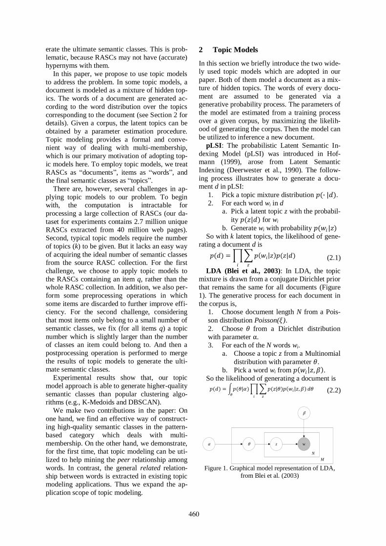
erate the ultimate semantic classes. This is prob-
lematic, because RASCs may not have (accurate) hypernyms with them.
In this paper, we propose to use topic models
to address the problem. In some topic models, a document is modeled as a mixture of hidden top-
ics. The words of a document are generated ac-
cording to the word distribution over the topics
corresponding to the document (see Section 2 for details). Given a corpus, the latent topics can be
obtained by a parameter estimation procedure.
Topic modeling provides a formal and conve-nient way of dealing with multi-membership,
which is our primary motivation of adopting top-
ic models here. To employ topic models, we treat
RASCs as “documents”, items as “words”, and the final semantic classes as “topics”.
There are, however, several challenges in ap-
plying topic models to our problem. To begin with, the computation is intractable for
processing a large collection of RASCs (our da-
taset for experiments contains 2.7 million unique RASCs extracted from 40 million web pages).
Second, typical topic models require the number
of topics (k) to be given. But it lacks an easy way
of acquiring the ideal number of semantic classes from the source RASC collection. For the first
challenge, we choose to apply topic models to
the RASCs containing an item q, rather than the whole RASC collection. In addition, we also per-
form some preprocessing operations in which
some items are discarded to further improve effi-ciency. For the second challenge, considering
that most items only belong to a small number of
semantic classes, we fix (for all items q) a topic
number which is slightly larger than the number of classes an item could belong to. And then a
postprocessing operation is performed to merge
the results of topic models to generate the ulti-mate semantic classes.
Experimental results show that, our topic
model approach is able to generate higher-quality
semantic classes than popular clustering algo-rithms (e.g., K-Medoids and DBSCAN).
We make two contributions in the paper: On
one hand, we find an effective way of construct-ing high-quality semantic classes in the pattern-
based category which deals with multi-
membership. On the other hand, we demonstrate, for the first time, that topic modeling can be uti-
lized to help mining the peer relationship among
words. In contrast, the general related relation-
ship between words is extracted in existing topic modeling applications. Thus we expand the ap-
plication scope of topic modeling.
2 Topic Models
In this section we briefly introduce the two wide-ly used topic models which are adopted in our
paper. Both of them model a document as a mix-
ture of hidden topics. The words of every docu-
ment are assumed to be generated via a generative probability process. The parameters of
the model are estimated from a training process
over a given corpus, by maximizing the likelih-ood of generating the corpus. Then the model can
be utilized to inference a new document.
pLSI: The probabilistic Latent Semantic In-
dexing Model (pLSI) was introduced in Hof-mann (1999), arose from Latent Semantic
Indexing (Deerwester et al., 1990). The follow-
ing process illustrates how to generate a docu-ment d in pLSI:
1. Pick a topic mixture distribution 𝑝(∙ |𝑑).
2. For each word wi in d a. Pick a latent topic z with the probabil-
ity 𝑝(𝑧|𝑑) for wi
b. Generate wi with probability 𝑝(𝑤𝑖 |𝑧)
So with k latent topics, the likelihood of gene-rating a document d is
𝑝(𝑑) = 𝑝 𝑤𝑖 𝑧 𝑝(𝑧|𝑑)
𝑧𝑖
(2.1)
LDA (Blei et al., 2003): In LDA, the topic mixture is drawn from a conjugate Dirichlet prior
that remains the same for all documents (Figure
1). The generative process for each document in
the corpus is, 1. Choose document length N from a Pois-
son distribution Poisson(𝜉).
2. Choose 𝜃 from a Dirichlet distribution
with parameter α.
3. For each of the N words wi.
a. Choose a topic z from a Multinomial
distribution with parameter 𝜃.
b. Pick a word wi from 𝑝 𝑤𝑖 𝑧,𝛽 . So the likelihood of generating a document is
𝑝(𝑑) = 𝑝(𝜃|𝛼)𝜃
𝑝(𝑧|𝜃)𝑝 𝑤𝑖 𝑧,𝛽 𝑑𝜃
𝑧𝑖
(2.2)
Figure 1. Graphical model representation of LDA,
from Blei et al. (2003)
wθ zα
β
N
M
460

3 Our Approach
The source data of our approach is a collection (denoted as CR) of RASCs extracted via applying
patterns to a large collection of web pages. Given
an item as an input query, the output of our ap-
proach is one or multiple semantic classes for the item. To be applicable in real-world dataset, our
approach needs to be able to process at least mil-
lions of RASCs.
3.1 Main Idea
As reviewed in Section 2, topic modeling pro-
vides a formal and convenient way of grouping
documents and words to topics. In order to apply topic models to our problem, we map RASCs to
documents, items to words, and treat the output
topics yielded from topic modeling as our seman-
tic classes (Table 3). The motivation of utilizing topic modeling to solve our problem and building
the above mapping comes from the following
observations. 1) In our problem, one item may belong to
multiple semantic classes; similarly in topic
modeling, a word can appear in multiple top-ics.
2) We observe from our source data that
some RASCs are comprised of items in mul-
tiple semantic classes. And at the same time, one document could be related to multiple
topics in some topic models (e.g., pLSI and
LDA).
Topic modeling Semantic class construction
word item (word or phrase)
document RASC
topic semantic class
Table 3. The mapping from the concepts in topic modeling to those in semantic class construction
Due to the above observations, we hope topic
modeling can be employed to construct semantic classes from RASCs, just as it has been used in
assigning documents and words to topics.
There are some critical challenges and issues
which should be properly addressed when topic models are adopted here.
Efficiency: Our RASC collection CR contains
about 2.7 million unique RASCs and 26 million (1 million unique) items. Building topic models
directly for such a large dataset may be computa-
tionally intractable. To overcome this challenge,
we choose to apply topic models to the RASCs containing a specific item rather than the whole
RASC collection. Please keep in mind that our
goal in this paper is to construct the semantic
classes for an item when the item is given as a query. For one item q, we denote CR(q) to be all
the RASCs in CR containing the item. We believe
building a topic model over CR(q) is much more effective because it contains significantly fewer
“documents”, “words”, and “topics”. To further
improve efficiency, we also perform preprocess-
ing (refer to Section 3.4 for details) before build-ing topic models for CR(q), where some low-
frequency items are removed.
Determine the number of topics: Most topic models require the number of topics to be known
beforehand1. However, it is not an easy task to
automatically determine the exact number of se-
mantic classes an item q should belong to. Ac-tually the number may vary for different q. Our
solution is to set (for all items q) the topic num-
ber to be a fixed value (k=5 in our experiments) which is slightly larger than the number of se-
mantic classes most items could belong to. Then
we perform postprocessing for the k topics to produce the final properly semantic classes.
In summary, our approach contains three
phases (Figure 2). We build topic models for
every CR(q), rather than the whole collection CR. A preprocessing phase and a postprocessing
phase are added before and after the topic model-
ing phase to improve efficiency and to overcome the fixed-k problem. The details of each phase
are presented in the following subsections.
Figure 2. Main phases of our approach
3.2 Adopting Topic Models
For an item q, topic modeling is adopted to
process the RASCs in CR(q) to generate k seman-
tic classes. Here we use LDA as an example to
1 Although there is study of non-parametric Bayesian mod-els (Li et al., 2007) which need no prior knowledge of topic number, the computational complexity seems to exceed our efficiency requirement and we shall leave this to future work.
R580
R1
R2
CR
Item q
Preprocessing
𝑅400∗
𝑅1∗
𝑅2∗
T5
T1
T2
C3
C1
C2
Topic modeling
Postprocessing
T3
T4
CR(q)
461

illustrate the process. The case of other genera-
tive topic models (e.g., pLSI) is very similar. According to the assumption of LDA and our
concept mapping in Table 3, a RASC (“docu-
ment”) is viewed as a mixture of hidden semantic classes (“topics”). The generative process for a
RASC R in the “corpus” CR(q) is as follows,
1) Choose a RASC size (i.e., the number of
items in R): NR ~ Poisson(𝜉).
2) Choose a k-dimensional vector 𝜃𝑅 from a
Dirichlet distribution with parameter 𝛼.
3) For each of the NR items an:
a) Pick a semantic class 𝑧𝑛 from a mul-
tinomial distribution with parameter
𝜃𝑅 .
b) Pick an item an from 𝑝(𝑎𝑛 |𝑧𝑛 ,𝛽) , where the item probabilities are pa-
rameterized by the matrix 𝛽.
There are three parameters in the model: 𝜉 (a
scalar), 𝛼 (a k-dimensional vector), and 𝛽 (a
𝑘 × 𝑉 matrix where V is the number of distinct
items in CR(q)). The parameter values can be ob-
tained from a training (or called parameter esti-mation) process over CR(q), by maximizing the
likelihood of generating the corpus. Once 𝛽 is
determined, we are able to compute 𝑝(𝑎|𝑧,𝛽),
the probability of item a belonging to semantic class z. Therefore we can determine the members
of a semantic class z by selecting those items
with high 𝑝 𝑎 𝑧,𝛽 values. The number of topics k is assumed known and
fixed in LDA. As has been discussed in Section
3.1, we set a constant k value for all different
CR(q). And we rely on the postprocessing phase to merge the semantic classes produced by the
topic model to generate the ultimate semantic
classes. When topic modeling is used in document
classification, an inference procedure is required
to determine the topics for a new document. Please note that inference is not needed in our
problem.
One natural question here is: Considering that
in most topic modeling applications, the words within a resultant topic are typically semantically
related but may not be in peer relationship, then
what is the intuition that the resultant topics here are semantic classes rather than lists of generally
related words? The magic lies in the “docu-
ments” we used in employing topic models.
Words co-occurred in real documents tend to be semantically related; while items co-occurred in
RASCs tend to be peers. Experimental results
show that most items in the same output seman-tic class have peer relationship.
It might be noteworthy to mention the exchan-
geability or “bag-of-words” assumption in most topic models. Although the order of words in a
document may be important, standard topic mod-
els neglect the order for simplicity and other rea-sons
2. The order of items in a RASC is clearly
much weaker than the order of words in an ordi-
nary document. In some sense, topic models are
more suitable to be used here than in processing an ordinary document corpus.
3.3 Preprocessing and Postprocessing
Preprocessing is applied to CR(q) before we build
topic models for it. In this phase, we discard from all RASCs the items with frequency (i.e.,
the number of RASCs containing the item) less
than a threshold h. A RASC itself is discarded from CR(q) if it contains less than two items after
the item-removal operations. We choose to re-
move low-frequency items, because we found
that low-frequency items are seldom important members of any semantic class for q. So the goal
is to reduce the topic model training time (by
reducing the training data) without sacrificing results quality too much. In the experiments sec-
tion, we compare the approaches with and with-
out preprocessing in terms of results quality and efficiency. Interestingly, experimental results
show that, for some small threshold values, the
results quality becomes higher after preprocess-
ing is performed. We will give more discussions in Section 4.
In the postprocessing phase, the output seman-
tic classes (“topics”) of topic modeling are merged to generate the ultimate semantic classes.
As indicated in Sections 3.1 and 3.2, we fix the
number of topics (k=5) for different corpus CR(q)
in employing topic models. For most items q, this is a larger value than the real number of se-
mantic classes the item belongs to. As a result,
one real semantic class may be divided into mul-tiple topics. Therefore one core operation in this
phase is to merge those topics into one semantic
class. In addition, the items in each semantic class need to be properly ordered. Thus main
operations include,
1) Merge semantic classes
2) Sort the items in each semantic class Now we illustrate how to perform the opera-
tions.
Merge semantic classes: The merge process is performed by repeatedly calculating the simi-
2 There are topic model extensions considering word order in documents, such as Griffiths et al. (2005).
462
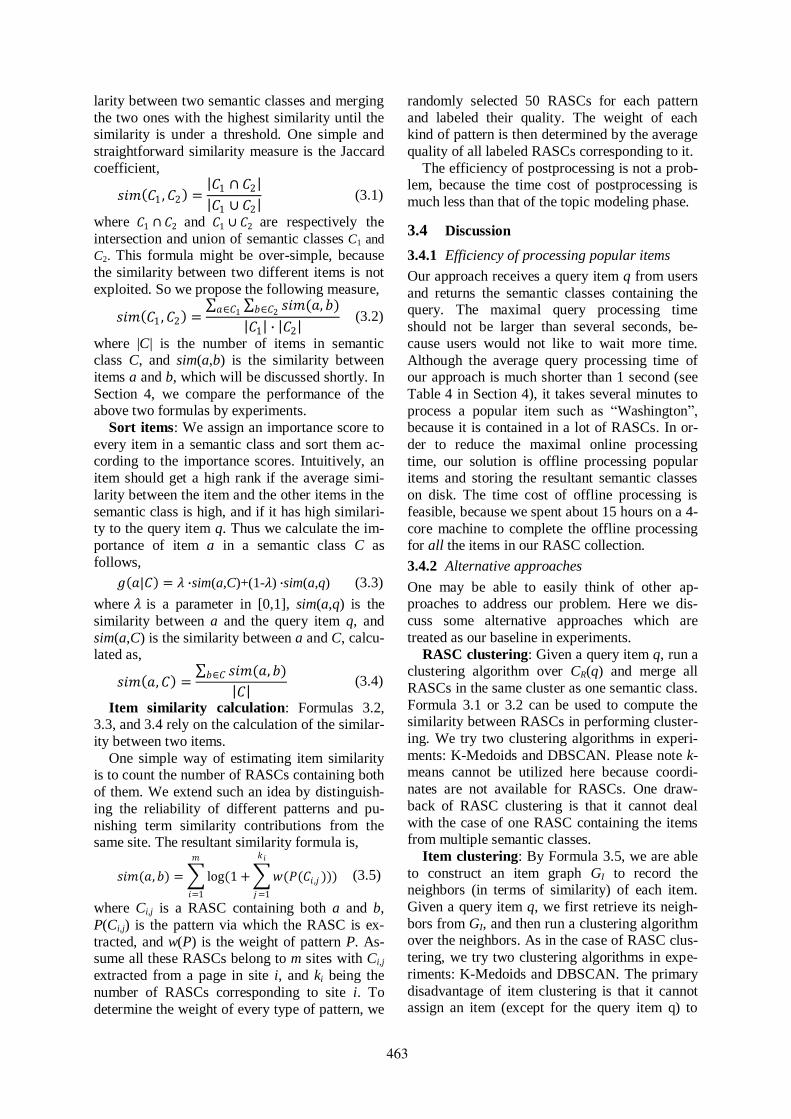
larity between two semantic classes and merging
the two ones with the highest similarity until the similarity is under a threshold. One simple and
straightforward similarity measure is the Jaccard
coefficient,
𝑠𝑖𝑚 𝐶1 ,𝐶2 = 𝐶1 ∩ 𝐶2
𝐶1 ∪ 𝐶2 (3.1)
where 𝐶1 ∩ 𝐶2 and 𝐶1 ∪ 𝐶2 are respectively the
intersection and union of semantic classes C1 and
C2. This formula might be over-simple, because
the similarity between two different items is not
exploited. So we propose the following measure,
𝑠𝑖𝑚 𝐶1 ,𝐶2 = 𝑠𝑖𝑚(𝑎, 𝑏)𝑏∈𝐶2𝑎∈𝐶1
𝐶1 ∙ 𝐶2 (3.2)
where |C| is the number of items in semantic class C, and sim(a,b) is the similarity between
items a and b, which will be discussed shortly. In
Section 4, we compare the performance of the above two formulas by experiments.
Sort items: We assign an importance score to
every item in a semantic class and sort them ac-cording to the importance scores. Intuitively, an
item should get a high rank if the average simi-
larity between the item and the other items in the
semantic class is high, and if it has high similari-ty to the query item q. Thus we calculate the im-
portance of item a in a semantic class C as
follows,
𝑔 𝑎|𝐶 = 𝜆 ∙sim(a,C)+(1-𝜆) ∙sim(a,q) (3.3)
where 𝜆 is a parameter in [0,1], sim(a,q) is the
similarity between a and the query item q, and
sim(a,C) is the similarity between a and C, calcu-lated as,
𝑠𝑖𝑚 𝑎,𝐶 = 𝑠𝑖𝑚(𝑎, 𝑏)𝑏∈𝐶
𝐶 (3.4)
Item similarity calculation: Formulas 3.2, 3.3, and 3.4 rely on the calculation of the similar-
ity between two items.
One simple way of estimating item similarity is to count the number of RASCs containing both
of them. We extend such an idea by distinguish-
ing the reliability of different patterns and pu-
nishing term similarity contributions from the same site. The resultant similarity formula is,
𝑠𝑖𝑚(𝑎,𝑏) = log(1 + 𝑤(𝑃(𝐶𝑖 ,𝑗 ))
𝑘𝑖
𝑗=1
)
𝑚
𝑖=1
(3.5)
where Ci,j is a RASC containing both a and b,
P(Ci,j) is the pattern via which the RASC is ex-
tracted, and w(P) is the weight of pattern P. As-sume all these RASCs belong to m sites with Ci,j
extracted from a page in site i, and ki being the
number of RASCs corresponding to site i. To
determine the weight of every type of pattern, we
randomly selected 50 RASCs for each pattern
and labeled their quality. The weight of each kind of pattern is then determined by the average
quality of all labeled RASCs corresponding to it.
The efficiency of postprocessing is not a prob-lem, because the time cost of postprocessing is
much less than that of the topic modeling phase.
3.4 Discussion
3.4.1 Efficiency of processing popular items
Our approach receives a query item q from users
and returns the semantic classes containing the query. The maximal query processing time
should not be larger than several seconds, be-
cause users would not like to wait more time.
Although the average query processing time of our approach is much shorter than 1 second (see
Table 4 in Section 4), it takes several minutes to
process a popular item such as “Washington”, because it is contained in a lot of RASCs. In or-
der to reduce the maximal online processing
time, our solution is offline processing popular items and storing the resultant semantic classes
on disk. The time cost of offline processing is
feasible, because we spent about 15 hours on a 4-
core machine to complete the offline processing for all the items in our RASC collection.
3.4.2 Alternative approaches
One may be able to easily think of other ap-proaches to address our problem. Here we dis-
cuss some alternative approaches which are
treated as our baseline in experiments.
RASC clustering: Given a query item q, run a clustering algorithm over CR(q) and merge all
RASCs in the same cluster as one semantic class.
Formula 3.1 or 3.2 can be used to compute the similarity between RASCs in performing cluster-
ing. We try two clustering algorithms in experi-
ments: K-Medoids and DBSCAN. Please note k-means cannot be utilized here because coordi-
nates are not available for RASCs. One draw-
back of RASC clustering is that it cannot deal
with the case of one RASC containing the items from multiple semantic classes.
Item clustering: By Formula 3.5, we are able
to construct an item graph GI to record the neighbors (in terms of similarity) of each item.
Given a query item q, we first retrieve its neigh-
bors from GI, and then run a clustering algorithm over the neighbors. As in the case of RASC clus-
tering, we try two clustering algorithms in expe-
riments: K-Medoids and DBSCAN. The primary
disadvantage of item clustering is that it cannot assign an item (except for the query item q) to
463

multiple semantic classes. As a result, when we
input “gold” as the query, the item “silver” can only be assigned to one semantic class, although
the term can simultaneously represents a color
and a chemical element.
4 Experiments
4.1 Experimental Setup
Datasets: By using the Open Directory Project (ODP
3) URLs as seeds, we crawled about 40 mil-
lion English web pages in a breadth-first way.
RASCs are extracted via applying a list of sen-tence structure patterns and HTML tag patterns
(see Table 1 for some examples). Our RASC col-
lection CR contains about 2.7 million unique RASCs and 1 million distinct items.
Query set and labeling: We have volunteers
to try Google Sets4, record their queries being
used, and select overall 55 queries to form our query set. For each query, the results of all ap-
proaches are mixed together and labeled by fol-
lowing two steps. In the first step, the standard (or ideal) semantic classes (SSCs) for the query
are manually determined. For example, the ideal
semantic classes for item “Georgia” may include
Countries, and U.S. states. In the second step, each item is assigned a label of “Good”, “Fair”,
or “Bad” with respect to each SSC. For example,
“silver” is labeled “Good” with respect to “col-ors” and “chemical elements”. We adopt metric
MnDCG (Section 4.2) as our evaluation metric.
Approaches for comparison: We compare our approach with the alternative approaches dis-
cussed in Section 3.4.2.
LDA: Our approach with LDA as the topic
model. The implementation of LDA is based on Blei’s code of variational EM for LDA
5.
pLSI: Our approach with pLSI as the topic
model. The implementation of pLSI is based on Schein, et al. (2002).
KMedoids-RASC: The RASC clustering ap-
proach illustrated in Section 3.4.2, with the K-Medoids clustering algorithm utilized.
DBSCAN-RASC: The RASC clustering ap-
proach with DBSCAN utilized.
KMedoids-Item: The item clustering ap-proach with the K-Medoids utilized.
DBSCAN-Item: The item clustering ap-
proach with the DBSCAN clustering algo-rithm utilized.
3 http://www.dmoz.org 4 http://labs.google.com/sets 5 http://www.cs.princeton.edu/~blei/lda-c/
K-Medoids clustering needs to predefine the
cluster number k. We fix the k value for all dif-ferent query item q, as has been done for the top-
ic model approach. For fair comparison, the same
postprocessing is made for all the approaches. And the same preprocessing is made for all the
approaches except for the item clustering ones
(to which the preprocessing is not applicable).
4.2 Evaluation Methodology
Each produced semantic class is an ordered list of items. A couple of metrics in the information
retrieval (IR) community like Precision@10,
MAP (mean average precision), and nDCG (normalized discounted cumulative gain) are
available for evaluating a single ranked list of
items per query (Croft et al., 2009). Among the metrics, nDCG (Jarvelin and Kekalainen, 2000)
can handle our three-level judgments (“Good”,
“Fair”, and “Bad”, refer to Section 4.1),
𝑛𝐷𝐶𝐺@𝑘 = 𝐺 𝑖 /log(𝑖 + 1)𝑘𝑖=1
𝐺∗ 𝑖 /log(𝑖 + 1)𝑘𝑖=1
(4.1)
where G(i) is the gain value assigned to the i’th
item, and G*(i) is the gain value assigned to the
i’th item of an ideal (or perfect) ranking list.
Here we extend the IR metrics to the evalua-
tion of multiple ordered lists per query. We use nDCG as the basic metric and extend it to
MnDCG.
Assume labelers have determined m SSCs (SSC1~SSCm, refer to Section 4.1) for query q
and the weight (or importance) of SSCi is wi. As-
sume n semantic classes are generated by an ap-
proach and n1 of them have corresponding SSCs (i.e., no appropriate SSC can be found for the
remaining n-n1 semantic classes). We define the
MnDCG score of an approach (with respect to query q) as,
𝑀𝑛𝐷𝐶𝐺 𝑞 =𝑛1
𝑛∙ 𝑤𝑖 ∙ 𝑆𝑐𝑜𝑟𝑒(SSC𝑖)𝑚i=1
𝑤𝑖mi=1
(4.2)
where
𝑆𝑐𝑜𝑟𝑒 𝑆𝑆𝐶𝑖 =
0 𝑖𝑓 𝑘𝑖 = 01
𝑘𝑖max𝑗 ∈[1, 𝑘𝑖]
(𝑛𝐷𝐶𝐺 𝐺𝑖 ,𝑗 ) 𝑖𝑓 𝑘𝑖 ≠ 0 (4.3)
In the above formula, nDCG(Gi,j) is the nDCG
score of semantic class Gi,j; and ki denotes the
number of semantic classes assigned to SSCi. For a list of queries, the MnDCG score of an algo-
rithm is the average of all scores for the queries.
The metric is designed to properly deal with
the following cases,
464

i). One semantic class is wrongly split into
multiple ones: Punished by dividing 𝑘𝑖 in Formula 4.3;
ii). A semantic class is too noisy to be as-
signed to any SSC: Processed by the
“n1/n” in Formula 4.2; iii). Fewer semantic classes (than the number
of SSCs) are produced: Punished in For-
mula 4.3 by assigning a zero value. iv). Wrongly merge multiple semantic
classes into one: The nDCG score of the
merged one will be small because it is computed with respect to only one single
SSC.
The gain values of nDCG for the three relev-
ance levels (“Bad”, “Fair”, and “Good”) are re-spectively -1, 1, and 2 in experiments.
4.3 Experimental Results
4.3.1 Overall performance comparison
Figure 3 shows the performance comparison be-
tween the approaches listed in Section 4.1, using metrics MnDCG@n (n=1…10). Postprocessing
is performed for all the approaches, where For-
mula 3.2 is adopted to compute the similarity
between semantic classes. The results show that that the topic modeling approaches produce
higher-quality semantic classes than the other
approaches. It indicates that the topic mixture assumption of topic modeling can handle the
multi-membership problem very well here.
Among the alternative approaches, RASC clus-
tering behaves better than item clustering. The reason might be that an item cannot belong to
multiple clusters in the two item clustering ap-
proaches, while RASC clustering allows this. For the RASC clustering approaches, although one
item has the chance to belong to different seman-
tic classes, one RASC can only belong to one semantic class.
Figure 3. Quality comparison (MnDCG@n) among
approaches (frequency threshold h = 4 in preprocess-
ing; k = 5 in topic models)
4.3.2 Preprocessing experiments
Table 4 shows the average query processing time
and results quality of the LDA approach, by va-
rying frequency threshold h. Similar results are observed for the pLSI approach. In the table, h=1
means no preprocessing is performed. The aver-
age query processing time is calculated over all items in our dataset. As the threshold h increases,
the processing time decreases as expected, be-
cause the input of topic modeling gets smaller. The second column lists the results quality
(measured by MnDCG@10). Interestingly, we
get the best results quality when h=4 (i.e., the
items with frequency less than 4 are discarded). The reason may be that most low-frequency
items are noisy ones. As a result, preprocessing
can improve both results quality and processing efficiency; and h=4 seems a good choice in pre-
processing for our dataset.
h Avg. Query Proc.
Time (seconds) Quality
(MnDCG@10) 1 0.414 0.281
2 0.375 0.294
3 0.320 0.322
4 0.268 0.331
5 0.232 0.328
6 0.210 0.315
7 0.197 0.315
8 0.184 0.313
9 0.173 0.288
Table 4. Time complexity and quality comparison
among LDA approaches of different thresholds
4.3.3 Postprocessing experiments
Figure 4. Results quality comparison among topic
modeling approaches with and without postprocessing
(metric: MnDCG@10)
The effect of postprocessing is shown in Figure 4. In the figure, NP means no postprocessing is
performed. Sim1 and Sim2 respectively mean
Formula 3.1 and Formula 3.2 are used in post-
processing as the similarity measure between
0
0.05
0.1
0.15
0.2
0.25
0.3
0.35
0.4
0.45
1 2 3 4 5 6 7 8 9 10
pLSI LDA KMedoids-RASC
DBSCAN-RASC KMedoids-Item DBSCAN-Itemn
0.27
0.28
0.29
0.3
0.31
0.32
0.33
0.34
LDA pLSI
NP
Sim1
Sim2
465
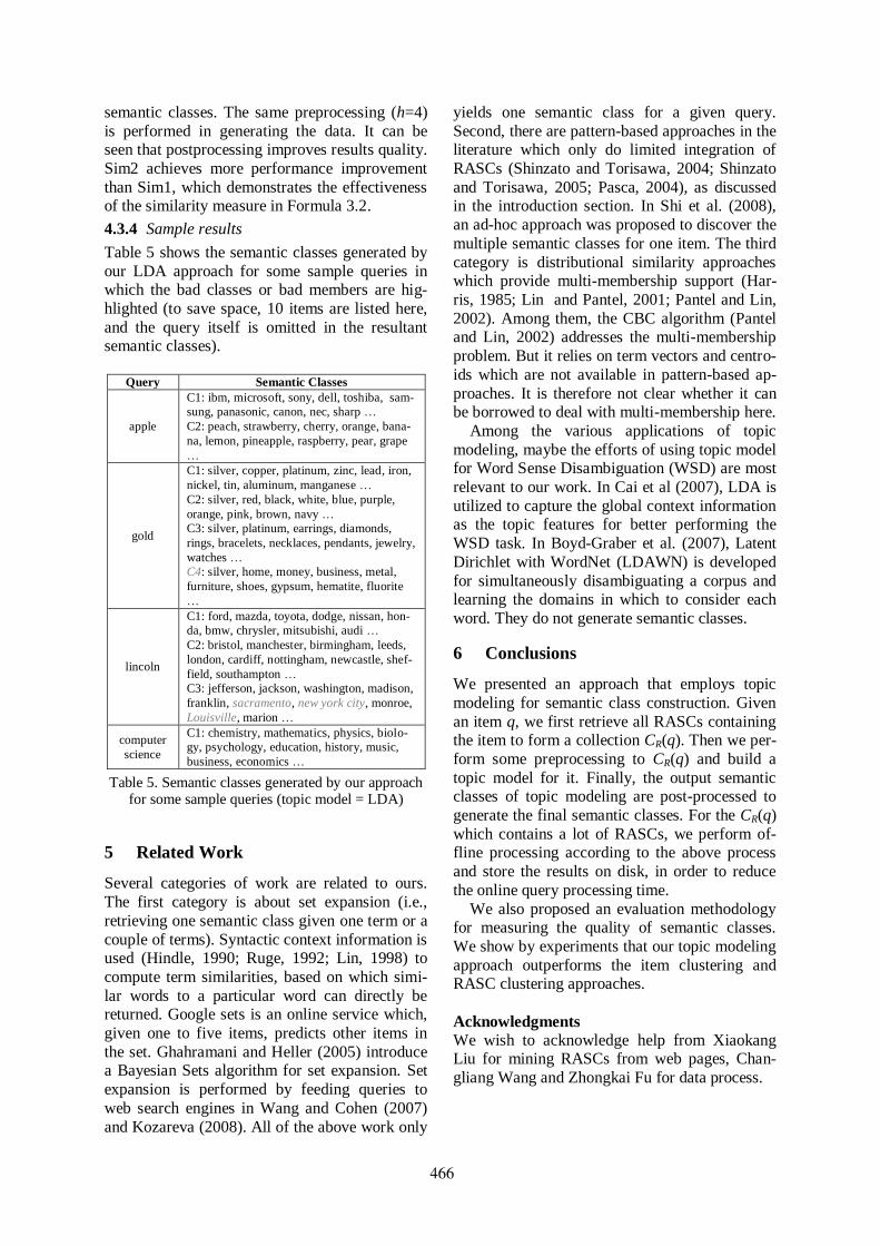
semantic classes. The same preprocessing (h=4)
is performed in generating the data. It can be seen that postprocessing improves results quality.
Sim2 achieves more performance improvement
than Sim1, which demonstrates the effectiveness of the similarity measure in Formula 3.2.
4.3.4 Sample results
Table 5 shows the semantic classes generated by
our LDA approach for some sample queries in which the bad classes or bad members are hig-
hlighted (to save space, 10 items are listed here,
and the query itself is omitted in the resultant semantic classes).
Query Semantic Classes
apple
C1: ibm, microsoft, sony, dell, toshiba, sam-
sung, panasonic, canon, nec, sharp …
C2: peach, strawberry, cherry, orange, bana-
na, lemon, pineapple, raspberry, pear, grape
…
gold
C1: silver, copper, platinum, zinc, lead, iron,
nickel, tin, aluminum, manganese …
C2: silver, red, black, white, blue, purple,
orange, pink, brown, navy …
C3: silver, platinum, earrings, diamonds,
rings, bracelets, necklaces, pendants, jewelry,
watches …
C4: silver, home, money, business, metal,
furniture, shoes, gypsum, hematite, fluorite
…
lincoln
C1: ford, mazda, toyota, dodge, nissan, hon-
da, bmw, chrysler, mitsubishi, audi …
C2: bristol, manchester, birmingham, leeds,
london, cardiff, nottingham, newcastle, shef-
field, southampton …
C3: jefferson, jackson, washington, madison,
franklin, sacramento, new york city, monroe,
Louisville, marion …
computer
science
C1: chemistry, mathematics, physics, biolo-
gy, psychology, education, history, music,
business, economics …
Table 5. Semantic classes generated by our approach for some sample queries (topic model = LDA)
5 Related Work
Several categories of work are related to ours.
The first category is about set expansion (i.e.,
retrieving one semantic class given one term or a
couple of terms). Syntactic context information is used (Hindle, 1990; Ruge, 1992; Lin, 1998) to
compute term similarities, based on which simi-
lar words to a particular word can directly be returned. Google sets is an online service which,
given one to five items, predicts other items in
the set. Ghahramani and Heller (2005) introduce a Bayesian Sets algorithm for set expansion. Set
expansion is performed by feeding queries to
web search engines in Wang and Cohen (2007)
and Kozareva (2008). All of the above work only
yields one semantic class for a given query.
Second, there are pattern-based approaches in the literature which only do limited integration of
RASCs (Shinzato and Torisawa, 2004; Shinzato
and Torisawa, 2005; Pasca, 2004), as discussed in the introduction section. In Shi et al. (2008),
an ad-hoc approach was proposed to discover the
multiple semantic classes for one item. The third
category is distributional similarity approaches which provide multi-membership support (Har-
ris, 1985; Lin and Pantel, 2001; Pantel and Lin,
2002). Among them, the CBC algorithm (Pantel and Lin, 2002) addresses the multi-membership
problem. But it relies on term vectors and centro-
ids which are not available in pattern-based ap-
proaches. It is therefore not clear whether it can be borrowed to deal with multi-membership here.
Among the various applications of topic
modeling, maybe the efforts of using topic model for Word Sense Disambiguation (WSD) are most
relevant to our work. In Cai et al (2007), LDA is
utilized to capture the global context information as the topic features for better performing the
WSD task. In Boyd-Graber et al. (2007), Latent
Dirichlet with WordNet (LDAWN) is developed
for simultaneously disambiguating a corpus and learning the domains in which to consider each
word. They do not generate semantic classes.
6 Conclusions
We presented an approach that employs topic
modeling for semantic class construction. Given
an item q, we first retrieve all RASCs containing the item to form a collection CR(q). Then we per-
form some preprocessing to CR(q) and build a
topic model for it. Finally, the output semantic classes of topic modeling are post-processed to
generate the final semantic classes. For the CR(q)
which contains a lot of RASCs, we perform of-fline processing according to the above process
and store the results on disk, in order to reduce
the online query processing time.
We also proposed an evaluation methodology for measuring the quality of semantic classes.
We show by experiments that our topic modeling
approach outperforms the item clustering and RASC clustering approaches.
Acknowledgments
We wish to acknowledge help from Xiaokang Liu for mining RASCs from web pages, Chan-
gliang Wang and Zhongkai Fu for data process.
466

References
David M. Blei, Andrew Y. Ng, and Michael I. Jordan.
2003. Latent dirichlet allocation. J. Mach. Learn.
Res., 3:993–1022.
Bruce Croft, Donald Metzler, and Trevor Strohman.
2009. Search Engines: Information Retrieval in
Practice. Addison Wesley.
Jordan Boyd-Graber, David Blei, and Xiaojin
Zhu.2007. A topic model for word sense disambig-
uation. In Proceedings EMNLP-CoNLL 2007, pag-
es 1024–1033, Prague, Czech Republic, June.
Association for Computational Linguistics.
Jun Fu Cai, Wee Sun Lee, and Yee Whye Teh. 2007.
NUS-ML: Improving word sense disambiguation
using topic features. In Proceedings of the Interna-
tional Workshop on Semantic Evaluations, volume
4.
Scott Deerwester, Susan T. Dumais, GeorgeW. Fur-
nas, Thomas K. Landauer, and Richard Harshman.
1990. Indexing by latent semantic analysis. Journal
of the American Society for Information Science,
41:391–407.
Zoubin Ghahramani and Katherine A. Heller. 2005.
Bayesian Sets. In Advances in Neural Information Processing Systems (NIPS05).
Thomas L. Griffiths, Mark Steyvers, David M.
Blei,and Joshua B. Tenenbaum. 2005. Integrating
topics and syntax. In Advances in Neural Informa-
tion Processing Systems 17, pages 537–544. MIT
Press
Zellig Harris. Distributional Structure. The Philoso-
phy of Linguistics. New York: Oxford University
Press. 1985.
Donald Hindle. 1990. Noun Classification from Pre-
dicate-Argument Structures. In Proceedings of ACL90, pages 268–275.
Thomas Hofmann. 1999. Probabilistic latent semantic
indexing. In Proceedings of the 22nd annual inter-
national ACM SIGIR99, pages 50–57, New York,
NY, USA. ACM.
Kalervo Jarvelin, and Jaana Kekalainen. 2000. IR
Evaluation Methods for Retrieving Highly Rele-
vant Documents. In Proceedings of the 23rd An-
nual International ACM SIGIR Conference on
Research and Development in Information Retriev-
al (SIGIR2000).
Zornitsa Kozareva, Ellen Riloff and Eduard Hovy. 2008. Semantic Class Learning from the Web with
Hyponym Pattern Linkage Graphs, In Proceedings
of ACL-08.
Wei Li, David M. Blei, and Andrew McCallum. Non-
parametric Bayes Pachinko Allocation. In Proceed-
ings of Conference on Uncertainty in Artificial In-
telligence (UAI), 2007.
Dekang Lin. 1998. Automatic Retrieval and Cluster-
ing of Similar Words. In Proceedings of COLING-
ACL98, pages 768-774.
Dekang Lin and Patrick Pantel. 2001. Induction of Semantic Classes from Natural Language Text. In
Proceedings of SIGKDD01, pages 317-322.
Hiroaki Ohshima, Satoshi Oyama, and Katsumi Tana-
ka. 2006. Searching coordinate terms with their
context from the web. In WISE06, pages 40–47.
Patrick Pantel and Dekang Lin. 2002. Discovering
Word Senses from Text. In Proceedings of
SIGKDD02.
Marius Pasca. 2004. Acquisition of Categorized
Named Entities for Web Search. In Proc. of 2004
CIKM.
Gerda Ruge. 1992. Experiments on Linguistically-
Based Term Associations. In Information
Processing & Management, 28(3), pages 317-32.
Andrew I. Schein, Alexandrin Popescul, Lyle H.
Ungar and David M. Pennock. 2002. Methods and
metrics for cold-start recommendations. In Pro-
ceedings of SIGIR02, pages 253-260.
Shuming Shi, Xiaokang Liu and Ji-Rong Wen. 2008.
Pattern-based Semantic Class Discovery with Mul-
ti-Membership Support. In CIKM2008, pages
1453-1454.
Keiji Shinzato and Kentaro Torisawa. 2004. Acquir-ing Hyponymy Relations from Web Documents. In
HLT/NAACL04, pages 73–80.
Keiji Shinzato and Kentaro Torisawa. 2005. A Simple
WWW-based Method for Semantic Word Class
Acquisition. In RANLP05.
Richard C. Wang and William W. Cohen. 2007. Lan-
gusage-Independent Set Expansion of Named Enti-
ties Using the Web. In ICDM2007.
467
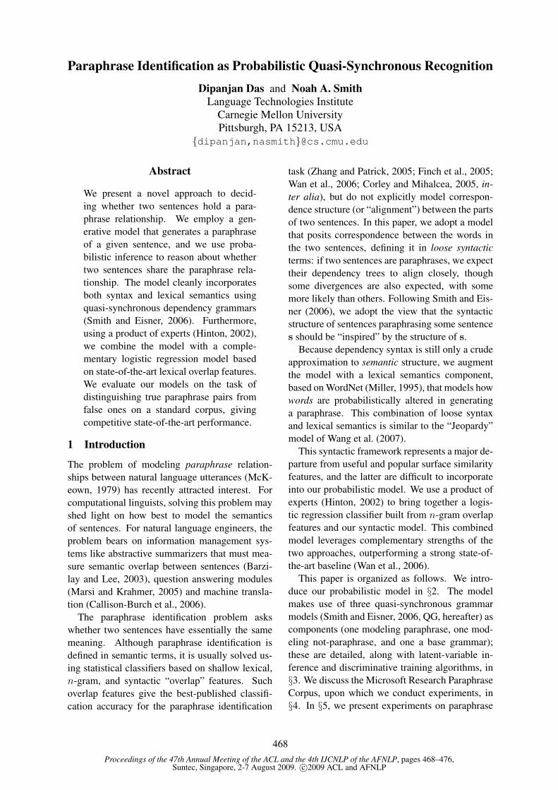
Proceedings of the 47th Annual Meeting of the ACL and the 4th IJCNLP of the AFNLP, pages 468–476,Suntec, Singapore, 2-7 August 2009. c©2009 ACL and AFNLP
Paraphrase Identification as Probabilistic Quasi-Synchronous RecognitionDipanjan Das and Noah A. Smith
Language Technologies InstituteCarnegie Mellon UniversityPittsburgh, PA 15213, USA
{dipanjan,nasmith}@cs.cmu.edu
Abstract
We present a novel approach to decid-ing whether two sentences hold a para-phrase relationship. We employ a gen-erative model that generates a paraphraseof a given sentence, and we use proba-bilistic inference to reason about whethertwo sentences share the paraphrase rela-tionship. The model cleanly incorporatesboth syntax and lexical semantics usingquasi-synchronous dependency grammars(Smith and Eisner, 2006). Furthermore,using a product of experts (Hinton, 2002),we combine the model with a comple-mentary logistic regression model basedon state-of-the-art lexical overlap features.We evaluate our models on the task ofdistinguishing true paraphrase pairs fromfalse ones on a standard corpus, givingcompetitive state-of-the-art performance.
1 Introduction
The problem of modeling paraphrase relation-ships between natural language utterances (McK-eown, 1979) has recently attracted interest. Forcomputational linguists, solving this problem mayshed light on how best to model the semanticsof sentences. For natural language engineers, theproblem bears on information management sys-tems like abstractive summarizers that must mea-sure semantic overlap between sentences (Barzi-lay and Lee, 2003), question answering modules(Marsi and Krahmer, 2005) and machine transla-tion (Callison-Burch et al., 2006).
The paraphrase identification problem askswhether two sentences have essentially the samemeaning. Although paraphrase identification isdefined in semantic terms, it is usually solved us-ing statistical classifiers based on shallow lexical,n-gram, and syntactic “overlap” features. Suchoverlap features give the best-published classifi-cation accuracy for the paraphrase identification
task (Zhang and Patrick, 2005; Finch et al., 2005;Wan et al., 2006; Corley and Mihalcea, 2005, in-ter alia), but do not explicitly model correspon-dence structure (or “alignment”) between the partsof two sentences. In this paper, we adopt a modelthat posits correspondence between the words inthe two sentences, defining it in loose syntacticterms: if two sentences are paraphrases, we expecttheir dependency trees to align closely, thoughsome divergences are also expected, with somemore likely than others. Following Smith and Eis-ner (2006), we adopt the view that the syntacticstructure of sentences paraphrasing some sentences should be “inspired” by the structure of s.
Because dependency syntax is still only a crudeapproximation to semantic structure, we augmentthe model with a lexical semantics component,based on WordNet (Miller, 1995), that models howwords are probabilistically altered in generatinga paraphrase. This combination of loose syntaxand lexical semantics is similar to the “Jeopardy”model of Wang et al. (2007).
This syntactic framework represents a major de-parture from useful and popular surface similarityfeatures, and the latter are difficult to incorporateinto our probabilistic model. We use a product ofexperts (Hinton, 2002) to bring together a logis-tic regression classifier built from n-gram overlapfeatures and our syntactic model. This combinedmodel leverages complementary strengths of thetwo approaches, outperforming a strong state-of-the-art baseline (Wan et al., 2006).
This paper is organized as follows. We intro-duce our probabilistic model in §2. The modelmakes use of three quasi-synchronous grammarmodels (Smith and Eisner, 2006, QG, hereafter) ascomponents (one modeling paraphrase, one mod-eling not-paraphrase, and one a base grammar);these are detailed, along with latent-variable in-ference and discriminative training algorithms, in§3. We discuss the Microsoft Research ParaphraseCorpus, upon which we conduct experiments, in§4. In §5, we present experiments on paraphrase
468

identification with our model and make compar-isons with the existing state-of-the-art. We de-scribe the product of experts and our lexical over-lap model, and discuss the results achieved in §6.We relate our approach to prior work (§7) and con-clude (§8).
2 Probabilistic Model
Since our task is a classification problem, we re-quire our model to provide an estimate of the pos-terior probability of the relationship (i.e., “para-phrase,” denoted p, or “not paraphrase,” denotedn), given the pair of sentences.1 Here, pQ denotesmodel probabilities, c is a relationship class (p orn), and s1 and s2 are the two sentences. We choosethe class according to:
ĉ = argmaxc∈{p,n}
pQ(c | s1, s2)
= argmaxc∈{p,n}
pQ(c)× pQ(s1, s2 | c) (1)
We define the class-conditional probabilities ofthe two sentences using the following generativestory. First, grammar G0 generates a sentence s.Then a class c is chosen, corresponding to a class-specific probabilistic quasi-synchronous grammarGc. (We will discuss QG in detail in §3. For thepresent, consider it a specially-defined probabilis-tic model that generates sentences with a specificproperty, like “paraphrases s,” when c = p.) Givens, Gc generates the other sentence in the pair, s′.
When we observe a pair of sentences s1 and s2
we do not presume to know which came first (i.e.,which was s and which was s′). Both orderingsare assumed to be equally probable. For class c,
pQ(s1, s2 | c) =
0.5× pQ(s1 | G0)× pQ(s2 | Gc(s1))
+ 0.5× pQ(s2 | G0)× pQ(s1 | Gc(s2))(2)
where c can be p or n; Gp(s) is the QG that gen-erates paraphrases for sentence s, while Gn(s) isthe QG that generates sentences that are not para-phrases of sentence s. This latter model may seemcounter-intuitive: since the vast majority of pos-sible sentences are not paraphrases of s, why is aspecial grammar required? Our use of a Gn fol-lows from the properties of the corpus currentlyused for learning, in which the negative examples
1Although we do not explore the idea here, the modelcould be adapted for other sentence-pair relationships like en-tailment or contradiction.
were selected to have high lexical overlap. We re-turn to this point in §4.
3 QG for Paraphrase Modeling
Here, we turn to the models Gp and Gn in detail.
3.1 BackgroundSmith and Eisner (2006) introduced the quasi-synchronous grammar formalism. Here, we de-scribe some of its salient aspects. The modelarose out of the empirical observation that trans-lated sentences have some isomorphic syntacticstructure, but divergences are possible. Therefore,rather than an isomorphic structure over a pair ofsource and target sentences, the syntactic tree overa target sentence is modeled by a source sentence-specific grammar “inspired” by the source sen-tence’s tree. This is implemented by associatingwith each node in the target tree a subset of thenodes in the source tree. Since it loosely linksthe two sentences’ syntactic structures, QG is wellsuited for problems like word alignment for MT(Smith and Eisner, 2006) and question answering(Wang et al., 2007).
Consider a very simple quasi-synchronouscontext-free dependency grammar that generatesone dependent per production rule.2 Let s =〈s1, ..., sm〉 be the source sentence. The grammarrules will take one of the two forms:
〈t, l〉 → 〈t, l〉〈t′, k〉 or 〈t, l〉 → 〈t′, k〉〈t, l〉
where t and t′ range over the vocabulary of thetarget language, and l and k ∈ {0, ...,m} are in-dices in the source sentence, with 0 denoting null.3
Hard or soft constraints can be applied between land k in a rule. These constraints imply permissi-ble “configurations.” For example, requiring l 6= 0and, if k 6= 0 then sk must be a child of sl in thesource tree, we can implement a synchronous de-pendency grammar similar to (Melamed, 2004).
Smith and Eisner (2006) used a quasi-synchronous grammar to discover the correspon-dence between words implied by the correspon-dence between the trees. We follow Wang et al.(2007) in treating the correspondences as latentvariables, and in using a WordNet-based lexicalsemantics model to generate the target words.
2Our actual model is more complicated; see §3.2.3A more general QG could allow one-to-many align-
ments, replacing l and k with sets of indices.
469

3.2 Detailed ModelWe describe how we model pQ(t | Gp(s)) andpQ(t | Gn(s)) for source and target sentences sand t (appearing in Eq. 2 alternately as s1 and s2).
A dependency tree on a sequence w =〈w1, ..., wk〉 is a mapping of indices of words toindices of syntactic parents, τp : {1, ..., k} →{0, ..., k}, and a mapping of indices of words todependency relation types in L, τ` : {1, ..., k} →L. The set of indices children of wi to its left,{j : τw(j) = i, j < i}, is denoted λw(i), andρw(i) is used for right children. wi has a singleparent, denoted by wτp(i). Cycles are not allowed,and w0 is taken to be the dummy “wall” symbol,$, whose only child is the root word of the sen-tence (normally the main verb). The label for wiis denoted by τ`(i). We denote the whole tree ofa sentence w by τw, the subtree rooted at the ithword by τw,i.
Consider two sentences: let the source sen-tence s contain m words and the target sentencet contain n words. Let the correspondence x :{1, ..., n} → {0, ...,m} be a mapping from in-dices of words in t to indices of words in s. (Werequire each target word to map to at most onesource word, though multiple target words canmap to the same source word, i.e., x(i) = x(j)while i 6= j.) When x(i) = 0, the ith target wordmaps to the wall symbol, equivalently a “null”word. Each of our QGs Gp and Gn generates thealignments x, the target tree τ t, and the sentencet. Both Gp and Gn are structured in the same way,differing only in their parameters; henceforth wediscuss Gp; Gn is similar.
We assume that the parse trees of s and t areknown.4 Therefore our model defines:
pQ(t | Gp(s)) = p(τ t | Gp(τ s))
=∑
x p(τt, x | Gp(τ s)) (3)
Because the QG is essentially a context-free de-pendency grammar, we can factor it into recur-sive steps as follows (let i be an arbitrary indexin {1, ..., n}):
P (τ t,i | ti, x(i), τ s) = pval (|λt(i)|, |ρt(i)| | ti)4In our experiments, we use the parser described by Mc-
Donald et al. (2005), trained on sections 2–21 of the WSJPenn Treebank, transformed to dependency trees followingYamada and Matsumoto (2003). (The same treebank datawere also to estimate many of the parameters of our model, asdiscussed in the text.) Though it leads to a partial “pipeline”approximation of the posterior probability p(c | s, t), we be-lieve that the relatively high quality of English dependencyparsing makes this approximation reasonable.
×∏
j∈λt(i)∪ρt(i)
m∑
x(j)=0
P (τ t,j | tj , x(j), τ s)
×pkid (tj , τt` (j), x(j) | ti, x(i), τ s) (4)
where pval and pkid are valence and child-production probabilities parameterized as dis-cussed in §3.4. Note the recursion in the second-to-last line.
We next describe a dynamic programming so-lution for calculating p(τ t | Gp(τ s)). In §3.4 wediscuss the parameterization of the model.
3.3 Dynamic ProgrammingLet C(i, l) refer to the probability of τ t,i, assum-ing that the parent of ti, tτtp(i), is aligned to sl. Forleaves of τ t, the base case is:
C(i, l) = pval (0, 0 | ti)× (5)∑mk=0 pkid (ti, τ
t` (i), k | tτtp(i), l, τ
s)
where k ranges over possible values of x(i), thesource-tree node to which ti is aligned. The recur-sive case is:
C(i, l) = pval (|λt(i)|, |ρt(i)| | ti) (6)
×∑mk=0 pkid (ti, τ
t` (i), k | tτtp(i), l, τ
s)
×∏
j∈λt(i)∪ρt(i)C(j, k)
We assume that the wall symbols t0 and s0 arealigned, so p(τ t | Gp(τ s)) = C(r, 0), where r isthe index of the root word of the target tree τ t. Itis straightforward to show that this algorithm re-quires O(m2n) runtime and O(mn) space.
3.4 ParameterizationThe valency distribution pval in Eq. 4 is estimatedin our model using the transformed treebank (seefootnote 4). For unobserved cases, the conditionalprobability is estimated by backing off to the par-ent POS tag and child direction.
We discuss next how to parameterize the prob-ability pkid that appears in Equations 4, 5, and 6.This conditional distribution forms the core of ourQGs, and we deviate from earlier research usingQGs in defining pkid in a fully generative way.
In addition to assuming that dependency parsetrees for s and t are observable, we also assumeeach word wi comes with POS and named entitytags. In our experiments these were obtained au-tomatically using MXPOST (Ratnaparkhi, 1996)and BBN’s Identifinder (Bikel et al., 1999).
470
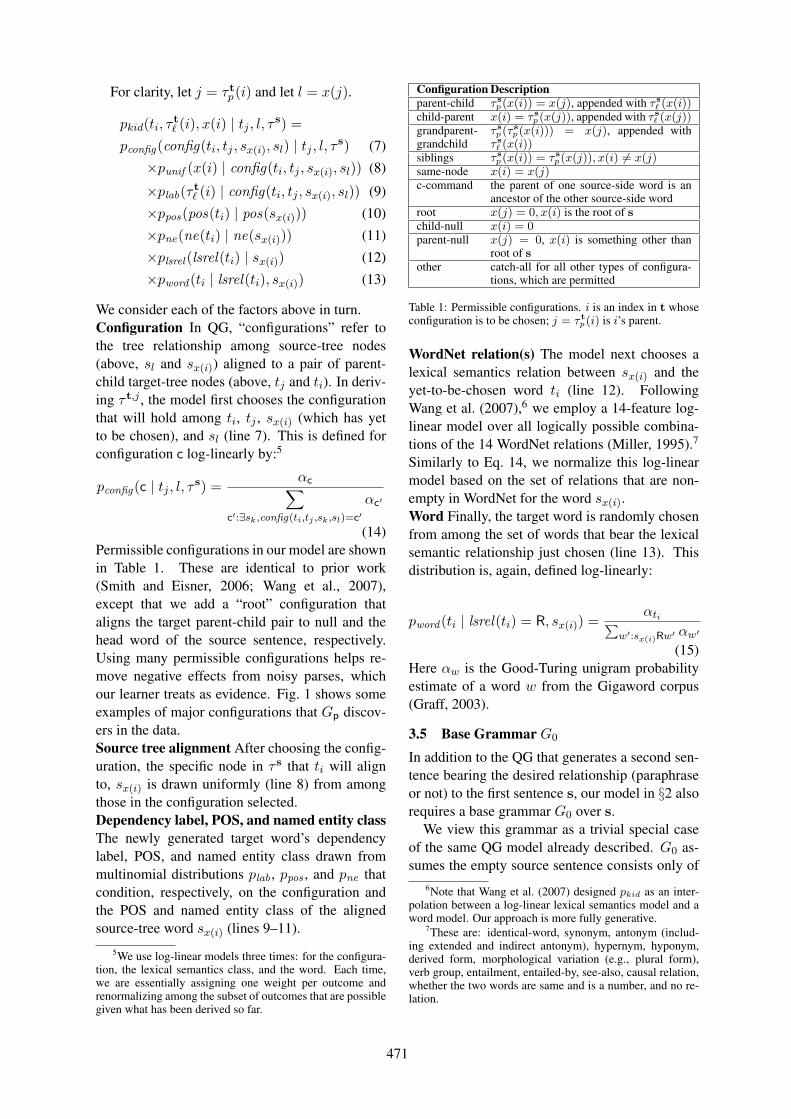
For clarity, let j = τ tp(i) and let l = x(j).
pkid(ti, τt` (i), x(i) | tj , l, τ s) =
pconfig(config(ti, tj , sx(i), sl) | tj , l, τ s) (7)
×punif (x(i) | config(ti, tj , sx(i), sl)) (8)
×plab(τ t` (i) | config(ti, tj , sx(i), sl)) (9)
×ppos(pos(ti) | pos(sx(i))) (10)
×pne(ne(ti) | ne(sx(i))) (11)
×plsrel (lsrel(ti) | sx(i)) (12)
×pword (ti | lsrel(ti), sx(i)) (13)
We consider each of the factors above in turn.Configuration In QG, “configurations” refer tothe tree relationship among source-tree nodes(above, sl and sx(i)) aligned to a pair of parent-child target-tree nodes (above, tj and ti). In deriv-ing τ t,j , the model first chooses the configurationthat will hold among ti, tj , sx(i) (which has yetto be chosen), and sl (line 7). This is defined forconfiguration c log-linearly by:5
pconfig(c | tj , l, τ s) =αc
∑
c′:∃sk,config(ti,tj ,sk,sl)=c′
αc′
(14)Permissible configurations in our model are shownin Table 1. These are identical to prior work(Smith and Eisner, 2006; Wang et al., 2007),except that we add a “root” configuration thataligns the target parent-child pair to null and thehead word of the source sentence, respectively.Using many permissible configurations helps re-move negative effects from noisy parses, whichour learner treats as evidence. Fig. 1 shows someexamples of major configurations that Gp discov-ers in the data.Source tree alignment After choosing the config-uration, the specific node in τ s that ti will alignto, sx(i) is drawn uniformly (line 8) from amongthose in the configuration selected.Dependency label, POS, and named entity classThe newly generated target word’s dependencylabel, POS, and named entity class drawn frommultinomial distributions plab , ppos , and pne thatcondition, respectively, on the configuration andthe POS and named entity class of the alignedsource-tree word sx(i) (lines 9–11).
5We use log-linear models three times: for the configura-tion, the lexical semantics class, and the word. Each time,we are essentially assigning one weight per outcome andrenormalizing among the subset of outcomes that are possiblegiven what has been derived so far.
Configuration Descriptionparent-child τ s
p(x(i)) = x(j), appended with τ s` (x(i))
child-parent x(i) = τ sp(x(j)), appended with τ s
` (x(j))grandparent-grandchild
τ sp(τ s
p(x(i))) = x(j), appended withτ s
` (x(i))siblings τ s
p(x(i)) = τ sp(x(j)), x(i) 6= x(j)
same-node x(i) = x(j)c-command the parent of one source-side word is an
ancestor of the other source-side wordroot x(j) = 0, x(i) is the root of schild-null x(i) = 0parent-null x(j) = 0, x(i) is something other than
root of sother catch-all for all other types of configura-
tions, which are permitted
Table 1: Permissible configurations. i is an index in t whoseconfiguration is to be chosen; j = τ t
p(i) is i’s parent.
WordNet relation(s) The model next chooses alexical semantics relation between sx(i) and theyet-to-be-chosen word ti (line 12). FollowingWang et al. (2007),6 we employ a 14-feature log-linear model over all logically possible combina-tions of the 14 WordNet relations (Miller, 1995).7
Similarly to Eq. 14, we normalize this log-linearmodel based on the set of relations that are non-empty in WordNet for the word sx(i).Word Finally, the target word is randomly chosenfrom among the set of words that bear the lexicalsemantic relationship just chosen (line 13). Thisdistribution is, again, defined log-linearly:
pword (ti | lsrel(ti) = R, sx(i)) =αti
∑
w′:sx(i)Rw′αw′
(15)Here αw is the Good-Turing unigram probabilityestimate of a word w from the Gigaword corpus(Graff, 2003).
3.5 Base Grammar G0
In addition to the QG that generates a second sen-tence bearing the desired relationship (paraphraseor not) to the first sentence s, our model in §2 alsorequires a base grammar G0 over s.
We view this grammar as a trivial special caseof the same QG model already described. G0 as-sumes the empty source sentence consists only of
6Note that Wang et al. (2007) designed pkid as an inter-polation between a log-linear lexical semantics model and aword model. Our approach is more fully generative.
7These are: identical-word, synonym, antonym (includ-ing extended and indirect antonym), hypernym, hyponym,derived form, morphological variation (e.g., plural form),verb group, entailment, entailed-by, see-also, causal relation,whether the two words are same and is a number, and no re-lation.
471
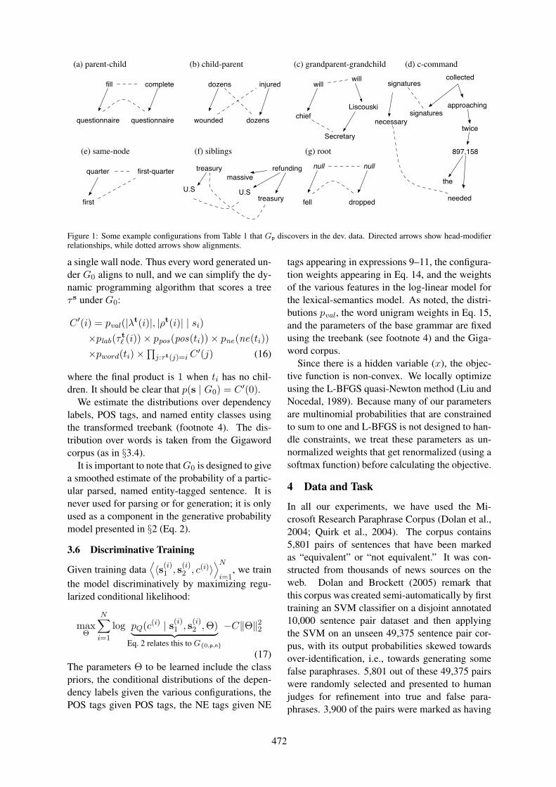
(a) parent-child
fill
questionnaire
complete
questionnaire
dozens
wounded
injured
dozens
(b) child-parent (c) grandparent-grandchild
will
chief
will
Secretary
Liscouski
quarter
first
first-quarter
(e) same-node
U.S
refundingmassive
(f) siblings
U.Streasury
treasury
(g) root
null
fell
null
dropped
(d) c-command
signatures
necessarysignatures
needed
897,158
the
twice
approaching
collected
Figure 1: Some example configurations from Table 1 that Gp discovers in the dev. data. Directed arrows show head-modifierrelationships, while dotted arrows show alignments.
a single wall node. Thus every word generated un-der G0 aligns to null, and we can simplify the dy-namic programming algorithm that scores a treeτ s under G0:
C ′(i) = pval (|λt(i)|, |ρt(i)| | si)×plab(τ t
` (i))× ppos(pos(ti))× pne(ne(ti))
×pword(ti)×∏
j:τt(j)=iC′(j) (16)
where the final product is 1 when ti has no chil-dren. It should be clear that p(s | G0) = C ′(0).
We estimate the distributions over dependencylabels, POS tags, and named entity classes usingthe transformed treebank (footnote 4). The dis-tribution over words is taken from the Gigawordcorpus (as in §3.4).
It is important to note thatG0 is designed to givea smoothed estimate of the probability of a partic-ular parsed, named entity-tagged sentence. It isnever used for parsing or for generation; it is onlyused as a component in the generative probabilitymodel presented in §2 (Eq. 2).
3.6 Discriminative Training
Given training data⟨
〈s(i)1 , s(i)
2 , c(i)〉⟩N
i=1, we train
the model discriminatively by maximizing regu-larized conditional likelihood:
maxΘ
N∑
i=1
log pQ(c(i) | s(i)1 , s(i)
2 ,Θ)︸ ︷︷ ︸
Eq. 2 relates this to G{0,p,n}
−C‖Θ‖22
(17)The parameters Θ to be learned include the classpriors, the conditional distributions of the depen-dency labels given the various configurations, thePOS tags given POS tags, the NE tags given NE
tags appearing in expressions 9–11, the configura-tion weights appearing in Eq. 14, and the weightsof the various features in the log-linear model forthe lexical-semantics model. As noted, the distri-butions pval , the word unigram weights in Eq. 15,and the parameters of the base grammar are fixedusing the treebank (see footnote 4) and the Giga-word corpus.
Since there is a hidden variable (x), the objec-tive function is non-convex. We locally optimizeusing the L-BFGS quasi-Newton method (Liu andNocedal, 1989). Because many of our parametersare multinomial probabilities that are constrainedto sum to one and L-BFGS is not designed to han-dle constraints, we treat these parameters as un-normalized weights that get renormalized (using asoftmax function) before calculating the objective.
4 Data and Task
In all our experiments, we have used the Mi-crosoft Research Paraphrase Corpus (Dolan et al.,2004; Quirk et al., 2004). The corpus contains5,801 pairs of sentences that have been markedas “equivalent” or “not equivalent.” It was con-structed from thousands of news sources on theweb. Dolan and Brockett (2005) remark thatthis corpus was created semi-automatically by firsttraining an SVM classifier on a disjoint annotated10,000 sentence pair dataset and then applyingthe SVM on an unseen 49,375 sentence pair cor-pus, with its output probabilities skewed towardsover-identification, i.e., towards generating somefalse paraphrases. 5,801 out of these 49,375 pairswere randomly selected and presented to humanjudges for refinement into true and false para-phrases. 3,900 of the pairs were marked as having
472

About 120 potential jurors were being asked to complete a lengthy questionnaire .
The jurors were taken into the courtroom in groups of 40 and asked to fill out a questionnaire .Figure 2: Discovered alignment of Ex. 19 produced by Gp. Observe that the model aligns identical words and also “complete”and “fill” in this specific case. This kind of alignment provides an edge over a simple lexical overlap model.
“mostly bidirectional entailment,” a standard def-inition of the paraphrase relation. Each sentencewas labeled first by two judges, who averaged 83%agreement, and a third judge resolved conflicts.
We use the standard data split into 4,076 (2,753paraphrase, 1,323 not) training and 1,725 (1147paraphrase, 578 not) test pairs. We reserved a ran-domly selected 1,075 training pairs for tuning.Wecite some examples from the training set here:
(18) Revenue in the first quarter of the year dropped 15percent from the same period a year earlier.With the scandal hanging over Stewart’s company,revenue in the first quarter of the year dropped 15percent from the same period a year earlier.
(19) About 120 potential jurors were being asked tocomplete a lengthy questionnaire.The jurors were taken into the courtroom in groups of40 and asked to fill out a questionnaire.
Ex. 18 is a true paraphrase pair. Notice the highlexical overlap between the two sentences (uni-gram overlap of 100% in one direction and 72%in the other). Ex. 19 is another true paraphrasepair with much lower lexical overlap (unigramoverlap of 50% in one direction and 30% in theother). Notice the use of similar-meaning phrasesand irrelevant modifiers that retain the same mean-ing in both sentences, which a lexical overlapmodel cannot capture easily, but a model like a QGmight. Also, in both pairs, the relationship cannotbe called total bidirectional equivalence becausethere is some extra information in one sentencewhich cannot be inferred from the other.
Ex. 20 was labeled “not paraphrase”:
(20) “There were a number of bureaucratic andadministrative missed signals - there’s not one personwho’s responsible here,” Gehman said.In turning down the NIMA offer, Gehman said, “therewere a number of bureaucratic and administrativemissed signals here.
There is significant content overlap, making a de-cision difficult for a naı̈ve lexical overlap classifier.(In fact, pQ labels this example n while the lexicaloverlap models label it p.)
The fact that negative examples in this corpuswere selected because of their high lexical over-lap is important. It means that any discrimina-tive model is expected to learn to distinguish mereoverlap from paraphrase. This seems appropriate,
but it does mean that the “not paraphrase” relationought to be denoted “not paraphrase but decep-tively similar on the surface.” It is for this reasonthat we use a special QG for the n relation.
5 Experimental Evaluation
Here we present our experimental evaluation usingpQ. We trained on the training set (3,001 pairs)and tuned model metaparameters (C in Eq. 17)and the effect of different feature sets on the de-velopment set (1,075 pairs). We report accuracyon the official MSRPC test dataset. If the poste-rior probability pQ(p | s1, s2) is greater than 0.5,the pair is labeled “paraphrase” (as in Eq. 1).
5.1 BaselineWe replicated a state-of-the-art baseline model forcomparison. Wan et al. (2006) report the best pub-lished accuracy, to our knowledge, on this task,using a support vector machine. Our baseline isa reimplementation of Wan et al. (2006), usingfeatures calculated directly from s1 and s2 with-out recourse to any hidden structure: proportionof word unigram matches, proportion of lemma-tized unigram matches, BLEU score (Papineni etal., 2001), BLEU score on lemmatized tokens, Fmeasure (Turian et al., 2003), difference of sen-tence length, and proportion of dependency rela-tion overlap. The SVM was trained to classifypositive and negative examples of paraphrase us-ing SVMlight (Joachims, 1999).8 Metaparameters,tuned on the development data, were the regu-larization constant and the degree of the polyno-mial kernel (chosen in [10−5, 102] and 1–5 respec-tively.).9
It is unsurprising that the SVM performs verywell on the MSRPC because of the corpus creationprocess (see Sec. 4) where an SVM was appliedas well, with very similar features and a skeweddecision process (Dolan and Brockett, 2005).
8http://svmlight.joachims.org9Our replication of the Wan et al. model is approxi-
mate, because we used different preprocessing tools: MX-POST for POS tagging (Ratnaparkhi, 1996), MSTParserfor parsing (McDonald et al., 2005), and Dan Bikel’sinterface (http://www.cis.upenn.edu/˜dbikel/software.html#wn) to WordNet (Miller, 1995) forlemmatization information. Tuning led to C = 17 and poly-nomial degree 4.
473
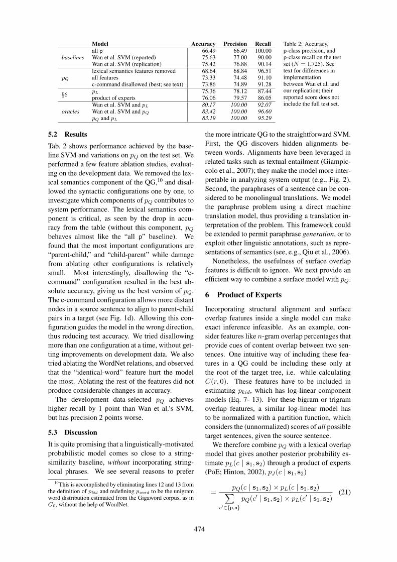
Model Accuracy Precision Recall
baselinesall p 66.49 66.49 100.00Wan et al. SVM (reported) 75.63 77.00 90.00Wan et al. SVM (replication) 75.42 76.88 90.14
pQ
lexical semantics features removed 68.64 68.84 96.51all features 73.33 74.48 91.10c-command disallowed (best; see text) 73.86 74.89 91.28
§6 pL 75.36 78.12 87.44product of experts 76.06 79.57 86.05
oraclesWan et al. SVM and pL 80.17 100.00 92.07Wan et al. SVM and pQ 83.42 100.00 96.60pQ and pL 83.19 100.00 95.29
Table 2: Accuracy,p-class precision, andp-class recall on the testset (N = 1,725). Seetext for differences inimplementationbetween Wan et al. andour replication; theirreported score does notinclude the full test set.
5.2 ResultsTab. 2 shows performance achieved by the base-line SVM and variations on pQ on the test set. Weperformed a few feature ablation studies, evaluat-ing on the development data. We removed the lex-ical semantics component of the QG,10 and disal-lowed the syntactic configurations one by one, toinvestigate which components of pQ contributes tosystem performance. The lexical semantics com-ponent is critical, as seen by the drop in accu-racy from the table (without this component, pQbehaves almost like the “all p” baseline). Wefound that the most important configurations are“parent-child,” and “child-parent” while damagefrom ablating other configurations is relativelysmall. Most interestingly, disallowing the “c-command” configuration resulted in the best ab-solute accuracy, giving us the best version of pQ.The c-command configuration allows more distantnodes in a source sentence to align to parent-childpairs in a target (see Fig. 1d). Allowing this con-figuration guides the model in the wrong direction,thus reducing test accuracy. We tried disallowingmore than one configuration at a time, without get-ting improvements on development data. We alsotried ablating the WordNet relations, and observedthat the “identical-word” feature hurt the modelthe most. Ablating the rest of the features did notproduce considerable changes in accuracy.
The development data-selected pQ achieveshigher recall by 1 point than Wan et al.’s SVM,but has precision 2 points worse.
5.3 DiscussionIt is quite promising that a linguistically-motivatedprobabilistic model comes so close to a string-similarity baseline, without incorporating string-local phrases. We see several reasons to prefer
10This is accomplished by eliminating lines 12 and 13 fromthe definition of pkid and redefining pword to be the unigramword distribution estimated from the Gigaword corpus, as inG0, without the help of WordNet.
the more intricate QG to the straightforward SVM.First, the QG discovers hidden alignments be-tween words. Alignments have been leveraged inrelated tasks such as textual entailment (Giampic-colo et al., 2007); they make the model more inter-pretable in analyzing system output (e.g., Fig. 2).Second, the paraphrases of a sentence can be con-sidered to be monolingual translations. We modelthe paraphrase problem using a direct machinetranslation model, thus providing a translation in-terpretation of the problem. This framework couldbe extended to permit paraphrase generation, or toexploit other linguistic annotations, such as repre-sentations of semantics (see, e.g., Qiu et al., 2006).
Nonetheless, the usefulness of surface overlapfeatures is difficult to ignore. We next provide anefficient way to combine a surface model with pQ.
6 Product of Experts
Incorporating structural alignment and surfaceoverlap features inside a single model can makeexact inference infeasible. As an example, con-sider features like n-gram overlap percentages thatprovide cues of content overlap between two sen-tences. One intuitive way of including these fea-tures in a QG could be including these only atthe root of the target tree, i.e. while calculatingC(r, 0). These features have to be included inestimating pkid, which has log-linear componentmodels (Eq. 7- 13). For these bigram or trigramoverlap features, a similar log-linear model hasto be normalized with a partition function, whichconsiders the (unnormalized) scores of all possibletarget sentences, given the source sentence.
We therefore combine pQ with a lexical overlapmodel that gives another posterior probability es-timate pL(c | s1, s2) through a product of experts(PoE; Hinton, 2002), pJ(c | s1, s2)
=pQ(c | s1, s2)× pL(c | s1, s2)
∑
c′∈{p,n}pQ(c′ | s1, s2)× pL(c′ | s1, s2)
(21)
474

Eq. 21 takes the product of the two models’ poste-rior probabilities, then normalizes it to sum to one.PoE models are used to efficiently combine severalexpert models that individually constrain differentdimensions in high-dimensional data, the producttherefore constraining all of the dimensions. Com-bining models in this way grants to each expertcomponent model the ability to “veto” a class bygiving it low probability; the most probable classis the one that is least objectionable to all experts.Probabilistic Lexical Overlap Model We de-vised a logistic regression (LR) model incorpo-rating 18 simple features, computed directly froms1 and s2, without modeling any hidden corre-spondence. LR (like the QG) provides a proba-bility distribution, but uses surface features (likethe SVM). The features are of the form precisionn(number of n-gram matches divided by the num-ber of n-grams in s1), recalln (number of n-grammatches divided by the number of n-grams in s2)and Fn (harmonic mean of the previous two fea-tures), where 1 ≤ n ≤ 3. We also used lemma-tized versions of these features. This model givesthe posterior probability pL(c | s1, s2), wherec ∈ {p, n}. We estimated the model parametersanalogously to Eq. 17. Performance is reported inTab. 2; this model is on par with the SVM, thoughtrading recall in favor of precision. We view it as aprobabilistic simulation of the SVM more suitablefor combination with the QG.Training the PoE Various ways of training a PoEexist. We first trained pQ and pL separately asdescribed, then initialized the PoE with those pa-rameters. We then continued training, maximizing(unregularized) conditional likelihood.Experiment We used pQ with the “c-command”configuration excluded, and the LR model in theproduct of experts. Tab. 2 includes the final re-sults achieved by the PoE. The PoE model outper-forms all the other models, achieving an accuracyof 76.06%.11 The PoE is conservative, labeling apair as p only if the LR and the QG give it strongp probabilities. This leads to high precision, at theexpense of recall.Oracle Ensembles Tab. 2 shows the results ofthree different oracle ensemble systems that cor-rectly classify a pair if either of the two individualsystems in the combination is correct. Note thatthe combinations involving pQ achieve 83%, the
11This accuracy is significant over pQ under a paired t-test(p < 0.04), but is not significant over the SVM.
human agreement level for the MSRPC. The LRand SVM are highly similar, and their oracle com-bination does not perform as well.
7 Related Work
There is a growing body of research that uses theMSRPC (Dolan et al., 2004; Quirk et al., 2004)to build models of paraphrase. As noted, the mostsuccessful work has used edit distance (Zhang andPatrick, 2005) or bag-of-words features to mea-sure sentence similarity, along with shallow syn-tactic features (Finch et al., 2005; Wan et al., 2006;Corley and Mihalcea, 2005). Qiu et al. (2006)used predicate-argument annotations.
Most related to our approach, Wu (2005) usedinversion transduction grammars—a synchronouscontext-free formalism (Wu, 1997)—for this task.Wu reported only positive-class (p) precision (notaccuracy) on the test set. He obtained 76.1%,while our PoE model achieves 79.6% on that mea-sure. Wu’s model can be understood as a stricthierarchical maximum-alignment method. In con-trast, our alignments are soft (we sum over them),and we do not require strictly isomorphic syntac-tic structures. Most importantly, our approach isfounded on a stochastic generating process and es-timated discriminatively for this task, while Wudid not estimate any parameters from data at all.
8 Conclusion
In this paper, we have presented a probabilisticmodel of paraphrase incorporating syntax, lexi-cal semantics, and hidden loose alignments be-tween two sentences’ trees. Though it fully de-fines a generative process for both sentences andtheir relationship, the model is discriminativelytrained to maximize conditional likelihood. Wehave shown that this model is competitive for de-termining whether there exists a semantic rela-tionship between them, and can be improved byprincipled combination with more standard lexicaloverlap approaches.
Acknowledgments
The authors thank the three anonymous review-ers for helpful comments and Alan Black, Freder-ick Crabbe, Jason Eisner, Kevin Gimpel, RebeccaHwa, David Smith, and Mengqiu Wang for helpfuldiscussions. This work was supported by DARPAgrant NBCH-1080004.
475

ReferencesRegina Barzilay and Lillian Lee. 2003. Learn-
ing to paraphrase: an unsupervised approach usingmultiple-sequence alignment. In Proc. of NAACL.
Daniel M. Bikel, Richard L. Schwartz, and Ralph M.Weischedel. 1999. An algorithm that learns what’sin a name. Machine Learning, 34(1-3):211–231.
Chris Callison-Burch, Philipp Koehn, and Miles Os-borne. 2006. Improved statistical machine transla-tion using paraphrases. In Proc. of HLT-NAACL.
Courtney Corley and Rada Mihalcea. 2005. Mea-suring the semantic similarity of texts. In Proc. ofACL Workshop on Empirical Modeling of SemanticEquivalence and Entailment.
William B. Dolan and Chris Brockett. 2005. Auto-matically constructing a corpus of sentential para-phrases. In Proc. of IWP.
Bill Dolan, Chris Quirk, and Chris Brockett. 2004.Unsupervised construction of large paraphrase cor-pora: exploiting massively parallel news sources. InProc. of COLING.
Andrew Finch, Young Sook Hwang, and EiichiroSumita. 2005. Using machine translation evalua-tion techniques to determine sentence-level seman-tic equivalence. In Proc. of IWP.
Danilo Giampiccolo, Bernardo Magnini, Ido Dagan,and Bill Dolan. 2007. The third PASCAL recog-nizing textual entailment challenge. In Proc. of theACL-PASCAL Workshop on Textual Entailment andParaphrasing.
David Graff. 2003. English Gigaword. LinguisticData Consortium.
Geoffrey E. Hinton. 2002. Training products of ex-perts by minimizing contrastive divergence. NeuralComputation, 14:1771–1800.
Thorsten Joachims. 1999. Making large-scale SVMlearning practical. In Advances in Kernel Methods -Support Vector Learning. MIT Press.
Dong C. Liu and Jorge Nocedal. 1989. On the limitedmemory BFGS method for large scale optimization.Math. Programming (Ser. B), 45(3):503–528.
Erwin Marsi and Emiel Krahmer. 2005. Explorationsin sentence fusion. In Proc. of EWNLG.
Ryan McDonald, Koby Crammer, and FernandoPereira. 2005. Online large-margin training of de-pendency parsers. In Proc. of ACL.
Kathleen R. McKeown. 1979. Paraphrasing usinggiven and new information in a question-answer sys-tem. In Proc. of ACL.
I. Dan Melamed. 2004. Statistical machine translationby parsing. In Proc. of ACL.
George A. Miller. 1995. Wordnet: a lexical databasefor English. Commun. ACM, 38(11):39–41.
Kishore Papineni, Salim Roukos, Todd Ward, and Wei-Jing Zhu. 2001. BLEU: a method for automaticevaluation of machine translation. In Proc. of ACL.
Long Qiu, Min-Yen Kan, and Tat-Seng Chua. 2006.Paraphrase recognition via dissimilarity significanceclassification. In Proc. of EMNLP.
Chris Quirk, Chris Brockett, and William B. Dolan.2004. Monolingual machine translation for para-phrase generation. In Proc. of EMNLP.
Adwait Ratnaparkhi. 1996. A maximum entropymodel for part-of-speech tagging. In Proc. ofEMNLP.
David A. Smith and Jason Eisner. 2006. Quasi-synchronous grammars: Alignment by soft projec-tion of syntactic dependencies. In Proc. of the HLT-NAACL Workshop on Statistical Machine Transla-tion.
Joseph P. Turian, Luke Shen, and I. Dan Melamed.2003. Evaluation of machine translation and itsevaluation. In Proc. of Machine Translation SummitIX.
Stephen Wan, Mark Dras, Robert Dale, and CécileParis. 2006. Using dependency-based features totake the “para-farce” out of paraphrase. In Proc. ofALTW.
Mengqiu Wang, Noah A. Smith, and Teruko Mita-mura. 2007. What is the Jeopardy model? a quasi-synchronous grammar for QA. In Proc. of EMNLP-CoNLL.
Dekai Wu. 1997. Stochastic inversion transductiongrammars and bilingual parsing of parallel corpora.Comput. Linguist., 23(3).
Dekai Wu. 2005. Recognizing paraphrases and textualentailment using inversion transduction grammars.In Proc. of the ACL Workshop on Empirical Model-ing of Semantic Equivalence and Entailment.
Hiroyasu Yamada and Yuji Matsumoto. 2003. Statis-tical dependency analysis with support vector ma-chines. In Proc. of IWPT.
Yitao Zhang and Jon Patrick. 2005. Paraphrase identi-fication by text canonicalization. In Proc. of ALTW.
476
Proceedings of the 47th Annual Meeting of the ACL and the 4th IJCNLP of the AFNLP, pages 477–485,Suntec, Singapore, 2-7 August 2009. c©2009 ACL and AFNLP
Stochastic Gradient Descent Training forL1-regularized Log-linear Models with Cumulative Penalty
Yoshimasa Tsuruoka†‡ Jun’ichi Tsujii†‡∗ Sophia Ananiadou†‡
† School of Computer Science, University of Manchester, UK‡ National Centre for Text Mining (NaCTeM), UK
∗ Department of Computer Science, University of Tokyo, Japan{yoshimasa.tsuruoka,j.tsujii,sophia.ananiadou}@manchester.ac.uk
Abstract
Stochastic gradient descent (SGD) usesapproximate gradients estimated fromsubsets of the training data and updatesthe parameters in an online fashion. Thislearning framework is attractive becauseit often requires much less training timein practice than batch training algorithms.However, L1-regularization, which is be-coming popular in natural language pro-cessing because of its ability to pro-duce compact models, cannot be effi-ciently applied in SGD training, due tothe large dimensions of feature vectorsand the fluctuations of approximate gra-dients. We present a simple method tosolve these problems by penalizing theweights according to cumulative values forL1 penalty. We evaluate the effectivenessof our method in three applications: textchunking, named entity recognition, andpart-of-speech tagging. Experimental re-sults demonstrate that our method can pro-duce compact and accurate models muchmore quickly than a state-of-the-art quasi-Newton method for L1-regularized log-linear models.
1 Introduction
Log-linear models (a.k.a maximum entropy mod-els) are one of the most widely-used probabilisticmodels in the field of natural language process-ing (NLP). The applications range from simpleclassification tasks such as text classification andhistory-based tagging (Ratnaparkhi, 1996) to morecomplex structured prediction tasks such as part-of-speech (POS) tagging (Lafferty et al., 2001),syntactic parsing (Clark and Curran, 2004) and se-mantic role labeling (Toutanova et al., 2005). Log-linear models have a major advantage over other
discriminative machine learning models such assupport vector machines—their probabilistic out-put allows the information on the confidence ofthe decision to be used by other components in thetext processing pipeline.
The training of log-liner models is typically per-formed based on the maximum likelihood crite-rion, which aims to obtain the weights of the fea-tures that maximize the conditional likelihood ofthe training data. In maximum likelihood training,regularization is normally needed to prevent themodel from overfitting the training data,
The two most common regularization methodsare called L1 and L2 regularization. L1 regular-ization penalizes the weight vector for its L1-norm(i.e. the sum of the absolute values of the weights),whereas L2 regularization uses its L2-norm. Thereis usually not a considerable difference betweenthe two methods in terms of the accuracy of theresulting model (Gao et al., 2007), but L1 regu-larization has a significant advantage in practice.Because many of the weights of the features be-come zero as a result of L1-regularized training,the size of the model can be much smaller than thatproduced by L2-regularization. Compact modelsrequire less space on memory and storage, and en-able the application to start up quickly. These mer-its can be of vital importance when the applicationis deployed in resource-tight environments such ascell-phones.
A common way to train a large-scale L1-regularized model is to use a quasi-Newtonmethod. Kazama and Tsujii (2003) describe amethod for training a L1-regularized log-linearmodel with a bound constrained version of theBFGS algorithm (Nocedal, 1980). Andrew andGao (2007) present an algorithm called Orthant-Wise Limited-memory Quasi-Newton (OWL-QN), which can work on the BFGS algorithmwithout bound constraints and achieve faster con-vergence.
477
An alternative approach to training a log-linearmodel is to use stochastic gradient descent (SGD)methods. SGD uses approximate gradients esti-mated from subsets of the training data and up-dates the weights of the features in an onlinefashion—the weights are updated much more fre-quently than batch training algorithms. This learn-ing framework is attracting attention because it of-ten requires much less training time in practicethan batch training algorithms, especially whenthe training data is large and redundant. SGD wasrecently used for NLP tasks including machinetranslation (Tillmann and Zhang, 2006) and syn-tactic parsing (Smith and Eisner, 2008; Finkel etal., 2008). Also, SGD is very easy to implementbecause it does not need to use the Hessian infor-mation on the objective function. The implemen-tation could be as simple as the perceptron algo-rithm.
Although SGD is a very attractive learningframework, the direct application of L1 regular-ization in this learning framework does not resultin efficient training. The first problem is the inef-ficiency of applying the L1 penalty to the weightsof all features. In NLP applications, the dimen-sion of the feature space tends to be very large—itcan easily become several millions, so the appli-cation of L1 penalty to all features significantlyslows down the weight updating process. The sec-ond problem is that the naive application of L1penalty in SGD does not always lead to compactmodels, because the approximate gradient used ateach update is very noisy, so the weights of thefeatures can be easily moved away from zero bythose fluctuations.
In this paper, we present a simple method forsolving these two problems in SGD learning. Themain idea is to keep track of the total penalty andthe penalty that has been applied to each weight,so that the L1 penalty is applied based on the dif-ference between those cumulative values. Thatway, the application of L1 penalty is needed onlyfor the features that are used in the current sample,and also the effect of noisy gradient is smoothedaway.
We evaluate the effectiveness of our methodby using linear-chain conditional random fields(CRFs) and three traditional NLP tasks, namely,text chunking (shallow parsing), named entityrecognition, and POS tagging. We show that ourenhanced SGD learning method can produce com-
pact and accurate models much more quickly thanthe OWL-QN algorithm.
This paper is organized as follows. Section 2provides a general description of log-linear mod-els used in NLP. Section 3 describes our stochasticgradient descent method for L1-regularized log-linear models. Experimental results are presentedin Section 4. Some related work is discussed inSection 5. Section 6 gives some concluding re-marks.
2 Log-Linear Models
In this section, we briefly describe log-linear mod-els used in NLP tasks and L1 regularization.
A log-linear model defines the following prob-abilistic distribution over possible structurey forinputx:
p(y|x) =1
Z(x)exp
∑
i
wifi(y,x),
wherefi(y,x) is a function indicating the occur-rence of featurei, wi is the weight of the feature,andZ(x) is a partition (normalization) function:
Z(x) =∑
y
exp∑
i
wifi(y,x).
If the structure is a sequence, the model is calleda linear-chain CRF model, and the marginal prob-abilities of the features and the partition functioncan be efficiently computed by using the forward-backward algorithm. The model is used for a va-riety of sequence labeling tasks such as POS tag-ging, chunking, and named entity recognition.
If the structure is a tree, the model is called atree CRF model, and the marginal probabilitiescan be computed by using the inside-outside algo-rithm. The model can be used for tasks like syn-tactic parsing (Finkel et al., 2008) and semanticrole labeling (Cohn and Blunsom, 2005).
2.1 Training
The weights of the features in a log-linear modelare optimized in such a way that they maximizethe regularized conditional log-likelihood of thetraining data:
Lw =N
∑
j=1
log p(yj |xj ;w)−R(w), (1)
whereN is the number of training samples,yj isthe correct output for inputxj , andR(w) is the
478
regularization term which prevents the model fromoverfitting the training data. In the case of L1 reg-ularization, the term is defined as:
R(w) = C∑
i
|wi|,
whereC is the meta-parameter that controls thedegree of regularization, which is usually tuned bycross-validation or using the heldout data.
In what follows, we denote byL(j,w)the conditional log-likelihood of each samplelog p(yj |xj ;w). Equation 1 is rewritten as:
Lw =N
∑
j=1
L(j,w)− C∑
i
|wi|. (2)
3 Stochastic Gradient Descent
SGD uses a small randomly-selected subset of thetraining samples to approximate the gradient ofthe objective function given by Equation 2. Thenumber of training samples used for this approx-imation is called thebatch size. When the batchsize isN , the SGD training simply translates intogradient descent (hence is very slow to converge).By using a small batch size, one can update theparameters more frequently than gradient descentand speed up the convergence. The extreme caseis a batch size of 1, and it gives the maximumfrequency of updates and leads to a very simpleperceptron-like algorithm, which we adopt in thiswork.1
Apart from using a single training sample toapproximate the gradient, the optimization proce-dure is the same as simple gradient descent,2 sothe weights of the features are updated at trainingsamplej as follows:
wk+1 = wk + ηk
∂
∂w(L(j,w)−
C
N
∑
i
|wi|),
wherek is the iteration counter andηk is the learn-ing rate, which is normally designed to decreaseas the iteration proceeds. The actual learning ratescheduling methods used in our experiments aredescribed later in Section 3.3.
1In the actual implementation, we randomly shuffled thetraining samples at the beginning of each pass, and thenpicked them up sequentially.
2What we actually do here is gradient ascent, but we stickto the term “gradient descent”.
3.1 L1 regularization
The update equation for the weight of each featurei is as follows:
wik+1 = wi
k + ηk
∂
∂wi(L(j,w)−
C
N|wi|).
The difficulty with L1 regularization is that thelast term on the right-hand side of the above equa-tion is not differentiable when the weight is zero.One straightforward solution to this problem is toconsider a subgradient at zero and use the follow-ing update equation:
wik+1 = wi
k + ηk
∂L(j,w)
∂wi−
C
Nηksign(wk
i ),
where sign(x) = 1 if x > 0, sign(x) = −1 if x <
0, and sign(x) = 0 if x = 0. In this paper, we callthis weight updating method “SGD-L1 (Naive)”.
This naive method has two serious problems.The first problem is that, at each update, we needto perform the application of L1 penalty to all fea-tures, including the features that are not used inthe current training sample. Since the dimensionof the feature space can be very large, it can sig-nificantly slow down the weight update process.
The second problem is that it does not producea compact model, i.e. most of the weights of thefeatures do not become zero as a result of train-ing. Note that the weight of a feature does not be-come zero unless it happens to fall on zero exactly,which rarely happens in practice.
Carpenter (2008) describes an alternative ap-proach. The weight updating process is dividedinto two steps. First, the weight is updated with-out considering the L1 penalty term. Then, theL1 penalty is applied to the weight to the extentthat it does not change its sign. In other words,the weight is clipped when it crosses zero. Theirweight update procedure is as follows:
wk+ 1
2i = wk
i + ηk
∂L(j,w)
∂wi
∣
∣
∣
∣
w=wk
,
if wk+ 1
2i > 0 then
wk+1i = max(0, w
k+ 12
i −C
Nηk),
else if wk+ 1
2i < 0 then
wk+1i = min(0, w
k+ 12
i +C
Nηk).
In this paper, we call this update method “SGD-L1 (Clipping)”. It should be noted that this method
479

-0.1
-0.05
0
0.05
0.1
0 1000 2000 3000 4000 5000 6000
Wei
ght
Updates
Figure 1: An example of weight updates.
is actually a special case of the FOLOS algorithm(Duchi and Singer, 2008) and the truncated gradi-ent method (Langford et al., 2009).
The obvious advantage of using this method isthat we can expect many of the weights of thefeatures to become zero during training. Anothermerit is that it allows us to perform the applica-tion of L1 penalty in a lazy fashion, so that wedo not need to update the weights of the featuresthat are not used in the current sample, which leadsto much faster training when the dimension of thefeature space is large. See the aforementioned pa-pers for the details. In this paper, we call this effi-cient implementation “SGD-L1 (Clipping + Lazy-Update)”.
3.2 L1 regularization with cumulativepenalty
Unfortunately, the clipping-at-zero approach doesnot solve all problems. Still, we often end up withmany features whose weights are not zero. Re-call that the gradient used in SGD is a crude ap-proximation to the true gradient and is very noisy.The weight of a feature is, therefore, easily movedaway from zero when the feature is used in thecurrent sample.
Figure 1 gives an illustrative example in whichthe weight of a feature fails to become zero. Thefigure shows how the weight of a feature changesduring training. The weight goes up sharply whenit is used in the sample and then is pulled backtoward zero gradually by the L1 penalty. There-fore, the weight fails to become zero if the featureis used toward the end of training, which is thecase in this example. Note that the weight wouldbecome zero if the true (fluctuationless) gradientwere used—at each update the weight would go
up a little and be pulled back to zero straightaway.Here, we present a different strategy for apply-
ing the L1 penalty to the weights of the features.The key idea is to smooth out the effect of fluctu-ating gradients by considering the cumulative ef-fects from L1 penalty.
Let uk be the absolute value of the total L1-penalty that each weight could have received upto the point. Since the absolute value of the L1penalty does not depend on the weight and we areusing the same regularization constantC for allweights, it is simply accumulated as:
uk =C
N
k∑
t=1
ηt. (3)
At each training sample, we update the weightsof the features that are used in the sample as fol-lows:
wk+ 1
2i = wk
i + ηk
∂L(j,w)
∂wi
∣
∣
∣
∣
w=wk
,
if wk+ 1
2i > 0 then
wk+1i = max(0, w
k+ 12
i − (uk + qk−1i )),
else if wk+ 1
2i < 0 then
wk+1i = min(0, w
k+ 12
i + (uk − qk−1i )),
whereqki is the total L1-penalty thatwi has actu-
ally received up to the point:
qki =
k∑
t=1
(wt+1i − w
t+ 12
i ). (4)
This weight updating method penalizes theweight according to the difference betweenuk andqk−1i . In effect, it forces the weight to receive the
total L1 penalty that would have been applied ifthe weight had been updated by the true gradients,assuming that the current weight vector resides inthe same orthant as the true weight vector.
It should be noted that this method is basi-cally equivalent to a “SGD-L1 (Clipping + Lazy-Update)” method if we were able to use the truegradients instead of the stochastic gradients.
In this paper, we call this weight updatingmethod “SGD-L1 (Cumulative)”. The implemen-tation of this method is very simple. Figure 2shows the whole SGD training algorithm with thisstrategy in pseudo-code.
480

1: procedure TRAIN(C)2: u← 03: Initializewi andqi with zero for alli4: for k = 0 to MaxIterations5: η ← LEARNINGRATE(k)6: u← u + ηC/N
7: Select samplej randomly8: UPDATEWEIGHTS(j)9:
10: procedure UPDATEWEIGHTS(j)11: for i ∈ features used in samplej
12: wi ← wi + η∂L(j,w)
∂wi
13: APPLYPENALTY (i)14:15: procedure APPLYPENALTY (i)16: z ← wi
17: if wi > 0 then18: wi ← max(0, wi − (u + qi))19: else if wi < 0 then20: wi ← min(0, wi + (u− qi))21: qi ← qi + (wi − z)22:
Figure 2: Stochastic gradient descent training withcumulative L1 penalty.z is a temporary variable.
3.3 Learning Rate
The scheduling of learning rates often has a majorimpact on the convergence speed in SGD training.
A typical choice of learning rate scheduling canbe found in (Collins et al., 2008):
ηk =η0
1 + k/N, (5)
whereη0 is a constant. Although this schedulingguarantees ultimate convergence, the actual speedof convergence can be poor in practice (Darkenand Moody, 1990).
In this work, we also tested simple exponentialdecay:
ηk = η0α−k/N , (6)
whereα is a constant. In our experiments, wefound this scheduling more practical than thatgiven in Equation 5. This is mainly because ex-ponential decay sweeps the range of learning ratesmore smoothly—the learning rate given in Equa-tion 5 drops too fast at the beginning and tooslowly at the end.
It should be noted that exponential decay is nota good choice from a theoretical point of view, be-cause it does not satisfy one of the necessary con-
ditions for convergence—the sum of the learningrates must diverge to infinity (Spall, 2005). How-ever, this is probably not a big issue for practition-ers because normally the training has to be termi-nated at a certain number of iterations in practice.3
4 Experiments
We evaluate the effectiveness our training algo-rithm using linear-chain CRF models and threeNLP tasks: text chunking, named entity recogni-tion, and POS tagging.
To compare our algorithm with the state-of-the-art, we present the performance of the OWL-QNalgorithm on the same data. We used the publiclyavailable OWL-QN optimizer developed by An-drew and Gao.4 The meta-parameters for learningwere left unchanged from the default settings ofthe software: the convergence tolerance was 1e-4;and the L-BFGS memory parameter was 10.
4.1 Text Chunking
The first set of experiments used the text chunk-ing data set provided for the CoNLL 2000 sharedtask.5 The training data consists of 8,936 sen-tences in which each token is annotated with the“IOB” tags representing text chunks such as nounand verb phrases. We separated 1,000 sentencesfrom the training data and used them as the held-out data. The test data provided by the shared taskwas used only for the final accuracy report.
The features used in this experiment were uni-grams and bigrams of neighboring words, and un-igrams, bigrams and trigrams of neighboring POStags.
To avoid giving any advantage to our SGD al-gorithms over the OWL-QN algorithm in terms ofthe accuracy of the resulting model, the OWL-QNalgorithm was used when tuning the regularizationparameterC. The tuning was performed in such away that it maximized the likelihood of the heldoutdata. The learning rate parameters for SGD werethen tuned in such a way that they maximized thevalue of the objective function in 30 passes. Wefirst determinedη0 by testing 1.0, 0.5, 0.2, and 0.1.We then determinedα by testing 0.9, 0.85, and 0.8with the fixedη0.
3This issue could also be sidestepped by, for example,adding a smallO(1/k) term to the learning rate.
4Available from the original developers’ websites:http://research.microsoft.com/en-us/people/galena/ orhttp://research.microsoft.com/en-us/um/people/jfgao/
5http://www.cnts.ua.ac.be/conll2000/chunking/
481
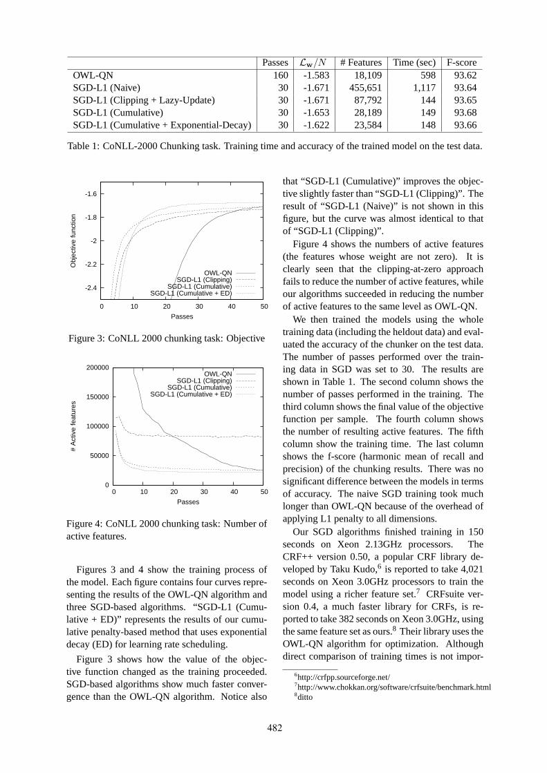
Passes Lw/N # Features Time (sec) F-scoreOWL-QN 160 -1.583 18,109 598 93.62SGD-L1 (Naive) 30 -1.671 455,651 1,117 93.64SGD-L1 (Clipping + Lazy-Update) 30 -1.671 87,792 144 93.65SGD-L1 (Cumulative) 30 -1.653 28,189 149 93.68SGD-L1 (Cumulative + Exponential-Decay) 30 -1.622 23,584 148 93.66
Table 1: CoNLL-2000 Chunking task. Training time and accuracy of the trained model on the test data.
-2.4
-2.2
-2
-1.8
-1.6
0 10 20 30 40 50
Obj
ectiv
e fu
nctio
n
Passes
OWL-QNSGD-L1 (Clipping)
SGD-L1 (Cumulative)SGD-L1 (Cumulative + ED)
Figure 3: CoNLL 2000 chunking task: Objective
0
50000
100000
150000
200000
0 10 20 30 40 50
# A
ctiv
e fe
atur
es
Passes
OWL-QNSGD-L1 (Clipping)
SGD-L1 (Cumulative)SGD-L1 (Cumulative + ED)
Figure 4: CoNLL 2000 chunking task: Number ofactive features.
Figures 3 and 4 show the training process ofthe model. Each figure contains four curves repre-senting the results of the OWL-QN algorithm andthree SGD-based algorithms. “SGD-L1 (Cumu-lative + ED)” represents the results of our cumu-lative penalty-based method that uses exponentialdecay (ED) for learning rate scheduling.
Figure 3 shows how the value of the objec-tive function changed as the training proceeded.SGD-based algorithms show much faster conver-gence than the OWL-QN algorithm. Notice also
that “SGD-L1 (Cumulative)” improves the objec-tive slightly faster than “SGD-L1 (Clipping)”. Theresult of “SGD-L1 (Naive)” is not shown in thisfigure, but the curve was almost identical to thatof “SGD-L1 (Clipping)”.
Figure 4 shows the numbers of active features(the features whose weight are not zero). It isclearly seen that the clipping-at-zero approachfails to reduce the number of active features, whileour algorithms succeeded in reducing the numberof active features to the same level as OWL-QN.
We then trained the models using the wholetraining data (including the heldout data) and eval-uated the accuracy of the chunker on the test data.The number of passes performed over the train-ing data in SGD was set to 30. The results areshown in Table 1. The second column shows thenumber of passes performed in the training. Thethird column shows the final value of the objectivefunction per sample. The fourth column showsthe number of resulting active features. The fifthcolumn show the training time. The last columnshows the f-score (harmonic mean of recall andprecision) of the chunking results. There was nosignificant difference between the models in termsof accuracy. The naive SGD training took muchlonger than OWL-QN because of the overhead ofapplying L1 penalty to all dimensions.
Our SGD algorithms finished training in 150seconds on Xeon 2.13GHz processors. TheCRF++ version 0.50, a popular CRF library de-veloped by Taku Kudo,6 is reported to take 4,021seconds on Xeon 3.0GHz processors to train themodel using a richer feature set.7 CRFsuite ver-sion 0.4, a much faster library for CRFs, is re-ported to take 382 seconds on Xeon 3.0GHz, usingthe same feature set as ours.8 Their library uses theOWL-QN algorithm for optimization. Althoughdirect comparison of training times is not impor-
6http://crfpp.sourceforge.net/7http://www.chokkan.org/software/crfsuite/benchmark.html8ditto
482
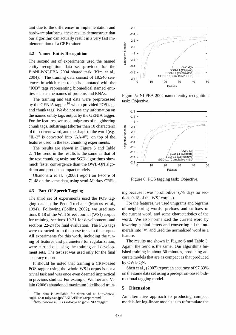
tant due to the differences in implementation andhardware platforms, these results demonstrate thatour algorithm can actually result in a very fast im-plementation of a CRF trainer.
4.2 Named Entity Recognition
The second set of experiments used the namedentity recognition data set provided for theBioNLP/NLPBA 2004 shared task (Kim et al.,2004).9 The training data consist of 18,546 sen-tences in which each token is annotated with the“IOB” tags representing biomedical named enti-ties such as the names of proteins and RNAs.
The training and test data were preprocessedby the GENIA tagger,10 which provided POS tagsand chunk tags. We did not use any information onthe named entity tags output by the GENIA tagger.For the features, we used unigrams of neighboringchunk tags, substrings (shorter than 10 characters)of the current word, and the shape of the word (e.g.“IL-2” is converted into “AA-#”), on top of thefeatures used in the text chunking experiments.
The results are shown in Figure 5 and Table2. The trend in the results is the same as that ofthe text chunking task: our SGD algorithms showmuch faster convergence than the OWL-QN algo-rithm and produce compact models.
Okanohara et al. (2006) report an f-score of71.48 on the same data, using semi-Markov CRFs.
4.3 Part-Of-Speech Tagging
The third set of experiments used the POS tag-ging data in the Penn Treebank (Marcus et al.,1994). Following (Collins, 2002), we used sec-tions 0-18 of the Wall Street Journal (WSJ) corpusfor training, sections 19-21 for development, andsections 22-24 for final evaluation. The POS tagswere extracted from the parse trees in the corpus.All experiments for this work, including the tun-ing of features and parameters for regularization,were carried out using the training and develop-ment sets. The test set was used only for the finalaccuracy report.
It should be noted that training a CRF-basedPOS tagger using the whole WSJ corpus is not atrivial task and was once even deemed impracticalin previous studies. For example, Wellner and Vi-lain (2006) abandoned maximum likelihood train-
9The data is available for download at http://www-tsujii.is.s.u-tokyo.ac.jp/GENIA/ERtask/report.html
10http://www-tsujii.is.s.u-tokyo.ac.jp/GENIA/tagger/
-3.8
-3.6
-3.4
-3.2
-3
-2.8
-2.6
-2.4
-2.2
0 10 20 30 40 50
Obj
ectiv
e fu
nctio
n
Passes
OWL-QNSGD-L1 (Clipping)
SGD-L1 (Cumulative)SGD-L1 (Cumulative + ED)
Figure 5: NLPBA 2004 named entity recognitiontask: Objective.
-2.8
-2.7
-2.6
-2.5
-2.4
-2.3
-2.2
-2.1
-2
-1.9
-1.8
0 10 20 30 40 50
Obj
ectiv
e fu
nctio
n
Passes
OWL-QNSGD-L1 (Clipping)
SGD-L1 (Cumulative)SGD-L1 (Cumulative + ED)
Figure 6: POS tagging task: Objective.
ing because it was “prohibitive” (7-8 days for sec-tions 0-18 of the WSJ corpus).
For the features, we used unigrams and bigramsof neighboring words, prefixes and suffixes ofthe current word, and some characteristics of theword. We also normalized the current word bylowering capital letters and converting all the nu-merals into ‘#’, and used the normalized word as afeature.
The results are shown in Figure 6 and Table 3.Again, the trend is the same. Our algorithms fin-ished training in about 30 minutes, producing ac-curate models that are as compact as that producedby OWL-QN.
Shen et al., (2007) report an accuracy of 97.33%on the same data set using a perceptron-based bidi-rectional tagging model.
5 Discussion
An alternative approach to producing compactmodels for log-linear models is to reformulate the
483
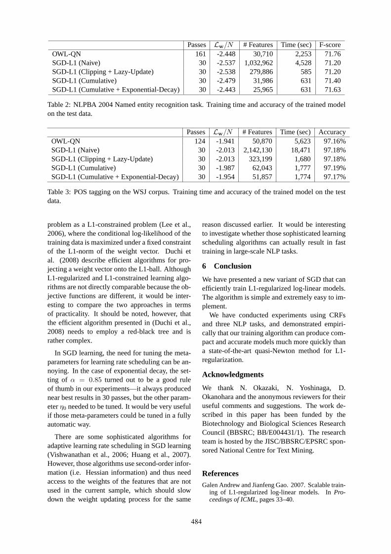
Passes Lw/N # Features Time (sec) F-scoreOWL-QN 161 -2.448 30,710 2,253 71.76SGD-L1 (Naive) 30 -2.537 1,032,962 4,528 71.20SGD-L1 (Clipping + Lazy-Update) 30 -2.538 279,886 585 71.20SGD-L1 (Cumulative) 30 -2.479 31,986 631 71.40SGD-L1 (Cumulative + Exponential-Decay) 30 -2.443 25,965 631 71.63
Table 2: NLPBA 2004 Named entity recognition task. Training time and accuracy of the trained modelon the test data.
Passes Lw/N # Features Time (sec) AccuracyOWL-QN 124 -1.941 50,870 5,623 97.16%SGD-L1 (Naive) 30 -2.013 2,142,130 18,471 97.18%SGD-L1 (Clipping + Lazy-Update) 30 -2.013 323,199 1,680 97.18%SGD-L1 (Cumulative) 30 -1.987 62,043 1,777 97.19%SGD-L1 (Cumulative + Exponential-Decay) 30 -1.954 51,857 1,774 97.17%
Table 3: POS tagging on the WSJ corpus. Training time and accuracy of the trained model on the testdata.
problem as a L1-constrained problem (Lee et al.,2006), where the conditional log-likelihood of thetraining data is maximized under a fixed constraintof the L1-norm of the weight vector. Duchi etal. (2008) describe efficient algorithms for pro-jecting a weight vector onto the L1-ball. AlthoughL1-regularized and L1-constrained learning algo-rithms are not directly comparable because the ob-jective functions are different, it would be inter-esting to compare the two approaches in termsof practicality. It should be noted, however, thatthe efficient algorithm presented in (Duchi et al.,2008) needs to employ a red-black tree and israther complex.
In SGD learning, the need for tuning the meta-parameters for learning rate scheduling can be an-noying. In the case of exponential decay, the set-ting of α = 0.85 turned out to be a good ruleof thumb in our experiments—it always producednear best results in 30 passes, but the other param-eterη0 needed to be tuned. It would be very usefulif those meta-parameters could be tuned in a fullyautomatic way.
There are some sophisticated algorithms foradaptive learning rate scheduling in SGD learning(Vishwanathan et al., 2006; Huang et al., 2007).However, those algorithms use second-order infor-mation (i.e. Hessian information) and thus needaccess to the weights of the features that are notused in the current sample, which should slowdown the weight updating process for the same
reason discussed earlier. It would be interestingto investigate whether those sophisticated learningscheduling algorithms can actually result in fasttraining in large-scale NLP tasks.
6 Conclusion
We have presented a new variant of SGD that canefficiently train L1-regularized log-linear models.The algorithm is simple and extremely easy to im-plement.
We have conducted experiments using CRFsand three NLP tasks, and demonstrated empiri-cally that our training algorithm can produce com-pact and accurate models much more quickly thana state-of-the-art quasi-Newton method for L1-regularization.
Acknowledgments
We thank N. Okazaki, N. Yoshinaga, D.Okanohara and the anonymous reviewers for theiruseful comments and suggestions. The work de-scribed in this paper has been funded by theBiotechnology and Biological Sciences ResearchCouncil (BBSRC; BB/E004431/1). The researchteam is hosted by the JISC/BBSRC/EPSRC spon-sored National Centre for Text Mining.
ReferencesGalen Andrew and Jianfeng Gao. 2007. Scalable train-
ing of L1-regularized log-linear models. InPro-ceedings of ICML, pages 33–40.
484
Bob Carpenter. 2008. Lazy sparse stochastic gradientdescent for regularized multinomial logistic regres-sion. Technical report, Alias-i.
Stephen Clark and James R. Curran. 2004. Parsing theWSJ using CCG and log-linear models. InProceed-ings of COLING 2004, pages 103–110.
Trevor Cohn and Philip Blunsom. 2005. Semantic rolelabeling with tree conditional random fields. InPro-ceedings of CoNLL, pages 169–172.
Michael Collins, Amir Globerson, Terry Koo, XavierCarreras, and Peter L. Bartlett. 2008. Exponen-tiated gradient algorithms for conditional randomfields and max-margin markov networks.The Jour-nal of Machine Learning Research (JMLR), 9:1775–1822.
Michael Collins. 2002. Discriminative training meth-ods for hidden markov models: Theory and exper-iments with perceptron algorithms. InProceedingsof EMNLP, pages 1–8.
Christian Darken and John Moody. 1990. Note onlearning rate schedules for stochastic optimization.In Proceedings of NIPS, pages 832–838.
Juhn Duchi and Yoram Singer. 2008. Online andbatch learning using forward-looking subgradients.In NIPS Workshop: OPT 2008 Optimization for Ma-chine Learning.
Juhn Duchi, Shai Shalev-Shwartz, Yoram Singer, andTushar Chandra. 2008. Efficient projections ontothe l1-ball for learning in high dimensions. InPro-ceedings of ICML, pages 272–279.
Jenny Rose Finkel, Alex Kleeman, and Christopher D.Manning. 2008. Efficient, feature-based, condi-tional random field parsing. InProceedings of ACL-08:HLT, pages 959–967.
Jianfeng Gao, Galen Andrew, Mark Johnson, andKristina Toutanova. 2007. A comparative study ofparameter estimation methods for statistical naturallanguage processing. InProceedings of ACL, pages824–831.
Han-Shen Huang, Yu-Ming Chang, and Chun-NanHsu. 2007. Training conditional random fields byperiodic step size adaptation for large-scale text min-ing. In Proceedings of ICDM, pages 511–516.
Jun’ichi Kazama and Jun’ichi Tsujii. 2003. Evalua-tion and extension of maximum entropy models withinequality constraints. InProceedings of EMNLP2003.
J.-D. Kim, T. Ohta, Y. Tsuruoka, Y. Tateisi, and N. Col-lier. 2004. Introduction to the bio-entity recognitiontask at JNLPBA. InProceedings of the InternationalJoint Workshop on Natural Language Processing inBiomedicine and its Applications (JNLPBA), pages70–75.
John Lafferty, Andrew McCallum, and FernandoPereira. 2001. Conditional random fields: Prob-abilistic models for segmenting and labeling se-quence data. InProceedings of ICML, pages 282–289.
John Langford, Lihong Li, and Tong Zhang. 2009.Sparse online learning via truncated gradient.TheJournal of Machine Learning Research (JMLR),10:777–801.
Su-In Lee, Honglak Lee, Pieter Abbeel, and Andrew Y.Ng. 2006. Efficient l1 regularized logistic regres-sion. InProceedings of AAAI-06, pages 401–408.
Mitchell P. Marcus, Beatrice Santorini, and Mary AnnMarcinkiewicz. 1994. Building a large annotatedcorpus of English: The Penn Treebank.Computa-tional Linguistics, 19(2):313–330.
Jorge Nocedal. 1980. Updating quasi-newton matriceswith limited storage.Mathematics of Computation,35(151):773–782.
Daisuke Okanohara, Yusuke Miyao, Yoshimasa Tsu-ruoka, and Jun’ichi Tsujii. 2006. Improvingthe scalability of semi-markov conditional randomfields for named entity recognition. InProceedingsof COLING/ACL, pages 465–472.
Adwait Ratnaparkhi. 1996. A maximum entropymodel for part-of-speech tagging. InProceedingsof EMNLP 1996, pages 133–142.
Libin Shen, Giorgio Satta, and Aravind Joshi. 2007.Guided learning for bidirectional sequence classifi-cation. InProceedings of ACL, pages 760–767.
David Smith and Jason Eisner. 2008. Dependencyparsing by belief propagation. InProceedings ofEMNLP, pages 145–156.
James C. Spall. 2005.Introduction to StochasticSearch and Optimization. Wiley-IEEE.
Christoph Tillmann and Tong Zhang. 2006. A discrim-inative global training algorithm for statistical MT.In Proceedings of COLING/ACL, pages 721–728.
Kristina Toutanova, Aria Haghighi, and ChristopherManning. 2005. Joint learning improves semanticrole labeling. InProceedings of ACL, pages 589–596.
S. V. N. Vishwanathan, Nicol N. Schraudolph, Mark W.Schmidt, and Kevin P. Murphy. 2006. Acceleratedtraining of conditional random fields with stochasticgradient methods. InProceedings of ICML, pages969–976.
Ben Wellner and Marc Vilain. 2006. Leveragingmachine readable dictionaries in discriminative se-quence models. InProceedings of LREC 2006.
485

Proceedings of the 47th Annual Meeting of the ACL and the 4th IJCNLP of the AFNLP, pages 486–494,Suntec, Singapore, 2-7 August 2009. c©2009 ACL and AFNLP
A global model for joint lemmatization and part-of-speech prediction
Kristina ToutanovaMicrosoft Research
Redmond, WA [email protected]
Colin CherryMicrosoft Research
Redmond, WA [email protected]
Abstract
We present a global joint model forlemmatization and part-of-speech predic-tion. Using only morphological lexiconsand unlabeled data, we learn a partially-supervised part-of-speech tagger and alemmatizer which are combined using fea-tures on a dynamically linked dependencystructure of words. We evaluate ourmodel on English, Bulgarian, Czech, andSlovene, and demonstrate substantial im-provements over both a direct transductionapproach to lemmatization and a pipelinedapproach, which predicts part-of-speechtags before lemmatization.
1 Introduction
The traditional problem of morphological analysisis, given a word form, to predict the set of all ofits possible morphological analyses. A morpho-logical analysis consists of a part-of-speech tag(POS), possibly other morphological features, anda lemma (basic form) corresponding to this tag andfeatures combination (see Table 1 for examples).We address this problem in the setting where weare given a morphological dictionary for training,and can additionally make use of un-annotated textin the language. We present a new machine learn-ing model for this task setting.
In addition to the morphological analysis taskwe are interested in performance on two subtasks:tag-set prediction (predicting the set of possibletags of words) and lemmatization (predicting theset of possible lemmas). The result of these sub-tasks is directly useful for some applications.1 Ifwe are interested in the results of each of these two
1Tag sets are useful, for example, as a basis of sparsity-reducing features for text labeling tasks; lemmatization isuseful for information retrieval and machine translation froma morphologically rich to a morphologically poor language,where full analysis may not be important.
subtasks in isolation, we might build independentsolutions which ignore the other subtask.
In this paper, we show that there are strong de-pendencies between the two subtasks and we canimprove performance on both by sharing infor-mation between them. We present a joint modelfor these two subtasks: it is joint not only in thatit performs both tasks simultaneously, sharing in-formation, but also in that it reasons about multi-ple words jointly. It uses component tag-set andlemmatization models and combines their predic-tions while incorporating joint features in a log-linear model, defined on a dynamically linked de-pendency structure of words.
The model is formalized in Section 5 and eval-uated in Section 6. We report results on English,Bulgarian, Slovene, and Czech and show that jointmodeling reduces the lemmatization error by up to19%, the tag-prediction error by up to 26% and theerror on the complete morphological analysis taskby up to 22.6%.
2 Task formalization
The main task that we would like to solve isas follows: given a lexicon L which containsall morphological analyses for a set of words{w1, . . . , wn}, learn to predict all morphologicalanalyses for other words which are outside of L.In addition to the lexicon, we are allowed to makeuse of unannotated text T in the language. We willpredict morphological analyses for words whichoccur in T. Note that the task is defined on wordtypes and not on words in context.
A morphological analysis of a word w consistsof a (possibly structured) POS tag t, together withone or several lemmas, which are the possible ba-sic forms of w when it has tag t. As an exam-ple, Table 1 illustrates the morphological analy-ses of several words taken from the CELEX lexi-cal database of English (Baayen et al., 1995) andthe Multext-East lexicon of Bulgarian (Erjavec,2004). The Bulgarian words are transcribed in
486
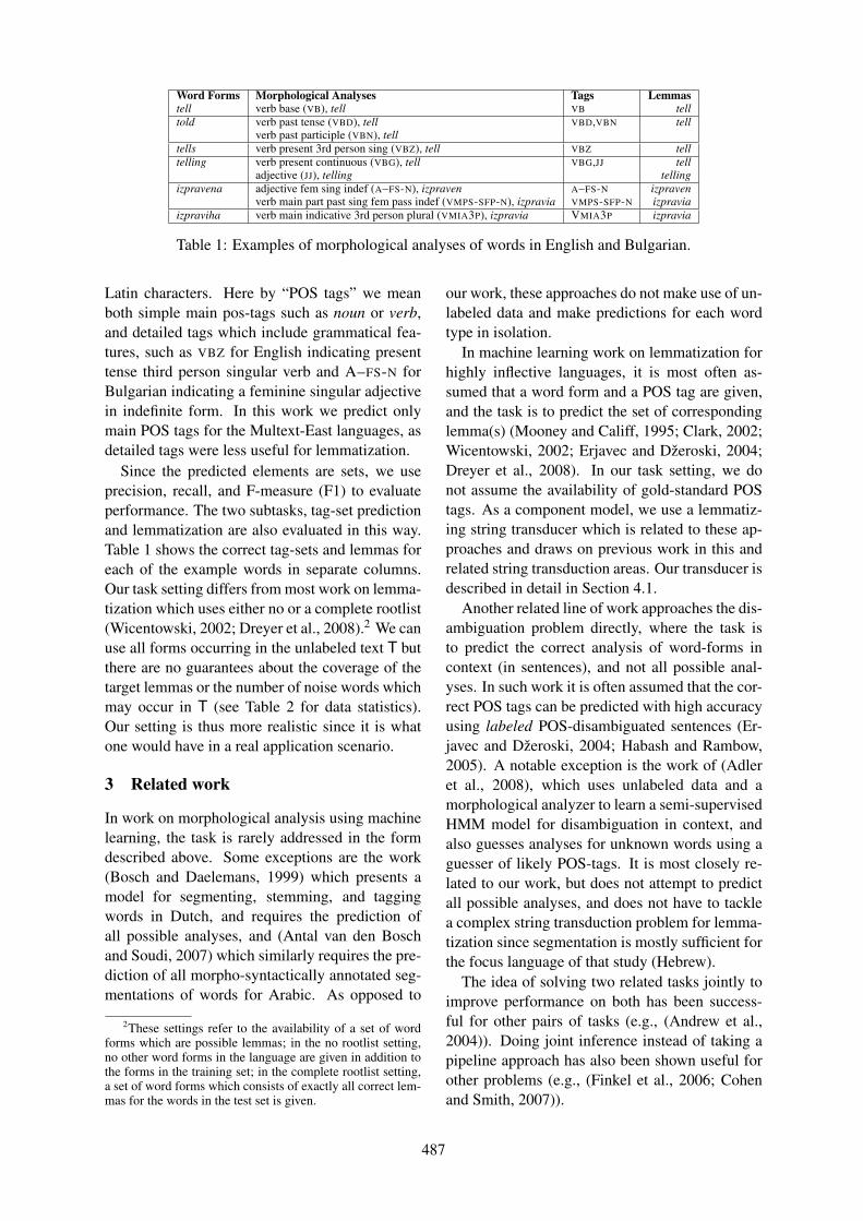
Word Forms Morphological Analyses Tags Lemmastell verb base (VB), tell VB telltold verb past tense (VBD), tell VBD,VBN tell
verb past participle (VBN), telltells verb present 3rd person sing (VBZ), tell VBZ telltelling verb present continuous (VBG), tell VBG,JJ tell
adjective (JJ), telling tellingizpravena adjective fem sing indef (A–FS-N), izpraven A–FS-N izpraven
verb main part past sing fem pass indef (VMPS-SFP-N), izpravia VMPS-SFP-N izpraviaizpraviha verb main indicative 3rd person plural (VMIA3P), izpravia VMIA3P izpravia
Table 1: Examples of morphological analyses of words in English and Bulgarian.
Latin characters. Here by “POS tags” we meanboth simple main pos-tags such as noun or verb,and detailed tags which include grammatical fea-tures, such as VBZ for English indicating presenttense third person singular verb and A–FS-N forBulgarian indicating a feminine singular adjectivein indefinite form. In this work we predict onlymain POS tags for the Multext-East languages, asdetailed tags were less useful for lemmatization.
Since the predicted elements are sets, we useprecision, recall, and F-measure (F1) to evaluateperformance. The two subtasks, tag-set predictionand lemmatization are also evaluated in this way.Table 1 shows the correct tag-sets and lemmas foreach of the example words in separate columns.Our task setting differs from most work on lemma-tization which uses either no or a complete rootlist(Wicentowski, 2002; Dreyer et al., 2008).2 We canuse all forms occurring in the unlabeled text T butthere are no guarantees about the coverage of thetarget lemmas or the number of noise words whichmay occur in T (see Table 2 for data statistics).Our setting is thus more realistic since it is whatone would have in a real application scenario.
3 Related work
In work on morphological analysis using machinelearning, the task is rarely addressed in the formdescribed above. Some exceptions are the work(Bosch and Daelemans, 1999) which presents amodel for segmenting, stemming, and taggingwords in Dutch, and requires the prediction ofall possible analyses, and (Antal van den Boschand Soudi, 2007) which similarly requires the pre-diction of all morpho-syntactically annotated seg-mentations of words for Arabic. As opposed to
2These settings refer to the availability of a set of wordforms which are possible lemmas; in the no rootlist setting,no other word forms in the language are given in addition tothe forms in the training set; in the complete rootlist setting,a set of word forms which consists of exactly all correct lem-mas for the words in the test set is given.
our work, these approaches do not make use of un-labeled data and make predictions for each wordtype in isolation.
In machine learning work on lemmatization forhighly inflective languages, it is most often as-sumed that a word form and a POS tag are given,and the task is to predict the set of correspondinglemma(s) (Mooney and Califf, 1995; Clark, 2002;Wicentowski, 2002; Erjavec and Džeroski, 2004;Dreyer et al., 2008). In our task setting, we donot assume the availability of gold-standard POStags. As a component model, we use a lemmatiz-ing string transducer which is related to these ap-proaches and draws on previous work in this andrelated string transduction areas. Our transducer isdescribed in detail in Section 4.1.
Another related line of work approaches the dis-ambiguation problem directly, where the task isto predict the correct analysis of word-forms incontext (in sentences), and not all possible anal-yses. In such work it is often assumed that the cor-rect POS tags can be predicted with high accuracyusing labeled POS-disambiguated sentences (Er-javec and Džeroski, 2004; Habash and Rambow,2005). A notable exception is the work of (Adleret al., 2008), which uses unlabeled data and amorphological analyzer to learn a semi-supervisedHMM model for disambiguation in context, andalso guesses analyses for unknown words using aguesser of likely POS-tags. It is most closely re-lated to our work, but does not attempt to predictall possible analyses, and does not have to tacklea complex string transduction problem for lemma-tization since segmentation is mostly sufficient forthe focus language of that study (Hebrew).
The idea of solving two related tasks jointly toimprove performance on both has been success-ful for other pairs of tasks (e.g., (Andrew et al.,2004)). Doing joint inference instead of taking apipeline approach has also been shown useful forother problems (e.g., (Finkel et al., 2006; Cohenand Smith, 2007)).
487

4 Component models
We use two component models as the basis ofaddressing the task: one is a partially-supervisedPOS tagger which is trained using L and the unla-beled text T; the other is a lemmatizing transducerwhich is trained from L and can use T. The trans-ducer can optionally be given input POS tags intraining and testing, which can inform the lemma-tization. The tagger is described in Section 4.2 andthe transducer is described in Section 4.1.
In a pipeline approach to combining the taggingand lemmatization components, we first predict aset of tags for each word using the tagger, and thenask the lemmatizer to predict one lemma for eachof the possible tags. In a direct transduction ap-proach to the lemmatization subtask, we train thelemmatizer without access to tags and ask it topredict a single lemma for each word in testing.Our joint model, described in Section 5, is definedin a re-ranking framework, and can choose fromamong k-best predictions of tag-sets and lemmasgenerated from the component tagger and lemma-tizer models.
4.1 Morphological analyser
We employ a discriminative character transduceras a component morphological analyzer. The inputto the transducer is an inflected word (the source)and possibly an estimated part-of-speech; the out-put is the lemma of the word (the target). Thetransducer is similar to the one described by Ji-ampojamarn et al. (2008) for letter-to-phonemeconversion, but extended to allow for whole-wordfeatures on both the input and the output. The coreof our engine is the dynamic programming algo-rithm for monotone phrasal decoding (Zens andNey, 2004). The main feature of this algorithm isits capability to transduce many consecutive char-acters with a single operation; the same algorithmis employed to tag subsequences in semi-MarkovCRFs (Sarawagi and Cohen, 2004).
We employ three main categories of features:context, transition, and vocabulary (rootlist) fea-tures. The first two are described in detail by Ji-ampojamarn et al. (2008), while the final is novelto this work. Context features are centered arounda transduction operation such as es → e , as em-ployed in gives → give. Context features includean indicator for the operation itself, conjoined withindicators for all n-grams of source context withina fixed window of the operation. We also employ a
copy feature that indicates if the operation simplycopies the source character, such as e → e. Tran-sition features are our Markov, or n-gram featureson transduction operations. Vocabulary featuresare defined on complete target words, accordingto the frequency of said word in a provided unla-beled text T. We have chosen to bin frequencies;experiments on a development set suggested thattwo indicators are sufficient: the first fires for anyword that occurred fewer than five times, while asecond also fires for those words that did not oc-cur at all. By encoding our vocabulary in a trie andadding the trie index to the target context trackedby our dynamic programming chart, we can ef-ficiently track these frequencies during transduc-tion.
We incorporate the source part-of-speech tag byappending it to each feature, thus the context fea-ture es → e may become es → e, VBZ. To en-able communication between the various parts-of-speech, a universal set of unannotated features alsofires, regardless of the part-of-speech, acting as aback-off model of how words in general behaveduring stemming.
Linear weights are assigned to each of the trans-ducer’s features using an averaged perceptron forstructure prediction (Collins, 2002). Note thatour features are defined in terms of the operationsemployed during transduction, therefore to cre-ate gold-standard feature vectors, we require notonly target outputs, but also derivations to pro-duce those outputs. We employ a deterministicheuristic to create these derivations; given a gold-standard source-target pair, we construct a deriva-tion that uses only trivial copy operations untilthe first character mismatch. The remainder ofthe transduction is performed with a single multi-character replacement. For example, the deriva-tion for living → live would be l → l , i → i ,v → v , ing → e. For languages with morpholo-gies affecting more than just the suffix, one caneither develop a more complex heuristic, or deter-mine the derivations using a separate aligner suchas that of Ristad and Yianilos (1998).
4.2 Tag-set prediction model
The tag-set model uses a training lexicon L andunlabeled text T to learn to predict sets of tagsfor words. It is based on the semi-supervised tag-ging model of (Toutanova and Johnson, 2008). Ithas two sub-models: one is an ambiguity class
488

or a tag-set model, which can assign probabili-ties for possible sets of tags of words PTSM (ts|w)and the other is a word context model, which canassign probabilities PCM (contextsw|w, ts) to allcontexts of occurrence of word w in an unlabeledtext T. The word-context model is Bayesian andutilizes a sparse Dirichlet prior on the distributionsof tags given words. In addition, it uses informa-tion on a four word context of occurrences of w inthe unlabeled text.
Note that the (Toutanova and Johnson, 2008)model is a tagger that assigns tags to occurrencesof words in the text, whereas we only need to pre-dict sets of possible tags for word types, such asthe set {VBD, VBN} for the word told. Their com-ponent sub-model PTSM predicts sets of tags andit is possible to use it on its own, but by also us-ing the context model we can take into accountinformation from the context of occurrence ofwords and compute probabilities of tag-sets giventhe observed occurrences in T. The two are com-bined to make a prediction for a tag-set of a testword w, given unlabeled text T, using Bayes rule:p(ts|w) ∝ PTSM (ts|w)PCM (contextsw|w, ts).
We use a direct re-implementation of the word-context model, using variational inference follow-ing (Toutanova and Johnson, 2008). For the tag-set sub-model, we employ a more sophisticatedapproach. First, we learn a log-linear classifier in-stead of a Naive Bayes model, and second, we usefeatures derived from related words appearing inT. The possible classes predicted by the classifierare as many as the observed tag-sets in L. Thesparsity is relieved by adding features for individ-ual tags t which get shared across tag-sets contain-ing t.
There are two types of features in the model:(i) word-internal features: word suffixes, capital-ization, existence of hyphen, and word prefixes(such features were also used in (Toutanova andJohnson, 2008)), and (ii) features based on re-lated words. These latter features are inspired by(Cucerzan and Yarowsky, 2000) and are defined asfollows: for a word w such as telling, there is anindicator feature for every combination of two suf-fixes α and β, such that there is a prefix p wheretelling= pα and pβ exists in T. For example, if theword tells is found in T, there would be a featurefor the suffixes α=ing,β=s that fires. The suffixesare defined as all character suffixes up to lengththree which occur with at least 100 words.
b o u n c e dVBD VBN JJ VBD VBN
b o u n c e rJJR NN
bounce
bouncer bounce
…
bounc
bouncer
boucer
fbounce bounce
bounced bounced b o u n c eVB NN VB
bounce bounce
… …
…
f
Figure 1: A small subset of the graphical model. Thetag-sets and lemmas active in the illustrated assignment areshown in bold. The extent of joint features firing for thelemma bounce is shown as a factor indicated by the blue cir-cle and connected to the assignments of the three words.
5 A global joint model for morphologicalanalysis
The idea of this model is to jointly predict the setof possible tags and lemmas of words. In addi-tion to modeling dependencies between the tagsand lemmas of a single word, we incorporate de-pendencies between the predictions for multiplewords. The dependencies among words are deter-mined dynamically. Intuitively, if two words havethe same lemma, their tag-sets are dependent. Forexample, imagine that we need to determine thetag-set and lemmas of the word bouncer. The tag-set model may guess that the word is an adjectivein comparative form, because of its suffix, and be-cause its occurrences in T might not strongly in-dicate that it is a noun. The lemmatizer can thenlemmatize the word like an adjective and come upwith bounce as a lemma. If the tag-set model isfairly certain that bounce is not an adjective, butis a verb or a noun, a joint model which looks si-multaneously at the tags and lemmas of bouncerand bounce will detect a problem with this assign-ments and will be able to correct the tagging andlemmatization error for bouncer.
The main source of information our joint modeluses is information about the assignments of allwords that have the same lemma l. If the tag-setmodel is better able to predict the tags of some ofthese words, the information can propagate to theother words. If some of them are lemmatized cor-rectly, the model can be pushed to lemmatize theothers correctly as well. Since the lemmas of testwords are not given, the dependencies between as-
489
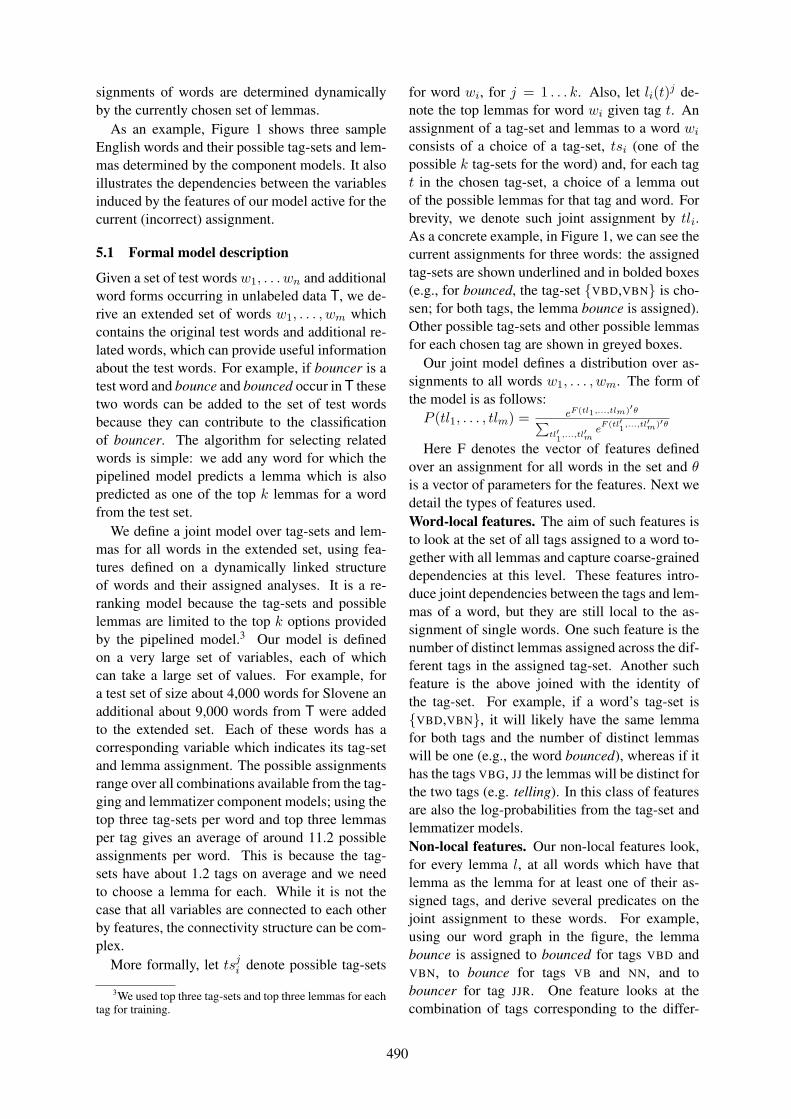
signments of words are determined dynamicallyby the currently chosen set of lemmas.
As an example, Figure 1 shows three sampleEnglish words and their possible tag-sets and lem-mas determined by the component models. It alsoillustrates the dependencies between the variablesinduced by the features of our model active for thecurrent (incorrect) assignment.
5.1 Formal model description
Given a set of test words w1, . . . wn and additionalword forms occurring in unlabeled data T, we de-rive an extended set of words w1, . . . , wm whichcontains the original test words and additional re-lated words, which can provide useful informationabout the test words. For example, if bouncer is atest word and bounce and bounced occur in T thesetwo words can be added to the set of test wordsbecause they can contribute to the classificationof bouncer. The algorithm for selecting relatedwords is simple: we add any word for which thepipelined model predicts a lemma which is alsopredicted as one of the top k lemmas for a wordfrom the test set.
We define a joint model over tag-sets and lem-mas for all words in the extended set, using fea-tures defined on a dynamically linked structureof words and their assigned analyses. It is a re-ranking model because the tag-sets and possiblelemmas are limited to the top k options providedby the pipelined model.3 Our model is definedon a very large set of variables, each of whichcan take a large set of values. For example, fora test set of size about 4,000 words for Slovene anadditional about 9,000 words from T were addedto the extended set. Each of these words has acorresponding variable which indicates its tag-setand lemma assignment. The possible assignmentsrange over all combinations available from the tag-ging and lemmatizer component models; using thetop three tag-sets per word and top three lemmasper tag gives an average of around 11.2 possibleassignments per word. This is because the tag-sets have about 1.2 tags on average and we needto choose a lemma for each. While it is not thecase that all variables are connected to each otherby features, the connectivity structure can be com-plex.
More formally, let tsji denote possible tag-sets
3We used top three tag-sets and top three lemmas for eachtag for training.
for word wi, for j = 1 . . . k. Also, let li(t)j de-
note the top lemmas for word wi given tag t. Anassignment of a tag-set and lemmas to a word wi
consists of a choice of a tag-set, tsi (one of thepossible k tag-sets for the word) and, for each tagt in the chosen tag-set, a choice of a lemma outof the possible lemmas for that tag and word. Forbrevity, we denote such joint assignment by tli.As a concrete example, in Figure 1, we can see thecurrent assignments for three words: the assignedtag-sets are shown underlined and in bolded boxes(e.g., for bounced, the tag-set {VBD,VBN} is cho-sen; for both tags, the lemma bounce is assigned).Other possible tag-sets and other possible lemmasfor each chosen tag are shown in greyed boxes.
Our joint model defines a distribution over as-signments to all words w1, . . . , wm. The form ofthe model is as follows:
P (tl1, . . . , tlm) = eF (tl1,...,tlm)′θ∑
tl′1
,...,tl′meF (tl′
1,...,tl′m)′θ
Here F denotes the vector of features definedover an assignment for all words in the set and θis a vector of parameters for the features. Next wedetail the types of features used.Word-local features. The aim of such features isto look at the set of all tags assigned to a word to-gether with all lemmas and capture coarse-graineddependencies at this level. These features intro-duce joint dependencies between the tags and lem-mas of a word, but they are still local to the as-signment of single words. One such feature is thenumber of distinct lemmas assigned across the dif-ferent tags in the assigned tag-set. Another suchfeature is the above joined with the identity ofthe tag-set. For example, if a word’s tag-set is{VBD,VBN}, it will likely have the same lemmafor both tags and the number of distinct lemmaswill be one (e.g., the word bounced), whereas if ithas the tags VBG, JJ the lemmas will be distinct forthe two tags (e.g. telling). In this class of featuresare also the log-probabilities from the tag-set andlemmatizer models.Non-local features. Our non-local features look,for every lemma l, at all words which have thatlemma as the lemma for at least one of their as-signed tags, and derive several predicates on thejoint assignment to these words. For example,using our word graph in the figure, the lemmabounce is assigned to bounced for tags VBD andVBN, to bounce for tags VB and NN, and tobouncer for tag JJR. One feature looks at thecombination of tags corresponding to the differ-
490
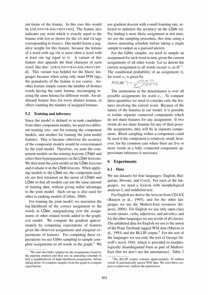
ent forms of the lemma. In this case this wouldbe [JJR,NN+VB-lem,VBD+VBN]. The feature alsoindicates any word which is exactly equal to thelemma with lem as shown for the NN and VB tagscorresponding to bounce. Our model learns a neg-ative weight for this feature, because the lemmaof a word with tag JJR is most often a word withat least one tag equal to JJ. A variant of thisfeature also appends the final character of eachword, like this: [JJR+r,NN+VB+e-lem,VBD+VBN-d]. This variant was helpful for the Slavic lan-guages because when using only main POS tags,the granularity of the feature is too coarse. An-other feature simply counts the number of distinctwords having the same lemma, encouraging re-using the same lemma for different words. An ad-ditional feature fires for every distinct lemma, ineffect counting the number of assigned lemmas.
5.2 Training and inference
Since the model is defined to re-rank candidatesfrom other component models, we need two differ-ent training sets: one for training the componentmodels, and another for training the joint modelfeatures. This is because otherwise the accuracyof the component models would be overestimatedby the joint model. Therefore, we train the com-ponent models on the training lexicons LTrain andselect their hyperparameters on the LDev lexicons.We then train the joint model on the LDev lexiconsand evaluate it on the LTest lexicons. When apply-ing models to the LTest set, the component mod-els are first retrained on the union of LTrain andLDev so that all models can use the same amountof training data, without giving unfair advantageto the joint model. Such set-up is also used forother re-ranking models (Collins, 2000).
For training the joint model, we maximize thelog-likelihood of the correct assignment to thewords in LDev, marginalizing over the assign-ments of other related words added to the graph-ical model. We compute the gradient approx-imately by computing expectations of featuresgiven the observed assignments and marginal ex-pectations of features. For computing these ex-pectations we use Gibbs sampling to sample com-plete assignments to all words in the graph.4 We
4We start the Gibbs sampler by the assignments found bythe pipeline method and then use an annealing schedule tofind a neighborhood of high-likelihood assignments, beforetaking about 10 complete samples from the graph to computeexpectations.
use gradient descent with a small learning rate, se-lected to optimize the accuracy on the LDev set.For finding a most likely assignment at test time,we use the sampling procedure, this time using aslower annealing schedule before taking a singlesample to output as a guessed answer.
For the Gibbs sampler, we need to sample anassignment for each word in turn, given the currentassignments of all other words. Let us denote thecurrent assignment to all words except wi as tl−i.The conditional probability of an assignment tlifor word wi is given by:
P (tli|tl−i) = eF (tli,tl−i)′θ∑
tl′ieF (tl′
i,tl−i)′θ
The summation in the denominator is over allpossible assignments for word wi. To computethese quantities we need to consider only the fea-tures involving the current word. Because of thenature of the features in our model, it is possibleto isolate separate connected components whichdo not share features for any assignment. If twowords do not share lemmas for any of their possi-ble assignments, they will be in separate compo-nents. Block sampling within a component couldbe used if the component is relatively small; how-ever, for the common case where there are five ormore words in a fully connected component ap-proximate inference is necessary.
6 Experiments
6.1 Data
We use datasets for four languages: English, Bul-garian, Slovene, and Czech. For each of the lan-guages, we need a lexicon with morphologicalanalyses L and unlabeled text.
For English we derive the lexicon from CELEX(Baayen et al., 1995), and for the other lan-guages we use the Multext-East resources (Er-javec, 2004). For English we use only open-classwords (nouns, verbs, adjectives, and adverbs), andfor the other languages we use words of all classes.The unlabeled data for English we use is the unionof the Penn Treebank tagged WSJ data (Marcus etal., 1993) and the BLLIP corpus.5 For the rest ofthe languages we use only the text of George Or-well’s novel 1984, which is provided in morpho-logically disambiguated form as part of Multext-East (but we don’t use the annotations). Table 2
5The BLLIP corpus contains approximately 30 millionwords of automatically parsed WSJ data. We used these cor-pora as plain text, without the annotations.
491
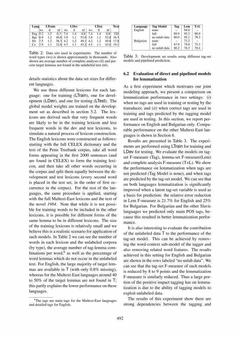
Lang LTrain LDev LTest Textws tl nf ws tl nf ws tl nf
Eng 5.2 1.5 0.3 7.4 1.4 0.8 7.4 1.4 0.8 320Bgr 6.9 1.2 40.8 3.8 1.1 53.6 3.8 1.1 52.8 16.3Slv 7.5 1.2 38.3 4.2 1.2 49.1 4.2 1.2 49.8 17.8Cz 7.9 1.1 32.8 4.5 1.1 43.2 4.5 1.1 43.0 19.1
Table 2: Data sets used in experiments. The number ofword types (ws) is shown approximately in thousands. Alsoshown are average number of complete analyses (tl) and per-cent target lemmas not found in the unlabeled text (nf).
details statistics about the data set sizes for differ-ent languages.
We use three different lexicons for each lan-guage: one for training (LTrain), one for devel-opment (LDev), and one for testing (LTest). Theglobal model weights are trained on the develop-ment set as described in section 5.2. The lex-icons are derived such that very frequent wordsare likely to be in the training lexicon and lessfrequent words in the dev and test lexicons, tosimulate a natural process of lexicon construction.The English lexicons were constructed as follows:starting with the full CELEX dictionary and thetext of the Penn Treebank corpus, take all wordforms appearing in the first 2000 sentences (andare found in CELEX) to form the training lexi-con, and then take all other words occurring inthe corpus and split them equally between the de-velopment and test lexicons (every second wordis placed in the test set, in the order of first oc-currence in the corpus). For the rest of the lan-guages, the same procedure is applied, startingwith the full Multext-East lexicons and the text ofthe novel 1984. Note that while it is not possi-ble for training words to be included in the otherlexicons, it is possible for different forms of thesame lemma to be in different lexicons. The sizeof the training lexicons is relatively small and webelieve this is a realistic scenario for application ofsuch models. In Table 2 we can see the number ofwords in each lexicon and the unlabeled corpora(by type), the average number of tag-lemma com-binations per word,6 as well as the percentage ofword lemmas which do not occur in the unlabeledtext. For English, the large majority of target lem-mas are available in T (with only 0.8% missing),whereas for the Multext-East languages around 40to 50% of the target lemmas are not found in T;this partly explains the lower performance on theselanguages.
6The tags are main tags for the Multext-East languagesand detailed tags for English.
Language Tag Model Tag Lem T+LEnglish none – 94.0 –
full 89.9 95.3 88.9no unlab data 80.0 94.1 78.3
Bulgarian none – 73.2 –full 87.9 79.9 75.3no unlab data 80.2 76.3 70.4
Table 3: Development set results using different tag-setmodels and pipelined prediction.
6.2 Evaluation of direct and pipelined modelsfor lemmatization
As a first experiment which motivates our jointmodeling approach, we present a comparison onlemmatization performance in two settings: (i)when no tags are used in training or testing by thetransducer, and (ii) when correct tags are used intraining and tags predicted by the tagging modelare used in testing. In this section, we report per-formance on English and Bulgarian only. Compa-rable performance on the other Multext-East lan-guages is shown in Section 6.
Results are presented in Table 3. The experi-ments are performed using LTrain for training andLDev for testing. We evaluate the models on tag-set F-measure (Tag), lemma-set F-measure(Lem)and complete analysis F-measure (T+L). We showthe performance on lemmatization when tags arenot predicted (Tag Model is none), and when tagsare predicted by the tag-set model. We can see thaton both languages lemmatization is significantlyimproved when a latent tag-set variable is used asa basis for prediction: the relative error reductionin Lem F-measure is 21.7% for English and 25%for Bulgarian. For Bulgarian and the other Slaviclanguages we predicted only main POS tags, be-cause this resulted in better lemmatization perfor-mance.
It is also interesting to evaluate the contributionof the unlabeled data T to the performance of thetag-set model. This can be achieved by remov-ing the word-context sub-model of the tagger andalso removing related word features. The resultsachieved in this setting for English and Bulgarianare shown in the rows labeled “no unlab data”. Wecan see that the tag-set F-measure of such modelsis reduced by 8 to 9 points and the lemmatizationF-measure is similarly reduced. Thus a large por-tion of the positive impact tagging has on lemma-tization is due to the ability of tagging models toexploit unlabeled data.
The results of this experiment show there arestrong dependencies between the tagging and
492
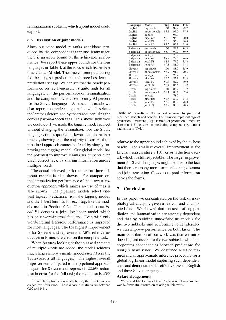
lemmatization subtasks, which a joint model couldexploit.
6.3 Evaluation of joint modelsSince our joint model re-ranks candidates pro-duced by the component tagger and lemmatizer,there is an upper bound on the achievable perfor-mance. We report these upper bounds for the fourlanguages in Table 4, at the rows which list m-bestoracle under Model. The oracle is computed usingfive-best tag-set predictions and three-best lemmapredictions per tag. We can see that the oracle per-formance on tag F-measure is quite high for alllanguages, but the performance on lemmatizationand the complete task is close to only 90 percentfor the Slavic languages. As a second oracle wealso report the perfect tag oracle, which selectsthe lemmas determined by the transducer using thecorrect part-of-speech tags. This shows how wellwe could do if we made the tagging model perfectwithout changing the lemmatizer. For the Slaviclanguages this is quite a bit lower than the m-bestoracles, showing that the majority of errors of thepipelined approach cannot be fixed by simply im-proving the tagging model. Our global model hasthe potential to improve lemma assignments evengiven correct tags, by sharing information amongmultiple words.
The actual achieved performance for three dif-ferent models is also shown. For comparison,the lemmatization performance of the direct trans-duction approach which makes no use of tags isalso shown. The pipelined models select one-best tag-set predictions from the tagging model,and the 1-best lemmas for each tag, like the mod-els used in Section 6.2. The model name lo-cal FS denotes a joint log-linear model whichhas only word-internal features. Even with onlyword-internal features, performance is improvedfor most languages. The the highest improvementis for Slovene and represents a 7.8% relative re-duction in F-measure error on the complete task.
When features looking at the joint assignmentsof multiple words are added, the model achievesmuch larger improvements (models joint FS in theTable) across all languages.7 The highest overallimprovement compared to the pipelined approachis again for Slovene and represents 22.6% reduc-tion in error for the full task; the reduction is 40%
7Since the optimization is stochastic, the results are av-eraged over four runs. The standard deviations are between0.02 and 0.11.
Language Model Tag Lem T+LEnglish tag oracle 100 98.9 98.7English m-best oracle 97.9 99.0 97.5English no tags – 94.3 –English pipelined 90.9 95.9 90.0English local FS 90.8 95.9 90.0English joint FS 91.7 96.1 91.0Bulgarian tag oracle 100 84.3 84.3Bulgarian m-best oracle 98.4 90.7 89.9Bulgarian no tags – 73.2 –Bulgarian pipelined 87.9 78.5 74.6Bulgarian local FS 88.9 79.2 75.8Bulgarian joint FS 89.5 81.0 77.8Slovene tag oracle 100 85.9 85.9Slovene m-best oracle 98.7 91.2 90.5Slovene no tags – 78.4 –Slovene pipelined 89.7 82.1 78.3Slovene local FS 90.8 82.7 80.0Slovene joint FS 92.4 85.5 83.2Czech tag oracle 100 83.2 83.2Czech m-best oracle 98.1 88.7 87.4Czech no tags – 78.7 –Czech pipelined 92.3 80.7 77.5Czech local FS 92.3 80.9 78.0Czech joint FS 93.7 83.0 80.5
Table 4: Results on the test set achieved by joint andpipelined models and oracles. The numbers represent tag-setprediction F-measure (Tag), lemma-set prediction F-measure(Lem) and F-measure on predicting complete tag, lemmaanalysis sets (T+L).
relative to the upper bound achieved by the m-bestoracle. The smallest overall improvement is forEnglish, representing a 10% error reduction over-all, which is still respectable. The larger improve-ment for Slavic languages might be due to the factthat there are many more forms of a single lemmaand joint reasoning allows us to pool informationacross the forms.
7 Conclusion
In this paper we concentrated on the task of mor-phological analysis, given a lexicon and unanno-tated data. We showed that the tasks of tag pre-diction and lemmatization are strongly dependentand that by building state-of-the art models forthe two subtasks and performing joint inferencewe can improve performance on both tasks. Themain contribution of our work was that we intro-duced a joint model for the two subtasks which in-corporates dependencies between predictions formultiple word types. We described a set of fea-tures and an approximate inference procedure for aglobal log-linear model capturing such dependen-cies, and demonstrated its effectiveness on Englishand three Slavic languages.Acknowledgements
We would like to thank Galen Andrew and Lucy Vander-wende for useful discussion relating to this work.
493
ReferencesMeni Adler, Yoav Goldberg, and Michael Elhadad. 2008.
Unsupervised lexicon-based resolution of unknown wordsfor full morpholological analysis. In Proceedings of ACL-08: HLT.
Galen Andrew, Trond Grenager, and Christopher Manning.2004. Verb sense and subcategorization: Using joint in-ference to improve performance on complementary tasks.In EMNLP.
Erwin Marsi Antal van den Bosch and Abdelhadi Soudi.2007. Memory-based morphological analysis and part-of-speech tagging of arabic. In Abdelhadi Soudi, An-tal van den Bosch, and Gunter Neumann, editors, ArabicComputational Morphology Knowledge-based and Em-pirical Methods. Springer.
R. H. Baayen, R. Piepenbrock, and L. Gulikers. 1995. TheCELEX lexical database.
Antal Van Den Bosch and Walter Daelemans. 1999.Memory-based morphological analysis. In Proceedingsof the 37th Annual Meeting of the Association for Compu-tational Linguistics.
Alexander Clark. 2002. Memory-based learning of mor-phology with stochastic transducers. In Proceedings ofthe 40th Annual Meeting of the Association for Computa-tional Linguistics (ACL), pages 513–520.
Shay B. Cohen and Noah A. Smith. 2007. Joint morpholog-ical and syntactic disambiguation. In EMNLP.
Michael Collins. 2000. Discriminative reranking for naturallanguage parsing. In ICML.
M. Collins. 2002. Discriminative training methods for hid-den markov models: Theory and experiments with percep-tron algorithms. In EMNLP.
S. Cucerzan and D. Yarowsky. 2000. Language independentminimally supervised induction of lexical probabilities. InProceedings of ACL 2000.
Markus Dreyer, Jason R. Smith, and Jason Eisner. 2008.Latent-variable modeling of string transductions withfinite-state methods. In Proceedings of the Conferenceon Empirical Methods in Natural Language Processing(EMNLP), pages 1080–1089, Honolulu, October.
Tomaž Erjavec and Saǎo Džeroski. 2004. Machine learn-ing of morphosyntactic structure: lemmatizing unknownSlovene words. Applied Artificial Intelligence, 18:17—41.
Tomaž Erjavec. 2004. Multext-east version 3: Multilingualmorphosyntactic specifications, lexicons and corpora. InProceedings of LREC-04.
Jenny Rose Finkel, Christopher D. Manning, and Andrew Y.Ng. 2006. Solving the problem of cascading errors:Approximate bayesian inference for linguistic annotationpipelines. In EMNLP.
Nizar Habash and Owen Rambow. 2005. Arabic tokeniza-tion, part-of-speech tagging and morphological disam-biguation in one fell swoop. In Proceedings of the 43rdAnnual Meeting of the Association for Computational Lin-guistics.
Sittichai Jiampojamarn, Colin Cherry, and Grzegorz Kon-drak. 2008. Joint processing and discriminative trainingfor letter-to-phoneme conversion. In Proceedings of ACL-08: HLT, pages 905–913, Columbus, Ohio, June.
M. Marcus, B. Santorini, and Marcinkiewicz. 1993. Build-ing a large annotated coprus of english: the penn treebank.Computational Linguistics, 19.
Raymond J. Mooney and Mary Elaine Califf. 1995. Induc-tion of first-order decision lists: Results on learning thepast tense of english verbs. Journal of Artificial Intelli-gence Research, 3:1—24.
Eric Sven Ristad and Peter N. Yianilos. 1998. Learningstring-edit distance. IEEE Transactions on Pattern Analy-sis and Machine Intelligence, 20(5):522–532.
Sunita Sarawagi and William Cohen. 2004. Semimarkovconditional random fields for information extraction. InICML.
Kristina Toutanova and Mark Johnson. 2008. A bayesianLDA-based model for semi-supervised part-of-speech tag-ging. In nips08.
Richard Wicentowski. 2002. Modeling and Learning Mul-tilingual Inflectional Morphology in a Minimally Super-vised Framework. Ph.D. thesis, Johns-Hopkins Univer-sity.
R. Zens and H. Ney. 2004. Improvements in phrase-basedstatistical machine translation. In HLT-NAACL, pages257–264, Boston, USA, May.
494

Proceedings of the 47th Annual Meeting of the ACL and the 4th IJCNLP of the AFNLP, pages 495–503,Suntec, Singapore, 2-7 August 2009. c©2009 ACL and AFNLP
Distributional Representations for Handling Sparsity in SupervisedSequence-Labeling
Fei HuangTemple University1805 N. Broad St.Wachman Hall 324
Alexander YatesTemple University1805 N. Broad St.Wachman Hall 324
Abstract
Supervised sequence-labeling systems innatural language processing often sufferfrom data sparsity because they use wordtypes as features in their prediction tasks.Consequently, they have difficulty estimat-ing parameters for types which appear inthe test set, but seldom (or never) ap-pear in the training set. We demonstratethat distributional representations of wordtypes, trained on unannotated text, canbe used to improve performance on rarewords. We incorporate aspects of theserepresentations into the feature space ofour sequence-labeling systems. In an ex-periment on a standard chunking dataset,our best technique improves a chunkerfrom 0.76 F1 to 0.86 F1 on chunks begin-ning with rare words. On the same dataset,it improves our part-of-speech tagger from74% to 80% accuracy on rare words. Fur-thermore, our system improves signifi-cantly over a baseline system when ap-plied to text from a different domain, andit reduces the sample complexity of se-quence labeling.
1 Introduction
Data sparsity and high dimensionality are the twincurses of statistical natural language processing(NLP). In many traditional supervised NLP sys-tems, the feature space includes dimensions foreach word type in the data, or perhaps even combi-nations of word types. Since vocabularies can beextremely large, this leads to an explosion in thenumber of parameters. To make matters worse,language is Zipf-distributed, so that a large frac-tion of any training data set will behapax legom-ena, very many word types will appear only a fewtimes, and many word types will be left out ofthe training set altogether. As a consequence, for
many word types supervised NLP systems havevery few, or even zero, labeled examples fromwhich to estimate parameters.
The negative effects of data sparsity have beenwell-documented in the NLP literature. The per-formance of state-of-the-art, supervised NLP sys-tems like part-of-speech (POS) taggers degradessignificantly on words that do not appear in thetraining data, or out-of-vocabulary (OOV) words(Lafferty et al., 2001). Performance also degradeswhen the domain of the test set differs from the do-main of the training set, in part because the test setincludes more OOV words and words that appearonly a few times in the training set (henceforth,rare words) (Blitzer et al., 2006; Dauḿe III andMarcu, 2006; Chelba and Acero, 2004).
We investigate the use of distributional repre-sentations, which model the probability distribu-tion of a word’s context, as techniques for find-ing smoothedrepresentations of word sequences.That is, we use the distributional representationsto share information across unannotated examplesof the same word type. We then compute featuresof the distributional representations, and providethem as input to our supervised sequence label-ers. Our technique is particularly well-suited tohandling data sparsity because it is possible to im-prove performance on rare words by supplement-ing the training data with additional unannotatedtext containing more examples of the rare words.We provide empirical evidence that shows howdistributional representations improve sequence-labeling in the face of data sparsity.
Specifically, we investigate empirically theeffects of our smoothing techniques on twosequence-labeling tasks, POS tagging and chunk-ing, to answer the following:1. What is the effect of smoothing on sequence-labeling accuracy for rare word types?Our bestsmoothing technique improves a POS tagger by11% on OOV words, and a chunker by an impres-sive 21% on OOV words.
495

2. Can smoothing improve adaptability to new do-mains? After training our chunker on newswiretext, we apply it to biomedical texts. Remark-ably, we find that the smoothed chunker achievesa higher F1 on the new domain than the baselinechunker achieves on a test set from the originalnewswire domain.3. How does our smoothing technique affect sam-ple complexity?We show that smoothing drasti-cally reduces sample complexity: our smoothedchunker requires under 100 labeled samples toreach 85% accuracy, whereas the unsmoothedchunker requires 3500 samples to reach the samelevel of performance.
The remainder of this paper is organized as fol-lows. Section 2 discusses the smoothing problemfor word sequences, and introduces three smooth-ing techniques. Section 3 presents our empiricalstudy of the effects of smoothing on two sequence-labeling tasks. Section 4 describes related work,and Section 5 concludes and suggests items for fu-ture work.
2 Smoothing Natural LanguageSequences
To smootha dataset is to find an approximation ofit that retains the important patterns of the origi-nal data while hiding the noise or other compli-cating factors. Formally, we define the smoothingtask as follows: letD = {(x, z)|x is a word se-quence,z is a label sequence} be a labeled datasetof word sequences, and letM be a machine learn-ing algorithm that will learn a functionf to pre-dict the correct labels. The smoothing task is tofind a functiong such that whenM is applied toD′ = {(g(x), z)|(x, z) ∈ D}, it produces a func-tion f ′ that is more accurate thanf .
For supervised sequence-labeling problems inNLP, the most important “complicating factor”that we seek to avoid through smoothing is thedata sparsity associated with word-based represen-tations. Thus, the task is to findg such that forevery wordx, g(x) is much less sparse, but stillretains the essential features ofx that are usefulfor predicting its label.
As an example, consider the string “Researcherstest reformulated gasolines on newer engines.” Ina common dataset for NP chunking, the word “re-formulated” never appears in the training data, butappears four times in the test set as part of theNP “reformulated gasolines.” Thus, a learning al-gorithm supplied with word-level features would
have a difficult time determining that “reformu-lated” is the start of a NP. Character-level featuresare of little help as well, since the “-ed” suffix ismore commonly associated with verb phrases. Fi-nally, context may be of some help, but “test” isambiguous between a noun and verb, and “gaso-lines” is only seen once in the training data, sothere is no guarantee that context is sufficient tomake a correct judgment.
On the other hand, some of the other contextsin which “reformulated” appears in the test set,such as “testing of reformulated gasolines,” pro-vide strong evidence that it can start a NP, since“of” is a highly reliable indicator that a NP is tofollow. This example provides the intuition for ourapproach to smoothing: we seek to share informa-tion about the contexts of a word across multipleinstances of the word, in order to provide more in-formation about words that are rarely or never seenin training. In particular, we seek to represent eachword by a distribution over its contexts, and thenprovide the learning algorithm with features com-puted from this distribution. Importantly, we seekdistributional representations that will provide fea-tures that are common in both training and testdata, to avoid data sparsity. In the next three sec-tions, we develop three techniques for smoothingtext using distributional representations.
2.1 Multinomial Representation
In its simplest form, the context of a word may berepresented as a multinomial distribution over theterms that appear on either side of the word. IfV isthe vocabulary, or the set of word types, andX is asequence of random variables overV, the left andright context ofXi = v may each be representedas a probability distribution overV: P (Xi−1|Xi =v) andP (Xi+1|X = v) respectively.
We learn these distributions from unlabeledtexts in two different ways. The first method com-putes word count vectors for the left and right con-texts of each word type in the vocabulary of thetraining and test texts. We also use a large col-lection of additional text to determine the vectors.We then normalize each vector to form a proba-bility distribution. The second technique first ap-plies TF-IDF weighting to each vector, where thecontext words of each word type constitute a doc-ument, before applying normalization. This givesgreater weight to words with more idiosyncraticdistributions and may improve the informativenessof a distributional representation. We refer to thesetechniques as TF and TF-IDF.
496
To supply a sequence-labeling algorithm withinformation from these distributional representa-tions, we compute real-valued features of the con-text distributions. In particular, for every wordxi in a sequence, we provide the sequence labelerwith a set of features of the left and right contextsindexed byv ∈ V: F
leftv (xi) = P (Xi−1 = v|xi)
andFrightv (xi) = P (Xi+1 = v|xi). For exam-
ple, the left context for “reformulated” in our ex-ample above would contain a nonzero probabilityfor the word “of.” Using the featuresF(xi), a se-quence labeler can learn patterns such as, ifxi hasa high probability of following “of,” it is a goodcandidate for the start of a noun phrase. Thesefeatures provide smoothing by aggregating infor-mation across multiple unannotated examples ofthe same word.
2.2 LSA Model
One drawback of the multinomial representationis that it does not handle sparsity well enough,because the multinomial distributions themselvesare so high-dimensional. For example, the twophrases “red lamp” and “magenta tablecloth”share no words in common. If “magenta” is neverobserved in training, the fact that “tablecloth” ap-pears in its right context is of no help in connectingit with the phrase “red lamp.” But if we can groupsimilar context words together, putting “lamp” and“tablecloth” into a category for household items,say, then these two adjectives will share that cat-egory in their context distributions. Any pat-terns learned for the more common “red lamp”will then also apply to the less common “magentatablecloth.” Our second distributional represen-tation aggregates information from multiple con-text words by grouping together the distributionsP (xi−1 = v|xi = w) andP (xi−1 = v′|xi = w)if v andv′ appear together with many of the samewordsw. Aggregating counts in this way smoothsour representations even further, by supplying bet-ter estimates when the data is too sparse to esti-mateP (xi−1|xi) accurately.
Latent Semantic Analysis (LSA) (Deerwester etal., 1990) is a widely-used technique for comput-ing dimensionality-reduced representations from abag-of-words model. We apply LSA to the set ofright context vectors and the set of left context vec-tors separately, to find compact versions of eachvector, where each dimension represents a com-bination of several context word types. We nor-malize each vector, and then calculate features as
above. After experimenting with different choicesfor the number of dimensions to reduce our vec-tors to, we choose a value of 10 dimensions as theone that maximizes the performance of our super-vised sequence labelers on held-out data.
2.3 Latent Variable Language ModelRepresentation
To take smoothing one step further, we presenta technique that aggregates context distributionsboth for similar context wordsxi−1 = v andv′,and for similar wordsxi = w and w′. Latentvariable language models (LVLMs) can be used toproduce just such a distributional representation.We use Hidden Markov Models (HMMs) as themain example in the discussion and as the LVLMsin our experiments, but the smoothing techniquecan be generalized to other forms of LVLMs, suchas factorial HMMs and latent variable maximumentropy models (Ghahramani and Jordan, 1997;Smith and Eisner, 2005).
An HMM is a generative probabilistic modelthat generates each wordxi in the corpus con-ditioned on a latent variableYi. EachYi in themodel takes on integral values from1 to S, andeach one is generated by the latent variable for thepreceding word,Yi−1. The distribution for a cor-pusx = (x1, . . . , xN ) given a set of state vectorsy = (y1, . . . , yN ) is given by:
P (x|y) =∏
i
P (xi|yi)P (yi|yi−1)
Using Expectation-Maximization (Dempster etal., 1977), it is possible to estimate the distribu-tions forP (xi|yi) andP (yi|yi−1) from unlabeleddata. We use a trained HMM to determine the op-timal sequence of latent statesŷi using the well-known Viterbi algorithm (Rabiner, 1989). Theoutput of this process is an integer (ranging from1to S) for every wordxi in the corpus; we include anew boolean feature for each possible value ofyi
in our sequence labelers.To compare our models, note that in the multi-
nomial representation we directly model the prob-ability that a wordv appears before a wordw:P (xi−1 = v|xi = w)). In our LSA model, we findlatent categories of context wordsz, and model theprobability that a category appears before the cur-rent wordw: P (xi−1 = z|xi = w). The HMMfinds (probabilistic) categoriesY for both the cur-rent wordxi and the context wordxi−1, and mod-els the probability that one category follows the
497
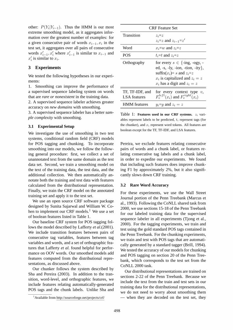
other: P (Yi|Yi−1). Thus the HMM is our mostextreme smoothing model, as it aggregates infor-mation over the greatest number of examples: fora given consecutive pair of wordsxi−1, xi in thetest set, it aggregates over all pairs of consecutivewordsx′i−1, x
′i wherex′i−1 is similar toxi−1 and
x′i is similar toxi.
3 Experiments
We tested the following hypotheses in our experi-ments:1. Smoothing can improve the performance ofa supervised sequence labeling system on wordsthat arerare or nonexistentin the training data.2. A supervised sequence labeler achieves greateraccuracy onnew domainswith smoothing.3. A supervised sequence labeler has a bettersam-ple complexitywith smoothing.
3.1 Experimental Setup
We investigate the use of smoothing in two testsystems, conditional random field (CRF) modelsfor POS tagging and chunking. To incorporatesmoothing into our models, we follow the follow-ing general procedure: first, we collect a set ofunannotated text from the same domain as the testdata set. Second, we train a smoothing model onthe text of the training data, the test data, and theadditional collection. We then automatically an-notate both the training and test data with featurescalculated from the distributional representation.Finally, we train the CRF model on the annotatedtraining set and apply it to the test set.
We use an open source CRF software packagedesigned by Sunita Sajarwal and William W. Co-hen to implement our CRF models.1 We use a setof boolean features listed in Table 1.
Our baseline CRF system for POS tagging fol-lows the model described by Laffertyet al.(2001).We include transition features between pairs ofconsecutive tag variables, features between tagvariables and words, and a set of orthographic fea-tures that Laffertyet al. found helpful for perfor-mance on OOV words. Our smoothed models addfeatures computed from the distributional repre-sentations, as discussed above.
Our chunker follows the system described bySha and Pereira (2003). In addition to the tran-sition, word-level, and orthographic features, weinclude features relating automatically-generatedPOS tags and the chunk labels. Unlike Sha and
1Available from http://sourceforge.net/projects/crf/
CRF Feature Set
Transition zi=z
zi=z andzi−1=z′
Word xi=w andzi=z
POS ti=t andzi=z
Orthography for everys ∈ {-ing, -ogy, -ed, -s, -ly, -ion, -tion, -ity},suffix(xi)= s andzi=z
xi is capitalized andzi = z
xi has a digit andzi = z
TF, TF-IDF, andLSA features
for every context typev,F
leftv (xi) andF
rightv (xi)
HMM features yi=y andzi = z
Table 1: Features used in our CRF systems. zi vari-
ables represent labels to be predicted,ti represent tags (for
the chunker), andxi represent word tokens. All features are
boolean except for the TF, TF-IDF, and LSA features.
Pereira, we exclude features relating consecutivepairs of words and a chunk label, or features re-lating consecutive tag labels and a chunk label,in order to expedite our experiments. We foundthat including such features does improve chunk-ing F1 by approximately 2%, but it also signifi-cantly slows down CRF training.
3.2 Rare Word Accuracy
For these experiments, we use the Wall StreetJournal portion of the Penn Treebank (Marcus etal., 1993). Following the CoNLL shared task from2000, we use sections 15-18 of the Penn Treebankfor our labeled training data for the supervisedsequence labeler in all experiments (Tjong et al.,2000). For the tagging experiments, we train andtest using the gold standard POS tags contained inthe Penn Treebank. For the chunking experiments,we train and test with POS tags that are automati-cally generated by a standard tagger (Brill, 1994).We tested the accuracy of our models for chunkingand POS tagging on section 20 of the Penn Tree-bank, which corresponds to the test set from theCoNLL 2000 task.
Our distributional representations are trained onsections 2-22 of the Penn Treebank. Because weinclude the text from the train and test sets in ourtraining data for the distributional representations,we do not need to worry about smoothing them— when they are decoded on the test set, they
498
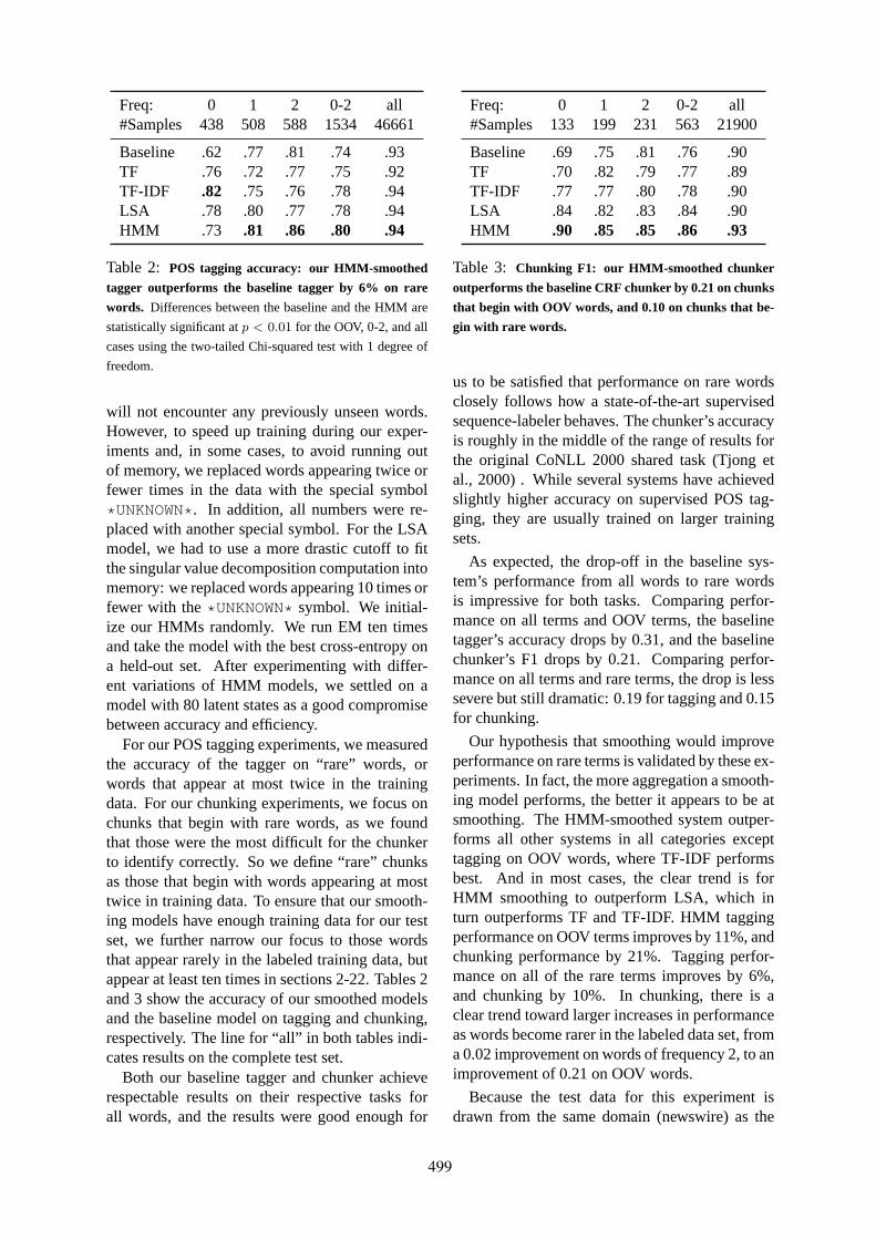
Freq: 0 1 2 0-2 all#Samples 438 508 588 1534 46661
Baseline .62 .77 .81 .74 .93TF .76 .72 .77 .75 .92TF-IDF .82 .75 .76 .78 .94LSA .78 .80 .77 .78 .94HMM .73 .81 .86 .80 .94
Table 2: POS tagging accuracy: our HMM-smoothed
tagger outperforms the baseline tagger by 6% on rare
words. Differences between the baseline and the HMM are
statistically significant atp < 0.01 for the OOV, 0-2, and all
cases using the two-tailed Chi-squared test with 1 degree of
freedom.
will not encounter any previously unseen words.However, to speed up training during our exper-iments and, in some cases, to avoid running outof memory, we replaced words appearing twice orfewer times in the data with the special symbol*UNKNOWN*. In addition, all numbers were re-placed with another special symbol. For the LSAmodel, we had to use a more drastic cutoff to fitthe singular value decomposition computation intomemory: we replaced words appearing 10 times orfewer with the*UNKNOWN* symbol. We initial-ize our HMMs randomly. We run EM ten timesand take the model with the best cross-entropy ona held-out set. After experimenting with differ-ent variations of HMM models, we settled on amodel with 80 latent states as a good compromisebetween accuracy and efficiency.
For our POS tagging experiments, we measuredthe accuracy of the tagger on “rare” words, orwords that appear at most twice in the trainingdata. For our chunking experiments, we focus onchunks that begin with rare words, as we foundthat those were the most difficult for the chunkerto identify correctly. So we define “rare” chunksas those that begin with words appearing at mosttwice in training data. To ensure that our smooth-ing models have enough training data for our testset, we further narrow our focus to those wordsthat appear rarely in the labeled training data, butappear at least ten times in sections 2-22. Tables 2and 3 show the accuracy of our smoothed modelsand the baseline model on tagging and chunking,respectively. The line for “all” in both tables indi-cates results on the complete test set.
Both our baseline tagger and chunker achieverespectable results on their respective tasks forall words, and the results were good enough for
Freq: 0 1 2 0-2 all#Samples 133 199 231 563 21900
Baseline .69 .75 .81 .76 .90TF .70 .82 .79 .77 .89TF-IDF .77 .77 .80 .78 .90LSA .84 .82 .83 .84 .90HMM .90 .85 .85 .86 .93
Table 3: Chunking F1: our HMM-smoothed chunker
outperforms the baseline CRF chunker by 0.21 on chunks
that begin with OOV words, and 0.10 on chunks that be-
gin with rare words.
us to be satisfied that performance on rare wordsclosely follows how a state-of-the-art supervisedsequence-labeler behaves. The chunker’s accuracyis roughly in the middle of the range of results forthe original CoNLL 2000 shared task (Tjong etal., 2000) . While several systems have achievedslightly higher accuracy on supervised POS tag-ging, they are usually trained on larger trainingsets.
As expected, the drop-off in the baseline sys-tem’s performance from all words to rare wordsis impressive for both tasks. Comparing perfor-mance on all terms and OOV terms, the baselinetagger’s accuracy drops by 0.31, and the baselinechunker’s F1 drops by 0.21. Comparing perfor-mance on all terms and rare terms, the drop is lesssevere but still dramatic: 0.19 for tagging and 0.15for chunking.
Our hypothesis that smoothing would improveperformance on rare terms is validated by these ex-periments. In fact, the more aggregation a smooth-ing model performs, the better it appears to be atsmoothing. The HMM-smoothed system outper-forms all other systems in all categories excepttagging on OOV words, where TF-IDF performsbest. And in most cases, the clear trend is forHMM smoothing to outperform LSA, which inturn outperforms TF and TF-IDF. HMM taggingperformance on OOV terms improves by 11%, andchunking performance by 21%. Tagging perfor-mance on all of the rare terms improves by 6%,and chunking by 10%. In chunking, there is aclear trend toward larger increases in performanceas words become rarer in the labeled data set, froma 0.02 improvement on words of frequency 2, to animprovement of 0.21 on OOV words.
Because the test data for this experiment isdrawn from the same domain (newswire) as the
499

training data, the rare terms make up a relativelysmall portion of the overall dataset (approximately4% of both the tagged words and the chunks).Still, the increased performance by the HMM-smoothed model on the rare-word subset con-tributes in part to an increase in performance onthe overall dataset of 1% for tagging and 3% forchunking. In our next experiment, we considera common scenario where rare terms make up amuch larger fraction of the test data.
3.3 Domain Adaptation
For our experiment on domain adaptation, we fo-cus on NP chunking and POS tagging, and weuse the labeled training data from the CoNLL2000 shared task as before. For NP chunking, weuse 198 sentences from the biochemistry domainin the Open American National Corpus (OANC)(Reppen et al., 2005) as or our test set. We man-ually tagged the test set with POS tags and NPchunk boundaries. The test set contains 5330words and a total of 1258 NP chunks. We usedsections 15-18 of the Penn Treebank as our labeledtraining set, including the gold standard POS tags.We use our best-performing smoothing model, theHMM, and train it on sections 13 through 19 ofthe Penn Treebank, plus the written portion ofthe OANC that contains journal articles from bio-chemistry (40,727 sentences). We focus on chunksthat begin with words appearing 0-2 times in thelabeled training data, and appearing at least tentimes in the HMM’s training data. Table 4 con-tains our results. For our POS tagging experi-ments, we use 561 MEDLINE sentences (9576words) from the Penn BioIE project (PennBioIE,2005), a test set previously used by Blitzeretal.(2006). We use the same experimental setup asBlitzer et al.: 40,000 manually tagged sentencesfrom the Penn Treebank for our labeled trainingdata, and all of the unlabeled text from the PennTreebank plus their MEDLINE corpus of 71,306sentences to train our HMM. We report on taggingaccuracy for all words and OOV words in Table5. This table also includes results for two previoussystems as reported by Blitzeret al. (2006): thesemi-supervised Alternating Structural Optimiza-tion (ASO) technique and the Structural Corre-spondence Learning (SCL) technique for domainadaptation.
Note that this test set for NP chunking con-tains a much higher proportion of rare and OOVwords: 23% of chunks begin with an OOV word,and 29% begin with a rare word, as compared with
Baseline HMMFreq. # R P F1 R P F1
0 284 .74 .70 .72 .80 .89 .841 39 .85 .87 .86 .92 .88 .902 39 .79 .86 .83 .92 .90 .91
0-2 362 .75 .73 .74 .82 .89 .85all 1258 .86 .87 .86 .91 .90 .91
Table 4:On biochemistry journal data from the OANC,
our HMM-smoothed NP chunker outperforms the base-
line CRF chunker by 0.12 (F1) on chunks that begin with
OOV words, and by 0.05 (F1) on all chunks. Results in
bold are statistically significantly different from the baseline
results atp < 0.05 using the two-tailed Fisher’s exact test.
We did not perform significance tests for F1.
All UnknownModel words words
Baseline 88.3 67.3ASO 88.4 70.9SCL 88.9 72.0HMM 90.5 75.2
Table 5: On biomedical data from the Penn BioIE
project, our HMM-smoothed tagger outperforms the
SCL tagger by 3% (accuracy) on OOV words, and by
1.6% (accuracy) on all words. Differences between the
smoothed tagger and the SCL tagger are significant atp <
.001 for all words and for OOV words, using the Chi-squared
test with 1 degree of freedom.
1% and 4%, respectively, for NP chunks in the testset from the original domain. The test set for tag-ging also contains a much higher proportion: 23%OOV words, as compared with 1% in the originaldomain. Because of the increase in the number ofrare words, the baseline chunker’s overall perfor-mance drops by 4% compared with performanceon WSJ data, and the baseline tagger’s overall per-formance drops by 5% in the new domain.
The performance improvements for both thesmoothed NP chunker and tagger are again im-pressive: there is a 12% improvement on OOVwords, and a 10% overall improvement on rarewords for chunking; the tagger shows an 8% im-provement on OOV words compared to out base-line and a 3% improvement on OOV words com-pared to the SCL model. The resulting perfor-mance of the smoothed NP chunker is almost iden-tical to its performance on the WSJ data. Throughsmoothing, the chunker not only improves by 5%
500
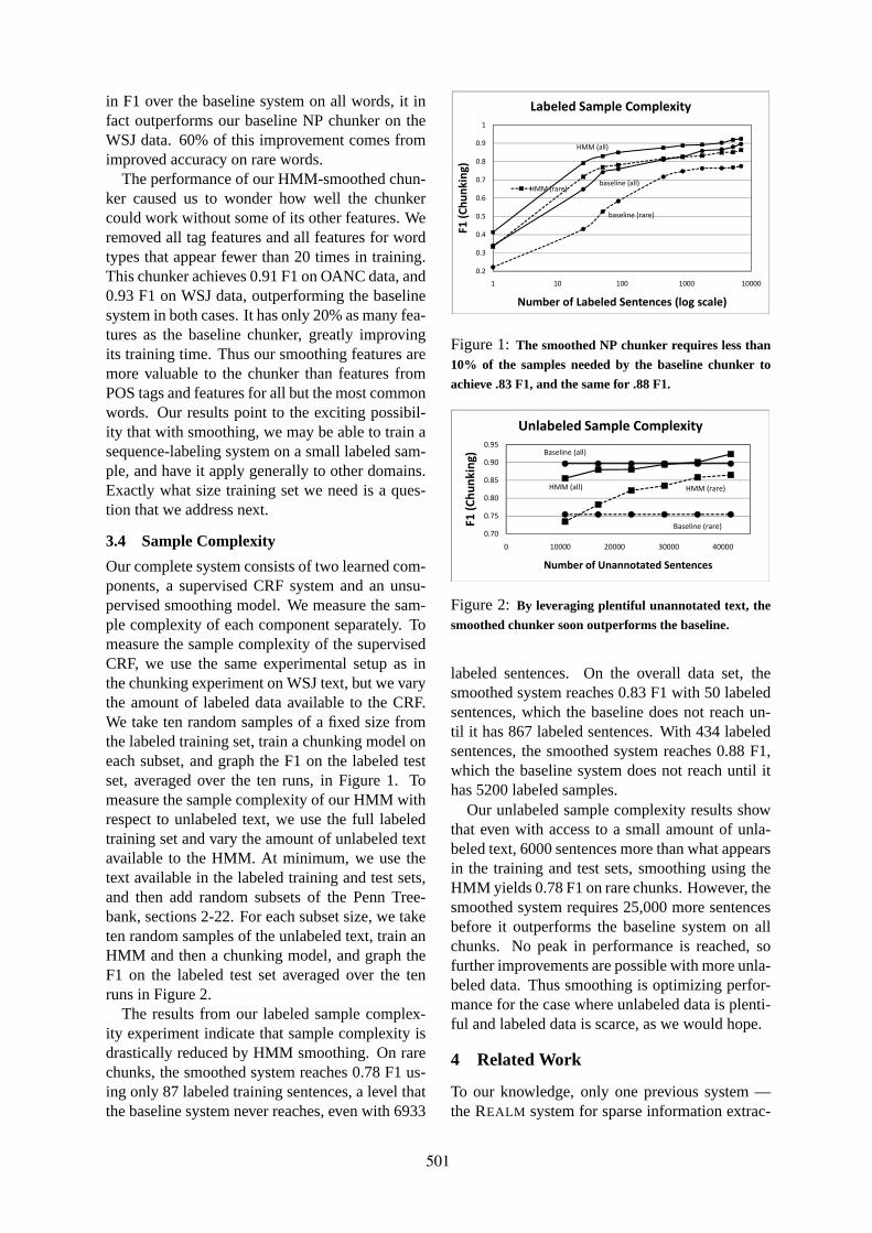
in F1 over the baseline system on all words, it infact outperforms our baseline NP chunker on theWSJ data. 60% of this improvement comes fromimproved accuracy on rare words.
The performance of our HMM-smoothed chun-ker caused us to wonder how well the chunkercould work without some of its other features. Weremoved all tag features and all features for wordtypes that appear fewer than 20 times in training.This chunker achieves 0.91 F1 on OANC data, and0.93 F1 on WSJ data, outperforming the baselinesystem in both cases. It has only 20% as many fea-tures as the baseline chunker, greatly improvingits training time. Thus our smoothing features aremore valuable to the chunker than features fromPOS tags and features for all but the most commonwords. Our results point to the exciting possibil-ity that with smoothing, we may be able to train asequence-labeling system on a small labeled sam-ple, and have it apply generally to other domains.Exactly what size training set we need is a ques-tion that we address next.
3.4 Sample Complexity
Our complete system consists of two learned com-ponents, a supervised CRF system and an unsu-pervised smoothing model. We measure the sam-ple complexity of each component separately. Tomeasure the sample complexity of the supervisedCRF, we use the same experimental setup as inthe chunking experiment on WSJ text, but we varythe amount of labeled data available to the CRF.We take ten random samples of a fixed size fromthe labeled training set, train a chunking model oneach subset, and graph the F1 on the labeled testset, averaged over the ten runs, in Figure 1. Tomeasure the sample complexity of our HMM withrespect to unlabeled text, we use the full labeledtraining set and vary the amount of unlabeled textavailable to the HMM. At minimum, we use thetext available in the labeled training and test sets,and then add random subsets of the Penn Tree-bank, sections 2-22. For each subset size, we taketen random samples of the unlabeled text, train anHMM and then a chunking model, and graph theF1 on the labeled test set averaged over the tenruns in Figure 2.
The results from our labeled sample complex-ity experiment indicate that sample complexity isdrastically reduced by HMM smoothing. On rarechunks, the smoothed system reaches 0.78 F1 us-ing only 87 labeled training sentences, a level thatthe baseline system never reaches, even with 6933
baseline (all)
HMM (all)
HMM (rare)
0.6
0.7
0.8
0.9
1
F1
(C
hu
nk
ing
)
Labeled Sample Complexity
baseline (rare)
0.2
0.3
0.4
0.5
1 10 100 1000 10000
F1
(C
hu
nk
ing
)
Number of Labeled Sentences (log scale)
Figure 1:The smoothed NP chunker requires less than
10% of the samples needed by the baseline chunker to
achieve .83 F1, and the same for .88 F1.
Baseline (all)
HMM (all) HMM (rare)
0.80
0.85
0.90
0.95
F1
(C
hu
nk
ing
)
Unlabeled Sample Complexity
Baseline (rare)0.70
0.75
0.80
0 10000 20000 30000 40000
F1
(C
hu
nk
ing
)
Number of Unannotated Sentences
Figure 2: By leveraging plentiful unannotated text, the
smoothed chunker soon outperforms the baseline.
labeled sentences. On the overall data set, thesmoothed system reaches 0.83 F1 with 50 labeledsentences, which the baseline does not reach un-til it has 867 labeled sentences. With 434 labeledsentences, the smoothed system reaches 0.88 F1,which the baseline system does not reach until ithas 5200 labeled samples.
Our unlabeled sample complexity results showthat even with access to a small amount of unla-beled text, 6000 sentences more than what appearsin the training and test sets, smoothing using theHMM yields 0.78 F1 on rare chunks. However, thesmoothed system requires 25,000 more sentencesbefore it outperforms the baseline system on allchunks. No peak in performance is reached, sofurther improvements are possible with more unla-beled data. Thus smoothing is optimizing perfor-mance for the case where unlabeled data is plenti-ful and labeled data is scarce, as we would hope.
4 Related Work
To our knowledge, only one previous system —the REALM system for sparse information extrac-
501
tion — has used HMMs as a feature represen-tation for other applications. REALM uses anHMM trained on a large corpus to help determinewhether the arguments of a candidate relation areof the appropriate type (Downey et al., 2007). Weextend and generalize this smoothing techniqueand apply it to common NLP applications involv-ing supervised sequence-labeling, and we providean in-depth empirical analysis of its performance.
Several researchers have previously studiedmethods for using unlabeled data for tagging andchunking, either alone or as a supplement to la-beled data. Ando and Zhang develop a semi-supervised chunker that outperforms purely su-pervised approaches on the CoNLL 2000 dataset(Ando and Zhang, 2005). Recent projects in semi-supervised (Toutanova and Johnson, 2007) and un-supervised (Biemann et al., 2007; Smith and Eis-ner, 2005) tagging also show significant progress.Unlike these systems, our efforts are aimed at us-ing unlabeled data to find distributional represen-tations that work well on rare terms, making thesupervised systems more applicable to other do-mains and decreasing their sample complexity.
HMMs have been used many times for POStagging and chunking, in supervised, semi-supervised, and in unsupervised settings (Bankoand Moore, 2004; Goldwater and Griffiths, 2007;Johnson, 2007; Zhou, 2004). We take a novel per-spective on the use of HMMs by using them tocompute features of each token in the data thatrepresent the distribution over that token’s con-texts. Our technique lets the HMM find param-eters that maximize cross-entropy, and then useslabeled data to learn the best mapping from theHMM categories to the POS categories.
Smoothing in NLP usually refers to the prob-lem of smoothingn-gram models. Sophisticatedsmoothing techniques like modified Kneser-Neyand Katz smoothing (Chen and Goodman, 1996)smooth together the predictions of unigram, bi-gram, trigram, and potentially highern-gram se-quences to obtain accurate probability estimates inthe face of data sparsity. Our task differs in that weare primarily concerned with the case where eventhe unigram model (single word) is rarely or neverobserved in the labeled training data.
Sparsity for low-order contexts has recentlyspurred interest in using latent variables to repre-sent distributions over contexts in language mod-els. Whilen-gram models have traditionally dom-inated in language modeling, two recent efforts de-
velop latent-variable probabilistic models that ri-val and even surpassn-gram models in accuracy(Blitzer et al., 2005; Mnih and Hinton, 2007).Several authors investigate neural network mod-els that learn not just one latent state, but rather avector of latent variables, to represent each wordin a language model (Bengio et al., 2003; Emamiet al., 2003; Morin and Bengio, 2005).
One of the benefits of our smoothing techniqueis that it allows for domain adaptation, a topicthat has received a great deal of attention fromthe NLP community recently. Unlike our tech-nique, in most cases researchers have focused onthe scenario where labeled training data is avail-able in both the source and the target domain(e.g., (Dauḿe III, 2007; Chelba and Acero, 2004;Dauḿe III and Marcu, 2006)). Our technique usesunlabeled training data from the target domain,and is thus applicable more generally, includingin web processing, where the domain and vocab-ulary is highly variable, and it is extremely diffi-cult to obtain labeled data that is representative ofthe test distribution. When labeled target-domaindata is available, instance weighting and similartechniques can be used in combination with oursmoothing technique to improve our results fur-ther, although this has not yet been demonstratedempirically. HMM-smoothing improves on themost closely related work, the Structural Corre-spondence Learning technique for domain adap-tation (Blitzer et al., 2006), in experiments.
5 Conclusion and Future Work
Our study of smoothing techniques demonstratesthat by aggregating information across manyunannotated examples, it is possible to find ac-curate distributional representations that can pro-vide highly informative features to supervised se-quence labelers. These features help improve se-quence labeling performance on rare word types,on domains that differ from the training set, andon smaller training sets.
Further experiments are of course necessaryto investigate distributional representations assmoothing techniques. One particularly promis-ing area for further study is the combination ofsmoothing and instance weighting techniques fordomain adaptation. Whether the current tech-niques are applicable to structured predictiontasks, like parsing and relation extraction, also de-serves future attention.
502
References
Rie Kubota Ando and Tong Zhang. 2005. A high-performance semi-supervised learning method fortext chunking. InACL.
Michele Banko and Robert C. Moore. 2004. Part ofspeech tagging in context. InCOLING.
Yoshua Bengio, Ŕejean Ducharme, Pascal Vincent, andChristian Janvin. 2003. A neural probabilistic lan-guage model. Journal of Machine Learning Re-search, 3:1137–1155.
C. Biemann, C. Giuliano, and A. Gliozzo. 2007. Un-supervised pos tagging supporting supervised meth-ods.Proceeding of RANLP-07.
J. Blitzer, A. Globerson, and F. Pereira. 2005. Dis-tributed latent variable models of lexical cooccur-rences. InProceedings of the Tenth InternationalWorkshop on Artificial Intelligence and Statistics.
John Blitzer, Ryan McDonald, and Fernando Pereira.2006. Domain adaptation with structural correspon-dence learning. InEMNLP.
E. Brill. 1994. Some Advances in Rule-Based Part ofSpeech Tagging. InAAAI, pages 722–727, Seattle,Washington.
Ciprian Chelba and Alex Acero. 2004. Adaptation ofmaximum entropy classifier: Little data can help alot. In EMNLP.
Stanley F. Chen and Joshua Goodman. 1996. An em-pirical study of smoothing techniques for languagemodeling. InProceedings of the 34th annual meet-ing on Association for Computational Linguistics,pages 310–318, Morristown, NJ, USA. Associationfor Computational Linguistics.
Hal Dauḿe III and Daniel Marcu. 2006. Domain adap-tation for statistical classifiers.Journal of ArtificialIntelligence Research, 26.
Hal Dauḿe III. 2007. Frustratingly easy domain adap-tation. InACL.
S. C. Deerwester, S. T. Dumais, T. K. Landauer, G. W.Furnas, and R. A. Harshman. 1990. Indexing bylatent semantic analysis.Journal of the AmericanSociety of Information Science, 41(6):391–407.
Arthur Dempster, Nan Laird, and Donald Rubin. 1977.Likelihood from incomplete data via the EM algo-rithm. Journal of the Royal Statistical Society, Se-ries B, 39(1):1–38.
Doug Downey, Stefan Schoenmackers, and Oren Et-zioni. 2007. Sparse information extraction: Unsu-pervised language models to the rescue. InACL.
A. Emami, P. Xu, and F. Jelinek. 2003. Using aconnectionist model in a syntactical based languagemodel. InProceedings of the International Confer-ence on Spoken Language Processing, pages 372–375.
Zoubin Ghahramani and Michael I. Jordan. 1997. Fac-torial hidden markov models.Machine Learning,29(2-3):245–273.
Sharon Goldwater and Thomas L. Griffiths. 2007.A fully bayesian approach to unsupervised part-of-speech tagging. InACL.
Mark Johnson. 2007. Why doesn’t EM find goodHMM POS-taggers. InEMNLP.
J. Lafferty, Andrew McCallum, and Fernando Pereira.2001. Conditional random fields: Probabilisticmodels for segmenting and labeling sequence data.In Proceedings of the International Conference onMachine Learning.
Mitchell P. Marcus, Mary Ann Marcinkiewicz, andBeatrice Santorini. 1993. Building a large anno-tated corpus of English: the Penn Treebank.Com-putational Linguistics, 19(2):313–330.
Andriy Mnih and Geoffrey Hinton. 2007. Three newgraphical models for statistical language modelling.In Proceedings of the 24th International Conferenceon Machine Learning, pages 641–648, New York,NY, USA. ACM.
F. Morin and Y. Bengio. 2005. Hierarchical probabilis-tic neural network language model. InProceedingsof the International Workshop on Artificial Intelli-gence and Statistics, pages 246–252.
PennBioIE. 2005. Mining the bibliome project.http://bioie.ldc.upenn.edu/.
Lawrence R. Rabiner. 1989. A tutorial on hiddenMarkov models and selected applications in speechrecognition. Proceedings of the IEEE, 77(2):257–285.
Randi Reppen, Nancy Ide, and Keith Suderman. 2005.American national corpus (ANC) second release.Linguistic Data Consortium.
F. Sha and Fernando Pereira. 2003. Shallow parsingwith conditional random fields. InProceedings ofHuman Language Technology - NAACL.
Noah A. Smith and Jason Eisner. 2005. Contrastiveestimation: Training log-linear models on unlabeleddata. In Proceedings of the 43rd Annual Meet-ing of the Association for Computational Linguistics(ACL), pages 354–362, Ann Arbor, Michigan, June.
Erik F. Tjong, Kim Sang, and Sabine Buchholz.2000. Introduction to the CoNLL-2000 shared task:Chunking. InProceedings of the 4th Conference onComputational Natural Language Learning, pages127–132.
Kristina Toutanova and Mark Johnson. 2007. Abayesian LDA-based model for semi-supervisedpart-of-speech tagging. InNIPS.
GuoDong Zhou. 2004. Discriminative hidden Markovmodeling with long state dependence using a kNNensemble. InCOLING.
503

Proceedings of the 47th Annual Meeting of the ACL and the 4th IJCNLP of the AFNLP, pages 504–512,Suntec, Singapore, 2-7 August 2009. c©2009 ACL and AFNLP
Minimized Models for Unsupervised Part-of-Speech Tagging
Sujith Ravi and Kevin KnightUniversity of Southern California
Information Sciences InstituteMarina del Rey, California 90292{sravi,knight}@isi.edu
Abstract
We describe a novel method for the taskof unsupervised POS tagging with a dic-tionary, one that uses integer programmingto explicitly search for the smallest modelthat explains the data, and then uses EMto set parameter values. We evaluate ourmethod on a standard test corpus usingdifferent standard tagsets (a 45-tagset aswell as a smaller 17-tagset), and show thatour approach performs better than existingstate-of-the-art systems in both settings.
1 Introduction
In recent years, we have seen increased interest inusing unsupervised methods for attacking differ-ent NLP tasks like part-of-speech (POS) tagging.The classic Expectation Maximization (EM) algo-rithm has been shown to perform poorly on POStagging, when compared to other techniques, suchas Bayesian methods.
In this paper, we develop new methods for un-supervised part-of-speech tagging. We adopt theproblem formulation of Merialdo (1994), in whichwe are given a raw word sequence and a dictio-nary of legal tags for each word type. The goal isto tag each word token so as to maximize accuracyagainst a gold tag sequence. Whether this is a real-istic problem set-up is arguable, but an interestingcollection of methods and results has accumulatedaround it, and these can be clearly compared withone another.
We use the standard test set for this task, a24,115-word subset of the Penn Treebank, forwhich a gold tag sequence is available. Thereare 5,878 word types in this test set. We usethe standard tag dictionary, consisting of 57,388
word/tag pairs derived from the entire Penn Tree-bank.1 8,910 dictionary entries are relevant to the5,878 word types in the test set. Per-token ambigu-ity is about 1.5 tags/token, yielding approximately106425 possible ways to tag the data. There are 45distinct grammatical tags. In this set-up, there areno unknown words.
Figure 1 shows prior results for this prob-lem. While the methods are quite different,they all make use of two common model ele-ments. One is a probabilistic n-gram tag modelP(ti|ti−n+1...ti−1), which we call the grammar.The other is a probabilistic word-given-tag modelP(wi|ti), which we call the dictionary.
The classic approach (Merialdo, 1994) isexpectation-maximization (EM), where we esti-mate grammar and dictionary probabilities in or-der to maximize the probability of the observedword sequence:
P (w1...wn) =∑
t1...tn
P (t1...tn) · P (w1...wn|t1...tn)
≈∑
t1...tn
n∏
i=1
P (ti|ti−2 ti−1) · P (wi|ti)
Goldwater and Griffiths (2007) report 74.5%accuracy for EM with a 3-gram tag model, whichwe confirm by replication. They improve this to83.9% by employing a fully Bayesian approachwhich integrates over all possible parameter val-ues, rather than estimating a single distribution.They further improve this to 86.8% by using pri-ors that favor sparse distributions. Smith and Eis-ner (2005) employ a contrastive estimation tech-
1As (Banko and Moore, 2004) point out, unsupervisedtagging accuracy varies wildly depending on the dictionaryemployed. We follow others in using a fat dictionary (with49,206 distinct word types), rather than a thin one derivedonly from the test set.
504
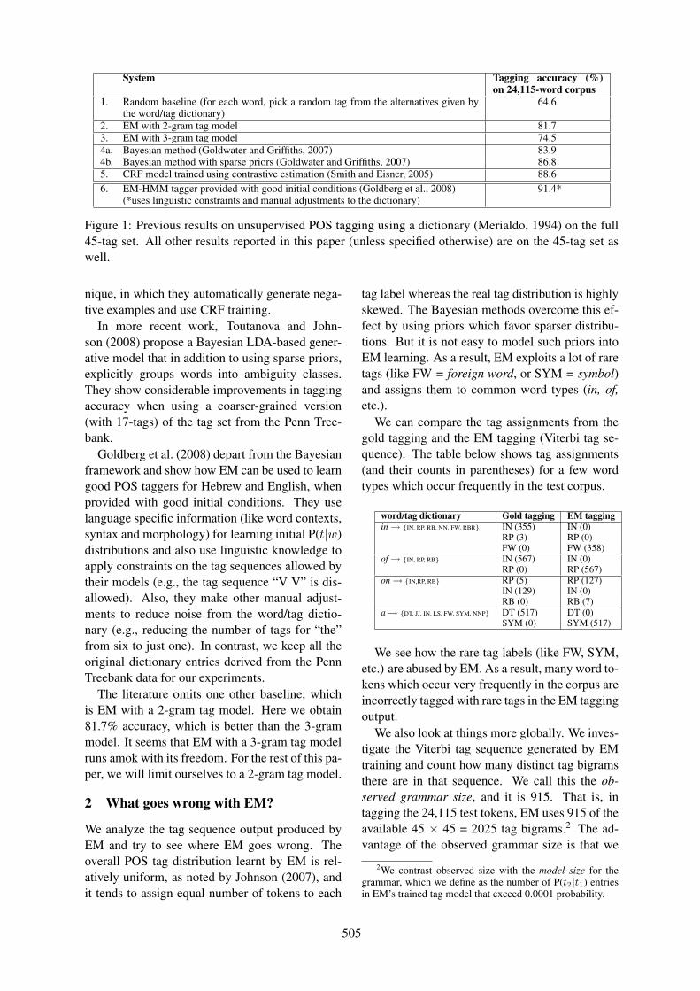
System Tagging accuracy (%)on 24,115-word corpus
1. Random baseline (for each word, pick a random tag from the alternatives given bythe word/tag dictionary)
64.6
2. EM with 2-gram tag model 81.73. EM with 3-gram tag model 74.54a. Bayesian method (Goldwater and Griffiths, 2007) 83.94b. Bayesian method with sparse priors (Goldwater and Griffiths, 2007) 86.85. CRF model trained using contrastive estimation (Smith and Eisner, 2005) 88.66. EM-HMM tagger provided with good initial conditions (Goldberg et al., 2008) 91.4*
(*uses linguistic constraints and manual adjustments to the dictionary)
Figure 1: Previous results on unsupervised POS tagging using a dictionary (Merialdo, 1994) on the full45-tag set. All other results reported in this paper (unless specified otherwise) are on the 45-tag set aswell.
nique, in which they automatically generate nega-tive examples and use CRF training.
In more recent work, Toutanova and John-son (2008) propose a Bayesian LDA-based gener-ative model that in addition to using sparse priors,explicitly groups words into ambiguity classes.They show considerable improvements in taggingaccuracy when using a coarser-grained version(with 17-tags) of the tag set from the Penn Tree-bank.
Goldberg et al. (2008) depart from the Bayesianframework and show how EM can be used to learngood POS taggers for Hebrew and English, whenprovided with good initial conditions. They uselanguage specific information (like word contexts,syntax and morphology) for learning initial P(t|w)distributions and also use linguistic knowledge toapply constraints on the tag sequences allowed bytheir models (e.g., the tag sequence “V V” is dis-allowed). Also, they make other manual adjust-ments to reduce noise from the word/tag dictio-nary (e.g., reducing the number of tags for “the”from six to just one). In contrast, we keep all theoriginal dictionary entries derived from the PennTreebank data for our experiments.
The literature omits one other baseline, whichis EM with a 2-gram tag model. Here we obtain81.7% accuracy, which is better than the 3-grammodel. It seems that EM with a 3-gram tag modelruns amok with its freedom. For the rest of this pa-per, we will limit ourselves to a 2-gram tag model.
2 What goes wrong with EM?
We analyze the tag sequence output produced byEM and try to see where EM goes wrong. Theoverall POS tag distribution learnt by EM is rel-atively uniform, as noted by Johnson (2007), andit tends to assign equal number of tokens to each
tag label whereas the real tag distribution is highlyskewed. The Bayesian methods overcome this ef-fect by using priors which favor sparser distribu-tions. But it is not easy to model such priors intoEM learning. As a result, EM exploits a lot of raretags (like FW = foreign word, or SYM = symbol)and assigns them to common word types (in, of,etc.).
We can compare the tag assignments from thegold tagging and the EM tagging (Viterbi tag se-quence). The table below shows tag assignments(and their counts in parentheses) for a few wordtypes which occur frequently in the test corpus.
word/tag dictionary Gold tagging EM taggingin→ {IN, RP, RB, NN, FW, RBR} IN (355) IN (0)
RP (3) RP (0)FW (0) FW (358)
of→ {IN, RP, RB} IN (567) IN (0)RP (0) RP (567)
on→ {IN,RP, RB} RP (5) RP (127)IN (129) IN (0)RB (0) RB (7)
a→ {DT, JJ, IN, LS, FW, SYM, NNP} DT (517) DT (0)SYM (0) SYM (517)
We see how the rare tag labels (like FW, SYM,etc.) are abused by EM. As a result, many word to-kens which occur very frequently in the corpus areincorrectly tagged with rare tags in the EM taggingoutput.
We also look at things more globally. We inves-tigate the Viterbi tag sequence generated by EMtraining and count how many distinct tag bigramsthere are in that sequence. We call this the ob-served grammar size, and it is 915. That is, intagging the 24,115 test tokens, EM uses 915 of theavailable 45 × 45 = 2025 tag bigrams.2 The ad-vantage of the observed grammar size is that we
2We contrast observed size with the model size for thegrammar, which we define as the number of P(t2|t1) entriesin EM’s trained tag model that exceed 0.0001 probability.
505

L8
L0
they can fish . I fish
L1
L2 L3
L4
L6
L5 L7
L9
L10
L11
START
PRO
AUX
V
N
PUNC
L0
they can fish . I fish
L1
L2
L1
L2 L3
L4
L6
L5 L7
L9
L10
L11
START
PRO
AUX
V
N
PUNC
d1 PRO-they
d2 AUX-can
d3 V-can
d4 N-fish
d5 V-fish
d6 PUNC-.
d7 PRO-I
g1 PRO-AUX
g2 PRO-V
g3 AUX-N
g4 AUX-V
g5 V-N
g6 V-V
g7 N-PUNC
g8 V-PUNC
g9 PUNC-PRO
g10 PRO-N
dictionary
variables
grammar
variables
Integer Program
Minimize: ∑i=1…10 gi
Constraints:
1. Single left-to-right path (at each node, flow in = flow out)
e.g., L0 = 1
L1 = L3 + L4
2. Path consistency constraints (chosen path respects chosen
dictionary & grammar)
e.g., L0 ≤ d1
L1 ≤ g1
IP formulation
training text
link
variables
Figure 2: Integer Programming formulation for finding the smallest grammar that explains a given wordsequence. Here, we show a sample word sequence and the corresponding IP network generated for thatsequence.
can compare it with the gold tagging’s observedgrammar size, which is 760. So we can safely saythat EM is learning a grammar that is too big, stillabusing its freedom.
3 Small Models
Bayesian sparse priors aim to create small mod-els. We take a different tack in the paper anddirectly ask: What is the smallest model that ex-plains the text? Our approach is related to mini-mum description length (MDL). We formulate ourquestion precisely by asking which tag sequence(of the 106425 available) has the smallest observedgrammar size. The answer is 459. That is, thereexists a tag sequence that contains 459 distinct tagbigrams, and no other tag sequence contains fewer.
We obtain this answer by formulating the prob-lem in an integer programming (IP) framework.Figure 2 illustrates this with a small sample wordsequence. We create a network of possible tag-gings, and we assign a binary variable to each linkin the network. We create constraints to ensurethat those link variables receiving a value of 1form a left-to-right path through the tagging net-work, and that all other link variables receive a
value of 0. We accomplish this by requiring thesum of the links entering each node to equal tothe sum of the links leaving each node. We alsocreate variables for every possible tag bigram andword/tag dictionary entry. We constrain link vari-able assignments to respect those grammar anddictionary variables. For example, we do not allowa link variable to “activate” unless the correspond-ing grammar variable is also “activated”. Finally,we add an objective function that minimizes thenumber of grammar variables that are assigned avalue of 1.
Figure 3 shows the IP solution for the exampleword sequence from Figure 2. Of course, a smallgrammar size does not necessarily correlate withhigher tagging accuracy. For the small toy exam-ple shown in Figure 3, the correct tagging is “PROAUX V . PRO V” (with 5 tag pairs), whereas theIP tries to minimize the grammar size and picksanother solution instead.
For solving the integer program, we use CPLEXsoftware (a commercial IP solver package). Alter-natively, there are other programs such as lp solve,which are free and publicly available for use. Oncewe create an integer program for the full test cor-pus, and pass it to CPLEX, the solver returns an
506

word sequence: they can fish . I fish
Tagging Grammar SizePRO AUX N . PRO N 5PRO AUX V . PRO N 5PRO AUX N . PRO V 5PRO AUX V . PRO V 5PRO V N . PRO N 5PRO V V . PRO N 5PRO V N . PRO V 4PRO V V . PRO V 4
Figure 3: Possible tagging solutions and corre-sponding grammar sizes for the sample word se-quence from Figure 2 using the given dictionaryand grammar. The IP solver finds the smallestgrammar set that can explain the given word se-quence. In this example, there exist two solutionsthat each contain only 4 tag pair entries, and IPreturns one of them.
objective function value of 459.3
CPLEX also returns a tag sequence via assign-ments to the link variables. However, there areactually 104378 tag sequences compatible with the459-sized grammar, and our IP solver just selectsone at random. We find that of all those tag se-quences, the worst gives an accuracy of 50.8%,and the best gives an accuracy of 90.3%. Wealso note that CPLEX takes 320 seconds to returnthe optimal solution for the integer program corre-sponding to this particular test data (24,115 tokenswith the 45-tag set). It might be interesting to seehow the performance of the IP method (in termsof time complexity) is affected when scaling up tolarger data and bigger tagsets. We leave this aspart of future work. But we do note that it is pos-sible to obtain less than optimal solutions faster byinterrupting the CPLEX solver.
4 Fitting the Model
Our IP formulation can find us a small model, butit does not attempt to fit the model to the data. For-tunately, we can use EM for that. We still giveEM the full word/tag dictionary, but now we con-strain its initial grammar model to the 459 tag bi-grams identified by IP. Starting with uniform prob-abilities, EM finds a tagging that is 84.5% accu-rate, substantially better than the 81.7% originallyobtained with the fully-connected grammar. Sowe see a benefit to our explicit small-model ap-proach. While EM does not find the most accurate
3Note that the grammar identified by IP is not uniquelyminimal. For the same word sequence, there exist other min-imal grammars having the same size (459 entries). In our ex-periments, we choose the first solution returned by CPLEX.
in onIN INRP RP
word/tag dictionary RB RBNNFWRBR
observed EM dictionary FW (358) RP (127)RB (7)
observed IP+EM dictionary IN (349) IN (126)RB (9) RB (8)
observed gold dictionary IN (355) IN (129)RB (3) RP (5)
Figure 4: Examples of tagging obtained from dif-ferent systems for prepositions in and on.
sequence consistent with the IP grammar (90.3%),it finds a relatively good one.
The IP+EM tagging (with 84.5% accuracy) hassome interesting properties. First, the dictionarywe observe from the tagging is of higher qual-ity (with fewer spurious tagging assignments) thanthe one we observe from the original EM tagging.Figure 4 shows some examples.
We also measure the quality of the two observedgrammars/dictionaries by computing their preci-sion and recall against the grammar/dictionary weobserve in the gold tagging.4 We find that preci-sion of the observed grammar increases from 0.73(EM) to 0.94 (IP+EM). In addition to removingmany bad tag bigrams from the grammar, IP min-imization also removes some of the good ones,leading to lower recall (EM = 0.87, IP+EM =0.57). In the case of the observed dictionary, usinga smaller grammar model does not affect the pre-cision (EM = 0.91, IP+EM = 0.89) or recall (EM= 0.89, IP+EM = 0.89).
During EM training, the smaller grammar withfewer bad tag bigrams helps to restrict the dictio-nary model from making too many bad choicesthat EM made earlier. Here are a few examplesof bad dictionary entries that get removed whenwe use the minimized grammar for EM training:
in → FW
a → SYM
of → RP
In → RBR
During EM training, the minimized grammar4For any observed grammar or dictionary X,
Precision (X) = |{X}∩{observedgold}||{X}|
Recall (X) = |{X}∩{observedgold}||{observedgold}|
507
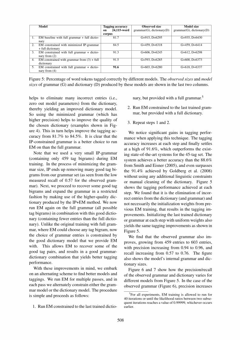
Model Tagging accuracy Observed size Model sizeon 24,115-wordcorpus
grammar(G), dictionary(D) grammar(G), dictionary(D)
1. EM baseline with full grammar + full dictio-nary
81.7 G=915, D=6295 G=935, D=6430
2. EM constrained with minimized IP-grammar+ full dictionary
84.5 G=459, D=6318 G=459, D=6414
3. EM constrained with full grammar + dictio-nary from (2)
91.3 G=606, D=6245 G=612, D=6298
4. EM constrained with grammar from (3) + fulldictionary
91.5 G=593, D=6285 G=600, D=6373
5. EM constrained with full grammar + dictio-nary from (4)
91.6 G=603, D=6280 G=618, D=6337
Figure 5: Percentage of word tokens tagged correctly by different models. The observed sizes and modelsizes of grammar (G) and dictionary (D) produced by these models are shown in the last two columns.
helps to eliminate many incorrect entries (i.e.,zero out model parameters) from the dictionary,thereby yielding an improved dictionary model.So using the minimized grammar (which hashigher precision) helps to improve the quality ofthe chosen dictionary (examples shown in Fig-ure 4). This in turn helps improve the tagging ac-curacy from 81.7% to 84.5%. It is clear that theIP-constrained grammar is a better choice to runEM on than the full grammar.
Note that we used a very small IP-grammar(containing only 459 tag bigrams) during EMtraining. In the process of minimizing the gram-mar size, IP ends up removing many good tag bi-grams from our grammar set (as seen from the lowmeasured recall of 0.57 for the observed gram-mar). Next, we proceed to recover some good tagbigrams and expand the grammar in a restrictedfashion by making use of the higher-quality dic-tionary produced by the IP+EM method. We nowrun EM again on the full grammar (all possibletag bigrams) in combination with this good dictio-nary (containing fewer entries than the full dictio-nary). Unlike the original training with full gram-mar, where EM could choose any tag bigram, nowthe choice of grammar entries is constrained bythe good dictionary model that we provide EMwith. This allows EM to recover some of thegood tag pairs, and results in a good grammar-dictionary combination that yields better taggingperformance.
With these improvements in mind, we embarkon an alternating scheme to find better models andtaggings. We run EM for multiple passes, and ineach pass we alternately constrain either the gram-mar model or the dictionary model. The procedureis simple and proceeds as follows:
1. Run EM constrained to the last trained dictio-
nary, but provided with a full grammar.5
2. Run EM constrained to the last trained gram-mar, but provided with a full dictionary.
3. Repeat steps 1 and 2.
We notice significant gains in tagging perfor-mance when applying this technique. The taggingaccuracy increases at each step and finally settlesat a high of 91.6%, which outperforms the exist-ing state-of-the-art systems for the 45-tag set. Thesystem achieves a better accuracy than the 88.6%from Smith and Eisner (2005), and even surpassesthe 91.4% achieved by Goldberg et al. (2008)without using any additional linguistic constraintsor manual cleaning of the dictionary. Figure 5shows the tagging performance achieved at eachstep. We found that it is the elimination of incor-rect entries from the dictionary (and grammar) andnot necessarily the initialization weights from pre-vious EM training, that results in the tagging im-provements. Initializing the last trained dictionaryor grammar at each step with uniform weights alsoyields the same tagging improvements as shown inFigure 5.
We find that the observed grammar also im-proves, growing from 459 entries to 603 entries,with precision increasing from 0.94 to 0.96, andrecall increasing from 0.57 to 0.76. The figurealso shows the model’s internal grammar and dic-tionary sizes.
Figure 6 and 7 show how the precision/recallof the observed grammar and dictionary varies fordifferent models from Figure 5. In the case of theobserved grammar (Figure 6), precision increases
5For all experiments, EM training is allowed to run for40 iterations or until the likelihood ratios between two subse-quent iterations reaches a value of 0.99999, whichever occursearlier.
508
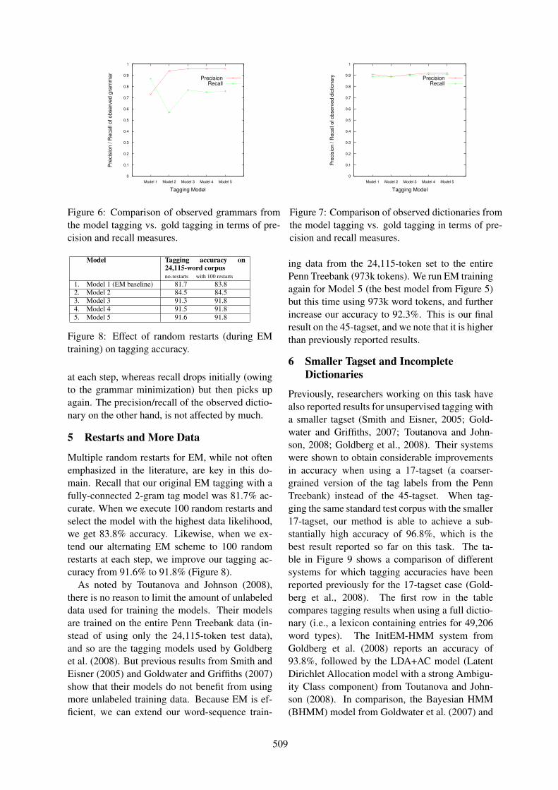
0
0.1
0.2
0.3
0.4
0.5
0.6
0.7
0.8
0.9
1
Pre
cis
ion
/ R
eca
ll o
f o
bse
rve
d g
ram
ma
r
Tagging Model
Model 1 Model 2 Model 3 Model 4 Model 5
PrecisionRecall
Figure 6: Comparison of observed grammars fromthe model tagging vs. gold tagging in terms of pre-cision and recall measures.
0
0.1
0.2
0.3
0.4
0.5
0.6
0.7
0.8
0.9
1
Pre
cis
ion / R
ecall
of observ
ed d
ictionary
Tagging Model
Model 1 Model 2 Model 3 Model 4 Model 5
PrecisionRecall
Figure 7: Comparison of observed dictionaries fromthe model tagging vs. gold tagging in terms of pre-cision and recall measures.
Model Tagging accuracy on24,115-word corpusno-restarts with 100 restarts
1. Model 1 (EM baseline) 81.7 83.82. Model 2 84.5 84.53. Model 3 91.3 91.84. Model 4 91.5 91.85. Model 5 91.6 91.8
Figure 8: Effect of random restarts (during EMtraining) on tagging accuracy.
at each step, whereas recall drops initially (owingto the grammar minimization) but then picks upagain. The precision/recall of the observed dictio-nary on the other hand, is not affected by much.
5 Restarts and More Data
Multiple random restarts for EM, while not oftenemphasized in the literature, are key in this do-main. Recall that our original EM tagging with afully-connected 2-gram tag model was 81.7% ac-curate. When we execute 100 random restarts andselect the model with the highest data likelihood,we get 83.8% accuracy. Likewise, when we ex-tend our alternating EM scheme to 100 randomrestarts at each step, we improve our tagging ac-curacy from 91.6% to 91.8% (Figure 8).
As noted by Toutanova and Johnson (2008),there is no reason to limit the amount of unlabeleddata used for training the models. Their modelsare trained on the entire Penn Treebank data (in-stead of using only the 24,115-token test data),and so are the tagging models used by Goldberget al. (2008). But previous results from Smith andEisner (2005) and Goldwater and Griffiths (2007)show that their models do not benefit from usingmore unlabeled training data. Because EM is ef-ficient, we can extend our word-sequence train-
ing data from the 24,115-token set to the entirePenn Treebank (973k tokens). We run EM trainingagain for Model 5 (the best model from Figure 5)but this time using 973k word tokens, and furtherincrease our accuracy to 92.3%. This is our finalresult on the 45-tagset, and we note that it is higherthan previously reported results.
6 Smaller Tagset and IncompleteDictionaries
Previously, researchers working on this task havealso reported results for unsupervised tagging witha smaller tagset (Smith and Eisner, 2005; Gold-water and Griffiths, 2007; Toutanova and John-son, 2008; Goldberg et al., 2008). Their systemswere shown to obtain considerable improvementsin accuracy when using a 17-tagset (a coarser-grained version of the tag labels from the PennTreebank) instead of the 45-tagset. When tag-ging the same standard test corpus with the smaller17-tagset, our method is able to achieve a sub-stantially high accuracy of 96.8%, which is thebest result reported so far on this task. The ta-ble in Figure 9 shows a comparison of differentsystems for which tagging accuracies have beenreported previously for the 17-tagset case (Gold-berg et al., 2008). The first row in the tablecompares tagging results when using a full dictio-nary (i.e., a lexicon containing entries for 49,206word types). The InitEM-HMM system fromGoldberg et al. (2008) reports an accuracy of93.8%, followed by the LDA+AC model (LatentDirichlet Allocation model with a strong Ambigu-ity Class component) from Toutanova and John-son (2008). In comparison, the Bayesian HMM(BHMM) model from Goldwater et al. (2007) and
509

Dict IP+EM (24k) InitEM-HMM LDA+AC CE+spl BHMMFull (49206 words) 96.8 (96.8) 93.8 93.4 88.7 87.3≥ 2 (2141 words) 90.6 (90.0) 89.4 91.2 79.5 79.6≥ 3 (1249 words) 88.0 (86.1) 87.4 89.7 78.4 71
Figure 9: Comparison of different systems for English unsupervised POS tagging with 17 tags.
the CE+spl model (Contrastive Estimation with aspelling model) from Smith and Eisner (2005) re-port lower accuracies (87.3% and 88.7%, respec-tively). Our system (IP+EM) which uses inte-ger programming and EM, gets the highest accu-racy (96.8%). The accuracy numbers reported forInit-HMM and LDA+AC are for models that aretrained on all the available unlabeled data fromthe Penn Treebank. The IP+EM models used inthe 17-tagset experiments reported here were nottrained on the entire Penn Treebank, but insteadused a smaller section containing 77,963 tokensfor estimating model parameters. We also includethe accuracies for our IP+EM model when usingonly the 24,115 token test corpus for EM estima-tion (shown within parenthesis in second columnof the table in Figure 9). We find that our perfor-mance does not degrade when the parameter esti-mation is done using less data, and our model stillachieves a high accuracy of 96.8%.
6.1 Incomplete Dictionaries and UnknownWords
The literature also includes results reported in adifferent setting for the tagging problem. In somescenarios, a complete dictionary with entries forall word types may not be readily available to usand instead, we might be provided with an incom-plete dictionary that contains entries for only fre-quent word types. In such cases, any word notappearing in the dictionary will be treated as anunknown word, and can be labeled with any ofthe tags from given tagset (i.e., for every unknownword, there are 17 tag possibilities). Some pre-vious approaches (Toutanova and Johnson, 2008;Goldberg et al., 2008) handle unknown words ex-plicitly using ambiguity class components condi-tioned on various morphological features, and thishas shown to produce good tagging results, espe-cially when dealing with incomplete dictionaries.
We follow a simple approach using just oneof the features used in (Toutanova and Johnson,2008) for assigning tag possibilities to every un-known word. We first identify the top-100 suffixes(up to 3 characters) for words in the dictionary.Using the word/tag pairs from the dictionary, wetrain a simple probabilistic model that predicts the
tag given a particular suffix (e.g., P(VBG | ing) =0.97, P(N | ing) = 0.0001, ...). Next, for every un-known word “w”, the trained P(tag | suffix) modelis used to predict the top 3 tag possibilities for“w” (using only its suffix information), and subse-quently this word along with its 3 tags are added asa new entry to the lexicon. We do this for every un-known word, and eventually we have a dictionarycontaining entries for all the words. Once the com-pleted lexicon (containing both correct entries forwords in the lexicon and the predicted entries forunknown words) is available, we follow the samemethodology from Sections 3 and 4 using integerprogramming to minimize the size of the grammarand then applying EM to estimate parameter val-ues.
Figure 9 shows comparative results for the 17-tagset case when the dictionary is incomplete. Thesecond and third rows in the table shows taggingaccuracies for different systems when a cutoff of2 (i.e., all word types that occur with frequencycounts < 2 in the test corpus are removed) anda cutoff of 3 (i.e., all word types occurring withfrequency counts < 3 in the test corpus are re-moved) is applied to the dictionary. This yieldslexicons containing 2,141 and 1,249 words respec-tively, which are much smaller compared to theoriginal 49,206 word dictionary. As the resultsin Figure 9 illustrate, the IP+EM method clearlydoes better than all the other systems except forthe LDA+AC model. The LDA+AC model fromToutanova and Johnson (2008) has a strong ambi-guity class component and uses more features tohandle the unknown words better, and this con-tributes to the slightly higher performance in theincomplete dictionary cases, when compared tothe IP+EM model.
7 Discussion
The method proposed in this paper is simple—once an integer program is produced, there aresolvers available which directly give us the so-lution. In addition, we do not require any com-plex parameter estimation techniques; we train ourmodels using simple EM, which proves to be effi-cient for this task. While some previous methods
510
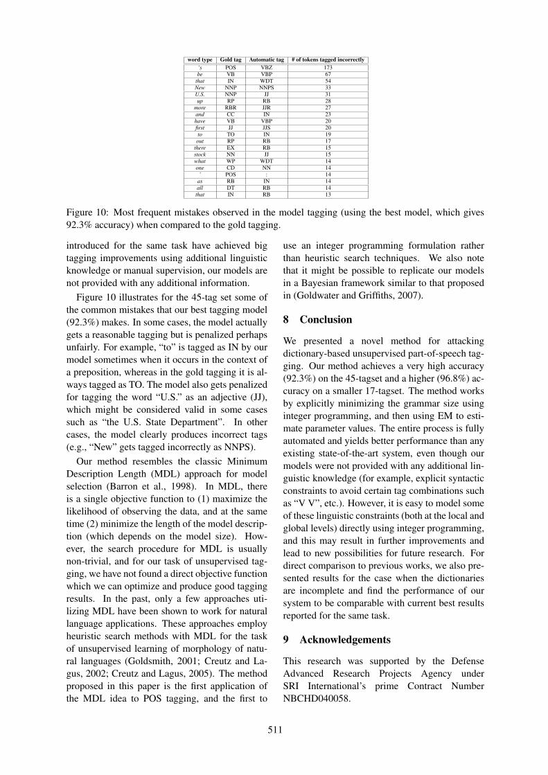
word type Gold tag Automatic tag # of tokens tagged incorrectly’s POS VBZ 173be VB VBP 67
that IN WDT 54New NNP NNPS 33U.S. NNP JJ 31up RP RB 28
more RBR JJR 27and CC IN 23have VB VBP 20first JJ JJS 20to TO IN 19
out RP RB 17there EX RB 15stock NN JJ 15what WP WDT 14one CD NN 14
’ POS : 14as RB IN 14all DT RB 14
that IN RB 13
Figure 10: Most frequent mistakes observed in the model tagging (using the best model, which gives92.3% accuracy) when compared to the gold tagging.
introduced for the same task have achieved bigtagging improvements using additional linguisticknowledge or manual supervision, our models arenot provided with any additional information.
Figure 10 illustrates for the 45-tag set some ofthe common mistakes that our best tagging model(92.3%) makes. In some cases, the model actuallygets a reasonable tagging but is penalized perhapsunfairly. For example, “to” is tagged as IN by ourmodel sometimes when it occurs in the context ofa preposition, whereas in the gold tagging it is al-ways tagged as TO. The model also gets penalizedfor tagging the word “U.S.” as an adjective (JJ),which might be considered valid in some casessuch as “the U.S. State Department”. In othercases, the model clearly produces incorrect tags(e.g., “New” gets tagged incorrectly as NNPS).
Our method resembles the classic MinimumDescription Length (MDL) approach for modelselection (Barron et al., 1998). In MDL, thereis a single objective function to (1) maximize thelikelihood of observing the data, and at the sametime (2) minimize the length of the model descrip-tion (which depends on the model size). How-ever, the search procedure for MDL is usuallynon-trivial, and for our task of unsupervised tag-ging, we have not found a direct objective functionwhich we can optimize and produce good taggingresults. In the past, only a few approaches uti-lizing MDL have been shown to work for naturallanguage applications. These approaches employheuristic search methods with MDL for the taskof unsupervised learning of morphology of natu-ral languages (Goldsmith, 2001; Creutz and La-gus, 2002; Creutz and Lagus, 2005). The methodproposed in this paper is the first application ofthe MDL idea to POS tagging, and the first to
use an integer programming formulation ratherthan heuristic search techniques. We also notethat it might be possible to replicate our modelsin a Bayesian framework similar to that proposedin (Goldwater and Griffiths, 2007).
8 Conclusion
We presented a novel method for attackingdictionary-based unsupervised part-of-speech tag-ging. Our method achieves a very high accuracy(92.3%) on the 45-tagset and a higher (96.8%) ac-curacy on a smaller 17-tagset. The method worksby explicitly minimizing the grammar size usinginteger programming, and then using EM to esti-mate parameter values. The entire process is fullyautomated and yields better performance than anyexisting state-of-the-art system, even though ourmodels were not provided with any additional lin-guistic knowledge (for example, explicit syntacticconstraints to avoid certain tag combinations suchas “V V”, etc.). However, it is easy to model someof these linguistic constraints (both at the local andglobal levels) directly using integer programming,and this may result in further improvements andlead to new possibilities for future research. Fordirect comparison to previous works, we also pre-sented results for the case when the dictionariesare incomplete and find the performance of oursystem to be comparable with current best resultsreported for the same task.
9 Acknowledgements
This research was supported by the DefenseAdvanced Research Projects Agency underSRI International’s prime Contract NumberNBCHD040058.
511

ReferencesM. Banko and R. C. Moore. 2004. Part of speech
tagging in context. In Proceedings of the Inter-national Conference on Computational Linguistics(COLING).
A. Barron, J. Rissanen, and B. Yu. 1998. The min-imum description length principle in coding andmodeling. IEEE Transactions on Information The-ory, 44(6):2743–2760.
M. Creutz and K. Lagus. 2002. Unsupervised discov-ery of morphemes. In Proceedings of the ACL Work-shop on Morphological and Phonological Learningof.
M. Creutz and K. Lagus. 2005. Unsupervisedmorpheme segmentation and morphology inductionfrom text corpora using Morfessor 1.0. Publicationsin Computer and Information Science, Report A81,Helsinki University of Technology, March.
Y. Goldberg, M. Adler, and M. Elhadad. 2008. EM canfind pretty good HMM POS-taggers (when given agood start). In Proceedings of the ACL.
J. Goldsmith. 2001. Unsupervised learning of the mor-phology of a natural language. Computational Lin-guistics, 27(2):153–198.
S. Goldwater and T. L. Griffiths. 2007. A fullyBayesian approach to unsupervised part-of-speechtagging. In Proceedings of the ACL.
M. Johnson. 2007. Why doesnt EM find good HMMPOS-taggers? In Proceedings of the Joint Confer-ence on Empirical Methods in Natural LanguageProcessing and Computational Natural LanguageLearning (EMNLP-CoNLL).
B. Merialdo. 1994. Tagging English text with aprobabilistic model. Computational Linguistics,20(2):155–171.
N. Smith and J. Eisner. 2005. Contrastive estimation:Training log-linear models on unlabeled data. InProceedings of the ACL.
K. Toutanova and M. Johnson. 2008. A BayesianLDA-based model for semi-supervised part-of-speech tagging. In Proceedings of the Advances inNeural Information Processing Systems (NIPS).
512

Proceedings of the 47th Annual Meeting of the ACL and the 4th IJCNLP of the AFNLP, pages 513–521,Suntec, Singapore, 2-7 August 2009. c©2009 ACL and AFNLP
An Error-Driven Word-Character Hybrid Modelfor Joint Chinese Word Segmentation and POS Tagging
Canasai Kruengkrai†‡ and Kiyotaka Uchimoto‡ and Jun’ichi Kazama‡Yiou Wang‡ and Kentaro Torisawa‡ and Hitoshi Isahara†‡
†Graduate School of Engineering, Kobe University1-1 Rokkodai-cho, Nada-ku, Kobe 657-8501 Japan
‡National Institute of Information and Communications Technology3-5 Hikaridai, Seika-cho, Soraku-gun, Kyoto 619-0289 Japan
{canasai,uchimoto,kazama,wangyiou,torisawa,isahara}@nict.go.jpAbstract
In this paper, we present a discriminativeword-character hybrid model for joint Chi-nese word segmentation and POS tagging.Our word-character hybrid model offershigh performance since it can handle bothknown and unknown words. We describeour strategies that yield good balance forlearning the characteristics of known andunknown words and propose an error-driven policy that delivers such balanceby acquiring examples of unknown wordsfrom particular errors in a training cor-pus. We describe an efficient frameworkfor training our model based on the Mar-gin Infused Relaxed Algorithm (MIRA),evaluate our approach on the Penn ChineseTreebank, and show that it achieves supe-rior performance compared to the state-of-the-art approaches reported in the litera-ture.
1 Introduction
In Chinese, word segmentation and part-of-speech(POS) tagging are indispensable steps for higher-level NLP tasks. Word segmentation and POS tag-ging results are required as inputs to other NLPtasks, such as phrase chunking, dependency pars-ing, and machine translation. Word segmenta-tion and POS tagging in a joint process have re-ceived much attention in recent research and haveshown improvements over a pipelined fashion (Ngand Low, 2004; Nakagawa and Uchimoto, 2007;Zhang and Clark, 2008; Jiang et al., 2008a; Jianget al., 2008b).
In joint word segmentation and the POS tag-ging process, one serious problem is caused byunknown words, which are defined as words thatare not found in a training corpus or in a sys-
tem’s word dictionary1. The word boundaries andthe POS tags of unknown words, which are verydifficult to identify, cause numerous errors. Theword-character hybrid model proposed by Naka-gawa and Uchimoto (Nakagawa, 2004; Nakagawaand Uchimoto, 2007) shows promising propertiesfor solving this problem. However, it suffers fromstructural complexity. Nakagawa (2004) describeda training method based on a word-based Markovmodel and a character-based maximum entropymodel that can be completed in a reasonable time.However, this training method is limited by thegeneratively-trained Markov model in which in-formative features are hard to exploit.
In this paper, we overcome such limitationsconcerning both efficiency and effectiveness. Wepropose a new framework for training the word-character hybrid model based on the MarginInfused Relaxed Algorithm (MIRA) (Crammer,2004; Crammer et al., 2005; McDonald, 2006).We describe k-best decoding for our hybrid modeland design its loss function and the features appro-priate for our task.
In our word-character hybrid model, allowingthe model to learn the characteristics of bothknown and unknown words is crucial to achieveoptimal performance. Here, we describe ourstrategies that yield good balance for learningthese two characteristics. We propose an error-driven policy that delivers this balance by acquir-ing examples of unknown words from particularerrors in a training corpus. We conducted our ex-periments on Penn Chinese Treebank (Xia et al.,2000) and compared our approach with the bestprevious approaches reported in the literature. Ex-perimental results indicate that our approach canachieve state-of-the-art performance.
1A system’s word dictionary usually consists of a wordlist, and each word in the list has its own POS category. Inthis paper, we constructed the system’s word dictionary froma training corpus.
513
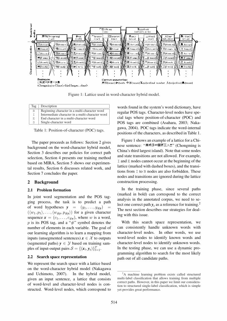
Figure 1: Lattice used in word-character hybrid model.
Tag DescriptionB Beginning character in a multi-character wordI Intermediate character in a multi-character wordE End character in a multi-character wordS Single-character word
Table 1: Position-of-character (POC) tags.
The paper proceeds as follows: Section 2 givesbackground on the word-character hybrid model,Section 3 describes our policies for correct pathselection, Section 4 presents our training methodbased on MIRA, Section 5 shows our experimen-tal results, Section 6 discusses related work, andSection 7 concludes the paper.
2 Background
2.1 Problem formationIn joint word segmentation and the POS tag-ging process, the task is to predict a pathof word hypotheses y = (y1, . . . , y#y) =(〈w1, p1〉, . . . , 〈w#y, p#y〉) for a given charactersequence x = (c1, . . . , c#x), where w is a word,p is its POS tag, and a “#” symbol denotes thenumber of elements in each variable. The goal ofour learning algorithm is to learn a mapping frominputs (unsegmented sentences) x ∈ X to outputs(segmented paths) y ∈ Y based on training sam-ples of input-output pairs S = {(xt, yt)}Tt=1.
2.2 Search space representationWe represent the search space with a lattice basedon the word-character hybrid model (Nakagawaand Uchimoto, 2007). In the hybrid model,given an input sentence, a lattice that consistsof word-level and character-level nodes is con-structed. Word-level nodes, which correspond to
words found in the system’s word dictionary, haveregular POS tags. Character-level nodes have spe-cial tags where position-of-character (POC) andPOS tags are combined (Asahara, 2003; Naka-gawa, 2004). POC tags indicate the word-internalpositions of the characters, as described in Table 1.
Figure 1 shows an example of a lattice for a Chi-nese sentence: “ ” (Chongming isChina’s third largest island). Note that some nodesand state transitions are not allowed. For example,I and E nodes cannot occur at the beginning of thelattice (marked with dashed boxes), and the transi-tions from I to B nodes are also forbidden. Thesenodes and transitions are ignored during the latticeconstruction processing.
In the training phase, since several paths(marked in bold) can correspond to the correctanalysis in the annotated corpus, we need to se-lect one correct path yt as a reference for training.2
The next section describes our strategies for deal-ing with this issue.
With this search space representation, wecan consistently handle unknown words withcharacter-level nodes. In other words, we useword-level nodes to identify known words andcharacter-level nodes to identify unknown words.In the testing phase, we can use a dynamic pro-gramming algorithm to search for the most likelypath out of all candidate paths.
2A machine learning problem exists called structuredmulti-label classification that allows training from multiplecorrect paths. However, in this paper we limit our considera-tion to structured single-label classification, which is simpleyet provides great performance.
514

3 Policies for correct path selection
In this section, we describe our strategies for se-lecting the correct path yt in the training phase.As shown in Figure 1, the paths marked in boldcan represent the correct annotation of the seg-mented sentence. Ideally, we need to build a word-character hybrid model that effectively learns thecharacteristics of unknown words (with character-level nodes) as well as those of known words (withword-level nodes).
We can directly estimate the statistics of knownwords from an annotated corpus where a sentenceis already segmented into words and assigned POStags. If we select the correct path yt that corre-sponds to the annotated sentence, it will only con-sist of word-level nodes that do not allow learningfor unknown words. We therefore need to choosecharacter-level nodes as correct nodes instead ofword-level nodes for some words. We expect thatthose words could reflect unknown words in thefuture.
Baayen and Sproat (1996) proposed that thecharacteristics of infrequent words in a trainingcorpus resemble those of unknown words. Theiridea has proven effective for estimating the statis-tics of unknown words in previous studies (Ratna-parkhi, 1996; Nagata, 1999; Nakagawa, 2004).
We adopt Baayen and Sproat’s approach asthe baseline policy in our word-character hybridmodel. In the baseline policy, we first count thefrequencies of words3 in the training corpus. Wethen collect infrequent words that appear less thanor equal to r times.4 If these infrequent words arein the correct path, we use character-level nodesto represent them, and hence the characteristics ofunknown words can be learned. For example, inFigure 1 we select the character-level nodes of theword “ ” (Chongming) as the correct nodes. Asa result, the correct path yt can contain both word-level and character-level nodes (marked with as-terisks (*)).
To discover more statistics of unknown words,one might consider just increasing the thresholdvalue r to obtain more artificial unknown words.However, our experimental results indicate thatour word-character hybrid model requires an ap-propriate balance between known and artificial un-
3We consider a word and its POS tag a single entry.4In our experiments, the optimal threshold value r is se-
lected by evaluating the performance of joint word segmen-tation and POS tagging on the development set.
known words to achieve optimal performance.We now describe our new approach to lever-
age additional examples of unknown words. In-tuition suggests that even though the system canhandle some unknown words, many unidentifiedunknown words remain that cannot be recoveredby the system; we wish to learn the characteristicsof such unidentified unknown words. We proposethe following simple scheme:
• Divide the training corpus into ten equal setsand perform 10-fold cross validation to findthe errors.
• For each trial, train the word-character hybridmodel with the baseline policy (r = 1) us-ing nine sets and estimate errors using the re-maining validation set.
• Collect unidentified unknown words fromeach validation set.
Several types of errors are produced by thebaseline model, but we only focus on those causedby unidentified unknown words, which can be eas-ily collected in the evaluation process. As de-scribed later in Section 5.2, we measure the recallon out-of-vocabulary (OOV) words. Here, we de-fine unidentified unknown words as OOV wordsin each validation set that cannot be recovered bythe system. After ten cross validation runs, weget a list of the unidentified unknown words de-rived from the whole training corpus. Note thatthe unidentified unknown words in the cross val-idation are not necessary to be infrequent words,but some overlap may exist. Finally, we obtain theartificial unknown words that combine the uniden-tified unknown words in cross validation and in-frequent words for learning unknown words. Werefer to this approach as the error-driven policy.
4 Training method
4.1 Discriminative online learningLet Yt = {y1
t , . . . , yKt } be a lattice consisting ofcandidate paths for a given sentence xt. In theword-character hybrid model, the lattice Yt cancontain more than 1000 nodes, depending on thelength of the sentence xt and the number of POStags in the corpus. Therefore, we require a learn-ing algorithm that can efficiently handle large andcomplex lattice structures.
Online learning is an attractive method forthe hybrid model since it quickly converges
515
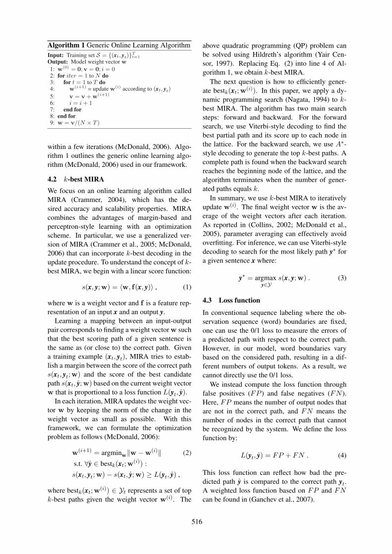
Algorithm 1 Generic Online Learning AlgorithmInput: Training set S = {(xt, yt)}Tt=1
Output: Model weight vector w
1: w(0) = 0; v = 0; i = 02: for iter = 1 to N do3: for t = 1 to T do4: w(i+1) = update w(i) according to (xt, yt)5: v = v + w(i+1)
6: i = i+ 17: end for8: end for9: w = v/(N × T )
within a few iterations (McDonald, 2006). Algo-rithm 1 outlines the generic online learning algo-rithm (McDonald, 2006) used in our framework.
4.2 k-best MIRAWe focus on an online learning algorithm calledMIRA (Crammer, 2004), which has the de-sired accuracy and scalability properties. MIRAcombines the advantages of margin-based andperceptron-style learning with an optimizationscheme. In particular, we use a generalized ver-sion of MIRA (Crammer et al., 2005; McDonald,2006) that can incorporate k-best decoding in theupdate procedure. To understand the concept of k-best MIRA, we begin with a linear score function:
s(x, y; w) = 〈w, f(x, y)〉 , (1)
where w is a weight vector and f is a feature rep-resentation of an input x and an output y.
Learning a mapping between an input-outputpair corresponds to finding a weight vector w suchthat the best scoring path of a given sentence isthe same as (or close to) the correct path. Givena training example (xt, yt), MIRA tries to estab-lish a margin between the score of the correct paths(xt, yt; w) and the score of the best candidatepath s(xt, ŷ; w) based on the current weight vectorw that is proportional to a loss function L(yt, ŷ).
In each iteration, MIRA updates the weight vec-tor w by keeping the norm of the change in theweight vector as small as possible. With thisframework, we can formulate the optimizationproblem as follows (McDonald, 2006):
w(i+1) = argminw‖w −w(i)‖ (2)
s.t. ∀ŷ ∈ bestk(xt; w(i)) :
s(xt, yt; w)− s(xt, ŷ; w) ≥ L(yt, ŷ) ,
where bestk(xt; w(i)) ∈ Yt represents a set of topk-best paths given the weight vector w(i). The
above quadratic programming (QP) problem canbe solved using Hildreth’s algorithm (Yair Cen-sor, 1997). Replacing Eq. (2) into line 4 of Al-gorithm 1, we obtain k-best MIRA.
The next question is how to efficiently gener-ate bestk(xt; w(i)). In this paper, we apply a dy-namic programming search (Nagata, 1994) to k-best MIRA. The algorithm has two main searchsteps: forward and backward. For the forwardsearch, we use Viterbi-style decoding to find thebest partial path and its score up to each node inthe lattice. For the backward search, we use A∗-style decoding to generate the top k-best paths. Acomplete path is found when the backward searchreaches the beginning node of the lattice, and thealgorithm terminates when the number of gener-ated paths equals k.
In summary, we use k-best MIRA to iterativelyupdate w(i). The final weight vector w is the av-erage of the weight vectors after each iteration.As reported in (Collins, 2002; McDonald et al.,2005), parameter averaging can effectively avoidoverfitting. For inference, we can use Viterbi-styledecoding to search for the most likely path y∗ fora given sentence x where:
y∗ = argmaxy∈Y
s(x, y; w) . (3)
4.3 Loss function
In conventional sequence labeling where the ob-servation sequence (word) boundaries are fixed,one can use the 0/1 loss to measure the errors ofa predicted path with respect to the correct path.However, in our model, word boundaries varybased on the considered path, resulting in a dif-ferent numbers of output tokens. As a result, wecannot directly use the 0/1 loss.
We instead compute the loss function throughfalse positives (FP ) and false negatives (FN ).Here, FP means the number of output nodes thatare not in the correct path, and FN means thenumber of nodes in the correct path that cannotbe recognized by the system. We define the lossfunction by:
L(yt, ŷ) = FP + FN . (4)
This loss function can reflect how bad the pre-dicted path ŷ is compared to the correct path yt.A weighted loss function based on FP and FNcan be found in (Ganchev et al., 2007).
516

ID Template ConditionW0 〈w0〉 for word-levelW1 〈p0〉 nodesW2 〈w0, p0〉W3 〈Length(w0), p0〉A0 〈AS(w0)〉 if w0 is a single-A1 〈AS(w0), p0〉 character wordA2 〈AB(w0)〉 for word-levelA3 〈AB(w0), p0〉 nodesA4 〈AE(w0)〉A5 〈AE(w0), p0〉A6 〈AB(w0), AE(w0)〉A7 〈AB(w0), AE(w0), p0〉T0 〈TS(w0)〉 if w0 is a single-T1 〈TS(w0), p0〉 character wordT2 〈TB(w0)〉 for word-levelT3 〈TB(w0), p0〉 nodesT4 〈TE(w0)〉T5 〈TE(w0), p0〉T6 〈TB(w0), TE(w0)〉T7 〈TB(w0), TE(w0), p0〉C0 〈cj〉, j ∈ [−2, 2] × p0 for character-C1 〈cj , cj+1〉, j ∈ [−2, 1] × p0 level nodesC2 〈c−1, c1〉 × p0
C3 〈T (cj)〉, j ∈ [−2, 2] × p0
C4 〈T (cj), T (cj+1)〉, j ∈ [−2, 1] × p0
C5 〈T (c−1), T (c1)〉 × p0
C6 〈c0, T (c0)〉 × p0
Table 2: Unigram features.
4.4 Features
This section discusses the structure of f(x, y). Webroadly classify features into two categories: uni-gram and bigram features. We design our featuretemplates to capture various levels of informationabout words and POS tags. Let us introduce somenotation. We write w−1 and w0 for the surfaceforms of words, where subscripts −1 and 0 in-dicate the previous and current positions, respec-tively. POS tags p−1 and p0 can be interpreted inthe same way. We denote the characters by cj .
Unigram features: Table 2 shows our unigramfeatures. Templates W0–W3 are basic word-levelunigram features, where Length(w0) denotes thelength of the word w0. Using just the surfaceforms can overfit the training data and lead to poorpredictions on the test data. To alleviate this prob-lem, we use two generalized features of the sur-face forms. The first is the beginning and endcharacters of the surface (A0–A7). For example,〈AB(w0)〉 denotes the beginning character of thecurrent word w0, and 〈AB(w0), AE(w0)〉 denotesthe beginning and end characters in the word. Thesecond is the types of beginning and end charac-ters of the surface (T0–T7). We define a set ofgeneral character types, as shown in Table 4.
Templates C0–C6 are basic character-level un-
ID Template ConditionB0 〈w−1, w0〉 if w−1 and w0
B1 〈p−1, p0〉 are word-levelB2 〈w−1, p0〉 nodesB3 〈p−1, w0〉B4 〈w−1, w0, p0〉B5 〈p−1, w0, p0〉B6 〈w−1, p−1, w0〉B7 〈w−1, p−1, p0〉B8 〈w−1, p−1, w0, p0〉B9 〈Length(w−1), p0〉TB0 〈TE(w−1)〉TB1 〈TE(w−1), p0〉TB2 〈TE(w−1), p−1, p0〉TB3 〈TE(w−1), TB(w0)〉TB4 〈TE(w−1), TB(w0), p0〉TB5 〈TE(w−1), p−1, TB(w0)〉TB6 〈TE(w−1), p−1, TB(w0), p0〉CB0 〈p−1, p0〉 otherwise
Table 3: Bigram features.
Character type DescriptionSpace SpaceNumeral Arabic and Chinese numeralsSymbol SymbolsAlphabet AlphabetsChinese Chinese charactersOther Others
Table 4: Character types.
igram features taken from (Nakagawa, 2004).These templates operate over a window of ±2characters. The features include characters (C0),pairs of characters (C1–C2), character types (C3),and pairs of character types (C4–C5). In addi-tion, we add pairs of characters and character types(C6).
Bigram features: Table 3 shows our bigramfeatures. Templates B0-B9 are basic word-level bigram features. These features aim tocapture all the possible combinations of wordand POS bigrams. Templates TB0-TB6 are thetypes of characters for bigrams. For example,〈TE(w−1), TB(w0)〉 captures the change of char-acter types from the end character in the previ-ous word to the beginning character in the currentword.
Note that if one of the adjacent nodes is acharacter-level node, we use the template CB0 thatrepresents POS bigrams. In our preliminary ex-periments, we found that if we add more featuresto non-word-level bigrams, the number of featuresgrows rapidly due to the dense connections be-tween non-word-level nodes. However, these fea-tures only slightly improve performance over us-ing simple POS bigrams.
517
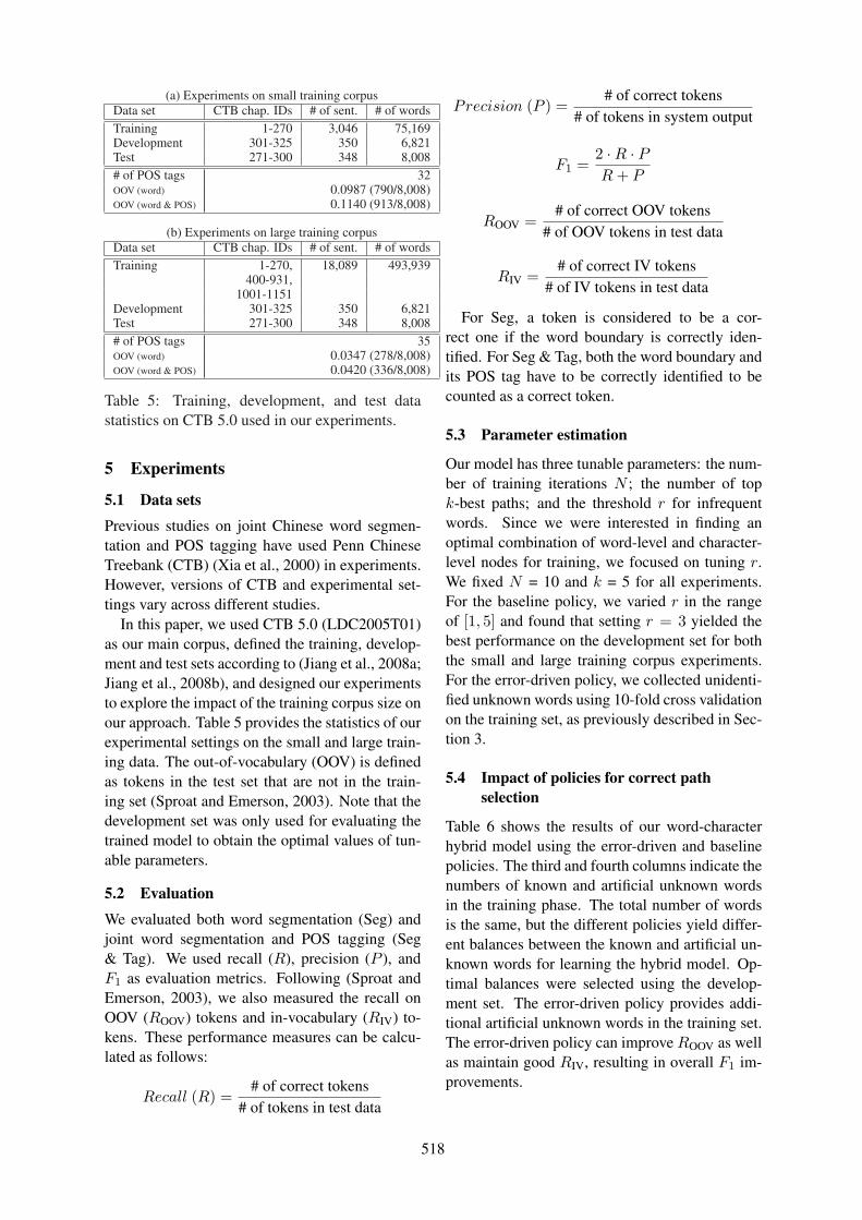
(a) Experiments on small training corpusData set CTB chap. IDs # of sent. # of wordsTraining 1-270 3,046 75,169Development 301-325 350 6,821Test 271-300 348 8,008# of POS tags 32OOV (word) 0.0987 (790/8,008)OOV (word & POS) 0.1140 (913/8,008)
(b) Experiments on large training corpusData set CTB chap. IDs # of sent. # of wordsTraining 1-270, 18,089 493,939
400-931,1001-1151
Development 301-325 350 6,821Test 271-300 348 8,008# of POS tags 35OOV (word) 0.0347 (278/8,008)OOV (word & POS) 0.0420 (336/8,008)
Table 5: Training, development, and test datastatistics on CTB 5.0 used in our experiments.
5 Experiments
5.1 Data sets
Previous studies on joint Chinese word segmen-tation and POS tagging have used Penn ChineseTreebank (CTB) (Xia et al., 2000) in experiments.However, versions of CTB and experimental set-tings vary across different studies.
In this paper, we used CTB 5.0 (LDC2005T01)as our main corpus, defined the training, develop-ment and test sets according to (Jiang et al., 2008a;Jiang et al., 2008b), and designed our experimentsto explore the impact of the training corpus size onour approach. Table 5 provides the statistics of ourexperimental settings on the small and large train-ing data. The out-of-vocabulary (OOV) is definedas tokens in the test set that are not in the train-ing set (Sproat and Emerson, 2003). Note that thedevelopment set was only used for evaluating thetrained model to obtain the optimal values of tun-able parameters.
5.2 Evaluation
We evaluated both word segmentation (Seg) andjoint word segmentation and POS tagging (Seg& Tag). We used recall (R), precision (P ), andF1 as evaluation metrics. Following (Sproat andEmerson, 2003), we also measured the recall onOOV (ROOV) tokens and in-vocabulary (RIV) to-kens. These performance measures can be calcu-lated as follows:
Recall (R) =# of correct tokens
# of tokens in test data
Precision (P ) =# of correct tokens
# of tokens in system output
F1 =2 ·R · PR+ P
ROOV =# of correct OOV tokens
# of OOV tokens in test data
RIV =# of correct IV tokens
# of IV tokens in test data
For Seg, a token is considered to be a cor-rect one if the word boundary is correctly iden-tified. For Seg & Tag, both the word boundary andits POS tag have to be correctly identified to becounted as a correct token.
5.3 Parameter estimation
Our model has three tunable parameters: the num-ber of training iterations N ; the number of topk-best paths; and the threshold r for infrequentwords. Since we were interested in finding anoptimal combination of word-level and character-level nodes for training, we focused on tuning r.We fixed N = 10 and k = 5 for all experiments.For the baseline policy, we varied r in the rangeof [1, 5] and found that setting r = 3 yielded thebest performance on the development set for boththe small and large training corpus experiments.For the error-driven policy, we collected unidenti-fied unknown words using 10-fold cross validationon the training set, as previously described in Sec-tion 3.
5.4 Impact of policies for correct pathselection
Table 6 shows the results of our word-characterhybrid model using the error-driven and baselinepolicies. The third and fourth columns indicate thenumbers of known and artificial unknown wordsin the training phase. The total number of wordsis the same, but the different policies yield differ-ent balances between the known and artificial un-known words for learning the hybrid model. Op-timal balances were selected using the develop-ment set. The error-driven policy provides addi-tional artificial unknown words in the training set.The error-driven policy can improveROOV as wellas maintain good RIV, resulting in overall F1 im-provements.
518
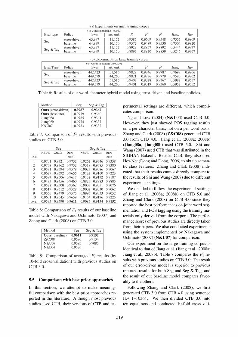
(a) Experiments on small training corpus# of words in training (75,169)
Eval type Policy kwn. art. unk. R P F1 ROOV RIV
Seg error-driven 63,997 11,172 0.9587 0.9509 0.9548 0.7557 0.9809baseline 64,999 10,170 0.9572 0.9489 0.9530 0.7304 0.9820
Seg & Tag error-driven 63,997 11,172 0.8929 0.8857 0.8892 0.5444 0.9377baseline 64,999 10,170 0.8897 0.8820 0.8859 0.5246 0.9367
(b) Experiments on large training corpus# of words in training (493,939)
Eval Type Policy kwn. art. unk. R P F1 ROOV RIV
Seg error-driven 442,423 51,516 0.9829 0.9746 0.9787 0.7698 0.9906baseline 449,679 44,260 0.9821 0.9736 0.9779 0.7590 0.9902
Seg & Tag error-driven 442,423 51,516 0.9407 0.9328 0.9367 0.5982 0.9557baseline 449,679 44,260 0.9401 0.9319 0.9360 0.5952 0.9552
Table 6: Results of our word-character hybrid model using error-driven and baseline policies.
Method Seg Seg & TagOurs (error-driven) 0.9787 0.9367Ours (baseline) 0.9779 0.9360Jiang08a 0.9785 0.9341Jiang08b 0.9774 0.9337N&U07 0.9783 0.9332
Table 7: Comparison of F1 results with previousstudies on CTB 5.0.
Seg Seg & TagN&U07 Z&C08 Ours N&U07 Z&C08 Ours
Trial (base.) (base.)
1 0.9701 0.9721 0.9732 0.9262 0.9346 0.93582 0.9738 0.9762 0.9752 0.9318 0.9385 0.93803 0.9571 0.9594 0.9578 0.9023 0.9086 0.90674 0.9629 0.9592 0.9655 0.9132 0.9160 0.92235 0.9597 0.9606 0.9617 0.9132 0.9172 0.91876 0.9473 0.9456 0.9460 0.8823 0.8883 0.88857 0.9528 0.9500 0.9562 0.9003 0.9051 0.90768 0.9519 0.9512 0.9528 0.9002 0.9030 0.90629 0.9566 0.9479 0.9575 0.8996 0.9033 0.905210 0.9631 0.9645 0.9659 0.9154 0.9196 0.9225
Avg. 0.9595 0.9590 0.9611 0.9085 0.9134 0.9152
Table 8: Comparison of F1 results of our baselinemodel with Nakagawa and Uchimoto (2007) andZhang and Clark (2008) on CTB 3.0.
Method Seg Seg & TagOurs (baseline) 0.9611 0.9152Z&C08 0.9590 0.9134N&U07 0.9595 0.9085N&L04 0.9520 -
Table 9: Comparison of averaged F1 results (by10-fold cross validation) with previous studies onCTB 3.0.
5.5 Comparison with best prior approaches
In this section, we attempt to make meaning-ful comparison with the best prior approaches re-ported in the literature. Although most previousstudies used CTB, their versions of CTB and ex-
perimental settings are different, which compli-cates comparison.
Ng and Low (2004) (N&L04) used CTB 3.0.However, they just showed POS tagging resultson a per character basis, not on a per word basis.Zhang and Clark (2008) (Z&C08) generated CTB3.0 from CTB 4.0. Jiang et al. (2008a; 2008b)(Jiang08a, Jiang08b) used CTB 5.0. Shi andWang (2007) used CTB that was distributed in theSIGHAN Bakeoff. Besides CTB, they also usedHowNet (Dong and Dong, 2006) to obtain seman-tic class features. Zhang and Clark (2008) indi-cated that their results cannot directly compare tothe results of Shi and Wang (2007) due to differentexperimental settings.
We decided to follow the experimental settingsof Jiang et al. (2008a; 2008b) on CTB 5.0 andZhang and Clark (2008) on CTB 4.0 since theyreported the best performances on joint word seg-mentation and POS tagging using the training ma-terials only derived from the corpora. The perfor-mance scores of previous studies are directly takenfrom their papers. We also conducted experimentsusing the system implemented by Nakagawa andUchimoto (2007) (N&U07) for comparison.
Our experiment on the large training corpus isidentical to that of Jiang et al. (Jiang et al., 2008a;Jiang et al., 2008b). Table 7 compares the F1 re-sults with previous studies on CTB 5.0. The resultof our error-driven model is superior to previousreported results for both Seg and Seg & Tag, andthe result of our baseline model compares favor-ably to the others.
Following Zhang and Clark (2008), we firstgenerated CTB 3.0 from CTB 4.0 using sentenceIDs 1–10364. We then divided CTB 3.0 intoten equal sets and conducted 10-fold cross vali-
519
dation. Unfortunately, Zhang and Clark’s exper-imental setting did not allow us to use our error-driven policy since performing 10-fold cross val-idation again on each main cross validation trialis computationally too expensive. Therefore, weused our baseline policy in this setting and fixedr = 3 for all cross validation runs. Table 8 com-pares the F1 results of our baseline model withNakagawa and Uchimoto (2007) and Zhang andClark (2008) on CTB 3.0. Table 9 shows a sum-mary of averaged F1 results on CTB 3.0. Ourbaseline model outperforms all prior approachesfor both Seg and Seg & Tag, and we hope thatour error-driven model can further improve perfor-mance.
6 Related work
In this section, we discuss related approachesbased on several aspects of learning algorithmsand search space representation methods. Max-imum entropy models are widely used for wordsegmentation and POS tagging tasks (Uchimotoet al., 2001; Ng and Low, 2004; Nakagawa,2004; Nakagawa and Uchimoto, 2007) since theyonly need moderate training times while they pro-vide reasonable performance. Conditional randomfields (CRFs) (Lafferty et al., 2001) further im-prove the performance (Kudo et al., 2004; Shiand Wang, 2007) by performing whole-sequencenormalization to avoid label-bias and length-biasproblems. However, CRF-based algorithms typ-ically require longer training times, and we ob-served an infeasible convergence time for our hy-brid model.
Online learning has recently gained popularityfor many NLP tasks since it performs comparablyor better than batch learning using shorter train-ing times (McDonald, 2006). For example, a per-ceptron algorithm is used for joint Chinese wordsegmentation and POS tagging (Zhang and Clark,2008; Jiang et al., 2008a; Jiang et al., 2008b).Another potential algorithm is MIRA, which in-tegrates the notion of the large-margin classifier(Crammer, 2004). In this paper, we first intro-duce MIRA to joint word segmentation and POStagging and show very encouraging results. Withregard to error-driven learning, Brill (1995) pro-posed a transformation-based approach that ac-quires a set of error-correcting rules by comparingthe outputs of an initial tagger with the correct an-notations on a training corpus. Our approach does
not learn the error-correcting rules. We only aim tocapture the characteristics of unknown words andaugment their representatives.
As for search space representation, Ng andLow (2004) found that for Chinese, the character-based model yields better results than the word-based model. Nakagawa and Uchimoto (2007)provided empirical evidence that the character-based model is not always better than the word-based model. They proposed a hybrid approachthat exploits both the word-based and character-based models. Our approach overcomes the limi-tation of the original hybrid model by a discrimi-native online learning algorithm for training.
7 Conclusion
In this paper, we presented a discriminative word-character hybrid model for joint Chinese wordsegmentation and POS tagging. Our approachhas two important advantages. The first is ro-bust search space representation based on a hy-brid model in which word-level and character-level nodes are used to identify known and un-known words, respectively. We introduced a sim-ple scheme based on the error-driven concept toeffectively learn the characteristics of known andunknown words from the training corpus. The sec-ond is a discriminative online learning algorithmbased on MIRA that enables us to incorporate ar-bitrary features to our hybrid model. Based on ex-tensive comparisons, we showed that our approachis superior to the existing approaches reported inthe literature. In future work, we plan to applyour framework to other Asian languages, includ-ing Thai and Japanese.
Acknowledgments
We would like to thank Tetsuji Nakagawa for hishelpful suggestions about the word-character hy-brid model, Chen Wenliang for his technical assis-tance with the Chinese processing, and the anony-mous reviewers for their insightful comments.
ReferencesMasayuki Asahara. 2003. Corpus-based Japanese
morphological analysis. Nara Institute of Scienceand Technology, Doctor’s Thesis.
Harald Baayen and Richard Sproat. 1996. Estimat-ing lexical priors for low-frequency morphologi-cally ambiguous forms. Computational Linguistics,22(2):155–166.
520
Eric Brill. 1995. Transformation-based error-drivenlearning and natural language processing: A casestudy in part-of-speech tagging. Computational Lin-guistics, 21(4):543–565.
Michael Collins. 2002. Discriminative training meth-ods for hidden markov models: Theory and exper-iments with perceptron algorithms. In Proceedingsof EMNLP, pages 1–8.
Koby Crammer, Ryan McDonald, and FernandoPereira. 2005. Scalable large-margin online learn-ing for structured classification. In NIPS Workshopon Learning With Structured Outputs.
Koby Crammer. 2004. Online Learning of Com-plex Categorial Problems. Hebrew Univeristy ofJerusalem, PhD Thesis.
Zhendong Dong and Qiang Dong. 2006. Hownet andthe Computation of Meaning. World Scientific.
Kuzman Ganchev, Koby Crammer, Fernando Pereira,Gideon Mann, Kedar Bellare, Andrew McCallum,Steven Carroll, Yang Jin, and Peter White. 2007.Penn/umass/chop biocreative ii systems. In Pro-ceedings of the Second BioCreative Challenge Eval-uation Workshop.
Wenbin Jiang, Liang Huang, Qun Liu, and Yajuan Lü.2008a. A cascaded linear model for joint chineseword segmentation and part-of-speech tagging. InProceedings of ACL.
Wenbin Jiang, Haitao Mi, and Qun Liu. 2008b. Wordlattice reranking for chinese word segmentation andpart-of-speech tagging. In Proceedings of COLING.
Taku Kudo, Kaoru Yamamoto, and Yuji Matsumoto.2004. Applying conditional random fields tojapanese morphological analysis. In Proceedings ofEMNLP, pages 230–237.
John Lafferty, Andrew McCallum, and FernandoPereira. 2001. Conditional random fields: Prob-abilistic models for segmenting and labeling se-quence data. In Proceedings of ICML, pages 282–289.
Ryan McDonald, Femando Pereira, Kiril Ribarow, andJan Hajic. 2005. Non-projective dependency pars-ing using spanning tree algorithms. In Proceedingsof HLT/EMNLP, pages 523–530.
Ryan McDonald. 2006. Discriminative Training andSpanning Tree Algorithms for Dependency Parsing.University of Pennsylvania, PhD Thesis.
Masaki Nagata. 1994. A stochastic japanese mor-phological analyzer using a forward-DP backward-A* n-best search algorithm. In Proceedings ofthe 15th International Conference on ComputationalLinguistics, pages 201–207.
Masaki Nagata. 1999. A part of speech estimationmethod for japanese unknown words using a statis-tical model of morphology and context. In Proceed-ings of ACL, pages 277–284.
Tetsuji Nakagawa and Kiyotaka Uchimoto. 2007. Ahybrid approach to word segmentation and pos tag-ging. In Proceedings of ACL Demo and Poster Ses-sions.
Tetsuji Nakagawa. 2004. Chinese and japanese wordsegmentation using word-level and character-levelinformation. In Proceedings of COLING, pages466–472.
Hwee Tou Ng and Jin Kiat Low. 2004. Chinese part-of-speech tagging: One-at-a-time or all-at-once?word-based or character-based? In Proceedings ofEMNLP, pages 277–284.
Adwait Ratnaparkhi. 1996. A maximum entropymodel for part-of-speech tagging. In Proceedingsof EMNLP, pages 133–142.
Yanxin Shi and Mengqiu Wang. 2007. A dual-layercrfs based joint decoding method for cascaded seg-mentation and labeling tasks. In Proceedings of IJ-CAI.
Richard Sproat and Thomas Emerson. 2003. The firstinternational chinese word segmentation bakeoff. InProceedings of the 2nd SIGHAN Workshop on Chi-nese Language Processing, pages 133–143.
Kiyotaka Uchimoto, Satoshi Sekine, and Hitoshi Isa-hara. 2001. The unknown word problem: a morpho-logical analysis of japanese using maximum entropyaided by a dictionary. In Proceedings of EMNLP,pages 91–99.
Fei Xia, Martha Palmer, Nianwen Xue, Mary EllenOkurowski, John Kovarik, Fu dong Chiou, andShizhe Huang. 2000. Developing guidelines andensuring consistency for chinese text annotation. InProceedings of LREC.
Stavros A. Zenios Yair Censor. 1997. Parallel Op-timization: Theory, Algorithms, and Applications.Oxford University Press.
Yue Zhang and Stephen Clark. 2008. Joint word seg-mentation and pos tagging on a single perceptron. InProceedings of ACL.
521
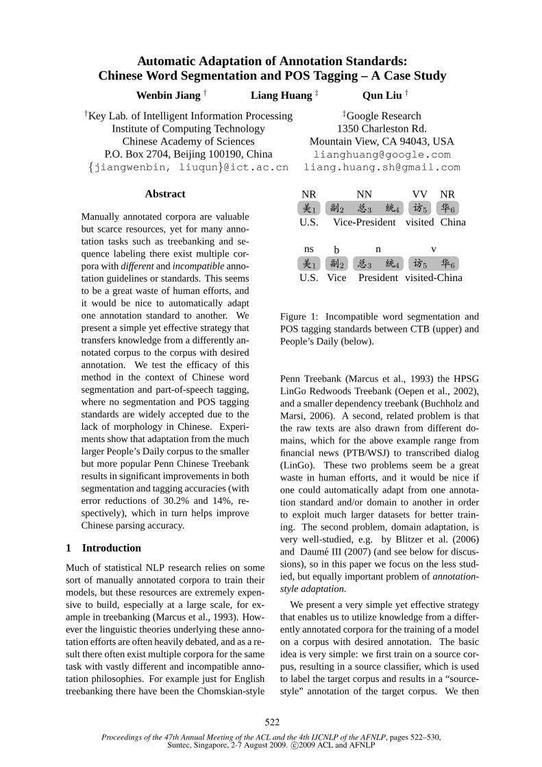
Proceedings of the 47th Annual Meeting of the ACL and the 4th IJCNLP of the AFNLP, pages 522–530,Suntec, Singapore, 2-7 August 2009. c©2009 ACL and AFNLP
Automatic Adaptation of Annotation Standards:Chinese Word Segmentation and POS Tagging – A Case Study
Wenbin Jiang † Liang Huang ‡ Qun Liu †
†Key Lab. of Intelligent Information Processing ‡Google ResearchInstitute of Computing Technology 1350 Charleston Rd.
Chinese Academy of Sciences Mountain View, CA 94043, USAP.O. Box 2704, Beijing 100190, China [email protected]
{jiangwenbin, liuqun}@ict.ac.cn [email protected]
Abstract
Manually annotated corpora are valuablebut scarce resources, yet for many anno-tation tasks such as treebanking and se-quence labeling there exist multiple cor-pora withdifferentandincompatibleanno-tation guidelines or standards. This seemsto be a great waste of human efforts, andit would be nice to automatically adaptone annotation standard to another. Wepresent a simple yet effective strategy thattransfers knowledge from a differently an-notated corpus to the corpus with desiredannotation. We test the efficacy of thismethod in the context of Chinese wordsegmentation and part-of-speech tagging,where no segmentation and POS taggingstandards are widely accepted due to thelack of morphology in Chinese. Experi-ments show that adaptation from the muchlarger People’s Daily corpus to the smallerbut more popular Penn Chinese Treebankresults in significant improvements in bothsegmentation and tagging accuracies (witherror reductions of 30.2% and 14%, re-spectively), which in turn helps improveChinese parsing accuracy.
1 Introduction
Much of statistical NLP research relies on somesort of manually annotated corpora to train theirmodels, but these resources are extremely expen-sive to build, especially at a large scale, for ex-ample in treebanking (Marcus et al., 1993). How-ever the linguistic theories underlying these anno-tation efforts are often heavily debated, and as a re-sult there often exist multiple corpora for the sametask with vastly different and incompatible anno-tation philosophies. For example just for Englishtreebanking there have been the Chomskian-style
{1 B2 o3 Ú4 �5 u6
NR NN VV NR
U.S. Vice-President visited China
{1 B2 o3 Ú4 �5 u6
ns b n v
U.S. Vice Presidentvisited-China
Figure 1: Incompatible word segmentation andPOS tagging standards between CTB (upper) andPeople’s Daily (below).
Penn Treebank (Marcus et al., 1993) the HPSGLinGo Redwoods Treebank (Oepen et al., 2002),and a smaller dependency treebank (Buchholz andMarsi, 2006). A second, related problem is thatthe raw texts are also drawn from different do-mains, which for the above example range fromfinancial news (PTB/WSJ) to transcribed dialog(LinGo). These two problems seem be a greatwaste in human efforts, and it would be nice ifone could automatically adapt from one annota-tion standard and/or domain to another in orderto exploit much larger datasets for better train-ing. The second problem, domain adaptation, isvery well-studied, e.g. by Blitzer et al. (2006)and Dauḿe III (2007) (and see below for discus-sions), so in this paper we focus on the less stud-ied, but equally important problem ofannotation-style adaptation.
We present a very simple yet effective strategythat enables us to utilize knowledge from a differ-ently annotated corpora for the training of a modelon a corpus with desired annotation. The basicidea is very simple: we first train on a source cor-pus, resulting in a source classifier, which is usedto label the target corpus and results in a “source-style” annotation of the target corpus. We then
522

train a second model on the target corpus with thefirst classifier’s prediction as additional featuresfor guided learning.
This method is very similar to some ideas indomain adaptation (Dauḿe III and Marcu, 2006;Dauḿe III, 2007), but we argue that the underly-ing problems are quite different. Domain adapta-tion assumes the labeling guidelines are preservedbetween the two domains, e.g., an adjective is al-ways labeled as JJ regardless of from Wall StreetJournal (WSJ) or Biomedical texts, and only thedistributionsare different, e.g., the word “control”is most likely a verb in WSJ but often a nounin Biomedical texts (as in “control experiment”).Annotation-style adaptation, however, tackles theproblem where the guideline itself is changed, forexample, one treebank might distinguish betweentransitive and intransitive verbs, while merging thedifferent noun types (NN, NNS, etc.), and for ex-ample one treebank (PTB) might be much flatterthan the other (LinGo), not to mention the fun-damental disparities between their underlying lin-guistic representations (CFG vs. HPSG). In thissense, the problem we study in this paper seemsmuch harder and more motivated from a linguistic(rather than statistical) point of view. More inter-estingly, our method, without any assumption onthe distributions, can be simultaneously applied toboth domainand annotation standards adaptationproblems, which is very appealing in practice be-cause the latter problem often implies the former,as in our case study.
To test the efficacy of our method we chooseChinese word segmentation and part-of-speechtagging, where the problem of incompatible an-notation standards is one of the most evident: sofar no segmentation standard is widely accepteddue to the lack of a clear definition of Chinesewords, and the (almost complete) lack of mor-phology results in much bigger ambiguities andheavy debates in tagging philosophies for Chi-nese parts-of-speech. The two corpora used inthis study are the much larger People’s Daily (PD)(5.86M words) corpus (Yu et al., 2001) and thesmaller but more popular Penn Chinese Treebank(CTB) (0.47M words) (Xue et al., 2005). Theyused very different segmentation standards as wellas different POS tagsets and tagging guidelines.For example, in Figure 1, People’s Daily breaks“Vice-President” into two words while combinesthe phrase “visited-China” as a compound. Also
CTB has four verbal categories (VV for normalverbs, and VC for copulas, etc.) while PD has onlyone verbal tag (v) (Xia, 2000). It is preferable totransfer knowledge from PD to CTB because thelatter also annotates tree structures which is veryuseful for downstream applications like parsing,summarization, and machine translation, yet it ismuch smaller in size. Indeed, many recent effortson Chinese-English translation and Chinese pars-ing use the CTB as thede factosegmentation andtagging standards, but suffers from the limited sizeof training data (Chiang, 2007; Bikel and Chiang,2000). We believe this is also a reason why state-of-the-art accuracy for Chinese parsing is muchlower than that of English (CTB is only half thesize of PTB).
Our experiments show that adaptation from PDto CTB results in a significant improvement in seg-mentation and POS tagging, with error reductionsof 30.2% and 14%, respectively. In addition, theimproved accuracies from segmentation and tag-ging also lead to an improved parsing accuracy onCTB, reducing38% of the error propagation fromword segmentation to parsing. We envision thistechnique to be general and widely applicable tomany other sequence labeling tasks.
In the rest of the paper we first briefly reviewthe popular classification-based method for wordsegmentation and tagging (Section 2), and thendescribe our idea of annotation adaptation (Sec-tion 3). We then discuss other relevant previouswork including co-training and classifier combina-tion (Section 4) before presenting our experimen-tal results (Section 5).
2 Segmentation and Tagging asCharacter Classification
Before describing the adaptation algorithm, wegive a brief introduction of the baseline characterclassification strategy for segmentation, as well asjoint segmenation and tagging (henceforth “JointS&T”). following our previous work (Jiang et al.,2008). Given a Chinese sentence as sequence ofn
characters:
C1 C2 .. Cn
whereCi is a character, word segmentation aimsto split the sequence intom(≤ n) words:
C1:e1 Ce1+1:e2 .. Cem−1+1:em
where each subsequenceCi:j indicates a Chineseword spanning from charactersCi to Cj (both in-
523
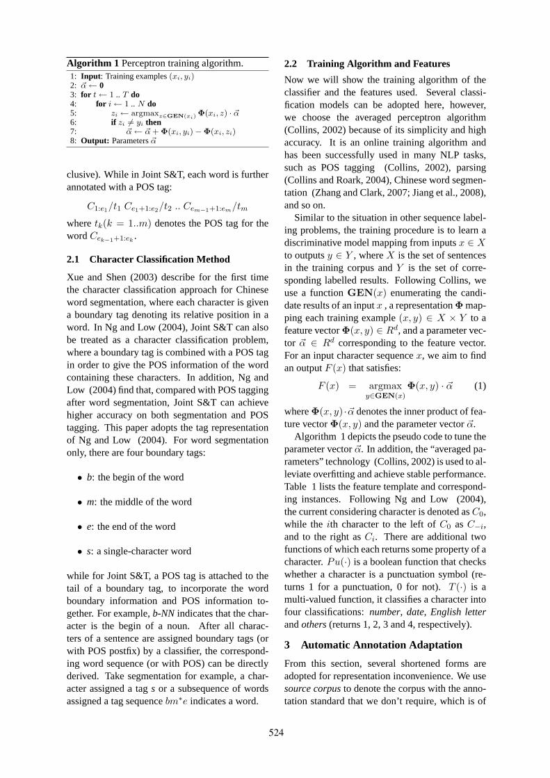
Algorithm 1 Perceptron training algorithm.1: Input : Training examples(xi, yi)2: ~α← 03: for t← 1 .. T do4: for i← 1 .. N do5: zi ← argmaxz∈GEN(xi)
Φ(xi, z) · ~α6: if zi 6= yi then7: ~α← ~α + Φ(xi, yi)−Φ(xi, zi)8: Output: Parameters~α
clusive). While in Joint S&T, each word is furtherannotated with a POS tag:
C1:e1/t1 Ce1+1:e2/t2 .. Cem−1+1:em/tm
wheretk(k = 1..m) denotes the POS tag for thewordCek−1+1:ek
.
2.1 Character Classification Method
Xue and Shen (2003) describe for the first timethe character classification approach for Chineseword segmentation, where each character is givena boundary tag denoting its relative position in aword. In Ng and Low (2004), Joint S&T can alsobe treated as a character classification problem,where a boundary tag is combined with a POS tagin order to give the POS information of the wordcontaining these characters. In addition, Ng andLow (2004) find that, compared with POS taggingafter word segmentation, Joint S&T can achievehigher accuracy on both segmentation and POStagging. This paper adopts the tag representationof Ng and Low (2004). For word segmentationonly, there are four boundary tags:
• b: the begin of the word
• m: the middle of the word
• e: the end of the word
• s: a single-character word
while for Joint S&T, a POS tag is attached to thetail of a boundary tag, to incorporate the wordboundary information and POS information to-gether. For example,b-NN indicates that the char-acter is the begin of a noun. After all charac-ters of a sentence are assigned boundary tags (orwith POS postfix) by a classifier, the correspond-ing word sequence (or with POS) can be directlyderived. Take segmentation for example, a char-acter assigned a tags or a subsequence of wordsassigned a tag sequencebm∗e indicates a word.
2.2 Training Algorithm and Features
Now we will show the training algorithm of theclassifier and the features used. Several classi-fication models can be adopted here, however,we choose the averaged perceptron algorithm(Collins, 2002) because of its simplicity and highaccuracy. It is an online training algorithm andhas been successfully used in many NLP tasks,such as POS tagging (Collins, 2002), parsing(Collins and Roark, 2004), Chinese word segmen-tation (Zhang and Clark, 2007; Jiang et al., 2008),and so on.
Similar to the situation in other sequence label-ing problems, the training procedure is to learn adiscriminative model mapping from inputsx ∈ X
to outputsy ∈ Y , whereX is the set of sentencesin the training corpus andY is the set of corre-sponding labelled results. Following Collins, weuse a functionGEN(x) enumerating the candi-date results of an inputx , a representationΦ map-ping each training example(x, y) ∈ X × Y to afeature vectorΦ(x, y) ∈ Rd, and a parameter vec-tor ~α ∈ Rd corresponding to the feature vector.For an input character sequencex, we aim to findan outputF (x) that satisfies:
F (x) = argmaxy∈GEN(x)
Φ(x, y) · ~α (1)
whereΦ(x, y) ·~α denotes the inner product of fea-ture vectorΦ(x, y) and the parameter vector~α.
Algorithm 1 depicts the pseudo code to tune theparameter vector~α. In addition, the “averaged pa-rameters” technology (Collins, 2002) is used to al-leviate overfitting and achieve stable performance.Table 1 lists the feature template and correspond-ing instances. Following Ng and Low (2004),the current considering character is denoted asC0,while the ith character to the left ofC0 asC−i,and to the right asCi. There are additional twofunctions of which each returns some property of acharacter.Pu(·) is a boolean function that checkswhether a character is a punctuation symbol (re-turns 1 for a punctuation, 0 for not).T (·) is amulti-valued function, it classifies a character intofour classifications:number, date, English letterandothers(returns 1, 2, 3 and 4, respectively).
3 Automatic Annotation Adaptation
From this section, several shortened forms areadopted for representation inconvenience. We usesource corpusto denote the corpus with the anno-tation standard that we don’t require, which is of
524
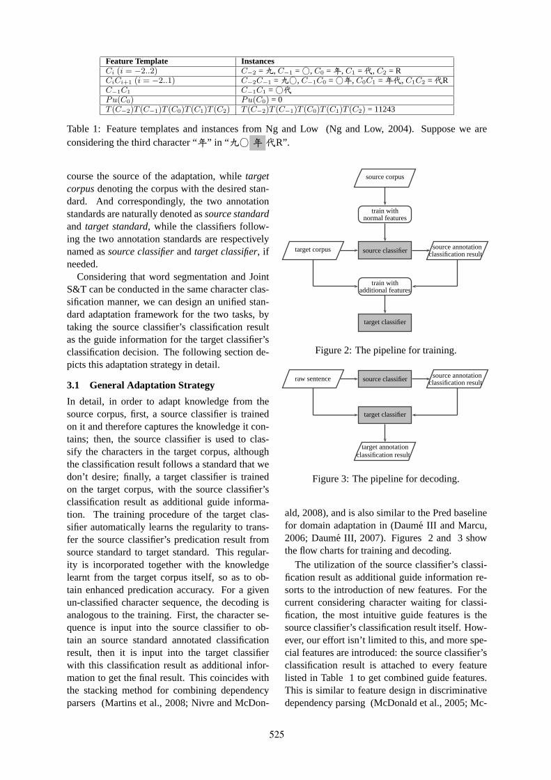
Feature Template InstancesCi (i = −2..2) C
−2 =Ê, C−1 =�, C0 =c, C1 =�, C2 = R
CiCi+1 (i = −2..1) C−2C−1 =Ê�, C
−1C0 =�c, C0C1 =c�, C1C2 =�RC−1C1 C
−1C1 =��Pu(C0) Pu(C0) = 0T (C
−2)T (C−1)T (C0)T (C1)T (C2) T (C
−2)T (C−1)T (C0)T (C1)T (C2) = 11243
Table 1: Feature templates and instances from Ng and Low (Ng and Low, 2004). Suppose we areconsidering the third character “c” in “Ê� c �R”.
course the source of the adaptation, whiletargetcorpusdenoting the corpus with the desired stan-dard. And correspondingly, the two annotationstandards are naturally denoted assource standardand target standard, while the classifiers follow-ing the two annotation standards are respectivelynamed assource classifierandtarget classifier, ifneeded.
Considering that word segmentation and JointS&T can be conducted in the same character clas-sification manner, we can design an unified stan-dard adaptation framework for the two tasks, bytaking the source classifier’s classification resultas the guide information for the target classifier’sclassification decision. The following section de-picts this adaptation strategy in detail.
3.1 General Adaptation Strategy
In detail, in order to adapt knowledge from thesource corpus, first, a source classifier is trainedon it and therefore captures the knowledge it con-tains; then, the source classifier is used to clas-sify the characters in the target corpus, althoughthe classification result follows a standard that wedon’t desire; finally, a target classifier is trainedon the target corpus, with the source classifier’sclassification result as additional guide informa-tion. The training procedure of the target clas-sifier automatically learns the regularity to trans-fer the source classifier’s predication result fromsource standard to target standard. This regular-ity is incorporated together with the knowledgelearnt from the target corpus itself, so as to ob-tain enhanced predication accuracy. For a givenun-classified character sequence, the decoding isanalogous to the training. First, the character se-quence is input into the source classifier to ob-tain an source standard annotated classificationresult, then it is input into the target classifierwith this classification result as additional infor-mation to get the final result. This coincides withthe stacking method for combining dependencyparsers (Martins et al., 2008; Nivre and McDon-
source corpus
train withnormal features
source classifier
train withadditional features
target classifier
target corpus source annotationclassification result
Figure 2: The pipeline for training.
raw sentence source classifier source annotationclassification result
target classifier
target annotationclassification result
Figure 3: The pipeline for decoding.
ald, 2008), and is also similar to the Pred baselinefor domain adaptation in (Dauḿe III and Marcu,2006; Dauḿe III, 2007). Figures 2 and 3 showthe flow charts for training and decoding.
The utilization of the source classifier’s classi-fication result as additional guide information re-sorts to the introduction of new features. For thecurrent considering character waiting for classi-fication, the most intuitive guide features is thesource classifier’s classification result itself. How-ever, our effort isn’t limited to this, and more spe-cial features are introduced: the source classifier’sclassification result is attached to every featurelisted in Table 1 to get combined guide features.This is similar to feature design in discriminativedependency parsing (McDonald et al., 2005; Mc-
525
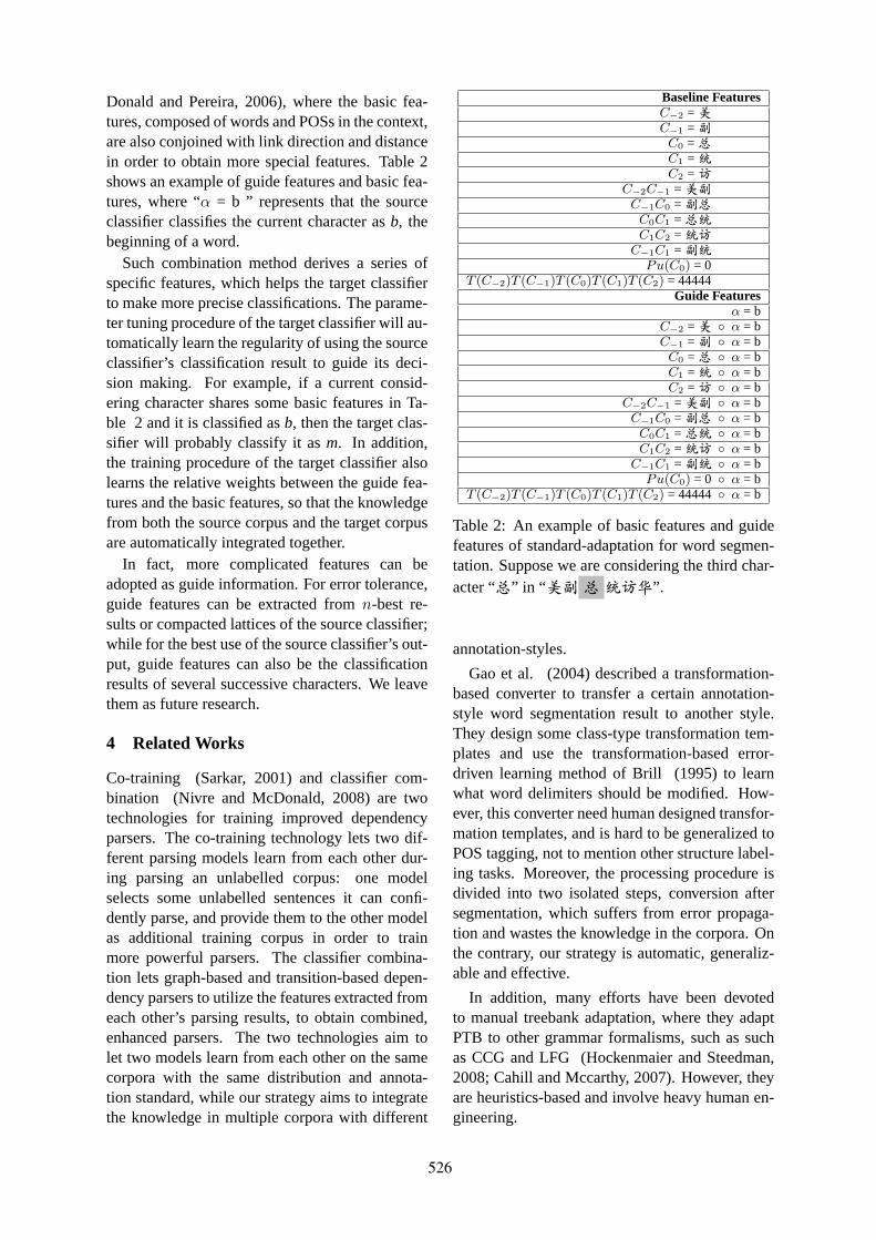
Donald and Pereira, 2006), where the basic fea-tures, composed of words and POSs in the context,are also conjoined with link direction and distancein order to obtain more special features. Table 2shows an example of guide features and basic fea-tures, where “α = b ” represents that the sourceclassifier classifies the current character asb, thebeginning of a word.
Such combination method derives a series ofspecific features, which helps the target classifierto make more precise classifications. The parame-ter tuning procedure of the target classifier will au-tomatically learn the regularity of using the sourceclassifier’s classification result to guide its deci-sion making. For example, if a current consid-ering character shares some basic features in Ta-ble 2 and it is classified asb, then the target clas-sifier will probably classify it asm. In addition,the training procedure of the target classifier alsolearns the relative weights between the guide fea-tures and the basic features, so that the knowledgefrom both the source corpus and the target corpusare automatically integrated together.
In fact, more complicated features can beadopted as guide information. For error tolerance,guide features can be extracted fromn-best re-sults or compacted lattices of the source classifier;while for the best use of the source classifier’s out-put, guide features can also be the classificationresults of several successive characters. We leavethem as future research.
4 Related Works
Co-training (Sarkar, 2001) and classifier com-bination (Nivre and McDonald, 2008) are twotechnologies for training improved dependencyparsers. The co-training technology lets two dif-ferent parsing models learn from each other dur-ing parsing an unlabelled corpus: one modelselects some unlabelled sentences it can confi-dently parse, and provide them to the other modelas additional training corpus in order to trainmore powerful parsers. The classifier combina-tion lets graph-based and transition-based depen-dency parsers to utilize the features extracted fromeach other’s parsing results, to obtain combined,enhanced parsers. The two technologies aim tolet two models learn from each other on the samecorpora with the same distribution and annota-tion standard, while our strategy aims to integratethe knowledge in multiple corpora with different
Baseline FeaturesC−2 ={
C−1 =BC0 =oC1 =ÚC2 =�
C−2C−1 ={BC−1C0 =BoC0C1 =oÚC1C2 =Ú�
C−1C1 =BÚPu(C0) = 0
T (C−2)T (C
−1)T (C0)T (C1)T (C2) = 44444Guide Features
α = bC−2 ={ ◦ α = b
C−1 =B ◦ α = bC0 =o ◦ α = bC1 =Ú ◦ α = bC2 =� ◦ α = b
C−2C−1 ={B ◦ α = bC−1C0 =Bo ◦ α = bC0C1 =oÚ ◦ α = bC1C2 =Ú� ◦ α = b
C−1C1 =BÚ ◦ α = bPu(C0) = 0 ◦ α = b
T (C−2)T (C
−1)T (C0)T (C1)T (C2) = 44444 ◦ α = b
Table 2: An example of basic features and guidefeatures of standard-adaptation for word segmen-tation. Suppose we are considering the third char-acter “o” in “{B o Ú�u”.
annotation-styles.
Gao et al. (2004) described a transformation-based converter to transfer a certain annotation-style word segmentation result to another style.They design some class-type transformation tem-plates and use the transformation-based error-driven learning method of Brill (1995) to learnwhat word delimiters should be modified. How-ever, this converter need human designed transfor-mation templates, and is hard to be generalized toPOS tagging, not to mention other structure label-ing tasks. Moreover, the processing procedure isdivided into two isolated steps, conversion aftersegmentation, which suffers from error propaga-tion and wastes the knowledge in the corpora. Onthe contrary, our strategy is automatic, generaliz-able and effective.
In addition, many efforts have been devotedto manual treebank adaptation, where they adaptPTB to other grammar formalisms, such as suchas CCG and LFG (Hockenmaier and Steedman,2008; Cahill and Mccarthy, 2007). However, theyare heuristics-based and involve heavy human en-gineering.
526
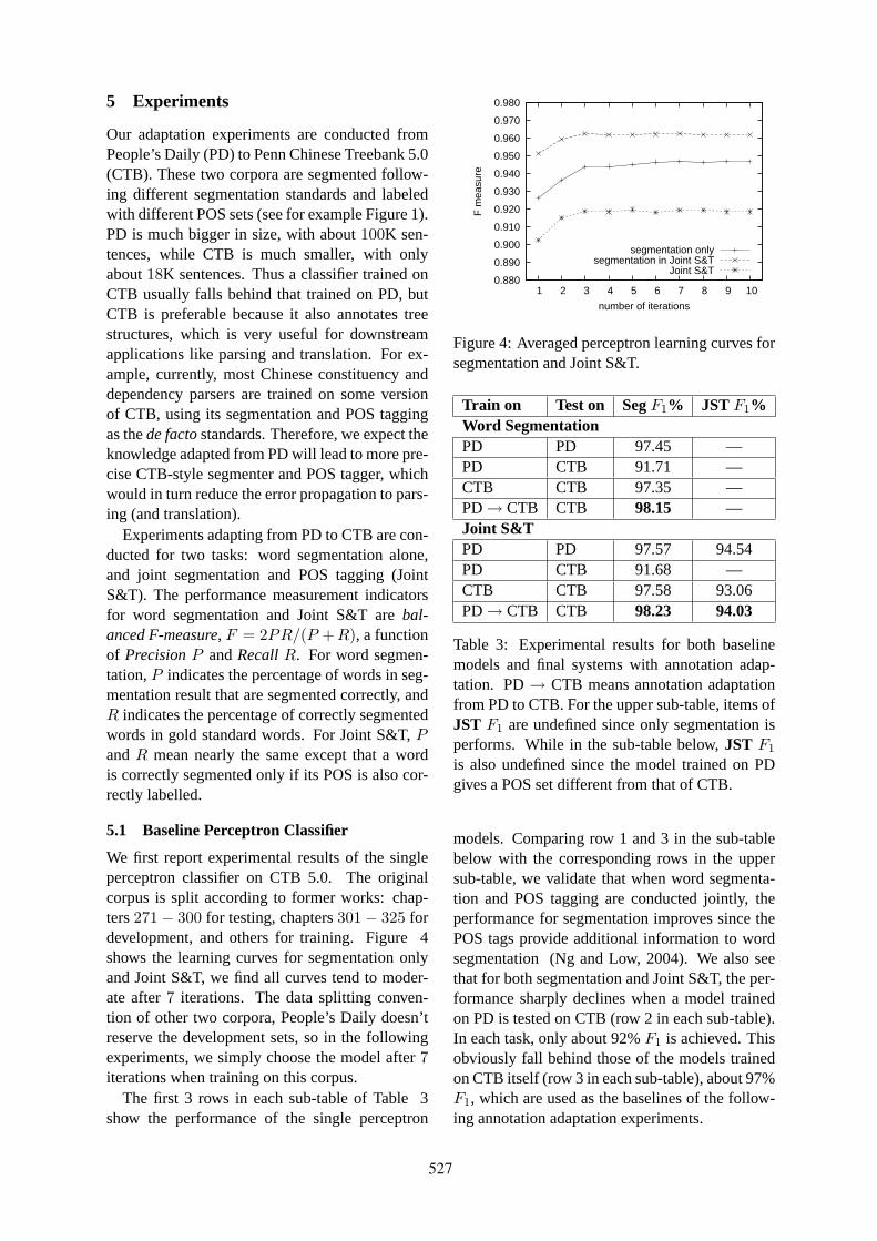
5 Experiments
Our adaptation experiments are conducted fromPeople’s Daily (PD) to Penn Chinese Treebank 5.0(CTB). These two corpora are segmented follow-ing different segmentation standards and labeledwith different POS sets (see for example Figure 1).PD is much bigger in size, with about100K sen-tences, while CTB is much smaller, with onlyabout18K sentences. Thus a classifier trained onCTB usually falls behind that trained on PD, butCTB is preferable because it also annotates treestructures, which is very useful for downstreamapplications like parsing and translation. For ex-ample, currently, most Chinese constituency anddependency parsers are trained on some versionof CTB, using its segmentation and POS taggingas thede factostandards. Therefore, we expect theknowledge adapted from PD will lead to more pre-cise CTB-style segmenter and POS tagger, whichwould in turn reduce the error propagation to pars-ing (and translation).
Experiments adapting from PD to CTB are con-ducted for two tasks: word segmentation alone,and joint segmentation and POS tagging (JointS&T). The performance measurement indicatorsfor word segmentation and Joint S&T arebal-anced F-measure, F = 2PR/(P + R), a functionof PrecisionP andRecallR. For word segmen-tation,P indicates the percentage of words in seg-mentation result that are segmented correctly, andR indicates the percentage of correctly segmentedwords in gold standard words. For Joint S&T,P
andR mean nearly the same except that a wordis correctly segmented only if its POS is also cor-rectly labelled.
5.1 Baseline Perceptron Classifier
We first report experimental results of the singleperceptron classifier on CTB 5.0. The originalcorpus is split according to former works: chap-ters271− 300 for testing, chapters301− 325 fordevelopment, and others for training. Figure 4shows the learning curves for segmentation onlyand Joint S&T, we find all curves tend to moder-ate after7 iterations. The data splitting conven-tion of other two corpora, People’s Daily doesn’treserve the development sets, so in the followingexperiments, we simply choose the model after7iterations when training on this corpus.
The first 3 rows in each sub-table of Table 3show the performance of the single perceptron
0.880
0.890
0.900
0.910
0.920
0.930
0.940
0.950
0.960
0.970
0.980
1 2 3 4 5 6 7 8 9 10
F m
easu
re
number of iterations
segmentation onlysegmentation in Joint S&T
Joint S&T
Figure 4: Averaged perceptron learning curves forsegmentation and Joint S&T.
Train on Test on SegF1% JST F1%Word SegmentationPD PD 97.45 —PD CTB 91.71 —CTB CTB 97.35 —PD→ CTB CTB 98.15 —Joint S&TPD PD 97.57 94.54PD CTB 91.68 —CTB CTB 97.58 93.06PD→ CTB CTB 98.23 94.03
Table 3: Experimental results for both baselinemodels and final systems with annotation adap-tation. PD→ CTB means annotation adaptationfrom PD to CTB. For the upper sub-table, items ofJST F1 are undefined since only segmentation isperforms. While in the sub-table below,JST F1
is also undefined since the model trained on PDgives a POS set different from that of CTB.
models. Comparing row 1 and 3 in the sub-tablebelow with the corresponding rows in the uppersub-table, we validate that when word segmenta-tion and POS tagging are conducted jointly, theperformance for segmentation improves since thePOS tags provide additional information to wordsegmentation (Ng and Low, 2004). We also seethat for both segmentation and Joint S&T, the per-formance sharply declines when a model trainedon PD is tested on CTB (row 2 in each sub-table).In each task, only about 92%F1 is achieved. Thisobviously fall behind those of the models trainedon CTB itself (row 3 in each sub-table), about 97%F1, which are used as the baselines of the follow-ing annotation adaptation experiments.
527
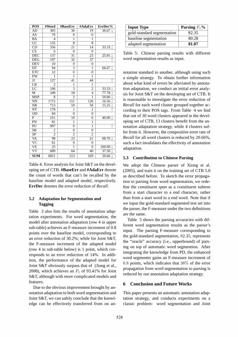
POS #Word #BaseErr #AdaErr ErrDec%AD 305 30 19 36.67↓AS 76 0 0BA 4 1 1CC 135 8 8CD 356 21 14 33.33↓CS 6 0 0DEC 137 31 23 25.81↓DEG 197 32 37 ↑DEV 10 0 0DT 94 3 1 66.67↓ETC 12 0 0FW 1 1 1JJ 127 41 44 ↑LB 2 1 1LC 106 3 2 33.33↓M 349 18 4 77.78↓MSP 8 2 1 50.00↓NN 1715 151 126 16.56↓NR 713 59 50 15.25↓NT 178 1 2 ↑OD 84 0 0P 251 10 6 40.00↓PN 81 1 1PU 997 0 1 ↑SB 2 0 0SP 2 2 2VA 98 23 21 08.70↓VC 61 0 0VE 25 1 0 100.00↓VV 689 64 40 37.50↓SUM 6821 213 169 20.66↓
Table 4: Error analysis for Joint S&T on the devel-oping set of CTB.#BaseErrand#AdaErr denotethe count of words that can’t be recalled by thebaseline model and adapted model, respectively.ErrDec denotes the error reduction ofRecall.
5.2 Adaptation for Segmentation andTagging
Table 3 also lists the results of annotation adap-tation experiments. For word segmentation, themodel after annotation adaptation (row 4 in uppersub-table) achieves an F-measure increment of 0.8points over the baseline model, corresponding toan error reduction of 30.2%; while for Joint S&T,the F-measure increment of the adapted model(row 4 in sub-table below) is 1 point, which cor-responds to an error reduction of 14%. In addi-tion, the performance of the adapted model forJoint S&T obviously surpass that of (Jiang et al.,2008), which achieves anF1 of 93.41% for JointS&T, although with more complicated models andfeatures.
Due to the obvious improvement brought by an-notation adaptation to both word segmentation andJoint S&T, we can safely conclude that the knowl-edge can be effectively transferred from on an-
Input Type ParsingF1%gold-standard segmentation 82.35baseline segmentation 80.28adapted segmentation 81.07
Table 5: Chinese parsing results with differentword segmentation results as input.
notation standard to another, although using sucha simple strategy. To obtain further informationabout what kind of errors be alleviated by annota-tion adaptation, we conduct an initial error analy-sis for Joint S&T on the developing set of CTB. Itis reasonable to investigate the error reduction ofRecallfor each word cluster grouped together ac-cording to their POS tags. From Table 4 we findthat out of 30 word clusters appeared in the devel-oping set of CTB, 13 clusters benefit from the an-notation adaptation strategy, while 4 clusters suf-fer from it. However, the compositive error rate ofRecallfor all word clusters is reduced by 20.66%,such a fact invalidates the effectivity of annotationadaptation.
5.3 Contribution to Chinese Parsing
We adopt the Chinese parser of Xiong et al.(2005), and train it on the training set of CTB 5.0as described before. To sketch the error propaga-tion to parsing from word segmentation, we rede-fine theconstituent spanas a constituent subtreefrom a start character to a end character, ratherthan from a start word to a end word. Note that ifwe input the gold-standard segmented test set intothe parser, the F-measure under the two definitionsare the same.
Table 5 shows the parsing accuracies with dif-ferent word segmentation results as the parser’sinput. The parsing F-measure corresponding tothe gold-standard segmentation,82.35, representsthe “oracle” accuracy (i.e., upperbound) of pars-ing on top of automatic word segmention. Afterintegrating the knowledge from PD, the enhancedword segmenter gains an F-measure increment of0.8 points, which indicates that38% of the errorpropagation from word segmentation to parsing isreduced by our annotation adaptation strategy.
6 Conclusion and Future Works
This paper presents an automatic annotation adap-tation strategy, and conducts experiments on aclassic problem: word segmentation and Joint
528

S&T. To adapt knowledge from a corpus with anannotation standard that we don’t require, a clas-sifier trained on this corpus is used to pre-processthe corpus with the desired annotated standard, onwhich a second classifier is trained with the firstclassifier’s predication results as additional guideinformation. Experiments of annotation adapta-tion from PD to CTB 5.0 for word segmentationand POS tagging show that, this strategy can makeeffective use of the knowledge from the corpuswith different annotations. It obtains considerableF-measure increment, about0.8 point for wordsegmentation and1 point for Joint S&T, with cor-responding error reductions of30.2% and 14%.The final result outperforms the latest work on thesame corpus which uses more complicated tech-nologies, and achieves the state-of-the-art. More-over, such improvement further brings striking F-measure increment for Chinese parsing, about0.8points, corresponding to an error propagation re-duction of38%.
In the future, we will continue to research onannotation adaptation for other NLP tasks whichhave different annotation-style corpora. Espe-cially, we will pay efforts to the annotation stan-dard adaptation between different treebanks, forexample, from HPSG LinGo Redwoods Treebankto PTB, or even from a dependency treebankto PTB, in order to obtain more powerful PTBannotation-style parsers.
Acknowledgement
This project was supported by National NaturalScience Foundation of China, Contracts 60603095and 60736014, and 863 State Key Project No.2006AA010108. We are especially grateful toFernando Pereira and the anonymous reviewersfor pointing us to relevant domain adaption refer-ences. We also thank Yang Liu and Haitao Mi forhelpful discussions.
References
Daniel M. Bikel and David Chiang. 2000. Two statis-tical parsing models applied to the chinese treebank.In Proceedings of the second workshop on Chineselanguage processing.
John Blitzer, Ryan McDonald, and Fernando Pereira.2006. Domain adaptation with structural correspon-dence learning. InProceedings of EMNLP.
Eric Brill. 1995. Transformation-based error-drivenlearning and natural language processing: a case
study in part-of-speech tagging. InComputationalLinguistics.
Sabine Buchholz and Erwin Marsi. 2006. Conll-xshared task on multilingual dependency parsing. InProceedings of CoNLL.
Aoife Cahill and Mairead Mccarthy. 2007. Auto-matic annotation of the penn treebank with lfg f-structure information. Inin Proceedings of theLREC Workshop on Linguistic Knowledge Acquisi-tion and Representation: Bootstrapping AnnotatedLanguage Data.
David Chiang. 2007. Hierarchical phrase-based trans-lation. Computational Linguistics, pages 201–228.
Michael Collins and Brian Roark. 2004. Incrementalparsing with the perceptron algorithm. InProceed-ings of the 42th Annual Meeting of the Associationfor Computational Linguistics.
Michael Collins. 2002. Discriminative training meth-ods for hidden markov models: Theory and exper-iments with perceptron algorithms. InProceedingsof the Empirical Methods in Natural Language Pro-cessing Conference, pages 1–8, Philadelphia, USA.
Hal Dauḿe III and Daniel Marcu. 2006. Domain adap-tation for statistical classifiers. InJournal of Artifi-cial Intelligence Research.
Hal Dauḿe III. 2007. Frustratingly easy domain adap-tation. InProceedings of ACL.
Jianfeng Gao, Andi Wu, Mu Li, Chang-Ning Huang,Hongqiao Li, Xinsong Xia, and Haowei Qin. 2004.Adaptive chinese word segmentation. InProceed-ings of ACL.
Julia Hockenmaier and Mark Steedman. 2008. Ccg-bank: a corpus of ccg derivations and dependencystructures extracted from the penn treebank. InComputational Linguistics, volume 33(3), pages355–396.
Wenbin Jiang, Liang Huang, Yajuan Lü, and Qun Liu.2008. A cascaded linear model for joint chineseword segmentation and part-of-speech tagging. InProceedings of the 46th Annual Meeting of the As-sociation for Computational Linguistics.
Mitchell P. Marcus, Beatrice Santorini, and Mary AnnMarcinkiewicz. 1993. Building a large annotatedcorpus of english: The penn treebank. InComputa-tional Linguistics.
André F. T. Martins, Dipanjan Das, Noah A. Smith, andEric P. Xing. 2008. Stacking dependency parsers.In Proceedings of EMNLP.
Ryan McDonald and Fernando Pereira. 2006. Onlinelearning of approximate dependency parsing algo-rithms. InProceedings of EACL, pages 81–88.
529
Ryan McDonald, Koby Crammer, and FernandoPereira. 2005. Online large-margin training of de-pendency parsers. InProceedings of ACL, pages 91–98.
Hwee Tou Ng and Jin Kiat Low. 2004. Chinese part-of-speech tagging: One-at-a-time or all-at-once?word-based or character-based? InProceedings ofthe Empirical Methods in Natural Language Pro-cessing Conference.
Joakim Nivre and Ryan McDonald. 2008. Integrat-ing graph-based and transition-based dependencyparsers. InProceedings of the 46th Annual Meetingof the Association for Computational Linguistics.
Stephan Oepen, Kristina Toutanova, Stuart Shieber,Christopher Manning Dan Flickinger, and ThorstenBrants. 2002. The lingo redwoods treebank: Moti-vation and preliminary applications. InIn Proceed-ings of the 19th International Conference on Com-putational Linguistics (COLING 2002).
Anoop Sarkar. 2001. Applying co-training methods tostatistical parsing. InProceedings of NAACL.
Fei Xia. 2000. The part-of-speech tagging guidelinesfor the penn chinese treebank (3.0). InTechnicalReports.
Deyi Xiong, Shuanglong Li, Qun Liu, and ShouxunLin. 2005. Parsing the penn chinese treebank withsemantic knowledge. InProceedings of IJCNLP2005, pages 70–81.
Nianwen Xue and Libin Shen. 2003. Chinese wordsegmentation as lmr tagging. InProceedings ofSIGHAN Workshop.
Nianwen Xue, Fei Xia, Fu-Dong Chiou, and MarthaPalmer. 2005. The penn chinese treebank: Phrasestructure annotation of a large corpus. InNaturalLanguage Engineering.
Shiwen Yu, Jianming Lu, Xuefeng Zhu, HuimingDuan, Shiyong Kang, Honglin Sun, Hui Wang,Qiang Zhao, and Weidong Zhan. 2001. Processingnorms of modern chinese corpus. Technical report.
Yue Zhang and Stephen Clark. 2007. Chinese seg-mentation with a word-based perceptron algorithm.In Proceedings of the 45th Annual Meeting of theAssociation for Computational Linguistics.
530
Copyright © 2022 FDOKUMEN