MC SCF molecular gradients and hessians: Computational aspects
Upload
khangminh22Category
view
1download
0
ACL 2018
Cognitive Aspects of Computational Language Learning andProcessing
Proceedings of the Eighth Workshop
July 19, 2018Melbourne, Australia
c©2018 The Association for Computational Linguistics
Order copies of this and other ACL proceedings from:
Association for Computational Linguistics (ACL)209 N. Eighth StreetStroudsburg, PA 18360USATel: +1-570-476-8006Fax: [email protected]
ISBN 978-1-948087-41-4
ii
Introduction
Marco Idiart1, Alessandro Lenci2, Thierry Poibeau3, Aline Villavicencio1,4
1 Federal University of Rio Grande do Sul (Brazil)2 University of Pisa (Italy)
3 LATTICE-CNRS (France)4 University of Essex (UK)
The 8th Workshop on Cognitive Aspects of Computational Language Learning and Processing(CogACLL) took place on July 19, 2018 in Melbourne, Australia, in conjunction with the ACL 2018.The workshop was endorsed by ACL Special Interest Group on Natural Language Learning (SIGNLL).This is the eighth edition of related workshops first held with ACL 2007 and 2016, EACL 2009, 2012and 2014, EMNLP 2015, and as a standalone event in 2013.
The workshop is targeted at anyone interested in the relevance of computational techniques forunderstanding first, second and bilingual language acquisition and change or loss in normal andpathological conditions.
The human ability to acquire and process language has long attracted interest and generated much debatedue to the apparent ease with which such a complex and dynamic system is learnt and used on the faceof ambiguity, noise and uncertainty. This subject raises many questions ranging from the nature vs.nurture debate of how much needs to be innate and how much needs to be learned for acquisition to besuccessful, to the mechanisms involved in this process (general vs specific) and their representations inthe human brain. There are also developmental issues related to the different stages consistently foundduring acquisition (e.g. one word vs. two words) and possible organizations of this knowledge. Thesehave been discussed in the context of first and second language acquisition and bilingualism, with crosslinguistic studies shedding light on the influence of the language and the environment.
The past decades have seen a massive expansion in the application of statistical and machine learningmethods to natural language processing (NLP). This work has yielded impressive results in numerousspeech and language processing tasks, including e.g. speech recognition, morphological analysis,parsing, lexical acquisition, semantic interpretation, and dialogue management. The good results havegenerally been viewed as engineering achievements. However, researchers have also investigated therelevance of computational learning methods for research on human language acquisition and change.The use of computational modeling has been boosted by advances in machine learning techniques,and the availability of resources like corpora of child and child-directed sentences, and data frompsycholinguistic tasks by normal and pathological groups. Many of the existing computational modelsattempt to study language tasks under cognitively plausible criteria (such as memory and processinglimitations that humans face), and to explain the developmental stages observed in the acquisitionand evolution of the language abilities. In doing so, computational modeling provides insight intothe plausible mechanisms involved in human language processes, and inspires the development ofbetter language models and techniques. These investigations are very important since if computationaltechniques can be used to improve our understanding of human language acquisition and change, thesewill not only benefit cognitive sciences in general but will reflect back to NLP and place us in a betterposition to develop useful language models.
1iii

We invited submissions on relevant topics, including:
• Computational learning theory and analysis of language learning and organization
• Computational models of first, second and bilingual language acquisition
• Computational models of language changes in clinical conditions
• Computational models and analysis of factors that influence language acquisition and use indifferent age groups and cultures
• Computational models of various aspects of language and their interaction effect in acquisition,processing and change
• Computational models of the evolution of language
• Data resources and tools for investigating computational models of human language processes
• Empirical and theoretical comparisons of the learning environment and its impact on languageprocesses
• Cognitively oriented Bayesian models of language processes
• Computational methods for acquiring various linguistic information (related to e.g. speech,morphology, lexicon, syntax, semantics, and discourse) and their relevance to research on humanlanguage acquisition
• Investigations and comparisons of supervised, unsupervised and weakly-supervised methods forlearning (e.g. machine learning, statistical, symbolic, biologically-inspired, active learning,various hybrid models) from a cognitive perspective.
Acknowledgements
We would like to thank the members of the Program Committee for the timely reviews and the authorsfor their valuable contributions. Marco Idiart is partly funded by CNPq (423843/2016-8). AlessandroLenci by project CombiNet (PRIN 2010-11 20105B3HE8) funded by the Italian Ministry of Education,University and Research (MIUR) ans Thierry Poibeau by the ERA-NET Atlantis project.
Marco IdiartAlessandro LenciThierry PoibeauAline Villavicencio
iv
Organizers:
Marco Idiart, Federal University of Rio Grande do Sul (Brazil)Alessandro Lenci, University of Pisa (Italy)Thierry Poibeau, LATTICE-CNRS (France)Aline Villavicencio, University of Essex (UK) and Federal University of Rio Grande do Sul(Brazil)
Program Committee:
Dora Alexopoulou, University of Cambridge (UK)Afra Alishahi, Tilburg University (The Netherlands)Colin Bannard, University of Liverpool (UK)Laurent Besacier, LIG - University Grenoble Alpes (France)Yevgeny Berzak, Massachusetts Institute of Technology (USA)Philippe Blache, LPL, CNRS (France)Emmanuele Chersoni, Aix-Marseille University (France)Alexander Clark, Royal Holloway, University of London (UK)Walter Daelemans, University of Antwerp (Belgium)Barry Devereux, University of Cambridge (UK)Afsaneh Fazly, University of Toronto (Canada)Richard Futrell, MIT (USA)Raquel Garrido Alhama, Basque Center on Cognition, Brain and Language (Spain)Gianluca Lebani, University of Pisa (Italy)Igor Malioutov, Bloomberg (USA)Tim O’Donnel, McGill University (Canada)David Powers, Flinders University (Australia)Ari Rappoport, The Hebrew University of Jerusalem (Israel)Sabine Schulte im Walde, University of Stuttgart (Germany)Marco Senaldi, University of Pisa (Italy)Mark Steedman, University of Edinburgh (UK)Remi van Trijp, Sony Computer Science Laboratories Paris (France)Rodrigo Wilkens, Université catholique de Louvain (Belgium)Shuly Wintner, University of Haifa (Israel)Charles Yang, University of Pennsylvania (USA)Menno van Zaanen, Tilburg University (Netherlands)
v


Table of Contents
Predicting Brain Activation with WordNet EmbeddingsJoão António Rodrigues, Ruben Branco, João Silva, Chakaveh Saedi and António Branco . . . . . . . 1
Do Speakers Produce Discourse Connectives Rationally?Frances Yung and Vera Demberg . . . . . . . . . . . . . . . . . . . . . . . . . . . . . . . . . . . . . . . . . . . . . . . . . . . . . . . . . . 6
Language Production Dynamics with Recurrent Neural NetworksJesús Calvillo and Matthew Crocker . . . . . . . . . . . . . . . . . . . . . . . . . . . . . . . . . . . . . . . . . . . . . . . . . . . . . . 17
Multi-glance Reading Model for Text UnderstandingPengcheng Zhu, Yujiu Yang, Wenqiang Gao and Yi Liu. . . . . . . . . . . . . . . . . . . . . . . . . . . . . . . . . . . . .27
Predicting Japanese Word Order in Double Object ConstructionsMasayuki Asahara, Satoshi Nambu and Shin-Ichiro Sano . . . . . . . . . . . . . . . . . . . . . . . . . . . . . . . . . . . 36
Affordances in Grounded Language LearningStephen McGregor and KyungTae Lim. . . . . . . . . . . . . . . . . . . . . . . . . . . . . . . . . . . . . . . . . . . . . . . . . . . .41
Rating Distributions and Bayesian Inference: Enhancing Cognitive Models of Spatial Language UseThomas Kluth and Holger Schultheis . . . . . . . . . . . . . . . . . . . . . . . . . . . . . . . . . . . . . . . . . . . . . . . . . . . . . 47
The Role of Syntax During Pronoun Resolution: Evidence from fMRIJixing Li, Murielle Fabre, Wen-Ming Luh and John Hale . . . . . . . . . . . . . . . . . . . . . . . . . . . . . . . . . . . 56
A Sound and Complete Left-Corner Parsing for Minimalist GrammarsMiloš Stanojevic and Edward Stabler . . . . . . . . . . . . . . . . . . . . . . . . . . . . . . . . . . . . . . . . . . . . . . . . . . . . . 65
vii


Workshop Program
July 19, 2018
09:00–09:10 Welcome and Opening Session
09:10–09:30 Session I - Semantics
09:10–09:30 Predicting Brain Activation with WordNet EmbeddingsJoão António Rodrigues, Ruben Branco, João Silva, Chakaveh Saedi and AntónioBranco
09:30–10:30 Invited Talk I
10:30–11:00 Coffee Break
11:00–11:50 Session II - Production
11:00–11:20 Do Speakers Produce Discourse Connectives Rationally?Frances Yung and Vera Demberg
11:20–11:50 Language Production Dynamics with Recurrent Neural NetworksJesús Calvillo and Matthew Crocker
ix

July 19, 2018 (continued)
11:50–12:30 Poster Session
11:50–12:30 Multi-glance Reading Model for Text UnderstandingPengcheng Zhu, Yujiu Yang, Wenqiang Gao and Yi Liu
11:50–12:30 Predicting Japanese Word Order in Double Object ConstructionsMasayuki Asahara, Satoshi Nambu and Shin-Ichiro Sano
11:50–12:30 Affordances in Grounded Language LearningStephen McGregor and KyungTae Lim
12:30–14:00 Lunch
14:00–15:00 Invited Talk II
15:00–15:30 Session III - Processing
15:00–15:30 Rating Distributions and Bayesian Inference: Enhancing Cognitive Models of Spa-tial Language UseThomas Kluth and Holger Schultheis
15:30–16:00 Coffee Break
x

July 19, 2018 (continued)
16:00–17:00 Session IV - Syntax and Parsing
16:00–16:30 The Role of Syntax During Pronoun Resolution: Evidence from fMRIJixing Li, Murielle Fabre, Wen-Ming Luh and John Hale
16:30–17:00 A Sound and Complete Left-Corner Parsing for Minimalist GrammarsMiloš Stanojevic and Edward Stabler
17:00–17:30 Panel, Business Meeting and Closing Session
xi

Proceedings of the Eighth Workshop on Cognitive Aspects of Computational Language Learning and Processing, pages 1–5Melbourne, Australia, July 19, 2018. c©2018 Association for Computational Linguistics
Predicting Brain Activation with WordNet Embeddings
Joao Antonio Rodrigues, Ruben Branco, Joao Ricardo Silva, Chakaveh Saedi, Antonio BrancoUniversity of Lisbon
NLX-Natural Language and Speech Group, Department of InformaticsFaculdade de Ciencias
Campo Grande, 1749-016 Lisboa, Portugal{joao.rodrigues, ruben.branco, jsilva, chakaveh.saedi, antonio.branco}@di.fc.ul.pt
Abstract
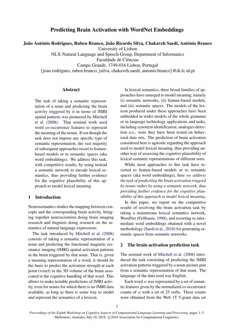
The task of taking a semantic represen-tation of a noun and predicting the brainactivity triggered by it in terms of fMRIspatial patterns was pioneered by Mitchellet al. (2008). That seminal work usedword co-occurrence features to representthe meaning of the nouns. Even though thetask does not impose any specific type ofsemantic representation, the vast majorityof subsequent approaches resort to feature-based models or to semantic spaces (akaword embeddings). We address this task,with competitive results, by using insteada semantic network to encode lexical se-mantics, thus providing further evidencefor the cognitive plausibility of this ap-proach to model lexical meaning.
1 Introduction
Neurosemantics studies the mapping between con-cepts and the corresponding brain activity, bring-ing together neuroscientists doing brain imagingresearch and linguists doing research on the se-mantics of natural language expressions.
The task introduced by Mitchell et al. (2008)consists of taking a semantic representation of anoun and predicting the functional magnetic res-onance imaging (fMRI) spatial activation patternsin the brain triggered by that noun. That is, givena meaning representation of a word, it should bethe basis to predict the activation strength at eachpoint (voxel) in the 3D volume of the brain asso-ciated to the cognitive handling of that word. Thisallows to make testable predictions of fMRI activ-ity, even for nouns for which there is no fMRI dataavailable, as long as there is some way to modeland represent the semantics of a lexicon.
In lexical semantics, three broad families of ap-proaches have emerged to model meaning, namely(i) semantic networks, (ii) feature-based models,and (iii) semantic spaces. The models of the lex-icon produced under these approaches have beenembedded in wider models of the whole grammaror in language technology applications and tasks,including synonym identification, analogies detec-tion a.o., were they have been tested on behav-ioral data sets. The prediction of brain activationconsidered here is agnostic regarding the approachused to model lexical meaning, thus providing an-other way of assessing the cognitive plausibility oflexical semantic representations of different sorts.
While most approaches to this task have re-sorted to feature-based models or to semanticspaces (aka word embeddings), here we addressthe task of prediciting the brain activation triggredby nouns rather by using a semantic network, thusproviding further evidence for the cognitive plau-sibility of this approach to model lexical meaning.
In this paper, we report on the competitiveresults of resolving the brain activation task bytaking a mainstream lexical semantics network,WordNet (Fellbaum, 1998), and resorting to inter-mediate word embeddings obatined with a novelmethodology (Saedi et al., 2018) for generating se-mantic spaces from semantic networks.
2 The brain activation prediction task
The seminal work of Mitchell et al. (2008) intro-duced the task consisting of predicting the fMRIactivation patterns triggered by a noun-picture pairfrom a semantic representation of that noun. Thelanguage of the data used was English.
Each wordw was represented by a set of seman-tic features given by the normalized co-occurrencecounts of w with a set of 25 verbs. These countswere obtained from the Web 1T 5-gram data set
1
(Brants and Franz, 2006), using the n-grams up tolength 5 generated from 1 trillion tokens of text.
The 25 verbs were manually selected due totheir correspondence to basic sensory and motoractivities.1 Sensory-motor features should be par-ticularly relevant for the representation of objectsand, in fact, alternative features based on a randomselection of 25 frequent words performed worse.
The fMRI activation pattern at every voxel inthe brain is calculated as a weighted sum of eachof the 25 semantic features, where the weights arelearned by regression to maximum likelihood esti-mates given observed fMRI data.
To produce the fMRI data, 9 participants wereshown 60 different word-picture pairs,2 the stim-uli, each presented 6 times. For each participant,a representative fMRI image for each stimuluswas calculated by determining the mean fMRI re-sponse from the 6 repetitions and subtracting fromeach the mean of all 60 stimuli.
Separate models were learned for each of the9 participants. These models were evaluated us-ing leave-two-out cross-validation, where in eachcross-validation iteration the model was asked topredict the fMRI activation for the two held-outwords. The two predictions were matched againstthe two observed activations for those words usingcosine similarity over the 500 most stable voxels.
Randomly assigning the two predictions to thetwo observations would yield a 0.50 accuracy. Themodels in the seminal paper (Mitchell et al., 2008)achieve a mean accuracy of 0.77, with all individ-ual accuracies significantly above chance.
These results support the plausibility of thetwo key assumptions underlying the task, namelythat (i) brain activation patterns can be predictedfrom semantic representations of words; and that(ii) lexical semantics can be captured by co-occurrence statistics, the assumption underlyingsemantics space models of the lexicon.
3 Related work
Several authors have addressed this brain activa-tion prediction task, keeping up with its basic as-sumptions and resorting to the same data sets for
1The verbs are: approach, break, clean, drive, eat, en-ter, fear, fill, hear, lift, listen, manipulate, move, near, open,push, ride, rub, run, say, see, smell, taste, touch, and wear.
2The 60 pairs are composed of 5 items from each of the 12concrete semantic categories (animals, body parts, buildings,building parts, clothing, furniture, insects, kitchen items,tools, vegetables, vehicles, and other man-made items).
the sake of the comparability of the performancescores obtained.
In an initial period, different authors sought toexplore the experimental space of the task by fo-cusing on different ways to set up the features.
Devereux et al. (2010) find that choosing the setof verbs used for the semantic features under anautomatic approach can lead to predictions that areequally good as when using the manually selectedset of verbs. Jelodar et al. (2010) use the same setof 25 features to represent a word, but instead ofbasing the features on co-occurrence counts theyresort to relatedness measures based on WordNet.Fernandino et al. (2015) use instead a set of fea-tures with 5 sensory-motor experience based at-tributes (sound, color, visual motion, shape, andmanipulation). The relatedness scores between thestimulus word and the attributes are based on hu-man ratings instead of corpus data.
Subsequently, as distributional semantics be-came increasingly popular, authors moved fromfeature-based representations of the meaning ofwords to experiment with different vector basedrepresentation models (aka word embeddings).
Murphy et al. (2012) compare different corpus-based models to derive word embeddings. Theyfind the best results with dependency-based em-beddings, where words inside the context windoware extended with grammatical functions. Binderet al. (2016) use word representations based on65 experiential attributes with relatedness scorescrowdsourced from over 1,700 participants. Xuet al. (2016) present BrainBench, a workbenchto test embedding models on both behavioral andbrain imaging data sets. Anderson et al. (2017) usea linguistic model based on word2vec embeddingsand a visual model built with a deep convolutionalneural network on the Google Images data set.
Recently, Abnar et al. (2018) evaluated 8 dif-ferent embeddings regarding their usefulness inpredicting neural activation patterns: the co-occurrence embeddings of (Mitchell et al., 2008);the experiential embeddings of (Binder et al.,2016); the non-distributional feature-based em-beddings of (Faruqui and Dyer, 2015); and5 different distributional embeddings, namelyword2vec (Mikolov et al., 2013), Fasttext(Bojanowski et al., 2016), dependency-basedword2vec (Levy and Goldberg, 2014), GloVe(Pennington et al., 2014) and LexVec (Salle et al.,2016). These authors found that dependency-
2

based word2vec achieves the best performanceamong the approaches resorting to word embed-dings, while the seminal approach resorting to 25features “is doing slightly better on average” withrespect to all the approaches experimented with.
The rationale guiding the various works pre-sented in this Section is that the better the per-formance of the system the higher is the cogni-tive plausibility of the lexical semantics model re-sorted to. It is also important to note, however, thatthere is not always a clearly better method sinceresults show that different methods have differenterror patterns (Abnar et al., 2018).
4 WordNet embeddings
The previous Sections indicate that approaches tothe brain activation task typically resort to feature-based models or to semantic spaces to representthe meaning of words.
In this paper, we address this task by using in-stead a semantic network as the base repositoryof lexical semantic knowledge, namely WordNet.We then resort to a novel methodology developedby us (Saedi et al., 2018) for generating seman-tic space embeddings from semantic networks,and use it to obtain WordNet embeddings. Thismethod is based on the intuition that the larger thenumber of paths and the shorter the paths connect-ing any two nodes in a network the stronger is theirsemantic association.
The conversion method begins by representingthe semantic graph as an adjacency matrix M ,where element Mij is set to 1 if there is an edgebetween word wi and word wj , and 0 otherwise.Then, this initial relatedness of immediately adja-cent words is “propagated” through the matrix byiterating the following cumulative addition
M(n)G = I + αM + α2M2 + · · ·+ αnMn (1)
where I is the identity matrix, the n-th power ofthe transition matrix, Mn, is the matrix whereeach Mij counts the number of paths of lenght nbetween nodes i and j, and α is a decay factor.
The limit of this sum is given by the followingclosed expression (see Newman, 2010, Eq. 7.63):
MG =∞∑
e=0
(αM)e = (I − αM)−1 (2)
Matrix MG is subsequently submitted to a Pos-itive Point-wise Mutual Information transforma-tion, each line is L2-normalized and, finally, Prin-cipal Component Analysis is applied, reducing
each line to the size of the desired embeddingspace. Row i of matrix MG is then taken as theembedding for word wi.
Using the methodology outlined above, embed-dings with size 850 were extracted from a subsetof 60k words in version 3 of English WordNet.3
When run on the mainstream semantic similaritydata set SimLex-999 (Hill et al., 2016), the re-sulting embeddings showed highly competitive re-sults, outperforming word2vec by some 15% Werefer to our embeddings as wnet2vec.4
5 Experiment
The good results obtained with wnet2vec in thesemantic similarity task lead to experiment withthem also in the brain activation prediction task.
5.1 System training
We resorted to the framework implementation5 byAbnar et al. (2018). Training ran for 1,000 epochs,with a batch size of 29 and a learning rate of 0.001.The loss function is calculated by adding the Hu-ber loss, the mean pairwise squared error and theL2-norm (on weights and bias). Like in previ-ous works, only the 500 most stable voxels are se-lected. Training was done on a Tesla K40m GPUand took 54 hours (6 hours per subject).
Figure 1 shows an example for Participant 1,with the model prediction and the observed fMRIactivation pattern for the word eye. The brain acti-vation images were generated with Nibabel (Brettet al., 2017) and Nilearn (Abraham et al., 2014).
5.2 Evaluation and discussion
We followed the usual evaluation procedure forthis framework. The cross-validated, leave-two-out mean accuracy was 0.71. The full scores, to-gether with the scores from the original paper, aresummarized in Table 1 and shown graphically inFigure 2 (0.50 corresponds to chance).6
This indicates that wnet2vec has a competitiveperformance in this task as the mean score ob-tained is in the range of the scores found for all ap-
3We used less than half of the 150k words in WordNet dueto computational limitations as the matrix inverse in (2) facessubstantial challenges in terms of the memory footprint.
4Available at https://github.com/nlx-group/WordNetEmbeddings
5https://github.com/samiraabnar/NeuroSemantics/
6Materials for replication available at https://github.com/nlx-group/BrainActivation
3

(a) predicted (b) observed
Figure 1: fMRI activations for Participant 1, word eye
Embeddings P1 P2 P3 P4 P5 P6 P7 P8 P9 mean
(Mitchell et al., 2008) 0.83 0.76 0.78 0.72 0.78 0.85 0.73 0.68 0.82 0.77wnet2vec 0.84 0.72 0.86 0.75 0.60 0.67 0.70 0.53 0.74 0.71
Table 1: Accuracy results for the 9 subjects
Figure 2: Accuracy results for the 9 subjects
proaches resorting to word embeddings, systemat-ically tested by (Abnar et al., 2018).
In line with all approaches resorting to wordembeddings (Abnar et al., 2018), the mean scoreobtained is also not outperforming the original 25verb-based co-occurrence features model reportedin the seminal paper (Mitchell et al., 2008).
When comparing the scores per participant, thebulk of the wnet2vec losses are due to P5, P6 andP8. For the other subjects, results are close or, inthree cases, even better than those from the semi-nal paper. This highlights the point already madein (Abnar et al., 2018), that different methods havedifferent error patterns, which suggests that an en-semble of classifiers could lead to better overallaccuracy. And also, that a dataset with only 9 sub-jects — the dataset used in the literature on thistask since (Mitchell et al., 2008) — may be hin-dering better empirically grounded conclusions.
Finally, it should be noted that these competitiveresults were obtained with wnet2vec generated onthe basis of 60k words only, thus less than half of
WordNet. It will be very interesting to see howthe performance of this approach progresses whenlarger portions of WordNet are taken into accountas computational limitations can be overcome.
6 Conclusions
We report on an experiment with the task of pre-dicting the fMRI spatial activation patterns in thebrain associated with a given noun.
We resorted to a semantic network of lexicalknowledge, viz. WordNet, and thus to a represen-tation of the meaning of the input nouns as ele-ments of concept nodes in a graph of semanticallyrelated edges. We also resorted to a derived inter-mediate vectorial semantic representation (wordembeddings) for the input nouns that was obtainedby a novel methodology to convert semantic net-works into semantic spaces, applied to WordNet.
The results indicate that this model has a com-petitive performance as its scores are within therange of the results obtained with state of the artmodels based on corpus-based word embeddingsreported in the literature. Though for one third ofthe 9 subjects this model surpasses Mitchell et al.(2008), on average it did not outperform that sem-inal model, which used hand-selected features.
The fact that less than half of the words inWordNet were used allows a positive expectationwith respect to the strength of the proposed ap-proach, and points towards future work that willseek to use larger portions of WordNet, and fur-ther lexical semantics networks and ontologies.
4
ReferencesSamira Abnar, Rasyan Ahmed, Max Mijnheer, and
Willem Zuidema. 2018. Experiential, distributionaland dependency-based word embeddings have com-plementary roles in decoding brain activity. In Pro-ceedings of the 8th Workshop on Cognitive Model-ing and Computational Linguistics (CMCL 2018) ,pages 5766.
Alexandre Abraham, Fabian Pedregosa, Michael Eick-enberg, Philippe Gervais, Andreas Mueller, JeanKossaifi, Alexandre Gramfort, Bertrand Thirion, andGaelVaroquaux. 2014. Machine learning for neu-roimaging with scikit-learn. Frontiers in Neuroin-formatics, 8:14.
Andrew J. Anderson, Douwe Kiela, Stephen Clark, andMassimo Poesio. 2017. Visually grounded and tex-tual semantic models differentially decode brain ac-tivity associated with concrete and abstract nouns.Transactions of the Association of ComputationalLinguistics, 5(1):17–30.
Jeffrey R. Binder, Lisa L. Conant, Colin J. Humphries,Leonardo Fernandino, Stephen B. Simons, MarioAguilar, and Rutvik H. Desai. 2016. Toward a brain-based componential semantic representation. Cog-nitive neuropsychology, 33(3-4):130–174.
Piotr Bojanowski, Edouard Grave, Armand Joulin,and Tomas Mikolov. 2016. Enriching word vec-tors with subword information. arXiv preprintarXiv:1607.04606.
Thorsten Brants and Alex Franz. 2006. Web 1T 5-gramversion 1.
Matthew Brett, Michael Hanke, et al. 2017.nipy/nibabel: 2.2.0.
Barry Devereux, Colin Kelly, and Anna Korhonen.2010. Using fMRI activation to conceptual stim-uli to evaluate methods for extracting conceptualrepresentations from corpora. In Proceedings ofthe NAACL HLT 2010 First Workshop on Compu-tational Neurolinguistics, pages 70–78. Associationfor Computational Linguistics.
Manaal Faruqui and Chris Dyer. 2015. Non-distributional word vector representations. arXivpreprint arXiv:1506.05230.
Christiane Fellbaum, editor. 1998. WordNet: An Elec-tronic Lexical Database. MIT Press.
Leonardo Fernandino, Colin J. Humphries, Mark S.Seidenberg, William L. Gross, Lisa L. Conant, andJeffrey R. Binder. 2015. Predicting brain activationpatterns associated with individual lexical conceptsbased on five sensory-motor attributes. Neuropsy-chologia, 76:17–26.
Felix Hill, Roi Reichart, and Anna Korhonen. 2016.Simlex-999: Evaluating semantic models with (gen-uine) similarity estimation. Computational Linguis-tics, 41:665–695.
Ahmad Babaeian Jelodar, Mehrdad Alizadeh, andShahram Khadivi. 2010. WordNet based featuresfor predicting brain activity associated with mean-ings of nouns. In Proceedings of the NAACL HLT2010 First Workshop on Computational Neurolin-guistics, pages 18–26. Association for Computa-tional Linguistics.
Omer Levy and Yoav Goldberg. 2014. Dependency-based word embeddings. In Proceedings of the 52ndAnnual Meeting of the Association for Computa-tional Linguistics (ACL), volume 2, pages 302–308.
Tomas Mikolov, Kai Chen, Greg Corrado, and Jef-frey Dean. 2013. Efficient estimation of wordrepresentations in vector space. arXiv preprintarXiv:1301.3781.
Tom M. Mitchell, Svetlana V. Shinkareva, AndrewCarlson, Kai-Min Chang, Vicente L. Malave,Robert A. Mason, and Marcel Adam Just. 2008.Predicting human brain activity associated with themeanings of nouns. Science, 320(5880):1191–1195.
Brian Murphy, Partha Talukdar, and Tom Mitchell.2012. Selecting corpus-semantic models for neu-rolinguistic decoding. In Proceedings of the FirstJoint Conference on Lexical and Computational Se-mantics, pages 114–123. Association for Computa-tional Linguistics.
Mark Newman. 2010. Networks: An Introduction. Ox-ford University Press.
Jeffrey Pennington, Richard Socher, and ChristopherManning. 2014. GloVe: Global vectors for wordrepresentation. In Proceedings of the 2014 Con-ference on Empirical Methods in Natural LanguageProcessing (EMNLP), pages 1532–1543.
Chakaveh Saedi, Antnio Branco, Joo Antnio Ro-drigues, and Joo Ricardo Silva. 2018. Wordnetembeddings. In Proceedings of the ACL2018 3rdWorkshop on Representation Learning for NaturalLanguage Processing (RepL4NLP). Association forComputational Linguistics.
Alexandre Salle, Marco Idiart, and Aline Villavicencio.2016. Matrix factorization using window samplingand negative sampling for improved word represen-tations. arXiv preprint arXiv:1606.00819.
Haoyan Xu, Brian Murphy, and Alona Fyshe. 2016.BrainBench: A brain-image test suite for distribu-tional semantic models. In Proceedings of the 2016Conference on Empirical Methods in Natural Lan-guage Processing (EMNLP), pages 2017–2021.
5
Proceedings of the Eighth Workshop on Cognitive Aspects of Computational Language Learning and Processing, pages 6–16Melbourne, Australia, July 19, 2018. c©2018 Association for Computational Linguistics
Do speakers produce discourse connectives rationally?
Frances Yung1 and Vera Demberg1,2
1Dept. of Language Science and Technology2Dept. of Mathematics and Computer Science, Saarland University
Saarland Informatic Campus, 66123 Saarbrucken, Germany{frances,vera}@coli.uni-saarland.de
Abstract
A number of different discourse connec-tives can be used to mark the same dis-course relation, but it is unclear what fac-tors affect connective choice. One recentaccount is the Rational Speech Acts the-ory, which predicts that speakers try tomaximize the informativeness of an utter-ance such that the listener can interpret theintended meaning correctly. Existing priorwork uses referential language games totest the rational account of speakers’ pro-duction of concrete meanings, such asidentification of objects within a picture.Building on the same paradigm, we designa novel Discourse Continuation Game toinvestigate speakers’ production of ab-stract discourse relations. Experimentalresults reveal that speakers significantlyprefer a more informative connective, inline with predictions of the RSA model.
1 Introduction
Discourse relations connect units of texts to a co-herent and meaningful structure. Discourse con-nectives (DC), e.g., but and so, are used to signaldiscourse relations. In Example (1), the connec-tive as is used to mark the causal relation betweenthe two clauses.
(1) That tennis player has been losing hismatches, as we know he is still recoveringfrom the injury.
However, discourse relations can often be ex-pressed by more than one DC, or not be markedby an explicit connective at all (these are referredto as implicit relations). For example, the connec-tives since or because can alternatively be usedin Example (1). Note however that there can be
small differences in meaning between alternativeconnectives: because stresses more strongly thatthe reason is the new information in the discourse.
There is a large body of literature on the com-prehension of DCs and unmarked discourse re-lations (see for example Sanders and Noordman(2000)), but the production of discourse relationsis under-studied. Patterson and Kehler (2013) andAsr and Demberg (2015) investigate the choiceof using a DC vs. omitting it, and find that ex-plicit connectives are more often used when thediscourse relation cannot be easily predicted fromprior context. More recently, Yung et al. (2017,2016) proposed a broad-coverage RSA model toaccount for relation signaling, and showed that theRSA-based modeling improves the prediction ofwhether a relation is marked explicitly or not.
Nonetheless, it is still unclear, what factors af-fect the speaker’s choice of a specific explicit con-nective. Given the previous success of the RSAaccount in predicting connective presence in acorpus, we here set out to investigate whetherthe choice of DCs follows the game-theoreticBayesian model of pragmatic reasoning (Frankand Goodman, 2012). As broad-coverage corpusanalyses can be very noisy and can include a lot ofconfounding effects, in particular with respect tosmall meaning differences between connectives,which we cannot control in a corpus study, we heretest for an RSA effect in a tightly controlled exper-imental setting.
2 Background: The rational account oflinguistic variation
Natural language allows us to formulate the samemessage in many different ways. The rationalspeech act (RSA) model (Frank and Goodman,2012; Frank et al., 2016) explains linguistic vari-ation in terms of speakers’ pragmatic reasoning
6

about the listeners’ interpretation in context. Us-ing Bayesian inference, the model formalizes theutility of an utterance to convey the intendedmeaning in context c. In our case, the utteranceis a DC and the meaning is a discourse relation r.Utility is defined in Equation 1:
Utility(DC; r, c)
= − logP (r|DC, c)− cost(DC)(1)
− logP (r|DC, c) quantifies the informative-ness of DC, i.e. how likely the intended mean-ing r can be interpreted by the listener in contextc. cost(DC) quantifies the production cost of theutterance. The probability that a rational speakerchooses DC is proportional to its utility.
P (DC|r, c) ∝ expαUtility(DC;r,c) (2)
According to the RSA theory, the rational ut-terance should provide the most unambiguous in-formation for the listener, and, at the same time,be as brief as possible. These goals correspondto Grice’s Maxims of effective communication(Grice, 1975).
The RSA model has been shown to accountfor speakers’ choice during production for variousphenomena, such as referential expressions (De-gen et al., 2013; Frank et al., 2016), scalar impli-catures (Goodman and Stuhlmuller, 2013), yes-noquestions (Hawkins et al., 2015), shape descrip-tions (Hawkins et al., 2017) and uncertainty ex-pressions (Herbstritt and Franke, 2017). In theseexisting works, speakers’ utterances are collectedby experiments in the form of referential languagegames. Although various types of speaker utter-ances have been investigated, the intended mean-ings to be conveyed in the experiments are com-monly the identification of concrete, visible ob-jects or attributes, such as figures, colors and quan-tities presented in pictures.
3 Methodology
In this work, we conduct language game experi-ments to test the rational account of speakers’ pro-duction of discourse relations. In contrast to pre-vious approaches that use RSA to predict the pres-ence or absence of DCs in corpus data (Yung et al.,2016, 2017), we compare the theoretical choiceof RSA with the choice of human subjects. Toour knowledge, this is the first attempt to manip-ulate the production of abstract meanings in thelanguage game paradigm.
According to RSA, among alternative DCs thatare literally correct for a given intended dis-course relation, speakers prefer the DC with largerP (DC|r, c) and thus larger utility (Equation 2).Since DCs are generally frequent expressions con-sisting of no more than a few words, we assumethat the production cost for all DCs is constant.Therefore, the DC that is more informative in con-text (larger P (r|DC, c)) is the one preferred by thespeaker (Equation 1).
We use crowdsourcing to collect discourse pro-cessing responses from naive subjects, followingprevious success (Rhode et al., 2016; Scholmanand Demberg, 2017). It is, nonetheless, challeng-ing to manipulate the intended meaning in a pro-duction scenario, because discourse relation can-not be presented visually, as in other referentiallanguage games. We design a novel DiscourseContinuation Game that induces the subjects tochoose a DC, among multiple options with differ-ent levels of informativeness, to convey a particu-lar discourse relation.
3.1 Task and stimulus design
In each Discourse Continuation Game, the sub-ject is asked to choose a DC as a hint for anotherplayer, Player 2, who is supposed to guess howthe discourse will continue1. There are three pos-sible continuations and three DC options in eachquestion. The subject (Player 1) is told that bothplayers see the possible continuations but onlyPlayer 1 knows which continuation is the target.Figure 1 shows the screen shot of one of the ques-tions.
Figure 1: Sample question of the Discourse Con-tinuation Game, under the with competitor condi-tion. Continuation B is replaced by “he was closein every match.” under the no competitor condi-tion.
1We focus on speaker’s production in this work, so the lis-tener, Player 2, does not exist. Fake responses are generatedby the system during the experiment. See Section 3.2.
7
Each continuation option represents a discourserelation and the target continuation is the discourserelation we want the subjects to produce. For theexample in Figure 1, continuations A, B and C rep-resent causal, temporal and concession relationsrespectively.
The three DC options differ in the level of in-formativeness in context, i.e. P (r|DC, c). For theexample in Figure 1, since is the ambiguous DCbecause it can be used to mark the target contin-uation A (causal relation), as well as continuationB (temporal relation). As is the unambiguous DCbecause, among the available continuations, it canbe used to mark the target continuation only. Butis the unrelated DC because it is used to mark con-tinuation C, which is not the target.
When the speaker utters since, continuation Bcan be seen as the competitor of the target contin-uation A. We modify the informativeness of sinceby replacing the competitor continuation with an-other unrelated continuation. Under this no com-petitor condition, both since and as are unambigu-ous DCs for the target continuation A. The no com-petitor condition serves as the control conditionbecause DC choice of a particular utterance can besubject to other factors on top of informativeness.By keeping the target identical and only manipu-lating the set of alternative continuations, we cancontrol for fine nuances in connective meaning: ifa connective is more suitable for marking the tar-get continuation than another one, this will be thesame for both conditions.
DC context c P (r|DC, c)
ambiguous since with comp. lowerunambiguous as with comp. highunrelated but with comp. lowestambiguous since no comp. highunambiguous as no comp. highunrelated but no comp. lowest
Table 1: Level of informativeness of the DC op-tions in the Discourse Continuation Game exam-ple in Figure 1.
The level of informativeness of various DC op-tions for target continuation A is summarized inTable 1. When the speaker intends to convey thediscourse relation represented by continuation A,both since and as are literally correct DCs, so bothDCs are similarly likely to be selected under theno competitor condition. But, according to RSA
theory, the unambiguous DC as is pragmaticallypreferred when there is a competitor in context.We crowdsource responses of the Discourse Con-tinuation Game to evaluate this RSA prediction.
3.2 Experiment
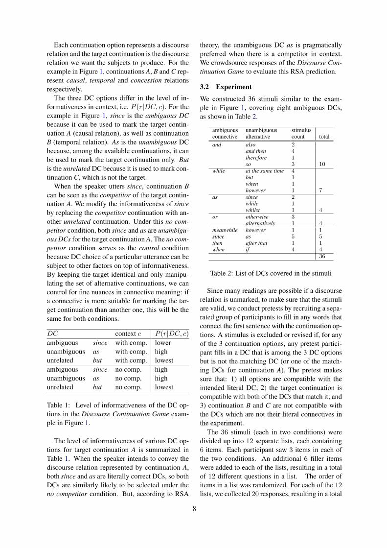
We constructed 36 stimuli similar to the exam-ple in Figure 1, covering eight ambiguous DCs,as shown in Table 2.
ambiguous unambiguous stimulusconnective alternative count totaland also 2
and then 4therefore 1so 3 10
while at the same time 4but 1when 1however 1 7
as since 2while 1whilst 1 4
or otherwise 3alternatively 1 4
meanwhile however 1 1since as 5 5then after that 1 1when if 4 4
36
Table 2: List of DCs covered in the stimuli
Since many readings are possible if a discourserelation is unmarked, to make sure that the stimuliare valid, we conduct pretests by recruiting a sepa-rated group of participants to fill in any words thatconnect the first sentence with the continuation op-tions. A stimulus is excluded or revised if, for anyof the 3 continuation options, any pretest partici-pant fills in a DC that is among the 3 DC optionsbut is not the matching DC (or one of the match-ing DCs for continuation A). The pretest makessure that: 1) all options are compatible with theintended literal DC; 2) the target continuation iscompatible with both of the DCs that match it; and3) continuation B and C are not compatible withthe DCs which are not their literal connectives inthe experiment.
The 36 stimuli (each in two conditions) weredivided up into 12 separate lists, each containing6 items. Each participant saw 3 items in each ofthe two conditions. An additional 6 filler itemswere added to each of the lists, resulting in a totalof 12 different questions in a list. The order ofitems in a list was randomized. For each of the 12lists, we collected 20 responses, resulting in a total
8
of 240 native-English-speaking participants whotook part in the experiment. 127 participants arefemales and 73 are males. Their average age is 34.148 participants come from the United Kingdom,34 from the United States and 18 from other coun-tries, including Canada, Ireland etc. The partici-pants were recruited through the Prolific platform.They took on average 8 minutes to complete thetask, and were reimbursed for their efforts with0.8 GBP each. The filler questions had the sameform as the stimuli, except that continuations B orC were set as the target instead of the experimen-tally interesting continuation A. Responses fromparticipants who chose more than 6 non-matchingDCs in their list were excluded and recollected.The experimental interface was constructed usingLingoturk (Pusse et al., 2016).
The experimental interface was designed to re-semble a communication scenario where two play-ers interact at real time, although the responsesof “Player 2” were actually automatically gener-ated by the system, and were shown to the subjectwith a time lag of 4 seconds. “Player 2” was pro-grammed to be an rational Gricean pragmatic lis-tener, who in the unambiguous condition alwayschose the continuation that best fits the connec-tive, and who supposed that the speaker wouldchoose an unambiguous DC when there was acompetitor in context. For example, if the par-ticipant chose the ambiguous since, “Player 2”would guess continuation B, assuming that the par-ticipant would have chosen the unambiguous as ifhe meant continuation A.
To motivate the participants, they were re-warded with a bonus of 0.06 GBP for each ques-tion where the “Player 2” successfully guessedthe target continuation.
4 Results
We calculate the agreement among the participantsfor each stimulus by
Count(majority response)
Count(all response)
and average it over the items. The average agree-ment of the filler items is 87% while that of thestimulus items is 68% and 71% respectively forthe no- and with competitor conditions. The agree-ment of the filler items is higher than that of thestimulus items. It is expected because only oneof the three connective options literally matches
the target continuation in the filler items while twoof the options are literally correct in the stimu-lus items. The agreement under the no competitorcondition is slightly lower than the with competi-tor condition. This follows our prediction that, un-der the no competitor condition, participants morefreely choose between the two literally correct op-tions, because they are equally informative.
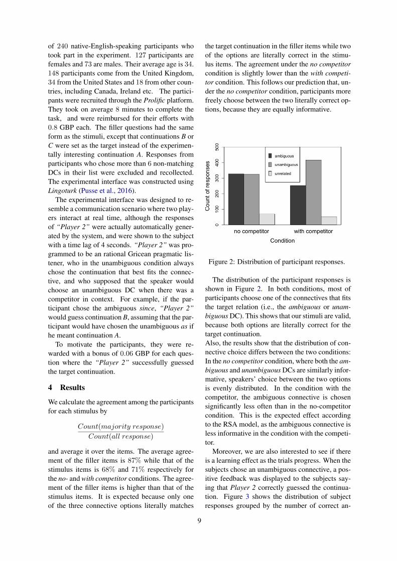
Figure 2: Distribution of participant responses.
The distribution of the participant responses isshown in Figure 2. In both conditions, most ofparticipants choose one of the connectives that fitsthe target relation (i.e., the ambiguous or unam-biguous DC). This shows that our stimuli are valid,because both options are literally correct for thetarget continuation.Also, the results show that the distribution of con-nective choice differs between the two conditions:In the no competitor condition, where both the am-biguous and unambiguous DCs are similarly infor-mative, speakers’ choice between the two optionsis evenly distributed. In the condition with thecompetitor, the ambiguous connective is chosensignificantly less often than in the no-competitorcondition. This is the expected effect accordingto the RSA model, as the ambiguous connective isless informative in the condition with the competi-tor.
Moreover, we are also interested to see if thereis a learning effect as the trials progress. When thesubjects chose an unambiguous connective, a pos-itive feedback was displayed to the subjects say-ing that Player 2 correctly guessed the continua-tion. Figure 3 shows the distribution of subjectresponses grouped by the number of correct an-
9
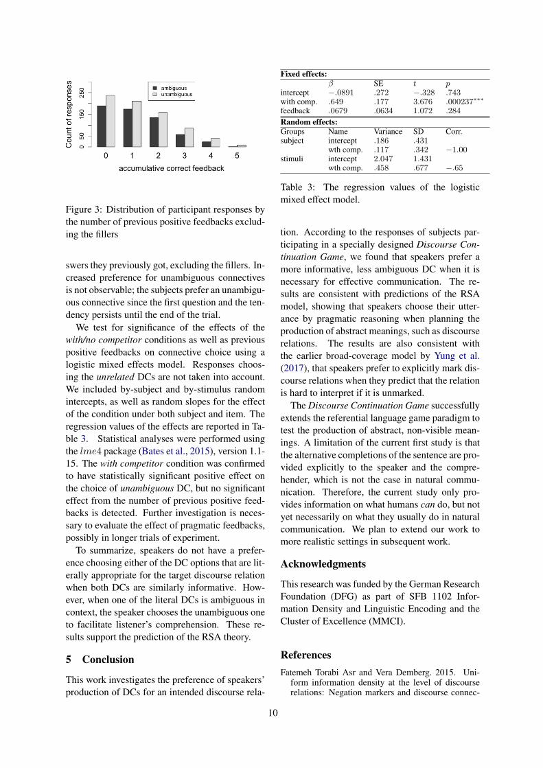
Figure 3: Distribution of participant responses bythe number of previous positive feedbacks exclud-ing the fillers
swers they previously got, excluding the fillers. In-creased preference for unambiguous connectivesis not observable; the subjects prefer an unambigu-ous connective since the first question and the ten-dency persists until the end of the trial.
We test for significance of the effects of thewith/no competitor conditions as well as previouspositive feedbacks on connective choice using alogistic mixed effects model. Responses choos-ing the unrelated DCs are not taken into account.We included by-subject and by-stimulus randomintercepts, as well as random slopes for the effectof the condition under both subject and item. Theregression values of the effects are reported in Ta-ble 3. Statistical analyses were performed usingthe lme4 package (Bates et al., 2015), version 1.1-15. The with competitor condition was confirmedto have statistically significant positive effect onthe choice of unambiguous DC, but no significanteffect from the number of previous positive feed-backs is detected. Further investigation is neces-sary to evaluate the effect of pragmatic feedbacks,possibly in longer trials of experiment.
To summarize, speakers do not have a prefer-ence choosing either of the DC options that are lit-erally appropriate for the target discourse relationwhen both DCs are similarly informative. How-ever, when one of the literal DCs is ambiguous incontext, the speaker chooses the unambiguous oneto facilitate listener’s comprehension. These re-sults support the prediction of the RSA theory.
5 Conclusion
This work investigates the preference of speakers’production of DCs for an intended discourse rela-
Fixed effects:β SE t p
intercept −.0891 .272 −.328 .743with comp. .649 .177 3.676 .000237∗∗∗
feedback .0679 .0634 1.072 .284
Random effects:Groups Name Variance SD Corr.subject intercept .186 .431
wth comp. .117 .342 −1.00stimuli intercept 2.047 1.431
wth comp. .458 .677 −.65
Table 3: The regression values of the logisticmixed effect model.
tion. According to the responses of subjects par-ticipating in a specially designed Discourse Con-tinuation Game, we found that speakers prefer amore informative, less ambiguous DC when it isnecessary for effective communication. The re-sults are consistent with predictions of the RSAmodel, showing that speakers choose their utter-ance by pragmatic reasoning when planning theproduction of abstract meanings, such as discourserelations. The results are also consistent withthe earlier broad-coverage model by Yung et al.(2017), that speakers prefer to explicitly mark dis-course relations when they predict that the relationis hard to interpret if it is unmarked.
The Discourse Continuation Game successfullyextends the referential language game paradigm totest the production of abstract, non-visible mean-ings. A limitation of the current first study is thatthe alternative completions of the sentence are pro-vided explicitly to the speaker and the compre-hender, which is not the case in natural commu-nication. Therefore, the current study only pro-vides information on what humans can do, but notyet necessarily on what they usually do in naturalcommunication. We plan to extend our work tomore realistic settings in subsequent work.
Acknowledgments
This research was funded by the German ResearchFoundation (DFG) as part of SFB 1102 Infor-mation Density and Linguistic Encoding and theCluster of Excellence (MMCI).
ReferencesFatemeh Torabi Asr and Vera Demberg. 2015. Uni-
form information density at the level of discourserelations: Negation markers and discourse connec-
10
tive omission. Proc. of the International Conferenceon Computational Semantics.
Douglas Bates, Martin Machler, Ben Bolker, and SteveWalker. 2015. Fitting linear mixed-effects mod-els using lme4. Journal of Statistical Software,67(1):1–48.
Judith Degen, Michael Franke, and Gerhard Jager.2013. Cost-based pragmatic inference about ref-erential expressions. In Proceedings of the annualmeeting of the cognitive science society, volume 35.
Michael C Frank, Andres Gomez Emilsson, BenjaminPeloquin, Noah D Goodman, and Christopher Potts.2016. Rational speech act models of pragmatic rea-soning in reference games.
Michael C Frank and Noah D Goodman. 2012. Pre-dicting pragmatic reasoning in language games. Sci-ence, 336(6084):998–998.
Noah D Goodman and Andreas Stuhlmuller. 2013.Knowledge and implicature: Modeling language un-derstanding as social cognition. Topics in cognitivescience, 5(1):173–184.
H Paul Grice. 1975. Logic and conversation. Syntaxand Semantics, 3:41–58.
Robert XD Hawkins, Michael C Frank, and Noah DGoodman. 2017. Convention-formation in iteratedreference games. In Proceedings of the 39th AnnualConference of the Cognitive Science Society. Cogni-tive Science Society.
Robert XD Hawkins, Andreas Stuhlmuller, Judith De-gen, and Noah D Goodman. 2015. Why do youask? good questions provoke informative answers.In CogSci. Citeseer.
Michele Herbstritt and Michael Franke. 2017. Mod-eling transfer of high-order uncertain information.CogSci.
Gary Patterson and Andrew Kehler. 2013. Predictingthe presence of discourse connectives. Proc. of theConference on Empirical Methods in Natural Lan-guage Processing, pages 914–923.
Florian Pusse, Asad Sayeed, and Vera Demberg. 2016.Lingoturk: Managing crowdsourced tasks for psy-cholinguistics. Proc. of the North American Chapterof the Association for Computational Linguistics.
H Rhode, A. Dickinson, N. Schneider, C. N. L. Clark,A. Louis, and B. Webber. 2016. Filling in the blanksin understanding discourse adverbials: Consistency,conflict, and context-dependence in a crowdsourcedelicitation task. Proc. of the Linguistic AnnotationWorkshop.
Ted JM Sanders and Leo GM Noordman. 2000. Therole of coherence relations and their linguisticmarkers in text processing. Discourse processes,29(1):37–60.
Merel Cleo Johanna Scholman and Vera Demberg.2017. Examples and specifications that provea point: Identifying elaborative and argumenta-tive discourse relations. Dialogue & Discourse,8(2):56–83.
Frances Yung, Kevin Duh, Taku Komura, and YujiMatsumoto. 2016. Modeling the usage of dis-course connectives as rational speech acts. Proc. ofthe SIGNLL Conference on Computational NaturalLanguage Learning, page 302.
Frances Yung, Kevin Duh, Taku Komura, and YujiMatsumoto. 2017. A psycholinguistic model for themarking of discourse relations. Dialogue & Dis-course, 8(1):106–131.
11

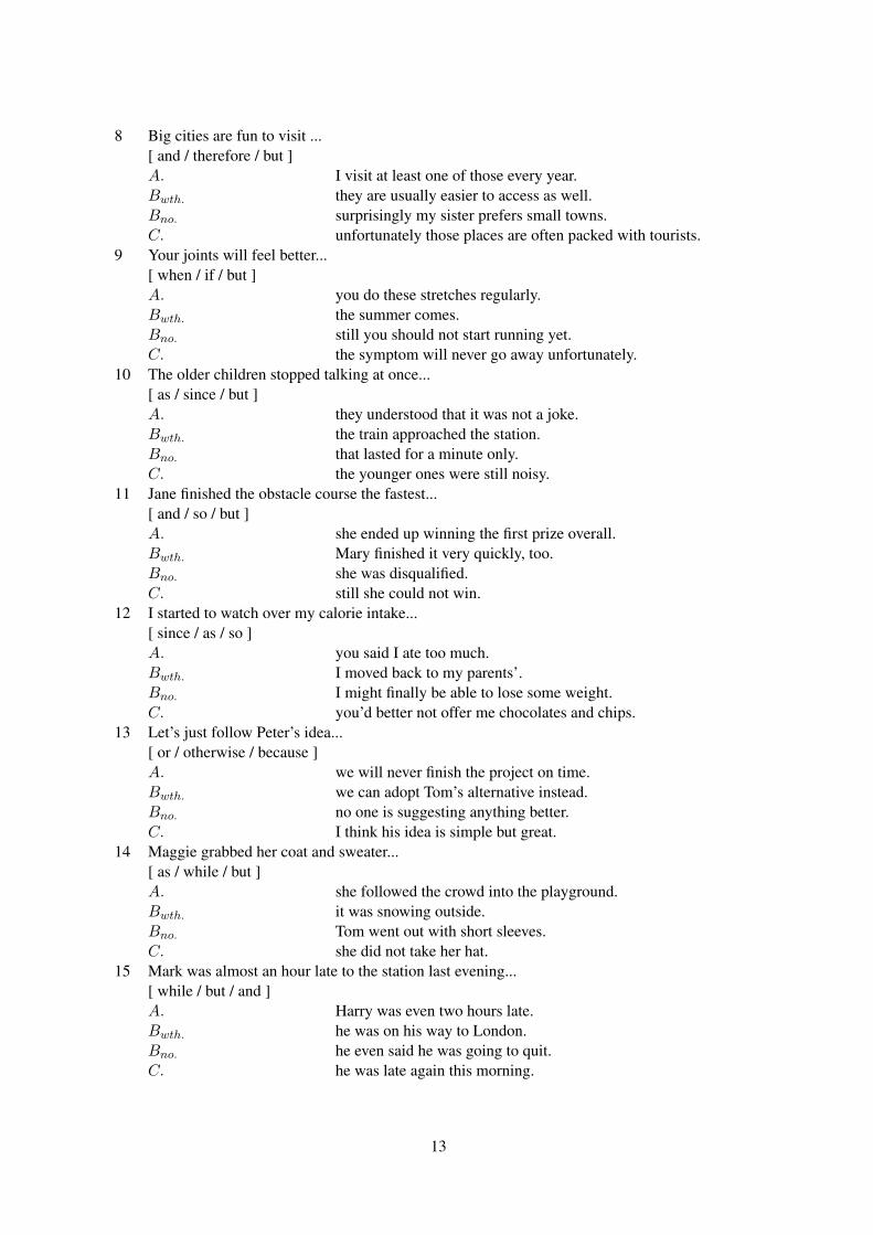
A Stimuli and fillers of the experiment
Continuations A, Bwth and C are displayed to the subjects under the with competitor condition, aswell as in the fillers. Continuations A, Bno and C are displayed under the no competitor condition.Continuation A is set as the target in the stimulus questions, while continuations Bwth or C are thetargets in the fillers. The connective options are in the order: ambiguous / unambiguous / unrelated.
1 Hard work is the key to success...[ and / also / unless ]A. patience is important.Bwth. honesty is the key to friendship.Bno. you are always lucky.C. you are a genius.
2 Harry was born in Scotland...[ and / and then / but ]A. he lived in Glasgow for 20 years.Bwth. his ancestors had origined from Scotland.Bno. both his parents are not Scottish.C. he would not have said so.
3 I listened to music on my mobile phone...[ while / when / because ]A. I was walking back home from work.Bwth. I knew there are more important things I should do instead.Bno. it helped me to concentrate.C. I was bored waiting for you for half an hour.
4 I will buy a bag for my son as promised...[ or / otherwise / because ]A. he will be very disappointed.Bwth. I will buy him a watch instead.Bno. he did well in his exams.C. it is his birthday tomorrow.
5 You must have been studying this afternoon...[ since / as / but ]A. I did not hear music from your room.Bwth. you came back from school.Bno. it doesn’t mean you will certainly get good marks in the exam.C. John has been playing video games all the time.
6 I had been longing for a cup of coffee...[ since / as / so ]A. you woke me up at five this morning.Bwth. the teacher of the first class came in.Bno. I rushed to the cafeteria as soon as the bell rang.C. please do me a favour and buy me an espresso.
7 I will finish this homework now...[ then / after that / although ]A. I will go to chill with my friends.Bwth. I can have something to hand in tomorrow.Bno. I don’t know the answers for half of the questions.C. it is not interesting at all.
12
8 Big cities are fun to visit ...[ and / therefore / but ]A. I visit at least one of those every year.Bwth. they are usually easier to access as well.Bno. surprisingly my sister prefers small towns.C. unfortunately those places are often packed with tourists.
9 Your joints will feel better...[ when / if / but ]A. you do these stretches regularly.Bwth. the summer comes.Bno. still you should not start running yet.C. the symptom will never go away unfortunately.
10 The older children stopped talking at once...[ as / since / but ]A. they understood that it was not a joke.Bwth. the train approached the station.Bno. that lasted for a minute only.C. the younger ones were still noisy.
11 Jane finished the obstacle course the fastest...[ and / so / but ]A. she ended up winning the first prize overall.Bwth. Mary finished it very quickly, too.Bno. she was disqualified.C. still she could not win.
12 I started to watch over my calorie intake...[ since / as / so ]A. you said I ate too much.Bwth. I moved back to my parents’.Bno. I might finally be able to lose some weight.C. you’d better not offer me chocolates and chips.
13 Let’s just follow Peter’s idea...[ or / otherwise / because ]A. we will never finish the project on time.Bwth. we can adopt Tom’s alternative instead.Bno. no one is suggesting anything better.C. I think his idea is simple but great.
14 Maggie grabbed her coat and sweater...[ as / while / but ]A. she followed the crowd into the playground.Bwth. it was snowing outside.Bno. Tom went out with short sleeves.C. she did not take her hat.
15 Mark was almost an hour late to the station last evening...[ while / but / and ]A. Harry was even two hours late.Bwth. he was on his way to London.Bno. he even said he was going to quit.C. he was late again this morning.
13

16 Dave ordered a tall glass of fine scotch...[ as / since / but ]A. we could order what ever we want.Bwth. the host was giving a speech.Bno. he could not finish half of it.C. Mary just ordered a soft drink.
17 Mary always wore a fancy dress to a ball...[ when / if / whereas ]A. her boyfriend was going as well.Bwth. she was at her 20s.Bno. she did not care much about her hair.C. she dressed casually to work.
18 That pizzaria has always been my favourite...[ since / as / but ]A. I like Italian food a lot.Bwth. I had dinner with Jill there two years ago.Bno. my boyfriend doesn’t really like it.C. I think this restaurant is not bad, too.
19 My parents will visit Canada again in December...[ and / and then / although ]A. they will visit South America in spring.Bwth. it will be their thrid visit in two years.Bno. the air tickets are expensive in that season.C. they hate cold weather.
20 I am sure David will burst into tears...[ when / if / but ]A. his children come to visit one day.Bwth. he comes home tonight.Bno. Kathy probably will not react much.C. that will be tears of happiness.
21 Leo is taking orders from the guests...[ while / at the same time / so ]A. George is serving the food.Bwth. there are too many tables for him to serve alone.Bno. he is not able to pick up the call right now.C. have patience, he will come to our table sooner or later.
22 Peter was watching the baseball match on TV this morning...[ while / at the same time / because ]A. his wife was making breakfast for him in the kitchen.Bwth. he didn’t understand the rules at all.Bno. there were not any other good shows on TV.C. he recently became a fan of the team that was playing.
23 Please buy some fruits for me...[ and / and then / if ]A. come home immediately afterwards.Bwth. don’t forget the milk.Bno. you still have money left.C. you pass by a supermarket.
14

24 Sam is going on a business trip to Seoul....[ while / at the same time / and ]A. his children are going to a summer camp.Bwth. he is not very optimistic about the Korean market.Bno. he will come back with signed contracts.C. later he will travel to Japan for an exhibition.
25 That task took me a lot of time...[ and / so / but ]A. I expected a higher reward.Bwth. it was so boring.Bno. it was not the worst.C. I enjoyed doing it.
26 The carnival was held on the main street for a week...[ while / at the meantime / because ]A. a film festival was being held in the same period.Bwth. it was held in the park for only one day.Bno. the central park was not big enough.C. people complained that three days were too short.
27 The cat always behaves weird at night ...[ when / if / but ]A. we have a visitor at home.Bwth. dad comes back from work early.Bno. she was normal last night.C. she will be fine the next morning.
28 The cleaning lady will come to clean our house in the morning...[ and / also / otherwise ]A. she will wash the cars.Bwth. we can just leave the dishes in the kitchen.Bno. we will have to do it ourselves.C. I think the house will just be in a mess forever.
29 The current situation is likely to change...[ while / however / before ]A. our standard of living is unlikely to improve.Bwth. the management is planning the next move.Bno. the summer holiday starts.C. you even notice it.
30 The talk will be delayed for an hour...[ meanwhile / however / because ]A. the conference room is already full of people.Bwth. people are having a coffee break.Bno. there is a technical problem.C. the speaker is coming late.
31 The teddy bear dropped from the baby’s hand...[ and / and then / as ]A. he cried aloud.Bwth. he has dropped it twice in a minute.Bno. he fell asleep.C. the stroller entered the elevator.
15

32 That tennis player has been losing his matches...[ since / as / but ]A. we know he is still recovering from the injury.Bwth. the season started.Bno. he was close in every match.C. his coach believes that he still has chance.
33 The next concert will be held this summer here in this city...[ and / so / but ]A. we are definitely going.Bwth. I heard that it will be an outdoor concert.Bno. unfortunately I cannot go this time.C. the dates are not yet confirmed.
34 We fell asleep immediately...[ as / whilst / but ]A. the moon rose higher in the sky.Bwth. we had been working the whole day.Bno. we woke up shortly in the middle of the night.C. the kids stayed up until early in the morning..
35 We should not walk but take the bus...[ or / alternatively / although ]A. we can take a taxi instead.Bwth. we will not arrive on time.Bno. it would have been nice to walk through the forest.C. it is still not the fastest way to get there.
36 You should bring something to eat...[ or / otherwise / although ]A. you will starve yourself.Bwth. alternatively, you can bring some drinks.Bno. it is not compulsory.C. some snacks will be served there.
16
Proceedings of the Eighth Workshop on Cognitive Aspects of Computational Language Learning and Processing, pages 17–26Melbourne, Australia, July 19, 2018. c©2018 Association for Computational Linguistics
Language Production Dynamics with Recurrent Neural Networks
Jesus Calvillo1,2 and Matthew W. Crocker1Saarland University1
Saarbrucken, GermanyPenn State Applied Cognitive Science Lab2
University Park, PA USA{jesusc,crocker}@coli.uni-saarland.de
Abstract
We present an analysis of the inter-nal mechanism of the recurrent neuralmodel of sentence production presentedby Calvillo et al. (2016). The results showclear patterns of computation related toeach layer in the network allowing to in-fer an algorithmic account, where the se-mantics activates the semantically relatedwords, then each word generated at eachtime step activates syntactic and seman-tic constraints on possible continuations,while the recurrence preserves informa-tion through time. We propose that suchinsights could generalize to other modelswith similar architecture, including someused in computational linguistics for lan-guage modeling, machine translation andimage caption generation.
1 Introduction
A Recurrent Neural Network (RNN) is an artifi-cial neural network that contains at least one layerwhose activation at a time step t serves as inputto itself at a time step t + 1. Theoretically, RNNshave been shown to be at least as powerful as aTuring Machine (Siegelmann and Sontag, 1995;Siegelmann, 2012). Empirically, in computationallinguistics they achieve remarkable results in sev-eral tasks, most notably in language modeling andmachine translation (e.g. Sutskever et al., 2014;Mikolov et al., 2010). In the human language pro-cessing literature, they have been used to modellanguage comprehension (e.g. Frank et al., 2009;Brouwer, 2014; Rabovsky et al., 2016) and pro-duction (e.g. Calvillo et al., 2016; Chang et al.,2006).
In spite of their success, RNNs are often usedas a black box with little understanding of their
internal dynamics, and rather evaluating them interms of prediction accuracy. This is due to thetypically high dimensionality of the internal statesof the network, coupled with highly complex in-teractions between layers.
Here we try to open the black box present-ing an analysis of the internal behavior of thesentence production model presented by Calvilloet al. (2016). This model can be seen as a semanti-cally conditioned language model that maps a se-mantic representation onto a sequence of wordsforming a sentence, by implementing an exten-sion of a Simple Recurrent Network (SRN, El-man, 1990). Because of its simple architectureand its relatively low dimensionality, this modelcan be analyzed as a whole, showing clear patternsof computation, which could give insights into thedynamics of larger language models with similararchitecture.
The method that we applied is based on Layer-wise Relevance Propagation (Bach et al., 2015).This algorithm starts at the output layer and movesin the graph towards the input units, tracking theamount of relevance that each unit in layer li−1 hason the activation of units in layer li, back to the in-put units, which are usually human-interpretable.For a review of this and some other techniques forinterpreting neural networks, see Montavon et al.(2017); for related work to this paper see Karpathyet al. (2015); Li et al. (2015); Kadar et al. (2017);Arras et al. (2016); Ding et al. (2017).
Our analysis reveals that the overall behaviorof the model is approximately as follows: the in-put semantic representation activates the hiddenunits related to all the semantically relevant words,where words that are normally produced early inthe sentence receive relatively more activation; af-ter producing a word, the word produced activatessyntactic and semantic constraints for the produc-tion of the next word, for example, after a deter-
17
miner, all the nouns are activated, similarly, aftera given verb, only semantically fit objects are ac-tivated; meanwhile, the recurrent units present atendency for self-activation, suggesting a mecha-nism where activation is preserved over time, al-lowing the model to implement dynamics overmultiple time steps. While some of the results pre-sented here have been suggested previously, wepresent a holistic integrative view of the internalmechanics of the model, in contrast to previousanalyses that focus on specific examples.
The next subsection describes the semantic rep-resentations used by the model. Section 2 de-scribes the language production model. Section 3presents the analysis. Discussion and Conclusionare presented in sections 4 and 5 respectively.
1.1 Semantic Representations
The semantic representations were derived fromthe Distributed Situation Space model (DSS,Frank et al., 2003, 2009), which defines amicroworld in terms of a finite set of basicevents (e.g., play(charlie,chess)). Basic eventscan be conjoined to form complex events (e.g.,play(charlie,chess)∧win(charlie)). However, themicroworld poses both hard and probabilistic con-straints on event co-occurrence, where some com-plex events are very common, and some others im-possible to happen.
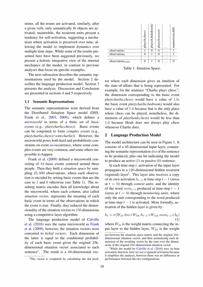
Frank et al. (2009) defined a microworld con-sisting of 44 basic events centered around threepeople. Then they built a situation space by sam-pling 25, 000 observations, where each observa-tion is encoded by setting basic events that are thecase to 1 and 0 otherwise (see Table 1). The re-sulting matrix encodes then all knowledge aboutthe microworld, where each column, also calledsituation vector, represents the meaning of eachbasic event in terms of the observations in whichthe event is true. Finally, they reduced the dimen-sionality of the situation vectors to 150 dimensionsusing a competitive layer algorithm.
The language production model of Calvilloet al. (2016) uses the same microworld as Franket al. (2009), however, the situation vectors wereconverted to belief vectors. Each dimension ofthe latter is equal to the conditional probabil-ity of each basic event given the original 25k-dimensional situation vector associated to eachsentence1. The result is a 44-dimensional vec-
1This vector is computed by calculating the dot prod-
play
(ch,
ches
s)
play
(ch,
hide
&se
ek)
play
(ch,
socc
er)
. . . man
ner(
win
,diff
)
observation1 1 0 0 . . . 1observation2 0 1 0 . . . 1. . . . . . . . . .observation25000 0 1 0 . . . 0
Table 1: Situation Space.
tor where each dimension gives an intuition ofthe state-of-affairs that is being represented. Forexample, for the sentence “Charlie plays chess.”,the dimension corresponding to the basic eventplay(charlie,chess) would have a value of 1.0,the basic event play(charlie,bedroom) would alsohave a value of 1.0 because that is the only placewhere chess can be played, nonetheless, the di-mension of play(heidi,chess) would be less than1.0 because Heidi does not always play chesswhenever Charlie does.
2 Language Production Model
The model architecture can be seen in Figure 1. Itconsists of a 45-dimensional input layer, contain-ing the semantic representation dss of the sentenceto be produced, plus one bit indicating the modelto produce an active (1) or passive (0) sentence.
At each time step t, activation of the input layerpropagates to a 120-dimensional hidden recurrent(sigmoid) layer2. This layer also receives a copyof its own activation ht−1 at time-step t− 1 (zerosat t = 0) through context units; and the identityof the word mont−1 produced at time-step t − 1(zeros at t = 0) through monitoring units, whereonly the unit corresponding to the word producedat time-step t − 1 is activated. More formally, ac-tivation of the hidden layer is given by:
ht = σ(Wih·dss+Whh·ht−1+Wmh·mont−1+bh)(1)
where Wih is the weight matrix connecting the in-put layer to the hidden layer, Whh is the weight
uct between the situation space matrix and the original 25k-dimensional situation vector, and then normalizing each di-mension of the resulting vector by the sum over the dimen-sions of the original 25k-dimensional situation vector.
2While the model by Calvillo et al. (2016) uses an htanactivation function, here we use a sigmoid activation becauseit simplifies the analysis, however there was no difference inperformance between the two configurations.
18
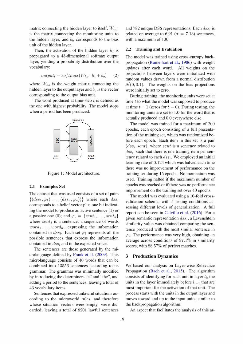
matrix connecting the hidden layer to itself, Wmh
is the matrix connecting the monitoring units tothe hidden layer, and bh corresponds to the biasunit of the hidden layer.
Then, the activation of the hidden layer ht ispropagated to a 43-dimensional softmax outputlayer, yielding a probability distribution over thevocabulary:
outputt = softmax(Who · ht + bo) (2)
where Who is the weight matrix connecting thehidden layer to the output layer and bo is the vectorcorresponding to the output bias unit.
The word produced at time-step t is defined asthe one with highest probability. The model stopswhen a period has been produced.
Figure 1: Model architecture.
2.1 Examples SetThe dataset that was used consists of a set of pairs{(dss1, ϕ1), . . . , (dssn, ϕn))} where each dssicorresponds to a belief vector plus one bit indicat-ing the model to produce an active sentence (1) ora passive one (0); and ϕi = {sent1, . . . , sentk}where sentj is a sentence, a sequence of wordsword1, . . . , wordn, expressing the informationcontained in dssi. Each set ϕi represents all thepossible sentences that express the informationcontained in dssi and in the expected voice.
The sentences are those generated by the mi-crolanguage defined by Frank et al. (2009). Thismicrolanguage consists of 40 words that can becombined into 13556 sentences according to itsgrammar. The grammar was minimally modifiedby introducing the determiners “a” and “the”, andadding a period to the sentences, leaving a total of43 vocabulary items.
Sentences that expressed unlawful situations ac-cording to the microworld rules, and thereforewhose situation vectors were empty, were dis-carded; leaving a total of 8201 lawful sentences
and 782 unique DSS representations. Each dssi isrelated on average to 6.91 (σ = 7.13) sentences,with a maximum of 130.
2.2 Training and Evaluation
The model was trained using cross-entropy back-propagation (Rumelhart et al., 1986) with weightupdates after each word. All weights on theprojections between layers were initialized withrandom values drawn from a normal distributionN (0, 0.1). The weights on the bias projectionswere initially set to zero.
During training, the monitoring units were set attime t to what the model was supposed to produceat time t− 1 (zeros for t = 0). During testing, themonitoring units are set to 1.0 for the word that isactually produced and 0.0 everywhere else.
The model was trained for a maximum of 200epochs, each epoch consisting of a full presenta-tion of the training set, which was randomized be-fore each epoch. Each item in this set is a pair(dssi, sent), where sent is a sentence related todssi, such that there is one training item per sen-tence related to each dssi. We employed an initiallearning rate of 0.124 which was halved each timethere was no improvement of performance on thetraining set during 15 epochs. No momentum wasused. Training halted if the maximum number ofepochs was reached or if there was no performanceimprovement on the training set over 40 epochs.
The model was evaluated using a 10-fold cross-validation schema, with 5 testing conditions as-sessing different levels of generalization. A fullreport can be seen in Calvillo et al. (2016). For agiven semantic representation dssi, a Levenshteinsimilarity value was obtained comparing the sen-tence produced with the most similar sentence inϕi. The performance was very high, obtaining anaverage across conditions of 97.1% in similarityscores, with 88.57% of perfect matches.
3 Production Dynamics
We based our analysis on Layer-wise RelevancePropagation (Bach et al., 2015). The algorithmconsists of identifying for each unit in layer li, theunits in the layer immediately before li−1 that aremost important for the activation of that unit. Theprocess starts with the units in the output layer andmoves toward and up to the input units, similar tothe backpropagation algorithm.
An aspect that facilitates the analysis of this ar-
19
chitecture is that the activation of all layers is pos-itive, ranging from 0 to 1. Then, the difference be-tween activation or inhibition of any unit onto an-other is given by the sign of the connection weightbetween them. Thus, units inhibiting a particu-lar unit ui will be those with a negative connec-tion weight to ui, and activating units will be thosewith a positive connection weight to ui.
Having this in mind, we performed the analy-sis. In this architecture the output layer dependssolely on the activation of the recurrent hiddenlayer. Thus, we will first analyze the influence ofthe hidden layer onto the output layer, and later wewill see how monitoring, input and context unitsaffect production via the hidden layer.
3.1 Word-Producing Hidden Units
As the first step, we would like to know whichhidden units are most relevant for the productionof each word. We begin by identifying the hid-den layer activation patterns that co-occur with theproduction of each word. In order to do so, we fedthe model with the training set. For each trainingitem, the model was given as input the correspond-ing semantic representation, and at each time stepthe monitoring units were set according to the cor-responding sentence of the training item. This isvery similar to one epoch of training, except thatno weight updates were made. During this pro-cess, for each time a word had an activation greaterthan 0.2, the activation of the hidden layer wassaved. This value was chosen in order to record ac-tivation patterns where the target word was clearlyactivated. At the end, for each word ok we ob-tained a set of vectors, each vector correspondingto a pattern of activation of the hidden layer thatled to the activation of ok. Then we averaged thesevectors, obtaining a vector that shows which hid-den units are active/inactive during the productionof ok, in general and not just for a single instance,providing us with a more general perspective ofthe dynamics of the model for each word.
Having these patterns, we can further infer thedirection and magnitude of their effect by lookingat the connection weights that connect the hiddenlayer to the output layer.
A hidden unit hj having a high average activa-tion aj when producing a word ok means in gen-eral that hj is relevant for ok. However, if theweight connecting hj to ok is close to 0, then theproduction of ok will not be so affected by hj . In
this case, it could be that hj is only indirectly af-fecting the production of ok by activating/inhibit-ing other words.
Intuitively, hidden units can lead to the produc-tion of ok directly by activating ok or indirectly byinhibiting other words. Similarly, they can lead tothe inhibition of ok directly by inhibiting ok, orindirectly by activating other words that competeagainst ok. Because of the large number of con-figurations that can possibly influence production,we will only focus on direct activation/inhibition.
For the case of activation, we obtain a scoreAhjok conveying the relevance of hidden unit hjon the activation of word ok, equal to the averageactivation that ok receives from hj when ok is pro-duced, normalized by the sum of all activation thatok receives:
Ahjok =akjw
+jk∑
j′akj′w
+j′k
(3)
where akj is the average activation of unit hj whenthe word ok is produced, and w+
jk is the positiveweight connecting hj to ok. This score is only de-fined for hidden units with a positive connectionweight to ok, which we call activating units.
Inhibiting hidden units are units with negativeweights to a word ok. For inhibition the averageactivation of an inhibiting hidden unit during theproduction of ok is expected to be close to 0. Then,the connection weight is irrelevant, as the productwould be close to 0 as well. Thus, for inhibitionwe do not take into account the average activation,but rather its complement. That is, for each hiddenunit hj , with average activation aj , we obtain 1−aj and multiply it by the corresponding connectionweight. The result gives us the relevance regardinginhibition of each hidden unit on a particular word:
Ihjok = −(1− akj )w
−jk∑
j′(1− akj′)w
−j′k
(4)
Based on these definitions, for each hidden unitwe obtained activation/inhibition relevance scoresfor each word in the vocabulary. This gives usan idea of the function of each hidden unit. Ex-amples for some hidden units are shown in Fig-ure 2, where columns represent hidden units androws are words in the output layer3. The first 5
3For better readability, all heatmaps presentedhere are also available at https://plot.ly/˜jesusctCogACLL
20
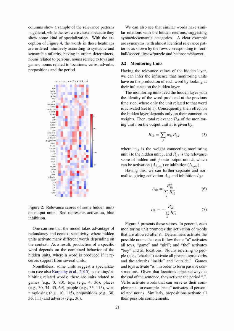
columns show a sample of the relevance patternsin general, while the rest were chosen because theyshow some kind of specialization. With the ex-ception of Figure 4, the words in these heatmapsare ordered intuitively according to syntactic andsemantic similarity, having in order: determiners,nouns related to persons, nouns related to toys andgames, nouns related to locations, verbs, adverbs,prepositions and the period.
Figure 2: Relevance scores of some hidden unitson output units. Red represents activation, blueinhibition.
One can see that the model takes advantage ofredundancy and context sensitivity, where hiddenunits activate many different words depending onthe context. As a result, production of a specificword depends on the combined behavior of thehidden units, where a word is produced if it re-ceives support from several units.
Nonetheless, some units suggest a specializa-tion (see also Karpathy et al., 2015), activating/in-hibiting related words: there are units related togames (e.g., 0, 80), toys (e.g., 4, 36), places(e.g., 30, 34, 35, 69), people (e.g., 35, 115), win-ning/losing (e.g., 10, 115), prepositions (e.g., 30,36, 111) and adverbs (e.g., 36).
We can also see that similar words have simi-lar relations with the hidden neurons, suggestingsyntactic/semantic categories. A clear exampleare synonyms, with almost identical relevance pat-terns, as shown by the rows corresponding to foot-ball/soccer, jigsaw/puzzle and bathroom/shower.
3.2 Monitoring Units
Having the relevance values of the hidden layer,we can infer the influence that monitoring unitshave on the production of each word by looking attheir influence on the hidden layer.
The monitoring units feed the hidden layer withthe identity of the word produced at the previoustime step, where only the unit related to that wordis activated (set to 1). Consequently, their effect onthe hidden layer depends only on their connectionweights. Then, total relevance Rik of the monitor-ing unit i on the output unit k, is given by:
Rik =∑
j
wijRjk (5)
where wij is the weight connecting monitoringunit i to the hidden unit j, and Rjk is the relevancescore of hidden unit j onto output unit k, whichcan be activation (Ahjok ) or inhibition (Ihjok ).
Having this, we can further separate and nor-malize, giving activation Aik and inhibition Iik:
Aik =R+
ik∑kR+
ik
(6)
Iik = − R−ik∑
kR−
ik
(7)
Figure 3 presents these scores. In general, eachmonitoring unit promotes the activation of wordsthat are allowed after it. Determiners activate thepossible nouns that can follow them: “a” activatesall toys, “game” and “girl”; and “the” activates“boy” and all locations. Nouns referring to peo-ple (e.g., “charlie”) activate all present tense verbsand the adverbs “inside” and “outside”. Gamesand toys activate “is”, in order to form passive con-structions. Given that locations appear always atthe end of the sentence, they activate the period “.”.Verbs activate words that can serve as their com-plements, for example “beats” activates all person-related nouns. Similarly, prepositions activate alltheir possible complements.
21
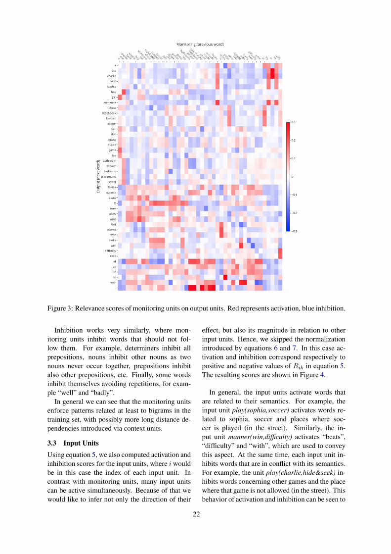
Figure 3: Relevance scores of monitoring units on output units. Red represents activation, blue inhibition.
Inhibition works very similarly, where mon-itoring units inhibit words that should not fol-low them. For example, determiners inhibit allprepositions, nouns inhibit other nouns as twonouns never occur together, prepositions inhibitalso other prepositions, etc. Finally, some wordsinhibit themselves avoiding repetitions, for exam-ple “well” and “badly”.
In general we can see that the monitoring unitsenforce patterns related at least to bigrams in thetraining set, with possibly more long distance de-pendencies introduced via context units.
3.3 Input UnitsUsing equation 5, we also computed activation andinhibition scores for the input units, where i wouldbe in this case the index of each input unit. Incontrast with monitoring units, many input unitscan be active simultaneously. Because of that wewould like to infer not only the direction of their
effect, but also its magnitude in relation to otherinput units. Hence, we skipped the normalizationintroduced by equations 6 and 7. In this case ac-tivation and inhibition correspond respectively topositive and negative values of Rik in equation 5.The resulting scores are shown in Figure 4.
In general, the input units activate words thatare related to their semantics. For example, theinput unit play(sophia,soccer) activates words re-lated to sophia, soccer and places where soc-cer is played (in the street). Similarly, the in-put unit manner(win,difficulty) activates “beats”,“difficulty” and “with”, which are used to conveythis aspect. At the same time, each input unit in-hibits words that are in conflict with its semantics.For example, the unit play(charlie,hide&seek) in-hibits words concerning other games and the placewhere that game is not allowed (in the street). Thisbehavior of activation and inhibition can be seen to
22
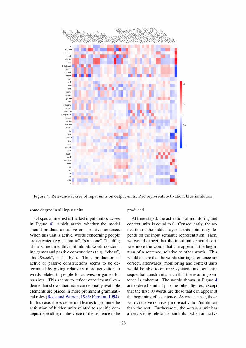
Figure 4: Relevance scores of input units on output units. Red represents activation, blue inhibition.
some degree in all input units.
Of special interest is the last input unit (activesin Figure 4), which marks whether the modelshould produce an active or a passive sentence.When this unit is active, words concerning peopleare activated (e.g., “charlie”, “someone”, “heidi”);at the same time, this unit inhibits words concern-ing games and passive constructions (e.g., “chess”,“hide&seek”, “is”, “by”). Thus, production ofactive or passive constructions seems to be de-termined by giving relatively more activation towords related to people for actives, or games forpassives. This seems to reflect experimental evi-dence that shows that more conceptually availableelements are placed in more prominent grammati-cal roles (Bock and Warren, 1985; Ferreira, 1994).In this case, the actives unit learns to promote theactivation of hidden units related to specific con-cepts depending on the voice of the sentence to be
produced.
At time step 0, the activation of monitoring andcontext units is equal to 0. Consequently, the ac-tivation of the hidden layer at this point only de-pends on the input semantic representation. Then,we would expect that the input units should acti-vate more the words that can appear at the begin-ning of a sentence, relative to other words. Thiswould ensure that the words starting a sentence arecorrect, afterwards, monitoring and context unitswould be able to enforce syntactic and semanticsequential constraints, such that the resulting sen-tence is coherent. The words shown in Figure 4are ordered similarly to the other figures, exceptthat the first 10 words are those that can appear atthe beginning of a sentence. As one can see, thosewords receive relatively more activation/inhibitionthan the rest. Furthermore, the actives unit hasa very strong relevance, such that when an active
23

sentence is queried, the words that can start an ac-tive sentence are more activated.
In sum, the input units influence production byactivating hidden units that are related to the se-mantics that is to be encoded, while additionallygiving an idea of the word order that they shouldfollow, specially at time step 0.
3.4 Context Units
At each time step, context units feed the hiddenlayer with its own activation at the previous timestep, providing the model with some kind of mem-ory over possibly unlimited time steps.
We will use the notation hi to refer to a hid-den unit i in the hidden layer, and ci to refer tothe corresponding context unit which contains theactivation of hi at the previous time step.
A way to preserve information over time is byreverberating activation over different time steps.For example, if the hidden unit ha gets active, thenthe corresponding context unit ca will be active atthe next time step; if the weight connecting ca toha is such that the activation of ca causes the acti-vation of ha, then this would form a cycle in whichha will be active indefinitely or until other units in-troduce inhibition, breaking the cycle.
We analyzed the connection weights betweenthe context and hidden layers in order to see ifthese cycles were present. In such cases, the ef-fect of ha in the current time step would be simi-lar to the effect of ca in the next time step. Thus,for each pair (hi, ci), if the effect of ci is similarto the one of hi, it would mean that ci is mainlyactivating hi or units similar to hi, forming a cy-cle. Note that if ci does not activate hi directly butother units similar to hi, it would mean that whilethe activation of the specific unit might not be pre-served, the model would still remain in the samearea within the hidden space.
As example, for the first 15 hidden units Fig-ure 5 presents these values. For each pair ofcolumns, the first column represents the direct ef-fect of each hidden unit on the output, identical tothe values in Figure 2, but normalized for each hid-den unit; the second column represents the effectof the corresponding context unit at the next timestep, calculated using the equations 5-7, where inthis case i is the index of each context unit.
The column of the right side (DimCorr) presentsfor all hidden units, the correlations between therelevance values of the hidden units and the rel-
Figure 5: Relevance scores of hidden and contextunits. Right: correlations for each word betweenthe relevance values of the hidden units and thecontext units. Bottom: correlations between allrelevance values of each hidden unit and the cor-responding context unit.
evance values of the context units, related onlyto each specific word; intuitively showing the de-gree to which activation related to each word ispreserved by all hidden units. The results sug-gest that the context units tend to preserve acti-vation related to most words, but to different de-grees, where activation of words related to toys,locations and adverbs is preserved more than ac-tivation of words related to people. Out of the 43words, 11 presented moderate correlation (0.4 ≤r < 0.6, n = 120, p < 0.00001), and 15 weakcorrelation (0.2 ≤ r < 0.4, n = 120, p < 0.11).
The row at the bottom (UnitCorr) presents cor-relations between all the relevance values of eachhidden unit and the corresponding context unit,that is, between the values of the two columnsabove. As we can see, some units seem to be-have like memory, while others seem to erase theircontent. For example, units 2, 3, 4, 5, 8, 10 and14 have a high correlation between the hiddenand context relevances, implying a cycle as de-scribed above, while units 9 and 11 present an an-
24
ticorrelation, which means that the context unit isactually inhibiting its corresponding hidden unit.Out of the 120 context units, 14 presented strongcorrelation (r ≥ 0.6, n = 43, p < 0.00001),26 moderate correlation (0.4 ≤ r < 0.6, n =43, p < 0.006) and 20 weak correlation (0.2 ≤r < 0.4, n = 43, p < 0.2). Regarding anticorrela-tion, there were 3 units with moderate anticorrela-tion (−0.6 ≤ r < −0.4, n = 43, p < 0.0036)and 6 with weak anticorrelation (−0.4 ≤ r <−0.2, n = 43, p < 0.2).
As we can see, about half of the context unitshave a tendency to preserve their activation, whichvaries according to each unit, and to the kind ofinformation. This suggests a tangible mechanismthat preserves information over time, which in thecase of language is necessary in order to enforcelong distance dependencies.
4 Discussion
In the above sections we separated the languageproduction model into its different modules in or-der to see their function. Trying to integrate theseparts into a global explanation of the internal me-chanics of the model, we arrive to the following:production starts when the model is fed a seman-tic representation at time step 0. At this point, thesemantic representation is the only source of in-formation. Based on it, the model must producea word that is in accordance to the semantics andthat is syntactically plausible for the beginning ofthe sentence. As we saw, the input units seem toselect the words necessary for production, and de-pending on the voice expected (active or passive)more activation is given to the words that can ful-fill the first position. After the initial word hasbeen produced, monitoring and context units gaininfluence. Monitoring units promote the produc-tion of words that can follow the previous word,and inhibit words that should not follow. At thesame time, context units keep information regard-ing previous and current activation, suggesting asort of memory, where information remains latentuntil the right time to be produced. This happensuntil a period is produced, which halts production.
Considering the high architectural similarity ofthe model of Calvillo et al. (2016) with othermodels of human language production (e.g., Dellet al., 1993; Chang et al., 1997), we expect thatthese results would also reflect their internal me-chanics. Furthermore, some models used in com-
putational linguistics also present an architecturewhere the main paths of computation are largelysimilar to the ones presented here: in languagemodels, at each time step the word previously pro-duced is fed to a recurrence that in turn feeds an-other layer yielding a probability distribution overthe vocabulary (e.g., Mikolov et al., 2010); ad-ditionally, a semantics is fed into the recurrencein semantically conditioned models, such as someused in machine translation (e.g., Sutskever et al.,2014) or image caption generation (e.g., Chen andLawrence Zitnick, 2015). One could argue thatlarger language models implement more complexinteractions because of their higher dimensional-ity or the use of more complex hidden units suchas LSTM (Hochreiter and Schmidhuber, 1997) orGRU (Cho et al., 2014). Nonetheless, the individ-ual results presented here are coherent with pre-vious findings on larger architectures (for exam-ple, similar words are known to have similar wordembeddings), suggesting that these results can begeneralized to such models.
While some adaptation might be needed forlarger models, the algorithm described abovemight serve as intuition of how those models work,and the methodology outlined here could serve totest such a hypothesis in future work.
5 Conclusion
We presented an analysis of the internal mecha-nism of a model of language production that usesa recurrent neural network at its core. The re-sults show clear patterns of computation that per-mit to infer its internal mechanism. Because ofarchitectural similarity, we expect that this mech-anism could be generalized to other models of hu-man language production (e.g., Dell et al., 1993;Chang et al., 1997), as well as models in compu-tational linguistics, such as those used in languagemodeling (e.g., Mikolov et al., 2010) or machinetranslation (e.g., Sutskever et al., 2014). In futurework, the methodology outlined here could alsoserve to test such a hypothesis.
Acknowledgments
This work was supported by DFG collaborative re-search center SFB 1102 ‘Information Density andLinguistic Encoding’. The first author was addi-tionally supported by National Science Founda-tion grant BCS-1734304.
25
ReferencesLeila Arras, Franziska Horn, Gregoire Montavon,
Klaus-Robert Muller, and Wojciech Samek. 2016.Explaining predictions of non-linear classifiers innlp. arXiv preprint arXiv:1606.07298.
Sebastian Bach, Alexander Binder, Gregoire Mon-tavon, Frederick Klauschen, Klaus-Robert Muller,and Wojciech Samek. 2015. On pixel-wise explana-tions for non-linear classifier decisions by layer-wiserelevance propagation. PloS one, 10(7):e0130140.
J Kathryn Bock and Richard K Warren. 1985. Concep-tual accessibility and syntactic structure in sentenceformulation. Cognition, 21(1):47–67.
Harm Brouwer. 2014. The Electrophysiology ofLanguage Comprehension: A NeurocomputationalModel. Ph.D. thesis, University of Groningen.
Jesus Calvillo, Harm Brouwer, and Matthew WCrocker. 2016. Connectionist semantic systematic-ity in language production. In Proceedings of the38th Annual Conference of the Cognitive ScienceSociety. Austin, TX: Cognitive Science Society.
Franklin Chang, Gary S Dell, and Kathryn Bock.2006. Becoming syntactic. Psychological review,113(2):234.
Franklin Chang, Zenzi M Griffin, Gary S Dell, andKathryn Bock. 1997. Modeling structural primingas implicit learning. Computational Psycholinguis-tics, Berkeley, CA, 29:392–417.
Xinlei Chen and C Lawrence Zitnick. 2015. Mind’seye: A recurrent visual representation for image cap-tion generation. In Proceedings of the IEEE con-ference on computer vision and pattern recognition,pages 2422–2431.
Kyunghyun Cho, Bart van Merrienboer, CaglarGulcehre, Fethi Bougares, Holger Schwenk, andYoshua Bengio. 2014. Learning phrase representa-tions using RNN encoder-decoder for statistical ma-chine translation. CoRR, abs/1406.1078.
Gary S Dell, Cornell Juliano, and Anita Govindjee.1993. Structure and content in language produc-tion: A theory of frame constraints in phonologicalspeech errors. Cognitive Science, 17(2):149–195.
Yanzhuo Ding, Yang Liu, Huanbo Luan, and MaosongSun. 2017. Visualizing and understanding neuralmachine translation. In Proceedings of the 55th An-nual Meeting of the Association for ComputationalLinguistics (Volume 1: Long Papers), volume 1,pages 1150–1159.
Jeffrey L Elman. 1990. Finding structure in time. Cog-nitive Science, 14(2):179–211.
Fernanda Ferreira. 1994. Choice of passive voice isaffected by verb type and animacy. Journal of Mem-ory and Language, 33(6):715–736.
Stefan L Frank, Willem FG Haselager, and Iris vanRooij. 2009. Connectionist semantic systematicity.Cognition, 110(3):358–379.
Stefan L Frank, Mathieu Koppen, Leo GM Noordman,and Wietske Vonk. 2003. Modeling knowledge-based inferences in story comprehension. CognitiveScience, 27(6):875–910.
Sepp Hochreiter and Jurgen Schmidhuber. 1997.Long short-term memory. Neural computation,9(8):1735–1780.
Akos Kadar, Grzegorz Chrupała, and Afra Alishahi.2017. Representation of linguistic form and func-tion in recurrent neural networks. ComputationalLinguistics, 43(4):761–780.
Andrej Karpathy, Justin Johnson, and Fei-Fei Li. 2015.Visualizing and understanding recurrent networks.CoRR, abs/1506.02078.
Jiwei Li, Xinlei Chen, Eduard Hovy, and Dan Jurafsky.2015. Visualizing and understanding neural modelsin nlp. arXiv preprint arXiv:1506.01066.
Tomas Mikolov, Martin Karafit, Lukas Burget, Jan Cer-nock, and Sanjeev Khudanpur. 2010. Recurrent neu-ral network based language model. In Interspeech,volume 2, page 3.
Gregoire Montavon, Wojciech Samek, and Klaus-Robert Muller. 2017. Methods for interpreting andunderstanding deep neural networks. arXiv preprintarXiv:1706.07979.
Milena Rabovsky, Steven S Hansen, and James L Mc-Clelland. 2016. N400 amplitudes reflect change ina probabilistic representation of meaning: Evidencefrom a connectionist model. In Proceedings of the38th Annual Conference of the Cognitive ScienceSociety. Austin, TX: Cognitive Science Society.
David E Rumelhart, Geoffrey E Hinton, and Ronald JWilliams. 1986. Learning representations by back-propagating errors. nature, 323(6088):533.
Hava T Siegelmann. 2012. Neural networks and ana-log computation: beyond the Turing limit. SpringerScience & Business Media.
Hava T Siegelmann and Eduardo D Sontag. 1995. Onthe computational power of neural nets. Journal ofcomputer and system sciences, 50(1):132–150.
Ilya Sutskever, Oriol Vinyals, and Quoc V Le. 2014.Sequence to sequence learning with neural net-works. In Advances in neural information process-ing systems, pages 3104–3112.
26

Proceedings of the Eighth Workshop on Cognitive Aspects of Computational Language Learning and Processing, pages 27–35Melbourne, Australia, July 19, 2018. c©2018 Association for Computational Linguistics
Multi-glance Reading Model for Text Understanding
Pengcheng Zhu1,2, Yujiu Yang1, Wenqiang Gao1, and Yi Liu2
Graduate School at Shenzhen, Tsinghua University1
Peking University Shenzhen Institute2
[email protected], [email protected],[email protected], [email protected]
Abstract
In recent years, a variety of recurrent neu-ral networks have been proposed, e.g LST-M, however, existing models only read thetext once, it cannot describe the situationof repeated reading in reading comprehen-sion. In fact, when reading or analyzinga text, we may read the text several timesrather than once if we couldn’t well under-stand it. So, how to model this kind of thereading behavior? To address the issue, wepropose a multi-glance mechanism (MG-M) for modeling the habit of reading be-havior. In the proposed framework, the ac-tual reading process can be fully simulat-ed, and then the obtained information canbe consistent with the task. Based on themulti-glance mechanism, we design twotypes of recurrent neural network modelsfor repeated reading: Glance Cell Model(GCM) and Glance Gate Model (GGM).Visualization analysis of the GCM andthe GGM demonstrates the effectivenessof multi-glance mechanisms. Experimentsresults on the large-scale datasets showthat the proposed methods can achieve bet-ter performance.
1 Introduction
Text understanding is one of the fundamental tasksin Natural Language Processing areas. Theseyears we have seen significant progress in apply-ing neural networks to text analysis applications.Recurrent neural network is widely used becauseof its effective capability of capturing the sequen-tial information. Long short-term memory (LST-M) (Hochreiter and Schmidhuber, 1997) and gatedrecurrent neural network (Chung et al., 2014) haveachieved state-of-the-art performance in many ar-
eas, such as sentiment analysis (Tang et al., 2014;Chen et al., 2016), document classification (Yanget al., 2016) and neural machine translation (Bah-danau et al., 2014). Besides the success achievedby these basic recurrent neural models, there arealso a lot of interesting research works conductedin text analysis (Kim, 2014; Zhang et al., 2015).Depending on the parsing tree structures, tree-LSTM (Tai et al., 2015) and recursive neural net-work(Socher et al., 2013) are proposed. Bidi-rectional recurrent neural networks (Schuster andPaliwal, 1997) can get the backward features. Inorder to align the hidden states, attention mecha-nism is widely used in language processing (Bah-danau et al., 2014; Vaswani et al., 2017).
One of the common characteristics of these ex-isting models is to model only single reading pro-cessing and generate a sequence of hidden statesht, as a function of the previous hidden statesht−1 and the current input (Sutskever et al., 2014;Karpathy et al., 2015). However, the fact is thatwhen we read a text only once, we may merelyknow the general idea of it, especially when thetext is long and obscure. More often than not, weknow that fast repeated reading is more effectivethan slow careful reading, so, for the obscure tex-t, our primary school teacher always teaches us toread several times to get the theme of the text. Inaddition, this kind of rereading can help us findsome of the details that are ignored when we firstglance.
In this paper, we propose a novel multi-glancemechanism to model our reading habit: whenreading a text, first we will glance through it toget the general meaning and then based on the in-formation we obtained, we will read the text againin order to find some important contents. Based onthe multi-glance mechanism we proposed (Fig.1),we design different models for processing theobtained information by the last glance, that it,
27
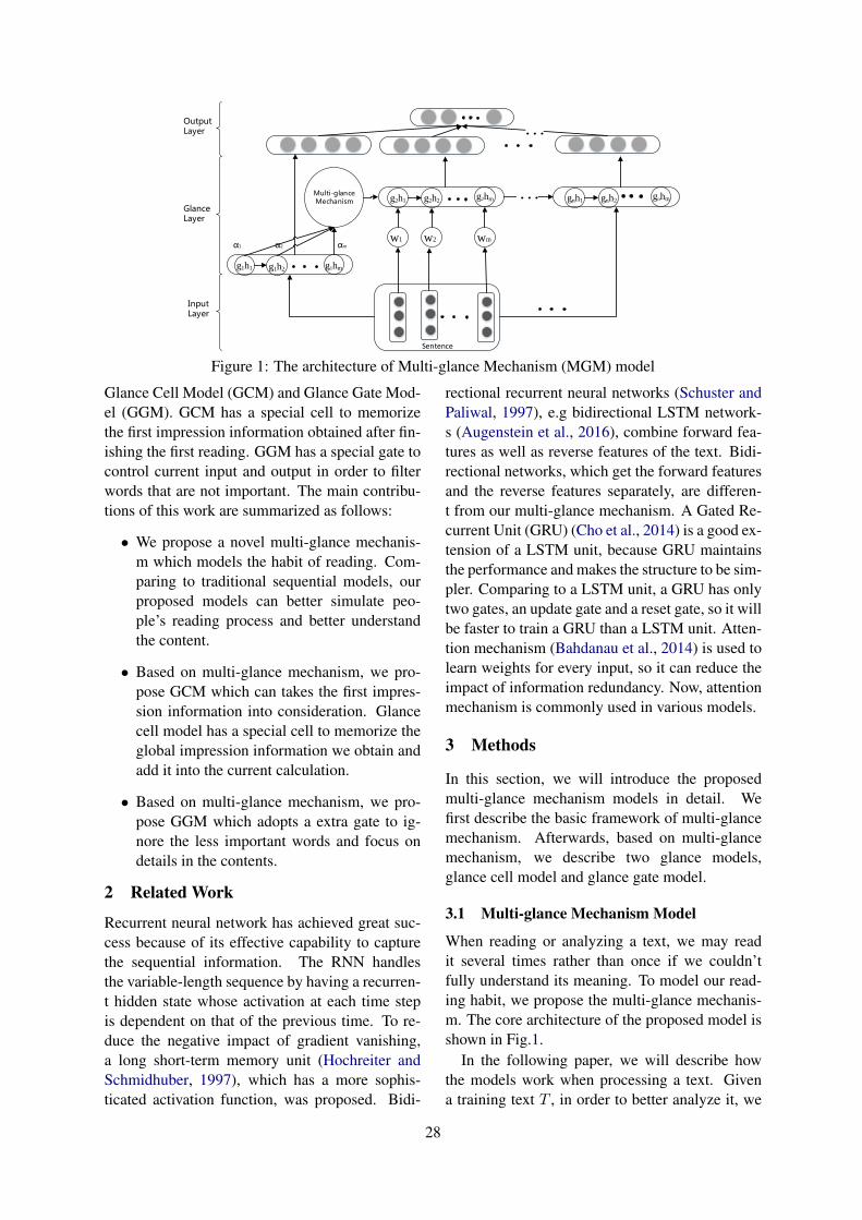
Sentence
g2h1 g2h2g2hm
w1 w2 wm
g1h1 g1h2 g1hm
Multi-glance Mechanism
α1 α2 αm
InputLayer
GlanceLayer
OutputLayer
gnh1 gnh2gnhm . . .
. . .
Figure 1: The architecture of Multi-glance Mechanism (MGM) model
Glance Cell Model (GCM) and Glance Gate Mod-el (GGM). GCM has a special cell to memorizethe first impression information obtained after fin-ishing the first reading. GGM has a special gate tocontrol current input and output in order to filterwords that are not important. The main contribu-tions of this work are summarized as follows:
• We propose a novel multi-glance mechanis-m which models the habit of reading. Com-paring to traditional sequential models, ourproposed models can better simulate peo-ple’s reading process and better understandthe content.
• Based on multi-glance mechanism, we pro-pose GCM which can takes the first impres-sion information into consideration. Glancecell model has a special cell to memorize theglobal impression information we obtain andadd it into the current calculation.
• Based on multi-glance mechanism, we pro-pose GGM which adopts a extra gate to ig-nore the less important words and focus ondetails in the contents.
2 Related Work
Recurrent neural network has achieved great suc-cess because of its effective capability to capturethe sequential information. The RNN handlesthe variable-length sequence by having a recurren-t hidden state whose activation at each time stepis dependent on that of the previous time. To re-duce the negative impact of gradient vanishing,a long short-term memory unit (Hochreiter andSchmidhuber, 1997), which has a more sophis-ticated activation function, was proposed. Bidi-
rectional recurrent neural networks (Schuster andPaliwal, 1997), e.g bidirectional LSTM network-s (Augenstein et al., 2016), combine forward fea-tures as well as reverse features of the text. Bidi-rectional networks, which get the forward featuresand the reverse features separately, are differen-t from our multi-glance mechanism. A Gated Re-current Unit (GRU) (Cho et al., 2014) is a good ex-tension of a LSTM unit, because GRU maintainsthe performance and makes the structure to be sim-pler. Comparing to a LSTM unit, a GRU has onlytwo gates, an update gate and a reset gate, so it willbe faster to train a GRU than a LSTM unit. Atten-tion mechanism (Bahdanau et al., 2014) is used tolearn weights for every input, so it can reduce theimpact of information redundancy. Now, attentionmechanism is commonly used in various models.
3 Methods
In this section, we will introduce the proposedmulti-glance mechanism models in detail. Wefirst describe the basic framework of multi-glancemechanism. Afterwards, based on multi-glancemechanism, we describe two glance models,glance cell model and glance gate model.
3.1 Multi-glance Mechanism Model
When reading or analyzing a text, we may readit several times rather than once if we couldn’tfully understand its meaning. To model our read-ing habit, we propose the multi-glance mechanis-m. The core architecture of the proposed model isshown in Fig.1.
In the following paper, we will describe howthe models work when processing a text. Givena training text T , in order to better analyze it, we
28
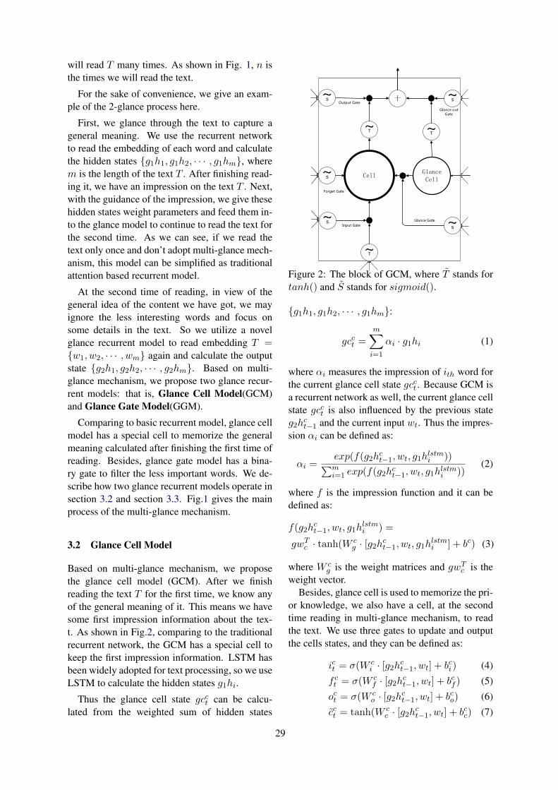
will read T many times. As shown in Fig. 1, n isthe times we will read the text.
For the sake of convenience, we give an exam-ple of the 2-glance process here.
First, we glance through the text to capture ageneral meaning. We use the recurrent networkto read the embedding of each word and calculatethe hidden states {g1h1, g1h2, · · · , g1hm}, wherem is the length of the text T . After finishing read-ing it, we have an impression on the text T . Next,with the guidance of the impression, we give thesehidden states weight parameters and feed them in-to the glance model to continue to read the text forthe second time. As we can see, if we read thetext only once and don’t adopt multi-glance mech-anism, this model can be simplified as traditionalattention based recurrent model.
At the second time of reading, in view of thegeneral idea of the content we have got, we mayignore the less interesting words and focus onsome details in the text. So we utilize a novelglance recurrent model to read embedding T ={w1, w2, · · · , wm} again and calculate the outputstate {g2h1, g2h2, · · · , g2hm}. Based on multi-glance mechanism, we propose two glance recur-rent models: that is, Glance Cell Model(GCM)and Glance Gate Model(GGM).
Comparing to basic recurrent model, glance cellmodel has a special cell to memorize the generalmeaning calculated after finishing the first time ofreading. Besides, glance gate model has a bina-ry gate to filter the less important words. We de-scribe how two glance recurrent models operate insection 3.2 and section 3.3. Fig.1 gives the mainprocess of the multi-glance mechanism.
3.2 Glance Cell Model
Based on multi-glance mechanism, we proposethe glance cell model (GCM). After we finishreading the text T for the first time, we know anyof the general meaning of it. This means we havesome first impression information about the tex-t. As shown in Fig.2, comparing to the traditionalrecurrent network, the GCM has a special cell tokeep the first impression information. LSTM hasbeen widely adopted for text processing, so we useLSTM to calculate the hidden states g1hi.
Thus the glance cell state gcct can be calcu-lated from the weighted sum of hidden states
CellGlance Cell
~s
~s
~s
~T
~T
~s
Output Gate
Forget Gate
Input Gate
~T
Glance out Gate
~s
Glance Gate
十
Figure 2: The block of GCM, where T stands fortanh() and S stands for sigmoid().
{g1h1, g1h2, · · · , g1hm}:
gcct =m∑
i=1
αi · g1hi (1)
where αi measures the impression of ith word forthe current glance cell state gcct . Because GCM isa recurrent network as well, the current glance cellstate gcct is also influenced by the previous stateg2h
ct−1 and the current input wt. Thus the impres-
sion αi can be defined as:
αi =exp(f(g2h
ct−1, wt, g1h
lstmi ))∑m
i=1 exp(f(g2hct−1, wt, g1hlstmi ))
(2)
where f is the impression function and it can bedefined as:
f(g2hct−1, wt, g1h
lstmi ) =
gwTc · tanh(W c
g · [g2hct−1, wt, g1hlstmi ] + bc) (3)
where W cg is the weight matrices and gwT
c is theweight vector.
Besides, glance cell is used to memorize the pri-or knowledge, we also have a cell, at the secondtime reading in multi-glance mechanism, to readthe text. We use three gates to update and outputthe cells states, and they can be defined as:
ict = σ(W ci · [g2hct−1, wt] + bci ) (4)
f ct = σ(W cf · [g2hct−1, wt] + bcf ) (5)
oct = σ(W co · [g2hct−1, wt] + bco) (6)
cct = tanh(W cc · [g2hct−1, wt] + bcc) (7)
29

where ict , fct and oct are the gates states, σ() is the
sigmoid function and cct stands for the input state.In GCM, in order to adopt the first impression
knowledge in the current cell state calculation andoutput the glance cell state, we use glance inputgate and output gate to connect the glance cell andthe cell state. The two gates can be defined as:
gict = σ(W cgi · [g2hct−1, wt, gc
ct ] + bcgi) (8)
goct = σ(W cgo · [g2hct−1, wt, gc
ct ] + bcgo) (9)
where gict and goct are the gate states.Thus the cellstate can be calculated as:
cct = f ct � cct−1 + ict � cct + gict � gcct (10)
where � stands for element-wise multiplication.According to the function, when we read the
text at the second time, the current cell state cctcontains the previous cell state cct−1, current inputstate cct and the current glance cell state gcct , whichis different from the existing recurrent models.
In view of two cells in GCM, the final output ofa single block can be calculated as:
g2hct = oct � tanh(cct) + goct � tanh(gcct) (11)
We feed the text T = {w1, w2, · · · , wm}embedding into the glance cell model andthen obtain the output hidden states g2h
c ={g2hc1, g2hc2, · · · , g2hcm}.
3.3 Glance Gate ModelBased on multi-glance mechanism, we also pro-pose the Glance Gate Model (GGM). The mainblock of GGM is shown in Fig.3. When we readthe text at the second time, in view of the firstimpression information we obtained, our habit isto ignore the less interesting words directly ratherthan still reading them again. However, existingRNN models, e.g. LSTM model, have an inputgate to control the current input, it still can’t setless interesting or important information to zero.
In GGM, we use a binary glance gate to controlthe input, and it is defined as:
gatet = softmax(W gg · [gggt , wt, g2h
gt−1] + bg) (12)
where W gg is the projection matrix, and softmax
only output two states {0, 1} . In glance gate mod-el (GGM), gggt still models the impression of thetext, and calculated by the weighted sum of hiddenstates {g1h1, g1h2, · · · , g1hm}:
gggt =
m∑
i=1
βi · hi (13)
Cell
Glance Gate
~s
~s
~s
~T
~T
Output Gate
Forget Gate
Input Gate
Figure 3: The block of GGM, where T stands fortanh() and S stands for sigmoid().
Where βi measures the impression of ith word forthe current glance gate cell state gggt . For brevi-ty, we will not repeat the function of impressionweight βi and impression function f here.
As shown in the Fig.4, here we give an exampleof the GGM to process a sentence. Comparing tothe LSTM model’s input gate, the glance gate onlyhas two states {0, 1}. When we care about the cur-rent word wi, we input the word wi into the GGMand update the hidden state. If the current wordis meaningless, the GGM will directly discard theinput word and keep the previous state without up-dating the hidden state. Thus the gates, cells statesand output hidden states are defined as follows:
igt = σ(W gi · [g2h
gt−1, wt] + bgi )� gatet (14)
fgt=σ(Wgf ·[g2h
gt−1,wt]+b
gf )�gatet⊕(1−gatet)(15)
ogt = σ(W go · [g2hgt−1, wt] + bgo)� gatet (16)
cgt = tanh(W gc · [g2ht−1, wt] + bgc) (17)
cgt = fgt � cgt−1 + igt � cgt (18)
g2hgt=o
gt�tanh(cgt)�gatet+g2hgt−1�(1−gatet)(19)
where ⊕ stands for the element-wise addition.Note that when the GGM close the glance gate,
gate={0}, the formulations above can be trans-formed as:
igt = 0 fgt = 1 ogt = 0
cgt = fgt � cgt−1 + igt � cgt = cgt−1
g2hgt=o
gt�tanh(cgt )�gatet+g2hgt−1�(1−gatet)
= g2hgt−1
30
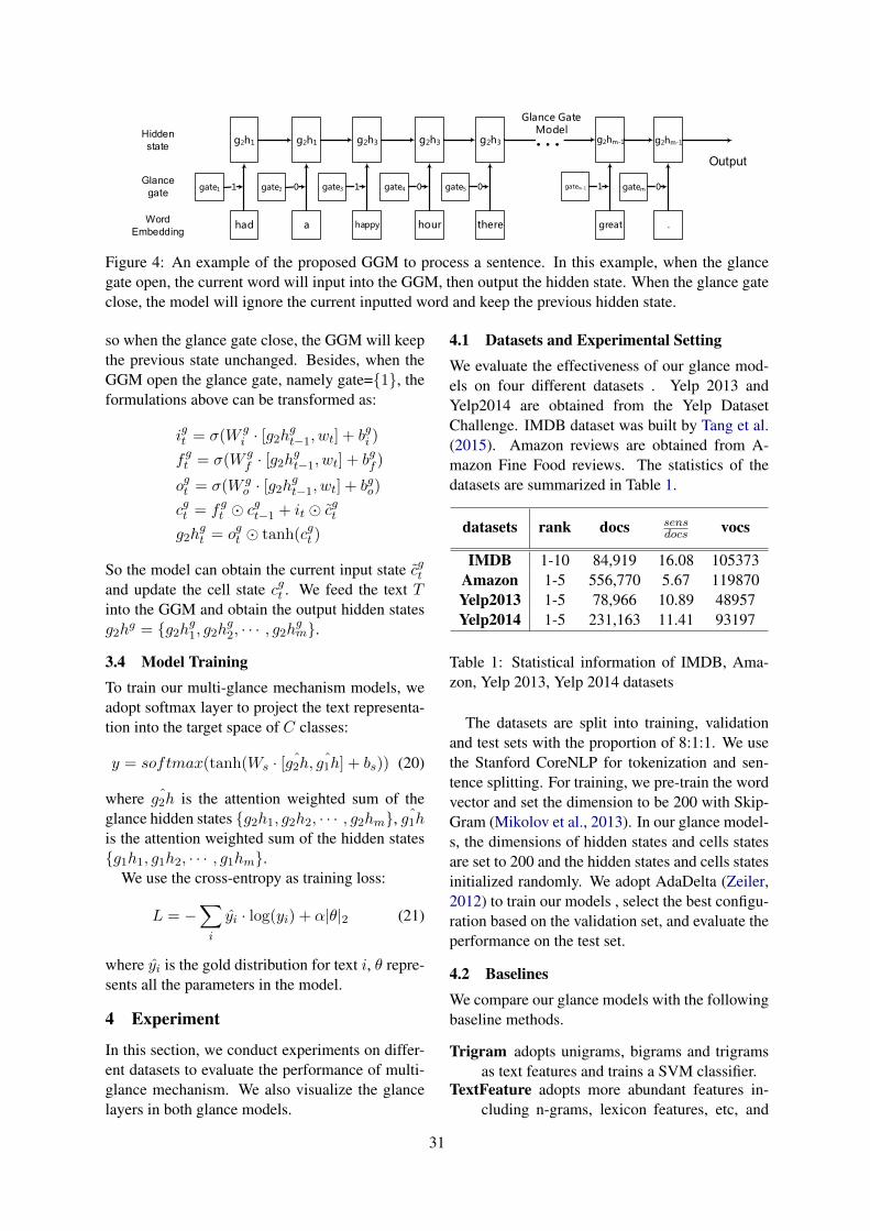
g2h1
had
gate1 1
g2h1
a
gate2 0
g2h3
happy
gate3 1
g2h3
hour
gate4 0
g2h3
there
gate5 0
g2hm-1
great
gatem-1 1
Hidden
state
Glance
gate
Word
Embedding
Output
g2hm-1
.
gatem 0
...
Glance Gate Model
Figure 4: An example of the proposed GGM to process a sentence. In this example, when the glancegate open, the current word will input into the GGM, then output the hidden state. When the glance gateclose, the model will ignore the current inputted word and keep the previous hidden state.
so when the glance gate close, the GGM will keepthe previous state unchanged. Besides, when theGGM open the glance gate, namely gate={1}, theformulations above can be transformed as:
igt = σ(W gi · [g2h
gt−1, wt] + bgi )
fgt = σ(W gf · [g2h
gt−1, wt] + bgf )
ogt = σ(W go · [g2hgt−1, wt] + bgo)
cgt = fgt � cgt−1 + it � cgtg2h
gt = ogt � tanh(cgt )
So the model can obtain the current input state cgtand update the cell state cgt . We feed the text Tinto the GGM and obtain the output hidden statesg2h
g = {g2hg1, g2hg2, · · · , g2hgm}.
3.4 Model TrainingTo train our multi-glance mechanism models, weadopt softmax layer to project the text representa-tion into the target space of C classes:
y = softmax(tanh(Ws · [ ˆg2h, ˆg1h] + bs)) (20)
where ˆg2h is the attention weighted sum of theglance hidden states {g2h1, g2h2, · · · , g2hm}, ˆg1his the attention weighted sum of the hidden states{g1h1, g1h2, · · · , g1hm}.
We use the cross-entropy as training loss:
L = −∑
i
yi · log(yi) + α|θ|2 (21)
where yi is the gold distribution for text i, θ repre-sents all the parameters in the model.
4 Experiment
In this section, we conduct experiments on differ-ent datasets to evaluate the performance of multi-glance mechanism. We also visualize the glancelayers in both glance models.
4.1 Datasets and Experimental SettingWe evaluate the effectiveness of our glance mod-els on four different datasets . Yelp 2013 andYelp2014 are obtained from the Yelp DatasetChallenge. IMDB dataset was built by Tang et al.(2015). Amazon reviews are obtained from A-mazon Fine Food reviews. The statistics of thedatasets are summarized in Table 1.
datasets rank docs sensdocs vocs
IMDB 1-10 84,919 16.08 105373Amazon 1-5 556,770 5.67 119870Yelp2013 1-5 78,966 10.89 48957Yelp2014 1-5 231,163 11.41 93197
Table 1: Statistical information of IMDB, Ama-zon, Yelp 2013, Yelp 2014 datasets
The datasets are split into training, validationand test sets with the proportion of 8:1:1. We usethe Stanford CoreNLP for tokenization and sen-tence splitting. For training, we pre-train the wordvector and set the dimension to be 200 with Skip-Gram (Mikolov et al., 2013). In our glance model-s, the dimensions of hidden states and cells statesare set to 200 and the hidden states and cells statesinitialized randomly. We adopt AdaDelta (Zeiler,2012) to train our models , select the best configu-ration based on the validation set, and evaluate theperformance on the test set.
4.2 BaselinesWe compare our glance models with the followingbaseline methods.
Trigram adopts unigrams, bigrams and trigramsas text features and trains a SVM classifier.
TextFeature adopts more abundant features in-cluding n-grams, lexicon features, etc, and
31
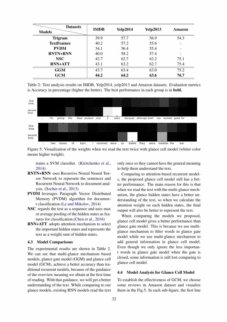
ModelsDatasets IMDB Yelp2014 Yelp2013 Amazon
Trigram 39.9 57.7 56.9 54.3TextFeature 40.2 57.2 55.6 -
PVDM 34.1 56.4 55.4 -RNTN+RNN 40.0 58.2 57.4 -
NSC 42.7 62.7 62.2 75.1RNN+ATT 43.1 63.2 62.7 75.4
GGM 43.7 63.4 63.0 75.2GCM 44.2 64.2 63.6 76.7
Table 2: Text analysis results on IMDB, Yelp2014, yelp2013 and Amazon datasets. Evaluation metricsis Accuracy in percentage (higher the better). The best performance in each group is in bold.
... I'm giving this Xlear product only 2 stars because although itself has worked great for ...
first time
second time
... two boxes of bars i received were so stable they were inedible the bar ...
first time
second time
Figure 5: Visualization of the weights when we read the text twice with glance cell model (whiter colormeans higher weight).
trains a SVM classifier. (Kiritchenko et al.,2014)
RNTN+RNN uses Recursive Neural Neural Ten-sor Network to represent the sentences andRecurrent Neural Network to document anal-ysis. (Socher et al., 2013)
PVDM leverages Paragraph Vector DistributedMemory (PVDM) algorithm for documen-t classification.(Le and Mikolov, 2014)
NSC regards the text as a sequence and uses maxor average pooling of the hidden states as fea-tures for classification.(Chen et al., 2016)
RNN+ATT adopts attention mechanism to selectthe important hidden states and represents thetext as a weight sum of hidden states.
4.3 Model ComparisonsThe experimental results are shown in Table 2.We can see that multi-glance mechanism basedmodels, glance gate model (GGM) and glance cellmodel (GCM), achieve a better accuracy than tra-ditional recurrent models, because of the guidanceof the overview meaning we obtain at the first timeof reading. With that guidance, we will get a betterunderstanding of the text. While comparing to ourglance models, existing RNN models read the text
only once so they cannot have the general meaningto help them understand the text.
Comparing to attention-based recurrent model-s, the proposed glance cell model still has a bet-ter performance. The main reason for this is thatwhen we read the text with the multi-glance mech-anism, the glance hidden states have a better un-derstanding of the text, so when we calculate theattention weight on each hidden states, the finaloutput will also be better to represent the text.
When comparing the models we proposed,glance cell model gives a better performance thanglance gate model. This is because we use multi-glance mechanism to filter words in glance gatemodel while we use multi-glance mechanism toadd general information in glance cell model.Even though we only ignore the less importan-t words in glance gate model when the gate isclosed, some information is still lost comparing toglance cell model.
4.4 Model Analysis for Glance Cell Model
To establish the effectiveness of GCM, we choosesome reviews in Amazon dataset and visualizethem in the Fig.5. In each sub-figure, the first line
32

−1.5 −1.0 −0.5 0.0 0.5 1.0 1.5 2.0−1.5
−1.0
−0.5
0.0
0.5
1.0
1.5
outputGCM hidden statessimple hidden states
(a)
−1.5 −1.0 −0.5 0.0 0.5 1.0 1.5 2.0−1.5
−1.0
−0.5
0.0
0.5
1.0
1.5
outputGCM hidden statessimple hidden states
(b)
Figure 6: Visualization of the hidden states calculated by simple RNN model {g1h1, g1h2, · · · , g1ht}(the purple spots), Glance Cell Model {g2hc1, g2hc2, · · · , g2hct} (the blue spots) and the final text repre-sentation (the red spots).
actually i'm not sure which film was better meet the parents or meet the fockers.
both films were equally enjoyable. this movie is really funny. maybe it's because of a
cast but everything works in this film. it's probably one of the best comedies made in this
decade. Dustin Hoffman and Barbra Streisand both did great as Gaylord's parents. every
character of this movie had it's own opinion and that was well portrayed in their dialogs.
not like the original, this part is more making fun of Robert de Nero's character than of
Ben Stiller 's character. i noticed that this film has many similarities with it's prequel but
that's ok because it still was very funny.
Figure 7: Visualization of the gate state in Glance Gate Model. The words in color (blue and red) areinput into the GGM, that meas the gate state is open. The words in gray are ignored by the GGM.
is the visualization of the weights when we readthe text at the first time, the second line is the vi-sualization that we read at the second time. Notethat, whiter color means higher weight.
As shown in Fig.5, the first review has wrotethe ranking stars in the text, which is a determin-ing factor in product reviews, but we ignore themwhen we read at the first time. Well, with the guid-ance of multi-glance mechanism, when we readthem again, we can not only find the ranking stars,but also give them high weights.
In the second review, comparing the results weread at the first time and the second time, thoughwe may focus on some of the same words, e.g.inedible, we will give them different weights. Wecan observe that when reading at the second time,we give word ‘inedible’ a higher weight and word‘the’ a lower the weight. The glance cell modelcan increase the weights of important words, sowe can focus on more useful words when usingmulti-glance mechanism and glance cell model.
Next, we also choose two reviews in the datasetand visualize the hidden states which calculated bythe glance cell model and a traditional recurren-
t model. As aforementioned in this paper, whenusing multi-glance mechanism, we will get the lo-cal information comparing to simple RNN model-s. As shown in Fig.6, the purple spots and the bluespots are the visualizations of the hidden states,and the purple spots belong to the simple RNNmodel while the blue spots belong to the glancecell model. The spot in red is the visualization ofthe final text representation. Note that, we use P-CA to reduce the dimensions of the hidden stateshere. We can see that the blue spots are much morecloser to the red spots than the purple spots, whichmean the glance cell hidden states are more clos-er to the final text representations. It is the localinformation that makes the difference. So we canobtain a more general idea when using the glancecell model we proposed.
4.5 Model Analysis for Glance Gate Model
To demonstrate the effectiveness of the glance gatemodel, we choose a review in IMDB dataset andvisualize the values of gates. As mentioned in thispaper, the gates only have two states, closed andopen. As shown in Fig. 7, the words in gray mean
33
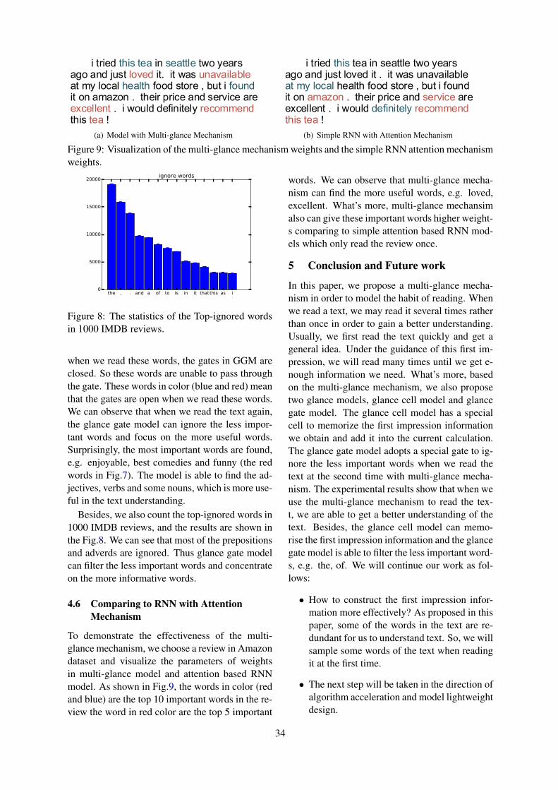
i tried this tea in seattle two years ago and just loved it. it was unavailable at my local health food store , but i found it on amazon . their price and service are excellent . i would definitely recommend this tea !
(a) Model with Multi-glance Mechanism
i tried this tea in seattle two years ago and just loved it . it was unavailable at my local health food store , but i found it on amazon . their price and service are excellent . i would definitely recommend this tea !
(b) Simple RNN with Attention Mechanism
Figure 9: Visualization of the multi-glance mechanism weights and the simple RNN attention mechanismweights.
the , . and a of to is in it thatthis as i0
5000
10000
15000
20000ignore words
Figure 8: The statistics of the Top-ignored wordsin 1000 IMDB reviews.
when we read these words, the gates in GGM areclosed. So these words are unable to pass throughthe gate. These words in color (blue and red) meanthat the gates are open when we read these words.We can observe that when we read the text again,the glance gate model can ignore the less impor-tant words and focus on the more useful words.Surprisingly, the most important words are found,e.g. enjoyable, best comedies and funny (the redwords in Fig.7). The model is able to find the ad-jectives, verbs and some nouns, which is more use-ful in the text understanding.
Besides, we also count the top-ignored words in1000 IMDB reviews, and the results are shown inthe Fig.8. We can see that most of the prepositionsand adverds are ignored. Thus glance gate modelcan filter the less important words and concentrateon the more informative words.
4.6 Comparing to RNN with AttentionMechanism
To demonstrate the effectiveness of the multi-glance mechanism, we choose a review in Amazondataset and visualize the parameters of weightsin multi-glance model and attention based RNNmodel. As shown in Fig.9, the words in color (redand blue) are the top 10 important words in the re-view the word in red color are the top 5 important
words. We can observe that multi-glance mecha-nism can find the more useful words, e.g. loved,excellent. What’s more, multi-glance mechansimalso can give these important words higher weight-s comparing to simple attention based RNN mod-els which only read the review once.
5 Conclusion and Future work
In this paper, we propose a multi-glance mecha-nism in order to model the habit of reading. Whenwe read a text, we may read it several times ratherthan once in order to gain a better understanding.Usually, we first read the text quickly and get ageneral idea. Under the guidance of this first im-pression, we will read many times until we get e-nough information we need. What’s more, basedon the multi-glance mechanism, we also proposetwo glance models, glance cell model and glancegate model. The glance cell model has a specialcell to memorize the first impression informationwe obtain and add it into the current calculation.The glance gate model adopts a special gate to ig-nore the less important words when we read thetext at the second time with multi-glance mecha-nism. The experimental results show that when weuse the multi-glance mechanism to read the tex-t, we are able to get a better understanding of thetext. Besides, the glance cell model can memo-rise the first impression information and the glancegate model is able to filter the less important word-s, e.g. the, of. We will continue our work as fol-lows:
• How to construct the first impression infor-mation more effectively? As proposed in thispaper, some of the words in the text are re-dundant for us to understand text. So, we willsample some words of the text when readingit at the first time.
• The next step will be taken in the direction ofalgorithm acceleration and model lightweightdesign.
34
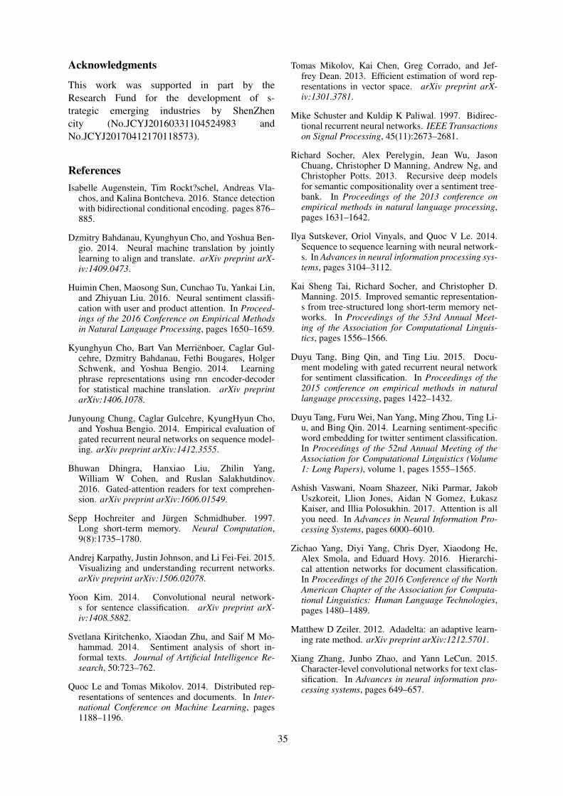
Acknowledgments
This work was supported in part by theResearch Fund for the development of s-trategic emerging industries by ShenZhencity (No.JCYJ20160331104524983 andNo.JCYJ20170412170118573).
ReferencesIsabelle Augenstein, Tim Rockt?schel, Andreas Vla-
chos, and Kalina Bontcheva. 2016. Stance detectionwith bidirectional conditional encoding. pages 876–885.
Dzmitry Bahdanau, Kyunghyun Cho, and Yoshua Ben-gio. 2014. Neural machine translation by jointlylearning to align and translate. arXiv preprint arX-iv:1409.0473.
Huimin Chen, Maosong Sun, Cunchao Tu, Yankai Lin,and Zhiyuan Liu. 2016. Neural sentiment classifi-cation with user and product attention. In Proceed-ings of the 2016 Conference on Empirical Methodsin Natural Language Processing, pages 1650–1659.
Kyunghyun Cho, Bart Van Merrienboer, Caglar Gul-cehre, Dzmitry Bahdanau, Fethi Bougares, HolgerSchwenk, and Yoshua Bengio. 2014. Learningphrase representations using rnn encoder-decoderfor statistical machine translation. arXiv preprintarXiv:1406.1078.
Junyoung Chung, Caglar Gulcehre, KyungHyun Cho,and Yoshua Bengio. 2014. Empirical evaluation ofgated recurrent neural networks on sequence model-ing. arXiv preprint arXiv:1412.3555.
Bhuwan Dhingra, Hanxiao Liu, Zhilin Yang,William W Cohen, and Ruslan Salakhutdinov.2016. Gated-attention readers for text comprehen-sion. arXiv preprint arXiv:1606.01549.
Sepp Hochreiter and Jurgen Schmidhuber. 1997.Long short-term memory. Neural Computation,9(8):1735–1780.
Andrej Karpathy, Justin Johnson, and Li Fei-Fei. 2015.Visualizing and understanding recurrent networks.arXiv preprint arXiv:1506.02078.
Yoon Kim. 2014. Convolutional neural network-s for sentence classification. arXiv preprint arX-iv:1408.5882.
Svetlana Kiritchenko, Xiaodan Zhu, and Saif M Mo-hammad. 2014. Sentiment analysis of short in-formal texts. Journal of Artificial Intelligence Re-search, 50:723–762.
Quoc Le and Tomas Mikolov. 2014. Distributed rep-resentations of sentences and documents. In Inter-national Conference on Machine Learning, pages1188–1196.
Tomas Mikolov, Kai Chen, Greg Corrado, and Jef-frey Dean. 2013. Efficient estimation of word rep-resentations in vector space. arXiv preprint arX-iv:1301.3781.
Mike Schuster and Kuldip K Paliwal. 1997. Bidirec-tional recurrent neural networks. IEEE Transactionson Signal Processing, 45(11):2673–2681.
Richard Socher, Alex Perelygin, Jean Wu, JasonChuang, Christopher D Manning, Andrew Ng, andChristopher Potts. 2013. Recursive deep modelsfor semantic compositionality over a sentiment tree-bank. In Proceedings of the 2013 conference onempirical methods in natural language processing,pages 1631–1642.
Ilya Sutskever, Oriol Vinyals, and Quoc V Le. 2014.Sequence to sequence learning with neural network-s. In Advances in neural information processing sys-tems, pages 3104–3112.
Kai Sheng Tai, Richard Socher, and Christopher D.Manning. 2015. Improved semantic representation-s from tree-structured long short-term memory net-works. In Proceedings of the 53rd Annual Meet-ing of the Association for Computational Linguis-tics, pages 1556–1566.
Duyu Tang, Bing Qin, and Ting Liu. 2015. Docu-ment modeling with gated recurrent neural networkfor sentiment classification. In Proceedings of the2015 conference on empirical methods in naturallanguage processing, pages 1422–1432.
Duyu Tang, Furu Wei, Nan Yang, Ming Zhou, Ting Li-u, and Bing Qin. 2014. Learning sentiment-specificword embedding for twitter sentiment classification.In Proceedings of the 52nd Annual Meeting of theAssociation for Computational Linguistics (Volume1: Long Papers), volume 1, pages 1555–1565.
Ashish Vaswani, Noam Shazeer, Niki Parmar, JakobUszkoreit, Llion Jones, Aidan N Gomez, ŁukaszKaiser, and Illia Polosukhin. 2017. Attention is allyou need. In Advances in Neural Information Pro-cessing Systems, pages 6000–6010.
Zichao Yang, Diyi Yang, Chris Dyer, Xiaodong He,Alex Smola, and Eduard Hovy. 2016. Hierarchi-cal attention networks for document classification.In Proceedings of the 2016 Conference of the NorthAmerican Chapter of the Association for Computa-tional Linguistics: Human Language Technologies,pages 1480–1489.
Matthew D Zeiler. 2012. Adadelta: an adaptive learn-ing rate method. arXiv preprint arXiv:1212.5701.
Xiang Zhang, Junbo Zhao, and Yann LeCun. 2015.Character-level convolutional networks for text clas-sification. In Advances in neural information pro-cessing systems, pages 649–657.
35

Proceedings of the Eighth Workshop on Cognitive Aspects of Computational Language Learning and Processing, pages 36–40Melbourne, Australia, July 19, 2018. c©2018 Association for Computational Linguistics
Predicting Japanese Word Order in Double Object Constructions
Masayuki AsaharaNational Institute for Japanese
Language and Linguistics, Japan
Center for Corpus Development
Satoshi NambuMonash University, Australia
School of Languages, Literatures,
Cultures and Linguistics
Shin-Ichiro SanoKeio University, Japan
Faculty of Business and Commerce
Abstract
This paper presents a statistical model topredict Japanese word order in the dou-ble object constructions. We employed aBayesian linear mixed model with man-ually annotated predicate-argument struc-ture data. The findings from the refinedcorpus analysis confirmed the effects ofinformation status of an NP as ‘given-new ordering’ in addition to the effects of‘long-before-short’ as a tendency of thegeneral Japanese word order.
1 Introduction
Because Japanese exhibits a flexible word order,potential factors that predict word orders of agiven construction in Japanese have been recentlydelved into, particularly in the field of compu-tational linguistics (Yamashita and Kondo, 2011;Orita, 2017). One of the major findings relevant tothe current study is ‘long-before-short’, wherebya long noun phrase (NP) tends to be scrambledahead of a short NP (Yamashita and Chang, 2001).
This paper sheds light on those factors in dou-ble object constructions (DOC), where either (1)an indirect object (IOBJ) or (2) a direct object(DOBJ) can precede the other object:
(1) Taro-gaTaro-SBJ
Hanako-niHanako-IOBJ
hon-obook-DOBJ
ageta.gave
‘Taro gave Hanako a book.’
(2) Taro-gaTaro-SBJ
hon-obook-DOBJ
Hanako-niHanako-IOBJ
ageta.gave
‘Taro gave Hanako a book.’
Since both of the word orders are available,studies in theoretical syntax have been disputingabout what is the canonical word order under thehypothesis of deriving one word order (i.e., either
IOBJ-DOBJ or DOBJ-IOBJ) from another in thecontext of derivational syntax (Hoji, 1985; Miya-gawa, 1997; Matsuoka, 2003). In this paper, we donot attempt to adjudicate upon the dispute solelybased on the frequency of the two word orders ina corpus, but aim to detect principal factors thatpredict the word order in the DOC, which mayeventually lead to resolving the issue in theoreti-cal syntax. To that end, we employed a Bayesianlinear mixed model with potential factors affectingthe word orders as a preliminary study.
Other than the factor ‘long-before-short’ pro-posed in previous studies, the key factor in thecurrent study is an information status of an NPin a given context under the theoretical frame-work of information structure (Lambrecht, 1994;Vallduvı and Engdahl, 1996). The frameworkprovides us key categories, such as (information-ally) given/old, new, topic, and focus, to classifyan NP as how it functions in a particular con-text. We assume the information status as oneof the principle predictors based on the followingtwo reasons; (i) a discourse-given element tendsto precede a discourse-new one in a sentence inJapanese (Kuno, 1978, 2004; Nakagawa, 2016),(ii) focused or new elements in Japanese tend toappear in a position immediately preceding thepredicate (Kuno, 1978; Kim, 1988; Ishihara, 2001;Vermeulen, 2012). These two claims regarding thegeneral word order of Japanese are combined intothe following hypothesis regarding the word or-ders in the DOC.
(3) Our hypothesis:In the DOC, a discourse-given objecttends to appear on the left of the other ob-ject, and a discourse-new object tends tobe on the right side.
Incorporating the information status of an NPwith another factor ‘long-before-short’ proposedin the previous studies, we built a statistical model
36
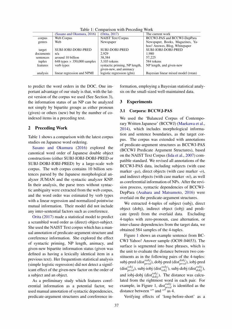
Table 1: Comparison with Preceding Work(Sasano and Okumura, 2016) (Orita, 2017) The current work
corpus Web Corpus NAIST Text Corpus BCCWJ-PAS and BCCWJ-DepParagenres Web Newspaper Newspaper, Books, Magazines, Ya-
hoo! Answes, Blog, Whitepapertarget SUBJ-IOBJ-DOBJ-PRED SUBJ-DOBJ-PRED SUBJ-IOBJ-DOBJ-PRED
documents n/a 2,929 1,980sentences around 10 billion 38,384 57,225
tuples 648 types × 350,000 samples 3,103 tokens 584 tokensfeatures verb types syntactic priming, NP length,
given-new, and animacyNP length, and given-new
analysis linear regression and NPMI logistic regression (glm) Bayesian linear mixed model (rstan)
to predict the word orders in the DOC. One im-portant advantage of our study is that, with the lat-est version of the corpus we used (See Section 3),the information status of an NP can be analyzednot simply by bipartite groups as either pronoun(given) or others (new) but by the number of co-indexed items in a preceding text.
2 Preceding Work
Table 1 shows a comparison with the latest corpusstudies on Japanese word ordering.
Sasano and Okumura (2016) explored thecanonical word order of Japanese double objectconstructions (either SUBJ-IOBJ-DOBJ-PRED orSUBJ-DOBJ-IOBJ-PRED) by a large-scale webcorpus. The web corpus contains 10 billion sen-tences parsed by the Japanese morphological an-alyzer JUMAN and the syntactic analyzer KNP.In their analysis, the parse trees without syntac-tic ambiguity were extracted from the web corpus,and the word order was estimated by verb typeswith a linear regression and normalized pointwisemutual information. Their model did not includeany inter-sentential factors such as coreference.
Orita (2017) made a statistical model to predicta scrambled word order as (direct) object-subject.She used the NAIST Text corpus which has a man-ual annotation of predicate-argument structure andcoreference information. She explored the effectof syntactic priming, NP length, animacy, andgiven-new bipartite information status (given wasdefined as having a lexically identical item in aprevious text). Her frequentism statistical analysis(simple logistic regression) did not detect a signif-icant effect of the given-new factor on the order ofa subject and an object.
As a preliminary study which features coref-erential information as a potential factor, weused manual annotation of syntactic dependencies,predicate-argument structures and coreference in-
formation, employing a Bayesian statistical analy-sis on the small-sized well-maintained data.
3 Experiments
3.1 Corpora: BCCWJ-PAS
We used the ‘Balanced Corpus of Contempo-rary Written Japanese’ (BCCWJ) (Maekawa et al.,2014), which includes morphological informa-tion and sentence boundaries, as the target cor-pus. The corpus was extended with annotationsof predicate-argument structures as BCCWJ-PAS(BCCWJ Predicate Argument Structures), basedon the NAIST Text Corpus (Iida et al., 2007) com-patible standard. We revised all annotations of theBCCWJ-PAS data, including subjects (with casemarker -ga), direct objects (with case marker -o),and indirect objects (with case marker -ni), as wellas coreferential information of NPs. After the revi-sion process, syntactic dependencies of BCCWJ-DepPara (Asahara and Matsumoto, 2016) wereoverlaid on the predicate-argument structures.
We extracted 4-tuples of subject (subj), directobject (dobj), indirect object (iobj) and predi-cate (pred) from the overlaid data. Excluding4-tuples with zero-pronoun, case alternation, orinter-clause dependencies from the target data, weobtained 584 samples of the 4-tuples.
Figure 1 shows an example sentence from BC-CWJ Yahoo! Answer sample (OC09 04653). Thesurface is segmented into base phrases, which isthe unit to evaluate the distance between two con-stituents as in the following pairs of the 4-tuples:subj-pred (distsubjpred), dobj-pred (distdobjpred), iobj-pred
(distiobjpred), subj-iobj (distsubjiobj ), subj-dobj (distsubjdobj ),
and iobj-dobj (distiobjdobj). The distance was calcu-lated from the rightmost word in each pair. Forexample, in Figure 1, distsubjpred is identified as thedistance between “” and “” as 4.
Verifying effects of ‘long-before-short’ as a
37
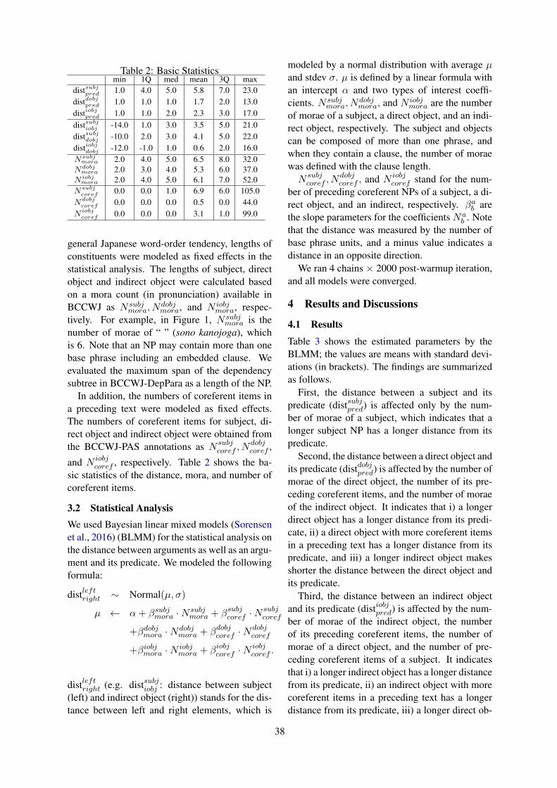
Table 2: Basic Statisticsmin 1Q med mean 3Q max
distsubjpred 1.0 4.0 5.0 5.8 7.0 23.0distdobjpred 1.0 1.0 1.0 1.7 2.0 13.0distiobjpred 1.0 1.0 2.0 2.3 3.0 17.0distsubjiobj -14.0 1.0 3.0 3.5 5.0 21.0distsubjdobj -10.0 2.0 3.0 4.1 5.0 22.0distiobjdobj -12.0 -1.0 1.0 0.6 2.0 16.0Nsubj
mora 2.0 4.0 5.0 6.5 8.0 32.0Ndobj
mora 2.0 3.0 4.0 5.3 6.0 37.0N iobj
mora 2.0 4.0 5.0 6.1 7.0 52.0Nsubj
coref 0.0 0.0 1.0 6.9 6.0 105.0Ndobj
coref 0.0 0.0 0.0 0.5 0.0 44.0N iobj
coref 0.0 0.0 0.0 3.1 1.0 99.0
general Japanese word-order tendency, lengths ofconstituents were modeled as fixed effects in thestatistical analysis. The lengths of subject, directobject and indirect object were calculated basedon a mora count (in pronunciation) available inBCCWJ as N subj
mora, Ndobjmora, and N iobj
mora, respec-tively. For example, in Figure 1, N subj
mora is thenumber of morae of “ ” (sono kanojoga), whichis 6. Note that an NP may contain more than onebase phrase including an embedded clause. Weevaluated the maximum span of the dependencysubtree in BCCWJ-DepPara as a length of the NP.
In addition, the numbers of coreferent items ina preceding text were modeled as fixed effects.The numbers of coreferent items for subject, di-rect object and indirect object were obtained fromthe BCCWJ-PAS annotations as N subj
coref , Ndobjcoref ,
and N iobjcoref , respectively. Table 2 shows the ba-
sic statistics of the distance, mora, and number ofcoreferent items.
3.2 Statistical AnalysisWe used Bayesian linear mixed models (Sorensenet al., 2016) (BLMM) for the statistical analysis onthe distance between arguments as well as an argu-ment and its predicate. We modeled the followingformula:
distleftright ∼ Normal(µ, σ)
µ ← α+ βsubjmora ·N subjmora + βsubjcoref ·N
subjcoref
+βdobjmora ·Ndobjmora + βdobjcoref ·N
dobjcoref
+βiobjmora ·N iobjmora + βiobjcoref ·N
iobjcoref .
distleftright (e.g. distsubjiobj : distance between subject(left) and indirect object (right)) stands for the dis-tance between left and right elements, which is
modeled by a normal distribution with average µand stdev σ. µ is defined by a linear formula withan intercept α and two types of interest coeffi-cients. N subj
mora, Ndobjmora, and N iobj
mora are the numberof morae of a subject, a direct object, and an indi-rect object, respectively. The subject and objectscan be composed of more than one phrase, andwhen they contain a clause, the number of moraewas defined with the clause length.N subj
coref , Ndobjcoref , and N iobj
coref stand for the num-ber of preceding coreferent NPs of a subject, a di-rect object, and an indirect, respectively. βab arethe slope parameters for the coefficients Na
b . Notethat the distance was measured by the number ofbase phrase units, and a minus value indicates adistance in an opposite direction.
We ran 4 chains × 2000 post-warmup iteration,and all models were converged.
4 Results and Discussions
4.1 Results
Table 3 shows the estimated parameters by theBLMM; the values are means with standard devi-ations (in brackets). The findings are summarizedas follows.
First, the distance between a subject and itspredicate (distsubjpred) is affected only by the num-ber of morae of a subject, which indicates that alonger subject NP has a longer distance from itspredicate.
Second, the distance between a direct object andits predicate (distdobjpred) is affected by the number ofmorae of the direct object, the number of its pre-ceding coreferent items, and the number of moraeof the indirect object. It indicates that i) a longerdirect object has a longer distance from its predi-cate, ii) a direct object with more coreferent itemsin a preceding text has a longer distance from itspredicate, and iii) a longer indirect object makesshorter the distance between the direct object andits predicate.
Third, the distance between an indirect objectand its predicate (distiobjpred) is affected by the num-ber of morae of the indirect object, the numberof its preceding coreferent items, the number ofmorae of a direct object, and the number of pre-ceding coreferent items of a subject. It indicatesthat i) a longer indirect object has a longer distancefrom its predicate, ii) an indirect object with morecoreferent items in a preceding text has a longerdistance from its predicate, iii) a longer direct ob-
38
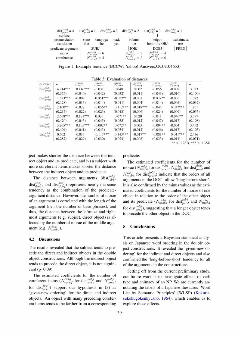
distsubjpred = 4 distdobjpred = 1 distiobjpred = 2 distsubjiobj = 2 distsubjdobj = 3 distiobjdobj = 1surface ł
pronunciation sono kanojoga mada bokuni keigoo tsukaimasutranslation that she yet me honorific-OBJ use
predicate-argument SUBJ IOBJ DOBJ PREDmorae Nsubj
mora = 6 N iobjmora = 3 Ndobj
mora = 4
coreference Nsubjcoref = 2 N iobj
coref = 3 Ndobjcoref = 0
Figure 1: Example sentence (BCCWJ Yahoo! Answers:OC09 04653)
Table 3: Evaluation of distancesdistance α βsubj
mora βdobjmora βiobj
mora βsubjcoref βdobj
coref βiobjcoref σ
distsubjpred 4.814*** 0.146*** -0.031 0.040 0.002 -0.056 -0.009 3.323(0.375) (0.040) (0.042) (0.032) (0.011) (0.043) (0.016) (0.100)
distdobjpred 1.593*** -0.009 0.061*** -0.032** -0.001 0.037** -0.005 1.072(0.128) (0.013) (0.014) (0.011) (0.004) (0.014) (0.005) (0.032)
distiobjpred 2.100** -0.022 -0.056** 0.112*** -0.018*** -0.045 0.037*** 1.861(0.217) (0.022) (0.023) (0.018) (0.006) (0.024) (0.009) (0.055)
distsubjiobj 2.668*** 0.171*** 0.026 0.071** 0.020 -0.011 -0.046** 3.577(0.420) (0.043) (0.045) (0.035) (0.012) (0.047) (0.017) (0.108)
distsubjdobj 3.205*** 0.155*** -0.092** 0.072** 0.003 -0.094** -0.004 3.452(0.404) (0.041) (0.043) (0.034) (0.012) (0.046) (0.017) (0.103)
distiobjdobj 0.502 -0.013 -0.117*** 0.143*** -0.017** -0.081** 0.041*** 2.436(0.287) (0.029) (0.030) (0.024) (0.008) (0.033) (0.011) (0.071)
** > ±2SD, *** > ±3SD
ject makes shorter the distance between the indi-rect object and its predicate, and iv) a subject withmore coreferent items makes shorter the distancebetween the indirect object and its predicate.
The distance between arguments (distsubjiobj ,
distsubjdobj , and distiobjdobj) represents nearly the sametendency as the combination of the predicate-argument distance. However, the number of moraeof an argument is correlated with the length of theargument (i.e., the number of base phrases), andthus, the distance between the leftmost and right-most arguments (e.g. subject, direct object) is af-fected by the number of morae of the middle argu-ment (e.g. N iobj
mora).
4.2 Discussions
The results revealed that the subject tends to pre-cede the direct and indirect objects in the doubleobject constructions. Although the indirect objecttends to precede the direct object, it is not signifi-cant (p=0.09).
The estimated coefficients for the number ofcoreferent items (Ndobj
coref for distdobjpred and N iobjcoref
for distiobjpred) support our hypothesis in (3) as‘given-new ordering’ for the direct and indirectobjects. An object with many preceding corefer-ent items tends to be farther from a corresponding
predicate.The estimated coefficients for the number of
morae (N subjmora for distsubjpred, Ndobj
mora for distdobjpred and
N iobjmora for distiobjpred) indicate that the orders of all
arguments in the DOC follow ‘long-before-short’.It is also confirmed by the minus values as the esti-mated coefficients for the number of morae of oneobject in relation to the order of the other objectand its predicate (Ndobj
mora for distiobjpred and N iobjmora
for distdobjpred), suggesting that a longer object tendsto precede the other object in the DOC.
5 Conclusions
This article presents a Bayesian statistical analy-sis on Japanese word ordering in the double ob-ject constructions. It revealed the ‘given-new or-dering’ for the indirect and direct objects and alsoconfirmed the ‘long-before-short’ tendency for allof the arguments in the constructions.
Setting off from the current preliminary study,our future work is to investigate effects of verbtype and animacy of an NP. We are currently an-notating the labels of a Japanese thesaurus ‘WordList by Semantic Principles’ (WLSP) (Kokurit-sukokugokenkyusho, 1964), which enables us toexplore those effects.
39

Acknowledgments
This work was supported by JSPS KAKENHIGrants Numbers JP15K12888 and JP17H00917and is a project of the Center for Corpus Devel-opment, NINJAL.
ReferencesMasayuki Asahara and Yuji Matsumoto. 2016.
BCCWJ-DepPara: A Syntactic Annotation Tree-bank on the ‘Balanced Corpus of ContemporaryWritten Japanese’. In Proceedings of the 12thWorkshop on Asian Language Resources (ALR12),pages 49–58, Osaka, Japan. The COLING 2016Organizing Committee.
Hajime Hoji. 1985. Logical Form Constraints andConfigurational Structures in Japanese. Ph.D. the-sis, University of Washington.
Ryu Iida, Mamoru Komachi, Kentaro Inui, and YujiMatsumoto. 2007. Annotating a Japanese Text Cor-pus with Predicate-Argument and Coreference Re-lations. In Proceedings of the Linguistic AnnotationWorkshop, pages 132–139, Prague, Czech Republic.Association for Computational Linguistics.
Shin-ichiro Ishihara. 2001. Stress, focus, and scram-bling in japanese. In Ora Matushansky Elena Guer-zoni, editor, MITWPL 39, pages 142–175. Cam-bridge, MA: MITWPL.
Alan Hyun-Oak Kim. 1988. Preverbal focusing andtype xxiii languages. In Jessica Wirth Michael Ham-mond, Edith A. Moravcsik, editor, Studies in syn-tactic typology, pages 147–169. Amsterdam: JohnBenjamins.
Kokuritsukokugokenkyusho, editor. 1964. Bunruigoi-hyo [Word List by Semantic Principles]. ShueiShuppan.
Susumu Kuno. 1978. Danwa no bunpoo [Grammar ofdiscourse]. Taishukan Shoten, Tokyo.
Susumu Kuno. 2004. Empathy and direct discourseperspectives. In Lawrence Horn and Gregory Ward,editors, The handbook of pragmatics, pages 315–343. Oxford: Blackwell.
Knud Lambrecht. 1994. Information Structure andSentence Form: Topic, Focus, and the Mental Rep-resentations of Discourse Referents, volume 71 ofCambridge Studies in Linguistics. Cambridge Uni-versity Press.
Kikuo Maekawa, Makoto Yamazaki, ToshinobuOgiso, Takehiko Maruyama, Hideki Ogura, WakakoKashino, Hanae Koiso, Masaya Yamaguchi, MakiroTanaka, and Yasuharu Den. 2014. Balanced Corpusof Contemporary Written Japanese. Language Re-sources and Evaluation, 48:345–371.
Mikinari Matsuoka. 2003. Two types of ditransitiveconstructions in japanese. Journal of East AsianLinguistics, 12:171–203.
Shigeru Miyagawa. 1997. Against optional scram-bling. Linguistic Inquiry, 28:1–26.
Natsuko Nakagawa. 2016. Information Structure inSpoken Japanese: Particles, word order, and into-nation. Ph.D. thesis, Kyoto University.
Naho Orita. 2017. Predicting Japanese scrambling inthe wild. In Proceedings of the 7th Workshop onCognitive Modeling and Computational Linguistics(CMCL 2017), pages 41–45, Valencia, Spain. Asso-ciation for Computational Linguistics.
Ryohei Sasano and Manabu Okumura. 2016. ACorpus-Based Analysis of Canonical Word Order ofJapanese Double Object Constructions. In Proceed-ings of the 54th Annual Meeting of the Associationfor Computational Linguistics (Volume 1: Long Pa-pers), pages 2236–2244, Berlin, Germany. Associa-tion for Computational Linguistics.
Tanner Sorensen, Sven Hohenstein, and Shravan Va-sishth. 2016. Bayesian linear mixed models usingstan: A tutorial for psychologists, linguists, and cog-nitive scientists. Quantitative Methods for Psychol-ogy, 12(3):175–200.
Enric Vallduvı and Elisabet Engdahl. 1996. The lin-guistic realization of information packaging. Lin-guistics, 34(3):459–520.
Reiko Vermeulen. 2012. The information structure ofjapanese. In Renate Musan Manfred Krifka, editor,The expression of information structure, pages 187–216. Berlin: De Gruyter Mouton.
Hiroko Yamashita and Franklin Chang. 2001. “LongBefore Short” Preference in the Production of aHead-final Language. Cognition, 81(2):B45–B55.
Hiroko Yamashita and Tadahisa Kondo. 2011. Lin-guistic constraints and long-before-short tendency.In IEICE Technocal report (TL), TL2011-19, pages61–65.
40
Proceedings of the Eighth Workshop on Cognitive Aspects of Computational Language Learning and Processing, pages 41–46Melbourne, Australia, July 19, 2018. c©2018 Association for Computational Linguistics
Affordances in Grounded Language Learning
Stephen McGregor KyungTae LimLATTICE - CNRS & École normale supérieure / PSL
Université Sorbonne nouvelle Paris 3 / USPC1, rue Maurice Arnoux, 92120 Montrouge, France
[email protected] [email protected]
Abstract
We present a novel methodology involv-ing mappings between different modes ofsemantic representations. We propose dis-tributional semantic models as a mecha-nism for representing the kind of worldknowledge inherent in the system of ab-stract symbols characteristic of a sophisti-cated community of language users. Then,motivated by insight from ecological psy-chology, we describe a model approximat-ing affordances, by which we mean a lan-guage learner’s direct perception of op-portunities for action in an environment.We present a preliminary experiment in-volving mapping between these two rep-resentational modalities, and propose thatour methodology can become the basis fora cognitively inspired model of groundedlanguage learning.
1 Introduction
Computational approaches to grounded languagelearning have typically involved mapping fromperceptual to linguistic modalities through the ap-plication of complex information processing oper-ations. Yu and Siskind (2013), for instance, usehidden Markov models to translate from objecttracks to natural language descriptions of eventobserved in video clips. Likewise the ImageNetdatabase has provided a platform for the produc-tive application of deep neural network architec-tures for mapping between images and natural lan-guage labels (Krizhevsky et al., 2012). Signifi-cantly with regard to the ideas outlined here, Ohet al. (2017) describe a methodology for trainingan agent to construct novel sequences of actionsbased on analogies with previously learned strate-gies; the mechanism for learning a vocabulary of
basic actions consists of a combination of convo-lutional and LSTM layers within a neural network.
Work of this nature highlights the state of the artin modelling technologies, and as an informationengineering approach to meaningful tasks such asquestion answering and image labelling a signifi-cant contribution is made. This is arguably done,however, at the expense of presenting interpretableor indeed plausible models of the way that envi-ronmentally embedded agents use relatively scantexposure to a language speaking community in or-der to develop a lexicon that is rich and produc-tive. In this regard, the conventional computa-tional stance on grounded language learning em-braces a view of the relationship between languageand the world as a symbol grounding problem, bywhich abstract symbols susceptible to formal op-erations are somehow associated with perceptionsand propositions: the hard work is done by a com-plex and philosophically opaque process of trans-forming signals into symbols, with the sense thatcomputation by way of deep nets in some sensestands in for an inscrutable mind-brain gestalt.
As an alternative to this approach, Raczaszek-Leonardi et al. (2018) propose a symbol unground-ing problem: by this account, language beginsas a semiotic structure with the representationalscheme of a nascent language learner iconicallyand indexically aligned to embodied and embed-ded experiences of the world. This alignment isunderstood in terms of Gibson’s (1979) notion ofaffordances, which we take to mean the direct per-ception of opportunities for action in an environ-ment. The connection of language to opportuni-ties for taking action on objects (and indeed theperception of language itself as an affordance forcommunication) creates a framework for under-standing how abstract symbols begin as groundedcomplexes of multi-modal interactions with a lan-guage teacher and then gradually emerge as con-
41
straints on the way that a cognitive agent behavesin an environment (Raczaszek-Leonardi, 2012).
The strength of thinking of perception in gen-eral and language in particular in terms of affor-dances is that this moves away from the prob-lem of the computational load associated with thespontaneous construction of contextually produc-tive representational structures. For Clark (1997),affordances play a role in the an action-orientedmodel of cognition revolving around light-weight,environmentally situated representations, whileChemero (2009) proposes affordances as a mecha-nism for resolving the issue of the mental gymnas-tics inherent in a computational cognitive model.These approaches, which seek to place mind inthe context of environmental embodiment and em-beddedness, prefigure recent attempts to intro-duce affordances as a component of a cognitivelyoriented theory of language in which words canbe mapped to denotations oriented towards ac-tion on objects in situations, and utterances them-selves become opportunities for communication(Raczaszek-Leonardi and Nomikou, 2015).
Despite these valuable theoretical contributions,affordances have proved resistant to empiricalmodelling, not least because it is difficult to comeup with a tractable scheme for representing a cog-nitive feature that is specifically conceived as anantidote to representational approaches to cogni-tion. Our present objective is to begin to mapa way towards the computational simulation ofthe role of affordances in language acquisitionthrough interaction with an established linguis-tic community. In order to do this, we’ll extractboth statistical and syntactic information from alarge-scale corpus to model two different modesof semantic representation, one geared towards thekind of world-knowledge inherent in the evolu-tion of language on the time-scale of a commu-nity of language users, the other designed to reflectthe way that an agent might encounter languagegrounded in the affordances of denoted objects.
In as much as we will be combining establisheddistributional semantic techniques with likewiseestablished syntactic analysis, this work can bebroadly positioned in the context of other recentmodels. Cheng and Kartsaklis (2015), for in-stance, compound co-occurrence and syntacticalinformation in order to generate word-embeddingsenhanced for compositional tasks. Vulic (2017)likewise uses information about dependency re-
lationships to map word embeddings from multi-ple languages into a shared vector space, achiev-ing impressive results on cross-lingual versions ofword similarity tasks. An important caveat re-garding our own research, however, is that weare using syntactical information as a kind ofstand-in for a simulation of the way that an agentmight encounter words aligned with events involv-ing objects: in the end, we would actually liketo see the methodology outlined here as ground-work towards a model of language acquisitionwhich specifically does not fall back on the kind ofrich linguistic knowledge inherent in either vectorspace models or dependency parsers.
2 Modelling Affordances
On the one hand, as a model for the type of lexicalsemantic representation imbued with the produc-tive world knowledge of an experienced languageuser, we propose distributional semantic vectorspace models (Clark, 2015), in which words arerepresented as points in high dimensional spaceswhere properties such as proximity and directioncan relate to semantic phenomena such as related-ness and intension. On the other hand, as a modelof the perception of objects mapped to linguisticunits and at the same time perceived in terms oftheir potential for being acted upon, we suggesta rudimentary framework for associating denota-tions with events and related objects.
Distributional semantic word-vectors have theadvantage of incorporating both world knowledge(Mikolov et al., 2013; Pennington et al., 2014)and at least the potential for compositionality(Mitchell and Lapata, 2010; Coecke et al., 2011)into a computationally tractable structure. Theycan also, importantly, be extrapolated in an es-sentially unsupervised way from large-scale tex-tual data, allowing for the construction of an openended lexicon characterised by the representa-tion of semantic properties through geometric fea-tures. In terms of our framework for modelling alanguage-learning agent, we propose that this typeof representation can stand in for interaction be-tween the agent and a tutor acting as a conduitto the knowledge embedded in a language as de-veloped by a community of language users (Smithet al., 2003).
In terms of actually instantiating this type ofmodel, we apply the word2vec technique tolearn a space of word embeddings (Mikolov et al.,
42
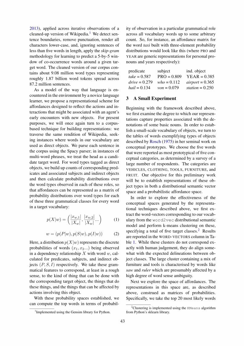
2013), applied across iterative observations of acleaned-up version of Wikipedia.1 We detect sen-tence boundaries, remove punctuation, render allcharacters lower-case, and, ignoring sentences ofless than five words in length, apply the skip-grammethodology for learning to predict a 5-by-5 win-dow of co-occurrence words around a given tar-get word. The cleaned version of our corpus con-tains about 9.08 million word types representingroughly 1.87 billion word tokens spread across87.2 million sentences.
As a model of the way that language is en-countered in the environment by a novice languagelearner, we propose a representational scheme foraffordances designed to reflect the actions and in-teractions that might be associated with an agent’searly encounters with new objects. For presentpurposes, we will once again turn to a corpus-based technique for building representations: wetraverse the same rendition of Wikipedia, seek-ing instances where words in our vocabulary areused as direct objects. We parse each sentence inthe corpus using the Spacy parser; in instances ofmulti-word phrases, we treat the head as a candi-date target word. For word types tagged as directobjects, we build up counts of corresponding pred-icates and associated subjects and indirect objectsand then calculate probability distributions overthe word types observed in each of these roles, sothat affordances can be represented as a matrix ofprobability distributions over word types for eachof these three grammatical classes for every wordin a target vocabulary:
p(X|w) =( |xw,1||Xw|
,|xw,2||Xw|
...
)(1)
w = (p(P |w), p(S|w), p(I|w)) (2)
Here, a distribution p(X|w) represents the discreteprobabilities of words (x1, x2...) being observedin a dependency relationship X with word w, cal-culated for predicates, subjects, and indirect ob-jects (P, S, I) respectively. We take these gram-matical features to correspond, at least in a roughsense, to the kind of thing that can be done withthe corresponding target object, the things that dothese things, and the things that can be affected byactions involving this object.
With these probability spaces established, wecan compute the top words in terms of probabil-
1Implemented using the Gensim library for Python.
ity of observation in a particular grammatical roleacross all vocabulary words up to some arbitrarycount. So, for instance, an affordance matrix forthe word taxi built with three-element probabilitydistributions would look like this (where PRO andYEAR are generic representations for personal pro-nouns and years respectively):
predicate subject ind. objecttake = 0.587 PRO = 0.809 YEAR = 0.385drive = 0.279 who = 0.112 airport = 0.365hail = 0.134 von = 0.079 station = 0.250
3 A Small Experiment
Beginning with the framework described above,we first examine the degree to which our represen-tations capture properties associated with the de-notations of some basic nouns. In order to estab-lish a small-scale vocabulary of objects, we turn tothe tables of words exemplifying types of objectsdescribed by Rosch (1975) in her seminal work onconceptual prototypes. We choose the five wordsthat were reported as most prototypical of five con-ceptual categories, as determined by a survey of alarge number of respondents. The categories areVEHICLES, CLOTHING, TOOLS, FURNITURE, andFRUIT. Our objective for this preliminary workwill be to establish representations of these ob-ject types in both a distributional semantic vectorspace and a probabilistic affordance space.
In order to explore the effectiveness of theconceptual spaces generated by the representa-tional techniques described above, we first ex-tract the word-vectors corresponding to our vocab-ulary from the word2vec distributional semanticmodel and perform k-means clustering on these,specifying a total of five target classes.2 Resultsare reported in the WORD-VECTORS column in Ta-ble 1. While these clusters do not correspond ex-actly with human judgement, they do align some-what with the expected delineations between ob-ject classes. The large cluster containing a mix offurniture and tools is characterised by words likesaw and ruler which are presumably affected by ahigh degree of word sense ambiguity.
Next we explore the space of affordances. Therepresentations in this space are, as describedabove, construed as matrices of probabilities.Specifically, we take the top 20 most likely words
2Clustering is implemented using the KMeans algorithmfrom Python’s sklearn library.
43
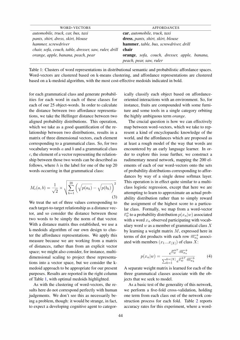
WORD-VECTORS AFFORDANCES
automobile, truck, car, bus, taxi car, automobile, truck, taxipants, shirt, dress, skirt, blouse dress, pants, shirt, skirt, blousehammer, screwdriver hammer, table, bus, screwdriver, drillchair, sofa, couch, table, dresser, saw, ruler, drill chairorange, apple, banana, peach, pear orange, sofa, couch, dresser, apple, banana,
peach, pear, saw, ruler
Table 1: Clusters of word representations in distributional semantic and probabilistic affordance spaces.Word-vectors are clustered based on k-means clustering, and affordance representations are clusteredbased on a k-medoid algorithm, with the most cost-effective medoids indicated in bold.
for each grammatical class and generate probabil-ities for each word in each of these classes foreach of our 25 object-words. In order to calculatethe distance between two affordance representa-tions, we take the Hellinger distance between twoaligned probability distributions. This operation,which we take as a good quantification of the re-lationship between two distributions, results in amatrix of three dimensional vectors, each elementcorresponding to a grammatical class. So, for twovocabulary words a and b and a grammatical classc, the element of a vector representing the relation-ship between those two words can be described asfollows, where h is the label for one of the top 20words occurring in that grammatical class:
Mc(a, b) =1√2×
√√√√20∑
h=1
(√p(ah)−
√p(bh)
)2
(3)We treat the set of three values corresponding toeach target-to-target relationship as a distance vec-tor, and so consider the distance between thosetwo words to be simply the norm of that vector.With a distance matrix thus established, we use ak-medoids algorithm of our own design to clus-ter the affordance representations. We apply thismeasure because we are working from a matrixof distances, rather than from an explicit vectorspace; we might also consider, for instance, multi-dimensional scaling to project these representa-tions into a vector space, but we consider the k-medoid approach to be appropriate for our presentpurposes. Results are reported in the right columnof Table 1, with optimal medoids highlighted.
As with the clustering of word-vectors, the re-sults here do not correspond perfectly with humanjudgements. We don’t see this as necessarily be-ing a problem, though: it would be strange, in fact,to expect a developing cognitive agent to categor-
ically classify each object based on affordance-oriented interactions with an environment. So, forinstance, fruits are compounded with some furni-ture and some tools in a single category orbitingthe highly ambiguous term orange.
The crucial question is how we can effectivelymap between word-vectors, which we take to rep-resent a kind of encyclopaedic knowledge of theworld, and the affordances which are proposed asat least a rough model of the way that words areencountered by an early language learner. In or-der to explore this issue further, we construct arudimentary neural network, mapping the 200 el-ements of each of our word-vectors onto the setsof probability distributions corresponding to affor-dances by way of a single dense softmax layer.This operation is in effect quite similar to a multi-class logistic regression, except that here we areattempting to learn to approximate an actual prob-ability distribution rather than to simply rewardthe assignment of the highest score to a particu-lar class. Formally, we map from a word-vector−→vw to a probability distribution p(xn|w) associatedwith a word xn observed participating with vocab-ulary word w as a member of grammatical class Xby learning a weight matrix M , expressed here interms of dot products with each row −−→mxk
associ-ated with members (x1...x|X|) of class X:
p(xn|w) =e−→vwT ·−−→mxn
∑k=|X|k=1 e
−→vwT ·−−→mxk
(4)
A separate weight matrix is learned for each of thethree grammatical classes associate with the ob-jects that we seek to model.
As a basic test of the generality of this network,we perform a five-fold cross-validation, holdingone term from each class out of the network con-struction process for each fold. Table 2 reportsaccuracy rates for this experiment, where a word-
44
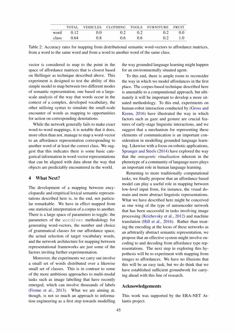
TOTAL VEHICLES CLOTHING TOOLS FURNITURE FRUIT
word 0.12 0.0 0.2 0.2 0.2 0.0class 0.64 0.8 0.6 0.6 0.2 1.0
Table 2: Accuracy rates for mapping from distributional semantic word-vectors to affordance matrices,from a word to the same word and from a word to another word of the same class.
vector is considered to map to the point in thespace of affordance matrices that is closest basedon Hellinger as technique described above. Thisexperiment is designed to test the ability of thissimple model to map between two different modesof semantic representation, one based on a large-scale analysis of the way that words occur in thecontext of a complex, developed vocabulary, theother utilising syntax to simulate the small-scaleencounter of words as mapping to opportunitiesfor action on corresponding denotations.
While the network generally fails to make exactword-to-word mappings, it is notable that it does,more often than not, manage to map a word-vectorto an affordance representation corresponding toanother word of at least the correct class. We sug-gest that this indicates there is some basic cate-gorical information in word-vector representationsthat can be aligned with data about the way thatobjects are predictably encountered in the world.
4 What Next?
The development of a mapping between ency-clopaedic and empirical lexical semantic represen-tations described here is, in the end, not particu-lar remarkable. We have in effect mapped fromone statistical interpretation of a corpus to another.There is a large space of parameters to toggle: theparameters of the word2vec methodology forgenerating word-vectors, the number and choiceof grammatical classes for our affordance space,the actual selection of target vocabulary words,and the network architecture for mapping betweenrepresentational frameworks are just some of thefactors inviting further experimentation.
Moreover, the experiments we carry out involvea small set of words distributed over a likewisesmall set of classes. This is in contrast to someof the more ambitious approaches to multi-modaltasks such as image labelling that have recentlyemerged, which can involve thousands of labels(Frome et al., 2013). What we are aiming at,though, is not so much an approach to informa-tion engineering as a first step towards modelling
the way grounded language learning might happenfor an environmentally situated agent.
To this end, there is ample room to reconsiderthe way in which we model affordances in the firstplace. The corpus-based technique described hereis amenable to a computational approach, but ulti-mately it will be important to develop a more sit-uated methodology. To this end, experiments onhuman-robot interaction conducted by (Gross andKrenn, 2016) have illustrated the way in whichfactors such as gaze and gesture are crucial fea-tures of early-stage linguistic interactions, and wesuggest that a mechanism for representing theseelements of communication is an important con-sideration in modelling grounded language learn-ing. Likewise with a focus on robotic applications,Spranger and Steels (2014) have explored the waythat the ontogentic ritualisation inherent in thephenotype of a community of language users playsan important role in human language learning.
Returning to more traditionally computationaltasks, we finally propose that an affordance basedmodel can play a useful role in mapping betweenlow-level input from, for instance, the visual do-main and more abstract linguistic representations.What we have described here might be conceivedas one wing of the type of autoencoder networkthat has been successful in tasks involving imageprocessing (Krizhevsky et al., 2012) and machinetranslation (Hill et al., 2016). Rather than treat-ing the encoding at the locus of these networks asan arbitrarily abstract semantic representation, wepropose that an effective system might involve en-coding to and decoding from affordance type rep-resentations. The next step in exploring this hy-pothesis will be to experiment with mapping fromimages to affordances. We have no illusions thatthis will be an easy task, but we do think that wehave established sufficient groundwork for carry-ing ahead with this line of research.
Acknowledgements
This work was supported by the ERA-NET At-lantis project.
45
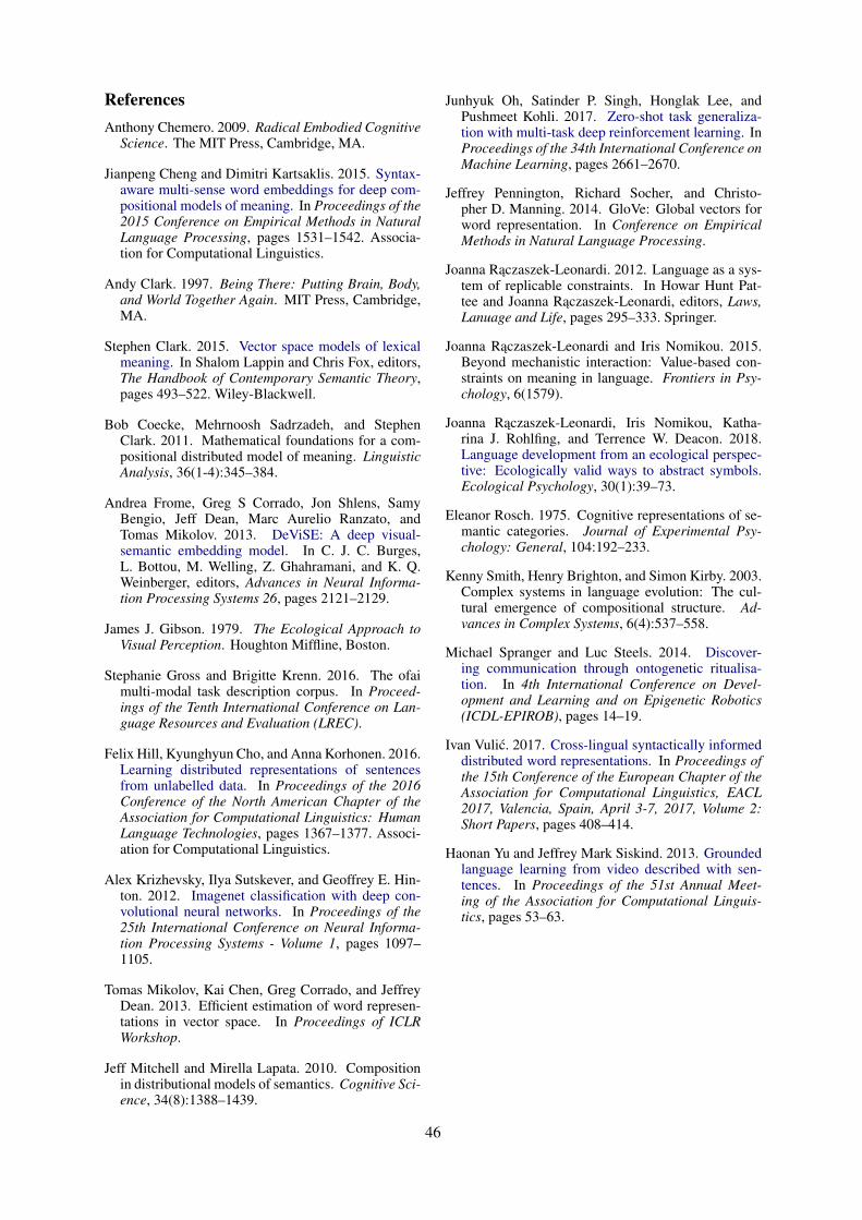
ReferencesAnthony Chemero. 2009. Radical Embodied Cognitive
Science. The MIT Press, Cambridge, MA.
Jianpeng Cheng and Dimitri Kartsaklis. 2015. Syntax-aware multi-sense word embeddings for deep com-positional models of meaning. In Proceedings of the2015 Conference on Empirical Methods in NaturalLanguage Processing, pages 1531–1542. Associa-tion for Computational Linguistics.
Andy Clark. 1997. Being There: Putting Brain, Body,and World Together Again. MIT Press, Cambridge,MA.
Stephen Clark. 2015. Vector space models of lexicalmeaning. In Shalom Lappin and Chris Fox, editors,The Handbook of Contemporary Semantic Theory,pages 493–522. Wiley-Blackwell.
Bob Coecke, Mehrnoosh Sadrzadeh, and StephenClark. 2011. Mathematical foundations for a com-positional distributed model of meaning. LinguisticAnalysis, 36(1-4):345–384.
Andrea Frome, Greg S Corrado, Jon Shlens, SamyBengio, Jeff Dean, Marc Aurelio Ranzato, andTomas Mikolov. 2013. DeViSE: A deep visual-semantic embedding model. In C. J. C. Burges,L. Bottou, M. Welling, Z. Ghahramani, and K. Q.Weinberger, editors, Advances in Neural Informa-tion Processing Systems 26, pages 2121–2129.
James J. Gibson. 1979. The Ecological Approach toVisual Perception. Houghton Miffline, Boston.
Stephanie Gross and Brigitte Krenn. 2016. The ofaimulti-modal task description corpus. In Proceed-ings of the Tenth International Conference on Lan-guage Resources and Evaluation (LREC).
Felix Hill, Kyunghyun Cho, and Anna Korhonen. 2016.Learning distributed representations of sentencesfrom unlabelled data. In Proceedings of the 2016Conference of the North American Chapter of theAssociation for Computational Linguistics: HumanLanguage Technologies, pages 1367–1377. Associ-ation for Computational Linguistics.
Alex Krizhevsky, Ilya Sutskever, and Geoffrey E. Hin-ton. 2012. Imagenet classification with deep con-volutional neural networks. In Proceedings of the25th International Conference on Neural Informa-tion Processing Systems - Volume 1, pages 1097–1105.
Tomas Mikolov, Kai Chen, Greg Corrado, and JeffreyDean. 2013. Efficient estimation of word represen-tations in vector space. In Proceedings of ICLRWorkshop.
Jeff Mitchell and Mirella Lapata. 2010. Compositionin distributional models of semantics. Cognitive Sci-ence, 34(8):1388–1439.
Junhyuk Oh, Satinder P. Singh, Honglak Lee, andPushmeet Kohli. 2017. Zero-shot task generaliza-tion with multi-task deep reinforcement learning. InProceedings of the 34th International Conference onMachine Learning, pages 2661–2670.
Jeffrey Pennington, Richard Socher, and Christo-pher D. Manning. 2014. GloVe: Global vectors forword representation. In Conference on EmpiricalMethods in Natural Language Processing.
Joanna Raczaszek-Leonardi. 2012. Language as a sys-tem of replicable constraints. In Howar Hunt Pat-tee and Joanna Raczaszek-Leonardi, editors, Laws,Lanuage and Life, pages 295–333. Springer.
Joanna Raczaszek-Leonardi and Iris Nomikou. 2015.Beyond mechanistic interaction: Value-based con-straints on meaning in language. Frontiers in Psy-chology, 6(1579).
Joanna Raczaszek-Leonardi, Iris Nomikou, Katha-rina J. Rohlfing, and Terrence W. Deacon. 2018.Language development from an ecological perspec-tive: Ecologically valid ways to abstract symbols.Ecological Psychology, 30(1):39–73.
Eleanor Rosch. 1975. Cognitive representations of se-mantic categories. Journal of Experimental Psy-chology: General, 104:192–233.
Kenny Smith, Henry Brighton, and Simon Kirby. 2003.Complex systems in language evolution: The cul-tural emergence of compositional structure. Ad-vances in Complex Systems, 6(4):537–558.
Michael Spranger and Luc Steels. 2014. Discover-ing communication through ontogenetic ritualisa-tion. In 4th International Conference on Devel-opment and Learning and on Epigenetic Robotics(ICDL-EPIROB), pages 14–19.
Ivan Vulic. 2017. Cross-lingual syntactically informeddistributed word representations. In Proceedings ofthe 15th Conference of the European Chapter of theAssociation for Computational Linguistics, EACL2017, Valencia, Spain, April 3-7, 2017, Volume 2:Short Papers, pages 408–414.
Haonan Yu and Jeffrey Mark Siskind. 2013. Groundedlanguage learning from video described with sen-tences. In Proceedings of the 51st Annual Meet-ing of the Association for Computational Linguis-tics, pages 53–63.
46
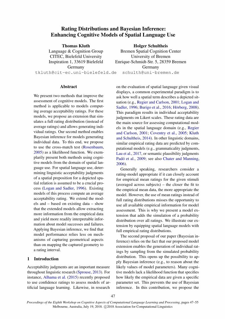
Proceedings of the Eighth Workshop on Cognitive Aspects of Computational Language Learning and Processing, pages 47–55Melbourne, Australia, July 19, 2018. c©2018 Association for Computational Linguistics
Rating Distributions and Bayesian Inference:Enhancing Cognitive Models of Spatial Language Use
Thomas KluthLanguage & Cognition GroupCITEC, Bielefeld University
Inspiration 1, 33619 BielefeldGermany
Holger SchultheisBremen Spatial Cognition Center
University of BremenEnrique-Schmidt-Str. 5, 28359 Bremen
Abstract
We present two methods that improve theassessment of cognitive models. The firstmethod is applicable to models comput-ing average acceptability ratings. For thesemodels, we propose an extension that sim-ulates a full rating distribution (instead ofaverage ratings) and allows generating indi-vidual ratings. Our second method enablesBayesian inference for models generatingindividual data. To this end, we proposeto use the cross-match test (Rosenbaum,2005) as a likelihood function. We exem-plarily present both methods using cogni-tive models from the domain of spatial lan-guage use. For spatial language use, deter-mining linguistic acceptability judgmentsof a spatial preposition for a depicted spa-tial relation is assumed to be a crucial pro-cess (Logan and Sadler, 1996). Existingmodels of this process compute an averageacceptability rating. We extend the mod-els and – based on existing data – showthat the extended models allow extractingmore information from the empirical dataand yield more readily interpretable infor-mation about model successes and failures.Applying Bayesian inference, we find thatmodel performance relies less on mech-anisms of capturing geometrical aspectsthan on mapping the captured geometry toa rating interval.
1 Introduction
Acceptability judgments are an important measurethroughout linguistic research (Sprouse, 2013). Forinstance, Alhama et al. (2015) recently proposedto use confidence ratings to assess models of ar-tificial language learning. Likewise, in research
on the evaluation of spatial language given visualdisplays, a common experimental paradigm is toask how well a spatial term describes a depicted sit-uation (e.g., Regier and Carlson, 2001; Logan andSadler, 1996; Burigo et al., 2016; Hörberg, 2008).This paradigm results in individual acceptabilityjudgments on Likert scales. These rating data arethe main source for assessing computational mod-els in the spatial language domain (e.g., Regierand Carlson, 2001; Coventry et al., 2005; Kluthand Schultheis, 2014). In other linguistic domains,similar empirical rating data are predicted by com-putational models (e.g., grammaticality judgments,Lau et al., 2017, or semantic plausibility judgmentsPadó et al., 2009; see also Chater and Manning,2006).
Generally speaking, researchers consider arating-model appropriate if it can closely accountfor empirical mean ratings for the given stimuli(averaged across subjects) – the closer the fit tothe empirical mean data, the more appropriate themodel. However, the use of mean ratings instead offull rating distributions misses the opportunity touse all available empirical information for modelassessment. This is why we present a model ex-tension that adds the simulation of a probabilitydistribution over all ratings. We illustrate our ex-tension by equipping spatial language models withfull empirical rating distributions.
The second proposal of our paper (Bayesian in-ference) relies on the fact that our proposed modelextension enables the generation of individual rat-ings by sampling from the simulated probabilitydistribution. This opens up the possibility to ap-ply Bayesian inference (e.g., to reason about thelikely values of model parameters). Many cogni-tive models lack a likelihood function that specifieshow likely the empirical data are given a specificparameter set. This prevents the use of Bayesianinference. In this contribution, we propose the
47

cross-match test developed by (Rosenbaum, 2005)as a means for computing the likelihood for cog-nitive models that are able to generate individualdata.
Again, we use a spatial language model to ex-emplify the application of the cross-match method.The thus computed posterior distribution of themodel’s parameters has surprising implications forthe interpretation of the model. Before we come tothis, we start with presenting the example models,followed by our model extension to simulate ratingdistributions.
1.1 Exemplary Spatial Language Models
We introduce both our methods by exemplarily ap-plying them to the AVS model (Regier and Carlson,2001) and the recently proposed AVS-BB, rAVS,and rAVS-CoO models (Kluth et al., 2017, underrevision). Given a depicted spatial layout and aspatial sentence (“The [located object] is above the[reference object]”), these cognitive models gener-ate mean acceptability ratings, i.e., judgments howwell the linguistic input describes the visual scene.All models can be interpreted as consisting of twocomponents: One component that captures geomet-ric aspects of the depicted spatial configuration andone component that maps the captured geometry toa rating interval (representing linguistic acceptabil-ity judgments).
The models process geometry by defining vec-tors on all points of one object of the spatial layout.These vectors point to the second object in the lay-out. In addition, each vector is weighted by a cer-tain amount of attention defined by a spotlight-likedistribution of attention. The overall direction ofthe vector sum is compared to a reference direction(e.g., canonical upright for the preposition above).This angular deviation is the outcome of the firstmodel component (processing geometry).
The first model component is where the twomodel families (AVS & AVS-BB vs. rAVS & rAVS-CoO) differ: The AVS and the AVS-BB modelsassume a shift of attention from the reference ob-ject to the located object (the vectors point fromthe reference object to the located object). In con-trast, the rAVS and rAVS-CoO models assume areversed shift of attention from the located object tothe reference object (hence their acronym: reversedAVS; the vectors point from the located object tothe reference object). The difference within themodel families (i.e., AVS vs. AVS-BB and rAVS
vs. rAVS-CoO) will be introduced in Section 3.The second model component is the same in all
models: A linear function that maps the angular de-viation from the first component to a rating interval.In Section 4.2.1 we introduce some details aboutthe role of rAVS-CoO’s parameters for the twomodel components. Applying our model extensionand the second proposal of our paper (Bayesianinference), we present evidence that the secondcomponent of the models (mapping geometry torating) seems to be more important than the firstone (processing geometry).
2 Model Extension: Rating Distributions
As an illustrating example of our model extension,consider the empirical rating distribution displayedas bars in Fig. 1c. This distribution shows 34 ac-ceptability ratings on a rating scale with K = 9categories (from 1–9). These ratings come from anempirical study by Kluth et al. (under revision) inwhich they asked 34 participants to judge the ac-ceptability of the German sentence “Der Punkt istüber dem Objekt” (“The dot is above the object”).Specifically, the distribution shown in Fig. 1c cor-responds to empirical ratings for the left black dotabove the asymmetrical object depicted in Fig. 1a.
Our method of simulating such a rating distribu-tion is inspired by a common approach of analyzingordinal data (i.e., discrete and ordered data) usinggeneralized linear (regression) models (e.g., Lid-dell and Kruschke, 2018; Kruschke, 2015, chapter23). Here, the cumulative probability of a latentGaussian distribution between two thresholds is theprobability of one specific rating k (see Fig. 1c).1
Based on this, we propose the following steps toextend mean-rating-models with the ability of sim-ulating full rating distributions:
1. Interpret the output of the model as the meanµ of a Gaussian distribution (see maximum ofdashed curve in Fig. 1c or 1d).
2. Treat σ of the Gaussian distribution and K −1 − 2 thresholds as additional model param-eters (see width of dashed curve and verticallines in Fig. 1c or 1d; K is the number of alloutcomes; first and last thresholds have fixedvalues).
3. Define a discrete probability distribution overall K ratings like in an ordinal regression (i.e,
1For the first / last outcome it is the cumulative probabilitybetween negative / positive infinity and the first / last threshold.
48
cumulative probabilities of the Gaussian distri-bution between thresholds, see model outputsin Fig. 1c or 1d).
4. To generate an individual rating: Sample a rat-ing from the discrete probability distributiondefined in the previous step.
Note that the discrete probability distributionover all K ratings defined in step 3 is fully deter-mined by the model parameters (i.e., it will notchange unless you change any of the model pa-rameters) while the individual rating generated instep 4 is subject to sampling noise.
To fit such an extended model to empirical data,we compute the Kullback-Leibler divergence fromthe model’s discrete probability distribution (seemodel outputs in Fig. 1c or 1d) to the empiricalrating distribution (relative frequencies of ratings,see bars in Fig. 1c or 1d) – for every dot-object pairthat served as a stimulus. Then we minimize themean Kullback-Leibler divergence (averaged overall stimuli). This procedure requires that individualempirical data are available.
Note that this approach of comparing model out-puts to empirical data still operates on the data fromall study participants (but it uses more informationas it does not operate only on a mean value). Thatis, instead of explicitly assessing the models onindividual behavior, our fitting approach aims tocapture the overall rating distribution. Given thatwith our model extension a model may also gener-ate individual outcomes, it is in principle possibleto explicitly model single individuals or groups ofindividuals with similar rating patterns. We leavethis for future work and note that the work fromNavarro et al. (2006) might prove valuable for thisendeavor.
3 Results: Fitting Models to RatingDistributions
To exemplarily apply our proposed model exten-sion, we extended the AVS model (Regier and Carl-son, 2001) as well as the recently proposed AVS-BB, rAVS, and rAVS-CoO models (Kluth et al.,2017, under revision) and fitted them to empiricaldata from Kluth et al. (under revision, asymmetri-cal objects only). We denote the extended modelswith a trailing + (see labels in Fig. 1). The sourcecode and all data are available under open licenses(GNU GPL and ODbL) from Kluth (2018).
×◦
d d
(a) Spatial configuration with two exemplary dot locationsused in acceptability rating study by Kluth et al. (under re-vision). × = center-of-mass, ◦ = center-of-object (of theasymmetrical object); d = same horizontal distance from ×for both dots. Participants saw only one dot and the asymmet-rical object (neither the centers nor the additional lines shownhere).
mea
nK
ullb
ack-
Lei
bler
dive
rgen
ce SHOGOF
0.00
0.05
0.10
0.15
0.20
AVS+ rAVS+ AVS-BB+ rAVS-CoO+
(b) Goodness-of-fit (GOF) and simple hold-out (SHO) resultsfor fitting extended models to whole empirical rating distribu-tion from Kluth et al. (under revision, 4 asymmetrical objects× 28 dots × 2 prepositions = 224 data points). Error barsshow 95% confidence intervals of SHO medians.
prop
ortio
n/p
roba
bilit
y
rating
empirical datarAVS-CoO+ model outputrAVS+ model outputlatent distribution rAVS-CoO+thresholds rAVS-CoO+
0.00
0.10
0.20
0.30
0.40
0.50
0.60
1 2 3 4 5 6 7 8 9
(c) Empirical “über” (“above”) rating distribution and modelprobabilities (rAVS+ and rAVS-CoO+) for the left dot shownin Fig. 1a. Model probabilities were computed using theparameters from the best fit plotted in Fig. 1b. Participantsnever chose rating 1.
prop
ortio
n/p
roba
bilit
y
rating
empirical datarAVS-CoO+ model outputrAVS+ model outputlatent distribution rAVS+thresholds rAVS+
0.00
0.10
0.20
0.30
0.40
0.50
0.60
1 2 3 4 5 6 7 8 9
(d) Empirical “über” (“above”) rating distribution and modelprobabilities (rAVS+ and rAVS-CoO+) for the right dotshown in Fig. 1a. Model probabilities were computed usingthe parameters from the best fit plotted in Fig. 1b. Participantsnever chose ratings 1-4 or 6.
Figure 1: Example experimental display, fits of ex-tended models, and empirical rating distributions.
49

Given a depicted spatial configuration contain-ing a geometric object and a single dot placedabove / below the object (see Fig. 1a), we asked34 German native speakers to rate the acceptabil-ity of the German sentences “Der Punkt ist überdem Objekt” and “Der Punkt ist unter dem Ob-jekt” (“The dot is above / below the object”) on aLikert scale from 1–9 (with lower ratings codinglower acceptability judgments). We placed 28 dotsabove and 28 dots below 4 asymmetrical objects(i.e., the whole data set consists of 224 data points;for the current work we did not consider data fromadditionally tested rectangular reference objects).
Fig. 1a shows two exemplary dot locations aboveone of the used asymmetrical objects. For thesetwo dots, we expected participants to give equal“über” (“above”) acceptability ratings (based onearlier research, e.g., Regier and Carlson, 2001).However, we found that participants rated the ac-ceptability of the “über” (“above”) sentence forthe right dot in Fig. 1a higher than for the left dot(Kluth et al., under revision). This finding gener-alized reliably to different objects with similar dotplacements suggesting that people possibly preferthe center-of-object (depicted as ◦ in Fig. 1a) overthe center-of-mass (depicted as × in Fig. 1a) fortheir judgments. To account for this finding, Kluthet al. (under revision) proposed the model refine-ments AVS-BB and rAVS-CoO (AVS-bounding-box and rAVS-center-of-object), which both usethe center-of-object instead of the center-of-mass(as AVS and rAVS do) for their computations.
Here, we use the two dot locations depicted inFig. 1a to exemplarily present our approach of sim-ulating rating distributions. To do so, we first ex-tended all models with the ability to simulate ratingdistributions and then fitted all extended modelsto the 224 data points (by minimizing the meanKullback-Leibler divergence as described above).These fits are plotted in Fig. 1b (as goodness-of-fitvalues alongside with the outcome of 101 simplehold-out iterations, a cross-validation measure tocontrol for overfitting, Schultheis et al., 2013). Interms of relative model performances, these fitsconfirm the results of simpler fits using only aver-aged rating data reported in Kluth et al. (under re-vision): Both models that take the center-of-objectinto account (the AVS-BB+ and the rAVS-CoO+models) fit the data more closely (lower meanKullback-Leibler divergence) than the models thatconsider the center-of-mass (AVS+ and rAVS+).
More interesting for our current purpose are theplots in Figs. 1c and 1d. These plots each depictthe empirical rating distributions for one of the twodots in Fig. 1a as bars: Fig. 1c shows the distribu-tion for the left dot while Fig. 1d depicts the distri-bution for the right dot. The empirical distributionsshow that the left dot received considerably less“9” ratings and more “2–7” ratings compared to theright dot. On top of the empirical distributions, weplotted the probabilities of each rating as computedwith the rAVS+ and the rAVS-CoO+ models. Tocompute these probabilities, we used the parame-ters found by fitting the models to the whole dataset (cf. Fig. 1b). Despite being fit to a much largerdata set, the two plots show that both models gener-ally capture the qualitative trend of each of the twosingle empirical data points. Considering Fig. 1cand Fig. 1d suggests that the rAVS-CoO+ modelbetter accounts for the data – confirming (and ex-plaining, see Kluth et al., under revision) the betterfit on the larger data set shown in Fig. 1b.
Fitting the models to rating distributions allowsfor a more fine-grained model assessment com-pared to model fits to averaged data. For example,the main source of the different performances ofthe rAVS+ and the rAVS-CoO+ models seems to betheir ability to account for the frequency of the high-est rating “9” (cf. Fig. 1c and Fig. 1d). Comparethis with the situation where only averaged data isused: Here the only information are mean ratings(for the left dot 7.38, for the right dot 8.18) andfits of the models to these mean ratings. Using thesame parameter settings as before, this yields forthe left dot 0.1326 (rAVS fit, normalized root meansquare error: nRMSE2) or 0.0093 (rAVS-CoO fit,nRMSE) and for the right dot 0.0333 (rAVS fit,nRMSE) or 0.1029 (rAVS-CoO fit, nRMSE). Noneof these numbers provides information about themodels’ properties as intuitive and informative asthe fit of the extended models using full rating dis-tributions. Moreover, our extension also enablesthe generation of individual data by sampling fromthe models’ discrete rating distribution (see step 4on page 3). This property can be used to analyzethe models with Bayesian inference as we shownext.
2 RMSE =√
1n
∑ni (datai −modelOutputi)2
nRMSE = RMSE/(ratingmax − ratingmin)
50

4 Method: Bayesian Inference
The Bayesian framework is a fruitful and theoret-ically sound approach to reason with probabilitydistributions over model parameters. However, thisframework requires that the analyzed model can beinterpreted in a probabilistic sense. As for manyother cognitive models, this is not the case for anyof the models discussed here (AVS, AVS-BB, rAVS,rAVS-CoO or their extended versions) because theylack a likelihood function that specifies how likelyempirical data are given a model with a specificparameter set. We propose to use the cross-matchtest developed by Rosenbaum (2005) as the likeli-hood function of cognitive models that are able togenerate individual data (e.g., the derivatives of theAVS+ model).
4.1 Cross-match Test
The cross-match test is a statistical test that com-putes the probability of whether multivariate re-sponses of two differently treated subject groupscome from the same distribution. In our case, thefirst group are empirical individual data and thesecond group are model-generated individual data(see top and bottom of Tab. 1), so the cross-matchtest becomes a measure of how likely it is that themodel-generated data come from the same distribu-tion as the empirical data. Given that we can onlychange the model-generated data (by using differ-ent parameter sets), this amounts to a likelihoodfunction.
Internally, the cross-match test is based on group-ing the multivariate responses (rows in Tab. 1)into pairs with minimal distances (Mahalanobisdistances of ranks). The more of these pairs “cross-match” between the two groups, the more similarare the data of the two groups and hence the higheris the probability that the cross-match test com-putes (for more details see Rosenbaum, 2005).
4.2 Estimating the Posterior Distribution
To apply the cross-match test as a likelihood func-tion of AVS+ derivatives, we propose the followingprocedure3:
1. For each stimulus, simulate as many ratingswith the model as there were participants in
3Note that for clarity of presentation we stay in our exem-plary domain: rating-models for spatial language. In principle,our approach is applicable to all models that are able to gener-ate individual data points (not necessarily ratings).
data type left dot right dot . . .
empirical 7 8 . . .empirical 9 9 . . .. . . . . . . . . . . .
model 8 9 . . .model 5 8 . . .. . . . . . . . . . . .
Table 1: Example input for the cross-matchtest (Rosenbaum, 2005). Each row describesthe response of one subject (empirical or model-generated), each column describes the response toa stimulus (e.g., the left or right dot from Fig. 1a).
the study by applying the procedure of gener-ating individual ratings described in step 4 onpage 3.
2. Compute the cross-match test comparing theempirical data with the model-generated data.
3. To account for sampling noise (see step 4 onpage 3 in the generation of individual data)and provide reliable cross-match results forthe same model parameters:
(a) For every individual rating to be gener-ated in step 1, sample s times and use themean outcome as generated rating.
(b) Use the following average of cross-match computations as likelihood value:
i. Compute the mean number of cross-matches from c cross-match tests andstore the probability for this numberof cross-matches.
ii. Repeat step i for b blocks and use themean of these b probabilities as thelikelihood value.
Step 3 (b) basically repeats steps 1 and 2 b · ctimes. In our case, we found a sufficiently stablelikelihood by applying step 3 with s = 10, b = 20,and c = 4 (standard error of averaged cross-matchresult < 0.05). Note that a too large value of swill generate model outputs that are too similar toeach other and thus possibly reduces the numberof cross-matches too much. The problem of anunstable likelihood value will reduce when moreempirical individual data are available.
Having the likelihood function defined in thisway, one can apply standard Markov Chain Monte
51
Carlo (MCMC) techniques to estimate the poste-rior distribution. Specifically, we implemented aMetropolis-Hastings algorithm and improved itsperformance by adding the adaptation algorithmproposed by Garthwaite et al. (2016). For the cross-match test, we used the R package crossmatch(Heller et al., 2012) and re-implemented parts ofit using the C++ library Armadillo (Sander-son and Curtin, 2016). The R package ggmcmc(Fernández-i Marín, 2016) helped in visualizingand analyzing the MCMC samples. Again, allsource code is available under the GNU GPL li-cense from (Kluth, 2018).
4.2.1 Example rAVS-CoO+: ModelParameters & Prior Distributions
We exemplarily estimated the posterior distributionof the parameters of the rAVS-CoO+ model. TherAVS-CoO+ model has four free parameters (notconsidering the additional parameters of our ordi-nal model extension: σ and thresholds). The twoparameters α and highgain are part of the compo-nent that processes the geometry of the depictedspatial configuration (cf. Section 1.1). In particularα controls the extraction of an angular deviationfrom the spatial relation. This angular deviationis mapped to a linguistic rating with the secondcomponent of the model. Specifically, high angulardeviation results in a low rating and low angulardeviation results in a high rating. This is realizedwith a linear function that maps angular deviationto rating. The intercept and slope parameters arethe parameters of this linear function.
Since this is the first study that investigates prob-ability distributions over the model parameters ofthe rAVS-CoO+ model, we had no prior informa-tion available about the likely values of the modelparameters. Accordingly, we used uniform distri-butions within the following parameter ranges as“uninformative” prior distributions:
α ∈ [0.001, 5]; highgain ∈[0, 10]intercept ∈ [0.7, 1.3]; slope ∈[−1/45, 0]
5 Results: Bayesian Inference
We exemplarily estimated the posterior distributionof the parameters of the rAVS-CoO+ model forthe same data set to which we fitted the model ear-lier (consisting of ratings for dots above / belowasymmetrical objects, see Fig. 1b for model fits).We used 4 MCMC chains with 125,000 samples ineach chain and checked the chains for convergence
by monitoring the potential scale reduction factorR (Gelman and Rubin, 1992). To obtain converg-ing chains, we had to change the parameterizationof the slope parameter to measure “change per ra-dian” instead of “change per degree”. Furthermore,we kept the additional model parameters for theordinal regression (σ of the latent Gaussian distri-bution and thresholds) constant on the values of thebest rAVS-CoO+ fit to the whole data set, becausewe were primarily interested in the original modelparameters. This parameter reduction improved theconvergence of the MCMC chains while it did notaffect the qualitative results. The results of the pos-terior estimation are plotted as density estimates ofthe marginal posterior distribution for each modelparameter of the rAVS-CoO+ model in Fig. 2. Thedifferent colors code the different MCMC chains.The high overlap of the colors confirms the conver-gence of the chains.
At a first glance, the marginal posterior distribu-tions are surprising as they lack clear maxima forany parameter in the considered ranges. In particu-lar the α and the highgain parameter seem to havelittle effect on the model output in terms of gener-ating data similar to empirical data. On the otherhand, the marginal posterior distributions suggestthat the following regions in the parameter spaceshould result in relatively poor model performance:α < 0.5, intercept > 1.0, and slope > −0.25.
To double-check these regions, we picked twoparameter sets and computed the model fits tothe empirical data with these parameters (meanKullback-Leibler divergence). The first parameterset lies in the presumably bad-performance region(highgain = 5.0, α = 0.2, intercept = 1.25,slope = −0.05) while the second parameter setconsists of parameter values from regions withhigh posterior density (highgain = 5.0, α = 3.0,intercept = 0.9, slope = −0.625). Indeed, thepresumably bad-performing parameter set fits thedata worse than the other parameter set (meanKullback-Leibler divergence: 0.484 vs. 0.266, re-spectively). This trend was confirmed with fits ofthe same parameter sets using mean ratings insteadof rating distributions (nRMSE for worse parame-ters 0.301 vs. 0.145 for better parameters). Thesetests provide evidence that using the cross-matchtest as a likelihood function appropriately capturesmodel performance.
After establishing the validity of the unexpectedresults, we discuss what we can learn from them.
52

Figure 2: Marginal posterior distributions for therAVS-CoO+ model given rating data from Kluthet al. (under revision, asymmetrical objects only)and “uninformative” prior distributions (uniformdistributions).
Keep in mind that the following conclusions areonly valid for the exemplary data set and modelfor which we computed the posterior estimationand may change with data highlighting differentaspects of spatial language use.
Despite the great range of the parameterhighgain its value does not affect the model per-formance. Accordingly, the parameter highgainseems to be irrelevant for the quality of the modeloutput. Almost the same is true for the parameter α,although the marginal posterior distribution showsweak performance for values less than 0.5. The roleof the parameter α in the rAVS-CoO+ model can beunderstood as an importance weight of two geomet-ric features known to affect spatial language accept-ability judgments: the proximal orientation and thecenter-of-object orientation (Regier and Carlson,2001; Kluth et al., under revision). The closer α isto 0.0, the more important gets the proximal orienta-tion and the less important gets the center-of-object
orientation for the rAVS-CoO+ model. Thus, themarginal posterior distribution provides evidencethat the center-of-object orientation is more impor-tant than the proximal orientation to account forthis data set.
The intercept and slope parameters control thesecond model component (cf. Section 1.1): theyare the parameters of a linear function contained inthe rAVS-CoO+ model that maps angular deviationto rating (between 0 and 1). These two parame-ters have a greater influence on model performancethan α and highgain (more diverse posterior pro-files for intercept and slope compared to α andhighgain, see Figure 2). That is, changing the val-ues of the intercept or slope parameters affects themodels’ ability to fit empirical data more stronglythan changing the values of α or highgain.
This is interesting, because one can interpret therAVS-CoO+ model (and related models such asAVS+, AVS-BB+, rAVS+) as consisting of (i) ageometric component (capturing / formalizing thegeometric properties of the involved objects andtheir spatial relation) and (ii) a mapping compo-nent (mapping the captured geometric aspects ontoa rating range, see Section 1.1). Given that oneof the prime research question motivating the de-velopment of these models concerns the influenceof geometric properties (such as relative spatiallocation of the objects or asymmetrical objects)on spatial language use, most researchers focusedon the geometric component of the models. Ourresults, however, suggest that the geometric compo-nent may be less important for model performancethan commonly assumed – in particular, less im-portant than the mapping component. That is, tounravel effects of geometry on spatial languageuse, it might be more insightful to re-consider themapping of assumed intermediate geometric rep-resentations (e.g., angular deviations) to linguisticjudgments instead of modeling the computation ofthese representations.
6 Discussion & Conclusion
Acceptability judgments are common in linguisticresearch (Sprouse, 2013). Many cognitive modelsof linguistic processes compute mean acceptabil-ity ratings. We propose a model extension thatenables these models (i) to simulate a probabilitydistribution over all possible ratings and (ii) to gen-erate individual ratings. To fit simulated probabilitydistributions to empirical rating distributions, we
53

propose to minimize the mean Kullback-Leiblerdivergence from the simulated to the empirical dis-tributions. This model extension moves the modelfits on a level that is closer to the actual empiri-cal data (by using full rating distributions insteadof mean ratings) while it avoids the problematictreatment of ordinal data as metric (Liddell and Kr-uschke, 2018). As future steps in this direction, weenvision an analysis whether the additional modelparameters can be mapped onto cognitive structuresand mechanisms and subsequently the explicit mod-eling of (groups of) individuals (e.g, via Navarroet al., 2006).
Since many cognitive models lack a likelihoodfunction, our additional contribution is to introducethe cross-match test (Rosenbaum, 2005) as a possi-ble approximation of the likelihood function. Thisadds the possibility to apply full Bayesian inferencefor the parameters of all cognitive models that areable to generate individual data (e.g., mean-rating-models enhanced with our model extension).
In the related work of Approximate BayesianComputation (ABC, for review see Turner andVan Zandt, 2012), researchers have developed sam-pling strategies to enable “likelihood-free infer-ence”. These techniques enable a modeler to usethe Bayesian toolkit without explicitly defining alikelihood function. However, ABC sampling algo-rithms add additional overhead to the workflow ofcognitive modelers, as they diverge from standardMCMC techniques used in Bayesian estimations.To overcome this overhead, we propose to use thecross-match test as an explicit likelihood function.We are currently evaluating our approach in com-parison to existing ABC algorithms.
We exemplarily applied both our proposals usingcomputational cognitive models of spatial languageuse like the AVS model (Regier and Carlson, 2001)and its derivatives (Kluth et al., 2017, under revi-sion). Given a depicted spatial layout and a spatialpreposition, these models compute mean accept-ability ratings. We showed that simulating ratingdistributions allows a more fine-grained model as-sessment compared to model fits using mean rat-ings.
An example application of Bayesian inferencerevealed surprising insights: We estimated the pos-terior distribution of rAVS-CoO+’s parameters andfound that the values of almost all parameters wereless important for model performance than wethought. Future research in this direction will help
to precisely identify and quantify the role of modelparameters for the rAVS-CoO+ model (and the re-lated models AVS+, AVS-BB+, and rAVS+). In ad-dition, the Bayesian toolkit comprises several othermethods for model inspection and model compari-son.
Acknowledgments
This research was supported by the Cluster of Ex-cellence Cognitive Interaction Technology ‘CITEC’(EXC 277) at Bielefeld University, which is fundedby the German Research Foundation (DFG).
ReferencesRaquel G. Alhama, Remko Scha, and Willem Zuidema.
2015. How should we evaluate models of segmenta-tion in artificial language learning? In Proceedingsof the 13th International Conference on CognitiveModeling.
Michele Burigo, Kenny R. Coventry, Angelo Can-gelosi, and Dermot Lynott. 2016. Spatial languageand converseness. Quarterly Journal of Experimen-tal Psychology, 69(12):2319–2337.
Nick Chater and Christopher D Manning. 2006. Prob-abilistic models of language processing and acquisi-tion. Trends in Cognitive Sciences, 10(7):335–344.
Kenny R. Coventry, Angelo Cangelosi, Rohanna Ra-japakse, Alison Bacon, Stephen Newstead, DanJoyce, and Lynn V. Richards. 2005. Spatial preposi-tions and vague quantifiers: Implementing the func-tional geometric framework. In Spatial CognitionIV. Reasoning, Action, Interaction. Springer.
Paul H. Garthwaite, Yanan Fan, and Scott A. Sis-son. 2016. Adaptive optimal scaling of Metropolis–Hastings algorithms using the Robbins–Monro pro-cess. Communications in Statistics-Theory andMethods, 45(17):5098–5111.
Andrew Gelman and Donald B. Rubin. 1992. Inferencefrom iterative simulation using multiple sequences.Statistical Science, 7(4):457–472.
Ruth Heller, Dylan Small, and Paul Rosenbaum. 2012.crossmatch: The cross-match test. R package ver-sion 1.3-1.
Thomas Hörberg. 2008. Influences of form and func-tion on the acceptability of projective prepositionsin Swedish. Spatial Cognition & Computation,8(3):193–218.
Thomas Kluth. 2018. A C++ implementationof cognitive models of spatial language under-standing as well as pertinent empirical dataand analyses. will soon be published un-der https://pub.uni-bielefeld.de/person/54885831/data.
54
Thomas Kluth, Michele Burigo, and Pia Knoeferle.2017. Modeling the directionality of attentionduring spatial language comprehension. In Jaapvan den Herik and Joaquim Filipe, editors, Agentsand Artificial Intelligence, Lecture Notes in Com-puter Science. Springer International PublishingAG.
Thomas Kluth, Michele Burigo, Holger Schultheis, andPia Knoeferle. under revision. Does direction mat-ter? Linguistic asymmetries reflected in visual atten-tion. Cognition.
Thomas Kluth and Holger Schultheis. 2014. Atten-tional distribution and spatial language. In ChristianFreksa, Bernhard Nebel, Mary Hegarty, and ThomasBarkowsky, editors, Spatial Cognition IX, LectureNotes in Computer Science. Springer.
John K. Kruschke. 2015. Doing Bayesian data analy-sis: A tutorial with R, JAGS, and Stan, 2nd edition.Academic Press.
Jey Han Lau, Alexander Clark, and Shalom Lappin.2017. Grammaticality, acceptability, and probabil-ity: a probabilistic view of linguistic knowledge.Cognitive Science, 41(5):1202–1241.
Torrin M. Liddell and John K. Kruschke. 2018. An-alyzing ordinal data with metric models: Whatcould possibly go wrong? Preprint, retrieved fromosf.io/9h3et.
Gordon D. Logan and Daniel D. Sadler. 1996. A com-putational analysis of the apprehension of spatial re-lations. In Paul Bloom, Mary A. Peterson, LynnNadel, and Merill F. Garrett, editors, Language andSpace, chapter 13. The MIT Press.
Xavier Fernández-i Marín. 2016. ggmcmc: Analysis ofMCMC samples and Bayesian inference. Journal ofStatistical Software, 70(9):1–20.
Daniel J. Navarro, Thomas L. Griffiths, Mark Steyvers,and Michael D. Lee. 2006. Modeling individual dif-ferences using Dirichlet processes. Journal of Math-ematical Psychology, 50(2):101–122.
Ulrike Padó, Matthew W. Crocker, and Frank Keller.2009. A probabilistic model of semantic plausi-bility in sentence processing. Cognitive Science,33(5):794–838.
Terry Regier and Laura A. Carlson. 2001. Ground-ing spatial language in perception: An empirical andcomputational investigation. Journal of Experimen-tal Psychology: General, 130(2):273–298.
Paul R. Rosenbaum. 2005. An exact distribution-freetest comparing two multivariate distributions basedon adjacency. Journal of the Royal Statistical Soci-ety: Series B (Statistical Methodology), 67(4):515–530.
Conrad Sanderson and Ryan Curtin. 2016. Armadillo:a template-based C++ library for linear algebra.Journal of Open Source Software, 1:26.
Holger Schultheis, Ankit Singhaniya, and Deven-dra Singh Chaplot. 2013. Comparing model com-parison methods. In Proc. of the 35th Annual Con-ference of the Cognitive Science Society, pages 1294– 1299, Austin, TX. Cognitive Science Society.
Jon Sprouse. 2013. Acceptability judgments. In Ox-ford Bibliographies. Oxford University Press.
Brandon M. Turner and Trisha Van Zandt. 2012. A tu-torial on approximate Bayesian computation. Jour-nal of Mathematical Psychology, 56(2):69–85.
55
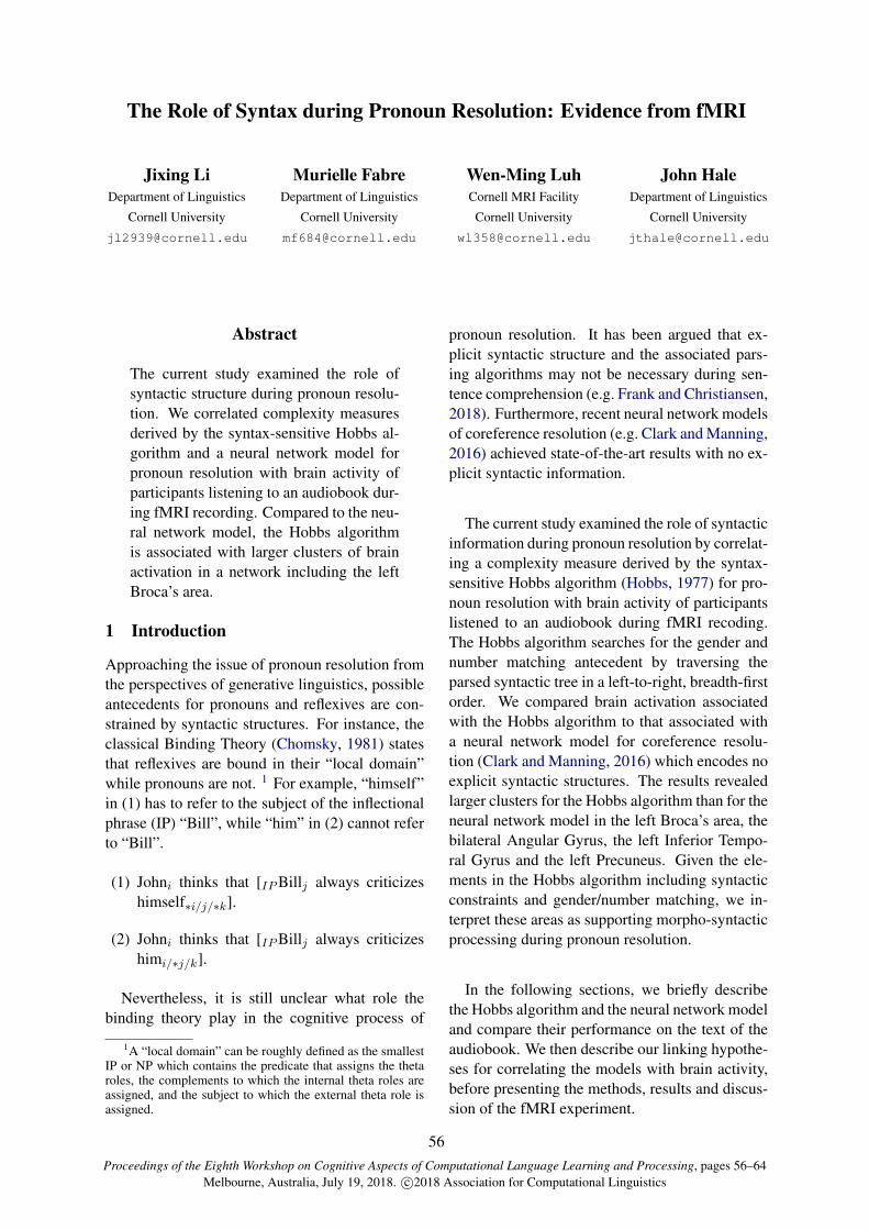
Proceedings of the Eighth Workshop on Cognitive Aspects of Computational Language Learning and Processing, pages 56–64Melbourne, Australia, July 19, 2018. c©2018 Association for Computational Linguistics
The Role of Syntax during Pronoun Resolution: Evidence from fMRI
Jixing LiDepartment of Linguistics
Cornell University
Murielle FabreDepartment of Linguistics
Cornell University
Wen-Ming LuhCornell MRI Facility
Cornell University
John HaleDepartment of Linguistics
Cornell University
Abstract
The current study examined the role ofsyntactic structure during pronoun resolu-tion. We correlated complexity measuresderived by the syntax-sensitive Hobbs al-gorithm and a neural network model forpronoun resolution with brain activity ofparticipants listening to an audiobook dur-ing fMRI recording. Compared to the neu-ral network model, the Hobbs algorithmis associated with larger clusters of brainactivation in a network including the leftBroca’s area.
1 Introduction
Approaching the issue of pronoun resolution fromthe perspectives of generative linguistics, possibleantecedents for pronouns and reflexives are con-strained by syntactic structures. For instance, theclassical Binding Theory (Chomsky, 1981) statesthat reflexives are bound in their “local domain”while pronouns are not. 1 For example, “himself”in (1) has to refer to the subject of the inflectionalphrase (IP) “Bill”, while “him” in (2) cannot referto “Bill”.
(1) Johni thinks that [IPBillj always criticizeshimself∗i/j/∗k].
(2) Johni thinks that [IPBillj always criticizeshimi/∗j/k].
Nevertheless, it is still unclear what role thebinding theory play in the cognitive process of
1A “local domain” can be roughly defined as the smallestIP or NP which contains the predicate that assigns the thetaroles, the complements to which the internal theta roles areassigned, and the subject to which the external theta role isassigned.
pronoun resolution. It has been argued that ex-plicit syntactic structure and the associated pars-ing algorithms may not be necessary during sen-tence comprehension (e.g. Frank and Christiansen,2018). Furthermore, recent neural network modelsof coreference resolution (e.g. Clark and Manning,2016) achieved state-of-the-art results with no ex-plicit syntactic information.
The current study examined the role of syntacticinformation during pronoun resolution by correlat-ing a complexity measure derived by the syntax-sensitive Hobbs algorithm (Hobbs, 1977) for pro-noun resolution with brain activity of participantslistened to an audiobook during fMRI recoding.The Hobbs algorithm searches for the gender andnumber matching antecedent by traversing theparsed syntactic tree in a left-to-right, breadth-firstorder. We compared brain activation associatedwith the Hobbs algorithm to that associated witha neural network model for coreference resolu-tion (Clark and Manning, 2016) which encodes noexplicit syntactic structures. The results revealedlarger clusters for the Hobbs algorithm than for theneural network model in the left Broca’s area, thebilateral Angular Gyrus, the left Inferior Tempo-ral Gyrus and the left Precuneus. Given the ele-ments in the Hobbs algorithm including syntacticconstraints and gender/number matching, we in-terpret these areas as supporting morpho-syntacticprocessing during pronoun resolution.
In the following sections, we briefly describethe Hobbs algorithm and the neural network modeland compare their performance on the text of theaudiobook. We then describe our linking hypothe-ses for correlating the models with brain activity,before presenting the methods, results and discus-sion of the fMRI experiment.
56

2 The Hobbs Algorithm
The Hobbs algorithm, originally presented inHobbs (1977), depends only on a syntactic parserplus a morphological gender and number checker.The input to the Hobbs algorithm includes the tar-get pronoun and the parsed trees for the currentand previous sentences. The algorithm searchesfor a gender and number matching antecedent bytraversing the tree in a left-to-right, breadth-firstorder, giving preference to closer antecedents. Ifno candidate antecedent is found in the currenttree, the algorithm searches on the preceding sen-tence in the same order. The steps of the Hobbsalgorithm are as follows:
(1) Begin at the NP node immediately dominating the pro-noun.
(2) Go up the tree to the first NP or S node encountered.Call this node X, and call the path used to reach it p.
(3) Traverse all branches below node X to the left of pathp in a left-to-right, breadth-first fashion. Propose as theantecedent any NP node that is encountered which hasan NP or S node between it and X.
(4) If node X is the highest S node in the sentence, tra-verse the surface parse trees of previous sentences inthe text in order of recency, the most recent first; eachtree is traversed in a left-to-right, breadth-first manner,and when an NP node is encountered, it is proposed asantecedent. If X is not the highest S node in the sen-tence, continue to step 5.
(5) From node X, go up the tree to the first NP or S nodeencountered. Call this new node X, and call the pathtraversed to reach it p.
(6) If X is an NP node and if the path p to X did not passthrough the N node that X immediately dominates,propose X as the antecedent.
(7) Traverse all branches below node X to the left of path pin a left-to-right, breadth-first manner. Propose any NPnode encountered as the antecedent.
(8) If X is an S node, traverse all branches of node X to theright of path p in a left-to-right. breadth-first manner,but do not go below any NP or S node encountered.Propose any NP node encountered as the antecedent.
(9) Go to step 4.
The Hobbs algorithm conforms to the BindingTheory as it always searches for the antecedent inthe left of the NP (Principle B: Step 3) and doesnot go below any NP or S node encountered (Prin-ciple A: Step 8). It also respects gender, person,and number agreement, and captures recency andgrammatical role preferences in the order it per-forms the search. Hobbs (1977) evaluated his al-gorithm on 300 examples containing third personpronouns, and it worked in 88.3% of the cases.With some selectional constraints on dates and lo-cation antecedents (i.e., restricting dates and loca-tion NPs such as “2018” and “school” to be the
antecedent of “it”), the algorithm achieved 91.7%accuracy. However, the test dataset was limitedin size and the performance degraded when therewere competing antecedents. We propose here totest its accuracy on a larger dataset including 1499sentences with 465 third person pronouns.
3 The Neural Network Model
The neural network model for pronoun resolutionis adapted from the neural network model for bothpronominal and nominal coreference resolution(Clark and Manning, 2016). This model consistsof a mention-pair encoder, a cluster-pair encoder,a mention-ranking model and a cluster-rankingmodel. The mention-pair encoder generates dis-tributed representations for pronoun-antecedentpairs, or mention pairs, by passing relevant fea-tures through a feed-forward neural network. Thecluster-pair encoder generates distributed repre-sentations for pairs of clusters through a poolingoperation over representations of relevant men-tion pairs. The mention-ranking model scores thecandidate antecedents to prune the set of possibleantecedent and the cluster-ranking model scorescoreference compatibility for each pair of clusters.
The input layer of the neural network modelconsists of a large set of features including wordembeddings for the mention pairs, type and lengthof the mentions, linear distance between the men-tion pairs, etc. (see Table 1). These feature vec-tors are concatenated to produce an I-dimensionalvector h0(a,m) as the representation for the men-tion m and the antecedent a. The input layer thenpasses through three hidden layers of rectified lin-ear units (ReLU), and the output of the last hiddenlayer is the vector representation for the mentionpair rm(a,m).
hi(a,m) = ReLU(Wihi−1(a,m) + bi)
For pairs of clusters ci = {mi1,m
i2, ...,m
ici}
and cj = {mj1,m
j2, ...,m
jcj}, the cluster-pair
encoder first forms a matrix Rm(ci, cj) =
[rm(mi1,m
j1), rm(mi
2,mj2), ..., rm(mi
ci ,mjcj )],
then applies a pooling operation over Rm(ci, cj)to produce a distributed representation for thecluster pair rc(ci, cj). The mention-ranking modelassigns a score for each mention pair by applyinga single fully connected layer of size one themention pair representation rm(a,m). The modelis then trained with the max-margin training
57

objective.
sm(a,m) = Wmrm(a,m) + bm
Similarly, the cluster-ranking model assigns acoreference score for each cluster pair and ananaphoricity score for mention m (i.e., how likelymention m has an antecedent). These scoresare used to decide whether mention m should bemerged with one preceding cluster or not duringtesting.
sc(ci, cj) = Wcrc(ci, cj) + bc
sNA(m) = WNArm(NA,m) + bNA
Feature Type DescriptionWord embedding head word
dependency parentfirst wordlast wordtwo preceding wordstwo following wordsaveraged of the five preceding wordsaveraged of five following wordsall words in the mentionall words in the mention’s sentenceand all words in the mention’s document
Mention type (pronoun/noun/proper name/list)position in the documentcontained in another mention or notlength of the mention in words
Document genre (broadcast news/newswire/web data)Distance intervening sentences
number intervening mentionsmentions overlap or not
String matching head matchexact string matchpartial string match
Table 1: Feature set of the neural network model(Clark and Manning, 2016).
The neural network model encodes no explicitsyntactic structures, but it captures semantic in-formation in its word embedding features. It alsoincorporates discourse-level information such aslinear distance between the mention pairs acrossseveral sentences, discourse genre, etc. Clark andManning (2016) trained the model on the CoNLL-2012 Shared Task (Pradhan et al., 2012) and itachieved state-of-the-art results in both the En-glish and Chinese test set.
The neural network model was evaluated onboth pronominal and nominal coreference reso-lution, however, pronouns and full noun phrases(NPs) may rely on very different set of features.For example, string matching and measures for se-mantic similarity are powerful features for nom-inal coreference resolution, but are not applica-ble for pronoun resolution as word embeddings do
not represent pronouns well. In addition, it hasbeen argued that pronouns serve a different dis-course function from that of full NPs in that fullNPs introduce new entities in the discourse andpronouns maintain the reference (Sanford et al.,1988). Based on these arguments, it is reasonableto say that pronoun resolution and full NP corefer-ence involves different cognitive processes.
4 Evaluating the Models on Text Data
4.1 Text DataThe text data is an English audiobook versionof Antoine de Saint-Exupery’s The Little Prince.Within the audiobook text, 1755 pronouns and3127 non-pronominal entities (4882 mentions intotal) are identified using the annotation tool brat(Stenetorp et al., 2012; see Figure 1). Reflex-ives (e.g., “herself”) and possessives (e.g., “his”)are excluded from the dataset as they have differ-ent “binding domains” from pronouns accordingto the Binding Theory and hence influences per-formance of the Hobbs algorithm. Pronouns withsentential antecedents (e.g, the second “it” in theconversation “That is funny where you live a dayonly last a minute.” “It is not funny at all.”), aswell as dummy pronouns (e.g., “it” in “It said inthe book that ...”) are also removed. The result-ing dataset contains 645 first person pronouns, 302second person pronouns and 675 third person pro-nouns (see Table 2).
1st i me we us505 121 16 3
2nd you302
3rd she her he him41 14 268 64it they them
136 94 58
Table 2: Attestations of each pronoun type in TheLittle Prince.
We decided to focus only on the third personpronouns because they provide gender and numberinformation that feeds the Hobbs algorithm. In ad-dition, third person pronouns have been suggestedto differ from first and second person pronouns inthat first and second person pronouns mark prox-imity in space and third person pronouns are fur-ther away (Ariel, 1990). Therefore, we further ex-cluded third person pronouns whose antecedents
58
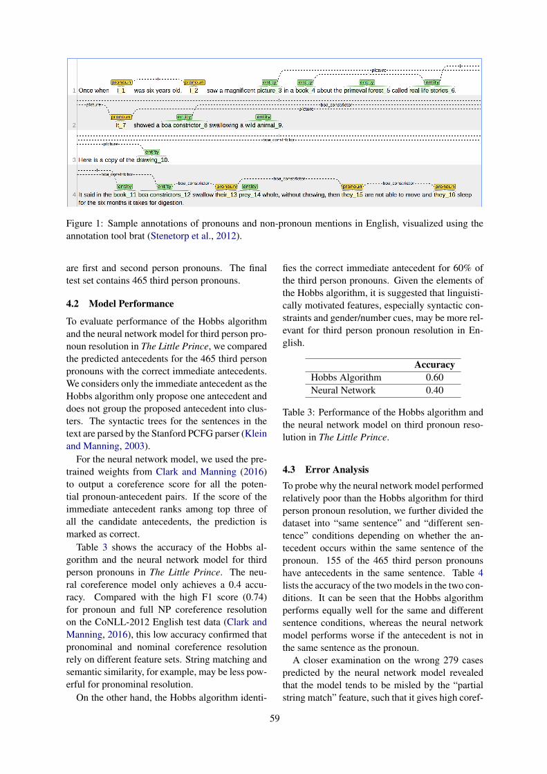
Figure 1: Sample annotations of pronouns and non-pronoun mentions in English, visualized using theannotation tool brat (Stenetorp et al., 2012).
are first and second person pronouns. The finaltest set contains 465 third person pronouns.
4.2 Model Performance
To evaluate performance of the Hobbs algorithmand the neural network model for third person pro-noun resolution in The Little Prince, we comparedthe predicted antecedents for the 465 third personpronouns with the correct immediate antecedents.We considers only the immediate antecedent as theHobbs algorithm only propose one antecedent anddoes not group the proposed antecedent into clus-ters. The syntactic trees for the sentences in thetext are parsed by the Stanford PCFG parser (Kleinand Manning, 2003).
For the neural network model, we used the pre-trained weights from Clark and Manning (2016)to output a coreference score for all the poten-tial pronoun-antecedent pairs. If the score of theimmediate antecedent ranks among top three ofall the candidate antecedents, the prediction ismarked as correct.
Table 3 shows the accuracy of the Hobbs al-gorithm and the neural network model for thirdperson pronouns in The Little Prince. The neu-ral coreference model only achieves a 0.4 accu-racy. Compared with the high F1 score (0.74)for pronoun and full NP coreference resolutionon the CoNLL-2012 English test data (Clark andManning, 2016), this low accuracy confirmed thatpronominal and nominal coreference resolutionrely on different feature sets. String matching andsemantic similarity, for example, may be less pow-erful for pronominal resolution.
On the other hand, the Hobbs algorithm identi-
fies the correct immediate antecedent for 60% ofthe third person pronouns. Given the elements ofthe Hobbs algorithm, it is suggested that linguisti-cally motivated features, especially syntactic con-straints and gender/number cues, may be more rel-evant for third person pronoun resolution in En-glish.
AccuracyHobbs Algorithm 0.60Neural Network 0.40
Table 3: Performance of the Hobbs algorithm andthe neural network model on third pronoun reso-lution in The Little Prince.
4.3 Error AnalysisTo probe why the neural network model performedrelatively poor than the Hobbs algorithm for thirdperson pronoun resolution, we further divided thedataset into “same sentence” and “different sen-tence” conditions depending on whether the an-tecedent occurs within the same sentence of thepronoun. 155 of the 465 third person pronounshave antecedents in the same sentence. Table 4lists the accuracy of the two models in the two con-ditions. It can be seen that the Hobbs algorithmperforms equally well for the same and differentsentence conditions, whereas the neural networkmodel performs worse if the antecedent is not inthe same sentence as the pronoun.
A closer examination on the wrong 279 casespredicted by the neural network model revealedthat the model tends to be misled by the “partialstring match” feature, such that it gives high coref-
59

Hobbs Neural NetworkSame Sentence 0.60 0.50Different Sentence 0.60 0.35
Table 4: Accuracy of the Hobbs algorithm and theneural network model for third person pronounsthat have antecedents in the same or different sen-tences.
erence scores for “that” and “they”. This con-firmed our hypothesis that pronominal and nom-inal coreference resolution rely on different set offeatures.
5 Correlating Model Prediction withBrain Activity
5.1 Linking HypothesesTo explain how the model performance are specif-ically brought to bear on brain activity, we furthercorrelated activation levels of the antecedents withfMRI time-courses when participants listened toThe Little Prince in the scanner.
We first selected the 277 third person pronounswhose antecedents are correctly predicted by theHobbs algorithm, i.e., the true positives, and wecalculated the Hobbs distance for each of the 277pronouns, namely, the number of NPs that theHobbs algorithm skips before the antecedent NPis proposed. Our linking hypotheses is that ahigher Hobbs distance induces a processing ef-fort for pronoun resolution, hence higher hemo-dynamic response.
Note that the Hobbs distance is different fromthe number of NP nodes between the pronounand the antecedents, as the Hobbs algorithm al-ways searches the antecedent to the left of the pro-noun in a left-to-right, breadth-first order. Figure2 shows the Hobbs distance for the two “they” inthe example sentence. The immediate antecedentfor “they 1” is “their”, and the Hobbs distance be-tween “their” and “they 1” is 2 because the algo-rithm skips the NP “boa constrictors” before pro-poses “their” as the antecedent. The Hobbs dis-tance for “they 2” is 1 because the correct an-tecedent is the first proposal by the algorithm.
In comparison, we recorded the coreferencescore Sm(a,m) generated by the neural networkmodel for the 277 pronouns that correctly pre-dicted by the Hobbs algorithm. We took the neg-ative of the score as a complexity measure for theneural coreference model: the higher the score,
the more difficult to retrieve the antecedent. Pear-son’s r revealed no significant correlation betweenthe Hobbs distance and the negative neural coref-erence score for the 227 third person pronouns(r = 0.05, p = 0.43).
5.2 Predicted Brain Activation
Based on the elements in the Hobbs algorithm andthe neural network model, we expected the diffi-culty of pronoun resolution modeled by the Hobbsdistance and the neural coreference score to teaseapart brain areas that are associated with syntac-tic and morphological processing, and brain areasthat are sensitive to semantic and discourse-levelinformation.
Previous neuroimaging results on pronoun res-olution have reported the bilateral Inferior FrontalGyrus (IFG), the left Medial Frontal Gyrus (MFG)and the bilateral Supramarginal/Angular Gyrus ingender mismatch between pronoun and antecedent(Hammer et al., 2007). We therefore expect activ-ity in these regions for the Hobbs distance met-ric. We also expect to see activity in the bi-lateral Superior Temporal Gyrus (STGs) as theyhave been associated with long distance pronoun-antecedent linking (Matchin et al., 2014). Theseregions could be relevant for both the Hobbs dis-tance and neural coreference score as they bothincorporate some form of “distance” between thepronoun-antecedent pairs. The Precuneus cortexmay also be activated with pronouns in generalas it has been suggested to track different sorts ofstory characters (Wehbe et al., 2014).
6 Brain Data
6.1 Participants
Participants were 49 healthy, right-handed, youngadults (30 female, mean age = 21.3, range = 18-37). They self-identified as native English speak-ers, and had no history of psychiatric, neurologi-cal or other medical illness that could compromisecognitive functions. All participants were paid for,and gave written informed consent prior to partic-ipation, in accordance with the guidelines of theHuman Research Participant Protection Programat Cornell University.
6.2 Stimuli
The stimulus was an audiobook version of Antoinede Saint-Exupery’s The Little Prince, translated
60

Figure 2: Demonstration of Hobbs distance for third person pronouns in a sentence. The red numbersbelow the pronouns indicates the Hobbs distance.
by David Wilkinson and read by Nadine Eckert-Boulet. This text contains 3127 non-pronominalmentions and 645 first person pronouns, 302 sec-ond person pronouns and 675 third person pro-nouns (see Table 2). Following the pruning criteriadescribed in Section 5, the final set of data include277 third person pronouns.
6.3 Procedure
After giving their informed consent, participantswere familiarized with the MRI facility and as-sumed a supine position on the scanner. The pre-sentation script was written in PsychoPy (Peirce,2007). Auditory stimuli were delivered throughMRI-safe, high-fidelity headphones (Confon HP-VS01, MR Confon, Magdeburg, Germany) in-side the head coil. The headphones were securedagainst the plastic frame of the coil using foamblocks. An experimenter increased the soundvolume stepwise until the participants could hearclearly.
The audiobook lasts for about 94 minutes, andwas divided into nine sections, each lasts for aboutten minutes. Participants listened passively to thenine sections and completed four quiz questionsafter each section (36 questions in total). Thesequestions were used to confirm their comprehen-sion and were viewed by the participants via a mir-ror attached to the head coil and they answeredthrough a button box. The entire session lastedaround 2.5 hours.
6.4 MRI Data Collection and Preprocessing
The brain imaging data were acquired with a3T MRI GE Discovery MR750 scanner witha 32-channel head coil. Anatomical scanswere acquired using a T1-weighted volumet-ric Magnetization Prepared RApid Gradient-Echo
(MP-RAGE) pulse sequence. Blood-oxygen-level-dependent (BOLD) functional scans wereacquired using a multi-echo planar imaging(ME-EPI) sequence with online reconstruction(TR=2000 ms; TE’s=12.8, 27.5, 43 ms; FA=77◦;matrix size=72 x 72; FOV=240.0 mm x 240.0mm; 2 x image acceleration; 33 axial slices, voxelsize=3.75 x 3.75 x 3.8 mm). Cushions and clampswere used to minimize head movement duringscanning.
All fMRI data is preprocessed using AFNI ver-sion 16 (Cox, 1996). The first 4 volumes ineach run were excluded from analyses to allowfor T1-equilibration effects. Multi-echo inde-pendent components analysis (ME-ICA; Kunduet al.,2012) were used to denoise data for motion,physiology and scanner artifacts. Images werethen spatially normalized to the standard space ofthe Montreal Neurological Institute (MNI) atlas,yielding a volumetric time series resampled at 2mm cubic voxels.
6.5 Statistical Analysis
At the single subject level, the observed BOLDtime course in each voxel were modeled by thedifficulty of pronoun resolution derived by theHobbs Algorithm and the Neural Network Modelfor third person pronouns time-locked at the off-set of each third person pronoun in the audiobook.To further examine the status of Hobbs and NeuralNetwork Models as cognitive models for pronounresolution, we also included a binary regressor thatsimply marks the presence of a third person pro-noun time-locked at the offset of each third personpronoun in the audiobook.
In addition, three control variables of non-theoretical interest were included in the GLManalysis: RMS intensity at every 10 ms of the au-
61
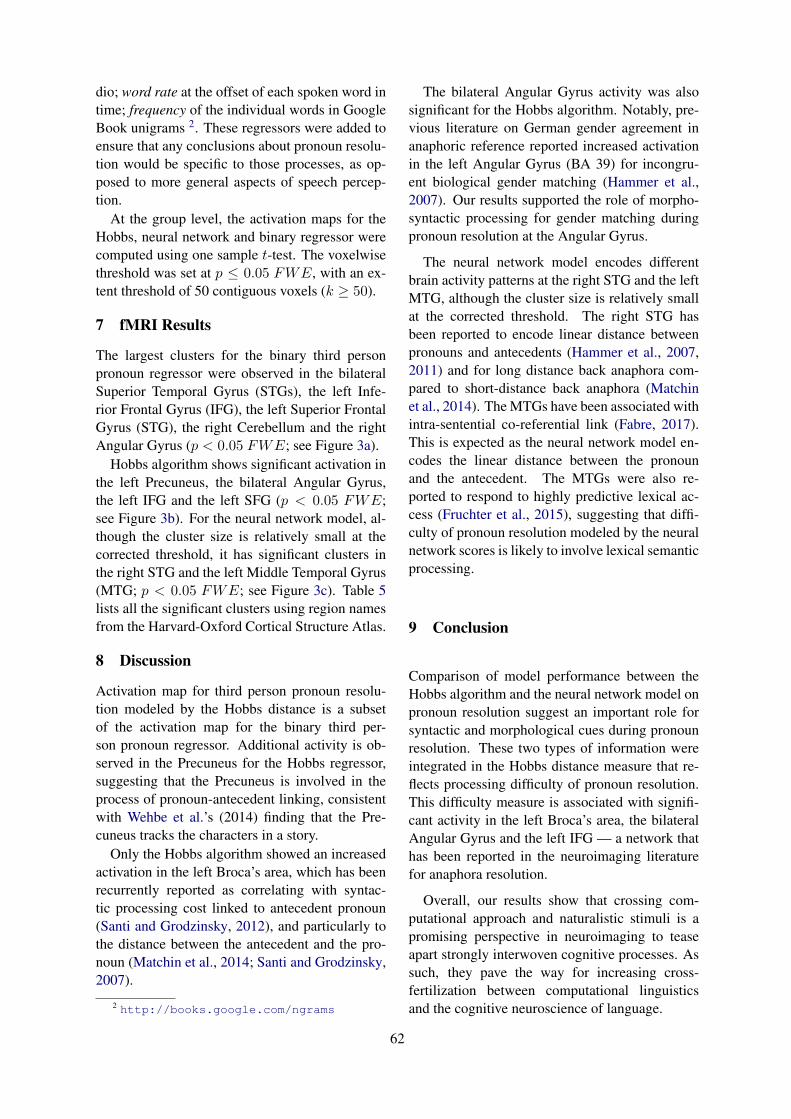
dio; word rate at the offset of each spoken word intime; frequency of the individual words in GoogleBook unigrams 2. These regressors were added toensure that any conclusions about pronoun resolu-tion would be specific to those processes, as op-posed to more general aspects of speech percep-tion.
At the group level, the activation maps for theHobbs, neural network and binary regressor werecomputed using one sample t-test. The voxelwisethreshold was set at p ≤ 0.05 FWE, with an ex-tent threshold of 50 contiguous voxels (k ≥ 50).
7 fMRI Results
The largest clusters for the binary third personpronoun regressor were observed in the bilateralSuperior Temporal Gyrus (STGs), the left Infe-rior Frontal Gyrus (IFG), the left Superior FrontalGyrus (STG), the right Cerebellum and the rightAngular Gyrus (p < 0.05 FWE; see Figure 3a).
Hobbs algorithm shows significant activation inthe left Precuneus, the bilateral Angular Gyrus,the left IFG and the left SFG (p < 0.05 FWE;see Figure 3b). For the neural network model, al-though the cluster size is relatively small at thecorrected threshold, it has significant clusters inthe right STG and the left Middle Temporal Gyrus(MTG; p < 0.05 FWE; see Figure 3c). Table 5lists all the significant clusters using region namesfrom the Harvard-Oxford Cortical Structure Atlas.
8 Discussion
Activation map for third person pronoun resolu-tion modeled by the Hobbs distance is a subsetof the activation map for the binary third per-son pronoun regressor. Additional activity is ob-served in the Precuneus for the Hobbs regressor,suggesting that the Precuneus is involved in theprocess of pronoun-antecedent linking, consistentwith Wehbe et al.’s (2014) finding that the Pre-cuneus tracks the characters in a story.
Only the Hobbs algorithm showed an increasedactivation in the left Broca’s area, which has beenrecurrently reported as correlating with syntac-tic processing cost linked to antecedent pronoun(Santi and Grodzinsky, 2012), and particularly tothe distance between the antecedent and the pro-noun (Matchin et al., 2014; Santi and Grodzinsky,2007).
2 http://books.google.com/ngrams
The bilateral Angular Gyrus activity was alsosignificant for the Hobbs algorithm. Notably, pre-vious literature on German gender agreement inanaphoric reference reported increased activationin the left Angular Gyrus (BA 39) for incongru-ent biological gender matching (Hammer et al.,2007). Our results supported the role of morpho-syntactic processing for gender matching duringpronoun resolution at the Angular Gyrus.
The neural network model encodes differentbrain activity patterns at the right STG and the leftMTG, although the cluster size is relatively smallat the corrected threshold. The right STG hasbeen reported to encode linear distance betweenpronouns and antecedents (Hammer et al., 2007,2011) and for long distance back anaphora com-pared to short-distance back anaphora (Matchinet al., 2014). The MTGs have been associated withintra-sentential co-referential link (Fabre, 2017).This is expected as the neural network model en-codes the linear distance between the pronounand the antecedent. The MTGs were also re-ported to respond to highly predictive lexical ac-cess (Fruchter et al., 2015), suggesting that diffi-culty of pronoun resolution modeled by the neuralnetwork scores is likely to involve lexical semanticprocessing.
9 Conclusion
Comparison of model performance between theHobbs algorithm and the neural network model onpronoun resolution suggest an important role forsyntactic and morphological cues during pronounresolution. These two types of information wereintegrated in the Hobbs distance measure that re-flects processing difficulty of pronoun resolution.This difficulty measure is associated with signifi-cant activity in the left Broca’s area, the bilateralAngular Gyrus and the left IFG — a network thathas been reported in the neuroimaging literaturefor anaphora resolution.
Overall, our results show that crossing com-putational approach and naturalistic stimuli is apromising perspective in neuroimaging to teaseapart strongly interwoven cognitive processes. Assuch, they pave the way for increasing cross-fertilization between computational linguisticsand the cognitive neuroscience of language.
62

(a) T-score map for the binary third person pronoun regressor
(b) T-score map for the Hobbs distance regressor
(c) T-score map for the negative neural network score regressor
Figure 3: Whole-brain effect with significant clusters for (a) binary third person pronouns effect, (b)difficulty for third pronoun resolution based on the Hobbs algorithm and (c) difficulty for third personpronoun resolution based on the neural coreference model. All images underwent FWE voxel correctionfor multiple comparisons with p < 0.05.
MNI coordinates Region p-value k-size t-scorex y z FWE-corr cluster peak
Third Person Pronoun -60 -12 -6 left Superior Temporal Gyrus < 0.001 4411 12.92(binary) 64 -10 -2 right Superior Temporal Gyrus < 0.001 1625 10.95
-46 30 -12 left Inferior Frontal Gyrus < 0.001 706 10.53-10 42 46 left Superior Frontal Gyrus < 0.001 2394 10.4518 -74 -30 right Cerebellum < 0.001 283 7.1552 -60 26 right Angular Gyrus 0.004 68 5.84
Hobbs Algorithm -6 -68 50 left Precuneus < 0.001 1163 8.86-32 -62 42 left Angular Gyrus < 0.001 1216 8.42-52 -56 -16 left Inferior Temporal Gyrus < 0.001 285 6.5434 -52 34 right Angular Gyrus 0.001 119 6.31-44 6 34 left Inferior Frontal Gyrus 0.005 55 5.01-26 12 60 left Superior Frontal Gyrus 0.007 62 5.63
Neural Network 62 -28 14 right Superior Temporal Gyrus 0.005 48 5.69-46 -54 4 left Middle Temporal Gyrus 0.008 13 5.55
Table 5: Significant clusters of BOLD activation for (a) third person pronouns, (b) difficulty for thirdperson pronoun resolution based on the Hobbs algorithm and (c) difficulty for third person pronounresolution based on the neural coreference model. Peak activations are given in MNI Coordinates (p <0.05, FWE).
63
Acknowledgments
This material is based upon work supported bythe National Science Foundation under GrantNo.1607441.
ReferencesM. Ariel. 1990. Accessing noun-phrase antecedents.
Routledge, London, UK.
Noam Chomsky. 1981. Lectures on government andbinding. Foris, Dordrecht, Holland.
Kevin Clark and Christopher D. Manning. 2016. Im-proving coreference resolution by learning entity-level distributed representations. arXiv:1606.01323.
R. W. Cox. 1996. AFNI: software for analysis andvisualization of functional magnetic resonance neu-roimages. Computers and Biomedical Research, anInternational Journal, 29(3):162–173.
Murielle Fabre. 2017. The sentence as cognitive object- The neural underpinnings of syntactic complex-ity in Chinese and French. Ph.D. thesis, INALCOParis.
Stefan L. Frank and Morten H. Christiansen. 2018. Hi-erarchical and sequential processing of language:A response to: Ding, Melloni, Tian, and Poeppel(2017). Rule-based and word-level statistics-basedprocessing of language: insights from neuroscience.Language, Cognition and Neuroscience . Language,Cognition and Neuroscience, pages 1–6.
Joseph Fruchter, Tal Linzen, Masha Westerlund, andAlec Marantz. 2015. Lexical Preactivation in Ba-sic Linguistic Phrases. Journal of Cognitive Neuro-science, 27(10):1912–1935.
Anke Hammer, Rainer Goebel, Jens Schwarzbach,Thomas F. Munte, and Bernadette M. Jansma. 2007.When sex meets syntactic gender on a neural ba-sis during pronoun processing. Brain Research,1146:185–198.
Anke Hammer, Bernadette M. Jansma, Claus Tempel-mann, and Thomas F. Munte. 2011. Neural mech-anisms of anaphoric reference revealed by fMRI.Frontiers in Psychology, 2.
Jerry Hobbs. 1977. Resolving pronouns. In Readingsin natural language processing. Morgan KaufmanPublishers, Inc., Los Altos, California, USA.
D. Klein and C. Manning. 2003. Accurate unlexical-ized parsing. In Proceedings of the 41st Meeting ofthe association for computational linguistics., pages423–430.
Prantik Kundu, Souheil J. Inati, Jennifer W. Evans,Wen-Ming Luh, and Peter A. Bandettini. 2012. Dif-ferentiating BOLD and non-BOLD signals in fMRItime series using multi-echo EPI. NeuroImage,60(3):1759–1770.
William Matchin, Jon Sprouse, and Gregory Hickok.2014. A structural distance effect for backwardanaphora in Broca’s area: An fMRI study. Brainand Language, 138:1–11.
Jonathan W. Peirce. 2007. PsychoPy—Psychophysicssoftware in Python. Journal of Neuroscience Meth-ods, 162(1-2):8–13.
Sameer Pradhan, Alessandro Moschitti, Nianwen Xue,Olga Uryupina, and Yuchen Zhang. 2012. CoNLL-2012 shared task: Modeling multilingual unre-stricted coreference in OntoNotes. In Proceedingsof the Sixteenth Conference on Computational Natu-ral Language Learning (CoNLL 2012), Jeju, Korea.
Anthony J. Sanford, K. Moar, and Simon C. Garrod.1988. Proper names as controllers of discourse fo-cus. Language and speech, 31(1):43–56.
Andrea Santi and Yosef Grodzinsky. 2007. Taxingworking memory with syntax: Bihemispheric modu-lations. Human Brain Mapping, 28(11):1089–1097.
Andrea Santi and Yosef Grodzinsky. 2012. Broca’sarea and sentence comprehension: A relation-ship parasitic on dependency, displacement or pre-dictability? Neuropsychologia, 50(5):821–832.
Pontus Stenetorp, Sampo Pyysalo, Goran Topic,Tomoko Ohta, Sophia Ananiadou, and Jun’ichi Tsu-jii. 2012. BRAT: a web-based tool for NLP-assistedtext annotation. In Proceedings of the Demonstra-tions at the 13th Conference of the European Chap-ter of the Association for Computational Linguistics,pages 102–107. Association for Computational Lin-guistics.
Leila Wehbe, Ashish Vaswani, Kevin Knight, andTom M. Mitchell. 2014. Aligning context-based sta-tistical models of language with brain activity duringreading. In EMNLP, pages 233–243.
64
Proceedings of the Eighth Workshop on Cognitive Aspects of Computational Language Learning and Processing, pages 65–74Melbourne, Australia, July 19, 2018. c©2018 Association for Computational Linguistics
A Sound and Complete Left-Corner Parsing for Minimalist Grammars
Milos StanojevicUniversity of Edinburgh
Edinburgh EH8 9AB, [email protected]
Edward P. StablerUCLA and Nuance Communications
California, [email protected]
Abstract
This paper presents a left-corner parser forminimalist grammars. The relation be-tween the parser and the grammar is trans-parent in the sense that there is a very sim-ple 1-1 correspondence between deriva-tions and parses. Like left-corner context-free parsers, left-corner minimalist parserscan be non-terminating when the grammarhas empty left corners, so an easily com-puted left-corner oracle is defined to re-strict the search.
1 Introduction
Minimalist grammars (MGs) (Stabler, 1997)were inspired by proposals in Chomskian syn-tax (Chomsky, 1995). MGs are strictly moreexpressive than context free grammars (CFGs)and weakly equivalent to multiple context freegrammars (MCFGs) (Michaelis, 2001; Harkema,2001a). The literature presents bottom-up and top-down parsers for MGs (Harkema, 2001b), whichdiffer in the order in which derivations are con-structed, and consequently they may differ in theirmemory demands at each point in the parse. Butpartly because of those memory demands, parsersthat mix top-down and bottom-up steps are oftenregarded as psycholinguistically more plausible(Hale, 2014; Resnik, 1992; Abney and Johnson,1991).
Among mixed strategies, left-cornerparsing (LC) is perhaps the best known(Rosenkrantz and Lewis, 1970). A left-cornerparser does not begin by guessing what’s in thestring, as a top-down parser does. But it also doesnot just reduce elements of the input, as a bottom-up parser does. A left-corner parser looks firstat what is in the string (completing the left-mostconstituent, bottom-up) and then predicting the
sisters of that element (top-down), if any. Thefollowing CFG trees have nodes numbered in theorder they would be constructed by bottom-up,left-corner and top-down strategies:
12
3 45
6 7
42
1 36
5 7
73
1 26
4 5top-down left-corner bottom-up
LC parsing is bottom-up on the leftmost leaf, butthen proposes a completed parent of that node oncondition that its predicted sister is found.
For CFGs, LC parsing is well understood(Aho and Ullman, 1972; Rosenkrantz and Lewis,1970). In a CF rule A → B C , the left cor-ner is of course always B. Johnson and Roark(2000) generalize from CFGs to unification-basedgrammars and show how to allow some selectedcategories to be parsed left-corner while othersare parsed top-down. Extending these ideas toMGs, we must deal with movements, with rulesthat sometimes have their first daughter on theleft and sometimes on the right, and with cate-gories that are sometimes empty and sometimesnot. Left corner parsers were developed for someother discontinuous formalisms with similar prop-erties (van Noord, 1991; Dıaz et al., 2002) but inall cases these parsers fall in the category ofthe arc-standard left corner parsing. Here wepresent a left corner parser that is of arc-eagertype which is argued to be more cognitively plau-sible due to its higher degree of incrementality(Abney and Johnson, 1991; Resnik, 1992).
A first approach to left-corner MG parsing, de-signed to involve a kind of psycholinguisticallymotivated search, has been presented (Hunter,2017), but that proposal does not handle all MGs.In particular, remnant movement presents the mainchallenge to Hunter’s parser. The parser proposedhere handles all MGs, and it is easily shown to besound and complete via a simple 1-1 correspon-
65
dence between derivations and parses. (However,as mentioned in the conclusion, the present pro-posal does not yet address the psycholinguistic is-sues raised by Hunter.) Following similar workon CFGs (Pereira and Shieber, 1987, §6.3.1), weshow how to compute a left-corner oracle that canimprove efficiency. And probabilities can be usedin a LC beam-parser to pursue the most proba-ble parses at each step (Manning and Carpenter,1997).
2 Minimalist grammars
We present a succinct definition adapted fromStabler (2011, §A.1) and then consider a sim-ple example derivation in Figure 1. An MGG=〈Σ, B, Lex,C, {merge,move}〉, where Σ is thevocabulary, B is a set of basic features, Lex is afinite lexicon (as defined just below), C ∈ B is thestart category, and {merge,move} are the gener-ating functions. The basic features of the set B areconcatenated with prefix operators to specify theirroles, as follows:
categories, selectees = Bselectors = {=f | f ∈ B}licensees = {-f | f ∈ B}licensors = {+f | f ∈ B}.
Let F be the set of role-marked features, that is,the union of the categories, selectors, licensors andlicensees. Let T={::, :} be two types, indicat-ing ‘lexical’ and ‘derived’ structures, respectively.Let C = Σ∗ × T × F ∗ be the set of chains. LetE = C+ be the set of expressions. An expressionis a chain together with its ‘moving’ sub-chains,if any. Then the lexicon Lex ⊂ Σ∗ × {::} × F ∗
is a finite set. We write ǫ for the empty string.Merge and move are defined in Table 1. Note thateach merge rule deletes a selection feature =f anda corresponding category feature f, so the resulton the left side of the rule has 2 features less thanthe total number of features on the right. Simi-larly, each move rule deletes a licensor feature +fand a licensee feature -f. Note also that the ruleshave pairwise disjoint domains; that is, an instanceof a right side of a rule is not an instance of theright side of any other rule. The set of structures,everything you can derive from the lexicon usingthe rules, S(G)=closure(Lex,{merge,move}). Thesentences L(G) = {s| s ·C ∈ S(G) for some type· ∈ {:, ::}}, where C is the ‘start’ category.
Example grammar G1 with start category c usesfeatures +wh and -wh to trigger wh-movements:
ǫ :: =v c knows :: =c =d vǫ :: =v +wh c likes :: =d =d vAca :: d what :: d -whBibi :: d
These 7 lexical items define an infinite language.An example derivation is shown in Figure 1.
Grammar G1 is simple in a way that can bemisleading, since the mechanisms that allow sim-ple wh-movement also allow remnant movements,that is, movements of a constituent out of whichsomething has already moved. Without remnantmovements, MGs only define context-free lan-guages (Kobele, 2010). So remnant movementsare responsible for deriving copying and othersorts of crossing dependencies that cannot be en-forced in a CFG. Consider G2:
⊥ :: T -r -l ⊤ :: =T +r +l Ta :: =A +l T -l a :: =T +r A -rb :: =B +l T -l b :: =T +r B -r
With T as the start category, this grammar definesthe copy language ⊥XX⊤ where X is any stringof a’s and b’s. Bracketing the reduplicated stringwith ⊥ and ⊤ allows this very simple grammarwith no empty categories, and makes it easy totrack how the positions of these elements is de-fined by the derivation tree on the left in Figure 2,with 6 movements numbered 0 to 4, with TP(0)moving twice.
This example shows that simple mechanismsand simple lexical features can produce sur-prising patterns. Some copy-like patternsare fairly easy to see in human languages(Bresnan et al., 1982; Shieber, 1985), and manyproposals with remnant derivations have becomequite prominent in syntactic theory, even wherecopy-like patterns are not immediately obvious(den Besten and Webelhuth, 1990; Kayne, 1994;Koopman and Szabolcsi, 2000; Hinterholzl, 2006;Grewendorf, 2015; Thoms and Walkden, 2018).Since remnant-movement analyses seem appropri-ate for some constructions in human languages,and since grammars defining those analyses areoften quite simple, and since at least in manycases, remnant analyses are easy to compute, itwould be a mistake to dismiss these derivations tooquickly. For present purposes, the relevant and ob-vious point is that a sound and complete left cornerparser for MGs must handle all such derivations.
66

Aca knows what Bibi likes:c
ǫ::=v c1
Aca knows what Bibi likes:v
knows what Bibi likes:=d v
knows::=c =d v3
what Bibi likes:c
Bibi likes:+wh c,what:-wh
ǫ::=v +wh c55
Bibi likes:v,what:-wh
likes:=d v,what:-wh
likes::=d =d v7
what::d -wh4
Bibi::d6
Aca::d2
cP
c
ǫ1
vP
dP
Aca2
v’
v
knows3
cP
dP(0)
what4
c’
c
ǫ5
vP
dP
Bibi6
v’
v
likes7
dP(0)
Figure 1: Derivation tree from G1 on the left, and corresponding X-bar derived tree on the right. Inthe derivation tree, the binary internal nodes are applications of merge rules, while the unary node is anapplication of move1. Computing the derived X-bar structure from the derivation is briefly described in§5 below. Note that in the X-bar tree, P is added to each category feature when the complex is the ‘max-imal projection’ of the head, while primes indicate intermediate projections, and the moved constituentis ‘coindexed’ with its origin by marking both positions with (0). For the LC parser, the derivation tree(not the derived X-bar tree) is the important object, since the derivation is what shows whether a stringis derived by the grammar. But which daughter is ‘leftmost’ in the derivation tree is determined by thederived string positions, counted here from 1 to 7, left to right. Derived categories become left cornerswhen they are completed, so for the nodes in the derivation tree, the leftmost daughter, in the senserelevant for LC parsing, is the one that is completed first in the left-to-right parse of the derived string.
⊥ a b a b ⊤:T
a b ⊤:+l T,⊥ a b:-l
⊤:+r +l T,⊥ a b:-l,a b:-r
⊤::=T +r +l T ⊥ a b:T -l,a b:-r
b:+l T -l,a b:-r,⊥ a:-l
b::=B +l T -l a b:B -r,⊥ a:-l
b:+r B -r,⊥ a:-l,a:-r
b::=T +r B -r ⊥ a:T -l,a:-r
a:+l T -l,a:-r,⊥:-l
a::=A +l T -l a:A -r,⊥:-l
a:+r A -r,⊥:-r -l
a::=T +r A -r ⊥::T -r -l
TP
TP(4)
TP(2)
TP(0)
⊥
T’
T
a
AP(1)
T’
T
b
BP(3)
T’
BP(3)
AP(1)
TP(0) A’
A
a
TP(0)
B’
B
b
TP(2)
T’
T
⊤TP(4)
Figure 2: Derivation tree from G2 on the left, and corresponding derived tree on the right. Note that theempty TP(0) moves twice, first with MOVE2 and then landing with MOVE1. That TP is just the emptyhead, the only element of G2 with 2 licensees. Graf et al. (2016) show that all MG languages can bedefined without moving any phrase more than once, but G2 is beautifully small and symmetric.
67
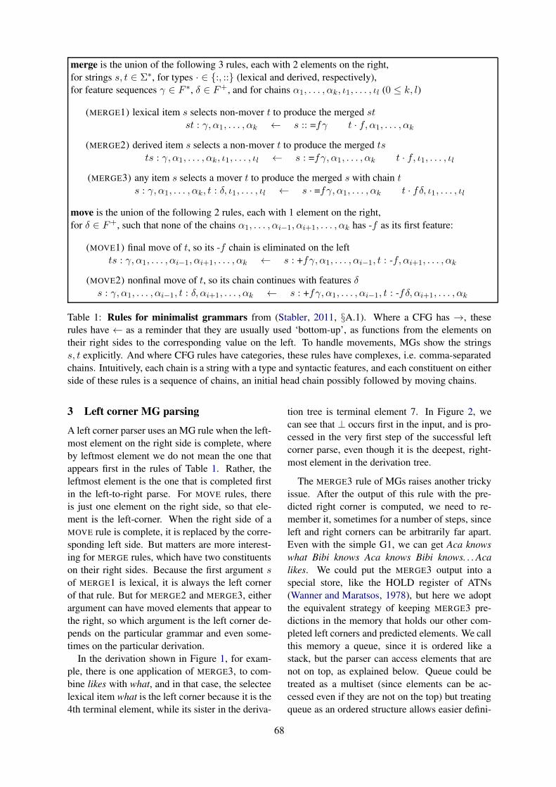
merge is the union of the following 3 rules, each with 2 elements on the right,for strings s, t ∈ Σ∗, for types · ∈ {:, ::} (lexical and derived, respectively),for feature sequences γ ∈ F ∗, δ ∈ F+, and for chains α1, . . . , αk, ι1, . . . , ιl (0 ≤ k, l)
(MERGE1) lexical item s selects non-mover t to produce the merged stst : γ, α1, . . . , αk ← s :: =fγ t · f, α1, . . . , αk
(MERGE2) derived item s selects a non-mover t to produce the merged tsts : γ, α1, . . . , αk, ι1, . . . , ιl ← s : =fγ, α1, . . . , αk t · f, ι1, . . . , ιl
(MERGE3) any item s selects a mover t to produce the merged s with chain ts : γ, α1, . . . , αk, t : δ, ι1, . . . , ιl ← s · =fγ, α1, . . . , αk t · fδ, ι1, . . . , ιl
move is the union of the following 2 rules, each with 1 element on the right,for δ ∈ F+, such that none of the chains α1, . . . , αi−1, αi+1, . . . , αk has -f as its first feature:
(MOVE1) final move of t, so its -f chain is eliminated on the leftts : γ, α1, . . . , αi−1, αi+1, . . . , αk ← s : +fγ, α1, . . . , αi−1, t : -f, αi+1, . . . , αk
(MOVE2) nonfinal move of t, so its chain continues with features δs : γ, α1, . . . , αi−1, t : δ, αi+1, . . . , αk ← s : +fγ, α1, . . . , αi−1, t : -fδ, αi+1, . . . , αk
Table 1: Rules for minimalist grammars from (Stabler, 2011, §A.1). Where a CFG has →, theserules have ← as a reminder that they are usually used ‘bottom-up’, as functions from the elements ontheir right sides to the corresponding value on the left. To handle movements, MGs show the stringss, t explicitly. And where CFG rules have categories, these rules have complexes, i.e. comma-separatedchains. Intuitively, each chain is a string with a type and syntactic features, and each constituent on eitherside of these rules is a sequence of chains, an initial head chain possibly followed by moving chains.
3 Left corner MG parsing
A left corner parser uses an MG rule when the left-most element on the right side is complete, whereby leftmost element we do not mean the one thatappears first in the rules of Table 1. Rather, theleftmost element is the one that is completed firstin the left-to-right parse. For MOVE rules, thereis just one element on the right side, so that ele-ment is the left-corner. When the right side of aMOVE rule is complete, it is replaced by the corre-sponding left side. But matters are more interest-ing for MERGE rules, which have two constituentson their right sides. Because the first argument sof MERGE1 is lexical, it is always the left cornerof that rule. But for MERGE2 and MERGE3, eitherargument can have moved elements that appear tothe right, so which argument is the left corner de-pends on the particular grammar and even some-times on the particular derivation.
In the derivation shown in Figure 1, for exam-ple, there is one application of MERGE3, to com-bine likes with what, and in that case, the selecteelexical item what is the left corner because it is the4th terminal element, while its sister in the deriva-
tion tree is terminal element 7. In Figure 2, wecan see that ⊥ occurs first in the input, and is pro-cessed in the very first step of the successful leftcorner parse, even though it is the deepest, right-most element in the derivation tree.
The MERGE3 rule of MGs raises another trickyissue. After the output of this rule with the pre-dicted right corner is computed, we need to re-member it, sometimes for a number of steps, sinceleft and right corners can be arbitrarily far apart.Even with the simple G1, we can get Aca knowswhat Bibi knows Aca knows Bibi knows. . . Acalikes. We could put the MERGE3 output into aspecial store, like the HOLD register of ATNs(Wanner and Maratsos, 1978), but here we adoptthe equivalent strategy of keeping MERGE3 pre-dictions in the memory that holds our other com-pleted left corners and predicted elements. We callthis memory a queue, since it is ordered like astack, but the parser can access elements that arenot on top, as explained below. Queue could betreated as a multiset (since elements can be ac-cessed even if they are not on the top) but treatingqueue as an ordered structure allows easier defini-
68

tion of oracle and easier definition of which con-stituent is triggering the next parser’s operation.
It will be convenient to number string positionsas usual: 0 Aca 1 knows 2 what 3 Bibi 4 likes 5.Substrings can then be given by their spans, so Acain our example is represented by 0-1, knows is 1-2,and an initial empty element would have the span0-0.
So the parser state is given by
(remaining input, current position, queue),
and we begin with
(input, 0, ǫ).
For any input of length n, we then attempt to applythe LC rules to get
(ǫ, n, 0-n·c),
where · is any type and c is the start category. TheLC rules are these:
(0) The SHIFT rule takes an initial (possiblyempty) element w with span x-y from the begin-ning of the remaining input, where the lexicon hasw :: γ, and puts x-y::γ onto the queue.
(1) For an MG rule R of the form A ← B Cwith left corner B, if an instance of B is on top ofthe queue, lc1(R) removes B from the top of thequeue and replaces it with an element C ⇒ A.Since any merge rule can have the selector as itsleft corner, we have the LC rules LC1(MERGE1),LC1(MERGE2), and LC1(MERGE3).
Let’s be more precise about being ‘an instance’.When R is A ← B C , the top element B′ ofthe queue is an instance of B iff we can find a(most general) substitution θ such that B′θ = Bθ.In that case, lc(R) replaces B′ with (C ⇒ A)θ.This computation of substitutions can be done bystandard unification (Lloyd, 1987). For example,looking at MERGE1 in Table 1, note that the firstconstituent on the right specifies the feature f , thesequence γ, and the string s, but not the string tor the 0 or more moving chains α1, . . . , αk. Sowhen LC1(MERGE1) applies, the unspecified el-ements are left as variables, to be instantiated bylater steps. So when s :: =fγ (for some particu-lar s, f, γ) is on top of the queue, LC1(MERGE1)replaces it by
(t · f, α1, . . . , αk ⇒ st : γ, α1, . . . , αk).
where underlined elements are variables.
(2) For an MG rule R of the form A ← B C ′
with completed left corner C and Cθ = C ′θ,lc2(R) replaces C on top of the queue by (B ⇒A)θ. For this case, where the second argument onthe right side is the left corner, we have the LCrules LC2(MERGE2) and LC2(MERGE3).
(3) Similarly for MG rules A ← B, theonly possible leftcorner is a constituent B whereBθ = B′θ, replacing B′ by Aθ. So we haveLC1(MOVE1) and LC1(MOVE2) in this case.
(4) We have introduced 8 LC rules so far. Thereis SHIFT, and there are 7 LC rules correspondingto the 5 MG rules in Table 1, because of the factthat the left corner of MERGE2 and MERGE3 canbe either the first or second element on the rightside of the rule. Each LC rule acts to put some-thing new on top of the queue. The ‘arc-eager’variant of LC parsing, which we will define here,adds additional variants of those 8 rules: instead ofjust putting the new element on top of the queue,the element created by a rule can also be used tocomplete a prediction on the queue, ‘connecting’the new element with structure already built.1 Im-portantly, the following completion variants of theLC rules can search below the top element to findconnecting elements:
c(R) If LC rule R creates a constituent B, andthe queue has B′ ⇒ A, where Bθ = B′θ, thenc(R) removes B′ ⇒ A puts Aθ onto the queue.
c1(R) If LC rule R creates B ⇒ A and we al-ready have C ⇒ B′ on the queue, where Bθ =B′θ, then c1(R) removes C ⇒ B′ and puts (C ⇒A)θ onto the queue.
c2(R) If LC rule R creates C ⇒ B and we al-ready have B′ ⇒ A on the queue, where Bθ =B′θ, c2(R) removes B′ ⇒ A and puts (C ⇒ A)θonto the queue.
c3(R) If LC rule R creates a constituent C ⇒ Band we already have B′ ⇒ A and D ⇒ C ′ on thequeue, where Bθ = B′θ and Cθ = C ′θ c3(R)removes B′ ⇒ A and D ⇒ C ′ and puts (D ⇒A)θ onto the queue.
These completion rules are similar to the ‘com-position’ rules of combinatory categorial grammar(Steedman, 2014).
1Instead of requiring completions to happen when an ele-ment is added to the queue, the ‘arc-standard’ variant of LCparsing uses separate complete rules, which means that a con-stituent need not (and sometimes cannot) be connected to pre-dicted structure at the time when it is first proposed.
69

That completes the specification of an arc-eagerleft corner parser for MGs. The rules are non-deterministic; that is, at many points in a parse,various different LC rules can apply. But for eachn-node derivation tree, there is a unique sequenceof n LC rule applications that accepts the derivedstring. This 1-1 correspondence between deriva-tions and parses is unsurprising given the defini-tion of LC. Intuitively, every LC rule is an MGrule, except that it’s triggered by its left corner, andit can ‘complete’ already predicted constituents.This makes it relatively easy to establish the cor-rectness of the parsing method (§5, below).
The 14 node derivation tree in Figure 1 has this14 step LC parse, indicating the rule used, theremaining input, and queue contents from top tobottom, with variables M and N for chain se-quences, Fs for features, for span positions, and[] represents the remaining input ǫ in the last 2steps of the listing:1. shift [Aca,knows,what,Bibi,likes]
0-0::=v c2. lc1(merge1) [Aca,knows,what,Bibi,likes]
(0-_.v _M => 0-_:c _M)3. shift [knows,what,Bibi,likes]
0-1::d(0-_.v _M => 0-_:c _M)
4. c1(lc2(merge2)) [knows,what,Bibi,likes](1-_:=d v _M => 0-_:c _M)
5. shift [what,Bibi,likes]1-2::=c =d v(1-_:=d v _M => 0-_:c _M)
6. c1(lc1(merge1)) [what,Bibi,likes](2-_.c _M => 0-_:c _M)
7. shift [Bibi,likes]2-3::d -wh(2-_.c _M => 0-_:c _M)
8. lc2(merge3) [Bibi,likes](_-_.=d _Fs_M => _-_:_Fs,2-3:-wh )(2-_.c _M => 0-_:c _M)
9. shift [Bibi,likes]3-3::=v +wh c(_-_.=d _Fs => _-_:_Fs,2-3:-wh )(2-_.c _M => 0-_:c _M)
10. lc1(merge1) [Bibi,likes](3-_.v _M => 3-_:+wh c _M)(_-_.=d _Fs => _-_:_Fs,2-3:-wh )(2-_.c _N => 0-_:c _N)
11. shift [likes]3-4::d(3-_.v _M => 3-_:+wh c _M)(_-_.=d _Fs => _-_:_Fs,2-3:-wh )(2-_.c _N => 0-_:c _N)
12. c3(lc2(merge2)) [likes](4-_.=d =d v => 3-_:+wh c ,2-3:-wh )(2-_.c _M => 0-_:c _M)
13. c(shift) []3-5:+wh c ,2-3:-wh(2-_.c _M => 0-_:c _M)
14. c(lc1(move1)) []0-5:c
The derivation tree in Figure 2 has 17 nodes,
and so there is a corresponding 17 step LC parse.For lack of space, we do not present that parsehere. It is easy to calculate by hand (especiallyif you cheat by looking at the tree in Figure 2), butmuch easier to calculate using an implementationof the parsing method.2
4 A left corner oracle
The description of the parsing method above spec-ifies the steps that can be taken, but does not spec-ify which step to take in situations where morethan one is possible. As in the case of CFG parsingmethods, we could take some sequence of stepsarbitrarily and then backtrack, if necessary, to ex-plore other options, but this is not efficient, in gen-eral (Aho and Ullman, 1972). A better alternativeis to use ‘memoization’, ‘tabling’ – that is, keepcomputed results in an indexed chart or table sothat they do not need to be recomputed – compare(Kanazawa, 2008; Swift and Warren, 2012). An-other strategy is to compute a beam of most prob-able alternatives (Manning and Carpenter, 1997).But here, we will show how to define an ora-cle which can tell us that certain steps cannotpossibly lead to completed derivations, followingsimilar work on CFGs (Pereira and Shieber, 1987,§6.3.1). This oracle can be used with memoizingor beam strategies, but as in prior work on CFGparsing, we find that sometimes an easily com-puted oracle makes even backtracking search effi-cient. Here we define a simple oracle that sufficesfor G1 and G2. For each grammar, we can effi-ciently compute a link relation that we use in thisway: A new constituent A′ or B′ ⇒ A′ can be putonto the queue only if A′ stands in the LINK rela-tion to a predicted category, that is, where the startcategory is predicted when the queue is empty, anda category B is predicted when we have B ⇒ Aon top of the queue. For many grammars, thisuse of a LINK oracle eliminates many blind alleys,sometimes infinite ones.
Let LINK(X,Y ) hold iff at least one of theseconditions holds: (1) X is a left corner of Y , (2)Y contains a initial licensee -f and the first featureof Y is +f, or (3) X and Y are in the transitiveclosure of the relation defined by (1) and (2). Tokeep things finite and simple, the elements relatedby LINK are like queue elements except the mover
2An implementation of this parser and our examplegrammars is provided at https://github.com/stanojevic/Left-Corner-MG-parser
70
lists are always variables, and spans are always un-specified. Clearly, for any grammar, this LINK re-lation is easy to compute. Possible head feature se-quences are non-empty suffixes of lexical features,suffixes that do not begin with -f. The possible leftcorners of those head sequences are computablefrom the 7 left corner rules above. This simpleLINK relation is our oracle.
5 Correctness, and explicit trees
We sketch the basic ideas needed to demonstratethe soundness of our parsing method (every suc-cessful parse is of a grammatical string) and itscompleteness (every grammatical string has a suc-cessful parse). Notice that while the top-down MGparser in Stabler (2013) needed indices to keeptrack of relative linear positions of predicted con-stituents, no such thing is needed in the LC parser.This is because in LC parsing, every rule has abottom-up left corner, and in all cases except forMERGE3, that left corner determines the linear or-der of any predicted sisters.
For MERGE3, neither element on the right sideof the rule, neither the selector nor the selectee,determines the relative position of the other. Butthe MERGE3 selectee has a feature sequence of theform: fγ-g, and this tells us that the linear posi-tion of this element will be to the left of the cor-responding +g constituent that is the left cornerof move1. That is where the string part of the -gconstituent ‘lands’. The Shortest Move Constraint(SMC) guarantees that this pairing of the +g and -gconstituents is unique in any well formed deriva-tion, and the well-formedness of the derivation isguaranteed by requiring that constituents built bythe derivation are connected by instances of the 5MG rules in Table 1.
Locating the relevant +g move1 constituent alsosufficiently locates the MERGE3 selector with itsfeature sequence of the form =fγ. It can comefrom anywhere in the +g move1 constituent’sderivation that is compatible with its features.Consequently, when predicting this element, theprediction is put onto the queue when the +g con-stituent is built, where the compose rules can useit in any feature-compatible position.
With these policies there is a 1-1 correspon-dence between parses and derivations. In fact,since all variables are instantiated after all subsi-tutions have applied, we can get the LC parser toconstruct an explicit representation of the corre-
sponding derivation tree simply by adding tree ar-guments to the syntactic features of any grammar,as in (Pereira and Shieber, 1987, §6.1.2). For ex-ample, we can augment G1 with derivation treearguments as follows, writing R/L for trees whereR is root and L a list of subtrees, where • is mergeand ◦ is move, and single capital letters are vari-ables:ǫ :: =v(V) c(•/[ǫ::=v c/[],V])ǫ :: =v(V) +wh c(◦/[•/[ǫ::=v c/[],V]])knows :: =c(C) =d(D) v(•/[•/[knows::=c =d v/[],C],D])likes :: =d(E) =d(D) v(•/[•/[likes::=d =d v/[],E],D])Aca :: d(Aca::d/[])Bibi :: d(Bibi::d/[])what :: d(what::d -wh/[]) -wh
Without any change in the LC method above, withthis grammar, the final start category in the laststep of the LC parse of Aca knows what Bibi likeswill have as its argument an explicit representationof the derivation tree of Figure 1, but with binaryinternal nodes replaced by • and unary ones by ◦.
A slightly different version of G1 will build thethe derived X-bar tree for the example in Figure 1,or any other string in the infinite language of G1:
ǫ :: =v(V) c(cP/[c/[ǫ/[],V]])ǫ :: =v(V) +wh(W) c(cP/[W,c’/[c/[ǫ/[]],V]])knows :: =c(C) =d(D) v(vP/[D,v’/[v/[knows/[]],C]])likes :: =d(E) =d(D) v(vP/[D,v’/[v/[likes/[]],E]])Aca :: d(dP/[Aca/[]])Bibi :: d(dP/[Bibi/[]])what :: d(dP(I)/[]) -wh(dP(I)/[what/[]])
Notice how this representation of the grammaruses a variable I to coindex the moved elementwith its original position. In the X-bar tree of Fig-ure 1, that variable is instantiated to 0. Note alsohow the variable W gets bound to the moved ele-ment, so that it appears in under cP, that is, wherethe moving constituent ‘lands’. See e.g. Stabler(2013, Appendix B) for an accessible discussionof how this kind of X-bar structure is related to thederivation, and see Kobele et al. (2007) for techni-cal details. (See footnote 2 for an implementationof the approach presented here.)
6 Conclusions and future work
This paper defines left-corner MG parsing. It isnon-deterministic, leaving the question of how tosearch for a parse. As in context free LC pars-ing, when there are empty left corners, backtrack-ing search is not guaranteed to terminate. So wecould use memoization or a beam or both. All ofthese search strategies are improved by discard-ing intermediate results which cannot contribute
71
to a completed parse, and so we define a very sim-ple oracle which does this. That oracle suffices tomake backtrack LC parsing of G1 and G2 feasible(see footnote 2). For grammars with empty leftcorners, stronger oracles can also be formulated,e.g. fully specifying all features and testing spansfor emptiness. But for empty left corners, prob-ably the left corner parser is not the best choice.Other ways of mixing top-down and bottom-upcan be developed too, for the whole range of gen-eralized left corner methods (Demers, 1977), someof which might be more appropriate for modelsof human parsing than LC (Johnson and Roark,2000; Hale, 2014).
As noted earlier, Hunter (2017) aims to definea parser that appropriately models certain aspectsof human sentence parsing. In particular, there issome evidence that, in hearing or reading a sen-tence from beginning to end, humans are inclinedto assume that movements are as short as possi-ble – “active gap-filling”. It looks like the presentmodel has a structure which would allow for mod-eling this preference in something like the wayHunter proposes, but we have not tried to capturethat or any other human preferences here. Ourgoal here has been just to design a simple left-corner mechanism that does exactly what an arbi-trary MG requires. Returning to Hunter’s projectwith this simpler model will hopefully contributeto the project of moving toward more reasonablemodels of human linguistics performance.
There are many other natural extensions ofthese ideas:
- The proposed definition of LC parsing is de-signed to make correctness transparent, butnow that the idea is clear, some simplifica-tions will be possible. In particular, it shouldbe possible to eliminate explicit unification,and to eliminate spans in stack elements.
- The LC parser could also be extended toother types of MG rules proposed for head-movement, adjunction, coordination, copy-ing, etc. (Torr and Stabler, 2016; Fowlie,2014; Gartner and Michaelis, 2010; Kobele,2006).
- Our LC method could also be adapted to mul-tiple context free grammars (MCFGs) whichare expressively equivalent, and to otherclosely related systems (Seki et al., 1991;Kallmeyer, 2010).
- Stanojevic (2017) shows how bottom-uptransition-based parsers can be provided forMGs, and those allow LSTMs and otherneural systems to be trained as oracles(Lewis et al., 2016). It would be interestingto explore similar oracles for slightly morepredictive methods like LC, and trained onrecently built MGbank (Torr, 2018).
- For her ‘geometric’ neural realizationsof MG derivations (Gerth and beim Graben,2012), Gerth (2015, p.78) says she wouldhave used an LC MG parser in her neuralmodeling if one had been available, so thatkind of project could be revisited.
We leave these to future work.
Acknowledgments
The first author is supported by ERC H2020Advanced Fellowship GA 742137 SEMANTAXgrant. The authors are grateful to Tim Hunter forsharing the early version of his LC paper and toMark Steedman for support in developing and pre-senting this work.
ReferencesSteven P. Abney and Mark Johnson. 1991. Memory re-
quirements and local ambiguities of parsing strate-gies. Journal of Psycholinguistic Research 20:233–249.
Alfred V. Aho and Jeffrey D. Ullman. 1972. The The-ory of Parsing, Translation, and Compiling. Volume1: Parsing. Prentice-Hall, Englewood Cliffs, NewJersey.
Joan Bresnan, Ronald M. Kaplan, Stanley Peters, andAnnie Zaenen. 1982. Cross-serial dependencies inDutch. Linguistic Inquiry 13(4):613–635.
Noam Chomsky. 1995. The Minimalist Program. MITPress, Cambridge, Massachusetts.
Alan J. Demers. 1977. Generalized left corner pars-ing. In 4th Annual ACM Symposium on Principlesof Programming Languages. pages 170–181.
Hans den Besten and Gert Webelhuth. 1990. Strand-ing. In G. Grewendorf and W. Sternefeld, editors,Scrambling and Barriers, Academic Press, NY.
Victor J. Dıaz, Vicente Carillo,and Miguel A. Alonso. 2002.A left corner parser for tree adjoining grammars.In Proceedings of the Sixth InternationalWorkshop on Tree Adjoining Grammar andRelated Frameworks (TAG+6). Association
72
for Computational Linguistics, pages 90–95.http://www.aclweb.org/anthology/W02-2213.
Meaghan Fowlie. 2014. Adjunction and minimalistgrammars. In G. Morrill, R. Muskens, R. Osswald,and F. Richter, editors, Formal Grammar: 19th In-ternational Conference. Springer, NY, pages 34–51.
Hans-Martin Gartner and Jens Michaelis. 2010. Onthe treatment of multiple wh-interrogatives in min-imalist grammars. In Thomas Hanneforth and Gis-bert Fanselow, editors, Language and Logos: Stud-ies in Theoretical and Computational Linguistics,Academie Verlag, Berlin, pages 339–366.
Sabrina Gerth. 2015. Memory limitations in sentencecomprehension. Universitatsverlag, Potsdam.
Sabrina Gerth and Peter beim Graben. 2012. Geomet-ric representations for minimalist grammars. Jour-nal of Logic, Language and Information 21(4):393–432.
Thomas Graf, Alena Aksenova, and Aniello De Santo.2016. A single movement normal form for minimal-ist grammars. In A. Foret, G. Morrill, R. Muskens,R. Osswald, and S. Pogodalla, editors, FormalGrammar: 20th and 21st International Conferences,Revised Selected Papers. Springer, Berlin, LNCS9804, pages 200–215.
Gunther Grewendorf, editor. 2015. Remnant Move-ment. Mouton de Gruyter, NY.
John T. Hale. 2014. Automaton Theories of HumanSentence Comprehension. CSLI, Stanford.
Henk Harkema. 2001a. A characterization of minimal-ist languages. In P. de Groote, G. Morrill, and C. Re-tore, editors, Logical Aspects of Computational Lin-guistics. Springer, NY, LNCS 2099, pages 193–211.
Henk Harkema. 2001b. Parsing Minimalist Lan-guages. Ph.D. thesis, University of California, LosAngeles.
Roland Hinterholzl. 2006. Scrambling, RemnantMovement, and Restructuring in West Germanic.Oxford University Press, NY.
Tim Hunter. 2017. Left-corner parsing of minimalistgrammars. Technical report, UCLA. Forthcoming.
Mark Johnson and Brian Roark. 2000. Compactnon-left-recursive grammars using the selective left-corner transform and factoring. In Proceedings ofthe 18th International Conference on ComputationalLinguistics, COLING. pages 355–361.
Laura Kallmeyer. 2010. Parsing Beyond Context-FreeGrammars. Springer, NY.
Makoto Kanazawa. 2008. A prefix correct Earleyrecognizer for multiple context free grammars. InProceedings of the 9th International Workshop onTree Adjoining Grammars and Related Formalisms.pages 49–56.
Richard S. Kayne. 1994. The Antisymmetry of Syntax.MIT Press, Cambridge, Massachusetts.
Gregory M. Kobele. 2006. Generating Copies: An In-vestigation into Structural Identity in Language andGrammar. Ph.D. thesis, UCLA.
Gregory M. Kobele. 2010. Without remnant move-ment, MGs are context-free. In C. Ebert, G. Jager,and J. Michaelis, editors, Mathematics of Language10/11. Springer, NY, LNCS 6149, pages 160–173.
Gregory M. Kobele, Christian Retore, and Sylvain Sal-vati. 2007. An automata-theoretic approach to min-imalism. In James Rogers and Stephan Kepser,editors, Model Theoretic Syntax at 10. ESSLLI’07Workshop Proceedings.
Hilda Koopman and Anna Szabolcsi. 2000. VerbalComplexes. MIT Press, Cambridge, Massachusetts.
Mike Lewis, Kenton Lee, and Luke Zettlemoyer. 2016.LSTM CCG parsing. In Proceedings of the 15th An-nual Conference of the North American Chapter ofthe Association for Computational Linguistics.
John W. Lloyd. 1987. Foundations of Logic Program-ming. Springer, Berlin.
Christopher D. Manning and Bob Carpenter. 1997.Probabilistic parsing using left corner languagemodels. In Proceedings of the 1997 InternationalWorkshop on Parsing Technologies. Reprinted inH. Bunt and A. Nijholt (eds.) Advances in Prob-abilistic and Other Parsing Technologies, Boston,Kluwer: pp. 105-124. Also available as arXiv:cmp-lg/9711003.
Jens Michaelis. 2001. Transforming linear contextfree rewriting systems into minimalist grammars. InP. de Groote, G. Morrill, and C. Retore, editors, Log-ical Aspects of Computational Linguistics. Springer,NY, LNCS 2099, pages 228–244.
Fernando C. N. Pereira and Stuart M. Shieber. 1987.Prolog and Natural Language Analysis. CSLI, Stan-ford.
Philip Resnik. 1992. Left-corner parsing and psycho-logical plausibility. In Proceedings of the 14th Inter-national Conference on Computational Linguistics,COLING 92. pages 191–197.
D. J. Rosenkrantz and P. M. Lewis. 1970. Determinis-tic left corner parsing. In IEEE Conference Recordof the 11th Annual Symposium on Switching and Au-tomata Theory. pages 139–152.
Hiroyuki Seki, Takashi Matsumura, Mamoru Fujii,and Tadao Kasami. 1991. On multiple context-freegrammars. Theoretical Computer Science 88:191–229.
Stuart M. Shieber. 1985. Evidence against the context-freeness of natural language. Linguistics and Phi-losophy 8(3):333–344.
73
Edward P. Stabler. 1997. Derivational minimalism.In C. Retore, editor, Logical Aspects of Compu-tational Linguistics, Springer-Verlag, NY, LNCS1328, pages 68–95.
Edward P. Stabler. 2011. Computational perspectiveson minimalism. In Cedric Boeckx, editor, OxfordHandbook of Linguistic Minimalism, Oxford Uni-versity Press, Oxford, pages 617–641.
Edward P. Stabler. 2013. Two models of minimalist,incremental syntactic analysis. Topics in CognitiveScience 5(3):611–633.
Milos Stanojevic. 2017. Minimalist grammartransition-based parsing. In International Confer-ence on Logical Aspects of Computational Linguis-tics, LACL. Springer, LNCS 10054, pages 273–290.
Mark J. Steedman. 2014. Categorial grammar. InA. Carnie, Y. Sato, and D. Siddiqi, editors, Rout-ledge Handbook of Syntax, Routledge, NY, pages670–701.
Terrance Swift and David S. Warren. 2012. XSB:Extending prolog with tabled logic programming.Theory and Practice of Logic Programming 12(1-2):157–187. ArXiv:1012.5123.
Gary Thoms and George Walkden. 2018. vP-frontingwith and without remnant movement. Journal ofLinguistics pages 1–54.
John Torr. 2018. Constraining mgbank: Agreement,l-selection and supertagging in minimalist gram-mars. In Proceedings of the 56th Annual Meetingon Association for Computational Linguistics. Asso-ciation for Computational Linguistics, Melbourne,Australia.
John Torr and Edward Stabler. 2016. Coordination inminimalist grammars. In Proceedings of the 12thAnnual Workshop on Tree-Adjoining Grammars andRelated Formalisms, TAG+.
Gertjan van Noord. 1991. Head corner parsing for dis-continuous constituency. In Proceedings of the 29thAnnual Meeting on Association for ComputationalLinguistics. Association for Computational Linguis-tics, Stroudsburg, PA, USA, ACL 1991, pages 114–121.
Eric Wanner and Michael P. Maratsos. 1978. An ATNapproach to comprehension. In M. Halle, J. Bres-nan, and G. A. Miller, editors, Linguistic Theory andPsychological Reality, MIT Press, Cambridge, Mas-sachusetts.
74

Author Index
António Rodrigues, João, 1Asahara, Masayuki, 36
Branco, António, 1Branco, Ruben, 1
Calvillo, Jesús, 17Crocker, Matthew, 17
Demberg, Vera, 6
Fabre, Murielle, 56
Gao, Wenqiang, 27
Hale, John, 56
Kluth, Thomas, 47
Li, Jixing, 56Lim, KyungTae, 41Liu, Yi, 27Luh, Wen-Ming, 56
McGregor, Stephen, 41
Nambu, Satoshi, 36
Saedi, Chakaveh, 1Sano, Shin-Ichiro, 36Schultheis, Holger, 47Silva, João, 1Stabler, Edward, 65Stanojevic, Miloš, 65
Yang, Yujiu, 27Yung, Frances, 6
Zhu, Pengcheng, 27
75
Copyright © 2022 FDOKUMEN