EPA/600/R-15/280EPA/600/R-15/280 || FebruaryFebruary 20201166 || www.epa.gov/researcwww.epa.gov/researchh

Regional Monitoring Networks (RMNs) Regional Monitoring Networks (RMNs) toto in in Freshwater Wadeable StreamsFreshwater Wadeable Streams

EPA/600/R-15/280 February 2016

Final Report

Regional Monitoring Networks (RMNs) to Detect Changing Baselines in Freshwater Wadeable Streams

National Center for Environmental Assessment Office of Research and Development

U.S. Environmental Protection Agency Washington, DC 20460

ii

DISCLAIMER

This document has been reviewed in accordance with U.S. Environmental Protection Agency policy and approved for publication. Mention of trade names or commercial products does not constitute endorsement or recommendation for use.

ABSTRACT

The United States Environmental Protection Agency (U.S. EPA) is working with its regional offices, states, tribes, river basin commissions and other entities to establish Regional Monitoring Networks (RMNs) for freshwater wadeable streams. RMNs have been established in the Northeast, Mid-Atlantic, and Southeast, and efforts are expanding into other regions. Long-term biological, thermal, hydrologic, physical habitat and water chemistry data are being collected at RMN sites to document current conditions and detect long-term changes. Consistent methods are being used to increase the comparability of data, minimize biases and variability, and ensure that the data meet data quality objectives. RMN surveys build on existing state and tribal bioassessment efforts, with the goal of collecting comparable data at a limited number of sites that can be pooled at a regional level. Pooling data enables more robust regional analyses and improves the ability to detect trends over shorter time periods. This document describes the development and implementation of the RMNs. It includes information on selection of sites, expectations for data collection, the rationale for collecting these data, data infrastructure and provides examples of how the RMN data will be used and analyzed. The report concludes with a discussion on the status of monitoring activities and next steps. Preferred citation: U.S. EPA (Environmental Protection Agency). (2016) Regional Monitoring Networks (RMNs) to detect changing baselines in freshwater wadeable stream. (EPA/600/R-15/280). Washington, DC: Office of Research and Development, Washington. Available online at http://www.epa.gov/ncea.

iii

TABLE OF CONTENTS

LIST OF TABLES ...........................................................................................................................v LIST OF FIGURES ....................................................................................................................... vi LIST OF ABBREVIATIONS ....................................................................................................... vii PREFACE viii AUTHORS, CONTRIBUTORS, AND REVIEWERS ................................................................. ix EXECUTIVE SUMMARY .............................................................................................................x

1. INTRODUCTION ......................................................................................... 1-1

2. PROCESS FOR SETTING UP THE REGIONAL MONITORINGNETWORKS (RMNS) .................................................................................. 2-1

3. REGIONAL MONITORING NETWORK (RMN) DESIGN ....................... 3-1 3.1. SITE SELECTION .................................................................................................... 3-1 3.2. METHODS FOR DATA COLLECTION ................................................................. 3-4

3.2.1. BIOLOGICAL INDICATORS ...................................................................... 3-6 3.2.2. TEMPERATURE DATA ............................................................................ 3-16 3.2.3. HYDROLOGIC DATA ............................................................................... 3-18 3.2.4. PHYSICAL HABITAT ............................................................................... 3-23 3.2.5. WATER CHEMISTRY ............................................................................... 3-25 3.2.6. PHOTODOCUMENTATION ..................................................................... 3-25 3.2.7. GEOSPATIAL DATA ................................................................................. 3-27

4. SUMMARIZING AND SHARING REGIONAL MONITORINGNETWORK (RMN) DATA ........................................................................... 4-1

4.1. BIOLOGICAL INDICATORS .................................................................................. 4-1 4.2. THERMAL STATISTICS ......................................................................................... 4-4 4.3. HYDROLOGIC STATISTICS .................................................................................. 4-5

5. DATA USAGE .............................................................................................. 5-1 5.1. APPLICATIONS IN A 1−5 YEAR TIMEFRAME .................................................. 5-1 5.2. APPLICATIONS IN A 5−10 YEAR TIMEFRAME ................................................ 5-8 5.3. APPLICATIONS IN A 10+ YEAR TIMEFRAME .................................................. 5-9

6. DATA MANAGEMENT............................................................................... 6-1

7. IMPLEMENTATION AND NEXT STEPS .................................................. 7-1

8. LITERATURE CITED .................................................................................. 8-1

iv

TABLE OF CONTENTS (continued)

APPENDIX A POWER ANALYSIS .................................................................................... A-1 APPENDIX B CHECKLIST FOR STARTING A REGIONAL MONITORING

NETWORK (RMN) .......................................................................................B-1 APPENDIX C PRIMARY REGIONAL MONITORING NETWORK (RMN) SITES

IN THE NORTHEAST, MID-ATLANTIC, AND SOUTHEAST RMN REGIONS ......................................................................................................C-1

APPENDIX D DISTURBANCE SCREENING PROCEDURE FOR RMN SITES ............ D-1 APPENDIX E SECONDARY REGIONAL MONITORING NETWORK (RMN)

SITES IN THE NORTHEAST AND MID-ATLANTIC REGIONS ............ E-1 APPENDIX F MACROINVERTEBRATE COLLECTION METHODS ............................ F-1 APPENDIX G LEVEL OF TAXONOMIC RESOLUTION ................................................ G-1 APPENDIX H SUMMARIZING MACROINVERTEBRATE DATA ................................ H-1 APPENDIX I MACROINVERTEBRATE THERMAL INDICATOR TAXA .................... I-1 APPENDIX J THERMAL SUMMARY STATISTICS ........................................................ J-1 APPENDIX K HYDROLOGIC SUMMARY STATISTICS AND TOOLS FOR

CALCULATING ESTIMATED STREAMFLOW STATISTICS ............... K-1

v

LIST OF TABLES

3-1. Main considerations when selecting primary sites for the regional monitoring networks (RMNs) .............................................................................. 3-2

3-2. There are four levels of rigor in the regional monitoring network (RMN) framework, with Level 1 being the lowest and Level 4 being the best/highest standard ............................................................................................ 3-6

3-3. Recommendations on best practices for collecting biological data at regional monitoring network (RMN) sites ........................................................... 3-7

3-4. Recommendations on best practices for collecting macroinvertebrate data at Northeast, Mid-Atlantic and Southeast regional monitoring network (RMN) sites .......................................................................................................... 3-9

3-5. Recommendations on best practices for collecting temperature data at regional monitoring network (RMN) sites ......................................................... 3-17

3-6. Recommendations on best practices for collecting hydrologic data at regional monitoring network (RMN) sites ......................................................... 3-21

vi

LIST OF FIGURES

1-1. States, tribes, river basin commissions (RBCs), and others in three RMN regions (Northeast, Mid-Atlantic, and Southeast) have established regional monitoring networks (RMNs). ............................................................................. 1-2

3-1. Seasonal differences (spring vs. summer) in percentage cold water taxa and individuals in the Mid-Atlantic 2014 data. ................................................. 3-12

3-2. Species accumulation curve based on the Mid-Atlantic 2014 data ................... 3-13

3-3. Staff gage readings provide a quality check of transducer data......................... 3-20

3-4. Photodocumentation of Big Run, WV, taken from the same location each year. .................................................................................................................... 3-27

4-1. Spatial distributions of macroinvertebrate taxa, based on the National Aquatic Resource Survey (NARS) data ............................................................... 4-3

5-1. RMN data can be used for multiple purposes, over short and long-term timeframes............................................................................................................ 5-2

5-2. Proportion of cold/cool indicator taxa at RMN sites, based on preliminary data from a subset of sites .................................................................................... 5-4

5-3. The thermal tolerances of Sweltsa and Tallaperla match very closely with brook trout ............................................................................................................ 5-4

5-4. Connecticut Department of Energy and Environmental Protection (CT DEEP) developed ecologically meaningful thresholds for three major thermal classes (cold, cool, warm) ....................................................................... 5-5

5-5. Salmon life cycle plotted in relation to yearly flow cycle (Ricupero, 2009). ...... 5-6

5-6. RMN data will help us gain a better understanding of natural variability in hydrologic conditions in small least disturbed streams, and will allow us to investigate relationships between biological, thermal, and hydrologic conditions. ............................................................................................................ 5-7

5-7. EPA and partners are conducting a broad-scale climate change vulnerability assessment on streams in the eastern United States, based on a scenario in which stream temperatures warm and the frequency and duration of summer low flow events increases .................................................. 5-10

5-8. Modeling results predict declines in species richness across much of the Northeast by mid-century (2040−2069). ........................................................... 5-11

5-9. Comparison of macroinvertebrate density values at 10 stream sites in Vermont before and after Tropical Storm Irene. ............................................... 5-12

7-1. Sampling has been underway at the Northeast, Mid-Atlantic and Southeast RMNs for several years. RMNs are currently being developed in the Midwest................................................................................................................ 7-1

vii

LIST OF ABBREVIATIONS

BCG biological condition gradient CT DEEP Connecticut Department of Energy and Environmental Protection CWA Clean Water Act E expected ELOHA ecological limits of hydrologic alteration EPT Ephemeroptera, Plecoptera, and Trichoptera GIS geographic information system GPS global positioning system MA DEP Massachusetts Department of Environmental Protection MD DNR Maryland Department of Natural Resources MMI multimetric index NARS EPA National Aquatic Resource Surveys NLCD National Land Cover Database NMDS nonmetric multidimensional scaling NRSA National Rivers and Streams Assessment NWQMC National Water Quality Monitoring Conference O observed QA/QC quality assurance/quality control QAPP Quality Assurance Project Plan RBC river basin commission RIFLS River Instream Flow Stewards Program RMN regional monitoring network SDM species distribution model SOP standard operating procedure SSN Sentinel Sites Network SWPBA Southeastern Water Pollution Biologists Association TNC The Nature Conservancy U.S. EPA U.S. Environmental Protection Agency USGS U.S. Geological Survey VT DEC Vermont Department of Environmental Conservation WQX Water Quality Exchange WV DEP West Virginia Department of Environmental Protection

viii

PREFACE

The U.S. Environmental Protection Agency (EPA) is working with states, tribes, river basin commissions, and other organizations in different parts of the country to establish regional monitoring networks (RMNs) to collect data that will further our understanding of biological, thermal, and hydrologic conditions in freshwater wadeable streams and allow for detection of changes and trends. This document describes the framework for the RMNs that have been developed in the Northeast, Mid-Atlantic, and Southeast regions for riffle-dominated, freshwater wadeable streams.

ix

AUTHORS AND REVIEWERS

The National Center for Environmental Assessment, Office of Research and Development is responsible for publishing this report. This document was prepared with the assistance of Tetra Tech, Inc. under Contract No. EP-C-12-060, EPA Work Assignments No.1-01 and 2-01. Dr. Britta Bierwagen served as the Technical Project Officer, providing overall direction and technical assistance. AUTHORS Center for Ecological Sciences, Tetra Tech, Inc., Owings Mills, MD Jen Stamp, Anna Hamilton U.S. EPA Region 3, Wheeling, WV Margaret Passmore (retired) Tennessee Department of Environment and Conservation Debbie Arnwine U.S. EPA, Office of Research and Development, Washington DC Britta G. Bierwagen Fairfax County Stormwater Planning Division, VA Jonathan Witt REVIEWERS U.S. EPA Reviewers Jennifer Fulton (R3), Ryan Hill, Ph.D. (ORISE Fellow within ORD), Sarah Lehmann (OW) External Peer Reviewers Lucinda B. Johnson, Ph.D. (University of Minnesota), Kent W. Thornton, Ph.D. (FTN), Chris O. Yoder, Ph.D. (Midwest Biodiversity Institute) ACKNOWLEDGMENTS

The authors would like to thank the many partners who reviewed early versions of this report for clarity and usefulness. Their comments substantially improved this document. Special thanks to K. Herreman and D. Infante (Michigan State University), P. Morefield, C. Mazzarella, and J. Fulton (U.S. EPA), former ORISE participant A. Murdukhayeva, and A. Olivero (The Nature Conservancy) for their contributions to the disturbance screening process described in Appendix D.

x

EXECUTIVE SUMMARY

The United States Environmental Protection Agency (EPA) is working with its regional offices, states, tribes, river basin commissions and other entities to establish Regional Monitoring Networks (RMNs) for freshwater wadeable streams. RMNs have been established in the Northeast, Mid-Atlantic, and Southeast, and efforts are expanding into other regions. Long-term biological, thermal, hydrologic, physical habitat and water chemistry data are being collected at RMN sites to document current conditions and detect long-term changes. Consistent methods are being used to increase the comparability of data, minimize biases and variability, and ensure that the data meet data quality objectives. RMN surveys build on existing state and tribal bioassessment efforts, with the goal of collecting comparable data at a limited number of sites that can be pooled at a regional level. Pooling data enables more robust regional analyses and improves the ability to detect trends over shorter time periods.

The goal of the RMNs is to provide data that can be used by biomonitoring programs for multiple purposes, spanning short and long-term timeframes. Uses include:

• Monitoring the condition of minimally and least disturbed streams • Detecting trends attributable to climate change • Supplementing Clean Water Act (CWA) programs and initiatives under Sections 303 and

305(b) − Defining natural conditions/quantifying natural variability − Informing criteria refinement or development − Developing biological indicators for protection planning

• Gaining a better understanding of relationships between biological, thermal, and hydrologic data

• Gaining a better understanding of ecosystem responses and recovery from extreme weather events

• Gaining insights into effects of regional phenomena such as drought, pollutant/nutrient deposition and riparian forest infestations on aquatic ecosystems and bioassessment programs

The need for RMNs stems from the lack of long-term, contemporaneous biological, thermal, and hydrologic data, particularly at minimally disturbed stream sites. To help fill this gap, efforts are underway to collect the following types of data from the RMN sites:

• Biological indicators: macroinvertebrates − Optional: fish and periphyton, if resources permit (fish are higher priority)

xi

• Temperature: continuous water and air temperature (30-minute intervals) • Hydrological: continuous water-level data (15-minute intervals); converted to discharge

if resources permit • Habitat: parameters agreed upon by regional working group • Water chemistry: In situ, instantaneous water chemistry parameters (specific

conductivity, dissolved oxygen, pH), plus additional or more comprehensive water chemistry measures agreed upon by regional working group

• Photodocumentation • Geospatial data

The RMNs are designed to detect potentially small trends in biological, thermal, hydrologic, physical habitat and water chemistry data at high quality sites in a decision-relevant timeframe (e.g., within 5 years to inform criteria development; in 10−20 years to inform changing baselines). The RMN design calls for sampling at least 30 sites with similar environmental and biological characteristics in each region on an annual basis for 10 or more years, using comparable methods. To help inform this design, EPA and partners performed power analyses on an aggregated biomonitoring data set from a 2012 Northeast pilot study. The power analyses suggest that significant trends in regional community composition can be detected within 10−20 years if 30 or more comparable sites are monitored regularly. EPA and partners also used literature and standard operating procedures (SOPs) from participating organizations to help inform design decisions.

A generic Quality Assurance Project Plan (QAPP)1 has been developed for the RMNs that details the core requirements for participation in the network, and outlines best practices for the collection of biological, thermal, hydrologic, physical habitat, and water chemistry data at RMN sites. The QAPP was written in a way that should be transferable across regions, with region-specific protocols included as addendums. The QAPP is intended to increase the comparability of data being collected at RMN sites, improve the ability to detect long-term trends by minimizing biases and variability, and to ensure that the data are of sufficient quality to meet data quality objectives. The ability of some participants to use the regional RMN methods has been limited by resource constraints, so in some situations, there have been differing levels of effort and differing methods across sites and organizations. While this is not ideal, the data can still be used, just in more limited ways. The data management system that EPA and partners are developing will contain metadata that will enable users to select data that meet their needs (e.g., collected using certain methods and at certain levels of rigor).

Sampling efforts at the RMNs are concentrated at a core group of sites called “primary” sites, where efforts are being made to collect the full suite of biological, thermal, hydrologic,

1The QAPP (U.S. EPA, 2016. Generic Quality Assurance Project Plan for monitoring networks for tracking long-term conditions and changes in high quality wadeable streams) is available online at http://cfpub.epa.gov/ncea/risk/recordisplay.cfm?deid=295758&inclCol=eco#tab-3.

xii

physical habitat and water chemistry data. Efforts were made to select sites that had as many of the following characteristics as possible:

• Part of established, long-term monitoring networks (e.g., U.S. Geological Survey [USGS], sentinel)

• Low level of anthropogenic disturbance • Exhibit similar environmental and biological characteristics • Longevity (e.g., accessible [day trip], opportunities to share the workload with outside

agencies or organizations) • Located in watersheds protected from future development • Lengthy historical sampling record for biological, thermal, or hydrological data

Most primary RMN sites are minimally or least disturbed sites (per Stoddard et al., 2006). High quality waters are being targeted because they are the standard against which other bioassessment sites are compared. It is critical to document current conditions at high quality sites and to track changes at these sites over time to understand how benchmarks may be shifting in response to changing environmental and climatic conditions. Data from additional, “secondary,” sites are also being considered for the RMNs. These are sites at which a subset of parameters are already being collected in accordance with RMN protocols as part of other independent monitoring efforts. Data from secondary sites will increase the sample size and range of conditions represented in the RMN data set, and may provide information about unique or underrepresented geographic areas.

Data collection has been underway in the Northeast, Mid-Atlantic, and Southeast RMNs for several years. This report describes the development and implementation of these pilot RMNs. It includes information on selection of sites, expectations for data collection, the rationale for collecting these data, and data infrastructure. The report also provides examples of how the RMN data will be used and analyzed, and concludes with a discussion on the status of monitoring activities. Currently, EPA and partners continue to build capacity and refine protocols, indicator lists, analytical techniques and data management systems for the RMNs, including working with regions to establish RMNs. Long-term data from RMNs can support CWA programs, fill data gaps, and help detect trends attributable to climate change. The RMN framework is flexible and allows for expansion to new regions, as well as to new stream classes and waterbody types. The monitoring data being collected from these regional efforts will provide important inputs for bioassessment programs as they strive to protect water quality and aquatic ecosystems under a changing climate.

1-1

1. INTRODUCTION

The U.S. Environmental Protection Agency (EPA) has been working with states, tribes, river basin commissions (RBCs), and other organizations in different parts of the United States to establish regional monitoring networks (RMNs) to collect contemporaneous biological, thermal, hydrologic, physical habitat, and water chemistry data from freshwater wadeable streams. RMNs have been established in the Northeast, Mid-Atlantic, and Southeast2 (see Figure 1-1), and efforts to establish new networks are expanding into other regions. The concept of the RMNs stems from work that began in 2006 with pilot studies that examined long-term climate-related trends in macroinvertebrate data from state biomonitoring programs in Maine, North Carolina, Ohio, and Utah (U.S. EPA, 2012a). During these studies, a lack of long-term, contemporaneous biological, thermal, and hydrologic data became apparent, particularly at minimally disturbed (Stoddard et al., 2006) stream sites. These data gaps have been documented elsewhere (e.g., Mazor et al., 2009; Jackson and Fureder, 2006; Kennen et al., 2011) and have been recognized as important gaps to fill by the National Water Quality Monitoring Council (NWQMC) (NWQMC, 2011).

The goal of the RMNs is to provide data that can be used by biomonitoring programs for multiple purposes, spanning short and long-term timeframes. Uses include:

• Monitoring the condition of minimally and least disturbed streams • Detecting trends attributable to climate change • Supplementing Clean Water Act (CWA) programs and initiatives

− Defining natural conditions/quantifying natural variability to support Section 305(b) programs

− Informing criteria refinement or development under Section 303 − Developing biological indicators for protection planning for Section 303(d) programs

• Gaining a better understanding of relationships between biological, thermal, and hydrologic data

• Gaining a better understanding of ecosystem responses and recovery from extreme weather events

• Gaining insights into effects of regional phenomena such as drought, pollutant/nutrient deposition and riparian forest infestations on aquatic ecosystems and bioassessment programs

2RMN regions are largely (but not exactly) based on EPA regions to help facilitate coordination and sharing of resources. Differences include: New York (EPA Region 2), which joined the EPA Region 1 states in the Northeast RMN; New Jersey (EPA Region 2), which joined the EPA Region 3 states in the Mid-Atlantic RMN; and Mississippi and Florida, which did not join EPA Region 4 states in the Southeast RMN because they lack the targeted habitat (medium to high gradient, cold, riffle-dominated streams).

1-2

Figure 1-1. States, tribes, river basin commissions (RBCs), and others in three RMN regions (Northeast, Mid-Atlantic, and Southeast) have established regional monitoring networks (RMNs).

The RMNs are designed to detect potentially small trends in biological, thermal, hydrologic, physical habitat and water chemistry data at high quality sites in a decision-relevant timeframe (e.g., 10−20 years to be relevant to climate change). Several states, tribes, RBCs, and others are already collecting annual biological and continuous temperature data at targeted sites, and to a lesser degree, hydrologic data. The goal is to supplement existing efforts like these, and to collect comparable data at a limited number of sites to pool at a regional level. Pooling data enables more robust regional analyses, improves the ability to detect trends over shorter time periods and can inform on changes at a spatial scale similar to climatic changes.

The RMN design calls for sampling at least 30 sites with similar environmental and biological characteristics in each region on an annual basis for 10 or more years, using comparable methods. To help inform this design, EPA and partners performed power analyses on an aggregated biomonitoring data set from the 2012 Northeast pilot study. The power analyses suggest that significant trends in regional community composition can be detected within 10−20 years if 30 or more comparable sites are monitored regularly. A detailed account of these analyses can be found in Appendix A. Design decisions were also informed by literature and standard operating procedures (SOPs) being used by the RMN participants. Efforts are being

1-3

made to use consistent methods at RMN sites to increase the comparability of data and minimize biases and variability. A Quality Assurance Project Plan (QAPP) has been developed for the RMNs to ensure that participating entities understand the requirements and meet the data quality objectives. Scientific considerations are balanced with practical considerations by participating entities. The RMN framework needs to be flexible enough to tie into existing state and tribal bioassessment efforts and must stay within the resource constraints of its participants.

Data collection in the Northeast, Mid-Atlantic, and Southeast RMNs has been underway for several years, and EPA and partners are starting to use these data in initial evaluations and data analyses. This report describes the development and implementation of these RMNs. It includes information on selection of sites, expectations for data collection, the rationale for collecting these data, and data infrastructure. The report also provides examples of how the RMN data will be used and analyzed. It concludes with a discussion on the status of monitoring activities and next steps.

2-1

2. PROCESS FOR SETTING UP THE REGIONAL MONITORING NETWORKS (RMNS)

The Northeast, Mid-Atlantic, and Southeast regions followed similar processes to establish their RMNs. A regional, tribal, or state coordinator formed a working group of interested partners to establish regional goals to determine basic survey bounds, such as selection of a target population (e.g., freshwater wadeable streams with abundant riffle habitat). Working groups selected RMN sites using consistent criteria (see Section 3.1), and selected appropriate data-collection protocols and methodologies (see Section 3.2). As part of this process, working groups considered the site selection criteria and methods being used in the other regions and tried to utilize similar protocols where practical to generate comparable data. The groups then identified logistical, training, and equipment needs and sought resources from agencies such as EPA and the U.S. Geological Survey (USGS) to help address high-priority goals. The regional working groups began implementation several years ago and are starting to use the RMN data in initial evaluations and data analyses. EPA and partners recently developed a generic RMN QAPP that details the core requirements for participation in the network, and outlines best practices for the collection of biological, thermal, hydrologic, physical habitat, and water chemistry data at RMN sites. The regional working groups are in the process of reviewing and approving the QAPP. The EPA and partners are also developing a data management system that will allow participating organizations and outside users to access data and metadata that are being collected at RMN sites (see Section 6). Appendix B includes a step-by-step checklist on the process for developing and implementing RMNs.

3-1

3. REGIONAL MONITORING NETWORK (RMN) DESIGN

The RMN design calls for sampling at least 30 sites with similar environmental and biological characteristics in each region on an annual basis for 10 or more years, using comparable methods. In 2011−2012, EPA collaborated with seven states in the northeastern United States on a pilot study that helped lay the groundwork for the RMNs. The goal of the pilot was to design a monitoring network that could detect potentially small trends in biological, thermal, hydrologic, physical habitat and water chemistry data at high quality sites in a decision-relevant timeframe (e.g., 10−20 years to be relevant to climate change). EPA and partners performed power analyses on an aggregated biomonitoring data set from the Northeast to explore questions such as: How long will it take to detect trends in biological metrics? How much of an effect does sampling frequency and classification scheme have on trend detection time? The results suggest that detection times of 10−20 years (at 80% power) are possible for some biological metrics if 30 or more sites with comparable environmental conditions and biological communities are monitored regularly. These results are consistent with a study by Larsen et al. (2004), which found that well-designed networks of 30−50 sites monitored consistently can detect underlying changes of 1−2% per year in a variety of metrics within 10−20 years, or sooner, if such trends are present. The Northeast power analyses are described in detail in Appendix A. 3.1. SITE SELECTION

Sampling efforts at the RMNs are concentrated at a core group of sites called “primary” sites, where efforts are being made to collect the full suite of biological, thermal, hydrologic, physical habitat and water chemistry data (see Section 3.2). The working groups selected 2 to 15 primary sites per state (depending on the size of the state and availability of resources), with the overall goal of sampling at least 30 primary sites in each RMN region. The site selection process takes into account numerous considerations, which are summarized in Table 3-1. Efforts were made to select sites that had as many of the desired characteristics listed in Table 3-1 as possible. Appendix C lists the primary RMN sites in each region as of September 2015.

3-2

Table 3-1. Main considerations when selecting primary sites for the regional monitoring networks (RMNs)

Consideration Desired characteristics at primary sites Existing monitoring network Located in established long-term monitoring networks to

build upon data already being collected by states, tribes, RBCs, and others.

Disturbance Low level of anthropogenic disturbance. Equipment Colocated with existing hydrologic equipment (e.g., USGS

gage, weather station). Classification Sites exhibit similar environmental and biological

characteristics, which minimizes natural variability across sites, improves power for detecting long-term trends and allows for pooling of data within and across regions.

Longevity Accessible (e.g., day trip), opportunities to share the workload with outside agencies or organizations.

Sampling record Lengthy historical sampling record for biological, thermal, or hydrological data.

Potential for future disturbance Located in watersheds that are protected from future development.

Where feasible, organizations colocated RMN sites with existing stations like USGS gages or in established long-term monitoring networks such as the sentinel networks of the Vermont Department of Environmental Conservation (VT DEC), the Connecticut Department of Energy and Environmental Protection (CT DEEP), Maryland Department of Natural Resources (MD DNR), West Virginia Department of Environmental Protection (WV DEP), and Tennessee Department of Environment and Conservation, continuous monitoring stations of the Susquehanna River Basin Commission, and USGS networks, such as the Northeast Site Network and the Geospatial Attributes of Gages for Evaluating Streamflow (GAGES-II) program. Some of these sites have lengthy historical records, which are preferred for primary RMN sites.

Efforts were made to select minimally disturbed or least disturbed sites (per Stoddard et al. 2006). High quality waters are being targeted because they are the standard against which other bioassessment sites are compared. It is critical to document current conditions at high quality sites and to track changes at these sites over time to understand how benchmarks may be shifting in response to changing environmental and climatic conditions. EPA and partners developed a standardized procedure for characterizing the present-day level of anthropogenic disturbance and applied this across RMNs so that sites from all states and regions are rated on a common scale (see Appendix D). Sites are screened for likelihood of impacts from land use disturbance, dams, mines, point-source pollution and other factors.

3-3

The selection criteria also prioritize sites that exhibit similar environmental and biological characteristics, as this helps reduce natural variability across sites (which improves power for detecting long-term trends) and allows for pooling of data within and potentially across regions. The Southeast working group used ecoregions during the initial site selection process because ecoregions dominate the reference-site-stratification approach used by many programs for assessing streams (Carter and Resh, 2013). Most of the RMN sites in the Southeast are located in ecoregions with hilly or mountainous terrain (e.g., Piedmont, Blue Ridge, Central, and North Central Appalachians), where streams generally have higher gradients and more riffle habitat. In the Northeast and Mid-Atlantic regions, size and gradient were key classification variables (see Appendix A).

To further inform stream classification, EPA performed a broad-scale analysis on macroinvertebrate survey data from the EPA National Aquatic Resource Surveys (NARS) program.3 The data set included minimally disturbed freshwater wadeable stream sites from the Northeast, Mid-Atlantic, and Southeast regions. A cluster analysis was performed, and sites were grouped into three classes based on similarities in taxonomic composition. EPA then developed a model based on environmental variables to predict the probability of occurrence of the three classes in watersheds in the eastern United States. The three classes are referred to as: (1) small to medium size, medium to high gradient, colder temperature; (2) small, low gradient; and (3) warmer temperature, larger size, lower gradient. Most of the primary RMN sites that wereselected fall within the small to medium size, medium to high gradient, colder temperaturestream class. On average, sites in this stream class have higher numbers of cold water taxa,which improves the likelihood of detecting temperature-related trends in this thermal indicatormetric over shorter time periods (see Appendix A).

There were several additional site selection considerations. Where feasible, sites with low potential for future development were selected because future alterations could limit trend detection power as well as the ability to characterize climate-related impacts at RMN sites. Participants utilized what they felt were the best, most current data to assess potential for future development. The Northeast utilized a spatial data set provided by The Nature Conservancy (TNC)4 that showed public and private lands and waters secured by a conservation agreement. Other RMN members contacted city planners and personnel from transportation and forestry departments to obtain information about the likelihood of future urban and residential development, road construction, and logging or agricultural activities.

Practical considerations were also important during the site screening process. For example, organizations generally selected sites that could be sampled during a day trip and were easy to access, which are factors that will likely increase the frequency at which sites can be visited. More sites visits may improve the quality of data being collected (particularly the

3Data available at http://water.epa.gov/type/rsl/monitoring/riverssurvey/index.cfm. 4Secured lands data set available at https://www.conservationgateway.org/ConservationByGeography/NorthAmerica/UnitedStates/edc/reportsdata/terrestrial/secured/Pages/default.aspx.

3-4

hydrologic data). Sites were prioritized if they were colocated with existing equipment, such as USGS gages, or if there were opportunities to share the workload with outside agencies or organizations. Efforts have been made to partner with national monitoring programs, such as the EPA NARS, Long Term Ecological Research Network and the National Ecological Observatory Network. For various reasons (e.g., sites are not revisited annually, sites are not located in same stream class), sites that are being sampled for these programs have not been selected as primary RMN sites, but EPA and partners are continuing to seek opportunities for collaboration with these and other potential partners.

Data from additional, “secondary,” sites are also being considered for the RMNs. These are sites at which a subset of parameters are already being collected in accordance with RMN protocols as part of other independent monitoring efforts. Data from secondary sites will increase the sample size and range of conditions represented in the RMN data set, and may provide information about unique or underrepresented geographic areas, such as the New Jersey Pine Barrens or the Coastal Plain ecoregion. Appendix E lists the candidate secondary RMN sites in each region as of September 2015.

3.2. METHODS FOR DATA COLLECTION Efforts are being made to collect the following types of data (consistent with existing

programs and scientific literature) from RMN sites:

• Biological indicators: macroinvertebrates− Optional: fish and periphyton, if resources permit (fish are higher priority)

• Temperature: continuous water and air temperature (30-minute intervals)• Hydrological: continuous water-level data (15-minute intervals); converted to discharge

if resources permit• Habitat: parameters agreed upon by regional working group• Water chemistry: in situ, instantaneous water chemistry parameters (specific

conductivity, dissolved oxygen, pH), plus additional or more comprehensive waterchemistry measures agreed upon by regional working group

• Photodocumentation: photographs taken from the same locations during each site visit• Geospatial data: percentage land use and impervious cover, climate, topography, soils,

and geology, if resources permit

The goal is to use methods that will maximize the likelihood of detecting subtle changes over as short a time period as possible, while staying within the resource constraints of participating organizations. EPA and partners used results from the Northeast power analyses (see Appendix A), literature and SOPs from participating organizations to help inform methods decisions. Efforts are being made to use as consistent and comparable methods as possible since

3-5

different methodologies may introduce biases in analyses and contribute to variability, which reduces the sensitivity of indicators and increases trend detection times.

During the initial phases of RMN development, the regional working groups agreed upon methods to use at primary RMN sites. These methods are summarized in Appendix F. EPA and partners recently developed a generic RMN QAPP that details the core requirements for participation in the network, and outlines best practices for the collection of biological, thermal, hydrologic, physical habitat, and water chemistry data at RMN sites. The QAPP is available online at http://cfpub.epa.gov/ncea/risk/recordisplay.cfm?deid=295758&inclCol=eco#tab-3. The regional working groups are in the process of reviewing and approving the QAPP, and are customizing it for their regions via addendums.

The ability of some participants to use the regional RMN methods has been limited by resource constraints, so there have been differing levels of effort and in some situations, differing methods across sites and organizations. While this is not ideal, the data can still be used, just in more limited ways. The data management system that EPA and partners are developing (see Section 6) will contain metadata that will enable users to select data that meet their needs (e.g., collected using certain methods and at certain levels of rigor). To account for the differing levels of effort across sites and organizations, EPA and partners have broken the sampling methodologies down into different elements, and different levels of rigor are established for each element. Examples of elements include type of habitat sampled, gear type, frequency of data collection, level of taxonomic resolution, level of expertise of field and laboratory personnel, and quality assurance/quality control (QA/QC) procedures. There are four levels of rigor in the RMN framework, with Level 1 being the lowest and Level 4 being the best/highest standard (see Table 3-2). Level 3 is the target for primary RMN sites. These elements and levels of rigor are covered in more detail in Sections 3.2.1 through 3.2.7.

3-6

Table 3-2. There are four levels of rigor in the regional monitoring network (RMN) framework, with Level 1 being the lowest and Level 4 being the best/highest standard. Level 3 is the target for primary RMN sites.

Level Usability for RMNs

1 Data are usable under certain or limited circumstances. Data are not collected and processed in accordance with methods agreed upon by the regional working group, which severely limit the data’s usefulness.

2 Data are usable under some, but not all circumstances. Only certain aspects of sample collection and processing are done using the protocols that are agreed upon by the regional working group, which limit the data’s usefulness.

3 Data meet the desired level of rigor. They are collected in accordance with the methods that are agreed upon by the regional working group. Where methodological differences exist, steps have been taken to minimize biases, and data are sufficiently similar to generate comparable indicators and meet RMN objectives.

4 (optional) Data exceed expectations. Data include optional high-quality data and meet or exceed the desired level of rigor agreed upon by the regional working group.

3.2.1. BIOLOGICAL INDICATORS Collection of multiple assemblages (macroinvertebrates, fish, periphyton) at RMN sites is

encouraged. At a minimum, macroinvertebrates should be collected at the primary RMN sites. Collections from this assemblage are central to the RMNs because macroinvertebrates are already collected by participating states, tribes, RBCs, and other agencies for a variety of other purposes. For example, macroinvertebrates are crucial for quantifying stream condition because (1) the assemblage responds to a wide range of stressors, (2) many (not all) are easily andconsistently identified, and (3) they have limited mobility, short life cycles, and are highlydiverse. Guidelines for collecting macroinvertebrates, fish, and periphyton can be found inSections 3.2.1.1, 3.2.1.2, and 3.2.1.3, respectively.

Data collection should be done by trained personnel (see Table 3-3) because formal training can have a large impact on observer agreement and repeatability and can reduce assessment errors (e.g., Herlihy et al., 2009; Haase et al., 2010). Repeatability is particularly important for RMNs because data are gathered from multiple sources. Ideally, participating organizations should adhere to the sample collection and processing protocols that are agreed upon by the regional working group. Some of these guidelines include QA/QC procedures, which improve data quality (Stribling et al., 2008; Haase et al., 2010). Example QA/QC procedures include collecting replicate samples in the field, conducting audits to ensure that crews are adhering to collection and processing protocols, replicate subsampling (meaning after subsampling occurs, the subsample is recombined with the original sample and subsampled again), and validating taxonomic identifications at an independent laboratory.

3-7

Table 3-3. Recommendations on best practices for collecting biological data at regional monitoring network (RMN) sites. The RMN framework has four levels of rigor for biological sampling, with 4 being the best/highest and 1 being the lowest. At primary RMN sites, RMN members should try to adhere to (at a minimum) the Level 3 practices, which are in bold italicized text.

Component 1 (lowest) 2 3 4 (highest) Expertise Work is conducted by

a novice or apprentice biologist or by untrained personnel

Work is conducted by a novice or apprentice biologist under the direction of a trained professional

Work is conducted by a trained biologist who has some prior experience collecting the assemblage of interest

Work is conducted by a trained biologist who has multiple years of experience collecting the assemblage of interest

Collection and processing

Some but not all of the recommended data are collected. Not all aspects of sample collection and processing use protocols agreed upon by the regional working group

All of the recommended data are being collected, but not all aspects of sample collection and processing use protocols agreed upon by the regional working group

All of the recommended data are being collected. All aspects of sample collection and processing use protocols agreed upon by the regional working group

In addition to the minimum recommended data, optional data are also being collected. All aspects of sample collection and processing use protocols agreed upon by the regional working group

QA/QC No QA/QC procedures are performed

Some but not all QA/QC procedures agreed upon by the regional working group are performed

All of the QA/QC procedures agreed upon by the regional working group are performed

QA/QC procedures that are more stringent than those being used by the regional working group are performed

3-8

3.2.1.1. Macroinvertebrates Developing recommendations on macroinvertebrate sampling protocols is challenging

because organizations use different collection and processing protocols when they sample macroinvertebrates, and each entity’s biological indices are calibrated to data that are collected and processed using these methods. When developing best practices at RMN sites, efforts were made to accommodate differences in sampling methodologies within regions (see Appendix F) while still providing data that are sufficiently similar that they can be used to generate comparable indicators at the regional level, and to minimize variability where possible.

At primary RMN sites, macroinvertebrate sampling should be conducted at least once annually (see Table 3-4). The Northeast power analyses showed that sampling frequency (1 vs. 2 vs. 5-year intervals) had a significant effect on trend detection time. Sampling macroinvertebrates on an annual basis improves trend detection times, particularly if trends are subtle (see Appendix A). Annual data are also important for quantifying temporal variability. As discussed in Section 5, the data will help us to better understand how natural variability affects the consistency of biological condition scores and metrics from year to year, and how this relates to changing thermal and hydrologic conditions.

In the Northeast, Mid-Atlantic and Southeast RMNs, macroinvertebrate samples are being collected in reaches with abundant riffle habitat (see Table 3-4). Cold water taxa, which are of particular interest due to their potential vulnerability to climate change, typically inhabit riffles. Furthermore, riffle habitat is being targeted because sample consistency is strongly associated with the type of habitats sampled (Parson and Norris, 1996; Gerth and Herlihy, 2006; Roy et al., 2003). Recent methods comparison studies indicate that where abundant riffle habitat is present, single habitat riffle, reach-wide, and multihabitat samples generally produce comparable classifications and assessments, especially when fixed counts and consistent taxonomy are used (e.g., Vinson and Hawkins, 1996; Hewlett, 2000; Ostermiller and Hawkins, 2004; Cao et al., 2005; Gerth and Herlihy, 2006; Rehn et al., 2007; Blocksom et al., 2008). While sampling at RMN sites is focused primarily on riffles, other habitats are also of interest. In the Southeast region, in addition to collecting quantitative samples from riffle habitat, some organizations are also collecting qualitative samples from multiple habitats. They are keeping taxa from the different habitats separate, which provides information on how changing thermal and hydrologic conditions impact taxa in nonriffle habitats. For example, taxa in edge habitats may show a greater response to extended summer low flow events than taxa in riffles because the edge habitats are more likely to go dry.

3-9

Table 3-4. Recommendations on best practices for collecting macroinvertebrate data at Northeast, Mid-Atlantic and Southeast regional monitoring network (RMN) sites. The RMN framework has four levels of rigor for macroinvertebrate sampling, with 4 being the best/highest and 1 being the lowest. At primary RMN sites, RMN members should try to adhere to (at a minimum) the Level 3 practices, which are in bold italicized text.

Component 1 (lowest) 2 3 4 (highest) Sampling frequency

Site is sampled every 5 or more years

Site is sampled every 2−4 years

Site is sampled annually Site is sampled more than once a year (e.g., spring and summer)

Habitat No riffle habitat Multihabitat composite from a sampling reach with scarce riffle habitat

Abundant riffle habitat Multihabitat sample with taxa from each habitat kept separate

Time period

Time period varies from year to year, and adjustments are NOT made for temporal variability

Time period varies from year to year, but adjustments are made for temporal variability

Adherence to a single time period

Samples are collected during more than one time period (e.g., spring and late summer/early fall)

Fixed count subsample

Presence/absence or field estimated categorical abundance (e.g., rare, common, abundant, dominant)

Fixed count with a target of 100 or 200 organisms

Fixed count with a target of 300 organisms

Fixed count with a target of more than 300 organisms

Processing Organisms are sorted, identified and counted in the field

Samples are processed in the laboratory by trained individuals. Some but not all aspects of sample processing use methods that are agreed upon by the regional working group

Samples are processed in the laboratory by trained individuals and use methods that are agreed upon by the regional working group

Samples are processed in the laboratory by trained individuals and use methods that are more stringent than those being used by the regional working group

3-10

Table 3-4. continued…

Component 1 (lowest) 2 3 4 (highest) Sorting efficiency

No checks on sorting efficiency

Sorting efficiency checked internally by a trained individual

Sorting efficiency checked internally by a taxonomist

Sorting efficiency checked by an independent laboratory

Qualifications Identifications are done by a novice or apprentice biologist with no certification

Identifications are done by experienced taxonomist without certification

an Identifications are done by a trained taxonomist who has the appropriate level of certification

Identifications are done by a certified taxonomist who is recognized as an expert in species-level taxonomy for one or more groups

Taxonomic resolution

Coarse resolution (e.g., order/family)

Mix of coarse and genus-level resolution (e.g., family-level Chironomidae, genus-level Ephemeroptera, Plecoptera, and Trichoptera [EPT])

Mix of species and genus level. Identifications are done to the level of resolution specified in Appendix G

Species level practical

for all taxa, where

Validation No validation Taxonomic checks are performed internally but not by an independent laboratory. The entire subsample (referred to as a “voucher sample”) is retained for each site.

Taxonomic checks are performed internally but not by an independent laboratory. The entire subsample (referred to as a “voucher sample”) is retained for each site as well as a reference collection with each unique taxon

Taxonomic checks are performed by an independent laboratory. The entire subsample (referred to as a “voucher sample”) is retained for each site, as well as a reference collection with each unique taxon verified by an outside expert

3-11

At primary RMN sites, macroinvertebrate sampling should occur during a consistent time period to minimize the variability associated with seasonal changes in the composition and abundances of stream biota and to allow for more efficient trend detection (Olsen et al., 1999). At RMN sites, samples should be collected during the same time period (or periods) each year, ideally within 2 weeks of a set collection date (see Table 3-4). If flooding or high water prevents sample collection within the specified time period, samples should be taken as closely to the target period as possible. In addition to taxonomic consistency, samples collected during the same time period can be used to explore whether long-term changes in continuous thermal and hydrologic measurements are occurring during the target period. For example, streams that were once perennial may become intermittent during a late summer or early fall sampling period, or changes in thermal and hydrologic conditions could result in lower abundances or replacement of certain taxa, which could affect biological condition scores.

In the Northeast RMN, sampling is taking place during a summer/early fall (July−September) index period because this range overlaps with existing state index periods and because environmental conditions in the spring are generally not conducive to sampling (e.g., potential ice cover). In the Southeast RMN, macroinvertebrate samples are being collected in April, with some states adding a September sample. States and RBCs in the Mid-Atlantic RMN are currently collecting samples in both spring and summer, as resources permit. The spring index period is being restricted to March−April and the summer index period to July−August because this range overlaps with existing state and RBC index periods and reduces potential temporal variability to a 2-month window. In the future, if only one collection is possible in the Mid-Atlantic RMN, the spring index period is preferred because preliminary data suggest that on average, assemblages are comprised of slightly higher proportions of cold water taxa and individuals in the spring (see Figure 3-1).

3-12

Figure 3-1. Seasonal differences (spring vs. summer) in percentage cold water taxa and individuals in the Mid-Atlantic 2014 data.

When macroinvertebrate samples from primary RMN sites are processed, subsampling should be performed in a laboratory by trained personnel. Participating organizations should perform fixed counts with a target of 300 (or more) organisms to reduce sample variability and ensure sample comparability (see Table 3-4). Consistent subsampling protocols are important because sampling effort and the subsampling method can affect estimates of taxonomic richness (Gotelli and Graves, 1996), taxonomic composition, and relative abundance of taxa (Cao et al., 1997). The 300-organism target is larger than what is specified in some state, tribal, and RBC methods. The purpose of using this larger fixed count is to increase the probability of collecting cold water indicator taxa that are rarer and to improve the chances of detecting trends in richness metrics over shorter time periods, as suggested in the Northeast pilot study (see Appendix A). Having a 300-organism or higher target is further supported by the species accumulation curve shown in Figure 3-2. The curve, which is based on preliminary 2014 data from the Mid-Atlantic RMN, shows that the larger the subsample size, the higher the richness of the thermal indicator taxa. If organizations normally use lower fixed targets (e.g., 100- or 200-count samples) for their assessments, computer software can be used to randomly subsample 300- or higher-count samples to those lower targets.

3-13

Figure 3-2. Species accumulation curve based on the Mid-Atlantic 2014 data. The larger the subsample size, the higher the richness of thermal indicator taxa.

Taxa collected at primary RMN sites should be identified to the lowest practical taxonomic level (see Table 3-4). Research has shown that finer levels of taxonomic resolution can discriminate ecological signals better than coarse levels (Lenat and Resh, 2001; Waite et al., 2000; Feio et al., 2006; Hawkins, 2006). If this level of resolution is not possible, efforts should be made to conform to the taxonomic resolution recommendations contained in Appendix G. These call for genus-level identifications (where possible) for Ephemeroptera, Plecoptera, Trichoptera, Chironomidae, and Coleoptera and specify certain genera within these taxonomic groups that should be taken to the species level. These genera were selected because they are believed to be good thermal indicators and have shown variability in thermal tolerances at the species level (U.S. EPA, 2012a). Following these recommendations will increase the chances of detecting temperature-related signals over shorter time periods at RMN sites, and will provide important information about which taxa are most sensitive to changing thermal conditions. The recommendations in Appendix G should be regarded as a starting point subject to revision as better data become available in the future.

3-14

High-quality taxonomy is a critical component of credible ecological research, and taxonomic identifications for RMN samples should be done by a trained taxonomist who has the appropriate level of certification (see Table 3-4). Analyses have shown that the magnitude of taxonomic error varies among taxa, laboratories and taxonomists, and that the variability can affect interpretations of macroinvertebrate data (Stribling et al., 2008). Sources of these errors include incorrect interpretation of technical literature, recording errors, and vague or coarse terminology, as well as differences in nomenclature, procedures, optical equipment, and handling and preparation techniques (Stribling et al., 2003; Dalcin, 2004; Chapman, 2005). Experience and training can prevent many of these errors (Haase et al., 2006; Stribling et al., 2008). A reference collection of each unique taxon should be housed by each agency and made available for verification or comparison. The entire fixed count subsample (referred to as “voucher samples”) for each primary RMN site should be preserved and archived. When a unique taxon is removed from a voucher sample for the reference collection, it must be clearly documented. Reference collections and voucher samples will be particularly important for RMN samples because identifications often will be made by different taxonomists. If resources permit, a subset of samples should be checked by a taxonomist from an independent laboratory to validate the identifications and ensure consistency across organizations.

The collection of certain types of demographic or life history data could reduce the amount of time needed to detect changes in biological indicators because these traits may respond to climate change earlier than species richness and abundance (Sweeney et al., 1992; Hogg and Williams, 1996; Harper and Peckarsky, 2006). Examples include rates of development, size structure, timing of emergence, and voltinism. More importantly, the frequency and occurrence of the traits themselves can be linked to environmental conditions and used to predict vulnerability of other species (e.g., Townsend and Hildrew, 1994; Statzner et al., 1994; Townsend et al., 1997; Richards et al., 1997; van Kleef et al., 2006; Poff et al., 2006). It is also worth considering qualitative collections of adult insects to verify or assist in species identification. At this time, the collection of these types of ancillary data at RMN sites is optional, and any discussions of additional sampling should consider the costs and benefits of the data for the states, tribes, or RBCs and RMN objectives.

When developing the macroinvertebrate methods for the RMNs, the intent was to balance the need to generate comparable data that meets RMN objectives with generating data that has value for individual RMN member’s routine bioassessment programs. Without additional resources and training, some organizations will not be able to attain these levels of rigor on a consistent, long-term basis. For example, some organizations will not be able to follow the regional protocols for the 300-organism count and species-level identifications. Instead, they will likely follow their normal processing protocols, with counts of 100 or 200 organisms and genus-level identifications. Reduced counts and coarser level identifications, in particular, are likely to affect the richness metrics (Stamp and Gerritsen, 2009; also see Figure 3-2).

RMN members should collect each sample using the method agreed upon by the regional working group and retain this sample, even if the organization lacks sufficient resources to count

3-15

300 organisms and perform species-level identifications at this time, since funds may become available at a future date to process samples in accordance with the RMN protocols. RMN members should periodically refresh these samples with preserving agent so that specimens remain in good enough condition to later be identified. In some cases, regional coordinators may be able to obtain funding to cover the costs of macroinvertebrate sample processing and species-level identifications at a common laboratory. For example, EPA Region 3 was able to achieve this during the 2014 sampling season for the Mid-Atlantic RMN members. Even if this can only be done for one year, it serves to establish valuable baseline information.

If the RMN protocols differ from those that are normally used by RMN members, EPA and partners are exploring the possibility of conducting methods comparison studies at a subset of sites. This could involve the collection of side-by-side samples using the different methods. After the paired samples are processed using the respective methods, results would be compared and differences between the methods could be quantified.

3.2.1.2. Fish The collection of fish at RMN sites is optional but encouraged. Fish are considered to be

a higher priority assemblage than periphyton at RMN sites because fish are routinely collected by monitoring programs, are easily and consistently identified, and are often species of economic and social importance. Further, the data can be obtained without a significant amount of further sample processing, making this assemblage a cost-effective group to analyze, and the behavioral and physiologic traits can be linked to environmental conditions. Many organizations have strong interests in protecting fisheries, and numerous studies are being done to predict and monitor how fish distributions will change in response to climate change (e.g., Clark et al., 2001; Flebbe et al., 2006; Trumbo, 2010; Wenger et al., 2011). Best practices for fish collection at RMN sites are shown in the following list.

• Participating organizations should follow the protocols that are agreed upon by theregional working group. At this time, only the Southeast region is consistently collectingfish data. Because fish sampling protocols are similar across organizations in this region,the Southeast regional working group agreed to let organizations use their own standardoperating procedures. If organizations in other regions start to sample fish on a regularbasis, this topic should be revisited and the working groups should take an in-depth lookat the comparability of fish sampling protocols within and across regions.

• There should be strict adherence to an index period (or periods).

• Species-level identifications should be done (where practical) by a trained fishtaxonomist.

• A reference collection of each unique taxon should be housed by each agency and bemade available for verification or comparison.

3-16

3.2.1.3. Periphyton The collection of periphyton at RMN sites is optional but encouraged, as periphyton are

important indicators of stream condition and stressors (Stevenson, 1998; McCormick and Stevenson, 1998). At this time, the Southeast is the only region that has written guidelines for periphyton collection. Their sampling protocols follow the Southeastern Plains instream nutrient and biological response protocols (U.S. EPA, 2006) or equivalent. They strictly adhere to a spring index period and have a subsampling target of 600 valves (300 cells). Species-level identifications are being done (where practical) by a qualified taxonomist, and reference collections of unique taxa are being retained. The protocols also recommend that the EPA rapid periphyton survey field sheet or equivalent be completed (Barbour et al., 1999).

If organizations from other RMNs start to collect periphyton, they should follow the protocols that are agreed upon by their regional working group. If standardized regional protocols are not used, the methods that each entity uses should be detailed and well documented. With periphyton, some programs have encountered problems with taxonomic agreement among different laboratories and taxonomists, so steps should be taken to ensure consistency in taxonomic identifications (e.g., send all samples to the same laboratory, photodocument taxa in reference collections, conduct taxonomic checks with an independent laboratory).

3.2.2. TEMPERATURE DATA Some states, tribes, and RBCs have been early adopters of continuous temperature sensor

technology and have written their own protocols for deploying these sensors. In an effort to increase comparability of data collection across states and regions, EPA and collaborators published a document on best practices for deploying inexpensive temperature sensors (U.S. EPA, 2014). The best practices for collecting temperature data at RMN sites closely follow these protocols.

At primary RMN sites, both air and water temperature sensors should be deployed (see Table 3-5). Together, the air and water temperature readings can be used to gain a better understanding of the responsiveness of stream temperatures to air temperatures (also referred to as thermal sensitivity), and provide insights into the factors that influence the vulnerability of streams to thermal change (see Section 5). Air temperature readings are also used for quality control (e.g., to determine when water temperature sensors are dewatered; Bilhimer and Stohr, 2009; Sowder and Steel, 2012).

3-17

Table 3-5. Recommendations on best practices for collecting temperature data at regional monitoring network (RMN) sites. The RMN framework has four levels of rigor for temperature monitoring, with 4 being the best/highest and 1 being the lowest. At primary RMN sites, RMN members should try to adhere to (at a minimum) the Level 3 practices, which are in bold italicized text.

a

Component 1 (lowest) 2 3 4 (highest) Equipment No temperature

sensors Water temperature sensor only

Air and water temperature sensors

Air temperature sensor plus multiple water temperature sensors to measure reach-scale variability

Period of record Single measurement/s taken at time of biological sampling event

Continuous measurements taken seasonally (e.g., summer only) at intervals of 90 minutes or less

Continuous measurements taken year-round at 30-minute intervals

Continuous measurements taken year-round at intervals of less than 30 minutes

Radiation shield Not installed Installed; the shield is made using an untested design (its effectiveness has not been documented)

Installed; the shield is made using a design that has undergone some level of testing to document its effectiveness

Installed; the shield is made using a design that has been tested year-round, under a range of canopy conditions

QA/QC―sensor accuracy

No accuracy checks are performed

No accuracy performed

checks are Predeployment accuracy check is performed, along with any other QA/QC checks that are agreed upon by the regional working group

In addition to the predeployment accuracy check, the following checks are also performed: initial deployment, mid-deployment, biofouling, and postdeploymenta

For more details, see the QAPP (U.S. EPA, 2016. Generic Quality Assurance Project Plan for monitoring networks for tracking long-term conditions and changes in high quality wadeable streams), which is available online at http://cfpub.epa.gov/ncea/risk/recordisplay.cfm?deid=295758&inclCol=eco#tab-3.

3-18

Temperature measurements at RMN sites should be taken year-round at 30-minute intervals (see Table 3-5). Year-round data are necessary to fully understand thermal regimes and how these regimes relate to aquatic ecosystems (U.S. EPA, 2014). Radiation shields should be installed for both water and air temperature sensors (see Table 3-5) to prevent direct solar radiation from hitting the temperature sensors and biasing measurements (Dunham et al., 2005; Isaak and Horan, 2011). The shields also serve as protective housings. Shield effectiveness varies by design (Holden et al., 2013), so it is suggested that organizations use tested designs (see Table 3-5). If a new design is used, organizations should test and document design performance. This can be done using techniques like those described in Isaak and Horan (2011) and Holden et al. (2013).

To ensure that data meet quality standards, at a minimum, predeployment accuracy checks should be performed. In addition, participants are encouraged to perform initial deployment, mid-deployment, biofouling and postdeployment checks. These types of QA/QC checks are important because sensors may record erroneous readings during deployment for a variety of reasons, such as being dewatered or buried in silt. The QA/QC checks improve data quality and allow for data to be corrected (if needed). The QAPP contains more detailed information on these checks.

3.2.3. HYDROLOGIC DATA Many of the primary RMN sites are located on smaller, minimally disturbed streams with

drainage areas less than 100 km2. Monitoring flow in headwater and mid-order streams is important because flow is considered a master variable that effects the distribution of aquatic species (Poff et al., 1997), and small streams in particular play a critical role in connecting upland and riparian systems with river systems (Vannote et al., 1980). These small upland streams, which are inhabited by temperature sensitive organisms, are also projected to experience substantial climate change impacts (Durance and Ormerod, 2007), though some habitats within these streams will likely serve as refugia from the projected extremes in temperature and flow (Meyer et al., 2007).

The USGS has been measuring flow in streams since 1889, and currently maintains over 7,000 continuous gages. This network provides long-term, high quality information about our nation’s streams and rivers that can be used for planning and trend analysis (e.g., flood forecasting, water allocation, wastewater treatment, and recreation). Efforts have been made to colocate RMN sites with active USGS gages, but many gages are located in large rivers that have multiple human uses, so only a limited number meet the site selection criteria for the primary RMN sites. As such, it is necessary to collect independent hydrologic data at most RMN sites.

A common way to collect hydrologic data at ungaged sites is with pressure transducers. If installed and maintained properly, pressure transducers will provide important information on the magnitude, frequency, duration, timing, and rate of change of flows. These devices can pose challenges. For one, pressure transducers are more expensive than the temperature sensors, which makes it more difficult for RMN participants to purchase the equipment. Then, if

3-19

participants are successful at obtaining the transducers, they need the expertise to install and operate the equipment, and also need resources to conduct QA/QC checks to ensure that the data meet quality standards. Because of these challenges, some participating organizations have adopted a “phased” approach, in which they start by installing pressure transducers at one or two RMN sites (instead of all sites at once), and add more as they gain experience and as resources permit.

When pressure transducers are installed at RMN sites, efforts should be made to follow the recommendations in Table 3-6. These closely follow the protocols described in the recently published EPA best practices document on the collection of continuous hydrologic data using pressure transducers (U.S. EPA, 2014). Transducer measurements should be taken year-round5 (see Table 3-6). The transducers should be encased in housings to protect them from currents, debris, ice, and other stressors. Staff gages should also be installed to allow for instantaneous readings in the field, verification of transducer readings, and correction of transducer drift (see Figure 3-3, Table 3-6).

When the pressure transducer is installed, the elevation of the staff gage and pressure transducer should be surveyed to establish a benchmark or reference point for the gage and transducer (see Table 3-6). This benchmark allows for monitoring of changes in the location of the transducer, which is important because if the transducer moves, water-level data will be affected and corrections will need to be applied (see Figure 3-3). While water-level measurements alone yield information about streamflow patterns, including the timing, frequency, and duration of high flows (McMahon et al., 2003), they do not give quantitative information about the magnitude of streamflows or flow volume, which makes it difficult to compare hydrologic data across streams.

If agencies have the resources to convert water-level measurements to streamflow (e.g., volume of flow per second), the most common approach is to develop a stage-discharge rating curve. To develop a rating curve, a series of discharge (streamflow) measurements are made at a variety of stages, covering as wide a range of flows as possible. The EPA best practices document (U.S. EPA, 2014) contains basic instructions on how to take discharge measurements in wadeable streams. More detailed guidance on this topic can be found in documents like Rantz et al. (1982), Shedd (2011), or Chase (2005). After establishing a rating curve, discharge should be measured quarterly. If resources don’t permit quarterly measurements, discharge should be measured at least once annually, and if possible, also after large storms and other potentially channel-disturbing activities. In addition, elevation surveys should be performed annually or as needed to check that the sensor has not moved.

5In places where streams become completely frozen during the winter, pressure transducers may be removed during winter months if freezing will result in damage to the equipment.

3-20

Figure 3-3. Staff gage readings provide a quality check of transducer data. In this example, staff gage readings stopped matching transducer readings in November, indicating that the transducer or gage may have changed elevation.

3-21

Table 3-6. Recommendations on best practices for collecting hydrologic data at regional monitoring network (RMN) sites. The RMN framework has four levels of rigor for hydrologic monitoring, with 4 being the best/highest and 1 being the lowest. At primary RMN sites, RMN members should try to adhere to (at a minimum) the Level 3 practices, which are in bold italicized text.

Component 1 (lowest) 2 3 4 (highest) Equipment Pressure transducer,

water only; no staff gage

Pressure transducer, water and air (encased in housings); no staff gage

Pressure transducer, water and air (encased in housings); staff gage installed

Same as Level 3, plus a precipitation gage or USGS gage

Type of data Stage/water level only; data are not corrected for barometric pressure

Stage/water level only; data are corrected for barometric pressure

Stage/water level corrected for barometric pressure. In addition, a minimum of 5−10 discharge measurements are taken at a variety of flow conditions to develop a stage-discharge rating curve. The stage-discharge rating curve is used to convert water level to flow/discharge

Stage/water level corrected for barometric pressure. In addition, 10 or more discharge measurements that capture the full range of flow conditions are taken to develop a stage-discharge rating curve. The stage-discharge rating curve is used to convert water level to flow/discharge.

Period of record

Discharge measurements taken with flow meter at time of biological sampling event

Continuous measurements taken seasonally (e.g., summer only)

Continuous measurements taken year-rounda

Continuous measurements taken year-rounda

Elevation survey

Not performed Performed once, at time of installation

Performed annually Performed more than once a year, as needed (e.g., if a storm moves the sensor and it has to be redeployed)

3-22

Table 3-6. continued…

Component 1 (lowest) 2 3 4 (highest)

QA/QC―sensor accuracy

No accuracy checks are performed

No accuracy checks are performed

At least once annually, field crews take a staff gage reading or water depth measurement over the transducer with a stadia rod or other measuring device and compare this to the sensor reading

Multiple times per year, field crews take a staff gage reading or water depth measurement over the transducer with a stadia rod or other measuring device and compare this to the sensor reading

QA/QC―stage-discharge rating curve

After the rating curve is established, no checks are performed to verify the stage-discharge rating curve

After the rating curve is established, no checks are performed to verify the stage-discharge rating curve

After the rating curve is established, discharge is measured at least once annually to verify the stage-discharge rating curve, and if possible, also after large storms or any other potentially channel-disturbing activities

After the rating curve is established, discharge measurements are taken quarterly to verify the stage-discharge rating curve, and if possible, also after large storms or any other potentially channel-disturbing activities

QA/QC― discharge

No discharge checks are performed

No discharge checks are performed

Periodically, duplicate discharge measurements are taken, ideally by different peopleb

Periodically, duplicate discharge measurements are taken, ideally by different people. Discharge measurements are also periodically compared to a standard, such as a real-time USGS gage, or to measurements obtained by an experienced hydrographer from the USGS or another agency.

aIn places where streams become completely frozen during the winter, pressure transducers may be removed during winter months if freezing will result in damage to the equipment.

bFor more details, see the QAPP (U.S. EPA, 2016. Generic Quality Assurance Project Plan for monitoring networks for tracking long-term conditions and changes in high quality wadeable streams), which is available online at http://cfpub.epa.gov/ncea/risk/recordisplay.cfm?deid=295758&inclCol=eco#tab-3.

3-23

As with temperature sensors, different types of errors can occur during deployment (e.g., the pressure transducers may become dewatered, buried in sediment, or fouled by algae). Participants are encouraged to perform QA/QC checks to improve data quality and allow for data to be corrected (if needed). For example, during site visits, field crews should take a staff gage reading or water depth measurement over the transducer with a stadia rod or other measuring device and compare this to the sensor reading. Periodically, the transducer measurements can also be compared to a standard, such as a real-time USGS gage, or to measurements obtained by an experienced hydrographer from the USGS or another agency. Additional information on QA/QC checks for the hydrologic data can be found in the QAPP.

Because the collection of high quality hydrologic data is resource-intensive, states, tribes, RBCs, and other participating organizations are encouraged to explore partnerships with the USGS, universities, and other organizations (e.g., volunteer watershed groups). Some states have been successful at forging such partnerships. For example, the Massachusetts Department of Environmental Protection (MA DEP) has formed a partnership with the Massachusetts River Instream Flow Stewards (RIFLS) program. MA DEP collects macroinvertebrate and temperature data from the primary RMN sites, while the RIFLS program collects the flow data. New Hampshire Department of Environmental Sciences has partnered with Plymouth State University, who provided pressure transducers and helped with installations at New Hampshire’s primary RMN sites.

In the future, it would be valuable to start collecting precipitation data as well at the primary RMN sites. Similar to air and water temperature relationships, these data can be used to track responsiveness of stream flow to precipitation. Partnerships through groups, such as the Community Collaborative Rain, Hail, and Snow Network (http://www.cocorahs.org/), can help in this regard. Any discussions of additional sampling should consider the costs and benefits of the data for the states, tribes, or RBCs and RMN objectives. 3.2.4. PHYSICAL HABITAT

During the first several years of data collection, EPA and partners considered the biological, thermal and hydrologic data to be higher priority than the habitat and chemistry data, so not all participants have been collecting habitat data. Of the entities that have been collecting habitat data, most have been using qualitative assessments like EPA’s Rapid Bioassessment Protocol (Barbour et al., 1999). These qualitative assessments rate instream, bank, and riparian habitat parameters using visual descriptions that correspond to various degrees of habitat condition (e.g., optimal, suboptimal, marginal, and poor). With the proper training, skilled field biologists can perform comparable and precise visual habitat assessments, and these data, combined with photographs, can be used to qualitatively track habitat changes at RMN sites through time.

The regional working groups are starting to reevaluate the habitat protocols. Many RMN participants feel that quantitative measurements would be better suited for trend detection. Quantitative habitat data would also be helpful for stream classification. EPA performed a

3-24

broad-scale classification analysis on macroinvertebrate survey data in the eastern United States and found that substrate (percentage sand, percentage fines, embeddedness), flow habitat (percentage pools), and reach-scale slope were important predictor variables (see Appendix A). Collecting these types of quantitative habitat data at RMN sites would improve the ability to accurately classify sites and help inform decisions on how data from RMN sites could be pooled together for analyses.

At this time, EPA and partners are encouraging RMN participants to collect the following types of quantitative habitat data at RMN sites:

• Geomorphological − Bankfull width (reach-wide mean or at an established transect) − Bankfull depth (reach-wide mean or at an established transect) − Reach-scale slope

• Habitat − Substrate composition (pebble counts to get percentage fines, percentage sand, etc.) − Flow habitat types (percentage riffle, percentage pool, percentage glide, percentage

run) − Canopy closure (measured with spherical densitometer, mid-stream and along bank)

There are several published methods, such as the EPA National Rivers and Streams Assessment protocols (U.S. EPA, 2013a; Kaufmann et al., 1999), for making these measurements. All of the methods require expertise and skill, and some can be time intensive. As such, the regional working groups will decide which specific quantitative habitat methods to use at RMN sites. The frequency with which quantitative habitat data should be collected from RMN sites also warrants further discussion. It may not be necessary to collect these types of data on an annual basis because channel forming flows that could change baseline geomorphological and instream habitat features generally have 1−2 year return periods for bankfull events or 1−5 year return periods for small flood events. However, specifying an exact timeframe for these measurements is difficult because channel-forming flows are hard to predict and their impacts at a given site can be highly variable. To help inform this discussion, one possibility would be to conduct a pilot study in which RMN members collect quantitative data on an annual basis at a subset of sites and then quantify how much the measurements vary from year to year and from site to site. If this type of comparison is not feasible, another option would be to take quantitative measurements less frequently but then also take measurements when visible geomorphic changes are seen in the photodocumentation (see Section 3.2.6). This topic warrants further discussion among RMN work group members and outside experts.

Also of interest are habitat measurements that are likely to be impacted by climate change. Climate change could contribute to temporally and spatially complex fluvial adjustments (Blum and Törnqvist, 2000). Some of the effects will be direct (e.g., changing precipitation

3-25

patterns will alter hydrologic regimes, rates of erosion, and sediment yields). Other effects will be indirect, such as increases in sediment yield, which may result from vegetation disturbances that stem from changing thermal and hydrologic conditions (e.g., wildfire, insect/pathogen outbreak, drought-related die off; Goode et al., 2012). Modeling studies from a range of different environments suggest that the increases in rates of erosion could be on the order of 25−50% (Goudie, 2006). Changes in the frequency or magnitude of peak flows could cause significant channel adjustments, especially in higher order streams (Faustini, 2000), but channel adjustments will vary according to many factors. For example, channel adjustments and changes in sediment transport and storage can be greatly influenced by large woody debris dams and boulders that increase roughness (Faustini and Jones, 2003). Climate-related changes in riparian vegetation may also occur (e.g., Iverson et al., 2008; Rustad et al., 2012), which could in turn affect the structure and composition of the benthic macroinvertebrate community (Sweeney, 1993; Whiles and Wallace, 1997; Foucreau et al., 2013).

Monitoring the effects of climate change on physical habitat at RMN sites could be greatly improved by adding carefully selected measurements of geomorphology and quantitative habitat indicators. These measures could include indicators that directly or indirectly reflect changes in hydrology and vertical or lateral channel adjustments (e.g., cross-sectional transects, mean bankfull height throughout a study reach, bank stability, and pebble counts). Indices of relative bed stability (Kaufmann et al., 2008; Kaufmann et al., 2009), measures of embeddedness, or metrics derived from pebble counts (e.g., percentage fines) might be useful measures in characterizing the effects of climate change if hydrological changes result in changes to rates of erosion, channel geometry, slope, bank stability, or sediment supply. However, more discussion among RMN work group members and outside experts is needed before recommending additional habitat measurements. 3.2.5. WATER CHEMISTRY

In situ, instantaneous water chemistry parameters (specific conductivity, dissolved oxygen, and pH) should be collected when RMN sites are visited for biological sampling. Some participating organizations have also been collecting more complete water quality data (e.g., alkalinity, major cations, major anions, trace metals, nutrients). The regional working groups are considering whether to require that a subset of these additional water quality parameters be collected at primary RMN sites. If sufficient resources are available, these water chemistry samples could potentially be collected multiple times per year during different flow conditions. The purpose of collecting these data is to document whether water quality changes are occurring that could potentially contribute to changes in biological assemblage composition and structure over time. 3.2.6. PHOTODOCUMENTATION

Digital photographs should be taken when RMN sites are visited for biological sampling. Photographs are important to document any changes to the monitoring locations, show the

3-26

near-stream habitat where data are being collected, provide qualitative evidence of changes in geomorphology (e.g., lateral and vertical channel stability), and to locate sensors during subsequent visits (U.S. EPA, 2014). During each visit, the photographs should be taken from the same location(s). Global positioning system (GPS) coordinates (latitude and longitude) should be recorded for the location where the photographs are taken, as well as cardinal direction. The coordinates should be recorded in decimal degrees, using the NAD83 datum for consistency. In areas with good satellite reception, field personnel should wait until there is coverage from four or more satellites before recording the coordinates. The accuracy of the coordinates should later be verified in the office or laboratory by using software (e.g., Google Earth or geographic information system [GIS] software) to plot the location on a map. If GPS coordinates are not available on-site, the location (or locations) should be marked on a map and the coordinates

At least one set of photographs should be taken from a location at mid-reach. The photos should be taken looking upstream and downstream from this location, and should include specific and easily identifiable objects such as large trees, large stable boulders, large woody debris, point bars, established grade control, and so forth (see Figure 3-4). In addition, field personnel are encouraged to take photos of the riffles where macroinvertebrates are collected and, for hydrologic data, the location where instantaneous discharge measurements are taken. Photos of point bars (dominant substrate, extent and type of vegetation) and of banks at established transects are also of interest to document any changes in physical habitat. The photos should be archived yet easily accessible for future use.

3-27

Figure 3-4. Photodocumentation of Big Run, WV, taken from the same location each year.

Source: Provided by West Virginia Department of Environmental Protection (WV DEP).

3.2.7. GEOSPATIAL DATA If resources permit, GIS software can be used to obtain land use and land cover data for

RMN sites based on exact watershed delineations for each site. Percentage land use and impervious cover statistics should be generated from the most recent National Land Cover Database (NLCD), and changes in these statistics should be tracked over time. For the RMNs, the most current NLCD data set is preferred over other land use data sets because it is a

3-28

standardized set of data that covers the conterminous United States and can be used with a standardized disturbance screening process (see Appendix D). Drainage area should also be calculated for each RMN site.

Having exact watershed delineations for RMN sites makes it possible to obtain a wide range of additional geospatial data (e.g., climate, topography, soils, geology), and can also be used to generate flow and temperature statistics (Carlisle et al., 2010; Carlisle et al., 2011; Hill et al., 2013). For purposes of the RMNs, data that are available at a national scale from the NLCD are preferred to landscape-level variables generated from sources that do not provide nationwide coverage, in order to standardize disturbance screening for sites and facilitate other comparisons and analyses. In addition, it would be valuable to examine aerial photographs of the RMN sites for signs of past disturbance, because past land use can have lasting impacts on stream biodiversity (Harding et al., 1998). The use of high resolution Light Detection and Ranging data is also encouraged (if available) to delineate geomorphic features.

4-1

4. SUMMARIZING AND SHARING REGIONAL MONITORING NETWORK (RMN) DATA

This section contains recommendations on how to summarize the biological, thermal and hydrologic data that are being collected at RMN sites.6 At a minimum, certain sets of metrics or statistics should be calculated from the RMN data so that samples can be characterized and compared in a consistent manner. A consistent set of summary metrics also helps in sharing data across organizations. Metrics were selected that are:

• Relevant in the context of biomonitoring and to RMN members • Straightforward to calculate and interpret • Known or hypothesized to be most strongly associated with biological indicators • Known or hypothesized to respond to climate change, and • Limited in redundancy

These lists of metrics are intended to serve as starting points and should be reevaluated after the first several years of data collection at RMN sites. Periodic literature reviews should also be conducted to help inform parameter selection. Given the rapid pace of research, it is important that the raw data collected at RMN sites be properly archived and stored so that additional metrics can be calculated in the future. 4.1. BIOLOGICAL INDICATORS

Hundreds of different metrics could potentially be calculated from the biological data being collected at RMN sites. When developing the list of recommended summary metrics for the macroinvertebrate data, EPA and partners used a combination of published literature and best professional judgment to narrow down the list. The list, which can be found in Appendix H, contains both taxonomic and traits-based metrics. The list of taxonomic-based metrics includes measures like total taxa richness and Ephemeroptera, Plecoptera, and Trichoptera (EPT) richness and composition (Barbour et al., 1999), which are commonly used by biomonitoring programs for site assessments. Traits-based metrics related to thermal and hydrologic conditions are also included (e.g., functional feeding group, habit, thermal, and flow preference). Trait assignments were obtained from the Freshwater Traits database7 (U.S. EPA, 2012b).

To derive the thermal preference metrics, methods described in Yuan (2006) were used to estimate the optimal temperature values and ranges of occurrence (tolerances) for taxa that had a sufficient distribution and number of observations to support the analysis. These data, along with

6The management and sharing of habitat and water chemistry data are discussed in Section 6 (Data Management). 7If time and resources permit, regional experts will review and edit the trait assignments and fill in data gaps where possible.

4-2

supplemental data provided by states and best professional judgment of regional experts, were used to derive lists of cold and warm water taxa for the eastern states that are participating in the current phase of RMN work (see Appendix I). Metrics known or hypothesized to be sensitive to changing hydrologic conditions are also included in Appendix H. These metrics were selected based primarily on literature review (e.g., Horrigan and Baird, 2008; Chiu and Kuo, 2012; U.S. EPA, 2012a; DePhilip and Moberg, 2013b; Conti et al., 2014). These thermal and hydrologic traits-based metrics should be reevaluated periodically and refined as more data become available and more is learned about relationships between biological, thermal and hydrologic data.

In addition to the taxonomic and traits-based metrics, metrics of persistence and stability are also being recommended. Persistence is a measure of variation in community richness over time (Holling, 1973), while stability measures the variability in relative abundance of taxa in a community over time (Scarsbrook, 2002; for formulas, see Appendix H). The persistence and stability metrics can be used to quantify year-to-year variation in long-term data sets (Durance and Ormerod, 2007; Milner et al., 2006). Quantifying natural variation in the occurrence and the relative abundance of individual taxa allows biomonitoring programs to assess how this variation affects the consistency of biological condition scores and metrics, and whether variation is linked to specific environmental conditions. In addition, changes in the occurrence (i.e., presence or absence) and the relative abundance of individual taxa should also be evaluated at RMN sites. Spatial distribution maps like the one shown in Figure 4-1 can be created periodically (e.g., every 5 years) to track changes in species distributions over time.

Biological condition scores should also be calculated at RMN sites. Biological indices often take the form of multimetric indices (MMIs) or predictive models like the River Invertebrate Prediction and Classification System (Wright, 2000). MMIs are generally a composite of biological metrics selected to capture ecologically important structural or functional characteristics of communities, where poor MMI scores represent deviations from reference condition (Karr, 1991; Barbour et al., 1995; DeShon, 1995; Yoder and Rankin, 1995; Sandin and Johnson, 2000; Böhmer et al., 2004; Norris and Barbour, 2009). Predictive models compare which reference site taxa are expected (E) to be present at a site, given a set of environmental conditions, to which taxa are actually observed (O) during sampling, where low O:E community ratios represent deviation from reference condition (Wright et al., 1984; Wright, 2000; Hawkins, 2006; Pond and North, 2013).

4-3

Figure 4-1. Spatial distributions of macroinvertebrate taxa, based on the National Aquatic Resource Survey (NARS) data. These types of maps could be created periodically to track shifts in spatial distributions of taxa over time. At regional monitoring network (RMN) sites, particular attention will be paid to changes in the thermal indicator taxa (in this example, the top two plots show spatial distributions of two of the cold water indicators; the bottom two plots show distributions of warm water indicators).

At this time, there are no plans to develop regional MMIs or O:E predictive models. Rather the biological condition scores should be calculated in accordance with each entity’s bioassessment methods. Because different organizations use different techniques for calculating biological condition scores, the index scores themselves may not be comparable across sites sampled by different organizations. However, as discussed in Section 5 (Data Usage) the direction of trends can be tracked over time. In some locations, it may be possible to obtain comparable biological condition scores from regional Biological Condition Gradient (BCG)

4-4

models. Section 5 (Data Usage) contains more detailed information on how the BCG could potentially be used to summarize RMN data.

The biological data from the RMN sites will need to undergo some level of review, formatting and standardization before it can be summarized and shared. For example, there will be differences in nomenclature across entities that need to be resolved, as well as differences in levels of taxonomic resolution. Users may need to develop operational taxonomic units (OTUs) to address changes in taxonomic naming and systematics that have occurred over time (Cuffney et al., 2007). EPA and partners are currently working on guidance, procedures and R scripts (R Core Team, 2015) that will help facilitate the sharing of the biological data. As discussed in Section 6, the biological data will be eventually be uploaded to a national water data system such as the Water Quality Exchange (WQX). Users will need to be able to access metadata from the data management system so that they can select data that meet their needs (e.g., collected using certain methods and at certain levels of rigor). The raw biological data collected at RMN sites should be properly archived and stored so that additional metrics can be calculated in the future. 4.2. THERMAL STATISTICS

Many metrics can be calculated from year-round air and water temperature measurements. Summer temperature metrics are typically used in analyses with biological data because summer captures a critical time period for most aquatic species’ survival, and have been found to predict macroinvertebrate distributions better than winter and summer temperature metrics (Hawkins et al., 2013). Beyond this, there is currently limited information on which temperature metrics are most ecologically meaningful in the context of biomonitoring.

When developing a list of potentially important temperature metrics for the RMN data, EPA and partners sought input from organizations that have been collecting and processing continuous stream temperature data for years, including MD DNR and the U.S. Forest Service Rocky Mountain Research Station (Isaak and Horan, 2011; Isaak et al., 2012; Isaak and Rieman, 2013). They recommended a list of basic statistics that cover daily, monthly, seasonal, and annual time periods, and basic percentage exceedance metrics (e.g., percentage of days that exceed 20°C). The metrics are easy to calculate and capture various aspects of thermal regimes, such as magnitude, frequency, duration, and variability. The list, which can be found in Appendix J, should be regarded as a starting point. Other unlisted metrics also have promise, including the use of more complex temperature exceedance metrics and moving average calculations that are related to specific biological thresholds. Some studies have found that moving average metrics such as 7-day mean and maximum are useful descriptors of thermal regimes and often associate well with stream fish distribution patterns (Wehrly et al., 2003; Nelitz et al., 2007). Other studies (e.g., Butryn et al., 2013) have found that additional metrics are needed to sufficiently capture the variation caused by irregular and extreme events. As such, it is important that the raw data collected at RMN sites is properly archived and stored so that additional metrics can be calculated in the future.

4-5

Before the temperature metrics are calculated, the continuous data should be run through a series of quality assurance checks, which are described in the QAPP. EPA and partners are in the process of developing R scripts and procedures to facilitate completion of quality control activities, summarizing and sharing the temperature data (see Section 6). Other options are also available for generating summary statistics, such as the ThermoStat software package (Jones and Schmidt, 2012) and the StreamThermal Version 1.0 R code package that was recently developed by Tsang et al. (in review). In addition to calculating the summary statistics, the metadata for each site should also be reviewed. Data should be interpreted with caution if no accuracy checks were performed during the deployment period. For more information on data management, see Section 6. 4.3. HYDROLOGIC STATISTICS

As with the thermal data, many different metrics can be calculated from daily hydrologic data. Researchers have investigated which hydrologic metrics are most ecologically meaningful in the context of state biomonitoring programs (e.g., Kennen et al., 2008; Chinnayakanahalli et al., 2011) but a detailed understanding of how flow affects ecological conditions remains elusive, in part because observed hydrologic data are unavailable for many biological sampling sites. Also, due to the highly variable nature of hydrologic data, it takes a long period of record to characterize hydrologic regimes. Richter et al. (1997) and Huh et al. (2005) suggest that at least 20 years of data are needed to calculate interannual variability for most hydrologic parameters, and that 30 to 35 years of data may be needed to capture extreme high and low events (e.g., 5- and 20-year floods; Olden and Poff, 2003; DePhilip and Moberg, 2013b).

When developing the list of recommended hydrologic metrics for the RMN data, EPA and partners used a combination of published literature and best professional judgment. The literature included reports from TNC and several partners (states, RBCs, other federal agencies), who developed ecosystem flow needs for some eastern and midwestern rivers and their tributaries (e.g., the Susquehanna, the Upper Ohio, the Delaware, and the Potomac Rivers; Cummins et al., 2010; DePhilip and Moberg, 2013a, 2013b; Buchanan et al., 2013). TNC and its partners utilized components of the Ecological Limits of Hydrologic Alteration (ELOHA) framework (Poff et al., 2010) to make recommendations on flows to protect species, natural communities, and key ecological processes within various stream and river types. For the Upper Ohio River, they recommended a list of flow statistics that capture ecologically meaningful aspects of hydrologic regimes (see Appendix K; DePhilip and Moberg, 2013b). Research by Olden and Poff (2003) and Hawkins et al. (2013; see Appendix K), which identifies hydrologic metrics that capture critical aspects of hydrologic regimes and are ecologically meaningful in different types of streams, also informed the list of metrics.

Appendix K contains the list of recommended hydrologic statistics to calculate for data from RMN sites where water-level or flow data are being collected. The metrics are relatively easy to calculate and include both summary statistics and measures of variability. As with the thermal metrics, this list should be regarded as a starting point and should be reevaluated over

4-6

time. The raw hydrologic data collected at RMN sites should be properly archived and stored so that additional metrics can be calculated in the future.

Before the hydrologic metrics are calculated, the data should be run through a series of quality assurance checks, which are described in the QAPP. EPA and partners are in the process of developing R scripts and procedures to facilitate completion of quality control activities, summarizing and sharing the hydrologic data (see Section 6). Other options may be available as well, such as software like Indicators of Hydrologic Alteration (TNC, 2009) and Aquarius.8 In addition to calculating the summary statistics, the metadata for each site should also be reviewed. Data should be interpreted with caution if no accuracy checks (e.g., staff gage readings) were performed during the deployment period, and if the elevations of the staff gage and pressure transducer were not surveyed. The latter are especially important, because they can determine changes in the location of the transducer. If the transducer moves, stage data will be affected and corrections should be applied.

To supplement missing field data or provide estimates of streamflow at ungaged sites, simulation models have been developed in some geographic areas. For example, the Baseline Streamflow Estimator simulates minimally altered streamflow at a daily time scale for ungaged streams in Pennsylvania. This freeware is publicly available, and has a user-friendly point‐and‐click interface (Stuckey et al., 2012). Other examples of tools used to simulate flows are listed in Appendix K. While these modeled data should not be regarded as a substitute for observational data, participating organizations may want to take advantage of these additional resources to supplement their monitoring efforts.

8http://aquaticinformatics.com/

5-1

5. DATA USAGE

Biomonitoring programs can use RMN data for multiple purposes, spanning time periods of 1−5, 5−10 and 10+ years (see Figure 5-1). Uses include:

• Monitoring the condition of minimally and least disturbed streams • Detecting trends attributable to climate change • Supplementing CWA programs and initiatives

− Defining natural conditions/quantifying natural variability to support Section 305(b) programs

− Informing criteria refinement or development under Section 303 − Developing biological indicators for protection planning for Section 303(d) programs

• Gaining a better understanding of relationships between biological, thermal, and hydrologic data

• Gaining a better understanding of ecosystem responses and recovery from extreme weather events

• Gaining insights into effects of regional phenomena such as drought, pollutant/nutrient deposition and riparian forest infestations on aquatic ecosystems and bioassessment programs

5.1. APPLICATIONS IN A 1−5 YEAR TIMEFRAME

Many of the RMN sites are located on minimally or least disturbed streams (per Stoddard et al. 2006), which are the standard against which other bioassessment sites are compared. It is critical to document current conditions at these sites and to monitor how conditions change over time, as this has implications for CWA programs. Monitoring high quality waters fits in with the long-term vision and goals for a number of CWA programs, such as the Section 303(d) Program. Historically, the 303(d) program has focused on the assessment and identification of waters that are not meeting State water quality standards and on the development of Total Maximum Daily Loads to inform restoration of those waters, but starting in 2016, protection planning priorities that target high quality sites will also be incorporated into the reporting cycle (U.S. EPA, 2013b). Monitoring high quality waters also ties into EPA’s Healthy Watershed Initiative, in which State and other partners identify high quality watersheds and develop and implement watershed protection plans to maintain the integrity of those waters (U.S. EPA, 2011).

5-2

Figure 5-1. RMN data can be used for multiple purposes, over short- and long-term timeframes.

To characterize current conditions at the RMN sites, the data, metrics, and summary statistics described in Section 4 and Appendices H, J, and K will be compiled for each site and sent to regional coordinators and EPA. Before this happens, the interim data infrastructure systems described in Section 6 will be put into place. The procedures and R scripts (R Core Team, 2015) that EPA and partners are currently working on will help facilitate these outputs. For the macroinvertebrate data, the output will include metrics that are commonly used by biomonitoring programs for site assessments (e.g., EPT metrics), as well as traits-based metrics related to thermal and hydrologic conditions. At this time, there are no plans to develop regional MMIs or O:E predictive models. Rather, assessments of overall biological condition will be based on biological condition scores that are calculated in accordance with each entity’s bioassessment methods. In many cases, the index scores will not be comparable across sites sampled by different organizations, but valuable information can be gleaned by monitoring the direction of trends in biocondition scores across RMN sites, in addition to changes in the biological metrics. Moreover, some programs may be able to use the biological data from RMN sites to help calibrate or refine biological indices specific to their programs.

In some places, it may be possible to obtain comparable biological condition scores from regional BCG models. The BCG is a conceptual, narrative model that describes how biological

5-3

structure and function of aquatic ecosystems change along a gradient of increasing anthropogenic stress (Davies and Jackson, 2006). The BCG model can be calibrated and applied to regional and local conditions and puts biological condition on a common, quantifiable scale that can be applied nationwide. BCG models are typically calibrated to six levels that reflect a continuum of quality from pristine (BCG Level 1) to severely degraded (BCG Level 6; Davies and Jackson, 2006). Thus, a BCG Level 2 sample in one region is comparable to a BCG Level 2 sample in another region because both assessments are dependent on comparisons to natural conditions. At this time regional BCG models for macroinvertebrate or fish assemblages have been developed for cold and cool streams in the Northern Forest region of the Midwest (Stamp and Gerritsen, 2009) and medium to high gradient streams in parts of New England (Stamp and Gerritsen, 2009). In addition, BCG models for fish and macroinvertebrate assemblages have been calibrated for northern Piedmont streams of Maryland (Stamp et al., 2014), and are currently being calibrated in Alabama, Illinois, and Indiana. These models can be applied to data collected from RMN sites and BCG-level scores, as well as the component metrics of the BCG models (which are typically related to tolerance of individual taxa), can be used to characterize biological condition and track changes at sites over time.

Once the first several years of biological data become available, taxonomic composition at the RMN sites will also be evaluated, along with the broad-scale macroinvertebrate classification model developed by EPA and partners (see Section 2.2). Based on the broad-scale model, which was developed using National Rivers and Streams Assessment (NRSA) data, most of the primary RMN sites fall within the small to medium-size, colder temperature, faster water stream class. EPA and partners will use nonmetric multidimensional scaling (NMDS) to evaluate similarities and differences in taxonomic composition across RMN sites and to test the performance of the classification model. Results will help inform if and how macroinvertebrate data can be pooled for regional analyses. The ability to pool data could be particularly valuable for biomonitoring programs that are trying to calibrate biocondition indices and develop numeric biocriteria but only have limited numbers of high quality sites.

EPA and partners will also assess the number of cold/cool thermal indicator taxa at RMN sites. Having higher numbers of cold/cool taxa at RMN sites will improve trend detection ability (see Appendix A). Based on preliminary analyses, RMN sites have relatively high proportions of cold/cool taxa (see Figure 5-2). The biological and continuous stream temperature data from RMN sites can be used to refine the regional list of cold/cool and warm water macroinvertebrate taxa, which were developed based on instantaneous stream temperature measurements (see Appendix I). Biological indicator lists can also be used for protection planning. For example, regulatory agencies in Maryland are currently assessing the accuracy of their current use designations for cold water streams as part of their protection planning process. As part of these efforts, MD DNR used continuous temperature data from its Sentinel Sites Network (SSN)9 to develop a thermal indicator organism list for macroinvertebrates. Two stoneflies, Sweltsa and

9MD DNR has been collecting biological data and continuous temperature data from 27 high quality sites since 2000 as part of it SSN. Five of the SSN sites are primary RMN sites. For more information, see Becker et al. (2010).

5-4

Tallaperla, meet obligate cold taxa requirements for Maryland streams and are being used in combination with trout to help identify and protect cold water streams (see Figure 5-3).

Figure 5-2. Proportion of cold/cool indicator taxa at RMN sites, based on preliminary data from a subset of sites. More details on the cold/cool taxa list can be found in Appendix I.

Figure 5-3. The thermal tolerances of Sweltsa and Tallaperla match very closely with brook trout. These two macroinvertebrate taxa are being used in combination with trout to help identify and protect cold water streams in Maryland. This figure was provided by the Maryland Department of Natural Resources.

5-5

The biological and stream temperature data from RMN sites can also be used to inform criteria refinement or development and to help identify ecologically meaningful thresholds. For example, some regulatory agencies are in the process of assessing whether their current temperature criteria are adequately protecting designated uses related to cold water fisheries. In Connecticut, Beauchene et al. (2014) used year-round temperature data and fish data to develop quantitative thresholds for three major thermal classes at which there are discernible temperature-related changes in stream fish communities (see Figure 5-4). This type of information is very useful for fisheries management and can be used to help make criteria more biologically meaningful and defensible.

Figure 5-4. Connecticut Department of Energy and Environmental Protection (CT DEEP) developed ecologically meaningful thresholds for three major thermal classes (cold, cool, warm). Outliers are shown with asterisks. Temperature in these three classes differ most in the summer (figure provided by Mike Beauchene, CT DEEP).

The hydrologic data being collected at RMN sites can be used for similar types of analyses and applications. For example, Maine used biological and hydrologic data to develop statewide environmental flow and lake level standards. The standards are based on thresholds derived from principles of natural flow variation necessary to protect aquatic life and maintain important hydrological processes (MDEP, 2007; see Figure 5-5; Ricupero, 2009). Other states are also exploring the development of flow criteria, utilizing the ELOHA framework (Poff et al., 2010). TNC and several partners (states, RBCs, other federal agencies) have used components of the ELOHA framework that consider flow needs for sensitive species and key ecosystem

5-6

processes to develop flow recommendations for some eastern and midwestern rivers (e.g., the Susquehanna, the Upper Ohio, the Delaware, and the Potomac Rivers; DePhilip and Moberg, 2010; Cummins et al., 2010; DePhilip and Moberg, 2013a, 2013b; Buchanan et al., 2013). Data from RMN sites can be used in similar ways to improve our understanding of these processes and to help develop regionally informed standards and management strategies.

Figure 5-5. Salmon life cycle plotted in relation to yearly flow cycle (Ricupero, 2009).

At many RMN sites, the year-round thermal and hydrologic regimes are poorly documented, so the first several years of continuous thermal and hydrologic data will be used to start characterizing these regimes. The continuous data will provide robust data sets that capture natural temporal patterns, episodic events and spatial variability, which may be missed by limited numbers of discrete measurements (see Figure 5-6). The collection of these types of data will also build capacity of biomonitoring programs that have limited experience with continuous sensors and management of continuous data.

5-7

Figure 5-6. RMN data will help us gain a better understanding of natural variability in hydrologic conditions in small least disturbed streams, and will allow us to investigate relationships between biological, thermal, and hydrologic conditions.

The continuous RMN data could also be used to help further the development of ecologically relevant classifications of thermal and hydrologic regimes. For example, Maheu et al. (2015) recently developed a thermal classification scheme for streams in the conterminous United States based on magnitude and variability (amplitude and timing), with six classes: highly variable cool, variable cold, variable cool, variable warm, stable cool, and stable cold. In another study, Dhungel (2014) developed an empirical model and hydrologic classification scheme for streams in the conterminous United States based on magnitude, timing, predictability, and intermittency of flows, with eight classes: small steady perennial, large steady perennial, steady intermittent, early intermittent, late intermittent, early flashy perennial, small flashy perennial, and large flashy perennial. Efforts are also underway to develop a hierarchical classification for natural flowing stream and river systems in the Appalachians (Olivero et al. 2015). These existing models could be used to classify RMN sites based on thermal and hydrologic data.

Once the RMN sites have been classified, the continuous thermal and hydrologic data can be used to help characterize baseline or reference conditions for the different stream classes. Characterization (and quantification) of these regimes is important because some water quality standards are based on comparisons with natural conditions. Thermal and hydrologic data from stream segments altered by anthropogenic activities such as dams and land use changes could potentially be compared to data from high quality RMN sites. Another potential application of the RMN data is to improve or validate models and simulations that predict stream temperature and flow. Several stream temperature models now exist for the conterminous United States, including empirical models developed by Hill et al. (2013) and Segura et al. (2015).

5-8

Advancements in flow models, such as the Variable Infiltration Capacity model (Liang et al., 1994), continue to be made as well. These models could potentially be applied to RMN sites, and the simulated stream temperatures and flows could then be compared to the observed values. If the models provide good approximations, the models could potentially be used to predict climate change effects on thermal and hydrologic regimes at RMN sites.

Another way in which RMN data can be used is to assess the “thermal sensitivity” of each site. The “thermal sensitivity” of a stream is often quantified as the slope of the regression line between air and stream temperature (Kelleher et al. 2012). Air temperature, which is projected to increase due to climate change (Melillo et al. 2014), is known to be an important predictor of water temperature (Kelleher et al., 2012; Hill et al., 2013). The relationship between air and water temperature, however, varies depending on numerous modifying factors, such as geographic location, stream size, and groundwater contributions (Kelleher et al., 2012; Hill et al., 2013). Hildebrand et al. (2014) used the paired continuous air-water temperature data from MD DNR’s sentinel sites to explore thermal sensitivities in different regions of Maryland. They found baseflow and riparian shading to be important modifying factors, along with discharge. In Pennsylvania, Kelleher et al. (2012) found that stream size and groundwater contribution were the primary controls of the sensitivity of stream temperature to air temperature. Relationships between the air and stream temperature data can also be used to characterize groundwater influence at local scales (Kanno et al., 2014; Snyder et al., 2015). The first several years of paired air-stream temperature data can be used to assess the sensitivity of each RMN site to rising air temperatures, and to gain a better understanding of factors that make some sites more vulnerable to climate change than others. This information could be very useful for management and conservation planning.

5.2. APPLICATIONS IN A 5−10 YEAR TIMEFRAME

Over the 5−10 year time period, RMN data will continue to be used to characterize current conditions against which future climate influences can be assessed, to support CWA programs in ways similar to those described in Section 5.1 and to evaluate and refine the lists of recommended metrics and indicators provided in Section 4 and Appendices H, J, and K. In addition, a variety of analyses can be performed to look for trends and patterns in the biological, thermal, hydrologic, habitat, and water chemistry data. Scatterplots, simple correlation and regression analyses, analysis of variance, NMDS ordinations, and other analytical tools will be used to explore differences or trends over time, as well as relationships between the different types of data. The analyses will be similar to those described in MD DNR’s SSN report (Becker et al., 2010) and the 2012 EPA pilot study in which long-term state biomonitoring data in Maine, North Carolina, Ohio, and Utah were evaluated for climate-related trends (U.S. EPA, 2012a). In both studies, there were examples of shifts in biological indicators occurring in association with changing thermal or hydrologic conditions. In the Maryland study, the lowest Index of Biological Integrity scores in the Coastal Plain―western shore region were recorded the year after the lowest flow and rainfall conditions occurred (Becker et al., 2010), and in the EPA pilot

5-9

study, a strong decline in EPT richness corresponded with a period of higher than normal temperatures and lower than normal flows at one of the Utah sites (U.S. EPA, 2012a). RMN data for the 5−10 year time period can also be used to assess temporal (year to year) variability, which is not well documented at high quality sites (Milner et al., 2006). The RMN data facilitates a better understanding of how natural variability affects the consistency of biological condition scores and metrics from year to year, and how this relates to changing thermal and hydrologic conditions.10 5.3. APPLICATIONS IN A 10+ YEAR TIMEFRAME

For the 10+ year timeframe, the data will continue to be used to characterize conditions and temporal variability, support CWA programs, evaluate and refine the lists of recommended metrics and indicators and perform trend analyses. In addition, climate change effects may start to become evident. A number of climate projections are relevant to aquatic life condition, including increasing temperatures, increasing frequency and magnitude of extreme precipitation events, and increasing frequency of summer low flow events (Melillo et al. 2014). The long-term data from high quality RMN sites will substantially enhance the ability to detect and characterize trends attributable to climate change.

Many organizations are performing vulnerability assessments and developing hypotheses about which organisms, community types, watersheds or stream classes are likely to be most vulnerable to climate change. For example, the EPA and partners are conducting a broad-scale climate change vulnerability assessment on streams in the eastern United States. They are assigning vulnerability ratings to each watershed11 based on a scenario in which stream temperatures warm and the frequency and duration of summer low flow events increases (see Figure 5-7). The RMN data can be used to help test these types of hypotheses and to track whether certain types of streams are showing greater resiliency to climate change effects than others. This type of information can inform adaptation strategies and conservation planning.

10In order to be able to attribute variability in the biological data to ‘natural’ vs. other factors, anthropogenic factors (such as changes in land use) also need to be tracked at each site over time. 11Watershed delineations are based on the NHDPlus v2 local catchment layer: http://www.horizon-systems.com/NHDPlus/NHDPlusV2_data.php.

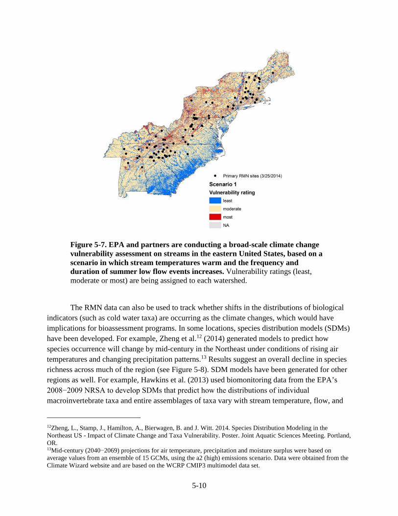
5-10

Figure 5-7. EPA and partners are conducting a broad-scale climate change vulnerability assessment on streams in the eastern United States, based on a scenario in which stream temperatures warm and the frequency and duration of summer low flow events increases. Vulnerability ratings (least, moderate or most) are being assigned to each watershed.

The RMN data can also be used to track whether shifts in the distributions of biological indicators (such as cold water taxa) are occurring as the climate changes, which would have implications for bioassessment programs. In some locations, species distribution models (SDMs) have been developed. For example, Zheng et al.12 (2014) generated models to predict how species occurrence will change by mid-century in the Northeast under conditions of rising air temperatures and changing precipitation patterns.13 Results suggest an overall decline in species richness across much of the region (see Figure 5-8). SDM models have been generated for other regions as well. For example, Hawkins et al. (2013) used biomonitoring data from the EPA’s 2008−2009 NRSA to develop SDMs that predict how the distributions of individual macroinvertebrate taxa and entire assemblages of taxa vary with stream temperature, flow, and

12Zheng, L., Stamp, J., Hamilton, A., Bierwagen, B. and J. Witt. 2014. Species Distribution Modeling in the Northeast US - Impact of Climate Change and Taxa Vulnerability. Poster. Joint Aquatic Sciences Meeting. Portland, OR. 13Mid-century (2040−2069) projections for air temperature, precipitation and moisture surplus were based on average values from an ensemble of 15 GCMs, using the a2 (high) emissions scenario. Data were obtained from the Climate Wizard website and are based on the WCRP CMIP3 multimodel data set.

5-11

other watershed attributes in the conterminous United States, for baseline (2000−2010) versus late century (2090−2100) time periods. SDMs are also being developed for stonefly species in the Midwest (Cao et al., 2013; DeWalt et al., 2013). If applied to RMN sites, SDMs could serve as valuable tools for conservation planning.

Figure 5-8. Modeling results predict declines in species richness across much of the Northeast by mid-century (2040−2069).14

Models have also been developed to predict climate change effects on stream temperature and flow. For example, at the national scale, Hill et al. (2013) developed a stream temperature model for the conterminous United States based on air temperature and watershed feature data (e.g., watershed area and slope) from reference-condition USGS sampling sites, and applied the model to simulate the effects of climate change on mean summer stream temperature (Hill et al. 2014). The model predicts a mean warming of 2.2°C for stream temperatures in the 14Zheng, L., Stamp, J., Hamilton, A., Bierwagen, B. and J. Witt. 2014. Species Distribution Modeling in the Northeast US—Impact of Climate Change and Taxa Vulnerability. Poster. Joint Aquatic Sciences Meeting. Portland, OR.

5-12

conterminous United States by late century (2090−2099) relative to a 2001−2010 baseline period, with values at individual sites ranging from 0°C to +6.2°C. In another study, Dunghel (2014) developed statistical models to predict flow responses to projected changes in precipitation and temperature. Results suggest that changes in flow attributes will be most evident in rain-fed small perennial streams and intermittent streams in the central and eastern United States. These models could potentially be applied to RMN sites, and the performance of the models could be tracked over time.

RMN data may also provide insights on how organisms respond to and recover from extreme weather events such as droughts and floods, which are projected to occur with greater frequency in the future (Melillo et al., 2014). Impacts can be evaluated through comparative analyses on the pre- and postevent data. For example, VT DEC performed these types of analyses on macroinvertebrate data collected before and after flooding from Tropical Storm Irene. Using data from 10 high-quality sites, VT DEC documented immediate decreases in invertebrate densities of 69% on average, but also found that most sites recovered to normal levels the following year (see Figure 5-9).15 The substantial decline in density and the rapid recovery would have been missed if sampling had occurred at longer intervals, such as on a 5-year rotational sampling schedule. Moreover, the collection of continuous thermal and hydrologic data will allow the magnitude, frequency and duration of the event to be documented. Whether or not the RMN data can fully capture biological responses to extreme weather events will depend on the timing of the event in relation to the RMN sampling period.

Figure 5-9. Comparison of macroinvertebrate density values at 10 stream sites in Vermont before and after Tropical Storm Irene.16

15Moore, A. and S. Fiske. (2012) What’s Left in Vermont’s Streams after Tropical Storm Irene―Monitoring Results From Long Term Reference Sites. Presentation. New England Association of Environmental Biologists Annual Conference. Falmouth, MA. 16Ibid.

6-1

6. DATA MANAGEMENT

The EPA and partners are developing a data management system that will allow participating organizations and outside users to access data and metadata that are being collected at RMN sites. The biological, habitat, and water chemistry data will be uploaded to a national water data system such as the WQX. At this time not all RMN partners have the capacity to upload these data into WQX, so the EPA and partners are working on an interim solution. Until the interim system is in place, the individual organizations will be custodians and owners of these data, and all data files will be backed up and stored in a centralized, secure location. Because WQX cannot accommodate continuous data, the thermal and hydrologic data being collected by RMN partners will be uploaded into a separate data management system. A multiagency effort is underway to develop a data management system for the continuous data. In the interim, EPA and partners are developing guidance for storing and managing the continuous RMN data files. This includes the development of R scripts (R Core Team, 2015) and procedures for performing QC on the data and for deriving standardized sets of summary outputs for desired time periods. Until the permanent data management system is in place, the individual organizations will be the custodians and owners of the continuous thermal and hydrologic monitoring data. The EPA and partners are also developing procedures for joining the different sets of data and facilitating the types of data analyses described in Section 5.

7-1

7. IMPLEMENTATION AND NEXT STEPS

Implementation of the RMNs is underway in the Northeast, Mid-Atlantic, and Southeast regions. Sampling efforts began in the Northeast in 2012, followed by the Southeast in 2013 and the Mid-Atlantic in 2014. Currently there are 25 primary RMN sites in the Northeast, 27 in the Mid-Atlantic and 38 in the Southeast (see Appendix C). More sites will be added in all regions as resources permit. Efforts are also underway to develop RMNs in the Midwest, where sampling is expected to start in 2016 (see Figure 7-1). A number of organizations in the western United States have also expressed interest in setting up RMNs.

Figure 7-1. Sampling has been underway at the Northeast, Mid-Atlantic and Southeast RMNs for several years. RMNs are currently being developed in the Midwest.

Efforts are being made to integrate RMN data collection flexibly within existing monitoring programs to maximize available resources. Some RMN partners have taken a phased approach to implementation, particularly with collecting hydrologic data at ungaged sites. For example, some participating organizations have installed pressure transducers at one or two sites, and are planning to add more as they gain experience and as resources permit. In many states, the collection of macroinvertebrate data and year-round temperature measurements have been feasible during the first year of implementation. However, it has been difficult for some participating organizations to find resources to process the macroinvertebrates samples in accordance with the regional methods. When this occurs, the preserved samples are being retained so that they can be processed at a later time, when resources become available.

7-2

To help build capacity and improve data quality, EPA and partners have held several training workshops on field protocols for continuous temperature sensors and pressure transducers, and wrote the EPA best practices document (U.S. EPA, 2014). In addition, the regional coordinator in the Mid-Atlantic is planning to hold a training workshop on species-level identifications for high priority taxa (see Appendix G). There are also plans to hold hands-on, interactive workshops on data management at annual meetings (e.g., the New England Association of Environmental Biologists conference, the Association of Mid-Atlantic Aquatic Biologists Workshop, the Southeastern Water Pollution Biologists Association conference).

As discussed in Section 3, EPA has also developed a QAPP for the RMNs to address the challenges of creating regionally consistent data sets. It is a generic QAPP that details the core requirements for participation in the network, and outlines best practices for the collection of biological, thermal, hydrologic, physical habitat, and water chemistry data at RMN sites. The QAPP was written in a way that should be transferable to other regions, with region-specific protocols included as addendums. The QAPP is intended to increase the comparability of data being collected at RMN sites, improve the ability to detect long-term trends by minimizing biases and variability, and to ensure that the data are of sufficient quality to meet data quality objectives. Efforts will be made to finalize the QAPPs for the Northeast, Mid-Atlantic, Southeast and Midwestern regions by 2016. The protocols in the QAPP will be reevaluated periodically and updated as needed. EPA and partners are also exploring the possibility of conducting methods comparison studies in regions where macroinvertebrate collection and processing protocols differ across participating organizations. This could involve the collection of side-by-side samples using the different methods. After the paired samples are processed using the respective methods, results would be compared and differences between the methods could be quantified.

In coming years, EPA and partners will continue to build capacity and refine protocols, indicator lists, analytical techniques and data management systems for the Northeast, Mid-Atlantic, and Southeast RMNs. Other regions have expressed interest in establishing RMNs as well. They recognize how these types of long-term data can support CWA programs, fill data gaps, and help detect trends attributable to climate change. The RMN framework is flexible and allows for expansion to new regions, as well as to new stream classes and waterbody types. For example, some parts of the Midwest lack the higher gradient, riffle-dominated cold water streams that are being targeted in the Northeast, Mid-Atlantic, and Southeast RMN pilot studies. Instead, these regions may focus their sampling efforts on low gradient, sandy-bottom, warm water streams. A Midwestern working group has also been formed to explore the possibility of setting up a RMN for inland lakes. The monitoring data being collected from these regional efforts will provide important inputs for bioassessment programs as they strive to protect water quality and aquatic ecosystems under a changing climate.

8-1

8. LITERATURE CITED

Barbour, MT; Stribling, JB; Karr, JR. (1995) The multimetric approach for establishing biocriteria and measuring biological condition. [p. 63−76]. In Davis, WS; Simon, TP (eds). Biological assessment and criteria: tools for water resource planning and decision making. Boca Raton, FL: CRC Press.

Barbour, MT; Gerritsen, J; Snyder, BD; Stribling, JB. (1999) Rapid bioassessment protocols for use in streams and wadeable rivers: Periphyton, benthic macroinvertebrates and fish, Second Edition. [EPA 841-B-99-002]. Washington, D.C: U.S. Environmental Protection Agency, Office of Water. Available online: http://water.epa.gov/scitech/monitoring/rsl/bioassessment/index.cfm.

Beauchene, M; Becker, M; Bellucci, C; Hagstrom, N; Kanno, Y. (2014) Summer thermal thresholds of fish community transitions in Connecticut streams. J N Am Fish Manage 34(1):119–131.

Becker, AJ; Stranko, SA; Klauda, RJ; Prochaska, AP; Schuster, JD; Kashiwagi, MR; Graves, PH. (2010) Maryland biological stream survey’s sentinel site network: A multi-purpose monitoring program. Annapolis, MD: Maryland Department of Natural Resources.

Bilhimer, D; Stohr, A. (2009) Standard Operating Procedures for continuous temperature monitoring of fresh water rivers and streams conducted in a Total Maximum Daily Load (TMDL) project for stream temperature, Version 2.3. Olympia, WA: Washington State Department of Ecology, Environmental Assessment Program. Available online: http://www.ecy.wa.gov/programs/eap/qa/docs/ECY_EAP_SOP_Cont_Temp_Monit_TMDL_v3_0EAP044.pdf.

Blocksom, KA; Autrey, BC; Passmore, M; Reynolds, L. (2008) A comparison of single and multiple habitat protocols for collecting macroinvertebrates in wadeable streams. JAWRA 44(3):577−593.

Blum, MD; Törnqvist, TE. (2000) Fluvial responses to climate and sea-level change: a review and look forward. Sedimentology 47:2−48.

Böhmer, J; Rawer-Jost, C; Zenker, A. (2004) Multimetric assessment of data provided by water managers from Germany: assessment of several different types of stressors with macrozoobenthos communities. Hydrobiologia 516(1-2):215−228.

Buchanan, C; Moltz, HLN; Haywood, HC; Palmer, JB; Griggs, AN. (2013) A test of The Ecological Limits of Hydrologic Alteration (ELOHA) method for determining environmental flows in the Potomac River basin, U.S.A. Freshw Biol 58(12):2632−2647.

Butryn, RS; Parrish, DL; Rizzo, DM. (2013) Summer stream temperature metrics for predicting brook trout (Salvelinus fontinalis) distribution in streams. Hydrobiologia 703:47–57.

Cao, Y; Williams, WP; Bark, AW. (1997) Effects of sample size (number of replicates) on similarity measures in river benthic Aufwuchs community analysis. Water Environ Res 69(1):107−114.

Cao, Y; Hawkins, CP; Storey, AW. (2005) A method for measuring the comparability of different sampling methods used in biological surveys: Implications for data integration and synthesis. Freshw Biol 50(6):1105−1115.

Cao, Y; DeWalt, RE; Robinson, JL; Tweddale, T; Hinz, L; Pessino, M. (2013) Using Maxent to model the historic distributions of stonefly species in Illinois streams: The effects of regularization and threshold selections. Ecol Model 259:30−39.

Carlisle, DM; Falcone, J; Wolock, DM; Meador, MR; Norris, HR. (2010) Predicting the natural flow regime: models for assessing hydrological alteration in streams. River Res Appl 26(2):118−36.

8-2

Carlisle, DM; Wolock, DM; Meador, MR. (2011) Alteration of streamflow magnitudes and potential ecological consequences: a multiregional assessment. Front Ecol Environ 9:264−270.

Carter, JL; Resh, VH. (2013) Analytical approaches used in stream benthic macroinvertebrate biomonitoring programs of state agencies in the United States. [USGS Open-File Report 2013-1129]. Reston, VA: U.S. Geological Survey. http://pubs.usgs.gov/of/2013/1129/.

Chapman, AD. (2005) Principles of data quality. Version 1.0. Report for the Global Biodiversity Information Facility (GBIF). Global Biodiversity Information Facility, Copenhagen, Denmark: Global Biodiversity Information Facility. Available online at http://www2.gbif. org/DataQuality.pdf.

Chase, R. (2005). Standard Operating Procedure: Streamflow measurement. [CN 68.0]. Massachusetts Department of Environmental Protection, Division of Watershed Management.

Chinnayakanahalli, KJ; Hawkins, CP; Tarboton, DG; Hill, RA. (2011) Natural flow regime, temperature and the composition and richness of invertebrate assemblages in streams of the western United States. Freshw Biol 56:1248−1265. doi: 10.1111/j.1365-2427.2010.02560.x.

Chiu, MC; Kuo, MH. (2012) Application of r/K selection to macroinvertebrate responses to extreme floods. Ecol Entomol 37(2):145−154.

Clark, ME; Rose, KA; Levine, DA; Hargrove, WW. (2001) Predicting climate change effects on Appalachian trout: combining GIS and individual-based modeling. Ecol Appl 11(1):161−178.

Conti, L; Schmidt-Kloiber, A; Grenouillet, G; Graf, W. (2014) A trait-based approach to assess the vulnerability of European aquatic insects to climate change. Hydrobiologia 721(1): 297−315.

Cuffney, TF; Bilger, MD; Haigler, AM. (2007) Ambiguous taxa: effects on the characterization and interpretation of invertebrate assemblages. J N Am Benthol Soc 26(2):286−307.

Cummins, J; Buchanan, C; Haywood, HC; Moltz, H; Griggs, A; Jones, C; Kraus, R; Hitt, NP; Bumgardner, R. (2010) Potomac large river ecologically sustainable water management report. [ICPRB Report 10-3]. Interstate Commission on the Potomac River Basin for The Nature Conservancy. Available online at www.potomacriver.org/pubs.

Davies, SP; Jackson, SK. (2006) The Biological Condition Gradient: A descriptive model for interpreting change in aquatic ecosystems. Ecol Appl 16(4):1251−1266.

DePhilip, M; Moberg, T. (2010) Ecosystem flow recommendations for the Susquehanna River Basin. Harrisburg, PA: The Nature Conservancy. Available online at http://www.srbc.net/policies/docs/TNCFinalSusquehannaRiverEcosystemFlowsStudyReport_Nov10_20120327_fs135148v1.PDF.

DePhilip, M; Moberg, T. (2013a) Ecosystem flow recommendations for the Delaware River basin. Harrisburg, PA: The Nature Conservancy.

DePhilip, M; Moberg, T. (2013b) Ecosystem flow recommendations for the Upper Ohio River basin in western Pennsylvania. Harrisburg, PA: The Nature Conservancy.

DeShon, J. (1995) Development and application of the Invertebrate Community Index (ICI). [p. 217−243]. In Davis, WS; Simon, TP (eds). Biological assessment and criteria: tools for water resource planning and decision making. Boca Raton:CRC Press.

DeWalt, RE; Cao, Y; Robinson, JL; Tweddale, T; Hinz, L. (2013) Predicting climate change effects on riverine stonefly (Insecta: Plecoptera) species in the Upper Midwest. INHS Technical Report 2013 (22). Prepared for U.S. Fish and Wildlife Service.

8-3

Dhungel, S. (2014) Prediction of climate change effects on streamflow regime important to stream ecology. All Graduate Theses and Dissertations: Paper 3083. http://digitalcommons.usu.edu/etd/3083.

Dunham, J; Chandler, G; Rieman, B; Martin, D. (2005) Measuring stream temperature with digital data sensors: a user’s guide. [Gen. Tech. Rep. RMRSGTR-150WWW]. Fort Collins, CO: U.S. Department of Agriculture, Forest Service, Rocky Mountain Research Station. 15 p. Available online at http://fresc.usgs.gov/products/papers/1431_Dunham.pdf.

Durance, I; Ormerod, SJ. (2007) Climate change effects on upland stream macroinvertebrates over a 25-year period. Glob Change Biol 13:942−957.

Faustini, JM. (2000) Stream channel response to peak flows in a fifth-order mountain watershed. Corvallis, OR: Oregon State University, Corvallis, OR.

Faustini, JM; Jones, JA. (2003) Influence of large woody debris on channel morphology and dynamics in steep, boulder-rich mountain streams, western Cascades, Oregon. Geomorphology 51(1−3):187−205.

Feio, MJ; Reynoldson, TB; Graça, MAS. (2006) The influence of taxonomic level on the performance of a predictive model for water quality assessment. Can J Fish Aquat Sci 63(2):367−376.

Flebbe, PA; Roghair, LD; Bruggink, JL. (2006) Spatial modeling to project southern Appalachian trout distribution in a warmer climate. Trans Am Fish Soc 135(5):1371−1382.

Foucreau, N; Piscart, C; Puijalon, S; Hervant, F. (2013) Effect of climate-related change in vegetation on leaf litter consumption and energy storage by Gammarus pulex from Continental or Mediterranean populations. PLoS ONE 8(10): e77242.

Gerth, WJ; Herlihy, AT. (2006) The effect of sampling different habitat types in regional macroinvertebrate bioassessment surveys. J N Am Benthol Soc 25:501−512.

Goode, JR; Luce, CH; Buffington, JM. (2012) Enhanced sediment delivery in a changing climate in semi-arid mountain basins: Implications for water resource management and aquatic habitat in the northern Rocky Mountains. Geomorphology 139–140:1−15.

Gotelli, NJ; Graves, GR. (1996) Null models in ecology. Washington, DC: Smithsonian Institution Press.

Goudie, AS. (2006) Global warming and fluvial geomorphology. Geomorphology 79(3−4):384−394.

Haase, P; Murray-Bligh, J; Lohse, S; Pauls, S; Sundermann, A; Gunn, R; Clarke, R. (2006) Assessing the impact of errors in sorting and identifying macroinvertebrate samples. Hydrobiologia, 566:505−521.

Haase, P; Pauls, SU; Schindehütte, K; Sundermann, A. (2010) First audit of macroinvertebrate samples from an EU Water Framework Directive monitoring program: human error greatly lowers precision of assessment results. J N Am Benthol Soc 29(4):1279−1291. 10.1899/09-183.1 http://www.jnabs.org/doi/abs/10.1899/09-183.1.

Harding, JS; Benfield, EF; Bolstad, PV; Helfman, GS; Jones III, EBD. (1998) Stream biodiversity: The ghost of land use past. Proc Nat Acad Sci 95:14843−14847.

Harper, MP; Peckarsky, BL. (2006) Emergence cues of a mayfly in a high-altitude stream ecosystem: Potential response to climate change. Ecol Appl 16:612−621.

Hawkins, CP. (2006) Quantifying biological integrity by taxonomic completeness: Its utility in regional and global assessment. Ecol Appl 16(4):1277−1294.

8-4

Hawkins, CP; Tarboton, DG; Jin, J. (2013) Consequences of global climate change for stream biodiversity and implications for the application and interpretation of biological indicators of aquatic ecosystem condition. Final Report. [EPA Agreement Number: RD834186]. Logan Utah: Utah State University. http://cfpub.epa.gov/ncer_abstracts/index.cfm/fuseaction/display.abstractDetail/abstract/9063.

Herlihy, AT; Sifneos, J; Bason, C; Jacobs, A; Kentula, ME; Fennessy, MS. (2009) An approach for evaluating the repeatability of rapid wetland assessment methods: The effects of training and experience. Environ Manage 44:369−377.

Hewlett, R. (2000) Implications of taxonomic resolution and sample habitat for stream classification at a broad geographic scale. J N Am Benthol Soc 19:352−361.

Hildebrand, RH; Kashiwagi, MT; Prochaska, AP. (2014) Regional and local scale modeling of stream temperatures and spatio-temporal variation in thermal sensitivities. Environ Manage 54:14−22.

Hill, RA; Hawkins, CP; Carlisle, DM. (2013) Predicting thermal reference conditions for USA streams and rivers. Freshw Sci 32(1):39−55.

Hill, RA; Hawkins, CP; Jin, J. (2014) Predicting thermal vulnerability of stream and river ecosystems to climate change. Clim Change 125:399–412. doi:10.1007/s10584-014-1174−4.

Hogg, ID; Williams, DD. (1996) Response of stream invertebrates to a global warming thermal regime: an ecosystem-level manipulation. Ecology 77:395−407.

Holden, ZA; Klene, A; Keefe, R; Moisen, G. (2013) Design and evaluation of an inexpensive solar radiation shield for monitoring surface air temperatures. Agric For Meteorol 180:281−286.

Holling, CS. (1973) Resilience and stability of ecological systems. Ann Rev Ecol Systems 4:1−23.

Horrigan, N; Baird, DJ. (2008) Trait patterns of aquatic insects across gradients of flow-related factors: a multivariate analysis of Canadian national data. Can J Fish Aquat Sci 65: 670−680.

Huh, S; Dickey, DA; Meador, MR; Rull, KE. (2005) Temporal Analysis of the frequency and duration of low and high streamflow: years of record needed to characterize streamflow variability. J Hydrol 310:78−94.

Isaak, DJ; Horan, DL. (2011) An assessment of underwater epoxies for permanently installing temperature in mountain streams. N Am J Fish Manage 31:134−137. Available online: http://www.treesearch.fs.fed.us/pubs/37476.

Isaak, DJ; Wollrab, S; Horan, D; Chandler, G. (2012) Climate change effects on stream and river temperatures across the Northwest U.S. from 1980−2009 and implications for salmonid fishes. Clim Change 113:499−524.

Isaak, DJ; Rieman, BE. (2013) Stream isotherm shifts from climate change and implications for distributions of ectothermic organisms. Glob Change Biol 19:742−751.

Iverson, L; Prasad, A; Matthews, S. (2008) Potential changes in suitable habitat for 134 tree species in the Northeastern United States. Mitig Adapt Strat Glob Change 13:517−540. http://treesearch.fs.fed.us/pubs/15295.

Jackson, JK; Fureder, L. (2006) Long-term studies of freshwater macroinvertebrates―A review of the frequency, duration, and ecological significance. Freshw Biol 51:591−603.

Jones, NE; Schmidt, B. (2012) ThermoStat version 3.0: Tools for analyzing thermal regimes. Ontario Ministry of Natural Resources, Aquatic Research and Development Section. http://people.trentu.ca/nicholasjones/thermostat.htm.

8-5

Kanno, Y; Vokoun, JC; Letcher, BH. (2014) Paired stream-air temperature measurements reveal fine-scale thermal heterogeneity within headwater brook trout stream networks. River Res Applic 30:745-755.

Karr, JR. (1991) Biological integrity: A long-neglected aspect of water resource management. Ecol Appl 1:66−84.

Kaufmann, PR; Levine, P; Robinson, EG; Seeliger, C; Peck, DV. (1999) Quantifying physical habitat in wadeable streams. [EPA/620/R-99/003]. Washington, DC: U.S. Environmental Protection Agency. http://www.epa.gov/emap/html/pubs/docs/groupdocs/surfwatr/field/phyhab.html.

Kaufmann, PR; Faustini, JM; Larsen, DP; Shirazi, MA. (2008) A roughness-corrected index of relative bed stability for regional stream surveys. Geomorphology 99(1−4):150−170.

Kaufmann, PR; Larsen, DP; Faustini, JM. (2009) Bed stability and sedimentation associated with human disturbances in Pacific Northwest streams. J Am Water Resour Assoc 45:434−459.

Kelleher, C; Wagener, T; Gooseff, M; McGlynn, B; McGuire, K; Marshall, L. (2012) Investigating controls on the thermal sensitivity of Pennsylvania streams. Hydrological Processes 26(5):771−785.

Kennen, JG; Kauffman, LJ; Ayers, MA; Wolock, DM; Colarull, SJ. (2008) Use of an integrated flow model to estimate ecologically relevant hydrologic characteristics at stream biomonitoring sites. Ecol Modell 211:57−76.

Kennen, JG; Sullivan, DJ; May, JT; Bell, AH; Beaulieu, KM; Rice, DE. (2011) Temporal changes in aquatic-invertebrate and fish assemblages in streams of the north-central and northeastern U.S. Ecol Indic 18:312−329.

Larsen, D; Kaufmann, P; Kincaid, T; Urquhart, N. (2004) Detecting persistent change in the habitat of salmon-bearing streams in the Pacific Northwest. Can J Fish Aqua Sci 61:283−291.

Lenat, DR; Resh, VH. (2001) Taxonomy and stream ecology―The benefits of genus- and species-level identifications. J N Am Benthol Soc 20:287−298.

Liang, X; Lettenmaier, DP; Wood, EF; Burges, SJ. (1994) A simple hydrologically based model of land surface water and energy fluxes for GSMs. J Geophys Res 99(D7):14,415−14,428.

Maheu, A; Poff, NL; St-Hilaire, A. (2015) A classification of stream water temperature regimes in the conterminous USA. River Research and Applications: doi: 10.1002/rra.2906.

MDEP (Maine Department of Environmental Protection). (2007) Chapter 587: In-stream flows and lake and pond water levels. In Sustainable water use program. Augusta, ME: Maine DEP. http://www.maine.gov/sos/cec/rules/06/096/096c587.doc.

Mazor, RD; Purcell, AH; Resh, VH. (2009) Long-term variability in benthic macroinvertebrate bioassessments: A 20-year study from two northern Californian streams. Environ Manage 43:1269−1286.

McCormick, PV; Stevenson, RJ. (1998) Periphyton as a tool for ecological assessment and management in the Florida Everglades. J Phycol 34(5):726−733.

McMahon, G; Bales, JD; Coles, JF; Giddings, EMP; Zappia, H. (2003) Use of stage data to characterize hydrologic conditions in an urbanizing environment. J Am Water Resources Assoc 39:1529−1536.

Melillo, JM; Richmond, TC; Yohe, GW. (2014) Climate change impacts in the United States: the third National Climate Assessment. US Global Change Research Program 841.

Meyer, JL; Strayer, DL; Wallace, JB; Eggert, SL; Helfman, GS; Leonard, NE. (2007) The contribution of headwater streams to biodiversity in river networks. J Am Water Resour Assoc 43:86−103.

8-6

Milner, AM; Conn, SC; Brown, LE. (2006) Persistence and stability of macroinvertebrate communities in streams of Denali National Park, Alaska: implications for biological monitoring. Freshw Biol 51:373−387.

Nelitz, MA; MacIsaac, EA; Peterman, RM. (2007) A science-based approach for identifying temperature-sensitive streams for rainbow trout. N Am J Fish Manage 27:405–424.

Norris, RH; Barbour, MT. (2009) Bioassessment of aquatic ecosystems. In: Likens, GE (Ed) Encyclopedia of inland waters, volume 3. Oxford: Elsevier. pp. 21−28.

NWQMC (National Water Quality Monitoring Council). (2011) Establishing a collaborative and multipurpose national network of reference watersheds and monitoring sites for freshwater streams in the United States. U.S. Department of the Interior, U.S. Geological Survey. http://acwi.gov/monitoring/workgroups/wis/National_Reference_Network_for_Streams.pdf.

Olden, JD; Poff, NL. (2003) Redundancy and the choice of hydrologic indices for characterizing streamflow regimes. River Res Appl 19:101−121.

Olivero SA; Barnett, A; Anderson, MG. (2015) A Stream Classification for the Appalachian Region. The Nature Conservancy, Eastern Conservation Science, Eastern Regional Office. Boston, MA.

Olsen, AR; Sedransk, J; Edwards, D; Gotway, CA; Liggett, W; Rathbun, S; Reckhow. KH; Young, LJ. (1999) Statistical issues for monitoring ecological and natural resources in the United States. Environ Monitor Assess 54:1−54.

Ostermiller, JD; Hawkins, CP. (2004) Effects of sampling error on bioassessments of stream ecosystems: application to RIVPACS-type models. J N Am Benthol Soc 23:363−382.

Parson, M; Norris, RH. (1996) The effect of habitat specific sampling on biological assessment of water quality using a predictive model. Freshw Biol 36:419−434.

Poff, NL; Allan, JD; Bain, MB; Karr, JR; Prestegaard, KL; Richter, BD; Sparks, RE; Stromberg, JC. (1997) The natural flow regime: a paradigm for river conservation and restoration. BioScience 47(11):769−784.

Poff, NL; Olden, JD; Vieira, NKM; Finn, DS; Simmons, MP; Kondratieff, BC. (2006) Functional trait niches of North American lotic insects: traits-based ecological applications in light of phylogenetic relationships. J N Am Benthol Soc 25(4):730−755.

Poff, NL; Pyne, MI; Bledsoe, BP; Cuhaciyan, CC; Carlisle, DM. (2010) Developing linkages between species traits and multiscaled environmental variation to explore vulnerability of stream benthic communities to climate change. J N Am Benthol Soc 29(4):1441−1458.

Pond, GJ; North, SH. (2013) Application of a benthic observed/expected-type model for assessing Central Appalachian streams influenced by regional stressors in West Virginia and Kentucky. Environ Monit Assess 185(11):9299−9320.

Rantz, SE; et al. (1982) Measurement and computation of streamflow, Volume I: Measurement of stage and discharge and Volume II: Computation of discharge. [USGS Water Supply Paper 2175]. U.S. Department of the Interior, U.S. Geological Survey. Available online at http://water.usgs.gov/pubs/wsp/wsp2175/.

R Core Team (2015) R: A language and environment for statistical computing. R Foundation for Statistical Computing, Vienna, Austria. Available online at http://www.R-project.org/.

Rehn, AC; Ode, PR; Hawkins, CP. (2007) Comparisons of targeted-riffle and reach-wide benthic macroinvertebrate samples: implications for data sharing in stream-condition assessments. J N Am Benthol Soc 26(2):332−348.

Richards, C; Haro, RJ; Johnson, LB; Host, GE. (1997) Catchment and reach-scale properties as indicators of macroinvertebrate species traits. Freshw Biol 37:219−230.

8-7

Richter, BD; Baumgartner, J; Wigington, R; Braun, D. (1997) How much water does a river need? Freshw Biol 37:231―249.

Ricupero, K. (2009) Changing streamflow patterns in the New England region: Implications for ecosystem services, water users and sustainable resources management. Master of Science thesis. Department of Civil and Environmental Engineering, University of Maine, Orono, 212 pages.

Roy, AH; Rosemond, AD; Leigh, DS; Paul, MJ; Wallace, JB. (2003) Habitat-specific responses of macroinvertebrates to land cover disturbance: biological consequences and monitoring implications. J N Am Benthol Soc 22:292−307.

Rustad, L; Campbell, J; Dukes, JS; Huntington, T; Lambert, KF; Mohan, J; Rodenhouse, N. (2012) Changing climate, changing forests: The impacts of climate change on forests of the Northeastern United States and Eastern Canada. [General Technical Report NRS-99]. Newtown Square, PA: United States Department of Agriculture, US Forest Service, Northern Research Station. Available online at http://nrs.fs.fed.us/pubs/41165.

Sandin, L; Johnson, RK. (2000) The statistical power of selected indicator metrics using macroinvertebrates for assessing acidification and eutrophication of running waters. Hydrobiologia 422/423:233−243.

Scarsbrook, MR. (2002) Persistence and stability of lotic invertebrate communities in New Zealand. Freshw Biol 47:417−431.

Segura, C; Caldwell, P; Sun, G; McNulty, S; Zhang, Y. (2015) A model to predict stream water temperature across the conterminous USA. Hydrol Process 29(9):2178−2195.

Shedd, JR. (2011) Standard operating procedure for measuring and calculating stream discharge. Washington State Department of Ecology, Environmental Assessment Program. Available online: http://www.ecy.wa.gov/programs/eap/quality.html.

Snyder, CD; Hitt, NP; Young, JA. (2015) Accounting for groundwater in stream fish thermal habitat responses to climate change. Ecological Applications 25(5):139−-1419.

Sowder, C; Steel, EA. (2012) A note on the collection and cleaning of water temperature data. Water 4:597−606.

Stamp, J; Gerritsen, J. (2009) Methods and assessment comparability among state and federal biological monitoring protocols. Lowell, MA: New England Interstate Water Pollution Control Commission.

Stamp, J; Gerritsen, J; Pong, G; Jackson, SK; Van Ness, K. (2014) Calibration of the Biological Condition Gradient (BCG) for Fish and Benthic Macroinvertebrate Assemblages in the Northern Piedmont region of Maryland. Prepared for U.S. EPA Office of Science and Technology and Montgomery County Department of Environmental Protection.

Statzner, B; Resh, VH; Dolédec, S. (1994) Ecology of the upper Rhône river: a test of habitat templet theories. Freshw Biol 31:253−554.

Stevenson, RJ. (1998) Diatom indicators of stream and wetland stressors in a risk management framework. Environ Monit Assess 51(1−2):107−118.

Stoddard, JL; Larsen, DP; Hawkins, CP; Johnson, RK; Norris, RH. (2006) Setting expectations for the ecological condition of streams: the concept of reference condition. Ecol Appl 16(4):1267−1276.

Stribling, JB; Moulton, SR; Lester, GL. (2003) Determining the quality of taxonomic data. J N Am Benthol Soc 22:621−631.

Stribling, JB; Pavlik, KL; Holdsworth, SM; Leppo, EW. (2008) Data quality, performance, and uncertainty in taxonomic identification for biological assessments. J N Am Benthol Soc 27(4):906−919. Available online at http://www.jnabs.org/doi/abs/10.1899/07-175.1.

8-8

Stuckey, MH; Koerkle, EH; Ulrich, J. (2012) Estimation of baseline daily mean streamflows for ungagged location on Pennsylvania streams, water years 1960‐2008. [USGS Scientific Investigations Report 2012‐5142]. New Cumberland, PA: U.S. Geological Survey. Available online at http://pubs.usgs.gov/sir/2012/5142/.

Sweeney, BW; Jackson, JK; Newbold, JD; Funk, DH. (1992) Climate change and the life histories and biogeography of aquatic insects in eastern North America. [Pages 143−176]. In Firth, P; Fisher, SG (eds). Global climate change and freshwater ecosystems. New York: Springer-Verlag.

Sweeney, BW. (1993) Effects of streamside vegetation on macroinvertebrate communities of White Clay Creek in eastern North America. Proc Acad Nat Sci Phil 144: 291−340.

TNC (The Nature Conservancy). (2009) Indicators of hydrologic alteration version 7.1 user's manual. Available online at http://www.conservationgateway.org/ConservationPlanning/ToolsData/Tools/CommonlyUsedTools/Pages/commonly‐used‐tools.aspx#IHA.

Townsend, CR; Hildrew, AG. (1994) Species traits in relation to a habitat templet for river systems. Freshw Biol 31:265−275.

Townsend, CR; Dolédec, S; Scarsbrook, MR. (1997) Species traits in relation to temporal and spatial heterogeneity in streams: a test of habitat templet theory. Freshw Biol 37:367−387.

Trumbo, BA. (2010) Sensitivity and exposure of brook trout (Salvelinus fontinalis) habitat to climate change. [Masters Thesis]. Harrisonburg, VA: Department of Biology, James Madison University.

Tsang, Y; Infante, DM; Stewart, J; Wang, L; Tingly III, RW; Thornbrugh, D; Cooper, AR; Daniel, WM. (submitted). StreamThermal: A software package for calculating thermal metrics from stream temperature data (submitted to Fisheries Magazine).

U.S. EPA (Environmental Protection Agency). (2006) Southeastern plains in-stream nutrient & biological response (SPINBR) study quality assurance project plan for state agency activities. [Project Number: 06-0267]. Region 4.

U.S. EPA (Environmental Protection Agency). (2011) Healthy Watersheds Initiative: National Framework and Action Plan. Publication Number: EPA 841-R-11-005.

U.S. EPA (Environmental Protection Agency). (2012a) Implications of climate change for state bioassessment programs and approaches to account for effects. [EPA/600/R-11/036F]. Washington, DC: Global Change Research Program, National Center for Environmental Assessment. http://cfpub.epa.gov/ncea/global/recordisplay.cfm?deid=239585.

U.S. EPA (Environmental Protection Agency). (2012b) Freshwater biological traits database (final report). [EPA/600/R-11/038F]. Washington, DC: National Center for Environmental Assessment. Available online at http://cfpub.epa.gov/ncea/global/recordisplay.cfm?deid=241813

U.S. EPA (Environmental Protection Agency). (2013a) National rivers and streams assessment 2013−2014: Field operations manual―wadeable. [EPA/841/B-12/007]. Washington, DC: U.S. Environmental Protection Agency, Office of Water.

U.S. EPA (Environmental Protection Agency). (2013b) A Long-Term Vision for Assessment, Restoration, and Protection under the Clean Water Act Section 303(d) Program. http://www2.epa.gov/sites/production/files/2015-07/documents/vision_303d_program_dec_2013.pdf.

U.S. EPA (Environmental Protection Agency). (2014) Best practices for continuous monitoring of temperature and flow in wadeable streams. Final report. [EPA/600/R-13/170F]. Washington, DC: Global Change Research Program, National Center for Environmental Assessment. Available online at http://cfpub.epa.gov/ncea/global/recordisplay.cfm?deid=280013.

8-9

van Kleef, HH; Verberk, WCEP; Leuven, RSEW; Esselink, H; Van der Velde, G; Van Duinen, GA. (2006) Biological traits successfully predict the effects of restoration management on macroinvertebrates in shallow softwater lakes. Hydrobiologia 565:201−216.

Vannote, RL; Minshall, GW; Cummins, KW; Sedell, JR; Cushing, CE. (1980) The river continuum concept. Can J Fish Aquat Sci 37(1):130−137.

Vinson, MR; Hawkins, CP. (1996) Effects of sampling area and subsampling procedure on comparisons of taxa richness among streams. J N Am Benthol Soc 15(3):392−399.

Waite, IR; Herlihy, AT; Larsen, DP; Klemm, DJ. (2000) Comparing strengths of geographic and nongeographic classifications of stream benthic macroinvertebrates in the Mid-Atlantic Highlands, USA. J N Am Benthol Soc 19(3):429−441.

Wehrly, KE; Wiley MJ; Seelbach, PW. (2003) Classifying regional variation in thermal regime based on stream fish community patterns. Trans Am Fish Soc 132:18–38.

Wenger, SJ; Isaak, DJ; Luce, CH; Neville, HM; Fausch, KD; Dunham, JB; Dauwalter, DC; Young, MK; Elsner, MM; Rieman, BE; Hamlet, AF; Williams, JE. (2011) Flow regime, temperature, and biotic interactions drive differential declines of trout species under climate change. Proc Nat Acad Sci USA 108(34):14175−14180.

Whiles, MR; Wallace, JB. (1997) Leaf litter decomposition and macroinvertebrate communities in headwater streams draining pine and hardwood catchments. Hydrobiologia 353:107−119.

Wright, JF; Moss, D; Armitage, PD; Furse, MT. (1984) A preliminary classification of running-water sites in Great Britain based on macroinvertebrate species and the prediction of community type using environmental data. Freshw Biol 14:221−256.

Wright, JF. (2000) An introduction to RIVPACS. [pgs 1−24]. In Wright, JF; Sutcliffe, DW; Furse, MT (eds). Assessing the biological quality of freshwaters: RIVPACS and other techniques. Ambleside, Cumbria, UK: Freshwater Biological Association.

Yoder, CO; Rankin, ET. (1995) Biological criteria program development and implementation in Ohio. [pp. 109−144, Chapter 9]. In Davis, WS; Simon, T (eds.). Biological assessment and criteria: Tools for water resource planning and decision making. Boca Raton FL: Lewis Publishers.

Yuan, L. (2006) Estimation and application of macroinvertebrate tolerance values. National Center for Environmental Assessment, Office of Research and Development, U.S. Environmental Protection Agency, Washington, DC; EPA/600/P-04/116F. http://cfpub.epa.gov/ncea/cfm/recordisplay.cfm?deid=154869.

A-1

APPENDIX A.

____ _____________________

POWER ANALYSIS

A-2

A.1. BACKGROUND In 2011−2012, EPA collaborated with seven states in the northeastern United States on a

pilot study that laid the groundwork for the Northeast Regional Monitoring Network (RMN). The intent was to design a monitoring network that could detect potentially small trends in biological, thermal, hydrologic, physical habitat, and water chemistry data at high quality sites in a decision-relevant timeframe (e.g., 10−20 years to be relevant to climate change). The design had to achieve a balance between scientific and practical considerations. It had to build on existing state and tribal bioassessment efforts and not exceed resource limitations of the biomonitoring programs.

To help inform the network design, EPA and partners performed a series of analyses on an aggregated data set to explore the following questions:

1) How long will it take to detect trends in biological metrics? 2) How much of an effect do different design decisions, such as sampling frequency and

classification scheme, have on trend detection times? A.2. METHODS A.2.1. Data Preparation

EPA performed a series of analyses on a regional data set comprised of benthic macroinvertebrate, habitat, and water quality data from participating state biomonitoring programs in New York, Connecticut, Maine, Massachusetts, New Hampshire, Rhode Island, and Vermont. In addition, macroinvertebrate data sets covering the same northeastern study area were obtained from the U.S. EPA Wadeable Streams Study (WSA; U.S. EPA, 2006), the New England Wadeable Streams project (NEWS; Snook et al., 2007), and the U.S. Geological Survey (USGS) National Water Quality Assessment (NAWQA). For purposes of the analyses, the data set was limited to reference sites only, which were defined as locations with the least amount of anthropogenic disturbance (Hughes et al., 1986). Table A-1 lists the reference criteria and Figure A-1 shows the locations of the reference sites. The data set was further limited to include samples collected from June−September1 and samples with 80 or more total individuals2. Samples that had only family-level or coarser identifications were also removed from the data set.

The final data set was comprised of 1,398 samples from 953 reference sites, with sample years ranging from 1981 to 2010. Ten different methods were represented (see Table A-2). The 1This encompasses the general timeframe during which participating organizations collected samples for routine assessments. 2We selected this threshold because it is 20% smaller than the smallest subsample target size among sampling entities, and a target of ±20% is in keeping with data quality objectives for most subsampling routines (Barbour et al., 1999). While some samples could have low densities due to natural conditions, others reasons, such as quality assurance issues, may account for the low count.

A-3

methods differ to varying degrees in sampling effort, sampling gear, habitats sampled, index periods, subsampling/sample processing, and/or level of taxonomic resolution (see Table A-3). Approximately 70% of the samples were collected using kick nets. The other sampling gear consisted of artificial substrates or Surber samplers. Most samples were collected from riffle habitats. Approximately 7% were collected from multiple habitats.

Table A-1. Reference site criteria

Variable Reference criterion

Percentage Natural land covera (NLCD 2001 upstream) >85%

Landscape Disturbance Index (LDI)b <1.5 index units

Percentage Imperviousness (2001 upstream) <1%

Percentage Imperviousness (2006 1-km radius)c <1%

NPDES major discharges >500 m from the site

Dams >500 m from the site

Dissolved oxygen >6 mg/L

Conductivity <200 μS/cm

aLand cover screenings were estimates based on data associated with the National Hydrography Dataset Plus Version 1 (NHDPlusV1) catchments in which the sites are located (http://www.horizon-systems.com/NHDPlus). Land use data were based on the 2001 National Land Cover Database (NLCD; Homer et al., 2007) (http://www.mrlc.gov/nlcd01_data.php). For this exercise, natural land cover included open water, forest, wetlands, barren, and grassland/herbaceous. Data were accumulated for the entire upstream catchment.

bThe LDI (Brown and Vivas, 2005) was calculated by associating land uses with a scale of disturbance intensity and weighting the index score by percentage coverage of the 2001 land uses in the upstream catchment of each site.

cPercentage impervious data for the 1-km radius were based on the 2006 National Land Cover Database (NLCD; Fry et al., 2011) (http://www.mrlc.gov/nlcd06_data.php).

A-4

Figure A-1. Reference site locations throughout New England and New York.

A-5

Table A-2. Distribution of samples across states, sampling agencies and methods

State Method # Samples CT CT DEEP Kick Riffle 53

NEWS Kick Multihabitat 6 MA CT DEEP Kick Riffle 1

MA DEP Kick Riffle 49 NEWS Kick Multihabitat 1 USGS Surber Riffle 14 WSA Kick Multihabitat 1

ME ME DEP Rock Basket 129 NEWS Kick Multihabitat 30 WSA Kick Multihabitat 7

NH NEWS Kick Multihabitat 25 NH DES Rock Basket 85 USGS Surber Riffle 1 WSA Kick Multihabitat 5

NY NY DEC Kick Riffle 497 USGS Surber Riffle 12 WSA Kick Multihabitat 13

RI NEWS Kick Multihabitat 4 RIDEM Kick Riffle 21

VT NEWS Kick Multihabitat 12 USGS Surber Riffle 1 VT DEC Kick Riffle 430 WSA Kick Multihabitat 1

Total 1,398

A-6

Table A-3. Description of collection and processing methods included in the analytical data set

Entity Collection method Gear Habitat Sample

area Subsampling Index period

CT DEEP

12 kick samples are taken throughout riffle habitats within the sampling reach

Rectangular net (18" wide × 9 " high ), 500 μm mesh

Riffle ~2 m2 200-organism minimumcount, randomly selectedfrom a 56 grid (5 cm × 5 cmgrids) subsampling tray

Sep 15−Nov 30

VT DEC

Kick samples taken from riffle habitat in 4 different locations in the sampling reach. Substrate disturbed at each for ~ 30 seconds, total active sampling effort 2 minutes.

D-frame net(18" wide ×12" high)with 500 μmmesh

Riffle ~1 m2 1/4 of the sample, with a minimum of 300 organisms (if less than 300 organisms are found, 1 grid at a time is picked until the target is reached or the whole sample is picked)

Sep− mid Oct

ME DEP

3 cylindrical rock-filled wire baskets, placed in locations with similar habitat characteristics for 28 ± 4 days.

Contents washed into sieve bucket with 600 μm mesh

Riffle/run preferred.

~0.3 m2

per basket

Subsampling rules are difficult to briefly summarize (see Davies and Tsomides, 2002). For this project, the entire samples were processed and identified.

Jul−Sep 30

NH DES

3 cylindrical rock-filled wire baskets in riffle habitat or at base of riffles at depths that cover the baskets by at least 5 inches, for 6 to 8 weeks.

Contents washed into sieve bucket with 600 μm mesh

Riffle/run preferred.

~0.3 m2 per basket

Quarter of the sample with a minimum of 100 organisms (if less than 100 organisms are found, then the entire sample is processed)

late Jul−Sep

NEWS A 0.2-m2 quadrat randomly tossed in a particular mesohabitat of stream reach; sampled for 1 minute. 20 total quadrats collected per site in proportion to existing habitat in reach.

1/5 meter square quadrat. D-frame net with 500 μm mesh.

Multihabitat Composite

~4 m2 200-organism minimumcount, randomly selectedfrom a Caton grid

Jul−Sep

A-7

Table A-3. continued…

Entity Collection method Gear Habitat Sample

area Subsampling Index period

WSA A 1 square foot area was sampled for 30 seconds at a randomly selected location at each of the 11 transects. The samples were composited into one sample per site.

Modified D-frame net (12" wide) with 500 μm mesh

Multihabitat Composite

~1 m2 500-organism minimum count, randomly selected from a Caton grid

Jun− mid Octa

MA DEP

10 kick-samples are taken in riffle habitats within the sampling reach and composited

kick-net, 46 cm wide opening, 500 µm mesh

Riffle/run preferred

~2 m2 Count-based, 100-organism randomized pick

Jul 1−Sep 30

RI DEM

Kick samples are taken from riffle habitats along 100 meter reach representative of the stream sampled timed for a total active sampling effort of 3 minutes.

D-frame net (0.3 m width) with 500 μm mesh

Riffle 100 liner meters

100 organism minimum count, grids randomly selected from a 16-grid tray until minimum is picked

Aug−Sep

NY DEC

Substrate is dislodged by foot, upstream of the net for 5 minutes and a distance of 5 meters. The preferred line of sampling is a diagonal transect of the stream

Rectangular net (9” × 18”) with 800−900 μm mesh

Riffle 2.5 m 100 Jul−Sep

USGS Semiquantitative sample, composite of 5 discrete collections from the richest targeted habitat (typically riffle, main-channel, coarse-grained substrate habitat type).

Slack sampler, 500-μm nets and sieves

Riffle 1.25 m2 300-organism target Late Jun−mid Oct

aThe WSA index period was supposed to end in September but some samples were collected in October

A-8

The analysis consisted of 7 different biological metrics. Three of the metrics (total taxa richness and EPT richness and percentage composition) are commonly used in bioassessments, and the other 4 (richness and percentage composition of cold and warm water taxa) are believed to be climate-sensitive. The list of cold and warm water taxa, which can be found in Appendix I, were derived from: (1) generalized additive modeling analyses (GAM; Yuan, 2006) on the Northeast data set; (2) supplemental data provided by participating organizations in the Northeast, Mid-Atlantic and Southeast regions; and (3) best professional judgment of regional experts. Samples with larger numbers of individuals are likely to have greater numbers of taxa, necessitating adjustments to account for differences in subsampling procedures before calculating richness metrics (Gotelli and Colwell, 2001). Samples were randomly subsampled to 120 organisms, which is the upper end of the 20% target used for most subsampling routines (Barbour et al., 1999). The subsampling routine was repeated 1,000 times, and metric values were averaged across these 1,000 runs. A.2.2. Classification

This study explored three different classification frameworks for the Northeast. The first one is based on an analysis of the regional macroinvertebrate data set (for details, see the supplemental data at the end of this appendix). The classification scheme is comprised of four broad stream classes based on slope (NHDPlus flowline slope; unitless) and size (NHDPlus cumulative drainage area; km2). The classes are broad enough to be represented in most states (see Figure A-2) and similar enough biologically to justify combining the macroinvertebrate data across the region. These analyses assessed the following 3 classes: high gradient, less than 100 km2 (HGL); moderate gradient, less than 100 km2 (MGL); and low gradient and/or greater than 100 km2 (LGG). The fourth class (‘other,’ which are streams that are low gradient [<0.005] with drainage areas <10 km2 or high gradient [>0.02] with drainage areas >100 km2) was excluded from the analysis because it occurs infrequently in the data set.

A-9

Figure A-2. Spatial distribution of NHDPlus local catchments grouped by size/slope class.

The other two stream classifications were: EPA Level 2 ecoregions (Omernik, 1995) and the Northeast Aquatic Habitat Classification (NAHC) developed by The Nature Conservancy (TNC; Olivero and Anderson, 2008). Ecoregions are delineated based on similarities in characteristics such as geology, physiography, vegetation, climate, soils, land use, wildlife, and hydrology, while the NAHC represents natural flowing-water aquatic habitat types using stream size (seven classes; headwaters to great rivers), NHDPlus flowline slope (six classes; very low to very high gradient), temperature (four classes: cold to warm water) and geology (three classes: buffered to acidic). These analyses evaluated two of the EPA Level 2 ecoregions (the Atlantic Highlands and Mixed Wood Plains, which encompass the majority of the study area) and two groupings of the NAHC classes (Creek―Moderate to High Gradient―Moderately Buffered―Cold [TNC 1]; and Creek―Moderate to High Gradient―Acidic―Cold [TNC 2]). Table A-4 summarizes the number of samples in each classification group.

A-10

Table A-4. Summary of the data sets on which the power analyses are based

Data set Class Description

Number of

Samples Years

covered Slope/size HGL High gradient (>0.02), drainage area <100 km2 515 1986−

2010 MGL Moderate gradient (0.005 to 0.02), drainage

area <100 km2 362 1987−

2010 LGG Low gradient (<0.005) and/or drainage area

>100 km2 EXCEPT low gradient (<0.005),drainage area <10 km2 and high gradient(>0.02), drainage area >100 km2

500 1981− 2010

EPA Level 2 Ecoregion

ER 5.3 Atlantic Highlands (5.3) 1,108 1983− 2010

ER 8.1 Mixed Wood Plains (8.1) 278 1981− 2009

Northeast Aquatic Habitat Classification (Olivero and Anderson 2008)

TNC 1 Creek (10−100 km2), moderate or high gradient (≥0.005 and <0.05), cold, moderately buffered or neutral

325 1986− 2010

TNC 2 Creek (10−100 km2), moderate or high gradient (≥0.005 and <0.05), cold, low buffered or acidic

159 1988− 2010

A.2.3. Analytical techniquesEstimations of variance components and power analyses simulations can help assess

differences in trend detection ability between:

• climate-sensitive and traditional metrics• sampling frequency (1 vs. 2 vs. 5-year)• effect size3 (0.5, 1, and 2%)• classification schemes (size/slope; Level 2 ecoregion; NAHC)

3Effect size refers to the annual rate of change (e.g., the 0.5% effect size represents the smallest rate of change while the 2% effect size represents the largest rate of change).

A-11

Power analyses are well-suited for experimental design because one can experiment with different settings, such as power4 (e.g., 80% or higher), sample size (e.g., 25 vs. 50), and effect size (0.5, 1, or 2%), to get a sense of how long it will take to detect a change of a given size at a certain level of confidence. Results can also be used to provide information on design decisions that minimize variability and increase the power to detect trends over shorter time periods.

The variance components analysis focused on three major components of variation: among methods, among subbasins (using eight digit hydrologic units, or HUC8s), and residual variation. Data were aggregated at the subbasin level instead of the site level because very few sites had a significant number of revisits. Variance among methods was included because methods strongly influence community structure (see Figure A-S1 in the supplemental material at end of this appendix). Variance components were estimated for each metric and stream class using mixed effects models of the form 𝑦𝑦𝑖𝑖𝑖𝑖𝑖𝑖 = 𝛽𝛽0 + 𝛽𝛽1 ∗ 𝑥𝑥𝑖𝑖𝑖𝑖𝑖𝑖 + 𝜖𝜖𝑖𝑖𝑖𝑖𝑖𝑖, where 𝑥𝑥𝑖𝑖𝑖𝑖𝑖𝑖 is the year (k) the sample was collected with a specific method (i) and within a specific subbasin (j), and where the error term is partitioned into three components, 𝜖𝜖𝑖𝑖𝑖𝑖𝑖𝑖 = 𝑏𝑏0,𝑖𝑖 + 𝑏𝑏0,𝑖𝑖 + 𝜂𝜂𝑖𝑖𝑖𝑖𝑖𝑖. The models produce linear equations of change in each metric over time, and estimate the variability among collection methods, 𝑏𝑏0,𝑖𝑖~𝑁𝑁(0,𝜎𝜎𝐶𝐶𝐶𝐶𝐶𝐶𝐶𝐶𝐶𝐶𝐶𝐶𝑡𝑡ℎ), among subbasins, 𝑏𝑏0,𝑖𝑖~𝑁𝑁(0,𝜎𝜎𝐻𝐻𝐻𝐻𝐶𝐶8), and unaccounted for interannual variation, 𝜂𝜂𝑖𝑖𝑖𝑖𝑖𝑖~𝑁𝑁(0,𝜎𝜎𝑟𝑟𝐶𝐶𝑟𝑟𝑖𝑖𝑟𝑟𝑟𝑟𝑟𝑟𝐶𝐶). In each simulation run, samples were assigned to an artificial subbasin and one of ten methods (3 samples per method). Each simulation was run 1,000 times, for a fixed number of years, ranging from 2 to 131 years, where power is the percentage of runs with a significant slope effect (𝛽𝛽1, p < 0.05). Variance components for each model were estimated with REML using the LME4 package in R (Bates et al., 2011).

Power analyses were conducted for each combination of stream class (using the 7 classes listed in Table A-4), invertebrate metric (7 metrics), effect size (0.5, 1.0, or 2.0%), and sampling frequency (1 vs. 2 vs. 5-year) as categorical main effects. For each metric and stream class combination, the power analyses calculated the number of years needed to reach 80% power by creating simulated data sets using the above estimated error components at different effect sizes (2.0, 1.0, or 0.5% annual rate of change) and sampling intervals (annual, biannual, or every five years). It was assumed that 30 sites were sampled at each sampling frequency5. To summarize these results, the number of years needed to exceed 80% power was analyzed using a linear model that included the stream class, invertebrate metric, effect size, and sampling frequency as categorical factors. Since it was expected that specific metrics would perform well in specific stream classes (e.g., that cold-water taxa would have higher detection probabilities in classes that included higher gradient, upland streams), a metric-class interaction was added into the model. Similarly, because it was expected that higher sampling frequency would be more important for low effect sizes, an effect size-sampling frequency interaction was also included in the model. To

4Power is the likelihood or probability of correctly detecting an outcome of a given size; for example, 80% power means that there is an 80% probability that an outcome of a given size is correctly detected. 5EPA and partners performed an exploratory analysis to evaluate how much of a difference it would make if 30 vs. 50 sites were sampled. They found that trend detection times were very similar (detection times differed by 1−2 years, depending on the effect size; the smaller the effect size, the greater the difference; unpublished data).

A-12

meet model assumptions, exceedances were log transformed before analysis. When applicable, follow-up multiple comparisons were conducted using a Bonferroni correction for multiple testing.

A.3. RESULTSTrend detection time was significantly (P < 0.0001) influenced by frequency of sampling,

type of metric, and stream classification (see Table A-5). The interactions included in the model were significant as well, indicating that detection times associated with each metric depended on the stream class, and that the relationship between sampling frequency and detection time depended on the effect size (P < 0.001; see Table A-5).

Table A-5. Power analysis model output table, assuming 80% power and a 30-site sample size

Factor DF SS MS F P

Biological metric 6 92.32 15.39 7,120.07 <0.0001

Stream class 6 0.92 0.15 70.63 <0.0001

Biological metric × stream class 36 3.95 0.11 50.75 <0.0001

Effect size 2 62.8 31.4 14,529.82 <0.0001

Sampling frequency 2 15.87 7.94 3,672.31 <0.0001

Effect size × sampling frequency 4 0.04 0.01 4.12 0.0003

Residual 384 0.83 0.002

Results suggest that trends in biological indicators can be detected within 10−20 years (at 80% power) if 30 or more sites that have comparable environmental conditions and biological communities are monitored regularly (see Figure A-3). As shown in Figure A-3, the ‘traditional’ metrics (total taxa richness and EPT richness and percentage composition) had shorter trend detection times than the climate-sensitive metrics, and the climate-sensitive richness metrics had shorter trend detection times than the climate-sensitive percentage composition metrics (see Figure A-3). Table A-6 contains a complete list of the number of years needed to exceed 80% power for each metric and stream class combination with different effect sizes (0.5, 1, and 2%) and sampling frequencies (1, 2 and 5-year). Overall, the total taxa richness metric had the shortest trend detection time (13−15 years, depending on classification scheme), while the warm-water percentage individual metric had the longest trend detection time (30+ years; see Table A-6). As expected, the total taxa and EPT richness metrics had higher mean values than the climate-sensitive richness metrics. As shown in Figure A-4, mean richness metric values are

A-13

inversely related to the number of years needed to detect a trend with 80% power. Put more simply, richness metrics that have higher mean values have shorter trend detection times.

There were differences in performance across the different stream classes (see Figure A-3, Table A-6). The differences were most evident in the climate-sensitive metrics. Overall, the Mixed Wood Plains (8.1) EPA Level 2 ecoregion generally had the longest trend detection times, particularly with the traditional metrics (see Figure A-3, Table A-6). The NAHC classes and 2 of the size/slope classes (high gradient/less than 100 km2 [HGL] and moderate gradient/less than 100 km2 [MGL]) generally had the shortest trend detection times for the traditional metrics and the cold water metrics, while the low gradient and/or greater than 100 km2 (LGG) class had the shortest trend detection times for the warm water metrics (see Figure A-3, Table A-6). Generally speaking, the classifications that were built to separate out small to medium-sized, moderate to high gradient, cold water streams versus large, low gradient warm water streams tended to detect trends in the climate-sensitive metrics in the shortest time periods.

Figure A-3. Mean (±SD) years to detect trends with 80% power for metric and stream class combinations. Results were averaged across the 3 effect sizes (0.5, 1, and 2%) and 3 sampling frequencies (1, 2 and 5-year; 9 estimates per data point). This analysis assumes a 30-site sample size. If the classes (top) share the same letter, this means that the mean number of years to detect trends with 80% power across those classes (for a given metric) are not significantly different (p < 0.001). If the biological metrics (bottom) share the same number, this means that the mean number of years to detect trends with 80% power across those metrics (for a given class) are not significantly different (p < 0.001).

A-14

Figure A-4. Relationship between mean metric richness values and number of years to detect trends. Each dot represents the number of years needed to exceed 80% power based on various combinations of the 4 richness metrics, 7 stream classes, 3 effect sizes, and 3 sampling frequencies. Richness metrics are color-coded (cold water richness = black; EPT richness = red; total richness = green; warm water richness = blue). This analysis assumes a 30-site sample size.

Sampling frequency (1 vs. 2 vs. 5-year) also had a significant effect on trend detection times. The weaker the trend (and lower the effect size), the more of a difference the sampling frequency made (see Figure A-5). Annual sampling had the shortest trend detection time across all effect sizes. Annual sampling at 1.0 and 0.5% effect sizes was equivalent to sampling every five years at 2.0 and 1.0% effect sizes, respectively (see Figure A-5).

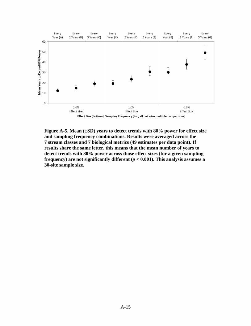
A-15

Figure A-5. Mean (±SD) years to detect trends with 80% power for effect size and sampling frequency combinations. Results were averaged across the 7 stream classes and 7 biological metrics (49 estimates per data point). If results share the same letter, this means that the mean number of years to detect trends with 80% power across those effect sizes (for a given sampling frequency) are not significantly different (p < 0.001). This analysis assumes a 30-site sample size.

A-16

Table A-6. Number of years to detect trends with 80% power for metric and stream class combinations with different effect sizes (0.5, 1, and 2%) and sampling frequencies (1, 2 and 5-year). This assumes a 30-site sample size. Asterisks (a) indicate that trend detection times exceed 40 years

Metric Class

2.0% 1.0% 0.5% 1 yr

2 yr

5 yr

1 yr

2 yr

5 yr

1 yr

2 yr

5 yr

Number of Total taxa

Atlantic Highlands (ER 5.3) 7 9 11 11 13 16 17 21 26 Mixed Wood Plains (ER 8.1) 7 9 11 11 13 16 18 23 26 High gradient, <100 km2 (HGL) 7 7 11 11 13 16 16 21 26

Low gradient and/or >100 km2a (LGG) 7 9 11 11 13 16 17 21 26

Moderate gradient, <100 km2 (MGL) 7 7 11 10 11 16 15 19 26

Creek, mod/high gradient, cold, mod buffer/neutral (TNC 1)

6 7 11 10 11 16 15 19 26

Creek, mod/high gradient, cold, low buffer/acidic (TNC 2)

6 7 11 9 11 16 15 19 21

Number of EPT taxa

Atlantic Highlands (ER 5.3) 9 11 11 13 17 21 21 25 31 Mixed Wood Plains (ER 8.1) 9 11 16 14 17 21 23 29 36 High gradient, <100 km2 (HGL) 8 9 11 13 15 21 20 25 31

Low gradient and/or >100 km2a (LGG) 9 11 11 13 17 21 21 25 36

Moderate gradient, <100 km2 (MGL) 9 11 11 14 17 21 21 27 36

Creek, mod/high gradient, cold, mod buffer/neutral (TNC 1)

8 9 11 12 15 21 19 23 31

Creek, mod/high gradient, cold, low buffer/acidic (TNC 2)

7 9 11 11 13 16 17 21 26

A-17

Table A-6. continued…

Metric Class

2.0% 1.0% 0.5% 1 yr

2 yr

5 yr

1 yr

2 yr

5 yr

1 yr

2 yr

5 yr

Percentage EPT individuals

Atlantic Highlands (ER 5.3) 9 11 16 14 17 21 22 29 36 Mixed Wood Plains (ER 8.1) 11 13 16 18 21 26 28 33 a High gradient, <100 km2 (HGL) 9 11 16 15 17 26 23 29 36

Low gradient and/or >100 km2a (LGG) 10 11 16 15 19 26 24 31 a

Moderate gradient, <100 km2 (MGL) 10 11 16 15 19 26 23 29 a

Creek, mod/high gradient, cold, mod buffer/neutral (TNC 1)

9 11 11 13 15 21 20 25 31

Creek, mod/high gradient, cold, low buffer/acidic (TNC 2)

8 9 11 13 15 21 20 25 31

Number of Cold water taxa

Atlantic Highlands (ER 5.3) 13 15 21 21 25 31 32 39 a

Mixed Wood Plains (ER 8.1) 13 15 21 21 25 31 32 a a

High gradient, <100 km2 (HGL) 11 15 16 18 21 26 29 35 a

Low gradient and/or >100 km2a (LGG) 13 17 21 21 25 36 33 a a

Moderate gradient, <100 km2 (MGL) 11 13 16 18 21 26 28 35 a

Creek, mod/high gradient, cold, mod buffer/neutral (TNC 1)

10 13 16 16 21 26 26 31 a

Creek, mod/high gradient, cold, low buffer/acidic (TNC 2)

11 13 16 18 21 26 28 35 a

A-18

Table A-6. continued…

Metric Class

2.0% 1.0% 0.5% 1 yr

2 yr

5 yr

1 yr

2 yr

5 yr

1 yr

2 yr

5 yr

Percentage Cold water individuals

Atlantic Highlands (ER 5.3) 18 23 31 28 35 a a a a

Mixed Wood Plains (ER 8.1) 17 21 26 26 33 a a a a

High gradient, <100 km2 (HGL) 14 17 21 22 29 36 35 a a

Low gradient and/or >100 km2a (LGG) 21 25 31 32 a a a a a

Moderate gradient, <100 km2 (MGL) 17 21 26 26 33 a 40 a a

Creek, mod/high gradient, cold, mod buffer/neutral (TNC 1)

14 17 21 22 27 36 34 a a

Creek, mod/high gradient, cold, low buffer/acidic (TNC 2)

14 17 21 21 25 36 33 a a

Number of Warm water taxa

Atlantic Highlands (ER 5.3) 17 21 26 27 33 a a a a

Mixed Wood Plains (ER 8.1) 17 21 26 26 33 a a a a

High gradient, <100 km2 (HGL) 17 21 26 28 33 a a a a

Low gradient and/or >100 km2a (LGG) 14 17 21 23 27 36 34 a a

Moderate gradient, <100 km2 (MGL) 16 21 26 26 33 a a a a

Creek, mod/high gradient, cold, mod buffer/neutral (TNC 1)

18 23 31 29 37 a a a a

Creek, mod/high gradient, cold, low buffer/acidic (TNC 2)

15 19 26 24 29 a 38 a a

A-19

Table A-6. continued…

2.0% 1.0% 0.5% 1 2 5 1 2 5 1 2 5

Metric Class yr yr yr yr yr yr yr yr yr Percentage Warm water Atlantic Highlands (ER 5.3) 25 31 a 39 a a a a a

individuals Mixed Wood Plains (ER 8.1) 26 31 a 40 a a a a a

High gradient, <100 km2 (HGL) 25 31 a 39 a a a a a

Low gradient and/or >100 km2a (LGG) 22 27 36 34 a a a a a

Moderate (MGL)

gradient, <100 km2 29 37 a a a a a a a

Creek, mod/high gradient, cold, mod buffer/neutral (TNC 1)

31 a a a a a a a a

Creek, mod/high gradient, cold, low buffer/acidic (TNC 2)

32 39 a a a a a a a

aExcept low gradient (<0.005), drainage area <10 km2 and high gradient (>0.02), drainage area >100 km2

Table A-7 contains 3 sets of results from the variance components analysis: (1) overall variability (estimates are averaged across all metric and stream class combinations); (2) mean variability for each biological metric (estimates are averaged across the stream classes); and (3) mean variability for each stream class (estimates are averaged across the biological metrics). Overall, the residual variation (which represents variability that cannot be attributed to the trend over time, the collection method, and HUC8) was largest (7.02), followed by collection method (4.9) and HUC8 subbasin (3.3; see Table A-7). Percentage individual metrics had higher mean variability than the richness metrics, particularly the percentage EPT and percentage cold water individuals metric (see Table A-7). The mean variability estimates were fairly similar across stream classes.

A-20

Table A-7. Results from the variance components analysis. For the overall average, estimates are averaged across all metric and stream class combinations. For the biological metrics, estimates are averaged across the stream classes and for the stream classes, estimates are averaged across the biological metrics.

Set of results Mean CollMeth Mean HUC8 Mean Residual Overall average 4.9 3.3 7.0

Biological metrics Total taxa richness 5.7 2.6 5.1 EPT richness 2.0 1.8 3.5 Cold water taxa richness 1.8 1.1 2.3 Warm water taxa richness 0.8 0.7 1.3 Percentage EPT individuals 14.1 6.8 16.5 Percentage Cold water individuals 7.0 6.7 13.0 Percentage Warm water individuals 3.0 3.3 7.4

Stream classes Atlantic Highlands (5.3) 5.0 3.0 7.5 Mixed Wood Plains (8.1) 5.3 3.2 7.7 High gradient, <100 km2 (HGL) 5.1 2.7 7.0 Moderate gradient, <100 km2 (MGL) 4.8 3.0 7.1 Low gradient and/or >100 km2* (LGG) 4.9 3.8 7.0 Creek, mod/high gradient, cold, mod buffer/neutral (TNC 1)

4.0 3.6 6.5

Creek, mod/high gradient, cold, low buffer/acidic (TNC 2)

5.5 4.0 6.3

A.4. CONCLUSIONSThe analyses suggest that detection times of 10−20 years (at 80% power) are possible for

several of the biological metrics if 30 or more sites with comparable environmental conditions and biological communities are monitored regularly. These results are consistent with other research. For example, Larsen et al. (2004) found that well-designed networks of 30−50 sites monitored consistently can detect underlying changes of 1−2% per year in a variety of metrics within 10−20 years, or sooner, if such trends are present. Larsen et al. (2004) also emphasized the importance of the duration of the survey, citing that trend detection capability increases substantially with time.

A-21

The analyses also show that richness metrics have lower variability than percentage individual metrics, which means that there is a greater likelihood of detecting trends in the richness metrics over shorter time periods. Because richness values increase with subsampling effort, it is important to identify an adequate number of organisms, particularly for metrics with low representation (e.g., cold-water taxa). Identifying a larger subsample of organisms at RMN sites (e.g., 300 or more organisms) will improve the power to detect trends. While this may increase costs in the short-term, the resulting increase in power lowers detection times, thereby reducing overall costs of the long-term monitoring effort. Moreover, the earlier detection may lead to management actions that could alleviate additional, costlier impacts.

The classification scheme also influences trend detection times. Thus, the Northeast should be partitioned to minimize environmental variability and gradients. Size and gradient are key variables to capture. Schemes that consider additional variables like thermal class and geology (like TNC’s NAHC) may further improve performance, but those variables are generally not as readily available (or dependable), and in this study, did not make a large difference in trend detection times. Classification is also an important consideration during site selection. Since one of the objectives of the RMNs is to detect trends attributable to climate change, tracking changes in the thermal indicator taxa (particularly cold water taxa) is of interest. As discussed above, the more cold water taxa present at the RMN sites, the greater the chance of detecting trends in the cold water richness metric over shorter time periods. Based on unpublished analyses on the Northeast data set, sites in small to medium-sized, medium to high gradient stream classes (MGL and HGL) have higher numbers of cold-water taxa, so selecting sites in these stream classes will improve the chances of detecting climate-related trends over shorter time periods.

Sampling frequency is another important consideration. The analyses show that sampling macroinvertebrates on an annual basis improves trend detection times, particularly if trends are subtle. If sites in the Northeast RMN are sampled annually over a long time period (e.g., 10+ years), this will improve the chances of detecting trends. Other design recommendations, which are described in Section 3.1.1, are based on literature and Standard Operating Procedures (SOPs) commonly used by RMN partners. These include recommendations on time periods for sample collection (also referred to as ‘index periods’), collection protocols, type(s) of habitats sampled, and level of taxonomic identification. The use of consistent methods will increase the comparability of data, minimize biases and variability, and ensure that the data meet data quality objectives of the Northeast RMN. These recommendations also can be applied to other regions interested in climate change detection in streams.

A-22

A.5. SUPPLEMENTAL MATERIAL A.5.1. Derivation of the Size/Slope Classification Scheme

Prior to running the classification analysis on the aggregated Northeast data set, the data set was reduced by randomly selecting one sample per site so that sites with multiple years of data would not receive unequal weight (sample size = 689). The 689 sites were distributed across the whole study region. For site classification, nonmetric multidimensional scaling (NMDS) ordination was used to explore predominant types of reference samples based on taxa presence and absence. The ecodist package in R was used to calculate Bray-Curtis similarity measures (Goslee and Urban, 2007; R Core Development Team, 2012) to perform NMDS. Prior to running the analysis, guidelines recommended in Cuffney et al. (2007) were used to develop Operational Taxonomic Units (OTUs) as necessary to achieve an acceptable level of taxonomic consistency across the data set. For interpretability, the NMDS was limited to four axes (Stress = 0.20, r2 = 0.4).

Initial NMDS ordination using all data showed that sites group by method (see Figure A-S1), indicating that method is an important determinant of taxonomic structure. These differences appeared along all four axes, but were most pronounced in the first three. For example, samples from Maine and New Hampshire (artificial substrate ellipsoid, see Figure A-S1) overlapped and were largely distinct from New York and Vermont samples (riffle D-net ellipsoid, see Figure A-S1). The strongest correlations (|r| > 0.3) between taxa and environmental variables included some combination of slope and drainage size in all four axes, but also included longitude on axis 2, and elevation and maximum temperature on axis four (see Table A-S1, left). Axis 1 can be interpreted as shifts in the macroinvertebrate community that occurred as measures of slope increased and drainage area decreased (particularly slope and log10 drainage area), while axes two and three separated the two. Axis two was most strongly related to mean slope (and longitude) and axis three to log10 drainage area. Axis four is less easily interpreted.

A-23

-0.4 -0.2 0.0 0.2 0.4 0.6

-0.6

-0.4

-0.2

0.0

0.2

0.4

Axis 2

Axi

s 1

CT DEEPMA DEPME DEPNEWSNH DESNY DECRI DEMUSGSVT DECWSAMulti-HabitatRiff leArtif icialSubstrate

Figure A-S1. Axes 1 and 2 from first NMDS ordination, using data from all methods. All four axis correlations are confounded by method. Methods are represented with different symbols and sampling devices are shown with two rings (solid and dashed 95% confidence ellipsoids). WSA and NEWS samples are also highlighted (dotted 95% confidence ellipsoid).

A-24

Table A-S1. Correlations between environmental variables and NMDS axes for all sites (left) and NEWS and WSA sites (right). Both analyses show consistent ties between taxonomic axes and aspects of slope and drainage area. |r2| > 0.3 are bolded.

Environmental All Sites NEWS and WSA sites

Variable X1 X2 X3 X4 X1 X2 X3 X4 Latitude −0.157 0.033 0.056 −0.178 0.062 −0.123 −0.241 0.121

Longitude −0.173 0.405 0.024 −0.244 0.270 −0.130 0.037 −0.001

Sinuosity −0.039 0.080 −0.002 0.068 0.128 −0.041 0.112 −0.223

Slope 0.405 −0.112 −0.093 −0.462 −0.205 0.174 −0.506 −0.320

Mean Slope 0.259 −0.327 0.219 −0.313 −0.064 0.028 −0.602 −0.237

Drainage Area −0.245 0.086 0.016 0.150 0.317 −0.257 0.154 0.136

Log10(Dr Area) −0.403 −0.117 0.369 0.366 0.403 −0.339 0.023 0.116

Elevation 0.215 −0.247 −0.073 −0.308 −0.203 0.278 −0.351 −0.095

Stream Aspect −0.070 0.015 −0.003 0.053 −0.256 0.112 0.060 0.094

Max Temp 0.041 0.165 −0.049 0.305 0.031 −0.004 0.416 −0.004

Min Temp 0.027 0.057 0.013 0.263 −0.086 −0.064 −0.013 0.253

Length 0.082 −0.118 0.143 −0.115 0.102 −0.002 −0.309 −0.324

To eliminate the confounding effects of method, a second NMDS ordination used data only from agencies that used similar methods and sampled across the region. This included 64 sites from the NEWS and WSA studies (multihabitat ellipsoid, see Figure A-S1). The resulting ordination also was limited to four axes for interpretability (Stress = 0.18, r2 = 0.53). This ordination showed high overlap between the two studies on all four axes. Likewise, the strongest correlations (|r| > 0.3) between taxa axes and environmental variables included some combination of slope or mean slope and drainage area or log10(drainage area) in all four axes, but also included elevation and maximum temperature on axis 3, and NHDPlus flowline length on axes 3 and 4 (see Table A-S1, right). Axes 1 and 2 reflected shifts in the macroinvertebrate community that occur as measures of drainage area change, while axes 3 and 4 showed shifts related to measures of slope.

Given the consistent appearance of slope and drainage area variables in both NMDS results, these two variables were chosen as a simple way to identify stream classes. Thresholds for both slope and drainage were selected to be consistent with the TNC’s Northeast Aquatic Habitat Classification (NAHC; Olivero and Anderson, 2008). The distributions of the biological metrics used in this study were compared in multiple categories of slope and catchment area. In streams with catchments <100 km2, slope was a dominant effect. Streams with similar slopes but

A-25

differing catchment size (<10 or >10 km2) had similar metric distributions. In small rivers with catchments >100 km2, slope was less of a factor and metric distributions resembled those in lower gradient smaller streams.

The end result was the following four broad stream classes based on slope (NHDPlus flowline slope; unitless) and size (NHDPlus cumulative drainage area; km2):

• High gradient, less than 100 km2 (HGL) • Moderate gradient, less than 100 km2 (MGL) • Low gradient and/or greater than 100 km2 (LGG) • ‘Other’―low gradient (<0.005), drainage area <10 km2 and high gradient (>0.02),

drainage area >100 km2

A-26

A.6. LITERATURE CITEDBarbour, MT; Gerritsen, J; Snyder, BD; Stribling, JB. (1999) Rapid bioassessment protocols for use in streams and

wadeable rivers: Periphyton, benthic macroinvertebrates and fish, Second Edition. [EPA 841-B-99-002]. Washington, D.C: U.S. Environmental Protection Agency, Office of Water. Available online: http://water.epa.gov/scitech/monitoring/rsl/bioassessment/index.cfm

Bates, D; Maechler, M; Bolker, B. (2011) lme4: Linear mixed-effects models using S4 classes. R package version 0.999375-42. Available online at http://CRAN.R-project.org/package=lme4.

Brown, MT; Vivas, MB. (2005) Landscape development intensity index. Environmental Monitoring and Assessment 101(289-309).

Cuffney, TF; Bilger, MD; Haigler, AM. (2007) Ambiguous taxa: effects on the characterization and interpretation of invertebrate assemblages. J N Am Benthol Soc 26(2):286−307.

Davies, SP; Tsomides, L. (2002). Methods for biological sampling and analysis of Maine’s rivers and streams. (DEP LW0387-B2002). August, Maine: Maine Department of Environmental Protection. http://www.maine.gov/dep/water/monitoring/biomonitoring/materials/finlmeth1.pdf

Fry, J; Xian, G; Jin, S; J.Dewitz, C.Homer, L.Yang, C.Barnes, N.Herold, and J. Wickham. (2011) Completion of the 2006 national land cover database for the conterminous United States. PE&RS 77(9): 859−864. Available online at www.mrlc.gov/downloadfile2.php?file=September2011PERS.pdf

Goslee, S; Urban, D. (2007) The ecodist package for dissimilarity-based analysis of ecological data. J Stat Soft 22:1−19.

Gotelli, NJ; Colwell, RK. (2001) Quantifying biodiversity: procedures and pitfalls in the measurement and comparison of species richness. Ecol Lett 4:379−391.

Homer, C; Dewitz, J; Fry, J; Coan, M; Hossain, N; Larson, C; Herold, N; McKerrow, A; VanDriel, JN; Wickham, J. (2007) Completion of the 2001 National Land Cover Database for the Conterminous United States. PE&RS 73(4):337−341. Available online at http://www.asprs.org/a/publications/pers/2007journal/april/highlight.pdf

Hughes, RM; Larsen, DP; Omernik, JM. (1986) Regional reference sites: a method for assessing stream potentials. Environmental Management 10(5):629-635.

Larsen, D; Kaufmann, P; Kincaid, T; Urquhart, N. (2004) Detecting persistent change in the habitat of salmon-bearing streams in the Pacific Northwest. Can J Fish Aqua Sci 61:283−291.

Olivero, AP; Anderson, MG. (2008) Northeast aquatic habitat classification. Denver, CO: The Nature Conservancy. Available online at http://rcngrants.org/content/northeastern-aquatic-habitat-classification-project

Omernik, JM. (1995) Ecoregions: a spatial framework for environmental management. In: Davis, W; Simon, T; Eds Biological assessment and criteria: tools for water resource planning and decision making. [pp 49−62]. Boca Raton, FL: Lewis Publishers.

R Core Development Team. (2012) R: A language and environment for statistical computing. Vienna, Austria.

Snook, H; Davies, S; Gerritsen, J; Jessup, B; Langdon, R; Neils, D;Pizutto, E. (2007) The New England Wadeable Stream Survey (NEWS): development of common assessments in the framework of the biological condition gradient. Prepared for USEPA Office of Science and Technology and Office of Wetlands, Oceans and Watersheds, Washington, DC.

U.S. EPA (Environmental Protection Agency). (2006) Wadeable Streams Assessment: a collaborative survey of the Nation's streams. Office of Water, Washington, DC; EPA 841/B-06/002.

A-27

Yuan, LL. (2006) Estimation and application of macroinvertebrate tolerance values. [EPA/60/P-04/116F]. Washington, DC National Center for Environmental Assessment. U.S. Environmental Protection Agency, Washington, DC.

B-1

APPENDIX B.

_ __________________

CHECKLIST FOR STARTING A REGIONAL

MONITORING NETWORK (RMN)

B-2

1. Establish the regional working group.

• Coordinator (e.g., from an U.S. EPA Region or a state) volunteers to lead the regionalworking group.

• The coordinator works with EPA and partners to create a contact list.• EPA and the coordinator hold a kick-off webinar to brief potential partners on current

RMN efforts, describe the RMN framework and development process, and discuss apotential timeline for implementation.

2. The coordinator requests candidate sites from each entity. During the site selection process,the working group considers site selection criteria being used in other RMN regions and triesto use similar criteria where practical. Desired site characteristics include:

• Part of established, long-term monitoring networks• Low level of anthropogenic disturbance• Colocated with existing equipment (e.g., USGS gage, weather station)• Exhibit similar environmental and biological characteristics• Longevity (e.g., accessible [day trip], opportunities to share the workload with outside

agencies or organizations)• In watersheds that are protected from future development• Lengthy historical sampling record for biological, thermal or hydrological data

3. The regional coordinator compiles information on data collection and processing protocolsbeing used by each regional working group member, and EPA distributes the generic RMNQAPP1. The regional working group reviews the generic QAPP and discusses appropriateprotocols for their region. The group attempts to use similar protocols to other RMNs. Thedraft (region-specific) protocols are written up in an addendum to the QAPP.

4. EPA has been conducting research on screening, classification, and vulnerability analyses forseveral pilot RMNs (additional documentation to conduct these steps are available fromEPA). Pending availability and funding, EPA may be able to assist with the following steps:

• Screening the candidate sites by running them through a disturbance screening processsimilar to what is described in Appendix D. This may include developing criteria for

1U.S. EPA. 2015. Draft generic Quality Assurance Project Plan for monitoring networks for tracking long-term conditions and changes in high quality wadeable streams. This document is available from EPA upon request. Contact Britta Bierwagen (bierwagen.britta@epa.gov).

B-3

“reference” sites in urban and agricultural areas. Disturbance ratings will be assigned to the candidate sites.

• Gathering information from the regional working group on existing classification schemes in the region and performing analyses to explore regional classification. Sites will be assigned to classification groups.

• Gathering information on existing climate change vulnerability assessments and performing broad-scale analyses to assess the vulnerability of the candidate RMN sites to climate change.

5. The regional coordinator works with EPA and regional working group members to finalize

site selection and protocols. These are included as addendums to the QAPP.

6. The group identifies and seeks resources for implementation. High priority start-up items

typically include obtaining equipment and finding funds to process macroinvertebrate samples.

C-1

APPENDIX C.

_____ _____________________

PRIMARY REGIONAL MONITORING NETWORK

(RMN) SITES IN THE NORTHEAST,

MID-ATLANTIC, AND SOUTHEAST RMN

REGIONS

C-2

Table C-1. Site information for primary RMN sites in the Northeast (3/2015). Drainage area, slope, and elevation are estimates based on NHDPlus v1a local catchment data. Percentage forest is derived from the NLCD 2001b data layer and is based on the total watershed

Longitude Latitude State Entity Station ID Water body name Drainage area

(km2) Slope

(unitless) Elevatio

n (m) Percentage Forest (%)

−73.27990 41.92670 CT CT DEEP CTDEP_2342 Brown Brook 14.7 0.026 286.4 90.2

−71.83424 41.47482 CT CT DEEP CTDEP_1748 Pendleton Hill 10.4 0.006 55.2 71.7

−72.83917 41.94639 CT CT DEEP CTDEP_1433 West Branch Salmon 34.5 0.021 169.35 81.6

−72.16196 42.03448 MA MA DEP MADEP_BB01 Browns 14.7 0.023 253.5 87.3

−73.03027 42.66697 MA MA DEP MADEP_CR01AA Cold River 16.8 0.026 592.4 89.3

−72.96731 42.06555 MA MA DEP MADEP_HRCC Hubbard 30.0 0.029 359.8 86.5

−72.04780 42.39431 MA MA DEP MADEP_PBCC Parkers Brook 13.8 0.011 244.9 79.5

−72.38454 42.46471 MA MA DEP MADEP_WSR01 West Branch Swift 9.8 0.011 209.9 91.5

−69.64424 44.95675 ME ME DEP MEDEP_57229 East Branch Wesserunsett Stream―Station 486

126.0 0.008 207.2 83.4

−71.35110 43.14410 NH NH DES NHDES_99M-44 Bear 25.7 0.005 138.9 81.5

−71.24924 44.21896 NH NH DES USGS_01064300 Ellis 28.2 0.031 686.7 88.6

−71.36166 44.35426 NH NH DES NHDES_19-ISR Israel 16.6 0.023 544.7 92.5

−71.29306 43.89639 NH NH DES NHDES_98S-44 Paugus 31.5 0.008 264.2 97.8

−71.87633 44.10563 NH NH DES NHDES_WildAmmo Wild Ammo 96.2 0.010 481.0 96.7

−73.54621 41.49457 NY NY DEC NYDEC_HAVI_01 Haviland Hollow 24.9 0.011 202.9 85.7

−74.26626 42.01954 NY NY DEC NYDEC_LBEA_01 Little Beaver Kill 42.7 0.008 393.3 90.3

−71.61201 41.83760 RI RI DEM RIDEM_RMR03a Rush 12.2 0.017 118.2 72.6

−71.63562 41.76482 RI RI DEM RIDEM_SCI01 Wilbur Hollow 11.2 0.008 124.3 74.5

−72.88583 43.87167 VT VT DEC VTDEC_135404000013 Bingo 29.2 0.017 458.5 97.3

−72.66250 42.76389 VT VT DEC VTDEC_670000000166 Green 67.8 0.010 293.3 89.9

C-3

Table C-1. continued…

Longitude Latitude State Entity Station ID Water body name Drainage area

(km2) Slope

(unitless) Elevatio

n (m) Percentage Forest (%)

−71.78528 44.58417 VT VT DEC VTDEC_211200000268 Moose 59.0 0.015 532.7 97.5

−72.53705 44.43400 VT VT DEC VTDEC_495400000161 North Branch Winooski 29.1 0.014 327.1 95.3

−72.93194 43.13833 VT VT DEC VTDEC_033500000081 Winhall 43.8 0.017 587.7 95.0

ahttp://www.horizon-systems.com/nhdplus/nhdplusv1_home.php bhttp://www.mrlc.gov/nlcd01_data.php

C-4

Table C-2. Equipment installed at primary RMN sites in the Northeast (3/2015)

State Entity Station ID Water body name Temperature Hydrologic equipment

Hydrologic data type Notes

CT CT DEEP CTDEP_2342 Brown Brook water none none

CT CT DEEP CTDEP_1748 Pendleton Hill water and air USGS gage (01118300)

discharge gage located at biological sampling site

CT CT DEEP CTDEP_1433 West Branch Salmon water none none

MA MA DEP MADEP_BB01 Browns water and air pressure transducer

stage and discharge

flow rating curve developed by MA RIFLS

MA MA DEP MADEP_CR01AA Cold River water and air pressure transducer/USGS gage

stage and discharge

flow rating curve developed by MA RIFLS; USGS gage is now being installed at this site

MA MA DEP MADEP_ HRCC Hubbard water and air USGS gage (01187300)

discharge gage is downstream of site but location looks representative of stream conditions

MA MA DEP MADEP_PBCC Parkers Brook water and air pressure transducer

stage and discharge

flow rating curve developed by MA RIFLS

MA MA DEP MADEP_WSR01 West Branch Swift water and air USGS gage (01174565)

discharge gage is downstream of site but location looks representative of stream conditions

ME ME DEP MEDEP_57229 East Branch Wesserunsett Stream―Station 486

watera USGS gage (01048220)

discharge gage located at biological sampling site

NH NH DES NHDES_99M-44 Bear water and air pressure transducer

stage

NH NH DES USGS_01064300 Ellis water and air pressure transducer

stage

C-5

Table C-2. continued…

State Entity Station ID Water body name Temperature Hydrologic equipment Hydrologic data type Notes

NH NH DES NHDES_19-ISR Israel water and air pressure transducer stage

NH NH DES NHDES_98S-44 Paugus water and air pressure transducer stage

NH NH DES NHDES_WildAmmo Wild Ammo water and air pressure transducer stage

NY NY DEC NYDEC_HAVI_01 Haviland Hollow water and air none none

NY NY DEC NYDEC_LBEA_01 Little Beaver Kill water and air USGS gage (01362497) discharge gage located at biological sampling site

RI RI DEM RIDEM_RMR03a Rush Water USGS gage (01115114) discharge gage located at biological sampling site

RI RI DEM RIDEM_SCI01 Wilbur Hollow Water USGS gage (01115297) discharge gage located at biological sampling site

VT VT DEC VTDEC_135404000013 Bingo watera none none

VT VT DEC VTDEC_670000000166 Green Water USGS gage (01170100) discharge gage is downstream of site but location looks representative of stream conditions

VT VT DEC VTDEC_211200000268 Moose water and air (Wx station)

pressure transducer stage working on flow rating curve

VT VT DEC VTDEC_495400000161 North Branch Winooski water none none

VT VT DEC VTDEC_033500000081 Winhall watera none none

anot deployed year-round

C-6

Table C-3. Site information for primary RMN sites in the Mid-Atlantic (3/2015). Most drainage area, slope, and elevation measurements are estimates based on NHDPlus v1a local catchment data. Percentage forest is based on total watershed and is mostly derived from the NLCD 2001b data layer. Better data were used, where available (e.g., MD DNR was able to provide information based on exact watershed delineations and the NLCD 2006c data layer)

Longitude Latitude State Entity Station ID Water body name

Drainage area (km2)

Slope (unitless)

Elevation (m)

Percentage Forest (%)

−75.74869 39.74567 DE DNREC 105212 Tributary of White Clay 2 0.023 84.4 57.9

−75.75587 39.72995 DE DNREC 105213 Tributary of White Clay 2.2 0.018 69.5 61.8

−79.27980 39.64252 MD MD DNR YOUG-432-S Bear Creek 22.7 0.011 805.9 65.9

−79.15566 39.50363 MD MD DNR SAVA-204-S Crabtree Creek 43.9 0.041 620.0 84.3

−77.43406 39.60929 MD MD DNR UMON-288-S High Run 3.3 0.075 310.7 100.0

−78.90556 39.54581 MD MD DNR PRLN-626-S Mill Run 2.0 0.108 522.0 100.0

−79.06689 39.59930 MD MD DNR SAVA-225-S Savage River 138.3 0.018 682.7 83.6

−75.12664 40.97143 NJ NJ DEP/EPA R2 AN0012 Dunnfield Creek 9.5 0.048 358.4 96.8

−74.43437 41.10693 NJ NJ DEP AN0260 Mossmans Brook 10.0 0.009 343.9 80.9

−74.52972 40.76500 NJ NJ DEP AN0215A Primrose 0.01 0.014 123.6

−77.45100 39.89700 PA PA DEP CR Carbaugh Run 15.5 0.022 435.3 91.0

−77.01929 41.42653 PA SRBC SRBC_Grays Grays Run 51.2 0.014 429.8 93.2

−79.23750 40.00333 PA PA DEP JMR/WQN_734 Jones Mill Run 12.8 0.019 710.1 93.1

−77.77068 41.49970 PA SRBC SRBC_Kettle Kettle 210.3 0.000 418.8 84.8

−79.57152 41.69451 PA PA DEP WBC/WQN_873 West Branch of Caldwell Creek 50.7 0.005 453.7 82.0

−79.44821 37.53920 VA VDEQ 2-HUO005.87 Hunting Creek 10 0.047 581.1 90.6

−78.40670074 38.48708676 VA Shen NP 3-RAP088.21 Rapidan River (upper) 12.7 0.030 928 96

−80.57352 37.37393 VA VDEQ 9-LRY007.02 Little Stony Creek 48.0 0.061 968.1 97.4

−78.26867 38.70296 VA Shen NP 3-PIY003.27 Piney River 10.0 0.047 578.8 96.1

C-7

Table C-3. continued…

Longitude Latitude State Entity Station ID Water body name

Drainage area (km2)

Slope (unitless)

Elevation (m)

Percentage Fores (%)t

−79.34634 38.32267 VA VDGIF 2-RAM007.29 Ramseys Draft 20.0 0.020 868.7 94.0

−80.33483 36.80553 VA VDEQ 4ARCC008.86 Rock Castle Creek 20.6 0.020 562.5 90.0

−81.75611 36.62583 VA TVA TVA_Whitetop Whitetop Laurel Creek 145.3 0.012 790.0 91.1

−79.60111 38.74322 WV WV DEP 3593 Big Run 10.4 0.031 1,099.0 98.3

−79.56808 38.62673 WV WV DEP 6112 Big Run 36.0 0.027 930.9 96.3

−79.67617 38.61844 WV WV DEP 2571 East Fork/Greenbrier River 28.0 0.011 1,078.6 93.5

−79.48686 38.84942 WV WV DEP 8756 Seneca Creek 42.5 0.024 873.8 98.3

−80.30063 38.23512 WV WV DEP 2039 South Fork/Cranberry River 36.3 0.004 1,143.6 97.5

ahttp://www.horizon-systems.com/nhdplus/nhdplusv1_home.php bhttp://www.mrlc.gov/nlcd01_data.phpchttp://www.mrlc.gov/nlcd2006.php

C-8

Table C-4. Equipment installed at primary RMN sites in the Mid-Atlantic (3/2015)

State Entity Station ID Water body

name Temperature Hydrologic equipment

Hydrologic data type Notes

DE DNREC 105212 Trib White Clay planning to install water and air temperature sensors and pressure transducers in 2015 DE DNREC 105213 Trib White Clay

MD MD DNR YOUG-432-S Bear Creek water and air USGS gage (03076600) downstream of site; about nine tributaries (including a major one) enter between gage and site

MD MD DNR SAVA-204-S Crabtree Creek water and air USGS gage (01597000)

discharge

MD MD DNR UMON-288-S High Run water and air stage

MD MD DNR PRLN-626-S Mill Run water and air stage

MD MD DNR SAVA-225-S Savage River water and air USGS gage (01596500)

discharge gage is downstream of site but location looks representative of stream conditions

NJ NJ DEP/ EPA R2

AN0012 Dunnfield Creek water and air applied for a grant to get a USGS gage installed here

NJ NJ DEP AN0260 Mossmans Brook water and air

NJ NJ DEP AN0215A Primrose water and air USGS staff gage (01378780)

occasional stage

applied for a grant to get a USGS gage installed here

PA PA DEP CR Carbaugh Run water and air Will try to install pressure transducer in 2015

PA SRBC SRBC_Grays Grays Run water and air pressure transducer

stage Working on flow rating curve

PA PA DEP JMR/WQN_734 Jones Mill Run water and air

PA SRBC SRBC_Kettle Kettle water and air pressure transducer

stage Working on flow rating curve

PA PA DEP WBC/WQN_873 West Branch of Caldwell Creek

water and air

VA VDEQ 2-HUO005.87 Hunting Creek water and air

C-9

Table C-4. continued…

State Entity Station ID Water body

name Temperature Hydrologic equipment

Hydrologic data type Notes

VA Shen NP 3-RAP088.21 Rapidan River (upper)

water and air Flow nearby though in another drainage (gage in Staunton R)

VA VDEQ 9-LRY007.02 Little Stony Creek

water and air

VA Shen NP 3-PIY003.27 Piney River water and air gage

VA VDGIF 2-RAM007.29 Ramseys Draft water and air

VA VDEQ 4ARCC008.86 Rock Castle Creek

water and air

VA TVA TVA_Whitetop Whitetop Laurel Creek

water and air pressure transducer

stage

WV WV DEP 3593 Big Run water and air pressure transducer

stage

WV WV DEP 6112 Big Run water and air pressure transducer

stage

WV WV DEP 2571 East Fork/Greenbrier River

water and air planning to install pressure transducer in 2015

WV WV DEP 8756 Seneca Creek water and air planning to install pressure transducer in 2015

WV WV DEP 2039 South Fork/Cranberry River

water and air planning to install pressure transducer in 2015

C-10

Table C-5. Site information for primary RMN sites in the Southeast (3/2015). Most drainage areas are estimates based on NHDPlus v1a local catchment data. Where available, data from exact watershed delineations were used. Slope and elevation are estimated based on NHDPlus v1 local catchment data. Percentage forest is derived from the NLCD 2001b data layer and is based on the total watershed

Longitude Latitude State Entity Station ID Water body name Drainage

area (km2) Slope

(unitless) Elevation

(m) Percentage Forest (%)

−87.2862 34.3307 AL AL DEM BRSL-3 Brushy Creek 23.6 0.002 240.8 96.9

−86.1330 34.9180 AL AL DEM HURR-2 Hurricane Creek 102.6 0.000 297.07 93.5

−87.3991 34.2856 AL AL DEM SF-1 Sipsey Fork 231.8 0.000 204.6 95.5

−83.5716 34.9590 GA GA DNR 66d-WRD768 Charlies Creek 7.2 0.040 927.0 99.0

−83.5166 34.9520 GA GA DNR 66d-44-2 Coleman River 13.6 0.033 866.9 96.8

−84.3851 34.9851 GA TVA 3890-1 Fightingtown Creek 182.9 0.003 468.8 86.8

−84.1512 34.6020 GA GA DNR 66g-WRD773 Jones Creek 9.1 0.011 586.0 98.4

−83.9039 37.4550 KY KY DEP DOW04036022 Hughes Fork 3.5 0.019 359.1 86.6

−83.1924 38.1311 KY KY DEP DOW06013017 Laurel Creek 37.8 0.002 294.3 72.9

−82.9940 37.0774 KY KY DEP DOW04055002 Line Fork UT 0.6 NA 335.6 100.0

−82.7916 37.0666 KY KY DEP DOW02046004 Presley House Branch 3.0 0.093 736.6 97.0

−82.1014 35.7347 NC NC DENR CB6 Buck Creek 37.5 0.011 529.7 96.6

−83.0728 35.6672 NC NC DENR/TVA EB320 Cataloochee Creek 127.0 0.010 939.2 99.0

−82.8089 35.2281 NC NC/DENR/TVA EB372 Cedar Rock Creek 3.1 0.042 985.9 98.6

−80.0303 35.3792 NC NC DENR QB283 Dutchmans Creek 9.1 0.014 177.5 92.2

−81.5672 35.5906 NC NC DENR CB192 Jacob Fork 66.5 0.001 380.1 89.4

−79.9906 36.5355 NC NC DENR NB28 Mayo River 626.8 0.010 254.9 73.4

−83.8552 35.3094 NC TVA 10605-2 Snowbird Creek 108.8 0.007 677.8 97.1

−83.0793 34.9235 SC SC DHEC SV-684 Crane Creek 4.0 0.078 623.6 97.0

−82.6477 35.0642 SC SC DHEC S-086 Matthews Creek 25.8 0.003 360.2 96.3

C-11

Table C-5. continued…

Longitude Latitude State Entity Station ID Water body name Drainage

area (km2) Slope

(unitless) Elevation

(m) Percentage Forest (%)

−82.5739 35.1254 SC SC DHEC S-076 Middle Saluda River 16.0 0.042 582.3 96.6

−82.2515 35.1831 SC SC DHEC B-099-7 Vaughn Creek 12.0 0.008 368.4 95.6

−87.5355 35.4217 TN TN DEC ECO71F19 Brush Creek 33.3 0.004 245.1 75.8

−84.1182 35.4548 TN TVA CITIC011.0MO Citico Creek 118.1 0.010 399.0 97.2

−82.5291 36.1508 TN TN DEC ECO66E09 Clark Creek 23.8 0.017 596.6 95.1

−84.0597 36.2136 TN TN DEC ECO67F06 Clear Creek 7.2 0.014 337.1 87.9

−85.9921 35.9286 TN TN DEC ECO71H17 Clear Fork Creek 38.1 0.005 262.9 88.8

−85.9111 35.1155 TN TN DEC ECO68C20 Crow Creek 47.7 0.006 311.5 84.5

−82.9381 36.5001 TN TN DEC/TVA ECO6702 Fisher Creek 30.0 0.003 429.7 82.0

−87.7614 35.9806 TN TN DEC ECO71F29 Hurricane Creek 177.6 0.003 156.3 81.0

−84.6981 36.5161 TN TN DEC ECO68A03 Laurel Fork Station Camp Creek

15.3 0.014 392.9 97.2

−83.5773 35.6533 TN TN DEC ECO66G05 Little River 81.2 0.029 879.5 99.8

−84.9827 36.1299 TN TN DEC/TVA MYATT005.1CU Myatt Creek 12.4 0.016 525.1 78.8

−84.4803 35.0539 TN TN DEC ECO66G20 Rough Creek 15.5 0.020 520.6 98.9

−84.6122 35.0031 TN TN DEC ECO66G12 Sheeds Creek 14.8 0.031 436.6 98.8

−83.8917 36.3436 TN TN DEC ECO67F13 White Creek 8.0 0.009 379.8 90.9

−82.9456 35.9224 TN TVA 12358-1 Wolf Creek 28.5 0.014 429.9 96.0

ahttp://www.horizon-systems.com/nhdplus/nhdplusv1_home.php bhttp://www.mrlc.gov/nlcd01_data.php

C-12

Table C-6. Equipment installed at primary RMN sites in the Southeast (3/2015). EPA R4 is planning to install equipment at the sites in North and South Carolina as resources permit

State Entity Station ID Water body name Temperature Hydrologic equipment

Hydrologic data type Notes

AL AL DEM BRSL-3 Brushy Creek water and air pressure transducer stage

AL AL DEM HURR-2 Hurricane Creek water and air pressure transducer stage

AL AL DEM SF-1 Sipsey Fork water USGS gage (02450250)

discharge water temperature is being measured at the USGS gage

GA GA DNR 66d-WRD768 Charlies Creek water and air pressure transducer stage

GA GA DNR 66d-44-2 Coleman River water and air pressure transducer stage

GA TVA 3890-1 Fightingtown Creek water and air pressure transducer stage Inactive USGS gage (03560000)

GA GA DNR 66g-WRD773 Jones Creek water and air pressure transducer stage

KY KY DEP DOW04036022 Hughes Fork water and air pressure transducer stage

KY KY DEP DOW06013017 Laurel Creek water and air pressure transducer stage

KY KY DEP DOW04055002 Line Fork UT water and air pressure transducer stage

KY KY DEP DOW02046004 Presley House Branch

water and air pressure transducer stage

NC NC DENR CB6 Buck Creek none none none

NC TVA EB320 Cataloochee Creek water USGS gage (03460000)

discharge water temperature is being measured at the USGS gage

NC NC DENR EB372 Cedar Rock Creek none none none USGS gage downstream on Catheys Creek (03440000)

NC NC DENR QB283 Dutchmans Creek none none none inactive USGS gage (02123567)

NC NC DENR CB192 Jacob Fork none USGS gage (02143040)

discharge precip is being measured at the USGS gage

NC NC DENR NB28 Mayo River none USGS gage (02070500)

discharge

C-13

Table C-6. continued…

State Entity Station ID Water body name Temperature Hydrologic equipment

Hydrologic data type Notes

NC TVA 10605-2 Snowbird Creek water and air pressure transducer

stage inactive USGS gage (03516000)

SC SC DHEC SV-684 Crane Creek none none none

SC SC DHEC S-086 Matthews Creek none none none

SC SC DHEC S-076 Middle Saluda River

none none none USGS gage (02162350) downstream of site but unsure whether it is representative (some major tributaries enter between site and gage); EPA R4 will install equipment as resources permit

SC SC DHEC B-099-7 Vaughn Creek none none none

TN TN DEC ECO71F19 Brush Creek water and air pressure transducer

stage

TN TVA CITIC011.0MO Citico Creek water and air pressure transducer

stage

TN TN DEC ECO66E09 Clark Creek water and air pressure transducer

stage

TN TN DEC ECO67F06 Clear Creek water and air pressure transducer

stage

TN TN DEC ECO71H17 Clear Fork Creek water and air pressure transducer

stage

TN TN DEC ECO68C20 Crow Creek water and air pressure transducer

stage

TN TN DEC/TVA

ECO6702 Fisher Creek water and air pressure transducer

stage

TN TN DEC ECO71F29 Hurricane Creek water and air pressure transducer

stage

TN TN DEC ECO68A03 Laurel Fork Station Camp Creek

water and air pressure transducer

stage

C-14

Table C-6. continued…

State Entity Station ID Water body name Temperature Hydrologic equipment

Hydrologic data type Notes

TN TN DEC ECO66G05 Little River water and air pressure transducer

stage

TN TN DEC/TVA

MYATT005.1CU Myatt Creek water and air pressure transducer

stage

TN TN DEC ECO66G20 Rough Creek water and air pressure transducer

stage

TN TN DEC ECO66G12 Sheeds Creek water and air pressure transducer

stage

TN TN DEC ECO67F13 White Creek water and air pressure transducer

stage

TN TVA 12358-1 Wolf Creek water and air pressure transducer

stage

D-1

APPENDIX D.

____ ______________________

DISTURBANCE SCREENING PROCEDURE FOR RMN SITES

D-2

D.1. BACKGROUND This project developed a screening procedure for candidate regional monitoring network

(RMN) sites to determine where the sites fall along a standardized disturbance gradient, using data that are available nationwide and that are derived using common data sources and methodologies. The first iteration of the screening process was developed during the Northeast RMN pilot study in 2012, when over 900 sites were screened. Additional screening considerations related to coal mining, shale gas drilling, atmospheric deposition and other stressors were added during the Mid-Atlantic RMN site selection process.

The screening processes that were performed during the development of the pilot RMNs have limitations. For one, there were insufficient resources to do exact watershed delineations for all of the candidate sites. Instead, the land use data for many of the candidate sites were based on data associated with the National Hydrography Dataset Plus Version 1 (NHDPlusV1) catchments in which the sites are located (U.S. EPA, 2005. While this approach generally provides a good approximation, sometimes there are discrepancies, which are described in Section D.2.1. To address this issue, additional checks were performed to verify the accuracy of the results before finalizing site selection (e.g., local experts who were familiar with the sites verified that results were in keeping with their expectations). In the future, as resources permit, the RMN site screening process will be further refined, and exact watershed delineations will be done for all of the RMN sites.

D.2. METHODOLOGY

Candidate RMN sites were spatially joined with NHDPlusV1 catchments (U.S. EPA and USGS, 2005) using Geographic Information System software (ArcGIS 10.0). Each NHDPlusV1 catchment has a unique identifier called a COMID. Many data were linked to sites via this COMID.

Three different types of disturbance screenings were performed:

1. Land use (see Section D.2.1); 2. Likelihood of impact from dams, mines, and point-source pollution sites (see

Section D.2.2); and 3. Likelihood of impact by the following other nonclimatic stressors:

• Roads (see Section D.2.3.1), • Atmospheric deposition (see Section D.2.3.2), • Coal (see Section D.2.3.3), • Shale gas (see Section D.2.3.4), • Future urban development (see Section D.2.3.5), and/or • Water withdrawals (see Section D.2.3.6).

D-3

These considerations are consistent with recent work performed by Michigan State University (MSU) on the National Fish Habitat Action Plan (NFHAP; DFW MSU et al., 2011; Esselman et al., 2011a). That work included the development of the cumulative disturbance index (DFW MSU et al., 2011; Esselman et al., 2011b).

D.2.1. Land Use Disturbance

The first set of screening was done on land use and impervious cover data from the 2001 National Land Cover Database (NLCD) version 1 data set (Homer et al., 2007). The land use disturbance screening was conducted at both the local catchment and total watershed scales [important note: for purposes of this exercise, the total watershed scale will be referred to as the “network” scale, in keeping with the work done by DFW MSU et al. (2011)]. Local catchments are defined as the land area draining directly to a reach, and network catchments are defined by all upstream contributing catchments to the reach's outlet, including the reach's own local catchment (see Figure D-1). GIS shapefiles with delineations of the local catchments were downloaded from the Horizon-Systems website: http://www.horizon-systems.com/NHDPlus/NHDPlusV1_data.php. The network-scale data were generated (and graciously shared) by MSU.

Figure D-1. Land use data were evaluated at both the (A) local catchment and (B) total watershed scales, using NHDPlusV1 delineations (U.S. EPA and USGS, 2005).

While these data generally provide good approximations of land use, they have limitations. For one, there are biases and accuracy issues associated with the NLCD data set (e.g., Novak and Greenfield, 2010; Wickham et al., 2013). Another limitation is that there is no information on whether landscape disturbance mitigation measures are being applied in a given

D-4

catchment, and if so, how effective those measures are. Thus, we had to assume that the impacts associated with each land use type are equal.

As mentioned earlier, the preliminary land use screening was not based on exact watershed delineations. Rather the data were associated with the entire catchment in which the site is located, regardless of where the site falls within the catchment (it would have been preferable to use data based on exact watershed delineations, but we lacked the resources needed to do exact watershed delineations for all of the candidate sites). The estimates that were used were readily available for all of the sites and generally provide a good approximation (especially when sites are located at the downstream end of the catchment). However, sometimes inaccuracies occur. An example is illustrated in Figure D-2. Maryland site UMON-288-S is located about halfway up the catchment flowline. Urban and agricultural land uses are located within this catchment, but are all downstream of the site. Because these land uses are in the catchment, they are included in the land cover output for this site. An accurate output for that site would only include forested land cover. To catch errors like these, an additional series of checks were performed on the top candidate sites (e.g., we asked local experts to verify that results were in keeping with their expectations and also performed additional desktop screening using aerial photos from Google Earth).

D-5

Figure D-2. Example of a situation in which the land use output for a site is inaccurate.

Land use disturbance was assessed at both the local catchment and network scales. This was done for the following four parameters (source: NLCD 2001 version 1 data set1):

1. Percentage impervious cover 2. Percentage urban (this includes low, medium, and high intensity developed―NLCD

codes 22 + 23 + 24) 3. Percentage cultivated crops (NLCD code 82) 4. Percentage pasture/hay (NLCD code 81)

The project developed a land use disturbance scale with six levels. Thresholds for each parameter, which are guided by literature where available (e.g., King and Baker, 2010; Carlisle et al., 2008), are listed in Table D-1. When rating a site, each parameter was first assessed 1http://www.mrlc.gov/nlcd01_data.php

D-6

separately. If the parameter values at the local catchment and network scales differed, the thresholds were applied to the maximum value. For example, if a site had 2% urban land cover at the local catchment scale and 1% urban land cover at the network scale, the threshold was applied to the maximum value (in this case, 2% or level 3 for urban land use). This was done for each parameter. Then, sites were assigned an overall disturbance level. This was based on the highest disturbance level assigned across parameters. For example, if a site was level 3 for impervious, level 2 for urban, level 1 for crops, and level 2 for pasture/hay, it was assigned to disturbance level 3. As a final step, local biologists familiar with the sites were consulted to find out their thoughts on the degree of land use impact and also to inquire about the availability of more detailed land use data to help better assess the potential degree of impact.

Table D-1. The thresholds used when assigning sites to the six levels of land use disturbance. Each of the four parameters (impervious, urban, crops, pasture/hay) were assessed separately. Then, sites were assigned an overall disturbance level based on the highest level of disturbance across parameters

Level of land use disturbance Percentage

Impervious (%) Percentage Urban (%)

Percentage Crops (%)

Percentage Pasture/hay (%)

1 <0.1 0 0 0 2 ≤1 ≤1 ≤1 ≤5 3 ≤2 ≤3 ≤5 ≤15 4 ≤5 ≤5 ≤15 ≤25 5 ≤10 ≤10 ≤25 ≤35 6 >10 >10 >25 >35

D.2.2. Likelihood of Impacts from Dams, Mines, and Point-source Pollution SitesIn the second set of screening, sites were flagged if they had a high likelihood of being

impacted by dams, mines, National Pollutant Discharge Elimination System (NPDES) major discharges and/or Superfund National Priorities List (SNPL) sites. Both the proximity of these stressors to the sites as well as the attribute data associated with each stressor were considered. The attribute data are important because there are many site-specific factors, such as dam size and storage capacity, that can greatly affect the degree of impact. Table D-2 contains a list of data that were assessed, along with the sources of those data.

The following screening procedures were performed:

1. The data listed in Table D-2 were gathered.

D-7

2. Using GIS software (ArcGIS 10.0), a 1-km buffer was created around the preliminary RMN sites (this included both the upstream and downstream areas).

3. Using GIS software (ArcGIS 10.0), a procedure was performed to identify whether any dams, mines, NPDES major discharges or SNPL sites were located within the 1-km buffer.

4. If so, those sites were flagged and the likelihood of impact based on the following considerations was assessed:

a. Location in relation to the site, assessed via a desktop screening with GIS software (ArcGIS 10.0) and Google Earth.

b. Attributes of the stressors (e.g., dam size, storage capacity, size of NPDES major discharge).

Best professional judgment was used to assign the flagged sites to one of three impact

categories:

• Unlikely impacted • Likely impacted • Unsure

Some examples of situations in which sites were assigned to the “unlikely impacted” category are:

• The site was flagged for an NPDES major discharge, but the discharge was relatively small and was located hundreds of meters downstream from the site.

• The site was flagged for a dam, but the dam was located on a different stream.

Some examples of situations in which sites were assigned to the “likely impacted” category are:

• The site was flagged for a NPDES major discharge. It was a large discharge occurring about 100 m upstream from the site.

• The site was flagged for a dam. It was a large dam located on the same stream, just upstream from the site.

D-8

Some examples of situations in which sites were assigned to the “unsure” category are:

• The site was flagged for a NPDES major discharge, but the site was located near a confluence and it was difficult to determine which stream contained the discharge.

• The stressor was small- or medium-sized and was located 500 m or more from the site.

One additional check was performed to assess the potential for flow alteration at the sites. We examined the type of NHDPlusV1 flowline (FTYPE) located on the site (e.g., stream/river, artificial pathway, canal/ditch, pipeline, connector; U.S. EPA and USGS, 2005). If the site was located on a flowline designated as something other than a stream/river, the site was flagged.

As a final step, local biologists familiar with the sites were consulted to find out their thoughts on the degree of impact and also to inquire about the availability of more detailed data to help better assess the potential degree of impact.

D.2.3. Likelihood of impact from other nonclimatic stressors

In the third set of screening, sites were flagged if they had a high likelihood of being impacted by:

• Roads, • Atmospheric deposition, • Coal mining, • Shale gas drilling, • Future urban development, and/or • Water withdrawals.

D-9

Table D-2. These data were assessed when screening for the likelihood of impacts from flow alteration, mines, National Pollutant Discharge Elimination System (NPDES) major discharges, and/or Superfund National Priorities List (SNPL) sites

Stressor Source

Dams USGS (U.S. Geological Survey). (2014) Major dams of the United States: National Atlas of the United States. Reston, VA: United States Geological Survey. Available online at : http://nationalatlas.gov/atlasftp.html#dams00x

Mines USGS (U.S. Geological Survey). (2005) Active mines and mineral processing plants in the United States in 2003. Reston, VA: USGS. Available online at http://tin.er.usgs.gov/metadata/mineplant.faq.html PASDA (Pennsylvania Spatial Data Access). (2013) Data download –mine and refuse permits. Available online at www.pasda.psu.edu.

National Pollutant Discharge Elimination System (NPDES) major discharges from the Permit Compliance System

U.S. EPA (U.S. Environmental Protection Agency). (2013) Geospatial data download service - Geospatial information for all publicly available FRS facilities that have latitude/longitude data [file geodatabase]. Available online at http://www.epa.gov/enviro/geo_data.html

Superfund National Priorities List (SNPL) from the Compensation and Liability Information System

Table D-3 contains a list of data that were gathered and assessed, along with the sources of those data. There are a lot of site-specific factors that can greatly affect the degree of impact from these stressors, which makes it difficult to set thresholds. For example, a site could be exposed to high concentrations of atmospheric deposition but may not be impacted by acidity because of site-specific mediating factors like calcareous geology. Another example is permit activity associated with coal mining. Just because mining permits have been issued in an area does not mean that mining activities are actually taking place. And even if mining activities are taking place, impacts can vary greatly depending on site-specific factors such as the size and type of mine.

D-10

Table D-3. These data were assessed when screening for the likelihood of impacts from roads, atmospheric deposition, coal mining, shale gas drilling, future urban development, and water withdrawals. These data were converted to relative measures, as described in the text.

Stressor Parameters/description Source

Roads Length of roads, local catchment, and network scales/catchment area

U.S. Census Bureau (2000) from DFW MSU et al. (2011)

Number of road crossings, local catchment, and network scales/catchment area

Atmospheric deposition

NO3 and SO4 concentrations, based on 2011 deposition grids

NADPa

The Nature Conservancy (TNC) geology class Olivero and Anderson (2008) Coal mining Potential for development, based on:

• whether the site is located in a coalfield and/or the mountaintop removal(MTR) region

• coal production by state

Coal fields (USGS, 2001) MTR region [unknown source; GIS layer was provided by Christine Mazzarella (U.S. EPA)] Coal production by State [see Table 6 in U.S. EIA (2012)]

Permit activity, based on number of permits issued within 1 km of the site. Data type and availability varied by state.

Alabama: • Number of active coal mine permits

Pennsylvania: • Anthracite permits• Anthracite refuse• Bituminous permits• Bituminous refuse

West Virginia: • WV_permitboundary• WV_refuse• WV_valleyfill• WV_all_mining

Virginia: • Surface mine permit boundaries

Alabama (Alabama Surface Mining Commission, 2013)

Pennsylvania (PASDA, 2013)

West Virginia (WVDEP, 2013; WVGES, 2014)

Virginia (VDEQ, 2013)

D-11

Table D-3. continued…

Stressor Parameters/description Source

Shale gas drilling

Potential for development, based on whether the site is located in the shale play region

U.S. EIA (2013)

Permit activity, based on the number of unconventional permits issued within 1 km of the site. These data were available for Pennsylvania (file name: PA_UncPermits_05092013) and West Virginia (file name: WV_Perm_05132013).

Frac Tracker (2013)

Future urban development

Potential for future urban development based on projected change in percentage imperviousness by 2050

U.S. EPA (2011); work performed by Angie Murdukhayeva (U.S. EPA)

Water withdrawals (county-level)

Irrigation, total withdrawals, fresh (Mgal/day) USGS (2010)

Total withdrawals, fresh (Mgal/day)

Total withdrawals, total (fresh + saline; Mgal/day)

ahttp://nadp.sws.uiuc.edu/NTN/annualmapsbyyear.aspx

Because of these factors, a relative scale (vs. firm thresholds) was used to assess the likelihood of impact. The relative scales were based on values found in NHDPlusV1 catchments across the entire study area. If a site had an elevated risk score (e.g., >75th percentile), it was flagged for further evaluation (the thresholds [e.g., 50%, 75%] vary depending on the distribution of data in each data set and best professional judgment). These thresholds should be regarded as a starting point, and should be further refined in future iterations of the screening procedure. Local biologists familiar with the sites were then consulted to find out their thoughts on the degree of impact and also to inquire about the availability of more detailed data to help better assess the potential degree of impact [e.g., is mining actually taking place? What are the pH and acid neutralizing capacity (ANC) values at sites flagged for atmospheric deposition?]. The specific screening procedures that were followed for each stressor are described below.

D.2.3.1. RoadsTwo aspects of potential road impacts were assessed:

• Length of roads and• Number of road crossings

D-12

First the roads data listed in Table D-3 were gathered for both the local catchment and network scales.

Next, to assess the likelihood of impact from length of roads, the following formulas were used to normalize the data:

Local catchment scale = Length of roads in the local catchment (m) ÷ Area of the local catchment (km2)

Network scale = Length of roads in the network (m) ÷ Area of the network (km2)

Then, the following formula was used to convert these values to a scoring scale ranging from 0 (no roads) to 100 (highest length of roads per area; note: the minimum and maximum values used in this formula are based on the range of values found across the entire study area):

100 × (Value − Minimum) ÷ (Maximum − Minimum)

If the parameter values at the local catchment and network scales differed, the maximum score was used for the assessment. For example, if the local catchment score was 80 and the network score was 50, the higher score of 80 was used for the assessment.

Sites were flagged for further evaluation if they received a score of ≥75%. The same procedure was followed when assessing the likelihood of impact from road

crossings. As a final step, we consulted with local biologists who were familiar with the sites to get

input on the degree of impact at flagged sites. D.2.3.2. Atmospheric Deposition

Two aspects of atmospheric deposition were assessed:

• Concentrations of NO3 • Concentrations of SO4

In addition, TNC geology class (Olivero and Anderson, 2008) was considered as a potential mediating factor. First the data listed in Table C-3 were gathered. Using GIS software (ArcGIS 10.0), the NO3 and SO4 deposition grid data (1-km resolution) were linked to the sites. Next, the NO3 and SO4 values were averaged. Then, the following formula was used to convert

D-13

these values to a scoring scale ranging from 0 (no nitrogen and sulfate deposition) to 100 (highest average concentration of NO3 and SO4; note: the minimum and maximum values used in this formula are based on the range of values found across the entire study area):

100 × (Value − Minimum) ÷ (Maximum − Minimum)

Sites were flagged for further evaluation if they received a score of ≥75%. Geology can potentially mediate some of the effects of atmospheric deposition. To assess

this potential, GIS software (ArcGIS 10.0) was used to link the TNC geology class (Olivero and Anderson, 2008) to the sites (note: at this time the TNC geology class data are only available for Northeast and Mid-Atlantic regions).

Sites were scored as follows:

• Sites located in areas designated as “low buffered, acidic” received a score of 100.

• Sites located in areas designated as “moderately buffered, neutral” or “assume moderately buffered (Size 3+ rivers)” received a score of 50.

• Sites located in areas designated as “highly buffered, calcareous” received a score of 0.

• Sites located in areas that lacked data or were designated as “unknown buffering/missing geology” were not assessed.

Sites were flagged if they received a score of 100%. As a final step, we consulted with local biologists who were familiar with the sites to get

input on the degree of impact at flagged sites, and to see if they had access to more detailed data, such as pH and ANC measurements, to help us better assess the potential degree of impact. D.2.3.3. Coal Mining

Two aspects of coal mining were assessed:

• Potential for mining • Permit activity

First the data listed in Table D-3 were gathered. To assess the potential for coal mining, the following were considered:

D-14

• Whether the site is located in an area that has been designated as a mountaintop removal (MTR) area and/or a coal field (USGS, 2001).

o If the site is located in a coal field, is it designated as “potentially minable” or is it tagged for “other uses”?

• What the total coal production is for the state where the site is located [source: Table 6 in the 2011 Annual Coal Report (U.S. EIA, 2012)].

The following steps were performed when assessing a site for mining potential:

1. First a coal field score was assigned, as follows:

• Using GIS software (ArcGIS 10.0), the coal field and MTR GIS layers were linked to the sites.

• If the site is located in a catchment that has been designated as a “potentially minable” coal field (USGS, 2001) and/or a mountaintop removal (MTR) area, it was assigned a score of 1.

• If the site is located in a catchment that has been designated as a coal field with “other uses” (USGS, 2001), it was assigned a score of 0.5.

• If the site is located in a catchment that is not part of a coal field or MTR area, it received a score of 0.

2. Then a coal production score was assigned, as follows:

• Total coal production values for each state were taken from Table 6 in the 2011 Annual Coal Report (U.S. EIA, 2012).

• Those values were converted to a scale of 0 to 100 using this formula (note: the minimum and maximum values used in this formula are based on the range of values found in the states in our study area):

100 × (Value − Minimum) ÷ (Maximum − Minimum)

• Sites were assigned scores based on what state they were located in. For example, West Virginia had the highest total coal production of all of the states in the study area, so any sites located in West Virginia received a coal production score of 100.

D-15

3. To get the final score for mining potential, the coal field score was multiplied by the coal production score. Scores ranged from 0 (no mining potential) to 100 (highest potential for mining).

Sites were flagged for further evaluation if they received a score of ≥75%. Permit data were not available for all the states, and where those data were available, data

type and quality varied, as did the attribute data. Therefore, permit activity was assessed on a state-by-state basis. If sites were located in states where permit data were available, the following steps were performed to assess the intensity of permit activity:

1. Gather the permit data listed in Table D-3.

2. Using GIS software (ArcGIS 10.0), create a 1-km buffer around the candidate RMN sites (this included both the upstream and downstream areas).

3. Using GIS software (ArcGIS 10.0), perform a procedure to determine how many mining permits had been issued within the 1-km buffer.

4. The following formula was used to convert those values to a scale of 0 to 100 (note: since the type of data available for each state varied, the minimum and maximum values used in this formula were based on the range of data found in each state):

100 × (Value − Minimum) ÷ (Maximum − Minimum)

Sites were flagged for further evaluation if they received a score of >0. As a final step, we consulted with local biologists who were familiar with the sites to get

input on the degree of impact at flagged sites, and to see if they had access to more detailed data to help us better assess the potential degree of impact. Just because mining permits have been issued in an area does not mean that mining activities are actually taking place. And even if mining activities are taking place, impacts can vary greatly depending on site-specific factors such as the size and type of mine.

D.2.3.4. Shale Gas Drilling

Two aspects of shall gas drilling were assessed:

• Potential for drilling • Permit activity

D-16

First the data listed in Table D-3 were gathered. To assess the potential for shale gas drilling, the following screening procedure was

performed:

• Using GIS software (ArcGIS 10.0), the shale play GIS layer (see Table D-3) was linked to the sites.

• If the site is located in a shale play region, it was assigned a score of 100 and flagged it for further evaluation.

Permit data were only available for the states of West Virginia and Pennsylvania. The following steps were performed to assess the intensity of permit activity at sites in those sites:

1. Gather the permit data listed in Table D-3.

2. Using GIS software (ArcGIS 10.0), create a 1-km buffer around the candidate RMN sites (this included both the upstream and downstream areas).

3. Using GIS software (ArcGIS 10.0), perform a procedure to determine how many unconventional permits had been issued within the 1-km buffer.

4. The following formula was used to convert those values to a scale of 0 to 100 (note: since the type of data available for each state varied, the minimum and maximum values used in this formula were based on the range of data found in each state):

100 × (Value − Minimum) ÷ (Maximum − Minimum)

Sites were flagged for further evaluation if they received a score of >0%. As a final step, we consulted with local biologists who were familiar with the sites to get

input on the degree of impact at flagged sites, and to see if they had access to more detailed data to help us better assess the potential degree of impact. Just because drilling permits have been issued in an area does not mean that drilling activities are actually taking place. And even if drilling activities are taking place, impacts can vary greatly depending on site-specific factors.

D.2.3.5. Potential for Future Urban Development

EPA’s ICLUS tools and data sets (Version 1.3 and 1.3.1; U.S. EPA, 2011) were used to assess the potential that a site will experience future urban development. The ICLUS Tools were used to project the percentage change in imperviousness in each NHDPlusV1 local catchment by

D-17

2050 based on high (A2) and low (B1) emissions scenarios (note: the ICLUS data have a resolution of 1-km).

GIS software (ArcGIS 10.0) was used to link sites with NHDPlusV1 local catchments. Sites were flagged for further evaluation if the following conditions occurred:

• The percentage impervious value in the NHDPlusV1 local catchment where the site is located is currently ≤10% (based on values derived from the 2001 NLCD version 1 data set), and

• The future projection is for a positive value ≥0.5% (this is based on an average of the high [A2] and low [B1] emissions scenarios).

As a final step, we checked with local biologists who were familiar with the sites to find out their thoughts on the potential for future development at flagged sites, and to see if they had access to more detailed data to help us better assess the potential degree of impact.

D.2.3.6. Water Withdrawals

Three aspects of water use were assessed:

• Irrigation, total withdrawals, fresh; • Total withdrawals, fresh only; and • Total withdrawals, total.

First the data listed in Table D-3 were gathered. These data are based on 2005 water use and are only available at the county-level (USGS, 2010). Then GIS software (ArcGIS 10.0) were used to associate the county-level data with NHDPlusV1 local catchments. Next sites were linked with NHDPlusV1 local catchments. For each parameter, the following formula was used to convert the values to a scoring scale ranging from 0 (no withdrawals) to 100 (highest withdrawals; note: the minimum and maximum values used in this formula are based on the range of values found across the entire study area):

100 × (Value − Minimum) ÷ (Maximum − Minimum)

Sites were flagged for further evaluation if they received a score of ≥50% for any of the three parameters.

D-18

As a final step, we checked with local biologists who were familiar with the sites to find out their thoughts on the potential for future development at flagged sites, and to see if they had access to more detailed data to help us better assess the potential degree of impact.

D-19

D.3. REFERENCES Alabama Surface Mining Commission. (2013) Alabama coal mine geospatial data – permit boundaries (1983-

present). Jasper, AL: State of Alabama http://surface-mining.alabama.gov/.

Carlisle, DM; Hawkins, CP; Meador, MR; Potapova, M; Falcone, J. (2008) Biological assessments of Appalachian streams based on predictive models for fish, macroinvertebrate, and diatom assemblages. J N Am Benthol Soc 27(1): 6–37.

DFW MSU (Department of Fisheries and Wildlife, Michigan State University), Esselman, PC; Infante, DM; Wang, L; Taylor, WW; Daniel, WM; Tingley, R; Fenner, J; Cooper, A; Wieferich, D; Thornbrugh, D; Ross, J. (2011) National Fish Habitat Action Plan (NFHAP) 2010 HCI scores and human disturbance data for conterminous United States linked to NHDPLUSV1. Denver, CO: National Fish Habitat Action Plan (NFHAP). Available online at https://www.sciencebase.gov/catalog/item/514afb90e4b0040b38150dbc

Esselman, PC; Infante, DM; Wang, L; Taylor, WW; Daniel, WM; Tingley, R; Fenner, J; Cooper, C; Wieferich, D; Thornbrugh, D; Ross, R, (2011a) A landscape assessment of fish habitat conditions in United States rivers and their watersheds. Denver, Co: National Fish Habitat Action Plan (NFHAP). Available online at http://fishhabitat.org/.

Esselman, PC; Infante, DM; Wang, L; Wu, D; Cooper, AR; Taylor, WW. (2011b) An index of cumulative disturbance to river fish habitats of the conterminous United States from landscape anthropogenic activities. Ecol Restor 29:133–151.

Frac Tracker. (2013) Frac Tracker – data [web page]. http://www.fractracker.org/downloads/

Homer, C; Dewitz, J; Fry, J; Coan, M; Hossain, N; Larson, C; Herold, N; McKerrow, A; VanDriel, JN; Wickham, J. (2007) Completion of the 2001 National Land Cover Database for the Conterminous United States. PE&RS 73(4):337−341. Available online at http://www.asprs.org/a/publications/pers/2007journal/april/highlight.pdf

King, RS; Baker, ME. (2010) Considerations for identifying and interpreting ecological community thresholds. J N Am Benthol Assoc 29(3):998-1008

Nowak, DJ; Greenfield, EJ. (2010) Evaluating the National Land Cover Database tree canopy and impervious cover estimates across the conterminous United States: a comparison with photo-interpreted estimates. Environ Manage 46:378–390.

Olivero, AP; Anderson, MG. (2008) Northeast aquatic habitat classification. Denver, CO: The Nature Conservancy. Available online at http://rcngrants.org/content/northeastern-aquatic-habitat-classification-project

PASDA (Pennsylvania Spatial Data Access). (2013) Data download –mine and refuse permits. Available online at www.pasda.psu.edu.

U.S. Bureau of the Census. (2000) Census 2000 TIGER/Line data. Available online at http://www.icpsr.umich.edu/icpsrweb/ICPSR/themes/tiger/2000/

U.S. EIA (Energy Information Administration). (2013) Maps: exploration, resources, reserves, and production - United States shale gas maps - Lower 48 states shale plays. Available online at http://www.eia.gov/pub/oil_gas/natural_gas/analysis_publications/maps/maps.htm

U.S. EIA (Energy Information Administration). (2012) Annual coal report 2011. http://www.eia.gov/coal/annual/

U.S. EPA/USGS (Environmental Protection Agency/U.S. Geological Survey). (2005). National hydrography dataset plus, NHDPlus Version 1.0. (NHDPlusV1). Available online at http://www.fws.gov/r5gomp/gom/nhd-gom/metadata.pdf

D-20

U.S. EPA (Environmental Protection Agency). (2011) ICLUS tools and datasets (Version 1.3 & 1.3.1). [EPA/600/R-09/143F]. Washington, DC: U.S. Environmental Protection Agency. Available on line at http://cfpub.epa.gov/ncea/global/recordisplay.cfm?deid=205305

U.S. EPA (U.S. Environmental Protection Agency). (2013) Geospatial data download service - Geospatial information for all publicly available FRS facilities that have latitude/longitude data [file geodatabase]. Available online at http://www.epa.gov/enviro/geo_data.html

USGS (U.S. Geological Survey). (2001) Coal fields of the United States: National Atlas of the United States. Reston, VA: USGS. Available online at http://nationalatlas.gov/atlasftp.html#coalfdp

USGS (U.S. Geological Survey). (2005) Active mines and mineral processing plants in the United States in 2003. Reston, VA: USGS. Available online at http://tin.er.usgs.gov/metadata/mineplant.faq.html

USGS (U.S. Geological Survey) (2010). Water use in the United States: Estimated use of water in the United States, 2005. Reston, VA: USGS. Available online at http://water.usgs.gov/watuse/

USGS (U.S. Geological Survey). (2014) Major dams of the United States: National Atlas of the United States. Reston, VA: United States Geological Survey. Available online at : http://nationalatlas.gov/atlasftp.html#dams00x

VDEQ (Virginia Department of Environmental Quality. (2013) Surface mine permit boundaries. Richmond, VA: Division of Mined Land Reclamation. Available online at ftp://ftp.dmme.virginia.gov/DMLR/downloads/permits/shape_files/nad83/

Wickham, JD; Stehman, SV; Gass, L; Dewitz, J; Fry, JA; Wade, TG. (2013) Accuracy assessment of NLCD 2006 land cover and impervious surface. Rem Sens Environ 130: 294–304.

WVDEP (West Virginia Department of Environmental Protection). (2013) Data download – mining permit shapefiles. Charleston, WV: Technical Applications and GIS Unit (TAGIS). Available online at http://tagis.dep.wv.gov/home/Downloads

WVGES (West Virginia Geological Ecomic Survey). (2014). West Virginia coal bed mapping [online mapper]. Available online at http://www.wvgs.wvnet.edu/www/coal/cbmp/coalims.html

E-1

APPENDIX E.

__________________________

SECONDARY REGIONAL MONITORING NETWORK (RMN) SITES IN THE NORTHEAST AND

MID-ATLANTIC REGIONS

E-2

Table E-1. Secondary RMN sites in the Northeast (4/2/2014). At all of the VT DEC and CT DEEP sentinel sites, macroinvertebrates are collected annually and water temperature sensors are deployed year-round. For this exercise, natural land cover included open water, forest, wetlands, barren, and grassland/herbaceous. Data were accumulated for the entire upstream catchment. Land cover screenings were estimates based on data associated with the National Hydrography Dataset Plus Version 1 (NHDPlusV1) catchments in which the sites are located (http://www.horizon-systems.com/NHDPlus). Land use data were based on the 2001 National Land Cover Database (NLCD; Homer et al., 2007) (http://www.mrlc.gov/nlcd01_data.php).

Longitude Latitude State Entity Station ID Water body name

Percentage natural

(%) Notes

−72.7464 43.7708 VT VT DEC 130000000324 White River 92.4 VT DEC sentinel site

−72.9458 43.8556 VT VT DEC 135411000013 Smith Brook 99 VT DEC sentinel site

−71.6356 44.7550 VT VT DEC 280000000003 Nulhegan River 90 VT DEC sentinel site

−72.7819 44.5036 VT VT DEC 493238200015 Ranch Brook 96 VT DEC sentinel site; USGS gage (04288230)

−73.2292 44.2483 VT VT DEC 530000000037 Lewis Creek 64 VT DEC sentinel site

−72.9384 42.0356 CT CT DEEP 1156 Hubbard Brook 96 CT DEEP sentinel site; colocated with USGS gage (01187300)

−72.3289 41.4100 CT CT DEEP 1236 Beaver Brook 89 CT DEEP sentinel site

−72.3343 41.4603 CT CT DEEP 1239 Burnhams Brook 85 CT DEEP sentinel site

−72.82146 41.93717 CT CT DEEP 359 West Branch Salmon 86 CT DEEP sentinel site

−73.2155 41.5575 CT CT DEEP 1468 Weekepeemee River 72 CT DEEP sentinel site; colocated with USGS gage (01203805)

−72.5365 41.6615 CT CT DEEP 2295 Mott Hill Brook 92 CT DEEP sentinel site

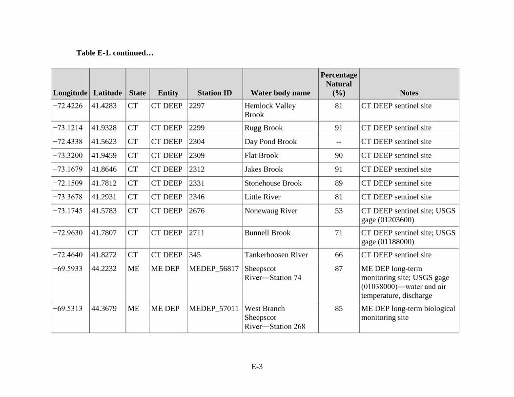
E-3

Table E-1. continued…

Longitude Latitude State Entity Station ID Water body name

Percentage Natural

(%) Notes −72.4226 41.4283 CT CT DEEP 2297 Hemlock Valley

Brook 81 CT DEEP sentinel site

−73.1214 41.9328 CT CT DEEP 2299 Rugg Brook 91 CT DEEP sentinel site

−72.4338 41.5623 CT CT DEEP 2304 Day Pond Brook -- CT DEEP sentinel site

−73.3200 41.9459 CT CT DEEP 2309 Flat Brook 90 CT DEEP sentinel site

−73.1679 41.8646 CT CT DEEP 2312 Jakes Brook 91 CT DEEP sentinel site

−72.1509 41.7812 CT CT DEEP 2331 Stonehouse Brook 89 CT DEEP sentinel site

−73.3678 41.2931 CT CT DEEP 2346 Little River 81 CT DEEP sentinel site

−73.1745 41.5783 CT CT DEEP 2676 Nonewaug River 53 CT DEEP sentinel site; USGS gage (01203600)

−72.9630 41.7807 CT CT DEEP 2711 Bunnell Brook 71 CT DEEP sentinel site; USGS gage (01188000)

−72.4640 41.8272 CT CT DEEP 345 Tankerhoosen River 66 CT DEEP sentinel site

−69.5933 44.2232 ME ME DEP MEDEP_56817 Sheepscot River―Station 74

87 ME DEP long-term monitoring site; USGS gage (01038000)―water and air temperature, discharge

−69.5313 44.3679 ME ME DEP MEDEP_57011 West Branch Sheepscot River―Station 268

85 ME DEP long-term biological monitoring site

E-4

Table E-1. continued…

Longitude Latitude State Entity Station ID Water body name

Percentage Natural

(%) Notes −68.2346 44.3934 ME ME DEP MEDEP_57065 Duck Brook―Station

322 83 ME DEP long-term biological

monitoring site

E-5

Table E-2. Secondary RMN sites in the Mid-Atlantic (4/2/2014). At all of the MD DNR sentinel sites, macroinvertebrates are collected annually and water and air temperature sensors are deployed year-round. At the WV DEP sites, macroinvertebrates are collected annually and water temperature sensors may be deployed. At the SRBC continuous monitoring sites, macroinvertebrates are collected annually and water temperature sensors are deployed year-round; stage and precipitation data are also being collected at some sites (see Notes field). At the NPS―ERMN sites (National Park Service sites that are in the Eastern Rivers and Mountains Network), macroinvertebrates are collected every other year and efforts will be made to install temperature sensors at high priority sites. Land use data, which were accumulated for the entire upstream catchment, were estimates based on data associated with the National Hydrography Dataset Plus Version 1 (NHDPlusV1) catchments in which the sites are located (http://www.horizon-systems.com/NHDPlus). Land use data were based on the 2001 National Land Cover Database (NLCD; Homer et al., 2007) (http://www.mrlc.gov/nlcd01_data.php).

Longitude Latitude State Entity Station ID Water body

name Notes Percentage Forest (%)

Percentage Urban (%)

Percentage Hay (%)

Percentage Crop (%)

−75.323216 41.73465 PA DRBC MB_Dyberry Middle Branch Dyberry Creek

79.9 0.0 14.0 0.6

−74.88980 40.77471 NJ EPA R2 1 Unnamed tributary to Musconetcong River

long-term monitoring site―Jim Kurtenbach (U.S. EPA R2)

67.9 0.0 4.2 23.9

−74.50486 40.95164 NJ EPA R2 17 Hibernia Brook long-term monitoring site―Jim Kurtenbach (U.S. EPA R2)

82.1 2.1 0.0 0.8

−74.84479 40.75211 NJ EPA R2 2 Teetertown Brook

long-term monitoring site―Jim Kurtenbach (U.S. EPA R2)

53.9 1.3 14.6 17.7

E-6

Table E-2. continued…

Longitude Latitude State Entity Station ID Water body

name Notes Percentage Forest (%)

Percentage Urban (%)

Percentage Hay (%)

Percentage Crop (%)

−77.54528 39.65833 MD MD DNR ANTI-101-S Unnamed tributary to Edgemont Reservoir

MD DNR sentinel site―Highlands

90.6 0.4 4.4 0.5

−76.09499 39.08754 MD MD DNR CORS-102-S Unnamed tributary to Emory Creek

MD DNR sentinel site―Coastal Plain

71.6 0.2 4.6 7.2

−78.45571 39.68672 MD MD DNR FIMI-207-S Fifteen Mile Creek

MD DNR sentinel site―Highlands

88.3 0.1 5.6 0.9

−76.04611 39.61055 MD MD DNR FURN-101-S Unnamed tributary to Principio Creek

MD DNR sentinel site―Highlands

80.5 0.5 9.3 8.1

−76.69843 39.43951 MD MD DNR JONE-109-S Unnamed tributary to Dipping Pond Run

MD DNR sentinel site―Highlands

45.3 2.5 32.4 6.7

−76.71875 39.42925 MD MD DNR JONE-315-S North Branch of Jones Falls

MD DNR sentinel site―Highlands

52.8 1.1 23.8 16.3

−76.86417 39.44055 MD MD DNR LIBE-102-S Timber Run MD DNR sentinel site―Highlands

70.1 0.3 12.7 15.5

−76.69829 39.48052 MD MD DNR LOCH-120-S Baisman Run MD DNR sentinel site―Highlands

71.2 0.3 24.4 2.4

E-7

Table E-2. continued…

Longitude Latitude State Entity Station ID Water body

name Notes Percentage Forest (%)

Percentage Urban (%)

Percentage Hay (%)

Percentage Crop (%)

−76.21896 39.19352 MD MD DNR LOCR-102-S Swan Creek MD DNR sentinel site―Coastal Plain

20.8 0.0 0.0 17.7

−77.09766 38.58225 MD MD DNR MATT-033-S Mattawoman Creek

MD DNR sentinel site―Coastal Plain

48.3 12.8 1.8 7.5

−77.08594 38.48386 MD MD DNR NANJ-331-S Mill Run MD DNR sentinel site―Coastal Plain

72.5 0.2 1.8 9.9

−75.49247 38.2495 MD MD DNR NASS-108-S Millville Creek MD DNR sentinel site―Coastal Plain

8.9 0.8 0.6 8.0

−75.46182 38.26359 MD MD DNR NASS-302-S Nassawango Creek

MD DNR sentinel site―Coastal Plain

18.8 0.4 4.4 17.0

−76.76012 38.56392 MD MD DNR PAXL-294-S Swanson Creek MD DNR sentinel site―Coastal Plain

67.3 0.2 2.4 15.3

−77.02912 38.51108 MD MD DNR PTOB-002-S Hoghole Run MD DNR sentinel site―Coastal Plain

74.2 1.0 0.7 12.1

E-8

Table E-2. continued…

Longitude Latitude State Entity Station ID Water body

name Notes Percentage Forest (%)

Percentage Urban (%)

Percentage Hay (%)

Percentage Crop (%)

−76.97198 39.16949 MD MD DNR RKGR-119-S Unnamed tributary to Patuxent River

MD DNR sentinel site―Highlands

31.8 0.5 44.0 14.2

−79.21349 39.54119 MD MD DNR SAVA-276-S Double Lick Run

MD DNR sentinel site―Highlands

92.1 0.0 6.6 0.0

−76.73717 38.36662 MD MD DNR STCL-051-S Unnamed tributary to St. Clements Creek

MD DNR sentinel site―Coastal Plain

69.8 0.0 2.2 15.8

−77.48935 39.58739 MD MD DNR UMON-119-S

Buzzard Branch

MD DNR sentinel site―Highlands

97.5 0.0 0.2 0.0

−75.96062 38.72408 MD MD DNR UPCK-113-S Unnamed tributary to Skeleton Creek

MD DNR sentinel site―Coastal Plain

23.9 0.3 10.7 29.4

−75.78362 39.28768 MD MD DNR UPCR-208-S Cypress Branch MD DNR sentinel site―Coastal Plain

40.3 0.2 4.0 26.7

−75.59259 38.41408 MD MD DNR WIRH-220-S Leonard Pond Run

MD DNR sentinel site―Coastal Plain

26.7 8.0 6.3 30.3

E-9

Table E-2. continued…

Longitude Latitude State Entity Station ID Water body

name Notes Percentage Forest (%)

Percentage Urban (%)

Percentage Hay (%)

Percentage Crop (%)

−76.90348 38.49936 MD MD DNR ZEKI-012-S Unnamed tributary to Zekiah Swamp Run

MD DNR sentinel site―Coastal Plain

89.8 0.0 0.6 5.3

−78.45247 40.41597 PA NPS―ERMN Blair Gap Run―Foot Ten

of 92.9 1.4 1.8 0.2

−78.51846 40.43269 PA NPS―ERMN Blair Gap Run― Muleshoe

96.1 0.4 0.5 0.1

−79.92348 39.78393 PA NPS―ERMN Dublin Run -- -- -- --

−79.58149 39.81449 PA NPS―ERMN Great Meadows Run

75.2 2.4 9.4 3.5

−79.93024 39.78248 PA NPS―ERMN Ice Pond Run -- -- -- --

−80.97161 37.58466 PA NPS―ERMN Little Bluestone River

75.7 1.5 15.3 0.9

−78.48373 40.41876 PA NPS―ERMN Milllstone Run 97.0 0.3 0.8 0.0

−81.02055 37.53483 PA NPS―ERMN Mountain Creek

75.9 1.6 14.9 0.6

−79.59970 39.81014 PA NPS―ERMN Unnamed tributary (Scotts Run)

95.9 0.0 0.0 0.0

−75.14398 40.97139 PA NPS―ERMN DEWA.3001 Caledonia Creek 13

NPS―ERMN high priority

78.0 1.0 8.0 1.5

−74.98444 41.11381 PA NPS―ERMN DEWA.3002 Van Campen Creek 12

74.2 2.4 0.1 0.1

E-10

Table E-2. continued…

Longitude Latitude State Entity Station ID Water body

name Notes Percentage Forest (%)

Percentage Urban (%)

Percentage Hay (%)

Percentage Crop (%)

−74.90309 41.19744 PA NPS―ERMN DEWA.3003 Deckers Creek 03

82.0 0.0 0.3 2.4

−74.87464 41.22245 PA NPS―ERMN DEWA.3004 Dingmans Creek 05

71.3 2.0 0.1 0.0

−75.12652 40.974 NJ NPS―ERMN DEWA.3005 Dunnfield Creek 03

96.8 0.0 0.3 0.0

−74.96252 41.13729 PA NPS―ERMN DEWA.3006 Toms Creek 20 80.2 0.6 0.0 0.0

−74.90598 41.1756 PA NPS―ERMN DEWA.3007 Spackmans Creek 08

91.1 0.5 0.7 0.4

−74.91831 41.23772 PA NPS―ERMN DEWA.3008 Dingmans Creek 57

69.8 2.0 0.1 0.0

−74.92372 41.09674 NJ NPS―ERMN DEWA.3010 Vancampens Brook 95

93.8 0.0 0.0 0.0

−74.87711 41.24882 PA NPS―ERMN DEWA.3011 Adams Creek 14

86.9 0.9 0.1 0.1

−74.89043 41.2578 PA NPS―ERMN DEWA.3012 Adams Creek 33

82.8 1.2 0.1 0.1

−75.00533 41.09383 PA NPS―ERMN DEWA.3013 Little Bushkill Creek 01

76.9 0.5 0.0 0.0

−74.96505 41.07109 NJ NPS―ERMN DEWA.3014 Vancampens Brook 43

95.3 0.0 0.0 0.0

−74.90343 41.23052 PA NPS―ERMN DEWA.3015 Dingmans Creek 39

69.8 2.0 0.1 0.0

−74.95916 41.12946 PA NPS―ERMN DEWA.3018 Toms Creek 07 80.2 0.6 0.0 0.0

−74.92673 41.16889 PA NPS―ERMN DEWA.3020 Mill Creek 25 83.5 0.3 0.4 0.4

E-11

Table E-2. continued…

Longitude Latitude State Entity Station ID Water body

name Notes Percentage Forest (%)

Percentage Urban (%)

Percentage Hay (%)

Percentage Crop (%)

−74.96279 41.1415 PA NPS―ERMN DEWA.3022 Toms Creek 25 80.2 0.6 0.0 0.0

−74.88573 41.23542 PA NPS―ERMN DEWA.3023 Unnamed tributary Dingmans Creek 07

71.3 2.0 0.1 0.0

−74.98445 41.0647 NJ NPS―ERMN DEWA.3025 Vancampens Brook 22

NPS―ERMN high priority

95.3 0.0 0.0 0.0

−74.94059 41.08567 NJ NPS―ERMN DEWA.3026 Unnamed tributary Vancampens Brook 05

97.8 0.0 0.0 0.0

−74.86975 41.24147 PA NPS―ERMN DEWA.3027 Adams Creek 03

NPS―ERMN high priority

86.9 0.9 0.1 0.1

−74.79550 41.29461 NJ NPS―ERMN DEWA.3028 White Brook 15

53.2 1.6 13.6 7.6

−75.01434 41.08235 PA NPS―ERMN DEWA.3029 Sand Hill Creek 08

63.5 6.1 0.8 0.0

−75.00528 41.03179 NJ NPS―ERMN DEWA.3030 Yards Creek 07 86.0 0.0 0.0 0.0

−74.89481 41.23067 PA NPS―ERMN DEWA.3031 Dingmans Creek 30

69.8 2.0 0.1 0.0

−74.84545 41.2952 PA NPS―ERMN DEWA.3032 Raymondskill Creek 13

73.7 1.0 0.9 0.1

−75.10517 40.98337 NJ NPS―ERMN DEWA.3033 Dunnfield Creek 26

96.8 0.0 0.3 0.0

−74.95645 41.12711 PA NPS―ERMN DEWA.3034 Toms Creek 03 81.2 0.5 0.0 0.2

E-12

Table E-2. continued…

Longitude Latitude State Entity Station ID Water body

name Notes Percentage Forest (%)

Percentage Urban (%)

Percentage Hay (%)

Percentage Crop (%)

−74.89987 41.19356 PA NPS―ERMN DEWA.3035 Hornbecks Creek 15

82.0 0.8 0.7 1.0

−74.92431 41.15917 PA NPS―ERMN DEWA.3036 Mill Creek 12 83.5 0.3 0.4 0.4

−74.94123 41.09062 NJ NPS―ERMN DEWA.3038 Vancampens Brook 76

93.8 0.0 0.0 0.0

−74.88168 41.25185 PA NPS―ERMN DEWA.3039 Adams Creek 21

85.0 1.0 0.1 0.1

−81.09167 37.9441 WV NPS―ERMN NERI.3001 Meadow Fork 1 74.1 6.1 6.1 0.1

−81.01278 37.91956 WV NPS―ERMN NERI.3005 Buffalo Creek 16

98.5 0.0 0.0 0.2

−81.02305 37.88808 WV NPS―ERMN NERI.3009 Slater Creek 20 97.7 0.0 0.0 0.0

−80.91077 37.81927 WV NPS―ERMN NERI.3011 Meadow Creek 17

84.9 2.5 4.6 1.1

−81.04551 37.87994 WV NPS―ERMN NERI.3013 Dowdy Creek 16

99.1 0.0 0.0 0.0

−81.04918 37.82895 WV NPS―ERMN NERI.3016 River Branch 4 95.9 0.0 3.8 0.3

−81.02102 38.03256 WV NPS―ERMN NERI.3018 Keeney Creek 10

89.7 2.3 1.5 0.8

−81.02453 37.94417 WV NPS―ERMN NERI.3021 Fire Creek 17 99.2 0.0 0.0 0.2

−80.90375 37.714 WV NPS―ERMN NERI.3024 Big Branch 10 95.3 0.2 2.9 0.0

−81.03647 37.87402 WV NPS―ERMN NERI.3025 Dowdy Creek 30

99.1 0.0 0.0 0.0

−80.97903 37.85864 WV NPS―ERMN NERI.3026 Little Laurel Creek 6

91.3 0.0 3.8 1.5

E-13

Table E-2. continued…

Longitude Latitude State Entity Station ID Water body

name Notes Percentage Forest (%)

Percentage Urban (%)

Percentage Hay (%)

Percentage Crop (%)

−81.08293 38.04904 WV NPS―ERMN NERI.3029 Wolf Creek 30 56.6 6.5 25.5 0.1

−81.04749 37.82782 WV NPS―ERMN NERI.3032 River Branch 6 WV DEP reference site

95.9 0.0 3.8 0.3

−81.02506 37.98267 WV NPS―ERMN NERI.3034 Unnamed tributary 21 New River 1

69.3 2.2 20.8 0.7

−81.06012 38.06032 WV NPS―ERMN NERI.3035 Fern Creek 11 88.1 2.9 3.1 0.4

−80.94296 37.74477 WV NPS―ERMN NERI.3036 Unnamed tributary Fall Branch 2

97.8 0.0 1.4 0.1

−81.00490 37.85802 WV NPS―ERMN NERI.3037 Laurel Creek 47

93.0 0.6 1.5 0.6

−81.08737 37.96331 WV NPS―ERMN NERI.3038 Arbuckle Creek 2

47.7 24.9 12.2 0.3

−81.01654 37.78795 WV NPS―ERMN NERI.3040 Polls Branch 14 70.0 1.2 20.5 0.1

−81.01984 37.8583 WV NPS―ERMN NERI.3041 Unnamed tributary Laurel Creek 3

93.0 0.6 1.5 0.6

−80.95156 37.87324 WV NPS―ERMN NERI.3042 Bucklick Branch 3

98.8 0.0 0.2 0.0

−80.89788 37.83271 WV NPS―ERMN NERI.3043 Meadow Creek 39

84.3 2.6 4.8 1.1

−81.03925 37.8512 WV NPS―ERMN NERI.3044 Laurel Creek 8 93.0 0.6 1.5 0.6

−80.92717 37.80196 WV NPS―ERMN NERI.3047 Sewell Branch 2

71.0 0.4 22.0 0.1

E-14

Table E-2. continued…

Longitude Latitude State Entity Station ID Water body

name Notes Percentage Forest (%)

Percentage Urban (%)

Percentage Hay (%)

Percentage Crop (%)

−81.05710 37.82369 WV NPS―ERMN NERI.3048 Slate Fork―Creek 12

Mill

81.9 2.9 9.9 0.1

−81.01080 37.91417 WV NPS―ERMN NERI.3049 Unnamed tributary Buffalo Creek 6

98.5 0.0 0.0 0.2

−81.01287 37.96168 WV NPS―ERMN NERI.3050 Ephraim Creek 8

NPS―ERMN high priority; WV DEP reference site

99.3 0.0 0.0 0.0

−80.93170 37.74969 WV NPS―ERMN NERI.3052 Fall Branch 7 NPS―ERMN high priority; WV DEP reference site

95.3 0.5 2.7 0.2

−81.02849 37.89156 WV NPS―ERMN NERI.3053 Slater Creek 13 97.7 0.0 0.0 0.0

−81.09031 37.96421 WV NPS―ERMN NERI.3054 Arbuckle Creek 5

47.7 24.9 12.2 0.3

−80.95197 37.86122 WV NPS―ERMN NERI.3058 Richlick Branch 17

97.1 0.0 0.3 0.5

−80.88025 37.83799 WV NPS―ERMN NERI.3059 Meadow Creek 58

81.4 3.5 5.8 1.2

−81.10399 37.84261 WV NPS―ERMN NERI.3064 Batoff Creek 7 75.6 6.6 5.9 0.0

−81.09510 37.94727 WV NPS―ERMN NERI.3065 Meadow Fork 6 74.0 5.1 6.5 0.1

E-15

Table E-2. continued…

Longitude Latitude State Entity Station ID Water body

name Notes Percentage Forest (%)

Percentage Urban (%)

Percentage Hay (%)

Percentage Crop (%)

−81.02195 37.91346 WV NPS―ERMN NERI.3069 Buffalo Creek 4

NPS―ERMN high priority; WV DEP reference site

98.5 0.0 0.0 0.2

−80.90266 37.71391 WV NPS―ERMN NERI.3072 Big Branch 9 95.3 0.2 2.9 0.0

−81.05947 37.88203 WV NPS―ERMN NERI.3077 Dowdy Creek 2 99.1 0.0 0.0 0.0

−81.05316 37.83172 WV NPS―ERMN NERI.3080 Slate Fork―Mill Creek 1

86.3 2.0 7.9 0.1

−81.01693 38.03013 WV NPS―ERMN NERI.3082 Keeney Creek 15

89.7 2.3 1.5 0.8

−80.98218 37.86476 WV NPS―ERMN NERI.3085 Laurel Creek 61

91.9 0.8 1.7 0.7

−81.08257 38.04763 WV NPS―ERMN NERI.3093 Wolf Creek 32 56.6 6.5 25.5 0.1

−81.05947 38.06101 WV NPS―ERMN NERI.3099 Fern Creek 12 88.1 2.9 3.1 0.4

−80.93452 37.74875 WV NPS―ERMN NERI.3100 Fall Branch 10 95.3 0.5 2.7 0.2

−76.91134 41.32519 PA PA DEP WQN_408 Loyalsock Creek

long-term data, EV (protected)

81.6 0.2 6.3 4.4

−76.15029 42.06312 NY SRBC Apal Apalachin Creek

precip gage 69.5 0.6 23.1 1.5

−77.60667 41.24694 PA SRBC BAKR0.1 Baker Run pressure transducer (real-time) and precip gage

97.0 0.0 0.0 0.0

−76.72019 42.04209 NY SRBC Baldwin Baldwin Creek precip gage 73.0 0.1 15.4 5.0

E-16

Table E-2. continued…

Longitude Latitude State Entity Station ID Water body

name Notes Percentage Forest (%)

Percentage Urban (%)

Percentage Hay (%)

Percentage Crop (%)

−77.23044 41.47393 PA SRBC BLOC Blockhouse Creek

precip gage 74.1 0.8 13.6 5.4

−78.59258 40.26388 PA SRBC BOBS Bobs Creek pressure transducer (real-time) and precip gage

88.5 0.2 4.7 2.1

−76.02756 41.42725 PA SRBC BOWN Bowman Creek 89.1 0.2 1.8 5.0

−77.73670 42.31903 NY SRBC CANA Canacadea Creek

precip gage 69.5 1.1 19.8 1.3

−76.47508 42.20472 NY SRBC Catatonk Catatonk Creek pressure transducer (stand-alone)

71.4 0.5 11.2 4.5

−74.79921 42.70639 NY SRBC Cherry Cherry Valley Creek

66.1 0.3 15.1 5.1

−78.64757 40.63052 PA SRBC CHEST Chest Creek 58.1 0.8 21.5 13.2

−76.00931 42.01582 NY SRBC CHOC Choconut Creek

pressure transducer (stand-alone)

72.7 0.2 19.9 2.3

−77.29313 41.85752 PA SRBC CROK Crooked Creek 45.9 0.1 27.1 21.6

−78.27008 41.52649 PA SRBC Driftwood Driftwood Branch Sinnemahoning Creek

pressure transducer (real-time)

92.0 0.0 1.0 0.1

E-17

Table E-2. continued…

Longitude Latitude State Entity Station ID Water body

name Notes Percentage Forest (%)

Percentage Urban (%)

Percentage Hay (%)

Percentage Crop (%)

−77.91244 41.57467 PA SRBC East Fork East Fork First Fork Sinnemahoning Creek

89.1 0.0 0.2 0.0

−76.34434 41.32261 PA SRBC EBFC East Branch Fishing Creek

92.4 0.0 0.1 0.0

−76.07111 41.78832 PA SRBC EBWC East Branch Wyalusing Creek

50.0 0.4 32.3 10.4

−77.58154 41.73642 PA SRBC ELKR Elk Run 81.8 0.0 10.4 0.4

−76.91233 41.99164 PA SRBC HAMM Hammond Creek

46.6 0.2 33.6 14.0

−78.25348 41.36235 PA SRBC Hicks Hicks Run 91.6 0.0 1.6 0.0

−78.17458 41.45256 PA SRBC Hunts Hunts Run precip gage 90.7 0.0 0.0 0.0

−76.24282 41.23366 PA SRBC Kitchen Kitchen Creek 85.9 0.2 3.5 0.5

−75.47324 41.68331 PA SRBC LACK Lackawanna River

68.2 0.4 11.3 9.0

−77.18943 41.32739 PA SRBC LARR Larrys Creek 75.7 0.1 19.1 1.0

−78.40722 40.97 PA SRBC LCLF0.1 Little Clearfield Creek

68.5 0.2 19.1 2.4

−76.06980 41.58154 PA SRBC LMEHOOP Little Mehoopany Creek

pressure transducer (real-time)

66.8 0.1 8.1 16.7

−76.64148 41.19353 PA SRBC LMUN Little Muncy Creek

56.1 0.2 23.1 13.9

E-18

Table E-2. continued…

Longitude Latitude State Entity Station ID Water body

name Notes Percentage Forest (%)

Percentage Urban (%)

Percentage Hay (%)

Percentage Crop (%)

−77.55928 41.76142 PA SRBC Long Long Run 82.0 0.0 10.4 1.9

−77.36278 41.31 PA SRBC LPIN0.2 Little Pine Creek

82.7 0.4 8.4 3.5

−76.33104 41.4588 PA SRBC LYSK5.0 Loyalsock Creek

pressure transducer (real-time) and precip gage

85.5 0.1 0.6 0.7

−77.60997 41.06022 PA SRBC MARS Marsh Creek 83.7 0.7 7.9 3.4

−77.41333 41.76306 PA SRBC Marsh Tioga Marsh Creek 72.0 1.3 15.5 5.0

−75.98474 41.61164 PA SRBC MESH Meshoppen Creek

pressure transducer (stand-alone)

47.1 0.2 18.5 27.3

−76.05357 42.20426 NY SRBC Nanticoke Nanticoke Creek

62.2 0.4 24.9 7.8

−77.76387 41.79146 PA SRBC Ninemile Ninemile Run precip gage 84.4 0.4 3.8 2.8

−78.46158 41.04564 PA SRBC PA_Moose Moose Creek 90.3 -- -- --

−77.45056 41.64694 PA SRBC Pine Blackwell

Pine Creek 80.5 0.4 7.7 2.0

−76.92300 41.49143 PA SRBC Ples Pleasant Stream 87.6 0.0 1.4 1.0

−78.22029 41.51169 PA SRBC Portage Portage Creek 91.9 0.3 2.5 0.1

−75.50220 42.77596 NY SRBC Sangerfield Sangerfield River

35.8 0.4 17.0 14.0

−75.77788 41.55783 PA SRBC SBTK South Branch Tunkhannock Creek

pressure transducer (real-time)

53.4 3.4 5.9 24.1

E-19

Table E-2. continued…

Longitude Latitude State Entity Station ID Water body

name Notes Percentage Forest (%)

Percentage Urban (%)

Percentage Hay (%)

Percentage Crop (%)

−76.92222 42.10278 NY SRBC SING 0.9 Sing Sing Creek

61.5 3.1 9.9 10.9

−75.84137 41.92994 PA SRBC SNAK Snake Creek pressure transducer (stand-alone)

67.1 0.2 23.0 2.8

−75.52351 41.95946 PA SRBC STAR Starrucca Creek 73.1 0.2 15.9 1.1

−76.27436 41.62644 PA SRBC Sugar Run Sugar Run 64.4 0.1 9.9 18.6

−76.76835 41.78974 PA SRBC SUGR Sugar Creek 44.9 1.0 34.3 13.2

−76.91416 41.70931 PA SRBC TIOG Tioga River 83.0 0.0 1.7 2.9

−76.60723 41.78132 PA SRBC TOMJ Tomjack Creek 42.7 0.3 35.9 15.6

−76.76011 41.65262 PA SRBC TOWA Towanda Creek 54.9 0.8 25.5 13.1

−78.36118 41.07359 PA SRBC TROT Trout Run pressure transducer (real-time) and precip gage

90.4 0.0 0.4 0.0

−76.10589 42.59277 NY SRBC Trout Brook Trout Brook precip gage 62.7 0.5 24.8 5.3

−77.37918 42.0752 NY SRBC Tuscarora Tuscarora Creek

pressure transducer (real-time)

42.9 0.3 35.1 13.6

−77.76123 41.79011 PA SRBC Upper Pine Pine Creek pressure transducer (real-time)

75.1 0.0 11.4 4.0

−76.28083 41.96661 PA SRBC WAPP Wappasening Creek

63.4 0.0 30.2 1.8

E-20

Table E-2. continued…

Longitude Latitude State Entity Station ID Water body

name Notes Percentage Forest (%)

Percentage Urban (%)

Percentage Hay (%)

Percentage Crop (%)

−78.80331 40.69289 PA SRBC WB SUS West Branch Susquehanna River

pressure transducer (stand-alone)

68.7 3.5 15.8 3.0

−78.27484 41.49444 PA SRBC West West Creek 83.8 0.5 6.5 0.4

−77.66985 41.72483 PA SRBC WPIN West Branch Pine Creek

87.0 0.0 0.5 0.0

−77.68520 41.40016 PA SRBC Young Young Woman's Creek

96.8 0.0 0.1 0.0

−74.50528 39.885 NJ USGS USGS 01466500

McDonalds Branch

USGS gage in Byrne State Forest (Pine Barrens)

-- -- -- --

−82.12353 38.48514 WV WV DEP 11897 Unnamed tributary/Left Fork river mile 1.69/Mill Creek

-- -- -- --

−79.69583 38.73825 WV WV DEP 12455 Laurel Fork/Dry Fork

89.5 0.0 0.1 0.1

−80.86781 38.88133 WV WV DEP 12689 Long Lick Run -- -- -- --

−81.09958 39.22211 WV WV DEP 12690 Unnamed tributary/North Fork river mile 22.26/Hughes River

-- -- -- --

E-21

Table E-2. continued…

Longitude Latitude State Entity Station ID Water body

name Notes Percentage Forest (%)

Percentage Urban (%)

Percentage Hay (%)

Percentage Crop (%)

−80.32127 38.25981 WV WV DEP 2046 North Fork/Cranberry River

long-term monitoring site impacted by acid rain

98.9 0.0 0.0 0.0

−81.14683 37.50275 WV WV DEP 2359 Mash Fork long-term monitoring site impacted by acid rain

93.1 0.0 5.2 0.0

−82.28014 38.06845 WV WV DEP 4513 Little Laurel Creek

-- -- -- --

−79.39594 38.97394 WV WV DEP 8255 Red Creek long-term monitoring site impacted by acid rain

97.7 0.0 0.1 0.0

−79.61147 39.04225 WV WV DEP 8357 Otter Creek long-term monitoring site impacted by acid rain

99.5 0.0 0.0 0.0

−81.93119 38.38489 WV WV DEP 8482 Sams Fork -- -- -- --

−80.37117 38.33544 WV WV DEP 9315 Middle Fork/Williams River

long-term monitoring site impacted by acid rain

99.5 0.0 0.0 0.0

E-22

E.1. REFERENCES

Homer, C; Dewitz, J; Fry, J; Coan, M; Hossain, N; Larson, C; Herold, N; McKerrow, A; VanDriel, JN; Wickham, J. (2007) Completion of the 2001 National Land Cover Database for the Conterminous United States. PE&RS 73(4):337−341. Available online at http://www.asprs.org/a/publications/pers/2007journal/april/highlight.pdf

F-1

APPENDIX F. __________________________

MACROINVERTEBRATE COLLECTION METHODS

F-2

Table F-1. Macroinvertebrate methods for medium-high gradient freshwater wadeable streams with abundant riffle habitat and rocky substrate. These are the methods that were agreed upon by the Northeast, Mid-Atlantic, and Southeast regional working groups during the pilot phase of the RMNs (before the QAPP was developed). At this time (fall 2015), the regional working groups are working on the region-specific QAPP addendums. It is possible that some updates will be made during this process.

Regional network Effort

Reach length Gear Habitat

Sampling area

Index period

Target # organisms

Taxonomic resolution

Northeast Kick samples are taken from riffle habitats in 4 different locations in the sampling reach. At each location the substrate is disturbed for approximately 30 seconds, for a total active sampling effort of 2 minutes.

150 m D-frame net (46 cm wide × 30 cm high) with 500-μm mesh

Riffles Approximately 1 m2

September−mid-October

300 Lowest practical (species whenever possible)

Mid-Atlantic

Data should be collected with existing state or RBC methods, or in such a way that the data can be rendered comparable to historical state methods. A minimum of 1 m2 is collected using a minimum of 4 separate kicks in riffle habitats throughout the 100-m reach.

100 m Varies by entity (either square frame kick nets or D-frame nets, with mesh size ranging from 450−600 μm)

Abundant riffles

Minimum of 1 m2

Spring (March− April) and summer (July− August)

300 Lowest practical (species whenever possible)

F-3

Table F-1. continued…

Regional network Effort

Reach length Gear Habitat

Sampling area

Index period

Target # organisms

Taxonomic resolution

Southeast Semiquantitative: riffle kick samples are taken from 2 riffles or upper or lower end of a large riffle and composited; in smaller streams, multiple riffles may need to be collected to achieve the desired area

100 m Kick-net with 500-μm mesh

Riffles Approximately 2 m2

April 2013. Subsequent samples will be collected annually within 2 weeks of the original collection

300 ± 10% Lowest practical (species whenever possible)

Qualitative: 3 “jabs” will be collected from all available habitats; taxa from each habitat will be kept in separate containers (separate species lists will be generated for each habitat)

100 m Dip-net with 500-μm mesh

Multihabitat NA (qualitative)

NA (qualitative)

F-4

Table F-2. Macroinvertebrate methods used by Northeastern states for routine sampling events in medium-high gradient freshwater wadeable streams with riffle habitat and rocky substrate

Entity Project or

stream type Effort Gear Habitat Sampling

area Index period

Target # organisms

Taxonomic resolution

CT DEEP

Streams with riffle habitat

12 kick samples are taken throughout riffle habitats within the sampling reach

Rectangular net (46 cm × 46 cm × 25 cm) with 500-μm mesh

Riffles Approximately 2 m2

October 1− November 30

200 Lowest practical (species whenever possible)

VT DEC

Moderate to high gradient streams with riffle habitat

Kick samples are taken from riffle habitats in 4 different locations in the sampling reach. At each location the substrate is disturbed for approximately 30 seconds, for a total active sampling effort of 2 minutes.

D-frame net (46 cm wide × 30 cm high) with 500-μm mesh

Riffles Approximately 1 m2

September−mid-October

300 Lowest practical (species whenever possible)

ME DEP

Streams with riffle and run habitat

3 cylindrical rock-filled wire baskets are placed in locations with similar habitat characteristics for 28 ± 4 days.

Contents are washed into a sieve bucket with 600-μm mesh

Riffle/run is the preferred habitat.

Approximately 0.3 m2 per basket

July 1− September 30

Entire samples are processed and identified, with exceptions

Lowest practical (species whenever possible)

F-5

Table F-2. continued…

Entity Project or

stream type Effort Gear Habitat Sampling

area Index period

Target # organisms

Taxonomic resolution

NH DES Streams with riffle and run habitat

3 cylindrical rock-filled wire baskets are placed in riffle habitats or at the base of riffles at depths that cover the artificial substrate by at least 5 inches for 6 to 8 weeks.

Contents are washed into a sieve bucket with 600-μm mesh

Riffle/run is the preferred habitat.

Approximately 0.3 m2 per basket

late July− September

100 Genus, except Chironomidae (family-level)

RI DEM Routine monitoring in streams with riffle habitat

Kick samples are taken from riffle habitats along 100-m reachrepresentative ofthe streamsampled timed fora total activesampling effort of3 minutes.

D-frame net (30-cm width) with 500-μm mesh

Riffle Within reach (100 linear meters)

August− September

100 Mostly genus-level. Chironomidae are identified to the subfamily or tribe-level

NY DEC Routine monitoring in streams with riffle habitat

Substrate is dislodged by foot, upstream of the net for 5 minutes and a distance of 5 m. The preferredline of sampling isa diagonal transectof the stream

Rectangular net (23 cm × 46 cm) with 800−900-μm mesh

Riffle 2.5 m2 July− September

100 Lowest practical (mostly genus- or species-level, some family-level [e.g., Gastropoda and Pelecypoda])

F-6

Table F-2. continued…

Entity Project or

stream type Effort Gear Habitat Sampling

area Index period

Target # organisms

Taxonomic resolution

MA DEP Routine monitoring in streams with riffle habitat

10 kick-samples are taken in riffle habitats within the sampling reach and composited

Kick-net, 46-cm wide opening, 500-µm mesh

Riffle/run is the preferred habitat

Approximately 2 m2

July 1− September 30

100 Lowest practical level

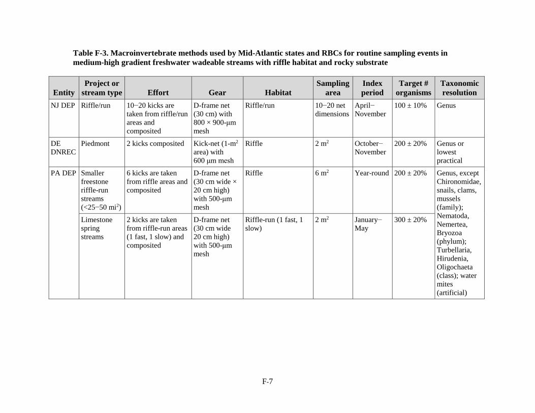
F-7

Table F-3. Macroinvertebrate methods used by Mid-Atlantic states and RBCs for routine sampling events in medium-high gradient freshwater wadeable streams with riffle habitat and rocky substrate

Entity Project or

stream type Effort Gear Habitat Sampling

area Index period

Target # organisms

Taxonomic resolution

NJ DEP Riffle/run 10−20 kicks are taken from riffle/run areas and composited

D-frame net (30 cm) with 800 × 900-μm mesh

Riffle/run 10−20 net dimensions

April− November

100 ± 10% Genus

DE DNREC

Piedmont 2 kicks composited Kick-net (1-m2 area) with 600 μm mesh

Riffle 2 m2 October− November

200 ± 20% Genus or lowest practical

PA DEP Smaller freestone riffle-run streams (<25−50 mi2)

6 kicks are taken from riffle areas and composited

D-frame net (30 cm wide × 20 cm high) with 500-μm mesh

Riffle 6 m2 Year-round 200 ± 20% Genus, except Chironomidae, snails, clams, mussels (family); Nematoda, Nemertea, Bryozoa (phylum); Turbellaria, Hirudenia, Oligochaeta (class); water mites (artificial)

Limestone spring streams

2 kicks are taken from riffle-run areas (1 fast, 1 slow) and composited

D-frame net (30 cm wide 20 cm high) with 500-μm mesh

Riffle-run (1 fast, 1 slow)

2 m2 January− May

300 ± 20%

F-8

Table F-3. continued…

Entity Project or

stream type Effort Gear Habitat Sampling

area Index period

Target # organisms

Taxonomic resolution

MD Maryland Approximately D-frame net Multihabitat (in order About 2 m2 March− 100 ± 20% Genus (or lowest DNR Biological

Stream Survey (MBSS)

20 kicks/jabs/sweeps/rubs from multiple habitats (sampled in proportion to availability in reach) are composited

(about 30 cm wide) with 450-μm mesh

of preference) riffles, root wads, root mats/woody debris/snag, leaf packs, SAV/associated habitat, undercut banks; less preferred = gravel, broken peat, clay lumps, detrital/sand areas in runs; moving water preferred to still water; sampled in proportion to availability in reach, ensuring all potentially productive habitats are represented in sample

April practical); crayfish and mussels identified to species (sometime subspecies?) in the field along with fish, reptiles, amphibians, and some invasive plants

F-9

Table F-3. continued…

Entity Project or

stream type Effort Gear Habitat Sampling

area Index period

Target # organisms

Taxonomic resolution

WV DEP

Wadeable streams (WVSCI)

4 kicks composited Rectangular kick net (50 cm wide × 30 cm high × 50 cm deep) with 600-μm net mesh (595-μm sieve); D-frame net (30 cm wide) can be used for smaller streams

riffle-run 1 m2 April 15− October 15

200 ± 20% Family (all insects)

Wadeable streams (GLIMPSS)―Mountain and Plateau

1 m2 Winter (December−mid-February), spring (March− May) ―Plateau only, summer (June−mid-October)

200 ± 20% Genus (all insects minus Collembola)

VA DEQ

Noncoastal Plain (VSCI)

6 kicks from riffle habitat (unless absent, then multihabitat) are composited

D-frame net (50 cm wide × 30 cm high × 50 cm deep) with 500 μm net mesh

Riffle, unless absent, then multihabitat

2 m2 Spring (March− May) and fall (September−November)

110 ± 10% Family (working toward developing a genus-level index)

F-10

Table F-3. continued…

Entity Project or

stream type Effort Gear Habitat Sampling

area Index period

Target # organisms

Taxonomic resolution

SRBC Aquatic Resource Surveys

6 kicks composited or 5 minutes for a distance of 5 m (PA or NY)

D-frame net/aquatic net (30 cm × 20 to 23 cm × 46 cm [PA or NY]); 500-μm; 800 µm × 900 µm (depending on PA or NY)

Riffle-run 6 m2 or distance of 5 m (PA or NY)

Typically late April into May, late June into July, and October

PADEP or NYSDEC protocol

Genus, except Chironomidae, snails, clams mussels (family); Nematoda, Nemertea, Bryozoa (phylum); Turbellaria, Hirudenia, Oligochaeta (class); water mites (artificial)

Subbasin Survey, Year 1/Interstate Streams

2 kicks composited Kick-net (1 m2) with 600-μm mesh

2 m2 Year 1― historically spring−fall, now spring−May 30. Interstate― May (Group 3) or August(Group 1 and2); variesdependingon siteclassification

200 ± 20%

Remote Water Quality Monitoring Network

6 kicks composited D-Frame Net (46 cm × 20 cm) with 500-μm mesh

6 m2 October 200 ± 20%

F-11

Table F-3. continued…

Entity Project or

stream type Effort Gear Habitat Sampling

area Index period

Target # organisms

Taxonomic resolution

NPS Eastern Rivers and Mountains Network

A semiquantitative sample consisting of 5 discrete collections from the richest targeted habitat (typically riffle, main-channel, coarse-grained substrate habitat type) are processed and combined into a single composited sample.

Slack sampler, 500-μm nets and sieves

Riffle Each discrete sample = 0.25 m2 area; total area sampled = 1.25 m2

April−early June

300 Genus, except Chironomidae, snails, clams mussels (family); Nematoda, Nemertea, Bryozoa (phylum); Turbellaria, Hirudenia, Oligochaeta (class); water mites (artificial)

F-12

Table F-4. Macroinvertebrate methods used by Southeast states for routine sampling events in medium-high gradient freshwater wadeable streams with riffle habitat and rocky substrate

Entity Stream

type Effort Gear Habitat Sampling

area Index period

Target # organisms

Taxonomic resolution

AL DEM

WMB-I protocols

Several samples are collected at a site by stream habitat type; each sample is processed separately; the taxa lists are recombined after standardizing individual counts to density units

Kick net, 2 A-frame nets, 2 #30 sieve buckets, 2 #30 sieves, plastic elutriation treys, 100% denatured ethanol, and plastic sample containers

Riffle, rock-log, Rootbank, CPOM, sand, and macrophytes (macrophytes not always available and excluded from index)

Approximately 4 m2

Late April− early July

100 organisms per habitat

Genus or lowest possible level

GA DNR

High (riffle/run) gradient

20 jabs from multiple habitats are composited

D-frame net (30-cm width) with 500-μm net mesh

Multihabitat― riffles, woody debris/snags, undercut banks/rootwads, leafpacks, soft sediment/sandy substrate, and submerged macrophytes (when present)

20 jabs, each for a linear distance of 1 m

Mid-September−February

200 ± 20% Lowest practical level (generally genus or species)

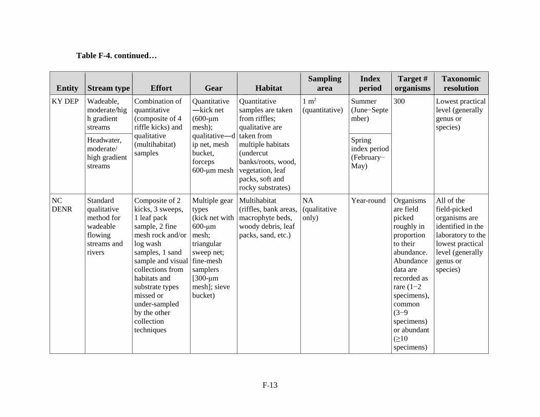
F-13

Table F-4. continued…

Entity Stream type Effort Gear Habitat Sampling

area Index period

Target # organisms

Taxonomic resolution

KY DEP Wadeable, moderate/high gradient streams

Combination of quantitative (composite of 4 riffle kicks) and qualitative (multihabitat) samples

Quantitative―kick net (600-μm mesh); qualitative―dip net, mesh bucket, forceps 600-μm mesh

Quantitative samples are taken from riffles; qualitative are taken from multiple habitats (undercut banks/roots, wood, vegetation, leaf packs, soft and rocky substrates)

1 m2 (quantitative)

Summer (June−September)

300 Lowest practical level (generally genus or species)

Headwater, moderate/ high gradient streams

Spring index period (February−May)

NC Standard Composite of 2 Multiple gear Multihabitat NA Year-round Organisms All of the DENR qualitative kicks, 3 sweeps, types (riffles, bank areas, (qualitative are field field-picked

method for 1 leaf pack (kick net with macrophyte beds, only) picked organisms are wadeable sample, 2 fine 600-μm woody debris, leaf roughly in identified in the flowing mesh rock and/or mesh; packs, sand, etc.) proportion laboratory to the streams and log wash triangular to their lowest practical rivers samples, 1 sand sweep net; abundance. level (generally

sample and visual fine-mesh Abundance genus or collections from samplers data are species) habitats and [300-μm recorded as substrate types mesh]; sieve rare (1−2 missed or bucket) specimens), under-sampled common by the other (3−9 collection specimens) techniques or abundant

(≥10 specimens)

F-14

Table F-4. continued…

Entity Stream type Effort Gear Habitat Sampling

area Index period

Target # organisms

Taxonomic resolution

SC Ambient Same as NC DENR Feb 1 to Same as NC DENR DHEC monitoring March 15:

Middle Atlantic Coastal Plain Ecoregion (EPA Level III 63); June 15 to Sept 1: Statewide, minus EPA Level III Ecoregion 63

TN DEC Streams with riffles

Single habitat, semiquantitative; composite of 2 riffle kicks

Kick net (1-m2, 500-μm mesh)

Riffle 2 m2 Year-round 200 ± 20% Genus level

F-15

Table F-5. Macroinvertebrate methods used in national surveys conducted by EPA and USGS

Entity Project or

stream type Effort Gear Habitat Sampling

area Index period

Target # organisms

Taxonomic resolution

EPA National Aquatic Resource Surveys

WSA and NRSA

A 0.1-m2 area was sampled for 30 seconds at a randomly selected location at each of the 11 transects. The samples were composited into one sample per site.

Modified D-frame net (30 cm wide) with 500-μm mesh

Multihabitat Composite

Approximately 1 m2

June− September

500 Genus level

USGS NAWQA A semiquantitative sample consisting of 5 discrete collections from the richest targeted habitat (typically riffle, main-channel, coarse-grained substrate habitat type) are processed and combined into a single composited sample.

Slack sampler, 500-μm nets and sieves

Riffle Each discrete sample = 0.25-m2 area; total area sampled = 1.25 m2

Late June−mid-October

300 Lowest practical level

G-1

APPENDIX G.

__________________________

LEVEL OF TAXONOMIC RESOLUTION

G-2

When possible, all taxa should be taken to the lowest practical taxonomic level (ideally species level). If this is not possible, efforts should be made to identify the taxa listed in Table G-1 to the level of resolution described in the table. Ephemeroptera, Plecoptera, Trichoptera, and Chironomidae that are not listed in Table G-1 should be identified to at least the genus level, where possible.

The taxa in Table G-1 were selected based on differences in thermal tolerances that were evident in analyses (U.S. EPA, 2012; unpublished Northeast pilot study) and from best professional judgment. The list in Table G-1 should be regarded as a starting point and should be updated as better data become available in the future. Table G-2 contains a list of taxa that were considered for inclusion in Table G-1 but for various reasons, were not selected.

G-3

Table G-1. At RMN sites, we recommend that the taxa listed below be taken to the specified level of resolution, where practical. The Chironomidae require a slide mount and a compound microscope to identify to the species-level.

Order Family Genus Level of

resolution Notes Coleoptera Elmidae Promoresia adults to

species Potential variability in thermal preferences of P. tardella (cold) and P. elegans (warm).

Diptera Chironomidae Eukiefferiella species Potential variability in thermal preferences of E. brevicalar, E. brehmi, and E. tirolensis (cold); and E. claripennis and E. devonica (warm).

Diptera Chironomidae Polypedilum species P. aviceps is generally regardedas a cold water taxon.

Diptera Chironomidae Tvetenia species group

T. vitracies is warm wateroriented in the Northeast.

Diptera Simuliidae genus General agreement that Prosimilium is a cold water indicator but there is potential for variability within this genus (e.g., P. mixtum vs. P. vernale), and species-level systematics are not well developed at this time.

Ephemeroptera Baetidae Baetis species Potential variability in thermal preferences (e.g., B. tricaudatus―cold; B. intercalaris and B. flavistriga―warm).

Ephemeroptera Ephemerellidae Ephemerella species (as maturity allows)

Potential variability in thermal preferences (e.g., E. subvaria―colder); need mature individuals (early instars are difficult to speciate).

Plecoptera Perlidae Acroneuria species Potential variability in thermal preferences of A. abnormis (warmer) and A. carolinensis (cooler).

G-4

Table G-1. continued…

Order Family Genus Level of

resolution Notes Plecoptera Perlidae Paragnetina species Potential variability in thermal

preferences of P. immarginata (cold) and P. media and P. kansanensis.

Plecoptera Pteronarcyidae Pteronarcys species P. dorsata may be warmer wateroriented.

Trichoptera Brachycentridae Brachycentrus species Potential variability in thermal preferences in the Northeast.

Trichoptera Hydropsychidae Ceratopsyche species Potential variability in thermal preferences.

Trichoptera Rhyacophilidae Rhyacophila species Most species are cold water, but some variability has been documented in the Northeast (U.S. EPA, 2012, unpublished data).

Trichoptera Uenoidae Neophylax species Some variability was noted in a pilot study in North Carolina (U.S. EPA, 2012).

G-5

Table G-2. Taxa that were considered for inclusion in Table G-1

Order Family Genus Level of

resolution Notes Coleoptera Elmidae Oulimnius species O. latiusculus is regarded as a

cold-water taxon in Vermont, butspecies-level IDs may not benecessary for the larger regionbecause most of the taxa are O.latiusculus.

Diptera Chironomidae Micropsectra species General agreement that there is variability in thermal preferences, but the taxonomy for this genus needs to be further developed.

Diptera Ceratopogonidae species General agreement that there is variability in thermal preferences, but the taxonomy for this family needs to be further developed.

Ephemeroptera Ephemerellidae Drunella species Variability in thermal tolerances within this genus was noted in the Utah pilot study, but in the Eastern states, species are believed to be all cold/cool water.

Ephemeroptera Ephemerellidae Eurylophella species Some variability was noted in a pilot study in North Carolina (U.S. EPA, 2012); could be seasonal phenology vs. thermal preference.

Ephemeroptera Heptageniidae Epeorus species Some variability was noted in a pilot study in Utah (U.S. EPA, 2012); can be difficult to speciate.

Ephemeroptera Heptageniidae Stenacron species In the Mid-Atlantic region, some regard S. interpunctatum as a warm-water taxon and the others as cooler/some cold. Taxonomy may be tricky.

G-6

Table G-2. continued…

Order Family Genus Level of

resolution Notes Trichoptera Goeridae Goera species Some variability was noted in a

pilot study in North Carolina (U.S. EPA, 2012). The two species found in Kentucky are associated with cold water. In New Jersey, this genus is found as often in the coastal plain as in northern high gradient streams and is currently not taken to the species level.

Trichoptera Hydropsychidae Hydropsyche species Some variability was noted in a pilot study in New England (U.S. EPA, 2012, unpublished data) but is generally considered to be eurythermal (not sure which species would be regarded as cold water taxa).

Trichoptera Leptoceridae Oecetis species Some variability was noted in a pilot study in North Carolina (U.S. EPA, 2012). The species found in Kentucky are associated with warm water. In New Jersey, this genus is typically found in low gradient coastal plain streams.

Trichoptera Philopotamidae Chimarra species Some variability was noted in a pilot study in New England (U.S. EPA, 2012, unpublished data) but most species were warm-water oriented. C. obscura and C. atterima predominate, but tend to co-occur.

Oligochaeta family Enchytraeidae is regarded as a cold-water family in Vermont. In the Mid-Atlantic region, it is found mostly in small streams. In New Jersey, it is found throughout the state.

G-7

Table G-2. continued…

Order Family Genus Level of

resolution Notes Amphipoda Gammaridae Gammarus species G. pseudolimnaeus is regarded as a

cold- or cool-water taxon inVermont (and is tolerant ofnutrients). Gammarus (assumed tobe pseudolimnaeus) is alsoregarded as a cold-water indicatorin Minnesota (Gerritsen andStamp, 2012).

Amphipoda Hyalellidae Hyallela species H. azteca is regarded as a cold/coolwater taxon in Vermont. InKentucky, Hyallela it is believed tobe a completely warm-water genus.

Isopoda Asellidae Caecidotea species C. brevicauda has been noted as apotential cold-water indicator inthe Midwest (Gerritsen and Stamp,2012).

Neoophora Planariidae Dugesia species D. tigrina is regarded as awarm-water taxon in Vermont, aswell as in New Jersey. Can bedifficult to speciate in specioseregions.

Neoophora Dugesiidae Cura species C. formanii is regarded as acold-water taxon in Vermont. Canbe difficult to speciate in specioseregions.

G-8

G.1. LITERATURE CITED:Gerritsen, J; Stamp, J. (2012) Calibration of the biological condition gradient (BCG) in cold and

cool waters of the upper Midwest for fish and benthic macroinvertebrate assemblages [Final Report]. Prepared by Tetra Tech, Inc. for the USEPA Office of Water and USEPA Region 5. Owings Mills, MD: Tetra Tech. Available online at http://www.uwsp.edu/cnr-ap/biomonitoring/Documents/pdf/USEPA-BCG-Report-Final-2012.pdf

U.S. EPA (Environmental Protection Agency). (2012) Implications of climate change for bioassessment programs and approaches to account for effects. [EPA/600/R-11/036F]. Washington, DC: Global Change Research Program, National Center for Environmental Assessment. Available online at http://cfpub.epa.gov/ncea/global/recordisplay.cfm?deid=239585

H-1

APPENDIX H. __________________________

SUMMARIZING

MACROINVERTEBRATE DATA

H-2

H.1. LIST OF CANDIDATE BIOLOGICAL INDICATORS

Table H-1. Recommendations on candidate biological indicators to summarize from the macroinvertebrate data collected at regional monitoring network (RMN) sites; many of these indicators are commonly used by biomonitoring programs for site assessments.

Type of indicator Biological indicator Expected response Source

Taxonomic-based metric

Total number of taxa (richness)

Predicted to decrease in response to increasing anthropogenic stress

Barbour et al., 1999 (compiled from DeShon, 1995; Barbour et al., 1996; Fore et al., 1996; Smith and Voshell, 1997); these metrics are commonly used in bioassessments

Number of EPT taxa (Ephemeroptera [mayflies], Plecoptera [stoneflies], and Trichoptera [caddisflies]) Number of Ephemeroptera (mayfly) taxa Number of Plecoptera (stonefly) taxa Number of Trichoptera (caddisfly) taxa Percentage EPT individuals Percentage Ephemeroptera individuals Percentage Plecoptera individuals Percentage Trichoptera individuals

Number of Odonata, Coleoptera, and Hemiptera (OCH) taxa

Expected to be more prevalent during summer, low flow (more pool-like) periods

Bonada et al., 2007a

Percentage OCH individuals

H-3

Table H-1. continued…

Type of indicator Biological indicator Expected response Source

Traits-based metric related to temperature (for list of thermal indicator taxa, see Appendix I)

Number of cold water taxa Predicted to decrease in response to warming temperatures

Lake, 2003; Hamilton et al., 2010; Stamp et al., 2010; U.S. EPA, 2012 Percentage cold water

individuals

Number of warm water taxa

Predicted to increase in response to warming temperatures Percentage warm

individuals water

Traits-based metric related to hydrology

Collector filterer Predicted to decrease during low flow conditions

Wills et al., 2006; Bogan and Lytle, 2007; Walters and Post, 2011

Collector gatherer Predicted to increase during slow velocity conditions

Heino, 2009

Scraper/herbivore Predicted to increase during conditions of stable flow and habitat availability; decrease during drought conditions

Richards et al., 1997; McKay and King, 2006; Wills et al., 2006; Fenoglio et al., 2007; Griswold et al., 2008; Diaz et al., 2008

Shredder Expected to respond to changing thermal and hydrologic conditions

Richards et al., 1997; Buzby and Perry, 2000; McKay and King, 2006; Foucreau et al., 2013

Predator Predicted to increase during low flow conditions

Bogan and Lytle, 2007; Miller et al., 2007; Walters and Post, 2011

Swimmer Predicted to comprise higher proportion of assemblage during drier, harsher, climatic conditions

Béche et al., 2006; Bonada et al., 2007b; Diaz et al., 2008

Rheophily―depositional Favor low flow/slow velocity conditions

Richards et al., 1997; Lake, 2003; Wills et al., 2006; Poff et al., 2010; Brooks et al., 2011 Rheophily―erosional Favor high flow/fast

velocity conditions

H-4

Table H-1. continued…

Type of indicator Biological indicator Expected response Source

Biological condition

Bioassessment score (e.g., multimetric index, predictive, biological condition gradient)

Expected to worsen in response to increasing anthropogenic stress

Barbour et al., 1995; DeShon, 1995; Hawkins et al., 2000; Davies and Jackson, 2006

Individual taxa Presence―absence Hypotheses have been developed for some individual taxa (e.g., the cold and warm water taxa listed in Appendix I)

Becker et al., 2010

Relative abundance

Spatial distribution

Variability Persistence (variability in presence/absence; see Section H.2 of this appendix)

Expect lower persistence in disturbed or climatically harsh environments

Holling, 1973; Bradley and Ormerod, 2001; Milner et al., 2006; Durance and Ormerod, 2007

Stability (variability in relative abundance; see Section H.2 of this appendix)

Expect lower stability in disturbed or climatically harsh environments

Scarsbrook, 2002; Milner et al., 2006

H.2. FORMULAS FOR CALCULATING PERSISTENCE AND STABILITYPersistence between samples can be calculated using Jaccard’s similarity coefficient (J):

J(AB) = ja + b − j

(H-1)

Here j is the number of taxa common to both years (or sites) A and B, while a and b are the number of taxa in year (or site) A and B, respectively. It is interpreted as the proportion of taxa common to both samples, such that values close to zero and one have low and high persistence, respectively.

Stability, on the other hand, can be calculated using Bray-Curtis similarity (BC [Bray and Curtis, 1957]):

H-5

BC(AB) = 1 − ∑ |𝑛𝑛𝐴𝐴𝐴𝐴 −𝑛𝑛𝐵𝐵𝐴𝐴|i NA + NB

(H-2)

Here nAi and nBi are the number of individuals of taxa i in year (or site) A and B, and NA and NB are the total number of individuals in year (or site) A and B, respectively. It is interpreted as the proportion of individuals (rather than taxa) common to both samples, such that values close to zero and one have low and high stability, respectively.

As an example, we calculate persistence and stability using Jaccard and Bray-Curtis similarities with the data in Table H-2:

J(AB) = 33 + 5 − 3

= 35

= 0.60

BC(AB) = 1 − |10 - 19| + |0 - 35| + |5 - 5| + |8 - 13| + |0 - 1|23 + 73

= 1 − 9 + 35 + 0 + 5 + 123 + 73

= 1 − 5096

= 0.48

(H-3)

(H-4)

(H-5)

Table H-2. Sample data for calculating persistence and stability

Samples Taxa V Taxa W Taxa X Taxa Y Taxa Z Sum

Sample year (or site) A 10 0 5 8 0 23

Sample year (or site) B 19 35 5 13 1 73

High persistence and stability are thought to occur where environmental conditions are similar or relatively constant, or where change occurs incrementally. For additional background and an example of these techniques applied to long-running surveys in Alaskan streams, see Milner et al. (2006). At these sites, mean persistence and stability between study years ranged from 0.49 to 0.70 and from 0.29 to 0.44, respectively, which suggests that even among the most persistent sites, substantial year-to-year shifts in relative abundances can occur.

H.1. REFERENCE:Barbour, MT; Stribling, JB; Karr, J. (1995) Multimetric approach for establishing biocriteria and measuring biological condition. In Davis, W.S. & T.P. Simon (eds). Biological Assessment and Criteria; Tools for Water Resource Planning and Decision Making. Lewis Publishers. Boca Raton, FL: 63-77.

H-6

Barbour, MT; Gerritsen, J; Griffith, GE; Frydenborg, R; McCarron, E; White, JS; Bastian, ML. (1996) A framework for biological criteria for Florida streams using benthic macroinvertebrates. J N Am Benthol Soc 15(2):185−211.

Barbour, MT; Gerritsen, J; Snyder, BD; Stribling, JB. (1999) Rapid bioassessment protocols for use in streams and wadeable rivers: Periphyton, benthic macroinvertebrates and fish, Second Edition. [EPA 841-B-99-002]. Washington, D.C: U.S. Environmental Protection Agency, Office of Water. Available online: http://water.epa.gov/scitech/monitoring/rsl/bioassessment/index.cfm.

Bêche, LA; McElracy, EP; Resh, VH. (2006) Long-term seasonal variation in the biological traits of benthic-macroinvertebrates in two Mediterranean-climate streams in California U.S.A. Freshw Biol 51:56−75.

Becker, AJ; Stranko, SA; Klauda, RJ; Prochaska, AP; Schuster, JD; Kashiwagi, MR; Graves, PH. (2010) Maryland biological stream survey’s sentinel site network: A multi-purpose monitoring program. Annapolis, MD: Maryland Department of Natural Resources.

Bonada, N; Rieradevall, M; Prat, N. (2007a). Macroinvertebrate community structure and biological traits related to flow permanence in a Mediterranean river network. Hydrobiologia 589:91−106.

Bonada, N; Dolédec, S; Statzner, B. (2007b). Taxonomic and biological trait differences of stream macroinvertebrate communities between Mediterranean and temperate regions: implications for future climatic scenarios. Global Change Biol 13:1658−1671.

Bogan, MT; Lytle, DA. (2007) Seasonal flow variation allows ‘time-sharing’ by disparate aquatic insect communities in montane desert streams. Freshw Biol 52(2):290−304. doi:10.1111/j.1365-2427.2006.01691.x

Bradley, DC; Ormerod, SJ. (2001) Community persistence among upland stream invertebrates tracks the North Atlantic Oscillation. J Animal Ecol 70(6):987−996.

Brooks, A; Chessman, B; Haeusler, T. (2011) Macroinvertebrate traits distinguish unregulated rivers subject to water abstraction. J N Am Benthol Soc 30(2):419−435.

Buzby, KM; Perry, SA. (2000). Modeling the potential effects of climate change on leaf pack processing in central Appalachian streams. Can J Fish Aquatic Sci 57(9):1773−1783.

Davies, SP; Jackson, SK. (2006) The Biological Condition Gradient: A descriptive model for interpreting change in aquatic ecosystems. Ecol Appl 16(4):1251−1266.

DeShon, J. (1995) Development and application of the Invertebrate Community Index (ICI). [p. 217−243]. In Davis, WS; Simon, TP (eds). Biological assessment and criteria: tools for water resource planning and decision making. Boca Raton:CRC Press.

Diaz, AM; Suarez Alonso, ML; Vidal-Abarca Gutierrez, MR. (2008) Biological traits of stream macroinvertebrates from a semi-arid catchment: patterns along complex environmental gradients. Freshw Biol 53:1−21.

Durance, I; Ormerod, SJ. (2007) Climate change effects on upland stream macroinvertebrates over a 25-year period. Glob Change Biol 13:942−957.

Fenoglio, S; Bo, T; Cucco, M; Malacarne, G. (2007) Response of benthic invertebrate assemblages to varying drought conditions in the Po river (NW Italy). Ital J Zool 74(2):191−201.

Fore, LS; Karr, JR; Wisseman, RW. (1996) Assessing invertebrate responses to human activities: Evaluating alternative approaches. J N Am Benthol Soc 15(2):212−231.

Foucreau, N; Piscart, C; Puijalon, S; Hervant, F. (2013) Effect of climate-related change in vegetation on leaf litter consumption and energy storage by Gammarus pulex from Continental or Mediterranean populations. PLoS ONE 8(10): e77242.

H-7

Griswold, MW; Berzinis, RW; Crisman, TL; Golladay, SW. (2008) Impacts of climatic stability on the structural and functional aspects of macroinvertebrate communities after severe drought. Freshw Biol 53(12):2465-2483. doi:10.1111/j.1365-2427.2008.02067.x.

Hamilton, AT; Stamp, J; Bierwagen, BG. (2010) Vulnerability of biological metrics and multimetric indices to effects of climate change. J N Am Benthol Soc 29(4):1379−1396.

Hawkins, CP; Norris, RH; Hogue, JN; Feminella, JW. (2000) Development and evaluation of predictive models for measuring the biological integrity of streams. Ecol Appl 10:1456−1477.

Heino, J. (2009) Species co-occurrence, nestedness and guild− environment relationships in stream macroinvertebrates. Freshw Biol 54(9):1947−1959.

Holling, CS. (1973) Resilience and stability of ecological systems. Ann Rev Ecol Systems 4:1−23.

Lake, PS. (2003) Ecological effects of perturbation by drought in flowing waters. Freshw Biol 48:1161−1172.

McKay, SF; King, AJ. (2006) Potential ecological effects of water extraction in small, unregulated streams. River Res Appl 22:1023−1037.

Miller, S; Wooster, D; Li, J. (2007) Resistance and resilience of macroinvertebrates to irrigation water withdrawals. Freshw Biol 52:2494−2510.

Milner, AM; Conn, SC; Brown, LE. (2006) Persistence and stability of macroinvertebrate communities in streams of Denali National Park, Alaska: implications for biological monitoring. Freshw Biol 51:373−387.

Poff, NL; Allan, JD; Bain, MB; Karr, JR; Prestegaard, KL; Richter, BD; Sparks, RE; Stromberg, JC. (1997) The natural flow regime: a paradigm for river conservation and restoration. BioScience 47(11):769−784.

Richards, C; Haro, RJ; Johnson, LB; Host, GE. (1997) Catchment and reach-scale properties as indicators of macroinvertebrate species traits. Freshw Biol 37:219−230.

Scarsbrook MR. (2002) Persistence and stability of lotic invertebrate communities in New Zealand. Freshw Biol 47:417−431.

Smith, EP; Voshell, Jr, JR. (1997) Studies of benthic macroinvertebrates and fish in streams within EPA Region 3 for development of biological indicators of ecological condition. Blacksburg, VA: Virginia Polytechnic Institute and State University.

Stamp, J; Hamilton, A; Zheng, L; Bierwagen, B. (2010) Use of thermal preference metrics to examine state biomonitoring data for climate change effects. J N Am Benthol Soc 29(4):1410−1423.

U.S. EPA (Environmental Protection Agency). (2012) Implications of climate change for state bioassessment programs and approaches to account for effects. [EPA/600/R-11/036F]. Washington, DC: Global Change Research Program, National Center for Environmental Assessment. http://cfpub.epa.gov/ncea/global/recordisplay.cfm?deid=239585.

Walters, AW; Post, D. (2011) How low can you go? Impacts of a low-flow disturbance on aquatic insect communities. Ecol Appl 21:163−174.

Wills, TC; Baker, EA; Nuhfer, AJ; Zorn, TG. (2006) Response of the benthic macroinvertebrate community in a northern Michigan stream to reduced summer streamflows. River Res Appl 22:819−836.

H.2. REFERENCE:

H-8

Bray, JR; Curtis, JT. (1957) An ordination of the upland forest communities of southern Wisconsin. Ecol Monogr 27:325–349.

Milner, AM; Conn, SC; Brown, LE. (2006) Persistence and stability of macroinvertebrate communities in streams of Denali National Park, Alaska: implications for biological monitoring. Freshw Biol 51:373−387.

I-1

APPENDIX I. __________________________

MACROINVERTEBRATE THERMAL INDICATOR

TAXA

I-2

This appendix contains lists of macroinvertebrate taxa that are believed to have strong thermal preferences based on analyses conducted by EPA (U.S. EPA, 2012; unpublished Northeast pilot study) and state biomonitoring programs (Maryland Department of Natural Resources [MD DNR], Pennsylvania Department of Environmental Protection [PA DEP], Tennessee Department of Environment and Conservation [TN DEC], Vermont Department of Environmental Conservation [VT DEC]). Best professional judgment from regional taxonomists was also considered. Table I-1 contains a list of cold- and warm-water preference taxa (benthic macroinvertebrates) for the eastern United States, based on Generalized Additive Models (GAM)―full temperature range model rank results from the Northeast pilot study (U.S. EPA, 2012) and the best professional judgment of regional experts. Table I-2 contains lists of taxa that have been identified as thermal indicators by VT DEC (Steve Fiske, Aaron Moore, and Jim Kellogg, unpublished). Table I-3 contains the list of taxa that have been identified as cold water taxa by MD DNR (Becker et al., 2010) and also contains information that was provided by PA DEP (Amy Williams and Dustin Shull, unpublished data). Table I-4 contains a list of indicator taxa identified based on thermal tolerance analyses (per Yuan, 2006) conducted on data from North Carolina (U.S. EPA, 2012), and also contains information that was provided by Debbie Arnwine from TN DEC. All of these lists are intended to be starting points, which can be revised as more data become available.

I-3

Table I-1. List of cold- and warm-water preference taxa (benthic macroinvertebrates) for the eastern United States, based on GAM―full temperature range model rank results from the Northeast pilot study (EPA, 2012) and the best professional judgment of regional experts

Order Family Genus Final identification Indicator Coleoptera Elmidae Oulimnius Oulimnius Cold

Coleoptera Elmidae Promoresia Promoresia tardella Cold

Diptera Chironomidae Brillia Brillia Cold

Diptera Chironomidae Eukiefferiella Eukiefferiella brevicalcar

Cold

Diptera Chironomidae Eukiefferiella Eukiefferiella claripennis

Cold

Diptera Chironomidae Heleniella Heleniella Cold

Diptera Chironomidae Parachaetocladius Parachaetocladius Cold

Diptera Chironomidae Polypedilum Polypedilum tritum Cold

Diptera Dixidae Dixa Dixa Cold

Diptera Psychodidae Pericoma Pericoma Cold

Diptera Simuliidae Prosimulium Prosimulium Cold

Ephemeroptera Ameletidae Ameletus Ameletus Cold

Ephemeroptera Baetidae Baetis Baetis tricaudatus Cold

Ephemeroptera Baetidae Diphetor Diphetor Cold

Ephemeroptera Ephemerellidae Drunella Drunella Cold

Ephemeroptera Ephemerellidae Ephemerella Ephemerella Cold

Ephemeroptera Ephemerellidae Eurylophella Eurylophella Cold

Ephemeroptera Heptageniidae Cinygmula Cinygmula Cold

Ephemeroptera Heptageniidae Epeorus Epeorus Cold

Ephemeroptera Heptageniidae Rhithrogena Rhithrogena Cold

Ephemeroptera Leptophlebiidae Habrophlebia Habrophlebia Cold

Odonata Gomphidae Lanthus Lanthus Cold

Plecoptera Capniidae Capniidae Cold

Plecoptera Chloroperlidae Chloroperlidae Cold

Plecoptera Nemouridae Nemouridae Cold

Plecoptera Peltoperlidae Peltoperla Peltoperla Cold

I-4

Table I-1. continued…

Order Family Genus Final identification Indicator

Plecoptera Peltoperlidae Tallaperla Tallaperla Cold

Plecoptera Perlodidae Isoperla Isoperla Cold

Plecoptera Perlodidae Malirekus Malirekus Cold

Plecoptera Pteronarcyidae Pteronarcys Pteronarcys Cold

Plecoptera Taeniopterygidae Taenionema Taenionema Cold

Plecoptera Taeniopterygidae Taeniopteryx Taeniopteryx Cold

Trichoptera Apataniidae Apatania Apatania Cold

Trichoptera Brachycentridae Brachycentrus Brachycentrus americanus

Cold

Trichoptera Glossosomatidae Agapetus Agapetus Cold

Trichoptera Glossosomatidae Glossosoma Glossosoma Cold

Trichoptera Hydropsychidae Arctopsyche Arctopsyche Cold

Trichoptera Hydropsychidae Ceratopsyche Ceratopsyche alhedra Cold

Trichoptera Hydropsychidae Ceratopsyche Ceratopsyche macleodi Cold

Trichoptera Hydropsychidae Ceratopsyche Ceratopsyche ventura Cold

Trichoptera Hydropsychidae Diplectrona Diplectrona Cold

Trichoptera Hydropsychidae Parapsyche Parapsyche Cold

Trichoptera Hydroptilidae Palaeagapetus Palaeagapetus Cold

Trichoptera Odontoceridae Psilotreta Psilotreta Cold

Trichoptera Philopotamidae Dolophilodes Dolophilodes Cold

Trichoptera Philopotamidae Wormaldia Wormaldia Cold

Trichoptera Rhyacophilidae Rhyacophila Rhyacophila Cold

- - - Turbellariaa Warm

Basommatophora Physidae Physella Physella Warm

Coleoptera Elmidae Stenelmis Stenelmis Warm

Coleoptera Hydrophilidae Berosus Berosus Warm

Diptera Chironomidae Ablabesmyia Ablabesmyia Warm

Diptera Chironomidae Cardiocladius Cardiocladius Warm

I-5

Table I-1. continued…

Order Family Genus Final identification Indicator Diptera Chironomidae Dicrotendipes Dicrotendipes Warm

Diptera Chironomidae Glyptotendipes Glyptotendipes Warm

Diptera Chironomidae Nilotanypus Nilotanypus Warm

Diptera Chironomidae Nilothauma Nilothauma Warm

Diptera Chironomidae Pentaneura Pentaneura Warm

Diptera Chironomidae Polypedilum Polypedilum convictum Warm

Diptera Chironomidae Polypedilum Polypedilum flavum Warm

Diptera Chironomidae Stenochironomus Stenochironomus Warm

Diptera Chironomidae Tanytarsus Tanytarsus Warm

Diptera Chironomidae Tvetenia Tvetenia vitracies Warm

Ephemeroptera Baetidae Baetis Baetis intercalaris Warm

Ephemeroptera Caenidae Caenis Caenis Warm

Ephemeroptera Heptageniidae Stenacron Stenacron Warm

Ephemeroptera Leptohyphidae Tricorythodes Tricorythodes Warm

Neotaenioglossa Hydrobiidae Hydrobiidae Warm

Odonata Coenagrionidae Argia Argia Warm

Odonata Coenagrionidae Ischnura Ischnura Warm

Odonata Corduliidae Helocordulia Helocordulia Warm

Odonata Corduliidae Macromia Macromia Warm

Trichoptera Hydropsychidae Macrostemum Macrostemum Warm

Trichoptera Hydroptilidae Hydroptila Hydroptila Warm

Trichoptera Leptoceridae Oecetis Oecetis Warm

Trichoptera Philopotamidae Chimarra Chimarra obscura Warm

Trichoptera Polycentropodidae Neureclipsis Neureclipsis Warm

Veneroida Pisidiidae Sphaerium Sphaerium Warm aClass Turbellaria

I-6

Table I-2. Thermal indicator taxa that have been identified by VT DEC (Steve Fiske, Aaron Moore and Jim Kellogg, unpublished data)

Order Genus Species Indicator Diptera Polypedilum aviceps Cold Diptera Neostempellina reissi Cold Diptera Tvetenia bavarica grp Cold Ephemeroptera Rhithrogena sp Cold Ephemeroptera Ameletus sp Cold Trichoptera Arctopsyche sp Cold Trichoptera Arctopsyche ladogensis Cold Trichoptera Rhyacophila carolina Cold Trichoptera Rhyacophila torva Cold Trichoptera Rhyacophila nigrita Cold Trichoptera Rhyacophila invaria Cold Trichoptera Rhyacophila acutiloba Cold Plecoptera Peltoperla sp Cold Plecoptera Tallaperla sp Cold Plecoptera Taenionema sp Cold Decapoda Cambarus bartoni Cold Trichoptera Palaeagapetus sp Cold Diptera Eukiefferella brevicalar, brehmi, and tirolensis Cold Coleoptera Oulimnius latiusculus Cold Coleoptera Promoresia tardella Cold Amphipoda Gammarus pseudolimnaeus Cold/cool Amphipoda Hyallela azteca Cold/cool Neoophora Cura formanii Cold Diptera Eukiefferella claripennis Warm Diptera Polypedilum flavum Warm Diptera Tvetenia discoloripes, vitracies Warm

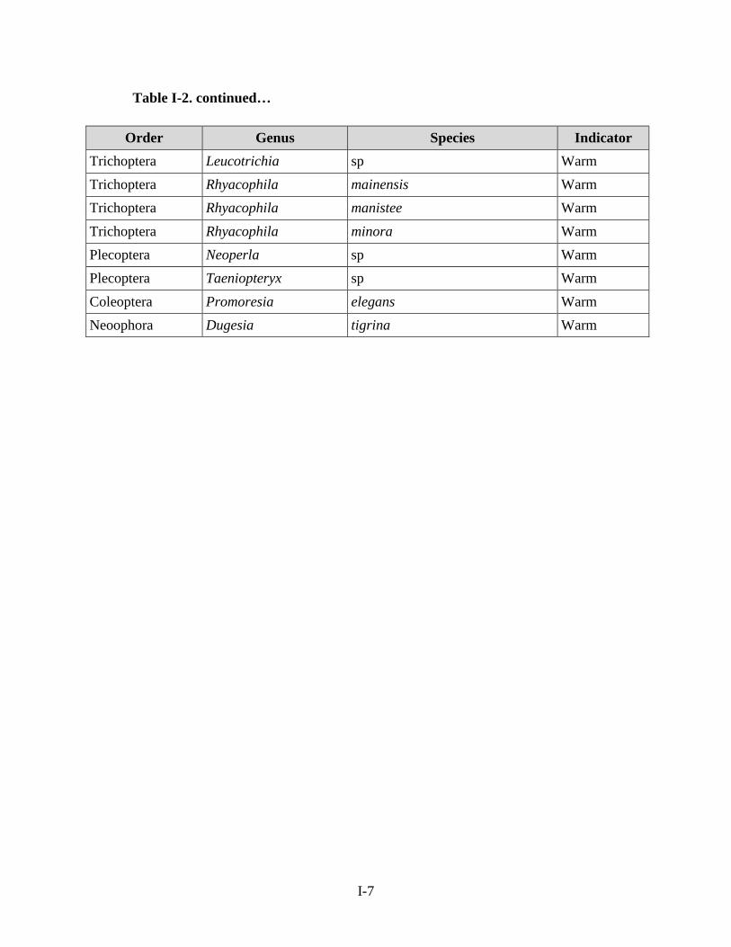
I-7

Table I-2. continued…

Order Genus Species Indicator Trichoptera Leucotrichia sp Warm Trichoptera Rhyacophila mainensis Warm Trichoptera Rhyacophila manistee Warm Trichoptera Rhyacophila minora Warm Plecoptera Neoperla sp Warm Plecoptera Taeniopteryx sp Warm Coleoptera Promoresia elegans Warm Neoophora Dugesia tigrina Warm

I-8

Table I-3. Taxa that have been identified as cold or cool water indicators by MD DNR (Becker et al., 2010) and/or PA DEP (Amy Williams and Dustin Shull, unpublished data)

Type Order Genus MD PA Occurrence in

PA DEP data set

Cold Diptera Bittacomorpha Yes

Cold Diptera Dixa Yes

Cold Diptera Heleniella Yes

Cold Diptera Prodiamesa Yes

Cold Ephemeroptera Ameletus Yes Common

Cold Ephemeroptera Cinygmula Yes Yes Common

Cold Ephemeroptera Diphetor Yes Yes Common

Cold Ephemeroptera Drunella Yes Common

Cold (MD)/cool (PA) Ephemeroptera Epeorus Yes Yes Common

Cold Ephemeroptera Ephemera Yes

Cold Ephemeroptera Ephemerella Yes Common

Cold Ephemeroptera Eurylophella Yes Common

Cold (MD)/cool (PA) Ephemeroptera Habrophlebia Yes Yes Rare

Cold Ephemeroptera Paraleptophlebia Yes

Cold Plecoptera Alloperla Yes Yes Common

Cold Plecoptera Amphinemura Yes Common

Cold Plecoptera Diploperla Yes Rare

Cold Plecoptera Haploperla Yes Rare

Cold Plecoptera Isoperla Yes Common

Cold Plecoptera Leuctra Yes

Cold Plecoptera Malirekus Yes Rare

Cold Plecoptera Peltoperla Yes Rare

Cold Plecoptera Pteronarcys Yes Rare

Cold Plecoptera Remenus Yes Rare

Cold Plecoptera Sweltsa Yes Yes Common

I-9

Table I-3. continued…

Type Order Genus MD PA Occurrence in

PA DEP data set Cold Plecoptera Tallaperla Yes Yes Common Cold Plecoptera Yugus Yes Rare Cold Trichoptera Diplectrona Yes Cold Trichoptera Wormaldia Yes Yes Common

I-10

Table I-4. Taxa that have been identified as cold, cool, or warm water indicators based on thermal tolerance analyses (per Yuan, 2006) conducted on data from North Carolina (U.S. EPA, 2012) and/or based on unpublished data provided by Debbie Arnwine from TN DEC

Type Order Genus

NC (U.S. EPA,

2012) TN Notes―TN Cold (NC)/ cool (TN)

Coleoptera Promoresia Yes Yes

Cold (NC)/ cool (TN)

Diptera Antocha Yes Yes

Cold (NC)/ cool (TN)

Diptera Atherix Yes Yes

Cold Diptera Cardiocladius Yes Cold Diptera Diamesa Yes Cold Diptera Dicranota Yes Cold Diptera Eukiefferiella Yes Cold Diptera Heleniella Yes Cold (NC)/ cool (TN)

Diptera Pagastia Yes Yes

Cold Diptera Potthastia Yes Cold Diptera Rheopelopia Yes Cold Ephemeroptera Acentrella Yes Cold Ephemeroptera Cinygmula Yes Cold (NC)/ cool (TN)

Ephemeroptera Drunella Yes Yes

Cold (NC)/ cool (TN)

Ephemeroptera Epeorus Yes Yes

Cold Ephemeroptera Nixe Yes Cold (NC)/ cool (TN)

Ephemeroptera Rhithrogena Yes Yes

Cold (NC)/ cool (TN)

Odonata Lanthus Yes Yes

Cold Plecoptera Amphinemura Yes

I-11

Table I-4. continued…

Type Order Genus

NC (U.S. EPA, 2012) TN Notes―TN

Cold Plecoptera Clioperla Yes Cold Plecoptera Cultus Yes

Cold Plecoptera Diploperla Yes Yes Uncommon in TN data set

Cold Plecoptera Isoperla Yes

Cold Plecoptera Malirekus Yes Yes Uncommon in TN data set

Cold Plecoptera Peltoperla Yes Uncommon TN data set

in

Cold Plecoptera Pteronarcys Yes Cold Plecoptera Tallaperla Yes Yes Cold Plecoptera Zapada Yes

Cold (NC)/ cool (TN)

Trichoptera Agapetus Yes Yes

Cold Trichoptera Apatania Yes Yes Uncommon in TN data set

Cold Trichoptera Arctopsyche Yes Yes Uncommon in TN data set

Cold Trichoptera Dolophilodes Yes Yes Mostly cool or cold

Cold Trichoptera Glossosoma Yes Yes Mostly cool or cold

Cold Trichoptera Parapsyche Yes Yes Uncommon in TN data set

Cold/cool Ephemeroptera Ameletus Yes

Cold/cool Trichoptera Lepidostoma Yes

Cool Ephemeroptera Habrophlebia Yes Uncommon in TN data set

Cool Plecoptera Alloperla Yes

I-12

Table I-4. continued…

Type Order Genus

NC (U.S. EPA, 2012) TN Notes―TN

Cool Plecoptera Sweltsa Yes Warm and cold but mostly cool

Cool Plecoptera Taenionema Yes uncommon in TN data set

Cool Trichoptera Diplectrona Yes Warm and cold―more common in cool or cold

Cool Trichoptera Wormaldia Yes Warm Arhynchobdellida Erpobdella Yes Warm Arhynchobdellida Mooreobdella Yes Warm Basommatophora Physella Yes Warm Coleoptera Berosus Yes Warm Coleoptera Lioporeus Yes Warm Decapoda Palaemonetes Yes Warm Diptera Nilothauma Yes Warm Diptera Parachironomus Yes Warm Diptera Pentaneura Yes Warm Diptera Procladius Yes Warm Diptera Stenochironomus Yes Warm Ephemeroptera Diphetor Yes Warm Ephemeroptera Tricorythodes Yes Warm Hemiptera Belostoma Yes Warm Isopoda Caecidotea Yes Warm Odonata Epicordulia Yes Warm Odonata Helocordulia Yes Warm Odonata Hetaerina Yes Warm Odonata Ischnura Yes

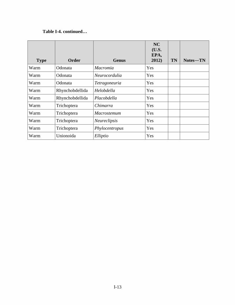
I-13

Table I-4. continued…

Type Order Genus

NC (U.S. EPA, 2012) TN Notes―TN

Warm Odonata Macromia Yes Warm Odonata Neurocordulia Yes Warm Odonata Tetragoneuria Yes Warm Rhynchobdellida Helobdella Yes Warm Rhynchobdellida Placobdella Yes Warm Trichoptera Chimarra Yes Warm Trichoptera Macrostemum Yes Warm Trichoptera Neureclipsis Yes Warm Trichoptera Phylocentropus Yes Warm Unionoida Elliptio Yes

I-14

I.1. REFERENCESBecker, AJ; Stranko, SA; Klauda, RJ; Prochaska, AP; Schuster, JD; Kashiwagi, MR; Graves, PH. (2010) Maryland biological stream survey’s sentinel site network: A multi-purpose monitoring program. Annapolis, MD: Maryland Department of Natural Resources.

U.S. EPA (Environmental Protection Agency). (2012) Implications of climate change for bioassessment programs and approaches to account for effects. [EPA/600/R-11/036F]. Washington, DC: Global Change Research Program,

National Center for Environmental Assessment. http://cfpub.epa.gov/ncea/global/recordisplay.cfm?deid=239585.

Yuan, L. (2006) Estimation and application of macroinvertebrate tolerance values. National Center for Environmental Assessment, Office of Research and Development, U.S. Environmental Protection Agency, Washington, DC; EPA/600/P-04/116F. http://cfpub.epa.gov/ncea/cfm/recordisplay.cfm?deid=154869.

J-1

APPENDIX J. __________________________

THERMAL SUMMARY

STATISTICS

J-2

Table J-1. Recommended thermal statistics to calculate for each year of continuous temperature data at regional monitoring network (RMN) sites.

Timeframe Thermal statistic Calculation Daily Daily mean Mean temperature for each day

Daily maximum Maximum temperature for each day Daily minimum Minimum temperature for each day Daily difference (maximum−minimum)

Difference between the maximum and minimum temperatures for each day

Daily variance Standard deviation for each day Monthly Monthly mean Mean of the daily means for each month

Monthly maximum Maximum value for each month Monthly minimum Minimum value for each month Monthly difference (maximum−minimum)

Difference between the maximum and minimum temperatures for each month

Monthly variance Standard deviation for each month

Seasonala Seasonal mean Mean of the daily means for each season

Seasonal maximum Maximum value for each season

Seasonal minimum Minimum value for each season

Seasonal difference (maximum−minimum)

Difference between the maximum and minimum temperatures for each season

Seasonal variance Standard deviation for each season

J-3

Table J.1. continued…

Timeframe Thermal statistic Calculation Annual Annual mean Mean of the daily means for the year

(January 1−December 31) Annual maximum Maximum value for the year

(January 1−December 31) Annual minimum Minimum value for the year

(January 1−December 31) Mean annual difference Mean of the daily difference

(January 1−December 31) Maximum annual difference Maximum of the daily difference

(January 1−December 31) Minimum annual difference Minimum of the daily difference

(January 1−December 31)

Variance of the annual mean difference

Standard deviation of the daily difference (January 1−December 31)

Percentage exceedance ([Number of measurements that exceed a thresholdb] ÷ [total number of measurements in a year]) × 100

aSeasons are defined as follows. Winter: December, January, February; Spring: March, April, May; Summer: June, July, August; Fall: September, October, November.

bThresholds may vary by entity and location.

K-1

APPENDIX K. __________________________

HYDROLOGIC SUMMARY STATISTICS AND TOOLS

FOR CALCULATING ESTIMATED

STREAMFLOW STATISTICS

K-2

K.1. LIST OF RECOMMENDED HYDROLOGIC SUMMARY STATISTICS FOR REGIONAL MONITORINGNETWORK (RMN) SITES

Table K-1. Recommended hydrologic statistics to calculate on each year of water-level or flow data from regional monitoring network (RMN) sites. These provide information on high, seasonal, and low flow components to maintain ecosystem flows. These candidate metrics were derived from DePhilip and Moberg (2013) for the Upper Ohio River Basin and Olden and Poff (2003). Work that was done by Hawkins et al. (2013) was also considered. For more details on these studies, see Sections K.2−K.4.

Timeframe Metric Calculation Daily Daily mean Mean stage or flow for each day

Daily median Median stage or flow for each day Daily maximum Maximum stage or flow for each day Daily minimum Minimum stage or flow for each day Daily difference (maximum−minimum)

Difference between the maximum and minimum stage or flows for each day

Coefficient of variation Standard deviation for stage or flow for each day/mean daily stage or flow

K-3

Table K-1. continued…

Timeframe Metric Calculation Monthly Monthly mean Mean stage or flow for each month

Monthly maximuma Maximum stage or flow for each month

Monthly minimumb Minimum stage or flow for each month

Monthly difference (maximum−minimum)

Difference between the maximum and minimum stage or flow values for each month

High flow magnitude (90th percentile)

90th percentile of monthly stage or flow values; this represents high flows similar to the Q10 measurement used in DePhilip and Moberg (2013)

and is

Median magnitude (50th percentile) 50th percentile of monthly stage or flow values; this represents the monthly median

Low (25th

flow magnitude percentile)

25th percentile of monthly stage or flow values; this represents low flows in smaller streams (drainage areas <50 mi2, per DePhilip and Moberg [2013]) and is similar to the Q75 measurement used in DePhilip and Moberg (2013)

Low (10th

flow magnitude percentile)

10th percentile of monthly stage or flow values; this represents low flows in medium to larger-sized streams (drainage areas >50 mi2 per DePhilip and Moberg [2013]) and is similar to the Q90 measurement used in DePhilip and Moberg (2013)

Extreme low flow magnitude (1st percentile)

1st percentile of monthly stage or flow values; this represents extreme low flows and is similar to the Q99 measurement used in DePhilip and Moberg (2013)

Percentage high flow and floods Percentage of stage or flow 90th percentile

measurements in each month that exceed the monthly

Percentage low flows Percentage of stage or flow measurements in each monthly 25th and 1st percentiles (similar to the Q75 DePhilip and Moberg [2013])

month that are between the and Q99 measurements used in

Percentage typical Percentage of stage or flow measurements in each month that are between the monthly 25th and 90th percentiles (similar to the Q75 and Q10 measurements used in DePhilip and Moberg [2013])

K-4

Table K-1. continued…

Timeframe Metric Calculation Seasonal Percentage high flows and floods in

spring and fall Percentage of stage or flow measurements in each month that exceed the monthly 90th percentile in spring (March−May) and fall (September−November)

Annual (January 1− December 31)

Annual mean Mean of the daily mean stage or flow

Annual maximum Maximum stage or flow

Julian date of annual maximum Julian date of annual maximum stage or flow

Annual minimum Minimum stage or flow

Julian date of annual minimum Julian date of annual minimum stage or flow

Mean annual difference Mean of the daily difference

Maximum annual difference Maximum of the daily difference

Minimum annual difference Minimum of the daily difference

Variance of the annual mean difference

Standard deviation of the daily difference

Number of zero flow days Number of days having stage or flow measurements of 0

aIn Olden and Poff (2003), mean maximum August flow and mean maximum October flow captured important aspects of high flow conditions. bIn Olden and Poff (2003), mean minimum April flow captured important aspects of low flow conditions.

K-5

K.2. HYDROLOGIC METRICS DERIVED FROM DEPHILIP AND MOBERG (2013)FOR THE UPPER OHIO RIVER BASIN

The Nature Conservancy and several partners (states, river basin commissions, other federal agencies) have developed ecosystem flow needs for some Eastern and Midwestern rivers and their tributaries (e.g., the Susquehanna, the Upper Ohio, and the Potomac Rivers) (DePhilip and Moberg, 2010; Cummins et al., 2010; DePhilip and Moberg, 2013; Buchanan et al., 2013). Table K-2 contains the lists of 10 flow statistics that were chosen to represent the high, seasonal, and low flow components in the Upper Ohio River basin (DePhilip and Moberg, 2013). These statistics were selected because they are easy to calculate, commonly used, and integrate several aspects of the flow regime, including frequency, duration, and magnitude (DePhilip and Moberg, 2013). Diagrams like the one shown in Figure K-1 can be generated for data from RMN sites.

Table K-2. Flow statistics that were selected to track changes to high, seasonal, and low flow components in the Upper Ohio River basin. These are flow exceedance values. For example, Q10 equals the 10% exceedance probability (Q10), which represents a high flow that has been exceeded only 10% of all days in the flow period. This is a reproduction of Table 3.2 in DePhilip and Moberg (2013)

Flow component Flow statistic High flows Annual/interannual (≥bankfull) Large flood Magnitude and frequency of 20‐year flood Small flood Magnitude and frequency of 5‐year flood Bankfull Magnitude and frequency of 1- to 2-year high flow event High flow pulses (<bankfull) Frequency of high flow pulses Number of events > monthly Q10 in spring and fall High pulse magnitude Monthly Q10

Seasonal flows Monthly magnitude Monthly median Typical monthly range Area under monthly flow duration curve between Q75 and

Q10 (or some part of this range)

Low flows Monthly low flow range Area under monthly flow duration curve between Q75 and

Q99 Monthly low flow magnitude Monthly Q75

Monthly Q90

K-6

Figure K-1. In the Upper Ohio River basin, monthly flow exceedance values (Qex) were plotted against daily discharges to highlight specific portions of the hydrograph and facilitate discussions about the ecological importance of each portion (from DePhilip and Moberg, 2013).

7

K.3. HYDROLOGIC METRICS DERIVED FROM OLDEN AND POFF (2003)Olden and Poff (2003) did a comprehensive review of 171 hydrologic metrics, including Indicators of Hydrologic Alteration.

They provided recommendations on a reduced set of metrics that capture critical aspects of the hydrologic regime, are not overly redundant, and are ecologically meaningful in different types of streams. Table K-3 contains a list of 34 metrics that, based on their analyses, effectively capture different aspects of flow regimes in all stream types and have limited redundancy.

Table K-3. Based on analyses done by Olden and Poff (2003), these 34 hydrologic flow statistics effectively capture different aspects of the flow regime in all stream types and have limited redundancy. This is a reproduction of Table 3 (all streams) in Olden and Poff (2003)

Category Metric Description Abbreviated

metric Magnitude―average flow conditions

Skewness in daily flows Mean daily flows divided by median daily flows Ma5 Mean annual runoff Mean annual flow divided by catchment area Ma41 Variability in daily flows 1 Coefficient of variation in daily flows Ma3 Spreads in daily flows Ranges in daily flows (25th/75th percentiles) divided by median

daily flows Ma11

Magnitude―low flow conditions

Baseflow index 1 7-day minimum flow divided by mean annual daily flowsaveraged across all years

Ml17

Mean minimum April flow Mean minimum monthly flow in April Ml4 Variability across annual minimum flows

Coefficient of variation in annual minimum flows averaged across all years

Ml21

Variability in baseflow index 1 Coefficient of variation in baseflow index (Ml17) Ml18

8

Table K-3. continued…

Abbreviated Category Metric Description metric

Magnitude― High flow discharge Mean of the 10th percentile from the flow duration curve divided Mh16 high flow by median daily flow across all years conditions Mean maximum August flow Mean maximum monthly flow in August Mh8

Mean maximum October flow Mean maximum monthly flow in October Mh10

Median of annual maximum Median of the highest annual daily flow divided by the median Mh14 flows annual daily flow averaged across all years

Frequency of Frequency of low flow spells Total number of low flow spells (threshold equal to 5% of mean Fl3 flow daily flow) divided by record length in years events―low flow conditions

Variability in low flow pulse count

Coefficient of variation in Fl1 Fl2

Low flow pulse count Number of annual occurrences during which the magnitude of Fl1 flow remains below a lower threshold. Hydrologic pulses are defined as those periods within a year in which the flow drops below the 25th percentile (low pulse) of all daily values for the time period.

9

Table K-3. continued…

Category Metric Description Abbreviated

metric Frequency of flow events―high flow conditions

High flood pulse count 2 Number of annual occurrences during which the magnitude of flow remains above an upper threshold. Hydrologic pulses are defined as those periods within a year in which the flow goes above three times the median daily flow and the value is an average instead of a tabulated count.

Fh3

Flood frequency Mean number of high flow events per year using an upper threshold of three times median flow over all years

Fh6

Flood frequency Mean number of high flow events per threshold of seven times median flow

year using an upper over all years

Fh7

Variability in high flood pulse count

Coefficient of variation in high pulse count (defined as 75th percentile)

Fh2

Duration Number of zero flow days Mean annual number of days having zero daily flow Dl18

Variability in low flow pulse duration

Coefficient of variation in low flow pulse duration Dl17

Low flow pulse duration Mean duration of Fl1 Dl16

Means of 30-day minimum daily discharge

Mean annual 30-day minimum divided by median flow Dl13

Means of 30-day maximum daily discharge

Mean annual 30-day maximum divided by median flow Dh13

Variability in high flow pulse duration

Coefficient of variation in Fh1 Dh16

High flow duration Upper threshold is defined as the 75th percentile of median flows Dh20

High flow pulse duration Mean duration of Fh1 Dh15

10

Table K-3. continued…

Category Metric Description Abbreviated

metric Timing of flow events

Constancy See Colwell (1974) Ta1

Seasonal predictability of nonflooding

Maximum proportion of the year (number of days/365) during which no floods have ever occurred over the period of record

Th3

Variability in Julian date of annual minimum

Coefficient of variation in Tl1 Tl2

Rate of change

Variability in reversals Coefficient of variation in Ra8 Ra9

Reversals Number of negative and positive changes in water conditions from 1 day to the next

Ra8

Change of flow Median of difference between natural logarithm of flows between 2 consecutive days with increasing/decreasing flow

Ra6

No day rises Ratio of days where flow is higher than the previous day Ra5

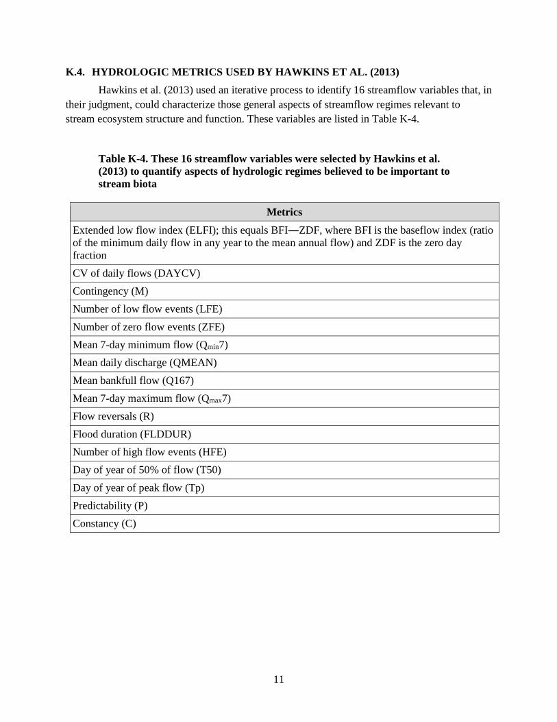
11

K.4. HYDROLOGIC METRICS USED BY HAWKINS ET AL. (2013)Hawkins et al. (2013) used an iterative process to identify 16 streamflow variables that, in

their judgment, could characterize those general aspects of streamflow regimes relevant to stream ecosystem structure and function. These variables are listed in Table K-4.

Table K-4. These 16 streamflow variables were selected by Hawkins et al. (2013) to quantify aspects of hydrologic regimes believed to be important to stream biota

Metrics Extended low flow index (ELFI); this equals BFI―ZDF, where BFI is the baseflow index (ratio of the minimum daily flow in any year to the mean annual flow) and ZDF is the zero day fraction CV of daily flows (DAYCV) Contingency (M) Number of low flow events (LFE) Number of zero flow events (ZFE) Mean 7-day minimum flow (Qmin7) Mean daily discharge (QMEAN) Mean bankfull flow (Q167) Mean 7-day maximum flow (Qmax7) Flow reversals (R) Flood duration (FLDDUR) Number of high flow events (HFE) Day of year of 50% of flow (T50) Day of year of peak flow (Tp) Predictability (P) Constancy (C)

12

K.5. TOOLS FOR ESTIMATING STREAMFLOW AT UNGAGED SITES

Table K-5. Examples of tools for estimating streamflow and/or streamflow statistics at ungaged sites. A similar tool is currently being developed for New York

Tool Geographic area Website Description USGS StreamStats1 Varies by state http://water.usgs.gov/osw/streamstats/ Available for most but not all states in the

eastern United States. The types of output statistics that are available vary by state. These statistics represent long-term averages and do not capture year-to-year variability.

BaSE (Stuckey et al., 2012)

Pennsylvania http://pubs.usgs.gov/sir/2012/5142/ This tool simulates minimally altered streamflow at a daily time scale for ungaged streams in Pennsylvania using data collected during water years 1960−2008. It is free, publicly available, and uses a point‐and‐click interface.

MA SYE (Archfield et al., 2010)

Massachusetts http://pubs.usgs.gov/sir/2009/5227/ The MA SYE can estimate a daily time series of unregulated, daily mean streamflow for a 44-year period of record spanning 1960 to2004.

West Virginia DEP 7Q10 Report Tool (Shank, 2011)

West Virginia http://tagis.dep.wv.gov/streamflow/ This free, publicly available tool utilizes a point-and-click interface. Seven Q10, annual and monthly flow estimates are generated when you click on a location.

1http://water.usgs.gov/osw/streamstats/

13

USGS = U.S. Geological Survey; BaSE = Baseline Streamflow Estimator; MA SYE = Massachusetts Sustainable Yield Estimator; DEP = Department of Environmental Protection

14

K.6. REFERENCESArchfield, SA; Vogel, RM; Steeves, PA; Brandt, SL: Weiskel, PK; Garabedian, SP. (2010) The Massachusetts

sustainable‐yield estimator: A decision‐support tool to assess water availability at ungaged stream locations in Massachusetts. [USGS Scientific Investigations Report 2009−5227]. Northborough, MA: Massachusetts-Rhode Island Water Science Center, U.S. Geological Survey. 41 pp. Available online: http://pubs.usgs.gov/sir/2009/5227/.

Buchanan, C; Moltz, HLN; Haywood, HC; Palmer, JB; Griggs, AN. (2013) A test of The Ecological Limits of Hydrologic Alteration (ELOHA) method for determining environmental flows in the Potomac River basin, U.S.A. Freshw Biol 58(12):2632−2647.

Colwell RK. (1974) Predictability, constancy, and contingency of periodic phenomena. Ecol. 55:1148–1153.

Cummins, J; Buchanan, C; Haywood, HC; Moltz, H; Griggs, A; Jones, C; Kraus, R; Hitt, NP; R. Bumgardner, R. (2010). Potomac large river ecologically sustainable water management report. [ICPRB Report 10-3]. Interstate Commission on the Potomac River Basin for The Nature Conservancy. Available online at www.potomacriver.org/pubs.

DePhilip, M; Moberg, T. (2010) Ecosystem flow recommendations for the Susquehanna River Basin. Harrisburg, PA: The Nature Conservancy. Available online at http://www.srbc.net/policies/docs/TNCFinalSusquehannaRiverEcosystemFlowsStudyReport_Nov10_20120327_fs135148v1.PDF

DePhilip, M; Moberg, T. (2013). Ecosystem flow recommendations for the Upper Ohio River basin in western Pennsylvania. Harrisburg, PA: The Nature Conservancy.

Hawkins, CP; Tarboton, DG; Jin, J. (2013) Consequences of global climate change for stream biodiversity and implications for the application and interpretation of biological indicators of aquatic ecosystem condition. Final Report. [EPA Agreement Number: RD834186]. Logan Utah: Utah State University. http://cfpub.epa.gov/ncer_abstracts/index.cfm/fuseaction/display.abstractDetail/abstract/9063

Olden, JD; Poff, NL. (2003) Redundancy and the choice of hydrologic indices for characterizing streamflow regimes. River Res Appl 19:101−121.

Stuckey, MH; Koerkle, EH; Ulrich, J. (2012) Estimation of baseline daily mean streamflows for ungagged location on Pennsylvania streams, water years 1960‐2008. [USGS Scientific Investigations Report 2012‐5142]. New Cumberland, PA: U.S. Geological Survey. Available online at http://pubs.usgs.gov/sir/2012/5142/.

Shank, M. (2011) West Virginia DEP 7Q10 report tool [web page]. Accessed 1 August 2014. Available online at http://tagis.dep.wv.gov/7q10/.

NationalNational CenterCenter forfor EnvironmentalEnvironmental AssessmenAssessmenttOffOfficeice ooff ResearResearcchh andand DevelopmenDevelopmenttWWaasshinghingttonon,, DCDC 2046204600OOfffifi cciaiall BBuussineinessssPPeenanallttyy ffoorr PPrriivvateate UUssee$3$30000