Regional climate model simulations for Europe at 6 k and 0.2 k yr BP: sensitivity to changes in...

Clim. Past, 10, 661–680, 2014www.clim-past.net/10/661/2014/doi:10.5194/cp-10-661-2014© Author(s) 2014. CC Attribution 3.0 License.

Climate of the Past

Open A

ccess

Regional climate model simulations for Europe at 6 and 0.2 k BP:sensitivity to changes in anthropogenic deforestation

G. Strandberg1,2, E. Kjellström 1,2, A. Poska3,5, S. Wagner4, M.-J. Gaillard 5, A.-K. Trondman 5, A. Mauri 6,B. A. S. Davis6, J. O. Kaplan6, H. J. B. Birks7,8,9,22,23, A. E. Bjune10, R. Fyfe11, T. Giesecke12, L. Kalnina 13,M. Kangur 14, W. O. van der Knaap15, U. Kokfelt16,3,5, P. Kuneš17, M. Latałowa18, L. Marquer 5, F. Mazier19,3,A. B. Nielsen20,5, B. Smith3, H. Seppä21, and S. Sugita14

1Swedish Meteorological and Hydrological Institute, Norrköping, Sweden2Department of Meteorology, Stockholm University, Stockholm, Sweden3Department of Earth and Ecosystem Science, Lund University, Lund, Sweden4Helmholtz-Zentrum Geesthacht, Geesthacht, Germany5Department of Biology and Environmental Science, Linnaeus University, Kalmar, Sweden6Institute for Environmental Sciences, University of Geneva, Geneva, Switzerland7Department of Biology and Bjerknes Centre for Climate Research, University of Bergen, Bergen, Norway8Environmental Change Research Centre, University College London, London, UK9School of Geography and the Environment, University of Oxford, Oxford, UK10Uni Climate, Uni Research AS and Bjerknes Centre for Climate Research, Bergen, Norway11School of Geography, Earth and Environmental Sciences, University of Plymouth, Plymouth, UK12Department of Palynology and Climate Dynamics, Albrecht-von-Haller Institute for Plant Sciences,University of Göttingen, Göttingen, Germany13Faculty of Geography and Earth Sciences, University of Latvia, Riga, Latvia14Institute of Ecology, Tallin University, Tallin, Estonia15Institute of Plant Sciences and Oeschger Centre for Climate Change Research, University of Bern, Bern, Switzerland16Center for Permafrost, Department of Geosciences and Natural Resource Management, University of Copenhagen,Copenhagen, Denmark17Department of Botany, Faculty of Science, Charles University in Prague, Prague, Czech Republic18Laboratory of Palaeoecology and Archaeobotany, Department of Plant Ecology, University of Gdansk, Gdansk, Poland19GEODE, UMR 5602, University of Toulouse, Toulouse, France20Department of Geology, Lund University, Lund, Sweden21Department of Geosciences and Geography, University of Helsinki, Helsinki, Finland22Environmental Change Research Centre, University College London, London, UK23School of Geography and the Environment, University of Oxford, Oxford, UK

Correspondence to:G. Strandberg ([email protected])

Received: 30 September 2013 – Published in Clim. Past Discuss.: 18 October 2013Revised: 27 January 2014 – Accepted: 17 February 2014 – Published: 28 March 2014

Abstract. This study aims to evaluate the direct effects ofanthropogenic deforestation on simulated climate at two con-trasting periods in the Holocene,∼ 6 and∼ 0.2 k BP in Eu-rope. We apply We apply the Rossby Centre regional cli-mate model RCA3, a regional climate model with 50 kmspatial resolution, for both time periods, considering three

alternative descriptions of the past vegetation: (i) potentialnatural vegetation (V) simulated by the dynamic vegetationmodel LPJ-GUESS, (ii) potential vegetation with anthro-pogenic land use (deforestation) from the HYDE3.1 (HistoryDatabase of the Global Environment) scenario (V + H3.1),and (iii) potential vegetation with anthropogenic land use

Published by Copernicus Publications on behalf of the European Geosciences Union.

662 G. Strandberg et al.: Sensitivity to changes in anthropogenic deforestation

from the KK10 scenario (V + KK10). The climate model re-sults show that the simulated effects of deforestation dependon both local/regional climate and vegetation characteristics.At ∼ 6 k BP the extent of simulated deforestation in Europeis generally small, but there are areas where deforestationis large enough to produce significant differences in sum-mer temperatures of 0.5–1◦C. At ∼ 0.2 k BP, extensive de-forestation, particularly according to the KK10 model, leadsto significant temperature differences in large parts of Eu-rope in both winter and summer. In winter, deforestationleads to lower temperatures because of the differences inalbedo between forested and unforested areas, particularlyin the snow-covered regions. In summer, deforestation leadsto higher temperatures in central and eastern Europe becauseevapotranspiration from unforested areas is lower than fromforests. Summer evaporation is already limited in the south-ernmost parts of Europe under potential vegetation condi-tions and, therefore, cannot become much lower. Accord-ingly, the albedo effect dominates in southern Europe also insummer, which implies that deforestation causes a decreasein temperatures. Differences in summer temperature due todeforestation range from−1◦C in south-western Europe to+1◦C in eastern Europe. The choice of anthropogenic land-cover scenario has a significant influence on the simulatedclimate, but uncertainties in palaeoclimate proxy data for thetwo time periods do not allow for a definitive discriminationamong climate model results.

1 Introduction

Humans potentially had an influence on the climate systemthrough deforestation and early agriculture already long be-fore we started to emit CO2 from fossil fuel combustion(Ruddiman, 2003). Deforestation affects the climate at manyscales, from microclimate to global climate (e.g. Bala et al.,2007). The effect on the global climate is conveyed by theincreased amounts of CO2 in the atmosphere from deforesta-tion, and by the regional and local changes of land-surfaceproperties (e.g. Forster et al., 2007). Such changes have adirect effect on the regional climate, including changes inalbedo and energy fluxes between the land surface and theatmosphere (e.g. Pielke et al., 2011). Since forests generallyhave a lower reflectivity than unforested areas, the albedo ef-fect from deforestation would lead to lower regional temper-ature. Reduced vegetation cover also means reduced evap-otranspiration that leads to higher air temperature, but theamplitude of the evapotranspiration changes depend on localconditions, such as soil moisture availability (Ban-Weiss etal., 2011; de Noblet-Ducoudré et al., 2012). The effects of in-creased atmospheric CO2 resulting from changing vegetationand land use over the last 8000 yr have been previously dis-cussed (e.g. Ruddiman, 2003; Pongratz et al., 2009a). The di-rect effects of past vegetation change have mostly been stud-

ied on a global scale (e.g. Brovkin et al., 2006; Pitman et al.,2009; Pongratz et al., 2009b, 2010; de Noblet-Ducoudré etal., 2012; Christidis et al., 2013).

Global climate models (GCMs) are run on coarse spatialresolutions; therefore, they can only reproduce large-scaleclimate features. Regional climate models (RCMs) preservethe large-scale climate features, but the higher spatial reso-lution in RCMs provides a better representation of the land–sea distribution and topography, which in turn allows a moredetailed description of the regional climate (Rummukainen,2010). This also applies to vegetation modelling. Only a de-tailed description of vegetation can account for biogeophysi-cal effects on climate at the regional scale (Wramneby et al.,2010). Since we expect vegetation change to affect climateat the local/regional spatial scale, a high spatial resolution inthe climate model is critical when evaluating model resultsby comparison with observations and/or proxies that repre-sent local to regional environment conditions. To date thereare no previous RCM-based studies of the feedback on cli-mate from historical changes in land use/anthropogenic landcover.

The present study investigates the direct effect on cli-mate from human-induced vegetation changes in Europe atthe regional spatial scale. We do not study the indirect ef-fects from changing atmospheric CO2 concentration. Thisstudy is part of the LANDCLIM (LAND cover–CLIMate in-teractions in NW Europe during the Holocene) project thataims to assess the possible effects on the climate of twohistorical processes (compared with a baseline of present-day land cover): (i) climate-driven changes in vegetation and(ii) human-induced changes in land cover (Gaillard et al.,2010). Specifically, this study asks (i) whether historical landuse influences the regional climate, (ii) how much the RCM-simulated climate differs depending on the scenario of pastanthropogenic land cover used, (iii) which processes are im-portant for climate–vegetation interaction, and (iv) to whatextent palaeoclimate proxy data are effective at evaluatingRCM-based simulation results.

We focus on two contrasting time periods in terms ofclimate and anthropogenic land cover change: the Mid-Holocene warm period (∼ 6 k BP) and the Little Ice Age(∼ 0.2 k BP= ∼ AD 1750). The Mid-Holocene was charac-terised by a relatively warm climate and low human impacton vegetation/land cover, while the Little Ice Age was cooland anthropogenic land use was extensive. The 6 k time-window has the advantage of being widely used in model-data comparison studies of global climate models (e.g. Har-rison et al., 1998; Masson et al., 1999; Kohfeld and Harri-son, 2000; see the Palaeoclimate Modelling IntercomparisonProject (PMIP) activities:http://pmip.lsce.ipsl.fr/), which al-lows us to set our results in a wider perspective. We use adynamic vegetation model, LPJ-GUESS (Smith et al., 2001),to simulate past climate-driven potential natural vegetationand two alternative scenarios of anthropogenic land-coverchange (ALCC): HYDE3.1 (History Database of the Global

Clim. Past, 10, 661–680, 2014 www.clim-past.net/10/661/2014/

http://pmip.lsce.ipsl.fr/

G. Strandberg et al.: Sensitivity to changes in anthropogenic deforestation 663

Table 1.Summary of forcing conditions in the RCA3 simulations; see text for details. The amount of greenhouse gases and irradiance variesfrom year to year, and the table shows average values.

Total solarCO2 CH4 N2O irradiance

Name Period Vegetation Land use (ppm) (ppb) (ppb) (W m−2)

6 kV6 k BP Potential 6 k

None265 572 260 13646kV + H3.1 HYDE3.1

6kV + KK10 KK10

0.2 kV0.2 k BP Potential 0.2 k

None277 710 277 13630.2kV+ H3.1 HYDE3.1

0.2kV+ KK10 KK10

Environment; Klein Goldewijk et al., 2011) and KK10 (Ka-plan et al., 2009). These scenarios of past human-inducedvegetation are widely used in climate modelling of the past,but they exhibit large differences for key periods of theHolocene (Gaillard et al., 2010; Boyle et al., 2011). Thesediscrepancies are due to differences in the modelling ap-proach. While previous studies demonstrated the large influ-ence of the choice of ALCC scenario on modelled changesin terrestrial carbon storage over the Holocene (Kaplan et al.,2009), little work has been done to assess the importance ofthe ALCC scenario used with respect to the biogeophysicalfeedback to climate. We therefore use both HYDE and KK10in our model simulations of regional climate.

In order to evaluate the RCM-simulated results, we use cli-mate proxy records based on (i) the LANDCLIM database ofpoint data, i.e. representing either local or regional climateconditions based on non-pollen proxies (e.g. tree-ring data,chironomid records from lake sediments, stalagmiteδ18Orecords, etc.; Nielsen et al., 2014) to avoid any circular rea-soning (where the same vegetation would be used both toforce and evaluate the model simulations), and (ii) an attemptat spatially explicit descriptions of past climate characteris-tics based on pollen data (Mauri et al., 2013).

2 Material and methods

2.1 The models

The main tool used in this study to produce high spatial reso-lution climate simulations is the Rossby Centre regional cli-mate model RCA3 (Samuelsson et al., 2011). Here, we de-scribe RCA3 and the models that provide the boundary con-ditions for the RCA3 runs. These models include the globalclimate model ECHO-G (Legutke and Voss, 1999), the dy-namic vegetation model (DVM) LPJ-GUESS (Smith et al.,2001), and the ALCC scenarios HYDE3.1 and KK10.

For each time period RCA3 uses lateral boundary con-ditions, sea-surface temperature and sea-ice conditionsfrom ECHO-G and in the first run modern-day vegetation(Samuelsson et al., 2011). The simulated climate is then

used to drive the vegetation model LPJ-GUESS to simu-late potential vegetation. For each time period, three 50 yrlong RCA3 simulations are then performed with three alter-native land-cover/vegetation descriptions: (i) potential veg-etation without human impact (V), (ii) V with the addi-tion of the HYDE3.1 estimate of anthropogenic deforestation(V + H3.1), and (iii) V with the addition of the KK10 esti-mate of anthropogenic deforestation (V+ KK10). The itera-tive modelling approach of RCM and DVM, RCA3→ LPJ-GUESS→ RCA3, has been shown to be a reasonable ap-proach where both simulated climate and vegetation are ingeneral agreement with available reconstructions, which arefew and uncertain (Kjellström et al., 2010; Strandberg et al.,2011). The simulations are summarised in Table 1. If notstated otherwise, “model simulation” stands for a simulationwith RCA3 forced with data from the other models describedbelow.

2.1.1 The general circulation model ECHO-G

ECHO-G has been used and evaluated earlier in palaeocli-matic studies (Zorita et al., 2005; Kaspar et al., 2007) andhas provided climate simulations in regional studies (e.g.Gómez-Navarro et al., 2011, 2012; Schimanke et al., 2012).Here, we use results from the transient Oetzi2 run cover-ing the period 7000 BP to present (Wagner et al., 2007). InOetzi2, ECHO-G is run with a horizontal resolution of T30(approximately 3.75◦ × 3.75◦) and 19 levels in the atmo-sphere, and a spatial resolution of approximately 2.8◦

× 2.8◦

and 20 levels in the oceans. The simulation was initialisedat the end of a 500 yr spin-down control (quasi-equilibrium)run with constant forcing (orbital, solar and greenhouse gas)for 7 ka BP.

The external forcings used in the global simulation withECHO-G are variations in Total Solar Irradiance (TSI),changes in atmospheric concentrations of greenhouse gases(GHGs), and changes in the Earth’s orbit. The TSI changeswere derived from the concentration of the cosmogenic iso-tope10Be in polar ice cores, and translated to TSI by scalingproduction estimates ofδ14C (cf. Solanki et al., 2004) such

www.clim-past.net/10/661/2014/ Clim. Past, 10, 661–680, 2014


that the difference between present-day and Maunder Mini-mum solar activity is 0.3 %. Past greenhouse gas concentra-tions were also estimated from air bubbles trapped in polarice cores (Flückiger et al., 2002). Finally, the changes in theorbital parameters obliquity, eccentricity and position of theperihelion can be accurately calculated for the last few mil-lion years (Berger and Loutre, 1991).

The vegetation in the global model is set to present-dayconditions for both simulations. Because the ECHO-G modelhas a very coarse resolution, vegetation changes in Europeare assumed not to have an overwhelming effect on the largescale atmospheric and oceanic circulation upstream, such asthe North Atlantic Oscillation (NAO) and North Atlantic sea-surface temperatures.

2.1.2 The Rossby Centre regional atmospheric climatemodel RCA3

RCA3 is used to downscale results from ECHO-G to higherresolution. RCA3 and its predecessors RCA1 and RCA2have been extensively used and evaluated in studies ofpresent and future climate (e.g. Rummukainen et al., 2001;Räisänen et al., 2004; Kjellström et al., 2011; Nikulin et al.,2011). Also, RCA3 has been used in palaeoclimatologicalapplications for downscaling global model results for the lastmillennium (Graham et al., 2009; Schimanke et al., 2012),parts of the Marine Isotope Stage 3 (Kjellström et al., 2010),and for the Last Glacial Maximum (Strandberg et al., 2011).

In RCA3, the present-day land–sea distribution and sur-face geopotential is used for 0.2 k. The land–sea distributionfor 6 k is taken from the ICE-5G database (Peltier, 2004). Thedifference in orography between the two periods is caused bythe changed coastline and the less detailed coastline in ICE-5G. Land and sea grid cells are therefore not exactly the samein the two periods (Fig. 1).

ECHO-G and RCA3 use the same solar irradiance. Theconcentrations of atmospheric GHG in RCA3 are repre-sented as CO2-equivalents, whereas in ECHO-G CO2 andCH4 are explicitly described. GHGs and solar irradiancechange from year to year and are read annually by the mod-els. Table 1 summarises the forcing from GHGs and insola-tion averaged over the two periods.

For snow in unforested areas, RCA3 has a prognosticalbedo that varies between 0.6–0.85; the albedo decreases assnow ages. For snow-covered land areas in forest regions thealbedo is set constant to 0.2. The snow-free albedo is set to0.28 and 0.15 for unforested and forested areas, respectively.Leaf Area Index (LAI) is calculated as a function of the soiltemperature with a lower limit set to 0.4, and upper limits to2.3 (unforested) and 4.0 (deciduous forest). If deep soil mois-ture reaches the wilting point the LAI is set to its lower limit.LAI in coniferous forests is set constant to 4.0 regardless ofsoil moisture (Samuelsson et al., 2011).

RCA3 is run on a horizontal grid spacing of 0.44◦ (corre-sponding to approximately 50 km) over Europe with 24 ver-

Fig. 1. Difference in land–sea distribution between 6 and 0.2 k BP;grid boxes with a difference of more than 50 % are shaded. Thethree regions used for analysis in Fig. 11 are marked as red squares;Iberian Peninsula (IB), western Europe (WE), eastern Europe (EE).The blue boxes represent the regions northern Europe and southernEurope described in Sect. 4.2.

tical levels and a time step of 30 min. Data for initialisingRCA3 are taken from ECHO-G. After that, every 12 h, RCA3reads surface pressure, humidity, temperature and wind fromECHO-G along the lateral boundaries of the model domain,and sea-surface temperature and sea-ice extent within themodel domain. All RCA3 simulations have been run for 50 yrwith 1 yr spin-up time (simulated years are 3909–3861 BCfor 6 k and AD 1701–1750 for 0.2 k), after which the effectof the initial conditions of atmosphere/land surface systemare assumed to have faded (Giorgi and Mearns, 1999).

For each simulation of a 50 yr period we calculate the av-erage of the nominal seasons winter (December, January andFebruary; henceforth DJF) and summer (June, July and Au-gust; henceforth JJA). In addition, the diurnal cycle is anal-ysed for some regions.

The statistical significance for the difference betweenthe simulations is determined by a bootstrapping technique(Efron, 1979). 500 bootstrap samples are used to estimate theinter-annual variability of seasonal and annual means of tem-perature, precipitation, latent heat flux and albedo for eachsimulation. The difference between two simulations is com-pared with the estimated distribution of a parameter (e.g.temperature) to see if the difference is statistically signifi-cant. We choose the 95 % level for significance.

2.1.3 The dynamic vegetation model LPJ-GUESS

LPJ-GUESS (Smith et al., 2001; Hickler et al., 2004, 2012)is used to simulate potential natural vegetation patterns con-sistent with the simulated climate in Europe during the two



selected time windows. The model has been previously usedto simulate past vegetation (Miller et al., 2008; Garreta et al.,2010; Kjellström et al., 2010; Strandberg et al., 2011) andto assess the effects of land use on the global carbon cycle(Olofsson and Hickler, 2008; Olofsson, 2013).

LPJ-GUESS is a process-based dynamic ecosystem modeldesigned for application at regional to global spatial scales. Itincorporates representations of terrestrial vegetation dynam-ics based on interactions between individual trees and shrubsand a herbaceous understory at neighbourhood (patch) scale(Hickler et al., 2004). It accounts for the effect of stochasti-cally recurring disturbances for heterogeneity among patchesin terms of accrued biomass, vegetation composition andstructure at the landscape scale. The simulated vegetation isrepresented by Plant Functional Types (PFTs; Table 2) dis-criminated in terms of bioclimatic limits to survival and re-production, leaf phenology, allometry, life-history strategyand aspects of physiology governing carbon balance andcanopy gas-exchange. Differences between PFTs in combi-nation with the present structure of the vegetation in eachpatch govern the partitioning of light and soil water amongindividuals as well as regeneration and mortality, affectingcompetition among PFTs and age/size classes of plants.

Inputs to the model are temperature (◦C), precipita-tion (mm), net downward short-wave radiation at surface(W m−2) and wet day frequency (days), all in monthlytimesteps provided by RCA3 at a 0.44◦ spatial resolutionover Europe and annual atmospheric CO2 concentration forthe 6 and 0.2 k time windows. The static, present-day soiltexture data described in Sitch et al. (2003) were used dur-ing all simulations. The PFT determination was based on theEuropean dominant species version described by Hickler etal. (2012) (Table 2).

2.1.4 The anthropogenic land cover changescenarios KK10 and HYDE3.1

The historical ALCC scenarios most often used in earth sys-tem modelling are HYDE3.1 (Klein Goldewijk et al., 2011),KK10 (Kaplan et al., 2009) and the scenarios of Pongratzet al. (2009b). We have chosen HYDE3.1 and KK10 forthis study because they represent the two extremes of esti-mated anthropogenic impact at the two selected time win-dows. These ALCC models use similar estimates of pasthuman population density, but differ in their estimates ofland requirement per capita and the assessment of the effectof contrasting technological development between regions.Therefore, they provide substantially different scenarios ofthe extent of deforestation and land-use intensity (Gaillard etal., 2010; Boyle et al., 2011; Kaplan et al., 2011).

KK10 represents the total amount of the land fraction usedfor agrarian activities at a 5′ spatial resolution. The HYDE3.1(hereafter referred to as H3.1, HYDE, 2011) land-use data setincludes information on the fraction of cropland, grasslandand urban areas, also at a 5′ spatial resolution. The different

land-use categories are summed up to represent the total frac-tion of anthropogenic deforestation. Upscaled (averaged to a0.5◦ resolution) versions of both data sets for the two selectedtime windows are used as input in the RCM runs (Fig. 2).

While proxy-based quantitative information on anthro-pogenic land use before the 20th century is rare, KK10and HYDE3.1 have been evaluated in western Europe northof the Alps (the LANDCLIM project study region) usingpollen-based quantitative reconstructions of vegetation coverbased on the “Regional Estimates of VEgetation Abundancefrom Large Sites” (REVEALS) model (Sugita, 2007). RE-VEALS is a mechanistic model of pollen dispersal thatcan reduce biases caused by inter-taxonomic differences inpollen productivity and dispersal/deposition characteristicsproperties. The comparison of KK10 and HYDE3.1 with theREVEALS-model estimates of open land for five time win-dows of the Holocene – 6000, 3000, 600, 200 cal yr BP andrecent past (LANDCLIM vegetation data set; Gaillard, 2013;Trondman et al., 2013) – shows that the KK10 scenarios tendto be more similar to the REVEALS-based reconstructionof vegetation cover than the HYDE3.1 scenarios (Kaplan etal., 2014). The REVEALS estimates of open land for thetwo time windows used in this study are shown in Fig. 2for comparison.

2.2 Alternative land-cover descriptions used in theRCA3 runs

Potential natural land cover (hereafter referred to as V) for6 and 0.2 k is simulated using LPJ-GUESS (forced with re-sults from RCA3). The resulting LAI per PFT and per gridcell is averaged over the modelling period for both time win-dows and then converted to foliage projective cover (FPC).The FPC is defined, applying the Lambert–Beer law (Monsiand Saeki, 1953), as the area of ground covered by foliagedirectly above it (Sitch et al., 2003):

FPC(PFT)= 1.0− exp(−k ∗ (LAI(PFT))),

wherek is the extinction coefficient (0.5).The calculated species-specific FPC-values were summed

up to three RCA3-specific PFTs (Table 2) per grid cell. Thefraction of non-vegetated land is calculated by subtractingthe sum of all the PFT-values per grid cell from one.

In order to obtain a description of the land cover includinginformation on both natural and human-induced vegetationthe LPJ-GUESS simulation results (V) are combined withthe two ALCC simulations, KK10 and H3.1. The V+ KK10and V+ H3.1 vegetation descriptions are constructed by sub-tracting the ALCC fraction determined by KK10 or H3.1from one, and thereafter homogeneously rescaling the PFTvalues provided by V in all grid cells to fit into the remain-ing space. The total unforested fraction is then calculated bysumming up the ALCC KK10 or H3.1 with the LPJ-GUESSsimulated PFT Grass fractions in each grid cell.



Table 2.The three plant functional types (PFTs) for regional climate model RCA3; LPJ-GUESS PFTs according to Hickler et al. (2012) andWolf et al. (2008); LANDCLIM REVEALS taxa (Mazier et al., 2012); and modern analogue technique (MAT) PFTs adapted from Peyron etal. (1998).

RCA3 PFT LPJ-GUESS PFT LANDCLIM REVEALStaxa*

MAT PFT

Coniferous

Picea_abies Picea Boreal evergreen/ cool-temperateconifer

tree

Abies_alba Abies

canopyPinus_sylvestris, P. halepensis Pinus

Tall shrub evergreen,Juniperusoxycedrus

Juniperus Eurythermic conifer

Boreal summergreen

Intermediate temperate

Broad-leaved

Alnus Temperate/borealsummergreen/arctic-alpine

tree

Betula pendula, B. pubescens Betula Boreal summergreenarctic-alpine

canopy

Corylus avellana Corylus Cool-temperate summergreen

Carpinus betulus Carpinus

Fagus sylvatica Fagus

Fraxinus excelsior Fraxinus Temperate summergreen

Mediterranean rain green shrub

Populus tremula Temperate/boreal summergreen

Quercus coccifera, Q. ilex Quercus Warm-temperate broad-leavedevergreen

Quercus pubescens, Q. robur Temperate summergreen

Tilia cordata Tilia Cool-temperate summergreen

Ulmus glabra Ulmus

Tall shrub summergreen Salix Temperate/borealsummergreen/arctic-alpine

Warm-temperate summergreen

Cool-tremperate broad-leavedevergreen

Warm-temperate

Warm-temperate sclerophylltrees/shrub

Unforested C3 Grass Cereals (Secale excluded)/Cerealia-t, Secale, Cal-luna, Artemisia, Cyper-aceae, Filipendula, Plan-tago lanceolata, P. mon-tana, P. media, Poaceae,Rumex p.p. (mainly R.acetosa R. acetosella)/R.acetosa-t

Non arboreal

* These taxa have specific pollen-morphological types. When the latter correspond to a botanical taxon, they have the same name; if not, it is indicated by theextension “-t”.



Fig. 2. The anthropogenic land-use scenarios HYDE3.1 (Klein Goldewijk et al., 2011) and KK10 (Kaplan et al., 2009), and the grid-based(GB) REVEALS reconstructions (Trondman et al., 2013) at 6 and 0.2 k BP and a spatial scale of 1’. The colour coding represents the degreeof human-induced deforestation in % cover (HYDE3.1 and KK10) and the % cover of plants characteristic of grassland (primarily grasses,sedges, sorrel and a few other herbs) and cultivated land (cereals) as estimated by the REVEALS model using pollen data. Reddish to redcolours represent> 50 % deforestation, and green colours< 50 % deforestation, These maps are not directly comparable as the methods usedin the model scenarios follow a totally different approach, and the REVEALS-based reconstructions represent actual openness, natural andhuman-induced (see method section for more details). Nevertheless, these maps show that in several areas of Europe, in particular westernEurope (e.g. Britain, France, Switzerland, Germany), the KK10 scenarios are closer to the pollen-based REVEALS reconstructions than theHYDE3.1 scenarios in terms of intensity of human land use, given that there was little natural openness at 6 k and most of the openness at0.2 k was human induced. A more in-depth/sophisticated comparison of these scenarios and the REVEALS reconstructions are discussed indetail in Kaplan et al. (2014).

The simulated V, V+ H3.1 and V+ KK10 land-cover de-scriptions are recalculated to 100 % vegetation, omitting thenon-vegetated fraction and upscaled to a 1◦ spatial resolu-tion. The agreement of the three sets of results is assessed bycomparison of the dominant (> 50 %) land cover type (un-forested or forested) between the sets.

2.3 Proxy data of past climate

We use two proxy data sets of past climate for compari-son with the RCA3 climate simulations at 6 and 0.2 k: theLANDCLIM database of past climate proxy records, consist-ing mainly of site specific/point reconstructions of past cli-mate based on non-pollen proxies (Nielsen et al., 2014); andthe spatially explicit pollen-based climate reconstruction ofMauri et al. (2013). The LANDCLIM project itself is con-cerned about circular reasoning and avoids using climatereconstructions based on pollen records because the RE-VEALS reconstructions of vegetation cover are also basedon pollen records (see below). Nevertheless, in this study, wechose to also use a pollen-based reconstruction of climate forEurope because it is the only spatially explicit description ofpast climate existing to date, keeping in mind, however, that

the pollen data used might bias the climate reconstructiondue to significant human-induced changes in vegetation fromca. 3 k (e.g. Gaillard, 2013) (see discussion). For the south-ern and eastern parts of the study area covered by the RCA3simulations but not by the LANDCLIM database, we relyprimarily on the non-pollen proxy-based climate reconstruc-tions presented in Magny and Combourieu Nebout (2013),and in particular the synthesis of palaeohydrological changesand their climatic implications in the central Mediterraneanregion and its surroundings (Magny et al., 2013). The Mauriet al. (2013) reconstruction in the Mediterranean area isalso compared to the pollen-based climate reconstructions inthe Mediterranean region published by Peyron et al. (2013).The latter reconstructions are based on the multi-method ap-proach that uses a combination of pollen-based weighted av-eraging, weighted-average partial least-squares regression,modern analogue technique (MAT), and non-metric multi-dimensional scaling/generalized additive model methods.

The LANDCLIM database of past climate records in-cludes data sets of palaeoecological proxies, data from writ-ten archives and instrumental measurements from 245 sitesin western Europe north of the Alps for the two time



windows 6 k (5700–6200 BP) and 0.2 k (AD 1700–1800) aswell as for the time after AD 1960. Climate reconstruc-tions based on proxies of vegetation (plant macrofossils andpollen) are excluded from the database to avoid circular rea-soning. The selected reconstructions are dated with mul-tiple radiocarbon dates of terrestrial plant material, varvecounts, dendrochronology, TIMS (thermal ionisation massspectrometry)-dated speleothems or historical records. Tocompare our model-simulated climate results with empiricalclimate reconstructions, we used primarily the proxies basedon diatoms, tree rings and chironomids for summer tempera-tures (JulyT ), and proxies based on lake-level changes, varvethickness in lake sediments, and13C and18O in carbonatesfor relative changes in yearly precipitation minus evaporation(P -E).

The climate reconstruction of Mauri et al. (2013) largelyfollows the modern analogue technique (MAT) approach de-scribed in Davis et al. (2003), but it is based on much im-proved pollen data sets. The modern surface sample data setwas compiled from the European Modern Pollen Database(Davis et al., 2013) and represents a substantial improvementcompared to that used in Davis et al. (2003), with an increasein the number of samples by∼ 80 % (total of 4287 sites). Thefossil data set includes 48 % more sites (total of 756 sites)compared with Davis et al. (2003), with this improvementin data coverage spread throughout Europe. The MAT ap-proach calculates a pollen–climate transfer function to recon-struct palaeoclimate from fossil pollen data, where the fossiland modern pollen samples are matched using pollen assem-blages grouped into PFTs (Table 2). The use of PFT groupsallows a wider range of taxa to be included in the analysiswithout over-tuning the transfer function, and allows taxa tobe included that may not be present in the modern pollencalibration data set. Since PFT groups are largely defined ac-cording to their climatic affinities (Prentice et al., 1996), theapproach also reduces the sensitivity of the transfer functionto non-climatic influences, such as human impact on vege-tation, disease, ecological competition or succession, or soilprocesses. Approximate standard errors for the reconstruc-tion were calculated following Bartlein et al. (2010) by as-similating samples at the interpolated spatial grid resolution,together with the standard error from the interpolation itself.

3 Results

3.1 LPJ-GUESS simulated vegetation

The simulated potential vegetation (V) at 6 k is characterisedby a forest cover of> 90 % in most of Europe (Fig. 3). Theareas with less than 50 % of forest cover (central Alps, Scan-dinavian mountains, northern Scandinavia and Iceland) aretypically related to high elevations and/or latitudes. The sim-ulated forest composition of northern and eastern Europe andelevated areas of central Europe is dominated by conifer-

ous trees, while western and lowland Europe is dominatedby broad-leaved trees. The average HYDE3.1 anthropogenicland cover/deforestation (H3.1) at 6 k is generally< 1 %;values> 5 % are restricted to some areas of southern Eu-rope (Fig. 3). Therefore, the V+ H3.1 land cover descrip-tion does not differ markedly from V. The KK10 estimatesof deforestation are higher (> 4 % in average) and reach val-ues> 50 % in southern Europe and restricted areas of south-ern Scandinavia, Belgium and the northern Alps. However,the additional unforested land predicted by HYDE3.1 andKK10 is negligible in comparison to the potential unforestedland simulated by LPJ-GUESS, which explains why the V,V + H3.1 and V+ KK10 land cover descriptions do not dif-fer significantly from each other at 6 k.

The V land-cover description at 0.2 k shows little differ-ence compared to V at 6 k (Fig. 3). The largest differencesare found in Scandinavia where areas with less than 50 % offorest cover are much larger than they are at 6 k. The averageH3.1 estimates of deforestation are ca. 10 %, but reach values> 50 % in southern Europe. The KK10 estimates of anthro-pogenic deforestation are> 40 % on average and the high-est values (> 95 %) are found in southern Europe. Owingto the high KK10 estimates in most of western, central andsouthern Europe, the forest cover is considerably reduced inV + KK10 in comparison to V+ H3.1 and particularly to V.

3.2 Simulated climate

The overall features of the simulated 6 and 0.2 kV regionalclimate are comparable. Winter (DJF) mean temperaturesrange from−15◦C in northern Europe to 10◦C over theIberian Peninsula (Figs. 4 and 5, upper left panels). In sum-mer (JJA), the highest temperatures (ca. 20◦C) occur inthe Mediterranean region, while summer mean temperaturesdo not reach more than ca. 10◦C in northern Scandinavia(Figs. 4 and 5, lower left panel). Summer temperatures at6 k are ca. 0–2◦C warmer than at 0.2 k in most of Europe(Fig. 6). In winter, northern Europe is 1–2◦C warmer at 6 kthan at 0.2 k, while large parts of central Europe are ca. 0.5◦Ccolder.

The largest precipitation amounts in winter (100–150 mm month−1) fall in the western parts and mountainranges of the study area, while the smallest amounts (30–60 mm month−1) are found in the eastern regions (Figs. 7and 8, top rows). In summer, most precipitation (60–100 mm month−1) falls over the land areas of the northernhalf of Europe, and the least around the Mediterranean (0–50 mm month−1) (Figs. 7 and 8, bottom rows). The only sig-nificant differences in precipitation are seen in summer inparts of eastern and central Europe where 6 kV is drier than0.2 kV by 10–20 mm month−1 (Fig. 9).

The difference between the simulated V climate andthe V+ H3.1 or V+ KK10 climate at 6 k is generally notstatistically significant, but the V+ KK10 climate exhibitsa few hotspots (southern Scandinavia, Belgium, north of



Fig. 3.Proportion of the LPJ-GUESS simulated potential natural vegetation cover (V) represented by fraction of forest (columns 1 and 3) andthree RCA3 PFTs (i.e. broad-leaved trees, needle-leaved trees and unforested) (columns 2 and 4) at 6 k BP (columns 1 and 2) and 0.2 k BP(columns 3 and 4). The simulation is forced by the initial RCA3 model-simulated climate. The simulated vegetation cover (V) is post-processed by overlaying the anthropogenic deforestation scenarios from the HYDE 3.1 database (Klein Goldewijk et al., 2010) (V + H3.1)and the KK10 scenarios of Kaplan et al. (2009) (V + K). The colour scales indicates the fractions of forest and the PFTs within each grid box.

the Alps) with summer temperatures 0.5–1◦C warmer thanthe V simulation (Fig. 4). Winter precipitation hardly dif-fers between the 6 k V, V+ H3.1 and V+ KK10 simulations,whereas small but statistically significant differences in sum-mer precipitation (not more than−10 mm month−1) betweenthe 6 k V+ KK10 simulation and the other two 6 k simula-tions are found mostly in central Europe (Fig. 7). The un-changed precipitation pattern during winter in between thedifferent RCA3 simulations might be due to the large influ-ence of the large-scale atmospheric circulation during winter,inheriting the information from ECHO-G into RCA3. Duringsummer this effect is much less, and more regional-to-localscale effects influence precipitation patterns.

At 0.2 k, deforestation (V+ H3.1 and V+ KK10) leads tolower winter (DJF) temperatures than potential vegetation(V) (Fig. 5, top row). The lower temperatures are confinedto the Alps and parts of eastern Europe in the V+ H3.1 sim-ulation, while they are found in all of eastern Europe and

southern Scandinavia in the V+ KK10 simulation, in someregions with as much as a 1–1.5◦C difference between theV + KK10 and V simulations. However, the winter tempera-ture differences between all simulations are statistically sig-nificant only in parts of eastern Europe. Summer (JJA) tem-peratures at 0.2 k are also lower (Fig. 5, bottom row), butonly in the Mediterranean region, again most pronounced inthe V+ KK10 simulation. Conversely, higher summer tem-peratures by up to 1◦C in parts of eastern Europe are a par-ticular feature in the V+ KK10 simulation at 0.2 k. Summerprecipitation is lower by 0–20 mm month−1 in scattered partsof central and southern Europe in the V+ H3.1 simulation at0.2 k, while it is lower in all regions where the simulated for-est fraction is reduced by more than 50 % in the V+ KK10simulation, with statistically significant differences of−10 to−30 mm month−1 in most of Europe (Fig. 8). Differences inwinter precipitation between the simulations are very small.



Fig. 4. Temperature (◦C) at 6 k BP for winter (top row) and summer (bottom row). Absolute temperature from run 6 kV (left), difference6 kV + H3.1–6 kV (middle) and 6 kV + KK10–6 kV (right). In the middle and right panels, grid boxes with a significant temperature differenceat the 95 % level are coloured. Isolines show changes in the remaining regions. The “zero isoline” is excluded.

Fig. 5.Temperature (◦C) at 0.2 k BP for winter (top row) and summer (bottom row). Absolute temperature from run 0.2 kV (left), difference0.2 kV + H3.1–0.2 kV (middle) and difference 0.2kV + KK10–0.2kV (right). In the middle and right panels, grid boxes with a significanttemperature difference at the 95 % level are coloured. Isolines show changes in the remaining regions. The “zero isoline” is excluded.

The difference between the 6 and 0.2 k simulations (6–0.2 k) greatly depends on the vegetation description usedin the climate model runs, i.e. V, V+ H3.1 or V+ KK10(Figs. 6 and 9). The climate simulations using vegetationdescriptions with high values of deforestation (V+ KK10)yield larger 6–0.2 k differences in summer temperature in

south-west Europe (by 1–2◦C higher) than in eastern Eu-rope (by ca. 1◦C). High values of deforestation at 0.2 k yieldlarger differences in (i) winter temperatures in eastern Eu-rope (by 1–2◦C higher at 0.2 k than at 6 k), while small orno differences are seen in the rest of Europe (Fig. 6), and(ii) summer precipitation in south-east Europe (by around



Fig. 6.Difference between RCA3 runs at 6 and 0.2 k BP (6–0.2 k) (columns 1–3) and pollen-based reconstruction (column 4) for temperature(1T , ◦C) in winter (DJF, top row) and summer (JJA, bottom row). Note that the map projection differs from the model results and proxyestimates.

Fig. 7. Precipitation (mm month−1) at 6 k BP for winter (top row) and summer (bottom row). Absolute precipitation and pressure from run6 kV (left), difference 6kV + H3.1–6 kV (middle) and difference 6kV + KK10–6 kV (right). In the left panels isolines indicate pressure (hPa).In the middle and right panels grid boxes with a significant precipitation difference at the 95 % level are coloured. Isolines show differencesin the remaining regions. The “zero isoline” is excluded.

30 mm month−1 higher at 0.2 than 6 k). In contrast, large de-forestation at 0.2 k leads to smaller differences in winter pre-cipitation between 0.2 and 6 k in central Europe (Fig. 9).

The general effect of changes in the extent of deforestationon the simulated climate is a change in the amplitude in tem-perature and/or precipitation differences between 6 and 0.2 krather than a change in the geographical pattern of those dif-ferences.

3.3 Climate response to land-use changes

The largest differences in seasonal mean temperature andprecipitation between the RCA3 simulations are found at0.2 k between the V and V+ KK10 simulations. In order toassess the processes behind land cover–climate interactions,we analyse the annual cycle of temperature and latent heatflux at 0.2 k for three regions with particularly large defor-estation but different climate responses (see section above):



Fig. 8. Precipitation (mm month−1) at 0.2 k BP for winter (top row) and summer (bottom row). Absolute precipitation and pressure fromrun 0.2 kV (left), difference 0.2kV + H3.1–0.2 kV (middle) and difference 0.2kV + KK10–0.2 kV (right). In the left panels isolines indicatepressure (hPa). In the middle and right panels grid boxes with a significant precipitation difference at the 95 % level are coloured. Isolinesshow differences in the remaining regions. The “zero isoline” is excluded.

Fig. 9.Difference between RCA3 runs at 6 and 0.2 k BP (6–0.2 k) (columns 1–3) and pollen-based reconstruction (column 4) for precipitation(1P , mm month−1) in winter (DJF, top row) and summer (JJA, bottom row). Note that the map projection differs from the model results andthe proxy estimates.

western Europe (WE), eastern Europe (EE) and the IberianPeninsula (IB). For each region, 3× 3 grid boxes are selected(Fig. 1).

In winter, lower temperatures due to deforestation are bestexplained by the albedo effect. The albedo is highest in theV + KK10 simulation since low herb vegetation has a higheralbedo than forests (Fig. 10, left column). The differencein albedo is even higher during the snow season, since un-

forested areas are more readily covered by snow. Moreover,the effect increases in late winter/spring because of more in-coming sunlight. Hence, deforestation leads to larger differ-ences in winter temperature in the north/east, where the snowseason is longer, than in the west/south.

When vegetation starts to be active in spring, the albedo ef-fect is counteracted by differences in latent heat flux. Gener-ally, the larger biomass of forests compared to low vegetation



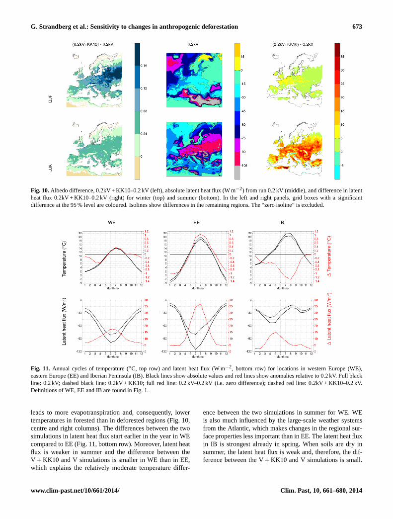
Fig. 10.Albedo difference, 0.2kV + KK10–0.2 kV (left), absolute latent heat flux (W m−2) from run 0.2 kV (middle), and difference in latentheat flux 0.2kV + KK10–0.2 kV (right) for winter (top) and summer (bottom). In the left and right panels, grid boxes with a significantdifference at the 95 % level are coloured. Isolines show differences in the remaining regions. The “zero isoline” is excluded.

Fig. 11. Annual cycles of temperature (◦C, top row) and latent heat flux (W m−2, bottom row) for locations in western Europe (WE),eastern Europe (EE) and Iberian Peninsula (IB). Black lines show absolute values and red lines show anomalies relative to 0.2 kV. Full blackline: 0.2 kV; dashed black line: 0.2kV + KK10; full red line: 0.2 kV–0.2 kV (i.e. zero difference); dashed red line: 0.2kV + KK10–0.2 kV.Definitions of WE, EE and IB are found in Fig. 1.

leads to more evapotranspiration and, consequently, lowertemperatures in forested than in deforested regions (Fig. 10,centre and right columns). The differences between the twosimulations in latent heat flux start earlier in the year in WEcompared to EE (Fig. 11, bottom row). Moreover, latent heatflux is weaker in summer and the difference between theV + KK10 and V simulations is smaller in WE than in EE,which explains the relatively moderate temperature differ-

ence between the two simulations in summer for WE. WEis also much influenced by the large-scale weather systemsfrom the Atlantic, which makes changes in the regional sur-face properties less important than in EE. The latent heat fluxin IB is strongest already in spring. When soils are dry insummer, the latent heat flux is weak and, therefore, the dif-ference between the V+ KK10 and V simulations is small.



In that case, the change in albedo dominates over the changein latent heat flux, leading to lower summer temperatures.

Differences in precipitation also correlate with differencesin latent heat flux (Figs. 8 and 10). Since differences in pre-cipitation are caused primarily by a change in convective pre-cipitation (not shown), it suggests that convective precipita-tion also changes as a result of deforestation. This would ex-plain that 0.2 k is drier in EE than 6 k in the V+ KK10 sim-ulations. Observations in the tropics have indeed shown thatregional deforestation decreases precipitation (Spracklen etal., 2012).

4 Discussion

4.1 Comparison of the RCA3-simulated regionalclimate with palaeoclimate reconstructions

Studies of diatoms (Korhola et al., 2000; Rosén et al., 2001;Bigler et al., 2006), tree rings (Grudd, 2002; Helama et al.,2002) and chironomids (Rosén et al., 2001; Bigler et al.,2003; Hammarlund et al., 2004; Laroque and Hall, 2004;Velle et al., 2005) indicate a 6–0.2 k difference in summertemperature of 0.5–2◦C in Scandinavia, which agrees withour simulations. Evidence from the presence of Mediter-ranean ostracods in the coastal waters of Denmark sug-gests that winter temperature at 6 k were up to 4–5◦C abovepresent (Vork and Thomsen, 1996). Proxy records of rela-tive precipitation indicate a drier climate at 6 k than at 0.2 kin Scandinavia (Digerfeldt, 1988; Ikonen, 1993; Snowballand Sandgren, 1996; Hammarlund et al., 2003; Borgmark,2005; Olsen et al., 2010), northern Germany (Niggeman etal., 2003) and the UK (Hughes et al., 2000), while there is nodetectable difference in the Alps (Magny, 2004). Our simu-lations show similar general features (Figs. 6 and 9). Unfor-tunately, quantitative proxy-based temperature estimates aremainly available for Scandinavia where differences betweenthe simulated climates with alternative land-use scenarios aresmall. Therefore, none of the simulated climates agrees sig-nificantly better with the proxies than the others.

In the Mediterranean region, independent non-pollenproxy-based data indicate contrasting patterns of palaeohy-drological changes between the regions north and south ofthe ca. 40◦ N latitude (Magny et al., 2013). The proxies im-ply that 6 k (0.2 k) were dry (wet) north of 40◦ and wet (dry)south of 40◦. The available data in the synthesis of Magnyet al. (2013) also suggest that these contrasting palaeohy-drological patterns operated throughout the Holocene, bothon millennial and centennial scales. Moreover, the combina-tion of lake-level records and fire data was shown to pro-vide information on the summer moisture availability. Firefrequency depends on the duration and intensity of the dryseason (Pausas, 2004; Vannière et al., 2011), while the mainproxies used in lake-level reconstructions are often relatedto precipitation during the warm season (dry in summer;

Magny, 2007). The fire records published by Vannière etal. (2011) indicate the same contrasting pattern between thenorth- and the south-western Mediterranean for the Mid-Holocene (including 6 k), with dry summers in the northand humid summers in the south. The evidence presented inMagny et al. (2013) suggests that, in response to centennial-scale cooling events, drier climatic conditions developed inthe south-central Mediterranean, while wetter conditions pre-vailed in the north-central Mediterranean. In general, the cen-tennial phases of higher lake-level conditions in west-centralEurope were shown to coincide with cooling events in theNorth Atlantic area (Bond et al., 2001; e.g. Magny, 2004,2007) and decreases in solar activity before 7 k, and with apossible combination of NAO-type circulation and solar forc-ing since ca. 7 k onwards.

The 6–0.2 k difference in the simulated climate is gener-ally small for all simulations (V, V+ H3.1 and V+ KK10)compared to the 6–0.2 k differences in the pollen-based cli-mate reconstructions (PB reconstructions). Moreover, thegeographical/spatial patterns of these 6–0.2 k differencesshow discrepancies between simulations and reconstructions(Fig. 6). The difference in summer temperatures ranges fromca. +1◦C in Scandinavia to ca.−2◦C in southern Europein the PB reconstructions, while it is ca.+2–3◦C in southernand central Europe and ca.+1◦C in northern and eastern Eu-rope in the RCA3 simulations. The difference in winter tem-peratures in the PB reconstructions ranges from ca.−3◦C insouthern Europe and ca.+3◦C in northern Europe, while theRCA3 simulations show a different pattern, with differencesranging from+2–3◦C in Scandinavia to around 0◦C in cen-tral Europe and ca.+1◦C in southern Europe. The differencein insolation in summer between 6 and 0.2 k is positive in allof Europe, but the difference is larger in northern Europe (seeFig. 2 in Wagner et al., 2007). When considering astronom-ical forcing alone, we would expect 6 k to be warmer than0.2 k and the temperature difference to be largest in summerin northern Europe. This is the signature we see in the modelsimulations. The non-pollen proxy based palaeoclimatic datapresented above and the pollen based reconstruction of Pey-ron et al. (2013) rather support the differences in summertemperatures simulated by RCA3 than the PB reconstructionof Mauri et al. (2013), in particular for southern and easternEurope. For the winter temperatures, we have no appropri-ate non-pollen proxy based data to evaluate the RCA3 andPB results. Of the three RCA3 simulations, the V+ KK10 isthe one that is closest to the PB reconstruction, which wouldimply that the description of land cover V+ KK10 is closestto the actual vegetation at 0.2 k and therefore the V+ KK10simulated climate is closer to the PB reconstruction.

The RCA3 simulations and the PB reconstructions bothshow a drier climate in summer at 6 k than at 0.2 k in north-ern and western Europe and a wetter climate in south-easternEurope, but they disagree in eastern/north-eastern Europewhere the RCA3 simulations indicate drier summer condi-tions at 6 k than at 0.2 k, while the PB reconstructions show



wetter summer conditions at 6 k than at 0.2 k (Fig. 9). Interms of winter precipitation, the RCA3 simulations and thePB reconstructions display entirely different results. Accord-ing to RCA3, winter precipitation is not significantly differ-ent between 6 and 0.2 k in most of Europe, while the PB re-constructions indicate wetter conditions at 6 k than at 0.2 k incentral and eastern Europe and drier in western Europe. Wehave no quantitative proxy records (other than pollen-basedreconstructions) available to evaluate the RCA3 results forsummer temperatures in eastern Europe and winter precipi-tation in the entire study region.

The two climate regions identified by Magny et al. (2013)are not seen in the PB reconstructions of Mauri et al. (2013)and the RCA3 simulations, except for a weak pattern of con-trasting summer temperatures on both side of latitude 40◦ Nin the RCA3 simulations. However, it should be noted that6 k is within the transition period (6.4–4.5 k) between the twoclimate regimes before and after 4.5 k described by Magnyet al. (2013), which may explain that the patterns around 6 kare difficult to capture both by the climate model and thePB reconstructions. Also, there is a general problem of ac-curately disentangling multiple climatic variables from thefossil pollen data, which causes uncertainties in the PB re-construction. Further, there is no equivalent in the non-pollenproxy-based palaeoclimatic records to the PB reconstructionof Mauri et al. (2013) in terms of higher winter precipitationsat 6 k than at 0.2 k in eastern Europe north of 40◦ N.

The comparison between climate model simulations andpollen-based palaeoclimate data indicates that discrepanciesoccur in the geographical patterns of the differences in cli-mate between 6 and 0.2 k. This is particularly clear for tem-peratures in southern Europe, where model and proxies ex-hibit opposite signs of the difference in temperature, andfor winter precipitation, where reconstructions exhibit muchlarger differences than the RCA3 simulations (Figs. 6 and 9).A wetter summer in western central Europe at 0.2 k than at6 k is in better agreement with the non-pollen proxy records(e.g. in the Jura mountains; Magny et al., 2013) than a drierwestern central Europe as indicated in the PB reconstruction.

As the differences between the three model simulations (V,V + H3.1 and V+ KK10) are generally smaller than the dif-ferences between the model simulations and the pollen-basedreconstructions of past climate, it is not possible to identifythe vegetation description (V, V+ H3.1 or V+ KK10) thatprovides the most coherent simulated climate for Europe at 6and 0.2 k.

4.2 Model simulations in a wider perspective

In this study, we use boundary conditions provided by theGCM ECHO-G. ECHO-G is one of many GCMs and the useof boundary conditions from another GCM may give differ-ent RCA3 results. Moreover, a different realisation of the cli-mate with ECHO-G would likely result in a different RCA3output as the impact of internal variability is large (Deser et

al., 2012). In order to assess to what degree our results mightbe biased by the choice of one single GCM realisation, wecompare our results with an ensemble of PMIP models. Thisensemble represents uncertainties related both to the choiceof GCM and to internal variability as each GCM starts withits own initial conditions. Figure 12 shows temperature dif-ference versus precipitation difference (6–0.2 k) for 7 PMIPGCMs, ECHO-G and RCA3. The differences are calculatedfor two large regions that are resolved at the scale of theGCMs, northern Europe (5–50◦ E, 55–70◦ N) and southernEurope (10◦ W–50◦ E, 35–55◦ N) (blue boxes in Fig. 1). Allmodel results share common features, but show some dif-ferences; the spread between models is largest in summerprecipitation and winter temperature in northern Europe, andsmallest in winter precipitation in southern Europe.

RCA3 follows ECHO-G to some extent, with the excep-tion of summer precipitation in northern Europe. The land–sea distribution in the RCA3 simulations differs between 6and 0.2 k (Fig. 1) with some grid boxes being sea at 6 kand land at 0.2 k. This difference leads to more convectiveprecipitation at 0.2 k than at 6 k for these coastal regions(cf. Fig. 9). A similar effect is seen along the coast of theMediterranean Sea. In ECHO-G the land–sea distribution isconstant through time. Thus, for some coastal areas, the pre-cipitation difference between 6 and 0.2 k is negative in theRCA3 simulation and positive in the ECHO-G simulation.

The choice of another GCM would obviously provide dif-ferent results, but the difference is difficult to quantify. It isnot obvious that the choice of another GCM would lead togenerally larger or smaller temperature and precipitation dif-ferences. Furthermore, RCA3 partly produces its “own” cli-mate. Interestingly enough, all of the GCMs show positivesummer temperature differences between 6 and 0.2 k. It in-dicates that the temperature differences are positive in themodel simulations as a result of the higher summer inso-lation at 6 k than at 0.2 k. For northern Europe, the pollen-based palaeoclimate reconstructions discussed above as wellas all quantitative and qualitative temperature reconstructionsbased on other palaeoecological records than pollen indicatewarmer conditions at 6k than at 0.2 k, in agreement withthe GCMs. For southern Europe, climate model simulationsand pollen-based reconstructions display different signs ofthe difference. The difference in signal between the GCMs(and RCA3) and the palaeoclimate reconstruction indicateseither an alternative forcing offsetting the insolation differ-ences or the influence of natural variability caused by cir-culation changes, which would yield a negative temperaturedifference between 6 and 0.2 k in southern Europe, i.e. lowertemperatures at 6 k than at 0.2 k.

4.3 Comparison with other studies of land cover –climate interactions

For past climate, studies conducted with global modelsat a coarse spatial resolution show that the albedo effect



Fig. 12. Difference in temperature (1T ) and precipitation (1P ) between 6 and 0.2 k BP in winter (left) and summer (right) in northernEurope (top) and southern Europe (bottom). The results from GCMs are shown as coloured squares, and the result from the regional climatemodel RCA3 as a circle.

dominates over the other biogeophysical effects leading to acolder climate when deforestation increases in the NorthernHemisphere (e.g. Jahn et al., 2005; Brovkin et al., 2006; Pit-man et al., 2009; Pongratz et al., 2009a; Goosse et al., 2012,He et al., 2014). Other experimental climate model studieswith simulated deforestation in large parts of the globe showa similar effect on global mean temperature (Kleidon et al.,2000). Some studies have also shown regional differences inthe effects of deforestation on climate, but the results fromchanging heat fluxes are described as ambiguous (Pitman etal., 2009) or hard to evaluate (Goosse et al., 2012).

Our results show that the albedo effect is indeed a majorprocess in the vegetation–climate interactions, and they alsoprovide a more detailed understanding of the relative impor-tance of different biogeophysical processes. We show thatland-cover changes can have significant effects on the simu-lated climate and be a driver of climate change at the regionalscale. The albedo effect dominates in winter, especially inregions with a relatively long snow season. In summer, thealbedo effect dominates in some regions, while changes inlatent heat fluxes are more important in other regions. Thedifferences in the importance of the various biogeophysicalprocesses depend on the land-cover descriptions used and lo-cal geographical characteristics.

5 Conclusions

This study demonstrates that past European anthropogenicland-cover changes prior to AD 1850 were large enough toinfluence the regional climate. The temperature response var-

ied by±1◦C in summer depending on local/regional charac-teristics that can only be captured by high-resolution climatemodels such as RCA3.

The differences in simulated climate depend mainly onchanges in the albedo and latent heat flux due to changes invegetation cover. Which of the biogeophysical processes willbe dominant depends on local/regional climate and vegeta-tion characteristics. The results show that the effect of albedodominates in winter, but that latent heat flux also plays animportant role with regard to the differences in simulated cli-mate in summer. Therefore, a comprehensive model includ-ing these effects is required in order to study effects of chang-ing land cover on climate. At 6 k the differences betweenthe land-cover descriptions (V, V+ H3.1 or V+ KK10) aresmall, leading to little difference between the simulated cli-mates. At 0.2 k the differences between the land-cover de-scriptions are large enough to result in significantly differ-ent simulated climates. Depending on the estimate of defor-estation, the difference between simulations varies in someregions between−1 and 0◦C in seasonal mean winter tem-perature,−1 and 1◦C in summer temperature and−30 and0 mm month−1 in summer precipitation.

Even though the difference in climate is significant be-tween simulations using different land-cover descriptions (V,V + H3.1 or V+ KK10), it is not possible to assess whichland-cover description is the most reasonable on the basis ofa comparison of modelled climate with palaeoclimate recon-structions. This is because the uncertainties of the palaeocli-mate reconstructions and the differences between them areat least as large as the differences between the climate sim-ulations at both 6 and 0.2 k. Nevertheless, it is clear that



vegetation cover plays an important role in the regional cli-mate and that a dynamic vegetation description is essential inregional climate modelling. The present study demonstratesthat reliable reconstructions of past vegetation are necessaryfor a better understanding of past land cover–climate rela-tionships in order to assess the role of changes in land coverin present and future climate change. Therefore, future re-search should include both evaluation of ALCC scenariosand the potential natural vegetation simulated by vegetationmodels using, for example, pollen-based methods such asthe REVEALS reconstruction for NW Europe (Kaplan et al.,2014; Marquer et al., 2014).

In future modelling efforts, it will also be important tostudy the indirect effects from increasing atmospheric CO2(He et al., 2014), and a model-ensembles approach wouldbe useful. This study shows that the choice of another GCMwould provide overall similar results, but multiple simula-tions may help to distinguish the climate change signal fromnatural variability and to better quantify uncertainties.

Acknowledgements.All model simulations with the RCM wereperformed on the Swedish climate computing resources Gimle andVagn funded with a grant from the Knut and Alice Wallenbergfoundation. Qiong Zhang helped collecting PMIP data. This studyis a part of the LANDCLIM (LAND cover–CLIMate interactionsin NW Europe during the Holocene) project and research networkcoordinated by M.-J. Gaillard and sponsored by the Swedish Re-search Council [VR], the Nordic Council of Ministers [NordForsk]and MERGE (see below). It is also a contribution to the Swedishstrategic research areas ModElling the Regional and Global Earthsystem (MERGE) and Biodiversity and Ecosystem Services in aChanging Climate (BECC).

Edited by: V. Rath

References

Bala, G., Caldeira, K., Wickett, M., Phillips, T. J., Lobell, D. B.,Delire, C., and Mirin, A.: Combined climate and carbon-cycleeffects of large-scale deforestation, Proc. Natl. Acad. Sci., 104,6550–6555, doi:10.1073/pnas.0608998104, 2007.

Ban-Weiss, G. A., Bala, G., Cao, L., Pongratz, J., and Caldeira,K.: Climate forcing and response to idealized changes in sur-face latent and sensible heat, Environ. Res. Lett., 6, 034032,doi:10.1088/1748-9326/6/3/034032, 2011.

Bartlein, P. J., Harrison, S. P., Brewer, S., Connor, S., Davis, B. A.S., Gajewski, K., Guiot, J., Harrison-Prentice, T. I., Henderson,A., Peyron, O., Prentice, I. C., Scholze, M., Seppä, H., Shuman,B., Sugita, S., Thompson, R. S., Viau, A. E., Williams, J., andWu, H.: Pollen-based continental climate reconstructions at 6 and21 ka: a global synthesis, Clim. Dynam., 37, 775–802, 2010.

Berger, A. and Loutre, M. F.: Insolation values for the climate of thelast 10 million years, Quaternary Sci. Rev., 10, 29–317, 1991.

Bigler, C., Grahn, E., Larocque, I., Jeziorski, A., and Hall, R.:Holocene environmental change at Lake Njulla (999 m a.s.l.),

northern Sweden: a comparison with four small nearby lakesalong an altitudinal gradient, J. Paleolimnol., 29, 13–29, 2003.

Bigler, C., Barnekow, L., Heinrichs, M. L., and Hall, R. I.: Holoceneenvironmental history of Lake Vuolop Njakajaure (Abisko Na-tional Park, northern Sweden) reconstructed using biologicalproxy indicators, Veget. Hist. Archaebot., 15, 309–320, 2006.

Bond, G., Kromer, B., Beer, J., Muscheler, R., Evans, M. N., Show-ers, W., Hoffmann, S., Lotti-Bond, R., Hajdas, I., and Bonani,G.: Persistent solar influence on North Atlantic climate duringthe Holocene, Science, 294, 2130–2136, 2001.

Borgmark, A.: Holocene climate variability and periodicities insouth-central Sweden interpreted from peat humification analy-sis, Holocene, 15, 387–395, 2005.

Boyle, J. F., Gaillard, M.-J., Kaplan, J. O., and Dearing, J. A.: Mod-elling prehistoric land use and carbon budgets: A critical review,Holocene, 21, 715–722, 2011.

Brovkin, V., Claussen, M., Driesschaert, E., Fichefet, T., Kick-lighter, D., Loutre, M. F., Matthews, H. D., Ramankutty, N.,Schaeffer, M., and Sokolov, A.: Biogeophysical effects of his-torical land cover changes simulated by six Earth system mod-els of intermediate complexity, Clim. Dynam., 26, 587–600,doi:10.1007/s00382-005-0092-6, 2006.

Christidis, N., Stott, P. A., Hegerl, G. C., and Betts, R. A.:The role of land use change in the recent warming ofdaily extreme temperatures, Geophys. Res. Lett., 40, 589–594,doi:10.1002/grl.50159, 2013.

Davis, B. A. S., Brewer, S., Stevenson, A. C., and Guiot, J.: Thetemperature of Europe during the Holocene reconstructed frompollen data, Quaternary Sci. Rev., 22, 1701–1716, 2003.

Davis, B. A. S., Zanon, M., Collins, P., Mauri, A., Bakker, J., Bar-boni, D., Barthelmes, A., Beaudouin, C., Bjune, A. E., Bozilova,E., Bradshaw, R. H. W., Brayshay, B. A., Brewer, S., Brugia-paglia, E., Bunting, J., Connor, S. E., Beaulieu, J.-L., Edwards,K., Ejarque, A., Fall, P., Florenzano, A., Fyfe, R., Galop, D.,Giardini, M., Giesecke, T., Grant, M. J., Guiot, J., Jahns, S.,Jankovská, V., Juggins, S., Kahrmann, M., Karpinska-Kołaczek,M., Kołaczek, P., Kühl, N., Kuneš, P., Lapteva, E. G., Leroy,S. A. G., Leydet, M., López Sáez, J. A., Masi, A., Matthias,I., Mazier, F., Meltsov, V., Mercuri, A. M., Miras, Y., Mitchell,F. J. G., Morris, J. L., Naughton, F., Nielsen, A. B., Novenko,E., Odgaard, B., Ortu, E., Overballe-Petersen, M. V., Pardoe, H.S., Peglar, S. M., Pidek, I. A., Sadori, L., Seppä, H., Severova,E., Shaw, H.,Swieta-Musznicka, J., Theuerkauf, M., Tonkov,S., Veski, S., Knaap, W. O., Leeuwen, J. F. N., Woodbridge,J., Zimny, M., and Kaplan, J. O.: The European Modern PollenDatabase (EMPD) project, Veget. Hist. Archaeobot., 22, 521–530, doi:10.1007/s00334-012-0388-5, 2013.

De Noblet-Ducoudré, N., Boisier, J.-P., Pitman, A., Bonan, G. B.,Brovkin, V., Cruz, F., Delire, C., Gayler, V., van den Hurk, B.J. J. M., Lawrence, P. J., van der Molen, M. K., Müller, C.,Reick, C. H., Strengers, B. J., and Voldoire, A.: DeterminingRobust Impacts of Land-Use-Induced Land Cover Changes onSurface Climate over North America and Eurasia: Results fromthe First Set of LUCID Experiments, J. Climate, 25, 3261–3281,doi:10.1175/JCLI-D-11-00338.1, 2012

Deser, C., Knutti, R., Solomon, S., and Phillips A. S.: Com-munication of the role of natural variability in futureNorth American climate, Nat. Clim. Change, 2, 775–779,doi:10.1038/nclimate1562, 2012.


http://dx.doi.org/10.1073/pnas.0608998104

http://dx.doi.org/10.1088/1748-9326/6/3/034032

http://dx.doi.org/10.1007/s00382-005-0092-6

http://dx.doi.org/10.1002/grl.50159

http://dx.doi.org/10.1007/s00334-012-0388-5

http://dx.doi.org/10.1175/JCLI-D-11-00338.1

http://dx.doi.org/10.1038/nclimate1562


Digerfeldt, G.: Reconstruction and regional correlation of Holocenelake-level fluctuations in Lake Bysjön, South Sweden, Boreas,17, 165–182, 1998.

Efron, B.: Bootstrap methods: Another look at the jackknife, Ann.Statist., 7, 1–26, 1979.

Flückiger, J., Monnin, E., Stauffer, B., Schwander, J., Stocker,T., Chappellaz, J., Raynaud, D., and Barnola, J. M.: Highresolution Holocene N2O ice core record and its relationshipwith CH4 and CO2, Global Biogeochem. Cy., 16, 10-1–10-8,doi:10.1029/2001GB001417, 2002.

Forster, P., Ramaswamy, V., Artaxo, P., Berntsen, T., Betts, R., Fa-hey, D. W., Haywood, J., Lean, J., Lowe, D. C., Myhre, G.,Nganga, J., Prinn, R., Raga, G., Schulz, M., and Van Dorland, R.:Radiative forcing of climate change, in: Climate Change 2007:The Physical Science Basis. Contribution of Working Group I tothe Fourth Assessment Report of the Intergovernmental Panel onClimate Change, edited by: Solomon, S., Qin, D., Manning, M.,Chen, Z., Marquis, M., Averyt, K. B., Tignor, M., and Miller, H.L., Cambridge and New York, NY, Cambridge University Press,129–234, 2007.

Gaillard, M.-J.: Archaeological Applications, in: The Encyclopediaof Quaternary Science 3, edited by: Elias S. A., Elsevier, Ams-terdam, 880–904, 2013.

Gaillard, M.-J., Sugita, S., Mazier, F., Trondman, A.-K., Broström,A., Hickler, T., Kaplan, J. O., Kjellström, E., Kokfelt, U., Kuneš,P., Lemmen, C., Miller, P., Olofsson, J., Poska, A., Rundgren,M., Smith, B., Strandberg, G., Fyfe, R., Nielsen, A. B., Ale-nius, T., Balakauskas, L., Barnekow, L., Birks, H. J. B., Bjune,A., Björkman, L., Giesecke, T., Hjelle, K., Kalnina, L., Kan-gur, M., van der Knaap, W. O., Koff, T., Lagerås, P., Latałowa,M., Leydet, M., Lechterbeck, J., Lindbladh, M., Odgaard, B.,Peglar, S., Segerström, U., von Stedingk, H., and Seppä, H.:Holocene land cover reconstructions for studies on land cover-climate feedbacks, Clim. Past, 6, 483–499, doi:10.5194/cp-6-483-2010, 2010.

Giorgi, F. and Mearns, L. O.: Introduction to special section: Re-gional climate modelling revisited, J. Geophys. Res., 104, 6335–6352, 1999.

Gómez-Navarro, J. J., Montávez, J. P., Jerez, S., Jiménez-Guerrero,P., Lorente-Plazas, R., González-Rouco, J. F., and Zorita, E.: Aregional climate simulation over the Iberian Peninsula for the lastmillennium, Clim. Past, 7, 451–472, doi:10.5194/cp-7-451-2011,2011.

Gómez-Navarro, J. J., Montávez, J. P., Jiménez-Guerrero, P., Jerez,S., Lorente-Plazas, R., González-Rouco, J. F., and Zorita, E.:Internal and external variability in regional simulations of theIberian Peninsula climate over the last millennium, Clim. Past,8, 25–36, doi:10.5194/cp-8-25-2012, 2012.

Goosse, H., Guiot, J., Mann, M. E., Dubinkina, S., and Sal-laz.Damaz, Y.: The medieval climate anomaly in Europe: Com-parison of the summer and annual mean signals in two re-constructions and in simulations with data assimilation, GlobalPlanet. Change, 84–85, 35–47, 2012.

Graham, L. P., Olsson, J., Kjellström, E., Rosberg, J., Hellström,S.-S., and Berndtsson, R.: Simulating river flow to the Baltic Seafrom climate simulations over the past millennium, Boreal Envi-ron. Res., 14, 173–182, 2009.

Grudd, H.: A 7400-year tree-ring chronology in northern SwedishLapland: natural climatic variability expressed on annual to mil-lenial timescales, Holocene, 12, 657–665, 2002.

Hammarlund, D., Björck, S., Buchardt, B., Israelson, C., and Thom-sen, C. T.: Rapid hydrological changes during the Holocene re-vealed by stable isotope records of lacustrine carbonates fromLake Igelsjön, southern Sweden, Quaternary Sci. Rev., 22, 353–370, 2003.

Hammarlund, D., Velle, G., Wolfe, B. B., Edwards, T. W. D.,Barnekow, L., Bergman, J., Holmgren, S., Lamme, S., Snowball,I., Wohlfarth, B., and Possnert, G.: Palaeolimnological responsesto Holocene forest retreat in the Scandes Mountains, west-centralSweden, Holocene, 14, 862–876, 2004.

Harrison, S. P., Jolly, D., Laarif, F., Abe-Ouchi, A., Dong, B., Her-terich, K., Hewitt, C., Joussaume, S., Kutzbach, J. E., Mitchell,J., de Noblet, N., and Valdes, P.: Intercomparison of SimulatedGlobal Vegetation Distributions in Response to 6 kyr BP OrbitalForcing, J. Climate, 11, 2721–2742, 1998.

He, F., Vavrus, S. J., Kutzbach, J. E., Ruddiman, W. F., Ka-plan, J. O., and Krumhardt, K. M.: Simulating global andlocal surface temperature changes due to Holocene anthro-pogenic land cover change, Geophys. Res. Lett., 41, 623–631,doi:10.1002/2013GL058085, 2014.

Helama, S., Lindholm, M., Timonen, M., Meriläinen, J., and Ero-nen, M.: The supra-long Scots pine tree-ring record for FinnishLapland. Part 2: Interannual to centennial variability in summertemperatures for 7500 years, The Holocene, 12, 681–687, 2002.

Hickler, T., Smith, B., Sykes, M. T., Davis, M. B., Sugita, S. andWalker, K.: Using a generalized vegetation model to simulatevegetation dynamics in northeastern USA, Ecology, 85, 519–530, 2004.

Hickler, T., Vohland, K., Feehan, J., Miller, P. A., Smith, B., Costa,L., Giesecke, T., Fronzek, S., Carter, T. R., Cramer, W., Kühn,I., and Sykes, M. T.: Projecting the future distribution of Eu-ropean potential natural vegetation zones with a generalized,tree species-based dynamic vegetation model, Global Ecol. Bio-geogr., 21, 50–63, 2012.

Hughes, P. D. M., Barber, K. E., Langdon, P. G., and Mauquoy, D.:Mire-development pathways and palaeoclimatic records from afull Holocene peat archive at Walton Moss, Cumbria, England,Holocene, 10, 465–479, 2000.

HYDE: available at: http://themasites.pbl.nl/en/themasites/hyde/download/index.html(last access: 13 December 2011), 2011.

Ikonen, L.: Holocene development and peat growth of the raisedbog Pesänsuo in southwestern Finland, Bulletin, Vol. 370, Geo-logical Survey of Finland, Espoo, 1993.

Jahn, A., Claussen, M., Ganopolski, A., and Brovkin, V.: Quantify-ing the effect of vegetation dynamics on the climate of the LastGlacial Maximum, Clim. Past, 1, 1–7, doi:10.5194/cp-1-1-2005,2005.

Kaplan, J., Krumhardt, K., and Zimmermann, N.: The prehistoricand preindustrial deforestation of Europe, Quaternary Sci. Rev.,28, 3016–3034, 2009.

Kaplan, J. O., Krumhardt, K. M., Ellis, E. C., Ruddiman, W. F.,Lemmen, C. and Goldewijk, K. K.: Holocene carbon emissionsas a result of anthropogenic land cover change, The Holocene,21, 775–791, doi:10.1177/0959683610386983, 2011.

Kaplan, J. O., Krumhardt, K. M., Gaillard, M.-J., Sugita, S.,Trondman, A.-K., and Mazier, F.: The deforestation history of


http://dx.doi.org/10.1029/2001GB001417

http://dx.doi.org/10.5194/cp-6-483-2010

http://dx.doi.org/10.5194/cp-6-483-2010

http://dx.doi.org/10.5194/cp-7-451-2011

http://dx.doi.org/10.5194/cp-8-25-2012

http://dx.doi.org/10.1002/2013GL058085

http://themasites.pbl.nl/en/themasites/hyde/download/index.html

http://themasites.pbl.nl/en/themasites/hyde/download/index.html

http://dx.doi.org/10.5194/cp-1-1-2005

http://dx.doi.org/10.1177/0959683610386983


northwest Europe: Evaluating anthropogenic land cover changescenarios with pollen-based landscape reconstructions, in prepa-ration, 2014.

Kaspar, F., Spangehl, T., and Cubasch, U.: Northern hemispherewinter storm tracks of the Eemian interglacial and the last glacialinception, Clim. Past, 3, 181–192, doi:10.5194/cp-3-5 181-2007,2007.

Kjellström, E., Brandefelt, J., Näslund, J. O., Smith, B., Strandberg,G., Voelker, A. H. L., and Wohlfarth, B.: Simulated climate con-ditions in Fennoscandia during a MIS 3 stadial, Boreas, 10, 436–456, doi:10.1111/j.1502-3885.2010.00143.x, 2010

Kjellström, E., Nikulin, G., Hansson, U., Strandberg, G., and Uller-stig, A.: 21st century changes in the European climate: uncertain-ties derived from an ensemble of regional climate model simula-tions, Tellus A, 63, 24–40, 2011.

Kleidon, A., Fraedrich, K., and Heimann, M.: A green planet versusa desert world: Estimating the maximum effect of vegetation onthe land surface climate, Clim. Change, 44, 471–493, 2000.

Klein Goldewijk, K., Beusen, A., de Vos, M., and van Drecht, G.:The HYDE 3.1 spatially explicit database of human induced landuse change over the past 12,000 years, Global Ecol. Biogeogr.,20, 73–86, 2011.

Kohfeld, K. E. and Harrison, S. P.: How well can we simulate pastclimates? Evaluating the models using global palaeoenvironmen-tal datasets, Quaternary Sci. Rev., 19, 321–346, 2000.

Korhola, A., Weckström, J., Holmström, L., and Erästö, P.: Aquantitative Holocene climatic record from diatoms in northernFennoscandia, Quaternary Res., 54, 284–294, 2000.

Laroque, I. and Hall, R. I.: Holocene temperature estimates and chi-ronomid community composition in the Abisko valley, northernSweden, Quaternary Sci. Rev., 23, 2453–2465, 2004.

Legutke, S. and Voss, R.: The Hamburg atmosphere-ocean cou-pled circulation model ECHOG, DKRZ-Report, German ClimateComputer Centre (DKRZ), Hamburg, Germany, 1999.

Magny, M.: Holocene climate variability as reflected by mid-European lake-level fluctuations and its probable impact on pre-historic human settlements, Quaternary Int., 113, 65–79, 2004.

Magny, M.: Holocene fluctuations of lake levels in west-centralEurope: methods of reconstruction, regional pattern, palaeocli-matic significance and forcing factors, Encyclopedia of Quater-nary Science, edited by: Elias, S., Elsevier, Oxford, 1389–1399,2007.

Magny, M. and Combourieu Nebout, N.: Holocene changes inenvironment and climate in the central Mediterranean as re-flected by lake and marine records, Clim. Past, 9, 1447–1454,doi:10.5194/cp-9-1447-2013, 2013.

Magny, M., Combourieu+Nebout, N., de Beaulieu, J. L., Bout-Roumazeilles, V., Colombaroli, D., Desprat, S., Francke, A.,Joannin, S., Ortu, E., Peyron, O., Revel, M., Sadori, L., Siani, G.,Sicre, M. A., Samartin, S., Simonneau, A., Tinner, W., Vannière,B., Wagner, B., Zanchetta, G., Anselmetti, F., Brugiapaglia, E.,Chapron, E., Debret, M., Desmet, M., Didier, J., Essallami, L.,Galop, D., Gilli, A., Haas, J. N., Kallel, N., Millet, L., Stock,A., Turon, J. L., and Wirth, S.: North-south palaeohydrologicalcontrasts in the central Mediterranean during the Holocene: ten-tative synthesis and working hypotheses, Clim. Past, 9, 2043–2071, doi:10.5194/cp-9-2043-2013, 2013.

Marquer, L., Gaillard, M.-J., Sugita, S., Poska, A., Trondman, A.-K., Mazier, F., Nielsen, A. B., Fyfe, R. M., Kaplan, J. O., Vad

Odgaard, B., Smith, B., Alenius, T., Birks, H. J. B., Bjune, A.E., Christiansen, J., Dodson, J., Edwards, K. J., Giesecke, T.,Herzschuh, U., Kangur, M., Koff, T., Latałowa, M., Lechter-beck, J., Lorenz, S., Schultr, M., and Seppä, H.: Climate andhuman-induced changes in Holocene plant diversity and ecologyin western/central and northern Europe: new insights based onland-cover reconstruction and modelling, in preparation, 2014.

Masson, V., Cheddadi, R., Braconnot, P., Joussaume, S., Texier, D.,and PMIP participants: Mid-Holocene climate in Europe: whatcan we infer from PMIP model-data comparisons?, Clim. Dy-nam., 15, 163–182, 1999.

Mauri, A., Davis, B. A. S., Collins, P. M., and Kaplan, J. O.: Theinfluence of atmospheric circulation on the mid-Holocene cli-mate of Europe: a data-model comparison, Clim. Past Discuss.,9, 5569–5592, doi:10.5194/cpd-9-5569-2013, 2013.

Nielsen, A. B., Kokfelt, U., Rundgren, M., and Gaillard, M.-J.: Areview of proxy based climate reconstructions for Northwest Eu-rope in the time slices 6000 BP and 200 BP, in preparation, 2014.

Niggeman, S., Mangini, A., Richter, D. K., and Wurth, G.: A paleo-climate record of the last 17.600 years from the B7 cave, Sauer-land, Germany, Quaternary Sci. Rev., 22, 555–567, 2003.

Nikulin, G., Kjellström, E., Hansson, U., Strandberg, G., and Uller-stig, A.: Evaluation and future projections of temperature, precip-itation and wind extremes over Europe in an ensemble of regionalclimate simulations, Tellus A, 63, 41–55, 2011.

Olofsson, J.: The Earth – climate and anthropogenic interactions ina long time perspective, PhD-thesis, Dept of Physical Geographyand Ecosystem Science, Lund, 2013.

Olofsson, J. and Hickler, T.: Effects of human land-use on theglobal carbon cycle during the last 6,000 years, Veget. Hist. Ar-chaeobot., 17, 606–615, 2008.

Olsen, J., Noe-Nygaard, N., and Wolfe, B. B.: Mid to Late Holoceneclimate variability and anthropogenic impacts; multi-proxy evi-dence from lake Bliden, Denmark, J. Paleolimnol., 43, 323–343,2010.

Pausas, J. G.: Changes in fire and climate in the eastern IberianPeninsula (Mediterranean basin), Clim. Change, 63, 337–350,2004.

Peltier, W. R.: Global glacial isostasy and the surface of the ice-agecirculation. Earth: The ICE-5G (VM2) model and GRACE, Ann.Rev. Earth Planet. Sci., 32, 111–149, 2004.

Peyron, O., Guiot, J., Cheddadi, R., Tarasov, P., Reille, M., deBeaulieu, J.-L., Bottema, S., and Andrieu, V.: Climatic Recon-struction in Europe for 18,000 YR B.P. from Pollen Data, Qua-ternary Res., 49, 183–196, 1998.

Peyron, O., Magny, M., Goring, S., Joannin, S., de Beaulieu, J.-L., Brugiapaglia, E., Sadori, L., Garfi, G., Kouli, K., Ioakim,C., and Combourieu-Nebout, N.: Contrasting patterns of cli-matic changes during the Holocene across the Italian Penin-sula reconstructed from pollen data, Clim. Past, 9, 1233–1252,doi:10.5194/cp-9-1233-2013, 2013.

Pielke Sr., R. A., Pitman, A., Niyogi, D., Mahmood, R., McAlpine,C., Hossain, F., Klein Goldewijk, K., Nair, U., Betts, R., Fall, S.,Reichstein, M., Kabat, P., and de Noblet, N.: Land use/land coverchanges and climate: modeling analysis and observational evi-dence, WIREs Clim. Change, 2, 828–850, doi:10.1002/wcc.144,2011.

Pitman, A. J., de Noblet-Ducoudre, N., Cruz, F. T., Davin, E. L.,Bonan, G. B., Brovkin, V. Claussen, M., Delire, C., Ganzeveld,


http://dx.doi.org/10.5194/cp-3-5 181-2007

http://dx.doi.org/10.1111/j.1502-3885.2010.00143.x

http://dx.doi.org/10.5194/cp-9-1447-2013

http://dx.doi.org/10.5194/cp-9-2043-2013

http://dx.doi.org/10.5194/cpd-9-5569-2013

http://dx.doi.org/10.5194/cp-9-1233-2013

http://dx.doi.org/10.1002/wcc.144


L., Gayler, V., van den Hurk, B. J. J. M., Lawrence, P. J., vander Molen, M. K., Muller, C., Reick, C. H., Seneviratne, S. I.,Strengers, B. J., and Voldoire, A.: Uncertainties in climate re-sponses to past land cover change: First results from the LU-CID intercomparison study, Geophys. Res. Lett., 36, L14814,doi:10.1029/2009GL039076, 2009.

Pongratz, J., Raddatz, T., Reick, C. H., Esch, M., andClaussen, M.: Radiative forcing from anthropogenic land coverchange since A.D. 800, Geophys. Res. Lett., 36, L02709,doi:10.1029/2008GL036394, 2009a.

Pongratz, J., Reick, C. H., Raddatz, T., and Claussen, M.: Ef-fects of anthropogenic land cover change on the carbon cycleof the last millennium, Global Biogeochem. Cy., 23, GB4001,doi:10.1029/2009GB003488, 2009b.

Pongratz, J., Reick, C. H., Raddatz, T., and Claussen, M.: Biogeo-physical versus biogeochemical climate response to historical an-thropogenic land cover change, Geophys. Res. Lett., 37, L08702,doi:10.1029/2010GL043010, 2010.

Prentice, I. C., Guiot, J., Huntley, B., Jolly, D., and Cheddadi, R.:Reconstructing biomes from palaeoecological data: a generalmethod and its application to European pollen data at 0 and 6ka, Clim. Dynam., 12, 185–194, 1996.

Räisänen, J., Hansson, U., Ullerstig, A., Döscher, R., Graham, L. P.,Jones, C., Meier, H. E. M., Samuelsson, P., and Willén, U: Euro-pean climate in the late twenty-first century: regional simulationswith two driving global models and two forcing scenarios, Clim.Dynam., 22, 13–31, 2004.

Rosén, P., Segerström, U., Eriksson, L., Renberg, I., and Birks,H. J. B.: Holocene climatic change reconstructed from diatoms,chironomids, pollen and near-infrared spectroscopy at an alpinelake (Sjuodjijaure) in northern Sweden, Holocene, 11, 551–562,2001.

Ruddiman, W. F.: The anthropogenic greenhouse era began thou-sands of years ago, Clim. Change, 61, 261–293, 2003.

Rummukainen, M.: State-of-the-art with regional climate models,WIREs Clim. Change, 1, 82–96, doi:10.1002/wcc.8, 2010

Rummukainen, M., Räisänen, J., Bringfelt, B., Ullerstig, A., Om-stedt, A., Willén, U., Hansson, U., Jones, C., and Jones, C.: Aregional climate model for northern Europe: model descriptionand results from the downscaling of two GCM control simula-tions, Clim. Dynam., 17, 339–359, 2001.

Samuelsson, P., Jones, C. G., Willen, U., Ullerstig, A., Gol-lvik, S., Hansson, U., Jansson, C., Kjellström, E., Nikulin, G.,and Wyser, K.: The Rossby Centre regional climate modelRCA3: model description and performance, Tellus A, 63, 4–23,doi:10.1111/j.1600-0870.2010.00478.x, 2011.

Schimanke, S., Meier, H. E. M., Kjellström, E., Strandberg, G., andHordoir, R.: The climate in the Baltic Sea region during the lastmillennium simulated with a regional climate model, Clim. Past,8, 1419–1433, doi:10.5194/cp-8-1419-2012, 2012.

Sitch, S., Smith, B., Prentice, I.C., Arneth, A., Bondeau, A., Cramer,W., Kaplan, J. O., Levis, S., Lucht, W., Sykes, M. T., Thonicke,K., and Venevsky, S.: Evaluation of ecosystem dynamics, plantgeography and terrestrial carbon cycling in the LPJ dynamicglobal vegetation model, Global Change Biol., 9, 161–185, 2003.

Smith, B., Prentice, I. C., and Sykes, M. T.: Representation of vege-tation dynamics in modelling of terrestrial ecosystems: compar-ing two contrasting approaches within European climate space,Global Ecol. Biogeogr., 10, 621–637, 2001.

Snowball, I. and Sandgren, P.: Lake sediment studies of Holoceneglacial activity, northern Sweden: contrasts in interpretation,Holocene, 6, 367–372, 1996.

Solanki, S. K., Usoskin, I. G., Kromer, B., Schussler, M., and Beer,J.: Unusual activity of the Sun during recent decades comparedto the previous 11,000 years, Nature, 431, 1084–1087, 2004.

Spracklen, D. V., Arnold, S. R., and Taylor, C. M.: Observations ofincreased tropical rainfall preceded by air passage over forests,Nature, 489, 282–286, doi:10.1038/nature11390, 2012.

Strandberg, G., Brandefelt, J., Kjellström, E., and Smith, B.: High-resolution regional simulation of the last glacial maximum cli-mate in Europe, Tellus A, 63, 107–125, 2011.

Sugita, S.: Theory of quantitative reconstruction of vegetation I:pollen from large sites REVEALS regional vegetation compo-sition, Holocene, 17, 229–241, 2007.

Trondman, A.-K., Gaillard, M.-J., Sugita, S., Mazier, F., Fyfe, R.,Lechterbeck, J., Marquer, L., Nielsen, A.B., Twiddle, C., Bar-ratt, P., Birks, H.J.B., Bjune, A.E., Caseldine, C., David, R., Dod-son, J., Dörfler, W., Fischer, E., Giesecke, T., Hultberg, T., Kan-gur, M., Kuneš, P., Latalowa, M., Leydet, M., Lindbaldh, M.,Mitchell, F., Odgaard, B., Peglar, S.M., Persson, T., Rösch, M.,van der Knaap, P., van Geel, B., Smith, A., and Wick, L.: Pollen-based land-cover reconstructions for the study of past vegetation-climate interactions in NW Europe at 0.2k, 0.5k, 3k and 6k yearsbefore present, J. Global Biol., submitted, 2013.

Vannière, B., Power, M. J., Roberts, N., Tinner, W., Carrién,J., Magny, M., Bartlein, P., Colombaroli, D., Daniau, A.-L.,Finsinger, W., Gil-Romera, G., Kaltenrieder, P., Magri, D., Pini,R., Sadori, L., Turner, R., Valsecchi, V., and Vescovi, E.: Circum-Mediterranean fire activity and climate changes during the mid-Holocene environmental transition (8500–2500 cal.BP), TheHolocene, 21, 53–73, doi:10.1177/0959683610384164, 2011.

Velle, G., Brooks, S. J., Birks, H. J. B., and Willassen, E.: Chi-ronomids as a tool for inferring Holocene climate: an assessmentbased on six sites in southern Scandinavia, Quaternary Sci. Rev.,24, 1429–1462, 2005.

Vork, K. A. and Thomsen E.: Lusitanian/Mediterranean ostracodsin the Holocene of Denmark: implications for the interpretationof winter temperatures during the postglacial temperature maxi-mum, Holocene, 6, 423–432, 1996.

Wagner, S., Widmann, M., Jones, J., Haberzettl, T., Lücke, A.,Mayr, C., Ohlendorf, C., Schäbitz, F., and Zolitschka, B.: Tran-sient simulations, empirical reconstructions and forcing mech-anism for the Mid-holocene hydrological climate in SouthernPatagonia, Clim. Dynam., 29, 333–355, 2007.

Wolf, A., Callaghan, T. V., and Larson, K: Future changes in veg-etation and ecosystem function of the Barents Region, Clim.Change, 87, 51–73, 2008.

Wramneby, A., Smith, B., and Samuelsson, P.: Hot spotsof vegetation-climate feedbacks under future green-house forcing in Europe, J. Geophys. Res., 115, D21119,doi:10.1029/2010JD014307, 2010.

Zorita, E., Gonzalez-Rouco, J. F., von Storch, H., Montavez, J.P., and Valero, F.: Natural and anthropogenic modes of surfacetemperature variations in the last thousand years, Geophys. Res.Lett., 32, L08707, doi:10.1029/2004GL021563, 2005.


http://dx.doi.org/10.1029/2009GL039076

http://dx.doi.org/10.1029/2008GL036394

http://dx.doi.org/10.1029/2009GB003488

http://dx.doi.org/10.1029/2010GL043010

http://dx.doi.org/10.1002/wcc.8

http://dx.doi.org/10.1111/j.1600-0870.2010.00478.x

http://dx.doi.org/10.5194/cp-8-1419-2012

http://dx.doi.org/10.1038/nature11390

http://dx.doi.org/10.1177/0959683610384164

http://dx.doi.org/10.1029/2010JD014307

http://dx.doi.org/10.1029/2004GL021563

Regional climate model simulations for Europe at 6 k and 0.2 k yr BP: sensitivity to changes in...

Documents

Transcript of Regional climate model simulations for Europe at 6 k and 0.2 k yr BP: sensitivity to changes in...