i

Refinancing Europe’s Higher Education through Deferred and Income-Contingent Fees: An empirical assessment

using Belgian, German and UK data

Vincent Vandenberghe O. Debande

Contents I. Introduction........................................................................................................................4 II. Model .............................................................................................................................7 III. Model specification and data .......................................................................................13 IV. Fees and the private rate of return................................................................................25 V. Income-contingent contributions and distributional issues..........................................27 VI. Income-contingency as an insurance mechanism........................................................33 VI. Conclusion ...................................................................................................................38 References................................................................................................................................40 Appendix..................................................................................................................................42 CASE/124 Centre for Analysis of Social Exclusion (CASE) June 2007 London School of Economics Houghton Street London WC2A 2AE CASE enquiries – tel: 020 7955 6679

ii

Centre for Analysis of Social Exclusion The ESRC Research Centre for Analysis of Social Exclusion (CASE) was established in October 1997 with funding from the Economic and Social Research Council. It is located within the Suntory and Toyota International Centres for Economics and Related Disciplines (STICERD) at the London School of Economics and Political Science, and benefits from support from STICERD. It is directed by Howard Glennerster, John Hills, Kathleen Kiernan, Julian Le Grand, Anne Power and Carol Propper. In addition to our discussion paper series (CASEpapers), we produce occasional summaries of our research in CASEbriefs, and reports from various conferences and activities in CASEreports. All these publications are available to download free from our website. Limited printed copies are available on request. For further information on the work of the Centre, please contact the Centre Manager, Jane Dickson, on: Telephone: UK+20 7955 6679 Fax: UK+20 7955 6951 Email: j.dickson@lse.ac.uk Web site: http://sticerd.lse.ac.uk/case © Vincent Vandenberghe O Debande All rights reserved. Short sections of text, not to exceed two paragraphs, may be quoted without explicit permission provided that full credit, including © notice, is given to the source.

iii

Editorial Note Dr Vandenberghe is based at the Université Catholique de Louvain. O Debande is at the European Investment Bank, Luxembourg (email: debandeo@eib.org). The authors would like to thank L. Jacquet , M. Spritsma, F. Waltenberg, P. Poutvaara, G. Pooley, participants of the CEE seminar at LSE and H. Glennerster for their helpful comments and suggestions on preliminary versions of this text. This paper was finalised during his stay at CASE from February to April 2007. We would like to thank members of CASE for they support. All remaining errors and omissions are the authors. This research benefited from the ARC convention 02/07-274 (French-Speaking Community of Belgium) and the grant PAI P5/10 (Belgian Federal Government).

Abstract The arguments for refinancing the European Union’s (EU) higher education via higher tuition fees largely rest on preserving the profitability of the educational investment and offering deferred and income-contingent payments. Using income survey datasets on Belgium, Germany and the United Kingdom (UK) we first estimate how graduates’ private return on educational investment is likely to be affected by higher private contributions. We then evaluate the effect of income-contingent and deferred payment mechanisms on lifetime net income and its capacity to account for graduates’ ability to pay, considering numerous ways of financing the cost of introducing income-contingency. Our analysis reveals that increasing individuals’ contributions to higher education costs, through income-contingent and deferred instruments, does not significantly affect the private rate of return of heterogeneous graduates, allows for payments to be indexed to ability to pay, and can be implemented in ways that minimize the risk of adverse selection. These findings prove robust to significant variations between countries’ unharmonised higher education institutional structures. JEL classification: I28, H520. Keywords: Higher Education Finance, income-contingent loans, risk pooling and risk shifting Corresponding author. Economics Department, IRES, Université Catholique de Louvain, 3 place Montesquieu, B-1348 Louvain-la-Neuve, Belgium. Email : vandenberghe@ires.ucl.ac.be. Fax : + 32 10 47 39 45

4

I. Introduction

A debate on the future of higher education financing is raging at the heart of recurrent policy discussions at national and European levels: should tuition fees be increased to support the effort of Europe's higher education sector to strengthen its quality and maintain its attractive position compared to the US and emerging countries? In most European countries, public financing has been considered the traditional approach to financing higher education. Pressures to reform the existing funding structure through a different sharing of the burden between taxpayers and students/graduates are increasing due to the evolution of the higher education market structure, changes in the economic structure, demographic developments, and increased competition within existing public service activities for finite public funds. In terms of public policy, the simplest way to increase private contributions is to raise tuition fees. Expressed as a percentage of the lifetime wage premium of a typical graduate, higher fees might still appear relatively small and harmless. However, proper evaluation of a higher tuition fee policy requires more than merely estimating the financial hardship imposed on the average graduate. Quite evidently, if some prospective students face credit or liquidity constraints they will not undertake higher education, even if wage premia and private returns remain relatively high. By contrast, they should not be deterred if fees are deferred. The other major point is that lifetime income heterogeneity among graduates1 justifies focussing on the income-contingent payment of deferred fees. These might produce completely different incentives and degrees of vertical justice from up-front fees or traditional loans. Income-contingent payments are indeed the only way to take account of the fact that graduates face diverse lifetime income prospects. The case for deferred payments also rests on problems with information (Barr, 2001 and 2004; Chapman, 1997). It is often claimed that private contributions should be a function of a student's income or ability to pay. But the former mainly consists of future earnings that are not known at the time of the investment. Consequently, enforcing this principle requires deferring its implementation to a time when the student’s resulting income is verifiable, through an income-contingency scheme. Finally, for political-economic reasons, this mechanism should facilitate the implementation of reforms in the financing of higher education by limiting the immediate potential negative effects of a new mechanism for sharing costs between the various stakeholders. As stated by Barr (2001), higher education could remain free at the point of use.

1 It seems that traditional estimates of the return on higher education investment have

underestimated the level of income heterogeneity among graduates. In the US, there is growing evidence that changes in wage inequality are increasingly concentrated at the very top end of the wage distribution, and observed among highly-educated workers (Lemieux, 2006).

5

Regarding deferred and income-contingent payment mechanisms, a distinction should be introduced between loan and equity contracts (Barr, 2001, 2004; Greenaway and Haynes, 2003; Jacobs, 2002). An income-contingent loan (ICL)2 allows students to raise capital based on their promise to repay a fixed amount, contingent on the additional revenue generated by their investment in higher education. In the case of equity contracts – also known as human capital contracts (HCC) – students commit a fraction of their future income for a predetermined period of time in exchange for capital (Palacios, 2004). Income-contingency is direct in the case of HCC, as payment is defined as a percentage of earnings. For ICL, the level of private contribution depends on the propensity of graduates to earn more (or less) than a predetermined income threshold, generally defined as the mean income among individuals who did not attend higher education. Income-contingency operates as an insurance against loss of income, but induces costs that need to be shared within the cohort of graduates (risk pooling) or transferred to taxpayers (risk shifting). Risk pooling is a system where the cost of default is shared amongst graduates. The higher cost of providing income-contingency to categories like women or graduates from less profitable fields of study could otherwise be shifted to the taxpayer via subsidies to individuals (borrowers) or investors (lenders)3. Each of these options needs to be carefully examined, bearing in mind the problem of adverse selection inherent in insurance mechanisms. Using data on income and employment for a small sample of European countries (UK, Germany and Belgium), we estimate payment flows for the various instruments (HCC, ICL) and for different categories of individuals with contrasting lifetime income profiles. Our analysis reveals that private income-contingency instruments are relatively effective at indexing contributions to lifetime income, thus limiting negative redistribution effects. In contrast with tuition fees paid up front or via normal loans, income-contingency generates a significant difference between low- and high-income graduates. Finally, we introduce the insurance dimension of income-contingency, paying particular attention to the cost of this insurance and the problem of adverse selection. We show that the cost, per EUR invested, of providing insurance to graduates ranges from 0.32 EUR (UK) to 0.37 EUR (Germany). This cost can be pooled amongst graduates with the risk of creating adverse selection through an inadequate pooling of high and low risk individuals. We show that payments by graduates with the most profitable prospects (Master’s degree graduates) are inflated by up to 19% when pooled with Bachelor’s degree graduates who face lower lifetime income. The cost to males of being pooled with female graduates can be more than 20%. To complete the analysis, various policy options are considered in order to

2 Student loan terminology is not yet stabilized. Some authors like Palacios (2004) prefer to talk of loans

with income forgiveness. 3 Chapman (2005) explains that the mechanism implemented in Australia from 1989 onwards is

essentially an ICL system with risk shifting in the sense that the government covers the cost of non-repayment.

6

address this issue: risk shifting, risk pooling with separation, and risk pooling with compulsory participation of students. This paper relates to an emerging literature on the use for the financing of higher education of new instruments that somehow overcome all these limitations. Friedman (1955, 1962), in the US, and Glennerster and Wilson (1968), in the UK, initiate the idea of income-contingent student contributions. Barr (2001 and 2004) provides arguments in favour of income-contingent loans (ICL); while Palacios (2004) introduces the concept of human capital contracts (HCC). However, particularly in the European context, the empirical evaluation of these instruments remains limited. Our empirical framework is connected to the approach developed by Jacobs (2002), investigating, in the case of the Netherlands, the consequences of using graduate tax or ICL systems for financing higher education. We pay greater attention to confronting the outcomes of income-contingent schemes than to those of more traditional instruments like up-front fees (FEE) and finance by taxation (TAX). Our paper also enlarges the analysis, first by considering HCC, and second by referring to a small sample of European countries exhibiting differences as to the way higher education, labour market and fiscal policies are designed. The paper also considers the various ways of financing the cost of income-contingency acknowledging adverse selection. Hence, it provides a more complete assessment of alternative higher education payment mechanisms. The paper is structured as follows: Section II details the simple empirical model we use to assess the outcomes of different deferred income-contingent solutions (ICL, HCC) and the benchmarks, higher up-front fees (FEE) and taxation (TAX). In Section III we present the income and employment data for Germany, Belgium and the UK, and in Section IV the upper bound estimates of the reduction in the private rate of return (PRR), caused by (cumulated) tuition fees of up to 20,000€. This section aims to gauge the financial disincentives for the average graduate generated by higher fees, on the pessimistic assumption that they have no positive effect on earning prospects (through the educational improvements they finance). In Section V we show that in order for heterogeneous graduates to enjoy the returns computed in Section IV, and to achieve vertical justice, payments should be determined via income-contingent mechanisms. Furthermore, ICL, HCC, FEE, and TAX are compared in terms of their relative capacity to account for students’ lifetime ability to pay. Section VI discusses financing the insurance inherent in income-contingency schemes, and in particular how to address adverse selection whilst pooling heterogeneous graduates. Section VII is the conclusion.

7

II. Model

Refinancing Europe's higher education amounts to identifying ways to raise additional funding per student, INV.4 This amount complements5 the current level of (cumulated) public funding per student. I.1. Lifetime income In order to properly assess the consequences of collecting INV from individuals, we first need to measure lifetime income of different types of graduates and non-graduates. If yj,k(a) represents the level of net income of a representative individual of age a and higher education status j (i.e. graduate (j=g) or non-graduate (j=ng)), and of type k (bachelor vs. master, male, vs female...), the present value of his cumulated net income, evaluated at, for instance, age 24, is: Yj,k= Σa [yj,k(a)(1+τ)a-24/(1+r)a-24)] (1) with:

- a ranging from the age individuals start earning an income till the moment they retire;

- τ capturing total factor productivity gains (technological progress, capital deepening, etc.);

- r representing the usual discount factor6. In all cases hereafter, income should be understood as net income, including net wages and replacement earnings. This reinforces our assumption that extra contributions to higher education are in addition to current levels of taxation, and independent from current social transfer programs. II.2. Higher tuition fees and average lifetime private rate of return Increasing private contributions to complement current public funding will increase students’ lifetime cost of studying. Our first investigation is thus how the lifetime profitability of higher education is affected given an increase in private contributions. If fees are raised, the average graduate is asked to contribute Cg=INV. Being private, this contribution is deducted from the current lifetime net wage premium (Yg - Yng). Ceteris paribus, this reduces the private rate of return (PRR): PRRg= (Yg - Yng - Cg) /(dur (1-χ) FYg) (2)

4 We assume hereafter that INV corresponds to a cumulated amount covering all years of study. 5 Some authors like Jacobs (2002) model private finance mechanisms as substitutes to public

finance. Although very sensitive when it comes to policy-making, this distinction does not fundamentally affect the results of the modelling exercise.

6 The preference for the present is captured by the return on risk-free and long-term bonds.

8

where - Cg=INV is the additional contribution of the typical graduate; - Yg - Yng is the cumulated net income premium of a representative

graduate evaluated at the age of 24; - dur is the duration of higher education; - FYg is the present value of forgone income for the typical graduate, it is

a function of the level of income non-graduates are able to accumulate during the period of study;

- 0<χ<1 is a parameter reducing the importance of foregone income, reflecting income students get by taking part-time jobs.

Here we focus on the direct and negative effect of fees on the private rate of return (PRR). We will abstain from considering the induced changes in enrolment rates. Finely modelling and evaluating the price elasticity of higher education demand in Europe is clearly beyond the scope of the paper7. Intuitively, a sharp reduction in PRR may weaken individual’s incentives to undertake advanced studies, or prove to be very unpopular. By contrast, a small reduction might have less of an effect and be more acceptable. It is important to bear in mind that Eq. 2 represents an upper bound of the effect of fees on private returns. This expression ignores the potentially positive effect of additional finance on the earnings prospects of individuals. These may arise through improvements to internal efficiency of the higher education system which translate into higher wages for graduates8, or higher growth rates induced by human capital externalities. It is even more important to realize that analysing how the average graduate 's PRR would be affected by higher tuition fees is just a preliminary step. Properly evaluating the higher private contributions proposal requires further considerations: Eq. 2 implicitly assumes that there is no credit or liquidity constraint, and more importantly, Eq. 2 might understate lifetime income heterogeneity amongst various types of graduates. The existence of credit or liquidity constraints9 could prevent prospective students from undertaking higher education, even if it appears that PRR remains relatively high and unaffected by higher tuition fees. Deferred contributions are obviously a way to circumvent the liquidity constrains specific to time of study. Lifetime income heterogeneity amongst graduates10 is the other major reason why ICL 7 The empirical evidence on the elasticity of higher education demand to tuition fees is still

debated. Jacobs (2002) reports that estimates for the Netherlands suggest that enrolment is hardly price-responsive. Similarly, in the US empirical evidence is mixed (Heckman and Carneiro, 2003).

8 Dale and Krueger (1999) report an elasticity of income to higher education spending of less than 0.1 which is not statistically significant, particularly when they allow for self-selection.

9 For a discussion of the prevalence of credit constraints among prospective higher education students, see Chapman (2005).

10 It seems that traditional estimates of the return of higher education investment have

9

and HCC might generate completely different private returns, and degrees of vertical justice, than FEE or traditional loans. The evidence is that graduates face heterogeneous lifetime income prospects. Implementing vertical redistribution and ensuring that each type k graduate achieves a return equals to the average one captured by Eq. 2 requires some adaptation of payments; in other words income-contingency. Assuming the terms of the denominator of Eq. 2 play a minor role – implementing income-contingency amounts to indexing a type k graduates' contributions (Cg,k) on her level of income (Yg,k). PRRg ≈PRRg,k= (Yg,k - Yn - Cg,k) /(durk (1-χk) FYg,k) (3) if Cg,k/Yg,k is the same for all k II.3. Instruments of finance As suggested above, we need to model various schemes of private finance (ICL, HCC), and properly evaluate the shape of the resulting distribution of contributions amongst types k of graduates Cg,k. We simultaneously model the outcomes of FEE and TAX as benchmarks. We assume that the various schemes used to raise INV a priori apply to all students11. The deferred payment schemes take the form of contracts which take effect when students turn 19 and last a predetermined period D: from the moment the student receives the capital INV to cover tuition fees (19)12 until the moment they make their last payment (19 +D). For simplicity of exposure, we neglect potential differences across countries regarding the length of studies and the timing of labour market entrance. We assume, in the case of ICL and HCC, that graduates start paying when they turn 24. D thus includes a grace period of 5 years. In the case of TAX, the additional public resources financing a particular cohort's higher education takes the form of public debt issued when individuals reach 19. Reimbursement of this public debt, via higher taxes, also starts at age 24 and ends at age 19+D13. Finally, throughout this paper, interest rate r should be seen as a discount factor, reflecting economic agents' preference for the present, not as a parameter crucially influencing the cost or distributional properties of ICL and HCC.

underestimated the level of income heterogeneity amongst graduates. In the US, there is growing evidence that changes in wage inequality are increasingly concentrated at the very top end of the wage distribution, observed amongst highly-educated workers (Lemieux, 2006).

11 We will discuss this particular point in greater detail in Section VI when examining the problem of adverse selection.

12 To simplify, we assume that students are paid in full, at the beginning of their studies. 13 Strictly speaking, non-graduates start paying taxes before the age of 24. However, this more

realistic modelling option, fundamentally, would not change our results.

10

i) Human capital contracts Characterising the human capital contract (HCC) amounts to finding a value of θ such that the present value of lifetime payments by a typical graduate (all types k pooled) equals the value of the investment14; INV = θ Yg (4) with

- INV ≡ inv(1+r)5 the value of additional investment on higher education (inv), expressed in EUR, at the age of 24 (the end of the grace period of 5 years);

- Yg ≡ Σa [yg(a) (1+τ)a-24/(1+r)a-24)] the present value of the sum of net income, with yg(a) the annual income/age function for a representative graduate (j=g);

- a ranges from 24 to 19 +D ; where D is the duration of the human capital contract (eg, 25 years), that include a grace period

- r representing the discount factor or interest rate on risk-free capital; ii) Income-contingent loans Modelling income-contingent loans (ICL) consists of finding the value of the annual instalment Ω such that: INV = Ω Мg (5) with :

- a ranges from 24 to 19 + D; where D is the duration of the ICL; - Мg ≡ Σa [μg(a)/(1+r)a-24)] the present value of the sum of probabilities of

payment for a typical graduate (all types k pooled) over the period considered, with μg(a) ≡ Prob(yg(a) >Θ(a)) the probability of payment at age a, Θ(a) being the age-specific annual net income threshold under which no payment is required. It is defined as the average income observed amongst non-graduates15.

iii) Benchmarks In our analysis, we systematically confront the outcomes of income-contingent instruments like ICL and HCC with those of the more traditional up-front fees and taxation.

14 We refer here to cumulated investment over the whole period of study. 15 This particular threshold has an economic justification that can be traced back to the seminal

work of Friedman (1955): private contributions should only be levied on the fraction of total income that can be ascribed to college or university attendance.

11

Up-front fees We abstract from the idea that fees are paid annually and assume the value of fees (FEE) at age 24 is simply equal to INV .

Income taxation Raising tax is the other traditional way of financing higher education. We first consider financing by (deferred) higher income taxes (ITAX). In such a framework, the problem is to find the percentage of additional taxation η such that: α INV = η [αTg + (1-α)Tng] (6) where:

- a ranges from 24 to 24+D- 5; where D is the predefined horizon of the public debt;

- Tg≡ Σa [tg(a) (1+τ)a-24 /(1+r)a-24) the present value of the stream of income tax paid by graduates (all types k pooled) , evaluated at age 24, with tg(a) the expected amount of annual income tax;

- Tng≡ Σa [tng(a) (1+τ)a-24 /(1+r)a-24) the present value of the stream of income tax paid by non-graduates with tng(a) the expected amount of annual income tax;

- α is the share of graduates in a cohort ; After dividing both sides by α, (6) becomes: INV = η[Tg + ψ Tng] (7) with ψ ≡ (1- α)/α the relative importance of non-graduates vis-à-vis graduates ; greater than 1 if, as expected in most EU countries, graduates represent a minority of the cohort.

General taxation A more realistic approach of finance by taxation (GTAX) is to assume that only a (country-specific) fraction 0<δ<1 of tax receipts comes from progressive income taxation. The residual part could come from fiscal instruments that operate more like a lump-sum levy (LS). In that context, we need to calculate the per-tax payer lump-sum levied LS such that LS = (1- δ)α INV (8) with δ the relative importance of income tax in the country’s total tax receipts/State budget. and finding η′ < η such that

12

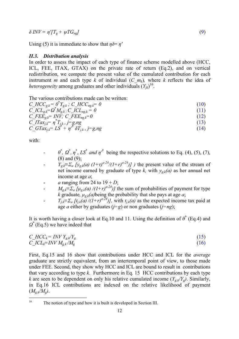
δ INV = η′[Tg + ψTGng] (9) Using (5) it is immediate to show that ηδ= η′ II.3. Distribution analysis In order to assess the impact of each type of finance scheme modelled above (HCC, ICL, FEE, ITAX, GTAX) on the private rate of return (Eq.2), and on vertical redistribution, we compute the present value of the cumulated contribution for each instrument m and each type k of individual (C_mk), where k reflects the idea of heterogeneity among graduates and other individuals (Yjk)16. The various contributions made can be written: C_HCCg,k = θ*Yg,k ; C_HCCng,k= 0 (10) C_ICLg,k=Ω*Mg,k ; C_ICLng,k = 0 (11) C_FEEg,k= INV; C_FEEng,k=0 (12) C_ITaxj,k= η*Tj,k , j=g,ng (13) C_GTaxj,k= LS* + η′* δTj,k , j=g,ng (14) with:

- θ*, Ω*, η*, LS* and η′* being the respective solutions to Eq. (4), (5), (7), (8) and (9);

- Yg,k≡Σa [yg,k(a) (1+τ)a-24/(1+r)a-24)] ) the present value of the stream of net income earned by graduate of type k, with yg,k(a) as her annual net income at age a;

- a ranging from 24 to 19 + D; - Mg,k≡Σa [μg,k(a) /(1+r)a-24)] the sum of probabilities of payment for type

k graduate, μg,k(a)being the probability that she pays at age a; - Tj,k≡Σa [tj,k(a) /(1+r)a-24)], with tj,k(a) as the expected income tax paid at

age a either by graduates (j=g) or non graduates (j=ng); It is worth having a closer look at Eq.10 and 11. Using the definition of θ* (Eq.4) and Ω* (Eq.5) we have indeed that C_HCCk = INV Yg,k/Yg (15) C_ICLk=INV Mg,k /Mg (16) First, Eq.15 and 16 show that contributions under HCC and ICL for the average graduate are strictly equivalent, from an intertemporal point of view, to those made under FEE. Second, they show why HCC and ICL are bound to result in contributions that vary according to type k. Furthermore in Eq. 15 HCC contributions by each type k are seen to be dependent on only his relative cumulated income (Yg,k/Yg). Similarly, in Eq.16 ICL contributions are indexed on the relative likelihood of payment (Mg,k/Mg). 16 The notion of type and how it is built is developed in Section III.

13

A simple way to capture each instrument’s ability to link contributions to income is to divide the present value of contributions, for each type k, by the present value of their cumulated net income over the period. Π_mj,k= C_mj,k /Yj,k (17) m= HCC, ICL, FEE, ITAX, GTAX j=g,ng Finally, it is also useful to stress that, from a distributional point of view, up-front fees (Eq.12) are equivalent to traditional loans. At age 24, the value of contributions made via a loan without income-contingency clause (no possibility to default) is strictly equal to INV, for every type k of graduates.

III. Model specification and data

We used OECD data (Table 1) to quantify the country-specific parameters used across all simulations: α (the share of graduates in the population) and δ (the share of income tax in the total tax receipts of the country).

Table 1: Country-specific parameters

Country Duration of Master

programs

Duration of Bachelor programs

Share of graduates in a cohort

α

Share of Masters among

graduates β

Share of income taxes

receipts in total taxes

δ Belgium 5 3 0.38 0.47 0.63 Germany 5 3 0.22 0.62 0.64 United Kingdom 5 3 0.36 0.20 0.46

Source: OECD (2005) National household surveys provide our principal data. For Belgium, we use the 2002 wave of the Panel Study on Belgian Households (PSBH). The datasets for the UK and Germany are the 2000 wave in CHER17. For representative samples of individuals (Table 2) these national surveys provide information on annual net and gross yearly18 earnings (and thus amount of income tax), participation to labour market, working hours, personal characteristics (age, gender and education) or place of residence. In 17 Consortium of Household Panels for European Socio-Economic Research, Luxembourg that

get its data for Germany and the UK from the German Socio-Economic panel (GSOEP) and the British Household Panel Survey (BHPS).

18 PSBH and CHER always define earnings and income as ‘last year income’.

14

the models above, the key variables are the net income profiles (y(a)), taxation profiles (t(a)) as well as the probability of paying loan instalments (μ(a)). In this section we estimate these profiles or parameters using data on income, employment rates and tax payments of both higher education graduates and non-graduates, separately for three European countries – the UK, Germany and Belgium. In the context of ICL, these data can be used to estimate the risk that a graduate’s net annual income falls below a certain threshold and, consequently, exonerates her from paying her annual instalment. PSBH (Belgium) provides information about wages, while CHER (Germany and UK) gives data on both gross and net income (earnings + replacement earnings). In the case of Belgium, in order to estimate the level of net (y) and gross income (gy) we add estimates of replacement earnings (rep) to net (w) or gross wages (gw). The former corresponds essentially to unemployment, health and disability or early-pension benefits19. Individuals’ type k is identified by combining information on gender, education (highest degree obtained by respondent), and region of residence. Education is a four-type variable : i) less than secondary ii) completed secondary iii) Bachelor graduates (3 years) and (iv) Master graduates (5 years)20; while the residence variable is a dummy variable equal to 1 if people work in the presumably wealthier regions21 and zero if they live elsewhere. At the most disaggregate level the number of types is 16. For each country, we then use individual income data to estimate income and taxation by age profiles. As a first step, individual net income (yi) is used to estimate the OLS coefficients of a second order polynomial function of experience (18), separately for each type k as well as for more aggregate categories (i.e. all graduates (j=g) and non-graduates (j=ng), all types k pooled) : yi,j,k = νj,k + ξj,k ei,j,k + ςj,k(ei,j,k)2 + εi,j,k (18)

where potential work experience (ei) is defined as the number of years since (theoretical) graduation age (i.e., 17 for secondary school drop-outs, 19 for those with secondary education; 23 for higher education graduates)22.

19 A presentation of these estimations is given in the appendix. 20 The first two categories of education form what we call the non-graduates, the latter, the

graduates. 21 Flanders in Belgium, Länder in the former Western Republic of Germany, and Greater

London for the UK. 22 Unfortunately, our data do not provide the actual labour market experience.

15

Table 2: Sample statistics for individual survey data. The sample size and breakdown by education level and gender are also given.

Country Gender Less than secondary

Secondary Higher education

(Bachelor*)

Higher Education (Master**)

Total

Belgium Male 569 639 347 358 1,913 Female 573 731 510 302 2,116 All 1,142 1,370 857 660 4,029 Germany Male 872 2,711 574 943 5,100 Female 832 2,386 369 756 4,343 All 1,704 5,097 943 1,699 9,443 United Kingdom Male 850 316 829 418 2,413 Female 1,012 292 705 358 2,367 All 1,862 608 1,534 776 4,780 * non-university ** university Source: CHER 2000 for Germany and the UK, PSBH 2000 for Belgium Using (Eq. 18) OLS coefficients, we then compute net income by age23 profiles (yj,k(a)) for each type k, but also for more aggregate categories. Examples of these profiles are displayed in Graphs 1 and 2.

23 The shift from income/experience to income/age function is immediate. We simply use the

relation between age and potential labour experience (i.e. a ≡ theoretical graduation age + e).

16

Graph 1: Annual net income fluctuations. Breakdown by degree. Male. All regions (1=total population, all ages, average income)

17

Graph 2: Annual net income functions/profiles. Breakdown by degee. Females. All regions (1=total population, all ages, average income)

18

19

Next, we estimate the expected gross income and income tax by age profile. This is done in two stages. We first estimate the OLS coefficients of the gross income (gyi) regressed on a second order polynomial of net income (yi)24. We then compute the gross income by age profiles as such (gyj,k(a)) by applying these OLS coefficients to the values generated by net income by age profile (yj,k(a)). Taxation profiles are simply generated by the difference between expected net and gross income (tj,k(a)≡ gyj,k(a)- yj,k(a)). We use the net income/age profiles to compute net present value of cumulated income Yj,k (Eq. 1). Following Jacobs (2002), we assume a 2% average growth rate of the level of earnings (τ), reflecting the idea that technical progress generates productivity gains that somehow benefit all individuals25. We also assume a discount rate (r) of 4%, equal to the historical return on risk-free European bonds. Results, displayed in Tables 3 and 4 suggest, within each country examined here, the presence of sizeable differences across types k of individuals even after progressive income taxation and transfers (Graph 3). They also clearly show, as expected from the human capital literature, that higher education graduates can expect much higher cumulated net income. These estimates also confirm the persistence of significant gender gaps. To assess the incidence of income-contingency for the ICL case, we define for each individual graduate an age/experience-specific payment dummy (Payi,g,k (e)), by comparing her level income (yi,g,k (e)) at a certain point of her career, with an experience-specific threshold Θ(e). The latter is defined as average net annual income amongst non-graduates with similar professional experience. In technical terms, it is equal to Θ(e) =νng + ξnge + ςnge2, where νng , ξng ,ςng are obtained by estimating Eq.18 using all non-graduates (j=ng and all k types pooled). In other words, higher education graduates should pay only if their annual net income is above the average income of non-graduates. This is a way of ensuring that contributions are levied on only the benefits obtained from achieving higher education26. Each time annual net income is below the (experience-specific) no-payment threshold we conclude a default (Payi,g,k=0), and to normal payment of instalment Ω otherwise (Payi,g,k =1).

24 This is done by pooling all available observations. 25 In the case of Belgium or Germany, but also the Netherlands (Jacobs, 2002), this might be a

lower bound. Long-term statistics of hourly wage growth suggest actual rates can reach 3%. 26 M. Friedman's seminal work (Friedman, 1955) suggests that private contributions should be

indexed to the fraction of income that can be imputed from higher education.

20

Table 3: Present value of lifetime (24-65) net income estimated at the age of 24 in EUR. Breakdown by country, education level, gender and region

Highest degree obtained

Country Gender Region Less than secondary Secondary

Higher Education (Bachelor)

Higher Education (Master)

Wallonia and Brussels 419,978 565,221 669,357 804,842 Female

Flanders 403,004 578,869 625,045 832,310 Wallonia and Brussels 690,404 888,250 847,211 1,096,633

Belgium Male

Flanders 676,380 848,462 962,819 1,121,024 East 516,126 599,269 682,692 849,727

Female West 468,835 605,562 749,238 901,750 East 864,345 923,025 1,220,946 1,365,637

Germany Male

West 873,676 981,504 1,188,522 1,373,691 All except G. London 454,893 544,194 663,286 968,123

Female Greater London 449,160 566,464 743,815 1,048,364

All except G. London 864,519 996,717 1,063,618 1,369,549 United Kingdom

Male Greater London 884,847 934,262 1,063,980 1,236,351

Assumptions: τ=0.02. r=0.04

21

Table 4: Relative present value of lifetime (24-65) net income estimated at the age of 24. Breakdown by education level. gender and region (1= category with

maximal lifetime net earnings)

Highest degree obtained

Country Gender Region Less than secondary Secondary

Higher Education (Bachelor)

Higher Education (Master)

Wallonia and Brussels 0.37 0.50 0.60 0.72 Female

Flanders 0.36 0.52 0.56 0.74

Wallonia and Brussels 0.62 0.79 0.76 0.98 Belgium

Male Flanders 0.60 0.76 0.86 1.00

East 0.38 0.44 0.50 0.62 Female

West 0.34 0.44 0.55 0.66

East 0.63 0.67 0.89 0.99 Germany

Male West 0.64 0.71 0.87 1.00

All except G London 0.33 0.40 0.48 0.71 Female

Greater London 0.33 0.41 0.54 0.77

All except G London 0.63 0.73 0.78 1.00 United Kingdom

Male Greater London 0.65 0.68 0.78 0.90

Assumptions: τ=0.02. r=0.04

22

Graph 3: Current average income tax (ie. taxes as % of gross income) according to level of gross income (i.e. tax progressivity)

The specification used for the probability of payment is a logistic function, with a third order polynomial function in potential experience as the argument. Again, the estimation is run separately for each type k as well as for more aggregate categories (i.e. all graduates (j=g) and non-graduates (j=ng)). μi,j,k ≡ Prob(Payi,j,k=1|ei,j,k) = 1/[1+exp(-(ρj,k + ςj,kei,j,k+ σj,k(ei,j,k)2 + ξj,k(ei,j,k)3)] (19) Estimated probability of payment according to age27 (uj,k(a)) are plotted in Graph 4 for both Bachelors and Masters graduates. The highest probability of payment (or lowest risk of default) is observed amongst Masters graduates. Graph 4 clearly suggests that in Belgium and the UK, the insurance effect of ICL is likely to be more important for students who attend Bachelor programs. This feature does not emerge in the case of Germany. This graph also indicates that the probability of payment varies with age. In Belgium, and to a lesser extent in Germany, it rises between the age of 24 and 30, particularly for students who graduate from Masters programs. This could be due to

27 Again, the shift from income/experience to income/age function is immediate (i.e. a ≡

theoretical graduation age + e).

23

the fact that, in these two countries, graduates on the labour market take longer to realise their income potential. Between ages 30 and 45, in every country considered, the probability of payment declines moderately. However, it rises quite dramatically beyond age 50. A possible explanation for this could be the growing employment gap between graduates and non-graduates, particularly the well-known concentration of early retirement amongst those less educated.

Graph 4: The probability that higher education graduates pay their income-contingent instalment according to age

24

25

IV. Fees and the private rate of return

The financial profitability of higher education attendance for the average graduate, and its sensitivity to enhanced tuition fees is our first result. We compute the value or the private rate of return (PRR Eq.1) for values of investment (INV) ranging from 0€28 to 20,000€. The income for student jobs parameter (1-χ) is set to 0.9 meaning that these jobs generate 10% of the annual income of a non-graduate29. Our results are displayed in Table 5. Here we compare the cumulated net income of the average graduate (Yg) with that of someone who completed upper secondary education (Yng). Table 5 shows significant differences across countries in terms of private rate of return (PRR). Belgium is the country with the lowest level of private profitability. More importantly, however, Table 5 states that the level of PRR is relatively unaffected by increases to private contributions. Raising the private cumulated contribution to higher education costs (Cg) by 20,000 €, in Belgium, would, at most30, reduce the PRR by less than 1 percentage point (from 4.66% to 3.87%). In Germany and the UK we observe similar reductions (8.85% to 8.17%. and 6.79% to 5.94%, respectively).

28 The status quo. 29 This is a fairly conservative assumption according to the EU literature (de la Fuente, 2003). 30 Remember that these simulations ignore the possible positive effect of spending on

subsequent income.

26

Table 5: Sensitivity of the marginal (i.e. per year of study) private rate of return (PRR) to different values of human capital investment (INV)*– Reference =

lifetime income of individuals (males or females) with upper-secondary degree

Cumulated investment (INV) in EUR Belgium Germany UK

0 € 0.047 0.088 0.068

1,000 € 0.046 0.088 0.068

2,000 € 0.046 0.088 0.067

3,000 € 0.045 0.087 0.067

4,000 € 0.045 0.087 0.066

5,000 € 0.045 0.087 0.066

6,000 € 0.044 0.086 0.065

7,000 € 0.044 0.086 0.065

8,000 € 0.043 0.086 0.065

9,000 € 0.043 0.085 0.064

10,000 € 0.043 0.085 0.064

11,000 € 0.042 0.085 0.063

12,000 € 0.042 0.084 0.063

13,000 € 0.041 0.084 0.062

14,000 € 0.041 0.084 0.062

15,000 € 0.041 0.083 0.062

16,000 € 0.040 0.083 0.061

17,000 € 0.040 0.083 0.061

18,000 € 0.039 0.082 0.060

19,000 € 0.039 0.082 0.060

20,000 € 0.039 0.082 0.059

Given Eq. 15 and 16, these values correctly reflect the sensitivity PRR to higher private contribution of for FEE, ICL and HCC when considering the average graduate.

27

V. Income-contingent contributions and distributional issues

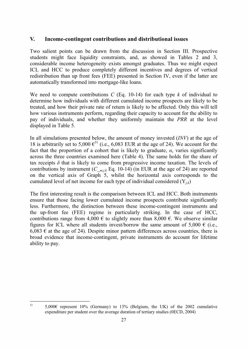
Two salient points can be drawn from the discussion in Section III. Prospective students might face liquidity constraints, and, as showed in Tables 2 and 3, considerable income heterogeneity exists amongst graduates. Thus we might expect ICL and HCC to produce completely different incentives and degrees of vertical redistribution than up front fees (FEE) presented in Section IV, even if the latter are automatically transformed into mortgage-like loans. We need to compute contributions C (Eq. 10-14) for each type k of individual to determine how individuals with different cumulated income prospects are likely to be treated, and how their private rate of return is likely to be affected. Only this will tell how various instruments perform, regarding their capacity to account for the ability to pay of individuals, and whether they uniformly maintain the PRR at the level displayed in Table 5. In all simulations presented below, the amount of money invested (INV) at the age of 18 is arbitrarily set to 5,000 €31 (i.e., 6,083 EUR at the age of 24). We account for the fact that the proportion of a cohort that is likely to graduate, α, varies significantly across the three countries examined here (Table 4). The same holds for the share of tax receipts δ that is likely to come from progressive income taxation. The levels of contributions by instrument (C_m,j,k Eq. 10-14) (in EUR at the age of 24) are reported on the vertical axis of Graph 5, whilst the horizontal axis corresponds to the cumulated level of net income for each type of individual considered (Yj,k) The first interesting result is the comparison between ICL and HCC. Both instruments ensure that those facing lower cumulated income prospects contribute significantly less. Furthermore, the distinction between these income-contingent instruments and the up-front fee (FEE) regime is particularly striking. In the case of HCC, contributions range from 4,000 € to slightly more than 8,000 €. We observe similar figures for ICL where all students invest/borrow the same amount of 5,000 € (i.e., 6,083 € at the age of 24). Despite minor pattern differences across countries, there is broad evidence that income-contingent, private instruments do account for lifetime ability to pay.

31 5,000€ represent 10% (Germany) to 13% (Belgium, the UK) of the 2002 cumulative

expenditure per student over the average duration of tertiary studies (0ECD, 2004)

28

Graph 5: Present value of contribution (Ck) for a 5,000 € investment, according to the present value of income (Yk) over the duration of the contract (D=25).

Breakdown by instrument of higher education finance

29

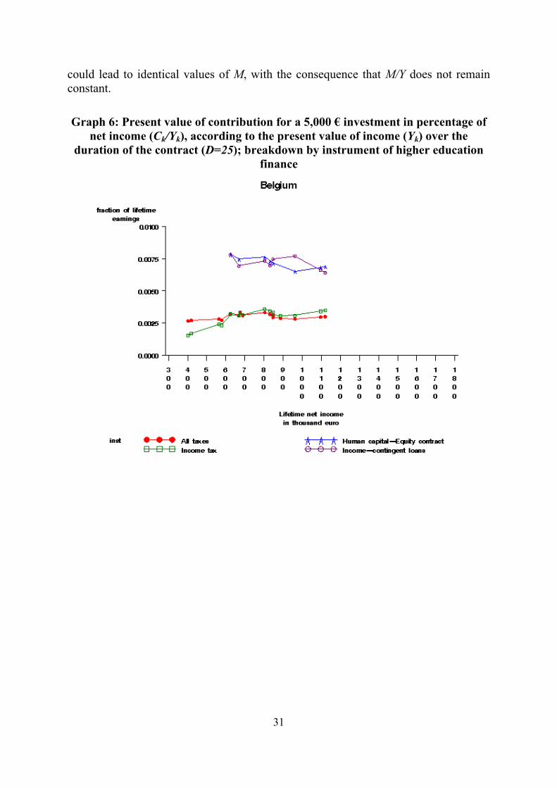
Graph 6 is based on the same results as Graph 5. Values on the horizontal axis correspond to the income of the various types of individuals (Yj,k). Unlike Graph 5, contributions on the vertical axis are now expressed in percentage of total lifetime net income (Π_mj,k= C_mj,k/Yj,k Eq.17). Expressed in relative terms, the contributions required by HCC and ICL contracts worth 5,000 € represent a fairly small fraction of lifetime net income (between 0.48% for Germany and 0.78% for Belgium). Although, these percentages are logically higher than those graduates would pay as taxpayers, were higher education refinanced via taxation (ITAX and GTAX). The shape of the curves on Graph 6 tells us whether contributions are indexed on lifetime income or ability to pay. Graph 6 shows whether the private rate of return (PRR) displayed in Table 5 is likely to be valid for all types k of individuals, and, consequently, whether financial incentives could be preserved uniformly across the distribution of income. A flat curve (HCC, ICL) would indicate that the instrument is capable of indexing contributions to income. A rising (GTAX) or declining curve (FEE) likewise shows no such indexing. An important result, visible in Graph 6, is thus that ICL and HCC do guarantee that all type k graduates face identical reductions of PRR. If we combine this particular result with those of Section IV, we can conclude that increasing individuals’ contribution to higher education costs – provided it is done via ICL or HCC – does not significantly affect the private rate of return. This holds not only for the average graduate but also for each type k.

30

As for vertical redistribution, a flat curve is indicative of the ‘proportionality’ (the contribution is equal to the same fraction of income for each type k (Eq.12)). A declining curve suggests ‘regressivity’ (a declining average contribution) whilst a rising curve would be synonymous with ‘progressivity’ (a rising average contribution). Thus, both HCC and ICL satisfy the principle of ‘proportionality’. Notably in Belgium, finance by income taxation (ITAX) is ‘progressive’. We see, however, that more general forms of taxation (GTAX), particularly in Germany and the UK, could be ‘regressive’. Finally, it should be noted that up-front fees (FEE)32, in each country considered, appear as very ‘regressive’ instruments. When comparing the two income-contingent instruments (Graph 6), we observe that HCC does not dramatically dominate ICL in its ability to index contributions to income. By definition, HCC is a scheme where contributions are strictly proportional to income (Eq. 4). By contrast, ICL, as it is modelled here, results in discontinuous contributions: below a predefined threshold, a graduate's contribution is nil, whilst above that threshold it amounts to a lump sum (Ω). We did not anticipate that ICL could make wealthier graduates contribute as much (in relative terms) as their poorer peers. Analytically, this result means that lifetime average probabilities of paying (defaulting on) ICL, estimated for each (broad) type of graduates k are closely linked to income pattern. By dividing both terms in Eq.11 by Yj,k we have C_ICLj,k/Yk=Ω Mj,k/Yj,k, where Mj,k is the (discounted) average probability that income is above the threshold Θ (Eq.5). Hence, if Mj,k/Yj,k is relatively constant across all types of graduates, ICL generates relative contributions that are constant. The reason we verify this condition is threefold. First, we retained a relatively high income threshold (i.e. average income amongst non-graduates). It is obvious that lower values of Θ would increase the average probability of payment M to the point it reaches its maximum above a certain level of income; with the consequence that relative contributions would decline33. The second reason is more empirical. In countries such as Belgium, Germany and the UK there are downward fluctuations in income, even amongst successful graduates. Occasionally, this results in graduates earning less than non-graduates (i.e. M is not equal to its maximum). Third, although we make considerable efforts in this paper to account for the heterogeneity amongst graduates, our categorisation remains coarse (males vs. females, Masters vs. Bachelors). What we fundamentally detect is the capacity of ICL to account for inter-type, but not inter-individual, income differences. Working with the full distribution of income would probably produce results more in line with what we anticipated. Indeed, the probability of graduates who form the very top percentiles of the income distribution ‘crossing’ the threshold line tends to zero. Hence, different values of Y

32 They can be considered equivalent to conventional loans from a distributional point of view. 33 We discuss this point further in the next section.

31

could lead to identical values of M, with the consequence that M/Y does not remain constant. Graph 6: Present value of contribution for a 5,000 € investment in percentage of

net income (Ck/Yk), according to the present value of income (Yk) over the duration of the contract (D=25); breakdown by instrument of higher education

finance

32

33

VI. Income-contingency as an insurance mechanism

Providing students with income-contingency is certainly a way to avoid distorting private rates of return (PRR) between types k of graduates. It is simultaneously a way to achieve vertical justice. It is also equivalent to insuring their human capital, partially34. From a political-economy perspective, income-contingency raises three interrelated issues: i) the size of the resulting insurance costs ii) the importance of implicit transfers35 between (easy to identify) categories of

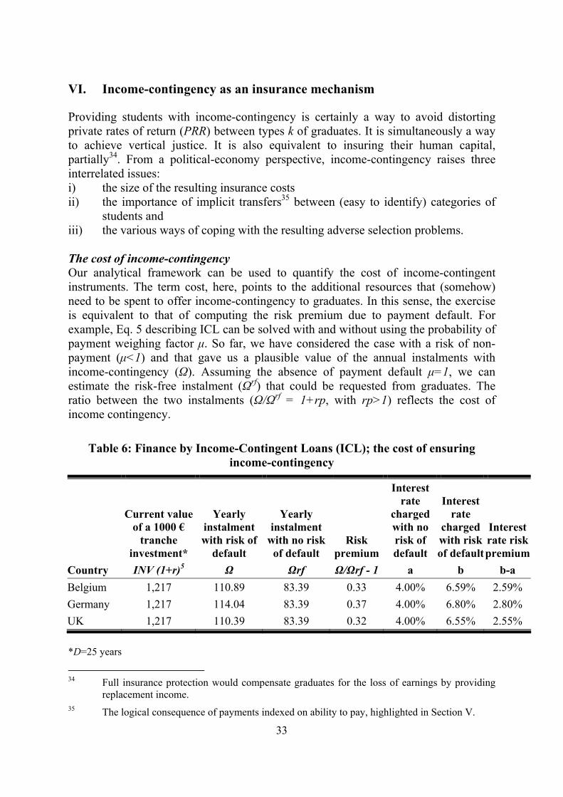
students and iii) the various ways of coping with the resulting adverse selection problems. The cost of income-contingency Our analytical framework can be used to quantify the cost of income-contingent instruments. The term cost, here, points to the additional resources that (somehow) need to be spent to offer income-contingency to graduates. In this sense, the exercise is equivalent to that of computing the risk premium due to payment default. For example, Eq. 5 describing ICL can be solved with and without using the probability of payment weighing factor μ. So far, we have considered the case with a risk of non-payment (μ<1) and that gave us a plausible value of the annual instalments with income-contingency (Ω). Assuming the absence of payment default μ=1, we can estimate the risk-free instalment (Ωrf) that could be requested from graduates. The ratio between the two instalments (Ω/Ωrf = 1+rp, with rp>1) reflects the cost of income contingency.

Table 6: Finance by Income-Contingent Loans (ICL); the cost of ensuring income-contingency

Country

Current value of a 1000 €

tranche investment* INV (1+r)5

Yearly instalment with risk of

default Ω

Yearly instalment

with no risk of default

Ωrf

Risk premiumΩ/Ωrf - 1

Interest rate

charged with no risk of default

a

Interest rate

charged with risk of default

b

Interest rate risk premium

b-a Belgium 1,217 110.89 83.39 0.33 4.00% 6.59% 2.59% Germany 1,217 114.04 83.39 0.37 4.00% 6.80% 2.80% UK 1,217 110.39 83.39 0.32 4.00% 6.55% 2.55% *D=25 years

34 Full insurance protection would compensate graduates for the loss of earnings by providing

replacement income. 35 The logical consequence of payments indexed on ability to pay, highlighted in Section V.

34

Our computations (Table 6) suggest a value for rp ranging from 0.32 (UK) to 0.37 (Germany). Thus Income-contingency costs on average up to 0.37 € per EUR invested. An alternative measure is provided by the interest rate risk premium (last column of Table 6). We estimate it using an internal rate of return (IRR) algorithm. This risk premium ranges from 2.55 (UK) to 2.80 (Germany) percentage points. The tentative conclusion is that income-contingency – as specified here with all the distributional benefits it entails (uniform PRR across types k, vertical justice) – is relatively expensive especially when applied to large and heterogeneous populations of students. One could argue that a lower income threshold would reduce the cost of income-contingency. However, this would also induce a countervailing effect. ICL would be closer to up-front fees or ordinary loans, implying that the distributional properties mentioned above, and highlighted in Graph 6, would vanish pro rata the lowering of the threshold. Risk pooling, implicit transfers and adverse selection One option to provide income-contingency, and avoid high non-take up rates amongst risk-averse students, would be to pool the cost of default amongst students. This is a system where the risk of default and its cost are shared amongst graduates. This principle of pooling was used for the Tuition Postponement Option at Yale University – an ICL scheme – in the early 1970s. It has been widely viewed as inefficient. Its main disadvantage is to put the borrowers at some risk, depending on the likely future income capacity of the borrowing class. More particularly, many potential high earners choose to exit the income-contingent repayment scheme to avoid the risk of getting into a cohort with too many potential low earners. This is a typical illustration of an adverse selection problem. In order to highlight the potential importance of adverse selection in the European context we compute the implicit transfers taking place under risk-pooling across a large (and diversified) set of students36. Computations reported in Table 7 suggest that, in the case of HCC, the cost for Masters program graduates to be pooled with Bachelors program individuals in Germany represents only a 2% increase in the percentage points of income the lender is likely to request (θ). But this is relatively low compared to Belgium’s figure of 13% and the UK’s, 19%. Hence, it seems clear that risk-pooling can imply significant redistribution from those with high lifetime income to those with lower income. Estimates in Table 7 reveal that an HCC scheme implemented with Masters-only graduates37 is less expensive than a scheme including Bachelors. This potential reduction of cost could be sufficient to trigger a secession as low risk graduates would be tempted to form a separate scheme synonymous with lower contributions.

36 Remember that we have assumed so far that the various instruments apply to all students. 37 Mainly university programs

35

Coping with Adverse selection: a menu-based approach

Separation An option to avoid the negative effect of pooling is to discriminate amongst risk categories. In the context of higher education finance, this would imply investing less money in the education of riskier students. In the case of an HCC, this means imposing that investment (INV) by (say) Bachelors students represents only a fraction 0<λ<1 of the one made by their peers. Adverse selection will be avoided when this fraction λ will be such that pooled contribution (θp) is equal to the one faced by Masters program graduates in a non-pooling context (θMaster).Using the relationship INV=θ Y (Eq. 4), we can thus identify λ, by solving: θp ≡ [β θMaster YMaster+ (1-β) λ θBachelor YBachelor] / Yp= θMaster (20) with:

- 0< λ < 1 - β being the proportion of Masters graduates in the total population of

graduates; - YP= βYMaster + (1-β)YBachelor

It is then immediate38 to show that λ= θMaster /θBachelor (21) Results in the last column of Table 7 reveal that the typical HCC investment on a Bachelors student should be equal to a fraction λ equal to 74% (UK), 79% (Belgium), and 90% (Germany) of that of a Masters student. Interestingly, this reduction factor is inferior to what we would expect in systems with uniform annual fees across higher education institutions but varying lengths of programs. Considering that Bachelors programs last 3 years, whilst it takes 5 years to complete a Masters, we should end up with a loan size ratio of 3/5 (i.e. 60%). In other words, pooling Bachelors and Masters students, with uniform annual fees (e.g. 1,000 EUR), would precipitate the need for investment size adjustments to counteract adverse selection. This remedy might also be applied across different subject specialisations. To avoid adverse selection induced by having higher-earning graduates (e.g. Engineering majors) subsidising the non-payment of a lower-earning graduates (Fine Arts majors), the latter should simply borrow less money.

38 β θMaster YMaster+ (1-β) λ θBachelor YBachelor= θMaster Yp . Using the definition of Yp we get β θMaster

YMaster+ (1-β) λ θBachelor YBachelor = β θMaster YMaster+ (1-β) θMaster YBachelor . Eliminating equivalent expressions on both sides, and isolating λ, we eventually obtain λ = θMaster/θBachelor

36

Table 7: Human capital contracts (HCC): 5,000 € investment; percentage of income over the duration of contract (24-44) committed depending on degree of

pooling amongst graduates

Country Category (k) Percentage of net

annual income committed* (θ)

Cost of pooling a/b

Adjustment factor to avoid adverse selection

λ= θMaster/θBachelor:

All graduates pooled a 1.35%

Graduate Master b 1.20% 1.13 0.79 Belgium

Graduates Bachelor c 1.51%

All graduates pooled a 0.98%

Graduate Master b 0.97% 1.02 0.90 Germany

Graduates Bachelor c 1.08%

All graduates pooled a 1.04%

Graduate Master b 0.87% 1.19 0.74 UK

Graduates Bachelor c 1.17%

* Duration of contract (D)=25 years Considering the consequence of pooling male and female Master graduates, Table 8 reveals that in Belgium, female students should be allowed to borrow only 80% of what their male peers borrow/invest. The fraction is lower in the UK (72%) and Germany (63%). Whilst quite similar in magnitude to those reported above, these results shed a completely different light on what can be achieved via separation of risk categories. In fact, Table 8 helps us identify the limits of that strategy. If differentiating (cumulated) tuition fees between Bachelors and Masters students is largely perceived as logical and legitimate, differences of treatment between other categories of students is strongly opposed, or simply illegal. Gender discrimination is prohibited by European law (Gender Discrimination Act).

37

Table 8: Human capital contracts (HCC): 5,000 € investment; percentage of income over the duration of contract (24-44) committed depending on degree of

pooling amongst male and female Masters graduates

Country Category (k) Percentage of net

annual income committed* (θ)

Cost of pooling a/c

Adjustment factor to avoid adverse

selection λ= θMale/θFemale

Male and female pooled a 1.20%

Female only b 1.35% 1.11 0.80 Belgium

Male only c 1.08%

Male and female pooled a 0.97%

Female only b 1.26% 1.21 0.63 Germany

Male only c 0.80%

Male and female pooled a 0.87%

Female only b 1.05% 1.15 0.72 United Kingdom

Male only c 0.76%

* Duration of contract (D)=25 years

Risk-shifting An alternative approach may consist of asking society to compensate for the low-earning group (here women), rather than shifting the cost of income-contingency onto the rest of the cohort (males). This is the risk shifting solution that most countries with ICL or HCC schemes, have implemented thus far (Palacios, 2004). Whilst full risk-shifting is clearly an efficient answer to adverse selection, our simulations presented in Table 6 indicate that the cost to the taxpayer would be non-negligible. In the EU context, as indicated by Barr (2001, 2002), full risk shifting could lead public watchdogs39 to classify student contracts as public debt.

39 Eurostat for the EU member states.

38

Compulsory pooling Another solution to mitigate the adverse selection problem, in the context of full or partial risk-pooling, is to impose participation in the income-contingent scheme. Borrowing money to finance higher education would be mandatory. This would clearly require the involvement of public authorities as this measure would turn out to be unpopular amongst certain categories of graduates, as the results of Tables 7 and 8 reveal. The practical response to adverse selection might combine risk shifting, separation and compulsory pooling depending on the exact configuration of the problem as well as the political preferences of different countries.

VI. Conclusion

The principal contribution of this paper is the finding that instruments of private finance, combining deferred and income-contingent payments, offer an opportunity to raise significant sums in order to (re)finance higher education in Europe without significantly eroding the profitability of the educational investment of individuals with heterogeneous lifetime incomes, and simultaneously addressing the risky nature of the investment. These results hold for a sample of countries (UK, Germany and Belgium) with potentially diverging institutional arrangements for their higher education, labour markets and fiscal systems. We estimate that investments of up to 20,000 € would reduce the current private rate of return by less than one percentage point. This is an upper bound estimate, as it is computed under the pessimistic assumption that the additional resources have no positive effect on individuals’ earning prospects. An investment of 5,000 € would represent a cost ranging from 0.47% (Germany) to 0.78% (Belgium) of lifetime (24-65) net income. One of the distinguishing advantages of ICL and HCC, compared to FEE (or ordinary loans), is that these moderate reductions in the rate of return can be achieved across the distribution of graduates’ incomes. As ICL and HCC create a significant payment gradient amongst individuals from the same cohort, they simultaneously display strong vertical justice properties. The comparison between HCC and ICL reveals that they are almost equally effective at indexing contributions to lifetime income. By definition, HCC are synonymous with contributions that are strictly proportional to income. ICL a priori modulates contributions in a much less precise way. This is certainly true from a cross-sectional perspective. However, it is less clear from an inter-temporal one, as lifetime average probabilities of defaulting on ICL can be relatively well indexed to lifetime income. Both ICL and HCC are income-contingent and thus contain an insurance component. It is this insurance element that allows contributions to be adapted to an individual’s lifetime income. The insurance mechanism is relatively expensive when applied to

39

large populations of students that are heterogeneous in terms of income prospects. If the cost is pooled amongst graduates, payments contain a premium to cover those who default. The main advantage of pooling is that redistribution takes place within each cohort of graduates. Its drawback is its exposure to adverse selection, as potential high earners might exit the scheme for fear of being in a cohort with too many low earners. Our last set of computations suggests that high-earning graduates would face an HCC price tag inflated by up to 19% (UK) if pooled with low earners. We also propose an alternative. Investing less money in students opting for less profitable programs potentially eliminates the cost of pooling for high earners. This could be equated with the separation equilibrium solution. Its underlying logic is that students opting for programs, but also fields of study, offering lower income prospects, should borrow less money. But in the case of income differentials by gender (but also ethnicity, religion, region of origin, etc.), policy-makers, and individuals in general, might be unwilling to accept a system that imposes different terms. A solution would then be to ask taxpayers to compensate the lower paid groups, like women. This is the risk-shifting solution. Full risk-shifting is clearly an answer to adverse selection. However, its cost for the taxpayer could be significant. In the European context, complete risk-shifting could also lead to the classification of student contracts as public debt, which would further inflate the already bloated public debt that most European countries struggle with. Another solution to adverse selection would consist of maintaining a certain level of pooling – and thus redistribution – whilst imposing participation. However, given the lack of support for this amongst certain categories of graduates, implementation might generate issues of political economy.

40

References

Barr, N. (2001), The Welfare State as Piggy Bank: Information, Risk, Uncertainty, and the Role of the State, Oxford University Press, Oxford.

Barr, N. (2004), ‘Higher Education Funding’, Oxford Review of Economic Policy, 20(2): 264-283.

Chapman, B. (1997), ‘Conceptual Issues and the Australian Experience with Income Contingent Charges for Higher Education’, The Economic Journal, 107 (442): 738-751.

Chapman, B. (2005), Income Contingent Loans for Higher Education: International Reform, Centre for Economic Policy Research, DP No 491, Australian National University.

Dale, S. and A. Krueger (1999), Estimates of the payoff of attending a selective college. An application of selection on observables and unobservables, NBER Working Paper, No 7322, Cambridge, Mass.

de la Fuente, A. (2003), Human capital in a global and knowledge-based economy, part II: assessment at the EU country level, Report for the European Commission, DG for Employment and Social Affairs.

Friedman, M. (1955), ‘The Role of Government in Education’, in R.A. Solo (ed.), Economics and the Public Interest, Rutgers University Press.

Friedman, M. (1962), Capitalism and Freedom, The University of Chicago Press, Chicago.

Glennerster, H. and Wilson, G. (1968). ‘A graduate tax’, Journal of Higher Education, 1(1): 26–38.

Greenaway, D. and Haynes, M. (2003), ‘Funding higher education in the UK: the role of fees and loans’, The Economic Journal, 113: 150-166.

Heckman, J. and Carneiro; P. (2003), ‘Human Capital Policy’, in J. Heckman, A. Krueger (eds.), Inequality in America: What Role for Human Capital Policies, MIT Press, Cambridge, Mass.

Jacobs, B. (2002), An investigation of education finance reform – Graduate taxes and income contingent loans in the Netherlands, CPB Discussion Paper, July, Den Hague, the Netherlands.

Lemieux, T. (2006), Post-Secondary Education and Increasing Wage Inequality, NBER Working Paper, No. 12077, Cambridge, Mass.

OECD (2004), Education at a Glance, OECD, Paris. OECD (2005), Revenue Statistics 1995-2004, OECD, Paris. Office National de l'Emploi (2003), Lien entre rémunération du travail et allocation

de chômage, Brussels.

41

Palacios, M. (2004), Investing in human capital: a capital markets approach to student funding, Cambridge University Press, Cambridge.

Van der Linden, B. and Dor, E. (2001), Labor market policies and equilibrium unemployment: Theory and application to Belgium, Working Paper 2001-5, IRES.

42

Appendix

Since we do not observe unemployment and other replacement benefits directly for Belgium, we use two simplifying assumptions to estimate them. First, following Van der Linden and Dor (2001), we consider a replacement ratio of 34%. This value adequately reflects the situation of cohabitants and the fact that benefits are decreasing over time for some categories of individuals. Second, we assume that replacement earnings’ benefits are sensitive to past income, since they are indexed on former income within a certain interval. According to Office National de l'Emploi (2003), the proportion of non-employed persons, for which the benefit is proportionally linked to former income, is 29%. Hence, for each of the 4,029 individuals in the data set the level of income is equal to: yi = mi wi + (1-mi/12) rep (1) gyi = mi gwi + (1-mi/12) rep (2) with

- rep = a W + b AW - a = (0.29) 0.34 = 0.0986 - b = (1 - 0.29) 0.34 = 0.2414 - mi the number of months in 2002 during which individual i had a

remunerated job; - W the average net wage amongst working indviduals with the same age,

gender and degree as individual i; - AW the economy-wide average net wage of working individuals;