Pay Me Later:Savings Constraints and the

Demand for Deferred Payments∗

Lasse Brune, Eric Chyn, and Jason Kerwin

January 17, 2021

Abstract

We study a simple savings scheme that allows workers to defer receipt of partof their wages for three months at zero interest. The scheme significantly increasessavings during the deferral period, leading to higher post-disbursement spending onlumpy goods. Two years later, after two additional rounds of the savings scheme, wefind that treated workers have made permanent improvements to their homes. Thepopularity of the scheme implies a lack of good alternative savings options. The resultsof a follow-up experiment suggest that demand for the scheme is partly due to itsability to address self-control issues.

∗Brune: Global Poverty Research Lab, Kellogg School of Management, Northwestern University,Evanston, IL 60208, USA; lasse.brune@northwestern.edu; Chyn: Department of Economics, Dartmouth Col-lege, 6106 Rockefeller Center, Hanover, NH 03755, USA, and NBER; eric.t.chyn@dartmouth.edu; Kerwin:Department of Applied Economics, University of Minnesota, 1994 Buford Avenue, St. Paul, MN 55108,USA; jkerwin@umn.edu. We are grateful for insightful comments from Achyuta Adhvaryu, Emily Breza,Lorenzo Casaburi, Michael Callen, Marcel Fafchamps, Xavi Gine, Reshma Hussam, Kelsey Jack, NamrataKala, Dean Karlan, Craig McIntosh, Doug Staiger, Chris Woodruff, Dean Yang, Jonathan Zinman, and fromseminar participants at the IPA Researcher Gathering on Financial Inclusion, Yale University, the ConsumerFinancial Protection Bureau, the University of Hong Kong, HKUST, Peking University, China AgriculturalUniversity, the Federal Reserve Bank of Philadelphia, the University of Utah, the University of Washington,MIEDC, CSAE, NEUDC, and ASSA. We gratefully acknowledge support from the Financial Services forthe Poor Research Fund at Innovations for Poverty Action, sponsored by a grant from the Bill and MelindaGates Foundation. We thank Rachel Sander for providing excellent research assistance, and Ndema Longwefor his outstanding diligent work in managing data collection. In addition, we also thank the editor EstherDuflo and two anonymous referees for detailed comments and feedback. This project would not have beenpossible without the help of the management at the Lujeri Tea Estate and the employees who participatedin the study, who generously shared their time with us. This work was supported by the USDA NationalInstitute of Food and Agriculture, Hatch project MIN14-164. This study was reviewed and approved byIRBs in Malawi (NCRSH, protocol number P.08/16/131) and at IPA (protocol number 13888). This studyis registered with the AEA RCT Registry under registration number AEARCTR-0001554.

A key prediction of standard economic models is that individuals should prefer to be paid

early. However, an emerging literature documents notable demand for deferred payments for

goods and services in developing countries (Casaburi and Macchiavello, 2019; Brune and

Kerwin, 2019; Kramer and Kunst, 2020). Similarly, millions in developed countries choose to

defer income by opting to overwithhold on tax payments that are later returned as refunds

(Thaler, 1994).

There are three main benefits to deferred payments. First, deferring pay naturally gen-

erates lump sums that can be used to purchase durable goods, make business investments,

or buy in bulk. This may be particularly important given qualitative evidence that suggests

poor households exert substantial effort to generate lump sums (Collins et al., 2009). Second,

deferred payments may be a relatively safer savings option because access to high-quality

formal banking is limited and informal saving options can be risky (Karlan, Ratan and Zin-

man, 2014; Dupas et al., 2016). Third, delaying pay can help address behavioral constraints

such as time-inconsistency (Laibson, 1997; Ashraf, Karlan and Yin, 2006; Bryan, Karlan and

Nelson, 2010; DellaVigna, 2018).

This paper provides evidence on the demand for deferred payments and the first ex-

perimental estimates of the impact of this savings method on downstream outcomes. Our

analysis is based on a sample of full-time workers at a large agricultural employer in rural

Malawi. We study a savings scheme that allowed workers to defer a fraction of their pay for

three months at zero interest. Access to this scheme was randomized for a sample of 870

workers who were interested in participating. All payments were provided in cash through

the firm’s regular payroll infrastructure. The scheme created a simple, no-frills option for

workers to save for lumpy purchases by piggybacking on existing firm payroll infrastructure

to shift the timing of payments.

Our analysis shows that the savings scheme was popular and changed worker behavior.

Nearly half of all workers who were contacted as part of outreach activities signed up for

the scheme.1 Those who enrolled had high rates of account usage (92 percent made more

1We conducted outreach by having field staff visit divisions of the firm. The staff held information sessionswith all permanent, full-time workers who were present on the day of the visit. We did not provide subsidies

1

than one deposit) and saved 14 percent of their wages on average. We find that the scheme

appears to have increased overall savings during the accumulation period, rather than just

substituting for other forms of savings. Much of the reported money saved was spent on

lumpy purchases: two-thirds of treatment workers’ additional spending in the two weeks

after payout goes toward lumpy purchases, including for durable purchases related to housing

investment.

Participation in the deferred wages scheme had significant effects on downstream out-

comes. Four months after the end of the scheme, a broad measure of the value of durable

assets increased by 10 percent. This increase was concentrated in stored materials for house

improvements such as sheets of metal roofing. The main threat to the interpretation of this

result is that we do not find impacts on asset purchases, which was one of our pre-specified

outcomes. However, we find further downstream effects on asset outcomes in long-run follow-

up data, after treatment-group workers were offered the scheme two more times. Specifically,

two years after the initial round of the scheme (and nine months after the last round),

treatment-group workers were 7.7 percentage points more likely to have metal roofs on their

homes. This result is robust to adjustment for multiple hypothesis testing.

The popularity and effectiveness of the deferred wages savings scheme implies a lack

of safe and convenient alternative savings options. Evidence from a follow-up experiment

supports this view and is also consistent with the idea that the scheme helps workers with

behavioral constraints. We randomly offered a new sample of workers either the original

scheme or a modified version of the product that required manual deposits at an easy-to-

reach workplace location. The manual deposits scheme resulted in substantially lower savings.

While initial sign-up rates were similar for the two schemes, workers in the manual deposits

scheme saved 50 percent less. We find suggestive evidence that these reductions are smaller

in magnitude for workers with higher reported self-control.2 At the same time, enrollment in

or conduct other marketing for the deferred wages scheme. A total of 1,897 workers were contacted throughoutreach. We subsequently followed up with interested workers and ultimately 870 workers agreed to enrollin the scheme if they were to receive an offer to participate. Thus, the final sign-up rate for all contactedworkers was 46 percent (=870/1,897).

2We conducted a pre-treatment survey that included questions on whether the respondent had feelingsof regret in consumption choices. We use the responses to this question as a measure of self-control problems.

2

the automatic deposits version is high even for people without reported self-control problems,

perhaps suggesting that there are benefits of the deferred wages scheme beyond addressing

self-control problems. In particular, workers may also lack safe places to store money.

Overall, this paper contributes to recent work on payment deferral in developing countries

(Casaburi and Macchiavello, 2019; Brune and Kerwin, 2019; Kramer and Kunst, 2020). We

build on prior studies in four main ways. First, we show robust demand for deferred payments:

workers sign up for a real-world savings scheme that pays them later, deposits are sizeable,

and the repeat sign-up rate is high.3 Second, we demonstrate sustained downstream impacts.

This finding suggests that deferring payments can substantially relax existing constraints.

In addition, the impact on downstream outcomes and the high repeat sign-up rate suggest

that deferred pay is welfare-enhancing in our setting (Chetty, 2015). Third, we provide

new evidence on the mechanisms driving demand for deferred payments. Consistent with

Casaburi and Macchiavello (2019), we find evidence that suggests self-control problems are

important. At the same time, our results show this is likely not the only explanation; the

evidence suggests that workers also lack safe and convenient ways to store money. Fourth,

we use the firm’s administrative records to show that the deferred wages scheme increases

worker productivity. This last result is in line with other recent work that suggests savings

products can increase labor supply by generating an increase in the effective interest rate

(Callen et al., 2019).

In addition, our findings contribute to the broader literature on savings interventions.

Prior studies have studied the impacts of providing subsidized bank accounts (Prina, 2015;

Dupas and Robinson, 2013a; Dupas et al., 2018), using automatic deposits (Breza, Kanz

and Klapper, 2020; Somville and Vandewalle, 2018), setting defaults (Brune et al., 2017;

Blumenstock, Callen and Ghani, 2018) or offering commitment savings schemes (Ashraf,

Our results should be interpreted cautiously given the potential measurement error in this proxy for self-control.

3Prior research by John (2019) suggests that individuals may sign up for savings products with commit-ment features by mistake. The finding of high re-enrollment in our sample largely rules out this possibility:people might enroll in a commitment product that is a bad idea one time, but they are not likely to re-enroll in it a second time. Our reasoning is similar to Schilbach (2019), which also studies a product withcommitment features and finds high rates of repeat enrollment.

3

Karlan and Yin, 2006; Karlan and Zinman, 2012; Dupas and Robinson, 2013b; Karlan and

Linden, 2014; Beshears et al., 2015; Brune et al., 2016). Compared to this literature, we study

a product that has relatively high account sign-up and more-extensive account usage.4 This

paper also stands as one of the few evaluations of a savings product that finds detectable

impacts on downstream outcomes. Alongside Dupas and Robinson (2013a) and Schaner

(2018), we find important effects on assets.

Finally, our results offer two potential insights on the optimal design of savings products

in developing countries. First, we provide suggestive evidence that time and transaction costs

are important determinants of product take-up and account usage. Demand for the deferred

wages scheme and contributions fell considerably when workers had to self-enroll at a payroll

office or make manual deposits, respectively. These findings on the importance of time and

transaction costs are consistent with Dupas and Robinson (2013a) and Prina (2015). Second,

this paper provides evidence that soft commitment features can be an important aspect of the

design of savings products. This finding aligns with previous studies that show commitment

devices can have important impacts in a range of contexts (Ashraf, Karlan and Yin, 2006;

Gine, Karlan and Zinman, 2010; Duflo, Kremer and Robinson, 2011; Dupas and Robinson,

2013b; Karlan and Linden, 2014; Brune et al., 2016; Kaur, Kremer and Mullainathan, 2015;

Royer, Stehr and Sydnor, 2015; Schilbach, 2019).5

4For example, Karlan, Ratan and Zinman (2014) survey studies of savings interventions and note thattake-up rates for commitment savings products are often 20 to 30 percent. In addition, they note that usagerates (defined as making two or more deposits within a year of account opening) are typically less than halfof the take-up rate. In our study, 92 percent of workers who sign up for the scheme make at least two depositswithin the twelve-week deduction period.

5For reviews of the broader literature on commitment devices, see Bryan, Karlan and Nelson (2010).Studies of commitment products do not always find evidence of positive impacts on welfare (Kremer, Raoand Schilbach, 2019). For example, John (2019) finds that many individuals who demand commitment savingsfail to follow through with their commitments and incur financial penalties. Bai et al. (2020) also provideevidence that commitment devices can have negative impacts on welfare in the context of a healthcareproduct.

4

I Background and Experimental Design

A Study Setting

This study took place in partnership with Lujeri Tea Estates, a large agricultural firm in

Malawi. The target population for our study comprises two broad categories of employees:

“pluckers” and “non-pluckers.” “Pluckers” pick tea for a piece rate per kilogram of tea they

harvest. They earn approximately PPP USD $7 (MK 5,400) per day on average during the

main agricultural season. The local currency is the Malawian Kwacha (MK). During the

study period the exchange rate was approximately MK 750 per USD. Pluckers can increase

their earnings by working harder because they are paid a piece rate. Other workers do jobs

like pruning, weeding, applying fertilizer, and tasks related to monitoring and management.

We refer to these other employees as “non-pluckers.” Non-pluckers receive fixed daily wages

based on the task they are performing.6 Lujeri is divided geographically and administratively

into 20 divisions; we use 11 of these in our main experiment. For all employees, Lujeri pays

earnings every two weeks.

Over the course of a year, workers at Lujeri experience substantial variation in income.

This is illustrated in the timeline illustrated in the top portion of Figure 1. The main tea

season typically lasts from December to April, and worker incomes are high during this

period. In the off-season, worker incomes are lower because tea growth is limited. Thus, the

main season is when workers have relatively high demand to save. Savings from the main tea

season can be used to smooth consumption across seasons and facilitate lumpy purchases

of durable goods (e.g., iron roof sheets or other building materials) and other indivisible

investments such as school fees. In addition, the end of the tea season coincides with the

harvest period for maize. Workers may wish to spend their savings on maize at this time

because prices are lower.

As in many developing countries, workers at Lujeri have limited savings options. Informal

6Non-pluckers occasionally pick tea and pluckers occasionally do other tasks. A worker’s pay is based onthe task she does on a specific day: if a plucker spends a day doing pruning, she gets the fixed daily wagefor pruning, and if a non-plucker spends a day plucking tea, she is paid based on the number of kilogramsof tea she harvests.

5

methods such as hiding cash at home and participating in savings groups are the most

popular choices. Savings groups are organized both in the form of Rotating Savings and Loan

Associations (ROSCAs), mostly with co-workers, or in the form of Accumulating Savings

and Loan Associations (ASCAs), mostly with other households in workers’ villages. In our

baseline survey, we found that workers held less than five percent of their total reported

savings in formal savings accounts (see Appendix Table A1). At the time of our study,

workers did have access to formal savings through a bank branch that was located on the

premises of the firm. The bank offered fee-free bank accounts that were subsidized by the firm.

Despite the physical proximity and low-cost of accounts, there was very little utilization of

formal savings through the bank branch. One possible explanation for this is that, according

to reports from our field staff, many workers found that the branch had inconvenient hours

and long wait times.7

B Main Intervention

Our main intervention provided a group of workers with the option of receiving a portion

of their earnings as a deferred lump-sum payment at the end of the main season in May 2017.

As detailed further below, we randomly assigned this option to a set of workers who were in-

terested in participating. Savings in the scheme earned no interest.8 Participants determined

their contributions to the scheme by setting two parameters for each two-week pay period:

a minimum level of take-home pay and maximum deferral amount. For example, a worker

might set a minimum take-home pay of MK 9,000 per payday and a maximum deduction

of MK 3,000. If this worker earned MK 10,000 in a pay period, they would contribute MK

1,000 to the scheme and take home the remaining MK 9,000. If this worker instead earned

MK 14,000, they would contribute MK 3,000 to the scheme and take home the remaining

MK 11,000. Workers could only receive early access to the balance in the deferred wages

scheme by exiting the program permanently. We explained that this process applied to cases

of emergency and emphasized that no future deductions through the deferred wages scheme

7Several years after our study, the branch closed as a result of low utilization.8Inflation was roughly 15 percent per year during the study period, or 3.75 percent over the course of

the deduction period, so the real interest rate on savings was negative (Reserve Bank of Malawi, 2019).

6

would take place after exit. However, there were no procedures in place for verifying that

the reasons for exiting qualified as actual emergencies.

C Sample Recruitment for the Main Intervention

We provide a timeline for the main intervention in Figure 1. Research assistants conducted

outreach on behalf of the firm and held information sessions explaining the main intervention

from October 31 to December 29, 2016. Specifically, field staff visited divisions at the firm,

and conducted product information sessions with all full-time workers who were present at

work on the day of the visit. Information sessions were typically held in small groups, with

four participants on average. About 17 percent of sessions were conducted one-on-one. Most

information sessions lasted between 10 and 30 minutes. Online Appendix B provides the

guide that field staff used during these sessions.

Our staff contacted 1,897 workers through the information sessions. All workers who

attended the sessions were full-time employees who had also worked full time during the

previous main tea season. From this group of full-time workers, 1,240 (65.4 percent) indicated

that they would be interested in participating in the deferred wages scheme.

In January 2017, we followed up with workers who had indicated interest in the scheme

and conducted baseline and social network surveys (discussed further in Section II). At

this stage, 1,092 workers could be contacted and consented to be surveyed. The remaining

148 workers could either not be found because they no longer worked at the firm or were

temporarily absent during fieldwork (n=109), or did not consent to participate in the study

(n=39).

As shown in Figure 2, the final sample for the analysis consists of 870 workers who re-

mained interested in the program in January 2017, during the social network survey. We

told workers that we would randomly select half of those who were interested in the product

to actually receive it. Sign-up for the program occurred on the spot for those who remained

interested and were randomly chosen to participate. All workers who were chosen for imple-

mentation actually enrolled in the deferred wages scheme. The 222 workers who were not

included in the randomization were no longer interested in the scheme. This 20.3 percent

7

(=222/1,092) decline in interest was partially due to the delay between the initial elicitation

of demand (which started in November 2016) and the point of contact for randomization in

January.

D Randomization Details for Main Intervention and Balance Analysis

We randomized enrollment in the deferred wages scheme among the 870 workers in the fi-

nal sample. We did this using pre-specified lists of treatment allocations for all workers who

were contacted at the sign-up stage, with 50 percent assigned to treatment. Randomiza-

tion was carried out using re-randomization, which aims to achieve allocations of treatment

that are balanced across a number of baseline characteristics. Our approach is similar to

prior experiments that use re-randomization (Ashraf, Berry and Shapiro, 2010; Fryer, 2011;

Behrman et al., 2015; Banerjee et al., 2015b; Royer, Stehr and Sydnor, 2015; Carvalho, Meier

and Wang, 2016; Brownback and Sadoff, 2020; Fink, Jack and Masiye, 2020).9 Using the base-

line survey and pre-treatment administrative data, we stratified workers by the division of

the estate and randomly assigned each to either the treatment or the control group. We

checked for balance on a set of 18 variables, repeating this process 1,000 times. We selected

the randomization with the lowest maximal t-statistic across the 18 balance variables.10

9Bruhn and McKenzie (2009) assess the performance of six different randomization methods (includingre-randomization) using Monte Carlo simulations. Specifically, they examine performance across six outcomevariables drawn from four datasets and three sample sizes (30, 100, and 300 observations). Two main resultsfrom their analysis have bearing on our analysis. First, they show that all six methods perform similarly interms of statistical power in samples of 300 or more. This is reassuring given that our sample size exceedsthis threshold. Second, Bruhn and McKenzie make recommendations for how to approach inference. Whenrandomization is not a single random draw, their simulation results lead them to write: “We recommendthat the standard should be to control for the method of randomization” (p. 229). For re-randomization,they recommend controlling for all the variables used to check balance in the re-randomization procedure.As detailed in Section III, we follow this recommendation, controlling for all of the covariates that we usedin the re-randomization approach.

10The variables we used included the following administrative variables measured from October 3rd 2016up to the baseline survey: attendance rate, average number of KGs of tea harvested, the share of days onwhich they plucked tea, and total net pay. They also included the following variables captured on the baselinesurvey: total expenditures in the past 14 days, total value of stored food, total income in the past 14 days, aPCA index of asset values, a PCA index of work motivation questions, savings motivation scale, participationin a savings group in the previous season, average daily number of meals eaten in past week, age, years ofeducation, and indicators for being married and female. Finally, we included two savings scheme preferencevariables captured for all workers in our experimental sample, since everyone expressed initial interest in theproduct: desired minimum take-home pay and maximum deduction.

8

Appendix Table A1 reports summary statistics and balance test results for the final

experimental sample of 870 workers. In terms of demographics, a minority of the sample is

female (around 35 percent), the average age is nearly 40, and most workers are married (70

percent). We also collected information on financial behaviors. We find that workers typically

have about USD $42 (MK 30,000) in savings, predominantly held informally. Column 3

shows that there are no statistically-significant differences between the treatment and control

groups for any of these characteristics. We fail to reject the null hypothesis in a test of joint

significance (p-value = 0.437).

E Supplemental Experiments

To study features that drive demand for the deferred wages scheme, we also conducted

the following three supplementary experiments after the main intervention:

1. Re-enrollment. We study whether mistakes or seasonality drive demand for the de-

ferred wages scheme. To do this, we offered workers in the treatment group the option

to re-enroll in the savings scheme for part of the off-season and for the next main sea-

son. Sign-up for this repeat enrollment experiment occurred in September 2017, and

took place during a follow-up survey.

2. Automatic versus manual deposits. We study how the method of deposit mat-

ters for the take-up and usage of the deferred wages scheme. For this analysis, we

recruited a new sample of 186 workers who were not involved in the main intervention.

We randomized workers into two groups. One group received offers to enroll in the

original scheme. The other group received offers to enroll in a version of the scheme

with manual deposits: workers had to make deposits manually by handing cash to a

project employee stationed next to the payroll site. Workers’ choices were actually im-

plemented. Recruitment and sign-up for this experiment occurred in February 2018.

Deductions took place from February to March 2018, and the payout occurred in May

2018.

3. Preferences over payout and access. We study whether the mode of payout matters

9

for the take-up of the deferred wages scheme. Again, we recruited a new sample of 542

workers who were not recruited for the initial experiment. We elicited preferences over

enrolling in (a) the original scheme, (b) a “smooth payout” version of the scheme, or (c)

a version that provided “more access” to the funds. The “smooth payout” version paid

out the savings smoothly over a period of several weeks instead of in a lump sum; the

“more access” version relaxed the restrictions on accessing savings during the scheme.

Workers’ responses were incentivized: they were asked about whether they preferred

each option to no savings scheme at all, and were told that one randomly-selected

worker in this experiment would have one of their choices implemented.11 Recruitment

and sign-up for this experiment occurred in February 2018. Deductions took place from

February to March 2018, and the payout occurred in May 2018.

II Data for Main Analysis

To study the effects of deferred wages, we use two sources of data for the workers who were

included in the main intervention (N = 870). First, we use individual-level administrative

data from Lujeri. This administrative data includes daily attendance and activity records

for all workers at the firm, including how much tea a worker harvested (if applicable). The

dataset also contains payroll data that shows earnings, taxes paid, deductions, and take-

home pay for each two-week pay period. Finally, the payroll data reports the balances the

workers held in the deferred wages scheme.

Second, we collected several rounds of survey data. The lower portion of Figure 1 reports

the timeline for the surveys. As discussed in Section I, we fielded an information session,

baseline, and social network surveys from November 2016 to January 2017. We collected

social network information to investigate potential spillover effects (a point we discuss in

detail in Section III). After randomization and sign-up, we fielded a first (FS1) and second

(FS2) follow-up surveys during the main tea season. This data allows us to measure treatment

effects during the deduction period of the intervention. After the lump-sum payout of the

11Each worker was asked about all three potential options, with the order randomized. We analyze onlythe first option each worker was asked about for simplicity, and to avoid potential question-order effects.

10

deferred wages scheme, we collected a third follow-up survey (FS3) to measure post-payout

outcomes. We fielded the survey over four weeks and designed questions to capture the effects

of the lump-sum payout over time.12 A fourth follow-up survey (FS4) took place in August

and September of 2017 to measure impacts after the scheme had completely ended. This

lets us test for downstream effects beyond mere shifts in the timing of expenditures caused

by the specific timing of the scheme. Finally, we conducted a fifth follow-up survey (FS5)

(not shown in Figure 1) in February through April of 2019. This data allows us to measure

longer-run outcomes a little over two years after the start of the first round of the scheme.

All the data and code used in the paper are available via openICPSR as Brune, Chyn and

Kerwin (2021).

A key objective of our experiment is to evaluate the impact of the savings scheme on

financial behaviors and downstream outcomes, particularly asset accumulation. With this in

mind, we designed the surveys to measure expenditures, savings, and assets. While much

of our analysis focuses on aggregate measures, we asked individuals to report on specific

items or sub-categories. We did this to reduce measurement error in the aggregate measures

and to provide details about changes within the broad categories. For example, we asked

about detailed expenditures within the last two weeks on specific items such as maize, house

improvements, and purchases of household items.

Appendix Table A2 provides statistics and an analysis of attrition in the follow-up sur-

veys. Attrition is low for the surveys we collected during the main season and immediately

after the payout (FS1-FS3)—we located 91 to 96 percent of the experimental sample in

each of these follow-up surveys. For the longer-run surveys, attrition is higher: we located

81 and 75 percent of the original sample for the fourth and fifth follow-up surveys, respec-

tively. Overall, we find little evidence that attrition rates are correlated with treatment in the

follow-up surveys. In four of the five surveys, there is no statistically-significant relationship

12As detailed further in Section IV, the recall period for flow measures on this survey varied based on theday of the survey. To experimentally vary the timing of surveys, we partially randomized the order in whichworkers were surveyed for FS3. First, to vary timing, we randomized the order in which surveyors visitedthe different divisions of the firm. Second, within each division, we randomly assigned workers to a first orsecond wave of surveying.

11

between treatment status and attrition. For the second follow-up survey, treated individuals

are slightly more likely (3.0 percentage points; p-value < 0.10) to be included in the survey.

Across all survey waves, we consistently find that individuals who attrit do not detectably

differ by treatment status in terms of their baseline characteristics.

III Empirical Strategy

To estimate the impact of the deferred wages scheme offered in our main intervention,

we rely on the following specification:

yist = α + βTreati + δs + γZi + yisb + εist (1)

where yist is the outcome of interest (e.g., total assets) for individual i measured at time t in

stratum s. The variable Treati is an indicator that takes the value of 1 if the individual was

given the option of participating in the deferred wages scheme. Fixed effects for randomiza-

tion strata (i.e., divisions of the tea estate) are included as δs. Following the recommendation

of Bruhn and McKenzie (2009), we control for all of the individual covariates Zi that we used

in the re-randomization procedure. In Equation 1, our parameter of interest is β, which gives

the effect of the deferred wages scheme on the outcome variable. Our random experiment

ensures that the treatment is uncorrelated with the error term in expectation, so Equation 1

yields unbiased estimates of β. As detailed in Section I above, all workers assigned to the

deferred wages treatment group enrolled. This complete compliance with the treatment im-

plies that β is an estimate of the treatment-on-the-treated (TOT) effect of participating in

the deferred wages scheme.13

We also estimate an augmented version of Equation 1 for our analyses of the effects of

the deferred wages scheme on labor supply (e.g., daily output or attendance). To provide

increased precision for these analyses, we use additional controls for workers’ pre-experiment

performance based on administrative records. Specifically, we control for the following vari-

13The intention-to-treat (ITT) effects for the broader population of all contacted workers would be smallerin magnitude than the estimated TOT impacts. This point should be kept in mind when comparing our resultsfor savings and downstream outcomes to other studies that report ITT estimates.

12

ables measured in the period before treatment status was assigned: the average, standard

deviation, 25th, 50th, and 75th percentiles of their daily kilograms (kg) of tea plucked (in-

cluding days with no tea plucking as zero kg), as well the share of work days they attended

work and the share of work days they plucked tea.14

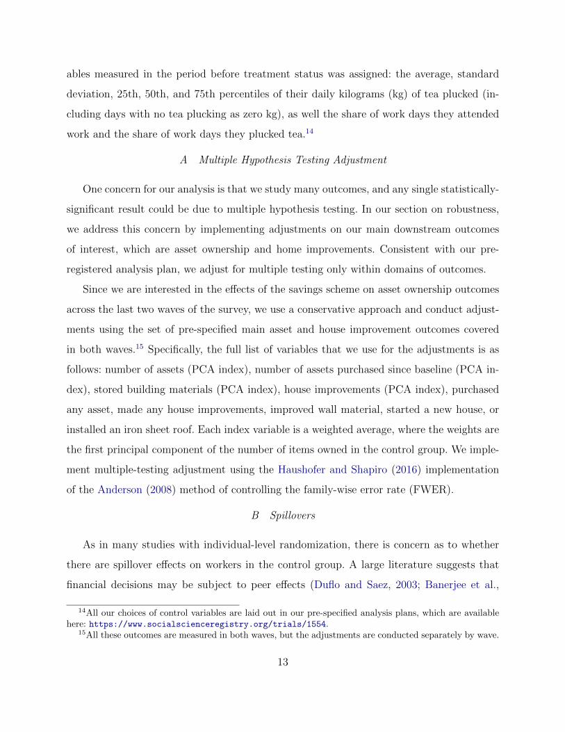
A Multiple Hypothesis Testing Adjustment

One concern for our analysis is that we study many outcomes, and any single statistically-

significant result could be due to multiple hypothesis testing. In our section on robustness,

we address this concern by implementing adjustments on our main downstream outcomes

of interest, which are asset ownership and home improvements. Consistent with our pre-

registered analysis plan, we adjust for multiple testing only within domains of outcomes.

Since we are interested in the effects of the savings scheme on asset ownership outcomes

across the last two waves of the survey, we use a conservative approach and conduct adjust-

ments using the set of pre-specified main asset and house improvement outcomes covered

in both waves.15 Specifically, the full list of variables that we use for the adjustments is as

follows: number of assets (PCA index), number of assets purchased since baseline (PCA in-

dex), stored building materials (PCA index), house improvements (PCA index), purchased

any asset, made any house improvements, improved wall material, started a new house, or

installed an iron sheet roof. Each index variable is a weighted average, where the weights are

the first principal component of the number of items owned in the control group. We imple-

ment multiple-testing adjustment using the Haushofer and Shapiro (2016) implementation

of the Anderson (2008) method of controlling the family-wise error rate (FWER).

B Spillovers

As in many studies with individual-level randomization, there is concern as to whether

there are spillover effects on workers in the control group. A large literature suggests that

financial decisions may be subject to peer effects (Duflo and Saez, 2003; Banerjee et al.,

14All our choices of control variables are laid out in our pre-specified analysis plans, which are availablehere: https://www.socialscienceregistry.org/trials/1554.

15All these outcomes are measured in both waves, but the adjustments are conducted separately by wave.

13

2013; Bursztyn et al., 2014). In our setting, this is a potential concern because all workers

are employees of the same firm, and they interact socially and financially. To address this

issue, we collected social network data prior to assigning workers to treatment. This data

allows us to conduct robustness tests that control for peer effects and test for potential

spillovers, by following the approach of Kremer and Miguel (2007) and Blumenstock, Callen

and Ghani (2018). Specifically, we augment Equation 1 by including terms for a worker’s

total number of peers and number of treated peers. We define peers as any coworker who

was identified by a worker as a friend or someone that they interact with financially.16

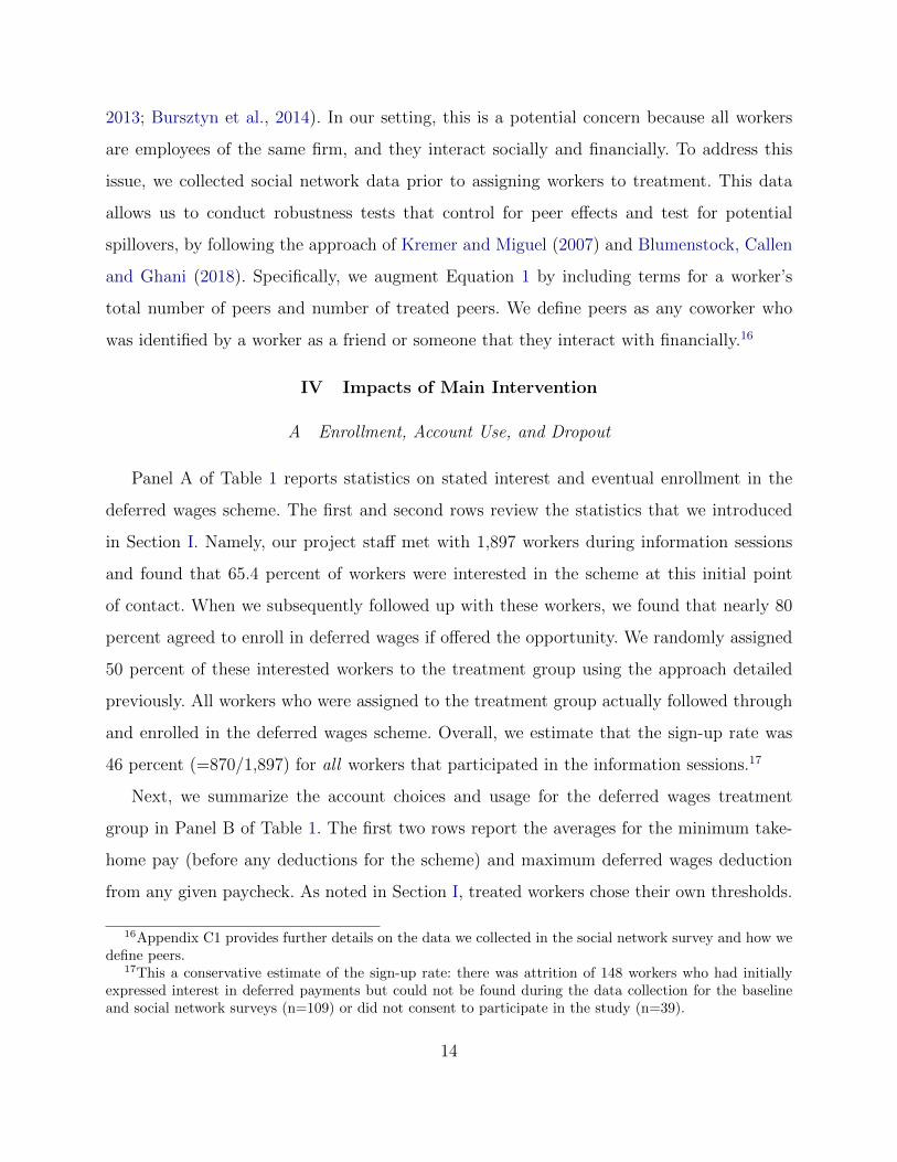
IV Impacts of Main Intervention

A Enrollment, Account Use, and Dropout

Panel A of Table 1 reports statistics on stated interest and eventual enrollment in the

deferred wages scheme. The first and second rows review the statistics that we introduced

in Section I. Namely, our project staff met with 1,897 workers during information sessions

and found that 65.4 percent of workers were interested in the scheme at this initial point

of contact. When we subsequently followed up with these workers, we found that nearly 80

percent agreed to enroll in deferred wages if offered the opportunity. We randomly assigned

50 percent of these interested workers to the treatment group using the approach detailed

previously. All workers who were assigned to the treatment group actually followed through

and enrolled in the deferred wages scheme. Overall, we estimate that the sign-up rate was

46 percent (=870/1,897) for all workers that participated in the information sessions.17

Next, we summarize the account choices and usage for the deferred wages treatment

group in Panel B of Table 1. The first two rows report the averages for the minimum take-

home pay (before any deductions for the scheme) and maximum deferred wages deduction

from any given paycheck. As noted in Section I, treated workers chose their own thresholds.

16Appendix C1 provides further details on the data we collected in the social network survey and how wedefine peers.

17This a conservative estimate of the sign-up rate: there was attrition of 148 workers who had initiallyexpressed interest in deferred payments but could not be found during the data collection for the baselineand social network surveys (n=109) or did not consent to participate in the study (n=39).

14

On average, workers opted for a minimum take-home pay of MK 8,239 and a maximum

deduction of MK 2,832. The amount deducted depended on these parameters as well as a

worker’s earnings in a given pay period. Table 1 shows that the average earnings and deferred

wages deductions for each two-week pay period were MK 14,552 and MK 2,054, respectively.

Figure 3 provides further insight into account use by reporting the distribution of the

total savings in the deferred wages scheme at the end of the entire main season (during which

there were a total of six deductions). The dashed line on the figure shows that the average

balance just before the lump-sum payout was MK 12,092, a sizable amount that equals 82

percent of the average payday for workers in our sample (i.e., two weeks of wages).

The last set of statistics reported in Table 1 show that there was minimal exit and high

satisfaction with the program during the main season. During the deduction period, workers

could not access their savings except in the case of an emergency (which they had report

in person at the division office). Anyone who pursued the emergency option was required to

exit the program, and their balance would be paid out at the payday associated with their

current pay period (between one and three weeks later). The first row in Panel C shows that

less than three percent of workers exited the scheme early. In line with this low observed

exit rate, we also see that few workers expressed a desire to leave the scheme or reduce their

savings contributions. The last three rows of Panel C show the results of an incentivized

survey with 50 percent of the treated workers (selected at random) after two deductions had

taken place. We asked these workers whether they wanted to exit the scheme or change their

contributions; workers were told there was a five percent chance their choice would actually

be implemented. Only about four percent of the sampled workers wanted to exit immediately,

which is broadly consistent with the rate of actual early exit from the scheme. Approximately

10 percent of workers (including those who wanted to immediately exit) wanted to reduce

their contributions to the scheme. Consistent with most workers being highly satisfied with

the savings scheme, 15 percent wanted to increase their contributions.

How do these results compare to prior studies? Broadly speaking, the rates of sign-up

and account usage in our sample are relatively high. Karlan, Ratan and Zinman (2014)

15

survey the literature on savings interventions and note that sign-up rates for products with

commitment features are often 20 to 30 percent. Rates of sign-up are often higher in studies of

interventions that feature basic savings products (e.g., standard bank accounts), but account

activity is often low for treated study participants. For example, Dupas et al. (2018) conduct

a multi-country study of the impact of reducing fees for bank accounts. They find that 69

and 54 percent of treated households open accounts in Malawi and Uganda, respectively.

Only 17 and 10 percent of account holders became active users, defined as having made at

least five deposits in the first two years.18 In our study, 73 percent of those who enrolled

made at least five deposits during the 12-week deduction period.

B Determinants of Enrollment

Appendix Table A3 provides further details on the correlates of enrollment in the deferred

wages scheme. This analysis relies on survey data collected during the short survey that was

conducted for all 1,897 workers that we reached through the information sessions. We rely

on this data since it is the only source of detailed information for individuals who indicated

that they were not interested in enrolling in the scheme. The data includes information on

basic demographics, economic status, and measures of savings-related behavior. To analyze

determinants of enrollment, we run a linear regression of an indicator for being interested in

enrolling in the scheme on each variable in the survey.

The results reveal two notable findings. First, we find that interest in the program varies

with savings goals. Workers who reported that saving to build or improve their house was

their main savings goal are eight percentage points more likely to express interest in signing

up. The table also shows that home building and improvement is the most popular savings

18While many studies find low take-up or little account use, two notable exceptions are work by Dupasand Robinson (2013a) and Prina (2015). Dupas and Robinson (2013a) covered bank account fees and helpedpeople open accounts, finding a take-up rate of 87 percent with 41 percent of people making more than onedeposit; average weekly deposits averaged 12 percent of weekly income. Studying a no-fee savings account,Prina (2015) found that 84 percent of those offered took up the account, and 80 percent made more than onedeposit. The average weekly amount deposited was about 8 percent of average weekly income among thosewho were offered the account. Both studies find usage numbers comparable to what we find for the deferredwages scheme. In our study, 46 percent of workers enroll in the scheme; of those who enrolled, 92 percentmade more than one deposit, and workers in the scheme saved an average of 14 percent of their wages.

16

goal in our sample. Second, we also find that self-reported savings challenges are important

predictors of interest in the deferred wages scheme. Individuals who find temptation spending

to be their biggest challenge are 12 percentage points more likely to enroll in the scheme.

C The Total Amount and Composition of Savings

The analysis of program participation reveals that the treatment group deposited sub-

stantial amounts into their deferred wages accounts. Next, we study how the availability of

the scheme affected the total amount of savings as well as its composition. Our analysis is

based on savings measures from both administrative data and follow-up surveys collected

during the deductions period. To improve precision, we pool observations across the two

rounds for flow variables (e.g., whether the worker had any deposits in formal savings ac-

counts in the past 14 days). Stock variables, such as a worker’s overall savings balance, were

collected in the second follow-up, which took place around the time of the final deduction

for the deferred wages scheme (but before the final lump-sum payout in May 2017). One

caveat for our analysis of this data is that the surveys may not fully capture all forms of

savings because respondents may under-report some forms of savings, such as cash kept at

home or by other household members. Previous studies of savings interventions in Malawi

have documented under-reporting of savings in survey data (Dupas et al., 2018).

Our main finding is that the deferred wages scheme appears to have had large positive

impacts on total reported savings and some composition effects. Table 2 shows estimated

effects on savings behavior using the specification from Equation 1. Columns 1-3 examine

the extensive margin of saving in the 14 days prior to the survey interviews. In line with

the results from the previous section, Column 1 shows that treated workers have a high

probability of making a deposit into their deferred wages account. Columns 2 and 3 show

that this was paralleled by negative impacts on the use of other types of saving. The scheme

reduced the likelihood of reporting another type of formal savings deposit by 1.5 percentage

points (p-value < 0.10), a 41 percent decrease relative to the control-group average. For

informal financial savings, we see a seven percentage-point (10 percent) reduction. Columns

4-8 show impacts on reported savings balances, which were measured during the second

17

follow-up survey. We find that the deferred wages treatment increased reported total savings

by MK 6,816 (p-value < 0.01), a 23 percent increase over the control group average. While

total savings appears to have increased, we see partial crowd-out of other forms of reported

savings, in particular informal savings, which decreased by MK 3,609 (p-value < 0.10) for

the treatment group.19

We show evidence on the distributional impact of the deferred wages scheme in Figure 4,

which plots the cumulative density functions (CDFs) for total reported savings separately

for the treatment and control groups. Notably, we see that the treatment group has higher

reported savings throughout most of the distribution, in particular at the bottom end. This

suggests that the scheme had impacts on workers who do not normally accumulate sav-

ings. Appendix Figure A3 further quantifies the distributional results by reporting quantile

treatment effects (QTEs) on total reported savings. The point estimates are statistically sig-

nificant at the five percent level and similar in magnitude across a wide range of quantiles.

D Labor Supply

Access to the deferred wages savings scheme could have impacts on labor supply out-

comes. As noted by Callen et al. (2019), a standard neoclassical model predicts that labor

supply will respond to the introduction of better savings options that change the effective in-

terest rate. This is relevant in our context because the demand for the deferred wages scheme,

as well as the effects it has on savings, suggest that it represents an improved savings option.

If the deferred wages scheme increases the effective return on savings by providing a safer

option with lower transaction costs, we might expect labor supply to increase. Similarly, the

commitment aspect of the scheme may reduce the cost of saving specifically for workers with

self-control problems. Again, this could lead to an increase in labor supply due to an increase

in the effective rate of return on savings.20

19Appendix Table A4 examines treatment effects on all the subcategories of informal savings. Two resultsstand out. First, the treatment group reduced their likelihood of making at least one deposit in an informalsavings group (Panel A, Column 6; p-value < 0.05). Second, treated workers also had lower balances formaize, a form of non-financial, stored food savings (Panel B, Column 10; p-value < 0.05). This effect onmaize balances drives the effect on total food storage savings (Table 2, Column 8; p-value < 0.05).

20As highlighted by Banerjee et al. (2015a) in the context of access to credit, improved access to financemight also lead households to increase labor supply, for example in order to purchase durable goods that are

18

Table 3 reports estimates of the effects of the deferred wages treatment on work out-

comes based on administrative panel data covering the deductions period. We study daily

productivity and earned income per two-week pay period. The odd-numbered columns (1,

3, etc.) report estimates based on Equation 1; the even-numbered columns (2, 4, etc.) re-

port estimates based on an augmented specification that includes interactions between the

treatment indicator and indicators for the worker being classified as a plucker or non-plucker

based on their work history before the treatment was assigned. This analysis is motivated by

the fact that pluckers receive piece-rate earnings, whereas workers employed in non-plucking

jobs have fixed daily wages. This implies that only workers employed as pluckers could have

adjusted their productivity in response to the treatment.21

Column 1 shows that the deferred wages scheme increased productivity on average by

1.6 kg (p-value < 0.05). Relative to the control-group average, this represents a 4.9 percent

increase. As expected, Column 2 shows that there is a larger impact for pluckers (1.8 kg,

p-value < 0.05) and no detectable impact for non-pluckers. The results for income earned

in Columns 3 and 4 are consistent with the positive impacts on productivity. Specifically,

we see that pluckers in the treatment group have MK 342 higher average earnings (p-value

< 0.05) per two-week pay period in the payroll data. The results in Columns 5-8 show that

the impacts on productivity are driven by significant effects on the intensive margin: there

are no effects on attendance or on whether the worker plucked any tea.22

These findings are in line with the mechanism highlighted above from Callen et al. (2019).

Callen et al. experimentally study the impact of providing unbanked households with weekly

deposit collection services from a local bank. They find that this treatment had large and

statistically-significant positive impacts on formal savings and household income. Consistent

with our results, they also find increases in labor supply, in particular for wage work.23

otherwise out of reach due to savings or credit constraints.21Approximately 77 percent of workers in the sample are coded as pluckers based on their pre-treatment

work history, but non-pluckers are sometimes tasked with plucking tea on a specific work day (and thus earnpiece rates on that day). Note that our analysis plan specified that we would examine effects of the deferredwages scheme separately for pluckers and non-pluckers.

22Conditional on plucking any tea there are strong effects on the quantity plucked (results available uponrequest).

23Dupas and Robinson (2013a) also study the relationship between savings options and labor supply.

19

Furthermore, Callen et al. (2019) also find that treatment effects on income and labor supply

are immediate in their sample. Appendix Figure A1 shows that we find the same pattern:

the treatment appears to affect productivity even in the initial weeks of deductions.

Finally, it is worth noting that our findings do not align with the results from Kaur et al.

(2020)’s study of financial strain and worker productivity. They find that early payment

increases the productivity of skilled workers and show that this effect is due to improved

attentiveness. Why does delaying a sizable fraction of pay for treated workers in our sample

not generate negative impacts on productivity? Potential explanations stem from two differ-

ences in study contexts. First, Kaur et al. (2020) conduct their intervention during the lean

season and document high levels of financial worry for their sample. Second, they study the

impact of financial strain for workers who perform cognitively-demanding tasks. Our study

differs in both these dimensions since we study productivity during the main season (when

there is relatively high income) and focus on a sample of workers who perform tasks that

use physical rather than cognitive skills.24

E Expenditures During the Deduction Period

Table 4 reports results from our analysis of expenditures during the deduction period

(from late January through mid-April 2017). The first two follow-up surveys collected mea-

sures of total expenditures and categories of expenditures during the 14 days prior to the

interview. We also collected information on bulk purchases within the past 30 days. To

increase precision, our analysis pools observations from both survey waves.

The results show that the estimated effects on expenditures are never statistically signif-

icant. However, the confidence intervals are sufficiently wide that we cannot rule out effects

They estimate the impact of providing a non-interest-bearing account to self-employed workers in Kenya.They find economically-meaningful impacts on incomes, but their estimates are not statistically significant.

24An additional point of interest concerns payday effects. Kaur, Kremer and Mullainathan (2015) studyproductivity for piece-rate workers who work for seven days and receive payment on the final day of the payperiod during the evening. They find that workers are least productive on days early in their pay period,and production rises through the pay cycle. We analyze productivity over the two-week pay period and findno evidence of payday effects in our context. One notable difference between the contexts of the two studiesis that paydays in our study occur seven days after the final work day in a two-week pay period, whereasworkers in Kaur, Kremer and Mullainathan are paid immediately at the end of the pay period.

20

that are large enough to be economically important. For example, Column 1 shows that the

95-percent confidence interval for the impact on total expenditures ranges from a decrease of

MK 1,343 (7.1 percent relative to the control-group average) up to an increase of MK 1,965

(10.4 percent). As such, we can only confidently rule relatively large negative effects on ex-

penditures. Similar points apply to the results for detailed expenditure categories (Column

2-6) and the measures of bulk purchases during the past 30 days (Columns 7 and 8).

How should we interpret these results? Given the positive and statistically-significant

impacts on total reported savings, it is natural to expect that the deferred wages treatment

would reduce expenditures during the deductions period. The point estimates for the ex-

penditure categories in Table 4 run counter to this in that they are consistently positive,

although small in magnitude. There are two points to consider for understanding these re-

sults. First, the point estimates for the labor supply effects documented above can provide

a partial explanation of the lack of a statistically-significant decline in spending. Using the

estimates from Table 3, we calculate that increased productivity over the entire deduction

period for the treatment group generated an additional MK 1,326 (= six pay periods ×

MK 221 per pay period). This amount is 20 percent of the estimated MK 6,816 increase in

reported savings (Table 2, Column 4) for the treatment group. Second, the remainder of the

impact on savings is sufficiently small that it could be entirely accounted for by a decline

in expenditures that is within the confidence interval in Table 4. Specifically, our estimates

suggest that the increase in savings net of labor supply effects is equal to MK 5,490 (=MK

6,816 − MK 1,326). To account for this solely through a reduction in expenditures implies

that we should see a reduction of MK 915 in expenditures every two weeks. This amount is

smaller in magnitude than the negative MK 1,343 lower bound of the 95-percent confidence

interval for total expenditures.25 The confidence intervals on the expenditure estimates are

wider than we anticipated ex ante, and mean the study is underpowered to detect plausible

magnitudes of the effect of the treatment on expenditures. Our minimum detectable effect

25An additional explanation could be that members of the treatment group avoided reductions in expen-ditures by taking on more loans or transfers. However, supplementary analyses show no detectable impactson these additional sources of income. These results can be provided on request.

21

size at 80 percent power for changes in total expenditures is 2.8 times the standard error

(Ioannidis, Stanley and Doucouliagos, 2017), which is 2.8 × 844 = MK 2,363. The total

increase in reported savings due to the deferred wages scheme is MK 6,816 (Table 2, Column

4), or is MK 1,136 per two-week period. We are thus only powered to detect effects on ex-

penditures that are twice as large as what we would expect based on the estimated changes

in savings.

F Expenditures After Payout

Next, we consider impacts on expenditures after treated workers received the lump-

sum payout of their savings. We anticipated that most spending would occur shortly after

the payout and began collecting surveys almost immediately after the payment in May

2017. To improve the precision of flow measures and focus respondent attention on the

post-disbursement period, we varied the recall period based on the timing of the survey.

Specifically, for surveys collected within the first 14 days of the lump-sum payout, the recall

period covered the time from the payout until the day of the survey; this recall period

ranged from four to 14 days, with a median of seven and an average of 8.4. For surveys after

the first 14 days following the lump-sum payout, we used a 14-day recall window, which is

consistent with what we had used in the preceding rounds and matches the two-week pay

periods at Lujeri. As noted in Section II, we partially randomized the order of surveying to

balance the characteristics of respondents surveyed earlier and later. Given that the recall

window changes for individuals surveyed during the first 14 days and afterward, we conduct

separate analyses for those interviewed within 14 days of the lump-sum payout and for those

interviewed afterward.

Panel A of Table 5 begins with results for total expenditures for the sample of respondents

interviewed within the first 14 days following the lump-sum payout. Column 1 shows that

the deferred wages treatment increased total expenditures by MK 5,787 (p-value < 0.01), a

36 percent increase relative to the control-group average.26 This impact is driven by large

26Appendix Table A5 shows that the treatment group also had a higher rate of saving, more net moneyloaned, and more net transfers made, but only the effect on net money loaned is statistically significant(p-value < 0.05).

22

and statistically-significant positive impacts on expenditures in major categories such as

food (column 2) and durables (column 5). The impacts on food spending are driven by a

MK 2,404 increase in maize purchases. This is a notable finding given that maize prices are

typically low at the end of the main tea season.27 Columns 7 and 8 show that we find large

and statistically-significant effects on the incidence and sum of spending on bulk purchases

(single purchases that amount to more than MK 5,000). Panel B reports effects for the sample

of respondents interviewed after the first 14 days after payout. The point estimate indicates

that total expenditures declined by MK 772 for the treatment group, but this result is not

statistically significant. We also find no detectable impacts on the categories of expenditures

or large purchase measures. Appendix Table A6 provides an alternative analysis of treatment

effects after the lump-sum payout. Specifically, we estimate impacts separately for each week.

In this analysis, we estimate effects on daily spending instead of total expenditures within a

recall window. The results yield very similar patterns to Table 5.

In sum, this analysis yields two main findings. First, the results suggest that workers

spent a large portion of their saved funds within the first 14 days after receiving the lump-

sum payout. Specifically, the MK 5,787 effect on total expenditures within the first 14 days

after the payout is equal to 85 percent of the estimated impact on total reported savings

(Table 3, Column 4). The remainder of the reported savings do not appear to be spent after

the first 14 days, although our power to detect effects on expenditures during this period

is limited. Second, expenditures increase substantially for bulk purchases and durables that

require lump sums. This result is consistent with the hypothesis that the deferred wages

scheme addresses savings constraints.

G Long-Run Outcomes

The evidence so far shows that the deferred wages treatment shaped savings behavior

during the main deduction period and had large impacts on expenditures in the period

immediately following payout of the lump sum. Our last analysis of the main intervention

27Maize is harvested in April and May, causing prices to fall. Our survey data shows that maize pricesfell by 65 percent between February and May 2017.

23

considers whether this translated into impacts on downstream outcomes. We rely on out-

comes measured in the fourth and fifth follow-up surveys. These surveys were collected four

months and a little less than two years after the payout of the main intervention, respectively.

Our analysis of assets is motivated by the fact that, at baseline, a substantial fraction of

our sample had asset-related purchases as saving goals. Appendix Table A3 shows that the

most common self-reported savings goals was improving or building a house (34 percent),

and purchasing a household asset (12 percent) was also a popular goal. Table 6 reports

results for assets. Columns 1-4 show impacts measured four months after the payout (i.e.,

the “medium run” period). The outcome in Column 1 is a PCA index of the number of

assets owned in 54 durable asset and seven livestock categories, which is one of the main

outcomes in our pre-registered analysis plan. The point estimate shows that the deferred

wages scheme increased the index of assets by 0.164 standard deviations (p-value < 0.01).28

Column 2 reports impacts on the total value of assets for ease of interpretation. We find that

there was an MK 11,362 (p-value < 0.05) increase in the value of assets in the medium run.

Column 3 indicates that this overall effect is driven by a MK 7,425 increase in stored building

materials (p-value < 0.01), which accounts for 65 percent of the effect on total assets. In line

with the pre-intervention survey responses on savings goals, Column 4 shows that there are

large treatment effects on iron sheets, a key building material for homes.

To expand on these results, we explore the distributional impacts of the deferred wages

scheme on the total value of reported assets four months after the payout. Figure 5 plots the

CDFs of assets separately for the treatment and control groups, while Appendix Figure A5

presents estimated QTEs. These results show that the treatment group appears to have more

assets throughout the distribution. The point estimates for the quantile treatment effects are

consistently positive and range from about MK 5,000 to roughly MK 13,000.

Columns 5-7 of Table 6 provide results for outcomes measured in the fifth follow-up survey,

just under two years after the main intervention—the longest-run data that we collected.

28Our pre-registered plan also specified analysis of assets purchased since baseline. Column 2 of AppendixTable A7 shows that we find no detectable impacts on asset purchases. We include this outcome in the setof variables that we use for multiple hypothesis testing adjustment, as detailed in the section on robustnesschecks.

24

The treatment group had been offered the deferred wages scheme two more times prior to the

fifth follow-up survey, with roughly 80 percent signing up; the last of these schemes ended

about nine months before the fifth follow-up survey. Column 7 shows that treated workers

are 7.7 percentage points (p-value < 0.01) more likely to report that they have an improved

type of roofing (iron sheets). To validate this result and obtain information about survey

measurement error, we physically verified the roofing material for 74 percent of respondents

during the fifth follow-up survey. We find that the field staff verification results match the

survey responses for 95 percent of cases.29 The effect on improved roofing is a 9 percent

increase relative to the control-group average. This impact on home improvements is in line

with the pattern of results from the four month follow-up survey. Table 6 and Appendix

Table A7 show that there are no detectable sustained impacts on any other type of asset in

the long run.

Overall, we conclude that the deferred wages scheme appears to have had strong impacts

on assets. Downstream effects on assets are fairly rare in the literature on savings interven-

tions. Many interventions to increase savings have no effects on any other financial outcome

(Dupas et al., 2018). To the best of our knowledge, there are only two prior studies that

show effects on assets. Dupas and Robinson (2013a) find that access to savings accounts

has impacts on business investments, but there are no detectable effects on household asset

ownership. Schaner (2018) finds that short-term interest rate subsidies for bank accounts

lead to short-run increases in savings and long-run increases in assets.

H Robustness Checks

In this section, we conduct three exercises to examine the robustness of our results.

First, we address concerns over multiple hypothesis testing by calculating adjusted p-values

using the Haushofer and Shapiro (2016) approach to FWER correction. Table 6 reports

adjusted p-values taking into account all outcomes in Columns 1-7. Our main findings are

generally robust, as nearly all outcomes that had statistically-significant naıve p-values are

29The measurement error we find is both symmetrical in direction and orthogonal to treatment status,which suggests high reliability for the other stock variables measured in our surveys as well.

25

also significant at the ten percent level or lower after FWER adjustment. The only exception

is the result for the value of assets owned (column 2) where the adjusted p-value equals 0.124.

Appendix Table A7 goes further with the FWER adjustment by using a larger set of nine

asset outcomes from the fourth and fifth follow-up surveys, as discussed in Section III. We

find that, using this approach, the impact on the PCA index of the number of assets owned

is still significant at the 10 percent level (p-value = 0.07). The long-run effect on improved

roofing is also robust to correcting for multiple testing (p-value = 0.041). Overall, these

findings provide reassurance that the effects we detect on assets are not spurious.

Second, we test for spillovers between workers in the treatment and control groups. Ap-

pendix Table A8 presents results based on an augmented version of Equation 1 that includes

terms for a worker’s total number of peers and the number of treated peers, following Kremer

and Miguel (2007). Appendix Table A9 presents the same specification for the extended set

of assets shown in Appendix Table A7. We see little evidence of peer effects for these out-

comes; the point estimates are generally small in magnitude and statistically insignificant.30

Critically, the estimates for the treatment group indicators are nearly unchanged for all out-

comes, suggesting that our estimates of the effect of the savings scheme on asset ownership

are not biased by spillovers.

Finally, our third robustness check is to adjust the treatment effect estimates for both

potential spillovers and multiple hypothesis testing at the same time. Our approach here

parallels the two approaches to multiple testing adjustments presented in Table 6. First,

Appendix Table A8 reports adjustments for all outcomes within the table. These within-table

FWER-adjusted p-values are still statistically significant for the number of assets owned

(p-value < 0.05) and stored building materials (p-value < 0.05). For the effect on metal

roofing, the FWER-adjusted p-value is higher than the naıve p-value, but remains statistically

significant at the ten percent level (p-value = 0.056). Second, Appendix Table A8 also reports

adjustments for the extended set of assets shown in Appendix Table A9. These extended

30The two exceptions are in the extended set of assets shown in Appendix Table A9. There is evidence ofnegative spillovers on making any improvements to one’s house in the short run (Panel A, Column 6) andpositive spillovers on buying any asset in the long run (Panel B, Column 5).

26

FWER adjustments leave the effects on both the asset ownership index (p-value < 0.10) and

metal roofing (p-value < 0.05) statistically significant at conventional levels.

V Explaining Take-up and Account Usage

As noted above, we find relatively high rates of program enrollment and account usage

when comparing our evaluation of the deferred wages scheme to prior studies of savings

products. This section reports results from several analyses that further explore determinants

of enrollment and utilization.

A Re-enrollment, Mistakes, and Seasonality

Mistakes may be one reason why we observe relatively high rates of participation in the

deferred wages scheme. Prior research has found that some individuals make mistakes when

signing up for products with commitment features (Bai et al., 2020; John, 2019). In addition,

seasonality and consumption smoothing is another potential reason that we might observe

demand for deferred wages. That is, workers may seek to use the lump sum payout in May to

help smooth consumption between the main season for tea and the off-season. Two factors

make this a particularly relevant consideration in our setting. First, Fink, Jack and Masiye

(2020) find high demand for credit during the lean season in Zambia, which neighbors Malawi.

Second, the end of the main tea season (and thus the arrival of the deferred wages payout)

coincides with the maize harvest, when maize prices are lowest. Workers may want to use

their deferred wages for strategically-timed maize purchases; we do observe large increase in

spending on maize just after the payout (Table 5, Column 4).

To explore the role of mistakes and seasonality in driving demand for the deferred wages

scheme, we offered the treatment group the chance to re-enroll in the savings scheme two

additional times: once during the ensuing off-season (from October to December 2017) and

once during the next main season (from February to April 2018). Prior studies have sim-

ilarly studied repeat enrollment to test for the possibility that mistakes drive take-up of

commitment devices (e.g., Schilbach 2019). We offered the opportunity to sign up for the

deferred wages scheme for the off-season and the next main season during the interviews for

27

the fourth follow-up survey in September 2017. Interested workers were re-enrolled on the

spot.

The results from this re-enrollment exercise provide no evidence that mistakes drive

decisions in our setting. Appendix Table A10 reports the sign-up rate for the off-season and

next main season savings schemes. Column 2 shows that 81 and 78 percent of the treatment

group opted into the scheme for the off-season and the next main season respectively. The

similarity in the sign-up rates also strongly rules out that seasonality plays a role in driving

the demand for the deferred wages scheme. We fail to reject the hypothesis that the sign-up

rates for the off-season and the next main season are equal (p-value = 0.18).

B Automatic versus Manual Deposits

One potential explanation for the high enrollment in and use of the deferred wages scheme

is that workers value having a savings product that features automatic deposits. In the main

intervention, workers make an allocation decision once, and funds are automatically deducted

each pay period. This feature could help workers meet savings goals by lowering transaction

costs, addressing behavioral biases that constrain saving behavior, or reducing social pressure

to share income with one’s friends and family.

To explore the importance of automatic deposits, we conducted a supplementary experi-

ment in February 2018 (after the main intervention). As previewed in Section I, this analysis

was conducted with a sample of 186 workers who were not part of the earlier study. We ran-

domly divided this new sample of workers into two groups. The first group received offers to

participate in the original version of the deferred wages scheme. The second group received

offers for a version of the deferred wages scheme that required participants to make manual

deposits with a member of our research staff. The location for these manual deposits was

easy to reach: workers could make deposits at a station next to the division office, which is

the location where they already went on paydays to pick up their wages.

Our goal in this section is to estimate the impact of the manual deposit feature on savings

28

behavior. We do this using the following specification:

yi = π + τManuali + ξi (2)

where yi is an outcome such as enrollment or account usage. The variable Manuali is equal

to one if worker i received the offer to join the manual deposit version of the deferred wages

scheme and zero otherwise. The omitted group in our specification received offers to sign up

for the original version of the deferred wages scheme (which featured automatic deposits).

Our parameter of interest is τ , which is the causal effect of offering the deferred wages

scheme with the manual deposit feature on take-up and account usage outcomes (e.g., total

savings balances). Random assignment in our experiment ensures that assignment to the

group receiving manual offers is uncorrelated with the error term ξi in expectation.31

Panel A of Table 7 reports estimates of the impact of the manual feature on enrollment

and account usage, based on Equation 2. Column 1 shows that when we approached workers,

those assigned to the manual deposits treatment group were not detectably less likely to

express interest in enrolling than those assigned to receive offers for the original deferred

wages scheme. However, we find that the manual treatment reduced the likelihood of making

at least one deposit by 30.3 percentage points (p-value < 0.01, Column 2). Relative to the

control group, which was offered the standard deferred wages scheme, this is a 60 percent

decrease. Columns 3 and 4 show that manual deposit offers also led to reductions in the

number of deposits by 1.9 (p-value < 0.01) and the account balance by MK 3,516 (p-value

< 0.05).

In light of these results demonstrating the importance of the automatic deposit feature,

we turn to analyzing potential mechanisms for this result. As mentioned above, it is possible

that demand in our context is driven by workers who face savings constraints in the form

self-control issues or kin taxes. To test this hypothesis, Panel B of Table 7 reports estimates

31To provide evidence for our identifying assumption, we regress the indicator for receiving a manual de-posit offer on fixed demographic characteristics (survey-based measures of the respondent’s age, sex, maritalstatus, and literacy status). The sample is well balanced: we are unable to reject the null hypothesis thatthe coefficients on these characteristics are jointly zero (p-value = 0.75).

29

of heterogeneity in the effects of the manual deposit feature using an augmented version of

Equation 2. Specifically, we include interactions between the indicator for a manual deposit

offer with measures of whether the respondent reported having self-control problems, faced

kin taxes, or had a formal savings account.32 We created three indicators for self-control

problems based on a survey question with three answer choices about the frequency with

which respondents regret past consumption choices. Similarly, we create a proxy for low,

medium, or high levels of kin taxes based on responses to a set of three questions about

whether the respondent would prefer to be receive a transfer privately or a higher amount

publicly. This survey question is motivated by evidence that publicly-received money is more

likely to be taxed by kin (Goldberg, 2017) and that people are willing to forgo part of their

earnings in order to hide money from kin (Jakiela and Ozier, 2016). We specify the interaction

terms such that the omitted group in the augmented model is the set of workers who have

the lowest self-reported self-control, face high kin taxes, and do not have formal savings

accounts.

The results in Panel B provide some evidence that the manual deposit feature has hetero-

geneous impacts in our sample. The main effect estimates in Column 1-4 show that workers

in the manual deposit group who have the lowest measured self-control and face high kin

taxes are 40 percentage points less likely to make at least one deposit (p-value < 0.05), make

2.6 fewer total deposits (p-value < 0.01), and have lower total savings balances by MK 8,215

(p-value < 0.05). While the interaction terms are imprecisely estimated on the extensive

margin of making any deposits, we do find detectable effects on the number of deposits and

on final balances. Columns 3 and 4 show that the manual deposit feature has a significantly

less negative impact for workers with high self-control. For high self-control workers, the im-

plied effect (based on the main effect and interaction term) is a small reduction in balances

of MK 423 that is not statistically different from zero (p-value = 0.93). The estimates of the

interaction terms that include proxies for kin taxes are never statistically significant and are

32Appendix C reproduces the exact text of the questions that we used to create proxy measures of self-control problems (Appendix C2) and kin taxes (Appendix C3), along with the available answer choices andthe frequencies of each response.

30

relatively imprecisely estimated.

Overall, the results in this section lead us to two conclusions. First, the evidence is

consistent with the hypothesis that automatic deposits are important to workers because this

feature helps mitigate self-control problems. Workers in the two treatment arms expressed

similar levels of interest, but the manual deposit group had difficulty building up savings,

particularly if the worker reported having self-control issues. In this way, our results align

with findings from Casaburi and Macchiavello (2019) that show individuals who have issues

with self-control demand deferred payments. Second, there is suggestive evidence that the

scheme is beneficial for workers beyond solving self-control problems. The sign-up rate for

the original version of the scheme is fairly high (about 41 percent) for people who report no

self-control problems. This would not be the case if self-control issues were the only reason

people were interested in deferred wages. One plausible alternative reason people may be

interested in deferred wages is a lack of alternative safe places to save.

An important caveat to this analysis of treatment effect heterogeneity is that we rely

on proxies for kin taxes and self-control problems that are likely subject to substantial

measurement error. Classical measurement error would attenuate the associated coefficients

in our regression analyses, which might mean that kin taxes matter more than the estimated

pattern of heterogeneity indicates. Misclassification could also mean that we underrate the

importance of self-control problems. In particular, we note that a substantial fraction of

people with high reported self-control sign up for the original deferred wages scheme. If self-

control is mismeasured, many of these apparently high self-control workers may actually have

self-control issues. The results should also be interpreted cautiously given that we examine

a number of outcomes and hypotheses in the heterogeneity analysis.

C Preferences Over Payout and Access

In addition to automatic deposits, the lump-sum payout and restricted access features

of the original scheme may be particularly attractive to workers. To study the importance

of these two features, we conducted an additional choice experiment in February 2018 (after

the main intervention). We recruited a new sample of 542 workers who were neither part of

31

the earlier study nor part of the experiment to study the importance of automatic versus

manual deposits.

In this experiment, all sampled workers received an overview of the original deferred

wages product and two modified versions. The first modified version had a “smooth payout”

feature: workers would receive six payments in two-week intervals after the end of the deduc-

tion period. The second modified version provided “more access”: workers could withdraw

accumulated funds at any point during the deduction period.

To study preferences over payout smoothness and ease of access, we randomly divided our

sample into three groups that answered hypothetical enrollment questions. The first group

was asked whether they would want to enroll in the original version of the deferred wages

scheme. The second and third groups were asked whether they wanted to enroll in one of

the two modified versions, respectively. We incentivized responses by informing workers that

one randomly-selected worker from each division of the company would have their choice

implemented.

Our goal in this section is to estimate the causal impact of the smooth-payout and more-

access features on the enrollment decisions. To do this, we estimate the following specification:

yi = ρ+ σSmoothPayoutsi + ψMoreAccessi + ωi (3)

where yi is an indicator equal to one if respondent i wanted to enroll in the deferred wages

scheme that was offered to them in this incentivized-choice survey question. The variables

SmoothPayoutsi and MoreAccessi are indicators equal to one if their question featured the

smooth payout or more access versions of the deferred wages schemes. The omitted group

is respondents who were asked about the original version. Our main parameters of interest

are σ and ψ, which are the causal effects on enrollment of offering deferred wages schemes

with smooth payouts or more access. Random assignment in our experiment ensures that

assignment to the group receiving smooth or more access questions is uncorrelated with the

error term ωi in expectation.33

33To provide evidence on our identifying assumption, we regress the indicator for receiving the question

32

Appendix Table A11 reports estimates from Equation 3. The control-group average shows

that 55.9 percent of workers were interested in enrolling in the original version of the scheme,

which is comparable to the sign-up rate that we observed for our main intervention. The

estimate in the second row indicates that workers who received the smooth payout offer were

about 20 percentage points less likely (a 35 percent decrease; p-value < 0.01) to express

interest in enrolling. The estimate in the third row suggests that the more access feature

reduces enrollment by 4 percentage points, but this result is not statistically significant.

There are two main findings from these results. First, the evidence suggests that workers

value the lump-sum payout in the original deferred wages scheme. An important caveat for

this interpretation is that our evidence is based on a specific form of payout. We did not

test other alternatives such as providing the ability to draw down the funds at any time.

Second, the evidence implies that rigid restrictions on access do not meaningfully affect

interest in enrolling. However, this does not rule out that workers value the commitment

feature of deferred wages. The more access version of the scheme still involved substantial

commitment, since funds could not be accessed for one to three weeks (until the payday

associated with their current pay period).

VI Conclusion

Large shares of the population in developing countries face barriers to saving income.

Market frictions hinder the supply of formal financial products, and nearly half of adults in

developing countries do not have access to an account at a bank or another formal financial

institution (Demirguc-Kunt et al., 2015). In addition, the ability to save could be depressed

by demand-side constraints such as time-inconsistency and social pressure to share income.

This paper provides evidence that deferred payments can be a popular and effective

savings device. Partnering with a tea firm in Malawi, we find that nearly half of workers would

on the original deferred wages scheme on fixed demographic characteristics (survey-based measures of therespondent’s age, marital status, sex and literacy status). The sample is well balanced: we are unable to rejectthe null hypothesis that the coefficients on these characteristics are jointly zero (p-value = 0.23). We observesimilar balance in tests where the dependent variables are indicators for receiving the questions featuringsmooth payout and more access versions of deferred wages, respectively.

33

enroll in a simple savings scheme that allowed workers to defer a fraction of their pay for

three months at zero interest. Figure 6 summarizes the main findings from our experimental

evaluation of the scheme. Most notably, we find that the deferred wages scheme generates

large positive impacts on reported savings and has impacts on downstream outcomes. In line

with savings goals elicited prior to our intervention, we find that treatment-group workers

were more likely to have made durable investments in their homes two years after the initial

round of the scheme and nine months after the last round of the scheme.

These findings have implications for our understanding of savings behavior. Rationaliz-

ing the popularity of deferred wages requires modifying neoclassical models of intertemporal

choice, potentially by introducing behavioral constraints and storage costs. Our supplemen-

tary experiments provide suggestive evidence for the importance of both factors. Requiring

manual (rather than automatic) deposits reduces follow-through, particularly among work-

ers who report having self-control problems. This result is consistent with previous studies

that show products with commitment features can have important impacts (Ashraf, Karlan

and Yin, 2006; Gine, Karlan and Zinman, 2010; Duflo, Kremer and Robinson, 2011; Dupas

and Robinson, 2013b; Karlan and Linden, 2014; Brune et al., 2016; Kaur, Kremer and Mul-

lainathan, 2015; Schilbach, 2019; Casaburi and Macchiavello, 2019). At the same time, the

evidence also suggests that workers might value deferred payments for reasons other than

self control. Workers without apparent self-control problems still sign up for the original,

automatic-deposits scheme at high rates, which would not happen if demand came solely

from self-control issues.34 A plausible alternative reason they might want to use the deferred

wages scheme is that they need a safe place to store money.

We conclude with the observation that further research is necessary to understand the

benefits of deferred payments in other settings. This paper demonstrates that an employer-

based deferred payment scheme can generate notable benefits for workers. An important

feature of our study is that we study a sample of individuals who had relatively limited

formal savings options prior to our intervention. It is an open question whether deferred

34An important caveat for this interpretation is that measurement error in our proxy for self-control couldalso explain this result.

34

payment schemes would be popular or effective in contexts where individuals can access

other low-cost or high-quality savings products.

35

References

Anderson, Michael L. 2008. “Multiple Inference and Gender Differences in the Effectsof Early Intervention: A Reevaluation of the Abecedarian, Perry Preschool, and EarlyTraining Projects.” Journal of the American Statistical Association, 103(484): 1481–1495.

Ashraf, Nava, Dean Karlan, and Wesley Yin. 2006. “Tying Odysseus to the Mast:Evidence from a Commitment Savings Product in the Philippines.” Quarterly Journal ofEconomics, 121(2): 635–672.

Ashraf, Nava, James Berry, and Jesse M Shapiro. 2010. “Can Higher Prices StimulateProduct Use? Evidence from a Field Experiment in Zambia.” American Economic Review,100(5): 2383–2413.

Bai, Liang, Benjamin Handel, Edward Miguel, and Gautam Rao. 2020. “Self-Control and Demand for Preventive Health: Evidence from Hypertension in India.” Reviewof Economics and Statistics, forthcoming.

Banerjee, Abhijit, Arun G. Chandrasekhar, Esther Duflo, and Matthew O. Jack-son. 2013. “The Diffusion of Microfinance.” Science, 341(6144).

Banerjee, Abhijit, Esther Duflo, Rachel Glennerster, and Cynthia Kinnan. 2015a.“The Miracle of Microfinance? Evidence from a Randomized Evaluation.” American Eco-nomic Journal: Applied Economics, 7(1): 22–53.

Banerjee, A., E. Duflo, N. Goldberg, D. Karlan, R. Osei, W. Pariente, J. Shapiro,B. Thuysbaert, and C. Udry. 2015b. “A multifaceted program causes lasting progressfor the very poor: Evidence from six countries.” Science, 348(6236): 1260799–1260799.

Behrman, Jere R., Susan W. Parker, Petra E. Todd, and Kenneth I. Wolpin. 2015.“Aligning Learning Incentives of Students and Teachers: Results from a Social Experimentin Mexican High Schools.” Journal of Political Economy, 123(2): 325–364.

Beshears, John, James J Choi, Christopher Harris, David Laibson, Brigitte CMadrian, and Jung Sakong. 2015. “Self Control and Commitment: Can Decreasing theLiquidity of a Savings Account Increase Deposits?” National Bureau of Economic ResearchWorking Paper 21474.

Blumenstock, Joshua, Michael Callen, and Tarek Ghani. 2018. “Why Do DefaultsAffect Behavior? Experimental Evidence from Afghanistan.” American Economic Review,108(10): 2868–2901.

Breza, Emily, Martin Kanz, and Leora F. Klapper. 2020. “Learning to Navigate a NewFinancial Technology: Evidence from Payroll Accounts.” National Bureau of EconomicResearch Working Paper 28249.

36

Brownback, Andy, and Sally Sadoff. 2020. “Improving College Instruction throughIncentives.” Journal of Political Economy, 128(8): 48.

Bruhn, Miriam, and David McKenzie. 2009. “In Pursuit of Balance: Randomizationin Practice in Development Field Experiments.” American Economic Journal: AppliedEconomics, 1(4): 200–232.

Brune, Lasse, and Jason T. Kerwin. 2019. “Income timing and liquidity constraints: Ev-idence from a randomized field experiment.” Journal of Development Economics, 138: 294–308.

Brune, Lasse, Eric Chyn, and Jason Kerwin. 2021. “Data and code for: Pay Me Later:Savings Constraints and the Demand for Deferred Payments.” Nashville, TN: AmericanEconomic Association [publisher], Ann Arbor, MI: Inter-university Consortium for Politi-cal and Social Research [distributor]. https://doi.org.10.3886/E130367V1.

Brune, Lasse, Xavier Gine, Jessica Goldberg, and Dean Yang. 2016. “FacilitatingSavings for Agriculture: Field Experimental Evidence from Malawi.” Economic Develop-ment and Cultural Change, 64(2): 187–220.

Brune, Lasse, Xavier Gine, Jessica Goldberg, and Dean Yang. 2017. “Savings de-faults and payment delays for cash transfers: Field experimental evidence from Malawi.”Journal of Development Economics, 129: 1–13.

Bryan, Gharad, Dean Karlan, and Scott Nelson. 2010. “Commitment Devices.” An-nual Review of Economics, 2(1): 671–698.

Bursztyn, Leonardo, Florian Ederer, Bruno Ferman, and Noam Yuchtman. 2014.“Understanding Mechanisms Underlying Peer Effects: Evidence From a Field Experimenton Financial Decisions.” Econometrica, 82(4): 1273–1301.

Callen, Michael, Suresh de Mel, Craig McIntosh, and Christopher Woodruff.2019. “What Are the Headwaters of Formal Savings? Experimental Evidence from SriLanka.” Review of Economic Studies, 86(6): 2491–2529.

Carvalho, Leandro S., Stephan Meier, and Stephanie W. Wang. 2016. “Poverty andEconomic Decision-Making: Evidence from Changes in Financial Resources at Payday.”American Economic Review, 106(2): 260–284.

Casaburi, Lorenzo, and Rocco Macchiavello. 2019. “Demand and Supply of InfrequentPayments as a Commitment Device: Evidence from Kenya.” American Economic Review,109(2): 523–555.

Chetty, Raj. 2015. “Behavioral Economics and Public Policy: A Pragmatic Perspective.”American Economic Review, 105(5): 1–33.

37

Collins, Daryl, Jonathan Morduch, Stuart Rutherford, and Orlanda Ruthven.2009. Portfolios of the Poor: How the World’s Poor Live on $2 a Day. Princeton UniversityPress.

DellaVigna, Stefano. 2018. “Structural Behavioral Economics.” In Handbook of BehavioralEconomics: Applications and Foundations 1. Vol. 1, 613–723. Elsevier.

Demirguc-Kunt, Asli, Leora F. Klapper, Dorothe Singer, and Peter Van Oud-heusden. 2015. “The Global Findex Database 2014: Measuring Financial InclusionAround the World.” Social Science Research Network Scholarly Paper 2594973.

Duflo, Esther, and Emmanuel Saez. 2003. “The Role of Information and Social Interac-tions in Retirement Plan Decisions: Evidence from a Randomized Experiment.” QuarterlyJournal of Economics, 118(3): 815–842.

Duflo, Esther, Michael Kremer, and Jonathan Robinson. 2011. “Nudging Farmersto Use Fertilizer: Theory and Experimental Evidence from Kenya.” American EconomicReview, 101(6): 2350–2390.

Dupas, Pascaline, and Jonathan Robinson. 2013a. “Savings Constraints and Microen-terprise Development: Evidence from a Field Experiment in Kenya.” American EconomicJournal: Applied Economics, 5(1): 163–192.

Dupas, Pascaline, and Jonathan Robinson. 2013b. “Why Don’t the Poor Save More?Evidence from Health Savings Experiments.” American Economic Review, 103(4): 1138–1171.

Dupas, Pascaline, Dean Karlan, Jonathan Robinson, and Diego Ubfal. 2018.“Banking the Unbanked? Evidence from Three Countries.” American Economic Journal:Applied Economics, 10(2): 257–297.

Dupas, Pascaline, Sarah Green, Anthony Keats, and Jonathan Robinson. 2016.“Challenges in Banking the Rural Poor: Evidence from Kenya’s Western Province.”In African Successes, Volume III: Modernization and Development. Chicago and Lon-don:University of Chicago Press.

Fink, Gunther, B. Kelsey Jack, and Felix Masiye. 2020. “Seasonal Liquidity, RuralLabor Markets, and Agricultural Production.” American Economic Review, 110(11): 3351–3392.

Fryer, Roland G. 2011. “Financial Incentives and Student Achievement: Evidence fromRandomized Trials.” Quarterly Journal of Economics, 126(4): 1755–1798.

Gine, Xavier, Dean Karlan, and Jonathan Zinman. 2010. “Put Your Money WhereYour Butt Is: A Commitment Contract for Smoking Cessation.” American Economic Jour-nal: Applied Economics, 2(4): 213–235.

38

Goldberg, Jessica. 2017. “The Effect of Social Pressure on Expenditures in Malawi.”Journal of Economic Behavior & Organization, 143: 173–185.

Haushofer, Johannes, and Jeremy Shapiro. 2016. “The Short-term Impact of Uncondi-tional Cash Transfers to the Poor: Experimental Evidence from Kenya.” Quarterly Journalof Economics, 131(4): 1973–2042.

Ioannidis, John P. A., T. D. Stanley, and Hristos Doucouliagos. 2017. “The Powerof Bias in Economics Research.” The Economic Journal, 127(605): F236–F265.

Jakiela, Pamela, and Owen Ozier. 2016. “Does Africa Need a Rotten Kin Theorem?Experimental Evidence from Village Economies.” Review of Economic Studies, 83(1): 231–268.

John, Anett. 2019. “When Commitment Fails: Evidence from a Field Experiment.” Man-agement Science, 66: 503–529.

Karlan, Dean, Aishwarya Lakshmi Ratan, and Jonathan Zinman. 2014. “Savingsby and for the Poor: A Research Review and Agenda.” Review of Income and Wealth,60(1): 36–78.

Karlan, Dean, and Leigh L Linden. 2014. “Loose Knots: Strong versus Weak Commit-ments to Save for Education in Uganda.” National Bureau of Economic Research WorkingPaper 19863.

Karlan, Dean S., and Jonathan Zinman. 2012. “Borrow Less Tomorrow: Behavioral Ap-proaches to Debt Reduction.” Social Science Research Network Scholarly Paper 2060548.

Kaur, Supreet, Michael Kremer, and Sendhil Mullainathan. 2015. “Self-Control atWork.” Journal of Political Economy, 123(6): 1227–1277.

Kaur, Supreet, Sendhil Mullainathan, Suanna Oh, and Frank Schilbach. 2020.“Does Financial Strain Lower Productivity?” J-PAL Working Paper.

Kramer, Berber, and David Kunst. 2020. “Intertemporal Choice and Income Regularity:Non-Fungibility in the Timing of Income among Kenyan Farmers.” Journal of DevelopmentStudies, 56(5): 1048–1064.

Kremer, Michael, and Edward Miguel. 2007. “The Illusion of Sustainability.” QuarterlyJournal of Economics, 122(3): 1007–1065.

Kremer, Michael, Gautam Rao, and Frank Schilbach. 2019. “Behavioral developmenteconomics.” In Handbook of Behavioral Economics: Applications and Foundations 1. Vol. 2,345–458. Elsevier.

Laibson, David. 1997. “Golden Eggs and Hyperbolic Discounting.” Quarterly Journal ofEconomics, 112(2): 443–477.

39

Prina, Silvia. 2015. “Banking the Poor via Savings Accounts: Evidence from a Field Ex-periment.” Journal of Development Economics, 115: 16–31.

Reserve Bank of Malawi. 2019. “Inflation Rates.” https://www.rbm.mw/Statistics/

InflationRates.

Royer, Heather, Mark Stehr, and Justin Sydnor. 2015. “Incentives, Commitments,and Habit Formation in Exercise: Evidence from a Field Experiment with Workers at aFortune-500 Company.” American Economic Journal: Applied Economics, 7(3): 51–84.

Schaner, Simone. 2018. “The Persistent Power of Behavioral Change: Long-Run Impactsof Temporary Savings Subsidies for the Poor.” American Economic Journal: Applied Eco-nomics, 10(3): 67–100.

Schilbach, Frank. 2019. “Alcohol and Self-Control: A Field Experiment in India.” Ameri-can Economic Review, 109(4): 1290–1322.

Somville, Vincent, and Lore Vandewalle. 2018. “Saving by Default: Evidence froma Field Experiment in Rural India.” American Economic Journal: Applied Economics,10(3): 39–66.

Thaler, Richard H. 1994. “Psychology and Savings Policies.” American Economic Review,84(2): 186–192.

40

VII Figures and Tables

Figure 1: Timeline for Experiment and Survey Collection

Oct. Nov. Dec. Jan. Feb. Mar. Apr. May June July Aug. Sep.

Low season

(Workers have

low income)

High season

(Workers have

high income)

Low season

(Workers have

low income)

Info.

sessions

Sign-up Deductions Payout

Baseline

survey

Social

network

survey

FS1 FS2 FS3 FS4

1

Notes: This figure illustrates the timeline for three types of events that are relevant to our study. First,the timeline shows the timing of tea seasons in Malawi. Second, the figure shows the timing of the samplerecruitment and main deferred wages intervention during the period from October 2016 to September 2017.Third, the figure provides details on the timing of survey data collection.

41

Figure 2: Sample Recruitment Flow Diagram

Initial sample: permanent full-time workers present for information sessions at work (n=1,897)

Excluded (n=1,027; 54%) ♦ Not initially interested in deferred wages

at information session (n=657) ♦ Not found again (n=109) ♦ No consent (n=39) ♦ No longer interested in enrolling when

sign-up offers were made (n=222)

Analyzed: n=438, 100% (varies by dataset): ♦ FS1: n=425, 98% ♦ FS2: n=415, 95% ♦ FS3: n=397, 91% ♦ FS4: n=372, 85% ♦ FS5: n=337, 77% ♦ Admin data: n=438, 100% Excluded workers are only those who were lost to follow-up for a given survey round.

Lost to follow-up (not found or no consent) ♦ FS1: n=13 (13 not found, 0 no consent) ♦ FS2: n=23 (23 not found, 0 no consent) ♦ FS3: n=41 (40 not found, 1 no consent) ♦ FS4: n=66 (60 not found, 6 no consent) ♦ FS5: n=101 (93 not found, 8 no consent) ♦ Admin. data: n=0 (0 not found, 0 no consent) Discontinued intervention (n=12) ♦ Emergency exit from scheme (n=12) (still surveyed & retained in data analysis)

Allocated to treatment group (n=438; 50%) ♦ Enrolled in deferred wages scheme (n=438)

Lost to follow-up (not found or no consent) ♦ FS1: n=16 (13 not found, 3 no consent) ♦ FS2: n=37 (32 not found, 5 no consent) ♦ FS3: n=41 (36 not found, 5 no consent) ♦ FS4: n=81 (75 not found, 6 no consent) ♦ FS5: n=107 (102 not found, 5 no consent) ♦ Admin. data: n=0 (0 not found, 0 no consent)

Allocated to control group (n=432; 50%) ♦ Did not enroll in scheme (n=432)

Analyzed: n=432, 100% (varies by dataset): ♦ FS1: n=416, 96% ♦ FS2: n=395, 91% ♦ FS3: n=391, 91% ♦ FS4: n=351, 81% ♦ FS5: n=325, 75% ♦ Admin data: n=432, 100% Excluded workers are only those who were lost to follow-up for a given survey round.

Allocation

Analysis

Follow-up

Randomized (n=870; 46%)

Enrollment

Notes: CONSORT Flow Diagram of sample selection, randomization, follow-up, and analysis. The 12 workerswho discontinued the intervention were still retained in the survey sample and included in data analysis.

42

Figure 3: Deferred Wages Balances After the Final Deduction

Average BalanceBefore Final

Payout: MK 12,092

0

20

40

60

80

100

0 10,000 20,000 30,000 40,000 50,000 60,000

MK

Frequency

Notes: This figure provides a histogram of deferred wages account balances after the final deduction (andbefore the lump-sum payout). These balances are based on workers’ contributions over six pay periods. Thedashed line in black illustrates the average account balance.

43

Figure 4: Impacts on the Distribution of Total Savings

0.0

0.2

0.4

0.6

0.8

1.0

0 50,000 100,000 150,000 200,000

Total Savings (Residuals)

Control Group Treatment Group

Cumulative Probability

Notes: This figure plots cumulative density functions (CDFs) of the residuals of total reported savings (MK).We compute residuals by regressing total savings on the full set of controls listed in in Equation 1; we thensubtract the minimum of the residuals to make the resulting distribution non-negative. See Appendix FigureA2 for the unresidualized distributions. CDFs are shown separately for the treatment and control groups,shown by the solid blue and dashed red lines, respectively. Total savings is calculated using data from thesecond follow-up survey and administrative data. Kolmogorov-Smirnov test of equality of distributions: D= 0.219, p-value < 0.001. Anderson-Darling test of equality of distributions: A2 = 0.087, p-value < 0.001.

44

Figure 5: Impacts on the Distribution of Total Assets Four Months After Payout

0.0

0.2

0.4

0.6

0.8

1.0

0 200,000 400,000 600,000

Total Assets (Residuals)

Control Group Treatment Group

Cumulative Probability

Notes: This figure plots cumulative density functions (CDFs) of the residuals of the total value of assets(MK). We compute residuals by regressing total assets on the full set of controls listed in in Equation 1; wethen subtract the minimum of the residuals to make the resulting distribution non-negative. See AppendixFigure A4 for the unresidualized distributions. CDFs are shown separately for the treatment and controlgroups, shown by the solid blue and dashed red lines, respectively. Asset values are calculated using data fromthe fourth follow-up survey, which occurred four months after the lump-sum payout of the deferred wagesscheme. Kolmogorov-Smirnov test of equality of distributions: D = 0.115, p-value = 0.017. Anderson-Darlingtest of equality of distributions: A2 = 0.028, p-value < 0.001.

45

Figure 6: Impacts of Deferred Wages on Selected Outcomes

0

10,000

20,000

30,000

40,000

Formalsavings

Totalsavings

Just beforepayout

(Apr. 2017)

Value (MK)

0

50,000

100,000

150,000

Assets Storedbuilding materials

Iron sheets

Four monthsafter payout

(Aug./Sep. 2017)

Value (MK)

0.0

0.2

0.4

0.6

0.8

1.0

Improved roof(iron sheets)

Two yearsafter payout

(Feb. to Apr. 2019)

Share

Control Treatment

Notes: This figure summarizes the impact of the deferred payment scheme on our main outcomes. Themaroon (left) bar for each outcome displays the average for workers in the control group. The navy (right) bardisplays the estimated average outcome for the treatment group, based on our main regression specification(Equation 1). The black bars on the navy (right) bar show the 95-percent confidence interval for the treatmenteffect on each outcome.

46

Table 1: Savings Scheme Take-up and Utilization

(1) (2) (3)Obs. Average S.D.

Panel A: Interest, assignment to treatment and actual sign-upWorkers contacted via information sessionsInterested in scheme at information session 1,897 0.654 0.476

Interested and could be found for sign-up offersWould enroll in product if offered 1,092 0.797 0.403

Final sample for randomizationAssigned to treatment group 870 0.503 0.500

Treatment groupEnrolled 438 1.000 0.000

Panel B: UtilizationTreatment groupMinimum take-home pay [MK] 438 8,239 4,971Maximum deduction [MK] 438 2,832 1,395Average two-weekly income from firm [MK] 438 14,552 2,914Average two-weekly deduction [MK] 438 2,054 1,386Deductions as share of income 437 0.142 0.093Savings balance before disbursement [MK] 438 12,092 8,512

Panel C: Changes after sign-upTreatment groupEarly exit from savings scheme 438 0.027 0.163

Treatment group satisfaction survey subsampleWants to drop out early right away 207 0.039 0.193Wants to reduce contributions (incl. drop out) 207 0.097 0.296Wants to increase contributions 207 0.145 0.353

Notes: Panel A provides statistics on expressed interest in participating in the savings scheme at the LujeriTea Estates. Panel B presents statistics on product choices for the individuals that we randomly assignedto the treatment group, who had access to the deferred wages savings accounts in 2017. Panel C reportsstatistics for the treatment group and for a randomly-selected 50 percent subsample of treatment-groupworkers who were selected to answer questions about satisfaction with the scheme during the second follow-up survey. These workers were asked if they wanted to drop out early or change their deduction thresholds,and were informed that their choice would be implemented with a five percent probability.

47

Table 2: Impacts on Savings Outcomes (February-April 2017)

(1) (2) (3) (4) (5) (6) (7) (8)

Treatment 0.819 -0.015 -0.072 6,816 10,891 11,274 -3,609 -2,258(0.016) (0.009) (0.025) (2,194) (587) (390) (1,926) (943)

SamplePooled Follow-up 1 & 2 x x xFollow-up 2 only x x x x x

Admin Surveys Surveys Mixed Mixed Admin Surveys SurveysObservations 1,651 1,651 1,651 810 810 810 810 810Adjusted R-squared 0.70 0.04 0.12 0.17 0.34 0.51 0.15 0.24Control-group Average 0.000 0.037 0.698 29,269 1,598 0.000 26,850 14,123

Any deposits [=1]in past 14 days to:

Formal

Total

InformalFood

storage

Savings balances at end of deduction period [MK]

Total informal

Source:

Savings scheme

Other Formal

Informal Financial

Savings Scheme

Total formal

Notes: All measures of savings outcomes are recorded during the deductions period of the savings scheme, which ran from February to April 2017.Each outcome is an aggregate or detailed measure of savings. Monetary values are in Malawi Kwacha (MK); $1 USD equalled approximatelyMK 750 at the time of the experiment. Heteroskedasticity-robust standard errors, clustered by worker, in parentheses.

48

Table 3: Impacts on Work Outcomes

(1) (2) (3) (4) (5) (6) (7) (8)

Treatment 1.63 221 -0.003 0.002(0.76) (156) (0.008) (0.011)

Treatment x Plucker 1.81 342 0.004 -0.0004(0.92) (172) (0.009) (0.012)

Treatment x Non-Plucker 0.59 -158 -0.025 0.0002(1.01) (352) (0.019) (0.018)

Worker-day level x x x x x xWorker-pay-period level x xObservations 73,610 73,610 5,220 5,220 73,610 73,610 73,610 73,610Number of workers 870 870 870 870 870 870 870 870Adjusted R-squared 0.35 0.36 0.22 0.22 0.03 0.03 0.47 0.47Control-group AverageAll 33.10 14,091 0.870 0.608Pluckers 42.57 14,079 0.858 0.781Non-pluckers 2.55 14,131 0.910 0.050

Daily output [kg]

Income earned [MK]

Attended work[=1]

Plucked Tea[=1]

Notes: All results are based on administrative data for workers at the Lujeri Tea Estates covering the months of the deductions periodfor the savings scheme. Monetary values are in Malawi Kwacha; $1 USD equalled approximately MK 750 at the time of the experiment.Heteroskedasticity-robust standard errors, clustered by worker, in parentheses.

49

Table 4: Effects on Expenditures During Deduction Period (Pooled Across Follow-ups 1 and 2)

(1) (2) (3) (4) (5) (6) (7) (8)

Allfood

All storable

Maize grain

Treatment 311 38 87 36 76 24 -0.025 748(844) (277) (221) (186) (626) (269) (0.025) (786)

Observations:From Follow-up 1 841 841 841 841 841 841 841 841From Follow-up 2 810 810 810 810 810 810 810 810Total 1,651 1,651 1,651 1,651 1,651 1,651 1,651 1,651

Adjusted R-squared 0.07 0.06 0.04 0.02 0.04 0.02 0.06 0.05Control-group Average 18,938 9,157 6,347 3,930 7,286 1,662 0.504 7,671

Bulk purchases in past 30 daysDetailed expenditures in past 14 days [MK]

House improve-ments

Food Durables Any purchase

> 5k[=1]

Sum of purchases

> 5k [MK]Total

StorableAll

durables

Notes: All measures of expenditure outcomes are recorded during the deductions period of the savings scheme, which ran from February toApril 2017. Each outcome is an aggregate or detailed measure of a type of expenditure. Monetary values are in Malawi Kwacha (MK); $1 USDequalled approximately MK 750 at the time of the experiment. Heteroskedasticity-robust standard errors, clustered by worker, in parentheses.

50

Table 5: Impacts on Short-term Expenditures Following Payout

(1) (2) (3) (4) (5) (6) (7) (8)

Allfood

All storable

Maize grain

Panel A: Interviewed within 14 days of payout (recall period = number of days since payout)Treatment 5,787 3,066 2,670 2,404 2,293 1,564 0.128 3,902

(1,261) (536) (487) (461) (991) (557) (0.050) (1,132)

Observations 342 342 342 342 342 342 342 342Adjusted R-squared 0.11 0.17 0.13 0.09 0.03 0.01 0.03 0.06Control-group Average 16,060 8,437 6,122 4,041 5,007 1,483 0.310 4,933

Panel B: Interviewed more than 14 days after payout (recall period fixed at 14 days)Treatment -772 2 420 387 -497 138 0.022 -334

(1,249) (605) (494) (438) (858) (434) (0.045) (1,007)

Observations 446 446 446 446 446 446 446 446Adjusted R-squared 0.04 0.03 0.02 0.02 0.02 0.04 -0.02 0.02Control-group Average 17,598 9,408 6,596 4,257 5,592 1,183 0.309 5,168

Bulk purchases

Total

Any purchase

> 5k[=1]

Sum of purchases

> 5k [MK]

Food DurablesStorable

All durables

House improve-ments

Detailed expenditures [MK]

Notes: All measures of expenditure outcomes are recorded in the period after the lump-sum payout of the savings scheme, which happened onMay 6, 2017. This data comes from the third follow-up survey (FS3). Each outcome is an aggregate or detailed measure of a type of expenditure.Monetary values are in Malawi Kwacha (MK); $1 USD equalled approximately MK 750 at the time of the experiment. Heteroskedasticity-robuststandard errors in parentheses.

51

Table 6: Downstream Effects on Asset Ownership

(1) (2) (3) (4) (5) (6) (7)

Asset ownership

index

Asset ownership value [MK]

Stored building materials

[MK]Stored iron sheets [MK]

Asset ownership

index

House improvement

indexIron sheet roof [=1]

Treatment 0.164 11,362 7,425 4,544 0.063 0.128 0.077(0.062) (5,686) (2,392) (1,865) (0.061) (0.083) (0.029)

p -valuesNaïve 0.008 0.046 0.002 0.015 0.302 0.124 0.007FWER-corr., in table 0.032 0.124 0.012 0.056 0.298 0.258 0.032FWER-corr., extended† 0.070 — — — 0.803 0.587 0.041

Observations 723 723 723 723 659 662 662Adjusted R-squared 0.39 0.30 0.04 0.02 0.40 0.00 0.05Control-group Average 0.000 112,239 17,682 13,426 0.000 0.000 0.788Control-group S.D. 1.000 87,969 29,129 23,552 1.000 1.000 0.410

Medium-run follow-up:Four months after payout of initial scheme

Long-run follow-up:About two years after initial scheme

Notes: Outcomes are measured after four months and after about two years (22 months) of the payout of the initial scheme, using survey datafrom the fourth and fifth follow-up surveys, respectively. The treatment group was re-treated twice between the four-month and the two-yearfollowup, and there was then a nine-month gap between data collection and the payout of the last round of the repeated schemes. Monetaryvalues are in Malawi Kwacha (MK); $1 USD equalled approximately MK 750 at the time of the experiment. Heteroskedasticity-robust standarderrors in parentheses.† Extended FWER correction uses a more-comprehensive set of assets from Appendix Table A7, not all of which appear in this table; see textfor details.

52

Table 7: Effect of Manual Deposit Requirement on Take-up and Contribution Rates

(1) (2) (3) (4)

Interested in enrolling [=1]

Any deposit [=1]

Number of deposits

(out of 6)

Final balance after 6 paydays

[MK]

Panel A: Average EffectsManual Deposits 0.090 -0.303 -1.9 -3,516

(0.073) (0.067) (0.4) (1,477)

Observations 186 186 186 186Adjusted R-squared 0.00 0.09 0.12 0.03Control-group Average 0.505 0.505 2.8 6,930

Panel B: Heterogeneous Effects

0.020 -0.400 -2.6 -8,215(0.183) (0.171) (0.9) (3,768)

Manual Deposits × Medium Self-Control -0.003 -0.080 0.1 3,600

(0.202) (0.186) (1.0) (3,076)High Self-Control 0.160 0.191 1.6 7,792

(0.175) (0.161) (0.8) (2,927)Medium Kin Tax -0.245 -0.207 -0.8 -1,463

(0.243) (0.212) (1.1) (5,842)Low Kin Tax -0.003 0.100 0.3 -1,314

(0.178) (0.153) (0.8) (4,772)0.143 0.054 0.3 5,337

(0.152) (0.135) (0.7) (3,255)

p -values of joint test of interactions with:Self-control 0.581 0.239 0.096 0.031Kin Tax 0.504 0.288 0.597 0.960

Observations 186 186 186 186Adjusted R-squared -0.02 0.08 0.11 0.04Control-group Average 0.505 0.505 2.8 6,930

Manual Deposits (Low Self-Control, High Kin Tax, No Account)

Any Formal Savings Account

Notes: This table reports the results of a supplementary experiment on a sample of 186 workers that were notinvolved in the main experiment, in which the treatment was having to make deposits manually instead ofhaving them automatically deducted. Panel A presents the main effects of the treatment; Panel B presentstreatment effect heterogeneity by baseline characteristics. Monetary values are in Malawi Kwacha (MK);$1 USD equalled approximately MK 750 at the time of the experiment. Heteroskedasticity-robust standarderrors in parentheses.

53