Reduction of the number of spectral bands in LANDSAT images with projection methods: Pertinence of...

Optical Engineering 45�6�, 067002 �June 2006�

Reduction of the number of spectral bandsin Landsat images: a comparison of linearand nonlinear methods

L. JournauxI. FoucherotP. GoutonUniversity of BurgundyLE2I, UMR CNRS 5158UFR Sciences & TechniquesBP 4787021078 Dijon Cedex, FranceE-mail: [email protected]

Abstract. We describe some applications of linear and nonlinear pro-jection methods in order to reduce the number of spectral bands in Land-sat multispectral images. The nonlinear method is curvilinear componentanalysis �CCA�, and we propose an adapted optimization of it for imageprocessing, based on the use of principal-component analysis �PCA, alinear method�. The principle of CCA consists in reproducing the topol-ogy of the original space projection points in a reduced subspace, keep-ing the maximum of information. Our conclusions are: CCA is an im-provement for dimension reduction of multispectral images; CCA is reallya nonlinear extension of PCA; CCA optimization through PCA �calledCCAinitPCA� allows a reduction of the computation burden but providesa result identical to that of CCA. © 2006 Society of Photo-Optical InstrumentationEngineers. �DOI: 10.1117/1.2212108�

Subject terms: curvilinear component analysis; principal-component analysis;Landsat 7; multispectral images; k-means; segmentation.

Paper 050497RR received Jun. 21, 2005; revised manuscript received Nov. 4,2005; accepted for publication Nov. 7, 2005; published online Jun. 19, 2006.

Tsa

dkctvsocmd

isqobt

tuma

1 Introduction

To analyze natural heritage, ecologists study the relationsbetween fauna distribution and landscape features.1–5 Theyare particularly interested in the relationship between faunaand flora along rivers: There, environmental conditionsvary gradually, which makes them interesting models forthe study of ecological gradients.1,6,7 The principal diffi-culty in studying ecological gradients remains access to thestandardization of the environmental description by vari-ables describing the river and its environment. Technologi-cal advances in remote sensing have encouraged the auto-matic analysis of landscape structure.

Satellite multispectral images seem to be nowadays themost encouraging tools for land cover analysis. This kindof data provides the most useful way to describe faunistichabitats in space and time through usable variables in mul-tivariate analysis. For example, a segmentation of such animage allows one to detect the limits of the different areasof the landscape.

The satellite sensors used nowadays supply images witha large number of spectral bands. This set of data can berepresented in a vector space with a number of dimensionsequal to the number of spectral bands.8,9

The main problem with multispectral images is the largenumber of data contained in them. This makes the analysisof such images very laborious. The run times of processessuch as segmentation or classification are very long. So thereduction of the vector space, that is to say, the reduction ofthe number of spectral bands of the collected data, is anecessary preprocessing step before multispectral imageanalysis. It would present the following advantages:

a0091-3286/2006/$22.00 © 2006 SPIE

Optical Engineering 067002-1

• Data compression• Data simplification. This will allow maximize use of

automatic processes.• Shortening of run times thanks to the reduction of the

amount of calculation during the segmentation, classi-fication, and fusion of images.

he problem is to reduce the number of data while keepingufficient information for structural and informationalnalysis of the image.

Some methods make it possible to reduce the number ofata while preserving their intrinsic properties. The bestnown is principal-component analysis �PCA�, alsoalled the “Hotelling transform” or “Karhunen-Loèveransform.”10–12 It consists in a linear transformation of theector space that leads to the reduction of the number ofpectral bands. The resulting image is represented by a setf new bands in which the quantity of information de-reases from the first band to the last. This well-knownethod has several advantages, among which are data

ecorrelation and compression.Other linear transformation methods, such as

ndependent-component analysis13,14 or the projection pur-uit introduced by Friedman and Tukey,15,16 are also fre-uently used in this context.8 Unfortunately, these methodsnly highlight the linear relations between the spectralands at the expense of the nonlinear relations. Therefore,heir exploitation is limited.

In order to go beyond the limits of linear transforma-ions, we can mention some nonlinear projection methodssed in the context of vector-space reduction, such as Sam-on’s mapping,17 multidimensional scaling,18,19 Isomap,20

nd locally linear embedding �LLE�.21 However, some dis-
dvantages limit their use in multispectral image process-
June 2006/Vol. 45�6�

a�pdetdtsIg

fb

E

w

HpIo

F

w

u

Fid

"

w

pt

fcvDt

Journaux, Foucherot, and Gouton: Reduction of the number of spectral bands in Landsat images¼

ing. In particular, some of these nonlinear methods requireprohibitive run times, and the convergence of their algo-rithms is not certain due to the manifold curvature. Isomapglobally takes into account the set of data to reduce thenumber of dimensions when a local approach seems to bebetter to conserve the information of the multispectralimages.20 The LLE method, though it does offer a localapproach and short run times, provides a projection of thedata set that is not very precise, because this method isbased on an eigenvector search.19

Stemming from nonlinear analysis processes, a newnonlinear projection method, called curvilinear componentanalysis �CCA�,22 is interesting. Used for some time invarious domains such as time-series prediction,23 thismethod has recently been used for hyperspectral imageprocessing.8

In this article we compare various multidimensionalprojection methods intended to reduce the number of datain satellite multispectral images, while keeping the neces-sary and sufficient information for segmentation orclassification.

Section 2 of the paper contains a theoretical presentationof CCA and a description of an optimization, calledCCAinitPCA, that we propose in order to transform Land-sat images into three-band images. In Sec. 3, we present theimages we have used for our experiments, show an ex-ample of the redundancy of information between the spec-tral bands of a Landsat image, and then explain how todecide on a sufficient number of bands to be retained asoutput of the nonlinear processing. In Sec. 4, we presentour experiment and comment its results. We apply threeprojection methods �PCA, CCA, and CCAinitPCA� toLandsat images and compare the reduced images with theinitial one with respect to relevance and conservation ofinformation. Our comparison is based on two approaches; astatistical analysis, and an analysis based on classification.

2 Nonlinear Methods

2.1 CCAHistorically, CCA was proposed by Demartines andHérault.22 Its function was to analyze nonlinear distribu-tions in order to capture the higher-order structure of non-Gaussian-distributed data and so reduce their dimensions.Frequently interpreted as a nonlinear extension of PCA,22,23

it is also considered as more advantageous than the othernonlinear methods because it is not based on eigenvectorsbut rather on the topology of the data set. Actually, thelinear projection methods cannot exploit all the informationof the space of variables. From a methodological point ofview, CCA is derived from the self-organizing maps ofKohonen.24 The two methods reproduce and preserve thelocal topology of the individuals’ distribution in a reducedsubspace. With CCA, no constraint is imposed on the set ofpoints in the projection space, and no neighborhood is de-fined a priori between points. Finally, CCA leads to a re-duction of the dimensional representation of eachindividual.

The principle of CCA is to reproduce the topology of theinitial set of data from a space Rn into a subspace Rp

�p�n�, without constraining statically the configuration of
the topology. Thus, the nonlinear topological cartography t

dapts itself to the shape of the original data distribution8,25

automatic self-adaptation to the real shape of the scatter ofoints in the vector space�. In an image, the topology isefined by the Euclidean distances between all pairs of pix-ls �all pairs of vectors of the original data�. Thus, CCAries to find all new vectors in the new subspace Rp repro-ucing the topology of the vectors of Rn. However, theopology cannot be entirely reproduced in the projectionubspace, because the transformation generates distortions.t is then more significant to support local topology thanlobal topology.

Mathematically, the aim of CCA is then to minimize theollowing error function, which characterizes the topologyetween initial space and the final projection subspace:

CCA =1

2�i

�j,�i�j�

�dijn − dij

p �2F�dijp � ,

heredij

n � Euclidean distance between the vec-tors xi and xj in the original space Rn

dijp � Euclidean distance between the vec-

tors xi and xj in the projection sub-space Rp

F: IR+→ �0,1� � decreasing function of dijp allowing

the local topology to be favored overthe global topology.

The function F�dijp � proposed by Demartines and

érault,22 is a balancing function that enables the local to-ology conservation to be favored over the global topology.n other words, it allows the short distances to be favoredver the long ones:

��t��dijp � = u��t� − dij

p � ,

here��t�: IR+→ IR+ � neighborhood factor, a decreasing

function of t

��t� − dijp � = �1 if dij

p � ��t� ,

0 if dijp � ��t� .

�Many works show that the characteristics of the function

�negative derivative�, leads to the possibility of minimiz-ng the cost function ECCA with a modified stochastic gra-ient descent8,22

i � j, �xip = ��t�

dijn − dij

p

dijp u��t� − dij

p ��xip − xj

p� ,

here ��t� is the training rate, a decreasing function of t.The training rate � is similar to those found in the back-

ropagation neural methods.26 The difference comes fromhe influence of the parameter F defined by Demartines.27

As in all iterative processes, the minimization of the costunction, particularly by a stochastic gradient descent, canonverge to a local minimum, in addition to incurring aery important time cost. To solve this problem,emartines8,22 proposed a simple and empirical rule to ob-

ain a reduced sampling of vectors from the original data in
he form of centroids. This rule consists in a vector quan-
June 2006/Vol. 45�6�

2

WttP

�opmsr


tization. However, in the framework of a discrete vectorspace, this method allows one to generate a nonlinear dis-crete subspace but not to project all the points of the initialspace. For this reason, this method is not really adapted toimage processing.8

In order to solve this problem, Lennon showed the ne-cessity of adding to the strategy an interpolation and ex-trapolation of the projected centroids to find the projectionof each point in the new space Rp. Unfortunately, this strat-egy, which also leads to the minimization of an error func-tion, does not allow exact reproduction of the real datatopology, even locally.8 However, this method has the ad-vantage of being fast, flexible, and functional, which con-

Fig. 1 Initial bands from the

stitutes an acceptable trade-off. R


.2 CCAinitPCA

e propose here an optimization of CCA adapted to mul-ispectral images without interpolation or extrapolation ofhe centroids. This method, called CCAinitPCA, combinesCA and CCA.28

The principle of PCA is to determine a vector subspacewhose number of dimensions is lower than that of theriginal space� in which the distribution of observations isreserved best. The resulting set of points is then an opti-ized linear projection of the initial one in a reduced sub-

pace. It is obvious that the result of PCA is close to theesult of CCA.

In practice, the projection of the points in the subspacep

sat 7 multispectral images.
Land
resulting from CCA is randomly initiated. Then, all the

June 2006/Vol. 45�6�

3

3TFt�apT

w1rsWalopcTe

3TLdajthid

dgmw


vectors are gradually moved at each iteration in order tominimize the cost function and converge to the final result.In CCAinitPCA, the random initialized matrix is replacedby the matrix of the main components resulting from PCA.

This has the advantage of providing projection datawhose topology is close to that of the optimal distribution.Effectively, PCA, like CCA, respects the topological rela-tions between the points in the space.

The initialization of CCA by PCA result allows us tobegin the transformation process at an advanced step and soto minimize the number of iterations �and calculations�. Incontrast, when CCA is randomly initialized, the initial con-figuration of the points can be very far from the initialtopology. The points are then moved in order to attain anoptimal configuration, which may be a local optimum.

Table 1 Spectral characteristics and spatial resolution of the Land-sat 7 images. Thematic mapper �TM� sensor, Scene size 170�185.2 km. Corner opening angle 14.8 deg.

ChannelWavelengths

�m� Light typePixel

size �m�

1 0.45–0.5515 Visible: blue 30

2 0.525–0.605 Visible: green 30

3 0.63–0.690 Visible: red 30

4 0.73–0.90 Near infrared 30

5 1.55–1.75 Mid-infrared 30

6 10.40–12.5 Thermal infrared 120

7 2.09–2.35 Shortwave infrared 30

8 0.52–0.90 Panchromatic 15

Table 2 Correlation between spectral bands of Lwith a correlation higher than 50%�.

Band 1 2 3

1 1 0.985 0.984

2 0.985 1 0.986

3 0.984 0.986 1

4 0.271 0.303 0.245

5 0.917 0.930 0.945

6 0.787 0.794 0.818

7 0.956 0.955 0.978

8 0.476 0.480 0.473


The Satellite Images

.1 Spectral Bandshe images used in this study have been provided by therench Institute of the Environment �IFEN�. They are mul-

ispectral images shot by the Landsat 7 satellite in 2001see for example Fig. 1�. The spatial resolution of the im-ges is 30 m/pixel. It includes seven spectral bands and aanchromatic band, whose characteristics are given inable 1.

The thermal band �band 6� and the panchromatic band,hose spatial resolutions are respectively 120 and5 m/pixel, must be resampled in order to obtain the sameesolution as the other spectral bands �30 m/pixel�. Fromatellite images, we extracted 198 64�64-pixel images.e chose this size in order to respect the work scale of the

vian population. However, we have tested the methods onarger images. Because of the estimation of the data topol-gy and the iterative calculation, the memory of the com-uter limits the size of the images we can process. With ouromputers, we cannot exceed a size of 1024�1024 pixels.he choice of 64�64-pixel images allows us to obtain tol-rable computing times during the processing.

.2 Information Redundancyhe correlation coefficients between spectral bands onandsat multispectral images show that they are highly re-undant �Table 2�. To reduce the number of bands, we needpriori knowledge of the real dimension of the initial pro-

ection space �the dimension sufficient to accommodate allhe information without redundancy�. In other words, weave to evaluate the real informative dimension of the datan order to preserve the maximum of useful informationuring the projection into the new subspace.

This dimension is called the intrinsic dimension of theata, and can be defined as the minimum number of de-rees of freedom of the initial space projection.22 The esti-ation of this intrinsic dimension is thus very important. Ife underestimate it, much information will be lost through

t 7 multispectral image �In bold the coefficients

5 6 7 8

0.917 0.787 0.956 0.476

0.930 0.794 0.955 0.480

0.945 0.818 0.978 0.473

0.332 0.107 0.244 0.249

1 0.849 0.971 0.442

0.849 1 0.841 0.449

0.971 0.841 1 0.450

0.442 0.449 0.450 1

andsa

4

0.271

0.303

0.245

1

0.332

0.107

0.244

0.249

June 2006/Vol. 45�6�

I

w

Fc


the reduction of dimensions. This will inevitably penalizethe results of the analysis. So we have devoted ourundivided attention to the determination of this intrinsicdimension.

3.3 Estimation of the Intrinsic DimensionSeveral methods can be used to estimate the intrinsic di-mension of our multispectral images. Here we present twoof them, the first based on the global eigenvalues and thesecond on the local eigenvalues.29 However, there also areother methods such as the analysis of fractal dimensions.30

3.3.1 Method of global eigenvaluesThe intrinsic dimension is generally lower than the dimen-sion of the initial set of data, corresponding here to thenumber of spectral bands. We initially estimated the intrin-sic dimension of the Landsat 7 images by applyingPCA12,23 to all eight spectral bands. The intrinsic dimensionis then estimated by the calculation of the percentage ofinertia allotted to each new principal axis �Table 3, Fig. 2�according to the following expression:

Table 3 Calculation of the percentages of inertia for each factorialaxis resulting from PCA.

Axis EigenvalueInertiaIi �%�

Cumulativeinertia I �%�

1 9.4387 79.59 79.58

2 2.26 19.06 98.64

3 0.123 1.04 99.68

4 0.0312 0.26 99.941

5 0.0066 0.056 99.997

6 0.0004 0.0035 100

7 0 0 100

8 0 0 100

Fig. 2 Cumulated percentage of inertia values. The first three axes
contribute to 99.68% of the information contained in the data.

k =�k

�i=1

n�i

� 100 and I = �k=1

p

Ik,

hereIk � percentage of inertia of the kth principal

component

ig. 3 Projection of the coordinates of each pixel after PCA on prin-ipal axes 1, 2, and 3.

P � number of retained principal components

June 2006/Vol. 45�6�

ddliaa

p

Adad

4

WLaswit

fter re


n � number of initial components�i � eigenvalue of the ith principal componentI � total inertia of the scatters of points.

This first method suggests that two bands are sufficientto retain 98.64% of the total inertia and thus that two re-duced spectral bands should be enough to provide the bestpart of the information. However, observation of the facto-rial axes �Fig. 3� shows that the contribution of the thirdprincipal axis to the total inertia is low �1.04%� but notinconsiderable compared to the first two principal axes.

In addition, the principal components preserve the linearrelations between all initial subspaces. The method of theeigenvalues thus adopts the implicit approach of linear de-pendences between components. When this linearity is notverified, the method becomes unable to consider correctlythe real intrinsic dimension of the data. However, studies ofsatellite multispectral images generally allow nonlinear re-lations to appear between the spectral bands.8 So we canconclude that the global eigenvalues method is not the mostsuitable method to estimate the intrinsic dimension.

3.3.2 Method of local eigenvaluesThe local linear transform �LLT� seems to be a bettermethod to estimate the intrinsic dimension taking into ac-count the nonlinear relations between the spectral bands.31

The LLT is also called method of local eigenvalues.The previous method globally considers the linear rela-

tions between the spectral bands. The LLT considers them

Fig. 4 Resulting bands in images a

locally. It allows one to study the local variability of the e


ata �via a mobile mask� and to extract a local intrinsicimension �pi� from each zone via the extraction of theocal eigenvalues of the various covariance matrices. Thentrinsic dimension p of the initial projection can be evalu-ted by calculating the average of local dimensions �pi�ccording to the following formula:

=1

N�i=1

N

pi.

ccording to this method, the intrinsic dimension of theata resulting from the multispectral images was estimatedt p=3. So CCA will project the image into a three-imensional subspace.

Experimental Results

e have applied PCA, CCA, and CCAinitPCA to 198andsat images and so obtained new three-dimensional im-ges. Figure 4 shows the three bands resulting from theame image after each transformation. On the new bandse can see regions that correspond to areas of the original

mage. However, these new components have no significa-ion with respect to the original spectral definition.

The images obtained with the three methods are differ-

ducing the number of dimensions.

nt. We now compare them from different angles.

June 2006/Vol. 45�6�

twtalaa

tCswpti

c5i�pgCfiogvfi


• We first compare the quality of the projection betweenCCA and CCAinitPCA.

• We then compare the images obtained from the vari-ous transformations, and thus evaluate the quality ofthe transformations. We have chosen two approaches:The first approach consists in a statistical analysis ofthe resulting images. The second approach is a seg-mentation of the images by unsupervised classifica-tion. Thus we show that the structure of landscapeoccupation is preserved by each transformation. Wethen carry out a comparison of the computing times ofthe algorithms.

• Finally, we compare the computational times of themethods and the convergence of the CCA and CCAin-itPCA algorithms.

4.1 Evaluation of the Projection QualityThe projection quality of CCA and CCAinitPCA can beevaluated by calculating the final error ECCA of theprojection:

ECCA =1

2�i

�j,�i�j�

�dijn − dij

p � .

Unfortunately, this process does not allow us to distin-guish between local and global topology; but it can be usedto compare the different methods of projection.8 Demar-tines and Hérault propose to plot the dy-dxrepresentation,22 which represents the joint distribution of

n p

Fig. 5 The dy-dx representation of CCA �a, b,calculation corresponds to an iteration for each

dij and dij for each pair of vectors. In such a representation C


he points close to the origin correspond to local topology,hile the distant points correspond to global topology. If

he topology is respected, all the points are concentratedlong the line y=x. While there are points away from thatine, CCA needs an other iteration. When all the points arelong it, the initial topology of the vectors is found again,nd CCA is successful.

The dy-dx representation is also of interest in estimatinghe number of necessary iterations for the convergence ofCA. Figure 5 shows the dy-dx representations at different

tages of CCA and CCAinitPCA. The goal is to carry onith the CCA until the dy-dx representation shows alloints along the line y=x. We can stop the process whenhere is no more representation difference between twoterations.

We can see in this figure that CCA and CCAinitPCAonverge towards the same results after 10 iterations �Fig.�c� and 5�f��. However, we can note that, after the firstteration, the projection of the points from CCAinitPCAFig. 5�d�� is more concentrated along the line y=x than therojection of the points from CCA �Fig. 5�a��. This sug-ests that CCA initialized by PCA converges earlier thanCA randomly initialized. That is because the points con-guration obtained from PCA respects the data topology. Inther words, the initialization by PCA allows us to start theradient descent at an advanced point of the optimum con-ergence. Figure 11 strengthens this assertion. This con-rms that the use of the PCA matrix for the initialization of

of CCAinitPCA �d, e, f�. One iteration of thethat is, to �64�2=4096 iterations.

c� andpoint,

CA corresponds to an improvement of CCA.

June 2006/Vol. 45�6�

PC

tomal


4.2 Statistical Analysis of ImagesIn order to evaluate the differences between resulting im-ages, we have calculated a correlation coefficient betweenthe resulting bands �all bands, all methods� �Table 4�.

The analysis of the interband correlation coefficientsshows three main facts:

• High correlation between the first band of PCA, firstband of CCA, and first band of CCAinitPCA

• Low correlation between the second band of PCA andsecond band of CCA or CCAinitPCA. We can observethe same phenomenon with the third bands.

These two points show that, for the first bands, the result of

Table 4 Coefficients of correlation between new spectral bands accthan 50%�.

Method Bands

PCA

1 2 3

PCA 1 1 0.00004 0.00110

2 0.00004 1 0.00228

3 0.00110 0.00228 1

CCA 1 0.98187 0.18376 0.02357

2 0.81070 0.56869 0.08374

3 0.01990 0.95644 0.19446

CCAinitPCA 1 0.98701 0.15501 0.03626

2 0.94614 0.07143 0.24229

3 0.48880 0.87074 0.04712

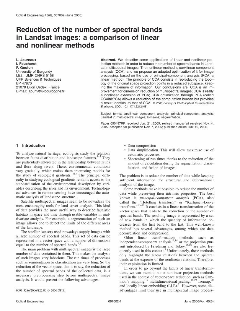
Fig. 6 Segmented images obtained by unsuperv�c� PCA image, �d� CCA image, �e� CCAinitPCAimage in the RGB space.


CA is close to the result of CCA and CCAinitPCA, andCA is really a nonlinear extension of PCA.

• High correlation between the second band of CCA andthe second band of CCAinitPCA �same observationwith the third bands of these methods�.

This allows us to prove that the initialization of CCA byhe PCA matrix leads to a result equivalent to the resultbtained by CCA initialized at random. Moreover, thisethod offers two advantages: faster convergence �Fig. 11�

nd a reduction of calculations and manipulations of data,eading to a reduction of run time.

to three methods �in bold, the coefficients with a correlation higher

CCA CCAinitPCA

2 3 1 2 3

87 0.81070 0.01990 0.98701 0.94614 0.48880

76 0.56869 0.95644 0.15501 0.07143 0.87074

57 0.08374 0.19446 0.03626 0.24229 0.04712

0.68552 0.18310 0.94011 0.94582 0.63937

52 1 0.48841 0.89022 0.71659 0.09668

10 0.48841 1 0.12424 0.06409 0.84870

11 0.89022 0.12424 1 0.91031 0.34946

82 0.71659 0.06409 0.91031 1 0.51060

37 0.09668 0.84870 0.34946 0.51060 1

lassification on �a� original image �eight bands�,e. Image �b� is the representation of the initial

ording

1

0.981

0.183

0.023

1

0.685

0.183

0.940

0.945

0.639

ised cimag

June 2006/Vol. 45�6�

ttsitfkncf

t

pace.

CA im


4.3 Analysis by SegmentationTo estimate the quality of the different transformations, wehave applied a segmentation to the initial and reduced im-ages. We have chosen an unsupervised method of classifi-cation usually applied in remote sensing: the method ofaggregation around mobile centers, called the k-meansmethod.32,33

The goal of the k-means algorithm is to minimize thewithin-cluster variability. The objective function J �whichis to be minimized� is the sum of distances �errors� squaredbetween each pixel and its assigned cluster center:34

J = �j=1

k

�i=1

n

�xi�j� − cj�2,

where cj is the mean of the cluster that the pixel xi�j� is

assigned to.In this case, minimizing the objective function is equiva-

lent to minimizing the mean squared error �MSE�. TheMSE is a measure of the within-cluster variability:

MSE =� j=1

k �i=1

n�xi

�j� − cj�2

�N − C�b=

J

�N − C�b,

whereN � the number of pixelsC � number of groups �that is to say, the num-

ber of classes�b � number of spectral bands.

We applied the k-means method to the images resultingfrom each reduction method and to the original Landsatimage �eight bands�. The goal was to compare the seg-mented images and so to see if the transformations preserve

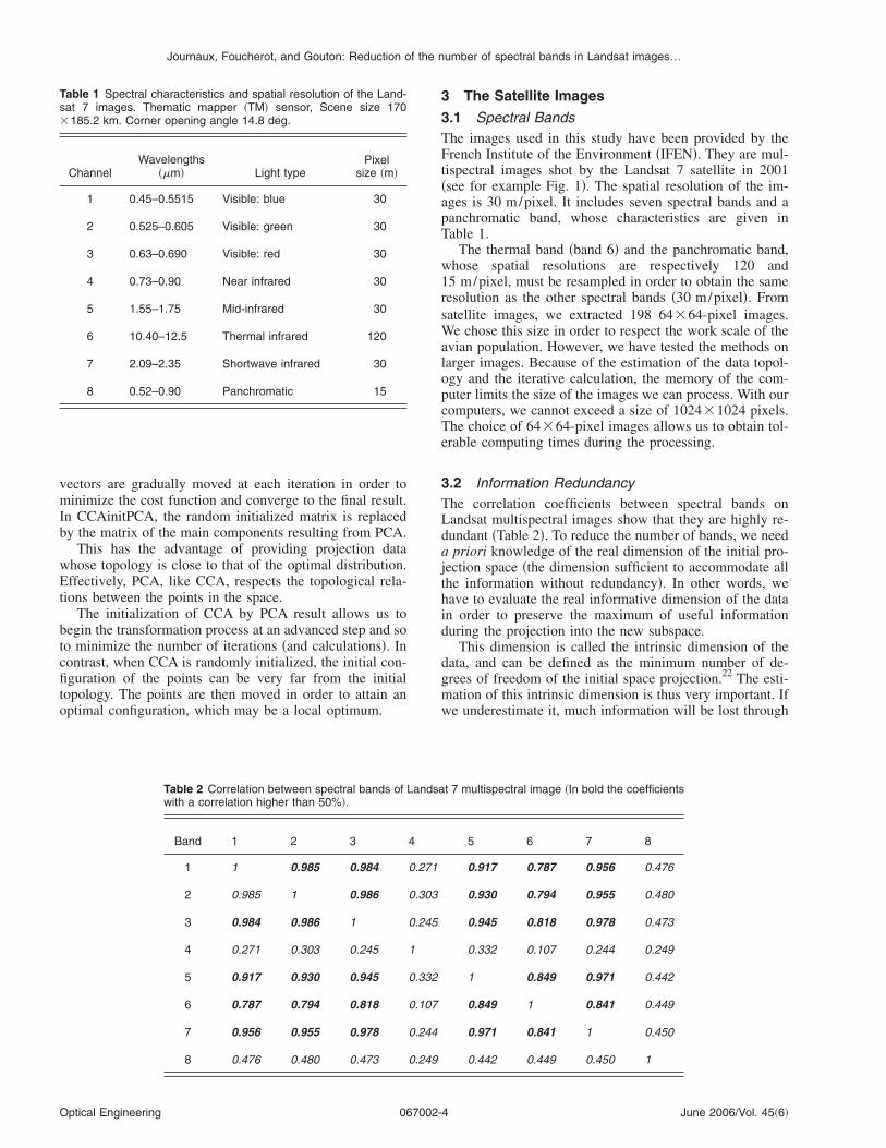
Fig. 7 Illustration �in the black circle� of the oveight spectral bands �b� compared to the redurepresentation of the initial image in the RGB s

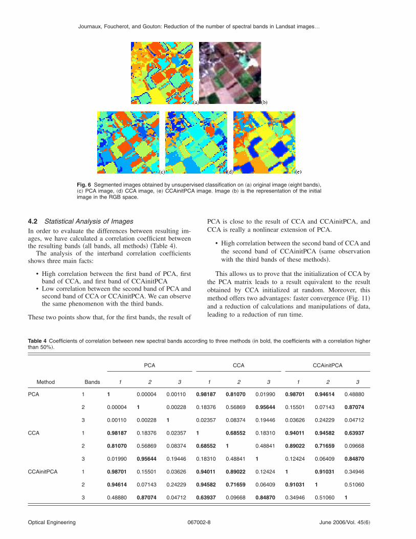
Fig. 8 �a� Color image; �b� segmented P


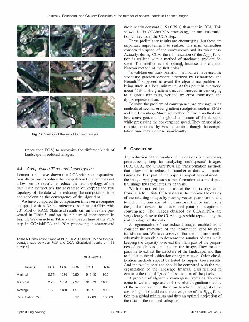
he space structure of the image. In other words, we wantedo know if our transformations enable us to preserve thepace configuration of the different zones of the landscapen spite of the reduction of dimensions. We arbitrarily fixedhe number of classes �C in the equation for the MSE� at 9or each image. This number was determined from a priorinowledge of the landscape. It corresponds to the averageumber of faunistic habitats in each image.35 Figure 12ontains a sample of the studied images �printed in RGBormat�. Figure 6 shows the classification results.

The observation of the segmented images obtained byhe k-means method shows several results:

• The first one is the conservation of the space organi-zation of the image. Indeed, for each transformationmethod and particularly for the nonlinear methods�Fig. 6�d� and 6�e��, the space organization and thegeometry of the different zones of the original imageare respected. This suggests that the transformationsby CCA �Fig. 6�d�� and CCAinitPCA �Fig. 6�e�� pre-serve the space organization of the various elementsconstituting the landscape in the original image �Fig.6�a��. Moreover, the comparison of the segmented im-ages resulting from CCA �Fig. 6�d�� and CCAinitPCA�Fig. 6�e�� shows that the processing leads to the sameresults. This comparison proves that the initializationof CCA by PCA does converge to the same result.

• The second result constitutes the main interest of thereduction of dimensions in multispectral images. In-deed, the segmentation of the initial eight-band imageleads to oversegmentation, in particular in texturedzones. This could be explained by the data redundancybetween the various bands of the Landsat image. Onthe reduced images, oversegmentation is lower. This

entation resulting from the original image withage with three spectral bands �c�. �a� is the

age; �c� segmented CCAinitPCA image.

ersegmced im

June 2006/Vol. 45�6�

Fc

Fc


suggests that the reduction of dimensions allows oneto keep only the essential information of the image�Fig. 7�.

• The original color image �Fig. 8�a�� enables us tocompare the quality of the segmentation on the re-duced images. On the image resulting from PCA �Fig.8�b��, several different parcels are merged in a sameregion by the segmentation. On the images resultingfrom the nonlinear methods �Fig. 8�c��, the differentparcels are better differentiated.

• Moreover, the image resulting from PCA leads tooversegmentation in the textured zones �Fig. 8�b��,while the images resulting from the nonlinear methodssmooth the noise, giving the segmentation a betterquality �Fig. 8�c��.

The segmentation of our images allowed us to observeunexpected and interesting results. Indeed, we can see thatthe same labels �the same colors� are associated with thesame kinds of landscape �Fig. 9�. In other words, we ob-serve not only conservation of the structure of the image,but also conservation of the spectral relations between theclasses. This was not obvious at the beginning, especiallywith the nonlinear transformation methods. In fact, nonlin-ear projections generally involve spectral distortions duringthe data unfolding36 because of the needed global consid-eration of the set of data. Apparently, a local approach, suchas in CCA, involves less distortion.

• Finally, we can observe areas with pond labels in thesegmented images resulting from the nonlinear meth-ods �Fig. 10�. These areas do not appear on the seg-mented image resulting from the PCA image. A veri-fication at the site has revealed the presence of pondsunder vegetable cover. This enables us to consolidatethe idea that CCA and CCAinitPCA make it possible

Fig. 9 �a� Color image; �b� segmented image resulting fromCCAinitPCA.

Fig. 10 �a� Color image; �b� PC


to reduce considerably the number of data with maxi-mum preservation of information sometimes lost bythe linear methods.

rom the analysis by segmentation, we draw the followingonclusions:

• All methods preserve the spatial organization of thelandscape.

• CCA and CCAinitPCA preserve sufficient information

ig. 11 Convergence obtained with CCA and CCAinitPCA. Theonvergence is faster for CCAinitPCA.

A image; �c� CCA image.

June 2006/Vol. 45�6�0

mst

icAtsN

sHbatd

malwrt

5

TpPtttt

fottcvr

ctoktptfiAoe

coct


�more than PCA� to recognize the different kinds oflandscape in reduced images.

4.4 Computation Time and ConvergenceLennon et al.8 have shown that CCA with vector quantiza-tion allows one to reduce the computation time but does notallow one to exactly reproduce the real topology of thedata. Our method has the advantage of keeping the realtopology of the data while reducing the computation timeand accelerating the convergence of the algorithm.

We have compared the computation times on a computerequipped with a 32-bit microprocessor at 2.4 GHz with704 Mbit of RAM. Statistical results on run times are pre-sented in Table 5, and on the rapidity of convergence inFig. 11. We can note in Table 5 that the run time of the PCAstep in CCAinitPCA and PCA processing is shorter and

Table 5 Computation times of PCA, CCA, CCAinitPCA and the per-centage ratio between PCA and CCA. �Statistical results on 198images.�

Time �s� PCA CCA

CCAinitPCA

PCA CCA Total

Minimal 0.75 1030 0.90 919.10 920

Maximal 2.25 1330 2.27 1065.73 1068

Average 1.5 1180 1.5 988.5 990

Contribution �%�: 0.17 99.83 100.00

Fig. 12 Sample of the set of Landsat images.

t


ore nearly constant �1.5±0.75 s� than that in CCA. Thishows that in CCAinitPCA processing, the run-time varia-ion comes from the CCA step.

These preliminary results are encouraging, but there aremportant improvements to realize. The main difficultiesoncern the speed of the convergence and its robustness.ctually, during CCA, the minimization of the ECCA func-

ion is realized with a method of stochastic gradient de-cent. This method is not optimal, because it is a quasi-ewton method of the first order.37

To validate our transformation method, we have used thetochastic gradient descent described by Demartines andérault,22 supposed to avoid the algorithmic problem ofeing stuck at a local minimum. At this point in our work,bout 45% of the gradient descents succeed in convergingo a global minimum, verified by error estimation andy-dx representation.

To solve the problem of convergence, we envisage usingethods of second-order gradient resolution, such as BFGS

nd the Levenberg-Marquart method.37 These methods al-ow convergence to the global minimum of the functionhile preserving the convergence speed. They ensure algo-

ithmic robustness by Hessian control, though the compu-ation time may increase significantly.

Conclusion

he reduction of the number of dimensions is a necessaryreprocessing step for analyzing multispectral images.CA, CCA, and CCAinitPCA are transformation methods

hat allow one to reduce the number of data while main-aining the best part of the objects’ properties contained inhe image. Applying such a transformation to a multispec-ral image thus facilitates its analysis.

We have noticed that the use of the matrix originatingrom PCA to initiate CCA allows us to improve the qualityf the resulting images by passing vector quantization, ando reduce the time cost of the transformation by initializinghe gradient descent to an advanced point of the optimumonvergence. The images obtained by CCAinitPCA areery clearly close to the CCA images while reproducing theeal topology of the data.

A segmentation of the reduced images enabled us toonsider the relevance of the information kept by eachransformation. We have observed that the nonlinear meth-ds make it possible to decrease the number of data whileeeping the capacity to reveal the main part of the proper-ies of the objects contained in the image. They make itossible to extract the structure of the landscape, and thuso facilitate the classification or segmentation. Other classi-cation methods should be tested to support these results.nd the results obtained should be compared with the realrganization of the landscape �manual classification� tovaluate the rate of “good” classification of the pixels.

A problem of algorithm convergence remains. To over-ome it, we envisage use of the resolution gradient methodf the second order in the error function. Though its timeost is high, it should ensure convergence of the ECCA func-ion to a global minimum and thus an optimal projection of
he data in the reduced subspace.
June 2006/Vol. 45�6�1

2

2

3

3

3

3

3

3

3

3

dfiimc


References

1. B. Frochot, M.-C. Eybert, L. Journaux, J. Roché, and B. Faivre,“Nesting birds assemblages along the River Loire: result from a12 years study,” Alauda 71, 179–190 �2003�.

2. J. Grand and S. A. Cushman, “A multi-scale analysis of species-environment relationships: breeding birds in a pitch pine–scrub oak�Pinus rigida–Quercus ilicifolia� community,” Biol. Conserv. 112,307–317 �2003�.

3. R. N. Chapman, D. M. Engle, R. E. Masters, and D. M. Leslie,“Grassland vegetation and bird communities in the southern GreatPlains of North America,” Agric., Ecosyst. Environ. 104, 577–585�2004�.

4. S. A. Cushman and K. McGarigal, “Patterns in the species-environment relationship depend on both scale and choice of re-sponse variables,” Oikos 105, 117–124 �2004�.

5. P. Laiolo, A. Rolando, and V. Valsania, “Responses of birds to thenatural reestablishment of wilderness in montane beechwoods ofnorth-western Italy,” Acta Oecolog. 25, 129–136 �2004�.

6. J. R. Miller, M. D. Dixon, and M. G. Turner, “Response of aviancommunities in large-river floodplains to environmental variation atmultiple scales,” Ecol. Appl. 14, 1394–1410 �2004�.

7. P. A. Reynaud and J. Thioulouse, “Identification of birds as biologicalmarkers along a neotropical urban-rural gradient �Cayenne, FrenchGuiana�, using co-inertia analysis,” J. Environ. Manage. 59, 121–140�2000�.

8. M. Lennon, G. Mercier, M. C. Mouchot, and L. Hubert-Moy, “Cur-vilinear component analysis for nonlinear dimensionality reduction ofhyperspectral images.,” presented at Image and Signal Processing forRemote Sensing VII, SPIE’s International Symposium on RemoteSensing 2001, Toulouse, France.

9. B. Tso and P. M. Mather, Classification Methods for Remotely SensedData, Taylor and Francis, London �2001�.

10. J. C. Devaux, P. Gouton, and F. Truchetet, “The Karhunen-Loevetransform applied to region-based segmentation of color aerial im-ages,” Opt. Eng. 40, 1302–1308 �2001�.

11. H. Hotelling, “Analysis of a complex statistical variable into principalcomponents,” J. Educ. Psychol. 24, 417–441, 498–520 �1933�.

12. R. Kouassi, J.-C. Devaux, P. Gouton, and M. Paindavoine, “Applica-tion of the Karhunen-Loève transform for natural color image analy-sis,” in Irish Machine Vision and Image Processing Conf., Vol. 1,pp. 20–27 �1997�.

13. P. Comon, “Independent component analysis, a new concept?” SignalProcess. 36, 287–314 �1994�.

14. M. Lennon, G. Mercier, M. C. Mouchot, and L. Hubert-Moy, “Inde-pendent component analysis as a tool for the dimensionality reduc-tion and the representation of hyperspectral images,” presented atIGARSS 2001, Sydney, Australia.

15. A. Ifarraguerri and C.-I. Chang, “Unsupervised hyperspectral imageanalysis with projection pursuit,” IEEE Trans. Geosci. Remote Sens.38, 2529–2538 �2000�.

16. J. H. Friedman and J. W. Tukey, “A projection pursuit algorithm forexploratory data analysis,” IEEE Trans. Comput. C23, 881–890�1974�.

17. J. W. Sammon, “A nonlinear mapping for data analysis,” IEEE Trans.Comput. C-18, 401–409 �1969�.

18. B. D. Ripley, Pattern Recognition and Neural Networks, CambridgeUniversity Press �1996�.

19. J. B. Tenenbaum, V. de Silva, and J. C. Langford, “A global geomet-ric framework for nonlinear dimensionality reduction,” Science 290,2319–2323 �2000�.

20. J. A. Lee, A. Lendasse, and M. Verleysen, “Nonlinear projection withcurvilinear distances: Isomap versus curvilinear distance analysis,”Neurocomputing 57, 49–76 �2004�.

21. S. T. Roweis and L. K. Saul, “Nonlinear dimensionality reduction bylocally linear embedding,” Science 290, 2323–2326 �2000�.

22. P. Demartines and J. Hérault, “Curvilinear component analysis: aself-organizing neural network for nonlinear mapping of data sets,”IEEE Trans. Neural Netw. 8, 148–154 �1997�.

23. A. Lendasse, J. Lee, E. De Bodt, V. Wertz, and M. Verleysen, “Inputdata reduction for the prediction of financial time series,” presented atESANN’2001.

24. T. Kohonen, Self-Organizing Maps, 3rd ed., Vol. 30. Springer, Berlin�2001�.

25. J. A. Lee, A. Lendasse, N. Donckers, and M. Verleysen, “A robustnon-linear projection method,” presented at ESANN 2000, 8th Euro-pean Symposium on Artificial Neural Networks, Bruges �Belgium�,2000.

26. C. M. Bishop, Neural Networks for Pattern Recognition, Oxford:Oxford University Press �1995�.

27. J. Herault, C. Jausions-Picaud, and A. Guerin-Dugue, “Curvilinear
component analysis for high dimensional data representation: I. The- R

oretical aspects and practical use in the presence of noise,” presentedat IWANN’99, Alicante, Spain.

8. L. Journaux, I. Foucherot, and P. Gouton, “Nonlinear reduction ofmultispectral images by curvilinear component analysis: applicationand optimization,” presented at CSIMTA’04 International Confer-ence, Cherbourg, France.

9. J. Bruske and E. Merényi, “Estimating the intrinsic dimensionality ofhyperspectral images,” presented at ESANN’1999, Bruges �Bel-gium�.

0. F. Camastra and A. Vinciarelli, “Estimating the intrinsic dimension ofdata with a fractal-based method,” IEEE Trans. Pattern Anal. Mach.Intell. 24, 1404–1407 �2002�.

1. N. Kambhatla and T. K. Leen, “Dimension reduction by local princi-pal component analysis,” Neural Comput. 9, 1493–1516 �1997�.

2. R. O. Duda, P. E. Hart, and D. G. Stork, Pattern Classification, 2nded., Wiley Interscience �2001�.

3. J. T. Tou and R. C. Gonzalez, Pattern Recognition Principles,Addison-Wesley �1974�.

4. J. MacQueen, “Some methods for classification and analysis of mul-tivariate observations,” presented at Proceedings of the Fifth BerkeleySymposium on Mathematical Statistics and Probability, Berkeley, CA�1967�.

5. C. Ferry and B. Frochot, “Bird communities of the forests of Bur-gundy and the Jura �eastern France�,” in Biogeography and Ecologyof Forest Birds Communities, A. Keast, Ed., pp. 183–195, SPB Aca-demic Publishing, The Hague �1990�.

6. D. Kulpinski, “LLE and Isomap analysis of spectra and colour im-ages,” Master’s Thesis, School of Computing Science, Simon FraserUniv. �2002�.

7. R. Fletcher, Practical Methods of Optimization, 2nd ed., John Wiley& Sons �2000�.

Ludovic Journaux has been working to-ward his PhD in image processing at theUniversity of Burgundy, France, since 2002.He is a member of the Image ProcessingGroup of the LE2I �Laboratoired’Electronique, Informatique et Image:Laboratory of Electronics, Computer Sci-ences, and Images�. His research interestsinclude image processing, multispectral im-ages, statistical analysis, multiresolutionsegmentation, and classification.

Irène Foucherot received her PhD in com-puter sciences from the University of Bur-gundy, France, in 1995. She has been anassistant professor at the University of Bur-gundy since 1996. Her earlier research areawas artificial life �genetic algorithms, cellularautomata�. She joined the Image Process-ing Group of the LE2I in 2001. Her researchinterest is now color image processing andespecially region-based segmentation ofmultispectral images.

Pierre Gouton obtained a PhD in compo-nents, signals, and systems at the Univer-sity of Montpellier 2 �France� in 1991. From1988 to 1992, he worked on passive powercomponents at the Laboratory of ElectricMachines of Montpellier. Appointed assis-tant professor in 1993 at the University ofBurgundy, France, he joined the Image Pro-cessing Group of the LE2I. Since then, hismain research topic has been the segmen-tation of images by linear methods �edge

etection� or nonlinear methods �mathematical morphology, classi-cation�. He is a member of ISIS �a research group in signal and

mage processing of the French National Scientific Research Com-ittee� and also a member of the French Color Group. Since De-

ember 2000, he has belonged to the HDR �Habilitation à Diriger les
echerches�.
June 2006/Vol. 45�6�2

Reduction of the number of spectral bands in LANDSAT images with projection methods: Pertinence of...

Documents

Transcript of Reduction of the number of spectral bands in LANDSAT images with projection methods: Pertinence of...