Electronic copy available at: http://ssrn.com/abstract=976826Electronic copy available at: http://ssrn.com/abstract=976826Electronic copy of this paper is available at: http://ssrn.com/abstract=976826

Reduced-form Models with RegimeSwitching: An Empirical Analysis for

Corporate Bonds

Hoi Ying Wong∗and Tsz Lim WongDepartment of Statistics

Chinese University of Hong Kong, Hong Kong, ChinaFirst version: March 4, 2007

March 28, 2007

Abstract

Empirical evidence shows that there is a close link between regime shiftsand business cycle fluctuations. A standard term structure of interest rates,such as the Cox, Ingersoll, and Ross (1985; CIR) model, is sharply rejectedin the Treasury bond data. Only Markov regime-switching models on theentire yield curve of the Treasury bond data can account for the observedbehavior of the yield curve. In this paper, we examine the impact of regimeshifts on AAA-rated and BBB-rated corporate bonds through the use of areduced-form model. The model is estimated by the Efficient Method ofMoments. Our empirical results suggest that regime-switching risk has sig-nificant implications for corporate bond prices and hence has a material im-pact on the entire corporate bond yield curve, providing evidence for theapproach of rating through the cycle employed by rating agencies.

JEL classification:To be determinedKeywords:Credit Risk, Regime Switching, Efficient Method of Moments.

∗Corresponding author; fax: (852) 2603-5188; email: hywong@cuhk.edu.hk.

1

Electronic copy available at: http://ssrn.com/abstract=976826Electronic copy available at: http://ssrn.com/abstract=976826Electronic copy of this paper is available at: http://ssrn.com/abstract=976826

1 Introduction

The term structure of defaultable bonds is one of the most important entities incredit risk modeling because it describes the relationshipbetween the yields ona defaultable discount bond and its maturity. It is one of thefundamentals forpricing credit risk derivatives. Many models of the term structure are based onthe assumption that all information about the economy is contained in a finite-dimensional vector of state variables, the dynamics of which are governed bystochastic processes. The dynamics may be derived by using absence of arbitragearguments, obtained endogenously in a general equilibriumframework, or iden-tified from market data using econometric methods. The exactexpression for theprice of defaultable bonds depends on the specification of the stochastic processesfor the state variables and the associated market price of risk.

Cox, Ingersoll, and Ross (1985; CIR) proposed the univariate square-root pro-cess for the instantaneous interest rate (spot rate) in a general equilibrium frame-work so that heteroscedasticity is introduced into the spotrate dynamics. Duffieand Singleton (1999) extended the framework to reduced-form models of creditrisk. They introduced an adjusted spot rate to account for both the probabilityand timing of default, and for the effect of losses on default. These models areknown as exponential affine models. The diffusion processesof the interest ratethat are specified in these models provide closed-from expressions for transitionand marginal densities of the interest rate, and also bond prices. As a result, thesemodels are analytically tractable and easy to implement. However, Ghysels andNg (1997) rejected current affine models in a semiparametrictest.

One potential problem of affine models is the assumption thatall the modelparameters are constant over time. Generally, business cycles and monetary poli-cies can affect real rates and expected inflation, and can cause interest rates tobehave differently in different time periods. An alternative to affine models incapturing these effects is the regime-switching model thatis proposed by Hamil-ton (1988). This model allows the parameters of the interestrate process to bedependent on a discrete regime variable. Hence, the conditional density dependson the current regime, and a Markov transition matrix governs the evolution of theregime variable.

Many papers demonstrate that the short interest rate process can be reasonablywell modeled in time series as a regime-switching process (see Garcia and Perron(1996), Gray (1996), and Ang and Bekaert (1998)). The results have motivatedrecent empirical studies to estimate an entire term structure of interest rates thatis based on regime-switching models (see Naik and Lee (1997), Evans (1998),

2

Bansal and Zhou (2002), and Wu and Zeng (2005)). The regime dependencethat is introduced by these empirical studies implies richer dynamic behavior ofthe market price of diffusion risk and regime-switching risk. Hence, they offergreater econometric flexibility for the term structure models to account for boththe time series and cross-sectional properties of interestrates.

In this paper, we extend this stream of literature to a reduced-form model ofcredit risk. We take seriously the idea that changes in regimes can potentially havesizable effects on the term structure of defaultable bonds;therefore, incorporatingthem can better account for the observed behavior of the termstructure of default-able interest rates. Motivated by this possibility, we develop a continuous timemodel with a general equilibrium framework of the term structure of defaultableinterest rates that incorporates regime shifts. The actualyield curve of a givencredit rating class fluctuates around the mean curve for the current regime. Some-times, discrete changes in the economy lead to a jump in the term structure ofyield volatilities and in the mean yield curve. At any time, the yield curve reflectsthe current regime and the expectation that the current regime may change.

Our work contributes to both the theoretical and empirical literature on theterm structure of defaultable interest rates. We obtain a closed-form solution ofthe term structure of defaultable interest rates using an affine-type model simi-lar to that in Bansal and Zhou (2002) and Wu and Zeng (2005). Wethen showhow the regime shifts affect the entire yield curve and dynamic behavior of bondyields for two credit rating classes - AAA-rated and BBB-rated. We use the Ef-ficient Method of Moments (EMM), developed in Bansal (1995) and Gallant andTauchen (1996), to estimate the models that are under consideration. The em-pirical exercise relies on the AAA-rated and BBB-rated defaultable bonds datafrom 1973 to 1997. We find that there is an improvement of modelspecificationwhen the regime-switching risk component is incorporated in both AAA-ratedand BBB-rated defaultable bonds.

There are two major motivations for modeling defaultable interest rates withregime switches. First, there exists a large body of statistical empirical evidencein the finance literature (see Garcia and Perron (1996), Gray(1996), and Angand Bekaert (1998)). This evidence motivated the studies ofthe impact of regimeshifts on the entire yield curve of defaultable bonds with reduced-form modelsof credit risk. Second, the evidence in the macroeconomics literature suggeststhat models with regime shifts can help explain the movements in a number ofreal and nominal macroeconomic variables, which are intimately related to inter-est rates (see Evans and Lewis (1995), and Boudoukh, Richardson, Smith, andWhitelaw (1999)). For example, the transitions between economic expansion and

3

recession have effects on monetary policy, inflationary expectations, and nominalinterest rates. However, term structure models such as the Cox, Ingersoll, andRoss (1985) and affine models do not incorporate them. The absence of theseimportant components in the models may explain why the models have poor em-pirical performance.

The rest of this paper is organized as follows. Section 2 presents a generalequilibrium model of credit risk with regime-switching. Section 3 conducts anempirical analysis of the model in which the details of the empirical formulationwill be given. Section 4 concludes the paper.

2 General Equilibrium Model

This section develops a general equilibrium approach for a reduced-form modelof defaultable bonds with systematic risk of regime shifts.A closed-form solutionfor the term structure of interest rates is obtained under anaffine model using log-linear approximation. We start by stating the similarity ofthe short-rate processbetween defaultable and default-free bonds, and then describe the state variables,investment opportunities for the economy, and the lifetimeutility function.

2.1 Recovery Models

Three main specifications of modeling the recovery of defaultable claims havebeen adopted in the literature: recovery of face value (RFV), recovery of treasury(RT) and recovery of market value (RMV). Jarrow, Lando and Turnbull (1997)consider the RT specification in which the recovery rate is anexogenous fractionof the value of an equivalent default-free bond. Duffie and Singleton (1999) con-sider the RMV specification in which the recovery rate is equal to an exogenousfraction of the market value of the bond just before default.Houweling and Vorst(2001) consider the RFV specification in which the recovery rate is an exogenousfraction of the face value of the defaultable bond.

Under the RMV specification, Duffie and Singleton (1999) showthat thisclaim can be priced as if it were default-free by replacing the usual short-terminterest rate processrt with the default-adjusted short-rate processyt = rt +λtLt.Lt is the expected loss rate in the market value if default were to occur at timet,

4

conditional on the information available up to timet

Rτ = (1 − Lτ )Q(τ−, T ), (1)

Q(τ−, T ) = lims→τ−

Q(s, T ), (2)

whereτ is the default time,Q(τ−, T ) is the market price of the bond just beforedefault andRτ is the market value of the defaulted bond. That is, under the techni-cal conditions, the market value of the defaultable claim to(2.11) shown by Duffieand Singleton (1999) is

Q(t, T ) = E

[

exp

(

−∫ T

t

ysds

)

M |Ft

]

. (3)

This is natural, in thatλtLt is the “risk-neutral mean-loss rate” of the instru-ment due to default. Discounting at the adjusted short rateyt therefore accountsfor both the probability and timing of default, and for the effect of losses on de-fault.

A key feature of the valuation equation (3) is that if the mean-loss rate processλtLt is exogenously given, standard term-structure models for default-free debtare directly applicable to defaultable debt by parameterizing yt instead ofrt.

2.2 State Variables

The economy is assumed to be driven by two types of state variables,x(t) =(x1(t), ..., xM(t))′ ands(t). Following Duffie and Singleton (1999), the first typeof variablex(t) has a continuous path, and is determined by the stochastic differ-ential equation

dxt = µ(xt)dt + σ(xt)dBt, (4)

whereB is the standard Brownian motion inRM, and the drift termµ(xt) inR

M and the diffusion termσ(xt) in RM×M are regime dependent. The second

type of variables(t) is a continuous-time Markov chain that representsN distinctregimes, taking on values of1, 2, ..., N . Following Landen (2000) and Wu andZeng (2005), the marked point process is used to obtain a convenient representa-tion of s(t). Let the mark spaceE be:

E = {(i, j) : i ∈ {1, ..., N}, j ∈ {1, ..., N}, i 6= j}, (5)

5

with σ-algebraE = 2E. Let z = (i, j) be a generic point inE, which representsa regime shift from statei to j. A marked point process,m(t, ·), is uniquelycharacterized by its stochastic intensity kernel and can bedefined as

γm(dt, dz) = h(z, x(t−))I{s(t−) = i}εz(dz)dt, (6)

whereh(z, x(t−)) is the regime-shift intensity from statei to statej at z = (i, j)conditional onx(t−), I{s(t−) = i} is an indicator function of the regime at timet−, andεz(A) is the Dirac measure forA, a subset ofE, at pointz = (i, j). It isdefined byεz(A) = 1 if z ∈ A, andεz(A) = 0 if z 6∈ A. Hence,γm(dt, dz) isthe conditional probability of shifting from statei to statej during[t, t+dt] givenx(t−) ands(t−) = i. Moreover,γm(dt, dz) is in general state dependent.

Let m(t, A) denote the cumulative number of regime shifts that belong toA,a subset ofE, during(0, t]. Thenm(t, A) has its compensator,γm(t, A), which isgiven by

γm(t, A) =

∫ t

0

∫

A

h(z, x(τ−))I{s(τ−) = i}εz(dz)dτ, (7)

which implies thatm(t, A) − γm(t, A) is a martingale.With the notation, it is now clear that the regimes(t) can be represented as

ds =

∫

E

Ψ(z)m(dt, dz), (8)

with the compensator given by

γs(t)dt =

∫

E

Ψ(z)γm(dt, dz), (9)

whereΨ(z) = Ψ((i, j)) = j − i.

2.3 Investment Opportunities

Following Merton (1990) and Wu and Zeng (2005), it is assumedthat expecta-tions about the dynamics of the price per share in the future are the same for allinvestors. Thus, the prices depend on both state variablesx(t) ands(t) as de-scribed by the stochastic differential equation

dPk

Pk

= µkdt + σkdBk +

∫

E

δk(z)m(dt, dz), k = 1, ..., n, (10)

6

wheren ≤ M , both the instantaneous expected rate of return,µk, and the instanta-neous standard deviation of return,σk, are functions ofx(t−) ands(t−), andδk(z)

is the discrete percentage change ink due to a regime shift, i.e.,Pk(t,s(t))−Pk(t−,s(t−))Pk(t−,s(t−))

.Hence, we assume that regime shifts not only affect the driftµk and the volatilityσk, but also directly result in discontinuous changes in the prices as the economyshifts from one regime to another.

We further assume that one of then assets is a defaultable pure discount bond,the price of which is given by

dQ

Q= µQdt + σQdBQ +

∫

E

δQ(z)m(dt, dz), (11)

where the driftµQ, the volatility σQ, and the discrete percentage changeδQ(z)are to be determined by the equilibrium conditions, andδQ(z) is the discrete per-centage change in the bond prices due to a regime shift, i.e.,Q(t,s(t))−Q(t−,s(t−))

Q(t−,s(t−)).

In other words, we allow that regime shifts not only affect the drift µQ and thevolatility σQ, but also directly result in discontinuous jumps in the prices.

By manipulating (11), one can obtain the following:

dQ

Q= µQdt +

∫

E

δQ(z)γm(dt, dz)

+ σQdBQ +

∫

E

δQ(z)[m(dt, dz) − γm(dt, dz)]. (12)

As the last two terms in this equation are martingales, the instantaneous expecteddefaultable bond return should be

Et−

(

dQ

Q

)

= µQdt +

∫

E

δQ(z)γm(dt, dz), (13)

where the first term is the regime-dependent expected defaultable bond return dueto diffusion, and the second term is an additional componentin the defaultablebond return due to discrete regime shifts.

2.4 Preferences

Given the initial wealthw0, we move to the problem of maximizing the expectedlifetime utility of a representative agent, which is given by

E0

[∫

∞

0

e−ρtU(c(t))dt

]

, (14)

7

wherec(t) is the flow of consumption andU(·) is the instantaneous utility func-tion. U(·) is assumed to be strictly concave, increasing, and twice differentiablewith U(0) = 0 andU

′

(0) = ∞.It is assumed that the representative agent is a mutual fund investing in a speci-

fied investment grade class. In other words, the agent only allocates wealth amongthen−1 assets in the same investment grade class, the defaultable borrowing andlending, and consumption. The dynamic of the wealth equation can be describedby the stochastic differential equation:

dw =

n∑

k=1

wφk

dPk

Pk

+ (b − c)dt, (15)

wherew(t) is the agent’s wealth at timet, φk is the fraction of wealth that isinvested in thekth security (hence

∑n

k=1 φk ≡ 1), b(t) is her income andc(t) isher flow of consumption. Substituting fordPk/Pk from (3.7), and assuming thatthenth asset is the defaultable borrowing and lending, we can rewrite (15) as

dw = wµwdt + wσwdBt +

∫

E

wδw(z)m(dt, dz), (16)

where

wµw = w

[

m∑

k=1

φk(µk − y) + y

]

+ (b − c), (17)

wσw = w

√

√

√

√

[

m∑

i=1

m∑

j=1

φiφjσij

]

, (18)

wδw(z) = w

[

m∑

k=1

φkδk(z)

]

, (19)

wherem ≡ n − 1 and theφ1, ..., φm are unconstrained becauseφn can always bechosen to satisfy the constraint

∑n

k=1 φk ≡ 1.

2.5 The Term Structure of Defaultable Bonds

In this section, we go on to obtain a closed-form solution forthe term structureof defaultable bonds. Assuming thatU(c) = log(c), the prices of the defaultablepure discount bonds are given by the following theorem.

8

Proposition 2.1. The price at timet of a defaultable discount bondQ(t, y(t), s(t), T )in a specified investment grade class which matures at timeT satisfies the follow-ing system of partial differential equations.

Qt + (µy − ηwσy)Qy +1

2σ2

yQyy

+

∫

E

(1 − λs(z))∆sQh(z, x)I{s = i}εz(dz) = yQ.

with the boundary conditionQ(T, y, s, T ) = 1 for all y ands.

Proposition (2.1) defines a system ofN partial differential equations if thereareN distinct regimes. As pointed out by Wu and Zeng (2005), the system gen-erally does not admit a closed-form solution to the bond price. Following Duffieand Kan (1996), Dai and Singleton (2000), Duffie, Pan, and Singleton (2000), andWu and Zeng (2005), we have the following affine specification, which is knownto offer a tractable model of the term structure of interest rate. We assume

µy = a0(s) + a1(s)y, (20)

σy =√

σ(s)y. (21)

Under (20) and (21), the default-adjusted short ratey(t) follows the square-root process with regime-dependent drift and diffusion terms

dy = (a0(s) + a1(s)y)dt +√

σ(s)ydBy. (22)

By manipulating (22), we have the standard CIR model that follows the square-root process

dy = κ(s)(y(s) − y)dt +√

σ(s)ydBy, (23)

whereκ(s) = −a1(s) andy(s) = a0(s)−a1(s)

.Furthermore, we assume that

h(z, x) = eνs(z), (24)

ηw = θ(s)√

σ(s)y, (25)

λs(z) = 1 − eφs(z). (26)

Equation (24) assumes that the Markov chains(t) has constant transition prob-abilities that are given byeνs(z) for simplicity. Equation (25) implies the market

9

price of the diffusion risk in equilibrium andθ(s) is the coefficient that determinesthe market price of diffusion risk. Equation (26) parameterizes the market price ofthe regime-switching risk, andφs(z) is the coefficient that determines the marketprice of regime-switching risk.

Assuming thatU(c) = log(c), the term structure of defaultable bonds can besolved and given by the following theorem.

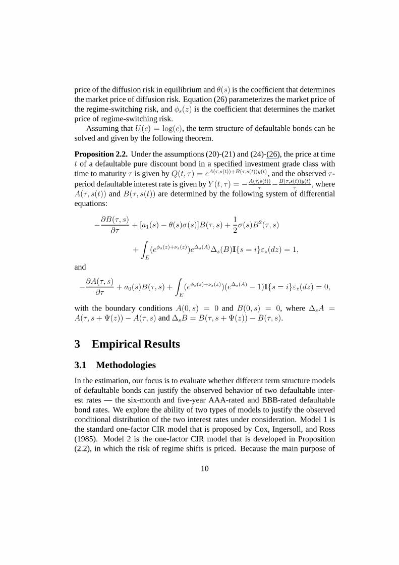
Proposition 2.2. Under the assumptions (20)-(21) and (24)-(26), the price attimet of a defaultable pure discount bond in a specified investmentgrade class withtime to maturityτ is given byQ(t, τ) = eA(τ,s(t))+B(τ,s(t))y(t) , and the observedτ -period defaultable interest rate is given byY (t, τ) = −A(τ,s(t))

τ−B(τ,s(t))y(t)

τ, where

A(τ, s(t)) andB(τ, s(t)) are determined by the following system of differentialequations:

−∂B(τ, s)

∂τ+ [a1(s) − θ(s)σ(s)]B(τ, s) +

1

2σ(s)B2(τ, s)

+

∫

E

(eφs(z)+νs(z))e∆s(A)∆s(B)I{s = i}εz(dz) = 1,

and

−∂A(τ, s)

∂τ+ a0(s)B(τ, s) +

∫

E

(eφs(z)+νs(z))(e∆s(A) − 1)I{s = i}εz(dz) = 0,

with the boundary conditionsA(0, s) = 0 and B(0, s) = 0, where∆sA =A(τ, s + Ψ(z)) − A(τ, s) and∆sB = B(τ, s + Ψ(z)) − B(τ, s).

3 Empirical Results

3.1 Methodologies

In the estimation, our focus is to evaluate whether different term structure modelsof defaultable bonds can justify the observed behavior of two defaultable inter-est rates — the six-month and five-year AAA-rated and BBB-rated defaultablebond rates. We explore the ability of two types of models to justify the observedconditional distribution of the two interest rates under consideration. Model 1 isthe standard one-factor CIR model that is proposed by Cox, Ingersoll, and Ross(1985). Model 2 is the one-factor CIR model that is developedin Proposition(2.2), in which the risk of regime shifts is priced. Because the main purpose of

10

this paper is to highlight the potential impact of the systematic risk of regime shiftson the term structure of defaultable bonds, we do not consider multi-factor termstructure models.

We assume that there are two distinct regimes(N = 2) for s(t). There-fore, Proposition (2.2) defines a system of four differential equations that mustbe solved simultaneously. There are 12 parameters in the model. We fit the modelto the data for the six-month and five-year rates. However, the data cannot be fit-ted to the model directly becauseY (t, τ) in Proposition (2.2) is a kind of spot rateand we only have corporate bond data. We need a model to extract zero-couponrates from current fixed coupon-bearing bond prices.

There is a direct method to fit a yield curve, known as the bootstrappingmethod, but it somewhat lacks robustness. Indirect methodsare therefore usu-ally preferred. The common character of all indirect modelsis that they involvefitting data to a pre-specified form of the zero-coupon yield curve. The generalapproach is to first select a reference set of bonds with market prices and cashflows that are taken as given. Then, one postulates a specific form of the discountfunction or zero-coupon rates.1 Finally, a set of parameters is estimated that bestapproximates given market prices.

Among all indirect methods, the Extended Nelson and Siegel (ENS) model ischosen to fit the yield curve. The curve-fitting technique first described by Nelsonand Siegel (1987) has been applied and modified in a number of ways,2 so that itis sometimes described as a family of curves. The ENS model offers a concep-tually simple and parsimonious description of the term structure of interest rates.It avoids over-parametrization while allowing for monotonically increasing or de-creasing yield curves and hump-shaped yield curves. It alsoavoids the problemin spline-based models of choosing knot points subjectively.

After obtainingY (t, τ) in Proposition (2.2) using the ENS model, the modelis fit to Y (t, τ) on the six-month and five-year AAA-rated and BBB-rated default-able bond rates. To utilize a consistent approach for evaluation and estimationacross the different models, we apply the simulation-basedefficient method ofmoments (EMM) estimator, developed by Gallant and Tauchen (1996).

The EMM estimator consists of two steps. First, the empirical conditional den-sity of the observed defaultable interest rates is estimated by an auxiliary modelthat is a close approximation of the true data generating process. Gallant and

1Examples of indirect methods include exponential spline, polynomial spline, Nelson andSiegel model and Vasicek model.

2Examples of Extended Nelson and Siegel models include thoseof Svensson (1994), Bliss(1997), and Landschoot (2003).

11

Tauchen (1996) suggest a semi-nonparametric (SNP) series expansion as a con-venient general purpose auxiliary model. As pointed out by Bansal and Zhou(2002), the advantage of using the semi-nonparametric specification for the auxil-iary model is that it can asymptotically converge to any smooth distributions, in-cluding the density of Markov regime-switching models. Second, the score func-tions from the log-likelihood of the SNP density are used as moments to constructa GMM-type criterion function. The scores are evaluated using the simulationoutput from a given term structure model, and the criterion function is minimizedwith respect to the parameters on the term structure model under consideration.A nonlinear optimizer is used to find the parameter setting that minimizes the cri-terion function.3 Further details regarding SNP density and EMM estimation areprovided in Appendix B.

Finally, note that the short-rate factory(t) in (23) is a standard one-factor CIRmodel. It defines interest rate movements in terms of the dynamics of the shortrate. The variance of the short rate is related to the level ofinterest rates, andthis feature has the effect of not allowing negative interest rates. It also reflects ahigher interest rate volatility in periods of relatively high interest rates, and corre-spondingly lower volatility when interest rates are lower.However, the short-ratefactor in the standard one-factor CIR model cannot be directly simulated usinga discrete time counterpart. Hence, the step-wisely moment-matched log-normalscheme is applied to simulate the short-rate factor under the CIR model. Furtherdetails of the step-wisely moment-matched log-normal scheme are provided inAppendix C.

3.2 Data Description

The data in this empirical study were obtained from the University of Houston’sFixed Income Database. This database consists of monthly information on mostpublicly traded bonds since 1973. Each issue is identified bya CUSIP number andincludes information on the issue date, maturity date, flat price, coupon, accruedinterest, bond rating, industry sector, and call and put features. As the latest updatewe have is March 1997, we use monthly data that run from January 1973 throughMarch 1997, 291 months in all. To study the term structure of defaultable bonds,we focus on two credit rating classes - AAA-rated and BBB-rated.

Several filters are imposed to construct the sample of defaultable corporatebonds. First, we choose non-callable and non-putable bondsthat are issued by

3Gallant and Tauchen (2006) provide user guides for the SNP and EMM programs.

12

industrial, utility, and transportation firms. Firms in broad industries such as fi-nance, real estate finance, insurance, and banking are excluded from our sample.Second, notes and bonds under one year to maturity, and billsunder one month tomaturity are eliminated from the sample due to liquidity problems.4 At this stage,our sample, on average, consists of 52 AAA-rated bonds and 74BBB-rated bondsfrom January 1973 through March 1997.

We then apply the Extended Nelson and Siegel (ENS) model to fitthe yieldcurve. Two sets of data, August 1975 and December 1984, are reported missing inthe database. Hence, we use the mean of the preceding and the following monthas proxies for these two yields. The summary statistics of the term structuresof AAA-rated and BBB-rated defaultable bonds data are givenin Table 1. It isclear that, on average, the yield curve is upward sloping. Moreover, the positiveskewness and kurtosis suggest departure from Gaussian distribution.

To incorporate important time-series and cross-sectionalaspects of term struc-ture data, we focus on a short-term yield on six-month bills and a long-term yieldon five-year notes. The two models that are mentioned in Chapter 4 are forced tomatch the conditional bivariate joint dynamics of the two yields. As pointed outby Bansal and Zhou (2002), one-month or three-month bill is not used to repre-sent short end, because it is more likely to be affected by liquidity needs.5 Thetime-series plots of the yields are given in Figure 1.

3.3 Estimation Results

Tables 2-5 contain the results of the chosen SNP specifications. The EMM esti-mator consists of two steps. In the first step of the EMM procedure, we fit an SNPdensity of the bivariate joint dynamics of the short-term and long-term yields. TheSNP density employs an expansion in Hermite functions as a convenient generalpurpose auxiliary model that is a close approximation of thetrue data generatingprocess. The dimension of this auxiliary model can be selected by the BayesianInformation Criterion (BIC) proposed by Schwarz (1978). The technical notationsof the SNP specifications are given in Appendix B.

Table 2 reports different choices of SNP density and their corresponding BICvalues of the term structures of AAA-rated defaultable bonds. We find that theoverall best fit based on BIC is the SNP specification with two lags (Lµ = 2) inthe VAR-based conditional mean, five lags (Lr = 5) in the ARCH specification,

4See Bliss (1997).5See Bansal and Coleman (1996) and Bansal and Zhou (2002).

13

Table 1:Summary Statistics of Term Structures of AAA-rated and BBB-rated DefaultableBonds Data, ranging from January 1973 to March 1997

Panel A: Term Structures of AAA-rated Defaultable Bonds Data

Maturity 3 Months 6 Months 1 Year 2 Years 3 Years 5 Years 7 Years10 Years

Mean 0.0790 0.0806 0.0821 0.0837 0.0851 0.0876 0.0897 0.0922Std. Dev. 0.0277 0.0265 0.0256 0.0245 0.0237 0.0231 0.0231 0.0236Skewness 0.9001 0.8112 0.7976 0.8730 0.9508 1.0783 1.1697 1.2543Kurtosis 0.9860 0.7523 0.5887 0.5184 0.5167 0.5992 0.7203 0.8759Maximum 0.1696 0.1679 0.1651 0.1617 0.1605 0.1617 0.1648 0.1695Minimum 0.0292 0.0315 0.0357 0.0420 0.0460 0.0520 0.0564 0.0605Range 0.1404 0.1364 0.1294 0.1196 0.1145 0.1096 0.1083 0.1089

Panel B: Term Structures of BBB-rated Defaultable Bonds Data

Maturity 3 Months 6 Months 1 Year 2 Years 3 Years 5 Years 7 Years10 Years

Mean 0.1003 0.1012 0.1024 0.1041 0.1055 0.1075 0.1089 0.1107Std. Dev. 0.0284 0.0272 0.0264 0.0254 0.0248 0.0239 0.0233 0.0229Skewness 0.8359 0.7489 0.7134 0.7083 0.7463 0.8721 0.9775 1.1111Kurtosis 0.5674 0.3565 0.2138 0.0359 0.0002 0.1722 0.3991 0.8066Maximum 0.1869 0.1824 0.1768 0.1724 0.1713 0.1738 0.1766 0.1821Minimum 0.0476 0.0499 0.0539 0.0583 0.0619 0.0683 0.0731 0.0780Range 0.1393 0.1325 0.1229 0.1141 0.1094 0.1056 0.1034 0.1042

and a polynomial of order four (Kz = 4) in the standardized residualz. The totalnumber of parameters for this SNP specification is 31 (lθ = 31). Table 3 reportsdifferent choices of SNP density and their corresponding BIC values of the termstructures of BBB-rated defaultable bonds. We find that the overall best fit basedon BIC is the SNP specification with one lag (Lµ = 1) in the VAR-based con-ditional mean, four lags (Lr = 4) in the ARCH specification, and a polynomialof order four (Kz = 4) in the standardized residualz. The total number of pa-rameters for this SNP specification is 26 (lθ = 26). The information criterion forchoosing the preferred SNP specification is the minimum value of BIC given in(47). Parameter estimates of the preferred SNP density are reported in Table 4 andTable 5.

After obtaining the estimated nonparametric SNP density, we can estimate the

14

1975 1980 1985 1990 19950

0.05

0.1

0.15

0.2Six−Month Yield Level

1975 1980 1985 1990 19950

0.05

0.1

0.15

0.2Five−Year Yield Level

BBBAAA

BBBAAA

Figure 1: Observed short-term yield and long-term yield

parameters of different term structure models using EMM estimation. Table 6shows the main EMM estimation results for two models. PanelsA and B givethe results for AAA-rated defaultable bonds and BBB-rated defaultable bondsrespectively. Model 1 is the standard one-factor CIR model that is proposed byCox, Ingersoll, and Ross (1985). Model 2 is the one-factor CIR model that isdeveloped in Theorem 3.2, in which the risk of regime shifts is priced.

As seen from Panel A of Table 6, the chi-square statistic of model 1 is 216.39and the chi-square statistic of model 2 drops to 79.46. This indicates an improve-ment when the regime-switching risk component is incorporated in AAA-rateddefaultable bonds. In model 1, the standard one-factor CIR model, the short-term AAA-rated defaultable interest rate has an average long-run mean level of7.13% (y = a0/ − a1 = 0.0063/0.0884) and an average conditional standard de-viation of 1.31% (

√σy =

√

(0.0024)(0.0713) ). The mean reversion parameteris 0.0884 (κ = −a1 = 0.0884), therefore the short-term AAA-rated defaultable

15

Table 2:SNP Score Generator for AAA-rated Defaultable Interest Rates

Lµ Lr Lp Kz Iz Kx Ix lθ sn(θ) BIC

1 0 1 0 0 0 0 9 0.02777 0.115502 0 1 0 0 0 0 13 -0.03253 0.094193 0 1 0 0 0 0 17 -0.03987 0.12585

2 1 1 0 0 0 0 15 -0.09418 0.052042 2 1 0 0 0 0 17 -0.10796 0.057762 3 1 0 0 0 0 19 -0.15274 0.032472 4 1 0 0 0 0 21 -0.17222 0.032492 5 1 0 0 0 0 23 -0.19230 0.031902 6 1 0 0 0 0 25 -0.19312 0.050582 7 1 0 0 0 0 27 -0.19571 0.06749

2 5 1 4 3 0 0 31 -0.30793 -0.005742 5 1 4 2 0 0 32 -0.31045 0.001492 5 1 4 1 0 0 34 -0.31187 0.019562 5 1 4 0 0 0 37 -0.31545 0.045232 5 1 5 4 0 0 33 -0.31297 0.008712 5 1 5 3 0 0 34 -0.31448 0.016952 5 1 5 2 0 0 36 -0.31563 0.035302 5 1 5 1 0 0 39 -0.32173 0.058442 5 1 5 0 0 0 43 -0.33176 0.08740

2 5 1 4 3 1 0 49 -0.36162 0.116032 5 1 4 3 2 1 67 -0.41532 0.237792 5 1 4 3 2 0 76 -0.44405 0.29680

interest rate is very persistent. In model 2, the one-factorCIR model in whichthe risk of regime shifts is priced is developed in Theorem 3.2. In Regime 0,the short-term AAA-rated defaultable interest rate has an average long-run meanlevel of 3.95% (y = a0/ − a1 = 0.0031/0.0784) and an average conditionalstandard deviation of1.07% (

√σy =

√

(0.0029)(0.0395) ). The mean rever-sion parameter is only0.0784 (κ = −a1 = 0.0784), and thus the short rateis very persistent in this regime. In Regime 1, the short-term AAA-rated de-faultable interest rate has a higher average long-run mean level of11.78% (y =a0/ − a1 = 0.0103/0.0874) and a higher average conditional standard devia-tion of 2.40% (

√σy =

√

(0.0049)(0.1178) ). The mean reversion parameter is

16

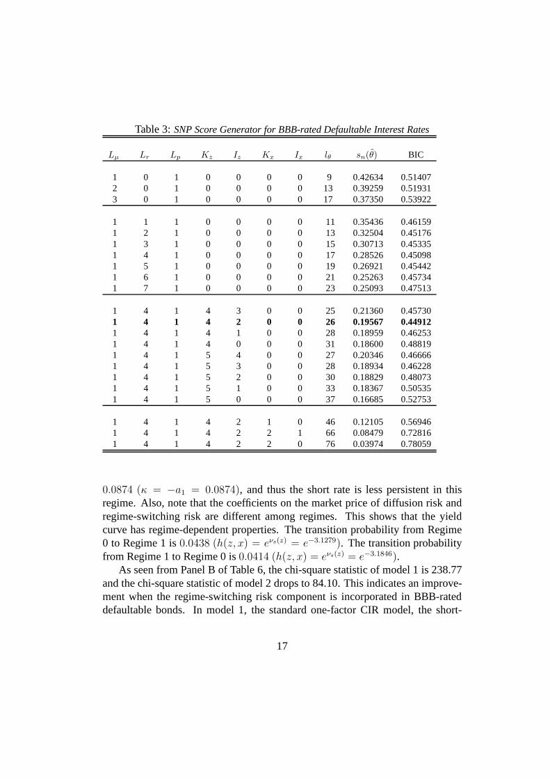
Table 3:SNP Score Generator for BBB-rated Defaultable Interest Rates

Lµ Lr Lp Kz Iz Kx Ix lθ sn(θ) BIC

1 0 1 0 0 0 0 9 0.42634 0.514072 0 1 0 0 0 0 13 0.39259 0.519313 0 1 0 0 0 0 17 0.37350 0.53922

1 1 1 0 0 0 0 11 0.35436 0.461591 2 1 0 0 0 0 13 0.32504 0.451761 3 1 0 0 0 0 15 0.30713 0.453351 4 1 0 0 0 0 17 0.28526 0.450981 5 1 0 0 0 0 19 0.26921 0.454421 6 1 0 0 0 0 21 0.25263 0.457341 7 1 0 0 0 0 23 0.25093 0.47513

1 4 1 4 3 0 0 25 0.21360 0.457301 4 1 4 2 0 0 26 0.19567 0.449121 4 1 4 1 0 0 28 0.18959 0.462531 4 1 4 0 0 0 31 0.18600 0.488191 4 1 5 4 0 0 27 0.20346 0.466661 4 1 5 3 0 0 28 0.18934 0.462281 4 1 5 2 0 0 30 0.18829 0.480731 4 1 5 1 0 0 33 0.18367 0.505351 4 1 5 0 0 0 37 0.16685 0.52753

1 4 1 4 2 1 0 46 0.12105 0.569461 4 1 4 2 2 1 66 0.08479 0.728161 4 1 4 2 2 0 76 0.03974 0.78059

0.0874 (κ = −a1 = 0.0874), and thus the short rate is less persistent in thisregime. Also, note that the coefficients on the market price of diffusion risk andregime-switching risk are different among regimes. This shows that the yieldcurve has regime-dependent properties. The transition probability from Regime0 to Regime 1 is0.0438 (h(z, x) = eνs(z) = e−3.1279). The transition probabilityfrom Regime 1 to Regime 0 is0.0414 (h(z, x) = eνs(z) = e−3.1846).

As seen from Panel B of Table 6, the chi-square statistic of model 1 is 238.77and the chi-square statistic of model 2 drops to 84.10. This indicates an improve-ment when the regime-switching risk component is incorporated in BBB-rateddefaultable bonds. In model 1, the standard one-factor CIR model, the short-

17

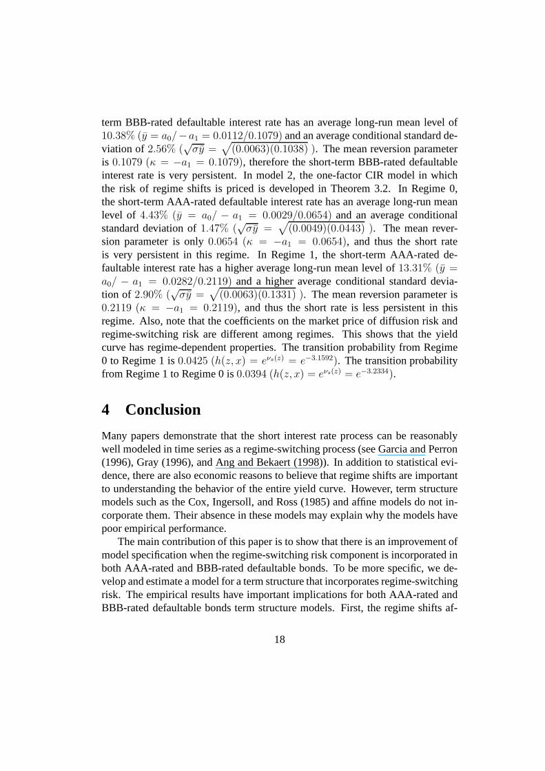
term BBB-rated defaultable interest rate has an average long-run mean level of10.38% (y = a0/−a1 = 0.0112/0.1079) and an average conditional standard de-viation of 2.56% (

√σy =

√

(0.0063)(0.1038) ). The mean reversion parameteris 0.1079 (κ = −a1 = 0.1079), therefore the short-term BBB-rated defaultableinterest rate is very persistent. In model 2, the one-factorCIR model in whichthe risk of regime shifts is priced is developed in Theorem 3.2. In Regime 0,the short-term AAA-rated defaultable interest rate has an average long-run meanlevel of 4.43% (y = a0/ − a1 = 0.0029/0.0654) and an average conditionalstandard deviation of1.47% (

√σy =

√

(0.0049)(0.0443) ). The mean rever-sion parameter is only0.0654 (κ = −a1 = 0.0654), and thus the short rateis very persistent in this regime. In Regime 1, the short-term AAA-rated de-faultable interest rate has a higher average long-run mean level of13.31% (y =a0/ − a1 = 0.0282/0.2119) and a higher average conditional standard devia-tion of 2.90% (

√σy =

√

(0.0063)(0.1331) ). The mean reversion parameter is0.2119 (κ = −a1 = 0.2119), and thus the short rate is less persistent in thisregime. Also, note that the coefficients on the market price of diffusion risk andregime-switching risk are different among regimes. This shows that the yieldcurve has regime-dependent properties. The transition probability from Regime0 to Regime 1 is0.0425 (h(z, x) = eνs(z) = e−3.1592). The transition probabilityfrom Regime 1 to Regime 0 is0.0394 (h(z, x) = eνs(z) = e−3.2334).

4 Conclusion

Many papers demonstrate that the short interest rate process can be reasonablywell modeled in time series as a regime-switching process (see Garcia and Perron(1996), Gray (1996), and Ang and Bekaert (1998)). In addition to statistical evi-dence, there are also economic reasons to believe that regime shifts are importantto understanding the behavior of the entire yield curve. However, term structuremodels such as the Cox, Ingersoll, and Ross (1985) and affine models do not in-corporate them. Their absence in these models may explain why the models havepoor empirical performance.

The main contribution of this paper is to show that there is animprovement ofmodel specification when the regime-switching risk component is incorporated inboth AAA-rated and BBB-rated defaultable bonds. To be more specific, we de-velop and estimate a model for a term structure that incorporates regime-switchingrisk. The empirical results have important implications for both AAA-rated andBBB-rated defaultable bonds term structure models. First,the regime shifts af-

18

fect the forecasting power in the term structure of defaultable bonds. Second, theregime shifts also affect the price of credit derivatives. The non-linear regimeswitching specification seems to add both statistical and economic values in pric-ing credit derivatives. It would be an interesting and valuable extension of thispaper.

References

[1] Ang, A. and Bekaert, G. 1998. Regime Switches in InterestRates, workingpaper, NBER.

[2] Bansal, R. and Coleman, W. J. 1996. A Monetary Explanation of the EquityPremium, Term Premium, and Risk-Free Rate Puzzles,Journal of PoliticalEconomy, 104, 1135-1171.

[3] Bansal, R., Gallant, R. and Tauchen, G. 1995. Nonparametric estimationof structural models for high-frequency currency market data, Journal ofEconometrics, 66, 251-287.

[4] Bansal, R. and Zhou, H. 2002. Term Structure of InteresetRates withRegime Shifts,Journal of Finance, 57, 1997-2043.

[5] Bliss, R. 1997. Testing Term Structure Estimation Methods, Advances inFutures and Options Research, 9, 197-231.

[6] Boudoukh, J., Richardson, M., Smith, T. and Whitelaw, R.1999. RegimeShifts and Bond Returns, working paper, New York University.

[7] Cox, J., Ingersoll, J. and Ross, S. 1985. A Theory of the Term Structure ofInterest Rates,Econometrica, 53, 385-407.

[8] Dai, Q. and Singleton, K. 2000. Specification Analysis ofAffine Term Struc-ture Models,Journal of Finance, 55, 1943-1978.

[9] Duffie, D. and Kan, R. 1996. A Yield-Factor Model of Interest Rates,Math-ematical Finance, 6, 379-406.

[10] Duffie, D., Pan, J. and Singleton, K. J. 2000. Transform Analysis and AssetPricing for Affine Jump-Diffusions,Econometrica, 68, 1343-1376.

19

[11] Duffie, D. and Singleton, K. J. 1999. Modeling Term Structures of Default-able Bonds,The Review of Financial Studies, 12, 687-720.

[12] Evans, M. 1998. Real Risk, Inflation Risk, and the Term Structure, workingpaper, Georgetown University.

[13] Evans, M. and Lewis, K. 1995. Do Expected Shifts in Inflation Affect Esti-mates of the Long-Run Fisher Relation?,Journal of Finance, 50, 225-253.

[14] Fons, J. 1994. Using Default Rates to Model the Term Structure of CreditRisk,Financial Analysts Journal, September-October, 25-32.

[15] Gallant, R. and Tauchen, G. 1996. Which moment to match,EconometricTheory, 12, 657-681.

[16] Gallant, R. and Tauchen, G. 2006a. SNP: A Program for NonparametricTime Series Analysis, working paper, Duke University.

[17] Gallant, R. and Tauchen, G. 2006b. EMM: A Program for Efficient Methodof Moments Estimation, working paper, Duke University.

[18] Garcia, R. and Perron, P. 1996. An Analysis of the Real Interest Rate underRegime Shifts,Review of Economics and Statistics, 78, 111-125.

[19] Ghysels, E. and Ng, S. 1997. A Semiparametric Factor Model of InterestRates and Tests of the Affine Term Structure,Review of Economics andStatistics, 80, 535-548.

[20] Gray, S. 1996. Modeling the Conditional Distribution of Interest Rates as aRegime-Switching Process,Journal of Financial Economics, 42, 27-62.

[21] Hamilton, J. 1988. Rational Expectations EconometricAnalysis of Changesin Regimes: An Investigation of the Term Structure of Interest Rates,Journalof Economic Dynamics and Control, 12, 385-423.

[22] Houweling, P. and Vorst, A. C. F. 2001. An Empirical Comparison of DefaultSwap Pricing Models, working paper, Erasmus University Rotterdam.

[23] Hughston, L. P. and Turnbull, S. 2001. Credit Risk: Constructing the BasicBuilding Blocks,Economic Notes, 30, 281-292.

20

[24] Jarrow, R., Lando, D. and Turnbull, S. 1997. A Markov Model for the TermStructure of Credit Spreads,Review of Financial Studies, 10, 481-523.

[25] Kushner, H. J. and Dupuis, P. 2001.Numerical Methods for Stochastic Con-trol Problems in Continuous Time, Springer.

[26] Landen, C. 2000. Bond Pricing in a Hidden Markov Model ofthe Short Rate,Finance and Stochastics, 4, 371-389.

[27] Landschoot, A. V. 2003. The Term Structure of Credit Spreads on Euro Cor-porate Bonds, working paper, Tilburg University.

[28] Litterman, R. and Iben, T. 1991. Corporate Bond Valuation and the TermStructure of Credit Spreads,Journal of Porfolio Management, Spring, 52-64.

[29] Martin, M. 1997. Credit Risk in Derivative Products, Ph.D. dissertation, Uni-versity of London.

[30] Merton, R. C. 1990.Continuous-Time Finance, Cambridge, Mass.

[31] Naik, V. and Lee, M. 1997. Yield Curve Dynamics with Discrete Shifts inEconomic Regimes: Theory and Estimation, working paper, University ofBritish Columbia.

[32] Nelson, C. R. and Siegel, A. F. 1987. Parsimonious Modeling of YieldCurves,Journal of Business, 60, 473-489.

[33] Nielsen, S. and Ronn, E. 1995. The Valuation of Default Risk in Corpo-rate Bonds and Interest Rate Swaps, working paper, University of Texas atAustin.

[34] Protter, P. 1990.Stochastic Intergration and Differential Equations, SpringerVerlag, Berlin.

[35] Pye, G. 1974. Gauging the Default Premium,Financial Analyst’s Journal,January-February, 49-50.

[36] Ramaswamy, K. and Sundaresan, S. M. 1986. The Valuationof Floating-Rate Instruments, Theory and Evidence,Journal of Financial Economics,17, 251-272.

21

[37] Schonbucher, P. J. 1997. The Term Structure of Defaultable BondPrices,working paper, University of Bonn.

[38] Schonbucher, P. J. 2003.Credit Derivatives Pricing Models, Wiley Finance.

[39] Schwarz, G. 1978. Estimating the Dimension of a Model,Annals of Statis-tics, 6, 461-464.

[40] Svensson, L. E. 1994. Estimating and Interpreting Forward Interest Rates,working paper, NBER.

[41] Wu, S. and Zeng, Y. 2005. A General Equilibrium Model of the Term Struc-ture of Interest Rates under Regime-Switching Risk,International Journalof Theoretical and Applied Finance, 8, 839-869.

[42] Wu, L. and Zhang, F. 2006. Libor Market Model with Stochastic Volatility,Journal of Industrial and Management Optimization, 2, 199 - 227.

22

Appendix

A Proof

A.1 Proof of Proposition 2.1

Let J(w(t), s(t), y(t)) = sup(φ1,...φm,c) Et

[∫

∞

te−ρ(τ−t)U(c(τ))dτ

]

be the indirectutility function. We assume that a solution to the agent’s problem exists. We alsoassume that indirect utility functionJ(w(t), s(t), y(t)), the optimal consumption,and portfolio choice satisfy the Bellman equation6

0 = sup(φ1,...φm,c)

(

U(c) − ρJ(w, s, y) + (wµw)Jw + µyJy +1

2(wσw)2Jww

+(wσwy)Jwy +1

2σ2

yJyy +

∫

E

∆sJγm(dz)

)

, (27)

where

wσwy = w

[

m∑

k=1

φkσky

]

, (28)

∆sJ = J(w(1 + δw(z)), s + Ψ(z), y) − J(w, s, y), (29)

γm(dz) = h(z, x(t−))I{s(t−) = i}εz(dz), (30)

andy(t) represents the defaultable interest rate that is associated in defaultablebonds of a given investment grade class defined in (2.14). Moreover,µw, σw

andδw are given in (17), (18), and (19), respectively, and the subscripts on theJ(w, s, y) function denote partial derivatives. The state variabley(t) is xn+1(t)as defined in (4), whileµy andσy are the drift and the volatility term ofy(t),respectively. Substitutingµw, σw, andδw from (17), (18), and (19), respectivelyinto (27), them + 1 first-order conditions are

0 = U′

(c) − Jw, (31)

0 = w(µk − y)Jw +

(

w2

m∑

j=1

φjσkj

)

Jww + (wσky)Jwy

+

∫

E

wδk(z)Jw(w(1 + δw(z)), s + Ψ(z), y)γm(dz), k = 1, ..., m.(32)

6See Kushner and Dupuis (2001) Ch. 3.

23

From (32), the first-order condition for a defaultable pure discount bond de-fined in (11) is given by

0 = w(µQ − y)Jw +

(

w2m∑

j=1

φjσQj

)

Jww + (wσQy)Jwy

+

∫

E

wδQ(z)Jw(w(1 + δw(z)), s + Ψ(z), y)γm(dz). (33)

This can be further rewritten as

0 = w(µQ − y)Jw +(

w2ηwσQ

)

Jww + (wσQy)Jwy

+

∫

E

wδQ(z)Jw(w(1 + δw(z)), s + Ψ(z), y)γm(dz), (34)

whereηw =∑m

j=1 φjρQjσj andρQj is the correlation between the defaultablebond and thejth asset.

By manipulating (34), we have

µQ − y =

(

−Jww

Jw

)

(wηwσQ) +

(

−Jwy

Jw

)

(σQy)

−∫

E

(

1 +∆sJw

Jw

)

δQ(z)γm(dz). (35)

Under logarithm utility functionU(c(t)) = log c(t), it can be proven that theindirect utility function is separable inw(t) andy(t). It can also be proven thatthe indirect utility function is separable inw(t) ands(t). Therefore,J(w, s, y)can be written as1

ρlog w + f(s, y), wheref(s, y) solves the system of differential

equation after substitutingJ(w, s, y) and the optimal choice of consumption(c∗)and portfolio(φ∗

1, ..., φ∗

m) into (27). This separability implies thatJwy = 0.Following Protter (1990), we can apply Ito’s formula toQ(t, w, s, y), and we

have

dQ =

[

Qt + (wµw)Qw + µyQy +1

2(wσw)2Qww + (wσwy)Qwy +

1

2σ2

yQyy

]

dt

+[(wσw)Qw + σyQy]dBQ +

∫

E

∆sQm(dt, dz). (36)

24

Matching the coefficients between (36) and (11), we have

µQ =1

Q[Qt + (wµw)Qw + µyQy

+1

2(wσw)2Qww + (wσwy)Qwy +

1

2σ2

yQyy], (37)

σQ =1

Q[(wσw)Qw + σyQy] , (38)

δQ(z) =∆sQ

Q. (39)

SubstitutingJwx = 0 and (37), (38), and (39) into (35), we have

Qt +1

2(wσw)2Qww + (wσwy)Qwy +

1

2σ2

yQyy

+

[

µy −(

−Jww

Jw

)

wηwσy

]

Qy

+

[

wµw −(

−Jww

Jw

)

w2ηwσw

]

Qw

+

∫

E

(

1 +∆sJw

Jw

)

∆sQγm(dz) = yQ. (40)

Moreover, we assume that the change of wealth of the representative agentis independent of the change of price of a defaultable bond. In other words, therepresentative agent is not the issuer of the defaultable bond. It impliesQw = 0,Qww = 0, andQwy = 0. Moreover,J = 1

ρlog w + f(s, y) impliesJw = 1

ρwand

Jww = − 1ρw2 . Therefore, (40) can be further simplified as

Qt +1

2σ2

yQyy + (µy − ηwσy)Qy +

∫

E

(

1 +∆sJw

Jw

)

∆sQγm(dz) = yQ. (41)

In addition, becauseJ = 1ρlog w + f(s, y), we have

1 +∆sJw

Jw

=1

1 + δw(z)= 1 − λs(z), (42)

whereλs(z) = δw(z)1+δw(z)

.Substituting (42) into (41), the proof is completed. 2

25

A.2 Proof of Proposition 2.2

SubstitutingQ(t, τ) = eA(τ,s(t))+B(τ,s(t))y(t) andτ = T − t into Proposition (2.1),we have

y = −∂A(τ, s)

∂τ− ∂B(τ, s)

∂τy

+[a0(s) + (a1(s) − θ(s)σ(s))y]B(τ, s) +1

2[σ(s)y]B2(τ, s)

+

∫

E

(eφs(z)+νs(z))(e∆s(A)+∆s(B)y − 1)I{s = i}εz(dz), (43)

where∆sA = A(τ, s + Ψ(z)) − A(τ, s) and∆sB = B(τ, s + Ψ(z)) − B(τ, s).Becausey is small, by applying the log-linear approximation, we can obtain

e∆s(B)y ≈ 1 + ∆s(B)y. By matching the coefficients ofy on both sides of theequation, the proof is completed. 2

B SNP Density and EMM Estimation

B.1 SNP Density

The method is termed semi-nonparametric (SNP) to suggest that it lies halfwaybetween parametric and nonparametric procedures. The method employs an ex-pansion in Hermite functions as a general purpose nonparametric estimator to ap-proximate the conditional density of a multivariate process. Following Gallant andTauchen (1996), any smooth conditional density function can be approximated ar-bitrarily close by a Hermite polynomial expansion. Lety denote the vector of theinterest rates under consideration andx be the vector of laggedy. The auxiliaryf -model has a density function that is defined by a modified Hermite polynomial

f(y|x, θ) =[P(z, x)]2nM(y|µx, Σx)

∫

{[P(z, x)]2nM(y|µx, Σx)}dz, (44)

whereP(z, x) is a polynomial with degreeKz and z, which is a standardizedtransformationz = R−1

x (y − µx) with Σx = RxR′

x. The square ofP(z, x) makesthe density positive, and the argument of the polynomial isz. The coefficientsof the polynomial are allowed to be another polynomial of degreeKx in x. Theconstant in the polynomial ofz is set to1 for identification. In addition,nM(·) is aGaussian density of dimensionM with a mean vectorµx and variance-covariance

26

matrix Σx, whereµx is estimated by using a VAR specification, andΣx is esti-mated by using an ARCH specification, which parameterizesRx. Note that bothµx andRx depend only on lags ofy.

The length of the auxiliary model parameter is determined bythe number oflags ofx used in constructing the coefficients of the polynomialLp, the degreeKz of the polynomial inz, the degreeKx of the polynomial inx, lags in the VARmean specificationLµ, and lags in the ARCH specificationLr. The polynomialP(z, x) take the form

P(z, x) =∑

λ1,λ2

a(λ1, λ2, x)zλ1

1 zλ2

2 , (45)

wherea(λ1, λ2, x) are the coefficients of the polynomial inz, and the sum is overall pairs of nonnegative integers(λ1, λ2) such thatλ1 + λ2 ≤ Kz. In general, apositiveIz means all interactions of order exceedingKz − Iz are suppressed to0.Similarly, the interactions terms ofKx of order exceedingKx − Ix are suppressedto 0. Putting certain of the tuning parameters to zero implies sharp restrictions onthe process{yt}.

Let {yt}nt=1 be the observed data andxt−1 be the lagged observations. The

parametersθn are estimated by minimizing

sn(θ) = (−1/n)

n∑

t=1

log[f(yt|xt−1, θ)]. (46)

The dimension of the auxiliaryf -model, the length ofθ, is selected by theSchwarz Bayes information criterion (Schwarz, 1978), which is computed as

BIC = sn(θn) + (lθ/2n) log(n), (47)

wherelθ is the length of the auxiliary model. The criterion rewards good fits asrepresented by smallsn(θn) but uses the term(lθ/2n) log(n) to penalize good fitsobtained by means of excessively rich parameterizations.

B.2 EMM Estimation

Let {yt}Nt=1 be a long simulation from a candidate value ofρ, the parameter vector

of the maintained structural model. The moment criterion is

mN(ρ, θn) =1

N

N∑

τ=1

(∂/∂θ) log f [yt(ρ)|xt−1(ρ), θn], (48)

27

and the GMM estimator of the structural parameter vector is

arg minρ

mN (ρ, θn)′

(In)−1mN(ρ, θn), (49)

whereIn is the weighting matrix. It is estimated by the mean-outer-product ofSNP scores

In =1

n

n∑

t=1

{

(∂

∂θ) log f [yt(ρ)|xt−1(ρ), θn]

}{

(∂

∂θ) log f [yt(ρ)|xt−1(ρ), θn]

}′

.(50)

The normalized criterion function value in the EMM estimation forms a spec-ification test for the overidentifying restrictions

nmN (ρ, θn)′

I−1n mN (ρ, θn) ∼ χ2(lθ − lp), (51)

where the degree of freedom equalslθ − lp, that is, the number of scores momentconditions in the auxiliary model,lθ, less the number of structural parameters,lp.It is assumed thatlp is smaller thanlθ.

C Moment-Matching of the CIR Model

The short-rate factor in the standard CIR model is assumed tofollow the square-root process

dr = κ(θ − r)dt + σ√

rdW, (52)

whereκ is the mean reversion parameter,θ is the long-run mean parameter, andσis the local volatility parameter.

The short-rate factor in the standard CIR model cannot be simulated using adiscrete-time counterpart directly. Wu and Zhang (2006) show that the short-ratefactor can be simulated according to the following step-wisely moment-matchedlog-normal scheme

r(t + ∆t) = EQt [r(t + ∆t)] exp

(

−1

2Γ2

t ∆t + Γt∆Wt

)

, (53)

where

Γ2t =

1

∆tlog

EQt [r2(t + ∆t)]

(EQt [r(t + ∆t)])2

, (54)

28

with

EQt [r(t + ∆t)] = θ + (r(t) − θ)e−κ∆t, (55)

EQt [r2(t + ∆t)] =

(

1 +σ2

2κθ

)

(EQt [r(t + ∆t)])2 − σ2

2κθe−2κ∆tr2(t). (56)

29

Table 4:Parameter Estimates of SNP Density for AAA-rated Defaultable Bonds

Parameter Estimate Standard Error

Hermite:a(0,0) 1.00000 (0.00000)a(0,1) 0.00638 (0.10447)a(1,0) 0.20973 (0.08471)a(0,2) -0.62401 (0.09267)a(2,0) -0.08536 (0.07443)a(0,3) -0.15094 (0.11192)a(3,0) 0.23417 (0.05429)a(0,4) 0.16303 (0.22990)a(4,0) -0.10477 (0.05595)

Mean:µ(2,0) -0.04549 (0.02630)µ(1,0) -0.04989 (0.02827)µ(2,4) -0.02216 (0.05423)µ(2,3) -0.13827 (0.04049)µ(2,2) 0.92669 (0.05741)µ(2,1) 0.17952 (0.03770)µ(1,4) -0.43903 (0.06370)µ(1,3) 0.11032 (0.05407)µ(1,2) 0.45267 (0.05964)µ(1,1) 0.83201 (0.05886)

ARCH:R(1,0) 0.08474 (0.02959)R(1,2) 0.19452 (0.02276)

R(3) 0.11277 (0.04153)R(1,1) 0.44506 (0.08765)R(2,1) 0.62252 (0.12043)R(1,2) -0.27063 (0.10311)R(2,2) -0.20607 (0.16883)R(1,3) 0.03205 (0.13836)R(2,3) 0.44619 (0.10371)R(1,4) -0.31903 (0.06837)R(2,4) -0.33327 (0.12196)R(1,5) 0.04459 (0.11355)R(2,5) 0.34684 (0.09001)

30

Table 5:Parameter Estimates of SNP Density for BBB-rated Defaultable Bonds

Parameter Estimate Standard Error

Hermite:a(0,0) 1.00000 (0.00000)a(0,1) -0.03099 (0.05858)a(1,0) -0.10675 (0.10617)a(0,2) -0.32663 (0.09267)a(1,1) 0.15431 (0.04718)a(2,0) 0.37065 (0.05042)a(0,3) 0.01324 (0.10127)a(3,0) -0.08556 (0.04141)a(0,4) 0.17069 (0.07264)a(4,0) 0.18115 (0.05296)

Mean:µ(2,0) 0.00172 (0.02304)µ(1,0) 0.06437 (0.02865)µ(2,2) 0.92679 (0.03035)µ(2,1) 0.04129 (0.02798)µ(1,2) 0.37820 (0.05805)µ(1,1) 0.55571 (0.05642)

ARCH:R(1,0) 0.09587 (0.02267)R(1,2) 0.16905 (0.01430)

R(3) 0.11637 (0.02255)R(1,1) -0.34786 (0.06822)R(2,1) -0.63774 (0.11182)R(1,2) -0.17104 (0.05820)R(2,2) -0.74861 (0.12060)R(1,3) 0.03381 (0.06624)R(2,3) 0.71594 (0.14145)R(1,4) -0.29285 (0.05839)R(2,4) -0.19392 (0.16617)

Note: The parameter in the Hermite polynomial functiona(i, j) stands for the term withith power

on the short yield andjth power on the long yield. The parameters in the VAR conditional mean

functionµ(1, 0), µ(2, 0), µ(1, 1), µ(2, 1), µ(1, 2), andµ(2, 2) are, respectively, constant in short

yield, constant in long yield, lag one short yield in short yield equation, lag one long yield in

short yield equation, lag one short yield in long yield equation, and lag one long yield in long

yield equation. The parameter in the ARCH standard deviation functionR(1, m) andR(2, n) is,

respectively, short yield with lag equalsm, and long yield with lag equalsn. The parameterR(3)

is the constant off-diagonal term.31

Table 6:Model Estimation by Efficient Method of Moments

Panel A: Panel B:Model 1 Model 2 Model 1 Model 2

Regime 0:a0 0.0063 (0.0003) 0.0031 (0.0005) 0.0112 (0.0003) 0.0029 (0.0005)a1 -0.0884 (0.0008) -0.0784 (0.0016)-0.1079 (0.0004) -0.0654 (0.0005)σ 0.0024 (0.0003) 0.0029 (0.0006) 0.0063 (0.0003) 0.0049 (0.0005)θ -8.3550 (0.0182) -12.2900 (0.0328)-7.4468 (0.0046) -10.8970 (0.0557)φ 0.1279 (0.0382) 0.1561 (0.0216)

Regime 1:a0 0.0103 (0.0006) 0.0282 (0.0005)a1 -0.0874 (0.0005) -0.2119 (0.0028)σ 0.0049 (0.0006) 0.0063 (0.0006)θ -12.9640 (0.0285) -13.0460 (0.0403)φ -0.3154 (0.0498) -0.3205 (0.0227)

TransitionalProbability:νs(0, 1) -3.1279 (0.0204) -3.1592 (0.0272)νs(1, 0) -3.1846 (0.0069) -3.2334 (0.0339)

Specification Test:χ2 216.39 79.46 238.77 84.10

d.o.f. 27 19 22 14

Note: The two term structure models are given in Chapter 4. Model 1 is the standard one-factor

model that is proposed by Cox, Ingersoll, and Ross (1985), without regime shifts. Model 2 is the

one-factor CIR model that is developed in Theorem 3.2, in which regime shift is priced. First,

a0(s), a1(s) andσ(s) are the coefficients that are given in the diffusion process of defaultable

interest ratey(t): dy = (a0(s) + a1(s)y)dt +√

σ(s)ydBy. Second,θ(s) is the coefficient on the

market price of diffusion risk that is given inηw = θ(s)√

σ(s)y, andφ(s) is the coefficient on

the market price of regime-switching risk that is given inλs(z) = 1 − eφs(z). Third,νs(z) is the

parameter which determines the transitional probability that is given inh(z, x) = eνs(z).

32