Redistribution of the low frequency acousticmodes of a room: a finite element-based

optimisation method

Christos I. Papadopoulos *

Department of Naval Architecture and Marine Engineering, NTUA,

Iroon Polytechneiou 9, 15773, Zografou, Greece

Received 10 July 2000; received in revised form 22 December 2000; accepted 13 January 2001

Abstract

This paper presents a method to redistribute the acoustic modes of a room in the low fre-quency range. The relationship between the acoustic modes and the room geometry is studied.

The fundamental problem of normalizing the acoustic modes of a simple, orthogonal room isexamined in depth. Several variable local geometric modifications of the room walls are intro-duced and an optimisation procedure is developed, based on finite element analysis. This proce-

dure is used for the calculation of the exact magnitude of the geometric modifications that willlead to smoother mode and consequently, smoother sound energy distribution in the frequencyrange of interest. The sound quality improvement of the modified room in the low frequencyrange with respect to ISO recommendations is verified. This work opens up the possibility of

constructing acoustic laboratories with extended suitability to perform acoustic measurementsin the low frequency range. # 2001 Published by Elsevier Science Ltd. All rights reserved.

1. Introduction

A basic limitation of modern laboratories for the measurement of transmissionloss (TL) of building elements is the inefficiency to perform accurate and repro-ducible measurements in the low frequency range (i.e. for frequencies lower than 100Hz). A typical laboratory consists of two independent reverberation rooms, which

Applied Acoustics 62 (2001) 1267–1285

www.elsevier.com/locate/apacoust

0003-682X/01/$ - see front matter # 2001 Published by Elsevier Science Ltd. All rights reserved.

PI I : S0003-682X(01 )00002 -0

* Corresponding author. Tel.: +30-1-7721114; fax: +30-1-7721117.

E-mail address: chpap@central.ntua.gr (C.I. Papadopoulos).

share a common interface. A sound field is generated in the source room by applyingacoustic load onto one of its upper-left corners. The geometry of both rooms is suchas perfectly diffuse-field conditions to be generated. The test specimen, whoseacoustical properties, in particular the transmission loss, are to be measured, isplaced along the common interface [8]. The transmission loss is given by:

TL ¼ SPL1 � SPL2 þ 10logS

Að1Þ

where SPL1 and SPL2 are the average sound pressure levels in dB of the source andreceiving room respectively, S is the surface of the specimen and A is the totalabsorption of the receiver room in Sabins. When performing measurements in thelow frequency range, the SPL of the source and the receiving room depend stronglyon the respective mode distribution of the room. If certain modes coincide within afrequency range, certain sound peaks are observed in the neighbourhood of thosemodes, due to modal superposition, while the sound pressure is significantly lowerfurther afield. Therefore, the sound power, which acts upon the test specimen, isunevenly distributed in the frequency domain, causing the acoustic field to be farfrom the ideally diffuse and certain structural modes of the specimen to be acousti-cally loaded more than others. That is, measurements performed at low frequenciesdepend not only on the properties of the test specimen but also on the geometry andthe dimensions of the room-wall-room system; thus they become a function of theroom they were obtained in. The results in that case are less reproducible and accu-rate [1,5,7,9]. It is, therefore, clear that the way the modes are distributed in the lowfrequency range affects the accuracy with which acoustic measurements can be per-formed. This problem has been extensively dealt with in [1] and parametric runshave been performed in order to show the measurement dependence upon thelaboratory facilities in the low frequency range. This is the main reason of trans-mission loss measurements being widely performed for acoustic frequencies greaterthan 100 Hz.Low frequency noise is a subject of growing importance in our modern commu-

nities. TV noise, modern music and home machinery are typical broadband soundsources, which usually cause a high level of annoyance in the low frequency range.Industrial machinery such as diesel engines, fans, pumps etc. are also noise sourceswith important low frequency content. Research should therefore be performed inorder for more accurate prediction of the acoustic behavior of insulating elements inthe low frequency range to be feasible. The acoustic engineer would then have moreefficiency in controlling such noise sources [7].Generally, small rooms have irregular distribution of mode frequencies in the low

frequency range [10]. Especially for rooms with dimensions that bear simple ratios toone another, intense superimposed phenomena are observed in the low frequencyrange. Work has been done in the past to find dimension ratios for rectangular roomswith distribution of acoustic modes as even as possible [10,11]. Generally, such ratiosas 2n=3 or 5n=3 should be preferably chosen [3], while extensive optimisation workexists in the literature comparing the dimension ratios of simple orthogonal rooms

1268 C.I. Papadopoulos / Applied Acoustics 62 (2001) 1267–1285

with respect to the uniformity of distribution of their acoustic modes [11]. However,it is stated that, in the case of a rectangular room, absolute uniformity of the modedistribution in the low frequency range cannot be achievedIn this paper, we explore the possibility to further normalize the distribution of the

acoustic modes of a room in order to provide smoother sound pressure distributionin the low frequency range. This mode normalization will be achieved by applicationof local geometric modifications to the room walls. More specifically, the funda-mental problem of redistributing the acoustic modes of a simple, orthogonal roomin the frequency range of 80–110 Hz will be studied. For that to be achieved, a finiteelement-based optimisation method is developed. A 5�4�3 m3 room is selected forthe application of the method. This room has a volume of 60 m3, which is compar-able to the 50 m3-limit set by ISO and to existing laboratory facilities and provides atest specimen area of 12 m3, which is comparable to the 10 m2 lower limit set by ISO.Furthermore, it has such dimension ratios as to provide primarily even mode dis-tribution in the low frequency range. Its low frequency modes are calculated bothanalytically and numerically. The mode distribution problem is focused and severalvariable local geometric modifications of the room walls are introduced. Thesemodifications form the independent variables of the optimisation procedure. Anobjective function of these variables is formulated so as to provide appropriatemathematical optimisation criterion. The finite element model of the room is con-structed using the PATRAN FE pre/post processor and ABAQUS FE Solver is usedfor the Eigenvalue extractions [2]. The GRG2 optimisation algorithm, by Windwardtechnologies [6], searches for the combination of those geometric modifications thatwill lead to a smoother mode distribution in the frequency range of interest. It willbe shown that this procedure can dictate several local geometric modifications thatcan extend the test range frequency of the room down to 80 Hz. After the optimalroom is constructed, the quality of its sound field, namely the improvement upon itsdiffusiveness (uniformity), in the low frequency range, is verified by means of finiteelement steady-state acoustic response analysis.

2. The fundamental problem

In order to develop a method for the redistribution of the acoustic modes ofarbitrary-shaped rooms, the simple orthogonal room illustrated in Fig. 1 will bestudied. Fig. 1 depicts the shape and the finite element representation of an ortho-gonal room with dimensions of 5�4�3 m3. This room will be utilized for the appli-cation and verification of the optimisation method. The appropriate finite elementmodel is constructed using the PATRAN preprocessor. The air of the room ismodeled with 3-D, 20-node hexahedral acoustic elements having density � equal to1.2 kg/m3 and speed of sound c equal to 343 m/s. The surfaces of common roomsconsist of painted walls and windows, materials highly reflective. The absorptioncoefficient of walls and windows is approximately 0.02 and 0.05 respectively, that is,95–98% of the incident sound is reflected back to the room. Thus, without loss ofgenerality, the surfaces of the room can be considered fully reflective and, therefore,

C.I. Papadopoulos / Applied Acoustics 62 (2001) 1267–1285 1269

the undamped modes and their respective mode shapes will be calculated [2]. Themodel properties are presented in Table 1. The selected mesh provides efficient cal-culation range of 0� f1 ¼

c5�l ¼ 171 Hz where l is the maximum distance between

adjacent nodes of the finite element model [2]. Supposed harmonic acoustic excita-tion, the Helmholtz wave equation governs the sound propagation within the roomand it will be solved by means of finite element analysis. In order to verify theaccuracy of the solution when performing Eigenvalue extractions, the mode fre-quencies of the room are calculated both analytically and numerically. The analy-tical calculation of the mode frequencies of the room takes into account the wavenumbers nx, ny, nz in each of the three axes and the corresponding dimensions lx, ly, lzof the room.

Fig. 1. Geometry and finite element representation of the 5�4�3 m3 room.

Table 1

Basic properties of the finite element model

Main dimensions 5�4�3 m3

Total volume 60 m3

Total acoustic mass 72 kg

No. of nodes 4691

No. of elements 1000

Air properties �=1.2 kg/m3

c=343 m/s

1270 C.I. Papadopoulos / Applied Acoustics 62 (2001) 1267–1285

fnx;ny;nz ¼c

2

ffiffiffiffiffiffiffiffiffiffiffiffiffiffiffiffiffiffiffiffiffiffiffiffiffiffiffiffiffiffiffiffiffiffiffiffiffiffiffiffiffiffiffiffiffiffinxlx

� �2

þnyly

� �2

þnzlz

� �2s

ð2Þ

The Eigenvalue extraction method is used for the numerical calculations. The first18 mode frequencies of the unmodified room (i.e. the room with no extra modifica-tions) are calculated. Table 2 compares the analytically calculated mode frequencieswith the numerically calculated ones. The percentage of the deviation between ana-lytical and numerical calculated values is in all of the cases less than 0.05%. That isthe results show good agreement, namely the finite element mesh is proved fineenough to accurately predict the mode frequencies of the room in the frequencyrange of interest [0, 110 Hz].The mode distribution in the frequency domain is graphically presented in Fig. 2a.

It can be seen that there are certain problematic areas with high concentration ofacoustic modes (modes 8–9, 14–15, 16–17). The sound pressure due to an excitationfrequency in the neighborhood of those mode frequencies is likely to be high, due tomultiple resonances, while much lower sound pressure is expected further afield.This can be verified by performing steady-state acoustic response analysis to theroom by applying a sound source to one of its upper-left corners (the methodologyand the tools to perform steady-state response analysis are presented in detail inSection 5). The source location is selected in such a way as to be in accordance withthe ISO recommendations concerning laboratory measurements and to contribute tothe diffusiveness of the room. The transfer function of the average sound pressure

Table 2

Analytical versus numerical calculation of the mode frequencies of the room

Mode

no.

Mode

shape

Analytical

solution (Hz)

Numerical

solution (Hz)

Deviation

(%)

1. 1, 0, 0 34.157 34.157 0

2. 0, 1, 0 42.696 42.696 0

3. 1, 1, 0 54.677 54.677 0

4. 0, 0, 1 56.928 56.928 0

5. 1, 0, 1 66.388 66.389 0.00151

6. 2, 0, 0 68.313 68.32 0.01025

7. 0, 1, 1 71.159 71.16 0.00141

8. 1, 1, 1 78.932 78.933 0.00127

9. 2, 1, 0 80.558 80.564 0.00745

10. 0, 2, 0 85.391 85.4 0.01054

11. 2, 0, 1 88.924 88.929 0.00562

12. 1, 2, 0 91.969 91.978 0.00979

13. 2, 1, 1 98.642 98.648 0.00608

14. 3, 0, 0 102.47 102.52 0.04879

15. 0, 2, 1 102.628 102.64 0.01169

16. 1, 2, 1 108.1623 108.17 0.00712

17. 2, 2, 0 109.3542 109.37 0.01445

18. 3, 1, 0 111.009 111.06 0.04594

C.I. Papadopoulos / Applied Acoustics 62 (2001) 1267–1285 1271

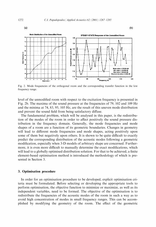
level of the unmodified room with respect to the excitation frequency is presented inFig. 2b. The maxima of the sound pressure at the frequencies of 79, 102 and 109 Hzand the minima at 74, 83, 95, 105 Hz, are the result of this uneven mode distributionand prevent the sound field from being satisfactory diffuse.The fundamental problem, which will be analysed in this paper, is the redistribu-

tion of the modes of the room in order to affect positively the sound pressure dis-tribution in the frequency domain. Generally, the mode frequencies and modeshapes of a room are a function of its geometric boundaries. Changes in geometrywill lead to different mode frequencies and mode shapes, acting positively uponsome of them but negatively upon others. It is shown to be quite difficult to exactlypredict the corresponding distribution of the acoustic modes following a geometricmodification, especially when 3-D models of arbitrary shape are concerned. Further-more, it is even more difficult to manually determine the exact modifications, whichwill lead to a globally optimised distribution solution. For that to be achieved, a finiteelement-based optimisation method is introduced the methodology of which is pre-sented in Section 3.

3. Optimisation procedure

In order for an optimisation procedure to be developed, explicit optimisation cri-teria must be formulated. Before selecting or developing the appropriate tools toperform optimisation, the objective function to minimize or maximize, as well as itsindependent variables, need to be formed. The objective of the optimisation is toredistribute the frequencies of the acoustic modes of the room in such a way as toavoid high concentration of modes in small frequency ranges. This can be accom-plished by modifying the geometry of the room. The effect of the geometric

Fig. 2. Mode frequencies of the orthogonal room and the corresponding transfer function in the low

frequency range.

1272 C.I. Papadopoulos / Applied Acoustics 62 (2001) 1267–1285

modifications can be explained by the following example. Reducing the modalresponse of a single mode can generally be achieved by adding or subtractingacoustic mass from the model. The exact location where acoustic mass should beadded to or subtracted from in order for an efficient modification to be constructedis analysed in Figs. 3 and 4. Fig. 3 illustrates the mode shape (1,1,1) at the frequencyof 78.93 Hz. In order to affect the mode frequency of mode (1,1,1) two differentgeometric modifications are chosen (Fig. 4); application of acoustic mass (namelyair) to a location where maximum (a) or minimum (b) sound pressure is observed.The resulting mode frequencies of the room are presented in Table 3. It is shownthat the added mass has a great effect on mode (1,1,1) when applied to locationswhere maximum sound pressure is observed (a), while in the opposite case (b), it hasan insignificant effect. Thus, the amount of acoustic mass that must be added inorder to change a single mode frequency as well as the exact location of the mod-ification must both be considered. The same can be observed when trying to reducethe modal response of specific modes of simple plates. When resonating a plate dueto some external dynamic load, the mode frequency of resonance must be changedin order to limit the effect of the phenomenon. This is usually done by placingweights to certain locations on the plate. When placed at locations of maximumdisplacement for the certain mode, the mode frequency decreases significantly, thusthe excitation frequency is no longer close to a resonant one.By affecting the boundaries of the room, higher as well as lower mode frequencies

are affected. It has already been stated that for a room with principle dimensions asthe one under consideration, the modal density at frequencies greater than 100 Hz ishigh (modal density is related to the square of the centre frequency), the higher

Fig. 3. Mode shape (1,1,1) at the frequency of 78.93 Hz.

C.I. Papadopoulos / Applied Acoustics 62 (2001) 1267–1285 1273

order modes carry substantially less energy and the corresponding acoustic field issatisfactory by diffuse. However, this is not the case for low-order, high-energymodes. Usually, they are randomly distributed in the frequency domain and carrysubstantial energy thus the respective resonant response is intensely modal, espe-cially when low-order mode superposition is observed. In order to simultaneouslyaccomplish a redistribution of those mode frequencies, one should take into accountthat different locations of geometry modifications affect different modes. That is,several locations of modifications should be chosen in order for every mode in thefrequency range of interest to be efficiently changed. These geometric modificationsshould be limited in extent, so that the total volume and shape of the room are notexcessively changed.In our case, five such modifications per room surface are selected leading to a total

of 30. After excessive numerical experiments, these modifications are chosen in sucha way as to account for the corresponding mode shapes of the room in the frequencyrange of interest. In order for the modifications to be applied, the nodes of the finiteelement model are changed in a such way as to create spatial irregularities over thewall surfaces acting either as cavities, if the modifications lead to increased airvolume, or as obstacles to the sound waves propagation, if the modifications lead todecreased air volume. If the cavity modifications needed are larger than the max-imum applicable (due to FE deformation limitations posed by the finite element

Fig. 4. Geometric modifications applied to locations where maximum (a) and minimum (b) sound pres-

sure is observed for mode (1,1,1).

Table 3

Effect of added mass to the room mode frequencies

Mode Mode frequency Added mass (a) Added mass (b)

2, 0, 0 68.313 67.501 67.482

0, 1, 1 71.159 69.658 71.095

1, 1, 1 78.932 74.223 78.859

2, 1, 0 80.558 79.917 79.917

0, 2, 0 85.391 83.992 80.548

2, 0, 1 88.924 86.633 82.972

1274 C.I. Papadopoulos / Applied Acoustics 62 (2001) 1267–1285

solver), extra acoustic elements are added, making it possible for the limitations tobe overcome. These geometric modifications, either cavities or obstacles, will con-stitute the independent variables array X(i) of the optimisation problem. Each oneof them is represented by a single number during the optimisation procedure, andthe extent of the respective modification is a linear function of this number. The finalvalue of each modification, which will lead to an optimal distribution of the acousticmodes, is the solution to the global problem, thus the modifications array Xfinal(i) isthe desired one. The way these modifications are applied is visually presented inFig. 5.The boundaries for each variable X(i) are 0.6 m for cavities and (�0.17, �0.16,

�0.15 m) for obstacles in each of the x, y, z axes respectively. This means that onlyobstacles with maximum length of 0.17 m (or 0.16 or 0.15 m depending on the axis)towards the interior of the room and only cavities with maximum length 0.6 mtowards the exterior of the room can be constructed. These values are limitationsarising from the finite element solver so as for construction of unacceptably dis-torted elements to be avoided. Apart from their effect upon the mode distribution,such modifications also serve as diffusing elements in the low frequency range (dueto their dimensions compared to the sound wavelength). It is evident that a reduc-tion of the total acoustic mass of the room (i.e. creation of obstacles) will generallyincrease the frequency of each mode while the opposite will decrease them.In order to verify the convergence of the numerical methods, which are used for the

eigenvalue extraction of the modes of the room when such geometric modificationsare constructed two equivalent F.E. models are with one geometric modification areconstructed. The first has with coarse mesh (1000, 20-node acoustic elements) andthe second has finer mesh (8000, 20-node acoustic elements). These models are pre-sented in Fig. 6. Eigenvalue analysis is performed for both models and the resultsare presented in Table 4. The deviation of results between the two models is shown

Fig. 5. Application of the geometric modifications to the room walls.

C.I. Papadopoulos / Applied Acoustics 62 (2001) 1267–1285 1275

to be negligible. Thus, it is obvious that, for the frequency range of interest, thecoarse mesh is proved capable of predicting the mode frequencies of the model,when geometric modifications of such size and type are invoked. This can surelydecrease the overall computational time of calculations.The objective of the optimising procedure is to predict the magnitude of those geo-

metric modifications that will smooth the mode distribution of the room. It is obviousthat the modes of the room follow a sigmoidal distribution (Fig. 2a). Non-linearregression models of the growth family can be used to approximate this distribution.The MMF (Morgan, Mercer & Florin) model provides a best fit to the mode dis-tribution and minimises the tolerance between real and optimum values. Its mathe-matical expression is presented below [13]:

Fig. 6. The finite element models with coarse and fine mesh.

Table 4

Estimation of the accuracy provided by the finite element mesh

Mode order Mode frequencies Deviation (%)

Coarse mesh Fine mesh

9 80.583 80.576 0.008687

10 85.423 85.412 0.012877

11 88.964 88.955 0.010116

12 91.999 91.989 0.01087

13 98.679 98.671 0.008107

14 102.47 102.42 0.048795

15 102.67 102.66 0.00974

16 108.21 108.19 0.018483

17 109.37 109.36 0.009143

18 110.99 110.94 0.045049

19 113.68 113.66 0.017593

20 117.11 117.05 0.051234

21 118.71 118.69 0.016848

22 121.42 121.4 0.016472

23 123.30 123.29 0.00811

24 124.63 124.58 0.040119

1276 C.I. Papadopoulos / Applied Acoustics 62 (2001) 1267–1285

fðiÞ ¼a�bþ c�id

bþ idð3Þ

where i is the mode order and a, b, c and d are fitting constants, which for this par-ticular case have the values a=1.71458 10�3, b=11.96262, c=195.282 andd=0.9658. Fig. 7 shows, graphically, the smooth fitted line, which corresponds tothe ideal mode distribution the room should have in order to be acoustically opti-mised. The geometric modifications previously discussed must therefore be appliedto modify the mode frequencies of the room in such a way as to correspond to theoptimal values suggested by Eq. (3 and Fig. 7. Other types of fitting curves couldalso be selected, but they would lead to heavily modified geometry of the room wallsin order for the optimal distribution to be achieved.Taking into account that (a) mode distribution is generally dense at frequencies

greater than 100 Hz (as stated in a previous paragraph) and (b) the fact that acousticresonances lower than 80 Hz carry substantial energy and are difficult to be tackled,the optimisation analysis will be performed for the frequency range of 80–110 Hz, inorder to extend the even energy distribution in that frequency range. Table 5 shows

Fig. 7. Untreated versus optimal acoustic mode distribution.

C.I. Papadopoulos / Applied Acoustics 62 (2001) 1267–1285 1277

the numerically calculated values of the unmodified and optimal room mode fre-quencies in this frequency range.The objective function F for the particular application will now be formulated.

With i varying from 9 to 17 (to account for the mode frequencies between 80 and110 Hz), M(i) being the mode frequencies of the room and f(i) the correspondingoptimal mode frequencies, we can define the norm between the optimal and non-optimal mode distribution. This norm, is the objective function F of the optimisa-tion problem and it can be expressed in terms of i, M(i) and f(i) as follows:

F ¼X17i¼9

f ið Þ �M XðiÞð Þ�� �� ð4Þ

Minimization of the objective function F would cause the sum of the absolutevalues of the deviation of each mode frequency from its respective optimum value tobe minimized, leading to a room with evenly distributed acoustic modes. The start-ing value of F for the unmodified room can be calculated from Eq. (4) and is 8.86 Hz(Fig. 7).The GRG2 Software is utilized for the solution of the optimisation problem [6].

GRG2 is a program, which solves non-linear optimisation problems of the followingform:

Minimize or maximise F Xð Þ

Subject to Fmin4FðXÞ4Fmax

xi min4xi4xi max for i ¼ 1; . . . ; n:

ð5Þ

Function F is the objective function to be minimized or maximized and Fmin and

Table 5

Unmodified versus optimal distribution of the acoustic modes

Mode

no.

Unmodified room

mode frequencies (Hz)

Optimal mode

frequencies (Hz)

Frequency range of interests 7 71.16

8 78.933

9 80.564 80.26351

10 85.4 85.11346

11 88.929 89.5563

12 91.978 93.64242

13 98.648 97.41407

14 102.52 100.9069

15 102.64 104.1514

16 108.17 107.1735

17 109.37 109.9957

18 111.06

19 113.87

1278 C.I. Papadopoulos / Applied Acoustics 62 (2001) 1267–1285

Fmax are its lower and upper bounds. X is the array of the independent variables xi,any of which can be non-linear and xi min and xi max are their lower and upperbounds respectively. The variables must be free to vary continuously subject only tothe constraints; problems with discrete-valued variables cannot be solved by directapplication of this software. The program utilizes the generalized reduced gradientmethod [6] to solve problems of this form. It uses first-order partial derivatives ofthe function F with respect to each variable xi. These are automatically computed byfinite difference approximations (either forward or central differences). After aninitial data entry segment, the program begins with a feasible solution (i.e. a solutionthat satisfies the F(X) constrains) and attempts to optimise the objective function. Bythe time a fully-optimised cycle is completed, summary output is provided. TheGRG2 optimisation code is compiled into a DLL executable and is implementedinto the main running code.

4. Optimisation results

The optimisation procedure is performed with starting values of 0.0 for each ofthe thirty variables. The starting value of the objective function F is 8.86 Hz (Fig. 7).It is calculated by adding the absolute values of the deviation of each mode fre-quency from the respective optimum value, over the frequency range of interest(80�110 Hz). The final values of the thirty independent variables, which lead to aglobal minimization of the objective function in the previously mentioned frequencyrange, are provided in Table 6. The notation used in describing these variables is asfollows: +x corresponds to changes in the yz surface for x=5 m, �x to changes inthe yz surface for x=0 m, +y to changes in the xz surface for y=4 m, �y to chan-ges in the xz surface for y=0 m, +z to changes in the xy surface for z=3 m and-z tochanges in the xy surface for z=0 m. The FE model, after the optimisation proce-dure has converged, is presented in Fig. 8. The total volume of the modified room isreduced to 58.6 m3 from 60 m3.The mode frequencies of the modified room are presented in Table 7. The opti-

misation procedure took 40 iterations to minimize the objective function. Takinginto account that each iteration requires 30 calls to the ABAQUS solver for thecalculation of the partial derivatives with respect to each independent variable, atotal of 1200 calls to the ABAQUS solver were needed. The total time the optimi-sation procedure run, utilizing the power of both a Pentium Pro PC and a SiliconGraphics O2 Unix workstation can be roughly estimated at 1200�260 s=86.7 h.The results are graphically presented in Fig. 9. The -^- line denotes the mode dis-tribution of the modified room, while the -~- one the corresponding distribution ofthe unmodified room. The gray smooth line is the desired optimum. The GRG2non-linear optimisation code converges reasonably well to a global minimum. Theobjective function attains a minimum at 3.21 Hz where the starting value was 8.86Hz. The effect of the optimisation method to the sound distribution of the room willbe considered in the next section.

C.I. Papadopoulos / Applied Acoustics 62 (2001) 1267–1285 1279

5. Verification of the acoustic field

The effect of the optimal geometric modifications on the acoustic field of the roomin the frequency range of interest is examined by performing steady-state responseanalysis for both the unmodified and optimised room. Steady-state dynamic analysisprovides the steady-state amplitude and phase of the response of a system due toharmonic excitation at a given frequency. This analysis is done as a frequency sweepby applying the loading at a series of different frequencies and recording theresponse. In the direct-solution steady-state analysis (which is used in this case) thesteady-state harmonic response is calculated directly in terms of the physical degreesof freedom of the model using the mass, damping, and stiffness matrices of the sys-

Table 6

Starting and final values of the optimisation procedure. Each value X(i), represents a single modification

of the geometry of the room

Modified

surface

Variables i Starting

values Xi,starting

Lower

bounds

Upper

bounds

Optimal

values Xi,final

+x 1 0 �0.17 0.6 0.193

2 0 �0.17 0.6 0.249

3 0 �0.17 0.6 0.231

4 0 �0.17 0.6 0.6

5 0 �0.17 0.6 0.109

�x 6 0 �0.17 0.6 0.167

7 0 �0.17 0.6 0.268

8 0 �0.17 0.6 �0.037

9 0 �0.17 0.6 �0.17

10 0 �0.17 0.6 �0.17

+y 11 0 �0.16 0.6 �0.16

12 0 �0.16 0.6 0.24

13 0 �0.16 0.6 �0.16

14 0 �0.16 0.6 �0.16

15 0 �0.16 0.6 �0.16

�y 16 0 �0.16 0.6 �0.16

17 0 �0.16 0.6 0.112

18 0 �0.16 0.6 0.015

19 0 �0.16 0.6 �0.16

20 0 �0.16 0.6 �0.16

+z 21 0 �0.15 0.6 0.1

22 0 �0.15 0.6 0.08

23 0 �0.15 0.6 �0.15

24 0 �0.15 0.6 �0.15

25 0 �0.15 0.6 �0.15

�z 26 0 �0.15 0.6 �0.134

27 0 �0.15 0.6 �0.15

28 0 �0.15 0.6 �0.15

29 0 �0.15 0.6 �0.15

30 0 �0.15 0.6 �0.15

1280 C.I. Papadopoulos / Applied Acoustics 62 (2001) 1267–1285

tem [2,12]. Boundary conditions of partial absorption of the room walls and loadingconditions are modelled. In particular, the surfaces of the two rooms are modelledas reflecting surfaces with absorbing coefficient a=0.10 [4]. The sound source islocated in the upper left corner of the room acting in all three dimensions, simulat-ing in this way a sinusoidal acoustic source with direction pointing to the centre ofthe room. This configuration ensures the creation of a near-diffuse sound fieldwithin the room, caused by the multiple reflections upon the room surfaces andfulfils the respective ISO recommendations [8]. The models of both the unmodifiedand the optimised room are shown in Fig. 1 and Fig. 8 respectively. The sameacoustic load is applied to both models.Steady-state analysis is performed for both models using the ABAQUS solver and

the frequency distribution of the acoustic field in the range of 70�120 Hz with aninterval of 1 Hz is presented in Fig. 10. The result presented at each frequency

Table 7

Starting verus achieved mode frequencies of the room

Mode

order

Optimal

values (Hz)

Starting

values (Hz)

Deviation

(absolute value)

Achieved

values (Hz)

Deviation

(absolute value)

9 80.26351 80.564 0.300 80.265 0.001

10 85.11346 85.4 0.287 85.85 0.737

11 89.5563 88.929 0.627 89.568 0.012

12 93.64242 91.978 1.664 92.652 0.990

13 97.41407 98.648 1.234 97.692 0.278

14 100.9069 102.52 1.613 100.9 0.007

15 104.1514 102.64 1.511 103.91 0.241

16 107.173 108.17 0.996 107.73 0.557

17 109.9957 109.37 0.626 109.6 0.396

Sum 8.86 3.21

Fig. 8. Finite element representation of the optimised room. These two views show graphically the geo-

metric modifications applied to each of the room surfaces. The location of the acoustic load application is

depicted in (a).

C.I. Papadopoulos / Applied Acoustics 62 (2001) 1267–1285 1281

interval, is the average SPL (sound pressure level) of the rooms and is calculatedover 4500 points inside the rooms using the following formula:

SPL ¼ 10� log10p21 þ p22 þ . . .þ p2n

n� p2refð6Þ

where p1, p2 . . . pn is the sound pressure at n points inside the room, and pref =20mPa is the reference sound pressure used for the logarithmic calculations. The sameaveraging procedure has been applied to both cases.It is evident that the improvement on the distribution of the modes has a positive

influence on the distribution of sound energy in the frequency range of interest. Forexample, the local minimum of the average sound pressure at 95 Hz, that is, betweenmodes 12 and 13 (see Table 7), has become less intense. In the unmodified room,that frequency is in the middle of two neighbouring frequency ranges with con-centrated modes (compare with analytical and calculated results of Table 2). That is,

Fig. 9. Starting verus achieved mode distribution of the room. The -�- line is the mode distribution of the

unmodified room, the -^- is the respective distribution of the modified room and the gray smooth line is

the desired optimum.

1282 C.I. Papadopoulos / Applied Acoustics 62 (2001) 1267–1285

no modes act near that frequency, therefore, the sound pressure is low. The same istrue for the frequencies of 86 and 105 Hz. The improved distribution of the modefrequencies spreads more evenly the sound energy to neighbouring frequency rangesand smoothes those global minima (Table 8). On the other hand, the maxima andminima of the sound distribution of the optimised room increase in number. Forexample at frequency of 79 Hz, the maximum of 125.5 dB is divided into two nearmaxima with a sound pressure of 123.5 dB. Quite the same can be observed at fre-quencies of 90, 102 and 107 Hz. In the frequency range of interest, it can be seen thatthe total number of minima and maxima increases from 13 to 18. If we put thoseobservations down to numbers, the tables on the lower right of Figs. 2b and 10 arise.It can be observed that the optimised room has greater average sound pressure levelthan the unmodified orthogonal room. This can be explained as follows: The geo-metric irregularities applied to the room walls, although slightly increasing the totalroom absorption, act as diffusers and distribute spatially the acoustic field in a more

Fig. 10. Transfer function of the average SPL of the optimised room verus frequency.

Table 8

Change in the SPL of certain problematic frequencies

Unmodified room Optimised room Level difference

86 Hz 122.08 117.62 4.46

95 Hz 116.45 113.85 2.6

105 Hz 119.79 115.96 3.83

C.I. Papadopoulos / Applied Acoustics 62 (2001) 1267–1285 1283

efficient way. The spatially averaged sound pressure level is therefore slightlyincreased. It can further be argued that, although the min and max values of thesound pressure are practically the same, the standard deviation with respect to themean sound pressure decreases significantly for the optimised room (from 3.302 to2.874 dB). That means that the sound energy is more evenly distributed within thefrequency range of interest and the effect of certain maxima or minima is reduced.This method showed effectiveness in improving the sound energy distribution of

the room in the frequency range of interest by

1. Increasing the number of local minima and maxima in the frequency range ofinterest.

2. Reducing the effect of those minima and maxima upon the sound energy dis-tribution.

3. Decreasing the standard deviation of the sound pressure with respect to themean sound pressure over the frequency range of interest.

Summarizing, this method resulted in a modified room where multiple resonancephenomena in the low frequency range were made less intense. Such a procedure canbe applied to the design of a laboratory for the measurement of Transmission Lossof building elements. Redistributing the acoustic modes of the measurement roomsin the low frequency range will positively affect the distribution of the total acousticenergy in the same range. The achieved diffusiveness of the acoustic field wouldallow for confident measurements to be performed. Such measurements can be ofgreat value for the acoustic consultants and the corresponding authorities, since lowfrequency sound (such as modern music, television sound etc.) has become anincreasing problem in our days, while reliable results of the behaviour of insulatingmaterials and structures in the lower frequency range cannot be obtained by thestandard procedures [1, 7].

6. Conclusions

The distribution of the acoustic mode frequencies of a room, in the low frequencyrange is an issue of great importance. The novel aspect of this paper is the intro-duction of an optimisation method to redistribute certain mode frequencies within afrequency range by means of geometric modifications of the room walls. The selec-tion of an efficient set of variable geometric modifications to affect the modes of aparticular frequency range is studied. The fundamental problem of the mode redis-tribution of a simple orthogonal room in the low frequency range is examined indepth. An optimisation procedure is developed to predict the exact magnitude ofthose geometric modifications that will lead to a normalized distribution of the modefrequencies of the room in that frequency range. The sound quality of the modifiedroom is examined and the extension of its suitability in the low frequency range isdiscussed. The optimisation procedure converges reasonably well to the same globalminimum even when different starting values of the independent variables are chosen.The proposed procedure could be extended to modify high performance acoustical

1284 C.I. Papadopoulos / Applied Acoustics 62 (2001) 1267–1285

spaces such as acoustic laboratories, in order for the sound criteria set by interna-tional regulations to be met.

Acknowledgements

The author would like to thank Professor John P. Ioannidis of National TechnicalUniversity of Athens, Greece, for his supervision and his valuable assistancethroughout this work. The author would also like to acknowledge helpful discussionswith Professor Vassilios J. Papazoglou, Professor Christos A. Fragopoulos, AssistantProfessor Ioannis T. Georgiou and Dr. George Skevis of National Technical Uni-versity of Athens, Greece and the financial support by the I.K.Y. foundation (GreekNational Fellowship Foundation).

References

[1] Osipov A, Mees P, Vermeir G. Low-frequency airborne transmission through single partitions in

buildings. Applied Acoustics 1997;52:273–88.

[2] ABAQUS Theory Manual. MSC/ABAQUS Corp., 1997.

[3] Skarlatos D. Applied acoustics. Athens: ION Publications, 1998 (in Greek).

[4] ELOT 834-86 (Hellenic Standard). Acoustics — measurement of the normal incidence acoustic

impedance ratio and of the normal incidence sound absorption coefficient by the standing sound

wave tube. ELOT, 1986 (in Greek).

[5] Alton Everest F. The master handbook of acoustics. McGraw-Hill, 1994.

[6] GRG2 User’s guide. Software for solving non-linear optimisation problems. Windward Technolo-

gies, Inc. and Optimal Methods, Inc., 1995.

[7] Fuchs HN, Zha X, Pommerer M. Qualifying freefield and reverberation rooms for frequencies below

100 Hz. Applied Acoustics 2000;59:303–22.

[8] ISO 140-3. Acoustics btr measurement of sound insulation of building elements — Part 3: laboratory

measurements of airborne sound insulation of building elements. ISO, 1995.

[9] Carin J. Design and evaluation of an impact noise laboratory. Applied Acoustics 1994;42:75–84.

[10] Sepmeyer LW. Computed frequency and angular distribution of the normal modes of vibration in

rectangular rooms. Journal of the Acoustical Society of America 1965;37:413–23.

[11] Louden MM. Dimension-ratios of rectangular rooms with good distribution of eigentones. Acous-

tica 1971;24:101–4.

[12] Dance SM, Shield BM. Modeling of sound fields in enclosed spaces with absorbent room surfaces.

Part I: performance spaces. Applied Acoustics 1999;58:1–18.

[13] SPSS. SPSS for Windows, base system user’s guide release 10.0. SPSS Inc., 1998.

C.I. Papadopoulos / Applied Acoustics 62 (2001) 1267–1285 1285